ASC500 Manual V3 2 1

User Manual:

Open the PDF directly: View PDF .
Page Count: 128 [warning: Documents this large are best viewed by clicking the View PDF Link!]

Version:

3.2.1

Modified:

November 12

Products:

ASC500

User Manual

ASC500

SPM Controller & Software v2.5.3

attocube systems AG, Königinstrasse 11a (Rgb), D - 80539 München Germany

Phone: +49 89-2877 80915 Fax: +49 89-2877 80919

E-Mail: info@attocube.com www.attocube.com

For technical queries, contact:

support@attocube.com

attocube systems office Munich:

Phone +49 89 2877 80915

Fax +49 89 2877 80919

Page 2

Page 3

respective companies. Any rights not expressly granted herein are reserved. ATTENTION: Specifications and technical

data are subject to change without notice.

Table of Contents

Table of Contents ................................................................... 3

I. Introduction ................................................................ 5

I.1. System Overview ........................................................... 5

I.2. Safety Information ........................................................ 5

I.2.a. Warnings ................................................................... 6

I.3. Declarations of Conformity .............................................. 8

I.4. Waste Electrical and Electronic Equipment (WEEE) Directive ... 9

II. Hardware Description ................................................... 10

II.1. Mechanical Installation ................................................. 10

II.2. Electrical Installation ................................................... 11

II.2.a. Connecting to the Voltage Supply ................................. 11

II.2.b. Fuses ...................................................................... 11

II.3. Front and Rear Panel Connections .................................... 12

II.3.a. Front Panel ASC500 v1 ............................................... 12

II.3.b. Rear Panel ASC500 v1 ................................................. 12

II.3.c. Cable description ASC500 v1 ........................................ 13

II.3.d. Front Panel ASC500 v2 ............................................... 14

II.3.e. Back Panel ASC500 v2 ................................................ 15

II.4. The iBox..................................................................... 16

III. Description of the Controller .......................................... 18

III.1. Key Features and Benefits .............................................. 18

III.2. Hardware Specifications ................................................ 18

III.3. General Functionality .................................................... 19

III.4. Hardware Requirements and Operating Systems ................. 20

III.5. Hardware Driver Installation .......................................... 20

III.5.a. Windows XP ............................................................. 21

III.5.b. Windows Vista / Windows 7 (32/64 bit) .......................... 22

IV. Data handling ............................................................. 25

IV.1. Quick guide for data saving ............................................ 25

IV.1.a. The DCC ................................................................... 25

IV.1.b. The Snapshot Preset Configuration ............................... 28

IV.2. Data handling details .................................................... 29

IV.2.a. Signals, data channels and data groups ......................... 29

IV.2.b. Internal Signal Flow................................................... 29

IV.2.c. Data processing chain ................................................ 30

IV.2.d. Sample time and Average ............................................ 31

IV.2.e. Data Channel Configuration (DCC) in detail ..................... 32

IV.2.f. DCC usage................................................................ 33

IV.2.g. Saving the data ........................................................ 34

IV.2.h. Parameter File .......................................................... 38

IV.2.i. Snapshot Presets ...................................................... 38

V. Operating the Controller: General Usage and Overview ......... 41

V.1. Software Installation and Getting Started.......................... 41

V.2. Description of Main Daisy Program ................................... 42

V.2.a. The main toolbar ....................................................... 42

V.2.b. The menu bar ........................................................... 44

V.2.c. Loading a profile ....................................................... 49

V.3. Profile configuration .................................................... 50

Page 4

V.3.a. User-configurable GUI appearance ................................ 51

V.3.b. Aliases menu ............................................................ 51

V.3.c. New signal and parameter names in v2.5 ........................ 54

V.4. General Usage and Description of Common GUI Controls ....... 55

V.4.a. Text Edit Boxes ......................................................... 55

V.4.b. Context Menu ........................................................... 56

V.4.c. Frame View context menu ............................................ 58

V.4.d. Display wizard .......................................................... 58

VI. Description of the AFM Profile ......................................... 62

VI.1. The Output section ....................................................... 62

VI.2. The Scanner Control ..................................................... 64

VI.2.a. Closed Loop Scanning ................................................ 67

VI.2.b. Lithography ............................................................. 72

VI.3. The Z Control feedback loop............................................ 76

VI.3.a. Slope Compensation .................................................. 77

VI.3.b. Setpoint Modulation .................................................. 80

VI.3.c. Z control P and I units ................................................ 81

VI.4. The Scan Data Displays .................................................. 81

VI.4.a. Frame View .............................................................. 81

VI.4.b. SCAN Line View Tab .................................................... 82

VI.4.c. Example for Shifting, Moving and Zooming the Scan Area .. 84

VI.5. The main functions tab section ....................................... 87

VI.5.a. Phase Locked Loop (PLL tab) ....................................... 87

VI.5.b. Lever excitation tab ................................................... 95

VI.5.c. The low frequency Lock-In tab (LF LockIn) ...................... 96

VI.5.d. Coarse Tab ............................................................... 96

VI.5.e. Pathmode Tab ........................................................ 100

VI.5.f. External Handshake ................................................. 101

VI.5.g. Dual Pass Mode ....................................................... 103

VI.5.h. Q Control ............................................................... 105

VI.5.i. Crosslink ............................................................... 109

VI.5.j. DAC Outputs ........................................................... 112

VI.5.k. Scan; Manual Positioning .......................................... 112

VI.6. 1-dimensional data displays ......................................... 112

VI.6.a. Spectroscopy Tab(s) ................................................ 112

VI.6.b. Resonance View ...................................................... 114

VI.6.c. Line View............................................................... 115

VI.6.d. Frequency Analysis View ........................................... 116

VI.7. Closed Loop Step Scanning .......................................... 118

VI.7.a. Concept ................................................................ 118

VI.7.b. Connection ............................................................ 120

VI.7.c. Operation .............................................................. 121

VII. Firmware Upgrade ...................................................... 125

VIII. Preventive Maintenance .............................................. 126

VIII.1. Safety Testing ........................................................... 126

VIII.2. Fuses ...................................................................... 126

VIII.3. Cleaning .................................................................. 126

Page 5

respective companies. Any rights not expressly granted herein are reserved. ATTENTION: Specifications and technical

data are subject to change without notice.

I. Introduction

I.1. System Overview

The SPM Scan Controller ASC500 is a complete scan control unit providing

the suitable signals for the use with the attoCFM Confocal Microscope, the

attoAFM Atomic Force Microscope, the attoSNOM Near-Field Optical

Microscope, the attoSTM Scanning Tunneling Microscope as well as any

other homebuilt or commercial scanning probe microscope.

The modular and flexible digital SPM controller ASC500 combines state of

the art hardware with innovative software concepts to offer an unmatched

variety of controlling many different scanning probe microscopy

applications to the customer. All desirable functions and high-end

specifications for controlling the experiment of your choice are available.

The flexible, FPGA-based architecture allows the implementation of your

particular requirements to the system.

In combination with the manual input box ASC500-iBox enabling fast and

controlled adjustment of the major parameters manually in addition to

using the software, this control unit is unique in the field of scanning

probe microscopy.

I.2. Safety Information

For the continuing safety of the operators of this equipment, and the

protection of the equipment itself, the operator should take note of the

Warnings, Cautions, and Notes throughout this handbook and, where

visible, on the product itself.

The following safety symbols may be used on the equipment:

Warning, risk of danger. Refer to the handbook for details on this hazard.

Warning, risk of electric shock. High voltages present.

Warning, laser radiation. Do not stare into beam. Class 1M Laser product.

Page 6

Functional (EMC) earth/ground terminal.

The following safety symbols may be used throughout the handbook:

Warning. An instruction which draws attention to the risk of injury or

death.

Caution. An instruction which draws attention to the risks of damage to

the product, process or surroundings.

Note. Clarification of an instruction or additional information.

I.2.a. Warnings

The unit must be connected only to an earthed fused supply of 110 to 230 V.

The equipment, as described herein, is designed for use by personnel

properly trained in the use and handling of mains powered electrical

equipment. Only personnel trained in the servicing and maintenance of

this equipment should remove its covers or attempt any repairs or

adjustments. If malfunction is suspected, immediately return the part to

attocube systems for repair or replacement. There are no user-serviceable

parts inside the electronics. Modified or opened electronics cannot be

covered by the attocube warranty anymore. Take special care if connecting

products from other manufacturers. Follow the General Accident

Prevention Rules.

If this equipment is used in a manner not specified by the manufacturer,

the protection provided by the equipment may be impaired. Do not operate

the instrument outside its rated supply voltages or environmental range.

In particular, excessive moisture may impair safety.

Page 7

respective companies. Any rights not expressly granted herein are reserved. ATTENTION: Specifications and technical

data are subject to change without notice.

Never connect any cabling to the electronics when contacts are

exposed! Never connect any cabling to the electronics when the

electronics is not in GND mode! Avoid short-cuts. Be careful not to cause

a short-cut between the contacts in the BNC or any other connectors.

For laboratory use only. This unit is intended for operation from a normal,

single phase supply, in the temperature range 5° to 40°C, 20% to 80% RH.

Page 8

I.3. Declarations of Conformity

For Customers in Europe

This equipment has been tested and found to comply with the EC Directives



amended by 93/68/EEC.

Compliance was demonstrated by conformance to the following

specifications which have been listed in the Official Journal of the

European Communities:

Safety EN61010: 2001

EMC EN61326: 1997

Page 9

respective companies. Any rights not expressly granted herein are reserved. ATTENTION: Specifications and technical

data are subject to change without notice.

I.4. Waste Electrical and Electronic Equipment (WEEE) Directive

DE16963721

Compliance

As required by the Waste Electrical and Electronic Equipment (WEEE)

Directive of the European Community and the corresponding national laws,

attocube systems offers all end users in the EC the possibility to return

"end of life" units without incurring disposal charges.

This offer is valid for attocube systems electrical and electronic equipment:

 sold after August 13th 2005,

 marked correspondingly with the crossed out "wheelie bin" logo

(see logo to the left),

 sold to a company or institute within the EC,

 currently owned by a company or institute within the EC,

 still complete, not disassembled, and not contaminated.

As the WEEE directive applies to self contained operational electrical and

electronic products, this "end of life" take back service does not refer to

other attocube products, such as

 pure OEM products, that means assemblies to be built into a unit

by the user (e. g. OEM electronic drivers),

 components,

 mechanics and optics,

 left over parts of units disassembled by the user (PCB's, housings

etc.).

If you wish to return an attocube unit for waste recovery, please contact

attocube systems or your nearest dealer for further information.

Waste treatment on your own responsibility

If you do not return an "end of life" unit to attocube systems, you must

hand it to a company specialized in waste recovery. Do not dispose of the

unit in a litter bin or at a public waste disposal site.

Ecological background

It is well known that WEEE pollutes the environment by releasing toxic

products during decomposition. The aim of the European RoHS directive is

to reduce the content of toxic substances in electronic products in the

future.

The intent of the WEEE directive is to enforce the recycling of WEEE. A

controlled recycling of end of live products will thereby avoid negative

impacts on the environment.

Page 10

II. Hardware Description

II.1. Mechanical Installation

Siting

Unpack all the components and retain all packing material and shipping

container for your future shipping needs. When placing the controller, do

not obstruct the ventilation slots in any way. Make also sure that the

controller is not paced close to any liquids or moisture.

Carefully unpack and visually inspect the controller and stages for any

damage. Place all components on a flat and clean surface.

Caution. When siting the unit, it should be positioned so as not to impede

the operation of the rear panel power supply plug and switch. Ensure that

proper airflow is maintained to the unit. Do not obscure the ventilation

holes

Warning. Operation outside the following environmental limits may

adversely affect operator safety:

Indoor use only

Maximum altitude 2000 m

Temperature range 5°C to 40°C

Maximum humidity less than 80% RH (non-condensing) at 31°C

To ensure reliable operation the unit should not be exposed to corrosive

agents or excessive moisture, heat or dust. If the unit has been stored at a

low temperature or in an environment of high humidity, it must be allowed

to reach ambient conditions before being powered up.

Note. In applications requiring the highest level of accuracy and

repeatability, it is recommended that the controller unit is powered up

approximately 30 minutes before use, in order to allow the internal

temperature to stabilize.

Caution. Do not connect cabling longer than 3m. Longer cabling may

increase the sensitivity of the device to external influences.

Page 11

respective companies. Any rights not expressly granted herein are reserved. ATTENTION: Specifications and technical

data are subject to change without notice.

II.2. Electrical Installation

II.2.a. Connecting to the Voltage Supply

Warnings. The unit must be connected only to an earthed fused supply of

110 to 230V.

Use only power supply cables supplied by attocube systems, other cables

may not be rated to the same current. The unit is shipped with appropriate

power cables for use in the UK, Europe, and the USA. When shipped to

other territories the appropriate power plug must be fitted by the user.

II.2.b. Fuses

Two T 4 A/250 V fuses are located on the back panel for the mains voltage.

Note. When replacing fuses:

Switch off the power and disconnect the power cord before removing the

fuse cover.

Always replace broken fuses with a fuse of the same rating and type.

Page 12

II.3. Front and Rear Panel Connections

II.3.a. Front Panel ASC500 v1

Figure 1:

Front panel of the ASC500.

-LED

indicating the power status of the unit. If the unit is on, the LED is lit.

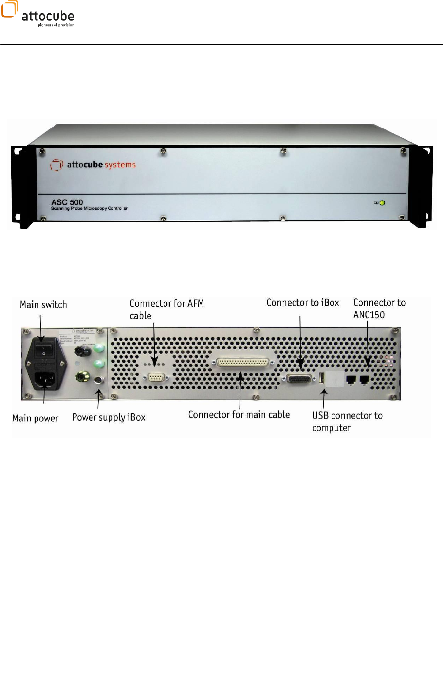
II.3.b. Rear Panel ASC500 v1

Figure 2:

Back panel of the ASC500 scan controller.

On the back panel, there are:

- the main power switch,

- the fuse holder (see fuse description above),

- the main power supply connector,

(110/220 V, 50  60 Hz, max. 20 VA),

- an earth terminal for additional connection of the unit to earth,

- the functional ground for connecting a setup to the electronics

ground,

- 3 power connectors for supplying additional hardware (e.g. iBox)

- the AFM connector (high speed input and output),

- the main SPM outputs,

- the connector for the iBox,

- the USB connector for connection to a PC,

- the serial connector to connect to the ANC150.

Page 13

respective companies. Any rights not expressly granted herein are reserved. ATTENTION: Specifications and technical

data are subject to change without notice.

II.3.c. Cable description ASC500 v1

Power supply:

Use the power cable to connect the ASC500 to the 100, 115 or 220 V jack.

USB cable from computer to ASC500:

Use the USB connector to connect to your computer.

ASC500-iBox:

Connect the cable attached to the ASC500-iBox to the respective connector

of the ASC500 and the round pin connector for the power supply.

Main cable - Signal In- and Outputs:

Use the main cable and connect it to the respective connector. The BNC

connectors are connected to the setup as follows:

ADC 1: sensor signal

ADC 2: optional input

ADC 3: optional input

DAC 1: optional output

DAC 2: optional output

x-Out: connects to the voltage amplifier for x-axis (e.g. ANC200)

y-Out: connects to the voltage amplifier for y-axis (e.g. ANC200)

z-Out: connects to the voltage amplifier for z-axis (e.g. ANC200)

AFM cable – High Speed Signal In- and Output:

Use the AFM cable and connect it to the respective connector. The BNC

connectors are connected to the AFM setup as follows:

Fosc: high frequency sensor signal (e.g. AFM tapping mode) as

feedback input

Fexc: high frequency excitation signal

Warning. Do not, under any circumstances attempt to connect the digital

I/O to any external equipment that is not galvanically isolated from the

mains or is connected to a voltage higher than the limits specified. In

addition to the damage that may occur to the controller there is a risk of

serious injury and fire hazard.

Page 14

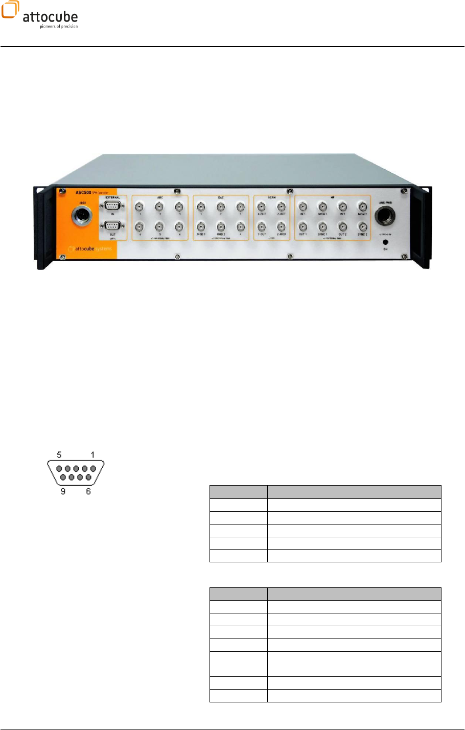
II.3.d. Front Panel ASC500 v2

Since end of 2008, a new hardware version of the ASC500 controller is

available. Although the basic hardware concept was kept similar, there are

many improvements implemented in the new version. This allows for even

more powerful applications in the future. The differences between the two

versions will be documented in the respective sections of this manual.

Figure 3:

Front panel of the ASC500 v2. The break-out cable of v1 was replaced by easily accessible BNC connectors

at the front panel. Please note that both input and output ranges and sampling rate of all converters are indicated

directly below the connector plugs.

With the new hardware versions, most connections to and from the

controller are available on the front panel. Different sections in the front

panel combine the plugs for certain functionalities like inputs, outputs,

trigger ports, etc. The different sections are (from left to right):

iBox connection: The iBox connector is to be pushed into this socket.

External: There are two 8 bit LVTTL (low voltage TTL, 3.3 V)

connectors, one for input and one for output triggering. Connectors are 9-

pin D-sub (Pin 9 is GND).

Figure 4

On the left, the pin numbering for the sub-D connector of the External lines

is shown. The upper input         

inputs:

Input pin

Usage

Counter input

Reserved

External Handshake SYNC

4-8

Reserved

GND

The output ows:

Output pin

Usage

Pixelclock output

Lineclock output

Frameclock output

External Handshake SYNC OUT

Shutter (used by lithography, see

section VI.2.b)

6-8

Reserved

GND

Page 15

respective companies. Any rights not expressly granted herein are reserved. ATTENTION: Specifications and technical

data are subject to change without notice.

ADC section: There are six ADC inputs available, labeled 1 through 6,

with 18 bit 400 kS/s each.

DAC section: There are four DAC outputs available (+/-10 V, 16 bit,

200 kS/s). Two additional modulation ports, labeled MOD1 and MOD2 can

be used to add any analog voltage to the outputs of DAC1 and DAC2,

respectively.

SCAN section: The SCAN section provides the outputs of the scan

engine Xout, Yout and Zout. In addition, there is a modulation input for

the Zout that gives you the possibility to externally modulate the voltage

output to the z scanner.

HF section: This section provides the high frequency inputs and

outputs (50 MS/s) of the controller. There are two independent groups of

in- and outputs. Each group features 16 bit, 50 MS/s ADCs and DACs, as

well as SYNC out (same output frequency than OUT with +/- 5V amplitude)

and MON out (pre-amplified IN signal).

AUX power: This connector provides stable +/- 15 V and +/- 5 V for

external devices. Maximum current is 200 mA at 5 V and 100 mA at 15 V.

The connector is a 5pin Binder series 440.

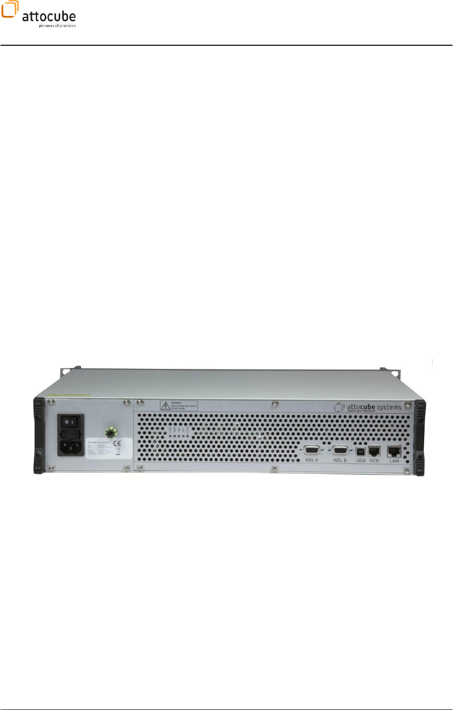
II.3.e. Back Panel ASC500 v2

The back panel of the ASC500 generation v2, features two new possibilities

to connect the controller to other devices. There is a digital serial interface

(called NSL A and NSL B) and a LAN connector.

Figure 5:

Back panel of the ASC500 v2. Please note the new digital interface (NSL) and the LAN connection.

The connectors will be described in more detail from left to right:

Power connection: Connection to mains. The ASC500 features auto

range for 110 - 115 V and 230 V, 50..60 Hz.

Ground: 4 mm plug for connecting to earth and housing

GND.

Voltage indicators: Shows correct availability of internal DC

voltages.

NSL A/B: Digital serial interface to connect to attocube

ANC350 Step/Scan-Controller. 9 pin D-sub connector.

USB: USB 2.0 interface to connect to the PC.

Page 16

Serial: Serial interface to connect to attocube ANC150

/ANC300 Step-Controller. RJ45 connector.

LAN: LAN 100 Mbit connection to the PC.

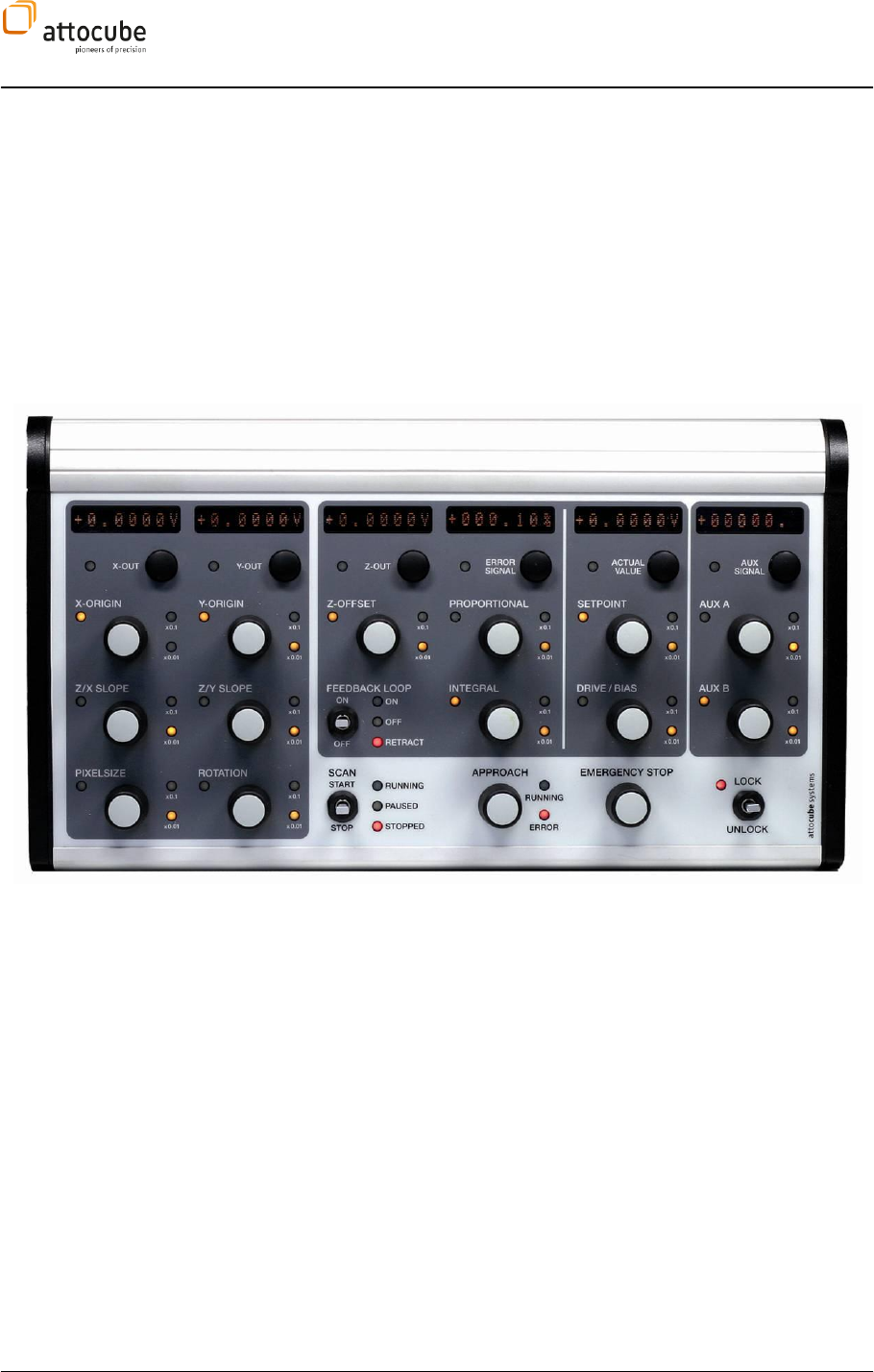
II.4. The iBox

Using the ASC500-iBox, the main scan- and feedback parameters can be

accessed manually. This enables e.g. precise and fast control of the

feedback loop and the scanning process itself.

Figure 6:

The ASC500-iBox (bottom) for manual control of all important scan and feedback parameter.

Page 17

respective companies. Any rights not expressly granted herein are reserved. ATTENTION: Specifications and technical

data are subject to change without notice.

On the lower right, there is the main Lock/Unlock switch. This is a security

feature against unwanted changes. If the iBox is locked, no values can be

changed; only different values for control purposes can be displayed. If the

iBox is unlocked, all parameters can be changed again.

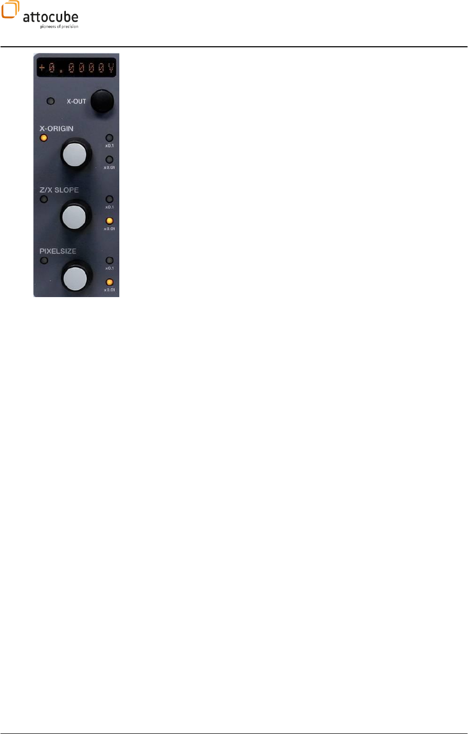
There are six displays at the top. Each display can show one of the values of

the knobs underneath, as well as one additional value which can be

selected by the button underneath. Which value it actually displays can be

seen by the yellow LED to the left of each row. If one of the knobs is

pressed or turned, the display directly switches to show this value.

In the example to the left, the display can show the x-output value (when

pressing on the black knob), or can show one of the three other values: X-

Origin, Z/X Slope or Pixelsize (for a description of these functions, please

refer to the respective sections).

By pushing the respective button, the sensitivity of the dial can be toggled

through three different nuances. The respective amplification is indicated

by the LEDs to the right of the knob. The amplification is either 1x (no LED

is lit), or 0.1x or 0.01x, if the respective LEDs are on.

Using the toggle switch in the bottom center of the iBox, the scan can be

started, paused, and stopped. Pushing the switch up once will start a scan,

whereas pushing it down will pause the scan. Pushing it down two times

will stop the scan.

The feedback loop control which can be found directly above can be

controlled in the same way (on, pause, retract).

With the emergency stop button right to the scan control, the scan and the

feedback loop can be switched off immediately.

The two knobs (AUX A and AUX B) on the right can be associated to

different parameters. This can be done via the Preferences tab (see section

I.1.a).

Page 18

III. Description of the Controller

III.1. Key Features and Benefits

AFM/SNOM Control

 18 bit 400 kS/s ADC input-channel for AFM contact mode signal

 digital measurement of frequency and phase for AFM non-contact

mode with feedback

 DDS for oscillation excitation / frequency range 1 kHz to 2 MHz

 14 bit 40 MS/s ADC input-channel for measurement of the

amplitude dampening (new v2 version: 16 bit 50 MS/s)

 Digital PI feedback loop for z controller

CFM Control

 18 bit 400 kS/s ADC input-channel for CFM signal

 photodiode amplifier with fiber-optical input

STM Control

 18 bit 400 kS/s ADC input-channel for measurement of tunneling

current

 16 bit 200 kS/s DAC output-channel for gap voltage

 Modulation input for gap voltage

 Digital PI feedback loop for z controller

Scan Generation

 2D xy-scan generator with 4 MHz pixel frequency,

 16 bit resolution in full range mode (16 bit offset + 16 bit scan),

 up to 26 bit resolution in small range mode,

 hardware rotation and hardware zoom,

 hardware crosstalk compensation,

 hardware slope compensation

 slewrate controlled movement,

 direct vectorized positioning

Other

 counter input: i.e. 24 bit 10 MHz min. pulse width 50 ns

 online data processing: digital filter, low-pass, averaging, offset

correction, calibration, FFT, ...

 several spectroscopy modes: dI/dV, dI/dZ, df/dZ, dφ/dZ

III.2. Hardware Specifications

Inputs (ADC1-6)

Voltage range: +/- 10 V

Max. allowed voltage: +/- 15 V

Converter resolution: 18 bit

Voltage resolution: 76 µV

Update rate: 400 kHz

Input resistance: 10 kOhm

INL +/- 2.5 LSB

DNL + 1.75/-1 LSB

Offsets: +/- 60 mV

Outputs (X-, Y-, Z-Out)

The scan outputs generate the scan voltage with 16 bit resolution. If the

Active Scan Area is smaller than the total scan range, the 16 bit output

pattern is automatically attenuated to match the Active Scan Area. By

Page 19

respective companies. Any rights not expressly granted herein are reserved. ATTENTION: Specifications and technical

data are subject to change without notice.

doing so, the full 16 bit resolution is available for any given scan range,

leading to an extremely high scan resolution in small range mode. The Z-

Out output to the z scanner features an 18 bit resolution with possible

14 bit attenuation. The scan outputs are designed in a way that you will

never reach the digital bit resolution limit!

Voltage range: +/- 10 V (uni- or bipolar)

Max. output current: +/- 20 mA

Converter resolution: 16 bit (18 bit for Z-Out)

Programmable attenuation: 14 bit

Programmable offset: +/- 10 V

Offset resolution: 16 bit

Max. resolution in small range mode: 16 bit over 1.2 mV

Update rate: 4 MHz

Outputs (DAC1-4)

Voltage range: +/- 10 V

Max. output current: +/- 20 mA

Converter resolution: 16 bit

Voltage resolution: 305 µV

Update rate: 200 kHz

INL: +/- 1 LSB

DNL: +/- 1 LSB

External

External 1: 8 LVTTL inputs (Pin 1-8)

External 2: 8 LVTTL outputs (Pin 1-8)

GND Pin: Pin 9

Pulse Level: 3.3 V

III.3. General Functionality

Scanning probe microscopy works by scanning a probe across a sample and

thereby recording certain physical variables. The ASC500 controller and

software controls the scan position and movement, acquires

simultaneously several signals during the scan and saves the acquired

images. Furthermore it offers the option of feedback for AFM

measurements in feedback mode.

In order to perform the scanning, the software calculates voltage ramps

depending on the scan amplitude, the scan speed and the number of pixels

of the image. The voltage ramps will be amplified by any o

voltage amplifiers (ANC200, ANC250, ANC300, and ANC350) and sent to

the piezos in X, Y and Z directions. A line by line scan is achieved.

In case of scanning in feedback mode, the feedback loop will keep the

sensor value as close as possible to the value called set level.

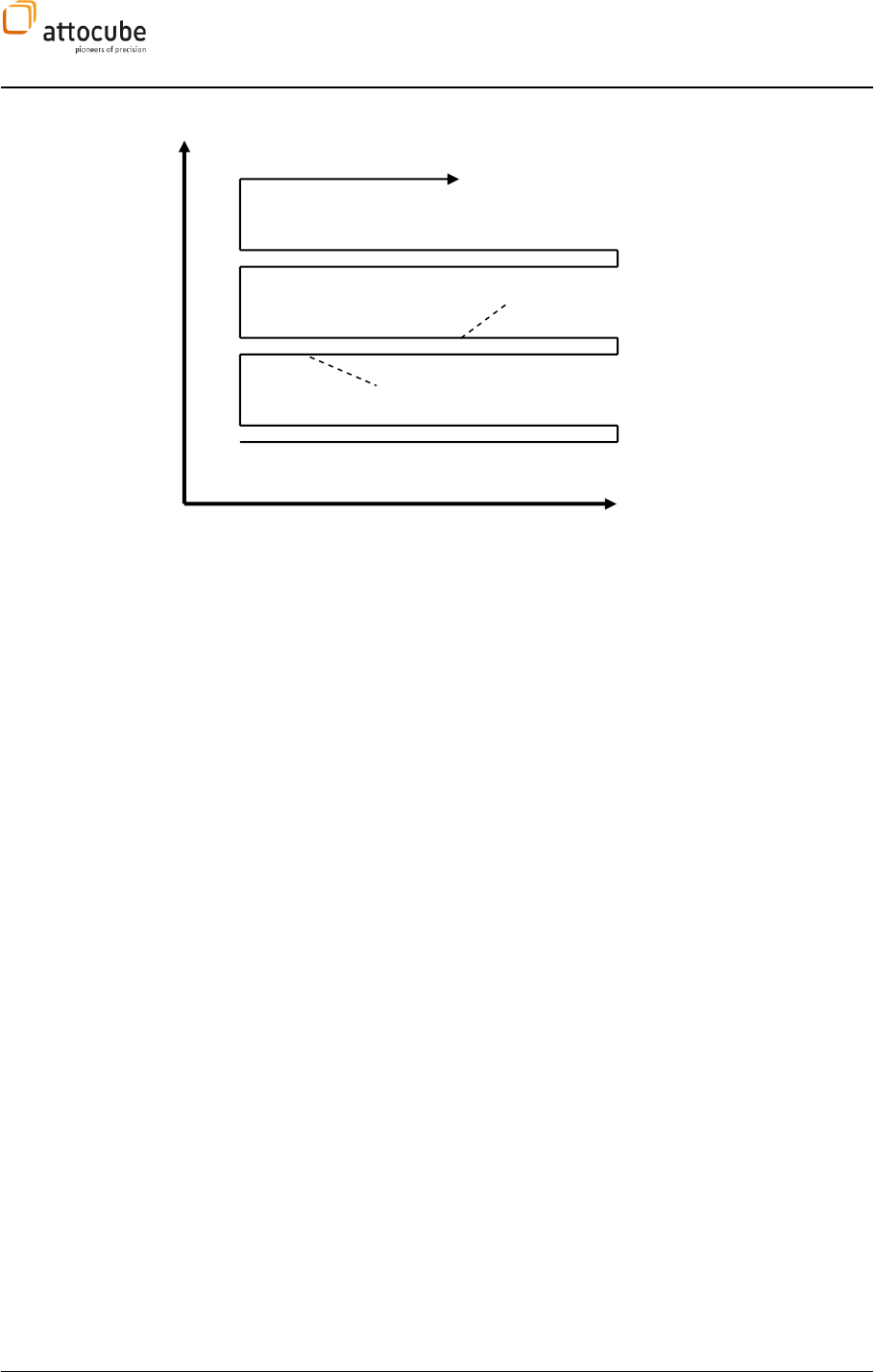
During the displacement in X direction, called the fast axis, the Y-position

remains constant. The x direction will be scanned in both forward and

backward directions, leading to two images: the forward and backward

image. All signals are acquired during both forward and backward motion.

Page 20

Figure 7

: Movement of the sample during the scan.

III.4. Hardware Requirements and Operating Systems

The recommended system has a 2 GHz processor, 1 GB RAM, 20 GB hard



windows environment and to ensure proper functionality of the program

for high speed acquisition. The hard disk space is necessary to store a

large amount of images. The current version of the software is available

for Windows® XP the appropriate drivers for the software are delivered

with the system.

III.5. Hardware Driver Installation

The controller is connected to the computer via USB. Software and drivers

are either installed on the computer delivered with the system or included

on a CD. In the latter case, please copy the software (folder

ASC500drivers (folder 

onto your computer.

When the ASC500 is connected to the computer and switched on for the

first time, the computer should recognize the new hardware. Please follow

the steps below to install the driver.

Forward

Backward

Line 1

Line 2

Line 3

Y (slow axis)

X (fast axis)

Page 21

respective companies. Any rights not expressly granted herein are reserved. ATTENTION: Specifications and technical

data are subject to change without notice.

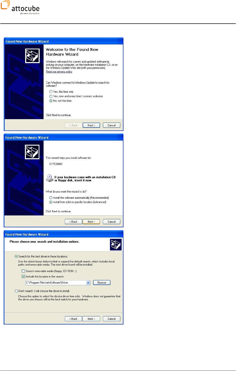
III.5.a. Windows XP

On first connection and if the driver is not

installed, a window as shown will pop up. Do not

search for the drivers automatically, but choose:





Next, you can choose between an automatic

installation of the software on an installation from

a specific location.





In this window, search for the driver at a defined

location.







following window.

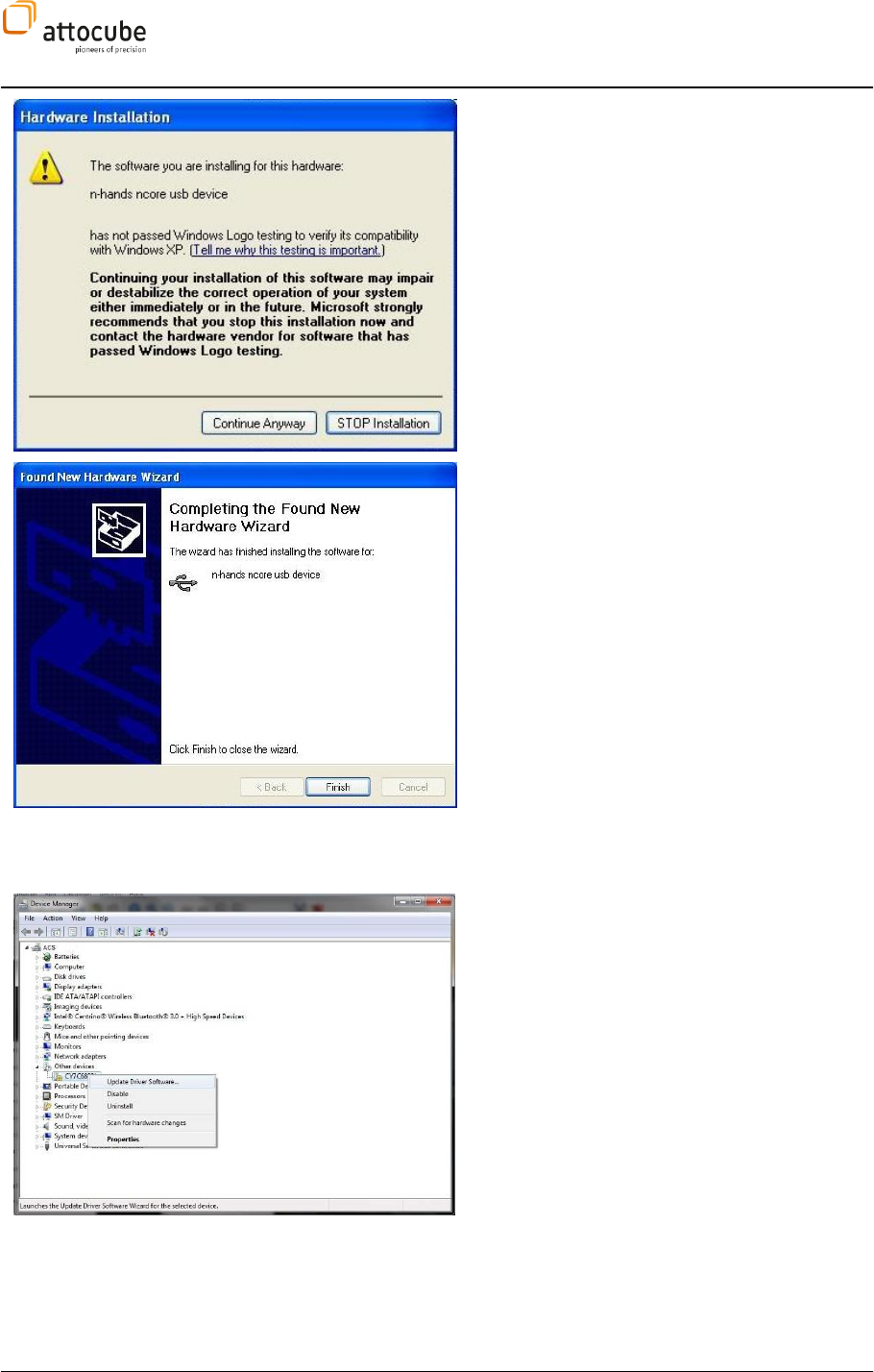
Page 22

In case a window as shown on the left appears,

indicating that the driver has not passed the

      

proceed with the installation.

Finish the installation.

III.5.b. Windows Vista / Windows 7 (32/64 bit)

Go to Control Panel -> Device Manager, and search

for the new device. Right click to select Update

Driver Software.

Page 23

respective companies. Any rights not expressly granted herein are reserved. ATTENTION: Specifications and technical

data are subject to change without notice.

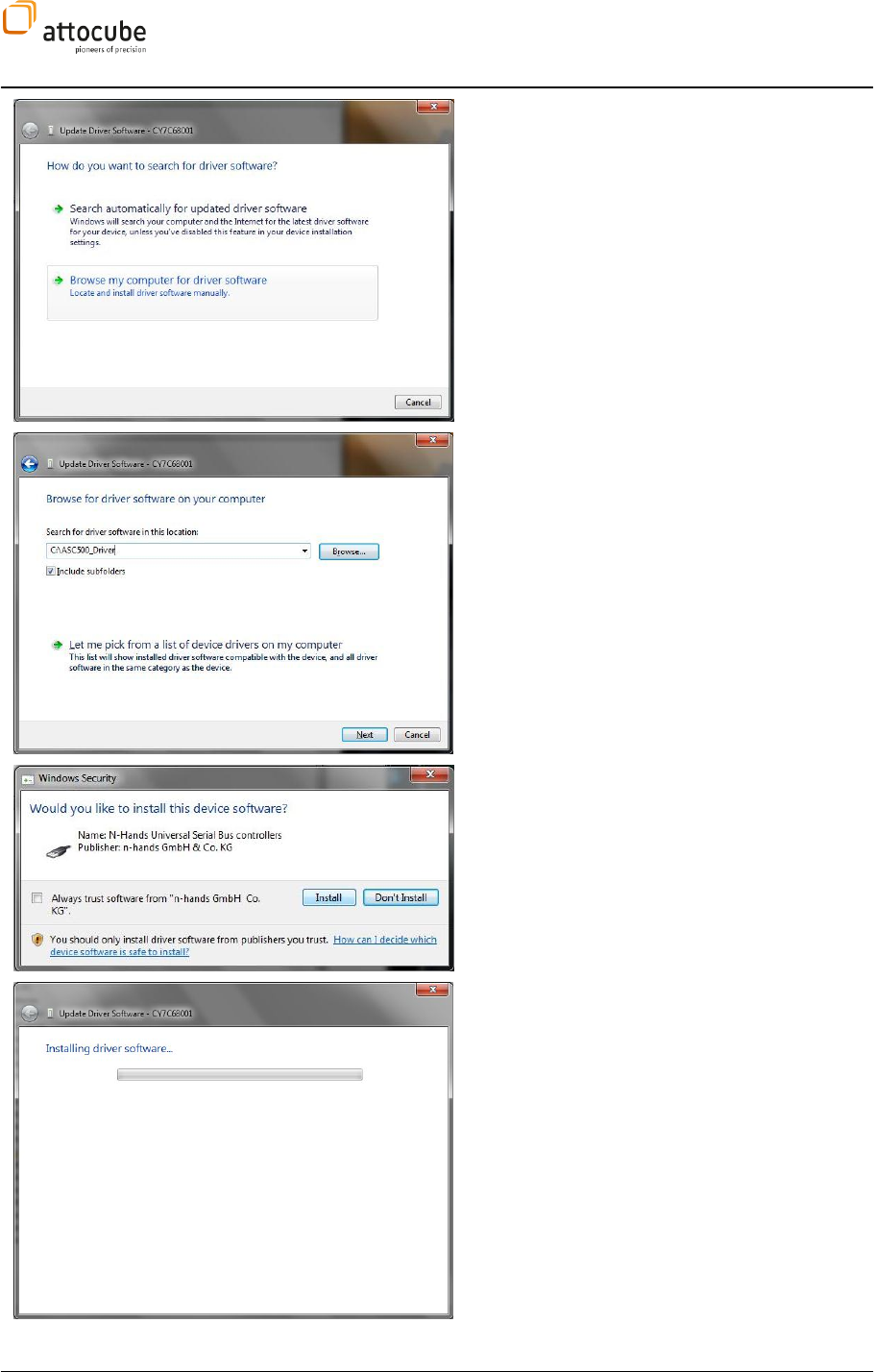
Select Browse my computer for driver software.

Browse to select the directory where you have

stored the ASC500 driver(s) and click Next.

(Note that there are separate driver files for

Windows Vista / Windows 7 32 bit and 64 bit

versions.)

Click on Install



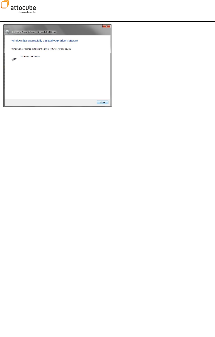
Page 24

Click Close to finish the installation procedure.

Page 25

respective companies. Any rights not expressly granted herein are reserved. ATTENTION: Specifications and technical

data are subject to change without notice.

IV. Data handling

Any successful experiment relies on a safe and reliable storage of its

outcome. Moreover, the quality of a measurement may not be immediately

apparent so the data has to be analyzed in a second step. The format of the

stored data has to be compatible to all tools the user might want to employ.

In this sense, the act of saving the experimental outcome is a task of major

importance in the course of the experiment. In the design of the ASC500

and its software, this importance was especially emphasized.

The software allows for fast and flexible procedures of data storage:

 data can be saved on a time basis from microseconds to hours

 data can be saved in a multiple of 1D, 2D and 3D file formats

 user defined data groups can be saved by one single mouse click

 automatic snapshots and text files containing parameters are

generated

 all file formats are compatible to all major analyzing software

(SPIP, MountainsMap, Gwyddion, Wsxm, ...) or can be directly

viewed in the Windows Explorer

In the following chapter, the data storage capabilities of the ASC500

controller as described in detail.

IV.1. Quick guide for data saving

This chapter will give a short overview to provide a quick entry on how to use

ctions will give all

necessary details for getting the maximum flexibility and time

effectiveness out of the product.

IV.1.a. The DCC

The central point for all data related processes in the ASC500 is the Data

Channel Configuration dialogue (DCC). It is used to define what signals are

accessible in the various modules of the controller and how these signals

are saved. The DCC is accessible from various points of the graphical user

interface (GUI) via the icon that is shown to the left.

Page 26

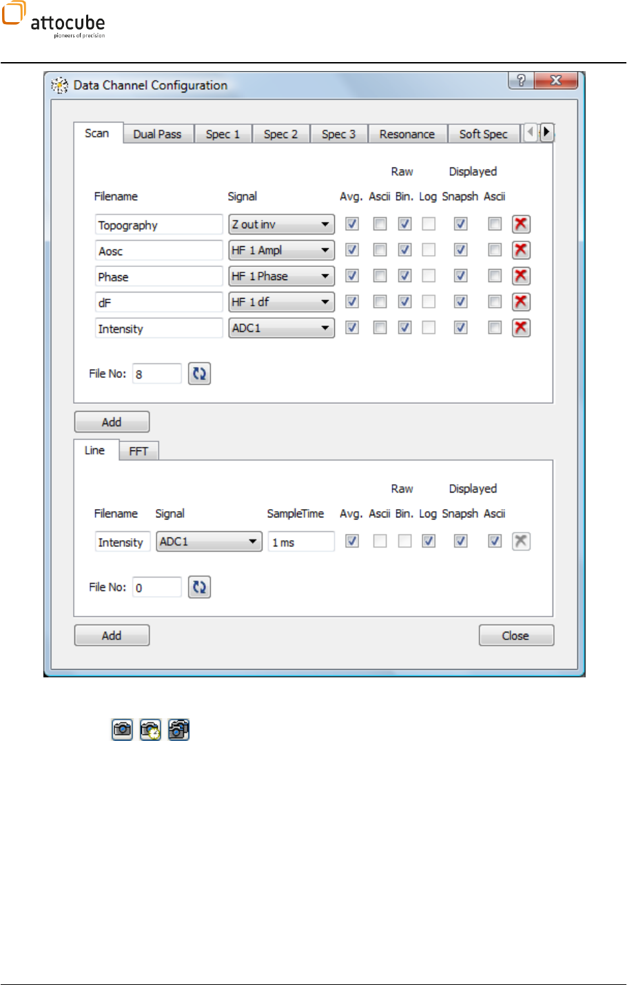
Figure 8:

The Data Channel Configuration dialogue.

Figure 8 shows the DCC in one example configuration. There will always be

one channel predefined in the LINE and FFT group. Only a filename has to be

defined. The AVG checkboxes should be turned ON and both SNAPSH and

ASCII should be checked under DISPLAYED. This means that clicking one of

the SNAPSHOT icons (as shown to the left) in either line view or FFT display

will save the corresponding data in both a data type format and as a

screenshot for better orientation. The signal that is to be shown in the

display can either be chosen in the DCC or directly in the line of FFT display.

The SCAN data group on the top of the DCC is responsible for all data

collected during an xy raster scan and is thus of major importance.

Normally, at least two channels will be defined here:

 One will be the topography signal, defined as the output of the z

controller. The corresponding signal is called Z out inv as shown in

Page 27

respective companies. Any rights not expressly granted herein are reserved. ATTENTION: Specifications and technical

data are subject to change without notice.

the example above.

 The other could be the error signal of the z controller. For contact

mode AFM, this would be the deflection signal usually connected to

ADC1. For non-contact AFM, it would be the output of the lockin

called HF 1 Ampl. For STM, it would be the tunneling current, again

usually connected to ADC1.

The AVG, RAW BIN, RAW ASCII and DISPLAYED SNAPSH checkboxes should all

be checked to save the SCAN data in a binary and text type data format as

well as as a snapshot. Any number of additional data channels can be added

by clicking the ADD button.

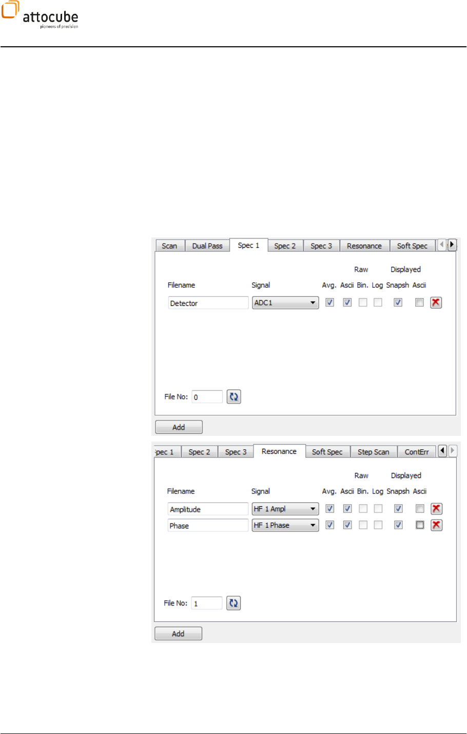
For most experiments, one or more spectroscopy and/or Resonance features

will be necessary. The data channels needed for these operations can be

created in one of the SPEC tabs and the Resonance tab.

DCC Spectroscopy Tab

DCC Resonance Tab

With the settings shown above, all of the basic experiments in scanning

probe microscopy can be done. Scan data will be recorded on two channels

simultaneously, spectroscopy and Resonance experiments can be done and

any given signal can be examined in a line and FFT display. The recorded

data can be stored to hard disk by clicking on one of the snapshot icons in a

Page 28

display. A snapshot trigger in a SCAN display will save the data of all SCAN

data channels simultaneously. The data will be stored in a multitude of

formats: for example the SCAN data of Figure 8 will be saved in ASCII and

binary type format and in addition as a PNG picture file. There will be extra

files for both forward and backward scan direction. There will also be a

snapshot of the SCAN line view and an extra text file with the most

important scan parameters. All of this will be saved by a single mouse click

and all files will automatically be numbered and grouped.

The point in time of the data saving will depend on the type of snapshot icon

that is used for triggering the data storage.

The Snapshot Immediate will save all data in its current state: It may be a

half-filled SCAN image or any arbitrary fraction of a LINE display.

Snapshot Delayed will save the data at the next completion of the

underlying operation. A SCAN will be saved when the scan area has been

completed, a spectroscopy will be saved once the sweep range has been



Snapshot Repeat will turn the Snapshot Delayed function in an endless

cycle. The cycle can be stopped upon the following click on the Snapshot

Repeat button.

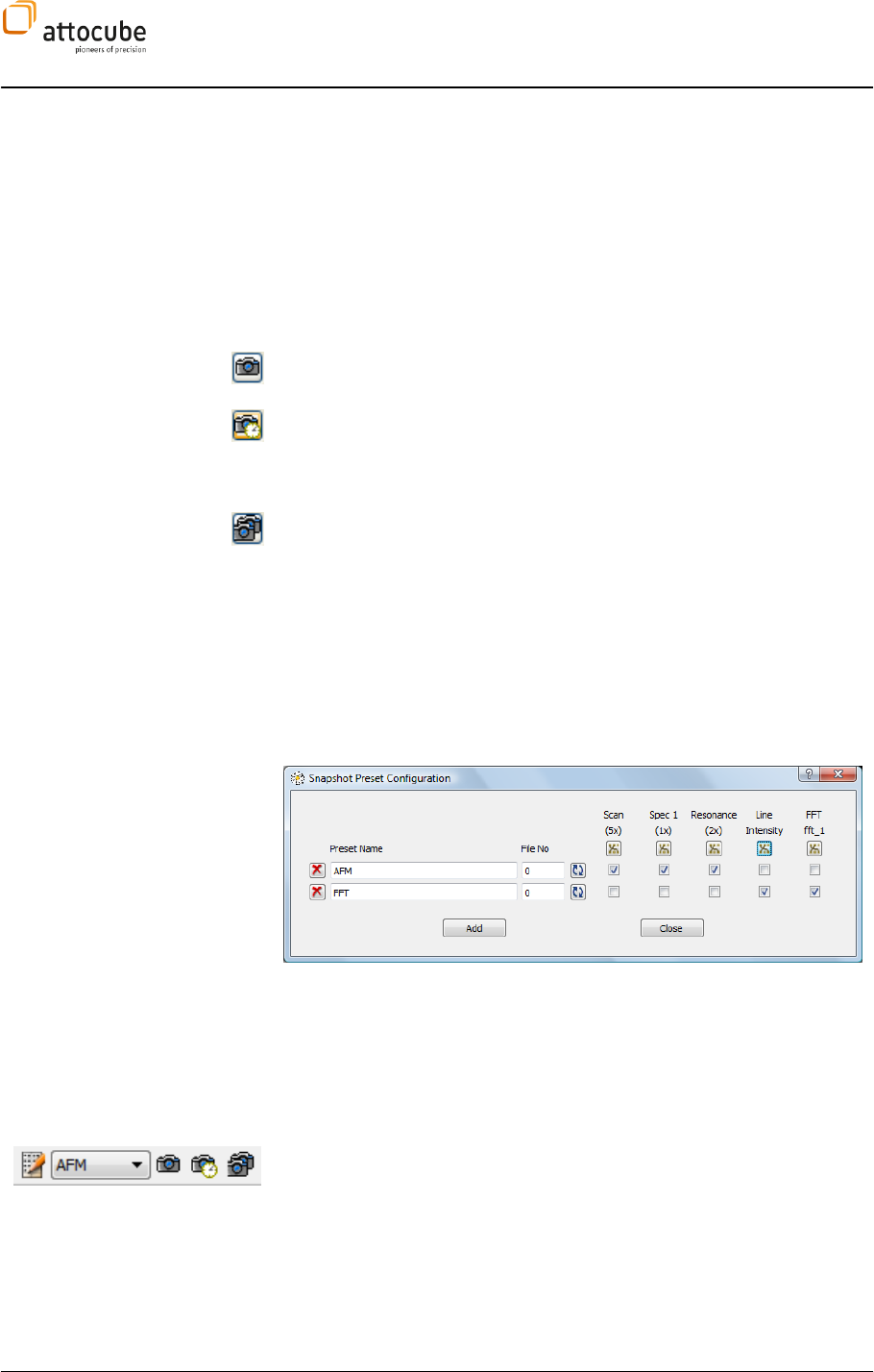
IV.1.b. The Snapshot Preset Configuration

A click on the snapshot icons within a display will trigger the data storage of

the complete data group that corresponds to the display. I.e. a snapshot

trigger in a SCAN display will save all data channels belonging to SCAN. To

save a multiple of data groups simultaneously, the SNAPSHOT PRESET

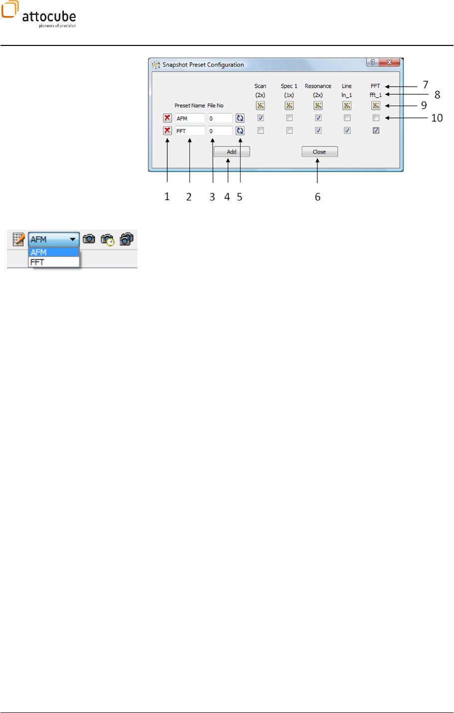
functionality can be used. An example is shown in Figure 9.

Figure 9:

The Snapshot Preset Configuration

For each preset, any combination of data groups can be chosen that will be

saved simultaneously. Only data groups with at least one data channel are

allowed in the preset configuration dialogue. Any number of presets can be

added with the Add button.

To trigger the data storage of a preset, the preset icons shown to the left

can be used. The icons can be found in the main status line of the Daisy

program. To reach the Snapshot Preset Configuration dialogue, the leftmost

icon has to be clicked. The drop-down list is used to choose the preset for

the next saving process. The preset snapshot icons to the right work similar

to their local display counterparts described in the section above.

Page 29

respective companies. Any rights not expressly granted herein are reserved. ATTENTION: Specifications and technical

data are subject to change without notice.

After this short overview, the next section will give details and background

on the data handling and saving capabilities of the ASC500 SPM controller.

IV.2. Data handling details

IV.2.a. Signals, data channels and data groups

A signal is a stream of data that can have two origins:

1. The signal is directly sampled through one of the input connectors.

This would be called an external signal. There are 8 external signals

that are named after its input connector (ADC1, ..., HF1 IN, ...,

Counter)

2. The signal is generated within the ASC500 (internal signal).

Internal signals could be the output of a PI controller (Z_out) or a

lock-in (HF 1 Ampl, HF 1 Phase).

Signals are routed in data channels. A data channel combines the

measurement data with some secondary data that carries additional

information like the position of a data point within an image or a time

stamp. Data channels are thus divided into different groups depending on

the context of the data. One signal is often used in different data channels

at the same time. For example the deflection read-out of an AFM (connected

to the ADC1 input) could be used for recording the topography and feeding

the FFT module at the same time. The ADC1 signal would then be used in two

data channels, one belonging to the data group SCAN and one belonging to

the data group FFT. Up to 14 data channels can be used at the same time.

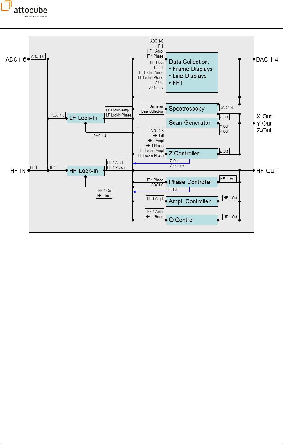
IV.2.b. Internal Signal Flow

The ASC500 SPM controller features a very flexible architecture. There are

many different ways to route the signals between the internal controller

modules to gain a maximum of functionality. Figure 10 gives an overview

on the internal signal flow. The most important controller functions are

illustrated by boxes. Each controller function is connected to other

functions via data lines. Data lines attached to the left of a controller

module show all possible input signals for the respective controller

function. Data lines starting from the right side or from the bottom of a

controller module show the possible output signal generated or altered by

the module.

For example in a standard non-contact mode AFM measurement, the lever

signal would be attached to the HF IN connector on the front panel. The

signal that is carrying the lever information is HF 1 which is automatically

routed into the high frequency HF Lock-In. The lock-in demodulates the HF

1 and generates the HF 1 Ampl signal which can then be used both as an

input value for the Z Controller and also to feed a two-dimensional display

during the scan in the Data Collection module.

Page 30

Figure 10

: Internal Signal Flow Diagram. This diagram gives an overview on the relation between input and

output connectors, the names of the signals and the most important controller functions. Data flow direction is

from left to right (otherwise indicated). Each controller function is depicted by a box, all possible input signal are

shown on the input side of the box, the output signal are shown to the right of the box.

The controller modules shown in Figure 10 are explained in more detail in

section Operating the Controller of this manual.

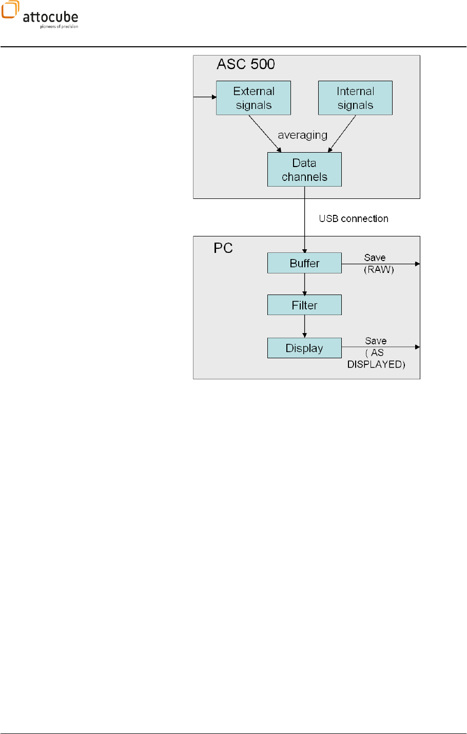
IV.2.c. Data processing chain

The diagram of the data processing chain is shown in Figure 11. All signals

are either recorded or generated within the physical unit of the ASC500

controller.          

(defined in the DCC, see IV.2.e). After transmission to the PC via USB, the

data is stored in a buffer. The content of the buffers can be saved directly to

hard disk, choosing from various types of file formats. In addition, it can be

routed to a display (optionally via one or more filtering stages). The content

of the display can then again be saved either in a Windows picture format

(for fast overview via Windows explorer) or in a data format that now

includes the filter stages (pre-processed or as-displayed data).

Page 31

respective companies. Any rights not expressly granted herein are reserved. ATTENTION: Specifications and technical

data are subject to change without notice.

Figure 11:

The data flow chain of the ASC500

IV.2.d. Sample time and Average

All internal and external signals use an internal general time base of 2.5 µs.

This time corresponds to the 400 kHz sampling frequency of the general ADC

inputs. In some cases, data is needed only in a slower repetition rate. In the

Daisy GUI the repetition time for signals is called Sample Time. If the Sample

Time is set to a value larger than the time base of 2.5 µs, data has to be

reduced. The user can choose from two options how the data reduction is

done:

1. Averaging ON: all values recorded within a Sample Time are averaged.

2. Averaging OFF: the first value of the Sample Time sets the signal value and

during the rest of the sample time, all other incoming data is ignored.

The data reduction is done in the ASC500 controller in order to reduce the

traffic on the USB connection between ASC500 and PC as much as possible.

The Sample Time of all channels within one data group will be equal.

However, there are two exceptions: the LINE and FFT groups leave it to the

user to define a separate sample time for each channel. For all groups, the

Sample Time is defined in the respective parts of the GUI corresponding to

the data group. For example, the Sample Time for the SCAN group is set via

choosing the scan speed. Still, the Average option is to be defined in the

DCC. It is set to Average ON for all channels per default.

Page 32

IV.2.e. Data Channel Configuration (DCC) in detail

A central point for the configuration of the data processing chain is the Data

Channel Configuration dialogue (DCC). It can be accessed from various

points in the graphical user interface by clicking on the DCC button shown to

the left. In the DCC, data channels are created and signals are assigned to

the data channels.

In the DCC, also the behaviour of the data channels at the time of data

storage is defined. Hereby it is important to distinguish between the

definition of possible file formats and other storage options and the actual

process of the data storage. The possibilities are to be defined within the

DCC; the trigger for the saving process will be done in the respective data

displays, using one of the snapshot icons.

The data channels are sorted in the following groups:

SCAN data associated with the scan motion. Each data point is

referenced within a 2-dimensional frame and has been

recorded in either forward or backward direction. Data from

the SCAN group can be represented in either a two

dimensional display (called a frame view) or as a one

dimensional display showing single or multiple lines of the

scan.

2nd PASS data associated with the Dual Pass Mode (see VI.5.g on page

103). If the dual pass mode is set to ON, the data group 2nd

PASS represents the data of each second line. Since the origin

of the data is very similar to the data of the SCAN group, it can

be viewed with the same display types.

SPEC1, SPEC2, SPEC3

data associated with the Spectroscopy feature. It will be

displayed in a 1D type display.

RESONANCE data associated with the Resonance feature. Representation:

two 1D type displays, usually showing the amplitude and

phase of a lever against frequency.

SOFT SPEC data associated with the Soft Spectroscopy feature.

Representation: 1D display

STEP SCAN data associated with the Step Scan feature. Representation:

2D frame, 1D line

Page 33

respective companies. Any rights not expressly granted herein are reserved. ATTENTION: Specifications and technical

data are subject to change without notice.

The above image shows the lower part of the DCC with both LINE and FFT

data groups.

LINE no data association. Any signal can be shown against time.

Representation: 1D line, multiple 1D line

FFT no data association. Any signal can be shown in frequency

space: Representation: 1D line

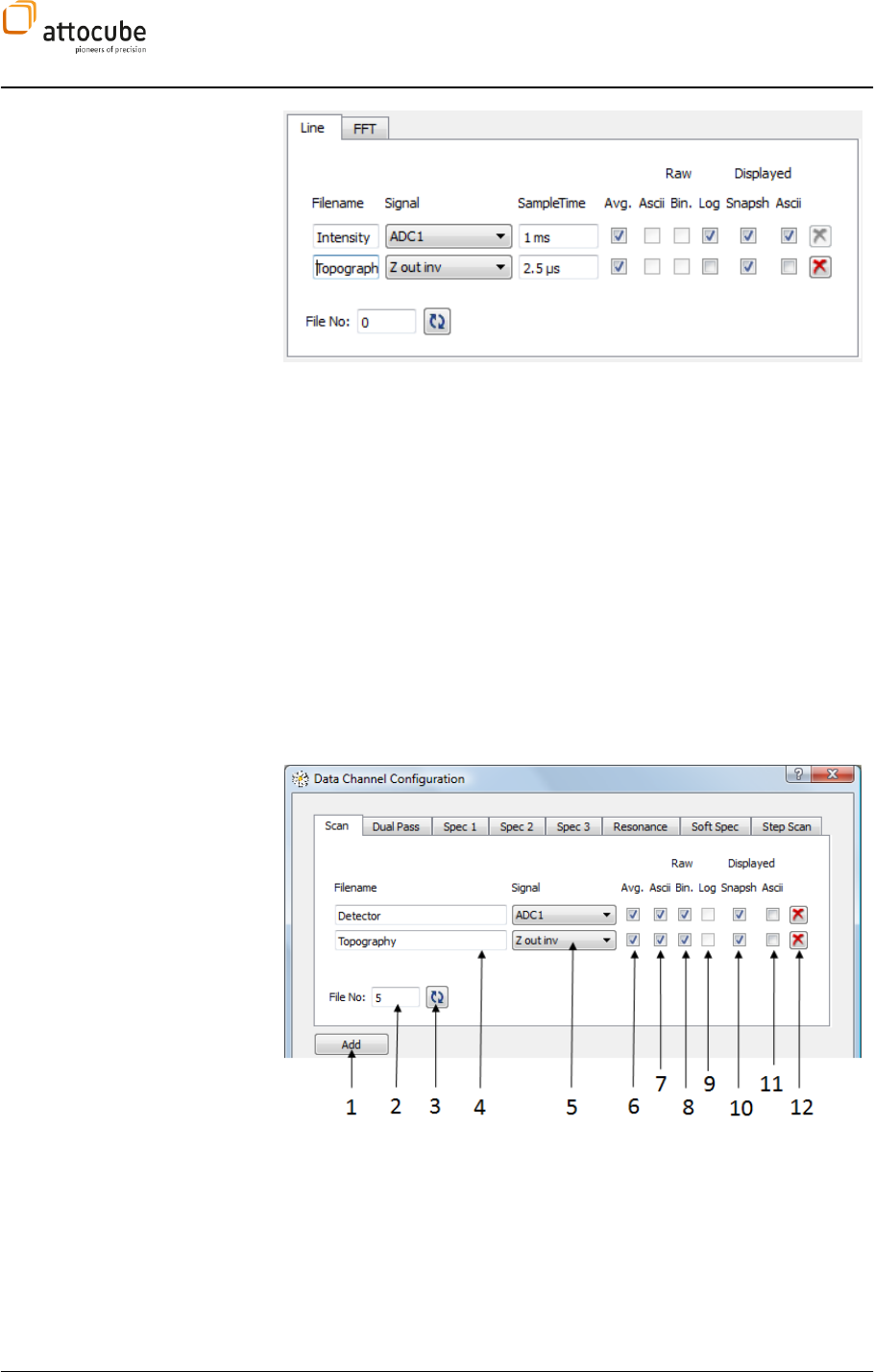
IV.2.f. DCC usage

Before the experiment is started, the data channel configuration has to be

defined in the DCC. After the definition, the data channel configuration can

be saved by saving the GUI profile under File – Save Profile or Save As. The

different sections of the DCC are described in more detail below.

1  Using the Add button, a new data channel can be created in the current

data group. Up to 14 data channels can be used at the same time. Please

note that it is not possible to add data channels during operation. For

Examples, DATA group channels can only be added when the scanner is not

running.

2  The current filename index number is shown here. It will be

automatically increased with each saving process. This number cannot be

Page 34

edited.

3  Reset the File No to 0.

4  Filename used for storing the data of the data channel.

5  The Signal that will be routed into the data channel.

6  Average button. The signal will be averaged over its sample time. See

IV.2.d for more details.

7, 8, 9, 10, 11  Here, the file and data format for the disk storage of the

data can be defined. There are in general five possible formats. Not every

data group has all five formats available. A more detailed description of the

formats is given in section IV.2.g. In the DCC, only the formats are defined.

To actually trigger the storage process, the snapshot icons in the data

displays have to be used.

12  the Remove button will remove the corresponding data channel from

the data group. Please note that the first data channel of both LINE and FFT

data group cannot be removed.

IV.2.g. Saving the data

Available options

There are several options for the storage of each data channel. In general,

the data can be saved either RAW or as DISPLAYED (see Figure 11 for clarity).

RAW means that the data is taken from the buffer, i.e. before any filtering.

For example, SCAN data will be saved without the underground filter if the

RAW option is chosen. The DISPLAYED option will save the data as it is shown

in the corresponding display, i.e. after the filter stages. NOTE: The

DISPLAYED option of any data channel will NOT be saved, if the data channel

is not connected (i.e. shown) in a DAISY display.

RAW ASCII: The data of the channel will be saved in an ASCII type format.

The data will be stored as recorded. For SCAN and similar data groups, there

will be one file for forward and one for the backward direction. This format is

available for SCAN, 2nd PASS, SPEC1-3, CALIB, SOFT SPEC and STEP SCAN data

groups.

RAW BIN: The data of the channel will be saved in a binary format. The data

will be stored as recorded. For SCAN and similar data, there will be one file

for forward and one for backward direction. This format is available for

SCAN, 2nd PASS and STEP SCAN data groups.

LOG: The LOG option is only accessible for LINE data. This option will write

the data to a file as a stream of points, one point with each Sample Time. The

resulting file will be of ASCII (text) type. Please note that LOG files can get

very large, so it is advisable to use the log function only with large Sample

Times. The logging is started and stopped by using the Snapshot Repeat

button in the respective LINE display.

DISPLAYED SNAPSHOT: If checked, the data will be saved as a screen

snapshot of the current display. It will be saved in a PNG file format by

default, but the format can be changed using the Settings – Preferences – File

Output – Snapshot Format. This feature is especially useful to provide an

Page 35

respective companies. Any rights not expressly granted herein are reserved. ATTENTION: Specifications and technical

data are subject to change without notice.

overview on the stored data on the harddisk using only the Windows

Explorer. NOTE: As with all DISPLAYED save options, data will only be saved

if the channel is dargestellt in a DAISY display. For SCAN channels, both

forward and backward scan snapshots will be saved, even if only one

direction is shown on the screen.

DISPLAYED ASCII: The content of the display that shows the data channel

will be stored in a text type format. In contrast to the RAW ASCII option, the

file will contain all data changes resulting from the filters the data might

have passed. Again, the data will only be saved if the data is shown in a

display at the time of the saving trigger.

Triggering data storage

Each display in the Daisy GUI contains three buttons for issuing a saving

trigger (shown to the left). These buttons will be used to trigger the process

of data storage

The Save Immediate button will save the data in its current state, i.e. a scan

frame that is half filled or a fraction of a LINE VIEW line.

The Save Delayed button will store the data when the corresponding data

unit will be completed for the next time. This means that a scan will be saved

once the frame is finished and a spectroscopy will be saved as soon as it is

completed. A save icon will appear in the corresponding display to note that

a data storage process is PENDING??.

A third option will be the SAVE REPEAT button. With this button pressed, the

data will be repeatedly saved in a manner that is equal to the SAVE

COMPLETE option. For example a scan will be repeatedly saved every time

the complete scan area has been imaged. The procedure can be stopped by a

second click on the SAVE REPEAT button. For LINE data, the SAVE REPEAT

button can have two meanings: 1. If the LOG option in the DCC is chosen,

the data will be saved as a continuous data stream in one file, one data

point for each sample time. 2. If the LOG option in the DCC is not chosen,

the SAVE REPEAT for LINE data will work similar to all other data groups:

data will be saved at the moment the display is full.

Triggering a data storage process will always save all channels of a data

group. For example, each click on a SAVE button in a frame display will write

all data belonging to the SCAN data group to the hard disk. This will be both

the 2D image, but also the 1D data of the corresponding scan line view

(meaning the line view that shows the scan data line per line). There are,

however, two exceptions for this rule: The LINE and FFT data group behave

differently: here a SAVE trigger will only store the data channel shown in the

display where the SAVE is triggered. If there are several displays with LINE

information and all of them need to be stored to hard disk, the user needs to

click on all corresponding SAVE buttons. Another possibility is to use the

Snapshot Preset option of the DAISY GUI to combine any combination of data

channels to be saved on one mouse click (see next section IV.2.i). The

reason for the different behaviour of LINE and FFT data compared to all

other data groups is that the time scales of various LINE or FFT displays may

be very different. One LINE view could show a signal on a microsecond time

scale, while another LINE display could very slowly log data from for

ng

process allows for a separate data storage for either long term or short term

Page 36

data. The differences between LINE/FFT compared to other data groups is

also highlighted in the splitting of the DCC, where LINE and FFT are shown in

an extra lower part of the DCC window.

Filename Convention

The filename will be composed from several parts. First, there will be a prefix

referencing the data group and an index number. The index number will be

automatically increased after each saving cycle. The next part of the

filename will be the data channel name as entered by the user in the DCC.

This is followed by an extension providing some closer description of the



It could also be the name of the display in case the data is saved AS

DISPLAYED. Finally, the Windows filename extension sets the file format



filenames will all start with the same prefix, so it will be immediately clear

that they are all based on the same data.

Please note that the name of any display can be changed via its context

menu.

Here are several examples:

SC002-Topography-bwd.asc

This filename is composed as follows:

SC SCAN data group

002 index

TOPOGRAPHY name taken from DCC

BWD backward scan

.ASC 2D ASCII type format

S1002-Tunnel Current-Spectroscopy 1.png

S1 data group SPEC1

002 index number

TUNNEL CURRENT Name from DCC

SPECTROSCOPY 1 Name of the display that was the origin of the

snapshot. The existence of the display name within the filename is a sign

that the data was saved as DISPLAYED.

.PNG picture file format

If a filename is already used in the target directory, DAISY will automatically

 to guarantee a

successful storage of the data.

Target directory

All files will be stored in the same directory. This directory can be changed

at any time under Settings – Preferences – File Output - Target Directory.

Page 37

respective companies. Any rights not expressly granted herein are reserved. ATTENTION: Specifications and technical

data are subject to change without notice.

File formats

All data saved by Daisy will contain a file header that is readable with any

standard text editor. A typical file header looks as follows:

# Daisy line view snapshot

# 2011-02-01T07:26:35

# display: FFT Display

# x-pixels: 813

# x-unit: Hz

# y-unit: V

X ; Y

Obviously, an FFT display was saved with a content of 813 pairs of voltage

versus Hz data points. After the header, the file contains the measurement

data in either ASCII or binary format (depending on the file format type). In

case of an ASCII file format, the data is written in a form similar to the last

line of the header: two columns separated by a semicolon.

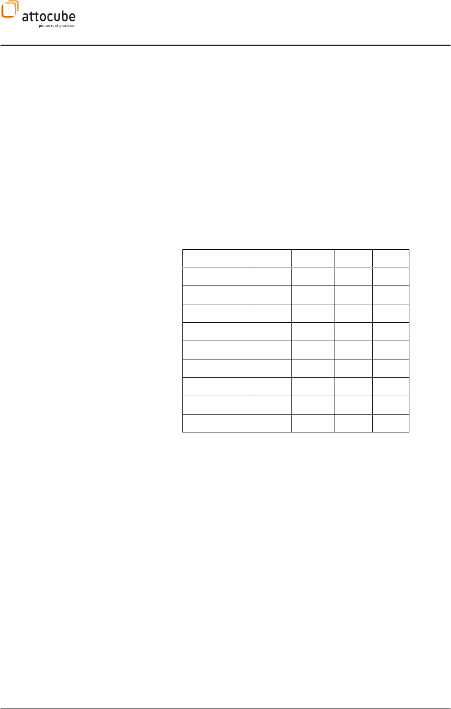
The following table provides an overview on the available file format types:

ASC

BCRF

PNG

CSV

SCAN

SCAN LINE

2ND PASS

SPEC 1-3

CALIB

SOFT SPEC

STEP SCAN

LINE

FFT

Note: SCAN LINE data is not a separate data group but belongs to the SCAN

data group and is saved by the same trigger. SCAN LINE data is only

available AS DISPLAYED and will thus be saved automatically if one of the

DISPLAYED checkboxes in the SCAN section of the DCC is marked.

ASC Format

The ASC format is used for 2D data (SCAN, 2nd PASS, STEP SCAN). The data

will be written to a file as ASCII text. The resulting files can be opened in a

text editor or any standard image analysing software. Due to the nature of

text files, the file size will be 2-5 times larger than its binary counterpart

BCRF. There are two slightly different versions of the ASC file format:

 The data points are separated by a line feed.

 Data within one scan line a separated by a TAB and the end of a

scan line is marked by a line feed (line oriented).

To choose between these two options, a checkbox under Settings –

Preferences – File Output – ASC Format can be used.

BCRF Format

The BCRF is the binary counterpart of the ASC format and can be used for the

same data (2D data). After the ASCII header, the data points are saved in a

binary format which leads to a file size reduction of up to 5.

Page 38

PNG Format

This format is a picture type format for screen snapshots. It is available for

all data and display types. The content of the display is saved to hard disk as

it is shown on the screen. For SCAN and similar data, there will be always the

forward and backward scan direction saved to a separate file (even if only

one direction is shown in the display). Data post processing is not possible

with this format. Still, saving screenshots provides an easy overview over

collected data. The format can be switched to JPEG, BMP and others under

Settings – Preferences – Snapshot Format.

CSV Format

The CSV format is an ASCII/text type file format for 1D data (LINE, SPEC1-3,

FFT). CSV (comma separated values) can be imported to every program that

is capable of analysing data sorted in columns and rows (Excel, Origin,

Sigmaplot, SciLab,...)

IV.2.h. Parameter File

For each data storage cycle an additional text file can be created that is

called the Parameter File. The Parameter File will contain the most important

parameters that were set in the Daisy GUI at the time of the saving process.

The filename is parameter.txt with a prefix equal to the prefixes of the

corresponding data files. The file is readable with any text editor. The user

can add any arbitrary text to the Parameter File via Displays – Snashot

Comments. The creation of Parameter File can be omitted under Settings –

Preferences – File Output – Parameter file.

IV.2.i. Snapshot Presets

Often during an experiment, several data groups need to be saved at the

same time. For example, FFT and LINE data are a common couple because

they represent complementary information on the same physical origin.

Also, SCAN and LINE data might be interesting to save together, if for

example the LINE data represents an additional parameter of the

measurement. The DAISY GUI is equipped with functionality to combine

several data groups in presets and save all data with one mouse click.

Moreover, different presets can be defined and activated via a simple drop

down list. A very flexible and powerful tool for data saving is thus at hand

for the user.

To enter the Snapshot Presets Configuration dialogue, the user has to click

on the button shown to the left in the status line of the DAISY. In the

following menu, the data groups can be assigned to certain presets. Each

preset will be represented by one line in the dialogue.

Page 39

respective companies. Any rights not expressly granted herein are reserved. ATTENTION: Specifications and technical

data are subject to change without notice.

1  The Remove button is used to remove one preset from the list.

2  Name of the preset. This is used to identify the preset in the trigger

dropdown list (shown to the left).

3  Index number of next data filename.

4  Reset index number to zero.

5  The Add button is used to add another preset to the list. There is no limit

to the number of presets.

6  The Close button will accept all changes and closes the dialogue.

7  Data Groups: all data groups with active data channels are shown. For

LINE and FFT data, each channel will be shown separately because these

channels could potentially be stored separately. For all other data groups,

all data channels of the group will always be stored combined.

8  This line shows either the number of active data channels in the group or

the name of the data channels for LINE or FFT group.

9  DCC shortcut. To change the data channel configuration, a click on this

icon leads to the DCC.

10  These checkboxes are used to add the corresponding data group to the

preset.

Snapshot Preset Filename

Convention

The filenames created by the snapshot presets are composed similarly to the

filenames from data group storage. The difference is the prefix numbers. All



the files corresponding to their common trigger.

1) Prefix: P0 .. Pn + 3-digit number. P0 corresponds to the first

preset, P1 to the second and so on.

2) Data channel name

3) Na source

4) for SCAN data: denotation of scan directions; fwd or bwd

5) filename extension

Example:

P0001-ln_1-Line View.csv

Page 40

This filename is composed as follows:

P0 Preset 0 was used to create the file

001 index number

ln_1 data channel name taken from the DCC

Line View Name of the display (marks that data was saved AS

DISPLAYED)

.csv 

How to trigger a snapshot

preset

The data storage of a Snapshot Preset is done via one of the three snapshot

buttons shown to the left. These buttons can be found in the main status

line of the Daisy program. The usage of these buttons is very similar to the

snapshot icons from the data group storage (see page 35)

Page 41

respective companies. Any rights not expressly granted herein are reserved. ATTENTION: Specifications and technical

data are subject to change without notice.

V. Operating the Controller: General Usage and Overview

This chapter gives a general overview on the Daisy software and its

functionalities.

V.1. Software Installation and Getting Started

Copy the folder on the CD \Software\ASC500 Software and all its contents to

a new folder c:\Programs\attoSoftware\ASC500. You are not required to

execute any installation program. It is possible to generate a shortcut on



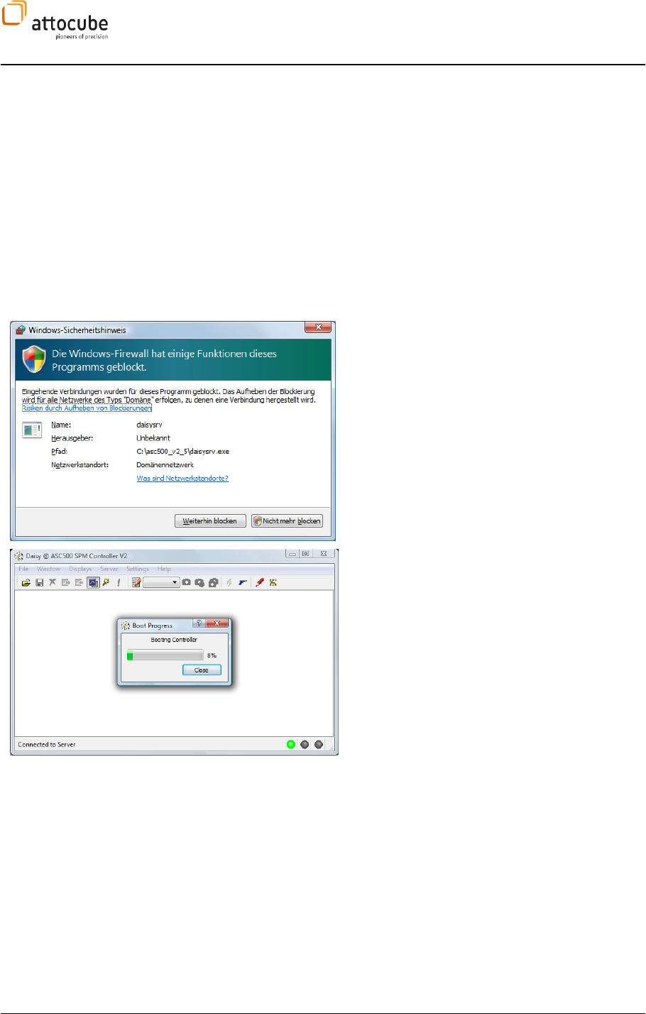
Switch on the controller.

    f your firewall is

activated, the following error message appears.



Now, the ASC500 hardware is automatically booted

and the window as shown to the left appears.

Remark: by booting the hardware, all FPGA and DSP

code is transferred from the computer to the

controller, thus defining its functionality. Please

note that upgrading to a new software version only

requires starting the new version of the Daisy

program. All changes will be automatically

programmed into the hardware. Furthermore, the

software will distinguish automatically between v1

and v2 hardware version of the ASC500 and load

corresponding files.

Page 42

V.2. Description of Main Daisy Program

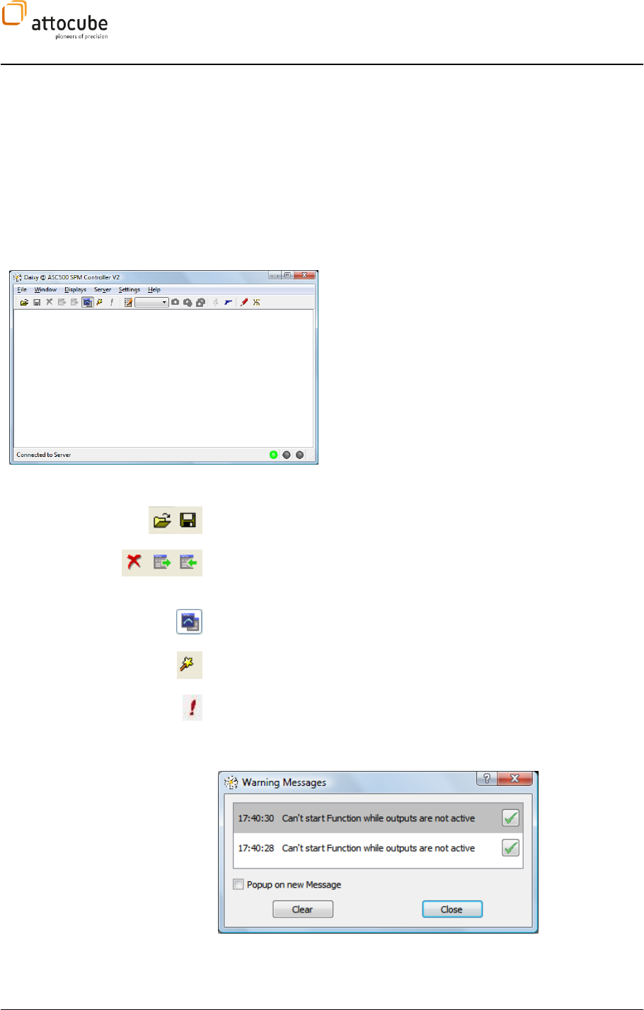
After booting, the main server program is running (see image below). It

enables the connection to the hardware and handles data inputs and

outputs. Also, it can reboot the controller and send new boot code. Yet, for

controlling parameters and outputs of the ASC500, a profile has to be loaded

that defines the graphical user interface (GUI). A profile (*.ngp) consists of

saved settings and a panel (*.ngc). Hence, user settings can be saved with

the profile.

On the lower right there are three status LEDs (from

left to right):

- the server is connected to the hardware (green

LED),

- the server is receiving data (green),

- an overload error occurred (red).

V.2.a. The main toolbar

Load/ Save Profile. Profiles and panels can also be loaded and saved with

the File menu.

Close/ Detach/ Collect Panel. If you have loaded one or several panels, it

is possible to detach them from the server application or re-collect them

also by using the Window menu.

Always on top. If this button is checked, Daisy windows will always stay on

top of other windows running on the computer.

Display wizard. You can open additional data windows using the display

wizard. Please see section V.4.d on page 58 for further information.

Warning messages. Press this button to show the warning messages

window., which can also be configured to pop up on every new message.

You can either clear the whole list, or check single messages to delete

them.

Page 43

respective companies. Any rights not expressly granted herein are reserved. ATTENTION: Specifications and technical

data are subject to change without notice.

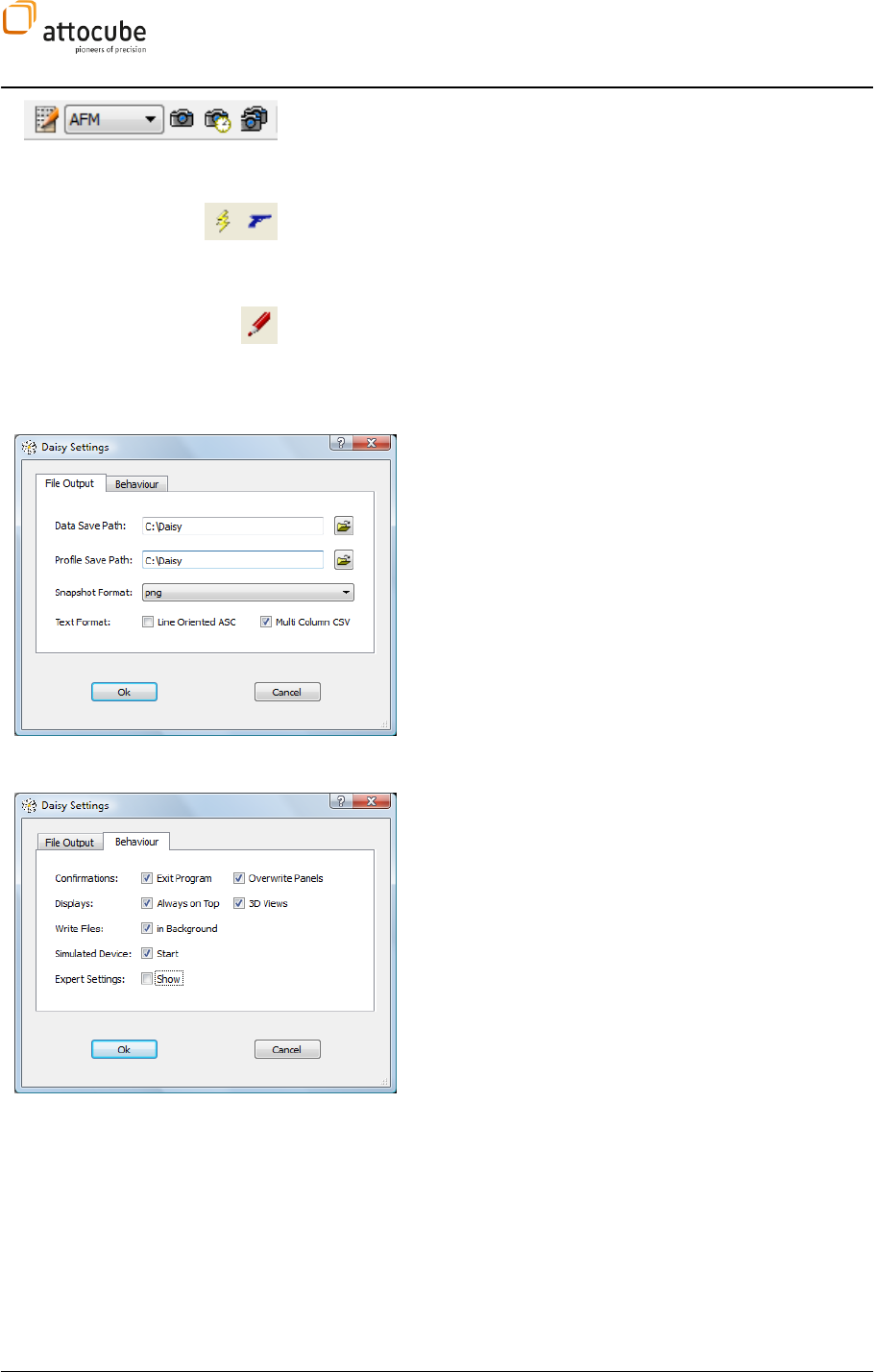
Snapshot Presets: Data of different context can be saved within one

mouse click. The Snapshot Preset icons shown to the left are used for this

functionality. Further details on data handling and saving are given in

section IV.

Start/ Shutdown Server. The server application on the PC as well as the

hardware can be booted or shut down using the Server menu. The boot

messages from the server program can also be opened here. In case of

problems, the Server Output can help to trace a problem.

Daisy settings. Open the preferences dialog to change certain global

settings. It is recommended not to change these settings unless needed.

The File Output tab features the following settings:

Data Save Path: Set the target directory in which all data

/ snapshots will be saved by selecting a path with the

Open icon to the right.

Profile Save Path: Set the target directory in which the

profiles will be saved.

Snapshot Format: You can choose between bmp, png,

ppm, xbm & xpm file formats for the snapshots.

Text Format: For 2D data, choose between Line Oriented

ASC and one data point per line.

For multiple curves, use multiple colums in .csv files or

alternatively, write multiple curves one after another.

The Behavior tab features the following settings:

Confirmations: Check the corresponding boxes if you

want to be notified before exiting the program, and before

overwriting panels respectively.

Displays: Check the corresponding boxes to activate

Always on Top for the displays, and for enabling 3

dimensional data displays (available upon right-clicking

in a frame view). Since this functionality is not supported

by all PC hardware configuration, the 3D views option is

set to OFF by default.

Write Files: Check this box to enable writing files in the

background.

Simulated Device: Check this box to start the Daisy in

siumulation mode (without actually connecting to the

ASC500 hardware).

Export settings: Check this box to show the Expert

Settings.

Page 44

V.2.b. The menu bar

In addition to the standard menu entries as already described above, there are the following options available in

the main menu bar:

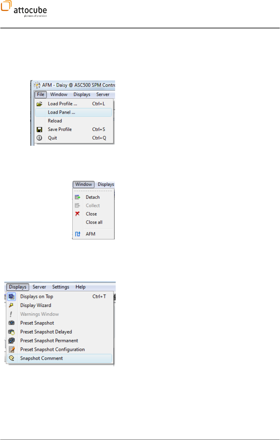
The File menu contains the following entries:

Load Profile: Click here to load a profile (.ngp).

Load Panel: In addition to profiles (.ngp), there is also a number

of preconfigured panels (.ngc) available.

Reload: Use this option to reload the current profile. This option

is helpful if e.g. settings have been changed which will only come

into effect after reloading the profile (such as changing Aliases,

see section V.3.b).

Save Profile: Use this option to save you profile.

Quit: Exit the program.

The Window menu contains the following entries:

Detach: Use this option to detach the current display from the

main Daisy window. This option is particularly useful when using

more than one screen or very large screens.

Collect: Use this option to re-attach detached displays to the

main GUI window.

Close: Use this option to close the current display.

Close all: Use this option to close all displays at once.

The last entry consists of all currently active / open displays; use

this to switch between the different windows.

The Displays menu contains the following entries:

Snapshot Comment: Here you can enter comments which will be

saved in the parameter file.

Page 45

respective companies. Any rights not expressly granted herein are reserved. ATTENTION: Specifications and technical

data are subject to change without notice.

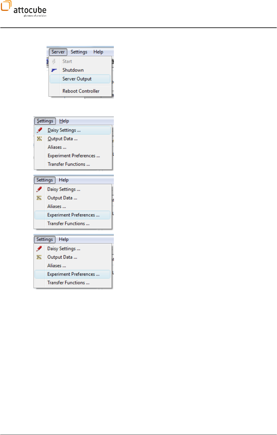
The Server menu contains the following entries:

Start & Shutdown: See the corresponding button descriptions

above (section V.2.a)

Server Output: This opens a window which lists the

communication between the Daisy server and the hardware.

Reboot Controller: Use this option to reboot the controller.

The Settings menu contains the following entries:

Daisy Settings: See the corresponding button description above

(section V.2.a).

Output Data: This opens the DCC window, see description in

section IV.1.a.

Experiment Preferences: This opens a window with several tabs

for certain settings associated with program behaviors during

experiments (in contrast to the Daisy Settings menu), which are

described below:

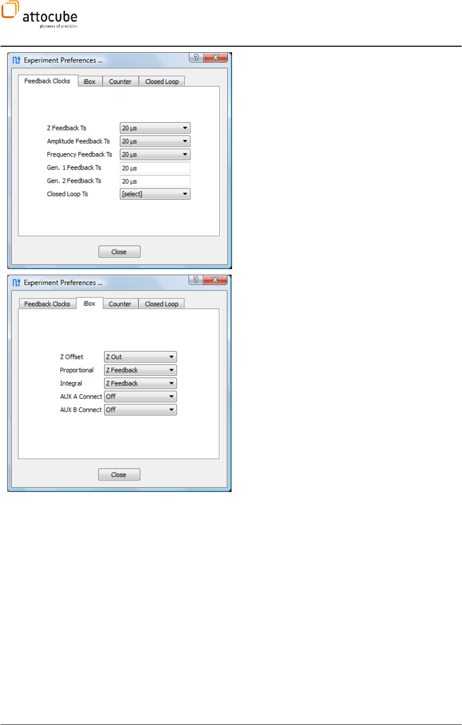
Page 46

In this tab, you can change the different Feedback

Clocks.

In this tab, you can change the assignments for some

iBox knobs to certain signals:

Z Offset: Choose between Z Out and Z Offset.

Proportional & Integral: Choose between Z Feedback,

Amplitude Feedback and Frequency Feedback.

AUX A & B Connect: On the iBox (see section II.4),

there are two auxiliary knobs that can be freely

assigned to one of a number of different parameters

using these settings.

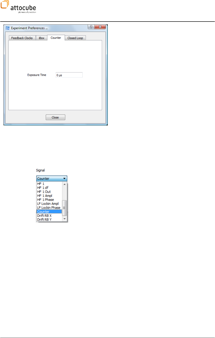
Page 47

respective companies. Any rights not expressly granted herein are reserved. ATTENTION: Specifications and technical

data are subject to change without notice.

The ASC500 has a dedicated input port for low-voltage

TTL pulses. Within the software, a counting procedure

keeps track on the number of received TTL pulses. It

can be used to display the number of counts in any line

or frame view. To use the counter, please connect the

source of the pulses to pin 1 of the External 1

connector (see Figure 3 on page 14).

Please note that the ASC500 accepts only low-voltage TTL pulses, i.e. pulses

with an amplitude of 3.3 V. The maximum repetition rate is 20 MHz.

To activate the Counter in the software, go to Preferences tab and enter an

Exposure Time for the counter. The exposure time is the time interval in

which the incoming pulses are accumulated. The exposure time can range

between 2.5 µs and 163 ms in 2.5 µs steps.

The counter signal can be chosen in all line and frame displays. If the

sample time of the display is larger than the exposure time, a number of

exposures can be averaged. In case the exposure time is larger than the



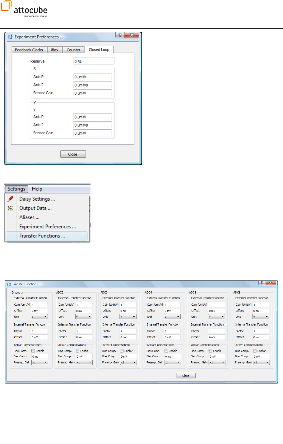
Page 48

For a description of this tab, please see section VI.2.a

on page 67.

Transfer Functions

The Transfer Functions offer the following functionalities:

1. Conversion of the voltage values read by ADC inputs towards physical

meaningful units. For example, if a photo-detector is used to collect your

data, Daisy can display all data in Watts. Use External Transfer Function for

the conversion.

2. Calibration of the ADC inputs. ADC voltage inputs usually show small

voltage offsets in the milli-Volt range. You can compensate for this offset

with the Internal Transfer Function.

3. Setting of a working point and an additional preamp gain. If you have e.g.

a small signal on a constant DC voltage, you can compensate for this DC part

and increase the gain for this channel.

External Transfer Function

Gain: Enter the conversion factor in Unit/V. For example, if a photo-

detector with an amplification of 5e6 V/W is used (corresponding to

0.2 µW/V), you can enter either Gain = 0.2 and Unit = uW or Gain = 200 and

Unit = nW. Please note that Daisy automatically displays the appropriate unit

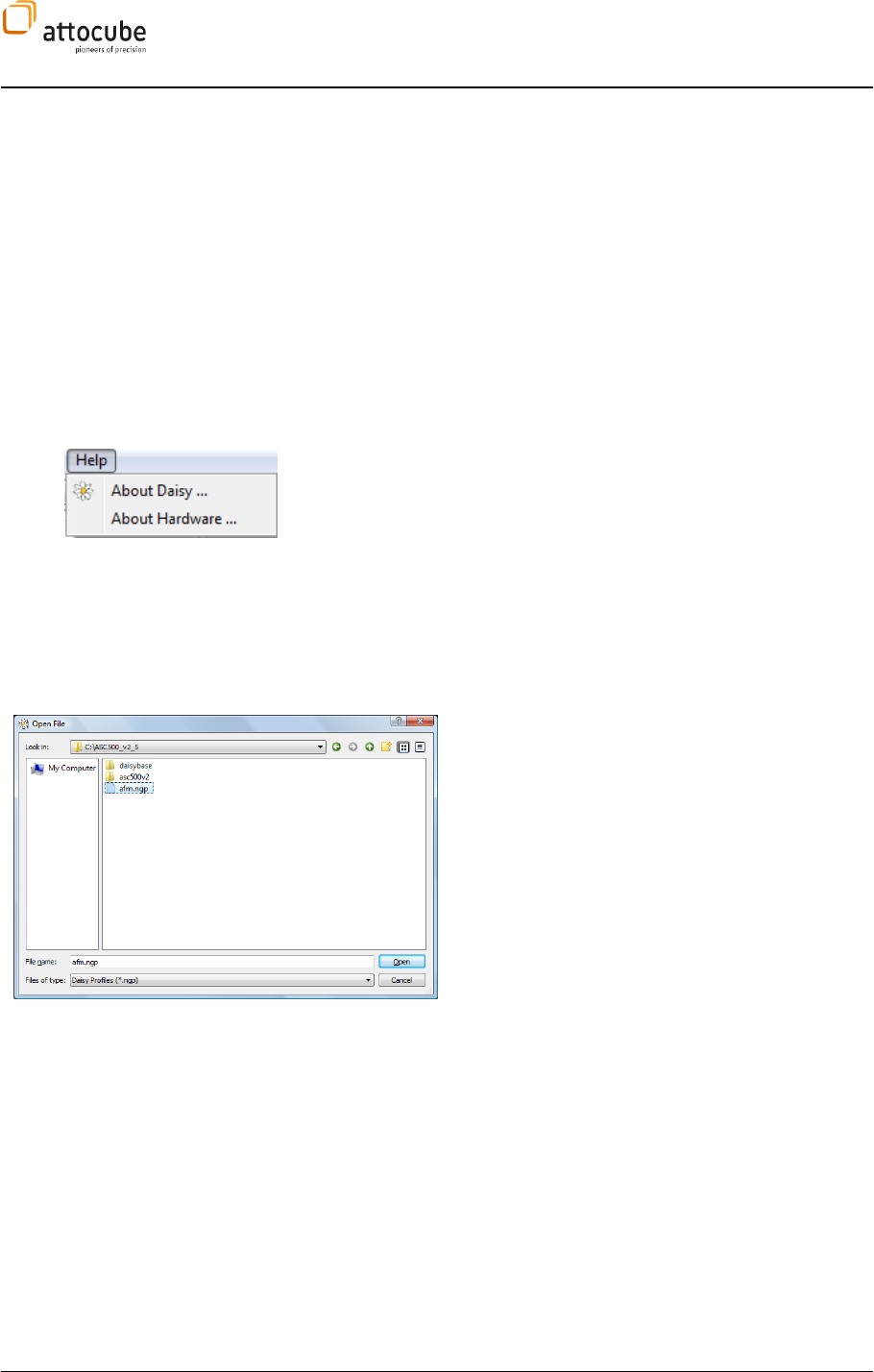
Page 49

respective companies. Any rights not expressly granted herein are reserved. ATTENTION: Specifications and technical

data are subject to change without notice.

prefix (nano- or micro-Watt) independent of the Unit setting.

Offset: Lets you specify an offset value added to the signal.

Internal Transfer Fuctions

Factor: Use this factor to correct for a ADC gain different to 1. Please note

that the actual signal will be divided by this factor.

Offset: Offset value to be added on the respective ADC.

Active Compensations

Bias Comp. Enable: Enable the active bias compensation.

Bias Comp.: Enter the DC offset on the input signal, that is to

be subtracted.

The Help menu contains the following entries:

About Daisy: Here you can find information about the Daisy software

version as well as licensing issues.

About Hardware: Here you can find information about your current ASC500

hardware.

V.2.c. Loading a profile

In order to perform a Scanning Probe Microscopy (SPM) measurement, a

profile needs to loaded, which defines the graphical user interface (GUI):

Open a 

force microscopy.

After opening the GUI, the main panel appears (see

below). In the main panel, all functions of the AFM can

be controlled.

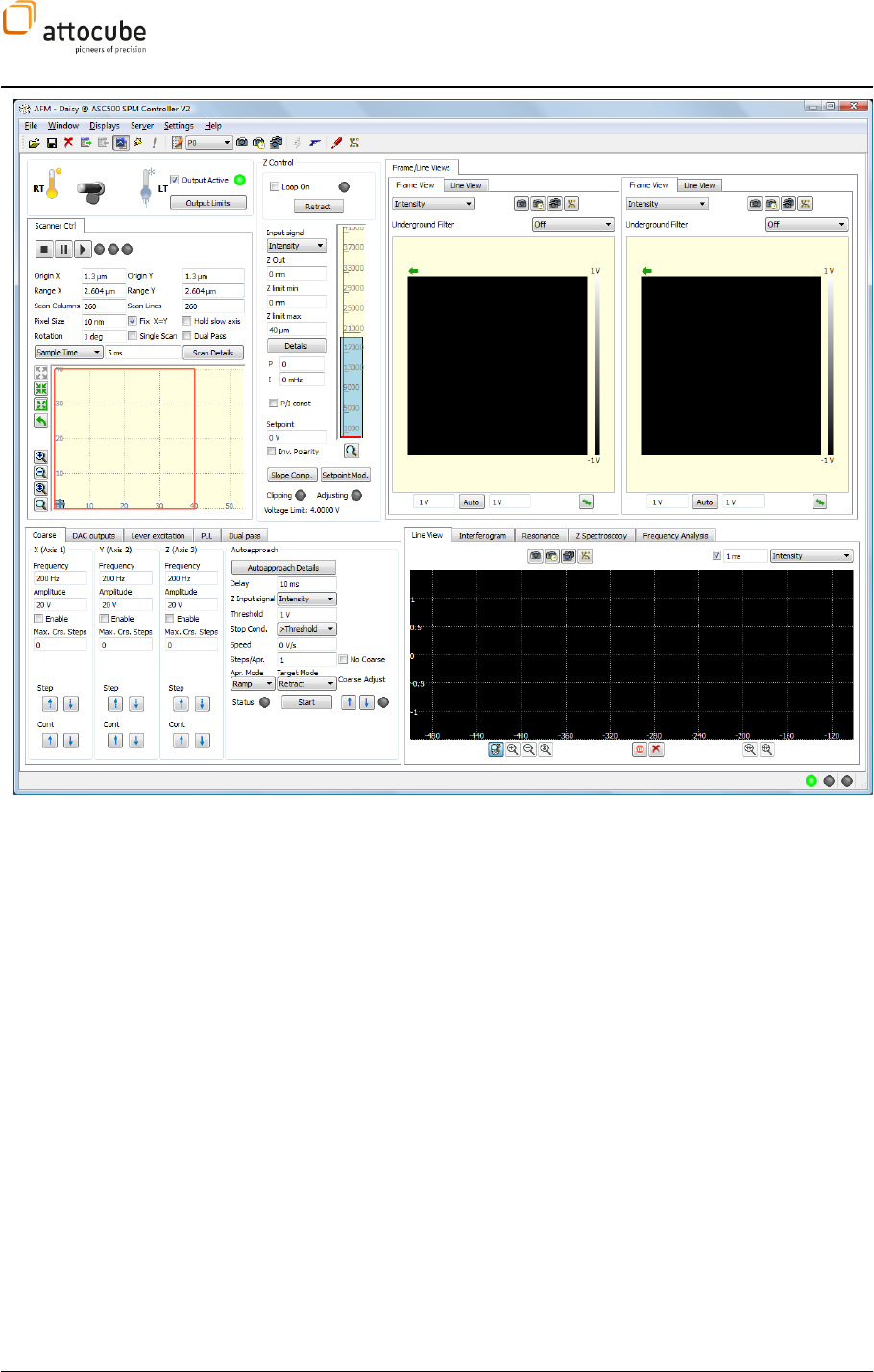
Page 50

The GUI is organized in 6 main sections: in the upper half of the screen, the

Output Limits, Scan Control, Z Control and the Scan Data Displays are located,

whereas the lower half contains tab section on the left for the main parameter

functions and a right tab section for the spectroscopies, a frequency analysis

and the time-based line view.

Special GUIs are available for all attocube systems microscopes. These have

been developed to adapt for the use of the specific instrument. In the CFM GUI

for example, there are less controls and parameters to facilitate the usage

with the confocal microscope. With the STM-GUI, the look-and-feel is slightly

different to enable the use of the software in this context. Both CFM and STM

GUI are subsets of the AFM GUI. Hence, the focus of this manual is the AFM

GUI.

V.3. Profile configuration

While preconfigured profiles (.ngp) are available for the most common

scanning probe methods, the new Daisy release v2.5 allows the user to

customize certain parts of the GUI, as will be described in the following

section. Besides, parameters (like output limits, scan ranges, slew rates

etc.) are also stored in the profile, such that every user of the instrument

can create his/her own presets.

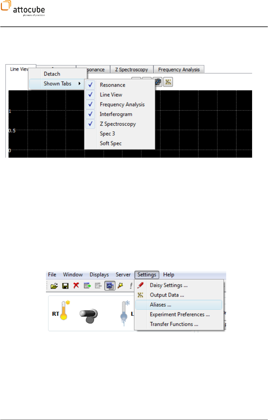
Page 51

respective companies. Any rights not expressly granted herein are reserved. ATTENTION: Specifications and technical

data are subject to change without notice.

V.3.a. User-configurable GUI appearance

By right-clicking on any of the tabs in the main GUI, the user can decide

whether to show, hide or detach it:

The order of the tabs can also be changed by dragging and dropping any of

the tabs to a new position within the tab bar.

The configuration of each tab section can be stored by creating a customized

profile.

V.3.b. Aliases menu

Since both the ASC500 hardware as well as the Daisy software serve the

purpose of a very generic, multipurpose and powerful SPM controller, many

of the signals, parameters and tab names within the software have also been

kept as generic as possible. However, many users are likely to stick to one or

two certain specific SPM methods as well as sets of parameters for their

experiments. Consequently, the user has been given the possibility to

rename most of the generic resources in the Aliases menu in order to

increase the user-friendliness:

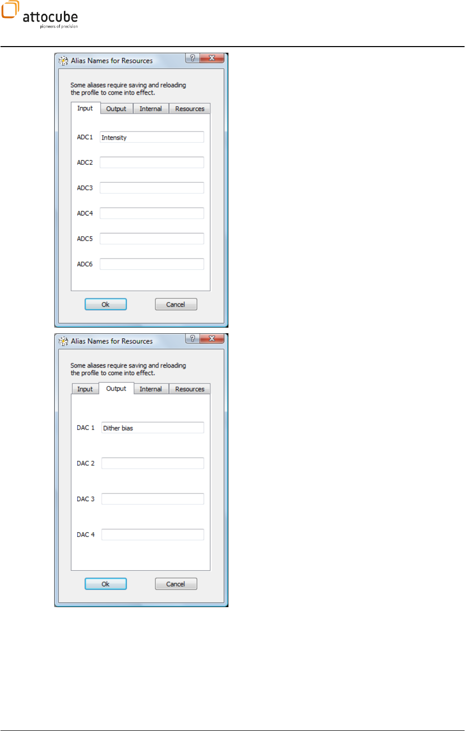
Page 52

Simply type in new Aliases for any of the shown Input

signal names and click OK.

Simply type in new Aliases for any of the shown Output

signal names and click OK.

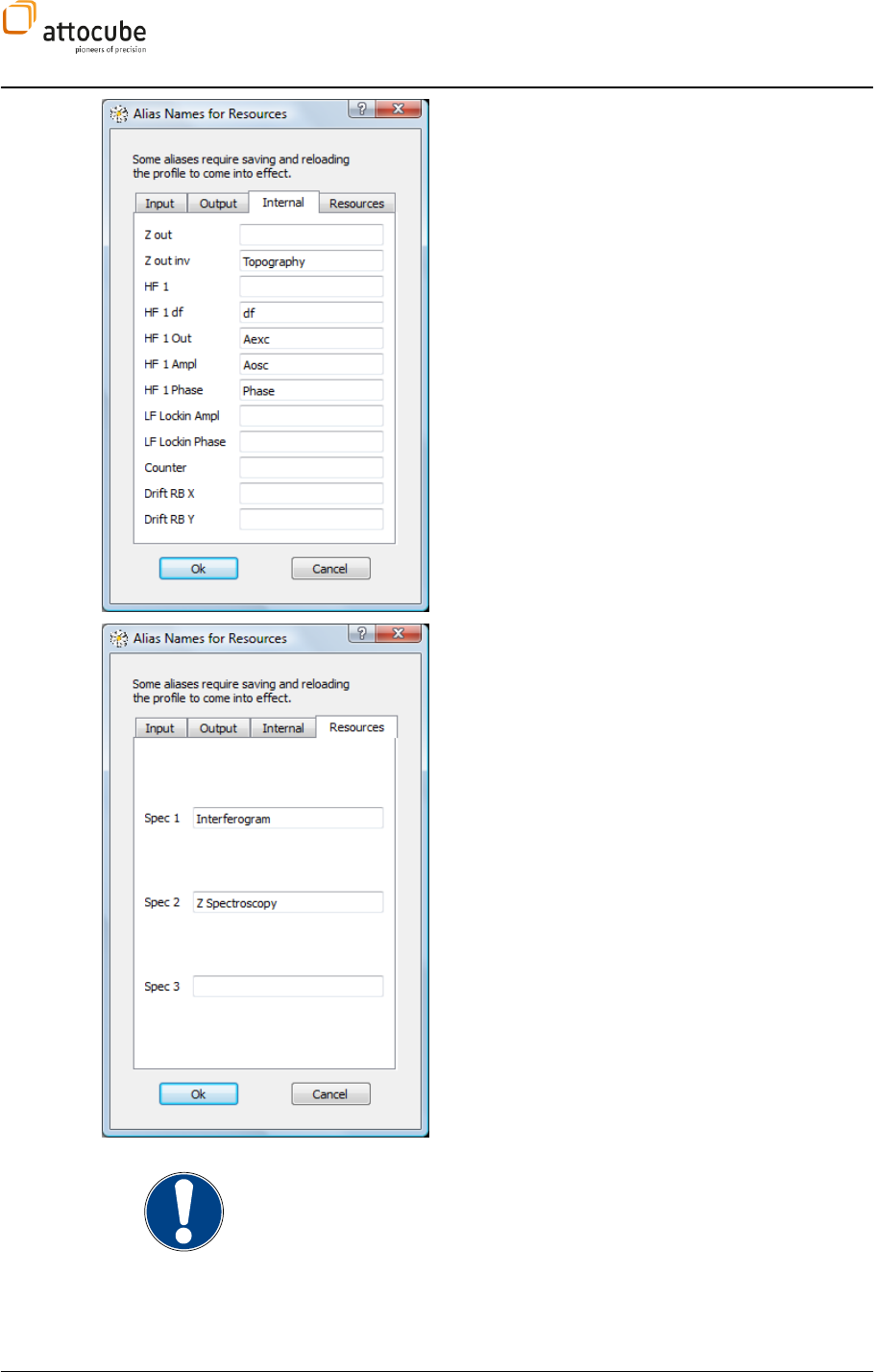
Page 53

respective companies. Any rights not expressly granted herein are reserved. ATTENTION: Specifications and technical

data are subject to change without notice.

Simply type in new Aliases for any of the shown Internal

signal names and click OK.

Simply type in new Aliases for any of the shown

Resources and click OK.

Note: The new Aliases for the resources will not come into effect until the

current profile is saved and reloaded.

Page 54

V.3.c. New signal and parameter names in v2.5

Starting from v2.5, several signals, parameters and tabs in the GUI have been renamed compared to previous

versions of the Daisy software (or have been equipped with the opportunity of aliases). The following table lists

the changes in order to help existing users with an updated Daisy software to get an overview of the mapping

between old and new names:

Signals

Previous name

New name in v2.5

SPM Z out

Z out

SPM Z out inv

Z out inv

AFM signal

HF 1

AFM df

HF 1 df

AFM Aexc

HF 1 OUT

AFM Aosc

HF 1 Ampl

AFM Phase

HF 1 Phase

LockIn Ampl

LF Lockin Ampl

LockIn Phase

LF Lockin Phase

Tabs

Previous name

New name in v2.5

Calibration

Resonance

LockIn

2 separate tabs:

- LF LockIn

- Lever excitation (=HF 1)

2nd Pass

Dual Pass

Pref

tab removed!

see:

- Output Limits (section VI.1),

- Experiment settings (section V.2.b), and

- Transfer Functions (section V.2.b)

Transfer

moved to Settings menu → Transfer

functions (section V.2.b):

all 6 transfer functions are now combined

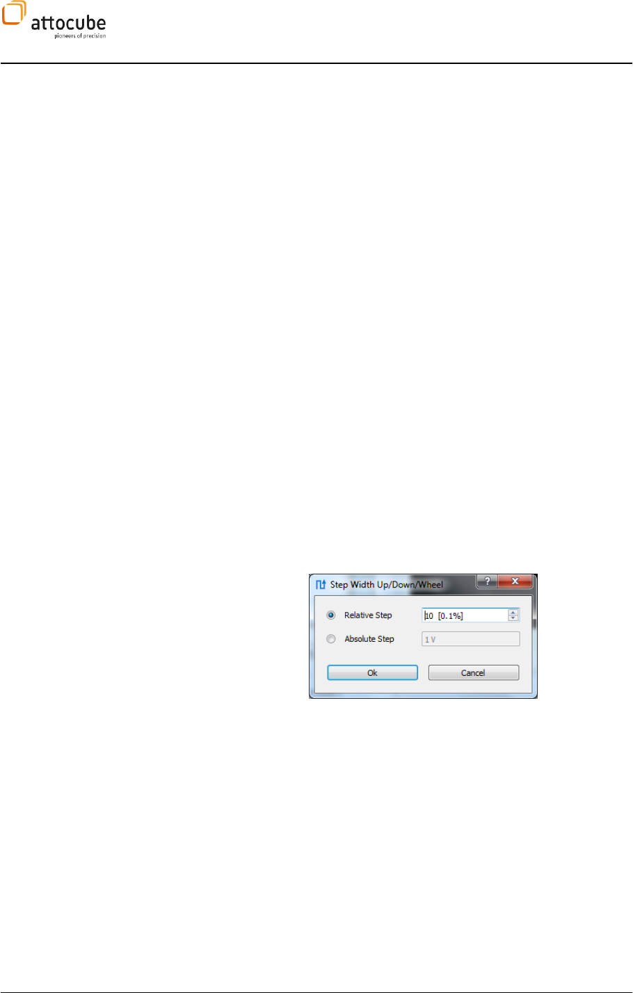
Page 55

respective companies. Any rights not expressly granted herein are reserved. ATTENTION: Specifications and technical

data are subject to change without notice.

V.4. General Usage and Description of Common GUI Controls

V.4.a. Text Edit Boxes

Most parameters of the experiment are controlled by entering numbers into

text edit boxes. The Daisy software provides a simple and intuitive way of

entering numbers.

Most numbers are accompanied by a physical unit. When entering or

changing a number, the units do not have to be entered. Just type the

number and press return; Daisy will automatically add the appropriate unit.





the prefix:

1. Enter a value greater than 1000 or less than 1. If you enter for

Daisy will change to microns



2. 

r pico-

for nano--- 

If you do not enter a prefix, Daisy will keep the last prefix. The only time



lease note that in this case it is usually sufficient



Using the mouse wheel

The mouse wheel can be used to conveniently edit the value of any text edit

box throughout the Daisy program. If the cursor is positioned on a text field,



decreased by turning the mouse wheel downward.

The sensitivity of the mouse wheel increment can be set for each text edit

box separately by using the Step Width 

It can be chosen between relative (default) or absolute steps. Even without

using the context menu, the sensitivity of the mouse wheel can be increased

by pressing the SHIFT and/or STRG key during turning of the mouse wheel.

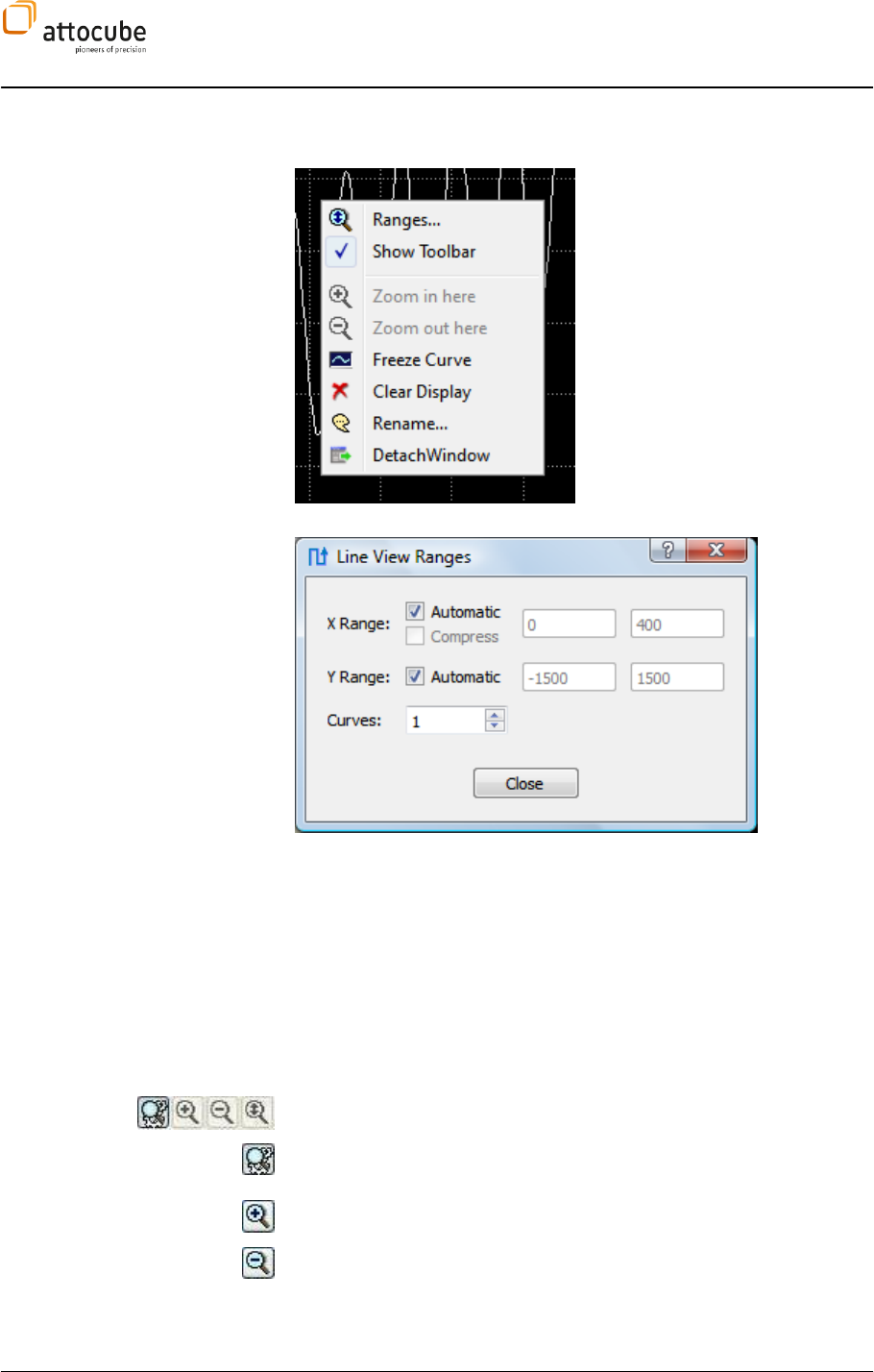
Page 56

V.4.b. Context Menu

By right-clicking on any graph window, one can open the corresponding

context menu. The functions that are available to the graphs are the same

throughout the program. The context menu looks as follows:

Ranges



The X Range and Y Range of the graph can be explicitly set. Deactivate the

check-boxes to enter the range values manually. Please note that it is not

recommended to use the manual X Range functionality. In the FFT graph,

please use the Fmin/Fmax parameters instead.

The Curves value allows for displaying several adjacent traces within the

same graph. The traces will be displayed in different colors for clarity.

Click on Close to close the window.

Show Toolbar

If the Show Toolbar button is activated, several toolbar icons will be shown

below the graph:

The four icons to the left comprise the Zoom Tools.

If this icon is enabled, auto-range mode is switched on. The Zoom Tools to

the right are not activated.

Zoom in.

Zoom out.

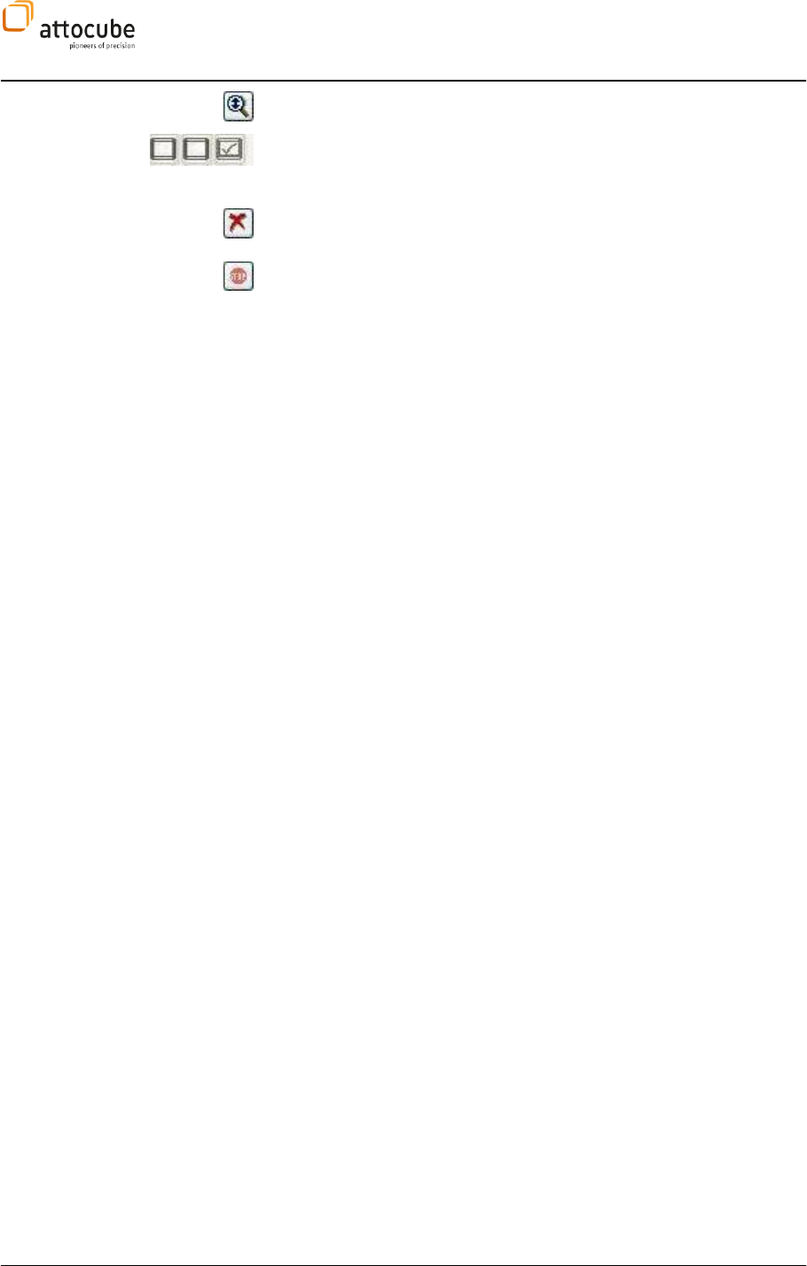
Page 57

respective companies. Any rights not expressly granted herein are reserved. ATTENTION: Specifications and technical

data are subject to change without notice.

Zoom to maximum range.

These buttons represent the Frame Tools. When active, certain operations to

modify the data range can be performed. See for example the description of

the Frame Tools in the Data Display section VI.4.

Clear the display. The current data will be deleted and the graph will start

over. Useful if you have chosen a slow display.

Stop the display from being updated. The graph will stay until cleared or

Stop is pressed again.

Freeze Curve

This function freezes the currently displayed curve. It can be used as a

reference to compare to. The frozen curve can be erased using the Clear

Display function.

Clear Display

Use this option to clear the current display.

Rename

Here you can rename the snapshot data of the current display.

Detach Window

Use this function to detach the graph from the Daisy window into an

independent window. You can then resize this window and move it wherever

it suits you best. This is especially useful when you use a system with two

monitors. This function can also be accessed by double-clicking on the

graph.

You can reattach the window either by using the context menu of the new

stand-alone graph (Attach window) or by right clicking on the empty space

in the Daisy window and selecting Attach Window.

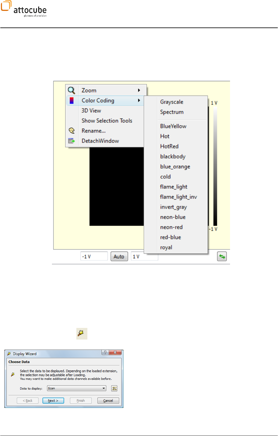
Page 58

V.4.c.

Frame View

context menu

The Frame view context menu offers mainly the same options as described

above, but in addition, one can also activate a 3 dimensional data view (3D

view), and/or change the Color Coding. One can choose the colors which

provide best contrast for the data. There is also the possibility to add more

color scales. Just copy a color scale in the *.lut format into the program

folder. It will automatically be added to the menu.

V.4.d. Display wizard

The Display Wizard is a powerful tool to personalize the GUI and to open

access to more data windows. It is possible to create line and frame views

(and combinations thereof) and to apply filters to them. The data in these

windows can be integrated into the automatic global snapshot routine,

giving you the possibility to save all interesting data with one mouse click.

This is especially useful for e.g. the Lift Mode, where one requires an

additional data display for the second pass data.

One can open a new display as described below:

First, click on the Display Wizard button.

The first wizard window appears, where you can define

additional data channels for the new display that you are

about to create, and use the pull-

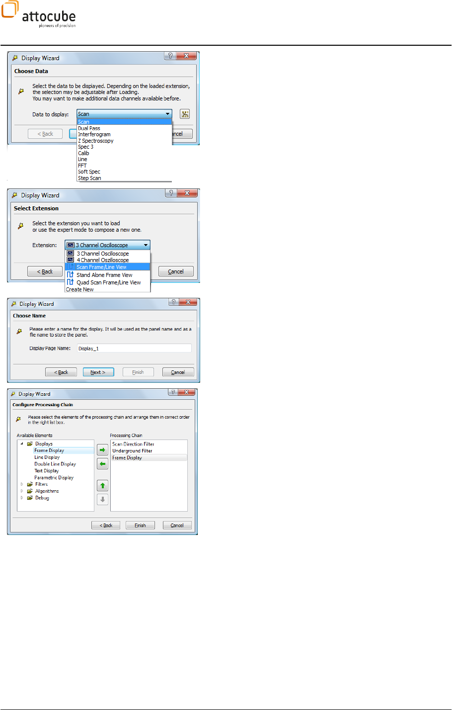
Page 59

respective companies. Any rights not expressly granted herein are reserved. ATTENTION: Specifications and technical

data are subject to change without notice.



left). After choosing the most appropriate one, click Next.

For most of the data categories, there are preconfigured

Extensions available, but you can also select Create New to

manually choose the details of your new display.

If you select one of the preconfigured Extensions, simply click

Finish to start using the new display.

In case you choose a data display that either lacks a

preconfiguration, or that you would like to manually set up,

you are first asked to assign a name to the new display. Click

Next.

Now, configure the processing chain. Select the actions and

elements you want to use for the new display. In this example,

a frame display together with a scan direction filter and an

underground filter is selected. Highlight the elements on the

list to the left, then press the right arrow button to add the

element to the processing chain. The processing chain will be

executed from top to bottom at runtime, so it is important to

place the filter before the display. To do this, highlight the

filters in the processing chain list and then press the up arrow

button. Press Finish.

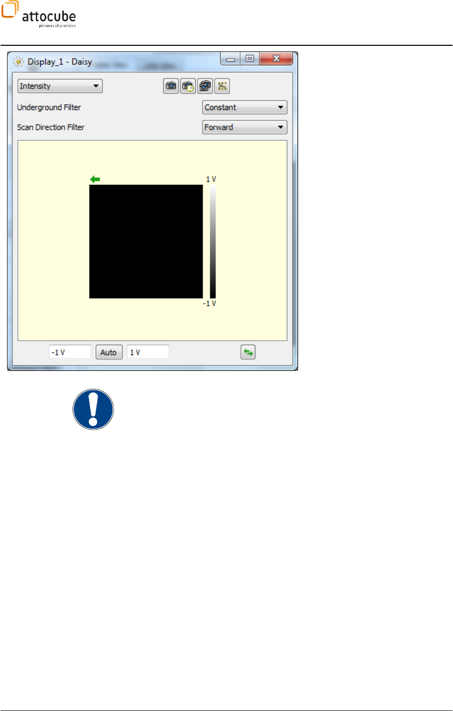
Page 60

The new window will appear. Detach

it from the Daisy window, or keep it

as another tab within your main

window. The signal can be chosen via

the drop down list in the upper left of

the window. Set the Scan Direction

Filter according to your needs

(forward or backward; Off means

forward and backward and will result

in backward). Now the new display is

configured for the measurement.

Note: Not every combination of Trigger, Filter and type of view will result in a

reasonable display. For example, an underground filter is only valuable in a

SCAN type context.

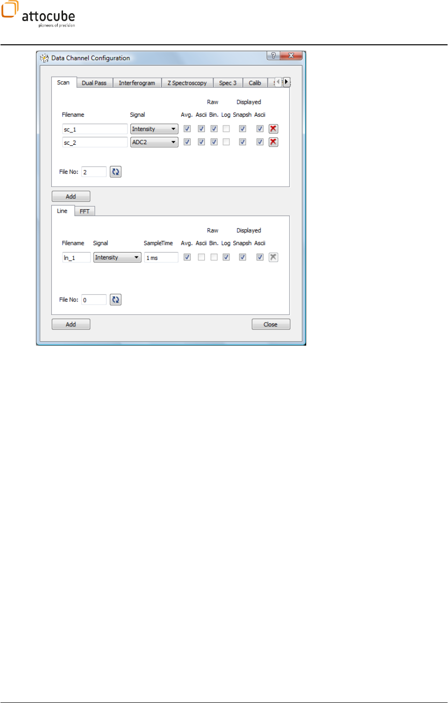
Page 61

respective companies. Any rights not expressly granted herein are reserved. ATTENTION: Specifications and technical

data are subject to change without notice.

If you have not done so already,

please check that your desired

signal(s) are available as data

channels in the DCC (see section

IV.1 for details.)

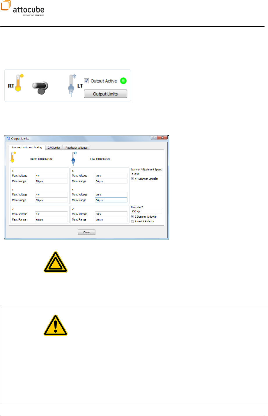
Page 62

VI. Description of the AFM Profile

VI.1. The Output section

The upper left corner of the GUI hosts the control

section for the activation of all controller outputs as

well as the settings for their corresponding limits.

The central switch to the left can be used to

conveniently alternate between room temperature (RT)

and low temperature (LT) settings.

The actual limiting values for each case can be defined

upon clicking on the Output Limits button.

The first tab contains the Scanner limits

and scaling details for RT and LT

respectively, as well as a switch to

toggle between uni- and bipolar

settings for all scanner outputs: using

the latter will also switch between

max. voltage ranges of either 0..max

(unipolar) or –max..+max (bipolar).

Furthermore, the presets for Scanner

Adjustment Speed (which controls the

rate at which the tip position is moved

upon changing the position of the scan

field), the slew rate of the Z output and

its polarity can be adjusted.

Important Note: Choose all of these settings very carefully, since wrong

voltage ranges (also wrong polarity settings) may damage the piezos of

your scanners!

Typical values are stored in the respective profiles provided by attocube

and/or can be found in the respective manual of your attocube microscope.



Caution. The output limit is the voltage supplied by the ASC500 controller.

This voltage is then typically fed into a voltage amplifier (e.g. the ANC300)

which amplifies this voltage by some factor before it is applied to the

piezos. 

amplifiers are:

ANC250 factor 20

ANC300 factor 15

ANC350 factor 14

ALWAYS TAKE INTO ACCOUNT THE AMPLIFICATION FACTOR PROVIDED BY YOUR

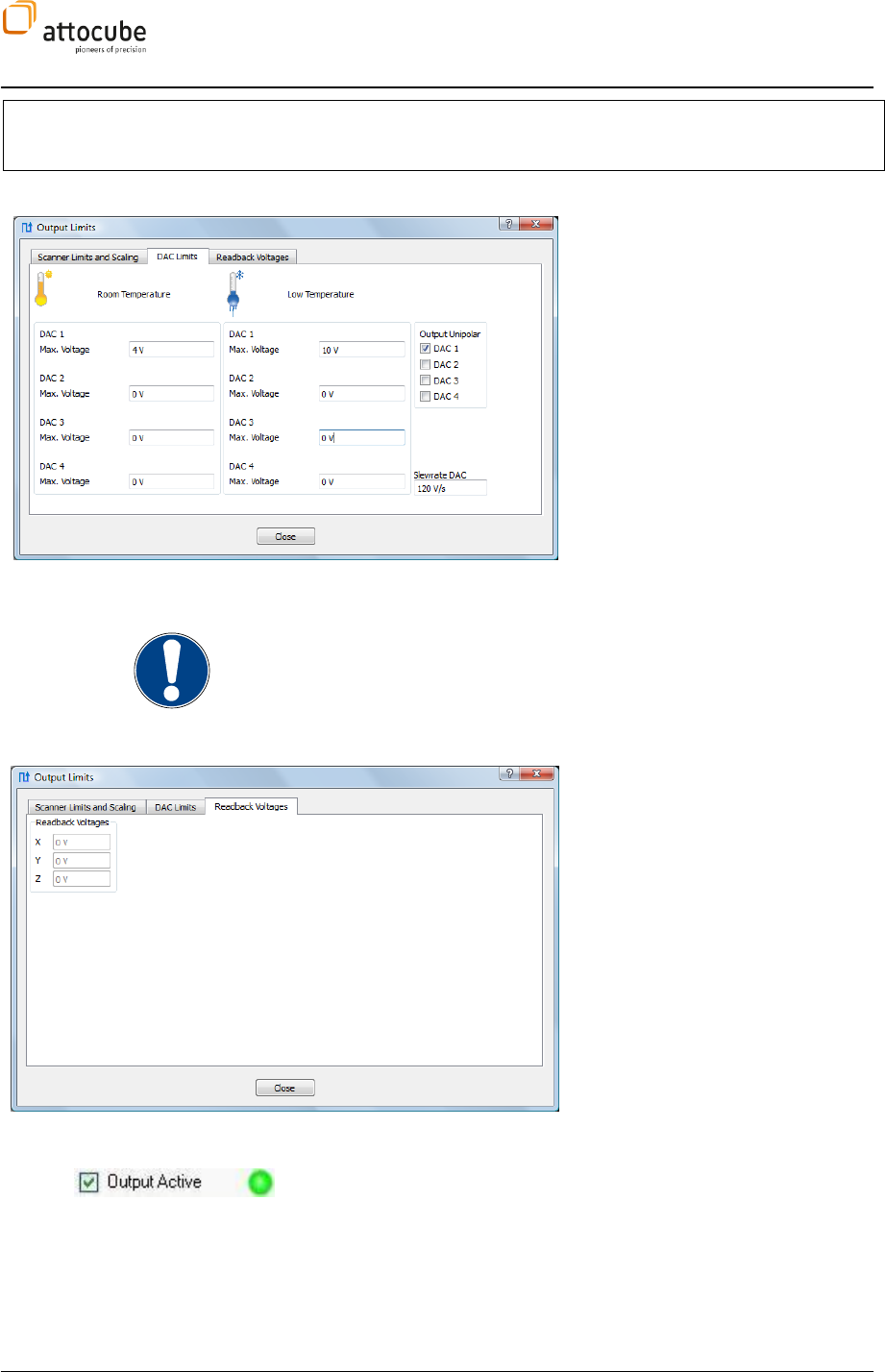
Page 63

respective companies. Any rights not expressly granted herein are reserved. ATTENTION: Specifications and technical

data are subject to change without notice.

VOLTAGE AMPLIFIER IN ORDER NOT TO EXCEED THE MAXIMUM ALLOWED

VOLTAGE.

The second tab contains the min. and

max. voltages for all DAC outputs at RT

and LT respectively. Besides, the slew

rate can be adjusted.

As an additional safety feature, the

user needs to allow bipolar outputs

for each DAC separately by checking

the corresponding box.

(Please note that when using aliases as

described in section V.3.b, they will be

used everywhere in the Daisy instead

of the original parameter names as

shown here in case of DAC1, which has

been renamed to Dither bias.)

Note:

Please be aware that also wrong DAC limits may damage your hardware,

such as in case of the cantilever based AFM/MFM the dither piezo, which is

usually connected to DAC1!

The third tab contains displays for the

actual voltages of x, y and z (read back

from the controller).

Output Active: With the Output Active button all electrical outputs of the

ASC500 controller can be enabled or deactivated. If disabled, all electrical

outputs are set to zero. The switching procedure may take some seconds.

The LED to the right of Output Active indicates whether the outputs are

active (green) or not (red).

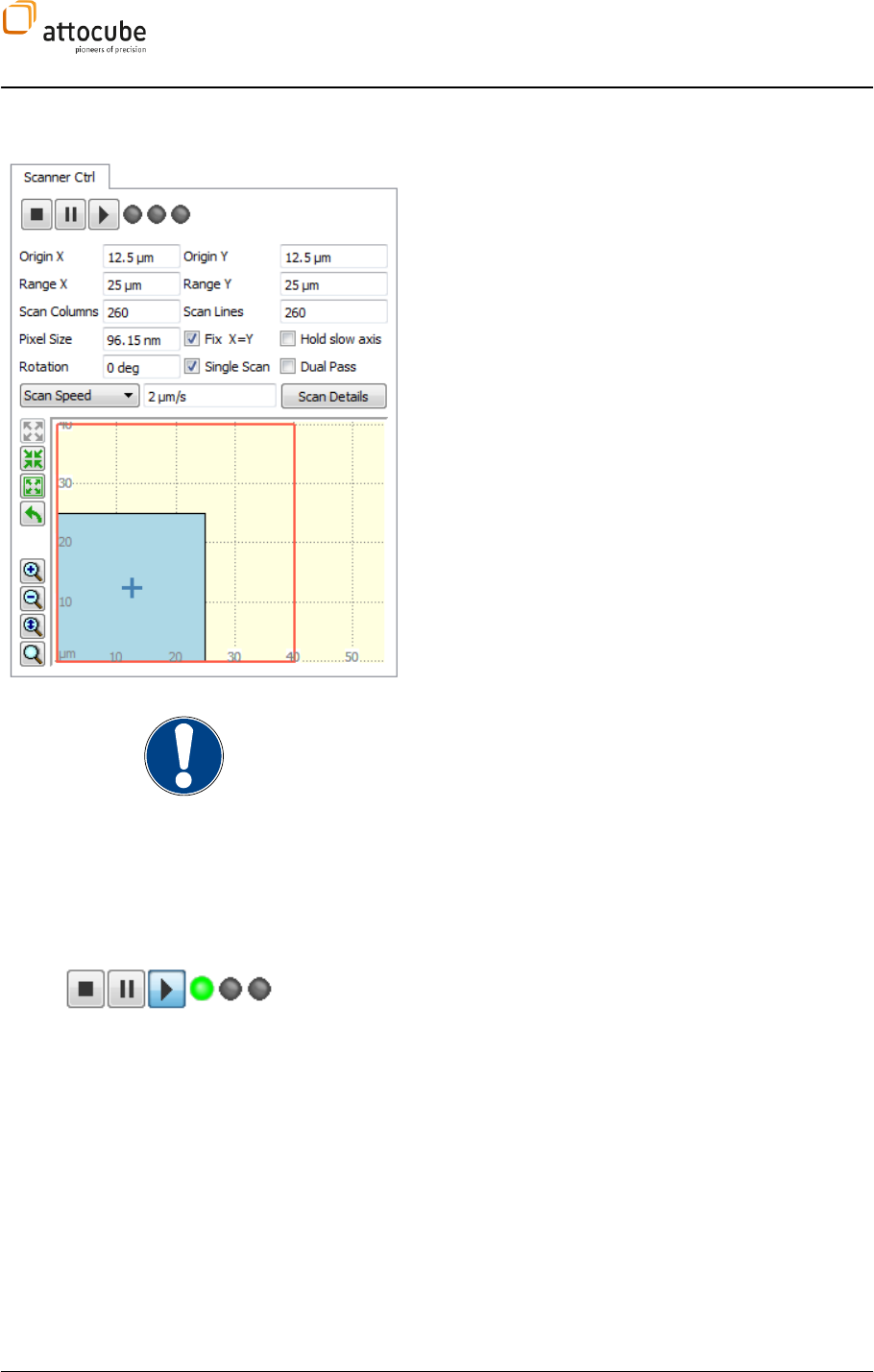
Page 64

VI.2. The Scanner Control

The scanner widget is the control center of the scan

generation. All important scan parameters, such as the

number of Scan Lines and Scan Columns, Pixel Size, and

Sample Time can be entered here. Furthermore, an offset

for the scan area can be set (Origin X and Origin Y).

The scan area can also be rotated by entering the desired

Rotation angle. Please note that a rotation can only be

performed if the space for this transaction is available, i.e.

the origin of x and y has to be moved (when using a

unipolar piezo scanner).

Note: Rotation is done by hardware mixing of the x- and y-channels. This

has the great advantage of a smooth and step-free rotation as compared to

digital rotation.

Due to this analog mixing procedure, there is a small error to the angle. A

slight angle error of about +/-150mdeg may be visible in certain check

measurements.

Start/Stop, Scan Status

LEDs

These buttons are the main scanner control. The following knobs and LEDs

are available:

Stop Scanner: The left icon is used to stop the scanner. The scanner is

moved to the lower left corner of the active scan area.

Pause Scanner: The middle icon is used to pause the scanning movement.

The scanner will stop at the current scan position and will restart from here

after the next click of the Start Scan button.

Start Scanner: The right icon is used to start the scanning process. A red

dot will mark the current position of the scanner in the Active Scan Area. If

the Single Scan button is active, the scanner will be stopped and

repositioned to the origin after one complete scan. If Single Scan is not

active, the scanner will run until you press either Stop or Pause Scan.

Scan Status LEDs: The left LED (green) is lit when the scanner is running

and image data is collected.

Scanner Moving LED: The middle LED (red) is lit when the scanner is

Page 65

respective companies. Any rights not expressly granted herein are reserved. ATTENTION: Specifications and technical

data are subject to change without notice.

moving without data collection (e.g. during the movement to the origin

after pressing the Stop Scanner button).

Adjusting LED: The right LED is lit, when the scanner is adjusted internally.

During this procedure, the scanner cannot be started.

Origin X/Origin Y [pm/nm/µm]: Offset of the center of the active scan

area.

Range X/Range Y [pm/nm/µm]: Enter your desired scan range.

Scan Lines/Scan Columns: Enter the number of pixels in x (columns) and y

(lines) direction that will be collected. The scan range will be Pixel Size

times the number of pixels in each direction. If the Fix X=Y button is active,

only square scan areas are allowed and each change in Scan Lines or Scan

Columns will immediately affect the complementary parameter.

Pixel Size [nm]: Enter the pixel size in nanometers.

Sample Time [µs]: Time for the collection of one image data point. Please

note that the Sample Time is usually much higher than the time needed to

acquire one data point (2.5 µs). If the Average button in the Data Display

window is not activated, Daisy will acquire one data point and saves it to the

image, then skips all data points for the rest of one Sample Time. If Average

is activated, then all data points within one Sample Time will be acquired

and averaged to give one image data point.

For a smooth scanning movement, the scanner is not stopped during the

Sample Time, but moves steadily to the next pixel.

Instead of the Sample Time, the user can choose to set and maintain the

following derived parameters:

Line Frequency: = Sample Time * Scan Columns *2

The factor two is given for forward and backward measurement.

Scan Speed: = Sample Time / Pixel Size

Time per Frame: = Sample Time * Scan Columns * Scan Lines * 2

Dependent on which parameter is chosen, Daisy will try to keep this

parameter constant if other parameters are changed. For example, if Time

per Frame is selected and Scan Columns and Lines are decreased (Fix x=y

enabled), the Sample Time is increased accordingly. If the Pixel Size is

increased, the Scan Speed will increase accordingly to meet the same Time

per Frame.

Rotation [deg]: Enter a value between 0 and 360 degree. The Active Scan

Area will be rotated around the Origin. Please note that a rotation can only

be performed if enough space in the total scan area is available.

Fix X=Y: Toggle between fixing the scan range to be equal in both directions

and allowing different ranges for X and Y.

Hold slow axis: Activate this option to always scan the same line.

Single Scan: Activate this option to automatically stop the scan upon

completion of the frame.

Dual Pass: Use this option for the Dual Pass mode, see also section VI.5.g.

In this mode, every line is scanned twice (fwd-bkwd, fwd-bkwd, next line).

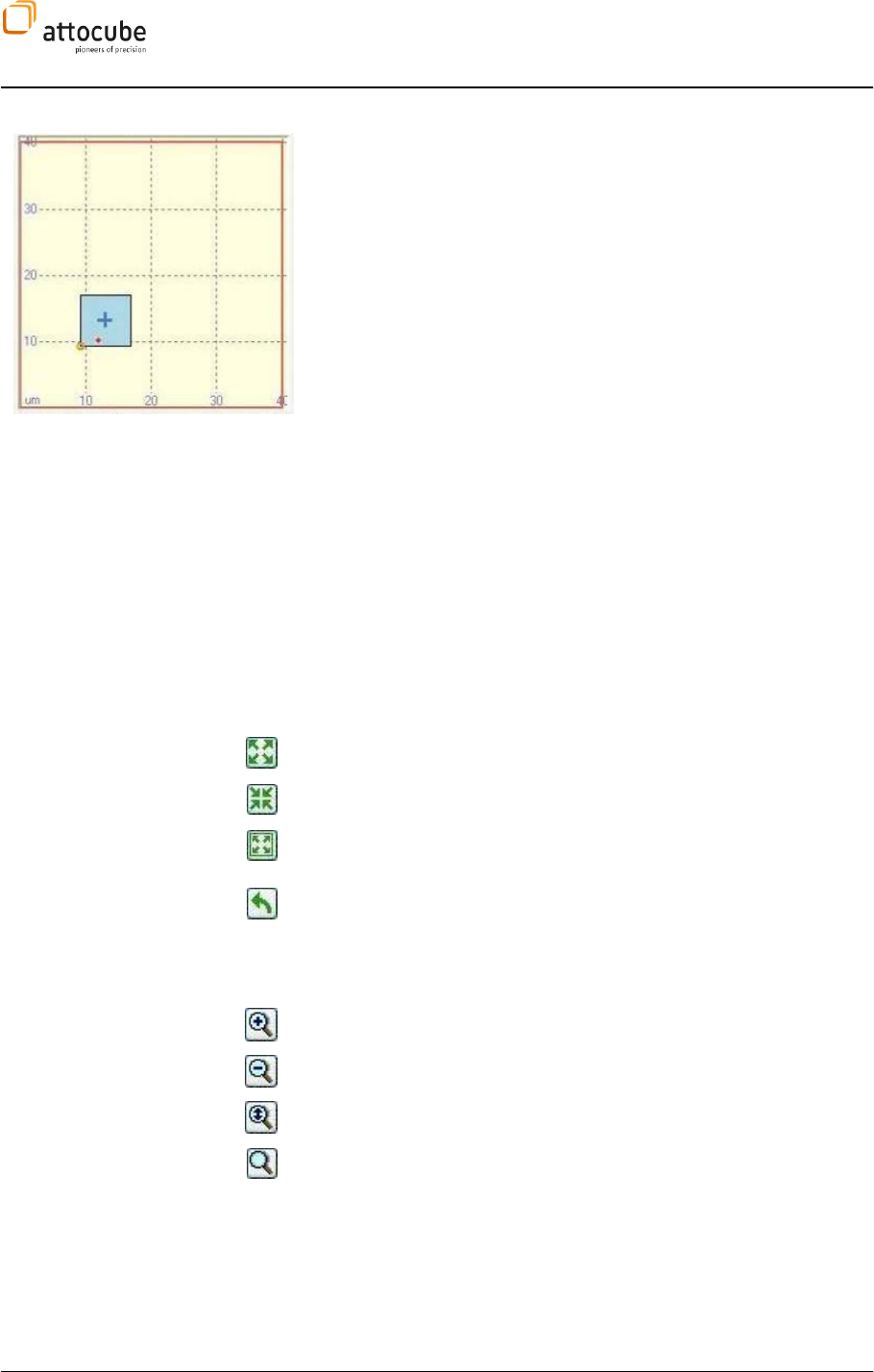
Page 66

The Scan Display

The Scan Display gives an overview over scan range and active scan area. In

its smallest magnification, the total available scan range is visible and

marked by a red rectangle. The Active Scan Area is marked by the blue

rectangle and can be arbitrarily chosen within the total scan range. During

scanning, a red dot marks the current position of the scanner (for very fast

scans, this dot is spreads out to a line). The yellow circle marks the origin of

the scan, whereas the blue cross marks the center of rotation.

To change the Active Scan Area, one can either enter the desired

parameters manually or adjust the Active Scan Area using the mouse. There

are three different possibilities to change the Active Scan Area with the

mouse:

Move: Position the mouse on the blue cross in the middle of the Active

Scan Area. The mouse pointer will change to a cross. Drag with the left

mouse button to reposition the scan area.

Resize: Position the mouse on the border of the Active Scan Area. The

mouse pointer will change to a rectangle. Drag the border with the left

mouse button until the desired size is reached. This will change the Pixel

Size, whereas the Scan Lines/Columns remain unchanged.

Rotate: Position the mouse somewhere between the border and the middle

of the Active Scan Area. The mouse pointer will change to a circle. Drag to

rotate.

Active Scan Area Size Tools

One can use the Size Tools to change the Active Scan Area.

Enlarge: Enlarges the Active Scan Area by 19%.

Shrink: Shrinks the Active Scan Area by 19%.

Maximize: Sets the Active Scan Area to fill the total available scan

range. Rotation is set to zero.

Rotate: Rotates the Active Scan Area by 90 degrees. This feature is

helpful if you want to quickly exchange the fast and slow scanning axis.

Active Scan Area Zoom

Tools

Use these icons to zoom in and out of the Scan Display. These tools do not

change the Active Scan Area.

Zoom in

Zoom out

Zoom all: Shows the total available scan area.

Zoom Adjust: Shows the Active Scan Area.

Scan Details

Click on Scan Details to display important additional scan parameters which

follow directly from the defined scan parameters.

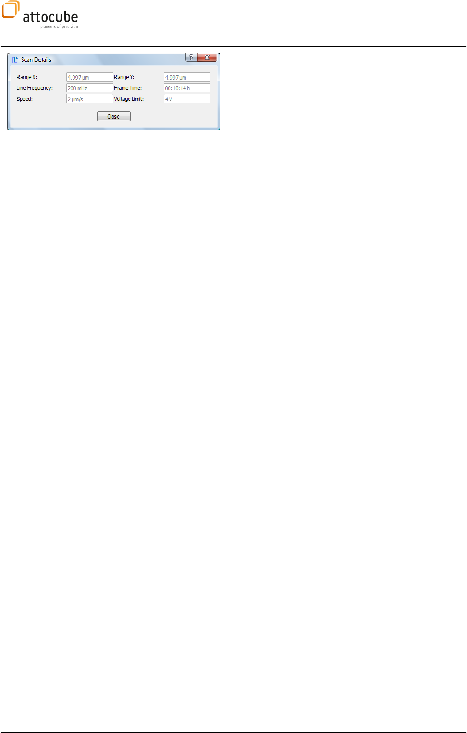
Page 67

respective companies. Any rights not expressly granted herein are reserved. ATTENTION: Specifications and technical

data are subject to change without notice.

Range X/Range Y: Size of the Active Scan Area.

Line Frequency: Line Frequency in Hertz. Please note that

Line Frequency is based on the time for forward and

backward scan of one line.

Frame Time: Time needed for the completion of one up

scan or one down scan.

Scan Speed: Speed of the scanner in micrometers per

second.

Voltage Limit: The current voltage output limit as

defined in the Preferences Tab.

VI.2.a. Closed Loop Scanning

The ASC500 supports the use of scan position sensors to provide closed

loop scanning functionality. In a closed loop scan mode, all non-

linearities of the scan motion that arise due to the non-linearities of the

But not only the scan motion will be

affected; also the point positioning within the path mode will be free of



p



range of either 1.2 mm or 5mm (depending on the model) and thus allow

for exact repositioning within the wide xy coarse range. 

Principle of operation

Figure 12 shows the principle of operation of the closed loop control

functionality. The target position will be fed into a PI controller that will

adjust the scanner control voltage until the current position matches the

target position. There are two PI controller, one for each x or y scan



will determine the speed in which the scanner will follow the target

position. If the target position changes continuously as in the scan

movement, there will be fixed shift between the target and the actual

position. This shift is called contouring error. It can be diminished by

maximizing the speed of the closed loop control loop. Still, the control

speed must be slow enough to still offer a stable feedback without any

oscillations.

attocube systems closed loop sensors offer a sensor range that is much

larger than the range of motion of the scanner. The scan range will thus

always be a small part of the sensor range. If coarse positioning is used,



is possible to recalibrate the scanner coordinates by a single mouse click

to define a new position of the scan range within the sensor range.

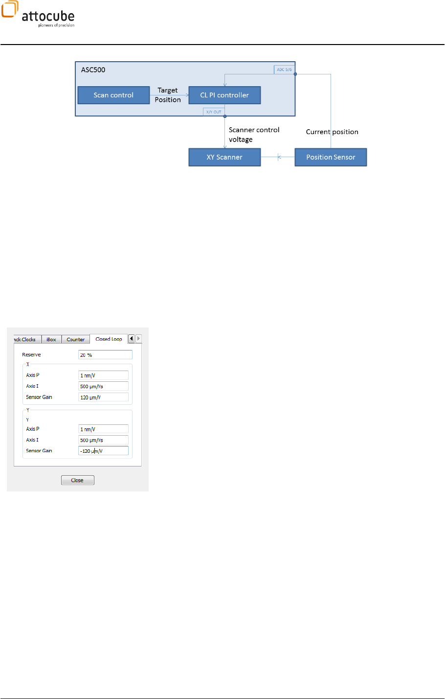
Page 68

Figure 12: Principle of operation of closed loop scanning

Preparation

The following preparation steps have to be finished before a closed loop

scan can be started. These steps are listed here for reference only,

because both software and hardware are readily configured after the



1. The sensors have to be mounted in the microscope setup and the



2. The sensor signal is an analog voltage that has to be fed into the

ADC5 input of the ASC500 for the x direction sensor and into the

ADC6 input for the y direction sensor. It is not possible to change

the input configuration to other ADC inputs.

3. The parameters of the closed loop PI controller can be set under

Settings – Experiment Preferences in the Closed Loop tab. An

example is shown to the left:

a. Reserve: Defines an extra scan range margin around the

actual scan range. This extra margin allows for

positioning the tip on the boundaries of the actual scan

range, even if the non-linearities of the scanner require

a scanner voltage that would lead to an out-of-range

tip position in open loop scan mode. In closed loop

scan mode, the actual scan range plus the reserve will

be mapped to the full 16 bit resolution of the scanner

output converters.

b. Axis P/Axis I: Defines the P and I feedback parameters

of either x or y closed loop controller. Good values to

start with are P = 1nm/V and I = 500 µm/V (I being the

much more important parameter). If feedback is too

slow, Axis I should be increased, if the feedback is

unstable, Axis I must be decreased.

c. Sensor Gain: Defines the position vs. voltage rate of the

sensor. For standard attocube sensors, this gain is

either 120 µm/V or 500 µm/V. The sign of the sensor

gain is important: a negative value will be appropriate

for a configuration where an increasing scanner voltage

leads to a decreased position value.

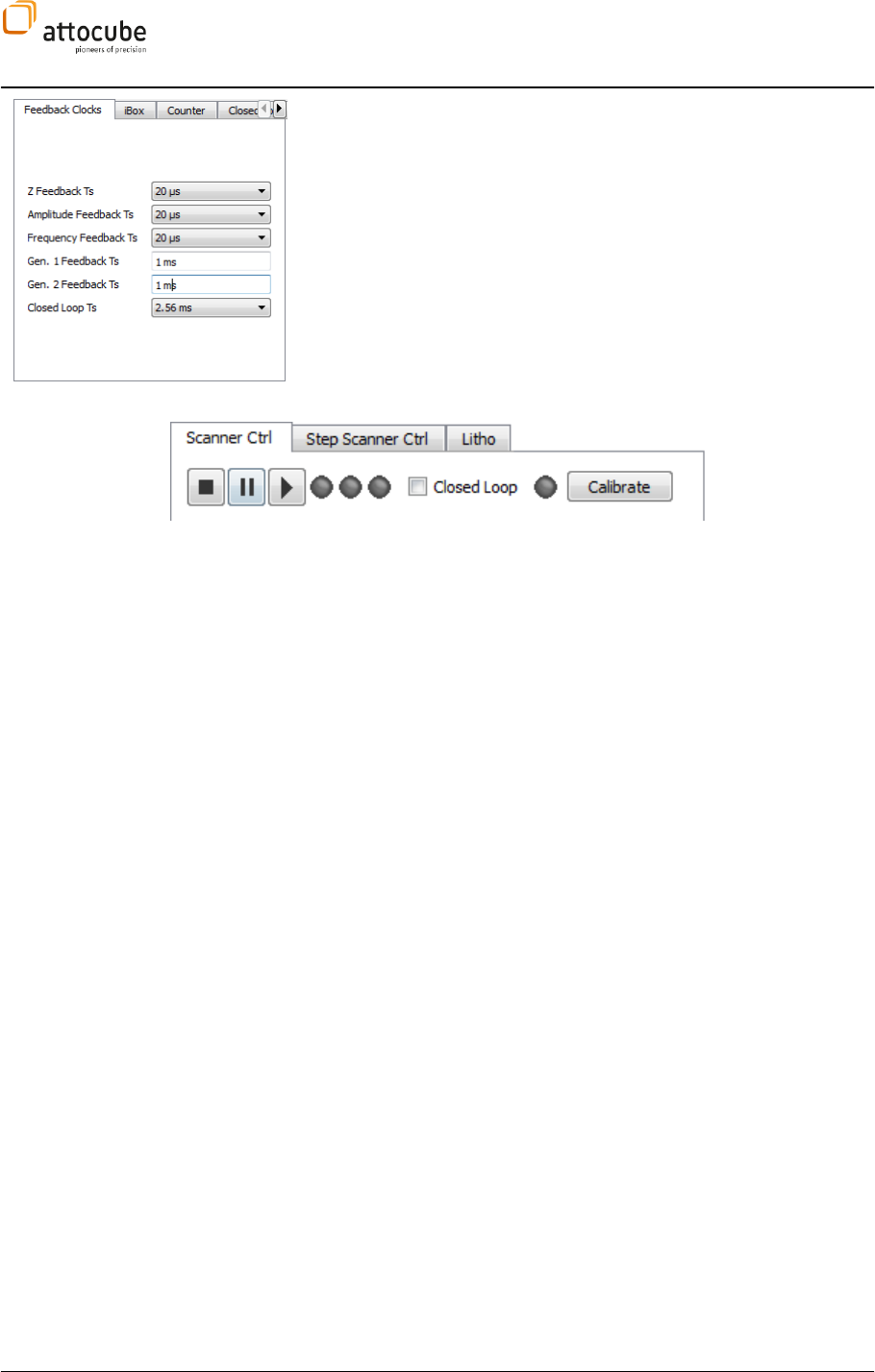
Page 69

respective companies. Any rights not expressly granted herein are reserved. ATTENTION: Specifications and technical

data are subject to change without notice.

4. The clock of the closed loop feedback should be set to 2.56 ms.

This value can be checked under Settings – Experiment

Preferences in the Feedback Clocks tab. This tab is shown to the

left.

Figure 13: The closed loop control buttons on the top of the scanner widget. From middle to right: Closed loop

activation checkbox, closed loop status LED and Calibrate button.

Operation of closed loop

scanning

Once the closed loop control is started, all scanner movements will be

operated in closed loop mode. Scanning movements, point positioning in

path mode and manual tip positioning will be free of non-linearities and

creep.

Before switching to closed loop mode, it is important to calibrate the



coordinates. This is done by pressing the Calibrate button on the upper

right of the scanner widget (see Figure 13). Then the closed loop mode

can be activated by checking the Closed Loop checkbox.

There are a few situations where the start of the closed loop mode will be

prohibited:

- Scanner is moving; scan movements have to be stopped

before turning on closed loop mode

- Lithography is running

- Pathmode is running

- The Hold Slow Axis option of the scanner widget is active

- Scan field rotation is not equal to zero; due to certain

hardware constraints, rotation of the scan field is not

possible in closed loop mode.

- The scanner is currently in a state of switching from

closed loop back to open loop (the closed loop LED will

be red)

In all cases above, an error message will be generated and closed loop

mode will not be activated.

The usage of the scanner in closed loop mode is similar to the open loop

mode situation. However there is a difference in the way the red dot in the

scanner widget indicates the actual scan position. The red dot will NOT

Page 70

show the current scan position. Instead, it will display the current scanner

output voltage transferred back to a position. To highlight the difference,

the following example might be helpful: Consider the origin of the actual

scan range is set to (5 µm/5 µm) and the scanner calibration is 10 µm/V

with the scanner being in STOP mode. In open loop mode, the red dot

would be located on the (5 µm/5 µm) position in the scan grid and the

output voltage would be (0.5 V/0.5 V). In closed lo

non-linearities might require a voltage output of (0.45 V/0.48 V) to

stabilize the scanner on a (5 µm/5 µm) position. The red dot will now

show a scan position corresponding to a (4.5 µm/4.8 µm) position, i.e.

outside of the actual scan range (that is displayed in blue in the scanner

widget). The advantage of this illustration is that the user has an

instantaneous indication on the status of the scanner. If the scanner

output voltage hits the voltage boundaries, it will be immediately obvious

to the user. The voltage boundaries could be either the boundaries of the

total scan range or the boundaries of the actual scan range plus Reserve.

In upcoming versions of the software, the user will have the choice

between this type of illustration and an illustration where the red dot

really indicates the position of the scanner/tip.

Contouring error

Scanning in closed loop mode requires the feedback system to operate

with a constantly changing setpoint. Consequently, the setpoint will

never be reached and there will always be a lag between the target

position (the setpoint) and the actual scan position. This lag is called

contouring error. Apart from some deviations at the turning points of the

scan, the contouring error will be constant for a certain scan speed and a



parameters). It is worth noting that the real physical position of a feature

on the sample is exactly in the middle between its position in the forward

and backward trace.

Using the position pick tools of the 2D SCAN views to mark a position

within the 2D image will result in a position that is shifted by the

contouring error in the fast scan direction (there will be no contouring

error in the slow scan direction). In contrast to the scan movement, the

point positioning movement in the Path Mode will not show a contouring

error and the target position will be reached within the resolution of the

sensor. Without any compensation, a given position will be missed in fast

scan direction by the amount of the contouring error.

The ASC500 Daisy software allows for compensation of the contouring

error. It is possible to define a fixed Compensation X value that will be

automatically added to all pathmode and lithography positions. This way

the contouring error can be easily compensated if its magnitude is known.

There is also a powerful tool to detect the magnitude of the contouring

error. This is done by an evaluation of the correlation between forward

and backward scan and is described in the next section.

Contouring error

compensation

The contouring error will show up as a shift between forward and

backward trace. In Figure 14, a line trace is shown with a clear shift

between forward and backward trace. In the lower section of Figure 14,

the CL Contouring Error menu of the right tab section is shown. It is

Page 71

respective companies. Any rights not expressly granted herein are reserved. ATTENTION: Specifications and technical

data are subject to change without notice.

composed from different fields:

- Compensation X: defines the value of the shift that will

automatically be added to all point positions of

Pathmode and Lithography. This value can be entered

either manually or automatically by using the Confirm

button that is described below.

Note: This value can be positive or negative. An

automatically detected Compensation X value will only

lead to the correct target position if the Pathmode or

Lithography points are referenced to a FORWARD scan

direction (i.e. if the points are chosen in a SCAN display

showing the forward scan direction).

- Signal: defines the signal that is chosen for the

correlation processing. The signal can be chosen from

all signals accessible in the SCAN section.

- Correlation Filter: can be set to either On or OFF. In OFF

mode, the display below the filter will show the forward

and backward line trace of the Signal. If the filter is

activated, the display will show the correlation between

forward and backward trace for all possible shifts

between both traces. The correlation will be maximized

if the shift equals the double contouring error.

- Contouring Error: If the correlation filter is activated,

the contouring error will be calculated for each scan

line as half of the shift where the maximum in the

correlation appears. It will be displayed for each line

and cannot be changed

- Confirm: By pressing the Confirm button, the current

value of the contouring error will be transferred to the

Compensation X field. Thus, the semiautomatic

compensation of the contouring error is finished.

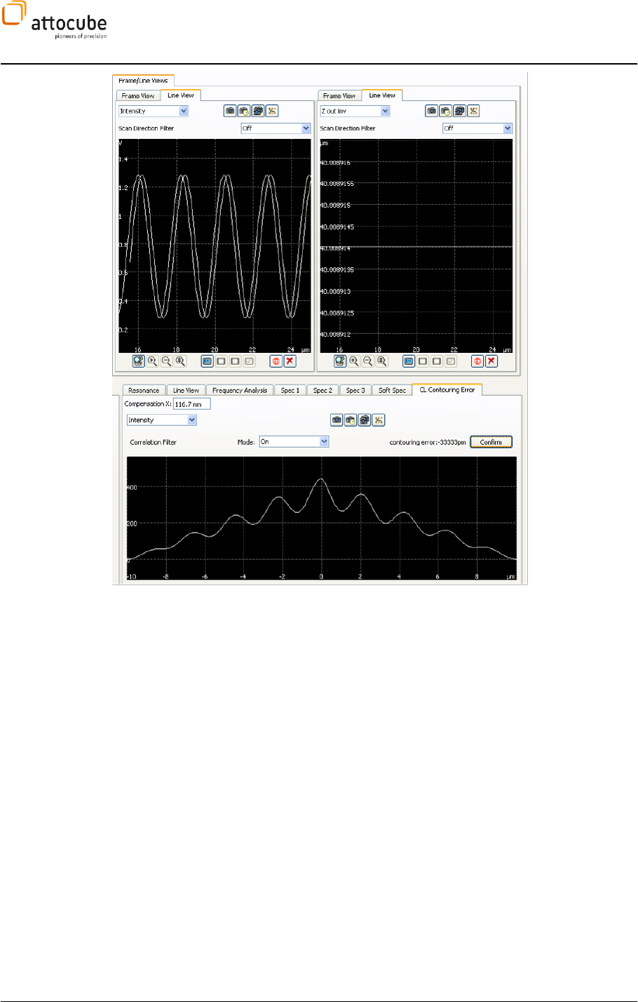
Page 72

Figure 14:

Closed Loop Contouring Error compensation using a forward-backward correlation.

VI.2.b. Lithography

The Daisy Lithography module can be used for defining geometrical

shapes that will be retraced by the sensor head. It allows the definition of

arbitrary convex polygons and single points. Moreover, a shutter can be

controlled via TTL pulses to allow for exposition of certain structures on

the sample surface.

Lithography can be operated in both closed loop and open loop mode.

Shape definition

The shape definition of the lithography pattern is done via a text file.

There are two basic shapes to define the lithography pattern: Polygons

and Points. Each of these basic shape definitions can be combined with a

command to control an optional shutter. An example for a shape file is

shown in Figure 15.

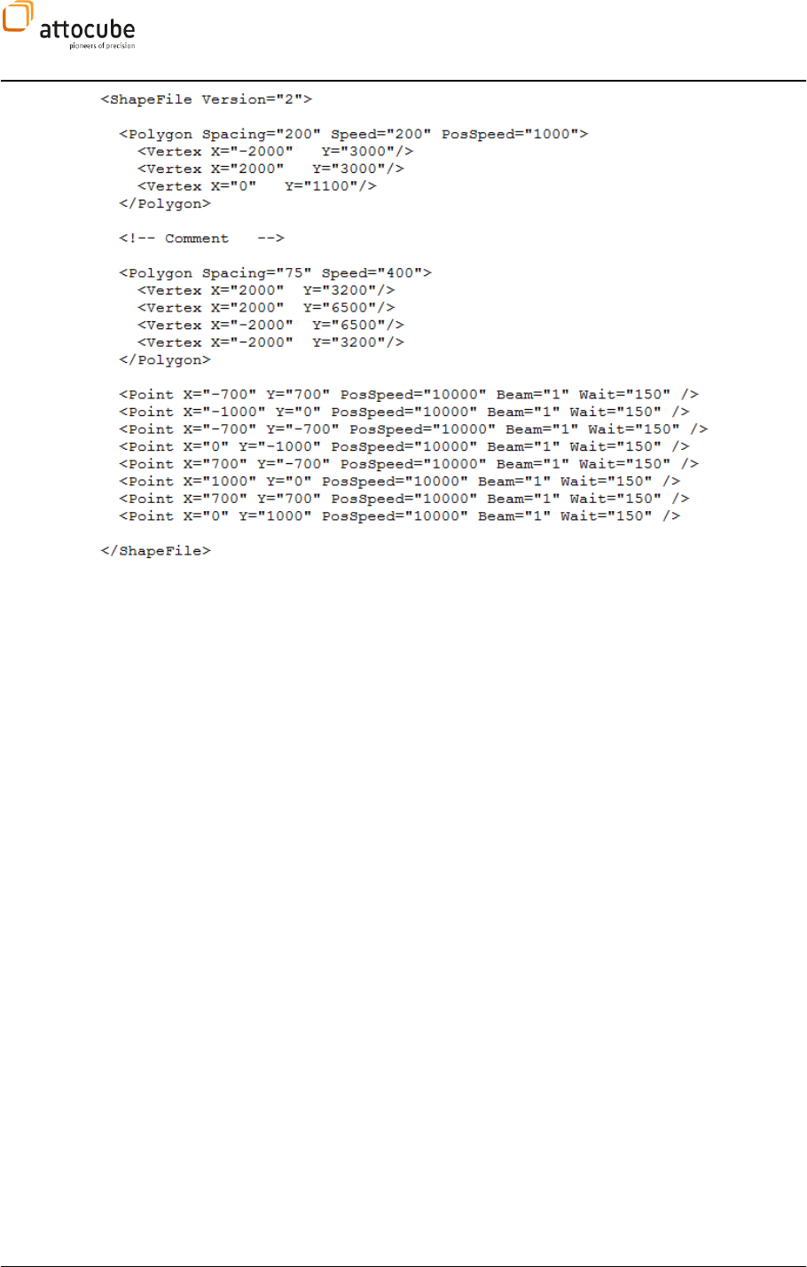
Page 73

respective companies. Any rights not expressly granted herein are reserved. ATTENTION: Specifications and technical

data are subject to change without notice.

Figure 15: Example of a shape definition file.

The shape file must be an ASCII file with an nls extension. It must start

with a <ShapeFile Version”2”> command and end with a

</ShapeFile> command. In between, there can be any number of

Polygon and Point commands. Comments can be inserted enclosed in a

respectively. All coordinates given in a shape definition

file are interpreted in nm and are relative to the center of the current scan

range.

The two basic definitions can be done via:

1. Polygon command:

</Polygon>

The Attributes can be:

a. Spacing : the spacing of the filling pattern in nm (default:

1). The polygon will be written by meandering lines with a

line spacing given the Spacing attribute.

b. Speed: the scan speed during the writing of the polygon in

nm/s (default: 10000)

c. PosSpeed: the scan speed during the approach of the

polygon in nm/s (default: 10000)

d. Beam: controls a shutter via a TTL output. Beam on (1)

leads to high voltage on the TTL output, Beam off (2) leads

to GND voltage on the output connector. The output

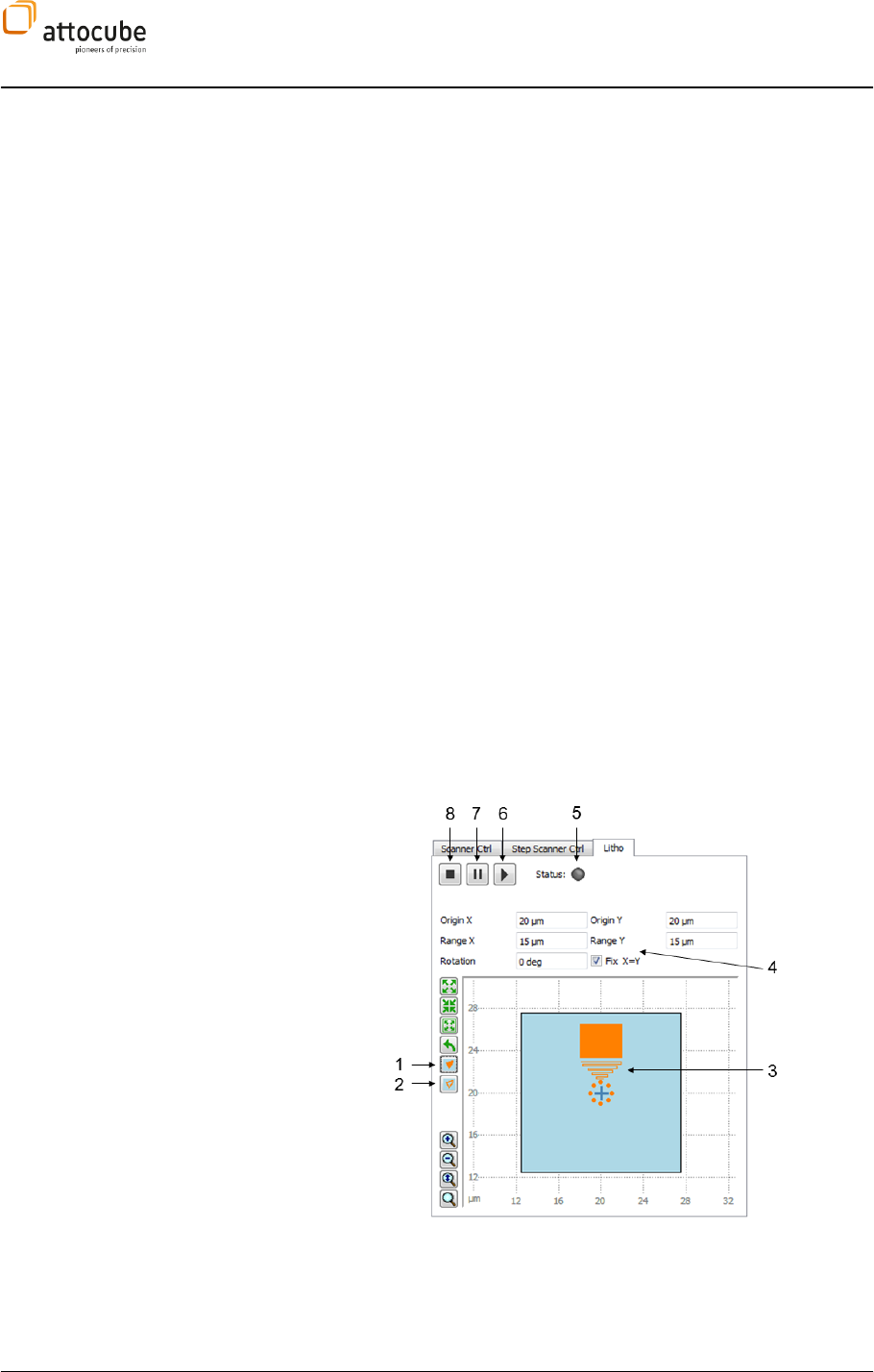
Page 74

connector for this functionality is pin number 5 of the

External OUT connector (see section II.3.d on page 14).

e. Handshake: Stop for handshake with external device

before scanning (Default: 0)

All attributes can be omitted. The default values will be used for

omitted attributes.

The polygon itself is defined via a sequence of vertices. Each vertex

has to be specified with a <Vertex/> command. It is important to

note that only convex polygon will result in a well-defined output.

2. Point command

a. X and Y: mandatory attributes in nm.

b. PosSpeed: the scan speed during the approach of the

point in nm/s (default 10000)

c. Wait: Wait time in ms after reaching the point (default: 0)

d. Beam: Beam on (1) or off (0) during wait time (default: 1)

To check the shape, the text file can be loaded into the Daisy software

where the shape will be displayed in the Lithography section of the

scanner widget. How this is done will be explained in the next section.

Operation of lithography

The lithography control is placed in the Litho tab of the scanner widget.

The tab is shown in Figure 16. The lithography tab is similar to the scanner

control tab. Some settings can be changed in both tabs and the changes

in one tab will immediately affect the other.

Figure 16: Lithography widget with shape definition. The shape that is

shown was produced by the shape definition file of Figure 15.

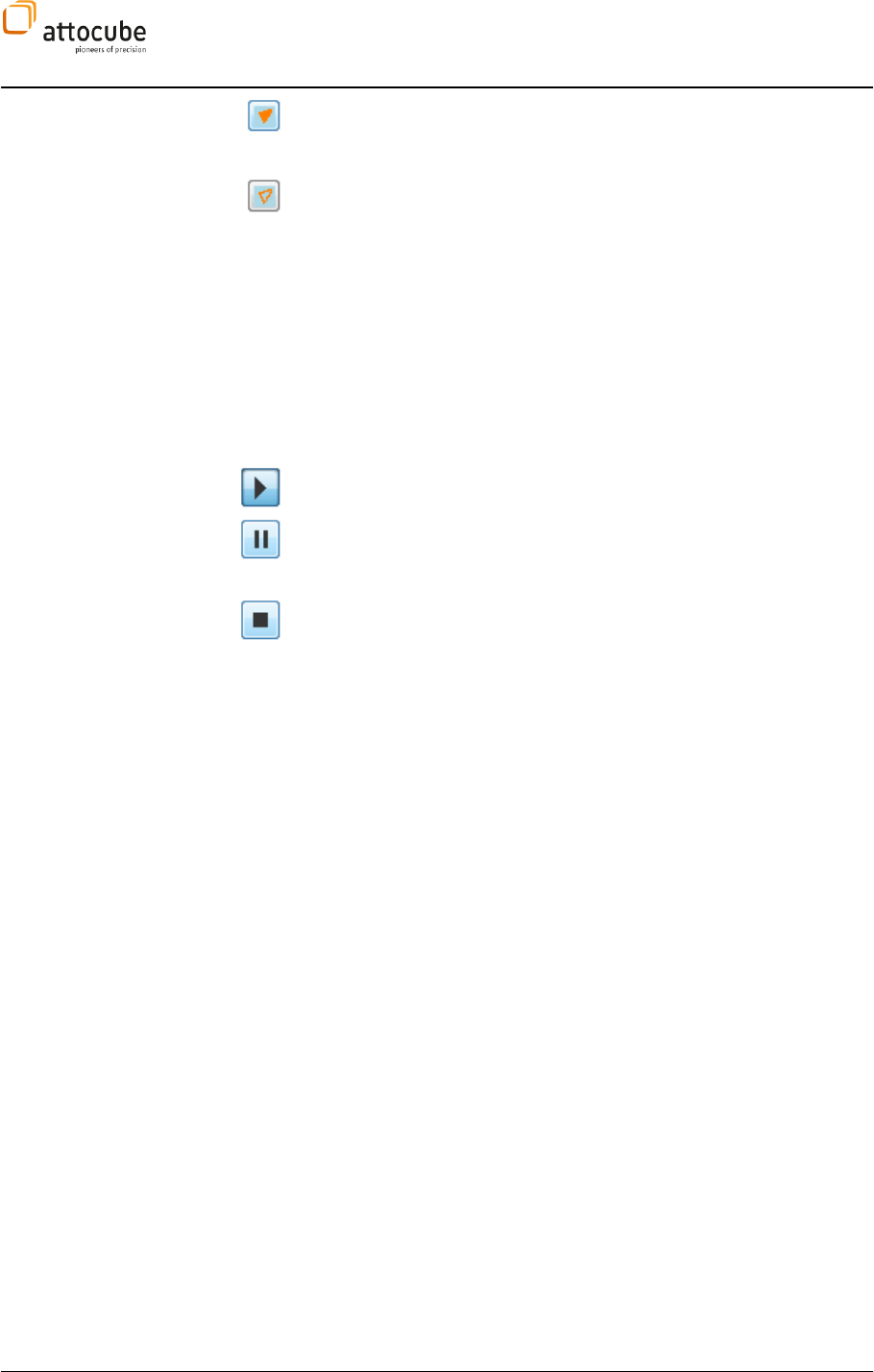
Page 75

respective companies. Any rights not expressly granted herein are reserved. ATTENTION: Specifications and technical

data are subject to change without notice.

1  load lithography definition file: upon a click on this button, a Windows

dialogue will appear to specify the lithography shape definition file. After

loading, the lithography shape will be shown in the display.

2  clear shape: with this button, any shape that is displayed will be

erased.

3  the loaded shape is drawn into the actual scan range. It is worth

noting that the meandering lines of the lithography are only resolved in

the lower triangle of the shape. Here, a line spacing of 200 nm was used.

The single lines of the rectangle (spaced 75 nm apart) can only be

displayed using the zoom buttons in the lower left of the panel.

4  here, the basic definition of the actual scan range can be set. Changes

will immediately affect the Scan Control Tab.

5  Status LED: green is lithography is running

6  Start button: starts the lithography

7  Pause button: pauses the lithography. During pause, the shutter will

be closed and reopen upon ending of the pause in case its status was open

before the pause.

8  Stop button: Stops the lithography. The shutter is closed and the

scanner moves to the origin

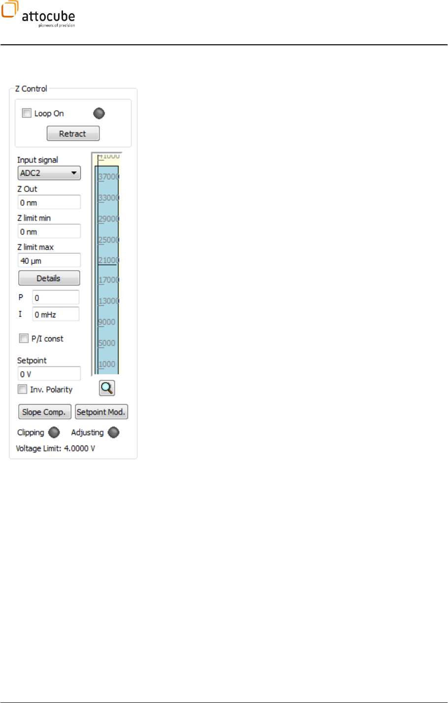
Page 76

VI.3. The Z Control feedback loop

The Z control loop controls the z-position of a sensor with respect to a

sample. There are several Input Signals to choose from, whereas the output

of the loop is strictly connected to Z OUT. The loop output is limited to a

voltage ranging from Z Offset to (Z Offset + Z Range) (see Details dialog). The

output can be additionally limited using the Z Limit min and Z limit max

settings.

The feedback loop always tries to modify z-out so that the input signal actual

value gets closer to the setpoint. Whether the loop needs to be in negative or

positive feedback, can be chosen with Inv. Polarity. The proportional gain P

is sensitive to sudden jumps in the signal, whereas the integral gain I is

sensitive to the integral of the signal.

The main loop-controls are: The Loop On checkbox, the Retract Button at the

top as well as the indicator LEDs at the bottom. The following states are

possible:

Loop on: Enable the check box to switch on the loop. The LED will

turn green.

Loop off: If the box is unchecked, the feedback loop will hold the

position of z-out and will not react on changes of the input signal.

Retract: If Retract has been pressed, the loop is switched off and

the voltage is taken down to Z Offset (i.e. the tip is retracted from the

sample).

Clipping: The Clipping LED is enabled, if the active loop reaches one

of the limits, i.e. either the lower limit Z Offset, or the upper limit

(Z Offset + Z Range).

Adjusting: This LED indicates that the red bar is not yet synchronized

with the real z-out value (due to lower update rate).

Inv. Polarity: For experiments, where the sensor signal increases with

decreasing sensor sample distance (e.g. in STM, the tip gets closer with

higher z-out voltage), leave this box unchecked. For experiments, where the

sensor signal decreases with decreasing sensor sample distance (e.g.

oscillation amplitude of a vibrating tip), do check the box.

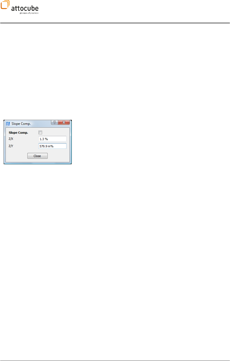
Page 77

respective companies. Any rights not expressly granted herein are reserved. ATTENTION: Specifications and technical

data are subject to change without notice.

VI.3.a. Slope

Compensation

The Slope Compensation is an important feature to compensate for a tilt of

the sample with respect to the horizontal plane. Quite often in SPM

experiments, the height of the investigated feature is much smaller than its

lateral dimension so the scan range will be large in xy and small in z. In this

configuration even a small tilt of the sample does disturb the image and

masks smallest topographic variations. To compensate for these sample tilts,

the ASC500 features a powerful Slope Compensation that enables scanning of

a tilted plane without any influence on the z controller. Once the Slope

Compensation is set and activated, the sample will be scanned as if it was

lying perfectly flat

             

mple distance constant even without employing

a z feedback.

The Slope Compensation is activated by clicking on the Slope Comp. button in

the z controller widget. A window as shown to the left will appear. The

compensation values for both X and Y axis can be entered separately in the

Z/X and Z/Y box, respectively. The Slope Compensation can be activated and

deactivated using the Slope Comp. toggle button.

A negative slope (of the forward scan) will be compensated by a positive

value and vice versa. The values can be chosen between -20% and 20%.

To set the correct values the compensates the sample tilt, it is best to do the

following:

1. Set the scan rotation to 0 degrees.

2. Scan a line and change the Z/X factor of the Slope Compensation

until a flat line appears horizontal.

3. Set the scan rotation to 90 degrees and repeat the previous step for

the Z/Y factor.

Figure 17 shows typical line scans with and without Slope Compensation for

an AFM scan of the 25 nm high grating with a 4 µm pitch. As can be seen in

the image, the Slope Compensation acts on the total scan range of the

scanner; the two line scans displayed here would meet at an x position of 0

µm, the offset between the white and the red scan line is thus the result of

the Slope Compensation together with a scan field that does not include the x

origin position.

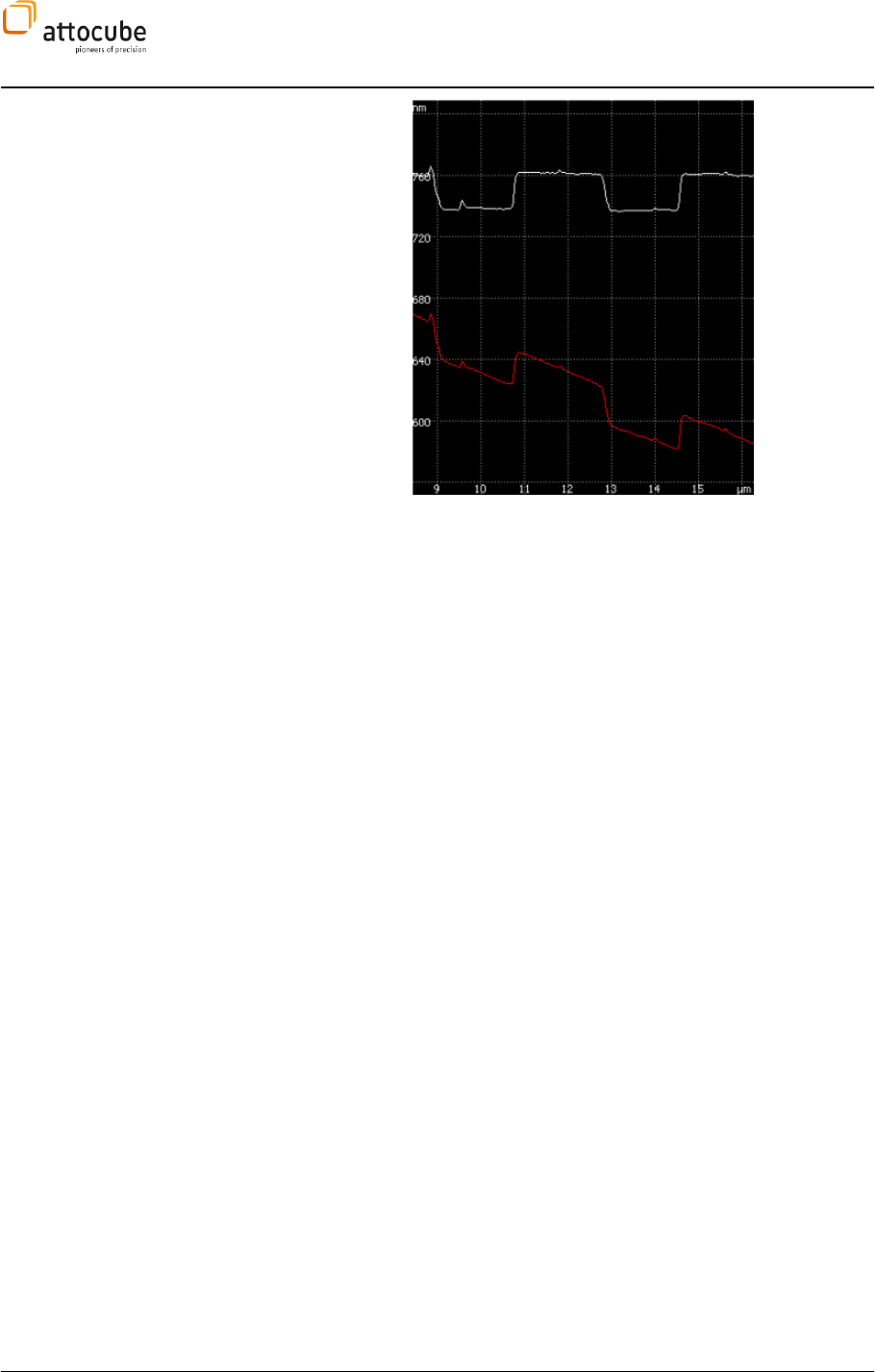
Page 78

Figure 17: A typical line scan before (red) and after (white) the sample tilt is

compensated by the Slope Compensation feature.

Slope Compensation

Details

The Slope Compensation is realized internally by an analog

adding/subtracting of some part of the X OUT and Y OUT voltages to the Z OUT

voltage. A positive Slope Compensation of 20 % for both X and Y axes will

thus lead to a large additional voltage (called Slope Compensation Voltage

SCV) in the Z OUT voltage output if the scanner moves to the upper right

corner of the total scan range. If for example the maximum allowed voltage

for all x, y and z scanner is 4 V, the SCV can vary between -1.6 V and 1.6 V

(These voltages will typically be amplified by a factor of 15 before applied to

the scanner). If the SCV would simply be added or subtracted to the Z OUT

voltage, the resulting voltage could possibly be either large enough to

damage the scanner piezo or negative enough to lead to some

depolarization of the scan piezo.

To overcome this problem, a safety margin for the Z OUT voltage is employed

in the following way: for the actual settings of Z/X and Z/Y, the maximum

positive a

of the SCV for a scanner position in the upper right corner of the total scan

range). If the Slope Compensation is activated, the Z OUT voltage range will

automatically be reduced by the exact values of the SCV. This way, the sum of

the Z OUT voltage (as set by the z controller) and the SCV will never exceed

the maximum allowed voltage and no harm will be done to the scanner.

The reduction of the z scan range is visualized in the z controller

The safety margin due to the slope compensation will be shown red in this

display. Below, there are several examples.

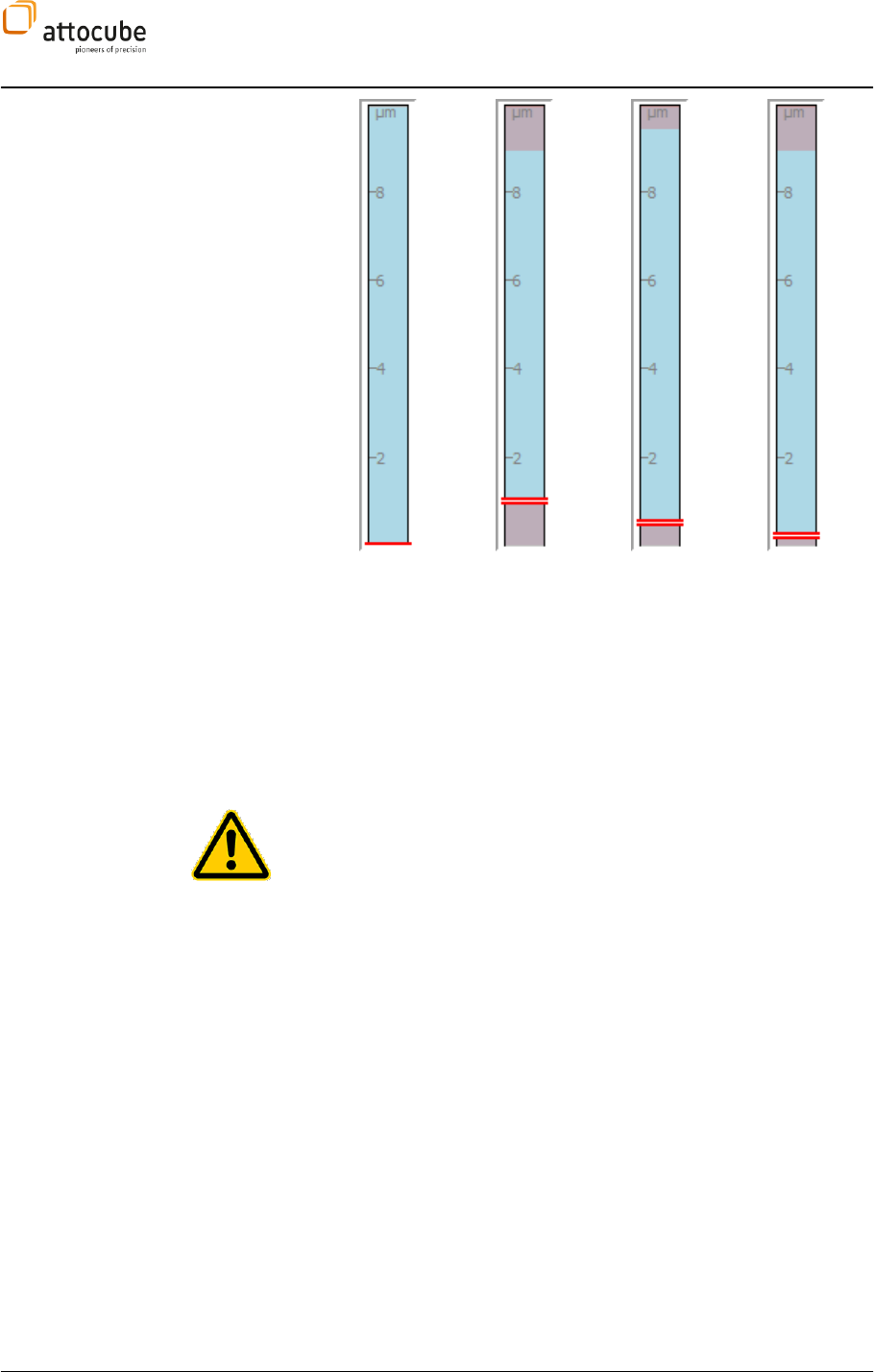
Page 79

respective companies. Any rights not expressly granted herein are reserved. ATTENTION: Specifications and technical

data are subject to change without notice.

1 2 3 4

(1) The display shows a z scan range of 10 µm that is not restricted

because the Slope Compensation factors are both set to zero.

The full range of the scanner is accessible for scanning.

(2) The display shows a z scan range with a restriction due to the

Slope Compensation by Z/X = 10 % and Z/Y = - 10%. In this

case, 10 % of X OUT means 1 µm safety margin in Z OUT. The

positive factor for Z/X leads to a reduction of 1 µm at the upper

limit of the z scan range. The negative Z/Y factor of -10 % leads

to a reduction of the z scan range of 1 µm at the lower limit of

the z scan range. It is important to note that this reduction

         

position. At the moment the Slope Compensation is activated,

the scanner will thus move the tip closer to the sample!

However, this will not harm the tip if the Slope Compensation is

set correctly. Basically, the tip will be driven closer to the





Overload Capacity

(3) As in (2), the display again shows a z scan range with a

restriction due to the Slope Compensation by Z/X = 10 % and

Z/Y = - 10%. The fact that the restrictions are smaller is due to

another margin that has not been discussed so far. There is a

hardware parameter called Slope Compensation Overload

Capacity that will increase the accessible z scan range. This

parameter is related to the fact that piezos in general have

some tolerance in their voltage ratings. A piezo rated for 0 V

to 60 V can safely be driven by a voltage of – 3 V to 63 V. This

Overload Capacity

can be used to regain some or all of the z

       Slope Compensation. In the

example shown above in (3), an Overload Capacity of 5% has

been employed to reduce the restrictions to merely 0.5 µm on

each end of the z scan range. The Overload Capacity can be set

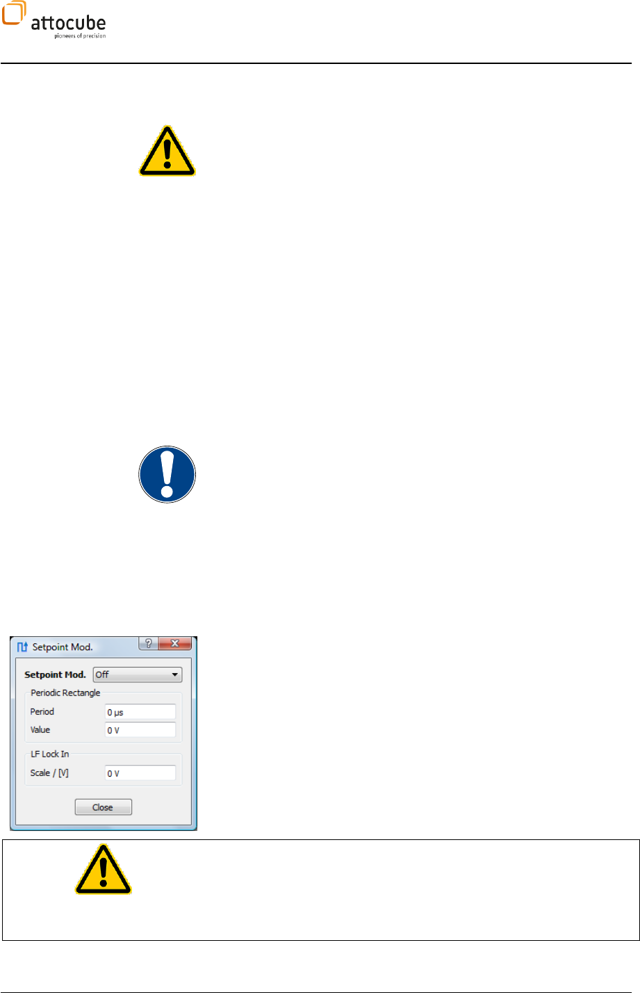
Page 80

in the Output Limits – Expert Settings – Overload Capacity

section.

It is strongly recommended not to change the

Overload

Capacity

and leave the value that is set in this field by the

manufacturer. False settings of the

Overload Capacity

may

damage the piezo and will lead to a loss of warranty.

(4) The display shows a 10 µm z scan range with the following

settings: Z/X = 15%, Z/Y = -7 %, Overload Capacity = 5 %. The

positive Slope Compensation factor of 15 % together with the

Overload Capacity leads to restriction of 1 µm at the upper limit

of the z scan range. At the lower side, the negative Slope

Compensation factor of -7% will be diminished by the 5%

Overload Capacity, leaving a restriction of 200 nm at the lower

end of the z scan range. The retract position is elevated to this

value.

Notes

a. The SCV will not be part of the internal signals Z OUT and Z OUT INV.

However, it will of course be a part of the Z OUT voltage.

b. The Slope Compensation can be set at any time during a scan. A

change in the Slope Compensation will immediately lead to a change

in the Z OUT voltage. The speed of this change is governed by the Z

Slewrate that can be set under Output Limits – Sanner Limits and

Scaling – Slewrate Z. If the Z Slewrate is faster than the speed of the

z control loop, a change in the Slope Compensation can potentially

lead to a tip degrading.

c. The limits of +/- 20% of the Slope Compensation are set by

hardware limits that where built into the ASC500. These limits were

designed on purpose to avoid an exceeding crosstalk of noise from

the X OUT and Y OUT voltage on the Z OUT voltage.

VI.3.b. Setpoint

Modulation

This feature is useful to optimize the P-I parameters with a tip in contact.

If you enable Setpoint Modulation, the setpoint of the feedback loop will be

switched with the given period between the value entered in the feedback

loop control and the value given in this dialog. Hence, this feature simulates

an ultimately sharp feature. This facilitates the tuning of the feedback loop

accordingly.

Note: Do not switch on the Setpoint Modulation before the setpoint

parameters are carefully defined. If there is e.g. still 0 V entered in the Value

field, the loop would try to reach this value, possibly crashing the tip.

Caution: The Setpoint Modulation has an immediate effect on setpoint of the

feedback loop. It is recommended to enter meaningful values before

enabling this feature. Also, sensitive tips may be damaged if the values for

the feedback loop and the two setpoints are not correctly chosen.

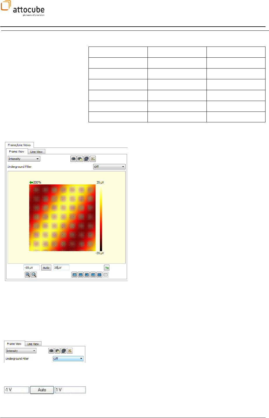
Page 81

respective companies. Any rights not expressly granted herein are reserved. ATTENTION: Specifications and technical

data are subject to change without notice.

VI.3.c. Z control P and

I units

The physical unit of the P and I parameters of the feedback loop are

dependent on the input signal of the loop. The units are:

Input Signal

P unit

I unit

ADC 1..6

µm/V

µm/V/s

HF 1 df

µm/Hz

µm/Hz/s

HF 1 Ampl

µm/V

µm/V/s

HF 1 Phase

µm/deg

µm/deg/s

LF Lockin Ampl

µm/V

µm/V/s

LF Lockin Phase

µm/deg

µm/deg/s

VI.4. The Scan Data Displays

In the main screen there are two display windows (left

and right display) showing the scanning results. In these

windows, either images (Frame View) or line scans (Line

View) can be displayed online. Furthermore, data can be

saved, and the scan area can be modified.

The drop down menu at the top of the window allows for

selecting the respective signal to be displayed. By

activating the Average button all incoming data within

one sample time (as specified in the Scanner Widget) is

averaged before it is displayed on the screen. If Average

is deactivated, Daisy displays the first incoming data

point at a new scan position and then discards all further

data within this sample time.

In the Frame View the acquired data is shown in a xy-plot,

with the intensity color-coded as specified (see section

V.4.c for a description of the context menu). In Line View

the data is shown as curves.

If the cursor is paused for a second over one of the

displays a pop-up window will display the physical

coordinates of the chosen point.

Also, you can double-click on the window to detach it

from the main window at any time, allowing for any user-

defined resizing or repositioning of the window on the

screen.

VI.4.a. Frame View

The drop down menu at the top of the window allows for selecting the

respective signal to be displayed. The signals can be chosen from a list a

defined in the DCC (see IV.1.a). To the right, the snapshot icons allow for

saving of SCAN data as described in section IV.2.g. The line below shows an

underground filter: this filter can be used to subtract a function of 0th

(Constant) or 1st order (Linear) from each line to remove scan artefacts.

Graduation Tools: Below the frame display area the Graduation Tools are

shown. By pressing the Auto button, the graduation limits will be calculated

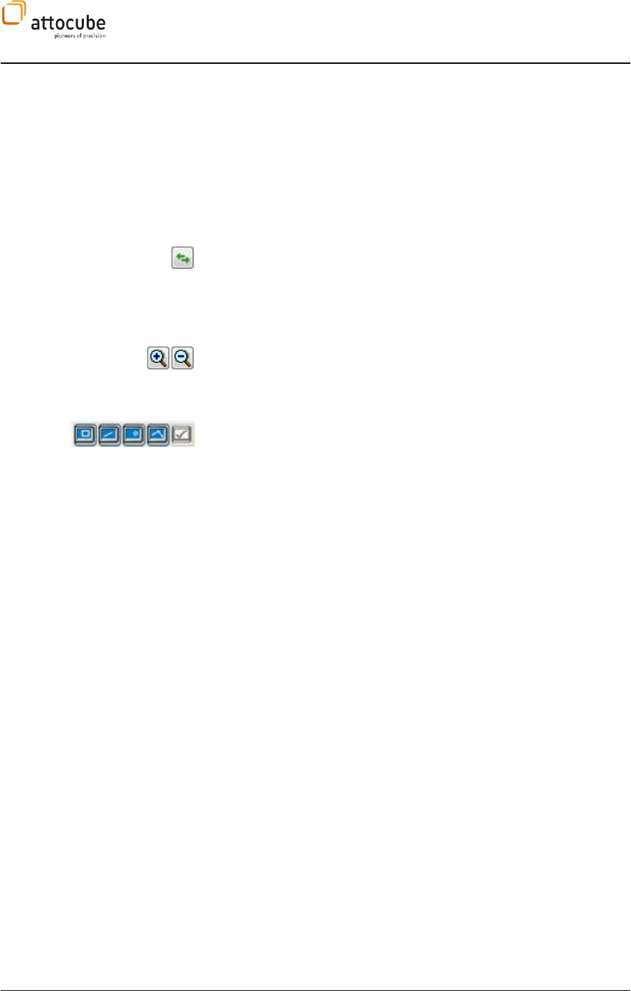
Page 82

from the currently displayed values, i.e. the currently chosen color scale will

be spread to match the data which is displayed at the moment of pressing

the button. To further enhance the contrast or highlight certain parts of the

image, one can choose the graduation limits manually by entering values to

the left (Graduation Minimum) and to the right (Graduation Maximum). It is

also very convenient to use the mouse wheel to change the graduation

settings. For this, just move the mouse pointer on the respective input field

and then use the mouse wheel to continually change the setting. Use STRG or

SHIFT key together with the mouse wheel to change the sensitivity of the

wheel (see also section V.4.a).

Scan Direction Switch: This button allows you to switch between displaying

either the Forward (data acquired in a left-to-right scan) or Backward (right-

to-left) data.

Please note that the following Selection tools are only shown when activated by right-clicking on the frame view,

see section V.4.c.

Frame Zoom Tools: The Frame Zoom Tools allow for zooming in or out. Please

note that only integer zoom factors (or 1/integer factors) are allowed to

avoid aliasing effects. If the image size in any zoom setting is larger than the

available size in the Frame View window, scroll bars appear.

Frame Tools: The Frame Tools are shown to the lower right of the Frame View.

The Frame Tools can be used to alter the current scan area. The Frame Tools

are advantageous when one wants to reposition the scan area based on

information that is currently shown in the Frame View. It is possible to (from

left to right):

- select a new rectangle for scanning,

- rotate the scan direction,

- select a new center of the scan area, or

- start the Pathmode.

The rightmost button is used to accept the selections made. Please note that

you cannot use that Frame Tools until one scan image has been taken and all

frame positions are initialized.

The second icon from the right under the left data display is used to start the

Pathmode. To select a path, first click on the button, then select points of

interest in the data display. These positions will be shown as small circles in

the display, with a line connecting the different points indicating the path.

After selecting the path, a click on the accept button will start the path

mode. Please see section VI.5.e on how to select the measurement type

performed on each point.

VI.4.b. SCAN Line View Tab

In the Line View Tab, single or multiple lines of the scan image can be displayed during scanning. The Line View is

constantly updated during scanning and shows the current values of the chosen Signal versus sample position.

Please note that a comment window appears if you stop the cursor over the line view graph, displaying the actual

position.

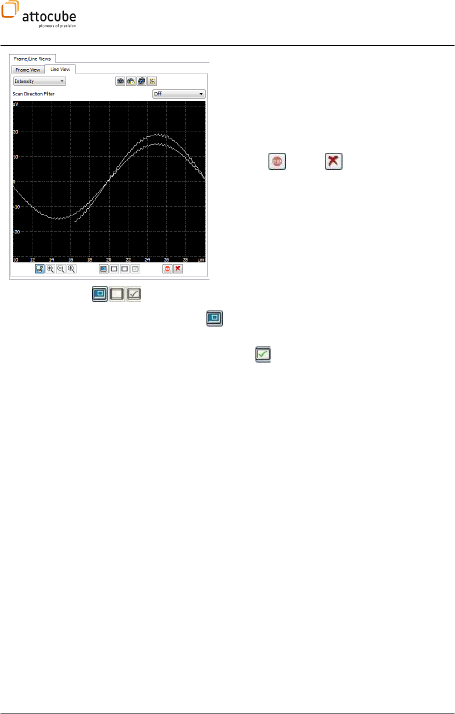
Page 83

respective companies. Any rights not expressly granted herein are reserved. ATTENTION: Specifications and technical

data are subject to change without notice.

You can use the Scan Direction Filter to either display the

Forward or the Backward scan. If the Scan Direction Filter is

turned off, then both forward and backward scans will be

displayed. You can increase the number of simultaneously

displayed lines using the Curves function in the Line View

Ranges context menu. Multiple lines are displayed in

different colors for better clarity.

Use the Zoom Tools to adjust the display range. You can also

use the Stop and Clear buttons as described in the

common controls and properties section V.4.b.

Frame Tools: One can set a new scan range directly from the

Line View graph of the Display using these buttons. Choose the Select New X

Range button and then drag the two vertical lines to enclose the desired

new x-range (as shown in the graph).

Click on the Accept button and note how the active scan area changes in

the Scanner Widget. If the Fix X=Y button is activated, the y scan range will be

changed, too.

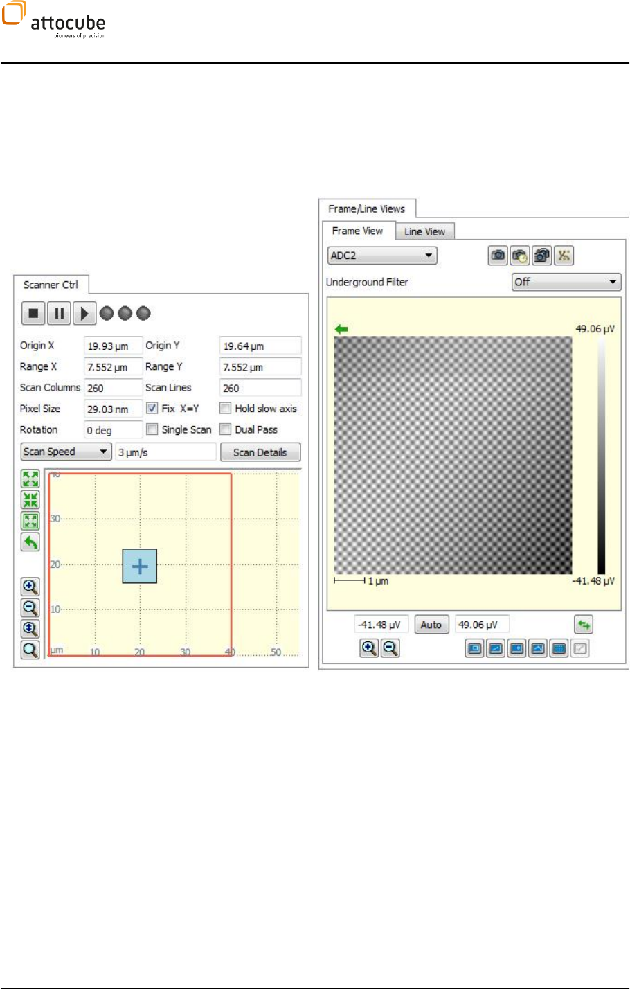
Page 84

VI.4.c. Example for Shifting, Moving and Zooming the Scan Area

As an example, an image in the simulation mode of the software was

acquired. As can be seen below, the full scan range of the xy scanner was

40 x 40 µm, and an 7.552 x 7.552 µm image (blue square) was taken

approximately in the middle of the full range. Also, the frame axes of the

image are parallel to the x- and y-direction of the scanner.

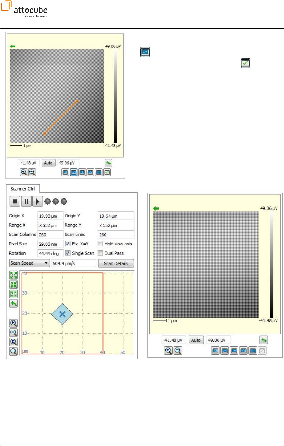
Page 85

respective companies. Any rights not expressly granted herein are reserved. ATTENTION: Specifications and technical

data are subject to change without notice.

To rotate the scan direction so that the artificial dot array has

a certain orientation to the frame axes, one has to activate

the button, then draw a line in the Frame View window, as

can be seen in the picture aside. Click on the button to

accept the choice. The next scan will be carried out with the x-

axis along the line.

All parameters in the Scanner Widget are automatically

adjusted and the blue square is rotated to show the new scan

area (see below).

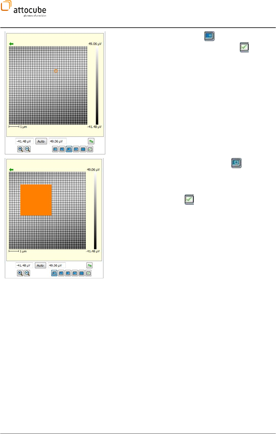
Page 86

To choose a new center of scan, use the button. Click on the new

center in the Frame View and accept the selection with .

The Scanner Widget will automagically adjust the scan area to be

centered on the new spot as close as possible within the allowed

maximum scan range of the scanner.

Finally, to zoom in on details of the image, use the button and

drag a rectangle around the area of interest. Please note that the

chosen rectangle is transformed to a square if the Fix X=Y button in

the Scanner Widget is activated.

Again, after accepting with the button, a new scan area will be

defined. The screen shot below shows the result of these actions.

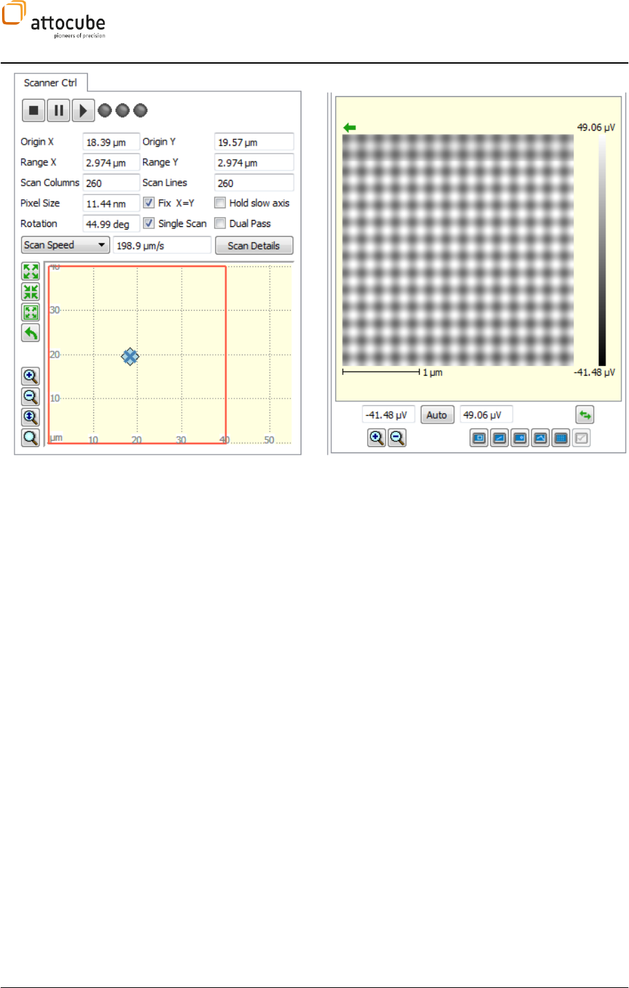
Page 87

respective companies. Any rights not expressly granted herein are reserved. ATTENTION: Specifications and technical

data are subject to change without notice.

VI.5. The main functions tab section

All main functions such as the PLL, coarse motion control, pathmode, Lock-In(s) & Q control, Dual pass and DAC

outputs are located in the tab section on the lower left part of the GUI. The user can conveniently adjust the order

of the tabs as well as choose which tabs to show and which to hide as described in section V.3.a.

VI.5.a. Phase Locked Loop (PLL tab)

Introduction

A completely digital Phase Locked Loop (PLL) is integrated in the ASC500.

With the PLL, an advanced operation mode is provided to control high Q

oscillators (like tuning forks at low temperatures). The PLL mode is an

alternative to standard non-contact mode operation, where the oscillator

(tuning fork or cantilever) is driven at a fixed frequency and the change in

oscillation amplitude is used to drive the z controller and to gain

topographic information. This latter mode will be called amplitude

modulation mode in the following sections, in contrast to frequency

modulation or PLL mode.

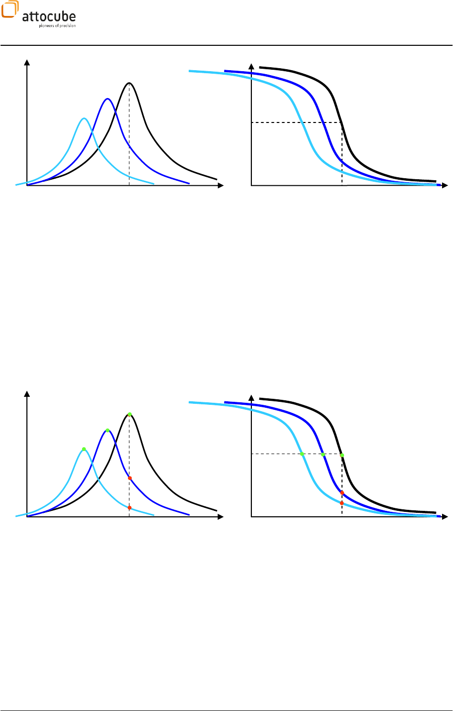
Page 88

Figure 18:

Amplitude and phase response of a driven oscillator in presence of a force gradient (black curve shows

response at no gradient, dark blue and light blue curves at increasing force gradient). f0 denotes the resonance

frequency of the oscillator without an applied force gradient. With increasing force, the amplitude maximum gets

damped and shifts to lower frequencies. The phase response is also shifted to lower frequencies and the maximum

slope of the curve is decreasing.

In a typical non-contact AFM measurement, the oscillating tip is brought

into the force field of the sample surface. Figure 19 shows the response of

the oscillation properties of the tip on the force gradient originating from

the sample. PLL and amplitude modulation mode differ in the way the

controller reacts to such changes in oscillation properties. In amplitude

modulation mode, the tip is constantly excited with the frequency f0, i.e.

the resonance frequency of the freely oscillating lever.

Figure 19:

Working points in amplitude modulation mode (red dots) and in PLL mode (green dots). The PLL mode

traces the resonance frequency of the oscillating lever.

Figure 19 demonstrates the different behavior of both modes. The

measured oscillation amplitude follows the red dots. The measurement

does not reflect the real amplitude damping due to sample forces, but

merely some amplitude drop due to the shape of the amplitude response

curve. In PLL mode, the excitation always follows the amplitude maximum

(i.e. the resonance frequency shown by the green dots), giving more

valuable physical information. The question is how it can be achieved that

the excitation always follows the resonance?

π/2

π /2

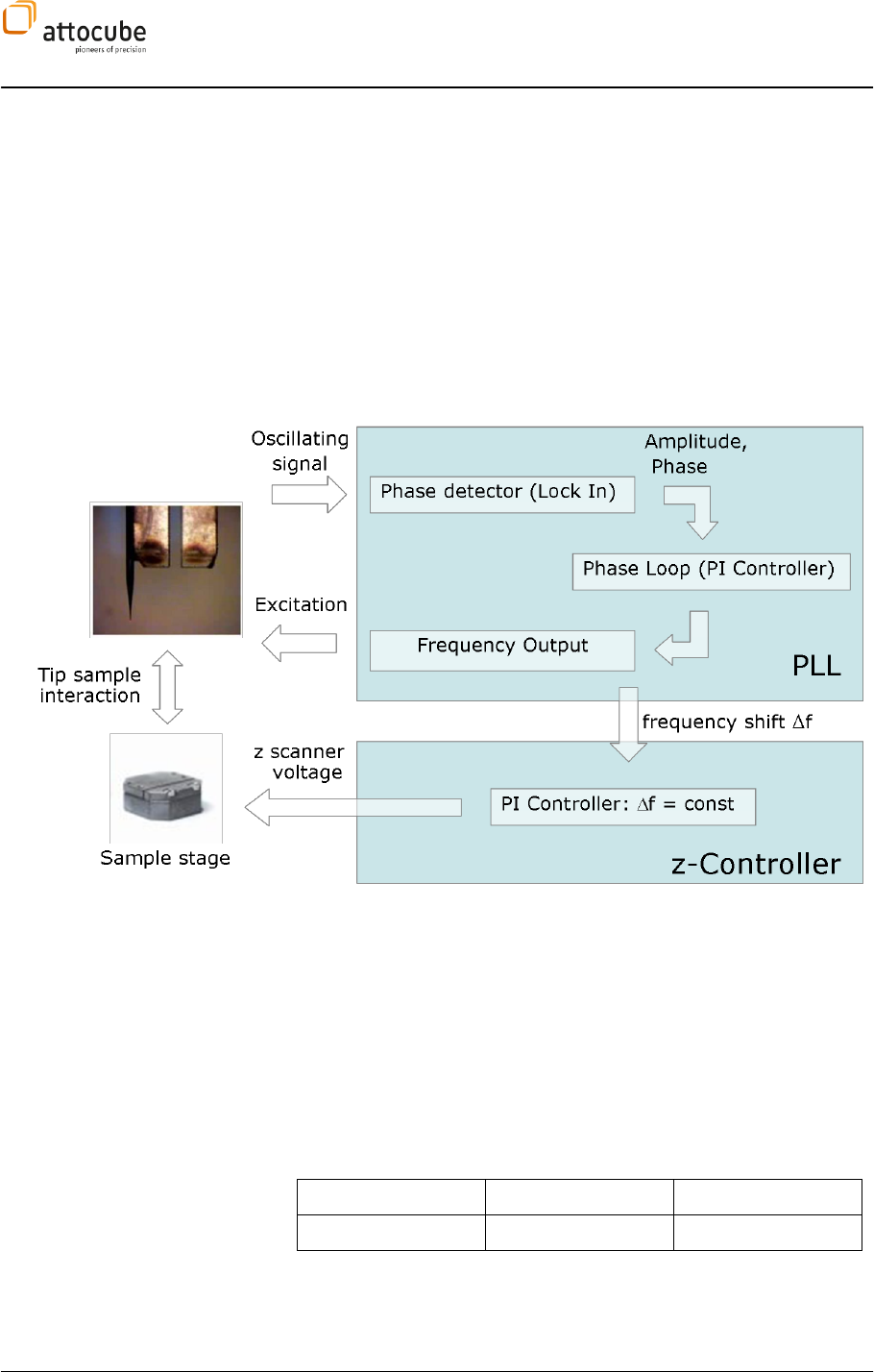
Page 89

respective companies. Any rights not expressly granted herein are reserved. ATTENTION: Specifications and technical

data are subject to change without notice.

At the resonance frequency, the phase shift between input and output

signal is always /2. This fact is used in PLL mode to control the excitation

frequency. An extra proportional integral control loop is operated to keep

the excitation on resonance. The input value for this loop is the phase

between excitation and oscillation signal as it is calculated by the internal

lock-in amplifier, the output value is the excitation frequency or simpler

the shift in excitation frequency f. This control loop is called phase loop.

The frequency shift f is directly proportional to the force gradient that is

affecting the lever oscillation. Figure 20 shows a schematic of the PLL

operation mode. The output of the phase loop will be used as an imput for

the z controller, keeping the frequency shift and thus the force on the tip

constant.

Figure 20:

Schematic of the PLL operation mode.

The PLL mode is an advanced mode to operate in the sense that two PI

loops have to be operated at the same time. Potential instabilities in one

loop will directly affect the other loop. The advantages are twofold:

1. The measured signal f will give a direct measure on the force

gradient acting on the tip.

2. The PLL allows higher scan speeds for high Q levers.

PLL controller P and I units

The physical units of the P and I parameters of the feedback controllers

can be found here:

Amplitdue Control

Input signal

P unit

I unit

HF 1 Ampl

V/V

V/V/s

Frequency Control

Page 90

Input Signal

P unit

I Unit

HF 1 Phase

kHz/deg

kHz/deg/s

ADC1 .. 6

kHz/V

kHz/V/s

Operation of the PLL

Preparations

Before employing the PLL, all relevant connections have to be made. In

particular, the signal from the oscillating lever has to be connected to the

HF IN 1 input and the dither signal has to be connected to HF OUT 1. With

these connections, the lever signal will be addressed via HF IN 1 AC within

the Daisy software, and the demodulated lock-in signal will be HF LI 1 and

HF LI 1 Phase.

While the PLL is running, a number of signals are interesting to observe:

 HF LI 1 Phase: the phase between lever excitation and lever

oscillation. This is the input signal for the phase loop.

 HF LI 1: the amplitude of the lever oscillation. In PLL mode this is

a measure of the oscillation damping due to sample forces.

 df: the frequency shift relative to the free resonance frequency of

the lever. This is the output signal of the phase loop and at the

same time the input value of the z controller

 Z out inv: this is the output value of the z controller that gives the

topographic information.

To have all relevant system parameters under control, it is convenient to

open three extra windows using the Display Wizard.

1. An extra line view with permanent trigger to show either

or HF LI 1.

2. An extra window with a Line View, an Underground Filter

and a Frame View that is triggered on scanner. This will

be used to display HF LI 1.

3. An window containing a Line View, an Underground Filter

and a Frame View that is also triggered on scanner. This

will be used to display HF LI 1 Phase.

Detach all the extra windows from the main Daisy application and

distribute them over the screen. In the main frame views, choose df for the

left and Z out inv for the right display and HF LI 1 Phase for the standard

Line View.

Find the resonance of the cantilever using the Resonance feature of the

ASC500. Choose and appropriate excitation amplitude in the Lock In tab

and set the Integration Time of the lock in to some reasonable value (500

µs .. 2 ms). After starting the Resonance, set the excitation frequency to

the match the resonance frequency and set the offset phase (under Lock

In, High Frequency, Demodulation, Phase Shift) so that the HF LI 1 Phase at

the resonance frequency is 0. The result should look similar to Figure 21.

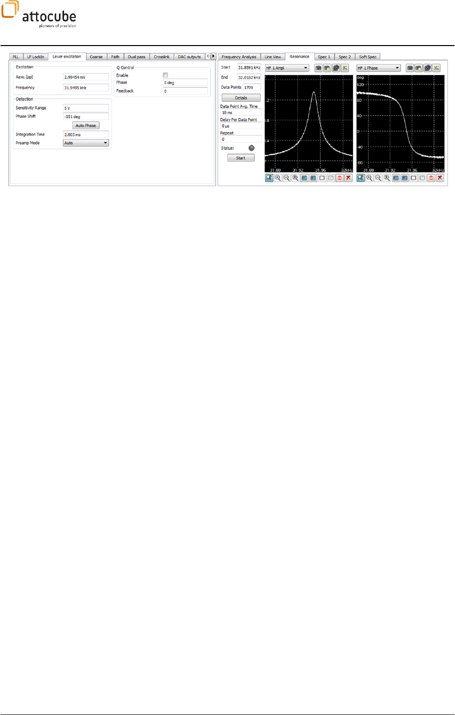
Page 91

respective companies. Any rights not expressly granted herein are reserved. ATTENTION: Specifications and technical

data are subject to change without notice.

Figure 21:

Recording amplitude and phase response of the lever using the Resonance tool.

Phase Loop settings

The phase loop settings can be found in the Non-Contact Mode tab under

Frequency Control. Before you turn on the loop, the following settings have

to be made:

 Limit the range of the output frequency to gain higher frequency

resolution. A range of 1 to 2 kHz around the resonance is

recommended. Insert the appropriate values to the Min and Max

fields.

 Choose the proportional and integral parameters for the loop.

Start with small values (P = 10 µ and I = 1 mHz). The P/I const

button always keeps the ratio of P and I constant when one

parameter is changed.

 The input signal for the phase loop can be selected in the Actual

Value list. Mostly, this will be set to HF LI 1 Phase, so that the

internal lock in is delivering the phase signal. In case an external

lock in amplifier is used for the phase detection, connect it to one

of the ADC inputs and choose the respective ADC in the Actual

Value list.

 If the phase offset was correctly compensated (see Preparations),

the Setpoint value is 0 deg. Check the Inv. Polarity button if the

phase response is has a negative slope.

The phase loop can now be started by checking the Loop button. The green

LED will be turned on and the value in the df field will by constantly

updated to show the current value of the frequency shift. The Frequency

Control widget should look similar to Figure 22.

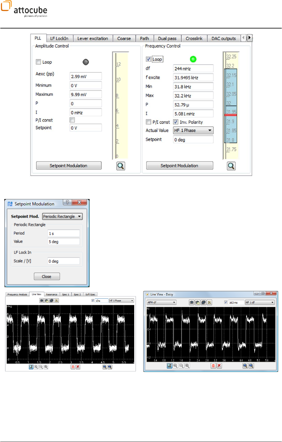
Page 92

Figure 22

: Phase loop settings.

Before the z controller is started, it is important to improve the P and I

settings of the phase loop. Open the Setpoint Modulation window and

choose HF LI 1 Phase and df to be shown in the two Line Views. The

Setpoint modulation will periodically change the phase loop setpoint

between two values, simulating the loop response to a step function input.

Choose a Period of 1 s and an alternate setpoint Value of 5 deg. Start the

setpoint modulation by checking the button. Change the phase loop P and

I parameters until the df line view shows a stable step function with only a

light overshoot as shown in Figure 23. Now that the phase loop is stable

and optimized, the setpoint modulation has to be stopped.

Figure 23:

Using the Setpoint Modulation to optimize the phase loop parameters.

Z controller settings

Now the z controller can be employed. Choose df as the Actual Value for the

z controller. The polarity of the z controller depends on the application:

for application with increasing frequency shift with increasing force on the

tip (mostly tuning forks) the z controller setpoint should be positive and

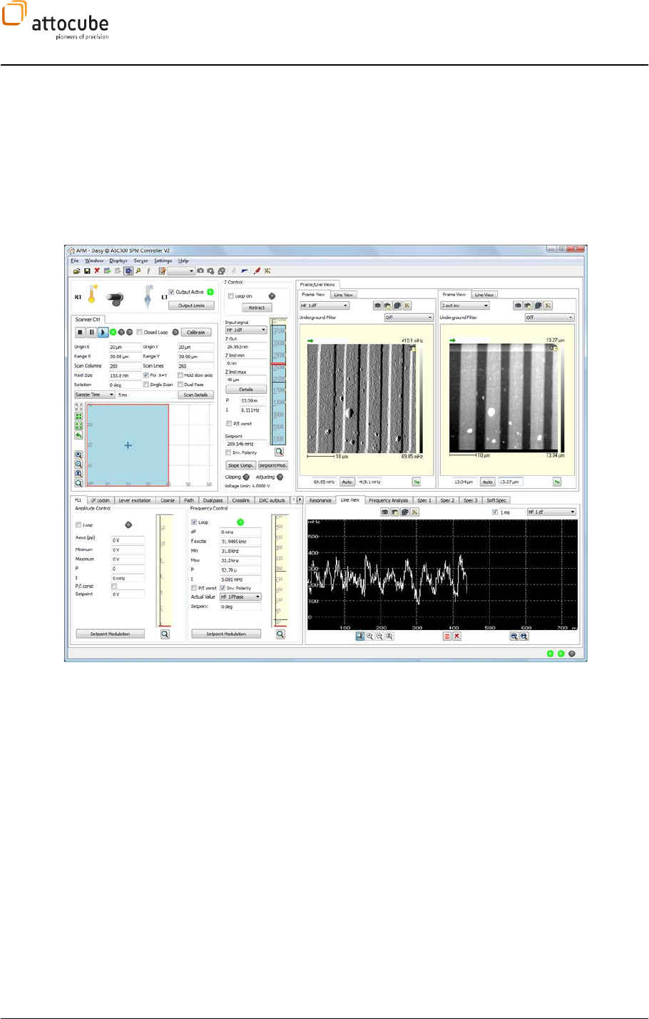
Page 93

respective companies. Any rights not expressly granted herein are reserved. ATTENTION: Specifications and technical

data are subject to change without notice.

the Inv. Polarity button in the z controller should be left unchecked. If the

frequency shift decreases with increasing force on the tip, the setpoint

should be chosen negative and the Inv. Polarity has to be checked. If the

tip is within z scanner reach of the sample, turn on the z feedback using

slow P and I parameters (if the tip is further away, employ the auto

approach). Start the scan with a low scan speed ( </= 1 µm/s) and tune



reached.

Figure 24 shows a measurement in PLL mode of a Si test grating.

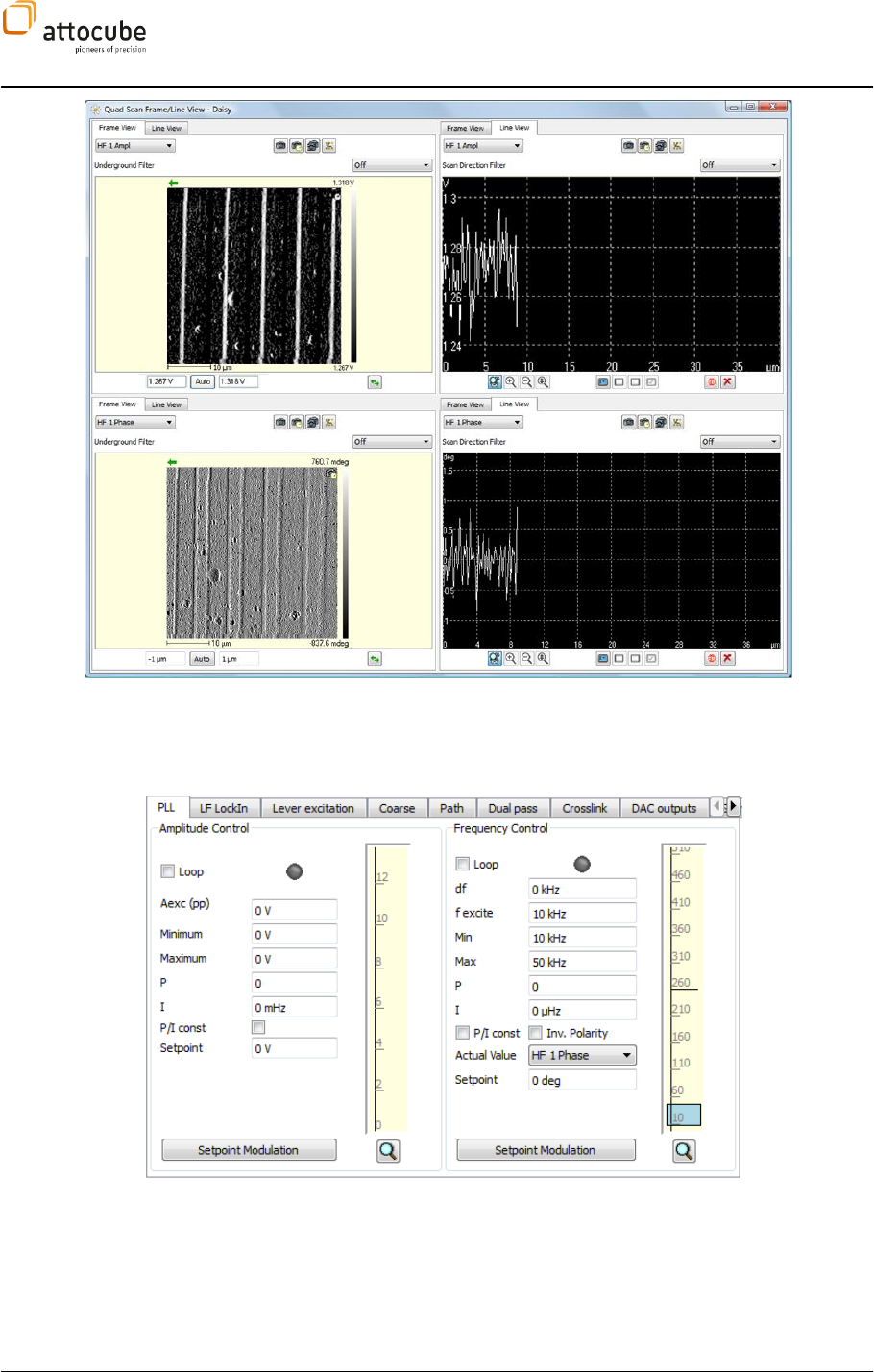
Page 94

Figure 24:

Screenshot of PLL operation.

The PLL tab

The PLL Tab contains the functionality needed to control any type of

oscillating appliance. There are two fields to enter fixed values for excitation

amplitude and frequency, as well as two loops for automated amplitude

control and frequency control.

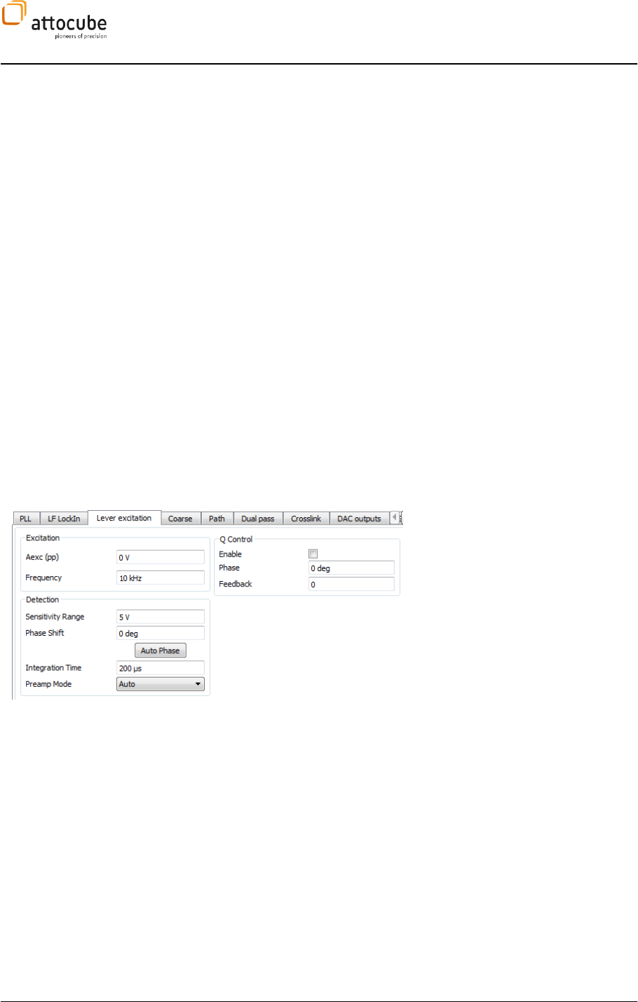
Page 95

respective companies. Any rights not expressly granted herein are reserved. ATTENTION: Specifications and technical

data are subject to change without notice.

Note that the amplitude and frequency value can also be addressed in the

Lock-in Tab (see section I.1.a).

The configuration of the PLL loops is similar to the z controller (see section

VI.3). They can act in a certain range between Min and Max. P and I

parameters need to be chosen accordingly. The Inv. Polarity checkbox can

invert the logic of the loop. The green LED will indicate an active loop.

The two loops are internally bound to certain input and output signals,

which cannot be changed (see section IV.2.b).For the Amplitude loop, the

input signal is HF LI 1 and the output signal is the excitation frequency Aexc.

For the phase control loop, the input signal may be chosen via a drop-down

list: it could be either one of the ADCs or the HF LI 1 Phase signal. This leaves

the user the choice to use an external lock-in (connected to one of the ADCs)

to drive the PLL.

In both loops one can use the setpoint modulation in order to find

reasonable P and I parameters.

VI.5.b. Lever excitation tab

Some of the most common scanning probe techniques like AFM or MFM use a mechanical oscillator given by a

cantilever to detect changes in the interaction strength between the probe (e.g. AFM tip) and the sample surface.

In this AC mode, the cantilever is excited (usually) at its resonance frequency, and the resulting oscillation signal

is recorded with a Lock-In amplifier. In the ASC500, this functionality is covered by the HF section, which is

controlled via the Lever excitation tab:

The input signal for this HF Lock-In is

HF IN 1 AC, the output is both HF LI 1

and HF LI 1 Phase. Refer to section

IV.2.b for the connection schematics.

The loop is configured with the

following values:

Amplitude: Amplitude of the output reference (peak to peak).

Frequency: Frequency of the reference output.

Sensitivity Range: Sensitivity of the Lock-In. If the signal exceeds the

Sensitivity Range, overflow may occur and wrong values may be displayed.

The maximum sensitivity is 5 V. Decreasing the Sensitivity increases the lock-

in resolution.

Phase Shift: Can correct for constant phase shifts of the Signal with

respect to the reference. Note, that this governs only the output of HF LI 1

Phase. HF LI 1measures the full amplitude of the signal.

Integration Time: Integration Time of the Lock-In. With longer

integration time the loop reacts slower, yet with having less noise.

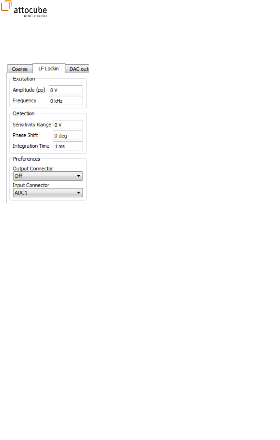
Page 96

VI.5.c. The low frequency Lock-In tab (LF LockIn)

The low frequency Lock-In produces a reference signal with a certain

Amplitude and Frequency which is passed to the respective Output

Connector. Note that the amplitude and frequency value can also be

addressed in the Non-Contact Mode Tab (see section VI.5.a).

The input signal (Input Connector) is then analyzed using the

demodulation values (Sensitivity Range, Phase Shift, and Integration Time).

The output channels of the LF Lock-In are LF LI 1 Ampl and LF LI 1 Phase.

These can be selected as source for most any display.

Other than that, the LF LockIn settings work in complete analogy to the

ones for the HF LockIn (= Lever excitation tab, see section VI.5.b).

VI.5.d. Coarse Tab

300 or

ANC350 controller, the Daisy software can be used to operate coarse

positioner movement. To use the coarse movement features, please make

sure that the ASC500 is connected to the controller using the respective

cabling (see section II.3.e).

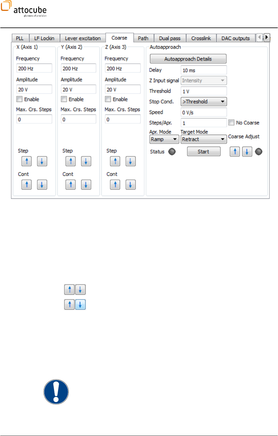
Page 97

respective companies. Any rights not expressly granted herein are reserved. ATTENTION: Specifications and technical

data are subject to change without notice.

The Coarse tab is divided into four different sections. The three sections to

the left belong to x, y, and z axis. All settings related to an automatic

approach are collected in the Autoapproach section to the right.

Axis 1 .. Axis 3

Each Axis section can operate one axis of the coarse positioners. Basic

parameters of the coarse movement are set in the Frequency and Amplitude

fields. For further details on these parameters, please see the respective

manuals of coarse positioners and coarse positioning controllers. The Enable

button will enable the coarse steps using the arrow buttons in the lower part

of the axis sections (The Autoapproach will automatically enable and disable

the coarse step movement).

The Step buttons can be used for single step movement.

The Cont buttons can be used for continuous movement. The movement will

start when the mouse button is pressed and will stop when the button is

released. If the text edit field Max. Crs. Steps is set to a value > 0, the Cont.

coarse movement can be used to execute a well-defined number of coarse

steps. If, for example, the Max. Crs. Steps is set to 100 and the Cont. button is

pressed for a sufficiently long time, the movement will stop after exactly 100

steps. For safety reasons, the movement will stop sooner if the button is

released before the total of 100 steps is completed. In case the Max. Crs.

Steps is set to zero, the movement will only be stopped by the release of the

mouse button.

Note. The Frequency and Amplitude values are programmed to the coarse

controller only if the value is changed and confirmed. These edit boxes are in

no way an indicator for the values that are currently set in the coarse control

device.

Page 98

Auto Approach

The Auto Approach is used to bring the tip into close proximity of the sample

surface. The procedure that is employed for this task works as follows: the z

scanner is continuously expanded while the sensor signal is being traced.

When the stop condition is met, i.e. when the tip is close to the sample, the

system will immediately finish the Auto Approach and enter the Target Mode.

The Target Mode can be defined to be either an activated z feedback loop or it

could also be a tip retract. If the stop condition is not met till the maximum

stroke of the z scanner, the z scanner will be retracted and a number of

coarse steps will be issued. After this the procedure will be restarted.

There are two different ramp modes for the Auto Approach: In the Ramp mode

the z scanner expansion is done in a constant speed. This speed must be

chosen small enough so that the tip is not damaged before the stop

condition is met. The alternative is to use the Loop mode, where the speed



setpoint parameters (the P parameter does not contribute due to the

definition of a proportional feedback gain). As in normal feedback

operation, the expansion speed will be depending on the difference between

the actual sensor signal and the setpoint. This means that the Loop mode will

react on slow changes in the sensor signal (for example due to long range

forces) with an adaption of the approach speed.

It is important to note that the parameters used to define the Auto Approach

behavior are partly set in the z controller section of the Daisy GUI (see

section VI.3). Most importantly, the sensor signal that is being traced for the

stop condition is defined through the Input Signal of the z feedback loop. In

case the Loop mode is used, of course all parameters of the z feedback loop

are taken as entered in the respective fields of the z controller.

In Loop mode, the approach can come to a halt if the sensor signal equals

the setpoint before the threshold condition is met. The system will be in a

stable condition, but the Auto Approach will still be active in the background.

If this behavior is to be avoided, the setpoint of the z controller and the

threshold value of the Auto Approach should be set to equal values.

The Auto Approach can be manually stopped either by clicking the Start

button of the Auto Approach section while the Auto Approach is running or by

clicking on the Retract button of the z controller. In the first case, the z

scanner will keep its current position; in the later case, the z scanner will be

driven to zero (i.e. maximum distance between tip and sample).

Delay: Delay after coarse stepping. As stepping may induce some

noise or ringing in the experiment. The settling time between the coarse

step and the start of the z scanner expansion can be defined here. During

this time, the sensor signal will not be traced for the threshold condition.

Z Input signal: This display shows the input signal used for the

autoapproach procedure. The Z Input signal can be changed in the Z Control

section (see section VI.3).

Threshold: Value for the stop condition.

Stop Cond.: Defines if the threshold represents a lower or upper

boundary of the sensor signal range. In STM type experiments, the Stop

Condition -contact AFM type experiments,

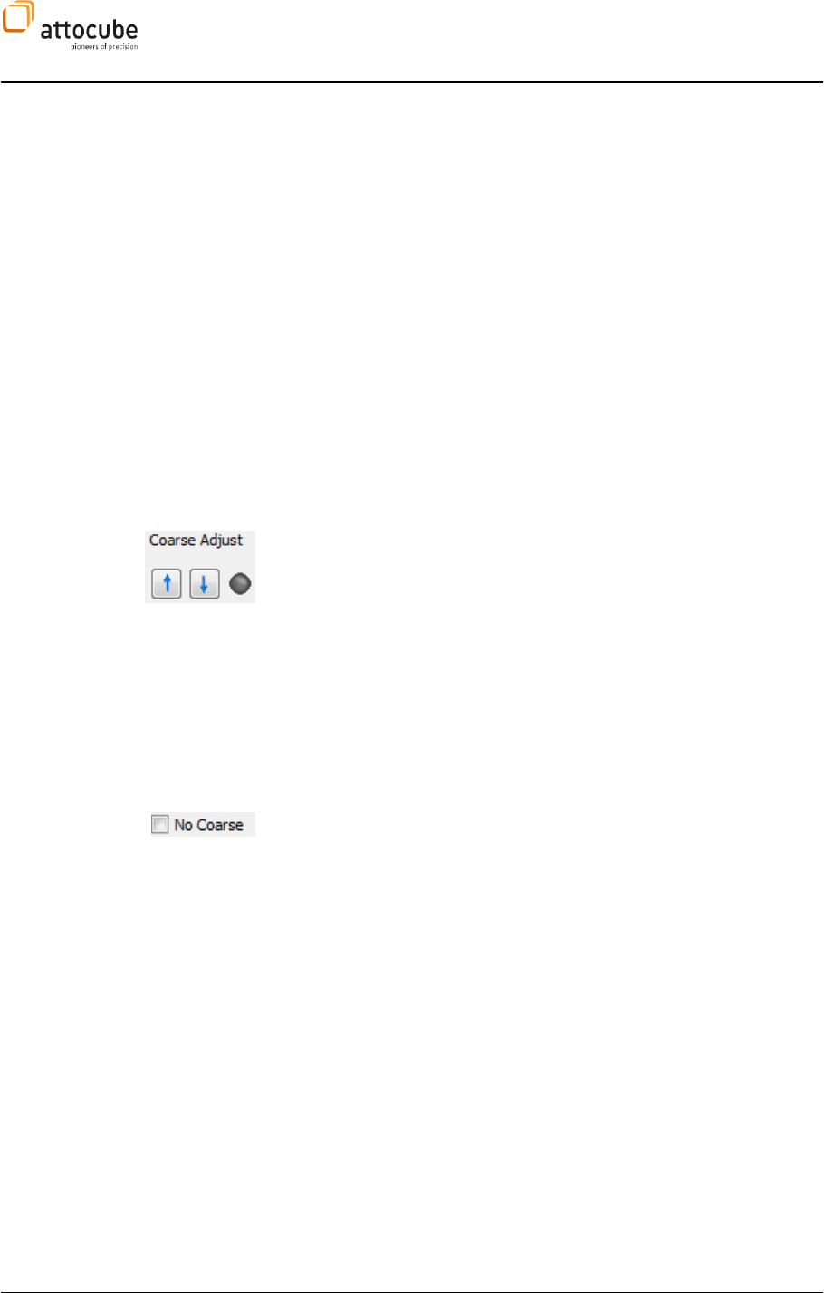
Page 99

respective companies. Any rights not expressly granted herein are reserved. ATTENTION: Specifications and technical

data are subject to change without notice.



Speed: Approach speed for Ramp Mode.

Steps/Apr.: Defines the number of coarse steps that will be executed

after each scanner ramp. Usually, this value will be defined depending on

the stroke of the z scanner in relation to the step width of the coarse device.

For attocube microscope systems, this value will be given in the operation

manual of the microscope.

Apr. Mode: Approach mode; defines whether Loop or Ramp mode is

used. Details are given in the text above.

Target Mode: Defines the mode that is activated after the stop condition

was reached. It is possible to switch on the feedback loop (Loop On), or to

retract the tip (Retract).

Status LED: The status LED indicates whether the autoapproach is

active or not.

Start: Press Start to start the Autoapproach.

Coarse Adjust: ssue single

steps with the autoapproach coarse axis. The coarse adjust button is meant

to set the contact range of the tip within the z scanner stroke. Normally,

after finishing the autoapproach the tip is in the upper part of the z scanner

range. Using the Coarse Adjust buttons, one can move the contact point of

the tip to a more convenient position in the middle of the z scanner range

(with better scanner linearity). This is done by deactivating the feedback

loop, triggering one coarse step and then restarting the feedback. So this

functionality can be used with the feedback turned ON without any risk of

damaging the tip.

Note: if the feedback was not active upon the triggering of the Coarse Adjust,

it will not be activated after the execution of the coarse step.

No coarse: If this option is chosen, the coarse movement of the

autoapproach will be deactivated.

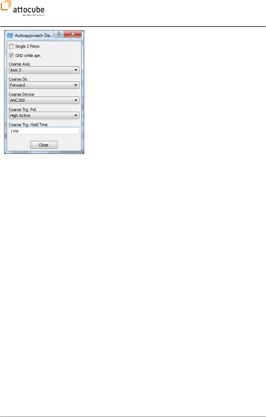
Page 100

The Autoapproach Details section includes all approach parameters that will

have to be set only once to configure a certain hardware configuration.

Single Z-Piezo: Enable, if the z positioner piezo and the z scan piezo are

the same physical device. In this case, the ANC300 will be switched to EXT

mode during the approach.

GND while apr.: When enabled, the coarse control device will be switched

to GND mode during z scanner expansion. For lowest noise, this option

should always be activated.

Coarse Axis: Defines the axis number of the z coarse positioner. The

attocube standard is to use axis no. 3 as the z-axis.

Coarse Dir.: Defines the coarse approach direction. Standard is

forward.

Coarse Device: Defines the coarse control device. The possibilities to

choose from are

1. ANC300 for operation with an attocube ANC300. The connection to

the ANC300 has to be done a serial cable.

2. TTL via DAC2: Can be used to control any coarse controller that can

be triggered by a TTL pulse (5V pulse amplitude). The connection

has to be made via the standard DAC2 output.

3. LVTTL via DAC2: Can be used to control any coarse controller that can

be triggered by a low voltage TTL pulse (2.2V pulse amplitude). The

connection has to be made via the standard DAC2 output.

4. ANC350 via NSL: For operation with an attocube ANC350. The

connection is done via a special NSL cable. For further information

on this connection, please contact attocube.

VI.5.e. Pathmode Tab

The Pathmode is used for experiments that are defined on a grid of points or

on a number of randomly selected points of the scan field. On each point, a

number of actions can be defined and grouped into action lists. Predefined

actions include any of the internal spectroscopies as well as handshake

actions (either manually or with external instruments). The flexibility and

diversity of this function makes it a very powerful tool for the

experimentalist.

The Pathmode is enabled using the Frame Tools of either frame view (see

section VI.4). To select a path, first click on the button, then select points of

interest in the data display. These positions will be shown as small circles in

the display, with a line connecting the different points indicating the path.

After selecting the path, a click on the accept button will initialize the

Pathmode. Paths and grids can be saved, edited and reloaded using the

respective items in the Path Control section of the Path tab.

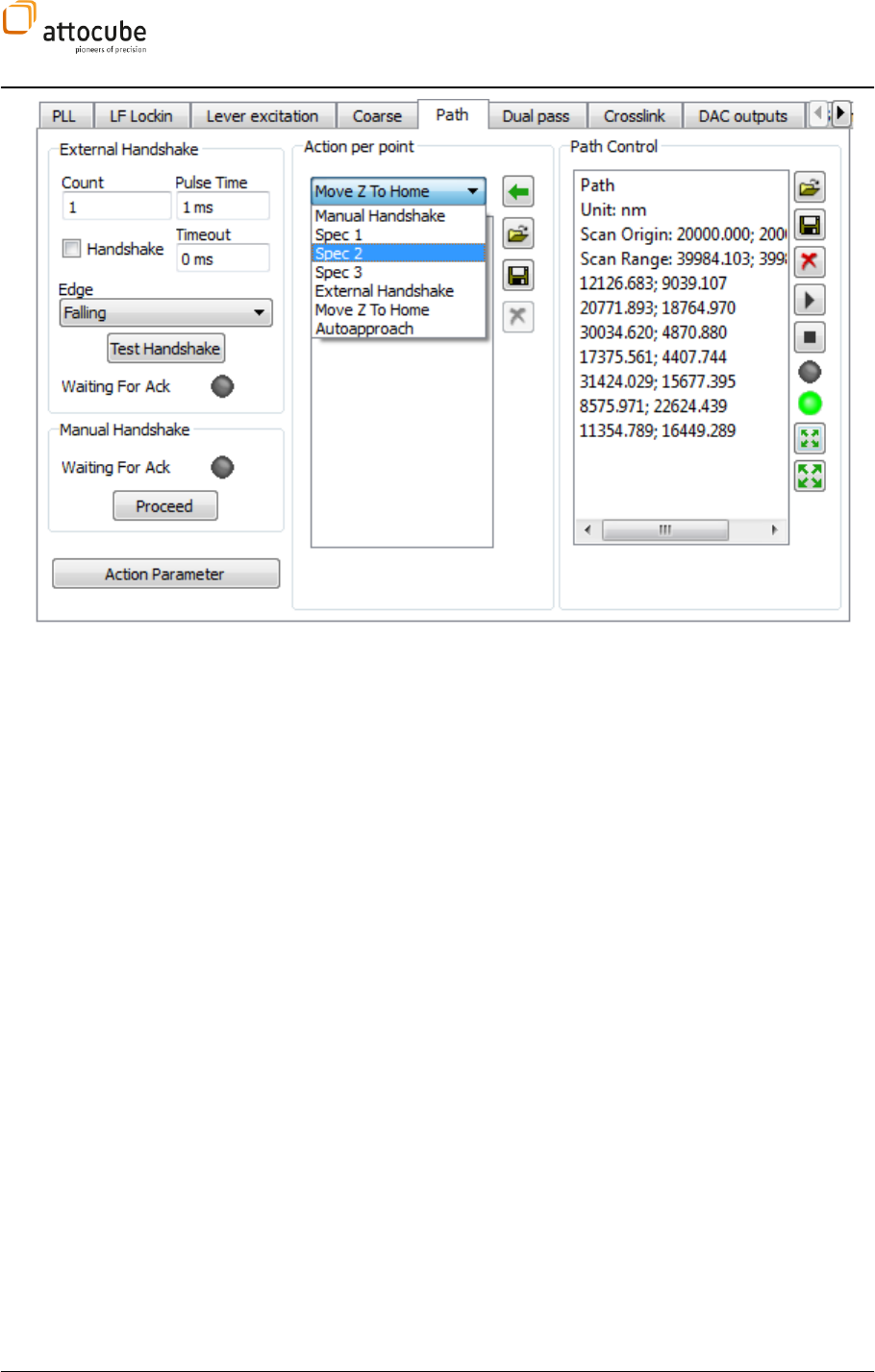
Page 101

respective companies. Any rights not expressly granted herein are reserved. ATTENTION: Specifications and technical

data are subject to change without notice.

Manual Handshake: If this option is enabled, the user has to confirm

each step with the Proceed button (in the Manual Handshake section). The

scanner position on each point can be manually altered using the Manual

Positioning option described in section VI.5.k.

VI.5.f. External Handshake

The External Handshake is used to integrate external devices into the control

capabilities of the ASC500. The interaction between the ASC500 and the

external device is done by means of TTL pulses. For the definition of the SNYC

connector pins, see Figure 4 on page 12. The idea of the procedure is the

following:

1. The ASC500 drives the tip to a certain spot of interest (defined by

the path mode)

2. A SNYC OUT TTL pulse is issued once the tip has reached the target

position to trigger the external device.

3. The external device (for example a spectrometer) executes a certain

measurement task.

4. After the measurement is finished, the external device issues

another TTL pulse which is triggered by the ASC500.

5. Upon receiving a SNYC IN TTL pulse, the ASC500 drives the tip to the

next point (or repeat the measurement circle).

To use this capability, the following conditions have to be fulfilled:

a) The SYNC OUT line of the ASC500 must be connected to the external

device

b) The SYNC IN line of the ASC500 has to be connected to the external

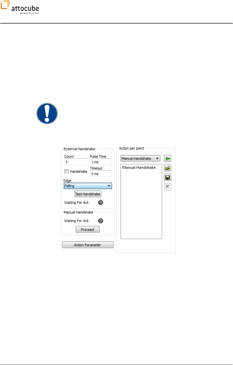
Page 102

device

c) The external device must be capable of being triggered by a TTL

pulse.

d) The external device must be capable of sending a TTL pulse after the

fulfillment of its measurement task. If this is not possible, the

ASC500 can also wait a predefined amount of time at each spot

before moving to the next spot. The waiting time at each point must

be adjusted to make sure the external device has finished its

measurement task.

NOTE on TTL pulses:

The ASC500 TTL input and output lines are using low-voltage TTL (LVTTL)

pulses, i.e. pulses with a high level of 3.3 V. However, the use of 5 V TTL

pulses (also commonly used) will not damage the input stage of the ASC500.

Also, since the threshold voltage for all TTL high levels is defined as 2.5 V,

communication with a 5 V-TTL device is guaranteed without problems.

Figure 25:

External Handshake dialog

To setup the handshake procedure with the external device, the External

Handshake section of the Path tab is used. The parameters will be explained

in the following:

Count: Number of handshake cycles to be executed per point.

Pulse Time: Defines the length of the SYNC OUT pulse.

Handshake: If activated, the controller waits for a return SYNC IN pulse

(or until timeout). If deactivated, the tip will smoothly move from point to

point sending a SYNC OUT whenever a new point is reached.

Timeout: Defines the maximum period of time the controller is

waiting for a SYNC IN pulse. After Timeout time has elapsed, the controller

will either proceed with the next SYNC OUT pulse (if Count > 1) or the tip will

move to the next point. The Timeout can be deactivated by setting it to 0. In

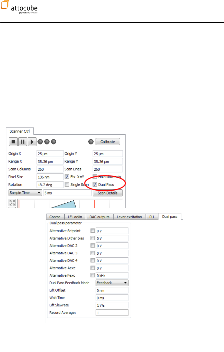
Page 103

respective companies. Any rights not expressly granted herein are reserved. ATTENTION: Specifications and technical

data are subject to change without notice.

this case, the tip will not move to the next pixel until a SYNC input is sensed.

Timeout can be used to control external devices that do not have the

capability to return a SYNC IN TTL pulse.

Edge: Defines if the SYNC input TTL pulse will be triggered on

either Falling or Raising edge.

Test Handshake: Runs one cycle of the Handshake procedure. A first click on

this button will issue a SYNC OUT TTL pulse. A second click will simulate the

SNYC input pulse, i.e. the tip will move to the next point (or repeat the cycle

if Count > 1). Note that a Timeout can occur before the second click is done

in which case the second click will not end the cycle but instead start a new

cycle.

Wait for Ack: This green LED is ON as long as the controller is waiting for

a SYNC IN pulse.

VI.5.g. Dual Pass Mode

The Dual Pass Mode changes the scan

movement so that each line is scanned twice

(forward  backward  forward  backward)

before proceeding to the next scan line.

Various parameters can be altered during the

second line pass, including a constant height

offset between the tip and the sample surface,

sometimes referred to as Lift Mode. The Dual

Pass Mode is activated within the scanner

widget; the parameters used for the second

line pass can be set in the Dual Pass Mode Tab.

Please employ the Display Wizard to open new

frame or line views to display the second pass

data.

Alternative Setpoint: Enter the z feedback setpoint that will be used for

every second line pass. Activate the alternative setpoint feature by checking

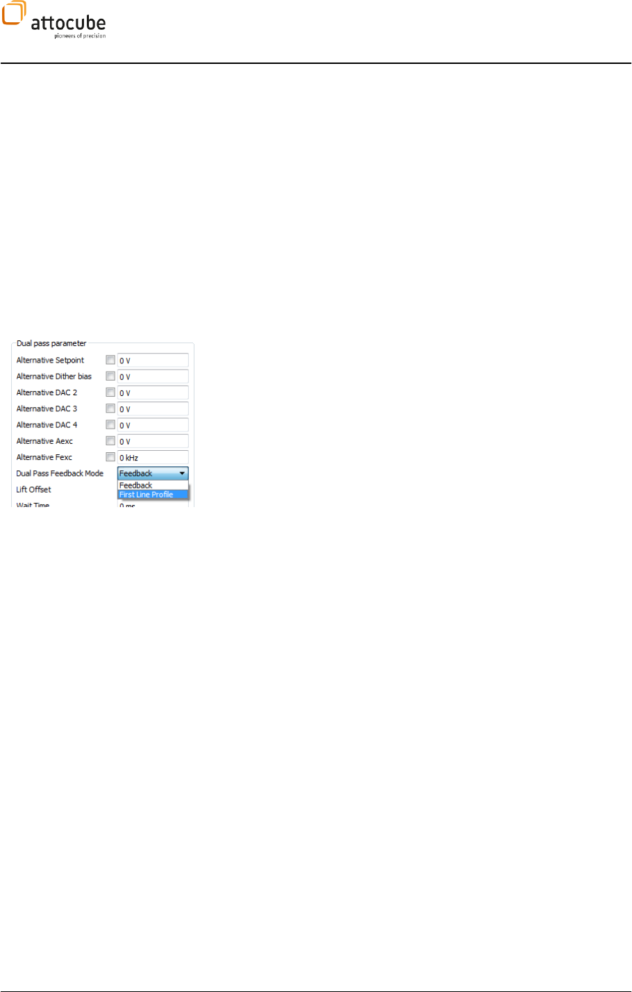
Page 104

the button left to the edit box. Please note that the alternative setpoint

feature will only work if Feedback is selected under Second Pass Feedback

Mode.

Alternative DAC1: Enter an alternative output voltage that will be

sent to the DAC1 output during the second line pass. Activate the feature by

checking the button left to the edit box. Again, this alternative output

feature will only work if Feedback is selected under Second Pass Feedback

Mode.

Dual Pass Feedback Mode: The Dual Pass Mode allows for two different

modes of operation:

1. Feedback: The z feedback will be still active during the second pass.

You can either choose a different z feedback setpoint (Alternative

Setpoint) or a different DAC1 voltage output (Alternative DAC 1 or

both) during the second line pass.

2. First Line Profile: This option records the sample topography during

the first pass. In the second pass, the feedback is turned off and the

tip is scanned along the recorded topography plus the Lift Offset.If

made correctly the the distance between tip and sample is kept

constant this way. This mode is especially useful to image long

range forces (i.e. electrostatic or magnetic) without topography

side effects.

Below is a detailed description of the behavior with the First Line

Profile Option enabled:

 The topography (i.e. Z_out) information during the first line

pass (forward and backward) is recorded.

 Before starting the second pass, the z feedback is stopped and

the tip is retracted to a certain height specified under Lift

Offset. The speed of this retraction movement is governed by

the Lift Slewrate. The scanner pauses for the Wait Time in order

to give the system the chance to settle.

 The topography of the first line pass is repeated in the defined

offset height. At each point, the tip is at the well defined

distance over the sample surface. Data recording on each of



Scanner) is stopped. The second pass data is recorded in data

windows triggered by Second Line.

 After completing the second pass (forward and backward) the z

feedback is turned on again and the scan is paused for another

Wait Time to let the system settle. The scanner is moved to the

next line and the first pass of the new line started.

Lift Offset: Specify the distance between tip and surface during the

second pass. Please note that a positive value will cause the tip to be lifted

by this height. Negative values are forbidden.

Wait Time: Defines the time the scanner is paused at the beginning

and the end of the second pass. Please note that the Lift Slewrate may

automatically be adapted to ensure that the scanner has reached the defined

lift height before the wait time has ended (before the second pass). After

Page 105

respective companies. Any rights not expressly granted herein are reserved. ATTENTION: Specifications and technical

data are subject to change without notice.

finishing the second pass, the z feedback will be turned on. Please make sure

that the Wait Time is long enough to give the feedback the possibility to

reach the first pass setpoint.

Lift Slewrate: Defines the voltage rate of change that is applied to the z

scanner to reach the lift height at the beginning of the second pass.

Record Average: This number shows the number of recorded topography

points that will be averaged to give one height data point for the second

pass. This value is automatically set by the system and it is not adjustable.

Normally, it will be set to 1 and it will only be increased for lines with a very

high number of data points.

Second Pass Frame Views

To display, record, and save the data from the second pass, one employs the

Display Wizard as described in section V.4.d on page 58. Use any free data

channel to open a frame or line view with the desired filters.

VI.5.h. Q Control

Any oscillating system showing resonance behavior can be described by a Q

factor. The Q factor is a measure of the damping of the oscillating system.

In non-contact mode AFM, the Q factor is a function of the internal damping

of the lever (cantilever or tuning fork) and the lever environment (fluid,

ambient, high vacuum, and UHV). The Q factor is a very important parameter

for non-contact AFM, because it determines or constrains important

measurement parameters such as sensitivity and scan speed.

Given a certain measurement environment and a certain lever, the Q factor

can be easily measured but it cannot be altered in standard SPM

applications. The ASC500 Q Control feature enables changing the Q factor

and thus gives access to the control of important measurement parameters.

The Q control can be especially helpful in two situations:

1. Non-contact measurements in a low temperature and/or UHV

environment. Q factors in these environments can get very high (up

to 105-106), resulting in very small damping of the oscillation

amplitude and thus to very large time constants for changes in the

oscillation amplitude (order of tens of seconds). In amplitude

modulation mode, the z feedback control will work directly on this

very slowly changing oscillation signal, thus reducing the scan

speed significantly. Q reduction is a very effective way to overcome

these speed limits.

2. Measurements in a liquid environment typically show very low Q

factors (< 100). Increasing the Q factor may give reasonable

sensitivity for these measurements.

Schematics

To gain access of the control over the Q factor, a sophisticated oscillation

scheme is necessary. The excitation signal for the lever is composed in the

Signal Adder from two parts:

The first part is the fixed AC signal at the resonance frequency of the lever

coming from the Lock-In amplifier.

The second part is the signal that is deduced from the oscillation signal of

the lever: The output of the lever is demodulated by the internal Lock-In

detector to obtain its amplitude and phase (relative to the fixed excitation

signal). These signals are routed into a phase shifter and an amplitude gain

Page 106

and a new oscillating signal is synthesized in the Oscillation Generator, called

Feedback Excitation.

One can show mathematically that feedback signals with a phase shift of +/-

/2 enhance or reduce the effective damping in the system. The lever will

behave exactly as if it was built in a different way or if the environment has

changed. Below, one can see the schematics of the Q control excitation.

The Q factor can be measured with the Resonance feature (see section VI.6.b

on page 114). Find the FWHM (full width half maximum) f from the

amplitude vs. frequency plot to the left. The Q factor is then calculated using

the relationship:

Q = fres/f

The Q Control controls can be found in the Lock In tab. There are only two

parameters and one Enable button. You can set the phase shift between the

cantilever oscillation (Aosc) and the feedback excitation signal and the gain

of the feedback signal.

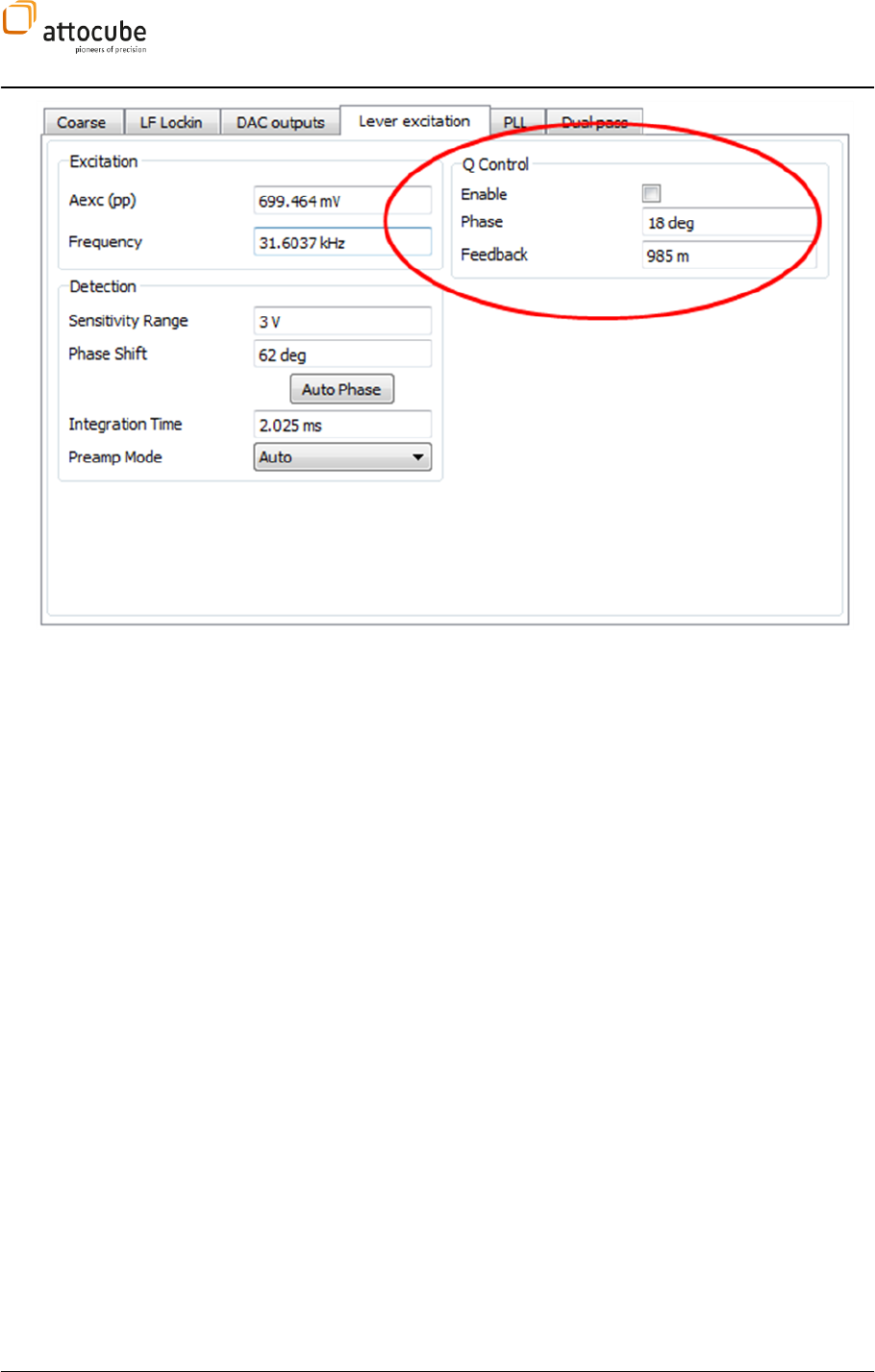
Page 107

respective companies. Any rights not expressly granted herein are reserved. ATTENTION: Specifications and technical

data are subject to change without notice.

Enable: Turns the Q control on or off. Please note that turning the

Q control on or off may change the oscillation amplitude of the lever

significantly. Although this will not damage the tip, you may want to use the

excitation amplitude field (found directly to the left under High

Frequency/Modulation/Amplitude (pp)) to reduce the excitation before

checking/unchecking the Enable button.

Phase: Sets the phase shift between the lever oscillation and the

feedback excitation signal. Although in theory this should be either +90 deg

or -90 deg, there are always additional phase shifts due to electronic

components in the signal path and due to the (short but non-zero) time it

takes for the ASC500 to demodulate the signal. The best way to find the right

value is to change the Phase systematically while repeatedly doing the

Resonance (set the Curves value of both Resonance views to 10 or larger to

have several frequency sweeps displayed in one graph). For values differing

from +/- 90 deg phase, the resonance frequency is shifted in frequency. By

going stepwise through the -180 deg .. +180 deg Phase range, one should

see the maximum of the amplitude resonance curve moving around in a

circle. Note the values for minimum resonance peak if you want to reduce the

Q factor or either note the Phase value of the maximum if you want to

Feedback

value.

Feedback: This sets the gain of the feedback excitation signal. The

range of this value is 0 to 1. Please note that for values above 0.5, the

effective value of the fixed excitation is reduced to strengthen the feedback

excitation part. One can easily increase the fixed excitation if only loosing

signal amplitude and not seeing any impact on the Q control. For most

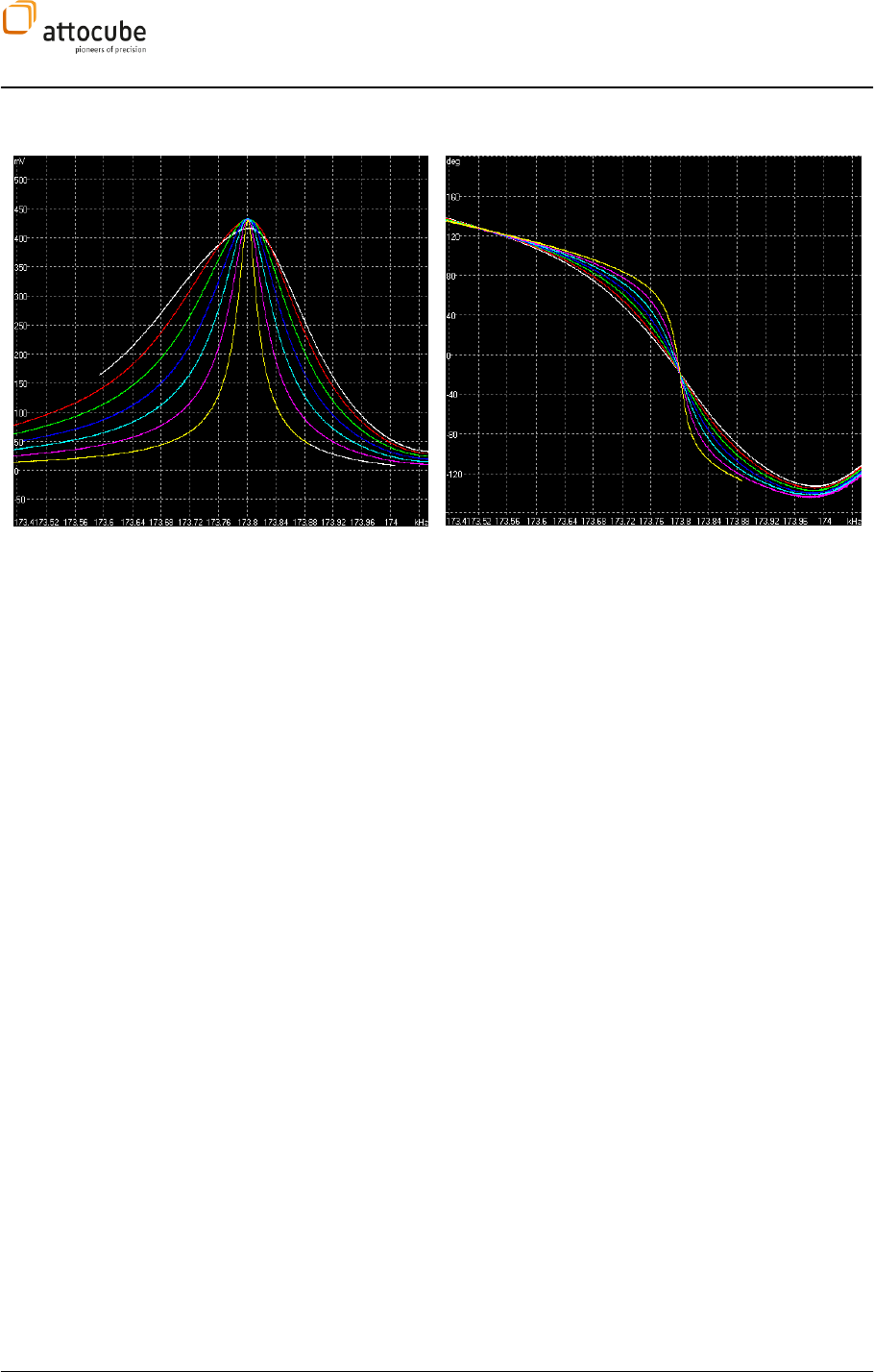
Page 108

applications, a value of larger than 0.85 will be necessary to effectively alter

the Q factor.

Example

The above examples show the Q reduction of a cantilever based AFM at 4 K.

The Q factor could be reduced by approximately one order of magnitude

(note that the original amplitude response is not shown).

Please note that due to the self-excitation nature of the Q control, the

oscillating system can show rather strange behavior far off the resonance

frequency of the lever. This does not have any consequences on the

reproducible and stable behavior of the Q control near the resonance

frequency.

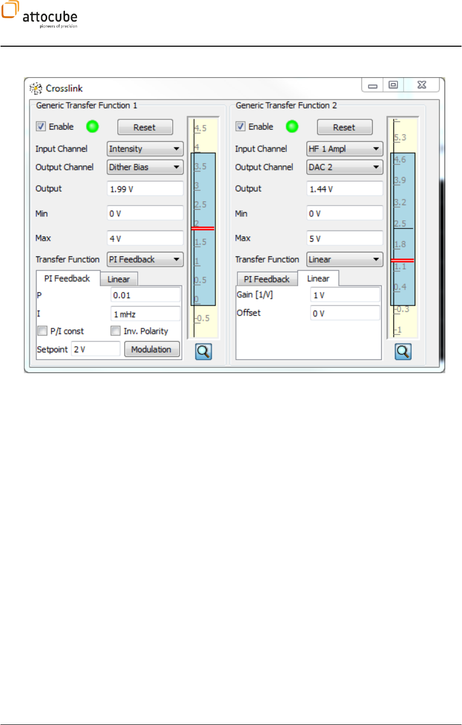
Page 109

respective companies. Any rights not expressly granted herein are reserved. ATTENTION: Specifications and technical

data are subject to change without notice.

VI.5.i. Crosslink

Figure 26: The Crosslink tab. The tab is divided into two parts both of which can be either used as a PI feedback loop

or for signal routing purposes.

The Crosslink tab provides two useful functionalities: one is a generic PI

feedback loop for general purpose feedback requirements. The second is a

routing functionality of any internal or external signal to any of the standard

DAC outputs of the ASC500. This can be used for example to combine the

internal lockin amplifiers with external hardware by routing its amplitude to

the DAC outputs and using the analog voltage with external equipment. As can

be seen in Figure 26, the tab is divided into two sections: each of the sections

can be used either as a feedback loop or for signal routing purposes.

The feedback loops are implemented as generic PI controllers. Any internal or

external signal can be used as a loop input. Any of the standard DAC outputs

can be used as a loop output. The control loops feature adjustable output

ranges, adjustable polarity and Setpoint Modulation for easy P and I tuning.

The operation of these feedback loops is very similar to that of the z feedback

controller (see section VI.3 on page 76).

The functionality of the tab section can be chosen in the drop-down list under

Transfer Function. It can be chosen between PI Feedback (in the left side of

Figure 26) or Linear (right side of Figure 26).

In the next section a detailed description of the operation is given.

Enable: Turns the functionality loop on and off. Please note that the

output value will not be retracted when the loop is turned off. To retract the

output to a home position, use the Reset button.

Page 110

Reset: Resets the output to a certain starting point.

Input Channel: Definition of the input signal for the control loop/signal

router.

Output Channel: Definition of the output channel. This can be any of the

standard DAC outputs.

Output: If the loop/router in enabled, this field shows the current

output value. In case the loop/router is stopped, this field can be used to

enter a certain static voltage on the Output Channel. It is worth noting that

this field overwrites its counterpart of the DAC Output tab (see section VI.5.j)

Min/Max: Defines the output voltage range.

Transfer Function: Defines the functionality of the section. It can be

chosen between PI Feedback and Linear. The parameters for either PI Feedback

or Linear functionality can be chosen in the respective sub-tabs described

below.

PI Feedback

P and I: Definition of the control parameters for the loop.

P/I const: With this button checked, a change in either P or I will also

change the respective other parameter to keep the ratio between P and I

constant.

Setpoint: Definition of the target value for the signal specified in Input

Channel.

Inverse Polarity: Definition of the polarity of the control loop. Unchecked

Inverse Polarity means that the control loop will decrease the output if the

input value is larger than the setpoint and vice versa. Check the Inverse

Polarity button to control signals with negative slopes, i.e. where the output

needs to be increased to decrease the input value.

Linear

Gain: Defines the gain between the analog voltage output and the

signal that is routed to the output.

Offset: Defines the offset of the linear transfer function between the

input channel and the output voltage.

In the display to the right of the text edit boxes, there is a display showing the

allowed output range together with the current output value.

Crosslink P and I units

The physical unit of the P and I parameters of the Crosslink feedback loops are

dependent on the input signal of the loop. The units are:

Input Signal

P unit

I unit

ADC 1..6

V/V

V/V/s

HF 1 df

V/Hz

V/Hz/s

HF 1 Ampl

V/V

V/V/s

HF 1 Phase

V/deg

V/deg/s

LF Lockin Ampl

V/V

V/V/s

Page 111

respective companies. Any rights not expressly granted herein are reserved. ATTENTION: Specifications and technical

data are subject to change without notice.

LF Lockin Phase

V/deg

V/deg/s

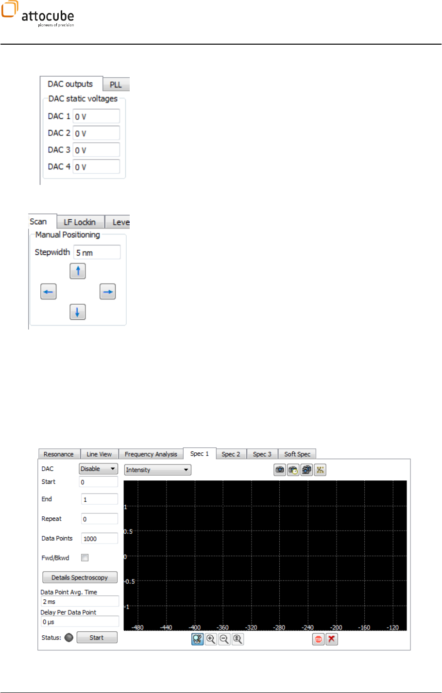
Page 112

VI.5.j. DAC Outputs

In the DAC Output section, static output voltages can be defined for all

standard DAC outputs. There is one edit box for each of the four DAC outputs,

each named with its alias as defined in the Aliases menu (see section V.3.b).

The numbers to be entered here are limited by the range that is defined in the

Output Limits menu (see section VI.1).

It is worth noting that the static voltages defined here can be overwritten by

either the output of the Crosslink section or can be modulated by the output of

the low frequency lock-in.

VI.5.k. Scan; Manual Positioning

Sometimes, it is useful to manually adjust the position of the tip. The Manual

Positioning tool in the Scan tab can be used for this task. If the scanning is not

moving (either in STOP mode or within the Pathmode tool) the scanner can be

moved in discrete steps in all lateral directions. The Stepwidth can be entered

in the respective text field and then the arrow icons can be used to step in the

respective directions.

VI.6. 1-dimensional data displays

VI.6.a. Spectroscopy Tab(s)

With the spectroscopy tabs (Spec 1-3), one or more signals can be recorded while changing certain system



photoluminescence as a function of the gate voltage.

Note that you can change the name of these three tabs in the Aliases menu, see section V.3.b for details.

Page 113

respective companies. Any rights not expressly granted herein are reserved. ATTENTION: Specifications and technical

data are subject to change without notice.

There are three basic types of spectroscopies:

1. DAC Spectroscopy: Any of the four standard DAC outputs can be used

for spectroscopy purposes.

2. Z Spectroscopy: this type of spectroscopy will sweep the Z Out

voltage while recording any kind of internal or external signal.

3. Low Freq: low frequency spectroscopy changes the frequency of the

low frequency lock-in.

The type of spectroscopy is defined in the DAC drop-down list of either of the

three Spec tabs. All types of spectroscopies are operated in the same way.

these are controlled in the same way. For simplicity, we refer in the following

only to a Z-Spectroscopy.

The voltage is swept in a step-like way: the sweep range is divided into a

number of steps (Data Points). The first voltage step is generated and is kept

constant during the measurement of the response signal. Only after the

measurement of the first data point is finished, the output voltage changes

to the next point.

Start: Specify the start position within the allowed z-range .

End: Specify the end position within the allowed z-range . If End is

smaller the Start, the output will be swept backwards.

Repeat: If the measurement should be repeated automatically, increase the

Repeat value. Please note that by default, the graph will only show one

measurement trace. To display more than one trace in the spectroscopy view,

open the Ranges dialog of the Spectroscopy View (see section 0 for details).

Data Points: Specify the number of data points between Start and End.

Please note that this number is slightly altered once you start the sweep.

This is because of the quantized nature of the digital output; the minimum

step size of the 16 bit DAC output is for example 300 µV.

Fwd/Bkwd: If activated, the voltage is swept from Start to End and

then back to Start. The backward sweep is displayed in a different color.

Loop Off: Switches the feedback loop off during the measurement.

Especially with the Z-Spectroscopy, it is important to switch the loop off;

otherwise the loop override the spectroscopy. When the spectroscopy

measurement is finished, the loop is automatically switched on again.

Limiter: If Limiter is enabled, the spectroscopy will stop if the limit

criterion as given in the Details dialog is met. You can use the limiter to

protect e.g. sensitive tips during the sweep.

Data Point Avg. Time: Specify here the measurement time per pixel. All

collected data during this measurement time will be averaged.

Delay Per Data Point: Enter a delay for each point after the new value

has been set, before the data is taken.

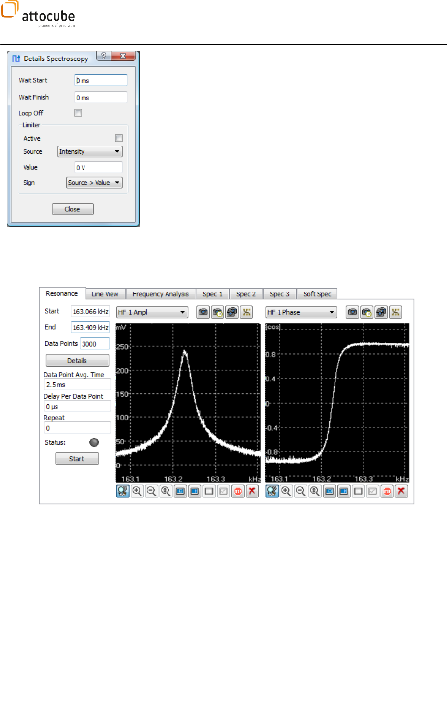
Page 114

Details Spectroscopy: Opens the Details dialog window:

Wait Start: Delay time before the spectroscopy is started.

Wait Finish: Delay time after the spectroscopy is finished.

Limiter Source: Signal to trace during the measurement.

Limiter Value: Exact value for the limit criteria.

Limiter Limit: If hit, the spectroscopy is stopped

The graph generated can be manipulated and saved using general graph

tools described in detail in section V.4.b.

VI.6.b. Resonance View

Use the Resonance View to find and characterize an oscillation with

frequency and phase response. By pressing the Start button, the given

frequency window will be scanned, while the response from the AFM Lock-in

is imaged in the amplitude (left) and in the phase window (right). See

section IV.2.bfor details on the internal signal flow. The settings for this

calibration are similar to the spectroscopy features.

Start: Enter a start frequency for the frequency sweep.

End: Enter a stop frequency for the frequency sweep.

Data Points: Enter the number of data points to be traced and displayed

in the images to the right. With fewer points the calibration run will be faster

of course.

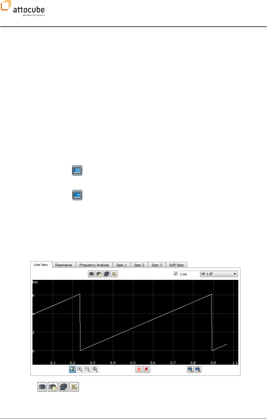
Page 115

respective companies. Any rights not expressly granted herein are reserved. ATTENTION: Specifications and technical

data are subject to change without notice.

Wait Start: This is a delay time before the calibration run is started.

Wait Finish: This is a delay time after the calibration run is stopped and

the system returns to the main frequency as given in the Lock-In Tab or Non-

Contact Mode Tab.

Data Point Avg. Time: Specify here the measurement time per pixel. All

collected data during this measurement time will be averaged.

Delay Per Data Point: Enter a delay for each point after the new

frequency value has been set, before the data is taken. This is to avoid

ringing after the excitation frequency has been changed.

Repeat: If the calibration run has to be repeated several times, this

can be done by entering a respective number in this field. Please note that

zero corresponds to no repetition.

Status: Indicates whether the calibration is running.

Start: Starts the calibration run.

Select new window: Use this Frame Tool to select a new frequency window

from the amplitude or phase display. This will enter the new start and end

values in the corresponding fields.

Select frequency: If you select a point in the amplitude or phase window,

the respective value will be entered as the new frequency in the Non-Contact

Mode Tab and Lock-In Tab, respectively (see sections 0 and I.1.a).

VI.6.c. Line View

The Line View is the most elementary form of displaying data. The data is

displayed against time. Although it is a very basic tool, the line view can be

highly useful because of its simplicity and versatility. It is capable of

displaying data in the time range from milliseconds to kiloseconds.

To the left of the line view graph, the input parameters can be chosen. Below

the graph are the common tools to change the display and save the displayed

data (described in detail in chapter V.4.b).

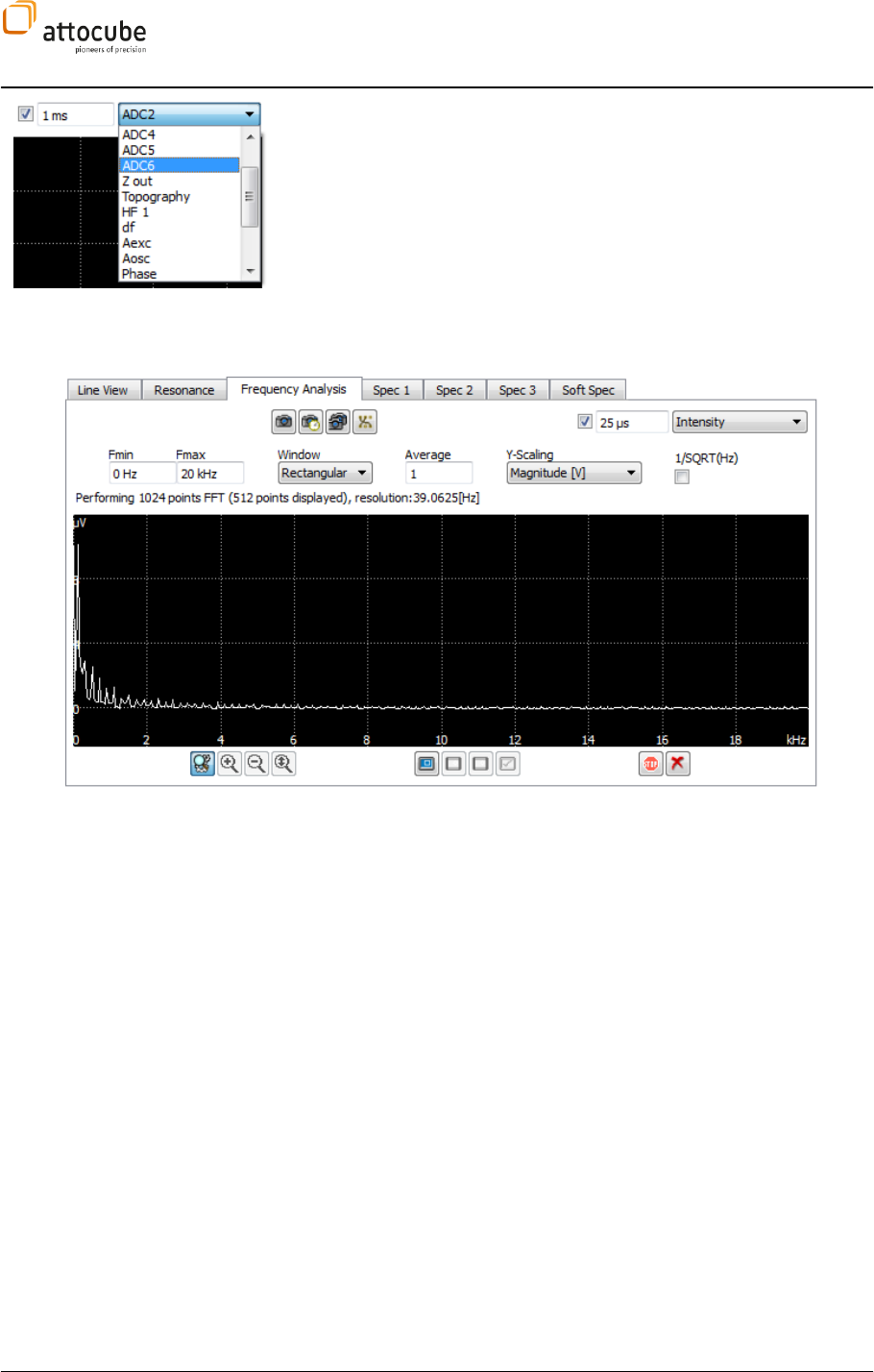
Page 116

Signal: Choose the input signal to be displayed in the line view.

Sample Time: The time which corresponds to one pixel in the line view

graph. Since the sampling speed of the ASC500 inputs is 400 kHz, the

smallest value to be entered here is 2.5 µs.

Average: With this check box you can activate data averaging. This

means that all incoming data within one Sample Time is averaged before it is

displayed in line view.

VI.6.d. Frequency Analysis View

The Frequency Analysis allows for examination of signals in a frequency

domain representation. The ASC500 offers an extremely powerful Frequency

Analysis tool to help optimizing the signal, analyzing mechanical or

electrical noise and to better understanding properties of oscillating systems

like cantilevers or tuning forks. Signals can be analyzed in a frequency range

from DC to 200 kHz, with a frequency resolution well below 1 Hz. Different

window functions can be used to reduce leakage and a number of

representations can be chosen to meet your application.

The image above shows the Frequency Analysis window. To the left of the

graph, the input Signal and the Sample Time can be chosen. Above the

graph, the FFT parameters can be set. The graph itself is displayed in a

frequency vs. amplitude style. The units are shown in the lower right and the

upper left corner of the graph. Please note that the unit of the amplitude

axis is automatically adjusted to the unit of the input signal as specified in

the Transfer Functions Panel.

Time Domain Parameters

Signal: Specification of the input signal. One can choose between

any ADC or AFM input, lock-in data, or Z-Out.

Sample Time: One can choose the sample time for the FFT input signal.

The sample time determines the maximum frequency which can be displayed

in the spectrum. Enter 2.5 µs to access the full sampling speed of the ADC

Page 117

respective companies. Any rights not expressly granted herein are reserved. ATTENTION: Specifications and technical

data are subject to change without notice.

converters (400 kHz), which will allow a FFT from DC to 200 kHz. Increase the

sample time in case the full frequency range is not needed and also to gain

higher frequency resolution. Also, higher sample times reduce the CPU load.

Average: This button activates time domain averaging, i.e. all

incoming data within one Sample Time is averaged before it is processed by

the FFT. One can use this averaging to reduce aliasing artifacts in low

frequency FFT data.

FFT Parameters

Fmin/Fmax: Enter the frequency range you want to analyse here. Fmax

must be smaller or equal to 1/(2*Sample Time). The status line below the

input fields immediately shows the frequency resolution corresponding to

the chosen settings.

Window: Setting of the window function used for FFT calculation.

Choose from Rectangular, Hamming, Blackman, and Flat Top to meet your

requirements in either amplitude or frequency resolution and leakage.

Average: Allows for applying a linear averaging to the FFT data. In

contrast to the time domain averaging, FFT averaging calculates the mean

value of several FFT traces, not input values. Please note that high Average

values may lead to long update intervals of the FFT graph.

Y-Scaling: Choose between Magnitude[V], logarithmic Magnitude

[dBV], Power Density [dBm] and Power Spectrum [dBm].

1/SQRT(Hz): Use this button to display the magnitudes normalized by a

Hz1

factor.

Page 118

VI.7. Closed Loop Step Scanning

A special feature of the ASC500 is the Closed Loop Step Scanning

functionality. It uses coarse positioning stages to raster a (usually large)

sample area by stepping from point to point. Position readout of the

coarse stages is used to drive the raster motion in closed loop to provide

maximum accuracy and repeatability. The scan area is only limited by the

range of the coarse positioners (usually mm range) and acquisition speed.

This feature is especially helpful for SPM techniques where the sensor in

not in direct contact with the sample such as confocal, Hall Probe and

SQUID.

VI.7.a. Concept

The Closed Loop Step Scanning requires a set of coarse positioners with

readout functionality and a step controller that is capable of step

triggering by means of TTL pulses. Although the functionality only requires

the position encoder to provide a position-proportional voltage signal, it

will be assumed in this manual that attocubes ANPxyz series positioners

with RES encoders are used and that these positioners are controlled by an

ANC350 step controller.

A schematic of the setup is shown in Figure 29. The ASC500 connects to

the ANC350 via a multi-pin trigger line. All parameters relevant for the

stepping are set in the ANC350. The logic of the closed loop scanning is

done in the ASC500. The step scanning is a two step process:

1. The origin of the scan is approached.

2. The step scan motion and data acquisition is started.

The step scan motion is done in a line-by-line mode. The x direction is

always the fast scan axis. The positioners will move in x direction from

point to point, and data will be collected at each target point of the closed

loop grid. After the line is finished, the starting point of the next line will

be approached without any data acquisition. Unlike the normal scan, a

step scan will thus only produce forward direction data in order to increase

the acquisition bandwidth.

Algorithm

The closed loop algorithm is shown in Figure 27. Upon approaching a grid

point, the actual position is compared to the target position. Data

acquisition is started if the actual position is larger or equal than the

target position. The positioner will always move in positive direction to

avoid hysteresis errors from the position encoder. Obviously, a single step

size of the positioner must be much smaller than the spacing between to

points of a grid to reach a good positioning accuracy.

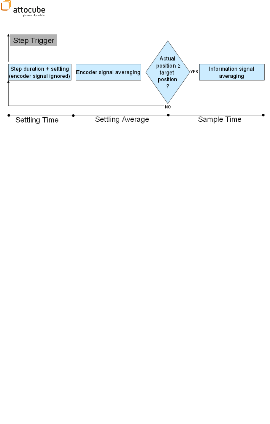
Page 119

respective companies. Any rights not expressly granted herein are reserved. ATTENTION: Specifications and technical

data are subject to change without notice.

Figure 27:

The closed loop step scan algorithm.

The determination of the actual position itself is a two step process:

During the first part (called the Settling Time) the encoder signal is

ignored. This time must be chosen sufficiently large to provide enough

time for the positioner to finish the step and to stabilize on the new

position. A good value is 2/fSTEP (fSTEP being the driving frequency of the

coarse positioners). During the second part of the process, the encoder

signal is averaged to obtain a reasonably accurate position value. This

period is called the Settling Average.

Origin Approach

The approach of the scan origin uses a different algorithm to approach its

target point. The origin of the step scan will be approached in a way so

that the first point of the scan grid lies very close but to right and below

the origin position. The tolerances of the target position for the approach

can be defined in the Approach Range field of the GUI. An Origin of X with

an Appr. Range of dx will result in a target position of X-2dx with a

tolerance of +/- dx. If for example the scan origin is set to 500 µm and the

Appr. Range is set to 1 µm, the controller will drive the coarse positioner

until the actual position lies within a range of 497 µm to 499 µm. The same

procedure is repeated for the y movement.

Maximum Steps

A step scan can run over long time scales (hours or even days). If a coarse

positioner experiences problems of motion during the scan (i.e. because

of mechanical blockage) it is highly likely that the user will not be there to

immediately notice the problem and fix it. The positioner would go on

stepping on the same point until the user interferes. To avoid this

behavior, a maximum number of steps can be defined. If the next target

point cannot be reached within this maximum number of steps, the

controller will stop the positioning and go into an error mode. A warning

LED in the step scan widget will be turned ON. Figure 28 shows the

appearance of the step scan control widget after the occurrence of a Max.

Steps error. The origin of the error is immediately clear by comparing the

Avg. Steps with the Max. Steps value. After this error, the scan can be

resumed by clicking on the Start Scan button. The scan will be continued

where it has stopped. The error can also be detected by means of the

LabView remote control and action can be taken automatically.

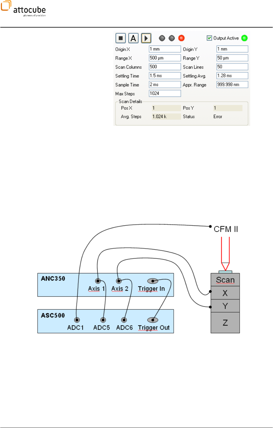
Page 120

Figure 28:

Status of step scan widget after a Maximum Steps error has

occurred.

VI.7.b. Connection

The positioners are connected to the ANC350 in a standard way. In

addition, the resistive signal is routed also to the ASC500 via customized

cables. These cables for room temperature operation are delivered with

the system. For special UHV or low temperature wiring, cables have to be

customized by the user. Details on the pin layout scheme of the wiring are

given in the ANC350 manual. The VSENS and GND pins of the positioner

cabling have to be routed through to the inputs of the ASC500.

Figure 29:

Schematics of a Closed Loop Step Scanning setup .The microscope part (attoCFM II)is only shown for

reference.

The sensor signal has to be fed into the ASC500 using fixed input

connectors:

 X sensor signal  ADC5

 Y sensor signal  ADC6

These two input connectors feature a high input resistance to eliminate

measurement errors when measuring high resistance loads.

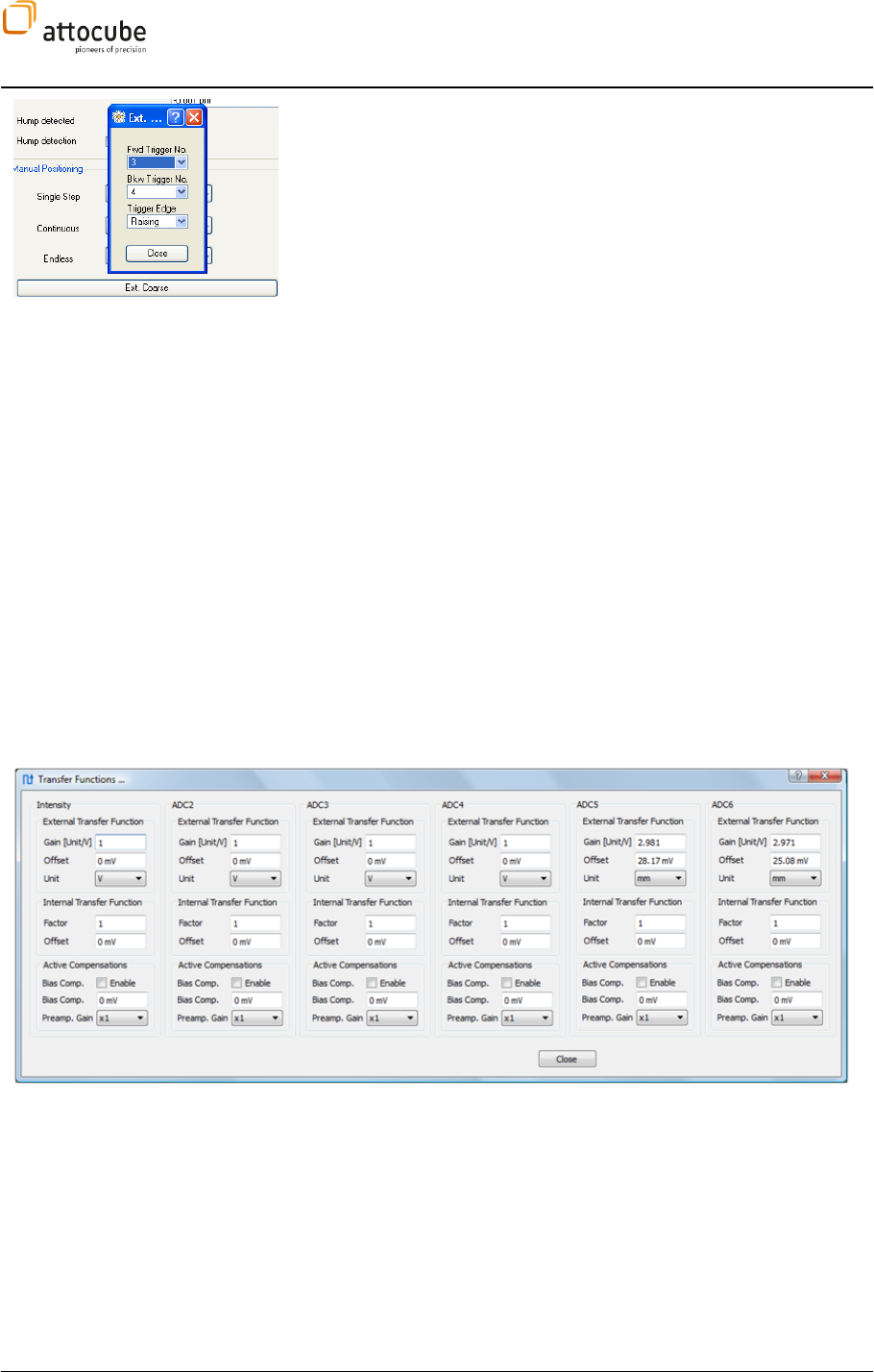
Page 121

respective companies. Any rights not expressly granted herein are reserved. ATTENTION: Specifications and technical

data are subject to change without notice.

The trigger lines use a dedicated cable that is provided together with the

controller. In the ASC350 software, the trigger pins have to be set to the

following values:

 Axis X (usually Axis 1):

o Forward trigger  3

o Backward trigger  4

 Axis Y (usually Axis 2)

o Forward trigger  5

o Backward trigger  6

Within the ANC350 software, the trigger pin configuration can be found in

the tab of the respective axis under Ext. Coarse (see image to the left)

VI.7.c. Operation

Calibration

To translate the sensor input signal from volts to a position in mm, the

Transfer Function standard feature of the ASC500 is used (see section

V.2.b). The calibration can be done as follows:

1. Drive the positioner to 1 mm (using the ANC350), then to 3 mm

and calculate the difference in the sensor signal (in Volts). The

sensor signal can be monitored using the Line View in the ASC500

with either ADC5 or ADC6 as a signal.

2. Calculate the transfer gain in mm/V by dividing by 2 and taking

the inverse. Enter the transfer gain to the Gain edit box of the

External Transfer Function.

3. Use the mouse wheel to change the External Transfer Function

Offset until the reading in the line view (in mm) corresponds to

the reading on the ANC350 axis.

4. Repeat steps 1 to 3 for the second axis.

A typical example of the transfer values is shown in Figure 30.

Figure 30:

A typical calibration of the input connectors for resistive position sensors.

Step Scan control

The 

graphical user interface. It is the second tab behind the standard scan

control. Figure 31 shows the control widget.

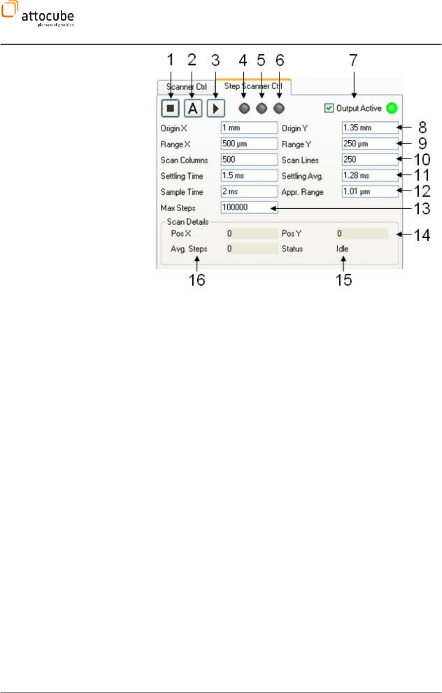
Page 122

Figure 31:

The Step Scan control widget.

1  Stop button: Stops the scan and finished data acquisition. The

positioners remain at their current position.

2  Approach button: Moves the positioners to the scan origin that is

defined in 8. The details of this movement are described on page 119.

3  Start Scan button: Starts scan and data acquisition. An approach to the

origin should have been done before starting the scan to make sure the

positioners are on the lower left of the scan field. After completion of the

scan, the positioners are driven back to the origin and the scan is stopped.

4  Scanner Running LED (green): Signals the undisturbed movement of

the step scanner.

5  Scanner Adjusting LED (green): Signals a scan movement that does not

belong to the data acquisition process.

6  Scanner Error LED (red): Signals a scan error that was caused by an

exceeding of Max Steps. If this LED is ON, the scan can be resumed by

pressing the Start Button.

7  Output Active button: Activated or deactivates all ASC500 outputs. It

can be used instead of its counterpart in the normal scan widget.

8  Origin X/Origin Y: Defines the origin (lower left) of the step scan field.

The user has to make sure that the origin lies within the movement

boundaries of the positioners.

9  Range X/Range Y: Defines the range of the step scan. The user has to

make sure that the range lies within the movement boundaries of the

positioners.

10  Scan Columns/Scan Lines: Defines the resolution of the scan and,

together with the Range, the spacing of the scan grid. The user has to



between two points. This can be reached by using a small amplitude for the



11  Settling Time: waiting period after the trigger of a coarse positioner

step. Details are shown in Figure 27.

Page 123

respective companies. Any rights not expressly granted herein are reserved. ATTENTION: Specifications and technical

data are subject to change without notice.

11  Settling Average: averaging period for the encoder signal after a

coarse positioner step. Details are shown in Figure 27.

12  Sample Time: period for data acquisition. The signal will be averaged

during this period and written into the data channel after completion.

12  Approach Range: target range for the origin approach process. This is

explained in more detail on page 119.

13  Max. Steps: defines the maximum steps to be triggered between two

points of the scan grid. Details can be found on page 119. The minimum

value is 1024.

14  Actual scan position: this gives a permanent update of the actual scan

position in x and y.

15  Status: this gives a permanent update on the status of the scan in text

form.

16  Average Steps: this gives a permanent update on the number of steps

between two points of the scan grid. If this field shows 0 or 1 often, either



scan has to be increased for reasonable control accuracy.

Scan Speed

The scan speed of the step scan cannot be chosen directly, as it is a

function of various parameters. The main source of uncertainty is the

number of steps needed from one point of the scan grid to the next. If the

number of steps per unit length were known, the three parameters Settling

Time, Settling Average and Sample Time fully determine the scan speed.

With the settings shown in Figure 31 and a step excitation with an

amplitude = 20 V and a frequency = 2 kHz, a typical scan speed of 100 µm/s

can be reached at room temperature. The step size was small enough to

reach a high control accuracy with a grid point spacing of 1 µm.

Step Scan Data Display

The Step Scan data displays can be found on the upper right side of the

Daisy panel. It is shown in Figure 32. It consists of one frame view showing

the 2D data of the scan and one scan line view to the left showing the scan

line by line. The displays are very similar to the SCAN data displays with

the only difference that there is no backward scan direction (and thus also

no scan direction filter). The Display Wizard can be used to define any

number of additional displays for Step Scan data.

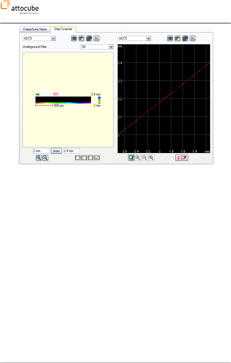
Page 124

Figure 32:

The Step Scan data display.

Page 125

respective companies. Any rights not expressly granted herein are reserved. ATTENTION: Specifications and technical

data are subject to change without notice.

VII. Firmware Upgrade



ASC500. As there is no permanent firmware inside the ASC500, all one has

to do is to boot the controller with the new software. This uploads the new

hardware program into the controller.

So, all that needs to be done is to install the software as written in section

V.1.

Page 126

VIII. Preventive Maintenance

Warning. The equipment contains no user serviceable parts. There is a risk

of severe electrical shock if the equipment is operated with the covers

removed. Only personnel authorized by attocube systems and trained in

the maintenance of this equipment should remove its covers or attempt any

repairs or adjustments. Maintenance is limited to safety testing and

cleaning as described in the following sections.

VIII.1. Safety Testing

Safety testing in accordance with local regulations, should be performed on

a regular basis, (typically annually for an instrument in daily use).

Caution. The instrument contains a power supply filter. Insulation testing

of the power supply connector should be performed using a DC voltage.

VIII.2. Fuses

Two T 4 A/250 V fuses are located on the back panel.

Note. When replacing fuses:

Switch off the power and disconnect the power cord before removing the

fuse cover.

Always replace broken fuses with a fuse of the same rating and type.

VIII.3. Cleaning

Warnings:

Disconnect the power supply before cleaning the unit.

Never allow water to get inside the case.

Do not saturate the unit.

Do not use any type of abrasive pad, scouring powder, or solvent, e.g.

alcohol or benzene.

The fascia may be cleaned with a soft cloth, lightly dampened with water or

a mild detergent.

Page 127

respective companies. Any rights not expressly granted herein are reserved. ATTENTION: Specifications and technical

data are subject to change without notice.

Note. Any time you call for technical support, the software version and the

serial number are essential to trouble-shoot a problem. The serial number

is shown on the backside of the ASC400. the software version can be

-

Page 128

attocube systems AG

Königinstrasse 11a (Rgb)

D-80539 München

Germany

Phone +49 89 2877 80915

Fax +49 89 2877 80919

ASC500 Manual V3 2 1

Navigation menu

Versions of this User Manual:

Views

Navigation