Advanced Modern Engineering Mathematics Glyn James Solutions Manual 4th Edition
User Manual:
Open the PDF directly: View PDF ![]() .
.
Page Count: 688 [warning: Documents this large are best viewed by clicking the View PDF Link!]
- Cover Page
- Title Page
- Copyright Page
- CONTENTS
- 1 Matrix Analysis
- 2 Numerical Solution of Ordinary Differential Equations
- 3 Vector Calculus
- 4 Functions of a Complex Variable
- 5 Laplace Transforms
- 6 The Z Transform
- 7 Fourier series
- 8 The Fourier Transform
- 9 Partial Differential Equations
- 10 Optimization
- 11 Applied Probability and Statistics

Advanced Modern
Engineering Mathematics
Glyn James
fourth edition
Solutions Manual

Solutions Manual
Advanced Modern
Engineering Mathematics
4th edition
Glyn James
ISBN 978-0-273-71925-0
c
Pearson Education Limited 2011
Lecturers adopting the main text are permitted to download the manual as
required.
c
Pearson Education Limited 2011
i

Pearson Education Limited
Edinburgh Gate
Harlow
Essex CM20 2JE
England
and Associated Companies throughout the world
VisitusontheWorldWideWebat:
www.pearsoned.co.uk
This edition published 2011
c
Pearson Education Limited 2011
The rights of Glyn James, David Burley, Dick Clements, Phil Dyke, John Searl,
Nigel Steele and Jerry Wright to be identified as authors of this work have been
asserted by them in accordance with the Copyright, Designs and Patents Act 1988.
ISBN: 978-0-273-71925-0
All rights reserved. Permission is hereby given for the material in this
publication to be reproduced for OHP transparencies and student handouts,
without express permission of the Publishers, for educational purposes only.
In all other cases, no part of this publication may be reproduced, stored
in a retrieval system, or transmitted in any form or by any means, electronic,
mechanical, photocopying, recording, or otherwise without either the prior
written permission of the Publishers or a licence permitting restricted copying
in the United Kingdom issued by the Copyright Licensing Agency Ltd,
90 Tottenham Court Road, London W1T 4LP. This book may not be lent,
resold, hired out or otherwise disposed of by way of trade in any form
of binding or cover other than that in which it is published, without the
prior consent of the Publishers.
ii
TABLE OF CONTENTS
Page
Chapter 1. Matrix Analysis 1
Chapter 2. Numerical Solution of Ordinary Differential Equations 86
Chapter 3. Vector Calculus 126
Chapter 4. Functions of a Complex Variable 194
Chapter 5. Laplace Transforms 270
Chapter 6. The zTransform 369
Chapter 7. Fourier Series 413
Chapter 8. The Fourier Transform 489
Chapter 9. Partial Differential Equations 512
Chapter 10. Optimization 573
Chapter 11. Applied Probability and Statistics 639
iii

1
Matrix Analysis
Exercises 1.3.3
1(a) Yes, as the three vectors are linearly independent and span three-
dimensional space.
1(b) No, since they are linearly dependent
⎡
⎣
3
2
5⎤
⎦−2⎡
⎣
1
0
1⎤
⎦=⎡
⎣
1
2
3⎤
⎦
1(c) No, do not span three-dimensional space. Note, they are also linearly
dependent.
2Transformation matrix is
A=1
√2⎡
⎣
11 0
1−10
00√2⎤
⎦⎡
⎣
100
010
001
⎤
⎦=⎡
⎣
1
√2
1
√20
1
√2−1
√20
001
⎤
⎦
Rotates the (e1,e2) plane through π/4 radians about the e3axis.
3By checking axioms (a)–(h) on p. 10 it is readily shown that all cubics
ax3+bx2+cx +dform a vector space. Note that the space is four dimensional.
3(a) All cubics can be written in the form
ax3+bx2+cx +d
and {1,x,x
2,x
3}are a linearly independent set spanning four-dimensional space.
Thus, it is an appropriate basis.
c
Pearson Education Limited 2011

2 Glyn James, Advanced Modern Engineering Mathematics, 4th Edition
3(b) No, does not span the required four-dimensional space. Thus a general
cubic cannot be written as a linear combination of
(1 −x),(1 + x),(1 −x3),(1 + x3)
as no term in x2is present.
3(c) Yes as linearly independent set spanning the four-dimensional space
a(1 −x)+b(1 + x)+c(x2−x3)+d(x2+x3)
=(a+b)+(b−a)x+(c+a)x2+(d−c)x3
≡α+βx +γx2+δx3
3(d) Yes as a linear independent set spanning the four-dimensional space
a(x−x2)+b(x+x2)+c(1 −x3)+d(1 + x3)
=(a+b)+(b−a)x+(c+d)x2+(d−c)x3
≡α+βx +γx2+δx3
3(e) No not linearly independent set as
(4x3+1)=(3x2+4x3)−(3x2+2x)+(1+2x)
4x+2x3,2x−3x5,x+x3form a linearly independent set and form a basis
for all polynomials of the form α+βx3+γx5.Thus,Sis the space of all odd
quadratic polynomials. It has dimension 3.
c
Pearson Education Limited 2011

Glyn James, Advanced Modern Engineering Mathematics, 4th Edition 3
Exercises 1.4.3
5(a) Characteristic polynomial is λ3−p1λ2−p2λ−p3with
p1=traceA=12
B1=A−12I=⎡
⎣−921
4−7−1
23−8⎤
⎦
A2=AB
1=⎡
⎣−17 −5−7
−18 −30 7
2−5−33 ⎤
⎦
p2=1
2trace A2=−40
B2=A2+40I=⎡
⎣
23 −5−7
−18 10 7
2−57
⎤
⎦
A3=AB
2=⎡
⎣
35 0 0
0350
0035
⎤
⎦
p3=1
3trace A3=35
Thus, characteristic polynomial is
λ3−12λ2+40λ−35
Note that B3=A3−35I= 0 confirming check.
5(b) Characteristic polynomial is λ4−p1λ3−p2λ2−p3λ−p4with
p1=traceA=4
B1=A−4I=⎡
⎢
⎣
−2−112
0−310
−11−31
111−4
⎤
⎥
⎦
A2=AB
1=⎡
⎢
⎣
−340−3
−1−2−21
20−2−5
−3−3−13
⎤
⎥
⎦⇒p2=1
2trace A2=−2
c
Pearson Education Limited 2011

4 Glyn James, Advanced Modern Engineering Mathematics, 4th Edition
B2=A2+2I=⎡
⎢
⎣
−140−3
−10−21
200−5
−3−3−15
⎤
⎥
⎦
A3=AB
2=⎡
⎢
⎣
−520−2
10−2−4
−1−7−34
04−2−7
⎤
⎥
⎦⇒p3=1
3trace A3=−5
B3=A3+5I=⎡
⎢
⎣
000−2
15−2−4
−1−824
04−2−2
⎤
⎥
⎦
A4=AB
3=⎡
⎢
⎣
−2000
0−200
00−20
000−2
⎤
⎥
⎦⇒p4=1
4trace A4=−2
Thus, characteristic polynomial is λ4−4λ3+2λ2+5λ+2
Note that B4=A4+2I= 0 as required by check.
6(a) Eigenvalues given by 1−λ
1
1
1−λ=λ2−2λ=λ(λ−2) = 0
so eigenvectors are λ1=2,λ
2=0
Eigenvectors given by corresponding solutions of
(1 −λi)ei1+ei2=0
ei1+(1−λi)ei2=0
Taking i=1,2 gives the eigenvectors as
e1=[11]
T,e2=[1 −1]T(1)
6(b) Eigenvalues given by 1−λ
3
2
2−λ=λ2−3λ−4=(λ+1)(λ−4) = 0
so eigenvectors are λ1=4,λ
2=−1
Eigenvectors given by corresponding solutions of
(l−λi)ei1+2ei2=0
3ei1+(2−λi)ei2=0
c
Pearson Education Limited 2011

Glyn James, Advanced Modern Engineering Mathematics, 4th Edition 5
Taking i=1,2 gives the eigenvectors as
e1=[23]
T,e2=[1 −1]T
6(c) Eigenvalues given by
1−λ0−4
05−λ4
−443−λ
=λ3+9λ2+9λ−81 = (λ−9)(λ−3)(λ+3)=0
So the eigenvalues are λ1=9,λ
2=3,λ
3=−3.
The eigenvectors are given by the corresponding solutions of
(1 −λi)ei1+0ei2−4ei3=0
0ei1+(5−λi)ei2+4ei3=0
−4ei1+4ei2+(3−λi)ei3=0
Taking i=1,λ
i= 9 solution is
e11
8=−e12
16 =e13
−16 =β1⇒e1=[−122]
T
Taking i=2,λ
i= 3 solution is
e21
−16 =−e22
16 =e23
8=β2⇒e2=[22 −1]T
Taking i=3,λ
i=−3solutionis
e31
32 =−e32
16 =e33
32 =β3⇒e3=[2 −12]
T
6(d) Eigenvalues given by
1−λ12
02−λ2
−113−λ
=0
Adding column 1 to column 2 gives
1−λ2−λ2
02−λ2
−103−λ
=(2−λ)
1−λ12
012
−103−λ
R1−R2(2 −λ)
1−λ00
012
−103−λ
=(2−λ)(1 −λ)(3 −λ)
c
Pearson Education Limited 2011

6 Glyn James, Advanced Modern Engineering Mathematics, 4th Edition
so the eigenvalues are λ1=3,λ
2=2,λ
3=1.
Eigenvectors are the corresponding solutions of (A−λiI)ei=0
When λ=λ1=3 wehave
⎡
⎣−212
0−12
−110
⎤
⎦⎡
⎣
e11
e12
e13 ⎤
⎦=0
leading to the solution e11
−2=−e12
2=e13
−1=β1
so the eigenvector corresponding to λ2=3 is e1=β1[221]
T,β
1constant.
When λ=λ2=2 wehave
⎡
⎣−112
002
−111
⎤
⎦⎡
⎣
e21
e22
e23 ⎤
⎦=0
leading to the solution e21
−2=−e22
2=e23
0=β3
so the eigenvector corresponding to λ2=2 is e2=β2[110]
T,β
2constant.
When λ=λ3=1 wehave
⎡
⎣
012
012
−112
⎤
⎦⎡
⎣
e31
e32
e33 ⎤
⎦=0
leading to the solution e31
0=−e32
2=e33
1=β1
so the eigenvector corresponding to λ3=1 is e3=β3[0 −21]
T,β
3constant.
6(e) Eigenvalues given by
5−λ06
011−λ6
66−2−λ
=λ3−14λ2−23λ−686 = (λ−14)(λ−7)(λ+7)=0
so eigenvalues are λ1=14,λ
2=7,λ
3=−7
c
Pearson Education Limited 2011

Glyn James, Advanced Modern Engineering Mathematics, 4th Edition 7
Eigenvectors are given by the corresponding solutions of
(5 −λi)ei1+0ei2+6ei3=0
0ei1+(11−λi)ei2+6ei3=0
6ei1+6ei2+(−2−λi)ei3=0
When i=1,λ
1=14 solutionis
e11
12 =−e12
−36 =e13
18 =β1⇒e1=[263]
T
When i=2,λ
2= 7 solution is
e21
−72 =−e22
−36 =e23
−24 =β2⇒e2=[6 −32]
T
When i=3,λ
3=−7solutionis
e31
54 =−e32
−36 =e33
−108 =β3⇒e3=[32 −6]T
6(f) Eigenvalues given by
1−λ−10
12−λ1
−21−1−λ
R1+R2
−1−λ0−1−λ
12−λ1
−21−1−λ
=(1+λ)
−10 0
12−λ0
−211−λ
=0,i.e. (1 + λ)(2 −λ)(1 −λ)=0
so eigenvalues are λ1=2,λ
2=1,λ
3=−1
Eigenvectors are given by the corresponding solutions of
(1 −λi)ei1−ei2+0ei3=0
ei1+(2−λi)ei2+ei3=0
−2ei1+ei2−(1 + λi)ei3=0
Taking i=1,2,3 gives the eigenvectors as
e1=[−111]
T,e2=[10 −1]T,e3=[12 −7]T
c
Pearson Education Limited 2011

8 Glyn James, Advanced Modern Engineering Mathematics, 4th Edition
6(g) Eigenvalues given by
4−λ11
25−λ4
−1−1−λ
R1+(R2+R3)
5−λ5−λ5−λ
25−λ4
−1−1−λ
=(5−λ)
10 0
23−λ2
−101−λ
=(5−λ)(3 −λ)(1 −λ)=0
so eigenvalues are λ1=5,λ
2=3,λ
3=1
Eigenvectors are given by the corresponding solutions of
(4 −λi)ei1+ei2+ei3=0
2ei1+(5−λi)ei2+4ei3=0
−ei1−ei2−λiei3=0
Taking i=1,2,3 and solving gives the eigenvectors as
e1=[23 −1]T,e2=[1 −10]
T,e3=[0 −11]
T
6(h) Eigenvalues given by
1−λ−4−2
03−λ1
124−λ
R1+2R2
1−λ2−2λ0
03−λ1
124−λ
=(1−λ)
10 0
03−λ1
104−λ
=(1−λ)(3 −λ)(4 −λ)=0
so eigenvalues are λ1=4,λ
2=3,λ
3=1
Eigenvectors are given by the corresponding solutions of
(1 −λi)ei1−4ei2−2ei3=0
2ei1+(3−λi)ei2+ei3=0
ei1+2ei2+(4−λi)ei3=0
c
Pearson Education Limited 2011

Glyn James, Advanced Modern Engineering Mathematics, 4th Edition 9
Taking i=1,2,3 and solving gives the eigenvectors as
e1=[2 −1−1]T,e2=[2 −10]
T,e3=[4 −1−2]T
Exercises 1.4.5
7(a) Eigenvalues given by
2−λ21
13−λ1
122−λ
R1−R2
1−λ−1+λ0
03−λ1
122−λ
=(1−λ)
10 0
14−λ1
132−λ
=(1−λ)[λ2−6λ+5]=(1−λ)(λ−1)(λ−5) = 0
so eigenvalues are λ1=5,λ
2=λ3=1
The eigenvectors are the corresponding solutions of
(2 −λi)ei1+2ei2+ei3=0
ei1+(3−λi)ei2+ei3=0
ei1+2ei2+(2−λi)ei3=0
When i=1,λ
1= 5 and solution is
e11
4=−e12
−4=e13
4=β1⇒e1=[111]
T
When λ2=λ3= 1 solution is given by the single equation
e21 +2e22 +e23 =0
Following the procedure of Example 1.6 we can obtain two linearly independent
solutions. A possible pair are
e2=[012]
T,e3=[10 −1]T
c
Pearson Education Limited 2011

10 Glyn James, Advanced Modern Engineering Mathematics, 4th Edition
7(b) Eigenvalues given by
−λ−2−2
−11−λ2
−1−12−λ
=−λ3+3λ2−4=−(λ+1)(λ−2)2=0
so eigenvalues are λ1=λ2=2,λ
3=−1
The eigenvectors are the corresponding solutions of
−λiei1−2ei2−2ei3=0
−ei1+(1−λi)ei2+2ei3=0
−ei1−ei2+(2−λi)ei3=0
When i=3,λ
3=−1 corresponding solution is
e31
8=−e32
−1=e33
3=β3⇒e3=[813]
T
When λ1=λ2= 2 solution is given by
−2e21 −2e22 −2e23 =0 (1)
−e21 −e22 +2e23 =0 (2)
−e21 −e22 =0 (3)
From (1) and (2) e23 = 0 and it follows from (3) that e21 =−e22 . We deduce that
there is only one linearly independent eigenvector corresponding to the repeated
eigenvalues λ= 2. A possible eigenvector is
e2=[1 −10]
T
7(c) Eigenvalues given by
4−λ66
13−λ2
−1−5−2−λ
R1−3R3
1−λ−3+3λ0
13−λ2
−1−5−2−λ
=(1−λ)
1−30
13−λ2
−1−5−2−λ
=(1−λ)
10 0
16−λ2
1−8−2−λ
=(1−λ)(λ2+λ+4)=(1−λ)(λ−2)2=0
c
Pearson Education Limited 2011

Glyn James, Advanced Modern Engineering Mathematics, 4th Edition 11
so eigenvalues are λ1=λ2=2,λ
3=1.
The eigenvectors are the corresponding solutions of
(4 −λi)ei1+6ei2+6ei3=0
ei1+(3−λi)ei2+2ei3=0
−ei1−5ei2−(2 + λi)ei3=0
When i=3,λ
3= 1 corresponding solution is
e31
4=−e32
−1=e33
−3=β3⇒e3=[41 −3]T
When λ1=λ2= 2 solution is given by
2e21 +6e22 +6e23 =0
e21 +e22 +2e23 =0
−e21 −5e22 −4e23 =0
so that e21
6=−e22
−2=e23
−4=β2
leading to only one linearly eigenvector corresponding to the eigenvector λ=2. A
possible eigenvector is
e2=[31 −2]T
7(d) Eigenvalues given by
7−λ−2−4
3−λ−2
6−2−3−λ
R1−2R2
1−λ−2+2λ0
3−λ−2
6−2−3−λ
=(1−λ)
1−20
3−λ−2
6−2−3−λ
=(1−λ)
10 0
36−λ−2
610−3−λ
=(1−λ)(λ−2)(λ−1) = 0
so eigenvalues are λ1=2,λ
2=λ3=1.
The eigenvectors are the corresponding solutions of
(7 −λi)ei1−2ei2−4ei3=0
3ei1−λiei2−2ei3=0
6ei1−2ei2−(3 + λi)ei3=0
c
Pearson Education Limited 2011

12 Glyn James, Advanced Modern Engineering Mathematics, 4th Edition
When i=1,λ
2= 2 and solution is
e11
6=−e12
−3=e13
6=β1⇒e1=[212]
T
When λ2=λ3= 1 the solution is given by the single equation
3e21 −e22 −2e23 =0
Following the procedures of Example 1.6 we can obtain two linearly independent
solutions. A possible pair are
e2=[02 −1]T,e3=[203]
T
8
(A−I)=⎡
⎣−4−7−5
233
121
⎤
⎦
Performing a series of row and column operators this may be reduced to the form
⎡
⎣
000
001
100
⎤
⎦indicating that (A−I) is of rank 2. Thus, the nullity q=3−2=1
confirming that there is only one linearly independent eigenvector associated with
the eigenvalue λ= 1. The eigenvector is given by the solution of
−4e11 −7e12 −5e13 =0
2e11 +3e12 +3e13 =0
e11 +2e12 +e13 =0
giving
e11
−3=−e12
−1=e13
1=β1⇒e1=[−311]
T
9
(A−I)=⎡
⎣
11−1
−1−11
−1−11
⎤
⎦
c
Pearson Education Limited 2011

Glyn James, Advanced Modern Engineering Mathematics, 4th Edition 13
Performing a series of row and column operators this may be reduced to the form
⎡
⎣
100
000
000
⎤
⎦indicating that (A−I) is of rank 1. Then, the nullity of q=3−1=2
confirming that there are two linearly independent eigenvectors associated with the
eigenvalue λ= 1. The eigenvectors are given by the single equation
e11 +e12 −e13 =0
and two possible linearly independent eigenvectors are
e1=[101]
Tand e2=[011]
T
Exercises 1.4.8
10 These are standard results.
11(a) (i) Trace A=4+5+0=9= sumeigenvalues;
(ii) det A=15=5×3×1 = product eigenvalues;
(iii) A−1=1
15 ⎡
⎣
4−1−1
−41−14
3318
⎤
⎦. Eigenvalues given by
4−15λ−1−1
−41−15λ−14
3318−15λ
C3−C2
4−15λ−10
−41−15λ−15 + 15λ
3315−15λ
=(15−15λ)
4−15λ−10
−41−15λ−1
331
=(15−15λ)(15λ−5)(15λ−3) = 0
confirming eigenvalues as 1,1
3,1
5.
c
Pearson Education Limited 2011

14 Glyn James, Advanced Modern Engineering Mathematics, 4th Edition
(iv) AT=⎡
⎣
42−1
15−1
14 0
⎤
⎦having eigenvalues given by
4−λ2−1
15−λ−1
14−λ
=(λ−5)(λ−3)(λ−1) = 0
that is, eigenvalue as for A.
11(b) (i) 2A=⎡
⎣
822
410 8
−2−20
⎤
⎦having eigenvalues given by
8−λ22
410−λ8
−2−2−λ
C1−C2
6−λ22
−6+λ10 −λ8
0−2−λ
=(6−λ)
122
−110−λ8
0−2−λ
=(6−λ)
12 2
012−λ10
0−2−λ
=(6−λ)(λ−10)(λ−2) = 0
Thus eigenvalues are 2 times those of A;namely6,10and2.
(ii) A+2I=⎡
⎣
611
27
4
−1−12
⎤
⎦having eigenvalues given by
6−λ11
27−λ4
−1−12−λ
=−λ3+15λ2−71λ+ 105 = −(λ−7)(λ−5)(λ−3) = 0
confirming the eigenvalues as 5 + 2,3+2,1+2.
Likewise for A−2I
c
Pearson Education Limited 2011

Glyn James, Advanced Modern Engineering Mathematics, 4th Edition 15
(iii) A2=⎡
⎣
17 8 8
14 23 22
−6−6−5⎤
⎦having eigenvalues given by
17 −λ88
14 23 −λ22 −λ
−6−6−5−λ
R1+(R2) + R3)
25 −λ25 −λ25 −λ
14 23 −λ22
−6−6−5−λ
=(25−λ)
10 0
14 9 −λ8
−601−λ
=(25−λ)(9 −λ)(1 −λ)=0
that is, eigenvalues A2are 25, 9, 1 which are those of Asquared.
12 Eigenvalues of Agiven by
−3−λ−3−3
−31−λ−1
−3−11−λ
R3+R2
−3−λ−3−3
−31−λ−1
0−2+λ2−λ
=(λ−2)
−3−λ−3−3
−31−λ−1
01−1
C3+C2(λ−2)
−3−λ−3−6
−3(1−λ)−λ
010
=−(λ−2)(λ+6)(λ−3) = 0
so eigenvalues are λ1=−6,λ
2=3,λ
3=2
Eigenvectors are given by corresponding solutions of
(−3−λi)ei1−3ei2−3ei3=0
−3ei1+(1−λi)ei2−ei3=0
−3ei1−ei2+(1−λi)ei3=0
Taking i=1,2,3 gives the eigenvectors as
e1=[211]
T,e2=[−111]
T,e3=[01−1]T
It is readily shown that
eT
1e2=eT
1e3=eT
2e3=0
so that the eigenvectors are mutually orthogonal.
c
Pearson Education Limited 2011

16 Glyn James, Advanced Modern Engineering Mathematics, 4th Edition
13 Let the eigenvector be e=[abc]Tthen since the three vectors are mutually
orthogonal
a+b−2c=0
a+b−c=0
giving c=0anda=−bso an eigenvector corresponding to λ=2ise=[1−10]
T.
Exercises 1.5.3
14 Taking x(0) =[111]
Titerations may then be tabulated as follows:
Iteration k01 2 3 4
1 0.9 0.874 0.869 0.868
x(k)11111
1 0.5 0.494 0.493 0.492
9 7.6 7.484 7.461 7.457
Ax
(k)10 8.7 8.61 8.592 8.589
5 4.3 4.242 4.231 4.228
λ10 8.7 8.61 8.592 8.589
Thus, estimate of dominant eigenvalue is λ8.59 and corresponding eigenvector
x[0.869 1 0.493]Tor x[0.61 0.71 0.35]Tin normalised form.
15(a) Taking x(0) =[111]
Titerations may then be tabulated as follows:
Iteration k012345 6
1 0.75 0.667 0.636 0.625 0.620 0.619
x(k)1111111
1111111
3 2.5 2.334 2.272 2.250 2.240
Ax
(k)4 3.75 3.667 3.636 3.625 3.620
4 3.75 3.667 3.636 3.625 3.620
λ4 3.75 3.667 3.636 3.625 3.620
Thus, correct to two decimal places dominant eigenvalue is 3.62 having
corresponding eigenvectors [0.62 1 1]T.
c
Pearson Education Limited 2011

Glyn James, Advanced Modern Engineering Mathematics, 4th Edition 17
15(b) Taking x(0) =[111]
Titerations may be tabulated as follows:
Iteration k012345
1 0.364 0.277 0.257 0.252 0.251
x(k)1 0.545 0.506 0.501 0.493 0.499
111111
4 2.092 1.831 1.771 1.756
Ax
(k)6 3.818 3.566 3.561 3.49
11 7.546 7.12 7.03 6.994
λ11 7.546 7.12 7.03 6.994
Thus, correct to two decimal places dominant eigenvalue is 7 having corresponding
eigenvector [0.25 0.51]
T.
15(c) Taking x(0) =[1111]
Titerations may then be tabulated as follows:
Iteration k01 2 3 4 5 6
11 1 1 1 1 1
x(k)10−0.5−0.6−0.615 −0.618 −0.618
11−0.5 −0.6 −0.615 −0.618 −0.618
11 1 1 1 1 1
1 2 2.5 2.6 2.615 2.618
Ax
(k)0−1−1.5 −1.6 −1.615 −1.618
0−1−1.5 −1.6 −1.615 −1.618
1 2 2.5 2.6 2.615 2.618
λ1 2 2.5 2.6 2.615 2.618
Thus, correct to two decimal places dominant eigenvalue is 2.62 having
corresponding eigenvector [1 −0.62 −0.62 1]T.
16 The eigenvalue λ1corresponding to the dominant eigenvector e1=[112]
T
is such that Ae
1=λ1e1so
⎡
⎣
311
131
115
⎤
⎦⎡
⎣
1
1
2⎤
⎦=λ1⎡
⎣
1
1
2⎤
⎦
so λ1=6.
c
Pearson Education Limited 2011

18 Glyn James, Advanced Modern Engineering Mathematics, 4th Edition
Then
A1=A−6ˆ
e1ˆ
eT
1where ˆ
e1=1
√6
1
√6
2
√6
T
so
A1=⎡
⎣
311
131
115
⎤
⎦−⎡
⎣
112
112
224
⎤
⎦=⎡
⎣
20−1
02−1
−1−11
⎤
⎦
Applying the power method with x(0) =[111]
T
y(1) =A1x(0) =⎡
⎣
1
1
−1⎤
⎦=x(1)
y(2) =A1x(1) =⎡
⎣
3
3
−3⎤
⎦=3 ⎡
⎣
1
1
−1⎤
⎦
Clearly, λ2=3 and ˆ
e2=1
√3[1 1 −1]T.
Repeating the process
A2=A1−λ2ˆ
e2ˆ
eT
2=⎡
⎣
20−1
02−1
−1−11
⎤
⎦−⎡
⎣
11−1
11−1
−1−11
⎤
⎦=⎡
⎣
1−10
−110
000
⎤
⎦
Taking x(0) =[1 −10]
Tthe power method applied to A2gives
y(1) =A2x(0) =⎡
⎣
2
−2
0⎤
⎦=2 ⎡
⎣
1
−1
0⎤
⎦
and clearly, λ3=2 with ˆ
e3=1
√2[1 −10]
T.
17 The three Gerschgorin circles are
|λ−5|=2,|λ|=2,|λ+5|=2
c
Pearson Education Limited 2011

Glyn James, Advanced Modern Engineering Mathematics, 4th Edition 19
which are three non-intersecting circles. Since the given matrix Ais symmetric its
three eigenvalues are real and it follows from Theorem 1.2 that
3<λ
1<7,−2<λ
2<2,−7<λ
3<7
(i.e., an eigenvalue lies within each of the three circles).
18 The characteristic equation of the matrix Ais
10 −λ−10
−12−λ2
023−λ
=0
that is (10 −λ)[(2 −λ)(3 −λ)−4] −(3 −λ)=0
or f(λ)=λ3−15λ2+51λ−17 = 0
Taking λ0= 10 as the starting value the Newton–Raphson iterative process
produces the following table:
iλ
if(λi)f(λi)−f(λi)
f(λi)
010 7 −51.00 0.13725
1 10.13725 −0.28490 −55.1740 −0.00516
2 10.13209 −0.00041 −55.0149 −0.000007
Thus to three decimal places the largest eigenvalue is λ=10.132
Using Properties 1.1 and 1.2 of section 1.4.6 we have
3
i=1
λi=traceA=15and
3
i=1
λi=|A|=17
c
Pearson Education Limited 2011

20 Glyn James, Advanced Modern Engineering Mathematics, 4th Edition
Thus,
λ2+λ3=15−10.132 = 4.868
λ2λ3=1.67785
so λ2(4.868 −λ2)=1.67785
λ2
2−4.868λ2+1.67785 = 0
λ2=2.434 ±2.0607
that is λ2=4.491 and λ3=0.373
19(a) If e1,e2,...,enare the corresponding eigenvectors to λ1,λ
2,...,λ
nthen
(KI−A)ei=(K−λi)eiso that Aand (KI−A) have the same eigenvectors and
eigenvalues differ by K.
Taking x(o)=
n
i=1
αreithen
x(p)=(KI−A)x(p−1) =(KI−A)2x(p−2) =...=
n
r=1
αr(K−λr)per
Now K−λn>K−λn−1>... >K−λ1and
x(p)=αn(K−λn)pen+
n
r=1
αr(K−λr)per
=(K−λn)p[αnen+
n−1
r=1
αrK−λr
K−λn
p
er]
→(K−λn)pαnen=Kenas p→∞
Also
x(p+1)
i
x(p)
i→(K−λn)p+1
(K−λn)p
αnen
αnen
=K−λn
Hence, we can find λn
19(b) Since Ais a symmetric matrix its eigenvalues are real. By Gerschgorin’s
theorem the eigenvalues lie in the union of the intervals
|λ−2|≤ 1,|λ−2|≤ 2,|λ−2|≤ 1
i.e. |λ−2|≤ 2or0≤λ≤4.
c
Pearson Education Limited 2011

Glyn James, Advanced Modern Engineering Mathematics, 4th Edition 21
Taking K=4 in(a)
KI−A=4I−A=⎡
⎣
210
121
012
⎤
⎦
Taking x(0) =[111]
Titerations using the power method are tabulated as follows:
Iteration k012345
1 0.75 0.714 0.708 0.707 0.707
x(k)111111
1 0.75 0.714 0.708 0.707 0.707
3 2.5 2.428 2.416 2.414
Ax
(k)4 3.5 3.428 3.416 3.414
3 2.5 2.428 2.416 2.414
λ4 3.5 3.428 3.416 3.414
Thus λ3=4−3.41 = 0.59 correct to two decimal places.
Exercises 1.6.3
20 Eigenvalues given by
Δ=
−1−λ6−12
0−13 −λ30
0−920−λ
=0
Now Δ = (−1−λ)−13 −λ30
−920−λ
=(−1−λ)(λ2−7λ+ 10)
=(−1−λ)(λ−5)(λ−2) so Δ = 0 gives λ1=5,λ
2=2,λ
3=−1
Corresponding eigenvectors are given by the solutions of
(A−λiI)ei=0
When λ=λ1=5 wehave
⎡
⎣−66−12
0−18 30
0−915
⎤
⎦⎡
⎣
e11
e12
e13 ⎤
⎦=0
c
Pearson Education Limited 2011

22 Glyn James, Advanced Modern Engineering Mathematics, 4th Edition
leading to the solution e11
−36 =−e12
−180 =e13
108 =β1
so the eigenvector corresponding to λ1=5 is e1=β1[1 −5−3]T
When λ=λ2=2,wehave
⎡
⎣−36−12
0−15 30
0−918
⎤
⎦⎡
⎣
e21
e22
e23 ⎤
⎦=0
leading to the solution e21
0=−e22
−90 =e23
45 =β2
so the eigenvector corresponding to λ2=2 is e2=β2[021]
T
When λ=λ3=−1, we have
⎡
⎣
06−12
0−12 30
0−921
⎤
⎦⎡
⎣
e31
e32
e33 ⎤
⎦=0
leading to the solution e31
18 =−e32
0=e33
0=β3
so the eigenvector corresponding to λ3=−1ise3=β3[1 0 0]T
AmodalmatrixMand spectral matrix Λare
M=⎡
⎣
101
−520
−310
⎤
⎦Λ=⎡
⎣
50 0
02 0
00−1⎤
⎦
M−1=⎡
⎣
01−2
03−5
1−12
⎤
⎦and matrix multiplication confirms M−1AM=Λ
21 From Example 1.9 the eigenvalues and corresponding normalised eigenvectors
of Aare λ1=6,λ
2=3,λ
3=1
ˆ
e1=1
√5[120]
T,ˆ
e2=[001]
T,ˆ
e3=1
√5[−210]
T,
ˆ
M=1
√5⎡
⎣
10−2
20 1
0√50
⎤
⎦
c
Pearson Education Limited 2011

Glyn James, Advanced Modern Engineering Mathematics, 4th Edition 23
ˆ
MTAM=1
5⎡
⎣
12 0
00√5
−21 0
⎤
⎦⎡
⎣
220
250
003
⎤
⎦⎡
⎣
10−2
20 1
0√50
⎤
⎦
=1
5⎡
⎣
612 0
003
√5
−21 0
⎤
⎦⎡
⎣
10−2
20 1
0√50
⎤
⎦
=1
5⎡
⎣
30 0 0
0150
005
⎤
⎦=⎡
⎣
600
030
001
⎤
⎦=Λ
22 The eigenvalues of Aare given by
5−λ10 8
10 2 −λ−2
8−211−λ
=−(λ3−18λ2−81λ+1458) = −(λ−9)(λ+9)(λ−18) = 0
so eigenvalues are λ1=18,λ
2=9,λ
3=−9
The eigenvectors are given by the corresponding solutions of
(5 −λi)ei1+10ei2+8ei3=0
10ei1+(2−λi)ei2−2ei3=0
8ei1−2ei2+(11−λi)ei3=0
Taking i=1,2,3 and solving gives the eigenvectors as
e1=[212]
T,e2=[12 −2]T,e3=[−221]
T
Corresponding normalised eigenvectors are
ˆ
e1=1
3[2 1 2]T,ˆ
e2=1
3[1 2 −2]T,ˆ
e3=1
3[−221]
T
ˆ
M=1
3⎡
⎣
21−2
122
2−21
⎤
⎦,ˆ
MT=1
3⎡
⎣
21 2
12−2
−22 1
⎤
⎦
c
Pearson Education Limited 2011

24 Glyn James, Advanced Modern Engineering Mathematics, 4th Edition
ˆ
MTAM=1
9⎡
⎣
21 2
12−2
−22 1
⎤
⎦⎡
⎣
510 8
10 2 −2
8−211
⎤
⎦⎡
⎣
21−2
122
2−21
⎤
⎦
=1
9⎡
⎣
36 18 36
918−18
18 −18 −9⎤
⎦⎡
⎣
21−2
122
2−21
⎤
⎦
=⎡
⎣
424
12−2
2−2−1⎤
⎦⎡
⎣
21−2
122
2−21
⎤
⎦
=⎡
⎣
18 0 0
09 0
00−9⎤
⎦=Λ
23
A=⎡
⎣
11−2
−12 1
01−1⎤
⎦
Eigenvalues given by
0=
1−λ1−2
−12−λ1
01−1−λ
=−(λ3−2λ2−λ+2) = −(λ−1)(λ−2)(λ+1) =0
so eigenvalues are λ1=2,λ
2=1,λ
3=−1.
The eigenvectors are given by the corresponding solutions of
(1 −λi)ei1+ei2−2ei3=0
−ei1+(2−λi)ei2+ei3=0
0ei1+ei2−(1 + λi)ei3=0
Taking i=1,2,3 and solving gives the eigenvectors as
e1=[131]
T,e2=[321]
T,e3=[101]
T
M=⎡
⎣
131
320
111
⎤
⎦,Λ=⎡
⎣
20 0
01 0
00−1⎤
⎦
M−1=−1
6⎡
⎣
2−2−2
−30−3
12−7⎤
⎦
c
Pearson Education Limited 2011

Glyn James, Advanced Modern Engineering Mathematics, 4th Edition 25
Matrix multiplication then confirms
M−1AM=Λand A=MΛM
−1
24 Eigenvalues given by
3−λ−24
−2−2−λ6
46−1−λ
=−λ3+63λ−162 = −(λ+9)(λ−6)(λ−3) = 0
so the eigenvalues are λ1=−9,λ
2=6,λ
3= 3. The eigenvectors are the
corresponding solutions of
(3 −λi)ei1−2ei2+44ei3=0
−2ei1−(2 + λi)ei2+6ei3=0
4ei1+6ei2−(1 + λi)ei3=0
Taking i=1,2,3 and solving gives the eigenvectors as
e1=[12 −2]T,e2=[212]
T,e3=[−221]
T
Since eT
1e2=eT
1e3=eT
2e3= 0 the eigenvectors are orthogonal
L=[
ˆ
e1ˆ
e2ˆ
e3]=1
3⎡
⎣
12−2
21 2
−22 1
⎤
⎦
ˆ
LAL=1
9⎡
⎣
12−2
21 2
−22 1
⎤
⎦⎡
⎣
3−24
−2−26
46−1⎤
⎦⎡
⎣
12−2
21 2
−22 1
⎤
⎦
=1
9⎡
⎣−9−18 18
12 6 12
−663
⎤
⎦⎡
⎣
12−2
21 2
−22 1
⎤
⎦
=1
9⎡
⎣−81 0 0
0540
0027
⎤
⎦=⎡
⎣−900
060
003
⎤
⎦=Λ
25 Since the matrix Ais symmetric the eigenvectors
e1=[120]
T,e2=[−210]
T,e3=[e31 e32 e33]T
c
Pearson Education Limited 2011

26 Glyn James, Advanced Modern Engineering Mathematics, 4th Edition
are orthogonal. Hence,
eT
1e3=e31 +2e32 =0andeT
2e3=−2e31 +e32 =0
Thus, e31 =e32 =0 and e33 arbitrary so a possible eigenvector is e3=[001]
T.
Using A=ˆ
MΛ ˆ
MTwhere Λ=⎡
⎣
600
010
003
⎤
⎦gives
A=⎡
⎣
1
√5−2
√50
2
√5
1
√50
001
⎤
⎦⎡
⎣
600
010
003
⎤
⎦⎡
⎣
1
√5
2
√50
−2
√5
1
√50
001
⎤
⎦
=⎡
⎣
220
250
003
⎤
⎦
26 A −I=⎡
⎣−4−7−5
233
121
⎤
⎦∼⎡
⎣
000
0−10
100
⎤
⎦is of rank 2
Nullity (A−I)=3−2 = 1 so there is only one linearly independent vector
corresponding to the eigenvalue 1. The corresponding eigenvector e1is given by
the solution of (A−I)e1=0 or
−4e11 −7e12 −5e13 =0
2e11 +3e12 +3e13 =0
e11 +2e12 +2
12 =0
that is, e1=[−311]
T. To obtain the generalised eigenvector e∗
1we solve
(A−I)e∗
1=e1or
⎡
⎣−4−7−5
233
121
⎤
⎦⎡
⎣
e∗
11
e∗
12
e∗
13 ⎤
⎦=⎡
⎣−3
1
1⎤
⎦
giving e∗
1=[−110]
T. To obtain the second generalised eigenvector e∗∗
1we solve
(A−I)e∗∗
1=e∗
1or
⎡
⎣−4−7−5
233
121
⎤
⎦⎡
⎣
e∗∗
11
e∗∗
12
e∗∗
13 ⎤
⎦=⎡
⎣−1
1
0⎤
⎦
c
Pearson Education Limited 2011

Glyn James, Advanced Modern Engineering Mathematics, 4th Edition 27
giving e∗∗
1=[2 −10]
T.
M=[e1e∗
1e∗∗
1]= ⎡
⎣−3−12
11−1
100
⎤
⎦
det M=−1andM−1=−⎡
⎣
00−1
−1−2−1
−1−1−2⎤
⎦=⎡
⎣
001
121
112
⎤
⎦
Matrix multiplication then confirms
M−1AM=⎡
⎣
110
011
001
⎤
⎦
27 Eigenvalues are given by
|A−λI|=0
that is, λ4−4λ3−12λ2+32λ+64=(λ+2)
2(λ−4)2= 0 so the eigenvalues are
−2, −2, 4 and 4 as required.
Corresponding to the repeated eigenvalue λ1,λ
2=−2
(A+2I)=⎡
⎢
⎣
300−3
03−30
−0.5−330.5
−3003
⎤
⎥
⎦∼⎡
⎢
⎣
1000
0100
0000
0000
⎤
⎥
⎦is of rank 2
Thus, nullity (A+2I)is4−2 = 2 so there are two linearly independent eigenvectors
corresponding to λ=−2.
Corresponding to the repeated eigenvalues λ3,λ
4=4
(A−4I)= ⎡
⎢
⎣
−300−3
0−3−30
−0.5−3−30.5
−300−3
⎤
⎥
⎦∼⎡
⎢
⎣
1000
0100
0000
0001
⎤
⎥
⎦is of rank 3
Thus, nullity (A−4I)is4−3 = 1 so there is only one linearly independent
eigenvector corresponding to λ=4.
c
Pearson Education Limited 2011

28 Glyn James, Advanced Modern Engineering Mathematics, 4th Edition
When λ=λ1=λ2=−2 the eigenvalues are given by the solution of (A+2I)e=0
giving e1=[0110]
T,e2=[1001]
Tas two linearly independent solutions. When
λ=λ3=λ4= 8 the eigenvectors are given by the solution of
(A−4I)e=0
giving the unique solution e3=[01−10]
T. The generalised eigenvector e∗
3is
obtained by solving
(A−4I)e∗
3=e3
giving e∗
3=(6 −10−6]T. The Jordan canonical form is
J=
⎡
⎢
⎢
⎢
⎢
⎢
⎢
⎢
⎣
−20 00
0−200
00 41
00 04
⎤
⎥
⎥
⎥
⎥
⎥
⎥
⎥
⎦
Exercises 1.6.5
28 The quadratic form may be written in the form V=xTAx where x=
[x1x2x3]Tand
A=⎡
⎣
221
252
122
⎤
⎦
The eigenvalues of Aare given by
2−λ21
25−λ2
122−λ
=0
⇒(2 −λ)(λ2−7λ+6)+4(λ−1) + (λ−1) = 0
⇒(λ−1)(λ2−8λ+7)=0⇒(λ−1)2(λ−7) = 0
giving the eigenvalues as λ1=7,λ
2=λ3=1
Normalized eigenvector corresponding to λ1=7 is
ˆ
e1=1
√6
2
√6
1
√6T
c
Pearson Education Limited 2011

Glyn James, Advanced Modern Engineering Mathematics, 4th Edition 29
and two orthogonal linearly independent eigenvectors corresponding to λ−1are
ˆ
e2=1
√20−1
√2T
ˆ
e3=−1
√3
1
√3−1
√3T
Note that ˆ
e2and ˆ
e3are automatically orthogonal to ˆ
e1.The normalized
orthogonal modal matrix ˆ
Mand spectral matrix Λare
ˆ
M=⎡
⎢
⎣
1
√6
1
√2−1
√3
2
√601
√3
1
√6−1
√2−1
√3
⎤
⎥
⎦,Λ=⎡
⎣
700
010
001
⎤
⎦
such that ˆ
MTAˆ
M=Λ.
Under the orthogonal transformation x=ˆ
My the quadratic form V reduces to
V=yTˆ
MTAˆ
My =yTΛy
=[y1y2y3]⎡
⎣
700
010
001
⎤
⎦⎡
⎣
y1
y2
y3⎤
⎦
=7y2
1+y2
2+y2
3
29(a) The matrix of the quadratic form is A=⎡
⎣
1−12
−12−1
2−17
⎤
⎦and its leading
principal minors are
1,
1−1
−12
=1,det A=2
Thus, by Sylvester’s condition (a) the quadratic form is positive definite.
29(b) Matrix A=⎡
⎣
1−12
−12−1
2−15
⎤
⎦and its leading principal minors are
1,
1−1
−12
=1,det A=0
Thus, by Sylvester’s condition (c) the quadratic form is positive semidefinite.
c
Pearson Education Limited 2011

30 Glyn James, Advanced Modern Engineering Mathematics, 4th Edition
29(c) Matrix A=⎡
⎣
1−12
−12−1
2−14
⎤
⎦and its leading principal minors are
1,
1−1
−12
=1,det A=−1.
Thus, none of Sylvester’s conditions are satisfied and the quadratic form is
indefinite.
30(a) The matrix of the quadratic form is A=a−b
−bc
and its leading
principal minors are aand ac −b2. By Sylvester’s condition (a) in the text the
quadratic form is positive definite if and only if
a>0andac −b2>0
that is,a>0andac > b2
30(b) The matrix of the quadratic form is A=⎡
⎣
2−10
−1ab
0b3⎤
⎦having principal
minors 2,2a−1 and det A=6a−2b2−3. Thus, by Sylvester’s condition (a) in
the text the quadratic form is positive definite if and only if
2a−1>0and6a−2b2−3>0
or 2a>1and2b2<6a−3
31 The eigenvalues of the matrix Aare given by
0=
2−λ1−1
12−λ1
−112−λ
R1+R3
3−λ3−λ0
12−λ1
−112−λ
=(3−λ)
11 0
12−λ1
−112−λ
=(3−λ)
10 0
11−λ1
−122−λ
=(3−λ)(λ2−3λ)
c
Pearson Education Limited 2011

Glyn James, Advanced Modern Engineering Mathematics, 4th Edition 31
so the eigenvalues are 3,3,0 indicating that the matrix is positive semidefinite.
The principal minors of Aare
2,
21
12
=3,det A=0
confirming, by Sylvester’s condition (a), that the matrix is positive semidefinite.
32 The matrix of the quadratic form is A=⎡
⎣
K11
1K−1
1−11
⎤
⎦having principal
minors
K,
K1
1K
=K2−1 and det A=K2−K−3
Thus, by Sylvester’s condition (a) the quadratic form is positive definite if and only
if
K2−1=(K−1)(K+1)>0andK2−K−3=(K−2)(K+1)>0
i.e. K>2orK<−1.
If K=2 then detA= 0 and the quadratic form is positive semidefinite.
33 Principal minors of the matrix are
3+a,
3+a1
1a
=a2+3a−1,det A=a3+3a2−6a−8
Thus, by Sylvester’s condition (a) the quadratic form is positive definite if and only
if
3+a>0,a
2+3a−1>0anda3+3a2−6a−8>0
or (a+1)(a+4)(a−2) >0
3+a>0⇒a>−3
a2+3a−1>0⇒a<−3.3ora>0.3
(a+1)(a+4)(a−2) >0⇒a>2or −4<a<−1
Thus, minimum value of afor which the quadratic form is positive definite is
a=2.
c
Pearson Education Limited 2011

32 Glyn James, Advanced Modern Engineering Mathematics, 4th Edition
34 A =⎡
⎣
12−2
2λ−3
−2−3λ⎤
⎦
Principal minors are
1,
12
2λ
=λ−4,det A=λ2−8λ+15=0
Thus, by Sylvester’s condition (a) the quadratic form is positive definite if and only
if
λ−4>0⇒λ>4
and (λ−5)(λ−3) >0⇒λ<3orλ>5
Thus, it is positive definite if and only if λ>5.
Exercises 1.7.1
35 The characteristic equation of Ais
5−λ6
23−λ
=λ2−8λ+3=0
Now A2=56
23
56
23
=27 48
16 21 so
A2−8A+3I=37 48
16 21 −40 48
16 24 +30
03
=00
00
so that Asatisfies its own characteristic equation.
36 The characteristic equation of Ais
1−λ2
11−λ
=λ2−2λ−1=0
c
Pearson Education Limited 2011

Glyn James, Advanced Modern Engineering Mathematics, 4th Edition 33
By Cayley–Hamilton theorem
A2−2A−I=0
36(a) Follows that A2=2A+I=24
22
+10
01
=34
23
36(b) A3=2A2+A=68
46
+12
11
=710
57
36(c) A4=2A3+A2=14 20
10 14 +34
23
=17 24
12 17
37(a) The characteristic equation of Ais
2−λ1
12−λ
=0
that is,λ
2−4λ+3=0
Thus, by the Cayley–Hamilton theorem
A2−4A+3I=0
I=1
3[4A−A2]
so that A−1=1
3[4I−A]
=1
340
04
−21
12
=1
32−1
−12
37(b) The characteristic equation of Ais
1−λ12
31−λ1
231−λ
=0
that is,λ
3−3λ2−7λ−11 = 0
c
Pearson Education Limited 2011

34 Glyn James, Advanced Modern Engineering Mathematics, 4th Edition
A2=⎡
⎣
112
311
231
⎤
⎦⎡
⎣
112
311
231
⎤
⎦=⎡
⎣
885
878
13 8 8 ⎤
⎦
Using (1.44)
A−1=1
11 (A2−3A−7I)
=1
11 ⎡
⎣−25−1
−1−35
7−1−2⎤
⎦
38 A2=⎡
⎣
231
312
123
⎤
⎦⎡
⎣
231
312
123
⎤
⎦=⎡
⎣
14 11 11
11 14 11
11 11 14 ⎤
⎦
The characteristic equation of Ais
λ2−6λ2−3λ+18=0
so by the Cayley–Hamilton theorem
A3=6A2+3A−18I
giving
A4=6(6A2+3A−18I)+3A2−18A=39A2−108I
A5= 39(6A2+3A−18I) + 108A= 234A2+9A−702I
A6= 234(6A2+3A−18I)+9A2−702A= 1413A2−4212I
A7= 1413(6A2+3A−18I) + 4212A= 8478A2+27A−25434I
Thus,
A7−3A6+A4+3A3−2A2+3I= 4294A2+36A−12957I
=⎡
⎣
47231 47342 47270
47342 47195 47306
47270 47306 47267 ⎤
⎦
c
Pearson Education Limited 2011

Glyn James, Advanced Modern Engineering Mathematics, 4th Edition 35
39(a) Eigenvalues Aare λ= 1 (repeated). Thus,
eAt=α0I+α1Awith
et=α0+α1
tet=α1⇒α1=tet,α
0=(1−t)et
so eAt=(1−t)etI+tetA=et0
tetet
39(b) Eigenvalues Aare λ=1 and λ=2. Thus,
eAt=α0I+α1Awith
et=α0+α1
e2t=α0+2α1⇒α0=2et−e2t,α
1=e2t−et
so eAt=(2et−e2t)I+(e2t−et)A=et0
e2t−ete2t
40 Eigenvalues of Aare λ1=π, λ2=π
2,λ
3=π
2.
Thus,
sin A=α0A+α1A+α2A2with
sin π=0=α0+α1π+α2π2
sin π
2=1=α0+α1
π
2+α2
π2
4
cos π
2=0=α1+πα2
Solving gives α0=0,α
1=4
π,α
2=−4
π2so that
sin A=4
πA−4
π2A2=⎡
⎣
000
010
001
⎤
⎦
41(a)
dA
dt =d
dt (t2+1) d
dt (2t−3)
d
dt (5 −t)d
dt (t2−t+3)=2t2
−12t−1
c
Pearson Education Limited 2011

36 Glyn James, Advanced Modern Engineering Mathematics, 4th Edition
41(b)
2
1
Adt =2
1(t2+1)dt 2
1(2t−3)dt
2
1(5 −t)dt 2
1(t2−t+3)dt =⎡
⎣
10
30
7
2
23
6
⎤
⎦
42
A2=t2+1 t−1
50
t2+1 t−1
50
=t4+2t2+5t−4t3−t2+t−1
5t2+5 5t−5
d
dt(A2)= 4t3+4t+5 3t2−2t+1
10t5
2AdA
dt =4t3+4t2t2+1
20t0
Thus, d
dt(A2)=2AdA
dt .
Exercises 1.8.4
43(a) row rank
A=⎡
⎣
123 4
34710
215 7
⎤
⎦
row2 −3row1
→
row3 −2row1 ⎡
⎣
12 3 4
0−2−2−2
0−3−1−1⎤
⎦
−1
2row2
→⎡
⎣
12 4 4
01 1 1
0−3−1−1⎤
⎦
row3 + 3row2
→⎡
⎣
1234
0111
0022
⎤
⎦
echelon form, row rank 3
column rank
A
col2 −2col1
→
col3 −3col1
col4 −4col1
⎡
⎣
10 00
3−2−22
2−320
⎤
⎦
col3 −col2
→
col4 −col2 ⎡
⎣
1000
0−200
2−322
⎤
⎦
col4 −col3
→⎡
⎣
1000
3−200
2−320
⎤
⎦
echelon form,column rank3
Thus row rank(A)=columnrank(A)=3
c
Pearson Education Limited 2011

Glyn James, Advanced Modern Engineering Mathematics, 4th Edition 37
(b) Ais of full rank since rank(A)=min(m, n)=min(3,4)= 3
44(a) AAT=411 14
87−2⎡
⎣
48
11 7
14 −2⎤
⎦=333 81
81 117 =937 9
913
The eigenvalues λiof AATare given by the solutions of the equations
AAT−λI=
333 −λ8
81 117 −λ
=0⇒λ2−450λ+ 32400 = 0
⇒(λ−360)(λ−90) = 0
giving the eigenvalues as λ1= 360,λ
2= 90. Solving the equations.
(AAT−λiI)ui=0
gives the corresponding eigenvectors as
u1=[3 1]
T,u2=[1 −2]
T
with the corresponding normalized eigenvectors being
ˆ
u1=3
√10
1
√10 T,ˆ
u2=1
√10 −3
√10 T
leading to the orthogonal matrix
ˆ
U=3
√10
1
√10
1
√10 −3
√10
ATA=⎡
⎣
48
11 7
14 −2⎤
⎦411 14
87−2=⎡
⎣
80 100 40
100 170 140
40 140 200 ⎤
⎦
Solving ATA−μI=
80 −μ100 40
100 170 −μ140
40 140 200 −μ
=0
gives the eigenvalues μ1= 360,μ
2=90,μ
3= 0 with corresponding normalized
eigenvectors
ˆ
v1=[1
3
2
3
2
3]T,ˆ
v2=[−2
3−1
3
2
3]T,ˆ
v3=[2
3−2
3
1
3]T
c
Pearson Education Limited 2011

38 Glyn James, Advanced Modern Engineering Mathematics, 4th Edition
leading to the orthogonal matrix
ˆ
V=⎡
⎣
1
3−2
3
2
3
2
3−1
3−2
3
2
3
2
3
1
3
⎤
⎦
The singular values of Aare σ1=√360 = 6√10 and σ2=√90 = 3√10 giving
Σ=6√1000
03
√10 0
Thus, the SVD form of Ais
A=ˆ
UΣ ˆ
VT=3
√10
1
√10
1
√10 −3
√10 6√1000
03
√10 0 ⎡
⎣
1
3
2
3
2
3
−2
3−1
3
2
3
2
3−2
3
1
3
⎤
⎦
(Direct multiplication confirms A=411 14
87−2)
(b) Using (1.55) the pseudo inverse of Ais
A†=ˆ
VΣ∗ˆ
U,Σ∗=⎡
⎣
1
6√10 0
02
3√10
00
⎤
⎦⇒⎡
⎣
1
3−2
3
2
3
2
3−1
3−2
3
2
3
2
3
1
3
⎤
⎦⎡
⎣
1
6√10 0
01
3√10
00
⎤
⎦
3
√10
1
√10
1
√10 −3
√10 ⇒A†=1
180 ⎡
⎣−113
48
10 −10 ⎤
⎦
AA†=1
180 411 14
87−2⎡
⎣−113
48
10 −10 ⎤
⎦=1
180 180 0
0 180 =I
(c) Rank(A)=2soAis of full rank. Since number of rows is less than the number
of columns A†may be determined using (1.58b) as
A†=AT(AAT)−1=⎡
⎣
48
11 7
14 −2⎤
⎦333 81
81 117 −1
=1
180 ⎡
⎣−113
48
10 −10 ⎤
⎦
which confirms with the value determined in (b).
c
Pearson Education Limited 2011

Glyn James, Advanced Modern Engineering Mathematics, 4th Edition 39
45 A =⎡
⎢
⎢
⎢
⎣
11
30
−21
02
−12
⎤
⎥
⎥
⎥
⎦
row2 −3row1
row3 + 2row1
→
row5 + row1
⎡
⎢
⎢
⎢
⎣
11
0−3
03
02
03
⎤
⎥
⎥
⎥
⎦
row3 + row2
row4 + 2
3row2
→
row5 + row2
⎡
⎢
⎢
⎢
⎣
11
0−3
00
00
00
⎤
⎥
⎥
⎥
⎦
echelon form so row rank = 2 = column rank
Thus, rank A= 2 =min(5,2) and so Ais of full rank.
Since Ais of full rank and number of rows is greater than number of columns we
can determine the pseudo inverse using result (1.58a)
A†=(ATA)−1AT=15 −3
−310
−113−20−1
10122
=1
141 10 3
315
13−20−1
10122
=1
141 13 30 −17 6 −4
18 9 9 30 27
A†A=1
141 13 30 −17 6 −4
18 9 9 30 27 ⎡
⎢
⎢
⎢
⎣
11
30
−21
02
−12
⎤
⎥
⎥
⎥
⎦
=1
141 141 0
0 141 =I
46(a) A =⎡
⎣
1−1
−22
2−2⎤
⎦
row2 + 2row1
→
row3 −2row1 ⎡
⎣
1−1
00
00
⎤
⎦
Thus, rank A= 1and is not of full rank
(b) AAT=⎡
⎣
1−1
−22
2−2⎤
⎦122
−12−2=⎡
⎣
2−44
−48−8
4−88
⎤
⎦
The eigenvalues λiare given by
2−λ−44
−42−λ−8
4−88−λ
=0⇒λ2(−λ+ 18) = 0
giving the eigenvalues as λ1=18,λ
2=0,λ
3= 0. The corresponding eigenvectors
and normalized eigenvectors are
c
Pearson Education Limited 2011

40 Glyn James, Advanced Modern Engineering Mathematics, 4th Edition
u1=[1 −22]
T⇒ˆ
u1=[1
3−2
3
2
3]T
u2=[011]
T⇒ˆ
u2=01
√2
1
√2T
u3=[210]
T⇒ˆ
u3=2
√5
1
√50T
leading to the orthogonal matrix
ˆ
U=⎡
⎢
⎣
1
302
√5
−2
3
1
√2
1
√5
2
3
1
√20⎤
⎥
⎦
ATA=1−22
−12−2⎡
⎣
1−1
−22
2−2⎤
⎦=91−1
−11
having eigenvalues μ1=18andμ2= 0 and corresponding eigenvectors
v1=[1 −1]
T⇒ˆ
v1=1
√2−1
√2T
v2=[1 1]
T⇒ˆ
v2=1
√2
1
√2T
leading to the orthogonal matrix
ˆ
V=1
√2
1
√2
−1
√2
1
√2
Ahas the single (equal to its rank) singular value σ1=√18 = 3√2sothat
Σ=⎡
⎣
3√20
00
00
⎤
⎦and the SVD form of Ais
A=ˆ
UΣ ˆ
VT=⎡
⎢
⎣
1
302
√5
−2
3
1
√2
1
√5
2
3
1
√20⎤
⎥
⎦⎡
⎣
3√20
00
00
⎤
⎦1
√2−1
√2
1
√2
1
√2
Direct multiplication confirms that A=⎡
⎣
1−1
−22
2−2⎤
⎦
(c) Pseudo inverse is given by
A†=ˆ
VΣ∗ˆ
UT=1
√2
1
√2
−1
√2
1
√21
3√200
000
⎡
⎣
1
3−2
3
2
3
01
√2
1
√2
2
√5
1
√50⎤
⎦=1
18 1−22
−12−2
c
Pearson Education Limited 2011

Glyn James, Advanced Modern Engineering Mathematics, 4th Edition 41
Direct multiplication confirms AA†A=AandA†AA†=A†
(d) Equations may be written as
⎡
⎣
1−1
−22
2−2⎤
⎦x
y=⎡
⎣
1
2
3⎤
⎦≡Ax =b
The least squares solution is x=A†b⇒x
y=1
18 1−22
−12−2⎡
⎣
1
2
3⎤
⎦=
1
6
−1
6giving x=1
6and y=−1
6
(e) Minimize L=(x−y−1)2+(−2x+2y−2)2+(2x−2y−3)2
∂L
∂x =0⇒2(x−y−1) −4(−2x+2y−2) + 4(2x−2y−3) = 18x−18y−6=0
⇒3x−3y−1=0
∂L
∂y =0⇒−2(x−y−1) + 4(−2x+2y−2) −4(2x−2y−3) = −18x+18y+6=0
⇒−3x+3y+1=0
Solving the two simultaneous equations gives the least squares solution x=1
6,
y=−1
6confirming the answer in (d)
47(a) Equations may be written as
⎡
⎣
3−1
13
11
⎤
⎦x
y=⎡
⎣
1
2
3⎤
⎦≡Ax =b
Using the pseudo inverse obtained in Example 1.39, the least squares solution is
x=A†b⇒x
y=1
60 17 4 5
−7165
⎡
⎣
1
2
3⎤
⎦=2
3
2
3
giving x=y=2
3
c
Pearson Education Limited 2011

42 Glyn James, Advanced Modern Engineering Mathematics, 4th Edition
(b) Minimize L=(3x−y−1)2+(x+3y−2)2+(x+y−3)2
∂L
∂x =0⇒6(3x−y−1) + 2(x+3y−2) + 2(x+y−3) = 0
⇒11x+y−8=0
∂L
∂y =0⇒−2(3x−y−1) + 6(x+3y−2) + 2(x+y−3) = 0
⇒x+11y−8=0
Solving the two simultaneous equations gives the least squares solution x=y=2
3
confirming the answer in (a)
48(a)
A=⎡
⎢
⎣
10−2
01−1
−11 1
2−12
⎤
⎥
⎦
row3 + row1
→
row4 −2row1 ⎡
⎢
⎣
10−2
01−1
01−1
0−16
⎤
⎥
⎦
row3 −row2
→
row4 + row2 ⎡
⎢
⎣
10−2
01−1
00 0
00 5
⎤
⎥
⎦
Thus, Ais of rank 3 and is of full rank as 3=min(4,3)
(b) Since Ais of full rank
A†=(ATA)−1AT=⎡
⎣
6−31
−33−2
1−210
⎤
⎦
−1⎡
⎣
10−12
011−1
−2−11 2
⎤
⎦
⇒A†=1
75 ⎡
⎣
26 28 3
28 59 9
399
⎤
⎦⎡
⎣
10−12
011−1
−2−11 2
⎤
⎦=1
15 ⎡
⎣
4516
2 1083
−3033
⎤
⎦
(c) Direct multiplication confirms that A†satisfies the conditions
AATand ATAare symmetric, AA†A=Aand A†AA†=A†
49(a) A =⎡
⎣
21
12
11
⎤
⎦is of full rank 2 so pseudo inverse is
A†=(ATA)−1AT=0.6364 −0.3636 0.0909
−0.3636 0.6364 0.0909
c
Pearson Education Limited 2011
Glyn James, Advanced Modern Engineering Mathematics, 4th Edition 43
Equations (i) are consistent with unique solution
x
y=A†⎡
⎣
3
3
2⎤
⎦⇒x=y=1
Equations (ii) are inconsistent with least squares solution
x
y=A†⎡
⎣
3
3
3⎤
⎦⇒x=1.0909,y =1.0909
(b) A=⎡
⎣
21
12
10 10 ⎤
⎦with pseudo inverse A†=0.5072 −0.4928 0.0478
−0.4928 0.5072 0.0478
Equations (i) are consistent with unique solution
x
y=A†⎡
⎣
3
3
20 ⎤
⎦⇒x=y=1
Equations (ii) are inconsistent and have least squares solution
x
y=A†⎡
⎣
3
3
30 ⎤
⎦⇒x=y=1.4785
(c) A=⎡
⎣
21
12
100 100 ⎤
⎦with pseudo inverse A†=0.5001 −0.4999 0.0050
−o.4999 0.5001 0.0050
Equations (i) are consistent with unique solution
x
y=A†⎡
⎣
3
3
200 ⎤
⎦⇒x=y=1
Equations (ii) are inconsistent with least squares solution
x
y=A⎡
⎣
3
3
300 ⎤
⎦⇒x=y=1.4998
c
Pearson Education Limited 2011

44 Glyn James, Advanced Modern Engineering Mathematics, 4th Edition
Since the sets of equations (i) are consistent weighting the last equation has no
effect on the least squares solution which is unique. However, since the sets of
equations (ii) are inconsistent the solution given is not unique but is the best in
the least squares sense. Clearly as the weighting of the third equation increases
from (a) to (b) to (c) the better is the matching to the third equation, and the last
case (c) does not bother too much with the first two equations.
50 Data may be represented in the matrix form
⎡
⎢
⎢
⎢
⎣
01
11
21
31
41
⎤
⎥
⎥
⎥
⎦m
c=⎡
⎢
⎢
⎢
⎣
1
1
2
2
3
⎤
⎥
⎥
⎥
⎦
Az =Y
MATLAB gives the pseudo inverse
A†=−0.2−0.100.10.2
0.80.40.20−0.2
and, the least squares solution
m
c=A†y=0.5
0.8
leads to the linear model
y=0.5x+0.8
Exercises 1.9.3
51(a) Taking x1=y
˙
x1=x2=dy
dt
˙
x2=x3=d2y
dt2
˙
x3=d3y
dt3=u(t)−4x1−5x2−4x3
c
Pearson Education Limited 2011

Glyn James, Advanced Modern Engineering Mathematics, 4th Edition 45
Thus, state space form is
˙
x=⎡
⎣
˙
x1
˙
x2
˙
x3⎤
⎦=⎡
⎣
010
001
−4−5−4⎤
⎦⎡
⎣
x1
x2
x3⎤
⎦+⎡
⎣
0
0
1⎤
⎦u(t)
y=x1=[100][x1x2x3]T
51(b)
x1=y
x2=˙
x1=dy
dt
x3=˙
x2=d2y
dt2
x4=˙
x3=d3y
dt3
˙
x4=d4y
dt4=−4x2−2x3+5u(t)
Thus, state space form is
˙
x=⎡
⎢
⎣
˙
x1
˙
x2
˙
x3
˙
x4
⎤
⎥
⎦=⎡
⎢
⎣
01 00
00 10
00 01
0−4−20
⎤
⎥
⎦⎡
⎢
⎣
x1
x2
x3
x4
⎤
⎥
⎦+⎡
⎢
⎣
0
0
0
5
⎤
⎥
⎦u(t)
y=x1=[1000][x1x2x3x4]T
52(a) Taking Ato be the companion matrix of the LHS
A=⎡
⎣
010
001
−7−5−6⎤
⎦
and taking b=[001]
Tand then using (1.67) in the text c=[5 3 1].
Then from (1.84) the state-space form of the dynamic model is
˙
x=Ax +bu, y=cx
(b) Taking Ato be the companion matrix of the LHS
A=⎡
⎣
01 0
00 1
0−3−4⎤
⎦
c
Pearson Education Limited 2011

46 Glyn James, Advanced Modern Engineering Mathematics, 4th Edition
and taking b=[001]
Tthen using (1.67) in the text c=[231].Then
from (1.84) the state-space form of the dynamic model is
˙
x=Ax +bu, y=cx
53 Applying Kirchhoff’s second law to the individual loops gives
e=R1(i1+i2)+vc+L1
di1
dt ,˙
vc=1
C(i1+i2)
e=R1(i1+i2)+vc+L2
di2
dt +R2i2
so that,
di1
dt =−R1
L1
i1−R1
L1
i2−vc
L1
+e
L1
di2
dt =−R1
L2
i1−(R1+R2)
L2
i2−vc
L2
+e
L2
dvc
dt =1
C(i1+i2)
Taking x1=i1,x
2=i2,x
3=vc,u=e(t) gives the state equation as
⎡
⎣
˙
x1
˙
x2
˙
x3⎤
⎦=⎡
⎣
−R1
L1−R2
L1−1
L1
−R1
L2−(R1+R2)
L2−1
L2
1
C
1
C0⎤
⎦⎡
⎣
x1
x2
x3⎤
⎦+⎡
⎣
1
L1
1
L2
0⎤
⎦u(t)(1)
The output y= voltage drop across R2=R2i2=R2x2so that
y=[0R20] [x1x2x3]T(2)
Equations (1) and (2) are then in the required form
˙
x=Ax+bu, y=cTx
54 The equations of motion, using Newton’s second law, may be written down
for the body mass and axle/wheel mass from which a state-space model can be
deduced. Alternatively a block diagram for the system, which is more informative
for modelling purposes, may be drawn up as follows
c
Pearson Education Limited 2011
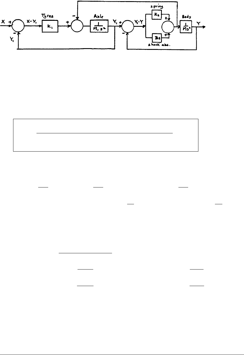
Glyn James, Advanced Modern Engineering Mathematics, 4th Edition 47
where sdenotes the Laplace ‘s’ and upper case variables X, Y, Y1denote the
corresponding Laplace transforms of the corresponding lower case time domain
variables x(t),y(t),y
1(t); y1(t) is the vertical displacement of the axle/wheel mass.
Using basic block diagram rules this block diagram may be reduced to the
input/output transfer function model
X
−→
K1(K+Bs)
(M1s2+K1)(Ms2+Bs +K)+Ms2(K+Bs)Y
−→
or the time domain differential equation model
M1Md4y
dt4+B(M1+M)d3y
dt3+(K1M+KM1+KM)d2y
dt2
+K1Bdy
dt +K1Ky =K1K2x+K1Bdx
dt
A possible state space model is
⎡
⎢
⎢
⎢
⎢
⎢
⎢
⎢
⎣
˙
z1
˙
z2
˙
z3
˙
z4
⎤
⎥
⎥
⎥
⎥
⎥
⎥
⎥
⎦
=
⎡
⎢
⎢
⎢
⎢
⎢
⎢
⎢
⎣
−B(M1+M)100
−(K1M+KM1+KM)
MM1010
−K1B
M1M001
−K1K
M1M000
⎤
⎥
⎥
⎥
⎥
⎥
⎥
⎥
⎦
⎡
⎢
⎢
⎢
⎢
⎢
⎢
⎢
⎣
z1
z2
z3
z4
⎤
⎥
⎥
⎥
⎥
⎥
⎥
⎥
⎦
+
⎡
⎢
⎢
⎢
⎢
⎢
⎢
⎢
⎣
0
0
K1B
M1M
K1K2
MM1
⎤
⎥
⎥
⎥
⎥
⎥
⎥
⎥
⎦
x(t)
y=[1000]z(t),z=[z1z2z3z4]T.
Clearly alternative forms may be written down, such as, for example, the
companion form of equation (1.66) in the text. Disadvantage is that its output
yis not one of the state variables.
c
Pearson Education Limited 2011

48 Glyn James, Advanced Modern Engineering Mathematics, 4th Edition
55 Applying Kirchhoff’s second law to the first loop gives
x1+R3(i−i1)+R1i=u
that is,(R1+R3)i−R3i1+x1=u
Applying it to the outer loop gives
x2+(R4+R2)i1+R1i=u
Taking α=R1R3+(R1+R3)(R4+R2)thengives
αi =(R2+R3+R4)u−(R2+R4)x1−R3x2
and αi1=R3u+R1x1−(R1+R3)x2
Thus,
α(i−i1)=(R4+R2)u−(R1+R2+R4)x1+R1x2
Voltage drop across C1:˙
x1=1
C1
(i−i1)
=1
αC1
[−(R1+R2+R4)x1+R1x2+(R4+R2)u](1)
Voltage drop across C2:˙
x2=1
C2
i1
=1
αC2
[R1x1−(R1+R3)x2+R3u](2)
y1=i1=R1
αx−(R1+R3)
αx2+R3
αu(3)
y2=R2(i−i1)=−R3
α(R1+R2+R4)x1+R3R1
αx2+R3
(R4+R2)
αu(4)
Equations (1)–(4) give the required state space model.
Substituting the given values for R1,R
2,R
3,R
4,C
1and C2gives the state matrix
Aas
A=⎡
⎣
−9
35.10−3
1
35.10−3
1
35.10−3−4
35.10−3
⎤
⎦=103
35 −91
1−4
c
Pearson Education Limited 2011

Glyn James, Advanced Modern Engineering Mathematics, 4th Edition 49
Let β=103
35 then eigenvalues are solutions of
−9β−λβ
β−4β−λ
=λ2+13βλ +35β2=0
giving
λ=−13 ±√29
2β−2.6×10²or −1.1×10²
Exercises 1.10.4
56 ΦΦ
Φ(t)=eAtwhere A=10
11
Eigenvalues of Aare λ=1,λ =1 so
eAt=α0(t)I+α1(t)A
where α0,α
1satisfy
eλt =α0+α1λ, λ =1
teλt =α1
giving α1=tet,α
0=et−tet
Thus,
ΦΦ
Φ(t)=eAt=et−tet0
0et−tet+tet0
tettet=et0
tetet
56(a) ΦΦ
Φ(0) = 10
01
=I
56(b)
ΦΦ
Φ(t2−t1)ΦΦ
Φ(t1)=et2e−t10
(t2−t1)et2e−t1et2e−t1et10
t1et1et1
=et20
(t2−t1)et2+t1et2et2=et20
t2et2et2=ΦΦ
Φ(t2)
c
Pearson Education Limited 2011

50 Glyn James, Advanced Modern Engineering Mathematics, 4th Edition
56(c) ΦΦ
Φ−1=1
e2tet0
−tetet=e−t0
−te−te−t=ΦΦ
Φ(−t)
57 Take x1=y, x2=˙
x1=dy
dt ,˙
x2=d2y
dt2=−x1−2x2so in vector–matrix
form the differential equation is
˙
x=01
−1−2x,y=[10]A
Taking A=01
−1−2its eigenvalues are λ=−1,λ=−1
eAt=α0I+α1Awhere α0,α
1satisfy
eλt =α0+α1λ, λ =−1
teλt =α1
giving α0=e−t+te−t,α
1=te−t.Thus,
eAt=e−t+te−tte−t
−te−te−t−te−t
Thus, solution of differential equation is
x(t)=eAtx(0),x(0) = [1 1]T
=e−t+2te−t
e−t−2te−t
giving y(t)=x1(t)=e−t+2te−t
The differential equation may be solved directly using the techniques of Chapter 10
of the companion text Modern Engineering Mathematics or using Laplace
transforms. Both approaches confirm the solution
y=(1+2t)e−2t
58 Taking A=10
11
then from Exercise 56
eAt=et0
tetet
c
Pearson Education Limited 2011

Glyn James, Advanced Modern Engineering Mathematics, 4th Edition 51
and the required solution is
x(t)=eAtx(0) = et0
tetet1
1=et
(1 + t)et
59 Taking A=01
−6−5its eigenvalues are λ1=−3,λ
2=−2.
Thus, eAt=α0I+α1Awhere α0,α
1satisfy
e−3t=α0−3α1,e
−2t=α0−2α1
α0=3e−2t−2e−3t,α
1=e−2t−e−3t
so
eAt=3e−2t−2e−3te−2t−e−3t
6e−3t−te−2t3e−3t−2e−2t
Thus, the first term in (6.73) becomes
eAtx(0) = eAt[1 −1]T=2e−2t−e−3t
3e−3t−4e−2t
and the second term is
t
0
eA(t−τ)bu(τ)dτ =t
0
26e−2(t−τ)−6e−3(t−τ)
18e−3(t−τ)−12e−2(t−τ)dτ
=2 3e−2(t−τ)−2e−3(t−τ)
6e−3(t−τ)−6e−2(t−τ)t
0
=2 1−3e−2t+2e−3t
6e−2t−6e−3t
Thus, required solution is
x(t)=2e−2t−e−3t+2−6e−3t+4e−3t
3e−3t−4e−2t+12e−2t−12e−3t
=2−4e−2t+3e−3t
8e−2t−9e−3t
that is,x
1=2−4e−2t+3e−3t,x
2=8e−2t−9e−3t
c
Pearson Education Limited 2011

52 Glyn James, Advanced Modern Engineering Mathematics, 4th Edition
60 In state space form,
˙
x=01
−2−3x+2
0u(t),u(t)=e−t,x(0) = [0 1]T
Taking A=01
−2−3its eigenvalues are λ1=−2,λ
2=−1so
eAt=α0I+α1Awhere α0,α
1satisfy
e−2t=α0−2α1,e
−t=α0−α1⇒α0=2e−t−e−2t,α
1=e−t−e−2t
Thus,
eAt=2e−t−e−2te−t−e−2t
−2e−t+2e−2t−e−t+2e−2t
and eAtx(0) = e−t−e−2t
−e−t+2e−2t
t
0
A(t−τ)bu(τ)dτ =t
04e−(t−τ)−2e−2(t−τ)
−4e−(t−τ)+4e−2(t−τ)e−τdτ
=t
04e−t−2e−2teτ
−4e−t+4e−2teτdτ
=4τe−t−2e−2teτ
−4τe−t+4e−2teτt
0
=4te−t−2e−t+2e−2t
−4te−t+4e−t−4e−2t
We therefore have the solution
x(t)=eAtx(0) + t
0
eA(t−τ)bu(τ)dτ
=4te−t+e−2t−e−t
−4te−t+3e−t−2e−2t
that is,
x1=4te−t+e−2t−e−t,x
2=−4te−t+3e−t−2e−2t
61 Taking A=34
21
its eigenvalues are λ1=5,λ
2=−1.
eAt=α0I+α1Awhere α0,α
1satisfy
e5t=α0+5α1,e
−t=α0−α1⇒α0=1
6e5t+5
6e−t,α
1=1
6e5t+1
6e−t
c
Pearson Education Limited 2011

Glyn James, Advanced Modern Engineering Mathematics, 4th Edition 53
Thus, transition matrix is
eAt=1
3e−t+2
3e5t2
3e5t−2
3e−t
1
3e5t−1
3e−t1
3e5t+2
3e−t
and eAtx(0) = eAt[1 2]T=2e5t−e−t
e5t+e−t
t
0
eA(t−τ)Bu(τ)dτ =t
0
eA(t−τ)01
11
4
3dτ
=t
0
At−τ3
7dτ
=t
020
3e5(t−τ)−11
3e−(t−τ)
10
3e5(t−τ)+11
3e−(t−τ)dτ
=−4
3e5(t−τ)−11
3e−(t−τ)
−2
3e5(t−τ)+11
3e−(t−τ)t
0
=−5+11
3e−t+4
3e5t
3−11
3e−t+2
3e5t
Thus, solution is
x(t)=eAtx(0) + t
0
eA(t−τ)Bu(t)dτ
=−5+8
3e−t+10
3e5t
3−8
3e−t+5
3e5t
Exercises 1.10.7
62 Eigenvalues of matrix A=−3
2
3
4
1−5
2are given by
|A−λI |=λ2+4λ+3=(λ+3)(λ+1)=0
that is, λ1=−1,λ
2=−3
having corresponding eigenvectors e1=[32]
T,e2=[1 −2]T.
Denoting the reciprocal basis vectors by
r1=[r11 r12]T,r2=[r21 r22]T
c
Pearson Education Limited 2011

54 Glyn James, Advanced Modern Engineering Mathematics, 4th Edition
and using the relationships rT
iej=δij (i, j =1,2) we have
3r11 +2r12 =1
r11 −2r12 =0 r1=[
1
4
1
8]T
3r21 +2r22 =0
r21 −2r22 =1 r2=[
1
4−3
8]T
Thus,
rT
1x(0) = 1
2+1
2=1,rT
2x(0) = 1
2−3
2=−1
so the spectral form of solution is
x(t)=e−te1−e−3te2
The trajectory is readily drawn showing that it approaches the origin along the
eigenvector e1since e−3t→0fasterthane−t. See Figure 1.9 in the text.
63 Taking A=−22
2−5eigenvalues are λ1=−6,λ
2=−1having
corresponding eigenvectors e1=[1 −2]T,e2=[21]
T.
Denoting the reciprocal basis vectors by
r1=[r11 r12]T,r2=[r21 r22]T
and using the relationships rT
iej=δij (i, j =1,2) we have
r11 −2r12 =1
2r11 +r12 =0⇒r11 =1
5,r
12 =−2
5⇒r1=1
5[1 −2]T
r21 −2r22 =0
2r21 +r22 =1⇒r21 =2
5,r
22 =−1
5⇒r2=1
5[2 1]T
Thus,
rT
1x(0) = 1
5[1 −2] 2
3=−4
5
rT
2x(0) = 1
5[2 1] 2
3=7
5
c
Pearson Education Limited 2011

Glyn James, Advanced Modern Engineering Mathematics, 4th Edition 55
then response is
x(t)=
2
i=1
rT
ix(0)eλitei
=−4
5e−6t1
−2+7
5e−t2
1=1
5−4e−6t+14e−t
8e−6t+7e−t
Again, following Figure 1.9 in the text, the trajectory is readily drawn and showing
that it approaches the origin along the eigenvector e2since e−6t→0fasterthan
e−t.
64 Taking A=0−4
2−4eigenvalues are λ1=−2+j2,λ
2=−2−j2having
corresponding eigenvectors e1=[2 1−j]T,e2=[2 1+j]T.
Let r1=r
1+jr
1be reciprocal base vector to e1then
rT
1e1=1=[r+jr
1]T[e
1+je
1]Twhere e1=e
1+je
1
rT
1e2=0=[r
1+jr
1]T[e
1−je
1]Tsince e2= conjugate e1
Thus,
[(r
1)Te
1−(r
1)Te
1]+j[(r
1)Te
1+(r
1)Te
1]=1
and
[(r
1)Te
1−(r
1)Te
1]+j[(r
1)Te1
1−(r
1)Te
1]=0
c
Pearson Education Limited 2011

56 Glyn James, Advanced Modern Engineering Mathematics, 4th Edition
giving
(r
1)Te
1=1
2,(r
1)Te
1=1
2,(r
1)Te
1=(r
1)Te
1=0
Now e
1=[21]
T,e
1=[0 −1]T
Let r
1=[ab]Tand r
1=[cd]Tthen from above
2a+b=1
2,−b=0 and −d=−1
2,2c+d=0
giving a=1
4,b=0,c=−1
4,d=1
2so that
r1=r
1+jr
1=1
4[1 −j2j]T
Since r2is the complex conjugate of r1
r2=1
4[1 + j−2j]T
so the solution is given by
x(t)=rT
1x(0)eλ1te1+rT
2x(0)eλ2te2
and since rT
1x(0) = 1
2(1 + j),rT
2x(0) = 1
2(1 −j)
x(t)=e−2t1
2(1 + j)e2jt 2
1−j+1
2(1 −j)e−2jt 2
1+j
=e−2t(cos 2t−sin 2t)2
1−(cos 2t+sin2t)0
−1
=e−2t(cos 2t−sin 2t)e
1−(cos 2t+sin2t)e
1where e1=e
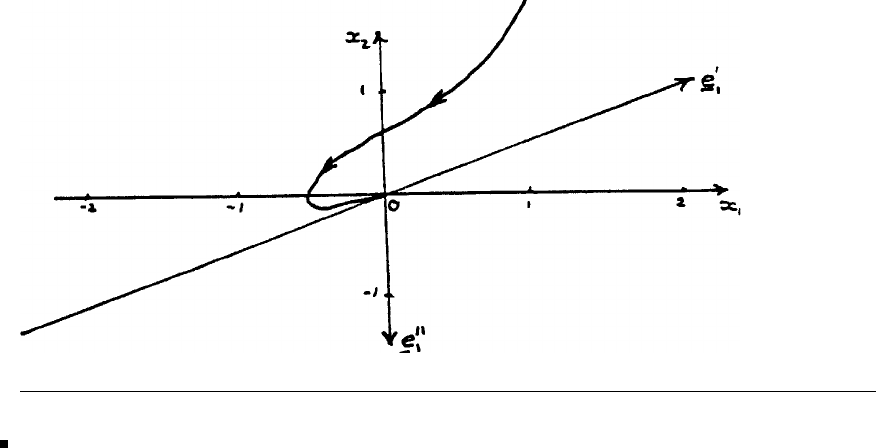
1+je
1
To plot the trajectory, first plot e
1,e
1in the plane and then using these as a frame
of reference plot the trajectory. A sketch is as follows
c
Pearson Education Limited 2011
Glyn James, Advanced Modern Engineering Mathematics, 4th Edition 57
65 Following section 1.10.6 if the equations are representative of
˙
x=Ax+bu, y=cTx
then making the substitution x=Mξξ
ξ,whereMis the modal matrix of A,
reduces the system to the canonical form
˙
ξξ
ξ=Λξξ
ξ+(M−1b)u, y=(cTM)ξξ
ξ
where Λis the spectral matrix of A.
Eigenvalues of Aare given by
1−λ1−2
−12−λ1
01−1−λ
=λ3−2λ2−λ+2=(λ−1)(λ+2)(λ+1)=0
so the eigenvalues are λ1=2,λ
2=1,λ
3=−1. The corresponding eigenvectors
are readily determined as
e1=[131]
T,e2=[321]
T,e3=[101]
T
Thus, M=⎡
⎣
131
320
111
⎤
⎦and Λ=⎡
⎣
20 0
01 0
00−1⎤
⎦
c
Pearson Education Limited 2011

58 Glyn James, Advanced Modern Engineering Mathematics, 4th Edition
M−1=1
det Madj M=−1
6⎡
⎣
2−2−2
−303
12−7⎤
⎦so required canonical form is
⎡
⎣
˙
ξ1
˙
ξ2
˙
ξ3⎤
⎦=⎡
⎣
20 0
01 0
00−1⎤
⎦⎡
⎣
ξ1
ξ2
ξ3⎤
⎦+⎡
⎣
1
3
0
−4
3
⎤
⎦u
y=[1 −4−2] [ξ1ξ2ξ3]T
66 Let r1=[r11 r12 r13]T,r2=[r21 r22 r23]T,r3=[r31 r32 r33]Tbe the
reciprocal base vectors to e1=[110]
T,e2=[011]
T,e3=[123]
T.
rT
1e1=r11 +r12 =1
rT
1e2=r11 +r13 =0
rT
1e3=r11 +2r12 +3r13 =0⎫
⎬
⎭⇒r1=1
2[1 1 −1]T
rT
2e1=r21 +r22 =0
rT
2e2=r22 +r23 =1
rT
2e3=r21 +2r22 +3r23 =0⎫
⎬
⎭⇒r2=1
2[−331]
T
rT
3e1=r31 +r32 =0
rT
3e2=r32 +r33 =0
rT
3e3=r31 +2r32 +3r33 =1⎫
⎬
⎭⇒r3=1
2[1 −11]
T
Then using the fact that x(0)=[111]
T
α0=rT
1x(0) = −1
2,α
1=rT
2x(0) = 1
2,α
3=rT
3x(0) = 1
2
67 The eigenvectors of Aare given by
5−λ4
12−λ
=(λ−6)(λ−1) = 0
so the eigenvalues are λ1=6,λ
2= 1. The corresponding eigenvectors are readily
determined as e1=[41]
T,e2=[1 −1]T.
Taking Mto be the modal matrix M=41
1−1then substituting x=Mξξ
ξ
into ˙
x=Ax(t) reduces it to the canonical form
˙
ξξ
ξ=ΛΛ
Λξξ
ξ
c
Pearson Education Limited 2011

Glyn James, Advanced Modern Engineering Mathematics, 4th Edition 59
where ΛΛ
Λ=60
01
. Thus, the decoupled canonical form is
˙
ξ1
˙
ξ2=60
01
ξ1
ξ2or ˙
ξ1=6ξ1and ˙
ξ2=ξ2
which may be individually solved to give
ξ1=αe6tand ξ1=βet
Now ξξ
ξ(0) = M−1x(0) = −1
5−1−1
−14
1
4=1
−3
so ξ1(0) = 1 = αand ξ2(0) = −3=β
giving the solution of the uncoupled system as
ξξ
ξ=e6t
−3et
The solution for x(t)as
x=Mξξ
ξ=41
1−1e6t
−3et=4e6t−3et
e6t+3et
68 Taking A=34
21
its eigenvalues are λ1=5,λ
2=−1having
corresponding eigenvectors e1=[21]
T,e2=[1 −1]T.
Let M=21
1−1be the modal matrix of A,then ˙
x=Mξξ
ξreduces the
equation to
˙
ξξ
ξ(t)= 50
0−1ξξ
ξ+M−101
11
u(t)
Since M−1=1
det Madj M=1
311
1−2we have,
˙
ξξ
ξ(t)= 50
0−1ξξ
ξ+1
312
−2−1u(t)
With u(t)=[43]
Tthe decoupled equations are
˙
ξ1=5ξ1+10
3
˙
ξ2=−ξ2−11
3
c
Pearson Education Limited 2011

60 Glyn James, Advanced Modern Engineering Mathematics, 4th Edition
which can be solved independently to give
ξ1=αe5t−2
3,ξ
2=βe−t−11
3
We have that ξξ
ξ(0) = MM
M−1x(0) = 1
311
1−21
2=1
−1so
1=α−2
3⇒α=5
3
−1=β−11
3⇒β=8
3
giving
ξξ
ξ=5
3e5t−2
3
8
3e−t−11
3
and x=MM
Mξξ
ξ=21
1−15
3e5t−2
3
8
3e−t−11
3=−5+8
3e−t+10
3e5t
3−8
3e−t+5
3e5t
which confirms Exercises 57 and 58.
Exercises 1.11.1 (Lyapunov)
69 Take tentative Lyapunov functionV(x)=xTPx giving
˙
V(x)=xT(ATP+PA)x=−xTQx where
ATP+PA =−Q(i)
Take Q=Iso that ˙
V(x)=−(x2
1+x2
2) which is negative definite. Substituting in
(i) gives
−43
2−2p11 p12
p12 p22 +p11 p12
p12 p22 −42
3−2=−10
0−1
Equating elements gives
−8p11 +6p12 =−1,4p12 −4p22 =−1,2p11 −6p12 +3p22 =0
Solving gives p11 =5
8,p
12 =2
3,p
22 =11
12 so that, P=5
8
2
3
2
3
11
12 Principal minors
of Pare: 5
8>0 and det P=(
55
96 −4
9)>0soPis positive definite and the system
is asymptotically stable
c
Pearson Education Limited 2011

Glyn James, Advanced Modern Engineering Mathematics, 4th Edition 61
Note that, in this case, we have V(x)= 5
8x2
1+4
3x1x2+11
12 x2
2which is positive
definite and ˙
V(x)=5
4x1˙
x1+4
3˙
x1x2+4
3x1˙
x2+11
6x2˙
x2=−x2
1−x2
2which is negative
definite.
70 Take tentative Lyapunov function V(x)=xTPx giving
˙
V(x)=xT(ATP+PA)x=−xTQx where
ATP+PA =−Q(i)
Take Q=Iso that ˙
V(x)=−(x2
1+x2
2) which is negative definite. Substituting in
(i) gives
−3−1
2−1p11 p12
p12 p22 +p11 p12
p12 p22 −32
−1−1=−10
0−1
Equating elements gives
−6p11 −2p12 =−1,4p12 −2p22 =−1,2p11 −4p12 −p22 =0
Solving gives p11 =7
40 ,p
12 =−1
40 ,p
22 =18
40 so that P=7
40 −1
40
−1
40
18
40
Principal minors of Pare: 7
40 >0 and det P=5
64 >0soPis positive definite
and the system is asymptotically stable.
71 Take tentative Lyapunov function V(x)=xTPx giving
˙
V(x)=xT(ATP+PA)x=−xTQx where
ATP+PA =−Q(i)
Take Q=Iso that ˙
V(x)=−(x2
1+x2
2) which is negative definite. Substituting in
(i) gives
0−a
1−bp11 p12
p12 p22 +p11 p12
p12 p22 01
−a−b=−10
0−1
Equating elements gives
−8p12 =−1,2p12 −2bp22 =−1,p
11 −bp12 −ap22 =0
c
Pearson Education Limited 2011

62 Glyn James, Advanced Modern Engineering Mathematics, 4th Edition
Solving gives p12 =1
2a,p
22 =a+1
2ab ,p
11 =b2+a2+a
2ab so that, P=b2+a2+a
2ab
1
2a
1
2a
a+1
2ab
For asymptotic stability the principal minors of Pmust be positive. Thus,
b2+a2+a
2ab >0(ii)
and (b2+a2+a)(a+1)>b
2(iii)
Case 1ab > 0
(ii) ⇒a2+b2+a>0 so (iii) ⇒a+1>b2
b2+a2+a
⇒a[a2+(a+1)
2]>0⇒a>0.
Since ab > 0⇒b>0 it follows that (ii) and (iii) are satisfied if a, b > 0
Case 2ab < 0 No solution to (ii) and (iii) in this case.
Thus, system is asymptotically stable when both a>0andb>0.
Note: This example illustrates the difficulty in interpretating results when using
the Lyapunov approach. It is a simple task to confirm this result using the Routh–
Hurwitz criterion developed in Section 5.6.2.
72(a)
˙
x1=x2(i)
˙
x2=−2x2+x3(ii)
˙
x3=−kx1−x3(iii)
If ˙
V(x) is identically zero then x3is identically zero ⇒x1is identically zero from
(iii)
⇒x2is identically zero from (i)
Hence ˙
V(x) is identically zero only at the origin.
(b) ATP+PA =−Q⇒
⎡
⎣
00−k
1−20
01−1⎤
⎦⎡
⎣
p11 p12 p13
p12 p22 p23
p13 p23 p33 ⎤
⎦+⎡
⎣
p11 p12 p13
p12 p22 p23
p13 p23 p33 ⎤
⎦⎡
⎣
010
0−21
−k0−1⎤
⎦=⎡
⎣
00 0
00 0
00−1⎤
⎦
c
Pearson Education Limited 2011

Glyn James, Advanced Modern Engineering Mathematics, 4th Edition 63
Equating elements and solving for the elements of Pgives the matrix
P=⎡
⎣
k2+12k
12−2k
6k
12−2k0
6k
12−2k
3k
12−2k
k
12−2k
0k
12−2k
6
12−2k
⎤
⎦
(c) Principal minors of Pare:
Δ1=k2+12k
12 −2k>0ifk>0and(12 −2k)>0⇒0<k<6
Δ2=k2+12k
12 −2k 3k
12 −2k−36k2
12 −2k=3k3
(12 −2k)2>0ifk>0
Δ3=(k2+12k)(8k−k2)
(12 −2k)3−216k2
(12 −2k)3>0if (6k3−k4)>0⇒0<k<6
Thus system asymptotically stable for 0 <k<6.
73 State-space form is
˙
x=˙
x1
˙
x2=01
−k−ax1
x2(i)
Take V(x)=kx2
1+(x2+ax1)2then
˙
V(x)=2kx1˙
x1+2(x2+ax1)( ˙
x2+a˙
x1)
=2kx1(x2)+2(x2+ax1)(−kx1−ax2+ax1)using (i)
=−2kax2
1
Since k>0anda>0then ˙
V(x) is negative semidefinite but is not identically zero
along any trajectory of (i). Consequently, this choice of Lyapunov function assures
asymptotic stability.
Review Exercises 1.13
1(a) Eigenvalues given by
−1−λ612
0−13 −λ30
0−920−λ
=(1+λ)[(−13 −λ)(20 −λ) + 270] = 0
c
Pearson Education Limited 2011

64 Glyn James, Advanced Modern Engineering Mathematics, 4th Edition
that is, (1 + λ)(λ−5)(λ−2) = 0
so eigenvalues are λ1=5,λ
2=2,λ
3=−1
Eigenvectors are given by corresponding solutions of
⎡
⎣−1−λi612
0−13 −λi30
0−920−λi⎤
⎦⎡
⎣
ei1
ei2
ei3⎤
⎦=0
When i=1,λ
i= 5 and solution given by
e11
198 =−e12
−90 =e13
54 =β1
so e1=[1153]
T
When i=2,λ
i= 2 and solution given by
e21
216 =−e22
−54 =e23
27 =β2
so e2=[821]
T
When i=3,λ
i=−1 and solution given by
e31
1=−e32
0=e33
0=β3
so e3=[100]
T
1(b) Eigenvalues given by
2−λ01
−14−λ−1
−120−λ
=
4−λ−1
2−λ
+−14−λ
−12
=0
that is,0=(2−λ)[(4 −λ)(−λ)+2]+[−2+(4−λ)]
=(2−λ)(λ2−4λ+3)=(2−λ)(λ−3)(λ−1) = 0
so eigenvalues are
λ1=3,λ
2=2,λ
3=1
Eigenvectors are given by the corresponding solutions of
(2 −λi)ei1+0ei2+ei3=0
−ei1+(4−λi)ei2−ei3=0
−ei1+2ei2−λiei3=0
c
Pearson Education Limited 2011

Glyn James, Advanced Modern Engineering Mathematics, 4th Edition 65
Taking i=1,2,3 gives the eigenvectors as
e1=[121]
T,e2=[210]
T,e3=[10 −1]T
1(c) Eigenvalues given by
1−λ−10
−12−λ−1
0−11−λ
R1+(R2+R3)
−λ−λ−λ
−12−λ−1
0−11−λ
=0
that is,λ
−1−1−1
−12−λ−1
0−11−λ
=λ
−10 0
−13−λ0
0−11−λ
=λ(3 −λ)(1 −λ)=0
so eigenvalues are λ1=3,λ
2=1,λ
3=0
Eigenvalues are given by the corresponding solutions of
(1 −λi)ei1−ei2−0ei3=0
−ei1+(2−λi)ei2−ei3=0
0ei1−ei2+(1−λi)ei3=0
Taking i=1,2,3 gives the eigenvectors as
e1=[1 −21]
T,e=[10 −1]T,e3=[111]
T
2Principal stress values (eigenvalues) given by
3−λ21
23−λ1
114−λ
R1+(R2+R3)
6−λ6−λ6−λ
23−λ1
114−λ
=(6−λ)
11 1
23−λ1
114−λ
=0
that is,(6 −λ)
10 0
21−λ−1
103−λ
=(6−λ)(1 −λ)(3 −λ)=0
so the principal stress values are λ1=6,λ
2=3,λ
3=1.
c
Pearson Education Limited 2011

66 Glyn James, Advanced Modern Engineering Mathematics, 4th Edition
Corresponding principal stress direction e1,e2and e3are given by the solutions
of (3 −λi)ei1+2ei2+ei3=0
2ei1+(3−λi)ei2+ei3=0
ei1+ei2+(4−λi)ei3=0
Taking i=1,2,3 gives the principal stress direction as
e1=[111]
T,e2=[11 −2]T,e3=[1 −10]
T
It is readily shown that eT
1e2=eT
1e3=eT
2e3= 0 so that the principal stress
directions are mutually orthogonal.
3Since [1 0 1]Tis an eigenvector of A
⎡
⎣
2−10
−13b
0bc
⎤
⎦⎡
⎣
1
0
1⎤
⎦=λ⎡
⎣
1
0
1⎤
⎦
so 2 = λ, −1+b=0,c =λ
giving b=1 and c=2.
Taking these values Ahas eigenvalues given by
2−λ−10
−13−λ1
012−λ
=(2−λ)
3−λ1
12−λ−(2 −λ)
=(2−λ)(λ−1)(λ−4) = 0
that is, eigenvalues are λ1=4,λ
2=2,λ
3=1
Corresponding eigenvalues are given by the solutions of
(2 −λi)ei1−ei2+0ei3=0
−ei1+(3−λi)ei2+ei3=0
0ei1+ei2+(2−λi)ei3=0
Taking i=1,2,3 gives the eigenvectors as
e1=[1 −2−1]T,e2=[101]
T,e3=[11 −1]T
c
Pearson Education Limited 2011

Glyn James, Advanced Modern Engineering Mathematics, 4th Edition 67
4The three Gerschgorin circles are
|λ−4|=|−1|+|0|=1
|λ−4|=|−1|+|−1|=2
|λ−4|=1
Thus, |λ−4|≤ 1and|λ−4|≤ 2so|λ−4|≤ 2or2≤λ≤6.
Taking x(o)=[−11 −1]Titerations using the power method may be tabulated
as follows
Iteration k0123456
−1−0.833 −0.765 −0.734 −0.720 −0.713 −0.710
x(k)1111111
−1−0.833 −0.765 −0.734 −0.720 −0.713 −0.710
−5−4.332 −4.060 −3.936 −3.88 −3.852
Ax
(k)6 5.666 5.530 5.468 5.44 5.426
−5−4.332 −4.060 −3.936 3.88 −3.852
λ6 5.666 5.530 5.468 5.44 5.426
Thus, correct to one decimal place the dominant eigenvalue is λ=5.4
5(a) Taking xx
x(o)=[111]
7iterations may be tabulated as follows
Iteration k01234567
1 0.800 0.745 0.728 0.722 0.720 0.719 0.719
x(k)1 0.900 0.862 0.847 0.841 0.838 0.837 0.837
11111111
4 3.500 3.352 3.303 3.285 3.278 3.275
Ax
(k)4.5 4.050 3.900 3.846 3.825 3.815 3.812
5 4.700 4.607 4.575 4.563 4.558 4.556
λ5 4.700 4.607 4.575 4.563 4.558 4.556
Thus, estimate of dominant eigenvalues is λ4.56 with associated eigenvector
x=[0.72 0.84 1]T
5(b) 3
i=1 λi=traceA⇒7.5=4.56 + 1.19 + λ3⇒λ3=1.75
c
Pearson Education Limited 2011

68 Glyn James, Advanced Modern Engineering Mathematics, 4th Edition
5(c) (i) det A=
3
i=1
λi=9.50 so A−1exists and has eigenvalues
1
1.19 ,1
1.75 ,1
4.56
so power method will generate the eigenvalue 1.19 corresponding to A.
(ii) A−3Ihas eigenvalues
1.19 −3,1.75 −3,4.56 −3
that is,−1.91,−1.25,1.56
so applying the power method on A−3Igenerates the eigenvalues corresponding
to 1.75 of A.
6˙
x=αλeλt,˙
y=βλeλt,˙
z=γλeλt so the differential equations become
αλeλt =4αeλt +βeλt +γeλt
βλeλt =2αeλt +5βeλt +4γeλt
γλeλt =−αeλt −βeλt
Provided eλt = 0 (i.e. non-trivial solution) we have the eigenvalue problem
⎡
⎣
411
254
−1−10
⎤
⎦⎡
⎣
α
β
γ⎤
⎦=λ⎡
⎣
α
β
γ⎤
⎦
Eigenvalues given by
4−λ11
25−λ4
−1−10
C2−C3
4−λ01
21−λ4
−1λ−1−λ
=(λ−1)
4−λ01
2−14
−11−λ
=−(λ−1)(λ−5)(λ−3)
so its eigenvalues are 5, 3 and 1.
When λ= 1 the corresponding eigenvector is given by
3e11 +e12 +e13 =0
2e11 +4e12 +4e13 =0
−e11 −e12 −e13 =0
c
Pearson Education Limited 2011

Glyn James, Advanced Modern Engineering Mathematics, 4th Edition 69
having solution e11
0=−e12
2=e13
2=β1
Thus, corresponding eigenvector is β[0 −11]
T
7Eigenvalues are given by
|A−λI|=
8−λ−8−2
4−3−λ−2
3−41−λ
=0
Row 1 −(Row 2 + Row 3) gives
|A−λI|=
1−λ−1+λ−1+λ
4−3−λ−2
3−41−λ
=(1−λ)
1−1−1
4−3−λ−2
3−41−λ
=(
1−λ)
10 0
41−λ2
3−14−λ
=(1−λ)[(1 −λ)(4 −λ)+2]
=(1−λ)(λ−2)(λ−3)
Thus, eigenvalues are λ1=3,λ
2=2,λ
3=1.
Corresponding eigenvectors are given by
(8 −λ)ei1−8ei2−2ei3=0
4ei1−(3 + λ)ei2−2ei3=0
3ei1−4ei2+(1−λ)ei3=0
When i=1,λ
i=λ1= 3 and solution given by
e11
4=−e12
−2=e13
2=β1
so a corresponding eigenvector is e1=[211]
T.
When i=2,λ
i=λ2= 2 and solution given by
e21
−3=−e22
2=e23
−1=β2
so a corresponding eigenvector is e2=[321]
T.
When i=3,λ
i=λ3= 1 and solution given by
e31
−8=−e32
6=e33
−4=β3
c
Pearson Education Limited 2011

70 Glyn James, Advanced Modern Engineering Mathematics, 4th Edition
so a corresponding eigenvector is e3=[432]
T.
Corresponding modal and spectral matrices are
M=⎡
⎣
234
123
112
⎤
⎦and Λ=⎡
⎣
300
020
101
⎤
⎦
M−1=⎡
⎣
1−21
10−2
−11 1
⎤
⎦and matrix multiplication confirms M−1AM=Λ
8Eigenvectors of Aare given by
1−λ0−4
05−λ4
−443−λ
=0
that is, λ3−9λ2−9λ+81=(λ−9)(λ−3)(λ+3)=0
so the eigenvalues are λ1=9,λ
2=3 and λ3=−3.
The eigenvectors are given by the corresponding solutions of
(1 −λi)ei1+0ei2−4ei3=0
0ei1+(5−λi)ei2+4ei3=0
−4ei1+4ei2+(3−λi)ei3=0
Taking i=1,2,3 the normalized eigenvectors are given by
ˆ
e1=[
1
3−2
3−2
3]T,ˆ
e2=[
2
3
2
3−1
3]T,ˆ
e3=[
2
3−1
3
2
3]T
The normalised modal matrix
ˆ
M=1
3⎡
⎣
122
−22−1
−2−12
⎤
⎦
so
ˆ
MTAˆ
M=1
9⎡
⎣
1−2−2
22−1
2−12
⎤
⎦⎡
⎣
10−4
054
−44 3
⎤
⎦⎡
⎣
122
−22−1
−2−12
⎤
⎦
=⎡
⎣
90 0
03 0
00−3⎤
⎦=Λ
c
Pearson Education Limited 2011

Glyn James, Advanced Modern Engineering Mathematics, 4th Edition 71
9˙
N=⎡
⎢
⎣
−6000
6−400
04−20
0020
⎤
⎥
⎦N,N=[N1N2N3N4]T
Since the matrix Ais a triangular matrix its eigenvalues are the diagonal elements.
Thus, the eigenvalues are
λ1=−6,λ
2=−4,λ
3=−2,λ
4=0
The eigenvectors are the corresponding solutions of
(−6−λi)ei1+0ei2+0ei3+0ei4=0
6ei1+(−4−λi)ei2+0ei3+0ei4=0
0ei1+4ei2+(−2−λi)ei3+0ei4=0
0ei1+0ei2+2ei3−λiei4=0
Taking i=1,2,3,4 and solving gives the eigenvectors as
e1=[1 −33 −1]T,e2=[01 −21]
T
e3=[001 −1]T,e4=[0001]
T
Thus, spectral form of solution to the equation is
N=αe−6te1+βe−4te2+γe−2te3+δe4
Using the given initial conditions at t=0 wehave
⎡
⎢
⎣
C
0
0
0
⎤
⎥
⎦=α⎡
⎢
⎣
1
−3
3
−1
⎤
⎥
⎦+β⎡
⎢
⎣
0
1
−2
1
⎤
⎥
⎦+γ⎡
⎢
⎣
0
0
1
−1
⎤
⎥
⎦+δ⎡
⎢
⎣
0
0
0
1
⎤
⎥
⎦
so C=α, 0=−3α+β, 0=3α−2β+γ, 0=−α+β−γ+δ
which may be solved for α, β, γ and δto give
α=C, β =3C, γ =3C, δ =C
Hence,
N4=−αe−6t+βe−4t−γe−2t+δ
=−Ce−6t+3Ce−4t−3Ce−2t+C
c
Pearson Education Limited 2011

72 Glyn James, Advanced Modern Engineering Mathematics, 4th Edition
10(a)
(i) Characteristic equation of Ais λ2−3λ+ 2 = 0 so by the Cayley–Hamilton
theorem
A2=3A−2I=40
31
A3=3(3A−2I)−2A=7A−6I=80
71
A4=7(3A−2I)−6A=15A−14I=16 0
15 1
A5= 15(3A−2I|)−14A=31A−30I=32 0
31 1
A6= 31(3A−2I)−30A=63A−62I=64 0
63 1
A7= 63(3A−2I)−62A= 127A−126I=128 0
127 1
Thus, A7−3A6+A4+3A3−2A2+3I=−29 0
−32 3
(ii) Eigenvalues of Aare λ1=2,λ
2=1. Thus,
Ak=α0I+α1Awhere α0and α1satisfy
2k=α0+2α1,1=α0+α1
α1=2
k−1,α
0=2−2k
Thus, Ak=α0+2α10
α1α0+α1=2k0
2k−11
10(b) Eigenvalues of Aare λ1=−2,λ
2=0. Thus,
eAt=α0I+α1Awhere α0and α1satisfy
e−2t=α0−2α1,1=α0⇒α0=1,α
1=1
2(1 −e−2t)
Thus, eAt=α0α1
0α0−2α1=11
2(1 −e−2t)
0e−2t
c
Pearson Education Limited 2011

Glyn James, Advanced Modern Engineering Mathematics, 4th Edition 73
11 The matrix A=⎡
⎣
123
014
001
⎤
⎦has the single eigenvalue λ= 1 (multiplicity 3)
(A−I)= ⎡
⎣
023
004
000
⎤
⎦∼⎡
⎣
010
001
000
⎤
⎦is of rank 2 so has nullity 3 −2=1
indicating that there is only one eigenvector corresponding to λ=1.
This is readily determined as
e1=[100]
T
The corresponding Jordan canonical form comprises a single block so
J=⎡
⎣
110
011
001
⎤
⎦
Taking T=A−Ithe triad of vectors (including generalized eigenvectors) has
the form {T2ω, Tω, ω}with T2ω=e1.SinceT2=⎡
⎣
008
000
000
⎤
⎦,wemaytake
ω=[00 1
8]T. Then, Tω=[
2
8
1
80]T. Thus, the triad of vectors is
e1=[100]
T,e∗
1=[
3
8
1
20]T,e∗∗
1=[00 1
8]T
The corresponding modal matrix is
M=⎡
⎣
13
80
01
20
001
8
⎤
⎦
M−1=16 ⎡
⎣
1
16 −3
64 0
01
80
00
1
2
⎤
⎦and by matrix multiplication
M−1AM=16 ⎡
⎣
1
16 −3
64 0
01
80
00
1
2
⎤
⎦⎡
⎣
123
014
001
⎤
⎦⎡
⎣
13
80
01
20
001
8
⎤
⎦
=⎡
⎣
110
011
001
⎤
⎦=J
c
Pearson Education Limited 2011

74 Glyn James, Advanced Modern Engineering Mathematics, 4th Edition
12 Substituting x=Xcos ωt, y =Ycos ωt, z =Zcos ωt gives
−ω2X=−2X+Y
−ω2Y=X−2Y+Z
−ω2Z=Y−2Z
or taking λ=ω2
(λ−2)X+Y=0
X+(λ−2)Y+Z=0
Y+(λ−2)Z=0
For non-trivial solution
λ−21 0
1λ−21
01λ−2
=0
that is,(λ−2)[(λ−2)2−1] −(λ−2) = 0
(λ−2)(λ2−4λ+2)=0
so λ=2orλ=2±√2
When λ=2,Y=0 and X=−Zso X:Y:Z=1:0:−1
When λ=2+√2,X=Zand Y=−√2Xso X:Y:Z=1:−√2:1
When λ=2−√2,X=Zand Y=√2Xso X:Y:Z=1:√2:1
13 In each section Adenotes the matrix of the quadratic form.
13(a) A =⎡
⎣
2−10
−11−1
0−12
⎤
⎦has principal minors of 2,
2−1
−11
=1 and
det A=0
so by Sylvester’s condition (c) the quadratic form is positive-semidefinite.
13(b) A =⎡
⎣
3−2−2
−270
−202
⎤
⎦has principal minors of 3,
3−2
−27
=17 and
det A=6
so by Sylvester’s condition (a) the quadratic form is positive-definite.
c
Pearson Education Limited 2011

Glyn James, Advanced Modern Engineering Mathematics, 4th Edition 75
13(c) A =⎡
⎣
16 16 16
16 36 8
16 8 17 ⎤
⎦has principal minors of 16,
16 16
16 36
= 320 and
det A=−704
so none of Sylvester’s conditions are satisfied and the quadratic form is indefinite.
13(d) A =⎡
⎣−21 15 −6
15 −11 4
−64−2⎤
⎦has principal minors of −21, −21 15
15 −11
=6
and det A=0
so by Sylvester’s condition (d) the quadratic form is negative-semidefinite.
13(e) A =⎡
⎣−111
1−31
11−5⎤
⎦has principal minors of −1, −11
1−3
=2 and
det A=−4 so by Sylvester’s condition (b) the quadratic form is negative-definite.
14 A e1=⎡
⎣
7
2−1
2−1
2
4−10
−3
2
3
2
1
2
⎤
⎦⎡
⎣
1
2
3⎤
⎦=⎡
⎣
1
2
3⎤
⎦
Hence, e1=[123]
Tis an eigenvector with λ1= 1 the corresponding eigenvalue.
Eigenvalues are given by
0=
−7
2−λ−1
2−1
2
4−1−λ0
−3
2
3
2
1
2−λ
=−λ3+3λ2+λ−3
=(λ−1)(λ2+2λ+3)
=−(λ−1)(λ−3)(λ+1)
so the other two eigenvalues are λ2=3,λ
3=−1.
Corresponding eigenvectors are the solutions of
(−7
2−λi)ei1−1
2ei2−1
2ei3=0
4ei1−(1 + λi)ei2+0ei3=0
−3
2ei1+3
2ei2+(1
2−λi)ei3=0
c
Pearson Education Limited 2011

76 Glyn James, Advanced Modern Engineering Mathematics, 4th Edition
Taking i=2,3 gives the eigenvectors as
e2=[110]
T,e3=[0 −11]
T
The differential equations can be written in the vector–matrix form
˙
x=Ax,x=[xyz]T
so, in special form, the general solution is
x=αeλ1te1+βeλ2te2+γeλ3te3
=αet⎡
⎣
1
2
3⎤
⎦+βe3t⎡
⎣
1
1
0⎤
⎦+γe−t⎡
⎣
0
−1
1⎤
⎦
With x(0) = 2,y(0) = 4,z(0) = 6 we have
α=2,β=0,γ=0
so
x=2et⎡
⎣
1
2
3⎤
⎦
that is, x=2et,y=4et,z=6et.
15(a)
AAT=1.20.9−4
1.61.23
⎡
⎣
1.21.6
0.91.2
−43
⎤
⎦=18.25 −9
−913
Eigenvalues λigiven by
(18.25 −λ)(13 −λ)−81 = 0 ⇒(λ−25)(λ−6.25) = 0
⇒λ1=25,λ
2=6.25
having corresponding eigenvectors
u1=[−43]
T⇒ˆ
u1=[−4
5
3
5]T
u2=[3 4]
T⇒ˆ
u2=[3
5
4
5]
c
Pearson Education Limited 2011

Glyn James, Advanced Modern Engineering Mathematics, 4th Edition 77
leading to the orthogonal matrix
ˆ
U=−4
5
3
5
3
5
4
5
ATA=⎡
⎣
1.21.6
0.91.2
−43
⎤
⎦1.20.9−4
1.61.23
=⎡
⎣
43 0
32.25 0
0025
⎤
⎦
Eigenvalues μigiven by
(25 −μ)[(4−μ)(2.25 −μ)−9] = 0 ⇒(25 −μ)μ(μ−6.25) = 0
⇒μ1=25,μ
2=6.25,μ
3=0
with corresponding eigenvalues
v1=ˆ
v1=[001]
T
v2=[430]
T⇒ˆ
v2=[4
5
3
50]
T
v3=[−340]
T⇒ˆ
v3=[−3
5
4
50]
T
leading to the orthogonal matrix
ˆ
V=⎡
⎣
04
5−3
5
03
5
4
5
10 0
⎤
⎦
The singular values of Aare σ1=√25 = 5 and σ2=√6.25 = 2.5sothat
Σ=500
02.50
giving the SVD form of Aas
A=ˆ
UΣ ˆ
VT=−0.80.6
0.60.8500
02.50
⎡
⎣
001
0.80.60
−0.60.80
⎤
⎦
(Direct multiplication confirms A=1.20.9−4
1.61.23
)
c
Pearson Education Limited 2011

78 Glyn James, Advanced Modern Engineering Mathematics, 4th Edition
(b) A†=ˆ
VΣ∗ˆ
UT=⎡
⎣
04
5−3
5
03
5
4
5
10 0
⎤
⎦⎡
⎣
1
50
02
5
00
⎤
⎦−4
5
3
5
3
5
4
5=1
125 ⎡
⎣
24 32
18 24
−20 15 ⎤
⎦
=⎡
⎣
0.192 0.256
0.144 0.192
−0.16 0.12 ⎤
⎦
AA†=I
CHECK
LHS =1
125 1.20.9−4
1.61.21
⎡
⎣
24 32
18 24
−24 15 ⎤
⎦=1
125 125 0
0 125 =I=RHS
(c) Since Ais of full rank 2 and there are more columns than rows
A†=AT(AAT)−1=⎡
⎣
1.21.6
0.91.2
−43
⎤
⎦18.25 −9
−913
−1
=1
156.25 ⎡
⎣
1.21.6
0.91.2
−43
⎤
⎦13 9
918.25
=1
156.25 ⎡
⎣
30 40
22.530
−25 18.25 ⎤
⎦=⎡
⎣
0.192 0.256
0.144 0.192
−0.16 0.12 ⎤
⎦
which checks with the answer in (b).
16 (a) Using partitioned matrix multiplication the SVD form of Amay be
expressedinthe
form
A=ˆ
UΣ ˆ
VT=[ˆ
Urˆ
Um−r]S0
00
ˆ
VT
r
ˆ
VT
n−r=ˆ
UrSˆ
VT
r
(b) Since the diagonal elements in Sare non-zero the pseudo inverse may be expressed
in the form
A†=ˆ
VΣ∗ˆ
UT=ˆ
VrS−1ˆ
UT
r
(c) From the solution to Q46, exercises 1.8.4, the matrix A=⎡
⎣
1−1
−22
2−2⎤
⎦has a single
singularity σ1=√18 so r=1andSis a scalar √18; ˆ
Ur=ˆ
U1=ˆ
u1=[1
3−2
3
2
3]T
and
ˆ
Vr=ˆ
V1=ˆ
v1=1
√2−1
√2T
c
Pearson Education Limited 2011
Glyn James, Advanced Modern Engineering Mathematics, 4th Edition 79
The SVD form of Ais
A=ˆ
u1Sˆ
vT
1=⎡
⎣
1
3
−2
3
2
3
⎤
⎦√18 1
√2−1
√2
with direct multiplication confirming A=⎡
⎣
1−1
−22
2−2⎤
⎦
Thus, the pseudo inverse is
A†=ˆ
v1S−1ˆ
uT
1=1
√2
−1
√21
√18 [1
3−2
3
2
3]=1
6
−1
6[1
3−2
3
2
3]
=1
18 1−22
−12−2
which agrees with the answer obtained in Q46, Exercises 1.8.4
17 ˙
x=Ax+bu, y=cTx
Let λi,e
i,i=1,2,...,n, be the eigenvalues and corresponding eigenvectors of A.
Let M=[e1,e2,...,en]thensinceλi’s are distinct the ei’s are linearly
independent and M−1exists. Substituting x=Mξξ
ξgives
M˙
ξξ
ξ=AMξξ
ξ+bu
Premultiplying by M−1gives
˙
ξξ
ξ=M−1AMξξ
ξ+M−1bu=Λξξ
ξ+b1u
where Λ=M−1AM=(λiδij ),i,j =1,2,...,n, and b1=M−1b
Also, y=cTx⇒y=cTMξξ
ξ=cT
1ξξ
ξ,cT
1=cTM. Thus, we have the desired
canonical form.
If the vector b1contains a zero element then the corresponding mode is
uncontrollable and consequently (A1b1c) is uncontrollable. If the matrix cT
has a zero element then the system is unobservable.
The eigenvalues of Aare λ1=2,λ
2=1,λ
3=−1 having corresponding
eigenvectors e1=[131]
T,e2=[321]
Tand e3=[101]
T.
c
Pearson Education Limited 2011

80 Glyn James, Advanced Modern Engineering Mathematics, 4th Edition
The modal matrix
M=[e1e2e3]= ⎡
⎣
131
320
111
⎤
⎦with M−1=−1
6⎡
⎣
2−2−2
−30 3
12−7⎤
⎦
so canonical form is
⎡
⎣
˙
ξ1
˙
ξ2
˙
ξ3⎤
⎦=⎡
⎣
20 0
01 0
00−1⎤
⎦⎡
⎣
ξ1
ξ2
ξ3⎤
⎦+⎡
⎣
1
3
0
−4
3
⎤
⎦u
y=[1 −4−2][ξ1ξ2ξ3]T
We observe that the system is uncontrollable but observable. Since the system
matrix Ahas positive eigenvalues the system is unstable. Using Kelman matrices
(i) A2=⎡
⎣
011
−343
−112
⎤
⎦,Ab=⎡
⎣
2
2
2⎤
⎦,A2b=⎡
⎣
0
4
0⎤
⎦
Thus, [bAbA
2b]= ⎡
⎣−120
124
−120
⎤
⎦∼⎡
⎣
100
010
000
⎤
⎦and is of rank 2
so the system is uncontrollable.
(ii) [cA
Tc(AT)2c]= ⎡
⎣−2−3−3
102
051
⎤
⎦∼⎡
⎣
001
100
010
⎤
⎦and is of full rank 3
so the system is observable.
18 Model is of form ˙
x=Ax+Bu and making the transformation x=Mzgives
M˙
z=AMz +Bu ⇒˙
z=M−1AMz +M−1Bu ⇒˙
z=Λz +M−1Bu
where Mand Λare respectively the modal and spectral matrices ofA.
The eigenvalues of Aare given by
−2−λ−20
0−λ1
0−3−4−λ
=0⇒−(2 −λ)(4λ+λ2+3)=0
⇒(λ+2)(λ+1)(λ+3)=0
⇒λ1−1,λ
2=−2,λ
3=−3
c
Pearson Education Limited 2011

Glyn James, Advanced Modern Engineering Mathematics, 4th Edition 81
with corresponding eigenvectors
e1=[−21−2]
T,e2=[100]
Tand e3=[−2−13]
T
Thus, the modal and spectral matrices are
M=⎡
⎣−21−2
10−4
−10−1⎤
⎦andΛ=⎡
⎣−10 0
0−20
00−3⎤
⎦
and det M=−2⇒M−1=⎡
⎣
03
2
1
2
142
01
2
1
2
⎤
⎦⇒M−1B=⎡
⎣
03
2
1
2
142
01
2
1
2
⎤
⎦⎡
⎣
10
01
11
⎤
⎦
=⎡
⎣
1
22
36
1
21⎤
⎦leading to the canonical form
˙
z=⎡
⎣
˙
z1
˙
z2
˙
z3⎤
⎦=⎡
⎣−10 0
0−20
00−3⎤
⎦⎡
⎣
z1
z2
z3⎤
⎦+⎡
⎣
1
22
36
1
21⎤
⎦u1
u2
From (1.99a) the solution is given by
⎡
⎣
z1
z2
z3⎤
⎦=⎡
⎣
e−t00
0e−2t0
00e−3t⎤
⎦⎡
⎣
z1(0)
z2(0)
z3(0) ⎤
⎦+t
0⎡
⎣
e−(t−τ)00
0e−2(t−τ)0
00e−3(t−τ)⎤
⎦
⎡
⎣
1
22
36
1
21⎤
⎦τ
1dτ
with z(0) = M−1x(0) = ⎡
⎣
03
2
1
2
142
01
2
1
2
⎤
⎦⎡
⎣
10
5
2⎤
⎦=[17
234 7
2]T.Thus,
z=⎡
⎣
17
2et
34e−2t
7
2e−3t⎤
⎦+t
0⎡
⎣
(2 + 1
2τ)e−(t−τ)
(6 + 3τ)e−2(t−τ)
(1 + 1
2τ)e−3(t−τ)⎤
⎦dτ ⇒z=⎡
⎣
17
2et
34e−2t
7
2e−3t⎤
⎦
+⎡
⎣
1
2t+3
2−3
2e−t
3
2t+9
4−9
4e−2t
1
6t+5
18 −5
18 e−3t⎤
⎦⇒z=⎡
⎣
1
2t+3
2+7e−t
3
2t+9
4−127
4e−2t
1
6t+5
18 +29
9e−3t⎤
⎦
c
Pearson Education Limited 2011

82 Glyn James, Advanced Modern Engineering Mathematics, 4th Edition
giving x=Mz =⎡
⎣−21−2
10−1
−10 3
⎤
⎦⎡
⎣
1
2t+3
2+7e−t
3
2t+9
4−127
4e−2t
1
6t+5
18 +29
9e−3t⎤
⎦
⇒x(t)=⎡
⎣−14e−t+127
4e−2t−58
9e−3t+1
6t−47
36
7e−t−29
9e−3t+1
3t+11
9
−7e−t+29
3e−3t−2
3
⎤
⎦
19(a) Eigenvalues of the matrix given by
0=
5−λ2−1
36−λ−9
111−λ
C1−C2
3−λ2−1
−3+λ6−λ−9
011−λ
=(3−λ)
12 −1
08−λ−10
011−λ
=(3−λ)(λ2−9λ+ 18) = (3 −λ)(λ−3)(λ−6)
so the eigenvalues are λ1=6,λ
2=λ3=3
When λ=3,A−3I=⎡
⎣
22−1
33−9
11−2⎤
⎦∼⎡
⎣
001
100
000
⎤
⎦is of rank 2
so there is only 3 −2 = 1 corresponding eigenvectors.
The eigenvector corresponding to λ1= 6 is readily determined as e1=[321]
T.
Likewise the single eigenvector corresponding to λ2= 6 is determined as
e2=[1 −10]
T
The generalized eigenvector e∗
2determined by
(A−2I)e∗
2=e2
or 3e∗
21 +2e∗
22 −e∗
23 =1
3e∗
21 +3e∗
22 −9e∗
23 =−1
e∗
21 +e∗
22 −2e∗
23 =0
giving e∗
2=[ 1
3
1
3
1
3]T.
For convenience, we can take the two eigenvectors corresponding to λ=3 as
e2=[3 −30]
T,e∗
2=[111]
T
c
Pearson Education Limited 2011

Glyn James, Advanced Modern Engineering Mathematics, 4th Edition 83
The corresponding Jordan canonical form being J=⎡
⎣
600
031
003
⎤
⎦
19(b) The generalised modal matrix is then
M=⎡
⎣
3−31
2−31
101
⎤
⎦
AM=⎡
⎣
52−1
36−9
11 1
⎤
⎦⎡
⎣
3−31
2−31
101
⎤
⎦=⎡
⎣
18 9 6
12 −90
603
⎤
⎦
MJ=⎡
⎣
331
2−31
101
⎤
⎦⎡
⎣
600
031
003
⎤
⎦=⎡
⎣
13 9 6
12 −90
603
⎤
⎦
so AM=MJ
19(c) M−1=−1
9⎡
⎣−3−36
−12−1
33−15 ⎤
⎦,e
Jt=⎡
⎣
e6t00
0e3tte3t
00e3t⎤
⎦
so
x(t)=−1
9⎡
⎣
331
2−31
101
⎤
⎦⎡
⎣
e6t00
0e3tte3t
00e3t⎤
⎦⎡
⎣−3−36
−12−1
33−15 ⎤
⎦⎡
⎣
0
1
0⎤
⎦
=1
9⎡
⎣
9e6t−9(1 + t)e3t
6e6t+(3+9t)e3t
3e6t−3e3t⎤
⎦
20 Substituting x=eλtu,whereuis a constant vector, in x=Axgives
λ2u=Auor (A−λ2I)u=0 (1)
so that there is a non-trivial solution provided
|A−λ2I|=0 (2)
c
Pearson Education Limited 2011
84 Glyn James, Advanced Modern Engineering Mathematics, 4th Edition
If λ2
1,λ
2
2,...,λ
2
nare the solutions of (2) and u1,u2,...,unthe corresponding
solutions of (1) define
M=[u1u2... un]andS=diag(λ2
1λ2
2... λ
2
n)
Applying the transformation x=Mq,q=[q1q2... q
n]gives
M¨
q=AMq
giving ¨
q=M−1AMqprovided u1,u2,...,u
nare linearly independent
so that ¨
q=Sq since M−1AM=S
This represents ndifferential equations of the form
¨
qi=λ2
iqi,i=1,2,...,n
When λ2
i<0 this has the solution of the form
qi=Cisin(ωit+αi)
where Ciand αiare arbitrary constants and λi=jωi
The given differential equations may be written in the vector–matrix form
˙
x=¨
x1
¨
x2=−32
1−2x1
x2
which is of the above form
¨
x=Ax
0=|A−λ2I|gives (λ2)2+5(λ2)+4=0 or λ2
1=−1,λ
2
2=−4.
Solving the corresponding equation
(A−λ2
iI)ui=0
we have that u1=[11]
Tand u2=[2 −1]T.Thus,wetake
M=12
1−1and S=−10
0−4
The normal modes of the system are given by
¨
q1
¨
q2=−10
0−4q1
q2
c
Pearson Education Limited 2011

Glyn James, Advanced Modern Engineering Mathematics, 4th Edition 85
giving
q1(t)=C1sin(t+α1)≡γ1sin t+β1cos t
q2(t)=C2sin(2t+α2)≡γ2sin 2t+β2cos 2t
Since x=Mqwe have that q(0) = M−1x(0) = −1
3−1−2
−11
1
2=5
3
−1
3
also ˙
q(0) = M−1˙
x(0) so that ˙
q1(0) = 2 and ˙
q2(0) = 0
Using these initial conditions we can determine γ1,β
1,γ
2and β2to give
q1(t)=5
3cos t+2sint
q2(t)=−1
3cos 2t
The general displacements x1(t)andx2(t)arethengivenbyx=Mqso
x1=q1+2q2=5
3cos t+2sint−2
3cos 2t
x2=q1−q2=5
3cos t+2sint−1
3cos 2t
c
Pearson Education Limited 2011

2
Numerical Solution of Ordinary
Differential Equations
Exercises 2.3.4
1Euler’s method for the solution of the differential equation dx
dt =f(t, x)is
Xn+1 =Xn+hFn=Xn+hf(tn,X
n)
Applying this to the equation dx
dt =−1
2xt with x(0) = 1 and a step size of h=0.1
yields
x0=x(0) = 1
X1=x0+hf(t0,x
0)=x0+h(−1
2x0t0)
=1−0.1×1
2×1×0=1.0000
X2=X1+hf(t1,X
1)=X1+h(−1
2X1t1)
=1.0000 −0.1×1
2×1.0000 ×0.1=0.9950
X3=X2+hf(t2,X
2)=X2+h(−1
2X2t2)
=0.9950 −0.1×1
2×0.9950 ×0.2×0.98505
Hence Euler’s method with step size h=0.1 gives the estimate X(0.3) = 0.98505.
2Euler’s method for the solution of the differential equation dx
dt =f(t, x)is
Xn+1 =Xn+hFn=Xn+hf(tn,X
n)
c
Pearson Education Limited 2011

Glyn James, Advanced Modern Engineering Mathematics, 4th Edition 87
Applying this to the equation dx
dt =−1
2xt with x(1) = 0.1andastepsizeof
h=0.025 yields
x0=x(1) = 0.1
X1=x0+hf(t0,x
0)=x0+h(−1
2x0t0)
=0.1−0.025 ×1
2×0.1×1=0.09875
X2=X1+hf(t1,X
1)=X1+h(−1
2X1t1)
=0.09875 −0.025 ×1
2×0.09875 ×1.025 = 0.09748
X3=X2+hf(t2,X
2)=X2+h(−1
2X2t2)
=0.09748 −0.025 ×1
2×0.09748 ×1.050 = 0.09621
X4=X3+hf(t3,X
3)=X3+h(−1
2X3t3)
=0.09621 −0.025 ×1
2×0.09621 ×1.075 = 0.09491
Hence Euler’s method with step size h=0.1 gives the estimate X(1.1) = 0.09491.
3Euler’s method for the solution of the differential equation dx
dt =f(t, x)is
Xn+1 =Xn+hFn=Xn+hf(tn,X
n)
Applying this to the equation dx
dt =x
2(t+1) with x(0.5) = 1 and a step of h=0.1
yields
x0=x(0.5) = 1
X1=x0+hf(t0,x
0)=x0+hx0
2(t0+1) =1+0.11
2(0.5+1) =1.0333
X2=X1+hf(t1,X
1)=X1+hX1
2(t1+1) =1.0333 + 0.11.0333
2(0.6+1) =1.0656
(Note that tn=t0+nh =0.5+0.1n.)X3,X
4and X5may be computed in similar
fashion. It is usually easier to set out numerical solutions in a systematic tabular
form such as the following:
nt
nXnf(tn,X
n)Xn+hf(tn,X
n)
0 0.5 1.0000 0.3333 1.0333
1 0.6 1.0333 0.3229 1.0656
c
Pearson Education Limited 2011

88 Glyn James, Advanced Modern Engineering Mathematics, 4th Edition
2 0.7 1.0656 0.3134 1.0969
3 0.8 1.0969 0.3047 1.1274
4 0.9 1.1274 0.2967 1.1571
5 1.0 1.1571
Hence Euler’s method with step size h=0.1 gives the estimate X(1) = 1.1571.
4Euler’s method for the solution of the differential equation dx
dt =f(t, x)is
Xn+1 =Xn+hFn=Xn+hf(tn,X
n)
Applying this to the equation dx
dt =4−t
t+xwith x(0) = 1 and a step size of h=0.05
yields
x0=x(0.0) = 1
X1=x0+hf(t0,x
0)=x0+h4−t0
t0+x0
=1+0.05 4−0
0+1 =1.2000
X2=X1+hf(t1,X
1)=X1+h4−t1
t1+X1
=1.2000 + 0.05 4−0.05
0.05 + 1.2000 =1.3580
(Note that tn=t0+nh =0.0+0.05n.)X3,X
4,...,X
10 may be computed in
similar fashion.
It is usually easier to set out numerical solutions in a systematic tabular form such
as the following:
tnXnf(tn,X
n)Xn+hf(tn,X
n)
0.00 1.0000 4.0000 1.2000
0.05 1.2000 3.1600 1.3580
0.10 1.3580 2.6749 1.4917
0.15 1.4917 2.3451 1.6090
0.20 1.6090 2.1006 1.7140
0.25 1.7140 1.9093 1.8095
0.30 1.8095 1.7540 1.8972
0.35 1.8972 1.6242 1.9784
0.40 1.9784 1.5136 2.0541
0.45 2.0541 1.4177 2.1250
0.50 2.1250
Hence Euler’s method with step size h=0.05 gives the estimate X(0.5) = 2.1250.
5Figure 2.1 shows a suitable pseudocode program for computing the estimates
Xa(2) and Xb(2). Figure 2.2 shows a Pascal implementation of the pseudocode
program.
c
Pearson Education Limited 2011

Glyn James, Advanced Modern Engineering Mathematics, 4th Edition 89
procedure deriv (t,x→f)
f←x∗t/(t∗t+2)
endprocedure
tstart ←1
xstart ←2
tend ←2
write (vdu, "Enter step size")
read (keyboard, h)
write (printer, tstart,xstart)
t←tstart
x←xstart
repeat
deriv (t,x→f)
t←t+h
x←x+h
∗f
write (printer, t,x)
until t>=t end
Figure 2.1: Pseudocode algorithm for Exercise 5
Using this program the results Xa(2) = 2.811489 and Xb(2) = 2.819944 were
obtained. Using the method described in Section 2.3.6, the error in Xb(2) will
be approximately equal to Xb(2) −Xa(2) = −0.008455 and so the best estimate
of X(2) is 2.819944 + 0.008455 = 2.828399. The desired error bound is 0.1% of
this value, 0.0028 approximately. Since Euler’s method is a first-order method, the
error in the estimate of X(2) varies like h; so, to achieve an error of 0.0028, a step
size of no more than (0.0028/0.008455) ×0.05 = 0.0166 is required. We will choose
a sensible step size which is less than this, say h=0.0125. This yields an estimate
X(2) = 2.826304.
The exact solution of the differential equation may be obtained by separation:
dx
dt =xt
t2+2 ⇒dx
x=tdt
t2+2 ⇒ln x=1
2ln(t2+2)+C⇒x=±Dt2+2
x(1) = 2 ⇒2=±√3D⇒x=2
t2+2
3
Hence x(2) = 2√2=2.828427 and the true errors in Xa(2),X
b(2) and the final
estimate of X(2) are 0.016938, 0.008483 and 0.002123 respectively. The estimate,
X(2), derived using the step size h=0.0125 is comfortably within the 0.1% error
requirement.
c
Pearson Education Limited 2011

90 Glyn James, Advanced Modern Engineering Mathematics, 4th Edition
var t start, x start, t end, h,x,t,f:real;
procedure deriv (t,x:real;var f:real);
begin
f:=x
∗t/(t∗t+2)
end;
begin
tstart := 1;
xstart := 2;
tend := 2;
write (Enter step size ==>);
readln (h);
writeln (t start : 5 : 2,xstart : 10 : 6) ;
t:=t
start;
x:=x
start;
repeat
deriv(t,x,f);
t:=t+h;
x:=x+h
∗f;
writeln (t:5:2, x:10:6);
until t>=tend;
end.
Figure 2.2: Pascal program for Exercise 5
6The programs shown in Figures 2.1 and 2.2 may readily be modified to solve
this problem. Estimates Xa(2) = 1.573065 and Xb(2) = 1.558541 should be
obtained. Using the method described in Section 2.3.6, the error in Xb(2) will
be approximately equal to Xb(2) −Xa(2) = −0.014524 and so the best estimate
of X(2) is 1.558541 −0.014524 = 1.544017. The desired error bound is 0.2% of
this value, 0.0031 approximately. Since Euler’s method is a first-order method, the
error in the estimate of X(2) varies like hso, to achieve an error of 0.0031, a step
size of no more than (0.0031/0.014524) ×0.05 = 0.0107 is required. We will choose
a sensible step size which is less than this, say h=0.01. This yields an estimate
X(2) = 1.547462.
The exact solution of the differential equation may be obtained by separation:
dx
dt =1
xt ⇒xdx =dt
t⇒1
2x2=lnt+C⇒x=±2(ln t+C)
x(1) = 1 ⇒1=2C⇒x(t)=√2lnt+1
c
Pearson Education Limited 2011

Glyn James, Advanced Modern Engineering Mathematics, 4th Edition 91
Hence x(2) = √2ln2+1 = 1.544764 and the true errors in Xa(2),X
b(2) and
the final estimate of X(2) are −0.028301, −0.013777 and −0.002698 respectively.
The estimate, X(2), derived using the step size h=0.01 is comfortably within the
0.2% error requirement.
7The programs shown in Figures 2.1 and 2.2 may readily be modified to solve
this problem. Estimates Xa(1.5) = 2.241257 and Xb(1.5) = 2.206232 should be
obtained. Using the method described in Section 2.3.6, the error in Xb(1.5) will be
approximately equal to Xb(1.5) −Xa(1.5) = −0.035025 and so the best estimate
of X(1.5) is 2.206232 −0.035025 = 2.171207. The desired error bound is 0.25%
of this value, 0.0054 approximately. Since Euler’s method is a first-order method,
the error in the estimate of X(1.5) varies like h; so, to achieve an error of 0.0054,
astepsizeofnomorethan(0.0054/0.035025) ×0.025 = 0.0039 is required. If we
choose h=0.04, this yields an estimate X(1.5) = 2.183610.
The exact solution of the differential equation may be obtained by separation:
dx
ct =1
ln x⇒ln xdx =dt ⇒xln x−x=t+C
x(1) = 1.2⇒1.2ln1.2−1.2=1+C⇒
C=−1.981214 ⇒xln x−x=t−1.981214
Hence, by any non-linear equation solving method (e.g. Newton–Raphson), we
may obtain x(1.5) = 2.179817 and the true errors in Xa(1.5),X
b(1.5) and the
final estimate of X(1.5) are 0.061440, 0.026415 and 0.003793 respectively. The
estimate, X(1.5), derived using the step size h=0.04 is comfortably within the
0.25% error requirement.
c
Pearson Education Limited 2011

92 Glyn James, Advanced Modern Engineering Mathematics, 4th Edition
Exercises 2.3.9
8The starting process, using the second-order predictor–corrector method, is
ˆ
X1=x0+hf(t0,x
0)
X1=x0+1
2hf(t0,x
0)+f(t1,ˆ
X1)
and the second-order Adams–Bashforth method is
Xn+1 =Xn+1
2h(3f(tn,X
n)−f(tn−1,X
n−1))
8(a) Applying this method to the problem dx
dt =x2sin t−x, x(0) = 0.2with
h=0.1, we have
ˆ
X1=x0+hf(t0,x
0)=0.2+0.1×(0.22sin 0 −0.2) = 0.1800
X1=x0+1
2hf(t0,x
0)+f(t1,ˆ
X1)
=0.2+ 1
20.1×(0.22sin 0 −0.2+0.182sin 0.1−0.18) = 0.1812
X2=X1+1
2h(3f(t1,X
1)−f(t0,x
0))
=0.1812 + 1
20.1×3(0.18122sin 0.1−0.1812) −(0.22sin 0 −0.2)=0.1645
X3,X
4and X5are obtained as X2. The computation is most efficiently set out
as a table.
ntnXnf(tn,X
n)1
2h(3f(tn,X
n)−f(tn−1,X
n−1)) Xn+1
0 0.0 0.2000 −0.2000 (use predictor–corrector) 0.1812
1 0.1 0.1812 −0.1779 −0.016685 0.1645
2 0.2 0.1645 −0.1591 −0.014970 0.1495
3 0.3 0.1495 −0.1429 −0.013480 0.1360
4 0.4 0.1360 −0.1288 −0.012175 0.1238
5 0.5 0.1238
Hence X(0.5) = 0.1238.
c
Pearson Education Limited 2011

Glyn James, Advanced Modern Engineering Mathematics, 4th Edition 93
8(b) Applying this method to the problem dx
dt =x2etx,x(0.5) = 0.5withh=
0.1, we have
ˆ
X1=x0+hf(t0,x
0)=0.5+0.1×0.52e0.5×0.5=0.5321
X1=x0+1
2hf(t0,x
0)+f(t1,ˆ
X1)
=0.5+ 1
20.1×(0.52e0.5×0.5+0.53212e0.6×0.5321)=0.5355
X2=X1+1
2h(3f(t1,X
1)−f(t0,x
0))
=0.5355 + 1
20.1×3×0.53552e0.6×0.5355 −0.52e0.5×0.5=0.5788
X3,X
4,X
5,X
6and X7are obtained as X2. The computation is most efficiently
set out as a table.
ntnXnf(tn,X
n)1
2h(3f(tn,X
n)−f(tn−1,X
n−1)) Xn+1
0 0.5 0.5000 0.3210 (use predictor–corrector) 0.5355
1 0.6 0.5355 0.3955 0.043275 0.5788
2 0.7 0.5788 0.5024 0.055585 0.6344
3 0.8 0.6344 0.6685 0.075155 0.7095
4 0.9 0.7095 0.9534 0.109585 0.8191
5 1.0 0.8191 1.5221 0.180645 0.9998
6 1.1 0.9998 3.0021 0.374210 1.3740
7 1.2 1.3740
Hence X(1.2) = 1.3740.
9The starting process, using the second-order predictor–corrector method, is
ˆ
X1=x0+hf(t0,x
0)
X1=x0+1
2hf(t0,x
0)+f(t1,ˆ
X1)
ˆ
X2=X1+hf(t1,X
1)
X2=X1+1
2hf(t1,X
1)+f(t2,ˆ
X2)
and the third-order Adams–Bashforth method is
Xn+1 =Xn+1
12 h(23f(tn,X
n)−16f(tn−1,X
n−1)+5f(tn−2,X
n−2))
c
Pearson Education Limited 2011

94 Glyn James, Advanced Modern Engineering Mathematics, 4th Edition
Applying this method to the problem dx
dt =x2+2t, x(0) = 1 with h=0.1, we
have
ˆ
X1=x0+hf(t0,x
0)=1.0+0.1×12+2×0=1.100
X1=x0+1
2hf(t0,x
0)+f(t1,ˆ
X1)
=1.0+ 1
20.1×12+2×0+1.12+2×0.1=1.1094
ˆ
X2=X1+hf(t1,X
1)=1.1094 + 0.1×1.10942+2×0.1=1.2290
X2=X1+1
2hf(t1,X
1)+f(t2,ˆ
X2)
=1.1094 + 1
20.1×1.10942+2×0.1+1.22902+2×0.2=1.2383
X3=X2+1
12 h(23f(t2,X
2)−16f(t1,X
1)+5f(t0,x
0))
=1.2383 + 1
12 0.1×231.23832+2×0.2−161.10942+2×0.1
+5
1.02+2×0=1.3870
X4and X5are obtained as X3. The computation is most efficiently set out as a
table.
ntnXnf(tn,X
n)h(23f(tn,X
n)−16f(tn−1,X
n−1)Xn+1
+5f(tn−2,X
n−2))/12
0 0.0 1.0000 1.0000 (use predictor–corrector) 1.1094
0 0.1 1.1094 1.1961 (use predictor–corrector) 1.2383
2 0.2 1.2383 1.3905 0.1487 1.3870
3 0.3 1.3870 1.5886 0.1689 1.5559
4 0.4 1.5559 1.7947 0.1901 1.7460
5 0.5 1.7460
Hence X(0.5) = 1.7460.
c
Pearson Education Limited 2011

Glyn James, Advanced Modern Engineering Mathematics, 4th Edition 95
10 The second-order predictor–corrector method is
ˆ
Xn+1 =Xn+hf(tn,X
n)
Xn+1 =Xn+1
2h(f(tn,X
n)+f(tn+1,ˆ
Xn+1))
10(a) Applying this method to the problem dx
dt =(2t+x)sin2t, x(0) = 0.5with
h=0.05, we have
ˆ
X1=x0+hf(t0,x
0)=0.5+0.05 ×(2 ×0+0.5) sin 0 = 0.5
X1=x0+1
2h(f(t0,x
0)+f(t1,X
1))
=0.5+ 1
20.05 ×((2 ×0+0.5) sin 0 + (2 ×0.05 + 0.5) sin(2 ×0.05)) = 0.5015
X2to X10 are obtained as X1. The computation is most efficiently set out as a
table.
ntnXnf(tn,X
n)ˆ
Xn+1 f(tn+1,ˆ
Xn+1)Xn+1
0 0.00 0.5000 0.0000 0.5000 0.0599 0.5015
1 0.05 0.5015 0.0150 0.5045 0.1400 0.5065
2 0.10 0.5065 0.0497 0.5135 0.2404 0.5160
3 0.15 0.5160 0.1034 0.5281 0.3614 0.5311
4 0.20 0.5311 0.1752 0.5492 0.5030 0.5527
5 0.25 0.5527 0.2637 0.5780 0.6651 0.5820
6 0.30 0.5820 0.3670 0.6153 0.8474 0.6198
7 0.35 0.6198 0.4832 0.6623 1.0490 0.6673
8 0.40 0.6673 0.6098 0.7199 1.2689 0.7254
9 0.45 0.7254 0.7442 0.7890 1.5054 0.7948
10 0.50 0.7948
Hence X(0.5) = 0.7948.
10(b) Applying this method to the problem dx
dt =−1+x
sin(t+1),x(0) = −2with
h=0.1, we have
ˆ
X1=x0+hf(t0,x
0)=−2+0.1×− 1−2
sin(0 + 1) =−1.8812
X1=x0+1
2hf(t0,x
0)+f(t1,ˆ
X1)
=−2+1
20.1×−1−2
sin(0 + 1) −1−1.8812
sin(0.1+1)=−1.8911
X2to X10 are obtained as X1. The computation is most efficiently set out as a
table.
c
Pearson Education Limited 2011

96 Glyn James, Advanced Modern Engineering Mathematics, 4th Edition
ntnXnf(tn,X
n)ˆ
Xn+1 f(tn+1,ˆ
Xn+1)Xn+1
00.0−2.0000 −1.3072 −1.8812 0.9887 −1.8911
10.1−1.8911 −1.2343 −1.7912 0.8488 −1.7987
20.2−1.7987 −1.1802 −1.7130 0.7400 −1.7189
30.3−1.7189 −1.1416 −1.6443 0.6538 −1.6489
40.4−1.6489 −1.1162 −1.5830 0.5845 −1.5867
50.5−1.5867 −1.1028 −1.5279 0.5281 −1.5309
60
.
6−1.5309 −1.1005 −1.4778 0.4818 −1.4803
70.7−1.4803 −1.1092 −1.4318 0.4434 −1.4339
80.8−1.4339 −1.1295 −1.3893 0.4114 −1.3910
90.9−1.3910 −1.1624 1.3497 0.3846 1.3511
10 1.0 −1.3511
Hence X(1.0) = −1.3511.
11 Taylor’s theorem states that
f(t+h)=f(t)+hdf
dt (t)+h2
2!
d2f
dt2(t)+h3
3!
d3f
dt3(t)+h4
4!
d4f
dt4(t)+K
Applying this to dx
dt (t−h)and dx
dt (t−2h) yields
dx
dt (t−h)=dx
dt (t)−hd2x
dt2(t)+h2
2!
d3x
dt3(t)+O(h3)
dx
dt (t−2h)=dx
dt (t)−2hd2x
dt2(t)+4h2
2!
d3x
dt3(t)+O(h3)
Multiplying the first equation by 2 and subtracting the second yields
2dx
dt (t−h)−dx
dt (t−2h)=dx
dt (t)−h2d3x
dt3(t)+O(h3)
that is,h
2d3x
dt3(t)=−2dx
dt (t−h)+dx
dt (t−2h)+dx
dt (t)+O(h3)
Multiplying the first equation by 4 and subtracting the second yields
4dx
dt (t−h)−dx
dt (t−2h)=3
dx
dt (t)−2hd2x
dt2(t)+O(h3)
that is,2hd2x
dt2(t)=−4dx
dt (t−h)+dx
dt (t−2h)+3dx
dt (t)+O(h3)
Now Taylor’s theorem yields
x(t+h)=x(t)+hdx
dt (t)+h2
2!
d2x
dt2+h3
3!
d3x
dt3(t)+O(h3)
c
Pearson Education Limited 2011

Glyn James, Advanced Modern Engineering Mathematics, 4th Edition 97
Hence, substituting for hd2x
dt2(t)andh2d3x
dt3(t) yields
x(t+h)=x(t)+hdx
dt (t)+h
4−4dx
dt (t−h)+dx
dt (t−2h)+3dx
dt (t)+O(h3)
+h
6−2dx
dt (t−h)+dx
dt (t−2h)+dx
dt (t)+O(h3)+O(h3)
=x(t)+ h
12 23dx
dt (t)−16dx
dt (t−h)+5dx
dt (t−2h)+O(h3)
12 Taylor’s theorem states that
f(t+h)=f(t)+hdf
dt (t)+h2
2!
d2f
dt2(t)+h3
3!
d3f
dt3(t)+h4
4!
d4f
dt4(t)+K
Applying this to dx
dt (t+h)anddx
dt (t−h) yields
dx
dt (t+h)=dx
dt (t)+hd2x
dt2(t)+h2
2!
d3x
dt3(t)+O(h3)
dx
dt (t−h)=dx
dt (t)−hd2x
dt2(t)+h2
2!
d3x
dt3(t)+O(h3)
Summing the two equations yields
dx
dt (t+h)+dx
dt (t−h)=2
dx
dt (t)+h2d3x
dt3(t)+O(h3)
that is,h
2d3x
dt3(t)=dx
dt (t+h)+dx
dt (t−h)−2dx
dt (t)+O(h3)
Subtracting the second from the first yields
dx
dt (t+h)−dx
dt (t−h)=2hd2x
dt2(t)+O(h3)
that is,2hd2x
dt2(t)=dx
dt (t+h)−dx
dt (t−h)+O(h3)
Now Taylor’s theorem gives
x(t+h)=x(t)+hdx
dt (t)+h2
2!
d2x
dt2+h3
3!
d3x
dt3(t)+O(h4)
c
Pearson Education Limited 2011

98 Glyn James, Advanced Modern Engineering Mathematics, 4th Edition
Hence, substituting for hd2x
dt2(t)andh2d3x
dt3(t), we have
x(t+h)=x(t)+hdx
dt (t)+h
4dx
dt (t+h)+dx
dt (t−h)+O(h3)
+h
6dx
dt (t+h)+dx
dt (t−h)−2dx
dt (t)+O(h3)+O(h4)
=x(t)+ h
12 5dx
dt (t+h)+8dx
dt (t)−dx
dt (t−h)+O(h4)
that is,x
n+1 =xn+h
12 5dx
dtn+1
+8dx
dtn−dx
dtn−1+O(h4)
13 Taylor’s theorem states that
f(t+h)=f(t)+hdf
dt (t)+h2
2!
d2f
dt2(t)+h3
3!
d3f
dt3(t)+h4
4!
d4f
dt4(t)+K
Applying this to x(t−h)and dx
dt (t−h) yields
x(t−h)=x(t)−hdx
dt (t)+h2
2!
d2x
dt2(t)−h3
3!
d3x
dt3(t)+O(h4)
dx
dt (t−h)=dx
dt (t)−hd2x
dt2(t)+h2
2!
d3x
dt3(t)+O(h3)
Multiplying the first equation by 2, the second equation by hand adding yields
2x(t−h)+hdx
dt (t−h)=2x(t)−hdx
dt (t)+h3
6
d3x
dt3(t)+O(h4)
that is,h3
6
d3x
dt3(t)=2x(t−h)+hdx
dt (t−h)−2x(t)+hdx
dt (t)+O(h4)
Multiplying the first equation by 3, the second equation by hand adding yields
3x(t−h)+hdx
dt (t−h)=3x(t)−2hdx
dt (t)+h2
2
d2x
dt2(t)+O(h4)
that is,h2
2
d2x
dt2(t)=3x(t−h)+hdx
dt (t−h)−3x(t)+2hdx
dt (t)+O(h4)
c
Pearson Education Limited 2011

Glyn James, Advanced Modern Engineering Mathematics, 4th Edition 99
Now Taylor’s theorem gives
x(t+h)=x(t)+hdx
dt (t)+h2
2!
d2x
dt2+h3
3!
d3x
dt3(t)+O(h4)
Hence, substituting for h2d2x
dt2(t)andh3d3x
dt3(t), we have
x(t+h)=x(t)+hdx
dt (t)+3x(t−h)+hdx
dt (t−h)−3x(t)+2hdx
dt (t)+O(h4)
+2x(t−h)+hdx
dt (t−h)−2x(t)+hdx
dt (t)+O(h4)+O(h4)
=−4x(t)+5x(t−h)+4hdx
dt (t)+2hdx
dt (t−h)+O(h4)
that is,x
n+1 =−4xn+5xn−1+2h2dx
dtn
+dx
dtn−1+O(h4)
This gives rise to the approximate scheme Xn+1 =−4Xn+5Xn−1+2h(2Fn+Fn−1)
which may equally be written as Xn+1 =5[Xn−1+2hFn]−4[Xn+1
2h(3Fn−Fn−1)];
in other words, this scheme gives an approximation for Xn+1 whichis5timesthe
central difference approximation minus 4 times the second-order Adams–Bashforth
approximation. Because of the inclusion of the central difference approximation,
this scheme will be unstable whenever the central difference scheme is.
14 The predictor–corrector scheme specified is
ˆ
Xn+1 =Xn+1
2h(3Fn−Fn−1)=Xn+1
2h(3f(tn,X
n)−f(tn−1,X
n−1))
Xn+1 =Xn+1
12 h(5Fn+1 +8Fn−Fn−1)=Xn+1
12 h(5f(tn+1,ˆ
Xn+1)
+8f(tn,X
n)−f(tn−1,X
n−1))
This is obviously not self-starting and requires that one initial step is taken using a
self-starting method. For the problem dx
dt =x2+t2,x(0.3) = 0.1 with a step size
c
Pearson Education Limited 2011

100 Glyn James, Advanced Modern Engineering Mathematics, 4th Edition
of h=0.05, using the fourth-order Runge–Kutta method for the initial step we
obtain
c1=hf(t0,x
0)=h(x2
0+t2
0)=0.05 ×(0.12+0.32)=0.0050
c2=hf(t0+1
2h, x0+1
2c1)=0.05 ×(0.1+1
20.0050)2+(0.3+1
20.05)2
=0.0058
c3=hf(t0+1
2h, x0+1
2c2)=0.05 ×(0.1+1
20.0058)2+(0.3+1
20.05)2
=0.0058
c4=hf(t0+h, x0+c3)=0.05 ×(0.1+0.0058)2+(0.3+0.05)2
=0.0067
X1=x0+1
6(c1+2c2+2c3+c4)=0.1+1
6(0.0050 + 2 ×0.0058
+2×0.0058 + 0.0067) = 0.1058
Now we can say
ˆ
X2=X1+1
2h(3f(t1,X
1)−f(t0,x
0))
=0.1058 + 1
20.05 ×3(0.10582+0.352)−(0.12+0.32)=0.1133
X2=X1+1
12 h5f(t2,ˆ
X2)+8f(t1,X
1)−f(t0,x
0)
=0.1058 + 1
12 0.05 ×5(0.11332+0.42)+8(0.10582+0.352)−(0.12+0.32)
=0.1134
Computing X3and X4in a similar manner and setting the computation out in
tabular fashion we obtain:
nt
nXnf(tn,X
n)ˆ
Xn+1 f(tn+1,ˆ
Xn+1)Xn+1
0 0.30 0.1000 0.1000 (done by Runge–Kutta method) 0.1058
1 0.35 0.1058 0.1337 0.1133 0.1728 0.1134
2 0.40 0.1134 0.1729 0.1230 0.2176 0.1231
3 0.45 0.1231 0.2177 0.1351 0.2683 0.1352
4 0.50 0.1352
Hence X(0.5) = 0.1352.
c
Pearson Education Limited 2011

Glyn James, Advanced Modern Engineering Mathematics, 4th Edition 101
15 The fourth-order Runge–Kutta method for the solution of the differential
equation dx
dt =f(t, x) using a stepsize of his given by
c1=hf(tn,X
n)
c2=hf(tn+1
2h, Xn+1
2c1)
c3=hf(tn+1
2h, Xn+1
2c2)
c4=hf(tn+h, Xn+c3)
Xn+1 =Xn+1
6(c1+2c2+2c3+c4)
15(a) To solve the equation dx
dt =x+t+xt, x(0) = 1, using a stepsize of
h=0.15, we write
c1=hf(t0,x
0)=0.15 ×(1 + 0 + 1 ×0) = 0.1500
c2=hf(t0+1
2h, x0+1
2c1)
=0.15 ×((1 + 1
20.1500) + (0 + 1
20.15) + (1 + 1
20.1500) ×(0 + 1
20.15))
=0.1846
c3=hf(t0+1
2h, x0+1
2c2)
=0.15 ×((1 + 1
20.1846) + (0 + 1
20.15) + (1 + 1
20.1846) ×(0 + 1
20.15))
=0.1874
c4=hf(t0+h, x0+c3)=0.15 ×((1 + 0.1874) + (0 + 0.15) + (1 + 0.1874)
×(0 + 0.15)) = 0.2273
X1=x0+1
6(c1+2c2+2c3+c4)=1+1
6(0.1500 + 2 ×0.1846
+2×0.1874 + 0.2273) = 1.1869
X2,X
3,X
4and X5may be computed in a similar manner. Setting the
computation out in tabular fashion we obtain:
c
Pearson Education Limited 2011

102 Glyn James, Advanced Modern Engineering Mathematics, 4th Edition
ntnXnc1c2c3c4Xn+1
0 0.00 1.0000 0.1500 0.1846 0.1874 0.2273 1.1869
1 0.15 1.1869 0.2272 0.2727 0.2769 0.3304 1.4630
2 0.30 1.4630 0.3303 0.3921 0.3984 0.4724 1.8603
3 0.45 1.8603 0.4721 0.5583 0.5681 0.6728 2.4266
4 0.60 2.4266 0.6724 0.7954 0.8109 0.9623 3.2345
5 0.75 3.2345
Hence X(0.75) = 3.2345.
15(b) To solve the equation dx
dt =1
x+t,x(1) = 2, using a stepsize of
h=0.1wewrite
c1=hf(t0,x
0)=0.1×1
2+1 =0.0333
c2=hf(t0+1
2h, x0+1
2c1)=0.1×1
(2 + 1
20.0333) + (1 + 1
20.1) =0.0326
c3=hf(t0+1
2h, x0+1
2c2)=0.1×1
(2 + 1
20.0326) + (1 + 1
20.1) =0.0326
c4=hf(t0+h, x0+c3)=0.1×1
(2 + 0.0326) + (1 + 0.1) =0.0319
X1=x0+1
6(c1+2c2+2c3+c4)=2+1
6(0.0333 + 2 ×0.0326
+2×0.0326 + 0.0319) = 2.0326
X2,X
3,...,X
10 may be computed in a similar manner. Setting the computation
out in tabular fashion we obtain:
ntnXnc1c2c3c4Xn+1
0 1.0 2.0000 0.0333 0.0326 0.0326 0.0319 2.0326
1 1.1 2.0326 0.0319 0.0313 0.0313 0.0306 2.0639
2 1.2 2.0639 0.0306 0.0300 0.0300 0.0295 2.0939
3 1.3 2.0939 0.0295 0.0289 0.0289 0.0284 2.1228
4 1.4 2.1228 0.0284 0.0279 0.0279 0.0274 2.1507
5 1.5 2.1507 0.0274 0.0269 0.0269 0.0265 2.1777
6 1.6 2.1777 0.0265 0.0260 0.0260 0.0256 2.2037
7 1.7 2.2037 0.0256 0.0252 0.0252 0.0248 2.2289
8 1.8 2.2289 0.0248 0.0244 0.0244 0.0241 2.2534
9 1.9 2.2534 0.0241 0.0237 0.0237 0.0234 2.2771
10 2.0 2.2771
Hence X(2) = 2.2771.
c
Pearson Education Limited 2011

Glyn James, Advanced Modern Engineering Mathematics, 4th Edition 103
16 In this exercise the differential equation problem dx
dt =x2+t3
2,x(0) = −1,
is solved using a variety of methods.
16(a) Figure 2.3 shows a pseudocode algorithm for solving the equation
using the second-order Adams–Bashforth method with a second-order predictor–
corrector starting step and Figure 2.4 shows a Pascal program derived from it.
procedure deriv (t,x→f)
f←x∗x+sqrt (t)∗t
endprocedure
tstart ←0
xstart ←−1
tend ←2
write (vdu, "Enter step size")
read (keyboard, h)
write (printer, t start , x start)
deriv (t start,xstart →f)
xhat ←xstart + h∗f
deriv(t start + h,xhat →fhat)
t←tstart + h
x←xstart + h∗(f + f hat)/2
write (printer, t,x)
fnminus one ←f
repeat
deriv (t,x→f)
t←t+h
x←x+h
∗(3∗f−f n minus one)/2
fnminus one ←f
write (printer, t,x)
until t>=tend
Figure 2.3: Pseudocode algorithm for Exercise 16(a)
c
Pearson Education Limited 2011

104 Glyn James, Advanced Modern Engineering Mathematics, 4th Edition
var x start, x hat, x,t start, t end; t:real;
h,f,f hat, f nminus one:real;
procedure deriv (t,x:real;var f:real);
begin
f := x*x+sqrt(t)*t
end;
begin
tstart := 0;
xstart := -1;
tend := 2;
write(Enter step size ==>);
readln(h);
writeln(t start:10:3, x start:10:6);
deriv(t start, x start, f);
xhat := x start + h*f;
deriv(t start + h, x hat, f hat);
t :=t start + h;
x :=x start + h *(f+f hat)/2;
writeln(t:10:3, x:10:6);
fnminus one := f;
repeat
deriv(t,x,f);
t:=t+h;
x := x + h*(3*f-f nminus one)/2;
fnminus one := f;
writeln(t:10:3, x:10:6);
until t>=tend;
end.
Figure 2.4: Pascal program for Exercise 16(a)
Using this program with h=0.2givesX(2) = 2.242408 and, with h=0.1,X(2) =
2.613104. The method of Richardson extrapolation given in Section 2.3.6 gives the
estimated error in the second of these as (2.613104 −2.242408)/3=0.123565.
For 3 decimal place accuracy in the final estimate we need error ≤0.0005; in
other words, the error must be reduced by a factor of 0.123565/0.0005 = 247.13.
Since Adams–Bashforth is a second-order method, the required step length will
be 0.1/√247.13 = 0.0064. Rounding this down to a suitable size suggests that
astepsizeofh=0.005 will give a solution accurate to 3 decimal places. In
fact the program of Figure 2.4 yields, with h=0.005,X(2) = 2.897195. With
c
Pearson Education Limited 2011

Glyn James, Advanced Modern Engineering Mathematics, 4th Edition 105
h=0.0025 it gives X(2) = 2.898175. Richardson extrapolation predicts the error
in the h=0.0025 solution as 0.000327 and therefore that in the h=0.005 as
0.001308. The required accuracy was therefore not achieved using h=0.005 but
was achieved with h=0.0025.
16(b) Figure 2.5 shows a pseudocode algorithm for solving the equation using the
second-order predictor–corrector method and Figure 2.6 shows a Pascal program
derived from it.
procedure deriv (t,x→f)
f←x∗x+sqrt (t)∗t
endprocedure
tstart ←0
xstart ←−1
tend ←2
write (vdu, "Enter step size")
read (keyboard, h)
write (printer, t start , x start)
t←tstart
x←xstart
repeat
deriv (t,x→f)
xhat ←x+h
∗f
derive (t + h,xhat →fhat)
t←t+h
x←x+h
∗(f + f hat)/2
write (printer, t,x)
until t>=tend
Figure 2.5: Pseudcode algorithm for Exercise 2.16(b)
Using this program with h=0.2givesX(2) = 2.788158 and, with h=0.1,X(2) =
2.863456. The method of Richardson extrapolation given in Section 2.3.6 gives the
estimated error in the second of these as (2.863456 −2.788158)/3=0.025099. For
3 decimal place accuracy in the final estimate we need error ≤0.0005; in other
words, the error must be reduced by a factor of 0.025099/0.0005 = 50.20. Since
the second-order predictor–corrector method is being used, the required step size
will be 0.1/√50.20 = 0.014. Rounding this down to a suitable size suggests that
astepsizeofh=0.0125 will give a solution accurate to 3 decimal places. In
fact the program of Figure 2.6 yields, with h=0.0125,X(2) = 2.897876. With
c
Pearson Education Limited 2011

106 Glyn James, Advanced Modern Engineering Mathematics, 4th Edition
h=0.00625 it gives X(2) = 2.898349.Richardson extrapolation predicts the error
in the h=0.00625 solution as 0.000158 and therefore that in the h=0.0125 as
0.000632. The required accuracy was therefore not quite achieved using h=0.0125
but was achieved with h=0.00625.
var x start,x hat,x,t start,t end, t:real;
h,f,f hat:real;
procedure deriv(t,x:real;var f:real);
begin
f := x*x+sqrt(t)*t
end;
begin
tstart := 0;
xstart := -1;
tend := 2;
write(‘Enter step size ==> ’);
readln(h);
writeln(t start:10:3,x start:10:6);
t:=t
start;
x:=x
start;
repeat
deriv(t,x,f);
xhat := x + h*f;
deriv(t + h,x hat,f hat);
t:=t+h;
x := x + h*(f + f hat)/2;
writeln (t:10:3,x:10:6);
until t >= t end;
end.
Figure 2.6: Pascal program for Exercise 16(b)
16(c) Figure 2.7 shows a pseudocode algorithm for solving the equation using
the fourth-order Runge–Kutta method and Figure 2.8 shows a Pascal program
derived from it. Using this program with h=0.4givesX(2) = 2.884046 and,
with h=0.2,X(2) = 2.897402. The method of Richardson extrapolation given
c
Pearson Education Limited 2011

Glyn James, Advanced Modern Engineering Mathematics, 4th Edition 107
in Section 2.3.6 gives the estimated error in the second of these as (2.897402 −
2.884046)/15 = 0.000890. For 5 decimal place accuracy in the final estimate we
need error ≤0.000005; in other words, the error must be reduced by a factor
of 0.000890/0.000005 = 178. Since Runge–Kutta is a fourth-order method the
required step size will be 0.2/(178)1/4=0.0547. Rounding this down to a suitable
size suggests that a step size of h=0.05 will give a solution accurate to 5 decimal
places. In fact the program of Figure 2.8 yields, with h=0.05,X(2) = 2.89850975.
With h=0.025 it gives X(2) = 2.89850824. Richardson extrapolation predicts
the error
procedure deriv (t,x →f)
f→x∗x + sqrt(t)∗t
endprocedure
tstart ←0
xstart ←−1
tend ←2
write(vdu, "Enter step size")
read(keyboard, h)
write (printer,t start,x start)
t←tstart
x←xstart
repeat
deriv(t,x,→f)
c1 ←h∗f
deriv(t + h/2,x+c1/2→f)
c2 ←h∗f
deriv(t + h/2,x+c2/2→f)
c3 ←h∗f
deriv(t + h,x+c3→f)
c4 ←h∗f
t←t+h
x←x+(c1+2
∗c2 + 2∗c3 + c4)/6
write(printer,t,x)
until t>=t
end
Figure 2.7: Pseudocode algorithm for Exercise 16(c)
c
Pearson Education Limited 2011

108 Glyn James, Advanced Modern Engineering Mathematics, 4th Edition
{Program for exercise 2.16c}
var x start,x,t start,t end,t:real;
h,f,c1,c2,c3,c4:real;
procedure deriv (t,x:real;var f:real);
begin
f:=x
∗x+sqrt(t)∗t
end;
begin
tstart := 0;
xstart := -1;
tend := 2;
write(‘Enter step size ==> ’);
readln(h);
writeln(t start:10:3,x start:10:6);
t:=t
start;
x:=x
start;
repeat
deriv(t,x,f);
c1 := h*f;
deriv(t + h/2,x + c1/2, f);
c2 := h*f;
deriv(t + h/2,x + c2/2, f);
c3 := h*f;
deriv(t + h,x + c3, f);
c4 := h*f;
t:=t+h;
x := x + (c1 + 2*c2 + 2*c3 + c4)/6;
writeln(t:10:3,x:10:6);
until t >= t end;
end.
Figure 2.8: Pascal program for Exercise 16(c)
in the h=0.025 solution as 0.000000101 and therefore that in the h=0.05 as
0.00000161. The required accuracy was therefore achieved using h=0.05.
17 The pseudocode algorithm shown in Figure 2.7 and the Pascal program in
Figure 2.8 may easily be modified to solve this problem. With a step size of h=0.5
the estimate X(3) = 1.466489 is obtained, whilst with a step size of h=0.25, the
estimate is X(3) = 1.466476. Richardson extrapolation suggests that the step
c
Pearson Education Limited 2011

Glyn James, Advanced Modern Engineering Mathematics, 4th Edition 109
size of h=0.25 gives an error of 0.00000087 which is comfortably within the
0.000005 range, which 5 decimal place accuracy requires. Hence, X(3) = 1.46648
to 5 decimal places. In fact, of course, the analytic solution of the problem is
e
e1−t+e−1and so x(3) = 1.466474.
Exercises 2.4.3
18 In each part of this question, the technique is to introduce new variables to
represent each derivative of the dependent variable up to one less than the order
of the equation. This can be done by inspection.
18(a)
dx
dt =v, x(0) = 1
dv
dt =4xt −6(x2−t)v, v(0) = 2
18(b)
dx
dt =v, x(1) = 2
dv
dt =−4(x2−t2),v(1) = 0.5
18(c)
dx
dt =v, x(0) = 0
dv
dt =−sin v−4x, v(0) = 0
18(d)
dx
dt =v, x(0) = 1
dv
dt =w, v(0) = 2
dw
dt =e2t+x2t−6etv−tw, w(0) = 0
18(e)
dx
dt =v, x(1) = 1
dv
dt =w, v(1) = 0
dw
dt =sint−tw −x2,w(1) = −2
c
Pearson Education Limited 2011

110 Glyn James, Advanced Modern Engineering Mathematics, 4th Edition
18(f)
dx
dt =v, x(2) = 0
dv
dt =w, v(2) = 0
dw
dt =(tw +t2x2)2,w(2) = 2
18(g)
dx
dt =v, x(0) = 0
dv
dt =w, v(0) = 0
dw
dt =u, w(0) = 4
du
dt =lnt−x2−xw, u(0) = −3
18(h)
dx
dt =v, x(0) = a
dv
dt =w, v(0) = 0
dw
dt =u, w(0) = b
du
dt =t2+4t−5+√xt −v−(v−1)tu, u(0) = 0
19 First, we recast the equation as a pair of coupled first-order equations in the
form
dx
dt =f1(t, x, v),x(0) = x0
dv
dt =f2(t, x, v),v(0) = v0
This yields
dx
dt =v, x(0) = 0
dv
dt =sint−x−x2v, v(0) = 1
c
Pearson Education Limited 2011

Glyn James, Advanced Modern Engineering Mathematics, 4th Edition 111
Now, applying Euler’s method to the two equations we have
X1=x0+h1f(t0,x
0,v
0)V1=v0+hf2(t0,x
0,v
0)
that is,X
1=0+0.1×1=0.10000 V1=1.00000 = 1 + 0.1×(sin 0 −0−02×1)
X2=X1+hf1(t1,X
1,V
1)V2=V1+hf2(t1,X
1,V
1)
that is,X
2=0.10000 + 0.1×1.00000 V2=1+0.1×(sin 0.10000
=0.20000 −0.10000 −0.100002×1.00000)
=0.99898
X3=X2+hf1(t2,X
2,V
2)
that is,X
2=0.20000 + 0.1×0.99898
=0.29990
20 The second-order Adams–Bashforth method applied to a pair of coupled
equations is
Xn+1 =Xn+1
2h(3f1(tn,X
n,Y
n)−f1(tn−1,X
n−1,Y
n−1))
Yn+1 =Yn+1
2h(3f2(tn,X
n,Y
n)−f2(tn−1,X
n−1,Y
n−1))
First, we recast the differential equation as a pair of coupled first-order equations.
dx
dt =v,
dv
dt =sint−x−x2v,
x(0) = 0
v(0) = 1
Now, since the Adams–Bashforth method is a two-step process, we need to start the
computation with another method. We use the second-order predictor–corrector.
This has the form
ˆ
Xn+1 =Xn+hf1(tn,X
n,Y
n)ˆ
Yn+1 =Yn+hf2(tn,X
n,Y
n)
Xn+1 =Xn+1
2hf1(tn+1,ˆ
Xn+1,ˆ
Yn+1)+f1(tn,X
n,Y
n)
Yn+1 =Yn+1
2hf2(tn+1,ˆ
Xn+1,ˆ
Yn+1)+f2(tn,X
n,Y
n)
Hence we have
ˆ
X1=0+0.1×1=0.10000ˆ
V1=1+0.1×(0 −0−02×1)1 = 1.00000
X1=0+0.05 ×(1 + 1) = 0.10000V1=1+0.05 ×(−0.01017 + 0) = 0.99949
c
Pearson Education Limited 2011

112 Glyn James, Advanced Modern Engineering Mathematics, 4th Edition
Now, continuing using the Adams–Bashforth method we have
X2=X1+1
2h(3f1(t1,X
1,Y
1)−f1(t0,x
0,v
0))
V2=V1+1
2h(3f2(t1,X
1,V
1)−f2(t0,x
0,v
0))
that is,X
2=0.10000 + 0.05 ×(3 ×0.99949 −1) = 0.19992
V2=0.99949 + 0.05 ×(3 ×−0.01016 −0) = 0.99797
X3=X2+1
2h(3f1(t2,X
2,V
2)−f1(t1,X
1,V
1))
that is,X
3=0.19992 + 0.05 ×(3 ×0.99797 −0.99949) = 0.29964
21 First, we formulate the problem as a set of 3 coupled first-order differential
equations
dx
dt =u, x(0.5) = −1
du
dt =v, u(0.5) = 1
dv
dt =x2−v(x−t)−u2,v(0.5) = 2
We can then solve these by the predictor–corrector method. Notice that we need to
compute the predicted values for all three variables before computing the corrected
values for any of them.
ˆ
X1=x0+hf1(t0,x
0,u
0,v
0)=−1+0.05(1) = −0.95000
ˆ
U1=u0+hf2(t0,x
0,u
0,v
0)=1+0.05(2) = 1.10000
ˆ
V1=v0+hf3(t0,x
0,u
0,v
0)=2+0.05((−1)2−2(−1−0.5) −1) = 2.15000
X1=x0+1
2hf1t1,ˆ
X1,ˆ
U1,ˆ
V1+f1(t0,x
0,u
0,v
0)
=−1+0.025 ×(1.10000 + 1.00000) = −0.94750
U1=u0+1
2hf2t1,ˆ
X1,ˆ
U1,ˆ
V1+f2(t0,x
0,u
0,v
0)
=1+0.025 ×(2.15000 + 2.00000) = 1.10375
V1=v0+1
2hf3t1,ˆ
X1,ˆ
U1,ˆ
V1+f3(t0,x
0,u
0,v
0)
=2+0.025 ×(2.91750 + 3.00000) = 2.14794
Continuing the process we obtain
c
Pearson Education Limited 2011

Glyn James, Advanced Modern Engineering Mathematics, 4th Edition 113
ˆ
X2=−0.94750 + 0.05 ×1.10375 = −0.89231
ˆ
U2=1.10375 + 0.05 ×2.14794 = 1.21115
ˆ
V2=2.14794 + 0.05 ×2.89603 = 2.29274
X2=−0.94750 + 0.025 ×(1.21115 + 1.10375) = −0.88963
U2=1.10375 + 0.025 ×(2.29274 + 2.14794) = 1.21477
V2=2.14794 + 0.025 ×(2.75083 + 2.89603) = 2.28911
ˆ
X3=−0.88963 + 0.05 ×1.21477 = −0.82889
ˆ
U3=1.21477 + 0.05 ×2.28911 = 1.32923
ˆ
V3=2.28911 + 0.05 ×2.72570 = 2.42539
X3=−0.88963 + 0.025 ×(1.32923 + 1.21477) = −0.82603
22 The first step in solving this problem is to convert the problem to a pair of
coupled first-order differential equations
dx
dt =v, x(0) = 0
dv
dt =sint−x2v−x, v(0) = 1
A pseudocode algorithm to compute the value of X(1.6) is shown in Figure 2.9.
Using a program derived from this algorithm with a step size h=0.4gives
X(1.6) = 1.220254 and, with a step size h=0.2, gives X(1.6) = 1.220055. The
method of Richardson extrapolation, given in Section 2.3.6, is equally applicable
to problems such as this one involving coupled equations. Since the Runge–
Kutta method has a local error of O(h)5the global error will be O(h4). The
method therefore gives the estimated error in the second value of X(1.6) as
(1.220254 −1.220055)/15 = 0.000013. For 6 decimal place accuracy in the final
estimate we need error ≤0.0000005; in other words, the error must be reduced
by a factor of 0.000013/0.0000005 = 26. Since Runge–Kutta is a fourth-order
method the required step length will be 0.2/4√26 = 0.088. Rounding this down to
a suitable size suggests that a step size of h=0.08 will give a solution accurate to
6 decimal places. In fact the program yields, with h=0.08,X(1.6) = 1.2200394.
With h=0.04 it gives X(1.6) = 1.2200390. Richardson extrapolation predicts the
c
Pearson Education Limited 2011

114 Glyn James, Advanced Modern Engineering Mathematics, 4th Edition
error in the h=0.04 solution as 0.00000003 and therefore that in the h=0.08 as
0.0000005. The required accuracy was therefore just achieved using h=0.08.
{program solves a pair of ordinary differential equations by the 4th
order Runge-Kutta Method}
procedure f1(t,x,v→f1)
f1 ←v
endprocedure
procedure f2(t,x,v→f2)
f2 ←sin(t) −x∗x∗v−x
endprocedure
{procedure computes values of x and v at the next time step}
procedure rk4(t,x,v,h→xn,vn)
c11 ←h∗f1(t,x,v)
c21 ←h∗f2(t,x,v)
c12 ←h∗f1(t + h/2,x+c11/2,v+c21/2)
c22 ←h∗f2(t + h/2,x+c11/2,v+c21/2)
c13 ←h∗f1(t + h/2,x+c12/2,v+c22/2)
c23 ←h∗f2(t + h/2,x+c12/2,v+c22/2)
c14 ←h∗f1(t + h,x+c13,v + c23)
c24 ←h∗f2(t + h,x+c13,v + c23)
xn ←x+(c11+2
∗(c12 + c13) + c14)/6
vn ←v+(c21+2
∗(c22 + c23) + c24)/6
endprocedure
tstart ←0
tend ←1.6
x0 ←0
v0 ←1
write(vdu, "Enter step size")
read(keyboard, h)
write(printer,t start,x0)
t←tstart
x←x0
v←v0
repeat
rk4(t,x,v,h→xn,vn)
x←xn
v←vn
t←t+h
write(printer,t,x)
until t>=tend
Figure 2.9: Pseudocode algorithm for Exercise 22
c
Pearson Education Limited 2011

Glyn James, Advanced Modern Engineering Mathematics, 4th Edition 115
23 The first step in solving this problem is to convert the problem to a set of
coupled first-order differential equations
dx
dt =v, x(0.5) = −1
dv
dt =w, v(0.5) = 1
dw
dt =x2−v2−(x−t)w, w(0.5) = 2
A pseudocode algorithm to compute the value of X(2.2) is shown in Figure 2.11.
The procedures used in the algorithm are defined in Figure 2.10.
{procedures for pseudocode algorithm in figure 2.11}
procedure f1(t,x,v,w→f1)
f1 ←v
endprocedure
procedure f2(t,x,v,w→f2)
f2 ←w
endprocedure
procedure f3(t,x,v,w→f3)
f3 ←x∗x−v∗v−(x −t)∗w
endprocedure
{procedure computes values of x, v and w at the next time step using
the 4th order Runge-Kutta procedure}
procedure rk4(t,x,v,w,h→xn,vn,wn)
c11 ←h∗f1(t,x,v,w)
c21 ←h∗f2(t,x,v,w)
c31 ←h∗f3(t,x,v,w)
c12 ←h∗f1(t + h/2,x+c11/2,v+c21/2,w+c31/2)
c22 ←h∗f2(t + h/2,x+c11/2,v+c21/2,w+c31/2)
c32 ←h∗f3(t + h/2,x+c11/2,v+c21/2,w+c31/2)
c13 ←h∗f1(t + h/2,x+c12/2,v+c22/2,w+c32/2)
c23 ←h∗f2(t + h/2,x+c12/2,v+c22/2,w+c32/2)
c33 ←h∗f3(t + h/2,x+c12/2,v+c22/2,w+c32/2)
c14 ←h∗f1(t + h,x+c13,v+c23,w + c33)
c24 ←h∗f2(t + h,x+c13,v+c23,w + c33)
c34 ←h∗f3(t + h,x+c13,v+c23,w + c33)
(Continued)
c
Pearson Education Limited 2011

116 Glyn James, Advanced Modern Engineering Mathematics, 4th Edition
xn ←x+(c11+2
∗(c12 + c13) + c14)/6
vn ←v+(c21+2
∗(c22 + c23) + c24)/6
wn ←w+(c31+2
∗(c32 + c33) + c34)/6
endprocedure
{procedure computes values of x, v and w at the next time step using
the 3rd order predictor-corrector procedure}
procedure pc3(t,xo,vo,wo,x,v,w,h→xn,vn,wn)
xp ←x+h
∗(3∗f1(t,x,v,w) −f1(t −h,xo,vo,wo))/2
vp ←v+h
∗(3∗f2(t,x,v,w) −f2(t −h,xo,vo,wo))/2
wp ←w+h
∗(3∗f3(t,x,v,w) −f3(t −h,xo,vo,wo))/2
xn ←x+h
∗(5∗f1(t + h,xp,vp,wp) + 8∗f1(t,x,v,w)
-f1(t-h,xo,vo,wo))/12
vn ←v+h
∗(5∗f2(t + h,xp,vp,wp) + 8∗f2(t,x,v,w)
-f2(t-h,xo,vo,wo))/12
wn ←w+h
∗(5∗f3(t + h,xp,vp,wp) + 8∗f3(t,x,v,w)
-f3(t-h,xo,vo,wo))/12
endprocedure
Figure 2.10: Pseudocode procedures for algorithm for Exercise 23
Using a program derived from this algorithm with a step size h=0.1gives
X(2.2) = 2.923350 and, with a step size h=0.05, gives X(2.2) = 2.925418. The
method of Richardson extrapolation given in Section 2.3.6, is equally applicable
to problems such as this one involving coupled equations. Since the third-order
predictor–corrector method used has a local error of O(h4), the global error will
be O(h3). The method therefore gives the estimated error in the second value of
X(2.2) as 2.923350−2.925418)/7=−0.000295. For 6 decimal place accuracy in the
finalestimateweneederror≤0.0000005; in other words, the error must be reduced
by a factor of 0.000295/0.0000005 = 590. Since we are using a third-order method,
the required step length will be 0.05/3√590 = 0.00596. Rounding this down to a
suitable size suggests that a step size of h=0.005 will give a solution accurate to
6 decimal places. In fact the program yields, with h=0.005,X(2.2) = 2.92575057.
With h=0.0025 it gives X(2.2) = 2.92575089. Richardson extrapolation predicts
the error in the h=0.0025 solution as 0.000000046 and therefore that in the
c
Pearson Education Limited 2011

Glyn James, Advanced Modern Engineering Mathematics, 4th Edition 117
h=0.005 as 0.00000037. The required accuracy was therefore comfortably
achieved using h=0.005.
{program solves three ordinary differential equations by the
3rd order predictor-corrector method}
tstart ←0.5
tend ←2.2
xstart ←−1
vstart ←1
wstart ←2
write(vdu, "Enter step size")
read(keyboard, h)
write(printer,tstart,xstart)
t←tstart
xo ←xstart
vo ←vstart
wo ←wstart
rk4(t,xo,vo,wo,h→x,v,w)
t←t+h
write(printer,t,x)
repeat
pc3(t,xo,vo,wo,x,v,w,h→xn,vn,wn)
xo ←x
vo ←v
wo ←w
x←xn
v←vn
w←wn
t←t+h
write (printer,t,x)
until t>=tend
Figure 2.11: Pseudocode algorithm for Exercise 23
Review exercises 2.7
1Euler’s method for the solution of the differential equation dx
dt =f(t, x)is
Xn+1 =Xn+hFn=Xn+hf(tn,X
n)
c
Pearson Education Limited 2011

118 Glyn James, Advanced Modern Engineering Mathematics, 4th Edition
Applying this to the equation dx
dt =√xwith x(0) = 1 and a step size of h=0.1
yields
x0=x(0) = 1
X1=x0+hf(t0,x
0)=x0+h√x0=1+0.1×√1=1.1000
X2=X1+hf(t1,X
1)=X1+hX1=1.1000 + 0.1√1.1000 = 1.2049
X3=X2+hf(t2,X
2)=X2+hX2=1.2049 + 0.1√1.2049 = 1.3146
X4=X3+hf(t3,X
3)=X3+hX3=1.3146 + 0.1√1.3146 = 1.4293
X5=X4+hf(t4,X
4)=X4+hX4=1.4293 + 0.1√1.4293 = 1.5489
Hence Euler’s method with step size h=0.1 gives the estimate X(0.5) = 1.5489.
2Euler’s method for the solution of the differential equation dx
dt =f(t, x)is
Xn+1 =Xn+hFn=Xn+hf(tn,X
n)
Applying this to the equation dx
dt =−ext with x(1) = 1 and a step size of h=0.05
yields
x0=x(1) = 1
X1=x0+hf(t0,x
0)=x0+h(−ex0t0)=1−0.05 exp(1 ×1) = 0.86409
X2=X1+hf(t1,X
1)=X1+h(−eX1t1)
=0.86409 −0.05 exp(0.86409 ×1.05) = 0.74021
X3=X2+hf(t2,X
2)=X2+h(−eX2t2)
=0.74021 −0.05 exp(0.74021 ×1.10) = 0.62733
X4=X3+hf(t3,X
3)=X3+h(−eX3t3)
=0.62733 −0.05 exp(0.62733 ×1.15) = 0.52447
Hence Euler’s method with step size h=0.05 gives the estimate X(1.1) = 0.52447.
3This question could be solved by hand computation or using a computer
program based on a simple modification of the pseudocode algorithm given in
Figure 2.1. With a step size of h=0.1 it is found that X(0.4) = 1.125584
and, with a step size of h=0.05,X(0.4) = 1.142763. Using the Richardson
c
Pearson Education Limited 2011

Glyn James, Advanced Modern Engineering Mathematics, 4th Edition 119
extrapolation method, because Euler’s method is a first-order method and the
global error is therefore of O(h), the error in the estimate of X(0.4) is approximately
1.142763 −1.125584 = 0.017179. To obtain X(0.4) accurate to 2 decimal places
we need error ≤0.005. To achieve this we would need to reduced step size by a
factor of 0.017179/0.005 = 3.44. This suggests a step size of 0.05/3.44 = 0.0145.
Rounding this down to a sensible figure suggests trying a step size of 0.0125 or 0.01.
4This question could be solved by hand computation or using a computer
program based on a simple modification of the pseudocode algorithm given in
Figure 2.1. With a step size of h=0.05 it is found that X(0.25) = 2.003749
and, with a step size of h=0.025,X(0.25) = 2.004452. Using the Richardson ex-
trapolation method, because Euler’s method is a first-order method and the global
error is therefore of O(h), the error in the estimate of X(0.25) is approximately
2.004452−2.003749 = 0.000703. To obtain X(0.25) accurate to 3 decimal places we
need error ≤0.0005. To achieve this we would need to reduce step size by a factor
of 0.0007/0.0005 = 1.4. This suggests a step size of 0.025/1.4=0.0179. Rounding
this down to a sensible figure suggests trying a step size of 0.0166667 or 0.0125.
5This question could be solved by hand computation or using a computer
program based on a simple modification of the pseudocode algorithm given in
Figure 2.5. By either method it is found that X1(1.2) = 2.374037,X
2(1.2) =
2.374148 and X3(1.2) = 2.374176. The local error of the second-order predictor–
corrector is O(h3) so the global error is O(h2). Hence it is expected
|X−x|∝h2that is,x≈X+αh2
therefore,|X1−X2|≈x−αh2−x−αh
22=3
4αh2
and |X2−X3|≈x−αh
22
−x−αh
42=3
16 αh2
Hence |X1−X2|
|X2−X3|≈
3
4ah2
3
16 ah2≈4
c
Pearson Education Limited 2011

120 Glyn James, Advanced Modern Engineering Mathematics, 4th Edition
In fact we find that |X1−X2|
|X2−X3|=|2.374037 −2.374148|
|2.374148 −2.374176|=|−0.000111|
|−0.000028|=3.97 ≈4
6This question is best solved using a computer program based on a simple
modification of the pseudocode given Figure 2.7. Let X1denote the solution using
astepsizeofh=0.2,X
2that using h=0.1andX3that using h=0.05.
By either method it is found that X1(2) = 5.19436687,X
2(2) = 5.19432575 and
X3(2) = 5.19432313. The local error of the fourth-order Runge–Kutta method is
O(h5) so the global error is O(h4). Hence, by Richardson extrapolation, we may
expect
x(2) = X2(2) + αh4=X3(2) + αh
24
therefore αh4≈16(x(2) −X3(2))
therefore x(2) = X2(2) + 16(x(2) −X3(2))
Hence x(2) = 16X3(2) −X2(2)
15 =16 ×5.19432313 −5.19432575
15 =5.19432296
and the most accurate estimate of x(2) is 5.19432296.
7The boundary conditions for this problem are p(r0)=p0and p(r1)=0.
Hence we have
p+rdp
dr =2a−p⇒dp
dr +2p
r=2a
r
This is a linear differential equation, so we first find the integrating factor.
2
rdr =2lnrso the integrating factor is e2lnr=r2
therefore,r
2dp
dr +2rp =2ar
that is,r
2p=ar2+C
c
Pearson Education Limited 2011

Glyn James, Advanced Modern Engineering Mathematics, 4th Edition 121
Now p(r0)=p0⇒r2
0p0=ar2
0+C⇒C=r2
0(p0−a)
p(r1)=0 ⇒0=ar2
1+C=ar2
1+r2
0(p0−a)⇒a=r2
0p0
r2
0−r2
1
Hence p(r)= r2
0p0
r2
0−r2
1
+p0−r2
0p0
r2
0−r2
1r2
0
r2=r2
0p0
r2
1−r2
0r2
1
r2−1
and p(1.5) = 121
22−1222
1.52−1=1
3(16
9−1) = 7
27
The problem to solve numerically is dp
dr =−2(3p+1)
3r,p(1) = 1. This may easily
be solved using a modification of the pseudocode algorithm of Figure 2.7 or
of the program of Figure 2.8. We find that, using a step size of h=0.05,
p(1.5) = 0.25925946.
8The first step is to recast the problem as a set of three coupled (linked)
first-order ordinary differential equations
dx
dt =v, x(1) = 0.2
dv
dt =w, v(1) = 1
dw
dt =sin(t)+xt −4v2−w2,w(1) = 0
Figure 2.12 shows a pseudocode algorithm for the solution of these three equations
by Euler’s Method.
{program solves three ordinary differential equations by the Euler
method}
procedure f1(t,x,v,w→f1)
f1 ←v
endprocedure
procedure f2(t,x,v,w→f2)
f2 ←w
endprocedure
procedure f3(t,x,v,w→f3)
f3 ←sin(t) + x∗t−4∗v∗v−w∗w
endprocedure
(Continued)
c
Pearson Education Limited 2011

122 Glyn James, Advanced Modern Engineering Mathematics, 4th Edition
{procedure computes values of x, v and w at the next time step using
the Euler procedure}
procedure euler(t,x,v,w,h→xn,vn,wn)
xn ←x+h
∗f1(t,x,v,w)
vn ←v+h
∗f2(t,x,v,w)
wn ←w+h
∗f3(t,x,v,w)
endprocedure
tstart ←1.0
tend ←2.0
xstart ←0.2
vstart ←1
wstart ←0
write(vdu, "Enter step size")
read(keyboard, h)
write(printer,tstart,xstart)
t←tstart
x←xstart
v←vstart
w←wstart
repeat
euler(t,x,v,w,h→xn,vn,wn)
x←xn
v←vn
w←wn
t←t+h
write(printer, t,x)
until t>=tend
Figure 2.12: Pseudocode algorithm for Review Exercise 8
Using a program derived from this algorithm with a step size h=0.025 gives
X(2) = 0.847035 and, with a step size h=0.0125, gives X(2) = 0.844067. The
method of Richardson extrapolation, given in Section 2.3.6, is equally applicable to
problems such as this one involving coupled equations. Since Euler’s method has a
local error of O(h2) the global error will be O(h). The method therefore gives the
estimated error in the second value of X(2) as (0.847035−0.844067)/1=0.002968.
This is less than 5 in the third decimal place, so we have two significant figures of
accuracy. The best estimate we can make is that x(2) = 0.84 to 2dp.
c
Pearson Education Limited 2011

Glyn James, Advanced Modern Engineering Mathematics, 4th Edition 123
9The first step is to recast the problem as a set of two coupled (linked) first-order
ordinary differential equations
dx
dt =v, x(0) = 0.02
dv
dt =(1−x2)v−40x, v(0) = 0
Figure 2.13 shows a pseudocode algorithm for the solution of these equations by
the second-order predictor–corrector method. Using a program derived from this
algorithm with a stepsize h=0.02 gives X(4) = 0.147123 and, with a step size
h=0.01, gives X(4) = 0.146075. The method of Richardson extrapolation,
given in Section 2.3.6, is applicable to problems such as this one involving coupled
equations. Since the second-order predictor–corrector method has a local error of
O(h3), the global error will be O(h2). The method therefore gives the estimated
error in the second value of X(4) as (0.147123 −146075)/3=0.001048. For 4
decimal place accuracy in the final estimate we need error ≤0.00005; in other
words, the error must be reduced by a factor of 0.001048/0.00005 = 20.96. Since
this predictor–corrector is a second-order method the required step length will be
0.01/√20.96 = 0.0022. Rounding this down to a suitable size suggests that a
step size of h=0.002 will give a solution accurate to 4 decimal places. In fact
the program yields, with h=0.002,X(4) = 0.145813. With h=0.001 it gives
X(4) = 0.145807. Richardson extrapolation predicts the error in the h=0.001
solution as 0.000002 and therefore that in the h=0.002 as 0.000008. The required
accuracy was therefore comfortably achieved using h=0.002. We can be confident
that x(4) = 0.1458 to 4dp.
{program solves two ordinary differential equations by the second
order predictor-corrector method}
procedure f1(t,x,v→f1)
f1 ←v
endprocedure
procedure f2(t,x,v→f2)
f2 ←(1 −x∗x)∗v−40∗x
endprocedure
(Continued)
c
Pearson Education Limited 2011

124 Glyn James, Advanced Modern Engineering Mathematics, 4th Edition
{procedure computes values of x, v and w at the next time step using
the second order predictor-corrector procedure}
procedure pc2(t,x,v,h→xn,vn)
xp ←x+h
∗f1(t,x,v)
vp ←v+h
∗f2(t,x,v)
xn ←x+h
∗(f1(t + h,xp,vp) + f1(t,x,v))/2
vn ←v+h
∗(f2(t + h,xp,vp) + f2(t,x,v))/2
endprocedure
tstart ←0.0
tend ←4.0
xstart ←0.02
vstart ←0
write(vdu, "Enter step size")
read(keyboard, h)
writeprinter,tstart,xstart
t←tstart
x←xstart
v←vstart
repeat
pc2(t,x,v,h→xn,vn)
x←xn
v←vn
t←t+h
write(printer,t,x)
until t>=tend
Figure 2.13: Pseudcode algorithm for Review Exercise 9
10 The first step is to recast the problem as a set of three coupled (linked)
first-order ordinary differential equations.
dx
dt =v, x(1) = −1
dv
dt =w, v(1) = 1
dw
dt =sin(t)+xt −4v3−|w|,w(1) = 2
A minor modification of the pseudocode algorithm shown in Figure 2.9 provides
an algorithm for the solution of this problem. Using a program derived from
this algorithm with a step size h=0.1givesX(2.5) = −0.651076 and,
c
Pearson Education Limited 2011

Glyn James, Advanced Modern Engineering Mathematics, 4th Edition 125
with a step size h=0.05, gives X(2.5) = −0.653798. We use the method
of Richardson extrapolation, given in Section 2.3.6. Since the Runge–Kutta
method has a local error of O(h5) the global error will be O(h4). The method
therefore gives the estimated error in the second value of X(2.5) as (0.651076 −
0.653798)/15 = −0.000181. For 4 decimal place accuracy in the final estimate we
need error ≤0.00005; in other words, the error must be reduced by a factor of
0.000181/0.00005 = 3.63. Since the Runge–Kutta is a fourth-order method the
required step length will be 0.054√3.63 = 0.036. Rounding this down to a suitable
size suggests that a stepsize of h=0.025 will give a solution accurate to 4 decimal
places. In fact the program yields, with h=0.025,X(2.5) = −0.653232. With
h=0.0125 it gives X(2.5) = −0.653217. Richardson extrapolation predicts the
error in the h=0.0125 solution as 0.0000009 and therefore that in the h=0.025
as 0.000015. The required accuracy is therefore easily achieved using h=0.025.
We can be confident that x(2.5) = −0.6532 to 4dp.
c
Pearson Education Limited 2011

3
Vector Calculus
Exercises 3.1.2
1(a) f(x, y)=c⇒x2+y2=1+e
c
Contours are a family of concentric circles, centre (0,0) and radius >1.
1(b) f(x, y)=c⇒y=(1+x)tanc
Contours are a family of straight lines whose yintercept equals their slope and
pass through (-1,0).
2(a) Flow lines are given by dx
dt=yand dy
dt=6x2−4x.
Thus,
dy
dx=6x2−4x
y
ydy=(6x2−4x)dx+c
1
2y2=2x3−2x2+c
y2=4x2(x−1) + C
2(b) Flow lines are given by dx
dt=yand dy
dt=1
6x3−x.
Thus,
dy
dx=
1
6x3−x
y
ydy=(1
6x3−x)dx+c
1
2y2=1
24 x4−1
2x2+c
y2=1
12 x2(x2−12) + C
c
Pearson Education Limited 2011

Glyn James, Advanced Modern Engineering Mathematics, 4th Edition 127
3(a) Level surfaces are given by f(r)=c⇒z=c+xy.
3(b) Level surfaces are given by f(r)=c⇒z=c−e−xy .
4(a) Field lines are given by dx
dt=xy,dy
dt=y2+1, dz
dt=z.
dz
dt=z⇒z=Aet
dy
dt=1+y2⇒y=tan(t+α)
dx
dt=xy ⇒ln x=C−ln(cos(t+α))
x=B
cos(t+α)
Since 1 + tan2θ=sec
2θ⇒1+y2=x
B2is a hyperbola, the curve is on a
hyperbolic cylinder.
4(b) Field lines are given by dx
dt=yz,dy
dt=zx,dz
dt=xy.
Hence,
dy
dx=x
y⇒y2=x2−c
dz
dx=x
z⇒z2=x2+k
The curve is the intersection of these hyperbolic cylinders.
5(a)
∂f
∂x =yz −2x∂f
∂y =xz +1 ∂f
∂z =xy −1
∂2f
∂x2=−2∂2f
∂y2=0 ∂2f
∂z2=0
∂2f
∂x∂y =z∂2f
∂y∂x =z∂2f
∂x∂z =y
∂2f
∂z∂x =y∂2f
∂y∂z =x∂2f
∂z∂y =x
c
Pearson Education Limited 2011

128 Glyn James, Advanced Modern Engineering Mathematics, 4th Edition
5(b)
∂f
∂x =2xyz3∂f
∂y =x2z3∂f
∂z =3x2yz2
∂2f
∂x2=2yz3∂2f
∂y2=0 ∂2f
∂z2=6x2yz
∂2f
∂x∂y =2xz3∂2f
∂y∂x =2xz3∂2f
∂x∂z =6xyz2
∂2f
∂z∂x =6xyz2∂2f
∂y∂z =3x2z2∂2f
∂z∂y =3x2z2
5(c)
∂f
∂x =z
1+(y
x)2−y
x2=−yz
x2+y2
∂f
∂y =z
1+(y
x)21
x=xz
x2+y2
∂2f
∂x2=2xyz
(x2+y2)2
∂2f
∂y2=−2xyz
(x2+y2)2
∂f
∂z =tan
−1y
x
∂2f
∂z2=0
∂2f
∂x∂y =z
x2+y2−2x2z
(x2+y2)2=z(x2+y2)−2x2z
(x2+y2)2=(y2−x2)z
(x2+y2)2
∂2f
∂y∂x =−z
x2+y2+2y2z
(x2+y2)2=2y2z−z(x2+y2)
(x2+y2)2=(y2−x2)z
(x2+y2)2
∂2f
∂x∂z =1
1+(y
x)2−y
x2=−y
x2+y2
∂2f
∂z∂x =−y
x2+y2
∂2f
∂y∂z =1
1+(y
x)21
x=x
x2+y2
∂2f
∂z∂y =x
x2+y2
6(a) ∂f
∂x =2x,∂f
∂y =2y,∂f
∂z =−1, dx
dt=3t2,dy
dt=2, dz
dt=−1
(t−1)2
df
dt=2(t3−1)(3t2)+2(2t)(2) + (−1) −1
(t−1)2
={2t(3t4−3t+4)(t−1)2+1}/(t−1)2
={2t(3t6−6t5+3t4−3t3+10t2−11t+4)+1}/(t−1)2
c
Pearson Education Limited 2011

Glyn James, Advanced Modern Engineering Mathematics, 4th Edition 129
6(b)
∂f
∂x =yz, ∂f
∂y =xz, ∂f
∂z =xy, dx
dt=e
−t(cos t−sin t),
dy
dt=−e−t(cos t+sint),dz
dt=1
df
dt=te−tcos t.e−t(cos t−sin t)−te−tsin t.e−t(cos t+sint)+e
−2tsin tcos t.(1)
=te−2t(cos2t−sin2t−2sintcos t)+e
−2tsin tcos t
=te−2t(cos 2t−sin 2t)+1
2e−2tsin 2t
7r2=x2+y2+z2,tan φ=y
x,tan θ=(x2+y2)1/2
z
∂r
∂y =y
r=sinθsin φ, ∂φ
∂y =1
1+(y
x)2
1
x=x
x2+y2=cos φ
rsin θ
∂θ
∂y =∂
∂y{tan−1(x2+y2)1/2
z}=yz
(x2+y2+z2)(x2+y2)1/2=sin φcos θ
r
∂f
∂y =sinθsin φ∂f
∂r +cos φ
rsin θ
∂f
∂φ +sin φcos θ
r
∂f
∂θ
∂r
∂z =z
r=cosθ, ∂φ
∂z =0
∂θ
∂z =1
1+x2+y2
z2−(x2+y2)1/2
z2=−(x2+y2)1/2
x2+y2+z2=−sin θ
r
∂f
∂z =cosθ∂f
∂r −sin θ
r
∂f
∂θ
8∂u
∂x =df
dr
∂r
∂x,∂r
∂x =x
r⇒∂u
∂x =x
r
df
dr
∂2u
∂x2=∂
∂x x
rdf
dr+x
r
∂
∂x df
dr
=r−x(x
r)
r2
df
dr+x
r
d2f
dr2
x
r
=y2+z2
r.r2
df
dr+x2
r2
d2f
dr2
c
Pearson Education Limited 2011

130 Glyn James, Advanced Modern Engineering Mathematics, 4th Edition
Similarly (by symmetry), ∂2u
∂y2=x2+y2
r.r2
df
dr+y2
r2
∂2f
∂r2,d2u
dz2=x2+z2
r.r2
df
dr+z2
r2
d2f
dr2
⇒∂2u
∂x2+∂2u
∂y2+∂2u
∂z2=2(x2+y2+z2)
r.r2
df
dr+x2+y2+z2
r2
d2f
dr2
=2
r
df
dr+d2f
dr2
Hence, the result.
9V(x, y, z)= 1
zexp −x2+y2
4z
∂V
∂x =1
zexp −x2+y2
4z−x
2z
∂2V
∂x2=1
zexp −x2+y2
4z−x
2z2−1
2z2exp −x2+y2
4z
∂V
∂y =1
zexp −x2+y2
4z−y
2z
∂2V
∂y2=1
zexp −x2+y2
4z−y
2z2−1
2z2exp −x2+y2
4z
∂V
∂z =−1
z2exp −x2+y2
4z+1
zexp −x2+y2
4zx2+y2
4z2
⇒∂2V
∂x2+∂2V
∂y2=∂V
∂z
10 V=sin3xcos 4ycosh 5z
∂2V
∂x2=−9sin3xcos 4ycosh 5z
∂2V
∂y2=−16 sin 3xcos 4ycosh 5z
∂2V
∂z2=25sin3xcos 4ycosh 5x
⇒∂2V
∂x2+∂2V
∂y2+∂2V
∂z2=0
c
Pearson Education Limited 2011

Glyn James, Advanced Modern Engineering Mathematics, 4th Edition 131
Exercises 3.1.4
11 x+y=u, y =uv
∂x
∂u +∂y
∂u =1,∂y
∂u =v⇒∂x
∂u =1−v
∂x
∂v +∂y
∂v =0,∂y
∂v =u⇒∂x
∂v =−u
∂(x, y)
∂(u, v)=
1−vv
−uu
=u−uv −(−uv)=u
12 x+y+z=u, y +z=uv, z =uvw
∂x
∂u +∂y
∂u +∂z
∂u =1,∂y
∂u +∂z
∂u =v, ∂z
∂u =vw
⇒∂z
∂u =vw, ∂y
∂u =v(1 −w),∂x
∂u =1−v
∂x
∂v +∂y
∂v +∂z
∂v =0,∂y
∂v +∂z
∂v =u, ∂z
∂v =uw
∂z
∂v =uw, ∂y
∂v =u−uw, ∂x
∂v =−u
∂x
∂w +∂y
∂w +∂z
∂w =0,∂y
∂w +∂z
∂w =0,∂z
∂w =uv
⇒∂z
∂w =uv, ∂y
∂w =−uv, ∂x
∂w =0
⇒∂(x, y, z)
∂(u, v, w)=
1−vv−vw vw
−uu−uw uw
0−uv uv
=
1−vvvw
−uuuw
00uv
=uv
1−vv
−uu
=u2v
1−vv
−11
=u2v
c
Pearson Education Limited 2011

132 Glyn James, Advanced Modern Engineering Mathematics, 4th Edition
13 x=e
ucos v, y =e
usin v
∂x
∂u =e
ucos v, ∂y
∂u =e
usin v
∂x
∂v =−eusin v, ∂y
∂v =e
ucos v
⇒∂(x, y)
∂(u, v)=
eucos veusin v
−eusin veucos v
=e
2u(cos2v+sin
2v)=e
2u
x2+y2=e
2u⇒u=1
2ln(x2+y2)
y
x=tanv⇒v=tan
−1y
x
∂u
∂x =x
x2+y2,∂u
∂y =y
x2+y2
∂v
∂x =−y
x2+y2,∂v
∂y =x
x2+y2
∂(u, v)
∂(x, y)=
x
x2+y2−y
x2+y2
y
x2+y2
x
x2+y2
=x2+y2
(x2+y2)2=1
x2+y2=1
e2u
Hence, the result.
14
∂(u, v)
∂(x, y)=
(−sin xcos y−λcos xsin y)(cosxcos y−λsin xsin y)
(−cos xsin y−λsin xcos y)(−sin xsin y+λcos xcos y)
=−(sin xcos y+λcos xsin y)(−sin xsin y+λcos xcos y)
+(cosxsin y+λsin xcos y)(cos xcos y−λsin xsin y)
=−[−sin2xsin ycos y+λsin xcos xcos2y−λsin xcos xsin2y
+λ2cos2xsin ycos y]+[cos
2xsin ycos y−λsin xcos xsin2y
+λsin xcos xcos2y−λ2sin2xsin ycos y]
=sinycos y−λ2sin ycos y
∂(u, v)
∂(x, y)=0⇒λ2=1⇒λ=−1or1
c
Pearson Education Limited 2011

Glyn James, Advanced Modern Engineering Mathematics, 4th Edition 133
15
∂(u, v, w)
∂(x, y, z)=
2Kx 3(3z+6y)
8y2(2z+6x)
2z1(2y+3x)
=2
Kx −3z0(3z−9x)
4y−2z0(2z−4y)
z1(2y+3x)
=−2
Kx −3z3z−9x
4y−2z2z−4y
=4
(z−2y)(−Kx +9x)
∂(u, v, w)
∂(x, y, z)=0⇒K=9
u=9x2+4y2+z2
v2=9x2+4y2+z2+12xy +6xz +4yz
2w=12xy +6xz +4yz
u=v2−2w
16
1=∂u
∂x
∂x
∂u +∂u
∂y
∂y
∂u (differentiating u=g(x, y) with respect to u)
0= ∂v
∂x
∂x
∂u +∂v
∂y
∂y
∂u (differentiating v=h(x, y) with respect to u)
⇒∂x
∂u =
1∂u
∂y
0∂v
∂y
∂u
∂x
∂u
∂y
∂v
∂x
∂v
∂y
=∂v
∂y/J
∂y
∂u =−∂v
∂x/J
Similarly, differentiating u=g(x, y)andv=h(x, y) with respect to vobtains the
other two expressions.
17
u=e
xcos y, v =e
−xsin y
∂u
∂x =e
xcos y=u, ∂v
∂x =−e−xsin y=−v
∂u
∂y =−exsin y, ∂v
∂y =e
−xcos y
c
Pearson Education Limited 2011

134 Glyn James, Advanced Modern Engineering Mathematics, 4th Edition
∂x
∂u =e−xcos y
cos2y−sin2y
∂x
∂v =exsin y
cos2y−sin2y
∂y
∂u =e−xsin y
cos2y−sin2y
∂y
∂v =excos y
cos2y−sin2y
Since 2uv =2sinycos y=sin2y, it is possible to express these results in terms of
uand v.
sin y=1
2(1 + √1−4u2v2)
cos y=1
2(1 −√1−4u2v2)
ex=1
2u(1 + √1−4u2v2)
Exercises 3.1.6
18(a)
∂
∂y(y2+2xy +1)=2y+2x
∂
∂x(2xy +x2)=2y+2x
Therefore, it is an exact differential.
Let ∂f
∂x =y2+2xy +1,then f(x, y)=xy2+x2y+x+c(y)
and ∂f
∂y =2xy +x2+dc
dy
But, ∂f
∂y =2xy +x2from the question. Hence, dc
dy=0;so cis independent of x
and y⇒f(x, y)=x2y+y2x+x+c.
18(b)
∂
∂y(2xy2+3ycos 3x)=4xy +3cos3x
∂
∂x(2x2y+sin3x)=4xy +3cos3x
Therefore, it is an exact differential.
c
Pearson Education Limited 2011

Glyn James, Advanced Modern Engineering Mathematics, 4th Edition 135
Let ∂f
∂x =2xy2+3ycos 3x,thenf(x, y)=x2y2+ysin 3x+c(y)
and ∂f
∂y =2x2y+ysin 3x+dc
dy
Hence, dc
dy=0 and cis a constant with respect to both xand y
⇒f(x, y)=x2y2+ysin 3x+c
18(c)
∂
∂y(6xy −y2)=6x−2y
∂
∂x(2xey−x2)=2e
y−2x
Not equal, so not an exact differential.
18(d)
∂
∂y(z3−3y)=−3∂
∂z(z3−3y)=3z2∂
∂z(12y2−3x)=0
∂
∂x(12y2−3x)=−3∂
∂x(3xz2)=3z2∂
∂y(3xz2)=0
Hence, exact. Let ∂f
∂x =z3−3y,thenf(x, y, z)=z3x−3xy +c(y, z)and
∂f
∂y =−3x+∂c
∂y . This inturn implies that ∂c
∂y =12y2and c(y, z)=4y3+k(z).
∂f
∂z =3z2x+∂c
∂z =3z2x+dk
dz.
This inturn implies that dk
dz=0 andso f(x, y, z)=z3x−3xy +4y3+K.
19 ∂
∂y(ycos x+λcos y)=cosx−λsin y
∂
∂x(xsin y+sinx+y)=siny+cosx
Equal, if λ=−1.
Let ∂f
∂x =ycos x−cos y,thenf(x, y)=ysin x−xcos y+c(y)and
∂f
∂y =sinx+xsin y+c(y)sothatc(y)=yand c(y)= 1
2y2+k.
c
Pearson Education Limited 2011

136 Glyn James, Advanced Modern Engineering Mathematics, 4th Edition
Hence, f(x, y)=ysin x−xcos y+1
2y2+k.
f(0,1) = 0 ⇒0=0+0+1
2+k⇒k=−1
2
and f(x, y)=ysin x−xcos y+1
2(y2−1).
20
∂
∂y(10x2+6xy +6y2)=6x+12y
∂
∂x(9x2+4xy +15y2)=18x+4y
Hence, not exact.
∂
∂y[(2x+3y)m(10x2+6xy +6y2)] = 3m(2x+3y)m−1(10x2+6xy +6y2)
+(2x+3y)m(6x+12y)
∂
∂x[(2x+3y)m(9x2+4xy +15y2)] = 2m(2x+3y)m−1(9x2+4xy +15y2)
+(2x+3y)m(18x+4y)
Hence, exact if
3m(10x2+6xy+6y2)+(2x+3y)(6x+12y)=2m(9x2+4xy+15y2)+(2x+3y)(18x+4y)
Comparing coefficients of x2gives m=2. Let
∂f
∂x =(2x+3y)2(10x2+6xy +6y2)=40x4+ 144x3y+ 186x2y2+ 126xy3+54y4
⇒f(x, y)=8x5+36x4y+62x3y2+63x2y3+54xy4+c(y)
∂f
∂y =36x4+ 124x3y+99x2y2+ 216xy3+c(y)
⇒c(y)=9y2×15y2⇒c(y)=27y5+k
Hence, f(x, y)=8x5+36x4y+62x3y2+63x2y3+5xy4+27y5+k.
c
Pearson Education Limited 2011

Glyn James, Advanced Modern Engineering Mathematics, 4th Edition 137
Exercises 3.2.2
21 grad f=(2xyz2,x
2z2,2x2yz).
At (1,2,3), grad f=(36,9,12) = 3(12,3,4).
21(a) Unit vector in direction of (−2,3,−6) is (−2,3,−6)
√(4+9+36) =1
7(−2,3,−6).
Directional derivative of fin direction of (−2,3,−6) at (1,2,3) is
3(12,3,4) ·(−2,3,−6)/7=−117/7
21(b) Maximum rate of change is |grad f|=3
(144 + 9 + 16) = 39 and is in
the direction of grad f, that is, (12,3,4)/13.
22(a) ∇(x2+y2−z)=(2x, 2y, −1)
22(b)
∇ztan−1y
x=−zy
x2+y2,zx
x2+y2,tan−1y
x
22(c)
∇e−x−y+z
x3+y2=−e−x−y+z
x3+y2−1
2
3x2e−x−y+z
(x3+y2)3/2,−e−x−y+z
x3+y2
−1
2
2ye−x−y+z
(x3+y2)3/2,e−x−y+z
x3+y2
=e−x−y+z
(x3+y2)3/2−x3−y2−3
2x2,−x3−y2−y, x3+y2
22(d)
∇(xyz sin π(x+y+z)) =(yz sin π(x+y+z)+πxyz cos π(x+y+z),
xz sin π(x+y+z)+πxyz cos π(x+y+z),
xy sin π(x+y+z)+πxyz cos π(x+y+z))
c
Pearson Education Limited 2011

138 Glyn James, Advanced Modern Engineering Mathematics, 4th Edition
23 grad (x2+y2−z)=(2x, 2y, −1).
At (1,1,2), grad f=(2,2,−1).
Unit vector in the direction of (4,4,−2) is 1
3(2,2,−1).
Directional derivative is (2,2,−1) ·1
3(2,2,−1) = 1
3(4 + 4 + 1) = 3.
24 ∇(xy2−3xz +5)=(y2−3z, 2xy, −3x).
At (1,−2,3), grad f=(−5,−4,−3).
Unit vector in the direction of grad fis (−5,−4,−3)/√50.
Unit normal to surface xy2−3xz +5=0 at (1,−2,3) is (5,4,3)/√50.
25(a) r=x2+y2+z2
∇r=x
x2+y2+z2,y
x2+y2+z2,z
x2+y2+z2
=1
r(x, y, z)
=r
r
25(b)
∇1
r=−x
(x2+y2+z2)3/2,−y
(x2+y2+z2)3/2,−z
(x2+y2+z2)3/2
=−r
r3
26 ∂φ
∂x =2xy +z2⇒φ(x, y, z)=x2y+xz2+f(y, z)
∂φ
∂y =x2+z⇒x2+z=x2+∂f
∂y ⇒f(y, z)=zy +g(z)
∂φ
∂z =y+2xz ⇒y+2xz =2xz +y+dg
dz
Hence, dg
dz=0⇒g(z)=c,aconstant.
Hence, φ(x, y, z)=x2y+xz2+zy +c.
c
Pearson Education Limited 2011

Glyn James, Advanced Modern Engineering Mathematics, 4th Edition 139
27 φ(x, y, z)=x2y−3xyz +z3
grad φ=(2xy −3yz, x2−3xz, −3xy +3z2)
At (3,1,2), grad φ=(0,−9,3).
Unit vector in direction of (3,−2,6) = (3,−2,6)/√49.
Directional derivative at (3,1,2) in the direction of (3,−2,6) is
(0,−9,3) ·(3,−2,6)/7=36/7
28 ∇(x2+y2+z2−9) = (2x, 2y, 2z).
At (2,−1,2), grad (x2+y2+z2−9) = (4,−2,4).
Unit normal to surface at (2,−1,2) is (2,−1,2)/3.
∇(x2+y2−z−3) = (2x, 2y, −1).
At (2,−1,2), grad (x2+y2−z−3) = (4,−2,−1).
Unit normal to surface at (2,−1,2) is (4,−2,−1)/√21.
Let angle between normals be θ,then
cos θ=(2,−1,2)
3·(4,−2,−1)
√21
⇒cos θ=8
3√21 ,hence,θ=54.41◦
29(a) ∇(x2+2y2+3z2−6) = (2x, 4y, 6z).
At (1,1,1), grad f=(2,4,6), so tangent plane at (1,1,1) is
(1,2,3) ·(x−1,y−1,z−1) = 0 i.e. x+2y+3z=6
and normal line is x−1
1=y−1
2=z−1
3
29(b) ∇(2x2+y2−z2+3)=(4x, 2y, −2z)
At (1,2,3), grad f=(4,4,−6), so the tangent plane at (1,2,3) is
(2,2,−3) ·(x−1,y−2,z−3) = 0 i.e. 2x+2y−3z=−3
and the normal line is x−1
2=y−2
2=3−z
3
c
Pearson Education Limited 2011

140 Glyn James, Advanced Modern Engineering Mathematics, 4th Edition
29(c) ∇(x2+y2−z−1) = (2x, 2y, −1)
At (1,2,4), grad f=(2,4,−1), so that the tangent plane is
(2,4,−1) ·(x−1,y−2,z−4) = 0 i.e. 2x+4y−z=6
and the normal line is
x−1
2=y−2
4=z−4
−1
30 The change Δrin the vector rcan be resolved into the three directions ur,
uθ,uφ.Thus,
Δr=Δrur+rΔθuθ+rsin θΔφuφ
Hence,
grad f= lim
Δr→0
f(r+Δr)−f(r)
|Δr|
=∂f
∂r ur+1
r
∂f
∂θ uθ+1
rsin θ
∂f
∂φuφ
Exercises 3.3.2
31(a) div (3x2y, z, x2)=6xy +0+0=6xy
31(b) div (3x+y, 2z+x, z −2y)=3+0+1=4
32 div F=2y2−2yz3+2yz −3xz2.
At (−1,2,3), div F=−61.
c
Pearson Education Limited 2011

Glyn James, Advanced Modern Engineering Mathematics, 4th Edition 141
33
∇(a·r)=∇(a1x+a2y+a3z)
=(a1,a
2,a
3)=a
(a·∇)r=a1
∂
∂x,a
2
∂
∂y,a
3
∂
∂z(x, y, z)
=(a1,a
2,a
3)=a
a(∇·r)=a(1+1+1)=3a
34
∇·v=1
r−x2
r3+1
r−y2
r3+1
r−z2
r3
since ∂
∂x x
x2+y2+z2=1
x2+y2+z2−1
2
x.(2x)
(x2+y2+z2)3/2
Hence,∇.v=3
r−x2+y2+z2
r3=2
r
∇2
r=2−1
2.(2x)
(x2+y2+z2)3/2,−1
2(2y)
(x2+y2+z2)3/2,−1
2(2z)
(x2+y2+z2)3/2
=−2
r3(x, y, z)=−2r
r3
35
div F=4xy2+9xy2+λxy2=(4+9+λ)xy2
div F=0⇒λ=−13
36 In spherical polar coordinates, an element of volume has side Δrin the ur
direction, rΔθin the uθdirection and rsin θΔφin the uφdirection.
The total flow out of the elementary volume is
∂
∂r(v·urr2sin θΔθΔφ)Δr+∂
∂θ(v·uθrsin θΔφΔr)Δθ+∂
∂φ(v·uφrΔθΔr)Δφ
+ terms of order |Δr|2
c
Pearson Education Limited 2011

142 Glyn James, Advanced Modern Engineering Mathematics, 4th Edition
Dividing by the volume of the element, r2sin θΔθΔφΔr, and proceeding to the
limit, we obtain
div v=1
r2
∂
∂r(r2vr)+ 1
rsin θ
∂
∂θ(rsin θvθ)+ 1
rsin θ
∂
∂φ(vφ)
37
div r
r3=divx
r3,y
r3,z
r3
=1
r3−3x2
r5+1
r3−3y2
r5+1
r3−3z2
r5
=3
r3−3(x2+y2+z2)
r5=0
Exercises 3.3.4
38
curl v=
ij k
∂
∂x
∂
∂y
∂
∂z
3xz2−yz x +2z
=(y, 6xz −1,0)
39
curl v=
ijk
∂
∂x
∂
∂y
∂
∂z
yz xz xy
=(x−x, y −y, z −z)=0
40
curl v=
ijk
∂
∂x
∂
∂y
∂
∂z
2x+yz 2y+zx 2z+xy
=(0,0,0) = 0
grad f=∂f
∂x,∂f
∂u,∂f
∂z ⇒∂f
∂x =2x+yz
∂f
∂x =2x+yz ⇒f(x, y, z)=x2+xyz +g(y, z)
∂f
∂y =2y+zx and ∂f
∂y =xz +∂g
∂y ⇒g(y, z)=y2+h(z)
∂f
∂z =2z+xy and ∂f
∂z =xy +dh
dz⇒h(z)=z2+c
Hence, f(x, y, z)=x2+y2+z2+xyz +C.
c
Pearson Education Limited 2011

Glyn James, Advanced Modern Engineering Mathematics, 4th Edition 143
41
∇×(fv)=
ijk
∂
∂x
∂
∂y
∂
∂z
zx3−zy 0−x4+xy
=(x, 5x3−2y, z)
f(∇×v)=(x3−y)
ijk
∂
∂x
∂
∂y
∂
∂z
z0−x
=(x3−y)(0,2,0) = (0,2x3−2y, 0)
(∇f)×v=(3x2,−1,0) ×v
=
ijk
3x2−10
z0−x
=(x, 3x3,z)
42
∇×F=
ijk
∂
∂x
∂
∂y
∂
∂z
4xy +az3bx2+3z6xz2+cy
=(c−3,3az2−6z2,2bx −4x)
∇×F=0⇒c=3,a =2,b =2
grad φ=∂φ
∂x ,∂φ
∂y ,∂φ
∂z
∂φ
∂x =4xy +2z3⇒φ(x, y, z)=2x2y+2xz3+f(y, z)
∂φ
∂y =2x2+3zand ∂φ
∂y =2x2+∂f
∂y ⇒∂f
∂y =3z
Hence, f(y, z)=3yz +g(z).
∂φ
∂z =6xz2+3yand ∂φ
∂z =6xz2+3y+dg
dz⇒dg
dz=0
Hence, φ(x, y, z)=2x2y+2xz3+3yz +C.
c
Pearson Education Limited 2011

144 Glyn James, Advanced Modern Engineering Mathematics, 4th Edition
43
ωω
ω=1
2curl u=1
2
ijk
∂
∂x
∂
∂y
∂
∂z
−yxxyz
=1
2(xz, −yz, 2)
At (1,3,2), ωω
ω=1
2(2,−6,2) = (1,−3,1)
⇒|ωω
ω|=√11
44
div v=a+d
curl v=
ijk
∂
∂x
∂
∂y
∂
∂z
ax +by cx +dy 0
=(0,0,c−b)
div v=0 ⇒a=−d
curl v=0⇒c=b
v=(ax +by)i+(bx −ay)j
=gradφ
⇒∂φ
∂x =ax +by and ∂φ
∂y =bx −ay
⇒φ(x, y)=1
2ax2+bxy +f(y)
∂φ
∂y =bx +f(y)⇒f(y)=−ay ⇒f(y)=−1
2ay2+K
Hence, φ(x, y)=1
2ax2+bxy −1
2ay2+K.
45 In spherical polar coordinates, an element of volume has side Δrin the ur
direction, rΔθin the uθdirection and rsin θΔφin the uφdirection.
Setting v·ur=vr,v·uθ=vθand v·uφ=vφ, we see that the circulation around
the urdirection is
∂
∂θ(vφrsin θΔφ)Δθ−∂
∂φ(vrΔθ)Δφ+ terms of order Δθ2etc.
c
Pearson Education Limited 2011

Glyn James, Advanced Modern Engineering Mathematics, 4th Edition 145
The area around which this circulation takes place is r2sin θΔθΔφ, so, proceeding
to the limit we have
(curl v)·ur=∂
∂θ(vφrsin θ)−∂
∂φ(vθr)/(r2sin θ)
Similarly (curl v)·uθ=∂
∂φ(vr)−∂
∂r(rsin θvφ)/(r2sin θ)
and (curl v)·uφ=∂
∂r(rvθ)−∂
∂θ(vr)/r
Hence, the result.
Exercises 3.3.6
46
grad g=∂g
∂x,∂g
∂y,∂g
∂z
=dg
dr
∂r
∂x,dg
dr
∂r
∂y,dg
dr
∂r
∂z
=dg
drx
r,y
r,z
rsince r2=x2+y2+z2
=1
r
dg
drr
div [(u×r)g]=(u×r)·grad g+g∇·(u×r)(3.19d)
∇·(u×r)=r·(∇×u)−u·(∇×r)(3.19f)
∇×r=0 ⇒∇·(u×r)=r·curl u
But (u×r) is perpendicular to grad g=1
r
dg
drr,so
(u×r)·grad g=0
Hence, div ((u×r)g)=r·curl u.
47 φ(x, y, z)=x2y2z3,F(x, y, z)=(x2y, xy2z, −yz2)
c
Pearson Education Limited 2011

146 Glyn James, Advanced Modern Engineering Mathematics, 4th Edition
47(a) ∇2φ=2y2z3+2x2z3+6x2y2z
47(b)
grad div F=grad(2xy +2xyz −2yz)
=(2y+2yz, 2x+2xz −2z, 2xy −2y)
47(c)
curl F=
ij k
∂
∂x
∂
∂y
∂
∂z
x2yxy
2z−yz2
=i(−z2−xy2)+j(0) + k(y2z−x2)
curl (curl F)=
ijk
∂
∂x
∂
∂y
∂
∂z
−z2−xy20y2z−x2
=i(2yz)+j(2x−2z)+k(2xy)
48
grad [(r·r)(a·r)] = [grad (r·r)](a·r)+(r·r)grad (a·r)(3.19b)
=2r(a·r)+(r·r)a
div {grad [(r·r)(a·r)]}=2div[r(a·r)] + div [(r·r)a]
=2{[div r](a·r)+r·grad (a·r)}
+ [grad (r·r)] ·a+(r·r)div a(3.19d)
=2{3(a·r)+r·a}+2r·a+0
=10(r·a)
c
Pearson Education Limited 2011

Glyn James, Advanced Modern Engineering Mathematics, 4th Edition 147
49
v=x3yi+x2y2j+x2yzk
∇2v=6xyi+2(x2+y2)j+2yzk
grad div v=grad(3x2y+2x2y+x2y) = grad (6x2y)=12xyi+6x2j
curl v=
ijk
∂
∂x
∂
∂y
∂
∂z
x3yx
2y2x2yz
=x2zi−2xyzj+(2xy2−x3)k
curl(curl v)=
ij k
∂
∂x
∂
∂y
∂
∂z
x2z−2xyz 2xy2−x3
=(4xy +2xy)i+(x2−2y2+3x2)j+(−2yz)k
grad div v−curl curl v=6xyi+2(x2+y2)j+2yzkas required.
50
u×v=
ijk
0xy xz
xy 0yz
=xy2zi+x2yzj−x2y2k
div (u×v)=y2z+x2z=(x2+y2)z
curl u=
ijk
∂
∂x
∂
∂y
∂
∂z
0xy xz
=0i−zj+yk
v·curl u=y2z
curl v=
ijk
∂
∂x
∂
∂y
∂
∂z
xy 0yz
=zi+0j−xk
u·curl v=−x2z
⇒v·curl u−u·curl v=(x2+y2)z
c
Pearson Education Limited 2011

148 Glyn James, Advanced Modern Engineering Mathematics, 4th Edition
curl (u×v)=
ij k
∂
∂x
∂
∂y
∂
∂z
xy2zx
2yz −x2y2
=−3x2yi+3xy2j+0k
udiv v=(xyj+xzk)(y+y)=2xy2j+2xyzk
vdiv u=(xyi+yzk)(x+x)=2x2yi+2xyzk
(v·∇)u=xy ∂
∂x +yz ∂
∂z(xyj+xzk)=xy2j+2xyzk
(u·∇)v=xy ∂
∂y +xz ∂
∂z(xyi+yzk)=x2yi+2xyzk
⇒udiv v−vdiv u+(v·∇)u−(u·∇)v=−3x2yi+3xy2j+0k
51(a)
grad 1
r=−r
r3
div grad 1
r=−div r
r3=−1
r3div r−r·grad 1
r3
=−3
r3−r·−3r
r5=−3
r3+3r2
r5=0
51(b)
curl k×grad 1
r=curl−k×r
r3=curl(yi−xj)1
r3
=[curl(yi−xj)] 1
r3+grad1
r3×(yi−xj)
=
ijk
∂
∂x
∂
∂y
∂
∂z
y−x0
1
r3−3r
r5×(yi−xj)
c
Pearson Education Limited 2011

Glyn James, Advanced Modern Engineering Mathematics, 4th Edition 149
=(0i+0j−2k)1
r3−3
r5
ijk
xyz
y−x0
=−2k
r3+3
r5(−xzi−yzj+(x2+y2)k)
grad k·grad 1
r=grad−k·r
r3=grad−z
r3
=−zgrad 1
r3−(grad z)1
r3
=−z−3r
r5−1
r3k
curl k×grad 1
r+grad k·grad 1
r=−3k
r3+3
r5(−xzi−yzj
+(x2+y2)k)
+3
r5(xzi+yzj+z2k)
=0
52(a)
grad A·r
r3=gradA
r3·r
=A
r3×curl r+r×curl A
r3+(r·∇)A
r3+A
r3·∇
r(3.19c)
=0+r×grad 1
r3×A+A(r·∇)1
r3+A
r3
=r×−3r
r5×A+A−3r2
r5+A
r3
Now, a×(b×c)=(a·c)b−(a·b)c
so r×A×3r
r5=r·3r
r5A−(A·r)3r
r5
Hence grad A·r
r3=A
r3−3r(A·r)
r5
c
Pearson Education Limited 2011

150 Glyn James, Advanced Modern Engineering Mathematics, 4th Edition
52(b)
curl A×r
r3=(r·∇)A
r3−r∇·A
r3−A
r3·∇
r+A
r3(∇·r)
=−3A
r3−r−3A·r
r5−A
r3+3A
r3
=3
r5(A·r)r−A
r3
(A×r)×r=(A·r)r−(r·r)A
(A·r)r=(A×r)×r+Ar2
curl A×r
r3=3
r5[(A×r)×r]+3Ar2
r5−A
r3
=2
A
r3+3
r5(A×r)×r
53(a)
Δ×r=curlr=
ijk
∂
∂x
∂
∂y
∂
∂z
xyz
=0
53(b)
(a·∇)r=a1
∂
∂x +a2
∂
∂y +a3
∂
∂z(xi+yj+zk)
=a1i+a2j+a3k=a
53(c)
∇×[(a·r)b−(b·r)a]=∇×[(a×b)×r]
=(a×b)(∇·r)−[(a×b)·∇]r
=3(a×b)−a×b
=2a×b
c
Pearson Education Limited 2011

Glyn James, Advanced Modern Engineering Mathematics, 4th Edition 151
53(d)
∇·[(a·r)b−(b·r)a]=∇·[(a×b)×r]
=(a×b)·(∇×r)
=(a×b)·(0)=0
54
∇f=∂f
∂r ur+1
r
∂f
∂θ uθ+1
rsin θ
∂f
∂φuφ(Exercise 30)
∇·(∇f)= 1
r2
∂
∂r r2∂f
∂r +1
rsin θ
∂
∂θ sin θ
r
∂f
∂θ +1
rsin θ
∂
∂φ 1
rsin θ
∂f
∂φ
(using Exercise 36)
=1
r2
∂
∂r r2∂f
∂r +1
r2sin2θ
∂2f
∂φ2+1
r2sin θ
∂
∂θ sin θ∂f
∂θ
55
div H=1
cdiv curl ∂Z
∂t =0 (3.22)
div E= div (curl curl Z)=0 (3.22)
curl H=1
c
∂E
∂t becomes
curl H=1
ccurl curl ∂Z
∂t
1
c
∂E
∂t =1
c
∂
∂t(curl curl Z)= 1
ccurl curl ∂Z
∂t
curl E= curl curl curl Z
1
c
∂H
∂t =1
ccurl ∂2Z
∂t2
curl E=−1
c
∂H
∂t ⇒curl curl curl Z=−1
ccurl ∂2Z
∂t2
⇒curl curl Z=−1
c
∂2Z
∂t2
⇒grad (div Z)−∇
2Z=−1
c
∂2Z
∂t2
Hence,∇2Z=1
c
∂2Z
∂t2when div Z=0
c
Pearson Education Limited 2011

152 Glyn James, Advanced Modern Engineering Mathematics, 4th Edition
Exercises 3.4.2
56
B
A
yds=24
3
(2√x)1+1/x dx
=24
3
2√x+1dx=4
3(x+1)
3/224
3
=4
3[125 −8] = 156
57 ∂S B
A
[2xy dx +(x2−y2)dy]=I
x2+y2=1 ⇒xdx=−ydy
I=y=1
y=0
[−2y2+(1−2y2)] dy
=1
0
(1 −4y2)dy =y−4
3y31
0
=−1
3
58
r=(t3,t
2,t)
dr=(3t2,2t, 1) dt
C
V·dr=1
0
[(2yz +3x2)(3t2)+(y2+4xz)2t+(2z2+6xy)1] dt
=1
0
[6t5+9t8+2t5+8t5+2t2+6t5]dt
=1
0
(22t5+9t8+2t2)dt=11
3+1+2
3=16
3
c
Pearson Education Limited 2011

Glyn James, Advanced Modern Engineering Mathematics, 4th Edition 153
59 A =(2y+3,xz,yz−x).
59(a) C
A·drwhere r=(2t2,t,t
3)anddr=(4t, 1,3t2)dt
C
A·dr=1
0
[(2t+3)4t+(2t5)1 + (t4−2t2)3t2]dt
=1
0
(12t+8t2−6t4+2t5+3t6)dt=6+8
3−6
5+1
3+3
7
=288
35
59(b) C
A·dr=Q
P
A·dr+R
Q
A·dr+S
R
A·dr
where P=(0,0,0), Q=(0,0,1), R=(0,1,1), S=(2,1,1)
(using straight lines)
On PQ A=3i(x=y=0) r=zk
On QR A=(2y+3)i+yk(x=0,z=1) r=yj+k
On RS A=5i+xj+(1−x)k(y=1,z =1) r=xi+j+k
C
A·dr=1
0
3i·kdz+1
0
[(2y+3)i+yk]·jdy+2
0
[5i+xj+(1−x)k]·idx
=10
since i·k= 0 etc.
59(c) C
A·dr=S
P
A·dr
where Cis a straight line, P=(0,0,0) and S=(2,1,1).
Parametrically, straight line is r=(2,1,1)t,so
C
A·dr=1
0
[(2t+3)i+2t2j+(t2−2t)k]·(2i+j+k)dt
=1
0
[4t+6+2t2+t2−2t]dt=1
0
(2t+6+3t2)dt
=[1+6+1]=8
c
Pearson Education Limited 2011

154 Glyn James, Advanced Modern Engineering Mathematics, 4th Edition
60 Fis conservative if there exists a φsuch that
F=(y2cos x+z3,2ysin x−4,3xz2+z)=−∂φ
∂x ,∂φ
∂y ,∂φ
∂z
Such a φis readily determined giving
F=−grad 4y−y2sin x−xz3−1
2z2
Hence, work done in moving an object is
C
F·dr=−4y−y2sin x−xz3−1
2z2(π/2,−1,2)
(0,1,−1)
=4−1
2−[−5−4π−2] = 4π+10.5
61(a) Curve is r=t, 1
4t2,3
8t3,sothatdr=1,1
2t, 9
8t2dtand
F=3t2,3
4t4−1
4t2,3
8t3
C
F·dr=2
03t2+3
8t5−1
8t3+27
64 t5dt
=t3+3
48 t6−1
32 t4+9
128 t62
0
=8+4−1
2+9
2=16
61(b) Curve is r=(2t, t, 3t),0≤t≤1, so that
dr=(2,1,3) dtand F=(12t2,12t2−t, 3t).
C
F·dr=1
0
(24t2+12t2−t+9t)dt
=1
0
(36t2+8t)dt=12+4=16
c
Pearson Education Limited 2011

Glyn James, Advanced Modern Engineering Mathematics, 4th Edition 155
61(c) No. If Fis conservative, there is a function U(x, y, z) such that
F=−grad U
Test for existence of U:F·drhas to be an exact differential
∂
∂y(3x2)=∂
∂x(2xz −y)
Hence, not exact and Fis not conservative.
62 F =(3x2−y, 2yz2−x, 2y2z)
∂
∂y(3x2−y)=−1= ∂
∂x(2yz2−1)
∂
∂z(3x2−y)=0= ∂
∂x(2y2z)
∂
∂y(2y2z)=4yz =∂
∂z(2yz2−x)
Hence, conservative and F=−grad Uwhere U=−x3+xy −y2z2.
div F=6x+2z2+2y2= 0, hence not solenoidal.
C
F·dr=x3−xy +y2z2(1,2,3)
(0,0,0) =1−2+36=35
63 F =(2t3,−t3,t
4), r=(t2,2t, t3), dr=(2t, 2,3t2)dt
F×dr=
ijk
2t3−t3t4
2t23t2
dt
=[(−3t5−2t4)i+(−4t5)j+(4t3+2t4)k]dt
C
F×dr=1
0
[(−3t5−2t4)i−4t5j+(4t3+2t4)k]dt
c
Pearson Education Limited 2011

156 Glyn James, Advanced Modern Engineering Mathematics, 4th Edition
=−1
2−2
5i−4
6j+1+2
5k
=−9
10 i−2
3j+7
5k
64
A×B=
ijk
3x+y−xy−z
2−31
=(3y−3z−x)i+(y−2z−3x)j+(−3y−7x)k
r=(2cosθ, 2sinθ, 0)
dr=(−2sinθ, 2cosθ, 0) dθ
On circle, z=0 and
A×B=(6sinθ−2cosθ)i+(2sinθ−6cosθ)j−(6 sin θ+14cosθ)k
(A×B)×dr=
ij k
6s
inθ−2cosθ2sinθ−6cosθ−6sinθ−14 cos θ
−2sinθ2cosθ0
dθ
C
(A×B)×dr=2π
0{(6 sin θ+14cosθ)2 cos θi+(6sinθ+14cosθ)2 sin θj
+[(6sinθ−2cosθ)(2 cos θ)+(2sinθ−6cosθ)(2 sin θ)]}dθ
2π
0
sin θcos θdθ=2π
0
1
2sin 2θdθ=1
4cos 2θ2π
0
=0
2π
0
sin2θdθ=2π
0
cos2θdθ=π
C
(A×B)×dr=28πi+12πj+0k
c
Pearson Education Limited 2011

Glyn James, Advanced Modern Engineering Mathematics, 4th Edition 157
Exercises 3.4.4
65(a)
3
02
1
xy(x+y)dydx=3
01
2x2y2+1
3xy32
1
dx
=3
01
2x2(4 −1) + 1
3x(8 −1)dx
=1
2x3+7
6x23
0
=27
2+21
2=24
65(b)
3
25
1
x2ydydx=3
2
x2dx5
1
ydy
=1
3x33
21
2y25
1
=1
3(27 −8) 1
2(25 −1)
=76
65(c)
1
−12
−2
(2x2+y2)dydx=1
−12x2y+1
3y32
−2
dx
=1
−18x2+16
3dx=16
3+32
3=16
66
2
12
0
x2
ydxdy=2
1
1
ydy2
0
x2dx
=(ln2)8
3=8
3ln 2
c
Pearson Education Limited 2011
158 Glyn James, Advanced Modern Engineering Mathematics, 4th Edition
67
1
01−x
0
(x2+y2)dydx=1
0x2y+1
3y31−x
0
dx
=1
0
x2(1 −x)+1
3(1 −x)3dx
=1
3x3−1
4x4−1
12 (1 −x)41
0
=1
3−1
4−−1
12 =1
6
68(a) 2
1
dx2x
x
dy
x2+y2
=2
11
xtan−1y
x2x
x
dx
=2
1
1
x(tan−12−tan−11) dx
= (tan−12−tan−11)[ln x]2
1
=tan
−11
3ln 2
68(b)1
0
dx1−x
0
(x+y)dy
=1
0xy +1
2y21−x
0
dx
=1
0x(1 −x)+1
2(1 −x)2dx
=−x2
2−x3
3−1
6(1 −x)31
0
=1
2−1
3+1
6=1
3
c
Pearson Education Limited 2011
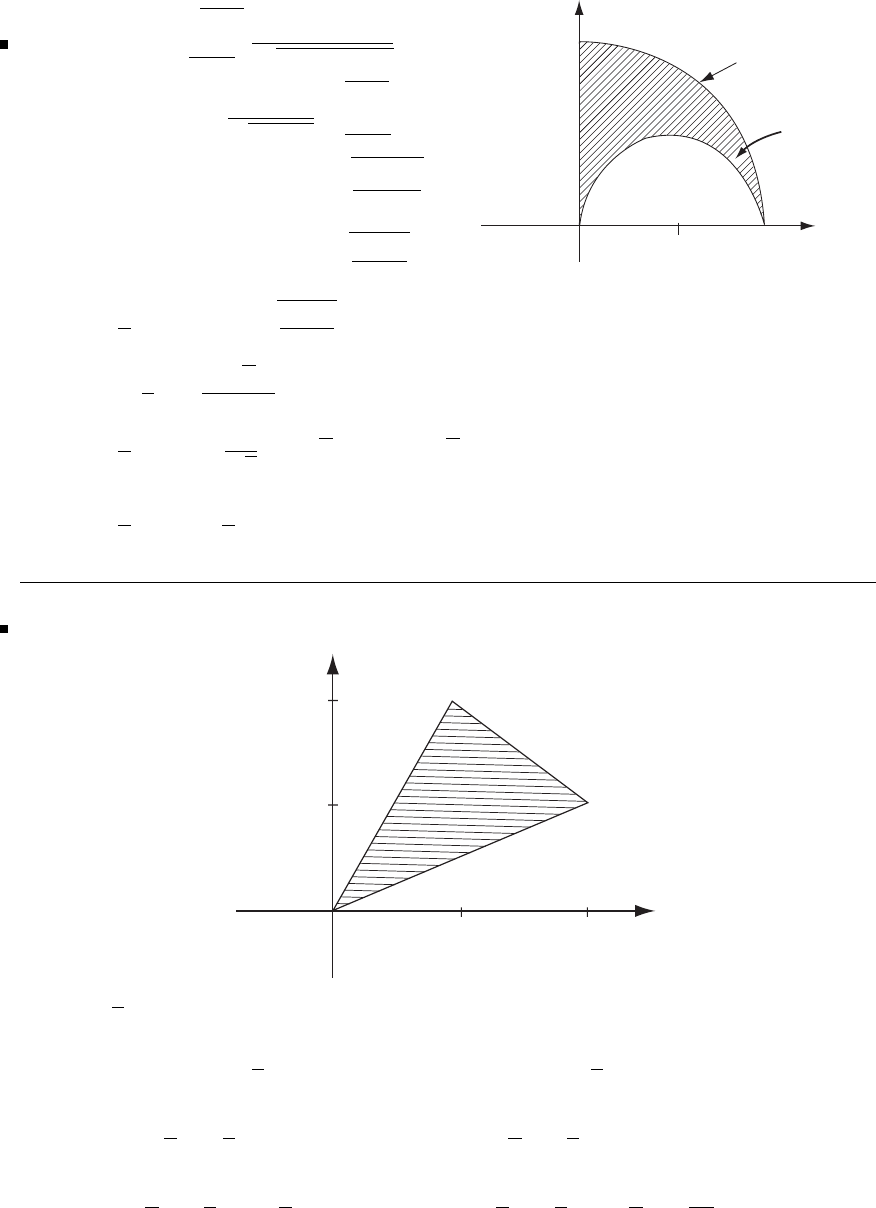
Glyn James, Advanced Modern Engineering Mathematics, 4th Edition 159
y
1
0 1/2 1 x
Part circle
Part circle
x2 + y2 = 1
x2 − x + y2 = 0
68(c)1
0
dx√1−x2
√x−x2
1
1−x2−y2dy
=1
0sin−1y
√1−x2√1−x2
√x−x2
dx
=1
0sin−11−sin−1x−x2
1−x2dx
=1
0sin−11−sin−1x
1+xdx
=π
2−xsin−1x
1+x1
0
+1
21
0
√x
(1 + x)dx
=π
2−sin−11
√2+√x−tan−1√x1
0,using substitution x=tan
2θ
=π
4+1−π
4=1
69 y
(1,2)
(2,1)
2
1
012
x
sin 1
2π(x+y)dxdy
=1
0
dxx
x/2
sin 1
2π(x+y)dy+2
1
dx3−x
x/2
sin 1
2π(x+y)dy
=1
0−2
πcos 1
2π(x+y)x
x/2
dx+2
1−2
πcos 1
2π(x+y)3−x
x/2
dx
=1
02
πcos 3
4πx −2
πcos πxdx+2
12
πcos 3
4πx −2
πcos 3π
2dx
c
Pearson Education Limited 2011
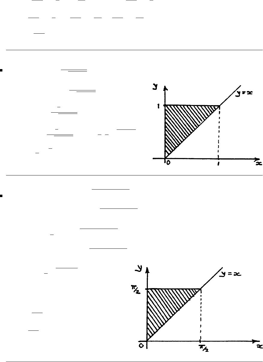
160 Glyn James, Advanced Modern Engineering Mathematics, 4th Edition
=8
3π2sin 3
4πx −2
π2sin πx1
0
+8
3π2sin 3
4πx2
1
=8
3π2sin 3
4π+8
3π2sin 3π
2−8
3π2sin 3π
4
=−8
3π2
70(a)1
0
dx1
x
xy
1+y4dy
=1
0
dyy
0
xy
1+y4dx
=1
01
2x2y
1+y4y
0
dy
=1
0
1
2y3
1+y4dy=1
8.2
11+y41
0
=1
4(√2−1)
70(b)π/2
0
dyy
0
cos 2y1−k2sin2xdx
=π/2
0
dxπ/2
x
cos 2y1−k2sin2xdy
=π/2
01
2sin 2y1−k2sin2xπ/2
x
dx
=π/2
0−sin xcos x1−k2sin2xdx
=−1
0
1
21+k2tdt
(Let t=−sin2x,then
dt=−2sinxcos xdx)
=1
3k2(1 + k2t)3/2−1
0
=1
3k2((1 −k2)3/2−1)
c
Pearson Education Limited 2011
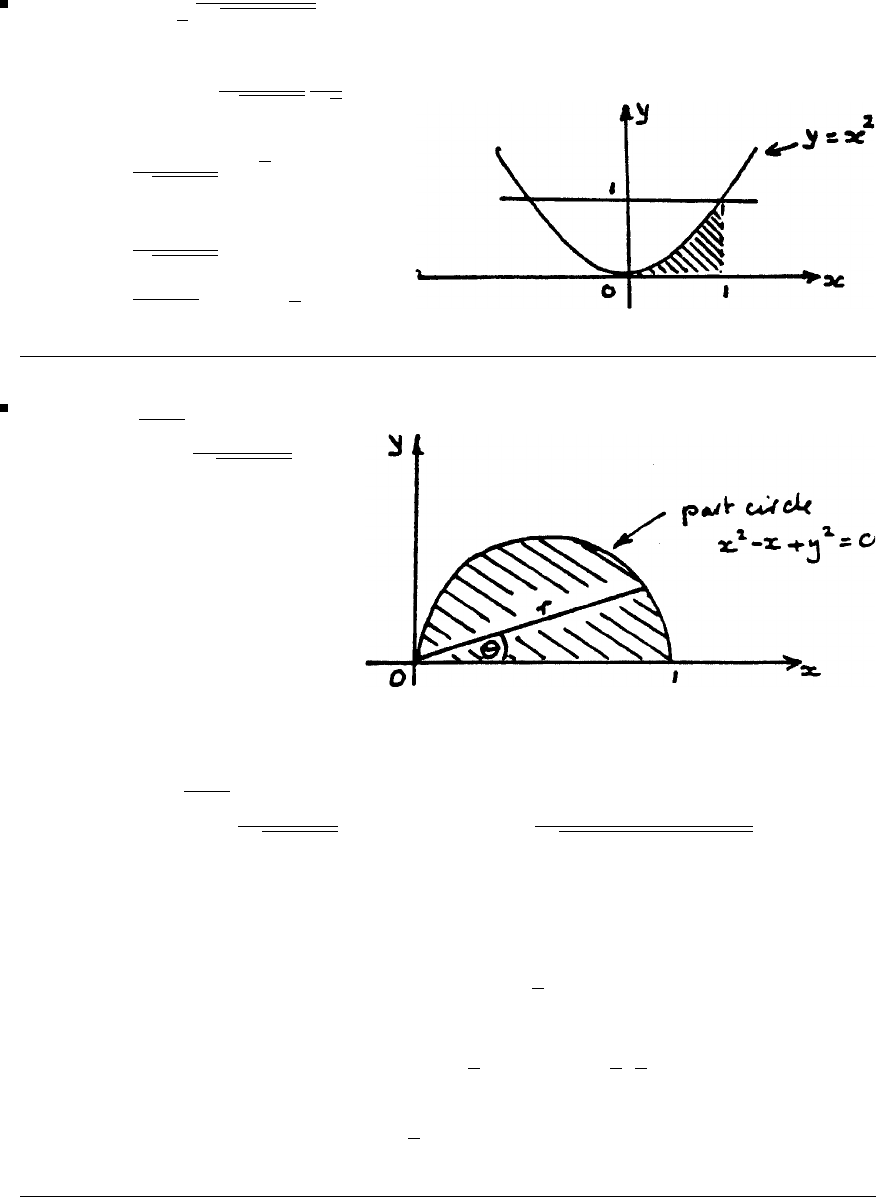
Glyn James, Advanced Modern Engineering Mathematics, 4th Edition 161
71 1
0
dy1
√y
dx
y(1 + x2)
=1
0
dxx2
0
1
√1+x2
1
√ydy
=1
0
1
√1+x2[2√y]x2
0dx
=1
0
2x
√1+x2dx
=[2
1+x2]1
0=2(
√2−1)
72
1
0
dx√x−x2
0
x
x2+y2dy
Equation of circle in polar coordinates is r=cosθ
1
0
dx√x−x2
0
x
x2+y2dy=π/2
0cos θ
0
rcos θ
r2cos2θ+r2sin2θrdrdθ
=π/2
0cos θ
0
(cos θ)rdrdθ
=π/2
0
cos θ1
2r2cos θ
0
dθ
=π/2
0
1
2cos3θdθ=1
2.2
3π/2
0
cos θdθ
=1
3
c
Pearson Education Limited 2011
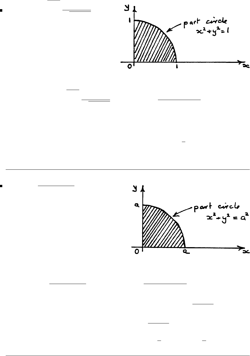
162 Glyn James, Advanced Modern Engineering Mathematics, 4th Edition
731
0
dx√1−x2
0
x+y
x2+y2dy
Change to polar coordinates
1
0
dx√1−x2
0
x+y
x2+y2dy=π/2
01
0
rcos θ+rsin θ
rrdrdθ
=π/2
0
(cos θ+sinθ)dθ1
0
rdr
=[sinθ−cos θ]π/2
01
2r21
0
=1
74 x+y
x2+y2+a2dxdy
over first quadrant of circle
using polar coordinates
x+y
x2+y2+a2dxdy=π/2
0a
0
rcos θ+rsin θ
r2+a2rdrdθ
=π/2
0
(cos θ+sinθ)dθa
0
r2
r2+a2dr
=2a
01−a2
r2+a2dr
=2r−atan−1r
aa
0=2a1−π
4
c
Pearson Education Limited 2011

Glyn James, Advanced Modern Engineering Mathematics, 4th Edition 163
75 Using polar coordinates, parabola becomes
r2sin2θ=4−4rcos θ
r2=4−4rcos θ+r2cos2θ
=(2−rcos θ)2
r=(2−rcos θ),positive root because r=2atθ=π
2
=2
1+cosθ
x2−y2
x2+y2dxdy=π/2
02
1+cos θ
0
(cos2θ−sin2θ)rdrdθ
=π/2
0
2(cos2θ−sin2θ)1
(1 + cos θ)2dθ
=π/2
0
2(2 cos2θ−1)
(1 + cos θ)2dθ
=(6π−20)/3=−0.3835
(use the substitution t=tan1
2θ).
76 Circles are r=acos θ,r=bsin θand intersect at θ=tan
−1a
b.
(x2+y2)2
(xy)2dxdy=tan−1a
b
0bsin θ
0
1
sin2θcos2θrdrdθ
+π/2
tan−1a
bacos θ
0
1
sin2θcos2θrdrdθ
=tan−1a
b
0
1
2
b2sin2θ
sin2θcos2θdθ+π/2
tan−1a
b
1
2
a2cos2θ
sin2θcos2θdθ
=tan−1a
b
0
1
2b2sec2θdθ+π/2
tan−1a
b
1
2a2cosec2θdθ
=1
2b2tan θtan−1a
b
0
+−1
2a2cot θπ/2
tan−1a
b
=1
2ab +1
2ab =ab
c
Pearson Education Limited 2011
164 Glyn James, Advanced Modern Engineering Mathematics, 4th Edition
Exercises 3.4.6
77C
[sin ydx+(x−cos y)dy]
=1
0sin 1
2πx +(x−cos 1
2πx)1
2πdx
+0
1sin 1
2πdx
+0
π/2
[−cos y]dy
=−2
πcos 1
2πx −1
4πx2−sin 1
2πx1
0
+xsin 1
2π0
1
+[−sin y]0
π/2
=−1+ 2
π+1
4π−1+1
=−1+ 2
π+π
4
C
[sin ydx+(x−cos y)dy]=
A[1 −cos y]dxdy
=1
0
dxπ/2
1
2πx
(1 −cos y)dy
=1
0π
2−π
2x−1+sin1
2πxdx
=π
2−π
4−1+ 2
π=π
4−1+ 2
π
78 [(x2y−y)dx+(x+y2)dy]
=
A(1 −x2+1)dxdy
=2
0
dxx
0
(2 −x2)dy
=2
0
(2x−x3)dx=x2−1
4x42
0
=4−4=0
c
Pearson Education Limited 2011
Glyn James, Advanced Modern Engineering Mathematics, 4th Edition 165
79 C
(xy dx+xdy)
=1
0
(x3+2x2)dx
+0
1x3/2+1
2x1/2dx
=1
4+2
3−2
5+1
3=11
60
C
(xy dx+xdy)=
A(1 −x)dxdy
=1
0
dx√x
x2
(1 −x)dy
=1
0
(1 −x)(√x−x2)dx
=1
0
√x−x3/2−x2+x3dx
=2
3−2
5−1
3+1
4=11
60
80
c(ex−3y2)dx+(e
y+4x2)dy=
A(8x+6y)dxdy
=2π
0
dθ2
0
(8rcos θ+6rsin θ)rdrdθ
=2π
0
(8 cos θ+6sinθ)dθ2
0
rdr
=0(2)=0
81 a
0
dx2a−x
x
y−x
4a2+(y+x)2dy=I
u=x+y
v=x−y⇒x=(u+v)/2
y=(u−v)/2and ∂(x, y)
∂(u, v)=
1
2
1
2
1
2−1
2
=−1
2
c
Pearson Education Limited 2011
166 Glyn James, Advanced Modern Engineering Mathematics, 4th Edition
y=x⇒u−v=u+v⇒v=0
y=2a−x⇒u−v=4a−u−v⇒u=2a
x=0 ⇒u=−v
(0,0) ⇒(0,0),(a, a)⇒(2a, 0),(0,2a)⇒(2a, −2a)
I=2a
0
du0
−u
−v
4a2+u2−1
2
dv=1
42a
0
u2
4a2+u2du
=1
42a
0
1−4a2
4a2+u2du
=1
4u−2atan−1u
2a2a
0=a
21−π
4
82 1
0
dy2−y
y
x+y
x2ex+ydx
u=x+y
v=y/x ⇒∂(u, v)
∂(x, y)=
1−y
x2
11
x
=1
x2(x+y)
c
Pearson Education Limited 2011

Glyn James, Advanced Modern Engineering Mathematics, 4th Edition 167
y=x⇒v=1
y=0 ⇒v=0
y=2−x⇒u=2
1
0
dy2−y
y
x+y
x2ex+ydx=2
0
du1
0
eudv
=e
2−1
Exercises 3.4.8
83 Surface area =
A1+∂z
∂x2
+∂z
∂y2
dxdy
where Ais the domain x2+y2≤2, z=0.
z=2−x2−y2⇒∂z
∂x =−2x, ∂z
∂y =−2y
Surface area =
A1+4x2+4y2dxdy
Set x=rcos θ,y=rsin θ,then
Surface area = 2π
0
dθ√2
01+4r2rdr
=2π1
12 (1 + 4r2)3/2√2
0
=2π1
12 (27 −1)
=52π/12 = 13π/3
84(a) Direction cosines of normal to Sare (2
3,1
3,2
3), so that
S(x2+y2)dS=
A(x2+y2)dxdy
2/3
c
Pearson Education Limited 2011

168 Glyn James, Advanced Modern Engineering Mathematics, 4th Edition
where Ais the area between y=6−2xand y=2−2xlying between y=0 and
y=3.
Thus
S(x2+y2)dS=3
0
dy6−y
2
2−y
2
3
2(x2+y2)dx
=3
0
3
2x3
3+y2x
6−y
2
2−y
2
dy
=3
013 −6y+15
4y2dy=183
4
84(b)
SzdS=1
0
dx+√x−x2
−√x−x2
z1+∂z
∂x2
+∂z
∂y2
dy
∂z
∂x =−x
z,∂z
∂y =−y
zand x2+y2+z2=1
SzdS=1
0
dx+√x−x2
−√x−x2
1dy
=2 1
0
√x−x2dx
=π
4
(Use the substitution x=1
2+1
2sin t. Alternatively, recognize area of circle of
radius 1
2.)
c
Pearson Education Limited 2011

Glyn James, Advanced Modern Engineering Mathematics, 4th Edition 169
85(a) v=(xy, −x2,x+z)
dS=ndS=2
3,2
3,1
3dS
⇒
Sv·dS=
S2
3xy −2
3x2+1
3(x+z)dS
=3
0
dx3−x
0
[xy −2x2+(x+6−2x−2y)] dy
=3
01
2xy2−2x2y−xy +6y−y23−x
0
dx
=3
0x
2(3 −x)2−2x2(3 −x)−x(3 −x)+6(3−x)dx
=27/4
85(b) Use cylindrical polar coordinates, then dS=(icos φ+jsin φ)dφdzon
cylinder and v=(3y, 2x2,z
3)=(3sinφ, 2cos
2φ, z3)
Sv·dS
=2π
0
dφ1
0
(3 sin φcos φ+2cos
2φsin φ)dz
=3
2sin2φ−2
3cos3φ2π
0
=0
86
Sz2dS=
Az2/(1 −x2−y2)dxdy
where x2+y2+z2=1 and Ais the interior of the circle x2+y2=1,z=0
Sz2dS=
A1−x2−y2dxdy
=2π
0
dθ1
0
√1−r2rdr
=2π−1
3(1 −r2)3/21
0
=2π
3
c
Pearson Education Limited 2011

170 Glyn James, Advanced Modern Engineering Mathematics, 4th Edition
87(a)
S1dS=
A11+4x2+4y2dxdy
where Ais the interior of the circle x2+y2=2
SdS=2π
0
dθ√2
01+4r2rdr
=2π1
12 (1 + 4r2)3/2√2
0
=2π
12 (27 −1)
=13π/3 Surface Area
87(b)
S(x2+y2)dS=2π
0
dθ√2
0
r21+4r2rdr
=2π
16 1
5(1 + 4r2)5/2−1
3(1 + 4r)3/2√2
0
=π
81
5(243 −1) −1
3(27 −1)= 149π/30
2nd moment of surface area about z-axis.
87(c)
SzdS=2π
0
dθ√2
0
(2 −r2)1+4r2rdr
=22π
0
dθ√2
01+4r2rdr−2π
0
dθ√2
0
r21+4r2dr
=26π
3−149π
30 =111π
30 =37π
10
88 Direction cosines of normal to Sare (2
3,1
3,2
3)sothat
SdS=
Adxdy
2/3
c
Pearson Education Limited 2011

Glyn James, Advanced Modern Engineering Mathematics, 4th Edition 171
where Ais the interior of x2+y2= 64 lying in the first quadrant.
SdS=π/2
0
dθ8
0
3
2rdr=π
2×3
21
2r28
0
=24π
89
SdS=
A1+x
22+y
22dxdy
where Ais the annulus between x2+y2=4 and x2+y2=12
SdS=2π
0
dθ√12
21+1
4r2rdr
=2π4
31+1
4r23/2√12
2
=8π
3[43/2−23/2]
=16π
3(4 −21/2)
90 Using cylindrical polar coordinates, dS=(4icos φ+4jsin φ)dφdz
and V=zi+2cosφj−12 sin2φzk
Thus V·dS=(4zcos φ+8sinφcos φ)dφdz
and
SV·dS=π/2
0
dφ5
0
(4zcos φ+8sinφcos φ)dz
=π/2
0
(50 cos φ+40sinφcos φ)dφ
=[50sinφ+40sin
2φ]π/2
0=90
91 F =yi+(x−2xz)j−xyk
curl F=
ij k
∂
∂x
∂
∂y
∂
∂z
yx−2xz −xy
=(x, y, −2z)
On sphere, x=asin θcos φ,y=asin θsin φ,z=acos θ
c
Pearson Education Limited 2011

172 Glyn James, Advanced Modern Engineering Mathematics, 4th Edition
and dS=a2(sin θcos φ, sin θsin φ, cos θ)sinθdθdφ
curl F·dS=a3(sin2θcos2φ+sin
2θsin2φ−2cos
2θ)sinθdθdφ
=a3(sin2θ−2cos
2θ)sinθdθdφ
Scurl F·dS=2π
0
dφπ
0
a3[sin3θ−2cos
2θsin θ]dθ
=2π
0
a3dφπ
03
4sin θ−1
4sin 3θ−2cos
2θsin θdθ
=a3φ2π
0−3
4cos θ+1
12 cos 3θ+2
3cos3θπ
0
=0
Exercises 3.4.10
92(a)
1
0
dx2
0
dy3
1
x2yz dz=1
0
x2dx2
0
ydy3
1
zdz
=1
3.1
2(4)1
2(32−1) = 8
3
92(b)
2
03
14
2
xyz2dzdydx=2
0
dx3
1
dy4
2
xyz2dz
=2
0
xdx3
1
ydy4
2
z2dz
=1
2(4)1
2(32−1) 1
3(43−23)
=448
3
93
1
−1
dzz
0
dxx+z
x−z
(x+y+z)dy=1
−1
dzz
0{2z(x+z)+2xz}dx
=1
−1
3z3dz=0
c
Pearson Education Limited 2011

Glyn James, Advanced Modern Engineering Mathematics, 4th Edition 173
94
Vsin(x+y+z)dxdydz=π
0
dxπ−x
0
dyπ−x−y
0
sin(x+y+z)dz
=π
0
dxπ−x
0
[−cos(x+y+z)]π−x−y
0dy
=π
0
dxπ−x
0
[1 + cos(x+y)] dy
=π
0
[y+sin(x+y)]π−x
0dx
=π
0
(π−x+sinπ−sin x)dx
=πx −x2
2+cosxπ
0
=1
2π2−2
95
Vxyz dxdydz=1
0
dx1−x
0
dy1−x−y
0
xyz dz
=1
0
xdx1−x
0
1
2y(1 −x−y)2dy
=1
0
1
2x1
2(1 −x)2y2−2
3(1 −x)y3+1
4y41−x
0
dx
=1
0
1
24 x(1 −x)4dx
=1
24 1
0
(x−4x2+6x3−4x4+x5)dx
=1
720
c
Pearson Education Limited 2011

174 Glyn James, Advanced Modern Engineering Mathematics, 4th Edition
96
V=
VdV=
Vdxdydz
=1
0
dx√x
x2
dy2−x−y
0
dz
=1
0
dx√x
x2
(2 −x−y)dy
=1
02√x−x3/2−1
2x−2x2+x3+1
2x4dx
=4
3−2
5−1
4−2
3+1
4+1
10 =11
30
97
V(x2+y2+z2)xdxdydz=π/2
0
dφπ/2
0
dθ1
0
r2rsin θcos φsin θr2dr
=π/2
0
cos φdφπ/2
0
sin2θdθ1
0
r5dr
=1×1
2×π
2×1
6=π
24
98
Vx2y2z2(x+y+z)dxdydz
=
Vx3y2z2dxdydz+
Vx2y2z3dxdydz+
Vx2y3z2dxdydz
=1
0
x3dx1−x
0
y2dy1−x−y
0
z2dz+1
0
y3dy1−y
0
z2dz1−z−y
0
x2dx
+1
0
z3dz1−z
0
x2dx1−z−x
0
y2dy
=31
0
x3dx1−x
0
y2dy1−x−y
0
z2dzfrom symmetry
c
Pearson Education Limited 2011

Glyn James, Advanced Modern Engineering Mathematics, 4th Edition 175
=31
0
x3dx1−x
0
1
3y2(1 −x−y)3dy
=1
0
x3dx1−x
0{y2[(1 −x)3−3(1 −x)2y+3(1−x)y2−y3]}dy
=1
0
x31
3(1 −x)6−3
4(1 −x)6+3
5(1 −x)6−1
6(1 −x)6dx
=1
60 1
0
x3(1 −x)6dx
=1
60 1
0
x6(1 −x)3dx
=1
60 1
0
x6(1 −3x+3x2−x3)dx
=1
60 1
7−3
8+3
9−1
10
=1
50400
99
u=x+y+z
uv =y+z
uvw =z⎫
⎬
⎭
x=u−uv
y=uv −uvw
z=uvw
∂(x, y, z)
∂(u, v, w)=
1−vv−vw vw
−uu−uw uw
0−uv uv
=
1−vvvw
−uuuw
00uv
=
1vvw
0uuw
00uv
=u2v
I=
Vexp(−(x+y+z)3)dxdydz
=1
0
dx1−x
0
dy1−x−y
0
exp(−(x+y+z)3)dz
x+y+z=1 ⇒u=1
x=0 ⇒u=y+z
uv =y+z⇒v=1
c
Pearson Education Limited 2011

176 Glyn James, Advanced Modern Engineering Mathematics, 4th Edition
y=0 ⇒
u=x+z
uv =z
uvw =z⎫
⎬
⎭⇒w=1
z=0 ⇒
u=x+y
uv =y
uvw =0 ⎫
⎬
⎭⇒w=0
I=1
0
du1
0
dv1
0
e−u3u2vdv
=1
0
u2e−u3du1
0
vdv1
0
dw
=−1
3e−u31
01
2v21
0
[w]1
0
=1
6[1 −e−1]
100
Vyz dxdydz=1
0
dx1−x
0
dy2−x−y
0
yz dz
=1
0
dx1−x
0
1
2y(2 −x−y)2dy
=1
0
dx1−x
0
1
2[y(2 −x)2−2y2(2 −x)+y3]dy
=1
0
1
21
2(1 −x)2(2 −x)2−2
3(1 −x)3(2 −x)+1
4(1 −x)4dx
=1
0
1
21
2t2(1 + t)2−2
3t3(1 + t)+1
4t4dt
=1
0
1
21
2t2+t3+1
2t4−2
3t3−2
3t4+1
4t4dt
=1
21
6+1
12 +1
60 =2
15
c
Pearson Education Limited 2011

Glyn James, Advanced Modern Engineering Mathematics, 4th Edition 177
Volume of prism =
Vdxdydz
=1
0
dx1−x
0
dy2−x−y
0
dz
=1
0
dx1−x
0
(2 −x−y)dy
=1
0(2 −x)(1 −x)−1
2(1 −x)2dx
=1
02−3x+x2−1
2+x−1
2x2dx
=3
2−1+1
6=2
3
Let the coordinates of the centroid be (x,y,z), the taking moments about
appropriate axes, we have
2
3x=
Vxdxdydz,2
3y=
Vydxdydz,
2
3z=
Vzdxdydz
From symmetry y=x.
x=3
21
0
dx 1−x
0
dy 2−x−y
0
xdz
=3
21
0
dx 1−x
0
x(2 −x−y)dy
=3
21
0
3
2x−2x2+1
2x3dx
=3
23
4−2
3+1
8=5
16
c
Pearson Education Limited 2011

178 Glyn James, Advanced Modern Engineering Mathematics, 4th Edition
z=3
21
0
dx 1−x
0
dy 2−x−y
0
zdz
=3
21
0
dx 1−x
0
1
2(2 −x−y)2dy
=3
21
0−1
6(2 −x−y)3y=1−x
y=0
dx
=3
21
0−1
61−(2 −x)3dx
=3
2−1
6x−1
24 (2 −x)41
0
=3
2×11
24 =11
16
101
Vzdxdydz=2π
0
dφπ/2
π/4
dθ1
0
r3cos θsin θdr
=2π
0
dφπ/2
π/4
1
2sin 2θ1
0
r3dr
=[2π]−1
4cos 2θπ/2
π/41
4=π
8
102
Vxdxdydz=π/2
0
dφπ/2
0
dθa
0
rsin2θ.r cos φdr
=π/2
0
cos φdφπ/2
0
sin2θdθa
0
r3dr
=[1]π
41
4a4=πa4/16
c
Pearson Education Limited 2011

Glyn James, Advanced Modern Engineering Mathematics, 4th Edition 179
Exercises 3.4.13
103
SF·dSF=(4xz, −y2,yz)
Shas six faces and the integral can be evaluated as the sum of six integrals.
SF·dS=
on
x=0
F·dS+
on
x=1
F·dS+
on
y=0
F·dS
+
on
y=1
F·dS+
on
z=0
F·dS+
on
z=1
F·dS
=1
01
0
(0,−y2,yz)·(−idydz)
+1
01
0
(4z, −y2,yz)·(idydz)
+1
01
0
(4xz, 0,0) ·(−jdxdz)
+1
01
0
(4xz, −1,yz)·(jdxdz)
+1
01
0
(0,−y2,0) ·(−kdxdy)
+1
01
0
(4x, −y2,y)·(kdxdy)
=0 + 1
01
0
4zdydz+0+1
01
0
(−1) dxdz+0+1
01
0
ydxdy
=2 −1+1
2=3
2
104
SF·dS=
Vdiv FdV
=
V(z+z+2z)dxdydz
=2π
0
dφπ/2
0
dθ2
0
4rcos θ.r2sin θdr
=[2π][−cos 2θ]π/2
01
4r42
0
=16π
c
Pearson Education Limited 2011

180 Glyn James, Advanced Modern Engineering Mathematics, 4th Edition
105 On z=0,dS=−kdxdy, F=(4x, −2y2,0),F·dS=0
On z=3,dS=kdxdy, F=(4x, −2y2,9),F·dS=9dxdy
On x2+y2=4,dS=(icos φ+jsin φ)2 dφdz, F=(8cosφ, −8sinφ, z2)
and F·dS= 16(cos2φ−sin3φ)dφdz
SF·dS=
(z=3)
9dxdy+2π
0
dφ3
0
16(cos2φ−sin3φ)dz
=36π+482π
0
cos2φ−sin3φdφ
=84π
Vdiv FdV=
V(4 −4y+2z)dxdydz
=2π
0
dφ2
0
dr3
0
(4 −4rsin φ+2z)rdz
=2π
0
dφ2
0
(21 −12rsin φ)rdr
=2π
0
(42 −32 sin φ)dφ=84π
106 div (F×grad φ) = grad φ·curl F−F·curl (grad φ) and curl (grad φ)≡
0 for all φ.
Hence
V grad φ·curl FdV=
S
(F×grad φ)·dS
107
SF·dS=
on
x=0
F·dS+
on
y=0
F·dS+
on
z=0
F·dS+
on
z=1
F·dS
+
on
x2+y2=4
F·dS
On x=0,F=(y2,0,0),dS=−idydz,
on
x=0
F·dS= 2
0dy 1
0−y2dz=−8
3
On y=0, F=(0,0,0), so contribution is zero
On z=0, F=(xy +y2,x
2y, 0), dS=−kdxdy, so contribution is zero
On z=1, F=(xy +y2,x
2y, 0), dS=kdxdy, so contribution is zero
c
Pearson Education Limited 2011

Glyn James, Advanced Modern Engineering Mathematics, 4th Edition 181
On x2+y2=4, F=(4(sinφcos φ+sin
2φ),8cos
2φsin φ, 0), dS=2(cosφi+
sin φj)dφdz
on
x2+y2=4
F·dS=π/2
0
dφ1
0
8sinφcos2φ+8sin
2φcos φ+ 16(cos2φsin2φ)dz
=−8
3cos3φ+8
3sin3φ+2φ−1
2sin 4φπ/2
0
=16
3+π
Vdiv FdV=
V(y+x2)dxdydz
=π/2
0
dφ2
0
dr1
0
(rsin φ+r2cos2φ)rdz
=π/2
0
dφ2
0
(r2sin φ+r3cos2φ)dr
=π/2
08
3sin φ+4cos
2φdφ
=8
3+π
Hence, result
108
curl F=
ijk
∂
∂x
∂
∂y
∂
∂z
36xz +6ycos x3+6sinx+zsin y18x2−cos y
=i(sin y−sin y)+j(36x−36x)+k(6 cos x−6cosx)
=0
Hence, there is a function φ(x, y, z), such that F=gradφ
c
Pearson Education Limited 2011

182 Glyn James, Advanced Modern Engineering Mathematics, 4th Edition
109 C
A·dr=
Scurl A·dS
curl A=
ijk
∂
∂x
∂
∂y
∂
∂z
−yx 0
=2k
C
A·dr=
S2k·dS
Let S be the ellipse x2
a2+y2
b2=1, z=0
Then, dS=k·dxdy,and
A·dr=2
Sdxdy=2πab
110
curl F=
ijk
∂
∂x
∂
∂y
∂
∂z
2x−y−yz2−y2z
=i(−2yz +2yz)+j(0) + k(1)
=k
Scurl F·dS=162π
0
dφπ/2
0
k·(sin θcos φi+sinθsin φj+cosθk)sinθdθ
=162π
0
dφπ/2
0
sin θcos θdθ= 16[2π]1
2sin2θπ/2
0
=16π
C
F·dr
On circle x2+y2=16, z=0, x=4cosφ,y=4sinφ,r=4(cosφ, sin φ, 0)
F=(8cosφ−4sinφ, 0,0),dr=4(−sin φ, cos φ, 0) dφ
C
F·dr=2π
0
(−32 cos φsin φ+16sin
2φ+0)dφ
=16π
c
Pearson Education Limited 2011

Glyn James, Advanced Modern Engineering Mathematics, 4th Edition 183
111
curl (af(r)) = −a×grad f(r)
S−(a×grad f(r)) ·ndS=C
af(r)·dr
⇒
S−(grad f(r)×n)·adS=C
af(r)·dr
⇒a·
S(n×grad f(r)) dS=a·C
f(r)dr
⇒
Sn×grad f(r)dS=C
f(r)dr
f(r)=3xy2⇒grad f(r)=(3y2,6xy, 0)
n×grad f(r)=k×grad f(r)=(−6xy, 3y2,0)
1
0
dx2
0
(−6xy, 3y2,0) dy=1
0
(−12x, 8,0) dx
=(−6,8,0)
C
f(r)dr=1
0
0.idx+2
0
3y2jdy+0
1
12xidx+0
2
0.jdy
=(−6,8,0)
112
Scurl F·dS=C
F·dr
curl F=
ijk
∂
∂x
∂
∂y
∂
∂z
2y+zx−zy−x
=(2,2,−1)
Scurl F·dS=
S(2,2,−1) ·(sin θcos φ, sin θsin φ, cos θ)sinθdφdθ
=π/2
0
dφπ/2
0
(2 sin θcos φ+2sinθsin φ−cos θ)sinθdθ
=π/2
0πsin φ−1
2dφ=3π
4
c
Pearson Education Limited 2011

184 Glyn James, Advanced Modern Engineering Mathematics, 4th Edition
Here, Chas three portions:
On z=0, r=(cosφ, sin φ, 0) ⇒dr=(−sin φ, cos φ, 0) dφ
and F=(2sinφ, cos φ, sin φ−cos φ)
F·dr=π/2
0
(−2sin
2φ+cos
2φ)dφ=−π
4
On y=0, r=(sinθ, 0,cos θ)⇒dr=(cosθ, 0,−sin θ)dθ
and F=(cosθ, sin θ−cos θ, −sin θ)
F·dr=π/2
0
(cos2θ+sin
2θ)dθ=π
2
On x=0, r=(0,sin θ, cos θ)⇒dr=(0,cos θ, −sin θ)dθ
and F=(2sinθ+cosθ, −cos θ, sin θ)
F·dr=0
π/2
(−cos2θ−sin2θ)dθ=π
2
Review Exercises 3.7
1∂u
∂x =nxn−1f(t)+xnf(t)−y
x2
∂u
∂y =xnf(t)1
x
x∂u
∂x +y∂u
∂y =nxnf(t)=nu (1)
Differentiate (1) w.r.t. x
∂u
∂x +x∂2u
∂x2+y∂2u
∂x∂y =n∂u
∂x (2)
Differentiate (1) w.r.t. y
x∂2u
∂x∂y +∂u
∂y +y∂2u
∂y2=n∂u
∂y (3)
c
Pearson Education Limited 2011

Glyn James, Advanced Modern Engineering Mathematics, 4th Edition 185
x×(2) + y×(3) ⇒
x∂u
∂x +y∂u
∂y +x2∂2u
∂x2+2xy ∂2u
∂x∂y +y2∂2u
∂y2=nx∂u
∂x +y∂u
∂y
⇒x2∂2u
∂x2+2xy ∂2u
∂x∂y +y2∂2u
∂y2=n(n−1)u
u(x, y)=x4+y4+16x2y2
x∂u
∂x =x(4x3+32xy2)
y∂u
∂y =y(4y3+32x2y2)
x∂u
∂x +y∂u
∂y =4(x4+16x2y2+y4)
x2∂2u
∂x2+2xy ∂2u
∂x∂y +y2∂2u
∂y2=x2(12x2+32y2)+2xy(64xy)+y2(12y2+32x2)
= 12(x4+y4+16x2y2)
2∂f
∂x =∂f
∂u +∂f
∂v,∂2f
∂x2=∂2f
∂u2+2 ∂2f
∂u∂v +∂2f
∂v2
∂2f
∂x∂y =a∂2f
∂u2+b∂2f
∂u∂v +∂2f
∂v2b+∂2f
∂v∂ua
∂f
∂y =∂f
∂ua+∂f
∂vb, ∂2f
∂y2=∂2f
∂u2a2+2 ∂2f
∂u∂vab +∂2f
∂v2b2
9∂2f
∂x2−9∂2f
∂x∂y +2∂2f
∂y2=(9 −9a+2a2)∂2f
∂u2+(9−9b+2b2)∂2f
∂v2
+29−9
2(a+b)+2ab∂2f
∂u∂v
⇒
9−9a+2a2=0
9−9b+2b2=0
9−9
2(a+b)+2ab =0
⎫
⎪
⎪
⎬
⎪
⎪
⎭
⇒a=b⇒a=3,b=3
2
∂2f
∂u∂v =0 ⇒f=F(u)+G(v)
i.e.f(x, y)=F(x+3y)+G(x+3y/2)
c
Pearson Education Limited 2011

186 Glyn James, Advanced Modern Engineering Mathematics, 4th Edition
f(x, 0) = F(x)+G(x)=sinx
∂f
∂y(x, 0) = 3F(x)+ 3
2G(x)=3cosx
⇒F(x)+1
2G(x)=sinx+k
⇒1
2G(x)=−kand F(x)=sinx+2k
⇒f(x, y)=sin(x+3y)
3
∇×(P, Q, R)=
ijk
∂
∂x
∂
∂y
∂
∂z
∂f
∂x
∂f
∂y
∂f
∂z
=i∂2f
∂y∂z −∂2f
∂z∂y+j∂2f
∂x∂z −∂2f
∂z∂x+k∂2f
∂x∂y −∂2f
∂y∂x
=0
⇒∇×(∇f)≡0
4(a) xy =c,hyperbolas
grad f=(y, x)=c
x,x
on hyperbola
y=c
x⇒dy
dx=−c
x2
That is, tangent in direction of 1,−c
x2=t
t·grad f=c
x−c
x= 0 that is, orthogonal
4(b) x
x2+y2=ccircles, centres on x-axis, through (0,0)
grad f=y2−x2
(x2+y2)2,−2y
(x2+y2)2
c
Pearson Education Limited 2011

Glyn James, Advanced Modern Engineering Mathematics, 4th Edition 187
5(a)
grad(ωω
ω·r)=ωω
ω×(∇×r)+r×(∇×ωω
ω)+(ωω
ω·∇)r+(r·∇)ωω
ω
=ωω
ω×0+0+ωω
ω+0
=ωω
ω
5(b)
curl (ωω
ω×r)=−(ωω
ω·∇)r+ωω
ω(∇·r)(+r·∇)ωω
ω−r(∇·ωω
ω)
=−ωω
ω+3ωω
ω+0+0
=2ωω
ω
6(a) See problem 3above.
6(b)
div v=div{grad [zf(r)] + αf(r)k}
=div{kf(r)+zgrad f(r)}+αk·∇f(r)
=k·∇f(r)+k·grad f(r)+z∇2f(r)+αk·∇f(r)
=(2+α)∂f
∂z
∇2v=∇(∇·v)−∇×(∇×v)
=(2+α)∇∂f
∂z −∇×(∇×(∇(zf)+αfk))
∇×∇(zf)≡0
∇×(αfk)=α∇f×k
∇×(∇×αfk)=α(k·∇)∇f−αk(∇2f)
=α∂
∂z(∇f)=α∇∂f
∂z
⇒∇
2v=2∇∂f
∂z
7F=(x2−y2+x)i−(2xy +y)j
∇×F=
ijk
∂
∂x
∂
∂y
∂
∂z
x2−y2+x−2xy −y0
=(0,0,−2y+2y)=0
c
Pearson Education Limited 2011

188 Glyn James, Advanced Modern Engineering Mathematics, 4th Edition
∇f=∂f
∂x,∂f
∂y,∂f
∂z =(x2−y2+x, −2xy −y, 0)
⇒f(x, y, z)=x3
3−y2x+x2−y2
2+c
(2,1)
(1,2)
F·dr=(2,1)
(1,2)
grad f·dr=[f](2,1)
(1,2) =22
3
dr=idx+jdy=(i−j)dx
as on y=3−x,dy=−dx
2
1
(x2−y2+x+2xy +y)dx=2
1
(x2−(3 −x)2+x+2(3−x)+3−x)dx
=22
3
8
W=C
F·dr
r=(1−cos θ)i+sinθj
dr=(sinθi+cosθj)dθ
8(a) F =2sin1
2θi
C
F·dr=π
0
4sin
2θ
2cos θ
2dθ
=8
3sin3θ
2π
0
=8
3
8(b) F =2sinθ
2ˆ
n=2sinθ
2(sin θi+cosθj)
C
F·dr=π
0
2sin θ
2dθ=4−cos θ
2π
0
=4
c
Pearson Education Limited 2011

Glyn James, Advanced Modern Engineering Mathematics, 4th Edition 189
9r=(i+j+k)t0≤t≤1
dr=(i+j+k)dt
W=1
0
F·dr
F=(xy, −y, 1) = (t2,−t, 1)
⇒W=1
0
(t2−t+1)dt=1
3−1
2+1= 5
6
10
F=IC
dr×B
r=sinθi+cosθj+sinθ
2k
dr=cos θi−sin θj+1
2cos θ
2kdθ
B=sinθi−cos θj+k
F=I2π
0i1
2cos θ
2cos θ−sin θ+j1
2cos θ
2sin θ−cos θ
+k(sin2θ−cos2θ)dθ=4
3Ij
11
Circulation = C
v·dr
=−1
1
−ydx
x2+y2+−1
1
xdy
x2+y2+1
−1
ydx
x2+y2+1
−1
xdy
x2+y2
on y=1 onx=−1ony=−1onx=1
=1
−1
1
1+x2dx+−1
1
dy
1+y2−1
−1
dx
1+x2+1
−1
dy
1+y2
=0
12
Iz=
Aρ(x2+y2)dA, where density ρ=kxy
=c
0
dxc
x2/c
(x2+y2)kxy dy
c
Pearson Education Limited 2011

190 Glyn James, Advanced Modern Engineering Mathematics, 4th Edition
=c
01
4kx(x2+y2)2c
x2/c
dx
=c
0−1
4kx x2+x4
c22
+1
4kx(x2+c2)2dx
=1
4kc
0−x9
c4+2x7
c2−2x3c2−xc4dx
=13
80 kc6
13 Equation of cone is x2+y2=a2
h2(z−h)2
V=2a
c
dx√a2−x2
0
zdy
=2a
c
dx√a2−x2
0h+h
ax2+y2dy
=2a
chy +hx2
2asinh−1y
x−hy
2ax2+y2√a2−x2
0
dx
=2a
ch
2√a2−x2+hx2
2asinh−1√a2−x2
xdx
=2ha2
3π
2−sin−1c
a−hc
3√a2−c2−hc3
3atanh−1√a2−c2
a
14 Volume is 8
x
y
z≥0
dV
x2+y2=a2is a cylinder with z-axis as axis of symmetry and radius a.
z2+y2=a2is a cylinder with x-axis as axis of symmetry and radius a.
⇒V=8a
0
dy√a2−y2
0
dx√a2−y2
0
dz
=8a
0
[x]√a2−y2
0[z]√a2−y2
0dy
=8a
0
(a2−y2)dy=8a2y−1
3y3a
0
=16a3
3
c
Pearson Education Limited 2011

Glyn James, Advanced Modern Engineering Mathematics, 4th Edition 191
15 Elastic energy of ΔVis q2ΔV/(2EI)whereq=q0ρ/r and ρis the distance
from the centre and ris radius of cylinder.
Total energy = 2π
0
dφr
0
dρl
0
q2
0ρ3
2EIr2dz
=2πl r
0
q2
0ρ3dρ
2EIr2
=πq2
0r2l
4EI
16 On x=0,dS=−idydzand v·dS=−3x2ydydz≡0
On y=0,v·dS=0 On z=0,v·dS=0
On z=1,v·dS=0 On x+y=1,dS=1
√2(i+j)dS
⇒
⊂⊃ v·dS=1
0
dx1
03
√2x2(1 −x)+ 1
√2x(1 −x)2√2dz
=1
0
(2x2+x)(1 −x)dx
=1
3
17
S
⊂⊃ v·dS
On S,dS=(isin θcos φ+jsin θsin φ+kcos θ)a2sin θdθdφ
and v=i2asin2θcos φsin φ−ja2sin2θsin2φ+k(asin θcos φ+asin θsin φ)
S
⊂⊃ v·dS=π
0
dθ2π
0{2a3sin4θcos2φsin φ−a4sin4θsin3φ
+a3sin2θcos θcos φ+a3cos θsin2θsin φ}dφ
=0
18 C
F·dr
Cis the circle x2+y2=16,z= 0, so that, on the circle
F=x2+y−4,3xy, 0,r=4(cosθ, sin θ, 0)
c
Pearson Education Limited 2011

192 Glyn James, Advanced Modern Engineering Mathematics, 4th Edition
and dr=(−4sinθ, 4cosθ, 0) dθ
C
F·dr=2π
θ=0 −16 4cos
2θ+sinθ−1sin θ+ 192 cos θsin2θdθ
=2π
0−16 sin2θdθ(from symmetries)
=−16π
curl F=
ijk
∂
∂x
∂
∂y
∂
∂z
x2+y−43xy 2xz +z2
=(0,−2z, 3y−1)
On the hemisphere
r=4(sinθcos φ, sin θsin φ, cos θ)
dS=16(sinθcos φ, sin θsin φ, cos θ)sinθdφdθ
S
curl F.dS=
π/2
0
dθ2π
0
16(−8sin
2θcos θsin φ+12sin
2θcos θcos φ−cos θsin θ)dφ
=π/2
0−16 cos θsin θ[2π]dθ=−16π
19
S
a·dS=
V
div adV −
S1
a·dS
where Vis the hemisphere x2+y2+z2=a2(different afrom the vector a), S1
is the circle x2+y2=a2,z=0. div a=0 anddS=−kdxdyon S1
S1
a·dS=
S
(xi+yj)·(−kdxdy)=0
Hence
S
a·dS=0
c
Pearson Education Limited 2011
Glyn James, Advanced Modern Engineering Mathematics, 4th Edition 193
20
V
xyz dV=1
01−x
02−x
0
xyz dzdydx
=1
01−x
0
1
2xy (2 −x)2dydx
=1
0
1
4x(1 −x)2(2 −x)2dx
=1
0
1
4x5−6x4+13x3−12x2+4xdx
=1
24 −3
10 +13
16 −1+1
2=13
240
21
ux
−u
v
y
−v
y + ∆
y
x + ∆
x
Net circulation (anti clockwise) is
−u(x, y)Δx−v(x+Δx, y)Δy+u(x, y +Δy)Δx+v(x, y)Δy
If net circulation is zero then, dividing by ΔxΔy,
u(x, y +Δy)−u(x, y)
Δy−v(x+Δx, y)−v(x, y)
Δx=0
Δx, Δy→0gives
∂u
∂y −∂v
∂x =0.
Since u=−∂ψ
∂y and v=∂ψ
∂x we obtain
∂2ψ
∂x2+∂2ψ
∂y2= 0 Laplace equation.
c
Pearson Education Limited 2011

4
Functions of a Complex Variable
Exercises 4.2.2
1(a) If |z−2+j|=|z−j+3|,sothat
|x+jy −2+j|=|x+jy −j+3|
or
(x−2)2+(y+1)
2=(x+3)
2+(y−1)2
x2−4x+4+y2+2y+1=x2+6x+9+y2−2y+1
Then cancelling the squared terms and tidying up,
y=5
2x+5
4
1(b) z+z∗+4j(z−z∗)=6
Using, z+z∗=2x, z −z∗=2jy gives
2x+4j2jy =6
y=1
4x−3
4
2The straight lines are
|z−1−j|=|z−3+j|
|z−1+j|=|z−3−j|
which, in Cartesian form, are
(x−1)2+(y−1)2=(x−3)2+(y+1)
2
that is,x
2−2x+1+y2−2y+1=x2−6x+9+y2+2y+1
y=x−2
c
Pearson Education Limited 2011

Glyn James, Advanced Modern Engineering Mathematics, 4th Edition 195
and (x−1)2+(y+1)
2=(x−3)2+(y−1)2
i.e. x2−2x+1+y2+2y+1=x2−6x+9+y2−2y+1
y=−x+2
These two lines intersect at π/2 (the products of their gradients is −1) and
y=0,x= 2 at their intersection, that is, z=2+j0.
3w=jz +4−3jcan be written as
w=ejπ/2z+4−3j(since j=cosπ
2+jsin π
2=ejπ/2)
which is broken down as follows:
z−→ ejπ/2z−→ ejπ/2z+4−3j=w
rotate translation
anticlockwise (0,0) →(4,−3)
by 1
2π
Let w=u+jv and z=x+jy
so that,u+jv =j(x+jy)+4−3j
=jx −y+4−3j
that is,u=−y+4 (1)
v=x−3(2)
Taking 6 times equation (2) minus equation (1) gives,
6v−u=6x+y−22
so that, if 6x+y=22,wemusthave 6v−u=0 sothat, u=6vis the image of
the line
6x+y=22
c
Pearson Education Limited 2011
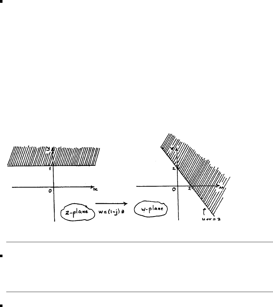
196 Glyn James, Advanced Modern Engineering Mathematics, 4th Edition
4Splitting the mapping w=(1−j)zinto real and imaginary parts gives
u+jv =(1−j)(x+jy)
=x+y+j(y−x)
that is,u=x+y
v=y−x
so that,u+v=2y
Therefore y>1 corresponds to u+v>2.
5Since w=jz +j
x=v−1,y=−u
so that x>0 corresponds to v>1.
6Since w=jz +1
v=x
u=−y+1
so that x>0⇒v>0
and 0 <y<2⇒−1<u<1or|u|<1.
This is illustrated below
c
Pearson Education Limited 2011
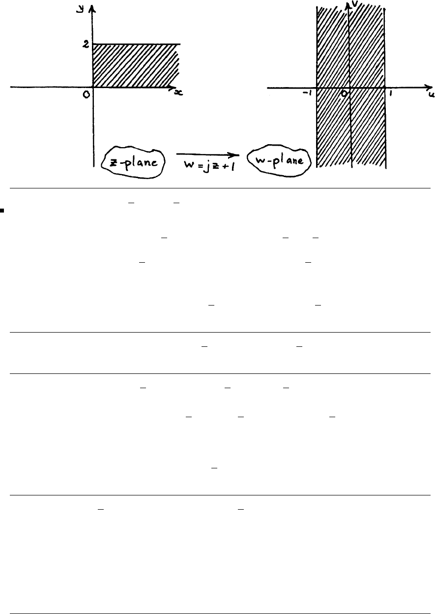
Glyn James, Advanced Modern Engineering Mathematics, 4th Edition 197
7Given w=(j+√3)z+j√3−1, we obtain, on equating real and imaginary
parts,
u=x√3−y−1,v=x+y√3+√3
or v√3−u=4y+4,and v+u√3=4x
on rearranging.
Thus 7(a) y= 0 corresponds to v√3−u=4 or u=v√3−4
7(b) x= 0 corresponds to v+u√3=0 or v=−u√3
7(c) Since u+1=x√3−yand v−√3=x+y√3 squaring and adding gives
(u+1)
2+(v−√3)2=(x√3−y)2+(x+y√3)2
=4x2+4y2
Thus, x2+y2=1⇒(u+1)
2+(v−√3)2=4
7(d) Since v√3−u=4y+4 and v+u√3=4x, squaring and adding gives
4v2+4u2= 16(y+1)
2+16x2
or u2+v2=4(x2+y2+2y+1)
Thus, x2+y2+2y= 1 corresponds to u2+v2=8
c
Pearson Education Limited 2011
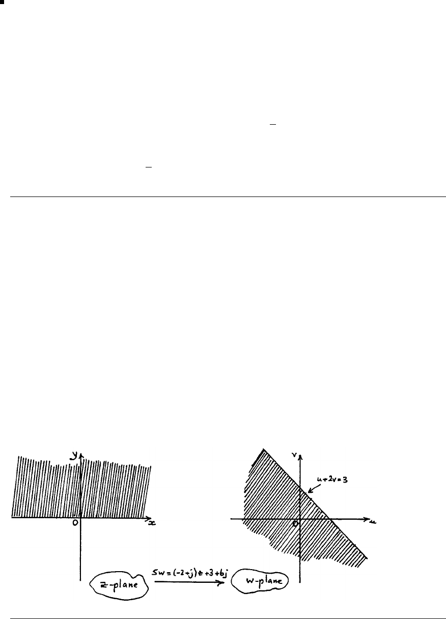
198 Glyn James, Advanced Modern Engineering Mathematics, 4th Edition
8(a) w=αz +β
Inserting z=1+j, w =jand z=−1,w=1+jgives the following two equations
for αand β
j=α(1 + j)+βor 1 + j=−α+β
from which, by subtraction,
−1=(2+j)αor α=1
5(−2+j)
so that, β=1+j+α=1
5(3 + 6j)gives5w=(−2+j)z+3+6j
8(b) Writing w=u+jv, z =x+jy and equating real and imaginary parts
gives
5u=−2x−y+3
5v=x−2y+6
Eliminating yyields
5v−10u=5xor v−2u=x
Eliminating xyields
5u+10v=−5y+15 or u+2v=−y+3
so that y>0 corresponds to u+2v<3
c
Pearson Education Limited 2011
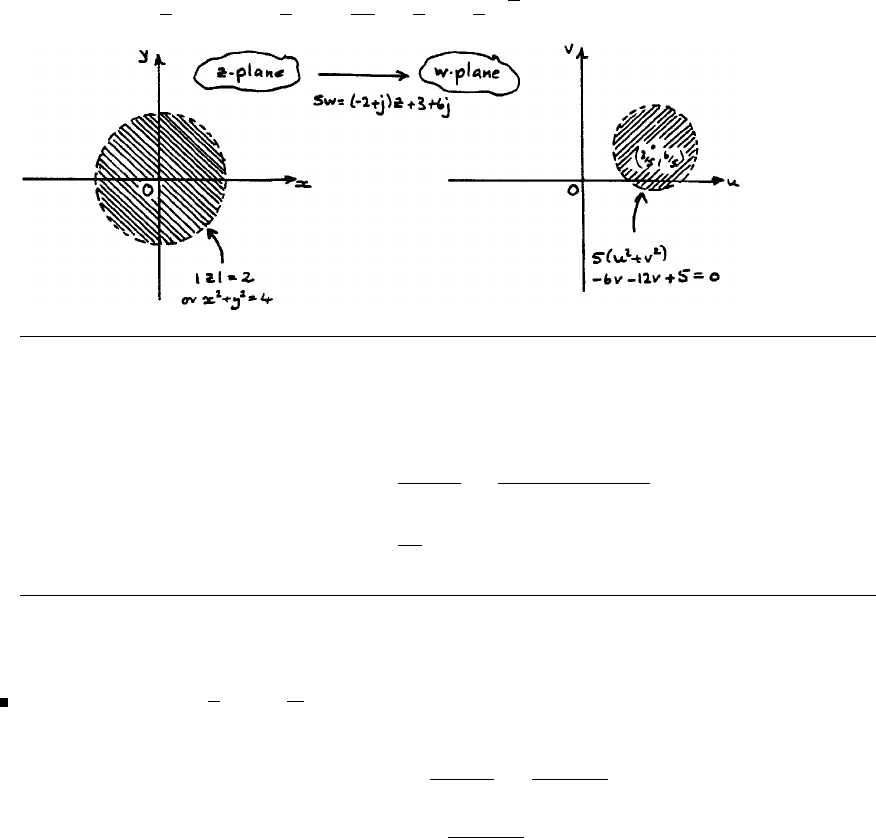
Glyn James, Advanced Modern Engineering Mathematics, 4th Edition 199
8(c) From part (b),
x=v−2u
y=3−u−2v
Squaring and adding gives
x2+y2=(v−2u)2+(3−u−2v)2
=5(u2+v2)−6u−12v+9
|z|<2⇒x2+y2<4
so that, 5(u2+v2)−6u−12v+5<0
or (5u−3)2+(5v−6)2<20
that is, v−3
5
2
+v−6
5
2
<20
25 =4
5=2
5√5
2
8(d) The fixed point(s) are given by
5z=(−2+j)z+3+6j
so that,z=3+6j
7−j=(3 + 6j)(7 + j)
50
=3
10 (1 + 3j)
Exercises 4.2.5
9Writing w=1
z,z=1
w
⇒x+jy =1
u+jv =u−jv
u2+v2
so that y=−v
u2+v2
c
Pearson Education Limited 2011
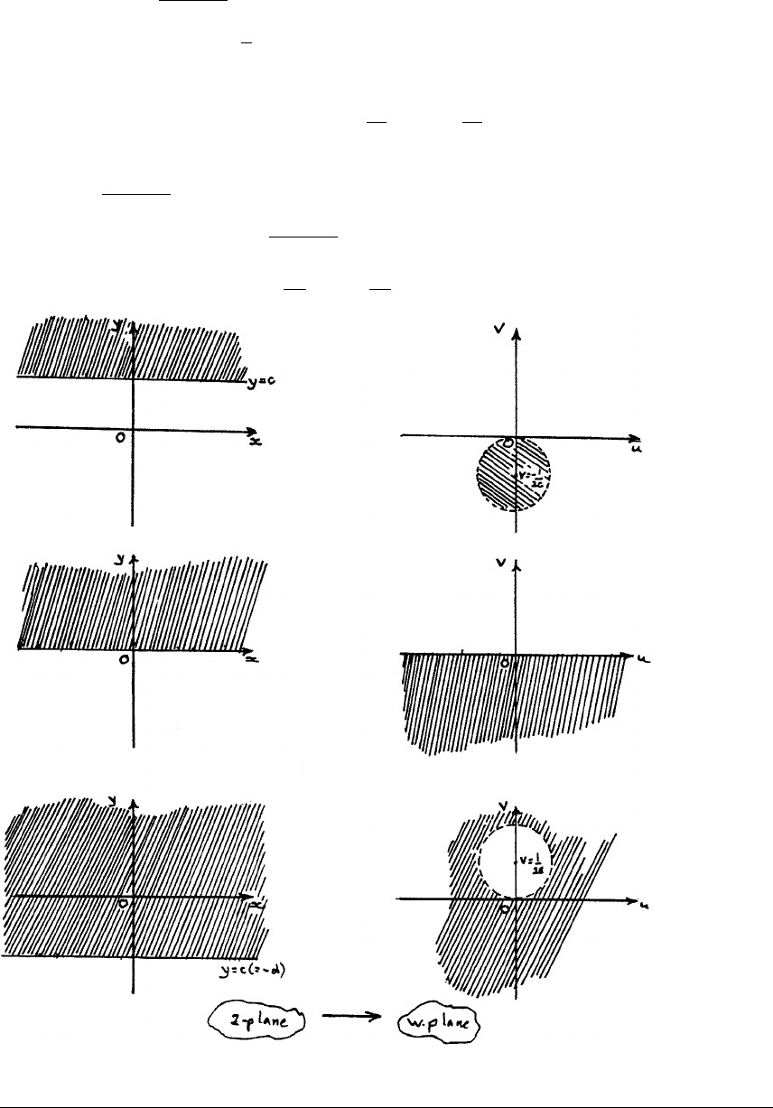
200 Glyn James, Advanced Modern Engineering Mathematics, 4th Edition
If y>c then, −v
u2+v2>c
or rearranging u2+v2+v
c<0
u2+v+1
2c2
<1
2c2
If c=0,−v
u2+v2>c⇒v<0
If c<0, put c=−dand −v
u2+v2>−d
or, on rearranging, u2+v−1
2d
2
>1
2d
2
c
Pearson Education Limited 2011
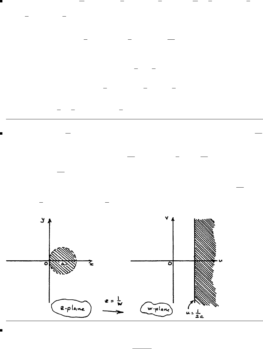
Glyn James, Advanced Modern Engineering Mathematics, 4th Edition 201
10 Putting z=1
win z+3
4+j=7
4gives
1
w+3
4+j=7
4or
1+3
4+jw=7
4|w|which, writing w=u+jv and expanding, gives
1+3
4u−v2
+3
4v+u2
=49
16 (u2+v2)
or, on rearranging gives
u2+v2−u+4
3v−2
3=0
u−1
22
+v+2
32
=7
62
a circle centre 1
2,−2
3and radius 7
6.
11 Putting z=1
win |z−a|=agives |1−aw |=a|w|from which u=1
2a
can be obtained (on writing w=u2+v2).
Hence |z−a|=amaps to Re{w}=1
2aunder w=1
z···=1
2a;thatis,thehalf
plane Re{w}>1
2a.
Moreover, the interior of |z−a|=amaps to right of the line Re{w}=1
2a.The
point z=1
2amapping to w=2
aconfirms this.
12 The general bilinear mapping is
w=az +b
cz +d
with z=0,w =j⇒b=jd,
c
Pearson Education Limited 2011

202 Glyn James, Advanced Modern Engineering Mathematics, 4th Edition
z=−j, w =1⇒d−jc =b−ja
and z=−1,w=0⇒a=b
Hence b=a, d =−ja and c=ja
and the mapping is
w=z+1
j(z−1)
Making zthe subject of this formula, we obtain
z=jw +1
jw −1
Writing z=x+jy, w =u+jv and equating real and imaginary parts
x=u2+v2−1
u2+(v+1)
2,y=−2u
u2+(v+1)
2
Lines x= constant = k, say, transform to
k[u2+(v+1)
2]=u2+v2−1
or u2+v2+2k
k−1v=−1
k−1
This can be rewritten as
u2+v+k
k−12
=k
(k−1)2−1
k−1=1
(k−1)2
which are circles (except k=1 whichis v=−1).
Lines y= constant = l,say,transformto
u2+(v+1)
2+2u
l=0
or u+1
l2
+(v+1)
2=1
l2
which are circles (except l=0 whichis u=0).
c
Pearson Education Limited 2011
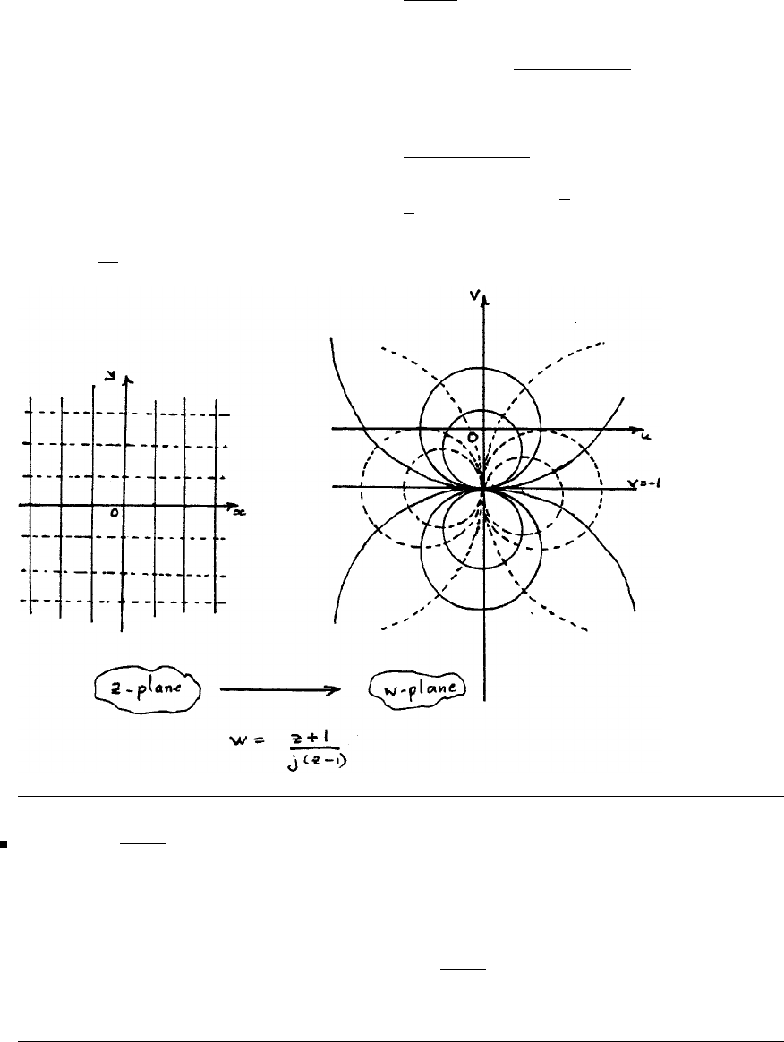
Glyn James, Advanced Modern Engineering Mathematics, 4th Edition 203
The fixed points are given by
z=z+1
jz −j
or jz2−(j+1)z−1=0
z=(j+1)±(j+1)
2+4j
2j
=(j+1)±√6j
2j
=1
2(j−1)(−1±√3)
(since √6j=±(1 + j)√3).
13 w=1+j
z
13(a)
z=1⇒w=1+j
z=1−j⇒w=1+j
1−j=j
z=0⇒w=∞
c
Pearson Education Limited 2011

204 Glyn James, Advanced Modern Engineering Mathematics, 4th Edition
13(b) |w|=|1+j|
|z|=√2
|z|
so that |z|=√2
|w|<1⇒| w|>√2
that is, interior of the unit circle maps to the exterior of the circle, centre as the
origin and radius √2.
13(c) z=1+j
w
⇒x+jy =(1 + j)
u2+v2(u−jv)sothat
x=u+v
u2+v2,y=u−v
u2+v2
Therefore x=ycorresponds to v= 0 (the real axis) and x+y= 1 corresponds
to 2u
u2+v2=1 thatis (u−1)2+v2= 1 a circle, centre (1.0) and radius 1.
13(d) The fixed point of the mapping is given by z2=1+j. Using the polar
form 1 + j=√2eπj/4,soz=±21/4eπj/8
14 The bilinear transformation
w=z+1
z−1
Writing z=x+jy, w =u+jv and equating real and imaginary parts gives
u=x2+y2−1
(1 + x)2+y2,v=2y
(1 + x)2+y2
Hence, all points on the circle x2+y2= 1 correspond to u=0.
From the point (0,−1) to the point (0,1) on the circle x2+y2=1weuse
the Parameterization x=cosθ, y =sinθ, π/2≤θ≤3π/2. Using v=
2y
(1 + x)2+y2=2y
1+x2+y2+2xwe note that v=y
1+xon x2+y2=1,sothat
v=sin θ
1+cosθ=2sin 1
2θcos 1
2θ
2cos
21
2θ=tan1
2θand between θ=π
2and θ=3π
2,tan 1
2θ
ranges from 1 to ∞and from −∞ to −1 hence |v|≥ 1.
c
Pearson Education Limited 2011
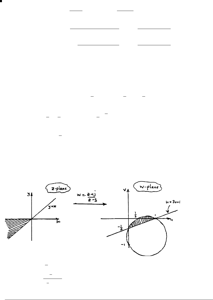
Glyn James, Advanced Modern Engineering Mathematics, 4th Edition 205
15(a) With w=u+jv and z=x+jy
The transformation w=z+j
z−3implies z=3w+j
w−1from which we deduce that
x=3(u2+v2)−3u+v
(u−1)2+v2,y=u−3v−1
(u−1)2+v2
and u=x2+y2−3x+y
(x−3)2+y2,v=x−3y−3
(x−3)2+y2
The line y= 0 corresponds to the line u−3v−1=0 inthe wplane. The line
x=ycorresponds to the curve
3(u2+v2)−3u+v=u−3v−1
that is,u−2
32
+v+2
32
=5
9(1)
a circle centre 2
3,−2
3and radius 1
3√5inthewplane.
The origin in the zplane (the intersection of the line y=0andx=y) corresponds
to the point w=−j1
3in the wplane. The point at infinity in the zplane (the
other ‘intersection’) corresponds to the point w=1 inthe wplane.
The origin (in the wplane) lies outside the circle (1), and is also outside the wedge
shaped region in the zplane (z=−j3 is its image).
So, the following figure can be drawn:
The point w=2
3lies inside the shaded region in the wplane, and corresponds to
the point z=3·2
3+j
2
3−1=−3(2 + j)=−6−3jinside the shaded region of the z
plane. (This is a useful check.)
c
Pearson Education Limited 2011
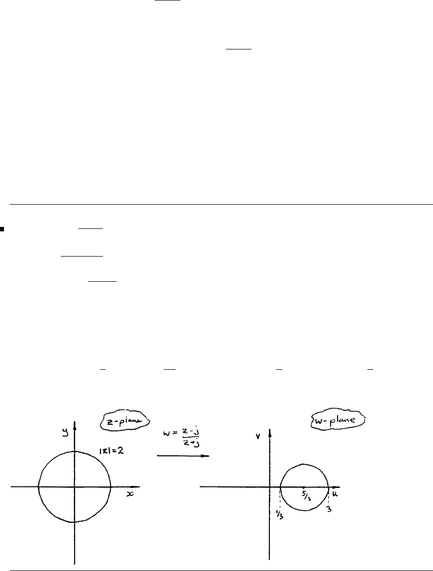
206 Glyn James, Advanced Modern Engineering Mathematics, 4th Edition
15(b) The fact that w= 1 does not correspond to any finite value of zhas
already been established.
Consider the equation w=z+j
z−3.
Taking the modulus of both sides gives
|w|=
z+j
z−3
If |w|=1⇒| z+j|=|z−3|
or x2+(y+1)
2=(x−3)2+y2
x2+y2+2y+1=x2−6x+9+y2
so that,2y=−6x+8
or y+3x=4
Hence the unit circle in the wplane, |w|= 1, corresponds to the line y+3x=4.
16 If w=z−j
z+j
then z=−wj −j
w−1
so that |z|=
w+1
w−1.
So if |z|=2,|w+1|=2|w−1|
or (u+1)
2+v2=4(u−1)2+4v2
which simplifies to
u−5
32
+v2=16
9,a circle centre 5
3,0and radius 4
3
c
Pearson Education Limited 2011

Glyn James, Advanced Modern Engineering Mathematics, 4th Edition 207
17 If w=ejθ0z−z0
z−z∗
0
then,
taking modulus
|w|=
z−z0
z−z∗
0since |ejθ0|=1
If zis real (i.e. zis on the real axis) then
|z−z0|=|z−z∗
0|=(x−x0)2+y2
01/2and z0=x0+jy0
Hence |w|= 1. Thus the real axis in the zplane corresponds to the unit circle
|w|=1 inthe wplane. Making zthe subject of the transformation gives
z=wz∗
0−ejθ0z0
w−ejθ0
Hence the origin in the wplane maps to z=z0.
Thus the inside of the unit circle in the wplane corresponds to the upper half of
the zplane provided
Im{z0}>0
Since w=0mapsto z=z0and z0=jand z=∞maps to w=ejθ0=−1it
gives θ0=π.
18 For the transformation
w=2jz
z+j
the fixed points are given by
z=2jz
z+j
z2+jz =2jz
or z(z−j)=0,z=0orj
Hence circular arcs or straight lines through z=0,j are transformed to circular
arcs or straight lines through w=0,j by the properties of bilinear transformation
(section 4.2.4).
The inverse transformation is
z=jw
2j−w
c
Pearson Education Limited 2011

208 Glyn James, Advanced Modern Engineering Mathematics, 4th Edition
|z−1
2|<1
2becomes
jw
2j−w−1
2<1
2which simplifies to |w−1|<1(use
w=u+jv and split into real and imaginary parts).
Similarly, |z−1
2|<1
2becomes |w−4
3|>2
3
19 The general bilinear mapping is
w=az +b
cz +d
if w= 0 corresponds to z=z0then
w=(z−z0)ejθ0
cz +d
If, additionally, |w|=1 ismappedto |z|=1 then
z−z0
cz +d=1 andtheinverse
of z0is also mapped to the inverse of w=0 thatis, w=∞.
Hence cz +dcan be replaced by z∗
0z−1 giving the mapping as
w=ejθ0z−z0
z∗
0z−1
where θ0is any real number.
Exercises 4.2.7
20 Under the mapping w=z2,u=x2−y2,v =2xy
It is not possible to achieve formulae of the type x=φ(u, v),y=ψ(u, v), however
we can use u=x2−y2,v=2xy to determine images. Points (0 + j0),(2 + j0)
and (0 + j2) transform to (0 + j0),(4 + j0) and (−4+j0) respectively.
The positive real axis y=0,x ≥0 transforms to the (positive) real axis
v=0,u =x2.
The positive imaginary axis x=0,y ≥0 transforms to the (negative) real axis
v=0,u =−y2.
The line joining the point 2 + j0to the point 0 + j2has equation x+y=2.
By using the equations u=x2−y2and v=2xy we obtain
u=4(1−y),v=2y(2 −y)
from which, eliminating ywe get
8v=16−u2
c
Pearson Education Limited 2011
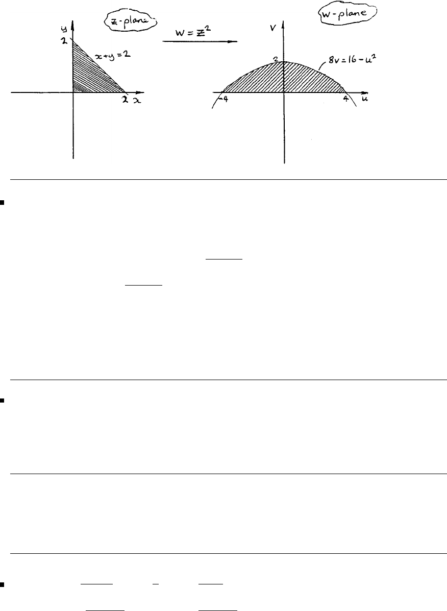
Glyn James, Advanced Modern Engineering Mathematics, 4th Edition 209
Hence we deduce the following picture:
21 Under the transformation w=z2,u=x2−y2and v=2xy.
Hence the line y=xtransforms to u=0,v >0
and the line y=−xtransforms to u=0,v< 0.
The line y=mx transforms to v=2m
1−m2u.
Putting m=tanθ0,2m
1−m2=tan2θ0.
Hence y=xtan θ0transforms to v=utan 2θ.
Thus lines through the origin of slope θ0in the zplane transform to lines through
the origin of slope 2θ0in the wplane. Hence the angle between the lines through
theorigininthezplane is doubled by the transformation w=z2.
22 w=zn
Writing z=rejθ,w=rnenjθ
22(a) Circles |z|=rare transformed to circles |w|=rn
22(b) Straight lines passing through the origin intersecting with angle θ0are
θ=kand θ=k+θ0. These are transformed to w=rnenjk and w=rnenj(k+θ0)
that is, lines φ=nk and φ=nk +nθ0as required.
23 If w=1+z2
z=z+1
z=z+z∗
|z|2
then u=x+x
x2+y2and v=y−y
x2+y2
c
Pearson Education Limited 2011

210 Glyn James, Advanced Modern Engineering Mathematics, 4th Edition
If |z|=r,thenu=x1+ 1
r2and v=y1−1
r2
x=r2u
r2+1 ,y=r2v
r2−1
Squaring and adding gives r2u
r2+1
2
+r2v
r2−1
2
=r2(r=1) (I).
If r=1 and v=0,|x|≤ 1 (because x2=1−y2)andu=2x. Hence the image
of the unit circle |z|=1,thatis, −2≤u≤2,v= 0 and the portion of the real
axis in the wplane is between −2and+2.
The curves (I) are ellipses, major axis 1+r2
r2and minor axis |r2−1|
r2if ris
very large, and both of these quantities tend to 1. Hence the image curve Itends
to a circle u2+v2=r2.
Exercises 4.3.3
24(a)
zez=(x+jy)ex+jy
=ex(x+jy)(cos y+jsin y)
=ex(xcos y−ysin y)+jex(ycos y+xsin y)
so u=(xcos y−ysin y)ex,v=(ycos y+xsin y)ex
We need to check the Cauchy–Riemann equations
∂u
∂x =(xcos y−ysin y+cosy)ex
∂u
∂y =(−xsin y−ycos y−sin y)ex
∂v
∂x =(ycos y+xsin y+siny)ex
∂v
∂y =(−ysin y+cosy+xcos y)ex
Hence ∂u
∂x =∂v
∂y and ∂u
∂y =−∂v
∂x
Thus the Cauchy–Riemann equations are valid and
d
dz(zez)=(z+1)ez
c
Pearson Education Limited 2011

Glyn James, Advanced Modern Engineering Mathematics, 4th Edition 211
24(b) Following the same procedure as in (a), we deduce that sin 4zis analytic
with derivative 4 cos 4z.
24(c) This time, zz∗=x2+y2which is real.
Obviously, therefore, ∂u
∂x(= 2x)=∂v
∂y(= 0).
Thus zz∗is not analytic.
24(d) Similarly to part (a), cos 2zis analytic with derivative −2sin2z.
25 w=x2+ay2−2xy +j(bx2−y2+2xy)=u+jy
∂u
∂x =2x−2y, ∂u
∂y =2ay −2x
∂v
∂x =2bx +2y, ∂v
∂y =−2y+2x
The Cauchy–Riemann equations are ∂v
∂x =−∂u
∂y ,∂v
∂y =∂u
∂x .
The second is satisfied and the first only holds if a=−1,b =1.Sincew(z)=
w(x+jy) we simply put y= 0 which gives w(x)=x2+jx2and hence w(z)=z2+jz2
and dw
dz =2(1+j)z
26 With u=2x(1 −y)=2x−2xy
∂u
∂x =2−2y, ∂u
∂y =−2x
The Cauchy–Riemann equations demand
∂v
∂y =2−2y, ∂v
∂x =2x
Integrating and comparing, these give
v=x2−y2+2y+C(take C=0)
Form u+jv =2x−2xy +j(x2−y2+2y)=w(z).
c
Pearson Education Limited 2011

212 Glyn James, Advanced Modern Engineering Mathematics, 4th Edition
Since z=x+jy, if we put y= 0, we can find w(x) which will give the functional
form of w.Thus
w(x)=2x+jx2
Hence w(z)=2z+jz2
27 φ(x, y)=ex(xcos y−ysin y)
∂φ
∂x =ex(xcos y−ysin y+cosy)
∂φ
∂y =ex(−xsin y−ycos y−sin y)
∂2φ
∂x2=ex(xcos y−ysin y+2cosy)
∂2φ
∂y2=ex(−xcos y+ysin y−2cosy)
hence ∂2φ
∂x2+∂2φ
∂y2=0 and φis harmonic.
Writing z=φ(x, y)+jψ(x, y), the Cauchy–Riemann equations demand
∂ψ
∂x =−∂φ
∂y =ex(xsin y+ycos y+siny)
∂ψ
∂y =∂φ
∂x =ex(xcos y−ysin y+cosy)
Integrating ∂ψ
∂x with respect to x(using integration by parts for the first term)
gives ψ=ex(xsin y+ycos y)+f(y). Examining φ(x, y) demands that f(y)=0
because all terms will be multiplied by ex.
Hence w(z)=φ(x, y)+jψ(x, y)=ex(xcos y−ysin y)+jex(xsin y+ycos y)and
w(x+j0) = w(x)=xex. Hence w(z)=zez.
28 Here we have u(x, y)=sinxcosh y
so that ∂u
∂x =cosxcosh yand ∂u
∂y =sinxsinh y
hence ∂2u
∂x2=−sin xcosh yand ∂2u
∂y2=sinxcosh y
so that ∇2u=∂2u
∂x2+∂2u
∂y2=0 and uis harmonic.
c
Pearson Education Limited 2011

Glyn James, Advanced Modern Engineering Mathematics, 4th Edition 213
Using the Cauchy–Riemann equations gives v=cosxsinh yso that u+jv =
w(z)=sinxcosh y+jcos xsinh y. Putting y=0 gives w(x+j0) = sin xso that
w(z)=sinz.
29 The orthogonal trajectories of a family of curves φ(x, y)=αare ψ(x, y)=β
where φand ψare conjugate functions: that is, φ(x, y)+jψ(x, y)=w(z)which
is an analytic function.
Proceeding as in the previous examples.
29(a) If φ(x, y)=x3y−xy3then ψ(x, y)= 1
4(x4+y4)−3
2x2y2
29(b) If φ(x, y)=e−xcos y+xy then ψ(x, y)=e−xsin y+1
2(x2−y2).
Hence the orthogonal trajectories are,
29(a) x4−6x2y2+y4=β,aconstant
29(b) 2e−xsin y+x2−y2=β,aconstant.
30(a) z2e2z
=(x+jy)2e2(x+jy)
=(x2−y2+2jxy)(e2x(cos 2y+jsin 2y))
=e2x((x2−y2)cos2y−2xy sin 2y)+je2x((x2−y2)sin2y+2xy cos 2y)
30(b) sin 2z
=sin(2x+j2y)
=sin2xcosh 2y+jcos 2xsinh 2y
Straightforward calculus reveals that both functions obey the Cauchy–Riemann
equations and are thus analytic. Their derivatives are (a) (2z2+2z)e2zand (b)
2cos2zrespectively.
31 Writing w=sin
−1zwe can say that
z=sinw=sin(u+jv)=sinucosh v+jcos usinh v
c
Pearson Education Limited 2011

214 Glyn James, Advanced Modern Engineering Mathematics, 4th Edition
so that, equating real and imaginary parts,
x=sinucosh v
and y=cosusinh v
Squaring and adding gives
x2+y2=sin
2ucosh2v+cos
2usinh2v
=sin
2ucosh2v+(1−sin2u)(cosh2v−1)
=sin
2u+cosh
2v−1
from which
x2+y2+1=sin
2u+x2
sin2u(I)
Solving for sin2ugives
sin2u=1
2(1 + x2+y2)−1
2(1 + x2+y2)2−4x2
where the minus sign is taken, since with u=π/2 (i.e. x=coshv, y =0)
inconsistencies result otherwise. From cosh2v=x2
sin2uwe obtain
cosh2v=1
2(1 + x2+y2)+1
2(1 + x2+y2)2−4x2
(This is most easily found by solving equation (I) for 1
sin2uthen using cosh2v=
x2
sin2u.)
Square rooting and inverting give uand vin terms of xand y.Itcanbeshown
that the expression under the square root sign is positive, for 1 + x2+y2−2x=
(x−1)2+y2≥0 for all real xand ythus (1+ x2+y2)2≥4x2. Hence w=sin
−1z
is an analytic function with derivative 1
√1−z2.
32
|sin z|2=|sin xcosh y+jcos xsinh y|2
=sin
2xcosh2y+cos
2xsinh2y
=cosh
2y−cos2x=sinh
2y+sin
2x
The result follows immediately from the last two expressions.
c
Pearson Education Limited 2011

Glyn James, Advanced Modern Engineering Mathematics, 4th Edition 215
Exercises 4.3.5
33 Mappings are not conformal at the points where dw
dz =0
33(a) dw
dz =2z=0 whenz=0. z= 0 is the only point where the mapping
fails to be conformal.
33(b) dw
dz =6z2−42z+72=0 when z2=7z+ 12 = 0 that is, non-conformal
points are z=4,z =3 (bothreal).
33(c) dw
dz =8−1
z3=0whenz3=1
8giving 1
2,1±j√3
4as non-conformal
points.
34 Proceeding as in Example 4.13, the mapping
w=z−1
z
has a fixed point at z=∞, is analytic everywhere except at z= 0 and conformal
except where dw
dz =0
that is,1+ 1
z2=0,z=±j
Since both of these occur on the imaginary axis, consideration of this axis is
adequate to completely analyse this mapping.
The image of z=jis w=2j, and the image of z=−jis w=−2j.Writing
z=j+jε, ε real, we find that
w=jε −1
j+jε
=j[1 + ε−(1 + ε)−1]
=j[1 + ε+1−ε+ε2+...]
j[2 + ε2]
So, no matter whether ε>0orε<0, the image point of z=j+jε is above
w=j2 on the imaginary axis.
c
Pearson Education Limited 2011
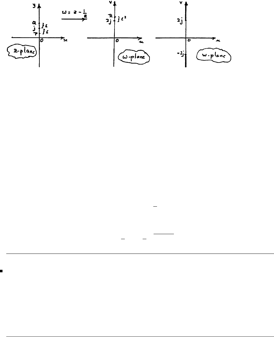
216 Glyn James, Advanced Modern Engineering Mathematics, 4th Edition
that is, points Q and P in the zplane both map to R in the wplane in a manner to
Example 4.13, the non-conformality of z=±jis confirmed and as the imaginary
axis (in the zplane) is traversed from −jz to 0, the imaginary axis (in similar the
wplane) is traversed from −jz to −j2 and back to −j∞(when z=−j, w reaches
−j2). Similarly, as the imaginary axis (in the zplane) is traversed from +j∞to
0, the imaginary axis (in the wplane) is traversed from +j∞to +j2 and back to
+j∞again.
Finally, points on the imaginary axis in the wplane such that w=aj, −2<a<2,
do not arise from any points on the imaginary axis in the zplane. This point is
obvious once one solves
aj =z−1
z
to obtain
z=1
2aj ±1
2√4−a2
35 If w=ez
then u=excos yand v=exsin y
Hence the expressions u2+v2=e2xand v=utan ycan be derived.
35(a) 0≤x<∞is mapped to the exterior of the unit circle u2+v2=1
35(b) 0≤x≤1 is mapped to the annulus 1 ≤u2+v2≤e2
0≤y≤1 is mapped to the region between the radiating lines v=0and
v=utan 1.
c
Pearson Education Limited 2011
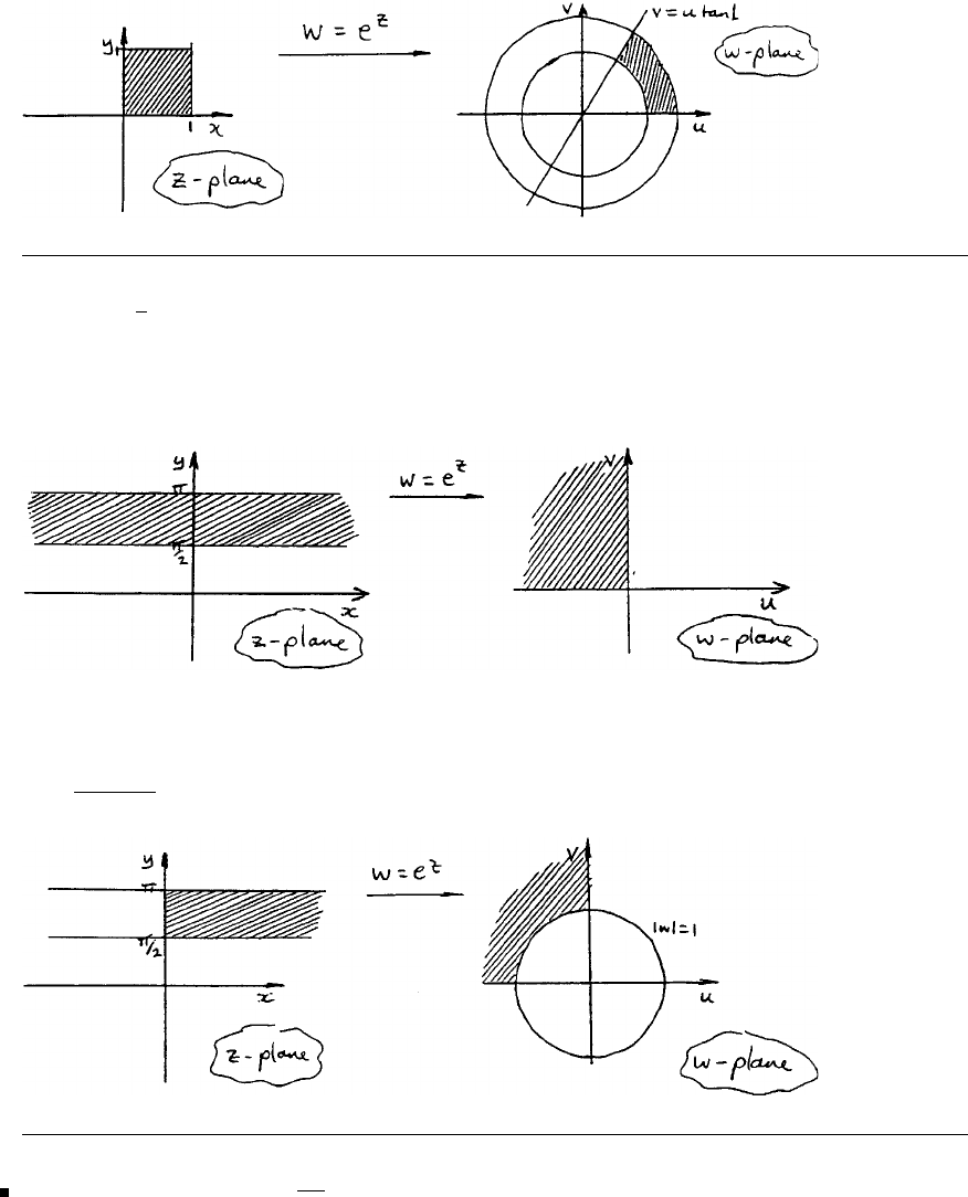
Glyn James, Advanced Modern Engineering Mathematics, 4th Edition 217
35(c) 1
2π≤y≤πis mapped to the region between u=0(v>0) and
v=0(u<0)
that is,
Thus if 0 ≤x<∞then the image region in the wplane is in the shaded quadrant,
but outside the unit circle.
36 If w=sinzthen dw
dz =cosz.
Since cos z=0 when z=(2n+1)π/2 these are the points where the mapping is
not conformal
w=sinz⇒u+jv =sinxcosh y+jcos xsinh y
c
Pearson Education Limited 2011
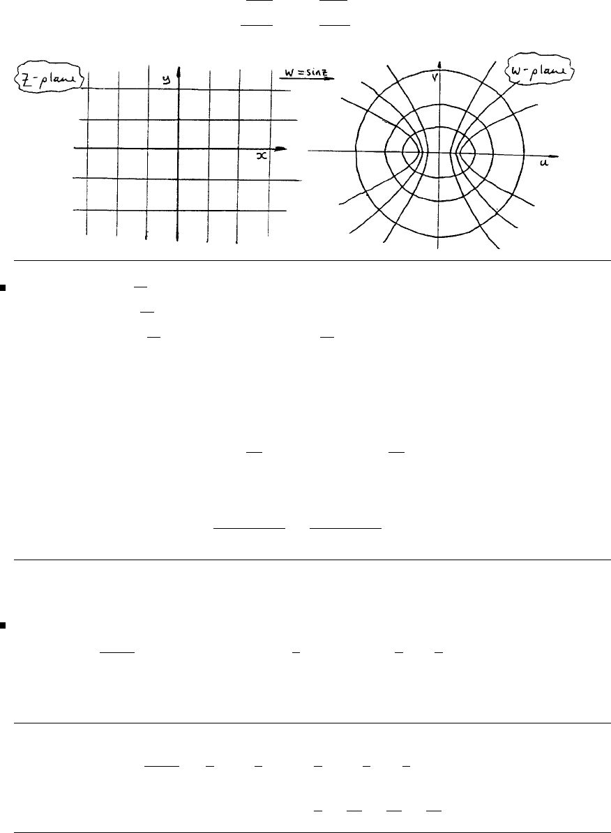
218 Glyn James, Advanced Modern Engineering Mathematics, 4th Edition
Hence v=sinxcosh y, v =cosxsinh y
thus lines x=ktransform to u
sin k2−v
cos k2= 1 (hyperbolae)
and lines y=ktransform to u
cosh l2+v
sinh l2= 1 (ellipses)
37 If z=ζ+a2
ζandζ=Rejθ
then z=Rejθ +a2
Re−jθ
so that x=R+a2
Rcos θand y=R−a2
Rsin θ.
If R=a, x =2acos θand y= 0 then the real line between ±2ais traversed.
Length of line segment = 4a.
For a circle of radius b,
x=b+a2
bcos θ, y =b−a2
bsin θ
Hence the image in the zplane is an ellipse of the form
b2x2
(a2+b2)2+b2y2
(b2−a2)2=1
Exercises 4.4.2
38(a) 1
z−j=(z−j)−1=j1−z
j−1=j1+z
j+z
j2+...
=j+z−jz2−z3+jz4...
38(b)
1
z−j=1
z1−j
z−1
=1
z1+ j
z+j
z
2
+...
=1
z+j
z2−1
z3−j
z4+...
c
Pearson Education Limited 2011

Glyn James, Advanced Modern Engineering Mathematics, 4th Edition 219
38(c) In order that |z−1−j|<√2wewrite
1
z−j=1
z−1−j+1 =(1+z−1+j)−1
=1−(z−1−j)+(z−1−j)2−(z−1−j)3+...
Which is valid inside |z−1−j|<|1−j|=√2.
39 1
z2+1 =(z2+1)
−1=1−z2+z4−z6+...
where |z|<1.
Using the fact that we can differentiate power series term-by-term and the radius
of convergence remains unaltered
−2z
(z2+1)
2=−2z+4z3−6z5+...
so
39(a)
1
(z2+1)
2=1−2z2+3z4−4z6+5z8+...
|z|<1
Operating on 1
(z2+1)
2in a similar fashion gives
−4z
(z2+1)
3=−4z+12z3−24z5+40z7...
so
39(b)
1
(z2+1)
3=1−3z2+6z4−10z6+15z8+...
|z|<1
c
Pearson Education Limited 2011

220 Glyn James, Advanced Modern Engineering Mathematics, 4th Edition
Exercises 4.4.4
40 Taylor’s theorem is
f(z)=f(a)+(z−a)f(a)+ (z−a)2
2! f(a)+...
We thus compute f(z) and its first few derivatives then evaluate them at z=a.
40(a)
f(z)= 1
1+z,f
(z)=−1
(1 + z)2,f
(z)= 2
(1 + z)3and f(z)=−6
(1 + z)4
Hence
f(1) = 1
2,f
(1) = −1
4,f
(1) = 2
8=1
4and f(1) = −3
8
thus 1
1+z=1
2−1
4(z−1) + 1
8(z−1)2−1
16 (z−1)3+...
The radius of convergence is the distance between the nearest singularity of f(z)
to the point about which the expansion is made. The point z=−1istheonly
singularity and the distance between this and z= 1 is 2 (along the real axis).
40(b)
f(z)= 1
z(z−4j)=j
41
z−1
z−4jusing partial fractions
f(z)= j
4−1
z2+1
(z−4j)2f(1) = 1
4;f(1) = 0
f(z)= j
4−2
z3+2
(z−4j)3f(1) = −1
8;f(1) = 0
f(z)= j
4−6
z4+6
(z−4j)4fiv(1) = +3
8;fv(1) = 0
fiv(z)= j
4−24
z4+24
(z−4j)5fvi(1) = −45
16
fv(z)= j
4−120
z6+120
(z−4j)6etc.
c
Pearson Education Limited 2011

Glyn James, Advanced Modern Engineering Mathematics, 4th Edition 221
Thus
1
z(z−4j)=1
4−1
16 (z−2j)2+1
64 (z−2j)4−1
256 (z−2j)6+...
The radius of convergence is 2 since z=2jis 2 from the singularities at z=0 and
z=4j.
40(c) f(z)= 1
z2
gives f(z)=−2
z3,f
(z)= 6
z4and f(z)=−24
z5.
Putting z=1+jgives
f(1 + j)=−j
2,f
(1 + j)=−2
(1 + j)3=1+j
2
f(1 + j)= 6
(1 + j)4=3
2and f(1 + j)=−24
(1 + j)5=−3(1 −j)
Hence
1
z2=−j
2+1
2(1 + j)(z−1−j)+3
4(z−1−j)2−1
2(1 −j)(z−1−j)3+...
The radius of convergence is the distance between the origin (a double pole) and
1+jthat is, √2.
41 With f(z)= 1
1+z+z2
we could use the binomial expansion
f(z)=(1+z+z2)−1gathering terms to O(z3)
This is certainly more efficient than using the derivatives of f(z). However, the
best way is to use the fact that (z3−1) = (z−1)(z2+z+1). That is
1
1+z+z2=z−1
z3−1=1−z
1−z3
=(1−z)(1 −z3)−1
c
Pearson Education Limited 2011

222 Glyn James, Advanced Modern Engineering Mathematics, 4th Edition
=1−z+z3...
to order z3
valid in the region |z|<1.
42 If f(z)= 1
z4−1the singularities are at the points where z4=1thatis,
z=1,−1,−jand j. The radii of convergence are the minimum distances of the
points z=0,1+jand 2 + j2 from these singularities.
z= 0 is equidistant (1) from each radius of convergence = 1.
z=1+jis distance (1) from z=1 and z=jwith radius of convergence = 1.
z=z+j2isadistance|2+j2−1|from 1 and a distance |2+j2−j|from j.
Both of these distances = [22+(2−1)2]1/2=√5.
43 If f(z)=tanzthen f(z)=sec
2(z)andf =2sec
2ztan zbut subsequent
derivatives get cumbersome to compute (except by using a Computer Algebra
package). Since tan z=sin z
cos z, we can use the series for sin zand cos zas follows:
tan z=z−z3
6+z5
120
1−z2
2+z4
24
=z1−z2
6+z4
120 1−z2
2−z4
24 −1
=z1−z2
6+z4
120 1+z2
2−z4
24 +z2
2−z4
24
2+...
=z+1
3z3+1
120 −1
12 −1
24 +1
4z5+...
tan z=z+1
3z3+2
15 z5+···
Since z=π/2 is the closest singularity, the radius of convergence is π
2.
Exercises 4.4.6
44 The function 1
z(z−1)2has a simple pole at z= 0 and a double pole at
z= 1. In order to find the Laurent expansions, we simply find the following
binomial expansions
c
Pearson Education Limited 2011

Glyn James, Advanced Modern Engineering Mathematics, 4th Edition 223
1
z(1 −z)−2=1
z(1 + 2z+3z2+4z3+...)
=1
z+2+3z+4z2+... about z=0
valid for 0 <|z|<1
and 1
(z−1)2(1−(1 −z))−1
=1
(z−1)2[1 + (1 −z)+(1−z)2+(1−z)3+...]
=1
(1 −z)2+1
1−z+1+(1−z)+(1−z)2+...
valid for 0 <|1−z|<1
45(a) With f(z)=z2sin 1
z, there is a singularity at z= 0 and another at
z=∞. Expanding sin 1
zas a power series in 1
zwe find
z2sin 1
z=z21
z−1
3!z3+1
5!z5−···
=z−1
3!z+1
5!z3−···
=···+1
5!z3−1
3!
1
z+z.
Since the principal part is infinite, there must be an essential singularity at z=0.
(b) Writing z=1
win order to investigate z=∞we obtain
z2sin 1
z=1
w2sin w=1
w2w−w3
3! +w5
5! −···
=1
w−w
3! +w3
5! −···
=z−1
z3! +1
z35! −···
which implies a simple pole at z=∞. (The expansion is the same as that about
z= 0, but re-interpreted.)
(c) At any other point z2sin 1
zis regular and has a Taylor series of the
form f(z)=a0+a1z+a2z2+.... specifically, about z=a, z2sin 1
z=
a2sin 1
a+a1z+a2z2+... where a1=f(a),a
2=f(a), etc.
c
Pearson Education Limited 2011

224 Glyn James, Advanced Modern Engineering Mathematics, 4th Edition
46 With f(z)= z
(z−1)(2−z)
there are simple poles at z=1 and z=2.
46(a) Inside the unit circle |z|= 1, therefore there is a Taylor series
z(1 −z)−1(2 −z)−1
=z
2(1 −z)−11−z
2−1
=z
2(1 + z+z2+z3+...)1+ z
2+z
22+z
23+···
=z
2+3
4z2+z
2z2+1
2z2+1
4z2+...
+z
2z3+1
2z3+1
4z3+1
8z3+...
=1
2z+3
4z2+7
8z3+15
16 z4+··· |z|<1
46(b) In the annulus 1 <|z|<2 we rearrange f(z) to obtain a Laurent series
as follows
z
(z−1)(z−2) =2
z−2−1
z−1=−1−z
2−1
−1
z1−1
z−1
=−1+ z
2+z2
4+···−1
z1+1
z+1
z2+···
=...−1
z3−1
z2−1
z−1−z
2−z2
4−···
46(c) For |z|>2 we rearrange as follows
z
(z−1)(z−2) =2
z−2−1
z−1
=2
z1−2
z−1
−1
z1−1
z−1
=2
z1+2
z+4
z2+8
z3+···−1
z1+1
z+1
z2+1
z3+···
=1
z+3
z2+7
z3+15
z4+···
46(d) For |z−1|>1wewrite 1
z−1=wand find a Taylor’s series in w.
If w=1
z−1then wz −w=1 or z=1+w
w
c
Pearson Education Limited 2011

Glyn James, Advanced Modern Engineering Mathematics, 4th Edition 225
so that z
(z−1)(z−2) =w1+w
1−w
=w(1 + w)(1 + w+w2+w3+...)
=w+2w2+2w3+...
=1
z−1+2
(z−1)2+2
(z−1)3+···
46(e) For 0 <|z−2|<1wewritew=z−2 hence
z
(z−1)(z−2) =w+2
w(w+1) =1+ 2
w(1 + w)−1
=1+ 2
w(1 −w+w2−w3+...)
=2
w−1+w−w2+w3−...
=2
(z−2) −1+(z−2) −(z−2)2+(z−2)3...
Exercises 4.5.2
47 The point at infinity is ignored in this question. Most if not all can be found
immediately by inspection.
47(a) cos z
z2: double pole at z= 0, zeros whenever cos z=0thatis,
z=1
2(2n+1)π, n = integer.
47(b) 1
(z+j)2(z−j): has a double pole at z=−j, a simple pole at z=j
and no zeros in the finite zplane.
47(c) z
z4−1: simple poles at z4=1 thatis, z=1,−1,j,−jand a zero at
z=0.
47(d) cosh z: since coth z=cosh z
sinh zthis has simple poles at those points where
z=jnπ and zero at those points where z=1
2j(2n+1)π, n =
integer.
c
Pearson Education Limited 2011

226 Glyn James, Advanced Modern Engineering Mathematics, 4th Edition
47(e) sin z
z2+π2: simple poles at z=±jπ and zeros at z=nπ, n = integer.
47(f) ez/(1−z): this has an essential singularity at z= 1 and no zeros.
47(g) z−1
z2+1 : this has simple poles at z=±jand a zero at z=1.
47(h) z+j
(z+2)
3(z−3) : this has a triple pole at z=−2,asimplepoleatz=3
and a zero at z=−j.
47(i) 1
z2(z2−4z+5) : this has simple poles at z2−4z+5 = 0, that is,
z=5,−1 and a double pole at z=0.
48(a) 1−cos z
z2.In order to investigate this, we expand cos z.Onlyz=0 isa
possible (finite) singularity
1−1−z2
2! +z4
4! −···
z2=1
2! −z2
4! +···
The RHS is a power series, thus the singularity at z=0 isremovable.
48(b) ez2
z3.Using the power series for ez2gives the expansion
ez2
z3=1
z31+z2+z4
2! +···
=1
z3+1
z+z
2! +···
z= 0 is thus a pole of order 3.
48(c) 1
zcosh 1
z. Obviously the point z=0 isaproblem.
1
z1+ 1
z22! +1
z44! +···is the Laurent series which indicates that z=0isan
essential singularity.
c
Pearson Education Limited 2011

Glyn James, Advanced Modern Engineering Mathematics, 4th Edition 227
48(d) tan−1(z2+2z+ 2). For this problem the easiest way to proceed is to find
the Maclaurin series from first principles. At z=0,tan−1(z2+2z+2)=tan
−12
which is finite. This means that z= 0 is a regular point, hence it is not actually
necessary to find the Laurent series (in this case Maclaurin series) for the function.
In fact
tan−1(z2+2z+2)=tan
−12+2
5z−6
25 z2+···
49 If f(z)=p(z)
q(z)where p(z)andq(z) are polynomials, then the only singularities
of f(z) are the algebraic zeros of q(z). These zeros are either distinct or multiple.
The distinct zeros give rise to simple poles of f(z) whereas the multiple zeros give
rise to poles of higher order. f(z) can only have these kinds of singularity, although
it may have none if qdivides p,sothatf(z) is polynomial. f(z) therefore cannot
have an essential singularity.
Exercises 4.5.4
50(a) 2z+1
(z2−z−2) =2z+1
(z−2)(z+1) hence the singularities are simple poles at
z=2,z =−1.
Using the formula residue = lim
z→z0
[(z−z0)f(z)] the residues are 5
3at z=2 and 1
3
at z=−1.
50(b) 1
z2(1 −z)has a simple pole at z= 1 and a double pole at z=0.
The residue at z= 1 is lim
z→1−1
z2=−1
1
z2(1 −z)=1
z2(1 + z+z2+...)= 1
z2+1
z+1+···
Hence the residue at z=0 is1.
c
Pearson Education Limited 2011

228 Glyn James, Advanced Modern Engineering Mathematics, 4th Edition
50(c) 3z2+2
(z−1)(z2+9) =3z2+2
(z−1)(z+j3)(z−j3)
Hence there are simple poles at z=1,j3,−j3
At z=1,residue = 3+2
(1 + j3)(1 −j3) =5
10 =1
2
at z=j3,residue = −3×9+2
(j3−1)j6=−25
6(−3−j)=5
12 (3 −j)
at z=−j3,residue = 5
12 (3 + j) by symmetry.
50(d) z3−z2+z−1
z3+4z=z3−z2+z−1
z(z+j2)(z−j2) =(z−1)(z2+4)
z(z+j2)(z−j2)
which has simple poles at z=0,j2,−j2.
At z=0,residue = −1
4
at z=j2,residue = lim
z→j2
(z−1)(z2+4)
(z+j2) =3
8(−1+2j)
at z=−j2,residue = 3
8(−1−2j) similarly.
50(e) z6+4z4+z3+1
(z−1)5has a pole of order 5 at z=1.
The formula for calculating residues is convenient for this problem.
Residue = 1
4! lim
z→1
d4
dz4(z6+4z4+z3+1)
=1
24 (6.5.4.3+4.4.3.2)
=456
24 =19
50(f) z+1
z−1
2
has a double pole at z=1.
Residue = lim
z→1
d
dz(z+1)
2=4
c
Pearson Education Limited 2011

Glyn James, Advanced Modern Engineering Mathematics, 4th Edition 229
50(g) z+1
(z−1)2(z+3) has a simple pole at z=−3 and a double pole at z=1.
Residue at z=−3is −1
8
Residue at z=1is d
dzz+1
z+3z=1 =1
8
50(h) 3+4z
z3+3z2+2z=3+4z
z(z+1)(z+2) has simple poles at z=−2,−1and0.
Residues are, respectively, −5
2,1and 3
2followingthesameprocedureaspart(c).
51(a) Thepoleof cos z
zat z= 0 is simple, thus the residue is cos(0) = 1.
51(b) The poles of sin z
z4+z2+1 are all simple, and the residue at z=eπj/3is
lim
z→eπj/3(z−eπj/3)sin z
z4+z2+1 =sineπj/3lim
z→eπj/3z−eπj/3
z4+z2+1
Using L’Hˆopital’s rule, the limit is
1
4eπj +2eπj/3
=1
−4+2
1
2+j√3
2=1
−3+j√3=1
12 (−3−j√3)
giving the residue −1
12 (3 + j√3) sin 1
2(1 + j√3)
51(c) The pole of z4−1
z4+1 at z=eπj/4is simple and we proceed as in the last
part. The residue is
−2 lim
z→eπj/4z−eπj/4
z4+1
=−21
4e3πj/4=−1
2
1
−1
√2+j1
√2
=1
21
√2+j
√2.
Hence the residue is √2
4(1 + j).
c
Pearson Education Limited 2011

230 Glyn James, Advanced Modern Engineering Mathematics, 4th Edition
51(d) z
sin zhas a simple pole at z=π
Residue = πlim
z→πz−π
sin z=−π.
51(e) 1
(z2+1)
2has a double pole at z=j
Residue = lim
z→j
d
dz(z−j)21
(z−j)2(z+j)2
= lim
z→j−2
(z+j)3
=−2
8j3=−j
4.
52(a) cos z
z3has a triple pole at z=0.
cos z
z3=1
z3−1
2z+1
24 z−··· residue = −1
2
52(b) z2−2z
(z+1)
2(z2+4) has a double pole at z=−1.
Residue = d
dz
(z+1)
2(z2−2z)
(z+1)
2(z2+4) at z=−1
=(2z−2)(z2+4)−2z(z2−2z)
(z2+4)
2z=−1=−14
25
52(c) The function ez
sin2zhas a double pole wherever
sin z= 0 that is at z=nπ, n = an integer
In order to find the residue, we need to compute
lim
z→nπ
d
dz(z−nπ)2ez
sin2z
c
Pearson Education Limited 2011

Glyn James, Advanced Modern Engineering Mathematics, 4th Edition 231
Now d
dz(z−nπ)2ez
sin2z=ezd
dz(z−nπ)2
sin2z+(z−nπ)2
sin2zez(I)
and
d
dz(z−nπ)2
sin2z=2
z−nπ
sin z·d
dzz−nπ
sin z
=2(z−nπ)
sin z·sin z−(z−nπ)cosz
sin2z
As z→nπ, z−nπ
sin z→1and
sin z−(z−nπ)cosz
sin2z→cos z−cos z+(z−nπ)sinz
2sinzcos z(using L’Hˆopital’s rule)
→0asz→nπ
Hence the RHS of equation (I) →enπ as z→nπ.
Thus the residue is enπ .
Exercises 4.6.3
53
C
(z2+3z)dz with z=x+jy and dz =dx +jdy
hence (z2+3z)dz =(x2−y2+j2xy +3x+j3y)(dx +jdy)
=(x2−y2+3x)dx −(2xy +3y)dy
+j[(x2−y2+3x)dy +(2xy +3y)dx]
53(a) The straight line joining 2 + j0to0+j2 has equation x+y=2in
Cartesian coordinates. This has parametric equation x=tand y=2−tfrom
which dx =dt and dy =−dt, and using the above expression for (z2+3z)dz
(z2+3z)dz =(t2−(2 −t)2+3t)dt +(2t(2 −t)+3(2−t))dt
+j[−(t2−(2 −t)2+3t)dt +(2t(2 −t)+3(2−t))dt]
and the range of integration is from t=2 to t=0.
c
Pearson Education Limited 2011

232 Glyn James, Advanced Modern Engineering Mathematics, 4th Edition
Hence
C
(z2+3z)dz =0
2
(8t−2t2+2)dt
+j0
2
(−6t−2t2+ 10)dt
=4t2−2
3t3+2t
0
2+j−3t2−2
3t3+10t
0
2
so C
(z2+3z)dz =−44
3−j8
3
53(b) On the straight line from 2 + j0to2+j2,x =2 and ygoes from 0 to
2, so that dx =0.
Therefore
C1
(z2+3z)dz =2
0−(4t+3t)dt
+j2
0
(4 −t2+6)dt
=−7
2t2
2
0+j10t−1
3t3
2
0
=−14 + j52
3
On the straight line from 2 + j2to0+j2,y =2 and xgoes from 2 to 0, so that
dy =0.
Therefore
C2
(z2+3z)dz =0
2
(t2−4+3t)dt
+j0
2
(4t+6)dt
=1
3t3−4t+3
2t2
0
2+j2t2+3t0
2
=−2
3−j14
Thus
C
(z2+3z)dz =
C1
(z2+3z)dz +
C2
(z2+3z)dz =−44
3−j8
3.
c
Pearson Education Limited 2011

Glyn James, Advanced Modern Engineering Mathematics, 4th Edition 233
53(c) For this part, we use z=2ejθ on |z|=2andθvaries between 0 and π/2
on the quarter circle joining 2+j0to0+j2. Thus (z2+3z)dz =(4e2jθ+6ejθ)2jejθdθ
so that
C
(z2+3z)dz =π/2
08je3jθ +12je2jθdθ
=8
3e3jθ +6e2jθπ/2
0
=−8
3−6−8
3+6
=−8j
3−44
3
Hence the integrals are all the same.
54(a) On |z|=1,z=ejθ,0≤θ≤2π
so that (5z4−z3+2)dz
=2π
0
(5e4jθ −e3jθ +2)jejθdθ
=5
5e5jθ −1
4e4jθ +2ejθ2π
0
=0
hence e2πj =e0=1
54(b) Integrating around the square in the order 0 + j0,1+j0,1+j1and
0+j1givestheanswers11
4,3+ j
4,−11
4and −3−j
4. Adding these together gives
0.
54(c) On the parabola y=x2,x=tand y=t2so that z=t+jt2and
dz =(1+2jt)dt.
On the parabola y2=x, x =t2and y=tso that z=t2+jt and dz =(2t+j)dt.
The computation of
C
(5z4−z3+2)dz is extremely long winded but straightforward
and gives the answer 0.
55 In order to evaluate C
dz
(z−z0)n
c
Pearson Education Limited 2011

234 Glyn James, Advanced Modern Engineering Mathematics, 4th Edition
we surround the point z=z0with a circle of radius εon which z=z0+εejθ ,
0≤θ<2π.
Using equation (4.45) the integral around Cis the same as the integral around the
circle on which z=z0+εejθdθ.Thus
C
dz
(z−z0)n=2π
0
jεejθ
εnenjθ dθ
If n= 1, then the integral integrates to
jε(1−n)e(1−n)jθ
(1 −n)j2π
0
=0
as in Example 4.30.
If n=1,
C
dz
(z−z0)n=2π
0
jdθ =2πj
56(a) If z= 4 is outside C, by Cauchy’s theorem,
C
dz
z−4=0
56(b) If z= 4 is inside C,byproblem55
C
dz
z−4=2πj
57 In order to use Cauchy’s integral theorem, we split into partial fractions
2z
(2z−1)(z+2) =2/5
2z−1+4/5
z+2
57(a) If Cis the circle |z|=1
C
2zdz
(2z−1)(z+2) =2
5C
dz
2z−1+4
5C
dz
z+2
=2
5·2πj +4
5·0
c
Pearson Education Limited 2011

Glyn James, Advanced Modern Engineering Mathematics, 4th Edition 235
since z=1
2is inside |z|= 1 whereas z=−2 is outside. Hence C
2zdz
(2z−1)(z+2)
=4
5πj
57(b) If Cis the circle |z|= 3, both singularities (poles) are inside C,and
hence C
2zdz
(2z−1)(z+2) =2
52πj +4
5·2πj
=12
5πj
58 This follows a pattern similar to Exercise 57.
Using partial fractions gives
5z
(z+1)(z−2)(z+4j)=
5
51 (−1−4j)
z+1 +
1
3(1 −2j)
z−2+
2
17 (−2+9j)
z+4j
58(a) Only the first two poles (z=−1,z=2) areinside |z|= 3 hence
C
5zdz
(z+1)(z−2)(z+4j)=2πj5
51 (−1−4j)+1
3(1 −2j)
=4π
17 (9 + 2j)
58(b) All three poles are inside |z|= 5 hence
C
5zdz
(z+1)(z−2)(z+4j)=2πj5
51 (−1−4j)+1
3(1 −2j)
+2
17 (−2+9j)
=0
59 Equation (4.48) gives the general form of Cauchy’s integral theorem
C
f(z)
(z−z0)n+1 dz =2πj
n!f(n)(z0)
where Cis a contour enclosing the point z=z0.
c
Pearson Education Limited 2011

236 Glyn James, Advanced Modern Engineering Mathematics, 4th Edition
59(a)
C
z3+z
(2z+1)
3dz =1
8C
z3+z
(z+1
2)3dz
=1
8
2πj
2
d2
dz2−1
2
(z3+z)(z=−1
2is inside |z|=1)
=π
8j6(−1
2)=−3πj
8
59(b) First of all we need to separate the integrand using partial fractions
4z
(z−1)(z+2)
2=
4
9
z−1−
4
9
z+2+
8
3
(z+2)
2
Hence C
4zdz
(z−1)(z+2)
2=2πj 4
9−2πj4
9+0=0
using Cauchy’s integral theorem (the derivative of 8
3is of course zero). All poles
of the integrand are inside the circle |z|=3.
Exercises 4.6.6
60 z
z2+1 has poles at z=±j
60(a) Since z
z2+1 is regular inside |z|=1
2
C
zdz
z2+1 =0 if Cis the circle |z|=1
2
60(b) The residues of z
z2+1 at z=±j(both inside |z|=2)are
lim
z→+j
(z−j)z
(z+j)(z−j)= lim
z→+j
z
z+j=1
2
and
lim
z→−j
(z+j)z
(z+j)(z−j)= lim
z→−j
z
z−j=1
2
c
Pearson Education Limited 2011

Glyn James, Advanced Modern Engineering Mathematics, 4th Edition 237
Hence, using the residue theorem
C
zdz
z2+1 =2πj1
2+1
2=2πj
61 The singularities of z2+3jz −2
z3+9zare at z3+9z=0,thatis, z=0,3j, −3j
(all simple poles). Only z= 0 is inside |z|= 1 but all three are inside |z|=4.
Hence we shall find all the residues.
At z= 0, residue is lim
z→0z2+3jz −2
z2+9 =−2
9
At z=3j, the residue is
lim
z→3j
(z−3j)(z2+3jz −2)
z(z−3j)(z+3j)
=(3j)2+3j3j−2
3j(3j+3j)=−9−9−2
−18 =10
9
At z=−3j, the residue is
lim
z→−3j
(z+3j)(z2+3jz −2)
z(z−3j)(z+3j)
=(−3j)2+(3j)(−3j)−2
(−3j)(−3j−3j)=−−9+9−2
−18 =1
9
61(a) For this part, since only the residue at z= 0 is inside C(|z|=1)
∴C
z2+3jz −2
z3+9zdz =2πj−2
9=−4πj
9
61(b) For this part, all residues need to be taken into account since all the poles
of f(z)areinsideC(|z|=4)
∴C
z2+3jz −2
z3+9zdz =2πj−2
9+10
9+1
9=2πj
Note that in this case, all the zeros of the denominator were obviously poles. In
general, we would need to check if they were not removable by factorizing the
numerator.
c
Pearson Education Limited 2011

238 Glyn James, Advanced Modern Engineering Mathematics, 4th Edition
62 f(z)=(z2+2)(z2+4)
(z2+1)(z2+6) has poles at z=±j, z =±j√6.
Residue at z=jis
lim
z→j
(z−j)(z2+2)(z2+4)
(z−j)(z+j)(z2+6) =(−1+2)(−1+4)
2j(−1+6) =−3j
10
Residue at z=−jis
lim
z→−j
(z+j)(z2+2)(z2+4)
(z+j)(z−j)(z2+6) =(−1+2)(−1+4)
(−2j)(−1+6) =3j
10
Residue at z=j√6is
lim
z→j√6
(z−j√6)(z2+2)(z2+4)
(z−j√6)(z+j√6)(z2+1) =(−6+2)(−6+4)
2j√6(−6+1) =8
2j√6(−5)
=2
15 j√6
Residue at z=−j√6isthus=−2
15 j√6
62(a) The circle |z|= 2 contains the poles at z=±jbut not those at
z=±j√6. The sum of the residues inside C=−3j
10 +3j
10 =0.
Hence the integral = 0.
62(b) The circle |z−j|= 1 contains the residue only at z=j.
Hence C
(z2+2)(z2+4)
(z2+1)(z2+6)dz =2πj−3j
10 =3π
5
62(c) The circle |z|= 4 contains all the poles. Since the sum of the residues is
zero, so is the integral.
63 The function 1
z2(1 + z2)2has double poles at z=0 and z=±j.
Residue at z=0 is
d
dz1
(1 + z2)2z=0
=−4z
(1 + z2)3z=0
=0
c
Pearson Education Limited 2011

Glyn James, Advanced Modern Engineering Mathematics, 4th Edition 239
Residue at z=jis
d
dz1
z2(z+j)2z=j
=−2(2z+j)
(z2+jz)3=−3
4j
Residue at z=−jis 3
4j
63(a) If Cis the circle |z|=1
2, only the residue at z= 0 is in C.Thus
C
dz
z2(1 + z2)2=2πj(0) = 0
63(b) All the singularities are inside |z|= 2, but since they sum to 0,
C
dz
z2(1 + z2)2=0
64(a) The singularities of 3z2+2
(z−1)(z2+4) are at z=1,±2j.
They are all simple poles. Using the formula (4.37) the residues are :-
at z=1 : 1
at z=2j:1
8(2 −j)
at z=−2j:1
8(2 + j)
(i) If Cis |z−2|= 2 only the residue at z= 1 is included, hence
C
3z2+2
(z−1)(z2+4)dz =2πj
(ii) If Cis |z|= 4, all the residues are included, hence
C
3z2+2
(z−1)(z2+4)dz =5
2πj
64(b) The singularities of z2−2z
(z+1)
2(z2+4) are at z=−1,±2j. A double pole
is at z=−1 and simple poles are at z=±2j.
c
Pearson Education Limited 2011

240 Glyn James, Advanced Modern Engineering Mathematics, 4th Edition
Residues are:-
at z=−1:−14
25
at z=2j:−1+j
at z=−2j:−1−j
(i) If Cis |z|= 3, all singularities are inside C.
Hence C
z2−2z
(z+1)
2(z+4)dz =2πj−14
25 −2=−128
25 πj
(ii) If Cis |z+j|=2 then z=−1andz=−2jare inside C, but z=2jis
not.
Hence
C
z2−2z
(z+1)
2(z2+4)dz =2πj−14
25 −1−j=2π
25 (25 −j39)
64(c) The function 1
(z+1)
3(z−1)(z−2)
Simple poles at z=1,2,triple poles at z=−1.
Residues :-
z=1 : −1
8
z=2 : 1
27
z=−1: 1
27 −1
8=−19
216
(i) The circle |z|=1
2contains none of the singularities and therefore
C
dz
(z+1)
3(z−1)(z−2) =0
(ii) The circle |z+1|= 1 contains the singularity z=−1 and therefore
C
dz
(z+1)
3(z−1)(z−2) =2πj−19
216 =−19πj
108
(iii) The rectangle and vertices ±j, 3±j, contains the singularities at z=1,z =2
and therefore C
dz
(z+1)
3(z−1)(z−2) =−19πj
108
c
Pearson Education Limited 2011

Glyn James, Advanced Modern Engineering Mathematics, 4th Edition 241
64(d) The function z−1
(z2−4)(z+1)
4has a pole of order 4 at z=−1andsimple
poles at z=±2.
Residue at z=2 is 1
324
Residue at z=−2is−3
4
Residue at z=−1isgivenby 1
3!
d3
dz3z−1
z2−4
This residue is calculated by using partial fractions
z−1
z2−4=
1
4
z−2+
3
4
z+2
whence
1
3!
d3
dz3z−1
z2−4=1
24
d3
dz31
z−2+1
8
d3
dz31
z+2
=−1
4(z−2)4−3
4(z+2)
4
putting z=−1 gives the residue −1
4.34−3
4=−61
81
(i) The circle |z|=1
2contains none of the singularities hence the integral
C
(z−1)
(z2−4)(z+1)
4dz =0
(ii) The circle |z+3
2|= 2 contains the singularities at z=−1andz=−2 but
not that at z=2
Hence
C
(z−1)
(z2−4)(z+1)
4dz =2πj−3
4−61
81 =−487πj
162
(iii) The triangle with vertices −3
2+j, −3
2−j, 3+j0 contains all the singularities,
hence
C
z−1
(z2−4)(z+1)
4dz =2πj1
4.34−3
4−1
4.34−3
4
=−3πj
c
Pearson Education Limited 2011
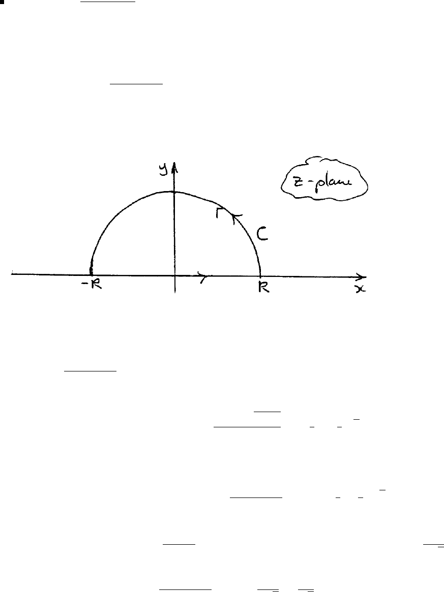
242 Glyn James, Advanced Modern Engineering Mathematics, 4th Edition
65(a) ∞
−∞
dx
x2+x+1
Since the integrand satisfies the condition for Type 1 infinite real integrals, given
in section 4.6.5, we consider
C
dz
z2+z+1 where Cis a semicircle with radius
Rand centre the origin in the upper half z-plane
By the residue theorem
C
dz
z2+z+1 =2πj {sum of residues of poles of integrand inside C}
z2+z+1=0⇒z=−1±√1−4
2=−1
2±j1
2√3
Only one of these simple poles lies inside C(the one with positive imaginary part)
Residue there = lim
z→z0
(z−z0)1
z2+z+1 ,z
0=−1
2+1
2j√3
That is, residue = limz→z01
2z+1using L’Hˆopital’s rule (for simplicity) = 1
j√3
Thus
C
dz
z2+z+1 =2πj ·1
j√3=2π
√3
c
Pearson Education Limited 2011

Glyn James, Advanced Modern Engineering Mathematics, 4th Edition 243
Now,
C
=Γ
+R
−R
and, as R→∞,
Γ→0
On
R
−R
,z=x=real.
Thus, letting R→∞we find that
∞
−∞
dx
x2+x+1 =2π
√3
65(b) This integral is done in precisely the same way as that of part (a). This
time, the poles are at ±jbut they are both double.
−C
dz
(z2+1)
2=2πj ×residue at j=2πj·1
4j=π
2
Thus
∞
−∞
dx
(x2+1)
2=π
2
65(c) To evaluate ∞
0
dx
(x2+1)(x2+4)
2we use the same semicircular contour,
except that we note
∞
0
dx
(x2+1)(x2+4)
2=1
2∞
−∞
dx
(x2+1)(x2+4)
2
plus the fact that 1
(z2+1)(z2+4)
2has two poles inside Cthis time, the simple
pole at z=jand the double pole at z=2j. Residue at z=jis 1
18jand residue
at z=2jis −11
288j.
Thus
∞
0
dx
(x2+1)(x2+4)
2=1
22πj1
18j−11
288j=5π
288
c
Pearson Education Limited 2011

244 Glyn James, Advanced Modern Engineering Mathematics, 4th Edition
65(d) In order to evaluate
2π
0
cos 3θ
5−4cosθdθ
we follow Example 4.39 and put z=ejθ so that
cos 3θ=1
2(z3+z−3)and cosθ=1
2(z+z−1)
With dz =jejθdθ. Hence we consider
C
1
2(z3+z−3)
jz(5 −2(z+z−1)) dz
The function under the integral can be written
1
2j
1+z6
5z4−2z5−2z3=1+z6
2j(z−2)(1 −2z)z3
The poles inside |z|= 1 are a triple pole at z= 0 and a simple pole at z=1
2.
Using the formula for the residue at z=1
2gives 65
48j. Using the Laurent expansion
about z= 0 yields the residue −21
16j.Thesumis 1
24j. Hence
2π
0
cos 3θ
5−4cosθdθ =1
2jC
1+z6
(z−2)(1 −2z)z3dz =1
24j2πj
=π
12
65(e)
2π
0
4dθ
5+4sinθ
This follows in the same way as part (d).
Putting z=ejθ yields dz =jejθdθ,thatis,dθ =dz
jz and sin θ=1
2j(z−z−1)
c
Pearson Education Limited 2011

Glyn James, Advanced Modern Engineering Mathematics, 4th Edition 245
Thus
2π
0
4dθ
5+4sinθ=C
4dz
jz(5 + 4
2j(z−z−1))
Thus
2π
0
4dθ
5+4sinθ=C
4dz
(2z+j)(z+2j)=2πj·4
3j=8π
3
(Cis the unit circle |z|=1)
65(f)
∞
−∞
x2dx
(x2+1)(x2+2x+2)
This follows along similar lines to parts (a) and (b). Consider the semicircular
contour and centre the origin radius Ron the upper half plane and labelled C
C
z2dz
(z2+1)(z2+2z+2) =2πj{sum of residues inside C}
Doublepoleisatz=j,simplepoleisatz=−1+j
Residue at z=jis 3
20 (−4+j3); residue at −1+jis 1
5(3 −j4)
Sum = −7
20 jgiving the integral as 7
10 π
65(g)
2π
0
dθ
3−2cosθ+sinθ
Once again let z=ejθ and consider the integral around the unit circle
2π
0
dθ
3−2cosθ+sinθ=C
dz
z2(1
2−j)+3jz −j−1
2
The poles are at −j
1−2jand −5
1−2j. Only the first is inside |z|=1.
The residue is 1
2jand so the value of the integral is 2πj 1
2j=π.
c
Pearson Education Limited 2011
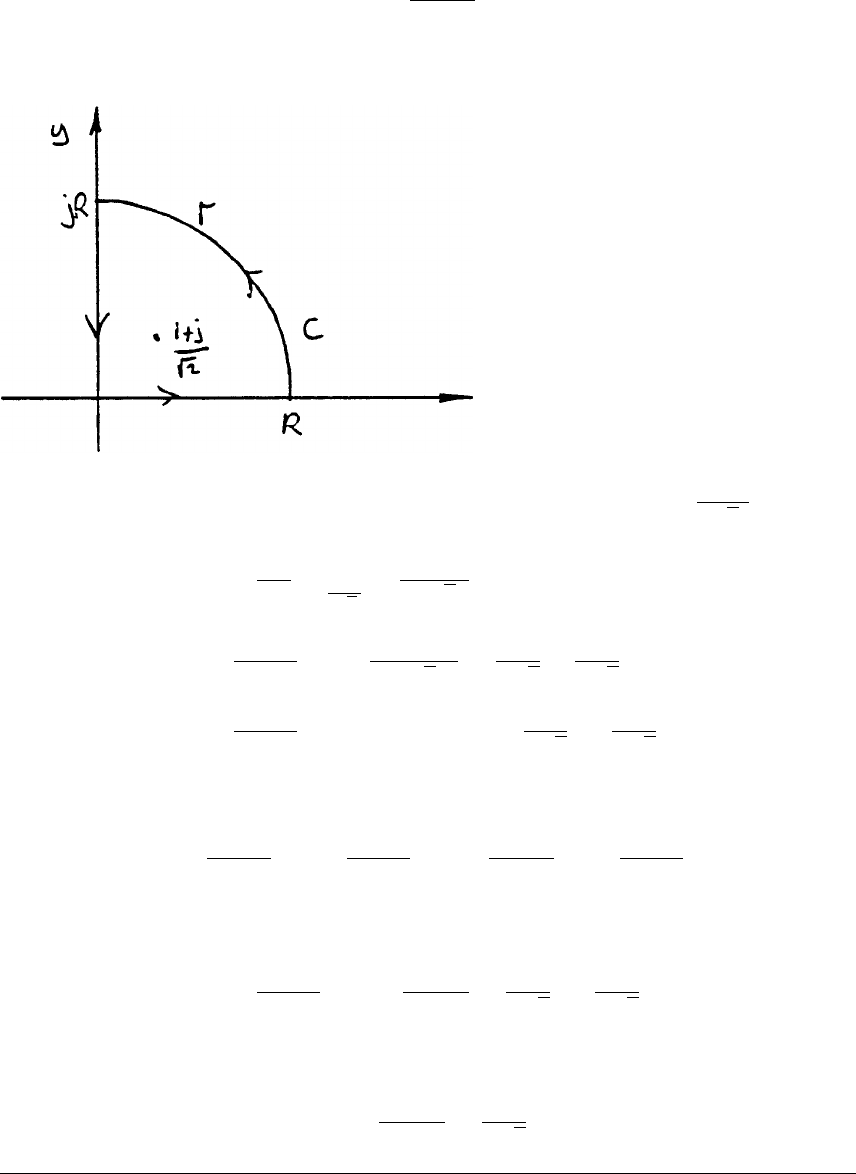
246 Glyn James, Advanced Modern Engineering Mathematics, 4th Edition
65(h) ∞
0
dx
x4+1
We have a choice here, let us choose a quarter circle contour as shown below.
Only the root of z4+ 1 = 0 in the positive quadrant, that is z=1+j
√2, needs to
be taken into account.
Residue at this point is 1
4z2|z=1+j
√2
=−1−j
4√2
Hence C
dz
1+z4=2πj (−1−j)
4√2=π
2√2−jπ
2√2
C
dz
z4+1 =0
jR
+R
0
+Γ
=π
2√2−jπ
2√2
on the imaginary axis, z=jy,andontherealaxisz=x. Therefore
C
dz
z4+1 =0
R
jdy
y4+1+R
0
dx
x4+1+Γ
dz
z4+1
wherewehaveused(jy)4=y4. Letting R→∞, the last integral →0. Thus
0
∞
jdy
y4+1+∞
0
dx
x4+1 =π
2√2−jπ
2√2
Equating real (or indeed imaginary) parts gives
∞
0
dx
x4+1 =π
2√2
c
Pearson Education Limited 2011

Glyn James, Advanced Modern Engineering Mathematics, 4th Edition 247
65(i)
∞
−∞
dx
(x2+4x+5)
2
The semicircular contour is used and the poles of 1
(z2+4z+5)
2are at
z=−2+j, −2−jboth double. Only the residue at z=−2+j,whichis 1
4j,
needs to be taken into account.
Hence
∞
−∞
dx
(x2+4x+5)
2=2πj 1
4j=π
2
65(j)
2π
0
cos θdθ
3+2cosθ
Again we use the unit circle on which z=ejθ . The integrand is z2+1
2j(z3+3z2+z)
with simple poles at z=0,−3
2+1
2√5,−3
2−1
2√5. Only the first two are inside
Cand residues are 1 and −3
√5. Hence the integral has the value π1−3
√5.
Exercises 4.8.3
66 Since w=1
z,u+jv =1
x+jy =x−jy
x2+y2
Thus u=x
x2+y2if u=1
2a,x
2+y2=2ax.
For the two wires shown in Figure 4.41 potentials are centred at V0or −V0
and are tangent to the imaginary (y) axis. They are thus circles of the form
x2+y2=2aV0x. The equipotential curves are shown
c
Pearson Education Limited 2011
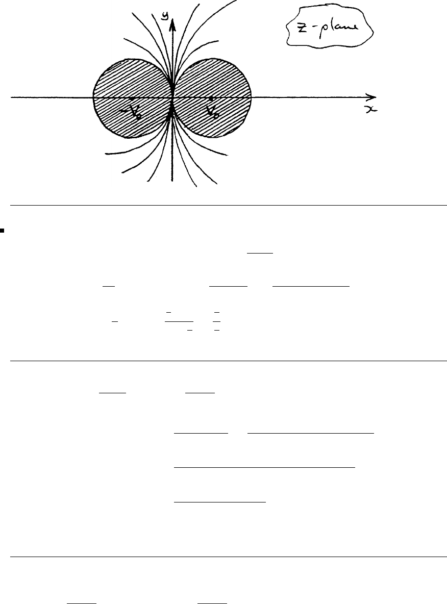
248 Glyn James, Advanced Modern Engineering Mathematics, 4th Edition
67(a)
z=−1⇒w−0,z=j⇒w=j+1
1−j=j
z=1
25 (24 + j7) ⇒w=49 + j7
1−j7=7
(7 + j)(1 + j7)
1+49 =j7
z=−3
4⇒w=
3
4+1
1−3
4
=
7
4
1
4
=7
giving images as (0,0),(0,1),(0,7),(7,0).
67(b) If w=z+1
1−zthen z=w−1
w+1
so that x+yj =u−1+jv
u+1+jv =(u−1+jv)(u+1−jv)
(u+1)
2+v2
or x+yj =(u2−1) + v2+j(vu +v−uv +v)
(u+1)
2+v2
x+yj =u2+v2−1+2vj
(u+1)
2+v2
Hence y= 0 corresponds to v=0.
67(c) If x2+y2=1⇒| z|=1
Since z=w−1
w+1 this means that
w−1
w+1=1
or (u−1)2+v2=(u+1)
2+v2from which u=0
c
Pearson Education Limited 2011
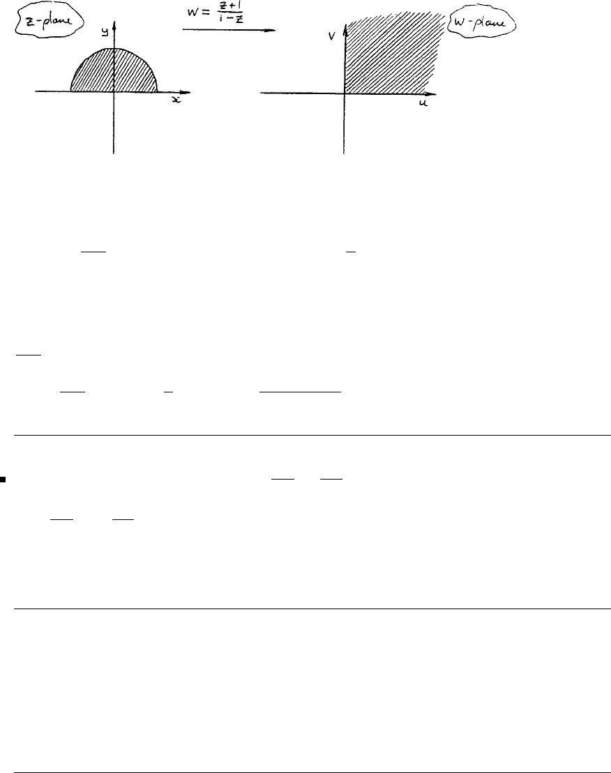
Glyn James, Advanced Modern Engineering Mathematics, 4th Edition 249
In order to progress, note that the image of the semicircular conductor in the
wplane is the positive quadrant u≥0,v ≥0. Instead of temperature ToCwe
consider πT
200 since this function has the value π
2on u=0(whereT= 100oC). The
mapping w=ez(Example 4.14) provides a means of eliminating the singularity at
w= 0. The complex variable zis already defined, therefore write w=eζ(complex
variable ζ). The imaginary part of ζis identified with the (scaled) temperature
πT
200 .
Thus πT
200 =tan
−1v
u=tan
−12y
1−x2−y2as required.
68(a) G(x, y)=2x−2xy;thus ∂H
∂y =∂G
∂x =2−2y
and ∂H
∂x =−∂G
∂y =2x
Integrating this gives H=x2−y2+2y
Hence W=G+jH =2z−jz2
68(b) If w=lnz,thenz=ew
Given H(z)=2z+jz2=2ew+je2w
equating real parts gives
G(x, y)=2eucos v−e2usin 2vas required
68(c) If w=f(z) then the real and imaginary parts of f(z) are harmonic
functions. Hence if ζ=g(w), then the real and imaginary parts of gare harmonic.
So ζ=g(w)=g(f(z)) implies that harmonic functions (the real and imaginary
c
Pearson Education Limited 2011

250 Glyn James, Advanced Modern Engineering Mathematics, 4th Edition
parts of f(z)) transform to harmonic functions (the real and imaginary parts of
g(w)).
69 If w=z+3
z−3then |w|=ktransforms to
z+3
z−3=k
that is, (x+3)
2+y2=k2(x−3)2+k2y2
or x2+y2+61+k2
1−k2x+9=0 as required.
If the centre of the circle is to be (−5,0), then
61+k2
1−k2=−10 or k=2
We thus (following section 4.8) require the potential Vto be a harmonic function
which has a constant value on a circle u2+v2= 4. Hence Vhas the general form
V=Aln(u2+v2)
on u2+v2=4,V=V0hence A=V0
ln 4
so that V=V0
ln 4 ln(u2+v2)
Now u2+v2=|w|2=
z+3
z−3
2
=(x+3)
2+y2
(x−3)2+y2
Thus
V=V0
ln 4{ln[(x+3)
2+y2]−ln[(x−3)2+y2]}
70 This problem follows a similar pattern to Exercise 67.
70(a) The points A, x =1,y =0; B, x =0,y =1; C, x =0,y =−1 under the
mapping of w=j(1 −z)
1+ztransform to
w= 0 that is (0,0),w=j(1 −j)
1+j= 1 that is (1,0)
and w=j(1 + j)
1−j=−1thatis(−1,0) respectively
c
Pearson Education Limited 2011
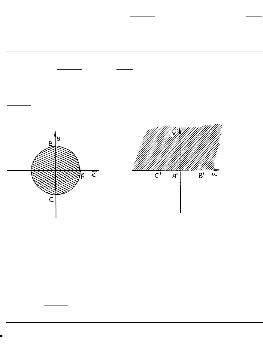
Glyn James, Advanced Modern Engineering Mathematics, 4th Edition 251
70(b) w=j(1 −z)
1+z
If z=x= real (i.e. y=0)then w=j(1 −x)
1+xis purely imaginary. Since 1−x
1+x
can take all real values, points on y= 0 correspond to points on u=0,the
imaginary axis.
70(c) If w=j(1 −z)
1+zthen z=j−w
j+w
So that |z|=1⇒| j−w|=|j+w|or v=0
For the last part we note the following property of the mapping that is, w=
j(1 −z)
1+z(from (a), (b), and (c))
In a way similar to Exercise 67, identify the function πT
100 which is (in the zplane),
πon the negative real axis, and 0 on the positive real axis. The mapping of w=eζ
(ζ- complex variable which has the values of πT
100 as imaginary part).
Thus πT
100 =tan
−1v
u=tan
−11−x2−y2
2y
(using w=j(1 −z)
1+zto find uand v). This gives the result.
71 This problem is similar to the last part of Exercise 69. The successive
mappings are
z1=z+j4
z−j4w=lnz
c
Pearson Education Limited 2011

252 Glyn James, Advanced Modern Engineering Mathematics, 4th Edition
In order for the circle centre 5jto be mapped to a circle centred at the origin in
the zplanewerequire
|z1|2=|z+j4
z−j4|2=k2for some constant k
that is, x2+y2+81+k2
1−k2y+ 16 = 0 needs a centre at 5j
Therefore,8(1 + k2) = 10(1 −k)2)orh=1
3
In the wplane, |w|=|ln z1|=|ln(x2
1+y2
1)|= 2 ln 3 on the boundary of the circle
on which T= 100.
Thus writing T=A|ln(x2
1+y2
1)|gives T= 100 when
x2
1+y2
1=1
9if 100 = A·2ln3 or A=50
ln 3
Thus
T=50
ln 3 ln(x2
1+y2
1)
=50
ln 3 ln x2+(4+y)2
x2+(4−y)2as required
Note that T= 0 corresponds to x2
1+y2
1=1ory= 0 as is also required
(|z+j4|2=|z−j4|2is y=0).
72 The mapping w=z+1
zwas studied in Example 4.13. Writing, as usual,
w=u+jv and z=x+jv leads to
u=x+x
x2+y2and v=y−y
x2+y2
Hence the unit circle x2+y2=1inthezplane corresponds to v= 0 (the real
axis) in the wplane.
Points ejπ/3and e2jπ/3(Pand Qof this problem) correspond to u=2cosπ
3and
2cos 2π
3respectively. The arc PQ thus corresponds to −1≤u≤1inthewplane.
The further mapping ζ=w+1
w−1takes this portion of the real axis (−1≤u≤1)
to −∞ ≤ Re{ζ}≤0 . This negative real axis corresponds to T= 100. Hence in
a similar fashion to Exercise 70, we identify the variable πT
100 (which = πon this
c
Pearson Education Limited 2011

Glyn James, Advanced Modern Engineering Mathematics, 4th Edition 253
line) with the imaginary part of ln ζwhich is argζ. We cannot use tan−1here
because the argument of the logarithm function is quadratic and so
πT
100 =argζ =argw+1
w−1=argz+1/z +1
z+1/z −1
that is,T=100
πarg(z2+z+1)−arg(z2−z+1)
as required.
Review Exercises 4.9
1(a) z=1+j, w =(1+j)z+j=(1+j)2+j=1+2j−1+j=3j
1(b) z=1−j2,w=j3z+j+1=j(1 −j2)3 + j+1=3j+6+j+1=4j+7
1(c) z=1,w=1
2(1 −j)z+1
2(1 + j)=1
1(d) z=j2,w=1
2(1 −j)z+1
2(1 + j)=(1−j)j+1
2(1 + j)=3
2(1 + j)
2(a) y=2x(b) x+y=1
For the mapping w=(1+j)z+j
u=x−y, v =x+y+1
so y=2x⇒v+3u=1
and x+y=1⇒v=2
For the mapping w=j3z+j+1
u=−3y+1,v=3x+1
so y=2x⇒u+2v=3
and x+y=1⇒v−u=3
For the mapping w=1
2(1 −j)z+1
2(1 + j)
u=1
2(x+y+1),v=1
2(x−y+1)
c
Pearson Education Limited 2011

254 Glyn James, Advanced Modern Engineering Mathematics, 4th Edition
so y=2x⇒3v−u=1
and x+y=1⇒u=1
3w=αz +β
when z=2−j, w =1,andwhen z=0,w =3+j
3(a) Solving the simultaneous equations gives α=−1
5(3 + j4),β =3+j.
3(b) Since
w=−1
5(3 + 4j)z+3+j
z=1
5(3 + j−w)(3 −j4)
so x=13−3u−4v
and Re{z}≤0 corresponds to 3u+4v≥13
3(c)
|z|=1
5|3+j−w|5≤1
⇒| w−3−j|≤ 1
5
3(d) Fixed point is given by
z=αz +βor z=β
1−α=1
4(7 −j)
4w=j
z⇒x=v
u2+v2,y=u
u2+v2
4(a) x=y+1⇒v
u2+v2=u
u2+v2+1 or u2+v2+u−v=0
4(b) y=3x⇒u=3v
4(c) Line joining A(1 + j)toB(z+j3) or (1,1) to (2,3) is y=2x−1which
transforms to u
u2+v2=2v
u2+v2−1oru2+v2+u−2v=0
c
Pearson Education Limited 2011
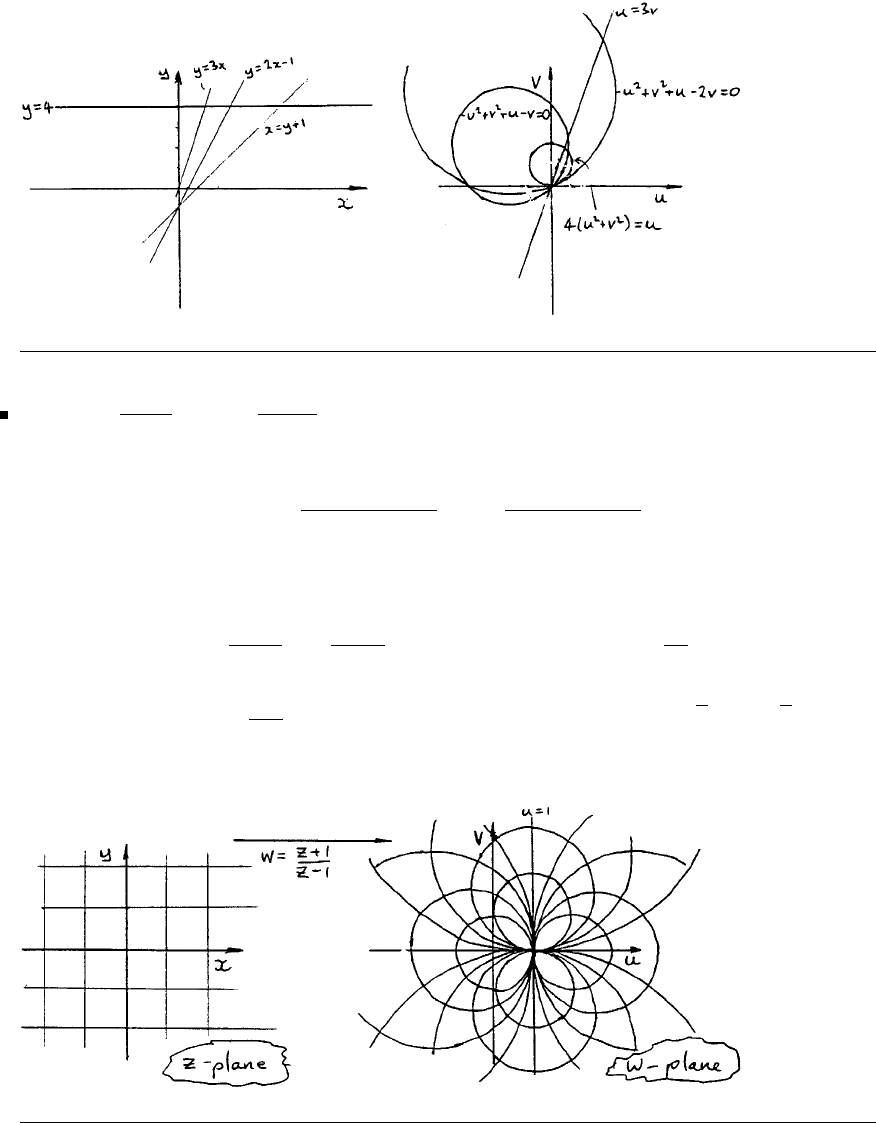
Glyn James, Advanced Modern Engineering Mathematics, 4th Edition 255
4(d) y=4⇒4(u2+v2)=u
The following Argand diagram shows all these curves.
5w=z+1
z−1⇒z=w+1
w−1
from which
x=u2+v2−1
(u−1)2+v2,y=−2v
(u−1)2+v2
lines x=kand y=lmap to circles
u2+v2−2k
k−1u+k+1
k−1=0 and u2+v2−2u+2v
l+1=0
Fixed points are z=z+1
z−1in z2−2z−1=0,thatis, z=1+√2,1−√2arethe
fixed points.
c
Pearson Education Limited 2011

256 Glyn James, Advanced Modern Engineering Mathematics, 4th Edition
6w=1−z2
z
Fixed points occur at z=1−z2
2
or z2=1−z2
z2=1/2
Hence z=±√2/2
Writing w=1
z−z=z∗
|z|2−z(z∗= complex conjugate).
Whence u=x
x2+y2−x,v=−−y
x2+y2−yand v=−y1
r2+1
so r2u
r2−1=x, −r2v
r2+1 =y
Squaring and adding gives
ur2
r2−12
+vr2
r2+12
=x2+y2=1
the required ellipses.
Since u=x
x2+y2−x,ifx2+y2=1 then u= 0 (imaginary axis in the wplane).
7w=z3
=(x+jy)3=x3+3jx2y+3j2xy +j3y3
so u=x3−3xy2
v=3x2y−y3are the real and imaginary parts.
∂u
∂x =3x2−3y2,∂u
∂y =−6xy
∂v
∂y =3x2−3y2,∂v
∂x =6xy
hence verifying the Cauchy–Riemann equations:
∂u
∂x =∂v
∂y,∂u
∂y =−∂v
∂x
c
Pearson Education Limited 2011

Glyn James, Advanced Modern Engineering Mathematics, 4th Edition 257
8u(x, y)=xsin xcosh y−ycos xsinh y
hence ∂u
∂x =sinxcosh y+xcos xcosh y+sinxsinh y
and ∂u
∂y =xsin xsinh y−ycos xcosh y−cos xsinh y
By the Cauchy–Riemann equations,
∂u
∂x =∂v
∂y and ∂u
∂y =−∂v
∂x
hence, integrating ∂u
∂x with respect to ygives:
v=sinxsinh y+xcos xsinh y+ysin xcosh y−sin xsinh y+f1(y)
Integrating −∂u
∂y with respect to xgives:
v=(xcos x−sin x)sinhy+ysin xcosh y+sinxsinh y+f2(x)
where f1and f2are arbitrary functions.
Comparing these gives v=ysin xcosh y+xcos xsinh y(ignoring the additive
constant).
Thus w=u+jv =xsin xcosh y−ycos xsinh y
+j(ysin xcosh y+xcos xsinh y)
Since this is f(z), we put y= 0 to find f(x) which will give the functional form
of f,namely
f(x)=xsin x. Thus f(z)=zsin z.
9Writing w=az +b
cz +d(the general bilinear mapping) since z=0⇒w=∞we
must have d= 0, hence (relabelling the constants) w=αz +β
z.
Writing this as wz =αz +βand inserting the pairs of values z=j, w =−jand
z=1
2(1 + j),w=1−jgives
1=αj +β, 1=1
2(1 + j)α+β
from which α=0,β= 1. Hence w=1
z.
c
Pearson Education Limited 2011

258 Glyn James, Advanced Modern Engineering Mathematics, 4th Edition
9(a) Since u=x
x2+y2and v=−y
x2+y2
the real axis (in the zplane) maps to the real axis (in the wplane).
If y>0thenv=−y
x2+y2<0andviceversa.
Thus the lower half of the zplane maps to the upper half of the wplane.
9(b) The circle |z−1
2j|=1
2is x2+y2−y=0
or v=−1v=−y
x2+y2
If |z−1
2j|<1
2then x2+y2−y<0orv<−1, that is, the interior of |z−1
2j|=1
2
maps to Im(w)<−1 as required.
10 The mapping z=ζ+a2
4ζ
maps R= constant (where ζ=Rejθ )tocurves
z=Rejθ +a2
4Re−jθ
which describe ellipses in the zplane as can be seen by writing
x=R+a2
4Rcos θ, y =R−a2
4Rsin θ
whence x2
(R+a2
4R)2+y2
(R−a2
4R)2=1
when R=1
2a, y = 0 (real axis). This mapping is used together with bilinear
mappings to map an aerofoil shape onto the unit circle. This is useful in
aeronautical engineering.
11 1
1+z3=(1+z3)−1
using the binomial expansion gives
1
1+z3=1−z3+z6−z9+···
Similarly 1
(1 + z3)2=1−2z3+3z6−4z9+···
and both are valid in the disc |z|<1.
c
Pearson Education Limited 2011

Glyn James, Advanced Modern Engineering Mathematics, 4th Edition 259
12(a) 1−z
1+z=2−1−z
1+z=2
1+z−1
Using the binomial series again gives
1−z
1+z=1−2z+2z2−2z3+...
since the nearest singularity of the function to z=0 isat z=−1, the radius of
convergence is 1.
12(b) f(z)= 1
z2+1. This time we need to expand about the point z=1. We
use Taylor’s series
f(z)= 1
z2+1,f
(z)=−2z
(z2+1)
2,f
(z)=−2
(z2+1)
2+8z2
(z2+1)
3
f(z)= 24z
(z2+1)
3−48z3
(z2+1)
4,f
iv(z)= 24
(z2+1)
3−288z2
(z2+1)
4+384z4
(z2+1)
5
At z=1 thesehavevalues 1
2,−1
2,1
2,0,−3
giving the expansion
1
z2+1 =1
2−1
2(z−1) + 1
4(z−1)2−1
6(z−1)4+...
The singularities of 1
1+z2are at z=±jwhich are a distance √2fromz=1,
hence the radius of convergence is √2.
12(c) z
1+z=1−1
1+z=f(z)
f(z)= 1
(1 + z)2,f
=−2
(1 + z)3,f
(z)=+ 6
(1 + z)4
Thus z
1+z=1
2(1 + j)+1
2j(z−j)−1
4(1 + j)(z−j)2−1
8(z−j)3+...
The radius of convergence is again √2.
13 The function 1
z(z2+1) has singularities at z=0,j,−j. The radius of
convergence is the distance of the centre of the point of expansion from the nearest
c
Pearson Education Limited 2011

260 Glyn James, Advanced Modern Engineering Mathematics, 4th Edition
of these singularities. These are found straightforwardly either by inspection or by
using Pythagoras’ theorem
z=1; 1; z=−1; 1,z =1+j;1,z=1+j1
2;1
2√5,z=2+j3; 2√2.
14 f(z)= 1
(z2+1)z
14(a) The Laurent expansion is
1
z(1 + z2)−1
=1
z(1 −z2+z4−z6+...)
=1
z−z+z3−z5+...
valid for 0 <|z|<1
14(b) Since f(z) is regular at z=1, f(z) has a Taylor expansion :
1
z(1 + z2)=f(1) + (z−1)f(1) + (z−1)2
2f(1) + ...
f(1) = 1
2,f
(z)=−1+3z2
(z+z3)2,f
(1) = −1
f(z)=−6z
(z+z3)2+2(1 + 3z2)2
(z+z3)3
so f(1) = −4
4+2×16
8=5
2
so that 1
z(1 + z2)=1
2−(z−1) + 5
4(z−1)2+...
valid for |z−1|<1
15 f(z)=ezsin 1
1−z
15(a) At z=0, f(z) is regular. Thus the principal part is zero and f(0) =
sin 1,f(z)=sin1+q1z+q2z2+... |z|<1, Taylor series.
c
Pearson Education Limited 2011

Glyn James, Advanced Modern Engineering Mathematics, 4th Edition 261
15(b) At z=1,f(z) has an essential singularity.
15(c) At z=∞,e
zhas an essential singularity. Hence for parts (b) and (c) the
principal part has infinitely many terms.
16(a)
ezsinh z=1
2ez(ez+e−z)=1
2(e2z+1)
=1
2(1 + e2x(e2jy))
=1
2(1 + e2xcos 2y+je2xsin 2y)
Real part = 1
2(1 + e2xcos 2y)
Imaginary part = 1
2e2xsin 2y
16(b)
cos 2z=cos(2x+j2y)
=cos2xcosh 2y−jsin 2xsinh 2y
16(c)
sin z
z=x−jy
x2+y2sin(x+jy)
=(x−jy)(sin xcosh y+jcos xsinh y)
x2+y2
=xsin xcosh y+ycos xsinh y+j(xcos xsinh y−ysin xcosh y)
x2+y2
16(d)
tan z=tan(x+jy)= tan x+tanjy
1−tan xtan jy
=tan x+jtanh y
1−jtan xtanh y·1+jtan xtanh y
1+jtan xtanh y
from which tan z=tan x(1 −tanh2y)+jtanh y(1 + tan2x)
1+tan
2xtanh2y
c
Pearson Education Limited 2011

262 Glyn James, Advanced Modern Engineering Mathematics, 4th Edition
17(a) Since dw
dz =−2
z3= 0, this mapping is conformal.
17(b)
dw
dz =6z2+6z+6(1−j)
=0whenz2+z+1−j=0
or (z−j)(z+j+1)=0
so z=j, −1−j
are the points where the mapping fails to be conformal.
17(c) w=64z+1
z3
dw
dz =64−3
z4=0
where z4=3
64
so z=0.465,−0.465,j0.465,−j0.465
are the points where the mapping fails to be conformal.
18 w=cosz, dw
dz =sinz=0 when z=nπ, n = an integer.
u+jv =cos(x+jy)=cosxcosh y−jsin xsinh y
u=cosxcosh y
v=−sin xsinh y
Lines x=kwill thus transform to
u2
cos2k−v2
sin2k=1−hyperpolae
Lines y=lwill thus transform to
u2
cosh2l+v2
sinh2l=1−ellipses
c
Pearson Education Limited 2011

Glyn James, Advanced Modern Engineering Mathematics, 4th Edition 263
19(a) sin z
z2=sin z
z·1
z.Sincesin z
z→1isz→0 this function has a simple role
at z=0.
19(b) 1
(z3−8)2has double poles when z3=8,thatis,at 2,2e2πj/3,2e4πj/3.
19(c) z+1
z4−1=z+1
(z2−1)(z2+1) =1
(z−1)(z2+1)
The singularity at z=−1 was removable, those at z=1,±jaresimplepoles.
19(d) sech z=1
cosh zwhich has simple poles wherever cosh z=0thatis,
z=1
2jπ(2n+1),n=0,±1,±2,...
19(e) sinh zis entire (no singularities in the finite plane).
19(f) Essential singularity at z=0.
19(g) zz=ezln z
which has an essential singularity at z=0.
20(a) e2z
(1 + z)2double pole at z=−1 residue given by
d
dz(e2z)z=−1
=2e−2
c
Pearson Education Limited 2011

264 Glyn James, Advanced Modern Engineering Mathematics, 4th Edition
20(b) cos z
2z−πsimple pole at z=π/2 residue is
lim
z→π/2(z−π/2) cos z
(2z−π)=1
2cos π
2=0
20(c) tan z
2z−π=sin z
cos z(2z−π)which has a double pole at z=1
2π
Writing w=z−π/2
tan z
2z−π=−cos w
2w=−cos w
2wsin w=−1−1
2w2+...
2w(w−1
6w3+...)
=−1
2w2+1
4+...
Hence residue is 0.
20(d) z
(z+8)
3has a triple pole at z=−8
Writing w=z+8 and z=w−8gives z
(z+8)
3=1
w3(w−8) = 1
w2−8
w3
Hence the residue is 0.
21
f(z)=(z2−1)(z2+3z+5)
z(z4+1)
Zeros are at z=±1 and at the roots of
z2+3z+5=0
z=−3±√9−20
2=−3
2±j1
2√11
Simple poles are at z=0 andwhere z4=−1
that is, z=(±1±j)/√2
The residue at z=0 isgivenby
lim
z→0
(z2−1)(z2+3z+5)
z4+1 =−5
c
Pearson Education Limited 2011

Glyn James, Advanced Modern Engineering Mathematics, 4th Edition 265
The residue at z=z0(where z4
0+1=0)is
lim
z→z0(z−z0)(z2−1)(z2+3z+5)
z(z4+1)
=(z2
0−1)(z2
0+3z0+5)
z0
lim
z→z0z−z0
z4+1
=(z2
0−1)(z2
0+3z0+5)
z0
1
4z3
0
=−1
4(z2
0−1)(z2
0+3z0+5)
(using z4
0=−1)
Putting z0=1+j
√2,−1+j
√2,−1−j
√2,1−j
√2in turn gives the residues 3
2+3
4√2−j,
3
2−3
4√2+j, 3
2−3
4√2−jand 3
2+3
4√2+jrespectively.
22 f(z)=z7+6z5−30z4
(z−1−j)3has a triple pole at z=1+j
Residue = 1
2!
d2
dz2(z7+6z5−30z4) is evaluated at z=1+j
=21z5+60z3−180z2z=1+j
= 21(−4−4j) + 60(−2+2j)−360j
=−204 −j324
23(a) The integrand z
z2+7z+6 has poles at z=−6andz=−1. Only the
second is inside C. Residue = z
z+6|z=−1=−1
5
Integral = −2πj
5
23(b) The integrand (z2+1)(z2+3)
(z2+9)(z2+4) has four simple poles ±2j, ±3jall
inside C.
Residues are −3
20 j, 3
20 j, 8
5jand −8
5jthe sum of which is 0.
The integral is thus 0 .
c
Pearson Education Limited 2011

266 Glyn James, Advanced Modern Engineering Mathematics, 4th Edition
23(c) The integrand 1
z2(1 −z2)2has double poles at z=0,1and−1.
Residues are, at z=0,
d
dz
1
(1 −z2)2z=0=+ 2z
(1 −z2)3z=0 =0
At z=1,d
dz−1
z2(1 + z)2=2(2z+1)
(z+z2)3z=1
=3
4
At z=−1,d
dz1
z2(1 −z)2=−2(1 −2z)
(z−z2)3z=−1
=3
4
(i) If Cis |z|=1
2then only z= 0 is inside C,sointegral=0
(ii) If Cis |z|=2 thenall poles are inside C,sointegral=3πj.
23(d) The integrand 1
(2z−3j)(z+j)has simple poles at 3j
2and −j.
Residues at 3j
2and −jare, respectively, −1
5jand 1
5j.
(i) Both poles are inside |z|= 2, but since their sum is zero so is the integral
(ii) Inside |z−1|= 1 the function 1
(2z−3j)(z+j)is regular. By Cauchy’s
theorem the integral = 0.
23(e) The integrand z3
(z2+1)(z2+z+1) has simple poles at
z=±j, −1
2±j1
2√3.
Cis the circle |z−j|=1
2which contains the pole at z=jbut not the other
three poles.
Residue at z=jis 1
2jhence the integral = −π.
23(f) z−1
z(z−2)2(z−3) has simple poles at z=0,3 and a double pole at z=2.
Residues at z=0,2 are respectively 1
12 and −3
4.
(i) If Cis |z|= 1 only the residue at z= 0 is considered : integral = πj
6
(ii) If Cis |z|=5
2, residues at 0 at 2 are summed; integral = πj1
12 −3
4=
−4πj/3.
c
Pearson Education Limited 2011

Glyn James, Advanced Modern Engineering Mathematics, 4th Edition 267
24(a) To evaluate ∞
−∞
x2dx
(x2+1)
2(x2+2x+2)
we use the semicircular contour Con the upper half plane (see Exercise 65). The
integral along the curved portion →0 as the radius of the semicircle →∞.The
residues in the upper half plane are at the (double) pole at jand the (simple) pole
at −1+j.
Residue of z2
(z2+1)
2(z2+2z+2) at z=jis d
dz
z2
(z+j)2(z2+2z+2) which is
evaluated at z=j.Thisis(aftersomealgebra) 9j−12
100 .
Residue at z=−1+jis z2
(z2+1)(z+1+j)evaluated at z=−1+jwhich is
3−4j
25 . Sum of residues is −7j
100
∞
−∞
x2dx
(x2+1)
2(x2+2x+2) =C
z2dz
(z2+1)
2(z2+2z+2) =2πj −7j
100 =7π
50
24(b) To evaluate ∞
0
x2dx
x4+16 one can either use a quarter circle contour (as in
Exercise 65(h)) or note that, by symmetry, ∞
0
x2dx
x4+16 =1
2
∞
−∞
x2dx
x4+16 and use
the same semicircular contour as above.
The disadvantage of doing this is that there are two poles inside the semicircular
contour, but only one in the quarter circle. However, this is compensated by the
easier manipulation of the integral. We shall thus use the semicircle.
The poles inside C, both simple, are at
z=√2(−1+j)andz=√2(1 + j)
The way to avoid unnecessary arithmetic/algebra is to determine the residue at
z=z0where z0is one of the above poles. This is given by
lim
z→z0(z−z0)z2
z4+16
Since z=z0is a root of z4+16,we canuseL’Hˆopital’s rule to obtain
Residue = 3z2−2zz0
4z3z=z0
=1
4z0
c
Pearson Education Limited 2011

268 Glyn James, Advanced Modern Engineering Mathematics, 4th Edition
Sum of residues is thus
1
4√2(−1+j)+1
4√2(1 + j)=−j
4√2
Thus ∞
−∞
x2dx
x4+16 =0
z2dz
z4+16 =2πj−j
4√2=π
2√2=π
4√2
Hence ∞
0
x2dx
x4+16 =π
8√2
24(c) To evaluate
2π
0
sin2θdθ
5+4cosθ
we follow Exercise 65(d) and put z=ejθ so that dz
jz =dθ and sin2θ
5+4cosθ=
z2−z4−1
(2z3+5z2+2z)4
Hence
2π
0
sin2θdθ
5+4cosθ=1
4jC
z2−z4−1
z2(2z+1)(z+2)dz
where Cis the unit circle. Residues at z=0 and z=−1
2(not that at z=−2)
are summed.
Residue at z=0is d
dzz2−z4−1
2z2+5z+2[evaluated at z=0]is 5
4. Residue at
z=−1
2is ( z2−z4−1
z2(z+2) )z=−1
2
=−13
6
Hence
2π
0
sin2θdθ
5+4cosθ=1
4j2πj5
4−13
6=−11π
24
24(d) The integral
2π
0
cos 2θ
5−4cosθdθ
c
Pearson Education Limited 2011

Glyn James, Advanced Modern Engineering Mathematics, 4th Edition 269
is evaluated similarly
2π
0
cos 2θ
5−4cosθdθ =1
2jC
z4+1
5z3−2z4−2z2dz =1
2j2πj17
6−5
4=19π
12
(In part (c) the negative sign arises from the choice of direction of the line integral.
Since the integrand sin2θ
5+4cosθis always positive it can be ignored.)
c
Pearson Education Limited 2011

5
Laplace Transforms
Exercises 5.2.6
1(a) L{cosh 2t}=L{1
2(e2t+e−2t)= 1
21
s−2+1
s+2=s
s2−4,Re(s)>2
1(b) L{t2}=2
s3,Re(s)>0
1(c) L{3+t}=3
s+1
s2=3s+1
s2,Re(s)>0
1(d) L{te−t}=1
(s+1)
2,Re(s)>−1
2(a) 5(b) -3 (c) 0(d) 3(e) 2(f) 0
(g) 0(h) 0(i) 2(j) 3
3(a) L{5−3t}=5
s−3
s2=5s−3
s2,Re(s)>0
3(b) L{7t3−2sin3t}=7.6
s4−2.3
s2+9 =42
s4−6
s2+9,Re(s)>0
3(c) L{3−2t+4cos2t}=3
s−2
s2+4.s
s2+4 =3s−2
s2+4s
s2+4,Re(s)>0
3(d) L{cosh 3t}=s
s2−9,Re(s)>3
3(e) L{sinh 2t}=2
s2−4,Re(s)>2
c
Pearson Education Limited 2011

Glyn James, Advanced Modern Engineering Mathematics, 4th Edition 271
3(f) L{5e−2t+3−2cos2t}=5
s+2+3
s−2.s
s2+4,Re(s)>0
3(g) L{4te−2t}=4
(s+2)
2,Re(s)>−2
3(h) L{2e−3tsin 2t}=4
(s+3)
2+4 =4
s2+6s+13,Re(s)>−3
3(i) L{t2e−4t}=2
(s+4)
3,Re(s)>−4
3(j)
L{6t3−3t2+4t−2}=36
s4−6
s3+4
s2−2
s
=36 −6s+4s2−2s3
s4,Re(s)>0
3(k) L{2cos3t+5sin3t}=2.s
s2+9+5.3
s2+9 =2s+15
s2+9 ,Re(s)>0
3(l)
L{cos 2t}=s
s2+4
L{tcos 2t}=−d
dss
s2+4=s2−4
(s2+4)
2,Re(s)>0
3(m)
L{tsin 3t}=−d
ds3
s2+9=6s
(s2+9)
2
L{t2sin 3t}=−d
ds6s
(s2+9)
2=−(s2+9)
26−6s(s2+9)
24s
(s2+9)
4
=18s2−54
(s2+9)
3,Re(s)>0
3(n) L{t2−3cos4t}=2
s3−3s
s2+16,Re(s)>0
c
Pearson Education Limited 2011

272 Glyn James, Advanced Modern Engineering Mathematics, 4th Edition
3(o)
L{t2e−2t−e−tcos 2t+3}=2
(s+2)
3+(s+1)
(s+1)
2+4 +3
s
=2
(s+2)
3+s+1
s2+2s+5 +3
s,Re(s)>0
Exercises 5.2.10
4(a) L−11
(s+3)(s+7)=L−1
1
4
s+3−
1
4
s+7=1
4[e−3t−e−7t]
4(b) L−1s+5
(s+1)(s−3) =L−1−1
s+1+2
s−3=−e−t+2e3t
4(c) L−1s−1
s2(s+3)=L−1
4
9
s−
1
3
s2−
4
9
s+3=4
9−1
3t−4
9e−3t
4(d) L−12s+6
s2+4=L−12.s
s2+2
2+3.2
s2+2
2=2cos2t+3sin2t
4(e)
L−11
s2(s2+ 16) =L−10
s+
1
16
s2−
1
16
s2+16
=1
16 t−1
64 sin 4t=1
64 [4t−sin 4t]
4(f) L−1s+8
s2+4s+5=L−1(s+2)+6
(s+2)
2+1=e−2t[cos t+6sint]
4(g)
L−1s+1
s2(s2+4s+8)=L−1
1
8
s+−1
8s+1
2
(s+2)
2+2
2
=L−11
8.1
s−1
8
(s+2)−3(2)
(s+2)
2+2
2
=1
8[1 −e−2tcos 2t+3e−2tsin 2t]
c
Pearson Education Limited 2011

Glyn James, Advanced Modern Engineering Mathematics, 4th Edition 273
4(h)
L−14s
(s−1)(s+1)
2=L−11
s−1−1
(s+1) +2
(s+1)
2
=et−e−t+2tet
4(i) L−1s+7
s2+2s+5=L−1(s+ 1) + 3(2)
(s+1)
2+2
2=e−t[cos 2t+3sin2t]
4(j)
L−1s2−7s+5
(s−1)(s−2)(s−3) =L−1
1
2
s−1−3
s−2+
1
2
s−3
=1
2et−3e2t+11
2e3t
4(k)
L−15s−7
(s+3)(s2+2)=L−1−2
s+3+2s−1
s2+2
=−2e−3t+2cos√2t−1
√2sin √2t
4(l)
L−1s
(s−1)(s2+2s+2)=L−1
1
5
s−1−1
5
s−2
s2+2s+2
=L−1
1
5
s−1−1
5
(s+1)−3
(s+1)
2+1
=1
5et−1
5e−t(cos t−3sint)
4(m) L−1s−1
s2+2s+5=L−1(s+1)−2
(s+1)
2+2
2=e−t(cos 2t−sin 2t)
4(n)
L−1s−1
(s−2)(s−3)(s−4) =L−1
1
2
s−2−2
s−3+
3
2
s−4
=1
2e2t−2e3t+3
2e−4t
c
Pearson Education Limited 2011

274 Glyn James, Advanced Modern Engineering Mathematics, 4th Edition
4(o)
L−13s
(s−1)(s2−4) =L−13s
(s−1)(s−2)(s+2)
=L−1−1
s−1+
3
2
s−2−
1
2
s+2
=−et+3
2e2t−1
2e−2t
4(p)
L−136
s(s2+1)(s2+9)=L−14
s−
9
2s
s2+1+
1
2s
s2+9
=4−9
2cos t+1
2cos 3t
4(q)
L−12s2+4s+9
(s+2)(s2+3s+3)=L−19
s+2−7s+9
(s+3
2)2+3/4
=L−19
s+2−7(s+3
2)−√3.√3/2
(s+3
2)2+(
√3/2)2
=9e−2t−e−3
2t7cos √3
2t−√3sin√3
2t
4(r)
L−11
(s+1)(s+2)(s2+2s+ 10) =L−1
1
9
s+1−
1
10
s+2−
1
90 s+1
9
s2+2s+10
=L−11
9
s+1−
1
10
s+2−1
90 s+10
(s+1)
2+3
2
=L−11
9
s+1−
1
10
s+2−1
90 (s+ 1) + 3(3)
(s+1)
2+3
2
=1
9e−t−1
10 e−2t−1
90 e−t(cos 3t+3sin3t)
c
Pearson Education Limited 2011

Glyn James, Advanced Modern Engineering Mathematics, 4th Edition 275
Exercises 5.3.5
5(a)
(s+3)X(s)=2+ 1
s+2 =2s+5
s+2
X(s)= 2s+5
(s+2)(s+3) =1
s+2+1
s+3
x(t)=L−1{X(s)}=e−2t+e−3t
5(b)
(3s−4)X(s)=1+ 2
s2+4 =s2+6
s2+4
X(s)= s2+6
(3s−4)(s2+4) =
35
26
3s−4−
3
26 s+4
26
s2+4
x(t)=L−1{X(s)}=35
78 e4
3t−3
26 (cos 2t+2
3sin 2t)
5(c)
(s2+2s+5)X(s)=1
s
X(s)= 1
s(s2+2s+5) =
1
5
s−1
5·s+2
s2+2s+5
=
1
5
s−1
5
(s+1)+ 1
2(2)
(s+1)
2+2
2
x(t)=L−1{X(s)}=1
5(1 −e−tcos 2t−1
2e−tsin 2t)
5(d)
(s2+2s+1)X(s)=2+ 4s
s2+4 =2s2+4s+8
s2+4
X(s)= 2s2+4s+8
(s+1)
2(s2+4)
=
12
25
(s+1) +
6
5
(s+1)
2−1
25 12s−32
s2+4
x(t)=L−1{X(s)}=12
25 e−t+6
5te−t−12
25 cos 2t+16
25 sin 2t
c
Pearson Education Limited 2011

276 Glyn James, Advanced Modern Engineering Mathematics, 4th Edition
5(e)
(s2−3s+2)X(s)=1+ 2
s+4 =s+6
s+4
X(s)= s+6
(s+4)(s−1)(s−2) =
1
15
s+4−
7
5
s−1+
4
3
s−2
x(t)=L−1{X(s)}=1
15 e−4t−7
5et+4
3e2t
5(f)
(s2+4s+5)X(s)=(4s−7) + 16 + 3
s+2
X(s)= 4s2+17s+21
(s+2)(s2+4s+5) =3
s+2+(s+2)+1
(s+2)
2+1
x(t)=L−1{X(s)}=3e−2t+e−2tcos t+e−2tsin t
5(g)
(s2+s−2)X(s)=s+1+ 5(2)
(s+1)
2+4
X(s)= s3+3s2+7s+15
(s+2)(s−1)(s2+2s+5)
=−1
3
s+2+
13
12
s−1+
1
4s−5
4
s2+2s+5
=−1
3
s+2+
13
12
s−1+1
4(s+1)−3(2)
(s+1)
2+2
2
x(t)=L−1{X(s)}=−1
3e−2t+13
12 et+1
4e−tcos 2t−3
4e−tsin 2t
c
Pearson Education Limited 2011

Glyn James, Advanced Modern Engineering Mathematics, 4th Edition 277
5(h)
(s2+2s+3)Y(s)=1+ 3
s2
Y(s)= s2+3
s2(s2+2s+3) =−2
3
s+1
s2+
2
3s+4
3
s2+2s+3
=−2
3
s+1
s2+2
3(s+1)−1
√2(√2)
(s+1)
2+(
√2)2
y(t)=L−1{Y(s)}=−2
3+t+2
3e−t(cos √2t+1
√2sin √2t)
5(i)
(s2+4s+4)X(s)=1
2s+2+ 2
s3+1
s+2
X(s)=s5+6s4+10s3+4s+8
2s3(s+2)
3
=
3
8
s−
1
2
s2+
1
2
s3+
1
8
s+2+
3
4
(s+2)
2+1
(s+2)
3
x(t)=L−1{X(s)}=3
8−1
2t+1
4t2+1
8e−2t+3
4te−2t+1
2t2e−2t
5(j)
(9s2+12s+5)X(s)= 1
s
X(s)= 1
9s(s2+4
3s+5
9)=
1
5
s−
1
5s+4
15
(s+2
3)2+1
9
=
1
5
s−1
5
[(s+2
3)+2
3]
(s+2
3)2+(1
3)2
x(t)=L−1{X(s)}=1
5−1
5e−2
3t(cos 1
3t+2sin1
3t)
c
Pearson Education Limited 2011

278 Glyn James, Advanced Modern Engineering Mathematics, 4th Edition
5(k)
(s2+8s+ 16)X(s)=−1
2s+1−4+16·4
s2+16 =−s3−6s2−16s+32
2(s2+ 16)
X(s)=−s3−6s2−16s+32
2(s+4)
2(s2+ 16)
=0
s+4+1
(s+4)
2−
1
2s
s2+16
x(t)=L−1{X(s)}=te−4t−1
2cos 4t
5(l)
(9s2+12s+4)Y(s)=9(s+1)+12+ 1
s+1
Y(s)= 9s2+30s+22
(3s+2)
2(s+1)
=1
s+1+0
3s+2+18
(3s+2)
2
y(t)=L−1{Y(s)}=e−t+2te−2
3t
5(m)
(s3−2s2−s+2)X(s)=s−2+ 2
s+1
s2
X(s)= s3−2s2+2s+1
s2(s−1)(s−2)(s+1)
=
5
4
s+
1
2
s2−1
s−1+
5
12
s−2−
2
3
s+1
x(t)=L−1{X(s)}=5
4+1
2t−et+5
12 e2t−2
3e−t
5(n)
(s3+s2+s+1)=(s+1)+1+ s
s2+9
X(s)= s3+2s2+10s+18
(s2+9)(s+1)(s2+1) =
9
20
s+1−1
16
7s−25
s2+1 −1
80
s+9
s2+9
x(t)=L−1{X(s)}=9
20 e−t−7
16 cos t+25
16 sin t−1
80 cos 3t−3
80 sin 3t
c
Pearson Education Limited 2011

Glyn James, Advanced Modern Engineering Mathematics, 4th Edition 279
6(a)
2sX(s)−(2s+9)Y(s)=−1
2+1
s+2
(2s+4)X(s)+(4s−37)Y(s)=1
Eliminating X(s)
[−(2s+ 9)(2s+4)−2s(4s−37)]Y(s)=(−1
2+1
s+2)(2s+4)−2s=−3s
Y(s)= 3s
12s2−48s+36 =1
4·s
(s−3)(s−1)
=1
4
3
2
s−3−
1
2
s−1
y(t)=L−1{Y(s)}=1
43
2e3t−1
2et=3
8e3t−1
8et
Eliminating dx
dt from the two equations
6dy
dt +4x−28y=−e−2t
x(t)=1
4−e−2t+28y−6dy
dt =1
4−e−2t+21
4e3t−7
2et−27
3e3t+3
4et
i.e. x(t)=1
415
4e3t−11
4et−e−2t,y(t)= 1
8(3e3t−et)
6(b)
(s+1)X(s)+(2s−1)Y(s)= 5
s2+1
(2s+1)X(s)+(3s−1)Y(s)= 1
s−1
Eliminating X(s)
[(2s−1)(2s+1)−(3s−1)(s+1)]Y(s)= 5
s2+1(2s+1)−s+1
s−1
Y(s)= 10s+5
s(s2+1)(s−2) −s+1
s(s−1)(s−2)
=−5
2
s+
5
2
s−2−5
s2+1−
1
2
s−2
s−1+
3
2
s−2
y(t)=L−1{Y(s)}=−5
2+5
2e2t−5sint−1
2+2et−3
2e2t
=−3+e2t+2et−5sint
c
Pearson Education Limited 2011

280 Glyn James, Advanced Modern Engineering Mathematics, 4th Edition
Eliminating dx
dt from the original equations
dy
dt +x−y=10sint−et
x(t)=10sint−et−3+e2t+2et−5sint−2e2t−2et+5cost
=5sint+5cost−3−et−e2t
6(c)
(s+2)X(s)+(s+1)Y(s)=3+ 1
s+3 =3s+10
s+3
5X(s)+(s+3)Y(s)=4+ 5
s+2 =4s+13
s+2
Eliminating X(s)
[5(s+1)−(s+2)(s+3)]Y(s)=15s+50
s+3 −(4s+ 13) = −4s2−10s+11
s+3
Y(s)= 4s2+10s−11
(s+3)(s2+1) =−1
2
s+3+
9
2s−7
2
s2+1
y(t)=L−1{Y(s)}=−1
2e−3t+9
2cos t−7
2sin t
From the second differential equation
5x=5e−2t+3
2e−3t−27
2cos t+21
2sin t−3
2e−3t
+9
2sin t+7
2cos t
x(t)=3sint−2cost+e−2t
6(d)
(3s−2)X(s)+3sY(s)=6+ 1
s−1=6s−5
s−1
sX(s)+(2s−1)Y(s)=3+1
s=3s+1
s
c
Pearson Education Limited 2011

Glyn James, Advanced Modern Engineering Mathematics, 4th Edition 281
Eliminating X(s)
[3s2−(3s−2)(2s−1)]Y(s)=s(6s−5)
s−1−(3s−2)(3s+1)
s
Y(s)= 9s2−3s−2
s(3s−1)(s−2) −6s2−5s
(s−1)(3s−1)(s−2)
=−1
s+
18
5
3s−1+
14
5
s−2
−−1
2
s−1−
9
10
3s−1+
14
5
s−2
=−1
s+
1
2
s−1+
9
2
3s−1
y(t)=L−1{Y(s)}=−1+1
2et+3
2et
3
Eliminating dx
dt from the original equations
x(t)=1
23−et−3+3
2et+9
2et
3−3
2et−3
2et
3
=3
2et
3−1
2et
6(e)
(3s−2)X(s)+sY(s)=−1+ 3
s2+1+5s
s2+1 =−s2+5s+2
s2+1
2sX(s)+(s+1)Y(s)=−1+ 1
s2+1+s
s2+1 =−s2+s
s2+1
Eliminating Y(s)
[(3s−2)(s+1)−2s2]X(s)= 1
s2+1[(−s2+5s+2)(s+1)−(−s2+s)s]
X(s)= 3s2+7s+2
(s+2)(s−1)(s2+1) =3s+1
(s−1)(s2+1)
=2
s−1−2s−1
s2+1
x(t)=L−1{X(s)}=2et−2cost+sint
c
Pearson Education Limited 2011

282 Glyn James, Advanced Modern Engineering Mathematics, 4th Edition
Eliminating dy
dt from the original equation
y(t)=−2sint−4cost−2x+dx
dt
=−2sint−4cost−4et+4cost−2sint+2et+2sint+cost
that is,y(t)=−2et−2sint+cost, x(t)=2et−2cost+sint
6(f)
sX(s)+(s+1)Y(s)=1+ 1
s2=s2+1
s2
(s+1)X(s)+4sY(s)=1+1
s=s+1
s
Eliminating Y(s)
[4s2−(s+1)
2]X(s)=4ss2+1
s2−(s+1)
2
s=3s2−2s+3
s
X(s)= 3s2−2s+3
s(s−1)(3s+1) =−3
s−1
s−1+9
3s+1
x(t)=L−1{X(s)}=−3+et+3e−t
3
Eliminating dy
dt from the original equation
y=1
44t−1+x+3dx
dt
=1
44t−1−3+et+3e−t
3−3et+3e−t
3
that is,y(t)=t−1−1
2et+3
2e−t
3,x(t)=−3+et+3e−t
3
6(g)
(2s+7)X(s)+3sY(s)=12
s2+7
s=14 + 7s
s2
(5s+4)X(s)−(3s−6)Y(s)= 14
s2−14
s=14 −14s
s2
c
Pearson Education Limited 2011

Glyn James, Advanced Modern Engineering Mathematics, 4th Edition 283
Eliminating Y(s)
[(2s+ 7)(3s−6) + (5s+ 4)(3s)]X(s)= 1
s2[(3s−6)(14 + 7s)+3s(14 −14s)]
21(s2+s−2)X(s) = 21(s+2)(s−1)X(s)=21
s2(−s2+2s−4)
X(s)= −s2+2s−4
s2(s+2)(s−1)
=−1
s−1+1
s+2+0
s+2
s2
x(t)=L−1{X(s)}=−et+e−2t+2t
Eliminating dy
dt from the original equations
6y=28t−7−11x−7dx
dt
=28t−7+7et+14e−2t−14 + 11et−11e−2t−22t
giving y(t)=t−7
2+3et+1
2e−2t,x(t)=−et+e−2t+2t.
6(h)
(s2+2)X(s)−Y(s)=4s
−X(s)+(s2+2)Y(s)=2s
Eliminating Y(s)
[(s2+2)
2−1]X(s)=4s(s2+2)+2s
(s4+4s2+3)X(s)=4s3+10s
X(s)= 4s3+10s
(s2+1)(s2+3) =3s
s2+1+s
s2+3
x(t)=L−1{X(s)}=3cost+cos√3t
From the first of the given equations
y(t)=2x+d2x
dt2=6cost+2cos√3t−3cost−3cos√3t
that is,y(t)=3cost−cos √3t, x(t)=3cost−cos √3t
c
Pearson Education Limited 2011

284 Glyn James, Advanced Modern Engineering Mathematics, 4th Edition
6(i)
(5s2+6)X(s)+12s2Y=s35
4+12
=83
4s
5s2X(s)+(16s2+6)Y(s)=s35
4+16
=99
4s
Eliminating X(s)
[60s4−(5s2+ 6)(16s2+6)]Y(s)= s
4[83(5s2)−99(5s2+6)]
[−20s4−126s2−36]Y(s)=s
4[−80s2−594]
Y(s)= s(40s2+ 297)
4(s2+ 6)(10s2+3)
=−1
4s
s2+6+
25
2s
10s2+3
y(t)=L−1{Y(s)}=−1
4cos √6t+5
4cos 3
10 t
Eliminating d2x
dt2from the original equations
3x=3y+3d2y
dt2=15
4−3
4cos 3
10 t+−3
4+3
cos √6t
i.e. x(t)=cos3
10 t+3
4cos √6t, x(t)=5
4cos 3
10 t−1
4cos √6t.
6(j)
(2s2−s+9)X(s)−(s2+s+3)Y(s)=2(s+1)−1=2s+1
(2s2+s+7)X(s)−(s2−s+5)Y(s)=2(s+1)+1=2s+3
Subtract
(−2s+2)X(s)−(2s−2)Y(s)=−2⇒X(s)+Y(s)= 1
s−1
⇒x(t)+y(t)=et(i)
Add
(4s2+ 16)X(s)−(2s+8)Y(s)=4(s+1)
2X(s)−Y(s)=2(s+1)
s2+4 ⇒2x(t)−y(t)
=2cos2t+sin2t(ii)
c
Pearson Education Limited 2011

Glyn James, Advanced Modern Engineering Mathematics, 4th Edition 285
Then from (i) and (ii)
x(t)=1
3et+2
3cos 2t+1
3sin 2t, y(t)=2
3et−2
3cos 2t−1
3sin 2t
Exercises 5.4.3
71μF=10
−6Fso50μ=5.105F
Applying Kirchhoff’s second law to the left hand loop
1
5.105i1dt +2
di1
dt −di2
dt =E. sin 100t
Taking Laplace transforms
2.104
sI1(s)+2s[I1(s)−I2(s)] = E. 100
s2+10
4
(104+s2)I1(s)−s2I2(s)=E. 50s
s2+10
4(i)
Applying Kirchhoff’s law to the right hand loop
100i2(t)−2di1
dt −di2
dt =0
which on taking Laplace transforms gives
sI1(s)=(50+s)I2(s) (ii)
Substituting in (i)
(104+s2)(50 + s)I2(s)−s2I2(s)=E. 50s2
s2+10
4
(s2+ 200s+10
4)I2(s)= Es2
s2+10
4
I2(s)=Es2
(s2+10
4)(s+ 100)2
then from (ii) I1(s)=Es(50 + s)
(s2+10
4)(s+ 100)2
c
Pearson Education Limited 2011

286 Glyn James, Advanced Modern Engineering Mathematics, 4th Edition
Expanding in partial functions
I2(s)=E−1
200
s+ 100 +
1
2
(s+ 100)2+
1
200 s
s2+10
4
i2(t)=L−1{I2(s)}=E−1
200 e−100t+1
2te−100t+1
200 cos 100t
8Applying Kirchhoff’s second law to the primary and secondary circuits
respectively gives
2i1+di1
dt +1di2
dt =10sint
2i2+2di2
dt +di1
dt =0
Taking Laplace transforms
(s+2)I1(s)+sI2(s)= 10
s2+1
sI1(s)+2(s+1)I2(s)=0
Eliminating I1(s)
[s2−2(s+1)(s+2)]I2(s)= 10s
s2+1
I2(s)=−10s
(s2+1)(s2+7s+6) =−10s
(s2+1)(s+6)(s+1)
=−−1
s+1+
12
37
s+6+
25
37 s+35
37
s2+1
i2(t)=L−1{I2(s)}=e−t−12
37 e−6t−25
37 cos t−35
37 sin t
9Applying Kirchhoff’s law to the left and right hand loops gives
(i1+i2)+ d
dt(i1+i2)+1i1dt =E0=10
i2+di2
dt −1i1dt =0
c
Pearson Education Limited 2011

Glyn James, Advanced Modern Engineering Mathematics, 4th Edition 287
Applying Laplace transforms
(s+1)I1(s)+(s+1)I2(s)+1
sI1(s)=10
s
(s+1)I2(s)−1
sI1(s)=0 ⇒I1(s)=s(s+1)I2(s)(i)
Substituting back in the first equation
s(s+1)
2I2(s)+(s+1)I2(s)+(s+1)I2(s)=10
s
(s2+s+2)I2(s)= 10
s(s+1)
I2(s)= 10
s(s+1)(s2+s+2)
Then from (i)
I1(s)= 10
s2+s+2 =10
(s+1
2)2+7
4
i1(t)=L−1{I1(s)}=20
√7e−1
2tsin √7
2t
10 Applying Newton’s law to the motion of each mass
¨
x1=3(x2−x1)−x1=3x2−4x1
¨
x2=−9x2−3(x2−x1)=−12x2+3x1
giving
¨
x1+4x1−3x2=0,x
1(0) = −1,x
2(0) = 2
¨
x2+12x2−3x1=0
Taking Laplace transforms
(s2+4)X1(s)−3X2(s)=−s
−3X1(s)+(s2+ 12)X2(s)=2s
c
Pearson Education Limited 2011

288 Glyn James, Advanced Modern Engineering Mathematics, 4th Edition
Eliminating X2(s)
[(s2+4)(s2+ 12) −9]X1(s)=−s(s2+ 12) + 6s
(s2+ 13)(s2+3)X1(s)=−s3−6s
X1(s)= −s3−6s
(s2+ 13)(s2+3) =−3
10 s
s2+3−
7
10 s
s2+13
x1(t)=L−1{X1(s)}=−3
10 cos √3t−7
10 cos √13t
From the first differential equation
3x2=4x1+¨
x1
=−6
5cos √3t−14
5cos √13t+9
10 cos √3t+91
10 cos √13t
x2(t)= 1
10 [21 cos √13t−cos √3t]
Thus, x1(t)=−1
10 (3 cos √3t+7cos√13t),x
2(t)= 1
10 [21 cos √13t−cos √3t]
Natural frequencies are √13 and √3.
11 The equation of motion is
M¨
x+b˙
x+Kx =Mg ;x(0) = 0 ,˙
x(0) = 2gh
The problem is then an investigative one where students are required to investigate
for different hvalues either analytically or by simulation.
12 By Newton’s second law of motion
M2¨
x2=−K2x2−B1(˙
x2−˙
x1)+u2
M1¨
x1=B1(˙
x2−˙
x1)−K1x1+u1
Taking Laplace transforms and assuming quiescent initial state
(M2s2+B1s+K2)X2(s)−B1sX1(s)=U2(s)
−B1sX2(s)+(M1s2+B1s+K1)X1(s)=U1(s)
c
Pearson Education Limited 2011

Glyn James, Advanced Modern Engineering Mathematics, 4th Edition 289
Eliminating X1(s)
[(M1s2+B1s+K1)(M2s2+B1s+K2)−B2
1s2]X2(s)
=(M1s2+B1s+K1)U2(s)+B1sU1(s)
i.e. X2(s)=B1s
ΔU1(s)+(M1s2+B1s+K1)
ΔU2(s)
and x2(t)=L−1{X2(s)}=L−1B1s
ΔU1(s)+(M1s2+B1s+K1)
ΔU2(s)
Likewise eliminating X2(t) from the original equation gives
x1(t)=L−1{X1(s)}=L−1(M1s+B1s+K2)
ΔU1(s)+B1s
ΔU2(s)
Exercises 5.5.7
13
f(t)=tH(t)−tH(t−1)
=tH(t)−(t−1)H(t−1) −1H(t−1)
Thus, using theorem 2.4
L{f(t)}=1
s2−e−s1
s2−e−s=1
s2(1 −e−s)−1
se−s
14(a)
f(t)=3t2H(t)−(3t2−2t+3)H(t−4) −(2t−8)H(t−6)
=3t2H(t)−[3(t−4)2+ 22(t−4) + 43]H(t−4) −[2(t−6) + 4]H(t−6)
Thus,
L{f(t)}=6
s3−e−4sL[3t2+22t+ 43] −e−6sL[2t+4]
=6
s3−6
s3+22
s2+43
se−4s−2
s2+4
se−6s
c
Pearson Education Limited 2011

290 Glyn James, Advanced Modern Engineering Mathematics, 4th Edition
14(b)
f(t)=tH(t)+(2−2t)H(t−1) −(2 −t)H(t−2)
=tH(t)−2(t−1)H(t−1) −(t−2)H(t−2)
Thus,
L{f(t)}=1
s2−2e−sL{t}+e−2sL{t}
=1
s2[1 −2e−s+e−2s]
15(a) L−1e−5s
(s−2)4=L−1{e−5sF(s)}where F(s)= 1
(s−2)4and by the first
shift theorem f(t)=L−1{F(s)}=1
6t3e2t.
Thus, by the second shift theorem
L−1e−5s
(s−2)4=f(t−5)H(t−5)
=1
6(t−5)3e2(t−5)H(t−5)
15(b) L−13e−2s
(s+3)(s+1)=L−1{e−2sF(s)}where
F(s)= 3
(s+3)(s+1) =−3
2
s+3+
3
2
s+1
f(t)=L−1{F(s)}=3
2e−t−3
2e−3t
so L−13e−2s
(s+3)(s+1)=f(t−2)H(t−2)
=3
2[e−(t−2) −e−3(t−2)]H(t−2)
15(c) L−1s+1
s2(s2+1)e−s=L−1{e−sF(s)}where
F(s)= s+1
s2(s2+1) =1
s+1
s2−s+1
s2+1
f(t)=L−1{F(s)}=1+t−cos t−sin t
c
Pearson Education Limited 2011

Glyn James, Advanced Modern Engineering Mathematics, 4th Edition 291
so
L−1s+1
s2(s2+1)e−s=f(t−1)H(t−1)
=[1+(t−1) −cos(t−1) −sin(t−1)]H(t−1)
=[t−cos(t−1) −sin(t−1)]H(t−1)
15(d) L−1s+1
s2+s+1e−πs=L−1{e−πsF(s)}where
F(s)= s+1
(s2+s+1) =(s+1
2)+ 1
√3(√3
2)
(s+1
2)2+(√3
2)2
f(t)=e−1
2tcos √3
2t+1
√3sin √3
2t
so
L−1s+1
s2+s+1e−πs=1
√3e−1
2(t−π)√3cos √3
2(t−π)+sin√3
2(t−π).H(t−π)
15(e) L−1s
s2+25e−4πs/5=L−1{e−4πs/5F(s)}where
F(s)= s
s2+25 ⇒f(t)=L−1{F(s)}=cos5t
so
L−1s
s2+25e−4πs/5=ft−4π
5Ht−4π
5
=cos(5t−4π)Ht−4π
5
=cos5tH
t−4π
5
15(f) L−1e−s(1 −e−s)
s2(s2+1) =L−1{(e−s−e−2s)F(s)}where
F(s)= 1
s2(s2+1) =1
s2−1
s2+1
f(t)=L−1{F(s)}=t−sin t
c
Pearson Education Limited 2011
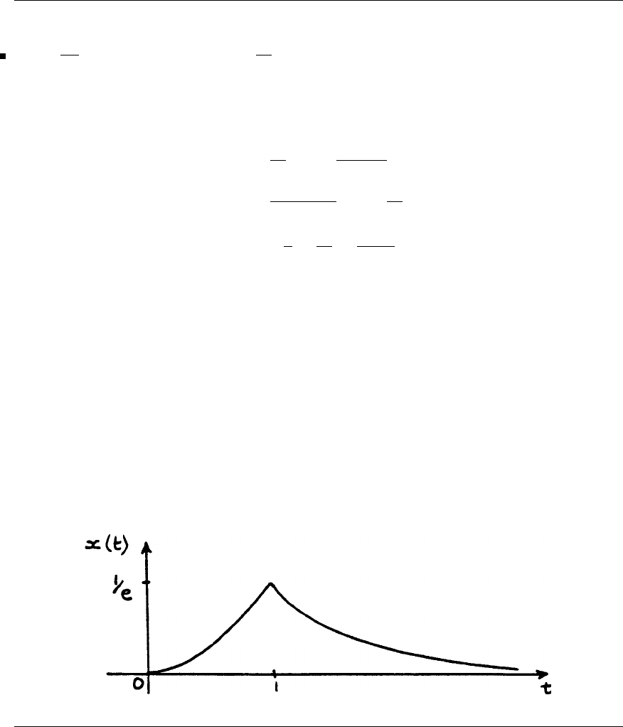
292 Glyn James, Advanced Modern Engineering Mathematics, 4th Edition
so
L−1{(e−s−e−2s)F(s)}=f(t−1)H(t−1) −f(t−2)H(t−2)
=[(t−1) −sin(t−1)]H(t−1)
−[(t−2) −sin(t−2)]H(t−2)
16 dx
dt +x=f(t),L{f(t)}=1
s2(1 −e−s−se−s)
Taking Laplace transforms with x(0) = 0
(s+1)X(s)= 1
s2−e−s(1 + s)
s2
X(s)= 1
s2(s+1) −e−s1
s2
=−1
s+1
s2+1
s+1−e−sL{t}
Taking inverse transforms
x(t)=−1+e−t+t−(t−1)H(t−1)
=e−t+(t−1)[1 −H(t−1)]
or x(t)=e−t+(t−1) for t≤1
x(t)=e−tfor t≥1
Sketch of response is
c
Pearson Education Limited 2011

Glyn James, Advanced Modern Engineering Mathematics, 4th Edition 293
17 d2x
dt2+dx
dt +x=g(t),x(0) = 1,˙
x(0) = 0
with L{g(t)}=1
s2(1 −2e−s+e−2s)
Taking Laplace transforms
(s2+s+1)X(s)=s+1+ 1
s2(1 −2e−s+e−2s)
X(s)= s+1
(s2+s+1) +1
s2(s2+s+1)(1 −2e−s+e−2s)
=(s+1)
(s2+s+1) +−1
s+1
s2+s
s2+s+1[1 −2e−s+e−2s]
=(s+1
2)+ 1
√3(√3
2)
(s+1
2)2+(√3
2)2
+−1
s+1
s2+(s+1
2)−1
√3(√3
2)
(s+1
2)2+(√3
2)2[1 −2e−s+e−2s]
x(t)=L−1{X(s)}=e−1
2tcos √3
2t+1
√3sin √3
2t
+t−1+e−1
2tcos √3
2t−1
√3sin √3
2t
−2H(t−1)t−2+e−1
2(t−1)cos √3
2(t−1)
−1
√3sin √3
2(t−1)
+H(t−2)t−3+e−1
2(t−2)cos √3
2(t−2)
−1
√3sin √3
2(t−2)
that is,
x(t)=2e−1
2tcos √3
2t+t−1
−2H(t−1)t−2+e−1
2(t−1)cos √3
2(t−1) −1
√3sin √3
2(t−1)
+H(t−2)t−3+e−1
2(t−2)cos √3
2(t−2) −1
√3sin √3
2(t−2)
c
Pearson Education Limited 2011

294 Glyn James, Advanced Modern Engineering Mathematics, 4th Edition
18
f(t)=sintHt−π
2=cost−π
2Ht−π
2
since cos t−π
2=sint.
Taking Laplace transforms with x(0) = 1,˙
x(0) = −1
(s2+3s+2)X(s)=s+2+Lcost−π
2Ht−π
2
=s+2+e−π
2sL{cos t}
=s+2+e−π
2s·s
s2+1
X(s)= 1
s+1+e−π
2ss
(s+1)(s+2)(s2+1)
=1
s+1+e−π
2s−1
2
s+1+
2
5
s+2+1
10 ·s+3
s2+1
=1
s+1+e−π
2sL−1
2e−t+2
5e−2t+1
10 (cos t+3sint)
so x(t)=L−1{X(s)}=e−t+−1
2e−(t−π
2)+2
5e−2(t−π
2)+1
10 (cos t−π
2
+3sint−π
2)Ht−π
2
=e−t+1
10 sin t−3cost+4eπe−2t−5eπ
2e−tHt−π
2
19
f(t)=3H(t)−(8 −2t)H(t−4)
=3H(t)+2(t−4)H(t−4)
L{f(t)}=3
s+2e−4sL{t}=3
s+2
s2e−4s
Taking Laplace transforms with x(0) = 1,˙
x(0) = 0
(s2+1)X(s)=s+3
s+2
s2e−4s
X(s)= s
s2+1+3
s(s2+1) +2
s2(s2+1)e−4s
=s
s2+1+3
5−3
s2+1+2
1
s2−1
s2+1e−4s
=3
5−2
s2+1+2e−4sL{t−sin t}
c
Pearson Education Limited 2011

Glyn James, Advanced Modern Engineering Mathematics, 4th Edition 295
Thus, taking inverse transforms
x(t)=3−2cost+2(t−4−sin(t−4))H(t−4)
20
¨
θ0+6
˙
θ0+10θ0=θi(1)
θi(t)=3H(t)−3H(t−a)
so L{θi}=3
s−3
se−as =3
s(1 −e−as)
Taking Laplace transforms in (1) with θ0=˙
θ0=0 at t=0
(s2+6s+ 10)Φ0(s)=3
s(1 −e−as)
Φ0(s)=3(1−e−as)1
s(s2+6s+ 10)
=3
10 (1 −e−as)1
s−(s+3)+3
(s+3)
2+1
=3
10 (1 −e−as)L1−e−3tcos t−3e−3tsin t
Thus, taking inverse transforms
θ0(t)= 3
10 [1 −e−3tcos t−3e−3tsin t]H(t)
−3
10 [1 −e−3(t−a)cos(t−a)−3e−3(t−a)sin(t−a)]H(t−a)
If T>a then H(T)=1,H(T−a) = 1 giving
θ0(T)=−3
10 [e−3Tcos T−e−3(T−a)cos(T−a)]
−3
10 [3e−3Tsin T−3e−3(T−a)sin(T−a)]
=−3
10 e−3T{cos T+3sinT−e3a[cos(T−a)+3sin(T−a)]}
21
θi(t)=f(t)=(1−t)H(t)−(1 −t)H(t−1)
=(1−t)H(t)+(t−1)H(t−1)
c
Pearson Education Limited 2011
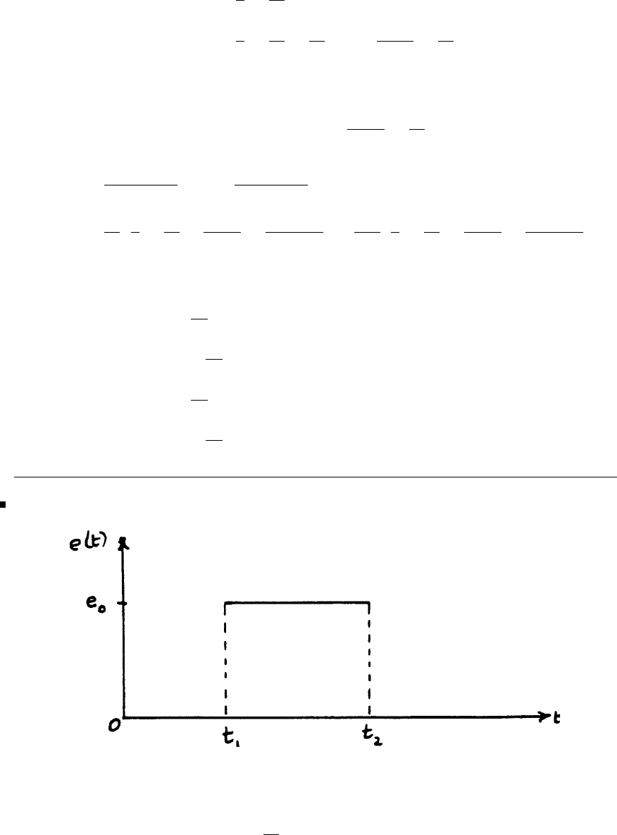
296 Glyn James, Advanced Modern Engineering Mathematics, 4th Edition
so
L{θi(t)}=1
s−1
s2+e−sL{t}
=1
s−1
s2+1
s2e−s=s−1
s2+1
s2e−s
Then taking Laplace transforms, using θ0(0) = ˙
θ0(0) = 0
(s2+8s+ 16)Φ0(s)=s−1
s2+1
s2e−s
Φ0(s)= s−1
s2(s+4)
2+e−s1
s2(s+4)
2
=1
s23
s−2
s2−3
s+4−10
(s+4)
2+e−s
32 3
s+2
s2+1
s+4+2
(s+4)
2
which on taking inverse transforms gives
θ0(t)=L−1{Φ0(s)}=1
32 [3 −2t−3e−4t−10te−4t]
+1
32 [−1+2(t−1) + e−4(t−1) +2(t−1)e−4(t−1)]H(t−1)
=1
32 [3 −2t−3e−4t−10te−4t]
+1
32 [2t−3+(2t−1)e−4(t−1)]H(t−1)
22
e(t)=e0H(t−t1)−e0H(t−t2)
L{e(t)}=e0
s(e−st1−e−st2)
c
Pearson Education Limited 2011
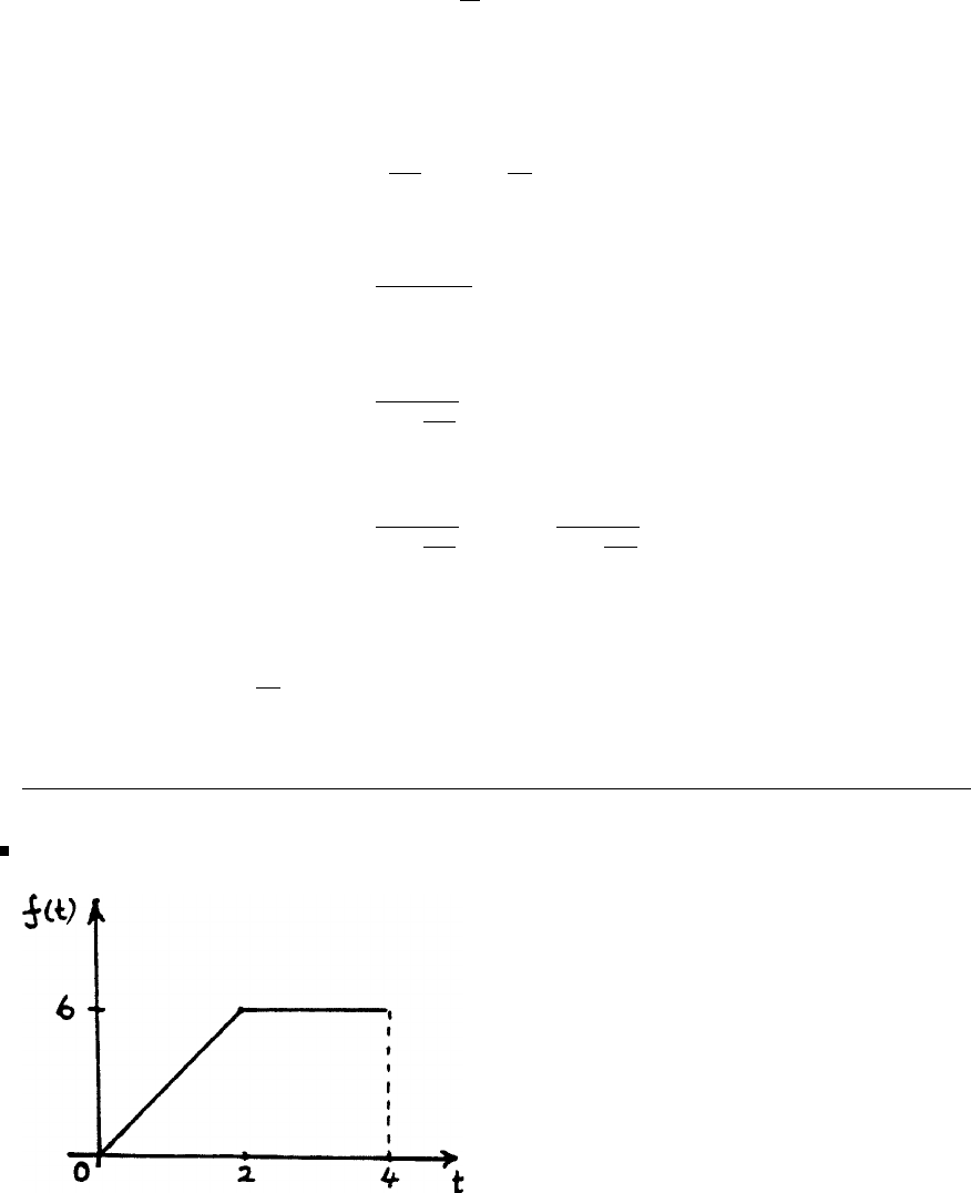
Glyn James, Advanced Modern Engineering Mathematics, 4th Edition 297
By Kirchhoff’s second law current in the circuit is given by
Ri +1
Cidt =e
which on taking Laplace transforms
RI(s)+ 1
Cs I(s)=e0
s(e−st1−e−st2)
I(s)= e0C
RCs +1(e−st1−e−st2)
=e0/R
s+1
RC
(e−st1−e−st2)
=e0/R
s+1
RC
e−st1−e0/R
s+1
RC
e−st2
then
i(t)=L−1{I(s)}
=e0
Re−(t−t1)/RC H(t−t1)−e−(t−t2)/RC H(t−t2)
23
Sketch over one period as shown and
readily extended to 0 ≤t<12.
c
Pearson Education Limited 2011

298 Glyn James, Advanced Modern Engineering Mathematics, 4th Edition
f1(t)=3tH(t)−(3t−6)H(t−2) −6H(t−4)
=3tH(t)−3(t−2)H(t−2) −6H(t−4)
L{f1(t)}=F1(s)= 3
s2−3
s2e−2s−6
se−4s
Then by theorem 5.5
L{f(t)}=F(s)= 1
1−e−4sF1(s)
=1
s2(1 −e−4s)(3 −3e−2s−6se−4s)
24 Take
f1(t)=K
Tt, 0<t<T
=0, t>T
then f1(t)=K
TtH(t)−Kt
TH(t−T)=K
TtH(t)−K
T(t−T)H(t−T)−KH(t−T)
L{f1(t)}=F1(s)= K
Ts2−e−sT K
Ts2−e−sT K
s=K
Ts2(1 −e−sT )−K
se−sT
Then by theorem 5.5
L{f(t)}=F(s)= 1
1−e−sT F1(s)= K
Ts2−K
s
e−sT
1−e−sT
Exercises 5.5.12
25(a)
2s2+1
(s+2)(s+3) =2−10s+11
(s+2)(s+3) =2+ 9
s+2−19
s+3
L−12s2+1
(s+2)(s+3)=2δ(t)+9e−2t−19e−3t
c
Pearson Education Limited 2011

Glyn James, Advanced Modern Engineering Mathematics, 4th Edition 299
25(b)
s2−1
s2+4 =1−5
s2+4
L−1s2−1
s2+4=δ(t)−5
2sin 2t
25(c)
s2+2
s2+2s+5 =1−2s+3
s2+2s+5
=1−2(s+1)+ 1
2(2)
(s+1)
2+s2
L−1s2+2
s2+2s+5=δ(t)−e−t2cos2t+1
2sin 2t
26(a) (s2+7s+ 12)X(s)=2
s+e−2s
X(s)= 2
s(s+4)(s+3)+1
(s+4)(s+3)e−2s
=
1
6
s−
2
3
s+3+
1
2
s+4+1
s+3−1
s+4e−2s
x(t)=L−1{X(s)}=1
6−2
3e−3t+1
2e−4t+e−3(t−2) −e−4(t−2)H(t−2)
26(b)
(s2+6s+ 13)X(s)=e−2πs
X(s)= 1
(s+3)
2+2
2e−2πs
=e−2πsL1
2e−3tsin 2t
so x(t)=L−1{X(s)}=1
2e−3(t−2π)sin 2(t−2π).H(t−2π)
=1
2e6πe−3tsin 2t.H(t−2π)
c
Pearson Education Limited 2011
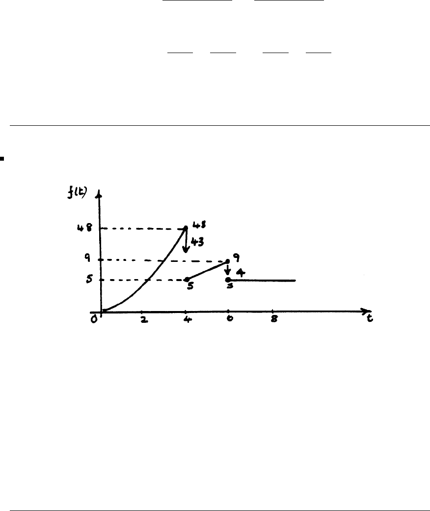
300 Glyn James, Advanced Modern Engineering Mathematics, 4th Edition
26(c)
(s2+7s+ 12)X(s)=s+8+e−3s
X(s)= s+8
(s+4)(s+3) +1
(s+4)(s+3)e−3s
=5
s+3−4
s+4+1
s+3−1
s+4e−3s
x(t)=L−1{X(s)}=5e−3t−4e−4t+[e−3(t−3) −e−4(t−3)]H(t−3)
27(a)
Generalized derivative is
f(t)=g(t)−43δ(t−4) −4δ(t−6)
where
g(t)=⎧
⎪
⎨
⎪
⎩
6t, 0≤t<4
2,4≤t<6
0,t≥6
c
Pearson Education Limited 2011
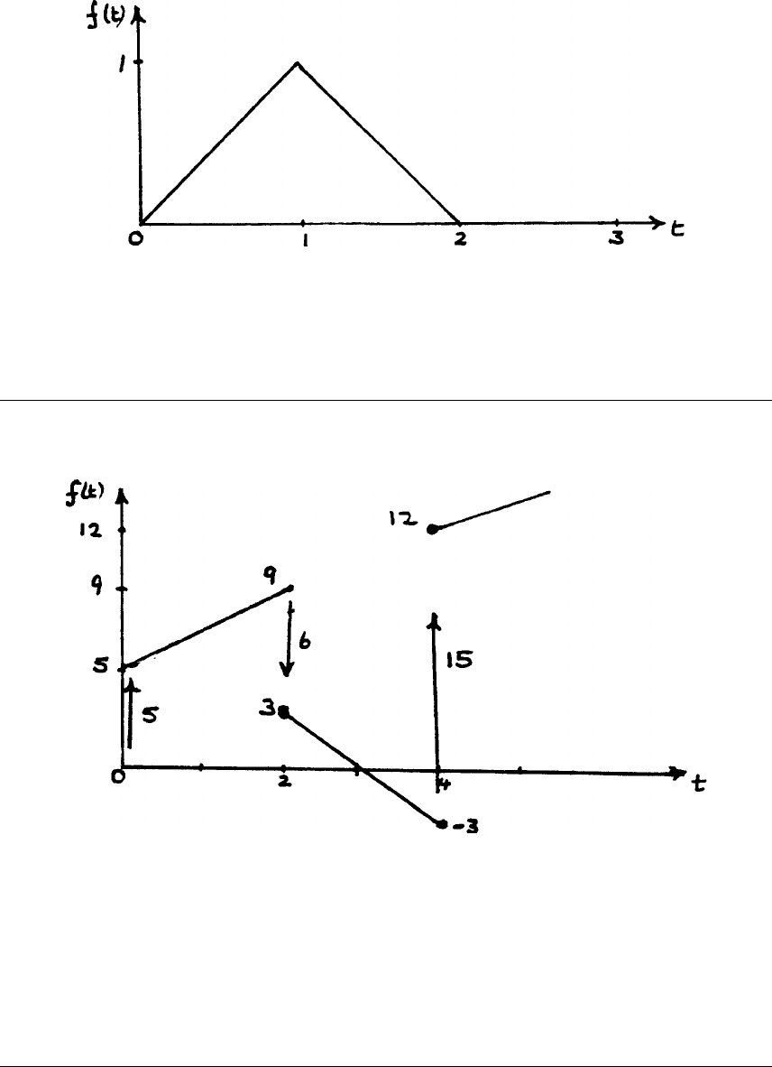
Glyn James, Advanced Modern Engineering Mathematics, 4th Edition 301
27(b)
f(t)=g(t)=⎧
⎨
⎩
1,0≤t<1
−1,1≤t<2
0,t≥2
27(c)
f(t)=g(t)+5δ(t)−6δ(t−2) + 15δ(t−4)
where
g(t)=⎧
⎨
⎩
2,0≤t<2
−3,2≤t<4
2t−1,t≥4
c
Pearson Education Limited 2011

302 Glyn James, Advanced Modern Engineering Mathematics, 4th Edition
28
(s2+7s+ 10)X(s)=2+(3s+2)U(s)
=2+(3s+2) 1
s+2 =5s+6
s+2
X(s)= 5s+6
(s+2)
2(s+5)
=
19
9
s+2−
4
3
(s+2)
2−
19
9
(s+5)
x(t)=L−1{X(s)}=19
9e−2t−4
3te−2t−19
9e−5t
29 f(t)= ∞
n=0
δ(t−nT)
Thus,
F(s)=L{f(t)}=∞
n=0 L{δ(t−nT)}=∞
n=0
e−snT
This is an infinite GP with first term 1 and common ratio e−sT and therefore
having sum (1 −e−sT )−1. Hence,
F(s)= 1
1−e−sT
Assuming zero initial conditions and taking Laplace transforms the response of the
harmonic oscillator is given by
(s2+w2)X(s)=F(s)= 1
1−e−sT
X(s)=∞
n=0
e−snT 1
s2+w2
=[1+e−sT +e−2sT +...]L1
wsin wt
giving x(t)=L−1{X(s)}=1
w[sin wt +H(t−T).sin w(t−T)+H(t−2T).
sin w(t−2T)+...]
or x(t)= 1
w
∞
n=0
H(t−nT)sinw(t−nT).
c
Pearson Education Limited 2011
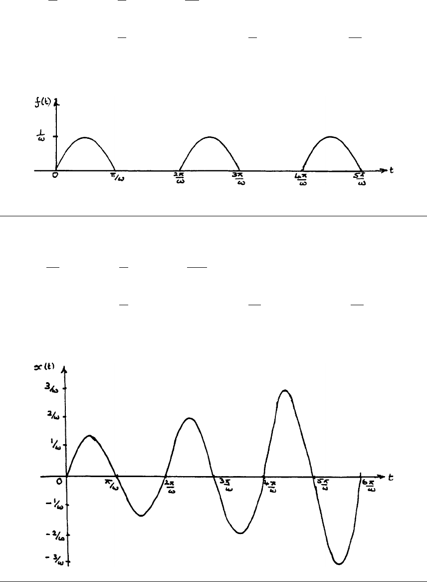
Glyn James, Advanced Modern Engineering Mathematics, 4th Edition 303
29(a)
T=π
w;x(t)= 1
w
∞
n=0
Ht−nπ
wsin(wt −nπ)
=1
wsin wt −sin wt. Ht−π
w+sinwt. Ht−2π
w+...
and a sketch of the response is as follows
29(b)
T=2π
w;x(t)= 1
w
∞
n=0
Ht−2πn
wsin(wt −2πn)
=1
wsin wt +sinwt.Ht−2π
w+sinwt.Ht−4π
w+...
and the sketch of the response is as follows
c
Pearson Education Limited 2011
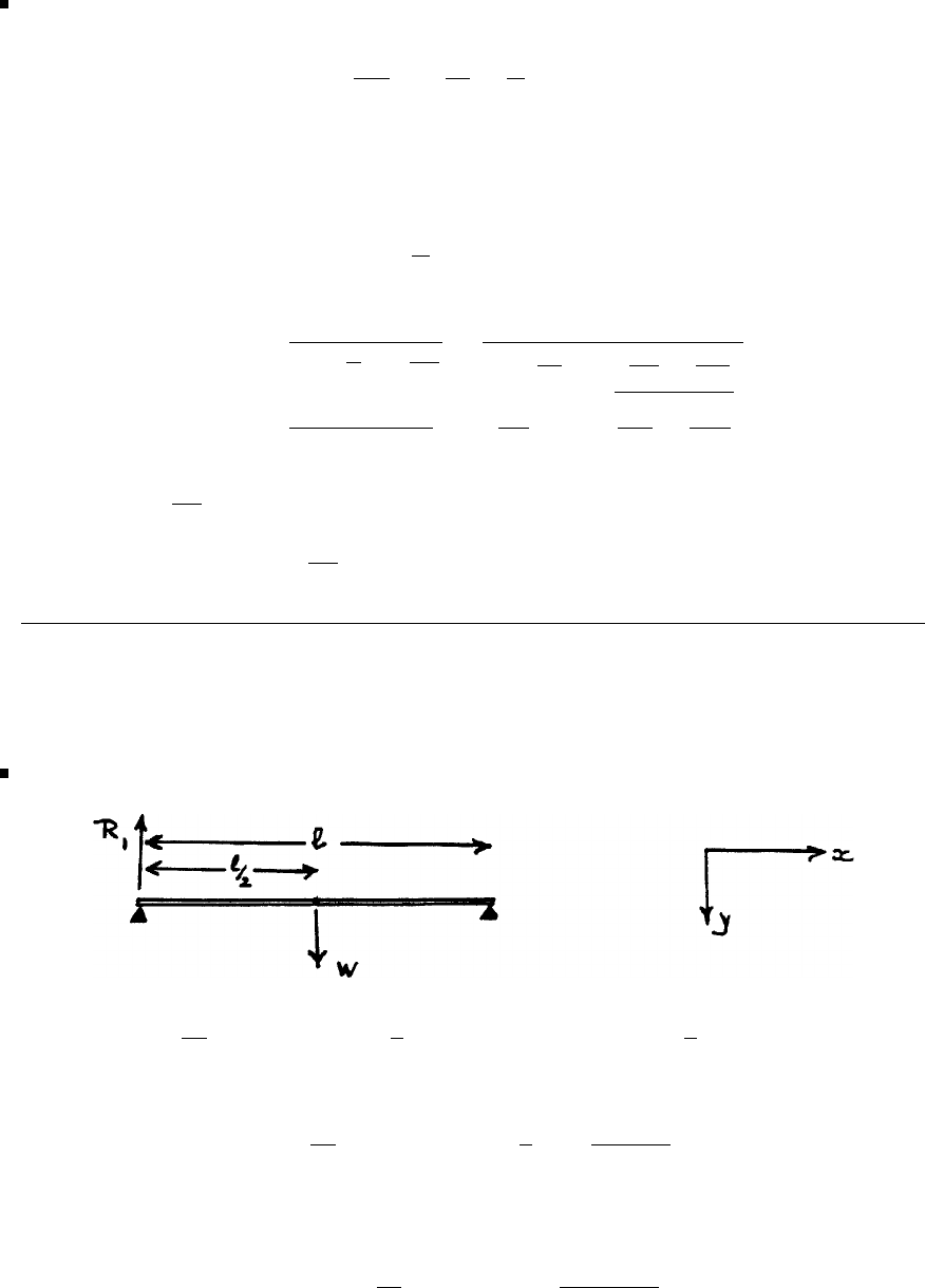
304 Glyn James, Advanced Modern Engineering Mathematics, 4th Edition
30 The charge qon the LCR circuit is determined by
Ld2q
dt2+Rdq
dt +1
Cq=e(t)
where e(t)=Eδ(t),q(0) = ˙
q(0) = 0.
Taking Laplace transforms
Ls2+Rs +1
CQ(s)=L{Eδ(t)}=E
Q(s)= E/L
s2+R
Ls+1
LC
=E/L
(s+R
2L)2+( 1
LC −R2
4L2)
=E/L
(s+μ)2+η2,μ=R
2L,η=1
LC −R2
4L2
Thus, q(t)= E
Lηe−μt sin ηt
and current i(t)=˙
q(t)= E
Lηe−μt(ηcos ηt −μsin ηt)
Exercises 5.5.14
31
Load W(x)=M
H(x)+Wδx−
2−R1δ(x), where R1=1
2(M+W)
so the force function is
W(x)=M
H(x)+Wδx−
2−M+W
2δ(x)
having Laplace transform
W(s)=M
s +We−s/2−(M+W)
2
c
Pearson Education Limited 2011

Glyn James, Advanced Modern Engineering Mathematics, 4th Edition 305
Since the beam is freely supported at both ends
y(0) = y2(0) = y()=y2()=0
and the transformed equation (2.64) of the text becomes
Y(s)= 1
EIM
s5+W
s4e−s/2−M+W
21
s4+y1(0)
s2+y3(0)
s4
Taking inverse transforms gives
y(x)= 1
EI1
24
M
x4+1
6W(x−
2)3·Hx−
2−1
12 (M+W)x3
+y1(0)x+1
6y3(0)x3
for x>
2
y(x)= 1
EI1
24
M
x4+1
6Wx−
2
3
−1
12 (M+W)x3+y1(0)x+1
6y3(0)x3
y2(x)= 1
EI1
2
M
x2+Wx−
2−1
2(M+W)x+y3(0)x
y2()=0 thengives y3(0) = 0 and y()=0 gives
0= 1
EIM3
24 +W3
24 −1
12 M3−1
2W3+y1(0)
y1(0) = 1
EI1
24 M2+1
16 W2
so y(x)= 1
48EI 2
Mx4+8W(x−
2)3Hx−
2−4(M+W)x3+(2M+3W)2x
c
Pearson Education Limited 2011
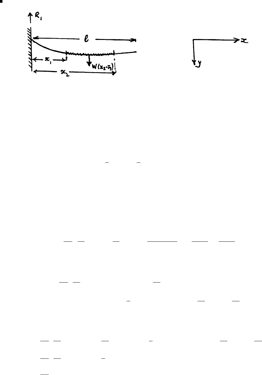
306 Glyn James, Advanced Modern Engineering Mathematics, 4th Edition
32
Load W(x)=w(H(x−x1)−H(x−x2)) −R1δ(x),R
1=w(x2−x1)
so the force function is
W(x)=w(H(x−x1)−H(x−x2)) −w(x2−x1)δ(x)
having Laplace transform
W(s)=w1
se−x1s−1
se−x2s−w(x2−x1)
with corresponding boundary conditions
y(0) = y1(0) = 0,y
2()=y3()=0
The transformed equation (2.64) of the text becomes
Y(s)= w
EI1
s5e−x1s−1
s5e−x2s−(x2−x1)
s4+y2(0)
s3+y3(0)
s4
which on taking inverse transforms gives
y(x)= w
EI1
24 (x−x1)4H(x−x1)−1
24 (x−x2)4H(x−x2)
−1
6(x2−x1)x3+y2(0)x2
2+y3(0)x3
6
For x>x
2
y(x)= w
EI1
24 (x−x1)4−1
24 (x−x2)4−1
6(x2−x1)x3+y2(0)x2
2+y3(0)x3
6
y2(x)= w
EI1
24 (x−x1)2−1
2(x−x2)2−(x2−x1)x+y2(0) + y3(0)x
y3(x)= w
EI(x−x1)−(x−x2)−(x2−x1)+y3(0) ⇒y3(0) = 0
c
Pearson Education Limited 2011
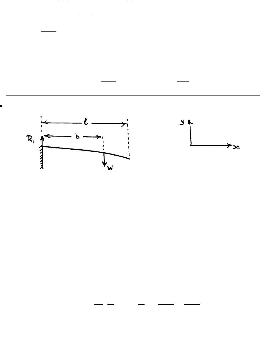
Glyn James, Advanced Modern Engineering Mathematics, 4th Edition 307
The boundary condition y2()=0 thengives
0= w
EI1
2(2−2x1+x2
1)−1
2(2−2x2+x2
2)−x2+x1+y2(0)
⇒y2(0) = w
2EI(x2
2−x2
1)
y(x)= w
24EI (x−x1)4H(x−x1)−(x−x2)4H(x−x2)−4(x2−x1)x3
+6(x2
2−x2
1)x2
When x1=0,x
2=, max deflection at x=
ymax =w
24EI {4−44+64}=w4
8EI
33
Load W(x)=Wδ(x−b)−R1δ(x),R
1=Wso the force function is
W(x)=Wδ(x−b)−Wδ(x)
having Laplace transform
W(s)=We−bs −W
with corresponding boundary conditions
y(0) = y1(0) = 0,y
2()=y3()=0
The transformed equation (2.64) of the text becomes
Y(s)=−1
EIW
s4e−bs −W
s4+y2(0)
s3+y3(0)
s4
which on taking inverse transforms gives
y(x)=−W
EI1
6(x−b)3H(x−b)−1
6x3+y2(0)x2
2+y3(0)x3
6
c
Pearson Education Limited 2011

308 Glyn James, Advanced Modern Engineering Mathematics, 4th Edition
For x>b
y(x)=−W
EI1
6(x−b)3−1
6x3+y2(0)x2
2+y3(0)x3
6
y2(x)=−W
EI(x−b)−x+y2(0) + y3(0)x
y3(x)=−W
EI1−1+y3(0) ⇒y3(0) = 0
Using the boundary condition y2()=0
0=−W
EI(−h)+y2(0) ⇒y2(0) = −Wb
EI
giving
y(x)= W
EIx3
6−(x−b)3
6H(x−b)−bx2
2
=⎧
⎪
⎨
⎪
⎩
−Wx2
6EI (3b−x),0<x≤b
−Wb2
6EI (3x−b),b<x≤
Exercises 5.6.5
34(a) Assuming all the initial conditions are zero taking Laplace transforms
gives
(s2+2s+5)X(s)=(3s+2)U(s)
so that the system transfer function is given by
G(s)=X(s)
U(s)=3s+2
s2+2s+5
c
Pearson Education Limited 2011
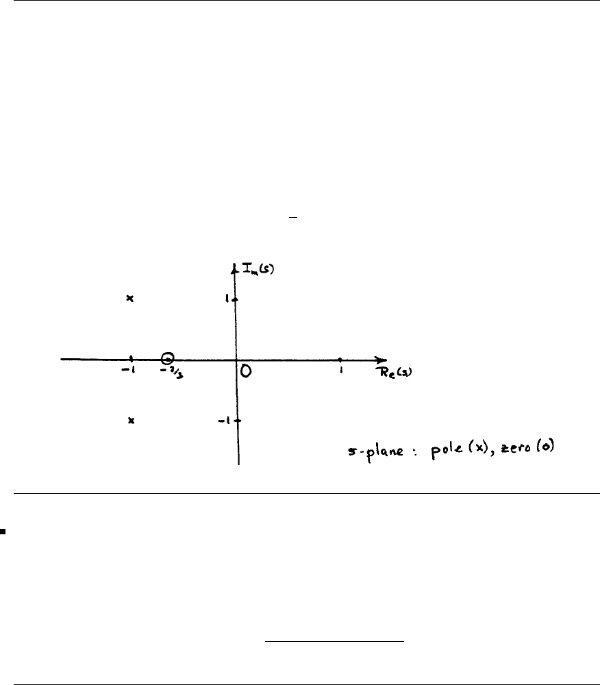
Glyn James, Advanced Modern Engineering Mathematics, 4th Edition 309
34(b) The characteristic equation of the system is
s2+2s+5=0
and the system is of order 2.
34(c) The transfer function poles are the roots of the characteristic equation
s2+2s+5=0
which are s=−1±j. That is, the transfer function has single poles at s=−1+j
and s=−1−j.
The transfer function zeros are determined by equating the numerator polynomial
to zero; that is, a single zero at s=−2
3.
35 Following the same procedure as for Exercise 34
35(a) The transfer function characterizing the system is
G(s)= s3+5s+6
s3+5s2+17s+13
c
Pearson Education Limited 2011
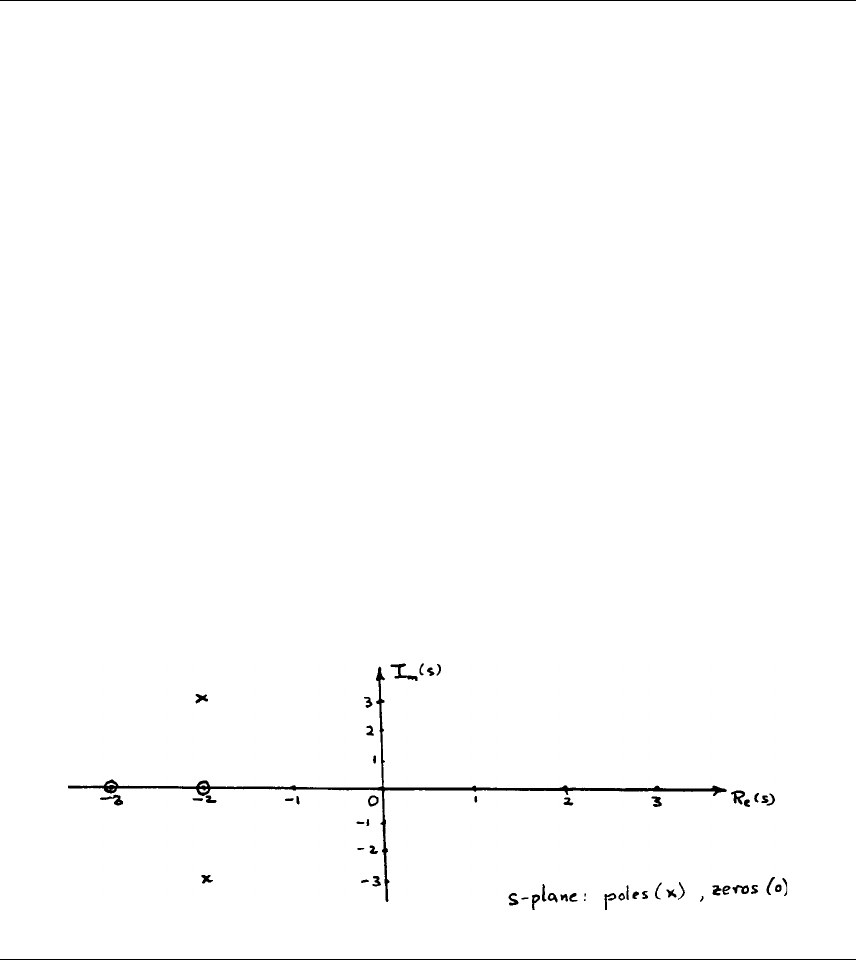
310 Glyn James, Advanced Modern Engineering Mathematics, 4th Edition
35(b) The characteristic equation of the system is
s3+5s2+17s+13=0
and the system is of order 3.
35(c) The transfer function poles are given by
s3+5s2+17s+13=0
that is,(s+1)(s2+4s+ 13) = 0
That is, the transfer function has simple poles at
s=−1,s=−2+j3,s=−2−j3
The transfer function zeros are given by
s2+5s+6=0
(s+3)(s+2)=0
that is, zeros at s=−3ands=−2.
c
Pearson Education Limited 2011

Glyn James, Advanced Modern Engineering Mathematics, 4th Edition 311
36(a) Poles at (s+2)(s2+4)=0; thatis, s=−2,s=+2j, s =−j.
Since we have poles on the imaginary axis in the s-plane, system is marginally
stable.
36(b) Poles at (s+1)(s−1)(s+4)=0;thatis, s=−1,s=1,s=−4.
Since we have the pole s= 1 in the right hand half of the s-plane, the system is
unstable.
36(c) Poles at (s+2)(s+4)=0;that is, s=−2,s=−4.
Both the poles are in the left hand half of the plane so the system is stable.
36(d) Poles at (s2+s+1)(s+1)
2=0;thatis,s=−1(repeated),
s=−1
2±j√3
2.
Since all the poles are in the left hand half of the s-plane the system is stable.
36(e) Poles at (s+5)(s2−s+ 10) = 0; that is, s=−5,s=1
2±j√39
2.
Since both the complex poles are in the right hand half of the s-plane the system
is unstable.
37(a) s2−4s+13=0 ⇒s=2±j3.
Thus, the poles are in the right hand half s-plane and the system is unstable.
37(b)
5s3
a3
+13s2
a2
+31s
a1
+15
a0
=0
Routh–Hurwitz (R-H) determinants are:
Δ1=13>0,Δ2=
13 5
15 31
>0,Δ3= 15Δ2>0
so the system is stable.
c
Pearson Education Limited 2011

312 Glyn James, Advanced Modern Engineering Mathematics, 4th Edition
37(c) s3+s2+s+1=0
R–H determinants are
Δ1=1>0,Δ2=
11
11
=0,Δ3=1Δ
2=0
Thus, system is marginally stable. This is readily confirmed since the poles are at
s=−1,s=±j
37(d) 24s4+11s3+26s2+45s+36=0
R–H determinants are
Δ1=11>0,Δ2=
11 24
45 26
<0
so the system is unstable.
37(e) s3+2s2+2s+1=0
R–H determinants are
Δ1=2>0,Δ2=
23
12
=1>0,Δ3=1Δ
2>0
and the system is stable. The poles are at s=−1,s=−1
2±j√3
2confirming the
result.
38 md3x
dt3+cd2x
dt2+Kdx
dt +Krx =0; m, K, r, c > 0
R–H determinants are
Δ1=c>0
Δ2=
cm
Kr K
=cK −mKr > 0providedr< c
m
Δ3=KrΔ2>0providedΔ
2>0
Thus, system stable provided r< c
m
c
Pearson Education Limited 2011

Glyn James, Advanced Modern Engineering Mathematics, 4th Edition 313
39 s4+2s2
a3
+(K+
a2
2)s2+7s
a1
+K
a0
=0
R–H determinants are
Δ1=|a3|=9>0
Δ2=
a3a4
a1a2
=
21
7K+2
=2K−3>0providedK> 3
2
Δ3=
a3a40
a1a2a3
0a0a1
=
210
7K+2 2
0K7
=10K−21 >0providedK>2
Δ4=KΔ3>0providedΔ
3>0
Thus, the system is stable provided K>2.1.
40 s2+15Ks2+(2K−1)s+5K=0,K>0
R–H determinants are
Δ1=15K>0
Δ2=
15K1
5K(2K−1)
=30K2−20K
Δ3=5KΔ2>0providedΔ
2>0
Thus, system stable provided K(3K−2) >0thatisK>2
3,sinceK>0.
41(a) Impulse response h(t) is given by the solution of
d2h
dt2+15dh
dt +56h=3δ(t)
with zero initial conditions. Taking Laplace transforms
(s2+15s+ 56)H(s)=3
H(s)= 3
(s+7)(s+8) =3
s+7−3
s+8
so h(t)=L−1{H(s)}=3e−7t−3e−8t
Since h(t)→0ast→∞the system is stable.
c
Pearson Education Limited 2011

314 Glyn James, Advanced Modern Engineering Mathematics, 4th Edition
41(b) Following (a) impulse response is given by
(s2+8s+ 25)H(s)=1
H(s)= 1
(s+4)
2+3
2
so h(t)=L−1{H(s)}=1
3e−4tsin 3t
Since h(t)→0ast→∞the system is stable.
41(c) Following (a) impulse response is given by
(s2−2s−8)H(s)=4
H(s)= 4
(s−4)(s+2) =2
3
1
s−4−2
3
1
s+2
so h(t)=L−1{H(s)}=2
3(e4t−e−2t)
Since h(t)→∞as t→∞system is unstable.
41(d) Following (a) impulse response is given by
(s2−4s+ 13)H(s)=1
H(s)= 1
s2−4s+13 =1
(s−2)2+3
2
so h(t)=L−1{H(s)}=1
3e2tsin 3t
Since h(t)→∞as t→∞system is unstable.
42 Impulse response h(t)= dx
dt =7
3e−t−3e−2t+2
3e−4t
System transfer function G(s)=L{h(t)};thatis,
G(s)= 7
3(s+1) −3
s+2+2
3(s+4)
=s+8
(s+1)(s+2)(s+4)
Note: The original unit step response can be reconstructed by evaluating
L−1G(s)1
s.
c
Pearson Education Limited 2011

Glyn James, Advanced Modern Engineering Mathematics, 4th Edition 315
43(a) f(t)=2−3cost, F(s)= 2
s−3s
s2+1
sF(s)=2−3s2
s2+1 =2−3
1+ 1
s2
Thus, lim
t→0+(2 −3cost)=2−3=−1
and lim
s→∞ sF(s)=2−3
1=−1 so confirming the i.v. theorem.
43(b)
f(t)=(3t−1)2=9t2−6t+1,lim
t→0+ f(t)=1
F(s)=18
s3−6
s2+1
sso lim
s→∞ sF(s) = lim
s→∞ 18
s2−6
s+1
=1
thus, confirming the i.v. theorem.
43(c)
f(t)=t+3sin2t, lim
t→0+ =0
F(s)= 1
s2−6
s2+4 so lim
s→∞ sF(s) = lim
s→∞ 1
s+6
s+4
s=0
thus, confirming the i.v. theorem.
44(a)
f(t)=1+3e−tsin 2t, lim
t→∞ f(t)=1
F(s)= 1
s+6
(s+1)
2+4 and lim
s→0sF(s) = lim
s→01+ 6s
(s+1)
2+4=1
thus confirming the f.v. theorem. Note that, sF(s) has its poles in the left half of
the s-plane so the theorem is applicable.
c
Pearson Education Limited 2011

316 Glyn James, Advanced Modern Engineering Mathematics, 4th Edition
44(b)
f(t)=t23e−2t,lim
t→∞ f(t)=0
F(s)= 2
(s+2)
3and lim
s→0sF(s) = lim
s→02s
(s+2)
3=0
thus confirming the f.v. theorem. Again note that sF(s) has its poles in the left
half of the s-plane.
44(c)
f(t)=3−2e−3t+e−tcos 2t, lim
t→∞ f(t)=3
F(s)=3
s−2
s+3+(s+1)
(s+1)
2+4
lim
s→0sF(s) = lim
s→03−2s
s+3+s(s+1)
(s+1)
2+4=3
confirming the f.v. theorem. Again sF(s) has its poles in the left half of the
s-plane.
45 For the circuit of Example 5.28
I2(s)=3.64
s+1.22
s+59.1−4.86
s+14.9
Then by the f.v. theorem
lim
t→∞ i2(t) = lim
s→0sI2(s) = lim
s→03.64 + 1.22s
s+59.1−4.86s
s+14.9
=3.64
which confirms the answer obtained in Example 5.28. Note that, sI2(s) has all its
poles in the left half of the s-plane.
46 For the circuit of Example 5.29
sI2(s)= 28s2
(3s+ 10)(s+1)(s2+4)
and since it has poles at s=±j2 not in the left hand half of the s-plane the
f.v. theorem is not applicable.
c
Pearson Education Limited 2011

Glyn James, Advanced Modern Engineering Mathematics, 4th Edition 317
47 Assuming quiescent initial state taking Laplace transforms gives
(7s+5)Y(s)= 4
s+1
s+3+2
Y(s)= 4
s(7s+5) +1
(s+ 3)(7s+5) +2
7s+5
sY(s)= 4
7s+5+s
(s+ 3)(7s+5) +2s
7s+5
By the f.v. theorem,
lim
t→∞ y(t) = lim
s→0sF(s) = lim
s→04
7s+5 +s
(s+ 3)(7s+5) +2s
7s+5
=4
5
By the i.v. theorem,
lim
t→0+y(t)=y(0+) = lim
s→∞ sF(s) = lim
s→∞ 4
7s+5 +s
(1 + 3
s)(7s+5) +2
7+5
s
=2
7
Thus, jump at t=0=y(0+) −y(0−)=1
2
7.
Exercises 5.6.8
48(a)
f∗g(t)=t
0
τcos(3t−3τ)dτ
=−1
3τsin(3t−3τ)+1
9cos(3t−3τ)
t
0
=1
9(1 −cos 3t)
g∗f(t)=t
0
(t−τ)cos3τdτ
=t
3sin 3τ−τ
3sin 3τ−1
9cos 3τ
t
0=1
9(1 −cos 3t)
c
Pearson Education Limited 2011

318 Glyn James, Advanced Modern Engineering Mathematics, 4th Edition
48(b)
f∗g(t)=t
0
(τ+1)e−2(t−τ)dτ
=1
2(τ+1)e−2(t−τ)−1
4e−2(t−τ)
t
0
=1
2t+1
4−1
4e−2t
g∗f(t)=t
0
(t−τ+1)e−2τdτ
=−1
2(t−τ+1)e−2τ+1
4e−2τ
t
0
=1
2t+1
4−1
4e−2t
48(c) Integration by parts gives
t
0
τ2sin 2(t−τ)dτ =t
0
(t−τ)2sin 2τdτ
=1
4cos 2t+1
2t2−1
4
48(d) Integration by parts gives
t
0
e−τsin(t−τ)dτ =t
0
e−(t−τ)sin τdτ
=1
2(sin t−cos t+e−t)
49(a) Since L−11
s=1=f(t)andL−11
(s+3)
3=1
2t2e−3t
L−11
s·1
(s+3)
3=t
0
f(t−τ)g(τ)dτ
=t
0
1.1
2τ2e−3τdτ
=1
4−τ2e−3τ−2
3τe−3τ−2
9e−3τ
t
0
=1
54 [2 −e−3t(9t2+6t+2)]
c
Pearson Education Limited 2011

Glyn James, Advanced Modern Engineering Mathematics, 4th Edition 319
Directly
L−11
s·1
(s+3)
3=L−11
54 2
s−18
(s+3)
3−6
(s+3)
2−2
(s+3)
=1
54 [2 −e−3t(9t2+6t+2)]
49(b) L−11
(s−2)2=te2t=f(t),L−11
(s+3)
2=te−3t=g(t)
L−11
(s−2)2·1
(s+3)
2=t
0
(t−τ)e2(t−τ).τe−3τdτ
=e−2tt
0
(tτ −τ2)e−5τdτ
=e2t−1
5(tτ −τ2)e−5τ−1
25 (t−2τ)e−5τ+2
125 e−5τ
t
0
=e2tt
25 e−5t+2
125 e−5t+t
25 −2
125
=1
125 e2t(5t−2) + e−3t(5t+2)
Directly
1
(s−2)2(s+3)
2=−2
125
s−2+
1
25
(s−2)2+
2
125
(s+3) +
1
25
(s+3)
2
∴L−11
(s−2)2(s+3)
2=−2
125 e2t+1
25 te2t+2
125 e−3t+1
25 te−3t
=1
125 [e2t(5t−2) + e−3t(5t+2)]
49(c) L−11
s2=t=f(t),L−11
(s+4)=e−4t=g(t)
L−11
s2·1
s+4=t
0
(t−τ)e−4tdτ
=−1
4(t−τ)e−4τ+1
16 e−4τ
t
0
=1
16 e−4t+1
4t−1
16
c
Pearson Education Limited 2011

320 Glyn James, Advanced Modern Engineering Mathematics, 4th Edition
Directly
L−11
s2(s+4)=L−11
16 ·1
s+4−1
16 ·1
s+1
4·1
s2
=1
16 e−4t−1
16 +1
4t
50 Let f(λ)=λand g(λ)=e−λso
F(s)= 1
s2and G(s)= 1
s+1
Considering the integral equation
y(t)=t
0
λe−(t−λ)dλ
By (5.80) in the text
L−1{F(s)G(s)}=t
0
f(λ)g(t−λ)dλ
=t
0
λe−(t−λ)dλ =y(t)
so
y(t)=L−1{F(s)G(s)}=L−11
s2(s+1)
=L−1−1
s+1
s2+1
s+1
=(t−1) + e−t
51 Impulse response h(t) is given by the solution of
d2h
dt2+7dh
dt +12h=δ(t)
subject to zero initial conditions. Taking Laplace transforms
(s2+7s+ 12)H(s)=1
H(s)= 1
(s+3)(s+4) =1
s+3−1
s+4
giving h(t)=L−1{H(s)}=e−3t−e−4t
c
Pearson Education Limited 2011

Glyn James, Advanced Modern Engineering Mathematics, 4th Edition 321
Response to pulse input is
x(t)=At
0
[e−3(t−τ)−e−4(t−τ)]dτH(t)
−At
T
[e−3(t−τ)−e−4(t−τ)]dτH(t−T)
=A1
3−1
4−1
3e−3t+1
4e−4tH(t)
−1
3−1
4−1
3e−3(t−T)−1
4e−4(t−T)H(t−T)
=1
12 A1−4e−3t+3e−4t−(1 −4e−3(t−T)+3e−4(t−T))H(t−T)
or directly
u(t)=A[H(t)−H(t−T)] so U(s)=L{u(t)}=A
s[1 −e−sT ]
Thus, taking Laplace transforms with initial quiescent state
(s2+7s+ 12)X(s)=A
s[1 −e−sT ]
X(s)=A1
12 ·1
s−1
3·1
s+3+1
4·1
s+4(1 −e−sT )
x(t)=L−1{X(s)}=A
12 [1 −4e−3t+3e−4t−(1 −4e−3(t−T)+3e−4(t−T))H(t−T)]
52 Impulse response h(t) is the solution of
d2h
dt2+4dh
dt +5h=δ(t),h(0) = ˙
h(0) = 0
Taking Laplace transforms
(s2+4s+5)H(s)=1
H(s)= 1
s2+4s+5 =1
(s+2)
2+1
so h(t)=L−1{H(s)}=e−2tsin t.
c
Pearson Education Limited 2011

322 Glyn James, Advanced Modern Engineering Mathematics, 4th Edition
By the convolution integral response to unit step is
θ0(t)=t
0
e−2(t−τ)sin(t−τ).1dτ
=e−2tt
0
e2τsin(t−τ)dτ
which using integration by parts gives
θ0(t)=e−2t
5e2τ[2 sin(t−τ)+cos(t−τ)]t
0
=1
5−1
5e−2t(2 sin t+cost)
Check
Solving
d2θ0
dt2+4dθ0
dt +5θ0=1,˙
θ0(0) = θ0(0) = 0
gives
(s2+4s+5)Φ
0(s)=1
s
Φ0(s)= 1
s(s2+4s+5) =1
5s−1
5·s+4
(s+2)
2+1
so θ0(t)=L−1{Φ0(s)}=1
5−1
5[cos t+2sint]e−2t.
Exercises 5.7.2
53 State–space form of model is
˙
x=Ax +bu ⇒˙
x1
˙
x2=−5−1
3−1x1
x2+2
5u
y=cTx⇒y=[1 2]x1
x2
System transfer function is
G(s)=cT(sI−A)−1b=[1 2]s+5 1
−3s+1−12
5
c
Pearson Education Limited 2011

Glyn James, Advanced Modern Engineering Mathematics, 4th Edition 323
det s+5 1
−3s+1=Δ=(s+5)(s+1)+3=(s+2)(s+4),
s+5 1
−3s+1−1
=1
Δs+1 −1
3s+5
Thus, G(s)= 1
Δ[1 2]s+1 −1
3s+52
5=1
Δ(12s+ 59)
so the system transfer function is
G(s)= 12s+59
(s+2)(s+4)
54 In this case, the denominator can be factorized
G(s)= Y(s)
U(s)=s+1
(s+1)(s+6)
and care must be taken not to cancel the common factor, to avoid the system being
mistaken for a first order system. To proceed it is best to model the system by the
differential equation
¨
y+7˙
y+6y=˙
u+u
from which ˙
x1=−7x1+x2+u
˙
x2=−6x1+u
y=x1
so that a state–space model is
˙
x=Ax +bu⇒˙
x1
˙
x2=−71
−60
x1
x2+1
1u
y=cTx⇒y=[1 0]x1
x2
Check
G(s)=cT(sI−A)−1b
det(sI−A)=Δ=
s+7 −1
6s
=s2+7s+6
G(s)= 1
Δ[1 0]s1
−6s+71
1=s+1
Δ=s+1
s2+7s+6
c
Pearson Education Limited 2011

324 Glyn James, Advanced Modern Engineering Mathematics, 4th Edition
55(a) Taking Ato be the companion matrix
A=⎡
⎣
010
001
−7−5−6⎤
⎦
then b=[001]
T
c=[531]
T
Then from equation (5.84) in the text the state space form of the dynamic model
is ˙
x=Ax+bu
y=cTx
55(b) Taking Ato be the companion matrix
A=⎡
⎣
010
001
0−3−4⎤
⎦
then b=[001]
T
c=[231]
T
And state space model is
˙
x=Ax+bu, y =cTx
56 We are required to express the transfer function in the state space form
˙
x=Ax+bu
y=cTx
where Ais the companion matrix A=⎡
⎣
010
001
−6−11 −6⎤
⎦and y=[100]x.To
determine b, we divide the denominator into the numerator as follows
s3+6s2+11s+6
5s−1−29s−2+ 120s−3
5s2+s+1
5s2+30s+55
−29s−54 |
|neglect these terms
−29s−174
120 |
|
c
Pearson Education Limited 2011

Glyn James, Advanced Modern Engineering Mathematics, 4th Edition 325
giving b=[5 −29 −120]T. Thus, state space form is
˙
x(t)= ⎡
⎣
˙
x1
˙
x2
˙
x3⎤
⎦=⎡
⎣
010
001
−6−11 −6⎤
⎦x(t)+ ⎡
⎣
5
−29
120 ⎤
⎦u(t)
y=[100]x(t)
It is readily checked that this is a true representation of the given transfer function.
57 [sI−A]= s−3−4
−2s−1,det[sI−A]=(s−5)(s+1)
Thus,
[sI−A]−1=1
(s−5)(s+1) s−14
2s−3=2/3
s−5+1/3
s+1
2/3
s−5−2/3
s+1
−1/3
s−5−1/3
s+1
1/3
s−5+2/3
s+1
∴L−1[sI−A]−1=2
3e5t+1
3e−t2
3e5t−2
3e−t
1
3e5t−1
3e−t1
3e5t+2
3e−t=Φ1
[sI−A]−1BU(s)= 1
(s−5)(s+1) s−14
25−301
11
4
s
7
s
=1
s(s−5)(s+1) 3s+25
7s−15 =−5
s+11/3
s+1 +4/3
s−5
3
s−11/3
s+1 +2/3
s−5
∴L−1{[sI−A]−1BU(s)}=−5+ 11
3e−t+4
3e5t
3−11
3e−t+2
3e5t=Φ2
Thus, solution is
x(t)=Φ
1x(0) + Φ2=−5+8
3e−t+10
3e5t
3−8
3e−t+5
3e5t
which confirms the answer obtained in Exercise 61 in Chapter 1.
c
Pearson Education Limited 2011

326 Glyn James, Advanced Modern Engineering Mathematics, 4th Edition
58 A =1−3
2−4,sI−A=s−13
−2s+4
|sI−A|=Δ=(s−1)(s+4)+6=(s+2)(s+1)
[sI−A]−1=1
Δs+4 −3
2s−1
=3
s+1 −2
s+2 −3
s+1 +3
s+2
2
s+1 −2
s+2 −2
s+1 +3
s+2
giving L−1[sI−A]−1=3e−t−2e−2t−3e−t+3e−2t
2e−t−2e−2t−2e−t+3e−2t
so L−1[sI−A]−1x(0) = e2t
e−2t
[sI−A]−1bU(s)= 1
Δs+4 −3
2s−11
11
s+3
=1
(s+2)(s+3)
1
(s+2)(s+3) =1
s+2 −1
s+3
1
s+2 −1
s+3
so L−1{[sI−A]−1bU(s)}=e−2t−e−3t
e−2t−e−3t
Thus,
x(t)= e−2t
e−2t+e−2t−e−3t
e−2t−e−3t
giving
x1(t)=x2(t)=2e−2t−e−3t
59 A =01
−2−3,b=2
0,u(t)=e−tH(t),x0=[10]
T
with X(s) and the solution x(t) given by equations (5.88) and (5.89) in the text
(sI−A)= s−1
2s+3giving (sI−A)−1=1
(s+1)(s+2) s+3 1
−25
so that,
(sI−A)−1x0=1
(s+1)(s+2) s+3
−2=2
s+1 −1
s+2
−2
s+1 +2
s+2
and
(sI−A)−1bU(s)= 1
(s+1)(s+2) 2(s+3)
−41
s+1 =2
s+2 +4
(s+1)2−2
s+1
4
s+1 −4
(s+1)2−4
s+2
c
Pearson Education Limited 2011

Glyn James, Advanced Modern Engineering Mathematics, 4th Edition 327
Thus, X(s)= 4
(s+1)2+1
(s+2)
2
(s+1) −2
(s+2) −4
(s+1)2
giving x(t)= 4te−t+e−2t
2e−t−2e−2t−4te−t
60 Taking Aas the companion matrix following the procedure of Example 5.61
we have
A=⎡
⎣
010
001
−6−11 −6⎤
⎦,b=[001]
T,c=[123]
T
Eigenvalue of Agiven by
−λ10
0−λ1
−6−11 −6−λ
=−(λ3+6λ2+11λ+6)=−(λ+1)(λ+2)(λ+3)=0
so the eigenvalues are λ1=−3,λ
2=−2,λ
3=−1. The eigenvectors are given by
the corresponding solutions of
−λiei1+ei2+0ei3=0
0ei1−λiei2+ei3=0
−6ei1−11ei2−(6 + λi)ei3=0
Taking i=1,2,3 and solving gives the eigenvectors as
e1=[1 −39]
T,e2=[1 −24]
T,e3=[1 −11]
T
Taking Mto be the modal matrix M=⎡
⎣
111
−3−2−1
941
⎤
⎦then the transformation
X=Mξξ
ξwill reduce the system to the canonical form
˙
ξξ
ξ=Λξξ
ξ+M−1bu, y=cTMξξ
ξ
M−1=1
2⎡
⎣
231
−6−8−2
651
⎤
⎦,M−1b=1
2⎡
⎣
1
−2
1⎤
⎦,cTM=[2292]
c
Pearson Education Limited 2011

328 Glyn James, Advanced Modern Engineering Mathematics, 4th Edition
Thus, canonical form is
⎡
⎣
˙
ξ1
˙
ξ2
˙
ξ3⎤
⎦=⎡
⎣−300
0−20
00−1⎤
⎦⎡
⎣
ξ1
ξ2
ξ3⎤
⎦+⎡
⎣
1
2
−1
1
2
⎤
⎦u
y=[2292][ξ1ξ2ξ3]T
Since the eigenvalues of Aare negative the system is stable. Since vector M−1b
has no zero elements the system is controllable and since cTMhas no zero elements
the system is also observable.
b=[001]
T,Ab=[01 −6]T,A2b= [1 6 25]T
[bAbA
2b]= ⎡
⎣
00 1
01 6
1−625
⎤
⎦∼⎡
⎣
001
010
100
⎤
⎦which is of full rank 3
so the system is controllable.
c=[123]
T,ATc=[−18 −32 −16],(AT)2c= [96 158 63]T
[cA
Tc(AT)2c]= ⎡
⎣
1−18 96
2−32 158
3−16 63 ⎤
⎦∼⎡
⎣
100
010
001
⎤
⎦which is of full rank 3
so the system is observable.
61 A =⎡
⎣
010
001
0−5−6⎤
⎦,b=[001]
T,c=[531]
T
Eigenvalues of Agiven by
0=
−λ10
0−λ1
0−5−6−λ
=−λ(λ+5)(λ+1)=0
so eigenvalues are λ1=−5,λ
2=−1,λ
3= 0. The corresponding eigenvectors are
determined as
e1=[1 −5 25]T,e2=[1 −11],e3=[100]
T
c
Pearson Education Limited 2011

Glyn James, Advanced Modern Engineering Mathematics, 4th Edition 329
Take Mto be the modal matrix M=⎡
⎣
111
−5−10
25 1 0 ⎤
⎦then the transformation
x=Mξξ
ξwill reduce the system to the canonical form
˙
ξξ
ξ=Λξξ
ξ+M−1bu, y=cTMξξ
ξ
M−1=1
20 ⎡
⎣
011
0−25 −5
20 24 4 ⎤
⎦,M−1b=1
20 ⎡
⎣
1
−5
4⎤
⎦,cTM=[1535]
Thus, canonical form is
⎡
⎣
˙
ξ1
˙
ξ2
˙
ξ3⎤
⎦=⎡
⎣−500
0−10
000
⎤
⎦⎡
⎣
ξ1
ξ2
ξ3⎤
⎦+⎡
⎣
1
20
−1
4
1
5
⎤
⎦u
y=[1535][ξ1ξ2ξ3]T
Since Ahas zero eigenvalues the system is marginally stable, since M−1bhas no
zero elements the system is controllable and since cTMhas no zero elements the
system is observable. Again as in Exercise 60 these results can be confirmed by
using the Kalman matrices.
Exercises 5.7.4
62 A =0−2
1−3,B=1−1
11
,u=1
t,x0=0
1
The solution x(t) is given by equation (5.97) in the text.
(sI−A)= s2
−1s+3giving (sI−A)−1=1
(s+1)(s+2) s+3 −2
1s
so that,
(sI−A)−1x0=1
(s+1)(s+2) −2
s=2
s+2 −2
s+1
2
s+2 −1
s+1
(sI−A)−1BU(s)= 1
(s+1)(s+2) s+3 −2
1s1−1
11
⎡
⎣
1
s
1
s2
⎤
⎦
=1
s(s+2) −(s+5)
s2(s+1)(s+2)
1
s(s+2) +s−1
s2(s+1)(s+2)
c
Pearson Education Limited 2011

330 Glyn James, Advanced Modern Engineering Mathematics, 4th Edition
Thus,
X1(s)=L{x1(t)}=2
s+2−2
s+1+1
s(s+2) −(s+5)
s2(s+1)(s+2)
=9/4
s+2−6
s+1+15/4
s−5/2
s2
giving x1(t)=9
4e−2t−6e−t+15
4−5
2t
63 ¨
y1+˙
y1−˙
y2+y1=u1(i)
¨
y2+˙
y2−˙
y1+y2=u2(ii)
Let x=[x1x2x3x4]T=[y1˙
y1y2˙
y2]Tthen
˙
x1=˙
y1=x2
(i)⇒¨
y1=˙
x2=−˙
y1+˙
y2−y1+u1⇒˙
x2=−x2+x4−x1+u1
˙
x3=˙
y2=x4
(ii)⇒¨
y2=˙
x4=xx −˙
y2+˙
y1−y2+u2⇒˙
x4=−x4+x2−x3+u2
giving the state–space representation
˙
x=Ax +Bu ⇒⎡
⎢
⎣
˙
x1
˙
x2
˙
x3
˙
x4
⎤
⎥
⎦=⎡
⎢
⎣
0100
−1−10 1
0001
01−1−1
⎤
⎥
⎦⎡
⎢
⎣
x1
x2
x3
x4
⎤
⎥
⎦+⎡
⎢
⎣
00
10
00
01
⎤
⎥
⎦u1
u2
y=Cx ⇒y1
y2=1000
0010
⎡
⎢
⎣
x1
x2
x3
x4
⎤
⎥
⎦
Transfer function = G(s)=Cadj(sI−A)B
det(sI−A)
det(sI−A)=Δ=
s−10 0
1s+1 0 −1
00s−1
0−11s+1
=s4+2s3+2s2+2s+1
⇒Δ=(s+1)
2(s2+1)
so that
G(s)= 1
Δs2+s+1 s
ss
2+s+1=1
(s+1)
2(s2+1)s2+s+1 s
ss
2+s+1
c
Pearson Education Limited 2011

Glyn James, Advanced Modern Engineering Mathematics, 4th Edition 331
Poles given by Δ = (s+1)
2(s2+1)=0
Eigenvalues associated matrix Agiven by det(λI−A)=(λ+1)
2(λ2+1)=0
Thus, poles and eigenvalues are identical.
64 (a) u2=R1(u1+x1+x2+x3)+L1˙
x1;R1=1,L
1=1
⇒˙
x1=−x1−x2−x3−u1+u2
u2=R1(u1+x1+x2+x3)+R2(x2+x3)+L2˙
x2;R2=2,L
2=1
⇒˙
x2=−x1−3x2−3x3−u1+u2
u2=R1(u1+x1+x2+x3)+R2(x2+x3)+R3x3+L3˙
x3;R3=3,L
3=1
⇒˙
x3=−x1−3x2−6x3−u1+u2
giving the state–space model
⎡
⎣
˙
x1
˙
x2
˙
x3⎤
⎦=⎡
⎣−1−1−1
−1−3−3
−1−3−6⎤
⎦⎡
⎣
x1
x2
x3⎤
⎦+⎡
⎣−11
−11
−11
⎤
⎦u1
u2
y1
y2=022
001
x1
x2
(b) Transfer matrix = G(s)=Y(s)
U(s)=C(sI−A)−1B=Cadj(sI−A)
det(sI−A)B
det(sI−A)=Δ=
s+1 1 1
1s+3 3
13s+6
=s3+10s2+16s+6
adj(sI−A)=⎡
⎣
s2+9s+9 −(s+3) −s
−(s+3) s2+7s+5 −(3s+2)
−s−(3s+2) s2+4s+2⎤
⎦
G(s)= 1
Δ022
001
⎡
⎣
s2+9s+9 −(s+3) −s
−(s+3) s2+7s+5 −(3s+2)
−s−(3s+2) s2+4s+2⎤
⎦⎡
⎣−11
−11
−11
⎤
⎦
=1
Δ−2s(2s+3) 2s(2s+3)
−s2s2with Δ = s3+10s2+16s+6
c
Pearson Education Limited 2011

332 Glyn James, Advanced Modern Engineering Mathematics, 4th Edition
(c) Y(s)=G(s)U(s)whereU(s)=1
s
1
s2
=1
Δ−2s(2s+3) 2s(2s+3)
−s2s21
s
1
s2
=1
Δ−4s2−2s+6
s
−s+1
To obtain response express in partial fractions and take inverse Laplace transforms
Factorizing Δ gives Δ = (s+8.12)(s+0.56)(s+1.32) so
Y1(s)= −4s2−2s+6
s(s+8.12)(s+0.56)(s+1.32) =1
s+0.578
s+8.12 −1.824
s+0.56 +0.246
s+1.32
⇒y1(t)=1+0.578e−8.12t−1.824e−0.56t+0.246e−1.32t
Y2(s)= −s+1
(s+8.12)(s+0.56)(s+1.32) =0.177
s+8.12 +0.272
s+0.56 −0.449
s+1.32
⇒y2(t)=0.177e−8.12t+0.272e−0.56t−0.449e−1.32t
Exercises 5.9.3
65 Choose x1(t)=y(t),x
2(t)= ˙
x1(t)=dy
dt then
˙
x(t)=01
1
2
1
2x(t)+0
1u(t),y(t)=[10]x(t)
Taking u(t)=K1x1(t)+K2x2(t)+uext(t)
˙
x(t)=01
K1+1
2K2+1
2x(t)+ 0
1uext
The eigenvalues of the matrix are given by
0−λ1
K1+1
2K2+1
2−λ
=0
or λ2−(K2+1
2)λ−(K1+1
2)=0
If the poles are to be at λ=−4 then we require the characteristic equation to be
λ2+8λ+16=0
c
Pearson Education Limited 2011

Glyn James, Advanced Modern Engineering Mathematics, 4th Edition 333
By comparison, we have −K2−1
2=8and−K1−1
2= 18 giving K1=−33
2,
K2=−17
2so u(t)=−33
2−17
2x+uext
66
˙
x(t)= 01
−1
4−5
4x(t)+ 0
1u(t),y(t)=[02]x(t)
Setting u=KTx+uext,K=[K1K2]Tgives the system matrix
A=01
K1−1
4K2−5
4
whose eigenvalues are given by λ2−(K2−5
4)λ−(K1−5
4) = 0. Comparing with
the desired characteristic equation
(λ+5)
2=λ2+10λ+25=0
gives K1=−99
4,K
2=−35
4.Thus,
u(t)=−99
4−35
4x(t)+uext
67 With u1=[K1K2]x(t) the system matrix Abecomes
A=K11+K2
6+K11+K2
having characteristic equation
λ2−λ(1 + K1+K2)−6(1 −K2)=0
which on comparing with
λ2+10λ+25=0
gives K1=−35
6,K
2=−31
6so that u1(t)=−35
6−31
6x(t)
Using u2(t)thematrixAbecomes 01
6+K11+K2where KT=[−31 −11]
68 See p. 472 in the text.
c
Pearson Education Limited 2011

334 Glyn James, Advanced Modern Engineering Mathematics, 4th Edition
69 For the matrix of Exercise 68 the Kalman matrix is
M=2−2
1−1∼10
00
which is of rank 1. Thus, the system is uncontrollable.
For the matrix of Exercise 65 the Kalman matrix is
M=01
11
2∼01
10
which is of full rank 2. Thus, the system is controllable.
70
M=(bAb)= 10
4−1,M−1=10
4−1,vT=[4−1]
vTA=[4 −1] 8−2
35 −9=[−31]soT=4−1
−31
,T−1=11
34
Taking z(t)=Txor x=T−1z(t)thenequationreducesto
T−1˙
z(t)= 8−2
35 −9T−1z(t)+1
4u
or ˙
z(t)=I8−2
35 −9T−1z(t)+T1
4u
=4−1
−31
8−2
35 −911
34
z(t)+4−1
−31
1
4u
=01
2−1z(t)+0
1u
Clearly both system matrices have the same eigenvalues λ=−2,λ = 1. This will
always be so since we have carried out a singularity transformation.
Review Exercises 5.10
1(a) d2x
dt2+4dx
dt +5x=8cost, x(0) = ˙
x(0) = 0 Taking Laplace transforms
(s2+4s+5)X(s)= 8s
s2+1
c
Pearson Education Limited 2011

Glyn James, Advanced Modern Engineering Mathematics, 4th Edition 335
X(s)= 8s
(s2+1)(s2+4s+5)
=s+1
s2+1−s+5
s2+4s+5
=s
s2+1+1
s2+1−(s+2)+3
(s+2)
2+1
giving x(t)=L−1{X(s)}=cost+sint−e−2t[cos t+3sint]
1(b) 5d2x
dt2−3dx
dt −2x=6,x(0) = ˙
x(0) = 1
Taking Laplace transforms
(5s2−3s−2)X(s)=5(s+1)−3(1) + 6
s=5s2+2s+6
s
X(s)= 5s2+2s+6
5s(s+2
5)(s+1)
=−3
5+
13
7
s−1+
15
7
s+2
5
giving x(t)=L−1{X(s)}=−3+13
7et+15
7e−2
5t
2(a)
1
(s+1)(s+2)(s2+2s+2) =1
s+1−1
2·1
s+2−1
2·s+2
s2+2s+2
=1
s+1−1
2·1
s+2−1
2·(s+1)+1
(s+1)
2+1
Thus ,L−11
(s+1)(s+2)(s2+2s+2)=e−t−1
2e−2t−1
2e−t(cos t+sint)
2(b) From equation (5.26) in the text the equation is readily deduced.
Taking Laplace transforms
(s2+3s+2)I(s)=s+2+3+V. 1
(s+1)
2+1
I(s)= s+5
(s+2)(s+1) +V1
(s+2)(s+1)(s2+2s+2)
=4
s+1−3
s+2+Vextended as in (a)
c
Pearson Education Limited 2011

336 Glyn James, Advanced Modern Engineering Mathematics, 4th Edition
Thus, using the result of (a) above
i(t)=L−1{I(s)}=4e−t−3e−2t+Ve−t−1
2e−2t−1
2e−t(cos t+sint)
3Taking Laplace transforms
(s2−1)X(s)+5sY(s)= 1
s2
−2sX(s)+(s2−4)Y(s)=−2
s
Eliminating Y(s)
[(s2−1)(s2−4) + 2s(5s)]X(s)=s2−4
s2+10= 11s2−4
s2
X(s)= 11s2−4
s2(s2+1)(s2+4)
=−1
s2+5
s2+1−4
s2+4
giving x(t)=L−1{X(s)}=−t+5sint−2sin2t
From the first differential equation
dy
dt =1
5t+x−d2x
dt2
=1
5[t−t+5sint−2sin2t+5sint−8sin2t]
=(2sint−2sin2t)
then y=−2cost+cos2t+const.
and since y(0) = 0, constant = 1 giving
y(t)=1−2cost+cos2t
x(t)=−t+5sint−2sin2t
4Taking Laplace transforms
(s2+2s+2)X(s)=sx0+x1+2x0+s
s2+1
c
Pearson Education Limited 2011

Glyn James, Advanced Modern Engineering Mathematics, 4th Edition 337
X(s)=sx0+x1+2x0
s2+2s+2 +s
(s2+1)(s2+2s+2)
=x0(s+1)+(x1+x0)
(s+1)
2+1 +1
5·s+2
s2+1−1
5·s+4
(s+1)
2+1
giving
x(t)=L−1{X(s)}
=e−t(x0cos t+(x1+x0)sint)+1
5(cos t+2sint)
−1
5e−t(cos t+3sint)
that is,
x(t)=1
5(cos t+2sint)+e−t(x0−1
5)cost+(x1+x0−3
5)sint
↑↑
steady state transient
Steady state solution is xs(t)=1
5cos t+2
5sin t≡Acos(t−α)
having amplitude A=(1
5)2+(2
5)2=1
√5
and phase lag α=tan
−12=63.4◦.
5Denoting the currents in the primary and secondary circuits by i1(t)andi2(t)
respectively Kirchoff’s second law gives
5i1+2di1
dt +di2
dt = 100
20i2+3di2
dt +di1
dt =0
Taking Laplace transforms
(5 + 2s)I1(s)+sI2(s)=100
s
sI1(s)+(3s+ 20)I2(s)=0
Eliminating I1(s)
[s2−(3s+ 20)(2s+5)]I2(s) = 100
c
Pearson Education Limited 2011

338 Glyn James, Advanced Modern Engineering Mathematics, 4th Edition
I2(s)= −100
5s2+55s+ 100 =−20
s2+11s+20
=−20
(s+11
2)2−41
4
=−20
√41 1
(s+11
2−√41
2)−1
(s+11
2+√41
2)
giving the current i2(t) in the secondary loop as
i2(t)=L−1{I2(s)}=20
√41 e−(11+√41)t/2−e−(11−√41)t/2
6(a)
(i)
L{cos(wt +φ)}=L{cos φcos wt −sin φsin wt}
=cosφs
s2+w2−sin φw
s2+w2
=(scos φ−wsin φ)/(s2+w2)
(ii)
L{e−wt sin(wt +φ)}=L{e−wt sin wt cos φ+e−wt cos wt sin φ}
=cosφw
(s+w)2+w2+sinφs+w
(s+w)2+w2
=[sinφ+w(cos φ+sinφ)]/(s2+2sw +2w2)
6(b) Taking Laplace transforms
(s2+4s+8)X(s)=(2s+1)+8+ s
s2+4
=2s3+9s2+9s+36
(s2+4)(s2+4s+8)
=1
20 ·s+4
s2+4+1
20 ·39s+ 172
s2+4s+8
=1
20 ·s+4
s2+4+1
20 ·39(s+ 2) + 47(2)
(s+2)
2+(2)
2
giving x(t)=L−1{X(s)}=1
20 (cos 2t+2sin2t)+ 1
20 e−2t(39 cos 2t+47sin2t).
7(a)
L−1s−4
s2+4s+13=L−1(s+2)−2(3)
(s+2)
2+3
2
=e−2t[cos 3t−2sin3t]
c
Pearson Education Limited 2011

Glyn James, Advanced Modern Engineering Mathematics, 4th Edition 339
7(b) Taking Laplace transforms
(s+2)Y(s)=−3+4
s+2s
s2+1+4
s2+1
Y(s)=−3s3+6s2+s+4
s(s+2)(s2+1)
=2
s−5
s+2+2
s2+1
Therefore,y(t)=L−1{Y(s)}=2−5e−2t+2sint
8Taking Laplace transforms
(s+5)X(s)+3Y(s)=1+ 5
s2+1−2s
s2+1 =s2−2s+6
s2+1
5X(s)+(s+3)Y(s)= 6
s2+1−3s
s2+1 =6−3s
s2+1
Eliminating Y(s)
[(s+5)(s+3)−15]X(s)=(s+3)(s2−2s+6)
s2+1 −3(6 −3s)
s2+1
(s2+8s)X(s)= s3+s2+9s
s2+1
X(s)= s2+s+9
(s+8)(s2+1) =1
s+8+1
s2+1
so x(t)=L−1{X(s)}=e−8t+sint
From the first differential equation
3y=5sint−2cost−5x−dx
dt =3e−8t−3cost
Thus, x(t)=e−8t+sint, y(t)=e−8t−cos t.
c
Pearson Education Limited 2011

340 Glyn James, Advanced Modern Engineering Mathematics, 4th Edition
9Taking Laplace transforms
(s2+ 300s+2×10⁴)Q(s) = 200·100
s2+10
4
(s+ 100)(s+ 200)Q(s)=10
4·2
s2+10
4
Q(s)= 2.104
(s+ 100)(s+ 200)(s2+10
4)
=1
100 ·1
s+ 100 −2
500 ·1
s+ 200 −1
500 ·3s−100
s2+10
4
giving q(t)=L−1{Q(s)}=1
100 e−100t−2
500 e−200t−1
500 (3 cos 100t−sin 100t)
that is,
q(t)= 1
500 [5e−100t−2e−200t]−1
500 [3 cos 100t−sin 100t]
↑↑
transient steady state
Steady state current = 3
5sin 100t+1
5cos 100t≡Asin(100t+α)
where α=tan
−11
5181
2
o.
Hence, the current leads the applied emf by about 181
2
o.
10
4dx
dt +6x+y=2sin2t(i)
d2x
dt2+x−dy
dt =3e−2t(ii)
Given x=2 and dx
dt =−2whent=0 sofrom(i) y=−4whent=0.
Taking Laplace transforms
(4s+6)X(s)+Y(s)=8+ 4
s2+4 =8s2+36
s2+4
(s2+1)X(s)−sY(s)=2s−2+4+ 3
s+2 =2s2+6s+7
s+2
Eliminating Y(s)
[s(4s+6)+(s2+1)]X(s)= 8s2+36
s2+4 +2s2+6s+7
s+2
c
Pearson Education Limited 2011

Glyn James, Advanced Modern Engineering Mathematics, 4th Edition 341
X(s)= 8s2+36
s(s2+4)(s+1)(s+1
5)+2s2+6s+7
5(s+2)(s+1)(s+1
5)
=
11
5
s+1−
227
505
s+1
5−1
505 ·76s−96
s2+4 +
1
3
s+2−
3
4
s+1+
49
60
s+1
5
=
29
20
s+1+
1
3
s+2+
445
1212
s+1
5−1
505 76s−96
s2+4
giving
x(t)=L−1{X(s)}=29
20 e−t+1
3e−2t+445
1212 e−1
5t−1
505 (76 cos 2t−48 sin 2t)
11(a) Taking Laplace transforms
(s2+8s+ 16)Φ(s)= 2
s2+4
Φ(s)= 2
(s+4)
2(s2+4)
=1
25 ·1
s+4+1
10 ·1
(s+4)
2−1
50 ·2s−3
s2+4
so θ(t)=L−1{Φ(s)}=1
25 e−4t+1
10 ·te−4t−1
100 (4 cos 2t−3sin2t)
that is, θ(t)= 1
100 (4e−4t+10te−4t−4cos2t+3sin2t)
11(b) Taking Laplace transforms
(s+2)I1(s)+6I2(s)=1
I1(s)+(s−3)I2(s)=0
Eliminating I2(s)
[(s+2)(s−3) −6]I1(s)=s−3
I1(s)= s−3
(s−4)(s+3) =
1
7
s−4+
6
7
s+3
giving i1(t)=L−1{I1(s)}=1
7(e4t+6e−3t)
c
Pearson Education Limited 2011

342 Glyn James, Advanced Modern Engineering Mathematics, 4th Edition
Then from the first differential equation
6i2=−2i1−di1
dt =−6
7e4t+6
7e−3t
giving i2(t)=1
7(e−3t−e4t),i
1(t)=1
7(e4t+6e−3t).
12 The differential equation
LCR d2i
dt2+Ldi
dt +Ri =V
follows using Kirchhoff’s second law.
Substituting V=Eand L=2R2Cgives
2R3C2d2i
dt2+2R2Cdi
dt +Ri =E
which on substituting CR =1
2nleads to
1
2n2
d2i
dt2+1
n
di
dt +i=E
R
and it follows that
d2i
dt2+2ndi
dt +2n2i=2n2E
R
Taking Laplace transforms
(s2+2ns +2n2)I(s)= 2n2E
R·1
s
I(s)= E
R2n2
s(s2+2ns +2n2)
=E
R1
s−s+2n
(s+n)2+n2
so that
i(t)= E
R[1 −e−nt(cos nt +sinnt)]
c
Pearson Education Limited 2011

Glyn James, Advanced Modern Engineering Mathematics, 4th Edition 343
13 The equations are readily deduced by applying Kirchhoff’s second law to the
left- and right-hand circuits.
Note that from the given initial conditions we deduce that i2(0) = 0.
Taking Laplace transforms then gives
(sL +2R)I1(s)−RI2(s)=E
s
−RI1(s)+(sL +2R)I2(s)=0
Eliminating I2(s)
[(sL +2R)2−R2]I1(s)=E
s(sL +2R)
(sL +3R)(sL +R)I1(s)=E
s(sL +2R)
I1(s)=E
Ls+2R
L
s(s+R
L)(s+3R
L)
=E
R
2
3
s−
1
2
s+R
L−
1
6
s+3R
L
giving i1(t)=L−1{I1(s)}=1
6
E
R4−3e−R
Lt−e−3R
Lt
For large t, the exponential terms are approximately zero and
i1(t)2
3
E
R
From the first differential equation
Ri2=2Ri1+Ldi1
dt −E
Ignoring the exponential terms we have that for large t
i24
3
E
R−E
R=1
3
E
R
c
Pearson Education Limited 2011

344 Glyn James, Advanced Modern Engineering Mathematics, 4th Edition
14 Taking Laplace transforms
(s2+2)X1(s)−X2(s)= 2
s2+4
−X1(s)+(s2+2)X2(s)=0
Eliminating X1(s)
[(s2+2)
2−1]X2(s)= 2
s2+4
X2(s)= 2
(s2+4)(s2+1)(s2+3)
=
2
3
s2+4+
1
3
s2+1−1
s2+3
so x2(t)=L−1{X2(s)}=1
3sin 2t+1
3sin t−1
√3sin √3t
Then from the second differential equation
x1(t)=2x2+d2x2
dt2=2
3sin 2t+2
3sin t−2
√3sin √3t−4
3sin 2t−1
3sin t+√3sin√3t
or x1(t)=−2
3sin 2t+1
3sin t+1
√3sin √3t
15(a)
(i)
L−1s+4
s2+2s+10=L−1(s+1)+3
(s+1)
2+3
2
=e−t(cos 3t+sin3t)
(ii)
L−1s−3
(s−1)2(s−2) =L−11
(s−1) +2
(s−1)2−1
s−2
=et+2tet−e2t
c
Pearson Education Limited 2011

Glyn James, Advanced Modern Engineering Mathematics, 4th Edition 345
15(b) Taking Laplace transforms
(s2+2s+1)Y(s)=4s+2+8+L{3te−t}
(s+1)
2Y(s)=4s+10+ 3
(s+1)
2
Y(s)= 4s+10
(s+1)
2+3
(s+1)
4
=4
s+1+6
(s+1)
2+3
(s+1)
4
giving y(t)=L−1{Y(s)}=4e−t+6te−t+1
2t3e−t
that is,y(t)= 1
2e−t(8 + 12t+t3)
16(a)
F(s)= 5
s2−14s+53 =5
2·2
(s−7)2+2
2
Therefore,f(t)=L−1{F(s)}=5
2e7tsin 2t
16(b) d2θ
dt2+2Kdθ
dt +n2θ=n2i
K,θ(0) = ˙
θ(0) = 0,iconst.
Taking Laplace transforms
(s2+2Ks +n2)Φ(s)= n2
K
i
s
Therefore,Φ(s)= n2i
Ks(s2+2Ks +n2)
For the case of critical damping n=Kgiving
Φ(s)= Ki
s(s+K)2=Ki
1
K2
s−
1
K2
s+K−
1
K
(s+K)2
c
Pearson Education Limited 2011
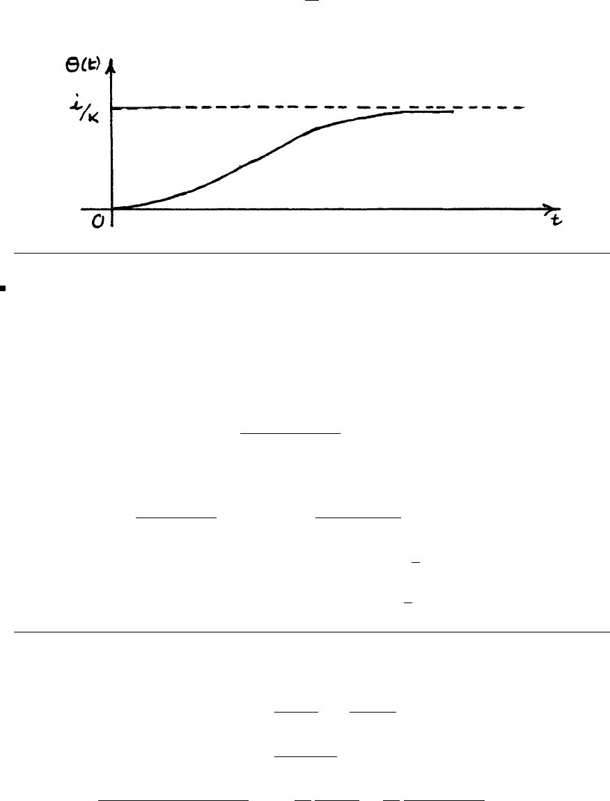
346 Glyn James, Advanced Modern Engineering Mathematics, 4th Edition
Thus,
θ(t)=L−1{Φ(s)}=i
K[1 −e−Kt −Kte−Kt]
17(a)
(i)
L{sin tH(t−α)}=L{sin[(t−α)+α]H(t−α)}
=L{[sin(t−α)cosα+cos(t−α)sinα]H(t−α)}
=cos α+ssin α
s2+1 .e
−αs
(ii)
L−1se−αs
s2+2s+5 =L−1e−αs (s+1)−1
(s+1)
2+4
=L−1eαsL[e−t(cos 2t−1
2sin 2t)]
=e−(t−α)[cos 2(t−α)−1
2sin 2(t−α)]H(t−α)
17(b) Taking Laplace transforms
(s2+2s+5)Y(s)= 1
s2+1−−e−sπ
s2+1by (i) above in part (a)
=1+e−πs
s2+1
Y(s)= 1+e−πs
(s2+1)(s2+2s+5) =−1
10
s−2
s2+1+1
10
s
s2+2s+5(1 + e−πs)
c
Pearson Education Limited 2011

Glyn James, Advanced Modern Engineering Mathematics, 4th Edition 347
giving
y(t)=L−1{Y(s)}=1
10 [2 sin t−cos t+e−(t−π)[2 sin(t−π)−cos(t−π)]H(t−π)]
+e−t(cos 2t−1
2sin 2t)+e−(t−π)[cos 2(t−z)
−1
2sin 2(t−π)]H(t−π)]
=1
10 e−t(cos 2t−1
2sin 2t)+2sint−cos t
+[e−(t−π)(cos 2t−1
2sin 2t)+cost−2sint]H(t−π)
18 By theorem 5.5
L{v(t)}=V(s)= 1
1−e−sT T
0
e−stv(t)dt
=1
1−e−sT T/2
0
e−stdt −T
T/2
e−stdt
=1
1−e−sT −1
se−st
T/2
0−−1
se−st
T
T/2
=1
s·1
1−e−sT (e−sT −e−sT/2−e−sT /2+1)
=1
s
(1 −e−sT/2)2
(1 −e−sT/2)(1 + e−sT /2)=1
s1−e−sT/2
1+e−sT/2
Equation for current flowing is
250i+1
C(q0+t
0
i(τ)dτ)=v(t),q
0=0
Taking Laplace transforms
250I(s)+ 1
10−4·1
s·I(s)=V(s)=1
s1−e−sT/2
1+e−sT /2
(s+ 40)I(s)= 1
250 1−e−sT/2
1+e−sT/2
or I(s)= 1
250(s+ 40) ·1−e−sT /2
1+e−sT/2
c
Pearson Education Limited 2011

348 Glyn James, Advanced Modern Engineering Mathematics, 4th Edition
I(s)= 1
250(s+ 40) (1 −e−sT /2)(1 −e−sT /2+e−sT −e−3
2sT +e−2sT ...)
=1
250(s+ 40) [1 −2e−sT /2+2e−sT −2e−3
2sT +2e−2sT ...]
Since L−11
250(s+ 40) =1
250 e−40tusing the second shift theorem gives
i(t)= 1
250 e−40t−2Ht−T
2e−40(t−T/2) +2H(t−T)e−40(t−T)
−2Ht−3T
2e−40(t−3T/2) +...
If T=10
−3s then the first few terms give a good representation of the steady state
since the time constant 1
4of the circuit is large compared to the period T.
19 The impulse response h(t) is the solution of
d2h
dt2+2dh
dt +2h=δ(t)
subject to the initial conditions h(0) = ˙
h(0) = 0. Taking Laplace transforms
(s2+2s+s)H(s)=L{δ(t)}=1
H(s)= 1
(s+1)
2+1
that is,h(t)=L−1{H(s)}=e−tsin t.
Using the convolution integral the step response xs(t)isgivenby
xs(t)=t
0
h(τ)u(t−τ)dτ
with u(t)=1H(t); that is,
xs(t)=t
0
1.e−τsin τdτ
=−1
2[e−τcos τ+e−τsin τ]t
0
that is,x
s(t)=1
2[1 −e−t(cos t+sint)].
c
Pearson Education Limited 2011
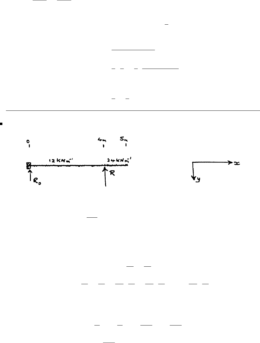
Glyn James, Advanced Modern Engineering Mathematics, 4th Edition 349
Solving d2xs
dt2+2dxs
dt +2xs= 1 directly we have taking Laplace transforms
(s2+2s+2)Xs(s)=1
s
Xs(s)= 1
s(s2+2s+2)
=1
2·1
s−1
2s+2
(s+1)
2+1
giving as before
xs(t)=1
2−1
2e−t(cos t+sint)
20
EI d4y
dx4=12+12H(x−4) −Rδ(x−4)
y(0) = y(0) = 0,y(4) = 0,y
(5) = y(5) = 0
With y(0) = A, y(0) = Btaking Laplace transforms
EIs4Y(s)=EI(sA +B)+12
s+12
se−4s−Re−4s
Y(s)= A
s3+B
s4+12
EI·1
s5+12
EI·1
s5e−4s−R
EI·1
s4e−4s
giving
y(x)=L−1{Y(s)}=A
2x2+B
6x3+1
2EIx4+1
2EI (x−4)4H(x−4)
−R
6EI(x−4)3H(x−4)
c
Pearson Education Limited 2011
350 Glyn James, Advanced Modern Engineering Mathematics, 4th Edition
or
EIy(x)= 1
2A1x2+1
6B1x3+1
2x4+1
2(x−4)4H(x−4) −R
6(x−4)3H(x−4)
y(4) = 0 ⇒0=8A1+32
3B1+ 128 ⇒3A1+4B1=−48
y(5) = 0 ⇒0=A1+5B1+6(25)+6−R⇒A1+5B1−R=−156
y(5) = 0 ⇒0=B1+ 12(5) + 12 −R⇒B1−R=−72
which solve to give A1=18,B
1=−25.5,R=46.5
Thus,
y(x)=⎧
⎨
⎩
1
2x4−4.25x3+9x2,0≤x≤4
1
2x4−4.25x3+9x2+1
2(x−4)4−7.75(x−4)3,4≤x≤5
R0=−EIy(0) = 25.5kN,M
0=EIy(0) = 18kN.m
Check:R0+R= 72kN, Total load = 12 ×4 + 24 = 72kN √
Moment about x=0 is
12 ×4×2+24×4.5−4R=18=M0√
21(a)
f(t)=H(t−1) −H(t−2)
and L{f(t)}=F(s)=e−s
s−e−2s
s
c
Pearson Education Limited 2011

Glyn James, Advanced Modern Engineering Mathematics, 4th Edition 351
Taking Laplace transforms throughout the differential equation
(s+1)X(s)=1
s(e−s−e−2s)
X(s)= 1
s(s+1)(e−s−e−2s)
=1
s−1
s+1e−s−1
s−1
s+1e−2s
giving x(t)=L−1{X(s)}=[1−e−(t−1)]H(t−1) −[1 −e−(t−2)]H(t−2)
21(b) I(s)= E
s[Ls +R/(1 + Cs)]
(i) By the initial value theorem
lim
t→0i(t) = lim
s→∞ sI(s) = lim
s→∞
E
Ls +R/(1 + Cs)=0
(ii) Since sI(s) has all its poles in the left half of the s-plane the conditions of
the final value theorem hold so
lim
t→∞ i(t) = lim
s→0sI(s)= E
R
22 We have that for a periodic function f(t)ofperiodT
L{f(t)}=1
1−e−sT T
0
e−sT f(t)dt
Thus, the Laplace transform of the half-rectified sine wave is
L{v(t)}=1
1−e−2πs π
0
e−sT sin tdt
=Im1
1−e−2πs π
0
e(j−s)tdt
=Im1
1−e−2πs e(j−s)t
j−s
π
0
=Im1
1−e−2πs (−e−πs −1)(−j−s)
(j−s)(−j−s)=1+e−πs
(1 −e−2πs)(1 + s2)
that is,L{v(t)}=1
(1 + s2)(1 −e−πs)
c
Pearson Education Limited 2011
352 Glyn James, Advanced Modern Engineering Mathematics, 4th Edition
Applying Kirchoff’s law to the circuit the current is determined by
di
dt +i=v(t)
which on taking Laplace transforms gives
(s+1)I(s)= 1
(1 + s2)(1 −e−πs)
I(s)= 1
1−e−πs 1
s+1−s+1
s2+1·1
2
=1
21
s+1−s+1
s2+11+e−πs +e−2πs +...
Since L−11
21
s+1−s+1
s2+1=1
2(sin t−cos t+e−t)H(t)=f(t)
we have by the second shift theorem that
i(t)=f(t)+f(t−π)+f(t−2π)+...=∞
n=0
f(t−nπ)
The graph may be plotted by computer and should take the form
23(a) Since L{t}=1
s2,L{te−t}=1
(s+1)
2
taking f(t)=tand g(t)=te−tin the convolution theorem
L−1[F(s)G(s)] = f∗g(t)
c
Pearson Education Limited 2011

Glyn James, Advanced Modern Engineering Mathematics, 4th Edition 353
gives
L−11
s2·1
(s+1)
2=t
0
f(t−τ)g(τ)dτ
=t
0
(t−τ)τe−τ
=−(t−τ)τe−τ−(t−2τ)e−τ+2e−τt
0
i.e. L−11
s2·1
(s+2)
2=t−2+2e−t+te−t.
23(b) y(t)=t+2t
0y(u)cos(t−u)du
Taking f(t)=y(t),g(t)=cost⇒F(s)=Y(s),G(s)= s
s2+1 giving on taking
transforms
Y(s)= 1
s2+2Y(s)s
s2+1
(s2+1−2s)Y(s)=s2+1
s2
or Y(s)= s2+1
s2(s−1)2=2
s+1
s2−2
s−1+2
(s−1)2
and y(t)=L−1{Y(s)}=2+t−2et+2tet.
Taking transforms
(s2Y(s)−sy(0) −y(0))(sY(s)−y(0)) = Y(s)
or (s2Y(s)−y1)(sY(s)) = Y(s)
giving Y(s)=0orY(s)=y1
s2+1
s3
which on inversion gives
y(t)=0ory(t)= 1
2t2+ty1
In the second of these solutions the condition on y(0) is arbitrary.
c
Pearson Education Limited 2011
354 Glyn James, Advanced Modern Engineering Mathematics, 4th Edition
24
Equation for displacement is
EI d4y
dx4=−Wδ(x−)
with y(0) = 0,y(3)=0,y
(0) = y(3)=0
with y(0) = A, y(0) = Bthen taking Laplace transforms gives
EIs4Y(s)=EI(sA +B)−We−s
Y(s)= −W
EIs4e−s +A
s3+B
s4
giving y(x)=−W
6EI (x−)3.H(x−)+A
2x2+B
6x3
For x>,y
(x)= −3W
6EI (x−)2+Ax +B
2x2
so y(3)=0 and y(3)=0 gives
0=−2W2
EI +3A +9B2
2
0=−4W3
3EI +9
2A2+9
2B3
giving A=−4W
9EI and B=20
27
W
EI
Thus, deflection y(x)is
y(x)=−W
6EI(x−)3H(x−)−2
9
W
EI x2+10
81
W
EIx3
c
Pearson Education Limited 2011

Glyn James, Advanced Modern Engineering Mathematics, 4th Edition 355
With the added uniform load the differential equation governing the deflection is
EI d4y
dx4=−Wδ(x−)−w[H(x)−H(x−)]
25(a) Taking Laplace transforms
(s2−3s+3)X(s)= 1
se−as
X(s)= 1
s(s2−3s+3)·e−as =
1
6
s−
1
6s−1
2
s2−3s+3·e−as
=1
61
s−(s−3
2)−√3( √3
2)
(s−3
2)2+(√3
2)2e−as
=e−as
6L1−e−3
2tcos √3
2t−√3sin√3
2t
giving
x(t)=L−1{X(s)}=1
61−e−3
2(t−a)cos √3
2(t−a)−√3sin√3
2(t−a)H(t−a)
25(b)
X(s)=G(s)L{sin wt}=G(s)w
s2+w2
=w
(s+jw)(s−jw)G(s)
Since the system is stable all the poles of G(s) have negative real part. Expanding
in partial fractions and inverting gives
x(t)=2ReF(jw)w
2jw ·ejwt+termsfromG(s) with negative exponentials
Thus, as t→∞the added terms tend to zero and x(t)→xs(t)with
xs(t)=ReejwtF(jw)
j
c
Pearson Education Limited 2011
356 Glyn James, Advanced Modern Engineering Mathematics, 4th Edition
26(a) In the absence of feedback the system has poles at
s=−3ands=1
and is therefore unstable.
26(b) G1(s)= G(s)
1+KG(s)=1
(s−1)(s+3)+K=1
s2+2s+(K−3)
26(c) Poles G1(s)givenbys=−1±√4−K.
These may be plotted in the s-plane for different values of K. Plot should be as
in the figure
26(d) Clearly from the plot in (c) all the poles are in the left half plane when
K>3. Thus system stable for K>3.
26(e) a2
1s2+
a1
2s+
a0
(K−3) = 0
Routh–Hurwitz determinants are
Δ1=2>0
Δ2=
a1a2
0a0
=
21
0K−3
=2(K−3) >0ifK>3
thus, confirming the result in (d).
c
Pearson Education Limited 2011
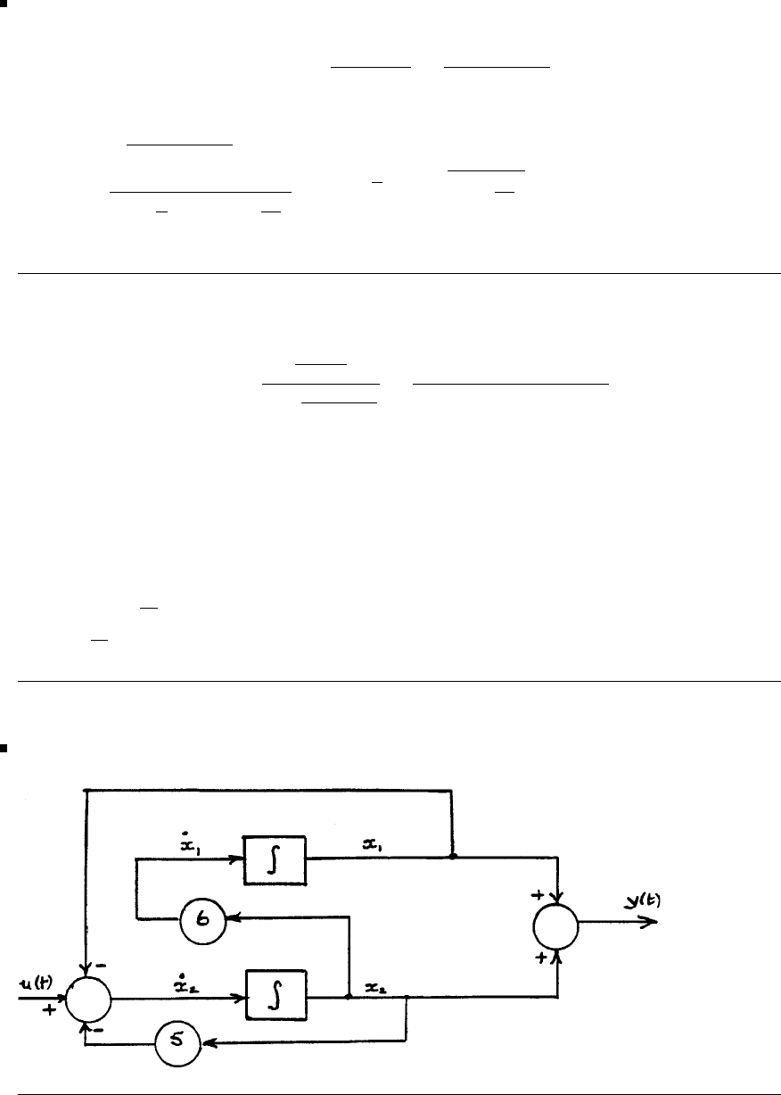
Glyn James, Advanced Modern Engineering Mathematics, 4th Edition 357
27(a) Closed loop transfer function is
G1(s)= G(s)
1+G(s)=2
s2+αs +5
Thus L−12
s2+αs +5=h(t)=2e−2tsin t
i.e. L−12
(s+α
2)2+(5−α2
4)=2e−α
2tsin (5 −α2
4)t=2e−2tsin t
giving α=4
27(b) Closed loop transfer function is
G(s)=
10
s(s−1)
1−(1+Ks)10
s(s−1)
=10
s2+(10K−1)s+10
Poles of the system are given by
s2+(10K−1)s+10=0
which are both in the negative half plane of the s-plane provided (10K−1) >0;
that is, K> 1
10 . Thus the critical value of Kfor stability of the closed loop system
is K=1
10 .
28(a)
c
Pearson Education Limited 2011

358 Glyn James, Advanced Modern Engineering Mathematics, 4th Edition
28(b)
L{eAt}=[sI−A]−1=1
(s+2)(s+3) s+5 6
−18
=3
s+2 −2
s+3
6
s+2 −6
s+3
1
s+3 −1
s+2 −2
s+2 −1
s+3
Taking inverse transforms gives
eAt=3e−2t−2e−3t6e−2t−6e−3t
e−3t−e−2t3e−3t−2e−2t
28(c) Taking Laplace transforms
[sI−A]X(s)=x(0) + bU(s); Y(s)=cTX(s)
With x(0) = 0 and U(s) = 1 the transform Xδ(s) of the impulse response is
Xδ(s)=[sI−A]−1b,Y
δ(s)=cT[sI−A]−1b
Inverting then gives the impulse response as
yδ(t)=[11] 6e−2t−6e−3t
3e−3t−2e−2t=4e−2t−3e−3t,t≥0
With x(0) = [1 0]Tand X(s)=1
s
Y(s)=[11] [sI−A]−11
0+[sI −A]−10
11
s
=[11] 3
s+2 −2
s+3 +6
1/6
s−1/2
s+2 +1/3
s+3
1
s+3 −1
s+2 +1
s+2 −1
s+3
so y(t)=[11] 3e−2t−2e−3t+1−3e−2t+2e−3t
e−3t−e−2t+e−2t−e−3t
that is,y(t)=1,t≥0
c
Pearson Education Limited 2011

Glyn James, Advanced Modern Engineering Mathematics, 4th Edition 359
29 L{eAt}=[sI−A]−1=s+2 1
−2s−1
=s
(s+1)2+1 −1
(s+1)2+1
2
(s+1)2+1
s+2
(s+1)2+1
Thus eAt=e−t(cos t−sin t)−e−tsin t
2e−tsin te
−t(cos t+sint)
and eAtx(0) = 0since x(0) = 0
With U(s)=L{u(t)}=1
swe have
[sI−A]−1bU(s)= s
s2+2s+2 −1
s2+2s+2
2
s2+2s+2
s+2
s2+2s+2 1
01
s=1
s2+2s+2
2
s(s2+2s+2)
=1
(s+1)2+1
1
s−s+2
(s+1)2+1
so L−1{(sI−A)−1bU(s)}=e−tsin t
1−e−t(cos t+sint)
Thus x(t)=eAtx(0) + L−1{(sI−A)−1bU(s)}
=e−tsin t
1−e−t(cos t+sint)
For the transfer function, we have,
Y(s)=cX(s)andwhenx(0) = 0
Y(s)=c[sI−A]−1bU(s)=HU(s)
where H=c[sI−A]−1b
For this system, we have H(s)=[11] s
s2+2s+1
2
s2+2s+1 =s+2
(s+1)
2+1
When u(t)=δ(t),U(s) = 1 and so the impulse response yδ(t)isgivenby
L{yδ(t)}=Yδ(s)= s+2
(s+1)
2+1 =s+1
(s+1)
2+1+1
(s+1)
2+1
⇒yδ(t)=e−t(cos t+sint)
c
Pearson Education Limited 2011

360 Glyn James, Advanced Modern Engineering Mathematics, 4th Edition
30 The controllability question can be answered by either reducing to canonical
form as in section 6.7.8 of the text or by using the Kalman matrix criterion given
in Exercise 61 of the text. Adopting the Kalman matrix approach
A=⎡
⎣
120
0−10
−3−3−2⎤
⎦and
b=⎡
⎣
0
1
0⎤
⎦,Ab=⎡
⎣
2
−1
−3⎤
⎦,A2b=⎡
⎣
0
1
9⎤
⎦
so the controllability Kalman matrix is
[bAbA
2b]= ⎡
⎣
020
1−11
0−39
⎤
⎦=C
Since det C=0,rank C= 3 so the system is controllable.
The eigenvalues of Aare given by
1−λ20
0−1−λ0
−3−3−2−λ
=(1−λ)−(1 + λ)0
−3−(2 + λ)
=(1−λ)(1 −λ)(2 + λ)=0
so that the eigenvalues are λ1=−2,λ
2=−1,λ
3= 1. The system is therefore
unstable with λ3= 1 corresponding to the unstable mode. The corresponding
eigenvectors of Aare given by
(A−λiI)ei=0
and are readily determined as
e1=[001]
T
e2=[1 −10]
T
e3=[10 −1]T
To determine the control law to relocate λ3=1 at −5 we need to determine the
eigenvector v3of ATcorresponding to λ3= 1. This is readily obtained as
v3=[110]
T
c
Pearson Education Limited 2011

Glyn James, Advanced Modern Engineering Mathematics, 4th Edition 361
Thus, the required control law is
u(t)=KvT
3x(t)=K[110]
Tx(t)
where K=p3−λ3
vT
3b=(−5) −1
[1 1 0] ⎡
⎣
0
1
0⎤
⎦
=6
1=−6
So u(t)=−6(x1(t)+x2(t))
31(a) Let x[x1x2]Tthen state −space model is
˙
x=Ax +bu⇒˙
x1
˙
x2=−24
01
x1
x2+1
1u
y=cTx⇒y=[1 0]x1
x2
(b) G(s)=Y(s)
U(s)=cT(sI−A)−1b
det(sI−A)=Δ=
s+2 −4
0s−1
=(s+2)(s−1)
adj(sI−A)=s−14
0s+2
G(s)= 1
Δ[1 0]s−14
0s+21
1=s+3
(s+2)(s−1)
System has positive pole s= 1 and is therefore is unstable.
(c) u(t)=r(t)−ky(t)⇒˙
x=Ax +b(r−kcTx)=(A−kbcT)x+br
(A−kbcT)=−24
01
−k1
1[1 0]=−2−k4
−k1
⇒Eigenvalues given by
λ+2+k4
−kλ−1
=0⇒
λ2+(k+1)λ+3k−2=0
so system is stable if and only if 3k−2>0ork>2
3
c
Pearson Education Limited 2011

362 Glyn James, Advanced Modern Engineering Mathematics, 4th Edition
(d) r(t)=H(t)⇒R(s)=1
s⇒Y(s)=cT(sI−A+kbcT)−1b1
s
Since k>2
3, system stable, the final value theorem gives
lim
t→∞ y(t) = lim
s→0sY(s) = lim
s→0[cT(sI−A+kbcT)−1b]=−cT(A−kbcT)−1b
=−[1 0]−2−k4
−k1−11
1=−[1 0] 1
3k−21−4
k−2−k
=3
3k−2
Thus, lim
t→∞ y(t) = 1 if and only if 3
3k−2=1⇒k=5
3
32(a) Overall closed loop transfer function is
G(s)=
K
s(s+1)
1+ K
s(s+1) (1 + K1s)=K
s2+s(1 + KK1)+K
32(b) Assuming zero initial conditions step response x(t)isgivenby
X(s)=G(s)L{1.H(t)}=K
s[s2+s(1 + KK1)+K]
=wn
s[s2+2ξwns+w2
n]
=1
s−s+2ξwn
s2+2ξwns+w2
n
=1
s−(s+ξwn)+ξwn
(s+ξwn)2+[w2
n(1 −ξ2)]
=1
s−(s+ξwn)+ξwn
(s+ξwn)2+w2
d
giving x(t)=L−1{X(s)}=1−e−ξwntcos wdt+ξ
1−ξ2sin wdt,t≥0.
32(c) The peak time tpis given by the solution of dx
dt t=tp=0
dx
dt =e−ξwntξwn−ξwd
1−ξ2cos wdtξ2wn
1−ξ2+wdsin wdt
=e−ξwntwn
1−ξ2sin wdt
c
Pearson Education Limited 2011

Glyn James, Advanced Modern Engineering Mathematics, 4th Edition 363
Thus, tpgiven by the solution of
e−ξwntpwn
1−ξ2sin wdtp=0
i.e. sin wdtp=0
Since the peak time corresponds to the first peak overshoot
wdtp=πor tp=π
wd
The maximum overshoot Mpoccurs at the peak time tp.Thus
Mp=x(tp)−1=e−ξwnπ
wdcos π+ξ
1−ξ2sin π
=e−ξwnπ
wd=e−ξπ/√1−ξ2π
We wish Mpto be 0.2 and tpto be 1s, thus
e−ξπ/√1−ξ2=0.2 giving ξ=0.456
and
tp=π
wd
=1givingwd=3.14
Then it follows that wn=wd
1−ξ2=3.53 from which we deduce that
K=w2
n=12.5
and K1=2wnξ−1
K=0.178.
32(d) The rise time tris given by the solution of
x(tr)=1=1−e−ξwntrcos wdtr+ξ
1−ξ2sin wdtr
Since e−ξwntr=0
cos wdtr+ξ
1−ξ2sin wdtr=0
c
Pearson Education Limited 2011

364 Glyn James, Advanced Modern Engineering Mathematics, 4th Edition
giving tan wdtr=−1−ξ2
ξ
or tr=1
wd
tan−1−1−ξ2
ξ=π−1.10
wd
=0.65s.
The response x(t)in(b)maybewrittenas
x(t)=1−e−ξwnt
1−ξ2sin wαt+tan
−11−ξ2
ξ
so the curves 1 ±e−ξwnt
1−ξ2are the envelope curves of the transient response to
a unit step input and have a time constant T=1
ξwn
. The settling time tsmay
be measured in terms of T. Using the 2% criterion tsis approximately 4 times
the time constant and for the 5% criterion it is approximately 3 times the time
constant. Thus,
2% criterion : ts=4T=4
ξwn
=2.48s
5% criterion : ts=3T=3
ξwn
=1.86s
Footnote : This is intended to be an extended exercise with students being
encouraged to carry out simulation studies in order to develop a better
understanding of how the transient response characteristics can be used in system
design.
33 As for Exercise 32 this is intended to be an extended problem supported by
simulation studies. The following is simply an outline of a possible solution.
Figure 5.67(a) is simply a mass-spring damper system represented by the
differential equation
M1
d2x
dt2+Bdx
dt +K1x=sinwt
Assuming that it is initially in a quiescent state taking Laplace transforms
X(s)= 1
M1s2+Bs +K1·w
s2+w2
c
Pearson Education Limited 2011

Glyn James, Advanced Modern Engineering Mathematics, 4th Edition 365
The steady state response will be due to the forcing term and determined by the
αs +β
s2+w2term in the partial fractions expansion of X(s). Thus, the steady state
response will be of the form Asin(wt +δ); that is, a sinusoid having the same
frequency as the forcing term but with a phase shift δand amplitude scaling A.
In the situation of Figure 5.67(b) the equations of motion are
M1
d2x
dt2=−K1x−Bdx
dt +K2(y−x)+sinwt
M2
d2y
dt2=−K2(y−x)
Assuming an initial quiescent state taking Laplace transforms gives
[M1s2+Bs +(K1+K2)]X(s)−K2Y(s)=w/(s2+w2)
−K2X(s)+(s2M2+K2)Y(s)=0
Eliminating Y(s)gives
X(s)=w(s2M2+K2)
(s2+w2)p(s)
where p(s)=(M1s2+Bs +K1+K2)(s2M2+K2).
Because of the term (s2+w2) in the denominator x(t) will contain terms in
sin wt and cos wt. However, if (s2M2+K2) exactly cancels (s2+w2) this will
be avoided. Thus choose K2=M2w2. This does make practical sense for if the
natural frequency of the secondary system is equal to the frequency of the applied
force then it may resonate and therefore damp out the steady state vibration of
M1.
It is also required to show that the polynomial p(s) does not give rise to any
undamped oscillations. That is, it is necessary to show that p(s) does not possess
purely imaginary roots of the form jθ, θ real, and that it has no roots with a positive
real part. This can be checked using the Routh–Hurwitz criterion.
To examine the motion of the secondary mass M2solve for Y(s) giving
Y(s)= K2w
(s2+w2)p(s)
Clearly due to the term (s2+w2) in the denominator the mass M2possesses an
undamped oscillation. Thus, in some sense the secondary system has absorbed the
energy produced by the applied sinusoidal force sin wt.
c
Pearson Education Limited 2011

366 Glyn James, Advanced Modern Engineering Mathematics, 4th Edition
34 Again this is intended to be an extended problem requiring wider exploration
by the students. The following is an outline of the solution.
34(a) Students should be encouraged to plot the Bode plots using the steps
used in Example 5.65 of the text and using a software package. Sketches of the
magnitude and phase Bode plots are given in the figures below.
34(b) With unity feedback the amplifier is unstable. Since the −180◦crossover
gain is greater than 0dB (from the plot it is +92dB).
34(c) Due to the assumption that the amplifier is ideal it follows that for
marginal stability the value of 1
βmust be 92dB (that is, the plot is effectively
lowered by 92dB). Thus
20 log 1
β=92
1
β= antilog 92
20 ⇒β2.5×10⁻⁵
34(d) From the amplitude plot the effective 0dB axis is now drawn through
the 100dB point. Comparing this to the line drawn through the 92dB point,
corresponding to marginal stability, it follows that
Gain margin = −8dB
and Phase margin = 24◦.
34(e)
G(s)= K
(1 + sτ1)(1 −sτ2)(1 + sτ3)
Given low frequency gain K= 120dB so
20 log K= 120 ⇒K=10
6
Ti=1
fi
where fiis the oscillating frequency in cycles per second of the pole.
c
Pearson Education Limited 2011

Glyn James, Advanced Modern Engineering Mathematics, 4th Edition 367
Since 1MHz = 10 cycles per second
τ1=1
f1
=1
106since f1=1MHz
τ2=1
f2
=1
10.106since f2= 10MHz
τ3=1
f3
=1
25.106since f3= 25MHz
Thus,
G(s)= 106
(1 + s
106)(1 + s
10.106)(1 + s
25.106)
=250.1024
(s+10
6)(s+10
7)(s+5
2.107)
The closed loop transfer function G1(s)is
G(s)= G(s)
1+βG(s)
34(f) The characteristic equation for the closed loop system is
(s+10
6)(s+10
7)(s+5
2.107)+β25.1025 =0
or
s3+36(10
6)s2+ (285)1012s+10
19(25 + 25β106)=0
↓
A1
↓
A2
↓
A3
By Routh–Hurwitz criterion system stable provided A1>0andA1A2>A
3.If
β=1thenA1A2<A
3and the system is unstable as determined in (b). For
marginal stability A1A2=A3giving β=1.40−5(compared with β=2.5.10−5
using the Bode plot).
c
Pearson Education Limited 2011
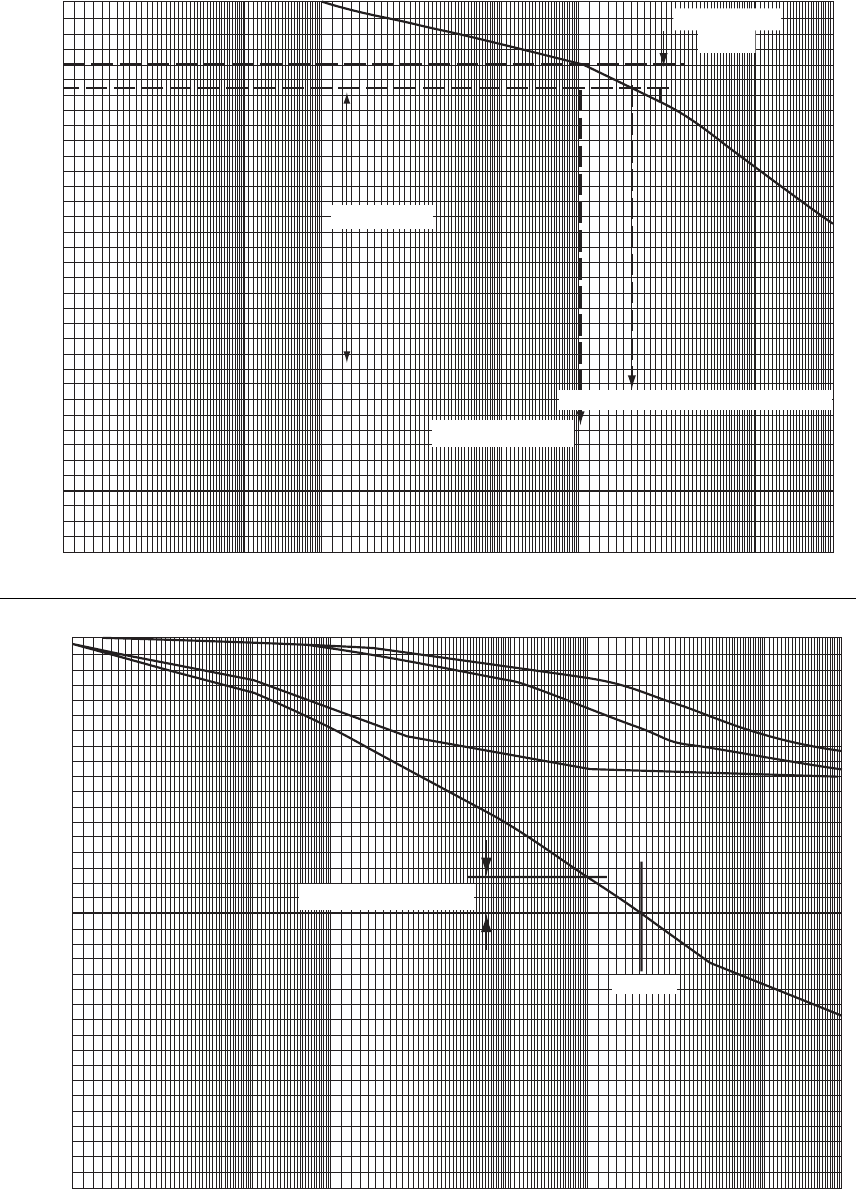
368 Glyn James, Advanced Modern Engineering Mathematics, 4th Edition
0
20
40
60
80
100
120 Data margin
– 8 dB
Corresponds to 180° phase lag
To phase plot
11025Lo
g
freq. MHz
1/β = 92 dB
Magnitude vs Frequency Plot
Gain dB
– 180°
– 270°
– 90°
0°
Phase margin 24°
16 MHz
11025
ln freq. MHz
Phase vs Frequency Plot
c
Pearson Education Limited 2011

6
The ZTransform
Exercises 6.2.3
1(a)
F(z)= ∞
k=0
(1/4)k
zk=1
1−1/4z=4z
4z−1if |z|>1/4
1(b)
F(z)= ∞
k=0
3k
zk=1
1−3/z =z
z−3if |z|>3
1(c)
F(z)= ∞
k=0
(−2)k
zk=1
1−(−2)/z =z
z+2 if |z|>2
1(d)
F(z)= ∞
k=0
−(2)k
zk=−1
1−2/z =−z
z−2if |z|>2
1(e)
Z{k}=z
(z−1)2if |z|>1
from (6.6) whence
Z{3k}=3 z
(z−1)2if |z|>1
2
uk=e−2ωkT =e−2ωT k
whence
U(Z)= z
z−e−2ωT
c
Pearson Education Limited 2011

370 Glyn James, Advanced Modern Engineering Mathematics, 4th Edition
Exercises 6.3.6
3
Z{sin kωT}=1
2
z
z−eωT −1
2
z
z−e−ωT
=zsin ωT
z2−2zcos ωT +1
4
Z{1
2k
}=2z
2z−1
so
Z{yk}=1
z3×2z
2z−1=2
z2(2z−1)
Proceeding directly
Z{yk}=∞
k=3
xk−3
zk=∞
r=0
xr
zr+3 =1
z3×Z{xk}=2
z2(2z−1)
5(a)
Z−1
5=∞
r=0 −1
5zr
=5z
5z+1 |z|>1
5
5(b)
{cos kπ}=(−1)k
so
Z{cos kπ}=z
z+1 |z|>1
6
Z1
2k=2z
2z−1
By (3.5)
Z(ak)=z
z−a
so
Z(kak−1)=z
(z−a)2
c
Pearson Education Limited 2011

Glyn James, Advanced Modern Engineering Mathematics, 4th Edition 371
thus
Z(kak)=az
(z−a)2
whence
Zk1
2k=2z
(2z−1)2
7(a)
sinh kα =1
2(eα)k−1
2(e−α)k
so
Z{sinh kα}=1
2z
z−eα−z
z−e−α=zsinh α
z2−2zcosh α+1
7(b)
cosh kα =1
2(eα)k+1
2(e−α)k
then proceed as above.
8(a)
uk=e−4kT =e−4Tk;Z{uk}=z
z−e−4T
8(b)
uk=1
2ekT −e−kT
Z{uk}=1
2z
z−eT −z
z−e−T =zsin T
z2−2zcos T+1
8(c)
uk=1
2e2kT +e−2kT
then proceed as in 8(b) to give
Z{uk}=z(z−cos 2T)
z2−2zcos 2T+1
9Initial value theorem: obvious from definition.
c
Pearson Education Limited 2011

372 Glyn James, Advanced Modern Engineering Mathematics, 4th Edition
9Final value theorem
(1 −z−1)X(z)= ∞
r=0
xr−xr−1
zr
=x0+x1−x0
z+x2−x1
z2+...+xr−xr−1
zr+...
As z→1andif lim
r→∞ xrexists, then
lim
z→1(1 −z−1)X(z) = lim
r→∞ xr
10 Multiplication property (6.19): Let Z{xk}=∞
k=0
xk
zk=X(z)then
Zakxk=∞
k=0
akxk
zk=X(z/a)
10 Multiplication property (6.20)
−zd
dzX(z)=−zd
dz
∞
k=0
xk
zk=∞
k=0
kxk
zk=Z{kxk}
The general result follows by induction.
Exercises 6.4.2
11(a) z
z−1;fromtablesuk=1
11(b) z
z+1 =z
z−(−1);fromtablesuk=(−1)k
11(c) z
z−1/2;fromtablesuk=(1/2)k
c
Pearson Education Limited 2011

Glyn James, Advanced Modern Engineering Mathematics, 4th Edition 373
11(d)
z
3z+1 =1
3
z
z+1/3←→ 1
3(−1/3)k
11(e) z
z−;fromtablesuk=()k
11(f) z
z+√2=z
z−(−√2) ←→ (−√2)k
11(g)
1
z−1=1
z
z
z−1←→ 0; k=0
1; k>0
using first shift property.
11(h)
z+2
z+1 =1+1
z
z
z+1 ←→ 1; k=0
(−1)k−1;k>0
=1; k=0
(−1)k+1;k>0
12(a)
Y(z)/z =1
3
1
z−1−1
3
1
z+2
so
Y(z)=1
3
z
z−1−1
3
z
z+2 ←→ 1
31−(−2)k
12(b)
Y(z)=1
7z
z−3−z
z+1/2←→ 1
7(3)k−(−1/2)k
12(c)
Y(z)=1
3
z
z−1+1
6
z
z+1/2←→ 1
3+1
6(−1/2)k
c
Pearson Education Limited 2011

374 Glyn James, Advanced Modern Engineering Mathematics, 4th Edition
12(d)
Y(z)=2
3
z
z−1/2−2
3
z
z+1 ←→ 2
3(1/2)k−2
3(−1)k
=2
3(1/2)k+2
3(−1)k+1
12(e)
Y(z)= 1
2z
z−−z
z−(−)
=1
2z
z−eπ/2−z
z−e−π/2
←→ 1
2(eπ/2)k−(e−π/2)k=sinkπ/2
12(f)
Y(z)= z
z−(√3+)z−(√3−)
=1
2z
z−(√3+)−z
z−(√3−)
=1
2z
z−2eπ/6−z
z−2e−π/6
←→ 1
22kekπ/6−2ke−kπ/6=2
ksin kπ/6
12(g)
Y(z)= 5
2
z
(z−1)2+1
4
z
z−1−1
4
z
z−3
←→ 5
2k+1
41−3k
12(h)
Y(z)/z =z
(z−1)2(z2−z+1) =1
(z−1)2−1
z2−z+1
so
Y(z)= z
(z−1)2−1
√3⎛
⎜
⎜
⎝
z
z−1+√3
2
−z
z−1−√3
2
⎞
⎟
⎟
⎠
c
Pearson Education Limited 2011

Glyn James, Advanced Modern Engineering Mathematics, 4th Edition 375
=z
(z−1)2−1
√3z
z−eπ/3−z
z−e−π/3
←→ k−2
√3sin kπ/3=k+2
√3cos(kπ/3−3π/2)
13(a)
Y(z)= ∞
k=0
xk
zk=1
z+2
z7
whence x0=0, x1=1, x2=x3=... =x6=0, x7=2and xk=0,k>7;
giving Y(z)↔{0,1,0,0,0,0,0,2,···}
13(b) Proceed as in Exercise 13(a) to give
Y(z)↔{1,0,3,0,0,0,0,0,0,−2,···}
13(c) Observe that
3z+z2+5z5
z5=5+ 1
z3+3
z4
and proceed as in Exercise 13(a) to give Y(z)↔{5,0,0,1,3,···}
13(d)
Y(z)= 1
z2+1
z3+z
z+1/3
←→ {0,0,1,1}+{(−1/3)k}
13(e)
Y(z)=1+3
z+1
z2−1/2
z+1/2
←→ {1,3,1}−1
20,k=0
(−1/2)k,k≥1
=⎧
⎪
⎪
⎪
⎨
⎪
⎪
⎪
⎩
1,k=0
5/2,k=1
5/4,k=2
−1
2(−1/2)k−1,k≥3
=⎧
⎪
⎪
⎪
⎨
⎪
⎪
⎪
⎩
1,k=0
5/2,k=1
5/4,k=2
−1
8(−1/2)k−3,k≥3
c
Pearson Education Limited 2011

376 Glyn James, Advanced Modern Engineering Mathematics, 4th Edition
13(f)
Y(z)= 1
z−1−2
(z−1)2+1
z−2
←→ 0,k=0
1−2(k−1) + 2k−1,k≥1
=0,k=0
3−2k+2
k−1,k≥1
13(g)
Y(z)= 2
z−1−1
z−2
←→ 0,k=0
2−2k−1,k≥1
Exercises 6.5.3
14(a) If the signal going into the left D-block is wkand that going into the right
D-block is vk,wehave
yk+1 =vk,v
k+1 =wk=xk−1
2vk
so
yk+2 =vk+1 =xk−1
2vk
=xk−1
2vk=xk−1
2yk+1
that is,
yk+2 +1
2yk+1 =xk
14(b) Using the same notation
yk+1 =vk,v
k+1 =wk=xk−1
4vk−1
5yk
c
Pearson Education Limited 2011

Glyn James, Advanced Modern Engineering Mathematics, 4th Edition 377
Then
yk+2 =xk−1
4yk+1 −1
5yk
or
yk+2 +1
4yk+1 +1
5yk=xk
15(a)
z2Y(z)−z2y0−zy1−2(zY(z)−zy0)+Y(z)=0
with y0=0,y
1=1
Y(z)= z
(z−1)2
so yk=k, k ≥0.
15(b) Transforming and substituting for y0and y1,
Y(z)/z =2z−15
(z−9)(z+1)
so
Y(z)= 3
10
z
z−9−17
10
z
z+1
thus
yk=3
10 9k−17
10 (−1)k,k≥0
15(c) Transforming and substituting for y0and y1,
Y(z)= z
(z−2)(z+2)
=1
4z
z−2eπ/2−z
z−2e−π/2
thus
yk=1
42kekπ/2−e−kπ/2=2
k−1sin kπ/2,k≥0
c
Pearson Education Limited 2011

378 Glyn James, Advanced Modern Engineering Mathematics, 4th Edition
15(d) Transforming, substituting for y0and y1, and rearranging
Y(z)/z =6z−11
(2z+1)(z−3)
so
Y(z)=2 z
z+1/2+z
z−3
thus
yk=2(−1/2)k+3
k,k≥0
16(a)
6yk+2 +yk+1 −yk=3,y
0=y1=0
Transforming with y0=y1=0,
(6z2+z−1)Y(z)= 3z
z−1
so
Y(z)/z =3
(z−1)(3z−1)(2z+1)
and
Y(z)=1
2
z
z−1−9
10
z
z−1/3+2
5
z
z+1/2
Inverting
yk=1
2−9
10 (1/3)k+2
5(−1/2)k
16(b) Transforming with y0=0,y
1=1,
(z2−5z+6)Y(z)=z+5 z
z−1
whence
Y(z)= 5
2
z
z−1+7
2
z
z−3−6z
z−2
so
yk=5
2+7
2(3)k−6(2)
k
16(c) Transforming with y0=y1=0,
(z2−5z+6)Y(z)= z
z−1/2
c
Pearson Education Limited 2011

Glyn James, Advanced Modern Engineering Mathematics, 4th Edition 379
so
Y(z)= 4
15
z
z−1/2−2
3
z
z−2+2
5
z
z−3
whence
yn=4
15 (1/2)k−2
3(2)k+2
5(3)k
16(d) Transforming with y0=1,y
1=0,
(z2−3z+3)Y(z)=z2−3z+z
z−1
so
Y(z)= z
z−1−z
z2−3z+3
=z
z−1−1
√3j ⎧
⎪
⎪
⎨
⎪
⎪
⎩
z
z−3+√3j
2
−z
z−3−√3j
2
⎫
⎪
⎪
⎬
⎪
⎪
⎭
=z
z−1−1
√3j z
z−√3ejπ/6−z
z−√3e−jπ/6
so
yn=1−2
√3(√3)kejnπ/6−e−jnπ/6
2j =1−2(√3)n−1sin nπ/6
16(e) Transforming with y0=1,y
1=2,
(2z2−3z−2)Y(z)=2z2+z+6 z
(z−1)2+z
z−1
so
Y(z)= z
z−2+zz+5
(z−1)2(2z+1)(z−2)
=12
5
z
z−2−2
5
z
z+1/2−z
z−1−2z
(z−1)2
so
yn=12
5(2)n−2
5(−1/2)n−1−2n
16(f) Transforming with y0=y1=0,
(z2−4)Y(z)=3 z
(z−1)2−5z
z−1
c
Pearson Education Limited 2011

380 Glyn James, Advanced Modern Engineering Mathematics, 4th Edition
so
Y(z)= z
z−1−z
(z−1)2−1
2
z
z−2−1
2
z
z+2
and
yn=1−n−1
2(2)n−1
2(−2)n
17(a) Write the transformed equations in the form
z−3/2
−0.21
1
z−1/2c(z)
e(z)=zC0
zE0
Then c(z)
e(z)=1
z2−2z+0.96 z−1/2
0.21 −1
z−3/2zC0
zE0
Solve for c(z)as
c(z) = 1200 z
z−1.2+ 4800 z
z−0.8
and
Ck= 1200(1.2)k+ 4800(0.8)k
This shows the 20% growth in Ckin the long term as required.
(b) Then
Ek=1.5Ck−Ck+1
= 1800(1.2)k+ 7200(0.8)k−1200(1.2)k+1 −4800(0.8)k+1
Differentiate wrt kand set to zero giving
0.6log(1.2) + 5.6xlog(0.8) = 0 where x=(0.8/1.2)k
Solving, x=0.0875 and so
k=log 0.0875
log(0.8/1.2) =6.007
The nearest integer is k= 6, corresponding to the seventh year in view of the
labelling, and C6= 4841 approximately.
18 Transforming and rearranging
Y(z)/z =z−4
(z−2)(z−3) +1
(z−1)(z−2)(z−3)
c
Pearson Education Limited 2011

Glyn James, Advanced Modern Engineering Mathematics, 4th Edition 381
so
Y(z)= 1
2
z
z−1+z
z−2−1
2
z
z−3
thus
yk=1
2+2
k−1
23k
19 Ik=Ck+Pk+Gk
=aIk−1+b(Ck−Ck−1)+Gk
=aIk−1+ba(Ik−1−Ik−2)+Gk
so
Ik+2 −a(1 + b)Ik+1 +abIk=Gk+2
Thus substituting
Ik+2 −Ik+1 +1
2Ik=G
Using lower case for the ztransform, we obtain
(z2−z+1
2)i(z)=(2z2+z)G+Gz
z−1
whence
i(z)/z =G⎡
⎢
⎣
1
z2−z+1
2
+2
z−1⎤
⎥
⎦
=G⎡
⎢
⎣
2
z−1+1
(z−1+
2)(z−1−
2)⎤
⎥
⎦
so
i(z)=G⎡
⎢
⎢
⎣
2z
z−1+2
2⎧
⎪
⎪
⎨
⎪
⎪
⎩
z
z−1
√2eπ/4−z
z−1
√2e−π/4
⎫
⎪
⎪
⎬
⎪
⎪
⎭
⎤
⎥
⎥
⎦
Thus
Ik=G#2+ 2
2(1
√2)k$ekπ/4−e−kπ/4%&
=2G'1+1
√2k
sin kπ/4(
c
Pearson Education Limited 2011

382 Glyn James, Advanced Modern Engineering Mathematics, 4th Edition
20 Elementary rearrangement leads to
in+2 −2coshαi
n+1 +in=0
with cosh α=1+R1/2R2. Transforming and solving for I(z)/z gives
I(z)/z =zi0+(i1−2i0cosh α)
(z−eα)(z−e−α)
=1
2sinhα#i0eα+(i1−2i0cosh α)
z−eα−i0e−α+(i1−2i0cosh α)
z−e−α&
Thus
ik=(i0eα+(i1−2i0cosh α))enα −(i0e−α+(i1−2i0cosh α))e−nα
2sinhα
=1
sinh α{i1sinh nα −i0sinh(n−1)α}
Exercises 6.6.5
21 Transforming in the quiescent state and writing as Y(z)=H(z)U(z), then
21(a)
H(z)= 1
z2−3z+2
21(b)
H(z)= z−1
z2−3z+2
21(c)
H(z)= 1+1/z
z3−z2+2z+1
22 For the first system, transforming from a quiescent state, we have
(z2+0.5z+0.25)Y(z)=U(z)
The diagram for this is the standard one for a second-order system and is shown
in Figure 6.1 and where Y(z)=P(z), that is yk=pk.
c
Pearson Education Limited 2011
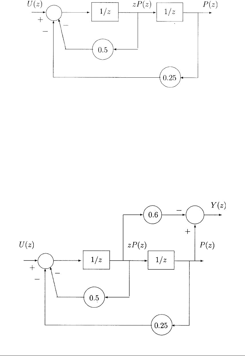
Glyn James, Advanced Modern Engineering Mathematics, 4th Edition 383
Figure 6.1: The block diagram for the basic system of Exercise 22.
Transforming the second system in the quiescent state, we obtain
(z2+0.5z+0.25)Y(z)=(1−0.6)U(z)
Clearly
(z2+0.5z+0.25)(1 −0.6z)P(z)=(1−0.6z)U(z)
indicating that we should now set Y(z)=P(z)−0.6zP(z) and this is shown in
Figure 6.2.
Figure 6.2: The block diagram for the second system of Exercise 22.
c
Pearson Education Limited 2011

384 Glyn James, Advanced Modern Engineering Mathematics, 4th Edition
23(a) Yδ(z)/z =1
(4z+ 1)(2z+1)
so
Yδ(z)=1
2
z
z+1/4−1
2
z
z+1/2
yk=1
2(−1/4)k−1
2(1/2)k
23(b) Yδ(z)/z =z
z2−3z+3
whence
Yδ(z)= 3+√3
2√3
z
z−(3 + √3)
2
−3−√3
2√3
z
z−(3 −√3)
2
so
yk=3+√3
2√3(√3)kekπ/6−3−√3
2√3(√3)ke−kπ/6
=2(
√3)k'√3
2sin kπ/6+1
2cos kπ/6(
=2(
√3)ksin(k+1)π/6
23(c)
Yδ(z)/z =z
(z−0.4)(z+0.2)
so
Yδ(z)= 2
3
z
z−0.4+1
3
z
z+0.2
then
yk=2
3(0.4)k+1
3(−0.2)k
23(d)
Yδ(z)/z =5z−12
(z−2)(z−4)
so
Yδ(z)= z
z−2+4 z
z−4
and
yk=(2)
k+(4)
k+1
c
Pearson Education Limited 2011

Glyn James, Advanced Modern Engineering Mathematics, 4th Edition 385
24(a)
Yδ(z)= 1
z2−3z+2
=1
z−2−1
z−1
yk=0,k=0
2k−1−1,k≥1
24(b)
Yδ(z)= 1
z−2
so
yk=0,k=0
2k−1,k≥1
25 Examining the poles of the systems, we find
25(a) Poles at z=−1/3andz=−2/3, both inside |z|= 1 so the system is
stable.
25(b) Poles at z=−1/3andz=2/3, both inside |z|= 1 so the system is
stable.
25(c) Poles at z=1/2±1/2,|z|=1/√2, so both inside |z|=1andthe
system is stable.
25(d) Poles at z=−3/4±√17/4, one of which is outside |z|=1 andsothe
system is unstable.
25(e) Poles at z=−1/4andz= 1 thus one pole is on |z|= 1 and the other is
inside and the system is marginally stable.
c
Pearson Education Limited 2011

386 Glyn James, Advanced Modern Engineering Mathematics, 4th Edition
26 To use the convolution result, calculate the impulse response as yδ,k −(1/2)k.
Then the step response is
yk=
k
j=0
1×(1/2)k−j=(1/2)k
k
j=0
1×(2)j=(1/2)k1−(2)k+1
1−2
=(1/2)k(2k+1 −1) = 2 −(1/2)k
Directly,
Y(z)/z =z
(z−1/2)(z−1) =2
z−1−1
z−1/2
so
yk=2−(1/2)k
27
G(s)= k
s(sτ +1) =k
s−k
s+1
τ⇒f(t)=k−ke−t
τ
⇒G(z)=k#k
z−1−z
z−e−T
τ&=kz(1 −e−T
τ)
(z−1)(z−e−T
τ)
Characteristic equation is 1 + G(z)=0
⇒(z−1)(z−e−T
τ)+kz(1 −e−T
τ)=0
⇒z2+[k(1 −e−a)−(1 + e−a)]z+e−a=0,where a=T
τ
⇒z2+Kz +e−a=0,where K=k(1 −e−a)−(1 + e−a)
Using Jury’s procedure:
F(z)=z2+Kz +e−a
F(1) = 1 + K+e−a=k(1 −e−a)>0sincek>0,(1 −e−a)>0
(−1)2F(−1) = 1 −Kz +e−a>0⇒2(1 + e−a)−k(1 −e−a)>0
⇒k<2(1 + e−α)
(1 −e−a)=2cotha
2=2cothT
2τ
Δ1=))))
1e−a
e−a1))))
=1−e−2a>0
Thus system is stable if and only if 0 <k<2coth T
2τ
c
Pearson Education Limited 2011

Glyn James, Advanced Modern Engineering Mathematics, 4th Edition 387
28 Substituting
yn+1 −yn+Kyn−1=K/2n
or
yn+2 −yn+1 +Kyn=K/2n+1
Taking ztransforms from the quiescent state, the characteristic equation is
z2−z+K=0
with roots
z1=1
2+1
2√1−4Kand z2=1
2−1
2√1−4K
For stability, both roots must be inside |z|=1 soif K<1/4then
z1<1⇒1
2+1
2√1−4K<1⇒K>0
and
z2>−1⇒1
2−1
2√1−4K>−1⇒k>−2
If K>1/4then
|1
2+1
2√4K−1|2<1⇒K<1
The system is then stable for 0 <K<1.
When k=2/9, we have
yn+2 −yn+1 +2
9yn=1
9
Transforming with a quiescent initial state,
(z2−z+2
9)Y(z)= 1
9
z
z−1/2
so
Y(z)=z1
9#1
(z−1/2)(z−1/3)(z−2/3) &
=2 z
z−1/3+2 z
z−2/3−4z
z−1/2
which inverts to
yn=2(1/3)n+2(2/3)n−4(1/2)n
c
Pearson Education Limited 2011

388 Glyn James, Advanced Modern Engineering Mathematics, 4th Edition
29
z2+2z+2=(z−(−1+))(z−(−1+))
establishing the pole locations. Then
Yδ(z)= 1
2
z
z−(−1+)−1
2
z
z−(−1−)
So since (−1±)=√2e±3π/4etc.,
yk=(
√2)ksin 3kπ/4
Exercises 6.8.3
30(a)
zI−A=#z−1
−4z&
(zI−A)−1=1
(z−2)(z+2) #z1
4z&='1/2
z−2+1/2
z+2
1/4
z−2−1/4
z+2
1
z−2−1
z+2
1/2
z−2+1/2
z+2 (
Ak=Z−1{z(zI−A)−1}=Z−1#1
2
1/2
z−2+1
2
1/2
z+2
1
4
z
z−2−1
4
z
z+2
z
z−2−z
z+2
1
2
z
z−2+z
z+2 &
=1
42k#21
42
&+(−2)k#2−1
−42
&
30(b)
zI−A=#z+1 −3
−3z+1&
(zI−A)−1=1
(z+4)(z−2) #z+1 3
3z+1&
='1/2
z+4 +1/2
z−2−1/2
z+4 +1/2
z−2
−1/2
z+4 +1/2
z−2
1/2
z−2+1/2
z+2 (
Ak=Z−1{z(zI−A)−1}=Z−1#1
2
z
z+4 +1
2
z
z−2−1
2
z
z+4 +1
2
z
z−2
−1
2
z
z+4 +1
2
z
z−2
1
2
z
z−2+1
2
z
z−2&
=1
2(−4)k#1−1
−11
&+(2)
k#11
11
&
c
Pearson Education Limited 2011

Glyn James, Advanced Modern Engineering Mathematics, 4th Edition 389
30(c)
zI−A=#z+1 −1
0z+1&
(zI−A)−1=1
(z+1)
2#z+1 1
0z+1&=#1
z+1
1
(z+1)2
01
z+1 &
Ak=Z−1{z(zI−A)−1}=Z−1#z
z+1
z
(z+1)2
0z
z+1 &=(−1)k#1−k
01
&
31 Taking x1=xand x2=ywe can express equations in the form
x(k+1)= #−74
−81
&x(k)withx(0) = [1 2]
The solution is given by
x(k+1)=Akx(0),A=#−74
−81
&
where Ak=α1I+α1A. That is, the solution is
x(k)= #α0−7α14α1
−8α1α0+α1
2&=#α0+α1
2α0−6α1&
The eigenvalues of Aare given by
λ2−6λ+25=0soλ=3±j4
or, in polar form, λ1=5ejθ
,λ
2=5e−jθ where θ=cos
−1(−3
5).
Thus, α0and α1are given by
5kejkθ =α0+α15ejθ
,5ke−jkθ =α0+α15e−jθ
which are readily solved to give
α0=−(5)ksin(k−1)θ
sin θ,α
1=1
5(5)ksin kθ
sin θ
c
Pearson Education Limited 2011

390 Glyn James, Advanced Modern Engineering Mathematics, 4th Edition
Then,α
0+α1=(5)k
sin θ#1
5sin kθ −sin(k−1)θ&
=5
4(5)k#1
5sin kθ +3
5sin kθ +4
5cos kθ&
=(5)
k[sin kθ +coskθ]
2α0−6α1=(5)k
sin θ#−2(sin kθ cos θ−cos kθ sin θ)−6
5sin kθ&
=(5)
k[2 cos(kθ)]
Thus, solution is
x(k)=(5)
k[sin kθ +coskθ]
y(k)=(5)
k[2 cos(kθ)]
We have
x(1) = 1 ,y(1) = −6,x(2) = −31 ,y(2) = −14
32 A =#01
−0.16 −1&zI−A=#z−1
0.16 z+1&
(zI−A)−1='z+1
(z+0.2)(z+0.8)
1
(z+0.2)(z+0.8)
−0.16
(z+0.2)(z+0.8)
z
(z+0.2)(z+0.8) (
=#4
3·1
z+0.2−1
3·1
z+0.8
5
3·1
z+0.2−5
3·1
z+0.8
−0.8
3
1
z+0.2+0.8
3
1
z+0.8−1
3
1
z+0.2+4
3·1
z+0.8&
Ak=Z−1{z(zI−A)−1}=#4
3(−0.2)k−1
3(−0.8)k5
3(−0.2)k−5
3(−0.8)k
−0.8
3(−0.2)k+0.8
3(−0.8)k−1
3(−0.2)k+4
3(−0.8)k&
Akx(0) = Ak[1 −1]T=#−1
3(−0.2)k+4
3(−0.8)k
0.2
3(−0.2)k−3.2
3(−0.8)k&
U(z)=Z{u(k)}=z/(z−1)
(zI−A)−1bU(z)= 1
(z+0.2)(z+0.8) #z+1 1
−0.16 z
1&z
z−1
c
Pearson Education Limited 2011

Glyn James, Advanced Modern Engineering Mathematics, 4th Edition 391
=z
(z+0.2)(z+0.8)(z−1) #z+2
z−0.16 &
='−5
2
z
z+0.2+10
9
z
z+0.8+25
18
z
z−1
1
2
z
z+0.2−8
9
z
z+0.8+7
18
z
z−1(
Z−1{(zI−A)−1bU(z)}=#−5
2(−0.2)k+10
9(−0.8)k+25
18
1
2(−0.2)k−8
9(−0.8)k+7
18 &
Thus, solution is
x(k)=Akx(0) + Z−1{(zI−A)−1bU(t)}
='−17
6(−0.2)k+22
9(−0.8)k+25
18
3.4
6(−0.2)k−17.6
9(−0.8)k+7
18 (
33 Let x1(k)=y(k),x
2(k)=x1(k+1)=y(k+ 1) then the difference equation
may be written
x(k+1)= #x1(k+1)
x2(k+1)&=#01
11
(k)
x2(k)&,x(0) = [0 1]T
Taking A=#01
11
&its eigenvalues are λ1=1+√5
2,λ
2=1√5
2
Ak=α1I+α1Awhere α0and α1satisfy
1+√5
2
k
=α0+1+√5
2α1,1−√5
2
k
=α0+1−√5
2α1
giving
α1=1
√5#1+√5
2
k
−1−√5
2
k&
α0=1
√5#1+√5
2
k
√5−1
2+1−√5
2
k
1+√5
2&
Solution to the difference equation is
x(k)=#y(k)
y(k+1)&=#α0α1
α1α0+α1�
1&=#α1
α0+α1&
so y(k)=α1=1
√5#1+√5
2
k
−1−√5
2
k&
c
Pearson Education Limited 2011

392 Glyn James, Advanced Modern Engineering Mathematics, 4th Edition
[Note that, y(k+1) = α0+α1=1
√5#1+√5
2
k
−1−√5
2
k+1&using above
values.]
As k→∞,1−√5
2
k
→0andy(k+1)/y(k)→(1+√5
2)k+1
(1+√5
2)k=1
2(√5+1)
Exercises 6.9.3
34 A=#01
0−2&B=#0
1&
sI−A=#s−1
0s+2&⇒(sI−A)−1=1
s(s+2)#s+2 1
0s&=⎡
⎢
⎣
1
s
1
2
s−
1
2
s+2
01
s+2
⎤
⎥
⎦
⇒G=e−AT=L−1{(sI−A)−1}=#11
2(1 −e−2T)
0e−2T&
H=*T
0
eAtBdt =#t1
2t+1
4e−2t
0−1
2e−2t&T
0#0
1&=#1
2T+1
4e−2T−1
4
1
2−1
2e−2T&
Discretized form is:
#x1[(k+1)T]
x2[(k+1)T]&=#1!
2(1 −e−2T)
0e−2T(kT)
x2(kT)&+#1
2T+1
4(e−2T−1)
1
2(1 −e−2T)&u(kT)
In the particular case, when sampling period is T= 1, this reduces to
#x1(k+1)
x2(k+1)&=#10.432
00.135 (k)
x2(k)&+#0.284
0.432 &u(k)
In MATLAB the commands:
A=[0,1; 0,−2]; B= [0; 1];
[G, H]=c2d(A, B, 1)
return
G=1.0000 0.4323
00.1353
H=0.2838
0.4324
which check with the answer.
c
Pearson Education Limited 2011

Glyn James, Advanced Modern Engineering Mathematics, 4th Edition 393
35
A=#01
−1−1&B=#0
1&
(a) Using (6.89),
G1=(TA+I)=#1T
−T1−T&
H1=TB=#0
T&
giving the Euler discretized form of state-space model as
x[(k+1)T]=#x1[(k+1)T]
x2[(k+1)T]&=#1T
−T1−T(kT)
x2(kT)&+#0
T&u(kT)
y(kT)=[1 0]x(kT)
(b)
sI−A=#s−1
1s+1&⇒(sI−A)−1=1
s2+s+1#s+1 1
−1s&
⇒(sI−A)−1=⎡
⎢
⎢
⎢
⎣
(s+1
2)+1
2
(s+1
2)2+(√3
2)2
1
(s+1
2)2+(√3
2)2
−1
(s+1
2)2+(√3
2)2
(s+1
2)−1
2
(s+1
2)2+(√3
2)2
⎤
⎥
⎥
⎥
⎦
⇒G=L−1{(sI−A)−1}
=e−T
2'cos( √3
2T)+ 1
√3sin(√3
2T)2
√3sin(√3
2T)
−2
√3sin(√3
2T)cos(
√3
2T)−1
√3sin(√3
2T)(
Since det(A)=0 thematrixHis best determined using (6.95),
H=(G−I)A−1B=(G−I)#−1
0&
⇒H='1−e−T
2cos( √3
2T)−1
√3e−T
2sin(√3
2T)
2
√3e−T
2sin(√3
2T)(
giving the step-invariant discretized form of the state-space model as
x[(k+1)]=Gx(kT)+Hu(kT)
y(kT)=[1 0]x(kT)
c
Pearson Education Limited 2011

394 Glyn James, Advanced Modern Engineering Mathematics, 4th Edition
36(a) The eigenvalues of the matrix Aare given by
det(λI−A)=0⇒))))
λ+1 −1
1λ+2))))
=0
⇒λ2+3λ+1=0⇒λ1=−3
2+j√3,λ
2=−3
2−j√3
Both eigenvalues have negative real parts so the matrix Arepresents a stable
system.
(b) From (6.89), the corresponding Euler discretized state matrix Adis given by
Ad=G1=I+TA=#1−TT
−T1−2T&
(c) The eigenvalues of the matrix Adare given by
))))
λ−1+T−T
Tλ−1+2T))))
=0
⇒λ2+(3T−2)λ+(3T2−3T+1)=0
Let F(λ)=λ2+(3T−2)λ+(3T2−3T+1) then
F(1) = 1 + (3T−2) + (1 −3T+3T2)=3T2>0ifT>0 (since T is non-negative
by definition).
(−1)2F(−1) = 1 −((3T−2) + 1 −3T+3T2=3T2−6T+4>0allT.
Taking a1=(3T−2) and a0=(1−3T+3T2)gives
F(λ)=λ2+a1λ+a0
leading to Jury table:
1a1a0
a0a11
Δ1=1−a2
0a1(1 −a0)
a1(1 −a0)1−a2
0
Δ2=(1−a2
0)2−a2
1(1 −a0)2=(1−a0)2[(1 + a0)2−a2
1]
with Δ1>0if1−a2
0>0⇒|a0|<1
and Δ2>0if[(1+a0)2−a2
1]>0⇒1+a0>|a1|or a0>−1+a1and
a0>−1−a1.
In terms of Tthese conditions become:
c
Pearson Education Limited 2011

Glyn James, Advanced Modern Engineering Mathematics, 4th Edition 395
Δ1>0⇒3T2−3T+1<1⇒T(T−1) <0⇒T<1
Δ2>0⇒3T2−3T+1>3T−3⇒3T2−6T+4>0 all T (as above);
and 3T2−3T+1>−3T−1⇒T2>0
Thus discrete system stable provided 0 <T<1.
37(a)
A=#−10
10
&B=#k10
0−1&
sI−A=#s+1 0
−1s&⇒(sI−A)−1=1
s(s+1)#s0
1s+1&=⎡
⎢
⎣
1
s+1 0
1
s−1
s+1
1
s
⎤
⎥
⎦
⇒G=eAT=L−1{(sI−A)−1}=#e−T0
(1 −e−T)1
&
H=*T
0
eAtBdt =#−e−tc
t+e−tt&T
0#k10
0−1&=#k1(1 −e−T)0
k1(e−T+T−1) −T&
Thus discrete form of model is
x[(k+1)T]=#e−T0
(1 −e−T)1
&x(kT)+#k1(1 −e−T)0
k1(e−T+T−1) −T&u(kT)
In the particular case T= 1, the model becomes
x(k+1)=#0.368 0
0.632 1 &x(k)+#0.632 k10
0.368k1−1&u(k)
(b) Taking sampling period T= 1 and feedback control policy,
u1(k)=kc−x2(k)
x(k+1)=#0.368 0
0.632 1 (k)
x2(k)&+#0.632k10
0.368k1−1&#kc−x2(k)
u2(k)&
⇒x(k+1)=#0.368 −0.632k1
0.632 1 (k)
x2(k)&+#0.632k10
0.368k1−1&# kc
u2(k)&
Given u2=1.1x1(0) and k1=3
16 , the discrete-time state-equation becomes
c
Pearson Education Limited 2011

396 Glyn James, Advanced Modern Engineering Mathematics, 4th Edition
x(k+1)=#0.368 −0.1185
0.632 1 (k)
x2(k)&+#0.1185 0
0.069 −1&# kc
1.1x1(0) &
(c) Adopting the feedback control policy
u1(t)=kc−x2(t)
the given continuous-time state model becomes
˙
x=#−1k1
10
&x+#k10
0−1&#kc
u2&
Taking k1=3
16 and u2=1.1x1(0) this reduces to
˙
x=#−1−3
16
10
&x+#3
16 0
0−1&# kc
1.1x1(0) &
(sI−Ac)=#s+1 3
16
−1s&⇒(sI−Ac)−1=1
s2+s+3
16 #s−3
16
1s+1&
⇒(sI−Ac)−1=⎡
⎢
⎢
⎣
−1
2
s+1
4
+
3
2
s+3
4
−3
8
s+1
4
+
3
8
s+3
4
2
s+1
4−2
s+3
4
3
2
s+1
4−
1
2
s+3
4
⎤
⎥
⎥
⎦
giving
eAct=L−1{(sI−Ac)−1}=#−1
2e−1
4t+3
2e−3
4t−3
8e−1
4t+3
8e−3
4t
2e−1
4t−2e−3
4t3
2e−1
4t−1
2e−3
4t&
The response of the continuous feedback system is
x(t)=eAct#x1(0)
kc&+*t
0
eA(t−τ)dτB#kc
1.1x1(0) &
Carrying out the integration and simplifying gives the response
x1(t)=x1(0)[1.1−2.15e−1
4t+2.05e−3
4t]
x2(t)=kc+x1(0)[−5.867 + 8.6e−1
4t−2.714e−3
4t]
c
Pearson Education Limited 2011

Glyn James, Advanced Modern Engineering Mathematics, 4th Edition 397
Exercises 6.11.6
38
H(s)= 1
s2+3s+2
Replace swith 2
Δ
z−1
z+1 to give
˜
H(z)= Δ2(z+1)
2
4(z−1)2+6Δ(z2−1) + 2Δ2(z+1)
2
=Δ2(z+1)
2
(4 + 6Δ + 2Δ2)z2+(4Δ
2−8)z+(4−6Δ + 2Δ2)
This corresponds to the difference equation
(Aq2+Bq +C)yk=Δ
2(q2+2q+1)uk
where
A=4+6Δ+2Δ
2B=4Δ
2−8C=4−6Δ + 2Δ2
Now put q=1+Δδto get
(AΔ2δ2+(2A+B)Δδ+A+B+C)yk
=Δ
2(Δ2δ2+4Δδ+4)uk
With t=0.01 in the qform the system poles are at z=0.9048 and z=0.8182,
inside |z|=1. Whent=0.01 these move to z=0.9900 and z=0.9802,
closer to the stability boundary. Using the δform with t=0.1, the poles are at
ν=−1.8182 and ν=−0.9522, inside the circle centre (−10,0) in the ν-plane with
radius 10. When t=0.01 these move to ν=−1.9802 and ν=−0.9950, within
the circle centre (−100,0) with radius 100, and the closest pole to the boundary
has moved slightly further from it.
39 The transfer function is
H(s)= 1
s3+2s2+2s+1
c
Pearson Education Limited 2011

398 Glyn James, Advanced Modern Engineering Mathematics, 4th Edition
To discretize using the bi-linear form use s→2
T
z−1
z+1 to give
˜
H(z)= T3(z+1)
3
Az3+Bz2+Cz +D
and thus the discrete-time form
(Aq3+Bq2+Cq +D)yk=T3(q3+3q2+3q+1)uk
where
A=T3+4T2+8T+8,B=3T3+4T2−8T−3,
C=3T3−4T2−8T+3,D=T3−4T2+8T−1
To obtain the δform use s→2δ
2+Δδgiving the δtransfer function as
(2 + Δδ)3
Aδ3+Bδ2+Cδ +D
This corresponds to the discrete-time system
(Aδ3+Bδ2+Cδ +D)yk=(Δ
3δ3+2Δ
2δ2+4Δδ+8)uk
where
A=Δ
3+4Δ
2+8Δ+8,B=6Δ
2+ 16Δ + 16,
C= 12Δ + 16,D=8
40 Making the given substitution and writing the result in vector–matrix form,
we obtain
˙
x(t)=#0
−2
1
−3&x(t)+#0
1&u(t)
and
y(t)=[1,0]x(t)
This is in the general form
˙
x(t)=Ax(t)+bu(t)
y=cTx(t)+du(t)
c
Pearson Education Limited 2011

Glyn James, Advanced Modern Engineering Mathematics, 4th Edition 399
The Euler discretization scheme gives at once
x((k+1)Δ)=x(kΔ) + Δ [Ax(kΔ) + bu(kΔ)]
Using the notation of Exercise 38 write the simplified δform equation as
#δ2+12 + 8Δ
Aδ+8
A&yk=1
A+Δ2δ2+4Δδ+4
,uk
Now, as usual, consider the related system
#δ2+12 + 8Δ
Aδ+8
A&pk=uk
and introduce the state variables x1(k)=pk,x2(k)=δpktogether with the
redundant variable x3(k)=δ2pk. This leads to the representation
δx(k)=⎡
⎣
01
−8
A−12 + 8Δ
A⎤
⎦x(k)+#0
1&u(k)
yk=#4
A−8Δ2
A2,4Δ
A−(12 + 8Δ)Δ2
A2&x(k)+ Δ2
Au(k)
or
x(k+1)=x(k)+Δ[A(Δ)x(k)+bu(k)]
yk=cT(Δ)x(k)+d(Δ)uk
Since A(0) = 4 it follows that using A(0), c(0) and d(0) generates the Euler
Scheme when x(k)=x(kΔ) etc.
41(a) In the zform substitution leads directly to
H(z)= 12(z2−z)
(12 + 5Δ)z2+(8Δ−12)z−Δ
When Δ = 0.1, this gives
H(z)= 12(z2−z)
12.5z2+−11.2z−0.1
c
Pearson Education Limited 2011

400 Glyn James, Advanced Modern Engineering Mathematics, 4th Edition
(b) The γform is given by replacing zby 1 + Δγ. Substitution and
rearrangement gives
˜
H(γ)= 12γ(1 + Δγ)
γ2Δ(12 + 5Δ) + γ(8Δ −12) + 12
when Δ = 0.1, this gives
˜
H(γ)= 12γ(1 + 0.1γ)
1.25γ2−11.2γ+12
Review exercises 6.12
1
Z{f(kT)}=Z{kT}=TZ{k}=Tz
(z−1)2
2
Zaksin kω=Zak(ekω −e−kω)
2
=1
2Z(aeω)k−(ae−ω)k
=1
2z
z−aeω −z
z−ae−ω
=az sin ω
z2−2az cos ω+a2
3Recall that
Zak=z
(z−a)2
Differentiate twice wrt a, then put a= 1 to get the pairs
k←→ z
(z−1)2k(k−1) ←→ 2z
(z−1)3
then
Zk2=2z
(z−1)3+z
(z−1)2=z(z+1)
(z−1)3
c
Pearson Education Limited 2011

Glyn James, Advanced Modern Engineering Mathematics, 4th Edition 401
4
H(z)= 3z
z−1+2z
(z−1)2
so inverting, the impulse response is
{3+2k}
5
YSTEP(z)= z
(z+1)(z+2)(z−1)
=−1
2
z
z+1+1
3
z
z+2+1
6
z
z−1
Thus
ySTEP,k =−1
2(−1)k+1
3(−2)k+1
6
6
F(s)= 1
s+1 =1
s−1
s+1
which inverts to
f(t)=(1−e−t)ζ(t)
where ζ(t) is the Heaviside step function, and so
˜
F(z)=Z{f(kT)}=z
z−1−z
z−e−T
Then
e−sT F(s)←→ f((t−T))
which when sampled becomes f((k−1)T)and
Z{f((k−1)T)}=∞
k=0
f((k−1)T)
zk=1
z˜
F(z)
That is
e−sT F(s)→1
z˜
F(z)
So the overall transfer function is
z−1
zz
z−1−z
z−e−T=1−e−T
z−e−T
c
Pearson Education Limited 2011

402 Glyn James, Advanced Modern Engineering Mathematics, 4th Edition
7H(s)= s+1
(s+2)(s+3) =2
s+3−1
s+2
yδ(t)=2e−3t−e2t−→ {2e−3kT −e2kT }
so
˜
H(z)=2 z
z−e−3T−z
z−e−2T
8(a) Simple poles at z=aand z=b. The residue at z=ais
lim
z→a(z−a)zn−1X(z) = lim
z→a(z−a)zn
(z−a)(z−b)=an
a−b
The residue at z=bis similarly bn
b−aand the inverse transform is the sum
of these, that is
an−bn
a−b
8(b)
(i) There is a only double pole at z= 3 and the residue is
lim
z→3
d
dz(z−3)2zn
(z−3)2=n3n−1
(ii) There are now simple poles at z=1
2±√3
2. The individual residues are
thus given by
lim
z→(1/2±√3/2)±1
2±√3
2n
√3
Adding these and simplifying in the usual way gives the inverse transform
as 2
√3sin nπ/3
9
H(z)= z
z+1−z
z−2
so
YSTEP(z)=z
z+1−z
z−2z
z−1
c
Pearson Education Limited 2011

Glyn James, Advanced Modern Engineering Mathematics, 4th Edition 403
=−3z
(z−1)(z+1)(z−2) .z
=3
2
z
z−1+1
2
z
z+1−2z
z−2
so
ySTEP,k=3
2+1
2(−1)k−2k+1
10
Y(z)= z2
(z+1)(z−1) ×1−1
z=z
z+1
so
yk=(−1)k
11
Y(z)= z2
(z−α)(z−β)×1−α+β
z+αβ
z2=1
so
yk={δk}={1,0,0, ...}
The response of the system with H(z)= z
(z−α)(z−β)is clearly given by
Y(z)=1/z, which transforms to
yk={δk−1}={0,1,0,0, ...}
12 From H(s)= s
(s+1)(s+2) the impulse response is calculated as
yδ(t)=(2e−2t−e−t)t≥0
Sampling gives
{yδ(nT)}=2e−2nT −enT t
with ztransform
Z{yδ(nT)}=2 z
z−e−2T−z
z−e−T=D(z)
Setting Y(z)=TD(z)X(z)gives
Y(z)=T-2z
z−e−2T−z
z−e−T.X(z)
c
Pearson Education Limited 2011

404 Glyn James, Advanced Modern Engineering Mathematics, 4th Edition
Substituting for Tand simplifying gives
Y(z)=1
2z#z−0.8452
z2−0.9744z+0.2231 &X(z)
so
(z2−0.9744z+0.2231)Y(z)=(0.5z2−0.4226z)X(x)
leading to the difference equation
yn+2 −0.9744yn+1 +0.2231yn=0.5xn+2 −0.4226xn+1
As usual (see Exercise 22), draw the block diagram for
pn+2 −0.9744pn+1 +0.2231pn=xn
then taking yn=0.5pn+2 −0.4226pn+1
yn+2 −0.9744yn+1 +0.2231yn=0.5pn+4 −0.4226pn+3
−0.9774(0.5pn+3 −0.4226pn+2)+0.2231(0.5pn+2 −0.4226pn+1)
=0.5xn+2 −0.4226xn+1
13
yn+1 =yn+avn
vn+1 =vn+bun
=vn+b(k1(xn−yn)−k2vn)
=bk1(xn−yn)+(1−bk2)vn
so
yn+2 =yn+1 +a[bk1(xn−yn)+(1−bk2)vn]
(a) Substituting the values for k1and k2,weget
yn+2 =yn+1 +1
4(xn−yn)
or
yn+2 −yn+1 +1
4yn=1
4xn
c
Pearson Education Limited 2011

Glyn James, Advanced Modern Engineering Mathematics, 4th Edition 405
Transforming with relaxed initial conditions gives
Y(z)= 1
(2z−1)2X(z)
(b) When X(z)= A
z−1,
Y(z)=A
4#4z
z−1−4z
z−1/2−2z
(z−1/2)2&
then
yn=A
4+4−4(1/2)n−2n(1/2)n−1,
14 Substitution leads directly to
yk−2yk−1+yk−2
T2+3yk−yk−1
T+2yk=1
Take the ztransform under the assumption of a relaxed system to get
[(1 + 3Tz +2T2)z2−(2 + 3T)z+1]Y(z)=T2z3
z−1
The characteristic equation is thus
(1 + 3Tz +2T2)z2−(2 + 3T)z+1=0
with roots (the poles)
z=1
1+T,z=1
1+2T
The general solution of the difference equation is a linear combination of these
together with a particular solution. That is
yk=α1
1+Tk
+β1
1+2Tk
+γ
This can be checked by substitution which also shows that γ=1/2. The
condition y(0) = 0 gives y0=0andsincey(t)→yk−yk−1
T,y(0) = 0
implies yk−1=0. Usingthesewehave
α+β+1
2=0
α(1 + T)+β(1 + 2T)+1
2=0
c
Pearson Education Limited 2011
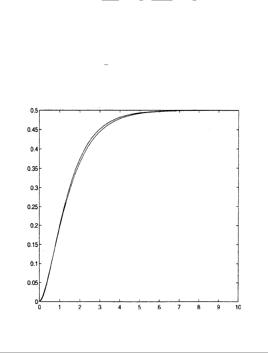
406 Glyn James, Advanced Modern Engineering Mathematics, 4th Edition
with solution α=−1, β=1/2so
yk=−1
1+Tk
+1
21
1+2Tk
+1
2
The differential equation is simply solved by inverting the Laplace transform
to give
y(t)=1
2(e−2t−2e−t+1),t≥0
T = 0.1
Figure 6.3: Response of continuous and discrete systems in Review Exercise 14 over
10 seconds when T=0.1.
c
Pearson Education Limited 2011
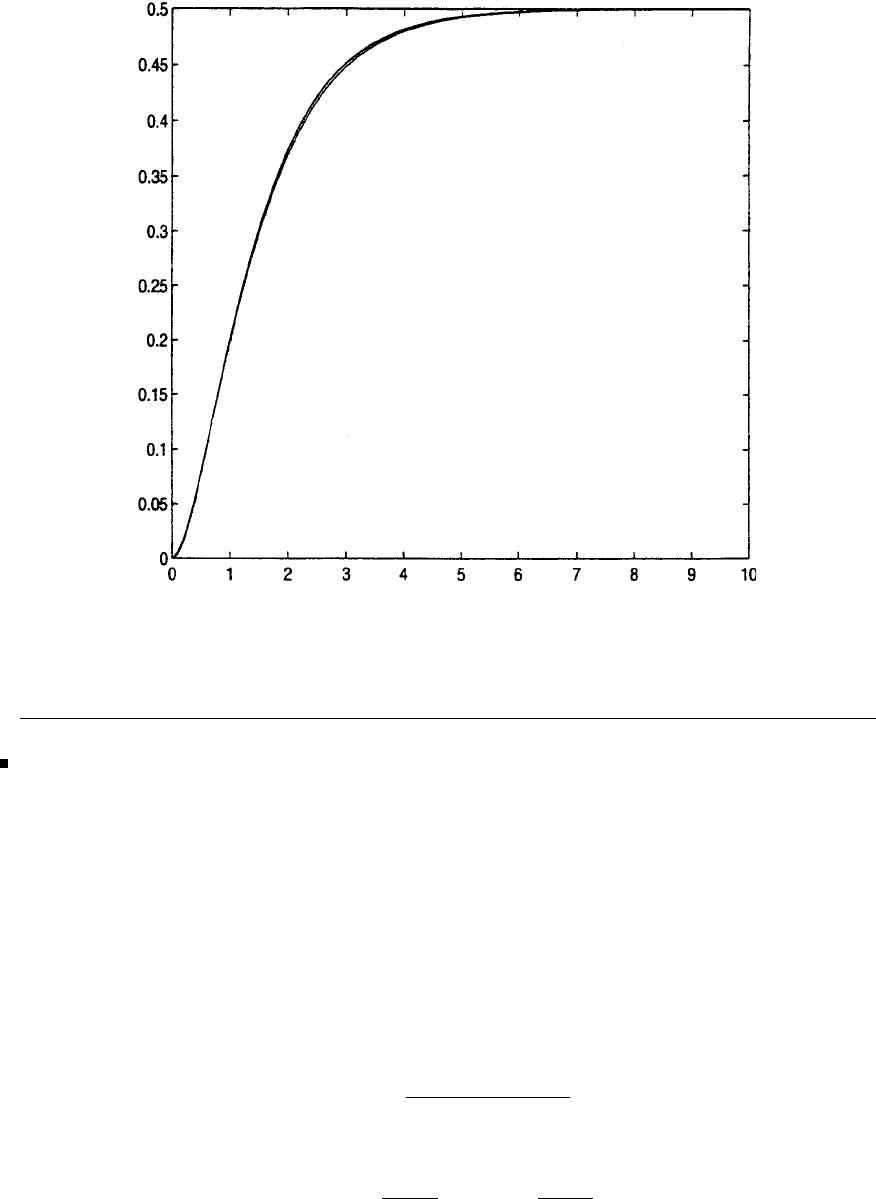
Glyn James, Advanced Modern Engineering Mathematics, 4th Edition 407
T = 0.05
Figure 6.4: Response of continuous and discrete systems in Review Exercise 14 over
10 seconds when T=0.05.
15 Substitution for sand simplifying gives
[(4 + 6T+2T2)z2+(4T2−8)z+(4−6T+2T2)]Y(z)
=T2(z+1)
2X(x)
The characteristic equation is
(4 + 6T+2T2)z2+(4T2−8)z+(4−6T+2T2)=0
with roots
z=8−4T2±4T
2(4 + 6T+2T2)
That is,
z=1−T
1+Tand z=2−T
2+T
c
Pearson Education Limited 2011
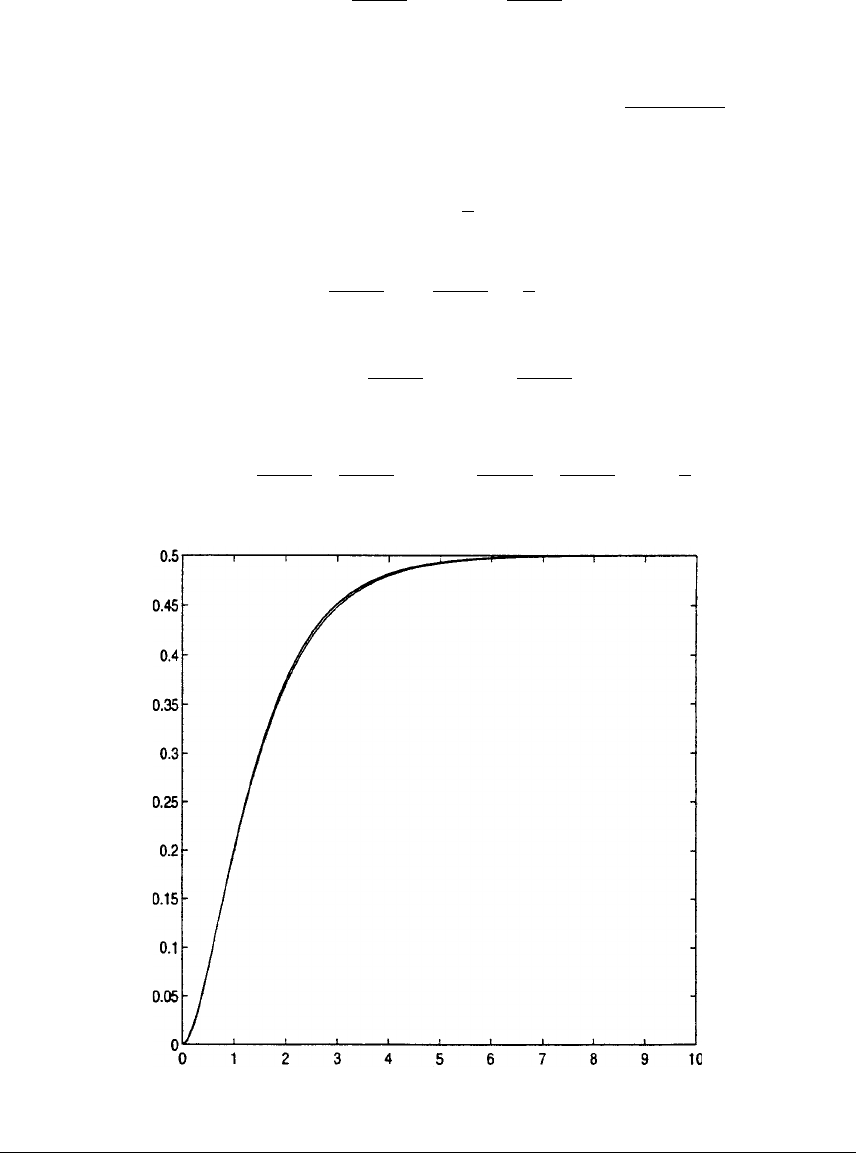
408 Glyn James, Advanced Modern Engineering Mathematics, 4th Edition
The general solution of the difference equation is then
yk=α1−T
1+Tk
+β2−T
2+Tk
+γ
This can be checked by substitution which also shows that γ=1/2. The
condition y(0) = 0 gives y0=0andsincey(t)→yk−yk−1
T,y(0) = 0
implies yk−1=0. Usingthesewehave
α+β+1
2=0
α1+T
1−T+β2+T
2−T+1
2=0
with solution
α=1−T
2β=−2−T
2
Thus,
yk=1−T
21−T
1+Tk
+−2−T
22−T
2+Tk
+1
2
T = 0.05
Figure 6.5: Response of continuous and discrete systems in Review Exercise 15 over
10 seconds when T=0.1.
c
Pearson Education Limited 2011
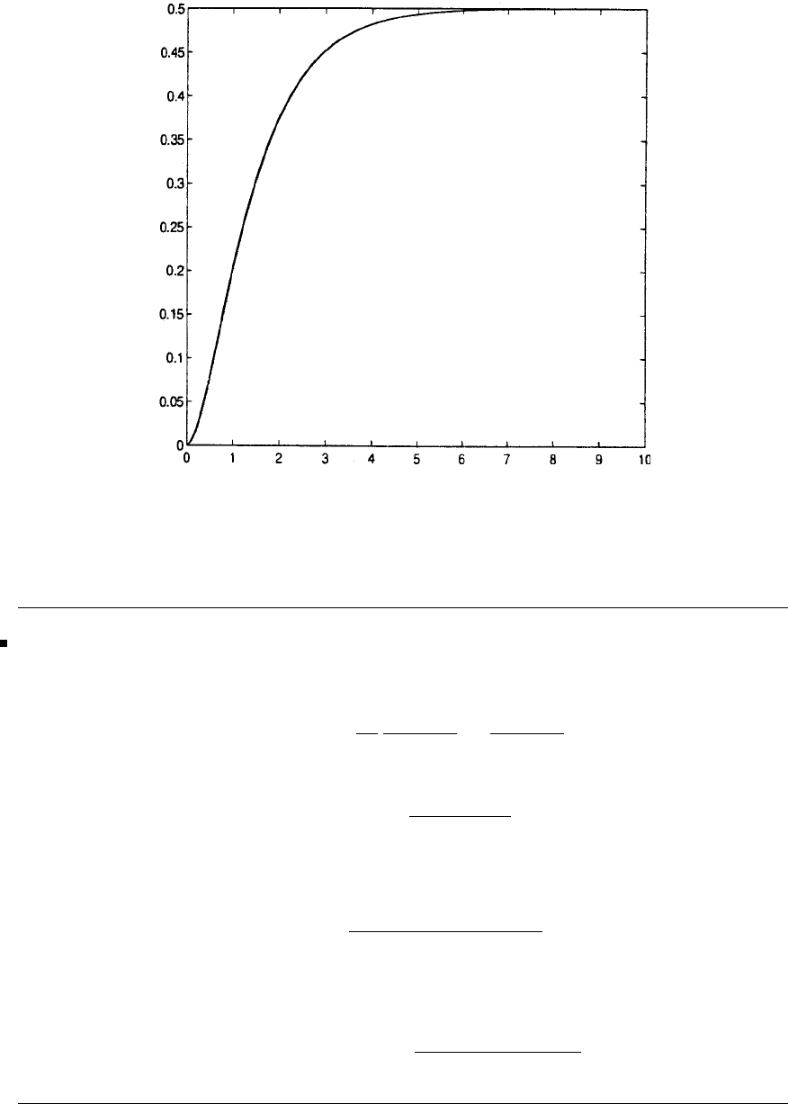
Glyn James, Advanced Modern Engineering Mathematics, 4th Edition 409
T = 0.05
Figure 6.6: Response of continuous and discrete systems in Review Exercise 14
over 10 seconds when T=0.05.
16 f(t)=t2,{f(kΔ)}=k2Δ2,k≥0
Now
Z{k2}=−zd
dz
z
(z−1)2=z(z+1)
(z−1)3
So
Z{k2Δ2}=z(z+1)Δ
2
(z−1)3
To get D-transform, put z=1+Δγto give
F
Δ(γ)=(1 + Δγ)(2 + Δγ)Δ2
Δ3γ3
Then the D-transform is
FΔ(γ)=ΔF
Δ(γ)=(1 + Δγ)(2 + Δγ)
γ3
c
Pearson Education Limited 2011

410 Glyn James, Advanced Modern Engineering Mathematics, 4th Edition
17 Eigenvalues are given by
0= ))))))
1−λ1−2
−12−λ1
01−1−λ))))))
=(1−λ)(λ2−λ−3) + (1 −λ)
=(1−λ)(λ−2)(λ+1)
so eigenvalues are λ1=2,λ
2=1,λ
3=−1
Corresponding eigenvectors are the solutions of
(1 −λi)ei1+ei2−2ei3=0
−ei1+(2−λi)ei2+ei3=0
0ei1+ei2−(1 + λi)ei3=0
Taking i=1,2,3 the eigenvectors are
e1=[131]
T,e2=[321]
T,e3=[101]
T
The modal matrix Mand spectral matrix Λare
M=⎡
⎣
131
320
111
⎤
⎦,Λ=⎡
⎣
20 0
01 0
00−1⎤
⎦
MΛ=⎡
⎣
23−1
62 0
21−1⎤
⎦,AM=⎡
⎣
11−2
−12 1
01−1⎤
⎦⎡
⎣
131
320
111
⎤
⎦
=⎡
⎣
23−1
62 0
21−1⎤
⎦=MΛ
Substituting x=Myin x(k+1)=Ax(k)gives
My(k+1)=AMy(k)
or y(k+1)=M−1AMy
(k)=Λy(k)
so y(1) = Λy(0),y(2) = Λy(1) = Λ2y(0)
⇒y(k)=Λky(0)
c
Pearson Education Limited 2011

Glyn James, Advanced Modern Engineering Mathematics, 4th Edition 411
Thus,
x(k)= ⎡
⎣
131
320
111
⎤
⎦⎡
⎣
2k00
01 0
00(−1)k⎤
⎦⎡
⎣
α
β
γ⎤
⎦say
=⎡
⎣
131
320
111
⎤
⎦⎡
⎣
α2k
β
γ(−1)k⎤
⎦
=⎡
⎣
α2k+3β+γ(−1)k
3α2k+2β
α2k+β+γ(−1)k⎤
⎦
When k=0 ⎡
⎣
1
0
0⎤
⎦=⎡
⎣
α+3β+γ
3α+2β
α+β+γ⎤
⎦
which gives α=−1
3,β=1
2,γ=1
6
so that
x(k)=⎡
⎣
−1
3(2)k+3
2+1
6(−1)k
−(2)k+1
−1
3(2)k+1
2+1
6(−1)k⎤
⎦
18 x1(k+1)=u(k)−3x1(k)−4x2(k)
x2(k+1)=−2x1(k)−x2(k)
y(k)=x1(k)+x2(k)
or in vector-matrix form
x(k+1)= #−3−4
−2−1&x(k)+ #1
0&u(k),y(k)=[1 −1]x(k)(1)
D(x)=c[zI−A]−1b=1
z2+4z−5[1 −1] #z+1 −4
−2z+3
0&
=z+3
z2+4z−5
(i) Mc=#1−3
0−2&
(ii) det Mc=−2=0 so Mcis of rank 2
c
Pearson Education Limited 2011

412 Glyn James, Advanced Modern Engineering Mathematics, 4th Edition
(iii) M−1
c=−1
2#−23
01
&=#1−3
2
0−1
2&
so vT=[0 −1
2]
(iv) T=#0−1
2
11
2&
(v) det T=0 and T−1=2 #1
2
1
2
−10
&=#11
−20
&
Substituting z(k)=Tx(k) in (1) gives
T−1z(k+1)=AT
−1z(k)+bu(k)
or z(k+1)=TAT
−1z(k)+Tbu(k)
=#0−1
2
11
2&#−3−4
−2−1
−20
&z(k)+ #0−1
2
11
2
0&u(t)
thatis,z(k+1)= #01
5−4&z(k)+#0
1&u(k)
Thus Cand bcare of the required form with α=−5,β= 4 which are coefficients
in the characteristic polynomial of D(z).
c
Pearson Education Limited 2011

7
Fourier series
Exercises 7.2.6
1(a)
a0=1
π0
−π−πdt +π
0
tdt
=1
π(−πt)0
−π+t2
2
π
0=1
π−π2+π2
2=−π
2
an=1
π0
−π−πcos ntdt +π
0
tcos ntdt
=1
π−π
nsin nt0
−π+t
nsin nt +1
n2cos nt
π
0
=1
πn2(cos nπ −1) = −2
πn2,nodd
0,neven
bn=1
π0
−π−πsin ntdt +π
0
tsin ntdt
=1
ππ
ncos nt0
−π+−t
ncos nt +1
n2sin nt
π
0
=1
n(1 −2cosnπ)=⎧
⎪
⎨
⎪
⎩
3
n,nodd
−1
n,neven
Thus, the Fourier expansion of f(t)is
f(t)=−π
4+
nodd −2
πn2cos nt +
nodd
3
nsin nt −
neven
1
nsin nt
i.e. f(t)=−π
4−2
π
∞
n=1
cos(2n−1)t
(2π−1)2+3 ∞
n=1
sin(2n−1)t
(2n−1) −∞
n=1
sin 2nt
2n
c
Pearson Education Limited 2011

414 Glyn James, Advanced Modern Engineering Mathematics, 4th Edition
1(b)
a0=1
π0
−π
(t+π)dt =1
πt2
2+πt0
−π
=π
2
an=1
π0
−π
(t+π)cosntdt =1
π(t+π)sin nt
n+cos nt
n20
−π
=1
πn2(1 −cos nπ)=0,neven
2
πn2,nodd
bn=1
π0
−π
(t+π)sinntdt =1
π−(t+π)cos nt
n+sin nt
n20
−π
=−1
n
Thus, the Fourier expansion of f(t)is
f(t)=π
4+
nodd
2
πn2cos nt −∞
n=1
1
nsin nt
i.e. f(t)=π
4+2
π
∞
n=1
cos(2n−1)t
(2n−1)2−∞
n=1
sin nt
n
1(c) From its graph we see that f(t) is an odd function; so it has Fourier
expansion
f(t)= ∞
n=1
bnsin nt
with
bn=2
ππ
0
f(t)sinnt =2
ππ
01−t
πsin ntdt
=2
π−1
n1−t
πcos nt −1
πn2sin ntπ
0
=2
nπ
Thus, the Fourier expansion of f(t)is
f(t)= 2
π
∞
n=1
sin nt
n
c
Pearson Education Limited 2011

Glyn James, Advanced Modern Engineering Mathematics, 4th Edition 415
1(d) From its graph f(t) is seen to be an even function; so its Fourier
expansion is
f(t)=a0
2+∞
n=1
ancos nt
with
a0=2
ππ
0
f(t)dt =2
ππ/2
0
2costdt =2
π[2 sin t]π/2
0=4
π
an=2
ππ
0
f(t)cosntdt =2
ππ/2
0
2costcos ntdt
=2
ππ/2
0
[cos(n+1)t+cos(n−1)t]dt
=2
πsin(n+1)t
(n+1) +sin(n−1)t
(n−1) π/2
0
=2
π1
(n+1)sin(n+1)π
2+1
(n−1) sin(n−1) π
2
=⎧
⎪
⎪
⎪
⎨
⎪
⎪
⎪
⎩
0,nodd
−4
π
1
(n2−1) ,n=4,8,12,...
4
π
1
(n2−1) ,n=2,6,10,...
Thus, the Fourier expansion of f(t)is
f(t)= 2
π+4
π
∞
n=1
(−1)n+1 cos 2nt
4n2−1
1(e)
a0=1
ππ
−π
cos t
2dt =1
π2sin t
2π
−π
=4
π
an=1
ππ
−π
cos t
2cos ntdt =1
2ππ
−πcos(n+1
2)t+cos(n−1
2)tdt
=2
2π2
(2n+1)sin(n+1
2)π+2
(2n−1) sin(n−1
2)π
=⎧
⎪
⎨
⎪
⎩
4
π(4n2−1) ,n=1,3,5,...
−4
π(4n2−1) ,n=2,4,6,...
bn=0
c
Pearson Education Limited 2011

416 Glyn James, Advanced Modern Engineering Mathematics, 4th Edition
Thus, the Fourier expansion of f(t)is
f(t)= 2
π+4
π
∞
n=1
(−1)n+1 cos nt
(4n2−1)
1(f) Since f(t) is an even function, it has Fourier expansion
f(t)=a0
2+∞
n=1
ancos nt
with
a0=2
ππ
0|t|dt =2
ππ
0
tdt =π
an=2
ππ
0
tcos ntdt =2
πt
nsin nt +1
n2cos ntπ
0
=2
πn2(cos nπ −1) = 0,neven
−4
πn2,nodd
Thus, the Fourier expansion of f(t)is
f(t)=π
2−4
π
nodd
1
n2cos nt
that is, f(t)=π
2−4
π
∞
n=1
cos(2n−1)t
(2n−1)2
1(g)
a0=1
ππ
0
(2t−π)dt =1
πt2−πtπ
0=0
an=1
ππ
0
(2t−π)cosntdt =1
π(2t−π)
nsin nt +2
n2cos ntπ
0
=2
πn2(cos nπ −1) = −4
πn2,nodd
0,neven
bn=1
ππ
0
(2t−π)sinntdt =1
π−(2t−π)
ncos nt +2
n2sin ntπ
0
=−1
n(cos nπ +1)=0,nodd
−2
n,neven
c
Pearson Education Limited 2011

Glyn James, Advanced Modern Engineering Mathematics, 4th Edition 417
Thus, the Fourier expansion of f(t)is
f(t)=
nodd −4
πn2cos nt +
neven −2
nsin nt
that is,f(t)=−4
π
∞
n=1
cos(2n−1)t
(2n−1)2−∞
n=1
sin 2nt
n
1(h)
a0=1
π0
−π
(−t+et)dt +π
0
(t+et)dt
=1
π−t2
2+et
0
−π+t2
2+et
π
0
=1
ππ2+(eπ−e−π)=π+2
πsinh π
an=1
π0
−π
(−t+et)cosntdt +π
0
(t+et)cosntdt
=1
π−t
nsin nt +1
n2cos nt
0
−π+1
(n2+1)netsin nt +etcos nt0
−π
+t
nsin nt +1
n2cos ntπ
0
+1
(n2+1)netsin nt +etcos ntπ
0
=2
πn2(−1+cosnπ)+ 2cosnπ
π(n2+1)eπ−e−π
2
=2
π(cos π−1)
n2+cos nπ
(n2+1)sinh π,cos nπ =(−1)n
bn=1
π0
−π
(−t+et)sinntdt +π
0
(t+et)sinntdt
=1
πt
ncos nt −1
n2sin nt
0
−π+−t
ncos nt +1
n2sin nt
π
0
+n2
π2+1−etcos nt
n+etsin nt
n2
π
−π
=−n
π(n2+1)cos nπ(eπ−e−π)=−2n
π(n2+1)cos nπ sinh π, cos nπ =(−1)n
c
Pearson Education Limited 2011

418 Glyn James, Advanced Modern Engineering Mathematics, 4th Edition
Thus, the Fourier expansion of f(t)is
f(t)=π
2+1
πsinh π+2
π
∞
n=1 (−1)n−1
n2+(−1)nsinh π
n2+1 cos nt
−2
π
∞
n=1
n(−1)n
n2+1 sinh πsin nt
2Since the periodic function f(t) is an even function, its Fourier expansion is
f(t)=a0
2+∞
n=1
ancos nt
with
a0=2
ππ
0
(π−t)2dt =2
π−1
3(π−t)3π
0
=2
3π2
an=2
ππ
0
(π−t)2cos ntdt =2
π(π−t)2
nsin nt −2(π−t)
n2cos nt −2
n3sin ntπ
0
=4
n2
Thus, the Fourier expansion of f(t)is
f(t)=π2
3+4 ∞
n=1
1
n2cos nt
Taking t=πgives
0=π2
3+4 ∞
n=1
1
n2(−1)n
so that
1
12 π2=∞
n=1
(−1)n+1
n2
c
Pearson Education Limited 2011

Glyn James, Advanced Modern Engineering Mathematics, 4th Edition 419
3Since q(t) is an even function, its Fourier expansion is
q(t)=a0
2+∞
n=1
ancos nt
with
a0=2
ππ
0
Qt
πdt =Q
an=2
ππ
0
Qt
πcos ntdt =2Q
π2t
nsin nt +1
n2cos ntπ
0
=2Q
π2n2(cos nπ −1) = 0,neven
−4Q
π2n2,nodd
Thus, the Fourier expansion of q(t)is
q(t)=Q1
2−4
π2
∞
n=1
cos(2n−1)t
(2n−1)2
4
a0=1
ππ
0
5sintdt =1
π[−5cost]π
0=10
π
an=5
ππ
0
sin tcos ntdt =5
2ππ
0
[sin(n+1)t−sin(n−1)t]dt
=5
2π−cos(n+1)t
(n+1) +cos(n−1)t
(n−1) π
0
,n=1
=5
2πcos nπ
n+1 −cos nπ
(n−1) −−1
n+1+1
n−1
=−5
π(n2−1) (cos nπ +1)=0,nodd,n=1
−10
π(n2−1) ,neven
Note that in this case we need to evaluate a1separately as
a1=1
ππ
0
5sintcos tdt =5
2ππ
0
sin 2tdt =0
bn=5
ππ
0
sin tsin ntdt =−5
2ππ
0
[cos(n+1)t−cos(n−1)t]dt
=−5
2πsin(n+1)t
(n+1) −sin(n−1)t
(n−1) π
0
,n=1
=0,n=1
c
Pearson Education Limited 2011

420 Glyn James, Advanced Modern Engineering Mathematics, 4th Edition
Evaluating b1separately,
b1=5
ππ
0
sin tsin tdt =5
2ππ
0
(1 −cos 2t)dt
=5
2πt−1
2sin 2t
π
0=5
2
Thus, the Fourier expansion of f(t)is
f(t)= 5
π+5
2sin t−10
π
∞
n=1
cos 2nt
4n2−1
5
a0=1
π0
−π
π2dt +π
0
(t−π)2dt
=1
ππ2t0
−π+1
3(t−π)3
π
0=4
3π2
an=1
π0
−π
π2cos ntdt +π
0
(t−π)2cos ntdt
=1
ππ2
nsin nt
0
−π+(t−π)2
nsin nt +2(t−π)
n2cos nt −2
n3sin nt
π
0
=2
n2
bn=1
π0
−π
π2sin ntdt +π
0
(t−π)2sin ntdt
=1
π−π2
ncos nt
0
−π+−(t−π)2
ncos nt +2(t−π)
n2sin nt +2
n3cos nt
π
0
=1
π−π2
n+π2
n(−1)n
=π
n(−1)n−2
πn3[1 −(−1)n]
c
Pearson Education Limited 2011
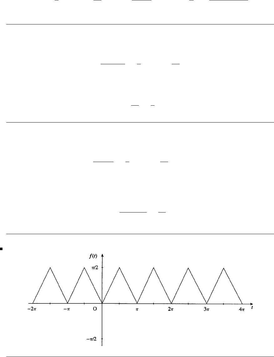
Glyn James, Advanced Modern Engineering Mathematics, 4th Edition 421
Thus, the Fourier expansion of f(t)is
f(t)=2
3π2+∞
n=1 2
n2cos nt +(−1)n
nπsin nt−4
π
∞
n=1
sin(2n−1)t
(2n−1)3
5(a) Taking t=0 gives
π2+π2
2=2
3π2+∞
n=1
2
n2
and hence the required result
∞
n=1
1
n2=1
6π2
5(b) Taking t=πgives
π2+0
2=2
3π2+∞
n=1
2
n2(−1)n
and hence the required result
∞
n=1
(−1)n+1
n2=1
12 π2
6(a)
c
Pearson Education Limited 2011
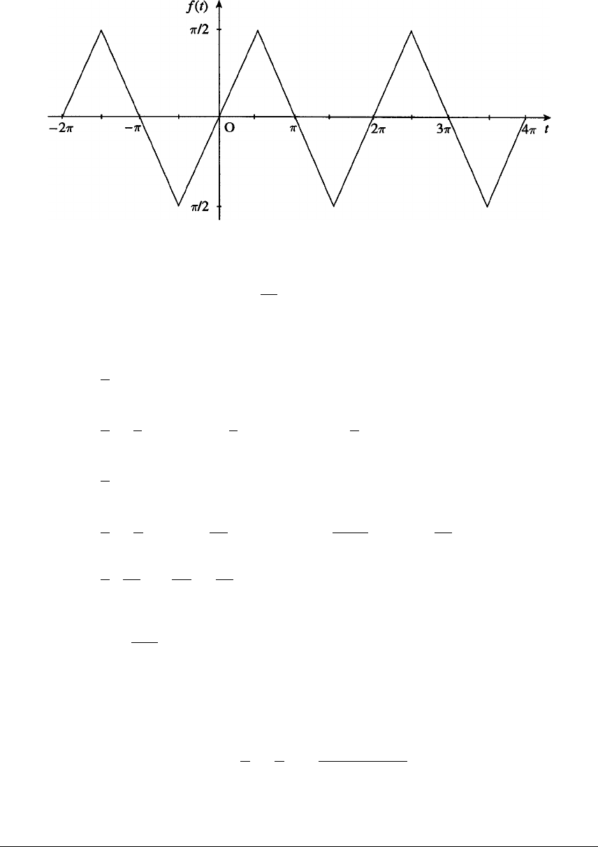
422 Glyn James, Advanced Modern Engineering Mathematics, 4th Edition
6(b)
The Fourier expansion of the even function (a)isgivenby
f(t)=a0
2+∞
n=1
ancos nt
with
a0=2
ππ/2
0
tdt +π
π/2
(π−t)dt
=2
π1
2t2
π/2
0+−1
2(π−t)2
π
π/2=π
2
an=2
ππ/2
0
tcos ntdt +π
π/2
(π−t)cosntdt
=2
πt
nsin nt +1
n2cos nt
π/2
0+π−t
nsin nt −1
n2cos nt
π
π/2
=2
π2
n2cos nπ
2−1
n2(1 + (−1)n)
=⎧
⎪
⎨
⎪
⎩
0,nodd
−8
πn2,n=2,6,10,...
0,n=4,8,12,...
Thus, the Fourier expansion of f(t)is
f(t)=π
4−2
π
∞
n=1
cos(4n−2)t
(2n−1)2
Taking t=0 where f(t) = 0 gives the required result.
c
Pearson Education Limited 2011
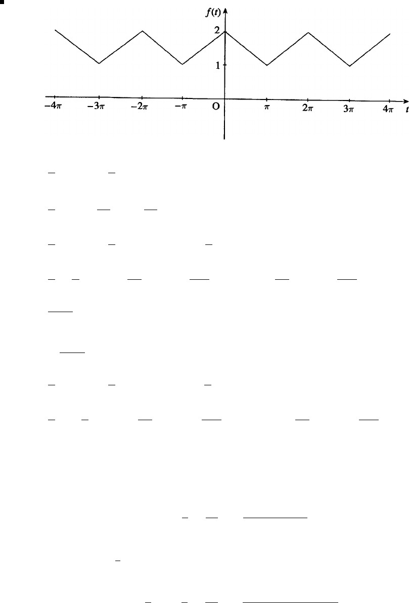
Glyn James, Advanced Modern Engineering Mathematics, 4th Edition 423
7
a0=1
ππ
0
(2 −t
π)dt +2π
π
t/πdt
=1
π2t−t2
2π
π
0+t2
2π
2π
π=3
an=1
ππ
0
(2 −t
π)cosntdt +2π
π
t
πcos ntdt
=1
π2
nsin nt −t
πn sin nt −1
πn2cos nt
π
0+t
πn sin nt +1
πn2cos nt
2π
π
=2
π2n2[1 −(−1)n]
=0,neven
4
π2n2,nodd
bn=1
ππ
0
(2 −t
π)sinntdt +2π
π
t
πsin ntdt
=1
π−2
ncos nt +t
πn cos nt −1
πn2sin nt
π
0+−t
πn cos nt +1
πn2sin nt
2π
π
=0
Thus, the Fourier expansion of f(t)is
f(t)=3
2+4
π2
∞
n=1
cos(2n−1)t
(2n−1)2
Replacing tby t−1
2πgives
f(t−1
2π)=3
2+4
π2
∞
n=1
cos(2n−1)(t−π)
(2n−1)2
c
Pearson Education Limited 2011

424 Glyn James, Advanced Modern Engineering Mathematics, 4th Edition
Since
cos(2n−1)(t−1
2π)=cos(2n−1)tcos(2n−1) π
2+sin(2n−1)tsin(2n−1) π
2
=(−1)n+1 sin(2n−1)t
f(t−1
2π)−3
2=4
π2
∞
n=1
(−1)n+1 sin(2n−1)t
(2n−1)2
The corresponding odd function is readily recognized from the graph of f(t).
Exercises 7.2.8
8Since f(t) is an odd function, the Fourier expansion is
f(t)= ∞
n=1
bnsin nπt
with
bn=2
0
tsin nπt
dt =2
−t
nπ cos nπt
+
nπ
2
sin nπt
0
=−2
nπ cos nπ
Thus, the Fourier expansion of f(t)is
f(t)=2
π
∞
n=1
(−1)n+1
nsin nπt
9Since f(t) is an odd function (readily seen from a sketch of its graph) its
Fourier expansion is
f(t)= ∞
n=1
bnsin nπt
with
bn=2
0
K
(−t)sinnπt
tdt
=2
−K
nπ cos nπt
+Kt
nπ cos nπt
−K
(nπ)2sin nπt
0
=2K
nπ
c
Pearson Education Limited 2011

Glyn James, Advanced Modern Engineering Mathematics, 4th Edition 425
Thus, the Fourier expansion of f(t)is
f(t)=2K
π
∞
n=1
1
nsin nπt
10
a0=1
55
0
3dt =3
an=1
55
0
3cos nπt
5dt =1
515
nπ sin nπt
55
0
=0
bn=1
55
0
3sin nπt
5dt =1
5−15
nπ cos nπt
55
0
=3
nπ[1 −(−1)n]=6
nπ ,nodd
0,neven
Thus, the Fourier expansion of f(t)is
f(t)= 3
2+6
π
∞
n=1
1
(2n−1) sin (2n−1)
5πt
11
a0=2ω
2ππ/ω
0
Asin ωtdt =ω
π−A
ωcos ωtπ/ω
0
=2A
π
an=Aω
ππ/ω
0
sin ωt cos nωtdt =Aω
2ππ/ω
0
[sin(n+1)ωt −sin(n−1)ωt]dt
=Aω
2π−cos(n+1)ωt
(n+1)ω+cos(n−1)ωt
(n−1)ωπ/ω
0
,n=1
=A
2π2(−1)n+1
n2−1−2
n2−1=A
π(n2−1) [(−1)n+1 −1]
=⎧
⎨
⎩
0,nodd , n=1
−2A
π(n2−1) ,neven
Evaluating a1separately,
a1=Aω
ππ/ω
0
sin ωt cos ωtdt =A
2ππ/ω
0
sin 2ωtdt =0
c
Pearson Education Limited 2011

426 Glyn James, Advanced Modern Engineering Mathematics, 4th Edition
bn=Aω
ππ/ω
0
sin ωt sin nωtdt =−Aω
2ππ/ω
0
[cos(n+1)ωt −cos(n−1)ωt]dt
=−Aω
2πsin(n+1)ωt
(n+1)ω−sin(n−1)ωt
(n−1)ωπ/ω
0
,n=1
=0,n=1
b1=Aω
ππ/ω
0
sin2ωtdt =Aω
2ππ/ω
0
(1 −cos 2ωt)dt =A
2
Thus, the Fourier expansion of f(t)is
f(t)=A
π1+π
2sin ωt −2∞
n=1
cos 2nωt
4n2−1
12 Since f(t) is an even function, its Fourier expansion is
f(t)=a0
2+∞
n=1
ancos nπt
T
with
a0=2
TT
0
t2dt =2
T1
3t3T
0
=2
3T2
an=2
TT
0
t2cos nπt
Tdt =2
TTt2
nπ sin nπt
T+2tT2
(nπ)2cos nπt
T−2T3
(nπ)3sin nπt
TT
0
=4T2
(nπ)2(−1)n
Thus, the Fourier series expansion of f(t)is
f(t)=T2
3+4T2
π2
∞
n=1
(−1)n
n2cos nπt
T
c
Pearson Education Limited 2011

Glyn James, Advanced Modern Engineering Mathematics, 4th Edition 427
13
a0=2
TT
0
E
Ttdt =2E
T21
2t2T
0
=E
an=2
TT
0
E
Ttcos 2πnt
Tdt
=2E
T2tT
2πn sin 2πnt
T+T
2πn
2
cos 2πnt
TT
0
=0
bn=2E
T2T
0
tsin 2πnt
Tdt
=2E
T2−tT
2πn cos 2πnt
T+T
2πn
2
sin 2πnt
TT
0
=−E
πn
Thus, the Fourier expansion of e(t)is
e(t)= E
2−E
π
∞
n=1
1
nsin 2πnt
T
Exercises 7.3.3
14 Half range Fourier sine series expansion is given by
f(t)= ∞
n=1
bnsin nt
with
bn=2
ππ
0
1sinntdt =2
π−1
ncos ntπ
0
=−2
nπ[(−1)n−1]
=0,neven
4
nπ ,nodd
Thus, the half range Fourier sine series expansion of f(t)is
f(t)= 4
π
∞
n=1
sin(2n−1)t
(2n−1)
Plotting the graphs should cause no problems.
c
Pearson Education Limited 2011

428 Glyn James, Advanced Modern Engineering Mathematics, 4th Edition
15 Half range Fourier cosine series expansion is given by
f(t)=a0
2+∞
n=1
ancos nπt
with
a0=2
11
0
(2t−1)dt =0
an=21
0
(2t−1) cos nπtdt
=2
(2t−1)
nπ sin nπt +2
(nπ)2cos nπt1
0
=4
(nπ)2[(−1)n−1]
=0,neven
−8
(nπ)2,nodd
Thus, the half range Fourier cosine series expansion of f(t)is
f(t)=−8
π2
∞
n=1
1
(2n−1)2cos(2n−1)πt
Again plotting the graph should cause no problems.
16(a)
a0=21
0
(1 −t2)dt =2
t−1
3t3
1
0=4
3
an=21
0
(1 −t2)cos2nπtdt
=2
(1 −t2)
2nπ sin 2nπt −2t
(2nπ)2cos 2nπt +2
(2nπ)3sin 2nπt1
0
=−1
(nπ)2
c
Pearson Education Limited 2011

Glyn James, Advanced Modern Engineering Mathematics, 4th Edition 429
bn=21
0
(1 −t2)sin2nπtdt
=2
−(1 −t2)
2nπ cos 2nπt −2t
(2nπ)2sin 2nπt −2
(2nπ)3cos 2nπt1
0
=1
nπ
Thus, the full-range Fourier series expansion for f(t)is
f(t)=f1(t)= 2
3−1
π2
∞
n=1
1
n2cos 2nπt +1
π
∞
n=1
1
nsin 2nπt
16(b) Half-range sine series expansion is
f2(t)= ∞
n=1
bnsin nπt
with
bn=21
0
(1 −t2)sinnπtdt
=2
−(1 −t2)
nπ cos nπt −2t
(nπ)2sin nπt −2
(nπ)3cos nπt1
0
=2
−2
(nπ)3(−1)n+1
nπ +2
(nπ)3
=⎧
⎪
⎨
⎪
⎩
2
nπ ,neven
21
nπ +4
(nπ)3,nodd
Thus, half-range sine series expansion is
f2(t)= 1
π
∞
n=1
1
nsin 2nπt +2
π
∞
n=1 1
(2n−1) +4
π2(2n−1)3sin(2n−1)πt
16(c) Half-range cosine series expansion is
f3(t)=a0
2+∞
n=1
ancos nπt
c
Pearson Education Limited 2011
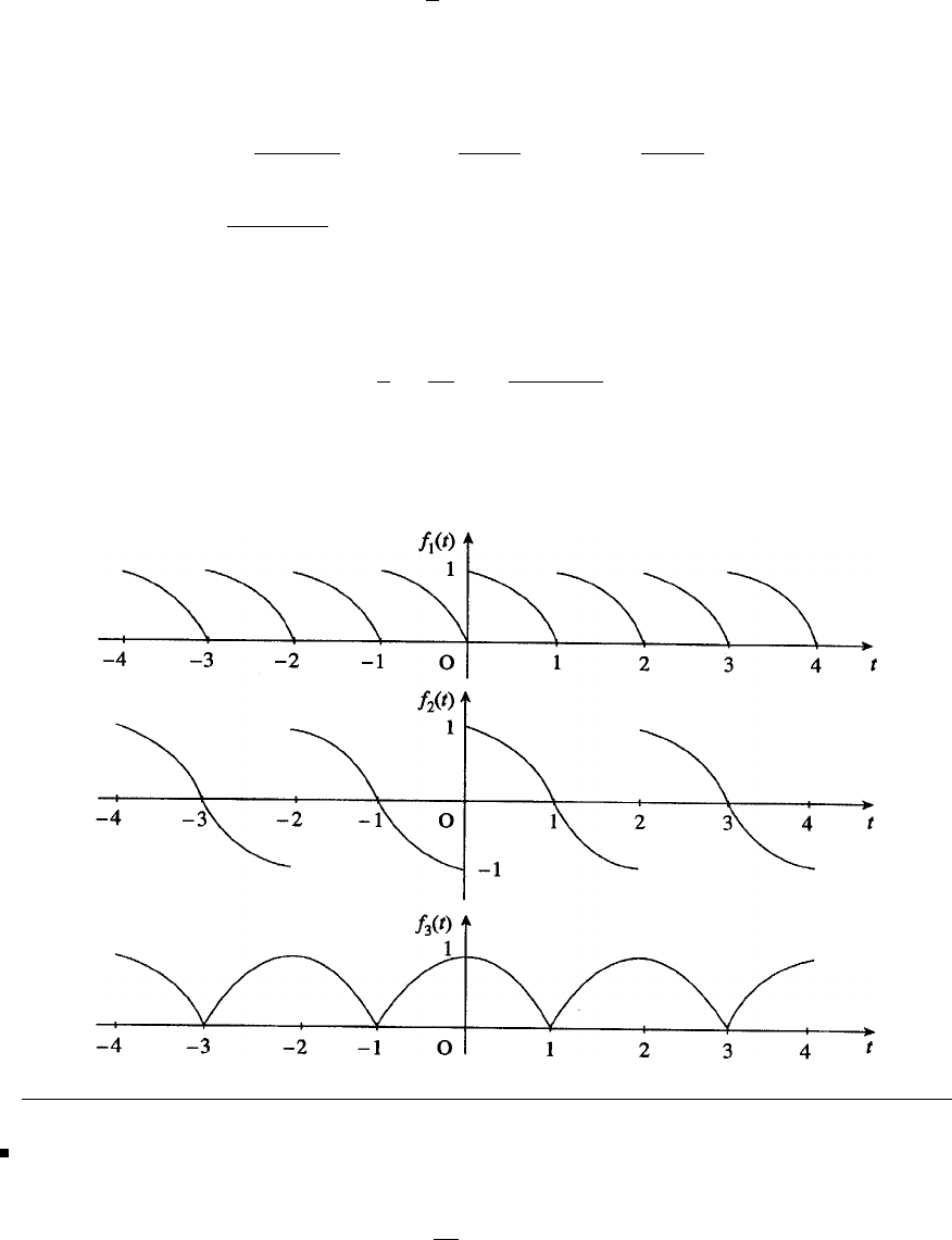
430 Glyn James, Advanced Modern Engineering Mathematics, 4th Edition
with
a0=21
0
(1 −t2)dt =4
3
an=21
0
(1 −t2)cosnπtdt
=2
(1 −t2)
nπ sin nπt −2t
(nπ)2cos nπt +2
(nπ)3sin nπt1
0
=−4(−1)n
(nπ)2
Thus, half-range cosine series expansion is
f3(t)=2
3+4
π2
∞
n=1
(−1)n+1
n2cos nπt
Graphs of the functions f1(t),f
2(t),f
3(t)for−4<t<4 are as follows:
17 Fourier cosine series expansion is
f1(t)=a0
2+∞
n=1
ancos nt
c
Pearson Education Limited 2011

Glyn James, Advanced Modern Engineering Mathematics, 4th Edition 431
with
a0=2
ππ
0
(πt −t2)dt =1
3π2
an=2
ππ
0
(πt −t2)cosntdt
=2
π(πt −t2)
nsin nt +(π−2t)
n2cos nt +2
n3sin ntπ
0
=−2
n2[1 + (−1)n]
=0,nodd
−4
n2,neven
Thus, the Fourier cosine series expansion is
f1(t)=1
6π2−∞
n=1
1
n2cos 2nt
Fourier sine series expansion is
f2(t)= ∞
n=1
bnsin nt
with
bn=2
ππ
0
(πt −t2)sinntdt
=2
π−(πt −t2)
ncos nt +(π−2t)
n2sin nt −2
n3cos ntπ
0
=4
πn3[1 −(−1)n]
=0,neven
8
πn3,nodd
Thus, the Fourier sine series expansion is
f2(t)= 8
π
∞
n=1
1
(2n−1)3sin(2n−1)t
c
Pearson Education Limited 2011
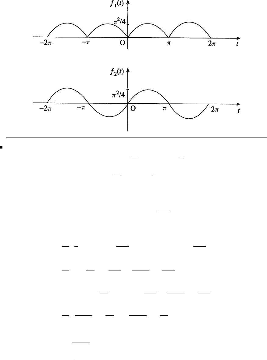
432 Glyn James, Advanced Modern Engineering Mathematics, 4th Edition
Graphs of the functions f1(t)andf2(t)for−2π<t<2πare
18
f(x)=2a
x, 0<x<
2
f(x)=2a
(−x),
2<x<
Fourier sine series expansion is
f(x)= ∞
n=1
bnsin nπx
with
bn=2a
·2
/2
0
xsin nπx
dx +
/2
(−x)sinnπx
dx
=4a
2−x
nπ cos nπx
+2
(nπ)2sin nπx
/2
0
+−
nπ(−x)cos nπx
−2
(nπ)2sin nπx
/2
=4a
222
(nπ)2sin nπ
2=8a
(nπ)2sin nπ
2
=⎧
⎪
⎪
⎪
⎨
⎪
⎪
⎪
⎩
0,neven
8a
(nπ)2,n=1,5,9,...
−8a
(nπ)2,n=3,7,...
c
Pearson Education Limited 2011

Glyn James, Advanced Modern Engineering Mathematics, 4th Edition 433
Thus, the required Fourier sine series expansion is
f(x)=8a
π2
∞
n=1
(−1)n+1
(2n−1)2sin (2n−1)πx
19
f(x)=⎧
⎪
⎪
⎪
⎪
⎨
⎪
⎪
⎪
⎪
⎩
x, 0<x<
4
2−x,
4<x<3
4
x−, 3
4<x<
Fourier sine series expansion is
f(x)= ∞
n=1
bnsin nπx
with
bn=2
/4
0
xsin nπx
dx +3/4
/4
2−xsin nπx
dx +
3/4
(x−)sinnπx
dx
=2
−x
nπ cos nπx
+2
(nπ)2sin nπx
/4
0
+−
nπ
2−xcos nπx
−2
(nπ)2sin nπx
3/4
/4
+−
nπ(x−)cos nπx
+2
(nπ)2sin nπx
3/4
=sin nπ
4−sin 3nπ
4
=−8
(nπ)2cos nπ
2sin nπ
4
=⎧
⎪
⎪
⎪
⎪
⎪
⎨
⎪
⎪
⎪
⎪
⎪
⎩
0,nodd
0,n=4,8,12,...
8
(nπ)2,n=2,10,18,...
−8
(nπ)2,n=6,14,22,...
c
Pearson Education Limited 2011

434 Glyn James, Advanced Modern Engineering Mathematics, 4th Edition
Thus, the required Fourier sine series expansion is
f(x)= 2
π2
∞
n=1
(−1)n+1
(2n−1)2sin 2(2n−1) πx
20 Fourier sine series expansion is
f(t)= ∞
n=1
bnsin nt
with
bn=2
ππ/2
0
sin tsin ntdt
=−1
ππ/2
0
[cos(n+1)t−cos(n−1)t]dt
=−1
π1
(n+1)sin(n+1)t−1
(n−1) sin(n−1)tπ/2
0
,n=1
=−1
π1
(n+1)sin(n+1)π
2−1
(n−1) sin(n−1) π
2
Using the trigonometric expansions for sin(A+B)andsin(A−B)gives
bn=−2n
π(n2−1) cos nπ
2,n=1
=⎧
⎪
⎪
⎪
⎨
⎪
⎪
⎪
⎩
0,nodd
2n
π(n2−1) ,n=2,6,...
−2n
π(n2−1) ,n=4,8,10,...
In the case n=1,
b1=2
ππ/2
0
sin2tdt =1
ππ/2
0
(1 −cos 2t)dt =1
2
Thus, the required Fourier sine series expansion is
f(t)=1
2sin t+4
π
∞
n=1
(−1)n+1 nsin 2nt
4n2−1
The corresponding plot presents no problem.
c
Pearson Education Limited 2011
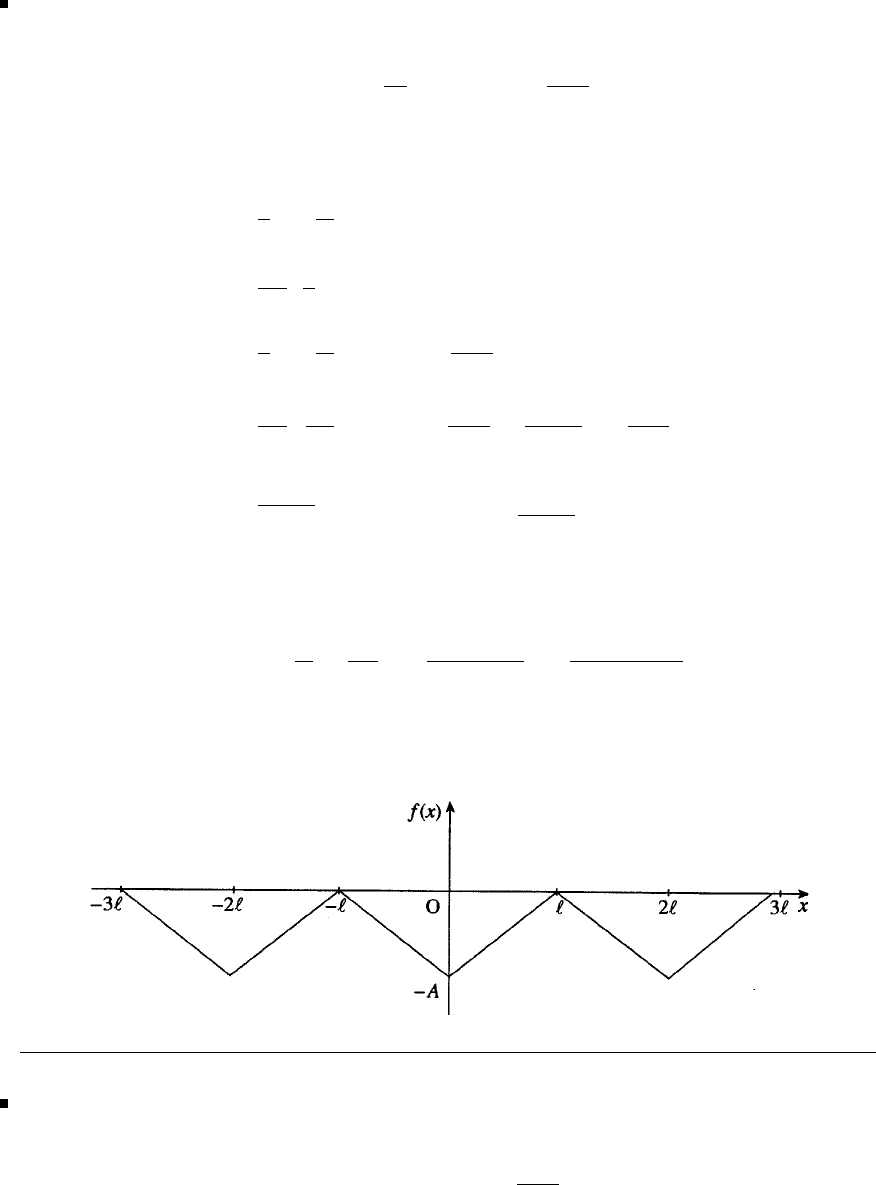
Glyn James, Advanced Modern Engineering Mathematics, 4th Edition 435
21 Since f(x) is an even function, the Fourier series expansion is
f(x)=a0
2+∞
n=1
ancos nπx
with
a0=2
0
A
(x−)dx, since |x|=xfor x≥0
=2A
21
2x2−x
0=−A
an=2
0
A
(x−)cos nπx
dx
=2A
2
nπ (x−)sinnπx
+2
(nπ)2cos nπx
0
=2A
(nπ)2(cos nπ −1) = 0,neven
−4A
(nπ)2,nodd
Thus, the Fourier series expansion is
f(t)=−A
2−4A
π2
∞
n=1
1
(2n−1)2cos (2n−1)πx
The graph represented by the series for −3≤x≤3is as follows:
22 Fourier sine series expansion is
T(x)= ∞
n=1
bnsin nπx
L
c
Pearson Education Limited 2011

436 Glyn James, Advanced Modern Engineering Mathematics, 4th Edition
with
bn=2
LL
0
Kx(L−x)sinnπx
Ldx
=2K
L−Lx(L−x)
nπ cos nπx
L+L2
(nπ)2(L−2x)sin nπx
L
−2L3
(nπ)3cos nπx
LL
0
=4KL2
(nπ)3(1 −cos nπ)=⎧
⎨
⎩
0,neven
8KL2
(nπ)3,nodd
Thus, the Fourier sine series expansion is
T(x)=8KL2
π3
∞
n=1
1
(2n−1)3sin (2n−1)πx
L
23
a0=2
20
−1
1dt +1
0
cos πtdt=[t]0
−1+1
πsin πt1
0
=1
an=0
−1
cos nπtdt +1
0
cos πt cos nπtdt
=1
nπ sin nπt0
−1
+1
21
0
cos(n+1)πt +cos(n−1)πtdt
=1
21
(n+1)πsin(n+1)πt +1
(n−1)πsin(n−1)πt1
0
,n=1
=0
a1=1
21
0
2cos 2
πtdt =1
21
0
(1 + cos 2πt)dt =1
2
bn=0
−1
sin nπtdt +1
0
cos πt sin nπtdt
=−1
nπ cos nπt0
−1
+1
21
0
sin(n+1)πt +sin(n−1)πtdt
=1
nπ [(−1)n−1] + 1
2π−1
(n+1)cos(n+1)πt −1
(n−1) cos(n−1)πt1
0
c
Pearson Education Limited 2011

Glyn James, Advanced Modern Engineering Mathematics, 4th Edition 437
=1
nπ[(−1)n−1] + 1
2π2n
(n2−1) [1 + cos nπ]
=⎧
⎪
⎨
⎪
⎩
−2
nπ ,nodd
2n
π(n2−1) ,neven
Thus, the Fourier series expansion is
f(t)=1
2+1
2cos πt −2
π
∞
n=1
1
(2n−1) sin(2n−1)πt +4
π
∞
n=1
n
4n2−1sin 2nπt
Exercises 7.4.4
24 Since f(t) is an odd function, its Fourier expansion is of the form
f(t)= ∞
n=1
bnsin nπ
Tt
with
bn=2
TT
0
tsin nπ
Tt
=2
T−Tt
nπ cos nπ
Tt+T2
n2π2sin nπ
TtT
0
=2
T−T2
nπ cos nπ=−2T
nπ (−1)n
Thus, the Fourier expansion is
f(t)=t=2T
π
∞
n=1
1
n(−1)n+1 sin nπ
Tt
Integrating term by term gives
t2
2=−2T2
π2
∞
n=1
1
n2(−1)n+1 cos nπ
Tt+const.
Taking mean value over a perio d,
1
2TT
−T
t2
2dt =−2T2
π2
∞
n=1
(−1)n+1
n2T
−T
cos nπ
Ttdt +1
2TT
−T
(const.)dt
c
Pearson Education Limited 2011

438 Glyn James, Advanced Modern Engineering Mathematics, 4th Edition
so that T2
6=0+ const.
giving (const.) = T2/6
Thus,
g(t)=t2=T2
3−4T2
π2(−1)n+1
n2cos nπ
Tt
25 π2−t2=h(t)=2
3π2+4∞
n=1
(−1)n+1
n2cos nt
Since h(t) is continuous within and at the end points of the interval −π≤t≤π,
we may apply Theorem 4.4 to obtain the Fourier series of
f(t)=t, −π<t<π;f(t+2π)=f(t)
Differentiating gives
−2t=−4∞
n=1
(−1)n+1
nsin nt
So that the Fourier series of f(t)is
f(t)=t=2 ∞
n=1
(−1)n+1
nsin nt
which confirms the series of Exercise 24 when T=π.
26(b) Derived series is
∞
n=1
4
n(−1)n+1 sin nt −
n
n=1
2(−1)ncos nt
This is not a Fourier expansion of g(t)sincef(t) is discontinuous at the end points
of −π≤t≤π.
26(c) Using the results of (a)
A0=1
π[f(π−)−f(−π+)] = 1
π·2π=2
An=(−1)nA0+nbn=(−1)n2−n2
n(−1)n=2(−1)n−2(−1)n=0
Bn=−nan=4
n(−1)n+1
c
Pearson Education Limited 2011

Glyn James, Advanced Modern Engineering Mathematics, 4th Edition 439
Thus, the Fourier expansion g(t)is
g(t)=A0
2+∞
n=1
Ancos nt +∞
n=1
Bnsin nt
=1+4 ∞
n=1
(−1)n+1
nsin nt
Using Euler’s formulae
A0=1
ππ
−π
(2t+1)dt =1
π[t2+t]π
−π=2
An=1
ππ
−π
(2t+1)cosnt dt
=1
π(2t+1)
nsin nt +2
n2cos ntπ
−π
=0
Bn=1
ππ
−π
(2t+1)sinnt dt
=1
π−(2t+1)
ncos nt +2
n2sin ntπ
−π
=1
πn−(2π+1)(−1)n+(−2π+1)(−1)n
=4
n(−1)n+1
thus confirming the values obtained using (a).
27(a)
p1(t)=−1p2(t)=1
d1=2 d2=−2
p(1)
1(t)=0 p(1)
2(t)=0
d(1)
1=0 d(1)
2=0
t1=0,t
2=πand since ω= 1 using (4.39) gives
an=1
nπ −
2
s=1
dssin nts−1
n
2
s=1
d(1)
scos nts
=1
nπ −2sin0+2sinnπ=0
c
Pearson Education Limited 2011

440 Glyn James, Advanced Modern Engineering Mathematics, 4th Edition
bn=1
nπ 2
s=1
dscos nts−1
n
2
s=1
d(1)
ssin nts
=1
nπ2cos0−2cosπ=2
nπ1−(−1)n=0,neven
4
nπ,nodd
a0=1
π0
−π
(−1)dt +π
0
1dt=0
Thus, Fourier series is
f(t)= 4
π
∞
n=1
1
(2n−1) sin(2n−1)t
confirming (7.21).
27(b)
p1(t)=t,d1=−2π
p(1)
1(t)=1, d(1)
1=0
t1=0, t2=π, ω =1
Thus, from (7.39)
an=1
nπ−d1sin nt1=1
nπ 2πsin 0=0
bn=1
nπd1cos nt1=1
nπ−2πcos 0=−2
n
a0=1
π2π
0
tat=2π
Thus, Fourier series is
f(t)=π−2∞
n=1
1
nsin nt
confirming the result obtained in Example 7.1.
27(c)
p1(t)=tp
2(t)=
1
2πp
3(t)=π−1
2t
d1=0 d2=0 d3=0
p(1)
1(t)=1 p(1)
2(t)=0 p(1)
3(t)=−1
2
d(1)
1=−1d(1)
2=−1
2d(1)
3=3
2
c
Pearson Education Limited 2011
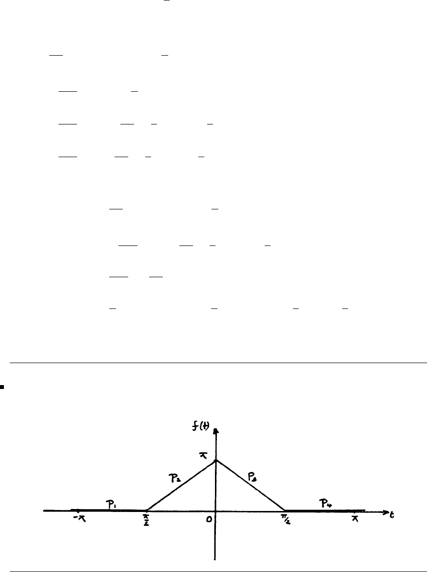
Glyn James, Advanced Modern Engineering Mathematics, 4th Edition 441
t1=π
2,t
2=π, t3=2π, ω =1
Thus, from (7.39)
an=1
nπ −
3
s=1
dssin nts−1
n
3
s=1
d(1)
scos nts
=−1
n2πd(1)
1cos nπ
2+d(1)
2cos nπ +d(1)
3cos 2πnsince ds=0,s=1,2,3
=−1
n2π−1cos nπ
2−1
2cos nπ +3
2cos 2nπ
=−1
n2π−cos nπ
2−1
2(−1)n+3
2
bn=1
nπ 3
s=1
dscos nts−1
n
3
s=1
d(1)
ssin nts
=−1
n2π−1sin nπ
2−1
2sin nπ +3
2sin 2nπ
=1
n2πsin nπ
2
a0=1
ππ/2
0
tdt+π
π/2
π
2dt +2π
π
(π−1
2t)dt=5
8π
which agree with the Fourier coefficients of Example 7.3.
28(a) Graph of f(t)for−π<t<πas follows and is readily extended to
−4π<t<4π:
c
Pearson Education Limited 2011

442 Glyn James, Advanced Modern Engineering Mathematics, 4th Edition
28(b)
p1(t)=0 p2(t)=π+2tp
3(t)=π−2tp
4(t)=0
d1=0 d2=0 d3=0 d4=0
p(1)
1(t)=0 p(1)
2(t)=2 p(1)
3(t)=−2p(1)
4(t)=0
d(1)
1=2 d(1)
2=−4d(1)
3=2 d(1)
4=0
p(2)
1(t)=0 p(2)
2(t)=0 p(2)
3(t)=0 p(2)
4(t)=0
d(2)
1=0 d(2)
2=0 d(2)
3=0 d(2)
4=0
t1=−π
2,t
2=0,t
3=π
2,t
4=π, ω =1
Thus, from (7.39)
an=1
nπ −
4
s=1
dssin nts−1
n
4
s=1
d(1)
scos nts+1
n2
4
s=1
d(2)
ssin ts
=−1
n2π2cos nπ
2−4cos0+2cos nπ
2
=−4
n2πcos nπ
2−1
bn=1
nπ 4
s=1
dscos nts−1
n
4
s=1
d(1)
ssin nts−1
n2
4
s=1
d(2)
scos nts
=−1
n2π−2sin nπ
2−4sin0+2sin nπ
2=0
a0=1
π−π/2
−π
0dt +0
−π/2
(π+2t)dt +π/2
0
(π−2t)dt +π
π/2
0dt
=π
2
Thus, Fourier series is
f(t)=π
4−4
π
∞
n=1
1
n2cos nπ
2−1cos nt
c
Pearson Education Limited 2011

Glyn James, Advanced Modern Engineering Mathematics, 4th Edition 443
29(a)
p1(t)=1 p2(t)=t2
d1=0 d2=−π2
p(1)
1(t)=0 p(1)
2(t)=2t
d(1)
1=0 d(1)
2=−2π
p(2)
1(t)=0 p(2)
2(t)=2
d(2)
1=2 d(2)
2=−2
p(3)
1(t)=0 p(3)
2(t)=0
d(3)
1=0 d(3)
2=0
t1=0,t
2=π, ω =1
Thus, from (7.39)
an=1
nπ −
2
s=1
dssin nts−1
n
2
s=1
d(1)
scos nts
+1
n2
2
s=1
d(2)
ssin nts
=1
nπ π2sin nπ +2π
ncos nπ
−2
n2sin nπ +2
n2sin 0
=2
π2(−1)n
bn=1
nπ −π2cos nπ +2π
nsin nπ
−2
n2cos 0 + 2
n2cos nπ
=1
π−π2
n(−1)n−2
n3+2
n3(−1)n
a0=1
ππ
0
t2dt =π2
3
From which the Fourier series may be readily written down.
c
Pearson Education Limited 2011

444 Glyn James, Advanced Modern Engineering Mathematics, 4th Edition
29(b)
p1(t)=2 p2(t)=t3p3(t)=−2
d1=−(2 + π3
8)d2=−(2 + π3
8)d3=4
p(1)
1(t)=0 p(1)
2(t)=3t2p(1)
3(t)=0
d(1)
1=3π2
4d(1)
2=−3π2
4d(1)
3=0
p(2)
1(t)=0 p(2)
2(t)=6tp
(2)
3(t)=0
d(2)
1=−3πd
(2)
2=−3πd
(2)
3=0
p(3)
1(t)=0 p(3)
2=6 p(3)
3(t)=0
d(3)
1=6 d(3)
2=−6d(3)
3=0
p(4)
1(t)=0 p(4)
2(t)=0 p(4)
3(t)=0
d(4)
1=0 d(4)
2=0 d(4)
3=0
t1=−π
2,t
2=π
2,t
3=π, ω =1
Thus, from (7.39)
an=1
nπ−(2 + π3
8)sinnπ
2+(2+ π3
8)sinnπ
2−4sinnπ −3π2
4ncos nπ
2
+3π2
4ncos nπ
2+3π
n2sin nπ
2−3π
n2sin nπ
2+6
n3cos nπ
2−6
n3cos nπ
2
= 0 (which is readily confirmed since odd function)
bn=1
nπ−(2 + π3
8)cos nπ
2−(2 + π3
8)cos nπ
2+4cosnπ +3π2
4nsin nπ
2
+3π2
4nsin nπ
2+3π
n2cos nπ
2+3π
n2cos nπ
2−6
n3sin nπ
2−6
n3cos nπ
2
=4
nπ(cos nπ −cos nπ
2)+23π
4n2sin nπ
2−π2
8ncos nπ
2
+3
n3cos nπ
2−6
πn4sin nπ
2
a0=1
ππ
−π
f(t)dt =0 sincef(t) is even function
Thus, Fourier series may be written down.
c
Pearson Education Limited 2011

Glyn James, Advanced Modern Engineering Mathematics, 4th Edition 445
29(c)
p1(t)=tp
2(t)=1−t
d1=−1d2=2
p(1)
1(t)=1 p(1)
2(t)=−1
d(1)
1=−2d(1)
2=2
p(2)
1(t)=0 p(2)
2(t)=0
d(2)
1=0 d(2)
2=0
t1=1,t
2=2,ω =π
Thus, from (7.39)
an=1
nπ −
2
s=1
dssin nπts−1
nπ
2
s=1
d(1)
scos nπts
=1
nπ 1sinnπ −2sin2nπ −1
nπ(−2cosnπ +2cos2nπ)
=2
n2π2[(−1)n−1] = 0,neven
−4
n2π2,nodd
bn=1
nπ 2
s=1
dscos nπts−1
nπ
2
s=1
d(1)
ssin nπts
=1
nπ −cos nπ +cos2nπ −0
=1
nπ 1−(−1)n=0,neven
2
nπ ,nodd
a0=2
22
0
f(t)dt =1
0
tdt +2
1
(1 −t)dt=0
The Fourier series is
f(t)=−4
π2
∞
n=1
cos(2n−1)πt
(2n−1)2+2
π
∞
n=1
sin(2n−1)t
(2n−1)
c
Pearson Education Limited 2011

446 Glyn James, Advanced Modern Engineering Mathematics, 4th Edition
29(d)
p1(t)=
1
2+tp
2(t)=
1
2−t
d1=0 d2=0
p(1)
1(t)=1 p(1)
2(t)=−1
d(1)
1=−2d(1)
2=2
p(2)
1(t)=0 p(2)
2(t)=0
d(2)
1=0 d(0)
2=0
t1=0,t
2=1
2,ω=2π
Thus, from (7.39)
an=1
nπ −
2
s=1
dssin 2πnts−1
2nπ
2
s=1
d(1)
scos 2nπts
=1
nπ −1
2nπ [−2cos0+2cosnπ]
=−1
(nπ)2(cos nπ −1) = 0,neven
2
(nπ)2,nodd
bn=1
nπ 2
s=1
dscos 2nπts−1
2nπ
2
s=1
d(1)
ssin 2nπts=0
a0=2
0
−1
2
(1
2+t)dt +1
2
0
(1
2−t)dt=1
2
Thus, Fourier expansion is
f(t)=1
4+2
π2
∞
n=1
1
(2n−1)2cos 2(2n−1)πt
Exercises 7.5.2
30 Fourier expansion to the voltage e(t)is
e(t)=a0
2+∞
n=1
ancos nωt +∞
n=1
bnsin nωt, ω = 100π
c
Pearson Education Limited 2011

Glyn James, Advanced Modern Engineering Mathematics, 4th Edition 447
where
a0= 100 1
100
0
dt =10
an= 100 1
100
0
10 cos 100nπtdt = 100100 sin 100nπt
100nπ
1
100
0=0
bn= 100 1
100
0
10 sin 100nπtdt = 100−10 cos 100nπt
100nπ
1
100
0
=10
nπ [1 −(−1)n]=0,n even
20
nπ ,n odd
Thus, Fourier expansion is
e(t)=5+20
π
∞
n=1
1
(2n−1) sin(2n−1)100πt
=5+ ∞
n=1
un(t),where un(t)= 20
π(2n−1) sin(2n−1)100πt
By Kirchhoff’s second law, charge on the capacitor is given by
0.02d2q
dt2+ 300dq
dt + 250000q=e(t)
System transfer function is G(s)= 1
0.02s2+300s+250000
giving |G(jω)|=1
(250000 −0.02ω2)2+ (300ω)2
argG(jω)=−tan−1300ω
250000 −0.02ω2
From (7.42), the steady-state response to the nth harmonic un(t)is
qssn(t)= 20
π(2n−1) |G(j(2n−1)100π)|sin[(2n−1)100πt +argG(j(2n−1)100π)]
So steady-state current response issn(t)tonth harmonic is
issn(t) = 2000 |G(j(2n−1)100π)|cos[(2n−1)100πt +argG(j(2n−1)100π)]
c
Pearson Education Limited 2011

448 Glyn James, Advanced Modern Engineering Mathematics, 4th Edition
Note that the d.c. term in e(t) gives no contribution to current steady-state res-
ponse, which becomes
iss =∞
n=1
issn(t)
Evaluating the first few terms gives
iss 0.008 cos(100πt −1.96) + 0.005 cos(300πt −0.33)
31 Since the applied force represents an odd function, its Fourier expansion is
f(t)= ∞
n=1
bnsin nπt
where
bn=4
21
0
100 sin nπtdt = 200−1
nπ cos nπt1
0
=200
nπ (1 −(−1)n)=0,neven
400
nπ ,nodd
Thus, Fourier expansion is
f(t)=400
π
∞
n=1
1
(2n−1) sin(2n−1)t=∞
n=1
un(t)
where un(t)=400
π
sin(2n−1)t
(2n−1)
From Newton’s law, the displacement x(t)ofthemassisgivenby
10d2x
dt2+0.5dx
dt + 1000 = f(t)
The transfer function is G(s)= 1
10s2+0.5s+ 1000
so that G(jω)= 1
−10ω2+0.5jω + 1000 =1000 −10ω2
D−j0.5ω
D
giving |G(jω)|=1
√D=1
(1000 −10ω2)2+0.25ω2
argG(jω)=−tan−10.5ω
1000 −10ω2
c
Pearson Education Limited 2011

Glyn James, Advanced Modern Engineering Mathematics, 4th Edition 449
Thus, from (7.42) the steady-state response to the nth harmonic un(t)is
xssn =400
π(2n−1) |G(j(2n−1)π)|sin[(2n−1)πt +argG(j(2n−1)π)]
and steady-state response to f(t)isxss(t)=∞
n=1 xssn(t)
Evaluating the first few terms gives
xss(t)0.14 sin(πt −0.1) + 0.379 sin(3πt −2.415)
+0.017 sin(5πt −2.83)
32 Since the applied force represents an odd function, its Fourier expansion is
f(t)= ∞
n=1
bnsin nωt, ω =2π
where
bn=4
11
2
0
100tsin 2nπtdt
= 400−t
2nπ cos 2nπt +1
(2nπ)2sin 2nπt1
2
0
=−100
nπ cos nπ =100
nπ (−1)n+1
Thus, Fourier expansion is
f(t)=100
π
∞
n=1
(−1)n+1
nsin 2nπt =∞
n=1
un
where un(t)=100(−1)n
πn sin 2nπt
From Newton’s law, the displacement x(t)ofthemassisgivenby
20d2x
dt2+0.02 dx
dt +80x=f(t)
Transfer function is G(s)= 1
20s2+0.02s+80
c
Pearson Education Limited 2011

450 Glyn James, Advanced Modern Engineering Mathematics, 4th Edition
giving
|G(jω)|=1
(80 −20ω2)2+(0.02ω)2,argG(jω)=−tan−10.02ω
80 −20ω2
Then from (7.42), the steady-state response to the nth harmonic un(t)is
xssn(t)= 100(−1)n
nπ |G(j2nπ)|sin[2nπt +argG(jnπ)]
and the steady-state response to f(t)is
xss(t)= ∞
n=1
xssn(t)
Evaluating the first few terms gives
xss(t)0.044 sin(2πt −3.13) −0.0052 sin(4πt −3.14)
33 Taking A= 100 and ω=50πin Exercise 11, gives the Fourier expansion of
the applied voltage e(t)as
e(t)=100
π+50sin50πt −200
π
∞
n=1
cos 100nπt
4n2−1
=u0+us−∞
n=1
un(t)
By Kirchhoff’s second law, the charge q(t) on the capacitor is given by
0.4d2q
dt2+ 100dq
dt +10
5q=e(t)
System transfer function is G(s)= 1
0.4s2+ 100s+10
5giving
|G(jω)|=1
[(105−0.4ω2)2+ (100ω)2],argG(jω)=−tan−1100ω
105−0.4ω2
From (7.42), the steady-state response to us=50sin50πt is
qsss(t)=50|G(j50π)|sin(50πt +argG(j50π))
=0.005 sin(50πt −0.17)
c
Pearson Education Limited 2011

Glyn James, Advanced Modern Engineering Mathematics, 4th Edition 451
and the steady-state response to un=200
πcos 100nπt
4n2−1is
qssn(t)= 200
π
1
4n2−1|G(j100nπ)|cos[100nπt +argG(j100nπ)]
Since the d.c. term u0does not contribute to the steady-state current, this is given
by
iss =0.785 cos(50πt−0.17)−∞
n=1
2×10⁴n
4n2−1|G(j100nπ)|sin[100nπt+argG(j100nπ)]
or
iss 0.785 cos(50πt −0.17) −0.1 sin(100πt −0.48)
Exercises 7.6.5
34 Since T=2πcomplex form of the Fourier series is
f(t)= ∞
n=−∞
cnejnt
with
cn=1
2ππ
−π
f(t)e−jntdt =1
2ππ
−π
t2e−jntdt
=1
2π−t2
jne−jnt −2t
(jn)2e−jnt −2
(jn)3e−jntπ
−π
,n=0
=1
2π(jπ2
ne−jnπ +2π
n2e−jnπ −2j
n3e−jnπ)
−(jπ2
nejnπ −2π
n2ejnπ −2j
n3ejnπ)
Since e−jnπ =ejnπ =cosnπ
cn=2
n2cos nπ =2
n2(−1)n,n=0
When n=0,c
0=1
2ππ
−πt2dt =π2
3
Thus, complex form of the Fourier series is
f(t)=π2
3+∞
n=−∞
n=0
2
n2(−1)nejnt
c
Pearson Education Limited 2011

452 Glyn James, Advanced Modern Engineering Mathematics, 4th Edition
Using (7.56),
a0=2c0=2π2
3
an−jbn=4
n2(−1)n,a
n+jbn=4
n2(−1)n
giving bn=0 andan=4
n2(−1)n
thus confirming the series obtained in Example 7.5.
35 Since T= 4, the complex form of the Fourier series is
f(t)= ∞
n=−∞
cnejnπ
2t
with
cn=1
42
−2
f(t)e−jnπ
2tdt =1
42
0
e−jnπ
2tdt
=1
4−2
jnπe−jnπ
2t2
0
,n=0
=j
2nπ [(−1)n−1],n=0
c0=1
42
0
1dt =1
2
Thus, the complex form of the Fourier series is
f(t)=1
2+∞
n=−∞
n=0
j
2nπ [(−1)n−1]ejnπ
2t
Using (7.56),
a0=2c0=1
an−jbn=j
nπ[(−1)n−1]
anj+bn=j
nπ[1 −(−1)n]
giving an=0,b
n=1
nπ [1 −(−1)n]=0,neven
2
nπ ,nodd
thus agreeing with series obtained in Example 7.7.
c
Pearson Education Limited 2011

Glyn James, Advanced Modern Engineering Mathematics, 4th Edition 453
36(a)
cn=1
2π0
−π
πe−jntdt +π
0
te−jntdt
=1
2π−π
jne−jnt0
−π
+−t
jne−jnt −1
(jn)2e−jnt
π
0
=1
2πjπ
n−1
n2(1 + (−1)n),n=0
c0=1
2π0
−π
πdt +π
0
tdt=3π
4
Thus, complex form of Fourier series is
f(t)=3π
4+∞
n=−∞
n=0
1
2πjπ
n−1
n2[1 + (−1)n]ejnt
36(b)
cn=1
TT
0
f(t)e−jnωtdt =a
TT/2
0
sin ωte−jnωtdt, T =2π
ω
=a
2jT T/2
0
(ejωt −e−jωt)e−jnωtdt
=a
2jT−e−j(n−1)ωt
j(n−1)ω+e−j(n+1)ωt
j(n+1)ωT/2
0
=a
4πe−jnωtejωt
n−1−e−jnωte−jωt
n+1 T/2
0
=a
4πe−jnπejπ
n−1−e−jnπe−jπ
n+1 −1
n−1−1
n+1
Since ejπ =e−jπ =−1,e
−jnπ =(−1)n
cn=a
4π−1
n−1−1
n+1(−1)n−2
n2−1
=−a
2π(n2−1) [1 + (−1)n],n=±1
c±1=a
TT/2
0
sin ωt(cos ωt ∓jsin ωt)dt
=a
T−1
2ωcos 2ωt ∓j
2(t−sin 2ωt
2ω)T/2
0
=∓ja/2
c
Pearson Education Limited 2011

454 Glyn James, Advanced Modern Engineering Mathematics, 4th Edition
Thus, complex form of Fourier series is
f(t)=a
2sin ωt −∞
n=−∞
n=±1
a
2π(n2−1) [1 + (−1)n]ejnωt
36(c)
cn=1
2π0
−π
2e−jntdt +π
0
1e−jntdt
=1
2π−2
jne−jnt
0
−π
+−1
jne−jnt
π
0
=−1
2jnπ2−2ejnπ +e−jnπ −1
=j
2nπ [1 −(−1)n],n=0
c0=1
2π0
−π
2dt +π
0
1dt=3/2
Thus, complex form of Fourier series is
f(t)=3
2+∞
n=−∞
n=0
j
2nπ [1 −(−1)n]ejnt
36(d)
cn=1
2π0
−π−sin te−jntdt +π
0
sin te−jntdt
=1
4nj 0
−π−(ejt −e−jt)e−jntdt +π
0
(ejt −e−jt)e−jntdt
=1
4πj 0
−π−e−j(n−1)t+e−j(n+1)tdt +π
0e−j(n−1)t−e−j(n+1)tdt
=1
4πj −e−j(n−1)t
−j(n−1) +e−j(n+1)t
−j(n+1)
0
−π
+e−j(n−1)t
−j(n−1) −e−j(n+1)t
−j(n+1)
π
0
=1
4π−4
n2−1−(−1)n
n−1+(−1)n
n+1 −(−1)n
n−1+(−1)n
n+1
=−1
π(n2−1) [1 + (−1)n],n=±1
c
Pearson Education Limited 2011

Glyn James, Advanced Modern Engineering Mathematics, 4th Edition 455
By direct calculation c±1= 0. Thus, complex form of Fourier series is
f(t)= ∞
n=−∞
n=±1
1
π(1 −n2)[1 + (−1)n]ejnt
=∞
n=−∞
2
π(1 −4n2)e2jnt
By noting that |sin t|is periodic with period π, we could have obtained the series
from
f(t)= ∞
n=−∞
cnej2nt
with
cn=1
ππ
0
sin te−j2ntdt
=1
2πj π
0
e−j(2n−1)t−e−j(2n+1)tdt
=1
2πe−j2ntejt
2n−1−e−j2nte−jt
2n+1 π
0
=−2
π(4n2−1)
Giving f(t)= 2
π
∞
n=−∞
1
(1 −4n2)ej2nt
37
a0=1
ππ
0
dt =1
an=1
ππ
0
cos ntdt =1
π1
πsin nt
π
0=0
bn=1
ππ
0
sin ntdt =1
π−1
ncos nt
π
0
=1
πn(1 −cos nπ)=0,neven
2
πn ,nodd
c
Pearson Education Limited 2011

456 Glyn James, Advanced Modern Engineering Mathematics, 4th Edition
Thus, by Parseval’s theorem
1
2ππ
0
12dt =1
4a2
0+1
2
∞
n=1
b2
n
or 1
2=1
4+1
2
∞
n=1
4
π2(2n−1)2
giving ∞
n=1
1
(2n−1)2=1
8π2
38(a) Fourier expansion is
f(t)=a0
2+∞
n=1
ancos nωt +∞
n=1
bnsin nωt
with ω=2π
T= 100πand
a0=2
TT
0
f(1)dt = 100 1
50
0
500πtdt =10π
an=2
TT
0
f(t) cos 100nπtdt = 100 1
50
0
500πt cos 100nπtdt
= 100.500π1
100nπ tsin 100nπt +1
(100nπ)2cos 100nπt1
50
0
=0
bn= 100 1
50
0
500πt sin 100nπtdt
= 100.500π−t
100nπ cos 100nπt +1
(100nπ)2sin 100nπt1
50
0
=−10
ncos 2nπ =−10
n
Thus, Fourier series expansion is
f(t)=5π−10 ∞
n=1
1
nsin 100nπt
c
Pearson Education Limited 2011

Glyn James, Advanced Modern Engineering Mathematics, 4th Edition 457
38(b) From (7.66), RMS value given by
f2
RMS =1
TT
0
[f(t)]2dt =501
50
0
(500πt)2dt
=100
3π2328.987
∴fRMS =18.14
Using 1
TT
0
[f(t)]2dt =1
4a2
0+1
2
∞
n=1
(a2
n+b2
n)
estimates using
(i) First four terms : 1
4a2
0+1
2(b2
1+b2
2+b2
3)314.79
Thus fRMS 17.74
(ii) First eight terms : 1
4a2
0+1
2(b2
1+b2
2+b2
3+b2
4+b2
5+b2
6+b2
7)322.32
Thus fRMS 17.95
38(c) True RMS value given by
f2
RMS =1
TT
0
[f(t)]2dt =501
50
0
(500πt)2dt
=100
3π2328.987
∴fRMS =18.14
% Error = Actual - Estimate
Actual ×100
giving the estimated percentage error in estimates (i) and (ii) as 2.20% and
1.05%, respectively.
39(a)
cn=1
55/4
0
60e−j2nπ
5tdt
=12
−5
j2nπe−j2nπ
5t
5/4
0
=30
jnπ[1 −e−jnπ
2],n=0
c0=1
5·60·5
4=15
c
Pearson Education Limited 2011

458 Glyn James, Advanced Modern Engineering Mathematics, 4th Edition
First five non-zero terms are
c0=15 c1=30
jπ (1 + j)=30
π(1 −j)
c2=30
jπ =−30
πjc
3=10
jπ (1 −j)=10
π(−1−j)
c4=0 c5=6
jπ(1 + j)= 6
π(1 −j)
39(b) Power associated with the five non-zero terms are
P0=152
15 = 15W
P1=1
15 [2 |c1|2]= 2
15 (13.50)2=24.30W
P2=1
15 [2 |c2|2]= 2
15 (9.55)2=12.16W
P3=1
15 [2 |c3|2]= 2
15 (4.50)2=2.70W
P4=0
P5=1
15 [2 |c5|2]= 2
15 (2.70)2=0.97W
Total power delivered by the first five terms is
P=P0+P1+P2+P3+P5=55.13W
39(c) Total power delivered by 15Ω resistor is
P=1
15 1
55/4
0
602dt=1
15 ·1
5·602·5
4= 60W
39(d) The % of total power delivered by the first five non-zero terms is
55.13
60 ×100 = 91.9%
c
Pearson Education Limited 2011

Glyn James, Advanced Modern Engineering Mathematics, 4th Edition 459
Exercises 7.7.4
40
MSE = 1
2ππ
−π
[f(t)]2dt −∞
n=1
πb2
n
Based on one term
(MSE)1=1
2π2π−π(4
π)2=0.19
Based on two terms
(MSE)2=1
2π2π−π(4
π)2−π(4
3π)2=0.10
Based on three terms
(MSE)3=1
2π2π−π(4
π)2−π(4
3π)2−π(4
5π)2=0.0675
41(a) From given formula,
P0(t)=1
P1(t)=1
2
d
dt(t2−1) = t
P2(t)=1
8
d2
dt2(t2−1)2=1
2(3t2−1)
or from given recurrence relationship
2P2(t)=3tP1(t)−P0(t)=3t2−1
Also from the relationship
3P3(t)=5tP2(t)−2P1(t)=5t
2(3t2−1) −2t
giving P3(t)=1
2(5t3−3t)
41(b)
1
−1
Pm(t)Pn(t)dt =1
2m+nm!n!1
−1
Dm(t2−1)mDn(t2−1)ndt, D ≡d
dt
=1
2m+nm!n!Im,n
c
Pearson Education Limited 2011

460 Glyn James, Advanced Modern Engineering Mathematics, 4th Edition
Integrating by parts mtimes
Im,n =(−1) 1
−1
Dm−1(t2−1)mDn+1(t2−1)ndt
.
.
.
=(−1)m1
−1
D0(t2−1)mDn+m(t2−1)ndt
If m=nsuppose m>n,thenm+n>2nwhich implies that
Dn+m(t2−1)n=0
so that Im,n =0
If m=nthen
Im,n =In,n =(−1)n1
−1
(t2−1)nD2n(t2−1)ndt
=(2n)!(−1)n1
−1
(t2−1)ndt
=2(2n)! 1
0
(1 −t2)ndt
Making the substitution t=sinθthen gives
In,n =2(2n)! π/2
0
cos2n+1 θdθ =2(2n)! 2
2n+1... 2
3
=22n+1
2n+1(n!)2
and the result follows.
41(c) f(t)=c0P0(t)+c1P1(t)+c2P2(t)+...
Multiplying by P0(t)
1
−1
f(t)P0(t)dt =c01
−1
P2
0(t)dt =2c0
giving
1
−1
(−1)1dt +1
0
(1)1dt =0 =2c0so that c0=0
c
Pearson Education Limited 2011

Glyn James, Advanced Modern Engineering Mathematics, 4th Edition 461
Multiplying by P1(t),
1
−1
f(t)P1(t)dt =c11
−1
P2
1(t)dt =2
3a1
giving
0
−1
(−1)tdt +1
0
(1)tdt =1=2
3c1,so that c1=3
2
Likewise,
1
−1
f(t)P2(t)dt =c21
−1
P2
2(t)dt =2
5c2
giving
1
20
−1
(−1)(3t2−1)dt +1
20
1
(1)(3t2−1)dt =0=2
5c2,so that c2=0
and
1
−1
f(t)P3(t)dt =c31
−1
P2
3(t)dt =2
7c3
giving
1
20
−1
(−1)(5t3−3t)dt +1
21
0
(1)(5t3−3t)dt =−1
4=2
7c3,so that c3=−7
8
42 Taking
f(x)=c0P0(x)+c1P1(x)+c2P2(x)+c3P3(x)+...
and adopting the same approach as in 41(c) gives
1
−1
f(x)P0(x)dx =c01
−1
P2
0(x)dx =2c0
giving
1
0
xdx =1
2=2c0,so that c0=1
4
1
−1
f(x)P1(x)dx =c11
−1
P2
1(x)dx =2
3c1
c
Pearson Education Limited 2011

462 Glyn James, Advanced Modern Engineering Mathematics, 4th Edition
giving
1
0
x2dx =1
3=2
3c1,so that c1=1
2
1
−1
f(x)P2(x)dx =c21
−1
P2
2(x)dx =2
5c2
giving
1
21
0
x(3x2−1)dx =1
8=2
5c2,so that c2=5
16
1
−1
f(x)P3(x)dx =c31
−1
P2
3(x)dx =2
7c3
giving
1
21
0
x(5x3−3x)dx =0=2
7c3,so that c3=0
43(a)
L0(t)=et(t0e−t)=1
L1(t)=et(−te−t+e−t)=1−t
Using the recurrence relation,
L2(t)=(3−t)L1(t)−L0(t)=t2−4t+2
L3(t)=(5−t)L2(t)−4L1(t)
=(5−t)(t2−4t+2)−4(1 −t)
=6−18t+9t2−t3
43(b) This involves evaluating the integral ∞
0e−tLm(t)Ln(t)dt for the 10
combinations of mand n.
43(c) If f(t)= ∞
r=0
crLr(t) to determine cn, multiply throughout by e−tLn(t)
and integrate over (0,∞)
∞
0
e−tLn(t)f(t)dt =∞
0
∞
r=0
cre−tLr(t)Ln(t)dt
c
Pearson Education Limited 2011

Glyn James, Advanced Modern Engineering Mathematics, 4th Edition 463
Using the orthogonality property then gives
∞
0
e−tLn(t)f(t)dt =cn∞
0
e−tLn(t)Ln(t)dt
=cn(n!)2
giving cn=1
(n!)2∞
0
e−tLn(t)f(t)dt, n =0,1,2,...
44(a) By direct use of formula,
H0(t)=(−1)0et2/2e−t2/2=1
H1(t)=(−1)et2/2d
dte−t2/2=t
Using recurrence relation,
Hn(t)=tHn−1(t)−(n−1)Hn−2(t)
H2(t)=t.t −1.1=t2−1
H3(t)=t(t2−1) −2(t)=t3−3t
H4(t)=t(t3−3t)−3(t2−1) = t4−6t2+3
44(b) This involves evaluating the integral ∞
−∞ e−t2/2Hn(t)Hm(t)dt for the 10
combinations of nand m.
44(c) If f(t)= ∞
r=0
crHr(t) to determine cn, multiply throughout by
e−t2/2Hn(t) and integrate over (−∞,∞) giving
∞
−∞
e−t2/2Hn(t)f(t)dt =∞
−∞
∞
r=0
cre−t2/2Hn(t)Hr(t)dt
=cn∞
−∞
e−t2/2Hn(t)Hn(t)dt
=cn(2π)n!
c
Pearson Education Limited 2011

464 Glyn James, Advanced Modern Engineering Mathematics, 4th Edition
so that
cn=1
n!(2π)∞
−∞
e−t2/2f(t)Hn(t)dt
45(a) Directly from the formula,
T0(t)=cos0=1
T1(t) = cos(cos−1t)=t
then from the recurrence relationship
T2(t)=2t(t)−1=2t2−1
T3(t)=2t(2t2−1) −t=4t3−3t
T4(t)=2t(4t3−3t)−(2t2−1) = 8t4−8t2+1
T5(t)=2t(8t4−8t2+1)−(4t3−3t)=16t5−20t3+5t
45(b) Evaluate the integral 1
−1
Tn(t)Tm(t)
(1 −t2)dt for the 10 combinations of n
and m.
45(c) If f(t)= ∞
r=0
crTr(t)toobtaincn, multiply throughout by
cnTn(t)/(1 −t2) and integrate over (−1,1) giving
1
−1
Tn(t)f(t)
(1 −t2)dt =1
−1
∞
r=0
crTn(t)Tr(t)
(1 −t)2dt
=cn1
−1
Tn(t)Tn(t)
(1 −t2)dt Tn=0,1,2,3,...
=c0π, n =0
cnπ
2,n=0
Hence the required results.
c
Pearson Education Limited 2011
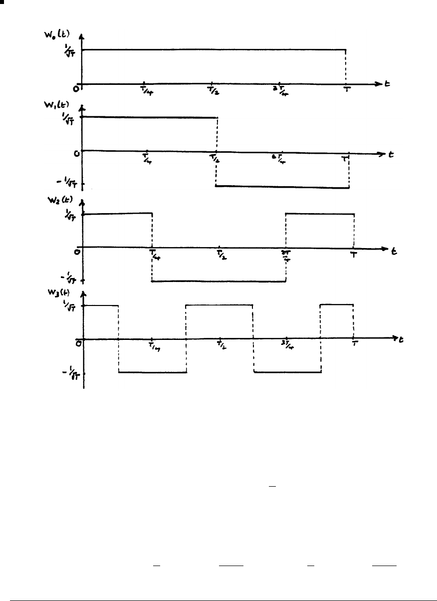
Glyn James, Advanced Modern Engineering Mathematics, 4th Edition 465
46(a)
To show that they are orthonormal on (0,T), evaluate the integral T
0Wn(t)
Wm(t)dt for the 10 combinations of nand m. For example,
T
0
W0(t)W0(t)dt =T
0
1
Tat =1
and it is readily seen that this extends to T
0W2
n(t)dt =1
T
0
W1(t)W2(t)dt =T/4
0
1
Tdt +T/2
T/4
(−1)
Tdt +3T/4
T/2
1
Tdt +T
3T/4
(−1)
Tdt =0
c
Pearson Education Limited 2011

466 Glyn James, Advanced Modern Engineering Mathematics, 4th Edition
46(b) f(t)=c0W0(t)+c1W1(t)+c2W2(t)+... where f(t) is the square wave
of Exercise 40. In this case T=2π. Multiplying throughout by the appropriate
Walsh function and integrating over (0,2π)gives
2π
0
W0(t)f(t)dt =c02π
0
W2
0(t)dt =c0,W
0(t)= 1
√2π
giving
c0=1
√2π2π
0
1f(t)dt =1
√2ππ
0
dt −2π
π
dt=0
2π
0
W1(t)f(t)dt =c12π
0
W2
1(t)dt =c1,W
1(t)=1
√2π,0<t<π
−1
√2π, π<t<2π
giving
c1=1
√2ππ
0
dt +2π
π
(−1)(−1)dt=√2π
2π
0
W2(t)f(t)dt =c2,W
2(t)=1
√2π,0<t<π
2,3
2π<t<2π
−1
√2π,π
2<t<3
2π
giving
c2=1
√2ππ/2
0
(1)(1)dt +π
π
2
(1)(−1)dt +3π
2
π
(−1)(−1)dt +2π
3π
2
(−1)(1)dt=0
Mean square error based on three terms is
1
2π2π
0
[f(t)]2dt −
3
n=0
c2
n=1
2π2π
0
dt −(√2π)2=0
This is zero in this case simply because the series based on three terms is exact as
W2(t) exactly ‘matches’ the given square wave f(t).
c
Pearson Education Limited 2011

Glyn James, Advanced Modern Engineering Mathematics, 4th Edition 467
Review Exercises 7.9
1
a0=1
ππ
0
t2dt =1
π1
3t3π
0
=π2
3
an=1
ππ
0
t2cos ntdt =1
πt2
nsin nt +2t
n2cos nt −2
n3sin ntπ
0
=2
n2cos nπ =2
bn=1
ππ
0
t2sin ntdt =1
π−t2
ncos nt +2t
n2sin nt +2
n3cos ntπ
0
=1
π2
n3[(−1)n−1] −π2
n(−1)n
=⎧
⎪
⎨
⎪
⎩
−π
n,neven
1
π−4
n3+π2
n,nodd
Thus, Fourier series expansion is
f(t)=π2
6+∞
n=1
2
n2(−1)ncos nt +∞
n=1 π
2n−1−4
π(2n−1)3sin(2n−1)t
−∞
n=1
π
2nsin 2nt
Taking t=πwhen the series converges to π2/2gives
π2
2=π2
6+∞
n=1
2
n2(−1)n(−1)n=∞
n=1
2
n2
that is,∞
n=1
1
n2=π2
6
c
Pearson Education Limited 2011
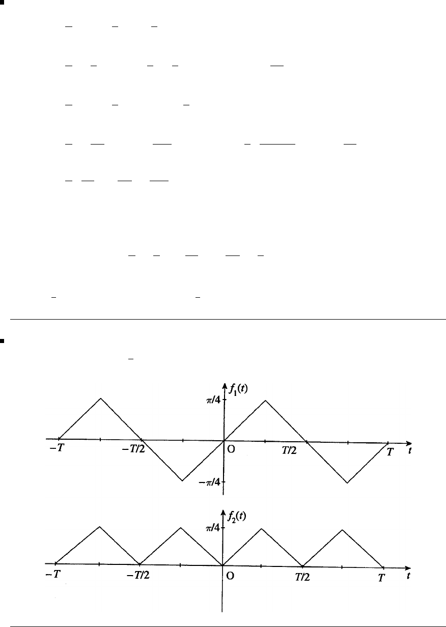
468 Glyn James, Advanced Modern Engineering Mathematics, 4th Edition
2
a0=2
ππ/3
0
2
3tdt +1
3π
π/3
(π−t)dt
=2
π1
3t2π/3
0
+1
3−1
2(π−t)2π
π/3=2π
9
an=2
ππ/3
0
2
3tcos ntdt +1
3π
π/3
(π−t)cosntdt
=2
π2t
3nsin nt +2
3n2cos ntπ/3
0
+1
3(π−t)
nsin nt −1
n2cos ntπ
π/3
=2
π1
n2cos nπ
3−1
3n2[2 + cos nπ]
Thus, the Fourier expansion of the even function is
f(t)=π
9+2
π
∞
n=1
1
n2cos nπ
3−1
3(2 + (−1)n)cos nt
At t=1
3πthe series converges to 2
9π.
3Sketches of odd function f1(t) and even function f2(t), having period Tand
equal to f(t),a≤t≤1
2T, are plotted for −T≤t≤Tbelow:
c
Pearson Education Limited 2011

Glyn James, Advanced Modern Engineering Mathematics, 4th Edition 469
3(a) Half-range Fourier sine series is
f(t)= ∞
n=1
bnsin 2nπt
T
with
bn=4
Tπ/4
0
tsin 2nπt
Tdt +π/2
π/41
2T−tsin 2nπt
Tdt
=4
T−Tt
2nπ cos 2nπt
T+T2
(2nπ)2sin 2nπt
Tt/4
0
+−T
2nπ 1
2T−tcos 2nπt
T−T2
(2nπ)2sin 2nπt
TT/2
T/4
=8T
(2nπ)2sin nπ
2=⎧
⎪
⎪
⎨
⎪
⎪
⎩
0,neven
2T
n2π2,n=1,5,9,...
−2T
n2π2,n=3,7,11,...
Thus, Fourier sine series expansion is
f(t)=2T
π2
∞
n=1
(−1)n+1
(2n−1)2sin 2(2n−1)πt
T
3(b) From the sketch of f1(t), the series converges to −T/4att=−1
4T.
3(c) Taking t=1
4T,thensin2(2n−1)
Tπt =(−1)n+1 giving
1
4T=2T
π2
∞
n=1
1
(2n−1)3
so that the sum of the series ∞
n=1
1
(2n−1)3is π2
8.
4g(−x)[c+f(−x)] = cg(−x)+g(−x)f(−x)
=−cg(x)−cg(x)f(x) from the given information
=−g(x)[c+f(x)]
c
Pearson Education Limited 2011
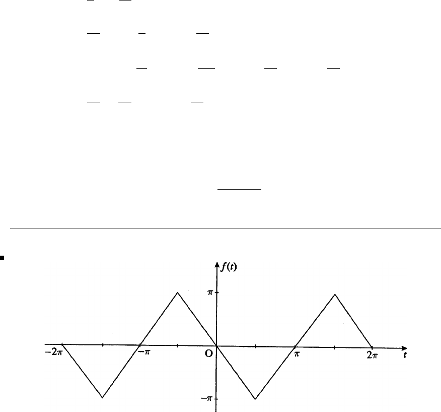
470 Glyn James, Advanced Modern Engineering Mathematics, 4th Edition
Thus, the product is an odd function.
Since y=θis an odd function and y=θ2is an even function, it follows from the
above that F(θ) is an odd function. Thus, it has a Fourier series of the form
F(θ)= ∞
n=1
bnsin nθ
with
bn=2
ππ
0
1
12 θ(π2−θ2)sinnθdθ
=1
6ππ2−θ
ncos nθ +1
n2sin nθ
π
0
−−θ3
ncos nθ +3θ2
n2sin nθ −6θ
n3cos nθ +6
n4sin nθ
π
0
=1
6π−6π
n3cos nπ=1
n3(−1)n+1
Thus, the Fourier expansion is
F(θ)= ∞
n=1
(−1)n+1
n3sin nθ
5
c
Pearson Education Limited 2011
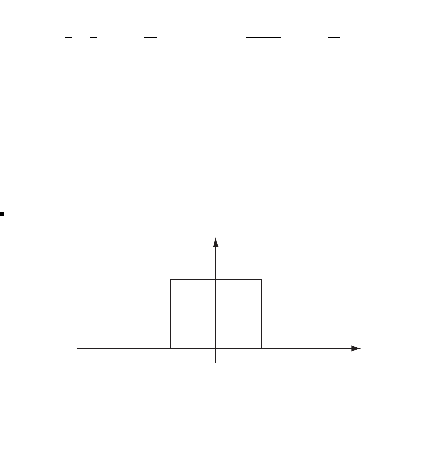
Glyn James, Advanced Modern Engineering Mathematics, 4th Edition 471
Clearly, f(t) is an odd function so it has a Fourier expansion of the form
f(t)= ∞
n=1
bnsin nt
with
bn=2
ππ/2
0−tsin ntdt +π
π/2
(t−π)sinntdt
=2
πt
ncos nt −1
n2sin ntπ/2
0
+−(t−π)
ncos nt +1
n2sin ntπ
π/2
=2
π−2
n2sin nπ
2
Thus, Fourier expansion is
f(t)= 4
π
∞
n=1
(−1)n
(2n−1)2sin(2n−1)t
6
f(x)
1/2ε
– 11
– εε
0
x
Since f(x) is an even function, over the interval −1≤x≤1, it may be represented
within this range by the Fourier cosine expansion
f(x)=a0
2+∞
n=1
ancos nπx
c
Pearson Education Limited 2011

472 Glyn James, Advanced Modern Engineering Mathematics, 4th Edition
with
a0=2
1
0
1
2dx =2
1
2x
0
=1
an=2
2
0
cos nπxdx =1
1
nπ sin nπx
0
=1
nπ sin nπ
Thus, Fourier expansion is
f(x)=1
2+∞
n=1
sin nπ
nπ cos nπx
valid in the interval −1≤x≤1.
7Half-range Fourier sine expansion is
f(t)= ∞
n=1
bnsin nt
with
bn=2
ππ
01−t
π
2
sin ntdt
=2
π−1
n1−t
π
2
cos nt −2
n2π1−t
πsin nt +2
n3π2cos ntπ
0
=2
nπ +4
n3π3[(−1)n−1]
Thus, Fourier expansion is
f(t)= ∞
n=1
2
nπ 1−2
n2π2[1 −(−1)n]sinnt
8Half-range Fourier sine expansion is
f(x)= ∞
n=1
bnsin nxdx
c
Pearson Education Limited 2011

Glyn James, Advanced Modern Engineering Mathematics, 4th Edition 473
with
bn=2
ππ/2
0
xsin nxdx +π
π/2
(π−x)sinnxdx
=2
π−x
ncos nx +1
n2sin nxπ/2
0
+−(π−x)
ncos nx −1
n2sin nxπ
π/2
=4
n2πsin nπ
2
Thus, half-range Fourier sine expansion is
f(x)= 4
π
∞
n=1
(−1)n+1
(2n−1)2sin(2n−1)x
Half-range Fourier cosine expansion is
f(x)=a0
2+∞
n=1
ancos nx
with
a0=2
ππ/2
0
xdx +π
π/2
(π−x)dx=π
2
an=2
ππ/2
0
xcos nxdx +π
π/2
(π−x)cosnxdx
=2
πx
nsin nx +1
n2cos nxπ/2
0
+π−x
nsin nx −1
n2cos nxπ
π/2
=2
π2
n2cos nπ
2−2
n2−2
n2cos nπ
=0,nodd
4
πn2(−1)n/2−1,neven
Thus, Fourier cosine expansion is
f(x)= π
4−2
π
∞
n=1
cos 2(2n−1)x
(2n−1)2
c
Pearson Education Limited 2011
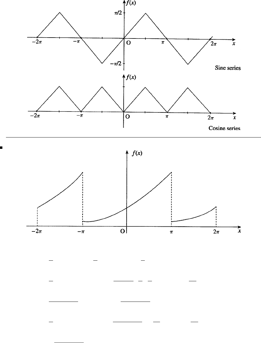
474 Glyn James, Advanced Modern Engineering Mathematics, 4th Edition
Sketches of the functions represented by the two Fourier series are
9
a0=1
ππ
−π
exdx =1
π[eπ−π−π]= 2
πsinh π
an=1
ππ
−π
excos nxdx =n2
n2+1·1
π1
nexsin nx +1
n2excos nxπ
−π
=(−1)n
π(n2+1)[eπ−e−π]= 2(−1)n
π(n2+1)sinh π
bn=1
ππ
−π
exsin nxdx =n2
π(n2+1)−ex
ncos nx +ex
n2sin nxπ
−π
=−n(−1)n
π(n2+1)sinh π
c
Pearson Education Limited 2011

Glyn James, Advanced Modern Engineering Mathematics, 4th Edition 475
Thus, Fourier expansion is
f(x)= 1
πsinh π+2
π
∞
n=1
(−1)n
n2+1sinh πcos nx −2
π
∞
n=1
(−1)n
n2+1sinh πcos nx
=2
π2sinh π1
2+∞
n=1
(−1)n
n2+1(cos nx −nsin x)
10(a) Half-range Fourier sine expansion is
f(t)= ∞
n=1
bnsin nt
with
bn=2
ππ
0
(π−t)sinntdt
=2
π−(π−t)
ncos nt −1
n2sin ntπ
0
=2
n
Thus, Fourier sine expansion is
f(t)= ∞
n=1
2
nsin nt
10(b) Half-range Fourier cosine expansion is
f(t)=a0
2+∞
n=1
ancos nt
with
a0=2
ππ
0
(π−t)dt =π
an=2
ππ
0
(π−t)cosntdt =2
π(π−t)
nsin nt −1
n2cos ntπ
0
=2
πn2[1 −(−1)n]=0,neven
4
πn2,nodd
c
Pearson Education Limited 2011
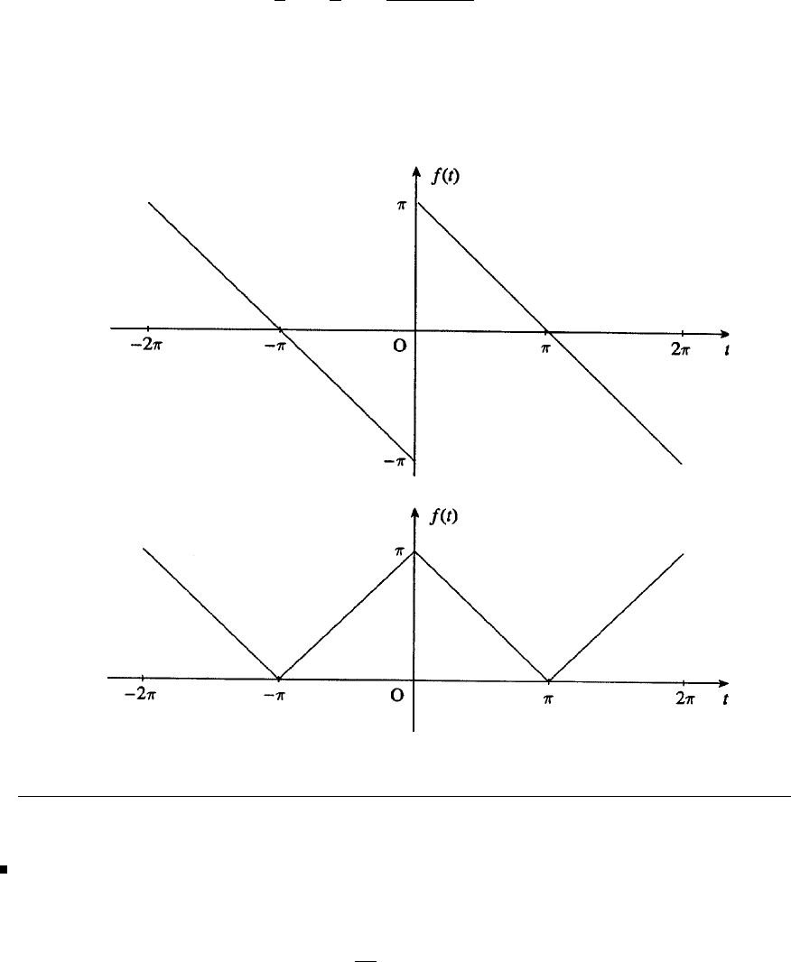
476 Glyn James, Advanced Modern Engineering Mathematics, 4th Edition
Thus, Fourier cosine expansion is
f(t)=1
2π+4
π
∞
n=1
1
(2n−1)2cos(2n−1)t
Graphs of the functions represented by the two series are
(a)
(b)
11 Since f(t) is an even function, it has a Fourier series expansion
f(t)=a0
2+∞
n=1
ancos nt
c
Pearson Education Limited 2011

Glyn James, Advanced Modern Engineering Mathematics, 4th Edition 477
where
a0=1
ππ
−π
f(t)dt =1
π0
−π−tdt +π
0
tdt=π
an=1
π0
−π−tcos ntdt +π
0
tcos ntdt
=1
π−t
nsin nt −cos nt
n2
0
−π+t
nsin nt +1
n2cos nt
π
0
=2
πn2(cos nπ −1) = 0,neven
−4
πn2,nodd
Thus, the Fourier expansion of f(t)is
f(t)=π
2−4
π
∞
n=1
1
(2n−1)2cos(2n−1)t
Since dx
dt +x=f(t) is linear, response is sum individual responses.
Steady-state response corresponds to the Particular Integral (PI). For f0(t)= π
2
steady-state response is x0(t)=π
2.
When f(t)=cosωt, then steady-state response is of the form x=Acos ωt +
Bsin ωt. Substituting back and comparing coefficients of sin ωt and cos ωt gives
A=1
1+ω2,B=ω
1+ω2
Taking ω=(2n−1), then required steady-state response is
x=1
2π−4
π
∞
n=1
1
(2n−1)2cos(2n−1)t+(2n−1) sin(2n−1)t
1+(2n−1)2
12 Since f(t) is an even function, Fourier series expansion is
f(t)=a0
2+∞
n=1
ancos nt
c
Pearson Education Limited 2011

478 Glyn James, Advanced Modern Engineering Mathematics, 4th Edition
where
a0=1
π2π
0
f(t)dt =1
ππ
0
t
πdt +2π
π
(2π−t)
πdt
=1
π21
2t2
π
0+2πt −1
2t2
2π
π=1
an=1
π2π
0
tcos ntdt +2π
π
(2π−t)cosntdt
=1
π2t
nsin nt +1
n2cos nt
π
0+(2π−t)
nsin nt −1
n2cos nt
2π
π
=2
π2n2(cos nπ −1) = −4
n2π2,nodd
0,neven
Thus, Fourier series expansion is
f(t)=1
2−4
π2
∞
n=0
cos(2n+1)t
(2n+1)
2
It can be shown by direct substitution that this satisfies the given differential
equation. Alternatively, we solve the differential equation
d2y
dt2+ω2y=1
2−∞
n=0
αncos ωnt, ω not integer
Solving the unforced system gives the complementary function as
y1=Acos ωt +Bsin ωt
The particular integral is the sum of the PI’s for the individual terms in f(t).
In the case of the 1
2on the RHS response is
y2=1
2ω2
For the term αncos ωntthe PI is of the form
yαn=Ccos ωnt+Dsin ωnt
c
Pearson Education Limited 2011

Glyn James, Advanced Modern Engineering Mathematics, 4th Edition 479
Substituting in d2y
dt2+ω2y=αncos ωntand comparing coefficients gives
C=αn/(ω2−ω2
n),D=0,sothat
yαn=αn
ω2−ω2
n
cos ωnt
Thus, the solution of the differential equation is
y=Acos ωt +Bsin ωt +1
2ω2−∞
n=0
αn
ω2−ω2
n
cos ωnt
From the given initial condition, y=dy/dt =0 at t=0,sothat
B=0andA=−1
2ω2+∞
n=0
αn
ω2−ω2
n
giving on taking αn=−4/[π2(2n+1)
2],ω
n=(2n+1)
y=1
2ω2(1 −cos ωt)−4
π2
∞
n=0
cos(2n+1)t−cos ωt
(2n+1)
2[ω2−(2n+1)
2]
13(a) Since f(t) is an even function, Fourier expansion is
f(t)=a0
2+∞
n=1
ancos nt
where
a0=1
ππ
−π
f(t)dt =1
π0
−π−tdt +π
0
tdt=π
an=1
π0
−π−tcos ntdt +π
0
tcos ntdt
=1
π−t
nsin nt −cos nt
n2
0
−π+t
nsin nt +cos nt
n2
π
0
=2
πn2(cos nπ −1) = 0,neven
−4
πn2,nodd
Thus, Fourier expansion f(t)is
f(t)=π
2−4
π
∞
n=1
1
(2n−1)2cos(2n−1)t
c
Pearson Education Limited 2011

480 Glyn James, Advanced Modern Engineering Mathematics, 4th Edition
Since bn= 0, Parseval’s theorem gives
1
2ππ
−π
[f(t)]2dt =1
4a2
0+1
2
∞
n=1
a2
n
i.e. π2
3=π2
4+1
2·16
π2
∞
n=1
1
(2n−1)4
or, rearranging, ∞
n=1
1
(2n−1)4=π4
96
13(b) Differentiating formally term by term, we obtain the Fourier expansion
of the square wave at
g(t)= 4
π
∞
n=1
1
(2n−1) sin(2n−1)t
Check.Sinceg(t) is an odd function it has Fourier expansion
g(t)= ∞
n=1
bnsin nt
where
bn=1
π0
−π−sin ntdt +π
0
sin ntdt
=1
π1
ncos nt
0
−π+−1
ncos nt
π
0
=2
nπ[1 −cos nπ]=4
nπ ,nodd
0,neven
confirming the Fourier expansion as
g(t)= 4
π
∞
n=1
1
(2n−1) sin(2n−1)t
14 Complex form of the Fourier series is
f(t)= ∞
n=−∞
cnejnt
c
Pearson Education Limited 2011

Glyn James, Advanced Modern Engineering Mathematics, 4th Edition 481
where
cn=1
2ππ
−π
sin t
2e−jntdt
=1
4πj π
−πe1
2jt −e−1
2jte−jntdt
=1
4πj π
−πe−j(n−1
2)t−e−j(n+1
2)tdt
=1
4πj e−j(n−1
2)t
−j(n−1
2)−e−j(n+1
2)t
−j(n+1
2)
π
−π
Using the results ejnπ =cosnπ +jsin nπ =(−1)n=e−jnπ
e1
2jπ =cosπ
2+jsin π
2=j, e−jπ
2=−j
gives
cn=1
4πj
(n−1
2)+j
(n+1
2)+j
(n−1
2)+j
(n+1
2)(−1)n
=j(−1)n
π4n
4n2−1
Thus, the complex form of the Fourier series is
f(t)= ∞
n=−∞
4nj(−1)n
π(4n2−1) ejnt
15(a) Following the same procedure as in Review Exercise 11 gives
a0=20
π
an=0,nodd, n=1
−20
π(n2−1) ,neven
a1=0
bn=0,n=1
b1=5
so that the Fourier representation is
v(t)=10
π+5sinω0t−20
π
∞
n=1
cos 2nω0t
4n2−1,ω
0=2π
T
c
Pearson Education Limited 2011
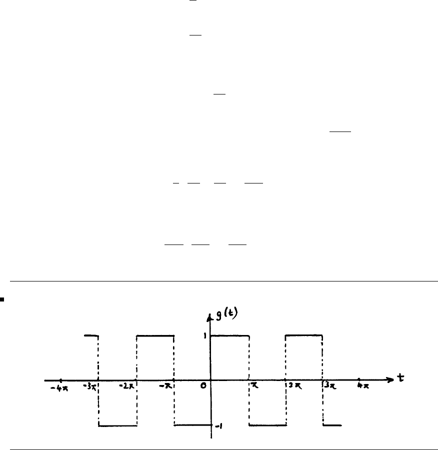
482 Glyn James, Advanced Modern Engineering Mathematics, 4th Edition
15(b)
Total power = 1
TT/2
0
100.sin2ω0tdt
=50
TT/2
0
(1 −cos 2ω0t)dt =25
Thus, total average power delivered to 10Ω resistor is
Pav =25
10 =2.5W
Coefficient second harmonic in series expansion v(t)isa2=−20
3π.
When applied to 10Ω resistor power associated with this harmonic is
1
220
3π
21
10 =20
9π2W
Thus, the percentage of the total power carried by the second harmonic is
100
Pav ·20
9π2=800
9π29.01
16(a) Asketchofg(t)is
16(b) Over the period −π<t<π g(t) is defined by
g(t)=−1,−π<t<0
g(t)=1,0<t<π
Since g(t) is an odd function, it has a Fourier series expansion of the form
g(t)= ∞
n=1
bnsin nt
c
Pearson Education Limited 2011

Glyn James, Advanced Modern Engineering Mathematics, 4th Edition 483
with bn=2
ππ
0
1.sin ntdt
=2
π−1
ncos nt
π
0=2
nπ [1 −(−1)n]=0,neven
4
nπ,nodd
Thus, the Fourier expansion of g(t)is
g(t)= 4
π
∞
n=1
sin(2n−1)t
(2n−1)
giving the Fourier expansion of f(t)=1+g(t)as
f(t)=1+4
π
∞
n=1
sin(2n−1)t
(2n−1)
17 Complex form of Fourier expansion is
f(t)= ∞
n=−∞
cnejnt
where cn=1
2π2π
0
f(t)e−jntdt =1
2π2π
0
te−jntdt
=1
2π−t
jne−jnt +1
n2e−jnt2π
0
Using the results e−j2nπ =cos2nπ −jsin 2nπ =1,e
o=1,wehave
cn=1
2π−2π
jn =−1
jn =j
n,n=0
When n=0,c
0=1
2π2π
0tdt =π
Hence, complex Fourier series is
f(t)=π+∞
n=−∞
n=0
j
nejnt
c
Pearson Education Limited 2011

484 Glyn James, Advanced Modern Engineering Mathematics, 4th Edition
18(a) Since v(t) is an odd function, its Fourier expansion is of the form
v(t)= ∞
n=1
bnsin 2nπt
T
with bn=4
TT/2
0
1.sin 2nπt
Tdt
=4
T−T
2nπ cos 2nπt
TT/2
0
=2
nπ [1 −cos nπ]
that is,b
n=0,neven
4
nπ ,nodd
Thus, Fourier expansion is
v(t)= 4
π
∞
n=1
1
(2n−1) sin 2(2n−1)πt
T
18(b) Response iω(t) of the circuit is given by
diω(t)
dt +iω(t)=vω(t)=sinωt
Taking Laplace transforms with iω(0) = 0 gives
Iω(s)= ω
(s+1)(s2+ω2)
=ω
ω2+1·1
(s+1)−ω
ω2+1·s
s2+ω2+1
ω2+1·2
s2+ω2
which, on taking inverse transforms, gives the response as
iω(t)= ω
ω2+1e−t−ω
ω2+1cos ωt +1
ω2+1sin ωt
Since the first term decays to zero, the steady-state response is
iωss =1
ω2+1(sin ωt −ωcos ωt)
c
Pearson Education Limited 2011

Glyn James, Advanced Modern Engineering Mathematics, 4th Edition 485
As the system is linear steady-state response is(t) to the square wave v(t)is
is(t)= ∞
n=1
iωn(t)
where iωn(t) is the steady-state response to vωn(t)with
ωn=2(2n−1)π/T
Thus,
is(t)= 4
π
∞
n=1
1
(2n−1) 1
ω2
n+1(sin ωnt−ωncos ωnt)
19(a)
cosnθ=1
2(ejθ +e−jθ)
n
=1
2nenjθ +n
1e(n−2)jθ +...+e−njθ
=1
2n(enjθ +e−njθ )+n
1(e(n−2)jθ +e−(n−2)jθ)+...
Hence,
cos2κθ=1
22κ2cos2κθ +2κ
12cos(2κ−2)θ+...+2κ
κ−12cos2θ+2κ
κ
Putting cos θ=t,
t2κ=1
2κ−1T2κ(t)+2κ
1T2κ−2(t)+...+2κ
κ−1T2(t)+1
22κ
κT0(t)
t2κ−1=1
2κT2κ+1(t)+2κ+1
1T2κ−1(t)+...+2κ+1
κT1(t)
Note that T0(t) may be omitted.
c
Pearson Education Limited 2011

486 Glyn James, Advanced Modern Engineering Mathematics, 4th Edition
19(b) cos nθ +cos(n−2)θ=2cos(n−1)θcos θHence, putting θ=cos
−1t
Tn(t)+Tn−2(t)=2tTn−1(t)
19(c)
T0(t)=cos(0.cos−1t)=cos0=1
T1(t)=cos(1.cos−1t) = cos(cos−1t)=t
T2(t)=2tT1(t)−T0(t)=2t2−1
T3(t)=2t(2t2−1) −t=4t3−3t
19(d)
t5−5t4+7t3+6t−8= 1
24(T5(t)+5T3(t)+10T1(t))
−5
23(T4(t)+4T2(t)+3)+ 7
22(T3(t)+3T1(t))
+6T1(t)−8
=1
16 T5(t)−5
8T4(t)+33
16 T3(t)
−5
2T2(t)+95
8T1(t)−79
8T0(t)
19(e) The required cubic polynomial is obtained by omitting the first two terms.
It is therefore,
33
16 (4t3−3t)−5
2(2t2−1) + 95
8t−79
8
or 33
4t3−5t2+91
16 t−59
8
Since |Tn(t)|≤ 1over(−1,1), the error can nowhere exceed 1
16 +5
8=11
16 in
absolute value. An error of this magnitude occurs at t=−1, since Tn(−1) =
cos nπ =(−1)n.
c
Pearson Education Limited 2011
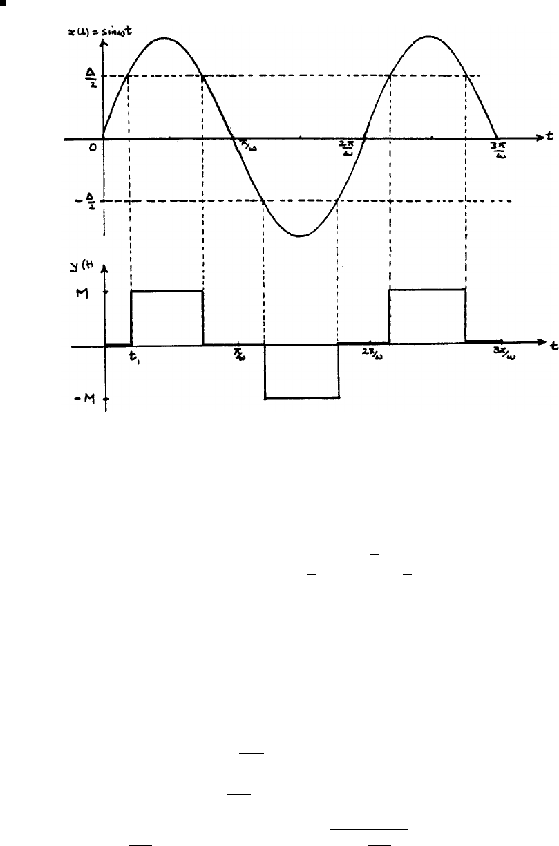
Glyn James, Advanced Modern Engineering Mathematics, 4th Edition 487
20
If the input is x(t)=Xisin ωt, then the input and output y(t) waveforms to the
non-linear element are shown in the figure. Clearly, the output waveform is an odd
function of period π/ω and over the interval 0 <t<π/ω,
y(t)=⎧
⎨
⎩
0,0<t<t
1
M, t1<t< π
ω−t1
0,π
ω−t1<t< π
ω
The amplitude of the fundamental harmonic is
b1=2
π/ω π/ω
0
y(t)sinωtdt
=2ω
ππ/ω−t1
t1
Msin ωtdt
=−2M
π[cos(π−ωt1)−cos ωt1]
=4M
πcos ωt1
Since sin ωt1=Δ
2Xi, we obtain cos ωt1=1−Δ
2Xi2
c
Pearson Education Limited 2011

488 Glyn James, Advanced Modern Engineering Mathematics, 4th Edition
Thus, the required describing function is
N(Xi)= 4M
πXi1−Δ
2Xi
2
1
2
Limit cycle will occur if N(Xi)≥− 1
KG(jω).
N(Xi) will have a maximum value when dN
dXi=0;thatis,whenXi=Δ/√2.
Maximum value is N(Xi)max =4M
πΔ. Since this is real, we are only interested in
the real values of 1/(KG(jω)).
In this case, 1
KG(jω)=1
Kjω(T1jω +1)(T2jω +1)
=1
K[−T1T2jω3−(T1+T2)ω2+jω]
and for this to be real
−T1T2ω3+ω=0 giving ω2=1/(T1T2)
At this frequency,
magnitude 1
KG(jω)=−T1+T2
Kω2=−(T1+T2)
KT1T2
and the required result follows, namely that limit cycles will not occur if
Δ>4MK
π·T1T2
T1+T2
c
Pearson Education Limited 2011

8
The Fourier Transform
Exercises 8.2.4
1F(jω)=0
−∞
eate−jωt dt+∞
0
e−ate−jωt dt
=2a
a2+ω2
2
F(jω)=0
−T
Ae−jωt dt+T
0−Ae−jωt dt
=T
0
2jA sin ωt dt
=2jA
ω(1 −cos ωT)
=4jA
ωsin2ωT
2
=jωAT2sinc2ωT
2
3
F(jω)=0
−TAt
T+Ae−jωt dt+T
0−At
T+Ae−jωt dt
=2T
0−At
T+Acos ωt dt
=AT sinc2ωT
2
Exercise 2 is T×derivative of Exercise 3, so result 2 follows as (jω ×T)
×result 3.
Sketch is readily drawn.
c
Pearson Education Limited 2011

490 Glyn James, Advanced Modern Engineering Mathematics, 4th Edition
4
F(jω)=2
−2
2Ke−jωt dt=8Ksinc(2ω)
G(jω)=1
−1
Ke−jωt dt=2Ksinc(ω)
H(jω)=F(jω)−G(jω)=2K(4 sinc(2ω)−sinc(ω))
5
F(jω)=−1
−2
e−jωt dt+1
−1
e−jωt dt+2
1−e−jωt dt
=1
jω2(ejω −e−jω)−(e2jω −e−2jω)
=4sinc(ω)−2sinc(2ω)
6
F(jω)= 1
2jπ
a
−π
a
(ejat −e−jat)e−jωt dt
¯
f(a)= 1
2jπ
a
−π
a
ejate−jωt dt=1
2jπ
a
−π
a
ej(a−ω)tdt
=sin ωπ
a
j(a−ω)
F(jω)=¯
f(a)+¯
f(−a)= 2jω
ω2−a2sin ωπ
a
7
F(jω)=∞
0
e−at.sin ω0t.e−jωt dt
=¯
f(ω0)−¯
f(−ω0)
where ¯
f(ω0)= 1
2j∞
0
e(−a+j(ω0−ω)t)dt
=1
2j1
a−j(ω0−ω)=1
2j1
(a+jω)−jω0
∴F(jω)= ω0
(a+jω)2+ω2
0
c
Pearson Education Limited 2011

Glyn James, Advanced Modern Engineering Mathematics, 4th Edition 491
8
Fc(x)=1
4a
0
(ejt +e−jt)(ejxt +e−jxt)dt
define g(x, b)=a
0
ej(b+x)tdt
=1
j(b+x)[ej(b+x)a−1]
Fc(x)=1
4[g(x, 1) + g(x, −1) + g(−x, 1) + g(−x, −1)]
=1
2sin(1 + x)a
1+x+sin(1 −x)a
1−x
9Consider F(x)=a
01.ejxt dt
=−j
x(cos ax +jsin ax −1)
Fc(x)=ReF(x)= sin ax
x
Fs(x)=ImF(x)=1−cos ax
x
10 Consider F(x)=∞
0e−atejxt dt
=a+jx
a2+x2
Fc(x)=ReF(x)= a
a2+x2
Fs(x)=ImF(x)= x
a2+x2
Exercises 8.3.6
11 Obvious
12 (jω)2Y(jω)+3jωY(jω)+Y(jω)=U(jω)
Y(jω)= 1
(1 −ω2)+3jω U(jω)
H(jω)= 1
(1 −ω2)+3jω
c
Pearson Education Limited 2011
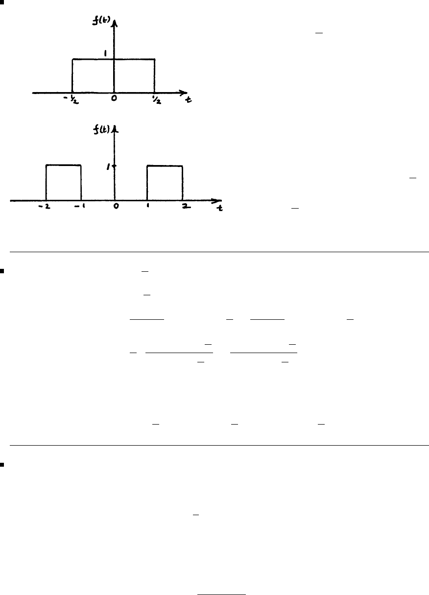
492 Glyn James, Advanced Modern Engineering Mathematics, 4th Edition
13
→sinc ω
2
→e−iω3/2+eiω3/2sinc ω
2
=2
ω(sin(2ω)−sin(ω))
=4sinc(2ω)−2sinc(ω)
14
F(jω)=T
2
−T
2
cos(ω0t)e−iωt dt
=1
ω0−ωsin(ω0−ω)T
2+1
ω0+ωsin(ω0+ω)T
2ω=±ω0
=T
2sin(ω0−ω)T
2
(ω0−ω)T
2
+sin(ω0+ω)T
2
(ω0+ω)T
2
Evaluating at ω=±ω0⇒
F(jω)=T
2sinc(ω0−ω)T
2+sinc(ω0+ω)T
2
15
F(jω)=T
0
cos ω0t.e−jωt dt
=1
2[¯
f(ω0)+¯
f(−ω0)]
where ¯
f(ω0)=T
0
ej(ω0−ω)tdt
=1
j(ω0−ω)[ej(ω0−ω)T−1] ω=ω0
c
Pearson Education Limited 2011

Glyn James, Advanced Modern Engineering Mathematics, 4th Edition 493
F(jω)=1
21
j(ω0−ω)(ej(ω0−ω)T−1) ω=ω0
−1
j(ω0−ω)(e−j(ω0+ω)T−1)
=e−jωT/2ejω0T/2
ω0−ωsin(ω0−ω)T
2
+e−jω0T/2
ω0+ωsin(ω0+ω)T
2ω=±ω0
Checking at ω=±ω0gives
F(jω)=T
2e−jωT/2ejω0T/2sinc(ω0−ω)T
2+e−jω0T/2sinc(ω0+ω)T
2
16
F(jω)=1
−1
sin 2t.e−jωt dt
=1
2j1
−1
e−j(ω−2)t−e−j(ω+2)tdt
¯
f(a)=1
−1
e−j(ω−a)tdt=2sinc(ω−a)
F(jω)= 1
2j¯
f(a)−1
2j¯
f(−a),a=2
=j[sinc(ω+2)−sinc(ω−2)]
Exercises 8.4.3
17
IH(s)= 1
s2+3s+2 h(t)=(e−t−e−2t)ξ(t)
H(jω)=∞
0
(e−t−e−2t)e−jωt dt=1
1+jω −1
2+jω
=1
2−ω2+3jω as required.
II H(s)= s+2
s2+s+1 h(t)=e−1/2tcos √3
2t+√3sin √3
2tξ(t)
c
Pearson Education Limited 2011
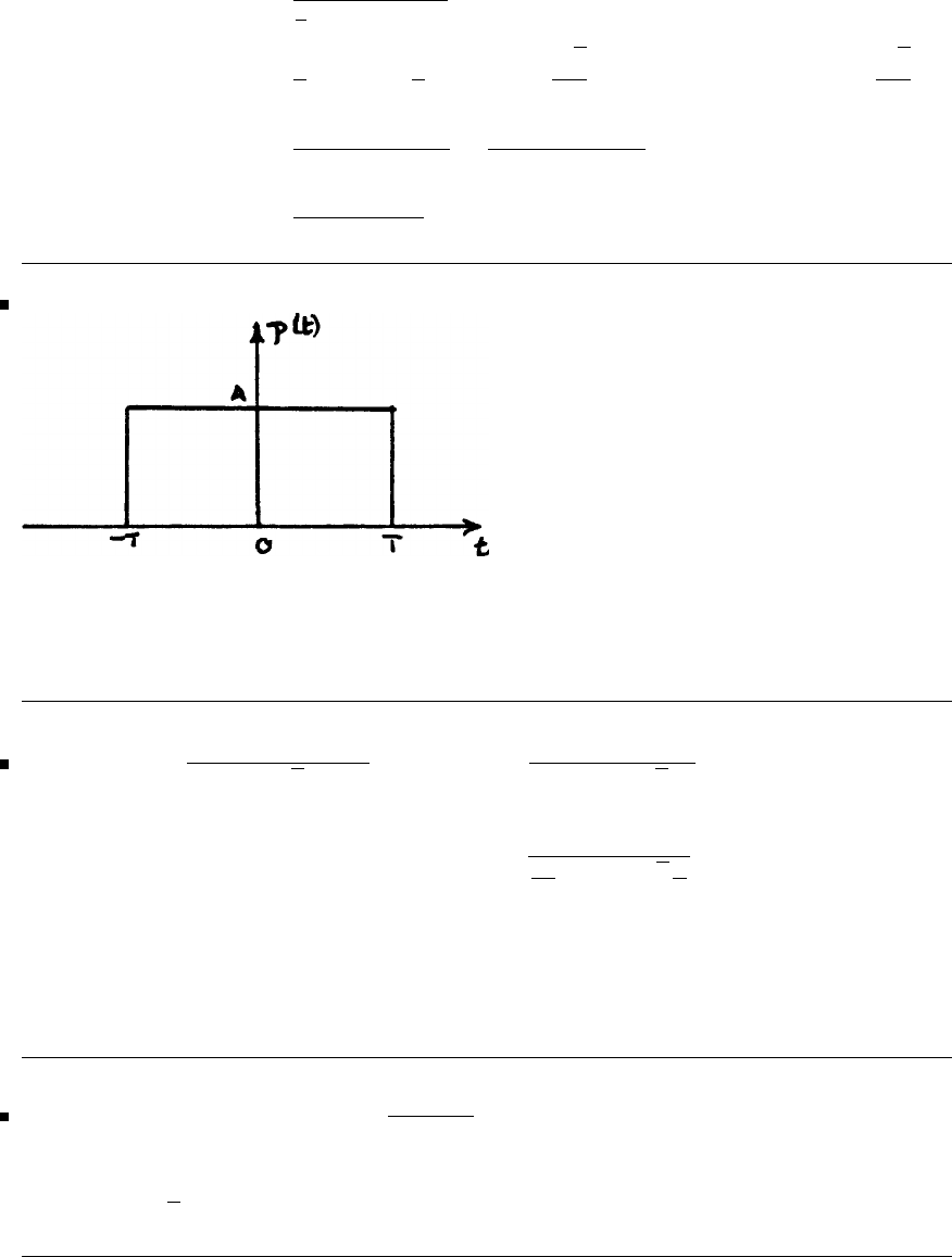
494 Glyn James, Advanced Modern Engineering Mathematics, 4th Edition
Consider G(ω0)=∞
0
e−(1/2tjω−jω0)tdt
=1
1
2+j(ω−ω0)
H(jω)=1
2G(ω0)+1
2G(−ω0)+√3
2j(G(ω0)−G(−ω0)),ω
0=√3
2
So H(jω)= 2+4jω
4+4jω −4ω2+6
4+4jω −4ω2
=2+jω
1−ω2+jω
18
P(jω)=2ATsinc ωT
So F(jω)=(e−jωτ +eiωτ )P(jω)
=4AT cos ωτ sinc ωT
19 G(s)= (s)2
(s)2+√2s+1 G(jω)= −ω2
1−ω2+√2jω
=1
1
ω2−1+√2j
ω
Thus, |G(jω)|→ 0asω→0
and |G(jω)|→ 1asω→∞
High-pass filter.
20 g(t)=e−a|t|−→ G(jω)= 2a
a2+ω2
f(jt)=1
2G(jt)−→ πg(−ω)=πe−a|ω|
c
Pearson Education Limited 2011

Glyn James, Advanced Modern Engineering Mathematics, 4th Edition 495
21 F{f(t)cosω0t}=1
2F(j(ω−ω0)) + 1
2F(j(ω+ω0))
F(jω)=2Tsinc ωT
∴F{PT(t)cosω0t}
=Tsinc(ω−ω0)T+sinc(ω+ω0)T
Exercises 8.5.3
22 1
2π∞
−∞
πδ(ω−ω0)ejωtdω +1
2π∞
−∞
πδ(ω+ω0)ejωtdω
=1
2(ejω0t+e−jω0t)
=cosω0t
23 F{e±jω0t}=2πδ(ω∓ω0)
∴F{sin ω0t}=1
2j{2πδ(ω−ω0)−2πδ(ω+ω0)}
=jπ[δ(ω+ω0)−δ(ω−ω0)]
1
2π∞
−∞
jπ[δ(ω+ω0)−δ(ω−ω0)]ejωtdω
=j
2[e−jω0t−e+jω0t]=sinω0t
24 G(jω)= ∞
−∞
g(t)e−jωt dt;G(jt)=∞
−∞ g(ω)e−jωtdω
So ∞
−∞
f(t)G(jt)dt
=∞
−∞
f(t)∞
−∞
g(ω)e−jωtdωdt
=∞
−∞
g(ω)∞
−∞
f(t)e−jωt dtdω
=∞
−∞
g(ω)F(jω)dω =∞
−∞
g(t)F(jt)dt
c
Pearson Education Limited 2011

496 Glyn James, Advanced Modern Engineering Mathematics, 4th Edition
25 Write result 24 as
∞
−∞
f(ω)F{g(t)}dω =∞
−∞ F{f(t)}g(ω)dω
so ∞
−∞
f(ω)F{G(jt)}dω =∞
−∞ F{f(t)}G(jω)dω
Now
g(t)→G(jω)
G(jt)→2πg(−ω)
G(−jt)→2πg(ω)⎫
⎬
⎭
symmetry
Thus,∞
−∞
f(ω).2πg(ω)dω =∞
−∞
F(jω)G(−jω)dω
or ∞
−∞
f(t)g(t)dt=1
2π∞
−∞
F(jω)G(−jω)dω
26 F{H(t)sinω0t}
=1
2π∞
−∞
πjδ(ω−u+ω0)−δ(ω−u−ω0)πδ(u)+ 1
judu
=j
2πδ(ω+ω0)−πδ(ω−ω0)+1
21
ω+ω0−1
ω−ω0
=πj
2δ(ω+ω0)−δ(ω−ω0)−ω0
ω2−ω2
0
27
an=A
Td/2
−d/2
e−nω0tdt =Ad
Tsinc nω0d
2,ω
0=2π/T
f(t)=Ad
T
∞
n=−∞
sinc nω0d
2enω0t,
F(ω)= 2πAd
T
∞
n=−∞
sinc nω0d
2δ(ω−nω0)
Exercises 8.6.6
28
T=1,N=4,Δω=2π/(4 ×1) = π
2
c
Pearson Education Limited 2011

Glyn James, Advanced Modern Engineering Mathematics, 4th Edition 497
G0=
3
n=0
gne−×n×0×π/2=2
G1=
3
n=0
gne−×n×1×π/2=0
G2=
3
n=0
gne−×n×2×π/2=2
G3=
3
n=0
gne−×n×3×π/2=0
G={2,0,2,0}
29
N=4,W
n=e−nπ/2
g
n=⎡
⎢
⎣
1010
0101
10−10
01 0−1
⎤
⎥
⎦⎡
⎢
⎣
1
0
1
0
⎤
⎥
⎦=⎡
⎢
⎣
2
0
0
0
⎤
⎥
⎦
G=⎡
⎢
⎣
G00
G10
G01
G11
⎤
⎥
⎦=⎡
⎢
⎣
1100
1−10 0
101−
001
⎤
⎥
⎦⎡
⎢
⎣
2
0
0
0
⎤
⎥
⎦=⎡
⎢
⎣
2
2
0
0
⎤
⎥
⎦
Bit reversal gives
G=⎡
⎢
⎣
2
0
2
0
⎤
⎥
⎦
30 Computer experiment.
31 Follows by direct substitution.
c
Pearson Education Limited 2011

498 Glyn James, Advanced Modern Engineering Mathematics, 4th Edition
Exercises 8.9.3
32 We have θc=π
2so
D(ejθ)=1,|θ|≤π
2
0,|θ|>π
2
The filter coefficients are given by
hd(n)= 1
2ππ
−π
D(ejθ)ejnθ dθ
=1
2ππ
2
−π
2
ejnθ dθ
=1
nπ sin nπ
2,n=0
=1
2sinc nπ
2
Hence,
h±5=0.06366,h
±4=0,h
±3=−0.10610
h±2=0,h
±1=0.31831,h
0=0.5
Thus, the non-causal transfer function is
˜
D(z)=0.06366z−5−0.1066z−3+0.31832z−1+0.5
+0.31831z−0.10610z3+0.06366z5
and the causal version is
D(z)=0.06366 −0.10660z−2+0.31831z−4+0.5z−5
+0.31831z−6−0.010660z−8+0.06366z−10
33 The Hamming window coefficients are given by
wH(k)=0.54 + 0.46 cos πk
5,|k|≤5
Note that wH(±4)andwH(±2)are not needed.
Now wH(±5) = 0.08000,w
H(±3) = 0.39785,w
H(±1) = 0.91215,w
H(0) = 1 and
the causal transfer function is found by multiplying the filter coefficients by the
appropriate wHgiving
D(z)=0.00509(1 + z−10)−0.04221(z−2+z−8)+0.29035(z−4+z−6)+0.5z−5
c
Pearson Education Limited 2011
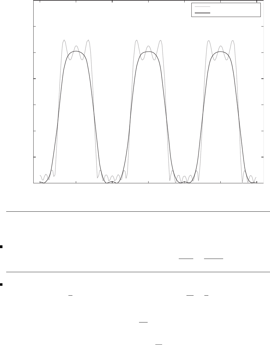
Glyn James, Advanced Modern Engineering Mathematics, 4th Edition 499
Plots of the frequency responses for both Exercises 32 and 33 are given in the
following figure.
1.4
1.2
1
0.8
0.6
0.4
0.2
0
Rectangular Window
Hamming Window
Frequency response
−3pi −2pi 2pi 3pi−pi pi0
q in radians
Review exercises 8.10
1
FS(x)=1
0
tsin xt dt+2
1
sin xt dt=sin x
x2−cos 2x
x
2
f(t)=−π
2H(−t−2) + (H(t+2)−H(t−2)) πt
4+π
2H(t−2)
F{H(t)}=1
ω +πδ(ω)
F{H(t−2)}=e−2jω1
jω+πδ(ω)
c
Pearson Education Limited 2011

500 Glyn James, Advanced Modern Engineering Mathematics, 4th Edition
F{H(−t−2)}=e2jω−1
jω+πδ(−ω)=e2jω−1
jω+πδ(ω)
F{f(t)}=F{−π
2H(−t−2)}+π
42
−2
te−jωt dt+Fπ
2H(t−2)
=−πj
ωsinc 2ω
3
F{H(t+T/2) −H(t−T/2)}=Tsinc ωT
2
F{cos ω0t}=π[δ(ω+ω0)+δ(ω−ω0)]
Using convolution,
F{f(t)}=π
2π∞
−∞
Tsinc T
2(ω−u)(δ(u+ω0)+δ(u−ω0))du
=T
2sinc(ω−ω0)T
2+sinc(ω+ω0)T
2
4
F{cos ω0tH(t)}=1
2π[πδ(ω−ω0)+πδ(ω+ω0)] ∗πδ(ω)+ 1
jω
=1
2π∞
−∞ {πδ(ω−u−ω0)+πδ(ω−u+ω0)}πδ(u)+ 1
judu
=π
2[δ(ω−ω0)+δ(ω+ω0)] + jω
ω2
0−ω2
5
F{f(t)cosωctcos ωct}
=F(jω+jωc)+F(jω−jωc)
2∗π[δ(ω−ωc)+δ(ω+ωc)]
=1
4∞
−∞
[F(j(u+ωc)) + F(j(u−ωc))] ×
[δ(ω−u−ωc)+δ(ω−u+ωc)] du
=1
2F(jω)+1
4[F(jω+2jωc)+F(jω−2jωc)]
c
Pearson Education Limited 2011

Glyn James, Advanced Modern Engineering Mathematics, 4th Edition 501
Or write as
f(t)1
2(1 + cos 2ωct)
etc.
6
H(t+1)−H(t−1) ↔2sincω
By symmetry,
2sinct↔2π(H(−ω+1)−H(−ω−1)) = 2π(H(ω+1)−H(ω−1))
7(a) Simple poles at s=aand s=b. Residue at s=ais eat/(a−b), at s=b
it is ebt/(b−a), thus
f(t)= 1
a−beat −ebtH(t)
7(b) Double pole at s= 2, residue is
lim
s→2
d
ds(s−2)2est
(s−2)2=te2t
So f(t)=te2tH(t)
7(c) Simple pole at s= 1, residue e−t, double pole at s= 0, residue
lim
s→0
d
dsest
s+1=(t−1)H(t)
Thus, f(t)=(t−1+e−t)H(t)
8(a)
y(t)=∞
−∞
h(t−τ)u(τ)dτ
Thus,
−sin ω0t=∞
−∞
h(t−τ)cosω0τdτ =f(t),say
c
Pearson Education Limited 2011

502 Glyn James, Advanced Modern Engineering Mathematics, 4th Edition
If u(τ)=cosω0(τ+π/4)
y(t)=∞
−∞
h(t−τ)cosω0(τ+π/4) dτ
=∞
−∞
h(t−(τ−π/4)) cos ω0τdτ=f(t+π/4)
=−sin ω0(t+π/4)
8(b) Since sin ω0t=cosω0(t−π/2ω0)
y(t)=∞
−∞
h(t−τ)sinω0tdτ
=∞
−∞
h(t−τ)cosω0(τ−π/2ω0)dτ
=∞
−∞
h(t−(τ+π/2ω0)) cos ω0τdτ
=f(t−π/2ω0)=−sin(ω0t−π/2) = cos ω0t
8(c)
ejω0t=cosω0t+jsinω0t
This is transformed from above to
−sin ω0t+jcosω0t=jejω0t
8(d) Proceed as above using
e−jω0t=cosω0t−jsinω0t
9
F(sgn(t)) = F(f(t)) = F(jω)= 2
jω,obvious
Symmetry,
F(jt)= 2
jt↔2/πf(−ω)=2πsgn(−ω)
That is, 1
jt↔−πsgn(ω)
c
Pearson Education Limited 2011

Glyn James, Advanced Modern Engineering Mathematics, 4th Edition 503
or
−1
πt↔jsgn(ω)
10
g(t)=−1
πt ∗f(t)=−1
π∞
−∞
f(τ)
t−τdτ=1
π∞
−∞
f(τ)
τ−tdτ=FHi(t)
so
g(x)= 1
π∞
−∞
f(t)
t−xdt=FHi(x)
So from Review Exercise 9
FHi(jω)=jsgn(ω)×F(jω)
so
|FHi(jω)|=|jsgn(ω)||F(jω)|=|F(jω)|
and
arg(FHi(jω)) = arg(F(jω)) + π/2,ω≥0
Similarly
arg(FHi(jω)) = arg(F(jω)) −π/2, ω<0
11 First part, elementary algebra.
FHi(x)= 1
π∞
−∞
t
(t2+a2)(t−x)dt
=1
π
1
x2+a2∞
−∞ a2
t2+a2+t
t−x−xt
t2+a2dt
=a
x2+a2
12(a)
H{f(t)}=1
π∞
−∞
f(t)
t−xdt=FHi(x)
H{f(a+t)}=1
π∞
−∞
f(a+t)
t−xdt
=1
π∞
−∞
f(t)
t−(a+x)dt=FHi(a+x)
c
Pearson Education Limited 2011

504 Glyn James, Advanced Modern Engineering Mathematics, 4th Edition
12(b)
H{f(at)}=1
π∞
−∞
f(at)
t−xdt
=1
π∞
−∞
f(t)
t−ax dt=FHi(ax),a>0
12(c)
H{f(−at)}=1
π∞
−∞
f(−at)
t−xdt
=−1
π∞
−∞
f(t)
t+ax dt=−FHi(−ax),a>0
12(d)
Hdf
dt=1
π∞
−∞
f(t)
t−xdt
=1
πf(t)
t−x
∞
−∞
+∞
−∞
f(t)
(t−x)2dt
Provided lim
|t|→∞ f(t)/t =0,then
Hdf
dt=1
π∞
−∞
f(t)
(t−x)2dt=1
π
d
dx∞
−∞
f(t)
t−xdt
=d
dxFHi(x)
12(e)
x
π∞
−∞
f(t)
t−xdt+1
π∞
−∞
f(t)dt=1
π∞
−∞
tf(t)
t−xdt
=H{tf(t)}
13 From Review Exercise 10
FHi(t)=−1
πt ∗f(t)
So from Review Exercise 9,
F{FHi(t)}=jsgn(ω)×F(ω)
c
Pearson Education Limited 2011

Glyn James, Advanced Modern Engineering Mathematics, 4th Edition 505
so
F(jω)=−jsgn (ω)×F{FHi(t)}
Thus,
f(t)=∞
−∞
1
π(t−τ)FHi(τ)dτ=−1
π∞
−∞
1
(x−τ)FHi(x)dx
14
fa(t)=f(t)−jFHi(t)
F{fa(t)}=F(jω)−j(jsgn (ω))F(jω)=F(jω)+sgn(ω)F(jω)
=2F(jω),ω>0
0,ω<0
15
F{H(t)}=1
jω+πδ(ω)=F(jw)
Symmetry,
F(t)= 1
jt+πδ(t)↔2πH(−ω)=2π[1 −H(ω)]
=2π[Fδ(t)−H(ω)]
or
H(ω)↔j
2πt +1
2δ(t)
Thus,
F−1{H(ω)}=j
2πt +1
2δ(t)
Then
ˆ
f(t)=21
2δ(t)+ j
2πt ∗f(t)=f(t)−j−1
πt∗f(t)
=f(t)−jFHi(t)
When f(t)=cosω0t, ω0>0, then
F(jω)=π[δ(ω−ω0)+δ(ω+ω0)]
so
F{ˆ
f(t)}=2πδ(ω−ω0)
c
Pearson Education Limited 2011

506 Glyn James, Advanced Modern Engineering Mathematics, 4th Edition
whence
ˆ
f(t)=f(t)−jFHi(t)=ejω0t=cosω0t+jsinω0t
and so
FHi(t)=−sin ω0t
When g(t)=sinω0t, ω0>0
G(jω)=jπ[δ(ω+ω0)−δ(ω−ω0)]
and thus
ˆ
g(t)=−jejω0t=−j(cos ω0t+jsinω0t)
so
H{sin ω0t}=cosω0t
16 If ¯
h(t)=0,t<0, then when t<0
¯
he(t)=1
2¯
h(−t),and ¯
ho(t)=−1
2¯
h(−t)
that is,¯
ho(t)=−¯
he(t)
When t>0, then
¯
he(t)=1
2¯
h(t),and ¯
ho(t)=1
2¯
h(t)
that is,¯
ho(t)=¯
he(t)
That is,
¯
ho(t)=sgn(t)¯
he(t)∀t
Thus,
¯
h(t)=¯
he(t)+sgn(t)¯
he(t)
When h(t)=sintH(t),
¯
he(t)=⎧
⎪
⎨
⎪
⎩
1
2sin t, t > 0
−1
2sin t, t < 0
and since
sgn (t)¯
he(t)=1
2sin t∀t
the result is confirmed.
c
Pearson Education Limited 2011

Glyn James, Advanced Modern Engineering Mathematics, 4th Edition 507
Then taking the FT of the result,
¯
H(jω)= ¯
He(jω)+F#sgn (t)¯
he(t)$
=¯
He(jω)+ 1
2π2
jω∗¯
He(jω)
=¯
He(jω)+jH#¯
He(jω)$
When
¯
H(jω)=∞
−∞
e−ate−jwt dt=a
a2+ω2−ω
a2+ω2
then
Ha
a2+ω2=−ω
a2+ω2
or
Ha
a2+t2=−x
a2+x2
Finally,
Hat
a2+t2=−xx
a2+x2+1
π∞
−∞
a
a2+t2dt=a2
a2+x2
So
Ht
a2+t2=a
a2+x2
17(a)
FH(s)=∞
0
e−at(cos 2πst +sin2πst)dt=a+2πs
a2+4π2s2
17(b)
FH(s)=T
−T
(cos 2πst +sin2πst)dt=1
πs sin 2πst
18
E(s)=∞
−∞
f(t)cos2πst dtO(s)=∞
−∞
f(t)sin2πst dt
E(s)−O(s)=∞
−∞
f(t)e−j2πst dt=F(js)
c
Pearson Education Limited 2011

508 Glyn James, Advanced Modern Engineering Mathematics, 4th Edition
From Review Exercise 17(a)
FH(s)= 1+πs
2+2π2s2
whence
E(s)= 1
2+2π2s2,O(s)= πs
2+2π2s2
so
F(s)= 1−jπs
2+2π2s2
agreeing with the direct calculation,
F(js)=∞
0
e−2te−j2πst dt=1−jπs
2+2π2s2
19
H{f(t−T)}=∞
−∞
f(t−T)cas2πst dt
=∞
−∞
f(τ)[cos2πsτ(cos 2πsT +sin2πsT)+
sin 2πsτ(cos 2πsT −sin 2πsT)] dt
=cos2πsTFH(s)+sin2πsTFH(−s)
20 The Hartley transform follows at once since
FH(s)={F(js)}−{F(js)}=1
2δ(s)+ 1
sπ
From time shifting,
FH(s)=sinπs 1
2δ(−s)−1
sπ+cosπs 1
2δ(s)+ 1
sπ
=1
2δ(s)+cos πs −sin πs
πs
21
H{δ(t)}=∞
−∞
δ(t)cas2πst dt=1
c
Pearson Education Limited 2011

Glyn James, Advanced Modern Engineering Mathematics, 4th Edition 509
From Review Exercise 18, it follows that the inversion integral for the Hartley
transform is
f(t)=∞
−∞
FH(s)cas2πstds
and so the symmetry property is simply
f(t)↔FH(s)=⇒FH(t)↔f(s)
Thus,
H{1}=δ(s)
At once,
H{δ(t−t0)}∞
−∞
δ(t−t0)cas2πst dt=cas2πst0
By symmetry,
H{cas 2πs0t}=δ(s−s0)
22 1
2FH(s−s0)+1
2FH(s+s0)
=1
2∞
−∞
f(t){cos 2π(s−s0)t+sin2π(s−s0)t
+cos2π(s+s0)t+sin2π(s+s0)t}dt
=∞
−∞
f(t)cos2πs0t[cos 2πst +sin2πst]dt
=H{f(t)cos2πs0t}
From Review Exercise 21, setting f(t)=1
H{cos 2πs0t}=1
2(δ(s−s0)+δ(s+s0))
also
H{sin 2πs0t}=H{cas 2πs0t}−H{cos 2πs0t}
=δ(s−s0)−1
2(δ(s−s0)+δ(s+s0)) = 1
2(δ(s−s0)−δ(s+s0))
c
Pearson Education Limited 2011

510 Glyn James, Advanced Modern Engineering Mathematics, 4th Edition
23
t
−∞
(1 + τ2)−1dτ=tan
−1t+π
2
Thus,
F{tan−1t}=Ft
−∞
(1 + τ2)−1dτ−Fπ
2
=F∞
−∞
(1 + τ2)−1H(t−τ)dτ−Fπ
2
=F1
1+t2∗H(t)−Fπ
2
=F1
1+t2×1
ω +πδ(ω)−π
2×2πδ(ω)
But from Review Exercise 1
Fe−|t|=2
1+ω2
and so by symmetry,
F1
1+t2=πe−|ω|
whence
F#tan−1t$=πe−|ω|×1
jω+πδ(ω)−π
2×2πδ(ω)
and so
F#tan−1t$=πe−|ω|
jω
24 1
2[1 + cos ω0t]↔1
2[2πδ(ω)+πδ(ω−ω0)+πδ(ω+ω0)]
and
H(t+T/2) −H(t−T/2) ↔2Tsinc ω
so
F{x(t)}=∞
−∞
2Tsinc (ω−u)
×πδ(u)+1
2(δ(ω−ω0)+δ(u+ω0))du
c
Pearson Education Limited 2011

Glyn James, Advanced Modern Engineering Mathematics, 4th Edition 511
=Tsinc ω+1
2sinc (ω−ω0)+1
2sinc (ω+ω0)
25
H(ν)=1
4
3
r=0
f(r)cas 2πνr
4
H(0) = 1
4[f(0) + f(1) + f(2) + f(3)]
H(1) = 1
4[f(0) + f(1) −f(2) −f(3)]
H(0) = 1
4[f(0) −f(1) + f(2) −f(3)]
H(0) = 1
4[f(0) −f(1) −f(2) + f(3)]
so
T=1
4⎡
⎢
⎣
1111
11−1−1
1−11−1
1−1−11
⎤
⎥
⎦
By elementary calculation, T2=1/4Tand if T−1exists, T−1=4T.Since
T−1T=I,itdoes.Then
T−1H=⎡
⎢
⎣
1111
11−1−1
1−11−1
1−1−11
⎤
⎥
⎦⎡
⎢
⎣
H(0)
H(1)
H(2)
H(3)
⎤
⎥
⎦=⎡
⎢
⎣
f(0)
f(1)
f(2)
f(3)
⎤
⎥
⎦
c
Pearson Education Limited 2011

9
Partial Differential Equations
Exercises 9.2.6
1Differentiating
∂2u
∂t2=−a2cos at sin bx and∂2u
∂x2=−b2cos at sin bx
and hence a2=c2b2
2Since the function is a function of a single variable only, on differentiating
∂2u
∂t2=α2f and ∂2u
∂x2=f and hence α2=c2.
3Verified by differentiation.
4Differentiating
Zr=−1
r2cos(r−ct)−1
rsin(r−ct)
Zrr =2
r3cos(r−ct)+ 2
r2sin(r−ct)−1
rcos(r−ct)
Ztt =−c2
rcos(r−ct)
and it can be checked that the equation is satisfied.
5Applying the given expression into the equation gives
α
κeαtV=eαtVor V =α
κV
and the solution clearly depends on the sign of α.
α=0⇒V = 0 and hence V=A+Bx
α>0⇒V =a2Vand hence V=Asinh ax +Bcosh ax
where a2=α
κ
c
Pearson Education Limited 2011

Glyn James, Advanced Modern Engineering Mathematics, 4th Edition 513
α<0⇒V =−b2Vand hence V=Acos bx +Bsin bx
where b2=−α
κ
6Substituting the expression into the LHS of the equation,
∂V
∂r =nrn−1(3 cos2θ−1) and ∂
∂r r2∂V
∂r =n(n+1)rn(3 cos2θ−1)
andintheRHS,
∂V
∂θ =−rn6cosθsin θand ∂
∂θ sin θ∂V
∂θ =−rn6(−sin3θ+2cos
2θsin θ)
Applying these expressions into the equation,
n(n+1)rn(3 cos2θ−1) −rn6(−sin2θ+2cos
2θ)=0
or n(n+1)rn(3 cos2θ−1) −rn6(−1+3cos
2θ)=0
and hence n(n+1)−6=0 withroots −3and2.
7Now,
c2∂2u
∂x2=−c2m2e−kt cos mx cos nt
∂u
∂t =−ke−kt cos mx cos nt −ne−kt cos mx sin nt
and
∂2u
∂t2=k2e−kt cos mx cos nt +2kne−kt cos mx sin nt −n2e−kt cos mx cos nt
Thus,
∂2u
∂t2+2k∂u
∂t =[k2−n2+2k(−k)]e−ktcos mx cos nt +[2kn +2k(−n)]e−ktcos mx sin nt
and comparing with the LHS gives k2+n2=c2m2
8Differentiating
Vx=3x2+ay2and Vy=2axy
c
Pearson Education Limited 2011

514 Glyn James, Advanced Modern Engineering Mathematics, 4th Edition
and evaluating
x∂V
∂x +y∂V
∂y =3x3+axy2+2axy2=3(x3+axy2)=3V
gives the required result.
Now Vxx +Vyy =6x+2ax ⇒rhs =0if a=−3
Putting r2=x2+y2,firstnotethat
2r∂r
∂x =2xand 2r∂r
∂y =2y
so
u=r3V⇒ux=r3Vx+3r2x
rV=r3Vx+3rxV
and differentiating again
uxx =r3Vxx +3r2x
rVx+3rxVx+3rV +3x2
rV
Similarly for uyy and adding the two expressions and using the two previous results
uxx +uyy =r3(Vxx +Vyy)+6r(xVx+yVy)+6rV +3(x2+y2)
rV
the quoted answer is proved.
9Differentiating φxx =Φ
xxe−kt/2and
φt=Φ
te−kt/2−k
2Φe−kt/2φtt =Φtt −kΦt+k2
4Φe−kt/2
and substituting gives
0=φxx −1
c2(φtt +kφt)= 1
c2e−kt/2c2Φxx −Φtt +kΦt−k2
4Φ−kΦt+k2
2Φ
Neglecting terms in k2, the RHS is just the wave equation for Φ.
c
Pearson Education Limited 2011

Glyn James, Advanced Modern Engineering Mathematics, 4th Edition 515
10(a) With r=g= 0, the equations become
−Ix=cvt
−vx=LIt⇒−Ixx =cvxt =c(−LIt)t=−cLItt
and hence satisfy the wave equation.
10(b) When L=0,
−Ix=gv +cvt
−vx=rI ⇒vxx =r(gv +cvt)=rgv +rcvt
and the result is a heat conduction equation with an additional forcing term rgv.
Applying W=vegt/c it may be noted that
Wxx =vxxegt/c and Wt=vt+g
cvegt/c
and hence comparing with the previous equation,
Wxx =(rc)Wt
which satisfies the usual heat conduction equation. The exponential damps the
solution to zero over a long time.
10(c) First eliminate I
−vxx =rIx+LIxt =r(−gv −cvt)+L(−gv −cvt)t
vxx =Lcvtt +(rc +Lg)vt+rgv
Apply in the expression for a
1
Lc vxx =vtt +2avt+rg
Lc v
and substitute v=we−at
1
Lcwxxe−at =(wtt −2awt+a2w)e−at +2a(wt−aw)e−at +rg
Lcwe−at
1
Lcwxx =wtt +−a2+rg
Lcw
c
Pearson Education Limited 2011

516 Glyn James, Advanced Modern Engineering Mathematics, 4th Edition
But
−a2+rg
Lc=rg
Lc −1
4r2
L2+2rg
Lc +g2
c2=−1
4r2
L2−2rg
Lc +g2
c2=0
from the condition rc =gL and hence the variable wsatisfies the wave equation.
Such a transmission line is called a balanced line and transmits the signal exactly
in shape, though damped by the exponential.
11 Applying the expression into the equation
−a2fsin(ay +b)=(f −2af)sin(ay +b)
so fmust satisfy
f −2af+a2f=0
which is a second-order constant coefficient equation with equal roots a.Thus,
f=(A+Bx)eax and agrees with the given result.
12 The given formula can be checked by differentiation.
The method of Section 9.2.5 solves the equations
dx
x=dy
y=df
4x2y2
dx
x=dy
y
yields
−→ x=Ay
dy
y=df
4x2y2
yields
−→ df =4A2y3dy yields
−→ f=A2y4+B
The arbitrary constants Aand Bcan be isolated as
A=x
yand B=f−x2y2
When x=x(t),y =y(t) are given on a curve with f=f(t)thenA(t)=x
y
and hence t=Fx
yfor some function F. Putting this into B(t)gives
c
Pearson Education Limited 2011

Glyn James, Advanced Modern Engineering Mathematics, 4th Edition 517
BFx
y=gx
yfor some function gand thus fis of the required form
f(x, y)=x2y2+gx
y
The MAPLE code produces this solution also.
Given that x=1−t, y =t, f =t2
x
y=1−t
tand t2=(1−t)2t2+gx
y
Eliminating tgives gx
y=y3(y+2x)
(x+y)4.
Use MAPLE to solve, as follows:
with (PDEtools):
Q12:=x∗diff(u(x,y),x)+y ∗diff(u(x,y),y)-4 ∗xˆ2∗yˆ2;
sol:=pdsolve(Q12,u(x,y));
# this instruction gives the solution
sol:= u(x,y) = x2y2+F1(y/x)
eval (sol,{x=1-t,y=t,u(x,y)=t^2});
simplify (eval(%,t=1/(1+z)));
solve(%,_F1(1/z));
# gives the solution (1 + 2z)/(1 + z)4
13 Write as ∂
∂x ∂u
∂y +u=0⇒∂u
∂y +u=f(y)
where fis an arbitrary function. Using an integrating factor ey,this partial
differential equation can now be written as
∂
∂y(uey)=eyf(y)
which can be integrated to give
u=e−y[H(x)+G(y)]
where H(x)andG(y) are arbitrary functions.
c
Pearson Education Limited 2011

518 Glyn James, Advanced Modern Engineering Mathematics, 4th Edition
14 The method of Section 9.2.5 solves the equations
dx
x2=dy
y2=du
(x+y)u
These equations yield dx
x2=dy
y2
yields
−→ 1
x=1
y−A
du
u=2
y+A
1−Aydy yields
−→ u=By2
1−Ay =Bxy
Hence from any starting curve, with parameter s,
A(s)=x−y
xy and B(s)= u
xy
Eliminating sgives u=xyF x−y
xy ,whereFis an arbitrary function
determined by the conditions on the starting curve.
MAPLE gives this general solution.
Putting in the data x=s, y =1,f =s2, the arbitrary function becomes
F(z)= 1
1−zand the given result for ufollows.
Exercises 9.3.4
15 From the separated solutions (9.25) choose
u=sin(λx)cos(λct)
Clearly, both initial conditions (a) and (b) are satisfied for λ=1.
The d’Alembert solution is obtained from equation (9.19) as
u=1
2[sin(x+ct)+sin(x−ct)]
which gives the same result when the sines are expanded.
16 First note that sin x(1 + cos x)=sinx+1
2sin 2x
The two initial conditions imply that the solution is of the form
u=Asin xsin ct +Bsin 2xsin 2ct
and matching the conditions gives A=1/c and B=1/4c.
c
Pearson Education Limited 2011

Glyn James, Advanced Modern Engineering Mathematics, 4th Edition 519
17 The MAPLE implementation is as follows:
f:=(x-c∗t)/(1+(x-c∗t)ˆ2)+(x+c∗t)/(1-(x+c∗t)ˆ2);
simplify (f); # gives the simplification - nearly
simplify(diff(f,x,x)-diff(f,t,t)/c^2); # gives zero as required
18 Let denote differentiation with respect to (ct −r) and ‘dot’ with respect to
(ct +r); then the terms of the spherically symmetric wave equation are
1
c2utt =1
r[f(ct −r)+¨
g(ct +r)]
and
ur=−1
r2[f(ct −r)+g(ct +r)] + 1
r[−f(ct −r)+˙
g(ct +r)]
urr =2
r3[f(ct −r)+g(ct +r)] −2
r2[−f(ct −r)+˙
g(ct +r)]
+1
r[f(ct −r)+¨
g(ct +r)]
Collecting terms together
1
c2utt −urr −2
rur=1
r3r2(f +¨
g)−2(f+g)−2r(f−˙
g)
−r2(f +¨
g)+2(f+g)+2r(f−˙
g)=0
so the equation is satisfied for any functions fand g. The two terms represent an
outward spherical wave emanating from the origin and an inward wave converging
into the origin. Note the singular behaviour at r=0.
19 The equation (9.28) is split by the trigonometric formula into two parts
2π2u
(4l)=sinπ
l(x−ct)+sinπ
l(x+ct)−1
9sin 3π
l(x−ct)−1
9sin 3π
l(x+ct)...
=[sinπ
l(x−ct)−1
9sin 3π
l(x−ct)+ 1
25 sin 5π
l(x−ct)+...]
+[sinπ
l(x+ct)−1
9sin 3π
l(x+ct)+ 1
25 sin 5π
l(x+ct)+...]
c
Pearson Education Limited 2011

520 Glyn James, Advanced Modern Engineering Mathematics, 4th Edition
The two terms depend on (x−ct)and(x+ct) respectively and represent travelling
waves in the +xand −xdirections.
20 The d’Alembert solution is obtained from equation (9.19) as
u=1
2c
x+ct
x−ct
xexp(−x2)dx
which on integration gives the quoted result.
21 Again the d’Alembert solution is obtained from equation (9.19) as
u=[F(x−ct)+F(x+ct)]/2
where Fis the function given in the exercise.
22 Try a solution of the form u=f(x+ky), so the equation gives
3f +6kf +k2f =0⇒3+6k+k2=0
which has solutions k=−3±√6 and hence the characteristics are
x+(−3+√6)y=const
x+(−3−√6)y=const
23 Substituting
6f −λf −λ2f =0⇒λ=2,−3
and hence a solution of the form
u=f(x+2t)+g(x−3t)
The initial conditions give
x2−1=f(x)+g(x)and2x=2f(x)−3g(x)
Integrating and solving for fand gproduces the solution
u=1
5[4(x+2t)2+(x−3t)2−5]
c
Pearson Education Limited 2011

Glyn James, Advanced Modern Engineering Mathematics, 4th Edition 521
24 Differentiating
∂u
∂r =−g
r2cos ωt +g
rcos ωt
and
∂2u
∂r2=2g
r3−2g
r2+g
rcos ωt
Applying these expressions into the equation gives
2g
r3−2g
r2+g
r+2
r−g
r2+g
rcos ωt =−ω2
c2
g
rcos ωt
and cancelling produces the equation for gas
g +ω2
c2g=0
This simple harmonic equation has sine and cosine solutions which are written in
the form
g=Acos ω
c(b−r)+Bsin ω
c(b−r)
The second boundary condition is now satisfied by applying A= 0 and the first
condition gives
u(a, t)=βcos ωt =B
asin ω
c(b−a)cosωt
and hence Bis known and the required solution is
u(r, t)=aβ cos ωt
r
sin ω
c(b−r)
sin ω
c(b−a)
25 This question is similar to Example 9.11 but initially the velocity is given and
the displacement is zero.
On the initial line t=0 thesolution
u=f(x+t)+g(x−t)
satisfies condition (a)onlyiff=−gand therefore the condition (b) gives
ut(x, 0) = 2f(x)=exp(−|x|)
Integrate to obtain f
c
Pearson Education Limited 2011

522 Glyn James, Advanced Modern Engineering Mathematics, 4th Edition
f=1
2exfor x<0
1−1
2e−xfor x>0
where it has been arranged that the function goes to zero at infinity and matches
at x=0.
The numerical solution can now be computed from the values on the initial line
given by f. The values at subsequent times t=0.5,1.0,1.5,2.0,... can be computed
easily from
u(x, 0.5) = f(x+0.5) −f(x−0.5)
u(x, 1) = f(x+1)−f(x−1)
u(x, 1.5) = f(x+1.5) −f(x−1.5)
etc.
to give the quoted solution. On a spreadsheet, applying f(x)intocolumnB
corresponding to values of x=−3,−2.5,...,2.5,3, then a typical entry, which
can be copied onto the other entries in the column,
in column D, D7 reads +B8 −B6
in column E, E7 reads +B9 −B5
in column F, F7 reads +B10 −B4
etc.
It is instructive to derive the exact solution and then compare with the numerical
solution.
u(x, t)=exsinh tfor x<−t
1−e−tcosh xfor −t<x<t
e−xsinh tfor x>t
26 From the possible separated solutions, the conditions (a) and (b) imply that
u=cosλct sin λx
is the only one that satisfies these conditions. The condition (c) gives sin λπ =
0⇒λ=Nwhich is an integer. Thus, a superposition of these solutions gives
u(x, t)= ∞
N=1
aNcos Nct sin Nx
c
Pearson Education Limited 2011

Glyn James, Advanced Modern Engineering Mathematics, 4th Edition 523
and the condition (d) gives the standard Fourier problem of evaluating the
coefficients in
πx −x2=∞
N=1
aNsin Nx
The coefficients are obtained from the usual integral and the result follows by two
integrations by parts
aN=4
πN3(1 −cos Nπ)
27 Taking the Laplace transform with respect to t, in equation (9.33) both u(x,0)
and ut(x, 0) are zero from conditions (a) and (b); so the equation is
c2d2U
dx2=s2Uwith solution U=Aesxlc +Be−sxlc
From condition (d), the constant A= 0 since the solution must be bounded for all
x>0. The condition (c) is transformed to
U(0,s)= aω
s2+ω2
and hence the solution for Utakes the form
U(x, s)= aω
s2+ω2e−sxlc
and the exponential just shifts the solution as
u(x, t)=asin ωt−x
cHωt−x
c
It is easily checked that all the conditions are satisfied by the function. For x>ct
the wave has not reached this value of x,sou= 0 beyond this point.
Exercises 9.3.6
28 The problem is best solved by using MATLAB.
Explicit
n=5;L=0.25;x=[0:1/(n-1):1];z=zeros(1,5);
zz=.25∗[0 .25 .5 .25 0]
c
Pearson Education Limited 2011

524 Glyn James, Advanced Modern Engineering Mathematics, 4th Edition
zzz=[0,2∗zz([2:n-1])-z([2:n-1])+L∗(zz([1:n-2])
-2∗zz([2:n-1])+zz([3:n])),0]
% gives 0 0.1250 0.2188 0.1250 0
z=zz;zz=zzz;
zzz=[0,2∗zz([2:n-1])-z([2:n-1])+L∗(zz([1:n-2])
-2∗zz([2:n-1])+zz([3:n])),0]
% gives 0 0.1797 0.2656 0.1797 0
Implicit
n=5;L=0.25;
a=[-L 2∗(1+L)-L];A=eye(n);for i=2:n-1,A(i,i-1:i+1)=a;end
b=[L/2 1-L L/2];C=eye(n);for i=2:n-1,C(i,i-1:i+1)=b;end
u=[0 0 0 0 0]’;v=C∗u+.25∗[0 .25 .5 .25 0]’;
B=inv(A);
w=4∗B∗v-u;w’
% gives 0 0.1224 0.2245 0.1224 0
u=v;v=w;w=4∗B∗v-u;w’
% gives 0 0.1741 0.2815 0.1741 0
29 Again MATLAB is a convenient method for the explicit calculation.
n=6;L=0.01;delt=0.02;
format long
z=eye(1,6);zz=[sin(delt/2∗pi),0 0000]
% gives 0.0314107 0 0 0 0 0
zzz=[sin(2∗delt/2∗pi),2∗zz([2:n-1])-z([2:n-1])
+L∗(zz([1:n-2])-2∗zz([2:n-1])+zz([3:n])),0]
% gives 0.062790 0.000314 0 0 0 0
z=zz;zz=zzz;
zzz=[sin(3∗delt/2∗pi),2∗zz([2:n-1])-z([2:n-1])
+L∗(zz([1:n-2])-2∗zz([2:n-1])+zz([3:n])),0]
% gives 0.094108 0.001249 0.000003 0 0 0
30 Care must be taken to include the ‘+2’ term but the MATLAB
implementation is quite straightforward.
c
Pearson Education Limited 2011

Glyn James, Advanced Modern Engineering Mathematics, 4th Edition 525
Explicit
n=6;L=0.25;delt=0.2;x=[0:0.2:1];z=x.∗(1-x)
zz=[0,(1-L)∗z([2:n-1])+L∗(z([1:n-2])
+z([3:n]))/2,0]+[0,deltˆ2∗ones(1,4),0]
% gives 0 0.1900 0.2700 0.2700 0.1900 0
zzz=[0,2∗zz([2:n-1])-z([2:n-1])+L∗(zz([1:n-2])-2∗zz([2:n-1])
+zz([3:n])),0] +[0,2∗deltˆ2∗ones(1,4),0]
% gives 0 0.2725 0.3600 0.3600 0.2725 0
z=zz;zz=zzz;
zzz=[0,2∗zz([2:n-1])-z([2:n-1])+L∗(zz([l:n-2])-2∗zz([2:n-1])
+zz([3:n])),0]+[0,2∗deltˆ2∗ones(1,4),0]
% gives 0 0.3888 0.5081 0.5081 0.3888 0
Implicit
n=6;L=0.25;delt=0.2;x=[0:0.2:1];
a=[-L2∗(1+L)-L];A=eye(n);for i=2:n-1,A(i,i-1:i+1)=a;end
b=[L/2 1-L L/2];C=eye(n);for i=2:n-1,C(i,i-1:i+1)=b;end
u=(x.∗(1-x))’;v=C∗u+[0;deltˆ2∗ones(4,1);0]
% gives 0 0.1900 0.2700 0.2700 0.1900 0
B=inv(A);
w=B∗(4∗v+[0;2∗deltˆ2∗ones(4,1);0])-u
%gives 0 0.2319 0.3191 0.3191 0.2319 0
u=v;v=w;w=B∗(4∗v+[0;2∗deltˆ2∗ones(4,1);0])-u
%gives 0 0.2785 0.3849 0.3849 0.2785 0
31 The problem is now more difficult since there is an infinite region. The
simplest way to cope with this difficulty for small times is to impose boundaries
some distance from the region of interest. Hopefully, the effect of any sensible
boundary condition would only affect the solution marginally. For longer times, an
alternative strategy must be sought. In the current problem, the region x=−1
to 2 is chosen with the solution quoted in the region x=0 to1.
Explicit
n=16;L=0.25;delt=0.2;
x=[-1:0.2:2];z=x.∗(1-x);
c
Pearson Education Limited 2011

526 Glyn James, Advanced Modern Engineering Mathematics, 4th Edition
zz=[-2,(1-L)∗z([2:n-1])+L∗(z([l:n-2])
+z([3:n]))/2,-2]+deltˆ2∗ones(1,16)
% gives 0.0300 0.1900 0.2700 0.2700 0.1900 0.0300
zzz=[-2,2∗zz([2:n-1])-z([2:n-1])+L∗(zz([1:n-2])-2∗zz([2:n-1])
+zz([3:n])),-2]+2∗deltˆ2∗ones(1,16)
% gives 0.1200 0.2800 0.3600 0.3600 0.2800 0.1200 -0.1200
z=zz;zz=zzz;
zzz=[-2,2∗zz([2:n-1])-z([2:n-1])+L∗(zz([1:n-2])-2∗zz([2:n-1])
+zz([3:n])),-2]+2∗deltˆ2∗ones(1,16)
% gives 0.2700 0.4300 0.5100 0.5100 0.4300 0.2700
Implicit
n=16;L=0.25;delt=0.2;
x=[-1:0.2:2];
a=[-L 2∗(1+L)-L];A=eye(n);for i=2:n-1,A(i,i-1:i+1)=a;end
b=[L/2 1-L L/2];C=eye(n);for i=2:n-1,C(i,i-1:i+1)=b;end
u=(x.∗(1-x))’;v=C∗u+deltˆ2∗ones(16,1)
% gives 0.0300 0.1900 0.2700 0.2700 0.1900 0.0300
B=inv(A);
w=B∗(4∗v+2∗deltˆ2∗ones(16,1))-u
% gives 0.0800 0.2400 0.3200 0.3200 0.2400 0.0800
u=v;v=w;w=B∗(4∗v+2∗deltˆ2∗ones(16,1))-u
% gives 0.1495 0.3099 0.3900 0.3900 0.3099 0.1495
Exercises 9.4.3
32 From the set of separated solutions in equation (9.40), the only ones that
satisfy condition (a) are u=e−αt cos λx and the second condition (b) implies
cos λ=0⇒λ=n+1
2πwhere nis an integer.
The third condition (c) can be rewritten as
u=a
2cos 3πx
2+cosπx
2for 0 ≤x≤1whent=0
Thus, the complete solution is
u=a
2[exp(−κπ2t/4) cos(πx/2) + exp(−9κπ2t/4) cos(3πx/2)]
c
Pearson Education Limited 2011

Glyn James, Advanced Modern Engineering Mathematics, 4th Edition 527
33 If v=ru, then differentiating produces
vr=u+rur
vrr =2ur+rurr
and hence urr +2ur
r=1
rvrr .
Applying these expressions into the spherically symmetric heat conduction equation
gives
1
rvrr =1
κrvt
Cancelling out the r, it is seen that vsatisfies the standard heat conduction
equation. If vremains bounded it may be noted that u→0asr→∞.
Since u=v/r, the boundary conditions for vare
u(a, t)=T0
yields
−→ v(a, t)=aT0for t > 0
u(b, t)=0 yields
−→ v(b, t)=0for t > 0
u(r, 0) = 0 yields
−→ v(r, 0) = 0 fora<r<b
The first two of these conditions are satisfied by the given expression
v(r, t)=aT0b−r
b−a−∞
N=1
ANe−κλ2tsin r−a
b−aNπ
and the third gives the Fourier problem
b−r
b−a=∞
N=1
ANsin r−a
b−aNπ
The coefficients can be obtained from integration or from standard tables of Fourier
series as AN=2/πN.
34 Substituting into the partial differential equation gives the ODE
4ηF +(2+η)F−αF =0
and applying F=exp(κη) gives the equation
c
Pearson Education Limited 2011

528 Glyn James, Advanced Modern Engineering Mathematics, 4th Edition
4ηκ2+(2+η)κ−α=0
which is clearly satisfied by κ=−1
4and α=−1
2and produces the classic similarity
solution.
35 Differentiating
∂u
∂t =−βf(x)cos(x−βt)and ∂u
∂x =f(x)sin(x−βt)+f(x)cos(x−βt)
and ∂2u
∂x2=f(x)sin(x−βt)+2f(x)cos(x−βt)−f(x)sin(x−βt)
Putting these expressions into the heat conduction equation and equating the sine
and the cosine terms gives
−βf =2fand f −f=0
Both equations can be satisfied only if β=2 and f=Ae−x; the solution is then
u=Ae−xsin(x−2t)
Physically, the slab of material is given an initial temperature of Ae−xsin x,the
temperature is zero at infinity and at the end x= 0 the temperature is periodic
taking the form u(0,t)=−Asin 2tand hence A=−u0.
36 The suggested substitution gives, on differentiation,
θ−θ0=ue−ht
θt=(ut−hu)e−ht
θxx =uxxe−ht
Putting the expressions into the given equation and cancelling the exponential gives
ut−hu =κuxx −hu ⇒ut=κuxx
c
Pearson Education Limited 2011

Glyn James, Advanced Modern Engineering Mathematics, 4th Edition 529
and produces the standard equation for u.Thetermh(θ−θ0)isaheatlossterm
proportional to the excess temperature over an ambient temperature θ0;thisis
the usual Newton cooling through a surface.
37 First it is clear that the final steady solution is U= 0. The general separated
solution in equation (9.40) is
u=e−αt(Asin λx +Bcos λx)whereλ2=α/κ
Condition (a) can only be satisfied at x=0 if A= 0. Condition (b) then implies
that
cos λl =0sothatλl =n+1
2π
and hence the solution takes the form
u(x, t)= ∞
n=0
anexp −κn+1
22π2t
l2cos n+1
2πx
l
The initial condition given in (c) leads to the Fourier problem of evaluating the
coefficients in the expression
u01
2−x
l=∞
n=0
ancos n+1
2πx
l
These can be evaluated by standard integration or using the standard series
∞
n=0
(−1)n
2n+1cos n+1
2πx
l=π
4for −l<x<l
and ∞
n=0
1
(2n+1)
2cos n+1
2πx
l=π2
81−x
lfor 0 <x<2l
Thus, the coefficients can be calculated as a combination of the last two expressions
as
an=u08
π2(2n+1)
2−2
π
(−1)n
2n+1
c
Pearson Education Limited 2011

530 Glyn James, Advanced Modern Engineering Mathematics, 4th Edition
38 At any time t, the sine term ensures that the sum is zero at x=0 and Lso
only the first term survives at the end points, and therefore v=v0at x=0 and
v=0 at x=L. From the basic solutions obtained in the text, or by inspection, it
is clear that the heat equation is also satisfied. The additional condition at t=0
leads to the Fourier series problem
0=v01−x
L+∞
n=1
cnsin nπx
L
with the coefficients evaluated from
0=v0L
01−x
Lsin nπx
Ldx +L
2cn
An integration by parts gives cn=−2v0
nπ as required.
39 At the ends of the bar the conditions are
(a) u=0atx=0fort>0, (b) u=0atx=lfor t>0 and the initial
condition is (c) u=10 for 0<x<lat t= 0. From the set of separated solutions
in equation (9.40), the only ones that satisfy condition (a) are u=e−αt sin λx.
The condition (b) then gives sin λl =0⇒λ=nx
lwhere nis an integer. The
solution is therefore of the form
u(x, t)= ∞
n=1
anexp −κn2π2t
l2sin nπx
l
The third condition (c) reduces the problem to a Fourier series, namely
10 = ∞
n=1
ansin nπx
l
Integrating in the usual way over the interval
l
0
10 sin nπx
ldx =l
2an
gives an=20
nπ (1 −cos nπ) and the required result.
c
Pearson Education Limited 2011
Glyn James, Advanced Modern Engineering Mathematics, 4th Edition 531
40 Taking Laplace transforms of the equation with respect to tleads to
s¯
φ−φ(x, 0) = a¯
φ +b
s
so using condition (b) the required equation is
¯
φ =s
a¯
φ−b
as
This equation has the obvious particular integral ¯
φ=b/s2and it is convenient
to write the complementary function in terms of sinh and cosh functions. The
solution is thus
¯
φ=b
s2+Asinh s
ax+Bcosh s
ax
The boundary conditions in (a) transform to ¯
φ(±h, s) = 0 and hence
0= b
s2+Asinh s
ah+Bcosh s
ah
0= b
s2−Asinh s
ah+Bcosh s
ah
Clearly, A=0 and Bis easily calculated to give
¯
φ=b
s21−cosh s
ax
cosh s
ah
To transform back to the real plane needs either some tricky integrations or the
use of advanced tables of Laplace transform pairs. Tables give the solution,
φ
b=1
2a(h2−x2)+16h2
aπ3
∞
n=1
(−1)n
(2n−1)3exp −(2n−1)2π2at
4h2cos (2n−1)πx
2h
Exercises 9.4.5
41 In the explicit formulation equation (9.48), the MATLAB implementation can
be written using the ‘colon’ notation to great effect.
n=6;L=0.5;x=0:0.2:1,u=x.^2
c
Pearson Education Limited 2011

532 Glyn James, Advanced Modern Engineering Mathematics, 4th Edition
v=[0,L∗(u([1:n-2])+u([3:n]))+(1-2∗L)∗u([2:n-1]),1]
% gives 0 0.0800 0.2000 0.4000 0.6800 1.0000
u=v;v=[0,L∗(u([l:n-2])+u([3:n]))+(1-2∗L)∗u([2:n-1]),1]
% gives 0 0.1000 0.2400 0.4400 0.7000 1.0000
Repeating the last line gives successive time steps.
42 Again a MATLAB formulation solves the problem very quickly; lamda (L in
the program) is chosen to be 0.4 and time step 0.05.
Explicit
n=6;L=0.4;u=[0 00001];
v=[0,L∗(u([1:n-2])+u([3:n]))+(1-2∗L)∗u([2:n-1]),exp(-0.05)]
% gives 00000.4000 0.9512
for p=2:20,u=v;v=[0,L∗(u([1:n-2])+u([3:n]))+(1-2∗L)
∗u([2:n-1]),exp(-p∗0.05)];end
v
% gives the values at t=1
as 0 0.1094 0.2104 0.2939 0.3497 0.3679
Repeating the last two lines produces the solution at successive times.
Implicit
There are some slight differences in the solution depending on how the right hand
boundary is treated. Equation (9.49) is constructed in MATLAB again using the
‘colon’ notation
L=0.4;M=2∗(1+L);N=2∗(1-L);
n=6;u=zeros(n,1);u(n)=1;
p=[-L M -L];A=eye(n);for i=2:n-1,A(i,i-1:i+1)=p;end
q=[L N L];B=eye(n);for i=2:n-1,B(i,i-1:i+1)=q;end
DD=inv(A)∗B;
v=DD∗u;v(n)=exp(-0.05); % for first step
for p=2:20,u=v;v=DD∗u;v(n)=exp(-p∗0.05);end
% gives for t=1 0 0.1082 0.2096 0.2955 0.3551 0.3679
Repeat the last line of code for further time steps.
c
Pearson Education Limited 2011

Glyn James, Advanced Modern Engineering Mathematics, 4th Edition 533
43 The equations are easily produced in MATLAB. Because of the derivative
boundary condition, the region is extended to x=−0.2andu(−0.2,t) is obtained
from
u(0.2,t)−u(−0.2,t)=0.4
L=0.5;M=2∗(1+L);N=2∗(1-L);n=7;
p=[-L M -L];A=eye(n);for i=2:n-1,A(i,i-1:i+1)=p;end
A(1,3)=1;A(1,1)=-1 % gives LHS matrix
q=[L N L];B=eye(n);for i=2:n-1,B(i,i-1:i+1)=q;end
B(1,1)=0 % gives RHS matrix
rhs=[0.4 000000]’;
% gives vector from derivative condition at x=0
AA=inv(A);
x=0:0.2:1,u=[-0.24,x.∗(1-x)]’ % starting data
v=AA∗(B∗u+rhs)
% produces next time step
-0.2800 -0.0400 0.1200 0.2002 0.2012 0.1269 0
u=v;v=AA∗(B∗u+rhs)
% produces next time step
-0.3197 -0.0799 0.0803 0.1613 0.1657 0.1034 0
Repeating the last line produces further time steps.
Exercises 9.5.2
44 From equation (9.52), the only separated solution to satisfy u→0asy→∞
is
u=(Asin μx+Bcos μx)(Ceμy +De−μy)withC=0
Thus
u=(asin μx +bcos μx)e−μy
To satisfy the boundary conditions,
u=0atx=0⇒b=0
u=0atx=1⇒sin μ=0⇒μ=nπ where nis an integer.
The condition at y= 0 can be satisfied by a sum of terms over n.
c
Pearson Education Limited 2011

534 Glyn James, Advanced Modern Engineering Mathematics, 4th Edition
On y=0,u =∞
n=1
ansin nπx =1
16 (10 sin πx −5sin3πx +sin5πx)
and the ancan be obtained by inspection to give the required solution.
45 The four boundary conditions are satisfied by inspection and the Laplace
equation is satisfied by straightforward differentiation.
46 It can easily be checked that the function x2ysatisfies the given Poisson
equation. The boundary conditions on u(x, y) become
u(x, 0) = 0 for 0 ≤x≤1
u(x, 1) = sin πx for 0 ≤x≤1
u(0,y)=0for0≤y≤1
u(1,y)=0for0≤y≤1
The only solution in equation (9.52d) that satisfies these conditions is
u=sinπxsinh πy
sinh π
and hence the final result
φ=x2y+sinπx sinh πy
sinh π
47 Differentiating
ur=Bnrn−1sin nθ
urr =Bn(n−1)rn−2sin nθ
uee =−Bn2rnsin nθ
and substitution gives
LHS = Bsin nθrn−2[n(n−1) + n−n2]=0=RHS
and hence the Laplace equation in plane polars is satisfied. To be periodic in θ
the constant nmust be an integer. A solution of the equation is a sum of the
expressions given, so that
c
Pearson Education Limited 2011

Glyn James, Advanced Modern Engineering Mathematics, 4th Edition 535
u(r, θ)= ∞
n=1
Bnrnsin nθ
Putting the condition on the rim, r=a, gives the Fourier problem to calculate
Bnas B1=3/4aand B3=−1/4a2and otherwise zero. Thus,
u(r, θ)=3
4r
asin θ−1
4r
a3sin 3θ
48 Let D=x2+y2+2x+ 1; then the derivatives can be computed as
ux=2y(2x+2)
D2and uxx =4y
D2−4y(2x+2)
2
D3
uy=−2
D+2y2y
D2and uyy =4y
D2+8y
D2−4y24y
D3
Adding the two second derivatives gives
∇2u=1
D316y(x2+y2+2x+1)−16y(x+1)
2−16y3
The RHS can easily be checked to be zero and hence the Laplace equation is
satisfied. A similar process shows that valso satisfies the Laplace equation.
The uand vcome from the complex variable expression
u+jv =j(x−1+jy)
x+1+jy =j(x−1+jy)(x+1−jy)
(x+1+jy)(x+1−jy)
Multiplying out
u+jv =−2y+j(x2+y2−1)
x2+y2+2x+1
gives the expressions quoted in the question.
A check can be made by using MAPLE.
u:=2∗y/(xˆ2+yˆ2+2∗x+1);
simplify(diff(u,x,x)+diff(u,y,y));
# gives zero as required -v follows similarly
h:=I∗(x+I∗y-1)/(x+I∗y+1);
simplify(evalc(h));
# gives the u and v of the question
c
Pearson Education Limited 2011

536 Glyn James, Advanced Modern Engineering Mathematics, 4th Edition
For fixed uand vthe two expressions can be rearranged as
x+v
v−12+y2=1
(v−1)2and (x+1)
2+y+1
u2
=1
u2
which are circles with radii 1
v−1and 1
u, centres ( −v
v−1,0) and (−1,−1
u) respectively.
Note that all the circles pass through the point (−1,0).
49 This is an important example that illustrates that sensible solutions can only
be obtained if correct boundary conditions are set. First, it is a matter of simple
differentiation to verify that the given function satisfies the Laplace equation.
Again, since the sinh function is zero at x= 0 the first condition is satisfied.
Differentiating with respect to x,
∂u
∂x =1
ncosh nx sin ny, so at x=0,∂u
∂x =1
nsin ny
The solution therefore satisfies all the conditions of the problem. It is known that
the solution is unique.
For any given n, however large, sinh nx can be made as large as required and even
when divided by n2it is still large; for instance, n=10,x =5 andy=π/200
gives u=4.1×10¹⁸ .
The ‘neighbouring’ problem has a boundary condition ux= 0 and solution u
identically zero. For the values chosen for illustration, the maximum change at
the boundary is 0.1; yet the solution changes by 1018 . Such behaviour is very
unstable; these boundary conditions give a unique solution; yet small changes in
the boundary produce huge changes in the solution. Figure 9.59 should be referred
for a summary of the ‘correctness’ of boundary conditions.
50 It is useful in solution by separation to try to modify the problem so that the
function is zero on two opposite boundaries. Apply u=x+f(x, y); then fsatisfies
the Laplace equation and the four boundary conditions become
f(0,y)=0 f(1,y)=0 for0<y<1
f(x, 0) = −xf(x, 1) = 1 −xfor 0 <x<1
The solution given in equation (9.52d) is the appropriate one and the cosine can
be omitted since it cannot satisfy the first of the four conditions. Thus,
c
Pearson Education Limited 2011

Glyn James, Advanced Modern Engineering Mathematics, 4th Edition 537
f=sinμx(acosh μy +sinhμy)
The second condition now gives sin μ=0⇒μ=Nπ where Nis an integer. The
solution therefore takes the form
f=∞
N=1
sin Nπx(aNcosh Nπy +bNsinh Nπy)
and the coefficients are derived as Fourier series from the other two sides of the
boundary as
−x=∞
N=1
aNsin Nπx
1−x=∞
N=1
sin Nπx(aNcosh Nπ +bNsinh Nπ)
Straightforward integration gives
aN=2cosNπ
Nπ and (aNcosh Nπ +bNsinh Nπ)= 2
Nπ
The final solution is obtained by substituting back
u=x+2
π
∞
N=1
1
Nsin Nπx cos Nπ cosh Nπy +(1−cos Nπ cosh Nπ)sinh Nπy
sinh Nπ
which can be tidied up to the given solution.
51 The boundary conditions on the four sides are
u(0,y)=0 u(a, y)=0 for 0<y<a
and u(x, 0) = 0 u(x, a)=u0for 0 <x<a
Clearly, the only relevant separated solutions involve sin λx sinh λy since these are
the ones that satisfy the conditions on x=0andy= 0. The condition u(a, y)=0
implies that sin λa =0⇒λa =mx where mis an integer. Thus, the solution
takes the form
u=∞
m=1
bmsin mπx
asinh mπy
a
and the final condition gives the Fourier problem of calculating the coefficients
from
c
Pearson Education Limited 2011
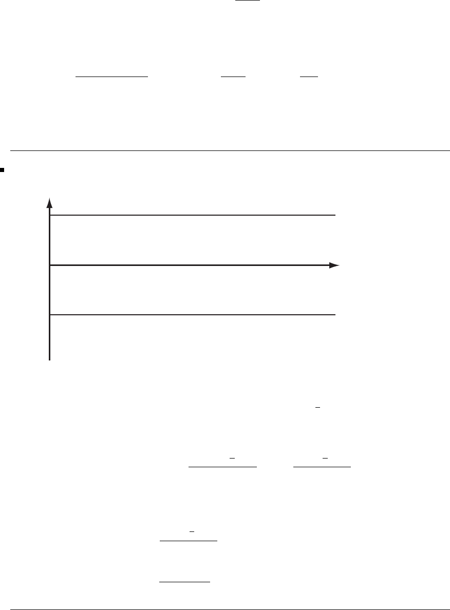
538 Glyn James, Advanced Modern Engineering Mathematics, 4th Edition
u0=∞
m=1
bmsin mπx
asinh(mπ)
The usual integration gives
asinh(mπ)bm
2=
a
0
u0sin mπx
adx =u0
a
mπ(1 −cos mπ)
The only coefficients that survive are the odd ones and putting m=2n+1 produces
the result quoted.
52 The configuration is illustrated in the figure
x
– a
a
u = +T
u = – T
⭸u /⭸x = 0
⭸u /⭸x = 0
u = 0
y
From the available separated solutions, the appropriate ones are u=e−λy sin λx
and to satisfy ux=0atx=±arequires λa =n+1
2π.Thus,thesolution
takes the form
u=∞
n=0
bnexp −n+1
2πy
asin n+1
2πx
a
so that at y= 0 the coefficients are required from the Fourier problem
∞
n=0
bnsin n+1
2πx
a=+Tfor 0 <x<a
−Tfor −a<x<0
The integration gives bn=4T
(2n+1)πas required.
c
Pearson Education Limited 2011

Glyn James, Advanced Modern Engineering Mathematics, 4th Edition 539
53 The separated solutions are put into the equation to give
r2
R(R +1
rR)=−¨
Θ
Θ=λ2
where the separation constant has been chosen to be positive to ensure that periodic
solution in Θ is possible. The equation
¨
Θ+λ2Θ = 0 has solution Θ = Asin λθ +Bcos λθ
and is periodic only if λ=N, which is an integer. Since T=0onθ=0and
θ=π, the constant Bis given by B=0.
The Requation is r2R +rR−N2R= 0 and trying solutions of the form R=rP
shows that p=Nor −N. The solution must be finite at the origin; so the negative
powers are omitted and the original equation has a solution
T=∞
N=1
bNrNsin Nθ
The condition on the boundary is
T0=∞
N=1
bNaNsin Nθ
and the coefficients are obtained by Fourier analysis. The integrations are given by
π
2bNaN=
π
0
T0sin Nθdθ =T0
N(1 −cos Nπ)
and the result follows applying N=2n+ 1 and starting the summation from
n=0.
54 The suggested separated form produces the equations
1
R
d
dr r2dR
dr =−1
ysin θ
d
dθ sin θdy
dθ =k(k+1)
where the RHS conforms with the given expression. The equation for yis obtained
by making the substitution x=cosθ.Now
dy
dx =dy
dθ
dθ
dx =1
sin θ
dy
dθ
c
Pearson Education Limited 2011

540 Glyn James, Advanced Modern Engineering Mathematics, 4th Edition
so putting this into the θequation gives
d
dx sin2θdy
dx+k(k+1)y=0or d
dx (1 −x2)dy
dx+k(k+1)y=0
To solve these equations, first put R=rnthen substitution leads to
n(n+1)=k(k+ 1) with solution n=kor −k−1
Secondly, the only solutions for ythat remain finite at x=+1and−1arethe
solutions given in the question (see an advanced book on Legendre polynomials).
Thus, the solution that involves k=1,2,3is
V=A+B
r+cosθAr+B
r2+1
2(3 cos2θ−1) Ar2+B
r3
The given boundary conditions involve only even functions of θ,soA=B=0.
The first of the two conditions gives
0=A+B
a+1
2(3 cos2θ−1) Aa2−B
a3for all θ
Hence B=−aA and B =−a5A and the solution can be rewritten
V=A1−a
r+A
2(3 cos2θ−1) r2−a5
r3
The final condition implies
αsin2θ=A1−a
b+A
2(2 −3sin
2θ)b2−a5
b3
so that identifying the two parts gives
A =−2α
3b2−a5
b3and A=2α
31−a
b
and the solution follows.
Exercises 9.5.4
55 For rectangular regions MATLAB has an easy setup procedure
G=numgrid(S,5) % gives the node numbering as
c
Pearson Education Limited 2011

Glyn James, Advanced Modern Engineering Mathematics, 4th Edition 541
G=00000
01470
02580
03690
00000
rhs(1)=0.25;rhs(4)=0.5;rhs(7)=0.75+0.9375;rhs(8)=0.75;
rhs(9)=0.4375;
rhs % sets up the right hand side, one entry for each of the 9 equations
(default = 0), as the transpose of
rhs= 0.2500 0 0 0.5000 0 0 1.6875 0.7500 0.4375
A=delsq(G); % MATLAB sets up the matrix stored in sparse form
full(A) % gives the full matrix
4-10-100000
-1 4 -1 0 -1 0 0 0 0
0-1400-1000
-1 0 0 4 -1 0 -1 0 0
0-1 0-1 4-1 0-1 0
00-10-1400-1
000-1004-10
0 0 0 0 -1 0 -1 4 -1
00000-10-14
A\rhs’ % gives the required solution
0.2026 0.1462 0.0776 0.4141 0.3047 0.1641 0.6490 0.4944 0.2740
56 For the small grid
The equations are
4u1=1+1+0+u2
4u2=1+u1+0+u1
which can be solved as
u1=9
14 and u2=4
7
y
u = 1
u = 0
u = 1
u(3) = u(1)
123
x
For the larger grid the MATLAB implementation needs more care since the
derivative boundary condition modifies the matrix set up by the package.
c
Pearson Education Limited 2011
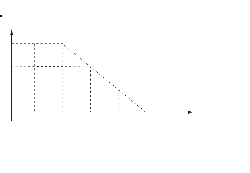
542 Glyn James, Advanced Modern Engineering Mathematics, 4th Edition
G=numgrid(S,5);
A=delsq(G); % A is modified in the next four lines
B=zeros(9,3);B(7,1)=-1;B(8,2)=-1;B(9,3)=-1;C=[A B];
D=zeros(3,12);D(1,10)=4;D(2,11)=4;D(3,12)=4;
D(1,7)=-2;D(1,11)=-1;
D(2,8)=-2;D(2,10)=-1;D(2,12)=-1;D(3,9)=-2;D(3,11)=-1;
E=[C;D];
full(E) % prints out the modified A
rhs=zeros(12,1);rhs(1)=2;rhs(2)=1;
rhs(3)=1;rhs(4)=1;rhs(7)=1;rhs(10)=1;
E\rhs % gives the solution
0.9008 0.7684 0.5348 0.8348 0.6379 0.3709 0.8007 0.5774 0.3110
0.7904 0.5602 0.2955
57 The mesh for this problem is shown in the figure
y
x
45
123
w = 0 on the boundary
Using the notation of the problem, at a typical node 0 with neighbours 1, 2, 3 and
4, the adaptation of equation (9.55) gives
w1+w2+w3+w4−4w0
h2+20=0
which is easily rearranged into the given form. Applying this formula to the
problem in hand produces the five equations
c
Pearson Education Limited 2011
Glyn James, Advanced Modern Engineering Mathematics, 4th Edition 543
4w1=w2+w4+20
4w2=w1+w3+w5+20
4w3=w2+20
4w4=w1+w5+20
4w5=w4+w2+20
which can be solved by a spreadsheet or MATLAB to give
000
0 10.337 10.674 0
0 10.674 12.360 8.090 0
000 0 00
58 The problem has more complicated boundary data and so requires a little
more effort to set up. The top boundary condition is derived from
φ+−φ−
2h=−φ0
For case (a) when h=1/2 the problem only has two unknowns.
(φ1–2h φ2)
y
2
2.75
33 2.5 2 x
1
11
21
The equations are
2.75 + 2.5+1+φ2−4φ1=0.125
2+φ1+1+(φ1−φ2)−4φ2=0.125
which are easily solved to give the quoted answer.
c
Pearson Education Limited 2011
544 Glyn James, Advanced Modern Engineering Mathematics, 4th Edition
(b) For the larger mesh, the MATLAB version is as follows; note the powerful
matrix building techniques:
G=numgrid(S,5);A=delsq(G);
b=eye(3);c=zeros(3);d=[4.5-1 0;-1 4.5-1; 0-1 4.5];
A=[[A;c c-2∗b][c;c;-b;d]];full(A) % A is printed out
rhs=[2.75+2.9375;2.5;3.25;2.75;0;1;2.4375;0;1;2;0;1];
z=[1/64;1/32;3/64];z=[z;z;z;z];
rhs=rhs-z % rhs is printed out
A\rhs % gives the final answer
1.6016 1.2868 1.0565
1.9680 1.5818 1.2572
2.2666 1.8465 1.4375
2.5175 2.1314 1.6930
59 In this problem, there are essentially five unknowns because of the symmetry
as
x
y
5
4
12323
4
5
seen in the figure
c
Pearson Education Limited 2011

Glyn James, Advanced Modern Engineering Mathematics, 4th Edition 545
The five equations are set up in matrix form as
⎡
⎢
⎢
⎢
⎣
−42020
1−4100
01−400
100−41
0001−4
⎤
⎥
⎥
⎥
⎦
⎡
⎢
⎢
⎢
⎣
φ1
φ2
φ3
φ4
φ5
⎤
⎥
⎥
⎥
⎦
=⎡
⎢
⎢
⎢
⎣
0
−2
−17
−2
−2
⎤
⎥
⎥
⎥
⎦
These equations can be solved on any suitable package to give
1.5909
2.0909
4.7727
1.0909
0.7727
Exercises 9.6.1
The exercises can only be solved sensibly on a computer package and need
considerable computer experience, in the present case MATLAB. Some M-files
are required by all the problems.
coeff.m
function [a0,a1,a2]=coeff(a,b,c)
A=[a 1];B=[b 1];C=[c 1];1x=[1 0 0];1y=[0 1 0];
den=0.5/det([A;B;C]);
L0=[det([1x;B;C]) det([1y;B;C])];
L1=[det([1x;C;A]) det([1y;C;A])];
L2=[det([1x;A;B]) det([1y;A;B])];
a0=L0∗L0∗den;a1=L1∗L0∗den;a2=L2∗L0∗den;
stiff.m
function a=stiff(mm,k,ll)
%mm=no of neighbours,k=current point,
ll=row of k’s neighbours
global CO
a=zeros(1,mm+1);
c
Pearson Education Limited 2011

546 Glyn James, Advanced Modern Engineering Mathematics, 4th Edition
for p=1:mm-1
[l,m,n]=coeff(CO(k,:),CO(ll(p),:),CO(ll(p+1),:));
a(1)=a(1)+1;a(p+1)=a(p+1)+m;a(p+2)=a(p+2)+n;
end
[l,m,n]=coeff(CO(k,:),CO(ll(mm),:),CO(ll(1),:));
a(1)=a(1)+1;a(mm+1)=a(mm+1)+m;a(2)=a(2)+n;
calcArhs.m % the following code needs to be copied to the main
program
for k=1:nin
r=link(k,:);m=nnz(r);
z=stiff(m,k,r);
A(k,k)=A(k,k)+z(1);
for i=1:m
if r(i)<=nin
A(k,r(i))=A(k,r(i))+z(i+1);
else
rhs(k)=rhs(k)-z(i+1)∗bdry(r(i)-nin);
end
end
end
60 Each of the FE problems has its own input, for this problem
60(a)
inform60.m % the node labelling is shown in the Figure
nin=2;nbdry=8;%number of internal and boundary nodes
global CO
r3=sqrt(3);
CO=[2,r3;4,r3;0,r3;1,0;3,0;5,0;6,
r3;5,2∗r3;3,2∗r3;1,2∗r3];
%coords of points internal first then bdry
link=[3 452910;1 5 6 7 8 9];
%links from interior points to neighbours,in CO order
bdry=[0 0001000];%boundary values,in CO order
A=zeros(nin);rhs=zeros(nin,1);
c
Pearson Education Limited 2011
Glyn James, Advanced Modern Engineering Mathematics, 4th Edition 547
3.5
3
2.5
2
1.5
1
0.5
00123456
13
456
8910
27
x
y
The
calculation then proceeds using inform.60 and the code from calcArhs.m
global CO
inform60
for k=1:nin
r=link(k,:);m=nnz(r);
z=stiff(m,k,r);
A(k,k)=A(k,k)+z(1);
for i=1:m
if r(i)<=nin
A(k,r(i))=A(k,r(i))+z(i+1);
else
rhs(k)=rhs(k)-z(i+1)∗bdry(r(i)-nin);
end
end
end
c
Pearson Education Limited 2011

548 Glyn James, Advanced Modern Engineering Mathematics, 4th Edition
A,rhs % gives A=3.4641 -0.57774 rhs= 0
0.5774 3.4641 0.5774
A \rhs % gives the final result 0.0286
0.1714
60(b) The larger mesh is treated similarly. The mesh information is in
inform60b.m, where an obvious node numbering has been used – print out CO
and link for details.
inform60b.m
nin=5;nbdry=12;%number of internal and boundary nodes
global CO
r3=sqrt(3);
a0=[3,r3;1.5,2∗r3/3;4.5,2∗r3/3;4.5,4∗r3/3;1.5,4∗r3/3];
a1=zeros(5,1);a2=[0;1;2;3;4]∗1.5;a3=ones(5,1)∗r3∗2;
CO=[a0;a2,a1;6,r3;flipud(a2),a3;0,r3];
%coords of points internal first then bdry
link=[2 834145;6781517;89101141;
1 3 11 12 13 14; 17 2 1 14 15 16];
%links from interior points to neighbours, in CO order
bdry=[0 00011100000];%boundary values, in
CO order
A=zeros(nin);rhs=zeros(nin,1);
The calculation is the same as part (a)
global CO
inform60
for k=1:nin
r=link(k,:);m=nnz(r);
z=stiff(m,k,r);
A(k,k)=A(k,k)+z(1);
c
Pearson Education Limited 2011

Glyn James, Advanced Modern Engineering Mathematics, 4th Edition 549
for i=1:m
if r(i)<=nin
A(k,r(i))=A(k,r(i))+z(i+1);
else
rhs(k)=rhs(k)-z(i+1)∗bdry(r(i)-nin);
end
end
end
A,rhs %prints out A and rhs
A\rhs %gives the required answer
0.1024 0.0208 0.2920 0.2920 0.0208
61 Because the problem now involves a Poisson equation, some modifications
are required. The M-file coeff.m is modified to
coeffr.m
function [a0,a1,a2,a3]=coeffr(a,b,c)
A=[a 1];B=[b 1];C[c 1];1x=[1 0 0];1y=[0 1 0];
den=0.5/det([A;B;C]);
L0=[det([1x;B;C]) det([1y;B;C)];
L1=[det([1x;C;A]) det([1y;C;A)];
L2=[det([1x;A;B]) det([1y;A;B)];
a0=L0∗L0∗den;a1=L1∗L0∗den;a2=L2 ∗L0 ∗den;
a3=-20/(12*den);
and stiff.m to
stiffr.m
function a=stiffr(mm,k,ll)
%mm=no of neighbours,k=current point,ll=row
of k’s neighbours
global CO
a=zeros(1,mm+2);
for p=1:mm-1
[l,m,n,q]=coeffr(CO(k,:),CO(ll(p),:),
CO(ll(p+1),:));
c
Pearson Education Limited 2011
550 Glyn James, Advanced Modern Engineering Mathematics, 4th Edition
a(1)=a(1)+l;a(p+1)=a(p+1)+m;a(p+2)=a(p+2)+n;
a(mm+2)=a(mm+2)+q;
end
[l,m,n,q]=coeffr(CO(k,:),CO(ll(mm),:),CO(ll(1),:));
a(1)=a(1)+l;a(mm+1)=a(mm+1)+m;a(2)+n;
a(mm+2)=a(mm+2)+q;
The mesh information for the problem is contained in
inform61
nin=5;nbdry=12;%number of internal and
boundary nodes
global CO
CO=[1 2;1 1;2 2;2 1;3 1;0 0;1 0;2 0;3 0;
4 0;4 1;3 2;2 3;1 3;0 3;0 2;0 1];
%coords of points internal first then bdry
link=[2 4 3 14 15 16;1 16 17743;145121314;
128953;491011123];
%links from interior points to neighbours, in CO order
bdry=[0 00000000000];%boundary values,
in CO order
A=zeros(nin);rhs=zeros(nin,1);
The calculation now proceeds as
inform61
for k=1:nin
r=link(k,:);m=nnz(r);
z=stiffr(m,k,r);
A(k,k)=A(k,k)+z(1);
for i=1:m
if r(i)<=nin
A(k,r(i))=A(k,r(i))+z(i+l);
else
rhs(k)=rhs(k)-z(i+l)∗bdry(r(i)-nin);
end
end
c
Pearson Education Limited 2011

Glyn James, Advanced Modern Engineering Mathematics, 4th Edition 551
rhs(k)=rhs(k)-z(m+2);
and
A,rhs % prints out A and rhs
A\rhs % gives the final result
10.3371 10.6742 10.6742 12.3596 8.0899
62 Although the problem has a great deal of symmetry, all the 9 internal nodes
and 16 boundary nodes are used in this implementation. An interesting exercise is
to modify the program using the full symmetry. The mesh data is
inform62
nin=9;nbdry=16;%number of internal and boundary nodes
global CO
r=1/3;s=2/3;
CO=[0 0;0 -r;r 0; 0 r;-r 0; 0 -s;s 0;0 s;-s 0;
-r -r;-r -1;0 -1;r -1;r -r;1 -r;1 0; 1 r;r r;r 1;
0 1;-r 1; -r r;-1 r;-1 0;-1 -r];
%coords of points internal first then bdry
link=[2 14 3 18 4 22 5 10; 1 10 6 14 0000;
1147180000;1188220000;
1229100000;2101112131400;
3 14 15 16 17 18 0 0;4 18 19 20 21 22 0 0;
5222324251000];
%links from interior points to neighbours, in CO order
bdry=[1 101199911011999];
%boundary values, in CO order
A=zeros(nin);rhs=zeros(nin,1);
The equation is Laplace and so no modifications are required to the other M-files.
global CO
inform53
for k=1:nin
r=link(k,:);m=nnz(r);
z=stiff(m,k,r);
A(k,k)=A(k,k)+z(1);
c
Pearson Education Limited 2011

552 Glyn James, Advanced Modern Engineering Mathematics, 4th Edition
for i=1:m
if r(i)<=nin
A(k,r(i))=A(k,r(i))+z(i+1);
else
rhs(k)=rhs(k)-z(i+1)*bdry(r(i)-nin);
end
end
end
A,rhs % prints out A and rhs
A\rhs % gives the final answer for the internal
nodes - note all the symmetries
1.6818 1.1152 2.2485 1.1152 2.2485 0.7788 5.3121 0.7788 5.3121
Exercises 9.7.4
63 The Poisson formula gives
T(r, θ)= T0
2π
π
0
a2−r2
a2+r2−2ar cos(θ−s)ds
The integral can be evaluated by a package such as MAPLE or by using the
substitution z=tan1/2(θ−s)togive
T(r, θ)=T0
πtan−1a+r
a−rtan θ
2+tan
−1a+r
a−rcot θ
2
It is instructive to show that T=T0/2whenr= 0 and to check that T=T0
when r=aand 0 ≤θ≤π.
64 Substitution readily shows that the Laplace equation is satisfied. Also by
inspection, it is easily seen that G=0onx=0andy= 0. No additional
singularities have been added in the quarter plane, so the function is the Green’s
function for the problem. Equation (9.74) thus becomes
T(x0,y
0)=
∞
0
f(x)∂G
∂y (x, 0; x0,y
0)dx +∞
0
g(y)∂G
∂x (0,y;x0,y
0)dy
c
Pearson Education Limited 2011

Glyn James, Advanced Modern Engineering Mathematics, 4th Edition 553
Differentiating Gwith respect to yand putting y= 0 gives after careful algebra
y0
π1
(x−x0)2+y2
0−1
(x+x0)2+y2
0
and similarly differentiating Gwith respect to xand putting x=0givesthe
expression given in the question.
If f(x)=1 and g(x) = 0 then the solution is
T(x0,y
0)=y0
π∞
01
(x−x0)2+y2
0−1
(x+x0)2+y2
0dx
=1
πtan−1(x−x0)
y0−tan−1(x+x0)
y0∞
0
=2
πtan−1x0
y0
65 We first note that if x=rcos θ, y =rsin θ, x0=r0cos θ0,y
0=r0sin θ0we
have
(x−x0)2+(y−y0)2=r2+r2
0−2rr0cos(θ−θ0)
Hence the given expression has the correct singularity. A similar calculation shows
that the other term does not have a singularity inside the circle r≤a. Applying
r=ainto the given Green’s function it follows almost immediately that G=0 as
required. The equation (9.74) now produces the solution as
u(r0,θ
0)=−2π
0
f(θ)∂G(a, θ;r0,θ
0)
∂r adθ
Evaluating the derivative of the Green’s function gives
∂G(a, θ;r0,θ
0)
∂r =1
2πa
a2−r2
0
a2+r2
0−2ar0cos(θ−θ0)
and hence the Poisson formula
u(r0,θ
0)= 1
2π2π
0
f(θ)a2−r2
0
a2+r2
0−2ar0cos(θ−θ0)dθ
66 The figure illustrates the configuration. At the point (x, y, z), the temperature
from the line source x=a, y =0,−L≤z≤Lis given in Example 9.44 as
qL
4ρcκπ sinh−1z+L
(x−a)2+y2−sinh−1z−L
(x−a)2+y2
c
Pearson Education Limited 2011
554 Glyn James, Advanced Modern Engineering Mathematics, 4th Edition
Note that the basic expression in
Example 9.44 has been shifted to
make the origin x=a,y=0,z =0.
Clearly, this result does not satisfy
the condition that the temperature
is zero on x= 0. A second constant
sink of length Lmust be added
symmetrically at x=−a, y =0,
−L≤z≤L. When the source and
the sink are added together we
obtain
aL
x
y
z
T(x, y, z)= qL
4ρcκπ sinh−1z+L
(x−a)2+y2−sinh−1z−L
(x−a)2+y2
−qL
4ρcκπ sinh−1z+L
(x+a)2+y2−sinh−1z−L
(x+a)2+y2
It can be seen that when x=0 then T= 0, and hence we have the solution to the
problem posed.
67 From equation (9.76), the temperature generated from the instantaneous
source adθ is
T(R, z, θ, t)= qa
8ρc(πκt)3/2exp −r2
4κtdθ
where r=AP. From the diagram, Ais the point a=(acos θ, a sin θ, 0) and Pis
the point p=(Rcos φ, R sin φ, z). Thus, we can calculate AP =|a−p|as
r2=R2+a2+z2−2aR cos(θ−φ)
The temperature can now be calculated by substituting and integrating the above
expression.
T(R, z)= qa
8ρc(πκt)3/2exp −R2+a2+z2
4κt 2π
0
exp aR cos(θ−φ)
2κt dθ
c
Pearson Education Limited 2011
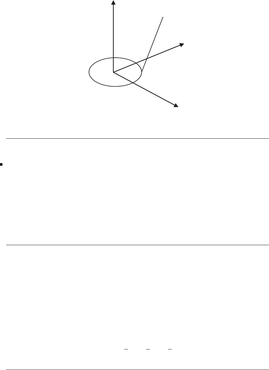
Glyn James, Advanced Modern Engineering Mathematics, 4th Edition 555
a
z
y
x
A
r
The integral is then identified with the definition given for the modified Bessel
function.
Exercises 9.8.3
68(a) Now ‘AC −B2’ = 0 in this case so the equation is parabolic. Applying
r=x−yand s=x+ythe derivatives are
ux=ur+us
uy=−ur+us
and
uxx =urr +2urs +uss
uyy =urr −2urs +uss
uxy =−urr +uss
Substituting into the given equation gives the parabolic equation uss =0.
68(b) Now ‘AC −B2’ = 4 in this case so the equation is elliptic. From the
theory in Section 9.8.1 substitute r=−3x+yand s=x+y; the derivatives are
ux=−3ur+us
uy=ur+us
and
uxx =9urr −6urs +uss
uyy =urr +2urs +uss
uxy =−3urr −2urs +uss
Substituting into the given equation gives the elliptic equation
urr +uss −9
8ur+3
8us+1
8u=0
c
Pearson Education Limited 2011

556 Glyn James, Advanced Modern Engineering Mathematics, 4th Edition
68(c) Now ‘AC −B2’=−25
4−3×2<0 in this case and so the equation is
hyperbolic. From the theory in Section 9.8.1 substitute r=9x+yand s=x+y;
the derivatives are
ux=9ur+us
uy=ur+us
and
uxx =81urr +18urs +uss
uyy =urr +2urs +uss
uxy =9urr +10urs +uss
Substituting into the given equation gives the hyperbolic equation
49urr =uss
69 The characteristic directions from Exercise 68 are r+7s=16x+8yand
r−7s=2x−6y. This suggests that the solution is of the form
u=f(2x+y)+g(x−3y)
where fand gare arbitrary functions. Substituting, the given equation
LHS = 3(4f +¨
g)−5(2f −3¨
g)−2(f +9
¨
g)=0=RHS
is satisfied, as expected.
70 The chain rule gives
fx=fuux+fvuxand
=fu+fv
fy=fuuy+fvuy
=fu−fv
and the second derivatives are
fxx =fuu +2fuv +fw,f
yy =fuu −2fuv +fw
fxy =fuu −fw
Substituting into the equation (9.84) reduces to fw=0.
Integrating with respect to v
fv=F(u)whereFis an arbitrary function of u.
c
Pearson Education Limited 2011
Glyn James, Advanced Modern Engineering Mathematics, 4th Edition 557
Integrating again with respect to v
f=vF(u)+G(u)whereGis another arbitrary function of u.
Hence,
f=(x−y)F(x+y)+G(x+y)
71 Now ‘AC −B2’=yand there are three cases (a) y>0wheretheequation
is elliptic. (b) y= 0 where the equation is parabolic and (c) y<0wherethe
equation is hyperbolic.
From equation (9.83), the characteristics are obtained from the solution of the
equation
dy
dx =±√−y
y
The equation only makes sense in the hyperbolic region where y<0. Substitute
z=−yand the differential equation becomes
dz
dx =±√z
z=±1
√z
which is easily integrated to
z3
2=±3
2x+K⇒(−y)3
2±3
2x=K
as the characteristics.
72 Differentiating
fx=3Ax2−2B
x3y(1 −y2)andfy=Ax3+B
x2(1 −3y2)
fxx =6Ax +B
x4y(1 −y2)andfyy =Ax3+B
x2(−6y)
The given equation can be checked by substitution.
Now ‘AC −B2’=x2(1 −y2)so
⎧
⎨
⎩
elliptic if |y|<1
parabolic if x=0ory=±1
hyperbolic if |y|>1
c
Pearson Education Limited 2011

558 Glyn James, Advanced Modern Engineering Mathematics, 4th Edition
73 Calculating ‘AC −B2’=−4p2+4q2, it can be deduced that the equations are
(a) p>q or p<−qthen the equations are hyperbolic
(b) p=qthen the equations are parabolic
(c) −q<p<q then the equations are elliptic
Using the substitution −p2+q2=−1
4(x4−2x2y2+y4−x4−2x2y2−y4)=x2y2>0,
hence leads to the elliptic region when it is expected that the equation will look
like the Laplace equation.
vx=xvp+xvq
vy=−yvp+yvq
and
vxx =vp+vq+x2(vpp +2vpq +vqq)
vyy =−vp+vq+y2(vpp −2vpq +vqq)
vxy =xy(−vpp +vqq)
It may be noted that
vxx +vyy =2vq+(x2+y2)vpp +2(x2−y2)vpq +(x2+y2)vqq
from which the required transformation to the Laplace follows immediately.
74 In this case, ‘AC −B2’=−(xy)2so the equation is hyperbolic away from
the axes. The characteristics are computed from equation (9.83) as
dy
dx =±x2y2
x2=±y
x
and the solution is obtained by integration as
ln y=±ln x+K⇒y=ax and yx =b
so one set of characteristics are straight lines through the origin and the other are
rectangular hyperbolas. The domain of dependence and the range of influence can
now be sketched.
Review exercises 9.11
1The boundary and initial conditions on y(x, t)are
y=0 at x=0 anda
String initially at rest ⇒∂y
∂t =0 at t=0
Initial displacement y=f(x)=εx
bfor 0 ≤x≤b
ε(a−x)
a−bfor b≤x≤aat t=0
c
Pearson Education Limited 2011

Glyn James, Advanced Modern Engineering Mathematics, 4th Edition 559
Out of the possible separated solutions (9.25) that satisfy the wave equation, the
only one that satisfies the conditions at x=0 andy=0is y=sinλx cos λct.
The condition at x=agives λa =nπ where nis an integer. Thus, the solution is
asumofsuchterms
y=∞
n=1
Ansin nπx
acos nπct
a
and the final condition produces the Fourier series
f(x)= ∞
n=1
Ansin nπx
a
The coefficients are evaluated from the integral
1
2aAn=
b
0
εx
bsin nπx
adx +
a
b
ε(a−x)
a−bsin nπx
adx
which, after some careful integration by parts, gives the required coefficient
An=2εa2
n2π2b(a−b)sin nπb
a
It is interesting to look at the solution for various values of bsince the solution gives
strengths of the harmonics for different musical instruments. It is these values that
give the characteristic sound of the instrument. For example, a violin has b=a/7;
it is seen that A7= 0 and sevenths do not occur for this instrument.
2Taking the Laplace transform of the equation and the boundary conditions
gives
¯
φ =s2¯
φ−sx2
and ¯
φ(0,s)=0,¯
φ(l, s)=2l
s
The most convenient form for the complementary function is
¯
φ=Acosh s(x−l)+Bsinh s(x−l)
The particular integral is a quadratic in xwhich when substituted into the equation
gives
c
Pearson Education Limited 2011

560 Glyn James, Advanced Modern Engineering Mathematics, 4th Edition
particular integral = x2
s+2
s3
The complete solution is therefore
¯
φ=Acosh s(x−l)+Bsinh s(x−l)+x2
s+2
s3
Putting the two conditions on ¯
φinto the solution
¯
φ(0,s)=0⇒0=Acosh(−sl)+Bsinh(−sl)+ 2
s3
¯
φ(l, s)=2l
s⇒2l
s=sB +2l
s⇒B=0
The Laplace transform of the solution is
¯
φ=x2
s+2
s3−2
s3
cosh s(x−l)
cosh sl
The solution in real space can be obtained from advanced tables of transform pairs.
3Take the separated solutions that are quoted and first note that the conditions
y(0) = y(l) = 0 are satisfied. Secondly, substitute into equation (9.92)
1
c2T
n+1
τT
n=−Tnnπ
l2
This equation can then be solved in the standard way by looking for solutions of
the form Tn=eαt which produces the quadratic equation
α2+1
τα+cnπ
l2=0
The equation has roots
α=1
2⎛
⎝−1
τ±#1
τ2
−4cnπ
l2⎞
⎠=−1
2τ±jcnπ
l#1−l
2τcnπ 2
and hence the solution is
Tn(t)=exp−t
2τ(ancos ωnt+bnsin ωnt)
c
Pearson Education Limited 2011

Glyn James, Advanced Modern Engineering Mathematics, 4th Edition 561
and general solution
y=∞
n=1
Tn(t)sinnπx
l
The condition ∂y
∂t (x, 0) = 0 implies, on differentiation and substituting t=0,
0=−1
2τan+bnωn
From the other condition it is seen that the only term to survive is when n=3.
Thus,
4sin3πx
l=anexp −0
2τcos ω30+ 1
2τω3
sin ω30sin 3πx
l
and hence the solution satisfying all the conditions is
y(x, t)=4exp−t
2τcos ω3t+1
2τω3
sin ω3tsin 3πx
l
and ω3giveninthequestion.
4This problem is the extension of the wave equation to beams. Simply
substituting the given form into the beam equation gives the equation (9.93) for V
and the end conditions follow immediately. Again simply substituting sin, sinh, cos
and cosh into the equation shows they are solutions of (9.93). A linear combination
of the functions is also a solution and since it contains four arbitrary constants, it
is the general solution.
To satisfy the end conditions
V(0) = 0 ⇒A+B=0
V(0) = 0 ⇒C+D=0
V(l)=0 ⇒Acosh αl +Bcos αl +Csinh αl +Dsin αl =0
V(l)=0 ⇒Asinh αl −Bsin αl +Ccosh αl +Dcos αl =0
Thus,
A(cosh αl −cos αl)=D(sinh αl −sin αl)
A(sinh αl +sinαl)=D(−cos αl +coshαl)
c
Pearson Education Limited 2011

562 Glyn James, Advanced Modern Engineering Mathematics, 4th Edition
Dividing these two equations, and using the trigonometric and hyperbolic identities,
produces the equation
cos αl cosh αl =1
from which the natural frequencies of vibration of the beam can be calculated.
5The separated solutions in equation (9.40) that satisfy the condition at x=0
are θ=e−αt cos λx. To satisfy the condition at x=lrequires that
λl =n+1
2πwhere nis an integer
Thus, the solution takes the form
θ(x, t)= ∞
n=0
A2n+1 cos (2n+1)πx
2lexp −(2n+1)π
2al 2
t
and the initial condition now produces the usual Fourier series problem with
1
2A2n+1 =
l
0
f(x)cos(2n+1)πx
2ldx
Integration by parts is required to obtain the coefficient for the given function
f(x)=θ0(l−x)as
A2n+1 =8θ0l
π2(2n+1)
2
and the temperature can be obtained from the series solution.
6Evaluating the partial derivatives
∂φ
∂x =1
√tf,∂φ
∂t =−1
2
x
t3/2fand ∂2φ
∂x2=1
tf
Substituting the derivatives back into the equation
κ1
tf =−1
2
x
t3/2f⇒f =−1
2κzf
c
Pearson Education Limited 2011

Glyn James, Advanced Modern Engineering Mathematics, 4th Edition 563
the problem has been reduced to an ordinary differential equation. Rearranging
the equation
df
f=−1
2κzdz which integrates to ln f=−z2
4κ+C
or f=Aexp −z2
4κwhich on further integration gives
f=A
z
0
exp −v2
4κdv +B
Substitute u=v
2√κthen the equation reduces to
f=a
z
2√κ
&
0
e−u2du +bwhere aand bare new arbitrary constants.
The solution is as required
f=aerf z
2√κ+b
For the particular problem,
at t=0 φ(x, 0) = 0 for all x>0
at x=0 φ(0,t)=φ0for t>0
In the expression containing the error function, these conditions give respectively
0=aerf(∞)+band φ0=aerf(0) + b
Since erf(0)= 0 and erf(∞) = 1, the solution can be constructed as
T(x, t)=T0+φ01−erf x
2√κt
7The problem is standard except for the treatment of the derivative boundary
conditions. Note the way that they are handled in the MATLAB implementation.
c
Pearson Education Limited 2011

564 Glyn James, Advanced Modern Engineering Mathematics, 4th Edition
Explicit
u=[1 11111];
u=0.1∗[u([2:6]),u(5)-0.4∗u(6)]+0.8∗u([1:6])
+.1∗[u(2)-0.4∗u(1),u([1:5])]
% gives 0.9600 1.0000 1.0000 1.0000 1.0000 0.9600
u=0.1∗[u([2:6]),u(5)-0.4∗u(6)]
+0.8∗u([1:6])+.1∗[u(2)-0.4∗u(1),u([1:5])]
% gives 0.9296 0.9960 1.0000 1.0000 0.9960 0.9296
u=0.1∗[u([2:6]),u(5)-0.4∗u(6)]+
0.8∗u([1:6])+.1∗[u(2)-0.4∗u(1),u([1:5])]
% gives 0.9057 0.9898 0.9996 0.9996 0.9898 0.9057
Repeating the last line of code produces subsequent time steps.
Implicit
A=[-2.4 20000;1-21000;01-2100;001-210;
0001-21;00002-2.4]
u=[1;1;1;1;1;1];
B=2∗eye(6)-0.1∗A
C=2∗eye(6)+0.1∗A
E=inv(B)∗C
u=E∗u
% gives 0.9641 0.9984 0.9999 0.9999 0.9984 0.9641
u=E∗u
% gives 0.9354 0.9941 0.9996 0.9996 0.9941 0.9354
u=E∗u
% gives 0.9120 0.9881 0.9988 0.9988 0.9881 0.9120
Repeating the last line of code produces subsequent time steps.
8From the possible solutions in equation (9.52), one that can be chosen to satisfy
the conditions on x=0 and y=ais
u=sinμx sinh μ(a−y)
c
Pearson Education Limited 2011
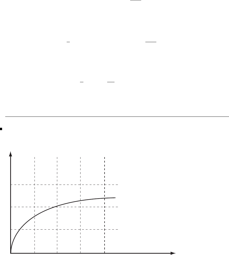
Glyn James, Advanced Modern Engineering Mathematics, 4th Edition 565
On x=a, u =0⇒sin μa =0⇒μa =nπ where nis an integer. The final
condition on y= 0 can be satisfied by taking a sum of such solutions
x(a−x)= ∞
n=1
bnsin nπx
asinh nπ
The problem is the usual evaluation of the Fourier coefficients
a
2bnsinh nπ =
a
0
(a−x)sinnπx
adx
and after two integrations by parts gives
a
2bn=2a
nπ3(1 −cos nπ)
All the even terms go to zero and putting n=2r+ 1, the expression quoted is
recovered.
9This exercise is a harder one since the regular mesh points do not lie on the
boundary.
x
y
y 2 = x
c
7
654
b
a
12 3
At a point such as node 4 the lengths of the mesh are not uniform, so the second
derivative needs to be approximated as
c
Pearson Education Limited 2011

566 Glyn James, Advanced Modern Engineering Mathematics, 4th Edition
f =f3−f0
Δx−f0−f1
Δx 2
Δx+Δx
for a typical configuration
103
x
x′
The curve does not pass through the mesh points and the lengths are calculated
as a=0.25,b =√0.5−0.5andc=√1.5−1. Working through the equations one
at a time, using this formula where appropriate
1+u2+2u4−4u1=0
u1+u3+2u5−4u2=0
u2+1+2u6−4u3=0
2
0.5+au5−u4
0.5+1−u4
a+2
0.5+b1−u4
b+u1−u4
0.5=0.5(0.5)2
u4+u2+1+u6−4u5=0.0625
u5+u3+u7+1−4u6=0.09375
1+1−2u7
0.52+2
c+0.51−u7
c+u6−u7
0.5=1.5
The equations can be transformed to matrix form as
a=
⎡
⎢
⎢
⎢
⎢
⎢
⎢
⎢
⎣
−410 2 0 0 0
1−41 0 2 0 0
01−40 0 2 0
5.6569 0 0 −35.3137 5.3333 0 0
010 1 −41 0
001 0 1 −41
000 0 05.5192 −25.7980
⎤
⎥
⎥
⎥
⎥
⎥
⎥
⎥
⎦
bT=[−10−1−24.1985 −0.9375 −0.9063 −18.7788 ]
and the solution of Ax =bcan be obtained from any package, for example
MATLAB, as
xT=[0.9850 0.9648 0.9602 0.9876 0.9570 0.9380 0.9286 ]
c
Pearson Education Limited 2011

Glyn James, Advanced Modern Engineering Mathematics, 4th Edition 567
10 Clearly, at z=0thevelocityu=Ucos ωt so the given solution has the correct
velocity on the wall. It also satisfies the equation of motion since substituting the
derivatives
ut=−Uωe−αz sin(ωt −αz)
uz=−αUe−αz cos(ωt −αz)−αUe−αz sin(ωt −αz)
uzz =α2Ue−αz cos(ωt −αz)−2α2Ue−αz sin(ωt −αz)
−α2Ue−αz cos(ωt −αz)
into the equation gives −Uω =−ν2α2Uwhich agrees precisely with the definition
of α.
11 Differentiating
Ut=ktk−1exp −r2
4t+tk−r2
4−1
t2exp −r2
4t
Ur=tk−2r
4texp r2
4t
∂
∂r(r2Ur)= −tk−1
23r2+r3−2r
4texp r2
4t
and applying into the spherically symmetric heat equation
−tk−1
23−r2
2texp −r2
4t=tk−1k+r2
4texp −r2
4t
gives the relation k=−3/2.
12 The equation is the same as Example 9.7 and can be dealt with in the same way,
see also equation (9.14). However, the MAPLE solution is very straightforward.
with (PDEtools):
rev 12:=diff(z(x,y),x) + diff(z(x,y),y);
sol:=pdesolve (rev12,z(x,y));
# gives the solution sol:=z(x,y)=_F1(y-x)
c
Pearson Education Limited 2011

568 Glyn James, Advanced Modern Engineering Mathematics, 4th Edition
The boundary conditions x=s, y =−s, z =2sfor s>0 give the solution
z(x, y)=x−yfor x>y
and not defined otherwise.
13 The separated solutions in equation (9.52) that tend to zero for large ymust
be of the form
φ=(Asin μx +Bcos μx)e−μy
The condition φ(0,y)=0⇒B=0andφ(π, y)=0⇒sin μπ =0;thus,the
required solution is
φ=∞
n=1
cne−ny sin nx
Yet again, the final condition requires the evaluation of the coefficients by Fourier
analysis. Integration by parts gives
π
2cn=
π
0
x(π−x)sinnxdx =2
n3(1 −cos nπ)
When nis even, the coefficient is zero and the odd values give the result in the
exercise.
14 First observe that the function χ=a2−x2satisfies ∇2χ=−2 and second
that a separated solution of the Laplace equation derived in equation (9.52) is
cosh μy cos μx and the overall solution is a combination of terms of these types.
The conditions that χ=0onx=±a⇒cos μa =0⇒μa =n+1
2πwhere nis
an integer. Thus, an appropriate solution is
χ(x, y)=a2−x2+∞
n=0
A2n+1 cosh n+1
2πy
acos n+1
2πx
a
The function is even, so only the condition at y=bneeds to be considered since
the other boundary is satisfied by symmetry. Therefore,
0=a2−x2+∞
n=0
A2n+1 cosh n+1
2πb
acos n+1
2πx
a
c
Pearson Education Limited 2011

Glyn James, Advanced Modern Engineering Mathematics, 4th Edition 569
and the coefficients are derived by Fourier analysis. From tables of Fourier series
it may be noted that
∞
n=0
(−1)n
(2n+1)
3cos (2n+1)πx
2a=π3
32a2(a2−x2)for −a<x<a
and thus the coefficient can be identified as
A2n+1 =32a2
π3
(−1)n+1
(2n+1)
3cosh (2n+1)πb
2a
15 The possible separated solutions of the wave equation are given in equation
(9.25) and to satisfy conditions (a) and (b), the solution sin λx cos λct must be
chosen. The condition at x= 1 implies that sin λ=0⇒λ=nπ where nis an
integer. Thus, the solution takes the form
u(x, t)= ∞
n=1
ansin nπx cos nπt
and condition (c) is substituted to give the Fourier series
1−x=∞
n=1
ansin nπx
The coefficients are obtained from
1
2an=
1
0
(1 −x)sinnπxdx
which can be integrated by parts to give an=2
nx and agrees with the quoted
answer.
16 Complete drainage at top and bottom implies u=0at z=0and z=h.
Since there are no sources the pressure tends to zero as time becomes infinite.
Thus the solution that is relevant to this problem is u=e−cα2tsin αz. It is readily
checked that this function is a solution of the consolidation equation. The only
c
Pearson Education Limited 2011

570 Glyn James, Advanced Modern Engineering Mathematics, 4th Edition
boundary condition not satisfied is at z=h; to do this choose αh =mπ where m
is an integer. Therefore,
u(z, t)= ∞
m=1
ansin mπz
hexp −cm2π2t
h2
and the initial uniform pressure leads to the Fourier series problem of evaluating
the coefficients in
A=∞
m=1
amsin mπz
h
so
h
2am=
h
0
Asin mπz
hdz =Ah
mπ(1 −cos mπ)
For m, even the coefficient is zero and substituting m=2n+1 provides the solution
quoted in the exercise.
17 Substituting φ=X(x)T(t) into the equation
X
X=1
c2
¨
T+K˙
T
T=−λ2
where the separation constant has been chosen to be negative, to ensure periodic
solutions for X.ThevariableXsatisfies
X +λ2X= 0 with solution X=Pcos λx +Qsin λx
From condition (a) the sine term must be zero so Q=0. Forthe Tequation,
¨
T+K˙
T+c2λ2T=0
so trying a solution of the form T=exp(at) gives the quadratic
a2+Ka +(cλ)2= 0 with solution a=1
2−K±K2−4(cλ)2
The constant λcan be identified as p, so the condition that (cp)2>1
4K2gives an
overall solution of the type
φ=cospx exp −Kt
2(Msin bt +Ncos bt)
c
Pearson Education Limited 2011

Glyn James, Advanced Modern Engineering Mathematics, 4th Edition 571
where b2=(cp)2−1
4K2.
Condition (a) requires that N=A
Condition (b) requires the derivative
∂φ
∂t =−K
2cos px exp −Kt
2(Msin bt +Ncos bt)
+bcos px exp −Kt
2(Mcos bt −Nsin bt)
At x=t=0
−1
2AK =−1
2NK +bM
and since N=Athen M= 0. The required solution is therefore
φ(x, t)=Acos px exp −Kt
2cos bt where b2=(cp)2−1
4K2
Results can be checked easily in MAPLE.
f:=cos(p∗x)∗exp(-k∗t/2)∗cos(b ∗t);
simplify(diff(f,x,x)-(diff(f,t,t)+k∗diff(f,t))/cˆ2);
gives
−4p2c2+k2+4b2
4c2cos(px)exp−1
2ktcos(bt)
18 Substituting the expressions for vrand vθinto the continuity equation, it is
satisfied for any stream function
LHS = ∂
∂r ∂ψ
∂θ +∂
∂θ −∂ψ
∂r =0=RHS
since the cross partial derivatives are equal for all differentiable functions. For the
given stream function,
vr=1
rUcos θr−a2
r=Ucos θ1−a2
r2
vθ=−Usin θ1+a2
r2
c
Pearson Education Limited 2011
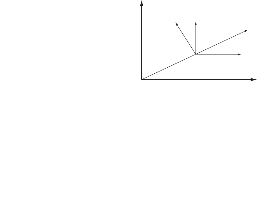
572 Glyn James, Advanced Modern Engineering Mathematics, 4th Edition
On the circle r=a, the radial velocity vr= 0 and there is no flow into the circle.
As rgets very large vr→Ucos θand vθ→−Usin θ
The velocities parallel and perpendicular to the axes are
V=vrcos θ−vθsin θ
→U
and
W=vrsin θ+vθcos θ
→0
y
Wvr
V
r
vθ
x
θ
and hence the flow far downstream is a
steady flow in the xdirection with
velocity U. Overall the flow represents
inviscid, irrotational flow past a circular
obstacle in uniform flow.
19, 20,and21 are intended to be open exercises extending the work of the chapter
to more investigative work. Consequently, no advice is offered for these problems.
For Exercises 19 and 20 the text quotes sources for the work and for Exercise 21
many books on heat transfer will have a version of this problem.
c
Pearson Education Limited 2011
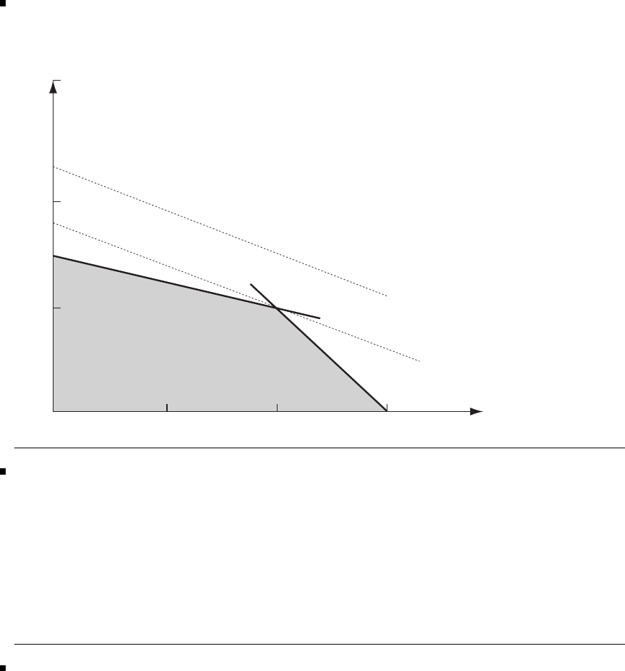
10
Optimization
Exercises 10.2.4
1The required region is shaded on the graph and the lines of constant cost are all
parallel to the lines labelled f=9 and f= 12. The point where fis a maximum
in the region is at the point x=1 and y= 1 giving a maximum cost of f=9.
0.5 1.0 1.5
2x + y = 3
3x + 7y = 10
f = 12
f = 9
3.0
y
2.0
1.0
x
2A graphical or a tabular solution is possible but the MAPLE solution is given
here.
with(simplex):
con2:={2∗x-y<=6,x+2∗y<=8,3∗x+2∗y<=18,y<=3};
obj2:=x+y;
maximize(obj2,con2,NONNEGATIVE);
# gives the solution {y=2, x=4}
3Let xbe number of type 1 and ythe number of type 2. The profit from these
numbers is
f=24x+12y
c
Pearson Education Limited 2011
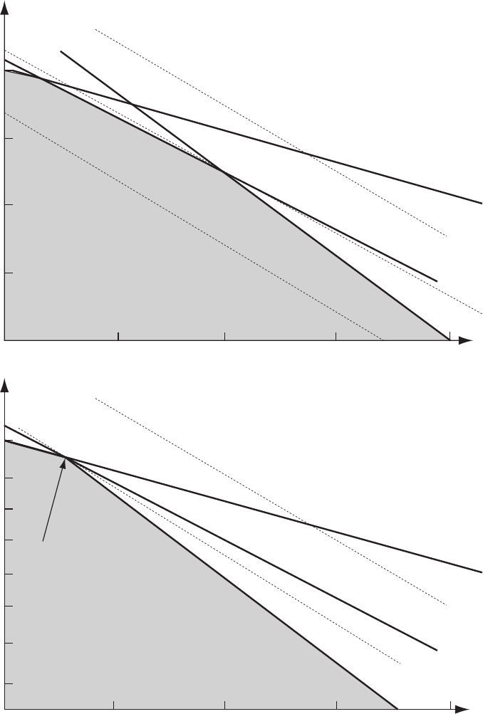
574 Glyn James, Advanced Modern Engineering Mathematics, 4th Edition
T2
5x + 2y = 200
f = 1320
4x + 5y = 400
5x + 3y = 250
f = 1080
40T13020
f = 840
10
20
40
60
80
T2
f = 1320
4x + 5y = 400
5x + 3y = 250
f = 1020
40T1302010
20
40
60
80
min at (5,75)
5x + 2y = 175
c
Pearson Education Limited 2011
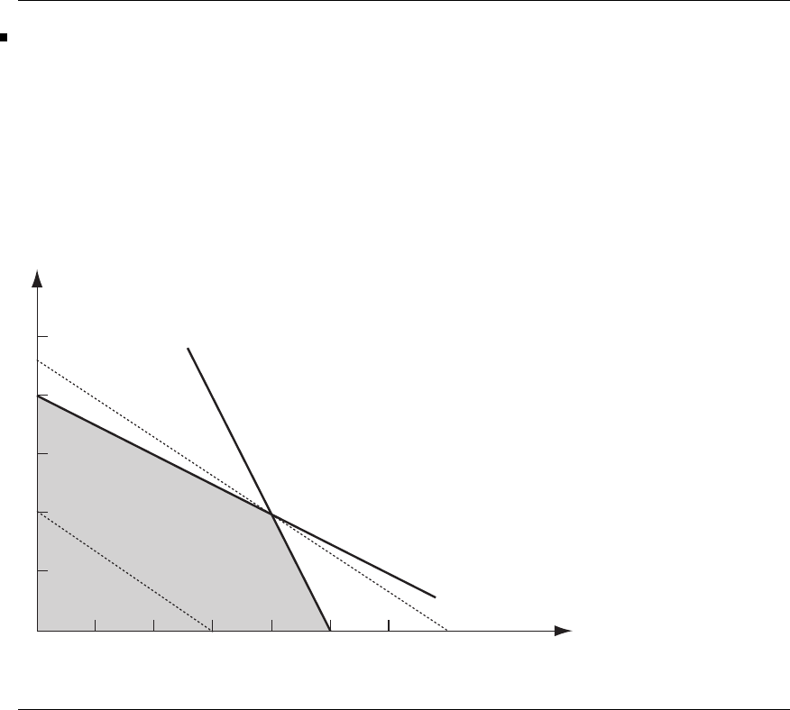
Glyn James: Advanced Modern Engineering Mathematics, 4th edition 575
and the constraints are, in the appropriate units,
chipboard
veneer
labour
4x+5y≤400
5x+2y≤200
5x+3y≤250
and the obvious constraints x≥0andy≥0. The first figure shows the feasible
region bounded by the axes and the three lines 4x+5y= 400,5x+2y= 200 and
5x+3y= 250. These lines intersect at x=20,y = 50 and give the optimum profit
of £1080.
Reducing the available amount of oak veneer to 175 m, the diagram changes as in
the second figure. It can be seen that the same two constraints are active. They
give the solution x=5,y = 75 and a reduced optimum profit of £1020.
4Let nand sbe the number of kg of nails and screws respectively. The profit
made is therefore z=2n+3s
The constraints are labour
material
3n+6s≤24
2n+s≤10
The figure shows the feasible region. The point of intersection of the two constraints
gives the maximum profit of 14p making 4 kg of nails and 2 kg of screws.
screws(Kg)
profit = 14
profit = 6
2n + s = 10
3n + 6s = 24
nails(Kg)
5
3
1
246
c
Pearson Education Limited 2011
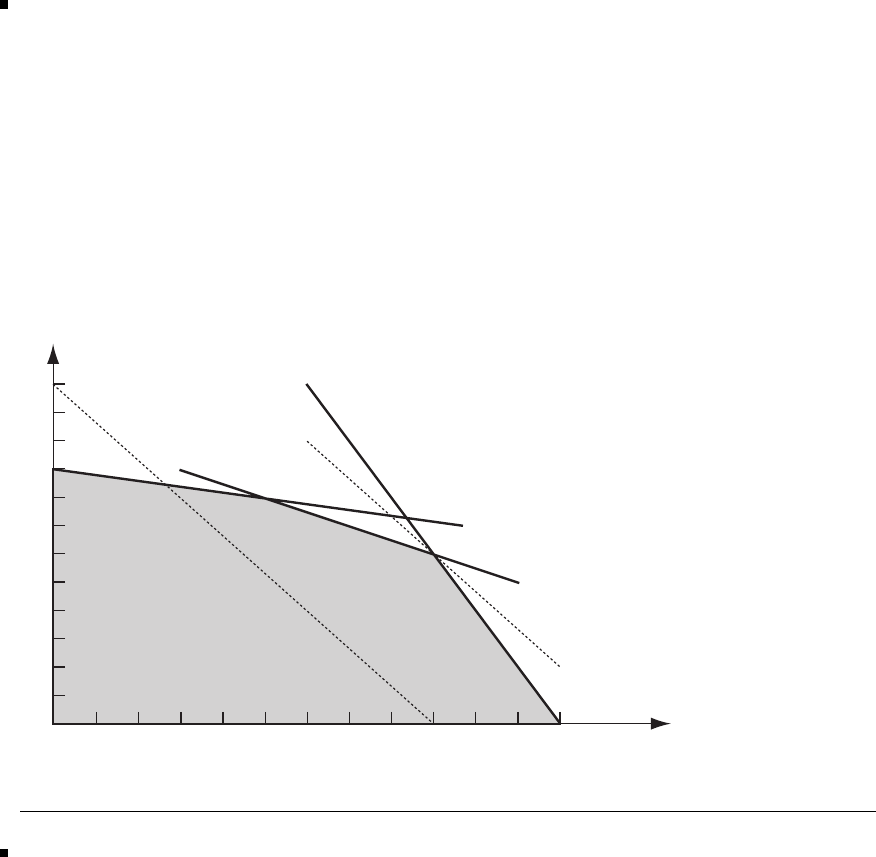
576 Glyn James, Advanced Modern Engineering Mathematics, 4th Edition
5Let C1andC2 be the number of cylinders CYL1 and CYL2 produced. The
profit is 4C1+3C2 and the constraints given by the availability of the materials are:
M1
M2
M3
C1+5C2≤45
C1+2C2≤21
2C1+C2≤24
It is clear from the figure that the optimum is z=54 with C1=9 and C2=6.
The constraints M2 and M3 are active so all these materials are used up. The
constraint M1 has some slack, it may be checked that 6 units remain unused.
C2
C1
12
10
8
6
4
2
24681012
profit = 36
profit = 54
2C1 + C2 = 24
C1 + 5C2 = 45
C1 + 2C2 = 21
6Let ybe the number of Yorks and wthe number of Wetherbys, then the profit
made is
z=25y+30w
The constraints are
cloth
labour
3y+4w≤400
3y+2w≤300
and the problem is a straightforward LP problem that can be solved graphically.
It can be seen from the figure that the optimum is at y=66.67 and w=50
with a profit of £3166.67. Note that the solution must be integral to make sense,
c
Pearson Education Limited 2011
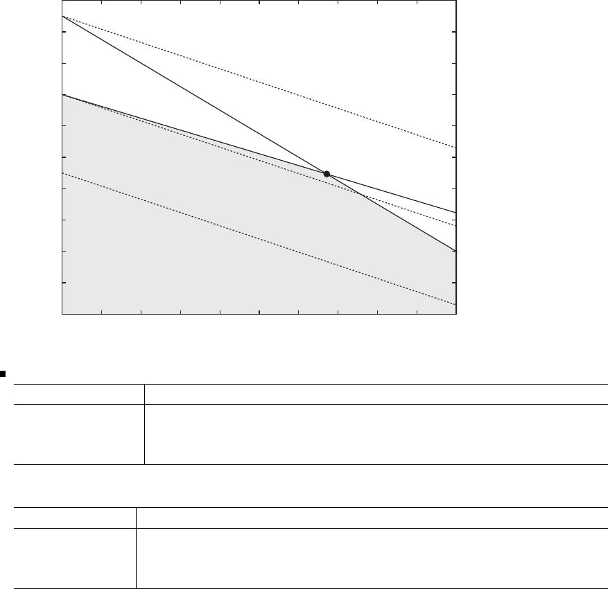
Glyn James: Advanced Modern Engineering Mathematics, 4th edition 577
two-thirds of a jacket is not much good to anyone. However, the solution is an
approximate one and, to proceed correctly, it is necessary to undertake the problem
as an Integer Programming problem. This is much harder and can be found in any
advanced book on Mathematical Programming.
If the amount of cloth is increased then the line 3y+4w=Cis moved from its
present C= 400 parallel and upwards. The intersection point moves upwards and
the profit is increased. This situation continues until the solution is y=0and
w= 150 and all the labour is used on the Wetherbys. The amount of cloth required
would be 600 m and the profit in this case is £4500. This is the maximum possible
profit even if unlimited cloth is available because of the labour constraint.
160
3y + 2w = 300
3y + 4w = 400
f = 3000
f = 1500
f = 4500
−40
−20
0
20
40
60
w
80
100
120
140
0 1020304050
y60 70 80 90 100
7The initial tableau is
x1x2x3x4Soln
z−k−20 0 0 0
x3121020
x4310125
Eliminating the x2column first
x1x2x3x4Soln
z10−k0100200
x20.5 1 0.5 0 10
x42.5 0 −0.5 1 15
c
Pearson Education Limited 2011
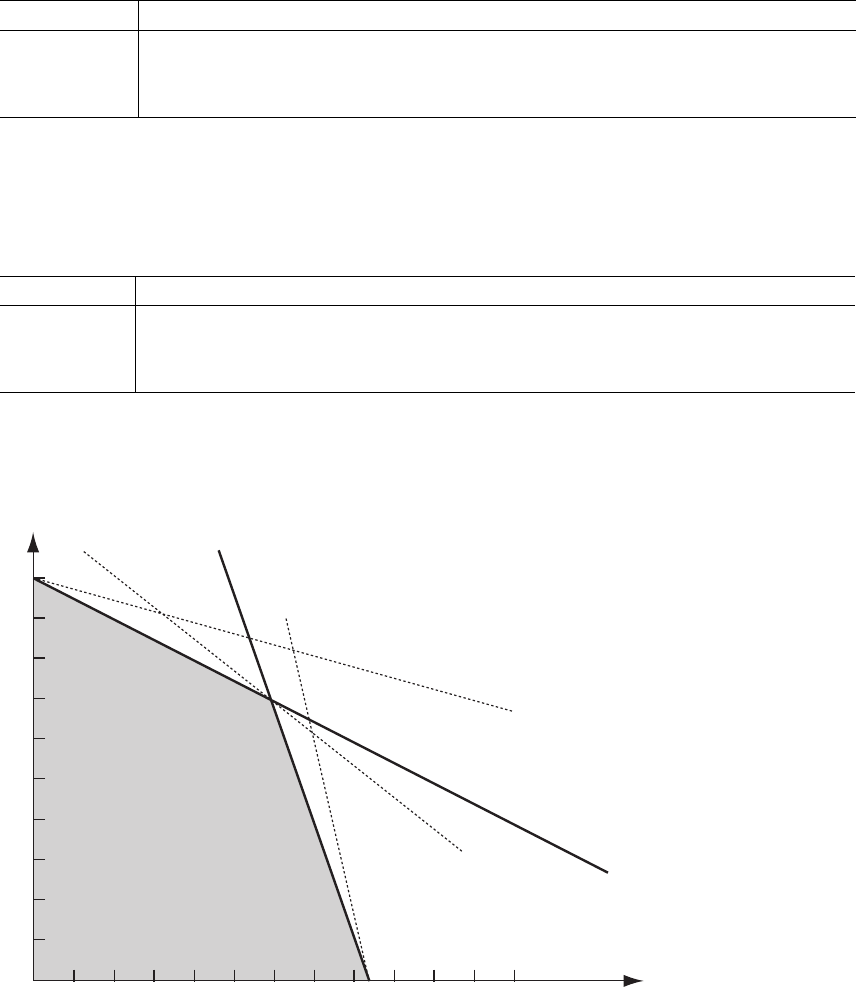
578 Glyn James, Advanced Modern Engineering Mathematics, 4th Edition
If k<10 then the tableau is optimal and the solution is x1=0,x
2=10and
the value of zis 200. If, however, k>10 then the method continues with the x1
column cleared.
x1x2x3x4Soln
z00(60−k)/52(k−10)/5 140 + 6k
x201 0.6 0.2 7
x110 −0.2 0.4 6
If 10 <k<60 then the solution is optimal and the solution is x1=6,x
2=7 and
ztakes the value 140 + 6k.If,however,k>60 then the solution is not optimal
and a further tableau needs to be formed using the x3column.
x1x2x3x4Soln
z0−(60 −k)/50(7k−120)/15 25k/3
x30 5/3 1 1/3 35/3
x11 1/3 0 7/15 25/3
For k>60, the zrow is positive and therefore optimal with x1=25/3,x
2=0
and z=25k/3.
x2
A
B
C
3x1 + x2 = 25
x1 + 2x2 = 20
optimum for k = 90
optimum for k = 5
optimum for k = 30
x1
10
8
6
4
2
2 4 6 8 10 12
The situation for this problem is illustrated in the figure. The feasible region
is shown together with three different cost functions corresponding to the three
c
Pearson Education Limited 2011
Glyn James: Advanced Modern Engineering Mathematics, 4th edition 579
different cases. Note that for small kthe optimum is at the corner A; as the cost
steepens, the corner B is optimum; and finally as the cost steepens further with
the highest values of k, the point C is the optimum.
8This problem has four variables and so it has to be solved using the simplex
algorithm. There are no difficulties with this problem and the tableaux are
presented, to two decimal places, without comment.
x1x2x3x4x5x6x7Soln
z−2−1−4−1 000 0
x5201 0 100 3
x61 0 3 1 0 1 0 4
x7041 1 001 3
x1x2x3x4x5x6x7Soln
z−0.67−1 0 0.33 0 1.33 0 5.33
x51.6700−0.33 1 −0.33 0 1.67
x30.33 0 1 0.33 0 0.33 0 1.33
x7−0.33 400.670−0.33 11.67
x1x2x3x4x5x6x7Soln
z−0.7500 0.5 01.250.255.75
x51.670 0 −0.33 1−0.33 01.67
x30.33 0 1 0.33 0 0.33 0 1.33
x2−0.0810 0.170−0.080.250.42
x1x2x3x4x5x6x7Soln
z0 0 0 0.35 0.45 1.1 0.25 6.5
x1100 −0.2 0.6 −0.2 0 1
x3001 0.4 −0.2 0.4 0 1
x20 1 0 0.15 0.05 −0.1 0.25 0.5
The solution is read off as x1=1,x
2=0.5,x
3=1 and x4=0;themaximumis
at z=6.5.
The MAPLE instructions
con8:= {2∗x1+x3<=3,x1+3∗x3+x4<=4,4∗x2+x3+x4<=3};
obj8:=2∗x1+x2+4∗x3+x4;
maximize(obj8,con8,NONNEGATIVE);
and the MATLAB instructions
c
Pearson Education Limited 2011

580 Glyn James, Advanced Modern Engineering Mathematics, 4th Edition
f=[-2;-1;-4;-1];A=[2,0,1,0;1,0,3,1;0,4,1,1];b=[3;4;3];
options=optimset(‘LargeScale’,‘off’,‘Simplex’,‘on’);
[x,fval]=linprog(f,A,b,[],[],zeros(4,1),[],[],options)
also produce the solution {x4=0, x1=1, x3=1, x2=1/2}.
9If b1,b2,b3 are the respective number(×1000) of books printed then the profit
will be
z= 900b1 + 800b2 + 300b3
and the constraints are
sales restriction
paper
b1+b2≤15
3b1+2b2+b3≤60
The first tableau is easily set up and the other tableaux follow by the usual rules.
b1b2b3b4b5Soln
z−900 −800 −300 0 0 0
b41 1 0 1 0 15
b53210 1 60
b1b2b3b4b5Soln
z0 100 −300 900 0 13,500
b111 010 15
b3 0 −1 1 −3 1 15
b1b2b3b4b5Soln
z0−200 0 0 300 18,000
b1 1 1 0 1 0 15
b30−11−3115
b1b2b3b4b5Soln
z200 0 0 200 300 21,000
b211 0 1 0 15
b310 1−21 30
Thus the optimal profit is made if none of book 1, 15,000 of book 2 and 30,000 of
book 3 are printed giving a profit of £21,000.
c
Pearson Education Limited 2011

Glyn James: Advanced Modern Engineering Mathematics, 4th edition 581
10 Let L, M, S be the respective number of long, medium and short range aircraft
purchased. The profit is
z=0.4L+0.3M+0.15S
and the constraints are
money available
pilots
maintenance
4L+2M+S≤60
L+M+S≤25
2L+1.5M+S≤30
The initial tableau is
LM SPQRSoln
z−0.4−0.3 −0.15 0 0 0 0
P4 2 1 1 0 0 60
Q11 101025
R21.5 1 0 0 1 30
The first column is chosen, since it has the most negative entry, and when the
ratios are calculated, the Pand Rrows produce the same value of 15. From the
two, the Prow is chosen arbitrarily.
LMSPQRSoln
z0−0.1 −0.05 0.1 0 0 6
L10.5 0.250.2500 15
Q00.5 0.75−0.2510 10
R00.5 0.5 −0.5 0 1 0
In this tableau the M, R element is the pivot and performing the elimination gives
LM S P Q R Soln
z0 0 0.05 0 0 0.2 6
L10−0.25 0.75 0 −115
Q0 0 0.25 0.25 1 −110
M01 1 −1020
Note that the final column has not changed between the last two tableaux because
of the zero in the very last entry. The optimal solution is to purchase 15 long range
aircraft and no medium or short range aircraft; the estimated profit is £6m.
c
Pearson Education Limited 2011
582 Glyn James, Advanced Modern Engineering Mathematics, 4th Edition
In the problem, it would seem that some operational constraints have been omitted.
In many optimisation problems it takes several steps to achieve a sensible cost and
set of constraints.
11 The first tableau is set up from the data. Choosing the pivot in the usual way,
x1and x5are interchanged and the elimination follows the basic rules. Again, the
pivot is found and x3and x6are interchanged; the elimination produces a top row
that is all positive so the solution is optimal. The solution is read from the tableau
as x1=1.5,x
2=0,x
3=2.5,x
4=0 and f=14.
x1x2x3x4x5x6x7Soln Ratio
z−6−1−2−4000 0
x521 0 1 1 0 0 3 1.5
x6101 1 010 44
x7113 20 0 1 10 10
x1x2x3x4x5x6x7Soln Ratio
z02−2−13009
x110.5 0 0.5 0.5 0 0 1.5
x60−0.5 10.5 −0.5 1 0 2.5 2.5
x700.5 31.5−0.5 0 1 8.5 2.83
x1x2x3x4x5x6x7Soln Ratio
z01 002 2014
x11 0.5 0 0.5 0.5 0 0 1.5
x30−0.5 1 0.5 −0.5 1 0 2.5
x702 001 −311
The MAPLE implementation just gives the ‘answer’. Some of the detail can be
extracted from MAPLE and the various tableau can be identified.
con11:={2∗x1+x2+x4<=3,x1+x3+x4<=4,x1+x2+3∗x3+2∗x4<=10};
obj11:=6∗x1+x2+2∗x3+4∗x4;
c
Pearson Education Limited 2011
Glyn James: Advanced Modern Engineering Mathematics, 4th edition 583
maximize(obj11,con11,NONNEGATIVE);
# gives the same solution {x4=0, x2=0, x1=3/2, x3=5/2}
# for the detail
z:=setup(con11);
z:={_SL1=3-2 x1-x2-x4,_SL2=4-x1-x3-x4,
_SL3=10-x1-x2-3 x3-2 x4}
piv:=pivoteqn(z,x1);
piv:=[_SL1=3-2 x1-x2-x4]
z:=pivot(z,x1,piv);
z:={x1=3/2-1/2_SL1-1/2 x2-1/2 x4,
_SL2=5/2+1/2_SL1+1/2 x2-1/2 x4-x3,
_SL3=17/2+1/2 _SL1-1/2 x2-3/2 x4-3 x3}
obj11:=eval(obj11,z);
obj11:= 9-3_SL1 - 2x2 + x4 + 2 x3
# compare with second tableau
piv:= pivoteqn(z,x3);
piv:=[_SL2=5/2 + 1/2_SL1 + 1/2x2 - 1/2x4-x3]
z:=pivot(z,x3,piv);
z:= {_SL3=-_SL1 + 1 + 3_SL2 - 2 x2,
x1 = 3/2 - 1/2_SL1 - 1/2 x2 - 1/2 x4,
x3=1/2_SL1 + 5/2 -_SL2 + 1/2 x2
- 1/2 x4}
obj11:=eval(obj11,z);
obj11:=-2_SL2 + 14 - 2_SL1-x2
# compare with the final tableau
Note that the entry in position (z, x4) is zero so we expect many solutions – this
is easily identified from the tableau but not from the MAPLE results. Continuing
with MAPLE code
piv:=pivoteqn(z,x4);
piv:=[x1=3/2 - 1/2_SL1 - 1/2 x2 - 1/2 x4]
z:=pivot(z,x4,piv);
c
Pearson Education Limited 2011
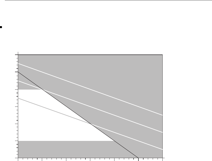
584 Glyn James, Advanced Modern Engineering Mathematics, 4th Edition
z:={_SL3 = -_SL1 + 1 + 3_SL2 - 2 x2,
x4 = -2 x1+3 -_SL1 - x2,
x3 =_SL1 + 1 -_SL2 + x2 + x1}
obj11:=eval(obj11,z);
obj11:=-2_SL2+14-2_SL1-x2
The new solutions are x1=x2=0,x
3=1,x
4=3andf= 14, giving, as expected,
the same function value.
The MATLAB instructions give the same result but no detail
f=[-6;-1;-2;-4];A=[2,1,0,1;1,0,1,1;1,1,3,2];b=[3;4;10];
options=optimset(‘LargeScale’,‘off’,‘Simplex’,‘on’);
[x,fval]=linprog(f,A,b,[],[],zeros(4,1),[],[],options)
Exercises 10.2.6
12 The problem can be easily plotted and it is clear that x=1,y=4 givesthe
solution f=x+2y=9.
6
5
4
3
2
1
12
y
x
3456
0
c
Pearson Education Limited 2011

Glyn James: Advanced Modern Engineering Mathematics, 4th edition 585
The MAPLE check is as follows:
with (simplex):
con12:={y>=1,y<=4,x+y<=5};
obj12:=x+2∗y;
maximize(obj12,con12,NONNEGATIVE);
# gives {y=4,x=1}
The graph can be plotted using the instructions
with(plots):
F:=inequal(con12,x=0..6,y=0..6):
G:=plot([(-x+7)/2,(-x+9)/2,(-x+11)/2],x=0..6,
thickness=3,labels=[‘x’,‘y’],color=yellow):
display(F,G);
13 The problem has ‘greater than’ constraints, so the two-phase method is
required. Note that a surplus variable x4and an artificial variable x7need to
be introduced. At the end of phase 1 the artificial variable x7will be eliminated
from the tableau. The cost function in phase 1 is −x7, but recall that this cost
has to be modified to ensure that the tableau is in standard form.
Phase 1
x1x2x3x4x5x6x7Soln
z−2−1 0 1 000−12
x341 1 0 000 32
x7210−1 001 12
x52−1 0 0 1 0 0 4
x6−21 0 0 010 8
x1x2x3x4x5x6x7Soln
z0−201 100−8
x30310 −200 24
x7020−1−1 0 1 8
x11−0.5 0 0 0.5 0 0 2
x60000 110 12
c
Pearson Education Limited 2011

586 Glyn James, Advanced Modern Engineering Mathematics, 4th Edition
x1x2x3x4x5x6x7Soln
z000 0 0 0 1 0
x3001 1.5−0.5 0 −1.5 12
x2010−0.5 −0.5 0 0.5 4
x1100−0.25 0.25 0 0.25 4
x6000 0 1 1 0 12
The artificial cost has been driven to zero so the artificial variable x7can be
eiiminated and the original cost function reinstated.
Phase 2
Note that the new cost is negative because the problem is a minimisation problem.
x1x2x3x4x5x6Soln
z000 3 −20−44
x3001 1.5 −0.5 0 12
x2010−0.5 −0.5 0 4
x1100−0.250.250 4
x60 0 0 0 1 1 12
x 2
30
f = 40
f = 30
f = 20
20
10
2468 x 1
2x1 + x2 = 12 4x1 + x2 = 32
2x1 – x2 = 4
– 2x1 – x2 = 8
c
Pearson Education Limited 2011

Glyn James: Advanced Modern Engineering Mathematics, 4th edition 587
x1x2x3x4x5x6Soln
z000 3 0 2 −20
x30011.500.5 18
x2010−0.5 0 0.5 10
x1100−0.25 0 −0.25 1
x50000 11 12
The solution is read off as x1=1,x
2= 10 with a minimal cost of 20.
14 Let Sbe the number of shoes produced and Bthe number of boots, then the
problem is to maximize the profit
z=8B+5S
production 2B+S≤250
sales B+S≤200
customer B≥25
The tableaux are constructed in the usual way.
Phase 1
BSPQ R TSoln
z−100 0 1 0−25
P2110 0 0 250
Q110 1 0 0 200
T1 0 0 0 −1 1 25
BSPQ R T Soln
z0000 0 1 0
P0110 2 −2 200
Q0101 1 −1 175
B1000−1125
Phase 2
BSPQRSoln
z0−500−8200
P0 1 1 0 2 200
Q01011175
B1000−125
c
Pearson Education Limited 2011
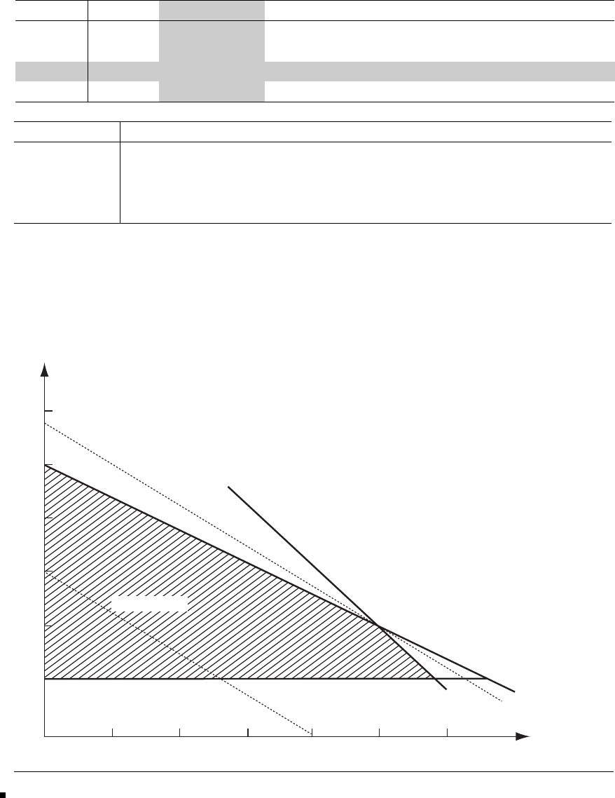
588 Glyn James, Advanced Modern Engineering Mathematics, 4th Edition
BSPQRSoln
z0−140 0 1000
R00.5 0.5 0 1 100
Q00.5 −0.5 1 0 75
B10.5 0.5 0 0 125
BS P Q R Soln
z0 0 3 2 0 1150
R00 1 −11 25
S01−1 2 0 150
B10 1 −10 50
Thus, the manufacturer should make 50 pairs of boots and 150 pairs of shoes and
the maximum profit is £1150.
A graphical solution is possible since the problem has only two variables. It is of
interest to follow the progress of the simplex solution on the graph.
boots
150
100
50
30 60
B = 25
90 120 150 180 shoes
profit = 1150
2B + S = 250
B + S = 200
profit = 600
15 There are techniques for adding a constraint to an existing solution and thence
determining the solution. However, here the whole problem will be recomputed.
From Exercise 9 the initial tableau can be constructed, but the additional constraint
is a ‘greater than’ constraint so the procedure for entering phase 1 must be followed.
c
Pearson Education Limited 2011

Glyn James: Advanced Modern Engineering Mathematics, 4th edition 589
b1b2b3b4b5b6b7Soln
z−1−1−10010−50
b41 1 0 1 0 0 0 15
b5321010060
b711 1 00−1150
Note that the last row gives the new constraint and that the z row involves the
artificial variable b7, which has been eliminated to bring the tableau to standard
form.
Phase I
b1b2b3b4b5b6b7Soln
z00−1 1010−35
b111 0 100015
b5 0 −1 1 −3 1 0 0 15
b700 1−10−1135
b1b2b3b4b5b6b7Soln
z0−10−2110−20
b11101 0 0015
b30−11−3 1 0015
b70102−1−1 1 20
b1b2b3b4b5b6b7Soln
z00 00 0 0 1 0
b11 0.5 0 0 0.5 0.5 −0.5 5
b300.510−0.5 −1.5 1.5 45
b400.501−0.5 −0.5 0.5 10
Phase 2
b1b2b3b4b5b6Soln
z0−200 0 0 300 0 18,000
b1 1 0.5 0 0 0.5 0.5 5
b300.5 1 0 −0.5 −1.5 45
b400.5 0 1 −0.5 −0.5 10
c
Pearson Education Limited 2011

590 Glyn James, Advanced Modern Engineering Mathematics, 4th Edition
b1b2b3b4b5b6Soln
z400 0 0 0 500 200 20,000
b121 0 0 1 1 10
b3−10 1 0−1−240
b410 0 1−1−15
The solution is optimal with the production schedule as none for book 1, 10,000
of book 2 and 40,000 of book 3. The profit is down to £20,000 because of the
additional constraint.
16 The MAPLE solution is presented.
with (simplex):
con16:={x>=1,x+2*y<=3,y+3*z<=4};
obj16:=x+y+z;
maximize(obj16,con16,NONNEGATIVE);
# gives the solution {y=0,z=4/3,x=3}, f=x+y+z=13/3
Note that there is no detail of the two-phase method and just the ‘answer’ is given.
It is not easy to rewrite phase 1 into MAPLE so that the detail can be extracted.
The same is true of MATLAB, the following instructions produce the correct result
f=[-1;-1;-1];A=[1,2,0;0,1,3;-1,0,0];b=[3;4;-1];
options=optimset(‘LargeScale’,‘off,’Simplex’,‘on’);
[x,fval]=linprog(f,A,b,[],[],zeros(3,1),[],[],options)
17 This is a standard two-phase problem with surplus variables x5,x
6and
artificial variables x7,x
8. With the cost constructed from the artificial variables
x7,x
8, and the tableau reduced to standard form, the sequence of tableaux is
presented.
Phase 1
x1x2x3x4x5x6x7x8Soln
z−1−1011100−2
x71 0 −1−1−10100
x90 1 1 0 0 −1 0 1 2
c
Pearson Education Limited 2011

Glyn James: Advanced Modern Engineering Mathematics, 4th edition 591
There is an arbitrary choice of the columns since two columns have the value −1;
the second one is chosen.
x1x2x3x4x5x6x7x8Soln
z−101110010
x71 0 −1−1−1 0 1 0 0
x201100−1012
x1x2x3x4x5x6x7x8Soln
z000000110
x110−1−1−10100
x201100−1012
The solution is optimal so phase 1 ends and the tableau is reconstituted for phase 2.
Phase 2
x1x2x3x4x5x6Soln
z00−1727−14
x110−1−1−10 0
x201 10 0−12
x1x2x3x4x5x6Soln
z010726−12
x1110−1−1−12
x3011 0 0−12
The solution is now optimal with x1=2,x
2=0,x
3=2,x
4=0andthecost
function being 12.
18 Let the company buy a,b,c litres of the products A,B,C, then the cost of the
materials will be
Cost
For a total of 100 litres
Glycol
Additive
1.8a+0.9b+1.5c
a+b+c= 100
0.65a+0.25b+0.8c≥50
0.1a+0.03b≥5
There are two ‘greater than’ constraints and an equality constraint. Recall that an
equality constraint is dealt with via an artificial variable. Thus, phase 1 is entered
c
Pearson Education Limited 2011

592 Glyn James, Advanced Modern Engineering Mathematics, 4th Edition
with two surplus variables and three artificial variables; the cost row is manipulated
until the tableau has the standard form.
Phase 1
ab cpqrstSoln
z−1.75−1.28 −1.81 1 000−155
r11 1 0 0 100 100
s0.65 0.250.8−1 0 0 1 0 50
t0.1 0.03 00−1 001 5
abcpqrstSoln
z−0.29−0.72 0−1.25102.250−42.5
r0.19 0.69 01.25 0 1 −1.25 0 37.5
c0.810.311−1.25001.25062.5
t0.1 0.03 0 0−10 0 15
abcpqrstSoln
z−0.1 −0.03 0 0 1 1 1 0 −5
p0.15 0.55 0 1 0 0.8−1030
c1 1 100100100
t0.1 0.03 0 0 −1 0 0 1 5
abcp q r s t Soln
z00 00 0 1 1 1 0
p0 0.51 0 1 1.5 0.8 −1−1.5 22.5
c00.710 10 1 0 −10 50
a10.300−10 0 0 10 50
The artificial cost has been driven to zero so phase 1 is complete and the three
artificial columns are deleted and the actual cost introduced. Recall that this is
a minimisation problem so the phase 2 tableau can now be extracted from the
tableau above.
Phase 2
abcpq Soln
z0−0.69 0 0 3 −165
p00.51 0 1 1.5 22.5
c00.71 0 10 50
a10.3 0 0 −10 50
c
Pearson Education Limited 2011

Glyn James: Advanced Modern Engineering Mathematics, 4th edition 593
abc p q Soln
z0 0 0 1.37 5.05 −134.26
b0 1 0 1.98 2.97 44.55
c001−1.39 7.92 18.81
a100−0.59 −10.89 36.63
The tableau is optimal so the solution can be read off as a=36.63%,
b=44.55%,c =18.81% and a minimum cost of £134.26.
MATLAB solves the problem as follows
f=[1.8;0.9;1.5];A=[-0.65,-0.25,-0.8;-0.1,-0.03,0];b=[-50;-5];
options=optimset(‘LargeScale’,‘off,‘Simplex’,‘on’);
[x,fval]=linprog(f,A,b,[1,1,1],[100],zeros(3,1),[],[],options)
% Note how MATLAB deals with the equality constraint
19 Let s1,s
2,s
3be the number of houses of the three styles the builder decides
to construct. His profit (×£100) is
10s1+15s2+25s3
and the constraints are
plots
facing stone
weather boarding
local authority
s1+2s2+2s3≤40
s1+2s2+5s3≤58
3s1+2s2+s3≤72
−s1+s2≥5
The solution requires the two-phase method. The tableaux are listed, to two
decimal places, without comment.
Phase 1
s1s2s3s4s5s6s7s8Soln
z1−1000010−5
s41221000040
s5125010 0 0 58
s6321001 0 0 72
s8−1 1 0 0 0 0 −1 1 5
c
Pearson Education Limited 2011

594 Glyn James, Advanced Modern Engineering Mathematics, 4th Edition
s1s2s3s4s5s6s7s8Soln
z0 00000 0 1 0
s43 02100 2 −230
s53 05010 2 −248
s65 01001 2 −262
s2−1 10000−115
Phase 2
s1s2s3s4s5s6s7Soln
z−250−25 000−15 75
s43 0 2100 230
s53 0 5 010 248
s65 0 1 001 262
s2−1 1 0 000 −15
s1s2s3s4s5s6s7Soln
z00−8.33 8.33 0 0 1.67325
s110 0.670.33 0 0 0.6710
s50 0 3 −1 1 0 0 18
s600−2.33 −1.6701−1.33 12
s201 0.670.33 0 0 −0.33 15
s1s2s3s4s5s6s7Soln
z0 0 0 5.56 2.78 0 1.67 375
s1100 0.56 −0.22 0 0.67 6
s3001−0.33 0.33 0 0 6
s6000−2.44 0.78 1 −1.33 26
s2010 0.56 −0.72 0 −0.33 11
The tableau is optimal, so the solution should build 6,11 and 6 houses of styles 1,2
and 3 respectively and make a profit of £37,500.
20 Let x1x2,x
3be the amounts (×1000 m2) of carpet of type C1,C2,C3 produced,
then the maximum of
2x1+3x2
is required subject to the constraints
c
Pearson Education Limited 2011

Glyn James: Advanced Modern Engineering Mathematics, 4th edition 595
M1 x1+x2+x3≤5
M2 x1+x2≤4
policy1 x1≥1
policy2 x1−x2+x3≥2
Phase 1
x1x2x3x4x5x6x7x8x9Soln
z21−1001 100−3
x411 1100 0005
x511 0010 0004
x61 0 0 0 0 −1 0 1 0 1
x91−11000−1012
x1x2x3x4x5x6x7x8x9Soln
z01100−1120−1
x401110 1 0 −10 4
x501001 1 0 −10 3
x110000−10101
x90−1 1 0 0 1 −1−1 1 1
x1x2x3x4x5x6x7x8x9Soln
z000000 0 1 10
x4020100 1 0−13
x5010011 0−103
x110000−10101
x30−11001−1−111
Phase 2
x1x2x3x4x5x6x7Soln
z03000−202
x4080 1 0 0 1 9
x501001 1 0 3
x110000−101
x301100 1 −11
x1x2x3x4x5x6x7Soln
z0001.50−21.5 6.5
x20100.50 00.51.5
x40 0 0 0.5 1 1 0.5 1.5
x11000 0 00 1.5
x30010.50 0−0.5 2.5
c
Pearson Education Limited 2011

596 Glyn James, Advanced Modern Engineering Mathematics, 4th Edition
x1x2x3x4x5x6x7Soln
z0 0 0 0.5 2 0 0.5 9.5
x20100.5 000.51.5
x6000−0.5 1 1 −0.5 1.5
x1100−0.5 1 0 −0.5 2.5
x3001 1 −100 1
Hence, the optimum is 2500 m2of C1, 1500 m2of C2 and 1000 m2of C3 giving a
profit of £9500.
Exercises 10.3.3
21 Introducing a Lagrange multiplier, the minimum is obtained from
2x+y+λ=0
x+2y+λ=0
x+y=1
with solution x=y=1/2. To prove that it is a minimum, put
x=1
2+εand y=1
2−ε
and substitute into fto give
f=3
4+ε2
and hence a minimum.
22 The answer to this exercise is geometrically obvious since it is just the length
of the minor axis which in this case, is a. It is required to find the minimum of
D2=x2+y2subject to x2
a2+y2
b2=1
The Lagrange equations are
0=2x+2λx
a2and 0 = 2y+2λy
b2
Since λcannot equal −a2and −b2at the same time then either x=0 or y=0.
If a<b the it is clear that y=0 and x=±agives the minimum
c
Pearson Education Limited 2011
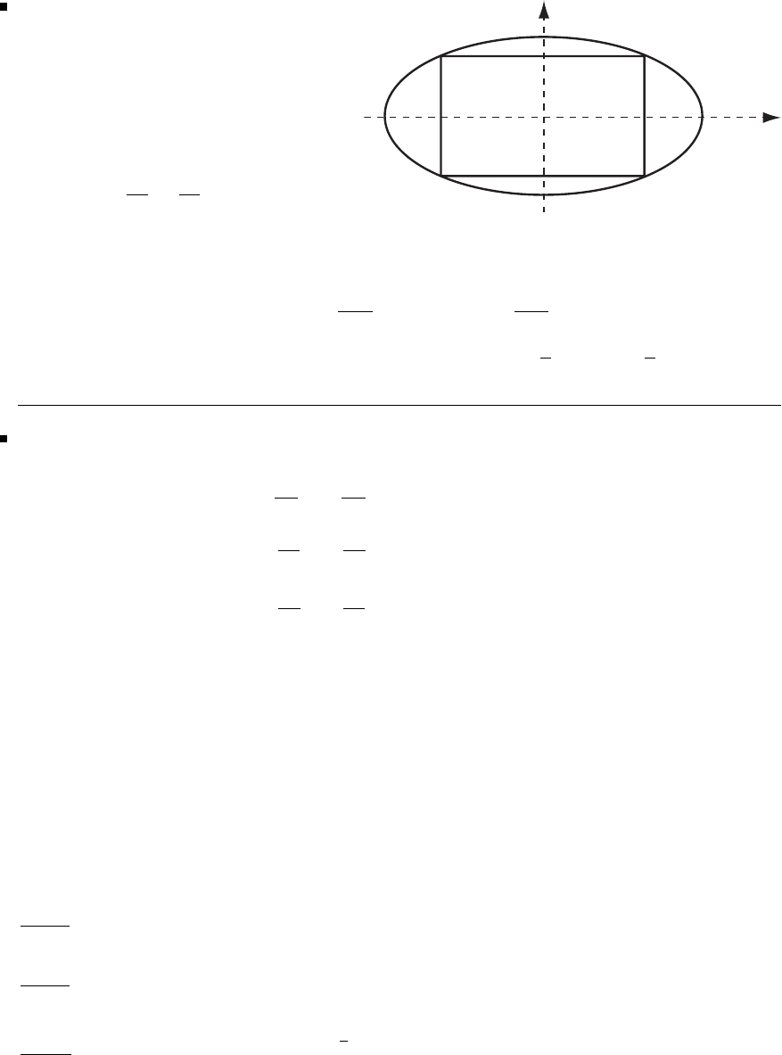
Glyn James: Advanced Modern Engineering Mathematics, 4th edition 597
23 The area of the rectangle is
A=4xy y
(x,y)
x
and since the point must lie
on the ellipse
x2
a2+y2
b2=1
and hence a Lagrange multiplier problem is produced. The two equations are
0=4y+2λx
a2and 0 = 4x+2λy
b2
It is soon checked that the required solution is x=a/√2,y=b/√2,A=2ab.
24 The necessary conditions for an optimum are
∂f
∂x +λ∂g
∂x =0=y2z+λ(1)
∂f
∂y +λ∂g
∂y =0=2xyz +2λ(2)
∂f
∂z +λ∂g
∂z =0=xy2+3λ(3)
together with the given constraint
x+2y+3z=6 (4)
Dividing equation (2) by two and then subtracting the first two equations gives
yz(x−y)=0
Thus, there are three cases
y=0 Note that all the equations except the constraint are satisfied since λ=0.
Thus, a possible solution is (6 −3α, 0,α) for any α.
z=0 Again, this implies that λ= 0 so from equation (3)x= 0 and hence from
(4)y= 3. The case when y= 0 in equation (3) has been covered in the first case.
x=yEquations (2) and (3) give 1
3x3=x2zso there are two cases
either x= 0 and hence y=0andz=2
c
Pearson Education Limited 2011

598 Glyn James, Advanced Modern Engineering Mathematics, 4th Edition
or x=3zand hence from (4) z=1/2andx=3/2,y =3/2
Equations (1) and (2) have been used to eliminate λ; so a similar exercise must be
undertaken with (2) and (3) to check whether any new solutions arise. They give
the equation
xy(y−3z)=0
and again three cases must be studied.
x=0 In this case λ= 0 so it reduces to one of the above.
y=0 Again, it reduces to the first case above.
y=3zFrom equations (1) and (2) it can be seen that the same cases arise and
correspond to the solutions already obtained.
Note that in the solutions quoted, (6,0,0) is included in the solution (6 −3α, 0,α)
with α=0.
25 Using λand μas the Lagrange multipliers, the equations that give the
optimum are as quoted
0=2x+λ+(2z−2y)μ
0=2y+λ+(z−2x)μ
0=2z−λ+(y+2x)μ
together with the two given constraints.
Adding the last two equations
2(y+z)+(y+z)μ=0⇒either y=−zor μ=−2
Adding the first and last equations
2(x+z)+(2z+2x−y)μ=0
So, λhas been eliminated.
y+z=0 In the first constraint x=−y+z=2z.Thus,(2t, −t, t)gives,in
the second constraint, 7t2=1 so t=±1/√7 and two of the quoted solutions are
obtained.
μ=−2From above 2(x+z)+(2z+2x−y)(−2) = 0 and so this expression
and the second constraint give a pair of equations
0=−x+y−z
0=x+y−z
c
Pearson Education Limited 2011
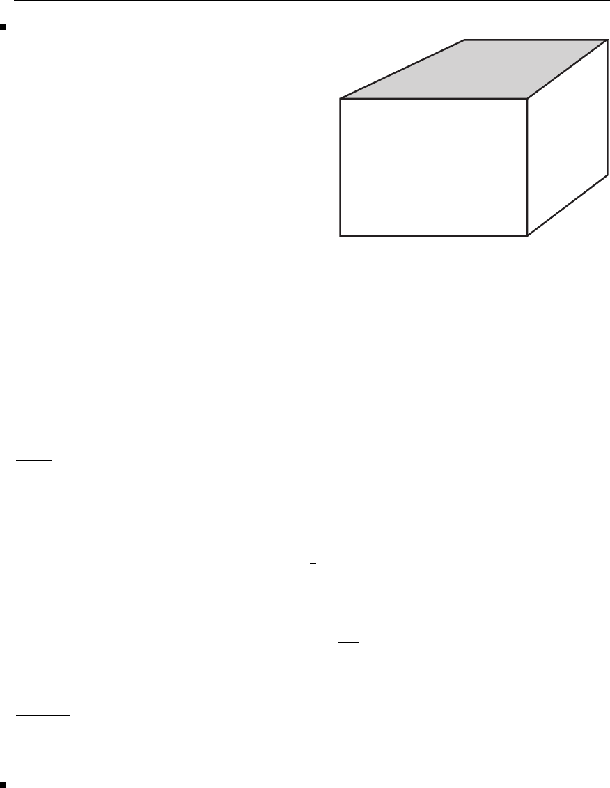
Glyn James: Advanced Modern Engineering Mathematics, 4th edition 599
and hence, x=0 and y=z. Putting these values into the second constraint gives
y=±1 and possible optimum points at (0, 1, 1) and (0,−1,−1).
26 The volume of the figure is
V=abc
and the surface area is
A=2ab +2ac +bc
c
a
b
The problem is a Lagrange multiplier
problem and the three equations are
0=bc +λ(2b+2c)
0=ac +λ(2a+c)
0=ab +λ(2a+b)
The last two equations give
a(c−b)+λ(c−b)=0⇒either c=bor λ=−a
c=bPutting back into the first equation gives
b2+4bλ = 0 so either b=0orλ=−b/4
The case b= 0 can be dismissed as geometrically uninteresting. In the third
equation this value of λgives 0 = ab −1
4b(2a+b)⇒b=2asince again the case
b= 0 is uninteresting.
Calculating agives the possible maximum as
c=b=2awith a=A
12 and V=4a3
λ=−aPutting this value back into the third of the Lagrange equations gives
a= 0 so gives zero volume and is geometrically uninteresting again.
27 This is a very tough problem but more typical of realistic problems in
engineering rather than most of the illustrative exercises in the book.
c
Pearson Education Limited 2011

600 Glyn James, Advanced Modern Engineering Mathematics, 4th Edition
The exercise will be solved using MAPLE. Note the efficient way it performs the
algebra and integrations for the simplest approximation
z:=A∗cos(Pi∗x/2)ˆ2∗cos(Pi∗y/2)ˆ2;
I1:int(int(z^2,x=-1..1),y=-1..1);
# gives
I1:=9/16 A2
f:=diff(z,x,x)+diff(z,y,y);
I2:=int(int(f^2,x=-1..1),y=-1..1);
# gives
I2:=1/2 A2Pi4
freq:=I2/I1;
# gives
freq:=8/9 Pi4= 86.58 as required.
The first approximation could be done by hand but the next approximation needs
a package like MAPLE.
zz:=cos(Pi∗x/2)ˆ2∗cos(Pi∗y/2)ˆ2
∗(A+B∗cos(Pi∗x/2)∗cos(Pi∗y/2));
I3:=evalf(int(int(zz^2,x=-1..1),y=-1..1));
# gives
I3:=.5624999999 A2+ .9222479291 A B + .3906249999 B2
ff:=diff(zz,x,x)+diff(zz,y,y);
I4:=evalf(int(int(ff^2,x=-1..1),y=-1..1));
# gives
I4:=58.21715209 B2+ 48.70454554 A 2+ 92.64268668 A B
dLbydA:=diff(I4+lam∗I3,A);
dLbydB:=diff(I4+lam∗I3,B);
fsolve({dLbydA,dLbydB,I3=1}, {A,B,lam});
# gives the solution
{lam=-81.38454660, A=-1.829151961, B=.6086242001}
The frequency is given by −lam which should be compared with the first
approximation.
c
Pearson Education Limited 2011

Glyn James: Advanced Modern Engineering Mathematics, 4th edition 601
28 The problem asks for a minimum, which is equivalent to the maximum of
−2x2
1−x2
2−2x1x2
The Kuhn–Tucker conditions for this problem are
−4x1−2x2−μ=0
−2x1−2x2+μ=0
x1−x2−α≤0
μ(x1−x2−α)=0
μ≥0
There are two cases
μ=0 The first two equations give x1=x2= 0 and these can only give the
optimum if the inequality is satisfied, namely α≥0.
x1−x2=αAdding the first two equations gives the solution in terms of the
simultaneous linear equations
3x1+2x2=0
x1−x2=α
which clearly have the solution x1=2α/5andx2=−3α/5. Calculation from the
first or second equation gives μ=−2α/5 which is only optimal if α≤0.
Exercises 10.4.2
29(a) The MATLAB version of this problem (note it deals with the maximum)
is as follows:
a=0.1;h=0.2;nmax=10;n=0;
zold=q29(a);a=a+h;z=q29(a);c=[z];
while(z(2)>zold(2))&(n<nmax)
n=n+1;zoldold=zold;zold=z;h=2∗h;a=a+h;z=q29(a);c=[c,z];
end
% gives x 0.3000 0.7000 1.5000 3.1000
f -11.4111 -2.7408 -1.9444 -3.2041
f73.0741 4.8309 -0.4074 -0.9329
where the function q29 is in the M-file
c
Pearson Education Limited 2011

602 Glyn James, Advanced Modern Engineering Mathematics, 4th Edition
function a=q29(x)
a=[x;-x-1/x^2;-1+2/x^3];
The maximum is in the region 0.7 to 3.1 only if the function values are known but
in the region 0.7 to 1.5 if the derivative is used.
29(b) Using the bracket and the mid point to start the maximization
p=[q29(0.7),q29(1.9),q29(3.1)]; u=p(1,:),v=p(2,:)
% gives u= 0.7000 1.9000 3.1000
v=-2.7408 -2.1770 -3.2041
[u,v]=qapp(u,v)
% gives u= 0.7000 1.7253 1.9000
v=-2.7408 -2.0612 -2.1770
[u,v]=qapp(u,v)
% gives u= 0.7000 1.5127 1.7253
v=-2.7408 -1.9497 -2.0612
where the M-file qapp.m contains the quadratic algorithm
function [x,f]=qapp(a,b) %note written for max problem
% a=[a1,a2,a3] is the input vector of three points from
bracketing
% b=[f(a1),f(a2),f(a3)] is the vector of function values
x=a;f=b;p=polyfit(a,b,2);
xstar=-0.5∗p(2)/p(1);z=q29(xstar);fstar=z(2);% for other
problems change q29
if fstar>b(2)
if xstar<a(2), x(3)=a(2);f(3)=b(2);
else x(1)=a(2);f(1)=b(2); end
x(2)=xstar;f(2)=fstar;
c
Pearson Education Limited 2011

Glyn James: Advanced Modern Engineering Mathematics, 4th edition 603
else
if xstar<a(2), x(1)=xstar;f(1)=fstar;
else x(3)=xstar;f(3)=fstar; end
end
% x contains the three points of the new bracket and f
the function values
29(c) For comparison the same bracket is used
p=q29(0.7);q=q29(3.1);p,q
% gives x=0.7000 f=-2.7408 f=4.8309
% and x=3.1000 f=-3.2041 f=-0.9329
[p,q]=cufit(p,q);p,q
% gives x=0.7000 f=-2.7408 f=4.8309
% and x=1.5129 f=-1.9498 f=-0.4224
[p,q]=cufit(p,q);p,q
% gives x=1.1684 f=-1.9009 f=0.2538
% and x=1.5129 f=-1.9498 f=-0.4224
where the cubic algorithm is contained in the M-file cufit.m
function [an,bn]=cufit(a,b)
% a=[x1 f(x1) fdash(x1)] and b=[x2 f(x2) fdash(x2)] are
the input vectors
f=[a(2);b(2);a(3);b(3)];
A=[a(1)^3 a(1)^2 a(1) 1;b(1)^3 b(1)^2 b(1) 1;
3∗a(1)ˆ22
∗a(1) 1 0;3∗b(1)ˆ22
∗b(1) 1 0];
p=A\f;xstar=(-p(2)-sqrt(p(2)ˆ2-3∗p(1)∗p(3)))/(3∗p(1));
c=q29(xstar);
% for other problems change the function q29
if c(3)>0 an=c;bn=b; else bn=c;an=a;end
% an and bn contain the new bracket values
c
Pearson Education Limited 2011

604 Glyn James, Advanced Modern Engineering Mathematics, 4th Edition
30 If the derivatives are not used, then the bracket is 0 <x<3, whilst using
the derivatives gives the much narrower range of 0 <x<1 but at the expense of
twice the number of function evaluations.
30(a) The calculation is identical to Exercise 29 with q29 replaced by q30 in qapp
p=[q30(0),q30(1),q30(3)]; u=p(1,:),v=p(2,:)
% gives u= 0 1 3
v= 0 0.4207 0.0141
[u,v]=qapp(u,v)
% gives u= 0 1.0000 1.5113
v= 0 0.4207 0.3040
[u,v]=qapp(u,v)
% gives u= 0 0.9898 1.0000
v= 0 0.4222 0.4207
where the function q30 is in the M-file
function a=q30(x)
a=[x;sin(x)/(1+xˆ2);cos(x)/(1+xˆ2)-2ˆ∗xˆ∗sin(x)/(1+xˆ2)ˆ2];
30(b) Again, as in Exercise 29, with q29 replaced by q30 in cufit
p=q30(0);q=q30(1);p,q
% gives x=0 f=0 f=1
% and x=1.0000 f=0.4207 f=-0.1506
[p,q]=cufit(p,q);p,q
% gives x=0 f=0 f=1
% and x=0.8667 f=0.4352 f=-0.0612
[p,q]=cufit(p,q);p,q
% gives x=0 f=0 f=1
% and x=0.8242 f=0.4371 f=-0.0247
The built in MATLAB procedure fminbnd gives x=0.7980,f =0.4374 in 9
iterations
c
Pearson Education Limited 2011

Glyn James: Advanced Modern Engineering Mathematics, 4th edition 605
f=@(x)-sin(x)/(1+x^2);
options=optimset(‘display’,‘iter’);
x=fminbnd(f,0,1,options)
31 The problem is a standard exercise to illustrate the use of the two basic
algorithms for a single variable search.
31(a) An adaptation of Exercise 29 with the appropriate function used gives
p=[q31(1),q31(5/3),q31(3)];u=p(1,:),v=p(2,:)
% gives u=1.0000 1.6667 3.0000
v=0.2325 0.2553 0.1419
[u,v]=qapp(u,v)
% gives u=1.000 1.6200 1.6667
v=0.2325 0.2571 0.2553
[u,v]=qapp(u,v)
% gives u=1.0000 1.4784 1.6200
v=0.2325 0.2602 0.2571
where q31 is the M-file
function a=q31(x)
a=[x;x∗(exp(-x)-exp(-2∗x));(exp(-x)-exp(-2∗x))
-x∗(exp(-x)-2∗exp(-2∗x))];
31(b) Use the same bracket and adapt the algorithm in Exercise 29.
p=q31(1);q=q31(3);p,q
% gives x=1.0000 f=0.2325 f = 0.1353
% and x=3.0000 f=0.1419 f= -0.0872
[p,q]=cufit(p,q);p,q
% gives x=1.0000 f=0.2325 f = 0.1353
% and x=1.5077 f=0.2599 f= -0.0136
[p,q]=cufit(p,q);p,q
c
Pearson Education Limited 2011

606 Glyn James, Advanced Modern Engineering Mathematics, 4th Edition
% gives x=1.0000 f=0.2325 f = 0.1353
% and x=1.4462 f=0.2603 f= -0.0001
The next iteration gives the three-figure accuracy required in (c).
x = 1.4456 f = 0.2603 f= 0.0000
32 The difficulty in this problem is that the eigenvalues must be computed at
each function evaluation. With a package such as MATLAB this is less of a problem
since the instruction eig(A) will give them almost instantly.
The M-file q32 performs this computation. Note the -max(eig(A)) since qapp
looks for a maximum
function a=q32(x)
A=[x -1 0;-1 0 -1;0 -1 x^2];
a=[x;-max(eig(A))];
The calculations are performed as in Exercise 29
p=[q32(-1),q32(0),q32(1)];u=p(1,:),v=p(2,:)
% gives u=-1 0 1
v=-1.7321 -1.4142 -2.0000
[u,v]=qapp(u,v)
% gives u=-1.0000 -0.1483 0
v=-1.7321 -1.3854 -1.4142
[u,v]=qapp(u,v)
% gives u=-1.0000 -0.2356 -0.1483
v=-1.7321 -1.3769 -1.3854
See the text for the MATLAB fminbnd code for this problem.
33 To establish the formula is a matter of simple substitution into (10.10).
To find when f(x) = 0, from the Newton method, requires the iteration of the
formula
xnew =x−f(x)
f(x)
If the function is known at x−h, x, x +hwith values f1,f
2,f
3respectively, then
the derivatives can be replaced by their approximations
c
Pearson Education Limited 2011
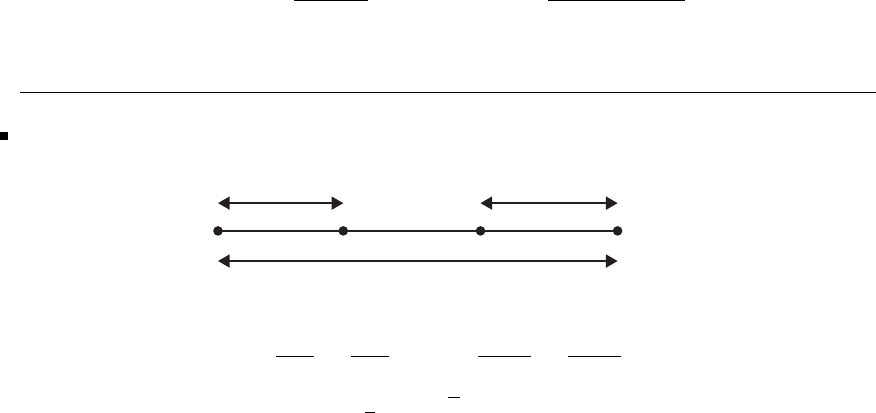
Glyn James: Advanced Modern Engineering Mathematics, 4th edition 607
f(x)≈f3−f1
2hand f(x)≈f1−2f2+f3
h2
and the formula follows immediately.
34(a) To obtain the Golden Section ratio, the figure gives
AC B D
ll
L
AC
AD =AD
AB
yields
−→ l
L−l=L−l
L
Solve for a=l/L to obtain a=1
2(3 −√5).
TheGoldenSectionalgorithmcanbewritteninMATLABas
alpha = (3-sqrt(5))/2;a=[0;1;1;2.5];
f=@(x)x∗sin(x);
a=[0;(1-alpha)∗a(1)+alpha∗a(4);alpha∗a(1)+(1-alpha)∗a(4);2.5];
F=[f(a(1));f(a(2));f(a(3));f(a(4))];aa=[a];FF=[F];
for i=1:5
if F(2)>F(3)a(4)=a(3);a(3)=a(2);F(4)=F(3);F(3)=F(2);
a(2)=(1-alpha)∗a(1)+alpha∗a(4);F(2)=f(a(2));
else a(1)=a(2);a(2)=a(3);F(1)=F(2);F(2)=F(3);
a(3)=alpha∗a(1)+(1-alpha)∗a(4);F(3)=f(a(3));
end, aa=[aa,a];FF=[FF,F];
end
The instructions aa, FF prints out xand fat five successive iterations
aa = 0 0.9549 1.5451 1.9098 1.9098 1.9098
0.9549 1.5451 1.9098 2.1353 2.0492 1.9959
1.5451 1.9098 2.1353 2.2746 2.1353 2.0492
2.5000 2.5000 2.5000 2.5000 2.2746 2.1353
c
Pearson Education Limited 2011

608 Glyn James, Advanced Modern Engineering Mathematics, 4th Edition
FF = 0 0.7795 1.5446 1.8011 1.8011 1.8011
0.7795 1.5446 1.8011 1.8040 1.8191 1.8183
1.5446 1.8011 1.8040 1.7341 1.8040 1.8191
1.4962 1.4962 1.4962 1.4962 1.7341 1.8040
with the best value at x=2.0492 and f=1.8191.
34(b) The algorithm is the same as part (a) except the function is now
f=@(x)(log(x)+2∗(1-x)/(1+x))/(1-x)∧2;
The five iterations give
aa =
1.5000 1.8820 1.8820 2.0279 2.1180 2.1180
1.8820 2.1180 2.0279 2.1180 2.1738 2.1525
2.1180 2.2639 2.1180 2.1738 2.2082 2.1738
2.5000 2.5000 2.2639 2.2639 2.2639 2.2082
FF =
0.0218604 0.0260436 0.0260436 0.0265463 0.0266783 0.0266783
0.0260436 0.0266783 0.0265463 0.0266783 0.0267059 0.0266998
0.0266783 0.0266780 0.0266783 0.0267059 0.0267051 0.0267059
0.0262879 0.0262879 0.0266780 0.0266780 0.0266780 0.0267051
Note that the function is so flat that it has been quoted to six figures; the best
result is x=2.1738,f =0.0267059.
Exercises 10.4.4
35 The gradient is given by
G=1
0+1−1
−12
x1
x2
so, at the first step
a=1
1,f=1.5,G=1
1
c
Pearson Education Limited 2011

Glyn James: Advanced Modern Engineering Mathematics, 4th edition 609
The first search is for min
μ[f(1 −μ, 1−μ)] and a simple calculation gives μ=2.
The second iteration can be started as
a=−1
−1,f=−0.5,G=1
−1
Note that the two gradients are perpendicular. The search min
μ[f(−1−μ, −1+μ)]
is easily performed (exactly in this problem) to give μ=0.4 and the problem is
ready for the next iteration.
a=−7/5
−3/5,f=−0.9,G=1/5
1/5
36 For this function the gradient is
G=6x+2y+3
2x+6y+2
and it easily checked that x=−7/16,y =−3/16 gives zero gradient and hence
the minimum at f=−0.84375.
The steepest descent method is easily written in MATLAB. For more complicated
functions two M-files are needed, one to set up the function and its gradient and
the second to set up the line search routine. Anonymous functions can be used for
more .straightforward functions. The following lines of code solve the problem.
f=@(x)2∗(x(1)+x(2))ˆ2+(x(1)-x(2))ˆ2+3∗x(1)+2∗x(2);
g=@(x)[4∗(x(1)+x(2))+2∗(x(1)-x(2))+3;4∗(x(1)+x(2))-2∗(x(1)-x(2))+2];
fm=@(t,xx,G)f(xx-t∗G);
% The function, its derivative and the line search are now set
xx=[0,0];ff=f(xx);G=g(xx);XX=[xx];FF=[ff];GG=[G];%Startvalues
[t,fval]=fminbnd@(t)fm(t,xx,G),0,2);% Note how the minimisation is done
xx=xx-t∗G;G=g(xx);ff=f(xx);XX=[XX,xx];GG=[GG,G];FF=[FF,ff];
%Next point
%Repeat the last two lines to iterate
c
Pearson Education Limited 2011

610 Glyn James, Advanced Modern Engineering Mathematics, 4th Edition
The first five values are produced in XX,FF and GG as
XX= 0 -0.3824 -0.4296 -0.4365 -0.4374
0 -0.2549 -0.1841 -0.1887 -0.1874
FF= 0 -0.8284 -0.8435 -0.8437 -0.8437
GG= 3.0000 0.1961 0.0545 0.0036 0.0010
2.0000 -0.2941 0.0363 -0.0053 0.0007
Because the function is a quadratic, the Newton method, which is based on the
assumption that the function is approximated by a quadratic, must converge in
one iteration.
37 The MATLAB implementation is similar to Exercise 36.
The program is identical except for the instructions that generate the functions,
which are now
f=@(x)(x(1)-x(2)+x(3))∧2+(2∗x(1)+x(3)-2)∧2+(x(3) ∧2-1) ∧2;
g=@(x)[2∗(x(1)-x(2)+x(3))+4∗(2∗x(1)+x(3)-2);2 ∗(x(1)-x(2)+x(3));...
2∗(x(1)-x(2)+x(3))+2∗(2∗x(1)+x(3)-2)+4∗x(3)∗(x(3) ∧2-1)];
The first few iterations are
XX = 2.0000 1.1518 0.4985 0.6175 0.4941 0.5178
2.0000 2.1696 1.8171 1.7505 1.6616 1.6358
2.0000 0.4733 0.7984 0.9653 1.0178 1.0300
FF = 29.0000 1.5023 0.4440 0.0729 0.0237 0.0158
GG = 20.0000 2.0184 -1.8592 0.4657 -0.2758 0.0859
-4.0000 1.0891 1.0405 0.3354 0.2995 0.1762
36.0000 -1.0044 -2.6078 -0.1980 -0.1414 0.2054
To use the built in routine fminunc, it is easier to use an M file.
function [f,g] = q37(x) %Question 37
f=(x(1)-x(2)+x(3))∧2+(2∗x(1)+x(3)-2)∧2+(x(3)∧2-1) ∧2;
g=[2∗(x(1)-x(2)+x(3))+4∗(2∗x(1)+x(3)-2);2∗(x(1)-x(2)+x(3));...
2∗(x(1)-x(2)+x(3))+2∗(2∗x(1)+x(3)-2)+4∗x(3)∗(x(3) ∧2-1)];
end
c
Pearson Education Limited 2011

Glyn James: Advanced Modern Engineering Mathematics, 4th edition 611
The main progam is
x=[2;2;2];
options=optimset(‘GradObj’,‘on’,‘display’,‘iter’,‘HessUpdate’,
‘steepdesc’,‘LargeScale’,‘off’);
[x,fval]=fminunc(@q37,x,options)
The first three and last three iterations are
Iteration Func-count f(x)
0 1 29 with starting point x=(2,2,2)
1 2 3.67901
2 4 2.35628
.............
59 119 8.6485e-010
60 121 6.17926e-010
61 123 4.41502e-010 with final point x=(0.5,1.5,1.0)
38 The function, gradient and Hessian matrix are computed in the M-file
newton38
function [a,agrad,ajac]=newton38(z)
t1=z(1)-z(2)+z(3);t2=2∗z(1)+z(3)-2;
a=t1ˆ2+t2ˆ2+(z(3)ˆ2-1)ˆ2;
agrad(1)=2∗t1+4∗t2;
agrad(2)=-2∗t1;
agrad(3)=2∗t1+2∗t2+4∗z(3)ˆ3-4 ∗z(3);
ajac(1,1)=10;ajac(1,2)=-2;ajac(1,3)=6;
ajac(2,1)=-2;ajac(2,2)=2;ajac(2,3)=-2;
ajac(3,1)=6;ajac(3,2)=-2;ajac(3,3)=12∗z(3)ˆ2;
and the Newton iteration proceeds as
a=[2;2;2];E=[0;0;0;0];
for i=1:5
[f,G,J]=newton38(a);E=[E,[f;a]];
c
Pearson Education Limited 2011
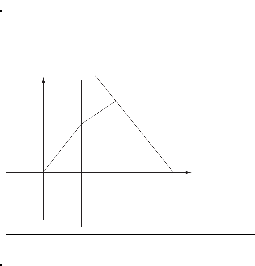
612 Glyn James, Advanced Modern Engineering Mathematics, 4th Edition
a=a-J\G;
end
% gives
f 29.0000 1.2448 0.1056 0.0026 0.0000
x 2.0000 0.2727 0.4245 0.4873 0.4995
y 2.0000 1.7273 1.5755 1.5127 1.5005
z 2.0000 1.4545 1.1510 1.0253 1.0009
39 The figure illustrates the cost of the road from (0,0) to (1,a)to(b,11-2b)is
C=2(1+a2)1/2+(b−1)2+(11−2b−a)21/2
and any of the minimization methods give a= 0.2294, b= 4.5083 and c= 5.9743,
giving equations of lines as y=0.2294x, y =0.5x−0.2706 and cost = 5.974.
y
(1,a)
(b,11– 2b)
y = 11 – 2x
x
(0,0)
Exercises 10.4.7
40(a) The gradient can be calculated as G=10x−2y−8
−2x+2yand the initial
choice of His the unit matrix.
c
Pearson Education Limited 2011

Glyn James: Advanced Modern Engineering Mathematics, 4th edition 613
Iteration 1
The computation commences
a1=2
2f1=4G1=8
0H1=10
01
and the minimization takes place in the direction a=2−8λ
2. The minimum
in this direction may be obtained as λ=0.1. The new values are
a2=1.2
2f2=0.8G2=0
1.6
and the values of h1and y1are calculated as
h1=a2−a1=−0.8
0and y1=G2−G1=−8
1.6
Finally, the His updated as
H2=10
01
−1
66.56 −8
1.6[−81.6] + 1
6.4−0.8
0[−0.80]
=10
01
−0.9615 −0.1923
−0.1923 0.0385 +0.10
00
=0.1385 0.1923
0.1923 0.9615
Iteration 2
The iteration starts with the variables computed from iteration 1
a2=1.2
2f2=0.8G2=0
1.6H2=0.1385 0.1923
0.1923 0.9615
The method follows the same pattern as iteration 1 and so the computations are
not written down in the same detail.
a3=1
1f3=0G3=0
0H3=0.1250 0.1250
0.1250 0.6250
The minimum has been achieved; this is expected since the function is quadratic
and it is known that the method converges in nsteps for an n-dimensional
quadratic, provided the minimizations are performed exactly.
c
Pearson Education Limited 2011

614 Glyn James, Advanced Modern Engineering Mathematics, 4th Edition
40(b) The problem has three variables and is not quadratic. The one-dimensional
minimizations need a numerical procedure; so it is better to use a package such as
MATLAB. The M-file required for the function is
function [f,G]=q40b(z)
t1=z(1)-z(2)+z(3);t2=2∗z(1)+z(3)-2;
f=t1ˆ2+t2ˆ2+z(3)ˆ4;
G(1)=2∗t1+4∗t2;
G(2)=-2∗t1;
G(3)=2∗t1+2∗t2+4∗z(3)ˆ3;
The main DFP segment is
1. a=[0;0;0];H=eye(3);[f,G]=q40b(a);
2. fm=@(t,xx,GG)q40b(xx-t∗GG);
3. aa=[a];ff=[f];gg=[G];HH=[H];
4. for n=1:4
5. D=H∗G;[t,fval]=fminbnd(@(t)fm(t,a,D),0,2);
6. aold=a;Gold=G;a=aold-t∗D;[f,G]=q40b(a);
7. h=a-aold;y=G-Gold;
8. H=H-H∗y∗y’∗H/(y’∗H∗y)+h∗h’/(h’ ∗y);
9. aa=[aa,a];ff=[ff,f];gg=[gg,G];HH=[HH,H];
10. end
The instructions give the results
aa= 0 0.5853 1.0190 1.0186 1.0184
0 0 0.9813 0.9814 0.9815
0 0.2926 -0.0372 -0.0372 -0.0369
ff= 4.0000 1.0662 0.0000 0.0000 0.0000
gg= -8.0000 -0.3916 0.0047 -0.0000 -0.0000
0 -1.7558 -0.0012 -0.0001 -0.0000
-4.0000 0.7823 0.0027 -0.0002 -0.0002
The convergence looks good but slows because Htends to a singular matrix.
c
Pearson Education Limited 2011

Glyn James: Advanced Modern Engineering Mathematics, 4th edition 615
41 Evaluating Hi+1 yiit is readily shown that equation (10.18) is satisfied.
The update is one that is quite effective but suffers from the problem that the
denominator can become zero when line searches are not exact. A great deal of
remedial action must be taken to ensure that the problem is overcome.
41(a) The function is quadratic so the solution is obtained in two steps. The
program in Exercise 39, suitably adapted, was used to compute the solution.
Iteration 1
a=1
2f=9G=2
8H=10
01
Iteration 2
a=0.4848
−0.0606 f=0.2424 G=0.9697
−0.2424 H=0.9948 −0.0619
−0.0619 0.2577
41(b) The exercise is similar to Exercise 40(b) but with a different function and
updating methods.
function [f,G]=q41b(z)
t1=z(1);t2=z(1)-z(2)+1;
f=t1ˆ2+t2ˆ2+z(2)ˆ2∗z(3)ˆ2;
G(1)=2∗t1+2∗t2;
G(2)=-2∗t2+2∗z(2)∗z(3)ˆ2;
G(3)=2∗z(3)∗z(2)ˆ2;
In the lines 1,2 and 6 of Exercise 40(b) the M file q41b replaces q40b. In line 8, the
Rank 1 and the BFGS updates replace the one in the program. Also, a different
start point is used. The results for Rank 1 update (i) are
aa= 0.5000 -0.0732 -0.1628 -0.00592 -0.0593
0.5000 0.8344 0.7747 0.9235 0.9234
0.5000 0.4522 0.0525 -0.0640 -0.0640
ff= 1.3125 0.1563 0.0321 0.0073 0.0073
gg= 3.0000 0.0386 -0.2006 -0.0839 -0.0839
-1.7500 0.1564 -0.1207 -0.0270 -0.0270
0.2500 0.6296 0.0630 -0.1091 -0.1092
c
Pearson Education Limited 2011

616 Glyn James, Advanced Modern Engineering Mathematics, 4th Edition
The results for BFGS update (ii) are
aa= 0.5000 -0.0732 0.0969 -0.0726 -0.0348
0.5000 0.8344 0.7384 0.9408 0.9344
0.5000 0.4522 0.0659 0.0141 0.0071
ff= 1.3125 0.1563 0.0389 0.0056 0.0022
gg= 3.0000 0.0386 0.1355 -0.1718 -0.0080
-1.7500 0.1564 -0.3229 0.0271 -0.0614
0.2500 0.6296 0.0718 0.0250 0.0124
Note that BFGS does better than Rank 1 and is the choice of method for the
built-in function fminunc.
42 It is easy to check that equation (10.18) is satisfied but note that the notation
has changed and y,hhave been replaced by u,vrespectively.
Hu=Hu +vpTu−HuqTu
=Hu +v−Hu =vsince pTu=qTu=1
To match with the Davidon formula (10.19) first choose β=α= 0 and hence
pTu=αvTu=1andqTu=βuTHu =1
Substituting gives
H=H−HuuTH
uTHu +vvT
vTu
as required.
The formula in Exercise 41(i) is obtained by putting β=β=−α=−α.Thus
p=q=α(V−Hu) and hence pTu=α(v−Hu)Tu=1
Substituting gives the formula
H=H+(v−Hu)(v−Hu)T
(v−Hu)Tu
This whole class of solutions was devised by Huang. Many general results can be
proved for this class and many of the commonly used formulae are included in it.
c
Pearson Education Limited 2011

Glyn James: Advanced Modern Engineering Mathematics, 4th edition 617
43 (a) The Fletcher-Reeves method is easily written as a MATLAB segment
global a b p
a=1;b=1;g=[3∗a;b];p=-g;
lam=fminbnd(@ffr,0,2)
% gives lam = 0.3571
a=a+lam∗p(1),b=b+lam∗p(2),gold=g;g=[3∗a;b]
% gives a= -0.0714 b= 0.6429 g= -0.2143 0.6429
p=-g+p∗(g∗g)/(gold ∗gold)
% gives p= 0.0765 -0.6888
lam=fminbnd(@ffr,0,2)
% gives lam = 0.9333
a=a+lam∗p(1),b=b+lam∗p(2),gold=g;g=[3∗a;b]
% gives a=-4.0246e-016 b=-1.1102e-016
which is the minimum point. The M-file used is
function v=ffr(x)
global a b p
v=3∗(a+x∗p(1))ˆ2+(b+x∗p(2))ˆ2;
43(b) The three-variable problem is handled in a similar manner.
global abcp
a=0.5;b=0.5;c=0.5;
f=(a-b+1)ˆ2+aˆ2∗bˆ2+(c-1)ˆ2;
g=[2∗(a-b+1)+4∗a∗bˆ2;-2∗(a-b+1)+2∗aˆ2∗b;2∗(c-1)];
p=-g;W=[f;a;b;c];
for i=1:5
gold =g;lam=fminbnd(@ffr2,-2,2);
a=a+lam∗p(1);b=b+lam∗p(2);c=c+lam∗p(3);
f=(a-b+1)ˆ2+aˆ2∗bˆ2+(c-1)ˆ2;W=[W[f;a;b;c]];
g=[2∗(a-b+1)+4∗a∗bˆ2;-2∗(a-b+1)+2∗aˆ2∗b;2∗(c-1)];
p=-g+p∗(g∗g)/(gold ∗ gold);
end
c
Pearson Education Limited 2011

618 Glyn James, Advanced Modern Engineering Mathematics, 4th Edition
W
% gives the sequence of iterations
f 1.3125 0.0764 0.0072 0.0007 0.0004 0.0000
a 0.5000 -0.0950 0.0057 -0.0251 -0.0079 -0.0032
b 0.5000 0.9165 0.9276 0.9633 0.9742 0.9978
c 0.5000 0.7380 0.9674 1.0009 1.0044 1.0014
Review Exercises 10.7
1The successive tableaux are as follows:
x1x2x3x4x5Soln
z−12−8000 0
x31 1 100350
x421 0 1 0 600
x51 3 001900
x1x2x3x4x5Soln
z0−20 6 0 3600
x300.5 1−0.5 050
x110.5 0 0.5 0 300
x502.5 0 −0.5 1 600
x1x2x3x4x5Soln
z0 0 4 4 0 3800
x201 2−1 0 100
x110−1 1 0 250
x500−5 2 1 350
Hence the solution is read from the table as x1= 250,x
2= 100 and F = 3800 .
2Let x1,x
2,x
3be the numbers of sailboard constructed of types 1,2,3. The
profit is
10x1+15x2+25x3
and the constraints are
5x1+10x2+25x3≤290
3x1+2x2+x3≤72
10x1+20x2+30x3≤400
c
Pearson Education Limited 2011

Glyn James: Advanced Modern Engineering Mathematics, 4th edition 619
The system only has ‘less than’ inequalities so the initial and subsequent tableaux
canbewrittendownimmediately.
x1x2x3x4x5x6Soln
z−10 −15 −25000 0
x4510 25 1 0 0 290
x5321 010 72
x610 2030 001400
x1x2x3x4x5x6Soln
z−5−501 00290
x30.20.410.040 0 11.6
x52.81.6 0 −0.041 0 60.4
x64 8 0−1.20 1 52
x1x2x3x4x5x6Soln
z050−0.5 0 1.25 355
x30010.1 0 −0.05 9
x50−400.81−0.724
x1120−0.3 0 0.2513
x1x2x3x4x5x6Soln
z0 2.5 0 0 0.62 0.81 370
x300.510−0.12 0.04 6
x40−5011.25−0.88 30
x11 0.5 0 0 0.37 −0.01 22
The solution is x1=22,x
2=0,x
3= 6 and maximum profit is £370.
3Let x1,x
2,x
3be the number of standard, super and deluxe cars respectively,
then the profit function is
100x1+ 300x2+ 400x3
and the constraints are
10x1+20x2+30x3≤1600
10x1+15x2+20x3≤1500
x2+x3≤50
x1+x2+x3≥70
c
Pearson Education Limited 2011

620 Glyn James, Advanced Modern Engineering Mathematics, 4th Edition
The problem includes a ‘greater than’ inequality, so the two-phase approach is
needed. An artificial variable is introduced and the artificial cost is introduced in
phase 1. The zrow of the tableau is manipulated to bring it to standard form.
x1x2x3x4x5x6x7x8Soln
z−1−1−100010−70
x410 20 30 1 0 0 0 0 1600
x510 15 20 0 1 0 0 0 1500
x60110010050
x81 1 1 0 0 0 −1 1 70
x1x2x3x4x5x6x7x8Soln
z0000000 10
x40102010010−10 900
x5051001010−10 800
x60110010 050
x1111000−1170
A feasible solution has been obtained so the method moves to phase 2. The zrow
is first re-calculated
x1x2x3x4x5x6x7Soln
z0−200 −300 0 0 0 −100 7000
x4010 20 1 0 0 10 900
x505 10 0 1 0 10 800
x601 1 001 0 50
x111 1 000 −170
x1x2x3x4x5x6x7Soln
z0−50015 005020500
x300.5 1 0.05 0 0 0.5 45
x5000−0.5 1 0 5 350
x600.5 0−0.05 0 1 −0.5 5
x110.5 0 −0.05 0 0 −1.5 25
x1x2x3x4x5x6x7Soln
z0 0 0 10 0 100 0 21,000
x3001 0.10−11 40
x5000 −0.5 1 0 5 350
x2010 −0.01 0 2 −110
x1100 0 0−1−120
c
Pearson Education Limited 2011

Glyn James: Advanced Modern Engineering Mathematics, 4th edition 621
The solution is read off the table as x1=20,x
2=10,x
3= 40 and the maximum
profit is £21,000.
Note that the (z, x7) entry is zero; so a non-unique solution is expected. Inter-
changing the x3and x7entries and completing one further tableau gives the
alternative solution x1=60,x
2=50,x
3= 0 and profit is still £21,000.
The MAPLE solution
with(simplex):
cor3:={10∗x+20∗y+30∗z<=1600,10 ∗x+15 ∗y+20 ∗z<=1500,
y+z<=50,x+y+z>=70};
obr3:=100∗x+300∗y+400∗z;
maximize(obr3,cor3,NONNEGATIVE);
# gives the solution {x=20, z=40,y=10}
MAPLE provides the same solution but does not identify the alternative solution.
Similarly, for the corresponding MATLAB code, which is
f=[-100,-300,-400];A=[10,20,30;10,15,20;0,1,1;-1,-1,-1];b=[1600;1500;50;-70];
options=optimset(‘LargeScale’,‘off’,‘Simplex’,‘on’);
[x,fval]=linprog(f,A,b,[],[],zeros(3,1),[],[],options)
4Let the student buy x1kg of bread and x2kg of cheese, then the cost to be
minimized is
60x1+ 180x2
and the two constraints are
1000x1+ 2000x2≥3000
25x1+ 100x2≥100
There are two surplus and two artificial variables in the tableau and the artificial
cost function which has been processed to standard form.
Phase 1
x1x2x3x4x5x6Soln
z−1025−21001100−3100
x51000 2000 −1 0 1 0 3000
x625100 0−1 0 1 100
c
Pearson Education Limited 2011

622 Glyn James, Advanced Modern Engineering Mathematics, 4th Edition
x1x2x3x4x5x6Soln
z−500 0 1 −200 21−1000
x5500 0−120 1 −201000
x20.251 0 −0.01 0 0.01 1
x1x2x3x4x5x6Soln
z00 0 0 1 1 0
x110−0.002 0.04 0.002 −0.04 2
x20 1 0.0002 −0.02 −0.0002 0.02 0.5
Phase 1 is completed so the tableau is reconstituted as
x1x2x3x4Soln
z0 0 0.03 1.2 −210
x110−0.002 −0.04 2
x20 1 0.0002 0.02 0.5
It may be noted that the zrow entries are positive; so the tableau is optimal and
there is no need to enter phase 2. Thus the minimum cost of the diet is 210p and
is made up of 2 kg of bread and 0.5 kg of cheese.
5The square of the distance from the origin to the point (x, y)is
f=x2+y2
so the problem is to optimize this function subject to the condition that it lies on
the curve
g=x2−xy +y2−1=0
so
0= ∂f
∂x +λ∂g
∂x =2x+λ(2x−y)
0=∂f
∂y +λ∂g
∂y =2y+λ(−x+2y)
Subtracting these two equations gives
0=2(x−y)+λ(3x−3y)⇒x=yor λ=−2
3
c
Pearson Education Limited 2011

Glyn James: Advanced Modern Engineering Mathematics, 4th edition 623
Adding the two equations gives
0=2(x+y)+λ(x+y)⇒x=−yor λ=−2
The first possibility, x=y, gives the points, (1,1) and (−1,−1) with f=2in
each case and the second possibility, x=−y,gives
1
√3,−1
√3and −1
√3,1
√3with f=2
3
In this problem the cases λ=−2
3and λ=−2 reproduce the identical solutions.
Although it is not proved, the first solution is the maximum and the second the
minimum.
6The volume of the solid is
V=x3+y3
where the sides of the two cubes are xand y. The surface area has essentially the
area of two faces of the smaller cube removed so
S=7=6x2+4y2
The Lagrange multiplier equations are
3x2+12xλ =0
3y2+8yλ =0
The solutions when x=y= 0 can be dismissed since the volume is zero. There
are three other cases
Case 1 x=0,y=−8
3λ=7
4,V=7
43
2
Case 2 y=0,x=−4λ=7
6,V=7
63
2
Case 3 x=−4λ, y =−8
3λ, ⇒7=96λ2+256
9λ2
c
Pearson Education Limited 2011

624 Glyn James, Advanced Modern Engineering Mathematics, 4th Edition
and hence λ=±3
(4√10) so the sides have lengths 3
√10 and 2
√10 and volume 35
(10) 3
2
The cases when either x=0 or y= 0 imply that the problem has collapsed to a
single cube so these solutions are omitted as geometrically uninteresting.
7The problem is to maximize the distance
(x−1)2+y2+z2
subject to
2x+y2+z=8
The Lagrange equations are
2(x−1) + 2λ=0⇒x=1−λ
2y+2yλ =0⇒y=0orλ=−1
2z+λ=0⇒z=−1
2λ
There are two cases
y=0
gives λ=−12
5so x=17
5,y=0,z=6
5
λ=−1
gives x=2,z=1
2and y=±7
2
The first of these possibilities gives the maximum distance.
8The Lagrange equations for this problem are
1+2λx =0
2+2λy =0
3+2λz =0
and putting back into the constraint gives 2λ=±1.The local extrema are therefore
at (1,2,3) and (−1,−2,−3) with corresponding F=14 and F=−14.
c
Pearson Education Limited 2011

Glyn James: Advanced Modern Engineering Mathematics, 4th edition 625
To obtain the global extremum all the points on each of the boundaries must be
examined. However, in this case, the geometry is sufficiently simple to establish
the result. The region is the inside of the sphere of radius √14 in the region
where all the variables are positive. The cost function comprises a series of parallel
planes, so the global maximum in the region is the local maximum at (1,2,3) and
the global minimum in the region is when all the variables are zero, namely (0,0,0)
and F=0.
9(i) We are given that 2s=a+b+c, so maximizing A2with respect to band
c, together with this constraint, gives
∂(A2)
∂b =s(s−a)(s−c)+λ=0,∂(A2)
∂c =s(s−a)(s−b)+λ=0
Clearly b=cand the triangle is isosceles.
(ii) Now, as a so to the above equations we add
∂(A2)
∂a =s(s−b)(s−c)+λ=0
and we see that we must have a=b=cand the triangle is equilateral.
10 We need to consider the problem of maximizing
V=πr2hsubject to the constraint a
r2+π
h2=b
Using the Lagrange multiplier approach we have the two equations
∂V
∂r =2πrh −2a2
r3λ=0
∂V
∂h =πr2−2π2
h3λ=0
together with the constraint itself. Eliminating λand solving gives
h2=3π2
band r2=3a2
2b
Note that it has not been proved that these values give the maximum but this can
be inferred from physical or geometric reasoning.
c
Pearson Education Limited 2011

626 Glyn James, Advanced Modern Engineering Mathematics, 4th Edition
11 Firstnoticethatask→∞then F→0 and a careful Taylor expansion
shows that lim
k→1F=0. Takeany k>1, then Ftakes a positive value so we know
there must be a maximum for k>1. We start the bracket procedure with k=1.1
and initial increment of 0.1.
k1.1 1.2 1.4 1.8 2.6 4.2
F/A 0.00721 0.01258 0.01962 0.02556 0.02602 0.01995
The maximum has been bracketed by 1.8≤k≤4.2 and the quadratic algorithm
is given in terms of anonymous functions as
qr11=@(x)[x;(log(x)-2∗(x-1)/(x+1))/(x-1)∧2]; %x and the function value
zz=[qr11(1.8),qr11(2.6),qr11(4.2)] % start values
zz = 1.8000 2.6000 4.2000
0.0256 0.0260 0.0200
% repeat from here
p=polyfit(zz(1,:),zz(2,:),2);
xstar=-0.5∗p(2)/p(1);zstar=qr11(xstar);
if zstar(2)>zz(2,2)
if zstar(1)<zz(1,2),zz(:,3)=zz(:,2);else zz(:,1)=zz(:,2);end
zz(:,2)=zstar;
else
if zstar(1)<zz(1,2),zz(:,1)=zstar;else zz(:,3)=zstar;end
end % to here
Successive iterations of the segment produces the results
% iteration 1 gives u = 1.8000 2.3594 2.6000
v = 0.0256 0.0266 0.0260
% iteration 2 gives u = 1.8000 2.2573 2.3594
v = 0.0256 0.0267 0.0266
% iteration 3 gives u = 1.8000 2.2203 2.2573
v = 0.0256 0.0267 0.0267
% iteration 4 gives u = 1.8000 2.2024 2.2203
v = 0.0256 0.0267 0.0267
Clearly we are near the solution and a value of k=2.2 would be adequate for
practical use in the bearing. Note Exercise 34(b).
c
Pearson Education Limited 2011

Glyn James: Advanced Modern Engineering Mathematics, 4th edition 627
12 The function is now sufficiently complicated that hand computations become
extremely tedious. At least one set of calculations should be done by hand
but a computer implementation should then be encouraged. For a bracket, the
calculations give
R2 2.5 3.5 5.5 9.5
Cost 83089 14899 1124 704 1418
and hence 3.5<R<9.5. Successive computations using the quadratic algorithm
described in Review Exercise 11 produce the output
R = 3.5000 5.5000 9.5000
cost = -1123.5 -704.4 -1417.5
R = 3.5000 5.5000 6.1210
cost = -1123.5 -704.4 -801.9
R = 3.5000 5.2493 5.5000
cost = -1123.5 -666.3 -704.4
R = 3.5000 5.0068 5.2493
cost = -1123.5 -631.6 -666.3
R = 3.5000 4.8615 5.0068
cost = -1123.5 -612.8 -631.6
The function can be put in an M-file or in the program as the anonymous function
qr12=@(x)[x;-2∗(1000/x+pi∗x∧2)∗(1+(1-1000/(4∗pi ∗x∧3)) ∧2)];
13 The problem is now beyond hand computation, except for the first step. The
bracket given is not useful since whatever internal point is chosen, the minimum is
always estimated at the mid point. It shows that these techniques are not foolproof
and a lot of checks must be inserted into any program. The following output was
produced from MATLAB.
best f -0.7729 -0.7584 -0.7524 -0.7508 -0.7503 -0.7501 -0.7500
x1 0.3147 0.5000 0.5629 0.6051 0.6243 0.6364 0.6427
x2 0.5000 0.5629 0.6051 0.6243 0.6364 0.6427 0.6464
x3 1.0000 1.0000 1.0000 1.0000 1.0000 1.0000 1.0000
c
Pearson Education Limited 2011

628 Glyn James, Advanced Modern Engineering Mathematics, 4th Edition
where the code in Review Exercise 11 and the function is given in the M-file
function z=frev13(x)
t=(-x+sqrt(xˆ2+4∗(1-xˆ2)))/2;
z=[x;-(1-t+tˆ2)];
14 Note that x=acos θ+√L2−a2sin2θand, by differentiating, the formula
for the velocity follows.
For the minimum, the bracketing
a=0;h=0.2;nmax=10;n=0;
zold=qr14(a);a=a+h;z=qr14(a);c=[z];
while((z(2)>zold(2))&(n<nmax))
n=n+1;zoldold=zold;zold=z;a=a+h;z=qr14(a);h=2∗h;c=[c,z];
end
yields
a 0.2000 0.4000 0.8000 1.6000 3.2000
V 0.2637 0.5100 0.8889 0.9893 -0.0389
so the bracket is 0.8 to 3.2.
The quadratic algorithm follows the code of Review Exercise 11
% repeated application gives
V2 0.9893 1.0452 1.0545 1.0546 1.0546 1.0546 1.0546
a1 0.8000 0.8000 0.8000 0.8000 0.8000 0.8000 0.8000
a2 1.6000 1.3959 1.2935 1.2815 1.2777 1.2773 1.2772
a3 3.2000 1.6000 1.3959 1.2935 1.2815 1.2777 1.2773
where the function qr14 is obtained from the M-file
function a=qr14(x)
a=[x;sin(x)∗(1+cos(x)/sqrt(9-sin(x)ˆ2))]; % note the sign
A similar calculation for the maximum gives a=5.006.
15 The time taken is t=D
νso the total cost is
C
D=5
ν+0.04ν1
4+0.002ν
c
Pearson Education Limited 2011

Glyn James: Advanced Modern Engineering Mathematics, 4th edition 629
The bracket procedure gives
ν5 10204080
C/D 1.06981 0.59113 0.37459 0.30559 0.34213
The quadratic approximation method follows:
ν1ν2ν3ν∗
ν20 40 80 53.72005
C/D 0.37459 0.30559 0.34213 0.30881
ν20 40 53.72005 45.78858
C/D 0.37459 0.30559 0.30881 0.30483
ν40 45.78858 53.72005 44.3291
C/D 0.30559 0.30483 0.30881 0.30466
ν40 44.3291 45.78858 44.06968
C/D 0.30559 0.30466 0.30483 0.30466
The optimum speed is about 44 mph.
16 The gradient and Hessian matrices are calculated as
G=⎡
⎣
2x+2(x−y)+1
4(x+y+1)
3
−2(x−y)+ 1
4(x+y+1)
3⎤
⎦
and
J=⎡
⎣
4+3
4(x+y+1)
2−2+3
4(x+y+1)
2
−2+3
4(x+y+1)
22+3
4(x+y+1)
2⎤
⎦
(a) Steepest descent
At a=0
0then f=0.0625 and G=0.25
0.25 so the first search takes place in
the direction
a=0
0−λ0.25
0.25 =−0.25λ
−0.25λ
Note the minus sign since a minimum is required. Putting these values into
the function and minimizing gives λ=0.4582 and hence the new point at
x=−0.1145,y=−0.1145 and f=0.0352.
c
Pearson Education Limited 2011
630 Glyn James, Advanced Modern Engineering Mathematics, 4th Edition
Further steps follow in a similar manner.
(b) Newton method
The use of a package like MATLAB is essential to make progress. The function,
gradient and Jacobian are computed in the M-file
function [f,G,J]=fnrev16(z)
f=z(1)ˆ2+(z(1)-z(2))ˆ2+(z(1)+z(2)+1)ˆ4/16;
G(1)=2∗(z(1)-z(2))+2∗z(1)+(z(1)+z(2)+1)ˆ3/4;
G(2)=-2∗(z(1)-z(2))+(z(1)+z(2)+1)ˆ3/4;
J(1,1)=4+(z(1)+z(2)+1)ˆ2∗3/4;
J(1,2)=-2+(z(1)+z(2)+1)ˆ2∗3/4;
J(2,1)=J(1,2); J(2,2)=2+(z(1)+z(2)+1)ˆ2∗3/4;
and the calculation follows
a=[0;0];[f,G,J]=fnrev16(a)
% gives f = 0.0625 G = 0.2500 0.2500
J = 4.7500 -1.2500
-1.2500 2.7500
a=a-J\G
% gives a=-0.0870 -0.1304
[f,G,J]=fnrev16(a)
% gives f = 0.0329 G = 0.0329 0.0329
J = 4.4594 -1.5406
-1.5406 2.4594
a=a-J\G
% gives a=-0.1023 -0.1534 and G very small
(c) DFP
Two M-files for the function make the computations straightforward
function [f,G]=frev16(z)
f=z(1)ˆ2+(z(1)-z(2))ˆ2+(z(1)+z(2)+1)ˆ4/16;
G(1)=2∗(z(1)-z(2))+2∗z(1)+(z(1)+z(2)+1)ˆ3/4;
G(2)=-2∗(z(1)-z(2))+(z(1)+z(2)+1)ˆ3/4;
c
Pearson Education Limited 2011

Glyn James: Advanced Modern Engineering Mathematics, 4th edition 631
and
function f=fcrev16(x)
global a D
c=a-x∗D;
f=(c(1)-c(2))ˆ2+c(1)ˆ2 + (c(1)+c(2)+1)ˆ4/16;
The DFP algorithm then iterates to the minimum
global a D
a=[0;0];H=eye(2);[f,G]=frev16(a)
% gives f = 0.0625 G = 0.2500 0.2500
for n=1:1
D=H∗G;lamda=fminbnd(@fcrev16,0,2);
aold=a;Gold=G;
a=aold-lamda∗D;h=a-aold;
[f,G]=frev16(a);y=G-Gold;
H=H-H∗y∗y∗H/(y ∗ H∗y)+h ∗h/(h∗ y);
end
a,gg=G,H,f
% gives a = -0.1145 -0.1145 f = 0.0352
gg = -0.1145 0.1145
H = 0.3504 -0.0974
-0.0974 1.1078
Repeating the lines of code, a further two iterations give,
a = -0.1027 -0.1540 f = 0.0323 gg = 0 0
H = 0.2959 0.1940
0.1940 0.5404
The built in function fminunc gives the solution in 5 iterations
options=optimset(‘GradObj’,‘on’,‘display’,‘iter’,‘HessUpdate’,‘DFP’,
‘LargeScale’,‘off’);
x=[0;0];
[x,fval]=fminunc(@frev16,x,options)
c
Pearson Education Limited 2011

632 Glyn James, Advanced Modern Engineering Mathematics, 4th Edition
17 The problem is not so straightforward since the variables Xand Yare
constrained and the search is not over the whole plane. It is reasonably simple
to evaluate the function on a spreadsheet for Xincreasing from −0.25 by steps of
0.05 and 0.25 and Yincreasing from 0 by steps of 0.1 to 2. It may be observed
that
Maximum value of 1.055 at X=0,Y=0.45
Minimum value of 0.528 at X=±0.25,Y=2
in the interior of the region
on the boundary of the region
A more accurate value of 1.0557 at X=0,Y =0.4736 for the maximum can be
found by any of the methods in the text. Typically one of the extreme points, in
this case the minimum, is on the boundary.
The MATLAB routine fmincon is set up to deal with exactly this type of problem
and can be accessed most easily through the Optimization Toolbox. From the
MATLAB window the single instruction gives the minimum immediately (similarly
for the maximum, with the sign fmincon(@(x)sqrt((.5+x(2))ˆ2+x(1)ˆ2)/
(x(1)ˆ2+x(2)ˆ2+.6979),[.1;1.5],[1,0;-1,0;0,1;0,-1],[.25;.25;2;0]) of
the function changed)
fmincon(@(x)sqrt((.5+x(2))∧2+x(1)∧2)/(x(1)∧2+x(2)∧2+.6979),[.1;1.5],
[1,0;-1,0;0,1;0,-1],[.25;.25;2;0])
18 The sketch of the progress over the first steps of Partan is shown in Figure
10.1.
The calculations of the first few steps are straightforward and give
Steepest descent
x1=0
0,f
1=1; x2=1
2
0,f
2=1
2;x3=⎡
⎢
⎣
1
2
1
2
⎤
⎥
⎦,f
3=1
4;x4=⎡
⎢
⎣
3
4
1
2
⎤
⎥
⎦,f
4=1
8
Partan
x1=0
0,f
1=1; x2=1
2
0,f
2=1
2;z2=⎡
⎢
⎣
1
2
1
2
⎤
⎥
⎦,f=1
4;x3=1
1,f
3=0
c
Pearson Education Limited 2011
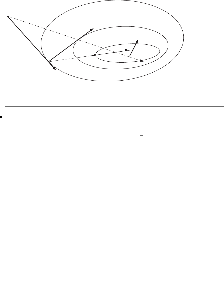
Glyn James: Advanced Modern Engineering Mathematics, 4th edition 633
Note that Partan obtains the minimum after one complete cycle. This method
was an improvement on steepest descent but has been superseded by DFP and
conjugate gradient methods which have been found to be superior in performance.
z 3
x 3
x 4
z 2
x 2
x 1
Figure 10.1: Illustration of the first steps of Partan in Exercise 18
19 The problem is to minimize the approximating quadratic
f(a+h)=f(a)+hTG+1
2hTJh
subject to hTh=L2. A Lagrange multiplier is required, so extending the argument
in section 10.4.3 gives the modified gradient as
0=G+Jh +λh=G+(J+λI)h
and hence
h=−(J+λI)−1G
The implementation suggested can be computed straightforwardly for this exercise.
The derivatives are obtained and hence
λ=0 x=1
1f=1G=0
1J=0−2
−22
so
x=1
1−1
−422
20
0
1=3/2
1and f=1
c
Pearson Education Limited 2011

634 Glyn James, Advanced Modern Engineering Mathematics, 4th Edition
Since there is no improvement, the next step is to take
λ=1 x=1
1f=1G=0
1J=0−2
−22
so
x=1
1−1
−132
21
0
1=3
2and f=−5
and the method is ready to proceed to the next iteration.
20(a) Here
f=x−y
1
4(x+y+1)
2and J=1−1
1
2(x+y+1) 1
2(x+y+1)
so the sequence of calculations is
x=0
0F=0.0625 f=0
0.25 J=1−1
0.50.5
x=−0.25
−0.25 F=0.0039 f=0
0.0625 J=1−1
0.25 0.25
x=−0.375
−0.375 F=0.00024 f=0
0.0156 J=1−1
0.125 0.125
20(b) The functions in this exercise are more complicated, although the method
is identical.
f=⎡
⎢
⎣
1
x+y
x
1+2x+y
⎤
⎥
⎦and J=⎡
⎢
⎢
⎣
−1
(x+y)2−1
(x+y)2
1+y
(1 + 2x+y)2−x
(1 + 2x+y)2
⎤
⎥
⎥
⎦
The computations follow in MATLAB
x=[1;1];
a=1/(x(1)+x(2)); b=2∗x(1)+x(2)+1;f=[a;x(1)/b]
% gives f= 0.5000 0.2500
J=[-a^2,-a^2;(1+x(2))/b^2,-x(1)/b^2]
% gives J= -0.2500 -0.2500
0.1250 -0.0625
c
Pearson Education Limited 2011

Glyn James: Advanced Modern Engineering Mathematics, 4th edition 635
x=x-inv(J∗ J)∗J∗ f,F=f∗ f
% gives x= 0.3333 3.6667 F= 0.3125
Repeating these three lines of code gives successive iterations. From the
calculations, the iterations gives x(1) approaches zero and x(2) approaches infinity!
21 Fitting data to any curve, except for a straight line, is quite a tricky job.
Optimization gives a method of finding a least squares fit of given data to a known
curve. The problem needs the method of Exercise 20 so the vector of functions and
the matrix of derivatives are required.
f=
⎡
⎢
⎢
⎢
⎢
⎢
⎢
⎢
⎢
⎢
⎣
1−1
a
0.6−1
a+b
0.3−1
a+2b
0.2−1
a+3b
⎤
⎥
⎥
⎥
⎥
⎥
⎥
⎥
⎥
⎥
⎦
and J=
⎡
⎢
⎢
⎢
⎢
⎢
⎢
⎢
⎢
⎢
⎢
⎣
1
a20
1
(a+b)2
1
(a+b)2
1
(a+2b)2
2
(a+2b)2
1
(a+3b)2
3
(a+3b)2
⎤
⎥
⎥
⎥
⎥
⎥
⎥
⎥
⎥
⎥
⎥
⎦
x=1
0F=1.29 f=⎡
⎢
⎣
0
−0.4
−0.7
−0.8
⎤
⎥
⎦J=⎡
⎢
⎣
10
11
12
13
⎤
⎥
⎦
x=1.07
0.27 F=0.239 f=⎡
⎢
⎣
0.0654
−0.1463
−0.3211
−0.3319
⎤
⎥
⎦J=⎡
⎢
⎣
0.8734 0
0.5569 0.5569
0.3858 0.7716
0.2829 0.8488
⎤
⎥
⎦
x=0.9810
0.6922 F=0.0316 f=⎡
⎢
⎣
−0.0194
0.0023
−0.1228
−0.1271
⎤
⎥
⎦J=⎡
⎢
⎣
1.0391 0
0.3572 0.3572
0.1787 0.3575
0.1070 0.3209
⎤
⎥
⎦
The computations continue until the values of aand bdo not change significantly.
MATLAB has built in programs for various versions of this problem, lscurvefit,
lsqlin, lsqnonlin, lsqnonneg.
22 It is assumed, without loss of generality, that Ais a symmetric matrix.
Putting the search direction in the quadratic gives, using the symmetry of A,
c
Pearson Education Limited 2011

636 Glyn James, Advanced Modern Engineering Mathematics, 4th Edition
f+c+bTa+λbTd+1
2(aTAa +2λaTAd +λ2dTAd)
and differentiating
0= ∂f
∂λ =bTd+aTAd +λdTAd
Collecting up the terms
λmin =−(b+Aa)Td
dTAd
gives the required result.
23 To use the results of Exercise 22 it is necessary to write the function in the
form
f=1+[−20]
x
y+1
2[xy]4−2
−22
x
y
and the gradient is evaluated as
G=−2+4x−2y
−2x+2y
The calculations proceed as
a=0
0f=1G=−2
0so d=2
0
and
λmin =−
[−20]
2
0
[2 0] 4−2
−22
2
0=1
4
The second iteration follows
a=0.5
0f=0.5G=0
−1so d=0
−1
and
c
Pearson Education Limited 2011

Glyn James: Advanced Modern Engineering Mathematics, 4th edition 637
λmin =−
[0 −1] 0
1
[0 1] 4−2
−22
0
1=1
2
The third iteration commences within the data
a=0.5
0.5f=0.25 G=−1
0
Because the function is a quadratic, the Newton method must converge in a single
iteration.
24 It is necessary to check that the solution given is appropriate.
y=(1 + b)
bex
band y =(1 + b)
b2ex
b
yy −y2+y=1+b
b2ex
b(1 + b)ex
b−b−1+b
b2
e2x
b+1+b
bex
and all the terms in the right hand side cancel to zero, so the differential equation
is satisfied. Also the point x=0,y = 1 satisfies the equation. To evaluate the
derivative at x=0
y(0) = α=1+b
b⇒b=1
α−1
Thus, given αthe value bcan be computed and
y(1) = (1 + b)e1
b−b
so that
f(α)=[(1 + b)e1
b−b−3]2
c
Pearson Education Limited 2011

638 Glyn James, Advanced Modern Engineering Mathematics, 4th Edition
Using the bracket 1.4<α<1.6 the values are calculated to be
αbf
1.4 2.5 0.0776
1.5 2 0.0029
1.6 1.6667 0.0369
and the quadratic algorithm gives α∗=1.5218,b =1.9278 and f=8.9×10⁻⁵;
the final iterated value is α=1.523,b =1.9133.
25 and 26 Exercises 25 and 26 are extended problems that are open ended, so
no advice is given on the solution of these two questions.
c
Pearson Education Limited 2011

11
Applied Probability and Statistics
Exercises 11.3.7
1Let X= lifetime, so X∼N(μ, 2500)
1(a) ¯
X= 780,n=30
Using z.025 =1.96 from the normal table, the 95% confidence interval for μis
780 ±1.96 ×50/√30 = (762,798)
1(b) We require nlarge enough so that
1.96 ×50
√n≤10
hence, n≥1.96 ×50
10
2
=96.04 i.e. n=97.
2From the data,
¯
X=76.06,S
X=31.85,n =36
Using z0.025 =1.96 we have the confidence interval
¯
X±1.96SX/√n=(65.7,86.5)
3From the data
¯
X=8.725,S
X,n−1=1.064,n=12
Using t.025,11 =2.201 from the t-distribution table, the 95% confidence interval
for the mean is
8.725 ±2.201 ×1.064/√12 = (8.05,9.40)
c
Pearson Education Limited 2011

640 Glyn James, Advanced Modern Engineering Mathematics, 4th Edition
4Given sample average ¯
X=73.2, standard deviation 5.4 and size 30, and using
t.025,29 =2.045, the 95% confidence interval for the mean is
73.2±2.045 ×5.4/√30 = (71.2,75.2)
The value (75) in the hypothesis lies within the interval and the hypothesis is
accepted.
5Given sample average ¯
X=3.42, standard deviation 0.68 and size 16, and
using t.005,15 =2.947, the 99% confidence interval for the mean is
3.42 ±2.947 ×0.68/√16 = (2.92,3.92)
6Given sample average ¯
X=26.4, standard deviation 4.28 and size 32, and
using t.025,31 t.025,29 =2.045 (alternatively the normal distribution figure of
1.96 could be used with a slight loss of accuracy), the 95% confidence interval for
the mean is
26.4±2.045 ×4.28/√32 = (24.9,27.9)
7Given sample average ¯
X= 56, standard deviation 3 and size 10, and using
t.025,9=2.262, the 95% confidence interval for the mean is
56 ±2.262 ×3/√10 = (53.9,58.1)
The value (58%) in the hypothesis lies within the interval and the hypothesis is
accepted at the 5% level.
8Given respective sample averages ¯
XA= 36300 and ¯
XB= 39100, standard
deviations SA,n−1= 5000 and SB,n−1= 6100, and sizes nA=nB=12,the
pooled estimate of standard deviation is
Sp=11 ×(50002+ 61002)
22 = 5577
c
Pearson Education Limited 2011

Glyn James, Advanced Modern Engineering Mathematics, 4th Edition 641
Using t.025,22 =2.074 the 95% confidence interval for μB−μAis
39100 −36300 ±2.074 ×5577 ×2
12 =(−1900,7500)
Because zero lies within this interval, the hypothesis that μB>μ
Ais rejected.
9From the data, respective sample averages ¯
XA= 7281 and ¯
XB= 6885,
standard deviations SA,n−1= 419.1andSB,n−1= 402.6, and sizes nA=nB=8,
the pooled estimate of standard deviation is
Sp=7×(419.12+ 402.62)
14 = 410.9
Using t.05,14 =1.761 and t.025,14 =2.145, confidence intervals for μA−μBare
90% : 7281 −6885 ±1.761 ×410.9×2
8=(34,758)
95% : 7281 −6885 ±2.145 ×410.9×2
8=(−45,837)
The hypothesis that μA=μBis rejected at the 10% level but accepted at the 5%
level.
10 The sample proportion ˆ
p=38
540 =0.0704 and n= 540.
Using z.05 =1.645 and z.025 =1.96, confidence intervals for the true proportion
pare
90% : 0.0704 ±1.645 ×0.0704 ×(1 −0.0704)
540 =(0.052,0.089)
95% : 0.0704 ±1.96 ×0.0704 ×(1 −0.0704)
540 =(0.049,0.092)
The hypothesis that p<0.05 is rejected at the 10% level but accepted at the 5%
level. Alternatively, the test statistic
Z=0.0704 −0.05
0.05 ×(1 −0.05)/540 =21.8
c
Pearson Education Limited 2011

642 Glyn James, Advanced Modern Engineering Mathematics, 4th Edition
leads to rejection at both 5% and 10% levels. The test statistic is more accurate
(the confidence interval is approximate).
11 Using z.05 =1.645, the 90% confidence interval for proportion is
ˆ
p±1.645ˆ
p(1 −ˆ
p)
n
Thus,
P|p−ˆ
p|≤ 1.645ˆ
p(1 −ˆ
p)
n=0.9
so with probability 0.9 the maximum error is 1.645ˆ
p(1 −ˆ
p)/n. Although ˆ
pis
unknown before the experiment, a figure in the region of 0.25 is expected, hence
we require
1.6450.25 ×0.75
n≤0.05
from which
n≥0.25 ×0.75
(0.05/1.645)2= 203
If in fact n= 200, the sample proportion is ˆ
p=55
200 =0.275, and the 90%
confidence interval for pis
0.275 ±1.6450.275 ×0.725
200 =(0.223,0.327)
12 Using sample proportions ˆ
p1=0.31 and ˆ
p2=74
150 =0.493, and z.05 =1.645
and z.025 =1.96, confidence intervals for p1−p2are
90% : ˆ
p1−ˆ
p2±1.645ˆ
p1(1 −ˆ
p1)
100 +ˆ
p2(1 −ˆ
p2)
150 1/2
=(−0.28,−0.08)
c
Pearson Education Limited 2011

Glyn James, Advanced Modern Engineering Mathematics, 4th Edition 643
95% : ˆ
p2−ˆ
p1±1.96ˆ
p1(1 −ˆ
p1)
100 +ˆ
p2(1 −ˆ
p2)
150 1/2
=(−0.30,−0.06)
The hypothesis that p1≤p2−0.08 is therefore accepted at the 10% level but
rejected at the 5% level.
13 Using sample proportions ˆ
p1=30
180 =0.1667 and ˆ
p2=32
500−180 =0.1, and
z.025 =1.96, the 95% confidence interval for p1−p2is
ˆ
p1−ˆ
p2±1.96ˆ
p1(1 −ˆ
p1)
180 +ˆ
p2(1 −ˆ
p2)
320 1/2
=(0.003,0.130)
The hypothesis that p1>p
2is therefore accepted at the 5% level. Alternatively,
the test statistic
Z=ˆ
p1−ˆ
p2
ˆ
p(1 −ˆ
p)1
180 +1
320 1/2=2.17 >z
.025
(where ˆ
p=30+32
500 =0.124) again leads to the hypothesis that p1>p
2is accepted.
Exercises 11.4.7
14
XX
X
YY
Y123total
1 0 0.17 0.08 0.25
2 0.20 0.11 0 0.31
3 0.14 0.25 0.05 0.44
total 0.34 0.53 0.13 1
14(a) Marginal distributions of Xand Y(summing rows and columns) are
P(X=1)=0.34,P(X=2)=0.53,P(X=3)=0.13
P(Y=1)=0.25,P(Y=2)=0.31,P(Y=3)=0.44
c
Pearson Education Limited 2011

644 Glyn James, Advanced Modern Engineering Mathematics, 4th Edition
14(b)
P(Y=3|X=2)= P(X=2∩Y=3)
P(X=2) =0.25
0.53 =0.472
14(c) The mean and variance of Xare given by
E(X)=1×0.34 + 2 ×0.53 + 3 ×0.13 = 1.79
E(X2)=1×0.34 + 4 ×0.53 + 9 ×0.13 = 3.63
so σ2
X=3.63 −1.792=0.426
Similarly the mean and variance of Yare given by
E(Y)=1×0.25 + 2 ×0.31 + 3 ×0.44 = 2.19
E(Y2)=1×0.25 + 4 ×0.31 + 9 ×0.44 = 5.45
so σ2
X=5.45 −2.192=0.654
The expected value of the product XY is given by
E(XY)=1×0+2×0.17 + 3 ×0.08 + 2 ×0.2+4×0.11 + 9 ×0
+3×0.14 + 6 ×0.25 + 9 ×0.05 = 3.79
Hence the correlation coefficient is
ρX,Y =3.79 −1.79 ×2.19
√0.426 ×0.654 =−0.246
15
E(X)=1/2
−1/2
xdx =0
E(X3)=1/2
−1/2
x3dx =0
Cov (X, X2)=E(X3)−E(X)E(X2)=0
c
Pearson Education Limited 2011

Glyn James, Advanced Modern Engineering Mathematics, 4th Edition 645
16 From cx ≤y≤cx +1 we infer y−1
c≤x≤y
c,so
fY(y)=fX,Y (x, y)dx
=⎧
⎪
⎪
⎨
⎪
⎪
⎩
y/c
01dx =y
cif 0 ≤y≤c
1
01dx =1 ifc≤y≤1
1
(y−1)/c 1dx =1−1
c(y−1) if 1 ≤y≤1+c
17(a)
P(X>100,Y >100) = 1
8∞
1∞
1
xe−(x+y)/2dydx
=1
8∞
1
xe−x/2[−2e−y/2]∞
1dx
=1
4e−1/2∞
1
xe−x/2dx
=−1
2e−1/2[xe−x/2]∞
1+1
2e−1/2∞
1
e−x/2dx
=1
2e−1+1
2e−1/2[−2e−x/2]∞
1
=3
2e=0.552
17(b)
fY(y)=1
8∞
0
xe−(x+y)/2dx =1
8e−y/2∞
0
xe−x/2dx
=e−y/2
4−xe−x/2|∞
0+∞
0
e−x/2dx=1
2e−y/2
Hence
P(Y>2) = ∞
2
1
2e−y/2dy =e−y/2|∞
2=1
e=0.368
c
Pearson Education Limited 2011

646 Glyn James, Advanced Modern Engineering Mathematics, 4th Edition
18 From the data, if Xdenotes height and Ydenotes weight, ¯
X= 174.26,
SX=7.184,¯
Y=75.7,S
Y=11.703,XY = 13270; so the sample correlation
coefficient is
r=13270 −174.26 ×75.7
7.184 ×11.703 =0.934
19 From the data,
¯
X=14.23,S
X=2.457,¯
Y=16.68,S
Y=3.4,XY = 243.47
so the sample correlation coefficient is
r=243.47 −14.23 ×16.68
2.457 ×3.4=0.732
20 Given a sample correlation coefficient r=0.7withn=30,andusing
z.025 =1.96,
c=exp2×1.96
√27 =2.126
and the 95% confidence interval for correlation is
1+r−c(1 −r)
1+r+c(1 −r),1+r−(1 −r)/c
1+r+(1−r)/c=(0.45,0.85)
21 From Exercise 18, r=0.934 with n=8. Using z.025 =1.96,
c=exp2×1.96
√5=5.772
and the 95% confidence interval for correlation is
1+r−c(1 −r)
1+r+c(1 −r),1+r−(1 −r)/c
1+r+(1−r)/c=(0.67,0.99)
c
Pearson Education Limited 2011

Glyn James, Advanced Modern Engineering Mathematics, 4th Edition 647
22 From the data, if Xand Ydenote mathematics and computer studies marks
respectively,
¯
X=56.80,S
X=8.880,¯
Y=54.40,S
Y=12.05,XY = 3137.4
so the sample correlation coefficient is
r=3137.4−56.8×54.4
8.88 ×12.05 =0.444
Using z.05 =1.645,
c=exp2×1.645
√17 =2.221
and the 90% confidence interval is
1+r−c(1 −r)
1+r+c(1 −r),1+r−(1 −r)/c
1+r+(1−r)/c=(0.08,0.70)
Similarly using z.025 =1.96,
c=exp2×1.96
√17 =2.588
and the 95% confidence interval is (0.00,0.74). This suggests that the correlation
coefficient is significant at the 10% level but is marginal at the 5% level. The test
statistic
Z=√17
2ln1+0.444
1−0.444 =1.968
leads to a similar conclusion. The ranks of the data are as follows:
Math. 3.5 20 2 16.5 13 16.5 13 7 19 3.5
10.5 5 18 10.5 7 7 15 13 9 1
Comp. 14 16.5 8 20 4 15 11.5 4 18.5 6.5
6.5 16.5 9 18.5 10 11.5 2 13 4 1
c
Pearson Education Limited 2011

648 Glyn James, Advanced Modern Engineering Mathematics, 4th Edition
The rank correlation is rs=0.401, and the test statistic
Z=rs√n−1=1.748
This is significant at the 10% level. (The approximate formula for rank correlation
gives a value 0.405, from which Z=1.767 with the same result.)
23(a)
1
01
x
fX,Y (x, y)dydx =1
01
x
c(1 −y)dydx
=1
0
c[y−y2
2]1
xdx
=1
0
c1
2−x+1
2x2dx
=c1
2x−1
2x2+1
6x31
0
=c
6
Since the joint density must integrate to unity, we must have c=6.
23(b)
P(X<3
4,Y> 1
2)=1
1/23/4
0
fX,Y (x, y)dxdy
=1
1/2min{3/4,y}
0
c(1 −y)dxdy
=3/4
1/2y
0
c(1 −y)dxdy +1
3/43/4
0
c(1 −y)dxdy
=3/4
1/2
c(1 −y)ydy +1
3/4
3
4c(1 −y)dy
=cy2
2−y3
33/4
1/2
+3
4cy−y2
21
3/4
=6
9
32 −27
192 −1
8+1
24 +9
21−1
2−3
4+9
32
=0.484
c
Pearson Education Limited 2011

Glyn James, Advanced Modern Engineering Mathematics, 4th Edition 649
23(c)
fX(x)=1
x
c(1 −y)dy =6
y−y2
21
x
=6
1
2−x+x2
2for 0 ≤x≤1
fY(y)=y
0
c(1 −y)dx =6(1−y)yfor 0 ≤y≤1
24 Individual density functions for Xand Yare
fX(x)=2 for 29.8<x<30.3
0otherwise
fY(y)=2 for 30.1<y<30.6
0otherwise
By independence, the joint density function is therefore
fX,Y (x, y)=4 for 29.8<x<30.3and30.1<y<30.6
0otherwise
The required probability is therefore
P(0 ≤Y−X≤0.6) = 30.3
29.8min{30.6,x+0.6}
max{30.1,x}
4dydx
=30.0
29.8x+0.6
30.1
4dydx
+30.1
30.030.6
30.1
4dydx +30.3
30.130.6
x
4dydx
=4
30.0
29.8
(x−29.5)dx +30.1
30.0
0.5dx
+30.3
30.1
(30.6−x)dx
=4
x2
2−29.5x
30.0
29.8+0.5×0.1+30.6x−x2
2
30.3
30.1
=0.84
c
Pearson Education Limited 2011
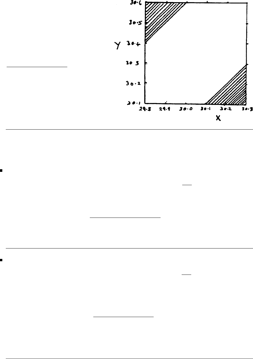
650 Glyn James, Advanced Modern Engineering Mathematics, 4th Edition
Alternatively, the shaded area
must be excluded from the
square. The two parts of
shaded area together form
asquareofside0.2, so
P(0 ≤Y−X≤0.6) =
0.5×0.5−0.2×0.2
0.5×0.5=0.84.
Exercises 11.5.5
25 From the data,
¯
X=16.370,S
x=6.789,¯
Y=36.110,S
y=14.576,XY = 689.343
Hence
ˆ
b=689.343 −16.37 ×36.11
6.7892=2.13
ˆ
a=36.11 −2.13 ×16.37 = 1.22
26 From the data,
¯
X=6.5,S
X=3.452,¯
Y= 101.5,S
Y=50.74,XY = 834.25
Hence, the regression coefficients are
ˆ
b=834.25 −6.5×101.5
3.4522=14.64
ˆ
a= 101.5−14.64 ×6.5=6.315
When load (X) is 15 kg, a deflection of 226 mm is predicted.
c
Pearson Education Limited 2011

Glyn James, Advanced Modern Engineering Mathematics, 4th Edition 651
27 From the results in Example 11.17 we find ˆ
a=−2.294 and ˆ
b=0.811, and
when 15 V is measured a tension of 9.88 kN is predicted.
Using t.025,12 =2.179 and
SE=S2
Y−ˆ
b2S2
X=√16.25 −0.8112×34.51 = 0.360
(remember that Xand Yare essentially reversed compared with Example 11.17),
the 95% confidence interval for tension when 15 V are measured is
9.88 ±2.179 ×0.36 ×1+(15−12.07)2/24.51
12 =(9.62,10.14)
28(a) From the data,
¯
X=34.17,S
X=11.70,¯
Y= 453.8,S
Y=59.34,XY = 15944
and the regression coefficients are
ˆ
b=15944 −34.17 ×453.8
11.72=3.221 (using unrounded figures)
ˆ
a= 453.8−3.221 ×34.17 −343.7
For advertising x=6 (£6000), sales of £537,000 are predicted.
28(b) SE=√59.342−3.2212×11.72=45.8 and using t.025,10 =2.228 the
95% confidence interval for regression slope is
ˆ
b±t.025,10
SE
SX√10 =(0.46,5.98)
The hypothesis that b= 0 is rejected at the 5% level.
28(c) The 95% confidence interval for mean sales when x=60 is
537 ±2.228 ×45.8×1+(60−34.17)2/136.8
10 = (459,615)
c
Pearson Education Limited 2011

652 Glyn James, Advanced Modern Engineering Mathematics, 4th Edition
29 From the data,
¯
X=11.5,S
X=2.291,¯
Y=13.25,S
Y=2.99,XY = 158.38
so the regression coefficients are
ˆ
b=158.38 −11.5×13.25
2.2912=1.143
ˆ
a=13.25 −1.143 ×11.5=0.107
and Y=16.1 is predicted when x=14. Alsousing
SE=S2
Y−ˆ
b2S2
X=1.442
and t.05,6=1.943, the 90% confidence interval for mean number of defectives per
hour when x=14 is
16.1±1.943 ×1.442 ×1+(14−11.5)2/5.25
6=(14.4,17.8)
30 Given a model (with no constant) of form
Yi=bXi+Ei
and minimizing
Q=
n
i=1
[Yi−bXi]2
we have
dQ
db =−2
n
i=1
Xi[Yi−ˆ
bXi]=0
hence
ˆ
b=n
i=1 XiYi
n
i=1 X2
i
c
Pearson Education Limited 2011

Glyn James, Advanced Modern Engineering Mathematics, 4th Edition 653
31 If Xdenotes voltage and Y=X/R denotes current then from the data,
ΣiXiYi= 5397,ΣiX2
i= 650
so that (using the result of the previous exercise)
ˆ
b=8.30
The estimated resistance is R=1000
8.3= 120Ω.
32 Taking logs we have
ln Pi+λln Vi=lnC
This is of the form Yi=a+bXiwith
Yi=lnPi,a=lnC, b =−λ, Xi=lnVi
From the data,
¯
X=4.272,S
X=0.254,¯
Y=3.423,XY =14.452
so that
ˆ
b=−2.664 and ˆ
a=14.80
Hence
ˆ
C=eˆa=2.69 ×10⁶and ˆ
λ=−ˆ
b=2.66
When V=80cm
3, a pressure P=22.9kg/cm3is predicted.
33 Taking logs we have
ln Yi=lna+bln Xi
or Yi
=a+bX
i
From the data,
¯
X=6.183,S
X=1.515,¯
Y=2.377, XY=12.266
c
Pearson Education Limited 2011

654 Glyn James, Advanced Modern Engineering Mathematics, 4th Edition
so
ˆ
b=−1.059,ˆ
a=8.927 and ˆ
a= 7533
For a lot size X= 300, a unit cost of 17.9 is predicted.
Exercises 11.6.3
34 Under the hypothesis, P(A)= 4
7,P(B)= 2
7,P(C)= 1
7.
observed probability expected χ2
χ2
χ2contribution
A63 4/7 57.14 0.601
B22 2/7 28.57 1.511
C15 1/7 14.29 0.035
Total 2.147
No parameters were estimated (t=0),sowecompare χ2=2.147 with χ2
0.05,2=
5.991.The hypothesis is accepted.
35 The total number of books is 640, so a uniform number would be 128 per
day. Hence
Obs. (fk)(fk)
(fk): 153 108 120 114 145
Exp. (ek)(ek)
(ek): 128 128 128 128 128
χ2
χ2
χ2contribution: 4.9 3.1 0.5 1.5 2.3
The total chi-square value is
χ2=12.3
and this is greater than χ2
.05,4=9.49 (significant at 5%, but not significant at
1%).
36 The observed mean number of flaws per sample is (12 + 6 ×2)/50 or 0.48.
Setting λ=0.48, the Poisson probabilities are given by λke−λ/k! and hence
expected values are as follows:
number
of flaws Obs. (fk)(fk)
(fk)probability exp. (ek)(ek)
(ek)χ2
χ2
χ2contribution
0 32 0.619 30.9 0.036
1 12 0.297 14.9 0.547
≥2 6 0.084 4.2 0.761
c
Pearson Education Limited 2011

Glyn James, Advanced Modern Engineering Mathematics, 4th Edition 655
The total chi-square value is
χ2=1.35
which is very small, so the Poisson hypothesis is accepted.
37 The observed average number of α-particles per time interval (taking class
>10 as 11 for this calculation) is
(203 + 2 ×383 + ...+11×6)/(57 + 203 + ...+6)=3.87
Using this value for λin the Poisson probabilities and proceeding as in the previous
exercise a total chi-square value
χ2=12.97
is obtained. One parameter has been estimated and used for predicting the exp-
ected values, so the comparison is with χ2
.05,10 =18.3, and the Poisson hypothesis
is accepted.
38 Using the measured average and standard deviation, probabilities can be
obtained from the normal table as follows:
P(X<6.5) = PX−10
2<6.5−10
2=Φ(−1.75) = 1 −Φ(1.75) = 0.0401
P(X<7.5) = 1 −Φ(1.25) = 0.1056
P(X<8.5) = 1 −Φ(0.75) = 0.2266
P(X<9.5) = 1 −Φ(0.25) = 0.4013
P(X<10.5) = Φ(0.25) = 0.5987
P(X<11.5) = Φ(0.75) = 0.7734
P(X<12.5) = Φ(1.25) = 0.8944
P(X<13.5) = Φ(1.75) = 0.9599
P(X<13.5) = 0.0401
c
Pearson Education Limited 2011

656 Glyn James, Advanced Modern Engineering Mathematics, 4th Edition
The class probabilities can now be inferred by
P(6.5<X<7.5) = P(X<7.5) −P(X<6.5) = 0.0655
and so on; hence, the following table:
Class Probability Expected Sample 1 Sample 2
<6.5 0.0401 4.01 4 3
6.5–7.5 0.0655 6.55 6 6
7.5–8.5 0.1210 12.10 16 16
8.5–9.5 0.1747 17.47 16 13
9.5–10.5 0.1974 19.74 17 26
10.5–11.5 0.1747 17.47 20 7
11.5–12.5 0.1210 12.10 12 19
12.5–13.5 0.0655 6.55 6 5
>13.5 0.0401 4.01 3 5
For sample 1, χ2=2.48 which is not significant.
For sample 2, χ2=15.51 which exceeds χ2
.025,6=14.45 (significant at 2.5% level)
but does not exceed χ2
.01,6=16.81 (not significant at 1% level). The second
subscript is m−t−1withm= 9 (classes) and t= 2 (parameters estimated).
39 The contingency table is as follows:
Perfect Intermediate Unacceptable Total
A89 (89.04) 23 (21.44) 12 (13.52) 124
B62 (58.88) 12 (14.18) 8 (8.94) 82
C119 (122.07) 30 (29.39) 21 (18.54) 170
Total 270 65 41 376
The expected values are shown in brackets,
270 ×124
376 =89.04
c
Pearson Education Limited 2011

Glyn James, Advanced Modern Engineering Mathematics, 4th Edition 657
and so on. Hence
χ2=(89 −89.04)2
89.04 +···+(21 −18.54)2
18.54
=1.30
This is less than χ2
.05,(3−1)(3−1) =9.49, so there is no significant difference in
quality.
40 The contingency table (with the expected values in brackets) is as follows:
o.k. defective total
442 (441.6) 8 (8.38) 450
536 (539.8) 14 (10.25) 550
544 (539.8) 6 (10.25) 550
397 (392.5) 3 (7.45) 400
593 (588.8) 7 (11.18) 600
442 (441.6) 8 (8.38) 450
434 (441.6) 16 (8.38) 450
195 (196.3) 5 (3.73) 200
438 (441.6) 12 (8.38) 450
594 (588.8) 6 (11.18) 600
585 (588.8) 15 (11.18) 600
541 (539.8) 9 (10.25) 550
5741 109 5850
Hence, χ2=(442 −441.6)2
441.6+···+(9 −10.25)2
10.25 =20.56 which exceeds χ2
.05,11 =
19.68 but is less than χ2
.025,11 =21.92. The variation is significant at the 5%
level. For a 2 ×ctable of this form, effectively, a comparison of cproportions, it
is quicker (and equivalent) to compute
χ2=
c
j=1
(fj−njˆ
p)2
njˆ
p(1 −ˆ
p)
where fjis the number of defectives in column j(total nj)andˆ
p=
c
j=1
fj/
c
j=1
nj
is the overall sample proportion of defectives.
c
Pearson Education Limited 2011

658 Glyn James, Advanced Modern Engineering Mathematics, 4th Edition
41 The contigency table (with expected values in brackets and adjusted residuals
underneath) is as follows:
Spending Jacket Shirt Trousers Shoes Total
level
Low 21(36) 94(92) 57(47) 113(110) 285
−3.0 0.4 1.8 0.4
Medium 66(66) 157(169) 94(87) 209(204) 526
0.0 −1.5 1.0 0.7
High 58(43) 120(110) 41(57) 125(133) 344
2.9 1.3 −2.8 −1.1
Total 145 371 192 447 1155
Chi-square = 20.7, d.f. = (4 −1)(3 −1) = 6, so compare with χ2
0.005,6=18.5:
significant at 0.5% level. High-spending customers are tending to buy more of the
jacket and less of the trousers. For low-spending customers, it is the other way
round.
42 If pis the proportion requiring adjustments, the number of such sets in
asampleofsizenis binomial with parameters n, p.Withn=4,totestthe
hypothesis that p=0.1wehave
P(0) = 0.94=0.6561
P(1) = 4
10.930.1=0.2916
P(2) = 4
20.920.12=0.0486
P(3) = 4
30.9×0.13=0.0036
Hence the following table:
kk
kfk
fk
fkpk
pk
pkek= 200pk
ek= 200pk
ek= 200pkχ2
χ2
χ2contribution
0 110 0.6561 131.22 3.43
1 73 0.2916 58.32 3.70
2 16 0.0486 9.72 4.06
3 1 0.0036 0.72 0.11
c
Pearson Education Limited 2011

Glyn James, Advanced Modern Engineering Mathematics, 4th Edition 659
The total chi-square value is χ2=11.30, which is significant at 5% (χ2
.05,3=7.82)
but not quite significant at 1% (χ2
.01,3=11.35).
Using proportions, the total number of sets requiring adjustments is 73 + 2 ×16 +
3×1 = 108, so
ˆ
p=108
800 =0.135
Using z.025 =1.96 and z.005 =2.576, confidence intervals for the proportion pof
sets requiring adjustments are
95% : ˆ
p±1.96ˆ
p(1 −ˆ
p)
800 =(0.111,0.159)
99% : ˆ
p±2.576ˆ
p(1 −ˆ
p)
800 =(0.104,0.166)
This indicates that p>0.1, significant (just) at the 1% level.
Exercises 11.7.4
43 We must have
1=∞
0
fX(x)dx =c∞
0
xe−2xdx
=−1
2c[xe−2x]∞
0+1
2c∞
0
e−2xdx
=1
2c−1
2e−2x∞
0
=c
4
so c=4. Them.g.f. isthen
MX(t)=∞
0
etxfX(x)dx =4∞
0
xe(t−2)xdx
=4
t−2[xe(t−2)x]∞
0−4
t−2∞
0
e(t−2)xdx
=4
(t−2)2provided t<2
c
Pearson Education Limited 2011

660 Glyn James, Advanced Modern Engineering Mathematics, 4th Edition
Hence
E(X)=M
X(0) = −8
(t−2)3t=0
=1
E(X2)=M
X(0) = 24
(t−2)4t=0
=3
2
Var(X)=E(X2)−[E(X)]2=1
2
44 If X1,...,X
nare independent Poisson random variables with parameters
λ1,...,λ
nand if Y=X1+...+Xnthen
MY(t)=MX1(t)...M
Xn(t)
=exp[λ1(et−1)] ...exp[λn(et−1)]
=exp[(λ1+...+λn)(et−1)]
Hence, Yis another Poisson random variable with parameter λ=λ1+...+λn.
45 Numbers of breakdowns in one hour are separately binomial with parameters
n1=30,p
1=0.01 and n2=40,p
2=0.005 respectively, and hence approximately
Poisson with parameters λ1=0.3andλ2=0.2 respectively. The total number of
breakdowns per hour is therefore also approximately Poisson with λ=λ1+λ2=
0.5, and
P(three or more) 1−e−λ1+λ+λ2
2! =0.014
46 Let the proportion defective be p. By the Poisson approximation,
P(kdefective in 100) λke−λ
k!
where λ= 100p. The requirement is
P(k≤1) e−λ(1 + λ)>0.9
from which λ<0.531 (solving this as a nonlinear equation) and hence p< 0.531
100 =
0.0053. Therefore, at least 99.47% of servomechanisms must be satisfactory.
c
Pearson Education Limited 2011

Glyn James, Advanced Modern Engineering Mathematics, 4th Edition 661
47 With
fZ(z)= 1
√2πe−z2/2,−∞ <z<∞
the m.g.f. is
MZ(t)= 1
√2π∞
−∞
etze−z2/2dz
=1
√2π∞
−∞
e−1
2(z2−2tz+t2)et2/2dz
=et2/2∞
−∞
1
√2πe−1
2(z−t)2dz
The integrand is the p.d.f. of a normal random variable with mean tand standard
deviation equalling one, hence
MZ(t)=et2/2
Exercises 11.9.7
48 From the table (Figure 11.29), with n=50,p =0.1sothatnp =5,weread
off the Shewhart warning limit as 9.5 and the action limit as 13.5. For the given
data, the warning limit is exceeded at samples 3, 9 and 11, and the action limit is
exceeded at sample 12. The upper control limit is given by
UCL = np +3
np(1 −p)=11.4
and this is first exceeded at sample 9.
49 From Figure 11.29, with n= 100,p=0.02 so that np =2,wehaveShewhart
warning and action limits 5.5 and 7.5 respectively. The warning limit is exceeded
three times (samples 20, 22 and 25) before the action limit is exceeded at sample
28. The upper control limit is given by
UCL = np +3
np(1 −p)=6.2
and this is first exceeded at sample 25.
c
Pearson Education Limited 2011

662 Glyn James, Advanced Modern Engineering Mathematics, 4th Edition
50 Using σ=3 and n= 10, the Shewhart warning and action limits are
cW=1.96σ/√n=1.86
cA=3.09σ/√n=2.93
(above and below the mean). Relative to the mean, the warning limit is exceeded
at samples 3 and 9, and the action limit at sample 12.
51 Using σ=3 and n= 10, the Shewhart warning and action limits above the
design mean μ=12 are
μ+1.96σ/√n=13.86
μ+3.09σ/√n=14.93
The warning limit is exceeded several times (at samples 6, 12, 15, 17 and 18) before
the action limit is crossed at sample 19.
52(a) Using σ=3 and n= 10, the cusum parameters are
r=σ
2√n=0.474 (relative to the mean)
h=5 σ
√n=4.74
The chart is built up in the following table:
value -0.2 1.3 2.1 0.3 -0.8 1.7 1.3 0.6 2.5 1.4 1.6 3.0
cusum 0 0.83 2.45 2.28 1.00 2.23 3.05 3.18 5.21 6.13 7.26 9.78
The decision interval (h) is exceeded at sample 9.
52(b) Using r=0.3andσ, n as above, the GMA action limits are
±3.09r
2−r
σ
√n=±1.23
c
Pearson Education Limited 2011

Glyn James, Advanced Modern Engineering Mathematics, 4th Edition 663
(relative to the mean). The chart is built up in the following table:
value -0.2 1.3 2.1 0.3 -0.8 1.7 1.3 0.6 2.5 1.4 1.6 3.0
GMA -0.06 0.35 0.87 0.70 0.25 0.69 0.87 0.79 1.30 1.33 1.41 1.89
The action limit is exceeded at sample 9.
53 For the cusum chart we have μ=12,σ=3 and n=10,so
r=μ+σ
2√n=12.47
h=5 σ
√n=4.74
For the GMA chart with r=0.3 we have action limits at
μ±3.09r
2−r
σ
√n=10.77 and 13.23
The control charts are built up in the following table:
¯
Xm
¯
Xm
¯
Xm12.8 11.2 13.4 12.1 13.6 13.9 12.3 12.9 13.8 13.1
cusum 0.33 0 0.93 0.55 1.68 3.10 2.93 3.35 4.68 5.31
GMA 12.24 11.93 12.37 12.29 12.68 13.05 12.82 12.85 13.13 13.12
¯
Xm
¯
Xm
¯
Xm12.9 14.0 13.7 13.4 14.2 13.1 14.0 14.0 15.1 14.3
cusum 5.73 7.26 8.48 9.41 11.13 11.76 13.28 14.81 17.44 19.26
GMA 13.06 13.34 13.45 13.43 13.66 13.49 13.65 13.75 14.16 14.20
The cusum chart indicates action at sample 10, the GMA chart at sample 12.
54 Using n=50,p =0.1sothatnp = 5, the cusum parameters from Figure
11.31 are r=7,h=8.5 (nearest values).
count 58115649712910 14
cusum 01 532022 7912 19
The chart indicates action at sample 10.
c
Pearson Education Limited 2011
664 Glyn James, Advanced Modern Engineering Mathematics, 4th Edition
55 Using n= 100,p =0.02 so that np = 2, the cusum parameters from Figure
11.31 are r=3,h=5.5 (nearest values).
count 33535031354 24354
cusum 00224110023 23356
count 34565644754 85667
cusum 6791214171819232526 3133363943
The chart indicates action at sample 16.
56 For the Shewhart chart we have n=12,σ = 1, and hence warning and action
limits given by
cW=1.96σ/√n=0.57
cA=3.09σ/√n=0.89
For the cusum chart we have
r=σ
2√n=0.144 (relative to the mean)
h=5 σ
√n=1.443
For the GMA chart with r=0.2, the action limit is
3.09r
2−r
σ
√n=0.297
¯
Xm
¯
Xm
¯
Xm0.1 0.3 -0.2 0.4 0.1 0 0.2 -0.1 0.2 0.4 0.5
cusum 0 .156 0 .256 .211 .067 .123 0 .056 .311 .667
GMA .020 .076 .021 .097 .097 .078 .102 .062 .089 .152 .221
¯
Xm
¯
Xm
¯
Xm0.1 0.4 0.6 0.3 0.4 0.3 0.6 0.5 0.4 0.2 0.3
cusum .623 .878 1.334 1.490 1.745 1.901 2.357 2.712 2.968 3.024 3.179
GMA .197 .238 .310 .308 .326 .321 .377 .402 .401 .361 .349
¯
Xm
¯
Xm
¯
Xm0.5 0.7 0.3 0.1 0.6 0.5 0.6 0.7 0.4 0.5
cusum 3.535 4.091 4.246 4.202 4.658 5.013 5.469 6.025 6.280 6.636
GMA .379 .443 .415 .352 .401 .421 .457 .505 .484 .488
For the Shewhart chart there are several warnings but no action indicated. For the
cusum and GMA charts, action is indicated at samples 15 and 14 respectively.
c
Pearson Education Limited 2011

Glyn James, Advanced Modern Engineering Mathematics, 4th Edition 665
57 The GMA Smis defined recursively by
S0=μX
Sm=r¯
Xm+(1−r)Sm−1for m≥1
Substituting for Sm−1,thenSm−2and so on gives
Sm=r¯
Xm+(1−r)[r¯
Xm−1+(1−r)Sm−2]
=r[¯
Xm+(1−r)¯
Xm−1]+(1−r)2[rXm−2+(1−r)Sm−3]
and eventually
Sm=r
m−1
i=0
(1 −r)i¯
Xm−i+(1−r)mμX
But E(¯
Xm−i)=μXand Var(¯
Xm−i)=σ2
X
nfor all i, m.
Using the result
m−1
i=0
xi=1−xm
1−xfor |x|<1
we have
E(Sm)=rμX
m−1
i=0
(1 −r)i+(1−r)mμX
=rμX
1−(1 −r)m
r+(1−r)mμX
=μX
Var(Sm)=σ2
X
nr2
m−1
i=0
[(1 −r)2]i=σ2
Xr2
n
1−(1 −r)2m
1−(1 −r)2
=σ2
X
n[1 −(1 −r)2m]r
2−r
−→ r
2−rσ2
X
nas m→∞
58 Let Xm= count of defectives for sample m,n= sample size, p= probability
of defective. Define
S0=np
Sm=rXm+(1−r)Sm−1for m≥1
c
Pearson Education Limited 2011

666 Glyn James, Advanced Modern Engineering Mathematics, 4th Edition
Substituting for Sm−1,S
m−2and so on (as in the previous exercise) leads to
Sm=r
m−1
i=0
(1 −r)iXm−i+(1−r)mnp
From the mean and variance of the binomial distribution,
E(Xm−i)=np
Var(Xm−i)=np(1 −p)
hence
E(Sm)=rnp
m−1
i=0
(1 −r)i+(1−r)mnp
=np[1 −(1 −r)m+(1−r)m]=np
Var(Sm)=np(1 −p)r2
m−1
i=0
[(1 −r)2]i
=r
2−r[1 −(1 −r)2m]np(1 −p)
−→ r
2−rnp(1 −p)asm→∞
The upper control limit for n=50,p=0.05,r=0.2is
UCL = np +3
r
2−rnp(1 −p)=4.04
Xm
Xm
Xm352216442 6
Sm
Sm
Sm2.6 3.08 2.86 2.69 2.35 3.08 3.27 3.41 3.13 3.70
Xm
Xm
Xm745586597 8
Sm
Sm
Sm4.36 4.29 4.43 4.55 5.24 5.39 5.31 6.05 6.24 6.59
The chart indicates action after 11 samples.
59 For the Shewhart chart we have n=10,μ=6,σ=0.2 and hence warning
and action limits given by
cW=μ±1.96σ/√n=5.88 and 6.12
cA=μ±3.09σ/√n=5.80 and 6.20
c
Pearson Education Limited 2011

Glyn James, Advanced Modern Engineering Mathematics, 4th Edition 667
For the cusum chart we have
r=μ+σ
2√n=6.032
h=5 σ
√n=0.316
For the GMA chart with r=0.2, the action limits are
μ±3.09r
2−r
σ
√n=5.935 and 6.065
¯
Xm
¯
Xm
¯
Xm6.04 6.12 5.99 6.02 6.04 6.11 5.97 6.06 6.05 6.06
cusum 0.01 0.10 0.06 0.04 0.05 0.13 0.07 0.10 0.12 0.14
GMA 6.01 6.03 6.02 6.02 6.03 6.04 6.03 6.03 6.04 6.04
¯
Xm
¯
Xm
¯
Xm6.17 6.03 6.13 6.05 6.17 5.97 6.07 6.14 6.03 5.99
cusum 0.28 0.28 0.38 0.40 0.54 0.47 0.51 0.62 0.62 0.58
GMA 6.07 6.06 6.07 6.07 6.09 6.07 6.07 6.08 6.07 6.05
¯
Xm
¯
Xm
¯
Xm6.10 6.01 5.96 6.12 6.02 6.20 6.11 5.98 6.02 6.12
cusum 0.65 0.62 0.55 0.64 0.63 0.80 0.88 0.82 0.81 0.90
GMA 6.06 6.05 6.03 6.05 6.05 6.08 6.08 6.06 6.05 6.07
The Shewhart chart indicates action after 26 samples, the cusum chart after 13
samples and the GMA chart after 11 samples.
Exercises 11.10.6
60 If gales occur at rate 15
12 =1.25 per month, and occur independently, then
the number of gales in any one month has a Poisson distribution, so
P(more than two in one month) = 1 −P(0) −P(1) −P(2)
=1−e−λT 1+λT +λ2T2
2!
=0.132
(with λ=1.25,T=1).
c
Pearson Education Limited 2011

668 Glyn James, Advanced Modern Engineering Mathematics, 4th Edition
61 If λ= 30 calls per hour (on average) arrive at the switchboard, and do so
independently, then the number of calls has a Poisson distribution. Hence
P(no calls in T=3min) =e−λT /60 =0.223
P(more than five calls in T=5min)
=1−e−λT /601+ λT
60 +...+(λT)5
6055!
=0.042
62 The steady-state distribution for the number (N) in the system is
P(nin system) = pn=(1−ρ)ρn,n≥0
Now
d
dρ
∞
n=0
ρn=∞
n=0
nρn−1=d
dρ(1 −ρ)−1=(1−ρ)−2
Hence, the mean number in the system is
NS=∞
n=0
n(1 −ρ)ρn=ρ(1 −ρ)∞
n=0
nρn−1
=ρ(1 −ρ)
(1 −ρ)2=ρ
1−ρ
If there are n>0 customers in the queue then there are n+ 1 in the system, so
P(n>0 in queue) = (1 −ρ)ρn+1,n≥1
(we do not need the probability for n= 0). Mean number in queue is
NQ=(1−ρ)∞
n=1
nρn+1 =ρ2(1 −ρ)∞
n=0
nρn−1
=ρ2(1 −ρ)
(1 −ρ)2=ρ2
1−ρ
c
Pearson Education Limited 2011

Glyn James, Advanced Modern Engineering Mathematics, 4th Edition 669
63 For a single-channel queue with λ= 3 arrivals per hour and μ= 4 patients
treated per hour,
63(a) P(0 in system) = 1 −λ
μ=1
4
63(b) NQ=(λ/μ)2
1−λ/μ =9
4
63(c)
P(>3 in queue) = P(>4insystem)
=1−P(0) −P(1) −P(2) −P(3) −P(4)
=1−1−λ
μ1+ λ
μ+λ
μ
2
+λ
μ
3
+λ
μ
4
=0.237
63(d) WQ=λ/μ
μ−λ=3
4hour.
63(e) P(wait more than one hour) = λ
μe−(μ−λ)=0.276
64 Mean number of aircraft on ground is
NS=λ
μ−λ
so, total mean cost per hour (waiting time plus servicing) is
E[total cost per hour] = c1λ
μ−λ+c2μ
c
Pearson Education Limited 2011

670 Glyn James, Advanced Modern Engineering Mathematics, 4th Edition
Minimizing this with respect to μ:
d
dμE[total cost per hour] = −c1λ
(μ−λ)2+c2=0
from which
(μ−λ)2=c1λ
c2
so μ=λ+c1λ/c2
65 Breakdown rate is λ= 3 per hour, and machine idle time is costed at £60
per hour per machine. For option A, service rate is μ=4 perhourat£20 per
hour, so mean hourly cost is
60NS+20= 60λ
μ−λ+ 20 = 200
For option B, service rate is μ=5 at£40 per hour, so mean hourly cost is
60NS+40= 60λ
μ−λ+ 40 = 130
Option B is preferred.
66 Ship arrival rate is λ=1
3per hour, and service rate per berth is μ=1
12 ,so
ρ=λ/μ = 4. Mean waiting time in the queue is
WQ=1
λρc+1
(c−1)!(c−ρ)2c−1
n=0
ρn
n!+ρc
(c−1)!(c−ρ)−1
where cis the number of berths. For c= 5 berths we find WQ=6.65 hours,
which exceeds the required minimum, so c= 6 berths are needed (WQ=1.71).
67 Arrival rate is λ= 2 per minute, and basic service rate per cashier is μ=5
4
per minute. If this service rate is doubled (by providing a packer) then mean
queueing time is
WQ=ρ
μ−λ=4/5
5/2−2=1.6min
c
Pearson Education Limited 2011

Glyn James, Advanced Modern Engineering Mathematics, 4th Edition 671
Alternatively, if an additional cash desk is provided then (using WQas in the
previous exercise, and ρ=8/5)
WQ=1
λρ3
(2 −ρ)21+ρ+ρ2
2−ρ−1
=0.076 min
Clearly, a second cash desk is preferable.
Exercises 11.11.3
68 We have
P(agent) = P(agent|option 1)P(option 1) + P(agent|option 2)P(option 2)
+P(agent|option 3)P(option 3)
=0.28 ×0.45 + 0.41 ×0.32 + 0.16 ×0.23
=0.294
69 Total probability of explosion is
P(E)=P(E|(a))P((a)) + P(E|(b))P((b))
+P(E|(c))P((c)) + P(E|(d))P((d))
=0.25 ×0.2+0.2×0.4+0.4×0.25 + 0.75 ×0.15
=0.3425
Hence, by Bayes’ Theorem,
P((a)|E)=P(E|(a))P((a))/P(E)=0.146
P((b)|E)=0.234
P((c)|E)=0.292
P((d)|E)=0.328
and sabotage is therefore the most likely cause of the explosion.
c
Pearson Education Limited 2011

672 Glyn James, Advanced Modern Engineering Mathematics, 4th Edition
70 If two bullets hit the target then they could be fired by each possible pair of
marksmen, so
P(two hits) = P(A∩B∩¯
C)+P(A∩¯
B∩C)+P(¯
A∩B∩C)
(where Adenotes ‘bullet from Ahits target’, etc)
=0.6×0.5×0.6+0.6×0.5×0.4+0.4×0.5×0.4
=0.38
Hence
P(C|two hits) = P(C∩two hits)
P(two hits)
=P(A∩¯
B∩C)+P(¯
A∩B∩C)
P(twohits)
=0.6×0.5×0.4+0.4×0.5×0.4
0.38
=0.526
Thus, it is more probable than not that Chit the target.
71 Prior probabilities are P(A)=1
3,P(B)=2
3.AlsoP(Smith |A)=0.1and
P(Smith |B)=0.05. Hence
P(A|Smith) = P(Smith |A)P(A)
P(Smith |A)P(A)+P(Smith |B)P(B)
=0.1×1
3
0.1×1
3+0.05 ×2
3
=1
2
72 Let Ddenote ‘has disease’ and + denote ‘positive diagnosis’, so that P(D)=
0.08,P(+ |D)=0.95 and P(+ |¯
D)=0.02
72(a) P(+) = P(+ |D)P(D)+P(+ |¯
D)P(¯
D)
=0.95 ×0.08 + 0.02 ×0.92 = 0.0944
c
Pearson Education Limited 2011

Glyn James, Advanced Modern Engineering Mathematics, 4th Edition 673
72(b) P(D|+) = P(+ |D)P(D)
P(+) =0.95 ×0.08
0.0944 =0.81
73 Let Gdenote ‘good stock’, B=¯
Gdenote ‘bad stock’,
gdenote ‘stockbroker says good’,
bdenote ‘stockbroker says bad’,
so that P(G)=0.5,P(g|G)=0.6,P(b|B)=0.8.
73(a)
P(G|g)= P(g|G)P(G)
P(g|G)P(G)+P(g|B)P(B)
=0.6×0.5
0.6×0.5+0.2×0.5=3
4
73(b) Let Edenote ‘kout of nstockbrokers say good’. Since the stockbrokers
are independent, by the binomial distribution
P(E|G)=n
k[P(g|G)]k[P(b|G)]n−k
P(E|B)=n
k[P(g|B)]k[P(b|B)]n−k
Hence
P(G|E)= P(E|G)P(G)
P(E|G)P(G)+P(E|B)P(B)
=n
k[P(g|G)]k[P(b|G)]n−kP(G)
n
k[P(g|G)]k[P(b|G)]n−kP(G)+n
k[P(g|B)]k[P(b|B)]n−kP(B)
=0.6k×0.4n−k×0.5
0.6k×0.4n−k×0.5+0.2k×0.8n−k×0.5
=1+1
3
k
2n−k−1
c
Pearson Education Limited 2011

674 Glyn James, Advanced Modern Engineering Mathematics, 4th Edition
74 Given that the probability of correct reception of a letter is 0.6, and the error
probabilities are 0.2 for the two alternatives, we have
P(ABCA received |AAAA transmitted) = 0.6×0.2×0.2×0.6=0.0144
P(ABCA received |BBBB transmitted) = 0.2×0.6×0.2×0.2=0.0048
P(ABCA received |CCCC transmitted) = 0.2×0.2×0.6×0.2=0.0048
Also P(AAAA transmitted) = 0.3 etc. Hence
P(ABCA received) = 0.0144 ×0.3+0.0048 ×(0.4+0.3)
=0.00768
and
P(AAAA transmitted|ABCA received) = 0.0144 ×0.3
0.00768 =0.5625
P(BBBB transmitted |ABCA received) = 0.25
P(CCCC transmitted |ABCA received) = 0.1875
75 Average number of accidents per day = 1×12+2×4
100 =1
5
First hypothesis (H1) is for a Poisson distribution, so set λ=1
5and probabilities
pi=P(iaccidents in one day) = λie−λ
i!
Hence, p0=0.8187,p
1=0.1637,p
2=0.0164. Second hypothesis (H2)isfora
binomial distribution with n=3,soset
np =1
5(hence p=1
15 ) and probabilities
qi=P(iaccidents in one day) = 3
ipi(1 −p)3−i
Hence, q0=0.8130,q
1=0.1742,q
2=0.0124. If Edenotes the evidence then the
odds are updated by
lnP(H1|E)
P(H2|E)=ln
P(E|H1)
P(E|H2)+lnP(H1)
P(H2)
c
Pearson Education Limited 2011

Glyn James, Advanced Modern Engineering Mathematics, 4th Edition 675
where
P(E|H1)=p84
0p12
1p4
2
P(E|H2)=q84
0q12
1q4
2
P(H1)/P(H2)=1
2(initial odds)
Hence
lnP(H1|E)
P(H2|E)=84ln
p0
q0
+12lnp1
q1
+4lnp2
q2
+ln1
2=0.247
and the updated odds are therefore 1.28 to 1 in favour of the Poisson distribution.
76 If the probabilities of the evidence (E) under H1and H2are
P(E|H1)= n!
n1!...n
k!pn1
1...p
nk
k
P(E|H2)= n!
n1!...n
k!qn1
1...q
nk
k
then the log-likelihood ratio becomes
lnP(E|H1)
P(E|H2)=ln
p1
q1n1···pk
qknk=
k
i=1
nilnpi
qi
77 Under hypothesis H1we have
p1=0.92,p
2=0.05,p
3=0.02,p
4=0.01
and under H2
q1=1−0.05 −q3−q4,q
2=0.05,q
3,q
4unknown
(where q3=pBand q4=PAB ). The likelihood of the evidence Eunder H2is
P(E|H2)= n!
n1!...n
4!(0.95 −q3−q4)n10.05n2qn3
3qn4
4
c
Pearson Education Limited 2011

676 Glyn James, Advanced Modern Engineering Mathematics, 4th Edition
where n1= 912,n
2=45,n
3=27,n
4=16. Thus
ln P(E|H2)=n1ln(0.95 −q3−q4)+n3ln q3+n4ln q4+ constant
∂ln P(E|H2)
∂q3
=−n1
0.95 −q3−q4
+n3
q3
=n3(0.95 −q3−q4)−n1q3
(0.95 −q3−q4)q3
=0if(n1+n3)q3+n3q4=0.95n3
∂ln P(E|H2)
∂q4
=−n1
0.95 −q3−q4
+n4
q4
=n4(0.95 −q3−q4)−n1q4
(0.95 −q3−q4)q4
=0ifn4q3+(n1+n4)q4=0.95n4
From the simultaneous equations
939q3+27q4=25.65
16q3+ 928q4=15.2
we find q3=0.0269,q
4=0.0159 and therefore q1=0.9072.
It follows that (using the result of the previous exercise)
lnP(E|H1)
P(E|H2)=
4
i=1
nilnpi
qi
= 912 ln 0.92
0.9072 +45 ln0.05
0.05 +27 ln 0.02
0.0269 +16 ln 0.01
0.0159
=−2.645
If initial odds are P(H1)/P(H2) = 5 then updated odds are
P(H1|E)
P(H2|E)=e−2.645 ×5=0.355
that is, 2.8 to 1 in favour of H2.
78 Under hypothesis H1we have separate estimates as follows:
λA= mean number of defects for A=24
6=4.0
λB= mean number of defects for B=36
5=7.2
Under hypothesis H2we have a single estimate as follows:
λ= overall mean number of defects = 60
11 =5.455
c
Pearson Education Limited 2011

Glyn James, Advanced Modern Engineering Mathematics, 4th Edition 677
The evidence Ecan be expressed as follows:
E={A: 2 with 3 defects, 2 with 4 defects, 2 with 5 defects;
B: 1 with 5 defects, 1 with 6 defects, 2 with 8 defects, 1 with 9 defects}
The log-likelihood ratio is
lnP(E|H1)
P(E|H2)=2ln
λ3
Ae−λA
λ3e−λ+2lnλ4
Ae−λA
λ4e−λ+2lnλ5
Ae−λA
λ5e−λ
+lnλ5
Be−λB
λ5e−λ+lnλ6
Be−λB
λ6e−λ+2lnλ8
Be−λB
λ8e−λ+lnλ9
Be−λB
λ9e−λ
= (6 + 8 + 10)ln λA
λ+(5+6+16+9)lnλB
λ
+(2+2+2)(λ−λA)+(1+1+2+1)(λ−λB)
=2.551
and the updated odds (with no initial preference) are
P(H1|E)
P(H2|E)=e2.551
or 12.8 to 1 in favour of H1.
Review Exercises 11.12
1For the standard corks, sample proportion oxidized is ˆ
p1=6
60 =0.1, whereas
for the plastic bungs, sample proportion oxidized is ˆ
p2=3
36 =0.0833. Overall
proportion oxidized is ˆ
p=9
96 =0.0938. Test statistic
z=ˆ
p1−ˆ
p2
ˆ
p(1 −ˆ
p)( 1
60 )+(1
36 )
=0.271
The hypothesis is accepted.
2The model is
d=d0e−λt
or equivalently
ln d=lnd0−λt
c
Pearson Education Limited 2011

678 Glyn James, Advanced Modern Engineering Mathematics, 4th Edition
which is of the form
Y=a+bX
From the data,
¯
X=5.746,S
X=3.036,¯
Y=−0.2811,S
Y=0.721,XY =−3.775
so
ˆ
b=XY −¯
X¯
Y
S2
X
=−0.234
ˆ
a=¯
Y−ˆ
b¯
X=1.065
From these we infer ˆ
λ=−ˆ
b=0.234
ˆ
d0=eˆa=2.90
Also the error variance is (using unrounded results)
S2
E=S2
Y−ˆ
b2S2
X=0.01418
and the 95% confidence interval for λis
ˆ
λ±t.025,8
SE
SX√8=(0.202,0.266)
3If position Pand load Xare related by
P=a+bX
then by linear regression on the data we find
ˆ
a=6.129
ˆ
b=0.0624
But extension Yand load Xare related by
ˆ
b=Y
X=L
ˆ
EA
c
Pearson Education Limited 2011

Glyn James, Advanced Modern Engineering Mathematics, 4th Edition 679
where L= 101.4andA=1.62 ×10⁻⁵. The estimate of Young’s modulus is
therefore
ˆ
E=L
ˆ
bA =1.003 ×10⁸
Also from the linear regression the error standard deviation is SE=0.00624, so
the 95% confidence interval for bis
ˆ
b±t.025,6
SE
SX√6=(0.0597,0.0651)
We infer the 95% confidence interval for E=L/bA as
(96.1×106,104.9×106)
4From the data, the mean time between arrivals is estimated as 9.422 hours,
and this is 1/λ for the exponential distribution. If we form a histogram of the
data, the expected probability of a class (a, b) under the exponential distribution
with parameter λis
P(a<X<b)=FX(b)−FX(a)=1−e−λb −(1 −e−λa)=e−λa −e−λb
Using class intervals of five hours we obtain the table as follows:
Class (k)(k)
(k)Observations (fk)(fk)
(fk)Probability Expected (ek)(ek)
(ek)
0-5 48 0.4118 43.24
5-10 22 0.2422 25.43
10-15 13 0.1425 14.96
15-20 12 0.0838 8.80
20-25 3 0.0493 5.18
25-30 3 0.0290 3.04
>30 4 0.0414 4.35
The value of χ2=3.35 is less than χ2
.05,5=11.07 (seven classes with one parameter
estimated) so the fit to the exponential distribution is good.
5The maximum value is Xmax = 72 and the total is iXi= 989.3, so
y=Xmax
ΣiXi
=0.0728
c
Pearson Education Limited 2011

680 Glyn James, Advanced Modern Engineering Mathematics, 4th Edition
and [1/y] = 13. Hence
P(Y≤0.0728) =
13
k=0
(−1)k105
k(1 −0.0728k)104
=0.9599
The probability of there occurring such a large value is therefore around 4%, so
the value 72 can be regarded as an outlier at the 5% significance level.
With the outlier included we have ¯
X=9.422,S
X=10.77 so the 95% confidence
interval for mean inter-arrival time is
¯
X±1.96 SX
√105 =(7.36,11.48)
With the outlier excluded we have ¯
X=8.820,S
X=8.90 so the confidence interval
is (7.11, 10.53).
6The contingency table (with expected values in brackets and adjusted residuals
underneath) is as follows:
Grade French German Spanish Total
Very satisfied 16 (15) 6 (7) 22 (22) 44
0.5 −0.5−0.1
Fairly satisfied 63 (50) 13 (24) 76 (77) 152
2.8 −3.2−0.2
Neutral 40 (42) 27 (20) 60 (64) 127
−0.51.9−1.0
Fairly dissatisfied 10 (18) 13 (9) 32 (28) 55
−2.51.6 1.2
Very dissatisfied 3 (7) 5 (3) 12 (10) 20
−1.80.8
Total 132 64 202 398
Chi-square = 20.0, d.f. = (5 −1)(3 −1) = 8, and so compare with χ2
0.025,8=17.54:
significant at 2.5% level. The French course scores highest, followed by Spanish
andthenGerman.
c
Pearson Education Limited 2011

Glyn James, Advanced Modern Engineering Mathematics, 4th Edition 681
7Let Ddenote ‘has disease’ and Odenote ‘operation performed’, then
P(survive |D∩O)= 1
2
P(survive |D∩¯
O)= 1
20
P(survive |¯
D∩O)=4
5
and we can assume that P(survive |¯
D∩¯
O) = 1. If the operation is performed,
then using the hint we have
P(survive |O)=P(survive |D∩O)P(D)+P(survive |¯
D∩O)P(¯
D)
=1
2p+4
5(1 −p)=4
5−3
10 p
(where p=P(D)). If the operation is not performed,
P(survive |¯
O)=P(survive |D∩¯
O)P(D)+P(survive |¯
D∩¯
O)P(¯
D)
=1
20 p+(1−p)=1−19
20 p
These probabilities are equal when
4
5−3
10 p=1−19
20 p
from which p=4
13 . The surgeon will operate if the assessment of P(D) exceeds
this value.
8With 200 machines each becoming misaligned every 200 hours on average, the
rate at which machines become misaligned is λ0=200
200 = one per hour on average.
The total cost per hour for each option is the sum of three components: the fixed
cost per hour, the cost of correcting the output and the cost of lost production.
For option A, the fixed cost is £1 per hour per machine, hence £200 per hour.
The average run length ARL0for a misaligned machine is 20 hours, and this
amount of output must be corrected, so the cost per hour of correcting the output
is λ0×ARL0×10 = £200. Lost production occurs while a machine is in the queue
and being serviced, and this occurs whether the machine is actually misaligned or
c
Pearson Education Limited 2011

682 Glyn James, Advanced Modern Engineering Mathematics, 4th Edition
not (false alarm). Actual misalignments occur at the rate λ0and are detected by
the control chart. False alarms occur at the rate
λ1=200
ARL1
=0.2 per hour
where ARL1= 1000 is the mean time between false alarms for a well-adjusted
machine. These two kinds of action are independent, so the total rate of actions is
λ=λ0+λ1=1.2. Also, the service rate μ=2perhoursoρ=λ/μ =0.6. With
σs=1
4, the mean number of machines out of production is
NS=ρ+(λσs)2+ρ2
2(1 −ρ)=1.163
and the cost per hour of lost production is 200NS=£232.5. The total cost for
option A is therefore £200 + £200 + £232.5 = £632.5 per hour.
For option B, the fixed cost is £1.50 per hour per machine, hence £300 per hour.
With ARL0= 4, the cost per hour of correcting the output is λ0×ARL0×10 = £
40. With ARL1= 750, false alarms occur at the rate λ1= 200/750 = 0.267 per
hour, so machines are taken out of production at the total rate λ=λ0+λ1=1.267,
hence ρ=λ/μ =0.633. The mean number of machines out of production is
therefore NS=1.317 at a cost per hour 200NS=£263.4. The total cost for
option B is therefore £300 + £40 + £263.4 = £603.4 per hour. This is less
than for option A.
9For the source, P(in = 0) = αand P(in = 1) = 1 −α. For the channel,
P(out = 0 |in = 1) = P(out = 1 |in = 0) = p.
9(a)
P(out = 0) = P(out = 0 |in = 0)P(in = 0) + P(out = 0 |in = 1)P(in = 1)
=(1−p)α+p(1 −α)=¯
pα +p¯
α
c
Pearson Education Limited 2011

Glyn James, Advanced Modern Engineering Mathematics, 4th Edition 683
(where ¯
p=1−p, ¯
α=1−α). Hence
P(in = 0 |out = 0) = P(out = 0 |in = 0)P(in = 0)
P(out = 0) =¯
pα
¯
pα +p¯
α
P(in = 1 |out = 0) = p¯
α
¯
pα +p¯
α
P(in = 0 |out = 1) = pα
pα +¯
p¯
α
P(in = 1 |out = 1) = ¯
p¯
α
pα +¯
p¯
α
9(b) P(in = 0 |out = 0) >P(in = 1 |out = 0) if
¯
pα > p¯
α
from which
¯
pα > p(1 −α)
hence
(¯
p+p)α=α>p
Similarly, P(in = 1 |out = 1) >P(in = 0 |out = 1) if
¯
p¯
α>pα
from which
¯
p(1 −α)>pα
hence
(p+¯
p)α=α<¯
p
The source symbol is assumed to be the same as the received symbol if p<α<¯
p.
10 For the binary symmetric channel, X={0,1}with P(X=0)=α,and
Y={0,1}with P(Y=0)=¯
pα +p¯
α, P(Y=1)=pα +¯
p¯
α(¯
p=1−p, ¯
α=1−α,
using the results of the previous exercise). Also
P(X=0∩Y=0)=P(Y=0|X=0)P(X=0)=¯
pα
P(X=0∩Y=1)=P(Y=1|X=0)P(X=0)=pα
c
Pearson Education Limited 2011

684 Glyn James, Advanced Modern Engineering Mathematics, 4th Edition
P(X=1∩Y=0)=P(Y=0|X=1)P(X=1)=p¯
α
P(X=1∩Y=1)=P(Y=1|X=1)P(X=1)=¯
p¯
α
The mutual information between Xand Yis as follows:
I(X;Y)=
1
x=0
1
y=0
P(x, y)log
2
P(x, y)
P(X=x)P(Y=y)
=¯
pα log2
¯
pα
α(¯
pα +p¯
α)+pα log2
pα
α(pα +¯
p¯
α)
+p¯
αlog2
p¯
α
¯
α(¯
pα +p¯
α)+¯
p¯
αlog2
¯
p¯
α
¯
α(pα +¯
p¯
α)
=¯
p(α+¯
α)log
2¯
p+p(α+¯
α)log
2p
−(¯
pα +p¯
α)log(
¯
pα +p¯
α)−(pα +¯
p¯
α)log(pα +¯
p¯
α)
=H(p)−H(¯
pα +p¯
α)
where H(t)=tlog2t+(1−t)log
2(1 −t) is called the ‘entropy function’. In
particular, when α=1
2we have
¯
pα +p¯
α=1
2(¯
p+p)= 1
2
and H(1
2)=1
2log21
2+1
2log21
2=−1
so that
I(X;Y)=1+H(p)=1+plog2p+(1−p)log
2(1 −p)
When p=1
2,I(X;Y)=1+1
2log21
2+1
2log21
2=0.
When p→0,plog2p→0and¯
plog2¯
p→0sothat
I(X;Y)→1
and similarly when p→1. Full information is transmitted through the channel
when either every bit is correct (p=0)oreverybitisinverted(p=1). No
information is transmitted when the bits are uniformly randomized (p=1
2).
c
Pearson Education Limited 2011