Effective Computation In Physics Anthony Scopatz, Kathryn D. Huff Field Guide To Research With%
User Manual:
Open the PDF directly: View PDF ![]() .
.
Page Count: 552 [warning: Documents this large are best viewed by clicking the View PDF Link!]
- Copyright
- Table of Contents
- Foreword
- Preface
- Part I. Getting Started
- Chapter 1. Introduction to the Command Line
- Chapter 2. Programming Blastoff with Python
- Chapter 3. Essential Containers
- Chapter 4. Flow Control and Logic
- Chapter 5. Operating with Functions
- Chapter 6. Classes and Objects
- Part II. Getting It Done
- Chapter 7. Analysis and Visualization
- Chapter 8. Regular Expressions
- Chapter 9. NumPy: Thinking in Arrays
- Chapter 10. Storing Data: Files and HDF5
- Chapter 11. Important Data Structures in Physics
- Chapter 12. Performing in Parallel
- Chapter 13. Deploying Software
- Part III. Getting It Right
- Chapter 14. Building Pipelines and Software
- Chapter 15. Local Version Control
- What Is Version Control?
- Getting Started with Git
- Local Version Control with Git
- Creating a Local Repository (git init)
- Staging Files (git add)
- Checking the Status of Your Local Copy (git status)
- Saving a Snapshot (git commit)
- git log: Viewing the History
- Viewing the Differences (git diff)
- Unstaging or Reverting a File (git reset)
- Discard Revisions (git revert)
- Listing, Creating, and Deleting Branches (git branch)
- Switching Between Branches (git checkout)
- Merging Branches (git merge)
- Dealing with Conflicts
- Version Conrol Wrap-Up
- Chapter 16. Remote Version Control
- Repository Hosting (github.com)
- Creating a Repository on GitHub
- Declaring a Remote (git remote)
- Sending Commits to Remote Repositories (git push)
- Downloading a Repository (git clone)
- Fetching the Contents of a Remote (git fetch)
- Merging the Contents of a Remote (git merge)
- Pull = Fetch and Merge (git pull)
- Conflicts
- Resolving Conflicts
- Remote Version Control Wrap-up
- Chapter 17. Debugging
- Chapter 18. Testing
- Part IV. Getting It Out There
- Chapter 19. Documentation
- Chapter 20. Publication
- Chapter 21. Collaboration
- Chapter 22. Licenses, Ownership, and Copyright
- Chapter 23. Further Musings on Computational Physics
- Glossary
- Bibliography
- Index
- About the Authors

SCIENCEPROGRAMMING
Effective Computation in Physics
ISBN: 978-1-491-90153-3
US $49.99 CAN $57.99
“
This is the book I wish
had existed when I
was a physics graduate
student. Now that
computing has become
central to virtually all
scientific research, it
should be essential
reading for scientists
from many disciplines:
practical, hands-on
knowledge that will help
with all stages of the
research cycle.
”
—Fernando Perez
Staff Scientist,
Lawrence Berkeley National Laboratory
Twitter: @oreillymedia
facebook.com/oreilly
More physicists today are taking on the role of software developer as
part of their research, but software development isn’t always easy or
obvious, even for physicists. This practical book teaches essential software
development skills to help you automate and accomplish nearly any aspect
of research in a physics-based field.
Written by two PhDs in nuclear engineering, this book includes practical
examples drawn from a working knowledge of physics concepts. You’ll
learn how to use the Python programming language to perform everything
from collecting and analyzing data to building software and publishing
your results.
In four parts, this book includes:
■Getting Started: Jump into Python, the command line, data
containers, functions, flow control and logic, and classes
and objects
■Getting It Done: Learn about regular expressions, analysis
and visualization, NumPy, storing data in files and HDF5,
important data structures in physics, computing in parallel,
and deploying software
■Getting It Right: Build pipelines and software, learn to use
local and remote version control, and debug and test your code
■Getting It Out There: Document your code, process and
publish your ndings, and collaborate eciently; dive into
software licenses, ownership, and copyright procedures
Kathryn Huff is a fellow with the Berkeley Institute for Data Science and a
postdoctoral scholar with the Nuclear Science and Security Consortium at the
University of California Berkeley. She received her Ph.D. in Nuclear Engineering
from the University of Wisconsin-Madison.
Anthony Scopatz, a computational physicist and longtime Python developer,
holds a Ph.D. in Mechanical/Nuclear Engineering from the University of Texas at
Austin. In August 2015, he'll start as a professor in Mechanical Engineering at the
University of South Carolina.
Anthony Scopatz &
Kathryn D. Hu
Effective
Computation
in Physics
FIELD GUIDE TO RESEARCH
WITH PYTHON
Effective Computation
in Physics Scopatz & Hu
www.it-ebooks.info

978-1-491-90153-3
[LSI]
Eective Computation in Physics
by Anthony Scopatz and Kathryn D. Huff
Copyright © 2015 Anthony Scopatz and Kathryn D. Huff. All rights reserved.
Printed in the United States of America.
Published by O’Reilly Media, Inc., 1005 Gravenstein Highway North, Sebastopol, CA 95472.
O’Reilly books may be purchased for educational, business, or sales promotional use. Online editions are
also available for most titles (http://safaribooksonline.com). For more information, contact our corporate/
institutional sales department: 800-998-9938 or corporate@oreilly.com.
Editor: Meghan Blanchette
Production Editor: Nicole Shelby
Copyeditor: Rachel Head
Proofreader: Rachel Monaghan
Indexer: Judy McConville
Interior Designer: David Futato
Cover Designer: Ellie Volckhausen
Illustrator: Rebecca Demarest
June 2015: First Edition
Revision History for the First Edition
2015-06-09: First Release
See http://oreilly.com/catalog/errata.csp?isbn=9781491901533 for release details.
The O’Reilly logo is a registered trademark of O’Reilly Media, Inc. Eective Computation in Physics, the
cover image, and related trade dress are trademarks of O’Reilly Media, Inc.
While the publisher and the authors have used good faith efforts to ensure that the information and
instructions contained in this work are accurate, the publisher and the authors disclaim all responsibility
for errors or omissions, including without limitation responsibility for damages resulting from the use of
or reliance on this work. Use of the information and instructions contained in this work is at your own
risk. If any code samples or other technology this work contains or describes is subject to open source
licenses or the intellectual property rights of others, it is your responsibility to ensure that your use
thereof complies with such licenses and/or rights.
www.it-ebooks.info

Table of Contents
Foreword. . . . . . . . . . . . . . . . . . . . . . . . . . . . . . . . . . . . . . . . . . . . . . . . . . . . . . . . . . . . . . . . . . . . . xv
Preface. . . . . . . . . . . . . . . . . . . . . . . . . . . . . . . . . . . . . . . . . . . . . . . . . . . . . . . . . . . . . . . . . . . . . . xvii
Part I. Getting Started
1. Introduction to the Command Line. . . . . . . . . . . . . . . . . . . . . . . . . . . . . . . . . . . . . . . . . . . . . 1
Navigating the Shell 1
The Shell Is a Programming Language 2
Paths and pwd 3
Home Directory (~) 5
Listing the Contents (ls) 6
Changing Directories (cd) 7
File Inspection (head and tail) 10
Manipulating Files and Directories 11
Creating Files (nano, emacs, vi, cat, >, and touch) 11
Copying and Renaming Files (cp and mv) 17
Making Directories (mkdir) 18
Deleting Files and Directories (rm) 18
Flags and Wildcards 20
Getting Help 21
Reading the Manual (man) 21
Finding the Right Hammer (apropos) 24
Combining Utilities with Redirection and Pipes (>, >>, and |) 25
Permissions and Sharing 26
Seeing Permissions (ls -l) 26
Setting Ownership (chown) 28
v
www.it-ebooks.info

Setting Permissions (chmod) 29
Creating Links (ln) 29
Connecting to Other Computers (ssh and scp) 30
The Environment 31
Saving Environment Variables (.bashrc) 33
Running Programs (PATH) 34
Nicknaming Commands (alias) 36
Scripting with Bash 36
Command Line Wrap-up 38
2. Programming Blasto with Python. . . . . . . . . . . . . . . . . . . . . . . . . . . . . . . . . . . . . . . . . . . 39
Running Python 40
Comments 41
Variables 42
Special Variables 44
Boolean Values 45
None Is Not Zero! 45
NotImplemented Is Not None! 45
Operators 46
Strings 49
String Indexing 50
String Concatenation 53
String Literals 54
String Methods 55
Modules 57
Importing Modules 58
Importing Variables from a Module 58
Aliasing Imports 59
Aliasing Variables on Import 59
Packages 60
The Standard Library and the Python Ecosystem 62
Python Wrap-up 63
3. Essential Containers. . . . . . . . . . . . . . . . . . . . . . . . . . . . . . . . . . . . . . . . . . . . . . . . . . . . . . . . 65
Lists 66
Tuples 70
Sets 71
Dictionaries 73
Containers Wrap-up 75
4. Flow Control and Logic. . . . . . . . . . . . . . . . . . . . . . . . . . . . . . . . . . . . . . . . . . . . . . . . . . . . . . 77
Conditionals 77
vi | Table of Contents
www.it-ebooks.info

if-else Statements 80
if-elif-else Statements 81
if-else Expression 82
Exceptions 82
Raising Exceptions 84
Loops 85
while Loops 86
for Loops 88
Comprehensions 90
Flow Control and Logic Wrap-up 93
5. Operating with Functions. . . . . . . . . . . . . . . . . . . . . . . . . . . . . . . . . . . . . . . . . . . . . . . . . . . . 95
Functions in Python 96
Keyword Arguments 99
Variable Number of Arguments 101
Multiple Return Values 103
Scope 104
Recursion 107
Lambdas 108
Generators 109
Decorators 112
Function Wrap-up 116
6. Classes and Objects. . . . . . . . . . . . . . . . . . . . . . . . . . . . . . . . . . . . . . . . . . . . . . . . . . . . . . . . 117
Object Orientation 118
Objects 119
Classes 123
Class Variables 124
Instance Variables 126
Constructors 127
Methods 129
Static Methods 132
Duck Typing 133
Polymorphism 135
Decorators and Metaclasses 139
Object Orientation Wrap-up 141
Part II. Getting It Done
7. Analysis and Visualization. . . . . . . . . . . . . . . . . . . . . . . . . . . . . . . . . . . . . . . . . . . . . . . . . . 145
Preparing Data 145
Table of Contents | vii
www.it-ebooks.info

Experimental Data 149
Simulation Data 150
Metadata 151
Loading Data 151
NumPy 152
PyTables 153
Pandas 153
Blaze 155
Cleaning and Munging Data 155
Missing Data 158
Analysis 159
Model-Driven Analysis 160
Data-Driven Analysis 162
Visualization 162
Visualization Tools 164
Gnuplot 164
matplotlib 167
Bokeh 172
Inkscape 174
Analysis and Visualization Wrap-up 175
8. Regular Expressions. . . . . . . . . . . . . . . . . . . . . . . . . . . . . . . . . . . . . . . . . . . . . . . . . . . . . . . 177
Messy Magnetism 178
Metacharacters on the Command Line 179
Listing Files with Simple Patterns 180
Globally Finding Filenames with Patterns (find) 182
grep, sed, and awk 187
Finding Patterns in Files (grep) 188
Finding and Replacing Patterns in Files (sed) 190
Finding and Replacing a Complex Pattern 192
sed Extras 193
Manipulating Columns of Data (awk) 195
Python Regular Expressions 197
Regular Expressions Wrap-up 199
9. NumPy: Thinking in Arrays. . . . . . . . . . . . . . . . . . . . . . . . . . . . . . . . . . . . . . . . . . . . . . . . . . 201
Arrays 202
dtypes 204
Slicing and Views 208
Arithmetic and Broadcasting 211
Fancy Indexing 215
Masking 217
viii | Table of Contents
www.it-ebooks.info

Structured Arrays 220
Universal Functions 223
Other Valuable Functions 226
NumPy Wrap-up 227
10. Storing Data: Files and HDF5. . . . . . . . . . . . . . . . . . . . . . . . . . . . . . . . . . . . . . . . . . . . . . . . 229
Files in Python 230
An Aside About Computer Architecture 235
Big Ideas in HDF5 237
File Manipulations 239
Hierarchy Layout 242
Chunking 245
In-Core and Out-of-Core Operations 249
In-Core 249
Out-of-Core 250
Querying 252
Compression 252
HDF5 Utilities 254
Storing Data Wrap-up 255
11. Important Data Structures in Physics. . . . . . . . . . . . . . . . . . . . . . . . . . . . . . . . . . . . . . . . . 257
Hash Tables 258
Resizing 259
Collisions 261
Data Frames 263
Series 264
The Data Frame Structure 266
B-Trees 269
K-D Trees 272
Data Structures Wrap-up 277
12. Performing in Parallel. . . . . . . . . . . . . . . . . . . . . . . . . . . . . . . . . . . . . . . . . . . . . . . . . . . . . . 279
Scale and Scalability 280
Problem Classification 282
Example: N-Body Problem 284
No Parallelism 285
Threads 290
Multiprocessing 296
MPI 300
Parallelism Wrap-up 307
Table of Contents | ix
www.it-ebooks.info

13. Deploying Software. . . . . . . . . . . . . . . . . . . . . . . . . . . . . . . . . . . . . . . . . . . . . . . . . . . . . . . 309
Deploying the Software Itself 311
pip 312
Conda 316
Virtual Machines 319
Docker 321
Deploying to the Cloud 325
Deploying to Supercomputers 327
Deployment Wrap-up 329
Part III. Getting It Right
14. Building Pipelines and Software. . . . . . . . . . . . . . . . . . . . . . . . . . . . . . . . . . . . . . . . . . . . . 333
make 334
Running make 337
Makefiles 337
Targets 338
Special Targets 340
Building and Installing Software 341
Configuration of the Makefile 343
Compilation 345
Installation 346
Building Software and Pipelines Wrap-up 346
15. Local Version Control. . . . . . . . . . . . . . . . . . . . . . . . . . . . . . . . . . . . . . . . . . . . . . . . . . . . . . . 349
What Is Version Control? 349
The Lab Notebook of Computational Physics 350
Version Control Tool Types 351
Getting Started with Git 352
Installing Git 352
Getting Help (git --help) 352
Control the Behavior of Git (git config) 354
Local Version Control with Git 355
Creating a Local Repository (git init) 355
Staging Files (git add) 357
Checking the Status of Your Local Copy (git status) 357
Saving a Snapshot (git commit) 358
git log: Viewing the History 361
Viewing the Differences (git diff) 362
Unstaging or Reverting a File (git reset) 363
Discard Revisions (git revert) 364
x | Table of Contents
www.it-ebooks.info

Listing, Creating, and Deleting Branches (git branch) 365
Switching Between Branches (git checkout) 366
Merging Branches (git merge) 367
Dealing with Conflicts 369
Version Conrol Wrap-Up 369
16. Remote Version Control. . . . . . . . . . . . . . . . . . . . . . . . . . . . . . . . . . . . . . . . . . . . . . . . . . . . 371
Repository Hosting (github.com) 371
Creating a Repository on GitHub 373
Declaring a Remote (git remote) 373
Sending Commits to Remote Repositories (git push) 374
Downloading a Repository (git clone) 375
Fetching the Contents of a Remote (git fetch) 379
Merging the Contents of a Remote (git merge) 380
Pull = Fetch and Merge (git pull) 380
Conflicts 381
Resolving Conflicts 382
Remote Version Control Wrap-up 384
17. Debugging. . . . . . . . . . . . . . . . . . . . . . . . . . . . . . . . . . . . . . . . . . . . . . . . . . . . . . . . . . . . . . . 385
Encountering a Bug 386
Print Statements 387
Interactive Debugging 389
Debugging in Python (pdb) 390
Setting the Trace 391
Stepping Forward 392
Querying Variables 393
Setting the State 393
Running Functions and Methods 394
Continuing the Execution 394
Breakpoints 395
Profiling 396
Viewing the Profile with pstats 396
Viewing the Profile Graphically 397
Line Profiling with Kernprof 400
Linting 401
Debugging Wrap-up 402
18. Testing. . . . . . . . . . . . . . . . . . . . . . . . . . . . . . . . . . . . . . . . . . . . . . . . . . . . . . . . . . . . . . . . . . 403
Why Do We Test? 404
When Should We Test? 405
Where Should We Write Tests? 405
Table of Contents | xi
www.it-ebooks.info

What and How to Test? 406
Running Tests 409
Edge Cases 409
Corner Cases 410
Unit Tests 412
Integration Tests 414
Regression Tests 416
Test Generators 417
Test Coverage 418
Test-Driven Development 419
Testing Wrap-up 422
Part IV. Getting It Out There
19. Documentation. . . . . . . . . . . . . . . . . . . . . . . . . . . . . . . . . . . . . . . . . . . . . . . . . . . . . . . . . . . 427
Why Prioritize Documentation? 427
Documentation Is Very Valuable 428
Documentation Is Easier Than You Think 429
Types of Documentation 429
Theory Manuals 430
User and Developer Guides 431
Readme Files 431
Comments 432
Self-Documenting Code 434
Docstrings 435
Automation 436
Sphinx 436
Documentation Wrap-up 440
20. Publication. . . . . . . . . . . . . . . . . . . . . . . . . . . . . . . . . . . . . . . . . . . . . . . . . . . . . . . . . . . . . . . 441
Document Processing 441
Separation of Content from Formatting 442
Tracking Changes 443
Text Editors 443
Markup Languages 444
LaTeX 445
Bibliographies 456
Publication Wrap-up 459
21. Collaboration. . . . . . . . . . . . . . . . . . . . . . . . . . . . . . . . . . . . . . . . . . . . . . . . . . . . . . . . . . . . . 461
Ticketing Systems 462
xii | Table of Contents
www.it-ebooks.info

Workflow Overview 462
Creating an Issue 464
Assigning an Issue 466
Discussing an Issue 467
Closing an Issue 468
Pull Requests and Code Reviews 468
Submitting a Pull Request 469
Reviewing a Pull Request 469
Merging a Pull Request 470
Collaboration Wrap-up 470
22. Licenses, Ownership, and Copyright. . . . . . . . . . . . . . . . . . . . . . . . . . . . . . . . . . . . . . . . . . 471
What Is Copyrightable? 472
Right of First Publication 473
What Is the Public Domain? 473
Choosing a Software License 474
Berkeley Software Distribution (BSD) License 475
GNU General Public License (GPL) 477
Creative Commons (CC) 478
Other Licenses 480
Changing the License 482
Copyright Is Not Everything 483
Licensing Wrap-up 485
23. Further Musings on Computational Physics. . . . . . . . . . . . . . . . . . . . . . . . . . . . . . . . . . . . 487
Where to Go from Here 487
Glossary. . . . . . . . . . . . . . . . . . . . . . . . . . . . . . . . . . . . . . . . . . . . . . . . . . . . . . . . . . . . . . . . . . . . . 493
Bibliography. . . . . . . . . . . . . . . . . . . . . . . . . . . . . . . . . . . . . . . . . . . . . . . . . . . . . . . . . . . . . . . . . 499
Index. . . . . . . . . . . . . . . . . . . . . . . . . . . . . . . . . . . . . . . . . . . . . . . . . . . . . . . . . . . . . . . . . . . . . . . 503
Table of Contents | xiii
www.it-ebooks.info

Foreword
Right now, somewhere, a grad student is struggling to make sense of some badly for‐
matted data in a bunch of folders called nal, nal_revised, and nal_updated.
Nearby, her supervisor has just spent four hours trying to reconstruct the figures in a
paper she wrote six months ago so that she can respond to Reviewer Number Two.
Down the hall, the lab intern is pointing and clicking in a GUI to run an analysis pro‐
gram for the thirty-fifth of two hundred input files. He won’t realize that he used the
wrong alpha for all of them until Thursday…
This isn’t science: it’s what scientists do when they don’t have the equivalent of basic
lab skills for scientific computing. They spend hours, days, or even weeks doing
things that the computer could do for them, or trying to figure out what they or their
colleagues did last time when the computer could tell them. What’s worse, they usu‐
ally have no idea when they’re done how reliable their results are.
Starting with their work at the Hacker Within, a grassroots group at the University of
Wisconsin that they helped found, Katy and Anthony have shown that none of this
pain is necessary. A few basic tools like the command shell and version control, and a
few basic techniques like writing modular code, can save scientists hours or days of
work per week today, and simultaneously make it easier for others (including their
future selves) to reproduce and build on their work tomorrow.
This book won’t make you a great programmer—not on its own—but it will make
you a better programmer. It will teach you how to do everyday tasks without feeling
like you’re wading through mud, and give you the background knowledge you need
to make effective use of the thousands of tutorials and Q&A forums now available on
the Web. I really wish I had written it, but if I had, I couldn’t have done a better job
than Anthony and Katy. I hope you enjoy it as much as I have.
—Gregory V. Wilson
xv
www.it-ebooks.info

Preface
Welcome to Eective Computation in Physics. By reading this book, you will learn the
essential software skills that are needed by anyone in a physics-based field. From
astrophysics to nuclear engineering, this book will take you from not knowing how to
make a computer add two variables together to being the software development guru
on your team.
Physics and computation have a long history together. In many ways, computers and
modern physics have co-evolved. Only cryptography can really claim the same time‐
line with computers as physics. Yet in spite of this shared growth, physicists are not
the premier software developers that you would expect. Physicists tend to suffer from
two deadly assumptions:
1. Software development and software engineering are easy.
2. Simply by knowing physics, someone knows how to write code.
While it is true that some skills are transferable—for example, being able to reason
about abstract symbols is important to both—the fundamental concerns, needs, inter‐
ests, and mechanisms for deriving the truth of physics and computation are often dis‐
tinct.
For physicists, computers are just another tool in the toolbox. Computation plays a
role in physics that is not unlike the role of mathematics. You can understand physi‐
cal concepts without a computer, but knowing how to speak the language(s) of com‐
puters makes practicing physics much easier. Furthermore, a physical computer is not
unlike a slide rule or a photon detector or an oscilloscope. It is an experimental device
that can help inform the science at hand when set up properly. Because computers are
much more complicated and configurable than any previous experimental device,
however, they require more patience, care, and understanding to properly set up.
xvii
www.it-ebooks.info

More and more physicists are being asked to be software developers as part of their
work or research. This book aims to make growing as a software developer as easy as
possible. In the long run, this will enable you to be more productive as a physicist.
On the other end of the spectrum, computational modeling and simulation have
begun to play an important part in physics. When experiments are too big or expen‐
sive to perform in statistically significant numbers, or when theoretical parameters
need to be clamped down, simulation science fills a vital role. Simulations help tell
experimenters where to look and can validate a theory before it ever hits a bench.
Simulation is becoming a middle path for physicists everywhere, separate from
theory and experiment. Many simulation scientists like to think of themselves as
being more theoretical. In truth, though, the methods that are used in simulations are
more similar to experimentalism.
What Is This Book?
All modern physicists, no matter how experimental, rely on a computer in some part
of their scientific workflow. Some researchers only use computers as word processing
devices. Others may employ computers that tirelessly collect data and churn analyses
through the night, outpacing most other members of their research teams. This book
introduces ways to harness computers to accomplish and automate nearly any aspect
of research, and should be used as a guide during each phase of research.
Reading this book is a great way to learn about computational physics from all angles.
It will help you to gain and hone software development skills that will be invaluable in
the context of your work as a physicist. To the best of our knowledge, another book
like this does not exist. This is not a physics textbook. This book is not the only way
to learn about Python and other programming concepts. This book is about what
happens when those two worlds inelastically collide. This book is about computa‐
tional physics. You are in for a treat!
Who This Book Is For
This book is for anyone in a physics-based field who must do some programming as a
result of their job or one of their interests. We specifically cast a wide net with the
term “physics-based field.” We take this term to mean any of the following fields:
physics, astronomy, astrophysics, geology, geophysics, climate science, applied math,
biophysics, nuclear engineering, mechanical engineering, material science, electrical
engineering, and more. For the remainder of this book, when the term physics is used
it refers to this broader sense of physics and engineering. It does not simply refer to
the single area of study that shares that name.
Even though this book is presented in the Python programming language, the con‐
cepts apply to a wide variety of programming languages, both modern and historical.
xviii | Preface
www.it-ebooks.info

Python was chosen here because it is easy and intuitive to use in a wide variety of
situations. While you are trying to learn concepts in computational physics, Python
gets out of your way. You can take the skills that you learn here and apply them
equally well in other programming contexts.
Who This Book Is Not For
While anyone is welcome to read this book and learn, it is targeted at people in phys‐
ics who need to learn computational skills. The examples will draw from a working
knowledge of physics concepts. If you primarily work as a linguist or anthropologist,
this book is probably not for you. No knowledge of computers or programming is
assumed. If you have already been working as a software developer for several years,
this book will help you only minimally.
Case Study on How to Use This Book: Radioactive
Decay Constants
To demonstrate, let’s take the example of a team of physicists using a new detector to
measure the decay constants of radium isotopes at higher precision. The physicists
will need to access data that holds the currently accepted values. They may also want
to write a small program that gives the expected activity of each isotope as a function
of time. Next, the scientists will collect experimental data from the detector, store the
raw output, compare it to the expected values, and publish a paper on the differences.
Since the heroes of this story value the tenets of science and are respectful of their
colleagues, they’ll have been certain to test all of their analyses and to carefully docu‐
ment each part of the process along the way. Their colleagues, after all, will need to
repeat this process for the thousands of other isotopes in the table of nuclides.
Accessing Data and Libraries
To access a library that holds nuclear data such as currently accepted nuclear decay
constants, λi, for each isotope i, our heroes may have to install the ENSDF database
into their filesystem. Insights about the shell (Chapter 1) and systems for building
software (Chapter 14) will be necessary in this simple endeavor.
Creating a Simple Program
The expected activity for an isotope as a function of time is very simple (Ai=Nie−λit).
No matter how simple the equation, though, no one wants to solve it by hand (or by
copying and pasting in Excel) for every 10−10 second of the experiment. For this step,
Chapter 2 provides a guide for creating a simple function in the Python program‐
ming language. For more sophisticated mathematical models, object orientation
Preface | xix
www.it-ebooks.info

(Chapter 6), numerical Python (Chapter 9), and data structures (Chapter 11) may be
needed.
Automating Data Collection
A mature experiment is one that requires no human intervention. Said another way, a
happy physicist sleeps at home while the experiment is running unaided all night
back at the lab. The skills gained in Chapter 1 and Chapter 2 can help to automate
data collection from an experiment. Methods for storing that data can be learned in
Chapter 10, which covers HDF5.
Analyzing and Plotting the Data
Once the currently accepted values are known and the experimental data has been
collected, the next step of the experiment is to compare the two datasets. Along with
lessons learned from Chapter 1 and Chapter 2, this step will be aided by a familiarity
with sophisticated tools for analysis and visualization (Chapter 7). For very complex
data analysis, parallelism (the basics of which are discussed in Chapter 12) can speed
up the work by employing many processors at once.
Keeping Track of Changes
Because this is science, reproducibility is paramount. To make sure that they can
repeat their results, unwind their analysis to previous versions, and replicate their
plots, all previous versions of the scientists’ code and data should be under version
control. This tool may be the most essential one in this book. The basics of version
control can be found in Chapter 15, and the use of version control within a collabora‐
tion is discussed in Chapter 16.
Testing the Code
In addition to being reproducible, the theory, data collection, analysis, and plots must
be correct. Accordingly, Chapter 17 will cover the basics of how to debug software
and how to interpret error messages. Even after debugging, the fear of unnoticed soft‐
ware bugs (and subsequent catastrophic paper retractions) compels our hero to test
the code that’s been written for this project. Language-independent principles for
testing code will be covered in Chapter 18, along with specific tools for testing Python
code.
Documenting the Code
All along, our physicists should have been documenting their computing processes
and methods. With the tools introduced in Chapter 19, creating a user manual for
code doesn’t have to be its own project. That chapter will demonstrate how a clicka‐
xx | Preface
www.it-ebooks.info

ble, Internet-publishable manual can be generated in an automated fashion based on
comments in the code itself. Even if documentation is left to the end of a project,
Chapter 19 can still help forward-thinking physicists to curate their work for poste‐
rity. The chapters on licenses (Chapter 22) and collaboration (Chapter 21) will also be
helpful when it’s time to share that well-documented code.
Publishing
Once the software is complete, correct, and documented, our physicists can then
move on to the all-important writing phase. Sharing their work in a peer-reviewed
publication is the ultimate reward of this successful research program. When the data
is in and the plots are generated, the real challenge has often only begun, however.
Luckily, there are tools that help authors be more efficient when writing scientific
documents. These tools will be introduced in Chapter 20.
What to Do While Reading This Book
You learn by doing. We want you to learn, so we expect you to follow along with the
examples. The examples here are practical, not theoretical. In the chapters on Python,
you should fire up a Python session (don’t worry, we’ll show you how). Try the code
out for yourself. Try out your own variants of what is presented in the book. Writing
out the code yourself makes the software and the physics real.
If you run into problems, try to solve them by thinking about what went wrong. Goo‐
gling the error messages you see is a huge help. The question and answer website
Stack Overflow is your new friend. If you find yourself truly stuck, feel free to contact
us. This book can only give you a finite amount of content to study. However, with
your goals and imagination, you will be able to practice computational physics until
the end of time.
Furthermore, if there are chapters or sections whose topics you already feel comforta‐
ble with or that you don’t see as being directly relevant to your work, feel free to skip
them! You can always come back to a section if you do not understand something or
you need a refresher. We have inserted many back and forward references to topics
throughout the course of the text, so don’t worry if you have skipped something that
ends up being important later. We’ve tried to tie everything together so that you can
know what is happening, while it is happening. This book is one part personal odys‐
sey and one part reference manual. Please use it in both ways.
Preface | xxi
www.it-ebooks.info
Conventions Used in This Book
The following typographical conventions are used in this book:
Italic
Indicates new terms, URLs, email addresses, filenames, and file extensions.
Constant width
Used for program listings, as well as within paragraphs to refer to program ele‐
ments such as variable or function names, databases, data types, environment
variables, statements, and keywords.
This element signifies a tip or suggestion.
This element signifies a general note.
This element indicates a warning or caution.
This book also makes use of a fair number of “code callouts.” This is where the coding
examples are annotated with numbers in circles. For example:
print("This is code that you should type.")
This is used to annotate something special about the software you are writing.
These are useful for drawing your attention to specific parts of the code and to
explain what is happening on a step-by-step basis. You should not type the circled
numbers, as they are not part of the code itself.
Using Code Examples
Supplemental material (code examples, exercises, etc.) is available for download at
https://github.com/physics-codes/examples.
xxii | Preface
www.it-ebooks.info

This book is here to help you get your job done. In general, if example code is offered
with this book, you may use it in your programs and documentation. You do not
need to contact us for permission unless you’re reproducing a significant portion of
the code. For example, writing a program that uses several chunks of code from this
book does not require permission. Selling or distributing a CD-ROM of examples
from O’Reilly books does require permission. Answering a question by citing this
book and quoting example code does not require permission. Incorporating a signifi‐
cant amount of example code from this book into your product’s documentation does
require permission.
We appreciate, but do not require, attribution. An attribution usually includes the
title, author, publisher, and ISBN. For example: “Eective Computation in Physics by
Anthony Scopatz and Kathryn D. Huff (O’Reilly). Copyright 2015 Anthony Scopatz
and Kathryn D. Huff, 978-1-491-90153-3.”
If you feel your use of code examples falls outside fair use or the permission given
above, feel free to contact us at permissions@oreilly.com.
Installation and Setup
This book will teach you to use and master many different software projects. That
means that you will have to have a lot of software packages on your computer to fol‐
low along. Luckily, the process of installing the packages has recently become much
easier and more consistent. We will be using the conda package manager for all of our
installation needs.
Step 1: Download and Install Miniconda (or Anaconda)
If you have not done so already, please download and install Miniconda. Alterna‐
tively, you can install Anaconda. Miniconda is a stripped-down version of Anaconda,
so if you already have either of these, you don’t need the other. Miniconda is a Python
distribution that comes with Conda, which we will then use to install everything else
we need. The Conda website will help you download the Miniconda version that is
right for your system. Linux, Mac OS X, and Windows builds are available for 32- and
64-bit architectures. You do not need administrator privileges on your computer to
install Miniconda. We recommend that you install the Python 3 version, although all
of the examples in this book should work with Python 2 as well.
If you are on Windows, we recommend using Anaconda because it allievates some of
the other package installation troubles. However, on Windows you can install Mini‐
conda simply by double-clicking on the executable and following the instructions in
the installation wizard.
Preface | xxiii
www.it-ebooks.info

Special Windows Instructions Without Anaconda: msysGit and Git Bash
If you are on Windows and are not using Anaconda, please down‐
load and install msysGit, which you can find on GitHub. This will
provide you with the version control system called Git as well as
the bash shell, both of these, which we will discuss at length. Nei‐
ther is automatically available on Windows or through Miniconda.
The default install settings should be good enough for our purposes
here.
If you are on Linux or Mac OS X, first open your Terminal application. If you do not
know where your Terminal lives, use your operating system’s search functionality to
find it. Once you have an open terminal, type in the following after the dollar sign ($).
Note that you may have to change the version number in the filename (the
Miniconda-3.7.0-Linux-x86_64.sh part) to match the file that you downloaded:
# On Linux, use the following to install Miniconda:
$ bash ~/Downloads/Miniconda-3.7.0-Linux-x86_64.sh
# On Mac OS X, use the following to install Miniconda:
$ bash ~/Downloads/Miniconda3-3.7.0-MacOSX-x86_64.sh
Here, we have downloaded Miniconda into our default download directory, ~/Down‐
loads. The file we downloaded was the 64-bit version; if you’re using the 32-bit ver‐
sion you will have to adjust the filename accordingly.
On Linux, Mac OS X, and Windows, when the installer asks you if you would like to
automatically change or update the .bashrc file or the system PATH, say yes. That will
make it so that Miniconda is automatically in your environment and will ease further
installation. Otherwise, all of the other default installation options should be good
enough.
Step 2: Install the Packages
Now that you have Conda installed, you can install the packages that you’ll need for
this book. On Windows, open up the command prompt, cmd.exe. On Linux and Mac
OS X, open up a terminal. You may need to open up a new terminal window for the
installation of Miniconda to take effect. Now, no matter what your operating system
is, type the following command:
$ conda install --yes numpy scipy ipython ipython-notebook matplotlib pandas \
pytables nose setuptools sphinx mpi4py
This may take a few minutes to download. After this, you are ready to go!
xxiv | Preface
www.it-ebooks.info

Safari® Books Online
Safari Books Online is an on-demand digital library that deliv‐
ers expert content in both book and video form from the
world’s leading authors in technology and business.
Technology professionals, software developers, web designers, and business and crea‐
tive professionals use Safari Books Online as their primary resource for research,
problem solving, learning, and certification training.
Safari Books Online offers a range of plans and pricing for enterprise, government,
education, and individuals.
Members have access to thousands of books, training videos, and prepublication
manuscripts in one fully searchable database from publishers like O’Reilly Media,
Prentice Hall Professional, Addison-Wesley Professional, Microsoft Press, Sams, Que,
Peachpit Press, Focal Press, Cisco Press, John Wiley & Sons, Syngress, Morgan Kauf‐
mann, IBM Redbooks, Packt, Adobe Press, FT Press, Apress, Manning, New Riders,
McGraw-Hill, Jones & Bartlett, Course Technology, and hundreds more. For more
information about Safari Books Online, please visit us online.
How to Contact Us
Please address comments and questions concerning this book to the publisher:
O’Reilly Media, Inc.
1005 Gravenstein Highway North
Sebastopol, CA 95472
800-998-9938 (in the United States or Canada)
707-829-0515 (international or local)
707-829-0104 (fax)
We have a web page for this book, where we list errata, examples, and any additional
information. You can access this page at http://bit.ly/eective-comp.
To comment or ask technical questions about this book, send email to bookques‐
tions@oreilly.com.
For more information about our books, courses, conferences, and news, see our web‐
site at http://www.oreilly.com.
Find us on Facebook: http://facebook.com/oreilly
Follow us on Twitter: http://twitter.com/oreillymedia
Watch us on YouTube: http://www.youtube.com/oreillymedia
Preface | xxv
www.it-ebooks.info

Acknowledgments
This work owes a resounding thanks to Greg Wilson and to Software Carpentry. The
work you have done has changed the conversation surrounding computational sci‐
ence. You have set the stage for this book to even exist. The plethora of contributions
to the community cannot be understated.
Equally, we must thank Paul P.H. Wilson and The Hacker Within for continuing to
inspire us throughout the years. Independent of age and affiliation, you have always
challenged us to learn from each other and unlock what was already there.
Stephen Scopatz and Bruce Rowe also deserve the special thanks afforded only to
parents and professors. Without them helping connect key synapses at the right time,
this book would never have been proposed.
The African Institute for Mathematical Sciences deserves special recognition for
demonstrating the immense value of scientific computing, even to those of us who
have been in the field for years. Your work inspired this book, and we hope that we
can give back to your students by writing it.
We also owe thanks to our reviewers for keeping us honest: Jennifer Klay, Daniel
Wooten, Michael Sarahan, and Denia Djokić.
To baristas all across the world, in innumerable cafés, we salute you.
xxvi | Preface
www.it-ebooks.info


CHAPTER 1
Introduction to the Command Line
The command line, or shell, provides a powerful, transparent interface between the
user and the internals of a computer. At least on a Linux or Unix computer, the com‐
mand line provides total access to the files and processes defining the state of the
computer—including the files and processes of the operating system.
Also, many numerical tools for physics can only be installed and run through this
interface. So, while this transparent interface could inspire the curiosity of a physicist
all on its own, it is much more likely that you picked up this book because there is
something you need to accomplish that only the command line will be capable of.
While the command line may conjure images of e Matrix, do not let it intimidate
you. Let’s take the red pill.
Navigating the Shell
You can access the shell by opening a terminal emulator (“terminal” for short) on a
Linux or Unix computer. On a Windows computer, the Git Bash program is equiva‐
lent. Launching the terminal opens an interactive shell program, which is where you
will run your executable programs. The shell provides an interface, called the
command-line interface, that can be used to run commands and navigate through the
filesystem(s) to which your computer is connected. This command line is also some‐
times called the prompt, and in this book it will be denoted with a dollar sign ($) that
points to where your cursor is ready to enter input. It should look something like
Figure 1-1.
1
www.it-ebooks.info

Figure 1-1. A terminal instance
This program is powerful and transparent, and provides total access to the files and
processes on a computer. But what is the shell, exactly?
The Shell Is a Programming Language
The shell is a programming language that is run by the terminal. Like other program‐
ming languages, the shell:
• Can collect many operations into single entities
•Requires input
• Produces output
• Has variables and state
• Uses irritating syntax
• Uses special characters
Additionally, as with programming languages, there are more shells than you’ll really
care to learn. Among shells, bash is most widely used, so that is what we’ll use in this
discussion. The csh, tcsh, and ksh shell types are also popular. Features of various
shells are listed in Table 1-1.
2 | Chapter 1: Introduction to the Command Line
www.it-ebooks.info

Table 1-1. Shell types
Shell Name Description
sh Bourne shell Popular, ubiquitous shell developed in 1977, still guaranteed on all Unixes
csh C shell Improves on sh
ksh Korn shell Backward-compatible with sh, but extends and borrows from other shells
bash Bourne again shell Free software replacement for sh, much evolved
tcsh Tenex C shell Updated and extended C shell
Exercise: Open a Terminal
1. Search your computer’s programs to find one called Terminal.
On a Windows computer, remember to use Git Bash as your
bash terminal.
2. Open an instance of that program. You’re in the shell!
The power of the shell resides in its transparency. By providing direct access to the
entire filesystem, the shell can be used to accomplish nearly any task. Tasks such as
finding files, manipulating them, installing libraries, and running programs begin
with an understanding of paths and locations in the terminal.
Paths and pwd
The space where your files are—your file space—is made up of many nested directo‐
ries (folders). In Unix parlance, the location of each directory (and each file inside
them) is given by a “path.” These can be either absolute paths or relative paths.
Paths are absolute if they begin at the top of the filesystem directory tree. The very top
of the filesystem directory tree is called the root directory. The path to the root direc‐
tory is /. Therefore, absolute paths start with /.
In many UNIX and Linux systems, the root directory contains directories like bin and
lib. The absolute paths to the bin and lib directories are then /bin and /lib, respec‐
tively. A diagram of an example directory tree, along with some notion of paths, can
be seen in Figure 1-2.
Navigating the Shell | 3
www.it-ebooks.info
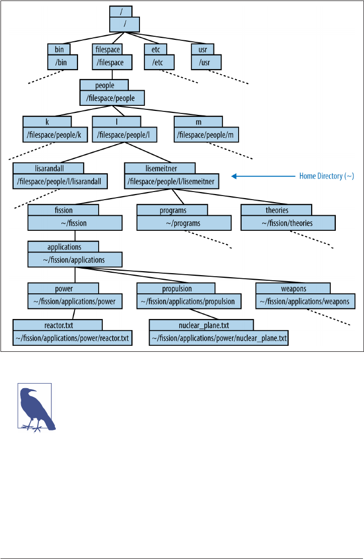
Figure 1-2. An example directory tree
The / syntax is used at the beginning of a path to indicate the top-
level directory. It is also used to separate the names of directories in
a path, as seen in Figure 1-2.
Paths can, instead, be relative to your current working directory. The current working
directory is denoted with one dot (.), while the directory immediately above it (its
“parent”) is denoted with two dots (..). Relative paths therefore often start with a dot
or two.
As we have learned, absolute paths describe a file space location relative to the root
directory. Any path that describes a location relative to the current working directory
4 | Chapter 1: Introduction to the Command Line
www.it-ebooks.info

instead is a relative path. Bringing these together, note that you can always print out
the full, absolute path of the directory you’re currently working in with the command
pwd (print working directory).
Bash was not available in the 1930s, when Lise Meitner was developing a theoretical
framework for neutron-induced fission. However, had Bash been available, Prof.
Meitner’s research computer might have contained a set of directories holding files
about her theory of fission as well as ideas about its application (see Figure 1-2). Let’s
take a look at how Lise would have navigated through this directory structure.
You can work along with Lise while you read this book. The direc‐
tory tree she will be working with in this chapter is available in a
repository on GitHub. Read the instructions at that site to down‐
load the files.
When she is working, Lise enters commands at the command prompt. In the follow‐
ing example, we can see that the command prompt gives an abbreviated path name
before the dollar sign (this is sometimes a greater-than sign or other symbol). That
path is ~/ssion, because ssion is the directory that Lise is currently working in:
~/fission $
When she types pwd at the command prompt, the shell returns (on the following line)
the full path to her current working directory:
~/fission $ pwd
/filespace/people/l/lisemeitner/fission/
When we compare the absolute path and the abbreviated prompt, it seems that the
prompt replaces all the directories up to and including lisemeitner with a single char‐
acter, the tilde (~). In the next section, we’ll see why.
Home Directory (~)
The shell starts your session from a special directory called your home directory. The
tilde (~) character can be used as a shortcut to your home directory. Thus, when you
log in, you probably see the command prompt telling you you’re in your home direc‐
tory:
~ $
These prompts are not universal. Sometimes, the prompt shows the username and
the name of the computer as well:
<user>@<machine>:~ $
For Prof. Meitner, who held a research position at the prestigious Kaiser Wilhelm
Institute, this might appear as:
Navigating the Shell | 5
www.it-ebooks.info

meitner@kaiser-wilhelm-cluster:~ $
Returning to the previous example, let us compare:
~/fission
to:
/filespace/people/l/lisemeitner/fission
It seems that the tilde has entirely replaced the home directory path (/lespace/
people/l/lisemeitner). Indeed, the tilde is an abbreviation for the home directory path
—that is, the sequence of characters (also known as a string) beginning with the root
directory (/). Because the path is defined relative to the absolute top of the directory
tree, this:
~/fission
and this:
/filespace/people/l/lisemeitner/fission
are both absolute paths.
Exercise: Find Home
1. Open the Terminal.
2. Type pwd at the command prompt and press Enter to see the
absolute path to your home directory.
Now that she knows where she is in the filesystem, curious Lise is interested in what
she’ll find there. To list the contents of a directory, she’ll need the ls command.
Listing the Contents (ls)
The ls command allows the user to print out a list of all the files and subdirectories
in a directory.
Exercise: List the Contents of a Directory
1. Open the Terminal.
2. Type ls at the command prompt and press Enter to see the
contents of your home directory.
From the ssion directory in Professor Meitner’s home directory, ls results in the fol‐
lowing list of its contents:
6 | Chapter 1: Introduction to the Command Line
www.it-ebooks.info
~/fission $ ls
applications/ heat-production.txt neutron-release.txt
In the ssion directory within her home directory, Lise types ls and then presses
Enter.
The shell responds by listing the contents of the current directory.
When she lists the contents, she sees that there are two files and one subdirectory. In
the shell, directories may be rendered in a different color than files or may be indica‐
ted with a forward slash (/) at the end of their name, as in the preceding example.
Lise can also provide an argument to the ls command. To list the contents of the
applications directory without entering it, she can execute:
~/fission $ ls applications
power/ propulsion/ weapons/
Lise lists the contents of the applications directory without leaving the ssion
directory.
The shell responds by listing the three directories contained in the applications
directory.
The ls command can inform Lise about the contents of directories in her filesystem.
However, to actually navigate to any of these directories, Lise will need the command
cd.
Changing Directories (cd)
Lise can change directories with the cd command. When she types only those letters,
the cd command assumes she wants to go to her home directory, so that’s where it
takes her:
~/fission $ cd
~ $
Change directories to the default location, the home directory!
As you can see in this example, executing the cd command with no arguments results
in a new prompt. The prompt reflects the new current working directory, home (~).
To double-check, pwd can be executed and the home directory will be printed as an
absolute path:
~ $ pwd
/filespace/people/l/lisemeitner
Print the working directory.
Navigating the Shell | 7
www.it-ebooks.info
The shell responds by providing the absolute path to the current working
directory.
However, the cd command can also be customized with an argument, a parameter
that follows the command to help dictate its behavior:
~/fission $ cd [path]
If Lise adds a space followed by the path of another directory, the shell navigates to
that directory. The argument can be either an absolute path or a relative path.
Angle and Square Bracket Conventions
Using <angle brackets> is a common convention for terms that
must be included and for which a real value must be substituted.
You should not type in the less-than (<) and greater-than (>) sym‐
bols themselves. Thus, if you see cd <argument>, you should type in
something like cd mydir. The [square brackets] convention
denotes optional terms that may be present. Likewise, if they do
exist, do not type in the [ or ]. Double square brackets ([[]]) are
used to denote optional arguments that are themselves dependent
on the existence of other [optional] arguments.
In the following example, Lise uses an absolute path to navigate to a sub-subdirectory.
This changes the current working directory, which is visible in the prompt that
appears on the next line:
~ $ cd /filespace/people/l/lisemeitner/fission
~/fission $
Lise uses the full, absolute path to the ssion directory. This means, “change
directories into the root directory, then the lespace directory, then the people
directory, and so on until you get to the ssion directory.” She then presses Enter.
She is now in the directory ~/ssion. The prompt has changed accordingly.
Of course, that is a lot to type. We learned earlier that the shorthand ~ means “the
absolute path to the home directory.” So, it can be used to shorten the absolute path,
which comes in handy here, where that very long path can be replaced with ~/
fission:
~/ $ cd ~/fission
~/fission $
The tilde represents the home directory, so the long absolute path can be short‐
ened, accomplishing the same result.
8 | Chapter 1: Introduction to the Command Line
www.it-ebooks.info

Another succinct way to provide an argument to cd is with a relative path. A relative
path describes the location of a directory relative to the location of the current direc‐
tory. If the directory where Lise wants to move is inside her current directory, she can
drop everything up to and including the current directory’s name. Thus, from the
ssion directory, the path to the applications directory is simply its name:
~/fission $ cd applications
~/fission/applications $
The applications directory must be present in the current directory for this com‐
mand to succeed.
If a directory does not exist, bash will not be able to change into that location and will
report an error message, as seen here. Notice that bash stays in the original directory,
as you might expect:
~/fission $ cd biology
-bash: cd: biology: No such file or directory
~/fission $
Another useful convention to be aware of when forming relative paths is that the cur‐
rent directory can be represented by a single dot (.). So, executing cd ./power is
identical to executing cd power:
~/fission/applications/ $ cd ./power
~/fission/applications/power/ $
Change directories into this directory, then into the power directory.
Similarly, the parent of the current directory’s parent is represented by two dots (..).
So, if Lise decides to move back up one level, back into the applications directory, this
is the syntax she could use:
~/fission/applications/power/ $ cd ..
~/fission/applications/ $
Using the two-dots syntax allows relative paths to point anywhere, not just at subdir‐
ectories of your current directory. For example, the relative path ../../../ means three
directories above the current directory.
Navigating the Shell | 9
www.it-ebooks.info

Exercise: Change Directories
1. Open the Terminal.
2. Type cd .. at the command prompt and press Enter to move
from your home directory to the directory above it.
3. Move back into your home directory using a relative path.
4. If you have downloaded Lise’s directory tree from the book’s
GitHub repository, can you navigate to that directory using
what you know about ls, cd, and pwd?
A summary of a few of these path-generating shortcuts is listed in Table 1-2.
Table 1-2. Path shortcuts
Syntax Meaning
/ The root, or top-level, directory of the lesystem (also used for separating the names of
directories in paths)
~ The home directory
. This directory
.. The parent directory of this directory
../.. The parent directory of the parent directory of this directory
While seeing the names of files and directories is helpful, the content of the files is
usually the reason to navigate to them. Thankfully, the shell provides myriad tools for
this purpose. In the next section, we’ll learn how to inspect that content once we’ve
found a file of interest.
File Inspection (head and tail)
When dealing with input and output files for scientific computing programs, you
often only need to see the beginning or end of the file (for instance, to check some
important input parameter or see if your run completed successfully). The command
head prints the first 10 lines of the given file:
~/fission/applications/power $ head reactor.txt
# Fission Power Idea
10 | Chapter 1: Introduction to the Command Line
www.it-ebooks.info

The heat from the fission reaction could be used to heat fluids. In
the same way that coal power starts with the production heat which
turns water to steam and spins a turbine, so too nuclear fission
might heat fluid that pushes a turbine. If somehow there were a way to
have many fissions in one small space, the heat from those fissions
could be used to heat quite a lot of water.
As you might expect, the tail command prints the last 10:
~/fission/applications/power $ head reactor.txt
the same way that coal power starts with the production heat which
turns water to steam and spins a turbine, so too nuclear fission
might heat fluid that pushes a turbine. If somehow there were a way to
have many fissions in one small space, the heat from those fissions
could be used to heat quite a lot of water.
Of course, it would take quite a lot of fissions.
Perhaps Professors Rutherford, Curie, or Fermi have some ideas on this
topic.
Exercise: Inspect a File
1. Open a terminal program on your computer.
2. Navigate to a text file.
3. Use head and tail to print the first and last lines to the
terminal.
This ability to print the first and last lines of a file to the terminal output comes in
handy when inspecting files. Once you know how to do this, the next tasks are often
creating, editing, and moving files.
Manipulating Files and Directories
In addition to simply finding files and directories, the shell can be used to act on
them in simple ways (e.g., copying, moving, deleting) and in more complex ways
(e.g., merging, comparing, editing). We’ll explore these tasks in more detail in the fol‐
lowing sections.
Creating Files (nano, emacs, vi, cat, >, and touch)
Creating files can be done in a few ways:
•With a graphical user interface (GUI) outside the terminal (like Notepad, Eclipse,
or the IPython Notebook)
Manipulating Files and Directories | 11
www.it-ebooks.info

• With the touch command
• From the command line with cat and redirection (>)
•With a sophisticated text editor inside the terminal, like nano, emacs, or vi
Each has its own place in a programming workflow.
GUIs for le creation
Readers of this book will have encountered, at some point, a graphical user interface
for file creation. For example, Microsoft Paint creates .bmp files and word processors
create .doc files. Even though they were not created in the terminal, those files are
(usually) visible in the filesystem and can be manipulated in the terminal. Possible
uses in the terminal are limited, though, because those file types are not plain text.
They have binary data in them that is not readable by a human and must be inter‐
preted through a GUI.
Source code, on the other hand, is written in plain-text files. Those files, depending
on the conventions of the language, have various filename extensions. For example:
•.cc indicates C++
•.f90 indicates Fortran90
•.py indicates Python
•.sh indicates bash
Despite having various extensions, source code files are plain-text files and should
not be created in a GUI (like Microsoft Word) unless it is intended for the creation of
plain-text files. When creating and editing these source code files in their language of
choice, software developers often use interactive development environments (IDEs),
specialized GUIs that assist with the syntax of certain languages and produce plain-
text code files. Depending on the code that you are developing, you may decide to use
such an IDE. For example, MATLAB is the appropriate tool for creating .m files, and
the IPython Notebook is appropriate for creating .ipynb files.
Some people achieve enormous efficiency gains from IDEs, while others prefer tools
that can be used for any text file without leaving the terminal. The latter type of text
editor is an essential tool for many computational scientists—their hammer for every
nail.
Creating an empty le (touch)
A simple, empty text file, however, can be created with a mere “touch” in the terminal.
The touch command, followed by a filename, will create an empty file with that
name.
12 | Chapter 1: Introduction to the Command Line
www.it-ebooks.info

Suppose Lise wants to create a file to act as a placeholder for a new idea for a nuclear
fission application, like providing heat sources for remote locations such as Siberia.
She can create that file with the touch command:
~/fission/applications $ touch remote_heat.txt
If the file already exists, the touch command does no damage. All files have metadata,
and touch simply updates the file’s metadata with a new “most recently edited” time‐
stamp. If the file does not already exist, it is created.
Note how the remote_heat.txt file’s name uses an underscore
instead of a space. This is because spaces in filenames are error-
prone on the command line. Since the command line uses spaces
to separate arguments from one another, filenames with spaces can
confuse the syntax. Try to avoid filenames with spaces. If you can’t
avoid them, note that the escape character (\) can be used to alert
the shell about a space. A filename with spaces would then be
referred to as my\ le\ with\ spaces\ in\ its\ name.txt.
While the creation of empty files can be useful sometimes, computational scientists
who write code do so by adding text to code source files. For that, they need text
editors.
The simplest text editor (cat and >)
The simplest possible way, on the command line, to add text to a file without leaving
the terminal is to use a program called cat and the shell syntax >, which is called redi‐
rection.
The cat command is meant to help concatenate files together. Given a filename as its
argument, cat will print the full contents of the file to the terminal window. To out‐
put all content in reactor.txt, Lise could use cat as follows:
~fission/applications/power $ cat reactor.txt
# Fission Power Idea
The heat from the fission reaction could be used to heat fluids. In
the same way that coal power starts with the production heat which
turns water to steam and spins a turbine, so too nuclear fission
might heat fluid that pushes a turbine. If somehow there were a way to
have many fissions in one small space, the heat from those fissions
could be used to heat quite a lot of water.
Of course, it would take quite a lot of fissions.
Perhaps Professors Rutherford, Curie, or Fermi have some ideas on this topic.
Manipulating Files and Directories | 13
www.it-ebooks.info

This quality of cat can be combined with redirection to push the output of one file
into another. Redirection, as its name suggests, redirects output. The greater-than
symbol, >, is the syntax for redirection. The arrow collects any output from the com‐
mand preceding it and redirects that output into whatever file or program follows it.
If you specify the name of an existing file, its contents will be overwritten. If the file
does not already exist, it will be created. For example, the following syntax pushes the
contents of reactor.txt into a new file called reactor_copy.txt:
~fission/applications/power $ cat reactor.txt > reactor_copy.txt
Without any files to operate on, cat accepts input from the command prompt.
Killing or Interrupting Programs
In the exercise above, you needed to use Ctrl-d to escape the cat program. This is not
uncommon. Sometimes you’ll run a program and then think better of it, or, even
more likely, you’ll run it incorrectly and need to stop its execution. Ctrl-c will usually
accomplish this for noninteractive programs. Interactive programs (like less) typi‐
cally define some other keystroke for killing or exiting the program. Ctrl-d will nor‐
mally do the trick in these cases.
As an example of a never-terminating program, let’s use the yes program. If you call
yes, the terminal will print y ad infinitum. You can use Ctrl-c to make it stop.
~/fission/supercritical $ yes
y
y
y
y
y
y
y
y
Ctrl-c
Exercise: Learn About a Command
1. Open a terminal.
2. Type cat and press Enter. The cursor will move to a blank line.
3. Try typing some text. Note how every time you press Enter, a
copy of your text is repeated.
4. To exit, type Ctrl-d. That is, hold down the Control key and
press the lowercase d key at the same time.
14 | Chapter 1: Introduction to the Command Line
www.it-ebooks.info

Used this way, cat reads any text typed into the prompt and emits it back out. This
quality, combined with redirection, allows you to push text into a file without leaving
the command line. Therefore, to insert text from the prompt into the remote_heat.txt
file, the following syntax can be used:
~fission/applications/power $ cat > remote_heat.txt
After you press Enter, the cursor will move to a blank line. At that point, any text
typed in will be inserted into remote_heat.txt. To finish adding text and exit cat, type
Ctrl-d.
Be careful. If the file you redirect into is not empty, its contents will
be erased before it adds what you’re writing.
Using cat this way is the simplest possible way to add text to a file. However, since
cat doesn’t allow the user to go backward in a file for editing, it isn’t a very powerful
text editor. It would be incredibly difficult, after all, to type each file perfectly the first
time. Thankfully, a number of more powerful text editors exist that can be used for
much more effective text editing.
More powerful text editors (nano, emacs, and vim)
A more efficient way to create and edit files is with a text editor. Text editors are pro‐
grams that allow the user to create, open, edit, and close plain-text files. Many text
editors exist. nano is a simple text editor that is recommended for first-time users.
The most common text editors in programming circles are emacs and vim; these pro‐
vide more powerful features at the cost of a sharper learning curve.
Typing the name of the text editor opens it. If the text editor’s name is followed by the
name of an existing file, that file is opened with the text editor. If the text editor’s
name is followed by the name of a nonexistent file, then the file is created and
opened.
To use the nano text editor to open or create the remote_heat.txt file, Lise Meitner
would use the command:
~fission/applications/power $ nano remote_heat.txt
Figure 1-3 shows the nano text editor interface that will open in the terminal. Note
that the bottom of the interface indicates the key commands for saving, exiting, and
performing other tasks.
Manipulating Files and Directories | 15
www.it-ebooks.info

Figure 1-3. e nano text editor
If Lise wanted to use the vim text editor, she could use either the command vim or the
command vi on the command line to open it in the same way. On most modern Unix
or Linux computers, vi is a short name for vim (vim is vi, improved). To use emacs,
she would use the emacs command.
Choose an Editor, Not a Side
A somewhat religious war has raged for decades in certain circles on the topic of
which text editor is superior. The main armies on this battlefield are those that herald
emacs and those that herald vim. In this realm, the authors encourage the reader to
maintain an attitude of radical acceptance. In the same way that personal choices in
lifestyle should be respected unconditionally, so too should be the choice of text edi‐
tor. While the selection of a text editor can powerfully affect one’s working efficiency
and enjoyment while programming, the choice is neither permanent nor an indica‐
tion of character.
Because they are so powerful, many text editors have a steep learning curve. The
many commands and key bindings in a powerful text editor require practice to mas‐
ter. For this reason, readers new to text editors should consider starting with nano, a
low-powered text editor with a shallower learning curve.
16 | Chapter 1: Introduction to the Command Line
www.it-ebooks.info

Exercise: Open nano
1. Open the Terminal.
2. Execute the command nano.
3. Add some text to the file.
4. Use the instructions at the bottom of the window to name and
save the file, then exit nano.
Copying and Renaming Files (cp and mv)
Now that we’ve explored how to create files, let’s start learning how to move and
change them. To make a copy of a file, use the cp command. The cp command has
the syntax cp <source> <destination>. The first required argument is the source file
(the one you want to make a copy of), as a relative or absolute path. The second is the
destination file (the new copy itself), as a relative or absolute path:
~/fission/applications/power $ ls
reactors.txt
~/fission/applications/power $ cp reactors.txt heaters.txt
~/fission/applications/power $ ls
reactors.txt heaters.txt
However, if the destination is in another directory, the named directory must already
exist. Otherwise, the cp command will respond with an error:
~/fission/applications/power $ cp ./reactors.txt ./electricity/power-plant.txt
cp: cannot create regular file `./electricity/power-plant.txt':
No such file or directory
If Lise doesn’t need to keep the original file during a copy, she can use mv (move),
which renames the file instead of copying it. The command evokes “move” because if
the new name is a path in another directory, the file is effectively moved there.
Suppose that when browsing through her ideas, Lise notices an idea for a nuclear
plane in the propulsion directory:
~/fission/applications/propulsion $ ls
nuclear_plane.txt
It really was not such a good idea, actually. A nuclear plane would probably be too
heavy to ever fly. She decides to rename the idea, as a warning to others. It should be
called bad_idea.txt. The mv command accepts two arguments: the original file path
followed by the new file path. She renames nuclear_plane.txt to bad_idea.txt:
~/fission/applications/propulsion $ mv nuclear_plane.txt bad_idea.txt
~/fission/applications/propulsion $ ls
bad_idea.txt
~/fission/applications/propulsion $ mv ./bad_idea.txt ../
Manipulating Files and Directories | 17
www.it-ebooks.info
~/fission/applications/propulsion $ ls ..
bad_idea.txt power/ propulsion/ weapons/
Move (rename) nuclear_plane.txt to bad_idea.txt.
Show the resulting contents of the directory.
Indeed, the file is now called bad_idea.txt.
Now, try moving bad_idea.txt to the applications directory.
List the contents of the applications directory to see the result.
The renamed file is now located in the applications directory above the propulsion
directory.
Once all of her files have been properly named, Lise may need new directories to
reorganize them. For this, she’ll need the mkdir command.
Making Directories (mkdir)
You can make new directories with the mkdir (make directory) command. Using our
usual path conventions, you can make them anywhere, not just in your current work‐
ing directory. When considering a new class of theories about the nucleus, Lise might
decide to create a directory called nuclear in the theories directory. The mkdir com‐
mand creates a new directory at the specified path:
~/theories $ mkdir nuclear
The path can be relative or absolute. In order to create a new directory within the
new nuclear directory, she can specify a longer path that delves a few levels deep:
~/theories $ mkdir ./nuclear/fission
Note, however, that the rule about not putting a file in a nonexistent directory applies
to new directories too:
~/theories/nuclear $ mkdir ./nuclear/fission/uranium/neutron-induced
mkdir: cannot create directory `./nuclear/uranium/neutron-induced':
No such file or directory
Making directories like this on the command line speeds up the process of organiza‐
tion and reduces the overhead involved. Of course, sometimes you may make a file or
directory by mistake. To fix this, you’ll need the rm command.
Deleting Files and Directories (rm)
Files and directories can be deleted using the rm (remove) command. Recall that there
was a bad idea in the applications directory:
18 | Chapter 1: Introduction to the Command Line
www.it-ebooks.info

~/fission/applications $ ls
bad_idea.txt power/ propulsion/ weapons/
After some time, Lise might want to delete that bad idea file entirely. To do so, she can
use the rm command. Given a path to a file, rm deletes it:
~/fission/applications $ rm bad_idea.txt
Once it’s removed, she can check again for its presence with the ls command. As you
can see, it has disappeared:
~/fission/applications $ ls
power/ propulsion/ weapons/
Note that once a file is removed, it is gone forever. There is no safety net, no trash
can, and no recycling bin. Once you delete something with rm, it is truly gone.
Be very careful when using rm. It is permanent. With rm, recall the
adage “Measure twice, cut once.” Before using rm, consciously con‐
sider whether you really want to remove the file.
Since propulsion with nuclear heat, in general, seems unlikely given the weight, Lise
may decide to delete the propulsion directory entirely. However, if she just provides
the path to the directory, the rm command returns an error, as shown here:
~/fission/applications $ rm propulsion
rm: propulsion: is a directory
This error is a safety feature of rm. To delete directories, it is necessary to use the -r
(recursive) flag. Flags such as -r modify the behavior of a command and are common
in the shell. This flag tells rm to descend into the directory and execute the command
all the way down the tree, deleting all files and folders below propulsion:
~/fission/applications $ rm -r propulsion
This requirement prevents you from deleting entire branches of a directory tree
without confirming that you do, in fact, want the shell to descend into all subdirecto‐
ries of the given directory and delete them, as well as their contents.
On some platforms, just to be safe, the rm command requests confirmation at each
new subdirectory it encounters. Before it deletes a subdirectory, it will ask: “rm:
descend into directory ‘subdirectoryname’?” Type y or n to confirm “yes” or “no,”
respectively. This can be avoided if an f (for force) is added to the flags. The com‐
mand to force removal of a directory and all its subdirectories is rm -rf <directory
name>.
Manipulating Files and Directories | 19
www.it-ebooks.info

While rm -rf can be used carefully to great effect, never execute rm
-rf *. Unscrupulous mischief-makers may recommend this, but it
will have catastrophic consequences. Do not fall for this
tomfoolery.
The next section will cover some examples of more flags available to commands in
the shell.
Exercise: Make and Remove Files and Directories
1. Open the Terminal.
2. Use mkdir to create a directory with a few empty subdirecto‐
ries.
3. Use touch to create five empty files in those directories, and
use ls to inspect your work.
4. With one command (hint: it will have to be recursive), remove
the whole directory. Do you need to use the force flag to avoid
typing y repeatedly?
Flags and Wildcards
Flags are often important when using these file and directory manipulation com‐
mands. For instance, you can mv a directory without any flags. However, copying a
directory without the recursive flag fails. Let’s look at an example. Since all applica‐
tions generating power start by generating heat, a new directory called heat could
start as a duplicate of the power directory:
~/fission/applications $ cp power/ heat/
cp: omitting directory `power/'
The copy command, not accepting a directory as a valid copy target, throws the error
“cp: omitting directory directoryname“. To copy the directory and its contents with cp,
the -r (recursive) flag is necessary:
~/fission/applications $ cp -r power/ heat/
An alternative to copying, moving, or removing entire directories is to use a wildcard
character to match more than one file at once. In the bash shell, the asterisk (*) is a
wildcard character. We’ll talk about this more in Chapter 8; for now, just note that the
asterisk means, approximately, match everything.
In the following example, all the files in the directory are matched by the asterisk.
Those files are all copied into the destination path:
20 | Chapter 1: Introduction to the Command Line
www.it-ebooks.info

~ $ cp beatles/* brits/
~ $ cp zeppelin/* brits/
~ $ cp beatles/john* johns/
~ $ cp zeppelin/john* johns/
~ $ ls brits
george jimmy john john_paul paul ringo robert
~ $ ls johns
john john_paul
But notice that we’ve overwritten a “john” during the second copy into each directory.
To help avoid making such mistakes, you can use -i to run the command interac‐
tively; the shell will then ask you to confirm any operations it thinks seem suspicious:
~ $ cp beatles/john* johns/.
~ $ cp -i beatles/john* johns/.
cp: overwrite `johns/./john'? y
In a sense, -i is the opposite of -f, which forces any operations that the shell might
otherwise warn you about:
~ $ mv zeppelin/john deceased/.
~ $ mv beatles/john deceased/.
mv: overwrite `deceased/./john'? n
~ $ mv -f beatles/john deceased/.
In this section, we have covered a few flags commonly available to commands on the
command line. However, we have only scratched the surface. Most available com‐
mands possess many customized behaviors. Since there are far too many to memo‐
rize, the following section discusses how to get help and find more information about
commands.
Getting Help
Now that you have become familiar with the basics, you can freely explore the termi‐
nal. The most important thing to know before venturing forth, however, is how to get
help.
Reading the Manual (man)
The program man (manual) is an interface to online reference manuals. If you pass the
name of a command or program to man as an argument, it will open the help file for
that command or program. To determine what flags and options are available to the
ls command, then, typing man ls would provide the instructions for its use. Since
man is itself a program, we can type man man to get the instructions for using man:
~ $ man man
NAME
man - an interface to the on-line reference manuals
Getting Help | 21
www.it-ebooks.info

SYNOPSIS
man [-c|-w|-tZ] [-H[browser]] [-T[device]] [-adhu7V]
[-i|-I] [-m system[,...]] [-L locale] [-p string] [-C
file] [-M path] [-P pager] [-r prompt] [-S list] [-e
extension] [[section] page ...] ...
man -l [-7] [-tZ] [-H[browser]] [-T[device]] [-p
string] [-P pager] [-r prompt] file ...
man -k [apropos options] regexp ...
man -f [whatis options] page ...
DESCRIPTION
man is the systems manual pager. Each page argument
given to man is normally the name of a program, utility
or function. The manual page associated with each of
these arguments is then found and displayed. A section,
if provided, will direct man to look only in that sec
tion of the manual. The default action is to search in
all of the available sections, following a pre-defined
order and to show only the first page found, even if
page exists in several sections.
<snip>
What follows man in the SYNOPSIS is a listing of the optional and required arguments,
options, and variables.
Arguments, options, and variables
In these man pages, you’ll see that there are different ways to pass information to the
command-line programs and commands you need to use. We’ve seen the first one:
arguments. An argument simply gets added after the command. You can add multiple
arguments if the command expects that behavior. We’ve added single arguments
when we’ve changed into a specific directory (e.g., cd ..). We also used two argu‐
ments at once with cp (e.g., cp <source> <destination>). We also saw, for example,
that the ls command with the single argument . lists the contents of the current
directory:
~/weaponry $ ls .
fear ruthless_efficiency surprise
We’ve also seen options, also called ags or switches (e.g., the recursive flag, -r). These
tell the program to run in some predefined way. Options are usually specified with a
minus sign (-) in front of them. For instance, if we run man ls and scroll down, we
see that the -r option lists directory contents in reverse order. That is:
~/weaponry $ ls -r .
surprise ruthless_efficiency fear
22 | Chapter 1: Introduction to the Command Line
www.it-ebooks.info

Be careful—flags (like -r) don’t necessarily have the same meaning
for every command. For many commands, -r indicates recursive
behavior, but for ls, it prints the directory contents in reverse
order.
Variables can be used to pass in specific kinds of information and are usually speci‐
fied with a double minus sign (--, typically pronounced “minus minus” or “dash
dash”). Further perusal of the ls man page indicates that a variable called sort can be
set to certain values to sort directory contents in various ways. To provide a value to
sort, we use an equals sign (=). For instance, --sort=time sorts directory contents by
file modification time, with the most recent file first:
~/weaponry $ ls --sort=time .
fear surprise ruthless_efficiency
All of the arguments, options, and variables for a command are detailed in the man
page for that command. To see how they are used, you will need to scroll down in the
man page document to where they are explained. To scroll down, it’s helpful to know
how to use less.
Moving around in less
man opens the help documents in a program called less, which you can use to look at
other text files as well (just call less [filename]). There’s lots to learn about less
(use man less to get an overview), but the most important things to know are as
follows:
• Use the up and down arrows to scroll up and down.
•Use Page Up and Page Down (or the space bar) to move up or down by an entire
page.
•Use a forward slash (/) followed by a search term and then Enter to search for a
particular word. The letter n (next) toggles through each occurrence.
•Use h to display help inside less—this displays all the possible commands that
less understands.
• Use q to quit.
less is modeled on an earlier program called more. However, more has fewer features,
and you probably shouldn’t bother with it. So, always remember: less is more.
Getting Help | 23
www.it-ebooks.info
Exercise: Use the man Pages with less
1. Open the Terminal.
2. Use the man command and the preceding notes on less to
learn about the commands covered already in this chapter
(e.g., mkdir, touch, mv, cp, etc.)
Of course, before you can use man and less to find information about available com‐
mands, you must know what commands are available. For that, we need a command
called apropos.
Finding the Right Hammer (apropos)
The bash shell has so many built-in programs, practically no one has all of their
names memorized. Since the man page is only helpful if you know the name of the
command you’re looking for, you need some tool to determine what that command
is. Thankfully, this tool exists. You can search the man pages for keywords with a com‐
mand called apropos. Let’s say you want to know what text editors are available. You
might search for the string “text editor”:
~ $ apropos "text editor"
ed(1), red(1) - text editor
vim(1) - Vi IMproved, a programmers text editor
To search for an installed command based on a keyword string, use apropos.
ed and red show up together, because their full description is “text editor.”
vim appears next, with its longer description. Other installed editors will not
appear if the exact phrase “text editor” does not appear in their man pages. What
happens if you try apropos editor?
An optimistic physicist, Lise might have been curious enough to query physics-
related commands. Unfortunately, she might be disappointed to find there aren’t
many:
~ $ apropos physics
physics: nothing appropriate
24 | Chapter 1: Introduction to the Command Line
www.it-ebooks.info

Exercise: Find and Learn About a Command
1. Open the Terminal.
2. Search your computer for commands by using apropos and a
keyword.
3. Take some time to explore the man page of a command we’ve
discussed or of another command or program you know of.
Learn about a couple of new arguments or options and try
them out. Practice killing or interrupting programs if neces‐
sary.
Now that this chapter has touched on the various commands for running processes
and manipulating files, let’s see how those commands can be combined into powerful
pipelines using redirection and pipes.
Combining Utilities with Redirection and Pipes (>, >>, and |)
The power of the shell lies in the ability to combine these simple utilities into more
complex algorithms very quickly. A key element of this is the ability to send the out‐
put from one command into a file or to pass it directly to another program.
To send the output of a command into a file, rather than printing it to the screen as
usual, redirection is needed. A text or data stream generated by the command on the
lefthand side of the arrow is sent (redirected) into the file named on the righthand
side. One arrow (>) will create a new file or overwrite the contents of an existing one
with the stream provided by the lefthand side. However, two arrows (>>) will append
the stream to the end of an existing file, rather than overwriting it. If Lise wants to
create a new file containing only the first line of another, she can combine the head
command and the redirection method to achieve this in one line:
~/fission/applications/power $ head -1 reactor.txt > reactor_title.txt
Now, the content of reactor_title.txt is simply:
# Fission Power Idea
To chain programs together, the pipe (|) command can be used in a similar fashion.
The output of one program can be used as the input of another. For example, to print
the middle lines of a file to the screen, head and tail can be combined. To print only
line 11 from the reactor.txt file, Lise can use head, tail, and a pipe:
~/fission/applications/power $ head -1 reactor.txt | tail -1
Of course, it would take quite a lot of fissions.
With these methods, any program that reads lines of text as input and produces lines
of text as output can be combined with any other program that does the same.
Getting Help | 25
www.it-ebooks.info

Now that you’ve seen how the many simple commands available in the shell can be
combined into ad hoc pipelines, the incredible combinatoric algorithmic power of
the shell is at your fingertips—but only if you have the right permissions.
Permissions and Sharing
Permissions are a subtle but important part of using and sharing files and using com‐
mands on Unix and Linux systems. This topic tends to confuse people, but the basic
gist is that different people can be given different types of access to a given file, pro‐
gram, or computer.
At the highest level, the filesystem is only available to users with a user account on
that computer. Based on these permissions, some commands allow users to connect
to other computers or send files. For example:
•ssh [user@host] connects to another computer.
•scp [file] [user@host]:path copies files from one computer to another.
Those commands only work if the user issuing them has permission to log into the
filesystem. Otherwise, he will not be able to access the file system at all.
Once they have accessed a computer’s filesystem, however, different types of users
may have different types of access to the various files on that system. The “different
types of people” are the individual user (u) who owns the file, the group (g) who’s
been granted special access to it, and all others (o). The “different types of access” are
permission to read (r), write to (w), or execute (x) a file or directory.
This section will introduce three commands that allow you to manage the permis‐
sions of your files:
•ls -l [file] displays, among other things, the permissions for that file.
•chown [-R] [[user]][:group] target1 [[target2 ..]] changes the individ‐
ual user and group ownership of the target(s), recursively if -R is used and one or
more targets are directories.
•chmod [options] mode[,mode] target1 [[target2 ...]] changes or sets the
permissions for the given target(s) to the given mode(s).
The first of these, ls -l, is the most fundamental. It helps us find out what permis‐
sion settings apply to files and directories.
Seeing Permissions (ls -l)
We learned earlier in this chapter that ls lists the contents of a directory. When you
explored the man page for ls, perhaps you saw information about the -l flag, which
26 | Chapter 1: Introduction to the Command Line
www.it-ebooks.info

lists the directory contents in the “long format.” This format includes information
about permissions.
Namely, if we run ls -l in a directory in the filesystem, the first thing we see is a
code with 10 permission digits, or “bits.” In her ssion directory, Lise might see the
following “long form” listing. The first 10 bits describe the permissions for the direc‐
tory contents (both files and directories):
~/fission $ ls -l
drwxrwxr-x 5 lisemeitner expmt 170 May 30 15:08 applications
-rw-rw-r-- 1 lisemeitner expmt 80 May 30 15:08 heat-generation.txt
-rw-rw-r-- 1 lisemeitner expmt 80 May 30 15:08 neutron-production.txt
The first bit displays as a d if the target we’re looking at is a directory, an l if it’s a link,
and generally - otherwise. Note that the first bit for the applications directory is a d,
for this reason.
To see the permissions on just one file, the ls -l command can be followed by the
filename:
~/fission $ ls -l heat-generation.txt
-rw-rw-r-- 1 lisemeitner expmt 80 May 30 15:08 heat-generation.txt
In this example, only the permissions of the desired file are shown. In the output, we
see one dash followed by three sets of three bits for the heat-generation.txt file (-rw-
rw-r--). Let’s take a look at what this means:
• The first bit is a dash, -, because it is not a directory.
•The next three bits indicate that the user owner (lisemeitner) can read (r) or
write (w) this file, but not execute it (-).
•The following three bits indicate the same permissions (rw-) for the group owner
(expmt).
•The final three bits (r--) indicate read (r) but not write or execute permissions
for everyone else.
All together, then, Lise (lisemeitner) and her Experiment research group (expmt)
can read or change the file. They cannot run the file as an executable. Finally, other
users on the network can only read it (they can never write to or run the file).
Said another way, the three sets of three bits indicate permissions for the user owner,
group owner, and others (in that order), indicating whether they have read (r), write
(w), or execute (x) privileges for that file.
The ls man page provides additional details on the rest of the information in this dis‐
play, but for our purposes the other relevant entries here are the two names that fol‐
Permissions and Sharing | 27
www.it-ebooks.info

low the permission bits. The first indicates that the user lisemeitner is the individual
owner of this file. The second says that the group expmt is the group owner of the file.
Exercise: View the Permissions of Your Files
1. Open a terminal.
2. Execute ls -l on the command line. What can you learn
about your files?
3. Change directories to the / directory (try cd /). What are the
permissions in this directory? What happens if you try to cre‐
ate an empty file (with touch <filename>) in this directory?
In addition to just observing permissions, making changes to permissions on a file
system is also important.
Setting Ownership (chown)
It is often helpful to open file permissions up to one’s colleagues on a filesystem. Sup‐
pose Lise, at the Kaiser Wilhelm Institute, wants to give all members of the institute
permission to read and write to one of her files, heat-generation.txt. If those users are
all part of a group called kwi, then she can give them those permissions by changing
the group ownership of the file. She can handle this task with chown:
~/fission $ chown :kwi heat-generation.txt
~/fission $ ls -l heat-generation.txt
-rw-rw-r-- 1 lisemeitner kwi 80 May 30 15:08 heat-generation.txt
Exercise: Change Ownership of a File
1. Open a terminal.
2. Execute the groups command to determine the groups that
you are a part of.
3. Use chown to change the ownership of a file to one of the
groups you are a part of.
4. Repeat step 3, but change the group ownership back to what it
was before.
However, just changing the permissions of the file is not quite sufficient, because
directories that are not executable by a given user can’t be navigated into, and directo‐
ries that aren’t readable by a given user can’t be printed with ls. So, she must also
28 | Chapter 1: Introduction to the Command Line
www.it-ebooks.info

make sure that members of this group can navigate to the file. The next section will
show how this can be done.
Setting Permissions (chmod)
Lise must make sure her colleagues can visit and read the dictionary containing the
file. Such permissions can be changed by using chmod, which changes the file mode.
Since this is a directory, it must be done in recursive mode. If she knows her home
directory can be visited by members of the kwi group, then she can set the permis‐
sions on the entire directory tree under ~/ssion with two commands. The first is
again chown. It sets the ssion directory’s group owner (recursively) to be kwi:
~ $ chown -R :kwi fission/
Next, Lise changes the file mode with chmod. The chmod syntax is chmod [options]
<mode> <path>. She specifies the recursive option, -R, then the mode to change the
group permissions, adding (+) reading and execution permissions with g+rx:
~ $ chmod -R g+rx fission/
Many other modes are available to the chmod command. The mode entry g+rx means
we add the read and execution bits to the group’s permissions for the file. Can you
guess the syntax for subtracting the group’s read permissions? The manual page for
chmod goes into exceptional detail about the ways to specify file permissions. Go there
for special applications.
Physicists using large scientific computing systems rely heavily on permissions to
securely and robustly share data files and programs with multiple users. All of these
permissions tools are helpful with organizing files. Another tool available for organiz‐
ing files across filesystems is the symbolic link.
Creating Links (ln)
The ln command allows a user to create a hard or symbolic link to a file or program.
This effectively creates more than one reference pointing to where the contents of the
file are stored. This section will focus on symbolic links rather than hard links.
Symbolic links are useful for providing access to large, shared resources on a net‐
worked filesystem. Rather than storing multiple copies of large datasets in multiple
locations, an effective physicist can create symbolic links instead. This saves hard
drive space, since a symbolic link only takes up a few bytes. Also, it saves time. Since
the links can be placed in easy-to-find locations, colleagues will spend less time
searching deeply nested subdirectories for desired programs and data files.
For our purposes, symbolic links (created with ln -s) are the safest and most useful.
Let’s say, for instance, that Lise has compiled a program that suggests a random pair
of isotopes likely to result from a uranium fission. Her colleagues have a hard time
Permissions and Sharing | 29
www.it-ebooks.info
remembering whether the program is called ssion_fragments or just fragments.
When they try ssion_fragments, bash responds with a warning—the command is
not a valid path:
~/programs/fission $ ./fission_fragments
./fission_fragments: Command not found.
One solution is to add a symbolic link. A new link at the incorrect filename, pointing
to the correct filename, can be created with the syntax ln -s <source_path>
<link_path>:
~/programs/fission $ ln -s fragments fission_fragments
With that complete, a new symbolic link has been created. It can be viewed with ls -
l, and appears to be just like any other file except for the arrow showing it is just a
pointer to the fragments program:
~/programs/fission $ ls -l
-rwxrwxr-x 1 lisemeitner staff 20 Nov 13 19:02 fragments
lrwxrwxr-x 1 lisemeitner staff 5 Nov 13 19:03 fission_fragments -> fragments
Input: Execute the “list in long form” command on the command line.
Output: the file listing now shows both the fragments file and, on the next line,
the ssion fragments file, with an arrow indicating that it is a symbolic link to the
fragments executable. Note also that the first of the 10 permission bits for that file
is an l for “link.”
Now, with this symbolic link in the directory, Lise’s colleagues can use either name
with the same success. Furthermore, recall that a dot (.) stands for the current direc‐
tory and that slashes (/) separate directory and file names. Therefore, ./myle refers to
myle in the current directory. When running a program in the current directory,
you must include the dot-slash. As you can see from the following, this works equally
well on symbolic links as it does on normal files:
~/programs/fission$ ./fission_fragments
140Xe 94Sr
Symbolic links are useful for providing access to large, shared resources, rather than
storing multiple copies in multiple hard-to-reach locations. Another common way
physicists gain access to large, shared resources is by accessing them on remote
machines. We’ll discuss the power of connecting to other computers in the next
section.
Connecting to Other Computers (ssh and scp)
This powerful feature of the command line, providing access to networked and
remote filesystems, is key to high-performance computing tasks. Since most large
30 | Chapter 1: Introduction to the Command Line
www.it-ebooks.info

high-performance or high-throughput computing resources can only be accessed by
SSH (Secure SHell) or similar protocols through the command line, truly high-
powered computer systems simply are not accessible without use of the shell.
If you have the right credentials, you can even get access to another machine through
the shell. You can do this using a program called ssh. For instance, for the user grace
to log on to a networked computer mk1, she would use the ssh command with an
argument specifying her username and the computer name, connected by the @
symbol:
~ $ ssh grace@mk1
Or, if mk1 is a computer located on the remote network domain harvard.edu, Grace
can connect to that computer from her home computer with the full location of the
computer in its domain:
~ $ ssh grace@mk1.harvard.edu
Once logged into the computer, Grace has access to the files and directories in the
remote filesystem and can interact with them just as she does locally.
She can use the scp (secure copy) command to copy files and directories from one
computer to another. It has the syntax scp <source_file> [[user@]host]:<desti
nation>. So, to copy a notes.txt file from her local computer to the COBOL directory
on the mk1.harvard.edu filesystem, she would execute:
~ $ scp ./notes.txt grace@mk1.harvard.edu:~/COBOL/notes.txt
Both ssh and scp require a valid username and password on the
remote machine.
When she connects to another computer, Grace has access to its filesystem. On that
system, there are not only different files, but also a different environment. We’ll look
at the environment and how it is configured next.
The Environment
In addition to providing commands, a filesystem hierarchy, and a syntax for naviga‐
tion, the bash shell defines a computing environment. This computing environment
can be customized using environment variables. We can investigate our environment
with a program called echo. The echo command prints arguments to the terminal. In
the case of a string argument, the string is printed verbatim:
~ $ echo "Hello World"
Hello World
The Environment | 31
www.it-ebooks.info

In the case of environment variables, however, echo performs expansion, printing the
values of the variables rather than just their names. You invoke these variables on the
command line by prepending a $ to the variable name.
When, in 1959, she began to design the first machine-independent programming lan‐
guage (COBOL), Grace Hopper did not have bash. Bash, after all, could never have
come into existence without her breakthrough. Hypothetically, though, if she had had
bash, her environment might have behaved liked this:
~ $ echo $USERNAME
grace
~ $ echo $PWD
/filespace/people/g/grace
Echo the value of the USERNAME environment variable. On certain platforms, this
variable is called USER.
The computer stores the working directory in the environment variable PWD; the
command pwd is simply a shortcut for echo $PWD.
Shell variables are replaced with their values when executed. In bash, you can create
your own variables and change existing variables with the export command:
~ $ export GraceHopper="Amazing Grace"
Variables are case-sensitive. For this reason, the following command will successfully
echo the assigned string:
~ $ echo $GraceHopper
Amazing Grace
However, none of the following will succeed:
~ $ echo GraceHopper
~ $ echo GRACEHOPPER
~ $ echo $GRACEHOPPER
Table 1-3 lists some of the most common and important shell variables. These vari‐
ables often become essential for defining the computer’s behavior when the user com‐
piles programs and builds libraries from the command line.
Table 1-3. Common environment variables
Variable name Meaning
USER User name
PATH List of absolute paths that are searched for executables
PWD Current directory (short for print working directory)
32 | Chapter 1: Introduction to the Command Line
www.it-ebooks.info

Variable name Meaning
EDITOR Default text editor
GROUP Groups the user belongs to
HOME Home directory
~Same as HOME
DISPLAY Used in forwarding graphics over a network connection
LD_LIBRARY_PATH Like PATH, but for precompiled libraries
FC Fortran compiler
CC C compiler
Environment variables can be used to store information about the environment and
to provide a shorthand for long but useful strings such as absolute paths. To see all of
the environment variables that are active in your terminal session, use the env com‐
mand. Rear Admiral Hopper might see something like:
~/fission $ env
SHELL=/bin/bash
USER=grace
EDITOR=vi
LD_LIBRARY_PATH=/opt/local/lib:/usr/local
PATH=/opt/local/lib:/filespace/people/g/grace/anaconda/bin:/opt/local/bin
PWD=/filespace/people/g/grace/languages
LANG=en_US.utf8
PWD=/filespace/people/g/grace
LOGNAME=grace
OLDPWD=/filespace/people/g/grace/languages/COBOL
To make an environment variable definition active every time you open a new termi‐
nal, you must add it to a file in your home directory. This file must be called .bashrc.
Saving Environment Variables (.bashrc)
A number of files in a bash shell store the environment variables that are active in
each terminal session. They are plain-text files containing bash commands. These
commands are executed every time a terminal window is opened. Thus, any environ‐
ment variables set with export commands in those files are active for every new ter‐
minal session.
To configure and customize your environment, environment variables can be added
or edited in ~/.bashrc, the main user-level bash configuration file. The export com‐
The Environment | 33
www.it-ebooks.info

mands we executed in the terminal before added new environment variables for a
single terminal session. To add or change an environment variable for every session,
we use .bashrc.
The leading . in .bashrc makes the file a hidden file.
User-specific configuration exists in many files. In addition to the .bashrc file, you
may see others, such as .bash_prole or, on newer Mac OS machines, .prole. Do any
of those exist on your computer? If so, open that file and confirm that it contains the
text source ~/.bashrc.
Exercise: Congure Your Shell with .bashrc
1. Use your text editor to open the .bashrc file in your home
directory. If no such file exists, create it.
2. Add an export command to set a variable called DATA equal to
the location of some data on your filesystem.
3. Open a new terminal window and query the DATA variable with
echo.
4. What is the result of cd $DATA? Can you imagine ways this
behavior could make navigating your files easier?
A new terminal instance will automatically reflect changes to the .bashrc file. How‐
ever, the source command can be used to make changes to .bashrc take effect imme‐
diately, in the current session:
~ $ source .bashrc
The bash shell can be customized enormously with commands executed in
the .bashrc file. This customization is ordinarily used to specify important paths and
default behaviors, making the shell much more efficient and powerful. The most
important variable in your .bashrc file is the PATH.
Running Programs (PATH)
Based on the environment, the shell knows where to find the commands and pro‐
grams you use at the command line. Unless you modify your environment, you can’t
run just any old program on your computer from any directory. If you want to run a
34 | Chapter 1: Introduction to the Command Line
www.it-ebooks.info

program in a nonstandard location, you have to tell the shell exactly where that pro‐
gram is by invoking it with an absolute or relative Unix path.
For instance, in Chapter 14, we will learn to build a program. However, after we’ve
done so, we can still only run that program if we tell the shell exactly where it is. With
the programs we have seen so far, the name of the command is sufficient. However,
because bash only searches certain locations for available commands, the fragments
command will not be found:
~/programs/fission $ fragments
fragments: Command not found.
We attempt to run the fragments program.
The shell’s response indicates that it cannot find the named program (because it
is not in the PATH).
Indeed, even in the proper directory, you must indicate the full path to the program
by adding the leading dot-slash before the computer understands what program to
run:
~/programs/fission $ ./fragments
136Cs 99Tc
In order for the computer to find the fragments program without us typing the full
path, the PATH environment variable must contain the directory holding the program.
Without the full path, the bash shell only executes commands found when searching
the directories specified in the PATH environment variable. To add this folder to the
PATH environment variable, Lise can execute the following command:
~/programs $ export PATH=$PATH:/filespace/people/l/lisemeitner/programs/fission
The first part of this command uses export to set the PATH variable. Everything on
the righthand side of the equals sign will become the new PATH. The first element of
that path is the old PATH variable value. The second element, after the colon, is the
new directory to add to the list of those already in the PATH. It will be searched last.
Exercise: Customize Your PATH
1. In the terminal, use echo to determine the current value of the
PATH environment variable. Why do you think these directo‐
ries are in the PATH?
2. Use export to add your current directory to the end of the list.
Don’t forget to include the previous value of PATH.
3. Use echo once again to determine the new value.
The Environment | 35
www.it-ebooks.info

Can you think of a way that the PWD environment variable could be used to shorten
the preceding command? In addition to shortening commands and paths by setting
environment variables, configuration files are an excellent place to permanently give
shorter nicknames to other commands. In the next section, we’ll see how to do this
with the alias command.
Nicknaming Commands (alias)
In the same way that you can create variables for shortening long strings (like $DATA,
the path to your data), you can create shorthand aliases for commands. alias does a
simple replacement of the first argument by the second. If, for example, you like col‐
ors to distinguish the files and directories in your shell session, you’ll always want to
use the --color variable when calling ls. However, ls --color is quite a lot to type.
It is preferable to reset the meaning of ls so that it behaves like ls --color. The
alias command allows you to do just that. To replace ls with ls --color, you
would type:
alias ls 'ls --color'
Once that command has been executed in the terminal, typing ls is equivalent to typ‐
ing ls --color. Just like an environment variable, to make an alias active every time
you open a new terminal, you must add this definition to your .bashrc file, which is
executed upon login.
To keep their .bashrc files cleaner and more readable, many indi‐
viduals choose to keep all of their aliases in a separate hidden file
(called something like .bash_aliases). To load it, they include the
following line in their .bashrc files:
source ~/.bash_aliases
Now that the .bashrc bash script has demonstrated the power of automating bash
commands, the following section will show how to write your own bash scripts.
Scripting with Bash
Repeating processes on the command line is made easy with files (like .bashrc) that
can store many commands and be executed at will. Any such series of commands can
be placed into a file called a script. This type of file, like a program, can be written
once and executed many times.
Bash scripts typically end in the .sh extension. So, the first step for creating a bash
script is to create such a file. As we did earlier in this chapter, you can do this by
opening a text editor like nano and supplying the filename as an argument:
~ $ nano explore.sh
36 | Chapter 1: Introduction to the Command Line
www.it-ebooks.info

Any commands that are valid in the terminal are valid in a bash script. Some text in a
bash script might be for reference, however. This text, called a comment, must be
denoted with a #.
If Lise would like to automate the process of exploring her directory tree, she might
write a bash script for the task. A very simple bash script that enters three levels of
parent directories and prints the contents as well as the directory names is only a few
simple lines:
# explore.sh
# explore the three directories above this one
# print a status message
echo "Initial Directory:"
# print the working directory
pwd
# list the contents of this directory
ls
echo "Parent Directory:"
# ascend to the parent directory
cd ..
pwd
ls
echo "Grandparent Directory:"
cd ..
pwd
ls
echo "Great-Grandparent Directory:"
cd ..
pwd
ls
Comments are preceded by a # symbol. They are reference text only and are not
executed.
After you save this file, there is only one more step required to make it a bona fide
program. To run this script on the command line, its permissions must be set to exe‐
cutable. To make this the case, Lise must execute (in the terminal) the command:
~ $ chmod a+x explore.sh
Now, the explore.sh script is runnable. To run the command, Lise must either call it
with its full path or add the location to her PATH environment variable. When we use
a relative path, the execution looks like:
~ $ ./explore.sh
Scripting with Bash | 37
www.it-ebooks.info

Exercise: Write a Simple Bash Script
1. Create a file called explore.sh.
2. Copy the example script into that file.
3. Change the permissions of the file so that it is executable.
4. Run it and watch the contents of your filesystem be printed to
the terminal.
Much more sophistication is possible in a bash script, but that is somewhat beyond
the scope of this chapter. To learn more about sophisticated bash scripting, check out
some of the O’Reilly books on the topic or sign up for a workshop like those run by
Software Carpentry.
The history Command
At the end of some series of bash commands, an effective physicist
may want to create a bash script to automate that set of commands
in the future. The history command provides a list of all the most
recent commands executed in the terminal session. It is very help‐
ful for recalling recent work and enshrining it in a bash script.
Command Line Wrap-up
This chapter has only just scratched the surface of the power the command line
holds. It has covered:
• Navigating the filesystem
• Creating, deleting, and moving files and directories
•Finding help
• Running commands
• Handling permissions
• Writing scripts
If you want to find out more about the command line, many books and Internet
resources are available. Cameron Newham’s Learning the bash Shell (O’Reilly) is a
good place to start, and Software Carpentry’s workshops and online resources pro‐
vide an excellent introduction to the deeper secrets of bash.
38 | Chapter 1: Introduction to the Command Line
www.it-ebooks.info

1For a detailed language comparison, please see Lutz Prechelt’s article “An Empirical Comparison of Seven Pro‐
gramming Languages.”
CHAPTER 2
Programming Blasto with Python
A lot of people talk about the greatness of Python as a programming language. They
are right! But what is Python, and why is it so awesome? Python is a general-purpose,
dynamic, high-level language that is easy to learn. Python is also known as a glue lan‐
guage because it plays nicely with other languages, including C, C++, and Fortran.
For these reasons it has established a strong foothold as a data analysis language. This
makes it popular in science and engineering, and in physics-related fields in
particular.
The main criticism of Python is its speed. Python is an interpreted language, which
makes it more similar to R, Ruby, and MATLAB than it is to compiled languages like
C, C++, or Fortran. Pythonistas everywhere live by the mantra that “premature opti‐
mization is bad.” Concerns that it is too slow are often refuted with these arguments:
•Developer time—the time the programmer spends programming—is more val‐
uable than execution time.1
•Most speed issues can be overcome by using the appropriate data structures and
algorithms.
•If you really have a need for speed you can always write the performance-critical
parts in a compiled language and then expose the functionality to Python.
The most important aspect of Python is it is fun to use! The more you learn, the more
you want to learn, and the more you find there is to learn. The Python ecosystem is
extraordinarily rich and the community members are, by and large, friendly.
Unfortunately, there is no way that this book can fully cover all of the excellent
39
www.it-ebooks.info

aspects of Python. This chapter is a meant as a first introduction to the basics of
Python syntax. Many more detailed references and resources are available. For instal‐
lation instructions, please refer back to the Preface.
Running Python
Python itself is a special type of program called an interpreter, because it translates
Python source code into instructions that your computer’s processor can understand.
The Python interpreter can be fired up in a number of ways. The most basic (and
least used) way is to type python at the command prompt in your terminal. This will
normally display some information about Python itself and then return with a line
that begins with >>>. This is the Python prompt, and from here you can start input‐
ting Python code:
$ python
Python 2.7.5+ (default, Sep 19 2013, 13:48:49)
[GCC 4.8.1] on linux2
Type "help", "copyright", "credits" or "license" for more information.
>>>
Hitting Enter will execute what you type in and return a >>> prompt:
>>> print("Hello Sir Newton.")
Hello Sir Newton.
>>>
To get help at any time, use the help() function. To exit back to the command line,
use the exit() function. If this looks a lot like bash, it is because this method of inter‐
acting with Python is the same as the one we used to interact with bash: a read-eval-
print loop, or REPL.
However, for Python, the stock REPL is not the only one available. IPython (which
stands for Interactive Python) provides a REPL that is in many ways superior to the
default one. You can get IPython in one of the following ways:
1. Visit ipython.org and download the latest stable release.
2. If you are using the Conda package manager, as described in the Preface, and fol‐
lowed the instructions in “Installation and Setup” on page xxiii, you should
already have IPython. If you like you can run the command conda update ipy
thon to be sure you have the most recent version.
3. If you have Python installed, run the command pip install ipython.
4. If you are using Ubuntu, run the command sudo apt-get install ipython.
Starting up and executing code in IPython looks like this:
40 | Chapter 2: Programming Blasto with Python
www.it-ebooks.info

$ ipython
Python 2.7.5+ (default, Sep 19 2013, 13:48:49)
Type "copyright", "credits" or "license" for more information.
IPython 1.1.0 -- An enhanced Interactive Python.
? -> Introduction and overview of IPython's features.
%quickref -> Quick reference.
help -> Python's own help system.
object? -> Details about 'object', use 'object??' for extra details.
In [1]: print("Good day, Madam Curie.")
Good day, Madam Curie.
In [2]:
In addition to the text-based REPL, IPython also comes with a web-browser-based
notebook that is similar in look and feel to the notebooks you find in Mathematica or
MATLAB. These notebooks are an excellent platform for data analysis and are fast
becoming a standard for creating and sharing information. It is highly encouraged
that you check them out.
While REPLs are often useful, they have a couple of drawbacks. The first is that it is
difficult, annoying, and error-prone to write multiline statements in them. The sec‐
ond is that it is hard to save and load work from them to a normal file. This makes it
difficult to share what you have done in a REPL environment.
Most people write the majority of their Python code in text files. If you run the inter‐
preter on a file whose name ends in .py, then Python will execute all of the code in the
file exactly as if each line had been typed into the REPL one after another.
For example, say we have a file called greetings.py with the following contents:
print("Hey Isaac, what's Newton?!")
print("How is it going, Gottfried?")
This may be executed from bash with:
$ python greetings.py
Hey Isaac, what's Newton?!
How is it going, Gottfried?
Now that we can run Python code, it is time to jump in and learn how the language
works!
Comments
All modern programming languages have comment characters. These indicate part of
the code that should be skipped by the interpreter, allowing the programmer to write
meaningful notes about the code right at the relevant locations. Python uses the #
Comments | 41
www.it-ebooks.info

character to denote comments. Any characters after a # on a line are skipped; there
are no multiline comments in Python:
# this whole line is a comment
this_part = "is not a comment" # this part is a comment
Variables
Variables consist of two parts: the name and the value. To assign a variable to a name,
use a single equals sign (=). Put the variable name on the left of the = and the value on
the right. Variable names may be made up of upper- and lowercase letters, digits (0–
9), and underscores (_). Here, we give the reduced Planck constant as the variable
h_bar:
h_bar = 1.05457e-34
Variable names cannot start with a digit, to prevent the clever user from redefining
what literal numbers mean; they must begin with a letter or underscore.
Variable names that start with numbers are not allowed!
2plus_forty = 42 # bad
two_plus40 = 42 # good
Once a variable has been defined, you can use or manipulate it however you wish. Say
we wanted to print Planck’s constant. We could first define π and then multiply h_bar
by 2π:
pi = 3.14159
h = 2 * pi * h_bar
print(h)
All variables in Python are typed. This means that the values have certain well-
defined properties that dictate how they are used. Different types have different prop‐
erties that satisfy different needs. Integers and floating-point numbers (int and
float) are meant for mathematical operations. Strings (str) are helpful for textual
manipulation. These are all literal types because Python provides a special syntax for
creating them directly:
dims = 3 # int, only digits
ndim = 3.0 # float, because of the '.'
h_bar = 1.05457e-34 # float, because of the '.' or 'e'
label = "Energy (in MeV)" # str, quotes surround the text
Integers and strings are sometimes known as precise types, because all variables of a
precise type will exactly represent the underlying idea. The integer 1 is the only one,
and there can be only one. Floats, on the other hand, are sometimes called imprecise.
42 | Chapter 2: Programming Blasto with Python
www.it-ebooks.info
2As a mathematical aside, the set of all floats is not a subfield of the real numbers, or even the extended reals.
In fact, floats are not a field at all! This is because floats contain a single element—NaN, or “Not a Number”—
that does not admit an inverse. This element spoils it for the rest of the floats.
In general, they are 64-bit approximations to real numbers.2 Some floats, like 1.0, may
be exactly represented with a finite amount of data. Unfortunately you cannot count
on this exact behavior. This leads to many gotchas in scientific computing. To learn
more, please read What Every Computer Scientist Should Know About Floating-
Point Arithmetic, by David Goldberg.
If you are ever unsure, you can always determine the type of a variable or a literal
value by using the built-in type() function. To use this function, put the variable you
want to know the type of in between the parentheses:
In [1]: type(h_bar)
Out[1]: float
In [2]: type(42)
Out[2]: int
You can use the type names to convert between types, in a similar fashion. First write
the name of the type, then surround the variable you want to convert with
parentheses:
In [1]: float(42)
Out[1]: 42.0
In [2]: int("28")
Out[2]: 28
In the expression int("28"), the string "28" is being converted to an integer. This is
possible because the string only contains characters that happen to be digits. If the
string has a value that makes no sense as an integer, then the conversion fails! For
example:
In [1]: int("quark")
ValueError Traceback (most recent call last)
<ipython-input-5-df7f23f9b45e> in <module>()
----> 1 int("quark")
ValueError: invalid literal for int() with base 10: 'quark'
The type of error we have (here, ValueError).
The location of the error—either the filename or (here) the interactive inter‐
preter.
The line number where the error occurred and a printout of the offending line.
Variables | 43
www.it-ebooks.info

The all-important error message. Read this to understand what the problem was.
If the error message is not clear or you do not understand what is going on,
search the Internet with the text of the error message.
This is a standard pattern in Python, which promotes exploration and creativity. If
the action is not allowed, then the code should fail as early as possible and return a
helpful error message. This “fail early and often” credo is central to the interactive
development process. The programmer is encouraged to experiment, adjust the code
in response to an error, try new code, and repeat until the code has converged on a
working version. In the previous example, “quark” will never be a base-10 number. It’s
probably best to change the value to be a string composed of only digits.
Python is dynamically typed. This means that:
1. Types are set on the variable values and not on the variable names.
2. Variable types do not need to be known before the variables are used.
3. Variable names can change types when their values are changed.
The following is completely valid Python:
x = 3
x = 1.05457e-34
x = "Energy (in MeV)"
Here, the type of x changes every time it is assigned to a new value. The new value
replaces the previous value, but the variable retains the same name. Such behavior
differs significantly from statically typed languages, such as C, C++, Fortran, and
Java, where:
1. Types are set on the variable names and not on the variable values.
2. Variable types must be specified (declared or inferred) before they are used.
3. Variable types can never change, even if the value changes.
We will not be discussing static languages much in this book, but it is important to
note that many of the language features of Python evolved in order to mitigate some
of the difficulty of working with lower-level languages. Variable typing is a great
example of Python abstracting away strict requirements in lower-level languages.
This flexibility comes with trade-offs, though, which will be presented as they come
up.
Special Variables
Python has a few special variables that are so important that their values are built into
the language: namely, True, False, None, and NotImplemented. Each of these variables
44 | Chapter 2: Programming Blasto with Python
www.it-ebooks.info

exists only once whenever you start up a Python interpreter. For this reason, they are
known as singletons. Let’s dig into these special variables and their meanings now.
Boolean Values
The variables True and False make up the entirety of the Boolean type bool. Boolean
variables are used to represent the truth value of other Python expressions and may
be used directly by the programmer as flags for turning behavior on or off. Other data
types can be converted into Booleans. In general, if the value is zero or the container
is empty, then it is converted to False. If the value is nonzero or nonempty in any
way, then it is converted to True. Luckily, these are the only two options!
In [1]: bool(0)
Out[1]: False
In [2]: bool("Do we need Oxygen?")
Out[2]: True
None Is Not Zero!
None is a special variable in Python that is used to denote that no value was given or
that no behavior was defined. This is different than just using zero, an empty string,
or some other nil value. Zero is a valid number, while None is not. If None happens to
make it to a point in a program that expects an integer or float, then the program
with rightfully break. With a zero, the program would have continued on. This fills
the same role as NULL in C/C++ and null in JavaScript. Additionally, None has a spe‐
cial place in Python as the default return value of functions, which we will discuss
more in upcoming chapters.
NotImplemented Is Not None!
Unlike None, the variable NotImplemented is used to signal not only that behavior is
not defined but also that the action is impossible, nonsensical, or nonexistent. For
example, NotImplemented is used under the covers when you are trying to divide a
string by a float. This results in a TypeError:
In [1]: "Gorgus" / 2.718
TypeError Traceback (most recent call last)
<ipython-input-1-8cdca6dc67bb> in <module>()
----> 1 "Gorgus" / 2.718
TypeError: unsupported operand type(s) for /: 'str' and 'float'
NotImplemented is important to know about when you are defining custom types of
your own, which we will cover in more depth in Chapter 6.
Special Variables | 45
www.it-ebooks.info

Now that we know about types, variables, and Python’s special variables, we are ready
to talk about what we can do with variables. The next section is about what actions
and operations are available as part of the Python language.
Operators
Operators are the syntax that Python uses to express common ways to manipulate
data and variables. Formally, Python has three kinds of operators: unary, binary, and
ternary. This means that these operators take one, two, or three variables as argu‐
ments, respectively.
Table 2-1 shows the operators you should know about for computational physics. Of
course, not all operators are made equal; we’ll discuss some of the most important
ones here, and others will be discussed as they come up. Note that not all operators
are valid for all types or all variables!
Table 2-1. Python operators using the variables x, y, and z
Name Usage Returns
Unary operators
Positive +x For numeric types, returns x.
Negative -x For numeric types, returns -x.
Negation not x Logical negation; True becomes False and vice versa.
Bitwise Invert ~x Changes all zeros to ones and vice versa in x’s binary representation.
Deletion del x Deletes the variable x.
Call x() The result of x when used as a function.
Assertion assert x Ensures that bool(x) is True.
Binary Operators
Assignment x = y Set the name x to the value of y.
Attribute Access x.y Get the value of y which lives on the variable x.
Attribute Deletion del x.y Remove y from x.
Index x[y] The value of x at the location y.
46 | Chapter 2: Programming Blasto with Python
www.it-ebooks.info

Name Usage Returns
Index Deletion del x[y] Remove the value of x at the location y.
Logical And x and y True if bool(x) and bool(y) are True, False otherwise.
Logical Or x or y x if bool(x) is True, otherwise the value of y.
Arithmetic Binary Operators
Addition x + y The sum.
Subtraction x - y The dierence.
Multiplication x * y The product.
Division x / y The quotient in Python 2 and true division in Python 3.
Floor Division x // y The quotient.
Modulo x % y The remainder.
Exponential x ** y x to the power of y.
Bitwise And x & y Ones where both x and y are one in the binary representation, zeros otherwise.
Bitwise Or x | y Ones where either x or y are one in the binary representation, zeros otherwise.
Bitwise Exclusive Or x ^ y Ones where either x or y but not both are one in the binary representation, zeros
otherwise.
Left Shift x << y Shifts the binary representation of x up by y bits. For integers this has the eect of
multiplying x by 2y.
Right Shift x >> y Shifts the binary representation of x down by y bits. For integers this has the eect of
dividing x by 2y.
In-Place x op= y For each of the above operations, op may be replaced to create a version which acts on
the variable ‘in place’. This means that the operation will be performed and the result
will immediately be assigned to x. For example, x += 1 will add one to x.
Comparison Binary Operators
Equality x == y True or False.
Not Equal x != y True or False.
Operators | 47
www.it-ebooks.info

Name Usage Returns
Less Than x < y True or False.
Less Than or Equal x <= y True or False.
Greater Than x > y True or False.
Greater Than or Equal x >= y True or False.
Containment x in y True if x is an element of y.
Non-Containment x not in y False if x is an element of y.
Identity Test x is y True if x and y point to the same underlying value in memory.
Not Identity Test x is not y False if x and y point to the same underlying value in memory.
Ternary Operators
Ternary Assignment x = y = z Set x and y to the value of z.
Attribute Assignment x.y = z Set x.y to be the value of z.
Index Assignment x[y] = z Set the location y of x to be the value of z.
Ternary Compare x < y < z True or False, equivalent to (x < y) and (y < z). The < here may be
replaced by >, <=, or >= in any permutation.
Ternary Or x if y else z x if bool(y) is True and z otherwise. It’s equivalent to the C/C++ syntax y?x:z.
Most of the operators presented in Table 2-1 can be composed with one another. This
means that you can chain them together, nest them within one another, and set their
order of operation by putting parentheses around them. This is exactly the same as
the composition of mathematical operators. For example:
(x < 1) or ((h + y - f) << (m // 8) if y and z**2 else 42)
However, for certain classes of operators—namely, the assignment (=) and deletion
(del) operators—composition is not possible. These must come on their own lines.
This is because they directly modify the variables they are working with, rather than
simply using their values. For example:
x = 1 # Create x
del x # Destroy x
If an operator is fully composable, then it can be part of a Python expression. An
expression is a snippet of code that does not require its own line to be executed. Many
48 | Chapter 2: Programming Blasto with Python
www.it-ebooks.info

expressions may be on the same line. On the other hand, if an operator is not fully
composable and requires its own line to work, then it is a statement. In essence, all
Python code is a series of statements, which are themselves composed of expressions.
Try running the following example:
x = (42 * 65) - 1
This is composed of the x = <code> assignment statement, which has the expression
(42 * 65) - 1 to the right of the equals sign. This expression is itself composed of
the subexpressions (42 * 65) and <code> - 1. Any of the subexpressions may be
executed on their own, too, which is also worth trying out:
In [1]: 42 + 65
Out[1]: 107
In [2]: (42 + 65) + 1
Out[2]: 108
Next up, we investigate a data type that is a little different from the numeric ones we
have seen so far. Strings are meant to represent text of all kinds. They are a critical
piece of the programming puzzle.
Strings
Strings are one of the fundamental data types in Python. The type name is str, and as
we saw earlier, it can be used to convert other types into strings. For example,
str(42) will return "42". The simplest ways to define string literals are by using
matching single quotes (') or matching double quotes ("):
x = "Nature abhors a vacuum"
y = 'but loves a mop!'
It is tempting but incorrect to think of a string as a sequence of individual characters.
Historically, strings have been represented by computers in this way, and for the most
part this remains a valid mental model. So what has changed about text processing?
Python has no character type, known as char in other languages. The char type is
made up of 8 bits (1 byte). All 256 (28) permutations of these bits correspond to spe‐
cific meanings given by extended ASCII. A quick Internet search will bring up the full
ASCII table. As an example, the numbers 65–90 represent the uppercase letters A–Z.
Strings used to be just bunches of these bytes living next to each other to form
human-readable phrases. This is fine so long as your human reads English.
In all of history, people have invented far more than 256 characters, in a huge variety
of languages. From the programmer’s perspective, it would be great not to have to
change the data type that is being used just to represent strings in a different natural
language. In the late 1980s, programmers began to experiment with the idea of hav‐
Strings | 49
www.it-ebooks.info

ing one number-to-character mapping to rule them all. This came to be known as
Unicode.
Unicode currently supports upward of 110,000 characters. In order to represent all of
these additional characters, it must use more space than just 8 bits per character. Dif‐
ferent encodings in Unicode use anywhere from 1 to 4 bytes, and the meaning of the
bytes changes based on which encoding is used.
Python 3, rather than continuing to use extended ASCII, adopted Unicode for its
implementation of strings. Because of this, strings are now not merely arrays of char‐
acters, like they used to be in Python 2 and before. A string in Python 3 is an array of
bytes and an associated encoding. Python’s strings have become a little more compli‐
cated to accommodate a more connected world. Thankfully, Python still makes them
easy and enjoyable to use.
For most tasks in scientific computing, the fundamental data is numeric. Unlike web
developers, we fret about the arcana of floating-point numbers rather than the intri‐
cacies of Unicode. Serious issues with strings should not arise often. The default
string behavior is typically good enough. When in doubt, use the UTF-8 encoding.
In Python 2, which remains popular in scientific computing, Uni‐
code is a separate unicode type while str remains ASCII. However,
this line is blurred, and this can lead to a lot of confusion. If you
want to be sure that you are using Unicode, simply add a u to the
front of the string: u"this bytes". In Python 3.3+, the u is
ignored, making this expression Python 3–compatible as well.
String Indexing
Indexing (or “indexing into”) a string is the process of retrieving data from part or all
of a string. Indexing actually applies to all sequences in Python and uses square
brackets ([]) to operate on the variable.
The indexing techniques described here will come up again and
again in later sections and chapters.
The simplest way to index a string is to put a single integer inside of the brackets and
place the brackets after the string. Python is zero-indexed. This means the element
count starts at 0, then 1, 2, etc. Therefore, to get the second element of a string, you
would use the index 1. To try this out, open up IPython from the command line with
the ipython command, and type in the following In lines. After hitting Enter, you
should see the results show up an Out line:
50 | Chapter 2: Programming Blasto with Python
www.it-ebooks.info

In [1]: p = "proton"
In [2]: p[1]
Out[2]: 'r'
If zero indexing seems a bit odd at first, do not worry. It is easy to
get used to, and many other languages, such as C/C++, are also
zero-indexed. MATLAB and others constitute a suite of languages
that are one-indexed (the count starts at 1). Still other languages,
such as Fortran, are arbitrarily indexed. This means that the pro‐
grammer can declare the integer assigned to the first element. All
other indices are scaled linearly from this point.
String elements can also be extracted with negative indices. Rather than counting from
the front, negative indices count from the back. The last element is –1, the second to
last is –2, and so on. This is a shortcut for having to write that you want to compute
the length of the string and then walk back a certain number of elements. You can
compute the length of a string s by writing len(s). Here are a couple of examples of
implicit and explicit negative indexing:
In [3]: p[-1]
Out[3]: 'n'
In [4]: p[len(p)-2] # also works, but why write len(p) all the time?
Out[4]: 'o'
Now suppose you want to pull out more than just a single element at a time. To
extract a substring, you index with a slice. A slice is a sequence-independent way of
defining a range of indices. In their simplest, literal form slices are spelled out as two
integer indices separated by a colon: s[start:stop]. Continue to try this in IPython
with the following:
In [5]: p[2:5]
Out[5]: 'oto'
Notice that the n at the end (p[5]) did not make it into the substring! This is because
slices are defined to be inclusive on the lower end and exclusive on the upper end. In
more mathematical terms, a slice is defined by [start,stop).
Slicing gets to the heart of why Python is zero-indexed. The difference between the
stop and start values will always be the length of the subsequence. Or, in code, the
following expression will always be true for any sequence s:
(stop - start) == len(s[start:stop])
It can be easier to think of the indices as living on either side of the element rather
than on the element itself. The slice then traverses from start to stop, picking up
elements as it goes. This can be seen in Figure 2-1.
Strings | 51
www.it-ebooks.info
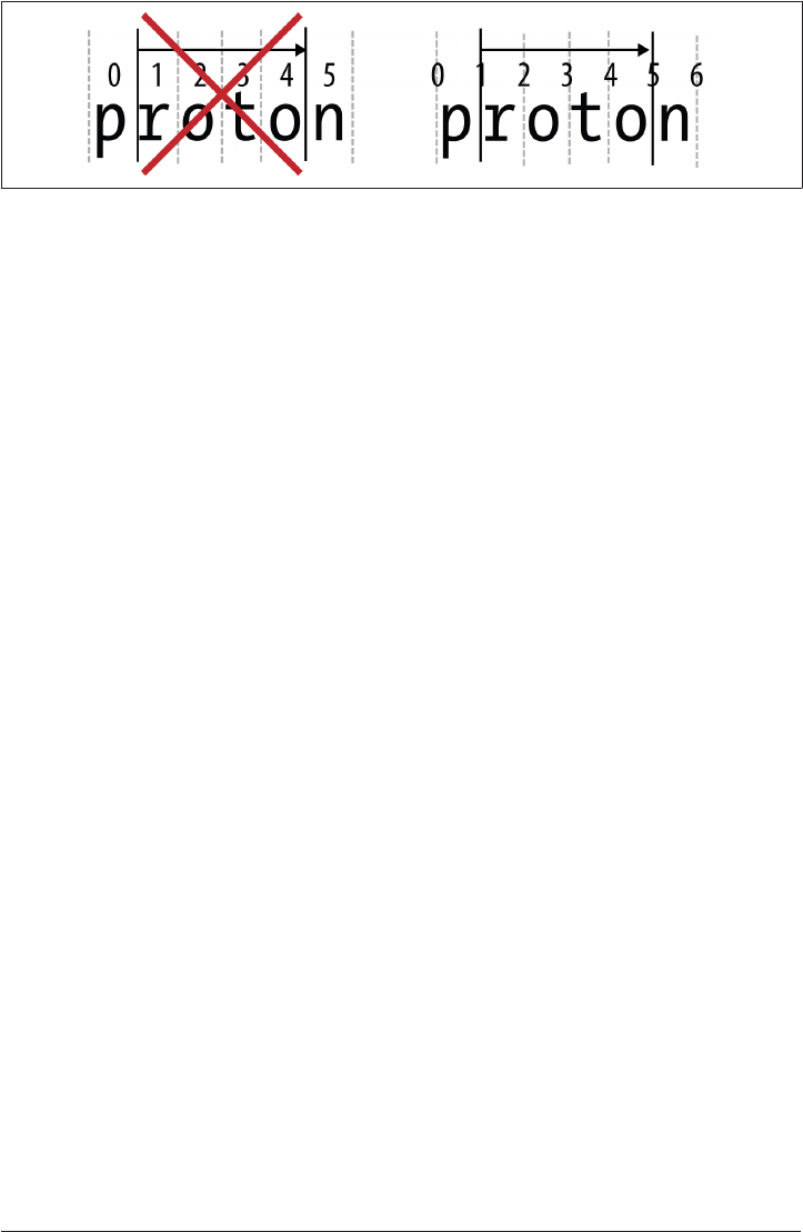
Figure 2-1. Indices are not on elements, but in between them
Feel free to mix positive and negative indices when slicing. However, the slice will not
wrap around the left or right edges of the sequence. If you do try to wrap around, you
get an empty sequence because there are no elements between the two indices:
In [6]: p[1:-1]
Out[6]: 'roto'
In [7]: p[-1:2]
Out[7]: ''
One of the greatest aspects of slicing is that the start and stop values are optional. If
either or both of these values are left out of the slice, then sensible defaults are used.
Namely, start becomes zero and stop becomes the length of the list. The colon (:) still
has to be present to delimit start and stop and to differentiate this as a slice rather
than an integer index, though. Here are some examples:
s[:2] # the first two elements
s[-5:] # the last five elements
s[:] # the whole string!
Slicing has one last parameter: the step. The step represents how many elements to go
in the sequence before picking up the next element for the slice. This is also some‐
times known as a stride. Stepping is useful if you want to only see every other ele‐
ment, every third element, and so on. The step defaults to one, meaning to grab every
element as we go and not skip any values. The syntax for stepping is very similar to
that of starting and stopping: simply add a colon and an integer after the stop value.
Thus, the full notation for slicing is s[start:stop:step]. Like the start and stop val‐
ues, the step can also be negative. This just means to go backward through the
sequence. Here are some stepping examples:
In [1]: q = "AaBbCcDdEeFfGgHhIiJjKkLlMmNnOoPpQqRrSsTtUuVvWwXxYyZz"
In [2]: q[2:-2:2]
Out[2]: 'BCDEFGHIJKLMNOPQRSTUVWXY'
In [3]: q[1::2]
Out[3]: 'abcdefghijklmnopqrstuvwxyz'
52 | Chapter 2: Programming Blasto with Python
www.it-ebooks.info

In [4]: q[::-3]
Out[4]: 'zYwVtSqPnMkJhGeDbA'
Because slicing is so easy, it comes up a lot in Python code. The most concise way to
reverse a sequence is simply by slicing with a step size of: -1: s[::-1]. This allows us
to write a very simple palindrome test:
In [1]: x = "neveroddoreven"
In [2]: x == x[::-1]
Out[2]: True
Slices are their own type and can be created independently of an indexing operation.
They can be stored and used multiple times. To create a raw slice, use the expression
slice(start, stop, step). If any of these need to have their default values, pass in
None rather than an integer index:
In [3]: my_slice = slice(3, 1415, 9) # my slice of the pi
In [4]: x[my_slice]
Out[4]: 'ee'
The indexing and slicing rules that we have just seen are very important. This is
because they generally apply to all Python sequences. Strings are the most basic
sequence, but we will be seeing more kinds of sequences in Chapter 3 and Chapter 9.
String Concatenation
Strings can be manipulated through a variety of operators. To start, consider the addi‐
tion (+) operator, which in the context of strings is known as concatenation. This
glues two strings together to make a bigger string:
In [1]: "kilo" + "meter"
Out[1]: 'kilometer'
Other data types will need to be converted to strings before they can be concatenated
with a string. Take a numeric example:
In [1]: "x^" + str(2)
Out[1]: 'x^2'
Given that addition is defined and multiplication (*) is many additions, multiplying a
string by an integer should yield that many copies of the string all concatenated
together:
In [1]: "newto" * 10
Out[1]: 'newtonewtonewtonewtonewtonewtonewtonewtonewtonewto'
These tricks only work for addition and multiplication. Strings cannot be subtracted,
divided, or exponentiated. The modulo (%) operator does apply to strings as a format‐
Strings | 53
www.it-ebooks.info

ting mechanism. However, modulo does not follow the concatenation logic here, and
its use is not recommended.
String Literals
What we have seen so far has been the most basic way to create strings. There are a
few other mechanisms that are also useful. First, any two string literals that are next
to each other are stuck together automatically:
In [1]: "H + H" " -> H2"
Out[1]: 'H + H -> H2'
Newlines are ignored between parentheses. Long strings can be built up over multiple
lines:
quote = ("Science is what we understand well enough to explain to a computer. "
"Art is everything else we do. "
"-Donald Knuth")
If a single- or double-quote character itself needs to be in the string, use the other
kind of quote to define the string at the outermost level:
x = "It's easy!"
y = 'The computer said, "Does not compute."'
This works as long as both types of quote characters are not needed inside of the
string. If they are, use the backslash character (\) to escape each quote character
inside of the string:
"Bones said, \"He\'s dead, Jim.\""
There are a number of special escape characters that can be used. All escape charac‐
ters start with a backslash and are interpreted as a single character even though they
take two characters to write. The most important of these are seen in Table 2-2.
Table 2-2. String escape characters
Character Interpretation
\\ Backslash
\n Newline—start a new line
\r Carriage return—go to the start of this line
\t Tab
\' Single quote
\" Double quote
54 | Chapter 2: Programming Blasto with Python
www.it-ebooks.info

String literals can also be prefixed with certain single characters that change how the
string is interpreted. These prefixes are shown in Table 2-3.
Table 2-3. String prexes
Prex Example Meaning
r r"escape!\n" Raw string: all backslashes are escaped automatically. In the example, the \n is a \ and
an n, not a newline.
b b"this bytes" Byte array: rather than becoming a string type, the value in quotes is interpreted as a
raw series of bytes.
u u"René Descartes" Unicode string: the string is explicitly interpreted as a Unicode type. Useful in Python 2
and ignored in Python 3.
Finally, Python has support for multiline strings, which preserve the newlines that are
inside of them. To create these, surround the text with either triple single quotes (''')
or triple double quotes ("""). Triple double quotes are much preferred. Multiline
string literals are essential for documentation, as we will see in future chapters. An
example of such a string is shown here—note that the """ appear only at the begin‐
ning and end of the string, even though there are newlines present:
"""Humpty, he sat on a wall,
Then Humpty, he had a great fall.
But all the king's horses
And men with their forces
Couldn't render his entropy small.
"""
Now that we can make strings, we can learn about how to manipulate them. The next
section describes string-based operations that are specific to the string type.
String Methods
Variables in Python have other variables that may “live on” them. These are known as
attributes. Attributes, or attrs for short, are accessed using the dot operator (.). Sup‐
pose that x has a y; then the expression x.y means “Go into x and get me the y that
lives there.” Strings are no exception to this.
Additionally, some attributes are function types, which makes them methods. The
details of what this means will be discussed in Chapter 5 and Chapter 6. For now,
know that methods define special operations that you can perform on strings. To use
methods, you call them with the parentheses (()) operator. In some cases, extra
parameters will need to go inside of the parentheses.
Strings | 55
www.it-ebooks.info

The following is not a comprehensive discussion of all string meth‐
ods. It includes only the ones that are most useful to computational
science.
The strip() method is incredibly useful for normalizing text-based data. It removes
all leading and trailing whitespace while preserving internal whitespace. Whitespace
is defined as spaces, tabs, newlines, and other blank characters. Suppose you had a
flat data file, but the header had some very strange spacing. To trim the leading and
trailing whitespace, you could fire up IPython and input the header string, then call
strip() on it:
In [1]: header = " temperature pressure\t value \n"
In [2]: header.strip()
Out[2]: 'temperature pressure\t value'
Here, we first define header to be the original string. Then we go into header and ask
for strip by writing header.strip. Lastly, we compute the stripped string by calling
the method immediately after accessing it, using the parentheses operator.
The upper() and lower() methods will return a version of the string with all alpha‐
betical letters in uppercase or lowercase, respectively:
In [3]: header.upper()
Out[3]: ' TEMPERATURE PRESSURE\t VALUE \n'
The swapcase() method will switch the existing case.
The isdigit() method returns True or False depending on whether or not the
string contains only integer numbers:
In [1]: "10".isdigit()
Out[1]: True
In [2]: "10.10".isdigit()
Out[2]: False
Lastly, the format() method creates new strings from templates with the template
values filled in. String formatting has its own mini-language, which will not be dis‐
cussed in detail here but may be found in the Python string documentation. The basic
template form uses integers inside of curly braces ({}). The integers index into the
values in the parentheses. For example:
In [1]: "{0} gets into work & then his {1} begins!".format("Hilbert", "commute")
Out[1]: 'Hilbert gets into work & then his commute begins!'
56 | Chapter 2: Programming Blasto with Python
www.it-ebooks.info

This helps convert data to strings without excess type conversion and concatenation.
The following two expressions are equivalent, but the first one, using format(), is a
lot shorter and easier to type than the second one:
In [1]: x = 42
In [2]: y = 65.0
In [3]: "x={0} y={1}".format(x, y)
Out[3]: 'x=42 y=65.0'
In [4]: "x=" + str(x) + " y=" + str(y)
Out[4]: 'x=42 y=65.0'
This covers the vast majority of string operations that you will need to perform for
now. This is particularly true for physics software, which tends to be light on string
manipulation. Probably the heaviest use of strings that you will do as a computational
physicist is to generate input for other physics code and to read and parse their out‐
put. In these cases, most of the strings end up representing numbers anyway. Next, we
will discuss how to access code from outside of the Python file or interpreter that we
are currently writing or running.
Modules
Python code is typically written in files whose names end in the .py extension. When
such a file is brought into a running Python interpreter, it is called a module. This is
the in-memory representation of all of the Python code in the file. A collection of
modules in a directory is called a package. It is worth noting that Python allows mod‐
ules to be written in languages other than Python. These are called extension modules
and are typically implemented in C.
Modules allow for a suite of related code files to all exist next to each other and to be
accessed in a common way. They also provide a mechanism for saving and sharing
code for use elsewhere and by other people. The Python standard library is itself an
extensive collection of modules for a huge variety of common and not-so-common
tasks. The batteries-included standard library is one of the things that makes Python
so versatile. Using modules is how you get your hands on anything more than pure
built-in Python.
Code from modules may be garnered in a number of different ways. All of these use
the import keyword to pull in the module itself and allow you to access all of the vari‐
ables that exist in that module. Modules may themselves use other modules.
Modules | 57
www.it-ebooks.info

Importing Modules
The import statement has four different forms. The first is just the import keyword
followed by the module name without the trailing .py:
import <module>
Once a module has been imported, you can obtain variables in that module using the
attribute access operator (.). This is exactly the same syntax that is used to get meth‐
ods on an object. For example, say that there was one file, constants.py, which stored
Planck’s constant and pi. Another module could import constants and use it to
compute h_bar:
constants.py
pi = 3.14159
h = 6.62606957e-34
physics.py
import constants
two_pi = 2 * constants.pi
h_bar = constants.h / two_pi
Importing Variables from a Module
Writing constants.<var> can be tedious if the <var> is going to be used many times.
To alleviate this, Python has the from-import syntax that imports specific variables
from a module. Either a single variable may be imported, or multiple comma-
separated variable names may be imported simultaneously:
from <module> import <var>
from <module> import <var1>, <var2>, ...
This is equivalent to importing the module, setting a local variable to the name found
in the module, and then deleting the module name, leaving only the local variable:
import <module>
<var> = <module>.<var>
del <module>
You can therefore think of from-import statements as renaming variable names for
convenience. The constants import could be written as follows:
constants.py
pi = 3.14159
h = 6.62606957e-34
58 | Chapter 2: Programming Blasto with Python
www.it-ebooks.info

physics.py:
from constants import pi, h
two_pi = 2 * pi
h_bar = h / two_pi
Aliasing Imports
The next form of importing changes the name of the module on import. This is help‐
ful if there is a local variable whose name would otherwise clash with the name of the
module. (Generally, you control the names of the variables you use but do not have
much say in the names of modules other people write.) This form uses the as key‐
word and has the following syntax:
import <module> as <name>
This is equivalent to importing the module, giving it a new name, and deleting the
name it had when it was imported:
import <module>
<name> = <module>
del <module>
In the constants example, if there was a local variable that was also named con
stants, pi and h would only be accessible if the module was renamed. Here’s how we
would import the module using this syntax:
constants.py
pi = 3.14159
h = 6.62606957e-34
evenmorephysics.py
import constants as c
constants = 2.71828
two_pi = 2 * c.pi
h_bar = c.h / 2 / c.pi
In evenmorephysics.py, constants is Euler’s number while the constants.py module is
renamed to the variable c.
Aliasing Variables on Import
The final form of import combines elements of the form-import syntax and import
aliasing to import only specific variables from a module, and rename them in the
process. You can import and rename a single variable or a comma-separated list of
variables, using the following syntax:
Modules | 59
www.it-ebooks.info

from <module> import <var> as <name>
from <module> import <var1> as <name1>, <var2> as <name2>, ...
This form of importing is equivalent to importing a variable from the module,
renaming the variable locally, and deleting the original name:
from <module> import <var>
<name> = <var>
del <var>
Here’s how we would import and rename the pi and h variables from the constant.py
module:
constants.py
pi = 3.14159
h = 6.62606957e-34
yetmorephysics.py
from constants import pi as PI, h as H
two_pi = 2 * PI
h_bar = H / two_pi
Packages
As mentioned previously, a collection of modules in the same directory is called a
package. For the package to be visible to Python, the directory must contain a special
file named __init__.py. The main purpose of this file is to signal to Python that the
directory is a package, and that other files in this directory whose names end in .py
are importable. This file does not need to have any code in it. If it does, this code will
be executed before any other modules in the package are imported.
The package takes on the name of the directory and may have subdirectories that are
subpackages. For example, the filesystem for a compphys package may be laid out as
follows:
compphys/
|-- __init__.py
|-- constants.py
|-- physics.py
|-- more/
| |-- __init__.py
| |-- morephysics.py
| |-- evenmorephysics.py
| |-- yetmorephysics.py
|-- raw/
| |-- data.txt
| |-- matrix.txt
| |-- orphan.py
60 | Chapter 2: Programming Blasto with Python
www.it-ebooks.info
Here, compphys is the package name. This package has three modules (__init__.py,
constants.py, and physics.py) and one subpackage (more). The raw directory does not
count as a subpackage because it lacks an __init__.py file. This is true even though it
contains other Python files, such as orphan.py, which are unreachable.
To import modules from a package, you use the attribute access operator (.). This is
the same syntax used for importing variables from a module. Packages may be
chained together with subpackage and module names, according to the filesystem
hierarchy that the Python files live in. If you import a subpackage or module from a
package, all of the packages above it in the hierarchy are automatically imported.
However, you do not have access to the automatically imported packages unless you
explicitly import them elsewhere. Once a module is imported, you can access all of
the variables that are defined inside of it with the dot operator. For example:
import compphys.constants
import compphys.more.evenmorephysics
two_pi = 2 * compphys.constants.pi
Import the constants module that lives in the compphys package.
Import the evenmorephysics module that lives in the more subpackage of the comp
phys package.
Access the pi variable of the constants module that lives in the compphys package
by using the dot attribute access operator.
These are called absolute imports because the full paths to the modules are given.
Absolute imports are recommended over all other styles of import‐
ing. This is because they provide the most clarity for the path to a
module.
Inside of a package, you may import modules at the same level without giving the
package name. This is called implicit relative importing. For example, evenmorephy‐
sics.py could import morephysics.py without your having to give the compphys.more
prefix. The import would be:
import morephysics
Or, from physics.py, you could import modules from the subpackage using only the
subpackage name:
import more.yetmorephysics
However, in modern Python, implicit relative imports are looked down upon.
Modules | 61
www.it-ebooks.info

Implicit relative imports have been removed from Python 3. They
are only available in Python 2. You probably shouldn’t use them.
Explicit relative imports replace the need for implicit ones. Here, the from keyword
must be used, and the module name is prefixed by either a single dot (.) or a double
dot (..). The single dot refers to the current package level. The double dot refers to
the package level one higher in the filesystem hierarchy. These have the same mean‐
ing that they do in bash.
For example, from physics.py, the following are valid imports:
from . import constants
from .constants import pi, h
from .more import morephysics
From evenmorephysics.py, the following imports would succeed:
from . import morephysics
from .. import constants
from ..constants import pi, h
Having more than two dots prefix the module name is not allowed. There is no way
to go up more than one subpackage at a time. Oftentimes, it is best to rethink the
filesystem layout if this much nesting is required.
Python enables you to write the modules and packages that you need to get your
work done. However, you don’t need to write everything from scratch yourself. The
language itself comes prepackaged with a wide variety of tools for many situations, as
we’ll see next.
The Standard Library and the Python Ecosystem
One aspect that makes Python invaluable as a tool is its comprehensive standard
library, which comes by default with the language. The standard library is a collection
of packages and modules that combine to make performing most everyday tasks easy
and Pythonic. It includes support for platform-independent operating system tasks,
mathematical functions, compression algorithms, databases, and basic web servers.
Wherever you have Python, you know you also have these standard tools. Table 2-4
describes some of the most useful Python modules that the standard library provides.
This is by no means a complete listing.
62 | Chapter 2: Programming Blasto with Python
www.it-ebooks.info

Table 2-4. Important and useful modules in the Python standard library
Module Description
os Operating system abstractions: le path operations, le removal, etc.
sys System-specic, gets into the guts of the Python interpreter
math Everyday mathematical functions and constants
re Regular expression library; see Chapter 8
subprocess Spawns child processes and shells, good for running other command-line tools
argparse Creates easy and beautiful command-line utilities
itertools Helpful tools for looping
collections Advanced collection types and tools for making custom collections
decimal Arbitrary-precision integers and oats
random Pseudo-random number generators
csv Tools for reading and writing comma-separated value les
pdb The Python debugger (similar to gdb for C/C++/Fortran)
logging Utilities for logging the progress of a program while it is running
Another excellent aspect of Python is the fabulous ecosystem of third-party modules
that has built up in support of the language. While these exist outside of the standard
library, they are even more rich and diverse, and many of them are ideally suited for
the needs of scientific computing and physics. Many of the other chapters in this
book focus on the excellent external packages that are available.
Python Wrap-up
At this point, you should be familiar with the following:
• How to start up a Python interpreter
• Dynamically typed variables
• Basic data types such as int, float, and str
• How to manipulate variables with built-in operators
Python Wrap-up | 63
www.it-ebooks.info

• String indexing and slicing
• How to import and use modules
From this foundation, you can start to build the more complicated representations of
data and logic that are needed in scientific software. Up next, in Chapter 3, we will
start tackling how to collect data together using mechanisms native to Python.
64 | Chapter 2: Programming Blasto with Python
www.it-ebooks.info

CHAPTER 3
Essential Containers
Let’s now delve further into the tools of the Python language. Python comes with a
suite of built-in data containers. These are data types that are used to hold many
other variables. Much like you might place books on a bookshelf, you can stick inte‐
gers or floats or strings into these containers. Each container is represented by its own
type and has its own unique properties that define it. Major containers that Python
supports are list, tuple, set, frozenset, and dict. All but frozenset come with
their own literal syntax so that creating them is effortless. dict is by far the most
important of these, for reasons that we’ll see in “Dictionaries” on page 73 and in
Chapter 6.
Before we dive in, there are two important Python concepts to understand:
• Mutability
• Duck typing
A data type is mutable if its value—also known as its state—is allowed to change after
it has been created. On the other hand, a data type is immutable if its values are static
and unchangeable once it is created. With immutable data you can create new vari‐
ables based on existing values, but you cannot actually alter the original values. All of
the data types we have dealt with so far—int, float, bool, and str—are immutable.
It does not make sense to change the value of 1. It just is 1, and so integers are immut‐
able. Containers are partially defined by whether they are mutable or not, and this
determines where and how they are used.
Duck typing, on the other hand, is one of the core principles of Python and part of
what makes it easy to use. This means that the type of a variable is less important than
the interface it exposes. If two variables expose the same interface, then they should
be able to be used in the same way. The argument goes, “If it looks like a duck and
65
www.it-ebooks.info

quacks like a duck, it is a duck!” Python believes that what a variable acts like at the
moment it is used is more important than the actual underlying type. This is in stark
contrast to lower-level languages, where it is more important what a variable “is” than
what it does.
Interfaces
An interface, in programing terminology, is a set of rules, expecta‐
tions, and protocols for how different pieces of software may inter‐
act with one another. Though these rules change from language to
language, for a program to be able to run it must hook up all the
interfaces in a valid way. Consider children’s block playsets as a
simple interface. Square pegs do not go into round holes; they only
go into square holes. There are formal mathematical definitions of
interfaces, but these rely on the notion of functions, which we’ll
meet in Chapter 5. Sometimes you will see the term application pro‐
gramming interface or API used. For our purposes here, “API” is
synonomous with the word “interface.”
We have already seen some examples of duck typing with indexing. The concept of
indexing applies to any sequence, but “sequence” is not a fully defined type on its
own. Instead, indexing can be applied to any variable that is sufficiently sequence-
like. For example, we learned how to index strings in “String Indexing” on page 50.
As will be seen shortly, the same indexing syntax may be used with lists and tuples.
The idea that you can learn something once (string indexing) and use it again later
for different types (list indexing and tuple indexing) is what makes duck typing so
useful. If duck typing sounds generic, that is because it is. The whole point of duck
typing is that the syntax of an operator should not change just because the type of the
underlying variable changes. This notion highlights one of the things that makes
Python easier to learn than other languages.
Lists
Lists in Python are one-dimensional, ordered containers whose elements may be any
Python objects. Lists are mutable and have methods for adding and removing ele‐
ments to and from themselves. The literal syntax for lists is to surround comma-
separated values with square brackets ([]). The square brackets are a syntactic hint
that lists are indexable. Here are some examples:
[6, 28]
[1e3, -2, "I am in a list."]
[[1.0, 0.0], [0.0, 1.0]]
66 | Chapter 3: Essential Containers
www.it-ebooks.info

In Python, unlike in other languages, the elements of a list do not have to match other
in type. Anything can go into a list, including other lists! You can concatenate two
lists together using the addition operator (+) to form a longer list:
In [1]: [1, 1] + [2, 3, 5] + [8]
Out[1]: [1, 1, 2, 3, 5, 8]
You can also append to lists in-place using the append() method, which adds a single
element to the end:
In [2]: fib = [1, 1, 2, 3, 5, 8]
In [3]: fib.append(13)
In [4]: fib
Out[4]: [1, 1, 2, 3, 5, 8, 13]
Since building up a list element by element using append() can be tedious, whole
sequences may be added to the end of a list in-place via the extend() method or the
(+=) operator:
In [5]: fib.extend([21, 34, 55])
In [6]: fib
Out[6]: [1, 1, 2, 3, 5, 8, 13, 21, 34, 55]
In [7]: fib += [89, 144]
In [8]: fib
Out[8]: [1, 1, 2, 3, 5, 8, 13, 21, 34, 55, 89, 144]
List indexing is exactly the same as string indexing, but instead of returning strings it
returns new lists. See “String Indexing” on page 50 for a refresher on how indexing
works. Here is how to pull every other element out of a list:
In [9]: fib[::2]
Out[9]: [1, 2, 5, 13, 34, 89]
In addition to element access, indexes can also be used to set or delete elements in a
list. This is because lists are mutable, whereas strings are not. Multiple list values may
be set simultaneously as long as the new values are stored in a sequence of the same
length as their destination. This can all be managed with the assignment (=) and del
operators:
In [10]: fib[3] = "whoops"
In [11]: fib
Out[11]: [1, 1, 2, 'whoops', 5, 8, 13, 21, 34, 55, 89, 144]
In [12]: del fib[:5]
In [13]: fib
Lists | 67
www.it-ebooks.info
Out[13]: [8, 13, 21, 34, 55, 89, 144]
In [14]: fib[1::2] = [-1, -1, -1]
In [15]: fib
Out[15]: [8, -1, 21, -1, 55, -1, 144]
Set the fourth element of the fib list to whoops.
See that the list was changed in-place.
Remove the first five elements of fib.
See that only the end of the original list remains.
Assign -1 to each odd element.
See how the odd elements have changed.
The same multiplication-by-an-integer trick for strings also applies to lists:
In [1]: [1, 2, 3] * 6
Out[1]: [1, 2, 3, 1, 2, 3, 1, 2, 3, 1, 2, 3, 1, 2, 3, 1, 2, 3]
You can also create lists of characters directly from strings by using the list() con‐
version function:
In [1]: list("F = dp/dt")
Out[1]: ['F', ' ', '=', ' ', 'd', 'p', '/', 'd', 't']
Another fascinating property is that a list will infinitely recurse if you add it to itself!
In [1]: x = []
In [2]: x.append(x)
In [3]: x
Out[3]: [[...]]
In [4]: x[0]
Out[4]: [[...]]
In [5]: x[0][0]
Out[5]: [[...]]
To explain how this is possible, we’ll need to explore of how Python manages mem‐
ory. Python is reference counted, which means that variable names are actually refer‐
ences to the underlying values. The language then keeps an internal count of how
many times a reference has been used and what its names are. Think of this as there
being data on the one hand, and names that are attached to data—like sticky notes—
68 | Chapter 3: Essential Containers
www.it-ebooks.info
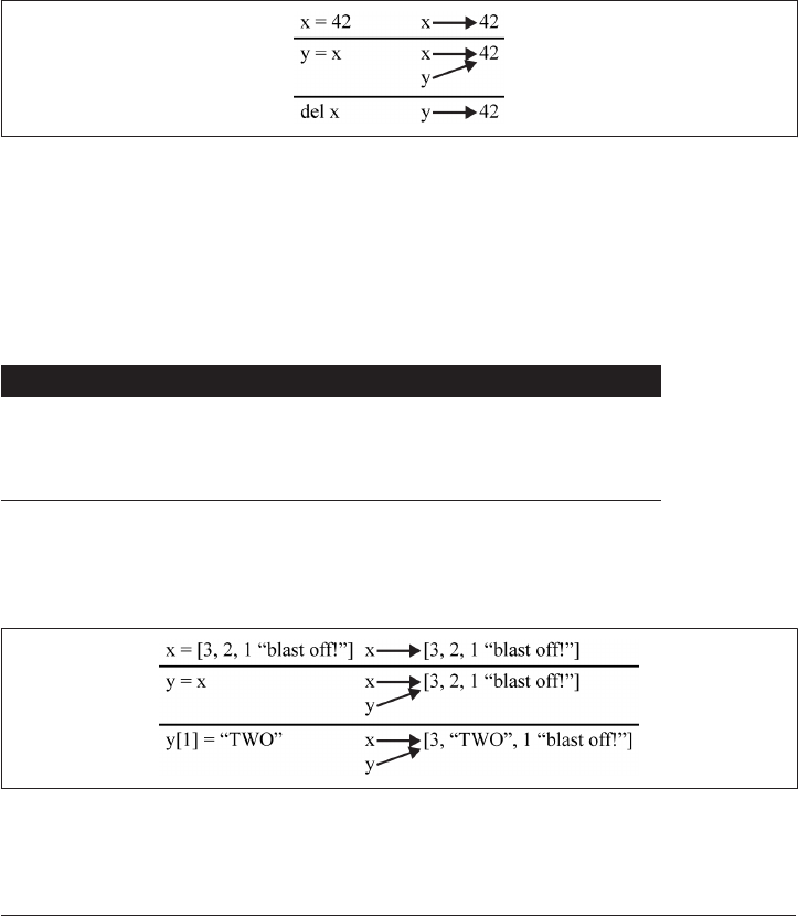
on the other hand. Names cannot refer to other names, but only to the underlying
data. Consider the following simple example:
x = 42
y = x
del x
In the code here, Python starts by first creating the number 42 in memory. It then sets
the name x to refer to the point in memory where 42 lives. On the next line, Python
then sees that y should point to the same place that x is pointing to. Now, 42 has two
names: x and y. Then x is deleted, but Python sees that 42 still has at least one name
(y), so it keeps both y and 42 around for later use. This can be seen in Figure 3-1.
Figure 3-1. Reference counting of simple variables
So how does this apply to lists? Lists are collections of names, not values! The name a
list gives to each of its elements is the integer index of that element. Of course, the list
itself also has a name. This means that when a list itself has two or more variable
names and any of them has an element changed, then all of the other variables also
see the alteration. Consider this example:
Code Output
x = [3, 2, 1, "blast off!"]
y = x
y[1] = "TWO"
print(x)
[3, "TWO", 1, "blast off!"]
Here, when y’s second element is changed to the string 'TWO', this change is reflected
back onto x. This is because there is only one list in memory, even though there are
two names for it (x and y). Figure 3-2 shows this graphically.
Figure 3-2. Reference counting with lists
Lists | 69
www.it-ebooks.info
This is the spooky action at a distance of programming. But it is also how Python
containers work. Python is not alone here; this is how all reference-counted lan‐
guages act. In compiled languages, this is what makes smart pointers smart. The rea‐
son this technique is used is that memory volume is handled much more efficiently,
though this often comes at the cost of increased CPU usage.
Now that you understand how Python is handling memory, it is not hard to use it
correctly. Though this is often a “gotcha” for people new to dynamic languages, it
becomes second nature very quickly.
The Python statement x = y = [] means that there is one new
empty list with two names (x and y). If you come from a C/C++
background, it is tempting to read this as meaning to create two
new empty lists with two names. However, this is incorrect because
of how Python’s memory management works.
Returning to the example of the infinitely recurring list, this is a list that holds a refer‐
ence to itself. This means that names in the series x, x[0], x[0][0], … point to
exactly the same place. This is partially drawn out in Figure 3-3.
Figure 3-3. Memory in an innitely recurring list
Now that we’ve covered the basics of lists, we can move on to a very similar container
that differs from lists in a single, but significant, way.
Tuples
Tuples are the immutable form of lists. They behave almost exactly the same as lists in
every way, except that you cannot change any of their values. There are no append()
or extend() methods, and there are no in-place operators.
They also differ from lists in their syntax. They are so central to how Python works
that tuples are dened by commas (,). Oftentimes, tuples will be seen surrounded by
parentheses. These parentheses serve only to group actions or make the code more
readable, not to actually define the tuples. Some examples include:
a = 1, 2, 5, 3 # length-4 tuple
b = (42,) # length-1 tuple, defined by comma
70 | Chapter 3: Essential Containers
www.it-ebooks.info

c = (42) # not a tuple, just the number 42
d = () # length-0 tuple- no commas means no elements
You can concatenate tuples together in the same way as lists, but be careful about the
order of operations. This is where the parentheses come in handy:
In [1]: (1, 2) + (3, 4)
Out[1]: (1, 2, 3, 4)
In [2]: 1, 2 + 3, 4
Out[2]: (1, 5, 4)
The tuple converter is just called tuple(). If you have a list that you wish to make
immutable, use this function:
In [1]: tuple(["e", 2.718])
Out[1]: ('e', 2.718)
Note that even though tuples are immutable, they may have mutable elements. Sup‐
pose that we have a list embedded in a tuple. This list may be modified in-place even
though the list may not be removed or replaced wholesale:
In [1]: x = 1.0, [2, 4], 16
In [2]: x[1].append(8)
In [3]: x
Out[3]: (1.0, [2, 4, 8], 16)
Other than immutability, what are the differences between lists and tuples? In princi‐
ple, there are not any. In practice, they tend to be used in different ways. However,
there are no strict rules and there are no predominant conventions. There is a loose
guideline that lists are for homogeneous data (all integers, all strings, etc.) while tuples
are for heterogeneous data with semantic meaning in each element (e.g., ("C14", 6,
14, 14.00324198843)). Other, more sophisticated data structures that we’ll see in
future chapters add semantic meaning to their elements. For tuples and lists, though,
this rule of thumb is only a suggestion.
Tuples are integral to functions and will be seen much more in Chapter 5. Both tuples
and lists may have duplicated elements. Sometimes this is exactly what you want. Up
next, though, is a container that ensures that each of its elements is unique.
Sets
Instances of the set type are equivalent to mathematical sets. Like their math coun‐
terparts, literal sets in Python are defined by comma-separated values between curly
braces ({}). Sets are unordered containers of unique values. Duplicated elements are
ignored. Because they are unordered, sets are not sequences and cannot be indexed.
Sets | 71
www.it-ebooks.info

Containment—is x in y?—is much more important for sets than how the elements
are stored. Here are some examples:
# a literal set formed with elements of various types
{1.0, 10, "one hundred", (1, 0, 0,0)}
# a literal set of special values
{True, False, None, "", 0.0, 0}
# conversion from a list to a set
set([2.0, 4, "eight", (16,)])
One common misconception of new Python programmers deals with the set of a sin‐
gle string. The set of a string is actually the set of its characters. This is because strings
are sequences. To have a set that actually contains a single string, first put the string
inside of another sequence:
In [1]: set("Marie Curie")
Out[1]: {' ', 'C', 'M', 'a', 'e', 'i', 'r', 'u'}
In [2]: set(["Marie Curie"])
Out[2]: {'Marie Curie'}
Sets may be used to compute other sets or be compared against other sets. These
operations follow mathematical analogies that can be seen in Table 3-1 (take s = {1,
2, 3} and t = {3, 4, 5} for the examples).
Table 3-1. Set operations
Operation Meaning Example
s | t Union {1, 2, 3, 4, 5}
s & t Intersection {3}
s - t Dierence—elements in s but not in t {1, 2}
s ^ t Symmetric dierence—elements not in s or t {1, 2, 4, 5}
s < t Strict subset False
s <= t Subset False
s > t Strict superset False
s >= t Superset False
The uniqueness of set elements is key. This places an important restriction on what
can go in a set in the first place. Namely, the elements of a set must be hashable. The
72 | Chapter 3: Essential Containers
www.it-ebooks.info

core idea behind hashing is simple. Suppose there is a function that takes any value
and maps it to an integer. If two variables have the same type and map to the same
integer, then the variables have the same value. This assumes that you have enough
integers and a reasonable mapping function. Luckily, Python takes care of those
details for us. Whether or not something is allowed to go into a set depends only on if
it can be unambiguously converted to an integer.
In Python, the hash function is just called hash(), and you can try using it on any
variable. If this function fails for some reason, that value cannot be placed in a set. If
two variables are hashable, though, the following logic statement is roughly true:
hash(x) == hash(y) implies that x == y
This assumption breaks down across type boundaries. Python handles differently
typed variables separately because it knows them to be different. For example, an
empty string and the float 0.0 both hash to 0 (as an int, because hashes are integers).
However, an empty string and the float 0.0 clearly are not the same value, because
they have different types:
hash("") == hash(0.0) == 0 does not imply that "" == 0.0
What makes a type hashable? Immutability. Without immutability there is no way to
reliably recompute the hash value. As a counterexample, say you could compute the
hash of a list. If you were then to add or delete elements to or from the list, its hash
would change! If this list were already in a set, list mutability would break the guaran‐
tee that each element of the set is unique. This is why lists are not allowed in sets,
though tuples are allowed if all of their elements are hashable.
Lastly, sets themselves are mutable. You can add(), discard(), or otherwise modify
sets in-place. This means that you cannot have a set inside of another set. To get
around this, there is an immutable version of the set type called frozenset. The rela‐
tionship between sets and frozensets is the same as that between lists and tuples: fro‐
zensets are exactly the same as sets, except that they cannot be modified once they are
created.
Highly related to sets and based on the same notion of hashability are the ever-
present dictionaries. We’ll look at these next.
Dictionaries
Dictionaries are hands down the most important data structure in Python. Everything
in Python is a dictionary. A dictionary, or dict, is a mutable, unordered collection of
unique key/value pairs—this is Python’s native implementation of a hash table. Dic‐
tionaries are similar in use to C++ maps, but more closely related to Perl’s hash type,
JavaScript objects, and C++’s unordered_map type. We will cover hash tables and how
they are implemented in much greater detail in “Hash Tables” on page 258. Right
Dictionaries | 73
www.it-ebooks.info

now, we will see just enough to understand how to use dictionaries, so we can move
forward with learning Python.
In a dictionary, keys are associated with values. This means that you can look up a
value knowing only its key(s). Like their name implies, the keys in a dictionary must
be unique. However, many different keys with the same value are allowed. They are
incredibly fast and efficient at looking up values, which means that using them incurs
almost no overhead.
Both the keys and the values are Python objects. So, as with lists, you can store any‐
thing you need to as values. Keys, however, must be hashable (hence the name “hash
table”). This is the same restriction as with sets. In fact, in earlier versions of Python
that did not have sets, sets were faked with dictionaries where all of the values were
None. The syntax for dictionaries is also related to that for sets. They are defined by
outer curly brackets ({}) surrounding key/value pairs that are separated by commas
(,). Each key/value pair is known as an item, and the key is separated from the value
by a colon (:). Curly braces are treated much like parentheses, allowing dictionaries
to be split up over multiple lines. They can also be defined with a list of 2-tuples. Here
are some examples:
# A dictionary on one line that stores info about Einstein
al = {"first": "Albert", "last": "Einstein", "birthday": [1879, 3, 14]}
# You can split up dicts onto many lines
constants = {
'pi': 3.14159,
"e": 2.718,
"h": 6.62606957e-34,
True: 1.0,
}
# A dict being formed from a list of (key, value) tuples
axes = dict([(1, "x"), (2, "y"), (3, "z")])
You pull a value out of a dictionary by indexing with the associated key. If we had
typed each of these dicts into IPython, we could then access their values as follows:
In [1]: constants['e']
Out[1]: 2.718
In [2]: axes[3]
Out[2]: 'z'
In [3]: al['birthday']
Out[3]: [1879, 3, 14]
74 | Chapter 3: Essential Containers
www.it-ebooks.info

Since dictionaries are unordered, slicing does not make any sense for them. However,
items may be added and deleted through indexing. Existing keys will have their val‐
ues replaced:
constants[False] = 0.0
del axes[3]
al['first'] = "You can call me Al"
Because dictionaries are mutable, they are not hashable themselves, and you cannot
use a dictionary as a key in another dictionary. You may nest dictionaries as values,
however. This allows for the infinitely recurring trick, like with lists:
In [4]: d = {}
In [5]: d['d'] = d
In [6]: d
Out[6]: {'d': {...}}
Note that dicts predate sets by over a decade in the language. Since the syntax col‐
lides, empty dicts are defined by just curly braces while an empty set requires the
type name and parentheses:
{} # empty dict
set() # empty set
Tests for containment with the in operator function only on dictionary keys, not
values:
In [7]: "N_A" in constants
Out[7]: False
Dictionaries have a lot of useful methods on them as well. For now, content yourself
with the update() method. This incorporates another dictionary or list of tuples in-
place into the current dict. The update process overwrites any overlapping keys:
In [8]: axes.update({1: 'r', 2: 'phi', 3: 'theta'})
In [9]: axes
Out[9]: {1: 'r', 2: 'phi', 3: 'theta'}
This is only enough to get started. Dictionaries are more important than any other
data type and will come up over and over again. Their special place in the Python
language will be seen in Chapter 5 and Chapter 6.
Containers Wrap-up
Having reached the end of this chapter, you should now be familiar with the follow‐
ing concepts:
Containers Wrap-up | 75
www.it-ebooks.info

• Mutability and immutability
• Duck typing
• Lists and tuples
• Hash functions
• Sets and dictionaries
These data containers and their underlying concepts are the building blocks for
higher-level, more complex structures. They let you represent your data in the way
that makes the most sense for the problem at hand. They also enable a wide variety of
expressive Python syntax, which we will start to explore in Chapter 4.
76 | Chapter 3: Essential Containers
www.it-ebooks.info

CHAPTER 4
Flow Control and Logic
Flow control is a high-level way of programming a computer to make decisions. These
decisions can be simple or complicated, executed once or multiple times. The syntax
for the different flow control mechanisms varies, but what they all share is that they
determine an execution pathway for the program. Python has relatively few forms of
flow control. They are conditionals, exceptions, and loops.
As someone primarily interested in physical reality, you might wonder why you
should care about flow control and logic. In some ways, this is like asking why arith‐
metic is important. Logic presents rules that allow you to build up and represent
more complex ideas. This enables the physics modeling you want to do by giving you
a means to express the choices and behavior of your model to the computer. With
basic flow control syntax, your models can make simple decisions. With more
advanced flow control, your models can make more sophisticated choices more
easily. In other situations, flow control allows you to reuse the same code many times.
This makes the software model faster to write and easier to understand, because it has
fewer total lines of code. Logic and flow control are indispensible to doing any signifi‐
cant amount of work with computers. So, without further delay, let’s jump into condi‐
tionals, our first bit of flow control.
Conditionals
Conditionals are the simplest form of flow control. In English, they follow the syntax
“if x is true, then do something; otherwise, do something else.” The shortest condi‐
tional is when there is only an if statement on its own. The format for such a state‐
ment is as follows:
if <condition>:
<if-block>
77
www.it-ebooks.info

Here, the Python keyword if is followed by an expression, <condition>, which is
itself followed by a colon (:). When the Boolean representation of the condition,
bool(condition), is True, the code that is in the <if-block> is executed. If bool(con
dition) is False, then the code in the block is skipped. The condition may be com‐
posed of any of the comparison operators (or a combination of these operators) that
were listed in Table 2-1. For convenience, just the comparison operators are shown
again here in Table 4-1.
Table 4-1. Python logical operators useful for comparing the variables x, y, and z
Name Usage Returns
Unary operators
Negation not x Logical negation—True becomes False, and vice versa.
Bitwise invert ~x Changes all zeros to ones and vice versa in x’s binary representation.
Binary operators
Logical and x and y True if bool(x) and bool(y) are True; False otherwise.
Logical or x or y x if bool(x) is True; otherwise the value of y.
Comparison binary operators
Equality x == y True or False.
Not equal x != y True or False.
Less than x < y True or False.
Less than or equal x <= y True or False.
Greater than x > y True or False.
Greater than or equal x >= y True or False.
Containment x in y True if x is an element of y.
Non-containment x not in y False if x is an element of y.
Identity test x is y True if x and y point to the same underlying value in memory.
78 | Chapter 4: Flow Control and Logic
www.it-ebooks.info

Name Usage Returns
Not identity test x is not y False if x and y point to the same underlying value in memory.
Ternary operators
Ternary compare x < y < z True or False, equivalent to (x < y) and (y < z). The <
here may be replaced by >, <=, or >= in any permutation.
For example, if we wanted to test if Planck’s constant is equal to one and then change
its value if it is, we could write the following:
h_bar = 1.0
if h_bar == 1.0:
print("h-bar isn't really unity! Resetting...")
h_bar = 1.05457173e-34
Here, since h_bar is 1.0 it is reset to its actual physical value (1.05457173e-34). If
h_bar had been its original physical value, it would not have been reset.
A key Pythonism that is part of the if statement is that Python is whitespace separa‐
ted. Unlike other languages, which use curly braces and semicolons, in Python the
contents of the if block are determined by their indentation level. New statements
must appear on their own lines. To exit the if block, the indentation level is returned
back to its original column:
h_bar = 1
if h_bar == 1:
print("h-bar isn't really unity! Resetting...")
h_bar = 1.05457173e-34
h = h_bar * 2 * 3.14159
The last line here (the one that defines h) indicates that the if block has ended
because its indentation level matches that of the if on the second line. The last line
will always be executed, no matter what the conditional decides should be done for
the if block.
While we are on the subject, it is important to bring up the distinction between the
equality operator (==) and the identity operator (is). The equality operator tests if
two values are equivalent. For example, 1 == 1.0 is True even though 1 is an integer
and 1.0 is a float. On the other hand, the identity operator tests if two variable names
are references to the same underlying value in memory. For example, 1 is 1.0 is
False because the types are different, and therefore they cannot actually be references
to the same value. is is much faster than ==, but also much more strict. In general,
you want to use is for singletons like None and use the safer == in most other situa‐
tions. The following examples show typical use cases and gotchas:
Conditionals | 79
www.it-ebooks.info
Code Output
1 == 1
1 == 1.0
1 is 1.0
1 is 1
10**10 == 10**10
10**10 is 10**10
None is None
0 is None
0 == None
To help with performance, Python only stores a single copy of small integers. So for small ints, every usage
will be the same value in memory.
However, for big integers a new copy is computed each time.
Only None is None.
True
True
False
True
True
False
True
False
False
Before we move on, it is important to note that, by tradition, Python uses four spaces
per level to indent all code blocks. Two spaces, eight spaces, or any other spacing is
looked down upon. Tabs cause many more problems than they are worth. Most text
editors have an option to automatically convert tabs to spaces, and enabling this can
help prevent common errors. Some people find the whitespace syntax a little awk‐
ward to begin with, but it becomes easy and natural very quickly. The whitespace-
aware aspect of Python is a codification of what is a best-practice coding style in other
languages. It forces programmers to write more legible code.
if-else Statements
Every if statement may be followed by an optional else statement. This is the key‐
word else followed by a colon (:) at the same indentation level as the original if.
The <else-block> lines following this are indented just like the if block. The code in
the else block is executed when the condition is False:
if <condition>:
<if-block>
else:
<else-block>
80 | Chapter 4: Flow Control and Logic
www.it-ebooks.info

For example, consider the expression sin(1/x). This function is computable every‐
where except a x = 0. At this point, L’Hôpital’s rule shows that the result is also zero.
This could be expressed with an if-else statement as follows:
if x == 0:
y = 0
else:
y = sin(1/x)
This is equivalent to negating the conditional and switching the if and else blocks:
if x != 0:
y = sin(1/x)
else:
y = 0
However, it is generally considered a good practice to use positive conditionals (==)
rather than negative ones (!=). This is because humans tend to think about an expres‐
sion being true rather than it being false. This is not a hard and fast rule, but it does
help eliminate easy-to-miss logic bugs.
if-elif-else Statements
Python also allows multiple optional elif statements. The elif keyword is an abbre‐
viation for “else if,” and such statements come after the if statement and before the
else statement. The elif statements have much the same form as the if statement,
and there may be as many of them as desired. The first conditional that evaluates to
True determines the block that is entered, and no further conditionals or blocks are
executed. The syntax is as follows:
if <condition0>:
<if-block>
elif <condition1>:
<elif-block1>
elif <condition2>:
<elif-block2>
...
else:
<else-block>
Suppose that you wanted to design a simple mid-band filter whose signal is 1 if the
frequency is between 1 and 10 Hertz and 0 otherwise. This could be done with an if-
elif-else statement:
if omega < 1.0:
signal = 0.0
elif omega > 10.0:
signal = 0.0
Conditionals | 81
www.it-ebooks.info

else:
signal = 1.0
A more realistic example might include ramping on either side of the band:
if omega < 0.9:
signal = 0.0
elif omega > 0.9 and omega < 1.0:
signal = (omega - 0.9) / 0.1
elif omega > 10.0 and omega < 10.1:
signal = (10.1 - omega) / 0.1
elif omega > 10.1:
signal = 0.0
else:
signal = 1.0
if-else Expression
The final syntax covered here is the ternary conditional operator. It allows simple if-
else conditionals to be evaluated in a single expression. This has the following
syntax:
x if <condition> else y
If the condition evaluates to True, then x is returned. Otherwise, y is returned. This
turns out to be extraordinarily handy for variable assignment. Using this kind of
expression, we can write the h_bar conditional example in one line:
h_bar = 1.05457173e-34 if h_bar == 1.0 else h_bar
Note that when using this format you must always include the else clause. This fills
the same role as the condition?x:y operator that is available in other languages.
Writing out if and else arguably makes the Python way much more readable,
though also more verbose.
Exceptions
Python, like most modern programming languages, has a mechanism for exception
handling. This is a language feature that allows the programmer to work around sit‐
uations where the unexpected and catastrophic happen. Exception handling is for the
truly exceptional cases: a user manually types in an impossible value, a file is deleted
while it is being written, coffee spills on the laptop and fries the motherboard.
82 | Chapter 4: Flow Control and Logic
www.it-ebooks.info

Exceptions are not meant for normal flow control and dealing with
expected behavior! Use conditionals in cases where behavior is
anticipated.
The syntax for handling exceptions is known as a try-except block. Both try and
except are Python keywords. try-excepts look very similar to if-else statements,
but without the condition:
try:
<try-block>
except:
<except-block>
The try block will attempt to execute its code. If there are no errors, then the pro‐
gram skips the except block and proceeds normally. If any error at all happens, then
the except block is immediately entered, no matter how far into the try block
Python has gone. For this reason, it is generally a good idea to keep the try block as
small as possible. Single-line try blocks are strongly preferred.
As an example, say that a user manually inputs a value and then the program takes
the inverse of this value. Normally this computes just fine, with the exception of when
the user enters 0:
In [1]: val = 0.0
In [2]: 1.0 / val
ZeroDivisionError Traceback (most recent call last)
<ipython-input-2-3ac1864780ca> in <module>()
----> 1 1.0 / val
ZeroDivisionError: float division by zero
This error could be handled with a try-except, which would prevent the program
from crashing:
try:
inv = 1.0 / val
except:
print("A bad value was submitted {0}, please try again".format(val))
The except statement also allows for the precise error that is anticipated to be caught.
This allows for more specific behavior than the generic catch-all exception. The error
name is placed right after the except keyword but before the colon. In the preceding
example, we would catch a ZeroDivisionError by writing:
try:
inv = 1.0 / val
Exceptions | 83
www.it-ebooks.info

except ZeroDivisionError:
print("A zero value was submitted, please try again")
Multiple except blocks may be chained together, much like elif statements. The first
exception that matches determines the except block that is executed. The previous
two examples could therefore be combined as follows:
try:
inv = 1.0 / val
except ZeroDivisionError:
print("A zero value was submitted, please try again")
except:
print("A bad value was submitted {0}, please try again".format(val))
Raising Exceptions
The other half of exception handling is raising them yourself. The raise keyword will
throw an exception or error, which may then be caught by a try-except block else‐
where. This syntax provides a standard way for signaling that the program has run
into an unallowed situation and can no longer continue executing.
raise statements may appear anywhere, but it is common to put them inside of con‐
ditionals so that they are not executed unless they need to be. Continuing with the
inverse example, instead of letting Python raise a ZeroDivisionError we could check
for a zero value and raise it ourselves:
if val == 0.0:
raise ZeroDivisionError
inv = 1.0 / val
If val happens to be zero, then the inv = 1.0 / val line will never be run. If val is
nonzero, then the error is never raised.
All errors can be called with a custom string message. The helps locate, identify, and
squash bugs. Error messages should be as detailed as necessary while remaining con‐
cise and readable. A message that states “An error occurred here” does not help any‐
one! A better version of the preceding code is:
if val == 0.0:
raise ZeroDivisionError("taking the inverse of zero is forbidden!")
inv = 1.0 / val
Python comes with 150+ error and exception types. (This is not as many as it seems
at first glance—these exceptions are sufficient to cover the more than one million
lines of code in Python itself!) Table 4-2 lists some of the most common ones you will
see in computational physics.
84 | Chapter 4: Flow Control and Logic
www.it-ebooks.info

Table 4-2. Common Python errors and exceptions
Exception Description
AssertionError Used when the assert operator sees False.
AttributeError Occurs when Python cannot nd a variable that lives on another variable. Usually this
results from a typo.
ImportError Occurs when a package or module cannot be found. This is typically the result of either a
typo or a dependency that hasn’t been installed.
IOError Happens when Python cannot read or write to an external le.
KeyboardInterrupt Automatically raised when an external user kills the running Python process with Ctrl-c.
KeyError Raised when a key cannot be found in a dictionary.
MemoryError Raised when your computer runs out of RAM.
NameError Occurs when a local or global variable name cannot be found. Usually the result of a typo.
RuntimeError Generic exception for when something, somewhere has gone wrong. The error message
itself normally has more information.
SyntaxError Raised when the program tries to run non-Python code. This is typically the result of a typo,
such as a missing colon or closing bracket.
ZeroDivisionError Occurs when Python has tried to divide by zero, and is not happy about it.
It is often tempting to create custom exceptions for specific cases. You’ll find more
information on how to do this in Chapter 6. However, custom exception types are
rarely necessary—99% of the time there is already a built-in error that covers the
exceptional situation at hand. It is generally better to use message strings to custom‐
ize existing error types rather than creating brand new ones.
Loops
While computers are not superb at synthesizing new tasks, they are very good at per‐
forming the same tasks over and over. So far in this chapter, we’ve been discussing the
single execution of indented code blocks. Loops are how to execute the same block
multiple times. Python has a few looping formats that are essential to know: while
loops, for loops, and comprehensions.
Loops | 85
www.it-ebooks.info

while Loops
while loops are related to if statements because they continue to execute “while a
condition is true.” They have nearly the same syntax, except the if is replaced with
the while keyword. Thus, the syntax has the following format:
while <condition>:
<while-block>
The condition here is evaluated right before every loop iteration. If the condition is or
remains True, then the block is executed. If the condition is False, then the while
block is skipped and the program continues. Here is a simple countdown timer:
Code Output
t = 3
while 0 < t:
print("t-minus " + str(t))
t = t - 1
print("blastoff!")
t-minus 3
t-minus 2
t-minus 1
blastoff!
If the condition evaluates to False, then the while block will never be entered. For
example:
Code Output
while False:
print("I am sorry, Dave.")
print("I can't print that for you.")
I can't print that for you.
On the other hand, if the condition always evaluates to True, the while block will
continue to be executed no matter what. This is known as an innite or nonterminat‐
ing loop. Normally this is not the intended behavior. A slight modification to the
countdown timer means it will never finish on its own:
86 | Chapter 4: Flow Control and Logic
www.it-ebooks.info

Code Output
t = 3
while True:
print("t-minus " + str(t))
t = t - 1
print("blastoff!")
t-minus 3
t-minus 2
t-minus 1
t-minus 0
t-minus -1
t-minus -2
t-minus -3
t-minus -4
t-minus -5
...
# blastoff is never reached
Integers counting down to negative infinity is not correct behavior in most situations.
Interestingly, it is impossible to predict whether a loop (or any pro‐
gram) will terminate without actually running it. This is known as
the halting problem and was originally shown by Alan Turing. If
you do happen to accidentally start an infinite loop, you can always
hit Ctrl-c to exit the Python program.
The break statement is Python’s way of leaving a loop early. The keyword break sim‐
ply appears on its own line, and the loop is immediately exited. Consider the follow‐
ing while loop, which computes successive elements of the Fibonacci series and adds
them to the fib list. This loop will continue forever unless it finds an entry that is
divisible by 12, at which point it will immediately leave the loop and not add the entry
to the list:
Code Output
fib = [1, 1]
while True:
x = fib[-2] + fib[-1]
if x%12 == 0:
break
fib.append(x)
[1, 1, 2, 3, 5, 8, 13, 21, 34, 55, 89]
This loop does terminate, because 55 + 89 == 144 and 144 == 12**2. Also note that
the if statement is part of the while block. This means that the break statement
needs to be additionally indented. Additional levels of indentation allow for code
blocks to be nested within one another. Nesting can be arbitrarily deep as long as the
correct flow control is used.
Loops | 87
www.it-ebooks.info

for Loops
Though while loops are helpful for repeating statements, it is typically more useful to
iterate over a container or other “iterable,” grabbing a single element each time
through and exiting the loop when there are no more elements in the container. In
Python, for loops fill this role. They use the for and in keywords and have the fol‐
lowing syntax:
for <loop-var> in <iterable>:
<for-block>
The <loop-var> is a variable name that is assigned to a new element of the iterable on
each pass through the loop. The <iterable> is any Python object that can return ele‐
ments. All containers (lists, tuples, sets, dictionaries) and strings are iterable. The for
block is a series of statements whose execution is repeated. This is the same as what
was seen for while blocks. Using a for loop, we could rewrite our countdown timer
to loop over the list of integers [3, 2, 1] as follows:
for t in [3, 2, 1]:
print("t-minus " + str(t))
print("blastoff!")
Again, the value of t changes on each iteration. Here, though, the t = t - 1 line is
not needed because t is automatically reassigned to the next value in the list. Addi‐
tionally, the 0 < t condition is not needed to stop the list; when there are no more
elements in the list, the loop ends.
The break statement can be used with for loops just like with while loops. Addition‐
ally, the continue statement can be used with both for and while loops. This exits
out of the current iteration of the loop only and continues on with the next iteration.
It does not break out of the whole loop. Consider the case where we want to count
down every t but want to skip reporting the even times:
Code Output
for t in [7, 6, 5, 4, 3, 2, 1]:
if t%2 == 0:
continue
print("t-minus " + str(t))
print("blastoff!")
t-minus 7
t-minus 5
t-minus 3
t-minus 1
blastoff!
Note that containers choose how they are iterated over. For sequences (strings, lists,
tuples), there is a natural iteration order. String iteration produces each letter in turn:
88 | Chapter 4: Flow Control and Logic
www.it-ebooks.info

Code Output
for letter in "Gorgus":
print(letter)
G
o
r
g
u
s
However, unordered data structures (sets, dictionaries) have an unpredictable itera‐
tion ordering. All elements are guaranteed to be iterated over, but when each element
comes out is not predictable. The iteration order is not the order that the object was
created with. The following is an example of set iteration:
Code Output
for x in {"Gorgus", 0, True}:
print(x)
0
True
Gorgus
Dictionaries have further ambiguity in addition to being unordered. The loop vari‐
able could be the keys, the values, or both (the items). Python chooses to return the
keys when looping over a dictionary. It is assumed that the values can be looked up
normally. It is very common to use key or k as the loop variable name. For example:
Code Output
d = {"first": "Albert",
"last": "Einstein",
"birthday": [1879, 3, 14]}
for key in d:
print(key)
print(d[key])
print("======")
birthday
[1879, 3, 14]
======
last
Einstein
======
first
Albert
======
Dictionaries may also be explicitly looped through their keys, values, or items using
the keys(), values(), or items() methods:
Loops | 89
www.it-ebooks.info

Code Output
d = {"first": "Albert",
"last": "Einstein",
"birthday": [1879, 3, 14]}
print("Keys:")
for key in d.keys():
print(key)
print("\n======\n")
print("Values:")
for value in d.values():
print(value)
print("\n======\n")
print("Items:")
for key, value in d.items():
print(key, value)
Keys:
birthday
last
first
======
Values:
[1879, 3, 14]
Einstein
Albert
======
Items:
('birthday', [1879, 3, 14])
('last', 'Einstein')
('first', 'Albert')
When iterating over items, the elements come back as key/value tuples. These can be
unpacked into their own loop variables (called key and value here for consistency,
though this is not mandatory). Alternatively, the items could remain packed, in
which case the loop variable would still be a tuple:
Code Output
for item in d.items():
print(item)
('birthday', [1879, 3, 14])
('last', 'Einstein')
('first', 'Albert')
It is a very strong idiom in Python that the loop variable name is a singular noun and
the iterable is the corresponding plural noun. This makes the loop more natural to
read. This pattern expressed in code is shown here:
for single in plural:
...
For example, looping through the set of quark names would be done as follows:
quarks = {'up', 'down', 'top', 'bottom', 'charm', 'strange'}
for quark in quarks:
print(quark)
Comprehensions
for and while loops are fantastic, but they always take up at least two lines: one for
the loop itself and another for the block. And often when you’re looping through a
container the result of each loop iteration needs to be placed in a new corresponding
90 | Chapter 4: Flow Control and Logic
www.it-ebooks.info

list, set, dictionary, etc. This takes at least three lines. For example, converting the
quarks set to a list of uppercase strings requires first setting up an empty list:
Code Output
upper_quarks = []
for quark in quarks:
upper_quarks.append(quark.upper())
upper_quarks = ['BOTTOM', 'TOP',
'UP', 'DOWN',
'STRANGE', 'CHARM']
However, it seems as though this whole loop could be done in one line. This is
because there is only one meaningful expression where work is performed: namely
upper_quarks.append(quark.upper()). Enter comprehensions.
Comprehensions are a syntax for spelling out simple for loops in a single expression.
List, set, and dictionary comprehensions exist, depending on the type of container
that the expression should return. Since they are simple, the main limitation is that
the for block may only be a single expression itself. The syntax for these is as follows:
# List comprehension
[<expr> for <loop-var> in <iterable>]
# Set comprehension
{<expr> for <loop-var> in <iterable>}
# Dictionary comprehension
{<key-expr>: <value-expr> for <loop-var> in <iterable>}
Note that these comprehensions retain as much of the original container syntax as
possible. The list uses square brackets ([]), the set uses curly braces ({}), and the dic‐
tionary uses curly braces {} with keys and values separated by a colon (:). The
upper_quarks loop in the previous example can be thus transformed into the follow‐
ing single line:
upper_quarks = [quark.upper() for quark in quarks]
Sometimes you might want to use a set comprehension instead of a list comprehen‐
sion. This situation arises when the result should have unique entries but the expres‐
sion may return duplicated values. For example, if users are allowed to enter data that
you know ahead of time is categorical, then you can normalize the data inside of a set
comprehension to find all unique entries. Consider that users might be asked to enter
quark names, and lowercasing the entries will produce a common spelling. The fol‐
lowing set comprehension will produce a set of just {'top', 'charm', 'strange'},
even though there are multiple spellings of the same quarks:
entries = ['top', 'CHARm', 'Top', 'sTraNGe', 'strangE', 'top']
quarks = {quark.lower() for quark in entries}
It is also sometimes useful to write dictionary comprehensions. This often comes up
when you want to execute an expression over some data but also need to retain a
Loops | 91
www.it-ebooks.info

mapping from the input to the result. For instance, suppose that we want to create a
dictionary that maps numbers in an entries list to the results of x**2 + 42. This can
be done with:
entries = [1, 10, 12.5, 65, 88]
results = {x: x**2 + 42 for x in entries}
Comprehensions may optionally include a lter. This is a conditional that comes after
the iterable. If the condition evaluates to True, then the loop expression is evaluated
and added to the list, set, or dictionary normally. If the condition is False, then the
iteration is skipped. The syntax uses the if keyword, as follows:
# List comprehension with filter
[<expr> for <loop-var> in <iterable> if <condition>]
# Set comprehension with filter
{<expr> for <loop-var> in <iterable> if <condition>}
# Dictionary comprehension with filter
{<key-expr>: <value-expr> for <loop-var> in <iterable> if <condition>}
Thus, list comprehensions with a filter are effectively shorthand for the following
code pattern:
new_list = []
for <loop-var> in <iterable>:
if <condition>:
new_list.append(<expr>)
Suppose you had a list of words, pm, that represented the entire text of Principia Math‐
ematica by Isaac Newton and you wanted to find all of the words, in order, that
started with the letter t. This operation could be performed in one line with the fol‐
lowing list comprehension with a filter:
t_words = [word for word in pm if word.startswith('t')]
Alternatively, take the case where you want to compute the set of squares of Fibonacci
numbers, but only where the Fibonacci number is divisible by five. Given a list of
Fibonacci numbers fib, the desired set is computable via this set comprehension:
{x**2 for x in fib if x%5 == 0}
Lastly, dictionary comprehensions with filters are most often used to retain or
remove items from another dictionary. This is often used when there also exists a set
of “good” or “bad” keys. Suppose you have a dictionary that maps coordinate axes to
indexes. From this dictionary, you only want to retain the polar coordinates. The cor‐
responding dictionary comprehension would be implemented as follows:
92 | Chapter 4: Flow Control and Logic
www.it-ebooks.info

coords = {'x': 1, 'y': 2, 'z': 3, 'r': 1, 'theta': 2, 'phi': 3}
polar_keys = {'r', 'theta', 'phi'}
polar = {key: value for key, value in coords.items() if key in polar_keys}
Comprehensions are incredibly powerful and expressive. The reasoning goes that if
the operation cannot fit into a comprehension, then it should probably be split up
into multiple lines in a normal for loop anyway. It is possible to nest comprehensions
inside of one another, just like loops may be nested. However, this can become pretty
convoluted to think about since two or more loops are on the same line. Python
allows for simple looping situations to be dealt with simply, and encourages complex
loops to be made readable.
Flow Control and Logic Wrap-up
Having reached the end of this chapter, you should be familiar with the following big
ideas:
•How to make decisions with if-else statements
• Handling the worst situations with exceptions
• Reusing code with loops
•The for single in plural loop pattern
• Using comprehensions to write concise loops
And now that you have seen the basics of decision making and code reuse, it is time
to step those ideas up to the next level with functions in Chapter 5.
Flow Control and Logic Wrap-up | 93
www.it-ebooks.info

CHAPTER 5
Operating with Functions
Successful software development is all about code reuse. This is neatly summarized
by the “don’t repeat yourself” (DRY) principle. Code reuse is great not just because it
involves less typing, but also because it reduces the opportunity for errors. This in
turn makes debugging easier. When you’re performing the same sequence of opera‐
tions multiple times, it is best to encapsulate this code into a function.
In the majority of modern high-level languages, the function is the most basic form
of code reuse. Functions are ubiquitous throughout programming languages, though
some languages have more primitive forms of code reuse, too, such as macros, jumps,
and blocks. Functions in code are based on the mathematical notion of functions. A
function (e.g., f(x)) is a name or reference to a sequence of possibly parameterized
operations. Just like mathematical functions play an essential role in pen-and-paper
physics, functions as a programming construct are crucial to computational physics.
Once a function is defined, it may be called as many times as desired. Calling a func‐
tion will execute all of the code inside of that function. What actions are performed
by the function depends on its definition and on what values are passed into the func‐
tion as its arguments. Functions may or may not return values as their last operation.
The logic that makes up a function may be simple or complex and is entirely at the
discretion of the programmer. As a concrete trigonometric example, take the sine
function: sin(0) returns 0 and sin(pi/2) returns 1. Using arguments with software
functions is much the same. Understanding and implementing any given function is
the hard part!
Let’s start with how to define functions in Python.
Operating with Functions | 95
www.it-ebooks.info

Functions in Python
Throughout history, there have evolved many ways to write down functions in math‐
ematics. Programming languages have created a host of new ways to define functions
in a much shorter amount of time. Each language seems to have its own unique take
on the subject. In Python, the first line of a function is defined with the def keyword
followed by the function name, the argument listing, and a colon (:). On the follow‐
ing lines, the operations that make up the function live in an indented block of code.
This indentation is the same as with “Conditionals” on page 77 and the function defi‐
nition ends when the block ends. A simple function that takes no arguments has the
following form:
def <name>():
<body>
Here, the empty parentheses indicate that the function is not parameterized in any
way; that is, it takes no arguments when called. For example, the following is a func‐
tion that creates a string and assigns it to a variable:
def sagan():
quote = "With insufficient data it is easy to go wrong."
Since every function must have a <body>, the pass keyword is available for when a
do-nothing function is truly desired. This is the Python no-op statement. Using the
pass statement, we can create a null() function as follows:
def null():
pass
Pretty simple, just like a no-op should be.
Functions such as null() are very minimalistic. In general, you
don’t want your code to be this sparse. This is because for more
complex situations it is hard for users or your future self to figure
out what the function is meant to do. To mitigate issues of under‐
standing functions, there exist a variety of conventions and best
practices that you should adopt when writing software. We will
introduce these as they come up over the rest of the chapter and
the book. The minimal examples that you see here are so that you
can learn how functions work and be able to understand the
upcoming conventions.
96 | Chapter 5: Operating with Functions
96
www.it-ebooks.info

Functions can also return values by using the return keyword followed by an expres‐
sion to be returned. A function may have more than one return statement. However,
the function will not execute any further operations after the first return it encoun‐
ters. Because of this, it is generally advisable to only have one return statement per
function. As a simple example, consider a function that simply returns 42 each time it
is called:
Code Output
# define the function
def forty_two():
return 42
# call the function
forty_two()
# call the function, and print the result
print(forty_two())
# call the function, assign the result
# to x, and print x
x = forty_two()
print(x)
# Defining a function does not
# return any output.
42
42
As seen here, the same function may be called multiple times after it is defined. The
return value may be ignored, used immediately, or assigned to another variable for
later use. The return statement itself is always part of the function body. You call a
function with the unary operator (), as seen in Table 2-1.
Functions, like their math counterparts, may take arguments. These are comma-
separated variable names that may be used in the function body and parameterize the
function. You call a function with arguments by separating the input values by com‐
mas as well. Functions may have as many arguments as required. The format for
functions with arguments is as follows:
def <name>(<arg0>, <arg1>, ...):
<body>
As an example, here is a function that either prints out 42 or 0, based on the value of a
single argument x:
Functions in Python | 97
www.it-ebooks.info

Code Output
def forty_two_or_bust(x):
if x:
print(42)
else:
print(0)
# call the function
forty_two_or_bust(True)
bust = False
forty_two_or_bust(bust)
# Parameterizing functions is
# important to code reuse.
42
0
As a demonstration of using multiple arguments, here is a reimplementation of the
power() function that takes both a base and an exponent. Note that the order in
which the arguments are defined determines the order in which they need to be pro‐
vided. For this reason, Python classifies these as positional arguments:
def power(base, x):
return base**x
Functions may also call other functions from within their bodies. They would not be
very useful if they could not! Consider again the mathematical expression sin(1/x).
This is well defined everywhere except at x = 0. However, it is easy to show that at
this point the expression converges to zero, even though the computer will fail to
evaluate it. A common strategy in cases like these is to special-case the troublesome
value. This may all be wrapped up into a single function:
from math import sin
def sin_inv_x(x):
if x == 0.0:
result = 0.0
else:
result = sin(1.0/x)
return result
The last bit of basic function syntax is that all functions may have optional documen‐
tation embedded within them. Such documentation is written as the first unassigned
string literal that occurs before any other operations in the function body. For this
reason these literals are known as docstrings. It is standard practice for docstrings to
be triple-quoted so that they may span multiple lines. Functions with docstrings have
the following format:
def <name>(<args>):
"""<docstring>"""
<body>
The docstring should be descriptive and concise. This is an incredibly handy way to
convey the intended use of the function to users. The docstring itself is available at
98 | Chapter 5: Operating with Functions
www.it-ebooks.info

runtime via Python’s built-in help() function and is displayed via IPython’s ? magic
command. A docstring could be added to the power() function as follows:
def power(base, x):
"""Computes base^x. Both base and x should be integers,
floats, or another numeric type.
"""
return base**x
Note that because Python is duck typed, as we saw in Chapter 3, the exact type of
each argument is neither specified nor verified. This means that a user could pass a
string and a list to the power() function, although it would not work. The flip side to
this is that if someone were to come up with a new numeric type this function would
work with it automatically, thereby making your code partially future-proof. With
duck typing being as prevalent as it is in Python, it is always a good idea to give users
a sense of what kinds of types the function arguments are intended for, even if it may
work in other contexts; the docstring is useful for this purpose.
Functions provide a lot of flexibility and, when used correctly, a lot of efficiency.
When properly leveraged, they form the basis of any good physics solver. Logic and
data generation are implemented in the function bodies, while functions themselves
are strung together to implement an algorithm. They are so powerful that the entirety
of computational physics could be implemented just with the basic function syntax.
However, doing so would not be pretty, which is why there are more complex pro‐
gramming structures (such as classes, as we will see in Chapter 6). Functions also
have more sophisticated features that aid in their development and use, as we will see
in the following sections of this chapter.
Keyword Arguments
Default values for arguments are a feature for when arguments should have a stan‐
dard behavior. In Python these are known as keyword arguments, and they have three
main advantages:
1. Keyword arguments are optionally supplied when the function is called, reducing
what must be explicitly passed to the function.
2. When used by name they may be called in any order and are not restricted to the
order in which they were defined.
3. They help define the kinds of values that may be passed into the function.
Keyword arguments are defined by the argument name (the key), an equals sign (=),
and the default value that is used if the argument is not supplied when the function is
Keyword Arguments | 99
www.it-ebooks.info

called. All keyword arguments must come after all of the regular positional argu‐
ments. The format of a function with default arguments is as follows:
def <name>(<arg0>, <arg1>, ..., <kwarg0>=<val0>, <kwarg1>=<val1>, ...):
"""<docstring>"""
<body>
As an example, consider the first-order polynomial ax + b. This could be imple‐
mented as a function with a and b having default values 1 and 0:
def line(x, a=1.0, b=0.0):
return a*x + b
The line() function could then be called with neither a nor b, either a or b, or both.
Since x is a positional argument, a value for it must always be given when the func‐
tion is called. If a keyword argument is used out of the order of the original function,
then the name of the argument must be given in the function call. Here are a few var‐
iations on how line() may be called:
line(42) # no keyword args, returns 1*42 + 0
line(42, 2) # a=2, returns 84
line(42, b=10) # b=10, returns 52
line(42, b=10, a=2) # returns 94
line(42, a=2, b=10) # also returns 94
Note that mutable data types such as lists, sets, and dictionaries should never be used
as default values. This is because they retain their state from one call to the next. This
is usually not intended and can lead to hard-to-find bugs. Consider the case of a cus‐
tom append function that optionally takes a list as well as the value to append. By
default, an empty list is provided:
# Do not do this!
def myappend(x, lyst=[]):
lyst.append(x)
print(lyst)
return lyst
Since lyst is not copied in the function body, the list that is defined in the default
argument is reused on each function call, even though it is also returned. This func‐
tion will display the following behavior:
Code Output
myappend(6) # seems right
myappend(42) # hmmm...
myappend(12, [1, 16])
myappend(65) # nope, not right!
[6]
[6, 42]
[1, 16, 12]
[6, 42, 65]
An ever-growing list is clearly not the right thing to have when the intention was to
have a new empty list each time. A common pattern for having mutable containers as
100 | Chapter 5: Operating with Functions
www.it-ebooks.info

default values is to have the default value be None in the function definition. Then this
keyword argument is set to be the actual default value in the function body if and
only if it is None when the function is called. Here’s how we would rewrite myappend()
with this pattern:
def myappend(x, lyst=None):
if lyst is None:
lyst = []
lyst.append(x)
print(lyst)
return lyst
This will have the intended behavior of creating a new empty list each time the func‐
tion is called if a list is not otherwise provided:
Code Output
myappend(6)
myappend(42)
myappend(12, [1, 16])
myappend(65)
[6]
[42]
[1, 16, 12]
[65]
Variable Number of Arguments
Some functions may take a variable number of arguments. To see why this is useful,
consider Python’s built-in max() function. This function will take any number of
arguments that are thrown at it and always return the highest value:
Code Returns
max(6, 2)
max(6, 42)
max(1, 16, 12)
max(65, 42, 2, 8)
6
42
16
65
As you can see, this is useful for preventing excessive nesting of data structures just to
make a function call. We did not need to put all of the values into a list first and then
call max() on that list.
To write a function that takes a variable number of arguments, you must define the
function with a single special argument that may have any name but is prefixed by an
asterisk (*). This special argument must come after all other arguments, including
keyword arguments. The format for such a function is thus:
def <name>(<arg0>, ..., <kwarg0>=<val0>, ..., *<args>):
"""<docstring>"""
<body>
Variable Number of Arguments | 101
www.it-ebooks.info

When the function is called, the <args> variable is a tuple into which all of the extra
arguments are packed. For example, we could write our own version of a minimum()
function:
def minimum(*args):
"""Takes any number of arguments!"""
m = args[0]
for x in args[1:]:
if x < m:
m = x
return m
This could be called in the same way that the max() function was earlier. However,
since args is a tuple we can also unpack an existing sequence into it when we call the
function. This uses the same single asterisk (*) prefix notation, but during the func‐
tion call rather than the definition. Here are a couple ways that minimum() could be
called:
Code Returns
minimum(6, 42)
data = [65, 42, 2, 8]
minimum(*data)
6
2
This is a great feature to have because it allows users to build up their data before call‐
ing the function. Data preparation can be a clean, separate step from data analysis.
A variable number of unknown keyword arguments may also be supplied. This works
similarly to supplying a variable number of positional arguments, but with two key
differences. The first is that a double asterisk (**) is used to prefix the variable name.
The second is that the keyword arguments are packed into a dictionary with string
keys. The definition of this dictionary in the function signature must follow the
*<args> definition and all other arguments. Therefore, the form of such a function is:
def <name>(<arg0>, ..., <kwarg0>=<val0>, ..., *<args>, **<kwargs>):
"""<docstring>"""
<body>
Much like with tuples and args, you can pack existing dictionaries (or other map‐
pings) into the kwargs variable using a double asterisk (**) prefix when the function
is called. Hence, the most general function signature—one that takes any positional
and any keyword arguments—is simply:
def blender(*args, **kwargs):
"""Will it?"""
print(args, kwargs)
102 | Chapter 5: Operating with Functions
www.it-ebooks.info

All keyword arguments must still come after all of the positional arguments in the
function call. Here are some examples of calling blender() to show that args and
kwargs are truly tuples and dictionaries:
Code Returns
blender("yes", 42)
blender(z=6, x=42)
blender("no", [1], "yes", z=6, x=42)
t = ("no",)
d = {"mom": "ionic"}
blender("yes", kid="covalent", *t, **d)
('yes', 42) {}
() {'x': 42, 'z': 6}
('no', [1], 'yes') {'x': 42, 'z': 6}
('yes', 'no') {'mom': 'ionic',
'kid': 'covalent'}
Notice that the tuples and dictionaries that are unpacked in the function call are
merged with the other arguments present in the call itself.
Multiple Return Values
In Python, as with many languages, only one object may be returned from a function.
However, the packing and unpacking semantics of tuples allow you to mimic the
behavior of multiple return values. That is, while the statement return x, y, z
appears to return three variables, in truth a 3-tuple is created and that tuple is
returned. Upon return, these tuples may either be unpacked inline or remain as
tuples. Consider a function that takes a mass and a velocity and returns the momen‐
tum and energy. Such a function may be defined via:
def momentum_energy(m, v):
p = m * v
e = 0.5 * m * v**2
return p, e
This may be called in either of the following two ways:
Code Output
# returns a tuple
p_e = momentum_energy(42.0, 65.0)
print(p_e)
# unpacks the tuple
mom, eng = momentum_energy(42.0, 65.0)
print(mom)
(2730.0, 88725.0)
2730.0
Having multiple return values is a useful feature for when a function computes two or
more things simultaneously. A good example of this situation is a Newton’s method
root finder. A function implementing this method should return not only the solu‐
Multiple Return Values | 103
www.it-ebooks.info

tion but also the numerical error associated with that solution. Multiple return values
let you obtain both the solution and the error with one function call and without
jumping through hoops.
Scope
Function scope is key to understanding how functions work and how they enable
code reuse. While the exact implementation of functions is language dependent, all
functions share the notion that variables defined inside of a function have lifetimes
that end when the function returns. This is known as local scope. When the function
returns, all local variables “go out of scope,” and their resources may be safely recov‐
ered. Both function arguments and variables created in the function body have local
scope.
Variables defined outside the function have global scope with respect to the function
at hand. The function may access and modify these variables, so long as their names
are not overridden by local variables with the same names. Global scope is also some‐
times called module scope because variables at this level are global only to the module
(the .py file) where they live; they are not global to the entire Python process.
The following example illustrates function scoping graphically. In this example, the
variables a, b, and c all share global scope. The x, y, and z variables are all local to
func():
# global scope
a = 6
b = 42
def func(x, y):
# local scope
z = 16
return a*x + b*y + z
# global scope
c = func(1, 5)
Functions are rst-class objects in Python. This means that they have two important
features:
1. They may be dynamically renamed, like any other object.
2. Function definitions may be nested inside of other function bodies.
Point 1 will be discussed in “Decorators” on page 112. Point 2 has important implica‐
tions for scope. The rule is that inner functions share scope with the outer function,
but the outer function does not share scope with the inner functions. Both the inner
104 | Chapter 5: Operating with Functions
www.it-ebooks.info

and outer functions have access to global variables. For example, consider the
following:
# global scope
a = 6
b = 42
def outer(m, n):
# outer's scope
p = 10
def inner(x, y):
# inner's scope
return a*p*x + b*n*y
# outer's scope
return inner(m+1, n+1)
# global scope
c = outer(1, 5)
Functions may be nested indefinitely, building up a hierarchy of scope. With each
nesting, the inner functions maintain the scope of the outer functions, while the outer
functions cannot peek into the scopes of the inner functions. Again, we’ll see decora‐
tors later in this chapter that provide an important use case for nested functions.
Now suppose that a function assigns a variable to a name that already exists in the
global scope. The global value is overridden for the remainder of the function call.
This means that the global variable remains unchanged, though locally the new value
is used when the variable name is accessed. For example, say that there is a variable a
at both global and local scope:
Code Output
a = 6
def a_global():
print(a)
def a_local():
a = 42
print(a)
a_global()
a_local()
print(a)
# set the global value of 'a'
6
42
6
This shows that when a_local() assigns a value to a, it creates its own local version
of a and the global variable named a remains unperturbed. In fact, whenever a func‐
tion defines a variable name, that variable becomes local. This is true even if the vari‐
Scope | 105
www.it-ebooks.info

able has yet to be assigned and there exists a global variable by the same name. The
following code will result in an unbound local error when func() is called. This error
means that a was used before it existed because a is reserved as local:
Code Output
a = "A"
def func():
# you cannot use the global 'a' because...
print("Big " + a)
# a local 'a' is eventually defined!
a = "a"
print("small " + a)
func()
Traceback (most recent call last):
File "<file>", line 8, in <module>
func()
File "<file>", line 4, in func
print("Big " + a)
UnboundLocalError: local variable 'a'
referenced before assignment
Python provides a global keyword that lets functions promote local variables to the
global scope. This can help fix issues like the unbound local error just shown. How‐
ever, it also means that the variable is truly at the global scope. The global keyword is
typically used at the top of the function body and is followed by a comma-separated
listing of global variable names. There may be as many global statements in a func‐
tion as desired. However, the global statement for a variable must precede any other
uses of that variable name. This is why putting these statements at the top of the func‐
tion is the best practice. It is also generally considered a best practice to not use the
global keyword at all and instead pick different variable names. Still, there are a few
rare situations where it is unavoidable.
Modifying our func() example to use the global keyword allows the function to be
called but also changes the value of the global a:
Code Output
a = "A"
def func():
global a
print("Big " + a)
a = "a"
print("small " + a)
func()
print("global " + a)
Big A
small a
global a
Scoping rules can sometimes be a little tricky to understand when you’re approaching
a new language. However, after a bit of use they become simple and painless. Scope is
also needed for the great and wonderful feature of recursion, which we’ll look at next.
106 | Chapter 5: Operating with Functions
www.it-ebooks.info

1Get it?!
Recursion
A function name is part of the surrounding scope. Therefore, a function has access to
its own name from within its own function body. This means that a function may call
itself. This is known as recursion. The simplest example of a recursive function is:
# DO NOT RUN THIS
def func():
func()
The classic recursive function is one that produces the nth value in the Fibonacci
sequence:
def fib(n):
if n == 0 or n == 1:
return n
else:
return fib(n - 1) + fib(n - 2)
Here, for all cases where n > 1, the fib() function is called for n - 1 and n - 2.
However, zero and one are fiducial cases for which further calls to fib() do not
occur. This recursion terminating property makes zero and one xed points of the
Fibonacci function. More mathematically, fixed points are defined such that x is a
fixed point of f if and only if x == f(x).
Fixed points are an important part of recursive functions because without them these
functions will recurse and execute forever. It is very easy to get the fixed points of a
function wrong, which leads to fairly painful (but obvious) bugs. In practice, Python
has a maximum recursion depth (this defaults to 1,000) such that if a function calls
itself this many times Python will raise an exception. This is a helpful feature of
Python that not all languages share. To get and set the recursion limit, use the appro‐
priate functions from the standard library sys module:
import sys
sys.getrecursionlimit() # return the current limit
sys.setrecursionlimit(8128) # change the limit to 8128
Recursion can be used to implement very complex algorithms with very little effort.
As was seen with fib(), any time a mathematical recursion relation is available,
recursive functions are a natural fit. However, recursion also has a special place in
computing itself. Most languages make heavy use of recursion in their implementa‐
tions. This has to do with how various language features, such as type systems, work.
Unfortunately, the details of language design and implementation are outside the
scope of this book. To read more about recursion, please see “Recursion” on page
107.1
Recursion | 107
www.it-ebooks.info

Now that you have seen functions in their full generality, we can discuss a few specific
types of functions: lambdas, generators, and decorators. Each of these can make your
life easier in its own way by manipulating the properties of being a function.
Lambdas
Lambdas are a special way of creating small, single-line functions. They are some‐
times called anonymous functions because they are defined in such a way as to not
have explicit names. Unlike normal functions, lambdas are expressions rather than
statements. This allows them to be defined on the righthand side of an equals sign,
inside of a literal list or dictionary, in a function call or definition, or in any other
place that a Python expression may exist.
Lambdas have a couple of important restrictions that go along with their flexibility.
The first is that lambdas must compute only a single expression. Because statements
are not allowed, they cannot assign local variables. The second restriction is that the
evaluation of this expression is always returned.
You define a lambda by using the lambda keyword followed by the function argu‐
ments, a colon (:), and then the expression that makes up the entirety of the function
body. The format of the lambda is thus:
lambda <args>: <expr>
The argument syntax for lambdas follows exactly the same rules as for normal func‐
tions. The expression may be as simple or as complex as desired, as long as it is a sin‐
gle expression. The following demonstrates common examples of lambdas in action.
Try running these yourself in IPython to see what they return:
# a simple lambda
lambda x: x**2
# a lambda that is called after it is defined
(lambda x, y=10: 2*x + y)(42)
# just because it is anonymous doesn't mean we can't give it a name!
f = lambda: [x**2 for x in range(10)]
f()
# a lambda as a dict value
d = {'null': lambda *args, **kwargs: None}
# a lambda as a keyword argument f in another function
def func(vals, f=lambda x: sum(x)/len(x)):
f(vals)
# a lambda as a keyword argument in a function call
func([6, 28, 496, 8128], lambda data: sum([x**2 for x in data]))
108 | Chapter 5: Operating with Functions
www.it-ebooks.info

One of the most common use cases for lambdas is when sorting a list (or another
container). The Python built-in sorted() function will sort a list based on the values
of elements of the list. However, you can optionally pass in a key function that is
applied to each element of the list. The sorting then occurs on the return value of the
key function. For example, if we wanted to sort integers based on modulo-13, we
could write the anonymous function lambda x: x%13. The following code sorts a list
of perfect numbers with and without this key function:
Code Output
nums = [8128, 6, 496, 28]
sorted(nums)
sorted(nums, key=lambda x: x%13)
[8128, 6, 496, 28]
[6, 28, 496, 8128]
[496, 28, 8128, 6]
Historically, lambdas come from the lambda calculus, which helps form the mathe‐
matical basis for computation. Their importance cannot be overstated. This topic has
spawned its own language paradigm called functional programming. Unlike in object-
oriented languages, where everything is an object, in a functional language everything
is a function. Functional languages have been gaining in popularity recently, and
well-established examples include Lisp, Haskell, and OCaml. For more information
about the lambda calculus, please see Henk P. Barendregt and Erik Barendsen’s article
“Introduction to Lambda Calculus.”
Lambdas may seem like a simple bit of unnecessary syntax, but as is true of many lan‐
guage constructs, they have a subtle beauty when you start using them. This is also
the case with generators, discussed next.
Generators
When a function returns, all execution of further code in the function body ceases.
Generators answer the question, “What if functions paused, to be unpaused later,
rather than stopping completely?” A generator is a special type of function that uses
the yield keyword in the function body to return a value and defer execution until
further notice.
When a function that has a yield statement is called, rather than returning its return
value—it does not have one—it returns a special generator object that is bound to the
original function. You can obtain the values of successive yield statements by calling
Python’s built-in next() function on the generator. As you would expect, using yield
statements is mutually exclusive with using return statements inside of a function
body.
Generators | 109
www.it-ebooks.info

Generators are very important for representing custom, complex data. In particular,
they are needed for efficient custom container types that are variants of lists, diction‐
aries, and sets. We’ll touch on this use case more in Chapter 6. For now, though, con‐
sider a simple countdown generator function:
def countdown():
yield 3
yield 2
yield 1
yield 'Blast off!'
Calling this will return a generator object, and calling next() on this object will tease
out the yielded values:
Code Output
# generator
g = countdown()
next(g)
x = next(g)
print(x)
y, z = next(g), next(g)
print(z)
next(g)
# yielded values
2
"Blast off!"
<StopIteration Error>
As you can see, generators are only valid for as many yield statements as they exe‐
cute. When there are no more yield statements, the generator raises a StopItera
tion error. This belies that generators are iterable and may be the antecedents of for
loops. In fact, using generators in for loops is much more common than using the
next() function. The countdown() generator would more commonly be used as
follows:
Code Output
for t in countdown():
if isinstance(t, int):
message = "T-" + str(t)
else:
message = t
print(message)
T-3
T-2
T-1
Blast off!
This demonstrates that any amount of work may take place between successive yield
calls. This is true both where the generator is defined and where it is called. As a more
complex example, take the case where you wish to return the square plus one of all
numbers from zero to n. The generator function for this could be written as:
def square_plus_one(n):
for x in range(n):
110 | Chapter 5: Operating with Functions
www.it-ebooks.info
x2 = x * x
yield x2 + 1
Using such a generator is just as simple as placing the generator in a for loop:
Code Output
for sp1 in square_plus_one(3):
print(sp1)
1
2
5
Note that in Python v3.3 and later, generators were extended with the yield from
semantics. This allows a generator to delegate to subgenerators. This makes yield
from statements shorthand for using multiple generators in a row. As a relatively sim‐
ple example of yield from usage, we can create a palindrome by yielding each ele‐
ment of a sequence in its forward direction and then yielding each element in the
backward direction. A use case for this kind of functionality would be a symmetric
matrix where only half of the elements are stored, but you want to iterate through all
elements as if they actually existed. The palindrome generator may be written as
follows:
# define a subgenerator
def yield_all(x):
for i in x:
yield i
# palindrome using yield froms
def palindromize(x):
yield from yield_all(x)
yield from yield_all(x[::-1])
# the above is equivalent to this full expansion:
def palindromize_explicit(x):
for i in x:
yield i
for i in x[::-1]:
yield i
This subgenerator yields all of the values, in order, from a list or other iterable.
The generator will yield every element from a list and then reverse the list and
yield each reversed element, thereby generating a palindrome.
The yield from to generate the forward direction.
The yield from to generate the backward direction.
Generators | 111
www.it-ebooks.info

An alternative palindrome generator that does not use yield froms must explic‐
itly yield each element itself.
Loop and yield in the forward direction.
Loop and yield in the backward direction.
The yield from expression also enables communication between generators, but
such communication is too advanced to cover here. For more information, please
refer to the Python documentation.
Generators and lambdas both introduce new pieces of Python syntax that enable
functions to be more expressive in more situations. Up next are decorators, which
again add a small piece of syntax to great effect.
Decorators
A decorator is a special flavor of function that takes only one argument, which is itself
another function. Decorators may return any value but are most useful when they
return a function. Defining a decorator uses no special syntax other than the single-
argument restriction. Decorators are useful for modifying the behavior of other func‐
tions without actually changing the source code of the other functions. This means
that they provide a safe way of changing other people’s software. This makes decora‐
tors especially useful in analysis libraries and toolkits. For instance, NumPy (see
Chapter 9) has a decorator called vectorize() that you may occasionally find useful
when the time comes. Here are a few primitive decorators that are of questionable
usefulness but are good for demonstration purposes:
def null(f):
"""Always return None."""
return
def identity(f):
"""Return the function."""
return f
def self_referential(f):
"""Return the decorator."""
return self_referential
Python uses the at sign (@) as a special syntax for applying a decorator to a function
definition. On the line above the function definition, you place an @ followed by the
decorator name. This is equivalent to:
1. Defining the function normally with the def keyword
2. Calling the decorator on the function
112 | Chapter 5: Operating with Functions
www.it-ebooks.info

3. Assigning the original function’s name to the return value of the decorator
For example, here we define a function nargs() that counts the number of argu‐
ments. In addition to its definition, it is decorated by our null() decorator:
@null
def nargs(*args, **kwargs):
return len(args) + len(kwargs)
Decorate the nargs() function with null().
Regular definition of nargs() function.
This performs the same operations as the following snippet, but with less repetition
of the function name:
def nargs(*args, **kwargs):
return len(args) + len(kwargs)
nargs = null(nargs)
Regular definition of nargs() function.
Manual decoration of nargs() with null() by passing nargs into null() and
overwriting the variable name nargs with the return value of null().
Decoration is only possible because functions are first-class objects in Python. This is
what lets us pass functions as arguments to other functions (as in the preceding
example, where nargs() is passed into null()). Functions being first-class objects is
also what allows the original function names to be overwritten and reused. All of
these pieces make functions very dynamic: you can modify, rename, and delete them
well after their creation.
In “Scope” on page 104, we discussed how function definitions can be nested inside of
other functions. This is important to decorators that wish to modify the arguments or
return values of the functions they are decorating. To do so, the decorator must create
its own new wrapper function and then return the wrapper. The wrapper typically—
though not necessarily—calls the original function. Even though the original function
is replaced where it is defined, this works because the scoping rules make the original
function a local variable to the decorator. Consider a decorator that adds one to the
return value of a function:
def plus1(f):
def wrapper(*args, **kwargs):
return f(*args, **kwargs) + 1
return wrapper
The decorator takes one argument: another function, f().
Decorators | 113
www.it-ebooks.info

Nested inside of the decorator, we create a wrapper() function that accepts any
and all arguments and keyword arguments.
The wrapper() function calls the function f() that was passed into the decorator
with all arguments and keyword arguments. It then adds one to the result, and
returns it.
The decorator itself returns the wrapper() function.
Typically, the signature (args and kwargs, in this example) of the original function is
not known. In order to ensure that a decorator is useful in as many places as possible
it is a good practice to always use (*args, **kwargs) as the arguments to the wrap‐
per function, because it is the one-size-fits-all signature. Suppose we wanted to write
a power() function and add one to the result. We could apply the plus1() decorator
we just created to the power() definition:
Code Output
@plus1
def power(base, x):
return base**x
power(4, 2)
17
You can chain decorators together by stacking them on top of each other. For chain‐
ing to really work at runtime, it assumes that each decorator returns a wrapper func‐
tion of its own. Here’s an example using decorators that have been defined here on a
newly defined square root() function:
Code Output
@plus1
@identity
@plus1
@plus1
def root(x):
return x**0.5
root(4)
5.0
Decorators only being able to accept one argument can feel fairly restrictive. With the
plus1() decorator, the behavior of adding one to the returned value was hardcoded.
Adding two to the value instead of one would require a separate decorator, as there is
no mechanism to parameterize the decorator itself to add n instead of one at decora‐
tion time. However, you can accomplish this flexibility by nesting the decorator defi‐
nition inside of another function. When the outermost function is called, it should
114 | Chapter 5: Operating with Functions
www.it-ebooks.info
return the decorator. The decorator in turn returns the wrapper function. The outer‐
most function is sometimes called a decorator factory, decorator generator (no relation
to “Generators” on page 109), or some other term that indicates that it creates a deco‐
rator. The decorator factory is not itself a decorator, even though it will be used in
much the same way. Decorator factories may accept as many arguments and keyword
arguments as you wish. The only real restriction on decorator factories is that they
actually return a decorator. A plus_n() decoration function, parameterized by the
argument n, may be defined as follows:
def plus_n(n):
def dec(f):
def wrapper(*args, **kwargs):
return f(*args, **kwargs) + n
return wrapper
return dec
The decorator factory that takes the number n to add.
The decorator dec() must adhere to the same rules as other decorators and only
accepts a single function argument, f().
The decorator dec() creates a wrapper function.
The wrapper function calls f(), adds n, and returns the value.
The decorator dec() still returns the wrapper function.
The decorator factory returns the decorator dec().
Again, this process works because of function scoping rules and because functions are
first-class objects and may be manipulated as you wish. For example, the following
defines the root() function, here decorated by @plus_n(6). We could not decorate by
just @plus_n because plus_n is a not a decorator, it is a decorator factory. We must call
plus_n() with a valid argument (6) in order to obtain the actual decorator:
Code Output
@plus_n(6)
def root(x):
return x**0.5
root(4)
8.0
This may be used seamlessly with other decorators. Further nesting for decoration is
redundant and is not required. Three levels—decorator factory, decorator, and wrap‐
per—are the most you will ever need.
Decorators | 115
www.it-ebooks.info

If you provide a decorator as part of one of your modules or packages, other people
can use this decorator to modify the behavior of their functions. Your users do not
have to know how the decorator is implemented, and you do not have to know how
the decorator will be applied. This strategy is used frequently in some packages. Some
major web frameworks, such as Flask, make extensive use of decorators to indicate
that a function actually returns the body of a web page. In scientific computing, deco‐
rators can be used to automatically validate the input of functions and ensure that the
arguments are on a physically valid range.
You can also use decorators to modify other people’s functions without them even
knowing. In this case, you cannot use the @ symbol syntax because the function has
already been defined; instead, you need to call the decorator like it was a normal
function. For example, if we wanted to always add one to the return value of Python’s
built-in max() function, we could use our plus1() decorator manually as follows:
max = plus1(max)
Here, max() is the argument to plus1(), and the returned wrapper function over‐
writes the name max locally. We highly recommend that you look into the Python
standard library functools module for a few invaluable decorators.
Function Wrap-up
This chapter has covered the basic, intermediate, and even some advanced features of
functions in Python. You should now understand:
• How functions enable code reuse
• The difference between positional and keyword arguments
• How to have a variable number of arguments and multiple return values
• That scoping rules determine what variable names are visible in a function body
•That recursion is possible because a function body can see the name of the func‐
tion itself
• That lambdas provide anonymous function expressions
• That generators make looping more customizable
•That decorators allow you to modify other people’s functions without changing
their source code
Functions form the basis of computation, and their usefulness to physics is apparent
through comparison to mathematical functions. Python’s take on functions, with all
of the bells and whistles, makes programming even easier. Still, functions are not the
only big idea in how to represent and manipulate data. At last, in Chapter 6, we will
be introduced to classes and object-oriented programming.
116 | Chapter 5: Operating with Functions
www.it-ebooks.info

CHAPTER 6
Classes and Objects
When physicists create a mathematical model of a physical process, they rely on the
mathematical framework that can represent that process as closely as possible. When
Newton developed a model of forces and motion, the appropriate mathematical
framework was calculus. When Einstein developed a model of wave-particle motion,
he relied on the mathematics of wave equations and eigenvalues. For many models in
scientific computation, the computational framework that best aligns with our need is
object orientation.
The universe presents itself as a collection of objects that humans (in particular, sci‐
entists) tend to classify based on their attributes and behaviors. Similarities, relation‐
ships, and hierarchies among these objects further help to structure our perception of
the world. In alignment with that conceptual model, object orientation facilitates rep‐
resentation of the world as classes of objects that possess attributes, behaviors, and
hierarchical relationships. Classes in object orientation organize data, methods, and
functions. Those classes manifest themselves as specific objects. We will discuss these
two concepts in great detail here.
This chapter will describe how object orientation allows the scientist to cleanly orga‐
nize behaviors and data. It will also mention the many objects this book has used
already and how they operate as particular instances of distinct classes. To demon‐
strate the use of classes for modeling physics, this chapter will implement some of the
classes needed to simulate the taxonomy of particles in the Standard Model. Along
the way, we will address many notions underlying object orientation, such as
attributes, methods, and interfaces. But first, let’s delve slightly deeper into what
object orientation is.
117
www.it-ebooks.info

Object Orientation
Object orientation, emphasizing descriptive classification of data and behaviors, will
feel familiar to the scientist, as it captures the basic concepts behind reductionism, a
fundamental driving philosophy underpinning science in general. In this sense,
object orientation is a computational version of the reductionist frameworks that sci‐
entists have relied on for centuries to formulate conceptual models of physical
systems.
Object orientation models systems in the same way that scientists have always
approached complex systems: by breaking them into their fundamental parts. In this
way, object orientation reduces the scientist’s cognitive load. As scientists increasingly
write large, complex models and simulations, the need for object orientation increa‐
ses. In the same way that the human brain is not effective at comprehending more
than approximately a paragraph of text at a time, it also is not effective at compre‐
hending enormous code blocks or endless variable lists. To solve this, from a simula‐
tion perspective, object orientation provides a framework for classifying distinct
concepts into comprehensible sizes. These smaller conceptual units facilitate cleaner,
more scalable modeling.
Main Ideas in Object Orientation
Very helpfully, the website Software Carpentry breaks down object orientation into
five main ideas:
• Classes and objects combine functions with data to make both easier to manage.
•A class defines the behaviors of a new kind of thing, while an object is a particu‐
lar thing.
•Classes have constructors that describe how to create a new object of a particular
kind.
• An interface describes what an object can do; an implementation defines how.
•One class can inherit from another and override just those things that it wants to
change.
Classically, object orientation is described by the following three features:
•Encapsulation is the property of owning data, which we will discuss in “Classes”
on page 123.
•Inheritance establishes a relationship hierarchy between models, which we will
discuss in “Superclasses” on page 137.
118 | Chapter 6: Classes and Objects
www.it-ebooks.info
•Polymorphism allows for models to customize their own behavior even when they
are based on other models, which we will discuss in “Polymorphism” on page
135.
That said, the fundamental notion of object orientation is that data, methods, and
functions are best organized into classes. Furthermore, classes in a simulation should
be able to manifest themselves as specific objects. Let’s learn more about those.
Objects
At this point in the book, you have encountered many objects already, because every‐
thing in Python is an object. That includes all variables, even simple integer variables.
After all, integers have attributes and methods—and anything with both of those is
certainly an object. All objects in Python have both attributes and methods.
To see this in action, open up a Python interpreter (by typing python or ipython on
the command line), create some simple variables, and request their docstrings with
the help() function. In the following example, we investigate the number 1. We
already know 1 is an integer. With the help() function, we can learn more about
integers:
Code Output
a = 1
help(a)
Help on int object:
class int(object)
. int(x=0) -> int or long
. int(x, base=10) -> int or long
.
. Convert a number or string to an integer,
. or return 0 if no arguments
. ...
The help() function clearly states that this integer is an object.
Aha. Integers are objects of the int class.
The results of help(a) in this example are a pretty clear indication that the integer is
an object. According to the rules mentioned earlier in the chapter, that must mean it
has data and behaviors associated with it. In Python, the dir() function lists all of the
attributes and methods associated with the argument that is passed into it. We can
therefore use the dir() function to see a list of the data and behaviors associated with
the int class:
Objects | 119
www.it-ebooks.info

Code Output
a = 1
dir(a)
['__abs__',
'__add__',
'__and__',
.
.
.
'bit_length',
'conjugate',
'denominator',
'imag',
'numerator',
'real']
Indeed, the dir() function lists attributes possessed by 1, an instance of the integer
(int) class. These attributes can be requested from any integer; any integer has an
absolute value (__abs__), can be added to another (__add__), can have its real (real)
and imaginary (imag) components teased out, etc.
What Are the Underscores For?
The first entries that appear when dir() is called are usually attributes named with
two leading and two trailing underscores. This is a meaningful naming convention in
Python. According to the PEP8 Style Guide, this naming convention is used for
“magic objects or attributes that live in user-controlled namespaces. E.g. __init__,
__import__ or __file__. Never invent such names; only use them as documented.” In
the Python parlance, these are called “dunder,” which stands for the mouthful that is
“double underscore.”
Here, it is important to note that the data attributes of this integer (a=1) take specific
values according to the value of a. Its specific absolute value is 1. A different integer
object instance, however, may have a different value for __abs__:
Code Output
a = 1
a.__abs__()
b = -2
b.__abs__()
The absolute value method is called on the integer a.
The absolute value method is called on the integer b.
1
2
120 | Chapter 6: Classes and Objects
www.it-ebooks.info

So, the data types we have seen in previous chapters are really objects under the hood.
The same is true for all data types and data structures in Python.
However, only in exceedingly rare circumstances should you ever call a dunder
method directly, like in the preceding examples. Instead, you should always call the
built-in function abs(). This implicitly goes to the underlying __abs__() method and
performs some additional safety and sanity checks. Calling a.__abs__() was done
solely for demonstration purposes to show how the Python magic works. The correct
version of the previous two examples is:
Code Output
a = 1
abs(a)
b = -2
abs(b)
1
2
You should always try to rely on the built-in Python functions or operators rather
than the dunder methods. For a detailed description of which Python dunder meth‐
ods map to which built-in functions and operators, please see the Python data model
documentation.
Exercise: Explore the Native Objects of Python
1. Open IPython.
2. Create some variables of the types introduced in Chapter 2.
3. Use the dir() and help() functions to learn more about the
attributes associated with them. Do you understand why some
data structures have certain methods that others are missing?
Are there any surprises?
Given that all the data structures that we have seen are objects in Python, what about
functions? Are they objects too? If we execute the dir() function on a function
instead, the response clearly shows that functions possess attributes as well. In
Python, even functions are objects.
Objects | 121
www.it-ebooks.info

Code Output
import math
dir(math.sin)
Import the math module.
Request the attribute listing for the sin function.
['__call__',
'__class__',
'__cmp__',
'__delattr__',
'__doc__',
.
.
.
'__self__',
'__setattr__',
'__sizeof__',
'__str__',
'__subclasshook__']
Looking over this list, you may notice that the sin() function has a __doc__ (or doc‐
string) attribute. This is how Python stores the docstrings we have been using to learn
about functions, as you can see in the following example:
Code Output
import math
math.sin.__doc__
'sin(x)\n\nReturn the sine of x (measured in radians).'
Docstrings, then, are not magic. They are simply attributes of the built-in function
class, stored by and explicitly associated with the function objects that they describe!
The results of dir() confirm a few things about the sin() function:
•Many attributes can be accessed with the dot (.) syntax.
• Some, like the __doc__ attribute, are very specific to the sin() function.
• A __self__ attribute is available for implicit passing into methods.
These things together indicate that the sin() function is explicitly associated with
attributes and methods. It must be an object.
Exercise: Turtles All the Way Down
1. Open IPython.
2. Import the math module.
3. Use the dir() function to determine whether the docstring of
the sin() function is an object. (Hint: use
dir(math.sin.__doc__).)
122 | Chapter 6: Classes and Objects
www.it-ebooks.info
Everything in Python truly is an object, functions included. Despite being simple,
built-in Python objects such as integers, lists, dictionaries, functions, and modules are
fully fledged, first-class objects. In particular, they encapsulate data and behaviors
within their attributes and methods. This section has shown examples of objects and
demonstrated how all entities in Python are objects. Earlier in the chapter, however,
we defined objects as particular instances of classes. So, what is a class, exactly?
Classes
Classes define logical collections of attributes describing a kind of object. They also
define how to create a particular object of that kind. Additionally, to capture the hier‐
archical nature of types, subtypes, and supertypes of objects in a system, classes can
inherit from one another. This section will describe all of these features of classes by
exploring the way a physicist might use classes to abstract away implementation
details of objects in a particle physics simulation.
First, the physicist must decide what classes to create. Classes should be chosen to
ensure that the internal data and functions related to different types of objects are
separated (encapsulated) from one another.
In particle physics, for example, particles are an obvious choice for our objects. The
first class we will need to create is, therefore, the Particle class. We can begin to
describe the notion of particles in a simulation by defining the Particle class. A class
definition begins with the class keyword.
The way a class definition begins with the class keyword is analo‐
gous to the way function definitions use the def keyword.
Our Particle class definition will take this form:
class Particle(object):
"""A particle is a constituent unit of the universe."""
# class body definition here
Begin the class definition and give it a name, Particle.
A docstring documents the class, just like the function docstrings we met in
Chapter 5.
The remainder of the class definition lives in a whitespace-indented block, just
like a function body.
Classes | 123
www.it-ebooks.info

We will explain in more detail later why the word object appears. For now, just trust
that this helps distinguish this as a class that defines a certain type of object.
A well-formed class can include many types of attributes:
Class variables
Data associated with the class itself.
Constructors
Special methods that initialize an object that is an instance of the class. Inside of
the constructor, instance variables and data that is associated with a specific
object may be assigned.
Methods
Special functions bound to a specific object that is an instance of the class.
The following sections will address these features, beginning with class variables.
Class Variables
Class variables should be thought of as data universally applicable to all objects of the
class. These class-level attributes are declared in the class definition. They are held in
the scope of the class. This means that they can be accessed even without reference to
a specific instance (object) of that class. However, it is also true that each object has
access to every class-level variable.
Particles have a lot of interesting features. Those that are true for every particle in the
universe should be included as class-level variables. The particles in Figure 6-1 do not
have a lot in common. However, every particle in the universe should be able to say,
“I am a particle!”
To begin the definition of the Particle class, then, we create a class-level variable:
# particle.py
class Particle(object):
"""A particle is a constituent unit of the universe."""
roar = "I am a particle!"
A class-level attribute, roar, is set equal to a string.
124 | Chapter 6: Classes and Objects
www.it-ebooks.info
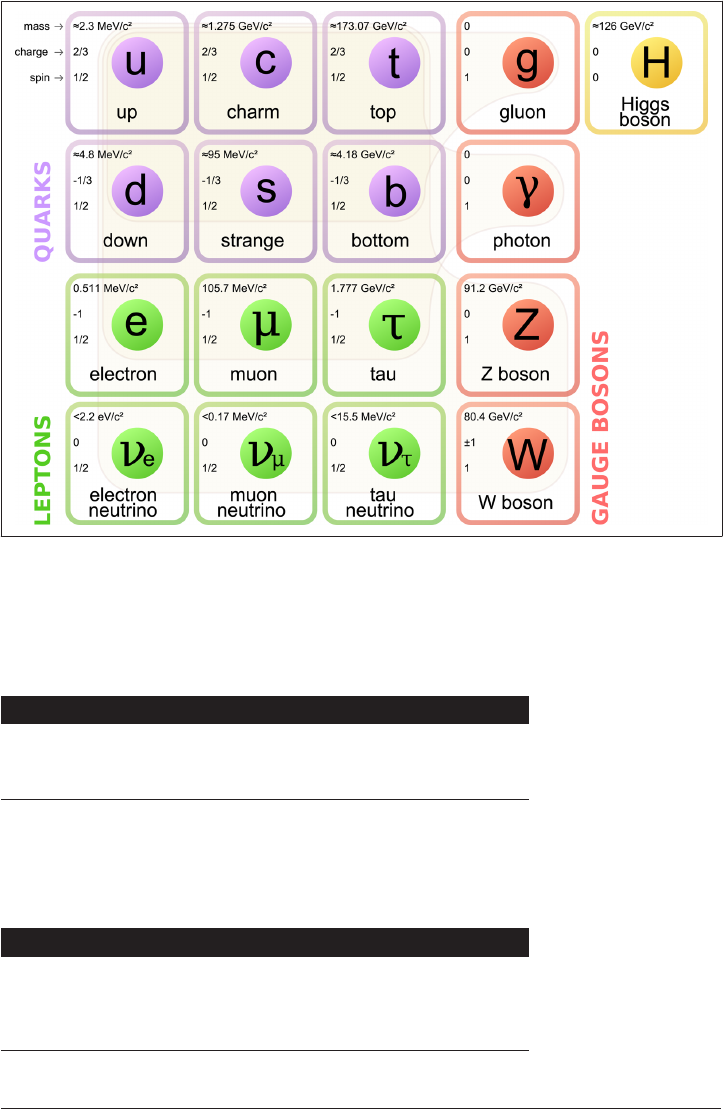
Figure 6-1. e Standard Model of Elementary Particles (source: Wikipedia)
This example makes the roar string an attribute that is accessible across all Particle
objects. To access this variable, it is not necessary to create a concrete instance of the
class. Rather, you are able to obtain roar directly from the class definition:
Code Output
# import the particle module
import particle as p
print(p.Particle.roar)
'I am a particle!'
This class variable, p.roar, can also be accessed by any object instance of the class, as
seen in the following example. For now, to create a Particle instance, call the class
definition like you would call a function with no arguments (i.e., Particle()):
Code Output
# import the particle module
import particle as p
higgs = p.Particle()
print(higgs.roar)
'I am a particle!'
Classes | 125
www.it-ebooks.info

Class-level attributes are excellent for data and methods that are universal across all
instances of a class. However, some attributes are unique to each object and should
not be changed by other objects, even those of the same class. Such attributes are
called instance variables.
Instance Variables
Every particle in the universe has a physical position, r, in the coordinate system.
Thus, position should certainly be an attribute of the Particle class. However, each
particle must have a dierent physical position at any particular time (see also the
“identity of indiscernibles” principle). So, an attribute storing the position data should
be bound specifically to each individual particle.
havior is not unlike the example earlier in the chapter concerning the different abso‐
lute values of different integers. That is, if the class is defined properly, it should be
possible to set the position variable uniquely for each particle. Using the class to cre‐
ate a list of observed Particle objects might, in that case, be achieved as shown here:
# import the Particle class from the particle module
from particle import Particle as p
# create an empty list to hold observed particle data
obs = []
# append the first particle
obs.append(p.Particle())
# assign its position
obs[0].r = {'x': 100.0, 'y': 38.0, 'z': -42.0}
# append the second particle
obs.append(p.Particle())
# assign the position of the second particle
obs[1].r = {'x': 0.01, 'y': 99.0, 'z': 32.0}
# print the positions of each particle
print(obs[0].r)
print(obs[1].r)
This code outputs:
{'y': 38.0, 'x': 100.0, 'z': -42.0}
{'y': 99.0, 'x': 0.01, 'z': 32.0}
This behavior is exactly what can be accomplished with instance variables. While the
task of describing the data and behaviors of particles may seem daunting at first, if we
start with the basics, it will soon become clear how object orientation simplifies the
cognitive task. For starters, all particles have position, mass, charge, and spin—much
of the rest can be derived.
126 | Chapter 6: Classes and Objects
www.it-ebooks.info

Thus, given these instance variables, not much more complexity is necessary to store
all the data associated with a particle observation. This example shows how, in an
object-oriented model, the individual data associated with multiple observations can
be kept impeccably organized in the instance variables of many objects.
The value of this reduced complexity using instance variables should be obvious, but
how is it accomplished in the class definition? To associate data attributes with a spe‐
cific instance of the class in Python, we use the special __init__() function, the con‐
structor. Implementation of constructors is addressed in the following section.
Constructors
A constructor is a function that is executed upon instantiation of an object. That is,
when you set higgs = p.Particle(), an object of the Particle type is created and the
__init__() method is called to initialize that object.
In Python, the constructor is always named __init__(), because it
sets the initial state of the object.
The constructor is one of the methods defined inside of the class definition. A user-
written constructor is not required to exist for a class definition to be complete. This
is because every class automatically has a default constructor. Furthermore, if the
__init__() method does exist, it needs only to perform constructor actions specific
to defining objects of this class. However, because it is always run when an object is
created, best practice is to make this function responsible for initializing all of the
instance variables of the object. That way, every time an object is created, it is guaran‐
teed to be fully initialized.
Introducing instance variables outside of an __init__() function is
somewhat risky, because there is no guarantee that they’ll be initial‐
ized by the time you need to use them. Try to avoid it.
As an example, a Particle() constructor can be introduced that defines and initial‐
izes a few instance variables that should be specific to particular particles:
# particle.py
class Particle(object):
"""A particle is a constituent unit of the universe.
Attributes
----------
Classes | 127
www.it-ebooks.info
c : charge in units of [e]
m : mass in units of [kg]
r : position in units of [meters]
"""
roar = "I am a particle!"
def __init__(self):
"""Initializes the particle with default values for
charge c, mass m, and position r.
"""
self.c = 0
self.m = 0
self.r = {'x': 0, 'y': 0, 'z': 0}
The self argument is required since this function is a method. More details will
be discussed in “Methods” on page 129. This parameter is used so the method is
bound to a specific instance of the class.
The instance attribute c is introduced (and assigned to self) with an initial value
of 0.
The instance variables c, m, and r introduced in the __init__() method are assigned
to the current object, called self, using the syntax self.<var> = <val>.
Note how the self parameter is passed to the __init__() method.
This argument represents the instance of the class. The function
becomes a method by being part of the class definition. All meth‐
ods are required to accept at least one argument, and the first argu‐
ment is the instance of the class. By a very strong convention, this
first argument is named self. However, since this is only a conven‐
tion, nothing prevents you from using me, this, x, or any other
variable name other than social pressure.
In the previous example, to set actual values for the instance variables we would have
to assign them outside of the constructor, just as we did with the positions in
“Instance Variables” on page 126. That’s a bit inefficient, though. This constructor
would be more powerful if it were capable of specifying specific data values upon ini‐
tialization. Then, it would take only one line of code to fully specify all of the data
attributes of the particle. To do just that, the __init__() method can instead be writ‐
ten to accept arguments that can be used directly to initialize the object. To achieve
this, we must replace the previous example with the following:
# particle.py
class Particle(object):
"""A particle is a constituent unit of the universe.
128 | Chapter 6: Classes and Objects
www.it-ebooks.info

Attributes
----------
c : charge in units of [e]
m : mass in units of [kg]
r : position in units of [meters]
"""
roar = "I am a particle!"
def __init__(self, charge, mass, position):
"""Initializes the particle with supplied values for
charge c, mass m, and position r.
"""
self.c = charge
self.m = mass
self.r = position
The self parameter remains the first argument. However, it is followed by the
three positional arguments with which the __init__() method will initialize the
object.
The instance attribute c is introduced (and assigned to self) with an initial
value, charge, provided in the method call.
We’ve mentioned that __init__() is a “method,” and arguably the most important
one since it is the constructor in Python. The next section will explain further what
methods are and how they are different from functions, and will give some examples
of other kinds of methods that can be defined in the class definition.
Methods
The constructor, as mentioned previously, is a special method in Python, but many
other methods can exist in a class definition. Methods are functions, like those cov‐
ered in Chapter 5. However, not all functions are methods. Methods are distinguished
from functions purely by the fact that they are tied to a class denition. Specifically,
when a method is called, the object that the method is found on is implicitly passed
into the method as the first positional argument. For this reason, methods may oper‐
ate on data contained by the object. Let’s add another method, hear_me(), to our Par
ticle class definition:
# particle.py
class Particle(object):
"""A particle is a constituent unit of the universe.
Attributes
----------
c : charge in units of [e]
m : mass in units of [kg]
Classes | 129
www.it-ebooks.info

r : position in units of [meters]
"""
roar = "I am a particle!"
def __init__(self, charge, mass, position):
"""Initializes the particle with supplied values for
charge c, mass m, and position r.
"""
self.c = charge
self.m = mass
self.r = position
def hear_me(self):
myroar = self.roar + (
" My charge is: " + str(self.c) +
" My mass is: " + str(self.m) +
" My x position is: " + str(self.r['x']) +
" My y position is: " + str(self.r['y']) +
" My z position is: " + str(self.r['z']))
print(myroar)
The object is passed to the hear_me() method as self.
The self argument is used to access the instance variable c.
The myroar string is printed from within the method. The roar is heard.
This example uses the global roar string. The self argument (representing the con‐
crete object) allows the attribute to be accessed from the hear_me() method. The
instance variables—roar, c, m, and r[*]—are used to construct a string that is specific
to this particle. All of this is done in the hear_me() method, which then prints the
string:
Code Output
from scipy import constants
import particle as p
m_p = constants.m_p
r_p = {'x': 1, 'y': 1, 'z': 53}
a_p = p.Particle(1, m_p, r_p)
a_p.hear_me()
I am a particle!
My mass is: 1.672621777e-27
My charge is: 1
My x position is: 1
My y position is: 1
My z position is: 53
In this example, a proton is described. Note that the mass of the proton was retrieved
from the scipy.constants module.
130 | Chapter 6: Classes and Objects
www.it-ebooks.info

Don’t hardcode well-known scientific constants into your program.
Use the constants provided by the scipy.constants module
instead.
Methods can also alter instance variables. As an example, let us imagine a Quark class
that has an instance variable called flavor. Quarks and leptons have flavors. The
“weak interaction” can alter that flavor, but symmetry must be preserved. So, in some
quantum superposition interactions, a flavor can flip, but only to its complementary
flavor. A method on the Quark class could flip the flavor. That flip() method would
be defined to reset the flavor variable from up to down, top to bottom, or charm to
strange:
def flip(self):
if self.flavor == "up":
self.flavor = "down"
elif self.flavor == "down":
self.flavor = "up"
elif self.flavor == "top":
self.flavor = "bottom"
elif self.flavor == "bottom":
self.flavor = "top"
elif self.flavor == "strange":
self.flavor = "charm"
elif self.flavor == "charm":
self.flavor = "strange"
else :
raise AttributeError("The quark cannot be flipped, because the "
"flavor is not valid.")
In this example, the flip() method is able to access and alter an attribute of a Quark
object. To witness this in action, we can create a Quark, set it to one flavor, and flip it
to the other:
Code Output
# import the class
from quark import Quark
# create a Quark object
t = Quark()
# set the flavor
t.flavor = "top"
# flip the flavor
t.flip()
# print the flavor
print(t.flavor)
bottom
Classes | 131
www.it-ebooks.info

Because they can access attributes of an object, methods are very powerful functions.
With this power, the scientist can begin to do impressive things with object orienta‐
tion. For example, the Particle class should capture the relationship between uncer‐
tainty in momentum and uncertainty in position. The Heisenberg Uncertainty
Principle states:
ΔxΔpx≥ℏ
2
A method that returns the minimum possible value of Δx can be added to the class
definition:
from scipy import constants
class Particle(object):
"""A particle is a constituent unit of the universe."""
# ... other parts of the class definition ...
def delta_x_min(self, delta_p_x):
hbar = constants.hbar
delx_min = hbar / (2.0 * delta_p_x)
return delx_min
Now the physics can really take over. What other methods would you add to a Parti
cle class? Do all of them need to be tied inextricably to the object instance? Some‐
times methods have a place in a class but don’t need to be associated with any other
attributes.
Static Methods
As just stated, functions are different from methods by virtue of being unattached to
a class. That is, a feature of the Quark class could be a function that lists all possible
values of quark flavor. Irrespective of the flavor of a specific instance, the possible val‐
ues are static. Such a function would be:
def possible_flavors():
return ["up", "down", "top", "bottom", "strange", "charm"]
Now, suppose that you wanted to have a method that was associated with a class, but
whose behavior did not change with the instance. The Python built-in decorator
@staticmethod allows for there to be a method on the class that is never bound to any
object. Because it is never bound to an object, a static method does not take an
implicit self argument. However, since it lives on the class, you can still access it
from all instances, like you would any other method or attribute. The following dem‐
onstrates how to bring possible_flavors() into the class definition as a static
method:
132 | Chapter 6: Classes and Objects
www.it-ebooks.info

from scipy import constants
def possible_flavors():
return["up","down","top","bottom","strange","charm"]
class Particle(object):
"""A particle is a constituent unit of the universe."""
# ... other parts of the class definition ...
def delta_x_min(self, delta_p_x):
hbar = constants.hbar
delx_min = hbar / (2.0 * delta_p_x)
return delx_min
@staticmethod
def possible_flavors():
return ["up", "down", "top", "bottom", "strange", "charm"]
All of the attributes described in the last few sections have defined the class interface.
The methods and data that are associated with an object present an interface to the
simulation. In Python, that interface is very important. Python interfaces rely heavily
on the notion of duck typing, which we first encountered in Chapter 3 and will go
into more detail on now.
Duck Typing
This peculiar name comes from the saying, “When I see a bird that walks like a duck
and swims like a duck and quacks like a duck, I call that bird a duck.” In the Python
context, this refers to checking at runtime whether or not an object quacks when it is
asked to quack. If instead the object is asked to swim, Python will check if it can
swim. The full duck-ish nature of an object is never checked automatically.
That is, Python does not explicitly check for object types in the way that other pro‐
gramming languages do. Python neither requires that variable types be declared upon
instantiation nor guarantees the types of variables passed into functions as parame‐
ters. Object behavior, but not object type, is checked when a method is called or an
attribute is accessed, and not before. In this way, Python only performs duck-type
checking. If two different object types (birds, say) implement identical interfaces
(“quack like ducks”), then they can be treated identically within a Python program. In
this paradigm, an object need not be of a certain type in order for its methods to be
invoked. It must merely possess those methods.
All particles with a valid charge() method, for example, can be used identically. You
can implement a function such as the following, calculating the total charge of a col‐
lection of particles, without knowing any information about the types of those
particles:
Classes | 133
www.it-ebooks.info

def total_charge(particles):
tot = 0
for p in particles:
tot += p.c
return tot
If the function is parameterized with a collection of Quarks, Protons, and Electrons,
it will sum the charges irrespective of the particle types. For two electrons and one
proton, the total charge is –1e.
Code Output
p = Proton()
e1 = Electron()
e2 = Electron()
particles = [p, e1, e2]
total_charge(particles)
-1.602176565e−19
Note that the type of container holding the collection of particles is also irrelevant.
Since the Python elemental iteration syntax for x in y is the same for many data
structures, the exact same behavior would result whether the container were a list, a
tuple, a set, or any other container with that iteration method. This, too, is an exam‐
ple of duck typing.
Explicit typing is sometimes helpful, though considered unpythonic. To trigger differ‐
ent methods for different types of object or to trigger a warning in the event of an
unsupported type, explicit typing can be used. Note that, when needed, the built-in
isinstance() function can be used to achieve explicit type checking. This function
takes the object that you want to test and the type you want to test against.
For example, in this case the letter c is somewhat ambiguous. Perhaps some other
object slips into the collection that possesses a method c with a dierent meaning
(perhaps c is the speed of light). Rather than accidentally allowing the addition of the
speed of light to one’s calculation, the cautious developer could choose to ignore any
objects that are not Particles:
def total_charge(collection):
tot = 0
for p in collection:
if isinstance(p, Particle):
tot += p.c
return tot
In this way, duck typing can be overruled when it is inconvenient. However, usually
duck typing adds flexibility and scalability to code. It is therefore highly desirable,
and cousins of duck typing are accordingly part of the object-orientation paradigm.
First up is polymorphism.
134 | Chapter 6: Classes and Objects
www.it-ebooks.info

Polymorphism
In biology, polymorphism refers to the existence of more than one distinct phenotype
within a single species. In object-oriented computation, polymorphism occurs when
a class inherits the attributes of a parent class. As a general rule, what works for a par‐
ent class should also work for the subclass, but the subclass should be able to execute
its own specialized behavior as well. This rule will be tempting to break, but should be
respected.
A quark, for example, should behave like any other elementary particle in many ways.
Like other elementary particles (e.g., an electron or a muon), a quark has no distinct
constituent particles. Additionally, elementary particles have a type of intrinsic angu‐
lar momentum called spin. Based on that spin, they are either fermions (obeying
Fermi-Dirac statistics) or bosons (obeying Bose-Einstein statistics). Given all this,
and making use of Python’s modulo syntax, we might describe the ElementaryParti
cle class thus:
# elementary.py
class ElementaryParticle(Particle):
def __init__(self, spin):
self.s = spin
self.is_fermion = bool(spin % 1.0)
self.is_boson = not self.is_fermion
Note that the ElementaryParticle class seems to accept the Particle class instead of
object. This is in order to denote that the ElementaryParticle class is a subclass of
the Particle class. That relationship is called inheritance because the ElementaryPar
ticle class inherits data and behaviors from the Particle class. The inheritance dia‐
gram for this relationship is shown in Figure 6-2.
Distinct from ElementaryParticles, however, CompositeParticles exist. These are
particles such as protons and neutrons. They are composed of elementary particles,
but do not share their attributes. The only attributes they share with ElementaryPar
ticles are captured in the parent (Particle) class. CompositeParticles have all the
qualities (charge, mass, position) of the Particle class and one extra, a list of constit‐
uent particles:
# composite.py
class CompositeParticle(Particle):
def __init__(self, parts):
self.constituents = parts
Classes | 135
www.it-ebooks.info
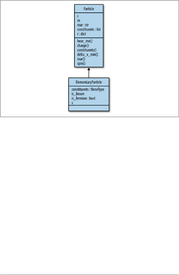
Figure 6-2. e ElementaryParticle class inherits from the Particle class
As a simulator or other physics software becomes more detailed, additional classes
like ElementaryParticle and CompositeParticle can be created in order to capture
more detailed resolution of Particle types. Additionally, since attributes vary
depending on the type of particle (e.g., electrons and protons have charge, but neu‐
trons do not), these classes may need to represent the various subtypes of particles as
well.
Subclasses
Because they inherit from the Particle class, ElementaryParticle objects and Compo
siteParticle objects are Particle objects. Therefore, an ElementaryParticle has
all of the functions and data that were previously assigned in the Particle class, but
none of that code needs to be rewritten. In this way, the code defining the Particle
class is reused.
Additionally, the ElementaryParticle class can override that data and those behav‐
iors, if desired. For example, the ElementaryParticle class inherits the hear_me()
function from the Particle class. However, it can override the roar string in order to
change its behavior. If the ElementaryParticle class is defined thus:
# elementary.py
class ElementaryParticle(Particle):
136 | Chapter 6: Classes and Objects
www.it-ebooks.info

roar = "I am an Elementary Particle!"
def __init__(self, spin):
self.s = spin
self.is_fermion = bool(spin % 1.0)
self.is_boson = not self.is_fermion
Then the following is the resulting behavior:
Code Output
from elementary import ElementaryParticle
spin = 1.5
p = ElementaryParticle(spin)
p.s
p.hear_me()
1.5
I am an Elementary Particle!
My charge is: -1
My mass is: 0
My x position is: 0
My y position is: 0
My z position is: 0
The power here lies in the customization of behavior. ElementaryParticle objects
have all of the attributes of Particle objects, so they can interact exactly as Parti
cles do. However, they also have additional attributes only possessed by Elementary
Particles, and they have specialized certain attributes of the Particle superclass.
Superclasses
Any class, including a subclass, can be a superclass or parent class. The subclass is
said to inherit from its parent. In the preceding examples, the Particle class is a
superclass and the ElementaryParticle class is a subclass. However, the Elementary
Particle class can also be a superclass. Since quarks are a type of elementary particle,
the Quark class might inherit from the ElementaryParticle class.
The superclass of Quark is ElementaryParticle. But since the ElementaryParticle
class still inherits from Particle, the Particle class is therefore a superclass of both
the ElementaryParticle class and the CompositeParticle class.
Quarks have typical ElementaryParticle characteristics (spin, is_fermion,
is_boson), as well as those that ElementaryParticle inherits from Particle (charge,
mass, position). However, Quarks also have avor. The flavor of the quark can take
one of six values (up, down, top, bottom, strange, and charm).
import randphys as rp
class Quark(ElementaryParticle):
def __init__(self):
phys = rp.RandomPhysics()
self.color = phys.color()
self.charge = phys.charge()
Classes | 137
www.it-ebooks.info

self.color_charge = phys.color_charge()
self.spin = phys.spin()
self.flavor = phys.flavor()
Polymorphism, subclasses, and superclasses are all achieved with inheritance. The
concept of inheritance is subtly distinct from polymorphism, however—a class is
called polymorphic if it has more than one subclass. Both of these concepts are dis‐
tinct from multiple inheritance, which we’ll look at next.
Multiple inheritance
Multiple inheritance is when a subclass inherits from more than one superclass. For
example, the quantum-mechanical phenomenon of wave-particle duality may need to
be modeled in the ElementaryParticle class.
In their behavior as waves, ElementaryParticles should possess Wave-like attributes
such as amplitude and frequency. These attributes rely on the energy of the Elemen
taryParticle object. Also, as a Wave, an ElementaryParticle should implement
interference methods based on this class when interacting with other Wave functions.
All that said, ElementaryParticles should also continue to exhibit the attributes of a
Particle (such as charge). To capture both its Particle nature and its Wave nature at
the same time, the ElementaryParticle class can inherit from both the Wave and Par
ticle classes.
# elementary.py
class ElementaryParticle(Wave, Particle):
def __init__(self, spin):
self.s = spin
self.is_fermion = bool(spin % 1.0)
self.is_boson = not self.is_fermion
This is multiple inheritance. The new, quantum-friendly model of the ElementaryPar
ticle is shown here. With only one changed line, it now adopts the behavior of the
Wave class as well as that of the Particle class.
If all of this is confusing, never fear. Figure 6-3 should clear things up somewhat.
Looking at or drawing an inheritance diagram is always useful for understanding the
relationships that exist in a class hierarchy. In practice, these hierarchies can become
quite deep and convoluted as a code base grows. If this isn’t enough, many resources
are available that go into greater detail. We will mention a few at the end of the
chapter.
138 | Chapter 6: Classes and Objects
www.it-ebooks.info
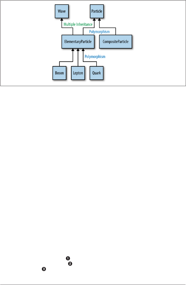
Figure 6-3. Inheritance, polymorphism, and multiple inheritance
Decorators and Metaclasses
Metaprogramming is when the definition of a class (or function) is specified, in part
or in full, by code outside of the class definition itself. We saw a bit of this in “Decora‐
tors” on page 112, where decorators were used to alter the behavior of functions. In
some programming languages, such as C++, metaprogramming is a central part of
the language. (If you have worked in C++, then you know it is impossible to get by
without templates for any length of time.) In Python, the need for metaprogramming
is less pervasive since everything is an object. However, it is there when you need it.
Admittedly this is rare in physics-based programming, but it does comes up when
you’re writing analysis frameworks.
The overwhelming majority of your metaprogramming needs can be handled by class
decorators. These work in exactly the same way as function decorators: just place an
@<decorator> above the class definition. This works because class definitions, like
everything else in Python, are objects. Thus they can be used as arguments to a func‐
tion and also returned from a function.
Inside of a class decorator we can add attributes or methods to an existing class. Or
we could throw out the original class entirely and return a brand new class. The deco‐
rator itself is still a function. However, instead of returning a new function, a class
decorator will typically return a class.
Suppose that we wanted to add an is_particle class attribute to our Particle class.
We could do this through the following add_is_particle() decorator:
def add_is_particle(cls):
cls.is_particle = True
return cls
Decorators and Metaclasses | 139
www.it-ebooks.info

@add_is_particle
class Particle(object):
"""A particle is a constituent unit of the universe."""
# ... other parts of the class definition ...
Defines the class decorator, which takes one argument that is the class itself.
Modifies the class by adding the is_particle attribute.
Returns the class.
Applies the decorator to the class. This uses the same syntax as a function
decorator.
Of course, nothing is stopping us from going all out and adding methods to the class
in the decorator, or removing them. For example, we could add a distance() method
that computes the distance between the current particle and another particle, as
follows:
from math import sqrt
def add_distance(cls):
def distance(self, other):
d2 = 0.0
for axis in ['x', 'y', 'z']:
d2 += (self.r[axis] - other.r[axis])**2
d = sqrt(d2)
return d
cls.distance = distance
return cls
@add_distance
class Particle(object):
"""A particle is a constituent unit of the universe."""
# ... other parts of the class definition ...
It is probably still a good idea to call the first argument self, since this function
will be a method, even though it is defined outside of the class.
Since we are modifying the class in-place, we again want to return the class.
In the unlikely event where, for some reason, class decorators are not enough, there
are always metaclasses. Class decorators are a relatively new addition to the Python
language, so you are more likely to see metaclasses floating around in legacy code. In
140 | Chapter 6: Classes and Objects
www.it-ebooks.info

the way that classes create objects, metaclasses generate classes. All metaclasses must
inherit from type, like all classes inherit from object. The type of type is, of course,
type:
In [1]: type(type)
Out[1]: type
Thus, defining a new metaclass is as easy as inheriting from type. A common pattern
in Python is for metaclasses to be prefixed with the phrase Is or Has. Let’s create an
IsParticle metaclass:
class IsParticle(type):
pass
This can then be applied to our Particle class by passing it in as the metaclass key‐
word argument to the inheritance listing:
class Particle(metaclass=IsParticle):
"""A particle is a constituent unit of the universe."""
# ... other parts of the class definition ...
Note that now the Particle class is an instance of the IsParticle metaclass. How‐
ever, any instance p of Particle is not an instance of the metaclass:
In [1]: isinstance(Particle, IsParticle)
Out[1]: True
In [2]: p = Particle()
In [3]: isinstance(p, IsParticle)
Out[3]: False
Metaclasses are mainly used to override the special __new__() method, which is used
to create new instances of a class prior to them being initialized via __init__(). The
__new__() method prepares an object for initialization. By modifying __new__() you
can dramatically change how a class creates instances of itself. Almost no one needs
to do this, though. Where it does arise is often in the context of describing data in
databases. But even then, there are more intuitive ways than metaclasses. Since the
type of the class is being modified, metaclasses can be tricky to get right. For now, just
know that they exist, they aren’t scary, and you can look them up in more detail in the
Python documentation.
Object Orientation Wrap-up
This chapter has covered object orientation from the perspective of simulating phys‐
ics and understanding Python. In particular, it covered what objects and classes are,
how they are defined, how classes create objects, and how classes relate to one
another. With all of that, the reader should now:
Object Orientation Wrap-up | 141
www.it-ebooks.info

•Understand how object orientation can be useful for the reductionist, encapsula‐
ted modeling necessary in physics simulation
• Know how to create a simple physical model using classes and objects in Python
Empowered with this knowledge, you can now apply object orientation to simula‐
tions and analyses in your subfield of physics. As you go forward, note that many
additional resources on object orientation in Python and other languages are avail‐
able online and in books; for example, Software Carpentry offers an excellent tutorial,
both online and in person, concerning object orientation in Python.
Finally, any discussion of object orientation would be remiss if it failed to mention the
existence and importance of design patterns. Many “patterns” have emerged over the
years in object-oriented programming. Some patterns enable efficient or robust
behavior. Others are common failure modes (these are often called antipatterns). The
book responsible for laying the groundwork and establishing the early vocabulary
around design patterns in object-oriented code is Design Patterns, by Erich Gamma,
Richard Helm, Ralph Johnson, and John Vlissides (Pearson). These four authors are
colloquially known as “The Gang of Four.”
142 | Chapter 6: Classes and Objects
www.it-ebooks.info


CHAPTER 7
Analysis and Visualization
Churning out terabytes of data from simulations or experiments does not, on its own,
constitute science. Only analysis and visualization can transform raw data into true
scientific insight. Unanalyzed data is merely data—only interpretation and communi‐
cation can sufficiently illuminate and clarify the scientific meaning of results. When
analysis and visualization succeed, compelling data becomes a convincing result.
There was an era in the physical sciences when data was collected in laboratory note‐
books, and when the time to publish plots of that data came about, it was done by
hand. Legend has it that this was sometimes begun on enormous sheets of graph
paper on the wall of a lab and scaled down to a reasonable publishable size by big,
slow scanning machines. Many physicists and mathematicians, Roger Penrose not
least among them, continue to make plots and diagrams with pen and paper. None‐
theless, it is an increasingly lost art.
While it is tempting to feel a nostalgia for freehand drawings of the complex plane,
this chapter should inspire you to embrace the future instead. This chapter will pro‐
vide an overview of principles and tools for data preparation, analysis, and visualiza‐
tion appropriate for publication-quality results in the physical sciences. Finally, a few
examples of analysis and visualization using Python tools will be addressed. This
chapter will provide a taste of the analysis tools that will then be discussed in detail in
Chapters 9, 10, and 11.
Preparing Data
Researchers encounter data in many formats, from many sources. They accordingly
can spend significant effort loading, cleaning, collapsing, expanding, categorizing,
and generally “munging” data into consistent formats that can be used for analysis
and plotting. Some basic methods for retrieving data from files will be covered in
145
www.it-ebooks.info

Chapter 10, as will more advanced data manipulation. Depending on the source of
the data, advanced data munging for myriad formats may be necessary. A few will be
discussed here.
Faced with imperfect data in one or more raw formats, the researcher must perform
several steps before even beginning to analyze or visualize it:
•Load the data into an analysis-ready format.
—Possibly convert the data to an intermediate data storage format (CSV, HDF5,
SQL, FITS, ENDF, ENSDF).
—Convert the data to an easy-access data structure (NumPy arrays, Pandas data
frames).
• Clean the data.
— Handle missing values.
— Drop them from analysis.
— Replace them with defaults.
—Count them for statistics.
— Fix mangled or erroneous entries.
— Detect errors.
— Sort disordered data.
— Standardize data formats.
—Handle stylistic issues.
— Rename long or irregular fields.
— Reformat irregularly formatted dates, times, numbers, strings, etc.
•Combine the data with metadata.
— Populate results tables with additional/external data.
— Add identifying numbers and dates, for provenance.
— Merge results from independent detectors, etc.
A visual representation of the aspects of this process appears in Figure 7-1.
146 | Chapter 7: Analysis and Visualization
www.it-ebooks.info
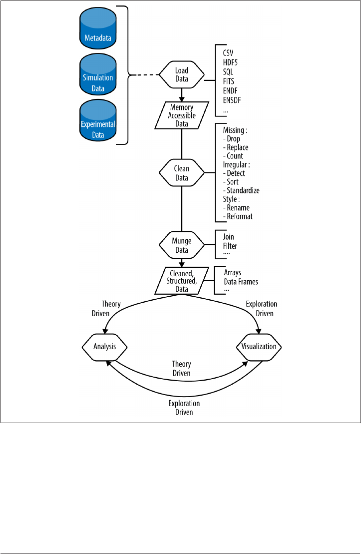
Figure 7-1. Data preparation for analysis and visualization
Due to this involved sequence of necessary tasks, many scientists spend vast portions
of their research careers:
• Cleaning data by hand
• Executing analysis steps one at a time
•Using a mouse when creating plots
Preparing Data | 147
www.it-ebooks.info

•Repeating the whole effort when new data appears or the process must be
tweaked
However, more efficient scientists automate these processes and have more time for
research. These efficient scientists spend their research careers doing the following:
• Scripting their data pipeline
•Gaining confidence in their results
• Doing additional research
• Publishing more papers
These scientists must invest extra effort up front, but they benefit from increased effi‐
ciency later. By taking the time to generate scripts that automate their pipelines (data
cleaning, processing, analysis, plotting, etc.), efficient scientists can more rapidly
incorporate new data into their analyses, test new analysis steps, and tweak plots. The
pipeline can be simple or complex and may include a wide array of actions, such as:
•Data entry
• Data cleanup
• Building any necessary software
• Running simulation analyses
• Data post-processing
• Uncertainty estimation
•Generating tables and plots for publication
• Building papers around that work
An astute reader may note that the former kind of scientist may publish results faster
if the datasets are pristine and reviewers are generous. Fools and optimists are invited
to rely on these two miracles. Realists should automate. Furthermore, those who are
sickened by the rampant lack of reproducibility in scientific computation should
move to automate their pipelines, irrespective of the cost-benefit ratio. Fully scripted
analysis and visualization is a necessary feature of reproducible science. Though
incentive structures in the research sciences currently fall short of rewarding repro‐
ducibility, the tables are turning. Be on the righteous side of history—heed the words
of Mario Savio, and automate your methods:
There’s a time when the operation of the machine becomes so odious, makes you so
sick at heart, that you can’t take part! You can’t even passively take part! And you’ve got
to put your bodies upon the gears and upon the wheels… upon the levers, upon all the
apparatus, and you’ve got to make it stop! And you’ve got to indicate to the people who
148 | Chapter 7: Analysis and Visualization
www.it-ebooks.info

run it, to the people who own it, that unless you’re free, the machine will be prevented
from working at all!
When you’re automating your methods, the first thing to automate is the processing
of raw data. How the data processing step is performed varies greatly depending on
whether your work is based on experimentation or simulation. The next sections will
cover each of those cases, as well as the metadata that is associated with them.
Experimental Data
Experimental data presents unique analysis challenges to the scientist. Such data usu‐
ally takes the form of detector responses and physical measurements resulting from
various experiments in the physical sciences.
Experiments that observe a variable changing over time will produce time series data,
where the independent variable is time and the dependent variable is the observation.
Time series data such as this is often stored in flat tabular plain-text or simple CSV
files. An example might be an experiment that seeks to identify the decay constant of
an isotope based on its dwindling radiation signature over time. Such data might be
structured as in Table 7-1.
Table 7-1. Isotope decay data (decays.csv)
Time(s) Decays (#)
0 10.0
1 1.353352832
2 0.183156389
3 0.024787522
4 0.003354626
5 0.000453999
6 6.1442e-05
7 8.315e-06
8 1.126e-06
9 1.52e-07
… …
Preparing Data | 149
www.it-ebooks.info

In its raw form, this data may be stored in a comma-separated or otherwise delimited
plain-text format, as seen here:
# Time (s), Decays (#)
0,10.0
1,1.353352832
2,0.183156389
3,0.024787522
4,0.003354626
5,0.000453999
6,6.1442e-05
7,8.315e-06
8,1.126e-06
9,1.52e-07
Experiments that seek certain parametric relationships between variables, however,
may produce multidimensional, structured, or tabular data. Many experiments have
qualities of both and produce multidimensional, structured time series data. The pos‐
sibilities are endless, but the structure of data often dictates the format it must be
stored in. While time series can be stored easily in CSV format, very complex struc‐
tured data typically calls for a standardized database format.
In special cases, scientific communities adopt their own very domain-specific file for‐
mats for storing experimental data. Astrophysicists, for example, store their enor‐
mous libraries of telescope images and telescope calibration metadata together in the
specialized Flexible Image Transport System (FITS) file format. In nuclear physics, on
the other hand, physicists do not deal with images. Rather, they deal primarily with
particle interaction probabilities called cross sections. Many international standards
exist for storing this type of data, but the most common nuclear data format is the
Evaluated Nuclear Data File (ENDF) format.
Once formatted, evaluated data like the data that appears in ENDF or FITS formats is
ready to be used in simulations.
Simulation Data
Simulations are just experiments in silico. A wise man, Professor Paul P.H. Wilson,
used to tell his students and colleagues that scientific computation is just experimen‐
tation for scientists who like to control more variables. An experimentalist, he would
explain, begins with the whole world of uncontrolled variables and designs an experi‐
ment that carefully controls those variables one at a time, step by step, until only the
experimental variables are left. The computationalist, on the other hand, starts with a
completely controlled simulation and carefully, one at a time, releases variables.
Because of the higher degree of control in simulation, simulation data output formats
are often already quite clean and well controlled. Raw simulation data typically
resides in databases.
150 | Chapter 7: Analysis and Visualization
www.it-ebooks.info

For provenance, databases may need to be accompanied by data about the simulation,
such as:
• The date the simulation was run
• The names and contents of the input files
• The version numbers of libraries used
This type of data, present in both experiments and simulations, is called metadata.
Metadata
Metadata is data about data. It is important to include metadata because the results
produced by an experiment or a simulation sometimes fail to capture all of its
features.
In an experiment, detector parameters, the date of the experiment, background radia‐
tion readings from another detector, and more. can all affect the interpretation of
results, but these factors may not have been captured in the experimental data output
stream. They can instead be captured in the metadata.
Metadata is not limited to experimentation, however. Metadata that may affect the
interpretation of the results of a simulation include simulation ID numbers, library
dependency version numbers, input file content, and more.
For reproducibility, as much of this data should be included in the workflow as possi‐
ble. From a data processing perspective, this metadata also often needs to be joined
with the experimental or simulation database. The steps necessary for preparing met‐
adata for this process will vary from application to application. However, metadata
should be held to the same standards of formatting and reproducibility as simulation
or experimental data.
Of course, once all of the experimental, simulation, and/or metadata has been pre‐
pared, it must be loaded into a form that can be analyzed. In Figure 7-1, this next step
is the “Load Data” step. It will be covered in the following section.
Loading Data
Many packages in Python enable data to be loaded quickly into a memory-accessible
data structure ready for cleaning, munging, analysis, and visualization. More about
data structures will be covered in Chapter 11. The choice of appropriate data struc‐
ture depends profoundly on the size and type of the data as well as its analysis and
visualization destiny. This section will merely cover how to load data into various
analysis-ready forms using four tools in the Python ecosystem:
•NumPy
Loading Data | 151
www.it-ebooks.info
• PyTables
• Pandas
• Blaze
When you are choosing among tools like these, a number of factors come into play.
Size is the first parameter to consider. For big, dense arrays of numbers or for enor‐
mous suites of images, loading all of the data into memory at once is not recom‐
mended. Rather, loading chunks of the data into memory while cleaning, processing,
or exploring it might be advised. For this and similar out-of-core computations on
data exceeding the bounds of system memory, a database choice that emphasizes
these features is warranted. On that topic, later sections will address loading data into
PyTables and Blaze.
The type of the data also may determine the appropriate data structure. Structured
data in a relational database format may be easiest to handle using extraction and
exploration tools in the sqlite3 or pandas packages.
All of that said, some data is small enough to fit into memory all at once, and much of
the data that physicists encounter or produce is best represented as an array of num‐
bers. For this application, the right tool is the numerical Python package, numpy.
NumPy
Due to their power, many solutions involve NumPy arrays. NumPy arrays will be cov‐
ered in detail in Chapter 9. For now, simply know that NumPy arrays are data struc‐
tures for holding numbers. One easy way to transform a file into a NumPy array is
with the loadtxt function. Using this function, plain-text files holding columns of
text delimited by commas, spaces, or tabs can be loaded directly into a NumPy array.
The decay data in our earlier CSV-formatted example can be loaded directly into a
NumPy array shown here:
import numpy as np
decays_arr = np.loadtxt('decays.csv', delimiter=",", skiprows=1)
Import numpy with the alias np.
Create a NumPy array object called decays_arr using the loadtxt() function.
In this example, the numpy package is loaded and given the short alias np. Next, a vari‐
able called decays_arr is declared and set equal to the output of the loadtxt() func‐
tion. The variable decays_arr is a NumPy array. In this case, the loadtxt() function
is parameterized with only one mandatory variable, the filename. The two optional
variables are the delimiter (a comma), and the number of rows to skip (the header
row, which is not numbers). Though not all were used in this example, many other
152 | Chapter 7: Analysis and Visualization
www.it-ebooks.info

options are available to customize the way a file is read with loadtxt(). To learn
more about those, consult the numpy.loadtxt() documentation using the help com‐
mand in IPython:
In [1]: import numpy as np
In [2]: help(np.loadtxt)
Import numpy with the alias np.
Learn more about the loadtxt() function.
Once data has been loaded into a NumPy array, one of the fastest ways to deal with
that data for large-scale problems is to enlist the help of PyTables.
PyTables
As you will learn in Chapter 10, PyTables provides many tools for converting HDF5
data into analysis-ready NumPy arrays. Indeed, because PyTables can help load, mod‐
ify, and manipulate HDF5 data in the form of NumPy arrays, it is a strong motivator
for the use of HDF5 as a raw data format. Perhaps the decay data in the previous
example could be more easily manipulated in the future if it were stored in an HDF5
database—PyTables can help with that. Any data loaded into a NumPy array can be
quickly and easily saved as an HDF5 database. So, once data has been loaded as a
NumPy array, it is ready for use with PyTables. This allows for faster filtering, joins,
and analysis later. However, PyTables and HDF5 are most useful for storing and
manipulating dense arrays of numbers, so if your data is heterogeneous or sparse, or
contains structured, relational information, it may be best stored in another format. If
that is the case, a multiformat Python package like pandas may be more appropriate
than PyTables. For information on when and how to load data into Pandas, read on.
Pandas
Pandas is currently the easiest to use and most broadly applicable of all of the data
analysis tools in the Python ecosystem. It is a good alternative to the previously dis‐
cussed tools, especially if your data is not in a format that is supported by NumPy
(CSV or plain text) or PyTables (HDF5). Also, Pandas may be the right choice even
for those formats if your data is not arrays of numbers or is the kind of data that you
would like to view, filter, browse, and interact with.
Pandas cleanly handles reading and writing of many of the data formats encountered
by scientists in the wild:
• CSV
•Excel
Loading Data | 153
www.it-ebooks.info
• HDF
• SQL
• JSON
•HTML
• Stata
•Clipboard
• Pickle
Also, loading data into a Pandas format is very straightforward. Note that the capabil‐
ity of numpy.loadtxt() can be repeated in Pandas with very similar syntax:
import pandas as pd
decays_df = pd.read_csv('decays.csv')
Import the pandas package and alias it as pd.
Create a data frame object that holds the data loaded by the read_csv() function.
A lovely quality in Pandas is that once data has been loaded, it can be converted into
any of the other supported formats. To write this data to an HDF5 file, we need to add
just one line to the previous example:
import pandas as pd
decays_df = pd.read_csv('decays.csv')
decays_df.to_hdf('decays.h5', 'experimental')
Import the pandas package and alias it as pd.
Create a data frame object that holds the data loaded by read_csv().
Convert it to HDF5, giving it the filename decays.h5, and create a group node
called “experimental” where this data will be stored.
Pandas is a top-notch tool for data analysis with Python. To learn how to fully wield
the power of Pandas, refer to Python for Data Analysis by the lead developer of Pan‐
das, Wes McKinney (O’Reilly). The data analysis in that book goes way beyond the
scope of this section. Here, we simply mean to introduce the existence of this tool,
alongside a few other tools that might also be considered. The final such data analysis
tool that we will introduce is Blaze. Like Pandas, it is intended for easily loading data
into an analysis-ready format and emphasizes ease of conversion between formats.
154 | Chapter 7: Analysis and Visualization
www.it-ebooks.info
Blaze
Blaze is another Python tool capable of converting data from format to format. This
tool is still in active development, but possesses impressive capabilities already. In
Blaze, the CSV data might be dealt with as a Blaze data descriptor or as a Blaze Table
object. The following example shows the transformation from CSV to data descriptor,
and an additional transformation from data descriptor to Blaze Table object:
import blaze as bz
csv_data = bz.CSV('decays.csv')
decays_tb = bz.Table(csv_data)
The blaze package is imported and given the alias bz.
Next, the CSV data is transformed into Blaze data with the CSV() constructor.
Finally, that data descriptor, csv_data, is transformed into a Blaze Table.
This example illustrates how one type of Blaze object can be quickly converted to
another data structure within Blaze quite straightforwardly. Since the aim of Blaze is
to support conversion between many data formats (or “backends,” in Blaze-speak), it
may be the right tool to use if your data files must be converted from one memory-
accessible format to another.
Blaze is still under active development. Unlike the other tools dis‐
cussed here (NumPy and PyTables in particular), it is not yet fully
stable. However, the features discussed here are quite mature, and
it will be a tool to watch closely as it improves.
This flexibility is likely to make Blaze very handy for certain applications, as this tool
not only provides an interface for converting between many data formats (CSV,
HDF5, SQLite, etc.) but also provides an interface to support workflows using many
computational engines. Blaze uses symbolic expression and typing systems to com‐
municate with other tools including Pandas, NumPy, SQL, Mongo, Spark, and PyTa‐
bles. Access to computational engines like those, which are capable of manipulating
the data, is essential for the next step in the process of data analysis: cleaning and
munging.
Cleaning and Munging Data
Data munging (or wrangling) is a term used to mean many different things within the
broad scope of dealing with data. Typically, as in Figure 7-1, the term refers to the
process of converting data from a raw form to a more well-structured form appropri‐
ate for plotting and mathematical transformation.
Cleaning and Munging Data | 155
www.it-ebooks.info

The scientist may wrangle the data by grouping, filtering, aggregating, collapsing, or
expanding it. Depending on your particular data, this step may need to happen before
the data is cleaned, or may not have to happen until after. Cleaning data can also take
many forms. Typically, this task deals with imperfect, incomplete, and disorganized
data.
Of course, ideally, experimentalists in the physical sciences use sophisticated, automa‐
ted, comprehensive data acquisition systems that produce clean, flawless datasets in
intuitive formats. However, even such systems can produce imperfect data in extreme
conditions.
The decay data being used in the previous examples, for instance, might have errors if
other radioactivity were present in the laboratory. Additionally, if the power to the
detector were cut off in an electrical blackout, data would be unavailable for a period
of time.
To explore this, let’s consider a more realistic version of the data we dealt with before.
It may have machine-generated timestamps instead of integer numbers of seconds,
and it may have missing or imperfect data. Imagine, for example, that about 15 sec‐
onds into the experiment, a colleague walked through the room carrying a slightly
more stable radioactive source, emitting two decays per second. Additionally, imagine
that a few seconds later, the lights in the room flashed off for a few seconds—the
storm outside must have interrupted power to the lab. The resulting data stream
looks like this:
#Time,Decays
2014-11-08T05:19:31.561782,10.0
2014-11-08T05:19:32.561782,1.35335283237
2014-11-08T05:19:33.561782,0.183156388887
2014-11-08T05:19:34.561782,0.0247875217667
2014-11-08T05:19:35.561782,0.00335462627903
2014-11-08T05:19:36.561782,0.000453999297625
2014-11-08T05:19:37.561782,6.14421235333e-05
2014-11-08T05:19:38.561782,8.31528719104e-06
2014-11-08T05:19:39.561782,1.12535174719e-06
2014-11-08T05:19:40.561782,1.52299797447e-07
2014-11-08T05:19:41.561782,2.06115362244e-08
2014-11-08T05:19:42.561782,2.78946809287e-09
2014-11-08T05:19:43.561782,3.77513454428e-10
2014-11-08T05:19:44.561782,5.10908902806e-11
2014-11-08T05:19:45.561782,6.91440010694e-12
2014-11-08T05:19:46.561782,9.35762296884e-13
2014-11-08T05:19:47.561782,2.000000000000000
2014-11-08T05:19:48.561782,2.000000000000000
2014-11-08T05:19:49.561782,2.000000000000000
2014-11-08T05:19:50.561782,2.000000000000000
2014-11-08T05:19:51.561782,2.000000000000000
2014-11-08T05:19:52.561782,2.000000000000000
2014-11-08T05:19:53.561782,2.000000000000000
156 | Chapter 7: Analysis and Visualization
www.it-ebooks.info

2014-11-08T05:19:54.561782,2.000000000000000
2014-11-08T05:19:55.561782,2.000000000000000
2014-11-08T05:19:56.561782,1.92874984796e-21
2014-11-08T05:19:57.561782,2.61027906967e-22
2014-11-08T05:19:58.561782,3.5326285722e-23
2014-11-08T05:19:59.561782,4.78089288389e-24
2014-11-08T05:20:00.561782,6.47023492565e-25
2014-11-08T05:20:01.561782,8.7565107627e-26
2014-11-08T05:20:02.561782,1.18506486423e-26
2014-11-08T05:20:03.561782,1.60381089055e-27
2014-11-08T05:20:04.561782,2.1705220113e-28
2014-11-08T05:20:05.561782,2.93748211171e-29
2014-11-08T05:20:06.561782,3.97544973591e-30
2014-11-08T05:20:07.561782,5.38018616002e-31
2014-11-08T05:20:08.561782,7.28129017832e-32
2014-11-08T05:20:09.561782,9.85415468611e-33
2014-11-08T05:20:10.561782,1.3336148155e-33
2014-11-08T05:20:11.561782,1.80485138785e-34
2014-11-08T05:20:12.561782,NaN
2014-11-08T05:20:13.561782,NaN
2014-11-08T05:20:14.561782,NaN
2014-11-08T05:20:15.561782,NaN
2014-11-08T05:20:16.561782,8.19401262399e-39
2014-11-08T05:20:17.561782,1.10893901931e-39
2014-11-08T05:20:18.561782,1.50078576271e-40
2014-11-08T05:20:19.561782,2.03109266273e-41
2014-11-08T05:20:20.561782,2.74878500791e-42
Uh oh, it looks like the reading was overwhelmed by another source moving
through the room.
At this point, it seems the detector was off, and no readings were made.
NaN entries, as in this example, indicate that no number is stored in
memory at the place where the data should be. NaN stands for “Not
a Number.”
Some experimentalists might see the NaN entries and immediately assume this data
must be thrown away entirely. However, since experiments are often expensive and
time-consuming to conduct, losing an entire run of data due to minor blips like this
is often unacceptable. Concerns about data quality and inconsistencies are very com‐
mon in science. Sometimes, dates are listed in a dozen different formats. Names are
inconsistent across files. And sometimes data is erroneous. In this case, the section
with too-high (2.0) counts due to the external radioactive source dwarfing the actual
signal must be dealt with. How this section of the data is handled is a choice for the
Cleaning and Munging Data | 157
www.it-ebooks.info

experimenter. Whatever the choice, however, tools exist to assist in the
implementation.
The data from this run is ugly, but can it be saved with intelligent cleaning and
modern tools? The following section will discuss one way to deal with missing data
using Pandas.
Missing Data
Sometimes, data is missing. In some situations, a missing data point may be appropri‐
ate or expected, and can be handled gracefully. Often, however, it may need to be
replaced with a default value, its effect on the statistical analysis of the results may
need to be taken into consideration, or those data points may just need to be
dropped.
Pandas is especially helpful in the event of missing data. In particular, Pandas has spe‐
cial methods for identifying, dropping, and replacing missing data.
With only a few lines in IPython, the NaN rows from the previous data can be dropped
from the dataset entirely:
In [1]: import pandas as pd
In [2]: decay_df = pd.read_csv("many_decays.csv")
In [3]: decay_df.count()
Out[3]:
Time 50
Decays 46
dtype: int64
In [4]: decay_df.dropna()
Out[4]:
Time Decays
0 2014-11-08T05:19:31.561782 1.000000e+01
1 2014-11-08T05:19:32.561782 1.353353e+00
2 2014-11-08T05:19:33.561782 1.831564e-01
3 2014-11-08T05:19:34.561782 2.478752e-02
4 2014-11-08T05:19:35.561782 3.354626e-03
5 2014-11-08T05:19:36.561782 4.539993e-04
6 2014-11-08T05:19:37.561782 6.144212e-05
7 2014-11-08T05:19:38.561782 8.315287e-06
8 2014-11-08T05:19:39.561782 1.125352e-06
9 2014-11-08T05:19:40.561782 1.522998e-07
10 2014-11-08T05:19:41.561782 2.061154e-08
11 2014-11-08T05:19:42.561782 2.789468e-09
12 2014-11-08T05:19:43.561782 3.775135e-10
13 2014-11-08T05:19:44.561782 5.109089e-11
14 2014-11-08T05:19:45.561782 6.914400e-12
15 2014-11-08T05:19:46.561782 9.357623e-13
158 | Chapter 7: Analysis and Visualization
www.it-ebooks.info

16 2014-11-08T05:19:47.561782 2.000000e+00
17 2014-11-08T05:19:48.561782 2.000000e+00
18 2014-11-08T05:19:49.561782 2.000000e+00
19 2014-11-08T05:19:50.561782 2.000000e+00
20 2014-11-08T05:19:51.561782 2.000000e+00
21 2014-11-08T05:19:52.561782 2.000000e+00
22 2014-11-08T05:19:53.561782 2.000000e+00
23 2014-11-08T05:19:54.561782 2.000000e+00
24 2014-11-08T05:19:55.561782 2.000000e+00
25 2014-11-08T05:19:56.561782 1.928750e-21
26 2014-11-08T05:19:57.561782 2.610279e-22
27 2014-11-08T05:19:58.561782 3.532629e-23
28 2014-11-08T05:19:59.561782 4.780893e-24
29 2014-11-08T05:20:00.561782 6.470235e-25
30 2014-11-08T05:20:01.561782 8.756511e-26
31 2014-11-08T05:20:02.561782 1.185065e-26
32 2014-11-08T05:20:03.561782 1.603811e-27
33 2014-11-08T05:20:04.561782 2.170522e-28
34 2014-11-08T05:20:05.561782 2.937482e-29
35 2014-11-08T05:20:06.561782 3.975450e-30
36 2014-11-08T05:20:07.561782 5.380186e-31
37 2014-11-08T05:20:08.561782 7.281290e-32
38 2014-11-08T05:20:09.561782 9.854155e-33
39 2014-11-08T05:20:10.561782 1.333615e-33
40 2014-11-08T05:20:11.561782 1.804851e-34
45 2014-11-08T05:20:16.561782 8.194013e-39
46 2014-11-08T05:20:17.561782 1.108939e-39
47 2014-11-08T05:20:18.561782 1.500786e-40
48 2014-11-08T05:20:19.561782 2.031093e-41
49 2014-11-08T05:20:20.561782 2.748785e-42
The data frame method count() successfully ignores the NaN rows automatically.
The dropna() method returns the data excluding all rows containing a NaN value.
Here, the time skips ahead 5 seconds, past the now-missing NaN rows.
Now the data is much cleaner, as the offending missing data has been dropped
entirely. This automation of dropping NaN data is quite useful when you’re preparing
data for the next step: analysis.
Analysis
A fleet of tools is available for loading, processing, storing, and analyzing data com‐
putationally. In a Python data analysis environment, the numpy, scipy, and pandas
packages are the big hammers for numerical analysis. However, many packages
within the SciPy and SciKits ecosystems complement those hard-working tools. Some
Python-based analysis toolkits to use, organized by discipline, can be found on the
Analysis | 159
www.it-ebooks.info

SciPy and SciKits websites. There are too many to list here. However, some highlights
include:
• Astronomy and astrophysics
—Astropy: Core astronomy and astrophysics tools; includes FITS, ASCII, VOT‐
able, and XML file format interfaces
—PyRAF: Python-based interface to IRAF
—SpacePy: Data, analysis, and plotting tools for space sciences
—SunPy: Solar data analysis environment
• Geophysics
—OSGeo: GIS data import/export and analysis
—Basemap: 2D mapping
• Engineering
—PyNE: Toolkit for nuclear engineering
—scikit-aero: Aeronautical engineering calculations in Python
• Mathematics
—SymPy: Symbolic mathematics in Python
• Neuroscience
—NIPY: Neuroimaging in Python
• Quantum physics and chemistry
—QuTiP: Quantum Toolbox in Python, simulating dynamics of open quantum
systems
—PyQuante: Python for Quantum Chemistry
The analysis step is very application specific and requires domain knowledge on the
part of the physicist. A large part of analysis in the physical sciences, when models are
derived, confirmed, or disproved based on experimental data, can be termed inference
or abstraction. Abstraction can be an art as well as a science. It can be driven by, gen‐
erally speaking, either side of the equation: the model or the data.
Model-Driven Analysis
In the case of the decay data, the model-driven analysis is very simple. To determine
the decay constant of the isotope in question, we can fit an exponential to the data.
The well-known and accepted model for the decay of a radioactive isotope is
N=N0e−λt.
160 | Chapter 7: Analysis and Visualization
www.it-ebooks.info

Of course, that is a simple example. Most analysis in the physical sciences requires
many steps of filtering and merging of data as well as integrations, interpolations,
scaling, and so on.
A Note on Floating-Point Arithmetic
An excellent resource as you embark on the task of implementing your own numeri‐
cal analysis algorithms is David Goldberg’s paper, What Every Computer Scientist
Should Know About Floating-Point Arithmetic. It sounds dry, but it truly is essential
reading for any researcher who deals with algorithms that manipulate floating-point
numbers.
The paper contains a series of best practices for reducing numerical error obtained
during even simple operations such as summation, multiplication, and division.
As an example, the accuracy of simply summing a list of floating-point numbers
varies strongly according to the order in which those numbers are summed. Errors, in
general, are reduced when smaller numbers are added before larger ones, but more
complex algorithms such as the Kahan summation algorithm improve greatly upon
simple ordering.
While many of those techniques have now been encapsulated in numerical libraries,
some algorithms for data analysis in physics have yet to be written. Furthermore, hav‐
ing a working knowledge of the implementation of the algorithms in the libraries
being used for your analysis will help you to determine the applicability of an algo‐
rithm to your problem, or to differentiate two options when multiple algorithmic
methods are available for a single problem.
Numerical Recipes: e Art of Scientic Computing, by William Press et al., is an excel‐
lent reference when implementing a common algorithm is necessary, and was once
required reading for computational analysis. It is particularly relevant for model-
driven analysis in the physical sciences, which often requires various methods for
numerical integrations, solutions of differential equations, and evaluation of large
systems of equations. This tome illuminates useful algorithms covering such elements
of numerical analysis as:
• Interpolation and extrapolation
•Integration and derivation
• Evaluation of functions
• Inverse functions
• Fermi-Dirac integrals
•Random numbers
Analysis | 161
www.it-ebooks.info

• Sorting
• Root finding
Beyond these algorithms, more elaborate methods exist. Many modern algorithms
emphasize analysis that does not seek to measure a model based on data. Instead, it
often seeks to generate models based on data. This is often termed data-driven
analysis.
Data-Driven Analysis
In data-driven analysis, fancier methods are common. These include clustering algo‐
rithms, machine learning processes, and exotic statistical methods. Such algorithms
are increasingly available in standard open source libraries and are increasingly com‐
mon in physical sciences applications. They typically are used to infer models from
the data (rather than confirm or deny models using the data). The Python ecosystem
possesses many tools enabling such algorithms, including:
•Machine learning and clustering
—scikit-learn
—PyBrain
—Monte
—PyPR
—scipy-cluster
• Statistics
—Statsmodels
—PyBayes
Which algorithms and implementations of those algorithms to use and how to apply
them to your data will be choices that are driven by your science. Whatever tools or
techniques you use, however, data analysis results in conclusions that can, usually, be
visualized.
Visualization
How you visualize your data is the first thing anyone will notice about your paper,
and the last thing they’ll forget. For this reason, visualization should be taken very
seriously and should be regarded as a first-class element of any data analysis
workflow.
A lot has been learned about how to present data and information most effectively.
Much of this knowledge has emerged from business and marketing contexts.
162 | Chapter 7: Analysis and Visualization
www.it-ebooks.info

In science—unlike in business, perhaps—visualization must not attempt to convince
or persuade. Bias, obfuscation, and distortion are the mortal enemies of scientific vis‐
ualization. Visualization in science must demonstrate, clarify, and explain.
Indeed, visualization best practices share many qualities with Python best practices.
Python contains an easter egg: a poem on Python best practices, “The Zen of Python,”
by Tim Peters, is printed in response to the command import this. Though it was
intended to illuminate guidelines for good Python programming, its first few lines
also capture key rules that can be equally well applied to the display of information:
Code Output
import this The Zen of Python, by Tim Peters
Beautiful is better than ugly.
Explicit is better than implicit.
Simple is better than complex.
Complex is better than complicated.
Flat is better than nested.
Sparse is better than dense.
Readability counts.
Special cases aren't special enough to break the rules.
Although practicality beats purity.
Combining these notions with insights gleaned from Edward Tufte’s book e Visual
Display of Quantitative Information and from Matthew Terry, physicist-turned-
software-engineer, I hereby recommend the following “Zen of Scientific Visualiza‐
tion”:
•Beautiful is better than ugly.
• Simple is better than complex.
• Complex is better than complicated.
•Clear is better than dense.
• Communicating is better than convincing.
• Text must not distract.
• People are not mantis shrimp.
The final recommendation may seem a bit odd. However, consider the biology of the
mantis shrimp. With vastly more color-perceiving cones in its eyes than a human, the
mantis shrimp is able to distinguish colors with vastly greater resolution. People are
not mantis shrimp. They are often confused and distracted by too many colors on a
Visualization | 163
www.it-ebooks.info

1While efforts are being made to improve the situation, it is an unfortunate fact that there is a long-standing
gender imbalance in the physical sciences: even today, there are far more males than females in these fields.
Because color vision deficiencies are more common in males than females, this imbalance means that color
blindness is, in turn, more common in the physical sciences than in the general population.
single plot. Additionally, many people in the physical sciences are colorblind,1 so plots
that rely too heavily on color to communicate may be somewhat discriminatory.
Avoid complicated colormaps, and be sensitive to color blindness by avoiding heavy
reliance on color.
Visualization Tools
Many libraries for plotting data exist. This section will introduce a few of the key
libraries available for plotting publication-quality scientific data. The tools covered
include:
Gnuplot
Best for simple plots, as the syntax is peculiar
matplotlib
A powerful plotting library in Python, robust and widely used
Bokeh
Produces interactive plots appropriate for the Web, also interfaces with
matplotlib
Inkscape
Good for hand editing of scalable vector graphics
This section will introduce these tools by demonstrating their use to plot the decay
data from our previous examples in a simple line plot. This introduction should be
enough to help you get started with the right tool very quickly when you need to plot
you work.
These tools are all available within the scientific Python ecosystem, with one excep‐
tion: gnuplot. Gnuplot is not a Python tool, but it stands strong as a plotting option
nonetheless.
Gnuplot
Gnuplot is a key tool in the physics arsenal. Though it is not a Python tool, it is suffi‐
ciently embedded in the physics community that we would be remiss were we to fail
to address it here. While it has never had the most beautiful graphics, plentiful error
messages, or pleasing syntax, physicists have loved it since its birth. Gnuplot is a
workhorse in physics, for better or worse.
164 | Chapter 7: Analysis and Visualization
www.it-ebooks.info
The gnuplot interpreter is launched with the command gnuplot. In that interpreter, it
is possible to enter commands to construct a plot. However, the most reproducible
way to use gnuplot is by creating a script, which is then provided as an argument to
the gnuplot command.
Exercise: Learn More About Gnuplot
Since gnuplot is a command-line tool, it is possible to learn more
about it using the man command.
1. Open a terminal.
2. Find out how to use the gnuplot command via its man page.
(Hint: For more on man pages, see Chapter 1.)
The following gnuplot script can be used to plot the decay data, along with a title and
axis labels:
set title 'Decays'
set ylabel 'Decays '
set xlabel 'Time (s)'
set grid
set term svg
set output 'plot_gnuplot.svg'
plot 'decays.csv' every ::1 using 1:2 with lines
The set keyword defines variables like the title and axis labels.
set can also add predefined customizations—in this case, grid lines.
This sets the output terminal (file) to the SVG file format.
This names the output file.
The plot command accepts data from the input file.
Of the rows in the input file, print all except the first.
Of the columns in the input file, plot 1 and 2 against one another.
This script can be run with the gnuplot command on the command line. Try placing
this code in a file called decay_plot.gnuplot and running the command gnuplot
decay_plot.gnuplot. This script produces the visualization in Figure 7-2.
Visualization | 165
www.it-ebooks.info
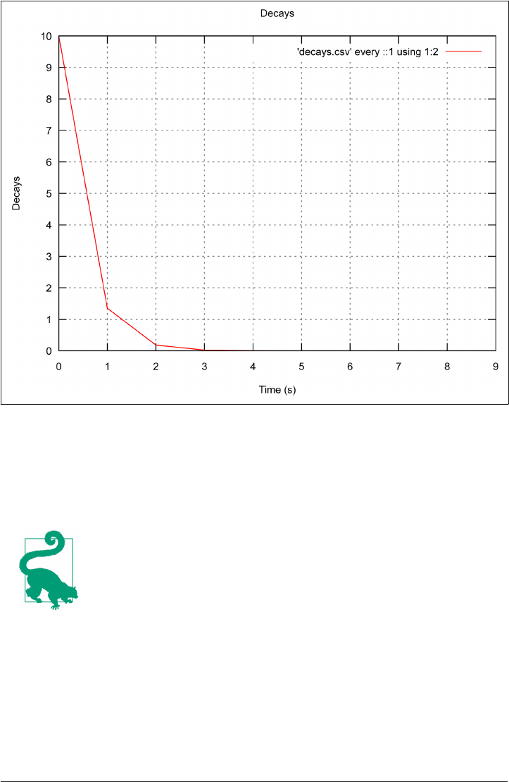
Figure 7-2. Gnuplot plot
By default, gnuplot uses red as the first color to plot in a line plot. Thus, the resulting
plot line is red, though we did not dictate a line color. While this is handy, the second
deployed default line color in gnuplot is green, which is unfortunate for color-blind
people.
Exercise: Change the Color
1. Open a terminal window.
2. Create the decay_plot.gnuplot file and Figure 7-2.
3. Modify the script to produce a blue line rather than red.
(Hint: Use the man page and documentation online to determine
how to change the color of the plot line.)
Though gnuplot is very simple and may be the first plotting library taught to a physi‐
cist on the command line, more effective physics can be accomplished if the plotting
library is able to make direct use of the data preparation steps described in the previ‐
166 | Chapter 7: Analysis and Visualization
www.it-ebooks.info
ous sections. Additionally, graphics features implemented in more modern Python
packages are somewhat superior aesthetically to the graphical capabilities in gnuplot.
One such alternative is matplotlib.
matplotlib
The workhorse for scientific plotting in Python is matplotlib. We can reproduce our
gnuplot plot with matplotlib by running the following Python script to create the new
file:
import numpy as np
# as in the previous example, load decays.csv into a NumPy array
decaydata = np.loadtxt('decays.csv', delimiter=",", skiprows=1)
# provide handles for the x and y columns
time = decaydata[:,0]
decays = decaydata[:,1]
# import the matplotlib plotting functionality
import pylab as plt
plt.plot(time, decays)
plt.xlabel('Time (s)')
plt.ylabel('Decays')
plt.title('Decays')
plt.grid(True)
plt.savefig("decays_matplotlib.png")
First we import numpy, so that we can load the data.
This generates a plot of decays vs. time.
This adds gridlines.
This saves the figure as a PNG file (matplotlib guesses based on the extension).
This Python script can be run with the python command on the command line. To
create the script on your own, place the code into a file called decay_plot.py. Running
the command python decay_plot.py produces the plot in Figure 7-3.
Visualization | 167
www.it-ebooks.info
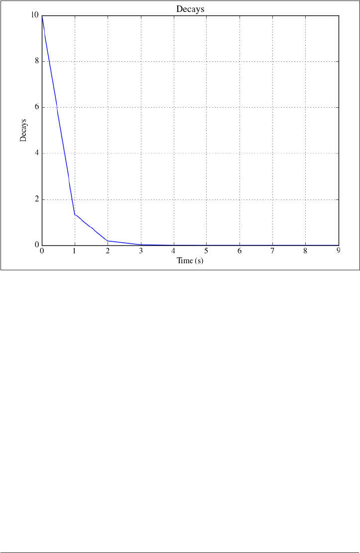
Figure 7-3. matplotlib plot
This plot is not very exciting, of course. When data is more complex—perhaps 2D or
3D, with multiple dependent parameters—matplotlib begins to show its true (very
powerful) colors. Equipped with a plethora of plot types and aesthetic options, the
power under the hood in matplotlib can be almost overwhelming. In such a situation,
the gallery in matplotlib comes to the rescue.
The gallery
The best way to start with matplotlib is with the gallery. Nearly every feature of the
matplotlib plotting library is demonstrated by an example plot in the gallery, along
with the source code that generated it. It contains a wealth of example scripts, lov‐
ingly created by the developers and users of the library.
In a physics context, the gallery is a powerful resource due to the speed with which it
enables a researcher to identify desired features of a plot. With the source code for
many features available, you can mix and match them to produce a compelling figure
with your own scientific data, or, really, any customization at all.
Indeed, matplotlib plots can be used for nearly any purpose. One of the coolest exam‐
ples in the gallery is certainly the polar plot used in the matplotlib logo (Figure 7-4).
168 | Chapter 7: Analysis and Visualization
www.it-ebooks.info

Figure 7-4. matplotlib logo
In 2010, one of the authors of this book had the opportunity to help organize a talk
by the creator of this extraordinary library, John D. Hunter.
When someone like this comes to give a talk about their plotting tool, the pressure is
on: one must make an excellent flyer to advertise the event. The first step in making a
flyer for the talk was to customize the script for the cool polar plot from the gallery.
With matplotlib annotations, text boxes were added at specific x, y coordinates. To
announce the event at the University of Wisconsin, both the Python script shown
here and the resulting PDF plot Figure 7-5 were emailed to the students and staff:
#!/usr/bin/env python
# Import various necessary Python and matplotlib packages
import numpy as np
import matplotlib.cm as cm
from matplotlib.pyplot import figure, show, rc
from matplotlib.patches import Ellipse
# Create a square figure on which to place the plot
fig = figure(figsize=(8,8))
# Create square axes to hold the circular polar plot
ax = fig.add_axes([0.1, 0.1, 0.8, 0.8], polar=True)
# Generate 20 colored, angular wedges for the polar plot
N = 20
theta = np.arange(0.0, 2*np.pi, 2*np.pi/N)
radii = 10*np.random.rand(N)
width = np.pi/4*np.random.rand(N)
bars = ax.bar(theta, radii, width=width, bottom=0.0)
for r,bar in zip(radii, bars):
bar.set_facecolor(cm.jet(r/10.))
bar.set_alpha(0.5)
# Using dictionaries, create a color scheme for the text boxes
bbox_args = dict(boxstyle="round, pad=0.9", fc="green", alpha=0.5)
bbox_white = dict(boxstyle="round, pad=0.9", fc="1", alpha=0.9)
patch_white = dict(boxstyle="round, pad=1", fc="1", ec="1")
# Create various boxes with text annotations in them at specific
# x and y coordinates
ax.annotate(" ",
xy=(.5,.93),
Visualization | 169
www.it-ebooks.info
xycoords='figure fraction',
ha="center", va="center",
bbox=patch_white)
ax.annotate('Matplotlib and the Python Ecosystem for Scientific Computing',
xy=(.5,.95),
xycoords='figure fraction',
xytext=(0, 0), textcoords='offset points',
size=15,
ha="center", va="center",
bbox=bbox_args)
ax.annotate('Author and Lead Developer \n of Matplotlib ',
xy=(.5,.82),
xycoords='figure fraction',
xytext=(0, 0), textcoords='offset points',
ha="center", va="center",
bbox=bbox_args)
ax.annotate('John D. Hunter',
xy=(.5,.89),
xycoords='figure fraction',
xytext=(0, 0), textcoords='offset points',
size=15,
ha="center", va="center",
bbox=bbox_white)
ax.annotate('Friday November 5th \n 2:00 pm \n1106ME ',
xy=(.5,.25),
xycoords='figure fraction',
xytext=(0, 0), textcoords='offset points',
size=15,
ha="center", va="center",
bbox=bbox_args)
ax.annotate('Sponsored by: \n The Hacker Within, \n'
'The University Lectures Committee, \n The Department of '
'Medical Physics\n and \n The American Nuclear Society',
xy=(.78,.1),
xycoords='figure fraction',
xytext=(0, 0), textcoords='offset points',
size=9,
ha="center", va="center",
bbox=bbox_args)
fig.savefig("plot.pdf")
This common feature of executable Python scripts alerts the computer which
Python to use.
This imports the colormaps library from matplotlib.
170 | Chapter 7: Analysis and Visualization
www.it-ebooks.info

This imports other libraries (color, figure, show, rc) from matplotlib.
This imports ellipse shapes from matplotlib (to be used as text boxes).
This creates an annotation box at certain x and y coordinates.
Those coordinates should be read as fractions of the figure height and width.
The horizontal and vertical text should be aligned to the center of the box.
The box being placed here should be white.
By executing the script (with python scriptname.py), everyone who received the
email could produce the flyer shown in Figure 7-5 using matplotlib, the topic of the
seminar.
It was a very proud moment for this author when John said he liked the flyer in
Figure 7-5. After all, matplotlib was a key ingredient at that time not only in many
dissertations, but also in the success of scientific Python. When John passed away in
2012, Fernando Perez described his contribution to the scientific computing commu‐
nity this way:
In 2002, John was a postdoc at the University of Chicago hospital working on the anal‐
ysis of epilepsy seizure data in children. Frustrated with the state of the existing propri‐
etary solutions for this class of problems, he started using Python for his work, back
when the scientific Python ecosystem was much, much smaller than it is today and this
could have been seen as a crazy risk. Furthermore, he found that there were many half-
baked solutions for data visualization in Python at the time, but none that truly met his
needs. Undeterred, he went on to create matplotlib and thus overcome one of the key
obstacles for Python to become the best solution for open source scientific and techni‐
cal computing.
Visualization | 171
www.it-ebooks.info
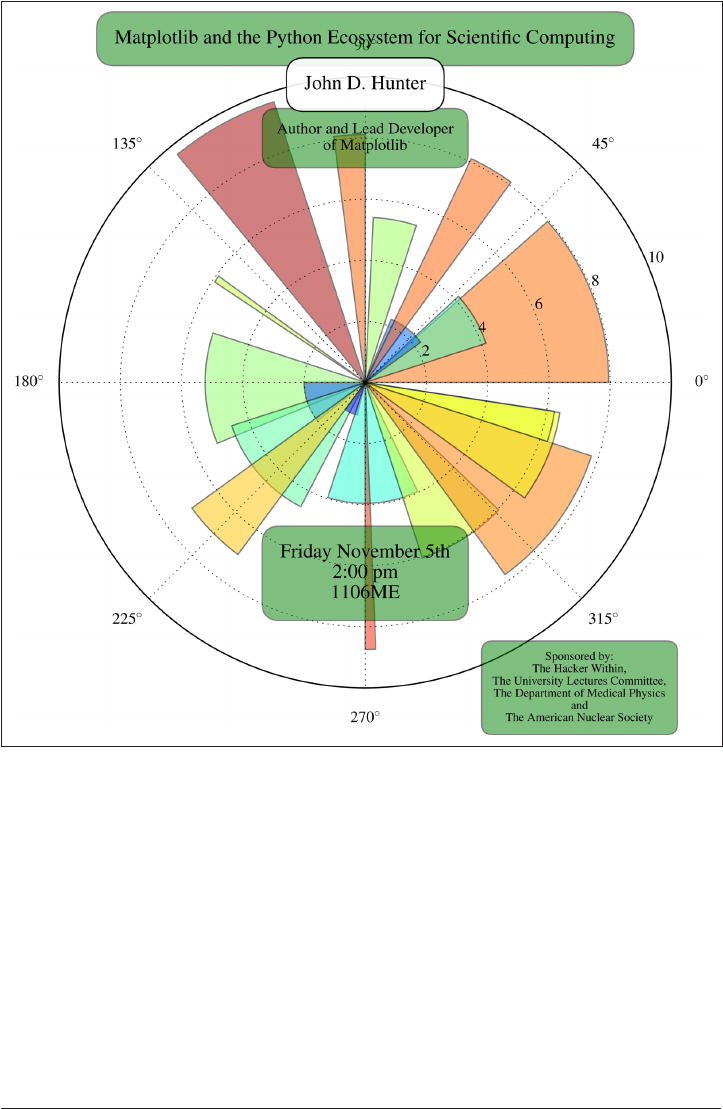
Figure 7-5. Announcement of 2010 John D. Hunter talk
Despite the loss of its creator, matplotlib continues to be improved by a vibrant team
of extraordinary people, including Michael Droetboom, who now leads matplotlib
development.
Additionally, matplotlib has provided a framework that other tools are capable of
linking with. One such tool that is compatible with matplotlib is Bokeh.
Bokeh
Bokeh is a very simple, matplotlib-friendly API that can generate interactive plots
appropriate for the Web. It abstracts somewhat from the matplotlib syntax, making
172 | Chapter 7: Analysis and Visualization
www.it-ebooks.info

the user experience cleaner. The following is a script to plot the decay data as an
HTML file using Bokeh:
decay_bokeh.py
import numpy as np
# import the Bokeh plotting tools
from bokeh import plotting as bp
# as in the matplotlib example, load decays.csv into a NumPy array
decaydata = np.loadtxt('decays.csv',delimiter=",",skiprows=1)
# provide handles for the x and y columns
time = decaydata[:,0]
decays = decaydata[:,1]
# define some output file metadata
bp.output_file("decays.html", title="Experiment 1 Radioactivity")
# create a figure with fun Internet-friendly features (optional)
bp.figure(tools="pan,wheel_zoom,box_zoom,reset,previewsave")
# on that figure, create a line plot
bp.line(time, decays, x_axis_label="Time (s)", y_axis_label="Decays (#)",
color='#1F78B4', legend='Decays per second')
# additional customization to the figure can be specified separately
bp.curplot().title = "Decays"
bp.grid().grid_line_alpha=0.3
# open a browser
bp.show()
While Bokeh can produce plots in many formats, it was intended to produce interac‐
tive plots for viewing in a browser. Thus, when this script is run with python
decay_bokeh.py, a browser opens automatically to display the interactive, pannable,
zoomable plot in Figure 7-6.
Visualization | 173
www.it-ebooks.info
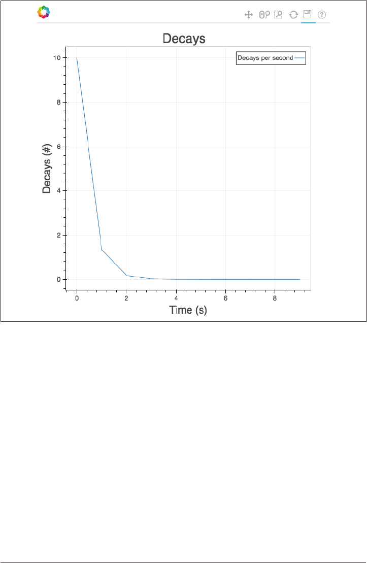
Figure 7-6. Decay plot with Bokeh
Bokeh is an excellent, easy-to-use tool for plots intended for publication on the Web.
However, if the plot is complex or is intended for print media, matplotlib or gnuplot
will serve that need better.
A key benefit of Bokeh, matplotlib, and gnuplot is their scriptable reproducibility.
These tools are therefore the right choice for creating plots that do not yet exist. How‐
ever, sometimes it is necessary to edit, crop, annotate, or otherwise manipulate an
image file that already exists. The scripting tools in this section are all fully capable of
handling these tasks. For cases when the original plot or diagram was not made with
one of these tools, Inkscape is a good option for the physicist who needs to quickly
tweak an image.
Inkscape
Inkscape is an open source project for producing and editing scalable vector graphics.
Vector graphics are incredibly powerful. Rather than being pixelated, in a fixed-
174 | Chapter 7: Analysis and Visualization
www.it-ebooks.info

resolution manner, scalable vector graphics are just that—scalable. Inkscape can be
difficult to automate, however, because it is a tool that relies on a graphical user inter‐
face for manipulating plots by hand. Of course, this should be done only as a last
resort because doing anything by hand does not scale, even if your resulting graphics
do.
Analysis and Visualization Wrap-up
The vastness of the fleet of data analysis and visualization tools available today is stag‐
gering, and new tools appear at a blinding rate. By walking through a common work‐
flow (Figure 7-1) that plotted the course from raw data to visualization, this chapter
briefly introduced some of the tools available for:
• Loading data
• Cleaning data
• Wrangling data
• Analyzing data
•Plotting data
However, we have only covered the bare minimum of available analysis and visualiza‐
tion tools. The intention here was simply to provide you with a notion of the land‐
scape of tasks at hand and tools available to perform them. The following chapters
will go into much more depth concerning NumPy (Chapter 9), storing data (Chap‐
ter 10), and data structures (Chapter 11).
This chapter covered a few general guidelines that can be followed concerning data
loading and preparation:
• Plain-text numerical data of a reasonable size should be loaded with NumPy.
•HDF5 data should be loaded with PyTables or Pandas.
• Pandas is useful for most everything else, especially munging.
• Data can be converted between formats using Blaze.
Visualization is key to presenting the results of your analyses, and before making a
decision about what visualization tools to use we recommend that you closely observe
the publication-quality plots in your particular subfield of the physical sciences, to get
an idea of what tools are typically used and what features are included. More complex
data visualizations were out of scope for this chapter. However, many tools for com‐
plex visualizations exist. In particular, for physicists with volumetric or higher-
dimensional datasets, we recommend sophisticated Python tools for volumetric data
such as yt and mayavi.
Analysis and Visualization Wrap-up | 175
www.it-ebooks.info

While the ideal tool varies depending on characteristics of the data, workflow, and
goals, keep in mind that some things are universal:
• Beautiful is better than ugly.
• Simple is better than complex.
• Complex is better than complicated.
•Clear is better than dense.
• Communicating is better than convincing.
• Text must not distract.
•People are not mantis shrimp.
176 | Chapter 7: Analysis and Visualization
www.it-ebooks.info

CHAPTER 8
Regular Expressions
The limits of my language mean the limits of my world.
—Ludwig Wittgenstein
The world’s first computers were women. They were the employees of research cen‐
ters and national labs, where they inspected data, executed algorithms, and reorgan‐
ized data. Their job title was “computer” because they computed. In the early days,
computing meant evaluating raw data by hand for a variety of applications and
experiments, including, famously, the Manhattan Project.
You, too, may have raw data. However, today’s data should not be processed by hand.
Today’s data is usually too big, the risk of carpal tunnel is too high, and computers are
too powerful to justify that. Processing raw textual physics data may require:
• Searching for and correcting irregularities
• Finding and replacing text across hundreds of files
• Evaluating mathematical expressions
• Manipulating number formatting
•Rearranging column-formatted data
This chapter will discuss regular expressions, a common syntax for matching patterns
of characters in text files, data files, filenames, and other sequences of characters. This
syntax is ubiquitous in the programming world because it can turn an enormous,
tedious file cleanup task into a tiny one-line command. Additionally, it can help with
day-to-day command-line navigation, file parsing, and text editing.
In the shell, regular expressions can be used to clean up and analyze raw data in con‐
junction with the search and print programs that will be discussed in this chapter.
These, like grep, sed, and awk, were designed for finding, displaying, editing, and
177
www.it-ebooks.info

doing calculations with information in files. The regular expression module in
Python (re) can be used in the same way, and this chapter will help to demonstrate
how it boosts the already awesome power of Python.
In particular, this chapter will discuss basic regular expression syntax in the context of
how it can help the physicist:
• Navigate the command line more efficiently.
•Quickly find files on the command line based on their content (grep).
• Find and replace a complex expression in many files at once (sed).
• Quickly do math on plain-text columns of data from the command line (awk).
We’ll explore how you can accomplish some of these things in Python, as well.
A Short History of Regular Expressions
Because regular expressions are one of the oldest and most powerful tools in comput‐
ing, let us take a brief foray into their history.
With inspiration from two neurologists, Stephen Kleene, a 1940s mathematician,
developed a formal notation for a logical classification of typeset characters. He called
them regular sets. Combining elements of these regular sets, he created regular
expressions. Ken Thompson, a programmer in the late 1960s, developed a text editor
called ed with the ability to search a file for patterns defined with this notation. To
search for a pattern within a document in ed, the user deployed the command to
search globally for a regular expression and print the modifications. It looked
like :g/re/p. That command would become what is now known as grep.
Now that we have covered the basics, we are going to dive in. The following sections
are a condensed, example-driven introduction that will help you get comfortable with
the syntax of regular expressions.
Messy Magnetism
Regular expressions are a tool for text matching. Command-line scripting tools like
grep, sed, awk, Python, and Perl make use of regular expressions. Using them (com‐
bined with a scripting language), a physicist can automate alteration of large files and
sets of files. Additionally, the syntax of regular expressions is often deployable from
within text editors like vim, and it can accordingly speed up code development enor‐
mously. As a concrete example, this chapter will follow the plight of a new graduate
student in a lab studying the Earth’s magnetism.
178 | Chapter 8: Regular Expressions
www.it-ebooks.info

Imagine you have just joined a research group that analyzes data gathered by hun‐
dreds of satellites all across Earth’s orbit. These satellites are being used to take simul‐
taneous magnetic field measurements around the Earth. However, they are
telecommunications satellites owned by private companies, so the researchers have
access to the data only through agreements with the companies that own them.
Accordingly, the data is sent to the researchers in many different formats. After a few
months of data collection, many gigabytes of readings are now stored haphazardly on
one of the computers in the lab. Before being analyzed, it will have to be organized
and the various formats will need to be standardized.
As the newest member of the research group, you have therefore been tasked to:
• Find the files from each company and collect them into a single directory.
• Standardize the formats of dates, times, and labels across all the files.
• If the flux energy is in units of gauss (G), convert it to teslas (T).
All of this could take a very long time by hand. In fact, with over 400 files and thou‐
sands of necessary changes per file, it could take a very long time indeed. This chap‐
ter will show how, with regular expressions, you can spend the morning setting up a
few scripts and leave the lab while the sun still shines in the sky.
To get started, we need to start navigating the filesystem to identify the files we are
looking for. In the next section, we will use metacharacters that we are already famil‐
iar with as well as more complex regular expressions to find the data files.
Metacharacters on the Command Line
Day-to-day tasks, like finding files on the command line, can be sped up with regular
expressions. By employing metacharacters, commands can be made to operate on
many files at once.
Metacharacters are characters that have a special meaning aside from their literal
meaning. Literal characters, on the other hand, are those that are being taken at face
value. Regular expressions are strings made of metacharacters and literal characters.
We have already seen a number of metacharacters on the command line. In particu‐
lar, in Chapter 1 we saw the use of the wildcard asterisk (*) and the backslash escape
character (\). However, there are many more, and they follow a few rules:
• Alphanumeric characters match themselves.
• A dot (.) matches any character.
•Repeating patterns are matched with *, +, and ?.
•Character sets ([]) and the or operator (|) can match alternatives.
Metacharacters on the Command Line | 179
www.it-ebooks.info

• The position markers ^ and $ match the beginning and end of a line, respectively.
• Parentheses can group things and extract information from matches.
Beginning with these basic rules, this section will show how to use the command-line
tools ls and find to locate files whose filenames match a pattern.
Listing Files with Simple Patterns
We don’t know a lot about the satellite data files we are looking for, but we do suspect
that some of them end in the .dat extension. Ideally, we could at least start the search
by browsing the directories and listing all files with names that end in “.dat”.
In Chapter 1 we saw how * is used to match all of the filenames in a directory. That
asterisk, or wildcard character, is actually capable of much more and can solve this
problem in a flash. In the next section, we’ll learn how.
The wildcard (*)
As discussed in Chapter 1, wildcard characters can be used to find files more effec‐
tively. Recall the asterisk. It allows the user to list all the text files in a directory by
typing ls *.txt, because * means “zero or more of any character.” This is because the
asterisk is a metacharacter in the shell. Regular expressions are a language of meta‐
characters used for the purpose of pattern matching.
In a regular expression, the wildcard * matches the preceding item zero or more
times. Some regular expressions and the text that they match within target strings are
listed in Table 8-1. The first column shows the regular expression and the second
shows the string to which it is applied. The bold elements of the string are those that
were matched by the regular expression. For example, the regular expression zo*
matches zoooo in “He zoooomed” and the first z in “motoguzzi.”
Table 8-1. Matching with the wildcard
Expression Matches
zo* zooomed
zo* motoguzzi
zo* protozoan
p*i mississippi
180 | Chapter 8: Regular Expressions
www.it-ebooks.info

To find all of the .dat files in the current working directory, then, we can execute a
simple ls command using the asterisk syntax. This command and its results are
shown in Table 8-2.
Table 8-2. e wildcard on the command line
Code Output
ls *.dat atmos_sat_42.dat
...
...
...
siriuscybernet_21.dat
siriuscybernet_22.dat
siriuscybernet_23.dat
siriuscybernet_24.dat
siriuscybernet_68.dat
siriuscybernet_92.dat
Telecomm99_2014.5.1.dat
Telecomm99_2014.5.2.dat
Telecomm99_2014.5.3.dat
Telecomm99_2014.5.4.dat
Telecomm99_2014.5.5.dat
Telecomm99_2014.5.6.dat
zorbital34l.2014.05.01.dat
zorbital34l.2014.05.02.dat
zorbital34l.2014.05.03.dat
zorbital34l.2014.05.04.dat
zorbital34l.2014.05.05.dat
zorbital34l.2014.05.06.dat
For brevity, not all of the les are listed; there are
many.
This syntax means “List all files beginning with zero or more of any character, fol‐
lowed by the .dat string.” While this will certainly uncover all of the .dat files in the
current directory, it’s not powerful enough for our task, for two reasons:
•The ls command only goes one level deep into the directory tree. Upon inspec‐
tion, it becomes clear that the filesystem is riddled with directories and subdirec‐
tories of the data. For example, executing ls (with no argument) illuminates a
few dozen directories named things like MegaCorp and Oscorp, which certainly
contain more satellite data from the satellites owned by those megacorporations.
•Further inspection also indicates that a few files in the home directory weren’t
caught because they had a different file extension. Observed extensions so far
include .txt, .data, and an all-caps .DAT.
Metacharacters on the Command Line | 181
www.it-ebooks.info

Does this mean we have to enter every directory and execute multiple forms of the ls
command? Traversing the filesystem one directory at a time, repeating a few ls *.dat
commands in each directory, is not the way to spend an afternoon.
Globally Finding Filenames with Patterns (nd)
A better way to spend the afternoon might be at the beach. To get out of the lab, we’ll
have to find a tool that can recursively search a lot of directories at once. That would
improve this situation mightily. Thankfully, that tool exists, and it is called find.
The find command can be used in many ways. One option is to use it with regular
expressions. In that mode, find is executed on the command line using the format:
find [path] -regex "<expression>"
With this syntax, the top level of the search will be the indicated <path>. find will
begin at that location and recursively parse filenames using regular expressions (-
regex). The expression for which it will seek matches is provided between the double
quotes.
To find all data files in the home directory and all subdirectories of the home directory,
find can be used thus, in our case:
find ~ -regex ".*\.dat"
This finds all files in ~ and all subdirectories of ~ whose names end in “.dat”. But why
are those dots and slashes needed? They weren’t necessary when we used the ls
command.
Irregular Expressions
Importantly, regular expressions are not as regular as one might imagine. That is, syn‐
tactic use of regular expressions will occasionally vary from tool to tool. grep, awk,
sed, Python, and Perl have slightly varying implementations of certain characters. The
find command can actually parse many flavors of regular expressions. You specify
the flavor by using flags. Available flavors include:
• Basic regular expressions (BRE)
• Extended regular expressions (ERE)
• Perl-compatible regular expressions (PCRE)
Of course, use of each flavor will require investigation into its documentation. In this
chapter, we’ll introduce the basic metacharacters and character class treatments rec‐
ognizable in most tools.
182 | Chapter 8: Regular Expressions
www.it-ebooks.info

Fundamentally, this is because the set of metacharacters available to the ls command
is a different flavor. While the wildcard is available on the command line, it doesn’t
mean the same thing on the command line that it does in proper regular expression
syntax. On the command line, .* means “one dot (.), then zero or more of any char‐
acter.” In a regex, it means “zero or more of any character (.).”
So, we need the extra characters because the dot character (.) is not a metacharacter
on the command line. On the command line, it signifies the current working direc‐
tory or, when it appears at the beginning of a filename, a hidden file, as discussed in
Chapter 1. However, the dot character (.) is a metacharacter in proper regular expres‐
sions. For this reason, the backslash is used before the real dot in “.dat” to indicate it
should be taken literally.
That all may be a bit confusing. Let’s take a step back and look at those two metachar‐
acters (dot and backslash) more closely, so that we can digest this syntax.
Representing any character (.)
The dot character in a regular expression is very simple: it represents exactly one of
any character. Note that the dot means something different on the command line, as
just described.
This bears repeating. On the command line, the dot does not mean
“any character.” In proper regular expressions, however, it does. On
the command line, the dot already has a special meaning; to repre‐
sent “any character,” the ? can be used instead.
Since the dot means any character, it can be used to help match many files whose
names share most, but not all, characters. Table 8-3 demonstrates the dot character in
action.
Table 8-3. Matching with the dot character
Expression Matches
r.d. rads
r.d. rodeo
r.d. rider
r.d. red!
r.d. r2d2
Metacharacters on the Command Line | 183
www.it-ebooks.info

In our example with the satellite .dat files, many of the Sirius Cybernetics satellite files
had very similar names:
siriuscybernet_21.dat
siriuscybernet_22.dat
siriuscybernet_23.dat
siriuscybernet_24.dat
siriuscybernet_68.dat
siriuscybernet_92.dat
Indeed, many of those filenames include numbers in the 20s. Those files with num‐
bers that start with 2 could be matched exactly with the regular expression:
siriuscybernet_2.\.dat
The first part of the expression, siriuscybernet_2, matches that string exactly. This
pattern therefore matches the first four filenames in the preceding list, but not the last
two (siriuscybernet_68.dat and siriuscybernet_92.dat).
The next character in the expression is the “one of any character” represented by the
dot (.). In the case of the first file, the dot matches the 1. In the case of the second file,
it matches the 2, and so on.
After that, however, there again is the backslash (\) character. Why does it keep pop‐
ping up? We’ll learn about this in the next section.
Escaping metacharacters (\)
Sometimes, as in the previous example, the pattern that you would like to match con‐
tains an actual dot (.) or an actual asterisk (*). To indicate the literal . character
rather than the . metacharacter, it must be escaped. To escape a metacharacter is to
escape its meta-meaning. We escape metacharacters by using the backslash (\). The
expression . means “exactly one of any character.” However, the expression \. means
“exactly one dot.” The difference is illustrated in Table 8-4.
Table 8-4. Escaping metacharacters
Expression Matches
deat.* deathstar
deat.\* death*
A common need for this escape character arises in the shell, where many commands
require arguments separated by spaces. That is, in the shell, the space is a metachar‐
acter for separating arguments, as in:
~ $ mv data.txt old.txt
184 | Chapter 8: Regular Expressions
www.it-ebooks.info

Since some of those arguments are filenames, the question arises: how does the com‐
puter know the difference between a filename containing a space and a pair of argu‐
ments? The answer is that it doesn’t know the difference:
~ $ mv data from yesterday.txt old.txt
usage: mv [-f | -i | -n] [-v] source target
mv [-f | -i | -n] [-v] source ... directory
Just as with the *, to make the space a literal space, you must use the backslash \.
~ $ mv data\ from\ yesterday.txt old.txt
So, metacharacters really have two meanings: their special meaning and their literal
meaning. The backslash can help you switch between the two.
Escaping Literals
Indeed, in addition to transforming metacharacters into literals, the ubiquitous back‐
slash transforms many literals into metacharacters. Some examples include the end-
of-line characters \n (linefeed) and \r (carriage return), as well as the tab
metacharacter \t, NULL metacharacter \0, and whitespace metacharacter \s. Myriad
other metacharacters exist, including the parentheses used in “Finding and Replacing
Patterns in Files (sed)” on page 190.
Exercise: Escaping the Escape Character
1. Open a terminal.
2. Try to create a file that has a backslash in the filename with a
command like touch file\name.
3. Use ls to examine the file you’ve just created. Did it work?
Where is the slash?
4. Use what you’ve just learned to escape the escape character.
Can you successfully make a file called le\name?
So, with this information, it is possible to execute the find command in such a way as
to find all files in all subdirectories of the home directory with names that end in .dat.
We can just use the pattern .*\.dat.
While that is a huge improvement over spending all afternoon traversing the filesys‐
tem, what about the files whose names end in .data, .txt, or .DAT? For that, we will
have to proceed to the following section.
Metacharacters on the Command Line | 185
www.it-ebooks.info

Finding either one pattern or another (|)
In order to match files with various extensions (.txt, .dat, .data, .DAT), we need to
have an or Boolean available. With regular expressions, this is called alternation and is
accomplished with the | syntax. That is, to search for any appearance of the word
proton or the word neutron, you would separate the two with a vertical bar: proton|
neutron. For more options, continue to expand the list: proton|neutron|electron|
boson.
Exercise: Reverse-Engineer a Regex
The following string will find either .dat or .DAT extended files:
~ $ find . -regextype posix-extended -regex ".*\(\.dat\|\.DAT\)"
1. Can you tell why?
2. What are the slashes there for?
3. What about the extra specification of -regextype posix-
extended?
4. Can you find out what that means from the man page for find?
Unfortunately, this “or” syntax is notoriously hard to read. There is a more readable
way to specify something similar with character sets. The next section will discuss
these.
Character sets ([…])
The syntax that allows matching of a set of characters is [] or [{}], depending on the
tool being used. A character set matches any one of the enclosed characters. A few
examples are given in Table 8-5.
Table 8-5. Character sets
Expression Matches
Col[ou]mbia Columbia, Colombia
[Dd]ata Data, data
[Dd][Aa][Tt][Aa] DATA, data, Data
2014[-.]05[-.]10 2014.05.10, 2014-05-10
186 | Chapter 8: Regular Expressions
www.it-ebooks.info

This makes it easy to avoid worrying about capitalization, varying spellings across the
pond, and many other matching issues. In our case, it means that .DAT, .dat,
and .data files can all be found with one expression:
~ $ find . -regex ".*\.[Dd][Aa][Tt][Aa]*"
Key Features of Character Sets
•A character set will match any one character from the set of characters between
the brackets. [Dd]ad will match Dad or dad.
•Character sets can be specified in shorthand over a range using a hyphen. For let‐
ters, [lmnop] is identical to [l-p]. Each set will match any one of the characters
“l” through “p” (like the “p” in “zap” or the “l” in “laser”). This works for both
numbers and letters. Thus, [0-9] matches any digit.
•A character set can indicate characters that we want to avoid. A caret in the
square brackets ([^{...}]) denotes a negated character set: it will match any‐
thing not in the square brackets. For instance, [\^aeiou] matches only
consonants.
•Character sets can be combined. [a-zA-Z] is valid notation matching all letters,
irrespective of case.
•These sets also can be referred to by nicknames, such as [:alpha:] (letters),
[:alnum:] (letters and numbers), [:lower:] (lowercase letters), [:digit:]
(numbers), etc.
We may make it to the beach this afternoon after all! Now that we have been able to
find all of the necessary files, we can go organize them. To write a shell script utilizing
the output of the find command, go back to Chapter 1 and bash scripting to deter‐
mine how to move all of the files we have found. It should take about six lines of
code.
Next, the task moves on into the content of the files themselves. The find command
on the command line only addresses the filenames. For more in-depth pattern
searching, we will need the tried and true family of tools grep, sed, and awk.
grep, sed, and awk
We said before that grep, sed, and awk are a family of tools that use regular expres‐
sions and are available on the command line. They each have different capabilities:
•The grep command has the basic syntax grep <pattern> <inputfile>. grep
grabs matched patterns and prints them.
grep, sed, and awk | 187
www.it-ebooks.info

•The sed command has the basic syntax sed "s/<pattern>/<substitution>/"
<inputfile>. Sed combines grep with a substitution command.
•The awk command has the basic syntax awk pattern [action]. awk handles
columns.
This chapter will touch on how each tool can help to accomplish the goals in the sat‐
ellite data problem. grep will help us to investigate the contents of the files, sed will
help us to make substitutions where formatting varies across the files, and awk will
allow us to do simple calculations on the columns of data.
Now that we have rearranged all of the found files into a directory, our next task
should be to learn some more about them. For this, we will use grep.
Finding Patterns in Files (grep)
grep is as essential a tool for programming as Google is for navigating the Internet. It
is useful for everything from inspecting files to debugging. Indeed, grep works a lot
like Google. It searches, globally, for regular expressions inside files, based on their
content.
Day-to-day scientific computing, accordingly, relies on grep to make sense of the files
encountered. For example, when I receive an error message generated from source
code, I immediately search the code files for the phrase given by the exception. From
this I can quickly find the filename and the line number at which the error was
thrown.
In the satellite data example, we want to know a few things before we start fixing the
files:
• How many and which of the files use Gs?
• Which files use the dash and which use the dot in date formats?
grep can help answer these questions. To answer the first question, we simply want to
tell grep “search for all instances of Gs among the files in this directory.” The syntax is
simply grep Gs *. It’s the simplest possible command, and yet it is so powerful! An
example of the use of this tool is seen in Table 8-6.
188 | Chapter 8: Regular Expressions
www.it-ebooks.info

Table 8-6. e wildcard with grep
Code Output
grep Gs * Oscorp.DAT_1:2000-1-1,481.983486734Gs
Oscorp.DAT_1:2000-1-2,254.229864682Gs
Oscorp.DAT_1:2000-1-3,57.4087373703Gs
Oscorp.DAT_1:2000-1-4,425.027959432Gs
Oscorp.DAT_1:2000-1-5,175.497450766Gs
Oscorp.DAT_1:2000-1-6,304.130011333Gs
Oscorp.DAT_1:2000-1-7,365.090569435Gs
Oscorp.DAT_1:2000-1-8,357.834192688Gs
Oscorp.DAT_1:2000-1-9,378.059846154Gs
Oscorp.DAT_1:2000-1-10,179.401350076Gs
...
If grep piques your curiosity, you may be interested in some of its extra features. Some
common options for use with grep include:
-r
The recursive flag. Do you recall from Chapter 1 what that means?
-c
Counts matched lines.
-i
Ignores capitalization. Can you think of an equivalent expression using brackets?
Additionally, further experience with grep can be had very safely within the system
files on your computer. On a Unix or Linux platform, all of the words that the default
spell-checker uses are stored in a plain-text file. The grep exercises in the following
sidebar can be performed safely on that file.
Extended Exercises with grep
Enter the directory /usr/share/dict, and investigate the document called words. Use wc
-l. Use -c. On the command line, try the following exercises to familiarize yourself
with grep:
•Look for the word hacker in the words document, using the command grep
"hacker" words.
• Compare grep -c "within" words and grep -c "\within" words.
• Compare grep -c ".ithin" words to grep -c "\within" words.
•Try grep -c ".*ithin" words, etc.
• Try grep -c "pre.+" words and grep -c ".+pre.+" words.
•Compare grep "cat" words and grep "^cat" words.
Finding Patterns in Files (grep) | 189
www.it-ebooks.info

• Compare grep "cat" words and grep "cat" words.
• Find blank lines with grep "^$" words.
• Compare grep ^[rstu]+$ words and grep ^[r-u]+$ words.
• Compare "grep \^[r-u]{3}" words to grep "[r-u]\{3,\}" words.
Now try the following challenges with the words file:
•Find all three-letter words.
• Find all three-letter words involving the letter r.
•Find the words with two consecutive as.
• Find the words ending in ’s.
As you can see, grep is indispensable to the efficient use of a computer. That you will
need such a tool should not be surprising, as the importance of being able to find
stuff efficiently scales directly with how much stuff is available. The speed with which
these two things grow in the modern world is, arguably, the reason a worldwide
megacompany was capable of bootstrapping itself out of no more than a search algo‐
rithm (Google).
All that said, it is often the case that even finding stuff is not powerful enough. Usu‐
ally, the scientist needs to find patterns primarily to replace them with something else.
The tool for this, on the command line, is sed. The next section will discuss sed in
more detail.
Finding and Replacing Patterns in Files (sed)
sed is a tool for substitution. It is essentially the same as grep, but has one major
extension: once a character string is matched, it can be substituted with something
else. Thus, sed differs from grep, but can duplicate grep as well.
Additionally, sed is enabled natively in the vim text editor. There, it
can be accessed with <ESC>:s. For more help on sed within vim,
type <ESC>:help sed and press Enter.
The syntax for sed substitution through a whole file is:
sed "s/<expression>/<substitution>/g" <inputfile>
This allows very quick substitution of a simple string in a file. In this example, the s
(before the first slash) indicates “substitution” and the g (following the final slash)
190 | Chapter 8: Regular Expressions
www.it-ebooks.info

indicates substituting “globally” on every line of the file. Without the g, sed will only
replace the first instance of the matched pattern in each line.
Take note! sed can be run with the syntax sed "s/<expression>/
<substitution>/" <inputfile>. However, without the g after the
final slash, sed only changes the first match in each line. This is
rarely the desired default behavior. Specify global substitution to
capture all matches in a line!
The result of this syntax is simple: sed outputs the altered text of the file to the com‐
mand line. With the default syntax, sed does not edit the file in-place. Rather, the
changed text is sent to the standard output of the terminal. To capture this output, a
temporary file is usually made.
Exercise: Redirect sed Output to a File
1. Execute a sed command on a file in your filesystem (try some‐
thing simple like "s/the/THE/g").
2. Note that the altered file text has appeared on the command
line.
3. Using your knowledge of redirection (from Chapter 1), re-
execute the command, this time sending the output to a tem‐
porary file.
If there were only one day’s worth of data in the satellite data, it might make sense to
directly substitute the badly formatted date type with the better-formatted date type,
like so:
sed "s/2014\.05\.01/2014-05-01/g" atmos_sat_42.dat
However, since we have many files, this will have to be scripted. Thankfully, it is pos‐
sible for sed to save output as a new file, using this syntax:
sed "s/<expression>/<substitution>/" <oldfile> > <newfile>
Also, for the brave, sed has a flag (-i) that causes it to edit the file in-place (no tempo‐
rary file necessary):
sed -i "s/<expression>/<substitution>/" <oldfile>
sed substituion can be made even more efficient if multiple replacement tasks are
necessary per file. In that case, you can give multiple commands by piping sed output
back into sed (recall the pipe from Chapter 1):
sed "s/a/A/" oldfile.txt | sed "s/b/B/"
Finding and Replacing Patterns in Files (sed) | 191
www.it-ebooks.info

This is equivalent to including the -e flag before each substitution:
sed -e "s/a/A/" -e "s/b/B/" oldfile.txt
That task was easy enough, but the more challenging task for the satellite data will be
to replace ill-formed date stamps with better-formed date stamps. In particular, a
complex expression will need to be formed in order to match all of the known ill-
formed date formats.
Finding and Replacing a Complex Pattern
To find and replace all dates, we must:
• Match the pattern for any ill-formatted date.
• Retrieve the date stamp and save the values.
• Substitute the format, using the saved date values.
As saving the values is necessary here, let us take a brief sidestep into capturing pat‐
terns during sed searches.
Since, sometimes, you’ll need to reuse part of the pattern you matched, sed has syntax
to hold the match in memory. It uses parentheses. Specifically, the following syntax
matches x and remembers the match:
\(x\)
These are capturing parentheses. With these parentheses, (20[01][0-9]) matches and
remembers the “2014” in “2014-05-01”. That string can then be retrieved and reused
during the substitution.
This remembering happens in a list that sed stores during the substitution. sed can
store many of these snippets per substitution task, and they are retrieved in the order
that they were created with a simple \N, where N is the index of the stored snippet.
We know that, in our example with the date formats, the pattern we would like to
match is:
"20[01][0-9].*[0-9][0-9].*[0-9][0-9]"
The types of strings that will be matched by this include:
2014-05-01
2014-09-10
2015-10-30
2014.06.24
2014/09/23
2010/12/29
.
.
.
192 | Chapter 8: Regular Expressions
www.it-ebooks.info

From this matched pattern, we would like to retrieve the year, month, and date sepa‐
rately so that the dates can be reformatted as “YYYY-MM-DD”. With sed and its
memory, the year is saved first and retrieved as \1. The month is saved second and
retrieved as \2, and so on.
The sed command that fixes all of the malformed dates is then:
sed "s/\(20[01][0-9]\).*\([0-9][0-9]\).*\([0-9][0-9]\)/\1-\2-\3/g" <filename.dat>
Take some time to digest that. It’s ugly, but should be comprehensible with some dis‐
section. Note that regular expressions, like Perl, are a written language. These are not
truly meant to be read.
Once that has been digested, we can allow the syntax to cement with some extra
exposure in the next section.
sed Extras
Many useful things are possible with sed. Let’s take the phone.txt file (in the code
repository for this book) as an example.
sed is best for editing files, and it will do so globally with only a few keystrokes. For
safety, we should try not to change important system files (woe betide he who dam‐
ages the hex color code for peach puff). Let’s relocate to the regex directory in the
code files associated with this book.
With sed, we can use the d character to delete all blank lines in the file of phone
numbers:
sed '/^$/d' phone.txt
It can also help us automatically double-space the file. We can do this in a brute-force
way by deleting blank lines and appending carriage returns (\n) to each line:
sed -e '/^$/d' -e 's/^\(.\+\)$/\1\n/' phone.txt
But there’s an easier way. Try G:
sed -e '/^$/d' -e G phone.txt
Or even just:
sed '/^$/d;G' phone.txt
Similar to our date exercise, it is possible to reformat the phone numbers in phone.txt.
Note that this task uses the tool for remembering strings, \(\), discussed earlier in
the chapter:
sed 's/.*\([0-9]\{3\}\).*\([0-9]\{3\}\).*\([0-9]\{3\}\).*/(\1)\2-\3/' phone.txt
You can number the lines of a file for a more readable display. The syntax for this one
is somewhat complex. See if you can figure it out:
Finding and Replacing Patterns in Files (sed) | 193
www.it-ebooks.info

sed '/./=' wordlist.txt | sed '/./N; s/\n/ /'
Also, if you only want to modify a small section of the file, you can specify a line
number to modify by indicating the line number at the beginning of the command:
sed '4 s/r/R/' wordlist.txt
You can even specify a range of line numbers to modify by specifying two numbers,
separated by a comma:
sed 'sed '4,6 s/r/T/' wordlist.txt
You can also select lines to modify by pattern matching:
sed '/^z/ s/$/zzzzzzzzzz$/' wordlist.txt
sed '/wade/,/salt/ s/m/PPPPPPPPPP/' wordlist.txt
Before we move forward (to fix the units in our satellite data files), let’s take a step
back and reflect in Table 8-7 on what we have learned is possible with regular expres‐
sions (and a couple of extra nuggets to whet your appetite for more).
Table 8-7. Regular expression examples
Expression Matches
uvwxyz uvwxyz
[u-z] One of either u, v, q, x, y, or z
[^ ] One of any character except a space
p*i Zero or more p characters followed by one i,
such as pi or ppppi or i
.* Zero or more of any character, such as super
califragilisticexpialidocious
or 42
\^spelunking.*(.*) A line starting with spelunking, followed
by an opening and closing parenthesis with
any string in them
\\$ A line ending with just one backslash
\$ A (literal) dollar sign
.\{4\}z Any four characters followed by a z
Now that we have successfully shown that regular expressions can be used to:
194 | Chapter 8: Regular Expressions
www.it-ebooks.info

• Find files based on their names (nd)
• Find files based on their content (grep)
•Replace content based on found patterns (sed)
The only remaining task is to show how to manipulate columns of data within files
using patterns. For this, we will introduce awk.
Manipulating Columns of Data (awk)
A lot of data in physics begins in a simple format: columns of numbers in plain-text
documents. Fortunately for us, a command-line tool called awk was invented long
ago to quickly and efficiently sort, modify, and evaluate such files. This tool, a sibling
to sed and grep, uses regular expressions to get the job done.
It’s not elegant or modern—indeed, it may be the oldest tool in this particular book—
but awk is always there. One day, you too will find yourself working on a high-
performance computing cluster that holds all of your data, where you don’t have per‐
mission to install a new version of Python. awk will be there to help you manipulate
your columns of data.
Before we fix the units in our satellite data example, it is worth taking some time to
understand awk. As an introductory example, we can investigate the files in the file‐
system. On a Linux platform, a list of colors available to the system is found in
the /usr/share/X11 directory. On a Unix (Mac OS X) platform, it is made available
in /usr/X11/share/X11.
The rgb.txt file in that directory looks like this:
255 250 250 snow
248 248 255 ghost white
248 248 255 GhostWhite
245 245 245 white smoke
245 245 245 WhiteSmoke
220 220 220 gainsboro
255 250 240 floral white
255 250 240 FloralWhite
253 245 230 old lace
253 245 230 OldLace
...
To get started investigating and manipulating this columnar data, note that awk can
somewhat replicate what sed and grep do. Given a regular expression to match, awk
will return the matching lines of a file. To get a feel for this, observe the results of the
awk commands in Table 8-8.
Manipulating Columns of Data (awk) | 195
www.it-ebooks.info

Table 8-8. Using awk to nd matching rows
Code Output
awk '/puff/' rgb.txt
awk '/144/' rgb.txt
255 218 185 peach puff
112 128 144 slate gray
112 128 144 SlateGray
112 128 144 slate grey
112 128 144 SlateGrey
30 144 255 dodger blue
30 144 255 DodgerBlue
208 32 144 violet red
208 32 144 VioletRed
30 144 255 DodgerBlue1
144 238 144 PaleGreen2
205 96 144 HotPink3
205 41 144 maroon3
144 238 144 light green
144 238 144 LightGreen
We can select the colors that have 144 in the beginning of their hex strings as in
Table 8-9—the caret tells awk to search for a match at the start of each line in the
input file.
Table 8-9. awk and the caret
Code Output
awk '/^144/' rgb.txt 144 238 144 PaleGreen2
144 238 144 light green
144 238 144 LightGreen
We can even pick out the only color with 144 in the middle, as in Table 8-10.
Table 8-10. awk extended pattern
Code Output
awk '/^.*\ 144\ .*/' rgb.txt 30 144 255 dodger blue
In addition to just replicating some of grep’s capabilities, awk can add an action. How‐
ever, it can only do actions on a column-wise basis. Note that dollar signs ($) indicate
columns:
awk '{print $1$2$3}' rgb.txt
awk '/^255/{print $1$2$3}' rgb.txt
awk '/^.+ +.+144/{print $1$2$3}' rgb.txt
The column order can also be switched:
awk '{print $1," ",$2," ",$2," "$1}' rgb.txt
196 | Chapter 8: Regular Expressions
www.it-ebooks.info

Or we can modify just one line:
awk NR==11'{print $1 $2 $3,"\t",$4}' rgb.txt
And finally, we can do math with awk:
awk NR==11'{print $1,"+",$2,"+",$3,"=",$1+$2+$3}' rgb.txt
The final task for the satellite data can be accomplished in an exactly analogous
fashion.
Exercise: Convert Gs to Tesla
1. Use sed to parse one of the data files for instances of “Gs”.
2. When found, use awk to multiply one column with another.
3. Finally, use sed to change the “Gs” string to “T”.
It’s okay to do this in multiple commands. However, it is possible to
do it in one command.
Now that this complex task is complete, we can take the afternoon off! Or, we can
spend it learning a little more Python. If you’re in the latter camp, read on!
Python Regular Expressions
Everything we’ve seen how to do so far in this chapter is also possible in Python.
Alternatives to all of these tools exist in the Python regular expression module re,
which comes as part of the Python standard library. The re module allows Python-
flavored regular expression pattern matching. Combined with the power of other
Python modules, the features of grep, sed, and awk can be replicated in Python in an
arguably cleaner and more robust syntax, ready for linking to other workflow process
subparts.
We’ve emphasized the command-line tools due to their day-to-day importance in the
life of a programmer. Very often, regular expression searches are one-offs, such that
they are most swiftly executed on the command line. However, the power of regular
expressions combined with the power of Python results in something quite
formidable.
grep’s capabilities can be replaced with:
•re.match(<pattern>, <string>) to match a regular expression pattern to the
beginning of a string
•re.search(<pattern>, <string>) to search a string for the presence of a pattern
Python Regular Expressions | 197
www.it-ebooks.info
•re.findall(<pattern>, <string>) to find all occurrences of a pattern in a string
Similarly, the capabilities of sed can be replaced with:
•re.sub(<pattern>, <replacement>, <string>) to substitute all occurrences of a
pattern found in a string
•re.subn(<pattern>, <replacement>, <string>) to substitute all occurrences of a
pattern found in a string and return the number of substitutions made
The re model provides a few more powerful utilities as well. Namely:
•re.split(pattern, string) splits a string by the occurrences of a pattern.
•re.finditer(pattern, string) returns an iterator yielding a match object for
each match.
•re.compile(pattern) precompiles a regular expression so the subsequent
matches occur much more quickly.
In all of these functions, if a match to a regular expression is not found, then None is
returned. If a match is found, then a special MatchObject is returned. MatchObjects
have methods and attributes that allow you to determine the position in the string of
the match, the original regular expression pattern, and the values captured by any
parentheses with the MatchObject.groups() method. For example, let’s try to match
a date regular expression to some actual dates:
In [1]: import re
In [2]: re.match("20[01][0-9].*[0-9][0-9].*[0-9][0-9]", '2015-12-16')
Out[2]: <_sre.SRE_Match object; span=(0, 10), match='2015-12-16'>
In [3]: m = re.match("20[01][0-9].*[0-9][0-9].*[0-9][0-9]", '2015-12-16')
In [4]: m.pos
Out[4]: 0
In [5]: m.groups()
Out[5]: ()
In [6]: m = re.match("20[01][0-9].*[0-9][0-9].*[0-9][0-9]", 'not-a-date')
In [7]: m is None
Out[7]: True
First, import the regular expression module.
The string matches the pattern, so a match is returned.
198 | Chapter 8: Regular Expressions
www.it-ebooks.info
Assign the match to a variable name for later use.
Find the index in the string of the start of the match.
Report all captured groups. This regular expression pattern had no capturing
parentheses, so no substrings are reported.
Try to match the date pattern against something that is not a date.
Note how None is returned when the match fails.
To speed up matching multiple strings against a common pattern, it is always a good
idea to compile() the pattern. Compiling takes much longer than matching. However,
once you have a compiled pattern, all of the same functions are available as methods
of the pattern. Since the pattern is already known, you don’t need to pass it in when
you call match() or search() or the other methods. Let’s compile a version of the date
regular expression that has capturing parentheses around the actual date values:
In [8]: re_date = re.compile("(20[01][0-9]).*([0-9][0-9]).*([0-9][0-9])")
In [9]: re_date.match('2014-28-01')
Out[9]: <_sre.SRE_Match object; span=(0, 10), match='2014-28-01'>
In [10]: m = re_date.match('2014-28-01')
In [11]: m.groups()
Out[11]: ('2014', '28', '01')
Compile the regular expression and store it as the re_date variable.
Use this variable to match against a string.
Assign the match to a variable m for later use.
Since the regular expression uses capturing parentheses, you can obtain the val‐
ues within them using the groups() method. A tuple that has the same length as
the number of capturing parentheses is returned.
More information on the re module can be found in the Python documentation.
Regular Expressions Wrap-up
At this point, your regular expressions skills should include:
• How to speed up command-line use with metacharacters
•How to find files based on patterns in their names (find)
Regular Expressions Wrap-up | 199
www.it-ebooks.info

• How to find lines in files based on patterns in their content (grep)
• How to replace text patterns in files (sed)
• How to manipulate columns of data based on patterns (awk)
This chapter, along with its descriptions and examples, has been adapted from Soft‐
ware Carpentry material, the official Perl documentation, Python’s re module docu‐
mentation, Mastering Regular Expressions by Jeffrey Friedl (O’Reilly), and the Mozilla
Developer Network. Those are all excellent resources and should be utilized for fur‐
ther information.
200 | Chapter 8: Regular Expressions
www.it-ebooks.info

CHAPTER 9
NumPy: Thinking in Arrays
At the core of most computational physics problems lives an array. From the physics
side, arrays are a natural way to describe numerical and discretized problems. This is
because geometry may be chopped up into tetrahedrons (pyramids) or hexahedrons
(cubes), and arrays may be used to represent scalar or vector values that live at every
point in three-dimensional space. Furthermore, operations on arrays can be used to
represent or approximate calculus operations, such as integration or derivatives.
From the software side, an array is a contiguous block of memory where every ele‐
ment has the same type and layout. From both a physical and a computational per‐
spective, arrays are concise, beautiful, and useful.
Every programing language that is serious about scientific computing has a notion of
an array data language, either built into the language’s core utilities or available as a
third-party package. Since an array is essentially just a sequence of bits, the array data
language adds semantics for handling arrays that are native to the host language while
taking advantage of the fact that you know you have an unbroken sequence of bits.
Some languages, such as MATLAB and IDL, are centered around the array data lan‐
guage concept. Other general-purpose languages, such as Fortran, are meant for
everyday programming but support powerful array constructs natively. In other
generic languages, the reference array implementations come as projects external to
the languages themselves. For example, Perl has PDL and Python has NumPy.
NumPy (pronounced numb-pie) is ubiquitous in the world of scientific Python. A
great many packages are written using it as a base. This is in part because NumPy
came out of the merger of two earlier competing array data languages in Python,
called Numeric and Numarray. NumPy also understands both C- and Fortran-style
arrays. It therefore provides a common exchange format for data coming from out‐
side of Python as well.
201
www.it-ebooks.info

What really makes NumPy popular, though, is that it is easy to learn, intuitive to use,
and orders of magnitude more performant than using pure Python for array-based
operations. If you are coming to NumPy from another array data language, you’ll see
a lot of Pythonic implementations of familiar concepts. If you are new to the world of
numerics, NumPy provides a beautiful learning curve for you to climb and master.
Arrays
The basic type that NumPy provides is the N-dimensional array class ndarray. Rather
than being created directly, ndarrays are often instantiated via the array() function
that NumPy also provides. To create an array, import numpy and call array() on a
sequence:
>>> import numpy as np
>>> np.array([6, 28, 496, 8128])
array([ 6, 28, 496, 8128])
A common abbreviation for numpy is np, and you will almost
always see the following import statement:
import numpy as np
This is so prevalent that we will use the np abbreviation from here
on out.
NumPy provides a number of ways to create arrays in addition to the normal array()
function. The four most common convenience functions are arange(), zeros(),
ones(), and empty(). The arange() function takes a start, stop, and step and works
exactly like Python’s range() function, except that it returns an ndarray. The
zeros() and ones() functions take an integer or tuple of integers and return an ndar
ray whose shape matches that of the tuple and whose elements are all either zero or
one. The empty() function, on the other hand, will simply allocate memory without
assigning it any values. This means that the contents of an empty array will be what‐
ever happened to be in memory at the time. Often this looks like random noise,
though sometimes you might get a single consistent number (often zero). Empty
arrays are therefore most useful if you have existing data you want to load into an
array, and you do not want to pay the cost of setting all the values to zero if you are
just going to overwrite them. Here are some examples of how to create new arrays
using the arange(), zeros(), ones(), and empty() functions:
202 | Chapter 9: NumPy: Thinking in Arrays
www.it-ebooks.info

Code Returns
np.arange(6)
np.zeros(4)
np.ones((2, 3))
np.empty(4)
array([0, 1, 2, 3, 4, 5])
array([ 0., 0., 0., 0.])
array([[ 1., 1., 1.],
[ 1., 1., 1.]])
array([1.28506949e-316, 6.95226953e-310,
8.30132260e-317, 6.95226842e-310])
The linspace() and logspace() functions are also important to know. These create
an even linearly or logarithmically spaced grid of points between a lower and upper
bound that is inclusive on both ends. Note that logspace() may also take a base key‐
word argument, which defaults to 10. The lower and upper bounds are then inter‐
preted as the base to these powers.
Code Returns
np.linspace(1, 2, 5)
np.logspace(1, -1, 3)
array([ 1. , 1.25, 1.5 , 1.75, 2.])
array([ 10. , 1. , 0.1])
You can also create arrays from iterators, HDF5 files, CSV files, and a special NumPy
binary file format called .npy. Please refer to the NumPy documentation for more
information on how to perform some of these more advanced tasks.
For all of these creation mechanisms, the ndarray class effectively represents a fixed-
sized block of memory and accompanying metadata that defines the features of the
array. The attributes of ndarray that define the layout of memory are listed in
Table 9-1. You can manipulate most of these attributes directly to change the way the
array functions without needing to create a whole new block of memory.
Table 9-1. Important ndarray attributes
Attribute Description
data Buer to the raw array data
dtype Type information about what is in data
base Pointer to another array where data is stored, or None if data is stored here
ndim Number of dimensions (int)
shape Tuple of integers that represents the rank along each dimension; has length of ndim
size Total number of elements (int), equal to the product of all of the elements of shape
itemsize Number of bytes per element (int)
Arrays | 203
www.it-ebooks.info

Attribute Description
nbytes Total number of bytes (int), equal to size times itemsize
strides Number of bytes between the ith element of each axis and the i+1th element along the
same axis (tuple of ints, length ndim)
flags Low-level memory layout information
Modifying the attributes in an allowable way will automatically update the values of
the other attributes. Since the data buffer is fixed-length, all modifications must pre‐
serve the size of the array. This fixed size restriction also implies that you cannot
append to an existing array without copying memory.
A common method of reshaping an existing array is to assign a new tuple of integers
to the shape attribute. This will change the shape in-place. For example:
Code Returns
a = np.arange(4)
a.shape = (2, 2)
array([0, 1, 2, 3])
array([[0, 1],
[2, 3]])
NumPy also provides a np.reshape() function that you can call with an array argu‐
ment. However, this returns a reshaped copy of the original array. This is one of the
central patterns of NumPy: operations that involve attributes or methods of ndarray
occur in-place, while functions that take an ndarray as an argument return a modi‐
fied copy.
The array attributes matter because they describe and determine the allowed opera‐
tions with the array. Chief among these is the dtype attribute, to which the whole
next section is dedicated.
dtypes
The dtype or data type is the most important ndarray attribute. The data type deter‐
mines the size and meaning of each element of the array. The default system of
dtypes that NumPy provides is more precise and broader for basic types than the
type system that the Python language implements. As you would expect, dtypes focus
on numeric types. The dtypes have a hierarchy based on abstract types, such as inte‐
gers and floating-point data. Each abstract type has a concrete default size in bits that
is used when precision is otherwise unspecified. Unlike Python types, all dtypes must
have a constant size in memory. Even strings must have a fixed size in an array! This
is so that the array as a whole has predictable properties. Modifying other attributes,
204 | Chapter 9: NumPy: Thinking in Arrays
www.it-ebooks.info

such as the shape and stride of an array, would not work if the length of a type were
allowed to change from element to element. Some types may or may not be present,
depending on the architecture of your system and how NumPy was built. The system
architecture may also affect the size of the default types.
The dtypes all have string character codes, as a concise mechanism for specifying the
type. These are useful for creating more complicated types, as will be seen later. Some
dtypes are exible. This means that while any given array must have a fixed size, the
dtype length may be different for different arrays. This is used for strings, where one
array may have strings of length 10 and another array may have strings of length 42.
The lengths for flexible types may be given explicitly in the dtype. Otherwise, they
are computed from the longest element of the array.
Table 9-2 describes the basic dtypes available, along with their character codes, num‐
ber of bytes (f means flexible), and corresponding Python types.
Table 9-2. Basic NumPy dtypes
dtype Code Bytes Python Description
bool_ ? 1 bool Boolean data type. Note that this takes up a full byte (8 bits) and is
somewhat inecient at storing a large number of bools. For a memory-
ecient Boolean array, please see Ilan Schnell’s bitarray package.
bool8 ? 1 bool Alias to bool_.
int_ int Default integer type; alias to either int32 or int64.
int0 int Same as int_.
int8 b 1 int Single-byte (8-bit) integer ranging from -128 to 127. Interchangeable
with the C/C++ char type.
byte b 1 int Alias of int8.
int16 h 2 int 16-bit integer ranging from -32768 to 32767. Convertible to the C/C++
short type.
int32 i 4 int 32-bit integer ranging from -2147483648 to 2147483647. Usually
interchangeable with the C/C++ int type; always convertible to the
C/C++ long type.
int64 l 8 int 64-bit integer ranging from -9223372036854775808 to
9223372036854775807. Usually interchangeable with the C/C++
long type; always convertible to the C/C++ long long type. This has
the same byte width as the native Python int type.
dtypes | 205
www.it-ebooks.info

dtype Code Bytes Python Description
uint_ int Default unsigned integer type; alias to either uint32 or uint64.
uint0 int Same as uint_.
uint8 B 1 int Single-byte (8-bit) unsigned integer ranging from 0 to 255.
Interchangeable with the C/C++ unsigned char type.
ubyte B 1 int Alias of uint8.
uint16 H 2 int 16-bit unsigned integer ranging from 0 to 65535. Convertible to the C/C
++ unsigned short type.
uint32 I 4 int 32-bit unsigned integer ranging from 0 to 4294967295. Usually
interchangeable with the C/C++ unsigned int type always
convertible to the C/C++ unsigned long type.
int64 L 8 int 64-bit unsigned integer ranging from 0 to 18446744073709551615.
Usually interchangeable with the C/C++ unsigned long type; always
convertible to the C/C++ unsigned long long type.
float_ d 8 float Alias to float64.
float16 e 2 float 16-bit oating-point number.
float32 f 4 float 32-bit oating-point number. Usually compatible with the C/C++ float
type.
float64 d 8 float 64-bit oating-point number. Usually compatible with the C/C++ dou
ble type.
float96 12 96-bit oating-point number. Sometimes compatible with the C/C++
long double type.
float128 g 16 128-bit oating-point number. Sometimes compatible with the C/C++
long double type.
complex_ D 16 complex Alias to complex128.
complex64 F 8 complex 64-bit complex oating-point number.
complex128 D 16 complex 128-bit complex oating-point number. Equivalent to the Python com
plex type and composed of two oats.
complex256 G 32 256-bit complex oating-point number.
206 | Chapter 9: NumPy: Thinking in Arrays
www.it-ebooks.info

dtype Code Bytes Python Description
string_ S f bytes Bytes (or str in Python 2) data type. This is a exible dtype.
string0 S f str Alias of string_.
str_ S f str Alias of string_.
unicode_ U f str String (or Unicode in Python 2) data type. This is a exible dtype.
unicode0 U f str Alias of unicode_.
void V f A raw data type of presumably C/C++ pointers. Arrays with this type
make no presumptions about their contents.
void0 V f Alias of void.
object_ O 1 object Generic dtype for holding any Python object. Implemented as an array of
PyObject*.
object0 O 1 object Alias of object_.
When you are creating an array, the dtype that is automatically selected will always be
that of the least precise element. Say you have a list that is entirely integers with the
exception of a single float. An array created from this list will have the dtype
np.float64, because floats are less precise than integers. The order of data types sor‐
ted from greatest to least precision is Boolean, unsigned integer, integer, float, com‐
plex, string, and object. An example of this downcasting follows, where 28 is an
integer in the a array and a float in the b array:
Code Returns
a = np.array([6, 28, 496, 8128])
a.dtype
b = np.array([6, 28.0, 496, 8128])
b.dtype
array([ 6, 28, 496, 8128])
dtype('int64')
array([6.00000000e+00, 2.80000000e+01,
4.96000000e+02, 8.12800000e+03])
dtype('float64')
You can always force an array to have a given data type by passing dtype=<type> as a
keyword argument to the array creation function. This will convert all elements of the
array to the given dtype, rather than relying on precision to figure out the type. In
some circumstances this can lead to a loss of information (float to integer conversion,
for instance). However, it has the benefit of giving you exactly what you want. Provid‐
ing an explicit dtype is a good idea in most cases because it makes the code more
readable. The dtypes that are passed in as keyword arguments may be any NumPy
dtypes | 207
www.it-ebooks.info

dtype (see Table 9-2), any of the string character codes (f, i, etc.), or any Python type
(float, int, object, etc.):
Code Returns
a = np.array([6, 28.0, 496, 8128],
dtype=np.int8)
b = np.array([6, 28.0, 496, 8128],
dtype='f')
array([ 6, 28, -16, -64], dtype=int8)
array([6.00000000e+00, 2.80000000e+01,
4.96000000e+02, 8.12800000e+03],
dtype=float32)
For flexible data types, when you’re using the character code the length of the type is
given after the character code, inside of the string—that is, the code for a string of
length 6 is 'S6'. The following example in IPython shows the result when an array
with this data type is initialized with strings longer than length 6:
In [1]: import numpy as np
In [2]: np.array(['I will have length six', 'and so will I!'], dtype='S6')
Out[2]:
array([b'I will', b'and so'], dtype='|S6')
Now that you know how to manipulate arrays through their dtypes and other
attributes, you are well poised to learn about other array manipulations. In the fol‐
lowing section we will tackle array slicing, which looks a lot like slicing other Python
sequences.
Slicing and Views
NumPy arrays have the same slicing semantics as Python lists when it comes to
accessing elements or subarrays. Python list slicing was discussed in “Lists” on page
66. As applied to NumPy arrays, we see:
Code Returns
a = np.arange(8)
a[::-1]
a[2:6]
a[1::3]
array([0, 1, 2, 3, 4, 5, 6, 7])
array([7, 6, 5, 4, 3, 2, 1, 0])
array([2, 3, 4, 5])
array([1, 4, 7])
What is different about slicing here is that because NumPy arrays are N-dimensional,
you may slice along any and all axes! In Python, if you wish to slice along multiple
axes—say, in a list of lists—you must slice the inner list for every element in the slice
of the outer list:
208 | Chapter 9: NumPy: Thinking in Arrays
www.it-ebooks.info
outer = [...]
selection = [inner[a:b:c] for inner in outer[x:y:z]]
The number of nested for loops that is needed to slice lists of lists is the number of
dimensions minus one. In NumPy, rather than indexing by a slice you can index by a
tuple of slices, which each act on their own dimensions:
outer = np.array([...])
selection = outer[x:y:z, a:b:c]
The for loops implied by multidimensional slicing are all implicitly handled by
NumPy at the C layer. This makes executing complex slices much faster than writing
the for loops explicitly in Python. This is only useful if the array has a dimensionality
greater than 1, however. If an axis is left out of a multidimensional slice, all elements
along that dimension are included. Also note that rows come before columns in
NumPy. In the following multidimensional slicing examples, we first need to create a
multidimensional array:
Code Returns
a = np.arange(16)
a.shape = (4, 4)
a[::2, 1::2]
a[1:3, 1:3]
a[2::-1, :3]
Create a 1D array and reshape it to be 4x4.
Slice the even rows and the odd columns.
Slice the inner 2x2 array.
Reverse the rst 3 rows, taking the rst 3 columns.
array([[ 0, 1, 2, 3],
[ 4, 5, 6, 7],
[ 8, 9, 10, 11],
[12, 13, 14, 15]])
array([[ 1, 3],
[ 9, 11]])
array([[ 5, 6],
[ 9, 10]])
array([[ 8, 9, 10],
[ 4, 5, 6],
[ 0, 1, 2]])
The most important feature of array slicing to understand is that slices are views into
the original array. No data is copied when a slice is made, making NumPy especially
fast for slicing operations. This is because slices are regular enough to always be inter‐
preted as manipulations of the original array’s metadata (shape, strides, etc.).
Because slices do not contain any of their data, the base attribute of the slice array is a
reference back to the array that holds the data. For instance, if you take a slice of an
Slicing and Views | 209
www.it-ebooks.info

array that is itself a slice, the bases of both slice arrays will point back to the original
array.
That slice arrays are views means that modifications to their elements are reflected
back in the original arrays. This makes sense, as there is only one block of memory
between them. As a demonstration, if you have two arrays a and b, where b is a slice
of a, then you can tell that b is a view if its base is a. Furthermore, changes to the
contents of either a or b will also affect the other array. You can see this in the follow‐
ing example:
Code Returns
a = np.arange(6)
b = a[1::2]
b[1] = 42
a
b.base is a
Changing an element of b…
…changes the corresponding element in a
b is a view of a
array([0, 1, 2, 3, 4, 5])
array([1, 3, 5])
array([ 1, 42, 5])
array([ 0, 1, 2, 42, 4, 5])
True
If you truly want a copy of a slice of an array, you can always create a new array from
the slice:
a = np.arange(16)
b = np.array(a[1::11])
Slices are not the only way to create a view. The ndarray class has a view() method
on it that will give you a view into the whole array. This method takes two keyword
arguments. The dtype keyword argument allows you to reinterpret the memory to
another type without copying the data. The type argument allows you to change the
kind of array that is returned. For example, we can view an int64 array as an int32
array with twice as many elements:
210 | Chapter 9: NumPy: Thinking in Arrays
www.it-ebooks.info

Code Returns
a = np.arange(6, dtype=np.int64)
a.view('i4')
array([0, 1, 2, 3, 4, 5])
array([0, 0, 1, 0, 2, 0,
3, 0, 4, 0, 5, 0],
dtype=int32)
Slices and views are an essential part of using NumPy efficiently. Knowing how to use
these everyday operations—which do not copy data—makes your code run faster. In
the next section you will learn about other common operations that do create new
arrays but are still indispensable.
Arithmetic and Broadcasting
A defining feature of all array data languages is the ability to perform arithmetic
operations in an element-wise fashion. This allows for concise mathematical expres‐
sions to be evaluated over an arbitrarily large amount of data. This works equally well
for scalars as it does for arrays with the same shape. In the following example, we see
how simple arithmetic operations (addition, subtraction, multiplication, etc.) are
evaluated with an array as a variable:
Code Returns
a = np.arange(6)
a - 1
a + a
2*a**2 + 3*a + 1
array([0, 1, 2, 3, 4, 5])
array([-1, 0, 1, 2, 3, 4])
array([ 0, 2, 4, 6, 8, 10])
array([ 1, 6, 15, 28, 45, 66])
Though this is extremely expressive, it can also be subtly expensive. For each opera‐
tion, a new array is created and all elements are looped over. For simple expressions
(such as a - 1) this overhead is fine, because the result is typically assigned to a new
variable name. However, for more complex operations (such as 2*a**2 + 3*a + 1)
the allocation of new arrays is somewhat wasteful since they are discarded immedi‐
ately after the next operation is completed. Why create a special array for a**2 if it is
going to be deleted when you finish computing 2*a**2? These ephemeral arrays are
called temporaries.
Furthermore, each operation iterates through all elements of the array on its own.
Since loops are more expensive than other forms of flow control (even in C), NumPy
is not the most efficient for dealing with complex expressions. This is because NumPy
does not store the context within which an operation is executed. This is natural for
how Python and most other languages work. What it ends up meaning is that you can
Arithmetic and Broadcasting | 211
www.it-ebooks.info

make performance improvements just by doing some algebraic rearrangements to
minimize the total number of operations. As a contrived example, 6*a would run
about twice as fast and use half the memory as the expression 3*(2*a). For more rig‐
orous and thorough resolution of the temporary issue, please investigate the excellent
numexpr package.
NumPy remains incredibly expressive and powerful for higher-order concepts, even
with temporaries being perpetually created and destroyed. Suppose you have two
arrays of the same shape, x and y. The numerical derivative dy/dx is given by this
simple expression:
(y[1:] - y[:-1]) / (x[1:] - x[:-1])
This method treats the points in x and y as bin boundaries and returns the derivative
for the center points ((x[1:] + x[:-1])/2). This has the side effect that the length of
the result is 1 shorter than the lengths of an original arrays. If instead you wish to
treat the points of the array as the center points with proper upper and lower bound
handling so that the result has the same length as the original arrays, you can use
NumPy’s a gradient() function. The numerical derivative is then just:
np.gradient(y) / np.gradient(x)
The process of performing element-wise operations on arrays is not limited to scalars
and arrays of the same shape. NumPy is able to broadcast arrays of different shapes
together as long as their shapes follow some simple compatibility rules. Two shapes
are compatible if:
•For each axis, the dimensions are equal (a.shape[i] == b.shape[i]), or the
dimension of one is 1 (a.shape[i] == 1 or b.shape[i] == 1).
•The rank (number of dimensions) of one is less than that of the other (a.ndim <
i or b.ndim < i).
When the ranks of two axes of two arrays are equal, the operation between them is
computed element-wise. This is what we have seen so far for cases like a + a. When
the length of an axis is 1 on array a and the length of the same axis on array b is
greater than 1, the value of a is virtually stretched along the entire length of b in this
dimension. Every element of b sees the value of a for this operation. This is where the
term broadcasting comes from: one element of a goes to all elements of b. Similarly,
for axes of b that are greater than the rank of a, the entire array a is stretched along
the remaining dimensions of b. We have also already seen this as scalars (which have
rank 0) have been applied to 1D and 2D arrays. Consider a 2×2 matrix times a 2×1
vector that broadcasts the multiplication:
212 | Chapter 9: NumPy: Thinking in Arrays
www.it-ebooks.info

Code Returns
a = np.arange(4)
a.shape = (2, 2)
b = np.array([[42], [43]])
a * b
array([[0, 1],
[2, 3]])
array([[42],
[43]])
array([[ 0, 42],
[ 86, 129]])
Here, every column of a is multiplied element-wise by the values in b. Notably, this
does not perform the dot product, which instead requires the aptly named dot()
function:
Code Returns
np.dot(a, b)array([[ 43],
[213]])
Normal Python multiplication (*) on arrays is implemented with broadcasting rules.
These rules stretch lower-dimensional data into a higher dimension for only long
enough to perform the operations. This is one kind of multiplication that can repre‐
sent an outer product, in some situations. Broadcasting, just like in mathematics, is
distinct from the inner product operation, where you should instead use the
np.dot() function. This distinction is necessary to understand. As a more sophistica‐
ted example with a different operator, broadcasting also applies to adding a 4×3 array
and a length-3 array:
Code Returns
a = np.arange(12)
a.shape = (4, 3)
b = np.array([16, 17, 18])
a + b
array([[ 0, 1, 2],
[ 3, 4, 5],
[ 6, 7, 8],
[ 9, 10, 11]])
array([16, 17, 18])
array([[16, 18, 20],
[19, 21, 23],
[22, 24, 26],
[25, 27, 29]])
Here, b is stretched along all four elements of the first axis of a. If instead a were a
3×4 array, the shapes would not match and the operation would fail. We can see this if
we transpose the shape of a, as shown here:
Arithmetic and Broadcasting | 213
www.it-ebooks.info

Code Returns
a.shape = (3, 4)
a + b
array([[ 0, 1, 2, 3],
[ 4, 5, 6, 7],
[ 8, 9, 10, 11]])
ValueError: operands could not
be broadcast together with
shapes (3,4) (3,)
If, however, b was a 3×1 vector, the shapes would be broadcastable and the operation
would be successful. Still, the result would be different than we saw previously:
Code Returns
b.shape = (3, 1)
a + b
array([[16],
[17],
[18]])
array([[16, 17, 18, 19],
[21, 22, 23, 24],
[26, 27, 28, 29]])
This demonstrates the important point that dimensions can always be added to an
existing ndarry as long as the length of the added dimension is 1. This is because the
total number of elements in the array does not change when length-1 dimensions are
added. This is a particularly useful feature with broadcasting.
Briefly adding fake dimensions for computations is so useful that NumPy has a spe‐
cial newaxis variable that you can use in an index to add a length-1 dimension. This
reduces the amount that you have to reshape explicitly. In the following example, the
dimensions do not match until b has a newaxis added to it:
Code Returns
a = np.arange(6)
a.shape = (2, 3)
b = np.array([2, 3])
a - b
b[:, np.newaxis] - a
array([[0, 1, 2],
[3, 4, 5]])
array([2, 3])
ValueError: operands could not
be broadcast together with
shapes (2,) (2,3)
array([[ 2, 1, 0],
[ 0, -1, -2]])
The newaxis index may appear as many times as needed before or after real data axes.
Note, though, that NumPy arrays have a maximum of 32 dimensions. Using newaxis,
you can show this easily:
214 | Chapter 9: NumPy: Thinking in Arrays
www.it-ebooks.info

>>> b[(slice(None),) + 32 * (np.newaxis,)] - a
IndexError: number of dimensions must be within [0, 32],
indexing result would have 33
>>> b[(slice(None),) + 31 * (np.newaxis,)] - a
array([[[[[[[[[[[[[[[[[[[[[[[[[[[[[[[[ 2, 1, 0],
[-1, -2, -3]]]]]]]]]]]]]]]]]]]]]]]]]]]]]]],
[[[[[[[[[[[[[[[[[[[[[[[[[[[[[[[ 3, 2, 1],
[ 0, -1, -2]]]]]]]]]]]]]]]]]]]]]]]]]]]]]]]])
As is hopefully clear, dealing with 32 dimensions can be somewhat tedious. Since you
have now seen the basics of array manipulations, it is time to move on to something
fancier.
Fancy Indexing
Slicing is a great way to pull out data from an array when the indices follow a regu‐
larly gridded pattern. With some multidimensional upgrades, slicing in NumPy fol‐
lows the same pattern as for the built-in Python types. However, what if you want to
pull out many arbitrary indices? Or you wish to pull out indices that follow a pattern,
but one that is not regular enough, like the Fibonacci sequence? NumPy arrays han‐
dle these cases via fancy indexing.
Fancy indexing is where you index by an integer array or a list of integers, instead of
indexing by a slice or newaxis. The fancy part comes from the following qualities:
• You may provide arbitrary indices.
•You can have repeated indices.
• Indices may be out of order.
• The shape of the index does not need to match the shape of the array.
• The shape of the index may have more or fewer dimensions than the array.
• Indices may be used seamlessly with slices.
The drawback to fancy indexing is that it requires copying the data into a new block
of memory. Fancy indexing cannot in general be a view into the original array, like
with slicing. This is due to the fact that there is no way to reason about what indices
will or won’t be present, since they are assumed to be arbitrary. Suppose we have the
array 2*a**2 + 1, where a is in the range 0 to 8. The following fancy indexes may be
applied:
Fancy Indexing | 215
www.it-ebooks.info

Code Returns
a = 2*np.arange(8)**2 + 1
# pull out the fourth, last, and
# second indices
a[[3, -1, 1]]
# pull out the Fibonacci sequence
fib = np.array([0, 1, 1, 2, 3, 5])
a[fib]
# pull out a 2x2 array
a[[[[2, 7], [4, 2]]]]
Note that the 1 index is repeated.
The shape of the fancy index determines the shape of the
result.
array([ 1, 3, 9, 19, 33, 51, 73, 99])
array([19, 99, 3])
array([ 1, 3, 3, 9, 19, 51])
array([[ 9, 99],
[33, 9]])
When you are mixing slicing with fancy indexing, each dimension must either be a
slice or a fancy index. There is no need to union a slice and a fancy index along a
single dimension, because such an operation can be fully described by a single fancy
index. Note that even when the slices are present, a single axis that uses a fancy index
will trigger the whole result to be a copy. It is always better to use slices when you can,
as mixing slices and fancy indexes requires a multidimensional array. The following
examples creates a 4×4 array that is then indexed by both slices and fancy indexes:
Code Returns
a = np.arange(16) - 8
a.shape = (4, 4)
# pull out the third, last, and
# first columns
a[:, [2, -1, 0]]
# pull out a Fibonacci sequence of
# rows for every other column, starting
# from the back
fib = np.array([0, 1, 1, 2, 3])
a[fib, ::-2]
array([[-8, -7, -6, -5],
[-4, -3, -2, -1],
[ 0, 1, 2, 3],
[ 4, 5, 6, 7]])
array([[-6, -5, -8],
[-2, -1, -4],
[ 2, 3, 0],
[ 6, 7, 4]])
array([[-5, -7],
[-1, -3],
[-1, -3],
[ 3, 1],
[ 7, 5]])
Note that you may also use a one-dimensional fancy index on each of the multiple
dimensions independently. Each index is then interpreted as the coordinate for that
dimension. Using the 4×4 array a from the example and a new fancy index i, we can
apply i or various slices of i to each axis of a:
216 | Chapter 9: NumPy: Thinking in Arrays
www.it-ebooks.info

Code Returns
# get the diagonal with a range
i = np.arange(4)
a[i, i]
# lower diagonal by subtracting one to
# part of the range
a[i[1:], i[1:] - 1]
# upper diagonal by adding one to part
# of the range
a[i[:3], i[:3] + 1]
# anti-diagonal by reversal
a[i, i[::-1]]
array([-8, -3, 2, 7])
array([-4, 1, 6])
array([-7, -2, 3])
array([-5, -2, 1, 4])
Fancy indexing is the feature that allows you to dice up NumPy arrays as you see fit.
The fact that it is so arbitrary is why it is so powerful. However, it is easy to overuse
this power, because the performance cost of copying data can sometimes be quite
high. In everyday NumPy usage, fancy indexes are used all of the time. Embrace
them, but also know their effects.
Related to the notion of fancy indexing and copying arbitrary data out of an array, the
idea of masking is discussed in the next section.
Masking
A mask is like a fancy index in many respects, except that it must be a Boolean array.
Masks may be used to index other arrays that have the same shape or the same length
along an axis. If the value of the mask at a given location is True, then the value from
the array appears in the result. If the value is False, then the data does not appear. As
with fancy indexing, the application of a mask to an array will produce a copy of the
data, not a view. A mask cannot be a Python list of bools; it must truly be a NumPy
array of bools. Here’s an example using a 3×3 matrix and a one-dimensional mask:
Code Returns
# create an array
a = np.arange(9)
a.shape = (3,3)
# create an all True mask
m = np.ones(3, dtype=bool)
# take the diagonal
a[m, m]
array([[0, 1, 2],
[3, 4, 5],
[6, 7, 8]])
array([ True, True, True], dtype=bool)
array([0, 4, 8])
Masking | 217
www.it-ebooks.info
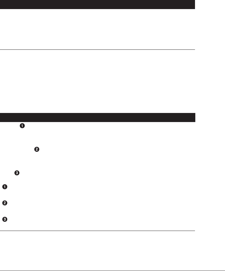
In computational physics, masks can be used to pick out a region of a problem to
either focus on or ignore. They are very useful for isolating the domain of a problem
that is truly of interest.
Masks may also be multidimensional themselves. In this case, the mask indexes the
array element-wise. The result of masking is typically a flat array. This is because the
true parts of the mask do not necessarily form a coherent shape. In the following, m is
a 3×3 Boolean array with four true elements. When used on our a array, the four val‐
ues at the true locations appear in the result:
Code Returns
# create a mask
m = np.array([[1, 0, 1],
[False, True, False],
[0, 0, 1]], dtype=bool)
a[m]
array([[ True, False, True],
[False, True, False],
[False, False, True]],
dtype=bool)
array([0, 2, 4, 8])
Masks are useful for hiding data that you know to be bad, unacceptable, or outside of
what you find interesting at the moment. NumPy makes it easy to generate masks.
The return of any comparison operator is a Boolean array. Rather than just being
True or False, comparisons act element-wise. Masks that are generated from com‐
parisons can be saved and used on other arrays. In the following example, less-than
and greater-than comparisons generate valid masks:
Code Returns
a < 5
m = (a >= 7)
a[m]
Create a mask array.
Create a mask and store it as m.
Apply m to the original array it was created from.
array([[ True, True, True],
[ True, True, False],
[False, False, False]],
dtype=bool)
array([[False, False, False],
[False, False, False],
[False, True, True]],
dtype=bool)
array([7, 8])
218 | Chapter 9: NumPy: Thinking in Arrays
www.it-ebooks.info

What is particularly beautiful about this is that the mask can be generated in the
indexing operation itself. You can read the following code as "a[i] such that a[i] is
less than 5 for all i“:
Code Returns
a[a < 5]array([0, 1, 2, 3, 4])
It is also possible to combine or modify masks with certain Python literal operators or
their NumPy function equivalents. Table 9-3 displays the bitwise operators that are
helpful when manipulating masks.
Table 9-3. NumPy bitwise operators
Operator Function Description
~ bitwise_not(x) True for elements where x is False and False for elements where x is True.
This is an alias to the numpy invert() function.
| bitwise_or(x, y) True for elements where either x or y or both are True.
^ bitwise_xor(x, y) True for elements where either x or y (but not both) is True.
& bitwise_and(x, y) True for elements where both x and y are True.
As an example, the following generates two masks and then uses the bitwise or opera‐
tor to combine them. The combined mask is then used to index an array:
Code Returns
a[(a < 5) | (a >= 7)] array([0, 1, 2, 3, 4, 7, 8])
Masks can and should be used in conjunction with NumPy’s where() function. If you
are familiar with the WHERE clause in SQL, this is conceptually similar. This function
takes a Boolean array and returns a tuple of fancy indices that are the coordinates for
where the mask is True. This function always returns a tuple so that it can be used in
an indexing operation itself:
Code Returns
np.where(a < 5)
a[np.where(a >= 7)]
(array([0, 0, 0, 1, 1]),
array([0, 1, 2, 0, 1]))
array([7, 8])
Masking | 219
www.it-ebooks.info

Passing the fancy index results of where() right back into the indexing operation is
not recommended because it will be slower and use more memory than just passing
in the mask directly. Taking the results of where() and modifying them in some way
is recommended. For example, the following takes every column from a where a has
any value that is less than 2:
Code Returns
a[:, np.where(a < 2)[1]] array([[0, 1],
[3, 4],
[6, 7]])
So far in this chapter you have learned how to manipulate arrays of a single, basic
data type. In the following section you will discover how to create richer dtypes of
your own that may better represent your data.
Structured Arrays
In most real-world data analysis scenarios, it is useful to have a notion of a table that
has named columns, where each column may have its own type. In NumPy, these are
called structured arrays or sometimes record arrays. This is because NumPy views
them as one-dimensional arrays of structs, like you would find in C or C++.
You can construct structured arrays by compounding dtypes together in the dtype()
constructor. The constructor may take a list of 2- or 3-tuples that describe the col‐
umns in the table. These tuples have the following form:
# 2-tuple
("<col name>", <col dtype>)
# 3-tuple
("<col name>", <col dtype>, <num>)
The first element of these tuples is the column name as a string. The second element
is the dtype for the column, which may itself be another compound dtype. Thus, you
can have subtables as part of your table. The third element of the tuple is optional; if
present, it is an integer representing the number of elements that the column should
have. If the number is not provided, a default value of 1 is assumed. Compound
dtypes are similar in nature to SQL schemas or a CSV file’s header line. Here are
some simple examples:
220 | Chapter 9: NumPy: Thinking in Arrays
www.it-ebooks.info

Code Returns
# a simple flat dtype
fluid = np.dtype([
('x', int),
('y', np.int64),
('rho', 'f8'),
('vel', 'f8'),
])
# a dtype with a nested dtype
# and a subarray
particles = np.dtype([
('pos', [('x', int),
('y', int),
('z', int)]),
('mass', float),
('vel', 'f4', 3)
])
dtype([('x', '<i8'),
('y', '<i8'),
('rho', '<f8'),
('vel', '<f8')])
dtype([('pos', [('x', '<i8'),
('y', '<i8'),
('z', '<i8')]),
('mass', '<f8'),
('vel', '<f4', (3,))])
All compound dtypes are implemented as void dtypes under the hood. There are also
two dtype attributes that are only useful in the context of compound dtypes. The
first, names, is a tuple of strings that gives the column names and their order. You can
rename columns by resetting this attribute. The second, fields, is a dict-like object
that maps the column names to the dtypes. The values in fields are read-only. This
ensures that the dtypes are immutable, which is important because changing their
size would change how the corresponding memory block of the array was sized. The
following examples demonstrate accessing these attributes:
Code Returns
particles.names
fluid.fields
('pos', 'mass', 'vel')
<dictproxy
{'rho': (dtype('float64'), 16),
'vel': (dtype('float64'), 24),
'x': (dtype('int64'), 0),
'y': (dtype('int64'), 8)}>
You can create structured arrays by passing these data types into the array creation
functions as usual. Note that in some cases, such as for arange(), the dtype that you
pass in may not make sense. In such cases, the operation will fail. Functions such as
zeros(), ones(), and empty() can take all data types. For example:
Structured Arrays | 221
www.it-ebooks.info

Code Returns
np.zeros(4, dtype=particles)array([((0, 0, 0), 0.0, [0.0, 0.0, 0.0]),
((0, 0, 0), 0.0, [0.0, 0.0, 0.0]),
((0, 0, 0), 0.0, [0.0, 0.0, 0.0]),
((0, 0, 0), 0.0, [0.0, 0.0, 0.0])],
dtype=[('pos', [('x', '<i8'),
('y', '<i8'),
('z', '<i8')]),
('mass', '<f8'),
('vel', '<f4', (3,))])
Here, the sub-dtype column pos is displayed as a tuple and the subarray column vel
is displayed as a list. This is because pos is implemented as three different named
components, while vel is a subarray. Also note that when you wish to use array() to
create a structured array from existing Python data the rows must be given as tuples.
This is to prevent NumPy from interpreting the data as having more than one dimen‐
sion along the structured axis. You can provide data to the array() function as
follows:
Code Returns
# note that the rows are tuples
f = np.array([(42, 43, 6.0, 2.1),
(65, 66, 128.0, 3.7),
(127, 128, 3.0, 1.5)],
dtype=fluid)
array([(42, 43, 6.0, 2.1),
(65, 66, 128.0, 3.7),
(127, 128, 3.0, 1.5)],
dtype=[('x', '<i8'),
('y', '<i8'),
('rho', '<f8'),
('vel', '<f8')])
Indexing a structured array by an integer will pull out a single row. Indexing by a slice
will return that slice of rows. Unlike with normal arrays, though, indexing by a string
will return the column whose name matches the string. This dictionary-like access is
further extended such that indexing by a list of strings will pull out multiple columns
in the order given. This must be a list—not a tuple—to distinguish it from regular
multidimensional indexing. For example:
222 | Chapter 9: NumPy: Thinking in Arrays
www.it-ebooks.info

Code Returns
f[1]
f[::2]
f['rho']
f[['vel', 'x', 'rho']]
(65, 66, 128.0, 3.7)
array([(42, 43, 6.0, 2.1),
(127, 128, 3.0, 1.5)],
dtype=[('x', '<i8'),
('y', '<i8'),
('rho', '<f8'),
('vel', '<f8')])
array([ 6., 128., 3.])
array([(2.1, 42, 6.0),
(3.7, 65, 128.0),
(1.5, 127, 3.0)],
dtype=[('vel', '<f8'),
('x', '<i8'),
('rho', '<f8')])
Having studied structured arrays, you now have seen a wide variety of different tech‐
niques for creating and manipulating arrays. The next section offers a brief peek into
how many of these operations are abstracted under NumPy’s hood.
Universal Functions
Now that we have seen how to define and manipulate arrays, we can discuss how to
transform them. NumPy has a notion of universal functions, or ufuncs, that provide
an interface for transforming arrays. Roughly speaking, a ufunc is a special callable
object that implements the reduce(), reduceat(), outer(), accumulate(), and at()
methods, as well as a handful of attributes. Knowing the details of how ufuncs are
implemented is not critical. Only the most advanced NumPy users and developers
truly need to worry about how to create and modify ufuncs.
What is much more important is understanding the suite of ufuncs that come as stan‐
dard with NumPy. A few of them have already been presented: the bitwise operators
we saw in Table 9-3 are universal functions.
Not all ufuncs will operate on all arrays, and some ufuncs may change the shape or
size of the result they return. However, the idea behind using ufuncs is to write data
transformations as generically as possible. A ufunc should fail if and only if the oper‐
ation that is being attempted is illogical or inconsistent. Table 9-4 displays some of the
most important ufuncs. For more information, please see the ufuncs documentation.
Table 9-4. Important NumPy universal functions
Function Description
add(a, b) Addition operator (+)
Universal Functions | 223
www.it-ebooks.info

Function Description
subtract(a, b) Subtraction operator (-)
multiply(a, b) Multiplication operator (*)
divide(a, b) Division operator (/)
power(a, b) Power operator (**)
mod(a, b) Modulus (%)
abs(a) Absolute value
sqrt(a) Positive square root
conj(a) Complex conjugate
exp(a) Exponential (e**a)
exp2(a) Exponential with base 2 (2**a)
log(a) Natural log
log2(a) Log base 2
log10(a) Log base 10
sin(a) Sine
cos(a) Cosine
tan(a) Tangent
bitwise_or(a, b) Bitwise | operator
bitwise_xor(a, b) Bitwise ^ operator
bitwise_and(a, b) Bitwise & operator
invert(a) Bitwise inversion (i.e., the ~ operator)
left_shift(a, b) Left bit shift operator (<<)
right_shift(a, b) Right bit shift operator (>>)
minimum(a, b) Minimum (note that this is dierent from np.min())
224 | Chapter 9: NumPy: Thinking in Arrays
www.it-ebooks.info

Function Description
maximum(a, b) Maximum (note that this is dierent from np.max())
isreal(a) Test for zero imaginary component
iscomplex(a) Test for zero real component
isfinite(a) Test for noninnite value
isinf(a) Test for innite value
isnan(a) Test for Not a Number
floor(a) Next-lowest integer
ceil(a) Next-highest integer
trunc(a) Truncate, remove noninteger bits
For example, we can take the sine of the linear range from zero to pi as follows:
Code Returns
x = np.linspace(0.0, np.pi, 5)
np.sin(x)
array([0. , 0.78539816,
1.57079633, 2.35619449,
3.14159265])
array([0.00000000e+00, 7.07106781e-01,
1.00000000e+00, 7.07106781e-01,
1.22464680e-16])
Universal functions are very significant in NumPy. One brilliant aspect of NumPy’s
design is that even though they are fundamental to many common operations, as a
user, you will almost never even notice that you are calling a universal function. They
just work.
It is common for new users of NumPy to use Python’s standard
math module instead of the corresponding universal functions. The
math module should be avoided with NumPy because it is slower
and less flexible. These deficiencies are primarily because universal
functions are built around the idea of arrays while math is built
around the Python float type.
However, not every operation can be expressed solely using univer‐
sal functions. Up next is a section that teaches about the vital odds
and ends that have yet to be detailed.
Universal Functions | 225
www.it-ebooks.info

Other Valuable Functions
In addition to the suite of ufuncs, NumPy also provides some miscellaneous func‐
tions that are critical for day-to-day use. In most cases these are self-explanatory; for
instance, the sum() function sums elements in an array. Many of these allow you to
supply keyword arguments. A common keyword argument is axis, which is None by
default, indicating that these functions will operate over the entire array. However, if
axis is an integer or tuple of integers, the function will operate only over those
dimensions. Using sum() as an example:
Code Returns
a = np.arange(9)
a.shape = (3, 3)
np.sum(a)
np.sum(a, axis=0)
np.sum(a, axis=1)
array([[0, 1, 2],
[3, 4, 5],
[6, 7, 8]])
36
array([ 9, 12, 15])
array([ 3, 12, 21])
Many of these functions appear as methods on the ndarray class as well. Table 9-5
shows some of the most important global functions that NumPy provides. Please
refer to the NumPy documentation for more information.
Table 9-5. Important NumPy global functions
function Description
sum(a) Adds together all array elements.
prod(a) Multiplies together all array elements.
min(a) Returns the smallest element in the array.
max(a) Returns the largest element in the array.
argmin(a) Returns the location (index) of the minimum element.
argmax(a) Returns the location (index) of the maximum element.
dot(a, b) Computes the dot product of two arrays.
cross(a, b) Computes the cross product of two arrays.
einsum(subs, arrs) Computes the Einstein summation over subscripts and a list of arrays.
226 | Chapter 9: NumPy: Thinking in Arrays
www.it-ebooks.info

function Description
mean(a) Computes the mean value of the array elements.
median(a) Computes the median value of the array elements.
average(a, weights=None) Returns the weighted average of an array.
std(a) Returns the standard deviation of an array.
var(a) Computes the variance of an array.
unique(a) Returns the sorted unique elements of an array.
asarray(a, dtype) Ensures the array is of a given dtype. If the array is already in the specied dtype,
no copy is made.
atleast_1d(a) Ensures that the array is least one-dimensional.
atleast_2d(a) Ensures that the array is least two-dimensional.
atleast_3d(a) Ensures that the array is least three-dimensional.
append(a, b) Glues the values of two arrays together in a new array.
save(file, a) Saves an array to disk.
load(file) Loads an array from disk.
memmap(file) Loads an array from disk lazily.
These functions can and do help, and using NumPy to its fullest often requires know‐
ing them. Some of them you will likely reach for very soon, like sum(). Others may
only rear their heads once or twice in a project, like save(). However, in all cases you
will be glad that they exist when you need them.
NumPy Wrap-up
Congratulations! You now have a breadth of understanding about NumPy. More
importantly, you now have the basic skills required to approach any array data lan‐
guage. They all share common themes on how to think about and manipulate arrays
of data. Though the particulars of the syntax may vary between languages, the under‐
lying concepts are the same. For NumPy in particular, though, you should now be
comfortable with the following ideas:
NumPy Wrap-up | 227
www.it-ebooks.info

• Arrays have an associated data type or dtype.
• Arrays are fixed-length, though their contents are mutable.
• Manipulating array attributes changes how you view the array, not the data itself.
•Slices are views and do not copy data.
• Fancy indexes are more general than slices but do copy data.
• Comparison operators return masks.
•Broadcasting stretches an array along applicable dimensions.
•Structured arrays use compound dtypes to represent tables.
• Universal and other functions are helpful for day-to-day NumPy use.
Still, NumPy arrays typically live only in memory. This means while it is a good men‐
tal model for performing calculations and trying to solve problems, NumPy is typi‐
cally not the right tool for storing data and sharing it with your friends and
colleagues. For those tasks, we will need to explore the tools coming up in Chap‐
ter 10.
228 | Chapter 9: NumPy: Thinking in Arrays
www.it-ebooks.info

CHAPTER 10
Storing Data: Files and HDF5
HDF5 stands for Hierarchical Data Format 5, a free and open source binary file type
specification. HDF5 is built and supported by the HDF Group, which is an organiza‐
tion that split off from the University of Illinois Champagne-Urbana. What makes
HDF5 great is the numerous libraries written to interact with files of this type and its
extremely rich feature set.
HDF5 has become the default binary database for scientific computing. Unlike other
software developers, scientists tend not to be primarily concerned with variable-
length strings, and our data is highly structured. What sets our data apart is the sheer
quantity of it.
The Big Data regime often deals with tables that have millions to billions of rows. The
cutting edge of computational science is trying to figure how out to deal with data on
the order of 1016 to 1018. HDF5 is at the forefront of tackling this quantity of data. At
this volume, data earns the term exascale because the size is roughly 1 exabyte. An
exabyte is almost unimaginably large. And at this scale, any improvements that can be
made to the storage size per element are worth implementing.
The beauty of HDF5 is that it works equally well on gargantuan data as it does on tiny
datasets. This allows users to play around with subsets of their data on their laptops
and then seamlessly deploy to the largest computers ever built, and everything in
between.
A contributing factor to the popularity of HDF5 is that it is accessible from almost
anywhere. The HDF Group supports interfaces in C, Fortran, Java, and C++ (mostly
deprecated; use the C interface instead). The C interface is the default and most fully
featured API. Third-party packages that interface with HDF5 are available in MAT‐
LAB, Mathematica, Haskell, and others. Python has two packages for using HDF5:
229
www.it-ebooks.info

h5py and PyTables. Here, we will use PyTables and occasionally reference aspects of
the C interface.
PyTables Versus h5py
Note that we have chosen PyTables here because its adds further
querying capabilities to the HDF5 interface. These are important to
learn about, as advanced querying comes up frequently in database
theory. On the other hand, h5py exposes HDF5’s underlying paral‐
lelism features directly to the user. For general use where you may
want to ask sophisticated questions of your data, go with PyTables.
In cases where you have large amounts of data that you don’t need
to question too deeply, go with h5py. For an excellent book on
h5py, please see Andrew Collette’s Python and HDF5 (O’Reilly).
Before we can shoot for storing astronomical datasets, we first have to learn how
normal-sized files are handled. Python has a lot of great tools for handling files of
various types, since they are how most data—not just physics data—is stored. Having
an understanding of how Python handles most files is needed to fully intuit how
large-scale databases like HDF5 work. Thus, this chapter starts out with an overview
section on normal files before proceeding on to HDF5 and all of its fancy features.
Files in Python
So far in this book, the discussion has revolved around in-memory operations. How‐
ever, a real computer typically has a hard drive for long-term persistent storage. The
operating system abstracts this into a collection of files. There are many situations in
which you may need to interact with a file on your hard drive:
•Your collaborator emails you raw data. You download the attachment and want
to look at the results.
• You want to email your collaborators some of your data, quickly.
•You need to use external code that takes an input or data file. You may need to
run the program thousands of times, so you automate the generation of input
files from data that you have in-memory in Python.
•An external program that you use writes out one (or more) result files, and you
want to read them and perform further analysis.
• You want to keep an intermediate calculation around for debugging or validation.
Reading and writing files is about interacting with the outside world. The senders and
receivers in these interactions can be humans, other programs, or both. Files provide
a common object that enables these interactions. That said, files are further special‐
230 | Chapter 10: Storing Data: Files and HDF5
www.it-ebooks.info

ized into formats, such as .csv, .doc, .json, .mp3, .png, and so on. These formats denote
the internal structure of the file. The .txt extension is an exception in that it is not a
format; it is traditionally used to flag that a file has no specific internal structure but
contains plain, free-flowing text. We do not have the time or space in this book to
fully describe even a fraction of the popular file formats. However, Python will be able
to open all of them (if not necessarily make sense of their internal structure).
In Python, to save or load data you go through a special le handle object. The built-
in open() function will return a file object for you. This takes as its argument the path
to the file as a string. Suppose you have a file called data.txt in the current directory.
You could get a handle, f, to this file in Python with the following:
f = open('data.txt')
The open() call implicitly performs the following actions:
1. Makes sure that data.txt exists.
2. Creates a new handle to this file.
3. Sets the cursor position (pos) to the start of the file, pos = 0.
The call to open() does not read into memory any part of the file, write anything out
to the file, or close the file. All of these actions must be done separately and explicitly
and are accomplished through the use of file handle methods.
Methods are functions that are defined on a class and bound to an
object, as seen in Chapter 6.
Table 10-1 lists the most important file methods.
Table 10-1. Important le handle methods
Method Description
f.read(n=-1) Reads in n bytes from the le. If n is not present or is -1, the entire rest of the le is read.
f.readline() Reads in the next full line from the le and returns a string that includes the newline
character at the end.
f.readlines() Reads in the remainder of the le and returns a list of strings that end in newlines.
f.seek(pos) Moves the le cursor to the specied position.
f.tell() Returns the current position in the le.
Files in Python | 231
www.it-ebooks.info

Method Description
f.write(s) Inserts the string s at the current position in the le.
f.flush() Performs all pending write operations, making sure that they are really on disk.
f.close() Closes the le. No more reading or writing can occur.
Suppose that matrix.txt represents a 4×4 matrix of integers. Each line in the file repre‐
sents a row in the matrix. Column values are separated by commas. Ideally, we would
be able to read this into Python as a list of lists of integers, since that is the most
Pythonic way to represent a matrix of integers. This is not the most efficient repre‐
sentation for a matrix—a NumPy array would be better—but it is fairly common to
read in data in a native Python format before continuing to another data structure.
The following snippet of code shows how to read in this matrix. To follow along, first
make sure that you create a matrix.txt file on your computer. You can do this by
copying the contents shown here into your favorite text editor and saving the file with
the right name:
matrix.txt Code Python matrix
1,4,15,9
0,11,7,3
2,8,12,13
14,5,10,6
f = open('matrix.txt')
matrix = []
for line in f.readlines():
row = [int(x) for x in line.split(',')]
matrix.append(row)
f.close()
[[1, 4, 15, 9],
[0, 11, 7, 3],
[2, 8, 12, 13],
[14, 5, 10, 6]]
Notice that the lines from a file are always strings. This means that you have to con‐
vert the string versions of the values in matrix into integers yourself. Python doesn’t
know that you mean for the content of the file to be a matrix. In fact, the only
assumption about data types that Python can make is that a file contains strings. You
have to tell it how to interpret the contents of a file. Thus, any numbers in the file
must be converted from string forms to integers or floats. For a reminder on how to
convert between variable types, see “Variables” on page 42. Special file readers for
particular formats, which we won’t see here, may perform these conversions for you
automatically. However, under the covers, everything is still a string originally. At the
end of the preceding code snippet, also note that the file must be closed manually.
Even when you have reached the end of a file, Python does not assume that you are
done reading from it.
232 | Chapter 10: Storing Data: Files and HDF5
www.it-ebooks.info

Files Should Always Be Closed!
A file that remains open unnecessarily can lead to accidental data
loss as well as being a security hazard. It is always better to close a
file prematurely and open a new file handle than it is to leave one
open and lingering. File handles are cheap to create, so perfor‐
mance should not be a concern.
Files are opened in one of multiple modes. The mode a file was opened with deter‐
mines the methods that can be used on the handle. Invalid methods are still present
on the handle, but trying to use them will raise an exception.
So far, we’ve only opened files in the default read-only mode. To change this, mode
flags may be passed into the open() call after the filename. The mode is specified as a
string of one or more characters with the special meanings listed in Table 10-2. A
common example is to open the file for writing and erase the existing contents. This
uses the 'w' flag:
f = open('data.txt', 'w')
Table 10-2. Useful le modes
Mode Meaning
'r' Read-only. No writing possible. Starting pos = 0.
'w' Write. If the le does not exist, it is created; if the le does exist, the current contents
are deleted (be careful!). Starting pos = 0.
'a' Append. Opens the le for writing but does not delete the current contents; creates the
le if it does not exist. Starting pos is at the end of the le.
'+' Update. Opens the le for both reading and writing; may be combined with other ags;
does not delete the current contents. Starting pos = 0.
As a more sophisticated example, the following adds a row of zeros to the top of our
matrix and a row of ones to the end:
Files in Python | 233
www.it-ebooks.info
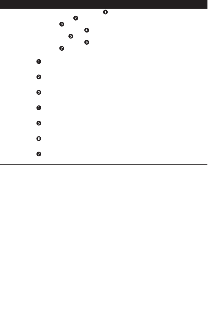
Old matrix.txt Code New matrix.txt
1,4,15,9
0,11,7,3
2,8,12,13
14,5,10,6
f = open('matrix.txt', 'r+')
orig = f.read()
f.seek(0)
f.write('0,0,0,0\n')
f.write(orig)
f.write('\n1,1,1,1')
f.close()
Open the le in read and write mode, without overwriting the contents.
Read the entire le into a single string.
Go back to the start of the le.
Write a new line, clobbering what was there.
Write the original contents back to the le after the line that was just added.
Write another new line after the original contents.
Close the le now that we are done with it.
0,0,0,0
1,4,15,9
0,11,7,3
2,8,12,13
14,5,10,6
1,1,1,1
There are many times when no matter what happens in a block of code—success or
failure, completion or exception—special safety code must be run at the end of the
block. This is to prevent data loss, corruption, or even ending up in the wrong place
on the filesystem. In Python, administering these potentially hazardous situations is
known as context management. There are many context managers that perform
defensive startup actions when the code block is entered (right before the first state‐
ment), and other cleanup actions when the block is exited. Code blocks may be exited
either right after the last statement or following an uncaught exception. File handles
are the most common context managers in Python. As we have mentioned before,
files should always be closed. However, files can act as their own context managers.
When using a file this way, the programmer does not need to remember to manually
close the file; the call to the file’s close() method happens automatically.
The with statement is how a context is entered and exited. The syntax for this state‐
ment introduces the with Python keyword and reuses the as keyword. The with
statement has the following format:
with <context-manager> as <var>:
<with-block>
234 | Chapter 10: Storing Data: Files and HDF5
www.it-ebooks.info

Here, the <context-manager> is the actual context object, <var> is a local variable
name that the context manager is assigned to, and the <with-block> is the code that
is executed while the manager is open. The as <var> portion of this syntax is
optional.
The matrix.txt file example from before can be expressed using a with statement as
follows:
matrix.txt Code matrix
0,0,0,0
1,4,15,9
0,11,7,3
2,8,12,13
14,5,10,6
1,1,1,1
matrix = []
with open('matrix.txt') as f:
for line in f.readlines():
row = [int(x) for x in line.split(',')]
matrix.append(row)
The le f is open directly following the colon (:).
f is closed by the context manager once the indentation level returns to
that of the with keyword.
[[0, 0, 0, 0],
[1, 4, 15, 9],
[0, 11, 7, 3],
[2, 8, 12, 13],
[14, 5, 10, 6],
[1, 1, 1, 1]]
Using with statements is the recommended way to use files, because not having to
explicitly call f.close() all of the time makes your code much safer and more robust.
Other kinds of context managers exist. You can write your own. However, files are the
context managers that you will most frequently encounter. This is because it is easy to
forget to close files, and the consequences can be relatively severe if you do.
Now that we have seen the basics of how to read and write normal Python files, we
can start to discover HDF5. HDF5 is one of the richest and most useful file formats
for scientific computing. HDF5 puts numeric data first. This helps distinguish it from
other file formats where strings rule, like we have seen in this section. Before getting
into the nitty-gritty, it will be helpful to first gain some perspective.
An Aside About Computer Architecture
Computers are physical tools, just like any other experimental device. So far, we have
been able to ignore how they work and their internal structure. When it comes to
data storage, though, there are enough subsystems simultaneously dancing that we
need to understand what a computer is in order to effectively program it. As you will
see later in this chapter, this knowledge can make the difference between your physics
software taking a week to run or five minutes.
Overlooking other peripheral devices (keyboard, mouse, monitor), a basic computer
has consisted of three main components since the 1980s: a central processing unit
An Aside About Computer Architecture | 235
www.it-ebooks.info
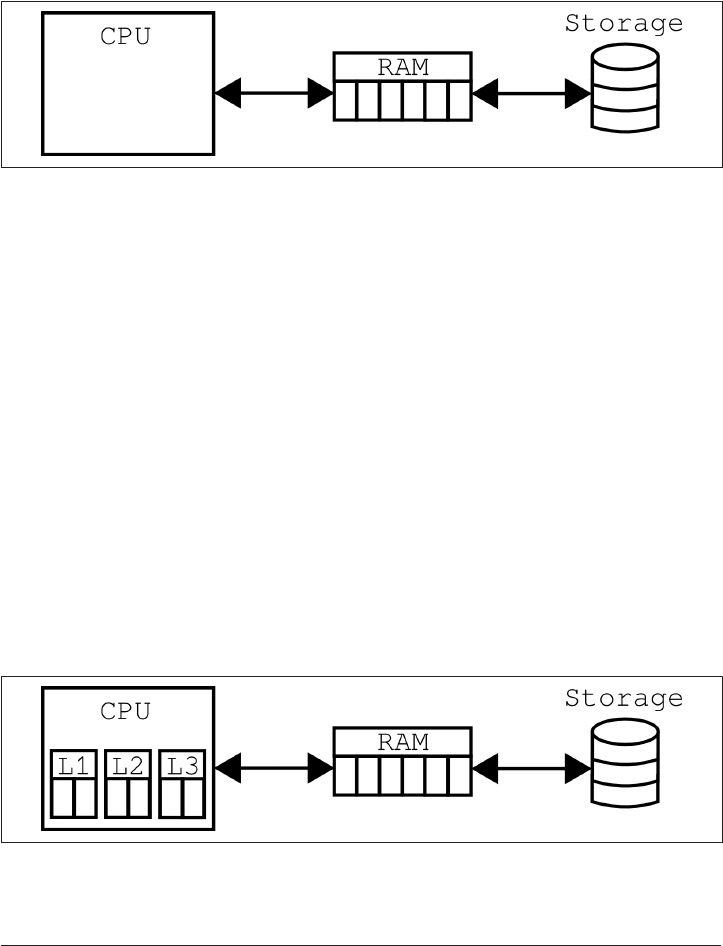
(CPU), random-access memory (RAM), and a storage drive. Historically, the storage
drive has gone by the name hard disk drive (HDD), because the device was made up
of concentric spinning magnetic disks. More recent storage devices are built like a
flash memory stick; these drives are called solid state drives (SSDs). The CPU, RAM,
and storage can be thought of as living in series with each other, as seen in
Figure 10-1.
Figure 10-1. A simple model of a computer
In this simple model, the CPU can be thought of as a dumb calculator; RAM is what
“remembers” what the CPU just did (it acts sort of like short-term memory), and the
storage is what allows the computer to save data even when it is turned off (it’s like
long-term memory). In practice, when we talk about the computer “doing some‐
thing,” we really mean the CPU. When we talk about the filesystem, we really mean
the storage. It is important to understand, therefore, that RAM is what shuffles bytes
between these two components.
Of course, computer architectures have become much more complicated than this
simple model. CPU caches are one major mainstream advancement. These caches are
like small versions of RAM that live on the CPU. They contain copies of some of the
data in RAM, but much closer to the processor. This prevents the computer from
having to go out to main memory all of the time. For commonly accessed data, the
caches can provide huge decreases in execution time. The caches are named after a
hierarchy of level numbers, such L1, L2, and so on. In general, the higher the level
number, the smaller the cache size, but the faster it is to access it. Currently, most
processers come with L1 and L2 caches. Some processors are now also starting to
come with L3 caches. Figure 10-2 represents a computer with CPU caches.
Figure 10-2. A computer with L1, L2, and L3 CPU caches
236 | Chapter 10: Storing Data: Files and HDF5
www.it-ebooks.info
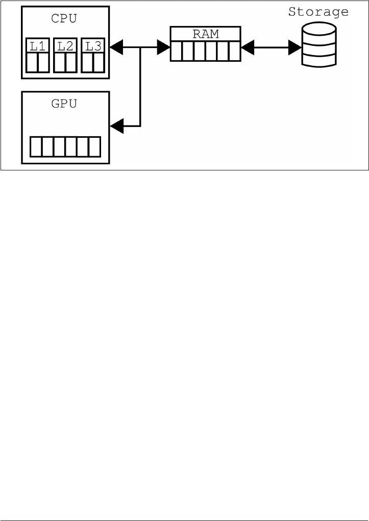
The other big innovation in computer architecture is graphics processing units, or
GPUs. These are colloquially known as graphics cards. They are processors that live
outside of the main CPU. A computer with a GPU is displayed in Figure 10-3.
Figure 10-3. A computer with a GPU
Though there are many important differences between GPUs and CPUs, very
roughly, you can think of GPUs as being really good at floating-point operations.
CPUs, on the other hand, are much better at integer operations than GPUs (while still
being pretty good with floating-point data). So, if you have an application that is pri‐
marily made up of floats, then GPUs may be a good mechanism to speed up your exe‐
cution time.
Naturally, there is a lot more to computer engineering and architecture than what you
have just seen. However, this gives you a good mental model of the internal structure
of a computer. Keep this in mind as we proceed to talking about databases and HDF5.
Many real-world programming trade-offs are made and balanced because of the
physical performance of the underlying machine.
Big Ideas in HDF5
Persisting structured, numerical data to binary formats is superior to using plain-text
ASCII files. This is because, by their nature, they are often smaller. Consider the fol‐
lowing comparison between integers and floats in native and string representations:
# small ints # medium ints
42 (4 bytes) 123456 (4 bytes)
'42' (2 bytes) '123456' (6 bytes)
# near-int floats # e-notation floats
12.34 (8 bytes) 42.424242E+42 (8 bytes)
'12.34' (5 bytes) '42.424242E+42' (13 bytes)
Big Ideas in HDF5 | 237
www.it-ebooks.info

In most cases, the native representation is smaller than the string version. Only by
happenstance are small integers and near-integer floats smaller in their string forms.
Such cases are relatively rare on average, so native formats almost always outperform
the equivalent strings in terms of space.
Space is not the only concern for files. Speed also matters. Binary formats are always
faster for I/O because in order to do real math with the numbers, if they are in a
string form you have to convert them from strings to the native format. The Python
conversion functions int() and float() are known to be relatively slow because the
C conversion functions atoi() and atof() that they wrap around are expensive
themselves.
Still, it is often desirable to have something more than a binary chunk of data in a file.
HDF5 provides common database features such as the ability to store many datasets,
user-defined metadata, optimized I/O, and the ability to query its contents. Unlike
SQL, where every dataset lives in a single namespace, HDF5 allows datasets to live in
a nested tree structure. In effect, HDF5 is a filesystem within a file—this is where the
“hierarchical” in the name comes from.
PyTables provides the following basic dataset classes that serve as entry points for
various HDF5 constructs:
Array
The files of the filesystem
CArray
Chunked arrays
EArray
Extendable arrays
VLArray
Variable-length arrays
Table
Structured arrays
All of these must be composed of what are called atomic types in PyTables. The
atomic types are roughly equivalent to the primitive NumPy types that were seen in
“dtypes” on page 204. There are six kinds of atomic types supported by PyTables.
Here are their names, descriptions, and supported sizes:
bool
True or false type—8 bits
int
Signed integer types—8, 16, 32 (default), and 64 bits
238 | Chapter 10: Storing Data: Files and HDF5
www.it-ebooks.info

uint
Unsigned integer types—8, 16, 32 (default), and 64 bits
float
Floating-point types—16, 32, and 64 (default) bits
complex
Complex floating-point types—64 and 128 (default) bits
string
Fixed-length raw string type—8 bits times the length of the string
Other elements of the hierarchy may include:
Groups
The directories of the filesystem; may contain other groups and datasets
Links
Like soft links on the filesystem
Hidden nodes
Like hidden files
These pieces together are the building blocks that you can use to richly describe and
store your data. HDF5 has a lot of features and supports a wide variety of use cases.
That said, simple operations are easy to implement. Let’s start with basic file reading
and writing.
File Manipulations
HDF5 files may be opened from Python via the PyTables interface. To get PyTables,
first import tables. Like with numpy and np, it is common to abbreviate the tables
import name to tb:
import tables as tb
f = tb.open_file('/path/to/file', 'a')
Files have modes that they may be opened in, similarly to how plain-text files are
opened in Python. Table 10-3 displays the modes that are supported by PyTables.
File Manipulations | 239
www.it-ebooks.info

Table 10-3. HDF5 le modes
Attribute Description
rRead-only—no data can be modied.
wWrite—a new le is created; if a le with that name exists, it is deleted.
aAppend—an existing le is opened for reading and writing, or if the le does not exist, it is created.
r+ Similar to a, but the le must already exist.
In HDF5, all nodes stem from a root node, "/" or f.root. In PyTables, you may
access subnodes as attributes on nodes higher up in the hierarchy—e.g.,
f.root.a_group.some_data. This sort of access only works when all relevant nodes
in the tree have names that are also valid Python variable names, however; this is
known as natural naming.
Creating new nodes must be done on the file handle, not the nodes themselves. If we
want to make a new group, we have to use the create_group() method on the file.
This group may then be accessed via the location it was created in. For example, cre‐
ating and accessing a group called a_group on the root node can be done as follows:
f.create_group('/', 'a_group', "My Group")
f.root.a_group
Possibly more important than groups, the meat of HDF5 comes from datasets. The
two most common datasets are arrays and tables. These each have a corresponding
create method that lives on the file handle, called create_array() and
create_table(). Arrays are of fixed size, so you must create them with data. The
type of the data in the HDF5 file will be interpreted via numpy. Tables, like NumPy
structured arrays, have a set data type. Unlike arrays, tables are variable length, so we
may append to them after they have been created. The following snippet shows how
to create an array and a table and how to populate them using Python lists and
NumPy arrays:
# integer array
f.create_array('/a_group', 'arthur_count', [1, 2, 5, 3])
# tables need descriptions
dt = np.dtype([('id', int), ('name', 'S10')])
knights = np.array([(42, 'Lancelot'), (12, 'Bedivere')], dtype=dt)
f.create_table('/', 'knights', dt)
f.root.knights.append(knights)
240 | Chapter 10: Storing Data: Files and HDF5
www.it-ebooks.info

At this point, the hierarchy of groups and datasets in the file is represented by the
following:
/
|-- a_group/
| |-- arthur_count
|
|-- knights
Arrays and tables attempt to preserve the original avor, or data structure, with
which they were created. If a dataset was created with a Python list, then reading out
the data will return a Python list. If a NumPy structured array was used to make the
data, then a NumPy structured array will be returned. Note that you can read data
from a dataset simply by slicing (described in Chapter 9). One great thing about
PyTables and HDF5 is that only the sliced elements will be read in from disk. Parts of
the dataset that are not included in the slice will not be touched. This speeds up read‐
ing by not making the computer do more work than it has to, and also allows you to
read in portions of a dataset whose whole is much larger than the available memory.
Using our sample arthur_count array, the following demonstrates flavor preservation.
Also note that the type of the dataset comes from PyTables, and this is separate from
the type of the data that is read in:
Code Returns
f.root.a_group.arthur_count[:]
type(f.root.a_group.arthur_count[:])
type(f.root.a_group.arthur_count)
[1, 2, 5, 3]
list
tables.array.Array
Since the arthur_count array came from a Python list, only Python list slicing is avail‐
able. However, if a dataset came from a NumPy array originally, then it can be
accessed in a NumPy-like fashion. This includes slicing, fancy indexing, and masking.
The following demonstrates this NumPy-like interface on our knights table:
File Manipulations | 241
www.it-ebooks.info
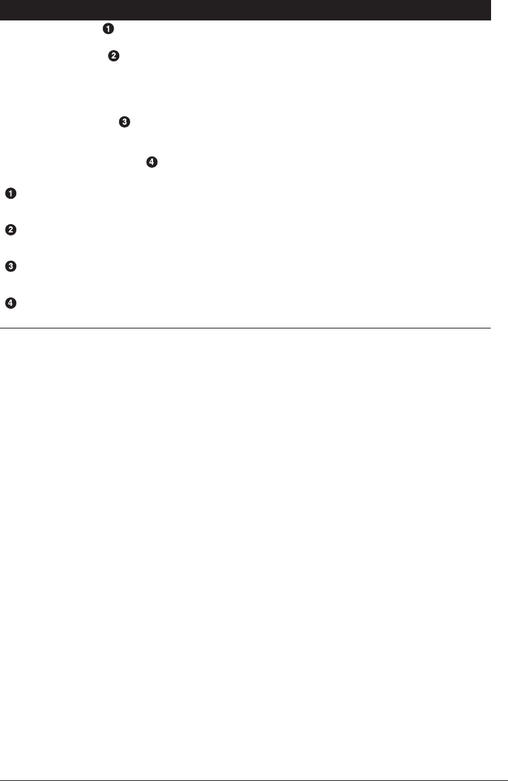
Code Returns
f.root.knights[1]
f.root.knights[:1]
mask = (f.root.knights.cols.id[:] < 28)
f.root.knights[mask]
f.root.knights[([1, 0],)]
Pull out just the second row.
Slice the rst row.
Create a mask from the on-disk id column and apply this to the table.
Fancy index the second and rst rows, in that order.
(12, 'Bedivere')
array([(42, 'Lancelot')],
dtype=[('id', '<i8'),
('name', 'S10')])
array([(12, 'Bedivere')],
dtype=[('id', '<i8'),
('name', 'S10')])
array([(12, 'Bedivere'),
(42, 'Lancelot')],
dtype=[('id', '<i8'),
('name', 'S10')])
Pulling in data from disk only as needed is known as memory mapping. HDF5 takes
care of this for you automatically; this is one way that reading and writing to HDF5
files is optimized.
Now you know how to create and use the core node types: groups, arrays, and tables.
However, you can use these elements of the hierarchy to even greater effect by com‐
bining them in meaningful ways. The following section discusses how to think about
your information more broadly than within the confines of a single dataset.
Hierarchy Layout
Suppose you have a big table of similar objects. For example, consider a table of all of
the particles that you have seen recently. This could be written as a list of tuples, as
follows:
# particles: id, kind, velocity
particles = [(42, 'electron', 72.0),
(43, 'proton', 0.1),
(44, 'electron', 76.8),
(45, 'neutron', 0.39),
(46, 'neutron', 0.72),
(47, 'neutron', 0.55),
(48, 'proton', 0.18),
(49, 'neutron', 0.23),
...
]
242 | Chapter 10: Storing Data: Files and HDF5
www.it-ebooks.info

Having a big table like this can be inefficient. If you know ahead of time that you nor‐
mally want to look at all of the neutral and charged particles separately, then why
search through all the particles all of the time? Instead, it would be better to split up
the particles into multiple tables grouped by whether they are neutral or charged. The
following shows such a split as applied to the original particles table:
neutral = [(45, 'neutron', 0.39),
(46, 'neutron', 0.72),
(47, 'neutron', 0.55),
(49, 'neutron', 0.23),
...
]
charged = [(42, 'electron', 72.0),
(43, 'proton', 0.1),
(44, 'electron', 76.8),
(48, 'proton', 0.18),
...
]
The kind column is now redundant in the neutral table because its value is the same
for all rows. We can delete this whole column and rely on the structure of these two
tables together to dictate that the neutral table always refers to neutrons. This space
saving can be seen here:
neutral = [(45, 0.39),
(46, 0.72),
(47, 0.55),
(49, 0.23),
...
]
charged = [(42, 'electron', 72.0),
(43, 'proton', 0.1),
(44, 'electron', 76.8),
(48, 'proton', 0.18),
...
]
With these transformations we are embedding information directly into the seman‐
tics of the hierarchy. The deeper and broader your hierarchy is, the more information
can be stored with it. For example, we could add another layer that distinguishes the
particles based on detector:
/
|-- detector1/
| |-- neutral
| |-- charged
|
|-- detector2/
Hierarchy Layout | 243
www.it-ebooks.info

| |-- neutral
| |-- charged
Data can and should be broken up like this to improve access time speeds. Such seg‐
regation based on available information is more efficient because there are:
• Fewer rows to search over
• Fewer rows to pull from disk
• Fewer columns in the description, which decreases the size of the rows
Dealing with less data is always faster than dealing with more. This is especially true
because of how long it takes to read data from disk. Waiting around for access prior
to computation is known as the starving CPU problem (Alted, 2010).
An analogy about access time with respect to different parts of a computer comes to
us from Gustavo Duarte’s article “What Your Computer Does While You Wait.” This
is helpful to keep in mind when making decisions about how to deal with large
amounts of data. The metaphor goes as follows. If a processor’s access of the L1 cache
is analogous to you finding a word on a computer screen (3 seconds), then:
• Accessing the L2 cache is like getting a book from a bookshelf (15 s).
•Accessing main memory is like going to the break room, getting a snack, and
chatting with your coworker (4 min).
•Accessing a (mechanical) HDD is like leaving your office, leaving your building,
wandering the planet for a year and four months, then returning to your desk
with the information finally made available.
From this analogy, you can see how important it is to minimize the number of times
the computer has to go to the hard disk, minimize the amount of data that must be
transferred from the hard disk, and keep the computer busy while it is waiting for
information to be retrieved. Manipulating the layout of the hierarchy is a useful tool
in this regard.
However, there are practical limits to hierarchy depth and breadth. For every new
group or dataset, there is overhead. In HDF5 there is 64 KB of space reserved for
metadata for every dataset. Thus, the practical limit is hit when the overhead size is
comparable to the size of the underlying data being stored. Though your mileage and
data may vary, a good rule of thumb is that three levels of hierarchy allowing any
number of datasets at each level is enough structure for most problems.
So far in this chapter, you have learned how to read and write data in HDF5. You have
even seen some manipulations to the file hierarchy that can be used to optimize your
data. Up next, though, is a discussion of how HDF5 stores datasets. Understanding
244 | Chapter 10: Storing Data: Files and HDF5
www.it-ebooks.info

what actions HDF5 is actually performing opens up new avenues to data manipula‐
tion and optimization.
Chunking
Chunking is the ability to split up a dataset into smaller blocks of equal or lesser rank.
Unlike the manipulations we saw in the previous section that occurred between mul‐
tiple datasets, chunking happens within a single dataset and is implemented automat‐
ically. Chunks are how HDF5 stores data. This is a feature of HDF5 that has no direct
analogy in NumPy.
Chunking requires that extra metadata be stored that points to the location of each
chunk in the file. Thus, there is some overhead per chunk. The more chunks that
exist, the more information must be stored about where those chunks live. However,
chunking enables two key features that allow HDF5 to deal with huge amounts of
data:
1. Sparse data may be stored efficiently.
2. Datasets may extend infinitely in all dimensions.
For example, suppose that you wanted to store a 109×109 item matrix. If this matrix
was mostly made up of zeros, you could use HDF5 to store only the nonzero elements
and obtain a gigantic savings in terms of execution time and database size. Currently,
PyTables only allows one extendable dimension, typically rows. However, there is no
such restriction in HDF5 itself, so if you use HDF5’s C interface (or h5py), you may
extend infinitely in every which way.
Consider that all datasets are composed of metadata (which describes the data type,
shape, and more) and bytes that represent the data itself. In a contiguous dataset, all
of the bytes are in a single array, right next to each other. This can be seen graphically
in Figure 10-4. Alternatively, a chunked dataset splits up this array of bytes into many
smaller arrays, each stored in a separate location. A representation of this may be seen
in Figure 10-5.
Chunking | 245
www.it-ebooks.info
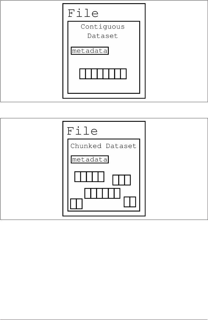
Figure 10-4. Contiguous dataset
Figure 10-5. Chunked dataset
All reading and writing in HDF5 happens per-chunk. Contiguous datasets, like
arrays, are the special case where there is only one chunk. Furthermore, the chunk
shape and size is a property of the dataset itself and independent of the actual data.
This has the following significant implications:
• Edge chunks may extend beyond the dataset.
•Default fill values are set in unallocated space, allowing for sparse datasets to only
store the data they have.
•Reading and writing of chunks may happen in parallel.
246 | Chapter 10: Storing Data: Files and HDF5
www.it-ebooks.info

• Small chunks are good for accessing only some of the data at a time.
• Large chunks are good for accessing lots of data at a time.
Chunks are not just a mechanism for laying out extensible datasets and efficiently
implementing sparse data. Rather, chunks are the way that HDF5 reasons about data
storage operations. HDF5 allows users to set the chunk size and shape on any
chunked dataset. In PyTables, the chunkshape is a keyword argument to the creation
methods. This is simply a tuple representing the chunk’s shape and size along each
dimension. In PyTables, we can make a new chunked array with the create_car
ray() method. The following is an example where we create a chunked array and
explicitly set the chunk shape:
f.create_carray('/', 'omnomnom', data, chunkshape=(42,42))
If we had not explicitly set a chunk shape, PyTables would have picked one for us,
using properties of the data and some heuristics to take a best guess as to the optimal
chunking. In general, if you are unsure of what the chunk shape should be, just let
PyTables pick one for you and do not set it manually.
Tables, CArrays, and EArrays all accept the chunkshape keyword
argument.
As a visual example of how chunking works, suppose you have a 3×3 matrix in mem‐
ory. Storing this as a contiguous dataset would only require one flat array with nine
elements. A diagram of this situation is displayed in Figure 10-6. However, we are free
to choose any chunk shape that is less than or equal to 3×3. As an example, take 2×2
to be the chunk shape. The 3×3 matrix would then be represented by four 2×2 tiles
overlaid onto the matrix. It is OK for the total shape of all of the tiles to extend
beyond the bounds of the original data. Overextended chunk elements will simply go
unused. Figure 10-7 shows this case, with shading used to denote the chunks.
Chunking | 247
www.it-ebooks.info
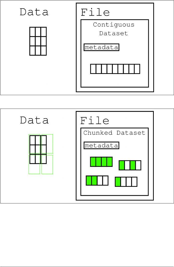
Figure 10-6. Contiguous 3x3 dataset, in memory and in an HDF5 le
Figure 10-7. Chunked 3x3 dataset, with 2x2 chunks shaded
Manipulating the chunk shape is a great way to fine-tune the performance of an
application. Typically, the best-guess chunk shape that PyTables provides is good
enough for most cases. However, when you really need to squeeze every ounce of
read and write speed out of your data, you can vary the chunk shape to try to find
that perfect value.
248 | Chapter 10: Storing Data: Files and HDF5
www.it-ebooks.info

While we are on the topic of performance, let’s examine the different ways to perform
calculations on our data. Sending and receiving data to and from the hard drive is not
the only way to leverage PyTables, as we will see in the next section.
In-Core and Out-of-Core Operations
Calculations depend on the memory layout of the data. When implementing array
operations, algorithms fall into two broad categories based on where you expect the
data to be in memory. Operations that require all data to be in memory are called in-
core and may be memory-bound. This means that the volume of data that may be
processed is limited to the size of the computer’s memory. For example, NumPy
arrays are memory-bound because in order to exist, the whole array must be in mem‐
ory. On the other hand, operations where the data can be external to memory are
known as out-of-core. Such operations may be CPU-bound. Thus, “in-core” and “out-
of-core” can be thought of in terms of which component (the RAM or the CPU) in
Figure 10-1 is limiting the behavior of the machine. Unlike in NumPy, computations
over HDF5 arrays may be performed in an out-of-core way. Let’s explore in-core and
out-of-core paradigms more deeply, before continuing. If you find any part of this
discussion overwhelming or confusing, feel free to skip ahead to “Querying” on page
252.
In-Core
For a classic example of in-core operations, say that there are two NumPy arrays, a
and b, sitting in memory. (The next section will discuss what to do if your data does
not fit into memory.) The expression defined as c here is independent of the size and
contents of a and b. As long as a and b are compatible, c may be computed:
a = np.array(...)
b = np.array(...)
c = 42 * a + 28 * b + 6
The expression for c creates three temporary arrays, which are discarded after they
are used. Still, these temporaries take up space in memory. Thus, the free space
needed in memory to compute c is at least six times the size of a or b. Here are the
temporaries that would be computed when evaluating c:
temp1 = 42 * a
temp2 = 28 * b
temp3 = temp1 + temp2
c = temp3 + 6
In general, for N operations there are N-1 temporaries that have to be constructed.
This wastes memory and is slower than if the temporaries were avoided altogether.
Still, given how long reading from a file can take, pulling the data from disk is even
slower than creating temporaries.
In-Core and Out-of-Core Operations | 249
www.it-ebooks.info

Alternatively, a less memory-intensive implementation would be to evaluate the
whole expression element-wise. The following snippet shows how such a computa‐
tion would be written:
c = np.empty(...)
for i in range(len(c)):
c[i] = 42 * a[i] + 28 * b[i] + 6
This algorithm is the idiomatic way that you would write such an operation in C,
C++, or Fortran. In those languages, this algorithm is very fast. However, in Python,
this method is much slower than the simpler NumPy solution, even with the tempo‐
raries. This is in part because Python loops are slow and in part because of the very
dynamic Python type system.
Slower still, suppose that a and b were HDF5 arrays on disk. The individual element
access times would make this computation take thousands of times longer, or more.
Repetitively reading small amounts of data from the hard drive is just that slow. Even
with fast solid-state drives, this algorithm would still run like a turtle through a tar
pit. In practice, idiomatic NumPy is good enough for almost all in-core operations. If
you truly need something faster, you probably need to look to other programming
languages.
Out-of-Core
Out-of-core operations combine the notions of element-wise evaluation and chunk‐
ing. Even though this is most useful when access times are slow (i.e., when reading
from disk), such operations can work on data that is fully inside of memory. Let’s take
again the example from the previous section, where c = 42 * a + 28 * b + 6. An
out-of-core algorithm would apply a chunksize of 256 to the element-wise algorithm.
The three possible solutions are seen here:
# setup
a = np.array(...)
b = np.array(...)
# how to compute c with numpy (in-core)
c = 42 * a + 28 * b + 6
# how to compute c element-wise (in-core)
c = np.empty(...)
for i in range(len(c)):
c[i] = 42 * a[i] + 28 * b[i] + 6
# how to compute c with chunks (out-of-core)
c = np.empty(...)
for i in range(0, len(a), 256):
r0, r1 = a[i:i+256], b[i:i+256]
np.multiply(r0, 42, r2)
np.multiply(r1, 28, r3)
250 | Chapter 10: Storing Data: Files and HDF5
www.it-ebooks.info

np.add(r2, r3, r2)
np.add(r2, 6, r2)
c[i:i+256] = r2
Using the out-of-core strategy, no more than 256 elements need to be in memory at
any time. While temporaries are created, their size is similarly limited to 256 ele‐
ments. Feeding in only discrete chunks at a time allows out-of-core algorithms to
function on infinite-length data while using only the finite memory resources of your
computer. This problem lends itself nicely to parallelism, since every chunk can be
assumed to be independent of every other chunk. We will learn more about parallel‐
ism in Chapter 12.
In Python, the numexpr library provides a way to perform chunked, element-wise
computations on regular NumPy arrays. PyTables uses this library internally, but
extends its application to HDF5 arrays on disk. The PyTables tb.Expr class imple‐
ments the out-of-core interface that handles the expression evaluation. This has the
distinct advantage that the full array is never in memory. The Expr class is critical
because it is easy to have HDF5 datasets that are thousands, millions, or billions of
times larger than the amount of memory on a laptop.
The expression for c can be calculated with the Expr class and with a and b as HDF5
arrays that live outside of memory. The following code represents this out-of-core
strategy. Note that in this snippet even the c array lives on disk and is never fully
brought into memory:
# open a new file
shape = (10, 10000)
f = tb.open_file("/tmp/expression.h5", "w")
# create the arrays
a = f.create_carray(f.root, 'a', tb.Float32Atom(dflt=1.), shape)
b = f.create_carray(f.root, 'b', tb.Float32Atom(dflt=2.), shape)
c = f.create_carray(f.root, 'c', tb.Float32Atom(dflt=3.), shape)
# evaluate the expression, using the c array as the output
expr = tb.Expr("42*a + 28*b + 6")
expr.set_output(c)
expr.eval()
# close the file
f.close()
Using tb.Expr or numexpr is much cleaner, simpler, and more robust than writing
your own custom chunking algorithm. Thus, it is generally recommended to use the
existing tools rather than trying to create your own.
In summary, in-core operations are fast and efficient when all of the data is already in
memory. However, if the data needs to be pulled in from disk or if the data is too
large to fit in memory, an out-of-core algorithm is best. For HDF5, PyTables provides
In-Core and Out-of-Core Operations | 251
www.it-ebooks.info

the Expr class to perform out-of-core operations. PyTables uses this out-of-core capa‐
bility to great effect by also giving users a mechanism to perform complex queries of
their data. We’ll look at this topic next.
Querying
One of the most common and most sophisticated operations is asking an existing
dataset whether its elements satisfy some criteria. This is known as querying. PyTables
defines special methods on tables to support fast and efficient querying. The follow‐
ing methods are defined for the Table class. Each takes a string condition, cond, that
represents the expression to evaluate:
tb.Table.where(cond) # Returns an iterator of matches
tb.Table.get_where_list(cond) # Returns a list of indices
tb.Table.read_where(cond) # Returns a list of results
tb.Table.append_where(dest, cond) # Appends matches to another table
The conditions used in these query calls are automatically evaluated as out-of-core
operations for every row in the table. The cond expressions must return a Boolean. If
the expression is True, then the row is included in the output. If the condition is
False, then the row is skipped. These conditions are executed in the context of the
column names and the other datasets in the HDF5 file. Variables in the current
Python locals() and globals() functions are available in the expressions as well.
The where() method returns an iterator over all matched rows. It is very common to
compare columns in a table to specific values or each other. The following example
shows iterating over all rows where column 1 is less than 42 and column 2 is equal to
column 3 for that row:
for row in tab.where('(col1 < 42) & (col2 == col3)'):
# do something with row
Queries may be quite complex. This makes the benefits of out-of-core computation
that much greater, since fewer temporaries are made and less data needs to be indi‐
vidually transferred from disk.
The where() method is a major reason why users choose PyTables over h5py or
HDF5 on its own. The query interfaces are easy and intuitive to use, even though
there are a lot of powerful tools beneath each method call. In the next section, we dis‐
cuss another great feature that PyTables exposes in a pleasant interface. Unlike query‐
ing, this one is implemented by HDF5 itself.
Compression
Another approach to solving the starving CPU problem, where the processor is wait‐
ing around not doing anything while data comes in from disk, is through compres‐
252 | Chapter 10: Storing Data: Files and HDF5
www.it-ebooks.info
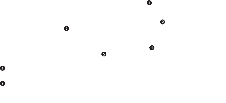
sion. Compression is when the dataset is piped through a zipping algorithm when it is
written to disk and the inverse unzipping algorithm when data is read from disk.
Compression happens on each chunk independently. Thus, compressed chunks end
up on disk with a varying number bytes, even though they all share the same chunk
shape. This strategy does have some storage overhead due to the zipping algorithm
itself. Even with the compression overhead, however, zipping may drastically reduce
file sizes and access times. For very regular data, it can reduce the data size nearly to
zero.
That compressing and decompressing each chunk can reduce read and write times
may, at first glance, seem counterintuitive. Compression and decompression clearly
require more processing power than simply copying an array directly into memory
from disk. However, because there is less total information transferred to and from
disk, the time spent unzipping the array can be far less than what would be required
to move the array around wholesale.
Compression is a feature of HDF5 itself. At a minimum, HDF5 is dependent on zlib,
a generic zipping library. Therefore, some form of compression is always available.
HDF5 compression capabilities are implemented with a plugin architecture. This
allows for a variety of different algorithms to be used, including user-defined ones.
PyTables supports the following compression routines: zlib (default), lzo, bzip2,
and blosc.
Compression is enabled through a mechanism called lters. Filters get their name
from the fact that they sit between the data in memory and the data on disk. Filters
perform transformations on any data passing through them. PyTables has a Filters
class that allows you to set both the compression algorithm name (as a string) and the
compression level, an integer from 0 (no compression) to 9 (maximum compression).
In PyTables, filters can be set on any group or dataset, or on the file itself. If unspeci‐
fied, a dataset or group will inherit the filters from the node directly above it in the
hierarchy. The following code demonstrates the various ways to apply filters:
# complevel goes from [0,9]
filters = tb.Filters(complevel=5, complib='blosc')
# filters may be set on the whole file
f = tb.open_file('/path/to/file', 'a', filters=filters)
f.filters = filters
# filters may also be set on most other nodes
f.create_table('/', 'table', desc, filters=filters)
f.root.group._v_filters = filters
Create a filters object.
Set filters when a file is created.
Compression | 253
www.it-ebooks.info

Set filters on a file after it is opened.
Set filters when a dataset is created.
Set filters on an existing dataset.
Additionally, note that when you’re choosing compression parameters, a mid-level (5)
compression is usually sufficient. There is no need to go all the way up to the maxi‐
mum compression (9), as it burns more processor time for only slight space improve‐
ments. It is also recommended that you use zlib if you must guarantee complete
portability across all platforms. This is because it is the only compression algorithm
guaranteed to be present by HDF5 itself. In general, if you are unsure of what to use
for compression, just use zlib. It is the safest and most portable option. If you know
you are going to stick to just using PyTables, however, it is ideal to use blosc. blosc
comes from PyTables and is optimized for HDF5 and tabular data. The performance
differences can be significant between blosc and zlib, which is a general-purpose
library.
You have now learned all the essential aspects of creating HDF5 files and using them
efficiently. However, you can interact with HDF5 in more ways than just through
PyTables. The next section will go over some of the tools that make working with
HDF5 even easier.
HDF5 Utilities
HDF5 is an excellent file format that supports many ways of accessing data from a
wide variety of programming languages. However, it can be a fair amount of work to
write a program to look into the contents of an HDF5 file every time you want to
inspect one. For this reason, a number of utilities have been developed that can help
you view or visualize the contents of these files. The three major command-line tools
for looking into HDF5 files are as follows:
h5ls
An ls-like tool for HDF5 files. This comes with HDF5. It displays metadata
about the file, its hierarchy, and its datasets.
h5dump
Prints the contents of an HDF5 table, in whole or in part, to the screen. This
comes with HDF5.
ptdump
A PyTables-based version of h5dump. This comes with PyTables.
254 | Chapter 10: Storing Data: Files and HDF5
www.it-ebooks.info

These three programs all take an HDF5 file as an argument. For example, using h5ls
on a file called 2srcs3rxts.h5 might display the following information about the data‐
sets in this file:
$ h5ls 2srcs3rxts.h5
AgentDeaths Dataset {7/Inf}
Agents Dataset {7/Inf}
Compositions Dataset {200/Inf}
InputFiles Dataset {1/Inf}
ResCreators Dataset {23/Inf}
Resources Dataset {85/Inf}
SimulationTimeInfo Dataset {1/Inf}
Transactions Dataset {17/Inf}
The first column contains the hierarchy node name. The second lists the node
type—every node here is a dataset, since we do not have any groups. The third
column contains the dataset size. The number before the slash is the current size
and the number after the slash is the maximum size. Here, Inf indicates that all
of the datasets are extensible and thus have infinite size.
For more information on how to use these utilities, type h5ls --help, h5dump --help,
or man ptdump at the command line, respectively.
For the more visually inclined, there are also graphical tools that can be used to inter‐
actively explore HDF5 files. The two major viewers right now are hdfview and ViTa‐
bles:
•hdfview is a Java-based HDF5 viewer and editor by the HDF group.
•ViTables is an independent PyTables- and Qt-based viewer for HDF5.
In general, hdfview is better at handling datasets that may extend infinitely in many
dimensions. On the other hand, ViTables is better at displaying large amounts of data
and also provides a graphical interface to the querying capabilities in PyTables. Both
tools are valuable in their own right. However, if you are mainly using PyTables to
interact with HDF5, ViTables should be all you need.
Storing Data Wrap-up
Having reached the end of this chapter, you should now be familiar with how to save
and load data, both to regular files and HDF5 databases. Most physics problems can
be cast into a form that is array-oriented. HDF5 is thus extremely helpful, since its
fundamental abstractions are all based on arrays. Naturally, other file formats and
databases exist and are useful for the cases they were designed around. Nothing quite
matches the sublime beauty of HDF5 for computational physics, though.
At this point, you should be comfortable with the following tasks:
Storing Data Wrap-up | 255
www.it-ebooks.info

• Saving and loading plain-text files in Python
• Working with HDF5 tables, arrays, and groups
• Manipulating the hierarchy to enable more efficient data layouts
and familiar with these concepts:
• HDF5 tables are conceptually the same as NumPy structured arrays.
•All data reading and writing in HDF5 happens per-chunk.
• A contiguous dataset is a dataset with only one chunk.
•Computation can happen per-chunk, so only a small subset of the data ever has
to be in memory at any given time.
• Going back and forth to and from disk can be very expensive.
• Querying allows you to efficiently read in only part of a table.
•Compressing datasets can speed up reading and writing, even though the pro‐
cessor does more work.
•HDF5 and other projects provide tools for inspecting HDF5 files from the com‐
mand line or from a graphical interface.
What you have learned so far with respect to storing data is the beginning of a very
deep topic. Sometimes as a computational scientist, you will need to dive in deeper
and learn more. Most of the time, you probably won’t. If you are already feeling over‐
whelmed, do not worry. Mastery of these topics will come through the natural course
of experience and practice. If you feel like this chapter has only started to get you
going, do not worry either. There is more to learn and more to enjoy. Understanding
data storage issues goes hand in hand with understanding how computers are built
and architected, and the trade-offs that are made in the process.
In the next chapter we shift gears, investigating data structures and their associated
algorithms that seem to crop up over and over again in computational physics.
256 | Chapter 10: Storing Data: Files and HDF5
www.it-ebooks.info

CHAPTER 11
Important Data Structures in Physics
In every domain there are algorithms and data structures that seem to pop up over
and over again. This is because of how useful these data structures are, rather than the
everything-is-a-nail-when-all-you-have-is-a-hammer phenomenon. This chapter will
present some of the important and common data structures for physics.
This is by no means a complete listing. Nor is this chapter meant to take the place of a
formal computer science data structures course—the canonical data structures in that
domain tend not to be the same as those in physics, though there is some overlap.
Rather, this is meant to whet your appetite. Many of the data structures here have
important variants, which will be mentioned but not discussed in detail.
We have already seen the most important data structure: arrays. Since these received
an entire chapter, we will forgo talking about them here. Instead, we will cover:
Hash tables
Useful whenever you want to create associations between data
Data frames
Similar to structured arrays or tables, but with added capabilities that make them
invaluable for experimental data
B-trees
Useful for managing array chunks and hierarchies
K-d trees
Space-partitioning data structures that are useful when trying to reason about the
closest neighboring points in space
Let’s start at the top of this list and work our way down.
257
www.it-ebooks.info

Hash Tables
Hash tables are everywhere in software development. The most common one that we
have used so far is the Python dictionary. This data structure is so important that it
forms the backbone of the Python language. Unlike in “Dictionaries” on page 73,
when they were first introduced, we now get to answer the question, “How does a
hash table work?”
A hash table is a special type of mapping from keys to values where the keys must be
unique. In the simplest case there is a keys column and a values column in the table.
The rows of this table are sorted according to the hash of the key modulus the length
of the table. Missing or empty rows are allowed. Item insertion and value lookup all
happen based on the hash value of the key. This means that their use presupposes a
good mechanism for hashing the keys, which, as discussed in “Sets” on page 71,
Python provides natively as the built-in hash() function.
For example, let’s look at a sample hash table that maps names of subatomic particles
to their mass in amu. We’ve set the length of the hash table to be eight even though
there will only be four entries, so some rows are unused. This can be seen in
Table 11-1.
Table 11-1. Sample hash table
i Key hash(key) hash(key)%8 Value
0
1 'neutrino' -4886380829903577079 1 3.31656614e-9
2
3
4
5 'proton' -4127328116439630603 5 1.00727647
6 'electron' 4017007007162656526 6 0.000548579909
7 'neutron' 3690763999294691079 7 1.008664
Note that the row index i where data appears in the table is exactly the same as the
result of the expression hash(key)%table_len. This lets us access elements based on
the key very quickly by recomputing the index expression and then jumping to that
point in the table. For example, the expression to find the value associated with the
258 | Chapter 11: Important Data Structures in Physics
www.it-ebooks.info

proton key, tab['proton'], would perform the following actions (in pseudocode) to
actually get that value:
table['proton'] ->
h = hash('proton')
i = h % size(tab)
return table[i].value
The main innovation of hash tables for associating data is that they prevent testing
equality over all of the keys to find the corresponding value. In fact, even though the
lookup mechanics are more complex, they perform on average much faster than if
you were to search through an equivalent data structure, like a list of tuples. In the
worst case, they still perform just as well as these alternatives.
For getting, setting, or deleting an item, hash tables are on average order-1. This
means that whether you have an array with 10 elements or 50 billion elements,
retrieving an item will take the same amount of time. In the worst case, getting, set‐
ting, and deleting items can take up to order-N, or O(N), where N is the size of the
table. This incredibly unlikely situation is equivalent to looping over the whole table,
which is what you would have to do in the worst case when using a list of tuples.
Big O Notation
Big O notation is a shorthand for describing the limiting behavior
of an algorithm with respect to the size of the data. This looks like a
function O() with one argument. It is meant to be read as “order
of” the argument. For example, O(N) means “order-N” and O(n
log(n)) is “order n log(n).” It is useful for quickly describing the
relative speed of an algorithm without having to think about the
specifics of the algorithm’s implementation.
However, there are two big problems with hash tables as formulated previously. What
happens when the table runs out of space and you want to add more items? And what
happens when two different keys produce the same hash?
Resizing
When a hash table runs out of space to store new items, it must be resized. This typi‐
cally involves allocating new space in memory, copying all of the data over, and reor‐
ganizing where each item lives in the array. This reorganization is needed because a
hash table takes the modulus by the table size to determine the row index.
From Table 11-1, take the neutrino key, whose hash is -4886380829903577079. This
hash value is the same no matter the table length. However, when you mod this value
by 8, it produces an index of 1. If the table size were doubled, then the neutrino hash
mod 16 would produce an index of 9. In general, each index will change as the result
Hash Tables | 259
www.it-ebooks.info

of a resize. Thus, a resize does more than just copy the data: it also rearranges it. For
example, consider resizing Table 11-1 to length 12. This expanded table can be seen
in Table 11-2.
Table 11-2. Longer sample hash table
i Key hash(key) hash(key)%12 Value
0
1
2 'electron' 4017007007162656526 2 0.000548579909
3 'neutron' 3690763999294691079 3 1.008664
4
5 'neutrino' -4886380829903577079 5 3.31656614e-9
6
7
8
9 'proton' -4127328116439630603 9 1.00727647
10
11
The two hash tables seen in Table 11-1 and Table 11-2 contain the same information
and are accessed in the same way. However, they have radically different layouts,
solely based on their size.
The size of the table and the layout are handled automatically by the hash table itself.
Users of a hash table should only have to worry about resizing insofar as to under‐
stand that multiple insertion operations that each emplace one item will almost
always be more expensive than a single insertion that emplaces multiple items. This is
because multiple insertions will force the hash table to go through all of the inter‐
mediate sizes. On insertion of multiple items, the hash table is allowed to jump
directly to the final size.
260 | Chapter 11: Important Data Structures in Physics
www.it-ebooks.info

For Python dictionaries, automatic resizing means that you should
try to update() dicts when possible rather than assigning new
entries (d[key] = value) over and over again. Given two dictionar‐
ies x and y, it is much better to use x.update(y) than to write:
for key, value in y.items():
x[key] = value
Different hash table implementations choose different strategies for deciding when to
resize (table is half full, three-quarters full, completely full, never) and by how much
to resize (double the size, half the size, not at all). Resizing answers the question of
what to do when a hash table runs out of space. However, we still need to address
what to do when two keys accidentally produce the same index.
Collisions
A hash collision occurs when a new key hashes to the same value as an existing key in
the table. Even though the space of hash values is huge, ranging from
-9223372036854775808 to 9223372036854775807 on 64-bit systems, hash collisions
are much more common than you might think. For simple data, it is easy to show
that an empty string, the integer 0, the float 0.0, and False all hash to the same value
(namely, zero):
hash('') == hash(0) == hash(0.0) == hash(False) == 0
However, even for random keys, hash collisions are an ever-present problem. Such
collisions are an expression of the birthday paradox. Briefly stated, the likelihood that
any two people in a room will have the same birthday is much higher than that of two
people sharing a specific birthday (say, October 10th). In terms of hash tables, this
can be restated as “the likelihood that any pair of keys will share a hash is much
higher than the probability that a key will have a given hash (say, 42) and that another
key will have that same hash (again, 42).”
Set the variable s as the size of the table and N as the number of distinct hash values
possible for a given hash function. An approximate expression for the likelihood of a
hash collision is given by pcs:
pcs=1−e
−s s − 1
2N
This may be further approximated as:
pcs=s2
2N
Hash Tables | 261
www.it-ebooks.info
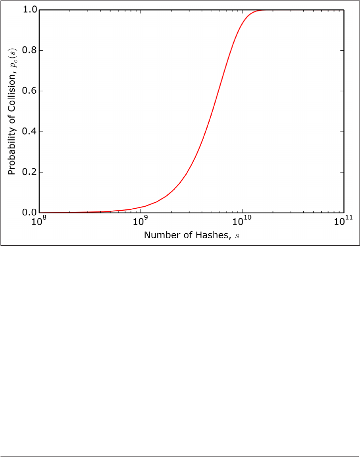
For Python dicts, N=2**64, and Figure 11-1 shows this curve. After about a billion
items, the probability of a hash collision in a Python dict starts going up dramati‐
cally. For greater than 10 billion items, a collision is effectively guaranteed. This is
surprising, since the total range of the space is about 1.844e19 items. This means that
a collision is likely to happen even though only one-billionth of the space is filled. It is
important to note that the shape of this curve is the same for all values of N, though
the location of the inflection point will change.
Figure 11-1. Hash collision probability for Python dictionaries
Given that hash collisions will happen in any real application, hash table implementa‐
tions diverge in the way that they choose to handle such collisions. Some of the
strategies follow the broad strokes presented here:
•Every index is a bucket, or list of key/value pairs. The hash will take you to the
right bucket, and then a linear search through every item in the bucket will find
the right value. This minimizes the number of resizes at the expense of a linear
search and a more complex data structure. This is known as separate chaining.
•In the event of a collision, the hash is modified in a predictable and invertible
way. Continued collisions will cause repeated modifications and hops. Searching
for a key will first try the hash and the successive modifications. This is known as
open addressing and is the strategy that Python dictionaries implement. This has
the benefit that all items live flat in the table. There are no sublists to search
262 | Chapter 11: Important Data Structures in Physics
www.it-ebooks.info

through. However, this comes at the cost that the index of a key is not computa‐
ble from the hash of the key alone. Rather, the index depends on the full history
of the hash table—when items were inserted and deleted.
•Always resize to the point of zero collisions. This works well where all of the keys
must share the same type. This is sometimes called a bidirectional or bijective
hash map because the keys are uniquely determined by their hashes, just like the
hashes are uniquely determined by their keys.
As a user of hash tables, the details of how the collisions are handled are less impor‐
tant than the fact that collisions happen and they affect performance.
In summary, hash tables are beautiful and ubiquitous. On average they have incredi‐
ble performance properties, being order-1 for all operations. This comes at the
expense of significantly increased implementation complexity over more fundamen‐
tal containers, such as arrays. Luckily, since almost every modern programming lan‐
guage supports hash tables natively, only in the rarest circumstances will you ever
need to worry about writing one yourself.
Up next, we will talk about another data structure that you should never have to
implement, but that is crucial to have in your analysis toolkit.
Data Frames
A relative newcomer, the data frame is a must-have data structure for data analysis. It
is particularly useful to experimentalists. The data frame is an abstraction of tables
and structured arrays. Given a collection of 1D arrays, the data frame allows you to
form complex relationships between those arrays. Such relationships extend beyond
being columns in a table, though that is possible too. One of the defining features of
data frames that makes them invaluable for experimentalists is that they gracefully
handle missing data. Anyone who has worked with real data before knows that this is
a feature that should not be overlooked.
The data frame was popularized by the R language, which has a native data frame
implementation and is largely (though not solely) used for statistics. More recently,
the pandas package for Python implements a data frame and associated tools.
Data frames are effectively tables made up of named columns called series. Unlike in
other table data structures we have seen, the series that make up a data frame may be
dynamically added to or removed from the frame. A series can be thought of as a 1D
NumPy array (it has a dtype) of values along with a corresponding index array. The
index specifies how values of the series are located. If no index is provided, regular
integers spanning from zero to one minus the length of the series are used. In this
case, series are very similar to plain old NumPy arrays. The value of indexes, as we
will see, is that they enable us to refer to data by more meaningful labels than zero
Data Frames | 263
www.it-ebooks.info

through N-1. For example, if our values represented particle counts in a detector, the
index could be made up of the strings 'proton', 'electron', and so on. The data
frames themselves may also have one or more index arrays. If no index is provided,
then zero to N-1 is assumed. In short, data frames are advanced in-memory tables
that allow human-readable data access and manipulation through custom indexes.
The usage of data frames was first presented in Chapter 8. Here, we will cover their
basic mechanics. For the following examples, you’ll need to import the pandas pack‐
age. Note that like numpy and pytables, the pandas package is almost always impor‐
ted with an abbreviated alias, namely pd:
import pandas as pd
Let’s start by diving into series.
Series
The Series class in pandas is effectively a one-dimensional NumPy array with an
optional associated index. While this is not strictly accurate, much of the NumPy fla‐
vor has been transferred to Series objects. A series may be created using array-like
mechanisms, and they share the same primitive dtype system that NumPy arrays use.
The following example creates a series of 64-bit floats:
Code Returns
pd.Series([42, 43, 44], dtype='f8') 0 42
1 43
2 44
dtype: float64
Index and values columns
dtype of the values
Note that the column on the left is the index, while the column on the right displays
the values. Alternatively, we could have passed in our own custom noninteger index.
The following shows a series s with various particle names used as the index and the
values representing the number of the associated particle that a detector has seen:
Code Returns
s = pd.Series([42, 43, 44],
index=["electron",
"proton",
"neutron"])
electron 42
proton 43
neutron 44
dtype: int64
264 | Chapter 11: Important Data Structures in Physics
www.it-ebooks.info

The index itself is very important, because this dictates how the elements of the series
are accessed. The index is an immutable ndarray that is composed of only hashable
data types. As with the keys in a dictionary, the hashability ensures that the elements
of an index may be used to safely retrieve values from a series. In the following code
snippet, we see that we can index into a series in a dict-like fashion to pull out a sin‐
gle value. We can also slice by indices to create a subseries, because the index itself has
an order. Finally, even though the series has an index, we can always go back to
indexing with integers:
Code Returns
s['electron']
# inclusive bounds
s['electron':'proton']
# integer indexing still OK
s[1:]
42
electron 42
proton 43
dtype: int64
proton 43
neutron 44
dtype: int64
Series may also be created from dictionaries. In this case, the keys become the index
and the elements are sorted according to the keys. The following code demonstrates a
series t being created from a dict with string particle keys and associated integer
values:
Code Returns
t = pd.Series({'electron': 6,
'neutron': 28,
'proton': 496,
'neutrino': 8128})
electron 6
neutrino 8128
neutron 28
proton 496
dtype: int64
Additionally, arithmetic and other operations may be performed on a series or a com‐
bination of series. When two series interact, if an element with a particular index
exists in one series and that index does not appear in the other series, the result will
contain all indices. However, the value will be NaN (Not a Number) for the missing
index. This means that the datasets will only grow, and you will not lose an index.
However, the presence of a NaN may not be desired. Reusing the s and t series from
our previous examples, the following code adds these two series together. Since t has
a neutrino element that s does not, the expression s + t will have a neutrino ele‐
ment, but its value will be NaN:
Data Frames | 265
www.it-ebooks.info

Code Returns
s + t electron 48
neutrino NaN
neutron 72
proton 539
dtype: float64
The advantage of having NaN elements show up in the resulting series is that they
make it very clear that the input series to the operation did not share a common basis.
Sometimes this is OK, like when you do not care about neutrinos. At other times, like
when you want to sum up the total number of counts, the NaN elements are problem‐
atic. This forces you to deal with them and adhere to best practices. There are two
approaches for dealing with a NaN. The first is to go back to the original series and
make sure that they all share a common index. The second is to filter or mask out the
NaN elements after the other operations have completed. In general, it is probably best
to go back to the original series and ensure a common basis for comparison.
Unless otherwise specified, for almost all operations pandas will return a copy of the
data rather than a view, as was discussed in “Slicing and Views” on page 208. This is
to prevent accidental data corruption. However, it comes at the cost of speed and
memory efficiency.
Now that we know how to manipulate series on their own, we can combine many ser‐
ies into a single data frame.
The Data Frame Structure
The DataFrame object can be understood as a collection of series. These series need
not share the same index, though in practice it is useful if they do because then all of
the data will share a common basis. The data frame is a table-like structure akin to a
NumPy structured array or a PyTables Table. The usefulness of data frames is the
same as other table data structures. They make analyzing, visualizing, and storing
complex heterogeneous data easier. Data frames, in particular, provide a lot of helpful
semantics that other table data structures do not necessarily have. Data frames are
distinct from other table-like structures, though, because their columns are series, not
arrays. We can create a data frame from a dictionary of arrays, lists, or series. The
keys of the dictionary become the column names. Reusing the definitions of s and t
from before, we can create a data frame called df:
266 | Chapter 11: Important Data Structures in Physics
www.it-ebooks.info

Code Returns
df = pd.DataFrame({'S': s, 'T': t}) S T
electron 42 6
neutrino NaN 8128
neutron 44 28
proton 43 496
[4 rows x 2 columns]
You can also create a data frame from a NumPy structured array or a list of tuples.
Data frames may be saved and loaded from CSV files, HDF5 files (via PyTables),
HTML tables, SQL, and a variety of other formats.
Data frames may be sliced, be appended to, or have rows removed from them, much
like other table types. However, data frames also have the sophisticated indexing
semantics that series do. The following code demonstrates some data frame manipu‐
lations:
Code Returns
df[::2]
dg = df.append(
pd.DataFrame({'S': [-8128]},
index=['antineutrino']))
dh = dg.drop('neutron')
Slice every other element.
Add a new index to the data frame and value to S.
Delete the neutron index.
S T
electron 42 6
neutron 44 28
[2 rows x 2 columns]
S T
electron 42 6
neutrino NaN 8128
neutron 44 28
proton 43 496
antineutrino -8128 NaN
[5 rows x 2 columns]
S T
electron 42 6
neutrino NaN 8128
proton 43 496
antineutrino -8128 NaN
[4 rows x 2 columns]
You may also easily transpose the rows and columns via the T attribute, as seen here:
Data Frames | 267
www.it-ebooks.info

Code Returns
df.T electron neutrino neutron proton
S 42 NaN 44 43
T 6 8128 28 496
[2 rows x 4 columns]
Arithmetic and other operations may be applied to the whole data frame. The follow‐
ing example creates a Boolean mask data frame by comparing whether the data is less
than 42. Note that the Boolean mask is itself another data frame:
Code Returns
df < 42 S T
electron True True
neutrino False False
neutron False True
proton True False
[4 rows x 2 columns]
A major innovation of the data frame is the ability to add and remove columns easily.
With NumPy structured arrays, adding a new column to an existing array involves
creating a new compound dtype to represent the new table, interleaving the new col‐
umn data with the existing table, and copying all of the data into a new structured
array. With data frames, the notion of a column is flexible and interchangeable with
the notion of an index. Data frames are thus much more limber than traditional
tables for representing and manipulating data. Column access and manipulation
occurs via dict-like indexing. Such manipulation can be seen with the existing df
data frame:
268 | Chapter 11: Important Data Structures in Physics
www.it-ebooks.info

Code Returns
# accessing a single column
# will return a series
df['T']
# setting a name to a series
# or expression will add a
# column to the frame
df['small'] = df['T'] < 100
# deleting a column will
# remove it from the frame
del df['small']
electron 6
neutrino 8128
neutron 28
proton 496
Name: T, dtype: int64
S T small
electron 42 6 True
neutrino NaN 8128 False
neutron 44 28 True
proton 43 496 False
[4 rows x 3 columns]
S T
electron 42 6
neutrino NaN 8128
neutron 44 28
proton 43 496
[4 rows x 2 columns]
These kinds of column operations, along with reindexing, groupby(), missing data
handling, plotting, and a host of other features, make data frames an amazing data
structure. We have only scratched the surface here. While they may not be able to
handle the kinds of data volumes that parallel chunked arrays do, for everyday data
analysis needs nothing beats the flexibility of data frames. As long as your data can
nicely fit into memory, then data frames are a great choice.
The next section takes us to the other end of the data volume spectrum, with a
detailed discussion of B-trees.
B-Trees
B-trees are one of the most common data structures for searching over big chunks of
data. This makes them very useful for databases. It is not an understatement to say
that HDF5 itself is largely based on the B-tree. Chunks in a dataset are stored and
managed via B-trees. Furthermore, the hierarchy itself (the collection of groups and
arrays and tables) is also managed through a B-tree.
A B-tree is a tree data structure where all of the nodes are sorted in a breadth-first
manner. Each node may have many subnodes. This structure makes it easy to search
for a specific element because, starting at the top root node, you can simply test
whether the value you are looking for is greater or less than the values in the nodes
that you are at currently. The following example represents a B-tree of the Fibonacci
sequence. Here, the square brackets ([]) represent nodes in the B-tree. The numbers
inside of the square brackets are the values that the B-tree is currently storing:
B-Trees | 269
www.it-ebooks.info

.--.--------[5 89]----------.
/ | |
[1 2 3] [21] .---.--[233 1597]--.
/ \ / | |
[8 13] [34 55] [144] [377 610 987] [2584 4181]
It is important to note that each node in a B-tree may store many values, and the
number of values in each node may vary. In the simplest case, where each node is
constrained to have a single value, the B-tree becomes a binary search tree (not to be
confused with a binary tree, which we won’t discuss here). The following diagram
shows a binary search tree specialization of a small B-tree:
[5]
/ \
[2] [8]
/ \
[1] [3]
B-trees (and binary search trees) may be rotated. This means that the nodes can be
rearranged to have a different structure without breaking the search and ordering
properties. For example, the tree above may be rotated to the following tree with
equivalent average search properties:
[2]
/ \
[1] [5]
/ \
[3] [8]
B-trees are very effective for nonlinearly organizing array data. The index of the array
determines on which node in the tree the array lives. The tree itself manages the loca‐
tions of all of the nodes. The nodes manage the data chunks assigned to them. The
ability for nodes to be inserted and removed at arbitrary indices allows for arrays to
have missing chunks, be infinitely long, and be extendable.
In practice, B-trees tend to follow some additional simple rules as a way of reaping
performance benefits and making the logic easier to understand:
•The height of the tree, h, is constant. All leaves (terminal nodes) exist at the same
height.
• The root node has height 0.
•The maximum number of child nodes, m, is kept below a constant number across
all nodes.
• Nodes should be split as evenly as possible over the tree in order to be balanced.
The size of a tree is measured by how many nodes (n) it has. Getting, setting, and
deleting nodes in a B-tree are all order log(n) operations on average. The worst-case
270 | Chapter 11: Important Data Structures in Physics
www.it-ebooks.info

behavior for these operations is also order log(n), and it is possible to do better than
this in the unlikely event that the node you are looking for is higher up the tree than
being on a leaf. These properties make B-trees highly desirable from a reliability
standpoint. Table 11-3 shows a comparison between B-tree and hash table perfor‐
mance.
Table 11-3. Performance comparison between B-trees and hash tables for common
operations
Operation Hash table average Hash table worst B-tree average B-tree worst
Get: x[key] O(1) O(n) O(log n) O(log n)
Set: x[key] = value O(1) O(n) O(log n) O(log n)
Delete: del x[key] O(1) O(n) O(log n) O(log n)
In practice, you will want to use a B-tree whenever you need to quickly find an ele‐
ment in a large, regular, and potentially sparse dataset. If you happen to be writing a
database, B-trees are probably what you want to use to index into the datasets on disk.
B-trees were presented here because they are used frequently under the covers of the
databases that we have already seen, such as HDF5. Furthermore, if you have a map‐
ping that you want to ensure is always sorted by its keys, you will want to use a B-tree
instead of a dictionary. Still, in most other circumstances, a dictionary, NumPy array,
or data frame is typically a better choice than a B-tree.
B-trees as a data structure are too complex to give a full and working example here.
While there is no accepted standard implementation in Python, there are many libra‐
ries that have support for B-trees. You can install and play around with them. A few
that are worth looking into are:
btree
A dict-like C extension module implementation
BTrees
A generic B-tree implementation optimized for the Zope Object Database
(ZODB)
blist
A list-, tuple-, set-, and dict-like data structure implemented as a B+-tree (a
variant of a strict B-tree)
Let’s take a quick look at the blist package, since it has the best support for Python 2
and 3. This package has a sorteddict type that implements a traditional B-tree data
structure. Creating a sorteddict is similar to creating a Python dictionary. The fol‐
B-Trees | 271
www.it-ebooks.info

lowing code imports sorteddict, creates a new B-tree with some initial values, and
adds a value after it has been created:
Code Returns
from blist import sorteddict
b = sorteddict(first="Albert",
last="Einstein",
birthday=[1879, 3, 14])
b['died'] = [1955, 4, 18]
list(b.keys())
sorteddict({'birthday': [1879, 3, 14],
'first': 'Albert',
'last': 'Einstein'})
['birthday', 'died', 'first', 'last']
The keys always appear sorted, because of how B-trees work. Even though the sorted
dict implements a dictionary interface, its performance characteristics and underly‐
ing implementation are very different from that of a hash table.
We have now seen three possible ways to store associations
between keys and values: hash tables, series, and B-trees. Which
one you should use depends on your needs and the properties of
the data structure.
B-trees are great for data storage and for organizing array chunks. For this reason,
they are used in databases quite a bit. The next section presents a different tree struc‐
ture that excels at storing geometry.
K-D Trees
A k-d tree, or k-dimensional tree, is another tree data structure. This one excels at
finding the nearest neighbor for points in a k-dimensional space. This is extraordi‐
narily useful for many physics calculations. Often times, when solving geometric par‐
tial differential equations, the effects that matter the most in the volume at hand come
from the directly surrounding cells. Splitting up the problem geometry into a k-d tree
can make it much faster to find the nearest neighbor cells.
The big idea behind k-d trees is that any point (along with the problem bounds)
defines a k-1 dimensional hyperplane that partitions the remaining space into two
sections. For example, in 1D a point p on a line l will split up the line into the space
above p and the space below p. In two dimensions, a line will split up a box. In three
dimensions, a plane will split a cube, and so on. The points in a k-d tree can then be
placed into a structure similar to a binary search tree. The difference here is that sort‐
ing is based on the point itself along an axis a and that a is equal to the depth level of
272 | Chapter 11: Important Data Structures in Physics
www.it-ebooks.info

the point modulo the number of dimensions, k. Thus, a effectively defines an orienta‐
tion for how points should partition the space.
K-d trees are not often modified once they are instantiated. They typically have get or
query methods but do not have insert or delete methods. The structure of space is
what it is, and if you want to restructure space you should create a whole new tree.
For n points, k-d trees are order log(n) on average for all of their operations. In the
worst case, they are order n.
Furthermore, k-d trees are most effective when k is small. This is ideal for physics cal‐
culations, where k is typically 3 for three spatial dimensions and rarely goes above 6.
For simplicity, the examples here will use k=2. This makes the partitions simple line
segments.
Since we do not need to worry about insertions or deletions, we can represent a sam‐
ple k-d tree algorithm as follows:
class Node(object):
def __init__(self, point, left=None, right=None):
self.point = point
self.left = left
self.right = right
def __repr__(self):
isleaf = self.left is None and self.right is None
s = repr(self.point)
if not isleaf:
s = "[" + s + ":"
if self.left is not None:
s += "\n left = " + "\n ".join(repr(self.left).split('\n'))
if self.right is not None:
s += "\n right = " + "\n ".join(repr(self.right).split('\n'))
if not isleaf:
s += "\n ]"
return s
def kdtree(points, depth=0):
if len(points) == 0:
return None
k = len(points[0])
a = depth % k
points = sorted(points, key=lambda x: x[a])
i = int(len(points) / 2) # middle index, rounded down
node_left = kdtree(points[:i], depth + 1)
node_right = kdtree(points[i+1:], depth + 1)
node = Node(points[i], node_left, node_right)
return node
A tree consists of nodes.
K-D Trees | 273
www.it-ebooks.info

A node is defined by its point. Since this is a binary search tree, it may have one
node to the left and one node to the right.
A string representation of the node given its relative location in the tree.
A recursive function that returns the root node given a list of points. This will
automatically be balanced.
As you can see, the Node class is very simple. It holds a point, a left child node, and a
right child node. The heavy lifting is done by the kdtree() function, which takes a
sequence of points and recursively sets up the nodes. Each node having only two chil‐
dren makes k-d trees much easier to manipulate than B-trees. As an example, con‐
sider the following random sequence of points internal to the range [0, 6] in 2-space.
These can be placed into a k-d tree using code like the following:.
Code Returns
points = [(1, 2), (3, 2),
(5, 5), (2, 1),
(4, 3), (1, 5)]
root = kdtree(points)
print(root)
[(3, 2):
left = [(1, 2):
left = (2, 1)
right = (1, 5)
]
right = [(5, 5):
left = (4, 3)
]
]
The partitioning generated by this k-d tree is visualized in Figure 11-2.
For a rigorously tested, out-of-the-box k-d tree, you should use the KDTree class
found in scipy.spatial. This is a NumPy-based formulation that has more impres‐
sive querying utilities than simply setting up the tree. The implementation of KDTree
also fails over to a brute-force search when the search space goes above a user-
definable parameter. Using the points list from our previous example, the following
creates an instance of the KDTree class:
from scipy.spatial import KDTree
tree = KDTree(points)
274 | Chapter 11: Important Data Structures in Physics
www.it-ebooks.info
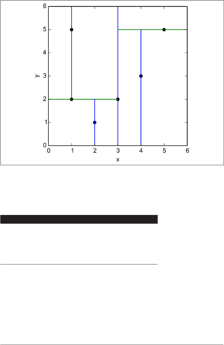
Figure 11-2. K-d tree partitioning example
This tree object has a data attribute that is a NumPy array representing the points. If
the points were originally a NumPy array the data attribute would be a view, not a
copy. The following shows that the tree’s data retains the order of the original points:
Code Returns
tree.data array([[1, 2],
[3, 2],
[5, 5],
[2, 1],
[4, 3],
[1, 5]])
The query() method on the KDTree class takes a sequence of points anywhere in
space and returns information on the N nearest points. It returns an array of distances
to these points as well as the indices into the data array of the points themselves. Note
that query() does not return the cell in which a point lives. Using the tree we con‐
structed previously again, let’s find the nearest point in the tree to the location (4.5,
1.25):
K-D Trees | 275
www.it-ebooks.info
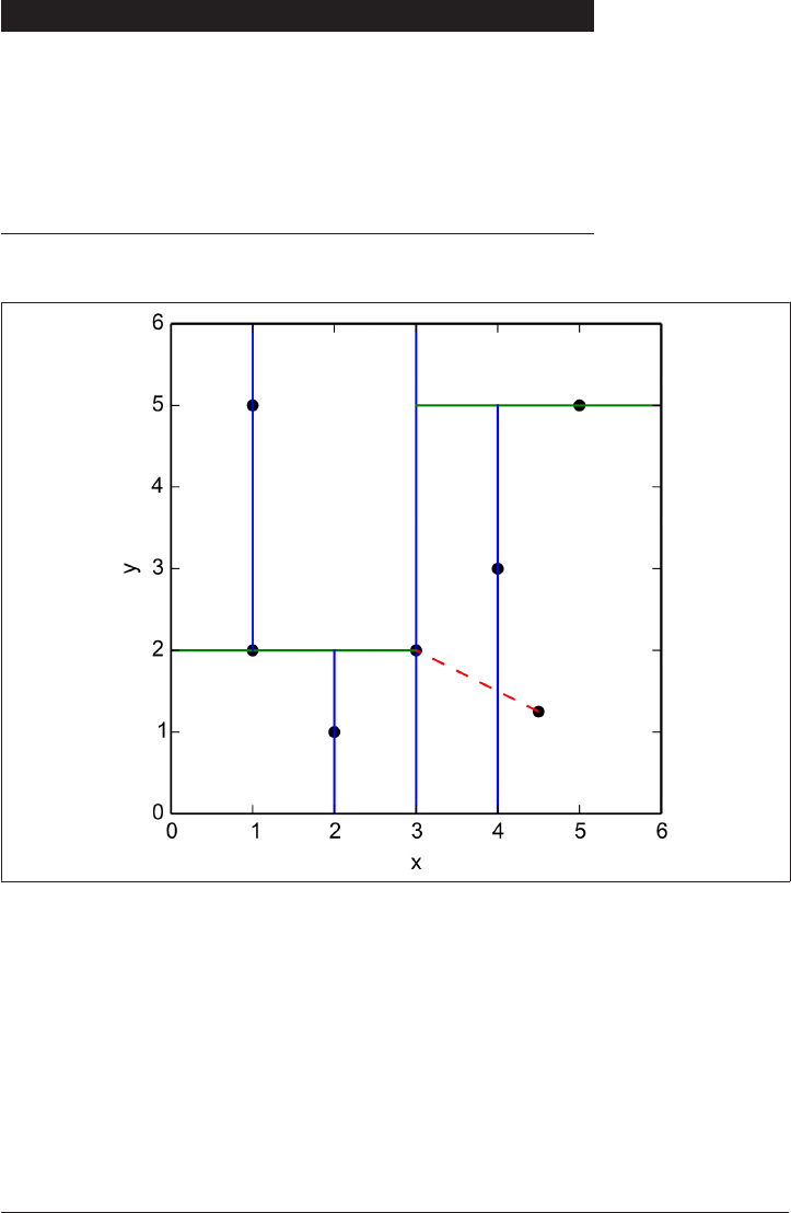
Code Returns
# query() defaults to only the closest point
dist, idx = tree.query([(4.5, 1.25)])
dist
idx
# fancy index by idx to get the point
tree.data[idx]
# results
array([ 1.67705098])
array([1])
array([[3, 2]])
The result of this query may be seen graphically in Figure 11-3.
Figure 11-3. K-d tree nearest neighbor query, distance shown as dashed line
These querying capabilities are very useful whenever you have data for some points
in space and want to compute the corresponding values for any other point based on
the data that you have. For example, say each of your points has a corresponding
measurement for magnitude of the electric field at that location. You could use a k-d
tree to determine the nearest neighbor to any point in space. This then lets you
approximate the electric field at your new point based on the distance from the clos‐
est measured value. In fact, this strategy may be used for any scalar or vector field.
276 | Chapter 11: Important Data Structures in Physics
www.it-ebooks.info

The underlying physics may change, but finding the nearest neighbors via a k-d tree
does not.
Due to their broad applicability, k-d trees come up over and over again in computa‐
tional physics. For more information on the KDTree class, please refer to the SciPy
documentation.
Data Structures Wrap-up
As a scientist, organizing data is an integral part of daily life. However, there are many
ways to represent the data you have. Familiarity with a variety of strategies gives you
more flexibility to choose the option that best fits any given task. What you have
learned here are some of the most significant to physics-based fields. Of these, hash
tables are useful to just about everyone (and are not limited to physics). K-d trees, on
the other hand, are most useful when you’re thinking about problems spatially. Physi‐
cists do so a lot more than other folks. You should now be familiar with the following
concepts:
• Hash tables require a good hash function, which is provided to you by Python.
• Resizing a hash table can be expensive.
•Hash collisions will happen.
• Series are like NumPy arrays but with more generic indexing capabilities.
• Data frames are like tables with series as columns.
•Data frames handle missing data through NaN values.
• B-trees can be used to organize chunks of an array.
•You may rotate B-trees to change their structure without altering their perfor‐
mance.
• A binary search tree is a B-tree with only one piece of data per node.
•K-d trees are a variant of the binary search tree that are organized by points in k-
dimensional space.
• K-d trees are exceptionally useful for problems involving geometry.
Now that you know how to represent your data, the next chapter will teach you how
to analyze and visualize it.
Data Structures Wrap-up | 277
www.it-ebooks.info

CHAPTER 12
Performing in Parallel
A natural way to approach parallel computing is to ask the question, “How do I do
many things at once?” However, problems more often arise in the form of, “How do I
solve my one problem faster?” From the standpoint of the computer or operating sys‐
tem, parallelism is about simultaneously performing tasks. From the user’s perspec‐
tive, parallelism is about determining dependencies between different pieces of code
and data so that the code may be executed faster.
Programming in parallel can be fun. It represents a different way of thinking from the
traditional "x then y then z" procedure that we have seen up until now. That said, par‐
allelism typically makes problems faster for the computer to execute, but harder for
you to program. Debugging, opening files, and even printing to the screen all become
more difficult to reason about in the face of P processors. Parallel computing has its
own set of rewards, challenges, and terminology. These are important to understand,
because you must be more like a mechanic than a driver when programming in
parallel.
Physicists often approach parallelism only when their problems finally demand it.
They also tend to push back that need as far as possible. It is not yet easier to program
in parallel than it is to program procedurally. Here are some typical reasons that par‐
allel solutions are implemented:
• The problem creates or requires too much data for a normal machine.
• The sun would explode before the computation would finish.
• The algorithm is easy to parallelize.
•The physics itself cannot be simulated at all with smaller resources.
This chapter will focus on how to write parallel programs and make effective use of
your computing resources. We will not be focusing on the underlying computer
279
www.it-ebooks.info

science that enables parallelism, although computer science topics in parallel comput‐
ing are fascinating. You do not need to know how to build a bicycle to be able to ride
one. By analogy, you can create computational physics programs without knowing
how to build your own supercomputer. Here, we opt to cover what you need to know
to be effective in your research. Let’s start with some terminology.
Scale and Scalability
While parallelism is often necessary for large problems, it is also useful for smaller
problems. This notion of size is referred to as scale. Computational scale is a some‐
what ambiguous term that can be measured in a few different ways: the number of
processes, the computation rate, and the data size.
A simple definition for scale is that it is proportional to the number of P processes
that are used. This provides the maximum degree of parallelism that is possible from
the point of view of the computer.
It is better to talk about the number of processes used rather than
the number of processors. This is because the number of processes
is independent of the hardware.
Another popular measure of parallelism is the number of floating-point operations
per second, or FLOPS. This is the rate at which arithmetic operations (addition, mul‐
tiplication, modulus, etc.) happen on float data over the whole machine. Since a lot of
scientific code mostly deals with floats, this is a reasonable measure of how fast the
computer can do meaningful computations. FLOPS can sometimes be misleading,
though. It makes no claims about integer operations, which are typically faster and
important for number theory and cryptography. It also makes no claims about string
operations, which are typically slower and important for genomics and biology. The
use of graphics processing units (GPUs) is also a way to game the FLOPS system.
GPUs are designed to pump through large quantities of floating-point operations, but
they need special programming environments and are not great in high-data situa‐
tions. FLOPS is a good measure of how fast a computer can work in an ideal situa‐
tion, but bear in mind that obtaining that ideal can be tricky.
The final measure of scale that is commonly used is how much data is generated as a
result of the computation. This is easy to measure; simply count how many bytes are
written out. This tells you nothing of how long it took to generate those bytes, but the
data size is still important for computer architects because it gives a scale of how
much RAM and storage space will be required.
There are two important points to consider given the different scale metrics:
280 | Chapter 12: Performing in Parallel
www.it-ebooks.info

1. A metric tends to be proportional to the other metrics—a machine that is large
on one scale is often large on the others.
2. Achieving a certain computation scale is preceded by having achieved lower
scales first.
For example, point 1 states that when you have more processes available, you are
capable of more FLOPS. Point 2 says that you cannot store a petabyte without storing
a terabyte, you cannot store a terabyte without storing a gigabyte, and so on.
Together, these points imply that you should try to scale up your code slowly and
methodically. Start with the trivial case of trying to run your code on one process.
Then attempt 10 processes, and then 100, and up. It may seem obvious, but do not
write code that is supposed to work on a million cores right out of the gate. You can’t,
and it won’t. There will be bugs, and they will be hard to track down and resolve.
Slowly scaling up allows you to address these issues one by one as they emerge, and
on the scale at which they first appear.
Scalability is an indication of how easy or hard it is to go up in scale. There are many
ways of measuring scalability, but the one that applies the most to computing is run‐
time performance. For a given machine, scalability is often measured in strong and
weak forms.
Strong scaling is defined as how the runtime changes as a function of the number of
processors for a fixed total problem size. Typically this is measured by the speedup, s.
This is the ratio of time it takes to execute on one processor, t1, to the time it takes to
execute on P processors, tP:
sP=t1
tP
In a perfectly efficient system, the strong scaling speedup is linear. Doubling the
number of processors will cause the problem to run in half the time.
Weak scaling, on the other hand, is defined as how the runtime changes as a function
of the number of processors for a fixed problem size per processor. This is typically
measured in what is known as the sizeup, z. For a problem size N, the sizeup is
defined as:
zP=t1
tP×NP
N1
In a perfectly weak scaling system, the sizeup is linear. Doubling the number of pro‐
cessors will double the size of the problem that may be solved.
Scale and Scalability | 281
www.it-ebooks.info

Both strong and weak scaling are constrained by Amdahl’s law. This law follows from
the observation that some fraction of an algorithm–call it α–cannot be parallelized.
Thus, the maximum speedup or sizeup possible for P processors is given as:
max s P =1
α−1 − α
P
Taking this to the limit of an infinite number of processors, the maximum possible
speedup is given as:
max s= lim
P∞
1
α−1−α
P
=1
α
Thus, Amdahl’s law states that if, for example, 10% of your program is unparalleliza‐
ble (α= 0. 1), then the best possible speedup you could ever achieve is a factor of 10.
In practice, it is sometimes difficult to know what α is in more sophisticated algo‐
rithms. Additionally, α is usually much smaller than 0.1, so the speedups achievable
are much greater. However, Amdahl’s law is important because it points out that there
is a limit.
What matters more than problem scale, though, is the algorithm. The next section
discusses the types of parallel problems that exist.
Problem Classication
Certain algorithms lend themselves naturally to parallelism, while others do not.
Consider summing a large array of numbers. Any part of this array may be summed
up independently from any other part. The partial sums can then be summed
together themselves and achieve the same result as if the array had been summed in
series. Whether or not the partial sums are computed on the same processor or at the
same time does not matter. Algorithms like this one with a high degree of independ‐
ence are known as embarrassingly parallel problems. Other embarrassingly parallel
examples include Monte Carlo simulations, rendering the Mandelbrot set, and certain
optimization techniques such as stochastic and genetic algorithms. For embarrass‐
ingly parallel problems, the more processors that you throw at them, the faster they
will run.
On the other hand, many problems do not fall into this category. This is often
because there is an unavoidable bottleneck in the algorithm. A classic operation that
is difficult to parallelize is inverting a matrix. In general, every element of the inverse
matrix is dependent on every element in the original matrix. This makes it more diffi‐
cult to write efficient parallel code, because every process must know about the entire
282 | Chapter 12: Performing in Parallel
www.it-ebooks.info

original matrix. Furthermore, many operations are the same or similar between
elements.
All hope is not lost for non-embarrassingly parallel problems. In most cases there are
mathematical transformations you can make to temporarily decrease the degree of
dependence in part of the problem. These transformations often come with the cost
of a little excess computing elsewhere. On the whole though, the problem solution
will have faster runtimes due to increased parallelism. In other cases, the more you
know about your data the more parallelism you can eke out. Returning to the inverse
matrix example, if you know the matrix is sparse or block diagonal there are more
parallelizable algorithms that can be used instead of a fully generic solver. It is not
worth your time or the computer’s time to multiply a bunch of zeros together.
At large scales, these classifications have names based on the architecture of the
machines that run them rather than the properties of the algorithm. The better
known of these is high-performance computing (HPC). Such machines are built to run
non-embarrassingly parallel problems. When people talk about supercomputers, they
are referring to HPC systems. As a rule, all of the nodes on an HPC system are the
same. Each node has the same number of CPUs and GPUs and the same amount of
memory, and each processor runs the same operating system. Though the nodes are
connected together in a predetermined topology (rings, tauruses, etc.), node homoge‐
nization gives the illusion that any subset of nodes will act the same as any other sub‐
set of nodes of the same size.
You should consider using HPC systems when your problems are large and not
embarrassingly parallel, or they are large and you need the node homogeneity. That
said, RAM per node has been on a downward trend in HPC, so if you have a high-
memory application, you have extra work to do in making the algorithm data parallel
in addition to compute parallel. Because they are a little trickier to program, but not
difficult conceptually, we will largely skip discussing data-parallel algorithms here.
HPC’s lesser-known sibling is called high-throughput computing (HTC). As its name
implies, HTC is designed to pump through as many operations as possible with little
to no communication between them. This makes HTC ideally suited to embarrass‐
ingly parallel problems. Nodes in an HTC system need not be the same. In some
cases, they do not even have to share the same operating system. It is incorrect to
think of an HTC system as a single machine. Instead, it is a coordinated network of
machines. When these machines are spread over a continent or the entire world,
HTC is sometimes known as distributed computing.
In both HPC and HTC systems, the most expensive component of a parallel algo‐
rithm is communication. The more frequently you have to communicate between
processes, and the more data that must be sent, the longer the calculation takes. This
almost invariably means that one node will be waiting while another node finishes. In
HPC, you can minimize communication time by trying to place communicating
Problem Classication | 283
www.it-ebooks.info

nodes topologically close to each other. In HTC systems, there are only two phases
with communication—task initialization and return. For short tasks, though, this
communication time can dominate the execution time. So, in HTC it is always a good
idea to perform as much work as possible on a node before returning.
Now that you have an understanding of the problem space, you can learn how to
solve actual problems in parallel.
Example: N-Body Problem
Throughout the rest of this chapter we will be exploring parallelism through the lens
of a real-world problem. Namely, we will be looking at the N-body problem. This is a
great problem for computational physics because there are no analytical solutions
except when N=2, or in certain cases when N=3. Numerical approximations are the
best that we can get. Furthermore, as we will see in the following sections, a major
portion of this problem lends itself nicely to parallelism while another portion does
not.
The N-body problem is a generalization of the classic 2-body problem that governs
the equations of motion for two masses. As put forward by Newton’s law of gravity,
we see:
dp
dt =Gm1m2
r2
where p is momentum, t is time, G is the gravitational constant, m1 and m2 are the
masses, and r is the distance between them. In most cases, constant mass is a reason‐
able assumption. Thus, the force on the ith mass from N-1 other bodies is as follows:
mi
d2i
dt2=∑
j= 1,i≠j
NGmimjj−i
j−i3
with i being the position of the ith body. Rearranging the masses, we can compute
the acceleration, i:
i=G∑
j= 1,i≠j
Nmjj−i
j−i3
This term for the acceleration can then be plugged into the standard time-discretized
equations of motion:
284 | Chapter 12: Performing in Parallel
www.it-ebooks.info

i,s=i,s− 1Δt +i,s− 1
i,s=i,s− 1Δt2+i,s− 1Δt +i,s− 1
where is the velocity, s indexes time, and Δt =ts−ts− 1 is the length of the time step.
Given the initial conditions i,0 and i, 0 for all N bodies and a time step Δt, these
equations will numerically solve for the future positions, velocities, and accelerations.
Now that we have a statement of the N-body problem, the following sections solve
this problem in their own illuminating ways.
No Parallelism
When you’re implementing a parallel algorithm, it is almost always easier to imple‐
ment and analyze a sequential version first. This is because you can study, debug, and
get a general sense of the behavior of the algorithm without adding an extra variable:
the number of processors. This version is also almost always easier to program and
requires fewer lines of code. A common and reliable strategy is to write once in series
and then rewrite in parallel. Related to this is the somewhat subtle point that a
sequential algorithm is not the same as a parallel algorithm with P=1. Though the two
both run on one processor, they may have very different performance characteristics.
The following collection of functions implements a non-parallel solution to a single
time step of the N-body problem, as well as generating some initial conditions:
import numpy as np
def remove_i(x, i):
"""Drops the ith element of an array."""
shape = (x.shape[0]-1,) + x.shape[1:]
y = np.empty(shape, dtype=float)
y[:i] = x[:i]
y[i:] = x[i+1:]
return y
def a(i, x, G, m):
"""The acceleration of the ith mass."""
x_i = x[i]
x_j = remove_i(x, i)
m_j = remove_i(m, i)
diff = x_j - x_i
mag3 = np.sum(diff**2, axis=1)**1.5
result = G * np.sum(diff * (m_j / mag3)[:,np.newaxis], axis=0)
return result
def timestep(x0, v0, G, m, dt):
"""Computes the next position and velocity for all masses given
No Parallelism | 285
www.it-ebooks.info
initial conditions and a time step size.
"""
N = len(x0)
x1 = np.empty(x0.shape, dtype=float)
v1 = np.empty(v0.shape, dtype=float)
for i in range(N):
a_i0 = a(i, x0, G, m)
v1[i] = a_i0 * dt + v0[i]
x1[i] = a_i0 * dt**2 + v0[i] * dt + x0[i]
return x1, v1
def initial_cond(N, D):
"""Generates initial conditions for N unity masses at rest
starting at random positions in D-dimensional space.
"""
x0 = np.random.rand(N, D)
v0 = np.zeros((N, D), dtype=float)
m = np.ones(N, dtype=float)
return x0, v0, m
We should not compute the acceleration from this mass to itself.
Compute the acceleration on the ith mass.
Update the locations for all masses for each time step.
Random initial conditions are fine for our sample simulator. In a real simulator,
you would be able to specify initial particle positions and velocities by hand.
Here, the function a() solves for the acceleration of the ith mass, timestep() advan‐
ces the positions and velocities of all of the masses, remove_i() is a simple helper
function, and initial_cond() creates the initial conditions for randomly placed unit
masses at rest. The masses are all placed within the unit cube. All of these functions
are parameterized for N masses in D dimensions (usually 2 or 3). The masses here are
treated as points and do not collide by hitting one another.
In most initial configurations, the masses will start accelerating toward one another
and thereby gain velocity. After this, their momentums are typically not aligned cor‐
rectly for the masses to orbit one another. They leave the unit cube, flying off in what‐
ever direction they were last pointed in.
Since this is for demonstration purposes, we will set the gravitational constant G=1. A
reasonable time step in this case is dt=1e-3. An example of the initial conditions and
the first time step may be seen in Figures 12-1 and 12-2.
286 | Chapter 12: Performing in Parallel
www.it-ebooks.info
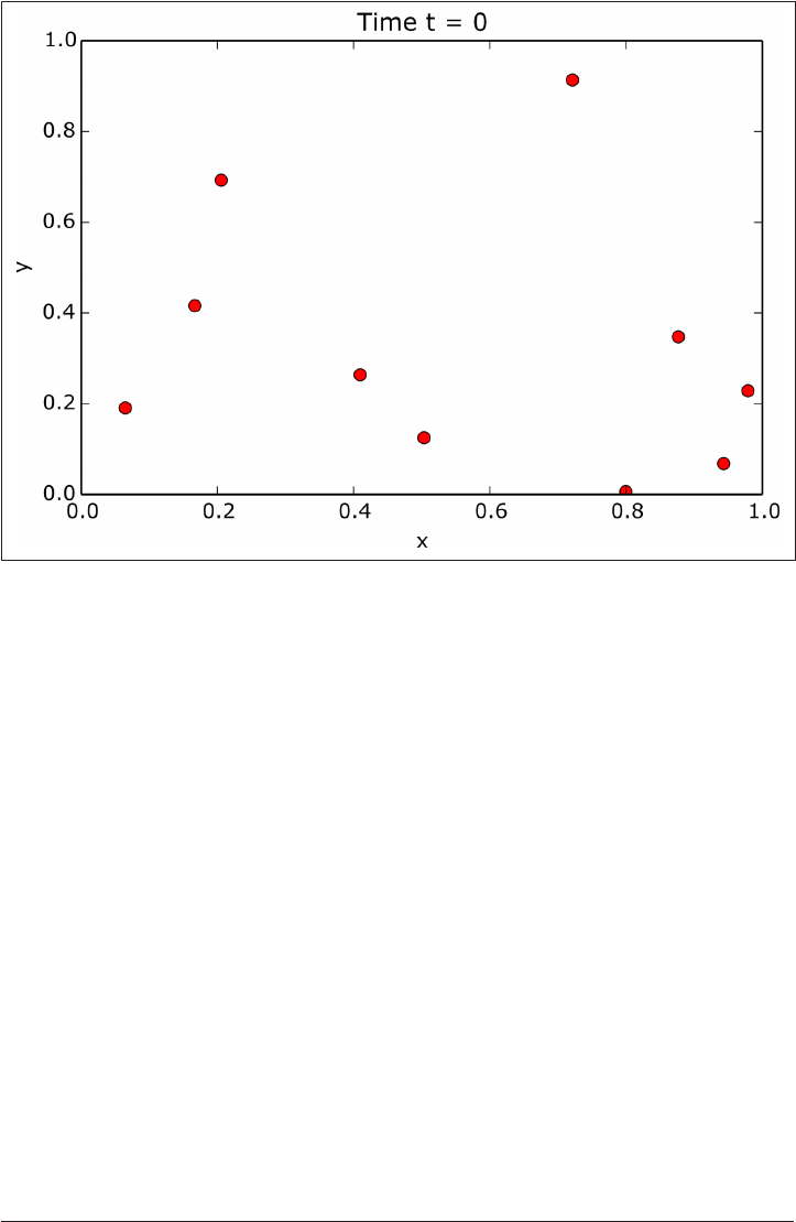
Figure 12-1. Example N-body positions for bodies at rest (initial conditions)
The data for these figures is generated by the following code:
x0, v0, m = initial_cond(10, 2)
x1, v1 = timestep(x0, v0, 1.0, m, 1.0e-3)
More generally, we can also write a simple driver function that simulates S time steps.
The simulate() function takes the positions and velocities and updates them for
each time step:
def simulate(N, D, S, G, dt):
x0, v0, m = initial_cond(N, D)
for s in range(S):
x1, v1 = timestep(x0, v0, G, m, dt)
x0, v0 = x1, v1
No Parallelism | 287
www.it-ebooks.info
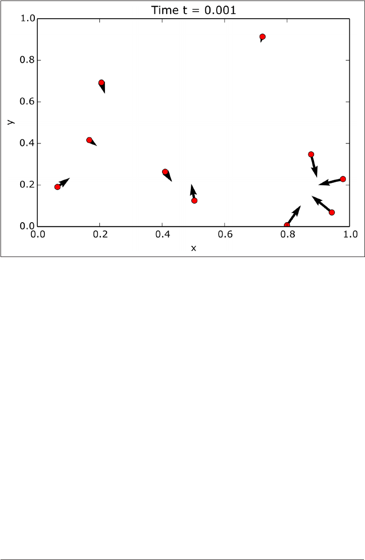
Figure 12-2. Example N-body positions and velocities aer one time step
We can measure the performance of this non-parallel algorithm by calling simu
late() for a variety of different N values and timing how long it takes. The following
snippet shows how to automate these timings using Python’s built-in time module.
Here, we scale the particles by increasing powers of two:
import time
Ns = [2, 4, 8, 16, 32, 64, 128, 256, 512, 1024, 2048, 4096, 8192]
runtimes = []
for N in Ns:
start = time.time()
simulate(N, 3, 300, 1.0, 1e-3)
stop = time.time()
runtimes.append(stop - start)
Here, 300 time steps were chosen because after this point almost all of the bodies have
left the original unit cube. The bodies are unlikely to engage in further interactions.
Three hundred time steps is also large enough that the overhead that comes from just
starting and running the simulations is minimized.
Intuition tells us that the N-body problem is order-N2. This is because for every new
body added, another iteration is added in the outer loop (the timestep() function)
and another iteration is added in the inner loop (the a() function). Thus, we would
expect the runtimes to be roughly parabolic as a function of N. Call the runtime of an
288 | Chapter 12: Performing in Parallel
www.it-ebooks.info
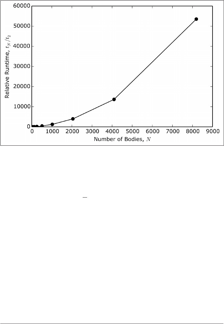
N-body simulation tN. Figure 12-3 shows the ratio between the runtimes of tN and t2,
the runtime of the 2-body problem.
Figure 12-3. Relative runtimes of a non-parallel N-body simulation
Figure 12-3 is more or less parabolic, especially for large values of N. Since this simu‐
lation is done in serial, it is a little excessive to go much beyond 8,192 bodies. More
telling, though, is the relative doubling time. This is defined as tN divided by the run‐
time of half as many bodies, tN
2
. Since the problem is order-N2, if you double the
number of particles the runtime should go up by a factor of 4 no matter how many
particles there are in the simulation. Figure 12-4 displays this quantity.
No Parallelism | 289
www.it-ebooks.info
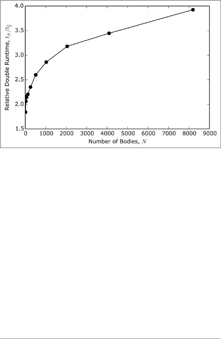
Figure 12-4. Relative doubling runtimes of a non-parallel N-body simulation
From this figure, there seem to be two distinct regimes in the relative doubling time.
For large N, the relative doubling time does indeed seem to approach the magic 4
value. However for small N, this ratio is much closer to 2. In some cases it is even
below 2, which implies that adding bodies decreases the amount of time spent on
each body.
That Figure 12-4 is not a flat line close to 4 means that for low N, the overhead of the
simulation dominates. Python, numpy, copying memory, and other facets of the
implementation take up more of the runtime than the actual computation of the posi‐
tions, velocities, and accelerations. It is not until about 2,000 bodies that the effects of
N are really pertinent. Thus, for small N it probably is not worth parallelizing at all.
The return on investment would be too low. For larger N, though, it will make a world
of difference.
Let’s now take a look at our first parallel N-body solver.
Threads
Threads are most people’s first thought when they approach parallelism. However,
threading in Python is almost certainly the wrong tool for the job. We cover thread‐
ing here because it introduces some basic parallel concepts. You should also know
why you should not use it.
290 | Chapter 12: Performing in Parallel
www.it-ebooks.info

You should not use threads in Python for most scientific tasks! You
should read this section anyway, though, because threading can be
useful outside of Python.
Threads are objects that perform work and are not blocked by the work that other
threads may be doing simultaneously. Executing code in a thread does not stop
another thread from executing its own code. Threads may communicate with each
other through their state. Threads may spawn child threads, and there is no limit to
how many threads a program may run. There is always at least one thread in Python
—the main thread.
Threads are one-time use. They have a run() method that, when it completes the
thread, is no longer considered alive. This run() method is not directly called but is
instead called implicitly when the start() method is called. This lets threads defer
their work until a later point in time when the work has been properly set up.
Threads cannot be killed externally; instead, the run() method must be allowed to
complete. The exception to this rule is that if the thread is a daemon, the thread will
die when the Python program itself exits.
Threads can be found in the threading module in the Python standard library. This
exposes an interface that is similar to the threading interfaces found in other lan‐
guages, such as Java or C.
Threading’s big gotcha is that all threads execute in the same process as Python itself.
This is because Python is an interpreted language, and the Python interpreter itself
lives in only one process. This means that even though the threads may not block
each other’s execution, their combined speed is limited to that of a single processor
on the machine. Number crunching for the most part is CPU-bound—that is, it is
limited by the speed of the processor. If the computer is already running at top speed,
adding more things for it to do does not make it go any faster. In fact, adding more
tasks often hurts execution time. The processor becomes crowded.
The one-processor limit to threads is due to a detail of the way that the standard
Python interpreter (called CPython, because it is written in C) is written. This detail is
called the global interpreter lock, or GIL. The GIL determines which thread is cur‐
rently running and when to switch from executing one thread to executing another.
Several attempts to have Python without the GIL have been proposed over time. Most
notable is the PyPy project. None of these, however, have usurped the popularity of
the classic CPython interpreter. CPython remains especially dominant in the scien‐
tific computing world.
So why do people use threads? For high-latency tasks, like reading a file from disk or
downloading information over a network, most of the time the program is just wait‐
Threads | 291
www.it-ebooks.info
ing to get back the next chunk of data before it can proceed. Threads work well in
these cases because the spare time can be put to good use executing other code.
However, in CPU-bound tasks, the processor is already as busy as it can be, and
threads cause more problems than they solve. Except for reading in the occasional
large dataset, scientific code is overwhelmingly CPU-bound.
Even though you probably should not use them, let’s take a look at how the N-body
problem is solved with threads. The first and easiest tactic for parallelization is to
identify the parts of the code that do not depend on one another. With complete
independence, the processes do not have to communicate with one another, so paral‐
lelism should come easy. In some algorithms this independence manifests as an inner
loop and in some it is an outer loop. In some algorithms you can even switch which is
the inner and which is the outer loop, to better fit your needs.
In the N-body problem, the loop in the timestep() function is the most easily paral‐
lelized. This allows us to only modify this one function. We can leave the implemen‐
tations of the remove_i(), a(), and initial_cond() functions the same as they were
in “No Parallelism” on page 285.
Before we can modify the timestep() function, we need to define threads that
instead do the work of a single iteration. The following code implements a thread for
use with the N-body problem:
from threading import Thread
class Worker(Thread):
"""Computes x, v, and a of the ith body."""
def __init__(self, *args, **kwargs):
super(Worker, self).__init__(*args, **kwargs)
self.inputs = []
self.results = []
self.running = True
self.daemon = True
self.start()
def run(self):
while self.running:
if len(self.inputs) == 0:
continue
i, x0, v0, G, m, dt = self.inputs.pop(0)
a_i0 = a(i, x0, G, m)
v_i1 = a_i0 * dt + v0[i]
x_i1 = a_i0 * dt**2 + v0[i] * dt + x0[i]
result = (i, x_i1, v_i1)
self.results.append(result)
To use threading, we need to subclass Thread.
292 | Chapter 12: Performing in Parallel
www.it-ebooks.info

inputs is a buffer of work for this thread to churn through. We cannot call the
run() method directly, so inputs provides a way to send data to the thread.
A buffer of return values. Again, since we do not call the run() method our‐
selves, we have to have a place to store our results.
Setting this to False will cause the run() method to end safely.
Allow the thread to be terminated when Python exits.
Check if there is work to do.
The body of the original timestep() function.
First, we grab the Thread class from the threading module that comes with Python.
To make this useful to the N-body problem, we subclass it under the name Worker
and then override the constructor and the run() methods.
The constructor has two major purposes: setting up data structures used for commu‐
nication and starting the thread. The inputs and results lists are used to load work
onto the thread and get corresponding return values. The running flag is used to end
the life of the thread cleanly—it will not stop midway while computing a result. The
daemon flag is used to tell Python that this thread may be stopped when the program
exits. Finally, the call to the start() method at the end of the constructor immedi‐
ately makes the thread available for work when it is created.
While the running flag is true, the run() method will sit around waiting for work.
Work comes in the form of a nonempty inputs list. The elements of this list are
tuples that contain all of the arguments to a() as well as the time step value dt. When
work arrives, the run() method proceeds to compute the next values of acceleration,
velocity, and position for the ith body. The run() method then stores i, the next posi‐
tion, and the next velocity as a tuple in the results list, so that they can be read back
by whoever put the arguments in the inputs list. It is important to keep i in the
results list because it creates an unambiguous way of later determining which input
goes with which result.
Managing individual one-time-use threads can be painful. Creating and starting
threads can be expensive. It is best if thread objects can be reused for as long as possi‐
ble. To handle this, a pattern known as thread pools is extremely common. The idea
here is that the pool is created with some fixed size, and it is then responsible for cre‐
ating, starting, farming out work to, stopping, and finally deleting the threads it man‐
ages. Python does not provide a thread pool to use off the shelf. However, they are
fairly easy to implement. The following is a pool that manages instances of the Worker
class:
Threads | 293
www.it-ebooks.info
class Pool(object):
"""A collection of P worker threads that distributes tasks
evenly across them.
"""
def __init__(self, size):
self.size = size
self.workers = [Worker() for p in range(size)]
def do(self, tasks):
for p in range(self.size):
self.workers[p].inputs += tasks[p::self.size]
while any([len(worker.inputs) != 0 for worker in self.workers]):
pass
results = []
for worker in self.workers:
results += worker.results
worker.results.clear()
return results
def __del__(self):
for worker in self.workers:
worker.running = False
Create new workers according to the size.
Evenly distribute tasks across workers with slicing.
Wait for all of the workers to finish all of their tasks.
Get back the results from the workers and clean out the workers.
Return the complete list of results for all inputs.
Stop the workers when the pool itself is shut down.
Instantiating a Pool creates as many workers as were requested and keeps references
to them for future use. The do() method takes a list of tasks—all of inputs that we
want to run—and appends them to the workers’ inputs lists. The tasks are appended
using slicing to spread them out among all workers as evenly as possible. The pool
then waits until the workers do not have anything left in their inputs lists. Once all of
the work has been completed, the results are aggregated together, the workers’
results lists are cleared for future work, and all of the results together are returned.
Note that the results are not guaranteed to be in the order of the tasks that spawned
them. In most cases, the order will be unpredictable. Lastly, the pool is responsible for
stopping the workers from running once the pool itself is shut down in the delete
method.
294 | Chapter 12: Performing in Parallel
www.it-ebooks.info
Using the Worker and Pool classes, our timestep() function can be rewritten to now
accept a pool object to use for its computation. Note that since the results come back
in an effectively random order, we must reconstruct them according to the i value.
Doing so, as well as setting up the tasks, is fairly simple and is very cheap compared
to the actual computation. The following reimplements the timestep() function:
def timestep(x0, v0, G, m, dt, pool):
"""Computes the next position and velocity for all masses given
initial conditions and a time step size.
"""
N = len(x0)
tasks = [(i, x0, v0, G, m, dt) for i in range(N)]
results = pool.do(tasks)
x1 = np.empty(x0.shape, dtype=float)
v1 = np.empty(v0.shape, dtype=float)
for i, x_i1, v_i1 in results:
x1[i] = x_i1
v1[i] = v_i1
return x1, v1
Create a task for each body.
Run the tasks.
Rearrange the results since they are probably out of order.
Rewriting timestep() necessitates rewriting the simulate() function to create a
Pool. To make scaling easy, simulate() should also be parameterized based on the
number of workers, P. Parallel algorithms need to be told with what degree of paral‐
lelism they should be run. A pool-aware version of simulate() is shown here:
def simulate(P, N, D, S, G, dt):
x0, v0, m = initial_cond(N, D)
pool = Pool(P)
for s in range(S):
x1, v1 = timestep(x0, v0, G, m, dt, pool)
x0, v0 = x1, v1
Unlike in “No Parallelism” on page 285, where we investigated how the N-body prob‐
lem behaved as a function of the number of bodies, here we can determine how the
simulation performs as a function of P. The following snippet has a fixed total prob‐
lem size of 64 bodies over 300 time steps:
Ps = [1, 2, 4, 8]
runtimes = []
for P in Ps:
start = time.time()
simulate(P, 64, 3, 300, 1.0, 1e-3)
stop = time.time()
runtimes.append(stop - start)
Threads | 295
www.it-ebooks.info
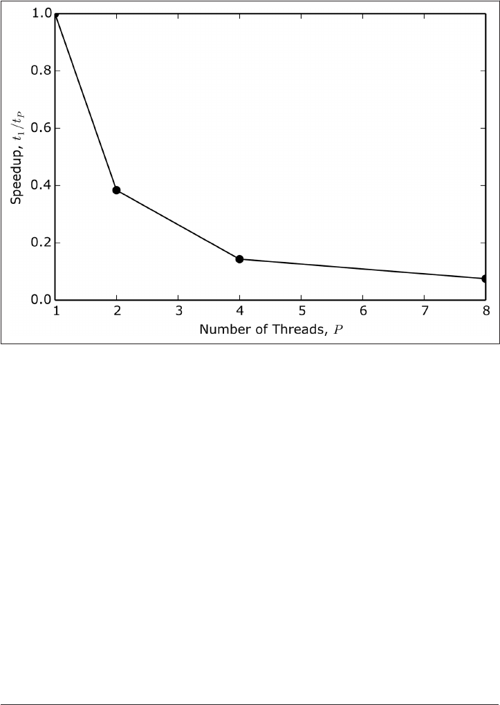
In a perfect world, the strong scaling would have a speedup factor of 2x for every time
P is doubled. However, the results here, shown in Figure 12-5, demonstrate that the
speedup is actually a slowdown.
Figure 12-5. Speedup in threaded N-body simulation
Why does this happen? Every time we add threads, we add more load to the CPU.
The single processor then has to spend more time figuring out which thread should
be allowed to execute. As you can see, this gets very ugly very fast. Adding more
threads to CPU-bound tasks does not enable more parallelism; it causes less. Even
when there is only one worker thread, the main thread still exists. This causes the P=1
case that performs the best here to still be around 2.5 times slower than the equivalent
non-parallel case seen in “No Parallelism” on page 285. These excessive slowdowns
are why you should avoid threads.
In the next section, we’ll see a strategy that actually does yield real speedups.
Multiprocessing
Multiprocessing is Python’s way of handing off the responsibility of scheduling paral‐
lel tasks to the operating system. Modern operating systems are really good at multi‐
tasking. Multitasking allows for the sum of all processes to vastly exceed the resource
limits of the computer. This is possible because multitasking does not necessarily
296 | Chapter 12: Performing in Parallel
www.it-ebooks.info

allow for all processes to be simultaneously active. Any time you are browsing the
Web, playing music, storing data on a flash drive, and running your fancy new USB
toaster at the same time, you and your computer are multitasking.
The capability for multitasking is central to being able to use a computer for common
tasks. On a single-CPU system, only one process can be physically executing at a
time. A multitasking OS may pause this process and switch contexts to another pro‐
cess. Frequent, well-timed context switching gives the illusion of several processes
running at once. When there are many processors available, multitasking can easily
distribute a process across them, granting a degree of parallelism for free.
Forgetting filesystems, device drivers, and other human interactions, it is common
for people to now view the main job of the operating system as scheduling tasks. At
this point, most operating systems have extremely well-implemented schedulers.
From Python’s perspective, why not let someone else take care of this hard problem?
It is, after all, a solved hard problem. For CPU-intensive tasks, multitasking is exactly
what you should do.
What is called “threading” in other languages is actually imple‐
mented more similarly to multiprocessing in Python.
Creating or spawning a new OS-level process is handled by Python. However, note
that on POSIX (Unix-like—i.e., Linux and Mac OS X) machines, all processes are
forks of the processes that spawned them. A fork inherits the environment of its par‐
ent. However, any modifications to the environment that the fork makes will not be
reflected back in the parent process. Forks may spawn their own forks, which will get
the modified environment. Killing a parent process will kill all of its forks. So, when
Python spawns more processes, they all see the environment that the main Python
process had. Multiprocessing interacts more directly with the OS, so other OS-level
concepts that were seen in Chapter 1, such as piping, sometimes make an appearance
here too.
Multiprocessing in Python is implemented via the standard library multiprocessing
module. This provides a threading-like interface to handling processes. There are
two major distinctions, though:
1. Multiprocessing cannot be used directly from an interactive interpreter. The
main module (__main__) must be importable by the forks.
2. The multiprocessing module provides a Pool class for us. We do not need to
write our own.
Multiprocessing | 297
www.it-ebooks.info

The Pool class has a number of different methods that implement parallelism in
slightly different ways. However, the map() method works extraordinarily well for
almost all problems.
Pool.map() has a similar interface to the built-in map() function. It takes two argu‐
ments—a function and an iterable of arguments to pass into that function—and
returns a list of values in the same order that was given in the original iterable.
Pool.map() blocks further execution of Python code until all of the results are ready.
The major limitation of Pool.map() is that the function that it executes must have
only one argument. You can overcome this easily by storing the arguments you need
in a tuple or dictionary before calling it.
For the N-body problem, we no longer need the Worker and Pool classes that we used
in “Threads” on page 290. Instead, we simply need a timestep_i() function that
computes the time step evolution of the ith body. To make it easier to use with multi
processing, timestep_i() should only have one argument. The following code
defines this function:
from multiprocessing import Pool
def timestep_i(args):
"""Computes the next position and velocity for the ith mass."""
i, x0, v0, G, m, dt = args
a_i0 = a(i, x0, G, m)
v_i1 = a_i0 * dt + v0[i]
x_i1 = a_i0 * dt**2 + v0[i] * dt + x0[i]
return i, x_i1, v_i1
Unpack the arguments to the original timestep() function.
The body of the original timestep() function.
Note that the first operation here is to unpack args into the variables we have come
to know for this problem. Furthermore, the actual timestep() function from
“Threads” on page 290 must be altered slightly to account for the new kind of process
pool and the timestep_i() function. Mostly, we need to swap out the old do() call
for the new Pool.map() call and pass it timestep_i, as well as the tasks:
def timestep(x0, v0, G, m, dt, pool):
"""Computes the next position and velocity for all masses given
initial conditions and a time step size.
"""
N = len(x0)
tasks = [(i, x0, v0, G, m, dt) for i in range(N)]
results = pool.map(timestep_i, tasks)
x1 = np.empty(x0.shape, dtype=float)
v1 = np.empty(v0.shape, dtype=float)
for i, x_i1, v_i1 in results:
298 | Chapter 12: Performing in Parallel
www.it-ebooks.info

x1[i] = x_i1
v1[i] = v_i1
return x1, v1
Replace the old do() method with multiprocessing’s Pool.map().
All of the other functions from “Threads” on page 290 remain the same, including
simulate().
So how does multiprocessing scale? Let’s take the fairly regular computing situation of
programming on a dual-core laptop. This is not a whole lot of parallelism, but it is
better than nothing. We would expect that a pool with two processes would run twice
as fast as a pool with one process. At one process per physical processor, we would
expect peak performance. For greater than two processes we would expect some per‐
formance degradation, as the operating system spends more time context switching.
Example results can be seen in Figure 12-6. These were generated with the following
code:
import time
Ps = [1, 2, 4, 8]
runtimes = []
for P in Ps:
start = time.time()
simulate(P, 256, 3, 300, 1.0, 1e-3)
stop = time.time()
runtimes.append(stop - start)
As you can see in Figure 12-6, it is not precisely 2x faster, but is in the neighborhood
of 1.8x. The extra 0.2x that is missing goes to overhead in Python, processing forking,
and the N-body algorithm. As expected, for pools of size 4 and 8 the speedup is worse
than in the two processes case, though it is still a considerable improvement over the
one processor case. Finally, it is worth noting that the one process case is 1.3x slower
than the equivalent case with no parallelism. This is because of the overhead in set‐
ting up the parallel infrastructure. However, this initial 30% burden is quickly over‐
come in the two processor case. All of these results together indicate that
multiprocessing is certainly worth it, even if you overestimate the number of process‐
ors that you have by a bit.
Multiprocessing | 299
www.it-ebooks.info
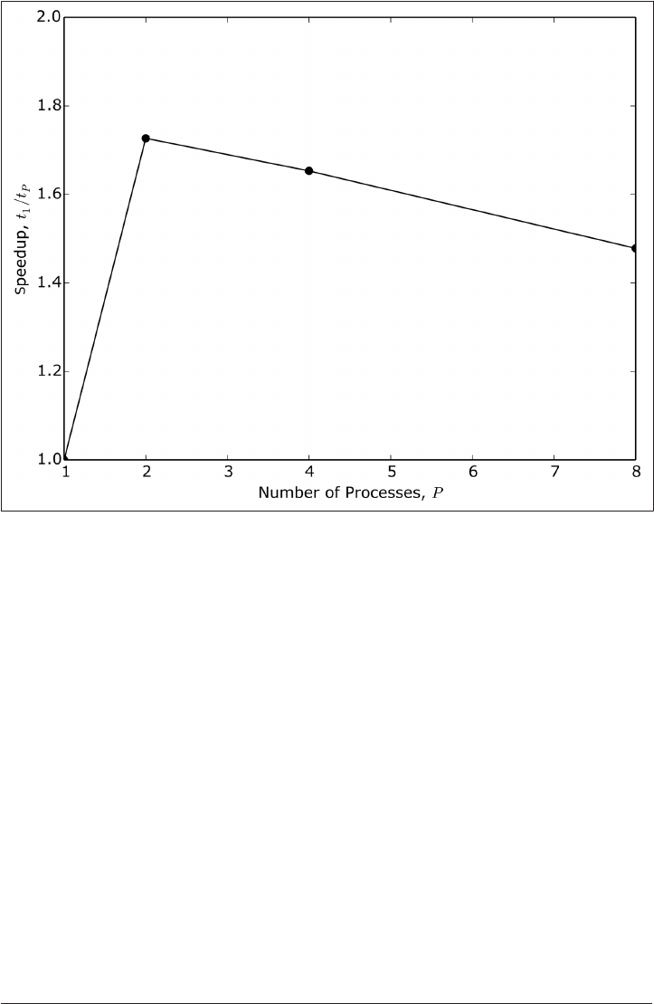
Figure 12-6. Speedup in multiprocessing N-body simulation on two processors
Multiprocessing is a great tool to use when you have a single machine and less than a
thousand physical processors. It is great for daily use on a laptop or on a cluster at
work. However, multiprocessing-based strategies do not scale up to supercomputers.
For that, we will need MPI, covered in the next section.
MPI
The gold standard for high-performance parallelism is MPI, the Message-Passing
Interface. As an interface MPI is a specification for how to communicate information
between various processes, which may be close to or very far from one another. The
MPI-3.0 Standard was released in September 2012. There are two primary open
source projects that implement MPI: MPICH and Open MPI. Since they implement
the same standard, these are largely interchangeable. They both take great care to
provide the MPI interface completely and correctly.
It is not an understatement to say that supercomputing is built on top of MPI. This is
because MPI is an abstraction for parallelism that is independent of the machine.
This allows physicists (and other domain experts) to learn and write MPI code and
300 | Chapter 12: Performing in Parallel
www.it-ebooks.info

have it work on any computer. Meanwhile, the architects of the supercomputers can
implement a version of MPI that is optimized to the machines that they are building.
The architects do not have to worry about who is going to use their version of MPI,
or how they will use it.
MPI is a useful abstraction for anyone who buys into its model. It is a successful
abstraction because almost everyone at this point does buy into it. MPI is huge and
very flexible, and we do not have space here to do it justice. It currently scales up to
the level of hundreds of thousands to millions of processors. It also works just fine on
a handful of processors. If you are serious about parallelism on even medium scales
(1,000+ processors), MPI is an unavoidable boon.
As its name states, MPI is all about communication. Mostly this applies to data, but it
is also true for algorithms. The basic elements of MPI all deal with how to communi‐
cate between processes. For a user, this is primarily what is of interest. As with all
good things, there is a Python interface. In fact, there are many of them. The most
commonly used one is called mpi4py. We will be discussing the mpi4py package rather
than the officially supported C, C++, or Fortran interfaces.
In MPI terminology, processes are called ranks and are given integer identifiers start‐
ing at zero. As with the other forms of parallelism we have seen, you may have more
ranks than there are physical processors. MPI will do its best to spread the ranks out
evenly over the available resources. Often—though not always—rank 0 is considered
to be a special “master” process that commands and controls the other ranks.
Having a master rank is a great strategy to use, until it isn’t! The
point at which this approach breaks down is when the master pro‐
cess is overloaded by the sheer number of ranks. The master itself
then becomes the bottleneck for doling out work. Reimagining an
algorithm to not have a master process can be tricky.
At the core of MPI are communicator objects. These provide metadata about how
many processes there are with the Get_size() method, which rank you are on with
Get_rank(), and how the ranks are grouped together. Communicators also provide
tools for sending messages from one processor and receiving them on other processes
via the send() and recv() methods. The mpi4py package has two primary ways of
communicating data. The slower but more general way is that you can send arbitrary
Python objects. This requires that the objects are fully picklable. Pickling is Python’s
native storage mechanism. Even though pickles are written in plain text, they are not
human readable by any means. To learn more about how pickling works and what it
looks like, please refer to the pickling section of the Python documentation.
NumPy arrays can also be used to communicate with mpi4py. In situations where
your data is already in a NumPy arrays, it is most appropriate to let mpi4py use these
MPI | 301
www.it-ebooks.info

arrays. However, the communication is then subject to the same constraints as nor‐
mal NumPy arrays. Instead of going into the details of how to use NumPy and mpi4py
together, here we will only use the generic communication mechanisms. This is
because they are easier to use, and moving to NumPy-based communication does not
add anything to your understanding of parallelism.
The mpi4py package comes with a couple of common communicators already instan‐
tiated. The one that is typically used is called COMM_WORLD. This represents all of the
processes that MPI was started with and enables basic point-to-point communication.
Point-to-point communication allows any process to communicate directly with any
other process. Here we will be using it to have the rank 0 process communicate back
and forth with the other ranks.
As with multiprocessing, the main module must be importable. This is because MPI
must be able to launch its own processes. Typically this is done through the
command-line utility mpiexec. This takes a -n switch and a number of nodes to run
on. For simplicity, we assume one process per node. The program to run—Python,
here—is then followed by any arguments it takes. Suppose that we have written our
N-body simulation in a file called n-body-mpi.py. If we wish to run on four processes,
we would start MPI with the following command on the command line:
$ mpiexec -n 4 python n-body-mpi.py
Now we just need to write the n-body-mpi.py file! Implementing an MPI-based solver
for the N-body problem is not radically different from the solutions that we have
already seen. The remove_i(), initial_cond(), a(), timestep(), and timestep_i()
functions are all the same as they were in “Multiprocessing” on page 296.
What changes for MPI is the simulate() function. To be consistent with the other
examples in this chapter (and because it is a good idea), we will also implement an
MPI-aware process pool. Let’s begin by importing MPI and the following helpers:
from mpi4py import MPI
from mpi4py.MPI import COMM_WORLD
from types import FunctionType
The MPI module is the primary module in mpi4py. Within this module lives the
COMM_WORLD communicator that we will use, so it is convenient to import it directly.
Finally, types is a Python standard library module that provides base classes for
built-in Python types. The FunctionType will be useful in the MPI-aware Pool that is
implemented here:
class Pool(object):
"""Process pool using MPI."""
def __init__(self):
self.f = None
self.P = COMM_WORLD.Get_size()
302 | Chapter 12: Performing in Parallel
www.it-ebooks.info
self.rank = COMM_WORLD.Get_rank()
def wait(self):
if self.rank == 0:
raise RuntimeError("Proc 0 cannot wait!")
status = MPI.Status()
while True:
task = COMM_WORLD.recv(source=0, tag=MPI.ANY_TAG, status=status)
if not task:
break
if isinstance(task, FunctionType):
self.f = task
continue
result = self.f(task)
COMM_WORLD.isend(result, dest=0, tag=status.tag)
def map(self, f, tasks):
N = len(tasks)
P = self.P
Pless1 = P - 1
if self.rank != 0:
self.wait()
return
if f is not self.f:
self.f = f
requests = []
for p in range(1, self.P):
r = COMM_WORLD.isend(f, dest=p)
requests.append(r)
MPI.Request.waitall(requests)
requests = []
for i, task in enumerate(tasks):
r = COMM_WORLD.isend(task, dest=(i%Pless1)+1, tag=i)
requests.append(r)
MPI.Request.waitall(requests)
results = []
for i in range(N):
result = COMM_WORLD.recv(source=(i%Pless1)+1, tag=i)
results.append(result)
return results
def __del__(self):
if self.rank == 0:
for p in range(1, self.P):
COMM_WORLD.isend(False, dest=p)
A reference to the function to execute. The pool starts off with no function.
MPI | 303
www.it-ebooks.info
The total number of processors.
Which processor we are on.
A method for receiving data when the pool has no tasks. Normally, a task is data
to give as arguments to the function f(). However, if the task is itself a function,
it replaces the current f().
The master process cannot wait.
Receive a new task from the master process.
If the task was a function, put it onto the object and then continue to wait.
If the task was not a function, then it must be a real task. Call the function on this
task and send back the result.
A map() method to be used like before.
Make the workers wait while the master sends out tasks.
Send all of the workers the function.
Evenly distribute tasks to all of the workers.
Wait for the results to come back from the workers.
Shut down all of the workers when the pool is shut down.
The purpose of the Pool class is to provide a map() method that is similar to the
map() on the multiprocessing pool. This class implements the rank-0-as-master strat‐
egy. The map() method can be used in the same way as for other pools. However,
other parts of the MPI pool operate somewhat differently. To start with, there is no
need to tell the pool its size. P is set on the command line and then discovered with
COMM_WORLD.Get_size() automatically in the pool’s constructor.
Furthermore, there will be an instance of Pool on each processor because MPI runs
the same executable (python) and script (n-body-mpi.py) everywhere. This implies
that each pool should be aware of its own rank so that it can determine if it is the
master or just another worker. The Pool class has to jointly fulfill both the worker
and the master roles.
304 | Chapter 12: Performing in Parallel
www.it-ebooks.info

The wait() method here has the same meaning as Thread.run() from “Threads” on
page 290. It does work when there is work to do and sits idle otherwise. There are
three paths that wait() can take, depending on the kind of task it receives:
1. If a function was received, it assigns this function to the attribute f for later use.
2. If an actual task was received, it calls the f attribute with the task as an argument.
3. If the task is False, then it stops waiting.
The master process is not allowed to wait and therefore not allowed to do real work.
We can take this into account by telling MPI to use P+1 nodes. This is similar to what
we saw with threads. However, with MPI we have to handle the master process
explicitly. With Python threading, Python handles the main thread, and thus the mas‐
ter process, for us.
The map() method again takes a function and a list of tasks. The tasks are evenly dis‐
tributed over the workers. The map() method is only runnable on the master, while
workers are told to wait. If the function that is passed in is different than the current
value of the f attribute, then the function itself is sent to all of the workers. Sending
happens via the “initiate send” (COMM_WORLD.isend()) call. We ensure that the func‐
tion has made it to all of the workers via the call to MPI.Request.waitall(). This
acts as an acknowledgment between the sender and all of the receivers. Next, the tasks
are distributed to their appropriate ranks. Finally, the results are received from the
workers.
When the master pool instance is deleted, it will automatically instruct the workers to
stop waiting. This allows the workers to be cleaned up correctly as well. Since the
Pool API here is different enough, a new version of the top-level simulate() func‐
tion must also be written. Only the master process should be allowed to aggregate
results together. The new version of simulate() is shown here:
def simulate(N, D, S, G, dt):
x0, v0, m = initial_cond(N, D)
pool = Pool()
if COMM_WORLD.Get_rank() == 0:
for s in range(S):
x1, v1 = timestep(x0, v0, G, m, dt, pool)
x0, v0 = x1, v1
else:
pool.wait()
Lastly, if we want to run a certain case, we need to add a main execution to the bot‐
tom of n-body-mpi.py. For 128 bodies in 3 dimensions over 300 time steps, we would
call simulate() as follows:
if __name__ == '__main__':
simulate(128, 3, 300, 1.0, 1e-3)
MPI | 305
www.it-ebooks.info
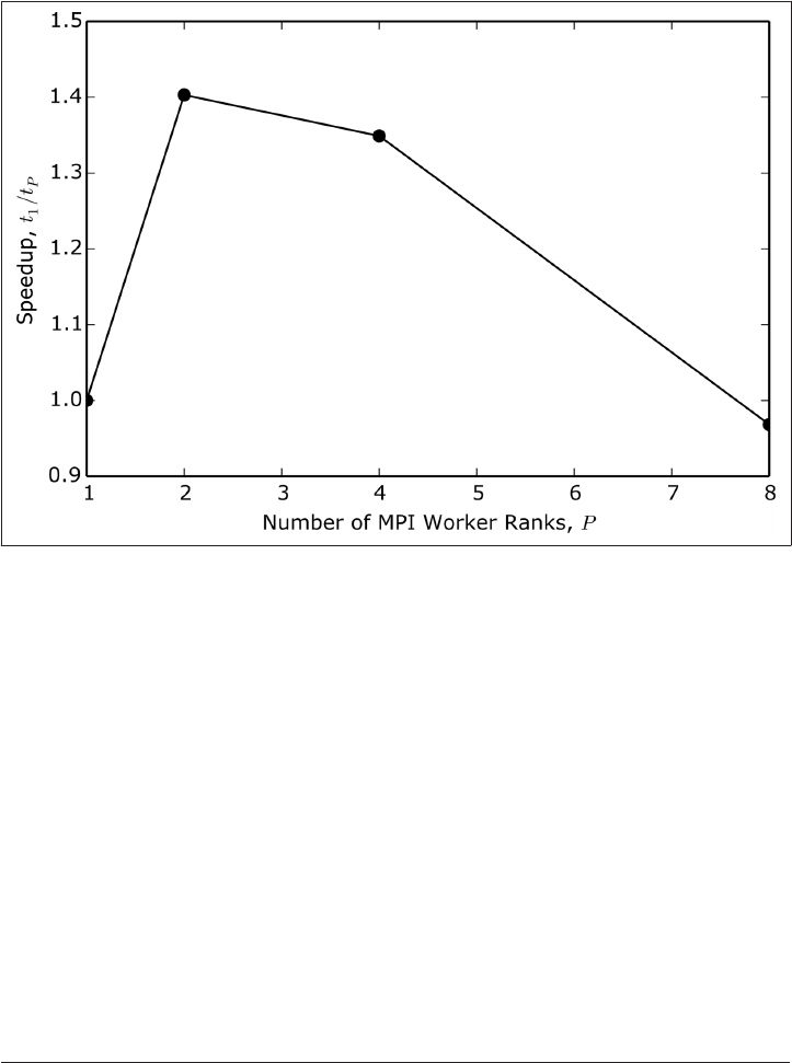
Given MPI’s fine-grained control over communication, how does the N-body prob‐
lem scale? With twice as many processors, we again expect a 2x speedup. If the num‐
ber of MPI nodes exceeds the number of processors, however, we would expect a
slowdown due to managing the excess overhead. Figure 12-7 shows a sample study
on a dual-core laptop.
Figure 12-7. Speedup in MPI N-body simulation
While there is a speedup for the P=2 case, it is only about 1.4x, rather than the hoped-
for 2x. The downward trend for P>2 is still present, and even steeper than with multi‐
processing. Furthermore, the P=1 MPI case is about 5.5x slower than the same
simulation with no parallelism. So, for small simulations MPI’s overhead may not be
worth it.
Still, the situation presented here is a worst-case scenario for MPI: arbitrary Python
code with two-way communication on a small machine of unspecified topology. If we
had tried to optimize our algorithm at all—by giving MPI more information or by
using NumPy arrays to communicate—the speedups would have been much higher.
These results should thus be viewed from the vantage point that even in the worst
case, MPI is competitive. MPI truly shines in a supercomputing environment, where
everything that you have learned about message passing still applies.
306 | Chapter 12: Performing in Parallel
www.it-ebooks.info

Parallelism Wrap-up
Parallelism is a huge topic, and we have only scratched the surface of what can be
accomplished, what mechanisms for parallelism exist, and what libraries implement
the various strategies. Having read this chapter, you are well prepared to go forth and
learn more about how to implement parallel algorithms in the context of scientific
computing. This is very different from the more popular web-based parallelism that
permeates our modern lives. The following list presents some excellent parallel sys‐
tems that you may find interesting or helpful to explore, beyond the essentials cov‐
ered here:
OpenMP
Preprocessor-based, easy to use, low-level parallelism for C, C++, and Fortran
GNU Portable reads
Cross-platform thread system for C, C++, and Fortran
IPython Parallel
The parallel architecture that IPython uses, based on ZeroMQ
Twisted
Event-driven parallelism for Python web applications
You should now be familiar with the following ideas:
• There are many ways to measure scale.
•Certain problems are embarrassingly easy to make parallel, while others are very
difficult.
•High-performance computing systems are built to handle non-embarrassingly
parallel problems.
•High-throughput computing systems are best used for embarrassingly parallel or
heterogeneous problems.
•Non-parallel algorithms are faster than parallel code used with one process.
• Stay away from Python threads when number crunching.
• Multitasking is great for problems involving up to around a thousand processes.
• Use MPI when you really need to scale up.
Now that you know how to write software in serial and parallel, it is time to talk
about how to get your software to other computers.
Parallelism Wrap-up | 307
www.it-ebooks.info

CHAPTER 13
Deploying Software
So far, we have mostly been concerned with how to write software that solves physics
problems. In this chapter, though, we will discuss how writing software that runs reli‐
ably—especially at scale—can prove almost as challenging.
Most software developers want users for their code. For scientific programs this is
doubly true, since science runs on a reputation system. Without users, code can
hardly be called reproducible. However, even in the event that you do not wish for
users, users are still extraordinarily helpful. A new user is a fresh set of eyes that can
point out the blind spots of a program better than anyone else. What is broken a new
user will break. What is unintuitive a new user will not understand. This process
starts at installation.
New users should realize that if they do not understand something
about a project after reading the documentation, then the moral
failing lies with the developers and not with themselves. Good
users in this situation will then kindly report their struggles back to
the developers.
That said, you are your first user. Writing code is a distinctly different process from
running the code. Even with tools to mitigate this distinction, such as testing, the dif‐
ference is never completely gone. Deploying code that you wrote for the first time is
an exciting experience. It probably will not work on the first try. As a developer, it is
easy to address the feedback that you yourself have as a user. You can iterate through
this develop-then-use cycle as many times as necessary until the code really does work
(for you, at least).
What confounds the deployment problem is that every system is different. Every lap‐
top, desktop, phone, operating system, and environment has its own history. This
309
www.it-ebooks.info

happens naturally as people use their computers. To make matters worse, oftentimes
the system might describe itself incorrectly. This can make installing and running on
a new system painful. Deployment often feels like an approximate art rather than an
exact science. Trying from the start to ensure that your software will run in as many
places as reasonably possible is the only way to preserve your sanity in the long term.
With a lot of attention and care, brand new systems can be forced to be the same.
This is incredibly useful to developers: if the software works on one copy of the sys‐
tem, it will likely work on all other copies. Strong guarantees like this often come
from virtualization in one form or another.
Virtualization is the act of isolating the software that you wish to run from the system
that is running it. This comes in two forms. A virtual machine allows for an entire
operating system to be installed and booted within another operating system. A vir‐
tual environment creates a new, clean space to run code in that is safely separated
from other parts of the operating system and environment.
Large-scale deployments of virtualizations can be found on supercomputers and in
the cloud. Supercomputers and smaller clusters often have login machines that users
connect to in order to launch jobs, compile their code, and perform other tasks. How‐
ever, the nodes that execute the software typically all run the same well-defined oper‐
ating system and environment. In the cloud, different virtualizations might exist to
fill different needs of an application. In all cases, the virtual environment is well
defined.
What these large deployments share is that the users are not allowed to touch the
software or environment directly. Users will break things. Such systems are too intri‐
cate and expensive to risk by giving even experienced people direct access. Removing
users from the mix removes a sure source of error. Virtualization in large computing
settings rightly remains a tool for developers. However, developers can prepackage a
virtualization and give it to users as a common starting point.
Deployment is a process, a struggle. Users want your software to work for them with
whatever they bring to the table. Users running Windows 98 Second Edition do not
care if your code works perfectly on a prerelease version of Linux. As in any negotia‐
tion, you will end up meeting somewhere in the middle, but it will likely be much
closer to the user’s side.
Figuring out what works for you as a developer and your users at the same time is
one of the great challenges in software engineering. Its importance and difficulty can‐
not be understated. Adversity breeds success, however, and the rewards for trying are
huge for software deployment. This chapter covers various modern tools that are
used to help in the deployment process.
310 | Chapter 13: Deploying Software
www.it-ebooks.info

Deploying the Software Itself
The first stage of deployment is often to figure out how to package the software. This
involves creating a file that is distributable to a wide audience. Once users have this
file, they can run the code after a few special commands to install its contents on their
systems.
The internal structure of the package, how the package is distributed, and how it is
installed by the user all vary by package manager. Package managers are special pieces
of software that are responsible for installing other software on a user’s computer.
Most operating systems now come with at least one package manager preinstalled.
Lacking a package manager, you can always fall back to giving users a download link
to the source code and have them follow instructions to install your code manually.
This tends to limit your users to other developers.
For our purposes here, package management falls into three broad distribution
categories:
1. Source-based
2. Binary
3. Virtualization
Source-based distributions are an automated extension of the “give people a link to
the code” idea. The package manager will download the source code and install it
onto the user’s machine. For dynamic languages this is fine. Installation is fast and
errors will crop up at runtime, if relevant. For compiled languages, source-based dis‐
tribution is somewhat out of vogue. This is because it requires users to have a com‐
piler available on their systems. This is a reasonable assumption on most Linux
systems but almost categorically false on Mac and Windows systems, where it is diffi‐
cult to get a compiler working in the first place.
For this reason, binary package management has proven more successful for both
dynamic and compiled languages. With this approach, the developers compile the
code into its binary form for every combination of architectures that they wish to
support. Architectures are at minimum specified by word size (32 bits, 64 bits) and
operating system (Linux, Mac OS X, Windows). The results of compilation are then
added to a ZIP file, given to the user, and unzipped by the user into the appropriate
location. For users, this is fast and vastly reduces the possibility of error. For develop‐
ers, the extra work of creating many combinations of packages can be a headache.
Lastly, virtualizations can be packaged up and sent to users. These are similar to
binary packages in the sense that the developer expends up-front effort to create a
version of the code that should just work for the user. Virtualizations, however, go the
extra step of also giving the user the environment that the software was created in.
Deploying the Software Itself | 311
www.it-ebooks.info

1For those current with their Monty Python humor, PyPI is sometimes pronounced cheeseshop.
The user then has to manage the virtualization host to be able to run the software.
While this approach is easy for the developer to create and maintain, it is often a little
more work for the users. It also sometimes takes away from the users’ sense of agency
since the code is no longer directly running on their machines.
Which strategy should be pursued depends a lot on the expectations of potential
users. The rest of this section, while by no means comprehensive, presents a few pop‐
ular options for distributing and deploying software to users. Keeping with the theme
of the book, we focus on deploying Python software.
pip
Python packaging has had a long and storied history. The culmination of this is a tool
called pip, which is the Python Packaging Authority’s (PyPA) recommended way to
install Python code. In the past, there have been a broad spectrum of tools for creat‐
ing and managing packages. Each of these tools had its own proclivities. Almost all of
them were based on or compatible with the distutils module that lives in the
Python standard library. For most scientific software, though, distutils is an insuf‐
ficient choice: it handles compiling code from other languages poorly, but just well
enough to lull scientists into a false sense of security. Sincere attempts at fixing distu
tils for the scientific use case have been made, but none to date have been success‐
ful. Still, for a purely Python code package, pip is a good solution that works well.
The endorsement by PyPA gives pip a weight that will carry it forward into the
future.
pip is a command-line, source-based package manager that finds and downloads its
packages from the Python Package Index, or PyPI.1
For users, pip is easy. Here is an excerpt from the pip help:
$ pip -h
Usage:
pip <command> [options]
Commands:
install Install packages.
uninstall Uninstall packages.
list List installed packages.
show Show information about installed packages.
search Search PyPI for packages.
help Show help for commands.
General Options:
312 | Chapter 13: Deploying Software
www.it-ebooks.info

-h, --help Show help.
-V, --version Show version and exit.
-q, --quiet Give less output.
For example, to install numpy, all the user has to do is execute the following
command:
$ pip install numpy
This will install numpy into the system Python. (On Linux, this command may need to
be run via sudo.) Alternatively, to install into user space, simply append the --user
switch. Other pip commands follow similarly.
As a developer, it is your job to create a pip-installable package and upload it to PyPI.
Luckily, if you have a source code directory structure like that which was presented in
“Packages” on page 60, then there are helpers that make this easy. Unfortunately,
picking which helper to use can be its own hardship. Historically, the distutils
package in the standard library was used to manage package installation. From here,
the setuptools package evolved to address certain issues in distutils. From setup
tools came the distribute package, which itself gave rise to distutils2. Attempts
at getting some version of these back into the standard library in some form have
failed. So, in the intervening years, different code packages have used whichever
option the developer felt was reasonable at the time. For more on this mess, please see
The Hitchhiker’s Guide to Packaging. pip, thankfully, simplifies our lives by recom‐
mending that we use setuptools. A strategy that is successful in almost all cases is to
use setuptools if it is available and fall back to distutils when it is not.
Before you romp off and start deploying packages willy-nilly, it is a
good idea to make sure that you are at least mostly following the
standard best practices of testing, documentation, and compliance
with a style guide. See Chapters 18, 19, and 20 for more details. Oh,
and of course, make sure that the code actually works! This is
harder than it sounds.
To use distutils or the other helpers to manage your Python package, create a file
called setup.py at the top level of your directory structure. This should live outside of
the modules that you want to install. Going back to the directory structure from
“Packages” on page 60, we would place the setup.py as follows:
setup.py
/compphys
|- __init__.py
|- constants.py
|- physics.py
/more
|- __init__.py
|- morephysics.py
Deploying the Software Itself | 313
www.it-ebooks.info
|- evenmorephysics.py
|- yetmorephysics.py
/raw
|- data.txt
|- matrix.txt
|- orphan.py
The setup.py file is at an equal level with the source code directory.
The sole purpose of setup.py is to import and call the setup() function with appro‐
priate arguments. This setup() function acts as a main function. It provides a
command-line interface for installing the software locally and also for making and
uploading packages to PyPI. The setup() function takes a number of keyword argu‐
ments that describe how the package source is laid out on the filesystem. It also
describes how the package should be installed on the user’s filesystem. The following
is an example of a setup.py that corresponds to file structure just shown:
import sys
try:
from setuptools import setup
have_setuptools = True
except ImportError:
from distutils.core import setup
have_setuptools = False
setup_kwargs = {
'name': 'compphys',
'version': '0.1',
'description': 'Effective Computation in Physics',
'author': 'Anthony Scopatz and Kathryn D. Huff',
'author_email': 'koolkatz@gmail.com',
'url': 'http://www.oreilly.com/',
'classifiers': [
'License :: OSI Approved',
'Intended Audience :: Developers',
'Programming Language :: Python :: 3',
],
'zip_safe': False,
'packages': ['compphys', 'compphys.more'],
'package_dir': {
'compphys': 'compphys',
'compphys.more': 'compphys/more',
},
'data_files': [('compphys/raw', ['*.txt'])],
}
if __name__ == '__main__':
setup(**setup_kwargs)
Use setuptools if we can.
314 | Chapter 13: Deploying Software
www.it-ebooks.info

Use distutils otherwise.
Create the package metadata before we call setup().
Call setup() like it is a main function.
While most of the keyword arguments here are self-explanatory, a full and complete
description of all of the available options can be found in the distutils documenta‐
tion. The two primary commands of the setup script are build and install. That
may be seen from the help:
$ python setup.py -h
Common commands: (see '--help-commands' for more)
setup.py build will build the package underneath 'build/'
setup.py install will install the package
Global options:
--verbose (-v) run verbosely (default)
--quiet (-q) run quietly (turns verbosity off)
--dry-run (-n) don't actually do anything
--help (-h) show detailed help message
usage: setup.py [global_opts] cmd1 [cmd1_opts] [cmd2 [cmd2_opts] ...]
or: setup.py --help [cmd1 cmd2 ...]
or: setup.py --help-commands
or: setup.py cmd --help
The build command builds the software into a build/ directory. This command will
create the directory if it does not already exist. The install command installs the
contents of the build directory onto the system (the computer you are currently
logged into). You can use the --user flag here to install into a user’s home directory
instead of installing systemwide. If the build command has not been run, the
install command will run build automatically. The following example shows how
to install the package from source and install into your user space:
$ python setup.py install --user
For pure Python code, source-only packages are easily created with the setup script
via the sdist command. This builds the package and puts it into a ZIP file that pip
knows how to unzip and install. The easiest way to create a package is by running this
command:
$ python setup.py sdist
At this point, you as a developer now have a ZIP file living on your computer. Thus,
sdist does not solve the problem of actually getting the software to users. PyPI is the
easiest service to use for Python source-based distribution. This is because setup
tools and distutils already plug into PyPI, and PyPI is free. Before you can upload
Deploying the Software Itself | 315
www.it-ebooks.info

a package, you have to register it with the PyPI server. This ensures that no two pack‐
ages have exactly the same package name. Registration is accomplished through the
aptly named register command:
$ python setup.py register
This requires that you have an existing account on PyPI and that you provide some
metadata in setup.py about the package in its current state, such as the version num‐
ber. After the package is registered, you may copy it to PyPI with the upload com‐
mand. This command must follow an sdist command, as seen here:
$ python setup.py sdist upload
And that is all there is to it. Your Python package is ready for users to download and
install with pip. For more information, see the sdist command documentation and
the PyPI documentation.
While pip is great for pure Python source code, it falls a little flat for multilanguage
and compiled code projects. Up next, we will see a package manager that is better
suited to the needs of scientific software.
Conda
Conda is a cross-platform binary package manager that aims to solve many of the
problems with deploying scientific software. It was developed relatively recently by
Continuum in response the deficiencies in using pip and distutils for scientific
programs. Like all good things, Conda is free and open source. Conda (at least ini‐
tially) took inspiration from Enthought’s Canopy/EPD Python distribution and pack‐
age manager, and it has gained considerable popularity lately.
Conda has three properties that jointly distinguish it from most other package man‐
agers, and from pip in particular:
1. It is general enough to seamlessly handle multilanguage and non-Python code
projects.
2. It runs on any operating system, and especially Linux, Mac OS, and Windows.
3. It runs in the user’s home space by default and does not try to install into the
system.
Many package managers have one or two of these features, but all of them are
required to satisfactorily cover the full range of scientific computing use cases. In the
past, deploying packages required the developers to target as many Linux distribu‐
tions as they cared to (apt, portage, pacman, yum, etc.), create packages for Mac OS X
for homebrew and macports, and create a custom binary installer for Windows. After
all of this effort, the developer had to hope that users had administrative privileges on
316 | Chapter 13: Deploying Software
www.it-ebooks.info

the machines that they were trying to install the package on. Conda replaces all of
that with a single distribution and interface.
The fastest and most reliable way to get Conda is to use the Miniconda distribution.
This is a package that installs Conda and its dependencies (including Python) into a
directory of the user’s choosing. The default install location is ~/miniconda. From
here, Conda can be used to search for and install all other desired packages. This
includes updates to Conda itself.
Using Conda is very similar to using pip or other package managers. An abbreviated
version of the conda help is shown here:
$ conda -h
usage: conda [-h] [-V] command ...
conda is a tool for managing environments and packages.
positional arguments:
command
help Displays a list of available conda commands and their help
strings.
list List linked packages in a conda environment.
search Search for packages and display their information.
create Create a new conda environment from a list of specified
packages.
install Install a list of packages into a specified conda
environment.
update Update conda packages.
remove Remove a list of packages from a specified conda environment.
clean Remove unused packages and caches
build Build a package from a (conda) recipe. (ADVANCED)
A user could install numpy via conda with the following command:
$ conda install numpy
This grabs numpy from the first channel that has a numpy package that matches the
user’s platform. A channel is a URL that points to a channel le, which in turn con‐
tains metadata about what packages are available on the channel and where to find
them. A channel can be added to the local Conda configuration with the following
command:
$ conda config --add channels http://conda.binstar.org/foo
Conda comes with a default channel that contains a wide variety of core packages.
Additional developer-supplied channels may be found at Binstar. Binstar serves the
same role as PyPI in that it is a place for developers to upload custom packages and
users to download them though Conda.
Conda’s package-building infrastructure is more general than that of distutils.
Rather than requiring a setup script, like pip, Conda looks for a directory of a certain
Deploying the Software Itself | 317
www.it-ebooks.info

structure, known as a recipe. The name of the recipe directory is the same as the pack‐
age name. The recipe may contain the following files:
•build.sh (a bash build script for building on Linux, Mac, and other POSIX
systems)
•bld.bat (a batch script for building on Windows)
•meta.yaml (the metadata for the package in YAML format)
•run_test.py (an optional file for running tests)
• Optional patches to the source code
• Optional other files that cannot be included in other ways
This system is more general because you can write anything that you want in the
build scripts, as long as the resultant software ends up in the correct place. This
allows developers to fully customize their packages. However, this freedom can some‐
times be daunting. In Conda, it is explicitly the developer’s responsibility to ensure
that the code builds on all systems where packages are desired. You might not know
anything about building code on a Mac platform, but if you want a Conda package
for this operating system you have to figure it out. Please consult the Conda build
documentation for more information on writing Conda recipes, and see the conda-
recipes GitHub page for many working recipe examples.
Once you have a Conda recipe, it is easy to build a package for the system that you
are currently on. Simply pass the path to the recipe to the build command. Say we
had a compphys recipe in the current directory. This could be built with the following
command:
$ conda build compphys
To upload the new package to Binstar, you need to have a Binstar account and the
binstar command-line utility. You can get an account from the website, and you can
obtain the binstar command-line utility though Conda itself, as follows:
$ conda install binstar
This allows you to sign into Binstar from the shell using the binstar login com‐
mand. When you are logged in, any builds that you perform will also prompt you to
upload the package to Binstar under your account name. Thus, to both build and
upload a package, you just need to run the following commands:
$ binstar login
$ conda build compphys
Conda is the preferred binary package manager. It solves many of the problems
caused by language-based or operating system–based package managers. However,
neither source nor binary packages give the user the same execution environment
318 | Chapter 13: Deploying Software
www.it-ebooks.info

that the developer had when the package was built. To distribute the environment
along with the code, we first turn to virtual machines.
Virtual Machines
A virtual machine, or VM, is a simulated computer that runs as a process on another
computer. The simulated computer is known as the guest and the computer that is
running the simulation is called the host. Everything about modern computer archi‐
tecture is replicated: the number of processors, memory, disk drives, external storage,
graphics processors, and more. This allows the guest VM to run any operating system
with nearly any specifications, completely independently of what the host happens to
be running as its operating system. As with other recursions, you can nest VMs inside
of VMs. You could run Ubuntu inside of Vista inside of Windows 7 inside of Red Hat
inside of Mac OS X, though your friends might question the sanity of such an
endeavor.
Calling a virtual machine a simulation is slightly incorrect. More correctly, VMs are
hypervisors. While it is true that the hardware interface is simulated, what happens
when code is executed on the guest is a little more involved.
Normally when you run software on a computer, the operating system’s kernel sched‐
ules time on a processor for your process to execute. The kernel is the Grand Poobah
of the operating system. It is the algorithm that decides what gets run, when it gets
run, and with how much memory. For a virtual machine, the hypervisor translates
requests for time and space from the guest kernel into corresponding requests made
to the host kernel.
To make these requests as speedy as possible, the hypervisor often has hooks into the
host’s operating system. The guest gets real compute time on the host’s processor, but
in such a way that it is completely hidden from other parts of the host. Thus, a VM
does not simulate the way a processor works; that would be horridly expensive.
Rather, it simulates the hardware that the guest believes is the computer.
Setting up a virtual machine requires you to specify all of the attributes of the
machine that you would like to create: the number of processors, the size of the hard
disk, the amount of memory, and so on. However, this process has been greatly sim‐
plified in recent years. It now takes just a handful of button clicks to get a new VM up
and running.
The effort of moving to a VM buys you reliability and reproducibility. For example,
before you touch it at all, a new VM with the latest version of Ubuntu is going to be
exactly the same as all other VMs with the latest version of Ubuntu (that have the
same virtual hardware specs). Furthermore, you can snapshot a virtual machine to a
file, store it, and ship it to your friends and colleagues. This allow them to restart the
VM on another machine exactly where you left it. These features are incredibly valua‐
Deploying the Software Itself | 319
www.it-ebooks.info
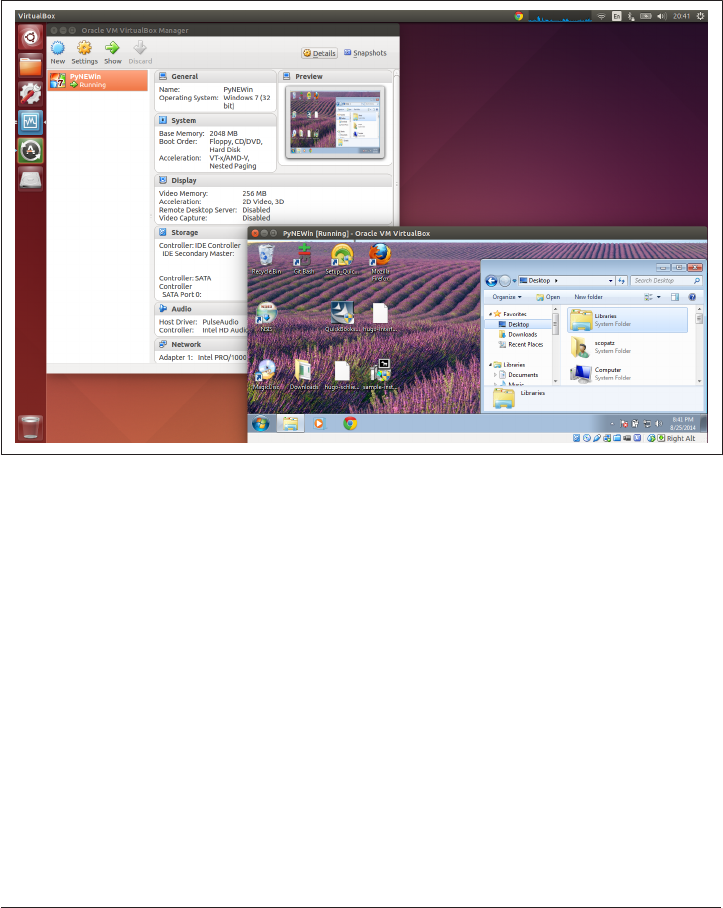
ble for reproducing your work, tracking down bugs, or opening Microsoft Office
while on a Linux machine.
The virtualization software that we recommend is Oracle’s VirtualBox. It is the most
popular open source VM software for day-to-day users. VirtualBox may run as a host
on Linux, Mac OS X, Windows, and a number of other operating systems. Competi‐
tors include VMware, XenServer, and KVM. Figure 13-1 shows an example virtual
machine with a 64-bit Ubuntu host running a 32-bit version of Windows 7 as a guest.
Figure 13-1. VirtualBox with a 64-bit Ubuntu 14.04 host and a 32-bit Windows 7 guest
Virtual machines are incredibly important for large-scale deployment. We will see
their primary strength when we get to “Deploying to the Cloud” on page 325. Yet
even when you’re working in small groups, it is useful to have a working virtual
machine with your software. Upload this VM to the Internet, and users can download
it and try out your code without actually trying to learn how to install it! The only
major disadvantage with this VM-based distribution strategy is that the virtual
machines can become quite large. The snapshot of a VM can easily range from 1 to
10 GB, depending on the guest operating system and the size of the code base.
The size and startup times of VMs can be crippling for small, automated tasks. This
has led to another valuable approach to packaging and deployment.
320 | Chapter 13: Deploying Software
www.it-ebooks.info

Docker
Motivated by the fact that virtual machines and hypervisors can be large and take a
long time to start up, a new technology called containers has recently rocketed to the
top of many people’s lists of deployment strategies. A container may be thought of as
operating system–level virtualization. Rather than the guest having to go through a
separate hypervisor, the operating system itself provides an interface for the guest to
request and access resources, safely shielded from other parts of the operating system.
This makes containers much lighter-weight and faster than traditional virtual
machines. It also adds restrictions, since the guest has to know about the host’s kernel
in order to access it.
Containers are typified by the Docker project. Initially released in March 2013,
Docker saw a stable v1.0 in June 2014. The velocity of its rise and adoption is
remarkable.
So why now? And why so fast? Without diving into too many of the details, Linux
Containers (LXC) have been around since Linux v2.6.24, which was released in Janu‐
ary 2008. However, they had some pretty large security holes. It was not until Linux
v3.8, released in February 2013, that these holes were fixed sufficiently to be viable for
large-scale deployment. The Docker project was started, and the rest is history.
The main limitation of containers is that the guest operating system must be the same
as the host operating system. Furthermore, LXC is a Linux-only technology right
now. Microsoft and Docker have recently announced a collaboration, so Windows
containers are on their way, but the Mac OS X platform has yet to start to catch up.
Critics of LXC will sometimes point out that other operating systems, such as
FreeBSD and Solaris, had container support long before Linux. For various historical
reasons, though, none of these container technologies gained the popularity that LXC
currently enjoys.
Since Docker is currently limited to Linux (and soon, hopefully,
Windows), feel free to skip the rest of this section if that is not your
platform of choice. What follows is a tutorial on how to use
Docker. You have now learned what you need to about containers
and their importance as a tool for collaboration; you can come
back to this section when you have a personal need for Docker
itself.
Using Docker is nearly synonymous with using Docker Hub, the online hosting ser‐
vice for Docker. Tight integration between the Docker command-line interface and
Docker the Internet service is part of what makes it so popular. If you do not already
have an account on Docker Hub, you should go create one now. It is easy and free.
Deploying the Software Itself | 321
www.it-ebooks.info
Assuming you have Docker installed and usable (on Ubuntu, run the command sudo
apt-get install -y docker docker.io), you can run a simple “hello world” con‐
tainer with the following command:
$ sudo docker run ubuntu:14.04 echo "Hello, World!"
This executes docker with the run command, downloading from Docker Hub an
Ubuntu 14.04 image, as specified by the ubuntu:14.04. The remaining arguments are
any bash commands that you wish to run from inside the container. Here, we simply
run echo. If you have not run docker before, the output of this command will look
like the following:
$ sudo docker run ubuntu:14.04 echo "Hello, World!"
[sudo] password for scopatz:
Unable to find image 'ubuntu:14.04' locally
Pulling repository ubuntu
c4ff7513909d: Download complete
511136ea3c5a: Download complete
1c9383292a8f: Download complete
9942dd43ff21: Download complete
d92c3c92fa73: Download complete
0ea0d582fd90: Download complete
cc58e55aa5a5: Download complete
Hello, World!
Note that you need root privileges to run docker.
That’s a secret!
Docker will intelligently stash containers for future use.
The output of our echo command.
This shows that the Ubuntu image, which was only around 225 MB, could not be
found locally, so Docker automatically downloaded it from Docker Hub for us.
Docker then executed the echo command. Compared to downloading and setting up
a whole virtual machine, using Docker is easy. (Of course, this is a “hello world”
example, so it should be easy!) Naturally, there are other tweaks you can make to this
process, such as specifying private resources other than Docker Hub for finding con‐
tainers. Note that the image that was downloaded was cached for later use. Rerunning
the same command will not require downloading the image again. The second time
around, we should only see the output of echo:
$ sudo docker run ubuntu:14.04 echo "Hello, World!"
Hello, World!
322 | Chapter 13: Deploying Software
www.it-ebooks.info

A list of all Docker images that are on the local system can be printed out with the
images command, as follows:
$ sudo docker images
REPOSITORY TAG IMAGE ID CREATED VIRTUAL SIZE
ubuntu 14.04 c4ff7513909d 2 weeks ago 225.4 MB
To avoid the business of downloading images when you want to run them, the pull
command allows you to download them ahead of time. Say we wanted to run the lat‐
est version of the WordPress blog. We could grab the corresponding image by passing
in wordpress:latest:
$ sudo docker pull wordpress:latest
Of course, you have to check the Docker Hub website to see what repositories
(ubuntu, wordpress, etc.) and what tags (14.04, latest, etc.) are available before you
can pull down an image.
You may also delete local Docker images from your system with the “remove image,”
or rmi, command. Suppose that we decided that we were not that into writing blogs
anymore and wanted to get rid of WordPress. This could be performed with the com‐
mand:
$ sudo docker rmi wordpress
Now, say that we wanted to add numpy to the ubuntu container so that it would be
readily available for future use. This kind of container customization is exactly what
Docker was built for, and it does it quite well. The first step is to launch the ubuntu
container in interactive mode. We do so by using the run command along with the -t
option to give us a terminal and the -i option to make it interactive. We will probably
want to run bash so that we can be effective once inside of the container, too. When
we run the following command we are dropped into a new interactive terminal
within the container:
$ sudo docker run -t -i ubuntu:14.04 /bin/bash
root@ae37c22b3c49:/#
While inside the container’s shell, Docker will automatically record anything that we
do. Let’s install Ubuntu’s package manager, install numpy, and then leave. These steps
are shown here:
$ sudo docker run -t -i ubuntu:14.04 /bin/bash
root@ae37c22b3c49:/# apt-get update
...
root@ae37c22b3c49:/# apt-get install -y python-numpy
...
root@ae37c22b3c49:/# exit
Note that while we are inside of the container, we have root privileges.
Deploying the Software Itself | 323
www.it-ebooks.info

Back on our host machine, to truly save our work we have to commit the changes.
This creates a new image based on the original one, any modifications we may have
made, and metadata about the change that we supply. The docker commit command
takes the identifier that we saw in the container (here, ae37c22b3c49), a message
string via the -m option, an author name via the -a option, and a repository name for
the new image (here, ubuntu-numpy). When following along at home, be sure to sub‐
stitute your own Docker Hub username for <user>. Putting this all together, we can
commit our changes with the command:
$ sudo docker commit -m "with numpy" -a "<name>" ae37c22b3c49 <user>/ubuntu-numpy
73188d24344022203bee5ef5d6cb31ccaa8b5f38085ae69fcf9502828220f81d
Our new container now shows up in the images list and is available for future use.
Running the images command from before now produces the following output on
my computer:
$ sudo docker images
REPOSITORY TAG IMAGE ID CREATED VIRTUAL SIZE
scopatz/ubuntu-numpy latest 73188d243440 About a minute ago 225.4 MB
ubuntu 14.04 c4ff7513909d 2 weeks ago 225.4 MB
Running docker with <user>/ubuntu-numpy will save us time, because numpy is pre‐
loaded. We could also have built this same container using a Dockerfile. Docker
files are more effort to set up, though also more reproducible. For most regular
Docker tasks, the interactive shell is good enough. Please see the Docker documenta‐
tion for more details.
At this point, the ubuntu-numpy image still lives only on our computer. However, we
can upload it to Docker Hub for ourselves and others to freely use. This is done with
the push command. This command will ask you to log into Docker Hub if you have
not done so already. As you can see here, push requires that you specify the image
that you want to upload:
$ sudo docker push scopatz/ubuntu-numpy
The push refers to a repository [scopatz/ubuntu-numpy] (len: 1)
Sending image list
Please login prior to push:
Username: scopatz
Password:
Email: scopatz@gmail.com
Login Succeeded
The push refers to a repository [scopatz/ubuntu-numpy] (len: 1)
Sending image list
Pushing repository scopatz/ubuntu-numpy (1 tags)
511136ea3c5a: Image already pushed, skipping
1c9383292a8f: Image already pushed, skipping
9942dd43ff21: Image already pushed, skipping
d92c3c92fa73: Image already pushed, skipping
324 | Chapter 13: Deploying Software
www.it-ebooks.info
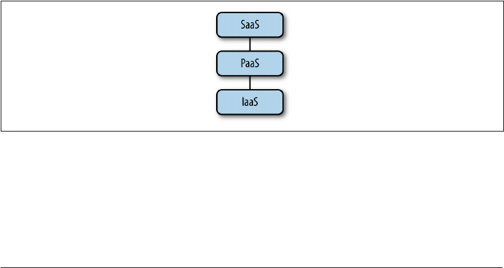
0ea0d582fd90: Image already pushed, skipping
cc58e55aa5a5: Image already pushed, skipping
c4ff7513909d: Image already pushed, skipping
73188d243440: Image successfully pushed
Pushing tag for rev [73188d243440] on {https://cdn-registry-1.docker.io/v1/
repositories/scopatz/ubuntu-numpy/tags/latest}
Docker is a sophisticated tool that puts power into its users’ hands. We have only
scratched the surface of what it can do here and not discussed how it works internally.
However, those details are not needed to use Docker to deploy physics code and you
can already see that it is an efficient and masterful way of creating, customizing, and
sharing software. Rightfully so, Docker is quickly replacing other, more traditional
methods of software deployment.
Now that you know how to deploy software through a variety of mechanisms, let’s go
on to where you might deploy it.
Deploying to the Cloud
Lately, it seems impossible to avoid hearing about the cloud: cloud systems, cloud
architectures, cloud business solutions, and the like. As a group of remote computers
that combine to provide a wide range of services to a local user or machine, the cloud
could easily be dismissed as just another phrase for the Internet itself. And to users,
there does not seem to be much distinction.
While there is no formal agreement on what the cloud is, a reasonable definition is
that it is the deployment of and interaction between three reliability strategies:
Software-as-a-Service (SaaS), Platform-as-a-Service (PaaS), and Infrastructure-as-a-
Service (IaaS). These technologies are enabled by virtual machines and containers,
which have already been covered in this chapter. You can envision cloud computing
as the stack shown in Figure 13-2.
Figure 13-2. Cloud computing stack
The cloud is not a revolution in terms of the kinds of technology that are deployed
(websites, email, databases, etc.). Rather, it is an evolution of who does the deploying,
at what scale, and with what level of redundancy. For example, if 10 years ago you
wanted an email server for your group, it often meant you would go over to the old
Deploying to the Cloud | 325
www.it-ebooks.info

1Author’s note: all of these have happened to me.
2This has not.
server in your closet, install the email server software, and then assign yourself and
your friends any email addresses you liked. This worked just fine until your hard
drive spun itself into oblivion, vermin ate through your ethernet cable, or your
Internet service provider suddenly decided to start blocking port 25.1 Alternatively,
suppose that you were running a website from your home and it suddenly became
extraordinarily popular.2 Your brand new DSL connection would probably not have
been able to handle the load. This would invariably lead to the site being down until it
was no longer popular. This used to happen so frequently that the phenomenon
earned the name the Slashdot eect, after the news website whose references caused
many pages to go down temporarily.
The cloud solves these problems by offloading services to a larger, more stable, and
better connected third party, such as Google or Amazon or Rackspace. It also allows
you to scale your services up or down as needed. Cloud service providers make it
very easy to provision new machines, bandwidth, or storage space as you need them.
They also make it easy to remove such resources once you are finished with them.
Starting at the bottom of the stack, Infrastructure-as-a-Service is where you rent
some or all of the physical parts of a large-scale computer system: hard drives,
servers, networking devices, electricity, an amazing Internet connection, and the roof
above all of this expensive machinery. You do not get an operating system, but you
are able to configure the kind of system you want temporarily. This is great to have if
you want to have a single machine to experiment with, 10 to do a trial run, 100 to do
a full release with, and then finally scale back to 50 when you realize you purchased
too many machines. IaaS maximizes flexibility and minimizes risk.
In the middle of the cloud stack live the Platform-as-a-Service vendors. In the PaaS
model, a developer will write an application and deploy it. The PaaS typically offers a
common way to set up and write applications, making it easy to do so once you have
adopted its platform. PaaS applications are often run on IaaS machinery. Examples of
PaaS include Google App Engine (GAE) and Heroku.
At the top level of the stack are user-facing Software-as-a-Service tools. These are
how most people interact with the cloud on a daily basis. Almost always, these tools
are websites that are either available publicly or to a limited set of people. The “soft‐
ware” here refers to the fact that a website is code-developed as a service-oriented
application, distinct from the hardware that runs the code. The classic example of
SaaS is Gmail, though in truth anything that involves an active user doing more than
looking at websites could be considered SaaS. Content generation sites such as Word‐
Press blogs represent this well.
326 | Chapter 13: Deploying Software
www.it-ebooks.info

Cloud service providers (Google, Amazon, Rackspace) tend to supply their customers
with IaaS, PaaS, and SaaS in whatever mix they believe best suits customers’ needs.
The lines between these three categories are often blurred. A company that sets out to
sell software might also end up selling hard disk space because it finds that its users
want more storage. A business that just wants to sell time on processors for virtual
machines will typically also end up adding a web interface to manage those VMs.
The power of the cloud comes from the realization that you can be more efficient if
you can offload at least part of the minutiae of managing your services to someone
else who specializes at it. How you deploy to a particular platform depends on your
needs and the supplier. Every company has its own guides and documentation. Once
you think you know what you want, it can help to look for guides and to shop around
online before committing to a particular vendor.
In the physical sciences, the cloud is most often utilized when you or your group have
outgrown the resources that you currently have available. Rather than buying and set‐
ting up expensive new machinery, you can rent the resources you need, when you
need them, for as long as you need them. Since the price point is so much lower than
buying your own in-house capabilities, the cloud effectively brings large-scale com‐
puting services to everyone.
That said, the cloud is centered around a high-throughput computing model. The
next section covers deploying high-performance computing applications, which tend
to be more common in computational physics.
Deploying to Supercomputers
Supercomputers are notoriously finicky devices. They are large computer engineering
experiments. Unlike the cloud, a supercomputer was not built to serve you or your
needs. If you reach the point where you need to have or you do have access to a
supercomputer for your work, it will be clear that supercomputers are shared resour‐
ces. You will almost never need to access the whole machine. If you do, that just
means that you’ll have to wait your turn in line even longer.
Deployment in a supercomputing environment is embodied by the following three
features:
• Uniform processors and memory across nodes
• A parallel filesystem
• A scheduler
As was touched on in Chapter 12, having the same processor and the same amount of
memory available everywhere in a supercomputer means that the code that you write
for one part of the machine is executable on all other parts. This is great. However,
Deploying to Supercomputers | 327
www.it-ebooks.info

you do not have direct access to the supercomputer’s compute nodes. First, you must
sign in to the login node to access the machine at all. From the login node, you may
then submit jobs to be executed by the scheduler. Typically, supercomputing environ‐
ments require you to compile custom versions of your code in order for that code to
be able to run. Furthermore, every machine is its own special work of art. The cus‐
tomizations that you make for one supercomputer do not necessarily apply to
another machine. These customizations often break when going from one generation
of machines to the next.
Supercomputers, as a shared resource, also have a parallel filesystem. This is because
many people and many processes will attempt to access files simultaneously. As a
user, this will look and feel much like a normal filesystem that you have on your lap‐
top or desktop or flash drive. However, it will perform much differently. On a parallel
filesystem, every file you access incurs a certain overhead. For a large number of files
this overhead becomes unbearable, because each file has to be checked individually.
For example, on a laptop, executing the ls command in a directory with a hundred
thousand files might take 1–3 seconds. On a parallel filesystem, this same operation
could take half an hour or longer. Limiting the number of files that you have to access
is the key to being successful. File metadata is just that much slower on these systems.
There are usually tricks to make commands faster, but these are not necessarily well
known. For example, using ls --color=never will sometimes bring the listing run‐
time back down to sane levels, but not if you use the -l option or any other possible
slowdowns.
Lastly, to actually run code on a supercomputer you need to go through the scheduler.
Common schedulers include TORQUE and Grid Engine. This program is responsi‐
ble for keeping track of how much total time each user has allocated and how much
has been used, and for determining which jobs get to be run and which ones remain
in the queue until the next job has finished. The point of the scheduler is to keep the
usage of the machine fair. As with most “fair” systems, it can leave its constituents
frustrated and annoyed. Almost all schedulers have a time limit. If a job exceeds the
time limit, the scheduler will abruptly kill the job. Time limits typically range from
three days to a week. Smaller and shorter jobs will typically move through the queue
more quickly than larger and longer jobs. However, since you are on a supercomputer
you likely need the greater resources. There is a balance that has to be struck.
Since every supercomputer is special, you will need to consult the machine-specific
documentation for yours to deploy to it. If this does not work, please consult your
friendly and overworked system administrator to help figure out where you went
wrong. Note that kindness serves you well in these scenarios. When nothing is work‐
ing and everything has gone wrong, five minutes of social engineering can easily save
a month’s worth of computer engineering. Being nice helps.
328 | Chapter 13: Deploying Software
www.it-ebooks.info

Deployment Wrap-up
We have now seen a wide range of strategies for deploying software. You should be
familiar with these main points:
•Deployment is ultimately about your users.
•You are your first user.
• Source-based package managers are good for high-level languages, like Python.
•Binary package managers are good for compiled languages because the users do
not need to have compilers themselves.
•Virtual machines package up the entire environment, including the operating
system.
•Containers are much lighter-weight than virtual machines, but have the same
advantages.
• Cloud computing is useful when reliability is needed.
•Supercomputers can be frustrating to interact with because they are shared
resources, while simultaneously being computer engineering experiments. How‐
ever, the benefits outweigh the costs when your problem demands such a device.
Now that you know how to write and deploy software, it is time to learn the best
practices of computational science.
Deployment Wrap-up | 329
www.it-ebooks.info


CHAPTER 14
Building Pipelines and Software
The most effective analysis and software tools are reused and shared often. Physics
software, libraries, and analysis pipelines are no exception. Indeed, this book is inten‐
tionally titled Eective Computation in Physics. Effective computational physicists
streamline repetitive work and liberate themselves from the mundane. They are also
able to build upon the work of others by installing and using external libraries. This
chapter will cover both strategies, since they are intricately related by an emphasis on
automation and by a versatile tool called make.
By the end of this chapter, you should be able to get started with the following tasks:
• Automating complex workflows and analysis pipelines
• Configuring and installing external libraries
•Creating build systems for your own software
By automating the tedious steps, you are much more likely to encourage colleagues to
extend your work and to, therefore, positively impact the future of your field. This
chapter will help you to assist your peers in building, installing, and reproducing your
analysis pipeline by automating the various steps of building that pipeline and your
software:
1. Configuration
2. Compilation
3. Linking
4. Installation
The first step, configuration, detects platform-dependent variables and user-specified
options. It then uses those to customize later steps in the process. For example, an
333
www.it-ebooks.info

analysis pipeline might run a Python program on a data file to create a particular plot.
However, the location of the data file may vary from analysis to analysis or from com‐
puter to computer. Therefore, the configuration step occurs before the program is
executed. The configuration step seeks out the proper data path by querying the envi‐
ronment and the user to configure the execution accordingly.
The next two steps, compilation and linking, are only necessary you’re when building
software written in a compiled language. The compilation step relies on a compiler to
convert source code into a machine-readable binary format. The linking step attaches
that binary-formatted library or executable to other libraries on which it may depend.
These two steps prepare the software for installation.
In Chapter 13, the installation step was addressed in a Python context. This step is
when compiled libraries, executables, data, or other files are placed in an accessible
place in the filesystem. This is all followed by the execution step, when the user
actually runs the analysis pipeline or software.
This chapter will address each of these five steps in the context of the make utility and
its makeles. These are ubiquitous in the computational physical sciences and are
integral to automating nearly any computational process.
make
make is a command-line utility that determines which elements of a process pipeline
need to be executed, and then executes them. It can be used to automate any process
with a tree of dependencies—that is, any process that builds files based on others.
Our case study in this chapter will be Maria Goeppert Mayer, who won the 1963
Nobel Prize in Physics for having theorized the nuclear shell model. She was a
remarkably effective scientist. Thus, we can be fairly certain that if she were still doing
science these days, she would definitely use make to automate her work. Any time a
new experiment generated new data or her theoretical model was tweaked, she might
want to update the figures in her draft theory paper.
make can automate this. Let us imagine that Professor Mayer is working on a paper
describing a new theory and that one day, she receives additional data to support her
theory. She would like to update her paper accordingly.
334 | Chapter 14: Building Pipelines and Software
www.it-ebooks.info

LaTeX and Its Dependencies
In the following examples, Prof. Mayer will be writing her papers in LaTeX. This pro‐
gram will be covered in great depth in Chapter 20, but some basic information about
it will be helpful for following along in this section. In particular, LaTeX is a program
that can be used to combine plain-text files and image files to create documents. Fun‐
damentally, an author creates some number of .tex files, image files, and others. The
LaTeX program converts those into a .dvi file, which is much like a .pdf.
To achieve this, first and foremost, she needs to add the new data to the list of data
files that she analyzes. Next, the data analysis program must be rerun using all of the
old data plus the new data. The results of the data analysis affect one of the figures in
her paper (“Figure 4: Photon-Photon Interactions”), so just adding the data and
rerunning the analysis won’t be enough; she also needs to rerun the plotting program
that generates the image for this figure. Of course, when any changes to the figures
or .tex files are made, the actual paper must be rebuilt using LaTeX (see Chapter 20).
This should sound familiar. It is the vast rabbit hole of tasks down which many physi‐
cists lose uncountably many research hours. These things that need to be done, the
tasks, are the nodes of a complex dependency tree. The file dependency tree for Prof.
Mayer’s project might resemble that in Figure 14-1. When a new data file is intro‐
duced, like 1948-12-21.h5, many of the files that depend on it must be regenerated.
A simple bash script like the ones discussed in Chapter 1 could be written to execute
every command on the tree, regenerating all of the figures and the paper any time it is
called. However, since the new data only affects one figure, not all of the figures need
be rebuilt. Such a bash script would spend a lot of time regenerating figures unneces‐
sarily: replotting the rest of the figures would be a waste of time, since they are
already up to date.
make | 335
www.it-ebooks.info
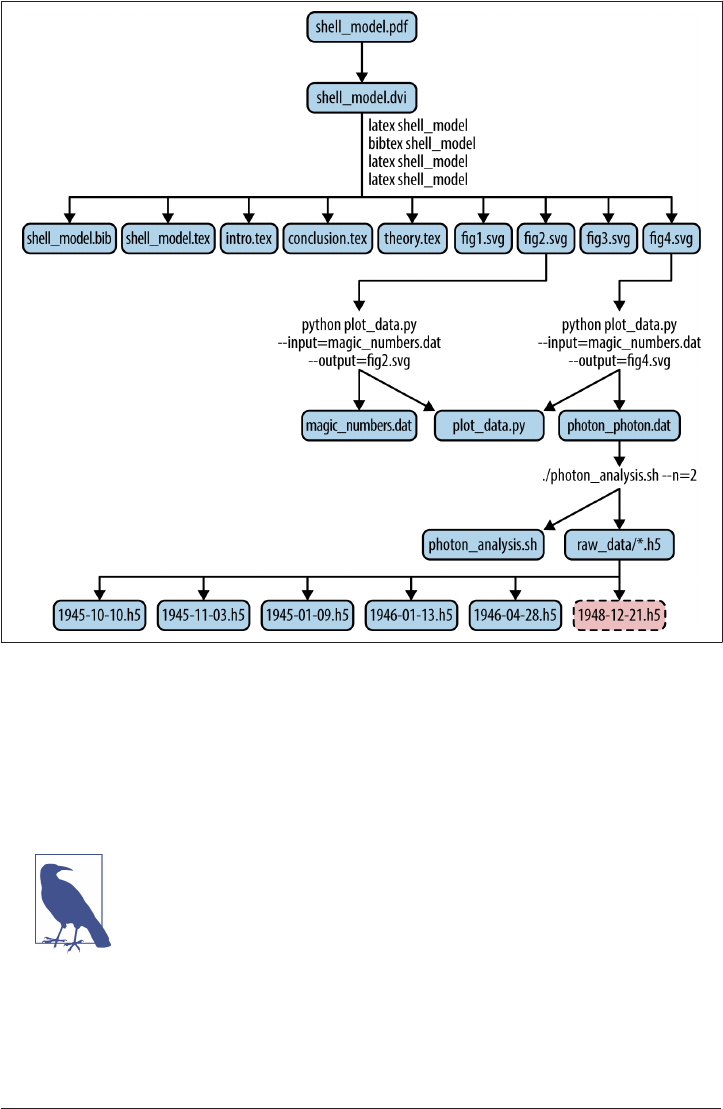
Figure 14-1. Mayer dependency tree
The make utility is superior. It can be used to automate every step of this situation
more efficiently, because it keeps track of how things depend on one another and
detects which pieces are not up to date. Given the file dependency tree and a descrip‐
tion of the processes that compile each file based on the others, make can execute the
necessary processes in the appropriate order.
Because it detects which files in the dependency tree have changed,
make executes only the necessary processes, and no more. This saves
time, especially when some actions take a long time to execute but
are not always necessary.
Can you tell what processes would need to be reexecuted if a new file in the raw_data
directory (1948-12-21.h5) were introduced? Try drawing a path up the branches of
the tree to the top. Which commands do you pass on the way?
336 | Chapter 14: Building Pipelines and Software
www.it-ebooks.info

Some platforms, like Windows and Mac OS X, do not have make
enabled in the Terminal by default. Try opening a terminal and typ‐
ing which make. If the make utility is available, this command will
output the path to the executable. If it is not available, an error will
be emitted: “make: command not found.” In the latter case, return
to the Preface for instructions on how to enable make on your
platform.
When a new data file is added, make can determine what analysis files, figures, and
documents are affected. It can then execute the processes to update them. In this way,
it can automatically rerun Prof. Mayer’s data analysis, regenerate appropriate plot,
and rebuild the paper accordingly.
It sounds glorious—too good be true, really. Prof. Mayer would like to try running
make.
Running make
make can be run on the command line with the following syntax:
make [ -f makefile ] [ options ] ... [ targets ] ...
It looks like the make command can be run without any arguments. So, in some direc‐
tory where Prof. Mayer holds these interdependent files, she can try typing this magi‐
cal make command:
~/shell_model $ make
make: *** No targets specified and no makefile found. Stop.
Uh oh, it looks like it may not be magic after all. But what is a makefile?
Makeles
A makefile is just a plain-text file that obeys certain formatting rules. Its purpose is to
supply the make utility with a full definition of the dependency tree describing the
relationships between files and tasks. The makefile also describes the steps for updat‐
ing each file based on the others (i.e., which commands must be executed to update
one of the nodes).
If the make command is run with no arguments, then the make utility seeks a file
called Makele in the current directory to fulfill this purpose. The error response
occurs because Prof. Mayer has not yet created a Makele in the directory where she
holds her analysis.
make | 337
www.it-ebooks.info
If the makefile has any name other than Makele, its name must be
provided explicitly. The -f flag indicates the location of that file to
the make utility. Makefiles with names other than Makele are typi‐
cally only necessary if more than one makefile must exist in a sin‐
gle directory. By convention, makefiles not called Makele end in
the .mk extension.
This section will discuss how to write makefiles by hand. Such makefiles can be used
to automate simple analysis and software pipelines. Prof. Mayer will create one to
update the plots in her paper based on new data.
Targets
First and foremost, the makefile defines targets. Targets are the nodes of the depend‐
ency tree. They are typically the files that are being updated. The makefile is made up
mostly of a series of target-prerequisite-action maps defined in the following syntax:
target : prerequisites
action
A colon separates the target name from the list of prerequisites.
Note that the action must be preceded by a single tab character.
The analyzed .dat files depend on the raw .h5 files in the raw_data directory. They
also depend on the bash scripts that churn through the .h5 files to convert them into
useful .dat files. Therefore, the photon_photon.dat target depends on two prerequi‐
sites, the set of ./raw_data/*.h5 files and the photon_analysis.sh shell script.
Let us imagine the shell script is quite clever, having been written by Prof. Mayer her‐
self. It has been written to generically model various interactions and accepts argu‐
ments at runtime that modify its behavior. One of the arguments it accepts is the
number of photons involved in the interaction. Since the photon_photon.dat file
describes the two-photon interaction, the shell script can be modified with the special
flag -n=2 indicating the number of photons. The following definition in a makefile
sets up the target with its prerequisites and passes in this argument:
# Building the Shell Model Paper
photon_photon.dat : photon_analysis.sh ./raw_data/*.h5
./photon_analysis.sh -n=2 > photon_photon.dat
The target file to be created or updated is the photon_photon.dat file. The prereq‐
uisites (the files on which it depends) are the shell script and the .h5 files.
This command is the action that must be taken to update the target using the
prerequisites.
338 | Chapter 14: Building Pipelines and Software
www.it-ebooks.info

In this example, the first line is a comment describing the file. That’s just good prac‐
tice and does not affect the behavior of the makefile. The second line describes the
target and the prerequisites, and the third line describes the action that must be taken
to update photon_photon.dat in the event that make detects any changes to either of
its prerequisites.
If this source code is saved in a file called Makele, then it will be found when make is
executed.
Exercise: Create a Makele
1. In the make directory of the files associated with this book,
create an empty file called Makele.
2. Add the photon_photon.dat target as described.
3. Save the file.
Now that the makefile defines a target, it can be used to update that target. To build or
update a target file using make, you must call it with the name of the target defined in
the makefile. In this case, if make photon_photon.dat is called, then make will:
1. Check the status of the prerequisites and photon_photon.dat.
2. If their timestamps do not match, it will execute the action.
3. However, if their timestamps do match, nothing will happen, because everything
is up to date already.
The makefile is built up of many such target-prerequisite-action maps. The full
dependency tree can accordingly be built from a set of these directives. The next node
Prof. Mayer might define, for example, is the one that rebuilds Figure 4 any time the
photon_photon.dat file is changed. That figure is generated by the plot_response.py
Python script, so any changes to that script should also trigger a rebuild of g4.svg.
The makefile grows accordingly as each target definition is added. The new version
might look like this:
# Building the Shell Model Paper
photon_photon.dat : photon_analysis.sh ./raw_data/*.h5
./photon_analysis.sh -n=2 > photon_photon.dat
fig4.svg : photon_photon.dat plot_response.py
python plot_dat.py --input=photon_photon.dat --output=fig4.svg
A new target, g4.svg, is defined.
make | 339
www.it-ebooks.info

The g4.svg file depends on photon_photon.dat as a prerequisite (as well as a
Python script, plot_response.py).
The action to build g4.svg executes the Python script with specific options.
Since the figure relies on photon_photon.dat as a prerequisite, it also, in turn, relies on
prerequisites of photon_photon.dat. In this way, the dependency tree is made. So,
when make fig4.svg is called, make ensures that all the prerequisites of its prerequi‐
sites are up to date.
Exercise: Add Additional Targets
1. Open the Makele created in the previous exercise.
2. Add the g4.svg target as above.
3. Can you tell, from Figure 14-1, how to add other targets? Try
adding some.
4. Save the file.
The final paper depends on all of the figures and the .tex files. So, any time a figure or
the .tex files change, the LaTeX commands must be reissued. The LaTeX program will
be covered in much greater detail in Chapter 20. At that time, you may combine your
knowledge of make with your knowledge of LaTeX to determine what targets should
be included in a makefile for generating a LaTeX-based document.
Special Targets
The first target in a file is usually run by default. That target is the one that is built
when make is called with no arguments. Often, the desired default behavior is to
update everything. An “all” target is a common convention for this. Note that the tar‐
get name does not have to be identical to the filename. It can be any word that is con‐
venient. The “all” target simply needs to depend on all other top-level targets.
In the case of Prof. Mayer’s paper, the all target might be defined using the wildcard
character (*):
# Building the Shell Model Paper
all: figure*.svg *.dat *.tex *.pdf
photon_photon.dat : photon_analysis.sh ./raw_data/*.h5
./photon_analysis.sh -n=2 > photon_photon.dat
fig4.svg : photon_photon.dat
python plot_response.py --input=photon_photon.dat --output=fig4.svg
340 | Chapter 14: Building Pipelines and Software
www.it-ebooks.info

...
Note how the all target does not define an action. It just collects prerequisites.
The all target tells make to do exactly what is needed. That is, when this target is
called (with make or make all), make ensures that all prerequisites are up to date, but
performs no final action.
Exercise: Create a Special Target
Another common special target is clean. This target is typically
used to delete generated files in order to trigger a fresh reupdate of
everything.
1. Open the Makele you have been working with.
2. Create a “clean” target.
3. What are the appropriate prerequisites? Are there any?
4. What is the appropriate command to delete the auxiliary files
created by LaTeX?
Now that she knows how to create a makefile, Prof. Mayer can use it to manage
dependencies for the entire process of building her paper from the raw data. This is a
common use for makefiles and facilitates many parts of analysis, visualization, and
publication. Another common use for makefiles is configuring, compiling, building,
linking, and installing software libraries. The next section will cover many aspects of
this kind of makefile.
Building and Installing Software
Python is called a compiled language because it does not need to be compiled. That is,
Python is precompiled. However, that compilation step is not handled so nicely by all
programming languages. C, C++ , Fortran, Java, and many others require multiple
stages of building before they are ready to run. We said in the introduction to this
chapter that these stages were:
1. Configuration
2. Compilation
3. Linking
4. Installation
Building and Installing Software | 341
www.it-ebooks.info

From a user’s perspective, this maps onto the following set of commands for instal‐
ling software from source :
~ $ .configure [options]
~ $ make [options]
~ $ make test
~ $ [sudo] make install
The configuration step may be called with a different command (i.e., ccmake or
scons). This step creates a makefile based on user options and system character‐
istics.
The build step compiles the source code into binary format and incorporates file
path links to the libraries on which it depends.
Before installing, it is wise to execute the test target, if available, to ensure that
the library has built successfully on your platform.
The installation step will copy the build files into an appropriate location on your
computer. Often, this may be a location specified by the user in the configuration
step. If the install directory requires super-user permissions, it may be necessary
to prepend this command with sudo, which changes your role during this action
to the super-user role.
For installation to succeed, each of these steps requires commands, flags, and custom‐
ization specific to the computer platform, the user, and the environment. That is, the
“action” defined by the makefile may involve commands that should be executed dif‐
ferently on different platforms or for different users.
For example, a compilation step can only use the compiler available on the computer.
Compilation is done with a command of the form:
compiler [options] <source files> <include files> [-l linked libraries]
For C++ programs, one user may use g++ while another uses clang and a third uses
gcc. The appropriate command will be different for each user. The makefile, therefore,
must be congured to detect which compiler exists on the machine and to adjust the
“action” accordingly. That is, in the action for the compilation step, the compiler com‐
mand and its arguments are not known a priori. Configuration, Compilation, Link‐
ing, and Installation depend on the computer environment, user preferences, and
many other factors.
For this reason, when you are building and installing software libraries, makefiles can
become very complex. However, at their core, their operation is no different than for
simple analysis pipeline applications like the one in the previous section. As the
dependency tree grows, more targets are added, and the actions become more com‐
342 | Chapter 14: Building Pipelines and Software
www.it-ebooks.info

plex or system-dependent, more advanced makefile syntax and platform-specific con‐
figuration becomes necessary. Automation is the only solution that scales.
Conguration of the Makele
It would be tedious and error-prone to write a custom makefile appropriate for each
conceivable platform-dependent combination of variables. To avoid this tedium, the
most effective researchers and software developers choose to utilize tools that auto‐
mate that configuration. These tools:
• Detect platform and architecture characteristics
• Detect environment variables
• Detect available commands, compilers, and libraries
•Accept user input
• Produce a customized makefile
In this way, configuration tools (a.k.a. “build systems”) address all aspects of the
project that may be variable in the build phase. Additionally, they enable the devel‐
oper to supply sensible default values for each parameter, which can be coupled with
methods to override those defaults when necessary.
Why Not Write Your Own Installation Makele?
Writing your own makefile from scratch can be time-consuming and error-prone.
Furthermore, as a software project is adopted by a diversity of users and scales to
include dependencies on external libraries, generating an appropriate array of make‐
files for each use case becomes untenable. So, the makefile should be generated by a
sophisticated build system, which will enable it to be much more flexible across plat‐
forms than would otherwise be possible.
Some common build system automation tools in scientific computing include:
•CMake
•Autotools (Automake + Autoconf)
•SCons
Rather than demonstrating the syntax of each of these tools, the following sections
will touch on shared concepts among them and the configurations with which they
assist.
First among these, most build systems enable customization based on the computer
system platform and architecture.
Building and Installing Software | 343
www.it-ebooks.info

Platform conguration
Users have various computer platforms with similarly various architectures. Most
software must be built differently on each. Even the very simplest things can vary
across platforms. For example, libraries have different filename extensions on each
platform (perhaps libSuperPhysics.dll on Windows, libSuperPhysics.so on Linux, and
libSuperPhysics.dyld on Unix). Thus, to define the makefile targets, prerequisites, and
actions, the configuration system must detect the platform. The operating system
may be any of the following, and more:
•Linux
• Unix
• Windows
•Mobile
• Embedded
Additionally, different computer architectures store numbers differently. For exam‐
ple, on 32-bit machines, the processors store integers in 32-bit-sized memory blocks.
However, on a 64-bit machine, an integer is stored with higher precision (64 bits).
Differences like this require that the configuration system detect how the current
architecture stores numbers. These specifications often must be included in the com‐
pilation command.
Beyond the platform and architecture customizations that must be made, the system
environment, what libraries are installed, the locations of those libraries, and other
user options also affect the build.
System and user conguration
Most importantly, different computers are controlled by different users. Thus, build
systems must accommodate users who make different choices with regard to issues
such as:
• What compiler to use
• What versions of libraries to install
• Where to install those libraries
• What directories to include in their PATH and similar environment variables
• What optional parts of the project to build
• What compiler flags to use (debugging build, optimized build, etc.)
The aspects of various systems that cause the most trouble when you’re installing a
new library are the environment variables (such as PATH) and their relationship to the
344 | Chapter 14: Building Pipelines and Software
www.it-ebooks.info

locations of installed libraries. In particular, when this relationship is not precise and
accurate, the build system can struggle to find and link dependencies.
Dependency conguration
When one piece of software depends on the functionality of another piece of soft‐
ware, the second is called a dependency. For example, if the SuperPhysics library
relies on the EssentialPhysics library and the ExtraPhysics library, then they are
its dependencies. Before attempting to install the SuperPhysics library, you must
install EssentialPhysics and ExtraPhysics.
The build can fail in either of these cases:
• The build system cannot locate a dependency library.
• The available library is not the correct version.
The build system seeks the libraries listed in the PATH, LD_LIBRARY_PATH, and similar
environment variables. Thus, the most common problems in building software arise
when too many or not enough dependency libraries appear in the directories target‐
ted by the environment.
When too many versions of the ExtraPhysics library are found, for example, the
wrong version of the library might be linked and an error may occur. At the other
extreme, if no EssentialPhysics library is found, the build will certainly fail. To fix
these problems, be sure all dependencies are appropriately installed.
Once all dependencies, environment variables, user options, and other configurations
are complete, a makefile or installation script is generated by the build system. The
first action it conducts is the compilation step.
Compilation
Now that the makefile is configured, it can be used to compile the source code. The
commands in the makefile for a software build will be mostly compiler commands.
Without getting into too much detail, compilers are programs that turn source code
into a machine-readable binary format.
The build system, by convention, likely generated a makefile with a default target
designed to compile all of the source code into a local directory. So, with a simple
make command, the compiled files are generated and typically saved (by the makefile)
in a temporary directory as a test before actual installation. Additionally, once com‐
piled, the build can usually be tested with make test.
If the tests pass, the build system can also assist with the next step: installation.
Building and Installing Software | 345
www.it-ebooks.info

Installation
As mentioned in Chapter 13, the key to attracting users to your project is making it
installable.
On Windows, this means creating a Setup.exe file. With Python, it means implement‐
ing a setup.py or other distribution utility. For other source code on Unix systems,
this means generating a makefile with an install target so that make install can be
called.
Why not just write a simple script to perform the installation?
The user may eventually want to upgrade or even uninstall your program, fantastic as
it may be. By tradition, the installation program is usually created by the application
developer, but the uninstall program is usually the responsibility of the operating sys‐
tem. On Windows, this is handled by the Add/Remove Programs tool. On Unix, this
is the responsibility of the package manager. This means the installation program
needs special platform-dependent capabilities, which are usually taken care of by the
build system.
For example, on Linux, make install is not used when creating packages. Instead,
make DESTDIR=<a_fake_root_dir> install installs the package to a fake root direc‐
tory. Then, a package is created from the fake root directory, and uninstallation is
possible because a manifest is generated from the result.
The build system will have created this target automatically. If the installation loca‐
tion chosen in the configuration step is a restricted directory, then you must execute
the make install command with sudo in order to act as the superuser:
sudo make install
At that point, the software should be successfully installed.
Building Software and Pipelines Wrap-up
At the end of this chapter, you should now feel comfortable with automating pipe‐
lines and building software using makefiles. You should also now be familiar with the
steps involved in building a non-Python software library from source:
1. Configuration
2. Compilation
3. Linking
4. Installation
346 | Chapter 14: Building Pipelines and Software
www.it-ebooks.info

Additionally, with the knowledge of how these steps and the makefile relate to the
platform, environment, user, and dependencies, you should feel prepared to under‐
stand a wide array of installation issues more fully.
If this chapter has succeeded in its purpose, you may be interested in researching
automated build systems (e.g., CMake, autotools, and SCons) more fully in order to
implement a build system for your own software project.
Building Software and Pipelines Wrap-up | 347
www.it-ebooks.info

CHAPTER 15
Local Version Control
In science, reproducibility is paramount. A fundamental principle of science, repro‐
ducibility is the requirement that experimental results from independent laboratories
should be commensurate. In scientific computation simulations, data munging and
analysis pipelines are experimental analogs. To ensure that results are repeatable, it
must be possible to unwind code and analysis to previous versions, and to replicate
plots. The most essential requirement is that all previous versions of the code, data,
and provenance metadata must be robustly and retrievably archived. The best prac‐
tice in scientific computing is called version control.
Rather than inventing a system of indexed directories holding full versions of your
code from each day in the lab, the best practice in software development is to use a
version control system that automates archiving and retrieval of text documents such
as source code.
This chapter will explain:
• What version control is
• How to use it for managing files on your computer
•And how to use it for managing files in a collaboration
First up, this chapter will discuss what version control is and how it fits into the
reproducible workflow of an effective researcher in the physical sciences.
What Is Version Control?
Very briefly, version control is a way to:
•Back up changing files
349
www.it-ebooks.info

• Store and access an annotated history
• And manage merging of changes between different change sets
There are many tools to automate version control. Wikipedia provides both a nice
vocabulary list and a fairly complete table of some popular version control systems
and their equivalent commands.
Fundamentally, version control provides capabilities similar to those that a laboratory
notebook historically has provided in the workflow of the experimental scientist. In
this way, it can be considered a sort of laboratory notebook for scientists who use
computation.
The Lab Notebook of Computational Physics
The Wu Experiment, one of the foundational experiments in nuclear physics, demon‐
strated a violation of the Law of Conservation of Parity. Dr. Chien Shiung Wu, a Chi‐
nese physicist at Columbia University, took great pains to construct a reproducible
experiment. Toward this goal, she even moved her experimental setup to the National
Bureau of Standards Headquarters in Maryland while her colleagues reproduced her
work back at her home institution. This work led to a Nobel Prize for her theorist
colleagues (and the inaugural Wolf Prize for Madame Wu).
A modern Dr. Wu (we will call her Dr. Nu) might simulate this physics experiment
with software. Dr. Nu is a persistent researcher, so she works on this important soft‐
ware project day and night until it accurately represents the theory of her colleagues.
When she finishes one day before dinnertime, she plots her results and is relieved to
be ready to submit them to a journal in the morning.
An unconscionable number of months later, she receives the journal’s review of her
work. It is a glowing review, but asks that the results be presented (in all plots, equa‐
tions, and analysis) with the inconvenient positive-current convention for charged
particle currents.
Since so many months have passed since the article was first submitted, the code has
changed significantly and plots are now rendered differently in preparation for a new
journal submission. For an alarming percentage of physicists, this would be a minor
disaster involving weeks of sorting through the files to recall the changes that have
happened in the last year (Merali 2010). It might even be impossible to roll back the
code to its previous state.
However, Dr. Nu breathes a sigh of relief. She has been using version control. With
version control, she can execute a single command to examine the record of her
actions over the last several months. Her version control system has kept, essentially,
a laboratory notebook of her software development history. When satisfied with her
understanding of the logs, she can execute another simple command to revert the
350 | Chapter 15: Local Version Control
www.it-ebooks.info

code to the state it was in the night she made the journal-ready plots. Before after‐
noon tea, Dr. Nu makes the simple change of sign convention in the plot, reruns her
plotting script, and submits the revisions. Once tea is over, she can bring the reposi‐
tory back up to date and get back to work, as if nothing had changed.
What would happen if you received a review asking for a convention change to
results you completed a year ago? If that’s a scenario that is simply too terrible to
imagine, you are not alone. This chapter will explain how Dr. Nu reached this envia‐
ble position, so that you can do the same.
We will start by explaining the types of version control available to a scientist. Then,
the rest of the chapter will explain version control concepts in the context of one ver‐
sion control system in particular.
Version Control Tool Types
Version control systems come in two fundamentally different categories. More
modern version control systems are “distributed” rather than “centralized.” Central‐
ized systems designate a single (central) definitive location for a repository’s source,
while distributed version control systems treat all (distributed) locations as equals.
Some common version control systems in each category include:
• Centralized
—Concurrent Versions System (cvs)
— Subversion (svn)
— Perforce (p4)
• Distributed
— Decentralized CVS (dcvs)
—mercurial (hg)
— bazaar (bzr)
— Git (git)
Recently, distributed version control systems have become more popular. They are
better suited to collaborative projects, since their capabilities for managing and merg‐
ing together changes from multiple developers are more powerful and user-friendly.
Choosing the appropriate option from among these should depend largely on the
expertise of your colleagues and their collaboration style. Due to its popularity, flexi‐
bility, and collaborative nature, we will demonstrate version control concepts using
the Git tool. Git, written by Linux creator Linus Torvalds, is an example of a dis‐
tributed version control system. It has a somewhat steep learning curve, so the sooner
we can get started, the better.
What Is Version Control? | 351
www.it-ebooks.info

Getting Started with Git
Git needs to be installed and configured before it can be used to control the versions
of a set of files. When Dr. Nu was first getting started with her simulation, she knew
she should keep versions of everything, just like in a laboratory notebook. So, she
decided to install Git on the computer where she writes her code and conducts her
analysis.
Installing Git
The first step for using Git is installing it. Dr. Nu wasn’t sure if she already had Git
installed on her computer, so to check she used the which command we met in Chap‐
ter 1.
To determine whether Git is already installed and to find help
using it, try executing which git in the terminal. Does it respond
with a path to the program, or does it return nothing?
If which git returns no executable path, then Git is not installed. To install it, she’ll
need to:
1. Go to the Git website.
2. Follow the instructions for her platform.
On some platforms, the default version of Git is quite old (developers call that stable).
Unfortunately, it may not have all the features of an up-to-date version. So, even if Git
is installed, you may consider updating it anyway.
Once Git has been installed (or updated), it can be used. But how?
Getting Help (git --help)
The first thing Dr. Nu likes to know about any tool is how to get help. From the com‐
mand line, she types:
~ $ man git
The manual entry for the Git version control system appears before her, rendered in
less. She may scroll through it using the arrow keys, or she can search for keywords
by typing / followed by the search term. Dr. Nu is interested in help, so she types /
help and then hits Enter.
By doing this, Dr. Nu finds that the syntax for getting help with Git is git --help.
352 | Chapter 15: Local Version Control
www.it-ebooks.info

Manual (man) pages are rendered in less. To exit the man page,
therefore, type the letter q and hit Enter.
To try this help syntax, Dr. Nu exits the man page and tests what happens when she
types:
~ $ git --help
Excellent! Git returns, to the terminal, a list of commands it is able to help with, as
well as their descriptions:
usage: git [--version] [--exec-path[=<path>]] [--html-path]
[-p|--paginate|--no-pager] [--no-replace-objects]
[--bare] [--git-dir=<path>] [--work-tree=<path>]
[-c name=value] [--help]
<command> [<args>]
The most commonly used git commands are:
add Add file contents to the index
bisect Find by binary search the change that introduced a bug
branch List, create, or delete branches
checkout Checkout a branch or paths to the working tree
clone Clone a repository into a new directory
commit Record changes to the repository
diff Show changes between commits, commit and working tree, etc
fetch Download objects and refs from another repository
grep Print lines matching a pattern
init Create an empty git repository or reinitialize an existing one
log Show commit logs
merge Join two or more development histories together
mv Move or rename a file, a directory, or a symlink
pull Fetch from and merge with another repository or a local branch
push Update remote refs along with associated objects
rebase Forward-port local commits to the updated upstream head
reset Reset current HEAD to the specified state
rm Remove files from the working tree and from the index
show Show various types of objects
status Show the working tree status
tag Create, list, delete or verify a tag object signed with GPG
See 'git help <command>' for more information on a specific command.
The help command even has a metacomment about how to get more specific
information about a particular command. Based on this, how would you learn
more about the git init command?
Getting Started with Git | 353
www.it-ebooks.info

That’s a lot of commands, but it isn’t everything Git can do. This chapter will cover
many of these and a few more. The first command we will show will complete the set-
up process: git config.
Control the Behavior of Git (git cong)
To complete the setup process for Git, a configuration step is necessary. Knowing
your name, email address, favorite text editor, and other data will help Git to behave
optimally and to correctly provide attribution for the work that you do with your
files.
Dr. Nu knows that version control provides an exceptional attribution service to sci‐
entists collaborating on code. When a change is made to code under version control,
it must be attributed to the author. To ensure that she is appropriately attributed for
her excellent work and held accountable for any code bugs, Dr. Nu configures her
instance of Git thus:
~ $ git config --global user.name "Nouveau Nu"
~ $ git config --global user.email "nu@university.edu"
~ $ git config --global core.editor "nano"
Changes made by Dr. Nu will be attributed to the name she provides to Git.
Her university email address will also be stored with each logged change.
Git can behave more optimally when it is aware of the author’s preferred text edi‐
tor. Later, we will see how.
Not only do scientists love to see their names in print next to a piece of excellent
work, but authorship metadata is essential to provide provenance and answer the
question, “Where did this work come from?” Indeed, attribution is central to the sci‐
entific process, since accountability is one of the fundamental motivators of scientific
excellence.
Exercise: Congure Git on Your Computer
1. Use the preceding example as a model to inform Git of your
name, email address, and favorite text editor.
2. List your new configuration settings with git config --list.
Now that Git is set up on her system, Dr. Nu is able to use it to manage the versions of
the files stored on her computer.
354 | Chapter 15: Local Version Control
www.it-ebooks.info
Local Version Control with Git
All researchers in scientific computing have at least one computer full of data, text
files, images, plots, scripts, and other software. Those files often constitute the bulk of
the day-to-day efforts of that researcher. Code and data are often created, manipu‐
lated, dealt with, and stored primarily on a single computer. Controlling versions of
those files involves:
•Creating a repository where those changes are stored
• Adding files to that repository so that they can be tracked
• Taking snapshots of incremental versions, so that they are logged
• Undoing changes
• Redoing them
•Trying new ideas in separate sandboxes
We will talk about all of these tasks in this section. So first, we must learn how to cre‐
ate a repository.
Creating a Local Repository (git init)
Dr. Nu would like to write code that simulates Dr. Chien-Shiung Wu’s landmark
experiment. Writing this code may take years and involve the effort of many graduate
students, and the code will undergo many iterations. To keep track of numerous ver‐
sions of her work without saving numerous copies, Dr. Nu can make a local repository
for it on her computer.
A repository is where the tracked files live and are edited. For each
version of those files, Git records the change set, or “diff”—the line-
by-line differences between the new version and the one before it.
To begin keeping a record of files within a directory, Dr. Nu must enter that directory
and execute the command git init . This creates an empty repository:
~ $ mkdir parity_code
~ $ cd parity_code
~/parity_code $ git init
Initialized empty Git repository in /filespace/people/n/nu/parity_code/.git/
First, she creates the directory where she will do the work.
She navigates to that directory.
Local Version Control with Git | 355
www.it-ebooks.info

She initializes a repository within that directory.
Git responds positively. An empty repository has been created here.
Because she is a scientist, Dr. Nu is curious about what happened. She can browse the
directory’s hidden files to see what happened here:
~/parity_code $ ls
~/parity_code $ ls -A
.git
~/parity_code $ cd .git && ls- A
HEAD config description hooks info objects refs
A simple listing of the directory contents results in nothing. The directory
appears to be empty. Where is the repository?
Curious, Dr. Nu lists all of the contents of the repository.
A hidden directory, .git, is visible.
Navigating into that directory and listing all of its contents reveals the mecha‐
nism by which the repository operates.
With ordinary use of Git, none of those hidden files will ever need to be altered.
However, it’s important to note that the infrastructure for the repository is contained
within this hidden subdirectory (.git) at the top level of your repository.
A whole repository directory can be moved from one location to
another on a filesystem as long as the .git directory inside moves
along with it.
This means that moving the entire repository directory to another location is irrele‐
vant to the behavior of the repository. However, moving files or directories outside of
the repository will move them outside of the space governed by the hidden
infrastructure.
Exercise: Create a Local Repository
1. From the Terminal, create a new directory like Dr. Nu’s and
use git init to make it an empty local repository.
2. Browse the files in the hidden directory and find out what you
can learn in one minute.
356 | Chapter 15: Local Version Control
www.it-ebooks.info

Now that a repository has been initialized, work can begin in this directory. As work
progresses, files must first be added to the directory.
Staging Files (git add)
Now, Dr. Nu has created a repository directory to start working in. So, she gets to
work creating a “readme” file. This is an important part of the documentation of any
software; it indicates basic information about the project, as well as where to find
more details.
First, she can create an empty file with the touch command:
~/parity_code $ touch readme.rst
Now the file exists in the directory. However, it is not yet being tracked by the reposi‐
tory. For the Git repository to know which files Dr. Nu would like to keep track of,
she must add them to the list of files that the repository knows to watch. This is called
“staging” the files. It is analogous to arranging people on a stage so that they are ready
for a photo to be taken. In this case, we are staging the file so that it can be included
in the upcoming snapshots.
Thus, to make Git aware of the file, she adds it to the repository with the git add
command:
~/parity_code $ git add readme.rst
Exercise: Add a File to a Local Repository
1. Create a readme file within your repository directory.
2. With git add, inform Git that you would like to keep track of
future changes in this file.
Now that something has been added to the repository, the state of the repository has
changed. Often, it is important to be able to check the state. For this, we will need the
git status command.
Checking the Status of Your Local Copy (git status)
The files you’ve created on your machine are your local “working” copy. The reposi‐
tory, as we have already said, stores versions of the files that it is made aware of. To
find out the status of those files, a status command is available:
~/parity_code $ git status
On branch master
Initial commit
Local Version Control with Git | 357
www.it-ebooks.info

Changes to be committed:
(use "git rm --cached <file>..." to unstage)
new file: readme.rst
Check the status of the repository in the current directory.
Git has something called “branches.” We are on the “master” branch by default.
We will talk more about branches later in the chapter.
Git knows that we have not yet used the commit command in this repository.
Git gives us a hint for what to do if we did not really intend to add the readme
file. We can “unstage” it with git rm!
Git reports that there is a new file “to be committed.” We will discuss committing
in the next section.
This result indicates the current difference between the repository records (which, so
far, are empty) and the parity_code directory contents. In this case, the difference is
the existence of this new readme.rst file. Git suggests that these changes are “to be
committed.” This means that now that the file has been added to the watch list, the
scene is set and the repository is ready for a snapshot to be taken. We save snapshots
with the git commit command.
Saving a Snapshot (git commit)
In order to save a snapshot of the current state of the repository, we use the commit
command. This command:
1. Saves the snapshot, officially called a “revision”
2. Gives that snapshot a unique ID number (a revision hash)
3. Names you as the author of the changes
4. Allows you, the author, to add a message
The git commit command conducts the first three of these tasks automatically. How‐
ever, the fourth requires input from the author. When executing the git commit
command, the author must provide a “commit message” describing the changes rep‐
resented by this commit and indicating their purpose. Informative commit messages
will serve you well someday, so make a habit of never committing changes without at
least a full sentence description.
358 | Chapter 15: Local Version Control
www.it-ebooks.info

Log messages have a lot of power when used well. To this end,
some open source projects even suggest information to include in
all commit messages. This helps the developers to more systemati‐
cally review the history of the repository. For example, the Pandas
project uses various three-letter keys to indicate the type of com‐
mit, such as (ENH)ancement, BUG, and (DOC)umentation.
In the same way that it is wise to often save a document that you are working on, so
too is it wise to save numerous revisions of your code. More frequent commits
increase the granularity of your “undo” button.
Commit often. Good commits are atomic, the smallest change that
remains meaningful. They should not represent more work than
you are willing to lose.
To commit her work, Dr. Nu simply types git commit into the command line. Git
responds by opening up an instance of the nano text editor, where she can add text to
a document recording the change. She does so by adding a message: “This is my first
commit. I have added a readme file.” When she saves the file, the commit is complete.
Exercise: Commit Your Changes
1. Use git commit to save the staged changes of the file you’ve
added to your repository.
2. Git will send you to your preferred text editor. There, create a
message, then save and exit.
3. Admire your work with the git status command. You should
see something like:
$ git status
# On branch master
nothing to commit (working directory clean)
If instead you receive a warning indicating that Git is not config‐
ured, you will need to return to “Control the Behavior of Git (git
config)” on page 354 and configure it.
Now, as she makes changes to the files in her repository, Dr. Nu can continue to com‐
mit snapshots as often as she likes. This will create a detailed history of her efforts.
Local Version Control with Git | 359
www.it-ebooks.info

Exercise: Stage and Commit New Changes
1. Edit your readme file. It should say something like:
Welcome
This is my readme file for a project on parity
violations in the standard model.
1. Stage it for the snapshot (git add).
2. Commit the snapshot (git commit).
3. Add a meaningful commit message.
So far, we’ve learned that the workflow should be :
1. Make changes.
2. git add the files you want to stage for a commit.
3. git commit those files.
4. Fill out the log message.
5. Repeat.
Since that is a lot of steps, note that command-line flags can cut this way down. Some
useful flags for git commit include:
-m: add a commit message from the command line
-a: automatically stage tracked files that have been modified or deleted
-F: add a commit message from a file
--status: include the output of git status in the commit message
--amend: fix the commit message at the repository tip
These can be used in combination to reduce the add/commit/message process to one
command: git commit -am "<useful log message goes here>".
Exercise: Commit and Add a Message in One Step
1. Edit your readme file to tell us whose it is (e.g., “This is Dr.
Nu’s readme…”).
2. Add the file, commit the changes, and append your log mes‐
sage with one command.
Whichever method you use to write commit messages, be sure to make those mes‐
sages useful. That is, write commit messages as if they were the scientific notation
360 | Chapter 15: Local Version Control
www.it-ebooks.info
that they are. Like section headings on the pages of your lab notebook, these messages
should each be one or two sentences explaining the change represented by a commit.
The frequency of commits is the resolution of your undo button.
Committing frequently makes merging contributions and revers‐
ing changes less painful.
Now we have successfully taken a snapshot representing an incremental change in the
repository and provided a message to go along with it. The fundamental innovation
in version control is that a record of that work has now been kept. To view that
record, we use the log command.
git log: Viewing the History
A log of the commit messages is kept by the repository and can be reviewed with the
log command:
~/parity_code $ git log
commit cf2631a412f30138f66d75c2aec555bb00387af5
Author: Nouveau Nu <nu@university.edu>
Date: Fri Jun 21 18:21:35 2013 -0500
I have added details to the readme to describe the parity violation project.
commit e853a4ff6d450df7ce3279098cd300a45ca895c1
Author: Nouveau Nu <nu@university.edu>
Date: Fri Jun 21 18:19:38 2013 -0500
This is my first commit. I have added a readme file.
The log command prints the logged metadata for each commit.
Each commit possesses a unique (hashed) identification number that can be used
to refer to that commit.
The metadata from the configuration step is preserved along with the commit.
Git automatically records the date and time at which the commit occurred.
Finally, the log message for each commit is printed along with that commit.
As more changes are made to the files, more snapshots can be committed, and the log
will reflect each of those commits. After making a number of commits, Dr. Nu can
review the summary of her work in the form of these commit messages.
Local Version Control with Git | 361
www.it-ebooks.info
When she wants to review her work in more detail than the commit messages can
offer, she may want to review the actual changes that were made between certain com‐
mits. Such differences between file versions are called “diffs,” and the tools that dis‐
play them are diff tools.
Viewing the Dierences (git di)
Let’s recall the behavior of the diff command on the command line. Choosing two
files that are similar, the command:
diff <file1> <file2>
will output the lines that differ between the two files. This information can be saved
as what’s known as a patch, but we won’t go deeply into that just now. Suffice it to say
that there are many diff tools. Git, however, comes with its own diff system.
The only difference between the command-line diff tool and Git’s diff tool is that the
Git tool is aware of all of the revisions in your repository, allowing each revision of
each file to be treated as a full file.
Thus, git diff will output the changes in your working directory that are not yet
staged for a commit. If Dr. Nu adds a definition of parity to her readme file, but does
not yet commit it, those changes are staged. When she asks Git for the diff, the fol‐
lowing occurs:
~/parity_code $ git diff
diff --git a/readme.rst b/readme.rst
index 28025a7..a5be27f 100644
--- a/readme.rst
+++ b/readme.rst
@@ -2,3 +2,5 @@ Welcome
This is my readme file for a project on parity violations in the standard
model.
+
+In the context of quantum physics, parity is a type of symmetric relation.
Dr. Nu executes the git diff command.
diff reports that the differences not staged for commit exist only in the readme
file versions a and b.
And indicates that these versions are those from the commits ending in 28025a7
and a5be27f, respectively.
To see how this works, make a change in your readme.rst file, but don’t yet commit it.
Then, try git diff.
A summarized version of this output can be seen with the --stat flag:
362 | Chapter 15: Local Version Control
www.it-ebooks.info

~/parity_code $ git diff --stat
readme.rst | 2 ++
1 file changed, 2 insertions(+)
For each line where one or more characters has been added, an insertion is coun‐
ted. If characters are deleted, this is called a deletion.
To see only what is staged for commit, you can try:
$ git diff --cached
What is the difference shown in the cached diff? What does this mean about what
files are staged?
Sometimes what you have staged is not what you actually want to commit. In the
same way, sometimes after reviewing a change that she has already committed, Dr.
Nu thinks better of it and would prefer to roll a file back to an earlier version. In both
of those instances, the git reset command can be used.
Unstaging or Reverting a File (git reset)
If, after reviewing the log, Dr. Nu decides that she prefers a past version of some file
to the previous revision, she can use git reset. This command can be used either to
unstage a staged file or to roll back a file or files to a previous revision.
If you added a file to the staging area that you didn’t mean to add, you can use reset
to “unstage” it (i.e., take it out of the staged set of commits):
git reset <filename>
In this case, reset acts like the opposite of add. However, reset has another use as
well. If you want to return the repository to a previous version, you can use reset for
that too. Just use the commit number:
git reset [<mode>] [<commit>]
reset has some useful mode flags:
--soft
Leaves the contents of your files and repository index alone, but resets repository
head
--mixed
Resets the index and repository head, but not the contents of your files
--hard
Returns the contents of all files and the repository index to the commit specified
Local Version Control with Git | 363
www.it-ebooks.info

Using reset, you can therefore undo changes that have already been committed. For
changes that have not yet been committed, you can use git checkout. This unstages
modifications:
git checkout -- <filename>
Note that git checkout has other purposes, which we’ll see soon.
Exercise: Discard Modications
1. Create five files in your directory, with one line of content in
each file.
2. Commit the files to the repository.
3. Change two of the five files and commit them.
4. Undo the changes in step 3.
5. Print out the last entry in the log.
Using reset or checkout, however, does not delete the commits permanently. The
record of those commits is still stored in the repository, and they can be accessed with
their commit revision hash numbers via git checkout. A more permanent option is
git revert.
Discard Revisions (git revert)
Much like git reset --hard, but with more permanence, git revert is a helpful
tool when you really want to erase history—for example, if you’ve accidentally com‐
mitted something with private or proprietary information. The syntax for git
revert is:
git revert <commit>
While she was working on her readme file, Dr. Nu decided to add contact informa‐
tion for herself. In doing so, she committed the following change to the readme:
diff --git a/readme.rst b/readme.rst
index a5be27f..0a07497 100644
--- a/readme.rst
+++ b/readme.rst
@@ -1,5 +1,8 @@
Welcome
+To contact Dr. Nouveau Nu, please send an email to nu@university.edu or call
+her cell phone at 837-5309.
+
This is my readme file for a project on parity violations in the standard
model.
364 | Chapter 15: Local Version Control
www.it-ebooks.info

A few seconds after committing this change, she regretted making her cell phone
number available. She could edit the readme to remove the number. However, even
after she commits that change, her number can still be accessed with git checkout.
To remove the record entirely, she must use the revert command. First, she needs to
know what commit number to revert, so she uses the log command:
~/parity_code $ git log
commit fc06a890ecba5d16390a6fb4514cb5ba45546952
Author: Nouveau Nu <nu@university.edu>
Date: Wed Dec 10 14:00:26 2014 -0800
Added my email address and phone number
...
Here, Dr. Nu finds the hash number to use.
She can use the whole hash number or as few as the first eight characters to uniquely
identify the commit she would like to revert:
~/parity_code $ git revert fc06a890
[master 2a5b0e1] Revert "Added my email address and phone number"
1 file changed, 3 deletions(-)
Now it has been completely removed from the history; she can breathe a sigh of relief
and move on. Now Dr. Nu would like to start programming in seriousness. However,
she is concerned about something. Since science involves trying things out and mak‐
ing mistakes, will she have to spend a lot of her time rewinding changes like this to
remove them from the master branch? What if she wants to try two new things at
once? In the next section, we will see that the answer to both of these questions is
“Using branches will make everything easier.”
Listing, Creating, and Deleting Branches (git branch)
Branches are parallel instances of a repository that can be edited and version con‐
trolled in parallel. They are useful for pursuing various implementations experimen‐
tally or maintaining a stable core while developing separate sections of a code base.
Without an argument, the git branch command lists the branches that exist in your
repository:
~/parity_code $ git branch
* master
The “master” branch is created when the repository is initialized. This is the default
branch and is conventionally used to store a clean master version of the source code.
With an argument, the branch command creates a new branch with the given name.
Dr. Nu would like to start a branch to hold some experimental code—that is, some
code that she is just trying out:
Local Version Control with Git | 365
www.it-ebooks.info
~/parity_code $ git branch experimetal
~/parity_code $ git branch
experimetal
* master
She creates a branch called “experimetal.”
To check that this worked, she lists the branches using the branch command.
The asterisk indicates which branch she is currently in. We’ll demonstrate how to
change branches shortly.
Whoops—Dr. Nu forgot to type the n in experimental. Simple typos like this happen
all the time in programming, but they are nothing to fear. Very few typos will break
everything. In this case, deleting the branch and trying again is very simple. To delete
a branch, she can use the -d flag:
~/parity_code $ git branch -d experimetal
Deleted branch experimetal (was 2a5b0e1).
~/parity_code $ git branch
* master
~/parity_code $ git branch experimental
~/parity_code $ git branch
experimental
* master
She deletes the misspelled branch.
Git responds that, yes, it has been deleted (and provides the hash number for the
HEAD, or most recent commit, of that branch).
Just to double-check, she can list the branches again.
And voilà, it’s gone. She can try again—this time without the typo.
At this point, Dr. Nu has created the “experimental” branch. However, she is still cur‐
rently working in the master branch. To tell Git that she would like to work in the
experimental branch, she must switch over to it with the checkout command.
Switching Between Branches (git checkout)
The git checkout command allows context switching between branches as well as
abandoning local changes and viewing previous commits.
To switch between branches, Dr. Nu can “check out” that branch:
~/parity_code $ git checkout experimental
Switched to branch 'experimental'
~/parity_code $ git branch
366 | Chapter 15: Local Version Control
www.it-ebooks.info

* experimental
master
Git is actually very good at keeping the user well informed. It can be very
reassuring.
How can you tell when you’ve switched between branches? When we used the branch
command before, there was an asterisk next to the master branch. Now it’s next to the
experimental branch—the asterisk indicates which branch you’re currently in.
Now, Dr. Nu can safely work on code in the experimental branch. When she makes
commits, they are saved in the history of the experimental branch, but are not saved
in the history of the master branch. If the idea is a dead end, she can delete the exper‐
imental branch without polluting the history of the master branch. If the idea is good,
however, she can decide that the commit history made in the experimental branch
should be incorporated into the master branch. For this, she will use a command
called merge.
Merging Branches (git merge)
At some point, the experimental branch may be ready to become part of the master.
The method for combining the changes in two parallel branches is the merge com‐
mand. To merge the changes from the experimental branch into the master, Dr. Nu
executes the merge command from the master branch:
~/parity_code $ git checkout master
~/parity_code $ git merge experimental
Now, the logs in the master branch should include all commits from each branch.
Give it a try yourself with the following long exercise.
Local Version Control with Git | 367
www.it-ebooks.info

Exercise: Create Two New Branches
1. Create a new repository and commit an empty readme file:
~ $ mkdir geography
~ $ cd geography
~/geography $ git init
~/geography $ touch readme.rst
~/geography $ git add readme.rst
~/geography $ git commit -am "first commit"
2. Create two new branches and list them:
~/geography $ git branch us
~/geography $ git branch texas
3. Add files describing each entity. In the “us” branch, include at
least a file called president. For “texas,” of course, you’ll need a
file called governor. You’ll probably also want one called ower:
~/geography $ git checkout us
Switched to branch 'us'
~/geography $ touch president
~/geography $ git add president
~/geography $ git commit -am "Added president to the us branch."
~/geography $ git checkout texas
Switched to branch 'texas'
~/geography $ touch flower
~/geography $ git add flower
~/geography $ git commit -am "Added bluebonnets to the
texas branch."
4. Merge the two branches into the master branch:
~/geography $ git checkout master
Switched to branch 'master'
~/geography $ git merge texas
Updating d09dfb9..8ce09f1
Fast-forward
flower | 0
1 file changed, 0 insertions(+), 0 deletions(-)
create mode 100644 flower
~/geography $ git merge us
Merge made by the 'recursive' strategy.
president | 0
1 file changed, 0 insertions(+), 0 deletions(-)
create mode 100644 president
The ability to automatically merge commits is powerful and quite superior to having
multiple versions of directories cluttering your filesystem. That said, the merge com‐
mand is only capable of combining changes that do not conflict with one another. In
the next section, you’ll get a taste of this problem.
368 | Chapter 15: Local Version Control
www.it-ebooks.info

Dealing with Conicts
Both Texas and the United States have a national anthem. However, we notice that the
national anthem isn’t there, so we add a file called national_anthem to the “us”
branch:
~/geography $ git checkout us
~/geography $ echo "Star-Spangled Banner" > national_anthem
~/geography $ git add national_anthem
~/geography $ git commit -am "Added star spangled banner to the us branch."
Next, of course, we put on our Wranglers and Stetsons and do the same for the
“Texas” branch, which does not yet have a national anthem file.
~/geography/$ git checkout texas
~/geography/$ echo "Texas, Our Texas" > national_anthem
~/geography/$ git add national_anthem
~/geography/$ git commit -am "Added Texas, Our Texas to the texas branch."
If we merge them into one another or into the master branch, what happens?
What happens is a conflict. This is a common issue when two different people are
working independently on different branches of a respository and try to merge them.
Since that is the context in which conflicts are most commonly encountered, the
explanation of how to deal with conflicts will be addressed in the next chapter. For
now. abort the merge with git merge --abort.
Version Conrol Wrap-Up
In this chapter, we have shown how to use git for recording versions of files, rewind‐
ing changes, and merging independent changes. These are the first steps toward
reproducible scientific computation. Having read this chapter, you are now prepared
to go forth and version control the work you do day to day. In fact, take a moment
now to place those analysis scripts you are working on under version control. Since
Git is an expansive and complex tool, you may find a need for additional resources.
We can recommend, in particular:
•Pro Git Book
•Software Carpentry’s Git Lessons
• The Software Carpentry quick reference
Now that you are comfortable with managing versions of files and source code
locally, you can move forward and program reproducibly. Next, you will need to
know how to harness the power of Git for collaboration. The next chapter will cover
the use of Git in combination with the immense power of the Internet.
Version Conrol Wrap-Up | 369
www.it-ebooks.info

CHAPTER 16
Remote Version Control
Now that you have learned how to version files locally with Git, you are ready to rev‐
olutionize the way you collaborate on software, papers, data, and everything else. This
chapter will cover the immense power of Git when it is combined with the broad
reach of the Internet.
Chapter 15 described tasks related to the local working copy of your repository. How‐
ever, the changes you make in this local copy aren’t backed up online automatically.
Until you send those changes to the Internet, the changes you make are local changes.
This chapter will discuss syncing your local working copy with remote copies online
and on other computers on your network. In particular, this chapter will explain how
to use Git and the Internet for:
•Backing up your code online
• Forking remote repositories to enable collaboration
• Managing files in a collaboration
• Merging simultaneous changes
• Downloading open source code to keep track of updates
First among these, this chapter will cover backing up code online.
Repository Hosting (github.com)
Repositories can be stored and accessed through repository hosting servers online.
Many people store their source code repositories on common repository hosting
services such as:
•Launchpad
371
www.it-ebooks.info

•Bitbucket
•Google Code
•SourceForge
•GitHub
This chapter will use GitHub as an example. It provides tools for browsing, collabo‐
rating on, and documenting code. These include:
• Landing page support
• Wiki support
•Network graphs and time histories of commits
• Code browser with syntax highlighting
• Issue (ticket) tracking
• User downloads
• Varying permissions for various groups of users
•Commit-triggered mailing lists
• Other service hooks (e.g., Twitter)
These services allow anyone with a repository to back up their work online and
optionally share it with others. They can choose for it to be either open source or pri‐
vate. Your home institution may have a repository hosting system of its own. To find
out, ask your system administrator.
Setting up a repository on GitHub requires a GitHub username
and password. Please take a moment to create a free GitHub
account.
Additionally, you may find it helpful to set up SSH keys for auto‐
matic authentication.
Dr. Nu can use GitHub as a way to back up her parity work, share it with her graduate
students, and demonstrate its fidelity to paper reviewers. Since her parity_code simu‐
lation software from the previous chapter already exists, she can upload it to GitHub
in four simple steps:
1. Create a user account on GitHub.
2. Create a space for her repository on GitHub.
3. Point to that remote from the local copy.
4. Push her repository to that location.
372 | Chapter 16: Remote Version Control
www.it-ebooks.info

The first two of these steps occur within the GitHub interface online.
Creating a Repository on GitHub
Setting up a user account creates a space for a user like Dr. Nu to collect all of the
repositories she uses. Creating a repository names location within that space for a
certain piece of software.
When she creates a username (NouveauNu) on GitHub, a location on its servers is
reserved for her at github.com/NouveauNu. If she navigates in her browser to that
location, she can click a big green button that says “New Repository.” She can supply
the repository name parity_code, and GitHub will respond by creating an empty
space at github.com/NouveauNu/parity_code.
This location is called a “remote” location because it is distant from the local working
copy. Now that the repository location has been created, Git can be used to send com‐
mits from the local copy to the remote. For this, Dr. Nu needs to alert the local copy
to the existence of the remote.
Declaring a Remote (git remote)
Remote repositories are just like local repositories, except they are stored online. To
synchronize changes between the local repository and a remote repository, the loca‐
tion of the remote must be registered with the local repository.
The git remote command allows the user to register remote repository URLs under
shorter aliases. In particular, this command can be used to add, name, rename, list,
and delete remote repository aliases. The original remote repository, with which a
local copy is meant to synchronize, is called “origin” by convention. In our example,
this repository is the one where Dr. Nu holds the master copy of parity_code. So, from
Dr. Nu’s local working copy of the parity_code repository, she creates an alias to the
remote thusly:
$ git remote add origin https://github.com/NouveauNu/parity_code.git
git remote command declares that Git should register something about a
remote repository. add declares that a remote repository alias should be added.
Dr. Nu chooses to use the conventional alias for this repository, origin. She then
associates the alias with the online location of the repository. This URL can be
copied from the GitHub page holding this repository.
Once she has executed this command, her local repository is now synced with the
one online. She is then capable of sending and receiving commits from the remote
repository. She can see a list of remotes registered with the remote command and its
“verbose” flag:
Creating a Repository on GitHub | 373
www.it-ebooks.info
~/parity_code $ git remote -v
origin https://github.com/NouveauNu/parity_code.git (fetch)
origin https://github.com/NouveauNu/parity_code.git (push)
The -v flag is common and means “verbose.” In this case, it means “verbosely list
the remotes.”
The origin alias is associated with the URL Dr. Nu provided. The meanings of
fetch and push will be covered very shortly.
She can now use this remote alias to “push” a full copy of the current status of the
parity_code repository onto the Internet.
Sending Commits to Remote Repositories (git push)
The git push command pushes commits in a local working copy to a remote reposi‐
tory. The syntax is:
git push [options] <remote> <branch>
To push a copy of her parity_code repository up to the Internet, Dr. Nu can therefore
execute the command:
~/parity_code (master) $ git push origin master
Username for 'https://github.com': nouveaunu
Password for 'https://nouveaunu@github.com':
Counting objects: 22, done.
Delta compression using up to 4 threads.
Compressing objects: 100% (15/15), done.
Writing objects: 100% (22/22), 2.19 KiB | 0 bytes/s, done.
Total 22 (delta 3), reused 0 (delta 0)
To https://github.com/NouveauNu/parity_code
* [new branch] master -> master
Dr. Nu pushes the current (master) branch up to the origin remote.
GitHub requires a username.
And a password.
The master branch has been pushed online.
This sends the full history of the local master branch up to the “origin” remote on
GitHub, as seen in Figure 16-1. For security, the GitHub servers ask Dr. Nu for her
username and password before the push is accepted. Only users with the appropriate
permissions can push changes to this repository. In this case, Dr. Nu is the only user
with permission to do so.
374 | Chapter 16: Remote Version Control
www.it-ebooks.info

Figure 16-1. Pushing to a remote
To access the files that are now online, Dr. Nu can navigate in a browser to the loca‐
tion of that repository online. Indeed, so can her collaborators. This is where the
magic begins. Since Dr. Nu has collaborators at other universities who rely on her
software to do their analysis, GitHub can be very helpful for sharing that software
with them. In particular, Fran Faraway, a postdoc on another continent, can now keep
up to date without any emails or phone calls to Dr. Nu. Now that Dr. Nu’s code is
online, Fran can use Git to download it from that location on GitHub using the clone
command.
Downloading a Repository (git clone)
Like Dr. Nu’s parity code, many useful open source scientific software libraries are
kept in repositories online. With the help of Git, scientists relying on these scientific
libraries can acquire up-to-date source code for their use and modification. The best
way to download such a repository is to clone it, as illustrated in Figure 16-2.
When a repository is cloned, a local copy is created on the local computer. It will
behave as a fully fledged local repository where local branches can be created, edits
can be made, and changes can be committed. To clone the parity_code repository,
Fran can use the syntax:
~/useful_software $ git clone https://github.com/NouveauNu/parity_code.git
This command downloads the online repository into a directory called parity_code.
Downloading a Repository (git clone) | 375
www.it-ebooks.info

Figure 16-2. Cloning a repository
Exercise: Clone a Repository from GitHub
1. Pick any repository you like. There are many cool projects
hosted on GitHub. Take a few minutes here to browse GitHub
and pick a piece of code of interest to you.
2. Clone it. If you didn’t find anything cool, we can suggest clon‐
ing the AstroPy libraries:
~ $ git clone https://github.com/astropy/astropy.git
Cloning into astropy...
remote: Counting objects: 24, done.
remote: Compressing objects: 100% (21/21), done.
remote: Total 24 (delta 7), reused 17 (delta 1)
Receiving objects: 100% (24/24), 74.36 KiB, done.
Resolving deltas: 100% (7/7), done.
3. You should see many files download themselves onto your
machine. These files will have been placed in a directory with
the name of the repository. Let’s make sure it worked. Change
directories, and list the contents:
~/ $ cd astropy
~/ $ ls
Now that she has cloned Dr. Nu’s repository, Fran has a full copy of its history. Fran
can even edit the source code for her own purposes and push that to her own reposi‐
376 | Chapter 16: Remote Version Control
www.it-ebooks.info
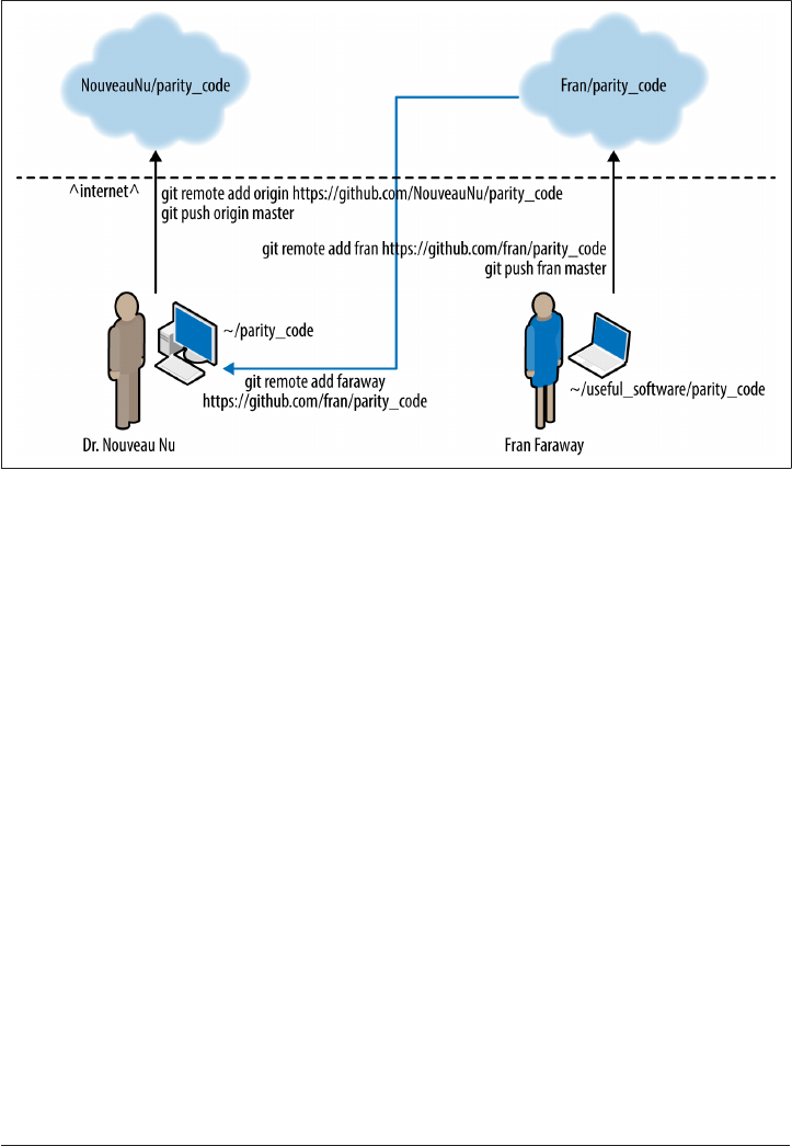
tory online without affecting Dr. Nu whatsoever. An example of this process is shown
in Figure 16-3.
Figure 16-3. Creating new remotes
In Figure 16-3, Fran has pushed her own changes up to her own GitHub repository.
Sometimes, when it is initialized in a particular way, this is called a “fork” of the origi‐
nal repository. Forks are a GitHub notion, rather than a Git notion. Basically, they are
mutually aware remote repositories. To create them, simply locate the Fork button at
the top-righthand corner of any repository on GitHub. That creates a new repository
in your user space from which you can clone your work. A project managed in this
way between the Curies might have the structure demonstrated in Figure 16-4.
Downloading a Repository (git clone) | 377
www.it-ebooks.info
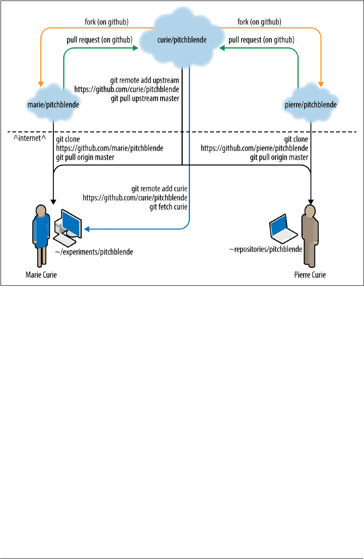
Figure 16-4. Forks in the Curie Pitchblende collaboration
This distributed system of remotes scales nicely for larger collaborations.
Since Dr. Nu’s code is under active development, Fran must update her own local
repository when Dr. Nu makes improvements to the code. By default, Fran’s cloned
repository is configured to be easily updated: the origin remote alias is registered by
default and points to the cloned URL. To download and incorporate new changes
from this remote repository (origin), Fran will require the git fetch and git merge
commands.
378 | Chapter 16: Remote Version Control
www.it-ebooks.info

Exercise: Fork the GitHub Repository
While you may already have a copy of this repository, GitHub
doesn’t know about it until you’ve made a fork. You’ll need to tell
GitHub you want to have an official fork of this repository.
1. Go to github.com/nouveaunu/parity_code in your Internet
browser, and click on the Fork button.
2. Clone it. From your terminal:
$ git clone https://github.com/<you>/parity_code.git
$ cd parity_code
In the place of <you>, put your actual GitHub username.
3. Now, create an alias for the remote repository:
$ git remote add nu \
https://github.com/nouveaunu/parity_code.git
$ git remote -v
origin https://github.com/YOU/parity_code (fetch)
origin https://github.com/YOU/parity_code (push)
nu https://github.com/nouveaunu/parity_code (fetch)
nu https://github.com/nouveaunu/parity_code (push)
Create a remote alias called nu that points at the original
repository.
List the remotes to see the effect.
The origin remote is set by default during the cloning
step.
Fetching the Contents of a Remote (git fetch)
Since the cloned repository has a remote that points to Dr. Nu’s online repository, Git
is able to fetch information from that remote. Namely, the git fetch command can
retrieve new commits from the online repository. In this case, if Fran wants to
retrieve changes made to the original repository, she can git fetch updates with the
command:
~/useful_software/parity_code $ git fetch origin
The fetch command merely pulls down information about recent changes from the
original master (origin) repository. By itself, the fetch command does not change
Fran’s local working copy. To actually merge these changes into her local working
copy, she needs to use the git merge command
Fetching the Contents of a Remote (git fetch) | 379
www.it-ebooks.info

Merging the Contents of a Remote (git merge)
To incorporate upstream changes from the original master repository (in this case,
NouveauNu/parity_code) into her local working copy, Fran must both fetch and
merge. If Fran has made many local changes and commits, the process of merging
may result in conflicts, so she must pay close attention to any error messages. This is
where version control is very powerful, but can also be complex.
Exercise: Fetch and Merge the Contents of a GitHub Repository
1. In the repository you cloned, fetch the recent remote reposi‐
tory history:
$ git fetch origin
2. Merge the origin master branch into your master branch:
$ git merge origin/master
3. Find out what happened by browsing the directory.
This process of fetching and merging should be undertaken any time a repository
needs to be brought up to date with a remote. For brevity, both of these steps can be
achieved at once with the command git pull.
Pull = Fetch and Merge (git pull)
The git pull command is equivalent to executing git fetch followed by git
merge. Though it is not recommended for cases in which there are many branches to
consider, the pull command is shorter and simpler than fetching and merging as it
automates the branch matching. Specifically, to perform the same task as we did in
the previous exercise, the pull command would be:
$ git pull origin master
Already up-to-date.
When there have been remote changes, the pull will apply those changes to your local
branch. It may require conflict resolution if there are conflicts with your local
changes.
When Dr. Nu makes changes to her local repository and pushes them online, Fran
must update her local copy. She should do this especially if she intends to contribute
back to the upstream repository and particularly before making or committing any
changes. This will ensure Fran is working with the most up-to-date version of the
repository:
~/useful_software/parity_code $ git pull
Already up-to-date.
380 | Chapter 16: Remote Version Control
www.it-ebooks.info

The “Already up-to-date” response indicates that no new changes need to be added.
That is, there have not been any commits to the original repository (origin) since the
most recent update.
Conicts
If Dr. Nu and Fran Faraway make changes in different files or on different lines of the
same file, Git can merge these changes automatically. However, if for some reason
they make different changes on the same line of a certain file, it is not possible for the
merge (or pull) command to proceed automatically. A conflict error message will
appear when Fran tries to merge in the changes.
This is the trickiest part of version control, so let’s take it very carefully.
In the parity_code repository, you’ll find a file called readme.rst. This is a standard
documentation file that appears rendered on the landing page for the repository in
GitHub. To see the rendered version, visit your fork on GitHub. The first line of this
file is “Welcome.”
For illustration, let’s imagine that both Dr. Nu and Fran Faraway suddenly decide they
would like to welcome visitors in the tongue of their home nation. Since these two
collaborators are from two different places, there will certainly be disagreements
about what to say instead of “Welcome.” This will cause a conflict.
First, since Dr. Nu is French, she alters, commits, and pushes the file such that it
reads:
Bonjour
This is my readme file for a project on parity violations in the standard
model.
In the context of quantum physics, parity is a type of symmetric relation.
Fran, however, is from Texas, so she commits her own version of “Welcome.”
Howdy
This is my readme file for a project on parity violations in the standard
model.
In the context of quantum physics, parity is a type of symmetric relation.
Before pushing her change to her own remote, Fran updates her repository to include
any changes made by Dr. Nu. The result is a conflict:
~/useful_software/parity_code $ git merge origin
Auto-merging readme.rst
CONFLICT (content): Merge conflict in readme.rst
Automatic merge failed; fix conflicts and then commit the result.
Conicts | 381
www.it-ebooks.info

Since the two branches have been edited on the same line, Git does not have an algo‐
rithm to merge the changes correctly.
Resolving Conicts
Now what?
Git has paused the merge. Fran can see this with the git status command:
$ git status
# On branch master
# Unmerged paths:
# (use "git add/rm <file>..." as appropriate to mark resolution)
#
# unmerged: readme.rst
#
no changes added to commit (use "git add" and/or "git commit -a")
The only thing that has changed is the readme.rst file. Opening it, Fran sees some‐
thing like this :
<<<<<<< HEAD
Howdy
=======
Bonjour
>>>>>>> master
This is my readme file for a project on parity violations in the standard
model.
In the context of quantum physics, parity is a type of symmetric relation.
Git has added this line to mark where the conflict begins. It should be deleted
before a resolution commit.
The change that Fran committed.
Git has added this line to mark the separation between the two conflicting ver‐
sions. It should be deleted before a resolution commit.
The change that Dr. Nu committed.
Git has added this line to mark where the conflict ends. It should be deleted
before a resolution commit.
The intent is for Fran to edit the file intelligently and commit the result. Any changes
that Fran commits at this point will be accepted as a resolution to this conflict.
382 | Chapter 16: Remote Version Control
www.it-ebooks.info
Fran knows now that Dr. Nu wanted the “Welcome” to say “Bonjour.” However, Fran
also wants it to say “Howdy,” so she should come up with a compromise. First, she
should delete the marker lines. Since she wants to be inclusive, she then decides to
change the line to include both greetings. Decisions such as this one must be made by
a human, and are why conflict resolution is not handled more automatically by the
version control system:
Howdy and Bonjour
This is my readme file for a project on parity violations in the standard
model.
In the context of quantum physics, parity is a type of symmetric relation.
This results in the status:
$ git status
# On branch master
# Unmerged paths:
# (use "git add/rm <file>..." as appropriate to mark resolution)
#
# both modified: readme.rst
#
...
no changes added to commit (use "git add" and/or "git commit -a")
Now, to alert Git that she has made appropriate alterations, Fran follows the instruc‐
tions it gave her in the status message (namely, git add and git commit those
changes):
$ git commit -am "Compromises merge conflict to Howdy and Bonjour"
$ git push origin master
Counting objects: 10, done.
Delta compression using up to 2 threads.
Compressing objects: 100% (6/6), done.
Writing objects: 100% (6/6), 762 bytes, done.
Total 6 (delta 2), reused 0 (delta 0)
To https://github.com/username/repositoryname.git
Explain your solution to the merge conflict in the log message.
Push the results online.
And that is it. Now the repository contains the history of both conflicting commits as
well as a new commit that merges them intelligently. The final result is the version
Fran has just committed.
Resolving Conicts | 383
www.it-ebooks.info

Remote Version Control Wrap-up
In this chapter, we have shown how to use Git along with GitHub for downloading,
uploading, and collaborating on code. Combined with remote repository hosting
sites, the skills learned in Chapter 15 allow the scientist to manage files and change
sets, merge simultaneous work among collaborators, and publish that work on the
Internet.
Having read this chapter, you are now prepared to open your code to your collabora‐
tors. Go forth and version control the work you do day to day. In fact, take a moment
now to place those analysis scripts you are working on under version control. Since
it’s an expansive and complex tool, you may find a need for additional resources on
Git. We can recommend, in particular:
•Pro Git book (Apress), a free and open source ebook
• Software Carpentry’s Version Control with Git
• Software Carpentry’s Git Reference
Now that you are comfortable with pulling, pushing, fetching, merging, and dealing
with conflicts, you should be able to collaborate with your colleagues on code and
papers more smoothly and reproducibly. Next, you will need to know how to find
and fix bugs so that your collaborative, reproducible software is reproducibly correct.
384 | Chapter 16: Remote Version Control
www.it-ebooks.info

CHAPTER 17
Debugging
The scientific method’s central motivation is the ubiquity of error—the awareness that
mistakes and self-delusion can creep in absolutely anywhere and that the scientist’s
effort is primarily expended in recognizing and rooting out error.
—Donoho 2009
In the very early days of computing, Admiral Grace Hopper and her team on the
Mark II computer encountered errors in the performance of the computer. Ulti‐
mately, a moth was discovered in one of the relays. Admiral Hopper reportedly
remarked that they were “debugging” the system. Though the term had been used
before in engineering, this event popularized the terms bug and debugging for the
causes and solutions, respectively, of errors in computer code and performance.
Bugs are errors in code, and they are ubiquitous reminders of our humanity. That is,
computers, by their very nature, do exactly what we tell them to do. Therefore, bugs
are typically imperfections in syntax and logic introduced by humans. However care‐
ful we are, bugs will be introduced while we are developing code. They begin to be
introduced as soon as we start writing a piece of code. For this reason, we must be
vigilant, and we must be prepared to fix them when they arise. This chapter will pre‐
pare you to recognize, diagnose, and fix bugs using various tools and methods for
“debugging” your code. It will do so by introducing:
•When, how, and by whom bugs are encountered
• Methods of diagnosing bugs
• Interactive debugging, for diagnosing bugs quickly and systematically
• Profiling tools to quickly identify memory management issues
•Linting tools to catch style inconsistencies and typos
385
www.it-ebooks.info

Of these, the most time will be spent on using the pdb interactive debugger in Python,
since it is essential for debugging issues whose source is not obvious from tests or
simple print statements. First, however, we will discuss the instigating event itself:
encountering a bug.
Encountering a Bug
A bug may take the form of incorrect syntax, imperfect logic, an infinite loop, poor
memory management, failure to initialize a variable, user error, or myriad other
human mistakes. It may materialize as:
•An unexpected error while compiling the code
• An unexpected error message while running the code
• An unhandled exception from a linked library
• An incorrect result
• An indefinite pause or hang-up
•A full computer crash
• A segmentation fault
• Silent failure
Developers may encounter bugs that they or their colleagues have introduced in their
source code. Users, also, test the limits of a program when they deploy it for their own
uses. Irrespective of when a bug is found or who finds it, bugs must be fixed. Faced
with any of them, whether it be a build error, a runtime exception, or a segmentation
fault, the user or developer should first try to track down and fix the bug.
Bugs can also be encountered at any time. In the next chapter, we will explain how
testing should do most of the verification work in a piece of scientific software. That
is, most bugs in a well-developed piece of software should be found by the tests
before they make it to the trusted version of the code.
A well-written test suite should do the heavy lifting in finding and
diagnosing bugs. Interactive debugging lifts the remainder.
However, tests rarely cover all edge and corner cases, so bugs can slip through the
cracks. The longer a bug exists undetected in a piece of trusted software, the more
dire the situation:
1. If a bug is found in testing, it can be fixed before the software is ever used.
386 | Chapter 17: Debugging
www.it-ebooks.info

2. If a bug is found before there are users, it can be fixed before it affects anyone
running the code.
3. If a bug is found when the code is run, it can be fixed before analysis is done on
the results.
4. If a bug is found when the results of the code are analyzed, it can be fixed before
the results are published in a journal article.
5. If a bug is found after the results are published, the paper has to be retracted.
Many papers are retracted every year due to bugs in code. Chapter 18 will show you
how to improve your software tests to avoid getting past stage 1 in the preceding list.
However, bugs occasionally slip through the cracks, so you must be ready to
encounter and fix them at any stage of your project.
While bugs can be found by anyone, they are usually only diagnosable and fixable by
people who know what the code is meant to do. Without knowing what the code is
meant to do, it is nearly impossible to know when a result is incorrect, when a long
pause is suspicious, or when silent termination indicates failure.
Now that you know how a bug is encountered, you are ready to learn how to diag‐
nose its cause. In order to walk before we run, we will first introduce a simplistic way
to diagnose bugs in code: print statements.
Print Statements
Print statements are every developer’s first debugger. Because of this, we’ll start here
—but know that they are not the best practice for effective computing and that we
will be covering better methods later in the chapter. Printing is typically a check that
asks one or both of these questions:
•Is the bug happening before a certain line?
• What is the status of some variable at that point?
In a simple, buggy program, a print statement can answer the first question if it is
inserted at a place where the program is suspected of misbehavior.
In Python 3, print(x) is a function call, and thus an expression. In
Python 2, print x was a statement and used a slightly different syn‐
tax. Still, the term print statement is used across many program‐
ming languages, even when printing to the screen is not technically
a statement on its own (like in Python 3, C, and C++).
In the following example, something about the code is causing it to “hang.” That is, it
simply seems to run forever, as if stalled:
Print Statements | 387
www.it-ebooks.info

def mean(nums):
bot = len(nums)
it = 0
top = 0
while it < len(nums):
top += nums[it]
return float(top) / float(bot)
if __name__ == "__main__":
a_list = [1, 2, 3, 4, 5, 6, 10, "one hundred"]
mean(a_list)
It is likely that you can determine the cause of this problem by visual inspection.
However, in the case that you cannot, a print statement can be inserted where the
code is suspected to be hanging:
def mean(nums):
bot = len(nums)
it = 0
top = 0
print("Still Running at line 5")
while it < len(nums):
top += nums[it]
print(top)
return float(top) / float(bot)
if __name__ == "__main__":
a_list = [1, 2, 3, 4, 5, 6, 10, "one hundred"]
mean(a_list)
This print() is added to determine where the error is happening.
This one is added to determine what is happening to the variables during the
loop.
Once a print statement is inserted at the suspected point of misbehavior, the program
can be executed, and the print statement either appears before the exception, or does
not appear at all. In the case shown here, many things are wrong with the code. How‐
ever, the most fatal is the infinite while loop. Since the print statement appears before
the code enters the infinite loop, the troublemaking line must be after the print state‐
ment. In this case, the first print statement is printed, so it is clear that the error
occurs after line 5. Additionally, the second print statement results in “1” being
printed infinitely. Can you tell what is wrong in the code using this information? The
infinite loop can certainly be fixed as in the code shown here:
def mean(nums):
top = sum(nums)
bot = len(nums)
return float(top) / float(bot)
388 | Chapter 17: Debugging
www.it-ebooks.info

if __name__ == "__main__":
a_list = [1, 2, 3, 4, 5, 6, 10, "one hundred"]
mean(a_list)
Rather than looping needlessly, the sum() function can be applied to the list.
Print statements like this can provide very helpful information for pinpointing an
error, but this strategy does not scale. In a large code base, it usually takes more than
a few tries or a few more print statements to determine the exact line at which the
error occurred. Additionally, the number of potentially problem-causing variables
increases as the size of the code base increases. A more scalable solution is needed:
interactive debugging.
Interactive Debugging
Rather than littering one’s code base with print statements, interactive debuggers
allow the user to pause during execution and jump into the code at a certain line of
execution. Interactive debuggers, as their name suggests, allow the developer to query
the state of the code in an interactive way. They allow the developer to move forward
through the code execution to determine the source of the error.
Interactive debugging tools generally enable the user to:
•Query the values of variables
• Alter the values of variables
• Call functions
• Do minor calculations
• Step line by line through the call stack
All of this can help the developer to determine the cause of unexpected behavior, and
these features make interactive debuggers an excellent exploratory tool if used sys‐
tematically and intentionally. That is, without a strong notion of the expected behav‐
ior or a consistent plan of action, an interactive debugger only enables a developer to
attempt random changes to the code and to query variables at random, just hoping
for a change in behavior. This strategy is inefficient and error-prone. There are ways
to ensure that you are being systematic:
•Before investigating a line of code, ask yourself how the error could be caused by
that part of the code.
•Before querying the value of a variable, determine what you expect the correct
value to be.
•Before changing the value of a variable, consider what the effect of that change
should be.
Interactive Debugging | 389
www.it-ebooks.info
•Before stepping forward through the execution, make an educated guess about
what will indicate an error or success.
•Keep track of the things you try and the changes you make. Use version control
to track changes to the files and use a pen and paper to track leads followed.
Now that you have some rules to live by, we can get started debugging interactively.
The next sections of this chapter will cover an interactive debugger in the Python
standard library, pdb.
Debugging in Python (pdb)
For Python code, interactive debugging can be achieved with the Python Debugger
(pdb). It provides an interactive prompt where code execution can be paused with a
trace and subsequent breakpoints. Then, the state of the code and variables can be
queried, stepped through line by line, restarted, and modified. This section will
describe all of these in the context of the still-failing mean code from the previous
example.
That is, even though we have fixed the infinite loop in the previous example, another,
different error arises.
Running
$ python a_list_mean.py
returns
Traceback (most recent call last):
File "a_list_mean.py", line 9, in <module>
mean(a_list)
File "a_list_mean.py", line 2, in mean
top = sum(nums)
TypeError: unsupported operand type(s) for +: 'int' and 'str'
There is still some kind of error. It looks like it has to do with the types of the
values in the list. Maybe we can use the debugger to check if changing the non-
int list values to a number will resolve the error.
To diagnose this error with pdb, we must first import the pdb module into the script:
import pdb
def mean(nums):
top = sum(nums)
bot = len(nums)
return float(top) / float(bot)
if __name__ == "__main__":
390 | Chapter 17: Debugging
www.it-ebooks.info

a_list = [1, 2, 3, 4, 5, 6, 10, "one hundred"]
mean(a_list)
Import pdb into the file containing the suspiciously buggy code.
We must make one more edit to the file in order to begin. To tell the debugger where
in the source code we would like to “jump into” the execution, we must set a trace.
Setting the Trace
Rather than inserting a new print statement on a new line every time new informa‐
tion is uncovered, you can set a trace point at the line where you would like to enter
the program interactively in the debugger. You do so by inserting the following line
into the source code:
pdb.set_trace()
This trace pauses the execution of the program at the line where it appears. When the
program is paused, pdb provides an interface through which the user can type pdb
commands that control execution. Using these commands, the user can print the
state of any variable that is in scope at that point, step further forward through the
execution one line at a time, or change the state of those variables.
Exercise: Set a Trace
1. Create a file containing the buggy mean code.
2. Import pdb in that file.
3. Decide where you would like to set a trace and add a line there
that reads pdb.set_trace().
4. Save the file. If you try running it, what happens?
In the mean script, an appropriate trace point to set might be at the very beginning of
execution. It is a short program, and starting at the beginning will cover all the bases:
import pdb
def mean(nums):
top = sum(nums)
bot = len(nums)
return float(top) / float(bot)
if __name__ == "__main__":
pdb.set_trace()
a_list = [1, 2, 3, 4, 5, 6, 10, "one hundred"]
mean(a_list)
Debugging in Python (pdb) | 391
www.it-ebooks.info

The trace point is set at the beginning of execution.
Now, when the script is run, the Python debugger starts up and drops us into the
code execution at that line.
python a_list_mean.py returns
> /filespace/users/h/hopper/bugs/a_list_mean.py(10)<module>()
-> a_list = [1, 2, 3, 4, 5, 6, 10, "one hundred"]
(pdb)
The pdb prompt looks like (pdb). This is where you enter debugging commands.
Since the location of the trace was set before anything happens at all in the program,
the only object in scope is the definition of the mean() function. The next line initial‐
izes the a_list object. If we were to step forward through the execution, we would
expect to see that happen. The interactive debugger enables us to do just that.
Stepping Forward
In any interactive debugger, once a trace point is reached, we can explore further by
stepping slowly forward through the lines of the program. This is equivalent to
adding a print statement at each line of the program execution, but takes much less
time and is far more elegant.
The first time using a tool, you should find out how to get help. In pdb, typing help
provides a table of available commands. Can you guess what some of them do?
Documented commands (type help <topic>):
========================================
EOF bt cont enable jump pp run unt
a c continue exit l q s until
alias cl d h list quit step up
args clear debug help n r tbreak w
b commands disable ignore next restart u whatis
break condition down j p return unalias where
Miscellaneous help topics:
==========================
exec pdb
Undocumented commands:
======================
retval rv
To move forward through the code, for example, we would use the command step.
Note also the s command listed above step. This is a shorthand for the step function.
Either s or step can be used to move forward through execution one step.
392 | Chapter 17: Debugging
www.it-ebooks.info

Exercise: Step Through the Execution
1. Run your script from the last exercise.
2. Determine the expected effects of stepping through the execu‐
tion by one line.
3. Type s. What just happened?
After the step, the program state is paused again. Any variables in scope at that line
are available to be queried. Now that we have stepped forward one line, the a_list
object should be initialized. To determine whether that is truly the case when the code
is run, and whether a_list has been assigned the list that we expect, we can use pdb
to print the value of the a_list variable that is suspicious.
Querying Variables
Since valid Python is valid in the pdb interpreter, simply typing the name of the vari‐
able will cause pdb to print its value (alternatively, the print function could be used):
Code Returns
(Pdb) s
(Pdb) a_list
> /filespace/users/h/hopper/bugs/
a_list_mean.py(10)<module>()
-> mean(a_list)
[1, 2, 3, 4, 5, 6, 10, 'one hundred']
Now, while it is clear that the variable is being set to the value we expect, it is suspect.
If you recall, the error we received involved a type mismatch during the summation
step. The string value one hundred may not be a valid input for the summation func‐
tion. If we can change the value of that element to an int, it may be a more valid
input for the summation. To test this with the debugger, we will need to execute a
command that resets the value of the last element of a_list. Then, if we continue the
execution of the code, we should see the summation function succeed.
Now, how do we change the last element of a_list while we are in pdb?
Setting the State
Since we have a guess about what the variable should be at this point, we can make
that happen in the interactive debugger with simple interactive Python. Just as we
could in the Python interpreter, we can set the value of the last element to 100 with
a_list[-1]=100:
Debugging in Python (pdb) | 393
www.it-ebooks.info

Code Returns
(Pdb) a_list[-1] = 100
(Pdb) a_list
[1, 2, 3, 4, 5, 6, 10, 100]
Excellent. That was easy! Now that the program should be in a state that will not
crash the summation function, we should check that the summation function works.
How do we execute functions within the debugger?
Running Functions and Methods
In addition to variables, all functions and methods that are in scope at the breakpoint
are also available to be run within the debugging environment. So, just as we would in
the Python interpreter, we can execute sum(a_list):
Code Returns
(Pdb) sum(a_list)131
It turns out that our initial hunch was correct. Changing the string version one hun
dred to the integer version (100) allowed the summation function not to choke. Now
we would like to tell pdb to continue the execution in order to see whether our
change allows the program to run through to its finish without error. How do we
continue the execution?
Continuing the Execution
Rather than stepping through the rest of the code one line at a time, we can continue
the execution through to the end with the continue command. The shorthand for
this command is c. If the execution succeeds, we, the developers, will know that
changing the code in the Python script will solve our problem.
Exercise: Continue the Execution to Success
1. Run the script from the previous exercise.
2. Step forward one line.
3. Change one hundred to 100 in a_list.
4. Continue execution with c. What happened? Was the mean of
the list printed correctly? Why?
Now that the final element of the list is no longer a string (it has been set to the inte‐
ger 100), the execution should succeed when the continue command is entered. The
394 | Chapter 17: Debugging
www.it-ebooks.info

continue command, as you can see, proceeds with the execution until the program
ends. The actual file can now be edited to capture this bug fix. The script that calcu‐
lates the mean should now be similar to the following:
def mean(nums):
top = sum(nums)
bot = len(nums)
return float(top) / float(bot)
if __name__ == "__main__":
a_list = [1, 2, 3, 4, 5, 6, 10, 100]
result = mean(a_list)
print result
Sometimes, however, you may not be interested in running the execution all the way
to the end. There may be some other place in the execution where the state of the
variable should be checked. For this reason, the continue command stops if a break‐
point is reached. What is a breakpoint?
Breakpoints
If there is only one suspicious point in the execution, then setting the trace at that
point or shortly before it is sufficient. However, sometimes a variable should be
checked at many points in the execution—perhaps every time a loop is executed,
every time a certain function is entered, or right before as well as right after the vari‐
able should change values. In this case, breakpoints are set.
In pdb, we can set a breakpoint using the break or shorthand b syntax. We set it at a
certain line in the code by using the line number of that place in the code or the name
of the function to flag:
b(reak) ([file:]lineno | function)[, condition]
With breakpoints, new lines can be investigated as soon as they become suspicious.
Just set the breakpoint and call the continue function. The execution will continue
until pdb encounters the line at which you have set the breakpoint. It will then pause
execution at that point.
However, for this to work, you have to know where to put the breakpoint. In order to
know that, the developer often has to know the code execution path that led to the
error or crash. That list is called the backtrace, and it can be accessed from the pdb
debugger quite easily with the bt command, which outputs the stack of commands
that led up to the current state of the program. Sometimes also called the call stack,
execution stack, or traceback, it answers the question “How did we get here?”
With that, you should have enough information to begin debugging your code. How‐
ever, the job is not done. Even when your code is no longer exhibiting actual errors,
there may still be issues that slow it down or are otherwise nonoptimal. To increase
Debugging in Python (pdb) | 395
www.it-ebooks.info
the speed of your code, it is helpful to know which parts are the slowest. The next
section focuses on just how to find that out.
Proling
Tools called prolers are used to sketch a profile of the time spent in each part of the
execution stack. Profiling goes hand in hand with the debugging process. When there
are suspected memory errors, profiling is the same as debugging. When there are
simply memory inefficiencies, profiling can be used for optimization.
For example, certain for loops may be the source of slowdowns in a piece of software.
Since we can often reduce for loops by vectorizing them, it is tempting to guess that
the best solution is to rewrite all for loops in this more complex manner. However,
that is a lower-level programming task that takes programmer effort. So, instead of
vectorizing all for loops, it is best to find out which ones are the slowest, and focus
on those.
In Python, cProfile is a common way to prole a piece of code. For our
xed_mean.py file, in which the bugs have been fixed, cProle can be executed on the
command line, as follows:
$ python -m cProfile -o output.prof fixed_mean.py
Give the output file a name. It typically ends in the prof extension.
Provide the name of the Python code file to be examined.
That creates a profile file in a binary format, which must be read by an interpreter of
such files. The next section will discuss such an interpreter.
Viewing the Prole with pstats
One fast option is to use the pstats module. In an interactive Python session, the
print_stats() function within the pstats package provides a breakdown of the time
spent in each major function:
In [1]: import pstats
In [2]: p = pstats.Stats('output.prof')
In [3]: p.print_stats()
Mon Dec 8 19:43:12 2014 output.prof
5 function calls in 0.000 seconds
Random listing order was used
ncalls tottime percall cumtime percall filename:lineno(function)
396 | Chapter 17: Debugging
www.it-ebooks.info

1 0.000 0.000 0.000 0.000 fixed_mean.py:1(<module>)
1 0.000 0.000 0.000 0.000 {sum}
1 0.000 0.000 0.000 0.000 fixed_mean.py:1(mean)
1 0.000 0.000 0.000 0.000 {method 'disable' of ...
1 0.000 0.000 0.000 0.000 {len}
A summary of the run. print_stats doesn’t have very fine resolution.
The print_stats function prints the number of calls to each function, the total
time spent in each function, the time spent each time that function was called,
the cumulative time elapsed in the program, and the place in the file where the
call occurs.
This view is more helpful for programs that take longer to run. The many zeros in
this example indicate that the time per function was never higher than 0.0009 sec‐
onds. Since the xed_mean.py script runs so quickly, pstats does not, by default,
print with fine enough resolution to capture the variable time spent in each function.
By using various configuration options, we can make pstats print with finer resolu‐
tion. That exercise is left up to the reader. A more effective way to view this informa‐
tion is with a graphical interface. We will move along to the next section to learn
more about that option.
Viewing the Prole Graphically
Many more beautiful and detailed ways to view this output exist. One is a program
called RunSnakeRun.
RunSnakeRun is a common graphical interpreter for profiler output from cProfile
and the kernprof tool (which we’ll meet in the next section). With the simple com‐
mand runsnake <file.prof> on the command line, RunSnakeRun opens a GUI for
browsing the profile output. The results from our simple mean function are shown in
Figure 17-1. In RunSnakeRun, the total amount of colored area is the amount of time
spent in the program. Within that box, any calls to functions are shown by the
amount of time spent in them, hierarchically.
Proling | 397
www.it-ebooks.info
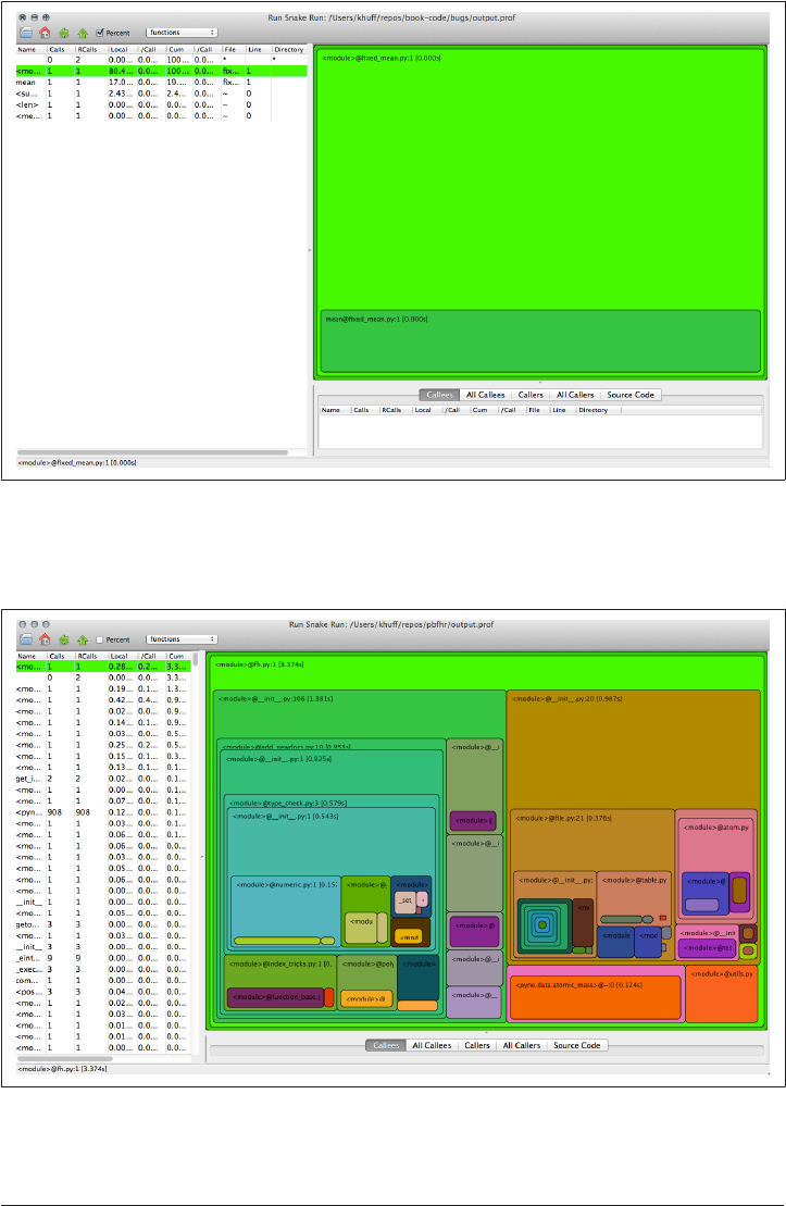
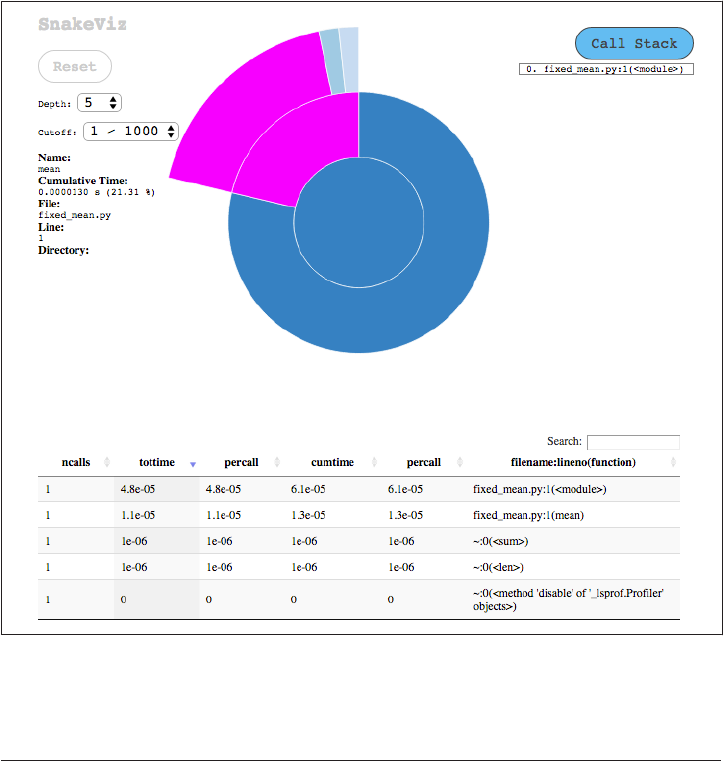
At the top is a percent button. That button will show a breakdown of the percentage
of time spent in each part of the code. This interactive graphic demonstrates the
behavior of each section of the code so that you can quickly see where time is being
wasted.
Another option, inspired by RunSnakeRun, is an in-browser viewer called SnakeViz.
To use SnakeViz, first make sure it is installed by running which snakeviz. If it is not
present, try installing it with pip (pip install snakeviz) using your package man‐
ager or downloading it from its website. Next, in the command line, type:
$ snakeviz output.prof
The SnakeViz program will cause a web browser to open and will provide an interac‐
tive infographic of the data in output.prof. The results for our simple code are shown
in Figure 17-3.
Figure 17-3. Proling with SnakeViz
Proling | 399
www.it-ebooks.info

With SnakeViz, the execution of the code can be browsed on a function-by-function
basis. The time spent in each function is rendered in radial blocks. The central circle
represents the top of the call stack—that is, the function from which all other func‐
tions are called. In our case, that is the main body of the module in the final four lines
of the file.
The next radial annulus describes the time spent in each function called by the main
function, and so on. When the mouse hovers over some section of the graph, more
information is shown. To learn more about SnakeViz and how to interperet its con‐
tents, see its website.
Combined with cProfile, these graphical interfaces for profiling are an efficient way
to pinpoint functions with efficiency issues. Sometimes, though, it is even more help‐
ful to know how much time you spend on each line. For this, consider kernprof.
Line Proling with Kernprof
For showing the specific lines at fault for slowdowns, you can use a line profiler called
kernprof. To use kernprof, you must alter the file itself with a decorator (@profile)
above each function definition of interest. The mean code becomes:
With that decorator in place, kernprof can then be run verbosely in line-by-line mode
thus:
kernprof -v -l fixed_mean.py
When kernprof is run in that way, the profile of time spent is printed to the terminal
in much greater detail than with the previous tools:
16.375
Wrote profile results to fixed_mean.py.lprof
Timer unit: 1e-06 s
Total time: 7e-06 s
File: fixed_mean.py
Function: mean at line 1
Line # Hits Time Per Hit % Time Line Contents
==============================================================
1 @profile
2 def mean(nums):
3 1 2 2.0 28.6 top = sum(nums)
4 1 0 0.0 0.0 bot = len(nums)
5 1 5 5.0 71.4 return float(top)/float(bot)
Since the code is run from start to finish, the code output is printed.
kernprof intelligently guesses the magnitude of time resolution to print.
400 | Chapter 17: Debugging
www.it-ebooks.info

The only profiled lines are those within the function that we decorated.
Each line has its own row in this table.
When you’re inspecting these results, the fifth column is the most important. It indi‐
cates the percentage of time spent on each line in the mean function. The results here
indicate that most of the time is spent calculating and returning the quotient. Perhaps
some speedup can be achieved. Can you think of any simplifications to the code? Try
making a change to determine whether it has an effect on the speed of execution.
Now that our code no longer exhibits errors and can be optimized for speed, the only
remaining debugging task is clean up. A tool used to cleanup code is called a linter.
Linting
Linting removes “lint” from source code. It’s a type of cleanup that is neither debug‐
ging nor testing nor profiling, but can be helpful at each of these stages of the pro‐
gramming process. Linting catches unnecessary imports, unused variables, potential
typos, inconsistent style, and other similar issues.
Linting in Python can be achieved with the pyakes tool. Get it? Errors are more than
just lint, they’re flakes!
As an example of how to use a linter, recall the elementary.py file from Chapter 6. To
lint a Python program, execute the pyflakes command on it:
$ pyflakes elementary.py
pyakes responds with a note indicating that a package has been imported but
remains unused throughout the code execution:
elementary.py:2: 'numpy' imported but unused
This information is more than just cosmetic. Since importing packages takes time
and occupies computer memory, reducing unused imports can speed up your code.
That said, most linting tools do focus on cosmetic issues. Style-related linting tools
such as ake8, pep8, or autopep8 can be used to check for errors, variable name mis‐
spelling, and PEP8 compatibility. For more on the PEP8 style standard in Python, see
Chapter 19. To use the pep8 tool, simply call it from the command line:
$ pep8 elementary.py
It will analyze the Python code that you have provided and will respond with a line-
by-line listing of stylistic incompatibilities with the PEP8 standard:
elementary.py:4:1: E302 expected 2 blank lines, found 1
elementary.py:5:3: E111 indentation is not a multiple of four
elementary.py:7:31: E228 missing whitespace around modulo operator
Linting | 401
www.it-ebooks.info

This indicates that the elementary.py file has a few insufficiencies related to the PEP8
Style Guide. The combined information of both tools can be retrieved with the much
more strict pylint tool on the command line:
$ pylint -rn elementary.py
The -rn flag simply tells pylint not to print its full report. The report provided by
pylint by default is quite lengthy indeed and could easily occupy half of the pages in
this chapter:
No config file found, using default configuration
************* Module elementary
W: 5, 0: Bad indentation. Found 2 spaces, expected 4 (bad-indentation)
W: 6, 0: Bad indentation. Found 4 spaces, expected 8 (bad-indentation)
W: 7, 0: Bad indentation. Found 4 spaces, expected 8 (bad-indentation)
W: 8, 0: Bad indentation. Found 4 spaces, expected 8 (bad-indentation)
W: 9, 0: Bad indentation. Found 4 spaces, expected 8 (bad-indentation)
C: 1, 0: Missing module docstring (missing-docstring)
C: 6, 4: Invalid attribute name "s" (invalid-name)
C: 7, 4: Invalid attribute name "isFermion" (invalid-name)
C: 8, 4: Invalid attribute name "isBoson" (invalid-name)
C: 4, 0: Missing class docstring (missing-docstring)
W: 5, 2: __init__ method from base class 'Particle' is not called...
Once the incorrect indentation, invalid names, and missing docstrings are fixed, your
code will be ready for prime time.
Debugging Wrap-up
Having read this chapter, you should feel ready to use an interactive debugger to
more efficiently and systematically:
• Understand bugs
• Track down their cause
• Prototype solutions
• Check for success
Additionally, this chapter should have prepared you to use profilers and linters to
optimize and clean your code once you’ve fixed the bugs. Now that you are prepared
to deal with bugs and inefficiencies that arise in your code, your focus can turn to
keeping them from appearing in the first place. In the next chapter, we will show you
how to avoid bugs with comprehensive, systematic testing.
402 | Chapter 17: Debugging
www.it-ebooks.info

CHAPTER 18
Testing
Before relying on a new experimental device, a good physicist will establish its accu‐
racy. A new detector will always have its responses to known input signals tested. The
results of this calibration are compared against the expected responses. If the device is
trustworthy, then the responses received will fall within acceptable bounds of what
was expected. To make this a fair test, the accuracy bounds are set prior to the test.
The same goes for testing in computational science and software development.
Code is assumed guilty until proven innocent. This applies to software written by
other people, but even more so to software written by yourself. The mechanism that
builds trust that software is performing correctly is called testing.
Testing is the process by which the expected results of code are compared against the
observed results of actually having run that code. Tests are typically provided along
with the code that they are testing. The collection of all of the tests for a given piece of
code is known as the test suite. You can think of the test suite as a bunch of precanned
experiments that anyone can run. If all of the tests pass, then the code is at least parti‐
ally trustworthy. If any of the tests fail, then the code is known to be incorrect with
respect to whichever case failed.
Now, you may have noticed that the test code itself is part of the software package.
Since the tests are just as likely to have bugs as the code they are testing, it is tempting
to start writing tests that test the tests. However, this quickly runs into an incomplete‐
ness problem. There is no set of tests that is the set of all possible tests. Suppose you
write a test suite for some code. Now your test suite is untested, so you add a test for
the test suite. Now your test suite tester is untested, so you write a test for that, and so
on. It is possible to escape this infinite-work trap using recursion, as discussed in
Chapter 5, but it probably is not worth your time.
403
www.it-ebooks.info

Even one level of testing—just testing main code and not the tests themselves—is
incredibly beneficial. Almost all of the scientific value comes from this first pass. This
is because the first level is where the physics is put directly in question. A sufficiently
rigorous test suite will find all of the physical and computational errors without hav‐
ing to worry about the philosophical and mathematical ramifications of whether a
test is itself sufficiently tested.
Testing is so central to both the scientific method and modern software development
that many computational scientists consider it a moral failing for a scientific program
not to include tests. They also know to not trust a code when the tests do not pass.
Neither should you. For software that you do not write, it is always a good idea to run
the test suite when you first start working with the code. The documentation will typ‐
ically include instructions on how to run the tests, since they can be different from
project to project.
In this chapter, we will be discussing testing in the context of Python. Specifically, we
will be using the nose testing framework. This is a package of tools that make writing
and running tests easy. Though other test frameworks exist in Python (pytest, uni
ttest), nose has become the standard testing tool for scientific Python. It helps that it
is also easier to use and understand than some of the others.
We start this chapter by asking a series of questions that illuminate good testing prac‐
tices that everyone should follow.
Why Do We Test?
Testing is a great practice that aids all of software development. However, not practic‐
ing good habits alone is not a moral failing. Testing is considered a core principle of
scientic soware because its impact is at the heart of knowledge generation.
In most other programming endeavors, if code is fundamentally wrong, even if it
goes uncorrected for years at a time, the impact of this error can be relatively small.
Perhaps a website goes down, or a game crashes, or a day’s worth of writing is lost
when the computer crashes. Scientific code, on the other hand, controls planes, weap‐
ons systems, satellites, agriculture, and (most importantly) physics simulations and
experiments. If the software that governs a computational or physical experiment is
wrong, then any decisions that are made based on its results will be completely
untrustworthy.
This is not to say that physicists have a monopoly on software testing. Arguably, test‐
ing is just as important in arenas such as finance, government, and health care. Gross
failures in these areas, however, tend to affect lives and livelihoods rather than knowl‐
edge itself.
404 | Chapter 18: Testing
www.it-ebooks.info

We would like to think that scientists are rigorous enough to realize the importance
of testing, but mistakes of negligence happen all too frequently. Everyone who has
been involved with scientific software for any length of time has a horror story or
two. The truth of the matter is that most scientists are poorly equipped to truly test
their code. The average blog or image-sharing website is better tested than most sci‐
entific software.
This chapter is here to help remedy the poor testing situation by explaining the moti‐
vation behind testing and giving you the tools you need to do better.
When Should We Test?
Always.
Testing should be a seamless part of the scientific software development process. Tests
should be created along with the code that is to be tested. At the very minimum, at
least one test should be written immediately following the initial implementation of a
function or a class. At the beginning of a new project, tests can be used to help guide
the overall architecture of the project. This is analogous to experiment design in the
experimental science world. The act of writing tests can help clarify how the software
should be performing. Taking this idea to the extreme, you could start to write the
tests before you even write the software that will be tested. We will discuss this prac‐
tice in greater detail in “Test-Driven Development” on page 419.
In Working Eectively with Legacy Code (Prentice Hall), Michael Feathers defines leg‐
acy code as “any code without tests.” This definition draws on the fact that after its
initial creation, tests provide a powerful guide to other developers (and to your for‐
getful self, a few months in the future) about how each function in a piece of code is
meant to be used. Without runnable tests to provide examples of code use, even
brand new programs are unsustainable.
Where Should We Write Tests?
While writing code, you can add exceptions and assertions to sound an alarm as run‐
time problems come up. These kinds of tests, however, are embedded in the software
itself. It is better to separate the code from the tests as much as possible. External tests
require a bit more sophistication, but are better suited to checking the implementa‐
tion against its expected behavior. These external tests are what is referred to as the
test suite. The runtime exceptions and assertions do not count as part of the test suite.
Many projects choose to have a top-level directory named after the project or called
src/. Similarly, many projects also have a top-level tests/ directory where the test suite
lives. This often mirrors the directory structure of the source directory. Mirroring
makes it obvious where the test lives for any corresponding piece of source code.
When Should We Test? | 405
www.it-ebooks.info

Alternatively, some projects choose to place the tests right next to the source code
that they are testing. Say you had a module called physics.py. In this schema, the tests
would live in a test_physics.py file to keep them somewhat separate. This strategy is
not recommended, though you will sometimes encounter it in the wild.
As with everything in software, the most important aspect of where to put the tests is
to be consistent. Choose one approach and follow that for all of the tests that you write
in a given project. If you are working on a more established project, be sure to con‐
form to whatever pattern was set before you started.
What and How to Test?
Consider again the analogy to a detector in a physical experiment. The behavior of
the detector must be characterized and calibrated across the valid range of interest.
However, it is often unnecessary to characterize the response to every possible valid
input. Most detectors rely on the physical quantity that they measure being either
continuous or discrete. Testing only a few key signals, typically at the upper and lower
edges of its range and some points in between, is enough to determine if and how
well the machine is working. This “test what is important” mindset applies equally to
scientific software development. Software tests should cover behavior from the com‐
mon to the extreme, but not every single value within those bounds.
Let’s see how this mindset applies to an actual physics problem. Given two previous
observations in the sky and the time between them, Kepler’s Laws provide a closed-
form equation for the future location of a celestial body. This can be implemented via
a function named kepler_loc(). The following is a stub interface representing this
function that lacks the actual function body:
def kepler_loc(p1, p2, dt, t):
...
return p3
As a basic test of this function, we can take three points on the planet Jupiter’s actual
measured path and use the latest of these as the expected result. We will then compare
this to the result that we observe as the output of the kepler_loc() function.
Tests compare expected outputs versus observed outputs for
known inputs. They do not inspect the body of the function
directly. In fact, the body of a function does not even have to exist
for a valid test to be written.
To start testing, we will raise an exception as a way of signaling that the test failed if
the expected value is not equal to the observed value. Frequently, tests are written as
functions that have the same name as the code that they are testing with the word
406 | Chapter 18: Testing
www.it-ebooks.info
test either before or after it. The following example is pseudocode for testing that the
measured positions of Jupiter, given by the function jupiter(), can be predicted with
the kepler_loc() function:
def test_kepler_loc():
p1 = jupiter(two_days_ago)
p2 = jupiter(yesterday)
exp = jupiter(today)
obs = kepler_loc(p1, p2, 1, 1)
if exp != obs:
raise ValueError("Jupiter is not where it should be!")
The test_kepler_loc() function tests kepler_loc().
Get the inputs to kepler_loc().
Obtain the expected result from experimental data.
Obtain the observed result by calling kepler_loc().
Test that the expected result is the same as the observed result. If it is not, signal
that the test failed by raising an exception.
Now, calling the test_kepler_loc() function will determine whether kepler_loc()
is behaving as intended. If a ValueError is raised, then we know something is wrong.
The test_kepler_loc() function follows a very common testing pattern:
1. Name the test after the code that is being tested.
2. Load or set the expected results.
3. Compute the observed result by actually running the code.
4. Compare the expected and observed results to ensure that they are equivalent.
This pattern can be boiled down to the following pseudocode:
def test_func():
exp = get_expected()
obs = func(*args, **kwargs)
assert exp == obs
It is critical to understand that tests should usually check for equivalence (==) and not
equality (is). It is more important that the expected and observed results are effec‐
tively the same than that they are actually the same exact object in memory. For the
floating-point data that is common in physics, it is often more pertinent for the
expected and observed results to be approximately equal than it is for them to have
precisely the same value. Floats are an approximation, and this needs to be accounted
for when you’re testing.
What and How to Test? | 407
www.it-ebooks.info

Testing equivalence via exceptions is rather like hammering a nail with a grenade.
The nail will probably go in (the test will run), but the grenade will take everything
else (i.e., the Python interpreter) along with it. A slightly more subtle way to accom‐
plish the same task would be to use assertions. From Table 2-1, recall that an assert
statement in Python ensures that the expression following it evaluates to True. If the
assertion is true, then Python continues on its merry way. If the assertion is false, then
an AssertionError is raised. We could rewrite test_keppler_loc() as follows:
def test_keppler_loc():
p1 = jupiter(two_days_ago)
p2 = jupiter(yesterday)
exp = jupiter(today)
obs = keppler_loc(p1, p2, 1, 1)
assert exp == obs
Now with an assertion instead of an exception.
The assertion approach still lacks subtlety, though all that we know when the test fails
is that it failed. We do not see the values of the expected and observed results to help
us determine where the fault lies. To get this kind of extra information in the event of
a failure, we need to supply a custom assertion. Rich and descriptive assertions are
exactly what a test framework like nose provides.
nose has a variety of helpful and specific assertion functions that display extra debug‐
ging information when they fail. These are all accessible through the nose.tools
module. The simplest one is named assert_equal(). It takes two arguments, the
expected and observed results, and checks them for equivalence (==). We can further
rewrite test_kepler_loc() as seen here:
from nose.tools import assert_equal
def test_kepler_loc():
p1 = jupiter(two_days_ago)
p2 = jupiter(yesterday)
exp = jupiter(today)
obs = keppler_loc(p1, p2, 1, 1)
assert_equal(exp, obs)
To obtain functionality from nose, first we have to import it.
Python’s assertion can be replaced with nose’s.
Using the test framework is the best way to write tests. Executing each of your tests by
hand, however, becomes tiresome when you have more than a handful in your test
suite. The next section goes over how to manage all of the tests you have written.
408 | Chapter 18: Testing
www.it-ebooks.info

Running Tests
The major boon a testing framework provides is a utility to find and run the tests
automatically. With nose, this is a command-line tool called nosetests. When nosetests
is run, it will search all the directories whose names start or end with the word test,
find all of the Python modules in these directories whose names start or end with test,
import them, and run all of the functions and classes whose names start or end with
test. In fact, nose looks for any names that match the regular expression (?:^|[\\b_\
\.-])[Tt]est. This automatic registration of test code saves tons of human time and
allows us to focus on what is important: writing more tests.
When you run nosetests, it will print a dot (.) on the screen for every test that passes,
an F for every test that fails, and an E for every test where there was an unexpected
error. In rarer situations you may also see an S indicating a skipped test (because the
test is not applicable on your system) or a K for a known failure (because the develop‐
ers could not fix it promptly). After the dots, nosetests will print summary informa‐
tion. Given just the one test_kepler_loc() test from the previous section, nosetests
would produce results like the following:
$ nosetests
.
Ran 1 test in 0.224s
OK
As we write more code, we would write more tests, and nosetests would produce more
dots. Each passing test is a small, satisfying reward for having written quality scien‐
tific software. Now that you know how to write tests, let’s go into what can go wrong.
Edge Cases
What we saw in “What and How to Test?” on page 406 is called an interior test. The
precise points that we tested did not matter. Any two initial points in an orbit could
have been used to predict further positions. Though this is not as true for cyclic prob‐
lems, more linear scenarios tend to have a clear beginning, middle, and end. The out‐
put is defined on a valid range.
The situation where the test examines either the beginning or the end of a range, but
not the middle, is called an edge case. In a simple, one-dimensional problem, the two
edge cases should always be tested along with at least one internal point. This ensures
that you have good coverage over the range of values.
Anecdotally, it is important to test edges cases because this is where errors tend to
arise. Qualitatively different behavior happens at boundaries. As such, they tend to
Running Tests | 409
www.it-ebooks.info

have special code dedicated to them in the implementation. Consider the following
simple Fibonacci function:
def fib(n):
if n == 0 or n == 1:
return 1
else:
return fib(n - 1) + fib(n - 2)
This function has two edge cases: zero and one. For these values of n, the fib() func‐
tion does something special that does not apply to any other values. Such cases
should be tested explicitly. A minimally sufficient test suite for this function would
be:
from nose.tools import assert_equal
from mod import fib
def test_fib0():
# test edge 0
obs = fib(0)
assert_equal(1, obs)
def test_fib1():
# test edge 1
obs = fib(1)
assert_equal(1, obs)
def test_fib6():
# test regular point
obs = fib(6)
assert_equal(13, obs)
Test the edge case for zero.
Test the edge case for one.
Test an internal point.
Different functions will have different edge cases. Often, you need not test for cases
that are outside the valid range, unless you want to test that the function fails. In the
fib() function negative and noninteger values are not valid inputs. You do not need
to have tests for these classes of numbers, though it would not hurt. Edge cases are
not where the story ends, though, as we will see next.
Corner Cases
When two or more edge cases are combined, it is called a corner case. If a function is
parametrized by two independent variables, a test that is at the extreme of both vari‐
410 | Chapter 18: Testing
www.it-ebooks.info

ables is in a corner. As a demonstration, consider the case of the function (sin(x) /
x) * (sin(y) / y), presented here:
import numpy as np
def sinc2d(x, y):
if x == 0.0 and y == 0.0:
return 1.0
elif x == 0.0:
return np.sin(y) / y
elif y == 0.0:
return np.sin(x) / x
else:
return (np.sin(x) / x) * (np.sin(y) / y)
The function sin(x)/x is called the sinc() function. We know that at the point
where x = 0, then sinc(x) == 1.0. In the code just shown, sinc2d() is a two-
dimensional version of this function. When both x and y are zero, it is a corner case
because it requires a special value for both variables. If either x or y (but not both) is
zero, these are edge cases. If neither is zero, this is a regular internal point.
A minimal test suite for this function would include a separate test for the corner
case, each of the edge cases, and an internal point. For example:
import numpy as np
from nose.tools import assert_equal
from mod import sinc2d
def test_internal():
exp = (2.0 / np.pi) * (-2.0 / (3.0 * np.pi))
obs = sinc2d(np.pi / 2.0, 3.0 * np.pi / 2.0)
assert_equal(exp, obs)
def test_edge_x():
exp = (-2.0 / (3.0 * np.pi))
obs = sinc2d(0.0, 3.0 * np.pi / 2.0)
assert_equal(exp, obs)
def test_edge_y():
exp = (2.0 / np.pi)
obs = sinc2d(np.pi / 2.0, 0.0)
assert_equal(exp, obs)
def test_corner():
exp = 1.0
obs = sinc2d(0.0, 0.0)
assert_equal(exp, obs)
Test an internal point.
Edge Cases | 411
www.it-ebooks.info

Test an edge case for x and internal for y.
Test an edge case for y and internal for x.
Test the corner case.
Corner cases can be even trickier to find and debug than edge cases because of their
increased complexity. This complexity, however, makes them even more important to
explicitly test.
Whether internal, edge, or corner cases, we have started to build up a classification
system for the tests themselves. In the following sections, we will build this system up
even more based on the role that the tests have in the software architecture.
Unit Tests
All of the tests that we have seen so far have been unit tests. They are so called
because they exercise the functionality of the code by interrogating individual func‐
tions and methods. Functions and methods can often be considered the atomic units
of software because they are indivisible from the outside.
However, what is considered to be the smallest code unit is subjective. The body of a
function can be long or short, and shorter functions are arguably more unit-like than
long ones. Thus, what reasonably constitutes a code unit typically varies from project
to project and language to language. A good rule of thumb is that if the code cannot
be made any simpler logically (you cannot split apart the addition operator) or practi‐
cally (a function is self-contained and well defined), then it is a unit. The purpose
behind unit tests is to encourage both the code and the tests to be as small, well-
defined, and modular as possible. There is no one right answer for what this means,
though. In Python, unit tests typically take the form of test functions that are auto‐
matically called by the test framework.
Additionally, unit tests may have test xtures. A fixture is anything that may be added
to the test that creates or removes the environment required by the test to successfully
run. They are not part of expected result, the observed result, or the assertion. Test
fixtures are completely optional.
A fixture that is executed before the test to prepare the environment is called a setup
function. One that is executed to mop up side effects after a test is run is called a
teardown function. nose has a decorator that you can use to automatically run fix‐
tures no matter whether the test succeeded, failed, or had an error. (For a refresher on
decorators, see “Decorators” on page 112.)
Consider the following example that could arise when communicating with third-
party programs. You have a function f() that will write a file named yes.txt to disk
412 | Chapter 18: Testing
www.it-ebooks.info

with the value 42 but only if a file no.txt does not exist. To truly test that the function
works, you would want to ensure that neither yes.txt nor no.txt existed before you ran
your test. After the test, you would want to clean up after yourself before the next test
comes along. You could write the test, setup, and teardown functions as follows:
import os
from nose.tools import assert_equal, with_setup
from mod import f
def f_setup():
files = os.listdir('.')
if 'no.txt' in files:
os.remove('no.txt')
if 'yes.txt' in files:
os.remove('yes.txt')
def f_teardown():
files = os.listdir('.')
if 'yes.txt' in files:
os.remove('yes.txt')
def test_f():
f_setup()
exp = 42
f()
with open('yes.txt', 'r') as fhandle:
obs = int(fhandle.read())
assert_equal(exp, obd)
f_teardown()
The f_setup() function tests ensure that neither the yes.txt nor the no.txt file
exists.
The f_teardown() function removes the yes.txt file, if it was created.
The first action of test_f() is to make sure the filesystem is clean.
The last action of test_f() is to clean up after itself.
This implementation of test fixtures is usually fine. However, it does not guarantee
that the f_setup() and f_teardown() functions will be called. This is because an
unexpected error anywhere in the body of f() or test_f() will cause the test to abort
before the teardown function is reached. To make sure that both of the fixtures will be
executed, you must use nose’s with_setup() decorator. This decorator may be
applied to any test and takes a setup and a teardown function as possible arguments.
We can rewrite test_f() to be wrapped by with_setup(), as follows:
Unit Tests | 413
www.it-ebooks.info

@with_setup(setup=f_setup, teardown=f_teardown)
def test_f():
exp = 42
f()
with open('yes.txt', 'r') as fhandle:
obs = int(fhandle.read())
assert_equal(exp, obd)
Note that if you have functions in your test module that are simply named setup()
and teardown(), each of these is called automatically when the entire test module is
loaded in and finished.
Simple tests are the easiest to write. For this reason, functions
should be small enough that they are easy to test. For more infor‐
mation on writing code that facilitates tests, we recommend Robert
C. Martin’s book Clean Code (Prentice Hall).
Having introduced the concept of unit tests, we can now go up a level in complexity.
Integration Tests
You can think of a software project like a clock. Functions and classes are the gears
and cogs that make up the system. On their own, they can be of the highest quality.
Unit tests verify that each gear is well made. However, the clock still needs to be put
together. The gears need to fit with one another.
Integration tests are the class of tests that verify that multiple moving pieces of the
code work well together. They ensure that the clock can tell time correctly. They look
at the system as a whole or at subsystems. Integration tests typically function at a
higher level conceptually than unit tests. Thus, programming integration tests also
happens at a higher level.
Because they deal with gluing code together, there are typically fewer integration tests
in a test suite than there are unit tests. However, integration tests are no less impor‐
tant. Integration tests are essential for having adequate testing. They encompass all of
the cases that you cannot hit through plain unit testing.
Sometimes, especially in probabilistic or stochastic codes, the precise behavior of an
integration test cannot be determined beforehand. That is OK. In these situations it is
acceptable for integration tests to verify average or aggregate behavior rather than
exact values. Sometimes you can mitigate nondeterminism by saving seed values to a
random number generator, but this is not always going to be possible. It is better to
have an imperfect integration test than no integration test at all.
414 | Chapter 18: Testing
www.it-ebooks.info

As a simple example, consider the three functions a(), b(), and c(). The a() func‐
tion adds one to a number, b() multiplies a number by two, and c() composes them.
These functions are defined as follows:
def a(x):
return x + 1
def b(x):
return 2 * x
def c(x):
return b(a(x))
The a() and b() functions can each be unit-tested because they each do one thing.
However, c() cannot be truly unit tested because all of the real work is farmed out to
a() and b(). Testing c() will be a test of whether a() and b() can be integrated
together.
Integration tests still follow the pattern of comparing expected results to observed
results. A sample test_c() is implemented here:
from nose.tools import assert_equal
from mod import c
def test_c():
exp = 6
obs = c(2)
assert_equal(exp, obs)
Given the lack of clarity in what is defined as a code unit, what is considered an inte‐
gration test is also a little fuzzy. Integration tests can range from the extremely simple
(like the one just shown) to the very complex. A good delimiter, though, is in opposi‐
tion to the unit tests. If a function or class only combines two or more unit-tested
pieces of code, then you need an integration test. If a function implements new
behavior that is not otherwise tested, you need a unit test.
The structure of integration tests is very similar to that of unit tests. There is an
expected result, which is compared against the observed value. However, what goes in
to creating the expected result or setting up the code to run can be considerably more
complicated and more involved. Integration tests can also take much longer to run
because of how much more work they do. This is a useful classification to keep in
mind while writing tests. It helps separate out which tests should be easy to write
(unit) and which ones may require more careful consideration (integration).
Integration tests, however, are not the end of the story.
Integration Tests | 415
www.it-ebooks.info

Regression Tests
Regression tests are qualitatively different from both unit and integration tests.
Rather than assuming that the test author knows what the expected result should be,
regression tests look to the past. The expected result is taken as what was previously
computed for the same inputs. Regression tests assume that the past is “correct.” They
are great for letting developers know when and how a code base has changed. They
are not great for letting anyone know why the change occurred. The change between
what a code produces now and what it computed before is called a regression.
Like integration tests, regression tests tend to be high level. They often operate on an
entire code base. They are particularly common and useful for physics simulators.
A common regression test strategy spans multiple code versions. Suppose there is an
input file for version X of a simulator. We can run the simulation and then store the
output file for later use, typically somewhere accessible online. While version Y is
being developed, the test suite will automatically download the output for version X,
run the same input file for version Y, and then compare the two output files. If any‐
thing is significantly different between them, the test fails.
In the event of a regression test failure, the onus is on the current developers to
explain why. Sometimes there are backward-incompatible changes that had to be
made. The regression test failure is thus justified, and a new version of the output file
should be uploaded as the version to test against. However, if the test fails because the
physics is wrong, then the developer should fix the latest version of the code as soon
as possible.
Regression tests can and do catch failures that integration and unit tests miss. Regres‐
sion tests act as an automated short-term memory for a project. Unfortunately, each
project will have a slightly different approach to regression testing based on the needs
of the software. Testing frameworks provide tools to help with building regression
tests but do not offer any sophistication beyond what has already been seen in this
chapter.
Depending on the kind of project, regression tests may or may not be needed. They
are only truly needed if the project is a simulator. Having a suite of regression tests
that cover the range of physical possibilities is vital to ensuring that the simulator still
works. In most other cases, you can get away with only having unit and integration
tests.
While more test classifications exist for more specialized situations, we have covered
what you will need to know for almost every situation in computational physics. In
the following sections, we will go over how to write tests more effectively.
416 | Chapter 18: Testing
www.it-ebooks.info
1See “Generators” on page 109 for a refresher on generators if you need one.
Test Generators
Test generators automate the creation of tests. Suppose that along with the function
you wished to test, you also had a long list of expected results and the associated
arguments to the function for those expected results. Rather than you manually creat‐
ing a test for each element of the list, the test generator would take the list and manu‐
facture the desired tests. This requires much less work on your part while also
providing more thorough testing. The list of expected results and function inputs is
sometimes called a test matrix.
In nose, test generators are written by turning the test function into a generator with
yield statements.1 In the test function, the assertion for each element of the matrix is
yielded, along with the expected value and the function inputs. Corresponding check
functions sometimes go along with the test generator to perform the actual work.
For demonstration purposes, take a simple function that adds two numbers together.
The function, the check function, and the test generator could all be written as
follows:
from nose.tools import assert_equal
def add2(x, y):
return x + y
def check_add2(exp, x, y):
obs = add2(x, y)
assert_equal(exp, obs)
def test_add2():
cases = [
(4, 2, 2),
(5, -5, 10),
(42, 40, 2),
(16, 3, 13),
(-128, 0, -128),
]
for exp, x, y in cases:
yield check_add2, exp, x, y
The function to test, add2().
The check function performs the equality assertion instead of the test.
The test function is now a test generator.
Test Generators | 417
www.it-ebooks.info

cases is a list of tuples that represents the test matrix. The first element of each
tuple is the expected result. The following elements are the arguments to add2().
Looping through the test matrix cases, we yield the check function, the
expected value, and the add2() arguments. Nose will count each yield as a sepa‐
rate full test.
This will produce five tests in nose, one for each case. We can therefore efficiently
create many tests and minimize the redundant code we need to write. Running
nosetests will produce the following output:
$ nosetests
.....
Ran 5 tests in 0.001s
OK
This is a very powerful testing mechanism because adding or removing tests is as easy
as modifying the cases list. Different testing frameworks implement this idea in dif‐
ferent ways. In all frameworks, it makes your life easier. Generating many test cases
will hopefully cover more of the code base. The next section will discuss how to
determine how many lines of your project are actually being executed by the test
suite.
Test Coverage
The term test coverage is often used to mean the percentage of the code for which an
associated test exists. You can measure this by running the test suite and counting the
number of lines of code that were executed and dividing this by the total number of
lines in the software project. If you have the coverage Python project installed (pip
install coverage), you can run nose and generate coverage statistics simultaneously
via the --with-coverage switch at the command line:
$ nosetests --with-coverage
At first glance this metric seems like a useful indicator of code reliability. But while
some test coverage is superior to none and broad test coverage is usually superior to
narrow coverage, this metric should be viewed critically. All code should ideally have
100% test coverage, but this alone does not guarantee that the code works as
intended. Take the following pseudocode for a function g() shown here, with two if-
else statements in its body:
def g(x, y):
if x:
...
else:
418 | Chapter 18: Testing
www.it-ebooks.info

...
if y:
...
else:
...
return ...
The following two unit tests for g() have 100% coverage:
from nose.tools import assert_equal
from mod import g
def test_g_both_true():
exp = ...
obs = g(True, True)
assert_equal(exp, obs)
def test_g_both_false():
exp = ...
obs = g(False, False)
assert_equal(exp, obs)
Every line of g() is executed by these two functions. However, only half of the possi‐
ble cases are covered. We are not testing when x=True and y=False or when x=False
and y=True. In this case, 100% coverage is only 50% of the possible code path combi‐
nations. In full software projects, 100% coverage is achieved with much less than 50%
of the code paths been executed.
Code coverage is an important and often cited measure. However, it is not the
pinnacle of testing. It is another tool in your testing toolbox. Use it as needed and
understand its limitations.
The next section covers another tool, but one that changes the testing strategy itself.
Test-Driven Development
Test-driven development (TDD) takes the workflow of writing code and writing tests
and turns it on its head. TDD is a software development process where you write the
tests first. Before you write a single line of a function, you first write the test for that
function.
After you write a test, you are then allowed to proceed to write the function that you
are testing. However, you are only supposed to implement enough of the function so
that the test passes. If the function does not do what is needed, you write another test
and then go back and modify the function. You repeat this process of test-then-
implement until the function is completely implemented for your current needs.
Test-Driven Development | 419
www.it-ebooks.info

Developers who practice strict TDD will tell you that it is the best thing since sliced
arrays. The central claim to TDD is that at the end of the process you have an imple‐
mentation that is well tested for your use case, and the process itself is more efficient.
You stop when your tests pass and you do not need any more features. You do not
spend any time implementing options and features on the off chance that they will
prove helpful later. You get what you need when you need it, and no more. TDD is a
very powerful idea, though it can be hard to follow religiously.
The most important takeaway from test-driven development is that the moment you
start writing code, you should be considering how to test that code. The tests should
be written and presented in tandem with the implementation. Testing is too impor‐
tant to be an afterthought.
Whether to pursue classic TDD is a personal decision. This design philosophy was
most strongly put forth by Kent Beck in his book Test-Driven Development: By Exam‐
ple. The following example illustrates TDD for a standard deviation function, std().
To start, we write a test for computing the standard deviation from a list of numbers
as follows:
from nose.tools import assert_equal
from mod import std
def test_std1():
obs = std([0.0, 2.0])
exp = 1.0
assert_equal(obs, exp)
Next, we write the minimal version of std() that will cause test_std1() to pass:
def std(vals):
# surely this is cheating...
return 1.0
As you can see, the minimal version simply returns the expected result for the sole
case that we are testing. If we only ever want to take the standard deviation of the
numbers 0.0 and 2.0, or 1.0 and 3.0, and so on, then this implementation will work
perfectly. If we want to branch out, then we probably need to write more robust code.
However, before we can write more code, we first need to add another test or two:
def test_std1():
obs = std([0.0, 2.0])
exp = 1.0
assert_equal(obs, exp)
def test_std2():
obs = std([])
exp = 0.0
assert_equal(obs, exp)
420 | Chapter 18: Testing
www.it-ebooks.info
def test_std3():
obs = std([0.0, 4.0])
exp = 2.0
assert_equal(obs, exp)
Test the fiducial case when we pass in an empty list.
Test a real case where the answer is not one.
A perfectly valid standard deviation function that would correspond to these three
tests passing would be as follows:
def std(vals):
# a little better
if len(vals) == 0:
return 0.0
return vals[-1] / 2.0
Special case the empty list.
By being clever, we can get away without doing real work.
Even though the tests all pass, this is clearly still not a generic standard deviation
function. To create a better implementation, TDD states that we again need to expand
the test suite:
def test_std1():
obs = std([0.0, 2.0])
exp = 1.0
assert_equal(obs, exp)
def test_std2():
obs = std([])
exp = 0.0
assert_equal(obs, exp)
def test_std3():
obs = std([0.0, 4.0])
exp = 2.0
assert_equal(obs, exp)
def test_std4():
obs = std([1.0, 3.0])
exp = 1.0
assert_equal(obs, exp)
def test_std5():
obs = std([1.0, 1.0, 1.0])
exp = 0.0
assert_equal(obs, exp)
Test-Driven Development | 421
www.it-ebooks.info

The first value is not zero.
Here, we have more than two values, but all of the values are the same.
At this point, we may as well try to implement a generic standard deviation function.
We would spend more time trying to come up with clever approximations to the
standard deviation than we would spend actually coding it. Just biting the bullet, we
might write the following implementation:
def std(vals):
# finally, some math
n = len(vals)
if n == 0:
return 0.0
mu = sum(vals) / n
var = 0.0
for val in vals:
var = var + (val - mu)**2
return (var / n)**0.5
It is important to note that we could improve this function by writing further tests.
For example, this std() ignores the situation where infinity is an element of the val‐
ues list. There is always more that can be tested. TDD prevents you from going over‐
board by telling you to stop testing when you have achieved all of your use cases.
Testing Wrap-up
Testing is one of the primary concerns of scientific software developers. It is a techni‐
cal solution to a philosophical problem. You should now be familiar with the follow‐
ing concepts in testing:
•Tests compare that the result observed from running code is the same as what
was expected ahead of time.
• Tests should be written at the same time as the code they are testing is written.
•The person best suited to write a test is the author of the original code.
• Tests are grouped together in a test suite.
• Test frameworks, like nose, discover and execute tests for you automatically.
•An edge case is when an input is at the limit of its range.
• A corner case is where two or more edge cases meet.
•Unit tests try to test the smallest pieces of code possible, usually functions and
methods.
• Integration tests make sure that code units work together properly.
•Regression tests ensure that everything works the same today as it did yesterday.
422 | Chapter 18: Testing
www.it-ebooks.info

• Test generators can be used to efficiently check many cases.
• Test coverage is the percentage of the code base that is executed by the test suite.
•Test-driven development says to write your tests before you write the code that is
being tested.
You should now know how to write software and how to follow the best practices that
make software both useful and great. In the following chapters we will go over how
you can let the world know about the wonderful things that you have done.
Testing Wrap-up | 423
www.it-ebooks.info


CHAPTER 19
Documentation
Computational science is a special case of scientific research: the work is easily shared
via the Internet since the paper, code, and data are digital and those three aspects are
all that is required to reproduce the results, given sufficient computation tools.
—Victoria Stodden, “The Scientific
Method in Practice: Reproducibility in
the Computational Sciences”
Scientists are nomads. As students, they contribute to a piece of research for no more
than four years at a time. As post-docs, their half-life on a project is even shorter.
They disappear after three years, maximum. Even once they settle down as faculty or
laboratory scientists, their workforce is composed primarily of these fly-by-night
individuals. As such, research work in laboratories and universities occurs on a time
scale rarely longer than the tenure of a typical PhD student.
In this environment, it is very common for scientists to crank out a piece of code as
quickly as possible, squeeze a few publications out of it, and disappear to lands
unknown. One victim in all of this is the student or researcher that follows them,
seeking to extend their work. Since the first scientist working on a project valued
speed over sustainability, the second researcher inherits a piece of code with no docu‐
mentation. Accordingly, the original work, often termed “legacy code,” seems to be
understood only by its author. The new contributors to such projects often think to
themselves that rewriting the code from scratch would be easier than deciphering the
enigmas before them. The cycle, of course, repeats itself.
Why Prioritize Documentation?
Chronic inefficiency permeates this situation, fundamentally disrupting the forward
progression of science. In her paper “Better Software, Better Research,” Professor
Carole Goble relates a favorite tweet on the topic:
427
www.it-ebooks.info

One of my favorite #overlyhonestmethods tweets (a hashtag for lab
scientists) is Ian Holmes’s “You can download our code from the
URL supplied. Good luck downloading the only postdoc who can
get it to run, though.”
Though the original tweet was intended as satire, it’s almost too true to be funny. The
status quo needs to change. Thankfully, there is hope. The whole culture of science
does not adhere to this unfortunate state of affairs out of ill will or malice. It’s all a
simple misunderstanding—namely, that “Documentation is not worth the time it
takes.”
This chapter will explain why this statement is so wrong.
Documentation Is Very Valuable
The first false premise behind this statement is that documentation is not valuable.
The truth is that documentation is valuable enough to be a top priority, almost irre‐
spective of how much time it takes to generate it. Its value is paramount because:
•The value and extent of your work is clearer if it can be understood by colleagues.
•Documentation provides provenance for your scientific process, for your collea‐
gues and yourself.
• Documentation demonstrates your skill and professionalism.
Other people will interact with your code primarily through its documentation. This
is where you communicate the value and intent of your research work. However, the
documentation serves as more than an advertisement to your colleagues. It guides the
interest of those who might desire to comment on your work or collaborate with you
on extensions to it. Somewhat cynically, in this way documentation is superior to
modern archival publications, which rarely contain enough detail to fully reproduce
work. Rather, they provide enough information to allow informed critique of the
methods and serve, frankly, to publicize your efforts as a scientist.
In a similar vein, documentation provides provenance for your scientic procedure.
That is, documentation is worthwhile because it preserves a record of your thought
process. This becomes indispensable as time passes and you inevitably forget how
your code works—just in time for a journal editor to ask about the features of the
results. Rather than having to frantically reread the code in the hopes of stumbling
upon its secrets, you’ll have the documentation there to remind you of the equations
you were implementing, the links to the journal articles that influenced your algo‐
rithm, and everything else that would, were this bench science, certainly be recorded
in a laboratory notebook.
428 | Chapter 19: Documentation
www.it-ebooks.info

Documentation also acts as a demonstration of your skill and professionalism. Stating
you have a piece of code is one thing, but without documentation, it will be difficult
to demonstrate that this code is a professionally developed, polished piece of work
that can be used by others. Furthermore, since most scientists labor under the false
assumption that documentation is difficult and time-consuming to write, they will be
all the more impressed with your efficiency.
Of course, they’re wrong. Documentation is relatively easy; it can even be automated
in many cases.
Documentation Is Easier Than You Think
The second false premise behind the idea that documentation isn’t worth the effort is
that writing documentation takes a lot of time. This is wrong for two reasons:
• Documentation pays for itself with the time it saves in the long run.
• Documentation requires little effort beyond writing the software itself.
Any time you spend on documentation will pay for itself with the time it will save in
the long run. New users need either documentation or hand-holding, but hand-
holding does not scale. Documentation, on the other hand, scales majestically. Funda‐
mentally, if something is written down, it will never need to be explained again. All
questions about how the software works can now be redirected to the user manual.
Your brain, then, remains free for something else. Well-documented code is some‐
what self-maintaining, because when someone new comes along to use your code, the
documentation does the work of guiding them so you don’t have to.
Even disregarding future time savings, producing documentation takes little effort
beyond writing the software itself. Documentation can be easily streamlined into the
programming workflow so that updates aren’t a separate task. For every modern pro‐
gramming language, there is a framework for automatically generating a user manual
based on well-formed comments in the source code (see “Automation” on page 436).
These frameworks minimize the effort on the part of the developer and help to
ensure that the documentation is always up to date, since it is version controlled right
alongside the code. Additionally, the necessity for comments can be reduced with use
of standardized style guides, descriptive variable naming, and concise functions.
Types of Documentation
Documentation comes in myriad forms. Each has its own purpose, benefits, and
drawbacks. A single project may have all, some, or none of the following types of doc‐
umentation. Ideally, they all work together or at least exhibit some separation of con‐
cerns. Types of documentation often encountered in research software include:
Types of Documentation | 429
www.it-ebooks.info

• Theory manuals
• User and developer guides
• Code comments
• Self-documenting code
• Generated API documentation
We’ll look at each of these, beginning with the one academics are typically most
familiar with: the theory manual.
Theory Manuals
In the universe of academic and research science, the theory manual most often takes
the form of a dissertation describing the theoretical foundations of the code base that
existed on the day of the defense. Depending on the origin of the code and the career
stage of the lead developer, the theory manual can also take the form of a series of
white papers, journal articles, or internal reports. Whatever the case may be, a theory
manual has a number of distinctly helpful qualities:
• It captures the scientific goals and provenance of the code.
• It has been peer-reviewed.
• It is archived.
• It can be cited.
However, theory manuals have disadvantages as well. Typically:
• They represent significant effort.
• They are not living documents.
• They do not describe implementation.
• They are not stored alongside the code.
A theory manual is a decidedly necessary and important piece of the documentation
menagerie for research software. However, integrating additional documentation into
the software development workflow can break the problem into more manageable
tasks, allow the documentation to evolve along with the code base, and illuminate
implementation decisions.
The theory manual, as its title might suggest, describes the theory, but rarely
describes the implementation.
430 | Chapter 19: Documentation
www.it-ebooks.info

User and Developer Guides
Similar to theory manuals, user guides often accompany mature research software.
These documents address more important implementation details and instruction for
use of the software. Unless generated automatically, however, they also represent sig‐
nificant effort on the part of the developers and are typically updated only when the
developers release a new version of the code.
Readme Files
In many code projects, a plain-text file sits among the source code files. With a name
like “readme,” it hopes not to be ignored. In most projects, the file is located in the
top-level directory and contains all the necessary information for installing, getting
started with, and understanding the accompanying code. In other projects, however,
a readme file might live in every directory or might be accompanied by other files
with more specific goals, like:
•install
•citation
•license
•release
•about
However, readme files are very common, especially in projects where users or devel‐
opers are likely to install the code from source. Since readme files are as unique as the
developers who write them, their contents are not standardized. However, the follow‐
ing is an example:
SQUIRREL, version 1.2 released on 2026-09-20
# About
The Spectral Q and U Imaging Radiation Replicating Experimental Library
(SQUIRREL) is a library for replicating radiation sources with spectral details
and Q and U polarizations of superman bubblegum.
# Installation
The SQUIRREL library relies on other libraries:
- The ACORN library www.acorn.nutz
- The TREEBRANCH database format API
Install those before installing the SQUIRREL library. To install the SQUIRREL
library:
Types of Documentation | 431
www.it-ebooks.info

./configure
make --prefix=/install/path
make install
...
Rather than being archived in the university library, in a journal article, or in a
printed, bound copy on the shelf of the lead developer, the readme lives alongside the
code. It is therefore more easily discoverable by individuals browsing the source code
on their own. GitHub, in a nod to the ubiquity of the readme file, renders each
readme file on the landing page of the directory containing it.
However, a readme is only one plain-text file, so it can only reasonably hope to com‐
municate the very bare minimum of information about the code base. Techniques
that improve readme files include markup formats, installation instructions, minimal
examples, and references to additional information.
Comments
A comment is a line in code that is not run or compiled. It is merely there for the
benefit of the reader, to help with interpreting code. Comments, ideally, assist us
when we face code written by other people or, often, our past selves. As discussed in
previous chapters, code comments are denoted syntactically by special characters and
are not read when the code is executed.
Code commenting syntax provides a mechanism for inserting metainformation
intended to be read by human eyes. In Python, comments can be denoted by a few
different special characters. The # precedes comments that occupy one line or less.
For longer comments and docstrings, triple quotes or apostrophes are used:
def the_function(var):
"""This is a docstring, where a function definition might live"""
a = 1 + var # this is a simple comment
return a
However, comments can also pollute code with unnecessary cruft, as in the following
example:
def decay(index, database):
# first, retrieve the decay constants from the database
mylist = database.decay_constants()
# next, try to access an element of the list
try:
d = mylist[index] # gets decay constant at index in the list
# if the index doesn't exist
except IndexError:
# throw an informative error message
raise Exception("value not found in the list")
return d
432 | Chapter 19: Documentation
www.it-ebooks.info

In this way, it is decidedly possible to over-document code with clutter. Comments
should never simply repeat what the code is doing. Code, written cleanly, will have its
own voice.
Nearly all of the comments in the previous example are unnecessary. It is obvious, for
example, that database.decay_constants() retrieves decay constants from the data
base object. Due to good variable naming, the comment adds nothing extra.
Indeed, the need for most comments can be reduced with intelligent naming deci‐
sions. For example, if the variable d in the preceding example were instead called
decay_constant or lambda, the standard mathematical symbol for the decay con‐
stant, the purpose of that line of code would be clear even without the comment. A
better version of this function might be:
def decay(index, database):
lambdas = database.decay_constants()
try:
lambda_i = lambdas[index] # gets decay constant at index in the list
except IndexError:
raise Exception("value not found in the list")
return lambda
Finally, comments can get out of date if they are not updated along with the code.
Even though they’re immediately adjacent to the code they describe, they’re easy to
miss when fixing a bug on the fly. For example, imagine that a change is made else‐
where in the code base such that the database.decay_constants() function starts to
return a dictionary, rather than a list.
The keys are all the same as the previous indices, so this doesn’t cause a problem for
the decay function. It still passes all but one of the tests: the one that checks the excep‐
tion behavior. That test fails because an IndexError is no longer raised for the wrong
index. Instead, because the dictionary analogy to IndexError is KeyError, what is
raised is a KeyError. This is not caught by the except clause, and the test fails.
To fix this problem, the developer changes the caught exception to the more general
LookupError, which includes both IndexErrors and KeyErrors:
def decay(index, database):
lambdas = database.decay_constants()
try:
lambda_i = lambdas[index] # gets decay constant at index in the list
except LookupError:
raise Exception("value not found in the decay constants object")
return lambda
However, when making the change, the developer may never have laid eyes on any
other line in this function. So, the comment has remained and states that lambdas is a
list. For new users of the code, the comment will lead them to believe that the
decay_constants object is a list.
Types of Documentation | 433
www.it-ebooks.info

How would you fix this code? Perhaps the whole function is better off without the
comment entirely. Can you think of anything else that should be changed in this
example? The answers to both of these questions can be found in the concept of self-
documenting code.
Self-Documenting Code
The only documentation that is compiled and tested for accuracy along with the code
is the code.
In the exceptional book Clean Code, Robert C. Martin discusses many best practices
for self-documenting code. Most of his principles of clean, self documenting code
revolve around the principle that the code should be understandable and should
speak for itself. Transparently written, clean code, after all, hides bugs poorly and
frightens away fewer developers. We’ll look at a few of those best practices here.
Naming
Chief among best practices is naming, which has already been covered somewhat. A
variable, class, or function name, Martin says:
…should answer all the big questions. It should tell you why it exists, what it does, and
how it is used. If a name requires a comment, then the name does not reveal its intent.
In the previous example, among other things that should be changed, the decay()
function should probably be renamed to decay_constant(). For more clarity, one
might consider get_decay_constant() or get_lambda() so that the user can guess
that it actually returns the value.
Simple functions
As has been mentioned previously, especially in Chapter 18, functions must be small
in order to be understandable and testable. In addition to this, they should do only
one thing. This rule helps code readability and usability enormously. When hidden
consequences are not present in a function, the DRY (don’t repeat yourself) principle
can be used confidently.
Consistent style
Finally, a key feature in readability is rich syntactic meaning. Programming languages
derive their vast power from the density of meaning in their syntax. However, any
language can be made rich beyond its defined parameters by use of consistent, stand‐
ardized style.
When variable and function names are chosen with a particular syntactic style, they
will speak volumes to the trained eye. Every language has at least one commonly used
style guide that establishes a standard. In Python, that style guide is PEP8.
434 | Chapter 19: Documentation
www.it-ebooks.info

In addition to dictating the proper number of spaces of indentation in Python code,
PEP8 also suggests variable and function naming conventions that inform the devel‐
oper of the intended purpose and use of those variables and functions. In particular:
# packages and modules are short and lowercase
packages
modules
# other objects can be long
ClassesUseCamelCase
ExceptionsAreClassesToo
functions_use_snake_case
CONSTANTS_USE_ALL_CAPS
# variable scope is *suggested* by style convention
_single_leading_underscore_ # internal to module
single_trailing_underscore_ # avoids conflicts with Python keywords
__double_leading_and_trailing__ # these are magic, like __init__
The syntactic richness demonstrated here increases the information per character of
code and, accordingly, its power.
Docstrings
As discussed in Chapter 5, Python documentation relies on docstrings within func‐
tions. As a reminder, a docstring is placed immediately after the function declaration
and is the first unassigned string literal. It must occur before any other operations in
the function body. To span multiple lines, docstrings are usually enclosed by three
pairs of double quotes:
def <name>(<args>):
"""<docstring>"""
<body>
Docstrings should be descriptive and concise. They provide an incredibly handy way
to convey the intended use of the functions to users. In the docstring, it is often useful
to explain the arguments of a function, its behavior, and how you intend it to be used.
The docstring itself is available at runtime via Python’s built-in help() function and is
displayed via IPython’s ? magic command. The Python automated documentation
framework, Sphinx, also captures docstrings. A docstring could be added to the
power() function as follows:
def power(base, x):
"""Computes base^x. Both base and x should be integers,
floats, or another numeric type.
"""
return base**x
Types of Documentation | 435
www.it-ebooks.info

In addition to giving your audience the gift of informative type definitions and vari‐
able names, it is often useful to explain a class, its purpose, and its intended contents
in a comment near its declaration. Python does this using docstrings as well:
class Isotope(object):
"""A class defining the data and behaviors of a radionuclide.
"""
Further documentation about Python docstrings can be found in PEP257. Addition‐
ally, docstrings are an excellent example of comments that can be structured for use
with automated documentation generators. For more on their importance in the use
of Sphinx, read on.
Automation
While taking the time to add comments to code can be tedious, it pays off hand‐
somely when coupled with an automated documentation generation system. That is,
if comments are constructed properly, they can be read and interpreted, in the con‐
text of the code, to generate clickable, interactive documentation for publication on
the Internet.
Tools for automatically creating documentation exist for every language. Table 19-1
shows a few of the most popular offerings. In Java, it’s Javadoc; for C and C++, a com‐
mon tool is Doxygen. For Python, the standard documentation generator is Sphinx.
Table 19-1. Automated documentation frameworks
Name Description
Doxygen Supports marked-up comments, created for C++
Javadoc Supports marked-up comments, created for Java
Pandoc Supports Markdown, reStructuredText, LaTeX, HTML, and others
Sphinx Standard Python system; supports reStructuredText
With these tools, well-formed comments in the code are detected and converted into
navigable API documentation. For an example of the kind of documentation this can
create, browse the documentation for the Python language (version 3). In keeping
with our focus on Python, we’ll look at Sphinx here.
Sphinx
Sphinx was created to automate the generation of the online Python 3 API documen‐
tation. It is capable of creating theory manuals, user guides, and API documentation
436 | Chapter 19: Documentation
www.it-ebooks.info

in HTML, LaTeX, ePub, and many other formats. It does this by relying on restruc‐
tured text files defining the content. With an extension called “autodoc,” Sphinx is
also capable of using the docstrings in source code to generate an API-documenting
final product.
Sphinx is a documentation system primarily for documenting Python code. This sec‐
tion will simply detail getting started with Sphinx and the autodoc extension. For a
more detailed tutorial on Sphinx, see the Sphinx documentation.
Getting started
Sphinx is packaged along with any scientific Python distribution (like Anaconda or
Canopy). The tool itself provides a “quickstart” capability. This section will cover how
to use that quickstart capability to build a simple website with *.rst files and the com‐
ments in source code.
As an example, we’ll use the object code used to demonstrate classes in Chapter 6.
Documentation for this code can be generated in a few simple steps. First, enter the
directory containing the source code and create a directory to contain the documen‐
tation:
~ $ cd book-code/obj
~/book-code/obj $ mkdir doc
Next, enter the doc directory and execute the Sphinx quickstart utility:
~/book-code/obj $ cd doc
~/book-code/obj/doc $ sphinx-quickstart
This utility is customized by answers from the user, so be ready to answer a few ques‐
tions and provide some details about your project. If unsure about a question, just
accept the default answer. To prepare for automatic documentation generation, be
sure to answer “yes” to the question about autodoc (“autodoc: automatically insert
docstrings from modules (y/n)”).
This step allows the documentation’s arrangement to be customized carefully. It will
create a few new files and directories. Typically, these include:
•A source directory for holding .rst files, which can be used to hold user guides
and theory manual content or to import documentation from the code package
•A makefile that can be used to generate the final product (by executing make
html, in this case)
• A build directory to hold the final product (in this case, .html files comprising the
documentation website)
Automation | 437
www.it-ebooks.info

Once the quickstart step has been completed, you can modify the files in the source
directory and add to them in order to create the desired structure of the website. The
source directory will include at least:
•A conf.py file, which can be used to customize the documentation and define
much of the metadata for your project
•An index.rst file, which will be the landing page of the website and can be cus‐
tomized to define the structure of its table of contents
The documentation in the build directory is based on files in the source directory. To
include documentation for a particular module, such as particle.py, you can create a
corresponding .rst file (particle.rst) that invokes autodoc on that class. The index.rst
file must also be modified to include that file. In the end, our index.rst file should look
like:
.. particles documentation master file, created by
sphinx-quickstart on Sun Jan 1 23:59:59 2999.
You can adapt this file completely to your liking, but it should at least
contain the root `toctree` directive.
Welcome to particles's documentation!
=====================================
Contents:
.. toctree::
:maxdepth: 2
Indices and tables
==================
* :ref:`genindex`
* :ref:`modindex`
* :ref:`search`
API
====
.. toctree::
:maxdepth: 1
particle
And the particle.rst file should look like:
.. _particles_particle:
Particle -- :mod:`particles.particle`
=====================================
438 | Chapter 19: Documentation
www.it-ebooks.info

.. currentmodule:: particles.particle
.. automodule:: particles.particle
All functionality may be found in the ``particle`` package::
from particles import particle
The information below represents the complete specification of the classes in
the particle module.
Particle Class
***************
.. autoclass:: Particle
Now, Sphinx has been informed that there is a particle.py module in the particles
package, and within that module is a Particle class that has docstrings to be
included in the documentation. This will work best if the docstrings are well formed.
Read on to find out more about how to format your docstrings for Sphinx.
Comment style
You can get more functionality out of Sphinx by formatting your docstrings in a syn‐
tax that it can parse easily. While Sphinx will often pick up comments just before a
function declaration, even if it is blank, you can control more of its behavior with
specific notation. A reference for this notation is on the Sphinx website, but to give
you an idea, here is an example of the Sphinx syntax for documenting a function:
.. function:: spin(self, s)
Set the spin of the particle to the value, s.
You can also add more detail, with specific syntax. With the help of this syntax,
Sphinx can interpret parts of the comment that are intended to illuminate the param‐
eters or the return value, for instance. In this case the function might have a comment
like:
.. function:: spin(self, s)
Set the spin of the particle to the value, s.
:param s: the new spin value
:type s: integer or float
:rtype: None
Now, armed with this syntax, take some time with a Python code base of your own.
Go back and make appropriate changes to the comments in that code in order to pro‐
vide Sphinx-style syntax for some of the key functions, classes, and variables. Then,
Automation | 439
www.it-ebooks.info

try running sphinx-quickstart and the Sphinx autodoc extension to generate docu‐
mentation accordingly.
Documentation Wrap-up
In this chapter, you have learned how to use comments to communicate the meaning
and purpose of your code to future users unfamiliar with its implementation. Proper
documentation will have an enormous impact on the usability and reusability of your
software, both by others and your future self. Additionally, you have learned how to
automate the generation of interactive and comprehensive API documentation based
on appropriately styled comments.
Equipped with these skills, you can distribute code to your colleagues and it will serve
them as more than just a black box. With proper API documentation, your code
becomes a legitimate research product. Of course, even though code is one of the
most useful kinds of modern research product, recognition is hard to gain without
journal publication as well. For help becoming more effective at publication, proceed
to the next chapter.
440 | Chapter 19: Documentation
www.it-ebooks.info

CHAPTER 20
Publication
In science one tries to tell people, in such a way as to be understood by everyone,
something that no one ever knew before. But in poetry, it’s the exact opposite.
—Paul Dirac
One day, I’ll find the right words, and they will be simple.
—Jack Kerouac
Publishing is an integral part of science. Indeed, the quality, frequency, and impact of
publication records make or break a career in the physical sciences. Publication can
take up an enormous fraction of time in a scientific career. However, with the right
tools and workflow, a scientist can reduce the effort spent on mundane details (e.g.,
formatting, reference management, merging changes from coauthors) in order to
spend more time on the important parts (e.g., literature review, data analysis, writing
quality). This chapter will emphasize tools that allow the scientist to more efficiently
accomplish and automate the former in order to focus on the latter. It will cover:
• An overview of document processing paradigms
• Employing text editors in document editing
• Markup languages for text-based document processing
• Managing references and automating bibliography creation
The first of these topics will be an overview of two competing paradigms in docu‐
ment processing.
Document Processing
Once upon a time, Homo sapiens etched our thoughts into stone tablets, on papyrus,
and in graphical document processing software. All of these early tools share a com‐
441
www.it-ebooks.info

monality. They present the author with a “What You See Is What You Get” (WYSI‐
WYG) paradigm in which formatting and content are inextricably combined. While
this paradigm is ideal for artistic texts and documents with simple content, it can dis‐
tract from the content in a scientific context and can make formatting changes a non‐
trivial task. Additionally, the binary format of most WYSIWYG documents increases
the difficulty of version control, merging changes, and collaborating on a document.
Common document processing programs include:
• Microsoft Word
•Google Docs
•Open Office
• Libre Office
Though these tools have earned an important seat at the table in a business environ‐
ment, they lack two key features that assist in efficient, reproducible paper-writing
workflows. The first shortcoming is that they fail to separate the content (text and
pictures) from the formatting (fonts, margins, etc.).
Separation of Content from Formatting
In the context of producing a journal publication, formatting issues are purely a dis‐
traction. In a WYSIWYG word processor, the act of choosing a title is polluted by the
need to consider font, placement, and spacing. In this way, WSYIWYG editors fail to
separate content from formatting. They thus prevent the author from focusing on
word choice, clarity of explanation, and logical flow.
Furthermore, since each journal requires submissions to follow unique formatting
guidelines, an efficient author avoids formatting concerns until a journal home is
chosen. The wise author separates the content from the formatting since that choice
may even be reevaluated after a rejection.
For all of these reasons, this chapter recommends a What You See Is What You Mean
(WYSIWYM) document processing system for scientific work. Most such systems are
plain text–based and rely on markup languages. Some common systems include:
•LaTeX
•DocBook
•AsciiDoc
•PanDoc
Among these, this chapter recommends the LaTeX context. Due to its powerful inter‐
face, beautiful mathematical typesetting, and overwhelming popularity in the physical
442 | Chapter 20: Publication
www.it-ebooks.info

sciences, LaTeX is a fundamental skill for the effective researcher in the physical sci‐
ences.
Plain-text WYSIWYM tools such as these cleanly separate formatting from content.
In a LaTeX document, layout specifications and formatting choices can be placed in a
completely separate plain-text file than the ones in which the actual content of the
paper is written. Because of this clean separation, switching from a document layout
required by journal A to the layout required by journal B is done by switching the
style files accordingly. The content of the paper is unaffected.
Additionally, this clean separation can enable efficient reference management. In the
LaTeX context, this chapter will cover how this is achieved with bibliography files.
One more reason we recommend WYSIWYM editors over WYSIWYG document-
processing tools is related to reproducibility: they facilitate tracking changes.
Tracking Changes
At the advent of computing, all information was stored as plain text. Now, informa‐
tion is stored in many complex binary formats. These binary formats are difficult to
version control, since the differences between files rarely make logical sense without
binary decoding. Many WYSIWYG document processors rely on such binary formats
and are therefore difficult to version control in a helpful way.
Of course, an adept user of Microsoft Word will know that changes in that program
can be tracked using its internal proprietary track-changes tool. While this is a dra‐
matic improvement and enables concurrent efforts, more transparent and robust ver‐
sioning can be achieved with version-controlled plain-text files. Since Microsoft’s
model requires that one person maintain the master copy and conduct the merges
manually, concurrent editing by multiple parties can become untenable.
At this point in the book, you should have an appreciation of the effectiveness, effi‐
ciency, and provenance of version-controllable plain-text formats. Of course, for the
same reasons, we strongly recommend the use of a plain-text markup language for
document processing. Accordingly, we also recommend choosing a text editor appro‐
priate for editing plain-text markup.
Text Editors
The editor used to write code can also be used to write papers. As mentioned in
Chapter 1, text editors abound. Additionally, most text editors are very powerful.
Accordingly, it can be a challenge to become proficient in the many features of more
than one text editor. When new programmers seek to make an informed decision
about which text editor to learn and use, many well-meaning colleagues may try to
influence their choice.
Text Editors | 443
www.it-ebooks.info

However, these well-meaning colleagues should be largely ignored. A review of the
features of a few common text editors (e.g., vi, emacs, eclipse, nano) should suffi‐
ciently illuminate the features and drawbacks of each.
Another argument for the use of plain-text markup is exactly this
array of available text editors. That is, the universality of plain-text
formatting and the existence of an array of text editors allows each
collaborator to choose a preferred text editor and still contribute to
the paper. On the other hand, with WYSIWYG, proprietary for‐
mats require that everyone must use the same tool.
Your efficiency with your chosen editor is more important than which text editor you
choose. Most have a basic subset of tools (or available plug-ins) to accomplish:
• Syntax highlighting
• Text expansion
•Multiple file buffers
• Side-by-side file editing
• In-editor shell execution
Technical writing in a text editor allows the distractions of formatting to be separated
from the content. To achieve this, the elements of a document are simply “marked up”
with the special text syntax of a markup language.
Markup Languages
Markup languages provide syntax to annotate plain-text documents with structural
information. A build step then produces a final document by combining that textual
content and structural information with separate files defining styles and formatting.
Most markup languages can produce multiple types of document (i.e., letters, articles,
presentations) in many output file formats (.pdf, .html).
The ubiquitous HyperText Markup Language (HTML) may provide a familiar exam‐
ple of this process. Plain-text HTML files define title, heading, paragraph, and link
elements of a web page. Layouts, fonts, and colors are separately defined in CSS files.
In this way, web designers can focus on style (CSS) while the website owner can focus
on the content (HTML).
This chapter will focus on the LaTeX markup language because it is the standard for
publication-quality documents in the physical sciences. However, it is not the only
available markup language. A few notable markup languages include:
•LaTeX
444 | Chapter 20: Publication
www.it-ebooks.info

• Markdown
• reStructuredText
• MathML
•OpenMath
Markdown and reStructuredText both provide a simple, clean, readable syntax and
can generate output in many formats. Python and GitHub users will encounter both
formats, as reStructuredText is the standard for Python documentation and Mark‐
down is the default markup language on GitHub. Each has syntax for including and
rendering snippets of LaTeX. MathML and its counterpart OpenMath are optional
substitutes for LaTeX, but lack its powerful extensions and wide adoption.
In markup languages, the term markup refers to the syntax for denoting the structure
of the content. Content structure, distinct from formatting, enriches plain-text con‐
tent with meaning. Directives, syntactically defined by the markup language, denote
or mark up titles, headings, and sections, for example. Similarly, special characters
mark up document elements such as tables, links, and other special content. Finally,
rather than working in a single huge document, most markup languages enable con‐
structing a document from many subfiles. In this way, complex file types, like images,
can remain separate from the textual content. To include an image, the author simply
references the image file by providing its location in the filesystem. In this way, the
figures in a paper can remain in their native place on the filesystem and in their origi‐
nal file format. They are only pulled into the final document during the build step.
The build step is governed by the processing tool. For HTML, the tool is your
browser. For the LaTeX markup language, however, it is the LaTeX program. The next
section will delve deeper into LaTeX.
LaTeX
LaTeX (pronounced lay-tekh or lah-tekh) is the standard markup language in the
physical sciences. Based on the TeX literate programming language, LaTeX provides a
markup syntax customized for the creation of beautiful technical documents.
At a high level, a LaTeX document is made up of distinct constituent parts. The main
file is simply a text file with the .tex file extension. Other LaTeX-related files may
include style files (.sty), class files (.cls), and bibliography files (.bib). However, only
the .tex file is necessary. That file need only contain four lines in order to constitute a
valid LaTeX document. The first line chooses the type of document to create. This is
called the LaTeX document class.
Markup Languages | 445
www.it-ebooks.info

LaTeX document class
The first required line defines the type of document that should result. Common
default options include article, book, and letter. The syntax is:
\documentclass{article}
This is a typical LaTeX command. It has the format:
\commandname[options]{argument}
The documentclass type should be listed in the curly braces. Options concerning the
paper format and the font can be specified in square brackets before the curly braces.
However, they are not necessary if the default styles are desired.
Note that many journals provide something called a class le and sometimes a style
le, which contain formatting commands that comply with their requirements. The
class file fully defines a LaTeX document class. So, for example, the journal publisher
Elsevier provides an elsarticle document class. In order to convert any article into
an Elsevier-compatible format, simply download the elsarticle.cls file to the directory
containing the .tex files, and change the documentclass command argument to elsar
ticle. The rest of the document can stay the same.
The next two necessary lines are the commands that begin and end the document
environment.
LaTeX environments
LaTeX environments are elements of a document. They can contain one another, like
Russian dolls, and are denoted with the syntax:
\begin{environment} ... \end{environment}
\begin{environment} and \end{environment} are the commands that indicate envi‐
ronments in LaTeX. The top-level environment is the document environment. The
document class, packages used, new command definitions, and other metadata
appear before the document environment begins. This section is called the preamble.
Everything after the document environment ends is ignored. For this reason, the
\begin{document} command and the \end{document} command must each appear
exactly once:
\documentclass{article}
\begin{document}
\end{document}
Since all actual content of the document appears within the document environment,
between the \begin{document} and \end{document} commands, the shortest possi‐
ble valid LaTeX file will include just one more line, a line of content!
446 | Chapter 20: Publication
www.it-ebooks.info
\documentclass{article}
\begin{document}
Hello World!
\end{document}
This is a completely valid LaTeX document. Note that no information about fonts,
document layout, margins, page numbers, or any other formatting details need clut‐
ter this document for it to be valid. However, it is only plain text right now. To render
this text as a PDF, we must build the document.
Building the document
If the preceding content is placed into a document—say, hello.tex—a PDF document
can be generated with two commands. The first runs the latex program, which com‐
piles and renders a .dvi file. The second converts the .dvi file to the portable docu‐
ment format .pdf:
$ latex hello.tex
$ dvipdf hello.dvi
LaTeX uses the .tex file to create a .dvi file.
The .dvi file can be directly converted to .pdf with dvipdf.
Alternatively, if pdatex is installed on your computer, that command can be used to
accomplish both steps at once:
$ pdflatex hello.tex
As shown in Figure 20-1, the document is complete and contains only the text “Hello
World!”
Figure 20-1. Hello World!
Now that the simplest possible document has been created with LaTeX, this chapter
can move on to using LaTeX to produce publication-quality scientific documents.
The first step will be to show how to appropriately mark up metadata elements of the
document, such as the author names and title.
LaTeX metadata
Document metadata, such as the title of the document and the name of the author,
may appear in many places in the document, depending on the layout. To make these
special metadata variables available to the whole document, we define them in a
scope outside of the document environment. The preamble holds information that
Markup Languages | 447
www.it-ebooks.info
can help to define the document; it typically includes, at the very minimum, a
\title{}* and \author{}, but can include other information as well.
When Ada Lovelace, often cited as history’s first computer programmer, began to
write the first mathematical algorithm, she wrote it in impeccable Victorian hand‐
writing on reams of paper before it was typeset and reprinted by a printing press.
This algorithm appeared in the appendices of a detailed technical description of its
intended computer, Charles Babbage’s Analytical Engine. The document itself, clev‐
erly crafted in the span of nine months, contained nearly all the common features of a
modern article in the physical sciences. It was full of mathematical proofs, tables, logi‐
cal symbols, and diagrams. Had she had LaTeX at her disposal at the time, Ada might
have written the document in LaTeX. She would have begun the document with
metadata in the preamble as seen here:
% notes.tex
\documentclass[11pt]{article}
\author{Ada Augusta, Countess of Lovelace}
\title{Notes By the Translator Upon the Memoir: Sketch of the Analytical Engine
Invented by Charles Babbage}
\date{October, 1842}
\begin{document}
\maketitle
\end{document}
In LaTeX, comments are preceded by a percent symbol.
Ada would like to create an article-type document in 11pt font.
She provides her formal name as the author metadata.
She provides the full title.
Another piece of optional metadata is the date.
The document environment begins.
The \maketitle command is executed. It uses the metadata to make a title.
The document environment ends.
448 | Chapter 20: Publication
www.it-ebooks.info

Figure 20-2. A Title in LaTeX
Ada’s name, as well as the title of the article, should be defined in the preamble. How‐
ever, they are only rendered into a main heading in the document with the use of the
\maketitle command, which takes no arguments and must be executed within the
document environment. The document that is produced appears in Figure 20-2.
Exercise: Create a Document with Metadata
1. Create the notes.tex file in the previous code listing.
2. Run latex notes.tex and dvipdf notes.tex to create a .pdf.
3. View it.
4. Remove the value for the date so that it reads \date{}.
5. Repeat steps 2 and 3. What changed?
Now that the basics are clear, scientific information can be added to this document.
In support of that, the document will need some underlying structure, such as sec‐
tions and subsections. The next section will show how LaTeX markup can be used to
demarcate those structural elements of the document.
Document structure
In the body of the document, the document structure is denoted by commands
declaring the titles of each structural element. In the article document class, these
include sections, subsections, subsubsections, and paragraphs. In a book, the struc‐
ture includes parts and chapters as well. Ada’s foundational notes were lettered A
through G. The body of her document, therefore, would have included one \section
command for each section:
% notes.tex
\documentclass[11pt]{article}
Markup Languages | 449
www.it-ebooks.info

\author{Ada Augusta, Countess of Lovelace}
\title{Notes By the Translator Upon the Memoir: Sketch of the Analytical Engine
Invented by Charles Babbage}
\date{October, 1842}
\begin{document}
\maketitle
\section{Note A}
\section{Note B}
\section{Note C}
\section{Note D}
\section{Note E}
\section{Note F}
\section{Note G}
\end{document}
Since each note is a separate entity, however, it may be wise for Ada to keep them in
separate files to simplify editing. In LaTeX, rather than keeping all the sections in one
big file, Ada can include other LaTeX files in the master file. If the content of Note A,
for example, is held in its own intro.tex file, then Ada can include it with the \input{}
command. In this way, sections can be moved around during the editing process with
ease. Additionally, the content is then stored in files named according to meaning
rather than document order:
\section{Note A}
\input{intro}
\section{Note B}
\input{storehouse}
...
\section{Note G}
\input{conclusion}
Any text and LaTeX syntax in intro.tex will be inserted by LaTeX at the line where the
command appeared. This multiple-file-inclusion paradigm is very powerful and
encourages the reuse of document subparts. For example, the text that acknowledges
your grant funding can stay in just one file and can be simply input into each paper.
Now that the document has a structure, we can get to work filling in the text and
equations that make up the content of the paper. That will utilize the most important
capability in LaTeX: typesetting math.
Typesetting mathematical formulae
LaTeX’s support for mathematical typesetting is unquestionably the most important
among its features. LaTeX syntax for typesetting mathematical formulae has set the
standard for technical documents. Publication-quality mathematical formulae must
450 | Chapter 20: Publication
www.it-ebooks.info
include beautifully rendered Greek and Latin letters as well as an enormous array of
logical, mathematical symbols. Beyond the typical symbols, LaTeX possesses an enor‐
mous library of esoteric ones.
Some equations must be rendered inline with paragraph text, while others should be
displayed on a separate line. Furthermore, some must be aligned with one another,
possess an identifying equation number, or incorporate interleaved text, among other
requirements. LaTeX handles all of these situations and more.
To render math symbols or equations inline with a sentence, LaTeX math mode can
be denoted with a simple pair of dollar signs ($). Thus, the LaTeX syntax shown here
is rendered as in Figure 20-3:
The particular function whose integral the Difference Engine was constructed to
tabulate, is $\Delta^7u_x=0$. The purpose which that engine has been specially
intended and adapted to fulfil, is the computation of nautical and astronomical
tables. The integral of $\Delta^7u_x=0$ being $u_z =
a+bx+cx^2+dx^3+ex^4+fx^5+gx^6$, the constants a, b, c, &c. are represented on the
seven columns of discs, of which the engine consists.
Note the dollar signs denoting the beginning and end of each inline mathematical
equation. In an equation, mathematical markup can be used. Symbols, like the capital
Greek letter delta, are denoted with a backslash. The caret (^) indicates a following
superscript, and an underscore (_) means subscript.
Figure 20-3. Inline equations
Alternatively, to display one or more equations on a line separated from the text, an
equation-focused LaTeX environment is used:
In fact the engine may be described as being the material expression
of any indefinite function of any degree of generality and complexity,
such as for instance,
\begin{equation}
F(x, y, z, \log x, \sin y, x^p),
\end{equation}
which is, it will be observed, a function of all other possible
functions of any number of quantities.
Markup Languages | 451
www.it-ebooks.info

An equation environment denotes an equation separated from the text, nicely
centered.
In this environment, mathematical markup can be used.
The equation is thereby drawn out of the text and is automatically given an equation
number, as in Figure 20-4.
Figure 20-4. e equation environment
LaTeX enables a multitude of such mathematical typesetting conventions common to
publications in the physical sciences. For example, multiple equations can be beauti‐
fully aligned with one another using the align math environment and ampersands (&)
to mark the point of alignment. The American Mathematical Society made this possi‐
ble by creating a package that it has made available to LaTeX users. To use this align‐
ing environment, Ada will have to load the appropriate package when running
LaTeX. That is done in the preamble.
Packages Extend LaTeX Capabilities
In addition to metadata, the preamble often declares the inclusion of any packages
that the document relies on. Standard packages include amsmath, amsfonts, and ams
symb. These are the American Mathematical Society packages for math layouts, math
fonts, and math symbols, respectively. Another common package is graphicx, which
allows the inclusion of .eps figures.
The align environment is available in the amsmath package, so if Ada wants to use it,
she must include that package in her preamble. To enable an extended library of sym‐
bols, she might also include the amssymb package. Finally, since the description of the
Bernoulli algorithm for the Analytical Engine required enormous, detailed tables
spanning many pages, Ada might have also wanted to use the longtable package,
which enables flexible tables that break across pages. Here are the lines she’ll need to
add to her preamble:
452 | Chapter 20: Publication
www.it-ebooks.info
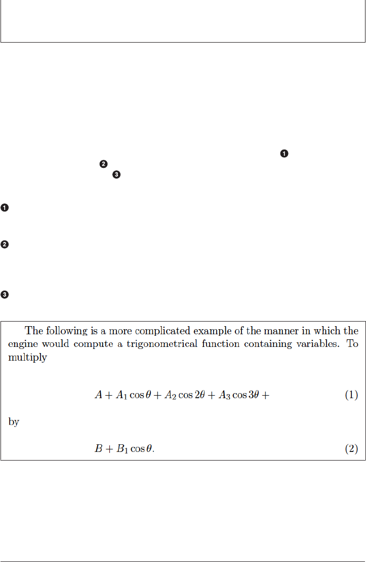
\usepackage{amsmath}
\usepackage{amssymb}
\usepackage{longtable}
If she has added the amsmath package to her preamble, Ada can thus make beautifully
aligned equations with the align environment, as in the snippet shown here (rendered
in Figure 20-5):
The following is a more complicated example of the manner in which the
engine would compute a trigonometrical function containing variables.
To multiply
\begin{align}
&A+A_1 \cos \theta + A_2\cos 2\theta + A_3\cos 3\theta + ···
\intertext{by}
&B + B_1 \cos \theta.
\end{align}
The ampersand marks the place in this equation that should line up with the next
equation.
The progression of mathematical operations can be documented with common
interleaved phrases such as “where,” “such that,” or “which reduces to.” To inter‐
leave such text in a math environment, the \intertext command is used.
The ampersand in the second equation marks the place in this equation that lines
up with the ampersand of the first equation.
Figure 20-5. Aligned LaTeX
As you can see, the equations line up just where the ampersands were placed, but the
ampersands do not appear in the rendered document. Of course, this is only a taste of
mathematical typesetting capabilities in LaTeX, and equations are only half the battle.
Markup Languages | 453
www.it-ebooks.info

How does LaTeX handle other elements of technical documents, such as tables and
figures?
Tables and gures
Tables and figures also often belong in their own files. In addition to the simplicity
gained by keeping such elements outside of the text, reusing these elements in other
documents becomes much simpler if they are kept in their own files. LaTeX is capable
(with the beamer package) of generating presentation-style documents, and these files
can be reused in those documents with a simple reference.
By keeping the figures themselves out of the main text file, the author can focus on
the elements of the figures that are related to the flow of the document: placement
relative to the text, captions, relative size, etc.
In Ada’s notes, diagrams of variables related to the algorithm were inserted. These
could be created in a LaTeX math environment, but they could also be included as
figures. The syntax for including an image is:
\begin{figure}[htbp]
\begin{center}
\includegraphics[width=0.5\textwidth]{var_diagram}
\end{center}
\caption{Any set of columns on which numbers are inscribed, represents
merely a general function of the several quantities, until the special
function have been impressed by means of the Operation and
Variable-cards.}
\label{fig:var_diagram}
\end{figure}
The figure environment begins. Placement options are specified as (h)ere, (t)op,
(b)ottom, or on its own (p)age.
The figure should appear horizontally centered on the page.
The name of the image file is indicated and the width option specifies that the
figure should be half the width of the text.
A verbose caption is added.
A label is added so that the figure can be referenced later in the document using
this name tag.
The result of this syntax is shown in Figure 20-6. In it, the image is brought into the
document, numbered, sized, and captioned exactly as was meant.
454 | Chapter 20: Publication
www.it-ebooks.info
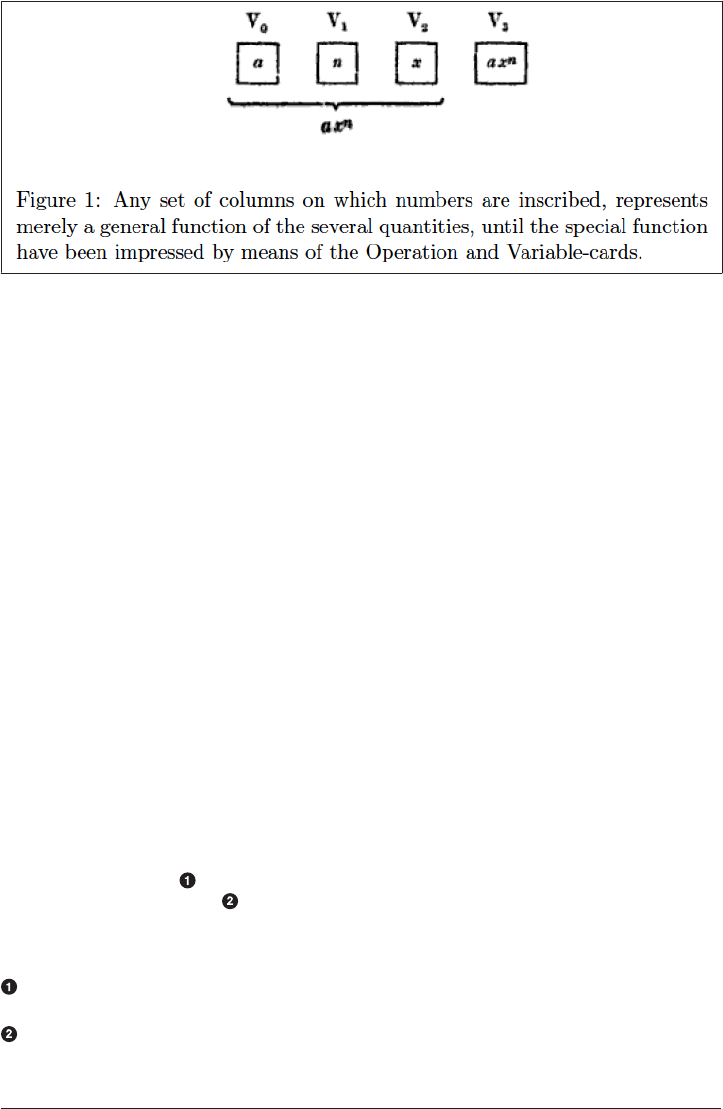
Figure 20-6. Labels in LaTeX
In this example, the figure was labeled with the \label command so that it can be
referenced later in the document. This clean, customizable syntax for internal refer‐
ences is a feature of LaTeX that improves efficiency greatly. The next section will
show how such internal references work.
Internal references
The LaTeX syntax for referencing document elements such as equations, tables, fig‐
ures, and sections entirely eliminates the overhead of matching equation and section
numbers with their in-text references. The \ref{} command can be embedded in the
text to refer to these elements elsewhere in the document if the elements have been
labeled with the corresponding \label{} command.
At build time, LaTeX numbers the document elements and expands inline references
accordingly. Since tables, figures, and sections are often reordered during the editing
process, referring to them by meaningful labels is much more efficient than trying to
keep track of meaningless numbers. In Note D (example.tex), for instance, Ada
presents a complex example and refers to Note B (storehouse.tex). Since the ordering
of the notes might not have been finalized at the time of writing, referring to Note B
by a meaningful name rather than a number—or, in this case, a letter—is preferred.
To do this, Ada must use the \label{} command in the storehouse.tex file so that the
example.tex file may refer to it with the \ref{} command:
% storehouse.tex
\label{sec:storehouse}
That portion of the Analytical Engine here alluded to is called the
storehouse. . .
The section on the storehouse is stored in a file called storehouse.tex.
That section is called Note B, but Ada remembers it as the storehouse section,
and labels it such.
Markup Languages | 455
www.it-ebooks.info

In this example, the label uses the prefix sec: to indicate that storehouse is a section.
This is not necessary. However, it is a common and useful convention. Similarly, fig‐
ures are prepended with fig:, tables with tab:, and so on. Ada can now reference
Note B from Note D as shown here:
% example.tex
We have represented the solution of these two equations below, with
every detail, in a diagram similar to those used in Note
\ref{sec:storehouse}; ...
Note D is held in example.tex.
Ada can reference Note B within this file using the memorable label.
When the document is built with these two files, a “B” will appear automatically
where the reference is. The same can be achieved with figure and table labels as well.
Now it is clear how to reference figures and sections. However, there is another kind
of reference common in publications. Bibliographic references (citations) are also
automated, but are handled a bit differently in LaTeX. The next section will explain
how.
Bibliographies
An even more powerful referencing feature of LaTeX is its syntax for citation of bib‐
liographic references and its automated formatting of bibliographies. Using BibTeX
or BibLaTeX, bibliography management in LaTeX begins with .bib files. These contain
information about resources cited in the text sufficient to construct a bibliography.
Had Ada desired to cite the Scientific Memoir her notes were concerned with, she
might have defined that work in a refs.bib file as follows:
% refs.bib
@article{menabrea_sketch_1842,
series = {Scientific Memoirs},
title = {Sketch of The Analytical Engine Invented by Charles Babbage},
volume = {3},
journal = {Taylor's Scientific Memoirs},
author = {Menabrea, L.F.},
month = oct,
year = {1842},
pages = {666--731}
}
To cite this work in the body of her text and generate an associated bibliography, Ada
must do only three things. First, she uses the \cite{} command, along with the key
(menabrea_sketch_1842), where she wants the reference to appear:
% intro.tex
...
These cards contain within themselves (in a manner explained in the Memoir
456 | Chapter 20: Publication
www.it-ebooks.info
itself \cite{menabrea_sketch_1842}) the law of development of the particular
function that may be under consideration, and they compel the mechanism to act
accordingly in a certain corresponding order.
...
Second, she must include a command placing the bibliography. Bibliographies appear
at the end of a document, so just before the \end{document} command in her main
notes.tex file, Ada adds two lines:
% notes.tex
...
\section{Note G}
\input{conclusion}
\bibliographystyle{plain}
\bibliography{refs}
\end{document}
These together define the bibliography style. The choices for this parameter are
myriad. The simplest choice is often “plain,” as has been used here. However, a one-
word change can alter the formatting to comply with Chicago, MLA, or any other
bibliography formatting style. The second line names the location(s) of the .bib file(s).
The final necessary step is to build the bibliography along with the document. For
this, an extra build step is required that employs the bibtex command. In a peculiar‐
ity of LaTeX, for the references to appear, you must call latex again twice after issu‐
ing the bibtex command. So, at the command line, Ada must type:
$ latex notes
$ bibtex notes
$ latex notes
$ latex notes
$ dvipdf notes
The result is marvelous. In the text, the \cite command is replaced with “[1]”, and
on the final page of her document, a bibliography appears as in Figure 20-7.
Figure 20-7. Automated bibliography generation
Never again need scientists concern themselves with the punctuation after a title in
an MLA-style bibliography—LaTeX has automated this. The only thing LaTeX does
not automate about bibliography creation is reading the papers and making the .bib
Markup Languages | 457
www.it-ebooks.info

file itself. Thankfully, other tools exist to make that process more efficient. The next
section introduces these.
Reference management
To generate a .bib file easily, consider using a reference manager. Such a tool helps to
collect and organize bibliographic references. By helping the researcher automate the
collection of metadata about journal articles and other documents, as well as the pro‐
duction of .bib files, these tools eliminate the tedious task of typing names, titles, vol‐
ume numbers, and dates for each reference cited in a paper. It can all be completely
automated. A number of open source tools for this task exist. These include, among
others:
• BibDesk
• EndNote
• JabRef
• Mendeley
•RefWorks
• Zotero
Reference managers help researchers to organize their sources by storing the meta‐
data associated with them. That metadata can typically be exported as .bib files.
Citing Code and Data
One thing that BibTeX lacks is a metadata format appropriate for uniquely referenc‐
ing code or data, unless it has a digital object identifier (DOI) number associated with
it. For truly reproducible publication, you should cite the code and data that pro‐
duced the analysis using a DOI.
Each commit in your version-controlled code repository has a commit hash number
that distinguishes it uniquely from others. For unique identification in a library or
bookstore, this book has an ISBN. Analogously, data and software objects can be
identified in a persistent way with a DOI number.
It is possible to acquire a DOI for any piece of software using archival services on the
Internet. Some are even free and open source.
The use of these reference managers is outside the scope of this chapter. Please go to
the individual tools’ websites to get started using them.
458 | Chapter 20: Publication
www.it-ebooks.info

Publication Wrap-up
Publication is the currency of a scientific career. It is the traditional way in which sci‐
entific work is shared with and judged by our peers. For this reason, scientists spend a
lot of time producing publication-quality documents. This chapter has sought to pro‐
vide an overview of the tools available to aid you in this pursuit and to give an intro‐
duction to the most ubiquitous, LaTeX. Now that you have read this chapter, you
should know that:
• Markup languages separate formatting from content.
• Markup-based text documents are more version-controllable.
• Many markup languages exist, but LaTeX is a particularly powerful tool for scien‐
tific publication.
In the context of LaTeX, you should also know how to:
• Produce a simple document
• Give structure to that document
• Add mathematical equations inline
•Display mathematics
• Include figures
• Reference those figures
• Cite bibliographic references
• Automate the creation of a bibliography
With these skills, you are equipped to begin generating lovely publication-quality
documents. Many resources are available online to enrich what you have learned
here. Two favorites are:
•“The Not So Short Introduction to LaTeX”, by Tobias Oetiker et al.
•Tex-LaTeX Stack Exchange
Publication Wrap-up | 459
www.it-ebooks.info

IPython Notebook
As an aside, please note that another option for reproducible document creation that
was not mentioned in this chapter (because it is in a class of its own) is the IPython
notebook. IPython Notebook is a part of the IPython interpreter that has been used in
previous chapters. It is an interface for Python that can incorporate markup languages
and code into a reproducible document. With an interface very similar to that of a
Mathematica notebook, the IPython (soon, Jupyter) notebook combines plain text,
LaTeX, and other markup with code input and output cells. Since the IPython note‐
book displays tables and plots alongside the code that generated them, a document in
this format is especially reproducible.
For more on IPython, Jupyter, and working with the Notebook, see the IPython web‐
site.
Publication is an essential part of bringing your work to your peers. Another way,
however, is direct collaboration. The next chapter will demonstrate how GitHub can
make collaboration on papers and software far more efficient.
460 | Chapter 20: Publication
www.it-ebooks.info

CHAPTER 21
Collaboration
It was once the case that collaboration involved letters being sent through the mail
from scientist to scientist.
Today, collaborations happen via email, conference calls, and journal articles. In addi‐
tion to these tools, web-based content and task management tools enable scientific
collaborations to be made effortlessly across continents, in myriad time zones, and
even between scientists who have never met. Indeed, some of the first enormous
modern collaborations in the physical sciences spurred the progenitors of the collab‐
oration tools that currently exist (not least of all, the Internet). In the context of com‐
putation, issue ticketing systems can be closely tied to version control systems and
become powerful tools for peer review.
This chapter will demonstrate how such tools expedite and add peer-review capabili‐
ties to collaborative research discussions, writing papers, and developing scientific
software. These ticket management systems provide a system for content manage‐
ment alongside version-controlled repositories. Sites like GitHub, Launchpad, and
Bitbucket, which provide content management for hosted version-controlled reposi‐
tories, are essential to modern collaboration.
Additionally, this chapter will describe the interface for pull requests that allows col‐
laborators to peer review code. Transparent archiving and opportunity for review do
for scientific software what the peer-reviewed journal system does for scientific
papers. Scientific code has historically gone unreviewed and unrecognized by the sci‐
entific community. However, thanks to these new tools, software is increasingly being
seen as a bona fide scientific research product in itself, not unlike a journal article.
Without the interfaces for peer review provided by sites like GitHub, this would never
be possible.
461
www.it-ebooks.info

In Chapter 15, version control was called the “laboratory notebook” of scientific com‐
puting. In that paradigm, the tools described in this chapter allow scientists to share,
review, and collaborate on laboratory notebooks, both among themselves and with
the world.
Scientific collaboration via the post was riddled with inefficiencies, bottlenecks, and
obfuscation of provenance. If Lise Meitner, Neils Bohr, Fritz Strassman, and Otto
Hahn had had this new kind of system when they were working on the research that
would yield the theory of nuclear fission, the process of discovery would have been
expedited enormously. In a modern version of their collaboration, their communica‐
tion would have been instantaneous and the provenance of ideas and effort would
have been more transparent to the scientific community. In such a version of their
collaboration, perhaps there might have even been sufficient provenance to guarantee
a Nobel Prize for Prof. Meitner alongside her colleagues Hahn and Strassman. The
next section will discuss how an open source scientific computing project today could
rely on ticket managers.
Ticketing Systems
For any research project, computational or otherwise, a ticket management system
(sometimes called a content management system or issue tracker) can vastly simplify
collaboration. Web-based ticket management systems allow progress on a project to
be tracked and managed at the level of individual tasks by providing a web interface
for task assignments, updates, and completion reports.
Almost all web-based services for code repository hosting (e.g., GitHub, Bitbucket,
Launchpad) have an associated issue tracker. These provided methods for creating
issues or tickets associated with necessary tasks related to the repository. The resulting
dashboard is an annotated, dynamic system for to-do list curation, communication,
and peer review.
Tickets are, fundamentally, the first step in the workflow for new features, bug fixes,
and other needs within the code base. The next section will give an overview of the
workflow associated with such ticketing systems.
Workow Overview
In the context of a collaborative research effort, community guidelines for using issue
trackers must arise organically in a way that appropriately reflects the structure and
culture of the collaboration. However, common workflow patterns have emerged in
the use of issue trackers in scientific computing projects that share a general
structure.
While many types of workflows exist, the workflow in Figure 21-1 is common for a
situation when a bug is found.
462 | Chapter 21: Collaboration
www.it-ebooks.info
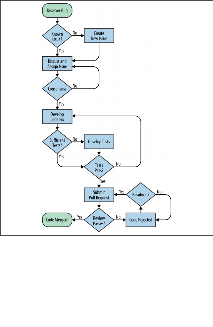
Figure 21-1. A bug resolution workow
First, before reporting a bug, the user or developer must check the rest of the cur‐
rently open issues to determine whether it has already been reported. If the bug is not
yet known, a new issue can be created describing the bug, and the collaborators can
agree upon related goals and subtasks.
When researchers take responsibility for completing issues, those tickets are assigned
to them (or they can self-assign it). As a researcher makes progress on the completion
of the task, comments and updates can be added to the ticket. If collaborators have
questions or comments about the progress of a task, the ensuing discussion can take
Ticketing Systems | 463
www.it-ebooks.info

place directly on the ticket through the web interface. Finally, when a conclusion is
reached, code committed to the repository can be referenced in the discussion. A pull
request holding the new changes is typically submitted, referencing one or more
issues. The new code submitted by pull request can then be reviewed, tested on multi‐
ple platforms, and otherwise quality checked. When the new code satisfies collabora‐
tors, the issue is declared solved or closed. It is typically closed by the person who
opened it, a project leader, or the person who solved it.
When a new feature is desired, a similar workflow is followed. However, the initial
steps can be quite different. Many open source projects have a notion of “enhance‐
ment proposals” that are necessary to initiate the process.
Of course, the first step in any of these workflows is to actually create the issue or
ticket.
Creating an Issue
Users and developers often find bugs in code. A bug found is better than a bug that
goes unnoticed, of course, because only known bugs can be fixed.
“Issues” on GitHub are tickets associated with a particular repository. Issues alert
code developers and users to a bug, feature request, or known failure. Primarily, issue
tickets exist to specifically designate a place for discussion and updates concerning
these topics.
A modern Otto Hahn, when faced with a peculiar result, could begin a discussion
with his colleagues in the hopes of solving the problem. Figure 21-2 shows the Git‐
Hub issue creation form through which Otto opens an issue and describes the
problem.
464 | Chapter 21: Collaboration
www.it-ebooks.info
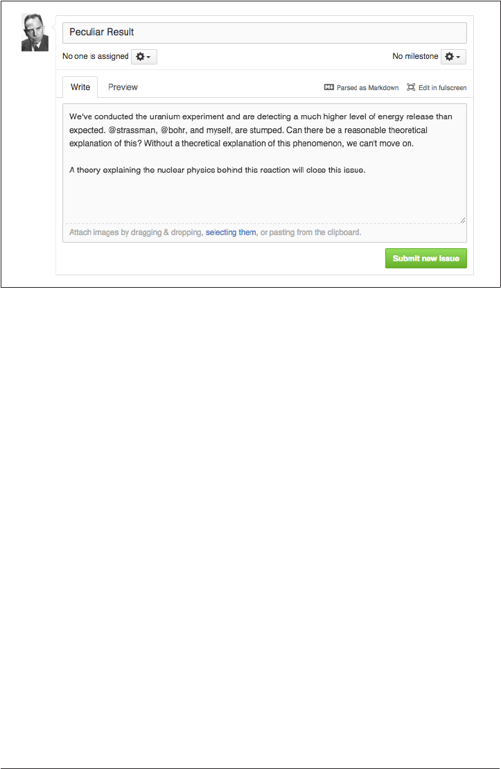
Figure 21-2. Hahn needs a theory
Core features of an issue
The most effective issues have a bit more information than the one in Figure 21-2,
however. In particular, issues typically answer a few key questions:
•What is needed? A description of the error or feature request.
•Why is it necessary? Sufficient information to replicate the error or need.
•What happens next? A proposal for a path forward.
•How will we know this issue is resolved? A clear end goal.
Without those features, it may be difficult for other collaborators to replicate the
issue, understand the need for a change, or move toward a solution. Furthermore, for
provenance, even more data about the issue itself can be helpful.
Issue metadata
In addition to this core information, metadata can be added to the issue that helps to
organize it and designate its place among others. Different web-based hosting plat‐
forms provide different features for defining tickets. Some of the neat features of Git‐
Hub issues include tags, user pings, cross-linking with the code base, and commit
hooks.
Tags, which are completely customizable for each project, can be used for categoriz‐
ing and differentiating groups of issues. Many tags may be used for a single issue, and
on GitHub, colors can be used creatively to help visually distinguish distinct topics.
Ticketing Systems | 465
www.it-ebooks.info

Issue tags may be used to categorize the issue along many different axes. For instance,
they may indicate the level of importance, the degree of complexity, the type of issue,
the component of the code affected, or even the status of the issue.
Table 21-1 gives some examples of the kinds of tags you might apply.
Table 21-1. GitHub tagging examples
Importance Diculty Type of issue Code component Issue status
Critical Expert Bug Installation New
High priority Challenging Feature Input/output Progress
Medium priority Mild eort Documentation Core In review
Low priority Beginner Test Visualization Won’t x
The customizability and power of this metadata are vast. In particular, it can help
code developers to decide which issues to tackle next. Together with a tool like
HuBoard or waffle.io, this metadata can even fuel dashboards for managing projects
under sophisticated workflow paradigms (e.g., “agile” or “kanban” systems).
Since so much of this metadata revolves around helping developers to approach and
handle tasks, it should make sense that the most important type of metadata in an
issue ticket is the assigned developer.
Assigning an Issue
To avoid duplicated effort, an issue can be assigned to a particular developer. Com‐
monly, in the open source world, issues are discussed among developers as soon as
they are created. Often, the developer who most clearly has expertise in that area of
the code is the one who is assigned to handle it.
An issue can also be left unassigned to indicate that it is unclaimed. Developers who
become interested in solving such issues can confidently assign them to themselves.
Grouping Issues into Milestones
On GitHub, issues can be grouped into milestones. Milestones are groups of issues
defining broader-reaching goals. Milestones also have due dates. This feature of the
GitHub interface can be used as a mechanism for project goal tracking of many kinds,
including research group organization and code release management.
466 | Chapter 21: Collaboration
www.it-ebooks.info
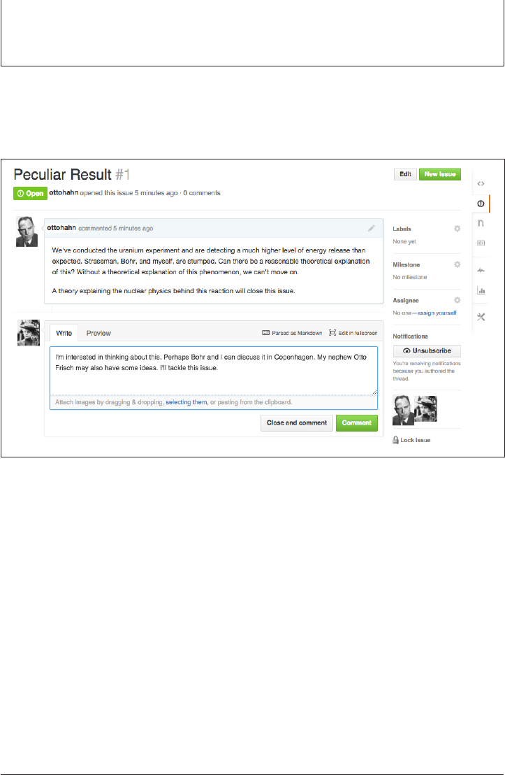
Grant-driven research, in particular, is well suited for milestone-based, due date–
driven work. Additionally, by bundling all of the issues needed for a desired feature
set, milestones are ideal for defining the necessary work remaining for a code release.
Even though she was far away from Otto Hahn, a modern Lise Meitner could have
commented on and assigned herself to handle the issue he opened. In Figure 21-3,
Lise makes a comment on the GitHub issue. By clicking the “assign yourself” link on
the right, she can claim the task.
Figure 21-3. Lise claims this task
Once she has claimed it, she can go ahead and start work on it. As she begins to
develop a theory, she may desire to bounce ideas off of her colleagues. Discussing an
issue can be done on GitHub as well, so she, her nephew Otto Frisch, and Neils Bohr
can discuss their thoughts right alongside the original question.
Discussing an Issue
To discuss an issue on GitHub, just enter a new comment into the comment box asso‐
ciated with the issue. The issue conversation is an appropriate place for:
•Asking and answering clarifying questions about the issue
• Sharing and discussing ideas for an approach
• Requesting and providing updates on the process
Ticketing Systems | 467
www.it-ebooks.info

Some research groups are tempted to discuss issues via email rather than within the
issue tracker. While that strategy seems equivalent, it is not. Discussion directly on
the issue page is superior at retaining context, transparency, and provenance.
All that said, very open-ended discussions are typically more appropriate for the
email format. Issues are meant to eventually be closed.
Closing an Issue
When the bug is fixed or the new feature implementation is complete, the issue
should be closed. The collaboration’s cultural norms, expertise distribution, leader‐
ship hierarchies, and verification and validation requirements all affect the process by
which an issue is deemed complete.
For example, in repositories dedicated to writing a research paper (see Chapter 20),
building a research website, or prototyping a quick idea, changes might not require
strict quality assurance methods. In those situations, the issue may be closed without
much fanfare or oversight at all.
In contrast, the scientific community expects a high level of robustness and quality
from scientific software. To assure quality and accuracy, new changes to a scientific
software project may need to undergo verification, validation, and peer review. In
such a project, closing an issue may therefore involve the effort and consensus of
multiple researchers, incorporation of an automated test suite, adherence to a style
guide, and appropriate documentation.
Indeed, the level of validation and verification necessary in high-quality software
projects typically requires that the issue review culture includes a system of pull
requests.
Pull Requests and Code Reviews
Historically, software developers shared, removed, and submitted changes through
patches passed around via email. The pull request is a hyper-evolved descendant of
that technology and, indeed, carries a patch at its core. Pull requests, however, repre‐
sent an enormous leap forward for collaborative software development. Pull requests
are a reasonable, provenance-aware interface for applying peer review to proposed
patches.
Chapter 15 demonstrated the power of version control for tracking small changes.
Importantly, a patch is just such a small change. Recall from Chapter 1 that the differ‐
ence between two files can be output to the terminal. Additionally, recall that any out‐
put can be redirected to a file instead of the terminal. The resulting file represents the
difference between two files. It is called a patch because the patch command is used
to apply that difference to the original file (resulting in the modified file).
468 | Chapter 21: Collaboration
www.it-ebooks.info

1See Edward R. Tufte’s e Visual Display of Quantitative Information (Graphics Press).
Submitting a Pull Request
With the pull-request interface, however, a researcher can submit a change for review
in a clean interface that links to actual commits, allows line comments, and persists
alongside the code on the GitHub servers.
In Lise Meitner’s case, perhaps the project repository might have held a text docu‐
ment outlining the working theory and experimental description for the project. To
make changes, Lise first forked the main repository, under the kaiserwilhelm user‐
name, then cloned it locally:
$ git clone git@github.com:lisemeitner/uranium_expmt
She might have solved the issue that Otto Hahn opened by creating a branch (see
“Listing, Creating, and Deleting Branches (git branch)” on page 365), “newtheory,”
and editing the text file there:
$ git checkout -b newtheory
At this point, she might choose to delete some of the text that incorrectly described
the theory, and to add lines that outline her theory of fission. After editing the file
and committing her changes, she can push that branch up to her fork on GitHub (see
“Downloading a Repository (git clone)” on page 375). In the directory containing her
local copy of the repository, Lise might perform the following to push her feature
branch up to her fork:
$ git commit -am "edits the old theory and replaces it with the new theory."
$ git push origin newtheory
Once she has pushed the branch up to GitHub, Lise can navigate within a web
browser to the dashboard of her repository. There, GitHub provides the option to
make a pull request to the master branch of the main kaiserwilhelm repository. When
that button is clicked, the pull request appears as a new issue in the kaiserwilhelm
repository, where it should be reviewed by collaborators before being merged into the
code base.
Reviewing a Pull Request
Reviewing a pull request is much like reviewing a paper. More accurately, it should be
like reviewing a section or paragraph of a paper. Humans are better at reviewing short
paragraphs of code rather than hundreds of lines at once—too much for us to hold in
our heads at once.1 For this reason, developers should avoid lengthy or complex pull
requests if possible. By addressing changes in an atomistic fashion (one bug fix or fea‐
Pull Requests and Code Reviews | 469
www.it-ebooks.info

ture addition at a time), developers reduce the likelihood of introducing a bug that
can be missed in the review stage.
At this stage, developers reviewing the pull request may ask a number of questions.
Does the code:
• Accomplish the goals?
•Introduce bugs?
• Include sufficient tests?
• Follow the style guide?
•Pass the existing tests?
• Pass new tests?
• Pass the tests on other platforms (Unix, Windows)?
Merging a Pull Request
Once reviewed, the code can be merged. This can be done in one of two ways. On
GitHub, within the pull request itself, there is a green button for merging noncon‐
flicting pull requests.
Alternatively, via the command line, a developer can use a combination of git
remote, git fetch, git merge, and git push. Review Chapter 16 to recall how these
commands are used.
Collaboration Wrap-up
Collaboration can be a very complex, time-consuming element of scientific work—
especially with old technology. However, readers of this book should now be
equipped to collaborate more efficiently using the power of Git and GitHub. In this
chapter, you have seen how to create, assign, discuss, and tag issues, as well as how to
generate solutions, make pull requests, review code, and incorporate changes effi‐
ciently online.
This efficiency should free up time for determining what license is best for distribut‐
ing your code with. For help with that, keep reading into the next chapter.
470 | Chapter 21: Collaboration
www.it-ebooks.info

CHAPTER 22
Licenses, Ownership, and Copyright
For any software project, the most important file in the project is the license. This file
states who owns the work, who is allowed to use the project and under what condi‐
tions, and what rights and guarantees are conferred to both the users and the owners.
If a license file is not present, it is conspicuous in its absence. Since the license is the
most important file in a project, this chapter is the most important one in this book to
read and fully understand.
License files should be easy and obvious to find. Most of the time they appear in the
top-level directory and go by the name LICENSE, license.txt, or another variant. Note
that sometimes different parts of a project are provided under different licenses.
Some projects also have the dubious practice of being licensed differently depending
on how they are used. Be sure to read and understand the license of any software
project that you use before you use it.
Get a Laywer
This chapter is not legal counsel. We are not qualified to help you
in a formal dispute. For that, you need to have a lawyer.
This chapter is only intended to provide friendly advice that aims to help you under‐
stand the basic concepts in publishing a creative work. Having a good grasp of these
fundamentals will help you make informed decisions. If for any reason you do end up
needing legal counsel in this area but do not know where to start, you can contact the
Electronic Frontier Foundation (EFF), the Software Freedom Conservancy (SWC),
Creative Commons (CC), the Free Software Foundation (FSF), or Numfocus (NF);
they may be able to help. Each of these organizations has experience with the legal
471
www.it-ebooks.info

aspects of software development and should be able to point you in the right direc‐
tion, at the very least.
The licenses discussed in detail in this chapter will mostly be open source licenses.
This is because without peer review of software and data, scientific code cannot fairly
be called reproducible. If something is not reproducible, then it is de facto not sci‐
ence, no matter how deeply it covers a scientific topic. Equal dissemination of knowl‐
edge is critical to the scientific method. This is not to diminish the technical prowess
of closed source code at all—propietary software is frequently among the most
sophisticated. It is just not science in the benefit-for-all-of-humanity-for-all-of-time
way. Open source licenses are ideally suited to research software.
This chapter will cover ideas and terms that you are probably already familiar with in
their common usage. Here, we seek to improve upon that lay understanding to fur‐
ther the aims of computational physics.
What Is Copyrightable?
Before we talk about licenses in depth, it is important to understand what they cover.
In western jurisprudence, from which most copyright law around the world stems,
ideas and concepts are not copyrightable. However, expressions of ideas are
copyrightable.
For instance, copyright does not apply to physical laws of nature and mathematical
facts. The number pi and the idea that it is the ratio between the area of a circle and
the square of its radius is not something that any human can claim ownership of.
Humans discovered this knowledge, but humans did not create it nor invent it. Pi just
is. Now, if I were to bake a pie with the letter pi cooked into the crust and the digits
proudly displayed around the perimeter and then took a picture of my handiwork, I
would have copyright over the picture. This tasty expression of pi would be uniquely
my own. Anyone claiming otherwise would be wrong.
The same logic applies even outside the world of strictly scientific endeavors. For
example, game rules are abstract concepts that are not copyrightable. However, any
published version of a game that you read is a copyrighted expression of those rules.
The rules for chess, Go, mancala, poker, bridge, basketball, rugby, cricket, e Settlers
of Catan, and Dungeons & Dragons are all not copyrightable. They are just ideas. That
said, the rule book that comes with any of these games is a creative and particular
expression of the rules and is subject to copyright law.
In software, the breakdown between what is and is not copyrightable is the distinc‐
tion between the implementation and the interface. The application programming
interface (API) is considered to be a set of ideas and therefore not copyrightable. The
actual implementation of an API, or how the actual work is performed, is copyrighta‐
ble. There are many possible implementations for any interface, and so any given
472 | Chapter 22: Licenses, Ownership, and Copyright
www.it-ebooks.info

implementation is a unique expression. For example, say we wanted a function
named std() that computed the standard deviation of a list of values named vals.
These name choices and the concept of what the function is supposed to do make up
the interface, which is not copyrightable. That said, any code that computes the stan‐
dard deviation with this interface is copyrighted. There is a fundamental distinction
both conceptually and legally between how one uses software and how that software
is written. Keep this distinction in mind as you read through the following sections.
Right of First Publication
Now that we know what can be copyrighted, we should understand when copyright
applies. Most copyright systems feature what is called the right of rst publication.
This is the idea that copyright automatically goes to the first publisher of a creative
work. This right is conferred whether or not it is specified by the publisher at the
time. Such laws protect publishers from having their work stolen as long as they can
demonstrate that they were there first.
This has important implications in the information age, where self-publishing is nor‐
mal behavior. Anyone who writes a blog post, tweets out “Happy Birthday, Mom!” or
puts code on GitHub personally retains the copyright to that work via the right of
first publication. Your work is your own unless you give it up.
In software, say you post a piece of code without a license. By rights this code is yours
and yours alone, even though it is publicly visible. You own the copyright, and you
have not specified how others are allowed to use your code. By default, legally, they
are not entitled to use it at all. If your intent was to share your code for reproducibil‐
ity, provenance, education, or general scientific goodwill, by not having a license you
have undermined your intended purpose.
Software licenses are important because they allow you to retain copyright and they
state the terms by which other people or organizations are entitled to use or modify
your software. That said, it is possible to completely forego all rights.
What Is the Public Domain?
What happens if you do not want to deal with licenses or you do not want to retain
copyright? If you just want the code that you produce to be for the unrestricted bene‐
fit of all, yielding completely to the better nature of scientific discourse? It is possible
to put a work into the public domain (PD) with a simple statement along the lines of,
“This work has been placed in the public domain.”
The public domain is a concept that society as a whole “owns” a work, and it is there‐
fore free and available for anyone and everyone to use and modify. Since everyone
owns it, nobody owns it. In most cases, the copyright of an existing work will expire
Right of First Publication | 473
www.it-ebooks.info

after a set number of years (25, 50, 90, etc.), at which point the work will enter the
public domain. The public domain is what allows anyone to republish the collected
works of Mark Twain, Socrates’s Apology, or Mary Shelley’s Frankenstein. However,
just because copyright will expire naturally does not mean that you have to wait that
long. You are free to add your own works to the public domain sooner if you so
desire.
That said, the public domain is one of the trickiest parts of international copyright
law. Not every country has a public domain that is compatible with the notions
expressed here. In some countries it may not be possible for an individual to place a
work into the public domain prior to the expiration of copyright. It is important to
understand the laws of the country where you live. Wikipedia is often a good first
resource. For anything deeper, you should probably seek out legal counsel. If you are
at a university, national lab, or private company, your organization will often have
resources available for you to use.
If you do not want to put your software in the public domain, but do want it to be
free and open, you have to do the work of picking a license.
Choosing a Software License
A license is a legal document that states how software is allowed to be used by its
users and what rights the author retains, and serves to protect both the users and the
authors. Without such a document, only the original author or publisher has any
right to use or modify the code. Having a software license that accurately reflects your
needs and the needs of your potential users is extremely important.
A variety of licenses have been created over the years, tailored to different situations.
At the broadest level, there are proprietary licenses and free/open source licenses. Pro‐
prietary licenses are usually written by companies that sell software. The Microsoft
Windows End-User License Agreement (EULA) is an example of such a document.
They typically proclaim the owner of the copyright to be the company, disclaim dam‐
ages if the software is abused, and promise litigation in the event of piracy. They are
often handcrafted by a team of lawyers to minimize the exposure to the company.
Free and open source software licenses, sometimes abbreviated as FOSS, FLOSS, or
OSS, are much more relevant to computational physics software, especially if it is pri‐
marily for research. Research-grade software typically has the following attributes:
• It does not have immediate and direct commercial interest.
•It must have source code inspectable by peers for review.
• It changes rapidly to fit the needs of the researcher.
474 | Chapter 22: Licenses, Ownership, and Copyright
www.it-ebooks.info

Licenses that give users and other developers the freedom to look at and modify code
encourage scientific discourse, education, comparison, quality assurance, and partici‐
pation in the project. Since most researchers do not have the funds available to hire
thousands of developers to do all of these activities, an open source license can help
establish a community of users and developers. Fellow scientists can pool together to
help in these essential tasks that make a software project successful. The exchange is
often nonmonetary. One person provides code, and others may help make that code
better. To be safe, open source licenses often explicitly include a no-warranty clause.
You cannot sue someone for damages because their open source code somehow
harmed your machine.
We will not cover proprietary licenses more here. There are a lot of them, since
almost every software product has its own license. On the other hand, the open
source world has converged on a much smaller number of licenses. However, there
are still far too many open source licenses to go into great depth on all of them. Here,
we will present only the most important and the most interesting ones. For a more
comprehensive review of open source licenses, please see the Open Source Initiative’s
(OSI) website or the GNU commentary page.
It is highly advisable to use an off-the-shelf open source license. Do not attempt to
write your own. Partly this is because you are not a lawyer, and it would be a waste of
your time. More importantly, licenses are not generally considered trustworthy until
they have been proven in court. This means that one party broke the terms of a
license, another party sued, and the license was upheld in a court of law. This is an
expensive and time-consuming process. Relatively few open source licenses have
gone through this crucible, but almost all of them that have survived the journey. Any
license you write will not have this benefit.
The choice of license can have a deep and lasting effect on the community that devel‐
ops around a code project. Given its importance, picking the right license receives
surprisingly little attention from developers. It is a core part of the social aspect of
software development. Everyone should know about the license and its implications,
not just the law nerds on a project. If you ever need help picking, the excellent Choo‐
seALicense.com will help you along your way.
Let’s examine some key licenses now to find out precisely what it means to be open
source.
Berkeley Software Distribution (BSD) License
The Berkeley software distribution or BSD license is actually a collection of three pos‐
sible licenses known as the BSD 4-Clause, 3-Clause, and 2-Clause licenses, respec‐
tively. Historically, the 4-clause is the oldest and the 2-clause is the most recent. The
4-clause is not recommended anymore, though both the 3- and 2-clause versions are
Berkeley Software Distribution (BSD) License | 475
www.it-ebooks.info

commonly used. Of all of the licenses that we will discuss, either the 3- or 2-clause
license is recommend for use in your software projects. These are the licenses best
tailored to science and research. Major projects such as NumPy, SciPy, IPython, and
the rest of the scientific Python ecosystem use either of these licenses. The text is as
follows:
Copyright (c) <year>, <owner>
All rights reserved.
Redistribution and use in source and binary forms, with or without
modification, are permitted provided that the following conditions are met:
* Redistributions of source code must retain the above copyright
notice, this list of conditions and the following disclaimer.
* Redistributions in binary form must reproduce the above copyright
notice, this list of conditions and the following disclaimer in the
documentation and/or other materials provided with the distribution.
* Neither the name of the <organization> nor the
names of its contributors may be used to endorse or promote products
derived from this software without specific prior written permission.
THIS SOFTWARE IS PROVIDED BY THE COPYRIGHT HOLDERS AND CONTRIBUTORS "AS IS" AND
ANY EXPRESS OR IMPLIED WARRANTIES, INCLUDING, BUT NOT LIMITED TO, THE IMPLIED
WARRANTIES OF MERCHANTABILITY AND FITNESS FOR A PARTICULAR PURPOSE ARE
DISCLAIMED. IN NO EVENT SHALL <COPYRIGHT HOLDER> BE LIABLE FOR ANY
DIRECT, INDIRECT, INCIDENTAL, SPECIAL, EXEMPLARY, OR CONSEQUENTIAL DAMAGES
(INCLUDING, BUT NOT LIMITED TO, PROCUREMENT OF SUBSTITUTE GOODS OR SERVICES;
LOSS OF USE, DATA, OR PROFITS; OR BUSINESS INTERRUPTION) HOWEVER CAUSED AND
ON ANY THEORY OF LIABILITY, WHETHER IN CONTRACT, STRICT LIABILITY, OR TORT
(INCLUDING NEGLIGENCE OR OTHERWISE) ARISING IN ANY WAY OUT OF THE USE OF THIS
SOFTWARE, EVEN IF ADVISED OF THE POSSIBILITY OF SUCH DAMAGE.
Copyright (c) <year>, <owner>
All rights reserved.
Redistribution and use in source and binary forms, with or without
modification, are permitted provided that the following conditions are met:
1. Redistributions of source code must retain the above copyright notice, this
list of conditions and the following disclaimer.
2. Redistributions in binary form must reproduce the above copyright notice,
this list of conditions and the following disclaimer in the documentation
and/or other materials provided with the distribution.
THIS SOFTWARE IS PROVIDED BY THE COPYRIGHT HOLDERS AND CONTRIBUTORS "AS IS" AND
ANY EXPRESS OR IMPLIED WARRANTIES, INCLUDING, BUT NOT LIMITED TO, THE IMPLIED
WARRANTIES OF MERCHANTABILITY AND FITNESS FOR A PARTICULAR PURPOSE ARE
DISCLAIMED. IN NO EVENT SHALL THE COPYRIGHT OWNER OR CONTRIBUTORS BE LIABLE FOR
ANY DIRECT, INDIRECT, INCIDENTAL, SPECIAL, EXEMPLARY, OR CONSEQUENTIAL DAMAGES
(INCLUDING, BUT NOT LIMITED TO, PROCUREMENT OF SUBSTITUTE GOODS OR SERVICES;
LOSS OF USE, DATA, OR PROFITS; OR BUSINESS INTERRUPTION) HOWEVER CAUSED AND
ON ANY THEORY OF LIABILITY, WHETHER IN CONTRACT, STRICT LIABILITY, OR TORT
(INCLUDING NEGLIGENCE OR OTHERWISE) ARISING IN ANY WAY OUT OF THE USE OF THIS
476 | Chapter 22: Licenses, Ownership, and Copyright
www.it-ebooks.info

SOFTWARE, EVEN IF ADVISED OF THE POSSIBILITY OF SUCH DAMAGE.
The views and conclusions contained in the software and documentation are those
of the authors and should not be interpreted as representing official policies,
either expressed or implied, of the <owner> Project.
The BSD licenses are known as permissive licenses. This is because they allow the fur‐
ther distribution of the code to be done under any license. Only the copyright notice
needs to be displayed. Additionally, further versions of the code need make no prom‐
ises as to what license they will be released under. Modifications to the code may be
released under any license that the author of the modification desires. Permissive
licenses give a lot of freedom to users and developers other than the original author,
while protecting the original author from liability.
For example, suppose person B copies person A’s code. A originally released the code
under a BSD license. B wants to modify the code and relicense the whole new code
base. B is completely free to do so, and does not even have to include a copy of the
original BSD license. The only requirement is to include the copyright notice, “Copy‐
right (c) <year>, Person A.” This ensures that person A gets credit for the work, but
without a lot of headache.
The freedom to modify and relicense is a major reason why BSD is the recommended
license for scientific computing. It leaves the most number of options open to future
scientists. The MIT license is considered to be equivalent to the BSD 2-clause and is a
perfectly reasonable substitute. Up next is one of BSD’s main competitors.
GNU General Public License (GPL)
The GNU General Public License (GPL) is again a collection of three distinct licenses:
GPLv1, GPLv2, and GPLv3. Additionally, there are v2.1 and v3 GNU Lesser General
Public Licenses (LGPLs). These are compatible with the corresponding GPLs of the
same major version but are closer in spirit to BSD and MIT licenses. All of the GPL
options are promoted by the FSF for both GNU and non-GNU software projects.
GPLv1 is out of date and should not be used. There remains debate over whether v3 is
an improvement over v2.
Linux is almost certainly the largest project that uses GPLv2, and it will continue to
do so until the end of time. The GNU Compiler Collection (GCC) is likely the largest
project to use GPLv3. The texts of both GPLv2 and GPLv3 are too long to include
here. However, the following preamble should be added to the top of every GPLv3
file:
<one line to give the program's name and a brief idea of what it does.>
Copyright (C) <year> <owner>
This program is free software: you can redistribute it and/or modify
it under the terms of the GNU General Public License as published by
GNU General Public License (GPL) | 477
www.it-ebooks.info

the Free Software Foundation, either version 3 of the License, or
(at your option) any later version.
This program is distributed in the hope that it will be useful,
but WITHOUT ANY WARRANTY; without even the implied warranty of
MERCHANTABILITY or FITNESS FOR A PARTICULAR PURPOSE. See the
GNU General Public License for more details.
You should have received a copy of the GNU General Public License
along with this program. If not, see <http://www.gnu.org/licenses/>.
Unlike BSD, the GPL licenses are not permissive. They instead exemplify a class of
licenses known as copyle by their punning proponents, or viral by their disinterested
detractors. In a copyleft license, modifications to the code must be licensed in the
same (or a similar) way as the original code. For open source code, this means that
any third party that forks your code also has to make the fork open source. In princi‐
ple, this is a good idea. Over time, it builds up an ecosystem of programs that are all
open source and work well with one another. In practice, however, sometimes this
requirement limits the freedom of the developers to the point where an improve‐
ment, modification, or fork will not even be written in the first place.
In general, GPL licenses are a good and reasonable choice for software projects. How‐
ever, the potential disincentives to contribution can be a barrier to entry for small and
medium-sized projects. Since physics programs—even when enormously popular—
are never large, GPL is not recommended for default use. There may still be situations
where it is the best choice, though. It’s important to always carefully consider your
options.
Another important concept for this suite of licenses is GPL compatibility. The FSF
defines compatibility as whether different portions of a code base can be released
under different licenses, where one license is the GPL. A license need not be copyleft
itself to be compatible with the GPL. Notably, the BSD 3- and 2-clause licenses are
both GPL compatible.
Even though the GPL may not be ideally suited to scientific endeavors, it is still a
wildly successful series of licenses that have been proven in court. In general, if you
want GPL-style copyleft but also want something less restrictive in terms of redistrib‐
ution, the LGPL offers a middle path that should be treated as a serious alternative.
Permissive and copyleft licenses are the main players in open source software. How‐
ever, there are also licenses that may be used for generic creative works and are not
restricted to software that may be appropriate.
Creative Commons (CC)
The Creative Commons (CC) license suite is an alternative that applies not only to
software but, more broadly, to all creative works. This includes poetry, prose, film,
478 | Chapter 22: Licenses, Ownership, and Copyright
www.it-ebooks.info

audio, and more. The CC suite is now in its fourth instantiation, sometimes called v4.
The goal of CC licenses is to make the ideas of sharing and collaboration evidenced in
open source software more broadly applicable to other endeavors. For example, all
content on Wikipedia is licensed under CC. This has been a remarkably successful
suite of licenses in its own right.
Creative Commons licenses are all quite lengthy, so it is not possible to print them
here. Their length comes partly from the fact that the licenses are designed to keep
the same spirit in every country in the world. As you might imagine, this can make
the documents quite wordy. They are a tremendous feat of legal engineering.
The CC licenses are distinguished from one another through one or more of the fol‐
lowing four modifiers:
BY (Attribution)
Other people must credit you when they use your work. This applies to all CC
licenses.
SA (ShareAlike)
Other people must reshare the work under the same license if they use or modify
your work.
ND (NoDerivatives)
Other people may share your work but are not allowed to modify it in any way.
NC (NonCommercial)
The work may be modified and shared as long as the result is not sold
commercially.
The six licenses that Creative Commons supplies are thus known under the following
monikers: CC BY, CC BY-SA, CC BY-ND, CC BY-NC, CC BY-NC-SA, and CC BY-
NC-ND. Naturally, ND and NC cannot be applied to the same license.
The CC BY license fills the same role as the BSD license. It has permissive terms that
allow modification of the work as long as credit is given where credit is due. The CC
BY-SA license fills the same role as the GPL or the LGPL: it adds copyleft provisions
to the attribution clause. Both of these are great choices for a scientific computing
project, depending on whether you need copyleft or not.
The ND and NC modifiers, on the other hand, are considered extremely harmful to
scientific software. They may have a place in other domains, such as the arts (notably,
the webcomic xkcd is released under a CC BY-NC license, which is why you do not
see any witty stick figures appearing in this book). However, for physics programs,
the inability to modify the software effectively renders the open source aspects use‐
less. This is true even with just commercial applications restricted. Such license terms
hamstring the development of vibrant science and software communities. Regard any
Creative Commons (CC) | 479
www.it-ebooks.info

use of either ND or NC with extreme prejudice. Luckily, examples of their use are
very rare in computational science.
Lastly, Creative Commons supplies a public domain substitute called CC0 (pro‐
nounced see-see-zero). In many ways, licensing code as CC0 is better than placing it
in the public domain because of the consistency problems with the public domain.
CC0 applies everywhere, including in countries where analogous public domain laws
do not exist. Moreover, in countries with a robust public domain, the CC0 license
effectively reduces to the public domain. Of all of the licenses that are discussed here,
CC0 is the freest. No major code projects of the size of Linux use this license, though
it is slowly gaining traction.
In summary, CC BY, CC BY-SA, and CC0 are all reasonable choices for a scientific
software project. The others should be avoided due to their implications being anti‐
thetical to evolving a scientific community.
The next section discusses licenses that you should not use, but which highlight inter‐
esting aspects of open source software.
Other Licenses
There are many other licenses that we are not able to cover in depth. A large number
of these fall into the broad categories of either being permissive or copyleft, though
with their own unique wording. Some of these have been defended in court. Unlike
the previously discussed licenses, most of these were initially written to apply to a sin‐
gle code project.
For instance, the Apache License was written for the Apache web server and is sup‐
ported by the Apache Software Foundation. It has a lot of use outside of Apache itself.
Unlike other licenses, it contains clauses pertaining to patents.
The Python Software Foundation License is a license that applies to the CPython
interpreter and some other Python Software Foundation code. It occasionally sees
some use in other parts of the Python ecosystem but is not commonly used outside of
that. It is a permissive license that is GPL compatible.
On the more problematic side is the JSON License. This is easily one of the most
commonly broken and flagrantly abused licenses in the world. The full text of the
license reads:
Copyright (c) 2002 JSON.org
Permission is hereby granted, free of charge, to any person
obtaining a copy of this software and associated documentation
files (the "Software"), to deal in the Software without restriction,
including without limitation the rights to use, copy, modify, merge,
publish, distribute, sub-license, and/or sell copies of the Software,
480 | Chapter 22: Licenses, Ownership, and Copyright
www.it-ebooks.info

and to permit persons to whom the Software is furnished to do so,
subject to the following conditions:
The above copyright notice and this permission notice shall be
included in all copies or substantial portions of the Software.
The Software shall be used for Good, not Evil.
THE SOFTWARE IS PROVIDED "AS IS", WITHOUT WARRANTY OF ANY KIND,
EXPRESS OR IMPLIED, INCLUDING BUT NOT LIMITED TO THE WARRANTIES
OF MERCHANTABILITY, FITNESS FOR A PARTICULAR PURPOSE AND
NONINFRINGEMENT. IN NO EVENT SHALL THE AUTHORS OR COPYRIGHT
HOLDERS BE LIABLE FOR ANY CLAIM, DAMAGES OR OTHER LIABILITY,
WHETHER IN AN ACTION OF CONTRACT, TORT OR OTHERWISE, ARISING
FROM, OUT OF OR IN CONNECTION WITH THE SOFTWARE OR THE USE OR
OTHER DEALINGS IN THE SOFTWARE.
The provision for Good and against Evil is considered indefensible due to the subjec‐
tive nature of these terms. While the broad strokes of good and evil can be largely
understood and agreed upon, the specifics, even in a strictly utilitarian context, can
get murky quickly. How any of this applies to software at all is even less well under‐
stood. The JSON License brings into relief the supposition that other open source
software allows for “more evil.”
Even though the pursuit of evil is antithetical to most open source software develop‐
ers and scientists, explicitly disallowing it is not reasonable. It is an unenforceable
claim. Suppose someone really wanted to do bad things and felt the need to use JSON
in order to accomplish the nefarious tasks. Would not the first evil act simply be to
break the JSON license? It ends up being prescriptive, not preventative. Suffice it to
say that no one has ever been successfully prosecuted for breaking the “Good, not
Evil” clause. This license serves as a cautionary tale as to why you should never write
your own license—it probably will not turn out like you thought.
Lastly, the FLASH code from the University of Chicago has a particularly interesting
license. FLASH is a plasma and high-energy density physics program. FLASH is open
source, though it is not directly redistributable by the user. Furthermore, users need
to sign a document registering themselves with the Flash Center prior to being given
access to the code. Item 7 of the FLASH license is unique in its academic nature:
7. Use Feedback. The Center requests that all users of
the FLASH Code notify the Center about all publications that
incorporate results based on the use of the code, or modified
versions of the code or its components. All such information
can be sent to info@flash.uchicago.edu.
Here we see an attempt to gather statistics about the impact factor of scientific soft‐
ware being enforced through the license itself. Given the 850+ publications found on
the FLASH website, this strategy has been very successful. The other nonstandard
provisions of the FLASH license are all justified in their own right, but it is not rec‐
Other Licenses | 481
www.it-ebooks.info

ommended that you adopt licenses such as the FLASH one (indeed, the authors are
not aware of another implementation of this kind of license). Your code is likely not
in a situation like that of the FLASH code. Using one of the stock licenses from the
previous sections is much easier for scientific programs. Uniqueness is not an asset
for software licenses.
Now that we have seen many license types, including permissive, copyleft, and more
exotic ones, it is reasonable to wonder how an existing project might transfer from
one license to another.
Changing the License
Occasionally developers will decide that it is time to change the license that their code
is distributed under. This can happened because of newfound legal implications in
the license, because the broader ecosystem has moved away from a license, or, more
commonly, because it is felt that the project will be easier to sustain under an alterna‐
tive license. One prominent and successful example of a computational physics
project that has undergone relicensing is yt; you can read about the campaign on the
project blog.
Even under the best conditions, changing a license is a long and painful process. It
has a high likelihood of failure even if all of the current developers are on board with
the decision.
Relicensing an open source project requires that you obtain consent from all previous
contributors to make the switch. Consent can be given either actively (sign a waiver,
send an email, etc.) or passively (if we do not hear from you in three months, we will
assume you do not object). If consent is not given by a former or current developer,
either the code that the developer worked on must remain with its original license, or
all of that person’s code must be rewritten to conform with the new license. Both of
these options are their own headaches.
If enough people do not agree with the relicensing activity, it becomes too much of a
hassle to actually relicense the code. In such cases it is easier to start from scratch
than to try to force the issue with the existing code base. The scorched-earth strategy
happens more frequently than many people would like to admit. Many of the worst
horror stories come from trying to switch between copyleft and permissive licenses,
or vice versa.
That said, relicensing is not impossible. It is just hard. When done successfully it will
take at least three or four months. The steps to proceed through a relicense are as
follows:
1. Privately and tentatively, present the idea of the new license to current core devel‐
opers. Make the case for the new license as a possibility and get a feel for the level
482 | Chapter 22: Licenses, Ownership, and Copyright
www.it-ebooks.info

of support. Solicit feedback from this team first. If the current core team is not
interested, stop.
2. Publicly present the option for hypothetically changing the license based on the
previous feedback to all core developers. Solicit opinions from the developers
and gauge the interest. If all members of the core team are happy with the change
and most of the current developers are either for it or do not care, proceed.
Otherwise, stop.
3. Publicly present the option for changing the license to the users. If the project
will lose a significant minority of users due to the change, stop. Users are your
most precious resource, and changing the license is not worth the setback.
4. Promise to change the license only on the following and further releases. Do not
apply the relicense retroactively to previous releases.
5. Obtain written consent from all current and past developers that the relicense is
acceptable. An email suffices. Put a healthy time limit on the opportunity to sub‐
mit the consent form. This allows for the opportunity to raise objections. A
month is typically enough. Still allow the relicensing to fail at this point.
6. Relicense the code on the next release after waiting an appropriate amount of
time.
There are many places where even a single person who has not worked on the project
in a decade can block this entire process. It also is not a technical concern that deals
with how the code operates. There are no right or wrong answers. This is a recipe for
hurt feelings and battered egos. You should enter into such an effort treading as softly
and as slowly as possible.
Even with the license’s chief position in a software project, you also need to under‐
stand its limitations.
Copyright Is Not Everything
Copyright and licensing are not all that there is to what is broadly known as intellec‐
tual property. Patents cover temporary monopolies over ideas and processes. The
original idea behind patents was to allow creators, inventors, and innovators a brief
opportunity to bring their ideas to market. Patenting software has recently come
under intense scrutiny due to “patent trolls” who hoard patents but do not attempt to
produce anything but lawsuits. Trademarks also fall into the realm of intellectual
property. They are recognizable symbols of a business or organization that uniquely
identify that group in a specific domain. Trademarks must be continually used or they
lapse and may be taken up by another group. Some people believe that it’s incorrect to
use the umbrella term “intellectual property,” as copyright, patents, and trademarks
Copyright Is Not Everything | 483
www.it-ebooks.info

are all distinct legal areas. Each of these requires a lawyer that specializes in that area.
Still, for us plebs, the term has stuck.
Intellectual property is not the only instrument of control over software. In fact, most
intellectual property does not truly apply to computational physics. Other mecha‐
nisms are much more effective and more present in many physics software projects.
Export control is a particularly strong system. This is when the government steps in
and forbids the transfer of source code to any other country or foreign national
without explicit permission. Typically even citizens who have access must sign a
document stating that they promise not to violate the terms of the export restrictions.
Export control is particularly powerful because it applies not only to software, but
also to data and ideas. As an extreme and unreasonable example, the government
could restrict you from telling anyone the value of pi on the basis of export control.
When a program is export controlled, it cannot just be put on the Internet. The rules
for sharing become much more complicated. Violating export control typically comes
with a long jail sentence. It is important to take it very seriously. In general, this is not
something you ever want to deal with personally.
Physics programs are subject to export control far more frequently than other soft‐
ware. The typical reason that a physics program becomes export controlled is because
it solves a class of problems that make it easier to build various kinds of highly
restricted weaponry. Furthermore, some contain or produce data that is considered
sensitive or secret and therefore may not be shared. Mathematics and computer sci‐
ence programs are sometimes export controlled due to their applications to cryptog‐
raphy. Be aware of and abide by your government’s laws regarding export control.
Lastly, in the United States there is the Health Insurance Portability and Accountabil‐
ity Act of 1996, or HIPAA. Since this deals with medicine, it comes up only occasion‐
ally in physics software. Software that deals with human patients must be properly
anonymized to ensure the public’s right to privacy. This is known as HIPAA compli‐
ance. The Department of Health and Human Services is responsible for overseeing
such compliance. Other countries have similar laws.
These alternative structures can be extraordinarily effective at limiting what can be
done with software. They are not always in the control of the author, either. While
patents and trademarks and other concerns in intellectual property may not apply,
HIPAA rules and privacy violations can be extraordinarily incriminating. And every
computational physicist needs to be cognizant of export control rules at all times.
Momentary lapses in good judgment are not allowed with respect to export control.
484 | Chapter 22: Licenses, Ownership, and Copyright
www.it-ebooks.info

Licensing Wrap-up
You have now seen a wide swath of the legal issues that surround software develop‐
ment and how they apply to computational physics. You should be familiar with the
following ideas:
•The license document is the most important file in your project.
• Scientific software should be free and open source.
•The permissive BSD licenses are recommended for most computational science
projects.
• The copyleft GPL licenses are also reasonable choices.
•The public domain is a great alternative to licensing your code, but it does not
apply everywhere. Use CC0 as a substitute for the public domain.
•Creative Commons licenses can apply to more than just software.
• You should not write your own license.
• Relicensing a project can be very difficult.
• It is important to be aware of the export control laws in your country.
Now that you’ve made it to the end of the book, the next chapter dives into some
parting thoughts about computational physics.
Licensing Wrap-up | 485
www.it-ebooks.info

CHAPTER 23
Further Musings on Computational Physics
At last, you have arrived! You are now ready to go forth into the wide world of com‐
putational physics. No matter where your specialty may take you, you now have the
skills, abilities, and understanding to perform and reproduce great feats of scientific
computing. For some of you, this book is all you will need to succeed. For others, this
is only the beginning.
Where to Go from Here
What is so beautiful about the skills that you have learned in this book is that they
empower you to go anywhere. Computational physics has taken us from deep within
the Earth’s crust to the farthest reaches of the universe, from pole to pole, all around
the world, and everything in between. Even asking “Where to?” can seem daunting.
The answer is that you should go where your interests lie. If you have a special part of
physics that you already call home, research what computational projects are out
there already. Then try a project out as a user. Join the mailing list. Ask the developers
if they need help with anything, and try contributing back. A good project will be
very welcoming to new users and contributors.
If there is nothing out there that does what you want, you don’t like the languages that
the existing projects are written in, or you don’t agree with their licenses, try starting
your own project—one that suits your needs. This is not scary, and with the existence
of repository hosting websites like GitHub, it has become very easy. Starting a new
project is a great way to hone your software architecture skills while also clarifying
what part of physics you find most interesting.
The following is a list of projects that might pique your interest. We have grouped
them according to subdomain. Most, but not all, of these have strong Python and
physics components. Here they are, in their own words:
487
www.it-ebooks.info

• Astronomy and astrophysics
—yt: A Python package for analyzing and visualizing volumetric, multi-
resolution data from astrophysical simulations, radio telescopes, and a bur‐
geoning interdisciplinary community.
—Astropy: A community effort to develop a single core package for astronomy
in Python and foster interoperability between Python astronomy packages.
—SunPy: The community-developed, free and open source solar data analysis
environment for Python.
• Geophysics, geography, and climate
—UV-CDAT: A powerful and complete frontend to a rich set of visual data
exploration and analysis capabilities well suited for climate data analysis
problems.
—Iris: A Python library for meteorology and climatology. The Iris library imple‐
ments a data model to create a data abstraction layer that isolates analysis and
visualization code from data format specifics.
—ArcPy: Python for ArcGIS.
—Shapely: A Python package for set-theoretic analysis and manipulation of pla‐
nar features using functions from the well-known and widely deployed GEOS
library.
• Nuclear engineering
—PyNE: A suite of tools to aid in computational nuclear science and engineer‐
ing. PyNE seeks to provide native implementations of common nuclear algo‐
rithms, as well as Python bindings and I/O support for other industry-
standard nuclear codes.
—OpenMC: A Monte Carlo particle transport simulation code focused on neu‐
tron criticality calculations. It is capable of simulating 3D models based on
constructive solid geometry with second-order surfaces. The particle interac‐
tion data is based on ACE format cross sections, also used in the MCNP and
Serpent Monte Carlo codes.
—Cyclus: The next-generation agent-based nuclear fuel cycle simulator, provid‐
ing flexibility to users and developers through a dynamic resource exchange
solver and plug-in, user-developed agent framework.
• Physics
—QuTiP: Open source software for simulating the dynamics of open quantum
systems.
—Trackpy: A Python package providing tools for particle tracking.
•Mathematics
488 | Chapter 23: Further Musings on Computational Physics
www.it-ebooks.info

—FiPy: An object-oriented, partial differential equation (PDE) solver, written in
Python, based on a standard finite volume (FV) approach.
—SfePy: Software for solving systems of coupled partial differential equations
(PDEs) by the finite element method in 1D, 2D, and 3D.
—NLPy: A Python package for numerical optimization. It aims to provide a
toolbox for solving linear and nonlinear programming problems that is both
easy to use and extensible. It is applicable to problems that are smooth, have
no derivatives, or have integer data.
—NetworkX: A Python-language software package for the creation, manipula‐
tion, and study of the structure, dynamics, and functions of complex net‐
works.
—SymPy: A Python library for symbolic mathematics. It aims to become a full-
featured computer algebra system (CAS) while keeping the code as simple as
possible in order to be comprehensible and easily extensible.
—Sage: A free, open source mathematics software system licensed under the
GPL.
• Scientific Python
—IPython: A rich architecture for interactive computing.
—NumPy: The fundamental package for scientific computing with Python.
—SciPy: The SciPy library is one of the core packages that make up the SciPy
stack. It provides many user-friendly and efficient numerical routines such as
routines for numerical integration and optimization.
—Pandas: An open source, BSD-licensed library providing high-performance,
easy-to-use data structures and data analysis tools for the Python program‐
ming language.
—matplotlib: A Python 2D plotting library that produces publication-quality
figures in a variety of hardcopy formats and interactive environments across
platforms.
—PyTables: A package for managing hierarchical datasets, designed to effi‐
ciently and easily cope with extremely large amounts of data.
—h5py: A Pythonic interface to the HDF5 binary data format. It lets you store
huge amounts of numerical data, and easily manipulate that data from
NumPy.
—PyROOT: A Python extension module that allows the user to interact with
any ROOT class from the Python interpreter.
—lmfit: A high-level interface to non-linear optimization and curve fitting prob‐
lems for Python. Lmfit builds on the Levenberg-Marquardt algorithm of
Where to Go from Here | 489
www.it-ebooks.info

scipy.optimize.leastsq(), but also supports most of the optimization
methods from scipy.optimize.
—scikit-image: A collection of algorithms for image processing.
•Enthought Tool Suite (ETS): A collection of components developed by
Enthought and its partners, which can be used every day to construct custom sci‐
entific applications.
—Mayavi: An application and library for interactive scientific data visualization
and 3D plotting in Python.
—ParaView: An open source, multiplatform data analysis and visualization
application. ParaView users can quickly build visualizations to analyze their
data using qualitative and quantitative techniques. The data exploration can
be done interactively in 3D or programmatically through ParaView’s batch
processing capabilities.
—VisIt: An open source, interactive, and scalable visualization, animation, and
analysis tool. From Unix, Windows, or Mac workstations, users can interac‐
tively visualize and analyze data ranging in scale from small desktop-sized
projects to large leadership-class computing facility simulation campaigns.
—Vispy: A high-performance interactive 2D/3D data visualization library. Vispy
leverages the computational power of modern graphics processing units
(GPUs) through the OpenGL library to display very large datasets.
—Cython: An optimizing static compiler for both the Python programming lan‐
guage and the extended Cython programming language. It makes writing C
extensions for Python as easy as Python itself.
•Pedagogy and community
—Software Carpentry: A nonprofit membership organization devoted to
improving basic computing skills among researchers in science, engineering,
medicine, and other disciplines. Its main goal is to teach researchers software
development skills to help them do more, in less time and with less pain.
—NumFOCUS: A nonprofit foundation that supports and promotes world-
class, innovative, open source scientific software. NumFOCUS aims to ensure
that money is available to keep projects in the scientific Python stack funded
and available.
—Mozilla Science Lab: A Mozilla Foundation initiative that helps a global net‐
work of researchers, tool developers, librarians, and publishers collaborate to
further science on the Web.
—PyLadies: An international mentorship group with a focus on helping more
women become active participants and leaders in the Python open source
community.
490 | Chapter 23: Further Musings on Computational Physics
www.it-ebooks.info


Glossary
absolute path
The full, unambiguous path from the root
directory at the top of the tree, all the way
to the file or directory being indicated.
API Application programming interfaces are
the public-facing functions, methods, and
data with which users and developers
interact.
assertion
An assertion, in software, is an operation
that compares two values. If the assertion
returns a false Boolean value, a runtime
exception is thrown.
assignment
Assignment statements apply values to
variable names. Most modern languages
use = to denote assignment. Notably, R
uses left and right arrows (<- and ->).
attributes
Any variable may have attributes, or attrs,
which live on the variable. Attributes are
also sometimes known as members. They
may be accessed using the binary . opera‐
tor.
awk A shell program for manipulation and
analysis of column-based text files.
bash The Bourne Again SHell, which combines
features from previous shells and seeks to
provide a scripting language for interact‐
ing with an operating system through a
terminal emulator.
binaryAn operator that takes exactly two vari‐
ables or expressions.
call stack
Also called the execution stack, this is the
list of function calls that have been made
but not completed. At a certain point of
execution, such as a crash, the call stack
makes up the traceback.
class A class defines a collection of functions
and data. Classes also define constructors,
which describe how to create the objects
that those functions and data are associ‐
ated with.
command-line interface
The command-line interface, or CLI, pro‐
vides access to the shell. Commands can
be entered into the command-line prompt
to navigate the filesystem, run programs,
and manipulate files.
compilation
A step in building software when a com‐
piler converts source code into binary
machine code.
493
www.it-ebooks.info

compiled language
A programming language in which source
code is first converted to binary machine
code and then executed. This two-step
process requires that all statements that
are to be executed be known before the
compilation step.
concatenate
A fancy word meaning “to append.”
conguration
A step in building software or executing
an analysis pipeline when platform-
dependent variables are detected and used
to customize a makefile or installation
script.
container
A data structure that holds other vari‐
ables. For example, a tuple, list, or dictio‐
nary.
continuous integration
A software development strategy in which
new code is tested and built regularly.
Usually, new code must pass all tests in
order to be accepted and cross-platform
installation issues are checked once or
more per day.
CPU-bound
Describes an operation that is limited by
the speed of the processor.
csh The C SHell—an early shell program,
based on sh, for interacting with an oper‐
ating system through a terminal emulator.
current working directory
When you’re using the terminal, the cur‐
rent working directory is the one that you
are in. That is, it is the location from
which all commands are executed. It is
output as the result of the pwd command.
docstring
A specific syntax for documentation in
Python. It is the first unassigned string lit‐
eral in a function body and is usually
enclosed by three double quotes.
DRY The “don’t repeat yourself” principle
states that any piece of code should be
defined once and only once and have a
single meaning. This promotes code
reuse.
dynamic language
A programming language where variable
types are not declared before they are
used.
exception
In software, an exception is a way of alert‐
ing the user to runtime errors in code
behavior. An exception can be thrown
from some place in the code and, option‐
ally, caught elsewhere in the code. If it is
thrown but not caught before reaching
global scope, it halts code execution and
prints a (hopefully) informative error
message.
executable
A runnable program.
general-purpose language
A programming language that is meant to
cover a broad range of domains and com‐
putational problems.
lobal scope
The namespace of the current module.
glue language
A programming language that can easily
interact with multiple other programming
languages and their libraries.
grep A command-line program for regular
expression–based pattern matching.
high-level language
A programming language that provides
useful, common abstractions over lower-
level languages. Such languages are typi‐
cally more concise and easier to use than
their counterparts. Examples include
Python, R, and MATLAB.
compiled language
494 | Glossary
www.it-ebooks.info

inheritance
When one class is a subclass of another,
the subclass is said to be inheriting from
the superclass. Indeed, data and behavio‐
ral attributes of the parent (super)class are
passed down to the child (sub)class.
installation
The step in building software where exe‐
cutables, libraries, and include files associ‐
ated with a program are put in an
accessible place in the filesystem.
integration test
A type of test that exercises more than a
few units (functions) in a code base. Inte‐
gration tests often check that for simple
inputs, the code arrives at a final expected
answer as an ultimate output.
interpreted language
A programming language in which state‐
ments in the language are executed at run‐
time by sequentially being fed into a
special interpreter loop. There is no need
for a separate compile step in order to
execute code because of the interpreter.
High-level languages are often inter‐
preted, though not always!
issue trackers
Also known as issue ticketing systems or
bug trackers, these systems help to
streamline a project. Most often, they pro‐
vide an interface for organizing the pro‐
cess of identifying, describing,
collaborating on, and solving software
bugs and new features.
ksh The Korn SHell is an early shell program
that is backward-compatible with sh, but
extends its ability to interact with an oper‐
ating system through a terminal emulator.
linking
The step in building software in which an
executable is attached to an external
library on which it depends.
Linux An open source operating system kernel
first developed by Linus Torvalds. There
are many flavors of Linux operating sys‐
tems available. The most popular of these
is Ubuntu.
local scope
The namespace of the current function.
memory-bound
Describes an operation whose speed is
limited by how much memory (typically
RAM) there is available.
metacharacter
A character that has a special meaning
aside from its literal meaning.
metadata
Data about data.
no-opA no-operation statement, function, class,
or other language construct that exists as a
placeholder for when a value is required
but nothing should be executed.
objectIn object-oriented programming, objects
are instances of a class. They are entities
that possess data and methods specific to
their class.
object orientation
A computational paradigm that associates
data and method attributes to classes of
objects.
redirection
When the output of one program is diver‐
ted into the input of another program or
file. Typically, this relies on the > syntax.
regression test
A test that serves to guarantee the preser‐
vation of expected behavior through
changes in the code base. A suite of unit
tests can serve as regression tests when
they are run after changes are made.
regression test
Glossary | 495
www.it-ebooks.info

regular expressions
A language of metacharacters for pattern
matching.
relative path
This is a string describing the path from
the current directory to the file or direc‐
tory being indicated.
REPL A read-eval-print loop is a standard
mechanism for text-based interactive
computing. Users type in commands that
are read in by the interpreter and evalu‐
ated while the user waits, and the results
are printed to the screen. This process
repeats until the user closes the interpreter
session.
root This word has two meanings in Unix par‐
lance. In the context of filesystems, the
“root” directory is the one at the top of the
directory tree, indicated by /. In the con‐
text of user permissions, “root” is the
administrator, the top-level user of the
machine.
scope Scope defines what variables are available
inside of different constructs in a pro‐
gramming language. Scoping rules deter‐
mine how variables are looked up and
vary from language to language.
sed A command-line program for regular
expression–based pattern matching and
substitution.
sequence
A term used to describe any data structure
that imposes an integer ordering on its
values. This is roughly equivalent to the
mathematical construct by the same
name.
sh The Bourne SHell, a venerable and popu‐
lar Unix shell that first appeared in Ver‐
sion 7 Unix.
singleton
A singleton is a class that only has one
instance in memory throughout the life‐
time of a program. The term “singleton”
may also apply to the variable itself. Sin‐
gletons are not necessarily constants.
stringA string is a character or list of characters.
It is a data type appropriate for data such
as names and paths.
symbolic link
A filesystem object that points to another
filesystem object (the “target”).
tcsh The TENEX C SHell. Like most shells, this
shell seeks to provide a scripting language
for interacting with an operating system
through a terminal emulator.
terminal emulator
A graphical user interface that allows the
user access to a text prompt and applica‐
tions such as the command-line interface.
ternary
An operator that takes exactly three vari‐
ables or expressions.
test framework
A system for collecting and running unit
tests. Examples include nose, jUnit, xUnit,
and GTest.
traceback
Also called the stack trace, backtrace, or
stack backtrace. The traceback is a report
of the active function calls at a certain
point during execution.
unaryAn operator that takes only one variable
or expression.
unit test
A test that operates on a single unit of
code. Typically, functions and methods
are the atomic units of code that are tested
in this case.
regular expressions
496 | Glossary
www.it-ebooks.info

Unix Any computer operating system platform
that derives from the original AT&T Unix,
developed at the Bell Labs research center.
variable type
A variable’s type defines the internal prop‐
erties of the value, how it is stored, and
how other parts of a language may use the
variable. Variable types may be primitive
and built into the language or defined by
users and developers. A variable may be
checked to verify whether it “is a” certain
type. Certain types may be converted to
other types.
version control
Version control is a method by which a
repository is created for holding versions
of a set of files. Version control systems
include Git, Mercurial, SVN, CVS, and
more. These systems allow storage, recall,
and distribution of sets of files under
development. Plain-text files, such as code
and markup, are well suited to version
control.
version control
Glossary | 497
www.it-ebooks.info

Bibliography
•Albrecht, Michael, Patrick Donnelly, Peter Bui, and Douglas Thain. “Makeflow:
A Portable Abstraction for Data Intensive Computing on Clusters, Clouds, and
Grids.” Proceedings of the 1st ACM SIGMOD Workshop on Scalable Workow Exe‐
cution Engines and Technologies (2012): 1–13. ACM Press. doi:
10.1145/2443416.2443417.
•Alted, F. “Why Modern CPUs Are Starving and What Can Be Done about It.”
Computing in Science & Engineering 12 (2010): 68–71. doi:10.1109/MCSE.
2010.51.
•Barendregt, Henk P., and Erik Barendsen. “Introduction to Lambda Calculus.”
Nieuw archief voor wisenkunde 4 (1984): 337–372.
•Beck, Kent. Test-Driven Development: By Examples. Boston, MA: Addison-
Wesley, 2002.
•Chacon, Scott, and Ben Straub. Pro Git. 2nd ed. New York: Apress, 2014. http://
git-scm.com/book/en/v2.
•Collette, Andrew. Python and HDF5: Unlocking Scientic Data. Sebastopol, CA:
O’Reilly Media, 2013.
•Donoho, David L., Arian Maleki, Inam Ur Rahman, Morteza Shahram, and Vic‐
toria Stodden. “Reproducible Research in Computational Harmonic Analysis.”
Computing in Science & Engineering (11): 8–18. doi:10.1109/MCSE.2009.15.
•Drepper, Ulrich. “What Every Programmer Should Know About Memory.” Sep‐
tember 21, 2007. http://lwn.net/Articles/250967/.
499
www.it-ebooks.info

•Duarte, Gustavo. “What Your Computer Does While You Wait.” November 30,
2008. http://bit.ly/comp-wait.
•Feathers, Michael. Working Eectively with Legacy Code. Upper Saddle River, NJ:
Prentice Hall, 2004.
•Fenner, Martin. “One-Click Science Marketing.” Nature Materials 11 (2012): 261–
63. doi:10.1038/nmat3283.
•Friedl, Jeffrey E.F. Mastering Regular Expressions. Sebastopol, CA: O’Reilly Media,
2002.
•Gamma, Eric, John Vlissides, Ralph Johnson, and Richard Helm. Design Patterns:
Elements of Reusable Object-Oriented Soware. Reading, MA: Addison-Wesley,
1995.
•Goble, Carole. “Better Software, Better Research.” IEEE Internet Computing 18
(2014): 4–8.
•Goldberg, David. “What Every Computer Scientist Should Know About Floating-
Point Arithmetic.” ACM Computing Surveys 23 (1991): 5–48.
•Inman, Matthew. “Why the Mantis Shrimp is my new favorite animal.” http://
theoatmeal.com/comics/mantis_shrimp.
•Irving, Damien. “Authorea: The Future of Scientific Writing?” April 20, 2014. Dr
Climate. Accessed September 29. http://bit.ly/authorea.
•Knight, Steven. “Building Software with SCons.” Computing in Science & Engi‐
neering 7 (2005): 79–88.
•Knuth, Donald Ervin. Computers & Typesetting, Volume A: e TeXbook. Read‐
ing, MA: Addison-Wesley, 1986. http://bit.ly/texbook.
•Lamport, Leslie. LaTeX: A Document Preparation System. 2nd ed. Reading, MA:
Addison-Wesley, 1994.
•Martin, Ken, and Bill Hoffman. Mastering CMake. Clifton Park, NY: Kitware,
2010.
500 | Bibliography
www.it-ebooks.info

•Martin, Robert C. Clean Code: A Handbook of Agile Soware Crasmanship.
Upper Saddle River, NJ: Prentice Hall, 2008.
•McKinney, Wes. Python for Data Analysis: Data Wrangling with Pandas, NumPy,
and IPython. Sebastopol, CA: O’Reilly Media, 2012.
•Merali, Zeeya. “Computational Science: …Error.” Nature 467 (2010): 775–77. doi:
10.1038/467775a.
•MissMJ. “Standard Model of Elementary Particles” June 27, 2006. http://bit.ly/
particle-model.
• Mozilla Developer Network. “Regular Expressions.” http://bit.ly/mdn-regex.
•Newham, Cameron. Learning the bash Shell. 3rd ed. Sebastopol, CA: O’Reilly
Media, 2005.
• NumPy developers. “NumPy.” http://www.numpy.org/index.html.
•Oetiker, Tobias, Hubert Partl, Irene Hyna, and Elisabeth Schlegl. “The Not So
Short Introduction to LaTeX2e.” Version 5.04, October 29, 2014. http://bit.ly/tex-
short.
•Pérez, Fernando, and Brian E. Granger. “IPython: A System for Interactive Scien‐
tific Computing.” Computing in Science and Engineering 9 (2007): 21–29. doi:
10.1109/MCSE.2007.53.
•Perl 5 Porters. “Perl 5 version 20.1 documentation - perlre.” http://perl‐
doc.perl.org/perlre.html.
•Prechelt, Lutz. “An Empirical Comparison of Seven Programming Languages.”
Computer 33 (2000): 23–29.
•Preshing, Jeff. “Hash Collision Probabilities.” May 4, 2011. http://bit.ly/hash-prob.
•Press, William H., Saul A. Teukolsky, William T. Vetterling, and Brian P. Flan‐
nery. Numerical Recipes 3rd Edition: e Art of Scientic Computing. Cambridge:
Cambridge University Press, 2007.
Bibliography | 501
www.it-ebooks.info

•The SciPy community. “NumPy Reference Manual- Universal functions
(ufuncs).” http://bit.ly/ufunc.
•Stodden, Victoria. “The Scientific Method in Practice: Reproducibility in the
Computational Sciences.” MIT Sloan School Working Paper 4773-10, February
2010. http://bit.ly/repro-sci.
•Terry, Matthew. SciPy 2013 Yoink Lightning Talk. http://bit.ly/scipy-talk.
•Tufte, Edward R. e Visual Display of Quantitative Information. 2nd ed. Chesh‐
ire, CT: Graphics Press, 2001.
•Van Rossum, Guido, Barry Warsaw, and Nick Coghlan. “PEP8 — Style Guide for
Python Code.” Python Software Foundation, 2001. http://bit.ly/pep-8.
• Verborgh, Ruben. Using OpenRene. Birmingham: Packt Publishing, 2013.
• Wikipedia. “Comparison of revision control software.” http://bit.ly/revcontrol.
•Wilson, Greg, D. A. Aruliah, C. Titus Brown, Neil P. Chue Hong, et al. “Best
Practices for Scientific Computing.” PLoS Biol 12 (2014): e1001745. doi:10.1371/
journal.pbio.1001745.
•Zach, Richard. “LATEX for Philosophers.” November 7, 2013. http://bit.ly/tex-
phil.
502 | Bibliography
www.it-ebooks.info

Index
Symbols
" (double quote), 49, 54
""" (triple double quotes), 55
# (comment character), 41, 432
$ (dollar sign), 1
% (modulo operator), 53
' (single quote), 49, 54
''' (triple single quotes), 55
( ) (parentheses operator), 55
* (wildcard character), 20, 180
+ (addition operator), 53
, (comma), 70
-- (double minus sign), 23
-r (recursive flag), 19
-rf (recursive force flag), 19
. (dot), 4, 55, 62, 183
.. (double dot), 62
/ (forward slash), 3
<> (angle brackets), 8
= (assignment operator), 48
= (equals sign), 23, 42
== (equality operator), 79
? (question mark), 183
@ sign, 112, 139
[ ] (square brackets), 8, 66, 186
[[]] (double square brackets), 8
\ (backslash character), 13, 54, 185
\ (escape character), 13, 54, 184
\n (newline character), 54
\r (carriage return character), 54
\t (tab character), 54
_ (underscore character), 13, 42
__ (double underscore character), 120
__init__( ) method, 127, 141
__new__( ) method, 141
{} (curly braces), 56, 71, 186
~ (tilde character), 5
ǀ (pipe command), 25, 186
˃ (arrow character), 25
˃˃ (double arrow), 25
˃˃˃ (Python prompt), 40
A
abs( ) function, 121
absolute imports, 61
absolute path, 3, 34, 493
accumulate( ) method, 223
add( ) method, 73
addition operator (+), 53
algorithms
data size and, 259
implementing, 161
in- and out-of-core, 249
non-parallel, 285-290
parallel, 282
zipping, 252
alias command, 36
alternation, 186
Amdahl's law, 281
American Mathematical Society, 452
Anaconda, installing, xxiii
analysis and visualization
analysis
data-driven, 162
model-driven, 160
tools for, 159
cleaning and munging data, 155-159
data preparation
503
www.it-ebooks.info

automated approach to, 148
experimental data, 149
metadata, 151
simulation data, 150
steps of, 145
importance of, 145
loading data
Blaze, 155
NumPy, 152
Pandas, 153
PyTables, 153
tools available, 151
visualization
best practices, 162, 176
Bokeh, 172
Gnuplot, 164
Inkscape, 174
matplotlib, 167-172
tool selection, 175
tools for, 164
analysis pipeline
automating creation of, 333
building/installing software
automation tools, 343
compilation, 345
dependency configuration, 345
makefile configuration, 343
overview of, 341
platform configuration, 344
system and user configuration, 344
compilation, 334
configuration, 333
execution, 334
installation, 334, 346
linking, 334
make utility
automatic updating by, 337
benefits of, 334
enabling, 337
makefiles, 337
running, 337
special targets, 340
target definition, 338
vs. bash scripts, 336
overview of tasks, 335
strategies for, 333
angle brackets (<>), 8
anonymous functions, 108
antipatterns, 142
APIs (application programming interfaces), 66,
472, 493
append( ) method, 67
approximations, 42
apropos command, 24
arange( ) function, 202, 221
arguments
adding, 22
keyword, 99
naming, 128
optional, 8
positional, 98
variable numbers of, 101
arithmetic operations, 211, 226, 280
array data languages, 201
array( ) function, 202
arrays
adding dimensions to, 214
Boolean arrays, 217
broadcasting, 212
comparison operators, 218
copying a slice, 210
creating, 202, 207
data types (dtypes), 204
fancy indexing, 215
fixed size of, 204
forcing data types in, 207
HDF5 data format, 240
immutability of dtypes, 221
manipulating attributes, 204
organizing with B-trees, 270
purpose of, 201
record arrays, 220
slicing and views, 208
structured arrays, 220
support for in programming languages, 201
temporary, 211
transforming, 223
arrow character (˃), 25
as keyword, 59
ASCII characters, 49
assertions, 405, 493
assignment, 42, 493
assignment operator (=), 48
astronomy and astrophysics projects, 487
at( ) method, 223
atof( ) function, 238
atoi( ) function, 238
atomic types, 238
504 | Index
www.it-ebooks.info

attributes, 493
listing, 119
manipulating in arrays, 204
ndarray attributes, 203
string, 55
Automake/Autoconf, 343
automatic resizing, 261
awk, 493
adding action with, 196
benefits of, 195
example of, 195
overview of, 188
vs. sed and grep, 195
B
B-trees
array organization with, 270
best application of, 257, 269
libraries supporting, 271
rotation of, 270
rules for, 270
structure of, 269
vs. binary search trees, 270
backslash character (\), 13, 54, 185
backtrace (see traceback report)
Bash (Bourne Again SHell), 493
Bash scripts, 36, 335
Basic regular expressions (BRE), 182
.bashrc file, 33
Berkeley Software Distribution (BSD), 475
bibliographies, 456
BibTex/BibLaTex, 456
bidirectional/bijective hash maps, 263
Big Data, 229
big O notation, 259
bin directory, 3
binary operators, 46, 493
binary package managers, 311, 316
binary search trees, 270
(see also B-trees)
Binstar, 318
birthday paradox, 261
Bitbucket, 371
bitwise operators, 219
blank lines, deleting, 193
Blaze, 155
blist package, 271
Bokeh, 172
Boolean arrays, 217
Boolean values, 45
boolean variable type, 45
Bourne Shell (sh), 496
branches, 365
break statement, 87
broadcasting, 212
buckets, 262
build system automation tools, 343
C
call stacks, 395, 493
capturing parentheses, 192
carriage return character (\r), 54
cat command, 13
CC0 (Creative Commons Zero) license, 480
cd (change directory) command, 7
central processing unit (CPU), 235, 244
change mode (chmod) command, 29
change ownership (chown) command, 28
changes, tracking in publication process, 443
char (character) type, 49
character sets, 186
child threads, 291
chmod (change mode) command, 29
chown (change ownership) command, 28
chunking, 245
citations, 456
classes
attribute types associated with, 124
class files, 446
class inheritance, 133, 495
class keyword, 123
class variables, 124
constructors, 127
decorators, 139
defining, 123
definition of term, 493
duck typing, 133
function of, 117
instance variables, 126
main ideas of, 118
metaclasses, 140
methods, 129
polymorphism, 135-138
purpose of, 123
static methods, 132
CLI (command-line interface), 493
additional resources, 38
basics of, 1
Index | 505
www.it-ebooks.info

computing environment, 31-36
getting help, 21-26
HDF5 utility commands, 254
managing files and directories, 11-21
metacharacters on, 179-187
navigating the shell, 1-11
permissions and sharing, 26-31
scripting with bash, 36
SSL (secure socket layer) protocol, 30
climate projects, 488
close( ) method, 234
cloud computing, 310, 325
CMake, 343
code
backing up online, 371
citing, 458
code reuse, 95
code reviews, 468
creating documentation for, 427-440
deploying, 309-328
direct collaboration, 461-470
legacy code, 427
legal issues surrounding, 471-484
scalability of, 281
scaling up, 281
self-documenting, 434
style guides for, 434
text editors for, 443
writing clean, 414, 434
code reuse, 104
collaboration
overview of, 461
pull requests, 468
ticketing systems
assigning issues, 466
benefits of, 462
closing issues, 468
discussing issues, 467
issue creation, 464
workflow, 462
collisions, 261
columns
manipulating data in, 195
working with in data frames, 268
comma (,), 70
comment character (#), 41, 432
commits, making, 374, 458
communicator objects, 301
community and pedagogy projects, 490
COMM_WORLD communicator, 302
comparison operators, 78, 218
compatibility, 478
compilation, 493
compiled languages, 39, 316, 334, 341, 494
complex patterns, 192
composable operators, 48
compound dtypes, 220
comprehensions, 90
compression, 252
computational physics
astronomy and astrophysics projects, 487
basic project steps, xix-xxi
benefits of regular expressions for, 178
geophysics, geography, and climate projects,
488
mathematics, 489
nuclear engineering projects, 488
pedagogy and community projects, 490
physics projects, 488
Python open source community, 491
Python operators for, 46
relationship of physics and computation,
xvii
scientific Python projects, 489
computational scale, 280
computer architecture, 235
computers, original use of term, 177
computing environment
configuring/customizing, 33
investigating with echo program, 31
nicknaming commands, 36
running programs, 34
saving variables, 33
computing systems
distributed computing, 283
high-performance, 283
high-throughput, 283, 327
simulated, 319
concatenation, 13, 53, 494
Conda package manager, xxiii, 316
conditionals
if-elif-else statements, 81
if-else statements, 80, 82
positive vs. negative, 81
syntax of, 77
configuration, 494
constants, scientific, 131
constructors, 127
506 | Index
www.it-ebooks.info

containers, 494
deployment with, 321-325
lists, 66
purpose of, 65
sets, 71
tuples, 70
types of, 65
content management systems (see ticketing sys‐
tems)
contents, listing, 6
context management, 234
contiguous datasets, 245
continuous integration, 494
copyleft licenses, 478
copyright (see legal issues)
corner cases, 410
countdown( ) generator, 110
cp (copy) command, 17
cProfile, 396
CPU-bound, 249, 291, 494
CPython, 291
create_array( ) method, 240
create_carray( ) method, 247
create_group( ) method, 240
create_table( ) method, 240
Creative Commons (CC), 471, 478
cross references, creating, 29, 455
csh (C SHell), 494
CSV (comma separated values), 152
Ctrl-c command, 14
Ctrl-d command, 14
curly braces ({}), 56, 71, 186
current working directory, 4, 494
D
daemon threads, 291
dash dash (--), 23
data
chunking, 245
citing, 458
concealing with masks, 218
converting between formats, 155
CSV format, 152
experimental data, 149
HDF5 format, 153
improving access to, 244, 252, 259
manipulating columns of, 195
missing, 158
mutable vs. immutable types, 65
processing raw, 177
saving/loading in Python, 231
simulation data, 150
size limitations, 259
structuring, 155
time series data, 149
various formats for, 153
wrangling, 155
data analysis and visualization
analysis, 159-162
cleaning and munging, 155-159
importance of, 145
loading data, 151-155
preparing data, 145-151
visualization, 162-175
data frames
benefits of, 263, 269
best application of, 257, 266
creating/working with, 267
handling of missing data, 265
makeup of, 263
series, 264
structure of, 266
vs. other structures, 266
vs. tables, 263
data structures
arrays, 201-227
B-trees, 269
data frames, 263-269
hash tables, 258-263
k-d trees, 272-277
overview of, 257
data-driven analysis, 162
datasets
B-trees and, 271
chunking, 245
compressing, 252
contiguous, 245
HDF5 format, 240
inspecting via command line, 254
inspecting via graphical interfaces, 255
debugging
encountering bugs, 386
functions and, 95
importance of, 386
interactive debugging, 389
linting, 401
overview of, 385
pdb interactive debugger
Index | 507
www.it-ebooks.info

continuing the execution, 394
features of, 390
getting help, 392
importing, 390
querying variables, 393
running functions and methods, 394
setting breakpoints, 395
setting the state, 393
setting the trace, 391
stepping forward, 392
print statements, 387
profiling, 396-401
reporting bugs with issue trackers, 463
decision making (see flow control and logic)
decorators
class, 139
function, 112-116
def keyword, 96, 123
default constructors, 127
degree of parallelism, 280
del (deletion) operator, 48
deployment
best practices for, 313
challenges of, 309
cloud-based, 325
develop-then-use cycle, 309
documentation, 427-440
goals for, 309
overview of, 329
packaging
binary package managers, 311, 316
Conda package manager, 316
containers, 321-325
cross-platform package managers, 316
distributable files, 311
package managers, 311
pip packaging tool, 312-316
source-based distributions, 311
virtual machines, 319
virtualizations, 311
supercomputer-based, 327
design patterns, 142
develop-then-use cycle, 309
developer guides, 431
dictionaries, 73, 89, 261
digital object identifier (DOI), 458
dimensions, adding to arrays, 214
dir( ) function, 119
directories
bin, 3
changing, 7
current working, 4, 494
deleting, 18
flags and wildcards, 20
home, 5
lib, 3
listing files and subdirectories, 6
making, 18
manipulating, 11-21
printing working, 4
root, 3, 496
searching multiple, 181
trees, 3
discard( ) method, 73
distributed computing, 283
distutils module, 312
Docker, 321-325
docstrings, 98, 122, 435, 494
document processing
common programs, 441, 442
separating content from formatting, 442
tracking changes, 443
WYSIWYG systems, 442
documentation
automated creation of, 436
avoiding over-documentation, 433
benefits of, 429
choices for, 429
comments, 432
docstrings, 435
importance of, 427
naming, 434
readme files, 431
self-documenting code, 434
theory manuals, 430
user/developer guides, 431
value of, 428
dollar sign ($), 1
dot (.), 4, 55, 62, 183
double arrow (˃˃), 25
double dot (..), 62
double minus sign (--), 23
double quote ("), 49, 54
double square brackets ([[]]), 8
double underscore character (__), 120
double-space formatting, 193
Doxygen, 436
DRY (don't repeat yourself) principle, 95, 494
508 | Index
www.it-ebooks.info

dtypes (data types), 204, 220
duck typing, 65, 133
dunder (see double underscore)
dynamic languages, 39, 44, 494
E
echo program, 31
edge cases, 409
Electronic Frontier Foundation (EFF), 471
element-wise operations, 211
emacs text editor, 15
embarrassingly parallel problems, 282
empty files, 12
empty( ) function, 202, 221
encapsulation, 118, 123
encodings, 50
End-User License Agreement (EULA), 474
env command, 33
environment variables, 32
equality operator (==), 79
equals sign (=), 23, 42
error messages, 43, 84
escape character (\), 13, 54, 184
Evaluated Nuclear Data File (ENDF), 150
exception handling, 82
exceptions, 84, 405, 494
executables, 1, 494
execution pathways, 77
execution stacks (see call stacks)
exit( ) function, 40
experimental data, 149
explicit indexing, 51
explicit relative imports, 62
explicit typing, 134
export command, 32
export control, 484
expressions, 48
extend( ) method, 67
Extended regular expressions (ERE), 182
extension modules, 57
F
"fail early and often" credo, 44
False variable, 45
fancy indexing, 215
figures, publishing in LaTeX, 454
file handle object, 231
file space, 3
filenames, 13
files
accessing remote, 30
appending contents of, 25
benefits of regular expressions for, 177
class files, 446
closing, 232
copying and renaming, 17
creating
choices for, 11
GUIs for, 12
text editors, 13
touch command, 12
creating links in, 455
creating links to, 29
cross-referencing, 29
deleting, 18
finding and replacing patterns in, 190-195
finding filenames with patterns, 182-187
finding patterns in, 188
flags and wildcards, 20
formats for, 230
granting access to, 26
handling in HDF5 format, 239-242
handling in Python, 230-235
hidden, 34
inspecting head and tail, 10
license files, 471
listing, 6
listing with simple patterns, 180
manipulating, 11-21
modes for, 233, 239
operating on multiple, 179-187
overwriting contents of, 25
reading, 233
readme files, 431
redirecting, 15, 25
reducing size of, 252
safety code, 234
setting ownership of, 28
setting permissions on, 29
sharing, 26, 41
style files, 446
user-specific configuration in, 34
version control of
citations, 458
local, 349-369
remote, 371-383
viewing permissions on, 26
writing to, 233
Index | 509
www.it-ebooks.info

filters, 92, 253
find and replace function, 190
find command, 182-187
fixed points, 107
flags
contextual meanings for, 23
using wildcards with, 20
FLASH license, 481
Flexible Image Transport System (FITS), 150
float( ) function, 238
floating-point arithmetic, 42, 161
FLOPS (floating-point operations per second),
280
flow control and logic
conditionals
if-elif-else statements, 81
if-else statements, 80, 82
syntax of, 77
exceptions, 82
importance of, 77
loops
comprehensions, 90
for loops, 88
formats for, 85
while loops, 86
types of, 77
for loops, 88
forks, 297
format( ) method, 56
forward slash (/), 3
FOSS/FLOSS licenses, 474
fragments command, 35
Free Software Foundation (FSF), 471
from keyword, 62
from-import statement, 58
frozenset data type, 73
full stop (.) (see dot)
functional programming, 109
functions
anonymous, 108
basis of, 95
best practices for, 434
constructors, 127
decorators, 112-116
defining, 96
dunder vs. built-in, 121
generators, 109
in NumPy, 226
keyword arguments, 99
lambdas, 108
modifying, 112
multiple return values, 103
object orientation and, 118
purpose of, 95
recursion, 107
scope, 104
string, 55
universal functions (ufuncs), 223
variable number of arguments, 101
vs. methods, 129
working with, 95
G
general-purpose languages, 39, 201, 494
generators, 109
geometry problems, 277
geophysics and geography projects, 488
Gitadditional resources on, 384
checking repo status (git status), 357
common commands, 353
configuring, 354
conflict resolution, 369
creating repositories (git init), 355
discarding revisions (git revert), 364
getting help, 352
installing, 352
merging branches (git merge), 367
saving a snapshot (git commit), 358
staging files (git add), 357
switching branches (git checkout), 366
unstaging (reverting) files (git reset), 363
version control tasks, 355
viewing file differences (git diff), 362
viewing repo history (git log), 361
working with branches (git branch), 365
Git Bash, 1
GitHub
account creation, 372
adding new remotes, 376
checking repo status (git status), 382
conflict resolution, 381
customizable tags in, 465
declaring a remote (git remote), 373
downloading repositories (git clone), 375
features of, 372
fetching and merging (git pull), 380
fetching remote contents (git fetch), 379
510 | Index
www.it-ebooks.info

forking a repository, 377
merging remote contents (git merge), 380
milestones in, 466
repository creation, 373
repository hosting, 371
sending commits (git push), 374
ticketing system in, 462-468
global interpreter lock (GIL), 291
global scope, 104, 494
global substitution, 191
globals( ) function, 252
glue languages, 39, 494
GNU General Public License (GPL), 477
GNU Portable Threads, 307
Gnuplot, 164
Google Code, 371
Google search, 188
GPUs (graphics cards), 237, 280
gradient( ) function, 212
graphicx, 452
grep, 494
finding patterns in files with, 188
history of, 178
overview of, 187
search options, 189
vs. sed, 195
Grid Engine, 328
group access, 26
H
h5dump command-line tool, 254
h5ls command-line tool, 254
h5py, 230
halting problem, 87
hard disk drives (HDDs), 235
hard links, 29
hash tables, 73
benefits of, 259, 263
best application of, 257, 277
bidirectional/bijective hash maps, 263
collisions, 261
example, 258, 260
inner workings of, 258
popularity of, 258
Python hash( ) function, 73, 258
resizing, 259
hashability, 72
HDF5
benefits of, 229, 235, 237
chunking, 245
compression, 252
converting into NumPy arrays, 153
features of, 238
file manipulation in, 239-242
hierarchical structure of, 238, 242
in- and out-of-core operations, 249
inspecting files
via command line, 254
via graphical interface, 255
memory mapping, 242
querying, 252
tables, 240
utility tools, 254
hdfview graphical tool, 255
head command, 10, 25
help
apropos command, 24
combining simple utilities, 25
man (manual) program, 21
help( ) function, 40
heterogeneous data, 71
heterogeneous problems, 282
Hierarchical Data Format 5 (see HDF5)
high-latency tasks, 292
high-level languages, 39, 95, 312, 494
high-performance computing (HPC), 283
high-throughput computing (HTC), 283, 327
HIPAA (Health Insurance Portability and
Accountability Act), 484
HMTL plots, 172
home directory, 5
homogeneous data, 71
HyperText Markup Language (HTML), 444
hypervisors, 319
I
identity operator (is), 79
if statement, 78
if-elif-else statements, 81
if-else statements, 82
immutable data types, 65, 73
implicit indexing, 51
implicit relative importing, 61
import statement, 58
imprecise types, 42
in-core operations, 249
indentations, 79
indexing
Index | 511
www.it-ebooks.info

duck typing and, 66
fancy indexing, 215
of data frames, 263
of hash tables, 262
of lists, 67
techniques for, 50
infinite loops, 86
Infrastructure-as-a-Service (IaaS), 325
inheritance, 495
class interface and, 133
definition of term, 118
graphic representation of, 138
in forks, 297
multiple inheritance, 138
polymorphism and, 135
vs. polymorphism, 138
initial state, 127
initialization, 127
Inkscape, 174
installation, 495
instance variables, 126, 131
instantiation, 133
int( ) function, 238
integers, 42
integration tests, 414, 495
integration, continuous, 494
interfaces, 66
interior tests, 409
internal references, 455
interpreted languages, 39, 291, 495
IPython, 40
IPython Notebook, 460
IPython Parallel, 307
is (identity operator), 79
isdigit( ) method, 56
isinstance( ) function, 134
issue trackers, 461, 495
items( ) method, 89
iteration, 86
J
JSON License, 480
K
k-d trees
best application of, 257, 272, 277
documentation on, 277
example, 273
KDTree class, 274
organization of, 273
vs. binary search trees, 272
k-dimensional trees (see k-d trees)
kernel, 319
kernprof, 400
key function, 109
key-value mapping, 258, 272
keys( ) method, 89
keyword arguments, 99
keywords, searching for, 24
ksh (Korn SHell), 495
KVM, 320
L
lambdas, 108
LaTeX
basics of, 335
benefits of, 442
building documents, 447
constituent parts of, 445
document class, 446
document structure, 449
environments, 446
extension packages, 452
internal references, 455
math formulae, 450
metadata, 447
preamble, 446
tables and figures, 454
legacy code, 427
legal issues
Berkeley Software Distribution (BSD), 475
changing licenses, 482
choosing a software license, 474
copyrights, 472
Creative Commons (CC), 478
export control, 484
GNU General Public License (GPL), 477
HIPAA compliance, 484
license files, 471
obtaining council, 471
other licenses, 480
patents, 483
public domain, 473
right of first publication, 473
trademarks, 483
less program, 23
lib directory, 3
licenses (see legal issues)
512 | Index
www.it-ebooks.info

line numbers, adding, 193
link (ln) command, 29
linking, 455, 495
linspace( ) function, 203
linting, 401
Linux, 495
Linux Containers (LXC), 321
list( ) conversion function, 68
lists, 66-70
literal characters, 179
literal types, 42, 49, 54
literals, escaping, 185
ln (link) command, 29
ln -s command, 29
loadtxt( ) function, 152
local scope, 104, 495
locals( ) function, 252
logic (see flow control and logic)
logical operators, 78
logspace( ) function, 203
loops
comprehensions, 90
customizing with generators, 109
for loops, 88
formats for, 85
infinite, 86
nonterminating, 86
while loops, 86
low-level languages, 66
lower( ) method, 56
ls (list) command, 6, 26, 181
M
magic objects, 120
make utility
automatic updating by, 337
benefits of, 334
enabling, 337
makefile configuration, 343
makefiles, 337
running, 337
special targets, 340
target definition, 338
vs. bash scripts, 336
man (manual) program, 21
markup languages
bibliographies, 456
choices of, 444
LaTeX
building documents, 447
constituent parts of, 445
document class, 446
document structure, 449
environments, 446
extension packages, 452
internal references, 455
math formulae, 450
metadata, 447
preamble, 446
tables and figures, 454
process of using, 444
reference managers, 458
masks, 217
math formulae, typesetting, 450
mathematics projects, 489
matplotlib, 167-172
max( ) function, 101
memory mapping, 242
memory-bound, 249, 495
metacharacters, 495
basic rules for, 179
escaping, 184
globally finding filenames with patterns,
182-187
listing files with simple patterns, 180
special vs. literal meaning of, 185
usefulness of, 179
vs. literal characters, 179
wildcard character, 180
metaclasses, 140
metadata, 495
importance of including, 151
in issue tracking, 465
in LaTeX, 447
reference managers and, 458
updating with touch command, 13
metaprogramming, 139
methods
instance variables and, 131
listing, 119
requirements for, 128
static methods, 132
string methods, 55
vs. functions, 129
Microsoft Word, 443
milestones, 466
Miniconda, installing, xxiii, 317
minus minus sign (--), 23
Index | 513
www.it-ebooks.info

missing data
dealing with in Pandas, 158
handling of in data frames, 265
mkdir (make directory) command, 18
model-driven analysis, 160
module scope, 104
modules
aliasing imports, 59
aliasing variables on import, 59
basics of, 57
benefits of, 57
distutils module, 312
extension modules, 57
importing, 58
importing variables from, 58
in Python standard library, 62
math module, 225
multiprocessing, 297
packages, 60
pstats module, 396
regular expression module, 177, 197
scipy.constants module, 131
third-party, 63
threading module, 291
modulo operator (%), 53
more program, 23
MPI (Message-Passing Interface)
appropriate use of, 301
basics of, 301
benefits of, 301
role in supercomputing, 300
scalability of, 306
specifications for, 300
mpi4py package, 301
msysGit, xxiv
multidimensional slicing, 209
multiline strings, 55
multiple inheritance, 138
multiprocessing
appropriate use of, 300
benefits of, 296
implementation of, 297
scalability of, 299
vs. threading, 297
multitasking, 296
munging, 155
mutability, 65
mv (move) command, 17
N
N-body problem, 284, 292
N-dimensional array class, 202
NaN (Not a Number) values, 265
nano text editor, 15
natural naming, 240, 434
negative conditionals, 81
negative indices, 51
nesting, 87, 114
newaxis variable, 214
newline character (\n), 54
next function( ), 109
nil value, 45
no-op (no-operation) statements, 495
nodes, 283
non-parallel programs, 285-290
None variable, 45
nonterminating loops, 86
normalization, 91
nose testing framework, 404
notebook web-based browser, 41
NotImplemented, 45
np (see NumPy)
nuclear engineering projects, 488
null( ) function, 96
NULL/null value, 45
numexpr library, 251
NumFOCUS (NF), 471
NumPy, 152
arithmetic, 211
array class in, 202, 301
array creation, 202
attribute modification, 204
benefits of, 201
bitwise operators, 219
broadcasting, 212
documentation on, 203
dtypes (data types), 204
fancy indexing, 215
linspace( ) and logspace( ) functions, 203
masking, 217
miscellaneous functions, 226
ndarray attributes, 203
newaxis variable, 214
np.dot( ) function, 213
np.reshape( ) function, 204
slicing and views in, 208
structured arrays, 220, 267
universal functions, 223
514 | Index
www.it-ebooks.info

where( ) function, 219
O
object orientation, 495
additional resources, 142
applications for, 117
basics of, 117
benefits of, 126
concept of, 118
design patterns, 142
features of, 118
main ideas of, 118
polymorphism in, 135
reductionism and, 118
objects, 119-123, 495
ones( ) function, 202, 221
online reference manuals, 21
open addressing, 262
open source community, 491
open( ) function, 231
open-source licenses, 474
OpenMP, 307
options, 22
"or" syntax, 186
OSS licenses, 474
out-of-core operations, 249
outer( ) method, 223
output, sending into files, 25
ownership (see legal issues)
P
packages
definition of, 57
installing, xxiv
managing, xxiii, 311
(see also deployment)
Python syntax for, 60
Pandas, 153, 263
parallelism
basics of, 279
benefits and drawbacks of, 279
challenges of, 283
cross-platform, 307
event-driven, 307
libraries for, 291, 297, 302
low-level, 307
maximum degree of, 280
measurement of, 280
multiprocessing, 296-306
N-body example problem, 284
problem classification, 282
scale and scalability, 280
threads, 290-296
vs. sequential programs, 285-290
vs. web-based parallelism, 307
parameterization, 97
parent classes, 137
parentheses operator ( ), 55
particle physics, 123
pass statement, 96
patches, 468
patents, 483
PATH environment variable, 35
path-generating shortcuts, 10
paths, 3, 34
pdb interactive debugger
continuing the execution, 394
features of, 390
getting help, 392
importing, 390
querying variables, 393
running functions and methods, 394
setting breakpoints, 395
setting the state, 393
setting the trace, 391
stepping forward, 392
pedagogy and community projects, 490
PEP8 Style Guide, 120, 434
Perl-compatible regular expressions (PCRE),
182
permissions and sharing
basics of, 26
connecting to other computers, 30
linking files/programs, 29
seeing permissions, 26
setting file ownership, 28
setting permissions, 29
permissive licenses, 477
physics
particle physics, 123
physics-based fields, xviii
projects in, 488
pickling, 301
pip packaging tool, 312-316
pipe command (ǀ), 25, 186
pipeline (see analysis pipeline)
plain text markup, 444
Platform-as-a-Service (PaaS), 325
Index | 515
www.it-ebooks.info

plotting libraries
Gnuplot, 164
matplotlib, 167-172
point-to-point communication, 302
polymorphism
graphic representation of, 138
inheritance and, 135
multiple inheritance, 138
overview of, 119
subclasses, 136
superclasses, 137
vs. inheritance, 138
positional arguments, 98
positive conditionals, 81
preamble, 446
precise types, 42
precompiled languages, 341
print statements, 387
print working directory (pwd) command, 4
profiling, 396-401
programs
chaining together, 25
creating links to, 29
interrupting, 14
locating built-ins in bash shell, 24
never-terminating, 14
running, 34
writing in parallel, 290-306
writing in serial, 285-290
projects
astronomy and astrophysics, 487
basics steps of, xix-xxi
geophysics, geography, and climate, 488
legal issues surrounding, 471-484
mathematics, 489
nuclear engineering, 488
pedagogy and community, 490
physics, 488
Python open source community, 491
scientific Phyton, 489
prompt, 1, 40
proprietary licenses, 474
pstats module, 396
ptdump command-line tool, 254
public domain, 473
publication
document processing
common programs, 442
overview of, 441
separating content from formatting, 442
tracking changes, 443
WYSIWYG systems, 442
legal issues surrounding, 471-484
markup languages
bibliographies, 456
choices of, 444
LaTeX, 445-456
process of using, 444
reference managers, 458
right of first publication, 473
self-publishing, 473
text editors, 443
pull requests, 468
pwd (print working directory) command, 4
pyflakes linting tool, 401
PyPy project, 291
PyTables
compression routines in, 253
dataset classes in, 238
loading data with, 153
obtaining, 239
querying, 252
vs. h5py, 230
Python
B-tree support libraries, 271
benefits of, 39, 63
built-in data containers, 65-76
comment characters, 41
dictionary resizing, 261
drawbacks of, 39
duck typing and, 65
dunder vs. built-in functions, 121
exiting, 40
expressions, 48
file handling in, 230-235
getting help, 40
hash( ) function in, 73, 258
installing, xxiii
math module, 225
modules
aliasing imports, 59
aliasing variables on import, 59
basics of, 57
importing, 58
importing variables from, 58
in standard library, 62
packages, 60
mutability and, 65
516 | Index
www.it-ebooks.info

numexpr library, 251
open source community, 491
operators in, 46
pandas package, 263
PEP8 Style Guide, 434
Python prompt, 40
reference counting in, 68
regular expression module in, 177, 197
running, 40
scientific Python, 489
special variables
Boolean values, 45
None, 45
NotImplemented, 45
standard library, 57, 62
statements, 49
strings
basics of, 49
concatenation, 53
indexing, 50
literals, 54
string methods, 55
threading in, 290
variables, 42
whitespace separation in, 79
Python 2, 50
Python 3.3, 50
Python Packaging Authority (PyPA), 312
Python Software Foundation License, 480
Q
querying
HDF5 data format, 252
k-d trees, 275
question mark (?), 183
R
raise keyword, 84
random-access memory (RAM), 235, 280
ranks, 301
read-only mode, 233
read/write permission, 26, 29
readme files, 431
record arrays, 220
recursion, 107
recursive flag (-r), 19
recursive force flag (-rf), 19
redirection, 13, 25, 495
reduce( ) method, 223
reduceat( ) method, 223
reductionism, 118
reference counting, 68
reference managers, 458
reference manuals, 21
references, internal, 455
regex (see regular expressions)
regression tests, 416, 495
regular expressions, 496
applications for, 177, 179
awk
adding action with, 196
benefits of, 195
example of, 195
overview of, 188
vs. sed and grep, 195
benefits of, 177
grep
finding patterns in files with, 188
overview of, 187
search options, 189
history of, 178
matching examples, 194
metacharacters
basic rules for, 179
escaping, 184
globally finding filenames with patterns,
182-187
listing files with simple patterns, 180
special vs. literal meaning of, 185
usefulness of, 179
vs. literal characters, 179
wildcard character, 180
sedadding double-space formatting, 193
adding line numbers, 193
complex patterns, 192
deleting blank lines, 193
multiple replacement tasks, 191
overview of, 188
saving output to new files, 191
syntax for, 190
vs. grep, 190
text matching with, 178
varied implementations of, 182
relative paths, 4, 34, 496
REPLs (read-eval-print loops), 40, 496
repositories
checking status of, 357
Index | 517
www.it-ebooks.info

creating, 355, 373
downloading, 375
forking, 377
hosting, 371
sending commits to, 374
reproducibility, 148, 309, 349, 472
resizing hash tables, 259
resources, sharing, 29, 327
return keyword, 97
right of first publication, 473
rm (remove) command, 18
root directory, 3, 496
root users, 496
RunSnakeRun, 397
S
scalability, 281
scale
definition of term, 280
measurement of, 280
strong scaling, 281
weak scaling, 281
scaling up, 281
schedulers, 328
scientific constants, 131
scientific plotting (see plotting libraries)
scientific Python, 489
scipy.constants module, 131
SCons, 343
scope, 104, 496
scp (secure copy) command, 31
scripts, creating, 36
search and replace function, 190
search function, 188
(see also grep)
sed, 496
adding double-space formatting, 193
adding line numbers, 193
complex patterns, 192
deleting blank lines, 193
multiple replacement tasks, 191
overview of, 188
saving output to new files, 191
syntax for, 190
vs. awk, 195
vs. grep, 190
self argument, 128
self-documenting code, 434
self-publishing, 473
separate chaining, 262
sequence, 50, 496
sequential programs, 285-290
series, 263
sets, 71
sh (Bourne SHell), 496
shared resources, 327
shell
basics of, 1
benefits of, 3
changing directories, 7
characteristic of, 2
escape characters in, 184
file inspection (head and tail), 10
home directory (~), 5
listing contents, 6
navigating, 1-11
paths and pwd, 3
types of, 2
shell variables, 32
simulation data, 150
single quote ('), 49, 54
singletons, 44, 496
Slashdot effect, 326
slices, 51, 208
SnakeViz, 399
software (see analysis pipeline; deployment;
programs)
Software Freedom Conservancy (SWC), 471
Software-as-a-Service (SaaS), 325
solid state drives (SSDs), 235
sort command, 23
sorted( ) function, 109
source code, 40
source command, 34
source-based package managers, 311
SourceForge, 371
spaces, vs. tabs, 80
spawning, 291, 297
special variables, 44
speedup (s), 281
Sphinx, 436
square brackets ([ ]), 8, 66, 186
SSH (Secure SHell), 30
ssh command, 31
stack backtrace (see traceback report)
stack trace (see traceback report)
"starving CPU" problem, 244
state, 65
518 | Index
www.it-ebooks.info

statements, 49
static methods, 132
statistical calculations, 263
StopIteration error, 110
strings, 496
basics of, 49
concatenation, 53
converting other types to, 49
defining string literals, 49
escape characters for, 54
indexing, 50
multiline strings, 55
prefixes for, 55
purpose of, 42
string methods, 55
working with string literals, 54
strip( ) method, 56
strong scaling, 281
structured arrays, 220
style files, 446
style guides, 434
subclasses, 136
subdirectories
listing, 6
packages, 60
searching multiple, 181
subpackages, 60
substitution, 190, 191
sum( ) function, 226
superclasses, 137
supercomputers, 300, 310, 327
swapcase( ) method, 56
switches, 22
symbolic links, 29, 496
syntactic style, 434
T
tab character (\t), 54
tables
HDF5 data format, 240
in NumPy, 220
publishing in LaTeX, 454
vs. data frames, 263
tabs, vs. spaces, 80
tcsh (TENEX C SHell), 496
temporary arrays, 211
terminal emulators, 1, 496
ternary operators, 46, 496
test frameworks, 404, 496
test suites, 403
test-driven development (TDD), 419
testing
as core principal, 404
benefits of, 404
concept of, 403
corner cases, 410
edge cases, 409
for equivalence vs. equality, 407
importance of, 404
integration tests, 414
interior tests, 409
placement of, 405
regression tests, 416
running tests, 409
selecting targets for, 406
test coverage, 418
test fixtures, 412
test generators, 417
test matrix, 417
timing of, 405
unit tests, 412
text editors, 13, 15, 443
text matching, 178
(see also regular expressions)
theory manuals, 430
third-party modules, 63
threads
appropriate use of, 290, 292
benefits of, 291
child threads, 291
communication and spawning in, 291
daemon threads, 291
drawbacks of, 291
module for, 291
N-body problem solution using, 292
speed limitations on, 291
vs. multiprocessing, 297
ticketing systems
assigning issues, 466
benefits of, 462
closing issues, 468
discussing issues, 467
issue creation, 464
workflow, 462
tilde character (~), 5
time series data, 149
TORQUE, 328
touch command, 12
Index | 519
www.it-ebooks.info

traceback report, 395, 496
tracking changes, 443
trademarks, 483
triple double quotes ("""), 55
triple single quotes ('''), 55
True variable, 45
tuples, 70
Twisted, 307
2-body problem, 284
type( ) function, 43
TypeError message, 45
U
unary operators, 46, 496
underscore character (_), 13, 42
Unicode, 49
unit tests, 412, 496
universal functions (ufuncs), 223
Unix, 497
update( ) method, 75
upper( ) method, 56
user access, 26
user guides, 431
UTF-8 encoding, 50
V
ValueError message, 43
values( ) method, 89
values, multiple return, 103
variables
assigning names, 42, 434
Boolean, 45
class-level variables, 124
environment, 32
in Python, 42
instance variables, 126, 131
specifying, 23
types of, 42, 497
variables, in Python, 58
vector graphics, 174
version control, 497
basics of, 349
benefits of, 349
example of, 350
importance to reproducibility, 349
local, 349-369
remote, 371-383
tool types, 351
tools for, 350
with Git, 352-369, 371
view( ) method, 210
views, 209
vim text editor, 15, 190
viral licenses, 478
virtual machines (VM), 319
VirtualBox, 320
virtualization, 310, 321
visualization (see analysis and visualization)
ViTables database viewer, 255
VMware, 320
W
weak scaling, 281
where( ) function, 219, 252
while loops, 86
whitespace separation, 79
whitespace syntax, 80
whitespace, removing, 56
wildcard character (*), 20, 180
write (w) mode, 233
WYSIWYG (What You See Is What You Get),
441
X
XenServer, 320
Y
yes program, 14
yield keyword, 109
Z
zero, 45
zero-indexed languages, 50
ZeroMQ, 307
zeros( ) function, 202, 221
zipping, 252
zlib library, 253
Zope Object Database (ZODB), 271
520 | Index
www.it-ebooks.info

About the Authors
Anthony Scopatz is a computational physicist and longtime Python developer.
Anthony holds a BS in Physics from UC Santa Barbara and a Ph.D. in Mechanical/
Nuclear Engineering from UT Austin. A former Enthought employee, he did his
postdoctoral studies at the Flash Center at the University of Chicago, in the Astrophy‐
sics Department. He is currently a staff scientist in the Department of Engineering
Physics at the University of Wisconsin–Madison. Anthony’s research interests revolve
around essential physics modeling of the nuclear fuel cycle, and information theory
and entropy. Anthony is proudly a fellow of the Python Software Foundation and has
published and spoken at numerous conferences on a variety of science and software
development topics.
Kathryn Hu is a fellow with the Berkeley Institute for Data Science and a postdoc‐
toral scholar with the Nuclear Science and Security Consortium at the University of
California Berkeley. In 2013, she received her Ph.D. in Nuclear Engineering from the
University of Wisconsin–Madison. She also holds a BS in Physics from the University
of Chicago. She has participated in varied research in areas including experimental
cosmological astrophysics, experimental non-equilibrium granular material phase
dynamics, computational nuclear fuel cycle analysis, and computational reactor acci‐
dent neutronics. At Wisconsin, she was a founder of scientific computing group The
Hacker Within, and she has been an instructor for Software Carpentry since 2011.
Among other professional services, she is currently a division officer in the American
Nuclear Society and has served two consecutive years as the Technical Program Co-
Chair of the Scientific Computing with Python (SciPy) conference.
Colophon
The animal on the cover of Eective Computation in Physics is a bobtail squid (of the
order Sepiolida). Bobtail squids are part of a group of cephalopods that are closely
related to cuttlefish, but do not have a cuttlebone. They have eight arms and two ten‐
tacles and are generally quite small (usually between 1 and 8 centimeters).
Bobtail squid can be found in the shallow coastal waters of the Pacific Ocean as well
as in some areas of the Indian Ocean and off the Cape Peninsula of South Africa. In
some parts of the world, they are known as the “dumpling squid” or “stubby squid”
because of their rounded bodies. Like cuttlefish, they can swim either by using the
fins on the outside of their bodies or by using jet propulsion.
Because they live in shallow waters, the bobtail squid has developed a symbiotic rela‐
tionship with the bioluminescent bacteria Vibrio scheri, which provide camouflage
in return for food and habitat. The bacteria live in a special organ inside the squid’s
mantle (body cavity) and are fed a sugar and amino acid mixture. The bacteria then
www.it-ebooks.info
emit enough light to match what hits the top of the squid’s body, hiding its silhouette
from predators swimming below. This symbiosis begins almost immediately after the
squid hatches and even induces the morphological changes that lead to maturity.
About 70 species of bobtail squid are known, but taxonomy within the Cephalopoda
class is controversial. The number could change in the future as more species and
evolutionary evidence are discovered.
Many of the animals on O’Reilly covers are endangered; all of them are important to
the world. To learn more about how you can help, go to animals.oreilly.com.
The cover image is from a loose plate of unknown origin. The cover fonts are URW
Typewriter and Guardian Sans. The text font is Adobe Minion Pro; the heading font
is Adobe Myriad Condensed; and the code font is Dalton Maag’s Ubuntu Mono.
www.it-ebooks.info
