Astra Manual_V3.2 Manual V3.2
Astra-Manual_V3.2
User Manual:
Open the PDF directly: View PDF ![]() .
.
Page Count: 117 [warning: Documents this large are best viewed by clicking the View PDF Link!]

A Space Charge Tracking Algorithm
Version 3.2
March 2017

Author: Klaus Floettmann
DESY
Notkestr.85
22603 Hamburg
Germany
Klaus.Floettmann@DESY.De
Copyright © DESY, Hamburg 1997 – Copyright and any other appropriate legal
protection of the computer program ASTRA and associated documentation reserved
in all countries of the world.
The ASTRA program package can be downloaded free of charge for non-commercial
and non-military use. Dissemination to third parties is illegal. DESY reserves
copyrights and all rights for commercial use for the program package ASTRA, parts
of the program package and of procedures developed for the program package.
DESY undertakes no obligation for the maintenance of the program, nor
responsibility for its correctness, and accepts no liability whatsoever resulting from its
use.

Table of Contents
1. Introduction ................................................................................................................ 1
2. Definition of the initial particle distribution .............................................................. 2
3. The program generator .............................................................................................. 4
4. The program Astra ..................................................................................................... 6
4.1. Namelist structure of Version 3 .......................................................................... 6
4.2. Example input file without space charge ............................................................ 6
4.3. Space Charge Calculation ................................................................................... 8
4.4. Calculation of the space charge field with the cylindrical grid algorithm .......... 8
4.4.1 Set up of the grid ........................................................................................... 9
4.4.2 Merging longitudinal grid cells ..................................................................... 9
4.4.3 Time step control ........................................................................................ 10
4.4.4 The emission of particles from a cathode ................................................... 10
4.4.5 Correction of the mirror charge for the case of a non-planar cathode ........ 11
4.4.6 Minimum time step without emission process ............................................ 11
4.4.7 Scaling of the space charge field ................................................................ 12
4.4.8 The Mélange option .................................................................................... 13
4.5. Calculation of the space charge field with the 3D FFT algorithm .................... 15
4.5.1 Restrictions of the 3D FFT algorithm ......................................................... 15
4.5.2 Estimation of the average number of particles per cell ............................... 15
4.5.3 Scaling of the space charge field and time step control .............................. 15
4.6. Automatic transition from 2D to 3D calculation .............................................. 16
4.7. Emission process ............................................................................................... 16
4.8. The Auto_phase option ..................................................................................... 17
4.9. Scanning and optimizing beam parameters ...................................................... 18
4.10. Definition of Modules ..................................................................................... 20
4.11. Apertures and Secondary Electron Emission in Astra .................................... 21
4.11.1 Secondary electron emission ..................................................................... 21
4.12. Data output and organization of output files ................................................... 24
4.13. Emittance calculation ...................................................................................... 28
4.13.1 Influence of solenoid fields ....................................................................... 28
4.13.2 Correction of a transverse beam tilt .......................................................... 28
4.13.3 Calculation of the projected emittance ..................................................... 29
4.13.4 Calculation of the Trace Space emittance ................................................. 29
4.13.5 Calculation of the core emittance ............................................................. 30
4.13.6 Calculation of the ‘reduced emittance’ ..................................................... 30
4.13.7 Calculation of the emittance excluding cross over particles ..................... 31
4.13.8 Emittance calculation of a sub-ensemble of particles ............................... 31
4.13.9 General redirection of the emittance calculation ...................................... 31
5. Graphics programs ................................................................................................... 33
5.1. Running the graphics programs on Windows PC systems ............................... 33
5.2. Running the graphics programs on Linux/UNIX systems ................................ 33
5.3. The win_config.dat file ..................................................................................... 33
5.4. The namelist WIN_CONFIG ............................................................................ 34
5.5. The program lineplot ......................................................................................... 35
5.5.1 Menu 1 of 4 ................................................................................................. 35
5.5.2 Menu 2 of 4 ................................................................................................. 37
5.5.3 Menu 3 of 4 ................................................................................................. 38
5.5.4 Menu 4 of 4 ................................................................................................. 38

5.6. The program postpro ......................................................................................... 39
5.6.1 Menu 1 of 2 ................................................................................................. 41
5.6.2 Menu 2 of 2 ................................................................................................. 42
5.6.3 Sub menu ‘Slice Emittance’ ........................................................................ 42
5.6.4 Sub menu ‘Phase Space Manipulations’ ..................................................... 43
5.7. The program fieldplot ....................................................................................... 45
5.7.1 Menu 1 of 2 ................................................................................................. 45
5.7.2 Menu 2 of 2 ................................................................................................. 46
5.7.3 Sub Menu ‘Space Charge Fields’ ............................................................... 46
6. Input namelists for Astra .......................................................................................... 49
6.1. The namelist NEWRUN ................................................................................... 49
6.2. The namelist OUTPUT ..................................................................................... 52
6.3. The namelist SCAN .......................................................................................... 55
6.4. The namelist MODULES ................................................................................. 58
6.5. The namelist ERROR ....................................................................................... 59
6.6. The namelist CHARGE .................................................................................... 63
6.7. The namelist APERTURE ................................................................................ 66
6.8. The namelist WAKE ......................................................................................... 68
6.9. The namelist CAVITY ...................................................................................... 70
6.10. The namelist SOLENOID ............................................................................... 79
6.11. The namelist QUADRUPOLE ........................................................................ 81
6.13. The namelist DIPOLE ..................................................................................... 84
6.14. The namelist LASER ...................................................................................... 87
7. Input namelist for generator .................................................................................... 93
7.1. The namelist INPUT ......................................................................................... 93
7.2. 1D distributions ................................................................................................. 98
7.2.1 uniform distribution .................................................................................... 98
7.2.2 plateau distribution ...................................................................................... 98
7.2.3 inverted parabola (longitudinal) ................................................................ 100
7.2.4 Gaussian distribution ................................................................................ 100
7.2.5 truncated Gaussian distribution ................................................................. 101
7.3. 2D distributions ............................................................................................... 102
7.3.1 radial uniform distribution ........................................................................ 102
7.3.2 (truncated) 2D-Gaussian distribution ........................................................ 102
7.4. 3D distributions ............................................................................................... 103
7.4.1 isotropic momentum distribution .............................................................. 103
7.4.2 photo emission from a Fermi-Dirac distribution ...................................... 104
7.4.3 uniformly filled ellipsoid .......................................................................... 105
7.5. Miscellaneous options ..................................................................................... 106
7.5.1 ring type distributions ............................................................................... 106
7.5.2 emission from a curved cathode ............................................................... 106
8. Appendix I: Field expansion formulas ................................................................... 107
9. Appendix II: Representation of a travelling wave by two standing waves ............ 110
10. Appendix III: Rotation of Elements in Astra ....................................................... 111
11. Selected references ............................................................................................... 112

List of Tables
Table 1: Structure of particle distribution files. ............................................................. 2
Table 2: Definition of important status flags. ................................................................ 3
Table 3: Generic file names, logical switches and scales for the data output with
Astra. .............................................................................................................. 25
Table 4: Data structure of output files. ........................................................................ 27
Table 5: Core emittance values of a double gaussian particle distribution. ................. 30
Table 6: Color and symbol code for postpro plots. ..................................................... 40

ASTRA User‘s manual
1
1. Introduction
The Astra (A Space Charge Tracking Algorithm) program package consists of the
four parts:
1. The program generator which may be used to generate an initial particle
distribution.
2. The program Astra which tracks the particles under the influence of external and
internal fields.
3. The graphic program fieldplot which is used to display electromagnetic fields of
beam line elements and space charge fields of particle distributions.
4. The graphic program postpro which is used to display phase space plots of particle
distributions and allows a detailed analysis of the phase space distribution.
5. The graphic program lineplot, which is used to display the beam size, emittance,
bunch length etc. versus the longitudinal beam line position or versus a scanned
parameter, respectively.
Astra is written in Fortran 90 and runs on different platforms. The main development
platforms are LINUX and Windows. Executables for other platforms are updated less
frequently.
The menu controlled graphic programs are based on the subroutine package
PGPLOT
1
.
They are basically self-explanatory, but some more details will be given in chapter 5.
The input files for the programs generator and Astra are organized in form of
Fortran 90 namelists. Each namelist starts with an ampersand (&) followed by the
name of the namelist and ends with a slash (/). Note that the slash has to be followed
by a line feed, even in the last line of the input deck.
Version 1 and 2 of Astra required that an input deck contained all valid namelists in a
fixed order. This restriction does not apply for Version 3, i.e. only those namelist
which are required need to be specified and they can appear in arbitrary order. The
minimal form of a namelist is:
&NAME
/
Within a namelist parameters are specified in the form: ‘name = Value’. The order of
the parameters within a namelist is free and only those parameters which are relevant
have to be specified. Specifications are separated by a comma or a line feed, with an
arbitrary number of blanks or blank lines in between. Character input (keywords and
file names) has in general to be enclosed by quotation marks (‘…‘). On some
platforms this is not mandatory, it is still recommended to ease exchange between
platforms. The input of keywords is not case sensitive. In general only the first
character(s) are significant. Significant characters are indicated by bold letters in this
manual. Most, but not all compilers allow to include comments in the input file
behind an exclamation mark.
1
PGPLOT is a graphics subroutine library freely available for non-commercial use. For downloading
and further information see: http://astro.caltech.edu/~tjp/pgplot .
2
2. Definition of the initial particle distribution
Rather than generating the initial particle distribution internally, the tracking program
Astra reads the initial particle coordinates from a file. This file may be generated by
the program generator or by a user written program. However, also any output
distribution of the Astra code, which has not been generated with the Local_emit = T
option, can be used as input distribution, thus supporting the piecewise tracking of a
long beam line. In order to be compatible with the graphic program postpro the input
distribution file name should end with the extension ‘.ini’ or with ‘.zpos.run’, where
zpos is a four digit number specifying the longitudinal beam position and run is a
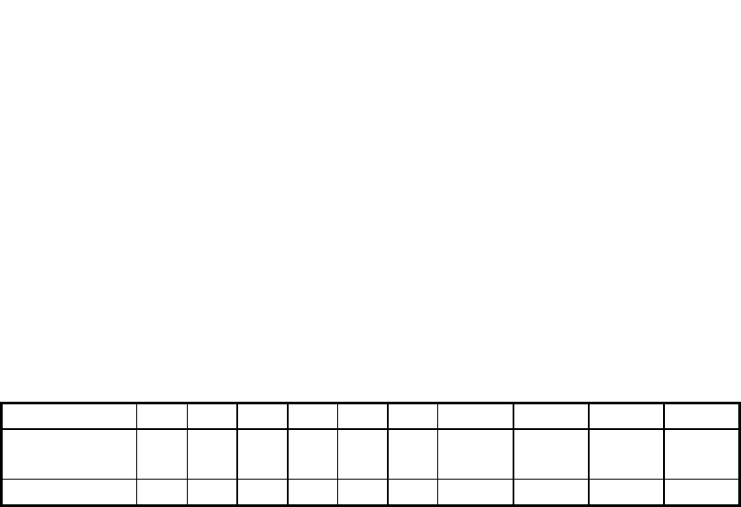
three digit number specifying the run number (see chapter 5.6). Table 1 lists the
structure of particle distribution files. The Fortran format depends on user settings and
is: 1P,8E12.4, 2I4 (default) or 1P,8E20.12,2I4 if High_res = T or binary if binary = T.
The same settings are valid for generator and Astra.
1
2
3
4
5
6
7
8
9
10
Parameter x y z px py pz clock macro
charge
particle
index status
flag
Unit m m m eV/c
eV/c
eV/c
ns nC
Table 1: Structure of particle distribution files.
The first line of the file defines the coordinates of the reference particle in absolute
coordinates. It is recommended to refer it to the bunch center. Longitudinal particle
coordinates, i.e. z, pz and t are given relative to the reference particle. (If the
reference particle is lost the average position of the particle position will be saved
with status flag = -99. Coordinates are relative to the average position in this case.) If
the particles shall be emitted from a cathode they have to be generated with the same
longitudinal position, e.g. z = 0.0 and with an appropriate spread in time, i.e. clock
values in nanoseconds. In addition the status flag has to be set accordingly (see Table
2).
The macro charge of the particle is given in nano Coulomb. It is possible to specify
each particle with a different charge; the emittance calculation will be done with the
appropriate weighting.
The particle index specifies the kind of particle to be tracked:
Index 1 refers to electrons,
2 to positrons,
3 to protons and
4 to hydrogen ions.
Index 5 – 14 refer to particles with user defined ratio of mass to charge state.
The sign of the charge specified in the column 8 is not relevant. It is possible to mix
different kinds of particles as an initial particle distribution.
The status flag contains information of the particle status as listed in Table 2. Particles
with a negative status flag are either lost by some mechanism or not yet started. (The
output files list the coordinates of all particles even of those that have been lost. The
order of the particles does not change; hence it is easily possible to follow the
development of individual particles.) Passive particles are tracked as normal particles
but they are not taken into account in the calculation of the beam emittance etc. and
they are not taken into account when the space charge field is calculated. They will,
however, be tracked taken the action of the space charge field onto them into account.
They are typically used to cut off beam tails or halo particles. The trajectories of
‘probe particles’ and the space charge fields acting onto these particles will be found
in an output file for later analysis.

ASTRA User‘s manual
3
Status
flag Comment Status
-99
1
average position of distribution will not be tracked
-95 ref. particle only; Z
0
> ZStop lost
-94 ref. particle only; more than Max_Step steps lost
-92
2
probe rejected by space charge at the cathode
lost
-91
2
rejected by space charge at the cathode lost
-90 probe particle before Z
min
lost
-89 particle before Z
min
lost
-86
3
probe particle traveling backwards lost
-85
3
particle traveling backwards lost
-31 particle discarded by user lost
-30 particle preliminary discarded by user lost
-22 probe secondary electron, lost on aperture lost
-21 secondary electron, lost on aperture lost
-20 passive probe particle, lost on aperture lost
-19 passive particle, lost on aperture lost
-17 trajectory probe particle, lost on aperture lost
-15 standard particle, lost on aperture lost
-6 passive probe particle, at the cathode not yet started
-5 passive particle, at the cathode not yet started
-4 secondary particle not yet started
-3 trajectory probe particle at the cathode not yet started
-1 standard particle, at the cathode not yet started
0 passive probe particle tracking
4
1 passive particle tracking
4
3 trajectory probe particle tracking
4 cross over particle
5
tracking
5 standard particle tracking
6, 9…33 probe secondary electrons of generation 1,
2…10 or higher tracking
8, 11...35 secondary electrons of generation 1, 2…10
or higher tracking
1 if the reference particle is lost the average position of the distribution will be saved with
index -99
2 only if Schottky parametrs are specified.
3 only active, if L_rm_back = T is set.
4 passive particles are not taken into account for the set-up of the space charge grid, the
calculation of space charge fields and for the calculation of internal beam parameters.
If the
2D space charge routine is active the particles are still tracked under the influence of space
charge fields, while in case of the 3D routines the space charge field is zero for these
particles.
5 only if cross_start ≠ cross_end. See section 4.13.7.
Table 2: Definition of important status flags.

4
3. The program generator
The program generator generates an initial particle distribution file according to the
previously described specifications.
The input file for generator has to have the extension ‘.in’. The default file name is
‘generator.in’. The input file consists of a single namelist named INPUT. A tabulated
listing of all possible input parameters is given in chapter 7. The below listed input
file gives a simple example for the generation of a Gaussian particle distribution:
&INPUT
FNAME = 'Example.ini'
Add=FALSE, N_add=0,
IPart=500, Species='electrons'
Probe=True, Noise_reduc=T, Cathode=F
Q_total=1.0E0
Ref_zpos=0.0E0, Ref_Ekin=2.0E0
Dist_z='gauss', sig_z=1.0E0, C_sig_z=2.0
Dist_pz='g', sig_Ekin=1.5, cor_Ekin=0.0E0
Dist_x='gauss', sig_x=0.75E0,
Dist_px='g', Nemit_x=1.0E0, cor_px=0.0E0
Dist_y='g', sig_y=0.75E0,
Dist_py='g', Nemit_y=1.0E0, cor_py=0.0E0
/
Running generator with this input file will result in the generation of the file
‘Example.ini’ containing the coordinates of 500 electrons with a total charge of 1 nC.
Since ‘Cathode = F(alse)’ the particles are not emitted from a cathode and a
longitudinal extension of the bunch has to be specified rather than a time spread.
‘Probe = True’ will result in the specification of six probe particles at the positions:
0.5 σx, 0.5 σz; 1.0 σx, 1.0 σz; 1.5 σx, 1.5 σz;
0.5 σy, -0.5 σz; 1.0 σy, -1.0 σz; 1.5 σy, -1.5 σz.
The trajectories of these particles and the space charge fields acting onto these
particles will be saved if ‘TrackS = True’ is set.
The specification ‘Noise_reduc = T(rue)’ forces the program to distribute the particles
not randomly but quasi-randomly following a so-called Hammersley sequence. As a
result statistical fluctuations are reduced, while at the same time artificial correlations
are avoided which would be generated by a set up on a grid.
The longitudinal position of the bunch is at 0.0 m and the kinetic energy is 2.0 MeV.
The longitudinal distribution is Gaussian with an rms width of 1mm and a cut at
2 sigma. The distribution of the longitudinal momenta is uniform with an rms width of
1.5 keV. Alternatively it would be possible to specify a longitudinal emittance rather
than the energy spread. No correlated energy spread is introduced.
The transverse distribution is Gaussian in x and y with an rms width of 0.75 mm. The
distribution of the transverse momenta is also Gaussian and is set up in a way that the
beam emittance will be 1 π mrad mm. No correlated beam divergence is introduced.
Besides the complete listing of all possible input parameters in chapter 7, a collection
of the properties of different distributions can be found in chapters 7.2 to 7.4.
In order to assemble more complicated distributions it is possible to add up several
distributions into a common file. In this case ‘Add = True’ and ‘N_add = n’ has to be
specified, where n is the number of distributions to be added. Than the namelist
INPUT has to be specified n times with different parameters. (FNAME, Add and
ASTRA User‘s manual
5
N_add might be specified only once in the first namelist.) The reference particle of the
combined distribution will be the reference particle defined in the first namelist.
If a dispersion is specified an energy correlated transverse offset will be added in a
final step. The calculated emittance will hence be larger than specified in the input
file.
After running generator the result can be visualized by calling postpro with the
appropriate input argument, e.g. ‘postpro Example.ini’. See chapter 5.6.
Besides the file Example.ini the file NORRAN will be created by generator. It
contains a new seed value for the random generator and will be updated every time
generator is used.

6
4. The program Astra
The program Astra tracks particles through user defined external fields taking into
account the space charge field of the particle cloud. The tracking is based on a non-
adapitve Runge-Kutta integration of 4
th
order.
The beam line elements are set up w.r.t. a global coordinate system in Astra. The axis
of the (preferred) motion of the bunch is the z-axis (longitudinal axis). The horizontal
plane is related to the x-axis, and the vertical plane is defined via the y-axis.
All calculations in Astra are done with double precision, while output and input may
be in single precision.
The input file for Astra has to have the extension ‘.in’. The default file name is
‘rfgun.in’. The input of each class of beam line element is organized in a separated
namelist. Besides the namelists for the beam line elements the namelist NEWRUN
contains general instructions for the tracking, CHARGE contains the settings for the
space charge calculation and SCAN contains instructions for the scanning routine. In
the following an example input file without space charge will be discussed. In a
second step the calculation of space charge fields will be included before finally the
scanning routine will be described.
4.1. Namelist structure of Version 3
Version 1 and 2 of Astra required that an input deck contained all valid namelists in a
fixed order. This restriction does not apply for Version 3, i.e. only those namelist
which are required need to be specified and they can appear in arbitrary order.
4.2. Example input file without space charge
&NEWRUN
Head=' Example of ASTRA users manual'
RUN=1
Distribution = 'Example.ini', Xoff=0.0, Yoff=0.0,
TRACK_ALL=T, Auto_phase=T
H_max=0.001, H_min=0.00
&OUTPUT
ZSTART=0.0, ZSTOP=1.5
Zemit=500, Zphase=1
RefS=T
EmitS=T, PhaseS=T
/
&CHARGE
LSPCH=F
Nrad=10, Cell_var=2.0, Nlong_in=10
min_grid=0.0
Max_Scale=0.05
/
&CAVITY
LEField=T,
File_Efield(1)='3_cell_L-Band.dat', C_pos(1)=0.3
Nue(1)=1.3, MaxE(1)=40.0, Phi(1)=0.0,
/

ASTRA User‘s manual
7
&SOLENOID
LBField=T,
File_Bfield(1)='Solenoid.dat', S_pos(1)=1,2
MaxB(1)=0.35, S_smooth(1)=10
/
NEWRUN starts with a header string and a run number, which should be used to
protocol different parameter settings. The run number will be found as an extension of
all output files generated by Astra. The input particle distribution has been previously
generated with generator. It is used without a transverse offset, i.e. on-axis. After the
phasing of the cavity (‘Auto_phase = T’, see chapter 4.8) the reference particle, i.e.
the first particle in the input distribution file, will be tracked through the beam line to
check the beam line settings
1
. In a second step the reference particle will be tracked
again, starting with an offset at x = x
rms
and y = y
rms
. If ‘TRACK_ALL = False’ is set
the tracking will stop here. The maximum time step for the Runge-Kutta integrator is
defined with the parameter H_max, while H_min is only active if the space charge
fields are taken into account (see section 4.4.3).
The second namelist OUTPUT is devoted to the generation of output
2
. While the
tracking starts at any position where the initial particle distribution is launched, output
will be generated between ZStart and ZStop. The tracking will stop when the bunch
position, i.e. the average position of all active particles is larger than ZStop.
The names of all files generated by Astra start with the project name, i.e. with the
name of the input file and end with the run number. In between, separated by dots a
type dependent name is given to the files. Table 3 gives a complete listing of all
output files generated by Astra including the logical switches to start or suppress the
generation of output.
Astra generates output on different length scales of the beam line. ‘RefS = True’
generates output of the off-axis reference trajectory, energy gain etc. at each
Runge-Kutta time step.
Output of the beam emittance and other statistical beam parameters is generated if
‘EmitS = True’. For the calculation of statistical bunch parameters the distance
ZStop-ZStart is divided into Zemit intervals. Note, that the Runge-Kutta time step is
adjusted, i.e. reduced if necessary, in order to interrupt the tracking close to the
specified locations. (The beam position refers to the average longitudinal beam
position.) This might lead to a reduction of each time step, i.e. to an increased
accuracy of the calculation, if the intervals are shorter than the bunch motion in one
time step. A warning is given in this case because the result of the calculation might
depend on an output parameter if H_max is too big!
The complete particle distribution is saved at Zphase different locations if
‘PhaseS = True’. The distance ZStop-ZStart is divided into Zphase intervals and the
nearest location defined by means of Zemit is chosen. Therefore it is recommended to
set Zemit = n·Zphase,
n
∈
ℕ
. The approximate position is indicated in the file name
as a four digit number, which corresponds in general to the rounded beam position in
cm. If necessary the units for the file name definition is changed (if the distance of the
output positions is too small, or if the last output position is too big). If required the
naming convention is changed to a relative position (i.e. output position minus start
position) which is indicated by a warning message.
All namelists but NEWRUN start with a logical switch, which allows to deactivate all
1
If ‘Track_On_Axis=True’ is set tracking will stop here.
2
Many but not all of the parameters in OUTPUT were in the namelist NEWRUN in previous versions
of ASTRA and are still accepted in this namelist.

8
elements in that list, without changing other parameters. Hence, with
‘LSPCH = False’, the calculation of space charge forces is deactivated.
The namelist CAVITY allows to include rotational symmetric fields of standing wave
cavities, as well as of traveling wave structures and electrostatic fields. The
dependence of the longitudinal electric field component on the longitudinal position
on the symmetry axis of the field has to be given in form of a table in case of standing
wave structures and electrostatic fields. The radial and magnetic field components are
deduced from the derivative of the longitudinal filed w.r.t. the longitudinal position.
File_Efield(n) contains the name of the file where this table can be found, for the n
th
cavity. Nue(n) states the frequency, MaxE(n) the
maximum
amplitude of the field
and Phi(n) the phase of the wave. By default the energy gain of each cavity is scanned
prior to the tracking of the reference particle in
Astra
. The user-defined phase refers
than to the phase of the maximum energy gain in a cosine-like manner. Note, that the
phase of the wave
t
ω φ
⋅ +
is increasing with time, i.e. the tail of the bunch ‘sees’ a
higher phase than the head. Thus, in order to give the tail a higher energy than the
head, one has to go to negative phases Phi(n). The phase, denoted by the program as a
result of the auto-phasing procedure, is the number used internally. It refers to the
phase of the wave at the time stamp of the reference particle when it is starting to be
tracked. The auto-phasing can be switched off by setting ‘Auto_Phase = False’ in
NEWRUN.
The namelist SOLENOID contains information about solenoid fields. Like in case of
cavity fields a table of the longitudinal field component along the symmetry axis is
required. Besides the file name of the table, only the
maximum
amplitude of the field
has to be specified. (The scaling of the field to the defined amplitude might also be
switched off by setting ‘S_noscale = True’.) In the example some smoothing is
applied to the field table.
No other elements are used in this example.
4.3. Space Charge Calculation
Astra
offers cylindrical symmetric and fully 3D options for the space charge
calculation. In terms of computing time the algorithms themselves are of comparable
performance, however, 3D space charge calculations require, due to the larger number
of grid cells, a much larger number of macro particles in order to avoid statistical
problems. Moreover is in case of the 3D algorithm only a linear interpolation within
the grid cells applied, while a cubic spline interpolation is employed within the
cylindrical grid algorithm. Therefore a finer grid resolution might be required in the
case of the 3D algorithm.
4.4. Calculation of the space charge field with the cylindrical grid
algorithm
For the calculation of the space charge field a cylindrical grid (r,
ϕ
, z coordinates),
consisting of rings in the radial direction and slices in the longitudinal direction, is set
up over the extension of the bunch. The grid is Lorentz transformed into the average
rest system of the bunch, where the motion of the particles is to good approximation
non relativistic and a static field calculation can be performed by integrating
numerically over the rings thereby assuming a constant charge density inside a ring.
The field contributions of the individual rings at the center points of the grid cells are
added up and transformed back into the laboratory system. Here the field at any given
point between the grid center points is calculated by means of a cubic spline
ASTRA User‘s manual
9
interpolation, so that the field and the first derivatives w. r. t. the space coordinates are
continuous functions. Outside of the grid a 1/r extrapolation is applied, so that the
space charge field is defined (with reduced accuracy) over the whole space. For the
tracking the space charge field is treated like the external field, i.e. an Runge-Kutta
integration is performed based on the sum of all external and internal forces. It would,
however, be too time consuming (and useless) to calculate the space charge field on
the grid center points again at every Runge-Kutta time step. Therefore an automatic
procedure has been implemented which scales the space charge field and the grid
dimensions with the variation of the beam size, the beam energy etc. A new
calculation of the field on the grid center points is initiated every time the scaling
factor of the field exceeds a user-defined limit.
4.4.1 Set up of the grid
The space charge fields are calculated on a cylindrical grid, consisting of rings in the
radial direction and of slices in the longitudinal direction. The grid is set up
dynamically, i.e. the grid dimensions are based on the actual dimensions of the bunch.
The user has to define the number of slices (parameter Nlong_in) and rings (parameter
Nrad) that shall match exactly the dimensions of the bunch. For the calculation two
more rings and four more slices are added outside of the bunch.
The total number of particles inside a ring scales, for a distribution with uniform
charge density, linearly with the radius in the outside region of the bunch but more
quadratically at the innermost region. As an example consider the case of 5000
particles uniformly distributed in a grid of 10 rings of equal thickness. In the
innermost ring only about 50 particles will be located, while in the outermost ring
about 950 particles will be counted. When these particles are additionally distributed
into 100 longitudinal slices, half of the innermost rings will be empty, which causes
statistical fluctuations in the field description. Furthermore one has to take into
account, that the field of a charge ring acts predominantly to the outside of the ring.
Thus the field in the outside region of the bunch is composed by more or less all
particles while this is not the case in the central region of the bunch. To counteract
this unfavorable situation it is possible to vary the radial grid height over the bunch
radius by means of the parameter Cell_var in
Astra
. If for example ‘Cell_var = 2’ is
chosen, the innermost ring will be twice as high as the outermost ring. In order to get
a sufficient statistical accuracy it is nevertheless necessary to choose a small number
of grid cells or a high number of particles, respectively. The description of the fields
will, however, have a better resolution than suggested by the grid size due to the
smooth interpolation algorithm.
The space charge fields generated by a particle distribution can be visualized with the
program
fieldplot
. (See chapter 5.7.) Here also the number of grid cells and the cell
variation may be changed and optimized.
4.4.2 Merging longitudinal grid cells
In order to vary the longitudinal grid size within the bunch neighboring cells can be
merged together. If, for example, the bunch consists out of a short spike and a long
tail the parameter N_long_in is specified so that the spike can be resolved. In order to
improve the statistical properties in the rarely populated tail cells can be merged with
the statements ‘Merge_1 =
i, j, k
’ to ‘Merge_10 =
i, j, k
’, where
i
is the starting cell,
j
is the end cell and
k
is the number of cells to be merged. For example with
Merge_1 = 1,50,10 cells number 1 to 50 are merged into 5 new cells each consisting
10
out of 10 original cells. Note that
1
j i
k
− +
has to be an integer. Use
fieldplot
to
visualize and optimize the longitudinal grid. An example application of this option is
described in [1].
4.4.3 Time step control
For an accurate simulation the time steps of the Runge-Kutta integrator shall not be
too large. The required time steps may differ strongly in different parts of a beam line,
depending on the relative contribution of space charge and external fields. Time steps
are adjusted automatically within user defined limits in
Astra.
The maximum time
step, often limited by external fields (RF fields, fringe fields), is determined by the
parameter H_max. The convergence of the simulation results for decreasing H_max
should be checked. Separate tracking of different sections of the beam line allows to
optimize H_max for each section.
The minimum time step is given by the parameter H_min. Criteria to set H_min are
discussed in the next two chapters. The scaling of the space charge field (section
4.4.7) is used to estimate the maximum allowable time step. Thus
Astra
performs time
steps between H_max and H_min. Even shorter time steps are made in order to reach
a certain position e.g. to generate output. The development of the average step size is
stored in a file when the option ‘TcheckS = True’ is set.
4.4.4 The emission of particles from a cathode
In order to simulate the emission of particles from a (plane) cathode the particles are
started from the cathode according to the timing spread of the initial particle
distribution. The particles are ordered according to their emission time and the space
charge field is scaled for the increased charge after the emission of each particle. Thus
a smoothly rising space charge field is obtained. The time step of each particle is
adjusted according to its emission time, and a complete recalculation of the space
charge field is performed after each user-defined step size H_min. No scaling of the
field other than the scaling with the charge within the time step is applied.
If during the emission the space charge field shall be updated
n
times, H_min has to
be
T/n
where
T
is the total emission time. In general H_min is an uncritical parameter
if
n
is reasonably high. It is however useless to set
n
very high if the number of
particles is not very high.
Alternatively, the average number of particles to be emitted during each emission step
can be specified with the parameter N_min. To activate this option H_min should be
specified as zero. Then it is set according to:
_ min
_ min N
H T
Npart
=
(4.1)
with
Npart
being the total number of particles in the bunch.
Since the number of particles is small during the first steps of the emission process the
number of longitudinal slices shall be reduced during the emission by means of the
parameter min_grid, which defines the minimal grid size in longitudinal direction.
Whenever the bunch length is so small, that the grid size would be below min_grid,
the number of slices is reduced accordingly. The bunch length
s
min
after the first time
step,
t =
H_min has been performed can be estimated as:
2
min 2
eE
s t
m
=
(4.2)
where
E
is the accelerating field strength and
m
is the rest mass of the particles in the
bunch.
ASTRA User‘s manual
11
If min_grid is set to this value the number of slices increases smoothly as the bunch
length and the number of particles during the emission process.
If min_grid is specified as zero, it is set automatically according to Eq. (4.2). For this
the mass of the reference particle is used, (important only in case of a particle
mixture.)
For setting up the grid also particles which are not emitted yet are taken into account
for the radial direction, in order to avoid too small radii during the first steps of the
process.
By default the mirror charge of the bunch at the cathode plane is taken into account if
the bunch is emitted from the cathode. The fields of the ‘mirror bunch’ are calculated
in the rest system of the mirror bunch at the Lorentz transformed distance between
bunch and mirror bunch, transformed back into the laboratory system and added to the
field of the bunch. The calculation of the mirror charge is switched off when the
contribution of the mirror bunch field at two positions of the bunch (in the center and
in the tail of the bunch) is below 1‰ of the bunch field. For the calculation of the
mirror charge the grid is modified in a way that the field is calculated directly in the
cathode plane, rather than in the center of a cell.
When the bunch is emitted from a cathode, the longitudinal position of the cathode is
set to the minimal particle position by default. When the bunch is not emitted from the
cathode but shall be started in front of the cathode the cathode position has to be
explicitly specified with the parameter Z_Cathode.
The calculation of the mirror charge can be suppressed by setting ‘Lmirror = False’.
Retarded time effects and radiation effects are not taken into account.
4.4.5 Correction of the mirror charge for the case of a non-planar cathode
In order to correct the mirror charge contribution in the case of a non-planar cathode
the cathode surface has to be described by means of a table. The table contains in the
first two columns the longitudinal and radial position of a number of points describing
the contour of the cathode. The third and fourth column of the table contains the
components of the tangential unit vector of the cathode at the same points. For each
point of the table a charge ring will be located slightly behind the cathode surface.
The rings carry charges such, that the electric field vector of the combined space
charge field is perpendicular to the cathode surface. In order to determine the charges
a system of equations with n unknowns has to be solved for n points in the input table.
In addition to the table the curvature of the cathode on the axis has to be specified in
the input deck. Special care is required in case of a field description by means of a 3D
field map because the map is defined on a rectangular grid and cannot follow the
cathode contour. By adjusting the field values on the grid positions behind the cathode
a correct field description is still possible.
The cathode contour incl. the position of the charge rings behind the cathode and the
field on the cathode surface can be visualized with
fieldplot
. See also section 7.5.2.
This procedure has been worked out by D. Janssen and V. Volkov. An example
application of this option is described in [2].
4.4.6 Minimum time step without emission process
When the simulation starts without emission from a cathode the parameter H_min is
in general uncritical. By default it is reset to H_max/100 if it is set to zero in the input
deck.
In cases of extreme space charge forces the following criterion becomes, however,
significant: In a real beam all particles move simultaneously, while in a simulation
12
particles move one after the other in small steps. In order to avoid that particles move
a significant fraction of a grid cell within one time step, which would lead to an
unphysical variation of the space charge field, the bunch dimension should change by
an amount which is small compared to a grid cell within a single time step. In cases of
extreme space charge fields this criterion might be violated. Hence
Astra
controls this
criterion and reduces the time steps if required. The user defined parameter
Exp_control specifies the maximum tolerable variation of the bunch extensions
relative to the gird cell size within one time step. Exp_control = 0.1 specifies, that the
bunch is allowed to expand by only 10% of the minimal grid size within a time step.
While the control of this criterion may lead to very small step sizes it does often not
increase the overall CPU time by a significant amount, because the efficiency of the
scaling procedure of the space charge field improves.
4.4.7 Scaling of the space charge field
The space charge field of the bunch is (at least at sufficient high energies) a slowly
with time varying function. Hence, instead of calculating new field coefficients at
every time step, it is justified to scale the field coefficients according to:
0 0
( ) ( )
( )
0 0
nr r nr z nr
r z
r
r z
Q
EQ
γ
σ σ γ
σ σ γ
∝ × × ×
0
( )
( )
0 0
0
nz r
nz z
rz
z
r z
Q
EQ
γ
σσ γ
σ σ γ
⋅
∝ × ×
0
B Er
φ
β
β
∝
where Q/Q
0
, σr/σr
0
, σz/σz
0
, γ/γ
0
and β/β
0
denote the relative variation of the bunch
charge, the bunch radius, length, energy and velocity, respectively.
At the same time the grid has to be scaled with the variation of the radial bunch size
and the bunch length.
( ), ( ), ( ), ( ) and ( )
nr r nr z nr nz r nz z
γ γ
are functions that depend on the aspect ratio
z
r
A
γ
σ
σ
=of the bunch in the rest system. They are constant for
A
>> 1
.
In case of a pancake like bunch the fields are proportional to:
0
2
0 0
r
r
r
Q
EQ
σ
γ
σ γ
∝ × ×
0 0
2
0
0
r z
z
r z
Q
EQ
σ σ γ
σ σ γ
∝ × ×
while a cigar like bunch scales like:
0 0
0
r z
r
r z
Q
EQ
σ σ
σ σ
∝ × ×
0
2
0
0
z
z
z
Q
EQ
σ γ
σ γ
∝
The functions used in
Astra
are only approximate functions that fit roughly numerical

ASTRA User‘s manual
13
results for a number of bunch dimensions with uniform longitudinal and radial
distribution. However, the scaling is in any case better than assuming a constant field.
If the scaling factor for the radial or longitudinal electric field exceeds a user-defined
limit a new space charge calculation is initiated. The parameter Max_scale defines
this limit; if for example ‘Max_scale = 0.05’ the scaling factor has to be between 1.05
and 0.95, respectively.
An extrapolation of the time depended scaling factors is used to determine the
maximum allowable next step size. If the next step size would be below H_min a new
calculation of the space charge field is initiated. Therefore the space charge field is
not only updated more frequently in regions of strongly varying space charge fields,
also the average step size is reduced.
Strong changes of the particle distribution, without variation of the bunch dimensions,
cannot be taken into account by the scaling routine and have to be treated separately.
This effect is observed during the compensation process of space charge induced
emittance growth close to the emittance minimum, when the particles in the bunch
center move outwards, while the particles in the head and the tail of the bunch are still
moving inward. In order to limit the number of scaling steps in this case, the
parameter Max_count can be set.
As long as particles are emitted from a cathode the scaling procedure is not active.
Instead the space charge fields are updated after each time step H_min.
The effectiveness of the scaling and the setting of Max_scale can be controlled by
setting ‘TrackS = True’. A file will be logged that contains the trajectories of particles
marked as probe particles and the space charge fields acting onto these particles. Both
can be displayed with the program
lineplot
. (While
Astra
can deal with any number of
probe particles,
lineplot
will support the display of only up to one hundred particles.)
Since the data are logged at each Runge-Kutta time step the generated files tend to be
large. Therefore one might consider using this option only for short critical sections
and not for long beam lines. Additional information about the scaling procedure can
be gained if the option ‘TcheckS = True’ is set. A file will be logged that contains the
scaling factors at each time step separated into the contributions
0 0
( ) ( )
( )
0
, ,
nr r nr z nr
r z
r z
γ
σ σ γ
σ σ γ
etc., which allows to identify the driving force of
the space charge field development. Also the scaling counter, which counts how often
the field is scaled before it is updated and the time between updates of the space
charge fields is saved. The later one is used to calculate the average Runge-Kutta time
step. See the description of
lineplot
section 5.5.2
for displaying results.
4.4.8 The Mélange option
With the Mélange option it is possible to define a particle distribution consisting of
groups of particles which will be treated separately in the space charge calculation.
These groups may have a different energy or may be different particle types. The
standard scaling of the time steps might not work in all cases as stable as usual in this
case, because it can react only on the average development of all particles. (In detail it
depends on how different the distributions are.) Careful convergence checks for the
space charge calculation parameters are recommended. Some parameters might need a
more strict definition and as a result the calculation might slow down. First tests
should be done on a short section.
The Mélange option works only with the 2D space charge routine, relative transverse

14
offsets of the particle groups are hence not possible.
The Mélange option is controlled with the parameter Melange in the namelist Charge.
Melange = 2 means that 2 different distributions are mixed together. Note that the
calculation takes place on a common grid, i.e. if the distributions are longitudinally
separated by a large distance a much larger grid will be set up and more grid cells are
needed.
To mark the two groups first a mixed distribution is created, e.g. with generator using
the ‘add’ command. This distribution needs to be modified externally: while the first
group of particles keeps the status flag 5 as usual, the second group gets the flag 7, a
third group would get flag 10 and for every further group the flag number would be
increased by 3 (10, 13, …).
Astra will calculate beam parameters for the mixed distribution with standard settings,
but can also be forced to take only one group into account, see section 4.13.9 of the
manual. Also the color settings in postpro can be redefined in a similar way, see
section 5.6.
References
[1]
C. Limborg-Depry, P. Emma, Z. Huang, J. Wu ‘Computation of the longitudinal
space charge effect in photoinjectors’ EPAC 2004.
http://accelconf.web.cern.ch/AccelConf/e04/PAPERS/TUPLT162.PDF
[2]
V. Vlokov, K. Floettmann, D. Janssen, ‘Superconducting RF Gun Cavities for
large Bunch Charges’ PAC 2007.
http://accelconf.web.cern.ch/AccelConf/p07/PAPERS/FRPMN063.PDF

ASTRA User‘s manual
15
4.5. Calculation of the space charge field with the 3D FFT
algorithm
To activate the 3D space charge calculation the parameter ‘Lspch3D = t’ has to be set
in addition to ‘Lspch = t’. For the 3D algorithm a Cartesian grid is used. The number
of grid lines is specified with the parameters Nxf, Nyf and Nzf for the x-, y- and z-
direction, respectively. Since the algorithm is based on a fast Fourier transform the
number of grid lines in each direction has to be equal to
2
n
,
n
∈
ℕ
.
Astra
will give a
warning and reset the grid cell specification to the nearest possible value in case of an
invalid input. The number of grid cells in each direction is equal to the number of grid
lines minus one. With the parameters Nx0, Ny0 and Nz0 the number of empty
boundary cells can be specified, which allows a finer tradeoff of computation time
and statistical noise in the computation (see section 4.5.2.). The space charge
calculation takes place as electro static calculation in the average rest frame of the
bunch. A constant charge density inside the cell is assumed. The potential of the space
charge field is derived by a convolution of the charge density of the grid with the
analytically calculated Green’s function as described in [1]. The derivatives of the
electrostatic potential yield then the components of the space charge field which is
transformed back into the laboratory frame. In order to suppress noise the potential
may be smoothed with a soft iterative procedure. The parameters Smooth_x,
Smooth_y and Smooth_z can be used to specify the number of iterations to be applied
for each direction. The setup of the grid and the effect of the smoothing should be
checked with
fieldplot
.
4.5.1 Restrictions of the 3D FFT algorithm
The 3D algorithm doesn’t provide special features for the emission of particles from
the cathode in its present form. Image charge forces cannot be included. During the
emission the complete grid is set up already after the first time step.
The field description is restricted to the grid; hence the optional use of passive
particles, which may travel outside of the grid, is limited.
4.5.2 Estimation of the average number of particles per cell
The Cartesian grid forms a cuboid around the bunch which leads necessarily to a
number of empty cells since a bunch is in general not cuboid. An adjustable number
of additional empty cells can be included in the boundaries in order to allow a finer
adjustment of grid resolution and required number of particles. Assuming a uniformly
filled cylindrical bunch with ellipsoidal transverse cross section the average number
of particles per grid cell
cell
N
can be estimated as:
( ) ( ) ( )
4
1 2 0 1 2 0 1 2 0
tot
cell
N
N
Nxf Nx Nyf Ny Nzf Nz
π
=− − − − − −
And for the case of a uniformly filled ellipsoid as:
( ) ( ) ( )
6
1 2 0 1 2 0 1 2 0
tot
cell
N
N
Nxf Nx Nyf Ny Nzf Nz
π
=− − − − − −
4.5.3 Scaling of the space charge field and time step control
The scaling of the space charge field and the setup of the time steps follows the same
procedures and formulas as described above for the 2D algorithm. Instead of the
radial field both transverse components are treated separately, so that the procedure
works also in case of varying transverse aspect ratio.
16
4.6. Automatic transition from 2D to 3D calculation
It is possible to switch between 2D and 3D space charge calculation within a tracking
calculation. For this the switch L2D_3D is set to true and the position at which the
transition should be made is specified with the parameter
z_trans
. When the bunch
passes
z_trans
the results of a 3D space charge calculation are applied to all particles
beyond
z_trans
, while a 2D calculation is made for particles before the specified
position. The number of longitudinal cells of the 2D grid has to be reduced as more
and more particles passing
z_trans
. Thus a minimal grid length has to be specified
with the parameter
min_grid_trans
equivalently to the minimal grid length defined for
the emission process.
4.7. Emission process
Important aspects of the simulation of the emission process in
Astra
are described in
section 4.4.4.
Particle distributions which can be generated with
generator
are described in chapter
7 and following. Besides this it is possible to load particle distributions from other
programs if they are compatible to the file structure described in chapter 2.
Within
Astra
it is possible to rescale a number of parameters of the particle
distribution (e.g. the bunch size, the charge etc., see chapter 6.1) and to define offsets,
which allows doing parameter scans as described in chapter 4.8.
Additionally it is possible to modify the emission form a cathode by specifying a
delay time and parameters to model the Schottky effect, respectively.
If the delay time
Tau
is not zero in the input deck an exponential delay will be applied
to the emission of the particles. Thus, if for example the input distribution represents
an incoming photon bunch, it is possible to model a delay of the photo emission
process of the cathode. The delay time is randomly chosen and added to the
predefined emission time. Note, that statistical noise might be increased if the initial
distribution is quasi-random.
The Schottky effect describes the lowering of the work function or electron affinity
of a material by an external electric field, which leads to an increased electron
emission from a cathode [2]. In
Astra
the charge of a particle is determined at the
time of its emission as:
0
_ _ _
Q Q Srt Q Schottky E Q Schottky E
= + +
where
E
is the combined (external plus space charge ) longitudinal electric field in the
center of the cathode.
The charge
Q
0 is the charge of the particle as defined in the input distribution
(eventually rescaled according to the parameter
Qbunch
) and
Srt_Q_Schottky
and
Q_Schottky
describe the field dependent emission process. For an exemplary
discussion of the Schottky and related effects see [3] and references therein.
To visualize the development of the space charge field on the cathode and important
beam parameters during the emission process set ‘CathodeS = True’. See Table 3 and
Table 4 and section 5.5.4.
ASTRA User‘s manual
17
References
[1]
Ji Qiang et al. ‚Erratum: Three-dimensional quasistatic model for high brightness
beam dynamics simulation‘ PRST-AB 10,129901 2007.
http://prst-ab.aps.org/abstract/PRSTAB/v10/i12/e129901
see also:
http://prst-ab.aps.org/abstract/PRSTAB/v9/i4/e044204
[2]
W. Schottky ‘Über kalte und warme Elektronenentladungen’ Zeitschrift für
Physik, Vol. 14, pp. 63-106, 1923.
[3]
J. H. Han et al. ‘Emission mechanisms in a photocathode RF gun’ PAC 2005.
http://accelconf.web.cern.ch/AccelConf/p05/PAPERS/WPAP003.PDF
4.8. The Auto_phase option
By default the energy gain of each cavity representing an accelerating RF mode is
scanned prior to the tracking of the reference particle in
Astra
. The user-defined input
phases refer to the phases of the maximum energy gain in a cosine-like manner. Note,
that the phase of the wave
t
ω φ
⋅ +
is increasing with time, i.e. the tail of the bunch
‘sees’ a higher phase than the head. Thus, in order to give the tail a higher energy than
the head, one has to go to negative phases. The auto-phasing procedure can be
switched off by setting ‘Auto_Phase = False’ in NEWRUN, in which case absolute
phases are requested. Absolute phases refer to the phase of the wave at the time stamp
at which the tracking is started. The results of the auto-phasing procedure (max.
energy gain and phases) are printed onto the screen. The phases may hence be used as
offset phases when the auto-phasing procedure is going to be switched off in
subsequent runs.
The Auto_phase option acts only on accelerating RF modes, i.e. DC fields, TE modes
and dipole modes are rejected from the scan.
In the auto-phasing procedure the reference particle is tracked through the consecutive
cavities. For each cavity the phase is scanned several times with decreasing phase
steps around the phase of maximum energy gain. Once the phase of maximum energy
gain has been determined with high accuracy the particle is finally tracked at the user
defined phase through the cavity and up to the entrance of the subsequent cavity.
Note, that the optimum phase of the complete particle distribution coincides only with
the optimum phase of the reference particle if it is located at the weighted average
longitudinal or temporal position of the distribution, respectively.
In the case of overlapping modes the order of the phasing procedure is determined by
the order of the start positions of the cavities or in the case of equal start positions, by
the order in which the modes appear in the input deck. If the particle velocity is
changing inside the cavity, the phases of overlapping modes are, however, not
independent of each other. It is recommended to use the auto-phasing option for each
mode separately and then use absolute phases in this case.
In long cavity sections a small discrepancy between the phases determined by the
auto-phasing procedure and the phases which minimize the energy spread of the beam
(without space charge fields) can be observed in some cases. Different factors
contribute to this discrepancy, one is, that the reference particle is due to statistical
fluctuations in general not exactly in the center of the particle distribution another one
are numerical inaccuracies.
The phasing of the cavities is related to the internal clock of the tracking program.
The starting time of the tracking program is determined via the input distribution, see
Table 1. The starting time can also be changed with the parameter Toff in the namelist
NEWRUN. If the RF structures described in the input deck have all the same

18
frequency a modification of Toff is equivalent to a phase shift of all cavities with the
parameter phi(0).
In general the starting time is an arbitrary value. In some cases, if for example a
timing jitter of the particle source shall be investigated a defined variation of the
starting time is necessary. (See the output parameters of the scanning routine in
chapter 6.3.) Note, however, that a modification of the starting time will be
compensated by a phase shift if ‘Auto_Phase = True’ is set.
4.9. Scanning and optimizing beam parameters
Astra
offers different options to perform parameter scans and optimizations. A simple,
predefined scan based on a single particle tracking (the reference particle) is
performed by setting ‘PHASE_SCAN = True’ in NEWRUN. The energy gain as
function of the cavity phase is stored as well as the bunch compression factor, i.e. the
ratio of the bunch length at the exit of the cavity to the bunch length at the entrance of
the cavity. From the derivative of the energy gain w.r.t. the cavity phase a quantity is
derived which is proportional to the RF induced energy spread. (See section 5.5.2.)
When the scan for one cavity is finished, the reference particle will be tracked through
the cavity on the user-defined phase up to the entrance of the next cavity. Thus, for
low energy beams (
β
< 1), the result of the scan for downstream cavities depends on
the user-defined phase.
User defined scans can be performed with the scanning procedure defined in the
namelist SCAN. The following example shows a setting for a scan of the cavity
gradient of cavity number one:
&SCAN
LScan=T
Scan_para=’MaxE(1)’
S_min=10.0, S_max=50.0, S_numb=5
FOM(1)=’hor. Emittance’
FOM(2)=’long. Emittance’
FOM(3)=’bunch length’
/
All valid scanning parameters are written in italic letters in the namelist tables of
chapter 6. Besides the minimum and maximum set point of the scanning parameter,
S_min and S_max, the total number of set points S_numb has to be specified. The
user also has to define which beam parameters shall be stored. Up to 10 different
output parameters can be specified (FOM(1) to FOM(10)). See chapter 6.3 for a
listing of valid keywords. The standard output generation (emittance vs. z etc.) is
suppressed when a scan is performed. Setting ‘LExtend = True’ allows to increase the
scanning range without losing data from a previously performed scan with the same
run number.
While with the specifications discussed above all parameters, as defined with FOM(1)
to FOM(10), are saved at the end of the beam line, it is also possible to look for a
minimum or maximum within a predefined longitudinal range with the scanning
routine. In this case ‘L_min = True’ or ‘L_max = True’ has to be specified. The
minimum or maximum value of FOM(1) within the longitudinal interval S_zmin to
S_zmax will be saved. The interval is divided into S_dz subintervals. At the end of
each subinterval the emittance etc. is calculated and the value of FOM(1) is updated
accordingly. The values of FOM(2) to FOM(10) will be saved at the position of the
minimum/maximum of FOM(1). The position of the minimum/maximum will also be
ASTRA User‘s manual
19
saved.
Automatically searching for a setting where the parameter FOM(1) reaches a
minimum, a maximum or a predefined value (match_value) by refined scans in
smaller intervals around the optimum is activated by setting O_min, O_max or
O_match true. The parameter O_depth defines the number of refined scans to be
performed. The total number of runs in this case is about S_numb
·
O_depth. If the
optimum is outside the initial interval (S_min – S_max) the interval is increased in
direction of the optimum by at most 10 steps.
The options O_min, O_max etc. and L_min, L_max etc. can be combined. With the
setting:
&SCAN
LScan=T
Scan_para=’MaxB(1)’
S_min=0.1, S_max=0.2, S_numb=5
O_min=.TRUE., O_depth=3
L_max=.TRUE., S_zmin=1.0, S_zmax=1.5, S_dz=10
FOM(1)=’hor. spot size’
/
the maximum of the horizontal beam size between 1 and 1.5 m will be minimized.
Another possibility for parameter scans is given with the looping option. All namelists
start with the parameters LOOP. If ‘LOOP = True’ is set, the parameter NLoop in the
namelist NEWRUN has to be set to a positive integer value. The complete namelist
for which the looping has been activated has to be specified NLoop times with
varying parameters. (With the exception of the namelist ERROR, see chapter 6.5.)
Astra
will perform NLoop complete tracking calculations, working successively
through the specified namelists and incrementing the run number automatically. It is
possible to specify ‘NLoop = True’ simultaneously in more than on namelist. With the
following settings two runs will be performed with two different solenoid field maps:
&NEWRUN
Loop=.FALSE.
...
...
NLoop=2
...
/
...
...
&SOLENOID
Loop=True
File_Bfield(1)=’Solenoid_1’
...
...
/
&SOLENOID
Loop=True
File_Bfield(1)=’Solenoid_2’
...
...
/

20
4.10. Definition of Modules
The namelist MODULES (chapter 6.4) allows to combine elements from other
namelists to modules. Modules can be used to do parameter scans or to introduce
correlated errors, e.g. for a number of magnetic elements which are powered by a
common power supply, a number of RF structures which are driven by the same
klystron or elements which are mounted on a common girder. Module definitions
don’t substitute the individual definitions in the respective namelists but act in
addition onto the elements. In the following example:
&MODULES
LModule=t
Module(1,1)=’cavity(2)’
Module(1,2)=’cavity(3)’
Module(2,1)=’quadrupole(1)’
Module(2,2)=’quadrupole(2)’
Module(2,3)=’cavity(3)’
Mod_Efield(1)=0.9
Mod_Phase(1)=-2.0
Mod_zpos(2)=1.5
Mod_xoff(2)=1.0e-3
Mod_xrot(2)=1.5e-3
Mod_Bfield(2)=1.15
/
elements 2 and 3 of the namelist cavity are combined to module 1 and elements 1 and
2 of the namelist quadrupole form together with element 3 of the namelist cavity
module number 2.
The strength of the RF elements of module 1 is scaled to 90% of their individual
settings and the phase is shifted (in addition to the individual settings) by -2.0 degree.
The strength of magnetic elements of module 2 is increased by 15 %. Module number
2 has an offset and is rotated in the x-z plane. The rotation of the module leads to an
additional offset and a rotation of the module elements depending on their individual
positions and the longitudinal pivot point of the module Mod_zpos. Individual offsets
and rotation angles can still be specified for each element in the respective namelist.
The program would accept also to scale the strength of RF elements of module
number 2 or to apply offsets to module number 1. Since element 3 of the namelist
cavity is an element of module 1 and module 2 this doesn’t make sense, however, the
user has to take care of this kind of conflicts.
ASTRA User‘s manual
21
4.11. Apertures and Secondary Electron Emission in Astra
The namelist APERTURE (chapter 6.7) allows to include apertures and to define
material properties for secondary electron emission. Circular apertures can be defined
either by a table containing the z-position and the corresponding aperture radius or
internally by keywords for the case of a simple collimating hole or cylinder. Planar
apertures can be defined internally by keywords only.
The boundaries of apertures defined by keywords are either parallel or perpendicular
to the z-axis.
The z-positions in an aperture table have to be in increasing order with a minimum
step size of 0, i.e. it is not allowed to step back and create nose-like structures.
The thickness
s
of a collimating wall has to be larger than a single particle step i.e.:
max
v
s H
≥ ⋅
with v being the particle velocity, so that a particle can’t pass through the wall in one
step. Especially when secondary emission is active this applies also for the case of a
closed structure (radius = 0), so that particles get lost with the condition r > rmax and
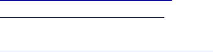
not with e.g. z < zmin. The aperture sketched on the left side of Fig. 1 does not ensure
this, while the aperture on the right side does.
Fig. 1 Sketch of closed apertures. The aperture on the left does not ensure that
particles are lost with the condition r > rmax since the closing walls have zero
wall thickness.
4.11.1 Secondary electron emission
Secondary emission of electrons from limiting apertures can be included
in the
namelist APERTURE.
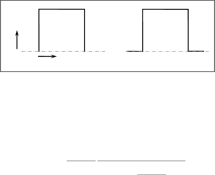
The Secondary Electron Yield (SEY) is modeled in
Astra
according to the following
function [1]:
( )
_
_
_ 0 __ 1 _
_ 1
kin
kin
kin
SE fs
ESE fs
SEY E SE d SE Epm E
SE fs SE Epm
SE fs
=
− +
≥
Here
kin
E
is the kinetic energy of the impact electron and
_ 0
SE d
, _
SE Epm
and
_
SE fs
are the user defined input parameters to describe the material properties.
Fig. 2 displays the secondary yield for various values of
_
SE fs
. While this
parameter describes the functional dependence of the secondary electron yield on the
impact energy,
_ 0
SE d
and _
SE Epm
are scaling parameters which determine the
maximum yield and the impact energy which gives the maximum yield.
z
r
22
Fig. 2 Secondary Electron Yield for various parameters
_SE fs
.
When an electron hits an aperture Astra generates a random integer number of
secondaries according to this model function using a Poisson generator. The macro
charge of the secondaries corresponds to the macro charge of the primary electron.
The initial kinetic energy of the secondaries is user defined. If the sum of the kinetic
energies of all secondaries produced in one event exceeds the kinetic energy of the
primary electron the kinetic energy of the secondaries is reduced accordingly. The
secondary electrons are emitted isotropically into the half space over the material
boundary equivalently to the distribution described in section 7.4.1. An exponential
delay time for the particle emission can be included.
While without secondary emission particles are lost somewhat inside the material of
an aperture, the entrance position and hence the emission position of the secondary
electrons is corrected to the surface boundary if secondary emission is active.
If an external electric field is applied the secondary electron yield can be increased by
a field enhancement factor R as:
_ 2 _ 2
exp _ 1 exp 1 2
SE ff SE ff
R SE ff E E
= ⋅ − +
where _ 1SE ff and _ 2SE ff are user defined parameters and E is the absolute value
of the externally applied field at the position and time of the emission process [4]. Fig.
3 shows R versus SE_ff1 for various values of SE_ff2. The factor R is not applied
when the field is directed into the material.
ASTRA User‘s manual
23
Fig. 3 Field Enhancement Factor R as function of parameter SE_ff1 for various
ratios of SE_ff2 to the applied gradient E.
Examples of Astra simulations including secondary emission can be found in
references [5]-[7].
References
[1]
M. A. Furmann, M. T. F. Pivi ‘Probabilistc model for the simulation of
secondary electron emission’, PRST-AB 5, 124404, 2002.
http://prst-ab.aps.org/pdf/PRSTAB/v5/i12/e124404
[4]
H. Jacobs, J. Freely, F. A. Brand ‘The Mechanism of Field Dependent Secondary
Emission’, Phys Rev 88, 1952.
http://prola.aps.org/abstract/PR/v88/i3/p492_1
[5]
J. H. Han, K. Floettmann, M. Krasilnikov ‘Secondary Electron Emission in a
Photocathode Gun’, PRST-AB 8, 03350, 2005.
http://prst-ab.aps.org/abstract/PRSTAB/v8/i3/e033501
[6]
J. H. Han ‘Dynamics of Electron Beam and Dark Current in Photocathode RF
Guns’, DESY-THESIS-2005-045, 2005.
http://www-library.desy.de/cgi-bin/showprep.pl?thesis05-045
[7]
J. H. Han, K. Floettmann, W. Hartung ‘Single-side electron multipacting at the
photocathode in rf guns’, PRST-AB 11, 013501
http://prst-ab.aps.org/abstract/PRSTAB/v11/i1/e013501

24
4.12. Data output and organization of output files
Output of the beam emittance and other statistical beam parameters is generated if
‘EmitS = True’. For the calculation of statistical bunch parameters the distance
ZStop-ZStart is divided into Zemit intervals. Note that the Runge-Kutta time step is
adjusted, i.e. reduced if necessary, in order to interrupt the tracking close to the
specified locations. (The beam position refers to the average longitudinal beam
position.) This might lead to a reduction of each time step, i.e. to an increased
accuracy of the calculation, if the intervals are shorter than the bunch motion in one
time step. A warning is given in this case because the result of the calculation might
depend on a parameter for the output generation if H_max is too big.
The complete particle distribution is saved at Zphase different locations if ‘PhaseS =
True’. The distance ZStop-ZStart is divided into Zphase intervals and the nearest
location defined by means of Zemit is chosen. It is recommended to set Zemit =
n
·
Zphase,
n
∈
ℕ
. Additional output positions can be specified by specifying screen
locations (see chapter 6.2). The approximate longitudinal position of a saved particle
distribution is indicated in the file name as a four digit number, which corresponds in
general to the rounded beam position in cm. If necessary the units for the file name
definition is changed (if the distance of the output positions is too small, or if the last
output position is too big). If required the naming convention is changed to a relative
position (i.e. output position minus start position) which is indicated by a warning
message.
In some cases it is desirable to generate output based on time steps rather than on
locations. For this purpose the switch T_PhaseS can be set true. A complete particle
distribution is saved in time intervals defined by Step_width
·
H, where Step_width is a
user defined integer number and H is the Runge-Kutta time step which is
automatically adjusted (between H_min and H_max). In order to limit the generation
of output with this option the parameter Step_max can be set to n
·
Step_width, where n
is the number of particle distributions to be saved. The T_PhaseS option can be
combined with the PhaseS option.
A log file is generated for each run. In the first section of the log file all namelists of
the input deck containing user specified or default values of all possible parameters
are stored. The output is generated in a system dependent format; hence this file can
in general not be transformed to a different system without problems. While this
section is somewhat difficult to read, the way the output is generated allows printout
also in cases of serious errors. In the second part of the log file a listing of the names
and z-locations or times of saved phase space distributions is stored which is required
by the graphic program postrpo. The third column of the listing contains the solenoid
field value at the location of the saved phase space distribution.
Astra produces output on different length scales, time scales or scales for the variation
of a parameter, respectively. Table 3 lists generic file names, logical switches and the
scale on which data are stored.
Table 4 lists the output file data structure, i.e. the parameters that can be found in the
different files, their units and the format of the files. Note, that the generation of
output increases the computation time, especially when it is created on short time
scales like tcheck and track files. Hence no superfluous output should be generated
when computation time is an issue.

ASTRA User‘s manual
25
generic name logical switch approx. scale
project.ref.run RefS Runge-Kutta time step H
max
project.track.run TrackS Runge-Kutta time step H
project.Cathode.run CathodeS Runge-Kutta time step H
project.Fields.run automatic
1
Runge-Kutta time step H
project.tcheck.run TcheckS Runge-Kutta time step H
project.Xemit.run
project.Yemit.run
project.Zemt.run
EmitS
(ZStop-ZStart)/Zemit
2
project.Xemit2.run
project.Yemit2.run Lsub_cor (ZStop-ZStart)/Zemit
2
project.TRemit.run TR_emitS (ZStop-ZStart)/Zemit
2
project.Cr_emit.run Cross_start
≠
Cross_end (ZStop-ZStart)/Zemit
2
project.Sub_emit.run Sub_EmitS (ZStop-ZStart)/Zemit
2
project.Cemit.run C_EmitS (ZStop-ZStart)/Zemit
2
project.C99emit.run C99_EmitS (ZStop-ZStart)/Zemit
2
project.Larmor.run LarmorS (ZStop-ZStart)/Zemit
2
project.Sigma.run SigmaS (ZStop-ZStart)/Zemit
2
project.Density.run DensityS (ZStop-ZStart)/Zemit
2
project.zpos.run PhaseS (ZStop-ZStart)/Zphase, Screen & Wake
positions
project.tstep.run T_PhaseS Step_width·Runge-Kutta time step
project.Lost_Part.run
LClean_Stack
Runge-Kutta time step H
project.Log.run PhaseS Start of the run and
(ZStop-ZStart)/Zphase and Screen positions
or Step_width·Runge-Kutta time step
project_E.Log.run Log_Error Start of the run
project.LandF.run LandFS (ZStop-ZStart)/Zphase and Screen positions
project.PScan.run Phase_scan 1 degree of the RF phase of each cavity
project.Scan.run LScan (S_max-S_min)/S_numb
project.lab.run LScan
project.Error.run ErrorS run end
run = run number, zpos = z-position, tstep = time step
1 cavity fields are saved when beam loading or time depending field options are used.
2
output is generated in addition at Screen positions and Step_width·Runge-Kutta time step.
Table 3: Generic file names, logical switches and scales for the data output with
Astra.

26
Name 1 2 3 4 5 6 7 8 9 Format
ref z
m t
ns pz
MeV/c
dE
dz
MeV/m
Larmor angle
rad x
off
mm y
off
mm px
eV/c py
eV/c 1P,9E12.4
1P,9E20.12
track seq.
numb stat. flag z
m x
mm y
mm Ez
V/m Er, or Ex
V/m 0.0, or Ey
V/m 2I5,1P,6E12.4
Cathode z
m t
ns long. sp. ch.
field on
cathode V/m
acc. field on
cathode
V/m
charge
nC min. grid
position
m
max grid
position
m
emission flag 1P,7E12.4,L3
Fields z
m t
ns Cavity gradient (i) (i = 1…number of cavities N
C
)
MV/m 1P,N
C
E12.4
tcheck z
m t
ns
( )
0
nr r
r
r
σ
σ
( )
0
nr z
z
z
σ
σ
( )
0
nr
γ
γ
γ
( )
0
nz r
r
r
σ
σ
( )
0 0
nz z
z
z
γ
σ γ
σ γ
scaling
counter 1P,7E12.4,I10
Xemit z
m t
ns x
avr
mm x
rms
mm x’
rms
mrad
ε
x,norm
π mrad mm
x·x’
avr
mrad 1P,7E12.4
Yemit z
m t
ns y
avr
mm y
rms
mm y’
rms
mrad
ε
y,norm
π mrad mm
y·y’
avr
mrad 1P,7E12.4
Zemit z
m t
ns E
kin
Mev z
rms
mm
∆
E
rms
kev
ε
z,norm
π keV mm
z·E’
avr
keV 1P,7E12.4
Xemit2 z
m
2,
x
Z
K
π rad m
3,
x
Z
K
π rad m
,
reduced z
x rms
ε
π mrad mm
2,
x
E
K
π rad m
3,
x
E
K
π rad m
&
,
reduced z E
x rms
ε
π mrad mm
1P,7E12.4
Yemit2 z
m
2,
y
Z
K
π rad m
3,
y
Z
K
π rad m
,
reduced z
y rms
ε
π mrad mm
2,
y
E
K
π rad m
3,
y
E
K
π rad m
&
,
reduced z E
y rms
ε
π mrad mm
1P,7E12.4
TRemit z
m t
ns
,
trace space
x rms
ε
π mrad mm
,
trace space
y rms
ε
π mrad mm
,
trace space
z rms
ε
π µm
1P,5E12.4
Cr_emit z
m t
ns x
rms
mm y
rms
mm
,
x rms
ε
π mrad mm
,
y rms
ε
π mrad mm
rest charge
nC cross over
charge
nC
1P,8E12.4
Sub_emit z
m t
ns x
rms
mm y
rms
mm
,
x rms
ε
π mrad mm
,
y rms
ε
π mrad mm
charge of
sub-
ensemble
nC
active rest
charge
nC
1P,8E12.4

27
Cemit z
m
ε
x,norm·,
Cx_95, Cx_90, Cx_80
ε
x,norm·,
Cy_95, Cy_90, Cy_80
ε
x,norm·,
Cz_95, Cz_90, Cz_80
π mrad mm π mrad mm π keV mm
1P,13E12.4
C99emit z
m
ε
x,norm·,
Cx_99.99, Cx_99.9, Cx_99
ε
x,norm·,
Cy_99.99, Cy_99.9, Cy_99
ε
x,norm·,
Cz_99.99, Cz_99.9, Cz_99
π mrad mm π mrad mm π keV mm
1P,13E12.4
Larmor z
m t
ns avr. Larmor
angle
rad
rms Larmor
angle
rad
1P,4E12.4
Sigma z
m E
kin
Mev sig
i,j
(i = 1..6, j = i..6) 1P,23E14.6
Density z
m t
ns Number of particles (i), Particle density (i) (i = 1..5) 1P,12E12.4
zpos
1
1P,8E12.4,2I4
1P,8E20.12,2I4
binary
tstep
1
Lost_Part
1
Log file
name z
m Bz
T A50,2D12.4
LandF
z
m Npart
2
Q
nC number of
lost particles
3
deposited
energy
3
J
tot. energy
exchange
with fields
3
J
1P,6E12.4
PScan phase
deg E
kin
MeV compression
factor
0
/
β β
1P,4E12.4
Scan Scan_
para z
m FOM(1)
−
FOM(10) 1P,12E17.8
lab Label for scan and error plots: X-axis, Y-axis, title A80
Error Run # z
m FOM(1)
−
FOM(10) 1P,12E17.8
1
zpos = z-position, tstep = time step; zpos, tstep and Lost_Part files have the same structure as input distribution files, the format depends on user settings.
2
Npart = number of active particles.
3 within the previous z-interval.
Table 4: Data structure of output files.

28
4.13. Emittance calculation
The standard emittance calculation in Astra is based on canonical variables, i.e.:
,
2
,
2
,
z
x x x
z
y y y
kin
eB
x p p p y
eB
y p p p x
z E
= +
= −
ɶ ɶ
ɶ ɶ
where x, y, z are the particle coordinates, p
x
, p
y
are the transverse particle momenta,
B
z
is the solenoid field at the particle position and E
kin
is the kinetic particle energy.
For the solenoid a constant field over the length of the bunch is assumed, i.e. the
solenoid field value at the center of the bunch is taken for all particles in the bunch.
All particles with status flag > 1 are taken into account for the emittance
calculation (see Table 2).
A number of options are provided in order to modify the emittance calculation (and
hereby the calculation of spot sizes etc.), which will be discussed below. For the
definition of the statistical emittance, relations to optical functions etc. see Ref. [1].
4.13.1 Influence of solenoid fields
Solenoid fields may introduce an angular momentum to a beam, which can appear as
correlated emittance contribution. Since the angular momentum introduced at the
entrance of a solenoid cancels exactly with the angular momentum generated in the
exit field of the solenoid, this emittance contribution should in general be suppressed
in the emittance calculation, otherwise it might cover smaller emittance diluting
effects inside the solenoid. For the case of a beam, which is generated in a solenoid
field free region, this is achieved by the canonical momenta used in the standard
settings of Astra. (The emittance exchange between the transverse planes due to
coupling in case of a non-rotational symmetric beam in x, y or p
x
, p
y
will of course
still be seen.)
This approach fails, if the beam is generated in a solenoid field (i.e. from an
immersed cathode) and stays inside a solenoid up to the point of interest, because the
beam is inside a solenoid but has no angular momentum (which is sometimes called a
magnetized beam). The option ‘Lmagnetized = True’ can be used in order to base the
transverse emittance calculation on ordinary rather than on canonical momenta. Each
variation of the beam size or the solenoid field strength, which leads to a rotation of
the beam, will however still lead to an emittance contribution.
A different approach is realized when the option Lsub_rot is set true. In this case the
angular momentum of the beam is calculated from a correlation in the x, p
y
and y, p
x
phase space and subtracted prior to the emittance calculations.
Even though the net angular momentum is zero when a beam travels through a
complete solenoid field, there remains a rotation of the coordinate system of the
outgoing beam relative to the incoming beam. This rotation of the transverse
coordinate system of the beam is taken into account when the switch Lsub_Larmor is
set true. The effect is a rotation of the output coordinate system only, i.e. the angular
momentum is not corrected. The switch is useful when the bunch is asymmetric or
imaging problems are to be investigated.
4.13.2 Correction of a transverse beam tilt
In order to correct the influence of a beam tilt in the x-y plane on the calculated

ASTRA User‘s manual
29
emittance the switch Lsub_coup can be set true. A simple rotation of the transverse
plane is applied in this case. If no rotation angle is specified an optimized rotation
angle is taken. This is however not necessarily constant when parameters change.
4.13.3 Calculation of the projected emittance
The tracking in Astra is based on time steps, i.e. the emittance is calculated at a
certain time step with the particles being at different longitudinal coordinates (non-
local emittance). This leads to a correlated emittance growth when external fields act
onto the bunch (Ref. [1]). The emittance of a parallel beam entering for example a
quadrupole increases, because the transverse moment of the head of the bunch, which
is given by the integral of the field gradient over the path length, is larger than the
transverse moment of the tail of the bunch, because the head has traveled a somewhat
longer path in the field of the quadrupole. Thus a fan-like structure opens up in phase
space. Even when the beam is leaving the quadrupole a small emittance contribution
remains, because the head of the bunch has a somewhat different transverse size than
the tail, while the transverse momenta are the same. The phase space may again be
described by a fan-like structure. This behavior is related to the way the emittance is
calculated and describes well-known effects as the luminosity loss due to the so-called
hourglass effect. Most transverse emittance diagnostics however measure the
emittance at a certain position (= monitor position), thus recording the particle
positions when they pass this position, which means at different times. In this way the
discussed correlated emittance contributions vanish.
Astra offers two options for the calculation of the emittance at a fixed position of all
particles (local emittance). For the first option the logical switch Lproject_emit is set
true in OUTPUT. With this option the coordinates of all particles are projected onto
the average longitudinal beam position prior to the calculation of the emittance, which
gives proper results in field free regions, but still has correlated contributions inside
external fields. The second option is activated by setting the logical switch
‘Local_emit = True’ in OUTPUT. In this case the particle coordinates are stored
when passing the monitor position and the emittance is calculated when the complete
bunch has passed the monitor. While this option avoids all correlated emittance
contributions discussed above, it also has some drawbacks. For the calculation of the
longitudinal emittance the longitudinal coordinates are estimated from the time the
particle has passed the monitor position and its velocity. Also saved phase space
distributions represent transverse coordinates of the particles when they passed the
monitor position (i.e. like one would measure it for example on a screen in a real
machine) and estimated longitudinal coordinates. Therefore these distributions should
no be used as input distributions for further tracking. Finally the distance between
monitor positions has to be larger than the bunch length when this option is active.
Monitors at shorter distance will be skipped.
4.13.4 Calculation of the Trace Space emittance
In addition to the standard emittance calculation which is based on canonical
coordinates the so-called Trace Space emittance is calculated when the option
Tr_emitS is set true. The Trace Space emittance is based on geometrical parameters,
i.e. x and x’, y and y’ or z and z’. Emittance measurements yield in general the Trace
Space emittance, since the beam divergence rather than the transverse momenta are
measured. The transverse Trace Space emittance differs from the canonical emittance
only in case of a beam with large energy spread and large beam divergence. See Ref.
[1] for a detailed discussion.
30
4.13.5 Calculation of the core emittance
Halo particles may have a significant contribution to the beam emittance. In order to
evaluate the emittance of the core of the beam the option ‘C_EmitS = True’
(‘C99_EmitS = True’) might be set. Based on an rms emittance calculation a single
particle emittance can be defined as:
rms i
ε ε
=
∑
For the calculation of the core emittance the individual contributions of all particles to
the rms emittance are calculated and sorted in ascending order. While Postpro allows
to plot the emittance as function of the percentage of particles taken into account,
Astra stores the core emittance for 95 %, 90 % and 80 % (99.99 %, 99.90 % and
90.00 %) of all particles along the beam line, respectively. Table 5 shows the core
emittance of a double Gaussian particle distribution as an example and for
comparison.
percentage of particles rms emittance
[arb. units]
100% 1.00
95% 0.80
90% 0.67
80% 0.48
Table 5: Core emittance values of a double Gaussian particle distribution.
4.13.6 Calculation of the ‘reduced emittance’
Space charge and RF fields can introduce correlated emittance contributions. Here the
transverse momenta p
s,i
of the particles are correlated with the longitudinal position
within the bunch. The correlations can be removed to a large extent and the so-called
reduced emittance, i.e. an emittance without these correlated emittance contributions
can be calculated by replacing p
s,i
by:
(
)
2
, , 0 1 2 3
s i s i i i i i i
p p C C s C s z C s z
= − + + +
ɶ
(4.3)
prior to the emittance calculation.
s
can be either of the transverse coordinates
x
and
y
and
z
is the relative longitudinal particle position within the bunch. The term in
brackets with the fit coefficients
0 3
C C
−
describes a curved plane in the
s
x p z
− −
space.
C0
is just the average transverse momentum and
C1
describes the correlated
beam divergence as in the standard emittance calculation.
C2
describes a linear
correlation of the linearly correlated beam divergence to the longitudinal position in
the bunch and
C3
describes a quadratic correlation of the linearly correlated beam
divergence to the longitudinal position in the bunch.
C2
is for example introduced by
the time dependence of RF fields but also in beam line elements if a non-local
emittance is calculated (see section 4.13.3), while
C3
approximates correlations as
they are introduced by space charge fields.
The same formalism can be applied to correlations with the other longitudinal phase
space coordinate, i.e. the kinetic energy.
When in
Astra
the option Lsub_cor is set true the reduced emittance is calculated in
addition to the standard emittance and saved into separate files. First the correlations
with
the longitudinal position are taken into account; in a second step the correlations

ASTRA User‘s manual
31
with the kinetic energy are subtracted. In addition the following terms are calculated
and stored:
2
2, 2,
2 2
3, 3,
2
2, 2,
2 2
3, 3,
0.5
0.5
0.5
0.5
rms
rms
s
Z Z rms
s
Z Z rms rms
s
E E rms
s
E E rms rms
K C s z
K C s z
K C s E
K C s E
=
=
=
=
(4.4)
The difference between standard emittance and reduced emittance can in most cases
be approximated by the sum of the absolute values of the terms in Eq. (4.4). Thus the
terms display the approximate contributions of the different correlations to the
emittance.
For the longitudinal coordinate 2
nd
and 3
rd
order polynomial correlations are
subtracted for the reduced emittance.
4.13.7 Calculation of the emittance excluding cross over particles
Particles going through a cross over can increase the emittance substantially. Astra
checks the crossover of particles within the user defined beam line section from
‘cross_start’ to ‘cross_end’. The particles status flag is set to 4 and a separate file
containing the emittance of the particle ensemble excluding particles marked as cross
over particles and the charge carried by the excluded particles is generated. The
algorithm checks whether particles move diagonally from one quadrant of a Cartesian
coordinate system into another. It should not be active within solenoid fields. For this
option the parameter Sub_EmitS has to false.
4.13.8 Emittance calculation of a sub-ensemble of particles
In order to calculate the emittance of a sub-ensemble of particles (e.g. all particles in a
slice) the status flag of all particles except those of the subensemble has to be set to 4
(-2 if starting at a cathode) and the option Sub_EmitS has to be set true in the namelist
OUTPUT. A file containing the emittance of the sub-ensemble and the charge
contained in the sub-ensemble is created in addition to the file containing the standard
emittance calculation of all particles.
4.13.9 General redirection of the emittance calculation
For the emittance calculation all particles with status flags > 1 are taken into account
with standard settings. In order to redirect the emittance calculation to a certain subset
of particles a file named ‘Astra_steering.par’ has to be created. The file should contain
the namelist ‘Steering_parameters’, in which the logical array Stat(2,-100:100) can be
redefined. The first index of the Stat array is always 2 (index 1 = 1 is for internal use
only). The second index numbers of the Stat array correspond to the status flags as
defined in Table 2. Particles with status flags to which the corresponding Stat array
entry is true will be taken into account in the emittance calculation. Hence, for the
standard settings Stat(2,I) is false for I
≤
1 and true for I > 1. If necessary it is possible
to use free status flags in order to mark a subset of particles (e.g. flag -2 and 4) and
redirect the emittance calculation to this subset.

32
References
[1]
K. Floettmann, ‘Some basic features of the beam emittance’, PRST-AB 6,
034202, 2005.
http://prst-ab.aps.org/abstract/PRSTAB/v6/i3/e034202

ASTRA User‘s manual
33
5. Graphics programs
While the programs
lineplot
and
postpro
allow to visualize output produced by
Astra
and
generator
the program
fieldplot
allows to visualize electric and magnetic fields of
beam line elements as they are used in
Astra.
Fieldplot
uses the same subroutines as
Astra
and is hence a tool to control the correct setup of the input deck and the
correctness of field maps and field tables. Furthermore it is possible to view space
charge fields of any particle distribution with
fieldplot
and to control the setup of the
space charge grid. It is highly recommended to download the graphics programs,
especially
fieldplot
, and to make use of these options.
The graphics programs are based on the subroutine package PGPLOT
1
. In general it
is, however, not necessary to install the PGPLOT subroutine library.
5.1. Running the graphics programs on Windows PC systems
The programs run on all windows systems from Windows 95 to Windows XP with
standard settings.
The position and size of the graphics windows can be changed with the mouse. The
last settings will be automatically stored in the win_config.dat file and used as input
the next time a graphics program is started. The win_config.dat file should not be
copied between PC’s with different screen size (e.g. Laptop and Desktop PC). Delete
the win_config.dat file in case of problems.
5.2. Running the graphics programs on Linux/UNIX systems
Besides the graphics programs the font file ‘grfont.dat’ and the PGPLOT windows
server (pgxwinserver) have to be downloaded and the path names have to be set
accordingly. In case of problems it is advisable to download and install the PGPLOT
subroutine package.
The size and position of the two graphics windows can be predefined in the
.Xresources file. The windows have the numbers 101 and 102. Position and resize the
windows with the mouse and extract the geometry information with the command
‘xwininfo’. The entry in the .Xresources may then look like:
.
.
.
pgxwin.win101.geometry: 274x660-18+10
pgxwin.win102.geometry: 274x660-18+10
pgxwin.server.visible: False
.
.
.
The last entry suppresses an icon for the pgxwinserver.
5.3. The win_config.dat file
The win_config.dat file is created by the graphics programs on first use. It contains
some basic settings for the graphics routines in the namelist WIN_CONFIG and the
position and the size of the graphic windows for Windows PCs.
The settings in the namelist WIN_CONFIG may be changed by the user.
1
PGPLOT is a graphics subroutine library freely available for non-commercial use. For downloading
and further information see: http://astro.caltech.edu/~tjp/pgplot .

34
5.4. The namelist WIN_CONFIG
Parameter Specification Unit Default Value
Fixed Logical FALSE
only for Windows PC version. If true, actual window size and position settings
will not be stored.
Line_width Integer 2
scaling factor for the line width of the plots.
Character_height Real 1.2
scaling factor for the character height of plots.
Color_mode Integer 2
defines the color scheme for color maps. Color maps are used by default in
postpro if the particle number is larger than 10000 and in some parts of
fieldplot. (The color schemes are copied from PGPLOT demo 4.)
color_mode = 1 gray scale
color_mode = 2 rainbow
color_mode = 3 heat
Contrast Real 1.0
contrast of color maps.
1
Brightness Real 0.5
brightness of color maps.
1
Plot_mode Integer 0
defines whether particle distributions shall be plotted with symbols or as color
maps in postpro:
Plot_mode = 0 color maps if more than 10000 particles, symbols else
Plot_mode = 1 symbols
Plot_mode = 2 color maps
Win101_Scale Real 1.0
only for Windows PC version. Scaling factor for window 101.
Win102_Scale Real 1.0
only for Windows PC version. Scaling factor for window 102.
1
To reverse the sense of a color scheme, reverse the sign of Contrast and set Brightness to
1 – Brightness.

ASTRA User‘s manual
35
5.5. The program lineplot
The program
lineplot
allows to display a number of beam parameters as the beam
emittance, the bunch length etc. versus the longitudinal beam position or versus a
scanned parameter. Start the program with ‘lineplot [project name],[run number]’.
The project name is the name of the
Astra
input file. If no project name is specified
the default name ‘rfgun’ is assumed. The run number has to be separated from the
project name by a comma without blanks. (Preceding zeros can be omitted.) If no run
number is specified run number 1 is assumed. When starting the code two windows,
one for displaying and one for selecting from the menu, will open. The menu contains
only ‘dishes’ of which parameter files exist, i.e. if ‘EmitS = False’ has been chosen in
the
Astra
input file no emittance plot will be offered. By clicking with the left mouse
button onto the circles different parameters can be displayed. By clicking onto the
word ‘menu’ different menus will be shown. Note, that additional text information
will be displayed in the window from which
lineplot
was started or in a third window
in the Windows version. Here also input might be requested.
5.5.1 Menu 1 of 4
1 Trans. Emittance:
Displays the horizontal (black) and vertical (red) rms emittance
of the beam along the z-axis. See chapter 4.13 for details on the emittance calculation.
2 rms Beam Size:
Displays the horizontal (black) and vertical (red) rms beam size of
the beam along the z-axis.
3 rms Beam Divergence:
Displays the horizontal (black) and vertical (red) rms
divergence of the beam along the z-axis.
4 Long. Emittance:
Displays the longitudinal rms emittance of the beam along the z-
axis. The calculation is based on a statistical approach equivalent to the transverse
case.
5 rms Bunch Length:
Displays rms bunch length of the beam along the z-axis.
6 rms Energy Spread:
Displays the rms energy spread of the beam along the z-axis.
7 cor. Energy Spread:
Displays the correlated part of the energy spread of the beam
along the z-axis.
8 average Energy:
Displays the average energy of the beam along the z-axis.
9 Particle velocity:
Displays the average velocity of the beam along the z-axis,
assuming electrons
.
10 Reference particle momentum:
Displays the momentum of the reference particle
along the z-axis. The data are based on the first, single particle tracking in
Astra
.
11 dp/dz:
Displays the momentum gain of the reference particle along the z-axis, i.e. it
reproduces the accelerating field as seen by the particle. The data are based on the
first, single particle tracking in
Astra
.

36
12 Ref. particle trajectory:
Displays the off-axis trajectory of the reference particle
along the z-axis. The data are based on the first, single particle tracking in
Astra
, i.e.
without space charge.
13 Larmor angle:
Displays the Larmor angle of the off-axis tracking of the reference
particle. Plots for the average Larmor angle and the rms Larmor angle (see Table 4)
are not provided.
14 Trajectories x vs. z; y vs. z:
Displays the trajectories of the probe particles along
the z-axis in cartesian coordinates. At maximum 100 trajectories can be displayed.
15 Trajectories r vs. z; x vs. y:
Displays the trajectories of the probe particles along
the z-axis in cylindrical coordinates. At maximum 100 trajectories can be displayed.
16 Space charge fields:
Displays the space charge fields (Er and Ez for 2D
calculations, Ex and Ey for 3D calculations) acting onto the probe particles along the
z-axis. At maximum the fields of 100 particles can be displayed.
18 include geometry:
Allows to include a sketch of the beam line aperture into any
plot. A file in accordance to an aperture file (see chapter 4.11) is required.
19 ZOOM:
Allows to zoom into all plots. Coordinates of the abscissa are requested.
20 fit, save & read:
Opens the sub menu ‘fit, save & read’, which allows to fit a
number of analytical functions to the presently displayed data. The data may also be
saved to a reference file or red from a reference file for comparison, respectively. The
fit, save & read menu is not accessible from all plots.
21 to file:
Generates a post script file of the present plot.
22 overview to file:
Generates a post script file which contains the first 9 plots of the
menu on one page. Uses default names for the files.
23 next run:
Increases the run number by one.
24 previous run:
Decreases the run number by one.
25 Exit:
Exits
lineplot
.

ASTRA User‘s manual
37
5.5.2 Menu 2 of 4
1 Energy vs. Phase:
Displays the energy gain versus the RF phase for all cavities in
one plot. See chapter 4.8.
2 dE/dz vs. Phase:
Displays the derivative of the energy gain versus the RF phase,
which is proportional to the correlated energy spread, for all cavities. See chapter 4.8.
3 Compression factor (z):
Displays the ratio of the final bunch length, i.e. at the exit
of the cavity to the initial bunch length, i.e. at the entrance of the cavity for all
cavities. In case of a gun cavity, the initial bunch length is replaced by the emission
time times the velocity of light. See chapter 4.8.
4 Compression factor (time):
Displays the ratio of the final bunch length to the initial
bunch length times the inverse ratio of the particle velocities for all cavities. In case of
a gun cavity, the initial bunch length is replaced by the emission time. See chapter 4.8.
5 Particle loss:
Displays the number of lost particles per meter along the z-axis. The
intervals are determined by the parameter Zphase.
6 Energy deposition:
Displays the energy deposited in the surrounding structure by
lost particles per meter along the z-axis. The intervals are determined by the
parameter Zphase.
7 Beam loading:
Displays the total energy exchange of the bunch with external fields
per meter along the z-axis. The intervals are determined by the parameter Zphase.
9 Sp. ch. scaling factors:
Displays the space charge scaling factors as described in
section 4.4.7.
10 Sp. ch. scaling counter:
Displays the space charge scaling counter as described in
section 4.4.7.
11 Average time step:
Displays the average Runge-Kutta time step between updates of
the space charge fields.
12
β
-function:
Displays the optical beta functions,
assuming electrons
, determined
as:
2
,
rms
x
x rms
x
βε
=
13 α-function:
Displays the optical alpha functions,
assuming electrons
, determined
as:
'
avr
x x
rms
x x
x
α β
= − ⋅
14 phase advance:
Displays the phase advance,
assuming electrons
, determined as:
1
θ
β
=
∫

38
15 coherence length:
Displays the coherence length of
electrons
, determined as:
0 ,
x
c
n rms
Lm c
σ
ε
=
ℏ
18 – 25:
See section 5.5.1.
5.5.3 Menu 3 of 4
1 - 10 left FOM(1) to FOM(10):
Displays the result of a scanning procedure according
to the
Astra
input deck. See chapter 6.3.
1 - 10 right Err. FOM(1) to Err. FOM(10):
Histograms of error scans according to the
Astra
input deck. See chapter 6.5.
11 left position:
Displays the longitudinal position at which the values of FOM(1) to
FOM(10) were saved.
11 right Err. position:
Displays the longitudinal position at which the values of Err.
FOM(1) to Err. FOM(10) were saved. It should be a constant, if the beam was not lost
during the runs.
15 change number of bins:
Allows to change the number of the bins in the histograms
of error scans.
16 change title:
Allows to change the labels and the title of the displayed plot.
18-25:
See section 5.5.1.
5.5.4 Menu 4 of 4
1 reduced trans. emittance z:
Displays the transverse emittance without correlations
with the longitudinal particle position as described in 4.13.6.
2 reduced trans. emittance z & E:
Displays the transverse emittance without
correlations with the longitudinal particle position and the particle energy as described
in section 4.13.6.
3 trans. emittance difference:
Displays the difference between standard emittance and
reduced emittance in the transverse planes.
4 trans. cor. emittance contributions x:
Displays the correlated emittance
contributions as defined in Eq. (4.4).
5 trans. cor. emittance contributions y:
Displays the correlated emittance
contributions as defined in Eq. (4.4).
6 reduced long. emittance:
Displays the longitudinal emittance minus 2
nd
and 3
rd
order correlations together with the canonical Phase Space emittance. See section
4.13.6

ASTRA User‘s manual
39
7 trans. Trace Space emittance:
Displays the transverse Trace Space emittance
together with the canonical Phase Space emittance. See section 4.13.4.
8 long. Trace Space emittance:
Displays the longitudinal Trace Space emittance
together with the canonical Phase Space emittance. See section 4.13.4
9 horizontal core emittance:
Displays different levels of the horizontal core emittance.
See section 4.13.5.
10 vertical core emittance:
Displays different levels of the vertical core emittance.
See section 4.13.5.
11 long. core emittance:
Displays different levels of the longitudinal core emittance.
See section 4.13.5.
12 Emittance w. o. cross over particles
or
sub-ensemble emittance:
Displays the
emittance without cross over particles or the emittance of a sub ensemble of particles.
See sections 4.13.7 and 4.13.8.
13 beam size w. o. cross over particles or beam size of sub-ensemble:
Displays the
beam size without cross over particles or the beam size of a sub ensemble of particles.
See sections 4.13.7 and 4.13.8.
14 Charge of cross over particles
or c
harge of sub-ensemble:
Displays the charge
carried by the cross over particles or by the sub-ensemble. See sections 4.13.7 and
4.13.8.
15 Ez on cathode:
Displays the longitudinal electric field in the center of the cathode
vs. time during the emission from a cathode.
16 charge vs. time:
Displays the development of the emitted charge vs. time during
the emission from a cathode.
17 Position v. time:
Displays the position of the head and the tail of the bunch and the
average bunch position vs. time during the emission from a cathode.
18-25:
See section 5.5.1.
5.6. The program postpro
The program
postpro
allows to display different phase space plots and to perform a
detailed phase space analysis.
Postpro
requires as input arguments the project name,
the run number and the z-position to be displayed at the start up. Within
postpro
one
can step through the different z-positions at which the phase space distributions have
been saved and through the different run numbers. Missing input arguments are
completed by the default values:
project name: rfgun
run number: 001
z-position: last saved distribution in the run
Thus valid calls are: ‘
postpro
’,
‘postpro name’,
‘
postpro name,run
’, ‘
postpro.zpos’,

40
‘postpro name.zpos,run’
or
‘postpro name.zpos.run’.
(Here name is the project name,
zpos represents a four digit number for the z-position and run represents the run
number. Preceding zeros can be omitted in the run number.) If no file with the
specified z-postion can be found, the next available file with a higher z-position will
be opened. Finally it is possible to display any distribution with the extension
‘.ini’
,
e.g. input files generated by
generator.
When starting the code two windows, one for displaying and one for selecting from
the menu will open, even if no data exists for the specified arguments. By clicking
with the left mouse button onto the circles different phase space plots can be
displayed. Note, that additional text information will be displayed in the window from
which
postpro
was started or in a third window in the Windows version. Here also
input might be requested.
Particle distributions are plotted either with symbols or in form of a color map,
depending on the settings in the win_config file and the number of particles,
respectively. With standard setting only particles with status flags
≥
-6 are plotted,
except for ‘z-plot’, which will show all particles (incl. lost particles) and plots in the
sub menus ‘Slice Emittance’ and ‘Phase Space Cuts’ as well as ‘core emittance’ plots
for which only particles with status flags >1 are taken into account.
For the plots with symbols a color and symbol code is used referring to the particle
status as shown in Table 6.
Particle status Status flag color & symbol
secondary particle > 5 green circle
normal particle 2,3,5 black star
marked particle 4 red star
passive particle 0, 1 green plus sign
particle at the cathode -1 to -6 brown cross
particle lost on aperture
-12 to –25 red dot
lost particle -26 to -30 blue circle
lost particle
≤
-30 blue star
Table 6: Color and symbol code for
postpro
plots.
Plots having the time as one coordinate show the emission time if the particles are not
yet started (status flags -1 to -6) or a time which is calculated from the relative
longitudinal particle position and the average longitudinal velocity of the bunch
(status flag > 0). A warning is given in case of a mixed distribution.
Equivalently to the redirection of the emittance calculation in
Astra
(section 4.13.7)
the emittance calculation and the display conditions can be redirected to different
status flags in
postpro
. A file named ‘Plot_steering.par’ has to be created. The file
should contain the namelist ‘Steering_parameters’, in which the logical array
Stat(2,-100:100) can be redefined. With the first index set to 2 only plots in the sub
menus ‘Slice Emittance’ and ‘Phase Space Cuts’ as well as the ‘core emittance’ plots
will be affected, while with the first index set to 1 all other plots except ‘z-plot’ will
be modified. The second index numbers of the Stat array correspond to the status flags
as defined in Table 2. Particles with status flags to which the corresponding Stat array
entry is true will be plotted.
In the case of particle distributions with user defined particles also the parameter
ion_mass needs to be specified in the namelist ‘Steering parameters’ in the same way
as in NEWRUN (6.1) or the
generator
(7) input deck.

ASTRA User‘s manual
41
In the case of mixed particle distributions it is possible to plot particles in accordance
to the particle index rather than to the status flag (only in combination with
Plot_mode = 1 (see chapter 5.4). For this purpose the arrays CP_ind_1 to CP_ind_15
can be defined in the namelist ‘Steering_parameters’. CP_ind_1 to CP_ind_4
correspond to particle indices 1 to 4 (electrons, positrons, protons and hydrogen ions)
while CP_ind_5 to CP_ind_14 correspond to ion_mass(1) to ion_mass(10). Note that
mass proportional results (energy and momenta) are normalized to the charge state!
For each array three numbers (between 0 and 1) can be defined corresponding to the
intensity of the RGB (red, green, blue) colors. E.g. with CP_ind_1 = 1.0, 0.0, 0.0,
CP_ind_2 = 0.5, 0.5, 0.5 all electrons with valid particle status will be plotted in red,
while all positrons with valid particle status will be plotted in grey. Particles will not
be plotted if the color setting is black (0.0, 0.0, 0.0).
5.6.1 Menu 1 of 2
1 Trans. phase space:
Displays the horizontal and vertical phase space and the
projection onto the horizontal and vertical space axis.
2 Long. phase space (z):
Displays the longitudinal phase space, the projection onto the
longitudinal space axis and the momentum distribution.
3 Long. phase space (time):
The same as plot 2 but with the time as coordinate instead
of the z-position.
4 Front, Top & Side view:
Displays a view of the bunch from different directions.
5 Front, Top & Side view vs time:
The same as plot 4 but with the time as coordinate
instead of the z-position.
6 core emittance:
Displays the transverse and longitudinal rms emittance as function
of the number of particles taken into account. See section 4.13.5.
7 slice emittance:
Opens the sub menu ‘Slice Emittance’. See section 5.6.3.
8 transverse core brightness:
Displays the transverse brightness defined as
n n
x y
Q
ε ε
as
function of a radial aperture cut.
9 core bunch length:
Displays the rms bunch length vs. charge as function of an
optimal cut in longitudinal direction.
10 z-plot:
Displays the position of all particles along the beam line.
11 phase space manipulations:
Opens the sub menu ‘Phase Space Manipulations’.
See section 5.6.4.
13 fit, save & read:
See section 5.5.1.
14 forward:
Moves to the next higher saved beam position. At the end of the beam
line
postpro
circles back to the first saved distribution.

42
15 backward:
Moves to the previous saved beam position up. At the beginning of the
beam line
postpro
circles back to the last saved distribution.
16 to file:
See section 5.5.1.
17 next run:
See section 5.5.1.
18 previous run:
See section 5.5.1
19 Exit:
Exits
postpro
.
5.6.2 Menu 2 of 2
Menu 2 allows to select parameters for particle distribution plots. The first choice
determines the parameter of the abscissa, the second choice determines the parameter
of the ordinate. Projections onto both axes can be added by pushing the ‘
add
projections
’ button. Subtracting a linear correlation from the plotted particle
distribution often allows visualizing details more clearly. As in the previous menu it is
possible to move forward and backward within the data of one run, go to the next or
to the previous run etc.
In order to overlay particle distribution plots it is possible to save and read particle
distribution plots in the sub menu ‘
fit, save & read’
. This option is only accessible if
no projections are added. When the Plot_mode = 2 (or 0 with high number of
particles) is activated the color scheme of the overlaid distribution is reversed in order
to increase the contrast. In Plot_mode = 1 (or 0 with low number of particles) the
overlaid distribution is plotted in black (see chapter 5.4).
5.6.3 Sub menu ‘Slice Emittance’
1 slice emittance:
Displays the emittance of longitudinal slices of the bunch.
2 mismatch parameter:
Displays an optical mismatch parameter defined as:
[ ]
0 0 0
1
2 1
2
i i i i
ς β γ α α γ β
= − + ≥
, where
,
α β
and
γ
are the Courant-Snyder
parameters,
for
electrons,
of the projected phase space (index
0
) and of the individual
slices (index
i
), respectively. See Ref. [1].
3 slice energy spread:
Displays the energy spread of longitudinal slices of the bunch.
4 projected emittance:
Displays projected rms slice emittance ellipses.
5 z-projection:
A line plot showing for example:
;
rms
rms
px
x
pz
and
.
.;
avr
avr
px
x
pz
versus the longitudinal position.
6 3D ellipses:
A 3D plot of the
rms slice emittance ellipses, which can be oriented
with the two slide bars below.
7 x-px; y-py; x-py; y-px:
Toggles between different phase space projections. Acts on
plot 4 - 6.

ASTRA User‘s manual
43
8 w.r.t. position:
If green the bunch is cut into slices with respect to the longitudinal
position.
9 w.r.t. energy:
If green the bunch is cut into slices with respect to the bunch energy.
10 change number of slices:
Allows to change the number of slices for the slice
emittance calculation. Note, that the slices are selected such, that they contain all the
same number of particles. In case of equal charge per particle all slices have hence the
same statistical weight and error. On the other hand have the slices in general a
different length.
11 subtract linear correlation:
Subtracts a linear correlation from the plotted phase
space ellipses. Acts on plot 4 - 6.
12 change cor. energy:
Allows to vary the correlated energy spread of the particle
distribution.
13 forward:
See section 5.6.1.
14 backward:
See section 5.6.1.
15 data to file:
Prints data of the slice emittance calculation into a text file.
16 plot to file:
Generates a post script file of the present plot.
17 next run:
See section 5.6.1.
18 previous run:
See section 5.6.1.
19 Exit sub menu:
Returns to main menu.
5.6.4 Sub menu ‘Phase Space Manipulations’
In the sub menu ‘phase space manipulations’ the particle distribution can be rotated in
space to transfer it to a rotated coordinate system and different cuts on the transverse
and longitudinal particle distribution can be applied.
Two classes of cuts are offered. Optimized cuts request input of an interval parameter,
for example the final bunch length, to which the distribution shall be cut. The cut is
applied in a way that the number of surviving particles is maximal. The second class
of cuts requires the positioning of cut levels with the mouse. Note, that some cuts
involve an iterative procedure, since the particle distribution will be re-matched after a
cut is applied. Hence, the plots may change their appearance during the cut procedure.
A thin grey frame around the plot indicates, that input with the mouse is requested.
The functions of the mouse buttons are as follows:
left button: select an arrow; if selected: position arrow.
right button: release arrow; if released: quit window.
Particles which have been cut are displayed in a different color first. They will
disappear from the plots only after selecting the ‘
accept changes
’ button. All cuts can
be reversed by pushing the ‘
reject changes
’ button.

44
A new particle distribution may be saved for further tracking before leaving the sub
menu. An exemplary application of phase space cuts is found in Ref. [8].
References
[1]
P. Emma, W. Spence ‘Grid Scans: A transfer map diagnostic’ PAC 1991.
http://accelconf.web.cern.ch/AccelConf/p91/PDF/PAC1991_1549.PDF
[8]
K. Floettmann ‘Preparing the decision: Conventional versus undulator based
positron source’ EUROTeV-Report-2005-015.
http://www.eurotev.org/e158/e1365/e1378/e1997/EUROTeV-Report-2005-
015.pdf

ASTRA User‘s manual
45
5.7. The program fieldplot
With the program
fieldplot
the electric and magnetic fields of beam line elements as
well as the space charge field of saved particle distributions can be displayed.
Fieldpot
refers to the
Astra
input file, i.e. only the project name has to be specified as
input argument.
When starting the code two windows, one for displaying and one for selecting from
the menu will open. By clicking with the left mouse button onto the circles different
plots can be displayed. Note, that additional information will be displayed in the
window from which
fieldplot
was started. Here also input might be requested.
5.7.1 Menu 1 of 3
1 Cavity fields:
Displays the amplitude of the longitudinal electric field of all TM
mode cavity fields in the beam line. By clicking onto ‘next page’ the transversal
electric field amplitude, the azimuthal magnetic field amplitude and the field
expansion radius
1
(for field tables only) can be displayed.
2 TE mode fields:
Displays the amplitude of the longitudinal magnetic field of all TE
mode fields in the beam line. By clicking onto ‘next page’ the transversal magnetic
field amplitude, the azimuthal electric field amplitude and the field expansion radius
1
(for field tables only) can be displayed.
3 Dipole mode fields:
Displays the amplitude of the transverse magnetic field of all
dipole mode fields in the beam line. By clicking onto ‘next page’ the transversal
electric field amplitude, the longitudinal electric and magnetic field amplitude and the
effective deflecting voltage can be displayed. For the plot it is assumed that at most
two cavities are in the beam line (index 1 and 2). The phase of the first cavity is set to
a phase of maximum deflection; the field is plotted as seen by the particle. The phase
of the second cavity is shifted by 90 degree to adopt for travelling wave cavities.
Phases and integrated field strengths are displayed on the screen.
4 Solenoid fields:
Displays the longitudinal magnetic field and the radial field gradient
of all solenoids in the beam line in one plot. By clicking onto ‘next page’ both
components can be displayed alone and the field expansion radius
1
is displayed.
5 Quadrupole fields:
Displays the horizontal and vertical field gradient of all
quadrupoles in the beam line. By clicking onto ‘next page’ the longitudinal magnetic
field and a combined plot of all components can be displayed, respectively.
6 Dipole fields: horizontal plane:
Displays field maps of all horizontal dipoles. By
clicking onto ‘next page’ different components are plotted.
7 Dipole fields: vertical plane:
Displays field maps of all vertical dipoles. By clicking
onto ‘next page’ different components are plotted
8 Curved cathode plot:
Displays the contour of a non-planar cathode and the position
of charge rings used to correct the mirror charge field, see section 4.4.5.
1
See Appendix (chapter 8).

46
9 Cathode surface field:
Displays a field map of the cavity field on the cathode
surface.
10 Space charge fields:
Opens the sub menu ‘Space Charge Fields. See section 5.7.4.
11 include geometry:
See section 5.5.1.
12 fit, save & read:
See section 5.5.1.
13 ZOOM:
See section 5.5.1.
14 next page:
Switches between different field components to be displayed.
15 to file:
See section 5.5.1.
16 Exit:
Exits
fieldplot
.
5.7.2 Menu 2 of 3
1 – 6:
Displays field maps of cavity fields defined by 3D maps along various cross
sections. By clicking onto ‘next page’ different components are plotted.
13 ZOOM:
Zoom option is mouse controlled: left button to select upper left and
lower right corner, right button to release zoom.
14 – 16:
See section 5.7.1.
5.7.3 Menu 3 of 3
1 – 6:
Displays field maps of laser fields along various cross sections. In addition the
rms beam envelope and the focus position are displayed. By clicking onto ‘next page’
different components are plotted.
8
Plasma fields vs. z
: Various plots of the fields as seen by a particle moving with
speed of light, the plasma density and other parameters vs. z. Use ‘next page’ to
toggle.
9
:
Plasma fields vs. zeta
: A plot of the fields versus the co-moving parameter zeta.
11 – 12:
See section 5.7.1.
13 ZOOM:
Zoom option for laser fields is mouse controlled: left button to select
upper left and lower right corner, right button to release zoom.
14 – 16:
See section 5.7.1.
5.7.4 Sub Menu ‘Space Charge Fields’
Sub menu for the graphical presentation of the space charge fields as calculated by
Astra
. The development of any field component along one direction at different
offsets in the orthogonal direction is shown. The green hatched area in the lower part

ASTRA User‘s manual
47
of the plot indicates the extension of the bunch; red broken lines show the grid cells.
A blue solid line indicates the position of the cathode, if defined and if the mirror
charge is not taken into account. If the mirror charge contribution is taken into
account the area behind the cathode is covered by a blue rectangle.
Within the sub menu it is possible to change grid parameters, scale the energy of the
particle distribution and switch between different solvers (2D - 3D). The menu
changes accordingly; below only the menu for the 2D solver is explained.
When started, the field components of the start distribution as defined in the input
deck will be shown. (Particle distributions to be emitted from a cathode have no
longitudinal extension; hence no space charge field can be displayed.) Select ‘
change
distribution’
to load any saved particle distribution with input arguments as used for
postpro
(chapter 5.6).
1 Er:
Displays the radial electric field component of the space charge field.
3 Ez:
Displays the longitudinal electric field component of the space charge field.
5 Bfi:
Displays the azimuthal magnetic field component times the velocity of light of
the space charge field.
7 Er eff:
Displays
Er -
β
c·Bfi
.
8 change number of lines:
Allows to change the number of lines to be displayed
(default = five). Each line represents the field component at a different offset in the
orthogonal direction. The offsets are equally distributed between plus/minus two
times the rms-width.
9 radial:
Field components are shown as function of the radial position.
10 longitudinal:
Field components are shown as function of the longitudinal position.
11 change grid:
Allows to change the number of radial and longitudinal grid cells and
of the cell variation. See section 4.4.1.
12 merge cells:
Allows to merge grid cells. See section 4.4.2.
13 suppress grid lines:
Suppresses the display of gridlines in the plot.
14 scale energy:
Allows to scale the energy for a given distribution.
15 mirror charge on/off:
Switches the contribution of the mirror charge to the space
charge field on or off. In general it will be necessary to specify the position of the
cathode plane.
16 velocity profile:
Displays the residual velocity components
,
z r
β β
and
φ
β
in the
average rest system of the bunch. The components are averaged over the volume of
the grid cells. Select several times to display the different components.
17 charge density:
Displays the charge density averaged over the volume of the grid
cells.

48
18 line charge density:
Displays the line charge density. Like the charge density this
plot is based on the grid parameters.
19 3D calculation FFT solver:
Switches
to a 3D calculation of the space charge field
using the FFT solver.
20 change distribution:
Allows to change the particle distribution to be displayed.
21 forward:
See section 5.6.1.
22 backward:
See section 5.6.1.
23 to file:
See section 5.5.1.
24 next run:
See section 5.5.1.
25 previous run:
See section 5.5.1.
26 Exit sub menu:
Returns to main menu.

ASTRA User‘s manual
49
6. Input namelists for Astra
6.1. The namelist NEWRUN
The namelist NEWRUN contains basic instructions for the tracking.
Parameter Specification Unit Default Value
Head Character*150
header line for protocol.
RUN Integer 1
the RUN number is used as extension for all output files (see Table 3). It is
automatically incremented if a LOOP is specified.
LOOP Logical FALSE
see chapter 4.9.
NLoop Integer
see chapter 4.9.
Distribution Character*150
name of the initial particle distribution, see chapters 2 and 3.
ion_mass( ) Real*8 Array eV/c
2
0.0
the mass divided by the charge state of user defined particles. Negatively
charged particles are defined by a negative value of the ion_mass parameter.
Particle index 5 – 14 in the input distribution file refer to ion_mass(1) – (10).
See also the corresponding generator definitions (7).
Mass proportional results (energy and momenta) are normalized to the charge
state!
N_red Integer 1
if > 1 only every N_red
th
particle of the distribution is used. The charge of the
particles is scaled accordingly.
Xoff Real*8 mm 0.0
horizontal offset of the input distribution. Active if Xoff ≠ 0.0.
Yoff Real*8 mm 0.0
vertical offset of the input distribution. Active if Yoff ≠ 0.0.
xp Real*8 rad 0.0
horizontal trajectory angle, additive to input distribution.
yp Real*8 rad 0.0
vertical trajectory angle, additive to input distribution.
Zoff Real*8 m 0.0
longitudinal offset of the input distribution. Active if Zoff ≠ 0.0.
Toff Real*8 ns 0.0
timing offset of the input distribution. Active if Toff ≠ 0.0.
Xrms Real*8 mm -1.0
horizontal rms beam size. Scaling is active if Xrms > 0.0.

50
Yrms Real*8 mm -1.0
vertical rms beam size. Scaling is active if Yrms > 0.0.
XYrms Real*8 mm -1.0
horizontal and vertical rms beam size. The parameter XYrms has priority over
the parameters Xrms and Yrms.
Zrms Real*8 mm -1.0
rms bunch length. Scaling is active if Zrms > 0.0.
Trms Real*8 ns -1.0
emission time of the bunch. Scaling is active if Trms > 0.0.
Tau Real*8 ns 0.0
exponential delay time of the emission. Active if Tau ≠ 0.0. Note that the delay
time is random and might interfere with the quasi random nature of an input
distribution.
cor_px Real*8 mrad 0.0
correlated divergence of the bunch. Scaling is active if cor_px ≠ 0.0.
cor_py Real*8 mrad 0.0
correlated divergence of the bunch. Scaling is active if cor_py ≠ 0.0.
Qbunch Real*8 nC 0.0
bunch charge. Scaling is active if Qbunch
≠
0.0.
SRT_Q_Schottky Real*8 nC·(m/MV)
1/2
0.0
variation of the bunch charge with the square root of the field on the cathode.
Scaling is active if SRT_Q_Schottky ≠ 0.0.
Q_Schottky Real*8 nC·m/MV 0.0
linear variation of the bunch charge with the field on the cathode. Scaling is
active if Q_Schottky ≠ 0.0.
debunch Real*8 0.0
‘debunched’ particles, i.e. particles with a distance to the bunch center
exceeding debunch·
z
σ
are passivated, i.e. their status will be set to 0 or 1.
Debunch is defined relative to the rms bunch length, hence it should not be
used close to the cathode where
z
σ
can be zero. The procedure is active when
debunch is ≠ 0.0
Track_All Logical TRUE
if false, only the reference particle will be tracked. The ref file contains the off-
axis results in this case.
Track_On_Axis Logical FALSE
if true, the reference particle will be tracked only on axis. The ref file contains
the on-axis results in this case.
Auto_Phase Logical TRUE
if true, the RF phases will be set relative to the phase with maximum energy
gain.

ASTRA User‘s manual
51
Phase_Scan Logical FALSE
if true, the RF phases of the cavities will be scanned between 0 and 360 degree.
Results are saved in the PScan file. The tracking between cavities will be done
with the user-defined phases.
check_ref_part Logical TRUE
if true, the run will be interrupted if the reference particle is lost during the on-
and off-axis reference particle tracking.
L_rm_back Logical FALSE
if true, particles are immediately discarded when they start to travel backwards.
If false, backward traveling particles are only discarded when they pass the
lower boundary Z_min. Note, that in some cases (phases) the particles can
change the direction of motion several times, before hitting a boundary.
Z_min Real*8 m
lower boundary for discarding particles. If Z_min is not specified by the user it
is automatically set by the program assuming that particles are supposed to
travel in positive Z-direction.
Z_Cathode Real*8 m
position of the cathode for the calculation of the mirror charge. If Z_Cathode is
not specified by the user it is automatically set by the program to the minimal
particle position provided the bunch is emitted from a cathode.
H_max Real*8 ns 0.001
maximum time step for the Runge-Kutta integration.
H_min Real*8 ns 0.0
minimum time step for the Runge-Kutta integration and min. time step for the
space charge calculation. During the emission process from a cathode the time
step is forced to H_min. If zero H_min is set automatically based on the
parameter N_min (namelist CHARGE) in accordance to Eq. (4.1).
Max_step Integer 100 000
safety termination: after Max_step Runge_Kutta steps the run is terminated.
Lmonitor Logical FALSE
if true, the particle number and average position will be reported on every time
step. For diagnostics only, slows down the calculation.
Lprompt Logical TRUE
only for Windows PC version. If true a pause statement is included at the end
of the run to avoid vanishing of the window in case of an error.

52
6.2. The namelist OUTPUT
In the namelist OUTPUT specifications for the generation of output are defined.
Parameter Specification Unit Default Value
ZSTART Real*8 m 0.0
minimal z postion for the generation of output, tracking may start at z
≠
ZSTART according to the definition of the initial particle distribution.
ZSTOP Real*8 m 0.3
tracking will stop when the bunch center passes ZSTOP.
Zemit Integer 100
the interval ZSTOP-ZSTART is divided into Zemit subintervals. At the end of
each subinterval output of line-typ is generated.
Zphase Integer 1
the interval ZSTOP-ZSTART is divided into Zphase subintervals. At the end of
each subinterval a complete particle distribution is saved. It is recommended to
set Zemit = n·Zphase,
n
∈
ℕ
.
Screen( ) Real*8 array m
additional position for the generation of output.
Scr_xrot( ) Real*8 array rad 0.0
rotation angle of the screen in the x-z plane. Active if Scr_xrot( ) ≠ 0.0 and
only in combination with Local_emit. The angles are measured relative to the
z-axis, i. e. the standard position corresponds to Scr_xrot( ) = π/2.
Scr_yrot( ) Real*8 array rad 0.0
rotation angle of the screen in the y-z plane. Active if Scr_yrot( ) ≠ 0.0 and
only in combination with Local_emit. The angles are measured relative to the
z-axis, i. e. the standard position corresponds to Scr_yrot( ) = π/2.
Step_width Integer 0
output generation based on time steps rather than on positions. Output is
generated every Step_width · time step.
Step_max Integer 0
terminates output based on Step_width. Run may continue if Max_step >
Step_max.
Lproject_emit Logical FALSE
if true, the transverse particle positions of all particles will be projected into a
common plane at the longitudinal bunch center position prior to the calculation
of the emittance, spot size etc. See section 4.13.3.
Local_emit Logical FALSE
if true, the transverse particle positions of all particles will be recorded when
passing the output position plane prior to the calculation of the emittance, spot
size etc. The longitudinal particle coordinates in output files are recalculated
based on times and velocities and are only approximate. Hence distributions
saved with this option should not be used as input distributions for further
tracking! The distance between subsequent output positions has to be larger
than the bunch length, or they will be skipped. See section 4.13.3.

ASTRA User‘s manual
53
Lmagnetized Logical FALSE
if true, solenoid fields are neglected in the calculation of the beam emittance.
See section 4.13.1.
Lsub_rot Logical FALSE
if true Lmagnetized will be set true and the angular momentum of the bunch is
subtracted for the emittance calculation based on the actual x-py and y-px
correlation of the bunch rather than by the canonical momentum. See section
4.13.1.
Lsub_Larmor Logical FALSE
if true a rotation of the transverse coordinate system induced by a solenoid will
be taken into account. See section 4.13.2.
Lsub_coup Logical FALSE
if true a rotation angle of the transverse beam spot will be corrected before the
emittance is calculated. See section 4.13.2.
Rot_ang Real*8 rad 0.0
rotation angle for emittance calculation in connection with Lsub_coup. If no
rotation angle is specified an optimized rotation angle will be taken. See
section 4.13.2.
Lsub_cor Logical FALSE
if true the reduced emittance is calculated in addition to the standard emittance.
See section 4.13.6.
RefS Logical FALSE
if true, output files according to Table 3 and
Table
4 are generated.
EmitS Logical FALSE
if true, output files according to Table 3 and
Table 4 are generated. See section 4.13.
C_EmitS Logical FALSE
if true, output files according to Table 3 and
Table 4 are generated. See section 4.13.5.
C99_EmitS Logical FALSE
if true, output files according to Table 3 and
Table 4 are generated. See section 4.13.5.
Tr_EmitS Logical FALSE
if true, output files according to Table 3 and
Table 4 are generated. See section 4.13.4.
Sub_EmitS Logical FALSE
if true, output files according to Table 3 and
Table 4 are generated. See section 4.13.8.
Cross_start Real 0.0
start point for detecting cross over particles (Sub_EmitS = False). See section
4.13.7.

54
Cross_end Real 0.0
end point for detecting cross over particles (Sub_EmitS = False). See section
4.13.7.
PhaseS Logical FALSE
if true, output files according to Table 3 and
Table 4 are generated.
T_PhaseS Logical FALSE
if true, output files according to Table 3 and
Table 4 are generated.
High_res Logical FALSE
if true, particle distributions are saved with increased accuracy. See
Table 4.
Binary Logical FALSE
if true, the particle distributions is saved in binary format.
TrackS Logical FALSE
if true, output files according to Table 3 and
Table 4 are generated.
TcheckS Logical FALSE
if true, output files according to Table 3 and
Table 4 are generated.
SigmaS Logical FALSE
if true, output files according to Table 3 and
Table 4 are generated.
CathodeS Logical FALSE
if true, output files according to Table 3 and
Table 4 are generated.
LandFS Logical FALSE
if true, output files according to Table 3 and
Table 4 are generated.
LarmorS Logical FALSE
if true, output files according to Table 3 and
Table 4 are generated.

ASTRA User‘s manual
55
6.3. The namelist SCAN
In the namelist SCAN parameters for the scanning procedure are specified. See
chapter 4.9.
Parameter Specification Unit Default Value
LOOP Logical FALSE
see chapter 4.9.
LScan Logical FALSE
if true a scan will be performed.
LExtend Logical FALSE
if true an already existing scan output file will be extended rather than
overwritten.
Scan_para Character*40
parameter to be scanned. Valid are all parameters that are written in italic
letters in the namelist tables of chapter 6.
S_min Real*8
minimal set point of the scanning parameter.
S_max Real*8
maximal set point of the scanning parameter.
S_numb Integer
number of scanning points.
O_min Logical FALSE
if true the minimum of the parameter FOM(1) is searched with decreasing
interval size around the minimum.
O_max Logical FALSE
if true the maximum of the parameter FOM(1) is searched with decreasing
interval size around the maximum.
O_match Logical FALSE
if true the match of the parameter FOM(1) to the match_value is searched with
decreasing interval size around the optimum.
match_value Real*8
value to which FOM(1) has to be matched if O_match = true.
O_depth Integer
optimization depth if one of O_min, O_max or O_match is true. The total
number of runs is about S_numb · O_depth.

56
L_min Logical FALSE
if true, the minimum value of FOM(1) in the interval S_zmin to S_zmax will
be saved. The value of FOM(2)-FOM(10) will be saved at the position of the
minimum of FOM(1). The position of the optimum will also be saved.
L_max Logical FALSE
if true, the maximum value of FOM(1) in the interval S_zmin to S_zmax will
be saved. The value of FOM(2)-FOM(10) will be saved at the position of the
maximum of FOM(1). The position of the optimum will also be saved.
S_zmin Real*8 m
minimum position for the search of an optimum of FOM(1)
S_zmax Real*8 m
maximum position for the search of an optimum of FOM(1)
S_dz Integer
the interval S_zmin to S_zmax is divided into S_dz equal intervals. At the end
of each interval emittances etc. are calculated.
FOM( ) Character*40 array
specifies the output to be found in the scan file. Valid keywords are:
bunch charge
horizontal rms emittance
horizontal trace-space emittance
horizontal reduced emittance z
horizontal reduced emittance z&E
horizontal sub-ensemble emittance
horizontal coherence length
horizontal rms spot size
horizontal sub-ensemble spot size
horizontal rms beam divergence
horizontal correlated beam divergence
mean horizontal beam offset
horizontal beam offset
*
mean horizontal trajectory angle
horizontal trajectory angle
*
vertical rms emittance
vertical trace-space emittance
vertical reduced emittance z
vertical reduced emittance z&E
vertical sub-ensemble emittance
vertical coherence length
vertical rms spot size
vertical sub-ensemble spot size
vertical rms beam divergence
vertical correlated beam divergence
mean vertical beam offset
vertical beam offset
*
mean vertical trajectory angle
vertical trajectory angle
*
emittance ratio
y
x
ε
ε
longitudinal rms emittance
longitudinal reduced emittance minus 2nd order correlation
longitudinal reduced emittance minus 3rd order correlation
rms bunch length
mean beam energy

ASTRA User‘s manual
57
energy
*
mean beam momentum
momentum
*
rms beam energy spread
correlated energy spread
horizontal core emittance 95% Cx_95
horizontal core emittance 90% Cx_90
horizontal core emittance 80% Cx_80
vertical core emittance 95% Cy_95
vertical core emittance 90% Cy_90
vertical core emittance 80% Cy_80
longitudinal core emittance 95% Cz_95
longitudinal core emittance 90% Cz_90
longitudinal core emittance 80% Cz_80
particle density in a sphere P_dens 1 to P_dens 5
phase of cavity #1 at end of run phi end
*
time of flight TOF
*
mean time of flight TOF
total time TOT (= TOF+Toff)
*
mean total time TOT (= TOF+Toff)
absolute time TABS (= TOF+Toff+Ref_clock)
*
mean absolute time TABS (= TOF+Toff+Ref_clock)
mean Larmor angle
Larmor angle
*
rms Larmor angle
statistics: total number of electrons
statistics: number of active particles
statistics: number of active secondary electrons
statistics: number of backward traveling particles
statistics: number of lost particles on an aperture
statistics: number of lost particles z < Zmin
*
output from single particle tracking (Track_All = FALSE.)

58
6.4. The namelist MODULES
In the namelist MODULES allows to combine elements from other namelists to
modules. See chapter 4.10 for an introduction.
Parameter Specification Unit Default Value
Loop Logical FALSE
see chapter 4.9.
LModule Logical FALSE
if false all module definitions will be ignored.
Module( , ) Character*40 array
specifies the elements of a module.
Mod_Xoff( ) Real*8 array m 0.0
transverse offset of a module in x.
Mod_Yoff( ) Real*8 array m 0.0
transverse offset of a module in y.
Mod_Zoff( ) Real*8 array m 0.0
longitudinal offset of a module.
Mod_Xrot( ) Real*8 array rad 0.0
rotation of a module in the x-z plane, i.e. around the y-axis.
Mod_Yrot( ) Real*8 array rad 0.0
rotation of a module in the y-z plane, i.e. around the x-axis.
Mod_Zrot( ) Real*8 array rad 0.0
rotation of a module in the x-y plane, i.e. around the z-axis.
Mod_Zpos( ) Real*8 array m 0.0
longitudinal position of a module. Rotations are defined with respect to this
position. Note, that Mod_zpos is not affected by a shift introduced with the
parameter Mod_zoff
Mod_Efield( ) Real*8 array 1.0
scaling strength for electric field of a module.
Mod_phase( ) Real*8 array degree 0.0
phase offset of the RF fields of a module.
Mod_Bfield( ) Real*8 array 1.0
scaling strength for magnetic fields of a module.

ASTRA User‘s manual
59
6.5. The namelist ERROR
The namelist ERROR allows adding randomly generated errors to element and bunch
parameters. Errors are Gaussian distributed; the input parameter corresponds to the
rms width of the distribution. A cut-off can be specified which is applied to all errors.
For statistical calculations the Loop function should be used. Other than the rest of the
namelists the ERROR namelist has to be specified only once in combination with the
Loop option. Output parameters can be specified with the parameter FOM(1) to
FOM(10) equivalently to the namelist SCAN (see chapters 4.9 and 6.3). Output other
than the error file is suppressed by default when LError is set true. Auto_phase
counteracts phase errors (except for module phase errors) and should hence not be
used in case of error calculations!
Parameter Specification Unit Default Value
Loop Logical FALSE
see chapter 4.9.
LError Logical FALSE
if false, no errors will be generated.
ErrorS Logical FALSE
if true an output file will be generated. See chapter 4.12.
Log_Error Logical FALSE
if true an additional log file will be generated which contains the actual
elemeent and bunch settings, i.e. including the variation due to the errors for
each run. Note that module errors are added to the module setting and not to the
individual parameter settings. See chapter 4.12.
LExtend Logical FALSE
if true an already existing error output file will be extended rather than
overwritten.
Suppress_output Logical TRUE
if true any generation of output other than the error file is suppressed.
FOM( ) Character*40 array
specifies the output to be found in the error file. Valid keywords are listed in
the description of the namelist SCAN in chapter 6.3.
Err_cutoff Real*8 3.0
cut off for Gaussian distributed errors in units of sigma. Applies to all errors.
Err_Qbunch Real*8 nC 0.0
error of the bunch charge.
Err_Xoff Real*8 mm 0.0
error of the initial bunch position in x.
Err_Yoff Real*8 mm 0.0
error of the initial bunch position in y.

60
Err_Toff Real*8 ns 0.0
error of the initial bunch timing.
Err_Xrms Real*8 mm 0.0
error of the initial bunch size in x.
Err_Yrms Real*8 mm 0.0
error of the initial bunch size in y.
Err_XYrms Real*8 mm 0.0
error of the initial bunch size in x and y. The parameter Err_XYrms has priority
over the parameters Err_Xrms and Err_Yrms.
Err_Zrms Real*8 mm 0.0
error of the initial bunch length.
Err_Trms Real*8 ns 0.0
error of the bunch emission time.
Err_A_xoff( ) Real*8 array m 0.0
error of the aperture offset in x.
Err_A_yoff( ) Real*8 array m 0.0
error of the aperture offset in y.
Err_A_xrot( ) Real*8 array rad 0.0
error of the aperture rotation around the y-axis.
Err_A_yrot( ) Real*8 array rad 0.0
error of the aperture rotation around the x-axis.
Err_A_zrot( ) Real*8 array rad 0.0
error of the aperture rotation around the z-axis.
Err_C_xoff( ) Real*8 array m 0.0
error of the cavity offset in x.
Err_C_yoff( ) Real*8 array m 0.0
error of the cavity offset in y.
Err_C_xrot( ) Real*8 array rad 0.0
error of the cavity rotation around the y-axis.
Err_C_yrot( ) Real*8 array rad 0.0
error of the cavity rotation around the x-axis.
Err_C_zrot( ) Real*8 array rad 0.0
error of the cavity rotation around the z-axis.
Err_phi( ) Real*8 array degree 0.0
error of the cavity phase.
Err_MaxE( ) Real*8 array MV/m 0.0
error of the cavity gradient.

ASTRA User‘s manual
61
Err_S_xoff() Real*8 array m 0.0
error of the solenoid offset in x.
Err_S_yoff( ) Real*8 array m 0.0
error of the solenoid offset in y.
Err_S_xrot( ) Real*8 array rad 0.0
error of the solenoid rotation around the y-axis.
Err_S_yrot( ) Real*8 array rad 0.0
error of the solenoid rotation around the x-axis.
Err_MaxB( ) Real*8 array T 0.0
error of the solenoid strength.
Err_Q_xoff() Real*8 array m 0.0
error of the quadrupole offset in x.
Err_Q_yoff( ) Real*8 array m 0.0
error of the quadrupole offset in y.
Err_Q_xrot( ) Real*8 array rad 0.0
error of the quadrupole rotation around the y-axis.
Err_Q_yrot( ) Real*8 array rad 0.0
error of the quadrupole rotation around the x-axis.
Err_Q_zrot( ) Real*8 array rad 0.0
error of the of the quadrupole rotation around the z-axis.
Err_Q_Grad( ) Real*8 array T/m 0.0
error of the quadrupole gradient.
Err_Q_K( ) Real*8 array m
-
2
0.0
error of the quadrupole strength.
Err_D_xoff( ) Real*8 array m
0.0
error of the dipole offset in x.
Err_D_yoff( ) Real*8 array m
0.0
error of the dipole offset in y.
Err_D_zoff( ) Real*8 array m
0.0
error of the dipole offset in z.
Err_D_xrot( ) Real*8 array rad 0.0
error of the dipole rotation around the y-axis.
Err_D_yrot( ) Real*8 array rad 0.0
error of the dipole rotation around the x-axis.

62
Err_D_zrot( ) Real*8 array rad 0.0
error of the dipole rotation around the z-axis.
Err_D_Strength( ) Real*8 array T 0.0
error of the dipole strength.
Err_D_Radius( ) Real*8 array m 0.0
error of the dipole bending radius.
Err_Mod_xoff() Real*8 array m 0.0
error of the module offset in x.
Err_Mod_yoff( ) Real*8 array m 0.0
error of the module offset in y.
Err_Mod_xrot( ) Real*8 array rad 0.0
error of the module rotation around the y-axis.
Err_Mod_yrot( ) Real*8 array rad 0.0
error of the module rotation around the x-axis.
Err_Mod_zrot( ) Real*8 array rad 0.0
error of the module rotation around the z-axis.
Err_Mod_Efield Real*8 array 0.0
relative error of the electric field strength of a module.
Err_Mod_phase Real*8 array degree 0.0
error of the RF phase of a module.
Err_Mod_Bfield Real*8 array 0.0
relative error of the magnetic field strength of a module.

ASTRA User‘s manual
63
6.6. The namelist CHARGE
In the namelist CHARGE parameters for the space charge calculation are specified.
See chapter 4.3.
Parameter Specification Unit Default Value
LOOP Logical FALSE
see chapter 4.9.
LSPCH Logical FALSE
if false, space charge fields are not taken into account.
LSPCH3D Logical FALSE
if true space 3D charge fields are calculated with an FFT algorithm, if false the
standard calculation on a cylindrical grid is used, see chapter 4.5.
L2D_3D Logical FALSE
if true a transition of 2D to 3D space charge calculation is made at position
z_trans. See chapter 4.6.
Lmirror Logical TRUE
if true, mirror charges at the cathode are taken into account. Only for
cylindrical grid algorithm, see section 4.4.4.
L_Curved_Cathode
Logical FALSE
if true, the mirror charge will be corrected for a non-planar cathode. Only for
cylindrical grid algorithm, see section 4.4.5.
Cathode_Contour Character*150 array
file name of the table describing the cathode contour.
R_zero Real*8 0.0
on-axis curvature of a curved cathode.
Nrad Integer 10
number of grid cells in radial direction up to the bunch radius. Only for
cylindrical grid algorithm.
Cell_var Real*8 2.0
variation of the cell height in radial direction. The innermost cell is cell_var
times higher than the outermost cell. Only for cylindrical grid algorithm.
Nlong_in Integer 10
maximum number of grid cells in longitudinal direction within the bunch
length. During the emission process the number is reduced, according to the
specification of the minimum cell length min_grid. Only for cylindrical grid
algorithm.
N_min Real*8 30
average number of particles to be emitted in one step during the emission from
a cathode. N_min is needed to set H_min automatically during emission. Only
for cylindrical grid algorithm.
64
min_grid Real*8 m 0.0
minimum grid length during emission. If the bunch is too short the number of
cells is reduced accordingly. If min_grid is zero it is set automatically
according to Eq. (4.2) based on the parameter H_min. Only for cylindrical grid
algorithm.
Merge_1 …
Merge_10 Integer array
parameter to merge longitudinal cells. Only for cylindrical grid algorithm, see
section 4.4.2
z_trans Real
longitudinal position for automatic transition of 2D to 3D space charge
calculation. See chapter 4.6.
min_grid_trans Real
minimal longitudinal length of 2D grid cells during automatic transition of 2D
to 3D space charge calculation. See chapter 4.6.
Nxf Integer 8
number of grid cells in x-direction. Only for 3D algorithms.
4
Nxf
≥
Nx0 Integer 2
number of empty boundary grid cells in x-direction on each side of the bunch.
2
1 0
2
Nxf
Nx
−
≤ ≤
. Only for 3D algorithms.
Nyf Integer 8
number of grid cells in y-direction. Only for 3D algorithms.
4
Nyf
≥
Ny0 Integer 2
number of empty boundary grid cells in y-direction
on each side of the bunch.
2
1 0
2
Nyf
Ny
−
≤ ≤
. Only for 3D algorithms.
Nzf Integer 8
number of grid cells in z-direction. Only for 3D algorithm.
4
Nzf
≥
Nz0 Integer 2
number of empty boundary grid cells in y-direction
on each side of the bunch.
2
1 0
2
Nzf
Nz
−
≤ ≤
. Only for 3D algorithms.
Smooth_x Integer 0
smoothing parameter for x-direction. Only for 3D FFT algorithm.
ASTRA User‘s manual
65
Smooth_y Integer 0
smoothing parameter for y-direction. Only for 3D FFT algorithm.
Smooth_z Integer 0
smoothing parameter for z-direction. Only for 3D FFT algorithm.
Max_scale Real*8 0.05
if one of the space charge scaling factors exceeds the limit 1± max_scale a new
space charge calculation is initiated.
Max_count Integer 40
if the space charge field has been scaled max_count times a new space charge
calculation is initiated.
Exp_control Real*8 0.1
specifies the maximum tolerable variation of the bunch extensions relative to
the gird cell size within one time step (see section 4.4.6).

66
6.7. The namelist APERTURE
The namelist APERTURE allows to include apertures and to define material
properties for secondary electron emission. Circular apertures can be defined either by
a table containing the z-position (column1 in m) and the corresponding aperture
radius (column 2 in mm) in a free format or internally for the case of a simple
collimating hole, a circular grid, or a cylindrical plug. Planar apertures can be defined
internally only.
Parameter Specification Unit Default Value
LOOP Logical FALSE
see chapter 4.9.
LApert Logical FALSE
if true apertures will be included.
File_Aperture( ) Character*150 array
user specified file name of an aperture table or keyword. Allowed keywords
are:
RAD for a simple circular aperture, i.e. a hole or a cylindrical plug.
Cir for a circular grid. Secondary emission does ot work for a circular grid.
Scr_X and Scr_Y for a single sided planar scraper in x or y, respectively.
Col_X and Col_Y for a double sided planar collimator in x or y, respectively.
Ap_Z1( ) Real*8 array m
longitudinal start position of an aperture. Only in combination with keyword
input.
Ap_Z2( ) Real*8 array m
longitudinal end position of an aperture. Only in combination with keyword
input.
Ap_R( ) Real*8 array mm
keyword RAD: Radius of the aperture. If Ap_R( ) is negative a cylindrical plug
rather than a hole is generated.
keywords Scr_X and Scr_Y: Distance of the scraper to the z-axis. If Ap_R( ) is
positive particles with positions larger than Ap_R( ) are scrapped off. If
Ap_R( ) is negative particles with position smaller than Ap_R( ) are scrapped
off.
keywords Col_X and Col_Y: Half gap of a double sided planar collimator.
Ap_GR( , ) Real*8 array mm
radii of grid elements in combination with keyword Cir. The first index is the
element number, the second a radius. Odd indices define the lower radius and
even indices define the upper radius of a grid element. The maximum number
of grid elements is 20.
A_pos( ) Real*8 array m 0.0
shifts the longitudinal aperture position. A_pos is added to the position defined
in File_Aperture( ) or to Ap_Z1( ) and Ap_Z2( ), respectively.
A_xoff( ) Real*8 array m 0.0
horizontal offset of the aperture.

ASTRA User‘s manual
67
A_yoff( ) Real*8 array m 0.0
vertical offset of the aperture.
A_xrot( ) Real*8 array rad 0.0
rotation angle of the aperture in the x-z plane, i.e. around the y-axis.
A_yrot( ) Real*8 array rad 0.0
rotation angle of the aperture in the y-z plane, i.e. around the x-axis.
A_zrot( ) Real*8 array rad 0.0
rotation angle of the aperture in the x-y plane, i.e. around the z-axis.
SE_d0( ) Real*8 array 0.0
maximum secondary electron emission yield.
SE_Epm( ) Real*8 array keV 10.0
kinetic electron impact energy which yields the maximum secondary electron
yield.
SE_fs( ) Real*8 array 0.0
parameter describing the functional dependence of the secondary electron yield
on the kinetic impact energy.
SE_Tau( ) Real*8 array ns 0.0
exponential delay time of the emission. Active if Tau ≠ 0.0.
SE_Esc( ) Real*8 array eV 0.0
mean kinetic energy of the secondary electrons. If the sum of the kinetic
energies of all secondaries produced in one event exceeds the kinetic energy of
the primary electron the kinetic energy of the secondaries is reduced
accordingly.
SE_ff1( ) Real*8 array 0.0
factor for field enhanced secondary emission. See section 4.11.1
SE_ff2( ) Real*8 array eV/m 0.0
factor for field enhanced secondary emission. See section 4.11.1
Max_Secondary Integer 500,000
maximum number of particles (primaries + secondaries) that can be held on the
stack during a run. The program is aborted if the particle number exceeds
Max_Secondary.
LClean_Stack Logical .FALSE.
Option to reduce the required memory space in combination with secondary
emission. If true lost particles will be taken from the stack, i.e. they don’t
appear anymore in saved particle distributions and in the particle statistics. The
particle coordinates of lost particles are printed to a file named
‘project.Lost_Part.run’ before they are taken from the stack. The file structure
of the Lost_Part file is equivalent to a standard particle distribution file, but all
coordinates are in absolute values and not relative to a reference particle.
The option TrackS cannot be used in combination with LClean_Stack.

68
6.8. The namelist WAKE
Wake fields can be added as localized kicks which are described by tabulated values
and coefficients. In order to perform convolution integrals the charge distribution is
sorted into a longitudinal grid of variable gird size. Smoothing and interpolation
parameters can be defined in order to optimize the result. Position and direction
vectors define the location of the wake field kick and its direction.
The input of monopole or dipole wake potentials requires two column tables
describing a pseudo Greens function of the wake potential in V/C, i.e. a numerical
result for a charge distribution short as compared to the distribution in the actual
calculation. The first line of the table consist of an integer number N and a zero. The
following N lines contain the position (column 1 in m) and the corresponding
longitudinal or transverse wake potential (column 2). For a detailed description see
Ref. [1].
Parameter Specification Unit Default Value
Loop Logical FALSE
see chapter 4.9.
LWAKE Logical FALSE
if false all WAKE definitions will be ignored.
Wk_Type( ) Character*40 array undefined
specifies the type or method of a wake field calculation. Valid keywords are
Monopole_Method_F, Dipole_Method_F and Taylor_Method_F for wake
field and Monopole_Method_P and Dipole_Method_P for wake potential
input types.
Wk_filename( ) Character*150 array
specifies the name of a file containing tabulated wake field or potential
coefficients.
Wk_testfile( ) Character*150 array
specifies the name of a file for test output. Output is only written if a file name
is defined. The 3 columns of the file refer to the longitudinal position in the
bunch [m], the local current [A] and the resulting longitudinal wake potential
[V/C]
Wk_screen( ) Logical FALSE
if true the phase space distribution will be saved right after the wake kick has
been applied.
Wk_scaling Real*8 1.0
scaling factor for wake kick.
Wk_x( ) Real*8 array m 0.0
transverse origin of a wake field in x.
Wk_y( ) Real*8 array m 0.0
transverse origin of a wake field in y.
Wk_z( ) Real*8 array m 1.0
longitudinal origin of a wake field in z.

ASTRA User‘s manual
69
Wk_ex( ) Real*8 array 0.0
x-component of the longitudinal direction vector.
Wk_ey( ) Real*8 array 0.0
y-component of the longitudinal direction vector.
Wk_ez( ) Real*8 array 1.0
z-component of the lonogitudinal direction vector.
Wk_hx( ) Real*8 array 1.0
x-component of the horizontal direction vector.
Wk_hy( ) Real*8 array 0.0
y-component of the horizontal direction vector.
Wk_hz( ) Real*8 array 0.0
z-component of the horizontal direction vector.
Wk_equi_grid( ) Real*8 1.0
if 1.0 an equidistant grid is set up, if 0.0 a grid with equal charge per grid cell is
employed. Values between 1.0 and 0.0 result in intermediate binning based on
a linear combination of the two methods.
Wk_N_bin( ) Integer array 10
number of bins.
Wk_ip_method( ) Integer array 2
interpolation method: 0 = rectangular, 1 = triangular, 2 = Gaussian.
Wk_smooth( ) Real*8 array 0.5
smoothing parameter for Gaussian interpolation.
Wk_sigma_min( ) Real*8 array 0.0
minimal sigma for Gaussian interpolation
Wk_sub( ) Integer array 1
sub binning parameter.
References
[1]
M. Dohlus et al. ‘Fast Particle Tracking with Wake Fields’, DESY 12-012
http://arxiv.org/abs/1201.5270.
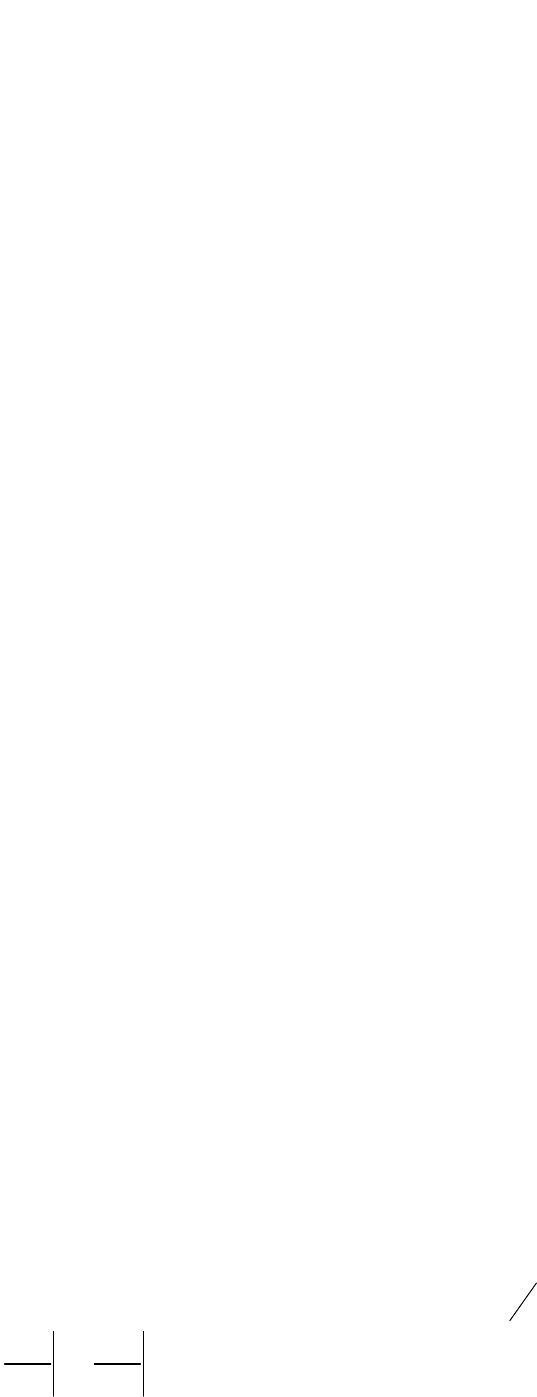
70
6.9. The namelist CAVITY
The namelist CAVITY allows the user to include, and to some extent to modify
arbitrary RF, static electric and magnetic fields and fields generated by linear plasmas.
The somewhat misleading name CAVITY is still kept for historical reasons.
The standard option to describe cavity fields is based on tables, which may be
generated by analytical calculations, measurements or numerical codes. A field table
has to contain the z-position (column 1 in m) and the corresponding longitudinal on-
axis electric field amplitude (column 2 in arbitrary units) in free format. The
transverse field components are calculated from the derivatives of the on-axis field;
see Appendix (chapter 8). The polynomial expansion extends to 1
st
order or, with
C_higher_order = True, to 3
rd
order. The polynomial expansion is perfect already in
first order for a pure sine-like spatial wave. Deviations from a sine-like spatial field
profile lead to increasing imperfections of the filed description with increasing radius.
Differences of calculations done with 1
st
and 3
rd
order expansion can be used to check
whether the field expansion approach is sufficient or a 3D field map is required. A
smoothing procedure can be applied to suppress numerical noise by setting
C_smooth( ) = n,
n
∈
ℕ
.
Static electric fields
To mark fields as static the name of the file containing the field
table should start with the letters ‘DC’ or the frequency, Nue( ), should be set to zero.
Static magnetic fields
The 3D field map option can be (ab)used to include static
magnetic field maps. See below for details. Parameters Ex_stat( ) and Ey_stat( ) can
be used to redirect the field scaling parameter MaxE( ) to a transverse component.
TE modes
To mark the field of a field table as TE mode – as opposed to a standard
TM mode – the file name has to start with the letters ‘TE_’. The field table in this
instance contains the position and the on-axis longitudinal magnetic field amplitude.
For TE modes the parameter MaxE( ) refers to the longitudinal on-axis magnetic field
component.
Dipole modes
Dipole modes can be inserted as 3D field maps; see below.
Traveling wave structures
Traveling wave structures can be inserted in its most
general form as superposition of real and imaginary parts of the general solution; see
Appendix (chapter 9). For periodic structures the description presented in Ref [1] has
been incorporated. The transverse field components are derived according to a 1
st
order polynomial expansion. The field table has to contain the on-axis longitudinal
field amplitude of at least one RF period plus the input and output coupler cells,
which are treated as standing wave cells.
To the file a first line is added, containing in a free format:
z
1
z
2
n m
where z
1
and z
2
are the start and end points of the traveling wave cells (i.e. the end
and starting point of the input and output cell) and n and m are two integers
characterizing the phase advance per cell 2
n
m
π
Θ = . Note that
1 2
( ) ( )
Ez z Ez z
=,
1 2
1, 2, 3
i i
i i
z z
Ez Ez i
z z
∂ ∂
= =
∂ ∂ should be fulfilled to high precision.
For a backward traveling wave structure set n < 0.
The file name has to start with the letters ‘TWS’.

ASTRA User‘s manual
71
For a beta matched structure a wave number K_wave( ) has to be specified. For a
1
β
=
structure the wave number is derived automatically from the frequency. The
length of a periodic structure can be specified with the parameter C_numb( ), which
contains the number of cells (excluding the input and output coupler cells). Note that
C_numb( )·n/m must be an integer.
3D field maps
3D field maps can be included in a most general form. The six field
components Ex, Ey, Ez, Bx, By and Bz have to be stored in six files with a common
name except for the name extension. The name of the files has to start with the letters
‘3D’, or have ‘3D’ at position 4 and 5 of the name; the extensions are .ex, .ey, .ez, .bx,
.by and .bz. In the input deck the file name without extension has to be specified. The
files start with a description of the grid, followed by the field values at each grid
point. The grid does not have to be equidistant and can be different for each
component except for the first and the last longitudinal grid coordinate, which has to
be the same for all components. A warning is given if a particle leaves the transverse
grid dimensions of a single component within the longitudinal grid boundaries at first
appearance only! The program does not stop anymore as it was the case in previous
versions! With Nx = number of grid knots in x, Ny = number of grid knots in y and
Nz = number of grid knots in z the file looks like:
Nx x[1] x[2] ....... x[Nx-1] x[Nx]
Ny y[1] y[2] ....... y[Ny-1] y[Ny]
Nz z[1] z[2] ....... z[Nz-1] z[Nz]
F[ 1, 1, 1] F[ 2, 1, 1]................... F[Nx, 1, 1]
F[ 1, 2, 1] F[ 2, 2, 1]................... F[Nx, 2, 1]
: :
: :
: :
F[ 1,Ny, 1] F[ 2,Ny, 1]................... F[Nx,Ny, 1]
F[ 1, 1, 2] F[ 2, 1, 2]................... F[Nx, 1, 2]
F[ 1, 2, 2] F[ 2, 2, 2]................... F[Nx, 2, 2]
: :
: :
: :
F[ 1,Ny, 2] F[ 2,Ny, 2]................... F[Nx,Ny, 2]
F[ 1, 1, 3] F[ 2, 1, 3]................... F[Nx, 1, 3]
: :
: :
: :
: :
: :
: :
: :
: :
F[ 1,Ny,Nz] F[ 2,Ny,Nz]................... F[Nx,Ny,Nz]
where
F
is the value of the respective field component. The number format is free; the
file has to contain line breaks as shown, but may contain additional line breaks as
appropriate. (Note that the maximum line length in a file is a system dependent
quantity.)
The maximum on axis value of the Ez component is scaled to MaxE( ), for standard
TM type modes, as in case of a field table, other components are scaled accordingly.
For TE type modes (file name TE_3D…) MaxE( ) refers to the on axis maximum of
the Bz component, while for dipole modes (file names DX_3D… or DY_3D…)
MaxE( ) refers to the on axis maximum of the Bx or By component, respectively.
72
In all cases it is assumed, that the ratio of electric to magnetic components is as V/m
to T. A linear interpolation is applied between the grid knots. A field map can be n
times periodically repeated by specifying C_numb( ) = n. Care has to be taken, that
the field values at the start and the end of the map do match in this case.
For static electric 3D fields the name of the files should start as ‘DC-3D’ or the
frequency, Nue( ), should be set to zero. Files with magnetic field components (.bx,
.by, .bz) are not required in this case. With parameters Ex_stat( ) and Ey_stat( ) the
scaling by means of MaxE can be redirected to the specified direction.
For static magnetic 3D fields one of the logical parametrs Bx_stat( ), By_stat( ) or
Bz_stat( ) has to be set to true. The parameter directs the field scaling parameter
MaxE( ) to the respective component. Files with electric field components (.ex, .ey,
.ez) are not required in this case.
If the electric field components are given on a common grid and the magnetic fields
components are given on a second common grid the parameter Com_gird = ’E,B’ may
be set to speed up the calculations. If all six components are given on a common grid
Com_grid = ’all’ may be set.
Tracking through 3D field maps is rather time consuming. Moreover the field
description is due to resolution and numerical noise problems not necessarily better
than a description with a field table unless non cylindrically symmetric features are to
be taken into account or field values far off-axis are required.
Field pointers
In order to save storage place for cavities which can be described by
the same field map it is possible to define a field pointer by specifying
File_Efield(j) = ‘3D_Point@(i)’, where
i
is the index of a cavity element specified as
3D field map and
i j
<
. Parameters related to the grid (e.g. Com_grid, C_numb) are
common for these cavities and are defined by index
i
. All other parameters are defined
independently for each element.
Overlaying modes or real and imaginary parts
When field tables or maps overlap
longitudinally
Astra
gives a warning. The field components are added up in the
overlapping region. Thus modes or real and imaginary parts of a mode can be
specified as two field entries at the same location. See Appendix (chapter 9) and [9]
for an application of this option.
Time dependent fields and beam loading
An exponentially increasing or decaying
field can be specified with the parameters T_dependent( ), T_null( ) and C_Tau( ).
The field value at the start off of the calculation is set as:
_
_
0
1
T null
C Tau
E E e
−
= −
and
_
_
0
T null
C Tau
E E e
−
=
, respectively.
If the stored energy of the cavity is specified, beam loading is taken into account
according as:
0
_
1_
E load
E E
E stored
= −
where
E_stored
is the stored energy at the actual
gradient and
E_load
is the energy transferred to a particle in the last time step.
Overlapping cavity fields cannot be treated correctly by this option. When time
dependent parameters are specified actual field values are stored in a file, see Table 3
and Table 4.
ASTRA User‘s manual
73
Modifying the field profile and local perturbations The parameter Flatness( )
allows modifications of the field profile by multiplying the longitudinal field (after the
scaling to MaxE) with a linear slope. It is not applicable for TWS and 3D structures.
A flatness parameter of ± 0.1 yields roughly 10% variation of field flatness. The exact
variation depends on the length of the field table and should be checked with
fieldplot
.
In order to approximate local asymmetries as they can be generated e.g. by input
couplers a local transverse offset of the field between two positions defined by
C_zkickmin( ) and C_zkickmax( ) can be introduced. A cosine-squared offset of
amplitude C_Xkick and C_Ykick is simulated. An example of this option is given in
Ref. [10].
Linear plasma wakefield Far behind the driver, the fields present in a linear plasma
wake [11] are given by
2 2 2 2
0
2 2
2
0
2 2
2
0
( )
( , ) exp cos( )
2 2 2
( , ) ( ) exp sin( )
2 2 2
( , ) ( ) exp sin( )
2 2 2
0
p e p z
z z p
p e p z
x z p
p e p z
y z p
z x y
k m c a r k
E z r k
e
k m c k
E z r a r k
e x
k m c k
E z r a r k
e y
B B B
σ
πσ ζ
σ
π
σ ζ
σ
π
σ ζ
⊥
⊥
⊥
= −
∂
= −
∂
∂
= −
∂
= = =
with the rest mass of electrons
e
m
, the elementary charge
e
and
c
the velocity of
light.
The wave number of the plasma
p
p
k
c
ω
≅
is given by
1
2
2
0
( )
p
e
e n z
m
ωε
=
with the
vacuum permittivity
0
ε
and the plasma density profile
( )
n z
.
E_sigz
z
σ
=
denotes the rms length of the driver laser intensity or the beam charge
density, respectively, and
g
z v t
ς
= −
denotes the co-moving coordinate, where
g
v
is
the group velocity of the driver in the plasma.
The normalized vector potential of a driver of longitudinal Gaussian shape is defined
as
2
2 2
0
2
( , ) ( ) exp 2
z
a r a r
ς
ς
σ
⊥
=
.
The transverse shape of the vector potential and its evolution in the longitudinal
direction can be either user-defined by a 3D field map of the vector potential
2
0
( , , )
a x y z
⊥
by specifying the file name File_A0( ), or it follows the free evolution as
2 2
2 2
02 2
_sig
( , ) _a0 exp
( ) 2 ( )
r r
E r
a z r E
z z
σ σ
⊥
= −
, with
( )
( )
2
2
2 2
2
2
2
2 2
2
E_eps E_Z0
( ) E_sig for an electron beam driver
E_sig
E_sig E_Z0
( ) E_sig for a laser driver
E_Zr
r
r
z
z
z
z
σ
σ
−
= +
−
= +
and the peak normalized vector potential defined as
2
0
E_a / ( )
e
eA m c
=

74
A constant plasma profile with rising and falling edge can be defined using the
parameters P_Z1, P_Z2, P_R1, and P_R2. Set File_Efield( ) = ’Plasma’ for this case.
The edge is modeled according to
( )
(
)
1
4
1 exp P_R
z
n z n
−
∆
∆ = +
where n is the
plasma density,
z
∆
is the distance to the edge, i.e.
P_Z1
z z
∆ = −
or
P_Z2
z z
∆ = −
and
P_R
1 or 2 is a taper parameter.
Arbitrary plasma profiles can be defined with a two-column file which contains the
longitudinal position z [m] and the plasma density n [arb. u.]. The plasma density will
be scaled so that the peak value is equal to P_n. The filename has to start with the
word ‘Plasma’ and is specified in the input deck via the parameter File_Efield( ).
When laser wavelength E_Lam is specified, the linear wakefield module includes
slippage effects due to the laser group velocity in the plasma. Changes of the bunch
phase in the wake due to changes in density are included.
References
[1]
G. A. Loew, R. H. Miller, R. A. Early, K. L. Bane ‘Computer Calculations of
Traveling Wave Periodic Structure Properties’, SLAC-PUB-2295, 1979.
http://www.slac.stanford.edu/cgi-wrap/getdoc/slac-pub-2295.pdf
[9]
P. Piot et al. ‘Steering and focusing effects in TESLA cavity due to high order
mode and input coupler’ PAC 2005.
http://accelconf.web.cern.ch/AccelConf/p05/PAPERS/WPAT083.PDF
[10]
M. Krassilnikov, R. Cee, T. Weiland ‘Impact of the RF-Gun Power Coupler on
Beam Dynamics’, EPAC 2002.
http://accelconf.web.cern.ch/AccelConf/e02/PAPERS/WEPRI077.pdf
[11]
E. Esarey, C. B. Schroeder, W. P. Leemans, ‘Physics of laser-driven plasma-
based electron accelerators’, Rev. of Mod. Phys., Vol 81, 2009.
https://doi.org/10.1103/RevModPhys.81.1229

ASTRA User‘s manual
75
Parameter Specification Unit Default Value
LOOP Logical FALSE
see chapter 4.9.
LEfield Logical FALSE
if false, all cavity fields are turned off.
File_Efield( ) Character*150 array
user specified file name for field tables, or maps, or key word plasma.
C_noscale( ) Logical array FALSE
if true, the cavity field will not be scaled, but the file values will be taken as
field values in MV/m (TM modes), or T (Te modes).
C_smooth( ) Integer array 0
controls the number of iterations of a soft, iterative procedure for smoothing
field tables. Since the transverse field components are based on derivatives of
the field table and can be noisy if the table is not precise, smoothing is
recommended. Use fieldplot to check that the longitudinal field component
remains basically unchanged and that the transverse components get smooth.
Not applicable for 3D maps.
Com_grid( ) Character array
either ’E,B’ if the E and B components of a 3D map are given on common
grids or ‘all’ if all six components of a 3D map are given on a common grid.
C_higher_order( ) Logical array FALSE
if true, the field expansion extends to 3
rd
order, if false the field expansion
extends only to 1
st
order. If true stronger smoothing of the field might be
required. Not applicable to TWS structures.
Nue( ) Real*8 array GHz
frequency of the RF field.
K_wave( ) Real*8 array m
-
1
wave number of the field, only for
β
matched traveling wave structures.
MaxE( ) Real*8 array MV/m or T
the absolute maximum, on-axis, longitudinal electric (TM mode) or magnetic
(TE mode) field amplitude of the RF field is scaled to this value.
Ex_stat( ) Logical array FALSE
redirects parameter MaxE( ) to the transverse electric component in x direction,
for DC fields only.
Ey_stat( ) Logical array FALSE
redirects parameter MaxE( ) to the transverse electric component in y direction,
for DC fields only.
Bx_stat( ) Logical array FALSE
redirects parameter MaxE( ) to the transverse magnetic component in x, for
static magnetic fields only.
By_stat( ) Logical array FALSE
redirects parameter MaxE( ) to the transverse magnetic component in y, for
static magnetic fields only.

76
Bz_stat( ) Logical array FALSE
redirects parameter MaxE( ) to the transverse magnetic component in z, for
static magnetic fields only.
Flatness( ) Real*8 array 0.0
modifies the field flatness by multiplying the longitudinal field component with
a linear slope; applied after scaling to MaxE. Not applicable for 3D and TWS
structures.
Phi( ) Real*8 array degree
phase of the RF field. Phi(0) defines a global phase shift of all cavities. See
section 4.30.
C_pos( ) Real*8 array m
shifts the longitudinal cavity position. C_pos is added to the position defined in
File_Efield( ).
C_numb( ) Integer array 1 (3 in ASTRA Vers. 1)
number of cells excluding the input and output cell for traveling wave
structures, or number of periods for 3D maps.
T_dependence( ) Character array
either ‘fill’ or ‘decay’ in order to activate filling or decaying of the cavity field,
respectively.
T_null( ) Real*8 array ns
for cavity filling: time between start of the filling of the cavity and start of the
particle tracking; for decay: time between start of decay and start of particle
tracking.
C_Tau( ) Real*8 array ns
filling time of the cavity.
E_stored( ) Real*8 array J·m
2
/MV
2
stored field energy of the cavity. If specified beam loading is taken into
account.
C_xoff( ) Real*8 array m
0.0
transverse offset of the cavity in x.
C_yoff( ) Real*8 array m
0.0
transverse offset of the cavity in y.
C_xrot( ) Real*8 array rad
0.0
rotation angle of the cavity in the x-z plane, i.e. around the y-axis.
C_yrot( ) Real*8 array rad
0.0
rotation angle of the cavity in the y-z plane, i.e. around the x-axis.
C_zrot( ) Real*8 array rad
0.0
rotation angle of the cavity around the z-axis, i.e. in the x-y plane.

ASTRA User‘s manual
77
C_zkickmin( ) Real*8 array m
start of local field offset.
C_zkickmax( ) Real*8 array m
end of local field offset.
C_Xkick( ) Real*8 array m
0.0
local transverse field offset in x.
C_Ykick( ) Real*8 array m
0.0
local transverse field offset in y.
File_A0( ) Character*150 array
for plasma wakefield: user specified file name for the normalized vector
potential
(
)
2
0
, ,
⊥
a x y z
of a drive laser, file format defined like 3D field maps. If
C_noscale( ) = False, values from File_A0 are normalized and scaled to E_a0.
If no File_A0 is defined, the driver spot size evolves according to the
parameters E_sig, E_Z0, and E_Zr or E_eps.
P_Z1( ) Real*8 m
effective longitudinal start point of the plasma field. Used if only the key word
plasma and no table is provided in File_Efield.
P_R1( ) Real*8 m
ramp parameter for the entrance of the plasma field. Field calculation starts at
P_Z1-2.5·P_R1. Used if only the key word plasma and no table is provided in
File_Efield.
P_Z2( ) Real*8 m
effective longitudinal end point of a plasma field. Used if only the key word
plasma and no table is provided in File_Efield.
P_R2( ) Real*8 m
ramp parameter for the exit of the plasma field. Field calculation ends at
P_Z2+2.5·P_R2. Used if only the key word plasma and no table is provided in
File_Efield.
P_n Real*8 cm
-
3
peak plasma density. In the entrance and exit region the plasma density is
scaled as described above, or P_n is used to scale the normalized profile
defined in File_Efield( ).
E_a0 Real*8
0.0
peak normalized vector potential
2
0
_ / ( )
e
E a eA m c
= of the generating driver
laser beam or charge density.
E_Z0 Real*8 m
0.0
position of the focus of the generating beam. Used if no File_A0 is defined.
E_sig Real*8 m
0.001
rms transverse beam size at the focus of the generating beam intensity. Used if
no File_A0 is defined.
E_sigz Real*8 m
0.001
rms longitudinal beam size of the generating beam intensity.
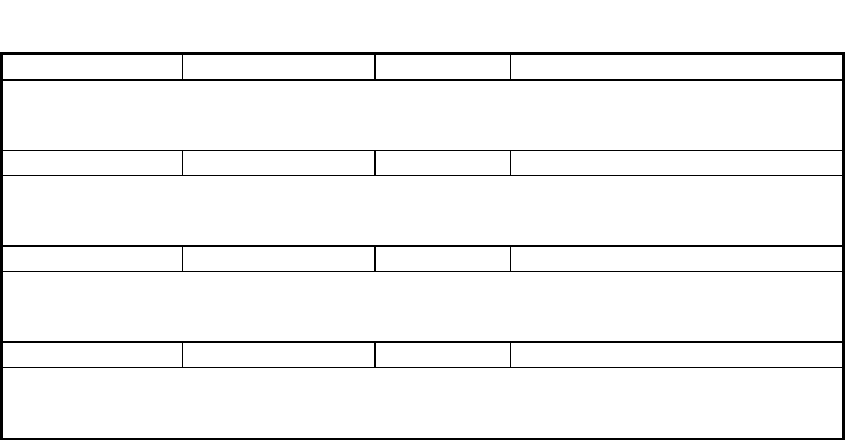
78
E_Zr Real*8 m
0.0
Rayleigh length of the generating beam. Alternative parameter to E_eps. It is
possible to specify E_Zr independently of E_sig. Used if no File_A0 is defined.
E_Eps Real*8 m
0.0
emittance of the generating beam. Alternative parameter to E_Zr. Used if no
File_A0 is defined.
E_lam Real*8 m
0.0
wavelength of the driving laser. If no wavelength is specified no correction for
the group velocity in the plasma is applied.
zeta Real*8 m
1.0
distance between driving laser (or electron beam) and electron beam at the
plasma start. Alternative to phase, active if < 0.

ASTRA User‘s manual
79
6.10. The namelist SOLENOID
The namelist SOLENOID allows to include arbitrary solenoid fields by means of
tables, which may be generated by analytical calculations, measurements or numerical
codes. The table has to contain the z-position (column1 in m) and the corresponding
longitudinal on-axis magnetic field amplitude (column 2 arb. units) in a free format.
The transverse field components are calculated from the derivatives of the on-axis
field; see Appendix (chapter 8). The polynomial expansion extends to 1
st
order or,
with S_higher_order = True, to 3
rd
order. A smoothing procedure can be applied to
suppress numerical noise by setting S_smooth( ) = n,
n
∈
ℕ
.
Parameter Specification Unit Default Value
LOOP Logical FALSE
see chapter 4.9.
LBfield Logical FALSE
if false, all solenoid fields are turned off.
File_Bfield( ) Character*150 array
user specified file name.
S_noscale( ) Logical FALSE
if true, the solenoid field will not be scaled, but the file values will be taken as
field values in T .
S_smooth( ) Integer array 0
controls the number of iterations of a soft, iterative procedure for smoothing
field tables. Since the transverse field components are based on derivatives of
the field table and can be noisy if the table is not precise, smoothing is
recommended. Use fieldplot to check that the longitudinal field component
remains basically unchanged and that the transverse components get smooth.
S_higher_order( ) Logical array TRUE
if true, the field expansion extends to 3
rd
order, if false the field expansion
extends only to 1
st
order. If true stronger smoothing of the field might be
required.
MaxB( ) Real*8 array T 0.0
maximum field value of the solenoid field. The field is scaled to this value.
S_pos( ) Real*8 array m 0.0
shifts the longitudinal solenoid position. S_pos is added to the position defined
in File_Bfield( ).
S_xoff( ) Real*8 array m 0.0
horizontal offset of the solenoid.
S_yoff( ) Real*8 array m 0.0
vertical offset of the solenoid.
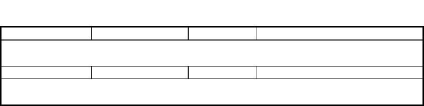
80
S_xrot( ) Real*8 array rad 0.0
rotation angle of the solenoid in the x-z plane, i.e. around the y-axis.
S_yrot( ) Real*8 array rad 0.0
rotation angle of the solenoid in the y-z plane, i.e. around the x-axis.
ASTRA User‘s manual
81
6.11. The namelist QUADRUPOLE
The namelist QUADRUPOLE allows to include quadrupole fields based on analytical
expressions and field profile data.
In case of the analytic describtion the fringe field is tapered according to the relation
( )
(
)
1
4
1 exp _
z
g z g Q bore
−
∆
∆ = +
where g is the quadrupole gradient and
z
∆
is the
distance to the quadrupole edge. The tapering is user-defined by means of the
parameter Q_bore, which might be set approximately to the diameter of the
quadrupole bore. The tapered region extents on both edges over a length of 3
·
Q_bore.
A longitudinal field component exists in the tapered region in accordance to
Maxwell’s law. Due to the tapering the actual field is longer than the specified
effective length by 3
·
Q_bore
. Fields of neighboring quadrupoles are superimposed if
they are too close. When the length of a quadrupole is shorter than 3
·
Q_bore
the
fringe fields of both edges start to overlap. In order to reach the specified gradient a
renormalization of the gradient is applied in this case and a warning is given. Strongly
overlapping fringe fields lead to unphysical field profiles and a reduction of the
effective magnet strength. The field profile should hence be checked with
fieldplot
in
such case. When a focusing strength is specified rather than a gradient
fieldplot
assumes a beam momentum of 1 MeV/c to set a gradient for the plot.
Other field profiles can be introduced by means of a data file containing the z-position
(column1 in m) and the corresponding gradient (column 2 arb. units) in a free format.
(Q_Type( ) = ’filename’).The file name has to contain the string ‘data’ as keyword. A
longitudinal field component is derived in regions of varying gradient in accordance
to Maxwell’s law.
Multipole components
Multipole components can be added with the parameters
_ _ ( , )
Q mult a i j
and
_ _ ( , )
Q mult b i j
, where index
i
refers to the multipole
coefficient and index
j
is the element number. The field parameterization follows
closely a standard multipole expansion. With
_ _ ( , )
i
a Q mult a i j
=
and
_ _ ( , )
i
b Q mult b i j
=
the field components write as:
( ) ( )
( )
( ) ( )
( )
( )
( )
62
1
62
1
cos sin
sin cos
_ ( )
_ ( )
i
r i i
i
i
i i
i
x r
y r
B r a i b i
B r a i b i
B Q grad j xB yB
B Q grad j yB xB
ϕ
ϕ
ϕ
ϕ ϕ
ϕ ϕ
−
−
−
−
= − ⋅ + ⋅
= ⋅ + ⋅
= − −
= − +
∑
∑
i.e. the coefficients are defined relative to the quadrupole gradient,
i
b
describes
normal coefficients, while
i
a
describes skew coefficients and
1...6
i
=
describe
dipole, quadrupole, sextupole etc. components, respectively. Note that
_ ( )
Q grad J
enters with reversed sign in order to comply to the sign convention as given below.
Multipole components are realized for standard quadrupoles and field profiles only.
The fringe field of the multipole components is tapered as the main quadrupole field
but the contribution of the multipole components onto the longitudinal field is
ignored.

82
Parameter Specification Unit Default Value
LOOP Logical FALSE
see chapter 4.9.
Lquad Logical FALSE
if false, all quadrupole fields are turned off.
Q_type( ) Character*150 array
besides standard quadrupoles (w. o. type specification) skew quadrupoles,
doublets and triplets and field data can be specified. Doublets have the same field
amplitude with reversed sign in the two magnets. For triplets the field amplitude
has the same magnitude for all magnets but opposite sign of the outer magnets as
compared to the inner one. The inner magnet is twice as long as the outer ones.
Q_grad( ) Real*8 array T/m
quadrupole gradient. Refers to the first quadrupole in case of doublets and triplets.
A positive gradient focusses negatively charged particles traveling into positive
z-direction in the x plane.
Q_K( ) Real*8 array m
-
2
focusing strength of the quadrupole. The gradient is set during the tracking of the
reference particle in dependence of the reference particle momentum. Refers to
the first quadrupole in case of doublets and triplets. A positive quadrupole
strength focusses negatively charged particles traveling into positive z-direction in
the x plane. If Q_K and Q_grad are specified, Q_K has a higher priority.
Q_noscale( ) Logical FALSE
if true, the field profile will not be scaled, but the file values will be taken as
gradients in T/m or as focusing strength in m
-2
.
Q_length( ) Real*8 array m
effective length of the quadrupole.
Q_smooth( ) Integer array 0
controls the number of iterations of a soft, iterative procedure for smoothing field
profile tables.
Q_bore( ) Real*8 array m 0.035
taper parameter for the quadrupole field edge.
Q_dist( ) Real*8 array m
distance between magnets in case of doublets and triplets.
Q_mult_a( , ) Real*8 array 0.0
skew multipole coefficients.
Q_mult_b( , ) Real*8 array 0.0
normal multipole coefficients.
Q_pos( ) Real*8 array m
longitudinal quadrupole position. Refers to the center of the magnet(s) also in case
of doublets and triplets.
ASTRA User‘s manual
83
Q_xoff( ) Real*8 array m
horizontal offset of the quadrupole, the doublet or the triplet.
Q_yoff( ) Real*8 array m
vertical offset of the quadrupole, the doublet or the triplet.
Q_xrot( ) Real*8 array rad
0.0
rotation angle of the quadrupole in the x-z plane, i.e. around the y-axis.
Q_yrot( ) Real*8 array rad
0.0
rotation angle of the quadrupole in the y-z plane, i.e. around the x-axis.
Q_zrot( ) Real*8 array rad
0.0
rotation angle of the quadrupole around the z-axis, i.e. in the x-y plane.
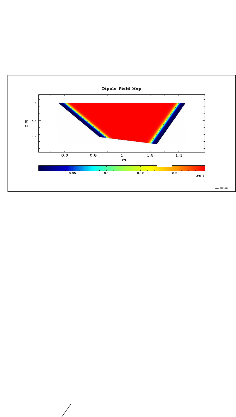
84
6.13. The namelist DIPOLE
The namelist DIPOLE allows to include dipole fields based on analytical expressions.
Dipoles are defined by two edge lines, defining the entrance and the exit face of the
dipole. Each line is defined by two points in the input deck. The connecting lines of
these points define the area in which the actual field calculation takes place. The
shape of the area is arbitrary, except that is has to be convex.
Fig. 4 Example for the definition of a dipole: The entrance and exit face of the
dipole are defined by the lines D1(i) = (1.0, 0.6) to D2(i) = (-1.0, 0.9) and
D3(i) = (1.0, 1.4) to D4(i) = (-1.3, 1.2). The lines D1 – D2 and D3 – D4 are
associated with the taper parameters D_Gap(1,i) and D_Gap(2,i). The entrance
and exit lines form together with the extrapolated connecting lines D1 – D3 and
D2 – D4 the area in which the dipole field is defined. Note the order of the
corner points. Exchanging D3 and D4 would be no valid input.
Dipoles can be defined to bend in the x-z plane (horizontal) or in the y-z plane
(vertical). Overlapping fields are superimposed if the magnets are defined in the same
bending plane. In the case of sections composed of horizontal and vertical dipoles the
user has to make sure, that magnets in the two principle planes do not overlap. (Note
that a dipole has an infinite extension into the direction perpendicular to the bending
plane.)
The pivot point for rotations is defined by the average of the four corner points.
Rotations and offsets within the bending plane are uncritical. The correct treatment of
overlapping fields is, in the case of rotations out of the bending plane, however only
possible, if the fields do also overlap when the magnets are not rotated out of the
bending plane. A section of dipoles which are rotated by a common angle is hence
uncritical. In complicated geometrical cases it is advisable to track sections wise.
The field strength is set either directly or by the bending radius. This radius is used to
calculate the field strength based on the energy of the reference particle. Negative
bending radii deflect electrons toward positive x-values. Fringe Fields are calculated
between two parallel lines around the dipole edges. They have a
1.5 D_Gap
± ⋅
offset
from the edge. For a horizontal magnet the Field
By
decays outside of the magnet as
(
)
1
0
4
( ) 1 exp D_Gap
y
d
B d B
−
= +
, where
d
is the normal distance to the edge.
D1(i)
D2(i)
D3(i)
D4(i)

ASTRA User‘s manual
85
The other field components are calculated according to Maxwell’s law. The fringe
fields of the same magnet are not allowed to overlap.
Parameter Specification Unit Default Value
LOOP Logical FALSE
see chapter 4.9.
LDipole Logical FALSE
if false all dipoles are turned off.
D_Type( ) Character*10 array
besides horizontal dipoles which bend in the x-plane vertical dipoles can be
specified to bend the beam in the y-plane.
D1( , ) Double Complex
array m (0.0,0.0)
coordinates of the first corner of a dipole. Two numbers, enclosed by brackets
and separated by a comma, are to be given. The first number defines the
horizontal or vertical (if D_type = ‘vertical’) coordinate, the second number
defines the longitudinal coordinate.
D2( , ) Double Complex
array m (0.0,0.0)
coordinates of the second corner of a dipole. Two numbers, enclosed by
brackets and separated by a comma, are to be given. The first number defines
the horizontal or vertical (if D_type = ‘vertical’) coordinate, the second number
defines the longitudinal coordinate.
D3( , ) Double Complex
array m (0.0,0.0)
coordinates of the third corner of a dipole. Two numbers, enclosed by brackets
and separated by a comma, are to be given. The first number defines the
horizontal or vertical (if D_type = ‘vertical’) coordinate, the second number
defines the longitudinal coordinate.
D4( , ) Double Complex
array m (0.0,0.0)
coordinates of the fourth corner of a dipole. Two numbers, enclosed by
brackets and separated by a comma, are to be given. The first number defines
the horizontal or vertical (if D_type = ‘vertical’) coordinate, the second number
defines the longitudinal coordinate.
D_Gap( , ) Real*8 array m 0.05
taper parameter for the dipole fringe field. The first index of the array is 1 or 2
for the first and second dipole edge, while the second index refers to the dipole
number.
D_strength( ) Real*8 array T 0.0
the dipole magnet strength.
D_radius( ) Real*8 array m 0.0
if a bending radius is defined the magnet strength is set during the tracking of
the reference particle in accordance to the beam energy. If D_radius and
D_strength are specified, D_radius has a higher priority.
86
D_xoff( ) Real*8 array m
0.0
transverse offset of the dipole in x.
D_yoff( ) Real*8 array m
0.0
transverse offset of the dipole in y.
D_zoff( ) Real*8 array m
0.0
longitudinal offset of the dipole in z.
D_xrot( ) Real*8 array rad
0.0
rotation angle of the dipole in the x-z plane, i.e. around the y-axis.
D_yrot( ) Real*8 array rad
0.0
rotation angle of the dipole in the y-z plane, i.e. around the x-axis.
D_zrot( ) Real*8 array rad
0.0
rotation angle of the dipole around the z-axis, i.e. in the x-y plane.

ASTRA User‘s manual
87
6.14. The namelist LASER
The namelist LASER allows to include an electromagnetic field as generated by a
laser beam. ASTRA treats a laser just as a special external field, effects as e.g.
Compton scattering are not included.
Besides a diffraction limited short pulse Gaussian laser model (
GLB
), a
CW
transversely Gaussian laser model has been implemented which allows to mimic
different longitudinal pulse forms by means of window functions. In addition a
radially polarized short pulse Gaussian laser (
RPL
) model is implemented.
Some input parameters are highly redundant, e.g. the intensity of the laser field can be
specified via the pulse energy, the pulse power, the peak electric field in the focus or
via the normalized vector potential. The relations used internally to convert the
different quantities are summarized below.
Since a laser beam moves it has to be synchronized to the electron beam to meet the
laser beam at a specified position. The interaction region is defined with parameters
L_Z1( ) and L_Z2( ). The laser field is only calculated when the electron bunch is in
between these longitudinal positions. For the synchronization purpose parameters
L_zstart( ) or L_tstart( ) can be set. An electron beam travelling with speed of light
will meet the laser beam in the interaction region when both start at z = L_zstart and
t = L_tstart. This applies also when the laser is rotated out of the coordinate system of
the electron beam. In general one will start the electron beam at z = t = 0.0 and use
L_zstart or L_tstart to adjust for time of flight differences due to velocities
differences.
Parameter L_H( ) allows to reduce the time steps of ASTRA within the interaction
region to cope with the short wave length of the laser field. Note that an uncertainty of
H_max
·
electron beam velocity exists concerning the exact location at which the step
width is reduced to L_H( ). L_Z1( ) should hence not be chosen to tight.
The Gaussian laser beam (short pulse and cw) is by default transversely polarized
with the electric field pointing into x direction. The polarization direction can be
rotated with parameter L_zrot( ). Parameter L_delta( ) allows to mix a second
component in, which is polarized perpendicular to the first component and shifted in
phase by 90 degree. Thus all sorts of elliptical and circular polarization can be
realized.
The propagation direction of the laser beam can be changed with the parameters
L_xrot( ) or L_yrot( ). The pivot point for the rotation is center of the interaction
region (L_Z1( ) + L_Z2( ))/2.
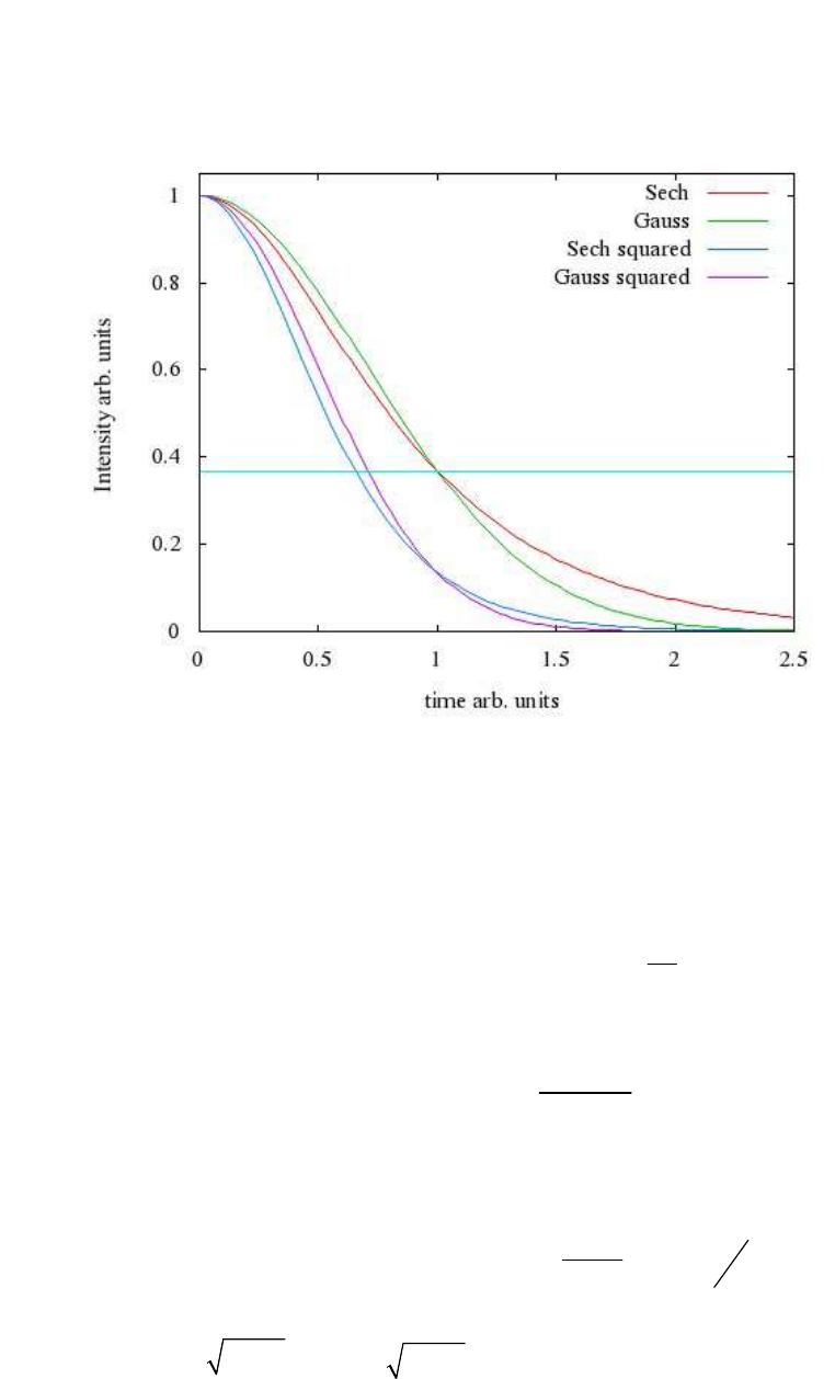
88
Laser beam models
The relations used to describe the field of a laser beam in
ASTRA follow closely the treatment by McDonald [1]. The temporal pulse shape of
the fields is assumed to be of hyperbolic secant shape (= 1/hyperbolic cosine) [1].
The pulse length relates to the 1/
e-
width of the field which is equal to 1.055 times the
rms width for the hyperbolic secant. Since the laser intensity is proportional to the
square of the laser field, the 1/e-width of the intensity is equal to 0.66 times the 1/e-
width of the field.
Peak power
P
and laser energy
U Pdt
=
∫
are related by
acosh( )
2
U
P e
τ
= with the 1/e
pulse length
τ
.
Approximations made are valid as long as
0
1, exp(1) 2.718...
acosh( ) e
e
ωτ
ξ
= > = =
holds.
For the internal description the longitudinal position is measured relative to the focus
position and in relation to the Rayleigh length
2
0
4
R
Z
πσ
λ
= as
R
z
Z
ζ
= with the rms
spot size of the laser intensity at the focus
0
σ
. The transverse rms laser beam size
develops as
(
)
2
2
00
11w w
σ σ ζ
ζ
= + = +
and the beam radius
w
is two times the
rms beam size.
Figure 1: Comparison of Gaussian and hyperbolic secant pulse shape with equal 1/e-
width and corresponding squared functions.
ASTRA User‘s manual
89
Gaussian Laser Beam
The phase for the Gaussian laser beam is given as:
2
2
CE G
r
w
ζ
ξ ϕ ϕ
Ψ = + + − with the Gouy phase
atan
G
ϕ ζ
=, the carrier envelope phase
CE
ϕ
and the phase
t kz
ξ ω
= −
.
With an envelope function defined as
0
2
2
0
0
Sech
r
w
nv E
w
E e
w
ξ
ξ
−
=
, where
2 2
r x y
= +
is
the transverse position, the field components read as:
cos
0
x
y
nv
E E
E
= ⋅ Ψ
=
( )
2
0
2
sin cos
z
R
nv
w
x
E E
Z w
ς
= − Ψ + Ψ
0
x
y x
B
B E
=
=
( )
2
0
2
sin cos
z
R
nv
w
y
B E
Z w
ς
= − Ψ + Ψ
The field amplitude follows from the Poynting theorem
2
0
1
2
A
E
P ds
η
=
∫
as
0
0
2
0
P
E
η
πσ
= with the vacuum impedance
0
η
. The normalized vector potential is given
as
0
0
2
0
eE
a
m c k
=
with the wave number
2
k
π
λ
=
.
For the orthogonal polarization state
x
and
y
are exchanged and an additional phase
shift by
2
π
is introduced, i.e.
cos sin
Ψ → − Ψ
and
sin cos
Ψ → Ψ
. The components
read thus as:
0
sin
x
y
nv
E
E E
=
= − ⋅ Ψ
ɶ
ɶ
( )
2
0
2
cos sin
z
R
nv
w
y
E E
Z w
ς
= − Ψ − Ψ
ɶ
0
x y
y
B E
B
=
=
ɶ ɶ
ɶ
( )
2
0
2
cos sin
z
R
nv
w
x
B E
Z w
ς
= − Ψ − Ψ
ɶ
The two components are mixed as:
( )
( )
1
22
1
22
ˆ1
ˆ1
x x y x
y y
E E E E
E E
δ δ
δ
δ
= + =
−
=−
ɶ
ɶ
( )
( )
( )
( )
21 1
02 2
2 2
2
ˆsin cos
1 1
z
R
nv
w
E
Ex y x y
Z w
δ ς δς
δ δ
= − Ψ + Ψ
− +
− −
90
( )
( )
( )
( )
( )
1
22
21 1
02 2
2 2
2
ˆ ˆ
1
ˆ ˆ
ˆsin cos
1 1
x x y
y y x
z
R
nv
B B E
B B E
w
E
By x y x
Z w
δ
δ
δ ς δς
δ δ
= =
−
= =
= − Ψ + Ψ
− +
− −
ɶ
Radially Polarized Laser beam
The phase for the radially polarized beam is given
as:
2
2
2
CE G
r
w
ξ ϕ ϕ ζ
Ψ = + + −
with the Gouy phase
atan
G
ϕ ζ
=
, the carrier envelope
phase
CE
ϕ
and the phase
t kz
ξ ω
= −
.
With an envelope function defined as
0
2
2
2
0
02
Sech
r
w
nv E
w
E e
w
ξ
ξ
−
=
, the field components
write as:
0
0
cos
cos
x
y
nv
nv
x
E E
w
y
E E
w
= Ψ
= Ψ
2
2
0
2
2
sin cos
1
z
R
nv
wr
r
E E
Zw
w
ζ
=
Ψ − Ψ
−
0.0
x y
y x
z
B E
B E
B
= −
=
=
The field amplitude follows from the Poynting relation
2
0
1
2
A
E
P ds
η
=
∫
as
0
0
2
0
2
P
E
η
πσ
=
with the vacuum impedance
0
η
. The normalized vector potential is
given as
0
0
2
0
eE
a
m c k
=
with the wave number
2
k
π
λ
=
. Note that while
0
E
is a factor
2
larger than in case of the linearly polarized beam the maximal transverse field at
2
w
r=
reaches only
0
0.43
E
⋅
and thus about 60% of the maximal field of the
linearly polarized case.
References
[1]
K. T. McDonald ‘Gaussian Laser Beams with Radial Polarization’, Princeton
University 2000.
http://puhep1.princeton.edu/~mcdonald/examples/axicon_big.pdf

ASTRA User‘s manual
91
Parameter Specification Unit Default Value
LOOP Logical FALSE
see chapter 4.9.
LLaser Logical FALSE
if false, all laser fields are turned off.
L_Type( ) Character*150 array
type of laser beam. Valid keywords are:
CW = cw Gaussian laser beam
GLB = short pulse Gaussian Laser Beam
RPL = short pulse Radially Polarized Laser beam
L_Z1( ) Real*8 m
start position of the interaction region with the laser field.
L_Z2( ) Real*8 m
end position of the interaction region with the laser field.
L_H( ) Real*8 ns 0.0
local time step setting, active if ≠ 0.0.
L_F( ) Real*8 m
longitudinal position of the focus.
L_zstart( ) Real*8 m 0.0
longitudinal start position of the laser beam.
L_tstart( ) Real*8 ns 0.0
start time of the laser beam.
L_xoff( ) Real*8 m 0.0
transverse offset of the laser field in x.
L_yoff( ) Real*8 m 0.0
transverse offset of the laser field in y.
L_xrot( ) Real*8 rad 0.0
rotation angle of the laser field in the x-z plane, i.e. around the y-axis.
L_yrot( ) Real*8 rad 0.0
rotation angle of the laser field in the y-z plane, i.e. around the x-axis.
L_zrot( ) Real*8 rad 0.0
rotation angle of the laser field around the z-axis, i.e. in the x-y plane.
L_E0( ) Real*8 J 0.0
pulse energy of the laser.
L_Pow( ) Real*8 W 0.0
pulse power of the laser.
92
L_a0( ) Real*8 0.0
normalized vector potential of the laser in the focus.
L_Epeak( ) Real*8 V/m 0.0
electric field amplitude of the laser in the focus.
L_tau( ) Real*8 s 0.0
temporal 1/e pulse width of the laser field.
L_phi( ) Real*8 rad 0.0
carrier envelope phase.
L_lam( ) Real*8 m 0.0
wave length of the laser radiation.
L_sig0( ) Real*8 m 0.0
transverse rms size of the laser intensity at the focus position (
x y
σ σ σ
= =
).
L_w0( ) Real*8 m 0.0
transverse size of the laser intensity at the focus position = 2· L_sig0( ). If
L_sig0( ) and L_w0( ) are specified L_sig0( ) has priority,
L_delta( ) Real*8 1.0
polarization factor; Abs(L_delta( )) ≤ 1
L_delta( ) = ±1.0 linear polarization in x direction
L_delta( ) = 0.0 linear polarization in y direction
L_delta( ) =
1 2
circularly polarized laser beam.
L_window( ) Character*150 array
defines a window type for cw Gaussian laser beam. The window is applied
over the interaction range. Valid types are:
Blackman: a standard Blackman window
Tukey: a Tukey window with taper parameter L_alpha( )
L_alpha( ) Real*8 1.0
Taper parameter for Tukey window; 0 < L_alpha( ) ≤ 1.

ASTRA User‘s manual
93
7. Input namelist for generator
7.1. The namelist INPUT
Parameter Specification Unit Default Value
FNAME Character*150 rfgun.ini
file name for initial particle distribution; recommended extensions are .ini or
.zpos.run, respectively.
Add Logical FALSE
if true the input list has to be specified N_add times and N_add different
distributions will be added.
N_add Integer 0
number of distributions to be added.
Ipart Integer 100
number of particles to be generated.
Species Character*80 Electrons
species of particles to be generated. Valid are: electrons, positrons, protons
hydrogen.
The key word ion allows to generate particles with user defined ratio of mass to
charge state. In addition to the keyword ion a number between 1 and 10 has to
be specified, e.g. ‘ion 1’. The number is used as index in the ion_mass
specification. The parameter ion_mass needs to be specified in generator and
again in the namelist NEWRUN of
Astra.
To adopt the graphics program
postpro
additional specifications in the
Plot_steering.par file are optional (see chapter 5.6).
ion_mass( ) Real*8 Array eV/c
2
0.0
the mass divided by the charge state of user defined particles. The index
number corresponds to the number specified together with the keyword ions in
the Species definition. Negatively charged particles are defined by a negative
value of the ion_mass parameter. Ion_mass(1) – (10) is mapped onto particle
index 5 – 14 in the saved particle distribution file.
Probe Logical TRUE
if true, 6 probe particles are generated at locations:
(0.5
σ
x, 0.5
σ
z), (1.0
σ
x, 1.0
σ
z), (1.5
σ
x, 1.5
σ
z),
(0.5
σ
y, -0.5
σ
z), (1.0
σ
y, -1.0
σ
z), (1.5
σ
y, -1.5
σ
z).
Passive Logical FALSE
if true only passive particles will be generated.
Noise_reduc Logical TRUE
if true, particle coordinates are generated quasi-randomly following a
Hammersley sequence.
Cathode Logical TRUE
if true the particles will be generated with a time spread rather than with a
spread in the longitudinal position, i.e. sig_z, Lz and rz are set to zero and
sig_clock, Lt and rt have to be specified. See chapter 7.2 to chapter 7.4. Status
flags will be set accordingly.
R_Cathode Real*8 m 0.0
radius in case of a curved, i.e. non planar cathode. Active if R_cathode is not
zero. See section 7.5.2.
94
High_res Logical FALSE
if true, the particle distribution is saved with increased accuracy. See
Table 4.
Binary Logical FALSE
if true, the particle distributions is saved in binary format.
Q_total Real*8 nC 1.0
total charge of the particles. The total charge is equally distributed on the Npart
particles. (
Astra
would allow also particles with varying macro charge in one
distribution.)
Type Character*80 standard
defines the type of the distribution. Valid are standard and ring.
Rad Real*8 mm 0.0
radius of ring type distributions.
Tau Real*8 ns 0.0
exponential delay time of the emission. Active if Tau ≠ 0.0. The delay is added
to any distribution in time, i.e. to any distribution starting at the cathode. Note
that the delay time is random and might interfere with the quasi random nature
of an input distribution.
Ref_zpos Real*8 m 0.0
z position of the reference particle, i.e the longitudinal bunch position.
Ref_clock Real*8 ns 0.0
initial clock value of the reference particle, can in general be set to zero.
Ref_Ekin Real*8 MeV 0.0
initial kinetic energy of the reference particle.
Dist_z Character*80 uniform
specifies the longitudinal particle distribution. For valid keywords and related
parameters see chapter 7.2 to chapter 7.4.
sig_z Real*8 mm 0.0
rms value of the bunch length.
C_sig_z Real*8 0.0
cuts off a Gaussian longitudinal distribution at C_sig_z times sig_z. Active
if ≠ 0.0.
Lz Real*8 mm 0.0
length of the bunch.
rz Real*8 mm 0.0
rising of the bunch distribution; only for plateau distribution.
sig_clock Real*8 ns 1.0D-3
rms value of the emission time, i.e. the bunch length if generated from a
cathode.

ASTRA User‘s manual
95
C_sig_clock Real*8 0.0
cuts off a Gaussian longitudinal distribution at C_sig_clock times sig_clock.
Active if ≠ 0.0.
Lt Real*8 ns 0.0
length of the bunch; only for plateau distribution.
rt Real*8 ns 0.0
rise time of the bunch; only for plateau distribution.
Dist_pz Character*80 uniform
specifies the longitudinal energy and momentum distribution, respectively. For
valid keywords and related parameters see chapter 7.2 to chapter 7.4.
sig_Ekin Real*8 keV 0.0
rms value of the energy spread.
C_sig_Ekin Real*8 100.0
cuts off a Gaussian energy and momentum distribution at C_sig_Ekin times
sig_Ekin. Active if ≠ 0.0.
LE Real*8 keV 0.0
width of the energy distribution.
rE Real*8 keV 0.0
rising of the energy distribution, only for plateau distribution.
emit_z Real*8
π
keV mm 0.0
longitudinal particle emittance. Can be specified instead of the energy spread.
If an energy spread and an emittance is specified the energy spread has priority.
cor_Ekin Real*8 keV 0.0
correlated energy spread.
E_photon Real*8 eV 0.0
photon energy for Fermi-Dirac distribution.
phi_eff Real*8 eV 0.0
effective work function for Fermi-Dirac distribution.
Dist_x Character*80 Gaussian
specifies the transverse particle distribution in the horizontal direction. For
valid keywords and related parameters see chapter 7.2 to chapter 7.4.
sig_x Real*8 mm 1.0
rms bunch size in the horizontal direction. Also the vertical bunch size if
Dist_x = radial.
C_sig_x Real*8 0.0
cuts off a Gaussian horizontal distribution at C_sig_x times sig_x. Active
if ≠ 0.0.
Lx Real*8 mm 0.0
width of the horizontal particle distribution.
rx Real*8 mm 0.0
rising of the horizontal particle distribution; only for plateau distribution.
96
x_off Real*8 mm 0.0
horizontal offset of the particle distribution.
Disp_x Real*8 m 0.0
horizontal dispersion; a horizontal offset is added to all particles according to:
_
P
x x Disp x
P
∆
= + ; increases the calculated bunch emittance.
Dist_px Character*80 Gaussian
specifies the transverse momentum distribution in the horizontal direction. For
valid keywords and related parameters see chapter 7.2 to chapter 7.4.
Nemit_x Real*8
π
mrad mm 0.0
normalized transverse emittance in the horizontal direction. Can be specified
instead of a transverse momentum spread. If a momentum spread and an
emittance is specified the emittance has priority. Also the normalized vertical
emittance if Dist_px = radial.
sig_px Real*8 eV/c 0.0
rms value of the horizontal momentum distribution.
C_sig_px Real*8 100.0
cuts off the horizontal momentum distribution at C_sig_px times sig_px.
Lpx Real*8 eV/c 0.0
width of the horizontal momentum distribution; only for plateau distribution.
rpx Real*8 eV/c 0.0
rising of the horizontal momentum distribution; only for plateau distribution.
cor_px Real*8 mrad 0.0
correlated beam divergence in the horizontal direction
[ ] [ ]
rms
x mm
m
α
β
= −
.
For extreme settings of cor_px the correlated beam divergence cannot be set
correctly and the beam energy will be increased by
generator
. A warning will
be given in this case.
Dist_y Character*80 Gaussian
specifies the transverse particle distribution in the vertical direction. For valid
keywords and related parameters see chapter 7.2 to chapter 7.4.
sig_y Real*8 mm 1.0
rms bunch size in the vertical direction. Not significant if Dist_x = radial.
C_sig_y Real*8 0.0
cuts off a Gaussian vertical distribution at C_sig_y times sig_py. Active
if ≠ 0.0.
Ly Real*8 mm 0.0
width of the vertical particle distribution.
ry Real*8 mm 0.0
rising of the vertical particle distribution; only for plateau distribution.
ASTRA User‘s manual
97
y_off Real*8 mm 0.0
the vertical offset of the particle distribution.
Disp_y Real*8 m 0.0
vertical dispersion; a vertical offset is added to all particles according to:
_
P
y y Disp y
P
∆
= +
; increases the calculated bunch emittance.
Dist_py Character*80 Gaussian
specifies the transverse momentum distribution in the vertical direction. For
valid keywords and related parameters see chapter 7.2 to chapter 7.4.
Nemit_y Real*8
π
mrad mm 0.0
normalized transverse emittance in the vertical direction. Can be specified
instead of a transverse momentum spread. If a momentum spread and an
emittance is specified the emittance has priority. Not significant if Dist_px =
radial.
sig_py Real*8 eV/c 0.0
rms value of the horizontal momentum distribution.
C_sig_py Real*8 0.0
cuts off a Gaussian vertical momentum distribution at C_sig_py times sig_py.
Active if ≠ 0.0.
Lpy Real*8 eV/c 0.0
width of the vertical momentum distribution; only for plateau distribution.
rpy Real*8 eV/c 0.0
rising of the vertical momentum distribution; only for plateau distribution.
cor_py Real*8 mrad 0.0
correlated beam divergence in the vertical direction
[ ] [ ]
rms
y mm
m
α
β
= −
.
For extreme settings of cor_py the correlated beam divergence cannot be set
correctly and the beam energy will be increased by
generator
. A warning will
be given in this case.
98
7.2. 1D distributions
7.2.1 uniform distribution
Definition and basic relations
1
( )
f x
FWHM
=
for
2
FWHM
x
≤
0 elsewhere
rms value
2 3
FWHM
σ
=
Generator specifications
Dimension Key word Parameter
FWHM
or
σ
unit
temporal
1
Dist_z = '
u
niform' Lt or sig_clock ns
longitudinal
2
z Dist_z = '
u
niform' Lz or sig_z mm
longitudinal E
kin
Dist_pz = '
u
niform' LE or sig_Ekin or
emit_z keV or keVmm
transverse x Dist_x = '
u
niform' Lx or sig_x mm
transverse y Dist_y = '
u
niform' Ly or sig_y mm
transverse p
x
Dist_px = '
u
niform' Lpx or sig_px or
Nemit_x eV/c or mrad mm
transverse p
y
Dist_py = '
u
niform' Lpy or sig_py or
Nemit_y eV/c or mrad mm
1
active if Cathode = TRUE,
2
active if Cathode = FALSE
7.2.2 plateau distribution
Definition and basic relations
( )
1 1
( ) 2
2
1 exp 2
L
f x rt
Lx L
rt
= ≤
+ −
Definition of rt:
rt is defined by a straight line with a slope A given by:
2
( )
L
d
A f x
dx
±
=
Within rt the straight line inclines form 0 to the plateau value of the distribution.
FWHM value FWHM = L
rms value
2.8 2
2 3
L L L
rt
σ
≤ ≤ ≤
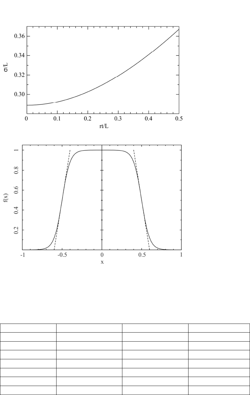
ASTRA User‘s manual
99
Relation of rms value and rise time
Example: Plateau distribution with L = 1 and rt = 0.2. Straight lines according to the
definition of rt.
Generator specifications
Dimension Key word
Parameter
L, rt
unit
temporal
1
Dist_z = '
p
lateau' Lt, rt ns
longitudinal
2
z Dist_z = '
p
lateau' Lz, rz mm
longitudinal E
kin
Dist_pz = '
p
lateau' LE, rE keV
transverse x Dist_x = '
p
lateau' Lx, rx mm
transverse y Dist_y = '
p
lateau' Ly, ry mm
transverse p
x
Dist_px = '
p
lateau' Lpx, rpx eV/c
transverse p
y
Dist_py = '
p
lateau' Lpy, rpy eV/c
1
active if Cathode = TRUE,
2
active if Cathode = FALSE
100
7.2.3 inverted parabola (longitudinal)
Definition and basic relations
The inverted parabola distribution produces linear longitudinal space charge fields. It
corresponds to the projection of a uniformly filled ellipsoid onto the z-axis.
2
max
2
max max
3
( ) 1
4
z
f z z z
z z
= − ≤
FWHM value
max
2
FWHM z
=
rms value
max
5
z
z
σ
=
Generator specifications:
Dimension Key word Parameter
σ
unit
temporal
1
Dist_z = '
inverted
' sig_clock ns
longitudinal
2
z Dist_z ='
inverted
' sig_z mm
7.2.4 Gaussian distribution
Definition and basic relations
2
2
1 1
( ) exp 2
2
x
f x
σ
πσ
= −
FWHM value
( )
2 2ln 0.5 2.35
FWHM
σ
= − =
Generator specifications:
Dimension Key word Parameter
σ
unit
temporal
1
Dist_z = '
g
auss' sig_clock ns
longitudinal
2
z Dist_z ='
g
auss' sig_z mm
longitudinal E
kin
Dist_pz = '
g
auss' sig_Ekin or emit_z keV or keVmm
transverse x Dist_x = '
g
auss' sig_x mm
transverse y Dist_y = '
g
auss' sig_y mm
transverse p
x
Dist_px = '
g
auss' sig_px or Nemit_x eV/c or mrad mm
transverse p
y
Dist_py = '
g
auss sig_py or Nemit_y eV/c or mrad mm
1
active if Cathode = TRUE,
2
active if Cathode = FALSE
ASTRA User‘s manual
101
7.2.5 truncated Gaussian distribution
Definition and basic relations
2
2
1 1
( ) exp 2
2
inp
inp
x
f x
σ
πσ
= −
for
Cut inp
x C
σ
≤
relation between
σ
inp
and rms value of the truncated distribution
σ
out
3
Cut inp
out inp
C
σ
σ σ
≤ ≤
Note that the cut produces a rectangular structure. Compare with the 2D-Gaussian
distribution 7.3.2.
Generator specifications
Dimension Key word Parameter ,
inp Cut
C
σ
unit
temporal
1
Dist_z = '
g
auss' sig_clock, C_sig_clock ns, dim. less
longitudinal
2
z Dist_z = '
g
auss' sig_z, C_sig_z mm, dim. less
longitudinal E
kin
Dist_pz = '
g
auss' sig_Ekin or emit_z,
C_sig_Ekin keV or keVmm,
dim. less
transverse x Dist_x = '
g
auss' sig_x, C_sig_x mm, dim. less
transverse y Dist_y = '
g
auss' sig_y, C_sig_y mm, dim. less
transverse p
x
Dist_px = '
g
auss' sig_px or Nemit_x,
C_sig_px eV/c or mrad mm,
dim. less
transverse p
y
Dist_py = '
g
auss' sig_py or Nemit_y,
C_sig_py eV/c or mrad mm,
dim. less
1
active if Cathode = TRUE,
2
active if Cathode = FALSE
102
7.3. 2D distributions
7.3.1 radial uniform distribution
Definition and basic relations
2
1
( , )f x y
r
π
= for
2 2 2
x y r
+ ≤
0 elsewhere
The projection onto the x-axis (eqv. y-axis) is a half ellipse
2 2
2
0
2
( ) 2 ( , )
m
y
r x
f x f x y dy x r
r
π
−
= = ≤
∫
with the following properties:
FWHM value FWHM =
3
r
rms value
2
r
σ
=
Generator specifications
Dimension Key word Parameter r or
σ
unit
transverse x, y Dist_x = '
r
adial
uniform' Lx or sig_x mm
transverse p
x
, p
y
Dist_px = '
r
adial
uniform' Lpx or sig_px or
Nemit_x eV/c or mrad mm
7.3.2 (truncated) 2D-Gaussian distribution
Equivalent to distributions 7.2.4 and 7.2.5 but with
( ) ( )
f y f x
=
. The cut will
produce a circular structure.
Generator specifications
Dimension Key word Parameter ,
inp Cut
C
σ
unit
transverse x, y Dist_x = '
2
D-
Gaussian’ sig_x, C_sig_x mm, dim. less
transverse p
x
, p
y
Dist_px = '
2
D-
Gaussian’ sig_px or Nemit_x,
C_sig_px eV/c or mrad mm,
dim. less
ASTRA User‘s manual
103
7.4. 3D distributions
7.4.1 isotropic momentum distribution
Definition and basic relations
A distribution with isotropic emission angles into a half sphere. The following
relations hold:
2 2 2 2 2
2
x y z kin kin
p p p P E E
+ + = = +
rms value
3
x y
P
p p
σ σ
= =
2 3
z
P
p
σ
=
mean value
,
2
z mean
P
p
=
normalized transverse emittances[1]:
, ,
2
0
2
1
3
kin
x y x y
E
m c
ε σ
=
Generator specifications
Dimension Key word
Parameter
E
kin
unit
p
x
, p
y
, p
z
Dist_pz = '
i
sotropic' LE keV
104
7.4.2 photo emission from a Fermi-Dirac distribution
Definition and basic relations
A distribution describing the photo emission from a metallic cathode at room
temperature according to ref. [2]. The random generator works only as true random
generator, the noise reduction option is hence switched off, if selected in the input
deck. As input parameters the effective work function
eff
Φ
, i.e. including a possible
reduction due to the Schottky effect, and the photon energy E
phot
need to be given.
The following relations hold:
rms value
2
0
3
phot eff
x y
E
p p m c
φ
σ σ
−
= =
mean Energy
( )
2
3
phot eff
kin
E
E
φ
−
=
Energy spread
( )
1
3 2
phot eff
Ekin
E
φ
σ
−
=
normalized transverse emittances:
, , 2
0
3
phot eff
x y x y
E
m c
φ
ε σ
−
=
Generator specifications
Dimension Key word Parameter
eff
Φ
, E
phot
units
p
x
, p
y
, p
z
Dist_pz = '
FD_300
' phi_eff,
E_photon eV
ASTRA User‘s manual
105
7.4.3 uniformly filled ellipsoid
Definition and basic relations
3
( , , ) 4
f x y z
Lx Ly Lz
π
= for
2 2 2
2 2 2
1
xyz
x y z
LLL
+ + ≤
0 elsewhere
the projection onto the z-axis (eqiv. x- and y-axis) is an inverted parabola:
2
2
0 0
3
( ) 4 ( , , ) 1
4
Ly
Lx
z
f z f x y z dx dy z Lz
Lz Lz
= = − ≤
∫ ∫
with the following properties:
FWHM value FWHM
z
= 2
Lz
rms value
5
z
Lz
σ
=
Generator specifications
Dimension Key word Parameter
,
,
z
x y
L
or σ
x, y, z
unit
temporal
1
Dist_z = '
u
niform
ellipsoid' Lt or sig_clock ns
longitudinal
2
z Dist_z = '
u
niform
ellipsoid' Lz or sig_z mm
transverse x Dist_z = '
u
niform
ellipsoid' Lx or sig_x mm
transverse y Dist_z = '
u
niform
ellipsoid' Ly or sig_y mm
1
active if Cathode = TRUE,
2
active if Cathode = FALSE

106
7.5. Miscellaneous options
7.5.1 ring type distributions
If Type = ‘Ring’ is specified any standard transverse distribution is offset by a radius
specified with parameter Rad and uniformly distributed on a circle. Thus a circular
charge distribution is generated. The cross section of the ring can vary from x to y
depending on the setting of transverse parameters.
7.5.2 emission from a curved cathode
In order to start a distribution from a curved cathode the radius of the cathode can be
specified with the parameter R_cathode. For this option photo emission is assumed,
hence the longitudinal starting position and the starting time are modified according to
the cathode radius. All other parameters remain unchanged.
References
[1] K. Floettmann ‘Note on the thermal emittance of electrons emitted by Cesium
Telluride photo cathodes’ TESLA-FEL Report 1997-01.
http://flash.desy.de/sites/site_vuvfel/content/e403/e1642/e839/e829/infoboxCont
ent830/fel1997-01.pdf
[2] D. Dowell, J. Schmerge ‘Quantum efficiency and thermal emittance of metal
cathodes’ PRST-AB 12,074201, 2009.
http://prst-ab.aps.org/pdf/PRSTAB/v12/i7/e074201
ASTRA User‘s manual
107
8. Appendix I: Field expansion formulas
A solenoid field can be described by a polynomial expansion as:
2 4 6
'' '''' ''''''
( ) ,0
3 5
' ''' '''''
( )
..
4 64 2304
...
2 16 384
r
z z z z z
r
r z z z
r r r
B B B B B
r r r
B B B B
= − + −
= − + −
where B
z,0
is the longitudinal on-axis magnetic field and the prime’s indicate
derivatives with respect to z.
In Astra the field expansion extends to 3
rd
order or is limited to the 1
st
order if
S_higher_order( ) = FALSE; higher order terms tend to be noisy and are hence
excluded. Since the expansion ends in both cases with an odd order the condition
div 0
B
=
is fulfilled, while the condition
rot 0
B
=
is only approximately fulfilled.
The 3
rd
order term contributes one percent to the radial magnetic field at a field
expansion radius R
3rd
given by:
'
3'''
0.08
z
rd
z
B
RB
=
This quantity can be plotted with fieldplot.
A cylindrical symmetric TM standing wave mode can be expanded as:
( )
( )
( )
2
2''
( ) ,0 ,0
2
2
3
' ''' '
( ) 2
2
3''
( ) ,0 ,0
2 2
sin
4
sin
2 16
cos
2 16
r
z z z z
r
r z z z
rz z z
r
E E E E t
c
r r
E E E E t
c
r r
B E E E t
c c
φ
ωω
ωω
ω ω
ω
= − +
= − + +
= − +
where E
z,0
is the longitudinal electric field and higher order terms are ignored. A TE
standing wave mode can equivalently be described by:
( )
( )
( )
2
2''
( ) ,0 ,0
2
2
3
' ''' '
( ) 2
2
3''
( ) ,0 ,0
2
cos
4
cos
2 16
sin
2 16
r
z z z z
r
r z z z
rz z z
r
B B B B t
c
r r
B B B B t
c
r r
E B B B t
c
φ
ωω
ωω
ω
ω ω
= − +
= − + +
= − +
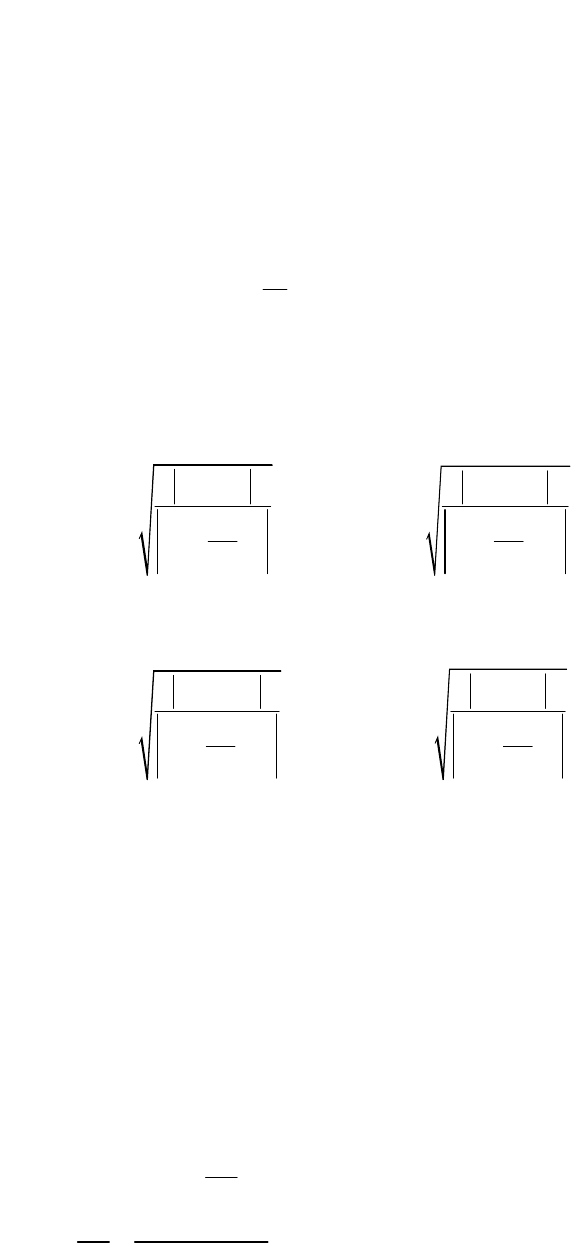
108
In Astra the field expansion extends to 3
rd
order or is limited to the 1
st
order if
C_higher_order( ) = FALSE; higher order terms tend to be noisy and are hence
excluded.
The polynomial expansion is perfect already in 1
st
order for a pure sine-like spatial
wave, since the higher order components yield zero in this case. Deviations from a
pure sine-like spatial field profile lead to approximations in the condition rot
E B
= −
ɺ
for TM modes and
2
rot
E
B
c
=
ɺ
for TE modes.
In the case of a DC field (only TM mode) the condition
rot 0
E
=
is only
approximately fulfilled equivalently to the description of solenoid fields.
The 3
rd
order term contributes one percent to the transverse electric or magnetic field
component at a field expansion radius R
3rd
given by:
'
,0
3 3
2 2
''' ' ''
,0
2 2
0.08 0.08
r
zz
B
E
rd rd
z z z z
EE
R R
E E E E
c c
φ
ω ω
= =
+ +
for a TM mode, and:
'
,0
3 3
2 2
'' ''' '
,0
2 2
0.08
0.08
r
z
z
EB
rd rd
z z z z
B
B
R R
B B B B
c c
φ
ω ω
= =
+ +
for a TE mode.
These quantities can be plotted with fieldplot.
The derivatives of the longitudinal field component are calculated by a division of
small numbers and are hence sensitive to numerical noise. The quality of a field table
can be judged by means of plots of the transverse field components and especially of
the quantity R
3rd
which is notably sensitive to numerical noise. Smooth transverse
fields require tables of high accuracy and not too short distance of the longitudinal
base points.
An iterative procedure can be applied in order to reduce the numerical noise. A field
value F (i.e. B
z,0
or E
z,0
) at index i is replaced by:
( ) ( 1)
( 1) ( 1)
( 1) ( 1)
( ) ( 1)
with
and
i i
i i
i i
i i
dF
F F z
dz
dF F F
dz z z
z z z
− +
+ −
+ −
−
= ∆
−
=−
∆ = −
This procedure is iterated n times where n is defined by the user.
The procedure is soft, i.e. a large number of iterations might be required. Than it
removes efficiently sharp, spiky structures in the transverse components but leaves the
average behavior unchanged. Fig. 5 shows an example of the transverse electric field
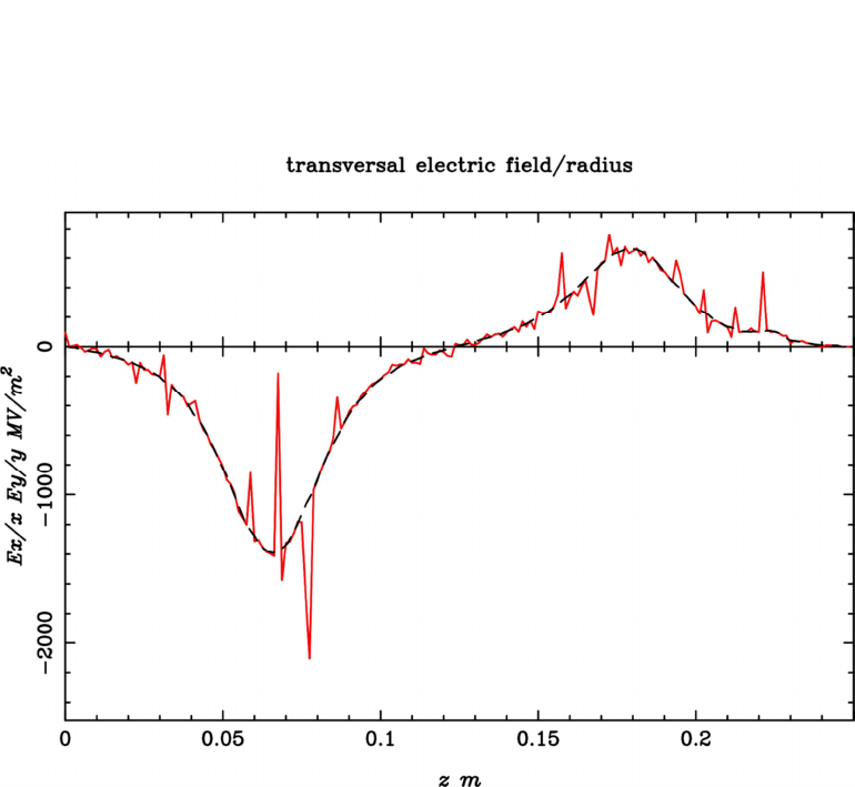
ASTRA User‘s manual
109
from a particularly bad field table. After smoothing with C_smooth( ) = 100 all
spikes are removed without influence onto the average behavior.
Fig. 5 Example of the transverse electric field components calculated with the
field expansion formulas from an inaccurate field table. The numerical noise in
the original data (red, solid line) is removed by the smoothing procedure
(dashed, black line) without influence onto the average behavior.
110
9. Appendix II: Representation of a travelling wave by two
standing waves
A field can be represented in complex form as:
exp z
V A i c
ω α ϕ
= ⋅ + +
with:
2 2 2
A Re Im
= +
cos
Re
A
α
=; sin
Im
A
α
=
,
r r
Re E B
=
,
i i
Im E B
=
where
r
E
and
r
B
denote the electric and magnetic component of the real part solution
and
i
E
and
i
B
the corresponding imaginary part of the solution, respectively.
Assume for simplicity that
0
ϕ
=
. Particle couple to the real part of the field
r
V
r
z
V A cos c
ω α
= ⋅ +
( ) ( )
z z
A cos cos A sin sin
c c
ω α ω α
= ⋅ − ⋅
z z
Re cos Im sin
c c
ω ω
= ⋅ − ⋅
r i
c
z z
E cos E sin
c
ω ω
= −
and
r i
z z
B cos B si
c
cn
ω ω
= −
An equivalent representation can be formulated by superimposing a standing wave
with
0
ϕ
=
(index
1
c
) with a second standing wave with
2
π
ϕ
= (index
2
c
):
1 1
;
c c
z z
E cos B sin
c c
ω ω
−
2 2
;
2 2
c c
z z
E cos B sin
c c
π π
ω ω
+ − +
2 2
;
c c
z z
E sin B cos
c c
ω ω
=− −
With the following identification both representations are identical:
1 1
;
c r c i
E E B B
= =
2 2
;
c i c r
E E B B
= = −
ASTRA User‘s manual
111
10. Appendix III: Rotation of Elements in Astra
Rotations of elements are defined by the angles …xrot (C_xrot, S_xrot …), …yrot
(C_yrot, S_yrot …) and …zrot (C_zrot, S_yrot …)
The angle …xrot defines a rotation in the x-z plane, i.e. around the y-axis of the
coordinate system. The sign of the angle is positive when the element rotates from
positive z to positive x.
The angle …yrot defines a rotation in the y-z plane, i.e. around the x-axis of the
coordinate system. The sign of the angle is positive when the element rotates from
positive z to positive y.
The angle …zrot defines a rotation in the x-y plane, i.e. around the z-axis of the
coordinate system. The sign of the angle is positive when the element rotates from
positive x to positive y.
Rotations are performed before transverse offsets are added.
The pivot point is in longitudinal direction defined by the center of the element, i.e.
the mean of start and end point. Note the special case of dipoles as described in
section 6.13.
Rotations are performed in the following order:
1
st
rotation around the y-axis (angle …xrot).
2
nd
rotation around the x-axis (angle …yrot). The angle …yrot is defined with respect
to the rotated (…xort) element.
3
rd
rotation around the z-axis (angle …zrot). The angle …zrot is defined with respect
to the rotated (…xort - …yrot) element.
The units for the rotation angles are radians.
Z
Y
X
yrot
around
x-axis
zrot
around
z-axis
xrot
around
y-axis
I
II
I
I
I

112
11. Selected references
The following selected references are related to code comparisons and benchmarking,
program developments and interesting applications, respectively. More references can
be found at the end of various subsections in the document above.
[1]
S. Setzer et al. ‘FEL photoinjector simulation studies by combining MAFIA TS2
and ASTRA’, EPAC 2002.
http://accelconf.web.cern.ch/AccelConf/e02/PAPERS/WEPRI076.pdf
[3]
C. Limborg et al. ‘Code comparison for simulations of photo-injectors’, PAC
2003.
http://www.slac.stanford.edu/pubs/slacpubs/10000/slac-pub-10735.html
[4]
G. Geloni et al. ‘Benchmark of ASTRA with analytical solution for the
longitudinal plasma oscillation problem’, FEL 2004.
http://accelconf.web.cern.ch/AccelConf/f04/papers/MOPOS09/MOPOS09.PDF
[5]
K. Floettmann et al. ‘Recent improvements to the ASTRA particle tracking
code’, PAC 2003.
http://accelconf.web.cern.ch/accelconf/p03/PAPERS/FPAG015.PDF
[6]
G. Poeplau et al. ‘3D space charge calculations for bunches in the tracking code
ASTRA’, EPAC 2006.
http://accelconf.web.cern.ch/AccelConf/e06/PAPERS/WEPCH121.PDF
[7]
A. Markovik et al. ‘Simulation of 3D space charge fields of bunches in a beam
pipe of elliptical shape’, EPAC 2006.
http://accelconf.web.cern.ch/AccelConf/e06/PAPERS/WEPCH120.PDF
[8]
I. V. Bazarov, C. K. Sinclair ‘Multivariate optimization of a high brightness
DC-gun photoinjector’, PRST-AB 8, 034202, 2005.
http://prst-ab.aps.org/onecol/PRSTAB/v8/i3/e034202
[9]
D. Janssen et al. ‘Emittance compensation in a superconducting RF gun with a
magnetic mode’ PRST-AB 7, 090702, 2004.
http://prst-ab.aps.org/abstract/PRSTAB/v7/i9/e090702
[10]
R. Brinkmann et al. ‘A low emittance, flat-beam electron source for linear
colliders’ PRST-AB 4, 053501, 2001.
http://prst-ab.aps.org/abstract/PRSTAB/v4/i5/e053501
[11]
A. Egbert et al. ‘High-repetition rate femtosecond laser-driven hard-x-ray source’
Appl. Phys. Lett. 81, No 113, 2002.
[12]
A. Egbert et al. ‘Electron-based EUV and ultrashort hard-x-ray sources’ X-Ray
Lasers 2002, AIP Conf. Proc. 614.
[13]
A. Pietzsch et al. ‘Towards time resolved core level photoelectron spectroscopy
with femtosecond x-ray free-electron lasers’ New Journal of Physics 10, 2008.
