Auto KEGGRec Manual
User Manual:
Open the PDF directly: View PDF ![]() .
.
Page Count: 17
AutoKEGGRec Manual
Emil Karlsen, Christian Schulz and Eivind Almaas
September 11, 2018
Contents
1 AutoKEGGRec 2
2 Installation and requirements 2
3 Usage 2
3.1 Optionalflags............................. 3
3.1.1 ConsolidatedRec . . . . . . . . . . . . . . . . . . . . . . . 4
3.1.2 SingleRecs........................... 5
3.1.3 CommunityRec........................ 5
3.1.4 writeSBML .......................... 6
3.1.5 OmittedData ......................... 7
3.1.6 OrgRxnGen.......................... 10
3.1.7 DisconnectedReactions . . . . . . . . . . . . . . . . . . . . 12
3.1.8 GenePlot ........................... 13
3.1.9 Histogram........................... 14
3.1.10 General statements concerning optional inputs . . . . . . 14
3.2 KEGG annotation and the ATTENTION field . . . . . . . . . . 15
3.3 Authors’ recommendation of usage . . . . . . . . . . . . . . . . . 15
4 Possible curation steps following execution of AutoKEGGRec 16
4.1 Generalsteps ............................. 16
4.2 Community reconstruction refinement . . . . . . . . . . . . . . . 17
1

1 AutoKEGGRec
This Matlab function rapidly assembles first-draft reconstructions (FDRs) from
KEGG based on KEGG organism IDs. See associated paper by E. Karlsen, C.
Schulz, and E. Almaas, ”Automated generation of genome-scale metabolic draft
reconstructions based on KEGG”.
2 Installation and requirements
AutoKEGGRec is a pipeline developed in Matlab 2017b and is designed to be
a part of the COBRA toolbox. The requirements are:
•A stable internet connection
•A personal computer running Matlab
•A functioning installation of the COBRA toolbox v.3
The AutoKEGGRec.m file should be copied into a folder included in the
Matlab search path, e.g. by use of the Matlab pathtool command. If every-
thing is installed and working correctly, the commands initCobraToolbox and
AutoKEGGRec 1should work and should auto-complete themselves by using
the TAB key.
3 Usage
The function takes one mandatory input and a number of optional inputs:
outputStruct =
AutoKEGGRec ( KEGG organism IDs , v a r a r g i n )
The variable KEGG organism IDs is a string array where the elements con-
sist of either 3- or 4-letter KEGG ID organism codes, or six letter code starting
with T; e.g. T00007 and eco are both KEGG organism IDs for Escherichia coli
K-12 MG1655.
Example input, using the five E. coli K-12 strains available as KEGG organism
IDs (09/2018):
outputStruct =
AutoKEGGRec ( [ ” eco ” ,” e c j ” ,” ecd ” ,”ebw” ,” ecok ” ] )
This function call generates an output structure containing the consoli-
dated model based on the five K-12 strains. This is the default output in the
1Note: The code uses the Matlab command parfor to download the reactions and com-
pounds from KEGG in parallel. Because of that, the parallel pool is started at the beginning
of the code. By default, the normal local parallel pool is used. You can change the number
of cores and threads by changing the parallel preferences in Matlab.
2

case that no further input options are given.
Optional flags can be specified as a list of keywords after the organism IDs.
Examples of recommended usage of the pipeline is given below.
3.1 Optional flags
The nine optional inputs (flags) to use within AutoKEGGRec are:
1. ’ConsolidatedRec’
2. ’SingleRecs’
3. ’CommunityRec’
4. ’writeSBML’
5. ’OmittedData’
6. ’OrgRxnGen’
7. ’DisconnectedReactions’
8. ’GenePlot’
9. ’Histogram’
They can be added to the function call as (e.g. for the above mentioned func-
tion):
outputStruct =
AutoKEGGRec ( [ ” eco ” ,” e c j ” ,” ecd ” ,” ebw” ,” ecok ” ] ,
’ CommunityRec ’ , ’OrgRxnGen ’ , ’ GenePlot ’ , ’ Histogram ’ ,
’OmittedData ’)
In this example, the options would add the community first draft recon-
struction of the five E. coli K-12 strains to the output Matlab structure named
outputStruct. That structure would also contain the Organisms-Reactions-
Genes matrix and a specification of the omitted reactions and compounds in-
cluding reasoning for omitting them. Furthermore, two Matlab plots would
appear, showing the gene plot and a histogram.
In the following part, the different options will be explained, including screen-
shots from Matlab 2017b and figures of the output. The three commands gener-
ating reconstructions, ConsolidatedRec,SingleRecs and CommunityRec, are
explained first.
As AutoKEGGRec is running, some information will be shown in the Mat-
lab command window, keeping the user updated on its progress. Note that
AutoKEGGRec takes some time to access all the KEGG-based information and
annotation available. For each reaction and compound, the annotation is stored
within the FDR, using the KEGG categories if no COBRA supported field is
available.
During determination of allowed compounds, the compound field ”EXACT MASS”
and the glycan field ”MASS” are summarized to into the field ”MASS”. This
does not affect the compound field ”MOL WEIGHT”.
3
3.1.1 ConsolidatedRec
Usage:
outputStruct =
AutoKEGGRec ( [ ” eco ” ,” e c j ” ,” ecd ” ,” ebw” ,” ecok ” ] ,
’ConsolidatedRec ’)
or
outputStruct =
AutoKEGGRec ( [ ” eco ” ,” e c j ” ,” ecd ” ,”ebw” ,” ecok ” ] )
This command prompts AutoKEGGRec to generate a consolidated first draft
reconstruction for the query organisms and provides them as a Matlab COBRA
model structure. It can be produced using the ’ConsolidatedRec’ option or
no option at all since this is the default output. The FDR will contain every
reaction in which at least one of the query organisms in KEGG is present. An
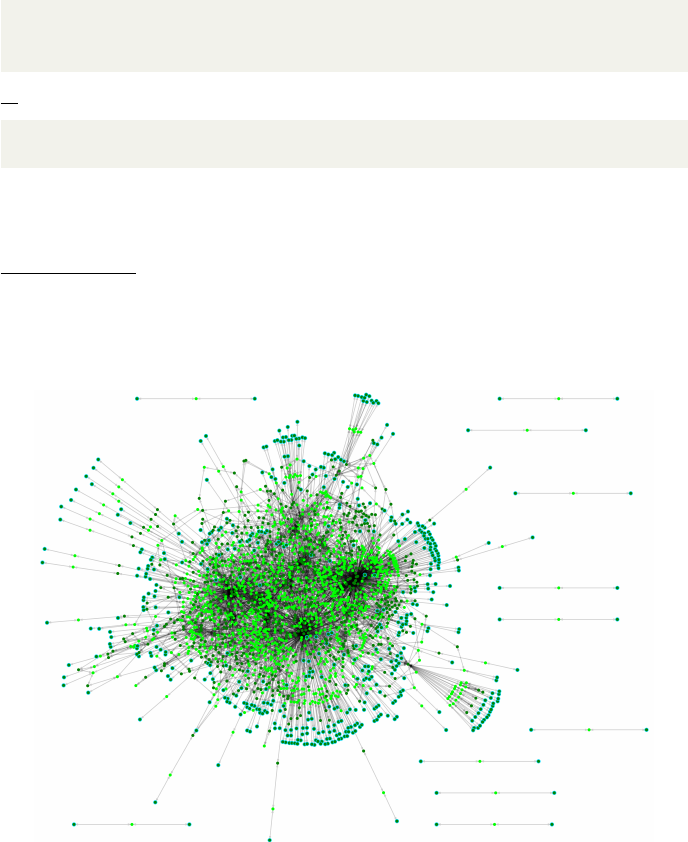
example can be seen in Fig. 1, where we have visualized the output metabolic
network produced by AutoKEGGRec for the E. coli K-12 strains, which have
the KEGG organism IDs eco,ecj,ecd,ebw, and ecok.
Figure 1: The consolidated reconstruction network based on the five E. coli
K-12 strains, based on an SBML file written using the writeSBML option.
The consolidated reconstruction contains no gene-protein-reaction rules since
different organisms will have different gene names, and possibly different num-
bers of genes, corresponding to the same reaction. The Matlab structures, how-
ever, include all possible KEGG based annotation for reactions and compounds.
4
3.1.2 SingleRecs
Usage:
outputStruct =
AutoKEGGRec ( [ ” eco ” ,” e c j ” ,” ecd ” ,” ebw” ,” ecok ” ] ,
’SingleRecs ’)
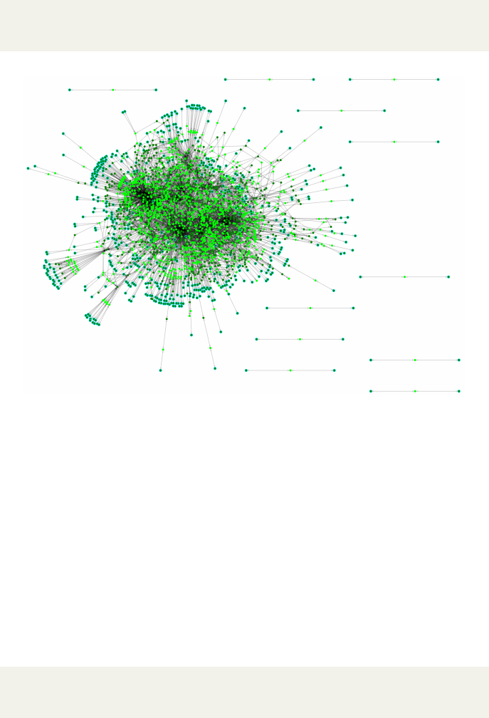
Figure 2: The reconstruction network of E. coli K-12 MG1655 using AutoKEG-
GRec for KEGG organism ID eco, based on an SBML file written using the
writeSBML option.
Using this option, AutoKEGGRec creates single first draft reconstructions
for each of the listed query organisms, each of which is stored by the organism
KEGG ID within the AutoKEGGRec output. In Fig. 2, we have visualized the
output metabolic network for E. coli K-12 MG1655 with KEGG organism ID
eco. Each reconstruction contains the reactions present in the KEGG organ-
ism and the gene-protein-reaction rules, including all possible annotations for
reactions and compounds based on the KEGG database.
3.1.3 CommunityRec
Usage:
outputStruct =
AutoKEGGRec ( [ ” eco ” ,” e c j ” ,” ecd ” ,” ebw” ,” ecok ” ] ,
’CommunityRec ’ )
5

This option creates a community first draft reconstruction based on the given
organisms. The different query organisms are placed in separate compartments,
specified by the organism KEGG ID as follows:
R00004 eco[c] : C00013 eco[c] + C00001 eco[c]⇔2C00009 eco[c]
Consequently, each organism with their respective reactions and compounds
is easy to identify. Each organism may have sub-compartments as well, as in-
dicated by the [c] (cytosol). Note that the single organisms are not connected.
The FDR is purely based on the information in KEGG and no transport re-
actions sharing a common compound is present because of the naming of the
compounds. For exchange reactions, typically [e] is used to signify extra-cellular
reactions/metabolites, which can be easily implemented with a Matlab program
using a for-loop.
Each of the separate organism reconstructions has gene-protein-reaction
rules included within the reconstruction, and an example of a community re-
construction can be seen in Fig. 3.
The FDR is stored within the AutoKEGGRec output as a COBRA model.
Since it contains every reaction of every organism, and thereby e.g. central
reactions several times, we decided to not include the most comprehensive Au-
toKEGGRec annotations possible. They are however stored within the other
structures given by using the options ConsolidatedRec or SingleRecs. There-
fore we recommend not only generating a community FDR using AutoKEG-
GRec but also a consolidated model of the given input organisms.
3.1.4 writeSBML
outputStruct =
AutoKEGGRec ( [ ” eco ” ,” e c j ” ,” ecd ” ,” ebw” ,” ecok ” ] ,
’ C onsolida tedRec ’ , ’ writeSBML ’ )
NB: This option requires a reconstruction to be built. Refer to one of the options
ConsolidatedRec,SingleRec or SommunityRec. If called without an explicit option to
generate a reconstruction, an error message will appear suggesting the user generate a
reconstruction.
This option calls the COBRA function writeCbM odel after creating the re-
quested reconstruction(s) to write the model as SBML file. The file will be saved
in the ”Current Folder” and automatically given a name based on the orgnaism
ID(s) and current time and date, according to the following format: ”Exam-
pleRec YYYY.MM.DD hh.mm.xml” (for example ConsolidatedRec 2018.04.10 11.43.xml
for a consolidated reconstruction generated 11:43 on the 10th of April 2018).
In case that several SBML files are to be written, a Matlab window pops up
showing the progress, where the progress of the loading bar is based on the num-
ber of reactions, not reconstructions, in order to give the user an impression of
progress in terms of required work.
Keep in mind that some fields added to the reconstructions by AutoKEG-
GRec are not supported by the COBRA writeCbM odel function, and so saving
6
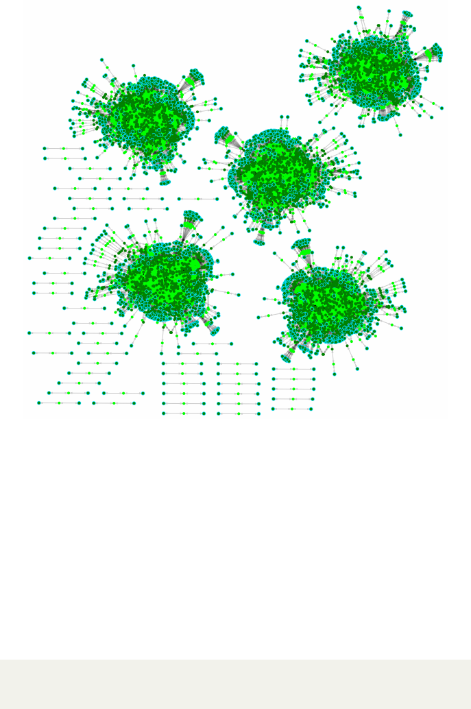
Figure 3: The community FDR network for the five E. coli K-12 strains. Since
no transport reactions are added, the separate compartments (different organ-
isms) are not connected.
the output variable as a Matlab structure is recommended if the user wants to
keep some of the additional data, such as the omitted reactions (see Sec. 3.1.5)
or the OrgRxnGen matrix (see Sec. 3.1.6). Other valuable annotations based on
the KEGG data, such as the mass of compounds, will also be lost if not stored
with a .mat file.
3.1.5 OmittedData
Usage:
outputStruct =
AutoKEGGRec ( [ ” eco ” ,” e c j ” ,” ecd ” ,” ebw” ,” ecok ” ] ,
’OmittedData ’)
This optional input can be used to analyze the KEGG reactions rejected
by AutoKEGGRec, and gives a sub-structure in the AutoKEGGRec output
7
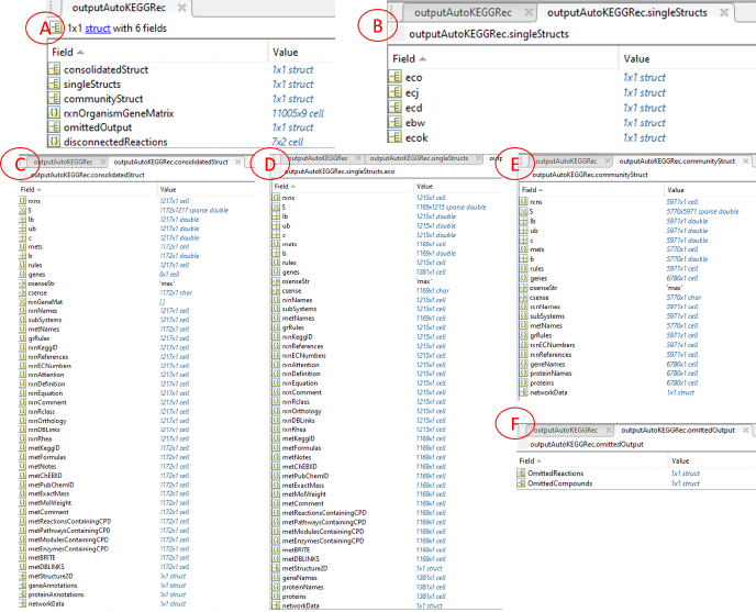
Figure 4: Screenshots of the AutoKEGGRec output structure of the FDRs for
the five E. coli K-12 strains that a user can expect. In (A), the structure of the
output variable (outputStruct in the examples) is shown. All the single first draft
reconstructions are shown in (B), whereas the single first draft reconstruction eco
is shown in (D), the consolidated first draft reconstruction and the community
first draft reconstruction are shown in (C) and (E), respectively. In (F) we
present the first layer of the omitted data, which is further presented in Fig. 5
and described in Sec. 3.1.5.
structure. Within that sub-structure are two fields, one which contains the
omitted compounds and two, which contains the omitted reactions (refer to
Fig. 4 (F) and Fig. 5 (A) and (B)).
Reactions omitted by AutoKEGGRec (e.g. polymerization reactions, gen-
eral reactions, reactions with generic compounds, etc.) are stored here with
their annotations, making these reactions available to the user. The reactions,
as well as the compounds, are stored within a sub-structure in the omitted
output and sorted, and are easily accessible by their KEGG IDs. Within the
KEGG annotation the original (i.e. not cleaned) reaction and any further data
available on the reaction in KEGG (example shown in Fig. 5 (D)) can be seen.
Furthermore, the field ”Attention” is added, including the the reason the reac-
tion was omitted. This allows the user to quickly determine whether and how
8
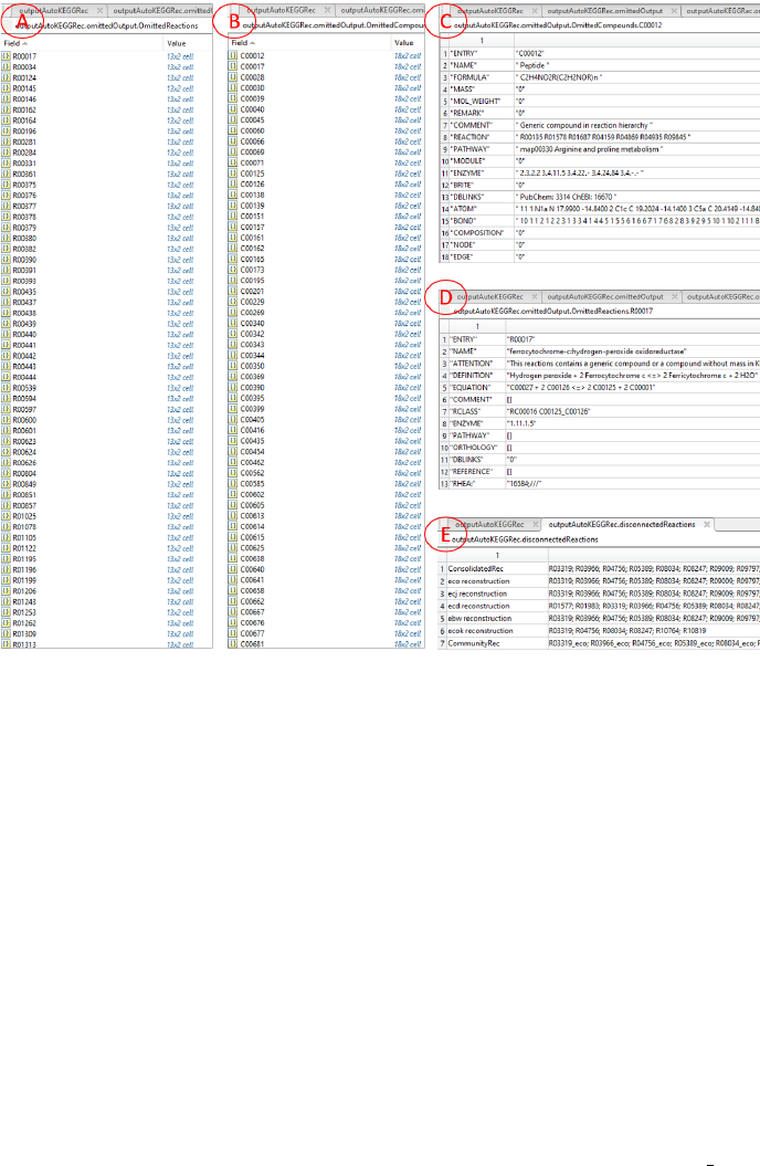
Figure 5: Screenshots of the output structure in Matlab for the five E. coli K-
12 strains. The fields within the omittedOutput using the options omittedData
are shown in Fig 4 (F). In (A) and (B), the omitted reactions and compounds,
respectively, are presented sorted by their KEGG IDs, each being a Matlab cell.
These cells are shown in (C) and (D) for the containing annotation based on
KEGG for the compound and reaction, respectively. Note the added ”Atten-
tion” field in (D), which contains the reason for omission. A corresponding field
for the compounds is not added, since the only criterion to omit a compound
is mass = 0. In (E) the content of the Matlab cell ”disconnectedReactions”
(see Fig. 4 (A)) using the AutoKEGGRec option DisconnectedReactions is
presented. Here, in a summary for each generated reconstruction, all reactions
that are not connected to the giant component (refer to the network figures in
Figs 1, 2 and 3) are summarized to allow the user easy access to these reactions.
to implement such reaction during the curation process.
The KEGG compounds are assessed within AutoKEGGRec and added to
the OmittedData if their mass is 0. Note that AutoKEGGRec uses the metMass
field to include the mass of specific glycan compounds as well as the exact mass
of KEGG compounds; they are also summarized in the field ”MASS” in the
9

omitted output where applicable, refer to Fig. 5 (C).
Within the listed the KEGG IDs of omitted compounds, the whole KEGG
annotation of each compound is stored as a Matlab cell (Fig. 5 C). The user
can access these fields, retrieve all stored KEGG annotations to the compound
in question directly to decide whether and how to implement that compound
and the corresponding reaction.
All strings within the specific fields in the Matlab struct are space-separated
fields, which allows the user quick access and possibilities for simple search in
e.g. the reactions a specific compound participates in.
3.1.6 OrgRxnGen
Usage:
outputStruct =
AutoKEGGRec ( [ ” eco ” ,” e c j ” ,” ecd ” ,” ebw” ,” ecok ” ] ,
’OrgRxnGen ’ )
This option instructs AutoKEGGRec to create the ”Organisms-Reactions-
Genes matrix” (example seen in Fig. 6) and store it within the output structure.
Within this matrix, all available KEGG reaction IDs are stored (first column).
Each following column represents one of the requested organisms, and if a certain
reaction is present within an organism, the gene name(s) for that reaction will
be in this field. In case of several genes they are listed and separated by a bar
(”|”), which represents the ”OR” relationship within the COBRA toolbox. In
reality, the relationship between genes pertaining to a given reaction may be any
combination of ”AND”/”OR” relationships, but this information is currently
not available in the KEGG database. This matrix is also the basis for generating
the reconstructions and implementing the gene-reaction-relationship.
The last three columns contain some summary data for each reaction, which
may be of help during analysis:
•Sum
•Total
•Genes
The ”Sum” column (third to last column) gives the sum of how many or-
ganisms contain genes related to a given reaction.
The ”Total” column (second to last column) gives the sum divided by the num-
ber of organisms, and therefore describes the fraction of organisms which has
the reaction in their metabolic network according to KEGG.
The ”Genes” column (last column) states the number of genes within the or-
ganisms related to this reaction. In case of different numbers of genes for the
different organisms for a given reaction, the values are comma separated.
This matrix may be useful for certain kinds of analysis on organisms stored
in KEGG, such as this short Matlab code snippet to select all the reactions that
have different number of genes related to them (example output seen in Fig. 7):
10
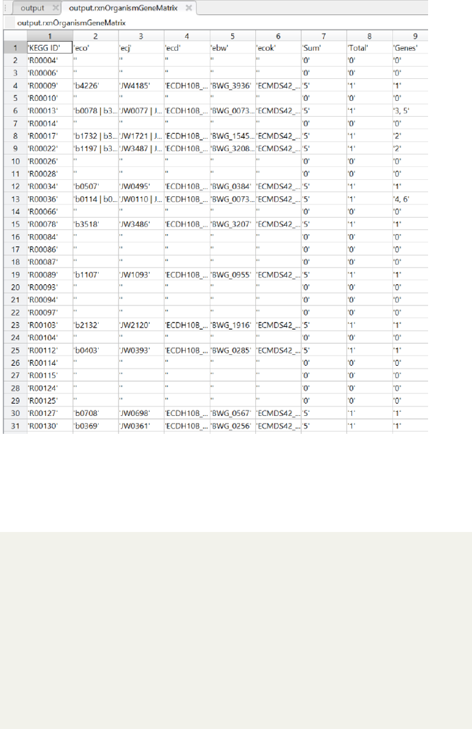
Figure 6: Screenshot of the ”Organisms-Reactions-Genes matrix” Matlab field
of the first draft reconstructions of the five E. coli K-12 strains provided by
AutoKEGGRec.
lines =
f a l s e ( length( outputStru c t . rxnOrganismGeneMatrix ) ) ;
l i n e s ( 1) = tr u e ;
f or l i n e =1:length ( l i n e s )
lineContents =
outputStr u c t . rxnOrganismGeneMatrix ( lin e , : ) ;
i f c o n t a i n s ( s t r i n g ( l i n e C o n t e n t s ( end) ) , ” , ” )
lines(line) = t r u e ;
end
end
s e l e c t e d L i n e s =
s t r i n g ( outputStr uct . rxnOrganismGeneMatrix ( l i n e s , : ) )
The potential of generic reconstructed models for a species is demonstrated
11
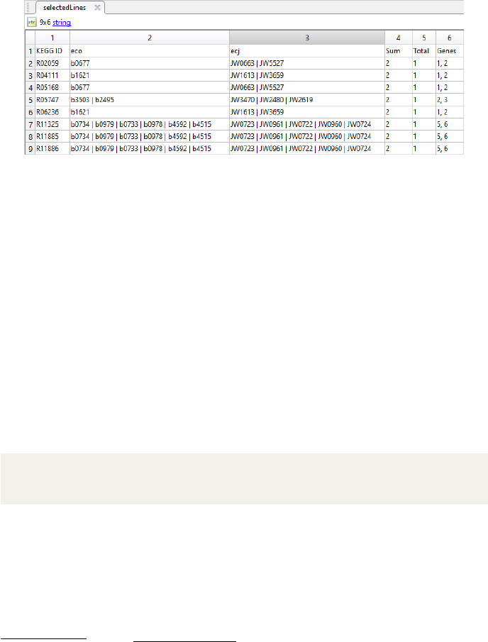
Figure 7: Screenshot of the output for shown Matlab code used on the OrgRxn-
Gen output based on two of the five E. coli K-12 strains. It shows the first part
of all reactions that are encoded by a different number of genes within the two
organisms.
in the human RECON model: Many different cell types can be stored within a
single model, making the data compact and manageable. Due to many similar
core reactions, which are used by all the different cells, this type of model gives a
detailed yet broad overview of the human cell’s metabolic network. In the case of
E. coli, more specifically the five E. coli K-12 strains, it gives a detailed overview
of the reaction network; the ORG matrix in combination with the different plots
describe similarities and differences among the E. coli K-12 strains.
3.1.7 DisconnectedReactions
Usage:
outputStruct =
AutoKEGGRec ( [ ” eco ” ,” e c j ” ,” ecd ” ,” ebw” ,” ecok ” ] ,
’ ConsolidatedRec ’ , ’ D i sconn e ctedR e actio ns ’ )
NB: This option requires a reconstruction to be built. Refer to one of the options
ConsolidatedRec,SingleRec or SommunityRec. If called without an order to generate a
reconstruction, an error message will appear, suggesting the user generate a reconstruction.
AutoKEGGRec creates a cell inside the output containing the KEGG reac-
tion IDs for all the reactions that are disconnected from the giant component.
It does not matter if the reactions are connected to each other; all reactions
not connected to the giant component are listed her for every generated recon-
struction. Example output is shown in Fig. 5 (E). AutoKEGGRec automatically
creates a ”networkData” entry for every reconstruction as an annotation field.
The user can easily access the network information such as the number of reac-
tions in the giant component and the sizes of the disconnected components, as
well as directly identify disconnected reactions.
12
3.1.8 GenePlot
Usage:
outputStruct =
AutoKEGGRec ( [ ” eco ” ,” e c j ” ,” ecd ” ,” ebw” ,” ecok ” ] ,
’ GenePlot ’ )
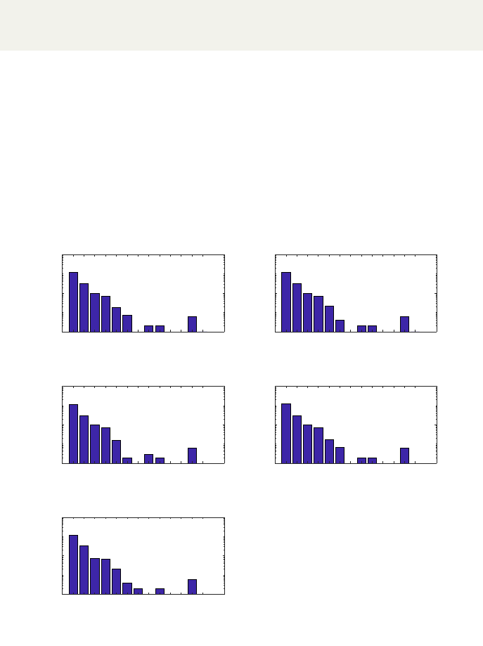
AutoKEGGRec creates a Matlab plot window containing the gene plot (ex-
ample seen in Fig. 8). It can be saved, processed and adapted within the Matlab
window. The plot shows the number of genes vs. the number of reactions for
each of the requested organisms. By default, the Y-axis is in log-scale, but this
can be changed within the Matlab plot window. In the figure the output for
five E. coli K-12 strains provided as input to AutoKEGGRec using this flag
is presented, resulting in the generation of five plots where each plot shows a
bar-diagram of reaction associations per organism.
KEGG organism ID:
eco
1 2 3 4 5 6 7 8 9 10 11 12 13
Number of genes per reaction
100
102
104
Number of reactions
KEGG organism ID:
ecj
1 2 3 4 5 6 7 8 9 10 11 12 13
Number of genes per reaction
100
102
104
Number of reactions
KEGG organism ID:
ecd
1 2 3 4 5 6 7 8 9 10 11 12 13
Number of genes per reaction
100
102
104
Number of reactions
KEGG organism ID:
ebw
1 2 3 4 5 6 7 8 9 10 11 12 13
Number of genes per reaction
100
102
104
Number of reactions
KEGG organism ID:
ecok
1 2 3 4 5 6 7 8 9 10 11 12 13
Number of genes per reaction
100
102
104
Number of reactions
Figure 8: The Matlab plot for the five E. coli K-12 strains. The plot for each
strain shows the number of genes vs. the number of reactions, which gives a
quick overview of the number of reactions encoded by a specific number of genes.
13
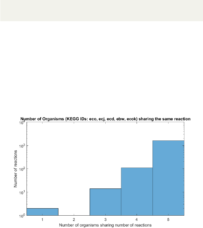
3.1.9 Histogram
Usage:
outputStruct =
AutoKEGGRec ( [ ” eco ” ,” e c j ” ,” ecd ” ,” ebw” ,” ecok ” ] ,
’ Histogram ’ )
AutoKEGGRec opens a Matlab plot window containing a histogram showing
the number of organisms sharing a number of reactions (example seen in Fig. 9
for the five E. coli K-12 strains). The X-axis shows the number of organisms,
starting at one and ending at the number of organisms, whereas the (by default
logarithmic) Y-axis gives the number of reactions that occur in the particular
number of organisms. The user can use this plot to get an idea of common
reactions throughout the input organisms; it could help the user to identify the
number of core/conserved reactions within the metabolic networks based on the
organisms. In this example, i.e. the five E. coli K-12 strains in KEGG, most
of the reactions are shared between the five organisms. Interestingly, there are
some which occur only in one of the strains, as well as some that are common
in three strains.
Figure 9: The histogram shows the number of organisms, here the five E. coli
K-12 strains, vs. the number of reactions. The plot helps to identify the amount
of core reactions shared within the input organism KEGG IDs.
3.1.10 General statements concerning optional inputs
To ensure that the options are correctly used, the options relying on model
building are checked, as well as spelling of the options. There will be error
messages stating what went wrong, and by referencing the help function or this
14

manual, typos can be rapidly identified. The order of the input options does
not matter.
3.2 KEGG annotation and the ATTENTION field
All KEGG annotation is saved within the same fields to be seen in KEGG
within the reconstructions as well as within the omitted output. Changes to
the category names, however, do happen in case of fields supported by COBRA
within the annotation of the reconstructions.
Additionally, AutoKEGGRec introduces a new field in reconstruction and
omitted output, the ”ATTENTION” field. Within the Reconstruction, Au-
toKEGGRec notes suspicious reactions for further inspection. The user may
use that field to note and annotate curated reactions for the tractability of in-
formation. Within the omitted output, AutoKEGGRec notes in that field, why
the reaction was rejected to be implemented (see Fig. 5 (D)). In case of e.g. the
rejected reaction
R00164 : C00562 + C00001 ⇔C00017 + C00009,
the user would find within the annotation field in the omitted output:
”This reactions contains a generic compound or a compound without mass
in KEGG. Check the compounds carefully before adding reaction to model!”,
which allows the user to quickly identify the reason. In this case, checking the
omitted compound list (see Fig. 5 (B)) for any of such points to the reason: the
compounds C00562 and C00017 (”phosphoprotein” and ”protein”, respectively)
do not have a mass and can therefore not be mass balanced. The user can check
all the compounds of the reaction and decide whether and how to implement
them.
3.3 Authors’ recommendation of usage
AutoKEGGRec is intended as a tool that generates various first-draft recon-
structions and delivers them to the user along with some helpful support for
the following manual curation to allow the creation of a high quality model.
Because of this, AutoKEGGRec ships with several different options to optimize
run-time for the purposes of the different users. This way, AutoKEGGRec can
be used not only to create reconstructions, but also to explore the KEGG reac-
tion universe for any number of given organisms and base any analysis on this
information.
However, to generate first-draft reconstructions, the recommended set of input
parameters is:
outputStr u c t = AutoKEGGRec(”ORGANISM IDs” ,
’RECONSTRUCTION’ , ’OrgRxnGen ’ , ’ OmittedData ’ ,
’ Disco nnecte dReact ions ’ , ’ GenePlot ’ , ’ Histogram ’ )
15
With this command, AutoKEGGRec creates (up to several) reconstructions
for the selected KEGG organism IDs and delivers supporting information to aid
in further model curation. The user is advised to save the plots and the gener-
ated Matlab output structure as .mat file. This way, all necessary information
is stored and can be retrieved quickly.
Additionally, using the ATTENTION field, users can implement comments
during the curation process, which allows future user of the model to easy trace
any kind of data and reasoning why such reaction is present within the model.
Thorough annotation and comments highly improves the (re)usability of the
model.
4 Possible curation steps following execution of
AutoKEGGRec
4.1 General steps
The most important part of your reconstruction process comes after you are
done using AutoKEGGRec. No matter where your first draft comes from, and
what functionality it does or does not contain, manual curation is absolutely
essential.
Drawing on the 96-step protocol for generating high-quality genome-scale
metabolic reconstructions set forth by Thiele and Palsson in 2010, we here sug-
gest what steps to take (without right of completeness) when generating your
own genome-scale metabolic reconstruction:
1. Generating the Reconstruction using AutoKEGGRec
2. Adding and correcting exchange reactions (import reactions for cytosol).
Adding exchange reactions can be done easily using addExchangeRxn()
3. Adding biomass and ATP maintenance functions and checking if the biomass
compounds are producible. Adding reactions is simple using the COBRA
function addReaction()
4. Checking mass and charge balance for reactions. For this you can use the
COBRA function checkMassChargeBalance()
5. Checking reversibility of reactions using such databases as KEGG path-
ways, as well as the COBRA function using thermodynamics
6. Gap filling algorithms (COBRA fastGapFill())
7. Manual gap filling (COBRA gapFind())
8. Adding additional compartments and the corresponding reactions and
transport reactions (COBRA addReaction(), addExchangeRxn())
16

9. Verify gene-protein-reaction association
10. Add demand and sink reactions (COBRA addSinkReaction(), addDeman-
dReaction())
11. Checking dead ends and flux consistency (COBRA detectDeadEnds(),
findFluxConsistentSubset(), fastLeakTest())
Repeat step 4 to 11 iteratively for different Biomass functions and/or envi-
ronments. These steps are partly carried out by some tools/functions but they
require active user involvement. Furthermore, in-between each step, which may
contain several substeps (as there will likely be more than one transport reaction
to be added), testing the model is absolutely necessary.
In the example presented here, most of the steps only usee Matlab COBRA
Toolbox functions. Other alternatives also exist, e.g. COBRApy. Since the
reconstructions contain all possible KEGG annotation, which includes for com-
pounds e.g. PubChem IDs, it is easy to cross-reference the compounds to other
databases as well, if other databases do not contain the KEGG IDs.
Many steps require manual curation to ensure high quality of the models,
the tools and functions only support the modeller.
Implementing as much data for compounds and reactions as possible into
the model may save future work, and has few drawbacks. It might allow for
easier comparison of models and also additional uses, e.g. the masses of the
compounds for further applications. In particular, including the masses allows
for a fast and easy check on the mass balance of the reconstructions.
4.2 Community reconstruction refinement
Since AutoKEGGRec is designed to also generate communities based on organ-
ism KEGG IDs, the Authors want to highlight possible further steps after using
AutoKEGGRec. A community reconstruction should be able to model interac-
tions between the organisms contained in the community. Therefore interaction
reactions are necessary.
As described in Section 3.1.3, all the reactions and compounds in the recon-
struction follow the same pattern
R00004 eco[c] : C00013 eco[c] + C00001 eco[c]⇔2C00009 eco[c],
which allows the user to edit several reactions at a time.
As shown in the example network in Fig 3.1.3, none of the organisms are
connected. AutoKEGGRec only generates reconstructions based on the KEGG
database, which includes few transport reactions to link the single organisms.
However, a short script to add ”standard uptakes” and linking the organisms
for gap filling might ease the modeler’s work as described in Section 4.1.
17
