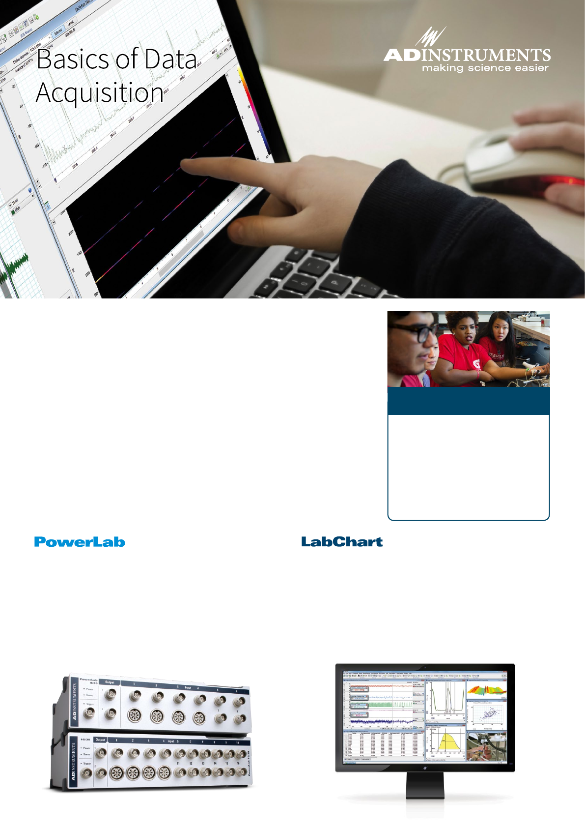
Basics Of Data Acquisition
User Manual: Basics of Data Acquisition Manuals | ADInstruments
Open the PDF directly: View PDF ![]() .
.
Page Count: 16
In 2010, Quacquarelli Symonds released
a list of the Top 100 universities for life
science, based on academic citations,
peer review, recruiter review, faculty
student ratio and international orientation.
PowerLab hardware and LabChart
soware are used at every one of these
institutions, including Harvard, Oxford,
and the University of Tokyo.
Top 100 universities
all use LabChart and PowerLab
About ADInstruments
ADInstruments provides complete and integrated data acquisition and
analysis solutions to academic institutions, government organisations
and private industry.
At the core of our product line is the world-renowned PowerLab system with
LabChart soware. Together they oer comprehensive signal processing, data
recording, display, and analysis features for a wide variety of research applications.
In conjunction with a computer, the systems provide the functionality of a multi-
channel, real-time chart recorder, polygraph, XY plotter and digital oscilloscope.
You can take advantage of variable sampling rates and remarkable resolution
with the benets of powerful, computer-based data handling and analysis.
Wherever your research leads, our team can support you with the latest technology
and powerful but simple tools that give you the power to innovate.
PowerLab is the original high-performance digital data
acquisition device engineered for precise, consistent,
reliable data acquisition, giving you reproducible data
while meeting the strictest international standards.
ADInstruments provides integrated solutions
to advance life science research
All your analysis in one place
LabChart analysis soware is at the centre of all
ADInstruments research solutions and acts as a platform to
integrate all your data streams into one place.
Designed specically for life science data, LabChart provides
up to 32 channels for data display and either automated or
customizable analysis options that are powerful and easy to use.
Basics of Data Acquisition Brochure 2017-A4 V1-0
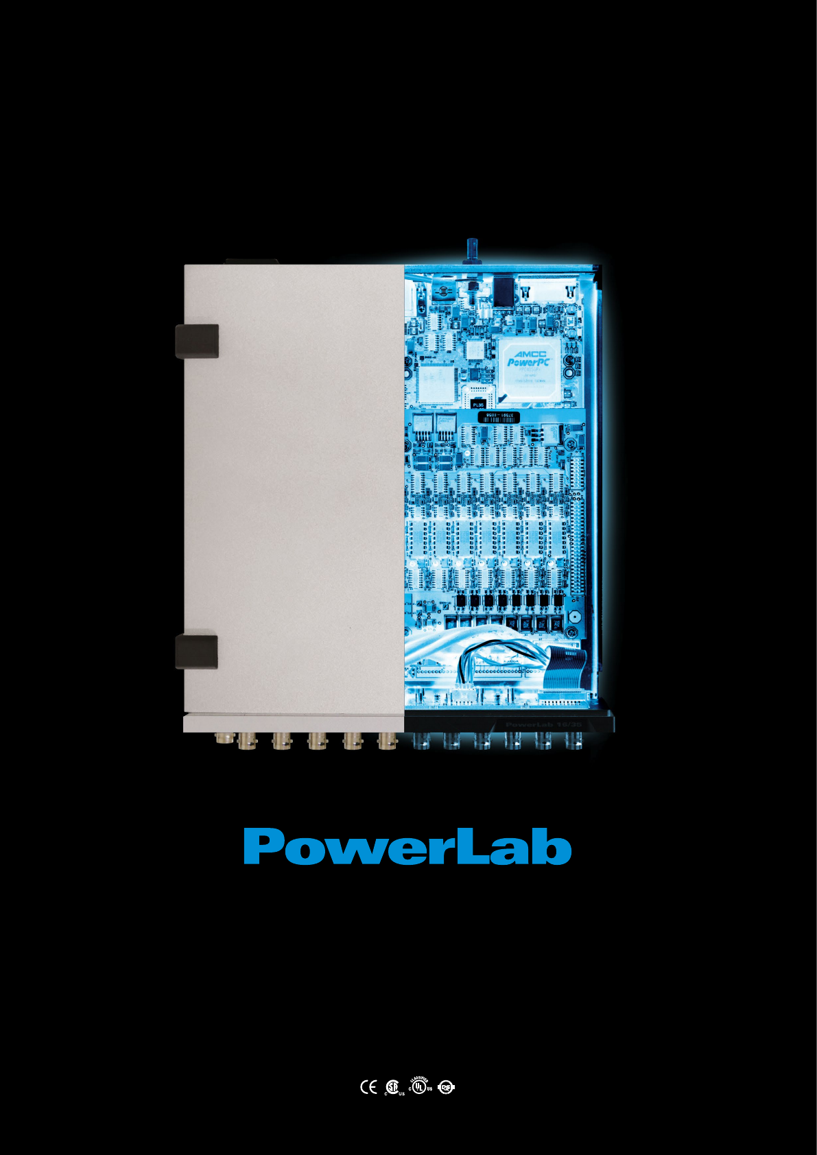
Much more
than a box
Data with integrity
PowerLab is engineered for precise, consistent, reliable data
acquisition, giving you the reproducible data you need while
meeting the strictest international safety standards.
Maximize
your
potential
If you have a particular
research need you
would like to discuss,
get in touch with our
experienced support
team. We can work
with you to customize
an eective solution to
record and analyze the
specic data that you
need.
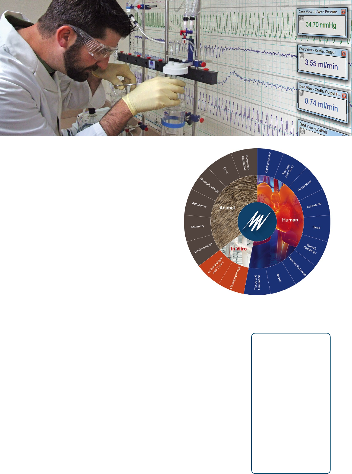
Extend your research into new territories
ADInstruments systems provide the exibility to extend
studies into any of these human, animal or in vitro
applications. Ask one of our experts to design a
system to suit your needs.
Investigating novel or niche research?
With ADInstruments, the power is in your hands. We oer high
spec solutions to acquire a range of quality signals, or you can
integrate your own custom hardware congurations with
PowerLab. With options for both standard analysis features
and smart tools for customization in LabChart, you can easily
apply advanced calculations as your experiment unfolds.
The ADInstruments advantage
•
Experience you can trust
ADInstruments systems have been installed in thousands of research
institutes, universities, hospitals and commercial laboratories worldwide.
With more than 45,000 systems installed worldwide and over 30,000 published
scientic research papers featuring our products, you can be assured that the
decision to purchase an ADInstruments data acquisition system is the right one.
•
Flexibility
The exibility of LabChart allows it to be used in a wide variety of life science
applications, maximising the returns of your investment in time and capital.
•
Intuitive and powerful soware
LabChart allows researchers to concentrate on the science. Powerful data extraction
and analysis features speed up the research process.
•
Data integrity
PowerLab systems are calibrated and tested to deliver data you can trust. The
soware incorporates data integrity features such as multiple block recording with
individual settings and calculations stored within a single le, preservation of raw
data, and date stamping.
•
GLP and 21 CFR Part 11 compliance
LabChart and our GLP soware provide the required user interface, audit trail and signing
components for non-repudiation of data under GLP and 21 CFR Part 11 compliance.
•
Quality and reliability
ADInstruments products are manufactured under a quality system certied by an
accredited body as complying with ISO 9001:2008
•
Excellence in customer training and support
Our international graduate and postgraduate support sta are dedicated to making
sure our customers are satised.
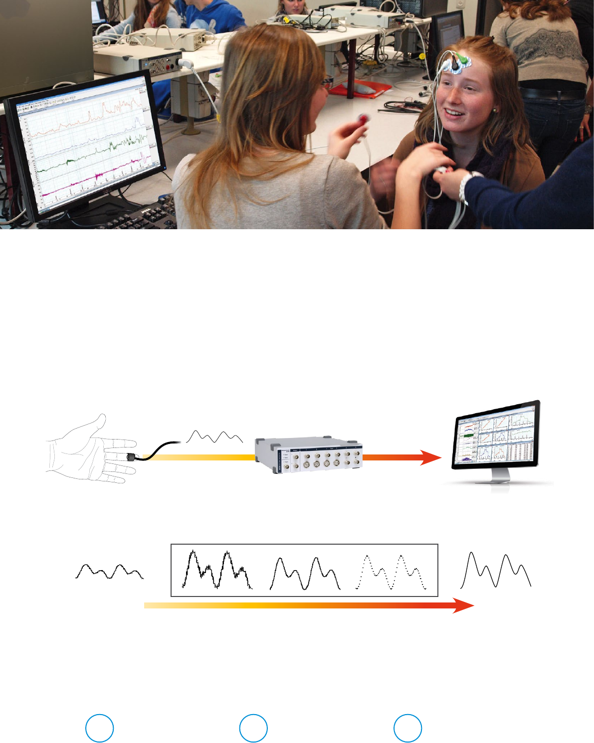
Background
The purpose of the PowerLab and LabChart data acquisition system is to acquire, store and analyze data. Figure 1 shows a
summary of the acquisition. Usually, the raw input signal, which may be from any number of biological or physical sources,
is in the form of an analog voltage whose amplitude varies continuously over time. This voltage enters the PowerLab via
the input connections and can be modied by amplication and ltering, a process called signal conditioning. Aer signal
conditioning, the analog voltage is sampled at regular intervals. The signal is then converted from analog to digital form
before transmission to the attached computer.
LabChart analysis soware displays the data directly; it plots the sampled and digitised data points and reconstructs the
original waveform by drawing lines between the points. Digital data can be stored on disk for later retrieval. LabChart soware
can also easily manipulate and analyze the data in a variety of ways.
Transducer
Input Amplification Filtering Sampling Display
Mechanical
signal
Analog
signal
PowerLab
Hardware
Computer with
LabChart software
Digital
signal
PowerLab hardware
Transducer
Analog signal
Mechanical
signal Digital signal
Computer
PowerLab hardware
Transducer
Analog signal
Mechanical
signal Digital signal
Computer
PowerLab hardware
Transducer
Analog signal
Mechanical
signal Digital signal
Computer
Input Amplification Filtering Sampling Display
Within PowerLab hardware
Figure 1 A summary of data acquisition using the PowerLab system.
Most of the parameters that aect acquisition can be set by the user through the soware. To make a good recording, the
parameters must be appropriate for the signals being recorded.
To acquire good data you need to:
In some disciplines you may be able to nd tables of suggested sampling rates, ranges, and lter settings, but these should
not be applied blindly. You still need to know the science (what you are recording, why you are recording it, and how it relates
to real phenomena) and the technique (how best to record, and what limitations or compromises are inherent in the process).
Select a suitable
sampling rate
1Apply the correct
input range
2Choose suitable
lter settings
3
Sampling rate
The rst thing to choose is a suitable sampling rate. Samples
are taken from the signal at regular time intervals. The
appropriate sampling rate depends on the signal to be
measured. If the sampling rate is too low, information is
irreversibly lost and the original signal will not be represented
correctly (Figure 2A). For example, if you sample at 200 Hz, this
will display 200 points every second. This would be adequate
for a human ECG but you would lose information from a mouse
ECG whose heart rate is 5-6 times higher. If the sampling rate is
too high, no information is lost, but the excess data increases
processing time and may give excessive noise in the signal or
result in unnecessarily large disk les.
You can calculate the size of the data le that will be
collected based on the sampling rate:
Amount of data (bytes) = 2 x number of channels
x sampling rate x recording length (in seconds)
200mV
10 Samples/sec
200 Samples/sec
0mV
200mV
0mV
Actual Signal
Signal wrongly
reconstructed
Amplitude
Time/s
0 1 2 3 4 5 6 7 8 9 10
Figure 2B Aliasing - sampling a higher frequency signal at
1 sample per second gives a misleading waveform (real-life
effects are more subtle).
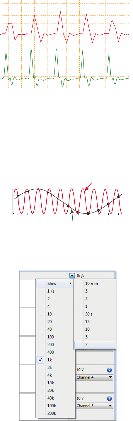
Figure 2A Undersampling - human finger pulse recorded at 10/s
and 200/s. The former sampling rate is too low to depict the
signal accurately.
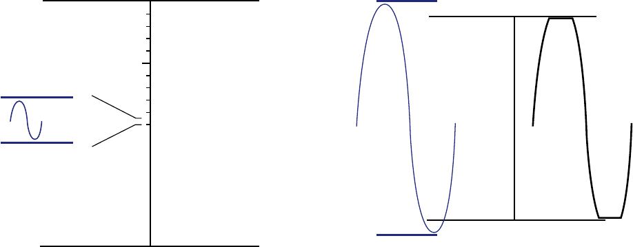
Figure 3 LabChart sampling rate options.
You will need this much space on your computer hard disk
to record the data, but LabChart will compress the le when
saving, so you will not require as much storage space.
Aliasing
Periodic waveform recordings that have been sampled
too slowly may be misleading as well as inaccurate. This is
known as aliasing where high frequency waveforms may be
represented as lower frequency waveforms (Figure 2B).
To prevent aliasing, the sampling rate must be at least twice
the rate of the highest expected frequency of the incoming
waveform. This sampling rate is known as the ‘Nyquist
frequency’, the minimum rate at which digital sampling can
accurately record an analog signal. For example, if a signal
has maximum frequency components of 100 Hz, the sampling
rate needs to be at least 200 Hz to record it accurately. To
provide a safety factor to guard against information loss, it
is usual to sample at ve to ten times the highest expected
frequency rather than the minimum two times.
You can select the sampling rate in LabChart using a small
drop-down menu in the top right corner of the Chart View
(Figure 3). The default setting is 1 KHz, but you can adjust it
to as low as 1 sample every 10 minutes and as high as 200
KHz (depending on the PowerLab model and the number of
channels being used).
In most cases, the highest expected frequency will be known.
It may be limited by the transducer used: a bridge transducer
to measure mechanical force will not produce high
frequencies, for instance. If you are unsure of the frequency
range (bandwidth) of your signal, a useful rule is to choose
a sampling rate high enough to allow at least 20 samples for
any transient peaks or recurring waves in the signal. You can
formally determine a signal’s highest frequency by sampling
the signal at the maximum rate, and looking at the frequency
spectrum of the signal using the Spectrum display available
under the Window menu item in LabChart.
Range and resolution
To accurately record a signal, it is important that the
range of the LabChart channel is greater than the signal’s
amplitude. Many systems use ‘gain’ when looking at
amplied signals. Range is inversely proportional to
gain (the amount of amplication), and is a more useful
concept than gain since it relates directly to the signal
being measured. With a PowerLab system, the range can
be set independently for each channel in the right-hand
drop down menus.
The resolution of the signal represents the accuracy
of the display. PowerLab has a 16-bit resolution which
means the range can be divided into a maximum of
216 levels (65 536) although LabChart ts 64 000 to the
range. So if you are looking at a ±10 V range the smallest
discernible level would be ~300 uV (20 V corresponding
to the ±10 V range divided by 64,000).
If a signal is very small in relation to the range (Figure 4A),
then its resolution will be degraded. In extreme cases,
the recorded waveform may appear stepped rather than
smooth. Even though you could see a ±380 mV signal on
±1 V Range, 16-bit resolution
±1 V
-1 V
+1.2 V
-1.2 V
input signal
Real signal is ±1.2 V
The digital signal is
clipped at ±1 V
Figure 4B If the signal is larger than the range, the top and
bottom is ‘clipped’ and maximum and minimum value is lost.
±10 V Range, 16-bit resolution
±10 V 64 000
-10 V 0
+0.5 V
0 V
input signal
0 V
5 V
Figure 4A A small signal on a large range will have poor
resolution as only a small part of the range is used.
the default 10 V range, it would be preferable to use 500
mV range to measure it at maximum resolution. It would
be safer in practice to use a 1 V or 2 V range, though, since
unexpectedly large peaks could exceed the 500 mV range if
the signal was unpredictable.
If the signal amplitude exceeds the range (Figure
4B), there will be severe information loss. Any signal
exceeding the range is ‘out of range’, a condition
indicated where no amplitude can be given. If there is
any possibility of this condition occurring, you should
set the range to a larger value.
For the best resolution, the maximum amplitude of the
signal you are interested in should be reasonably close
to the chosen range without exceeding it. That way, the
minimum change in voltage discernible in digitisation
remains small in relation to the signal being measured.
Note that changing a waveform’s on screen display (by
enlarging it in the Zoom window or by stretching or
shrinking its Amplitude axis, for instance) does not aect
its resolution, just its appearance.
Using single-sided or differential inputs
The Single-sided and Dierential options in LabChart control signals acquired through the dierential inputs (i.e. the
pod connectors). These options do not appear where the input for a channel is only single-sided — in this case, the input
functions as if the single-sided option were checked permanently.
Single-sided — When this option is selected, only the positive (non-inverting) input on the front of the PowerLab is used,
and a positive signal fed into it will be shown as a positive signal on the display. The inverting input is grounded.
Dierential — When the Dierential option is selected, both positive (non-inverting) and negative (inverting) inputs for
that channel are used, and neither is grounded. The signal shown on the display is the dierence between the signals at
the positive and negative inputs. If both input signals were the same, they would cancel each other out.
Filtering and smoothing
Filters and smoothing are used to get rid of noise from a
signal. Noise can be referred to as unwanted signal. It is
likely to be a problem at lower range settings, when trying to
measure very small signals. Random noise (such as thermal
noise) is inherent in all electronic circuits, including those of
the PowerLab recording unit. It can be minimised through
ltering. Other causes of noise are stray electromagnetic
and electrostatic elds including interference (oen at
the mains frequency of 50 Hz or 60 Hz) from unshielded
power lines, switching equipment, uorescent tubes and
computers. Interference can signicantly aect a signal, but
can be reduced through reasonable care in the arrangement
and shielding of equipment and cables.
There are two types of lter available within PowerLab
and LabChart: analog/hardware lters or digital/
soware lters.
Analog/hardware lters
Analog/hardware lters are used to lter the incoming,
continuous signal before it is sampled by the analog
to digital converter (ADC). These lters are built into
ADInstruments front-ends (Bio Amps, Bridge Amps etc)
and some PowerLab units. ADInstruments front-ends
initially amplify the signal to a level suitable for ltering.
The analog lters are then used to remove unwanted
frequencies, before further amplication is performed
before digitisation. Filtering the signal prior to full
amplication is essential for biopotential measurements
to improve the signal-to-noise ratio.
Digital/soware lters
LabChart’s digital or soware lters lter the data aer it
has been sampled and recorded by the PowerLab. Digital
lters are used during or aer data acquisition and are
advantageous because:
•
It is possible to design digital lters that are
impractical to make in analog form
•
They are stable over time and provide consistent,
reproducible signal ltering
•
In LabChart, they can be applied post data acquisition
while the raw data is retained
A disadvantage of post-acquisition digital ltering is that
unless analog/hardware lters have also been used prior
to digitisation, any noise or baseline oset will also be
amplied. This will have a negative eect on the signal’s
resolution.
Basic ltering terms
To understand the basics of ltering, it is rst necessary
to learn some important terms used to dene lter
characteristics. While these terms apply to all types of
lters, for simplicity the following examples will only
refer to low-pass lters.
•
Cut-o frequency (fc) — Also referred to as the
corner frequency, this is the frequency or frequencies
that dene(s) the limits of the lter range(s). It is the
desirable cut-o point for the lter.
•
Stop band — The range of frequencies that is ltered out.
•
Pass band — The range of frequencies that is let through.
•
Transition band — The range of frequencies between
the pass band and the stop band where the gain of
the lter varies with frequency.
Low-pass lters
A low-pass lter allows signal frequencies below the low
cut-o frequency to pass and blocks frequencies above
the cut-o frequency. It is commonly used to help reduce
environmental noise and provide a smoother signal.
A simple way to understand how a lter works is to plot
signal frequency against signal gain (Figure 5A). When a
signal is unltered, it is recorded at a gain of 1, that is,
the full signal is being recorded. All low-pass lters have
a frequency (fa) above which the gain is very small and
the signal is virtually non-existent.
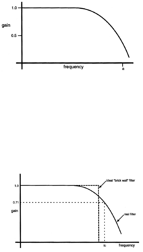
Ideally, a perfect low-pass lter would have a gain of 1
for signals having frequencies that are meant to pass
through the lter, and a gain of zero for frequencies
that are meant to be blocked (like the ideal brick wall
lter in Figure 5B). However, lters are imperfect, and
the gain of a low-pass lter never quite falls to zero.
The frequency at which the gain starts to decrease by a
reasonable amount is the cut-o (corner) frequency (fc).
This reduction in signal gain aer the cut-o frequency is
oen referred to as signal attenuation and is commonly
presented in decibel (dB) units.
Figure 5A Gain versus frequency (S.S. Young, 2001).
Figure 5B Effect of low-pass filtering on signal gain (S.S. Young, 2001).
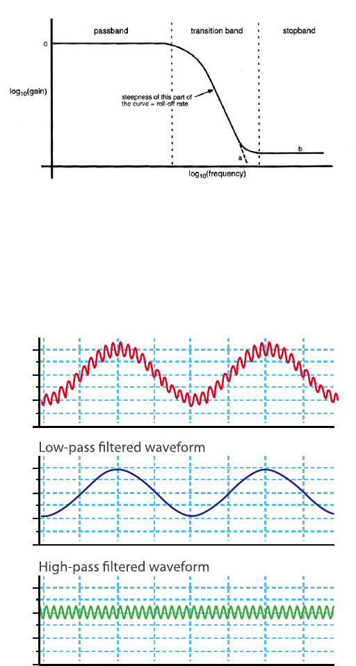
Figure 7 Comparison of the effects of low and high pass filters
on a signal waveform.
1
0
-1
-2
1
0
-1
-2
1
0
-1
-2
Original waveform (low and high frequencies)
Note: Decibels are not units of measurement in the
conventional sense but represent a log ratio, thereby
describing how much bigger or smaller one thing is
compared to another.
All signal frequencies below the cut-o frequency
are referred to as the pass band (Figure 6). All signal
frequencies above the cut-o frequency are referred to
as the stop band. The region between the pass and stop
bands is referred to as the transition band or transition
width. This width (in Hz) depends on how sharply the
lter response drops from the pass band to the stop
band. Related to this is the roll-o rate, which, for low-
pass lters is the rate at which the signal gain decreases
when the signal is above the cut-o frequency. The
narrower the transition band, the steeper the roll-o.
Other lter types
High-pass lters
A high-pass lter allows frequencies higher than the
cut-o frequency to pass and removes any steady direct
current (DC) component or slow uctuations from
the signal. Such lters are oen used to stabilise the
baseline of a signal (i.e. minimise baseline dri in an ECG
signal). A useful comparison of the eects of a low-pass
lter in comparison to a high-pass lter is presented in
Figure 7.
Mains lters
Mains interference (50/60 Hz) from power lines or
electrical equipment is not static and may vary during
the day, with more variation in some countries than
others. An adaptive mains lter tracks and removes
the mains noise (including the harmonics of the
fundamental) with minimal distortion to the recorded
signal. Digital mains lters are included in LabChart
for use with PowerLab/10, /15, /20, /25, /26, /30 and/35
series models.
Notch lters
A notch lter removes a particular frequency from a
signal and has a frequency response that falls to zero
over a narrow range of frequencies. For example, a 50 Hz
notch may block signals from 49.5 – 50.5 Hz. Notch lters
are available in all ADInstruments Bio Amps.
Narrow band-pass lters
Narrow band-pass lters are used to remove all signal
frequencies except for a particular band, say to record
8 – 12 Hz activity in EEG recordings. Frequencies either
side of this band are blocked.
Band-pass lters
A band-pass lter may be used to pass a larger range of
frequencies say 0 – 100 Hz in EEG activity. Frequencies
either side of this band are blocked.
Figure 6 Filter bands (S.S. Young, 2001).
Band-stop lters
A band-stop lter blocks a certain range of frequencies
and allows frequencies either side of this range to be
passed. For example, you may wish to block Beta [ß1:
16 – 32 Hz] activity from an EEG recording but record all
other frequencies between 0 – 15 Hz and 33 – 100 Hz.
Anti-aliasing lters
The anti-aliasing lter is a sampling rate-dependant
low-pass lter. Aliasing can be caused by under sampling,
so for this lter to be eective it is important that the
correct sampling rate has been applied. In LabChart, the
cut-o frequency of the anti-aliasing lter is set to half
the sampling frequency but disabled at sampling rates
lower than 100 Hz. The anti-aliasing lter is a digital
lter available in the 15 and 26 series PowerLabs.
Smoothing
Another means of removing unwanted high frequencies, noise or clutter from a waveform, is to use ‘smoothing’. In
LabChart, it works both oline and online. Choosing the Smoothing… command from any Channel Function drop-down
menu displays the Smoothing dialogue for that channel.
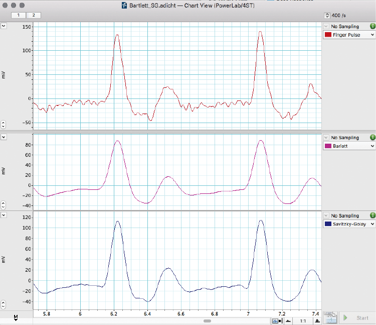
Four smoothing methods are available: a moving average with a Triangular Window, Savitzky–Golay, Median Filter and
Averaging.
•
Triangular (Bartlett) window smoothing works by taking the sample point together with a variable number of points
on each side in the moving average window, weighting the values (most at the middle, which decreases to zero going
out towards the window edges) and averaging them to give the smoothed value at the sample point (Figure 8).
Figure 8 Example used in LabChart Training courses, examining the differing effects of the Bartlett
and Savitsky-Golay smoothing functions.
•
Savitzky–Golay smoothing works by tting a polynomial in a window around each sample point, using least squares
tting. You can specify the order of the polynomial from two to six.
•
Median lter smoothing sorts the data values in the window around each sample point and returns the middle value.
•
Averaging (decimation) smoothing replaces all the data values in the window with a true (“boxcar”) averaged value.
This compresses the data and eectively results in a change to the sampling rate.
With all the smoothing methods, the number of points used to calculate each smoothed value is set with Window width.
The window width is always an odd number (3–2000001 for triangular smoothing, 3–999 for Savitzky–Golay smoothing,
3–255 for the median lter and 2–2000001 for averaging). The window width should be chosen with caution. A window
width that is large in comparison with the time-span of changes in the signal slope will bias the calculation of the
smoothed value, whereas a too-small width will not eectively remove noise.

Suggested settings for selected life science applications
Signal Range Sampling rate Filters/Other information
ECG 10 -20 mV • Mouse 4 kHz
• Rat 2 – 4 kHz
• Rabbit 1 – 2 kHz
• Guinea Pig 1 – 2 kHz
• Dog 400 Hz – 1 kHz
• Pig 400 Hz – 1 kHz
• Human 400 Hz – 1 kHz
Should be 15-30
sample points in
the QRS Complex
ECG signals contain limited information above 100 Hz.
• High pass: 0.3 Hz to minimise iso-electric (baseline) drift
• Low pass: ≤ 25 – 50 % sampling rate
(typically 200 – 1 kHz low-pass cut-off)
• Notch: Do NOT use as may distort ECG signal.
• Mains: Will suppress electrical interference without
distorting signal.
EEG/ECoG 200 – 500 μV 400 – 1000 Hz EEG signals contain limited information above
50 – 100 Hz (Humans, Rats, Mice and Sheep).
• High-pass: 0.1 or 0.3
• Low-pass: 100 – 200 Hz cut-off
• Notch: No (unless the user is aware of affect on signal)
• Mains: Yes
Frequencies of particular interest:
• Delta: 0.5 – < 4 Hz
• Theta: 4 – < 8 Hz
• Alpha: 8 – < 12 Hz
• Spindles: 12 – 14 Hz
• Sigma: 12 – < 16 Hz
• Beta: (ß1) 16 – 32 Hz
• Beta: (ß2) 30 – 60 Hz
EMG Variable
between
species and
muscle types
2 – 4 kHz EMG signals contain variable frequencies; however, most
common frequency bands recorded are 0.3 Hz – 1 or 2 kHz.
• Notch: No (unless the user is aware of effect on signal)
• Mains: Yes
Removing ECG artifacts, particularly in intrathoracic
recordings (i.e. esophageal EMG) often requires difficult
template matching (not available in LabChart). If you
need to remove low frequency artifacts > 2 Hz
(i.e. respiratory or ECG artifacts) prior to recording/
digitizing the signal, then use the high-pass filters
available in the Bio Amps.
Blood Pressure For accurate
reproduction of
dicrotic notches and BP
harmonics, sampling
speeds of 50 to 100
times the heart rate
(in Hz) are desirable.
• Humans: 400 Hz
• Guinea Pigs/Rats:
2 kHz
• Mice: 2 kHz
Typical heart rates:
• Humans: 80 – 200 bpm (max 4 Hz)
• Guinea Pigs/Rats: 200 – 400 bpm (max 7 Hz)
• Mice: 500 – 700 bpm (max 12 Hz)
As a minimum, the low-pass filter frequency should be
10 times the heart rate (in Hz) and half the sampling rate.
Recommended low-pass cut-off frequency:
• Humans: 100 – 200 Hz
• Guinea Pigs/Rats: 100 Hz – 1 kHz
• Mice: 100 Hz – 1 kHz
Data display
Apart from biopotential signals such as ECG and EEG (where you are interested in the electrical signal as a voltage), few
biological signals will have much meaning as a raw voltage signal and may require further modication to display the
parameters of interest.
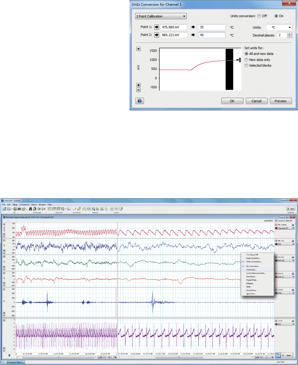
Calibration
Most transducers require calibrating before use.
The calibration process converts the voltage
signal into units of the quantity being measured
by the transducer, such as units of pressure or
temperature.
Most transducers and ampliers are linear.
This means the voltage output relative to the
quantity measured is a straight line. These can
be calibrated in LabChart with a 2-point ‘units
conversion’, where the two points cover the range
of interest. For example, if recording mammalian
body temperature, the temperature probe could
be calibrated with 35°C and 45°C. In this case, the
voltage output would be measured with the probe
in a solution at each temperature. These readings
would be then converted to the temperature in °C
(Figure 9). If the transducer or amplier is non-linear
then a multi-point calibration must be carried out
which requires an additional LabChart extension.
Data calculations
Even with the data being displayed in the correct units, you may wish to display other features of the signal which may have
more meaning for your study such as a heart rate, the change in pressure over time (dP/dt) or the area under the signal. Each
LabChart Channel has a Channel Function drop-down menu with additional features (Figure 10).
Figure 9 Two points conversion of a voltage signal into temperature.
Figure 10 LabChart Channel Function drop-down menu.
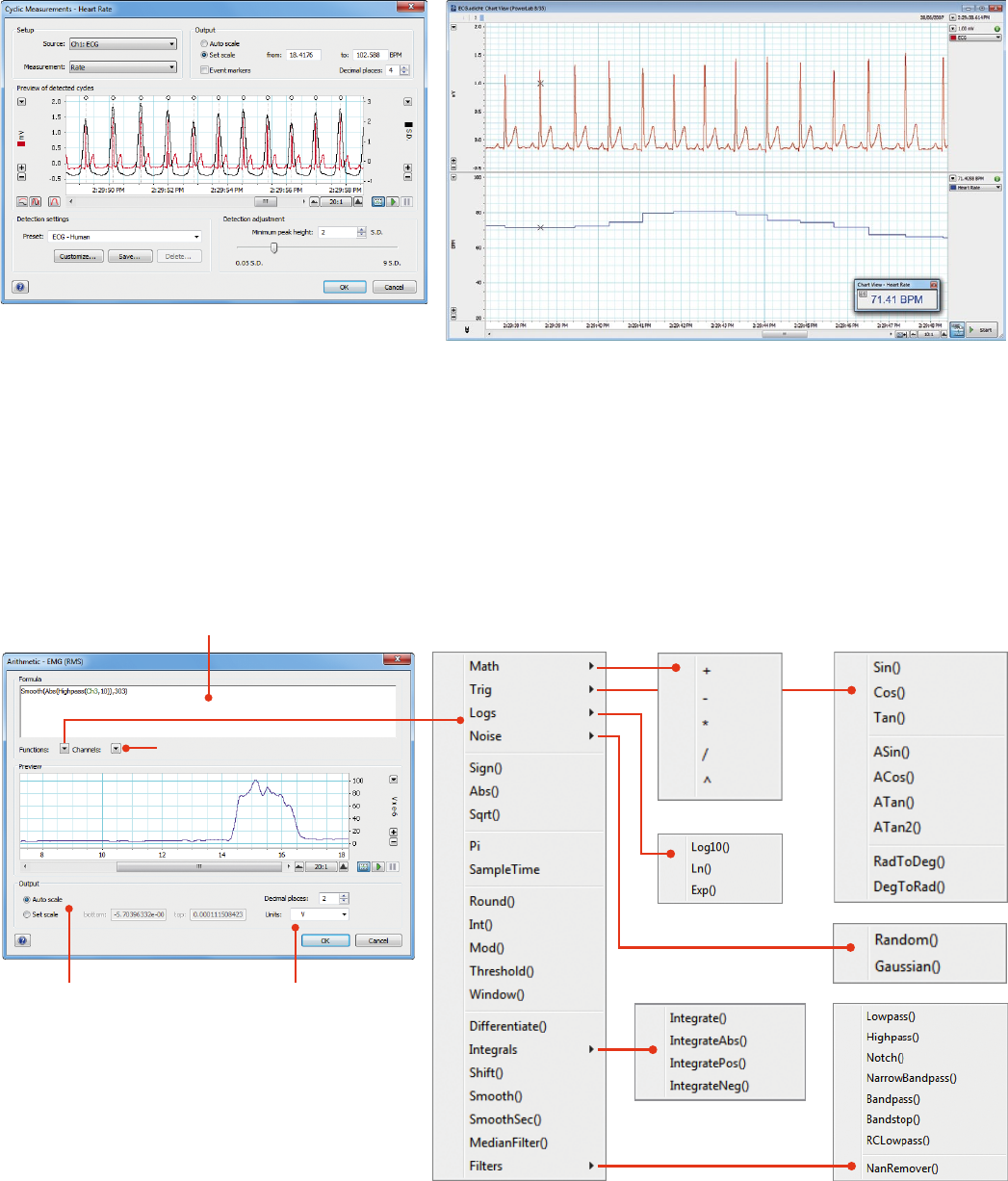
Cyclic measurements
Cyclic Measurements analyse periodic waveforms, either online or oline. LabChart preprocesses the signal, detects cycles in
the waveform, and then uses those detected cycles to perform various calculations on the cycles (cyclic minimum, maximum,
mean, rate, period frequency etc). Choose Cyclic Measurements… from the Channel Function drop-down menu. The input
data is selected and the cyclic function chosen. LabChart has a series of pre-set detection waveforms to allow the cycles to be
determined and then the selected measurement can be displayed over the raw data or on a separate channel (Figure 11).
Figure 11 Cyclic Measurements set-up (left)
and output display.
Expression entry box
Source data channel
Manually set the
Amplitude Axis scale,
or ask LabChart to do it
automatically.
Enter units for the
calculated channel.
Figure 12 Arithmetic set-up.
Arithmetic
The Arithmetic calculation allows you to arithmetically combine waveform data from dierent channels as well as applying
an algorithm to data inputs. It works online (during recording) as well as oline.
Choose Arithmetic… from the Channel Function drop-down menu to open the Arithmetic dialogue (Figure 12). The channel
in which results will be displayed is indicated in the dialogue title.
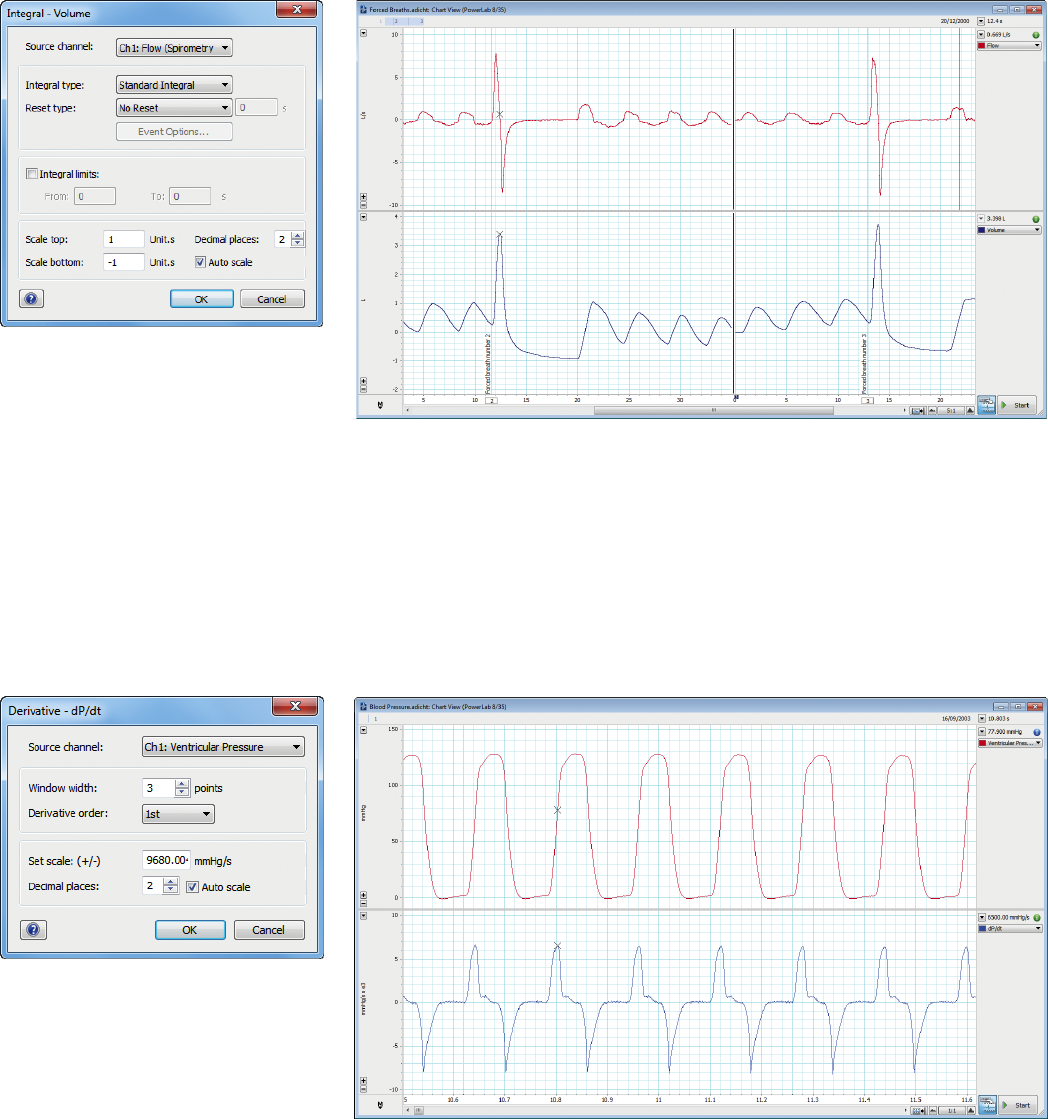
Integral
The integral of a waveform is equal to the area underneath it. The Integral calculation can calculate integrals with respect
to time both online and oline.
A typical application where this is useful is in respiratory work where air movement is normally quantied by measuring
ow with a pneumotachograph. The ow signal is then integrated to give the volume.
Choose Integral… from the Channel Function drop-down menu of the channel you wish to display the calculation result.
In the Integral dialogue (Figure 13) for that channel, you choose the source channel, the type of integral, the resetting
mode, the limits of the integral and the scale to be used. The accumulative integration can be displayed
(no reset) or it can be reset by time, cycle or event.
Derivative
It is also possible to nd the rst or second order derivative of a signal waveform with LabChart. A typical application
where this may be of use is when measuring ventricular pressure and you are interested in the rate of the pressure change
(dP/dt). You can determine this using the rst order derivative of the pressure signal (Figure 14). Choosing the Derivative…
command from a Channel Function drop-down menu displays the Derivative dialogue for that channel. As with most
channel calculations, you specify a source channel in the Source channel drop-down list.
Figure 13 Integral set-up. The Flow of
Channel 1 is integrated to give Volume on
Channel 2.
Figure 14 Derivative set-up. The
dP/dt (mmHg/s) of the pressure
waveform is displayed.
Summary
The bare essentials of data acquisition and display
•
Dene the variables to be measured. You will need to know the normal range and allow for any potential eects of your
intervention.
•
Convert the physiological eect to a voltage. A transducer and amplier will be required to convert the variable into a
voltage signal.
•
Choose the sampling rate. The general rule is to sample at least twice the highest expected frequency of the incoming signal.
•
Set the range. This allows you to record your signal with good resolution, but be careful not to set it too low or data
could be irreversibly lost.
•
Apply appropriate lters. Use lters to reduce noise or unwanted frequencies either with a hardware or digital lter.
Using the latter in LabChart allows you to maintain your raw data.
•
Calibrate your transducer. Change the voltage signal into meaningful units.
•
Set up channels for calculated data. Channel calculations can display meaningful parameters of your raw input signal.
Advanced data acquisition and analysis - LabChart Modules
LabChart Modules are application-specic acquisition and analysis LabChart Add-Ons soware.
Module Purpose
• Blood Pressure
Module
The Blood Pressure Module detects, analyzes, displays and reports a set of cardiovascular
parameters from arterial or ventricular pressure signals. It can be used online or offline.
• Cardiac Output
Module
The Cardiac Output Module allows for cardiac output calculations to be derived from a
LabChart recording of a thermodilution curve.
• DMT Normalization
Module
The DMT Normalization Module calculates the optimal pretension conditions for microvessels
prior to commencing experiments using DMT wire myographs.
• Dose Response
Module
The Dose Response Module generates dose response curves and calculated values such as EC50
and Hill slopes within LabChart. It can be used in online or offline modes.
• ECG Analysis
Module
The ECG Analysis Module detects and examines ECG components online or offline providing
statistical and graphical analysis. It features ECG averaging and is suitable for human and
animal recordings.
• HRV Module The HRV Module analyzes variability in ECG or arterial pulse recordings. A number of heart rate
variability parameters, graphs and a report can be generated online or offline.
• Metabolic Module The Metabolic Module enables real-time acquisition and online or offline analysis of human
metabolic parameters such as RER, VCO2, VO2 and VE.
• Peak Analysis
Module
The Peak Analysis Module provides automatic detection and analysis of multiple signal peaks in
acquired waveforms. The module can be used in online or offline modes.
• PV Loop Module The PV Loop Module provides a variety of views, plots and tables for the analysis of left
ventricular pressure and volume data in small and large mammals. The module can be used in
online or offline modes.
• Spike Histogram
Module
The Spike Histogram Module allows the detection, discrimination and analysis of extracellular
neural spike activity online or offline.
• Video Capture
Module
The Video Capture Module is used to record and synchronize a video movie with a LabChart data file.
This allows simultaneous playback and correlation between data and video recorded events.
Reference
S.S Young – ‘Computerised Data Acquisition and Analysis for the Life Sciences – a Hands-On Guide’. 2001.
PowerLab systems and signal conditioners meet the European EMC directive. ADInstruments signal conditioners for human use are approved to the
IEC60601-1 patient safety standard and meet international standards. ISO 9001: 2008 Certied Quality Management System. PowerLab and LabChart are
trademarks of ADInstruments Pty Ltd. All other trademarks are the property of their respective owners.
All your analysis
in one place
Enabling discovery
LabChart data analysis soware creates a framework for all of your
recording devices to work together, allowing you to acquire signals
from multiple sources simultaneously and apply advanced calculations
as your experiment unfolds. Even better, LabChart tracks every action
you take and never modifies your raw data, ensuring the integrity of
your results so you can focus on the true insights of your research.
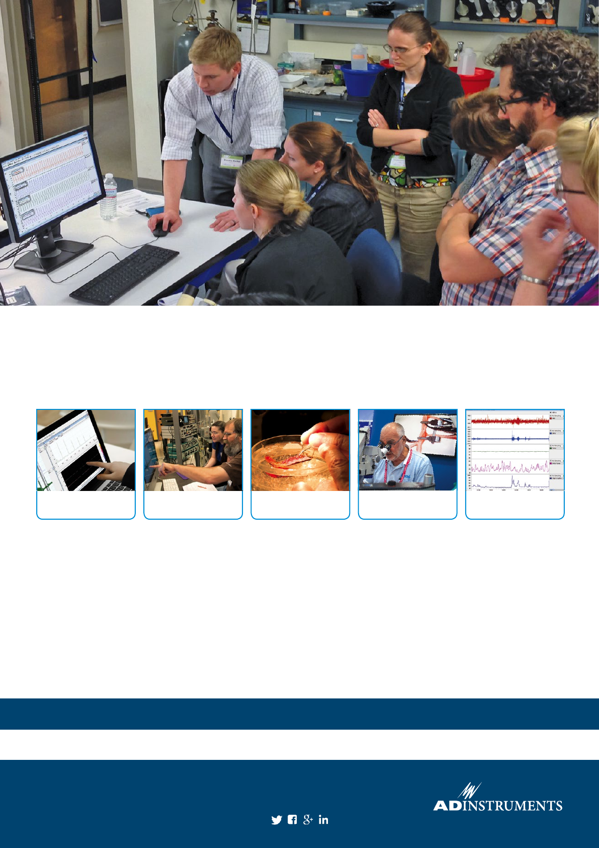
How else can ADInstruments support you?
Maximize time and resources with our customized training services delivered at your facility, on your
equipment, on your terms. Our range of interactive, hands-on courses and workshops reduce
on-boarding time and work to increase eiciency and output — helping you achieve your research and
education aims, faster.
Find out more at adi.to/training or visit our website for many additional free resources:
How-to Videos • Knowledge Base • Soware Forum • Downloads
We can help you:
•
Develop your technical expertise with application-
focused sessions or on-site demonstrations.
•
Experience a range of tools to acquire and display
data, and apply calculations automatically for research
or education.
•
Learn to customize hardware and soware settings to
how you want your results to appear, every time.
•
Lower operational costs by reducing the time between
acquiring hardware and optimizing your research techniques.
•
Train all the members of your team at once with on-site
training - get your entire lab on the same page.
•
Gain condence in the lab and learn skills and knowledge
you can apply to existing and future experimental
protocols.
Soware
Training
Personalized
Training
Research Application
Workshops
Surgical
Training
Live
Webinars
ADInstruments Worldwide
Australia l Brazil l Europe l India l Japan l Mainland China l Middle East l New Zealand l North America l Pakistan l South America l South East Asia l United Kingdom
Visit our website or contact your local ADInstruments salesperson for more information
adinstruments.com
