Bellhop3D User Guide 2016 7 25
User Manual:
Open the PDF directly: View PDF ![]() .
.
Page Count: 76


Heat, Light, and Sound Research, Inc.
!
Table of Contents
BELLHOP3D User Guide! "2

Heat, Light, and Sound Research, Inc.
BELLHOP3D USER GUIDE 1
I. Introduction 1
II. Under the Hood: the BELLHOP algorithm 3
A. Introduction: Beam types and overview of beam tracing"3#
B. Theory"8#
C. Geometric Beams"11#
D. The Compound Matrix Method"12#
E. Beam changes across interfaces"14#
III. Running BELLHOP3D 17
A. Environmental Information: Basic input file"17#
B. Environmental Information: Bathymetry"20#
C. Environmental Information: Oceanography"23#
D. Ray trace run: Nx2D"27#
E. Ray trace run: Full 3D Mode"31#
F. Transmission Loss"31#
IV. Test Cases 34
A. Free-Space and Half-Space Propagation"35#
B. The Perfect Wedge"39#
C. Truncated Wedge"43#
D. Seamount"49#
E. The Harvard Case Eddy Scenario"53#
F. Rotated Munk Profile"55#
BELLHOP3D User Guide! "3

Heat, Light, and Sound Research, Inc.
G. Korean Seas"59#
H. Incoherent and Semi-Coherent TL options"68#
V. Summary 71
Acknowledgments 72
BELLHOP3D User Guide! "4

Heat, Light, and Sound Research, Inc.
BELLHOP3D USER GUIDE
I. Introduction
BELLHOP3D is a beam tracing model for predicting acoustic pressure fields in ocean
environments. It is an extension to 3D environments of the popular BELLHOP model and includes
(optionally) horizontal refraction in the lat-long plane. Of course, 3D pressure fields can be
calculated by a 2D model simply by running it on a series of radials (bearing lines) from the source.
This is the so-called Nx2D or 2.5D approach. However, that approach neglects the refraction of
sound energy out of the vertical plane associated with each bearing line. Such out-of-plane effects
can be important when there are significant horizontal gradients in the environment. These occur
with strong oceanographic features such as nonlinear internal waves, or in areas with strong
bathymetric features. This is currently an active area of research.
A very preliminary research version of BELLHOP3D was written in 1985 in FORTRAN. However, it
did not allow environmental information (sound speed and bathymetry) to be read in from input
files. Instead, the research version required a user-defined analytic function for the sound speed,
c( x, y, z ), as a function of latitude, longitude, and depth. The research version also did not allow
variable bathymetry.
Separately a Matlab conversion of the original research code was done around 2004. The Matlab
environment is much easier to develop in; however, we have chosen not to build off of that here,
since the Matlab code runs much more slowly (about 50 times slower).
The beam tracing structure leads to a particularly simple algorithm. Several types of beams are
implemented including Gaussian and hat-shaped beams, with both geometric and physics-based
spreading laws. BELLHOP3D can produce a variety of useful outputs including transmission loss,
eigenrays, arrivals, and received time-series. It allows for lat-long variation in the top and bottom
boundaries (altimetry and bathymetry), as well as full 3D variation in the sound speed profile.
Additional input files allow the specification of directional sources as well as geoacoustic properties
for the bounding media. Top and bottom reflection coefficients may also be provided. BELLHOP3D
is implemented in Fortran with Matlab wrappers to display the input and output. The code
BELLHOP3D User Guide! "1

Heat, Light, and Sound Research, Inc.
conforms closely to standards and can be used on a variety of platforms (Mac, Windows, and
Linux). This report describes the code and illustrates its use.
BELLHOP3D User Guide! "2

Heat, Light, and Sound Research, Inc.
II. Under the Hood: the BELLHOP algorithm
A. Introduction: Beam types and overview of beam tracing
BELLHOP3D includes 4 different types of beams:
•Cerveny Beams: We use this term to refer to the original beams derived in the 1982 paper by
Cerveny, Popov, and Psencik. These beams evolve roughly as a true propagating beam would;
however, the beam field is only accurate near the axis of the ray which can cause problems.
•Geometric Hat-Beams: Much more reliable than the Cerveny beams; recovers conventional ray
theory but with the advantages of a beam-tracing algorithm. Good framework for algorithmic
testing because any flaws are obvious.
•Geometric Gaussian-Beams: Much improved accuracy relative to the hat beams with some
increase in run time.
•Geometric Hat-Beams in Cartesian Coordinates: Improved efficiency compared to the hat
beams in ray-centered coordinates. Results are essentially identical to the ray-centered beams.
These last two options should generally be the standard for use with BELLHOP3D; however, we
provide the other choices for research purposes.
The initial version of BELLHOP3D has been developed using what we call ‘Cerveny’ beams. This
style of Gaussian beam follows the classic 1983 paper by Cerveny, Popov, and Psencik in which
the beams evolve according to physical laws. In other words, they focus and defocus roughly as a
real beam in space would do. The reason for starting with this formulation is essentially historical.
In practice, with our 2D version of BELLHOP we had implemented quite a few different types of
beams. Originally BELLHOP (2D) also started off with the Cerveny beams. The first change we did
was to implement a formulation of the Cerveny beams is Cartesian coordinates rather than ray-
centered coordinates. Ray-centered coordinates are the arclength, s, and normal distance from the
ray, n. Cartesian coordinates are the range coordinate, r, and the vertical distance, delta z, from the
ray. The representation in Cartesian coordinates leads to a much more efficient code for evaluating
the contribution of a given beam to the total acoustic field.
The next stage in the evolution of BELLHOP was to implement ‘geometric’ hat-shaped beams.
These beams are not physical per se, but instead spread according to the expansion of a ray-tube.
By using a hat-shape (triangle) for each beam one obtains a construction inspired by the finite-
element literature. The result recovers precisely the ray-theoretic result. However, the beam
BELLHOP3D User Guide! "3

Heat, Light, and Sound Research, Inc.
implementation provides an elegant framework for the implementation and yielded a ray-tracing
result that was free of many of the traditional problems of ray models.
Finally, we replaced the hat-shaped beams with Gaussian beams but still implement with a
geometric spreading function. Further, we implemented a stop on the minimum width of the beams
to eliminate caustics in the ray field.
In summary, the 2D version of BELLHOP has beams implemented in both ray-centered and
Cartesian coordinates. It also has beam types that spread physically (Cerveny) or geometrically.
The geometric beams are either hat-shaped or Gaussian. Finally, they may optionally have a limit
on the minimum width.
The obvious question then is which is the best? The answer is that we generally obtain the best
accuracy with geometrically-spreading Gaussian beams that have the minimum-width constraint.
However, we also often use the geometrically-spreading hat-shaped as they are faster. They are
faster because with the Gaussian beams one gets many contributing beams of a given class at a
specific receiver location; with hat-shaped beams, exactly two beams of a given class contribute.
To get the hat-shaped geometric beams to work, one must be extremely careful in the
implementation. If the beams are too narrow, then gaps between the beams will show up in the
field plots. If they are too wide, then that is also easy to observe in the beam plots. Once they are
correctly implemented, then the Gaussian beam version is trivial to implement and smooths out
many of the flaws of ray theory.
A further subtlety that is unique to the 3D version of Gaussian beams is that they can be
implemented two ways. The traditional form from the literature solves the beam spreading
equations twice. The first solution gives the spreading in the vertical plane. The second solution
gives the spreading in the horizontal plane. These are called fundamental solutions.
In our original formulation we combined these using a technique that is not well-known, called
variously the delta-matrix formulation or compound-matrix formulation. This technique recognizes
that all the final quantities of interest to construct the Gaussian beams involve determinants of the
fundamental solutions. Rather than solve differential equations for the fundamental solutions, we
solve a new set of differential equations for the determinants of the fundamental solutions.
However, to simplify our development and debugging, we have gone back during to a formulation
using the fundamental solutions. This allows us to check the spreading behavior of the beams in
the various planes.
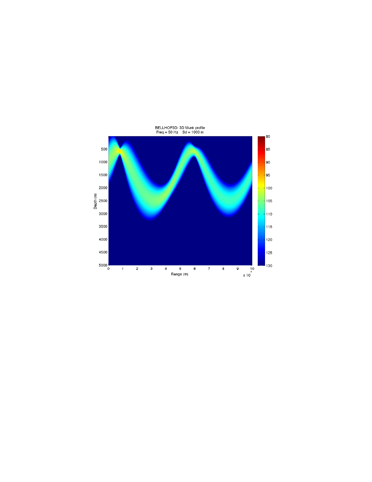
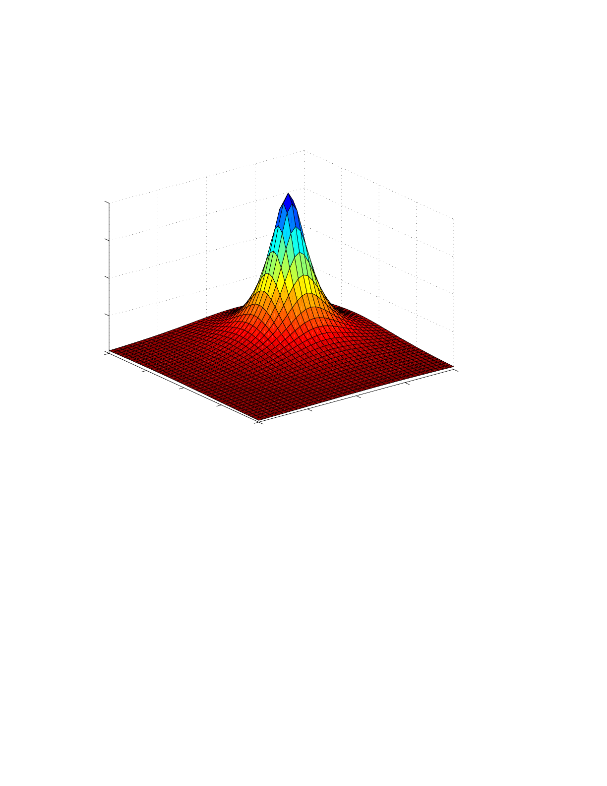
To illustrate the features of the different beam types we consider a canonical deep water sound
speed profile. First, we show in Fig. 1 how a Cerveny beam in BELLHOP3D looks in side view.
Note that the beam refracts within the water column and focuses and defocuses due to those
BELLHOP3D User Guide! "4
Heat, Light, and Sound Research, Inc.
same refractive effects. At the frequency used (50 Hz) the wavelength is about 30 m so it is difficult
to get beams narrower than a few hundred meters. (This is discussed in more detail in the latest
edition of Computation Ocean Acoustics.) The fact that the beams are this large is in fact one of
the limitations of the method, since the beam field is only accurate near the axis of the beam.
Figure 1: A Cerveny-style beam as first implemented in BELLHOP3D.
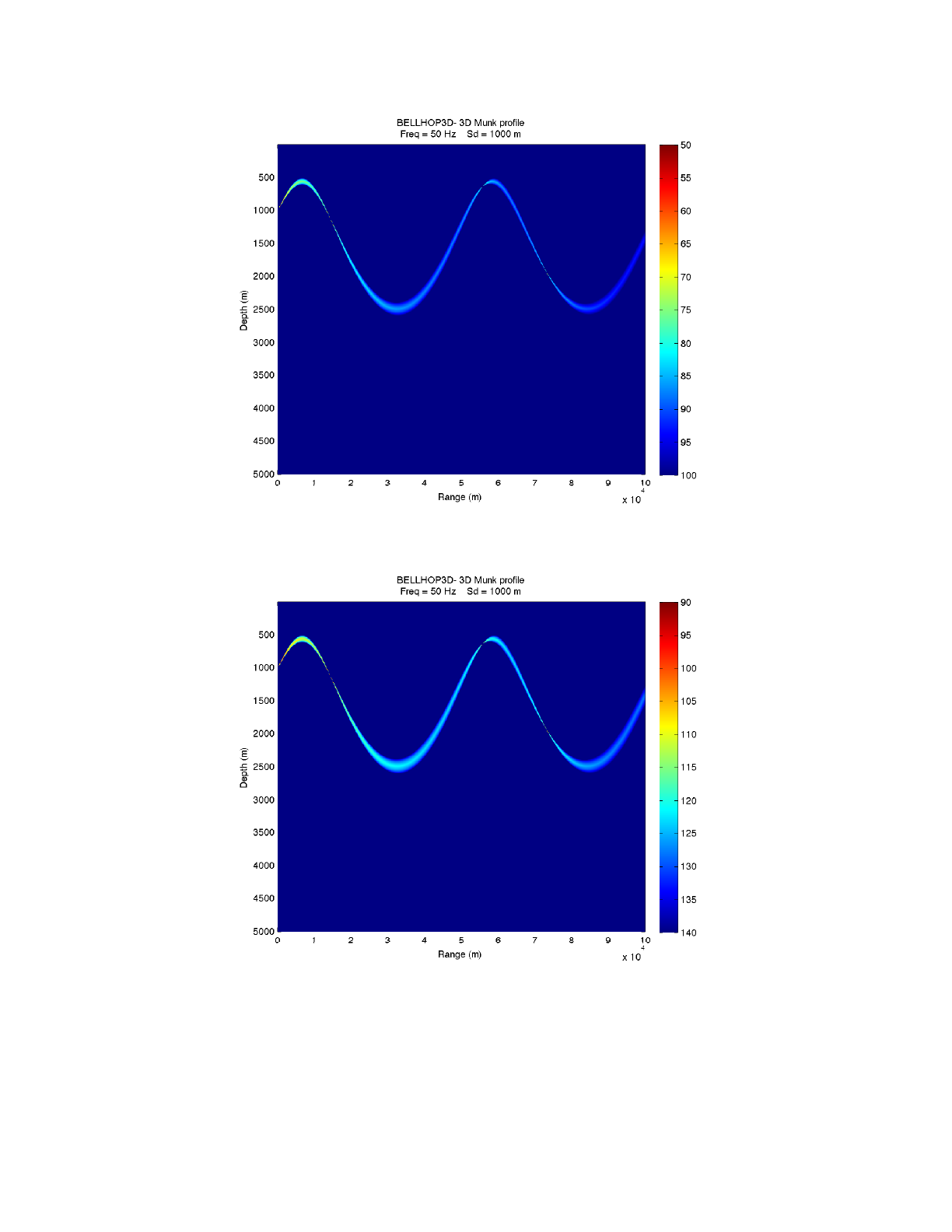
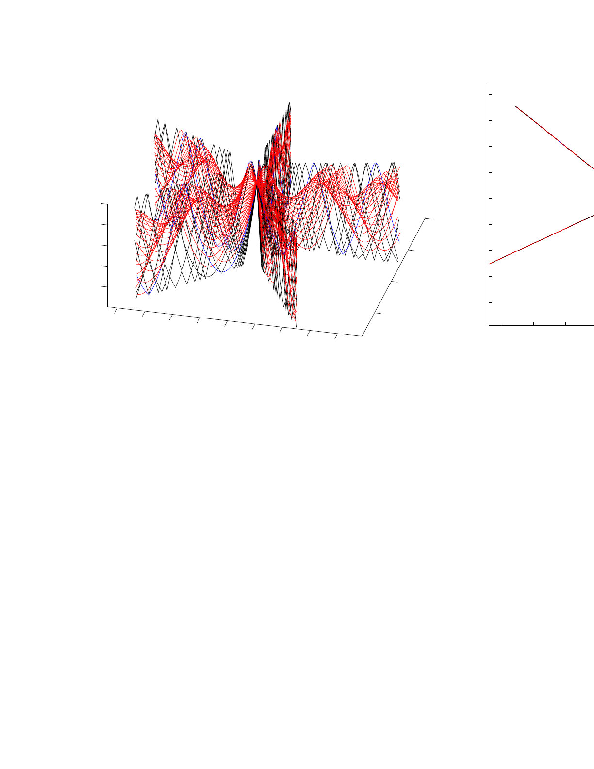
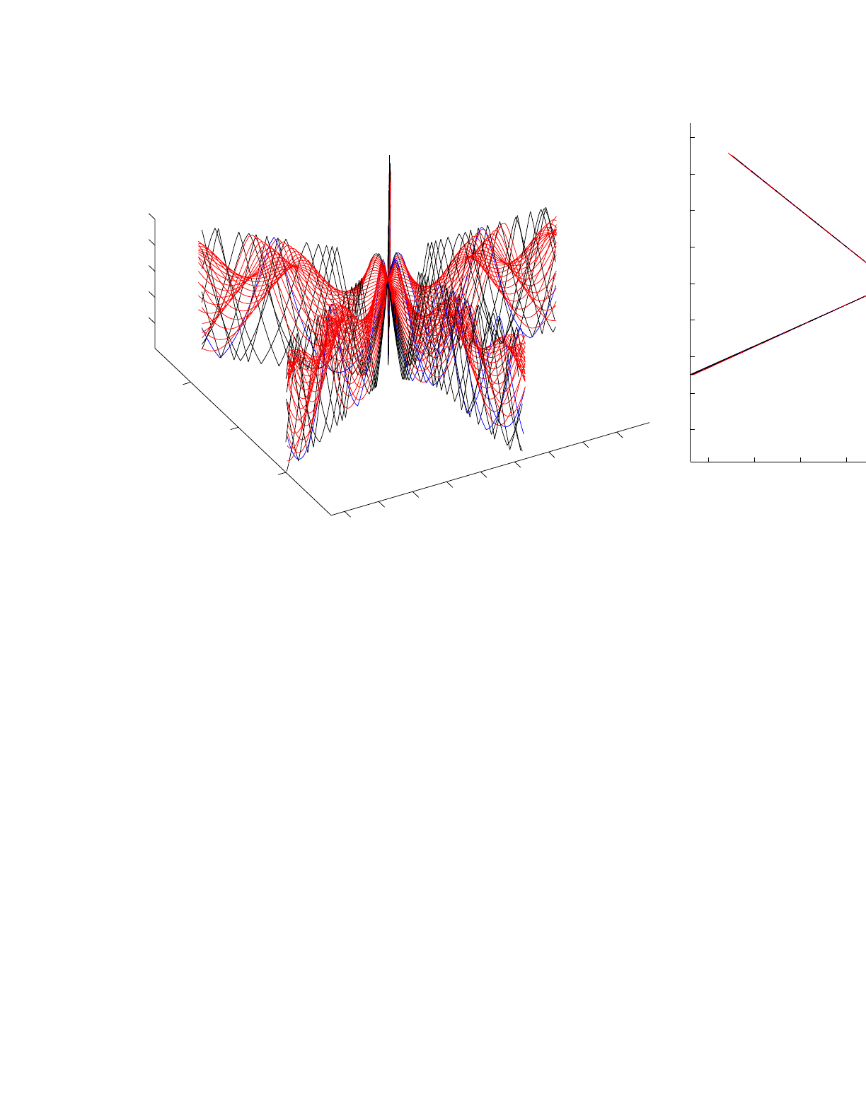
Figure 2 shows the new implementation of geometric, hat-shaped beams. In this case, the width of
the beams is determined entirely by the spacing of the fan of rays. As we increase the number of
rays that are traced, the beams get narrower and narrower. To check the implementation, we
compare the result to the geometric, hat-shaped beams in BELLHOP3D, but using the Nx2D
option (Figure 3). This is essentially the same as what is in the standard 2D version of BELLHOP
and has been tested extensively. We see that there is an excellent correspondence between the
two.
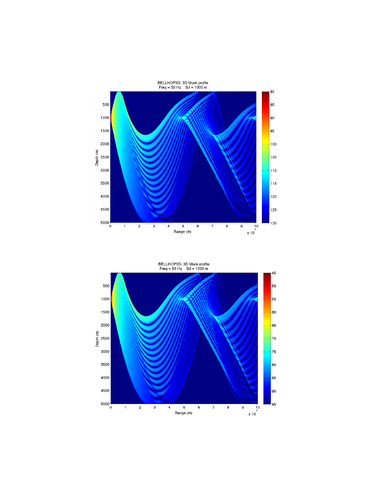
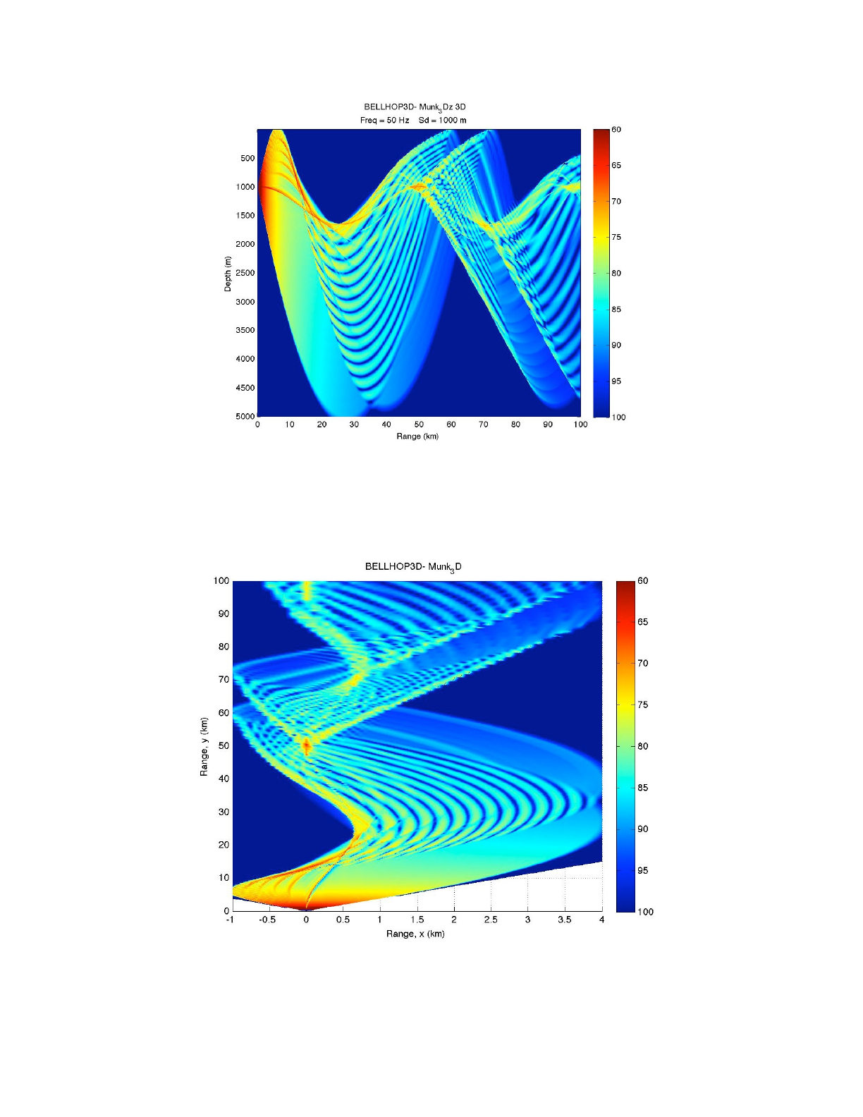
Finally, we compute the entire acoustic field by summing up the contributions of a fan of such
beams. The comparison of BELLHOP3D with geometric beams using the full 3D option and the
Nx2D option is shown in Figure 4 and is excellent. These results have also been checked again
normal mode and wavenumber integration solutions and are of high quality.
!
BELLHOP3D User Guide! "5
Heat, Light, and Sound Research, Inc.
Figure 2: A geometric beam in the full 3D option.
Figure 3: A geometric beam in the Nx2D option.
BELLHOP3D User Guide! "6
Heat, Light, and Sound Research, Inc.
Figure 4: Transmission loss calculated with geometric beams with the full 3D option.
Figure 5: Transmission loss calculated using geometric beams in the Nx2D option.
BELLHOP3D User Guide! "7

Heat, Light, and Sound Research, Inc.
B. Theory
The extension of Gaussian beams to three dimensions is described by Babich and Popov and
requires fairly minor modifications to the 2D algorithm. Let us go through the three steps required
for constructing the beam solution. As usual we begin by tracing a set of rays however in the 3D
case the rays form a fan over both azimuthal and elevation-declination angles. The ray equations
in 3D are given by
where c( x, y, z, ) is the ocean sound speed ( x( s), y( s ), z( s ) ) is the ray trajectory. This first-order
system of ordinary differential equations (ODEs) is integrated using a simple second-order Runge-
Kutta method. The initial conditions prescribe that the rays emanate from the source position (xs,
ys, zs) and with take-off angles alpha and beta corresponding to the declination angle and the
azimuthal angle of the ray:
The Gaussian beam is constructed around a central ray and defined in terms of ray-centered
coordinates (s, m, n) as indicated in the figure. Here s is the arclength along the ray, and (m,n) are
normal distances from a field point to the central ray. It is usually not an important issue; however,
this coordinate system has a zone of regularity around the central ray where a receiver point has a
well-defined ray-centered coordinate. However, for some other receiver points there is more than
one normal from the ray to the receiver. For instance if the ray is a circular arc, then radials from the
center of the circle are all valid normals.
BELLHOP3D User Guide! "8
dx
ds =c(s),d
ds =
1
c2
dc
dx ,
dy
ds =c(s),d
ds =
1
c2
dc
dy ,
dz
ds =c(s),d
ds =
1
c2
dc
dz ,
x(0) = xs,=1
c(0) cos cos ,
y(0) = ys,=1
c(0) cos sin ,
z(0) = zs,=1
c(0) sin .

Heat, Light, and Sound Research, Inc.
To be specific, the values of (m,n) are defined as normal distances in the direction of the following
two normal vectors to the ray:
and ". (These formulas are derived in Cerveny and Hron. This ray-centered
coordinate system " is a rotating trihedral with rotation angle " satisfying the differential
equation:
which must also be integrated along the central ray of the beam. This is one of many ways of
calculating the rotating trihedral.
The coordinate system defined by the rotating trihedral is magical. As discussed by Popov (1977)
we can use Hamilton’s Principle to derive equations that characterize how a ray displaces as we
make infinitesimal changes to its original position or take-off angles. These equations are amazingly
simple when presented in the coordinate system of the rotating trihedral. Furthermore, the way the
ray displaces characterizes the spreading of the ray tube and therefore the intensity along the
central ray.
The construction of beams in the neighborhood of the central rays requires the integration of a
system of auxilliary equations
L=2+2
(˜
t, ˜em,˜en)
BELLHOP3D User Guide! "9
˜em=(L1[c cos +sin ],
L1[c cos sin ], cL cos ),
˜en=(L1[c sin cos ],
L1[c sin +cos ],cL cos ),
d
ds =1
c(s)
(cx
cy)
2+2
dP
ds =
1
c2VQ
dQ
ds =cP

Heat, Light, and Sound Research, Inc.
where V is a matrix of curvatures of the sound speed taken in two normal directions:
The derivatives cnn, cmm, etc indicate derivatives in direction of the normal vectors . We
can rewrite these in terms of the x, y, z derivatives of the sound speed as:
The P-Q differential equation tells us how the ray is perturbed due to a change in the ray initial
condition (either by displacing the source position or changing the ray angle). To obtain Gaussian
beams, we use the initial conditions:
˜em,˜en
BELLHOP3D User Guide! "10
V=cnn cnm
cmn cmm
Q=˜q1ˆq1
˜q2ˆq2
P=˜p1ˆp1
˜p2ˆp2
cnn =cxxe2
1x+cyye2
1y+czze2
1z+2cxy e1xe1y+2cxz e1xe1z+2cyz e1ye1z
cmn =cxxe1xe2x+cyy e1ye2y+czz e1ze2z+
cxy (e1xe2y+e2xe1y)+cxz (e1xe2z+e2xe1z)+cyz(e1ye2z+e2ye1z)
cmm =cxxe2
2x+cyye2
2y+czze2
2z+2cxy e2xe2y+2cxz e2xe2z+2cyz e2ye2z
˜p1ˆp1
˜p2ˆp2
˜q1ˆq1
˜q2ˆq2
=
10
01
10
02

Heat, Light, and Sound Research, Inc.
where " are the beam constants that control the initial beam widths in the two normal directions
to the ray. The epsilons are in general complex numbers and their real and imaginary parts allow
independent control of both the beam width and the beam curvature (that is, the curvature of its
wavefronts).
Once we have integrated these equations along the ray we form a Gaussian beam as:
The expression for " has been obtained here by using the cofactor representation of the inverse of
Q. In addition |Q| denotes the determinant of Q. In general the determinant of Q is a complex
number that wraps around the origin. To get the correct branch of the square root we need to track
these rotations. This produces the so-called KMAH index that accounts for phase changes at
caustics.
C. Geometric Beams
As discussed earlier the geometric beam is designed to have a beam width that expands and
contracts in proportion to the ray tube. The hat-shaped beam decays linearly away from the central
ray. One may envision a beam that has an amplitude decay in the form of a pyramid; however,
since the ray tube does not necessarily have a square cross-section the beam shape is really
tetrahedral. The formula for the hat-shaped beam is simply:
for |n|< L1 and |m|<L2. (The beam vanishes outside that tube.) Here L1 and L2 are the widths of
the ray tube. To get those cross-sectional widths we simply set the initial beam constants, " to
1,2
1,2
BELLHOP3D User Guide! "11
ubeam(s, m, n)= 1
|Q(s)|ei[(s)+ 1
2qt(s)q]
=PQ
1=˜p1ˆq2ˆp1˜q2˜p1ˆq1+ˆp1˜q1
˜p2ˆq2ˆp2˜q2˜p2ˆq1+ˆp2˜q1/|Q|
ubeam(s, m, n)= 1
|Q(s)|ei(s)[L1(s)n][L2(s)m]
L1(s)L2(s)

Heat, Light, and Sound Research, Inc.
zero. In that case, the P-Q initial conditions imply that we are perturbing the ray in the declination
direction (for ") or the azimuthal direction (for ").
where " and " is the angular spacing between the rays at the source. The hat-shaped beams
reproduce the classical ray-theoretic result since the beam intensity is exactly the ray-theoretic
result on the central ray and the beam sum produces a linear interpolation for the field in between
the rays.
As discussed above, we typically obtain better accuracy by using Gaussian beams but still within
the geometric framework. The field at any point is then the sum of contributions from a number of
nearby beams, rather than just the two bracketing beams that the hat-shaped beams provide. This
integration over many beams smooths out caustics and also allows leakage energy into shadow
zones. The formula for the Geometric Gaussian beams is simply:
At caustics the beam widths and the determinant of Q(s) vanish. To avoid this singularity we limit
the minimum beam width to one wavelength as suggested by Keenan and Burridge.
D. The Compound Matrix Method
It commonly occurs that one is solving a system of ordinary differential equations with different
initial conditions to assemble a final solution that involves determinants of the resulting independent
solutions. In this case one can do some simple manipulations to derive a new set of ordinary
differential equations that is solved with just one set of initial conditions to yield the determinants
directly. This is sometimes called the compound matrix method or the delta-matrix formulation. As
we shall see there is typically a redundant equation that can be eliminated leading the to the so-
called reduced delta-matrix formulation. The advantage of this approach is that it yields a simpler
and faster algorithm.
˜p, ˜q
ˆp, ˆq
BELLHOP3D User Guide! "12
L1(s)
L2(s)=|˜q1(s)|
c(s)
|cos | |ˆq2(s)|
c(s)
ubeam(s, m, n)= 1
|Q(s)|ei(s)e
.5»n
L1(s)–2»m
L2(s)–2
L1(s)L2(s)

Heat, Light, and Sound Research, Inc.
To derive the new system, we first arrange the original ODE from a matrix to a vector form as
follows:
where the prime denotes the derivative with respect to arc length. Next we consider two
independent solutions for the p-q vector using tildes for one solution and hats for the other
solution. We then assemble those two column vectors into a matrix and construct a new vector
consisting of all the principal minors of that matrix. We note that those principal minors correspond
to all the elements in the beam field above.
Thus, we can write the beam field as:
To get all the terms needed in this new formulation, we require the differential equation for the
vector of minors, y. This is obtained by simply differentiating the expression for each principal minor
using the product rule. Then from the original ODE we can replace derivatives. The final result is:
BELLHOP3D User Guide! "13
p1
p2
q1
q2
=
00 cnn cnm
00cmn cmm
c00 0
0c00
p1
p2
q1
q2
˜p1ˆp1
˜p2ˆp2
˜q1ˆq1
˜q2ˆq2
˜p1ˆp2˜p2ˆp1
˜p1ˆq1˜q1ˆp1
˜p1ˆq2˜q2ˆp1
˜p2ˆq1˜q1ˆp2
˜p2ˆq2˜q2ˆp2
˜q1ˆq2˜q2ˆq1
=
|P|
12|Q|
+11|Q|
22|Q|
+21|Q|
|Q|
=
p
h
+f
g
+h
q
=
y1
y2
y3
y4
y5
y6
ubeam =1
|Q|ei[+1
2(fn2+2hmn+gm2)]
y1
y2
y3
y4
y5
y6
=
0cmn /c2
cmm /c2cnn /c2cnm /c20
00 0 0 0cnm /c2
c0000cnn /c2
c0000cmm /c2
00 0 0 0cnm /c2
00 cc00
y1
y2
y3
y4
y5
y6

Heat, Light, and Sound Research, Inc.
The equation for y5 is just the negative of that for y2, so it can be eliminated. We are left with a first-
order system for five components:
Here cmm and cnn are second derivatives of the sound speed in the two normal directions
" . Once this system is integrated one obtains a representation of the beam as,
This representation follows from application of the reduced delta matrix method to the equations
given by Babich and Popov. Initial conditions are given forming the same principal minors of the
initial conditions from the original P-Q equations:
where " are the (complex) beam constants which characterize the beam width and curvature in
directions " respectively.
Finally, the complex pressure is computed by summing up all of the individual beams with
appropriate weighting,
E. Beam changes across interfaces
˜em,˜en
1,2
˜em,˜en
BELLHOP3D User Guide! "14
dQ
ds =1
c2(cmm f+2cmn hcnn g),
dP
ds =c(f+g),
df
ds =cP
1
c2cnn Q,
dg
ds =cP
1
c2cmm Q,
dh
ds =
1
c2cmn Q.
ubeam(s, m, n)=AQ(s) exp i(s)+f(s)n2+2h(s)mn +g(s)m2
2Q(s)
(P, Q, f, g, h) = (1,12,2,1,0)
u(r, z)=
N
k=1
N
l=1
12
2c0
3ubeam
kl .

Heat, Light, and Sound Research, Inc.
An interface is defined here as a curve across which the sound speed or its derivative is
discontinuous. The most important of these are the ocean boundaries. These perhaps should not
be considered interfaces but if we view the reflected field as simply an image of the incident field,
then we can equate it with a direct ray that has crossed through from the other side. Therefore it
sees a jump in the gradient of the sound speed that is double the gradient at the boundary. The
formulas for interfaces and boundaries are essentially the same.
The other important interfaces are those associated with the oceanography. BELLHOP3D uses
various piecewise approximations to the sound speed, e.g. piecewise linear in depth and in range.
These lead to so-called weak discontinuities, that is, discontinuities in the derivative of the sound
speed.
The curvature of these interfaces also effects the beam; however, all interfaces in BELLHOP3D are
flat (locally) so we ignore these effects. The 2D version of BELLHOP does allow for a curved
interpolation of the boundaries and incorporates those effects.
As beams cross such interfaces they change. Since the sound speed and density is continuous
there is no change in the intensity of the beam; however, the curvature of the phase fronts of the
beams changes. These changes are agnostic to the rotating trihedral. That is to say the the
curvature change is directly related to the shape of the beam in the reflection plane. The reflection
plane is formed by the tangent ray and the normal to the interface (both are contained in the
reflection plane). Therefore, we must convert the representation of the beam from its coordinate
system involving the rotating trihedral to the coordinate system of the reflection plane before
converting it. Then after the interaction with the interface we need to convert it back to the
coordinate system of the rotating trihedral.
Our first step is to get a new coordinate system in the reflection (or transmission plane). This is
defined by the ray tangent, together with two normal vectors to the ray. The first of these normal
vectors must be in the reflection plane and the second is normal to the reflection plane. If we form
a normalized cross product of the ray tangent and the normal to the boundary we obtain a unit
normal vector to the reflection plane:
Taking the cross-product of the ray tangent and this normal to the reflection plane yields the other
normal to the ray that is in the reflection plane:
Then to express the p’s into the new coordinate system we transform as follows:
BELLHOP3D User Guide! "15
n2=nRef lP lane =
tray nbdry
tray nbdry
n1=
tray nRef lP lane

Heat, Light, and Sound Research, Inc.
where the prime denotes here the values of p in the new coordinate system. The same
transformation is applied to the q’s.
Now that we have the representation of the p’s and q’s in the new coordinate system we apply the
curvature change formulas from Popov and Psencik (1978). (See also Cerveny and Psencik (1979);
however, there is a typo in the jump equations.) These are:
where,
and alpha is the angle of incidence. In addition " refers to the jump in the
derivatives of the sound speed across the interface (s for the derivative along the ray, 1, 2, for the
derivatives in the two normal directions. The final step is to convert the ps and qs back into the ray-
centered coordinate system.
These formulas are also applied for boundary reflection; however, as noted above the jumps in the
derivatives of the sound speeds are doubled and the sign of alpha is flipped.
Getting the signs right in all these equations is difficult because the signs of normal vectors to the
boundaries and the rays need to be carefully defined.
[c1],[c2],[cs]
BELLHOP3D User Guide! "16
ˆp
˜p
=e1·n1e1·n2
e2·n1e2·n2 ˆp
˜p
[˜p]=˜qR1ˆqR2
[ˆp]=˜qR2
R1=2
c2tan c1
c
tan2
c2[cs]
R2=tan
cc2
c

Heat, Light, and Sound Research, Inc.
III. Running BELLHOP3D
A. Environmental Information: Basic input file
Our template for BELLHOP3D is the existing 2D code (BELLHOP) which is a mature code capable
of handling all the practical inputs (2D sound speed profile, range-dependent bathymetry, source
radiation patterns, volume attenuation, boundary reflection coefficients, etc.). As this work
continues, all of these capabilities will be incorporated in BELLHOP3D. During this period, a major
rewrite was done on BELLHOP3D to make the algorithm have a parallel structure to the 2D code.
In the process, BELLHOP3D was set up to read essentially the same input file as BELLHOP, apart
from two additional inputs required to specify the bearing lines for receivers, as well as the bearing
lines used to trace the fan of beams. (These are independent; in a typical run many more beams
will be traced in the azimuthal direction than there are bearing lines for the receivers.)
An example of the BELLHOP3D input file is shown below:
'3D Munk profile'"! TITLE#
50.0""""! FREQ (Hz)#
1""""! NMEDIA#
'CVW'""""! SSPOPT (Analytic or C-linear interpolation)#
51 0.0 20000.0"""! DEPTH of bottom (m)#
0.0 1548.52 /#
200.0 1530.29 /#
250.0 1526.69 /#
400.0 1517.78 /#
600.0 1509.49 /#
800.0 1504.30 /#
1000.0 1501.38 /#
1200.0 1500.14 /#
1400.0 1500.12 /#
1600.0 1501.02 /#
1800.0 1502.57 /#
2000.0 1504.62 /#
2200.0 1507.02 /#
2400.0 1509.69 /#
2600.0 1512.55 /#
2800.0 1515.56 /#
3000.0 1518.67 /#
3200.0 1521.85 /#
3400.0 1525.10 /#
3600.0 1528.38 /#
BELLHOP3D User Guide! "17

Heat, Light, and Sound Research, Inc.
3800.0 1531.70 /#
4000.0 1535.04 /#
4200.0 1538.39 /#
4400.0 1541.76 /#
4600.0 1545.14 /#
4800.0 1548.52 /#
5000.0 1551.91 /#
20000 1551.91 /#
'A~' 0.0#
20000.0 1600.00 0.0 1.8 0.8 /#
1 ! NSD#
1000.0 / ! SD(1:NSD) (m)#
1 ! NRD#
1000 5000 ! RD(1:NRD) (m)#
1001 ! NR#
0.0 100.0 / ! R(1:NR ) (km)#
37 ! Ntheta (number of bearings)#
0.0 360.0 / ! bearing angles (degrees)#
'CC 3' ! 'R/C/I/S'#
200 ! Nalpha#
-14.66 20 / ! alpha1, 2 (degrees) Elevation/declination angle fan#
144 ! Nbeta#
0 360 / ! beta1, beta2 (degrees) bearine angle fan#
0.0 20500.0 99.1 ! STEP (m), ZBOX (m), RBOX (km)#
'MS' 0.3 100.0" ! BeamType, epmult, Rloop (km)#
1 5 'P' ! NImage IBWin#
Sample BELLHOP3D input file.
The reader interested in the full details of this input file can find them in the Acoustics Toolbox
documentation, which can be downloaded from the Ocean Acoustics Library at http://
oalib.hlsresearch.com/. However, the basic structure is probably fairly obvious. There is a sound
speed profile at the beginning, followed by a series of lines that give the coordinates of the
receivers in terms of receiver depth (RD), receiver range (RR), and receiver bearings. Finally, on the
line showing ‘CC 3’, the ‘3’ is to indicate a full 3D run. BELLHOP3D can also to a 2D run by setting
that to ‘2’. This is useful for assessing the importance of the 3D effects. We shall present some
results of the code.
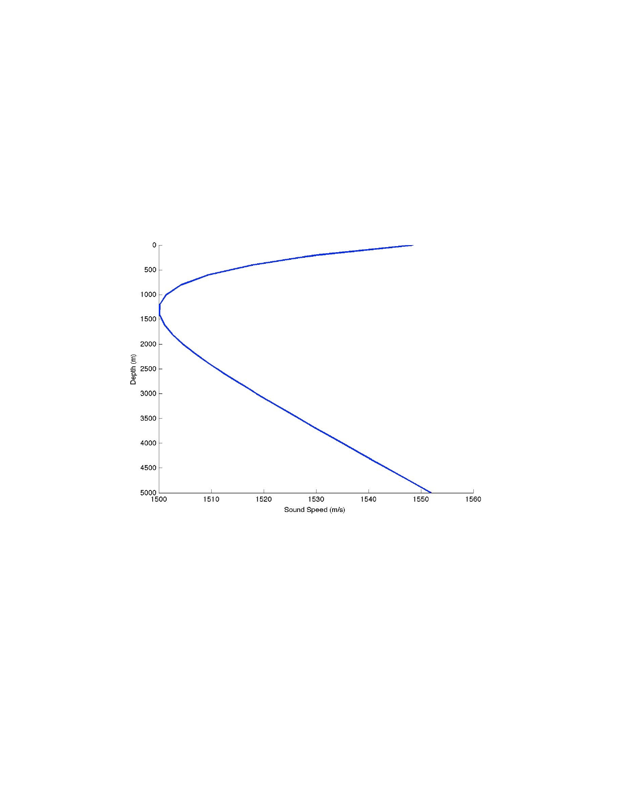
To display the sound-speed profile, we use the Matlab function ‘plotssp.m’ in the Acoustics
Toolbox. The result is shown in the Figure to the right.
BELLHOP3D User Guide! "18
Heat, Light, and Sound Research, Inc.
Figure 1: Plot of the sound speed.
We have not yet implemented the capability to read a 3D sound speed so BELLHOP3D is currently
still reading this as an analytic function implemented in FORTRAN.
BELLHOP3D User Guide! "19
1500 1510 1520 1530 1540 1550 1560
0
500
1000
1500
2000
2500
3000
3500
4000
4500
5000
Sound Speed (m/s)
Depth (m)

Heat, Light, and Sound Research, Inc.
B. Environmental Information: Bathymetry
The bathymetric data is read as a matrix of ocean bottom depths, sampled on a regular grid and
stored in a bathymetry file with extension ‘.bty’. An example bathymetry file is shown below:
'R'
6
-100.000000 100.000000 /
6
-100.000000 100.000000 /
4976.608187 4968.503937 4959.595960 4954.022989 4956.043956 4963.963964
4968.503937 4951.807229 4927.272727 4906.976744 4914.893617 4940.298507
4959.595960 4927.272727 4851.851852 4733.333333 4789.473684 4897.435897
4954.022989 4906.976744 4733.333333 3666.666667 4428.571429 4851.851852
4956.043956 4914.893617 4789.473684 4428.571429 4636.363636 4870.967742
4963.963964 4940.298507 4897.435897 4851.851852 4870.967742 4921.568627
Sample bathymetry file.
The first line with the letter ‘R’ indicates the file contains a Regular grid. (Other options are ‘L’ and
‘C’ which are used in the 2D BELLHOP for piecewise linear or curvilinear interpolation of
bathymetry on a single slice.) The next 2 lines specify the number of points in x, the minimum and
maximum values of x. The 2 lines after that have the corresponding information in y. Finally, we
have the matrix containing the depth in meters of the bottom.
The rectilinear grid does not have to be uniform. It there is an irregular spacing then one must
simply supply the full set of x and y coordinates. The ‘/’ in the above example is a standard Fortran
convention that terminates the input line. When the ‘/’ is detected BELLHOP3D fills in a complete
set of x-y points using a regular spacing and treating the input values as a min and max.
We have also implemented exactly the same capability for surface elevation, allowing an ‘altimetry’
file to be specified. This can be used to study the effects of ocean surface waves.
The above file describes a hill. For our model run, we actually chose to sample it more finally with
41 points in both x and y. We also implemented a Matlab function called ‘plotbty3D’ to display it.
The result is shown in the figure below.
BELLHOP3D User Guide! "20
Heat, Light, and Sound Research, Inc.
"
Figure 2: Plot of the bathymetry.
In this bathymetry plot you can see how the ocean bottom is described by a pattern of rectangles.
The process internal to BELLHOP3D involved quite a bit of work. In fact each rectangle is really
treated as a pair of triangles. The reason for this is that three points define a plane; 4 points is too
many. Thus each set of 4 points forms two triangular facets. The ray is then reflected off the
triangular facet using the normal vector to that facet, which is pre-computed before the rays are
traced. BELLHOP3D first identifies the particular triangle which is below the source location. The
rays are then traced by stepping in arc length using a default step size. However, as the rays are
traced BELLHOP checks to see if a ray will cross into the zone above another triangle. It also
checks to see if the ray would cross the bottom (or surface) boundary. Then it reduces the step to
land precisely on that boundary. These details are important in obtaining a precise ray trace where
all the reflections are treated properly. The 2D version of BELLHOP does a similar thing; however,
−100
−50
0
50
100
−100
−50
0
50
100
3000
3500
4000
4500
5000
Range−x (km)
Range−y (km)
Depth (m)
BELLHOP3D User Guide! "21

Heat, Light, and Sound Research, Inc.
the process is obviously much simple for a single bathymetry slice versus the 2D bathymetry that
BELLHOP3D processes.
BELLHOP3D User Guide! "22

Heat, Light, and Sound Research, Inc.
C. Environmental Information: Oceanography
It was decided to use hexahedral interpolation of the 3D oceanographic field (‘brick’ elements in
the terminology of the finite element literature). Furthermore we assume rectilinear elements, i.e. the
corner angles of the hexahedron are each 90 degrees. Then as a ray traverses through the
oceanographic field, the sound speed is interpolated by ‘trilinear’ interpolation. To summarize this
process, consider a particular ray location x. A search is done to identify the particular segments
iSegx, iSegy, iSegz, in x, y, and z, that define the element or cell containing that ray coordinate. We
then construct the sound speed at the corners of a lat/lon box by interpolating the sound speed
matrix, cMat, in depth:
c11 = cMat( iSegx, iSegy , Layer ) + ( x( 3 ) - zSeg( Layer ) ) * !
czMat( iSegx, iSegy , Layer )
c21 = cMat( iSegx + 1, iSegy , Layer ) + ( x( 3 ) - zSeg( Layer ) ) *!
czMat( iSegx + 1, iSegy , Layer )
c12 = cMat( iSegx, iSegy + 1, Layer ) + ( x( 3 ) - zSeg( Layer ) ) *!
czMat( iSegx, iSegy + 1, Layer )
c22 = cMat( iSegx + 1, iSegy + 1, Layer ) + ( x( 3 ) - zSeg( Layer ) ) *!
czMat( iSegx + 1, iSegy + 1, Layer )
where czMat is the gradient in depth of the sound speed, which is calculated when the matrix of
sound speed values is first read in.
Next we calculate the proportional distances of the ray coordinate within the active cell. Denoting
the proportional distances in x and y by s1 and s2 respectively, we calculate:
s1 = ( x( 1 ) - xSeg( iSegx ) ) / ( xSeg( iSegx + 1 ) - xSeg( iSegx ) )
s2 = ( x( 2 ) - ySeg( iSegy ) ) / ( ySeg( iSegy + 1 ) - ySeg( iSegy ) )
where xSeg and ySeg are the coordinates of the segment defining the active cell. We then
interpolate the soundspeed in the y direction, at the two endpoints in x (top and bottom sides of
rectangle):
c1 = ( 1.0D0 - s2 ) * c11 + s2 * c12"
c2 = ( 1.0D0 - s2 ) * c21 + s2 * c22
Finally we interpolate the soundspeed in the x direction, at the two endpoints in y (top and
bottom sides of the rectangle)
c = ( 1.0D0 - s1 ) * c1 + s1 * c2
BELLHOP3D User Guide! "23

Heat, Light, and Sound Research, Inc.
The details here are not terribly important but hopefully this outline conveys the notion that the
soundspeed is interpolated linearly within a cell. Gradients are also easily calculated in this process.
An example BELLHOP3D input file (KoreanSea3d_ray.env) to invoke an oceanography field is
shown below. The key parameter is ‘H’ in the SSOPT line, which indicates hexahedral interpolation.
The lines with depths from 0 to 5500 would normally contain the actual sound speed profile;
however, they are ignored when the ‘H’ option is selected.
#
'Korean Sea 3D'"! TITLE#
250.0""""! FREQ (Hz)#
1""""! NMEDIA#
'HVW'""""! SSPOPT (Analytic or C-linear interpolation)#
51 0.0 5500.0"""! DEPTH of bottom (m)#
0 /#
10 /#
20 /#
30 /#
50 /#
75 /#
100 /#
125 /#
150 /#
200 /#
250 /#
300 /#
400 /#
500 /#
600 /#
700 /#
800 /#
900 /#
1000 /#
1100 /#
1200 /#
1300 /#
1400 /#
1500 /#
1750 /#
2000 /#
2500 /#
3000 /#
3500 /#
4000 /#
4500 /#
BELLHOP3D User Guide! "24

Heat, Light, and Sound Research, Inc.
5000 /#
5500 /#
'A~' 0.0#
5500.0 1600.00 0.0 1.8 0.8 /#
1 ! NSD#
100.0 / ! SD(1:NSD) (m)#
1 ! NRD#
25.0 /"" ! RD(1:NRD) (m)#
1001 ! NR#
0.0 50.0 /"" ! R(1:NR ) (km)#
6 ! Ntheta (number of bearings)#
0.0 360.0 / ! bearing angles (degrees)#
'RC 3' ! 'R/C/I/S'#
25 ! Nalpha#
-10 10 / ! alpha1, 2 (degrees) Elevation/declination angle fan#
4 ! Nbeta#
90 270 / ! beta1, beta2 (degrees) bearine angle fan#
0.0 5500.0 50. ! STEP (m), ZBOX (m), RBOX (km)#
'MS' 0.3 100.0"" ! BeamType, epmult, Rloop (km)#
1 5 'P' ! NImage IBWin#
Sample BELLHOP3D input file (KoreanSea3d_ray.env) when 3D oceanography is included.
The actual sound speed field is then provided as an additional input file with the extension ‘SSP’ (in
this case ‘KoreanSea3d_ray.ssp’). The format of the SSP file is as follows:
151 ! Nx!
0.000000 7.712187 15.424375 … 1149.115967 1156.828125 ! x-coordinates
169 ! Ny!
0.000000 7.204473 14.408945 … 1203.146851 1210.351318 ! y-coordinates
33 ! Nz!
0.000000 10.000000 … 5000.000000 5500.000000 ! z-coordinates
Sample BELLHOP3D SSP file (KoreanSea3d_ray.ssp) when 3D oceanography is included.
BELLHOP3D User Guide! "25

Heat, Light, and Sound Research, Inc.
These lines are then followed with the matrix of sound speed values. In this cases we consider a
3D volume consisting of 151 points in x, 169 points in y, and 33 points in depth. To avoid wasting
space, we deleted some of the data as indicated by the ellipses.
Besides the hexahedral option, a full set of SSP interpolation routines was also implemented for
purely stratified problems. Thus BELLHOP3D can also be easily run with a single SSP, which can
be interpolated in several ways (c-linear, n2-linear, cubic spline) in depth, just like the 2D version of
BELLHOP.!
BELLHOP3D User Guide! "26

Heat, Light, and Sound Research, Inc.
D. Ray trace run: Nx2D
Here we are following a typical procedure where we first plot the environmental information to
make sure that the problem is set up as intended. Next we usually like to look at a ray trace to see
how the sound energy is traveling. This is done by selecting the RunType to be ‘R’ in BELLHOP3D.
For our initial run, we also select the 2D option in BELLHOP3D. After the run is completed,
BELLHOP3D echoes information to a print file as shown below.
BELLHOP- 3D Munk profile
frequency = 50.00 Hz
Dummy parameter NMedia = 1
C-linear approximation to SSP
Attenuation units: dB/wavelength
VACUUM
Depth = 20000.000000000000 m
C-Linear SSP option
Sound speed profile:
0.00 1548.52
200.00 1530.29
250.00 1526.69
400.00 1517.78
600.00 1509.49
800.00 1504.30
1000.00 1501.38
1200.00 1500.14
1400.00 1500.12
1600.00 1501.02
1800.00 1502.57
2000.00 1504.62
2200.00 1507.02
2400.00 1509.69
2600.00 1512.55
2800.00 1515.56
3000.00 1518.67
3200.00 1521.85
3400.00 1525.10
3600.00 1528.38
3800.00 1531.70
4000.00 1535.04
4200.00 1538.39
4400.00 1541.76
4600.00 1545.14
4800.00 1548.52
BELLHOP3D User Guide! "27

Heat, Light, and Sound Research, Inc.
5000.00 1551.91
20000.00 1551.91
( RMS roughness = 0.00 )
Bathymetry file selected
ACOUSTO-ELASTIC half-space
20000.00 1600.00 0.00 1.80 0.8000 0.0000
__________________________________________________________________________
Number of source depths = 1
Source depths (m)
1000.00
Number of receiver depths = 1
Receiver depths (m)
1000.00
Number of ranges = 1001
Receiver ranges (km)
0.00000 0.100000 0.200000 0.300000 0.400000
0.500000 0.600000 0.700000 0.800000 0.900000
1.00000 1.10000 1.20000 1.30000 1.40000
1.50000 1.60000 1.70000 1.80000 1.90000
2.00000
... 100.000000
Number of bearings = 5
Receiver bearings (degrees)
0.00000 75.0000 150.000 225.000 300.000
__________________________________________________________________________
Ray trace run
Cartesian beams
Point source (cylindrical coordinates)
Rectilinear receiver grid: Receivers at rr( : ) x rd( : )
N x 2D calculation (neglects horizontal refraction)
Number of beams in elevation = 30
Beam take-off angles (degrees)
-14.6600 -13.4648 -12.2697 -11.0745 -9.87931
-8.68414 -7.48897 -6.29379 -5.09862 -3.90345
-2.70828 -1.51310 -0.317931 0.877241 2.07241
3.26759 4.46276 5.65793 6.85310 8.04828
9.24345
Replacing beam take-off angles, beta, with receiver bearing lines, theta
Number of beams in bearing = 5
Beam take-off angles (degrees)
0.00000 75.0000 150.000 225.000 300.000
BELLHOP3D User Guide! "28

Heat, Light, and Sound Research, Inc.
__________________________________________________________________________
Step length, deltas = 2000.0000000000000 m
Maximum ray Depth, Box%z = 20500.000000000000 m
Maximum ray range, Box%r = 99100.000000000000 m
Type of beam = M
Standard curvature condition
Epsilon multiplier 0.29999999999999999
Range for choosing beam width 100.000000000000000
Number of images, Nimage = 1
Beam windowing parameter = 5
Component = P
*********************************
Using bottom-bathymetry file
Regular grid for a 3D run
Number of bathymetry points in x-direction 41
xMin (km) = -100.000000000000000 xMax ( km ) =
100.000000000000000
Number of bathymetry points in y-direction 41
yMin (km) = -100.000000000000000 yMax ( km ) =
100.000000000000000
Minimum width beams
HalfWidth1 = 977.65495322067386
HalfWidth2 = 977.65495322067386
epsilonOPT1 = ( 0.0000000000000000 , 150138159.23471510 )
epsilonOPT2 = ( 0.0000000000000000 , 150138159.23471510 )
EpsMult = 0.29999999999999999
ibeta 1 0.0000000000000000
ibeta 2 75.000000000000000
ibeta 3 150.00000000000000
ibeta 4 225.00000000000000
ibeta 5 300.00000000000000
CPU Time = 0.893E-01s
Sample BELLHOP3D print file.
BELLHOP3D User Guide! "29

Heat, Light, and Sound Research, Inc.
Following the pattern of all the models in the Acoustics Toolbox, the user’s input data is echoed to
the print file as soon as it is read. Thus, if there is an error, one can see at precisely which line of
the input file the error occurred. In addition, we have structured BELLHOP3D to use the same
subroutine as the standard BELLHOP to read in this data. That routine is called with a flag to
indicate whether the input file has the additional 3D information needed for a BELLHOP3D run.
Notice the CPU time displayed on the last time, which indicates that this run took less than a tenth
of a second on a MacBook Pro laptop computer.
The key output of this run is a ray file with extension ‘.ray’. The format differs slightly from a 2D
BELLHOP ray file in that the rays are now trajectories in x-y-z space, rather than r-z (range-depth)
space. We have also implemented a Matlab function called ‘plotray3D’ to display the rays. The
resulting display is shown in Figure 6.
Like the 2D BELLHOP, ‘plotray3D’ automatically colors the ray based on whether it hits the top
and/or bottom boundaries. This makes for a clearer display of where the energy is traveling. The
source depth here is 800 meters, which is close to the sound channel axis. This leads to an
interesting pattern of refracted rays within the water column, showing the well-known convergence
zone effect. The results cross-check with the 2D version of BELLHOP, indicating that BELLHOP3D
is implemented correctly.
If we rotate this ray plot to look straight down on the ocean, we get the display shown below. Note
that all the rays lie precisely in vertical planes defined by the bearing lines. This is because we ran
BELLHOP3D in its 2D mode, so horizontal refraction is neglected. Finally, we can display both the
rays and the bathymetry in a single plot as shown in Figure 7. Here you can see more clearly how
the rays are being reflected off the ocean bottom.
Figure 6: Ray trace in the Nx2D mode (upper plot is a side view, lower plot is a top view).!
BELLHOP3D User Guide! "30
Heat, Light, and Sound Research, Inc.
Figure 7: Ray trace plotted over the bottom bathymetry.
E. Ray trace run: Full 3D Mode
Next we illustrate BELLHOP3D in its full 3D mode. As mentioned above, this is accomplished by
changing a single character in the input file. The print file is essentially the same so we will not
repeat it here. However, the 3D option is a bit slower, requiring 0.17 seconds. The ray plot is shown
below.
Again, to see more clearly the horizontal refraction effects we switch to a view from above where
now you can see the rays have refracted out of the vertical plane due to multiple reflections from
the hill, as well as the gradients in the ocean sound speed. The paths going over the hill naturally
show more out of plane refraction.
Figure 8: Ray trace in the 3D mode (upper plot is a side view, lower plot is a top view).
F. Transmission Loss
BELLHOP3D User Guide! "31
−50
0
50
100
−80 −60 −40 −20 020 40 60 80
0
1000
2000
3000
4000
Range, x (km)
BELLHOP− 3D Munk profile
Range, y (km)
Depth (m)
−80 −60 −40 −20 0 20 40 60 80 100
−80
−60
−40
−20
0
20
40
60
80
Range, x (km)
BELLHOP− 3D Munk profile
Range, y (km)
Heat, Light, and Sound Research, Inc.
To do a transmission loss calculation we change the RunType from ‘R’ (ray trace) to ‘C’ (coherent
transmission loss). In addition, we increase the number of takeoff angles in the vertical from 30 to
200. For a ray trace we typically find the plots are too cluttered if we use this many rays; however,
the TL results are more accurate with finer ray fans.
Similarly, to get a well sampled transmission loss plot in the lat./long. plane, we increase the
number of bearing lines for the receivers to be every 10 degrees. For a 2D run of BELLHOP 3D,
the code automatically uses this same set of angles for the azimuthal launch directions of the rays.
However, for a 3D run we increase this to 144 to get finer sampling. This is necessary because the
beams are now modeling the horizontal refraction. The resulting 2D and 3D plots are shown in
Figure 9. The run time for the Nx2D calculation was 1.5 seconds versus 26.2 seconds for the full
3D calculation. The 3D calculations are slower because the governing equations are more
complicated, but also because a finer sampling of rays is needed in the azimuthal direction.
Currently we are not taking advantage of the multiprocessors that are available.!
BELLHOP3D User Guide! "32
−80
−60
−40
−20 020 40 60 80
−50
0
50
0
1000
2000
3000
4000
Range, x (km)
BELLHOP− 3D Munk profile
Range, y (km)
Depth (m)
−80 −60 −40 −20 0 20 40 60 80
−80
−60
−40
−20
0
20
40
60
80
Range, x (km)
BELLHOP− 3D Munk profile
Range, y (km)
Heat, Light, and Sound Research, Inc.
Figure 9: BELLHOP3D transmission loss (upper plot is an Nx2D calculation, lower plot is a 3D calculation).!
BELLHOP3D User Guide! "33

Heat, Light, and Sound Research, Inc.
IV. Test Cases
A number of test cases have been used to benchmark BELLHOP3D and also demonstrate its
capabilities. These test cases are provided in their entirety in the directory at/tests/bellhop3d. On
overview of the test cases follows:
•Free space: This simple point source problem is used to verify that the geometric beams are
space-filling in all directions and have the correct angle-dependent scale factors for
transmission loss.
•Perfect Wedge: This case approximates a continental shelf region as a wedge. The term
‘perfect’ refers to the fact that the boundaries are perfectly reflecting.
•Truncated Wedge: A case taken from the text by Jensen, Kuperman, Porter, and Schmidt;
similar to the perfect wedge treated in the last report but has a penetrable bottom.
•Seamount: Another benchmark case with an analytic solution.
•Harvard Eddy Scenario: A test case originally used for the FOR3D parabolic equation model.
•Rotated Munk Profile: A classical deep-water case turned on its side. Essentially exact
solutions are available from other numerical models; however, turning it on its side exercises
all the out-of-plane effects in BELLHOP3D.
•Rotated Lloyd’s Mirror: An analytic solution exists. Again, the rotation allows us to test the
treatment of out-of-plane effects and the complicated effects of beam reflection off sloped
boundaries.
In the following sections we provide more detail on these benchmark cases.
BELLHOP3D User Guide! "34
Heat, Light, and Sound Research, Inc.
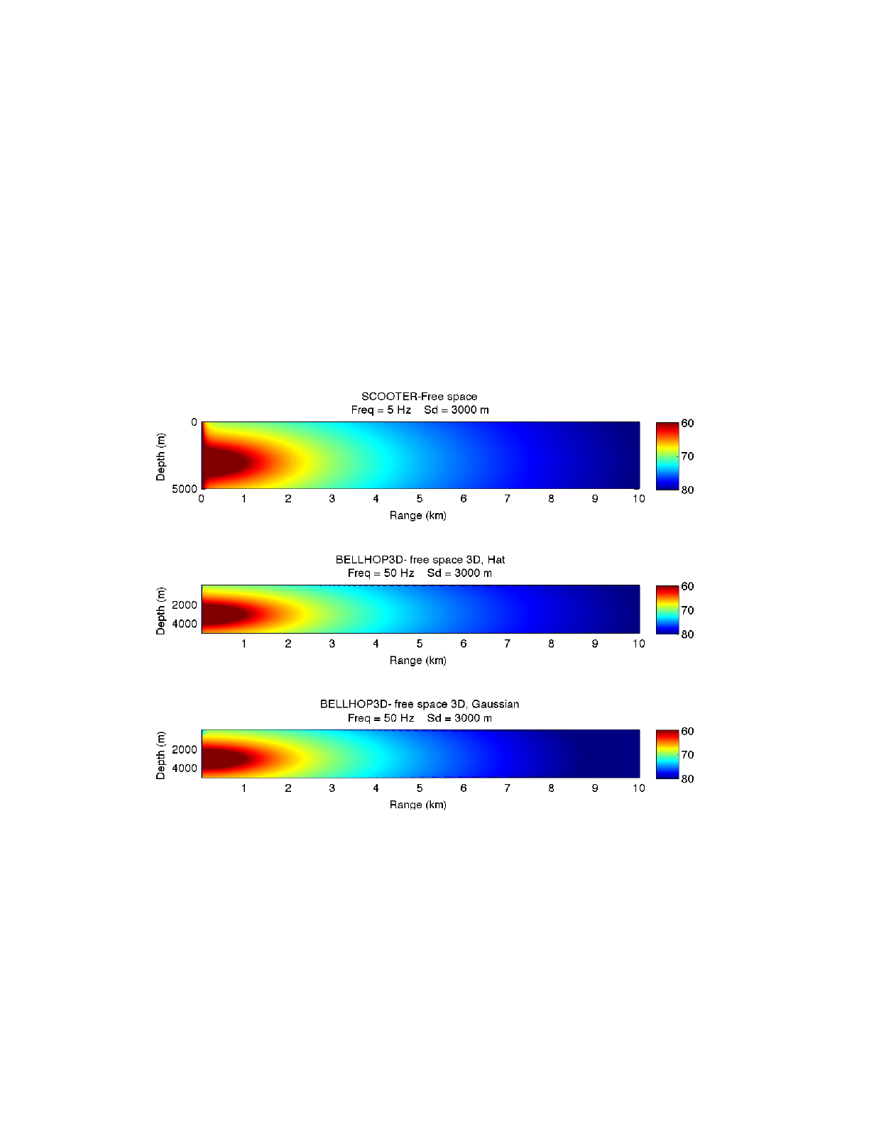
A. Free-Space and Half-Space Propagation
An isovelocity problem is the simplest test case. However, it is not entirely trivial. The simple
spherical decay of the field allows any small flaws in the beam widths to show up. If the beams are
either too narrow or too wide, the field will show obvious irregularities. In Fig. 10 below we present
in succession the results of a wavenumber integration code (SCOOTER), and BELLHOP3D run
with Geometric hat and Geometric Gaussian beams. The agreement is excellent except in the very
near field where we see an artifact due to a far-field approximation normally used in wavenumber
integration models.
Figure 10: Field due to a point source in free space. Top panel is a reference solution calculated using SCOOTER. The
middle panel is calculated using BELLHOP3D with Geometric Hat Beams. The Lower panel is calculated using
BELLHOP3D with Geometric Gaussian beams.
BELLHOP3D User Guide! "35
Heat, Light, and Sound Research, Inc.
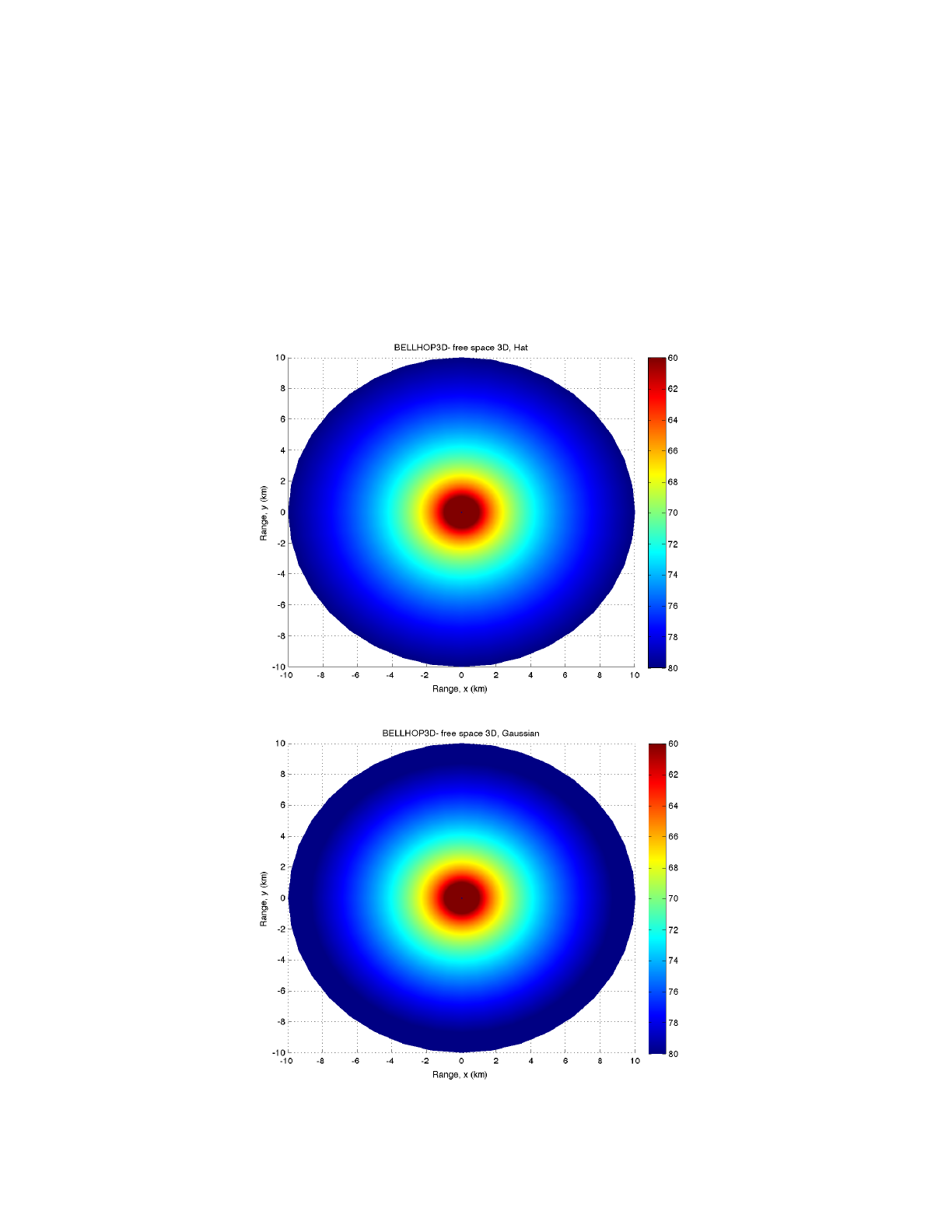
Figure 11 shows the BELLHOP3D results taken for a slice at fixed depth; i.e., a plan view. In the
upper panel we have used the hat-shaped beams. In the lower panel we have used Gaussian
beams. Collectively these results demonstrate that the code is producing a beautiful image of the
field due to a point source regardless of the slicing plane and with both hat and Gaussian beams.
This might seem like an easy test case but in fact it is a fairly stringent test of the model function.
"
BELLHOP3D User Guide! "36

Heat, Light, and Sound Research, Inc.
Figure 11: Acoustic field calculated by BELLHOP3D at a fixed receiver depth. The upper panel
uses Geometric Hat beams while the lower panel uses Geometric Gaussian beams.
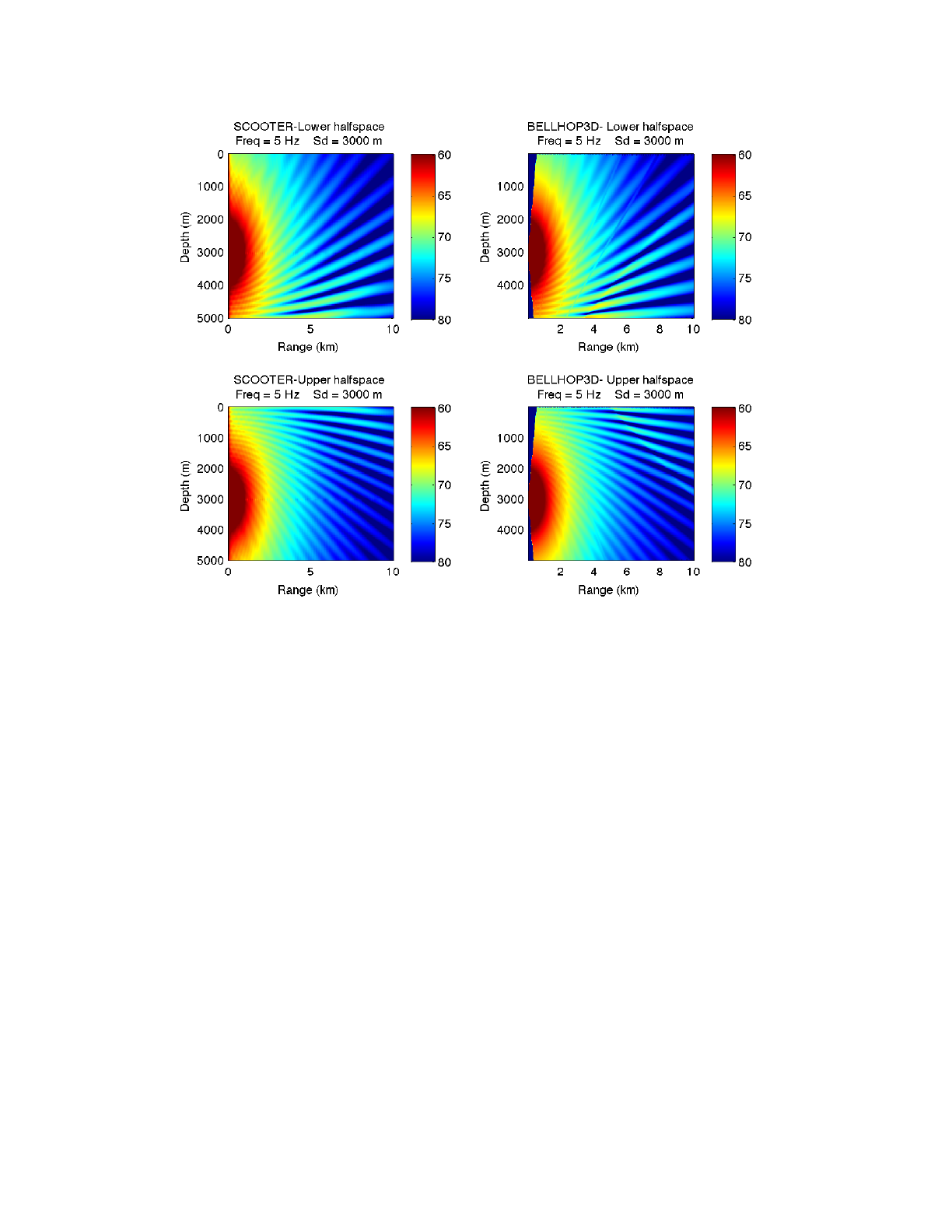
Next we introduce upper and lower halfspaces with a sound speed of 1750 m/s over an ocean
with a sound speed of 1500 m/s. There is no density contrast. The result in Fig. 3 shows the
expected interference pattern. The left panels are a reference solution from the SCOOTER
wavenumber integration code. The right panels are the results of the new BELLHOP3D code. The
upper panels are for a lower halfspace the the lower panels are for an upper halfspace.
One can see a variation in the energy vs. angle that is due to the corresponding variation in the
reflection coefficient for a halfspace. The precise positions of the lobes in the resulting interference
pattern are extremely sensitive to the phase. The excellent agreement between all the results gives
a lot of confidence in the treatment of the boundary reflection.
BELLHOP3D User Guide! "37
Heat, Light, and Sound Research, Inc.
Figure 12: Comparison of BELLHOP3D to a reference solution calculated by SCOOTER for lower and upper halfspaces
BELLHOP3D User Guide! "38
Heat, Light, and Sound Research, Inc.
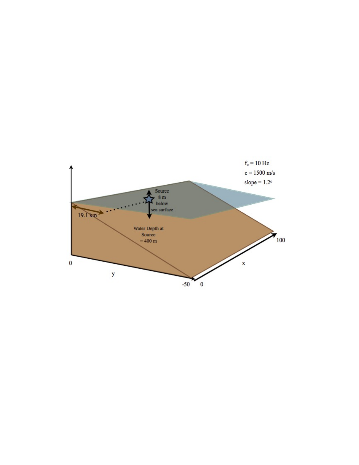
B. The Perfect Wedge
The perfect wedge is a classic problem has been studied by various people (Bradley and Hudimac,
Buckingham, Tolstoy, …). Here we use an analytic formula reported by Buckingham, which we
(Xavier Zabal at HLS) coded up in Matlab. We consider a case studied previously by Tolstoy,
Buckingham, and Doolite with a 10 Hz source at 19.1 km from the apex. The source depth is 8 m
and the receiver depth is 80 m (Fig. 13). The water depth at the source location is 400 m and the
pressure vanishes at both the top and bottom boundaries. The resulting transmission loss is shown
in Fig. 14.
Figure 13: Schematic of the wedge problem.
Figure 14: Transmission loss for the wedge problem derived from the analytic solution.
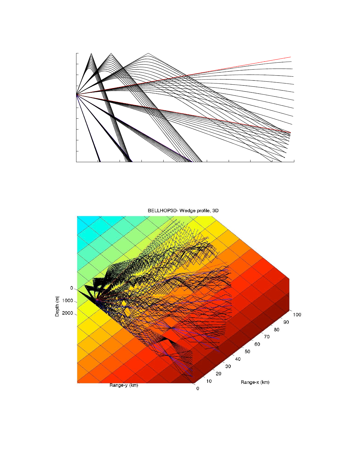
To interpret this figure it is useful to start with the BELLHOP3D ray traces. Here we have selected
10 rays in the azimuthal direction going from -90 to +90 degrees. In the vertical we chose 21
beams from -20 to +20 degrees. The top view of the rays is shown in Fig. 15 and the perspective
view is shown in Fig. 16. Here we can see that the energy that propagates upslope is gradually
refracted back downslope through repeated interactions with the sloping seafloor. The analytic
BELLHOP3D User Guide! "39
Heat, Light, and Sound Research, Inc.
formula of Buckingham (implemented by Xavier Zabal at HLS) shows that the field is actually
formed from 5 sets of wedge modes. The major bands of energy in the TL plot correspond to the
caustics associated with the ray paths of the modes.
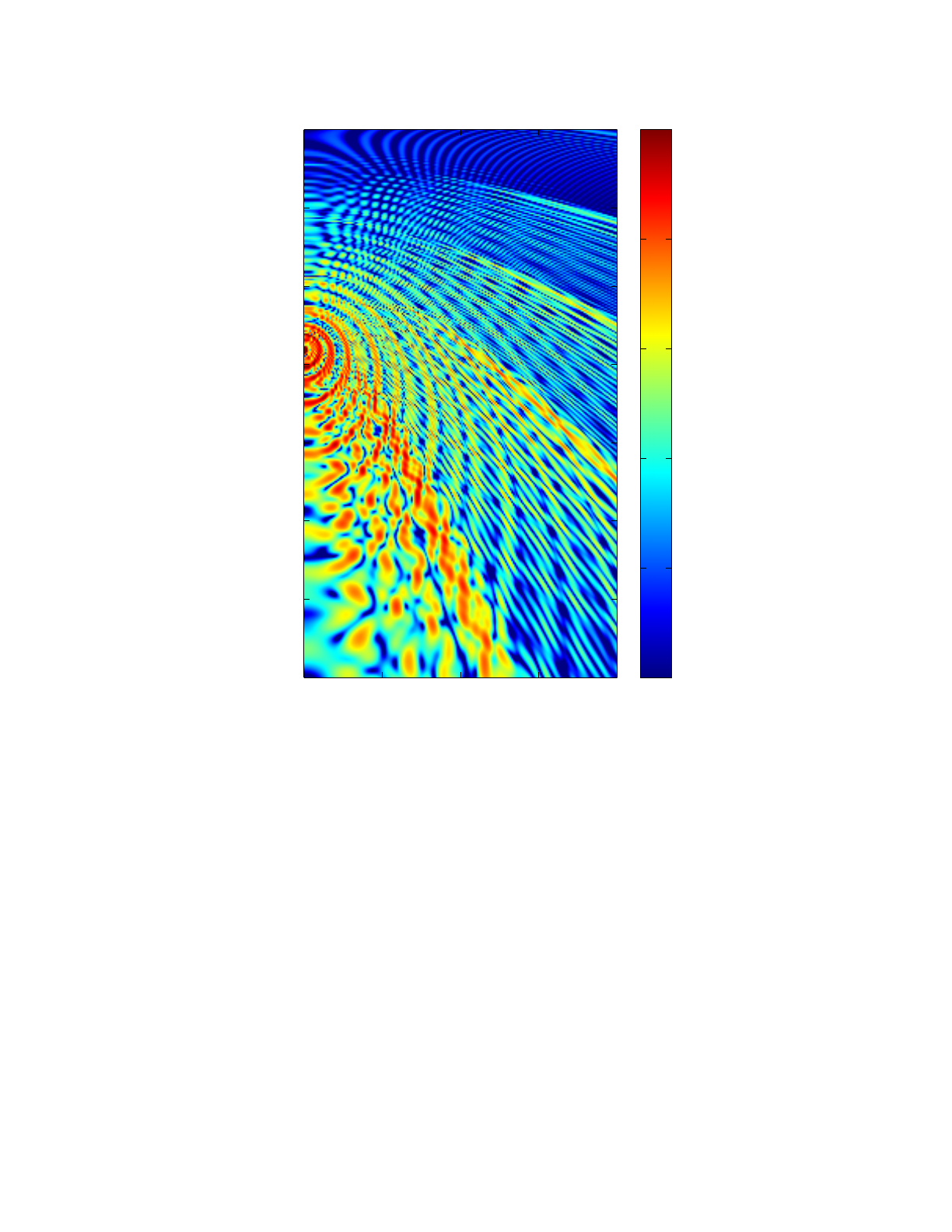
Finally, in Fig. 17 we show the TL as calculated by BELLHOP3D. The result shows nicely the
general characteristics of the field; however, it is not reproducing the fine details of the interference
pattern. This indicates that there is still some error in the code that needs to be fixed. It should be
noted that this is an extraordinarily difficult test case. We are going out a very long distance and
generating a large number of bottom reflections. The vertical angles of propagation go to 90
degrees and, because the boundaries are perfectly reflecting, all the upslope energy is returned
downslope where it forms a delicate interference pattern with itself.
BELLHOP3D User Guide! "40
Crossrange (km)
Range from Apex (km)
0 5 10 15 20
5
10
15
20
25
30
35
40
60
65
70
75
80
85
Heat, Light, and Sound Research, Inc.
Figure 15: Top view of the rays for the wedge problem.
Figure 16: Perspective view of the rays for the wedge problem.
BELLHOP3D User Guide! "41
0 10 20 30 40 50 60 70 80 90 100
−50
−45
−40
−35
−30
−25
−20
−15
−10
−5
0
Range, x (km)
BELLHOP3D− Wedge profile, 3D
Range, y (km)
Heat, Light, and Sound Research, Inc.
Figure 17: Transmission loss for the wedge calculated by BELLHOP3D; hat-beams (upper) and Gaussian beams (lower).!
BELLHOP3D User Guide! "42
Heat, Light, and Sound Research, Inc.
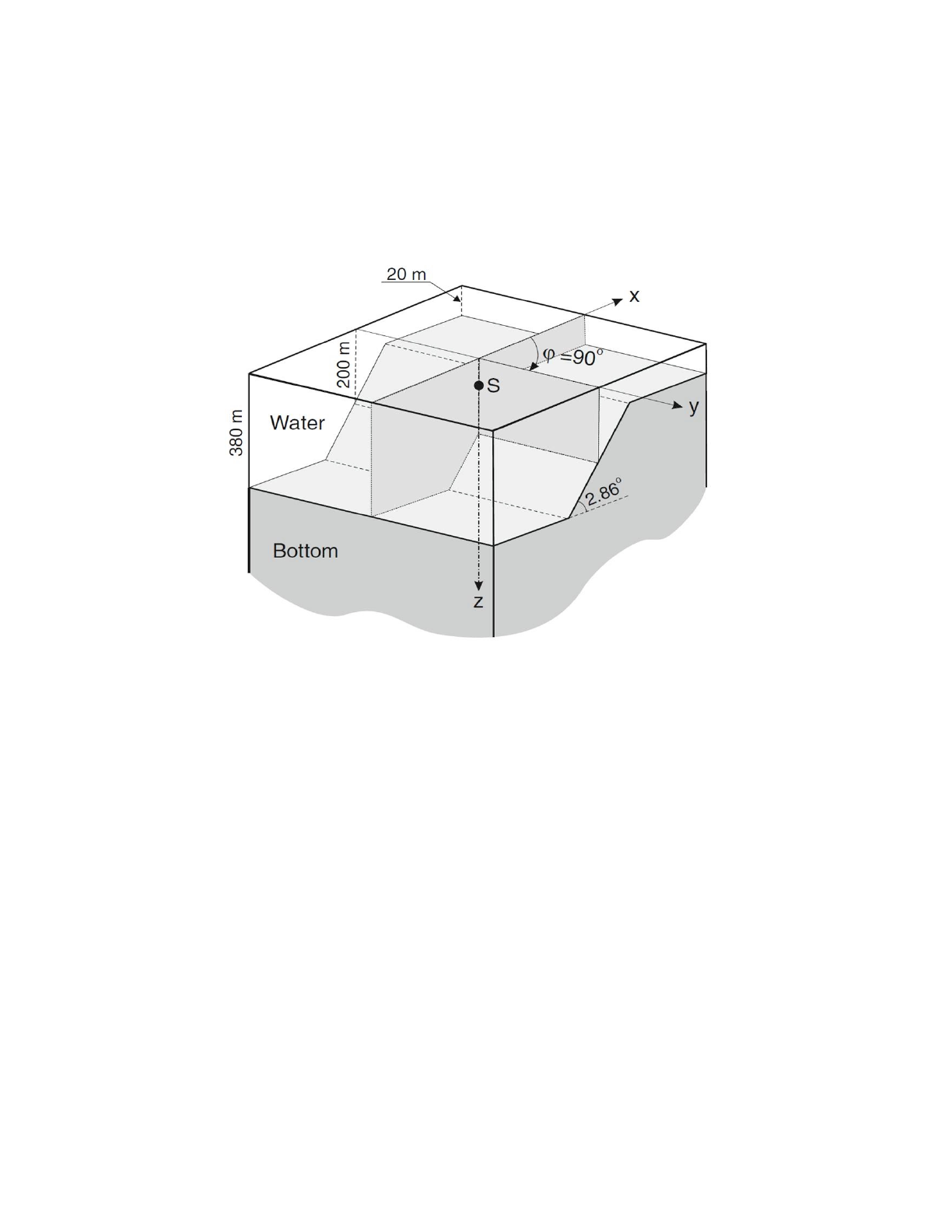
C. Truncated Wedge
This test case explores the effects of a sloping bottom on acoustic propagation. The geometry
considered is that of a truncated wedge as shown in the Fig. 18.
"
Figure 18: Schematic of the truncated wedge problem (from Jensen, Kuperman, Porter, and
Schmidt).
The angle of the wedge is 2.86 degrees and runs from a shallow depth of 20 m to a depth of 380
m in a range of 7.2 km. The sound speed in the water is 1500 m/s while the homogeneous fluid
bottom has a speed of 1700 m/s, a density of 1500 kg/m3, and an attenuation of 0.5 dB/λ. The
source transmits at a frequency of 25 Hz, and is located halfway down the slope at a depth of 40
m. At the source position the depth of the water is 200 m. The acoustic field is sampled at a
depth of 30 m around the source.
The BELLHOP3D environment file for this case is shown below.
'TWedge profile, 3D Hat beams 721 x 721' ! TITLE
25.0 ! FREQ (Hz)
1 ! NMEDIA
'CVW' ! SSPOPT (Analytic or C-linear interpolation)
0 0.0 20000.0 ! DEPTH of bottom (m)
0.0 1500.00 /
20000 1500.00 /
'A~' 0.0
BELLHOP3D User Guide! "43

Heat, Light, and Sound Research, Inc.
20000 1700.0 0.0 1.5 0.5 /
1 ! Nsx number of source coordinates in x
0.0 / ! x coordinate of source (km)
1 ! Nsy number of source coordinates in y
0 / ! y coordinate of source (km)
1 ! NSD
40.0 / ! SD(1:NSD) (m)
1 ! NRD
30 / ! RD(1:NRD) (m)
1001 ! NR
0.0 25.0 / ! R(1:NR ) (km)
1441 ! Ntheta (number of bearings)
-90 90 / ! bearing angles (degrees)
'CG 3' ! 'R/C/I/S'
1441 ! Nalpha
-89 89 / ! alpha1, 2 (degrees) Elevation/declination angle fan
1441 %144 ! Nbeta
-90 90 / ! beta1, beta2 (degrees) bearine angle fan
0 25 4 20500.0 ! STEP (m), Box%x (km) Box%y (km) Box%z (m)
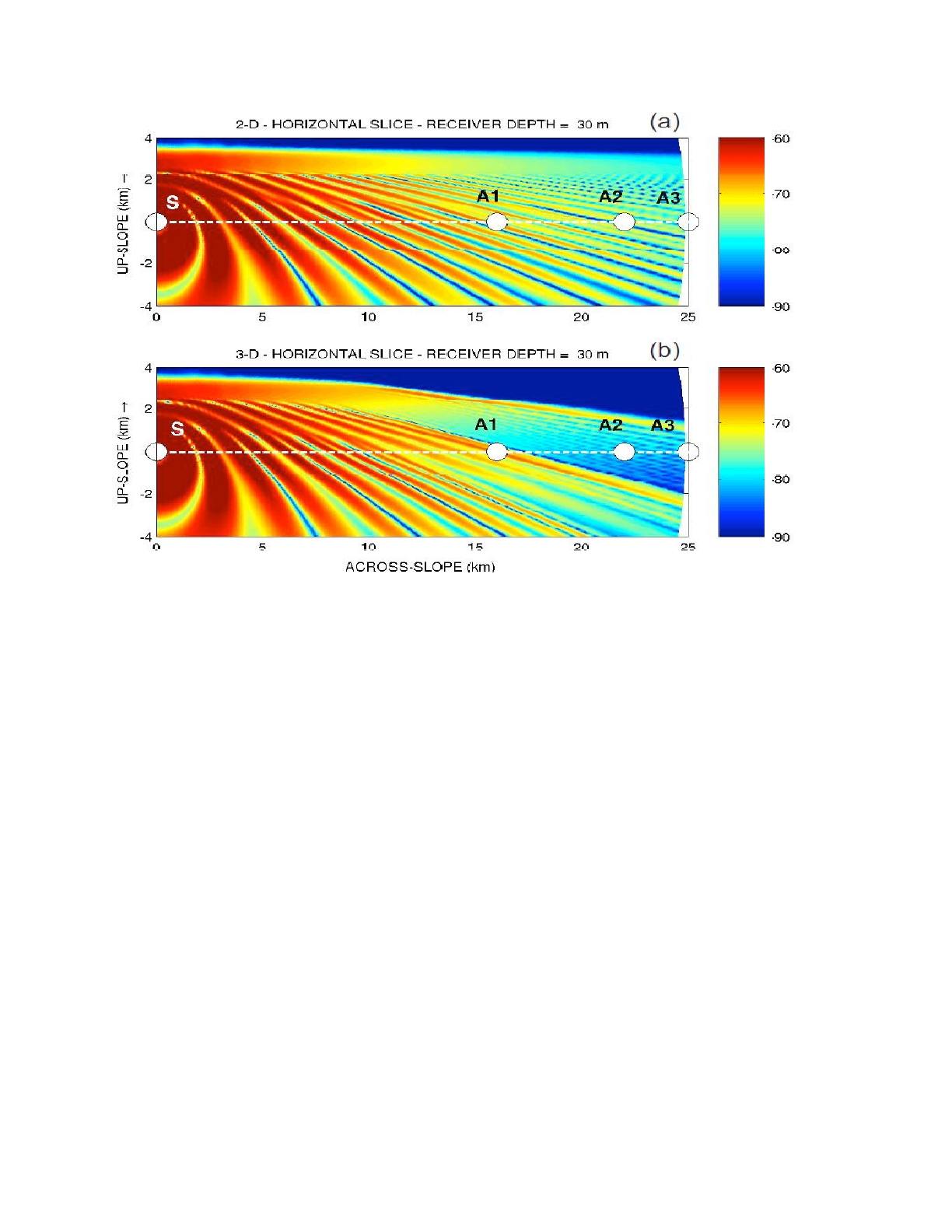
For this test case there is no analytic solution for the propagation, but the BELLHOP3D results are
compared to the Nx2-D and 3-D solutions reported by Sturm , using a 3-D PE model.
1
Figure 19 presents the results obtained by Sturm for the propagation loss computed using an
Nx2D method in the top panel, and with a full 3D PE method in the bottom panel.
"F."Sturm,"“Numerical"study"of"broadband"sound"pulse"propaga;on"in"three"dimensional"oceanic"waveguides”,"J."
1
Acoust."Soc."Am."1117,"1058-1079"(2005)
BELLHOP3D User Guide! "44
Heat, Light, and Sound Research, Inc.
"
Figure 19: Comparison of Nx2D and 3D results from the Sturm PE for the truncated wedge (figure
from Jensen, Kuperman, Porter, and Schmidt).
BELLHOP3D User Guide! "45
Heat, Light, and Sound Research, Inc.
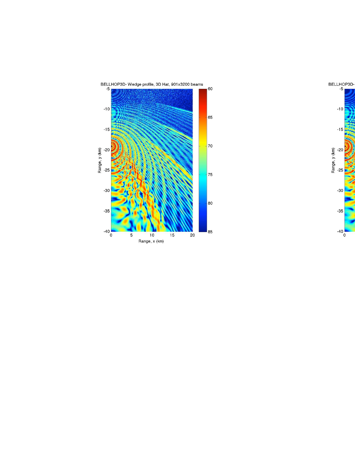
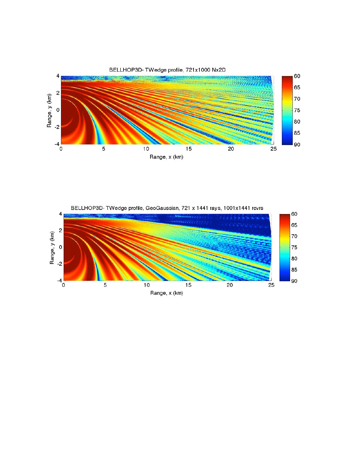
Figure 20: Comparison of Nx2D and 3D results from BELLHOP3D for the truncated wedge.
These results may be compared to the BELLHOP3D outputs for the Nx2-D (top) and full 3D
(bottom) methods shown in Fig. 20.
Both results show a significant difference between the Nx2D and 3D methods, and the horizontal
refraction effects are clearly visible and qualitatively similar in the two models. If we look closely at
the interference pattern we see excellent agreement towards the right side (cross-slope); however,
in the lower left (down-slope) there are some clear differences. There are approximations in both
BELLHOP3D and in Sturm’s PE (narrow-angle) so from this test we cannot be sure which is the
more accurate solution. However, there is a significant difference in the starting fields for the two
BELLHOP3D User Guide! "46
Heat, Light, and Sound Research, Inc.
models. Sturm used a starting field consisting of just the first few modes; however, in BELLHOP3D
we use a point source starting field.
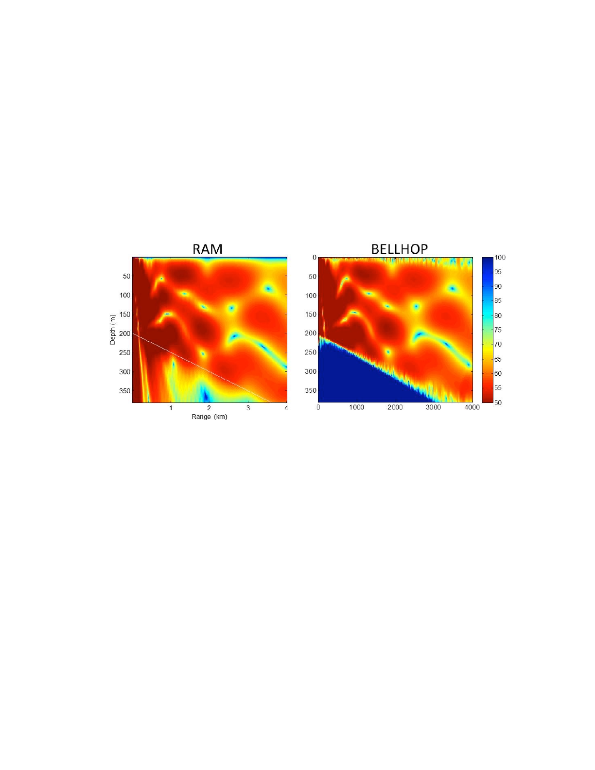
To try to resolve this discrepancy, the propagation down the slope was compared to the prediction
of the RAM acoustic model. Figure 21 shows the output of the RAM model next to the BELLHOP
results. The agreement is excellent, but detailed analysis shows that there is a small range-
dependent shift between both models, a difference due to the fact that the beam-shift effect
caused by the penetrable bottom is not implemented in BELLHOP3D right now. There is also a bit
of noise in the BELLHOP3D results near the boundary which is a normal characteristic that can be
reduced by using additional beams.
"
Figure 21: Comparison of RAM (PE) and BELLHOP3D for a downslope track in the truncated
wedge.
Another model we can compare to is Ding Lee’s FOR3D code. The result from FOR3D for this case
is shown in Fig. 22. There is an artifact in the lower right corner whose cause is not known at the
moment. However, the rest of the figure is in general agreement with BELLHOP3D. Here we can
also see excellent agreement in the lower-left or downslope region.
Figure 22: Results from FOR3D (3D PE model) for the truncated wedge.
In summary, we have presented results from 4 different acoustic models (BELLHOP3D, RAM,
Sturm PE, FOR3D). The results generally agree; however no single pair shows really the level of
agreement we would hope for. Given that BELLHOP3D agrees with RAM and FOR3D in the
downslope region and with the Sturm PE in the cross-slope region, we conjecture that
BELLHOP3D is providing the best solution throughout the domain. The two PEs use different
BELLHOP3D User Guide! "47
Heat, Light, and Sound Research, Inc.
operator splittings and the differences between them are probably largely due to that. However, the
difference in the starting field is another important issue.
BELLHOP3D User Guide! "48

Heat, Light, and Sound Research, Inc.
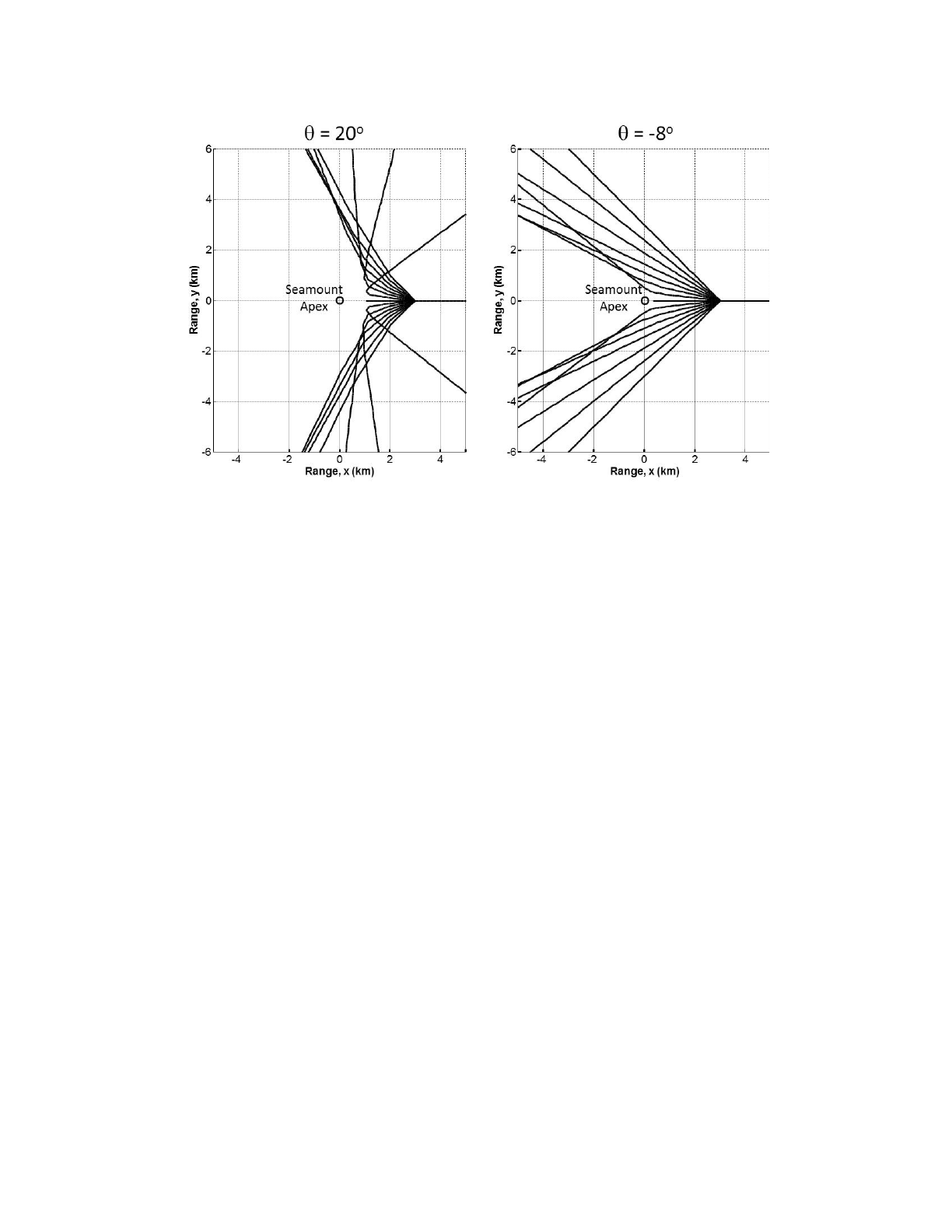
D. Seamount
This test case involves propagation around a conical seamount that extends all the way to the sea
surface. Both the sea surface and the seamount are assumed to be perfect reflectors, and this
assumption permits an analytical solution to the Helmholtz equation based on a separation of
variables technique, as developed by Buckingham .
2
For this test it is assumed that the seamount slope gradient is 75 degrees (channel angle of 15
degrees). The source is at a depth of 100 m and located at a range of 3 km to the right of the
seamount apex, and the transmitted frequency is 20 Hz. The acoustic field around the seamount
is also sampled at a depth of 100 m.
The BELLHOP3D environment file used to run this problem is shown below:
'Seamount3D, Gaussian 361x601 rcvrs, 361x301 beams' ! TITLE
5.0 ! FREQ (Hz)
1 ! NMEDIA
'CVW' ! SSPOPT (Analytic or C-linear interpolation)
0 0.0 20000.0 ! DEPTH of bottom (m)
0.0 1500.00 /
20000 1500.00 /
'R~' 0.0
1 ! Nsx number of source coordinates in x
3.0 / ! x coordinate of source (km)
1 ! Nsy number of source coordinates in y
0.01 / ! y coordinate of source (km)
1 ! NSD
100.0 / ! SD(1:NSD) (m)
1 ! NRD
100 / ! RD(1:NRD) (m)
601 ! NR
0.0 12.0 / ! R(1:NR ) (km)
361 ! Ntheta (number of bearings)
90 180 / ! bearing angles (degrees)
'CB 3' ! 'R/C/I/S'
301 ! Nalpha
-89 89/ ! alpha1, 2 (degrees) Elevation/declination angle fan
361 ! Nbeta
90 180 / ! beta1, beta2 (degrees) bearing angle fan
100 9 9 20500.0 ! STEP (m), Box%x Box%y Box%z (m)
"M.J."Buckingham,"“Theory"of"acous;c"propaga;on"around"a"conical"seamount”,"J."Acoust."Soc."Am."80,"265-277"
2
(1986).
BELLHOP3D User Guide! "49

Heat, Light, and Sound Research, Inc.
Figure 23 presents a top view of the trajectory of 15 rays leaving the source at angles between 135
and 225 degrees relative to the horizontal axis. The left panel corresponds to rays with a grazing
angle of +20 degrees (downward from the source), while the right panel corresponds to rays with
an upward grazing angle of 8 degrees.
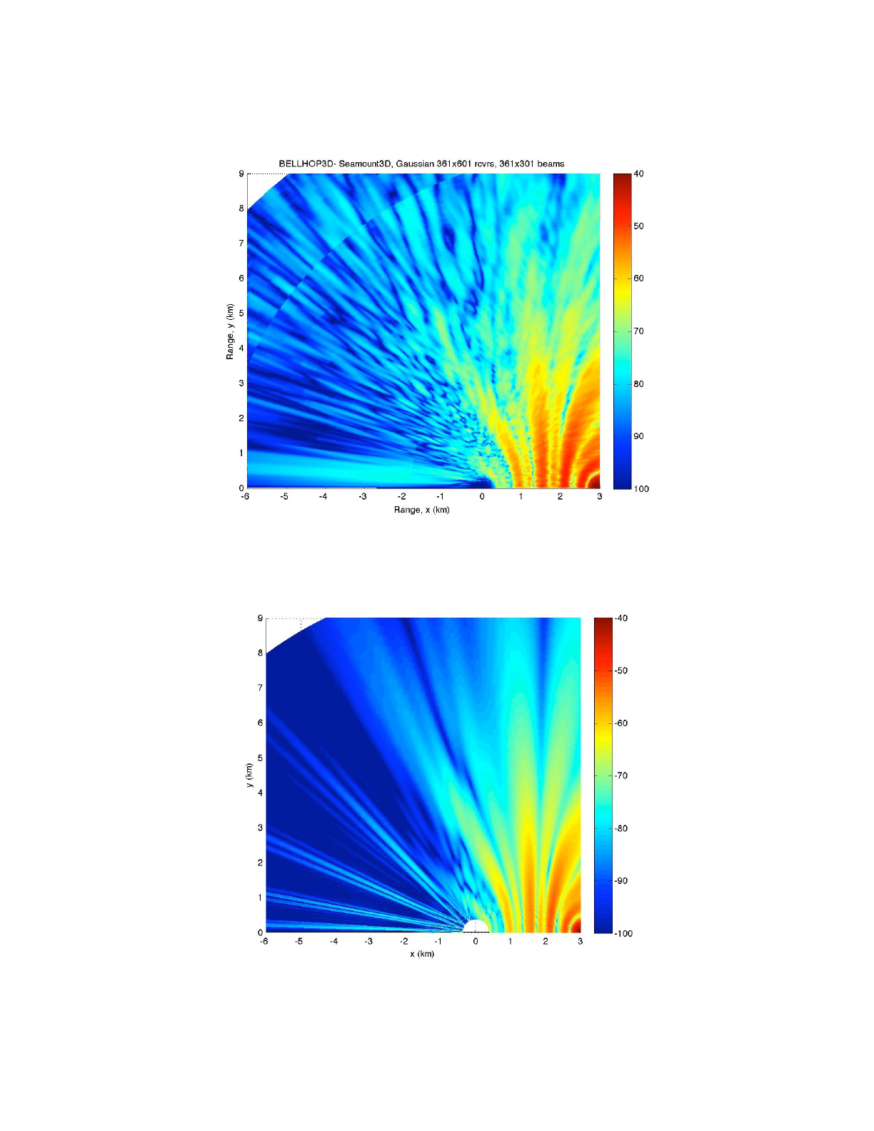
Figure 24 shows the results of the BELLHOP3D run along with the results of the analytical model.
In the BELLHOP3D case the coordinate system is centered at the source position while for the
analytical model the coordinates are centered at the apex of the seamount. The overall energy
levels show a reasonable match; however, the BELLHOP3D result is more ‘broken up’. We assume
this is the ‘disco ball’ effect, i.e. due to the fact that BELLHOP3D uses a facetted description of the
bottom rather than the perfect cone used in the analytic formulation. Real oceans are or course
neither perfect cones nor perfectly facetted.
BELLHOP3D User Guide! "50
Heat, Light, and Sound Research, Inc.
"
Figure 23: Top view of the BELLHOP3D rays for the seamount problem.
BELLHOP3D User Guide! "51
Heat, Light, and Sound Research, Inc.
Figure 24: Comparison of BELLHOP3D transmission loss to the analytic model.!
BELLHOP3D User Guide! "52

Heat, Light, and Sound Research, Inc.
E. The Harvard Case Eddy Scenario
Another approach to validating BELLHOP3D is to compare it to other numerical solutions.
However, there are not so many models capable of handling 3D scenarios. Generally, this remains
a research issue even though basic 3D models were developed back in the 1980s. The reason
such models have not really taken off is 1) environmental information (oceanography especially) has
not readily been available, 2) run times have been excessive for 3D models. BELLHOP3D is very
practical for such 3D problems largely because of the basic efficiency of ray-based models.
Meanwhile, the speed of typical computers has increased perhaps by a factor of 10,000 since
those original models were developed. Nevertheless, it remains difficult to run other model types at
reasonable frequencies to generate comparison solutions. Generally, we are forced to take
artificially low frequencies (where BELLHOP3D tends to be less accurate) to create a test problem
that can be solved by both BELLHOP3D and another model type.
We have chosen to use Ding Lee’s FOR3D Parabolic Equation (PE) model here. This is one of the
few 3D PE models available and is openly distributed on the Ocean Acoustics Library. However, it
is more that 30 years old and there was considerable work required to install it. While the code was
generally carefully implemented, there were a number of problems that showed up with the code,
e.g. DO loops using real variables and issues with uninitialized variables. In the process of installing
this, she also converted it to a more modern FORTRAN 95 version. We present here our first test
case of the model. BELLHOP3D comparisons have not been made yet.
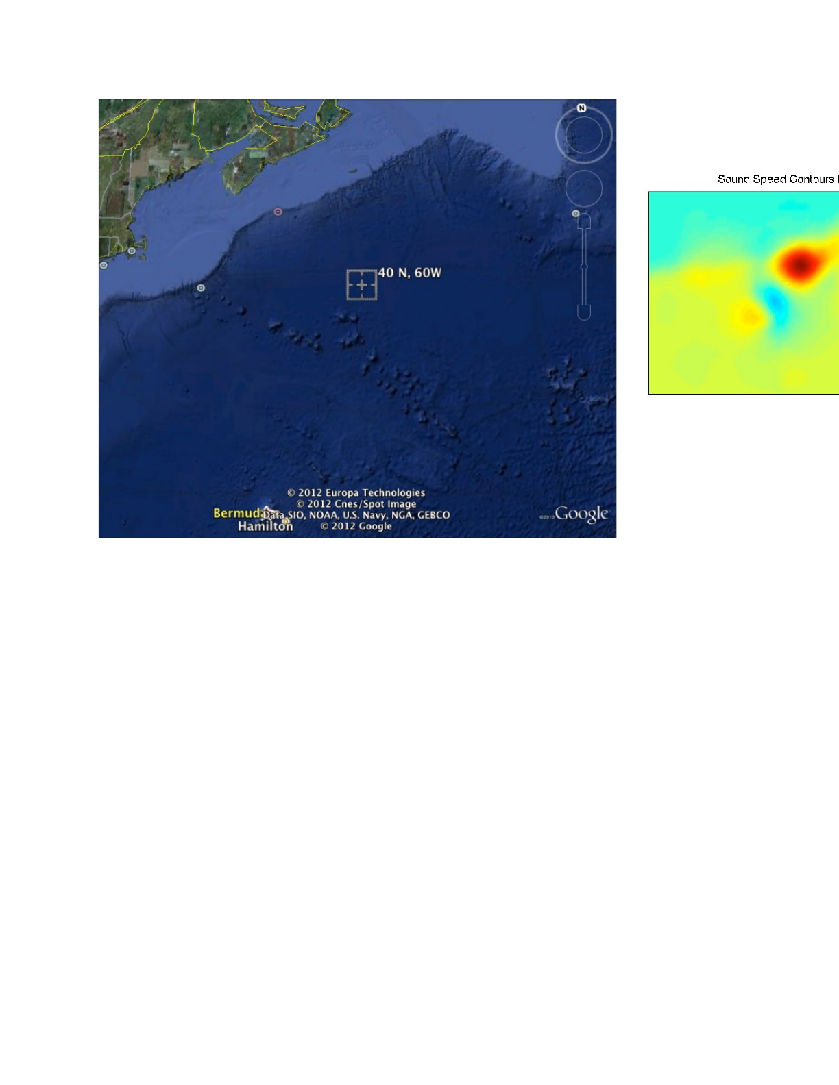
The scenario is the ‘Harvard’ Case provided with the code, which involves long-range propagation
(over about 4 degrees in latitude and longitude) in an area of the North Atlantic where the Gulf
Stream is present, spinning off numerous warm and cold core eddies. The actual site with a cross
showing the source location is shown in Fig. 25. There is a mild bathymetric variation; however, the
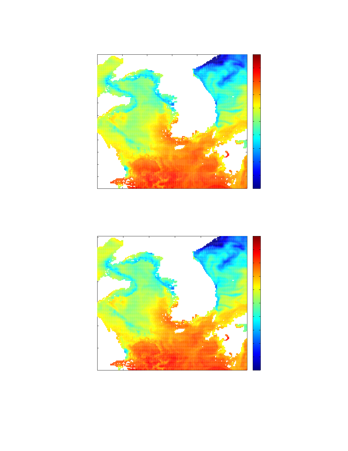
key feature of interest is probably the oceanography with the various eddies. The SSP on a
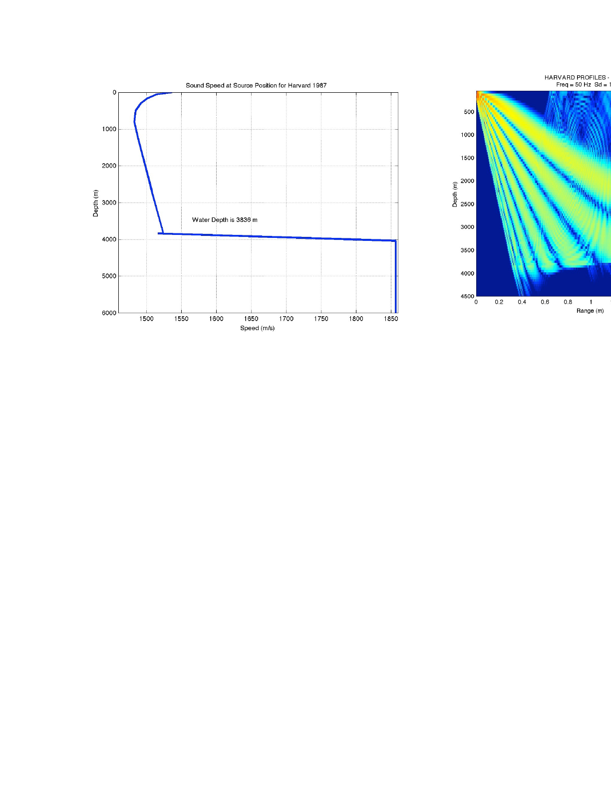
horizontal slice is shown in Fig. 26; the SSP on a vertical slice at the source location is shown in
Fig. 27. Finally Figs. 28 and 29 show the transmission loss computed by FOR3D on both vertical
and horizontal slices.
These are just preliminary results that show that we have been able to install the FOR3D model
successfully.
Figure 25: Model site for the Harvard scenario.
BELLHOP3D User Guide! "53
Heat, Light, and Sound Research, Inc.
Figure 26: Sound speed on a horizontal slice.
Figure 27: Sound speed profile at the source location for the Harvard scenario.
Figure 28: Transmission loss on a vertical slice for the Harvard scenario.
Figure 29: Transmission loss on a horizontal slice for the Harvard scenario.
BELLHOP3D User Guide! "54
Heat, Light, and Sound Research, Inc.
F. Rotated Munk Profile
The Munk profile is a classic deep water profile as shown in Fig. 30 below. We have used this
frequently as a test and have reference solutions calculated by a wide variety of models. In Fig. 31
we show the transmission loss as calculated by BELLHOP3D using the Geometric Hat-Beam
option. The important test on this figure was to verify that it reproduced exactly the result from the
standard 2D BELLHOP. In fact, both 2D and 3D versions of BELLHOP call the same influence
routine and the results agree at the pixel level. (See also the results presented in Progress Report
5.)
However, the main motivation for this case was to verify that BELLHOP3D was handling all the
lateral interfaces in the oceanography correctly. For this to work properly we also had to add logic
to BELLHOP3D to detect all the oceanography interfaces, not just those in depth. (As noted
previously, the ray traces do not come out precisely if the rays are allowed to step over interfaces.)
In addition, the logic for beam curvature changes had to be implemented. This involves rotating the
beam equations into a coordinate system relative to the plane of the incident ray on the interface.
The point of this discussion is just to emphasize that there is quite a bit of code required to handle
all of this properly.
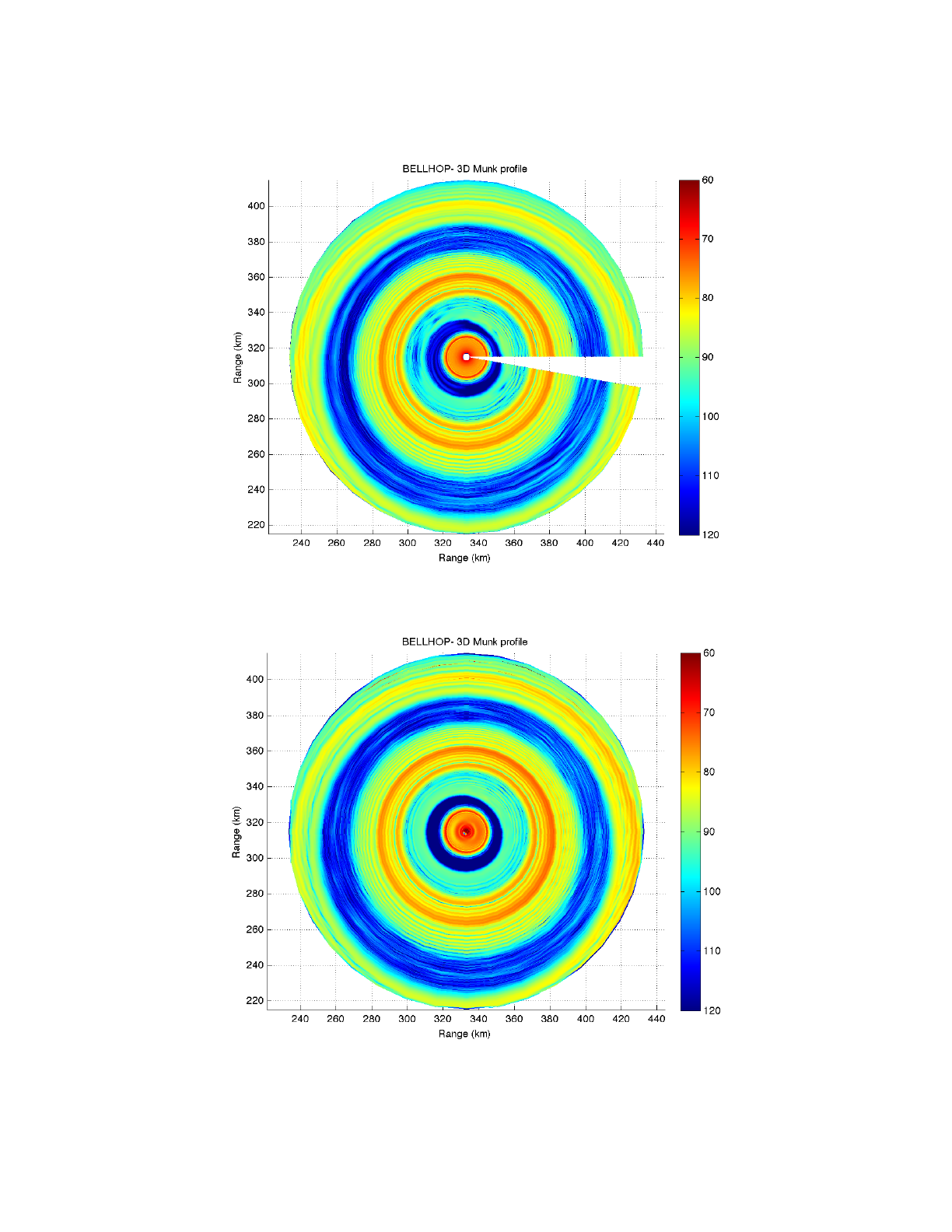
To capture these effects, we simply rotate the sound speed profile so that the gradients are all in
the x-direction, not the usual z-direction. The profile is completely unphysical but that does not
matter for this benchmark objective. The resulting transmission loss from BELLHOP3D is shown in
BELLHOP3D User Guide! "55
Heat, Light, and Sound Research, Inc.
Fig. 32. Note that it is virtually identical to the previous figure except for the axis rotation. One
difference that can be seen is that the new result appears fuzzier at long ranges. This is because
BELLHOP3D uses a polar coordinate system with radials emanating from the source— at longer
ranges the radials spread further apart.
The excellent match here may seem anticlimactic; however, initial results showed a variety of
problems and a great deal of work was necessary to reach this exact agreement.
Figure 30: Plot of the Munk sound speed profile.!
BELLHOP3D User Guide! "56
Heat, Light, and Sound Research, Inc.
Figure 31: Transmission loss for the Munk profile calculated by BELLHOP3D.
Figure 32: Transmission loss for the Rotated Munk Profile calculated by BELLHOP3D.
BELLHOP3D User Guide! "57

Heat, Light, and Sound Research, Inc.
BELLHOP3D User Guide! "58

Heat, Light, and Sound Research, Inc.
G. Korean Seas
Here we consider a modeling exercise for the Korean Seas (East, South, West). An oceanographic
field was derived from the HYCOM (Hybrid Coordinate Ocean Model). The HYCOM model is
discussed on http://hycom.org/. The associated consortium provides global oceanographic
forecasts on a daily basis. For this example, we downloaded the global forecast for Julian day 204
of 2011 with output provided at about 12.5 points per degree. A short Matlab script was written to
1) read the global NetCDF data for salinity and temperature, 2) extract a desired operational area,
3) convert the salinity and temperature to sound speed, and 4) write the SSP field in the above
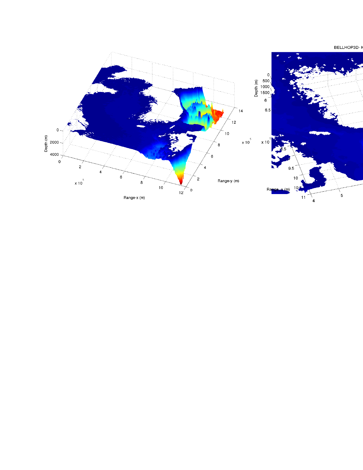
described format that BELLHOP3D requires. The resulting field is plotted in Figure 33 below.
BELLHOP3D requires the SSP field to be provided on a Cartesian grid (x-y-z) coordinates. The
lower left corner of the box is arbitrarily selected as the coordinate origin. The results on the
Cartesian grid are plotted in the lower panel of Figure 33.
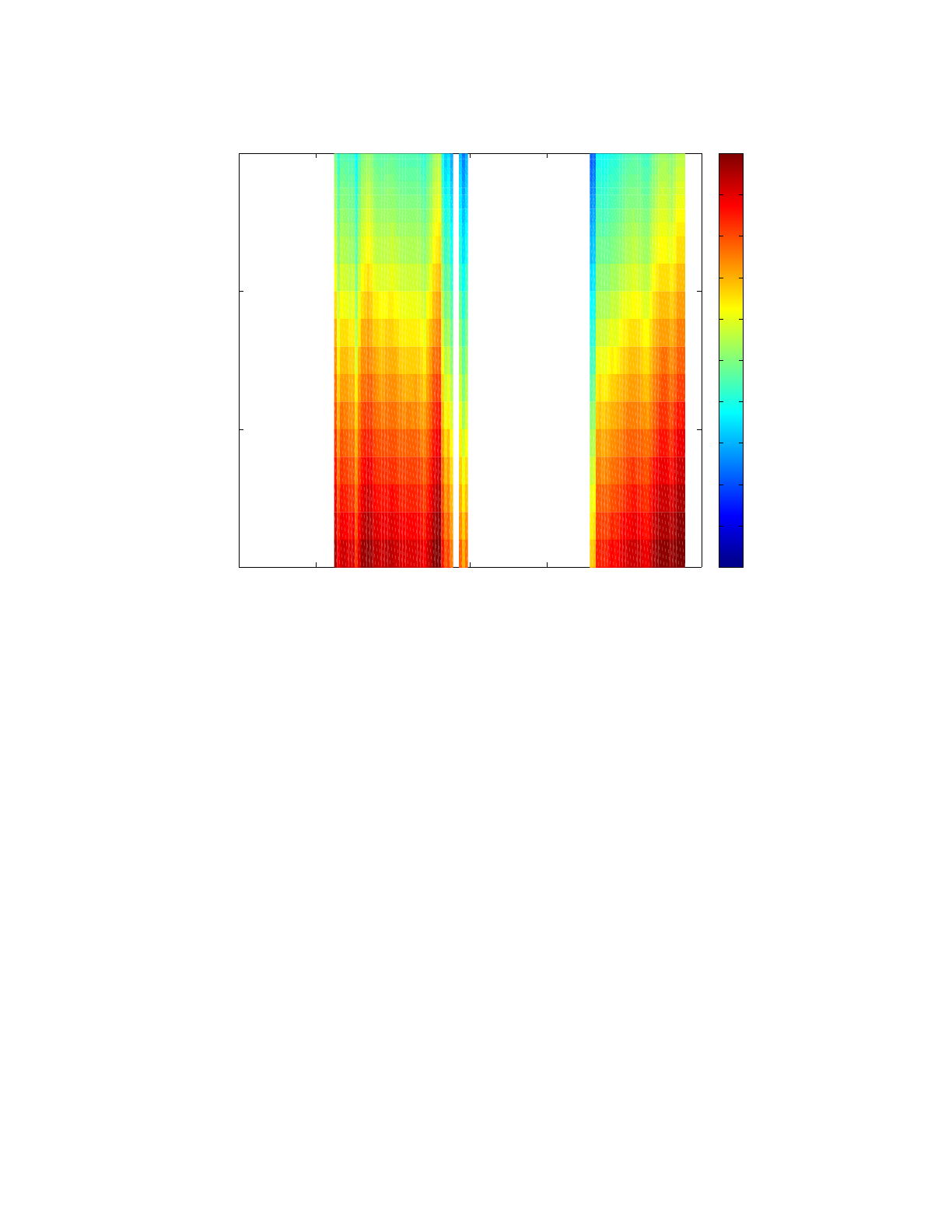
In Figure 34 we display also a section at constant latitude (y = 700 km) to illustrate the upward
refracting nature of the profile. The ‘white’ sections in the plot a NaNs corresponding to areas of
land.
BELLHOP3D User Guide! "59
Heat, Light, and Sound Research, Inc.
Figure 33: Horizontal slice (at a depth of 50 m) of the sound speed field. Top panel presented with latitude/longitude in
degrees; bottom panel presented in Cartesian coordinates.!
BELLHOP3D User Guide! "60
120 122 124 126 128 130 132
31
32
33
34
35
36
37
38
39
40
Longitude (degrees)
Latitude (degrees)
1500
1505
1510
1515
1520
1525
1530
1535
1540
1545
1550
0 200 400 600 800 1000
0
200
400
600
800
1000
1200
x (km)
y (km)
1500
1505
1510
1515
1520
1525
1530
1535
1540
1545
1550
Heat, Light, and Sound Research, Inc.
Figure 34: Vertical slice (at a latitude of 700 km) of the sound speed field.
The other critical piece of environmental information is the bathymetry. The actual bathymetry used
in the HYCOM simulations can also be downloaded from the HYCOM website. However, rather
than sort out the format of that file, we download the bathymetry data for this same box from the
National Geophysical Data Center website (http://www.ngdc.noaa.gov/ ). In particular we select
the ETOPO1 database which provides data on a 1’ grid. The data was downloaded in the standard
xyz format. A routine was then written to read the xyz file and write it in the format the BELLHOP3D
requires for a bathymetry file.
Thus, we now have simple tools that enable us to download an operational area anywhere on the
globe and immediately generate the SSP and bathymetry files that BELLHOP3D requires. The
bathymetry for this test case is shown in Figure 35.
Figure 35: Bathymetry for the Korean Seas from the ETOPO1 database.
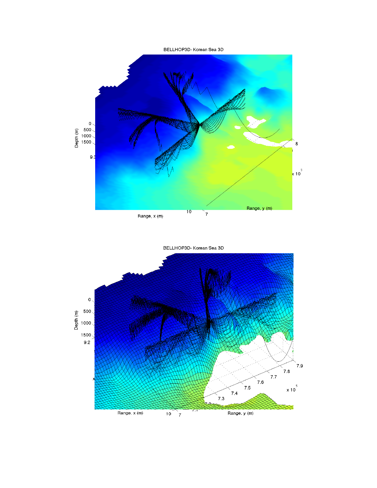
Figure 36: Ray trace over the bathymetry, showing the location of the source.
BELLHOP3D User Guide! "61
0 200 400 600 800 1000 1200
0
500
1000
1500
x (km)
Depth (m)
1500
1505
1510
1515
1520
1525
1530
1535
1540
1545
1550
Heat, Light, and Sound Research, Inc.
Figure 37: Ray trace over the bathymetry. In the lower panel faceting has been turned on to show more clearly the
interaction of the rays with the bathymetry.
We selected a source location in the East Sea at (1000 km, 750 km) in our x-y grid and traced a
fan of rays as shown in Figure 36. Figure 38 shows a blowup (with surface faceting both on and off)
where you can clearly see the role of the bathymetry. With the faceting turned off, the picture is less
cluttered, making it easier to see the actual ray trace. However, the faceting allows one to see more
clearly how the actual bathymetry causes the rays to refracts out of the vertical plane.
BELLHOP3D User Guide! "62
Heat, Light, and Sound Research, Inc.
Figure 38: Ray trace over the bathymetry for a source closer to shore.
BELLHOP3D User Guide! "63
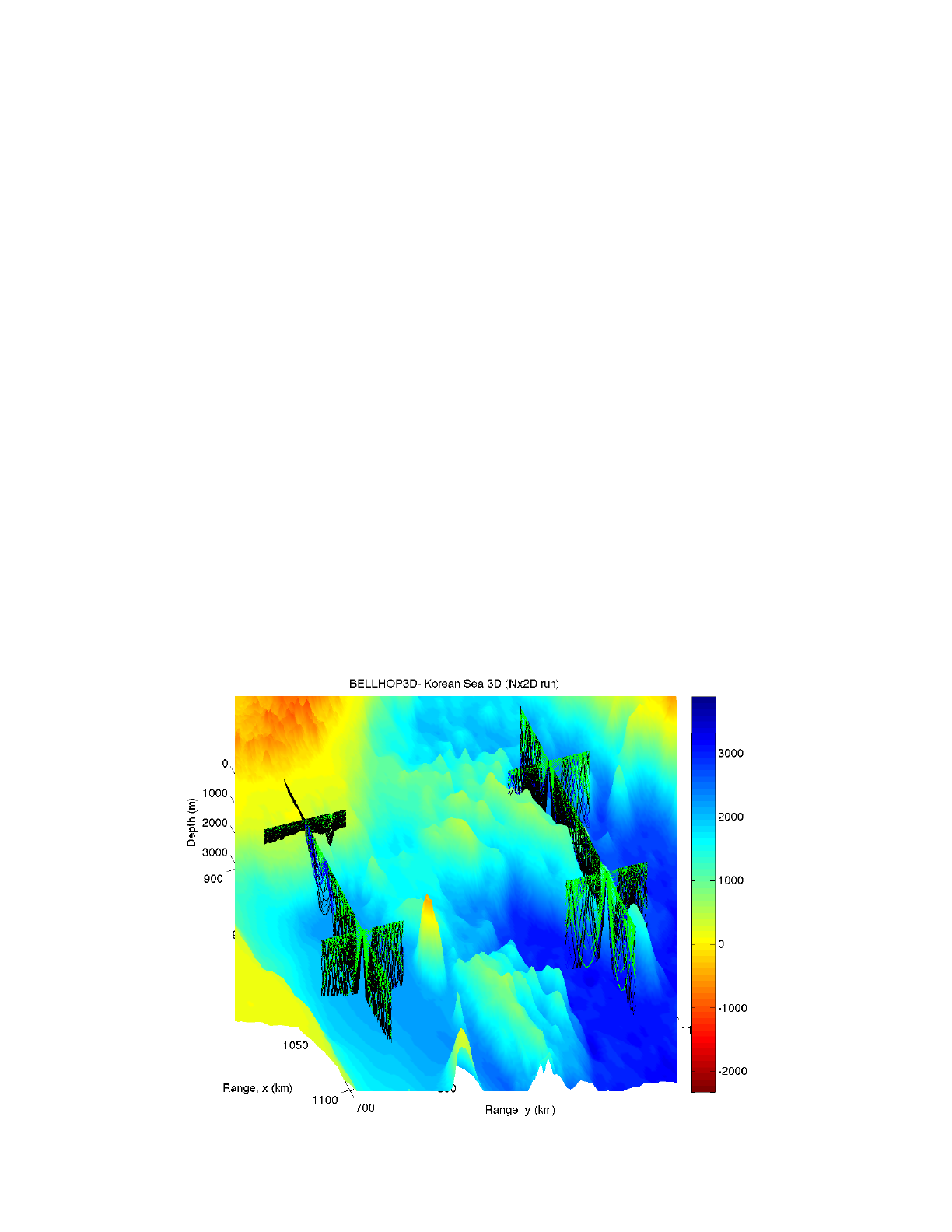
Heat, Light, and Sound Research, Inc.
To accentuate the horizontal refraction effects we experimented with different source positions. We
show here another example, where the source location is shifted slightly towards the coast at (970
km, 750 km). Again we present the results with faceting turned off and on (Fig. 38). Here we can
see dramatic refractive effects in the horizontal plane. Those effects are primarily due to the
bathymetry since the coarsely sampled oceanographic field does not have very strong gradients.
Note also that some of the rays are completely turned around. In practice the energy associated
with these rays will be severely attenuated due to bottom losses.
Figures 39 and 40 demonstrate the multi-source capability for the ray traces. In this case 4 sources
have been placed at different lat/longs and rays were traced in the North, South, East, and West
directions. The upper plot was done using the Nx2D option so there is no horizontal refraction.
Figures 41 and 42 show slices of the transmission loss field using the Nx2D option, and full 3D
option. The range-depth slice is taking along the 0 degree (eastward) bearing for the first source.
The lat/long slice is taken at a receiver depth of 400 m.
Differences between the two plots are partially due to horizontal refraction. However, we expect
that there are also some differences here due to the different beam types used. The Nx2D model
uses Geometric Beams here, while the 3D run uses Cerveny beams. Typically we find the
Geometric Beams are more reliable.
BELLHOP3D User Guide! "64
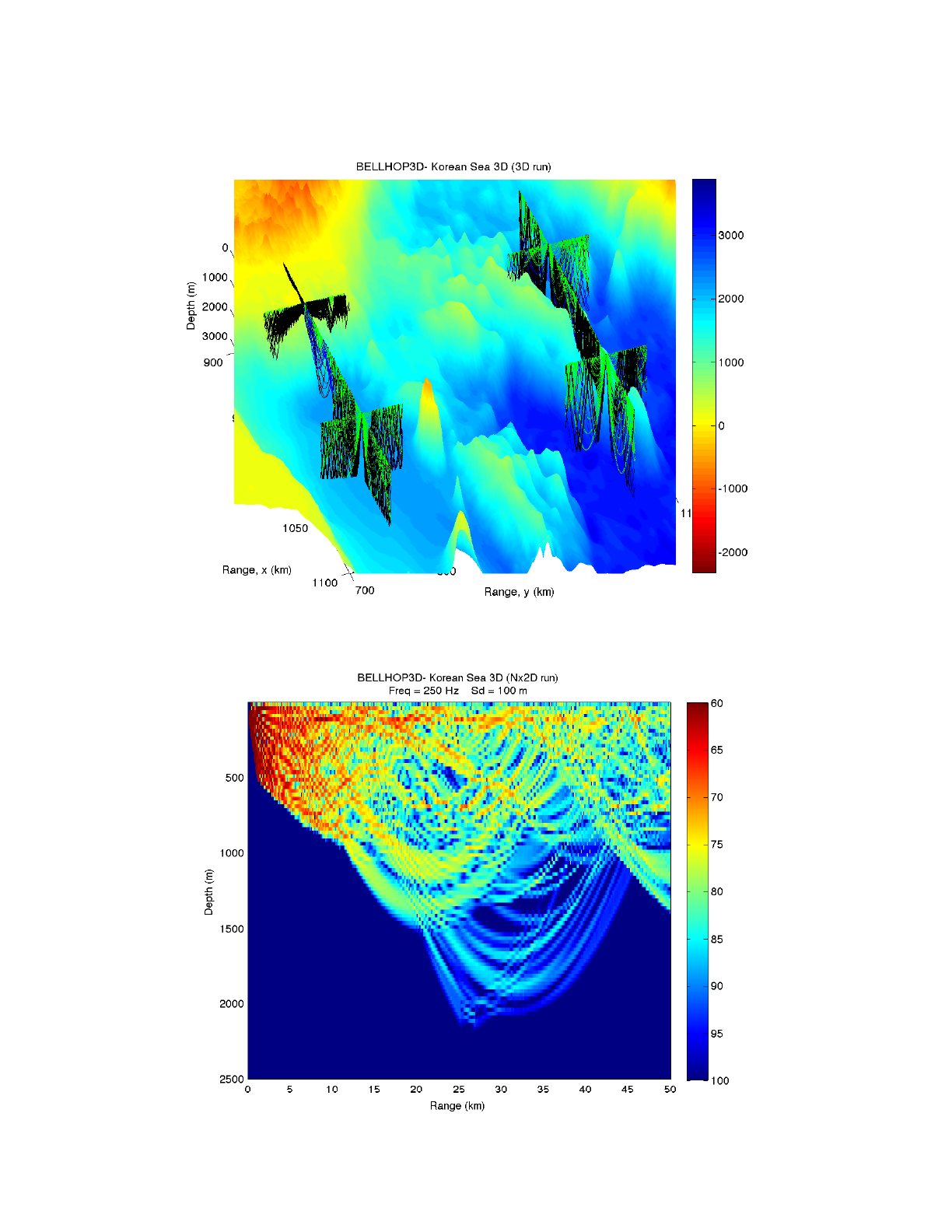
Heat, Light, and Sound Research, Inc.
Figure 39: Ray trace (Nx2D option) showing the multi-source capability.
Figure 40: Ray trace (3D option) showing the multi-source capability.
BELLHOP3D User Guide! "65
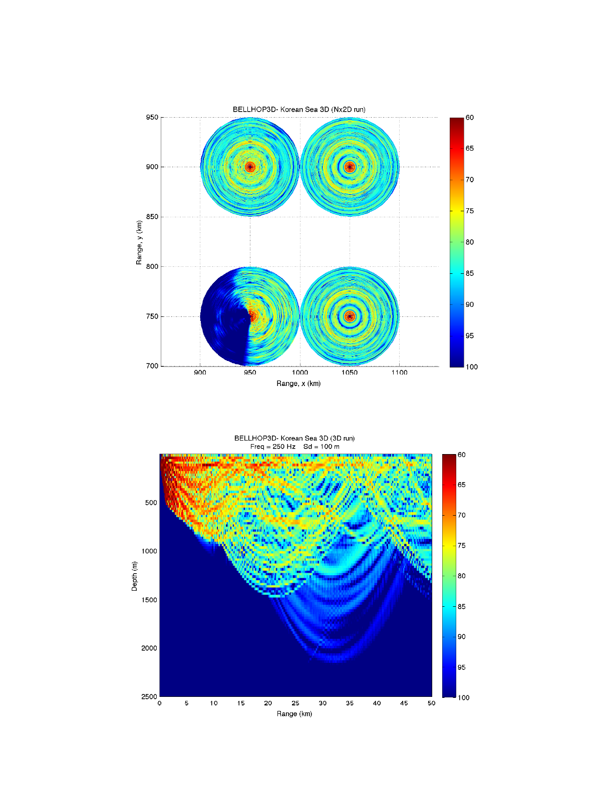
Heat, Light, and Sound Research, Inc.
Figure 41: Transmission loss (Nx2D option, side and plan views) showing the multi-source capability.
BELLHOP3D User Guide! "66
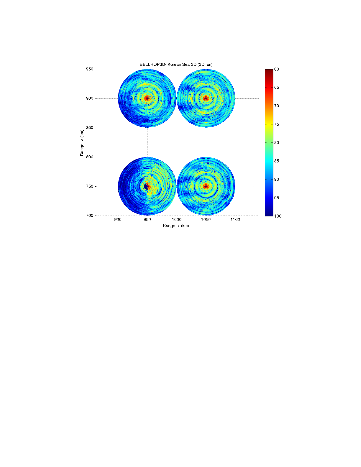
Heat, Light, and Sound Research, Inc.
Figure 42: Transmission loss (3D option, side and plan views) showing the multisource capability.!
BELLHOP3D User Guide! "67

Heat, Light, and Sound Research, Inc.
H. Incoherent and Semi-Coherent TL options
As discussed in the text Computational Ocean Acoustics (Jensen, et al., Springer-Verlag),
incoherent and semi-coherent options are often useful for treating certain types of sources. Briefly,
the motivation for this is that particularly at higher frequencies; e.g., mid-frequency sonar, the
transmission loss pattern is a complicated field that results from constructive and destructive
interference. That field is extremely sensitive to the details of the oceanography and bathymetry--
more detail than the oceanography and bathymetry can provide--and therefore is not really
conveying meaningful information. Instead what is often desired is some kind of average results
that captures the general level of the field.
As it turns out, there are also computational benefits in computing such an averaged quantity since
the sampling requirements (number of beams) is greatly reduced.
Two types of averaged results have been found to be useful. The first is an incoherent field in which
the phase of the rays or beams is discarded. This produces a very smooth field. The second is a
semi-coherent field in which the phase is discarded except that a beam pattern is applied at the
source representing the Lloyd mirror pattern that results from the interference of the direct field and
the surface reflected field. Thus one captures a dominant interference effect that may be a robust
feature, but ignores other effects that might not be stable with respect to small fluctuations in the
environment or source/receiver geometry. The choice of which of these options is best depends on
the source frequency and other features of the scenario.
We have implemented this incoherent and semi-coherent option in 1) geo-hat, 2) geo-hat in
Cartesian coordinates, 3) geo-Gaussian beams. To introduce the problem we begin with the
standard coherent result. Our test case is the Munk profile (standard deep water profile) and we
present BELLHOP3D results in Fig. 43 below. The upper panels are for the Hat-shaped beams,
while the lower panels use Gaussian beams. The left panels use the Nx2D option and the right
panels use the full 3D option. We have solved this problem previously with a variety of other codes
and can say that the results are excellent. One may also note the excellent agreement between the
Nx2D and 3D results and the improved accuracy in the Gaussian beam results.
Figure 43: Fully coherent calculations of the TL using BELLHOP3D with hat and Gaussian beams and with Nx2D and full
3D options.
Figure 44 shows the results with the new incoherent and semi-coherent options in BELLHOP3D.
We show first the results with the geometric, hat-shaped beams. Note how the incoherent result in
the top panel shows a much more smoothed field that conveys the general energy levels. The
lower panel shows the semi-coherent option. Note here how it reproduces an interference pattern
BELLHOP3D User Guide! "68
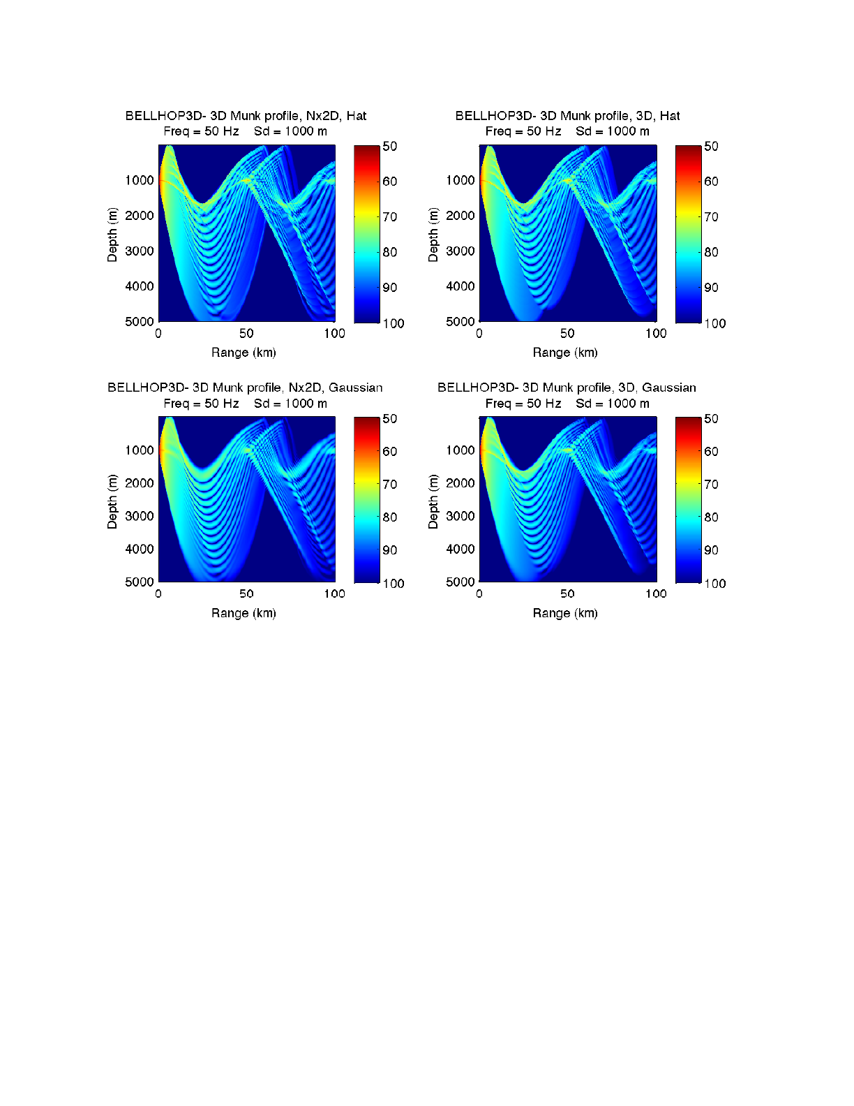
Heat, Light, and Sound Research, Inc.
that is reminiscent of the fully coherent solution, but differs in some details. As discussed above, it
is capturing the interference due to the surface image, but not other interference features.
Figure 44: Incoherent and semi-coherent TL fields calculated by BELLHOP3D using hat-shaped beams.
The remaining figures are perhaps less interesting but show that we have also implemented this
capability for other beam types. Figure 45 shows the same pair of results but using the geo-hat
beams in Cartesian coordinates. These results should be, and are, identical to the previous set.
The significance of the implementation in Cartesian coordinates is simply that the computer time is
significantly reduced.
Figure 45: Incoherent and semi-coherent TL fields calculated by BELLHOP3D using hat-shaped beams in Cartesian
coordinates..
BELLHOP3D User Guide! "69
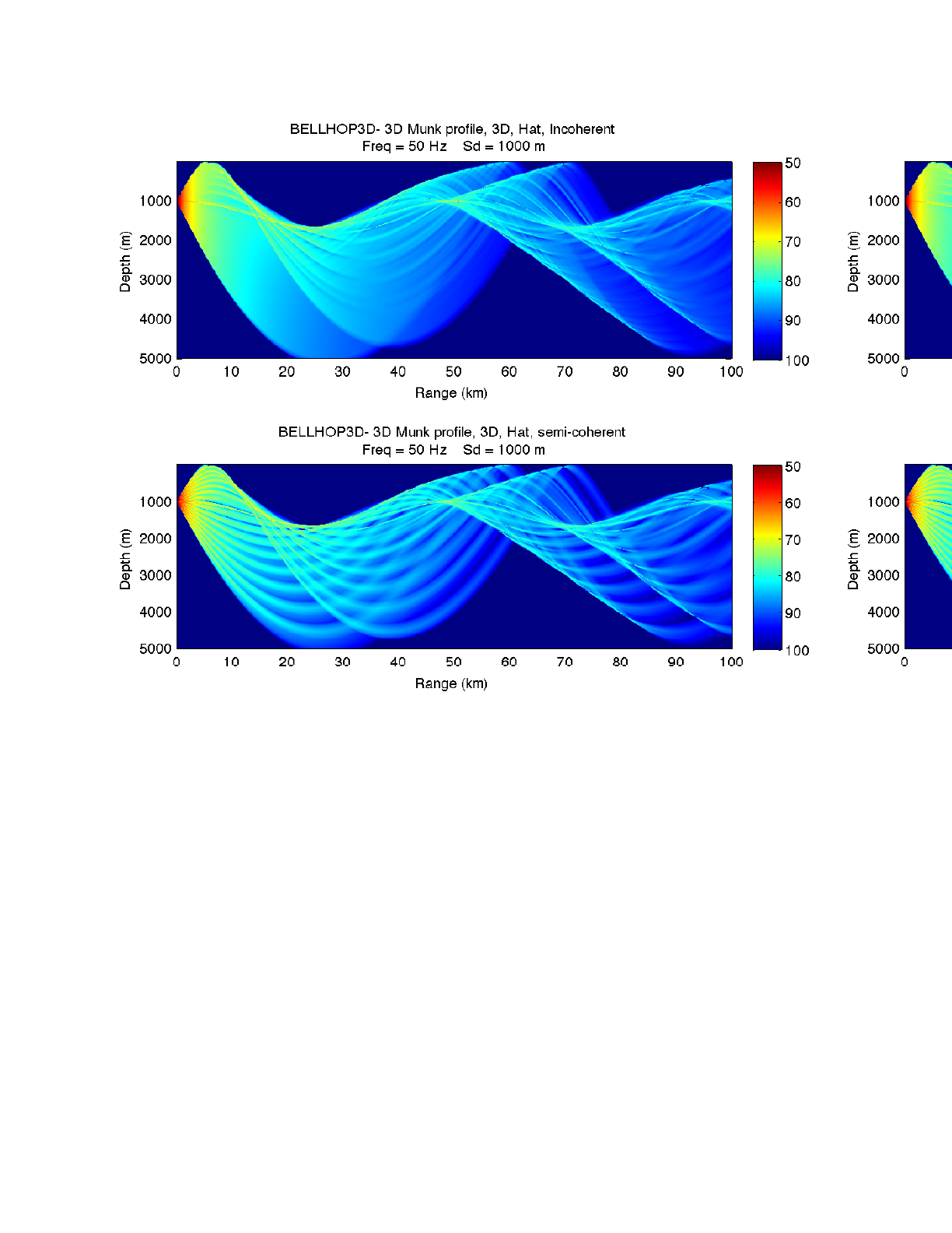
Heat, Light, and Sound Research, Inc.
Finally, in Fig. 46 we show the results using Gaussian beams. As usual the Gaussian beams
smooth out artifacts in the field. However, there is a level bias. This is due to the fact that all the
beams are added incoherently when in fact beams of the same group, that is, with the same
number of upper and lower turning points should always be added coherently. It is possible to
derive a simple formula that compensates for that.
Figure 46: Incoherent and semi-coherent TL fields calculated by BELLHOP3D using Gaussian beams.
BELLHOP3D User Guide! "70
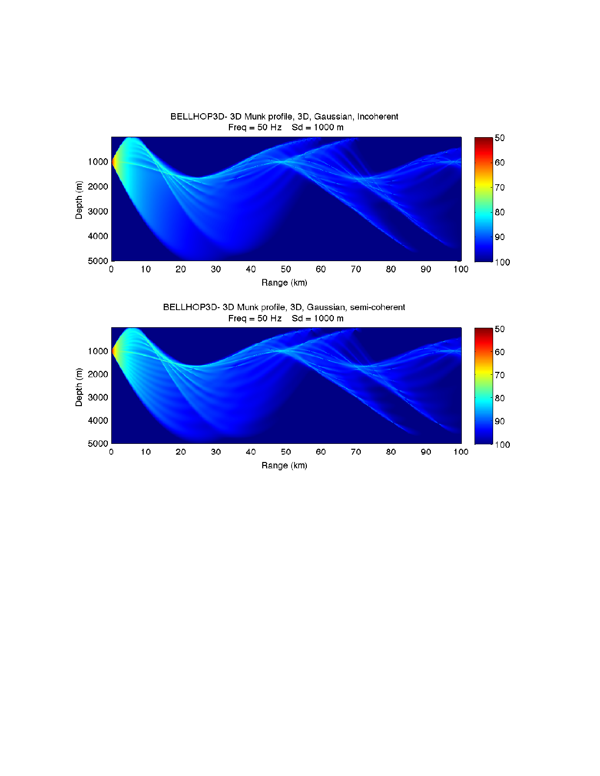
Heat, Light, and Sound Research, Inc.
V. Summary
BELLHOP3D is now a fully capable production model at the level of the widely used BELLHOP
code that has been used previously for 2D problems. This report focuses on the aspects that are
new for the 3D capability; however, the code has been structured in a manner that parallels the
earlier BELLHOP code. We refer the user to the BELLHOP manual for additional info in using the
code.
BELLHOP3D User Guide! "71

Heat, Light, and Sound Research, Inc.
Acknowledgments
BELLHOP3D was originally developed at the Naval Research Laboratory around 1985 as a
preliminary research code. This new version of BELLHOP3D including the User Guide has been
largely supported by the Agency for Defense Development, Republic of Korea. It greatly extends
the original by including options for gridded environmental data supplied by the user. It also
provides a number of new outputs such as eigenrays and ‘arrivals files’. Finally additional beam
types were implemented and different types of TL calculations. Collectively these changes brought
BELLHOP3D to a level of maturity approaching the original 2D BELLHOP. The Office of Naval
Research has provided important additional support for studying out-of-plane effects and for
further testing and development. Laurel Henderson implemented Ding Lee’s FOR3D code at HLS
and ran all the test cases that used FOR3D. Xavier Zabal provided the analytic solutions for the
perfect wedge, the truncated wedge, and the seamount.
BELLHOP3D User Guide! "72
