Chapter 5 Black 8e Student Solutions Manual Ch05
User Manual:
Open the PDF directly: View PDF ![]() .
.
Page Count: 29
Student’s Solutions Manual and Study Guide: Chapter 5 Page 1
Chapter 5
Discrete Distributions
LEARNING OBJECTIVES
The overall learning objective of Chapter 5 is to help you understand a
category of probability distributions that produces only discrete outcomes,
thereby enabling you to:
1. Define a random variable in order to differentiate between a discrete
distribution and a continuous distribution
2. Determine the mean, variance, and standard deviation of a discrete
distribution
3. Solve problems involving the binomial distribution using the binomial
formula and the binomial table
4. Solve problems involving the Poisson distribution using the Poisson
formula and the Poisson table
5. Solve problems involving the hypergeometric distribution using the
hypergeometric formula
Student’s Solutions Manual and Study Guide: Chapter 5 Page 2
CHAPTER OUTLINE
5.1 Discrete Versus Continuous Distributions
5.2 Describing a Discrete Distribution
Mean, Variance, and Standard Deviation of Discrete Distributions
Mean or Expected Value
Variance and Standard Deviation of a Discrete Distribution
5.3 Binomial Distribution
Solving a Binomial Problem
Using the Binomial Table
Using the Computer to Produce a Binomial Distribution
Mean and Standard Deviation of the Binomial Distribution
Graphing Binomial Distributions
5.4 Poisson Distribution
Working Poisson Problems by Formula
Using the Poisson Tables
Mean and Standard Deviation of a Poisson Distribution
Graphing Poisson Distributions
Using the Computer to Generate Poisson Distributions
Approximating Binomial Problems by the Poisson Distribution
5.5 Hypergeometric Distribution
Using the Computer to Solve for Hypergeometric Distribution
Probabilities
KEY TERMS
Binomial Distribution Hypergeometric Distribution
Continuous Distributions Lambda (
-
)
Continuous Random Variables Mean, or Expected Value
Discrete Distributions Poisson Distribution
Discrete Random Variables Random Variable

Student’s Solutions Manual and Study Guide: Chapter 5 Page 3
STUDY QUESTIONS
1. Variables that take on values at every point over a given interval are called
_______________ _______________ variables.
2. If the set of all possible values of a variable is at most finite or a countably infinite number of
possible values, then the variable is called a _______________ _______________ variable.
3. An experiment in which a die is rolled six times will likely produce values of a
_______________ random variable.
4. An experiment in which a researcher counts the number of customers arriving at a
supermarket checkout counter every two minutes produces values of a _______________
random variable.
5. An experiment in which the time it takes to assemble a product is measured is likely to
produce values of a _______________ random variable.
6. A binomial distribution is an example of a _______________ distribution.
7. The normal distribution is an example of a _______________ distribution.
8. The long-run average of a discrete distribution is called the __________________ or
______________________________________.
Use the following discrete distribution to answer 9 and 10 x P(x)
1 .435
2 .241
3 .216
4 .108
9. The mean of the discrete distribution above is ____________.
10. The variance of the discrete distribution above is _______________.
11. On any one trial of a binomial experiment, there can be only _______________ possible outcomes.
12. Suppose the probability that a given part is defective is .10. If four such parts are randomly drawn
from a large population, the probability that exactly two parts are defective is ________.
13. Suppose the probability that a given part is defective is .04. If thirteen such parts are randomly
drawn from a large population, the expected value or mean of the binomial distribution that
describes this experiment is ________.
14. Suppose a binomial experiment is conducted by randomly selecting 20 items where p = .30. The
standard deviation of the binomial distribution is _______________.
Student’s Solutions Manual and Study Guide: Chapter 5 Page 4
15. Suppose forty-seven percent of the workers in a large corporation are under thirty-five years of age.
If fifteen workers are randomly selected from this corporation, the probability of selecting exactly
ten who are under thirty-five years of age is _______________.
16. Suppose that twenty-three percent of all adult Americans fly at least once a year. If twelve adult
Americans are randomly selected, the probability that exactly four have flown at least once last year
is _______________.
17. Suppose that sixty percent of all voters support the President of the United States at this time. If
twenty voters are randomly selected, the probability that at least eleven support the President is
_______________.
18. The Poisson distribution was named after the French mathematician _______________.
19. The Poisson distribution focuses on the number of discrete occurrences per _______________.
20. The Poisson distribution tends to describe _______________ occurrences.
21. The long-run average or mean of a Poisson distribution is _______________.
22. The variance of a Poisson distribution is equal to _______________.
23. If Lambda is 2.6 occurrences over an interval of five minutes, the probability of getting six
occurrences over one five minute interval is _______________.
24. Suppose that in the long-run a company determines that there are 1.2 flaws per every twenty pages
of typing paper produced. If ten pages of typing paper are randomly selected, the probability that
more than two flaws are found is _______________.
25. If Lambda is 1.8 for a four minute interval, an adjusted new Lambda of _______ would be used to
analyze the number of occurrences for a twelve minute interval.
26. Suppose a binomial distribution problem has an n = 200 and a p = .03. If this problem is worked
using the Poisson distribution, the value of Lambda is ________.
27. The hypergeometric distribution should be used when a binomial type experiment is being
conducted without replacement and the sample size is greater than or equal to ________% of the
population.
28. Suppose a population contains sixteen items of which seven are X and nine are Y. If a random
sample of five of these population items is selected, the probability that exactly three of the five are
X is ________.
29. Suppose a population contains twenty people of which eight are members of the Catholic church. If
a sample of four of the population is taken, the probability that at least three of the four are
members of the Catholic church is ________.
30. Suppose a lot of fifteen personal computer printers contains two defective printers. If three of the
fifteen printers are randomly selected for testing, the probability that no defective printers are
selected is _______________.
Student’s Solutions Manual and Study Guide: Chapter 5 Page 5
ANSWERS TO STUDY QUESTIONS
1. Continuous Random 16. .1712
2. Discrete Random 17. .755
3. Discrete 18. Poisson
4. Discrete 19. Interval
5. Continuous 20. Rare
6. Discrete 21. Lambda
7. Continuous 22. Lambda
8. Mean, Expected Value 23. .0319
9. 1.997 24. .0232
10. 1.083 25. 5.4
11. Two 26. 6.0
12. .0486 27. 5
13. 0.52 28. .2885
14. 2.049 29. .1531
15. .0661 30. .6286

Student’s Solutions Manual and Study Guide: Chapter 5 Page 6
SOLUTIONS TO THE ODD-NUMBERED PROBLEMS IN CHAPTER 5
5.1 x P(x) x·P(x) (x-µ)2 (x-µ)2·P(x)
1 .238 .238 2.775556 0.6605823
2 .290 .580 0.443556 0.1286312
3 .177 .531 0.111556 0.0197454
4 .158 .632 1.779556 0.2811700
5 .137 .685 5.447556 0.7463152
µ = [x·P(x)] = 2.666
2 = [(x-µ)2·P(x)] = 1.836444
=
836444.1
= 1.355155
5.3 x P(x) x·P(x) (x-µ)2 (x-µ)2·P(x)
0 .461 .000 0.913936 0.421324
1 .285 .285 0.001936 0.000552
2 .129 .258 1.089936 0.140602
3 .087 .261 4.177936 0.363480
4 .038 .152 9.265936 0.352106
E(x) = µ = [x·P(x)]= 0.956
2 = [(x-µ)2·P(x)] = 1.278064
=
278064.1
= 1.1305

Student’s Solutions Manual and Study Guide: Chapter 5 Page 7
5.5 a) n = 4 p = .10 q = .90
P(x=3) = 4C3(.10)3(.90)1 = 4(.001)(.90) = .0036
b) n = 7 p = .80 q = .20
P(x=4) = 7C4(.80)4(.20)3 = 35(.4096)(.008) = .1147
c) n = 10 p = .60 q = .40
P(x > 7) = P(x=7) + P(x=8) + P(x=9) + P(x=10) =
10C7(.60)7(.40)3 + 10C8(.60)8(.40)2 + 10C9(.60)9(.40)1 +10C10(.60)10(.40)0 =
120(.0280)(.064) + 45(.0168)(.16) + 10(.0101)(.40) + 1(.0060)(1) =
.2150 + .1209 + .0403 + .0060 = .3822
d) n = 12 p = .45 q = .55
P(5 < x < 7) = P(x=5) + P(x=6) + P(x=7) =
12C5(.45)5(.55)7 + 12C6(.45)6(.55)6 + 12C7(.45)7(.55)5 =
792(.0185)(.0152) + 924(.0083)(.0277) + 792(.0037)(.0503) =
.2225 + .2124 + .1489 = .5838
Student’s Solutions Manual and Study Guide: Chapter 5 Page 8
5.7 a) n = 20 p = .70 q = .30
µ = np = 20(.70) = 14
=
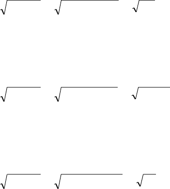
2.4)30)(.70(.20 qpn
= 2.05
b) n = 70 p = .35 q = .65
µ = np = 70(.35) = 24.5
=
925.15)65)(.35(.70 qpn
= 3.99
c) n = 100 p = .50 q = .50
µ = np = 100(.50) = 50
=
25)50)(.50(.100 qpn
= 5
5.9 Looking at the graph, the highest probability appears to be at x = 1 followed by x = 2. It is
most likely that the mean falls between x = 1 and x = 2 but because of the size of the drop
from x = 1 to x = 2, the mean is much closer to x =1. Thus, the mean is something like 1.2.
Since the expected value
= n∙ p, if n = 6 and
is 1.2, solving for p results in p = .20. So,
p is near to .20 and the mean or expected value is around 1.2.
5.11 a) n = 20 p = .27 x = 8
20C8 (.27)8(.73)12 = 125,970(.000028243)(.022902) = .0815
b) n = 20 p = .30 x = 0
20C0 (.30) 0(.70)20 = (1)(1)(.0007979) = .0007979
c) n = 20 p = .30 x > 7
Use table A.2:
P(x=8) + P(x=9) + . . . + P(x=14)=
.114 + .065 + .031 + .012 + .004 + .001 + .000 + … = .227

Student’s Solutions Manual and Study Guide: Chapter 5 Page 9
5.13 n = 25 p = .60
a) x > 15
P(x > 15) = P(x = 15) + P(x = 16) + · · · + P(x = 25)
Using Table A.2 n = 25, p = .60
x Prob
15 .161
16 .151
17 .120
18 .080
19 .044
20 .020
21 .007
22 .002
.585
b) x > 20
P(x > 20) = P(x = 21) + P(x = 22) + P(x = 23) + P(x = 24) + P(x = 25) =
Using Table A.2 n = 25, p = .60
.007 + .002 + .000 + .000 + .000 = .009
c) P(x < 10)
Using Table A.2 n = 25, p = .60 and x = 0, 1, 2, 3, 4, 5, 6, 7, 8, 9
x Prob.
9 .009
8 .003
7 .001
<6 .000
.013
Student’s Solutions Manual and Study Guide: Chapter 5 Page 10
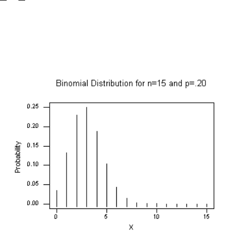
5.15 n = 15 p = .20
a) P(x = 5) = 15C5(.20)5(.80)10 = 3003(.00032)(.1073742) = .1032
b) P(x > 9): Using Table A.2
P(x = 10) + P(x = 11) + . . . + P(x = 15) = .000 + .000 + . . . + .000 = .000
c) P(x = 0) = 15C0(.20)0(.80)15 = (1)(1)(.035184) = .0352
d) P(4 < x < 7): Using Table A.2
P(x = 4) + P(x = 5) + P(x = 6) + P(x = 7) = .188 + .103 + .043 + .014 = .348
e) Graph

Student’s Solutions Manual and Study Guide: Chapter 5 Page 11
5.17 a) P(x=5
-
= 2.3) =
2 3
5
64 36343 100259
120
5 2 3
.
!
( . )(. )
.
e
= .0538
b) P(x=2
-
= 3.9) =
39
2
1521 020242
2
2 3 9
.
!
( . )(. )
.
e
= .1539
c) P(x < 3
-
= 4.1) = P(x=3) + P(x=2) + P(x=1) + P(x=0) =
41
3
68 921 016573
6
3 4 1
.
!
( . )(. )
.
e
= .1904
41
2
1681 016573
2
2 4 1
.
!
( . )(. )
.
e
= .1393
41
1
41 016573
1
1 4 1
.
!
( . )(. )
.
e
= .0679
41
0!
1016573
1
0 4 1
. ( )(. )
.
e
= .0166
.1904 + .1393 + .0679 + .0166 = .4142
d) P(x=0
-
= 2.7) =
2 7
0!
106721
1
0 2 7
. ( )(. )
.
e
= .0672
e) P(x=1
-
= 5.4)=
54
1
54 0045166
1
1 5 4
.
!
( . )(. )
.
e
= .0244
f) P(4 < x < 8
-
= 4.4): P(x=5
-
= 4.4) + P(x=6
-
= 4.4) + P(x=7
-
= 4.4)=
4 4
5
5 4 4
.
!
.
e
+
4 4
6!
6 4 4
.
.
e
+
4 4
7
7 4 4
.
!
.
e
=
( . )(. )16491622 01227734
120
+
( . )(. )72563139 01227734
720
+
( , . )(. )31927 781 01227734
5040
= .1687 + .1237 + .0778 = .3702
Student’s Solutions Manual and Study Guide: Chapter 5 Page 12
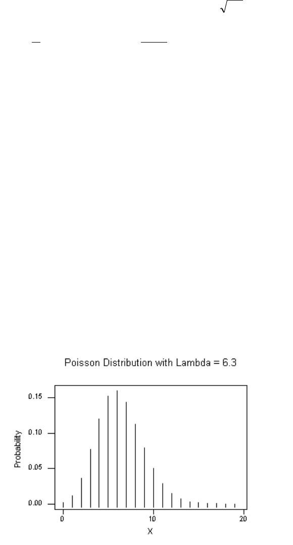
5.19 a)
-
= 6.3 mean = 6.3 Standard deviation =
3.6
= 2.51
x Prob
0 .0018
1 .0116
2 .0364
3 .0765
4 .1205
5 .1519
6 .1595
7 .1435
8 .1130
9 .0791
10 .0498
11 .0285
12 .0150
13 .0073
14 .0033
15 .0014
16 .0005
17 .0002
18 .0001
19 .0000
Student’s Solutions Manual and Study Guide: Chapter 5 Page 13
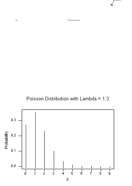
b)
-
= 1.3 mean = 1.3 standard deviation =
3.1
= 1.14
x Prob
0 .2725
1 .3542
2 .2303
3 .0998
4 .0324
5 .0084
6 .0018
7 .0003
8 .0001
9 .0000
Student’s Solutions Manual and Study Guide: Chapter 5 Page 14
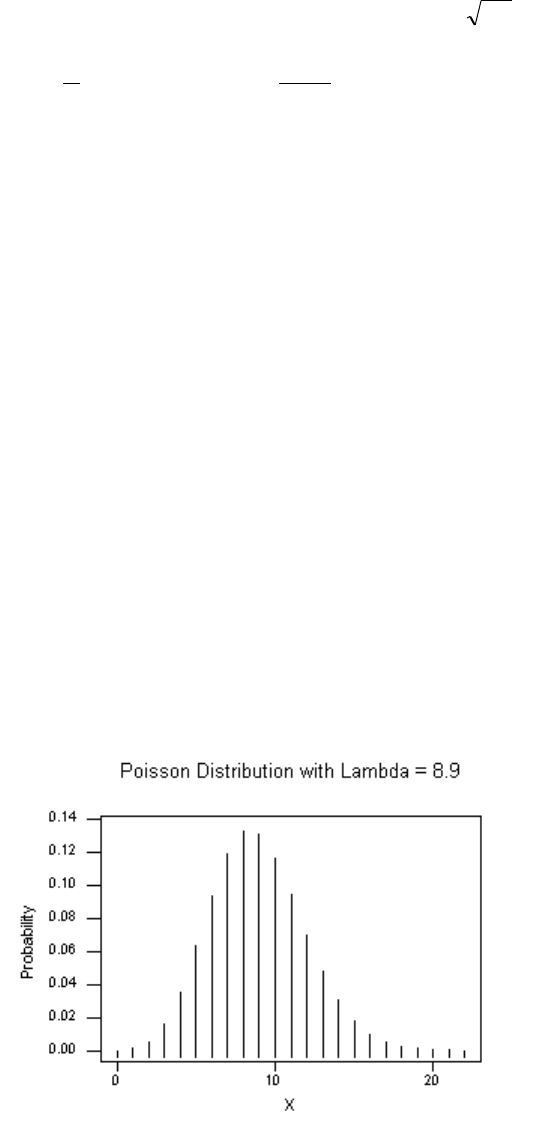
c)
-
= 8.9 mean = 8.9 standard deviation =
9.8
= 2.98
x Prob
0 .0001
1 .0012
2 .0054
3 .0160
4 .0357
5 .0635
6 .0941
7 .1197
8 .1332
9 .1317
10 .1172
11 .0948
12 .0703
13 .0481
14 .0306
15 .0182
16 .0101
17 .0053
18 .0026
19 .0012
20 .0005
21 .0002
22 .0001
Student’s Solutions Manual and Study Guide: Chapter 5 Page 15
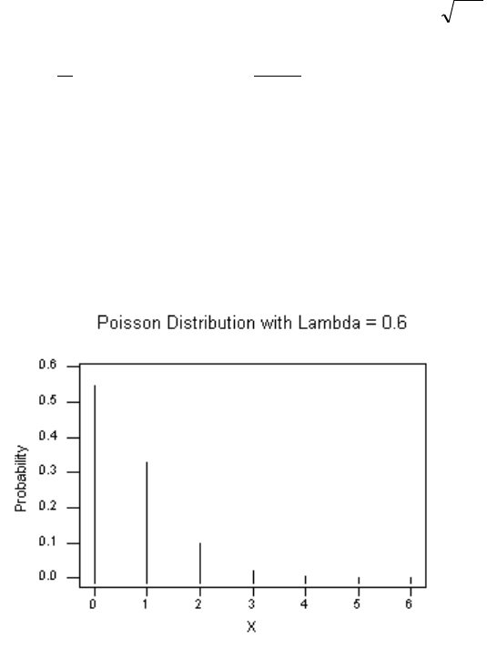
d)
-
= 0.6 mean = 0.6 standard deviation =
6.0
= .775
x Prob
0 .5488
1 .3293
2 .0988
3 .0198
4 .0030
5 .0004
6 .0000

Student’s Solutions Manual and Study Guide: Chapter 5 Page 16
5.21
-
= x/n = 126/36 = 3.5
Using Table A.3
a) P(x = 0) = .0302
b) P(x > 6) = P(x = 6) + P(x = 7) + . . . =
.0771 + .0385 + .0169 + .0066 + .0023 +
.0007 + .0002 + .0001 = .1424
c) P(x < 4 10 minutes)
Double Lambda to - = 7.010 minutes
P(x < 4) = P(x = 0) + P(x = 1) + P(x = 2) + P(x = 3) =
.0009 + .0064 + .0223 + .0521 = .0817
d) P(3 < x < 6 10 minutes)
-
= 7.0 10 minutes
P(3 < x < 6) = P(x = 3) + P(x = 4) + P(x = 5) + P(x = 6)
= .0521 + .0912 + .1277 + .1490 = .42
e) P(x = 8 15 minutes)
Change Lambda for a 15 minute interval by multiplying the original Lambda by 3.
-
= 10.5 15 minutes
P(x = 815 minutes) =
!8
))(5.10(
!
5.108
e
x
e
x
-
-
= .1009

Student’s Solutions Manual and Study Guide: Chapter 5 Page 17
5.23
-
= 1.2 collisions4 months
a) P(x=0
-
= 1.2):
from Table A.3 = .3012
b) P(x=22 months):
The interval has been decreased (by ½)
New Lambda =
-
= 0.6 collisions2 months
P(x=2
-
= 0.6):
from Table A.3 = .0988
c) P(x < 1 collision6 months):
The interval length has been increased (by 1.5)
New Lambda =
-
= 1.8 collisions6 months
P(x < 1
-
= 1.8):
from Table A.3 x Prob.
0 .1653
1 .2975
.4628
The result is likely to happen almost half the time (46.26%). Ship channel and
weather conditions are about normal for this period. Safety awareness is
about normal for this period. There is no compelling reason to reject the
lambda value of 0.6 collisions per 4 months based on an outcome of 0 or 1
collisions per 6 months.

Student’s Solutions Manual and Study Guide: Chapter 5 Page 18
5.25 n = 100,000 p = .00004
a) P(x > 7n = 100,000 p = .00004):
-
= µ = np = 100,000(.00004) = 4.0
Since n > 20 and np < 7, the Poisson approximation to this binomial problem is
close enough.
P(x > 7
-
= 4):
Using Table A.3 x Prob.
7 .0595
8 .0298
9 .0132
10 .0053
11 .0019
12 .0006
13 .0002
14 .0001
.1106
b) P(x >10
-
= 4):
Using Table A.3 x Prob.
11 .0019
12 .0006
13 .0002
14 .0001
.0028
c) Since getting more than 10 is a rare occurrence, this particular geographic region
appears to have a higher average rate than other regions. An investigation of
particular characteristics of this region might be warranted.

Student’s Solutions Manual and Study Guide: Chapter 5 Page 19
5.27 a) P(x = 3 N = 11, A = 8, n = 4)
330
)3)(56(
411
1338
C
CC
= .5091
b) P(x < 2)N = 15, A = 5, n = 6)
P(x = 1) + P (x = 0) =
615
51015
C
CC
+
615
61005
C
CC
=
5005
)210)(1(
5005
)252)(5(
.2517 + .0420 = .2937
c) P(x=0 N = 9, A = 2, n = 3)
84
)35)(1(
39
3702
C
CC
= .4167
d) P(x > 4 N = 20, A = 5, n = 7) =
P(x = 5) + P(x = 6) + P(x = 7) =
720
21555
C
CC
+
720
11565
C
CC
+
720
01575
C
CC
=
77520
)105)(1(
+ 5C6 (impossible) + 5C7(impossible) = .0014

Student’s Solutions Manual and Study Guide: Chapter 5 Page 20
5.29 N = 17 A = 8 n = 4
a) P(x = 0) =
417
4908
C
CC
=
2380
)126)(1(
= .0529
b) P(x = 4) =
417
0948
C
CC
=
2380
)1)(70(
= .0294
c) P(x = 2 non computer) =
417
2829
C
CC
=
2380
)28)(36(
= .4235
5.31 N = 10 n = 4
a) A = 2 x = 2 P(x = 2):
1333.
210
)28)(1(
410
2822
C
CC
b) A = 5 x = 0 P(x = 0):
0238.
210
)5)(1(
410
4505
C
CC
c) A = 4 x = 3 P(x = 3):
1143.
210
)6)(4(
410
1634
C
CC
5.33 N = 18 A = 11 Hispanic n = 5
P(x < 1) = P(1) + P(0) =
518
47111
C
CC
+
518
57011
C
CC
=
8568
)21)(1(
8568
)35)(11(
= .0449 + .0025 = .0474
It is fairly unlikely that these results occur by chance. A researcher might want to
further investigate this result to determine causes. Were officers selected based on
leadership, years of service, dedication, prejudice, or some other reason?

Student’s Solutions Manual and Study Guide: Chapter 5 Page 21
5.35 a) P(x = 14 n = 20 and p = .60) = .124
b) P(x < 5 n = 10 and p =.30) =
P(x = 4) + P(x = 3) + P(x = 2) + P(x = 1) + P(x=0) =
x Prob.
0 .028
1 .121
2 .233
3 .267
4 .200
.849
c) P(x > 12 n = 15 and p = .60) =
P(x = 12) + P(x = 13) + P(x = 14) + P(x = 15)
x Prob.
12 .063
13 .022
14 .005
15 .000
.090
d) P(x > 20 n = 25 and p = .40) = P(x = 21) + P(x = 22) +
P(x = 23) + P(x = 24) + P(x=25) =
x Prob.
21 .000
22 .000
23 .000
24 .000
25 .000
.000

Student’s Solutions Manual and Study Guide: Chapter 5 Page 22
5.37 a) P(x = 3
-
= 1.8) = .1607
b) P(x < 5
-
= 3.3) =
P(x = 4) + P(x = 3) + P(x = 2) + P(x = 1) + P(x = 0) =
x Prob.
0 .0369
1 .1217
2 .2008
3 .2209
4 .1823
.7626
c) P(x > 3
-
= 2.1) =
x Prob.
3 .1890
4 .0992
5 .0417
6 .0146
7 .0044
8 .0011
9 .0003
10 .0001
11 .0000
.3504
d) P(2 < x < 5
-
= 4.2):
P(x=3) + P(x=4) + P(x=5) =
x Prob.
3 .1852
4 .1944
5 .1633
.5429

Student’s Solutions Manual and Study Guide: Chapter 5 Page 23
5.39 n = 25 p = .20 retired
a) from Table A.2: P(x = 7) = .1108
b) P(x > 10): P(x = 10) + P(x = 11) + . . . + P(x = 25) = .012 + .004 + .001 = .017
c) Expected Value = µ = np = 25(.20) = 5
d) n = 20 p = .40 mutual funds
P(x = 8) = .1797
e) P(x < 6) = P(x = 0) + P(x = 1) + . . . + P(x = 5) =
.000 + .000 + .003 +.012 + .035 + .075 = .125
f) P(x = 0) = .000
g) P(x > 12) = P(x = 12) + P(x = 13) + . . . + P(x = 20) = .035 + .015 + .005 + .001 = .056
h) x = 8 Expected Number = µ = n p = 20(.40) = 8
5.41 N = 32 A = 10 n = 12
a) P(x = 3) =
1232
922310
C
CC
=
840,792,225
)420,497)(120(
= .2644
b) P(x = 6) =
1232
622610
C
CC
=
840,792,225
)613,74)(210(
= .0694
c) P(x = 0) =
1232
1222010
C
CC
=
840,792,225
)646,646)(1(
= .0029
d) A = 22 P(7 < x < 9) =
1232
510722
C
CC
+
1232
410822
C
CC
+
1232
310922
C
CC
=
840,792,225
)120)(420,497(
840,792,225
)210)(770,319(
840,792,225
)252)(544,170(
= .1903 + .2974 + .2644 = .7521

Student’s Solutions Manual and Study Guide: Chapter 5 Page 24
5.43 a) n = 20 and p = .25
The expected number = µ = np = (20)(.25) = 5.00
b) P(x < 1 n = 20 and p = .25) =
P(x = 1) + P(x = 0) = 20C1(.25)1(.75)19 + 20C0(.25)0(.75)20
= (20)(.25)(.00423) + (1)(1)(.0032) = .0212 +. 0032 = .0244
Since the probability is so low, the population of your state may have a lower
percentage of chronic heart conditions than those of other states.
5.45 n = 12
a.) P(x = 0 long hours):
p = .20 12C0(.20)0(.80)12 = .0687
b.) P(x > 6) long hours):
p = .20
Using Table A.2: .016 + .003 + .001 = .020
c) P(x = 5 good financing):
p = .25, 12C5(.25)5(.75)7 = .1032
d.) p = .19 (good plan), expected number = µ = n(p) = 12(.19) = 2.28

Student’s Solutions Manual and Study Guide: Chapter 5 Page 25
5.47 P(x < 3) n = 8 and p = .60): From Table A.2:
x Prob.
0 .001
1 .008
2 .041
3 .124
.174
17.4% of the time in a sample of eight, three or fewer customers are walk-ins by
chance. Other reasons for such a low number of walk-ins might be that she is
retaining more old customers than before or perhaps a new competitor is
attracting walk-ins away from her.
5.49
-
= 1.2 hoursweek
a) P(x = 0
-
= 1.2) = (from Table A.3) .3012
b) P(x > 3
-
= 1.2) = (from Table A.3)
x Prob.
3 .0867
4 .0260
5 .0062
6 .0012
7 .0002
8 .0000
.1203
a) P(x < 5 3 weeks)
If
-
= 1.2 for 1 week, the
-
= 3.6 for 3 weeks.
P(x < 5
-
= 3.6) = (from Table A.3)
x Prob.
4 .1912
3 .2125
2 .1771
1 .0984
0 .0273
.7065

Student’s Solutions Manual and Study Guide: Chapter 5 Page 26
5.51 N = 24 n = 6 A = 8
a) P(x = 6) =
596,134
)1)(28(
624
01668
C
CC
= .0002
b) P(x = 0) =
596,134
)8008)(1(
624
61608
C
CC
= .0595
d) A = 16 East Side
P(x = 3) =
596,134
)56)(560(
624
38316
C
CC
= .2330

Student’s Solutions Manual and Study Guide: Chapter 5 Page 27
5.53
-
= 2.4 calls1 minute
a) P(x = 0
-
= 2.4) = (from Table A.3) .0907
b) Can handle x < 5 calls Cannot handle x > 5 calls
P(x > 5
-
= 2.4) = (from Table A.3)
x Prob.
6 .0241
7 .0083
8 .0025
9 .0007
10 .0002
11 .0000
.0358
c) P(x = 3 calls2 minutes)
The interval has been increased 2 times.
New Lambda: - = 4.8 calls2 minutes.
from Table A.3: .1517
d) P(x < 1 calls15 seconds):
The interval has been decreased by ¼.
New Lambda =
-
= 0.6 calls15 seconds.
P(x < 1
-
= 0.6) = (from Table A.3)
P(x = 1) = .3293
P(x = 0) = .5488
.8781

Student’s Solutions Manual and Study Guide: Chapter 5 Page 28
5.55 p = .005 n = 1,000
-
= np = (1,000)(.005) = 5
a) P(x < 4) = P(x = 0) + P(x = 1) + P(x = 2) + P(x = 3) =
.0067 + .0337 + .0842 + .1404 = .265
b) P(x > 10) = P(x = 11) + P(x = 12) + . . . =
.0082 + .0034 + .0013 + .0005 + .0002 = .0136
c) P(x = 0) = .0067
5.57 N = 25
a) n = 5 x = 3 A = 17
3584.
130,53
)28)(680(
525
28317
C
CC
b) n = 8 x < 2 A = 5
825
82005
C
CC
825
72015
C
CC
825
62025
C
CC
575,081,1
)760,38)(10(
575,081,1
)520,77)(5(
575,081,1
)970,125)(1(
.1165 + .3584 + .3584 = .8333
c) n = 5 x = 2 A = 3
5C2(3/25)2(22/25)3 = (10)(.0144)(.681472) = .0981

Student’s Solutions Manual and Study Guide: Chapter 5 Page 29
5.59 a)
-
= 3.051,000 for U.S.
0474.
!0
05.3
)0(
05.30
e
xP
b)
-
= 6.102,000 for U.S. (just double previous lambda)
1605.
720
)002243)(.37.520,51(
!6
10.6
)6(
104.66
e
xP
c)
-
= 1.071,000 and - = 3.213,000
from Table A.3:
P(x < 7) = P(x = 0) + P(x = 1) + . . . + P(x = 6) =
( . )( ) ( . )( )
!
( . )( )
!
( . )( )
!
( . )( )
!
( . )( )
!
( . )( )
. . . . . . .
321
0!
321
1
321
2
321
3
321
4
321
5
321
6!
0 3 21 1 3 21 2 3 21 3 3 21 4 3 21 5 3 21 6 3 21
e e e e e e e
.0404 + .1295 + .2079 + .2225 + .1785 + .1146 + .0613 = .9547
5.61 This printout contains the probabilities for various values of x from zero to eleven from a
Poisson distribution with
-
= 2.78. Note that the highest probabilities are at x = 2 and
x = 3 which are near the mean. The probability is slightly higher at x = 2 than at x = 3
even though x = 3 is nearer to the mean because of the “piling up” effect of x = 0.
5.63 This is the graph of a Poisson Distribution with
-
= 1.784. Note the high
probabilities at x = 1 and x = 2 which are nearest to the mean. Note also that the
probabilities for values of x > 8 are near to zero because they are so far away
from the mean or expected value.