Bolo Calc User Manual

User Manual:

Open the PDF directly: View PDF .
Page Count: 31

BoloCalc User Manual

Version 1.0

Charles Hill, UC Berkeley

Last Updated: 2018-06-14

This document is still under construction and will be updated frequently

Contents

1 Quick Start

This section covers how to get BoloCalc up and running. For more detailed information about

how to deﬁne an experiment, run simulations, and read output ﬁles, see the following sections.

1.1 System Requirements

BoloCalc runs on a Linux and has the following dependencies:

1. Python v2.7.2

2. Numpy v1.8 or above

1.2 Code location

BoloCalc is stored on Charles Hill’s GitHub account chill90/ within the repository

chill90/BoloCalc. To clone a local copy of the calculator, make sure that you have Git installed

on your machine (I’ve been using Git version 2.13.5) and run

1git clo ne http s :// git hub . com / chil l90 / Bolo Calc . gi t

All executables are stored at in the top-most directory

1~/ Bo loCalc /

and all libraries are stored in the src/ directory

1~/ B olo Calc / src /

This code is still under construction and therefore is frequently being updated. Therefore, it is

encouraged that the user git pull often, preferably before using the code at all.

1.3 Running mappingSpeed.py

The primary BoloCalc executable is called mappingSpeed.py, which calculates

•Optical power

•Noise-equivalent power (NEP) contributions from

◦Photon noise

◦Bolometer thermal carrier noise

◦Readout noise

•Per-detector noise-equivalent temperature (NET)

•Array NET

•Mapping speed

•Map depth

given some instrument conﬁguration. mappingSpeed.py takes as input an experiment conﬁguration

directory, which is stored in BoloCalc/Experiments/ and has the following structure:

1BoloCalc/

2|-- Experiements/

3| |- - [ Experimen t1 ]/

4| | |-- [ExperimentDesign1]/

5| | |-- [ExperimentDesign2]/

6| | |- - ...

7| |- - [ Expiermen t2 ]/

8| |- - ...

where the square brackets indicate the directories that can be named by the user.

To calculate the sensitivity an experiment, pass its [ExperimentDesign] directory to

mappingSpeed.py.BoloCalc comes with an example experiment that can be used to get started:

1Bo lo Cal c$ p yth on2 .7 m ap pi ngS pe ed . p y Exp er ime nt s / E xa mpl eE xp er im en t / V0 /

By default, mappingSpeed.py will calculate one experiment realization, which should be shown by

the status bar that appears upon execution. For information about how to tune the simulation

parameters, see Section ??.

After it has ﬁnished running, mappingSpeed.py generates several tables that display the cal-

culated quantities for the simulated instrument. These tables are stored in three ﬁles named

sensitivity.txt, with each ﬁle located at a diﬀerent level of the experiment directory structure

and containing diﬀerent information:

•Experiments/ExampleExperiment/V0/sensitivity.txt: contains the sensitivity, combined

by observation frequency, of all telescopes in this experiment.

•Experiments/ExampleExperiment/V0/Tel/sensitivity.txt: contains the sensitivity, com-

bined by observation frequency, of all cameras in this telescope.

•Experiement/ExampleExperiment/V0/Tel/Cam/sensitivity.txt: contains the sensitivity

for channel in this camera.

For more information about the contents of the sensitivity.txt ﬁles, see Section ??.

1.4 Running mappingSpeed vary.py

The other BoloCalc executable is mappingSpeed vary.py, which calculates mapping speed for a

set of instrument conﬁgurations determined by a set of speciﬁed parameters varied with linear

spacing over a speciﬁed range with and with a speciﬁed step size. To run mappingSpeed vary.py,

pass it the instrument conﬁguration at the command line

1Bo lo Cal c$ p yth on2 .7 m ap pi ng Sp eed _v ar y . py E xp eri me nts / E x amp leE xp / V0 /

There are optional command line arguments that can be passed to the executable, which are deﬁned

below

•-vt: Vary the input parameters together instead of computing all possible combinations of

parameters. The parameter array lengths, set by minimum, maximum, and step values, must

be the same

•-fh [File Handle]: Choose a custom ﬁle handle for saving the parameter variations.

The input parameter variations are stored stored in BoloCalc/config/paramsToVary.txt. An

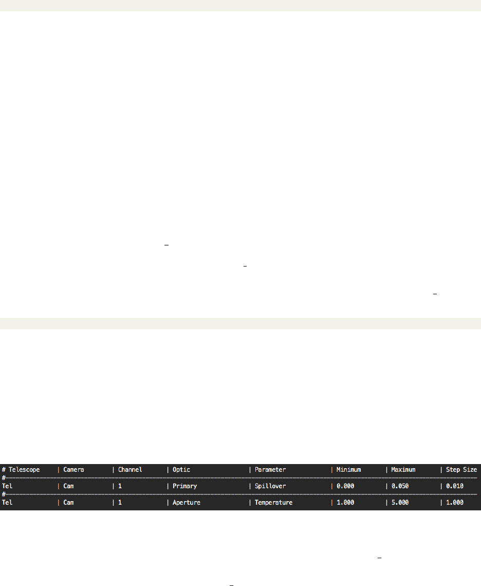
example of the paramsToVary.txt is shown in Figure ??

Figure 1: Example of paramsToVary.txt

For information on how to deﬁne parameters to be varied by mappingSpeed vary.py, see Section

??.

By default upon download, mappingSpeed vary.py will calculate one experiment realization

for each and every parameter combination (see Section ?? for details on simulation inputs). The

status bar will show progression towards calculating all combinations of parameters deﬁned over

the ranges. mappingSpeed vary.py saves three quantities1to ﬁles within the directory

BoloCalc/Experiments/ExampleExp/V0/paramsToVary/. The ﬁle handle can be speciﬁed us-

ing the command line argument -fh [File Handle], or it if is not speciﬁed, it will default to

[Tel] [Cam] [Channel] [Param]. Below is the expected default ﬁle names that the data from the

parameter-varied calculation will be saved to

•Optical power: mappingSpeedVary Popt [Tel] [Cam] [Channel] [Param].txt

•Photon NEP: mappingSpeedVary NEPph [Tel] [Cam] [Channel] [Param].txt

•Array NET: mappingSpeedVary NETarr [Tel] [Cam] [Channel] [Param].txt

where [Tel] [Cam] [Channel] [Param] is a ﬁle handle that contains the speciﬁer for every pa-

rameter varied in the calculation. For example, if we looped over the following two parameters

•Telescope “Tel,” camera “Cam,” channel “1,” optic “Mirror,” Parameter “Spillover”

•Telescope “Tel,” camera “Cam,” channel “1,” Parameter “Pixel Size”

the Popt output ﬁle would have the ﬁlename

1ma pp in gS pe ed Va ry _P opt _T el _C am _1 _M ir ror _S pi ll ov er _T el _Ca m_ 1_ Pi xe lS iz e . txt

For information about the contents of the mappingSpeed vary.py output ﬁle, see Section ??.

For more information about the output parameters, see Section ??.

1.5 Contact and Citation

Please send any comments, requests, questions, or bugs to Charles Hill at chill@lbl.gov. If

you use this code for published results, please cite the SPIE proceeding from 2018 “BoloCalc:

a sensitivity calculator for the design of Simons Observatory,” which can be found at https:

//arxiv.org/abs/1806.04316.

2 Sensitivity Calculation

The primary function of BoloCalc is to import low-level instrument parameters and use them to

estimate the instrument’s noise-equivalent CMB temperature (NET). This calculation is outlined

by the following steps:

1. Collect input parameters and construct an instrument model

2. Calculate per-detector noise-equivalent power (NEP) due to contributions from

•Photon shot and wave noise

•Bolometer thermal carrier noise

•Readout noise

3. Convert NEP to NET

4. Calculate the array-averaged NET, where the noise contributions from each detector are

inverse-variance weighted to estimate the instantaneous sensitivity of the full camera

5. Calculate mapping speed (MS), a quantiﬁcation of instrument noise in the power spectrum

domain

We detail the assumptions and inputs for the calculation in the following subsections.

1More quantities can be added to this list upon request, or as needed.

2.1 Optical power

BoloCalc assumes an array of single-moded bolometers2within an instrument that is stationary

in time. The propagation of optical power from the sky to the focal plane is represented by a one-

dimensional chain of blackbody absorbers/emitters in thermal equilibrium. The power deposited

on the detectors is then an analytic integral over the summation of each optical element’s Planck

spectra modiﬁed by its frequency-dependent eﬃciency and emissivity. Explicitly, the optical power

on a detector is given as

Popt =Z∞

0"Nelem

i=1

pi(ν)#B(ν) dν , (1)

where νis frequency, pi(ν) is the power spectral density of optical element ireferred to the detector

input, the summation contains all Nelem optical elements in the sky/telescope/camera and runs from

the CMB to the focal plane, and B(ν) is the detector bandpass.

The power spectral density pi(ν) for optical element iis determined by its blackbody tempera-

ture Ti, the transmission eﬃciency of all optics between it and the focal plane [ηi+1(ν), ..., ηNelem (ν)],

its emissivity i(ν), its spillover coeﬃcient βi, the eﬀective temperature by which its spilled power

is absorbed Tβ;i, its scattering coeﬃcient δi, and the eﬀective temperature by which its scattered

power is absorbed Tδ;i

pi(Ti,[ηi+1(ν), ..., ηNelem (ν)] , i(ν), βi, Tβ;i, δi, Tδ;i, ν) =

Nelem

j=i+1

ηj(ν) [i(ν)S(Ti, ν) + βiS(Tβ;i, ν) + δiS(Tδ;i, ν)] .(2)

The power spectral density function S(T, ν) of the emitted and scattered power from each element

is given by the Planck spectral density3for a diﬀraction-limited, single-moded polarimeter

S(T, ν) = hν

exp hhν

kBTi−1

.(3)

2.2 Photon noise

Photon noise in bolometric detection is the result of ﬂuctuations in the arrival times of photons at

the absorbing element

NEPph =v

t2Z∞

0"hν

Nelem

i=1

pi(ν) + Nelem

i=1

pi(ν)2#B(ν) dν . (4)

There are two contributions to NEPph. The ﬁrst term represents shot noise NEPshot, which

dominates when the photon occupation number 1 (e.g. optical wavelengths) and is ∝pPopt.

The second term represents wave noise NEPwave, which dominates when the photon occupation

number is 1 (e.g. radio wavelengths) and is ∝Popt. For ground-based experiments, the photon

occupation number at ∼100 GHz is ∼1, and therefore a careful handling of both terms is necessary

for an accurate NET estimate.

2If there is a demand, BoloCalc can be expanded to include other detector architectures, such as KIDs.

3BoloCalc can be expanded to incorporate non-thermal spectral densities if there is a demand for them.

2.3 Bolometer thermal carrier noise

Thermal carrier noise in bolometers arises due to ﬂuctuations in heat ﬂow between the absorbing

element and the bath to which it is weakly connected

NEPg=q4kBFlinkT2

operG , (5)

where Toper is the operating temperature of the bolometer, Gis the thermal conductance from the

absorbing element to the bath, and Flink is a numerical factor that depends on the link’s thermal

conduction index n.Flink is can be theoretically calculated via the equation

Flink =n+ 1

2n+ 3

1−(Tbath/Toper)2n+3

1−(Tbath/Toper)n+1 ,(6)

where Tbath is the bath temperature. However, NEPgcan vary depending on the speciﬁcs of the

bolometer geometry, composition, and fabrication. For example, transition-edge sensors (TES’s)

have known pathological noise sources, such as ﬂux ﬂow noise and non-equilibrium Johnson noise,

that increase the measured NEPgbeyond that of Mather’s theoretical prediction. Therefore,

BoloCalc provides an option for Flink to be set independent of Tbath and n, allowing NEPgto

be tuned phenomenologically.

Thermal conductance can be parameterized in terms of n,Tbath, and the bolometer saturation

power Psat—or the power conducted from the bolometer to the bath—as

G=Psat(n+ 1) Tn

oper

Tn+1

oper −Tn+1

bath

.(7)

Therefore, NEPg∝√Psat, making the tuning of saturation power important to optimizing detector

sensitivity.

2.4 Readout noise

Modern CMB detectors are low-impedance, voltage-biased bolometers read out using superconduct-

ing quantum interference device (SQUID) transimpedance ampliﬁers. Therefore, ampliﬁer-induced

readout noise can be modeled as a noise-equivalent current (NEI), referred to the power at the

detector by the inverse of the detector responsivity. For a voltage-biased bolometer operating with

negative feedback and high loop gain L  1, responsivity is ≈1/Vbias, and readout NEP is given

NEPread =pPelec Rbolo ×NEI ,(8)

where the bias power Pelec =Psat −Popt and Rbolo is the bolometer operating resistance.

2.5 Noise-equivalent CMB temperature

A CMB bolometer is built to measure ﬂuctuations in incident power due to ﬂuctuations in CMB

temperature. Therefore, it is useful to convert bolometer NEP into a noise-equivalent CMB tem-

perature (NET). The total noise in the bolometer output is the quadrature sum of photon noise,

thermal carrier noise, and readout noise, and the conversion to NET is given by

NETdet =MqNEP2

ph + NEP2

g+ NEP2

read

√2 (dP/dTCMB),(9)

where the Mis a “margin” applied to the expected per-detector NET, and the √2 arises due to a

unit conversion from output bandwidth 1/√Hz to integration time √s. The conversion factor from

optical power to CMB temperature is deﬁned as

dP/dTCMB =

ξZ∞

0"Nelem

i=1

ηi(ν)1

kBhν

TCMB (exp [hν/kBTCMB]−1)2

exp [hν/kBTCMB]#B(ν)dν , (10)

and has units of W/KCMB.ξis an optical coupling factor that quantiﬁes SNR degradation associ-

ated with image degradation at the focal plane.

When reconstructing the sky during analysis, data from each detector are co-added in the map

domain to improve signal-to-noise. To quantify this SNR increase in the time domain, we deﬁne

“array NET” as the inverse-variance-weighted average of the NETs of all yielded detectors within

the camera

NETarr =NETdet

√Y Ndet

Γ,(11)

where Ndet is the number of deployed bolometers, Yis the yield, and Γ is a factor ≥1 that quantiﬁes

the degree to which white noise is correlated between detector pixels on the focal plane.

2.6 Map Depth

Finally, array NET—white noise in the time domain—is converted from units of K√s to units of

K-arcmin—white noise in the map domain—using the equation

σS=s4πfsky NET2

arr

ηobs tobs 10800 arcmin

π,(12)

where fsky the fraction of sky observed, tobs is the observation time of the experiment, and ηobs is

the observation eﬃciency.

2.7 Mapping speed

While NET is useful for estimating noise in the time and map domain, mapping speed (MS) is

useful for describing instrument performance in the power spectrum domain

MS = 1

NET2

arr

(13)

and has units of K−2s−1.

2.8 Auxiliary Calculations

There are a few calculations that are carried out “under the hood” if speciﬁc sets of parameters are

deﬁned in the input ﬁles (for more information about parameter deﬁnitions and dependencies, see

. Ultimately, as shown in Equation , the calculate needs a temperature, emissivity, and eﬃciency

in order to calculate the power from each element.

2.8.1 Synchrotron Emission

Synchrotron power in units of W/Hz is given by the following equation

psynch(ν) = Asνns(14)

where Asis the amplitude, νis the observation frequency, and nsis the spectral index. This

quantity is integrated over the observation band when calculating the in-band optical power and

signal attenuation referenced to the detector.

2.8.2 Dust Emission

Thermal dust power in units of W/Hz is given by the following equation

pdust(ν) = Adν

νdnd

S(Td, ν) (15)

where Adis the amplitude, νis the observation frequency, νdis the pivot frequency, ndis the

power law index, and Tdis the eﬀective blackbody temperature. This quantity is integrated over

the observation band when calculating the in-band optical power and signal attenuation referenced

to the detector.

2.8.3 Atmosphere Emission

BoloCalc utilizes atmospheric simulations of the atmosphere at the Atacama and South Pole sites4

generated by the AM atmospheric modeling code5, which uses data from the MERRA-2 meteoro-

logical reanalysis6as input. The output from AM produces results consistent with measured sky

loading in existing Atacama experiments. The range of input elevations handled by BoloCalc is

from 20–90 deg, and the range of input PWV values is from 0–8 mm.

2.8.4 Cold Stop Spillover Eﬃciency

Aperture eﬃciency can be speciﬁed explicitly, or, if it is left as “NA,” it can be derived from a

combination of other parameters. The equation for aperture eﬃciency assumes a Gaussian beam

which is parameterized by the ratio of the pixel diameter to the beam waist wf=D/w0

ηstop(λ)=1−exp h−π2

2D

F λwf2i,(16)

where Dis the pixel diameter, Fis the F/# at the focal plane, and λis the observation wavelength.

This quantity is integrated over the observation band when calculating the in-band optical power

and signal attenuation referenced to the detector.

2.8.5 Dielectric Absorption/Emission

Absorption in an refractive optical element can be speciﬁed explicitly, or, if it is left as “NA,” it

can be derived using the following equation

(λ)=1−exp [−2πtn tan δ/λ] (17)

4More site proﬁles exist and can be added if requested.

5https://www.cfa.harvard.edu/~spaine/am/

6https://gmao.gsfc.nasa.gov/reanalysis/MERRA-2/

where tis the thickness of the substrate, nis the refractive index, tan δis the loss tangent, and λis

the observation wavelength. This quantity is integrated over the observation band when calcuating

the in-band optical power and signal attenuation referenced to the detector.

2.8.6 Reﬂector Absorption/Emission

Absorption in a reﬂective optical element can be speciﬁed explicitly, or, if it is left as “NA,” it can

be derived using the following equation

(ν)=4rπνµ0

σc

(18)

where νis the observation frequency, µ0is the permeability of free space, Z0=pµ0/0is the

impedance of free space, and σcis the reﬂector conductivity at the reﬂector’s operating temperature.

This quantity is integrated over the observation band when calculating the in-band optical power

and signal attenuation referenced to the detector.

2.8.7 Ruze Scattering

Scattering of a reﬂective or refractive optical element can be speciﬁed explicitly, or, if it is left as

“NA,” it can be derived using Ruze’s equation

δ(λ) = exp "4πσr

λ2#(19)

where σris the RMS surface roughness of the optical element and λis the observation wavelength.

This quantity is integrated over the observation band when calculating the in-band optical power

and signal attenuation referenced to the detector.

2.8.8 Eﬃciency

Eﬃciency can be deﬁned explicitly for any optic or detector by passing a band ﬁle (see Section ??

and ?? for more details about band ﬁles). However, if a band ﬁle is not passed, eﬃciency is derived

using the following equation

η(ν) = 1 −r(ν)−(ν)−β−δ(20)

where r(ν) is the reﬂection, (ν) is the dielectric absorption, βis the spillover coeﬃcient, and δis

the scattering coeﬃcient. This quantity is integrated over the observation band when calculating

the in-band optical power and signal attenuation referenced to the detector.

2.8.9 Pixel Elevation

In order to calculate the expected loading on each detector, we need to know the elevation of

its projected detector pixel on the sky. This is calculated as the sum of the telescope boresight

elevation, the camera boresight elevation w.r.t. telescope boresight, and the pixel elevation w.r.t.

camera boresight. Therefore, the pixel elevation is given by

θelv =θtel +θcam +θpix (21)

2.8.10 Saturation Power Factor

BoloCalc has an option to set saturation power Psat (see Section ?? for more details) as a fraction

of the optical power (as deﬁned in Equation ??) if the parameter “Saturation Power” is set to “NA”

Psat =Popt ×fpsat (22)

where fpsat is the saturation power factor.

2.8.11 Operating Temperature Fraction

BoloCalc has an option to set the operating temperature Toper (see Section ?? for more details) as

a fraction of the camera base temperature Tbase if the parameter “Tc” is set to “NA”

Toper =Tbath ×foper (23)

where foper is the operating temperature fraction.

2.8.12 Fractional Readout Noise

BoloCalc has an option to set readout noise not explicitly but instead as a fractional increase on

the total NEP. If either Rbolo or NEI from Equation ?? are “NA,” and if the parameter “Read Noise

Frac” is not “NA” in the channels.txt ﬁle (see Section ?? for more detail), then the following

equation is used to calculate readout noise:

NEPread =p(1 + ∆read)2−1×qN EP 2

ph +NEP 2

g(24)

where ∆read is the fractional increase in the total NEP due to readout noise.

2.8.13 Number of Detectors

The number of total detectors in a given channel Ndet is determined by the number of detectors

per wafer Ndet/waf , the number of wafers per optics tube (or equivalently, per camera) Nwaf/OT,

and the number of optics tubes per telescope NOT.

Ndet =Ndet/waf ×Nwaf/OT ×NOT (25)

3 Deﬁning an Experiment

BoloCalc has a modular object-oriented structure, which allows for arbitrary mixtures of sites,

telescopes, cameras, optics, focal planes, and detectors. A BoloCalc project has the parent-child

structure shown in Figure ?? and is built with four layers: experiments, telescopes, cameras, and

channels, which are deﬁned in Tab. ??. Each experiment can have an arbitrary set of telescopes

(at diﬀerent sites), each telescope an arbitrary set of cameras, and each camera an arbitrary set of

channels.

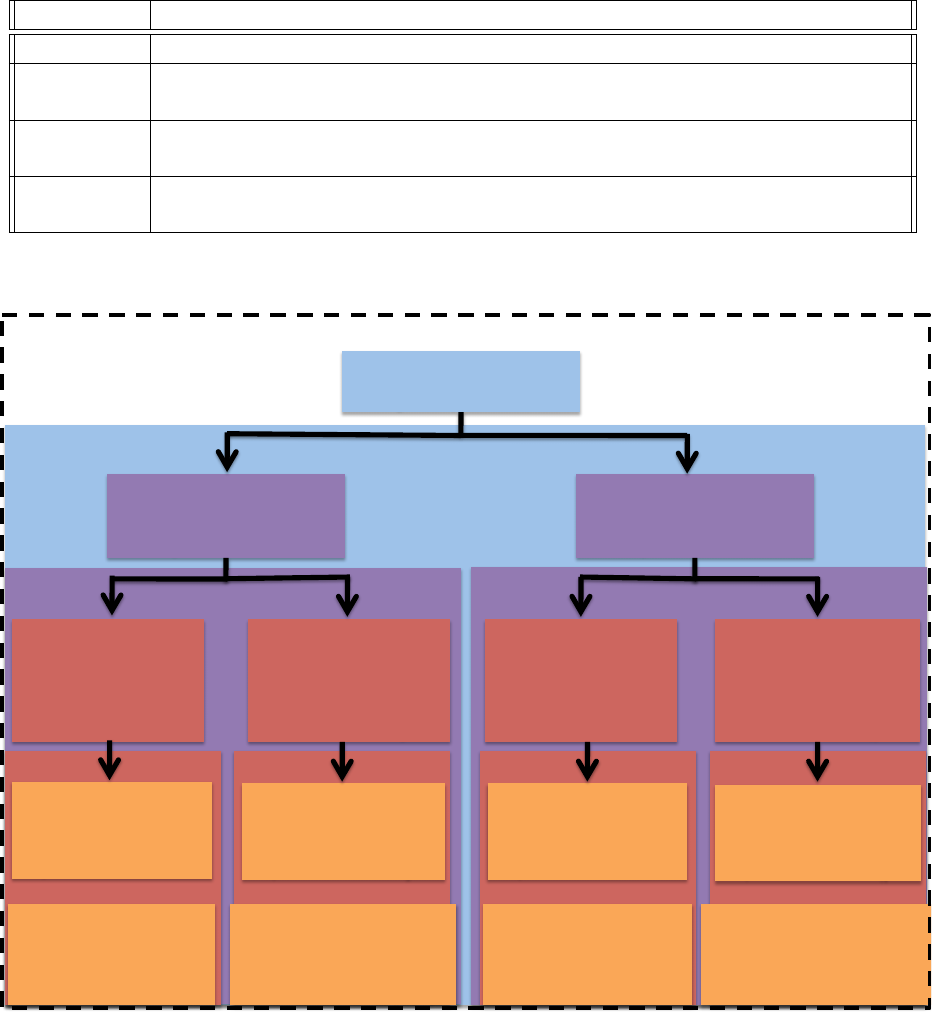
Layer Deﬁnition

Experiment An assemblage of CMB telescopes.

Telescope A platform that carries and points one or more cameras. It observes at a spec-

iﬁed site with a speciﬁed observation strategy and can include warm reﬂectors.

Camera A cryostat that houses cryogenic optics, ﬁlters, and detectors. Multiple cam-

eras can be mounted on the same telescope.

Channel A frequency band observed by some set of detectors within a camera. A

multichroic camera will have multiple channels.

Table 1: Deﬁnitions of the layers used to build a BoloCalc project.

Experiment*

• *Foreground)params)

Telescope*1*

• *Atmosphere)at)site)1)

• )Boresight)Eleva7on)PDF)1)

Telescope*N*

• *Atmosphere)at)site)N)

• )Boresight)Eleva7on)PDF)N)

Camera*1.1))

• )F/#)1.1)

• )Op7cal)stack)1.1)

• )Focal)Plane)Temp)1.1)

• )Pixel)Elev)PDF)1.1)

…*

Channel*1.1.1*

• )Detector)Band)1.1.1)

• )Detector)Params)1.1.1)

• )Op7cal)Params)1.1.1)

…*

Camera*1.M1))

• )F/#)1.M1)

• )Op7cal)stack)1.M1)

• )Focal)Plane)Temp)1.M1)

• )Pixel)Elev)PDF)1.M1)

Camera*N.1))

• )F/#)N.1)

• )Op7cal)stack)N.1)

• )Focal)Plane)Temp)N.1)

• )Pixel)Elev)PDF)N.1)

Camera*N.MN)

• )F/#)N.MN)

• )Op7cal)stack)N.MN)

• )Focal)Plane)Temp)N.MN)

• )Pixel)Elev)PDF)N.MN)

Channel*1.1.P11*

• )Detector)Band)1.1.P11)

• )Detector)Params)1.1.P11)

• )Op7cal)Params)1.1.P11)

…*

Channel*1.M1.1*

• )Detector)Band)1.M1.1)

• )Detector)Params)1.M1.1)

• )Op7cal)Params)1.M1.1)

Channel*1.M1.P1M1*

• )Detector)Band)1.M1.P1M1)

• )Detector)Params)1.M1.P1M1)

• )Op7cal)Params)1.M1.P1M1)

…*

Channel*N.1.1*

• )Detector)Band)N.1.1)

• )Detector)Params)N.1.1)

• )Op7cal)Params)N.1.1)

Channel*N.1.PN1*

• )Detector)Band)N.1.PN1)

• )Detector)Params)N.1.PN1)

• )Op7cal)Params)N.1.PN1)

Channel*N.MN.1*

• )Detector)Band)N.MN.1)

• )Detector)Params)N.MN.1)

• )Op7cal)Params)N.MN.1)

Channel*N.MN.PNMN*

• )Detector)Band)N.MN.PNMN)

• )Detector)Params)N.MN.PNMN)

• )Op7cal)Params)N.MN.PNMN)

Layer)1)

Layer)2)

Layer)3)

Layer)4)

…*

BoloCalc'Project'

Figure 2: Layout of a BoloCalc project.

3.1 Experiment Directory Layout

The experiment directory is meant to be easily generalizable to various kinds of experiments and

telescopes. For information about how experiments are stored within the BoloCalc/Experiments/

directory, see Section ??. Below is an overview of the ﬁle structure within an experiment directory.

Each layer of an experiment has several parameters that deﬁne the input experiment. In this

section, we go through them by input ﬁle.

1BoloCalc / E xperiements /[ E xper iment Name ]/[ Ex perime nt De si gn ]

2|- - config

3| |- - foreground s .txt

4|- - Telescop e1 /

5| |- - config /

6| | |- - tel escope . txt

7| | |- - ele vation . txt

8| | |- - [ Custom At mo spheric Pr of il e ] ( opti onal )

9| |- - Cam era1 /

10 | | |- - config /

11 | | | -- ca mera . t xt

12 | | | -- c hann els . t xt

13 | | | -- op tics . t xt

14 | | | -- e lev atio n . txt

15 | | |- - Band s /

16 | | |- - [ Optic Band File 1] ( optional )

17 | | |- - [ Optic Band File 2] ( optional )

18 | | |- - ...

19 | | |- - [ Detec tor Band File 1] ( optio nal )

20 | | |- - [ Detec tor Band File 2] ( optio nal )

21 | | |- - ...

22 | |- - Cam era2 /

23 | |- - ...

24 |- - Telesco pe2 /

25 |- - ...

As stated in Section ??, an experiment deﬁnition has four layers:

1. Experiment (Layer 1)

•Composed of (multiple) telescopes

•All telescopes in a given experiment see the same galactic foregrounds

2. Telescopes (Layer 2)

•Composed of (multiple) cameras

•All cameras in a given telescope see the same atmosphere

•All cameras in a given telescope have the same scan strategy

3. Cameras (Layer 3)

•Composed of (multiple) frequency channels

•All frequency channels in a given camera have the same camera parameters

•All frequency channels in a given camera see the same optical chain

4. Channels (Layer 4)

•Each channel has independent detector and optical element parameters

These layers allow telescopes to added to an experiment in an arbitrary location, each with

arbitrary cameras, each with arbitrary frequency channels.

3.2 Parameter Deﬁnitions

All parameters in BoloCalc are deﬁned with a central value and an error bar. Therefore, all

parameter variation is assumed to have an underlying Gaussian distribution, and all parameters

are assumed to be uncorrelated.

Parameters deﬁned foregrounds.txt,telescope.txt,camera.txt, and channels.txt have

the following format:

1Mean +/ - Std D ev

The following formatting rules should be followed for the code to work robustly and the tables

to render neatly:

1. All central values and standard deviations should have ﬁve characters. For instance, 1.000

and 10.00 are valid, while 10.000 is not.

2. All central values and standard deviations should be separated by +/- , noting the spaces

on either side of the +/−sign.

Parameters deﬁned in optics.txt are deﬁned for multiple bands in multi-chroic cameras and

therefore follow a diﬀerent format:

1[ Mean for Band 1, Mean for Band 2, ...] +/ - [ Std Dev for Band 1, Std Dev for

Band 2, ...]

In a similar way as with the single values, the following formatting rules should be followed for

the code to work robustly and the tables to render neatly:

1. All central values and standard deviations should have ﬁve characters. For instance, 1.000

and 10.00 are valid, while 10.000 is not.

2. All arrays of central values and arrays of standard deviations should be separated by +/- ,

noting the spaces on either side of the +/−sign

3.3 Experiment Parameters (Layer 1)

The experiment is comprised of an arbitrary set of telescopes, which are assumed to see the same

the same celestial loading, including power from the CMB and galactic foregrounds.

3.3.1 foregrounds.txt

The below list overviews the parameters deﬁned in

[Experiment Name]/[Experiment Version]/config/foregrounds.txt, the ﬁle that deﬁnes the

galaxy through which the telescope must observe the CMB. This galactic parameters will be the

same for all telescopes.

•Synchrotron Spec Index

◦Deﬁnition: “ns” in Equation ??

◦Description: Spectral index of the synchrotron power law spectrum

◦Allowed Values: Floating point value between (−∞, +∞]

◦Default Value: 2 ×10−3+/- 0 ×10−3

•Synchrotron Amplitude

◦Deﬁnition: “As” in Equation ??

◦Description: Amplitude of the synchrotron power law spectrum

◦Allowed Values: Floating point value between (0.0, +∞) W/Hz

◦Default Value: 6 ×103+/- 0 ×103W/Hz

•Dust Temperature

◦Deﬁnition: “Td” in Equation ??

◦Description: Dust modiﬁed blackbody temperature

◦Allowed Values: Floating point value between (0.0, +∞) K

◦Default Value: 19.70 +/- 0.00 K

•Dust Spec Index

◦Deﬁnition: “nd” in Equation ??

◦Description: The spectral index of the dust modiﬁed blackbody spectrum

◦Allowed Values: Floating point value between (−∞, +∞)

◦Default Value: 1.50 +/- 0

•Dust Amplitude

◦Deﬁnition: “Ad” in Equation ??

◦Description: Amplitude of the dust modiﬁed blackbody spectrum

◦Allowed Values: Floating point value between (0.0, +∞)

◦Default Value: 2 ×10−3+/- 0 ×10−3

•Dust Scale Frequency

◦Deﬁnition: “νd” in Equation ??

◦Description: Scale frequency for the dust modiﬁed blackbody spectrum

◦Allowed Values: Floating point value between (0.0, +∞)

◦Default Value: 353.0 +/- 0.0 GHz

3.4 Telescope Parameters (Layer 2)

The following sections overview the input parameters for each of the telescope input ﬁles.

3.4.1 telescope.txt

The below list overviews the parameters deﬁned in telescope.txt. These parameters are used to

deﬁne the site, atmospheric proﬁle, and patch coverage parameters for the telescope.

•Site

◦Description: Site at which the telescope observes, which deﬁnes the atmospheric condi-

tions.

◦Allowed Values: Either “Atacama” or “Pole”

◦Default Value: “Atacama”

•Elevation

◦Deﬁnition:θtel deﬁned in ??

◦Description: Elevation at which the telescope observes.

◦Allowed Values: [20.0, 90.0] deg above the horizon

◦Default Value: 50.0 +/- 0.0 deg

◦If “NA,” the elevation distribution deﬁned in Telescope/config/elevation.txt, will

be assumed.

•PWV

◦Description: Precipitable water vapor of the atmosphere through which the telescope

observes.

◦Allowed Values: [0.0, 8.0] mm

◦Default Value: 1.0 +/- 0.0 mm

◦If “NA,” the PWV distribution deﬁned in Telescope/config/pwv.txt, will be assumed.

•Observation Time

◦Deﬁnition:tobs in Equation ??

◦Description: How long this telescope will observe

◦Allowed Values: Floating point value between (0.0, +∞) years

◦Default Value: 3.0 +/- 0.0

•Sky Fraction

◦Deﬁnition:fsky in Equation ??

◦Description: What fraction of the sky this telescope will observe

◦Allowed Values: Floating point value between (0.0, 1.0]

◦Default Value: 0.7 +/- 0.0

•Observation Eﬃciency

◦Deﬁnition:ηobs in Equation ??

◦Description: What fraction of the observation time will the telescope be actually ob-

serving

◦Allowed Values: Floating point value between (0.0, 1.0]

◦Default Value: 0.8 +/- 0.0

•NET Margin

◦Deﬁnition:Min Equation ??

◦Description: Agnostic factor which multiplies the detector NETs for this telescope

◦Allowed Values: Floating point value between (0.0, +∞)

◦Default Value: 1.0 +/- 0.0

3.4.2 elevation.txt

elevation.txt is an optional ﬁle that deﬁnes the elevation probability distribution function (PDF),

which is determined by the scan strategy of the telescope. The ﬁrst column is the elevation above

the horizon in degrees, and the second column is the fraction of time spent at that elevation. This

ﬁle is only used if the parameter “Elevation” in Telescope/config/telescope.txt is deﬁned to

be “NA” (see Section ?? for more information about telescope.txt). The probabilities should

add up to one, and if they do not, the fraction will be determined by the provided probability

divided by the sum of the provided probabilities.

Below is a made-up example for elevation.txt. Notice that each row is separated by a

commented line of hyphens, while each column is separated by a vertical bar.

1#***** Elevat ion D is tribution ******

3Eleva tion | Probabili ty

4#---------------------------

5[ deg ] | NA

6#---------------------------

730.0 | 0.100

8#---------------------------

940.0 | 0.100

10 #---------------------------

11 50.0 | 0.300

12 #---------------------------

13 60.0 | 0.400

14 #---------------------------

15 70.0 | 0.100

16 #---------------------------

3.4.3 pwv.txt

pwv.txt is an optional ﬁle that deﬁnes the precipitable water vapor (PWV) probability distribution

function (PDF), which is determined by the weather conditions at the observation site. The ﬁrst

column is the PWV in mm, and the second column is the fraction of time spent at that PWV value.

This ﬁle is only used if the parameter “PWV” in Telescope/config/telescope.txt is deﬁned to

be “NA” (see Section ?? for more information about telescope.txt). The probabilities should

add up to one, and if they do not, the fraction will be determined by the provided probability

divided by the sum of the provided probabilities.

Below is a made-up example for pwv.txt. Notice that each row is separated by a commented

line of hyphens, while each column is separated by a vertical bar.

1#***** Site PWV Di st ribution * *****

3PWV | Probabili ty

4#---------------------------

5[ mm ] | N A

6#---------------------------

70.200 | 0.100

8#---------------------------

90.400 | 0.100

10 #---------------------------

11 0.600 | 0.200

12 #---------------------------

13 0.800 | 0.200

14 #---------------------------

15 1.000 | 0.100

16 #---------------------------

17 1.200 | 0.100

18 #---------------------------

19 1.400 | 0.100

20 #---------------------------

21 1.600 | 0.100

22 #---------------------------

3.4.4 atm.txt

There is an option to override the code’s handling of the atmosphere by providing a custom

atmospheric proﬁle. The atmosphere ﬁle must be in [Telescope Name]/config/, and the ﬁle-

name must have the form atm [Elevation]deg [PWV]um.txt. For example, a valid ﬁlename is

atm 60deg 1000um.txt.

The atmosphere ﬁle should have four columns, delimited by white space:

1. Column 1: Frequency [GHz]

2. Column 2: Optical Depth

3. Column 3: Planck Temperature [K]

4. Column 4: Transmission

Note that the temperature is in Planck units, not Rayleigh-Jeans. The passed frequency range

in the atmosphere ﬁle needs to be large enough to cover the frequency bands observed by the

telescope—which are deﬁned in the “channels.txt” and “Bands/” ﬁles at the camera directory level

(see Section ?? and Section for more details)—with at least a 15% buﬀer on the bandwidths of the

highest and lowest bands. For instance, if your detector bands range from 240 to 300 GHz, your

atmosphere ﬁle should have values that go from at least 205 to 345 GHz.

Below is an example of an atmospheric proﬁle generated using the AM simulation code and a

conﬁguration ﬁle designed using the 10-year MERRA dataset for the Chajnantor Observatory.

11.000 0000 e +01 3.66 4259 e -03 3. 58955 7 e +00 9.963424 e -01

21.002 0000 e +01 3.66 7538 e -03 3. 59033 9 e +00 9.963392 e -01

31.004 0000 e +01 3.67 1011 e -03 3. 59116 3 e +00 9.963357 e -01

41.006 0000 e +01 3.67 4741 e -03 3. 59204 3 e +00 9.963320 e -01

51.008 0000 e +01 3.67 8826 e -03 3. 59300 1 e +00 9.963279 e -01

61.010 0000 e +01 3.68 3414 e -03 3. 59406 9 e +00 9.963234 e -01

71.012 0000 e +01 3.68 8744 e -03 3. 59530 1 e +00 9.963181 e -01

81.014 0000 e +01 3.69 5220 e -03 3. 59678 8 e +00 9.963116 e -01

91.016 0000 e +01 3.70 3583 e -03 3. 59869 8 e +00 9.963033 e -01

10 1.018 0000 e +01 3.71 5317 e -03 3. 60137 4 e +00 9.962916 e -01

11 1.020 0000 e +01 3.73 3976 e -03 3. 60566 0 e +00 9.962730 e -01

12 ...

3.5 Camera Parameters (Layers 3 and 4)

In the following sections, we will overview the input parameters for each of the camera input ﬁles.

3.5.1 camera.txt

camera.txt deﬁnes parameters that are the same for all frequency bands observed with this camera.

The ﬁle must be located within [Telescope Name]/[Camera Name]/config/.

•Boresight Elevation

◦Deﬁnition:θcam in Equation ??.

◦Description: The elevation of the camera boresight with respect to the telescope bore-

sight.

◦Allowed Values: Floating point value between (-40.0, 40.0] deg

◦Default Value: 0.0 +/- 0.0 deg

•Optical Coupling

◦Deﬁnition:ξin Equation ??.

◦Description: A parameter that quantiﬁes the SNR degradation associated with how well

the far-ﬁeld image couples to the detector pixels on the focal plane.

◦Allowed Values: Floating point value between (0.0, 1.0]

◦Default Value: 1.0 +/- 0.0

•F-number

◦Deﬁnition:Fin Equation ??.

◦Description: The focal ratio at the focal plane

◦Allowed Values: Floating point value between (0.0, +∞)

◦Default Value: 2.5 +/- 0.0

•Bath Temp

◦Deﬁnition:Tbath in Equation ??.

◦Description: The temperature of the focal plane

◦Allowed Values: Floating point value between (0.0, +∞) K

◦Default Value: 0.100 +/- 0.000 K

3.5.2 elevation.txt

elevation.txt is an optional ﬁle that deﬁnes the elevation distribution with respect to the camera

boresight of pixels on the focal plane. This ﬁle sets the value for θelv deﬁned in equation ??.

This pixel elevation distribution ﬁle has the exact same structure as the ﬁle

Telescope/config/elevation.txt, which instead deﬁnes the scan strategy and is described in

section ??. The ﬁrst column is the elevation above the horizon in degrees, and the second column

is the fraction if time spent at that elevation.

This ﬁle is only used if the parameter “Elevation” in Telescope/config/elevation.txt is

deﬁned to be “NA” (see Section ?? for more information about telescope.txt).

The probabilities should add up to one, and if they don not, the fraction will be determined by

the provided probability divided by the sum of the provided probabilities.

Below is a made-up example of correct formatting for elevation.txt. Notice that each row is

separated by a commented line of hyphens, while each column is separated by a vertical bar.

1#***** Elevat ion D is tribution ******

3Eleva tion | Probabili ty

4#---------------------------

5[ deg ] | NA

6#---------------------------

730.0 | 0.100

8#---------------------------

940.0 | 0.100

10 #---------------------------

11 50.0 | 0.300

12 #---------------------------

13 60.0 | 0.400

14 #---------------------------

15 70.0 | 0.100

16 #---------------------------

3.5.3 channels.txt

channels.txt deﬁnes the parameters of the frequency bands and detectors that are observing in

this camera. The ﬁle must be located within [Telescope Name]/[Camera Name]/config/.

•Band ID

◦Description: The identiﬁcation number for this band.

◦Allowed Values: An integer value between [1, +∞)

◦Default Value: 1

◦Cannot have two bands with same Band ID on the same pixel

•Pixel ID

◦Description: The identiﬁcation number for the pixel this band observes from

◦Allowed Values: An integer value between [1, +∞)

◦Default Value: 1

◦Cannot have two bands with same Band ID on the same pixel

•Band Center

◦Deﬁnition:νcin Equation ??.

◦Description: The central frequency for this band.

◦Allowed Values: A ﬂoating point value between (0.0, +∞) GHz

◦Default Value: [90, 150] +/- [0, 0] GHz

•Fractional BW

◦Deﬁnition:fBW in Equation ??.

◦Description: Fractional arithmetic bandwdith for this band

◦Allowed Values: A ﬂoating point value between (0.0, 2.0]

◦Default Value: [0.350, 0.275] +/- [0.000, 0.000]

•Pixel Size

◦Deﬁnition:Din Equation ??.

◦Description: Size of the pixel via which this band is observing

◦Allowed Values: A postive ﬂoating point value between (0.0, +∞) mm

◦Default Value: 6.8 +/- 0.0 mm

•Num Det per Wafer

◦Deﬁnition:Ndet/waf in Equation ??

◦Description: Number of detectors per wafer within this band

◦Allowed Values: An integer value between [1, +∞)

◦Default Value: 542

•Num Waf per OT

◦Deﬁnition:Nwaf/OT in Equation ??.

◦Description: Number of wafers with this band per camera.

◦Allowed Values: An integer value between [1, +∞)

◦Default Value: 7

•Num OT

◦Deﬁnition:NOT in Equation ??.

◦Description: Number of cameras in this telescope observing at this frequency.

◦Allowed Values: An integer value between [1, +∞)

◦Default Value: 1

•Waist Factor

◦Deﬁnition:wfin Equation ??.

◦Description: The ratio of the Gaussian beam waist coming from the pixel aperture to

the pixel aperture diameter for this band.

◦Allowed Values: A ﬂoating point value between [2.0, +∞)

◦Default Value: 3.0 +/- 0.0

•Det Eﬀ

◦Deﬁnition:ηdet in Equation ??.

◦Description: Eﬃciency of the detector from the entry point of the pixel aperture to the

bolometer.

◦Allowed Values: A ﬂoating point value between (0.0, 1.0]

◦Default Value: 0.700 +/- 0.000

•Psat

◦Deﬁnition:Psat in Equation ??.

◦Description: Saturation power of the bolometer.

◦Allowed Values: A ﬂoating point value between (0.0, +∞] pW

◦Default Value: “NA”

◦If “NA,” use Equation ?? to calculate Psat

•Psat Factor

◦Deﬁnition:fpsat in Equation ??.

◦Description: Safety factor used to caculate saturation power from optical power

◦Allowed Values: A ﬂoating point value between (0.0, +∞)

◦Default Value: 3.0 +/- 0.0

◦If “Psat” is not “NA,” this parameter is ignored.

•Carrier Index

◦Deﬁnition:nin Equations ?? and ??.

◦Description: Thermal carrier index for bolometer leg conductivity

◦Allowed Values: A ﬂoating point value between (0.0, +∞)

◦Default Value: 2.7 +/- 0.0

•Tc

◦Deﬁnition:Toper in Equations ??,??, and ??.

◦Description: Bolometer operating temperature

◦Allowed Values: A ﬂoating point value between (0.0, +∞) K

◦Default Value: 0.165 +/- 0.000 K

◦If “NA,” use Equation ?? to calculate operating temperature.

•Tc Fraction

◦Deﬁnition:foper in Equation ??.

◦Description: Factor used to calculate transition temperature from the bath temperature

◦Allowed Values: A ﬂoating point value between (1.0, +∞)

◦Default Value: “NA”

◦If “Tc” is not “NA,” this parameter is ignored.

•Yield

◦Deﬁnition:Yin Equation ??.

◦Description: Fraction of deployed detectors that are observing. This is also commonly

referred to as “end-to-end” yield.

◦Allowed Values: A ﬂoating point value between (0.0, 1.0]

◦Default Value: 0.7 +/- 0.0

•SQUID NEI

◦Deﬁnition: NEI in Equation ??.

◦Description: SQUID noise equivalent current.

◦Allowed Values: A ﬂoating point value between (0.0, +∞) pA/√Hz

◦Default Value: “NA”

◦If “NA,” use Equation ?? to calculate readout noise NEPread

•Bolo Resistance

◦Deﬁnition:Rbolo in Equation ??.

◦Description: Bolometer operating resistance.

◦Allowed Values: A ﬂoating point value between (0.0, +∞) Ω

◦Default Value: “NA”

◦If “NA,” use Equation ?? to calculate readout noise NEPread

•Read Noise Frac

◦Deﬁnition: ∆read in Equation ??.

◦Description: Fraction of the total NEP that is due to readout noise.

◦Allowed Values: A ﬂoating point value between [0.0, +∞)

◦Default Value: 0.1 +/- 0.0

◦If “SQUID NEI” and “Bolo Resistance” are not “NA,” this parameter is ignored.

3.5.4 optics.txt

optics.txt deﬁnes the parameters the frequency bands and detectors that are observing in this

camera. The ﬁle must be located within [Telescope Name]/[Camera Name]/config/.

•Element

◦Description: Name of optical element

◦Allowed Values: Any string

◦Default Value: “Element”

◦RESERVED NAMES: “Primary,” “Mirror,” “Aperture,” and “Stop” trigger addi-

tional calculations and therefore must be used purposefully

•Temperature

◦Deﬁnition:Tiin Equation ??.

◦Description: Temperature of the optical element

◦Allowed Values: An ﬂoating point value between (0.0, +∞) K

◦Default Value: 4 +/- 0 K

•Absorption

◦Deﬁnition:iin Equation ??.

◦Description: Fractional power attenuation/emission due to absorption within the optical

element

◦Allowed Values: A ﬂoating point value between [0.0, 1.0)

◦Default Value: 0.000 +/- 0.000

◦If “NA” ...

∗If “Mirror” or “Primary” is in “Element,” Equation ?? is used to calculate ohmic

losses in the reﬂective optical element.

∗If “Mirror” or “Primary” is not in “Element,” Equation ?? is used to calculate

dielectric loss in the refractive optical element.

•Reﬂection

◦Deﬁnition:rin Equation ??.

◦Description: Fractional power lost due to reﬂection at the optical element.

◦Allowed Values: A ﬂoating point value between [0.0, 1.0)

◦Default Value: 0.000 +/- 0.000

◦If “NA,” Equation ?? is used to calculate reﬂection loss

•Thickness

◦Deﬁnition:tin Equation ??

◦Description: Thickness of the optical element

◦Allowed Values: A ﬂoating point value between (0.0, +∞) mm

◦Default Value: “NA”

◦If “Mirror” or “Primary” is in “Element,” this parameter is ignored

◦If “Absorption” is not “NA,” this parameter is ignored

•Index

◦Deﬁnition:nin Equation ??.

◦Description: Index of refraction of the optical element.

◦Allowed Values: A ﬂoating point value between [1.0, +∞)

◦Default Value: “NA”

◦If “Mirror” or “Primary” is in “Element,” this parameter is ignored

◦If “Absorption” is not “NA,” this parameter is ignored

•Loss Tangent

◦Deﬁnition: tan δin Equation ??.

◦Description: Loss tangent of the optical element.

◦Allowed Values: A ﬂoating point value between [0.0, +∞)

◦Default Value: “NA”

◦If “Mirror” or “Primary” is in “Element,” this parameter is ignored

◦If “Absorption” is not “NA,” this parameter is ignored

•Conductivity

◦Deﬁnition:σcin Equation ??.

◦Description: Electrical conductivity of the optical element.

◦Allowed Values: A ﬂoating point value between (0.0, +∞)

◦Default Value: “NA”

◦If “Mirror” or “Primary” is not in “Element,” this parameter is ignored

◦If “Absorption” is not “NA,” this parameter is ignored

•Scatter Frac

◦Deﬁnition:δiin Equation ??.

◦Description: Fractional power lost due to scattering.

◦Allowed Values: A ﬂoating point value between [0.0, 1.0]

◦Default Value: “NA”

◦If “NA,” Equation ?? is use to calculate scattering loss.

•Surface Rough

◦Deﬁnition:σrin Equation ??.

◦Description: Surface roughness of the optical element.

◦Allowed Values: A ﬂoating point value between [0.0, +∞)

◦Default Value: “NA”

◦If “Scatter Frac” is not “NA,” this parameter is ignored.

◦If “NA” and “Scatter Frac” is “NA,” scattering is assumed to be zero.

•Scatter Temp

◦Deﬁnition:Tδ;iin Equation ??.

◦Description: The eﬀective temperature that the scattered power lands on.

◦Allowed Values: A ﬂoating point value between [0.0, +∞)

◦Default Value: “NA”

◦If “NA,” scattered power is assumed to land at “Temperature,” the temperature of the

optical element itself

•Spillover

◦Deﬁnition:βiin Equation ??.

◦Description: Fractional power that spills over the optical element.

◦Allowed Values: A ﬂoating point value between [0.0, 1.0)

◦Default Value: “NA”

◦If “NA,” spillover is assumed be zero

•Spillover Temp

◦Deﬁnition:Tβ;iin Equation ??.

◦Description: The eﬀective temperature that the spilled power lands on.

◦Allowed Values: A ﬂoating point value between [0.0, +∞)

◦Default Value: “NA”

◦If “NA,” spillover is assumed to land at “Temperature,” the temperature of the element

itself

3.6 Custom Bands

By default, BoloCalc assumes top hat bands for all detectors and optical elements, whose height is

determined soley by the mean and standard deviation of the end-to-end optical eﬃciency. However,

custom bands can be input for any optical element.

The general ﬁle format for all band ﬁles is the same:

1| Frequ ency [ GHz ] | Mean Ef ficienc y | Stand ard Devi ation ( o ptional ) |

Each column is separated by a vertical bar, and the ﬁnal column, which contains the error bars,

can be omitted. If only two columns are present, all stand deviations are assumed to be zero.

An example of a made-up detector bandpass text ﬁle, which is space-delimited, is shown below:

170. 0.000 0.000

275. 0.500 0.100

380. 0.700 0.100

485. 0.650 0.100

590. 0.700 0.100

6100. 0.800 0.100

7105. 0.600 0.100

8110. 0.700 0.100

9115. 0.500 0.100

10 120. 0.000 0.000

3.6.1 Detectors

Detector band ﬁles are stored in

1[ Teles cope Name ]/[ Cam era Name ]/ config / Bands / Detect ors /

The band is identiﬁed using its ﬁlename, which must have the format [Camera Name][Band

ID].txt for text ﬁles, or [Camera Name][Band ID].csv for comma-separated value ﬁles; both ﬁle

formats work equally well. For example, to load a text ﬁle for a camera named “MF” (in the

directory [Telescope Name]/MF/ and a Band ID “1,” the ﬁle name should be MF1.txt. Note that

for a multi-chroic camera, there should be multiple band ﬁles, one for each frequency channel.

3.6.2 Optics

Optics band ﬁles are stored in

1[ Te lesc ope Name ]/[ Camera Name ]/ c on fig / Band s / Optics /

The band is identiﬁed using its ﬁlename, which must have the format [Optical Element

Name].txt for text ﬁles, or [Optical Element Name].csv for comma-separated value ﬁles; both

ﬁle formats work equally well. For example, to load a text ﬁle for an optical element named

“Lens1,” the ﬁle name should be Lens1.txt. Note that there is only one band ﬁle for optical

elements, even in multi-chroic cameras, as all detectors are all frequencies see the same bandpass.

Also note that you can apply the same band to multiple optical elements by duplicating matching

names in optics.txt.

3.7 Default Bands

If no custom bands are deﬁned, BoloCalc assumes a top-hat band function, which is determined

by the detector bandpass.

3.7.1 Detectors

If no custom detector bandpass is provided, then a top-hat band is assumed with an overall eﬃciency

factor for the detector ηdet

B(ν) = ηdet if νlo ≤ν≤νhi

0 otherwise ,(26)

where the high and low band edges are deﬁned as

νlo =νc1 + fBW

2;νhi =νc1−fBW

2(27)

where νcis the band central frequency and fBW is the fractional bandwidth.

3.7.2 Optics

If no custom bandpass is provided for an optical element i, then the bandpass is assumed to be a

top-hat with an overall eﬃciency factor deﬁned in Equation ??

B(ν) = ηiif νlo ≤ν≤νhi

0 otherwise (28)

If a custom detector bandpass is deﬁned, then the frequency range covered νlo to νhi are the

highest and lowest frequencies deﬁned in the custom band. Otherwise, νlo and νhi are set by

Equation ??.

4 Monte Carlo Simulation

BoloCalc has two executables mappingSpeed.py and mappingSpeed vary.py that, when run, use

independent sampling of all parameters using the Monte Carlo (MC) method to generate NET

distributions from variations in the underlying instrument parameters. For information on how to

run the executables, see Sections ?? and ??.

The MC simulation iterates using a nest of the following structure:

•Nexp Experiment realizations

◦Nobs Observations per experiment realization

∗Ndet Detector realizations per observation

4.1 Simulation Inputs

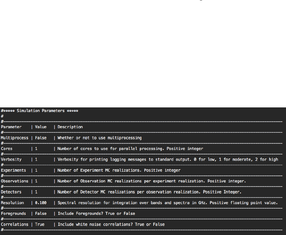
Simulation inputs are stored in the ﬁle BoloCalc/config/simulationInputs.txt. An example of

the ﬁle is shown in Figure ??. Below, we deﬁne the parameters for the simulation explicitly.

Figure 3: Example of simulation input ﬁle simulationInputs.txt

•Multiprocess

◦Description: Whether or not to use multiprocessing to calculate statistics in parallel

◦Allowed Values: “True” or “False”

◦Default Value: “False”

•Cores

◦Description: Number of cores to pool for parallel processing

◦Allowed Values: Positive integer between [1, +∞)

◦Default Value: 1

•Verbosity

◦Description: Logging verbosity. 2 to print all logging output, 1 to print some output, 0

to print little output

◦Allowed Values: Integer between [0, 2]

◦Default Value: 1

•Experiments

◦Description: Number of experiment realizations to Monte Carlo; each time an experi-

ment is MC-ed, its foreground, telescope, camera, and optical parameters are re-sampled.

◦Allowed Values: Positive integer [1, +∞)

◦Default Value: 1

◦If 1, assume central value (i.e. ignore the spread) for all parameters set by the experiment

realization.

•Observations

◦Description: Number of independently observations, which draw the PWV and telescope

boresight elevation from the distributions deﬁned in Telescope/config/pwv.txt and

Telescope/config/elevation.txt.

◦Allowed Values: Positive integer [1, +∞)

◦Default Value: 1

•Detectors

◦Description: Number of independently-sampled detector parameters deﬁned in channels.txt

per observation.

◦Allowed Values: Positive integer [1, +∞)

◦Default Value: 1

◦If 1, assume central value for all detector parameeters

•Resolution

◦Description: Frequency resolution assumed in the simulation.

◦Allowed Values: A positive ﬂoating-point value between (0.0, 20.0] GHz

◦Default Value: 0.1

◦Reducing the resolution can have a dramatic impact on the speed of the MC simulations.

•Foregrounds

◦Description: Whether or not to include foregrounds in the estimate of the optical loading.

◦Allowed Values: “True” or “False”

◦Default Value: “False”

◦Celestial loading doesn’t have a noticeable impact on ground-based telescopes but can

be important for satellite experiments.

•Correlations

◦Description: Whether to impose white noise correlations when calculating array NET

◦Allowed Values: “True” or “False”

◦Default Value: “True”

◦This switch is useful for computing the impact of white-noise correlations on array NET.

4.2 Parameter Variation

mappingSpeed vary.py calculates the NET distribution using the MC method for a set of ex-

periment conﬁgurations deﬁned by the variation in user-deﬁned parameters, which are deﬁned

in BoloCalc/config/paramsToVary.txt. An example of the paramsToVary.txt ﬁle is shown in

Figure ??.

Parameters are deﬁned by row and have the following descriptors, which are organized by

column:

•Column 1: Telescope in which the parameter is deﬁned

◦Leave blank if the parameter is deﬁned in config/foregrounds.txt

•Column 2: Camera in which the parameter is deﬁned

◦Leave blank if the parameter is deﬁned in Tel/config/telescope.txt

•Column 3: Channel for which the parameter is deﬁned

◦Leave blank if the parameter is deﬁned in Cam/config/camera.txt of if Column 2 is

blank.

•Column 4: Optic for which the parameter is deﬁned

◦Leave blank unless the parameter is deﬁned in Cam/config/optics.txt

•Column 5: Parameter name, as displayed in the input text ﬁles

•Column 6: Minimum parameter value to be calculated

•Column 7: Maximum parameter value to be calculated

•Column 8: Step size with which the parameter will be calculated over the range [Minimum,

Maximum]

The user can deﬁne as many simultaneous parameter variations as desired, and

mappingSpeed vary.py will calculate the NET distribution for all combinations of those param-

eters. The results are then stored in [ExperimentDesign]/config/paramVary/. For more infor-

mation regarding the contents of the output ﬁles, see Section ??.

5 Output Files

Running mappingSpeed.py and/or mappingSpeed vary.py generates several output ﬁles, which

quantify the performance of the simulated experiment. In this section, we go through the layout of

the output ﬁles as well as their contents.

5.1 Sensitivity Tables

BoloCalc produces tables of outputs related to the white noise performance of the instrument.

All sensitivity tables are in ﬁles named sensitivity.txt, and there are multiple tables generated

at multiple directory tree levels, describing the performance of the camera, telescope, and entire

experiment.

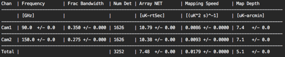
5.1.1 [ExperimentDesign]/sensitivity.txt

When mappingSpeed.py is run, it generates the following parameters in the ﬁle

[ExperimentDesign]/sensitivity.txt:

•Chan

◦Description: Frequency channel name [Camera Name][Band ID]

•Frequency

◦Deﬁnition:νcin Equation ??

◦Description: Central frequency of the frequency channel

•Frac Bandwidth

◦Deﬁnition:fBW in Equation ??

◦Description: Fractional bandwidth of frequency channel

•Num Det

◦Deﬁnition:Ndet in Equation ??

◦Description: Total number of detectors deployed in this frequency channel, combined

for all telescopes within the experiment

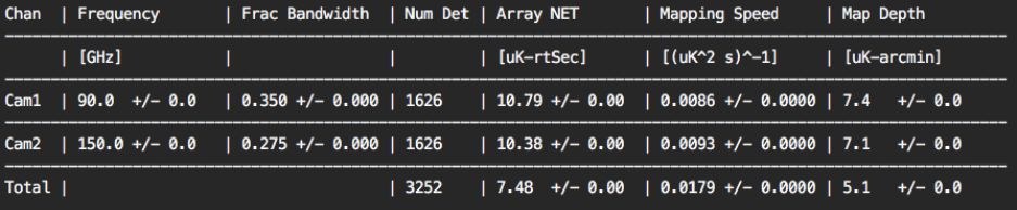
•Array NET

◦Deﬁnition: NETarr in Equation ??

◦Description: Array-averaged noise-equivalent CMB temperature of this frequency chan-

nel, combined for all telescopes within the experiment

•Mapping Speed

◦Deﬁnition: MS in Equation ??

◦Description: Mapping speed of this frequency channel, combined for all telescopes within

the experiment

•Map Depth

◦Deﬁnition:σsin Equation ??

◦Description: Map depth achieved by this frequency channel, combined for all telescopes

within the experiment

Note that if identical band names are shared between telescopes and/or cameras, the detectors are

combined in this table, with the combined Array NET of that combined band is found by taking

the inverse-variance average of the duplicated bands.

Figure ?? shows an example of sensitivity.txt at the Experiment directory level, using the

provided ExampleExperiment/V0/ conﬁguration.

Figure 4: ExampleExperiment sensitivity at the experiment level.

5.1.2 [ExperimentDesign]/[Telescope]/sensitivity.txt

When mappingSpeed.py is run, it generates the following parameters in the ﬁle

[ExperimentDesign]/[Telescope]/sensitivity.txt:

•Chan

◦Frequency channel name [Camera Name][Band ID]

•Frequency

◦Deﬁnition:νcin Equation ??

◦Description: Central frequency of the frequency channel

•Frac Bandwidth

◦Deﬁnition:fBW in Equation ??

◦Description: Fractional bandwidth of frequency channel

•Num Det

◦Deﬁnition:Ndet in Equation ??

◦Description: Total number of detectors deployed in this frequency channel, combined

for all cameras within the telescope

•Array NET

◦Deﬁnition: NETarr in Equation ??

◦Description: Aarray-averaged noise equivalent temperature of this frequency channel,

combined for all cameras within the telescope

•Mapping Speed

◦Deﬁnition: MS in Equation ??

◦Description: Mapping speed of this frequency channel, combined for all cameras within

the telescope

•Map Depth

◦Deﬁnition:σsin Equation ??

◦Description: Map depth achieved by this frequency channel, combined for all cameras

within the telescope

Note that if identical band names are shared between cameras, the detectors are combined in this

table, with the combined Array NET of that band is found by taking the inverse-variance average

of the duplicated bands.

Figure ?? shows an example of sensitivity.txt at the telescope directory level, using the

provided ExampleExperiment/V0/ conﬁguration.

Figure 5: ExampleExperiment sensitivity at the telescope level. Note that for the simple, single-

telescope design of ExampleExperiment, this ﬁle is identical to what is shown in Figure ??.

5.1.3 [ExperimentDesign]/[Telescope]/[Camera]/sensitivity.txt

When mappingSpeed.py is run, it generates the following parameters in the ﬁle

[ExperimentDesign]/[Telescope]/[Camera]/sensitivity.txt:

•Chan

◦Frequency channel name [Camera Name][Band ID]

•Frequency

◦Deﬁnition:νcin Equation ??

◦Description: Central frequency of the frequency channel

•Frac Bandwidth

◦Deﬁnition:fBW in Equation ??

◦Description: Fractional bandwidth of frequency channel

•Num Det

◦Deﬁnition:Ndet in Equation ??

◦Description: Total number of detectors deployed in this frequency channel within this

camera

•Lyot Efficiency

◦Deﬁnition:ηstop in Equation ??

◦Description: Lyot stop spillover eﬃciency of the frequency channel

•Optical Power

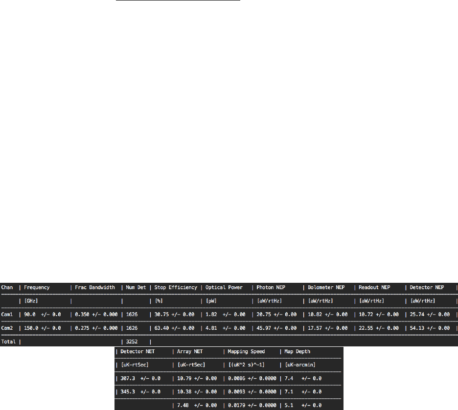
◦Deﬁnition:Popt in Equation ??

◦Description: Total optical power on detectors within this frequency channel

•Photon NEP

◦Deﬁnition: NEPph in Equation ??

◦Description: Noise-equivalent power due to photon noise for detectors within this fre-

quency channel

•Bolometer NEP

◦Deﬁnition: NEPgin Equation ??

◦Description: Noise-equivalent power due to bolometer thermal carrier noise for detectors

within this frequency channel

•Readout NEP

◦Deﬁnition: NEPread in Equation ??

◦Description: Noise-equivalent power due to readout for detectors within this frequency

channel

•Detector NEP

◦Deﬁnition:qNEP2

ph + NEP2

g+ NEP2

read in Equation ??

◦Description: Total noise-equivalent power due to the combination of photon, thermal

carrier, and readout noise for detectors within this frequency channel

•Detector NET

◦Deﬁnition: NETdet in Equation ??

◦Description: Per-detector noise-equivalent temperature for detectors within this channel

•Array NET

◦Deﬁnition: NETarr in Equation ??

◦Description: Array-averaged noise equivalent temperature of this frequency channel

within this camera

•Mapping Speed

◦Deﬁnition: MS in Equation ??

◦Description: Mapping speed of this frequency channel within this camera

•Map Depth

◦Deﬁnition:σsin Equation ??

◦Description: Map depth achieved by this frequency channel within this camera

for every frequency channel in the provided camera.

Figure ?? shows an example of sensitivity.txt at the camera directory level. Note that this

sensitivity ﬁle contains the most information about each individual channel. No combining of like

channels happens at this low level.

Figure 6: ExampleExperiment sensitivity at the camera level.

5.1.4 [ExperimentDesign]/paramVary/*.txt

mappingSpeed vary.py saves three quantities7to ﬁles within the directory

BoloCalc/Experiments/[Experiment]/[ExperimentDesign]/paramVary/

•Optical power: mappingSpeedVary Popt [Tel] [Cam] [Channel] [Param].txt

•Photon NEP: mappingSpeedVary NEPph [Tel] [Cam] [Channel] [Param].txt

•Array NET: mappingSpeedVary NETarr [Tel] [Cam] [Channel] [Param].txt

where [Tel] [Cam] [Channel] [Param] is a string that contains the speciﬁer for every parameter

varied in the calculation. For example, if we looped over the following two parameters

•Telescope “Tel,” camera “Cam,” channel “1,” optic “Mirror,” Parameter “Spillover”

•Telescope “Tel,” camera “Cam,” channel “1,” Parameter “Pixel Size”

the Popt output ﬁle would have the ﬁlename

1ma pp in gS pe ed Va ry _P opt _T el _C am _1 _M ir ror _S pi ll ov er _T el _Ca m_ 1_ Pi xe lS iz e . txt

An example of the Popt output ﬁle generated by running the provided example experiment, as

described in Section ??, is shown in Figure ??. A similar ﬁle will be generated for photon NEP

NEPph and array NET NETarr. As the example output shows,

5.2 Optical Power Table

BoloCalc also outputs tables of optical powers, including the the following information in columns:

•Element

◦Name of optical element, as deﬁned within optics.txt for this camera

•Power from Sky

◦Power incident on this optical element from the sky side

•Power to Detect

◦Power emitted from this optical element which is seen by the detector

•Cumulative Eff

◦Cumulative Eﬃciency between this optical element and the detector

These values are useful for understanding how signal propagates to the detector through the tele-

scope optical chain, as well as seeing what the major sources of parasitic loading are.

5.2.1 [ExperimentDesign]/[Telescope]/[Camera]/opticalPower.txt

Optical powers are listed for each channel in the camera, formatted as one table per frequency.

Figure ?? is an example optical power table for

7More quantities can be added to this list upon request, or as needed.

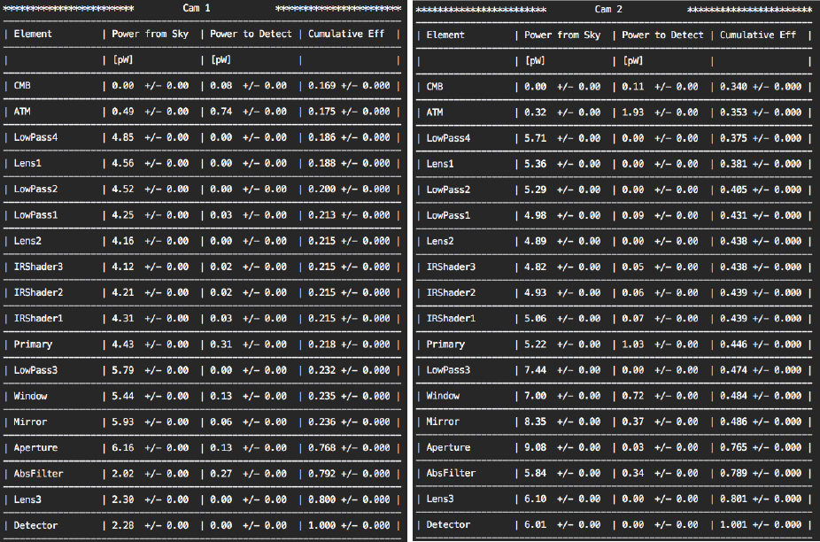
Figure 7: ExampleExperiment optical tables for camera Cam in both of its bands. Each

opticalTable.txt table is labeled by “[camera name] + [band name].”

Bolo Calc User Manual

Navigation menu

Versions of this User Manual:

Views

Navigation