Bordner Survey User Guide
User Manual:
Open the PDF directly: View PDF  .
.
Page Count: 11

1
User Guide:
Wisconsin Land Economic Inventory (WLEI) Digitized
Maps
History and Background Information
The WLEI was a comprehensive and extremely detailed mapping of Wisconsin’s counties. The genesis of the
program was in the Progressive era. By the 1920s court and law rulings had clarified that states had authority for land
use planning that included private lands. Following the cutover era in Northern Wisconsin, with devastated forests,
burned land, and abandoned farms, the state of Wisconsin saw the need for comprehensive inventory of the land to
guide planning.
Field mapping started in 1928, and it was completed under WPA funding in the late 1930s. Each township was
inventoried by crews traversing each section of land along the “40” lines, or every one-quarter mile. Essentially
everything about the land and what was on it was mapped and described. Eventually this resulted in over 100 classes
of information, from polygons of forest type and quality, to detailed classes of agricultural use, and all infrastructure
features that could be identified. The survey was executed by field workers who were by and large trained foresters,
with a standard accuracy of 2 chains for open country, and 4 chains (1 chain = 66’) for wild or densely wooded
country. Field workers’ hand drawn maps were later adjusted with aerial photography to produce a published maps
for nearly every township in Wisconsin.
The published maps – often referred to as the Bordner maps named for the director of the program – have been
optically scanned and are available online through the UW Libraries Digital Collections site
(https://uwdc.library.wisc.edu/collections/EcoNatRes/WILandInv/). Milwaukee and Menominee Counties were not
mapped. Lincoln, Manitowoc, and Sheboygan County township maps were never published. For those counties with
unpublished maps, the original sketch maps were located in the Historical Archives at the Wisconsin Historical
Society, and scanned.
While the original published maps offer an insight to landscape features, they do not allow for complex analysis using
modern technologies and techniques. Over seventy years after the last map was published, the Forest Ecosystem
and Landscape Ecology Lab (FLEL) of the University of Wisconsin-Madison, Department of Forest and Wildlife
Ecology has collaborated with the Wisconsin State Cartographer’s Office (SCO) to digitize the maps into a GIS
dataset and make the data available to the public. This digitized dataset can help researchers and educators further
understand the landscape of Wisconsin during the time of peak deforestation and land abandonment. Furthermore,
this digitized dataset offers a tool for future landscape management including but not limited to; shoreline changes,
erosion, reforestation, and wetland restoration.
Digitization Processes and Methodology
Step 1: Georeference Original Maps
First part of the GIS digitization process of the Bordner survey maps was to georeference the original
published township maps. Using section line intersections as a reference, these scanned maps were then
georeferenced to the Department of Natural Resource’s 'Landnet' GIS database layer containing the section
lines, using section line intersections as tie points. In cases where there were missing section lines on the
original maps, aerial photography was used to help with geo-referencing. The maps were referenced using

2
the NAD 1983 HARN Transverse Mercator coordinate system, with the transformation “adjust”, and an
output raster having a cell size of 1m.
Step 2: Digitize
Next the section lines for a given township were overlaid on top of the geo-referenced image using a hollow
display.
Polygons:
Polygon features include land cover land use features, such as forest, agriculture, lakes etc.
Polygon features were cut using the “Cut Polygon” editing tool by tracing the land cover land use
boundary lines on the geo-referenced maps. Wacom digitizing tablets were used to increase
digitization precision and speed.
Lines:
Linear features include roads, telephone lines, power lines, streams etc. Digitizers traced these
features, and in cases where two or more features followed the same path, one line was drawn
then copied and pasted to insure accuracy. Linear features that cross township borders were
sometimes displaced slightly when their path didn’t match exactly between two georeferenced
township maps.
Points:
Point features include houses, churches, cheese factories, mills, taverns etc. Digitizers place the
appropriate point in the center of these features. In some cases the map indicates number of
buildings in a group and/or the distance a building is located from a road, this information was also
captured by the digitizers.
Step 3: Assign Attributes
Point and line features were attributed during the digitization process.
Once all of the polygon features for a township were cut, they were each assigned an attributes reflecting
the information present on the original map. Land Cover, Diameter Classes, and Density of Stand were all
captured during the attribution process. Labels for water bodies and urban areas were documented in the
“Notes
” field when present. In cases where survey lines were unclear, or polygons were left blank, judgment
calls were made using the help of aerial photography when necessary. In these instances the type of
judgement call that was made was recorded in the database, often with a note explaining the judgement call
in the “Notes
” field.
Step 4: Review
Finally, when all of the survey maps for a county were digitized and attributed, they were then reviewed for
quality control. This review process consisted of checking for null values, sliver and overlap of polygons
(topology), diameter and percentage outliers, and an overview of the documented notes/judgment calls.
After reviewing the digitization work, all of the individually digitized townships were merged for their given
county and stored in a geodatabase for future processing.
Additional Information Regarding the Bordner Dataset

3
● Some land cover polygons have up to four forest cover species. In some cases the original survey maps
included a percentage for polygons with more than one cover type, however in many cases they did not.
●The Bordner Survey was a project that took 20 years to complete. Dates for each county can be found
online at:
https://www.library.wisc.edu/steenbock/wisconsin-land-economic-inventory-the-bordner-survey-land-cover-m
aps/. In some cases bordering counties could have over a decade between the production of survey maps.
● Section lines were used for the digitization process. Sometimes these lines transverse a single polygon
feature, dividing it into a few smaller polygons. This can cause inaccuracies when trying to count a number
of stands, or calculate average size of a stand, etc.
● Some maps have land cover codes that remain unknown due to fact the were absent from the legend.
● When a polygon was missing a land cover attribute in the original maps, historic aerial photos were used to
identify whether the land cover should be attributed as either “unknown forest” or “unknown grassland”.
Field Descriptions
Polygons:
Field
Description
Cov1
Dominant Cover Type
MinDiam1
Minimum Diameter Size at Breast Height for Cov1
MaxDiam1
Maximum Diameter Size at Breast Height for Cov1
Den1
Density for Cov1
PctCov1
Percent of Stand that Cov1 Occupies (not all townships include this)
Cov2
Second Most Prevalent Cover Type
MinDiam2
Minimum Diameter Size at Breast Height for Cov2
MaxDiam2
Maximum Diameter Size at Breast Height for Cov2
Den2
Density for Cov2
PctCov2
Percent of Stand that Cov2 Occupies (not all townships include this)
Cov3
Third Most Prevalent Cover Type
MinDiam3
Minimum Diameter Size at Breast Height for Cov3
MaxDiam3
Maximum Diameter Size at Breast Height for Cov3
Den3
Density for Cov3
PctCov3
Percent of Stand that Cov3 Occupies (not all townships include this)
Cov4
Fourth Most Prevalent Cover Type
MinDiam4
Minimum Diameter Size at Breast Height for Cov4
MaxDiam4
Maximum Diameter Size at Breast Height for Cov4
Den4
Density for Cov4
PctCov4
Percent of Stand that Cov4 Occupies (not all townships include this)
Judgement
Call
Confusing Line Work, Missing Attribute, Missing Line, Poor Scan/Faint Lines
Notes
Labels, Unique Features, Details Regarding Judgement Calls
● Crown Cover Dominance:
○Cov2,
Min2,
Max2
etc. indicates a secondary cover within a stand, there are up to 4 different cover
types within a single polygon (Cov1
..., Cov2
..., Cov3
..., Cov4
...). Dominance is determined by the
relative amount of space occupied by each type in the combination. Neither the size nor the
4
number of trees alone will indicate the correct result. It must be remembered that it requires many
small trees, size 0-3, to occupy as much space from the site of a single 30 inch tree.
● Diameter Classes:
○ The approximate age and size of the forest growth is indicated on the map, in three-inch diameter
classes, by the figures in type symbol.
■ 0-3 indicates that the -majority of the trees are less than three inches in diameter.
■ 3-6 indicates that the -majority of the trees are between three and six inches in diameter.
■ 6-9 indicates that the -majority of the trees are between six and nine inches in diameter.
● Density indicates the relative number of trees per acre and the completeness with which they utilize the
available land and light. Young forest growth in any degree of stocking will have more trees per acre than a
mature stand of the same degree of stocking.
○ 1-Good Stand = Trees are so numerous that there is little to no waste of land or light, the individual
trees develop small crowns and tall, clean straight bowls. Such stands need no artificial seeding or
planting to obtain full use of land and light by forest growth.
○ 2-Medium Stand = Trees are less numerous and openly spaced so that there is material waste of
land and light. Some of the individual trees develop rather large, irregular crowns and knotty
crooked bowls. Such stands may need some natural artificial seeding or planting to obtain full use
of the land and light by forest growth.
○ 3-Poor Stand = Trees are so few and scattered that there is a very considerable waste of land and
light. Many individual trees develop spreading, limby crowns and short knotty trunks. Such stands
need much artificial seeding or planting to obtain full use of the land and light by forest growth.
○ 4-Scattered Stand
● Coded Symbol First letter (eg. A1, B2, C4) generally does not represent a specific land cover type.
● Coded Symbol Additional Letters (eg. C4b, D1u, D1uu)
○ b = Inferior (represented on the original map as one line ABOVE the coded symbol)
○ u = Unknown (represented on the original map as one or more lines BELOW the coded symbol)
○ A, R, RS, RX, RY, X, Y, Z = All appear to be variations of agricultural cover types (eg. CPP; CPPA,
CPPR, CPPRX etc.)
○ Note that b does not always indicate inferior and little to no documentation can be found to the
meanings of u, uu, uuu, and uuuu. These symbols appear as a line above
the Cover Code for b,
and one to four lines below
the Cover Code for u on the original published maps.
Lines:
Field
Description
Line_Type
Indicates the type of line represented
Highway_Ty
Indicates the type of highway; county, state, or federal
Highway_Co
Indicates the highway code. County Highways represented in letters, State and Federal Highways represented as a number
Notes
Labels, Judgement Calls, etc.
● Cliff heights are indicated in the Notes
field (eg. ‘60).
● Banks are indicated with Line_Type
= CL AND Note
= Bank (ex. 20-50’ Bank).
● When more than one
Highway_Ty
covers a particular stretch of road, the secondary
Highway_Co
is
indicated in the Notes
field.
● Other labels including Railroads and Streams are indicated in the
Notes
field.

5
Points:
Field
Description
Point_Type
Indicates the type of point represented
Num_of_Hou
Indicates the number of houses in a group
Dis_to_Roa
Indicates the number of feet a building is located from the center of a road
Notes
Labels, Judgement Calls, etc.
Land Cover Descriptions
UPLAND FOREST ASSOCIATIONS:
Basswood, birch, maple, ash, elm -- A1 - The forest association of the better hardwood site.
Maple, birch, hemlock, balsam, fir -- B1 - The more common hardwood association in Upper Wisconsin.
1. Popple and white birch predominant -- C1
(i.e.) This association may seed in on almost any site. However, the popple appears almost pure, except on gravelly
rolling sites, then white birch occasionally makes up the dominant part of the association.
2. Scrub oak predominant -- B1
(i.e.) Scrub oak frequently is the survival of frequent fires on Norway and white pine sites, i.e. it is sprout growth. Red
maple and white birch frequently appear with scrub oak on the less severely burned areas.
3. Cheery predominant -- E1
(i.e.) Pin or so-called “fire” cherry in some areas is the immediate succession generally of a very severe burn
following the logging of virgin hardwood hemlock stands.
4. Hemlock predominant with hardwoods and balsam –- A2
(i.e.) Hemlock predominant appears in very old stands where the hardwood was either logged or where decay
eliminated many of the very old hardwoods and the hemlock of the under story became dominant. (Few Remain)
5. White pine predominant with some Norway -- B2
(i.e.) The association of white pine and Norway or either with for example, hardwood, and especially C1, is generally
on the better white pine sites.
6. Norway pine predominant with some Jack pine – C2
(i.e.) Where Norway is predominant the site may still be capable of producing excellent white pine but frequent fires
have destroyed the less resistant white pine and left the more resistant Norway pine.
7. Jack pine predominant with some Norway pine -- D2
(i.e.) Jack pine in natural forest successions falls out of the picture, following the logging of the virgin white pine and
Norway pine. Followed by frequent burns, has occupied some areas almost completely due to its fire habit and early
seeding potential.
LOWLAND FOREST ASSOCIATIONS:

6
8. Elm, Black Ash, Red Maple, White Pine --A3
(i.e.) This Land association is not very extensive and quite variable being found on stream bottom lands and also in
so-called black ash swamps where little other than black ash appears in the stand.
9. Cedar predominant with some Tamarack, Balsam and Spruce --B3
(i.e.) This association may appear on almost any naturally wet land where drainage is sufficient to keep the soil from
becoming strongly acid.
10. Tamaracks predominant with some Cedar, Balsam and Spruce --C3
(i.e.) The more poorly drained lowland sites have this association.
11. Spruce, Balsam Predominant -- D3
(i.e.) This is the least desirable of wetland. Spruce has changed from white to black and the leather leaf bog is the
final succession on much of this site.
MARSH AND BOG VEGETATION TYPES:
12. High Shrub Type -- A4. Alder, Willow, Red Dogwood, etc.
(i.e.) Alder, willow, the red dogwood, striped maple and numerous species of the honeysuckle family, appear in this
association and sometimes completely occupy the site barring the possible seeding in of forest species. However,
where this is true, such disturbing bionomic factors as for example, fire and lumbering operations are primarily casual
in bringing about the successions.
13. Cat Tail Marsh -- B4.
Grass Meadow -- C4.
(i.e.) Cat Tail marshes are not numerous but-sometimes appear where water levels have been suddenly changed by
beaver dams and also by power dams. Sudden drainage or the lowering of the water table is followed by the grass
meadow.
14. Leather Leaf Bog -- D4.
(i.e.) The leather leaf bog is always evidence of extremely toxic soil conditions and is the final succession with the
Leather (heather) vegetation dominant.
OPEN WILD TYPE OF GROUND COVER:
15. Raspberries, etc. – A5.
Briars, sweet fern and grass – B5
Arbutus and winter-green, Blue berry, - Bear berry -- 05.
Recent burn -- D5.
(i.e.) These upland ground cover associations are in general an index of site. However, in some instances fire has
been such a disturbing factor, that their presence may be a final survival. Again the condition of the soil has been
changed by the fires, so that for example, sweet fern and even bracken thrives better than the more tolerant heather
plants such as blue berry, bear berry, arbutus and winter-green.
Funding/Credits
This project was a result of a joint effort of the Forest Ecosystem and Landscape Ecology Lab (FLEL) and the State
Cartographer's Office (SCO).

7
Funded by the Wisconsin Coastal Management Program and the National Oceanic and Atmospheric Administration,
Office for Coastal Management under the Coastal Zone Management Act, Grant #NA16NOS4190108
The Bordner digitizing project has also received funding from the University of Wisconsin-Madison Graduate School,
the UW-Madison College of Agricultural and Life Sciences, Wisconsin Alumni Research Foundation Research Fund,
and the Wisconsin Alumni Research Foundation Kellett Mid-Career Faculty Award.
Sources
Koch, John. “Touching Every Forty: John Bordner and The Wisconsin Land Economic Inventory.” Wisconsin
Magazine
of
History
, 2006, pp. 14–25.
“Land Economic Inventory Maps (Bordner Survey).” Wisconsin
Historical
Society
, 24 Aug. 2012,
www.wisconsinhistory.org/Records/Article/CS3338.
“Wisconsin Land Economic Inventory Maps (The Bordner Survey).” Steenbock
Library
, 3 Nov. 2016,
www.library.wisc.edu/steenbock/wisconsin-land-economic-inventory-the-bordner-survey-land-cover-maps
“Wisconsin Land Economic Inventory Mapping Instructions for Vilas County, Wisconsin.” Vilas County, Wisconsin,
1930.
8
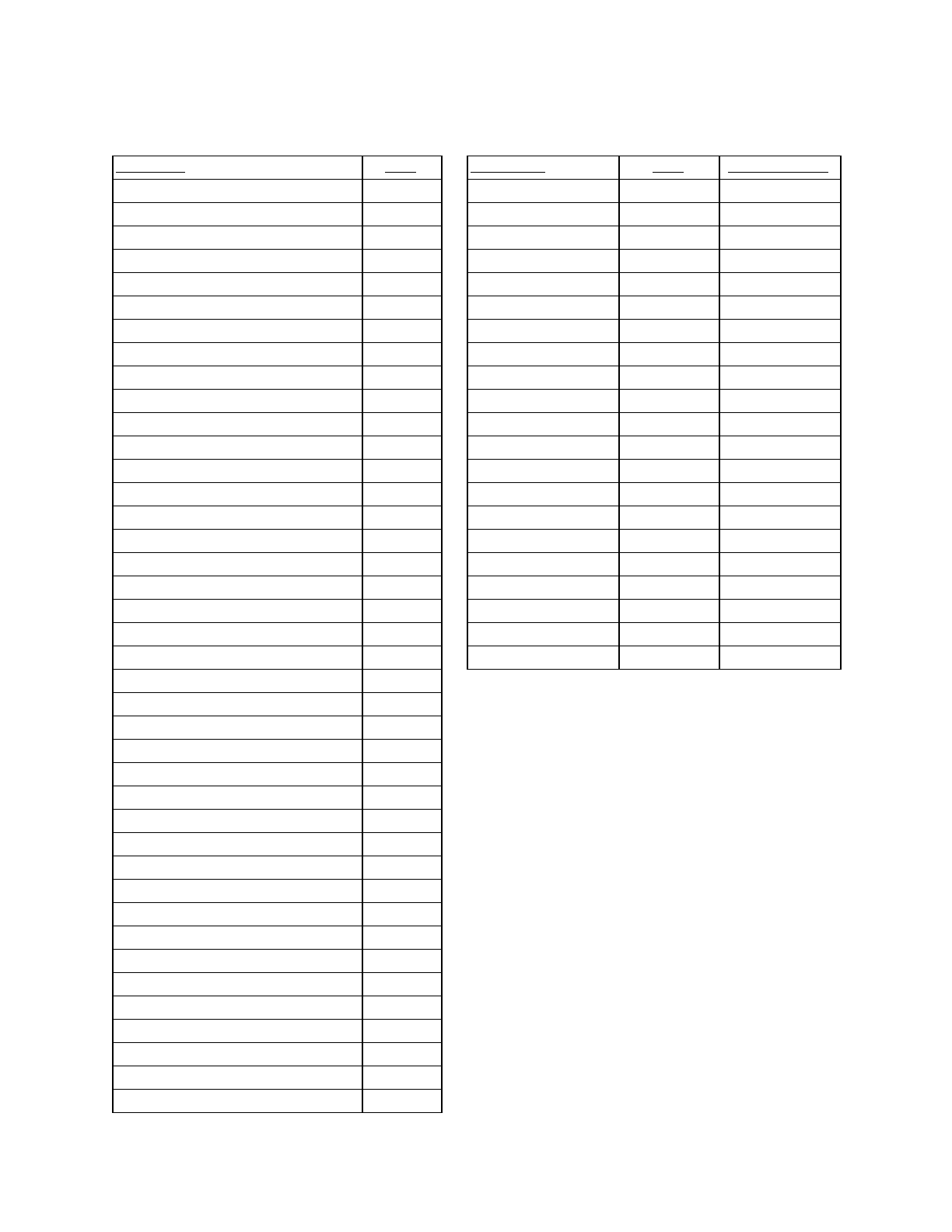
Point Feature
Count
Linear Feature
Count
Total Length(miles)
Beaver Dam
9
Abandoned Railroad
618
652
Cannery/Canning Factory
1
Bog Shoreline
107
51
Cemetery
343
Civil Town Boundary
324
329
Cheese Factory
303
Cliff
256
126
Church
275
Drainage Ditch
932
742
Country Club
1
Drivable Fire Lane
142
321
Creamery
23
Hard Surfaced Road
745
1,430
Dam
24
Improved Dirt Road
6,808
5,187
Erosion
101
Improved Gravel Road
3,115
4,975
Farm Bldg. Less than 100 ft from center of Road
210
Intermittent Stream
1,703
886
Filling Station or Garage
214
Non-Drivable Fire Lane
26
56
Fire Tower
34
Power Line
3,313
4,222
Fish Hatchery
4
Railroad
543
1,549
Fur Farm
64
Shoreline
59
39
Golf Course
11
Stream
7,130
7,030
Gravel Pit
493
Telephone Line
3,690
5,150
Greenhouse
1
Trail
1,942
1,363
Grist Mill
9
Unimproved Dirt Road
4,486
2,662
Hotel
27
Unimproved Gravel Road
1,882
2,230
Lime Kiln
1
Unknown
29
18
Logging Camp
43
Total
37,850
39,021
Nursery
31
Occupied House
38,086
Occupied School
830
Orchard
1,972
Post Office
2
Quarry
34
Ranger Station
2
Ruins
1
Saw Mill
36
Ski Jump
8
Spring
387
Store
192
Summer House
1,754
Tavern
431
Town Hall
58
Unknown
179
Vacant House
2,273
Vacant School
20
Total
48,487

9
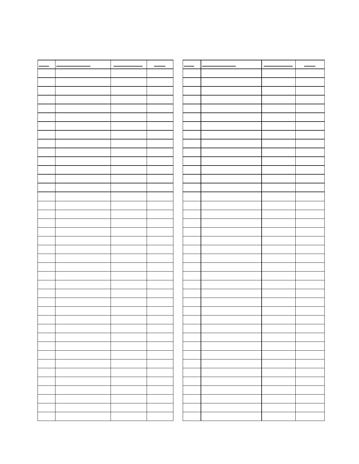
Code
Code Description
Polygon Count
Acres
Code
Code Description
Polygon Count
Acres
A
Abandoned
1,057
18,067
C1b
Inferior C1
4,083
290,917
A1
Upland Hardwoods
25,419
776,637
C1uu
C1uu
9
294
A1u
A1u
2
28
C2
Norway Pine
1,471
47,304
A1uu
A1uu
4
59
C3
Tamarack
4,460
140,392
A2
Hemlock with Hardwood
3,048
169,314
C3uu
C3uu
1
66
A3
Swamp Hardwoods
19,251
627,720
C3uuu
C3uuu
2
9
A3u
A3u
1
48
C4
Grass Marsh
20,207
537,556
A3uu
A3uu
2
27
C4b
Sedge Marsh
6,132
188,866
A4
Tagalder, Willow, Dogwood, Etc.
16,955
413,815
C4u
C4u
87
4,062
A5
Raspberries, etc.
49
3,193
CA
Camp
16
258
AA
AA
1
7
CAT
Catalpa Plantation
2
7
AC
AC
19
455
CC
CC
1
52
AO
AO
2
29
CCC
CCC
6
62
AP
Abandoned Pasture
764
18,759
CL
Clay Pit
126
8,976
AR
AR
8
315
CM
Cemetery
706
3,033
ARPT
Airport
12
587
CO
County Farm
1
3
ARX
ARX
1
10
CP
CP
22
291
AX
AX
2
60
CPP
Poor Land Previously Cropped
2,252
63,327
AY
AY
2
42
CPPA
CPPA
18
745
AZ
AZ
6
152
CPPR
CPPR
4
194
B
Birch
902
18,402
CPPRX
CPPRX
4
78
B1
Hardwood with Conifers
14,005
747,841
CPPRY
CPPRY
4
133
B1b
Inferior B1
710
49,307
CPPRZ
CPPRZ
2
78
B2
White Pine
2,904
79,073
CPPX
CPPX
32
830
B2b
B2b
2
25
CPPY
CPPY
9
253
B3
White Cedar
9,367
326,776
CPPZ
CPPZ
7
157
B4
Cat Tail Marsh
1,086
37,299
CR
CR
74
2,749
B5
Briars, sweet fern and grass
1
16
CRS
CRS
1
9
BA
Ball Park
1
7
CRX
CRX
38
1,666
BB
Blueberry
30
1,298
CRY
CRY
44
2,439
BD
Beaver Dam
1
3
CRZ
CRZ
16
694
BE
Bee Farm
1
2
CS
Cultivated Stump Land
245
2,903
BF
Beaver Flowage
18
444
CT
City
1,526
240,042
BL
Blowdown
1
17
CUT
Cutover
30
5,521
BOG
Bog
3
14
CV
Urban Property
1
7
BP
Beaver Pond
25
242
Cx
Cx
723
46,243
BU
Bluff
1
5
CY
CY
251
14,165
BY
Brick Yard
3
24
CZ
CZ
42
1,953
C
Cleared Cropland
57,947
5,812,310
D
Scrub Oak
3,292
150,711
C1
Popple with White Birch
39,345
2,532,490
D1
Oak - Hickory
11,162
325,243
10
Code
Code Description
Polygon Count
Acres
Code
Code Description
Polygon Count
Acres
D1b
Inferior D1
8
343
MF
Mud Flats
29
822
D1u
Good Quality with White Oak
1,204
31,242
MP
Marl Pit
1
4
D1uu
Medium Gr. Mostly Red Oak
3,489
87,983
MY
Mill Yard
13
359
D1uuu
D1uuu
144
2,298
NF
National Forest
12
5,948
D2
Jack Pine
4,684
224,413
NP
NP
2
39
D3
Black Spruce
12,097
363,808
NU
Nusery
35
672
D3b
Balsam
1,486
47,814
O
Open
5,556
191,979
D3u
D3u
2
45
OA
OA
3
39
D4
Leather Leaf
4,746
86,395
OC
OC
3
38
D4b
D4b
2
19
OP
Open Pasture
5
58
D5
Recent Burn
1,046
83,962
OPP
OPP
2
21
D5b
Dead Timber
125
6,104
OR
Orchard
2,587
19,377
DA
DA
6
279
ORB
Old River Bed
21
424
DH
DH
1
8
P
Pasture
18,448
262,002
Duu
Duu
4
84
P.V.
P.V.
14
110
Duuu
Duuu
5
46
PA
PA
79
1,142
E1
Pin Cherry
1,498
76,132
PD
Public Dump
63
870
E2
E2
1
9
PG
PG
1
4
E3
E3
5
114
PK
Park
26
593
E4
Weedy Peat
366
15,931
PO
PO
1
14
EP
EP
2
15
PP
Permanent Pasture
10,969
163,319
ER
Erosion
408
1,977
PPR
PPR
5
86
F
F
32
202
PPRX
PPRX
3
74
F4
Cranberry Marsh
31
741
PPX
PPX
31
354
FF
Fur Farm
57
1,470
PPY
PPY
29
408
FG
Fair Grounds
2
53
PPZ
PPZ
17
234
FH
FH
1
12
PR
PR
9
78
FP
Forest Plantation
52
789
PRX
PRX
2
56
FX
Fox Farm
2
26
PRY
PRY
3
51
GC
Golf Course
112
6,021
PRZ
PRZ
2
20
GG
GG
33
206
PS
PS
1
4
GP
Gravel Pit
160
1,457
PX
PX
89
1,188
Gr
Gravel
7
181
PY
PY
59
895
IN
IN - Indian Mounds
1
5
PZ
PZ
82
987
IS
Island
184
575
Qz
Quarry
50
713
K
K
2
71
RC
Red Cedar
14
259
KC
Kentucky Coffee Trees
1
1
RCT
Recent Cut
3
166
LA
Lake Dried Up
1
3
RE
Reserve
2
71
LO
Locust
2
15
Rec
Recreation Area
57
1,999
MA
Maple
17
333
RM
RM
1
5

11
Code
Code Description
Polygon Count
Acres
RO
Rock Outcrop
77
1,199
S
Stump
1,250
32,241
Sand
Sand
25
671
SB
Sand Bar
10
55
SC
SC
39
679
Sch.Gs
Sch.Gs
1
4
SD
SD
34
1,577
SF
State Farm
1
78
SFH
State Fish Hatchery
1
77
SFN
State Forest Nursery
1
93
SL
Slash
37
1,881
SLP
Slag Pile
1
14
SN
SN
57
4,741
Snags
Snags
2
26
SP
Stump Pasture
18,749
320,193
SPC
SPC
1
47
SPRZ
SPRZ
1
11
SPX
SPX
25
483
SPY
SPY
29
570
SPZ
SPZ
9
100
SR
SR
1
61
SRG
Spring
4
19
St
Shoal Bottom With Debris
17
745
STKYD
Stock Yard
2
3
U
U
86
3,153
UF
UF
4,651
42,677
UG
UG
2,328
20,875
UR
UR
100
311
Urban
Urban
312
9,670
WD
Windfall
2
1
WE
WE
2
36
WO
Open Water
11,374
978,188
WR
River
4,977
81,174
Z
Z
1
7
Total
364,629
16,915,530
