CAT L1.5 ECONOMICS & THE BUSINESS ENVIRONMENT Study Manual
User Manual:
Open the PDF directly: View PDF ![]() .
.
Page Count: 305 [warning: Documents this large are best viewed by clicking the View PDF Link!]
- Economics and the Business Environment CAT Study Manual a Cover RO'Neill 1 08 12
- Economics and the Business Environment CAT Study Manual Contents RO'Neill 1 08 12 docx
- Economics and the Business Environment CAT Study Manual Introduction RO'Neill 1 08 12 docx
- Economics and the Business Environment CAT Study Manual Study Unit 1 RO'Neill 1 08 12 docx
- Economics and the Business Environment CAT Study Manual Study Unit 2 RO'Neill 1 08 12 docx
- Economics and the Business Environment CAT Study Manual Study Unit 3 RO'Neill 1 08 12 docx
- A. Influences on Demand
- a. influences on demand
- Flow of Demand
- Product’s Own Price
- Prices of Other Products
- Income Available for Spending
- Price and Availability of Money and Credit
- Market Size
- Advertising or Marketing Effort
- Taste
- Expectations
- Other Influences
- Summary of Influences
- The Relative Importance of Influences
- Shifts in the Demand Curve
- Some Further Considerations
- b. revenue and REVENUE changes
- c. price elasticity of demand
- d. further demand elasticities
- Change in Quantity Demanded
- Change in Price
- Change in Quantity Demanded
- Change in Price
- Economics and the Business Environment CAT Study Manual Study Unit 4 RO'Neill 1 08 12 docx
- Economics and the Business Environment CAT Study Manual Study Unit 5 RO'Neill 1 08 12 docx
- Economics and the Business Environment CAT Study Manual Study Unit 6 RO'Neill 1 08 12 docx
- Economics and the Business Environment CAT Study Manual Study Unit 7 RO'Neill 1 08 12 docx
- Economics and the Business Environment CAT Study Manual Study Unit 8 RO'Neill 1 08 12 docx
- Economics and the Business Environment CAT Study Manual Study Unit 9 RO'Neill 1 08 12 docx
- Economics and the Business Environment CAT Study Manual Study Unit 10 RO'Neill 1 08 12 docx
- a. Keynes and aggregate demand
- b. two sector model
- Figure 10.1: Consumption and savings functions
- Figure 10.2: Changes in the average propensities to consume and save
- Figure 10.3: Investment function
- Figure 10.4: Aggregate demand
- Figure 10.5: Equilibrium in the two-sector model
- Figure 10.6: Deflationary gap
- Figure 10.7: Underemployment equilibrium
- Figure 10.8: Increasing aggregate demand
- D. THE MULTIPLIER EFFECT
- E. THE PARADOX OF THRIFT
- Economics and the Business Environment CAT Study Manual Study Unit 11 RO'Neill 1 08 12 docx
- Economics and the Business Environment CAT Study Manual Study Unit 12 RO'Neill 1 08 12 docx
- Economics and the Business Environment CAT Study Manual Study Unit 13 RO'Neill 1 08 12 docx
- Economics and the Business Environment CAT Study Manual Study Unit 14 RO'Neill 1 08 12 docx
- Economics and the Business Environment CAT Study Manual Study Unit 15 RO'Neill 1 08 12 docx
- Economics and the Business Environment CAT Study Manual Study Unit 16 RO'Neill 1 08 12 docx

Page 0
Twinning Arrangement to develop Capacity Building for ICPAR

BLANK

Page 1
© iCPAR
All rights reserved.
The text of this publication, or any part thereof, may not be reproduced or transmitted in any
form or by any means, electronic or mechanical, including photocopying, recording, storage
in an information retrieval system, or otherwise, without prior permission of the publisher.
Whilst every effort has been made to ensure that the contents of this book are accurate, no
responsibility for loss occasioned to any person acting or refraining from action as a result of
any material in this publication can be accepted by the publisher or authors. In addition to
this, the authors and publishers accept no legal responsibility or liability for any errors or
omissions in relation to the contents of this book.
INSTITUTE OF
CERTIFIED PUBLIC ACCOUNTANTS
OF
RWANDA
Foundation F2
F2.2 ECONOMICS & THE BUSINESS
ENVIRONMENT
First Edition 2012
This study manual has been fully revised and updated
in accordance with the current syllabus.
It has been developed in consultation with experienced lecturers.

Page 2
BLANK

Page 3
CONTENTS
Study Unit Title Page
Introduction to the Course 7
1 The Economic Problem and Production 11
Basic Economic Problems and Systems 12
Nature of Production 13
Total, Average and Marginal Product 16
Production Possibilities 21
Some Assumptions Relating to the Market Economy 23
2 Consumption and Demand 25
Utility 26
Indifference Curves 29
The Demand Curve 39
Utility, Price and Consumer Surplus 43
3 Demand and Revenue 45
Influences on Demand 46
Revenue and Revenue Changes 50
Price Elasticity of Demand 58
Further Demand Elasticities 62
Elasticity: Summary of Key Concepts 64
4 Costs of Production 69
Factor and Input Costs 70
Economic Costs 82
External Costs and Benefits 83
Costs and the Growth of Organisations 85
Small Firms in the Modern Economy 88
5 Profit, Supply and Expenditure Taxes 93
The Nature of Profit 94
Maximisation of Profit 97
Influences on Supply 104
Price Elasticity of Supply 110
Supply, Indirect Taxes and Subsidies 115
6 Markets and Prices 119
Nature of Markets 120
Functions of Markets 121
Prices in Unregulated Markets 122
Price Regulation 128
Market Defects - The Case for a Public Sector 131
Price Changes and Indirect Taxes and Subsidies 134

Page 4
7 Market Structures and Competition 139
Meaning and Importance of Competition 140
Perfect Competition 142
Monopoly 148
Monopolistic Competition 153
Oligopoly 155
Profit Maximisation and Alternative Objectives for the Firm 160
8 Further Aspects of Markets and Prices; Factor Markets 165
Market Structures and Economic Welfare 166
Price Discrimination 170
Factor Markets 176
Economic Rent 186
9 National Income 191
From Micro to Macro Economics 192
Measuring Economic Activity 193
Interpreting the Figures 198
10 The Determination of National Income 201
Keynes and Aggregate Demand 202
Two Sector Model 203
Underemployment equilibrium 210
The Multiplier Effect 213
The Paradox of Thrift 221
11 Government in the Circular Flow 223
Government Policies and Objectives 224
Closed Economy Model 224
Active Fiscal Policy 229
Open Economy Model 231
Limitations of the simple Keynesian Model 234
12 Money and Banking 237
Money in Modern Economies 238
Credit Creation and the Money Supply 240
The Central Bank 243
Monetary Policy 244
The Demand for Money 246
Determination of the Rate of Interest 248
The Quantity Theory of Money 250
Taxation 252
13 International Trade 257
International Trade 258
Balance of Payments 263
The Terms of Trade 267
Inter-industry and Intra-industry Trade 268
Free Trade and Protection 269
Impact of a Tariff 270

Page 5
14 Exchange Rates 273
Nominal, Effective and Real Exchange Rates 274
Determination of the Nominal Exchange Rates 275
Purchasing Power Parity 278
Fixed and Floating Exchange Rates 279
Exchange Rates and the Balance of Payments 282
Monetary and Fiscal Policy with fixed and floating exchange rates 284
15 The Economics of East African Community (EAC) 287
Economic integration 288
Trade Creation and Trade Diversion Effects of a Customs Union 289
The Single Market Programme 291
___________________________________________________________________________
16 Growth Strategies of Firms 295
Horizontal Growth 296
Vertical Growth 296
Diversified Growth 298
Growth by Mergers 299
Economies of Scope 300
Profit Maximisation Objective 301
Alternative Theories of the Firm 301
Principal – Agent Theory 302

Page 6
BLANK
Page 7
INTRODUCTION TO THE COURSE
Stage: Level 1
Subject Title: L1.5 Economics and the Business
Environment
Aim
The aim of this subject is to ensure that students have a solid foundation in economics
contributing to the development of a competent and well-rounded member of the profession.
This subject embraces a knowledge of the sources, interpretations and limitations of
economic/business statistics.
Learning Outcomes
On successful completion of this subject students should be able to:
• Explain economic concepts and terms and their uses and application.
• Explain the market environment and income determination.
• Analyse and discuss the impact of government policy and international economic
institutions on economic issues.
• Apply micro economic techniques to interpret and explain business and consumer
behaviour.
• Describe the modifying and opportunistic aspect of the particular market environment
in which a firm operates.
• Discuss and analyse the factors determining the contribution of various resources to
the firm’s revenue.
• Explain the upper and lower limits to income determination and the distribution of
economic rents.
• Explain the national economic parameters within which business is conducted.
• Discuss the interrelationship of the various sectors within the economy.
• Describe the factors governing the operation of financial institutions and the
significance of these for economic activity.
• Discuss the global forces that influence the open Rwandan economy.
Page 8
Syllabus:
1. Concepts
• Types of economic systems (The free enterprise, command and maximum price
control systems
• Supply and demand.
• Determination of price.
• Equilibrium.
• Market systems and the allocation of scarce resources.
• Concepts of cost –opportunity, fixed, variable, marginal, average.
• Time aspect –short run, long run.
• Aspect of size –economies and diseconomies of scale, economies of scope.
• Implications of various elasticity concepts.
2. The Firm in the Market Place
• The meaning and levels of Production (Primary, Secondary and Tertiary or Service
Industries).
• Factors of Production (Land, Labour, Capital and Entrepreneur),
• Factor mobility and factor intensity in industries
• Production, Revenue and cost functions (product, revenue and cost curves)
• Economies and diseconomies of scales both internal and external
• The concept of profit and revenue maximisation.
• The conditions for long run profit maximisation.
• The conditions for short run profit maximisation.
• An understanding of the various forms of market structures - Perfect Competition,
Monopolistic (Imperfect) Competition, and Monopoly.
• Long run price/output determination for each of the above forms of market structure.
• Economic efficiency in respect of each of these forms of market structure.
3. Influence of Competitors on Behaviour of Firms
• Strategic Rivalry.
• Oligopoly and interdependence
• Natural and strategic entry barriers
• Kinked demand curves
• Perfect competition, imperfect competition, monopoly and oligopoly
Page 9
4. Growth Strategies of Firms
• Horizontal growth.
• Vertical growth.
• Diversified growth.
• Growth by merger.
• Economies of scope.
• Profit maximisation objective when management is separate from ownership.
• Alternative theories of the firm.
• Principal-agent theory.
5. Factor Markets and Income Determination
• Marginal productivity theory.
• Wage determination.
• Rent, interest and profit.
• Economic rents.
6. The Macroeconomic Environment
• The circular flow of income.
• Potential and actual levels of aggregate demand.
• National Income determination in an open economy with government.
• Interrelationship between National Income Statistics – GNP / GDP /
• National Income.
• Accelerator and Multiplier.
7. Government and the Macroeconomy
• Objectives of national economic policy.
• Interaction of objectives.
• Policy instruments.
• Economic cycles.
• Budget strategies.
• Fiscal stabilisers.
• Economic implications of direct and indirect forms of taxation.
Page 10
8. Money and Banking
• Development of the money economy.
• Functions of money.
• Credit creation by the banking sector.
• Money multiplier.
• Central Banking.
• Monetary policy / Exchange rate policy.
• Interest Rates and the macro-economy
9. Global Economics
• Law of comparative advantage.
• Terms of trade.
• Restrictions to free international trade.
• Fixed versus floating exchange rates.
• Balance of payments.
• The global market environment.
• Economic benefits to a firm from a global strategy.
• The pattern of international trade flow.

Page 11
Study Unit 1
The Economic Problem and Production
Contents
A. Basic Economic Problems and Systems
Some Fundamental Questions
Choice and Opportunity Cost
B. Nature of Production
Economic Goods and Free Goods
Production Factors
Enterprise as a Production Factor
Fixed and Variable Factors of Production
Production Function
C. Total, Average and Marginal Product
Total Product
Marginal Product of Labour
Average Product of Labour
D. Production Possibilities
E. Some Assumptions Relating to the Market Economy
Consistency and Rationality
The Forces of Supply and Demand
Basic Objectives of Producers and Consumers
Consumer Sovereignty
Page 12
A. BASIC ECONOMIC PROBLEMS AND SYSTEMS
Some Fundamental Questions
Economics is concerned with people’s efforts to make use of their available resources to
maintain and develop their patterns of living according to their perceived needs and
aspirations. Throughout the ages people have aspired to different lifestyles with varying
degrees of success in achievement but always they have had to reconcile what they have
hoped to do with the constraints imposed by the resources available within their environment.
Frequently they have sought to escape from these constraints by modifying that environment
or moving to a different one. The restlessness and mobility implied by this conflict between
aspiration and constraint has, of course, profound social and political consequences but, as far
as possible, in economics courses we limit ourselves to considering the strictly economic
aspects of human society.
It is usual to identify three basic problems which all human groups have to resolve. These
are:
• What, in terms of goods and/or services, should be produced
• How resources should be used in order to produce the desired goods and services
• For whom the goods and services should be produced.
These questions of production and distribution are problems because, for most human
societies, people’s aspirations or wants are unlimited - we often seem to want more of
everything - whereas the resources available are scarce. This term has a rather special
meaning in economics. When we say that resources are scarce we do not mean necessarily
that they are in short supply but that we cannot make unlimited use of them. In particular
when we use, for example, land for one purpose, say as a road, then that land cannot, at the
same time, be used for anything else.
Choice and Opportunity Cost
Since human wants are unlimited but resources scarce, choices have to be made. If it is not
possible to have a school, hospital or housing estate all on the same piece of land, the choice
of any one of these involves sacrificing the others. Suppose the community’s priorities for
these three options are hospital, housing estate and then school. If it chooses to build the
hospital it sacrifices the opportunity for having its next most favoured option - the housing
estate. It is logical, therefore, to say that the housing estate is the opportunity cost of using
the land for a hospital.
Opportunity cost is one of the most important concepts in economics and also one of the most
valuable contributions that economists have made to the related disciplines of business
management and politics. Awareness of opportunity cost forces us to take account of what we
are sacrificing when we use our available resources for any one particular purpose and this
awareness helps us to make the best use of these resources by guiding us to choose those
activities, goods and services which we perceive as providing the greatest benefits compared
with the opportunities we are sacrificing.
Page 13
Throughout history societies have experimented with many different forms and structures for
decision-making in relation to the allocation of the total resources available to the community.
Through much of the twentieth century there has been conflict between the centrally
planned economy, with decisions taken mostly by the Government, and the free market
economy, where decisions are taken mainly by individuals and groups operating in markets
where they can choose to buy or not to buy the goods and services offered by suppliers
according to their own assessment of the benefits and opportunity costs of the many choices
with which they are faced. In the free market economy supply, demand and prices determine
what is produced, how and for whom.
B. NATURE OF PRODUCTION
Economic Goods and Free Goods
Goods/services are economic if scarce resources have to be used to obtain or modify them so
that they are of use, i.e. have utility, for people. They are free if they can be enjoyed or used
without any sacrifice of resources. The air we breathe under normal conditions is free, but
not when it has to be purified or kept at a constant and bearable pressure in an airliner.
Rainwater, when it falls in the open on growing crops, is free but not when it has to be carried
to the crops along irrigation channels or purified to make it safe for humans to drink. Free
goods are indeed very precious and people are becoming increasingly aware of the costs of
destroying them by their activities, e.g. by polluting the air in the areas where we live.
Production Factors
Since there are very few free goods most have to be modified in some way before they
become capable of satisfying a human want. The process of want satisfaction can also be
termed the creation of utility or usefulness and is also what we understand by production. In
its widest economic sense production includes any human effort directed towards the
satisfaction of people’s wants. It can be as simple as picking berries or washing clothes in a
stream, or as involved as manufacturing a jet airliner or performing open heart surgery.
Production is simple when it involves the use of very few scarce resources but much more
involved and complex when it involves a long chain of interrelated activities and a wide range
of resources.
We now need to examine this general term resources, or economic resources, more closely.
The resources employed in the processes of production are usually called the factors of
production and, for simplicity, these can be grouped into a few simple classifications.
Economists usually identify the following production factors.
• Land
This is used in two senses:
(i) The space occupied to carry out any production process, e.g. space for a factory or
office
Page 14
(ii) The basic resources within land, sea or air which can be extracted for productive use,
e.g. metal ores, coal and oil. Or even used for agriculture such as cassava, coffee,
milk or pigs
• Labour
Any mental or physical effort used in a production process. Some economists see labour
as the ultimate production factor since nothing happens without the intervention of
labour. Even the most advanced computer owes its powers ultimately to some human
programmer or group of programmers.
• Capital
This is also used in several senses, and again we can identify two main categories:
(i) Real capital consists of the tools, equipment and human skills employed in
production. It can be either physical capital, e.g. factory buildings, machines or
equipment, or human capital - the accumulated skill, knowledge and experience
without which physical capital cannot achieve its full productive potential.
(ii) Financial capital is the fund of money which, in a modern society, is usually needed
to acquire and develop real capital, both physical and human.
Notice how closely related all the production factors are. Most production requires some
combination of all the factors. Only labour can function purely on its own, if we ignore the
need for space. A singer or story teller can entertain with voice alone, but will usually give
more pleasure with the aid of a musical instrument and is likely to benefit from earlier
investment in some kind of training. The hairdresser requires a least a pair of scissors!
Enterprise as a Production Factor
All economic texts will include land, labour and capital as factors of production. There is not
quite such universal agreement over what is often described as the fourth production factor,
which is most commonly termed enterprise.
The concept of enterprise as a fourth factor was developed by economists who wished to
explain the creation and allocation of profit. These economists saw profit as the reward
which was earned by the initiator and organiser of an economic activity - the person who had
the enterprise and special quality needed to identify an unsatisfied economic want and to
combine successfully the other production factors in order to supply the production to satisfy
it.
In an age of the small business organisation, owned and managed by one person or family,
this seemed quite a reasonable explanation. The skilled worker who gives up secure and
often well-paid employment to take the risks of starting and running a business is most likely
to be showing enterprise and is prepared to take risks in the hope of achieving profits above
the level of his or her previous wage. Many modern firms have been formed in the recent
past by initiators, innovators and risk takers of the kind that certainly fit the usual definition
of the business entrepreneur. Their names appear constantly in the business press. Few
would wish to deny that profit has been and often remains the spur that drives them.
Page 15
Nevertheless this identification of enterprise in terms of individual risk-taking raises a great
many problems when we attempt to apply it generally to the modern business environment.
Much contemporary business activity is controlled by large companies such as MTN, Petro-
Rwanda, Engen and Braliwra Ltd (Brasseries Et Limonaderies Du Rwanda SA). Who are the
entrepreneurs in such organisations? Are they rewarded by profits? How do these companies
recruit and foster enterprise? You, yourself, may work in a large organisation. Can you
reconcile the traditional economic concept of enterprise as a factor of production with your
observations of the structure of your company?
Fixed and Variable Factors of Production
Both economists and accountants make an important distinction between production factors,
based on the way they can be varied as the level of production changes. To take a simple
example, suppose you own a successful shop. Initially you do not employ anyone but soon
find you do not have time to do everything and are losing sales because you cannot serve
more than one customer at a time. So, you employ an assistant. This gives you more time
and flexibility and allows you to buy better stock; your monthly sales more than double. You
employ another assistant and again your sales increase. You realise, however, that you cannot
go on increasing the number of assistants since space in your shop is limited and you can only
meet demand in a small local market. You begin to think about opening another shop in
another area.
This example helps to illustrate the difference between a production factor which you can
vary as the level of production varies, i.e. a variable factor, in this case the assistants
(labour), and a factor which you can only move in steps at intervals when production levels
change. This latter, which in our example is the shop, i.e. land (space) and capital (the shop
building and equipment), is the fixed factor.
In most examples at this level of study it is usual to regard capital as a fixed factor and labour
as a variable factor. Although it is not possible to have a fraction of a worker we can think in
terms of worker-hours and recognise that many workers are prepared to vary the number of
hours worked per week. It is more difficult to have half a shop and even if a shop is rented
rather than bought, tenancies are usually for fixed periods. It is more difficult to reduce the
amount of fixed factors employed than the variable factors. When a machine or piece of
equipment is bought it can only be sold at a considerable financial loss.
This distinction between fixed and variable production factors is very important, particularly
when we come to examine production costs in Study Unit 4. It also gives us an important
distinction in time. When analysing production, economists distinguish between the short run
and the long run. By short run they mean that period during which at least one production
factor, usually capital, is fixed, e.g. one shop, one factory, one passenger coach. By long run
they mean that period when it is possible to vary all the factors of production, e.g. increase the
number of shops, factories or passenger coaches. Sometimes you may find the short and long
run referred to as short and long term.
Page 16
Production Function
We can now summarise the main implications of our recognition of factors of production. We
can say that to produce most goods and services we need some combination of land, capital
and labour. At present we can leave out enterprise as this is difficult to quantify. In slightly
more formal language we say that production is a function of land, capital and labour. Using
the symbols Q for production, S for land, K for capital and L for labour, this allows us, if we
wish, to use the mathematical expression:
Q = f(S, K, L)
C. TOTAL, AVERAGE AND MARGINAL PRODUCT
Total Product
In this study unit we examine what happens when production increases in the short run, when
the production factor, capital, is fixed and when the factor, labour, is variable. Once again we
can take a simple example of a small business which is able to increase its use of labour. For
simplicity we can use the term worker as a unit of labour, but you may wish to regard a
worker as a block of worker-hours which can be varied to meet the needs of the business.
Suppose the effect of adding workers to the business is reflected by the following table, where
the quantity of production is measured in units and relates to a specific period of time, say, a
month. The amount of capital employed by the business is fixed.
Number of workers
Quantity of production
(units per month)
1
30
2
70
3
120
4
170
5
220
6
260
7
290
8
310
9
320
10
320
11
310
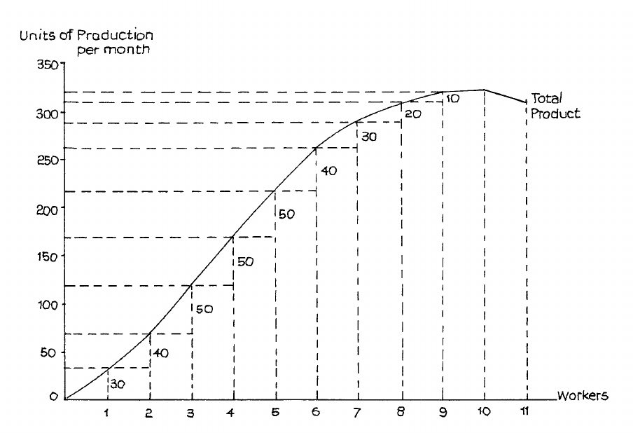
The quantity of production measured here in units produced per month and shown as a graph
in Figure 1.1, is, of course, the total product. In this example total product continues to rise
until the tenth worker is added to the business; this worker is unable to increase total product.
This is because, given the fixed amount of capital, no further increase in productive output is
possible. The addition of an eleventh worker would actually cause a fall in production.
Page 17
Marginal Product of Labour
Examine now the amount of change to total product as each additional worker is added to the
business. The following table shows this change in the third column which is headed
marginal product. Strictly speaking, this is the marginal product of labour because it results
from changes in the amount of labour (workers) added to the business.
Number of
workers
Quantity of production
(units per month)
Marginal Product of labour
0
0
30
1
30
40
2
70
50
3
120
50
4
170
50
5
220
40
6
260
30
7
290
20
8
310
10
9
320
0
10
320
−10
11
310
The marginal product of labour is the change in total product resulting from a change in
the amount of labour employed. It is called marginal because it is the change at the edge, and
the term ‘marginal’ is used in economics to denote a change in the total of one variable which
results from a single unit change in another variable. Here the total is quantity of production
resulting from changes in the number of workers employed.
The marginal product column shows the difference in the total product column at each level
of employment. Notice that the marginal value is shown midway between the values for total
product and number of workers. This is because it shows the change that takes place as we
move from one level of employment to the next. In Figure 1.1 the marginal product is
represented by the vertical distance between each step in production as each worker is added.
Page 18
The sum of the marginal product values up to each level of worker is equal to the total
product at that level.
Figure 1.1
Notice how these marginal product values change as total product rises: one worker alone
can produce 30 units but another enables the business to increase production by 40 units and
one more by 50 units. There are many ways in which this increase might be achieved, e.g. by
specialisation and by freeing the manager to improve administration, purchasing and selling.
However, these increases cannot continue and the additional third, fourth and fifth workers all
add a constant amount to production. Thereafter, further workers, while still increasing
production, do so by diminishing amounts until the tenth worker adds nothing to the total. At
this level of labour employment production has reached its maximum, and the eleventh
worker actually provides a negative return - total production falls. Perhaps people get in each
other’s way or cause distraction and confusion. If the business owner wishes to continue to
expand production, thought must be given to increasing capital through more buildings and/or
equipment. Short-run expansion at this level of capital has to cease. Only by increasing the
fixed factors can further growth be achieved.
Diminishing Marginal Productivity Theory
The figures are chosen deliberately to illustrate some of the most important principles of
economics, the so-called laws of varying proportions and diminishing returns. It has been
constantly observed in all kinds of business activities that when further increments of one,
variable production factor are added to a fixed quantity of another factor, the additional
production achieved is likely, first, to increase, then to remain roughly constant and eventually
to diminish. It is this third stage that is usually of the greatest importance, this is the stage of
Page 19
diminishing marginal product, more commonly known as diminishing returns. Most firms
are likely to operate under these conditions and it is during this stage that the most difficult
managerial decisions, relating to additional production and the expansion of fixed production
factors, have to be taken.
The production level at which further employment ceases to be profitable depends on several
other considerations, including the value of the marginal product, which depends on the
revenue gained from product sales, and the cost of employing labour, made up of wages and
labour taxes. The higher the cost of employing labour, the less labour will be employed in the
short run and the sooner will employers seek to replace labour by capital in the form of
labour-saving equipment.
Average Product of Labour
The average product of labour employed is found simply by dividing the total product at any
given level of employment by the number of workers (or some unit of worker-hours). The
average product of labour, though a measure easily understood and used by many business
managers and their accountants, is less important than the marginal product. However, the
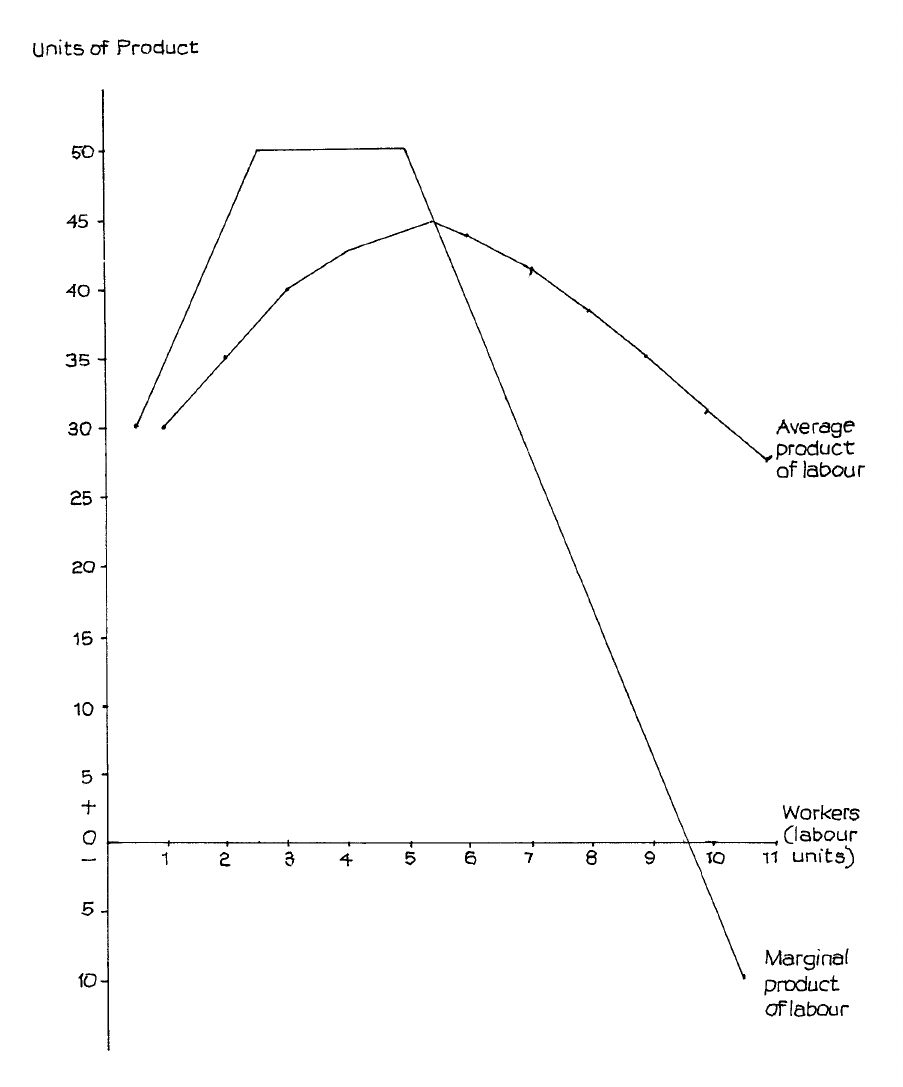
following table adds average product to our earlier statistics, and Figure 1.2 shows both
marginal and average product in graph form.
Number of
workers
Quantity of production
(units per month)
Marginal
Average
Product of labour (units per
month)
0
0
30
1
30
40
30.00
2
70
50
35.00
3
120
50
40.00
4
170
50
42.50
5
220
40
44.00
6
260
30
43.33
7
290
20
41.43
8
310
10
38.75
9
320
0
35.56
10
320
−10
32.00
11
310
28.18
Page 20
Figure 1.2
The falling marginal product curve intersects the average product curve at about the 5th
worker. Average product then starts to fall because for more workers marginal product is
below average product.
Notice the relationship between average and marginal product. Average product continues to
rise until it is the same as the falling marginal product, then it falls.
Page 21
D. PRODUCTION POSSIBILITIES
If individual firms are likely to face a point of maximum production as they reach the limits
of their available resources the same is likely to be true of communities, whose total potential
product must also be limited by the resources available to the community and by the level of
technology which enables those resources to be put to productive use.
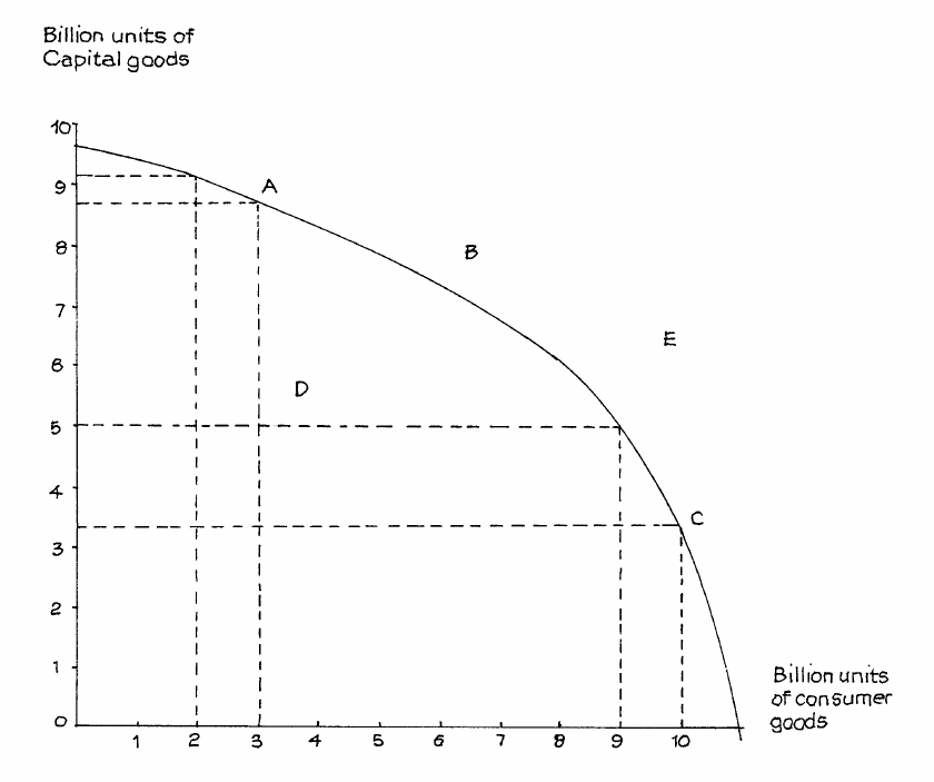
This idea is frequently illustrated by economists through what is usually termed the
production possibilities frontier (or curve), which is illustrated in Figure 1.3.
The frontier represents the limit of what can be produced by a community from its available
resources and at its current level of production technology. Because we wish to illustrate this
through a simple two-dimensional graph we have to assume just two classes of goods and, for
simplicity, we can call these consumer goods (goods and services for personal and household
use) and capital goods (goods and services for use by production organisations for the
production of further goods).
Because resources are scarce in the sense explained earlier in this study unit, we cannot use
the same production factors to produce both sets of goods at the same time. If we want more
of one set we must sacrifice some of the other set. However, the extent of the sacrifice, i.e.
the opportunity cost, of increasing production of each set is unlikely to be constant through
each level of production since some factors are likely to be more efficient at some kinds of
production than others. Consequently the shape of the frontier curve can be assumed to
reflect the principle of increasing opportunity costs. This is shown in Figure 1.3.
The curve illustrates other features of the production system. For example, the community
can produce any combination of consumer and capital goods within and on the frontier but
cannot produce a combination outside the frontier - say at E. If it produces the mixtures
represented by points A or C on the frontier all resources (production factors) are fully
employed, i.e. there are no spare or unused resources. The community can produce within the
frontier, say at D, but at this point some production factors must be unemployed.
Page 22
Figure 1.3: The Production Possibilities Frontier
To raise production of consumer goods from 2 to 3 billion units involves sacrificing the
possibility of producing 0.3 billion units of capital goods. However when production of
consumer goods is 9 billion units, an additional 1 billion units involves the sacrifice of 1.6
billion units of capital goods.
The shape of the curve is based on the principle of increasing opportunity costs.
We can, of course, turn the argument round. If we know that some production factors are
unemployed, e.g. if people are out of work, farm land is left uncultivated, factories and offices
left empty, then we must be producing within and not on the edge of the frontier. The
community is losing the opportunity of increasing its production of goods and services and is
thus poorer in real terms than it need be. If, at the same time, some goods and services are in
evident inadequate supply - e.g. if there are long hospital waiting lists, many families without
homes, some people short of food or unable to obtain the education or training to fit them for
modern life - then the production system of the community is clearly not operating efficiently
to meet its expressed requirements.
Although generally used in relation to the economy as a whole the production possibilities
curve can also be used to illustrate the options open to a particular firm. In this case the shape
of the curve need not always follow the pattern of Figure 1.3. It might be that if the firm
Page 23
devoted all its resources to the production of one good instead of to more than one then it
would be able to use them more efficiently. They would then gain from what will later be
described as increasing returns to scale.
Yet another possibility is that the firm could switch resources without any gain or loss in
efficiency, i.e. it would experience constant returns from scale in using its resources.
E. SOME ASSUMPTIONS RELATING TO THE MARKET
ECONOMY
Consistency and Rationality
It is possible to predict with rather more confidence what groups of people are likely to do
over a period of time rather than individuals. On this basis it becomes possible to estimate,
for example, how many sweet potatoes will be consumed in a certain town each week or
month. A supermarket manager does not know what any shopper will buy when that shopper
enters the store, but can estimate how much, on average, the total number of shoppers will
spend on any given day in the month and will know how much is likely to be spent on each of
the many classes of goods stocked. There will be trends that will enable projections to be
made into the future with some degree of confidence. As groups, therefore, people tend to be
consistent and to behave according to consistent and predictable patterns and trends.
People are also assumed to be rational in their behaviour. For example if, given the choice
between, say, bread and tea and sweet potatoes and porridge for breakfast we choose bread
and tea and if given the choice between, say, sweet potatoes and porridge and fruit we choose
sweet potatoes and porridge, then, if we are rational and offered the choice between bread and
tea and fruit we would be expected to choose bread and tea, because we prefer bread and tea
to sweet potatoes and porridge and sweet potatoes and porridge to fruit. It would be irrational
to choose fruit in preference to bread and tea if we have already indicated a preference for
sweet potatoes and porridge over fruit and for bread and tea over sweet potatoes and porridge.
If we accept consistency and rationality in human behaviour then analysis of that behaviour
becomes possible, and we can start to identify patterns and trends and measure the extent to
which people are likely to react to specific changes in the economic environment, such as
price, in ways that we can identify, predict and measure. If we could not do this the entire
study of economics would become virtually impossible.
The Forces of Supply and Demand
In studying the modern market economy we assume that the economic community is large
and specialised to the extent that we can realistically separate organisations which produce
goods and services from those that consume them. We are not studying village, subsistence
economies which can consume only what they themselves produce. Those who have to live
on what theyproduce do not have a high standard of living. We can, of course, be both
producer and consumer, but the goods and services we help to produce are sold and we
receive money which enables us to buy the things we wish to consume.
Page 24
As individuals and members of households we are, therefore, part of the force of consumer
demand. As workers and employers we are part of the separate force of production supply.
Right at the start of your studies it is important to recognise that supply and demand are two
separate forces. These do, of course, interact in ways that we examine in later study units but
essentially they exist independently. It is quite possible for demand to exist for goods where
there is no supply and only too common for goods to be supplied when there is no demand, as
thousands of failed business people can testify. As students of economics you must never
make the mistake of saying that supply influences demand or that demand influences supply.
Basic Objectives of Producers and Consumers
In a market economy we assume that all people wish to maximise their utility. This is
simplified to suggest that producers seek to maximise profits, since the object of production
for the market is to make a profit and, if given the choice between producing A or B and if A
is more profitable than B, we would expect the producer to choose to produce A.
At the same time consumers can be expected to devote their resources, represented by money,
to acquiring the goods and services that give them the greatest satisfaction. This is not to say
that we all spend our money wisely or eat the most healthy foods or wear the most sensible
clothes. We perceive satisfaction or utility in more complex ways. Economists, as
economists, do not pass judgements on the wisdom or folly of particular consumer wants.
They recognise that a want exists when it is clear that a significant group of people are
prepared to sacrifice their resources to satisfy that want.
When this happens there is demand which can be measured and which becomes part of the
total force of consumer demand.
Unfortunately this does not stop some groups of people from seeking to dictate what the rest
of the community should or should not want, consume or enjoy.
Consumer Sovereignty – The Customer is King
The market economy operates on the assumption that, of supply and demand, consumer
demand is dominant. Consumers decide what they want to buy and that influences suppliers;
however, monopolies and advertising reduce customer sovereignty. The market production
system is demand-led: supply adjusts to meet demand. In this sense the consumer is
sovereign. Producers who cannot sell their goods at a profit fail and disappear from the
production system. Profit is the driving force of the production system, and profit is achieved
by the ability to produce goods that people will buy at prices that people will pay while
enabling the producer to earn sufficient profit to stay in business - and to wish to stay in
business. However strong the demand for goods, if they cannot be produced at a profit they
will not, in the long run, be supplied.
Page 25
Study Unit 2
Consumption and Demand
Contents
______________________________________________________________
A. Utility
Meaning of Utility
Total and Marginal Utility
Maximising Utility from Available Resources
____________________________________________________________________
B. Indifference Curves
What is an Indifference Curve?
Indifference Curve Analysis and Income Changes
Indifference Curve Analysis and Price Changes - Giffen Goods
___________________________________________________________________
C. The Demand Curve
What is a Demand Curve?
Indifference Curves and the Demand Curve
Use and Importance of Demand Curves
General Form of Demand Curves
___________________________________________________________________
D. Utility, Price and Consumer Surplus
___________________________________________________________________
Page 26
A. UTILITY
Meaning of Utility
Economists have always faced problems in explaining clearly why people are prepared to
make sacrifices to obtain many of the goods and services which they evidently wish to have.
In a market economy this difficulty can be stated as “Why do we buy the things we buy?”
Often we do not “need” them in the strict sense that they are necessary to our survival. In fact
our basic needs are really very small compared with many of the things on which we spend
our money in advanced market economies. We can talk in terms of “wants” and recognise
that there seems to be no limit to these wants. We also have to recognise that at any given
time we are likely to want some things more than others.
What, then, is the quality that goods must possess that makes us want to acquire them?
Clearly this will differ with different goods. Some may be pleasant to eat, some attractive to
look at, some comfortable or fashionable to wear and so on. The one general term we can
apply to all goods and services is that they provide us with utility. This does not necessarily
mean that they are useful in the sense that they help us to do something we could not do
before we had them but simply that we perceive in them some quality that makes us willing to
make some degree of sacrifice (usually of money) in order to acquire them.
Most of us measure the strength of our desire to buy something in terms of the price we are
prepared to pay for it. When, therefore, an estate agent asks a potential house buyer, “How
much are you prepared to offer for this house?” the agent is, in effect, asking the buyer to
indicate the value of the utility which the house has for him or her.
More often we find ourselves making comparisons of utility. This arises partly because of the
basic economic problem of unlimited wants and scarce resources, so that ranking our wants
so we can decide what we can afford to buy is for most people an almost daily occurrence; but
it also arises because, in modern advanced economies there is likely to be a range of different
goods to satisfy any particular want. If I want to travel by public transport from Kigali to
Goma I could do so by motor coach or by air. My want is to get from Kigali to Goma, and
two options offer the utility to satisfy this want. Each involves different sacrifices of money
and time and offers different associated utilities of convenience and comfort. My choice will
depend on the resources available to me (how much money I can afford to pay and how much
time I have) and on my valuation of the utility afforded by each option. Notice, further, that
this utility is not an absolute quality but depends on why I want to make the journey. If it is
part of a holiday then I might prefer the coach, but if I am attending a business meeting from
which I hope to achieve a financial benefit and need to be fresh and alert then the air option is
likely to offer the greatest utility - greater, probably, than the price of the fare.
All this may seem very involved, but an appreciation of utility and how it can influence our
actions can be a very great help in understanding the true nature of economic demand.
Total and Marginal Utility
Our valuation of the utility provided by any good depends on how strongly we want to
acquire it. While there may be several elements involved in this, e.g. we find it attractive or
Page 27
useful, or think it will impress our friends or neighbours, one factor that is always relevant is
the amount of that or a similar good we already possess. Suppose I have enough spare cash at
the end of the week to buy either a pair of trousers or a pair of shoes but not both, though I
would like both. If I already have an adequate supply of trousers for the next few months but
do not have any spare shoes then, assuming that their prices are roughly similar, I am likely to
buy the shoes. This does not mean that I always value shoes more highly than trousers but
that, considering what I already have at the present time, I perceive greater utility in some
additional shoes than in additional trousers.
By now, especially if you have remembered the explanation of marginal product in Study Unit
1, you will recognise that I have just given an example of marginal utility, i.e. the change in
total utility for a good or group of goods when there is a change in the quantity of those
goods already possessed.
Most of the important decisions relating to the demand for goods and services are influenced
by valuations of marginal utility compared with the prices of these goods. The more pairs of
trousers I possess the less value am I likely to place an obtaining more and the more likely am
I to spend my available money on other things of comparable price whose marginal utilities
are higher.
Willingness to buy thus depends on the comparison of marginal utility with price, so to some
extent it is reasonable to value utility in terms of price. To return to the original house buyer
example, if the buyer says to the agent, “My highest offer is RWF20,000,000”, then for this
buyer the value of the marginal utility of the house is RWF20,000,000. If this is or will be the
buyer’s only house then, of course, it is also the total utility.
We must also bear in mind that money itself has utility. If I am saving money for a major
holiday or for an expensive durable (long lasting) good such as a house or furniture, then I
may place a high value on money savings and be less inclined to buy trousers and shoes as
long as I have enough of these for my immediate needs. If my income is secure and rising,
my valuation of the marginal utility of money could be lower and I am more likely to spend it
on goods. If, however, my job is not secure and redundancy or retirement is a serious
possibility, my valuation of the marginal utility of money is likely to rise and I will spend less
on goods and services. You can easily see the implications of this for the general demand for
consumer goods during periods of economic uncertainty when people think they are likely to
have less money in the future. Just as the marginal utility of a good diminishes as the quantity
already possessed rises, so marginal utility rises as the quantity of a good already possessed
falls - or is expected to fall in the near future.
Maximising Utility from Available Resources
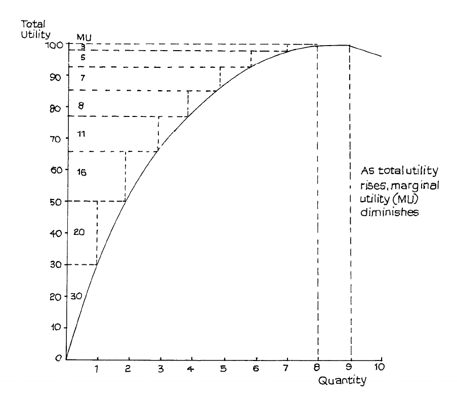
This relationship between total and marginal utility can be illustrated in a simple graph as in
Figure 2.1.
Page 28
Figure 2.1: Marginal and Total Utility
Suppose I have no use for more than 8 pairs of trousers. This number would provide
maximum utility to which we can give a hypothetical numerical value of, say, 100
(representing 100% of the total) but clearly the largest marginal utility would be provided by
the first pair. After this purchase the marginal utility of each additional pair diminishes, as
indicated by the figures under MU to the right of the vertical axis. The total of 100 is reached
with the eighth pair. If I have a ninth, no further utility is added - the total remains at 100.
Should I receive a tenth pair my total utility actually falls: perhaps they take up space in my
wardrobe I would rather have for something else.
Does this, then, mean that I should aim at keeping eight pairs of trousers all the time? Not
necessarily, since Figure 2.1 takes no account of other important considerations, which
include:
− the price of trousers, i.e. the sacrifice I must make to buy them

Page 29
− my desire for other goods and services, i.e. other marginal utilities ( I would not, for
example, be too pleased to have eight pairs of trousers if I possessed only one shirt, nor
would trousers satisfy my hunger if I did not have enough food to eat)
− how much money I have, i.e. my marginal utility for money
Only when all these are taken into account would it be possible to estimate how many pairs of
trousers would represent, for me, the best total to try and achieve.
Assuming rationality, in the sense explained in Study Unit 1, the most satisfactory quantity of
trousers for me would be where my marginal utility gained from the last RWF1 spent on
trousers just equalled the marginal utility per RWF1 spent on all other available goods and
services, and where this also equalled the marginal utility of money. On the assumption that
we are valuing utility in monetary terms the marginal utility of the last RWF1 of money = 1.
Putting this statement a little more formally as an equation and using the symbols, MUA to
denote the marginal utility for the good A, MUB for the marginal utility for the good B, PA for
the price of A, PB for the price of B and so on, we can say that consumers achieve a position
of equilibrium in their expenditure when for them:
MU
P
MU
P MU
P
A
A
B
B
N
N
= = = 1
(which = the marginal utility of money)
In this state of equilibrium consumers cannot increase their total utility from all goods and
services by any kind of redistribution of spending. Spending more on A and less on B, for
example, would mean that the marginal utility of A would fall and so be less than that of the
marginal utility of B, which would rise and be less than the marginal utility of other goods,
including money. Also the utility gain from A would be less than the utility lost from B so
total utility would have fallen. No one rationally spends RWF1 to receive less than RWF1’s
worth of utility.
B. INDIFFERENCE CURVES
What is an Indifference Curve?
An indifference curve is a graph linking all the combinations of two goods or two groups of
goods which provide the same level of total utility for an individual, group of people or
community. It is called an indifference curve because there is no preference for one
combination over any of the others. All offer the same amount of utility or satisfaction, so
that people are indifferent as to which combination they have.
One curve can, of course, indicate only one level of utility. If the resources available to
acquire the goods were increased people could move to a higher level, and if resources fell
they would have to be satisfied with a lower level. We can, therefore, imagine that any one
curve is really part of a map of very many curves all representing different levels of total
utility.
Page 30
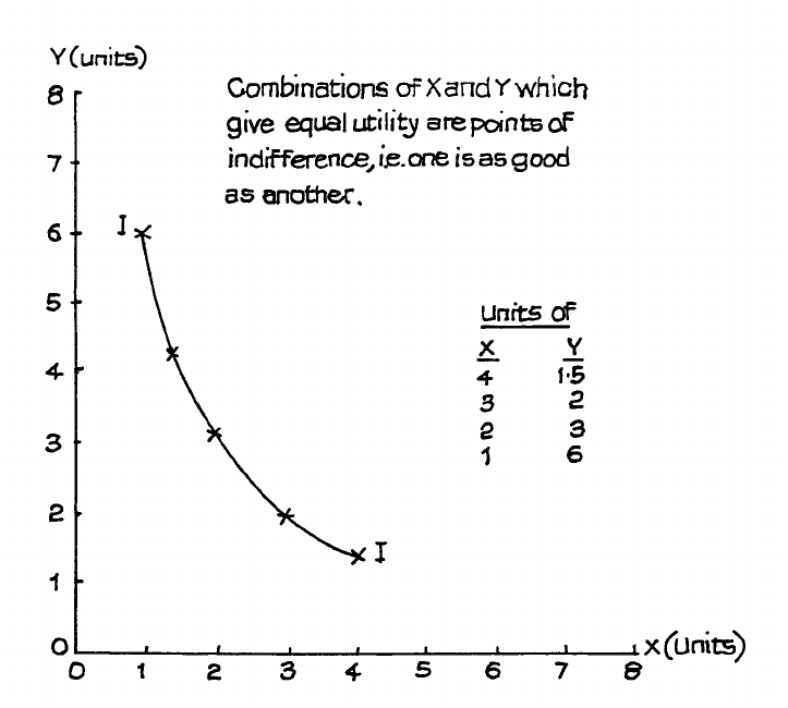
A simple example of an indifference curve is shown in Figure 2.2.
Figure 2.2
From the table and the curve we see that the person whose curve this is would have the same
utility from 4 units of X and 1.5 of Y as from 3 units of X and 2 of Y or from 2 units of X and
3 of Y. The curve is convex to the origin of the graph since it is based on the principle already
explained, of diminishing marginal utility.
According to this curve, when the person has just 1 unit of X but 6 of Y, he or she is prepared
to give up 3 units of Y to gain 1 more unit of X, i.e. 1X has the same value as 6Y. However,
when that person has 3 units of X, he or she will only be prepared to give up 0.5Y in return
for one more X, i.e. with 3 units of X possessed, a further unit of X is valued at only 0.5Y.
Thus the marginal utility of X has diminished from 3Y to 0.5Y as more X is accumulated.
You may think this is a rather involved way to illustrate the fairly common-sense principle
that most people readily accept - that the more we have of something the less value we put on
gaining yet more of the same and the more we would prefer to have something else. This is
all that we mean by diminishing marginal utility.
Indifference Curve Analysis and Income Changes
Remember that the indifference curve is not a demand curve. By itself it tells us nothing
about how much of a good we are likely to buy; it only indicates relative preferences between
different goods or groups of goods. As we noted earlier in this study unit, to be able to
Page 31
estimate how much of a good people may be prepared to buy, in a market economy, we also
need to know:
− the price of the good
− the amount of money they have available.
To carry out any kind of indifference curve analysis, therefore, we must take these two factors
into consideration.
Suppose that the price of X is RWF3 per unit while that of Y is RWF2 per unit. Suppose also
that the amount of money available for spending on X and Y is limited to RWF12.
Assuming that the full RWF12 is spent there is a range of spending possibilities. These are:
• The whole RWF12 is used to buy X with nothing spent on Y. At a unit price of X of
RWF3 this would buy 4 units of X.
• The whole RWF12 is used to buy Y with nothing spent on X. At a unit price of Y of
RWF2 this would buy 6 units of Y.
• A combination of X and Y which involves a total price of RWF12, e.g. 2 units of X (2 ×
RWF3 = RWF6) and 3 units of Y (3 × RWF2 = RWF6).
These possibilities are illustrated in the linear (straight line) spending possibilities curve of
Figure 2.3. The spending possibilities curve is sometimes called the spending possibilities
line, to help to distinguish it from the indifference curve, and it is also sometimes called the
budget line.
Figure 2.3
We now have two curves: one, the indifference curve, shows us combinations of X and Y that
provide us with the same level of total utility or satisfaction; the other, the spending
possibilities line, tells us what it is possible to buy at given prices and a given amount of
money for spending.
When the two curves are combined, as in Figure 2.4, we see that the only combination on the
indifference curve that we can buy is 2X and 3Y.

Page 32
Figure 2.4
Consider now what would happen if the person had RWF16, not RWF12 to spend. The
spending possibilities line changes as shown in Figure 2.5. The RWF16 can be used to obtain
more of X or more of Y, or some new and larger combinations of the two.
Figure 2.5
If the amount available for spending is increased from
RWF12 to RWF16 (represented by the dotted
spending possibility line) the consumer can move to a
higher indifference curve where 4 units of Y and 2.67
units of X can be bought. Note the further the
indifference curve is from the corner (0) of the graph,
the greater the level of utility it represents as more of
both Y and X can be obtained
Page 33
Figure 2.5 also shows how movement to a higher spending possibility line allows movement
to a higher indifference curve, where there is a greater level of total utility or satisfaction. The
point where the new curve just touches the higher spending possibility line is at a level where
more of both X and Y is obtained.
This movement to a higher indifference curve results in more of both X and Y being bought.
This is a reasonable expectation: if our income rises we can spend more on most goods.
However, there may be some exceptions. As incomes rise, people’s pattern of spending may
change; the extra income may permit people to switch spending from some goods to preferred
substitutes. The diet of people on low incomes may include a substantial amount of cassava
or potatoes, but as their incomes rise they may choose a more varied diet, spending less on
cassava or potatoes. If this happens we can say that cassava and potatoes are perceived by
such people as inferior goods; they may, perhaps, buy more fruit, biscuits and other foods.
When this happens there has been a change in the relative preferences between goods and this
will be reflected in a change in the shape of a higher indifference curve, as illustrated in
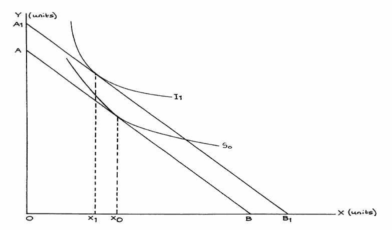
Figure 2.6. Here a rise in income allows the spending possibilities line to move outwards
from AB to A1B1 and the higher spending permits movement to a preferred combination of
goods on the higher indifference curve I1. This indifference curve is flatter than the lower
curve I, which means that X is valued less highly compared with Y. The amount of X that has
to be given up to gain a given amount of Y is less as you move along I1 than if you move
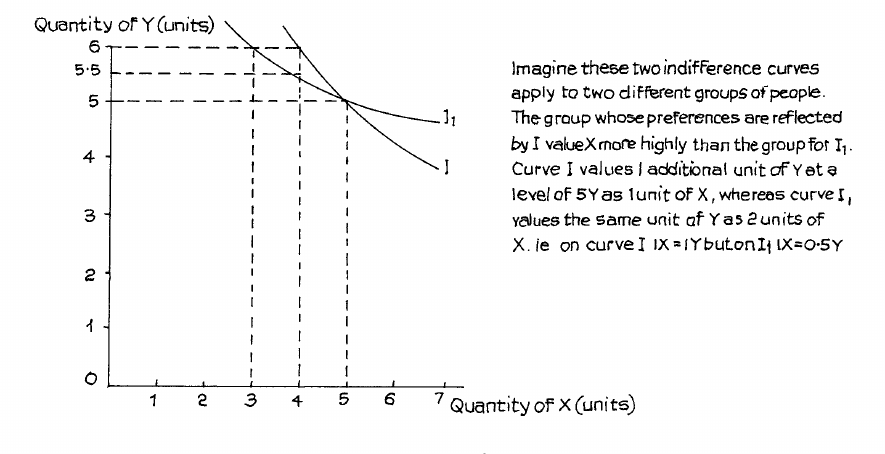
along I. You can see this in Figure 2.7.
Figure 2.6
Page 34
Figure 2.7
In curve I the group puts the same utility value on 5 units of X and 5 units of Y as it does on 4
units of X and 6 units of Y. Thus at this level on indifference curve I, 1 unit of X = 1 unit of
Y.
In curve I1 the different group puts the same utility value on 5X and 5Y as it does on 3 units
of X and 6 units of Y or 4 units of X and 5.5 units of Y. The flatter curve, therefore, values X
at half as much Y as the steeper curve at the levels examined.
Notice that showing two curves intersecting in this way indicates that they must either reflect
the preferences of different groups or the same group at different times. They cannot possibly
relate to the same group at the same time, since 5X and 5Y cannot at the same time have the
same utility as both 4X and 6Y and 3X and 6Y.
Remember the flatter the indifference curve the greater the preference for the good measured
along the vertical or Y axis; the steeper the indifference curve the greater the preference for
the good measured along the horizontal or X axis. Thus, if the indifference curves get flatter
as income and total utility levels increase, this suggests that people are switching their
spending preferences towards the good or goods measured along the Y axis. If they do this to
the extent that the quantity purchased actually falls following an income rise then the goods
on the horizontal axis can be described as “inferior” in economic terms.
Indifference Curve Analysis and Price Changes - Giffen Goods
The change illustrated in Figure 2.5 assumed that the prices of X and Y remained the same.
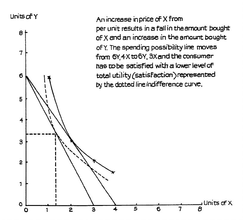
Suppose that, instead of a spending change, there was a price change. Let us say that the
price of X is increased to RWF4 per unit but that of Y stays the same at RWF2. The two
extreme possibilities for a total amount of spending of RWF12 are now 6 units of Y (no X)
and 3 units of X (no Y). The line between these two points on the graph shows all possible
combinations of X + Y that can be bought for the RWF12. This line no longer meets our
original indifference curve. The old combinations of 2X + 3Y would now cost RWF14 -
Page 35
above the limit of RWF12. A new mixture of X and Y has to be obtained, and this we see in
Figure 2.8.
Figure 2.8
The lower indifference curve (dotted in the graph) touches the spending line, to give a
package of rather less X but a little more Y. When using indifference curves in this way
remember, as mentioned earlier in this study unit, to imagine that there is an indifference
“map” containing a mass of curves, each representing a particular level of total utility or
satisfaction. The further away from the origin (where the axes of the graph meet) we move,
the higher the level of utility represented by the curve because it represents more of both X
and Y.
The changes shown in these illustrations all support the earlier statement that a rise in price of
a commodity will lead to a fall in the quantity demanded of that commodity.
In Figure 2.8 a price rise for X resulted in less of X being purchased; this is what we would
normally expect for most goods. However, some economists have argued that this may not
always be the case. They point out that a price change will not only change people’s
perception of other goods as substitutes but will also affect the income that is available for
spending, particularly if the price in question relates to something which is bought regularly
and so makes up a significant part of people’s incomes, especially if the incomes were low. If
RWF3 to RWF4
Page 36
the price of this basic good rose so that people could no longer afford to buy preferred
substitutes then it is, perhaps, conceivable that they would be forced to buy more rather than
less of the good whose price has risen. In this very special (and extremely rare) case a price
rise could be said to lead to increased purchases while a price fall, by releasing spendable
income to buy preferred goods, could lead to less being bought.
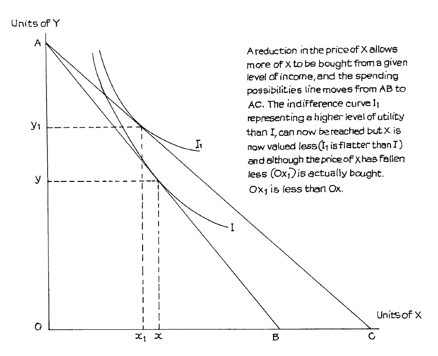
This possibility is illustrated in Figure 2.9, where a reduction in the price of X allows the
spending possibility line AB to move to AC for the same level of income. This allows buyers
to achieve the higher level of utility or satisfaction represented by the indifference curve I1
which is higher than the curve I - the highest attainable by spending possibility AB. The
preferred combination of X and Y is now Ox1 and Oy1. This provides more satisfaction than
the old combination of Ox and Oy but, as we see from the diagram, x1 represents a smaller
quantity of X than x. Thus people have used the extra money made available by the price
reduction of x to buy more of Y and less of X rather than more of both, which would have
been the case if X had been a normal good.
Figure 2.9
The reason for this is clear from the diagram. The higher indifference curve I1 is flatter than
the lower curve I. Thus X is perceived as being so inferior to Y that even the amount of
spendable income change resulting from the price reduction is sufficient to allow people to

Page 37
switch their buying to Y from X. Such a good is known as a Giffen good, Giffen being the
name of the person who first drew attention to the possibility.
As well as illustrating the so-called Giffen effect, this example also shows that when a good’s
price changes there are two consequences, both of which are likely to affect people’s
purchases.
1. If a price of, say, X changes while the prices of other goods, say Y, Z and so on, stay the
same there is a change in the pattern of relative prices. If good Y is seen as substitute for
X, and if the price of X rises with the price of Y staying unchanged, then X has become
dearer compared with Y and some people who previously bought X are likely to transfer
to Y which is now relatively cheaper than before. For X and Y, think of, perhaps,
potatoes and rice or tea and coffee. If the price of tea rises, people will not stop drinking
tea but some will start to switch to coffee when previously they would have drunk tea.
We can expect that there will be some switching of purchases to substitutes when one
good becomes relatively more expensive than its rivals. This is called the substitution
effect of the price change.
2. As we have seen earlier, if the price of tea rises any given quantity of tea purchased
requires more income than it did before the price rise. This will reduce the amount of
income available for spending on other things, including possible extra purchases of tea.
In the same way if, say, the price of coffee were to fall, this would increase the amount of
income available for spending on other things - including extra coffee. This is called the
income effect of the price change.
These two effects together make up the total shift in buying following a price rise or fall.
They can be analysed with the help, once more, of indifference curves.
Look at Figure 2.10. This uses the symbols X and Y as before to show they can apply to any
goods but you can think of X as coffee and Y as tea, if you wish.
Here we see the effect of a reduction in the price of X from RWF3 per unit to RWF2 per unit.
Y stays at RWF3 per unit and disposable income stays at RWF48. The maximum possible
purchases of X, assuming no purchases of Y, rises from 16 to 24 units.
Suppose the original combination of X and Y actually purchased, given the indifference curve
I, was:
9Y(RWF27) + 7X(RWF21) = RWF48 at B, before the price change.
After the change in price, the new combination on the higher indifference curve I1 would be:
91
3
Y(RWF28) + 10X(RWF20) = RWF48 at A.
To help you understand the income and substitution effects, let us imagine that, after the price
change, available income was reduced to an amount which just allowed consumption to stay
on the lower indifference curve I at C. This is represented by the dotted line which runs
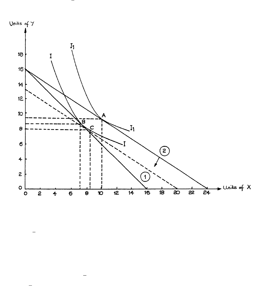
Page 38
parallel to the second consumption possibility line and which just touches indifference curve I
at C. The dotted line is called the “income compensation line”. At C, the consumption
package would be 8Y + 8 1
3
X.
Figure 2.10
The increased consumption of X between points B and C on the same indifference curve, i.e.
from 7 to 8
1
3 units, the result of a movement along the indifference curve, is the substitution
effect. It is the result purely of the change in price of X from RWF3 to RWF2, because the
total utility gained from consuming both X and Y has not changed.
Thus, if we consider the actual consumption movement from B to A, we see that it is made up
of two parts. These are the 1 1
3
units rise which we have explained as the substitution effect,
plus the 1
3
2 units rise which is the result of the increased income available for spending and
which has enabled movement to the higher indifference curve I1.
This increase resulting from movement to a higher level of satisfaction is the income effect,
because the reduction in price of X has provided more spendable income and some of this has
been used to purchase more X.
In this example X and Y are clearly normal goods since the full movement from B to A is the
sum of B to C plus C to A. But suppose X had been an inferior good: in this case the
indifference curve I1 would have been flatter and the point of tangency (A) with the
Consumption possibility line “1” based on
Price of Y = RWF3,X = RWF3
Consumption possibility line “2” based on
Price of Y = RWF3,X = RWF2
Income = RWF48
Page 39
consumption possibility line 2 would have been to the left of C, indicating a reduction in
purchases as a result of the income effect. The total change B to A would then have been the
distance B to C minus C to A, i.e. a total somewhere between B and C to a quantity level of X
below 8.33.
Taking this one stage further, consider the possibility of a Giffen good. In this case the
inferior nature of the income effect would have been even greater and the indifference curve
I1 even flatter until the point of tangency A would actually move to the left of the starting
point of B and the new level of purchases of X would be under 7X.
Notice that the income effect of a price change can move the level of consumption for the
affected good in either direction.
• For normal goods (the majority) a rise in income available for spending on the good
produces an increase in purchases. Similarly a fall in income results in a reduction in
purchases.
• For inferior goods a rise in income available for spending on the goods produces a
reduction in purchases, while a fall in income results in an increase in purchases.
However the substitution effect is always in the same direction, i.e. in the reverse direction to
that of the price change and in favour of the good whose price has become lower relative to
the price of the substitute. In effect the substitution effect is a movement along the
indifference curve caused by the change in gradient of the consumption possibilities line,
which is itself caused by the changes in the relative prices. Thus we can say that:
• For all goods the substitution effect causes a rise in the consumption of the good whose
price has become relatively lower and a reduction in consumption of the good whose
price has become relatively more expensive.
The Giffen effect, where a price rise produces an increase in consumption and a price fall
leads to a decline in consumption, occurs when the “inferior” income effect is actually greater
than the substitution effect.
C. THE DEMAND CURVE
What is a Demand Curve?
So far in this study unit we have considered some of the consequences of price and income
changes for the amounts of goods purchased. The general, and in most cases “normal”
relationship between price and quantity changes is frequently illustrated by graphing the
anticipated amounts of a good that people can be expected to buy, in a given time period, at a
series of different prices within a given price range. This produces a demand curve.
Bear in mind that the demand curve is a simple two-dimensional graph. It shows the
relationship between just two variables - the price of a good and the quantity of that good that
we believe is likely to be purchased over a given time period.
Page 40
In concentrating on just price and quantity we make the assumption that all other possible
influences on demand (quantities of possible purchases) are held constant. These other
influences, including income and prices of other goods, already noted, will be considered
again in the next study unit but for now we can conveniently ignore them. Our concern, for
the moment, is with price.
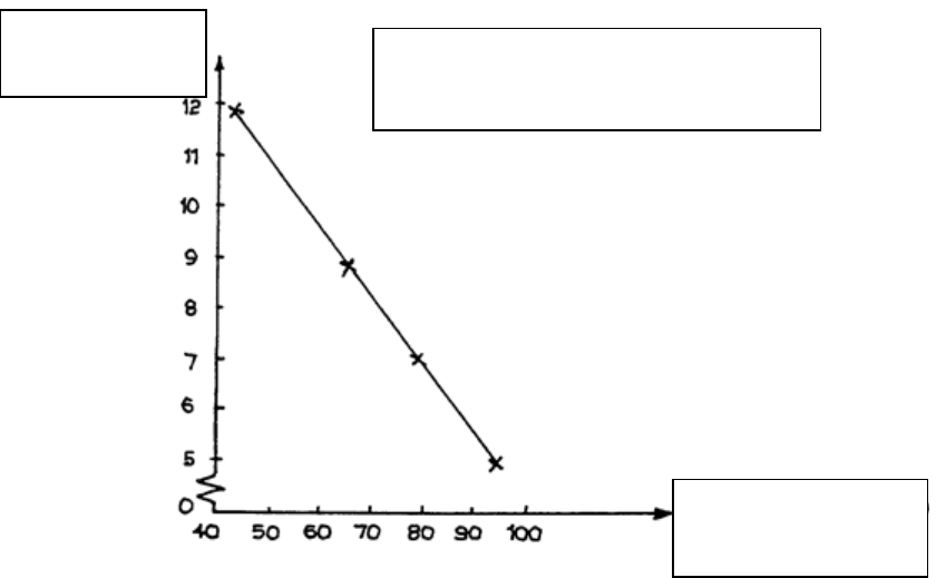
Indifference Curves and the Demand Curve
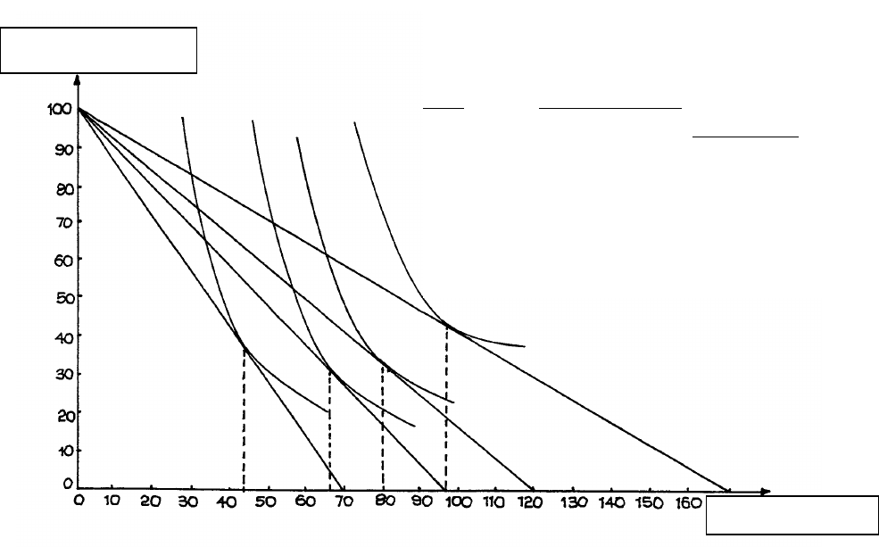
We can make use of simple indifference curve analysis for a normal good to show how it is
possible to derive a demand curve. Suppose a group of consumers have, between them, an
amount to spend each week of RWF840,000 and they spend this on a combination of products
or product “baskets”, X and Y. Assume that the price of Y stays constant at RWF8,400 per
unit but that X varies between RWF12,000 and RWF5,000 per unit.
Given these figures, the maximum possible consumption of Y (no X consumed) is 100 units,
whereas that of X (no Y consumed) moves from 70 units per week at a price of RWF12,000
to 168 units at the lower price of RWF5,000. These total possible consumption (spending)
figures assume that the whole income is spent on Y or X only. This enables us to draw the
series of possible consumption or spending possibility lines in Figure 2.11, which also shows
the actual consumption of X at the prices of RWF12,000, RWF8,750, RWF7,000 and
RWF5,000, given the indifference curves of the diagram
.
Figure 2.11
Total income is RWF84000
Price of Y is RWF8400
Then for X:
Price Max.Consumption Actual
Consumption
RWF12000 70 44
RWF875 0 96 68
RWF7000 120 80
RWF5000 168 96
given the indifference curves shown
‘000 Units of
Y
‘000 Units of X
Page 41
We see that actual consumption of X, given the relative preferences of X and Y represented by
the indifference curves, rises from 44 units per week at the price of RWF12,000 per unit to 96
units per week at the price of RWF5,000 per unit. The actual consumption figures, related to
these prices, are shown in Figure 2.12. This graph shows the demand for X at the range of
prices RWF12,000 to RWF5,000. It is the demand curve for the good X.
Figure 2.12
This example illustrates the general shape of the demand curve and the normal relationship
between price and quantity demanded of a product. If all other influences remain constant,
we would expect the quantity demanded to rise as price falls and to fall as price rises. Notice
that, in our example, we have made the following assumptions:
(a) Other prices, represented by Y, stay constant at RWF8,400 per unit.
(b) Income also stays constant, at RWF840,000. Another point to remember is that we are
here considering a flow of demand related to a set period of time. It is always necessary
to do this. We cannot compare a weekly amount at one price directly with a monthly
amount at another. When we change one variable - here price - to analyse its effect on
quantity, we have to keep all other elements constant, including the time period to which
the stated quantity relates. In our example, this period was a week.
Use and Importance of Demand Curves
As you will see as you progress through this course, the demand curve is used extensively in
economic analysis. The price-quantity relationship is one of the most important things we
need to know when considering sales of products. A firm must know the likely result of a
change in price, because any alteration in quantity demanded will affect the total sales
revenue.
Demand for X at prices from
RWF5,000 to RWF12,000 per unit
Price per ‘000
units
Quantity per week
(‘000 units of X)
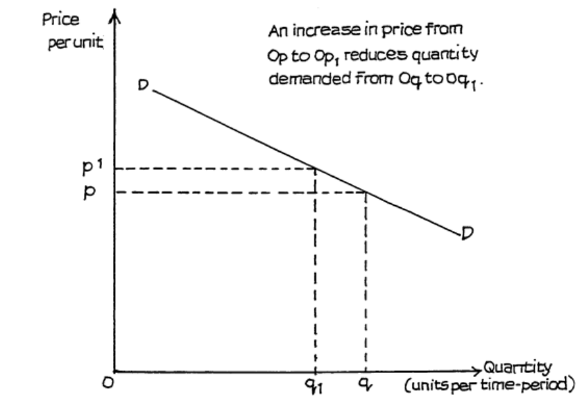
Page 42
Governments also need to know the probable effects of any change in a tax imposed on
products. Because such a tax will influence price, the price-quantity relationship is, again, an
important issue. If a government is considering an increase in a tax such as value added tax,
which influences a very wide range of goods, it needs to know what extra total revenue it can
expect to gain from the tax increase. It cannot assume that quantities consumed of all goods
affected will remain the same; it must take into account the probable changes in quantity
demanded that will result from the changes in price.
General Form of Demand Curves
Notice that in Figure 2.13 a given change in price appears to produce a greater change in
quantity demanded than in Figure 2.14. This is assuming that they are drawn to the same
scale. You must remember that the steepness of a demand curve will be affected by the scale
of the (horizontal) X-axis, and graphs must be drawn to the same scale, so that comparisons
can be made.
It is a convention (general rule) in economics that price per unit is measured on the vertical
(often called the Y) axis, while quantity in units per period of time is measured along the
horizontal X-axis. It is often customary to label the axes simply “Price” and “Quantity”.
Figure 2.13

Page 43
Figure 2.14
D. CONSUMER SURPLUS
The Consumer Surplus is the difference between what a consumer would have been willing to
pay for units of a good and what the consumer actually does pay.
Figure 2.15
Page 44
These ideas are illustrated in Figure 2.15, which shows a normal demand curve for a product
the price of which is 0P. The fact that the demand curve extends to prices higher than 0P
indicates that there are consumers who are willing to pay a higher price. However, if the price
charged is 0P, then these consumers achieve a surplus which is represented by the shaded
area.
What the consumer is willing to pay is shown by the demand curve. What he actually does
pay is shown by the market price.
Page 45
Study Unit 3
Demand and Revenue
Contents
___________________________________________________________________________
A. Influences on Demand
Flow of Demand
Product’s Own Price
Prices of Other Products
Income Available for Spending
Price and Availability of Money and Credit
Market Size
Advertising or Marketing Effort
Taste
Expectations
Other Influences
Summary of Influences
The Relative Importance of Influences
Shifts in the Demand Curve
Some Further Considerations
___________________________________________________________________________
B. Revenue and Revenue Changes
Total Revenue
Average Revenue
Marginal Revenue
___________________________________________________________________________
C. Price Elasticity of Demand
Calculation
Influences on Price Elasticity of Demand
___________________________________________________________________________
D. Further Demand Elasticities
Income Elasticity of Demand
Influences on Income Elasticity of Demand
Cross Elasticity of Demand
Influences on Cross Elasticity of Demand
The Importance of Elasticity Calculations
___________________________________________________________________________
E. Elasticity: Summary of Key Concepts
Five Types of Elasticity
Value of Elasticity
Factors Influencing Demand Elasticity
Income Elasticity of Demand (YED)
Cross Price Elasticity of Demand (CED)
Elasticity of Supply ( Ys )
Factors Affecting Supply Elasticity
___________________________________________________________________________
Page 46
A. INFLUENCES ON DEMAND
Flow of Demand
The demand curve which we identified in the previous study unit illustrates the quantities of a
product that a group of consumers are prepared to buy at a range of possible prices. We must
remember that these quantities are always related to a time period. Demand is seen in terms
of a flow of purchases over a stated time. A greengrocer, for example, may want to know the
weekly quantity of apples he can sell at a price of RWF80 per kilo, and compare this with the
weekly quantity he could sell at RWF90 per kilo. The time is not always shown in simple
demand graphs, but we must not forget its importance. It is not much use being able to sell
100 kilos instead of 50 kilos if it takes three times as long to do so.
If we clearly understand this idea of demand flow, remembering the points we made in Study
Unit 2, we can go on to identify the various influences which affect that flow.
Product’s Own Price
This is regarded as the most important influence on demand: normally, we expect a rise in
price to lead to a fall in quantity demanded, and a price fall to produce a rise in quantity.
It is claimed that some goods operate in the reverse way, as explained in Study Unit 2. These
are known as “Giffen goods”. Although, strictly, the term “Giffen” applies only when the
“inferior” income effect is more powerful than the normal price substitution effect, it is often
used more widely whenever demand appears to rise as price rises for whatever reason. There
are a number of other possible explanations. For example, people may, rightly or wrongly,
associate price with quality - e.g. for tomatoes - and prefer to pay a little more in anticipation
of obtaining a more satisfactory fruit. If there were some other trusted mark of quality, the
normal price-quantity relationship would hold. Demand may also rise for a work of art which
people think is gaining acceptance in the art world. If people think that the price is going to
rise even more in the future, they may buy the work of art as an investment and not simply
because they get pleasure from looking at it. In this case, we are really dealing with a
different product. In yet more cases, the rise in demand is just the result of other influences as
described in this study unit and these are proving more powerful than the influence of price
on its own.
In general, therefore, we can accept that, if all other considerations are equal (which they
seldom are), people will prefer to pay a lower rather than a higher price for a product the
quality of which they know and accept.
We should also recognise that expectations of future price movements can influence current
demand. If people expect prices to rise next week, they will, if possible, prefer to buy now at
the lower price. On the other hand, this may be regarded as a temporary distortion of demand
which will have little effect over a longer period of time. If the longer-term effect is not taken
into account, it might look as though demand was rising as prices rose - when, in fact, people
had taken the view that a price rise today was likely to be followed by further rises tomorrow,
and were acting accordingly.
Page 47
If a new product is introduced to the market, there is likely to be an effect on other goods.
The introduction of cheap electronic calculators destroyed the demand for slide rules. On the
other hand the development of portable radios and personal stereos also created a demand for
the associated (complementary) product - the batteries needed for their operation. If a major
product is introduced and becomes popular enough to absorb a significant part of personal
income then people will reduce purchases of other products which they may consider less
desirable. There may be no obvious association between the desired product and the one
neglected. For example, a person who decides to pay for a part-time degree course to enhance
career prospects may think it worthwhile, perhaps, to spend less on entertainment or to put off
replacing a car or furniture.
Prices of Other Products
In our earlier illustrations, a little more was bought of Y when the price of X rose. This was
because Y and X were, to some extent, substitutes for each other. The indifference curve was
based on the assumption that more X could compensate for less Y. This will not always be
the case. Sometimes, two products are clearly associated - petrol and motor oil or motor-car
tyres, for instance. A rise in petrol costs may lead to a fall in the use of cars and, hence, to
reductions in demand for oil and tyres. Even when products are not directly linked, a change
in the price of one may still influence a wider demand. If a man smokes heavily and is unable
to check his habit, a rise in tobacco prices will lead him to spend less on a wide range of other
products. In the same way, a rise in mortgage interest will force families to spend less on
other goods.
Income Available for Spending
In Study Unit 2 substitution analysis showed how an increase in income could lead either to a
rise or a fall in the demand for goods. For the majority of goods and services, i.e. for normal
goods, we would expect the change in demand to be in the same direction as the change in
income but for some, inferior goods, the changes would be in the reverse direction so that a
rise in income produces a fall in demand and vice versa.
Notice that a good is inferior only if it is perceived as offering less satisfaction for a particular
type of want. Thus, as a normal means of transport a motor cycle may be perceived as
inferior to a car even though, as a piece of engineering, it may be superior. Suppliers may be
able to revive demand for an inferior good by changing its appeal; adapted and marketed as a
sporting and leisure good, the motor cycle has enjoyed such a demand revival and as such is
often bought by people who also possess cars.
Price and Availability of Money and Credit
Many goods are bought with the help of borrowed money (credit). Money and credit have an
influence on demand separate from the effect of income. If the cost of credit, i.e. the rate of
interest, rises there is likely to be a reduction in demand for the more expensive goods.
Market Size
Many factors can change market size. A firm selling clothes to teenagers will benefit from
any increase in the numbers of teenagers in the population. Specialist shops selling babies’
Page 48
and children’s wear suffered from the declining birth rate since 2005. Market size can be
increased by improvements in communications and technology. The development of
commercial television greatly increased the market area open to many consumer-goods firms.
Increased foreign travel helped to extend the demand and market area for foreign wines and
foods. Improved techniques of refrigeration extended the market for frozen vegetables.
Advertising or Marketing Effort
Very few products sell themselves. Most have to be marketed, and the more extensive the
advertising effort, the more is likely to be sold. Some marketing specialists suggest that there
is a direct relationship between the firm’s share of market advertising and its share of market
sales. Certainly, it is the volume of advertising in relation to competitors’ advertising that is
likely to be important.
Taste
This is a quality difficult to define. People’s desire to buy products is the result of many
influences, not all of which are fully understood. Fashions change, and these changes cannot
always be caused by advertising. The successful firm is often the one that is able to make an
accurate prediction of changes in fashion and taste.
Expectations
Expectations of future changes in any of the above influences can affect present demand. For
example, people expecting rising prices will buy now rather than later. On the other hand, if
they fear unemployment and falling incomes, they will cut down their present spending.
Notice that these reactions may actually help to bring about the feared future changes.
Other Influences
Certain products may be subject to special influences other than the ones we have already
mentioned. The demand for soft drinks or for waterproof clothing, for instance, will be
influenced by weather conditions. The demand for private higher education in an area will be
influenced by the reputation of State-owned schools in that area.
Summary of Influences
All these influences on demand for a product can be expressed in a form of mathematical
shorthand. Thus, we can say that:
Q = f (Po, Pa, Yd, N, A, T).
This simply means that the quantity demanded of any product (Q) is a function of, i.e. is
dependent upon, (f), its own price (Po), the prices of other goods (Pa), disposable income (Yd),
market size (N), marketing effort (A), and customer taste (T).
The Relative Importance of Influences
The relative importance of these influences varies, of course, for different products and it is
necessary for suppliers to estimate this if they are to avoid damaging errors. For example, if
Page 49
price is not of first importance, a price reduction will simply reduce revenue and profit. The
supplier would, perhaps, have more to gain from increases in price and advertising
expenditure.
Suppliers can attempt to estimate the relative importance of the demand influences by
recording and measuring the effect of those, such as price and advertising, under their control
and also noting the effects of other measurable changes such as movements in average
incomes. Much information may also be gained from market research, e.g. by asking people
why they favour certain brands and what their reactions would be to price movements. In
some cases, shopping simulations can be staged with people given a certain amount of money
and then asked to spend it on a range of goods displayed in a store. The scientific study and
calculation of demand functions from information gained from all available sources is known
as econometrics. In some cases these studies have resulted in calculations that have proved
remarkably accurate but others have been less successful. There are many things that can go
wrong in the estimation of future demand! Business decisions still have to be made against a
background of market uncertainty.
Shifts in the Demand Curve
Because a normal two-dimensional graph can cope with only one influence in addition to
quantity changes, and because the normal demand curve relates quantity to the product’s own
price, a change in quantity demanded brought about by a change in one or more of the other
influences has to be represented graphically by a shift in the whole demand curve.
Suppose there is an increase in disposable income which increases the quantity demanded at
each price within a given range. This effect can be shown as in Figure 3.1, where the price
remains constant at 0p but the increase in income has shifted the curve from DD to D1D1, so
that the quantity demanded at 0p rises from 0q to 0q1. A fall in income or a decline in taste,
etc. would produce the reverse result, i.e. a shift from D1D1 to DD.
Remember always to distinguish a movement along a demand curve produced by a change in
price (all other influences remaining unchanged) as shown in Figure 2.14 from a shift in the
whole curve, showing that demand has moved at all prices within the range under
consideration.
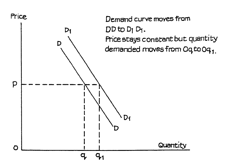
Page 50
Figure 3.1
Some Further Considerations
It has been argued that the “normal” influences identified above do not tell the full story, and
that a fuller understanding of social psychology can give further insights into consumer
behaviour. For example, supermarket chains well know the importance of impulse buying,
when goods are skilfully displayed. There is also a recognised “snob” effect, when goods
may be bought because they are expensive and they appear to be indicators of the owner’s
wealth and status. While these considerations are interesting and are clearly of importance to
marketing specialists, we can include them under the more general headings of advertising
and taste, for the purposes of general analysis of consumer demand.
B. REVENUE AND REVENUE CHANGES
Total Revenue
Revenue, in general, refers to the money received from the sales of a product. For this reason,
the term “sales revenue” is often used. To have any practical meaning, revenue should also be
related either to a time period or to a definite quantity of goods sold. For example, a
shopkeeper may refer to his weekly sales revenue (the total amounts of sales achieved in a
week) or to his revenue from the sales of, say, n pairs of shoes or k kilos of potatoes. A
statement that his revenue is RWFy means nothing, unless we can relate it to some quantity of
time.
Revenue will not always increase as more goods are sold - this will be the case only if the
firm can continue to charge the same price, regardless of quantity it sells. If, say, I make
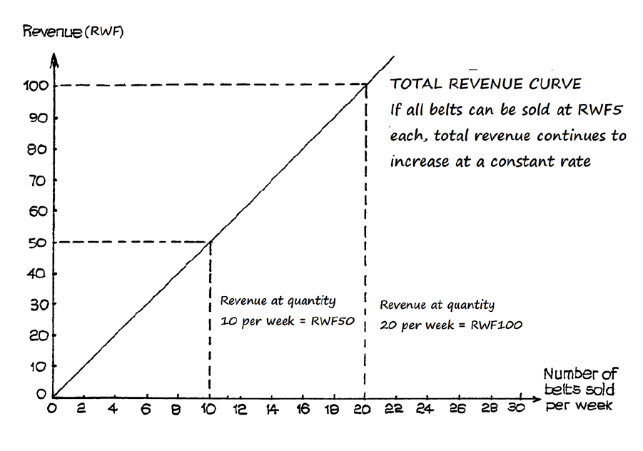
Page 51
leather belts and can sell all the belts I can make at a standard price of RWF5, then my total
revenue is always RWF5 multiplied by whatever quantity I sell.
This can be shown in the form of a total revenue curve, as in Figure 3.2.
However, if I continue to produce more and more belts, there will come a time when
customer resistance sets in. I shall have difficulty in finding more people who value belts at
this price of RWF5, i.e. the marginal utility of which is at least RWF5. When this time
comes, I may still, however, find more people who are willing to pay RWF4.
Figure 3.2
Now, in the modern world, shopping conditions are often such that I cannot leave my belts
un-priced and hope to sort out from the people who visit my shop those willing to pay RWF5
and those willing to pay RWF4. If I want to sell more belts and am willing to charge RWF4,
then I must charge this price to everyone. If I continue to produce even more, I might then
find that, to sell the increased quantity, I have to charge RWF3. If I go on doing this, I am
likely to find that my total revenue starts to fall.
Suppose I find that total revenue rises if I reduce the price from RWF5 to RWF4, but falls if I
reduce the price to RWF3. This will happen if the reduction from RWF4 to RWF3 does not
produce enough additional sales to make good the loss suffered when I charge RWF3 to those
people who would still have bought at prices of RWF5 or RWF4. My sales schedule at the
three prices might, perhaps, be as follows:
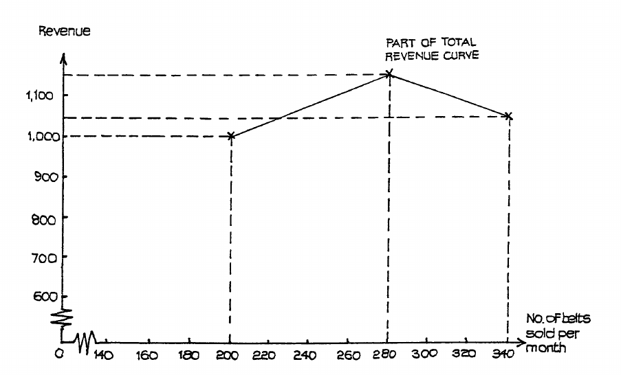
Page 52
Price per belt
Number of belts I can sell
per month
Total revenue
RWF5
200
RWF1,000
RWF4
280
RWF1,120
RWF3
340
RWF1,020
This effect can be shown in the form of a simple graph but this time the turning point can be
seen (Figure 3.3). If I try to reduce the price still further, below RWF3, I shall lose even more
revenue.
Figure 3.3
Average Revenue
The term “average” here is used in its commonest sense - that familiar to you, perhaps, in the
form of “cricket average” or “goal average”. It is the total revenue divided by the quantity of
goods sold. If a shop’s weekly revenue from selling broccoli is RWF600 and it sells 300 kilos
in the week, the average revenue of the broccoli sold is RWF2 per kilo.
If all goods are sold at the same price in the given time period - as, say, with our leather belts -
then the average revenue is the same as the price. The average revenue curve for the belts is
shown in Figure 3.4.
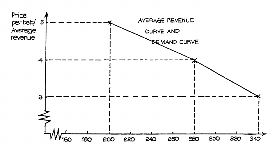
Page 53
Figure 3.4
Notice, in this case, that the average revenue curve is really just the same as the demand
curve. This will always be the case where all items sold in the time period are sold at the
same price, i.e. where there is no price discrimination between different customers.
Now, to return to our shopkeeper selling broccoli at RWF2 per kilo; let us suppose that he is
selling every kilo for RWF2 and that he finds he can sell as much broccoli as he can handle at
that price. He does not need to reduce his price to increase quantity sold from, say, 200 kilos
per week to 300, to 400, and again to 500 kilos. The average revenue curve in this case is still
the same as the demand curve but it reflects this increasing quantity sold at a constant price.
This produces the horizontal line graph shown in Figure 3.5.
RWF
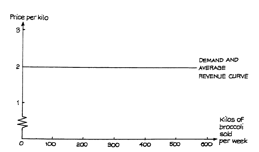
Page 54
Figure 3.5
Marginal Revenue
If the firm is able to maintain a constant price as it increases output, then the additional
amount it receives for each extra unit sold is, of course, that unit’s price. In this case, the
price, which is the same as average revenue, is also the same as the change in total revenue
resulting from the sale of the extra unit. The change in total revenue brought about by a small
or unit change in the quantity flow of sales is known as the marginal revenue.
Marginal revenue is not always the same as the price or average revenue. Remember the
example of the leather belts.
There, an increase in sales from 280 to 340 belts per month produced a fall in total revenue.
For the change in this output range, the marginal revenue must be negative. The reason is the
same as for the fall in total revenue - in order to increase sales, the price had to be brought
down and, in this case, the revenue gained on the additional quantity sold was not enough to
make good the revenue lost for customers who would have been prepared to buy at the higher
price.
A simple example will show how marginal revenue can change when price has to be reduced
in order to increase the quantity sold. Look at Table 3.1. There are some important features
to note about this table. The marginal revenue column has its figures placed mid-way
between the rows. This emphasises that the marginal revenue relates to the change from one
output level to the next. On a graph, the marginal revenue is also plotted mid-way between
the output levels. This is shown in Figure 3.6.
The shopkeeper can sell any quantity up to 700
kilos a week at the price of RWF2 per kilo

Page 55
Number of TV sets
sold per week
Price per set
Total Revenue
Marginal Revenue
RWF
RWF
RWF
1
600
600
550
2
575
1,150
500
3
550
1,650
450
4
525
2,100
400
5
500
2,500
350
6
475
2,850
300
7
450
3,150
250
8
425
3,400
200
9
400
3,600
150
10
375
3,750
100
11
350
3,850
50
12
325
3,900
0
13
300
3,900
−50
14
275
3,850
Table 3.1
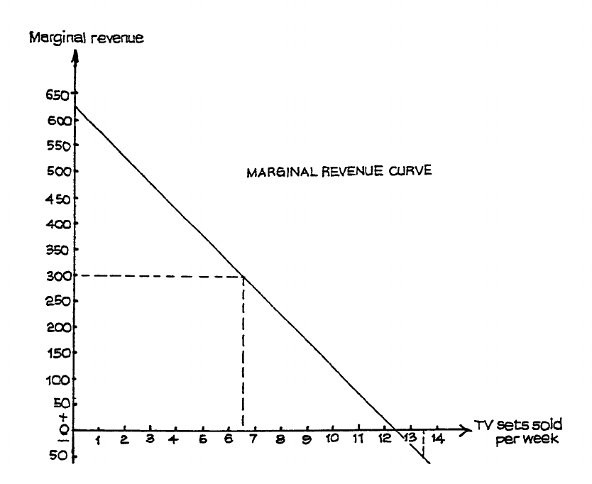
Page 56
Figure 3.6
Look carefully at the price and marginal revenue columns. Notice that, as each additional TV
set is sold, the price (average revenue) falls RWF25. The fall in marginal revenue for each
additional set is exactly double this - RWF50. In Figure 3.7, we see the marginal and the
average revenue curves together. Notice that, at each price level, the marginal revenue is
exactly halfway between the price axis and the average revenue. Although Figure 3.7 does
not continue the average curve until it meets the quantity axis, we can deduce where it would
meet if continued in the same straight line. It would meet the quantity axis at 25 TV sets -
twice the marginal revenue quantity when marginal revenue = 0, thus indicating that this
supplier would be able to dispose of only 25 sets, even if he did not charge any price at all.
The average revenue curve cannot, of course, pass below the quantity axis, as we do not
expect suppliers to pay customers to take their goods. The marginal revenue curve can,
however, pass into the negative area of the graph, and so indicate quantities where continued
price reductions would result in an actual fall in total revenue. We can see this clearly from
Table 3.1. Marginal revenue remains positive until 12 sets are sold. The increase from 12 to
13 sets does not change total revenue at all, so marginal revenue here is zero. If we continue
to reduce price and sell 14 sets, then total revenue falls to RWF3,850 and marginal revenue
indicates the loss as
−
RWF50.
RWF
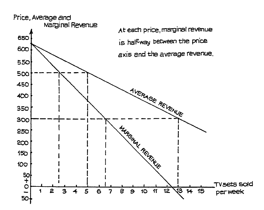
Page 57
Figure 3.7
The total revenue curve for this table is shown in Figure 3.8. Compare this with Figure 3.7
and see how the marginal revenue relates to the total revenue at the various numbers of TV
sets sold.
This example has illustrated an important rule. Whenever we have a linear average revenue
curve, i.e. where there is a constant relationship between price and quantity changes, resulting
in a “straight-line graph”, then the marginal revenue curve is also linear (a straight line) and
always bisects (cuts into two equal halves) the horizontal distance between the price/revenue
axis and the average revenue curve.
RWF
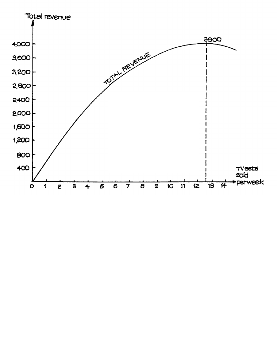
Page 58
Figure 3.8
C. PRICE ELASTICITY OF DEMAND
We have now seen that there is a definite relationship between price, revenue and quantity
changes. This is most important for practical studies of price and sales movements, and we
need to have a precise way of measuring and analysing the various possible relationships.
Because demand is seen as stretching and shrinking in response to price movements, the
concept we use is called the price elasticity of demand.
Calculation
This can be denoted by the symbol Ed. It is the relationship between a proportional change in
quantity demanded and a proportional change in price, so that Ed = proportional change in
quantity demanded ÷ proportional change in price, or
∆Q
Q
DP
P
÷where P = price of the product
As explained earlier, for the great majority of goods a rise in price leads to a reduction in
quantity demanded and a fall in price leads to an increase in quantity demanded. Thus the
change in quantity is the reverse of the change in price. One of the changes will be negative,
indicating a reduction; thus the value of Ed will also be negative. In some older text books
Q = quantity demanded of the product
∆
= a significant change in.
Total revenue is at its
maximum (RWF3,900)
between 12 and 13 sets per
week. If more than 13 sets
are sold, total revenue starts
to fall, i.e
. marginal revenue
is negative

Page 59
this used to be ignored but the general tendency today - and the one you should follow - is to
keep strictly to using this negative sign. So:
• When the calculation of price elasticity of demand produces a result which is more
negative than
−
1, i.e. when the proportional change in quantity is greater than the
proportional change in price, we say that demand is price elastic.
• When the calculation of price elasticity of demand produces a result which is less
negative than −1, i.e. when the proportional change in quantity is less than the
proportional change in price, we say that demand is price inelastic.
• When the calculation of price elasticity of demand produces a figure of
−
1, i.e. when the
proportional change in quantity is equal to the proportional change in price, we say that
demand has unitary elasticity.
The demand for fish is likely to have a price elasticity of around
−
0.9, that for washing
powder about
−
0.3, and that for eggs around
−
0.02. These demand elasticities are price
inelastic but fish is clearly much more price-sensitive than eggs. Notice that while the
demand for washing powder is price inelastic, that for a particular brand of washing powder
might well be price elastic - say, around
−
1.3.
One important feature of price elasticity of demand is that it changes as price changes.
Consider the demand curve shown in Figure 3.9.
At point A, Ed =
−
1, so that here demand is neither elastic nor inelastic. Here, revenue
remains the same at both prices because the change in price produces exactly the same
proportional change i.e.
∆
=
∆
P
P
Q
Q
.
At point B, however, Ed is more negative than
−
1, so that demand is price elastic -
∆
>
∆
P
P
Q
Q
.
A reduction in price at B results in a more than proportional increase in quantity demanded,
so that there is an increase in total revenue. A firm in this position will increase revenue by
reducing price but lose revenue if it increases price.
At point C, the position is completely reversed and Ed is less negative than
−
1, so that
demand is price inelastic.
∆
<
∆
P
P
Q
Q
. A reduction in price here results in a less than
proportional increase in quantity demanded, so that there is a fall in total revenue. A firm in
this position will lose revenue by reducing price but gain revenue by increasing price.
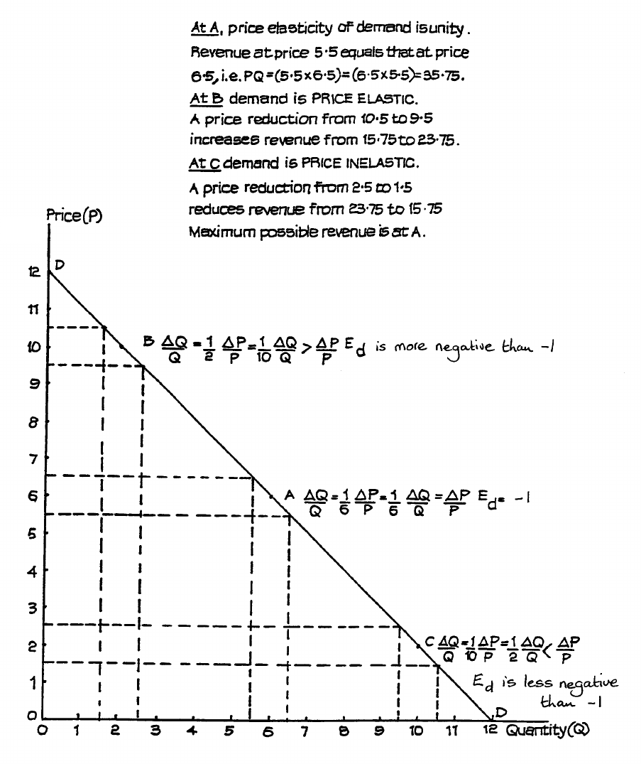
Page 60
Figure 3.9
The point of greatest possible revenue on any linear demand curve is where price elasticity is
at unity (where Ed =
−
1).
Notice also that the calculations shown in this illustration are made around the mid-point of
each change. Calculations made in this way are called “arc elasticity”, and they are the
correct way to measure price elasticity, unless we are able to use the necessary mathematical
techniques to calculate point elasticity at a particular point on the demand curve. For all but
RWF
Page 61
very small changes, point-elasticity calculations will show different results depending on
whether we assume a price rise or a price fall, and this is confusing and inaccurate. You can
test this for yourself if you compare the calculation for a price rise from RWF9.50 to
RWF10.50 with a price fall from RWF10.50 to RWF9.50.
Influences on Price Elasticity of Demand
We have seen that the price elasticity of demand can be expected to change as price changes,
so that the product’s own price can normally be regarded as an influence on its elasticity. The
important point, really, is whether buyers are likely to pay much attention to the price when
deciding whether to buy, or if other influences are more important. These may include
current fashion or social attitudes, strong habits (even addiction, in some cases such as
tobacco smoking) or the need to buy in order to achieve some other desired objective, such as
buying petrol in order to drive to work.
If the product price is only a relatively small amount compared with normal income then price
is likely to be less important than the other influences affecting demand, which is thus likely
to be price inelastic. Toothbrushes, matches, shoe polish, are all examples of products likely
to be price inelastic. Here, high relative price changes at normal price levels are unlikely to
weigh heavily with consumers, because annual spending on these items is only a very small
part of total income. Other influences, e.g. social attitudes (toothbrushes), smoking decline,
the move away from coal fires (matches), and development of non-leather shoes (polish), are
likely to be much more important.
We must also be careful to distinguish between the demand elasticity for the class or product
and that for a particular brand of the product. My decision whether or not to buy household
soap is not likely to be greatly influenced by a 10% rise in its price, but when I am actually
making my purchase I am quite likely to compare the prices of two brands and choose the
cheaper, assuming that I do not think that one is superior in quality to the other. Thus,
demand for a product can be price inelastic, whereas demand for a specific brand of the
product can be price elastic. This difference can often be seen in foods. Families may keep to
the eating of chicken or beef for dinner and pay roughly the same price for this each week -
thus showing a demand price elasticity of around unity. However, the choice of which to buy
can be very much influenced by its price, so that we can expect the demand price elasticity for
beef and chicken, and certainly for some particular cuts of beef, to be higher than unity,
especially if the general level of all meat prices has been rising.
Page 62
D. FURTHER DEMAND ELASTICITIES
The general concept of elasticity can be applied to any of the influences on demand. If you
think about the concept, you will realise that it is simply the ratio of a proportional change in
quantity demanded to the proportional change in the influence considered to be responsible
for that quantity movement. The only limiting element in using elasticity is that the influence
must be capable of some sort of precise measurement or evaluation. This makes it difficult to
produce a definite calculation for, say, changes in taste or fashion, as this is very difficult to
measure. The most commonly used elasticities, in addition to the product’s own price, are
those for income and for other prices.
Income Elasticity of Demand
This relates to proportional change in quantity demanded to the proportional change in
disposable income of customers for the product.
It can be denoted by Ey, so that Ey = proportional change in quantity demanded ÷ proportional
change in disposable income.
This may be positive or negative, because there may be an increase in demand following an
income increase or a fall in demand. If the income and quantity changes are in the same
direction, then the figure for Ey is positive. If the changes are in the opposite directions to
each other, then the figure carries the negative sign (
−
). A rise in income usually leads to a
rise in demand, but demand for some goods may fall. The demand for motor cycles fall as
incomes rise and people buy cars. As we saw earlier, such goods are known as inferior
goods.
Notice that we are referring here to “disposable income”, i.e. the income left to the consumer
after compulsory deductions have been taken. The most important of these are income tax
and Social Security contributions. We may also include contributions to pension schemes or
to trade unions or professional bodies, where membership is necessary for employment.
In recent years, some economists have argued that we should really be thinking in terms of
“discretionary income”. This is the income that is left after all the regular and largely
essential household payments have been made, over which the individual has very little
control once a particular pattern of life has been chosen. The further deductions which
would, then, be made to arrive at discretionary income would be such items as rent or
mortgage interest, essential fuel charges (gas and/or electricity) and possibly the cost of
travelling to and from work. When these items have all been allowed for, the amount of
discretionary income, i.e. the income which people are genuinely free to spend as they
choose, is usually very small in relation to the original gross income.
Page 63
Influences on Income Elasticity of Demand
The following influences are likely to increase a product’s income elasticity of demand:
(a) A high price in relation to income. If a period of saving is required before purchase is
possible, or if consumers have to borrow money to obtain a product, then demand can
increase only when an income rise makes this possible.
(b) If goods are preferred to “inferior” substitutes, then people may be ready to buy more of
these when income increases make this possible.
(c) Association with a higher living standard than that currently enjoyed is likely to lead to
rising demand when incomes do rise.
In general, the more highly-priced durable goods (household machines, motor vehicles, etc.)
and services are more likely to be income elastic than the staple items of food and clothing.
We do not usually buy twice as much of these if we receive double our former income. On
the other hand, our spending on holidays may increase by far more than double. Increased
spending on motor transport is also associated with rising incomes. Although we have been
considering income rises, very similar comments apply to income reductions. Holidays and
motor cars are often the first things to be sacrificed in the face of a sudden drop in income.
Cross Elasticity of Demand
This relates the proportional change in demand of one product to the proportional change in
price of another.
Ex = proportional change in quantity demanded of X ÷ proportional change in price of Y.
Again, the demand movement may be in the same or the opposite direction to the price
movement, and the same rules for negative signs apply.
If two products are substitutes for each other, we can expect a rise in price of one to lead to a
rise in demand for the other. Beef and pork are in this position, or meat and fish.
If, however, the two products are linked together, e.g. petrol and motor-car tyres, then a rise in
price in one leads to a fall in demand for the other, and Ex carries the negative sign (
−
).
Influences on Cross Elasticity of Demand
The more close substitutes a product has, the more likely it is to react to changes in price of
any of those substitutes. The demand for travel by bus reacts to changes in train fares..
Brands of goods are normally much more cross elastic with each other than the good itself is
with other goods. We are not unduly influenced by other price movements when we decide
how much soap to buy, but we are much more ready to switch to a competing brand when
there is a rise in the price of the brand we normally buy.
In the same way, the intensity of negative cross elasticity depends on how closely products are
associated with each other.

Page 64
The Importance of Elasticity Calculations
The calculation of elasticities is not just of academic interest. Anyone, including the business
manager and the member of government who wishes to predict accurately the effect of
changes in price or income on revenue and on quantities bought, needs to have a clear idea of
elasticity and its calculation. If a business manager thinks that a price rise will always
increase sales revenue, then he or she needs to be reminded that this is far from being true. A
price rise when demand is price elastic will, as you have seen, reduce total sales revenue.
Governments making changes in income or expenditure taxes must be able to calculate their
effects on demand. If they do not, then their predictions about the results of the tax change
are likely to prove badly out of line with reality.
A government wishing to increase its tax revenue will tend to choose goods the demand for
which is price inelastic - tobacco for example, or petrol. If, however, it goes on increasing the
tax, the time will eventually come when demand becomes price elastic and any further
increase will result in a reduction in sales revenue and a fall in tax receipts. This can be seen
by referring to Figure 3.9 where a price rise from, say 5 to 7 will move the good to that part of
the demand curve where price rises produce a reduction in total revenue. Price elasticity of
demand can also change as a result of other influences. If, for example, there is a long-term
trend away from smoking, we can expect demand for cigarettes to become price elastic at
lower price levels in the future.
If governments wish to influence consumer demand by price changes, they are likely to try to
make demand more price elastic by ensuring that suitable substitutes are available for the
target product. For instance, if they wish to reduce consumption of leaded petrol, they must
encourage the availability and demand for unleaded petrol, and ensure that vehicle engines
can be converted easily and cheaply to unleaded petrol. They may wish to support any tax
changes by changes in the law, perhaps requiring all new vehicles to be adapted to use
unleaded fuel.
E. ELASTICITY: SUMMARY OF KEY CONCEPTS
Demand and Supply Curves show the Direction of Changes in Quantity, Elasticity shows the
Extent of the change.
Five Types of Elasticity
1. Price Elasticity of Demand (PED)
2. Cross Price Elasticity. (Substitutes and Complements)
3. Income Elasticity (YED)
4. Price Elasticity of Supply
5. Interest Elasticity of Demand
Elasticity =
% Change in Quantity
% Change in Price (or Income)
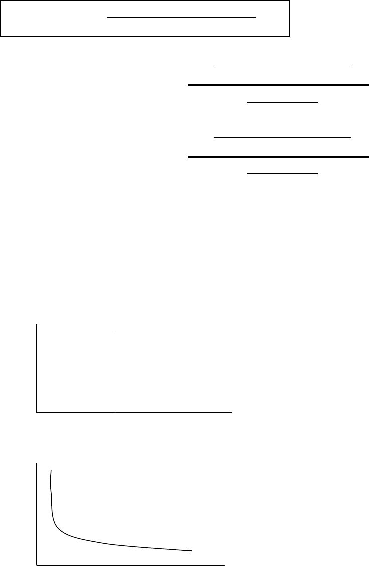
Page 65
Price Elasticity of Demand PED: measures the percentage change in quantity demanded for
a good in response to a change in its own price.
Point Elasticity of Demand =
Arc Elasticity of Demand =
NB: Demand elasticity is normally negative because quantity demanded normally falls when
price rises. However, the negative sign is not always written in.
Value of Elasticity
The value of elasticity may be anything between zero and infinity.
(i) Price Elasticity of Demand PED = 0, i.e. perfectly INELASTIC demand
(e.g. Drugs) (i.e. no change in Quantity Demanded no matter how much price changes)
(ii) Price Elasticity of Demand = 1, i.e. unit elasticity of demand (i.e. any percentage
change in price causes the SAME percentage change in Quantity Demanded.
(iii) Price Elasticity of Demand = , (i.e. infinity) i.e. perfectly elastic, so at the given
price there is an infinite amount demanded but any change in price causes Quantity
Demanded to fall to Zero.
PED =
% Change in Quantity Demanded
% Change in Own Price
Change in Quantity Demanded
Change in Own Price
Change in Price
Original Price
Change in Quantity Demanded
Average of Old and New Quantity
Change in Price
Average of Old and New Price
P
Q
P
Q
h
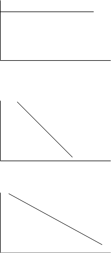
Page 66
(iv) Price Elasticity of Demand < 1, inelastic demand (e.g. cigarettes)
(i.e. any percentage change in price causes a SMALLER percentage change in Quantity
Demanded .
(v) Price Elasticity of Demand < 1, elastic demand (i.e. any percentage change in price
causes a BIGGER percentage change in Quantity Demanded.
Significance of Demand Elasticity
Demand Elasticity is important because it shows the percentage by which quantity demanded
changes when price changes.
1. Total Revenue = Price X Quantity
Therefore, to maximise revenue a price must cause a smaller % fall in Quantity
Demanded or a fall in prices must lead to bigger % increase in Quantity Demanded
otherwise total revenue will fall.
Producers usually want to increase total revenue.
2. The government use Demand Elasticity to help them decide on the optimum tax rate to
charge.
Relationship Between Demand Elasticity and Total Revenue
P
Q
P
Q
P
Q

Page 67
(Knowledge of this relationship is used by Business and Government in setting prices
and tax rates.)
(i) Inelastic Demand and Total Revenue
When demand is Inelastic a Price Increase Raises total Revenue.
(ii) Elastic Demand and Total Revenue
When demand is Elastic, a reduction in price increases total revenue.
(iii) Unit Demand Elasticity and Total Revenue
When demand is unit elastic, a price change causes no change in total revenue because
any price change is cancelled out by an equal and opposite change in Quantity
Demanded.
Factors Influencing Demand Elasticity
1. Availability of Substitutes
The easier it is to switch away from a good the more elastic will its demand be.
2. Time
It is easier to substitute away from a good in the longer-term so demand is more elastic in
the long-term
3. Competitors Policy
If, when one firm changes its price, other firms selling similar goods also change price,
demand will be less elastic (i.e. there will be a smaller change in Quantity Demanded.
4. Percentage of Income Spent on the Good
The higher the percentage spent on the good the more elastic will its demand be.
Income Elasticity of Demand (YED)
Income Elasticity of Demand measures the responsiveness of demand to changes in income.
Income Elasticity of Demand is normally positive because when incomes rise people
consume more of most goods EXCEPT INFERIOR GOODS (e.g. white bread)
If Income Elasticity of Demand is greater than one = income Elastic, i.e. a small change in
income causes a bigger change in Quantity Demanded e.g. Luxury Goods and Services.
If Income Elasticity of Demand is less than one = income Inelastic, i.e. a change in income
causes a smaller change in Quantity demanded e.g. Basic necessities.
Note: There are always some necessities demanded even at zero income, Luxuries are not
demanded until a certain threshold of income has been reached then their demand accelerates
as income increases from there.
YED =
% Change in Quantity Demanded
% Change in Income
Page 68
Cross Price Elasticity of Demand (CED)
Cross Price Elasticity of Demand measures the responsiveness of demand for one good to
changes in the price of another good (i.e. a substitute or a complement).
For Substitutes, Cross Price Elasticity of Demand is positive. (e.g. if the price of butter rises
people switch away from butter to margarine so demand for margarine increases
For Complements, Cross Price Elasticity of Demand is negative. (e.g. if price of cars rises,
people demand less cars and also less tyres etc.)
Elasticity of Supply ( Ys )
Elasticity of Supply measures the responsiveness of SUPPLY to a change in the price of the
good.
NB: Elasticity of Supply is normally positive because suppliers will want to supply more at
high prices because that increases their revenues.
Factors Affecting Supply Elasticity
1. Time (longer time period means more elasticity supply)
2. Alternative Goods that could be Produced (i.e. if easy to switch to produce / other
goods, Elasticity of Supply will be greater).
3. Cost of Attracting Factors of Production and Laying them off. (The cheaper and
easier to get extra factors means higher Elasticity of Supply)
CED =
% Change in Quantity Demanded of Good A
% Change in Price of Good B
Ys =
% Change in Quantity Demanded
% Change in Income

Page 69
Study Unit 4
Costs of Production
Contents
A. Factor and Input Costs
Production Factors and Costs
Fixed Costs
Variable Costs
Total and Average Costs
Marginal Costs
Long-run Costs
_________________________________________________________________________
B. Economic Costs
_________________________________________________________________________
C. External Costs and Benefits
External Costs
External Benefits
Economics of Externalities
Externalities and the Government
__________________________________________________________________________
D. Costs and the Growth of Organisations
Returns to Scale
Economies of Scale
Diseconomies of Scale
External Economies
__________________________________________________________________________
E. Small Firms in the Modern Economy
Economies of Scale
Services
Recent Trends
___________________________________________________________________________
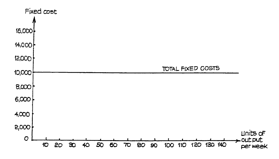
Page 70
A. FACTOR AND INPUT COSTS
Production Factors and Costs
In Study Unit 1 we examined how the factors of production - land, labour and capital -
contributed to total production. We also saw that some factors could be regarded as fixed and
others variable, and that this distinction helped to provide us with the important distinction
between the short run, when at least one significant production factor was fixed, and the long
run when all factors could be varied.
The payments made to the owners of production factors in return for their use in the process
of production are, of course, the costs of production which the production organisation (firm)
has to pay in order to produce goods and services. More strictly these are termed the private
production costs. These factor payments, in very general terms are rent to the owners of land,
interest to the owners of capital and wages to the providers of labour. Disregarding land for
the sake of using very simple models we can, initially, regard capital as the major fixed
production factor and labour as the variable factor.
Fixed Costs
These are the costs of the fixed factors, i.e. those elements which are not being increased as
production or output is being raised. The total fixed costs for a given range of output can be
illustrated in the simple graph shown in Figure 4.1.
Figure 4.1
Examples of fixed costs include rent for land or buildings, the rental charge for telephone or
telex, rates, the salary of a manager, and the fee for a licence to make use of another
RWF
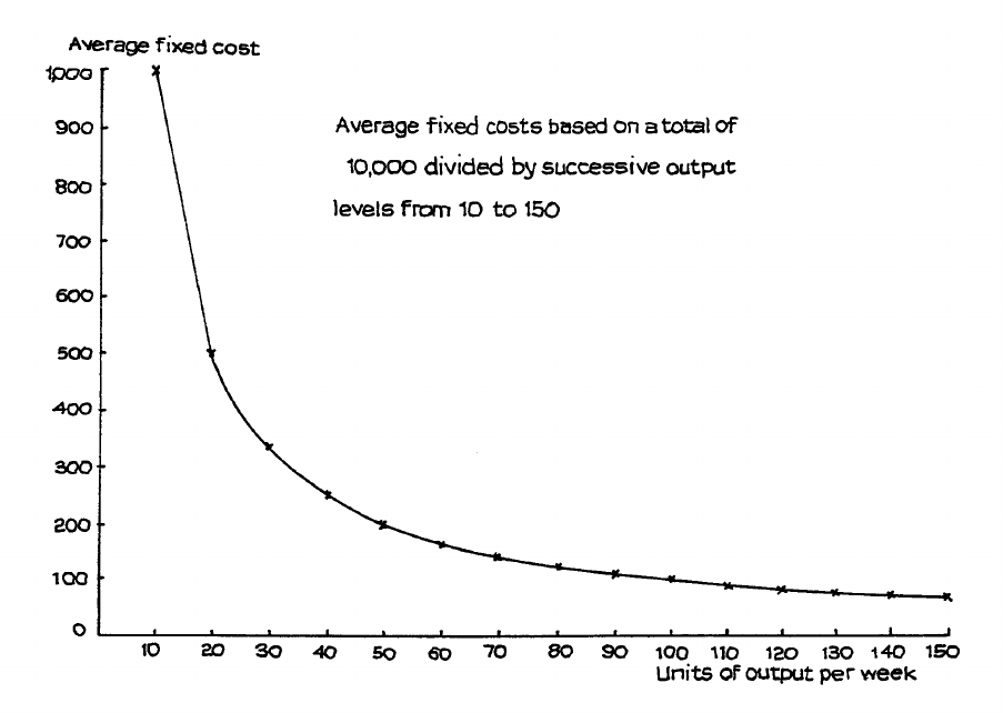
Page 71
company’s patent. All these costs can change, but the point is they do not change as
production level changes. The cost has to be met, whatever the level of output and sales.
The graph of average fixed costs, i.e. total fixed costs divided by the number of units of
output produced, is shown in Figure 4.2. This is based on the fixed costs of RWF10,000
assumed in Figure 4.1. Notice the steep fall at the lower levels of output, and the much more
gentle slope of the curve at higher levels. Between 140 and 150 units of output per week, the
fall in average fixed costs is only from RWF71 to RWF67 (approximately).
Figure 4.2
Variable Costs
These are the costs of inputs which are increased as output increases. They include the costs
of basic materials, of some labour - e.g. engineering machinists paid on “piece rates”
(according to the amount produced) - petrol for delivery vehicles, and so on.
The behaviour of variable costs depends on the pattern of production returns. If production is
rising faster than the input of variable elements, then costs are increasing proportionally less
than the rise in output. This is because each extra unit of input is adding more to production
than it is to cost. This is possible at the lower levels of production represented by 0a in Figure
4.3.
RWF
RWF
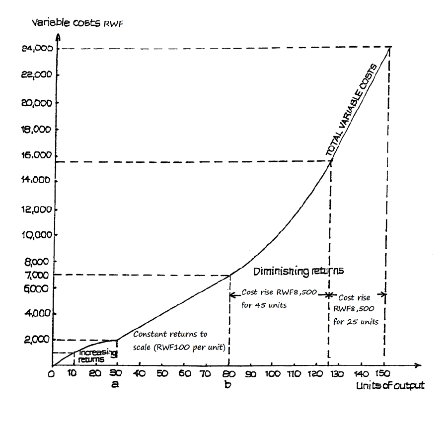
Page 72
Figure 4.3
Later, costs are likely to rise in the same proportion as output - this being the stage of constant
returns, shown between output levels 0a and 0b. Then, as we reach the level of diminishing
returns, costs rise faster (more steeply) than production. This is shown beyond level 0b.
Total and Average Costs
If we combine fixed and variable costs, we obtain total costs. So, if we combine Figure 4.1
which shows total fixed costs, with Figure 4.3, we obtain the graph of total costs. This is
shown in Figure 4.4.
From the total costs we can obtain average total costs, simply by dividing the total by each
successive level of output. Average total costs are often referred to just as average costs.
Figure 4.5 shows the graph of average total costs, which has been derived from the total cost
curve shown in Figure 4.4.
Page 73
This is the typical shape of the curve in the short run (remember, while fixed costs remain
fixed). Because it falls to a minimum point and then rises, it is often referred to as the “U-
shaped” average cost curve, although as you can see, a more accurate description is that of an
L with its toe turned upwards. Only if there are particularly severe increasing costs
(diminishing returns) to scale, and fixed costs are a very small proportion of total costs, will
the second half of the “U” be at all steep, and the efficient firm should never allow itself to
reach this position.
The modern firm is more likely to have a high proportion of fixed to total costs, because of
the swing from labour to labour-saving machinery.

Page 74
Figure 4.4
Marginal Costs
You have already met marginal utility and marginal revenue - the change in total utility or
revenue as output changes. You will not then be surprised to know that marginal cost is the
change in total cost as output changes. Once again, we relate this change to a single unit of
output, so that, if we are moving in steps of ten, as in our cost example so far, we shall have
to divide any change from one step to the next by ten.
RWF
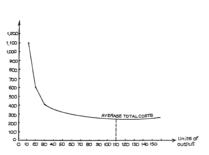
Page 75
Figure 4.5
Table 4.1 is a table of total (fixed plus variable) costs which correspond to our previous
graphs. In this table, further columns have been added to show the change in total cost
between each output step of ten units per week, and then division by ten to produce the
marginal cost. Notice that the figures of the marginal cost column have been placed mid-way
between the figures of the other columns, to emphasise that they relate to a change from one
output level to the next.
On a graph, the marginal cost is plotted at the mid-points of the various output levels. You
will see that this has been done in Figure 4.6, which illustrates the marginal costs shown in
Table 4.1.
RWF
Page 76
1
Quantity
(units per week)
2
Total Cost
3
Changes in Total Cost
from One Quantity
Level to the Next
4
Marginal Cost
(column 3 divided by
10)
RWF
RWF
RWF
0
10,000
100
10
11,000
1,000
60
20
11,600
600
40
30
12,000
400
100
40
13,000
1,000
100
50
14,000
1,000
100
60
15,000
1,000
100
70
16,000
1,000
100
80
17,000
1,000
115
90
18,150
1,150
135
100
19,500
1,350
165
110
21,150
1,650
210
120
23,250
2,100
275
130
26,000
2,750
355
140
29,550
3,550
445
150
34,000
4,450
Table 4.1: Cost Table
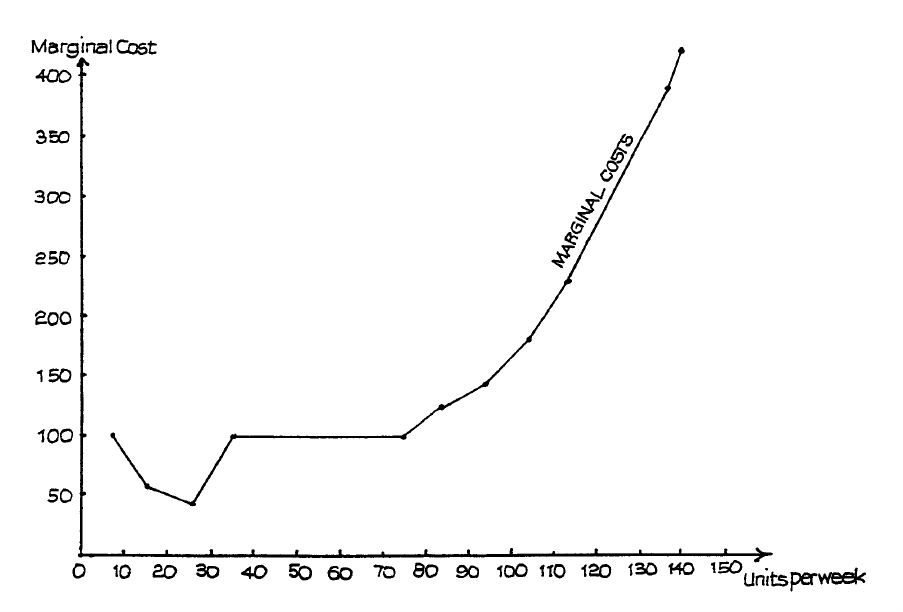
Page 77
Figure 4.6
RWF
Page 78
In Figure 4.7, the marginal cost graph has been combined with the average cost graph. Notice
where these two curves intersect.
The rising marginal cost curve cuts the average cost curve roughly at 110 units per week.
This is the output level which we have already noted as the lowest level of the average total
cost curve. This illustrates a rule that you must remember. The rising marginal cost curve
always cuts the average cost curve at its lowest point. If you think a little, you will see that it
must do that. If the cost of the last unit to be produced is less than the average up to that
point, then the new average will be a little lower. If the cost of the last unit is higher than the
average up to that point, then the new average will be a little higher.
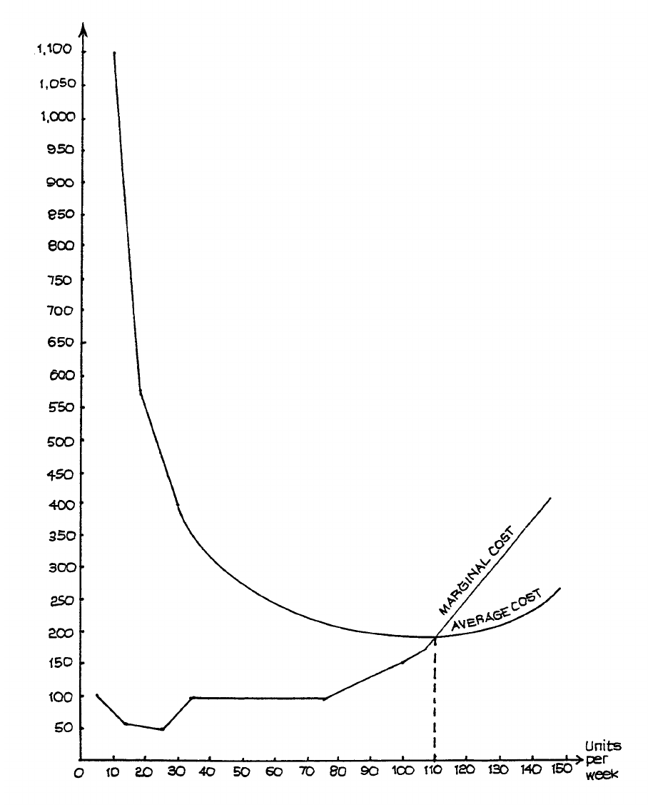
Page 79
Figure 4.7
RWF
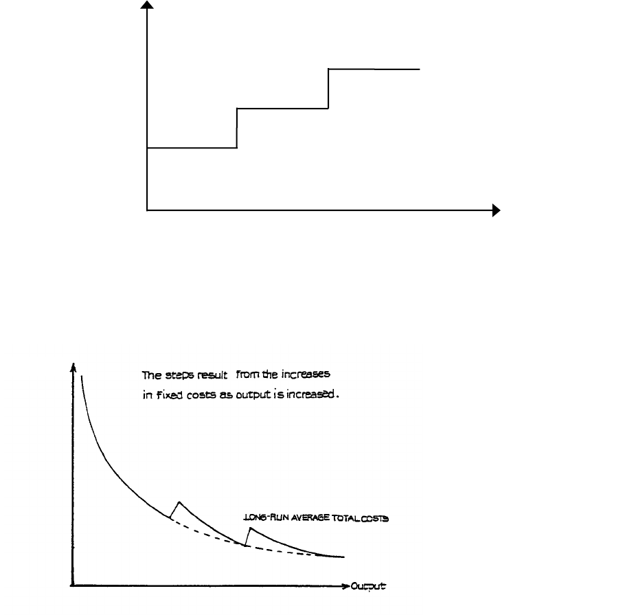
Page 80
Long-run Costs
In the long run all factors of production may be increased, i.e. no costs are completely fixed.
In practice, of course, the factors which are fixed in the short run will be increased in definite
stages - e.g. when a new factory is built, new technology introduced, etc. The graph of fixed
costs in the long run, therefore, appears as in Figure 4.8.
Figure 4.8
The effect of this on the average total cost curve in the long run is shown in Figure 4.9.
Figure 4.9
The “flat” part of the average cost curve is prolonged. The question, then, is whether this
merely stretches the average cost curve - delaying the point of eventual diminishing returns
and the rise of the U shape - or whether it can be continued indefinitely in order to prevent the
U shape completely and make the long-run average cost curve L-shaped.
Costs
LONG-RUN
FIXED COSTS
Output
Costs RWF
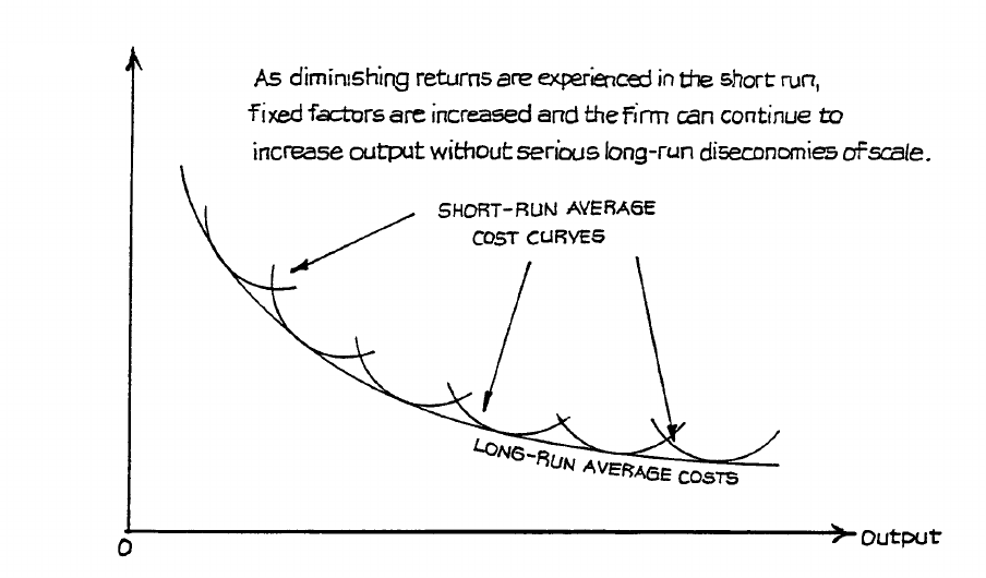
Page 81
The relationship between short- and long-run average cost curves is sometimes shown as in
Figure 4.10. This emphasises the fact that one reason for the increase in fixed factors and
costs is to overcome the effect of short-run diminishing returns.
Figure 4.10
Costs RWF
Page 82
B. ECONOMIC COSTS
We are now beginning to see production costs from a variety of angles.
• Opportunity Costs
These were identified in Study Unit 1 and may be defined as the cost of using resources
in one activity measured in terms of the lost opportunity of using them to produce the
next best alternative that had to be sacrificed.
• Absolute Costs
These are the full costs of the factors used in the activity under consideration. They may
be measured in monetary terms but the real absolute cost is best measured by the actual
quantity of factors used, e.g. the amount of land or the numbers of people employed.
• Private Costs
These are the costs actually paid by the producer to the owners or providers of the
production factors employed. They are the costs usually taken into account by the
accountant and are measured in monetary terms, since the accountant has to account for
the use of whatever finance has been entrusted to the production organisation. We have
been looking at these costs in this study unit and have also examined the important
distinction between fixed and variable costs.
• External Costs
We will go on to look at these now.
Page 83
C. EXTERNAL COSTS AND BENEFITS
These are also sometimes referred to as “externalities”.
External Costs
Not all the costs of factors used in the production process are paid by the producer as private
costs. Suppose, for example, that, during a dry summer, a farmer watered his crops with
water pumped from a canal, and as a result, the canal level fell and it could no longer be used
by waterway travellers. Unless the farmer paid compensation to the travellers, it is clear that
they would be contributing to the costs of the farmer’s production. Because these costs are
being paid by people external to the production process, they are called “external costs”.
We can think of many examples of such costs. Travellers who incur additional fuel and
machine-wear costs resulting from traffic delays, when these delays are caused by repairs
needed to make good damage brought about by very heavy lorries travelling at high speeds,
are contributing to the costs of transporting goods by these heavy lorries. If a proportion of
the cost of road repairs is paid from general taxation, then all taxpayers are contributing to the
costs of road travel - even those tax payers who rarely travel at all.
Other examples of external costs include the poisoning of rivers by industrial waste, the
pollution of sea coasts by waste oil discharged by oil tankers, the sickness and early deaths of
workers from industrial diseases. The list is almost endless, and you can probably add to it
from your own observation. Some costs may even be borne by later generations e.g.
pollution.
External Benefits
In contrast, it is possible for people to receive benefits from production towards the cost of
which they have not contributed. These are external benefits. If a large firm builds modern
roads or provides other transport facilities which are then available for use by the general
community, then that community gains external benefits. If a business firm provides a good
canteen and housing for its workers and, by improving standards of housing and welfare,
improves the health of workers and their families, then this, too, is an external benefit. We
are well aware of cases where firms cause damage to the environment but there are also cases
where firms improve the environment by renovating property, creating sports grounds, or
even parks.
Economics of Externalities
It might be thought that economists would favour external benefits and dislike external costs
but, in fact, economic theory suggests that all externalities distort the use of resources, and
that even external benefits are probably better provided in other ways. The danger of external
costs can easily be recognised. If, for example, road users, especially heavy goods vehicle
users, do not pay the full costs of their road use but pass some of these on to the rest of the
community, then the relative costs of, say, transporting goods by road - as opposed to by rail
or water - are distorted in favour of road. Consequently, goods are carried by road transport at
a higher cost to the community than it would have paid if they had been carried, say, by rail.
The community is not making the most efficient possible use of its available resources, and
Page 84
its living standards are lower than they would otherwise be because some production is being
lost. Moreover, the problem tends to increase. If road transport is artificially cheap, then
goods are diverted to road from rail. Road services are overcrowded, and there is pressure to
devote more land to roads. Rail services are under-used. Agricultural and residential land is
lost to roads to carry traffic which could otherwise have been carried by substitute services.
This is what we mean when we say that externalities distort the use of scarce economic
resources.
Externalities and the Government
What can be done about externalities? Does the community just have to accept their
existence? Clearly neither the producers who are able to pass costs to others nor the buyers of
their goods or services who obtain reduced prices because of the reduction in private costs are
likely to volunteer to pay more unless they are obliged to do so. They could not do so as
individuals in competitive markets. Only the government, acting on behalf of the community
as a whole and reacting to political pressures, can take effective measures and the options
open to government are the following.
• Legislate to make actions considered undesirable illegal and enforce the law. In a
democracy such laws must be acceptable to the community as a whole; care must be
taken to ensure that desirable benefits are not lost and that the cost of law enforcement is
not out of proportion to the costs avoided.
• Legislate to ensure that producers behave in a socially acceptable way and follow
practices designed to avoid the undesirable external costs. Water and sanitation
companies may be required to achieve certain minimum standards. The costs of
complying with the law thus become private costs and part of the production cost which
must be met by users of the goods and services. All producers then become subject to
the same requirements so that none can gain a competitive advantage by not complying
with the standards. If producers have to compete with foreign imports, the government
will have to ensure that these imports are subject to the same minimum standards.
• Impose special taxes designed to make some products very expensive and so discourage
their use. There are several objections to this course of action. The government might
start to rely on the revenue from the taxes and so take care to keep them at a level where
the products are still bought and used; the taxes may well then cease to deter or reduce
the external costs. Alternatively the government might impose very high taxes with the
result that there is widespread tax evasion; the cost of collecting the tax and punishing
evaders then rises to impose additional burdens on the community.
Clearly it is more desirable to try and ensure that external costs are removed altogether than
that they should simply become private costs. Even if employers are forced to pay adequate
compensation to workers whose lungs are damaged by dusty manufacturing processes, the
workers still suffer. However, if manufacturers are required to have efficient dust extraction
equipment, private costs are increased but the health of the workers is improved. At the same
time care must be taken to ensure that external costs are not simply exported. For example,
one way of dealing with dangerous gases might be to ensure that they are expelled through
Page 85
very high chimneys, but unfortunately these may simply redirect the gases to another country
for that country to bear the cost.
There is no universal and simple method of dealing with externalities, but on the whole it
does appear that the market economies have been more successful in controlling and reducing
undesirable external costs associated with environmental pollution than have the old
command economies. This is probably because in the more open and consumer-oriented
societies producers and government have had to be willing to respond to pressures from the
public when that public has been determined to eliminate socially unacceptable practices.
D. COSTS AND THE GROWTH OF ORGANISATIONS
Returns to Scale
We have already seen the results of increasing inputs of a variable factor when at least one
other production factor is held constant. We saw that this was likely to bring about
increasing, then constant, and then diminishing marginal returns. However, we have also
pointed out that, in the long run, all factors can be increased, and there is the possibility of
economies of scale resulting for the continued growth in size of the firm. We must now look
at this possibility more closely, but first we must be clear as to the meaning of returns to scale
when all factors are being increased. If a given proportional increase in factors results in a
larger proportional increase in output, then the firm is enjoying increasing returns, or
economies of scale. This would be the case, for example, if a 10% increase in factor inputs
produced a 20% increase in production output.
If the proportional increase in output is the same as the proportional increase in factor inputs -
e.g. when a 15% increase in factors produces a 15% increase in output - then the firm is
experiencing constant returns. If, however, a 15% increase in factor inputs produces less than
a 15% increase in output - only 10%, say - then the firm is suffering decreasing returns, or
diseconomies of scale.
Economies of Scale
Real scale economies, as defined above, should be distinguished from purely pecuniary or
monetary economies which do not represent a more efficient use of factors but which are the
result of the superior bargaining power of the large firm in the market. A large customer, for
instance, can often gain discounts greater than can be justified on the grounds of savings in
delivery or distribution costs, and workers in some large firms may be willing to accept a
lower wage in return for what is believed to be greater security of employment or the social
prestige of working for a famous organisation. Real economies - the genuine efficiencies in
the use of production factors resulting from growth in the scale of activities - can be identified
in the following main areas.
(a) Labour Economies
Page 86
These result from greater opportunities for the division of labour which increase with the
skills of the work-force, save time and allow greater mechanisation. The automated
assembly line in modern motor-vehicle assembly is an extreme example of this.
(b) Technical Economies
These result chiefly from the use of specialised capital equipment. Large firms are able
to make use of equipment that could not be fully employed by smaller operations, and
large firms are also able to support reserve machines to avoid disruption following
breakdown. A small firm, using three machines, adds one-third to its capital cost if it
tries to add a further machine to keep in reserve. A large firm employing 20 machines
adds only one-twentieth if it decides to do likewise.
(c) Marketing Economies
Very great economies are available from large-scale advertising. A television-
commercial film using “top” stars is very expensive to make, but the cost per potential
customer is very low if essentially the same film can be shown in several different
countries. Large firms can also afford to keep very skilled marketing specialists fully
employed.
(d) Financial Economies
Large firms are able to obtain finance from markets that are denied to small firms, and
multinationals can raise money in many different countries. Nevertheless, although
financial economies still exist, we do have to recognise that finance markets have, in
recent years, become more responsive to the needs of smaller enterprises.
(e) Distribution and Transport Economies
Transport movements and the location of depots can be carefully planned by large
organisations, so that vehicles and storage space are used efficiently.
(f) Managerial Economies
These arise from the employment of specialised managers and managerial techniques,
although many of these techniques have been developed in order to overcome the
problems of managing large organisations, so that many economists suggest that
managerial economies of scale are often exaggerated and difficult to achieve in practice.
Diseconomies of Scale
Diseconomies of scale are usually associated with the problems rising out of the management
and control of large organisations. Formal communication systems are necessary but are
expensive to maintain. Whereas the manager of a small organisation can see what is going on
around him in the course of his daily work, the manager of a large firm may have to establish
an inspection system to obtain equivalent information - which is unlikely to be as reliable.
There can also be a loss of control over managers at the lower levels of the “managerial
pyramid”. These managers may then pursue their own private objectives - e.g. building up
the power of their own department - at the expense of efficiency and profitability.
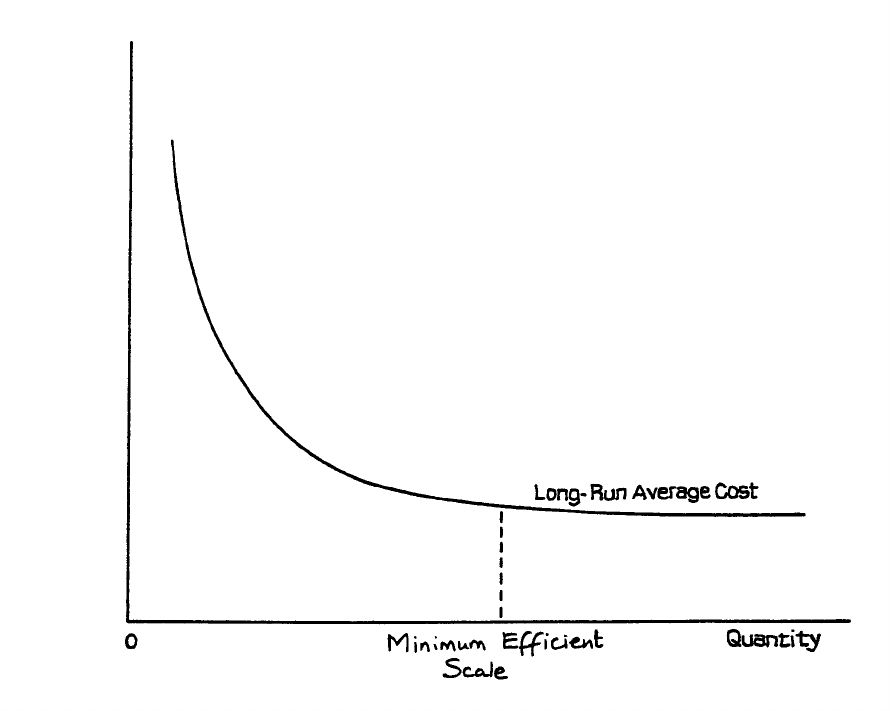
Page 87
Diseconomies of scale, then, are mostly managerial. If diseconomies just balance economies,
i.e. when a 10% increase in factor inputs produces the same (10%) increase in production
output, the long-run average cost curve will have the L shape of Figure 4.11. If economies of
scale continue roughly to balance diseconomies, this shape may be retained over a long
period. If, however, diseconomies start to rise substantially, then the long-run average cost
will again start to rise.
Figure 4.11
Notice here the position of what is called the Minimum Efficient Size (or Scale) (MES),
also known as the Minimum Optimum Scale (MOS). Up to this output level there are
significant gains from internal economies of scale, and firms below the MES are at a cost
disadvantage when competing against those up to or beyond that size. However, beyond the
MES, further cost savings are not significant, and there is no cost advantage in further growth.
On the other hand the shape of the curve can change as firms learn how to overcome sources
of inefficiency, in particular managerial inefficiency, especially when new managerial skills
and communication technology are introduced. It is possible to control very large firms today
in ways that would have been impossible half a century ago. Jet travel and modern
telecommunications, not to mention computers and microelectronics, have transformed
management techniques.
Costs RWF
Page 88
External Economies
The economies of scale listed earlier all apply to the individual firm and they are known as
internal economies of scale. There are other economies that are external to the firm and
which arise when an industry grows large or when business firms congregate in a particular
area. External economies usually arise from the development of specialised services
available to many firms. For example, an area containing numbers of small engineering
companies may provide opportunities to support one or more specialised toolmakers. Each
engineering company can call on the specialist, without having to carry the full cost of having
its own specialised department. External economies help small firms to survive in
competition with larger organisations. However, if one or two companies become dominant
and they internalise these economies by setting up their own specialised departments which
they are large enough to keep fully employed, then the external economies may be lost to the
smaller firms, which can then no longer survive in the market.
E. SMALL FIRMS IN THE MODERN ECONOMY
It is sometimes assumed that, because of economies of scale, large firms are always likely to
be more efficient and to be able to produce at lower cost than small firms. If this were true,
small firms would be much less numerous than they are. Of course, one reason for their
survival is that the definition of a small firm tends to change in time. As the average size of
the firm grows, so firms which would have been considered large become classified as small.
Moreover, if we take as the main qualification to be considered a small firm, the fact that the
whole enterprise is controlled by a small group of employer-managers (usually all belonging
to the one family), continued advances in technology, including information technology,
enable one or two people to control larger enterprises, so that in fact, many more firms can
now grow larger and still, in fundamental respects, remain small.
Economies of Scale
A closer look at economies of scale shows that large firms are not always inevitable. If we
assume that the typical successful large company has an L-shaped cost curve, this can still
cover a number of different possibilities.
Figure 4.12 shows two possible long-run average cost curves. It shows that each reaches a
point where further cost reductions as output increases are very small. As noted in the
previous section, this point is known as the minimum efficient size: it is reached at 0b for
industry B and 0a for industry A. We would, therefore, expect firms in industry A to be rather
larger than in industry B. There is no further significant advantage for firms when they grow
beyond these points.
This minimum efficient size, of course, must be related to the size of the market. If, for
example, industry B served a much larger market than industry A then we would expect many
more firms competing in B than in A. Some world markets have room only for a very few
firms. Here, fixed costs are very high and only very large organisations can consider entry.
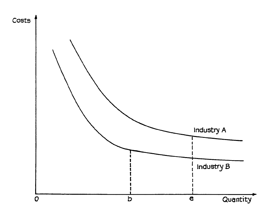
Page 89
Figure 4.12: Long-Run Average Costs
The oil industry is an example of this. In contrast, the manufacture of many kinds of plastic
household fittings does not require very expensive equipment, and many small firms are able
to compete successfully in the market. The general term “economies of scale” also covers
both internal and external economies, and it is only internal economies that favour large
firms. External economies, such as specialised services, are available to all firms in an area
or industry, and these, in fact, often help small firms to survive. It is when the number of
small firms drops below the level necessary for the survival of the specialist as an
independent organisation that all the remaining small firms are faced with severe problems,
and may have to disappear.
Special services to industry - such as industrial cleaners, photographers, designers and others
- often serve a restricted market and are likely to remain small. This is especially likely to be
true if the service is localised. The service may only be needed occasionally by any one firm,
but when it is needed the need is urgent and some one has to be found very quickly. Small
local firms are better placed to provide a satisfactory service than a large national
organisation.
The minimum efficient size is not the only determinant of the size of firm likely to be found
within an industry. The attitudes, abilities and objectives of owners or senior executives play
an important part. We can always expect to find some large firms in sectors when small firms
form the majority.
Page 90
At the same time we are also likely to find small firms in industries where the MES is large,
implying that only very large firms could survive. This may be because they serve a specialist
niche which forms a small part of a larger market. Industry definitions can be misleading.
The term “motor industry” covers activities ranging from motor vehicle assembly to the
manufacture of small, specialised components. These activities are not really comparable and
the MES for a component manufacturer could be much smaller than for vehicle assembly.
Nevertheless it is the giant corporations which dominate the industry. If one of these fails,
large numbers of the satellite firms which supply goods and services to it are also likely to
fail. If the dominant firms all prosper, the satellites also flourish.
Services
Services generally tend to be smaller than manufacturing organisations, although there are, of
course, some very large service firms developing in activities such as the law, accounting and
business consultancy. On the other hand, these large firms tend to serve large-scale
customers. A leading international accountant is not really suited to “do the books” of the
small corner shop. In any case, the shop would not be able to pay the accountant’s fees.
There will always, therefore, be small local firms of accountants, solicitors and so on. If any
of these meet problems they cannot handle themselves, then they may be able to call on the
specialist services of the giant.
As the service sector of the economy, including the rising leisure services, grows, so the scope
for small firms continues to increase and as already suggested, new technology based on the
chip and the microcomputer is enabling the small firm to achieve a level of administrative
efficiency that would have seemed impossible only a short while ago. A business-owner who
can afford to spend around RWF2,000,000 to RWF3,000,000 on a computer, software
packages and a good printer can maintain accounting and secretarial services with just one or
two people, whereas the same standard of service would have required an office of 15 or more
people - or a very expensive mainframe computer complete with specialist programmer - only
twenty years or so ago.
Traditionally, the small-firm sector has been seen as the seed-bed of enterprise and the nursery
in which tomorrow’s giants are reared. The microcomputer industry itself is an example. It
was not the giant computer monopolists that produced the microcomputer but brilliant
electronics engineers working on their own initiative. There will always be scope for the
entrepreneurial genius.
Recent Trends
During the 1980s, in the UK for instance, small firms faced a more favourable financial
climate. Small-scale enterprise became fashionable and received government support through
the Business Expansion and Small Business Loans Guarantee Schemes. The London Stock
Exchange also sought to make it easier for smaller companies to raise capital by developing
the Unlisted Securities Market (USM) and, for a time, a Third Market. The USM was closed
in the mid-1990s and has been replaced by an “alternative market”, the AIM which is
intended to operate more effectively for smaller companies within the structure of the London
Stock Exchange. You should look out for this development and watch its progress.
Page 91
Any form of government intervention tends to distort markets. Even socially worthy schemes
to assist the unemployed can create as many problems as they solve. If, for example, an
unemployed person is given government financial help to start a new window-cleaning
business in an area where demand is roughly in equilibrium with supply from existing
window cleaners, the entry of a new, subsidised cleaner is likely to undermine and drive out
of business one or more of the established small firms which do not enjoy government
financial help. The result may be that one person leaves the dole queue and is replaced in it
by two others.
The banks also became disillusioned with the small-firm sector and reversed the policies that
were proving to lead to heavy losses. There is still official encouragement for the creation of
new small firms, and the number of people entering self-employment always increases when
unemployment rises, as many people decide that the risks of starting in business are
preferable to unemployment; but no one any longer believes that small firms offer a serious
solution to current economic problems.
In an economic depression, large as well as small firms suffer and many companies which had
developed into conglomerates of different, often unrelated, activities as a result of the mergers
of the 1960s and 1970s rediscovered the virtues of specialisation and sold, closed or allowed
managers to “buy out” those enterprises which did not fit into the mainstream of their “core
activities”. Many of the management buy-outs were heavily dependent on bank finance and a
high proportion have become victims of the depression. Others have survived and prospered
once released from the weight of large company bureaucracy. In spite of the difficulties, there
are still large numbers of small firms and as the 1990s have shown that growth and size are
no guarantee of security, fewer of these will wish to grow too rapidly and become too
dependent on borrowed funds.
In recent years earlier tendencies which resulted in large firms internalising specialised
activities have been reversed. Specialist departments which had proved difficult to keep fully
employed have been closed and in many cases the specialists have been helped to form their
own businesses, supported with contracts from their former employers. These newly
independent firms are once again able to provide their specialist services to large and small
organisations.
New communications technology is leading to a revival of a very old form of enterprise -
what may be seen as a collection of independent firms, all working under the overall guidance
of a central, largely marketing, organisation. Computer software production is often produced
on this basis, with self-employed programmers producing software to detailed requirements
set by the central marketing body.
Many small retailers have found it possible to survive as members of a larger “voluntary
chain” made up of retailers and wholesalers, e.g. Super Spar in South Africa.
Franchising is another way in which independent traders work under a degree of central
control. These organisational structures all combine some of the advantages of large-scale
operation with the benefits of the small entrepreneur working for him/herself.
Page 92
Although the life expectancy of the majority of small firms continues to be short, there are
nearly always people willing to fill the gaps left by the casualties. The small firm sector as
such continues to exist and the record of innovation and enterprise from small firms compares
favourably with the large corporations. A healthy and dynamic economy requires a diversity
of firms of all sizes and activities. Most large organisations have occasion to rely on the
services of small firms: often they use them to fulfil contracts which are too small for them to
carry out profitably but which are necessary to retain the goodwill of valued customers.
Moreover the continued existence of smaller rivals can often be a healthy reminder to large
corporations that they are neither immortal nor indispensable. The growth of own-brand
labels developed by the large supermarket chains has provided openings for many smaller
manufacturers who could not otherwise have hoped to compete with the established food
corporations.
The flexibility and versatility of the modern market economy, then, depends on the existence
of many different sorts and sizes of organisation, and this diversity is essential to the
maintenance of high living standards and wide employment opportunities.

Page 93
Study Unit 5
Profit, Supply and Expenditure Taxes
Contents
A. The Nature of Profit
Profit as a Factor Payment
Normal and Abnormal Profit
Profit as a Surplus
Summary of Explanations of Profit
___________________________________________________________________________
B. Maximisation of Profit
Calculation
Profit Maximisation
Do Firms Maximise Profits?
__________________________________________________________________________
C. Influences on Supply
Costs and Supply
Supply Curve
Other Influences on Supply
Effect of Other Influences on Supply Curve
Relative Importance of Supply Influences
__________________________________________________________________________
D. Price Elasticity of Supply
Calculation of Elasticity
Elastic and Inelastic Supply Curves
Elasticity of Supply in the Long Run
___________________________________________________________________________
E. Supply, Indirect Taxes and Subsidies
What Are Indirect Taxes and Subsidies?
Effect on Supply
___________________________________________________________________________
Page 94
A. THE NATURE OF PROFIT
The simplest definition of profit is that it is the excess of revenue over cost. This is a little
deceptive because it is not always easy, in practice, to decide what is revenue and what is
cost, and there are also problems arising from changes in the value of property. For example,
the value of a building may rise or fall for reasons that have nothing to do with the trade
carried on in that building. At this stage, however, it is convenient to overlook problems of
this kind and keep simply to the idea of profit as the excess of the revenue gained by selling
products over the cost of producing those products.
Nevertheless the above definition does not satisfy the economist’s desire to explain why profit
exists and what its economic function really is; and here we come up against two rather
conflicting ideas. On the one hand there is what might be called the traditional view of profit
as a payment to a factor of production, just as wage is the payment to labour or rent the
payment to capital; while on the other there is the view that profit is surplus which remains
when the payments to production factors have all been made. Both views present difficulties
as we shall now see.
Profit as a Factor Payment
Although considered by many as being rather old-fashioned and difficult to reconcile with
modern realities, this is the view which still dominates most of the basic economics text
books and, as far as it is possible to tell, the thinking of most of today’s examiners of
economics in the professional examinations. You must, therefore, take it into account.
Attempts to reconcile the idea of profit as a factor payment with the reality that it is very
uncertain and subject to all kinds of pressures, as well as being impossible to predict or
guarantee, have resulted in the development of the concepts of “normal” and “abnormal”
profit.
Normal and Abnormal Profit
Here profit is seen as a payment to a fourth factor of production, the factor “enterprise”
provided by entrepreneurs, people who take economic risks by organising and combining
the other factors to produce goods and services for sale in the markets. Normal profit is, thus,
frequently described as the reward to the entrepreneur - an attractive idea, but one which
raises many difficulties.
• How do we quantify “normal”? The usual answer to this question is to suggest that it is
the minimum necessary to keep the entrepreneur in the market. However, this surely
depends as much on conditions in other possible markets as on the amount of profit
available in the one under scrutiny. Firms that have been operating in a particular market
for a lengthy period, or which operate in that market only, face greater costs of transfer to
another market than newcomers, especially those which already operate in many markets.
Thus, the minimum required to keep firm A in the market is unlikely to be the same
amount as that sought by firm B. As economics have become more and more precise,
scientific and mathematical, fewer people have been prepared to accept a concept as
vague and unquantifiable as “normal” profit, in this sense.
Page 95
• Why is the entrepreneur entitled to “normal” profit? The early economists who
developed the concept were accustomed to markets containing small, individually owned
and controlled firms, so that the entrepreneur who was the driving force behind the firm
was usually identifiable without much trouble.
Modern markets, on the other hand, are dominated by large, corporate organisations with
clear, bureaucratic, managerial structures. The success of this type of enterprise may lie
as much in the ability of managers to reduce risks as to take them and, while individual
managers may be expected to show enterprise in their work, this is rarely rewarded
directly with a proportionate share in profits - even if the profit attributable to the
enterprise shown could be calculated. The statistical profit of the organisation belongs
legally to the ordinary shareholders, who are specifically denied any right to share in
management and who rarely have much detailed knowledge of the activities of the
organisation. When we further recognise that the large public company, today, is likely to
operate in many markets, in many countries, we have to agree that all this is impossible
to reconcile with the definition of “normal profit”.
If, however, it is accepted that there is such a thing as normal profit then this implies that
there can be “abnormal” profit. Some text books do, in fact, describe all profits above the
normal as abnormal. Others, clearly unhappy at the emotive implications of this term, use the
less derogatory “supernormal”. In either case, the impression is usually given that firms
should not be permitted to earn profits above normal.
Instead of either abnormal or supernormal, some writers have referred to what they call “pure
profit”, by which they appear to mean any surplus over and above all payments to factors
including the “normal” profit due to the entrepreneur.
Profit as a Surplus
If we see profit not as a factor payment but as a surplus remaining after the production factors
have been paid for, the question then arises as to who owns, or should own, this surplus.
To Marxist economists the answer is clear. Economic value is created by human labour,
without which there can be no economic activity. The berries growing wild on the bush
belong to the picker, whose labour of picking has turned them into food. Thus any surplus
created by work belongs to those who carry out the work. Profit, therefore, to the Marxist
who does not recognise a separate entrepreneur, belongs to the workers. However, the
Marxist recognises that, in the modern capitalist society where production is organised by the
owners of capital and, in the Marxist view, for the benefit of the owners of capital, profit is, in
practice, allocated to the owners of capital.
If this view is accepted, profit, not interest, becomes the payment to the owners of capital. To
the Marxist, the fact that it is paid to the owners of capital rather than to the rightful owners,
the contributors of labour, is the result of the domination of capital over labour in the modern
capitalist society.
In support of this view it is possible to point to company law, which provides that a
company’s profit belongs to the company’s shareholders or, more precisely, to the contributors
Page 96
of the “risk capital” or “equity”, the ordinary shareholders - in American terminology, the
common stock holders. There is no legal requirement that the company should share its
profits with the suppliers of labour (employees) or with the suppliers of loan capital, who
receive their agreed rate of interest.
Still largely accepting this concept of profit as a surplus other economists, some of whom
belong to what has been called the “Austrian school”, take a very different view of its
economic function. They see it as the driving force of the modern economy and the incentive
which has been largely instrumental in bringing about the enormous improvement in general
living standards in the market economies over the past two centuries. They see the striving
for profit as the force that produces new products, new production technology, new forms of
business organisation and new uses for basic resources. The profit that produces this
economic energy and invites people of all kinds to take risks with their own resources of
money, time and futures, is not “normal profit” but the largest possible profit that can be made
in the circumstances within which business operates. There is no need to distinguish between
normal and abnormal profit. All profit is necessary to stimulate future economic activity and
to provide the investment finance necessary to make the activity possible and raise the level
of technology.
Unlike Marxists, the economists who take this view do not see profit as being stolen from
workers, nor do they see any need for labour to be given only the lowest possible wage.
Indeed for business enterprise to succeed, goods and services have to be sold to workers
whose incomes are well above subsistence levels, who have disposable incomes and the
freedom to choose how to spend these incomes and who expect to have rising incomes.
Workers therefore, benefit from profitable economic activity by earning rising wages.
Summary of Explanations of Profit
One economist who recognised the various ways in which profit has been explained was the
great American writer and teacher, Professor Samuelson. He identified six distinct “views”,
which can be summarised as follows:
(a) Profit is seen as a balancing item and a result of accounting conventions but should
properly be seen as a return to one or more of the production factors. For example, most
of what accountants show as the “profit” of the majority of small family firms would
better be described as the proprietor’s wage for his physical and mental effort and interest
on his personal savings invested in the business.
(b) The second view sees profit as a reward to “enterprise and innovation” and a return
for the temporary monopoly achieved by being first in the field with a successful new
commercial idea.
(c) The third sees profit as a reward for successful risk-taking and, although willingness to
take risks does not always (or often) bring compensating profits, it is usually the hope of
earning such profits that provides the spur to help business people overcome their natural
inclination to avoid risk.
Page 97
(d) The fourth view simply takes the third view further; profit is a positive incentive to
“coax out the supply of risk-bearing capital”. It is the high return sought by providers
of what is often known as “venture capital”.
(e) The fifth view regards profit as a return to monopoly, whether natural or achieved by
artificial means. It is this association of “abnormal” profit with monopoly that has
coloured so much teaching about business profits and objectives.
(f) The sixth view recognises the Marxist explanation of profit as surplus value which, for
Marx, is properly the reward of the labour that created the value but which, in a capitalist
economy, is appropriated by the owners of capital.
Clearly there is no simple or generally agreed explanation of the economic function of profit,
though most would agree that both profit and a spirit of enterprise are extremely important
elements in modern market economies.
B. MAXIMISATION OF PROFIT
Calculation
We can arrive at the amount of profit for any given level of output in at least two ways. We
can calculate total revenue and total cost and find the difference, or we can calculate the
average revenue and the average cost, find the difference and multiply this by the quantity
sold.
We shall first consider profit as the difference between total revenue and total cost. Suppose
we return to the example of the last study unit and assume that all units of the product are
sold at a given market price of RWF210 per unit. Costs remain as before. We can now show
total revenue and cost columns for each range of output up to 150 units per week - as in Table
5.1.

Page 98
Quantity
(units per week)
Total Cost
Total Revenue
(output level ×
Rwf210)
RWF
RWF
0
10,000
0
10
11,000
2,100
20
11,600
4,200
30
12,000
6,300
40
13,000
8,400
50
14,000
10,500
60
15,000
12,600
70
16,000
14,700
80
17,000
16,800
90
18,150
18,900
100
19,500
21,000
110
21,150
23,100
120
23,250
25,200
130
26,000
27,300
140
29,550
29,400
150
34,000
31,500
Table 5.1
From this table we can see that revenue exceeds total cost at output levels 90 to 130 units per
week. At all other output levels, total costs are greater than total revenue, so losses would be
suffered.
The following table shows the profit at each output level.
Quantity
Profit
RWF
90
750
100
1,500
110
1,950
120
1,950
130
1,300
The position is illustrated in Figure 5.1, where the shaded area represents the profit produced
when total revenue is greater than total cost.
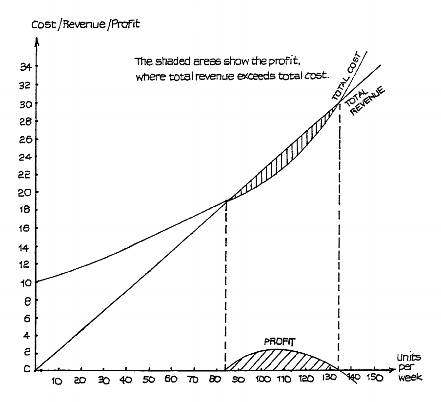
Page 99
Figure 5.1
The same position is shown by the average cost and price/average revenue curves of Figure
5.2. In this case, however, the shaded area does not represent the total profit but the profit per
unit of output. Total profit would be given by multiplying the profit per unit by the number of
units produced.
In this example, the firm is selling all units at a given price, so that the total revenue curve
continues to increase - though this does not, of course, mean that it is possible to make a
profit at output levels above 130 or so units per week.
RWF ‘000
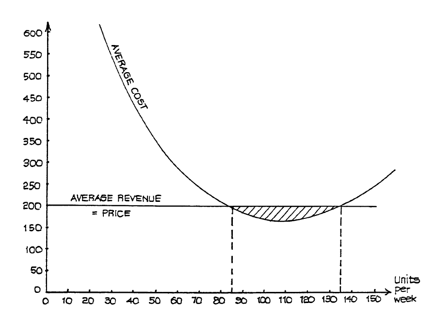
Page 100
Figure 5.2
We saw in an earlier study unit that the revenue position could be rather different where the
firm had to reduce price in order to increase output. Such a situation is illustrated in Figure
5.3. No figures are shown here - this is a general model - and it shows that the firm can make
profits at all output levels between 0a and 0b.
These levels, where total revenue just equals total cost, are called the break-even output levels
or sometimes “break-even points”.
It is often more convenient, however, to show the average cost and revenue curves (see Figure
5.4).
If we assume that the firm is selling all units at any given output level at the same price, i.e. is
not discriminating between different customers over price, then the average revenue curve is
also the price/output curve, i.e. the demand curve. In this model, we can also see that the firm
makes profits between output levels 0a and 0b. This is the quantity range where average
revenue is greater than average cost.
RWF
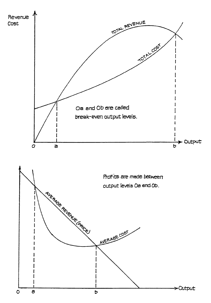
Page 101
Figure 5.3
Figure 5.4
RWF
RWF
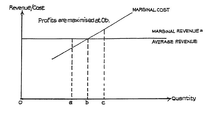
Page 102
Profit Maximisation
So far, we have seen the output levels where profits are made, but we have not yet identified
the output level where the largest possible (maximum) profit can be made. However, if we
refer back to our profit table, we see that there are two points where points are at their largest
- at output levels of 110 and 120 units per week. Here, total profit stays at RWF1,950. If the
firm wants to make the largest possible profit, it can choose either of these two levels. It is
not unusual for profit to have a rather “flat top” and stretch across two stages in this way. In
other cases it can peak at a single stage.
Now look back at Table 4.1 in the last study unit, which showed marginal costs. Bearing in
mind that we assumed the firm to be selling at a constant price of RWF210, look at the
marginal cost column. We have explained that, when the firm can sell at a constant price at
all levels of output, the price is also the average and the marginal revenue. Thus, in this case,
the firm’s marginal revenue is RWF210. If you look down column 4, you will see that the
marginal cost is RWF210 at the mid-point, representing the change from output level 110 to
120 units per week. This is precisely the output range where profits are at their highest level,
i.e. RWF1,950.
This is no accident. It illustrates the general rule that profits are always maximised at the
output levels where marginal cost is equal to marginal revenue.
The general position is illustrated in Figures 5.5 and 5.6. Figure 5.5 shows the case where
average revenue = marginal revenue (constant price at all output levels) and Figure 5.6 shows
the sloping average revenue curve with the marginal revenue curve in the correct position, as
we explained before.
Figure 5.5
In both cases, the argument is the same. It does not matter whether the marginal revenue
curve slopes or not. If the firm produces at output level 0a, i.e. below the level where
marginal cost = marginal revenue, it would pay it to increase output because the revenue
received for each additional unit is greater than the cost of producing that unit. If the firm is
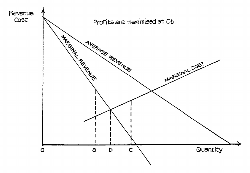
Page 103
producing at output level 0c, above the level where marginal cost = marginal revenue, then it
will pay it to reduce output because revenue lost for each unit of output sacrificed is less than
the cost of its production. Only at output level 0b, where marginal cost = marginal revenue,
will it pay the firm to stay at the same level. It cannot then increase profit by any change in
quantity produced. This is the level where profits are maximised.
This is a most important rule which you should remember carefully, i.e. to maximise profits
the firm produces at the output level where marginal cost is equal to marginal revenue.
Figure 5.6
Do Firms Maximise Profits?
It is often argued that we should not automatically assume firms do seek to maximise profit.
It is suggested that they may have other objectives, e.g. to maximise revenue, to increase
output or to achieve a given share of the market, or simply to please and reconcile the
conflicting objectives of shareholders, managers and employees.
All this may be true - many firms may not be seeking to maximise their profits. Many may
not have sufficient information about market demand and their costs to profit-maximise even
if they wished. On the other hand, this does not rule out our view that the profit-maximising
output level and the rule for achieving this are matters of very great importance for an
understanding of business decisions. The firm may decide to sacrifice some profit in order to
pursue some other objective, but it should know how much profit is being sacrificed.
An assumption of profit-maximising behaviour is an essential starting point for the analysis
of the business organisation. As long as we recognise that it is not necessarily the finishing
point, then we can accept this assumption at this stage of our studies unless there is a very
good reason to do otherwise.
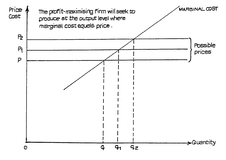
Page 104
C. INFLUENCES ON SUPPLY
Costs and Supply
If we accept that business firms exist to make profits, then we can recognise that there must
be a close link between costs, profits and the willingness of firms to produce the goods and
services that consumers wish to buy. After all, profit is the difference between revenue and
costs, so that at any given price the amount of profit will depend on production costs. If price
remains constant and costs rise, then profit falls and we can expect firms to be less willing to
supply goods and services. Similarly, if costs remain unchanged and price rises, then profits
will rise and firms will wish to supply more in order to secure the increased profit.
We thus have no difficulty in accepting the link between costs and the amount that firms are
prepared to supply at a given price or range of prices. If we accept the aim of profit
maximisation, then we can be a little more precise than this.
Suppose a firm is seeking to maximise profits and can sell all it can produce at the ruling
market price. Suppose, too, that this market price can change. What, then, will be the firm’s
response? Look at Figure 5.7. The profit-maximising firm will seek to produce at that output
level where marginal cost is equal to price, i.e. at quantity 0q at price 0p, at 0q1 at price 0p1,
and 0q2 at price 0p2.
Figure 5.7

Page 105
Thus, we can see that the firm will increase the quantity it is willing to supply as price
increases - and, conversely, reduce quantity as price falls - and that the actual change in
quantity will be governed by the marginal cost curve.
Under conditions of perfect competition, therefore, the individual firm’s supply curve is its
marginal cost curve and, consequently, the market supply curve is derived from the sum of the
marginal cost curves of all the firms operating within the market.
This argument continues to hold good when we abandon the assumption of the firm accepting
the market price. If the firm faces a downward-sloping demand curve for its product, and
hence a downward-sloping marginal revenue curve, we still get the same increase in quantity
following the marginal cost curve if we again move the marginal revenue curve outwards,
further from the point of origin. This is shown in Figure 5.8.
Notice, however, that Figure 5.8 is drawn on the assumption that the average revenue curve is
moving outwards evenly and with its slope unchanged. There is no guarantee that this will
ever happen in practice. If the slope of the average revenue curve changes, then so too will
the slope of the marginal revenue curve, and there will no longer be the smooth increase in
quantity suggested by Figure 5.8. For this reason, we cannot say that, in imperfect markets,
the market supply curve will represent the sum of the marginal cost curves of the individual
firms. Nevertheless, the general link between supply and marginal costs remains, although it
is unlikely to be as direct as in perfect competition.
Figure 5.8
Here again, a movement of the marginal revenue curve produces a shift in quantity supplied,
in accordance with the marginal cost curve.
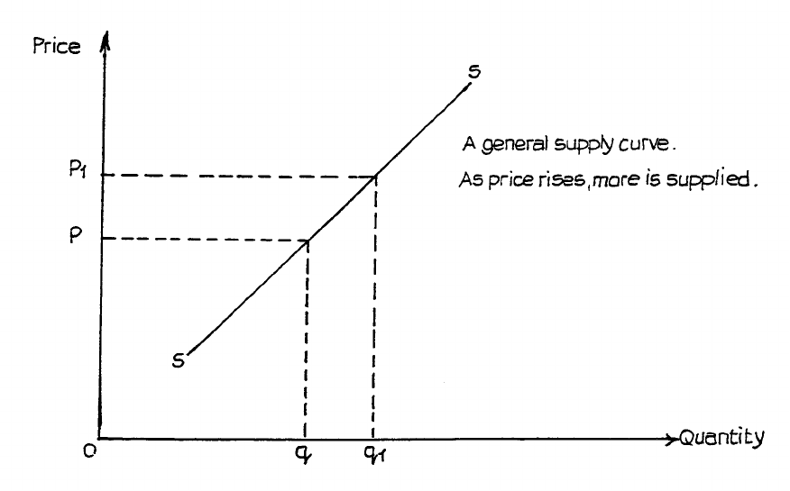
Page 106
You can, if you wish, add the average revenue curves to this graph, and thus show the prices
corresponding to the three quantity levels 0q, 0q1 and 0q2. Remember the relationship
between average and marginal revenue, and remember that price will be shown by the vertical
line from any given quantity level to the average revenue curve.
Supply Curve
If we accept this view that firms will seek to increase the quantity supplied if price increases,
and reduce it if price falls, then we can produce a supply curve showing the amounts
involved. A supply curve can be for an individual firm - in which case, assuming profit-
maximising objectives, it will be the marginal cost curve - or for all firms supplying a
particular product, where it will be made up of the sum of the marginal cost curves of all the
firms supplying the product.
However the supply curve is formed, we can accept that its general shape will be as in Figure
5.9. This shows the general assumption that more will be supplied as the price rises - all
other influences remaining the same.
Figure 5.9
Other Influences on Supply
The concept of the supply curve reflects the view that price is one of the most important
influences on the quantity supplied. There are other influences, however, and these are
mostly concerned with the cost of production and with profits. Remember that, in a market
economy, the great driving force for supply is profit, so anything that affects profit will affect
supply. In very broad terms, since profit is the difference between revenue and costs, supply
will be directly affected by anything affecting revenue, price and costs.
Page 107
We can summarise some of the most important influences as follows:
(a) Costs of Factors and Other Inputs
Any change in costs, with price staying constant, will change the profit expectations and
will thus influence decisions regarding supply. For the profit-maximising firm, a change
in variable costs will change the marginal cost curve, and so change the supply schedule.
Examples of factor costs include wages, land and property rents, interest rates on capital,
basic material prices and the prices of fuel and power. Any of these may also affect the
prices of intermediate products and services required by the firm, and so further influence
supply.
(b) Changes in Taxes
If a tax, payable to the government, is charged at any stage of production or on the profits
of the business, then any change in the tax rate will affect the profits anticipated from
supply, and thus affect supply intentions. An increase in a production tax, such as value
added tax, will have the same effect as an increase in factor costs; it will tend to reduce
the quantity that firms are willing to supply at all prices in a given range.
(c) Changes in Technology
By “technology” is meant the methods of combining factors and inputs in order to
achieve production. An improvement in technology, which allows a given level of
production to be achieved with fewer factor inputs or with a different combination of
factors, so that the total cost is lower, will tend to increase the quantity likely to be
supplied at all prices within the range. Some types of technology may be possible only if
production is required on a large scale. This can have a marked effect on supply. Thus,
small-scale supply may be possible only at much higher prices than large-scale supply,
when the different technology becomes worthwhile. The result may be to shift the whole
supply curve when production reaches the critical level required for the large-scale
technology.
(d) Efficiency of the Firm
Multinational production of similar products has shown that firms in country A can
sometimes produce more from a given combination of labour and capital than similar
firms in country B, even though production methods and levels of technology are all
much the same. Differences in the productivity of labour and capital (the amount
produced per unit of labour and capital) must, in these cases, be caused by differences in
managerial efficiency or in the conditions under which people work. In some cases, the
movement of managers from one country to the other makes little difference to the gap in
factor productivity. The causes of these differing levels of efficiency are not fully
understood, but they do help to explain why large multinational firms tend to prefer some
countries to others. A change in the level of business efficiency will, of course, influence
supply.
(e) Changes in Relative Profitability of Products
If a firm can produce either product X or product Y from similar factors, machines and
skills, and if it becomes more profitable to produce Y, then the firm is likely to switch its
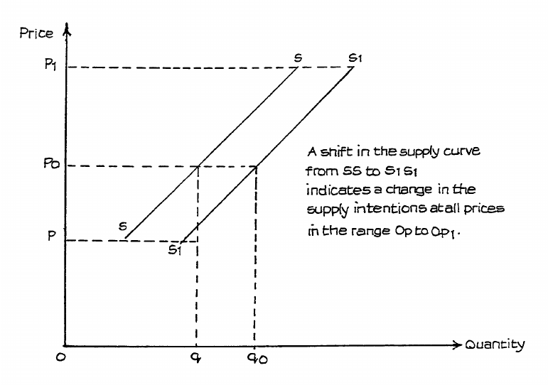
Page 108
production activities from X to Y. This may happen if the firm normally makes X, but
the price of Y rises while the price of X stays the same.
There can be other causes of production switches. If there are numbers of firms able to
choose between producing X or Y, and the market for Y suddenly disappears, perhaps
because of a political decision, then firms previously making Y will have to switch to X
if they wish to remain in business. The result will be to increase the supply of X at all
prices.
Effect of Other Influences on Supply Curve
All the above changes can be illustrated by a movement of the whole supply curve, indicating
a change in supply intentions throughout the given price range. Such a shift in the supply
curve is illustrated in the general graphical model of Figure 5.10.
Figure 5.10
A shift of this type may follow a change in one or more of the influences as described above.
Moreover, several influences may be operating, in different directions. For example, a tax
increase may be depressing supply intentions while an improvement in technology is raising
them. The final result depends on the relative strength of the influences. It is not easy to
analyse these effects through simple graphical models. This is why more advanced studies
make rather more use of algebraic models which can be easily handled by computers, and
why you should begin to become familiar with functional expressions such as the following:
Page 109
Qs = f(P, C, T, v, y,
π
o
)
where Qs = quantity of a product supplied
P = product’s price
C = factory and input costs
T = business taxes
v = level of technology
y = level of business efficiency
π
o
= relative profitability of products
This simply states that quantity supplied is a function of, or is dependent on, the various
influences symbolised.
Relative Importance of Supply Influences
As with demand, different products will be affected to different degrees by the various
influences on supply. In the case of supply, much will depend on the methods of production
and the ease with which producers can respond to changes in factor costs and availability as
well as in technology. Consequently, it is easier to assess the relative importance of the
supply influences than those on demand. A careful study of production technology and
relative factor costs will indicate which are likely to have the most impact on producer
intentions. A production process heavily dependent on labour (labour-intensive) will be more
responsive to changes in wage levels than one that is highly mechanised or automated and
thus capital-intensive. On the other hand, production which is highly capital-intensive will be
more vulnerable to changes in interest rates, since much capital is likely to be borrowed in
one form or another. The potential costs of changing production levels tend to be greater with
capital-intensive production methods.
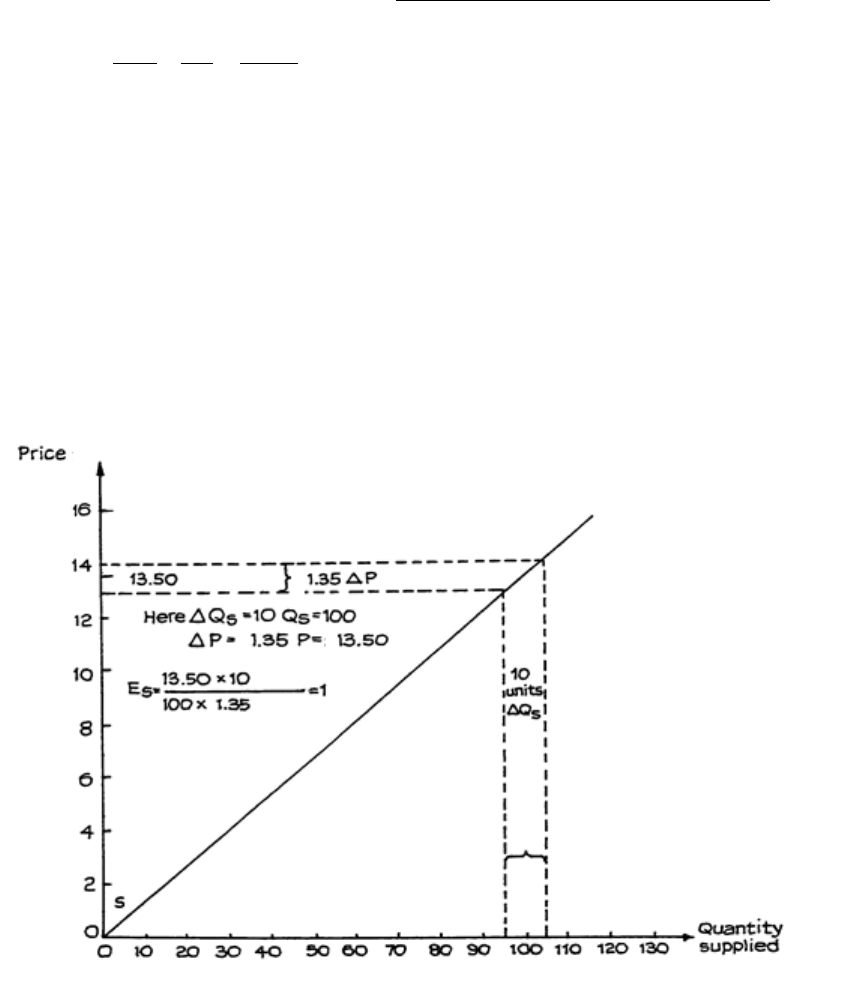
Page 110
D. PRICE ELASTICITY OF SUPPLY
Calculation of Elasticity
The concept of elasticity, which we applied to demand, can also be applied to supply.
However, here it is usually only price elasticity with which we are concerned. The method of
calculating supply elasticity is exactly the same as for price elasticity of demand, i.e.
Supply elasticity of a product (Es) =
Proportional change in quantity supplied
Proportional change
in the product's price
or Es=
∆ ∆ ∆
∆
Q
Q
P
P
P Q
Q P
s
s
s
s
÷ =
Notice that the value of Es is always positive (+). This is because the change of quantity is in
the same direction as the change in price.
Figure 5.11 shows an example of a simple supply-elasticity calculation.
Notice here that figures for both P and Q are obtained from the mid-point of the change in
price and quantity, so that the calculation is the same for both a rise and a fall in price. Notice
also that the result of this particular calculation is that Es = unity (1).
If you calculate values for Es at any other price level on this curve, you should obtain the
same results. The reason for this is explained in the next subsection.
Figure 5.11
RWF ‘000
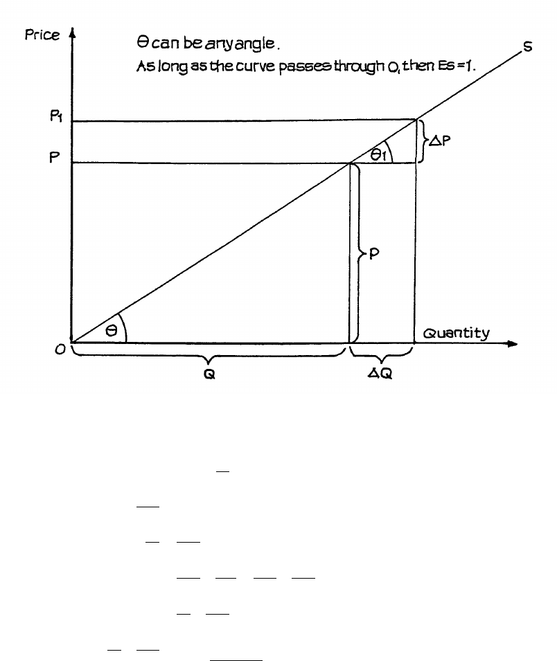
Page 111
Elastic and Inelastic Supply Curves
Price elasticity of demand was shown to change as price changed. A rather different position
obtains in the case of supply elasticity. We said that the value of Es for the supply curve of
Figure 5.11 would always be 1. This is because the curve starts at the point of origin.
A simple proof follows, relating to Figure 5.12, and assuming a knowledge of simple
geometry.
Figure 5.12
From the diagram:
θ θ θ
θ
= =
=
=
= ÷ = ×
= ×
× =
1
1
s
s
and
P
Qtan
and P
Qtan
so P
Q
P
Q.
But EQ
Q
P
P
Q
Q
P
P
P
Q
Q
P
so P
Q
P
Q1and E = 1.
∆
∆∆
∆
∆∆∆
∆
∆
∆
∆
∆
A supply curve which passes through the vertical (price) axis is elastic, and one which passes
(or, if extended, would pass) through the horizontal (quantity) axis is inelastic. This holds
regardless of the slope of the curve, and it applies to the whole curve when this is linear
(forming a straight line).
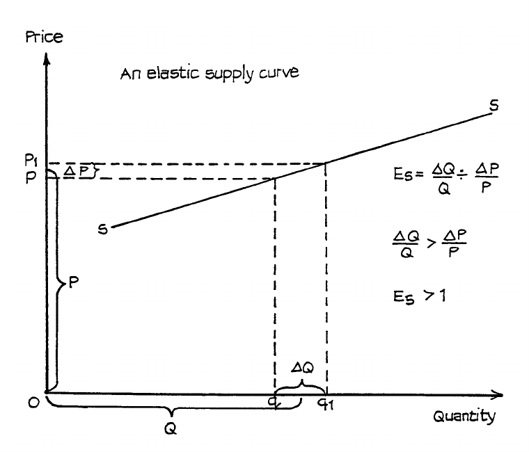
Page 112
These statements can be proved by the same method as in Figure 5.12. Don’t worry if you
can’t prove them yourself - just remember the position. Examples are given in Figures 5.13
and 5.14.
Figure 5.13
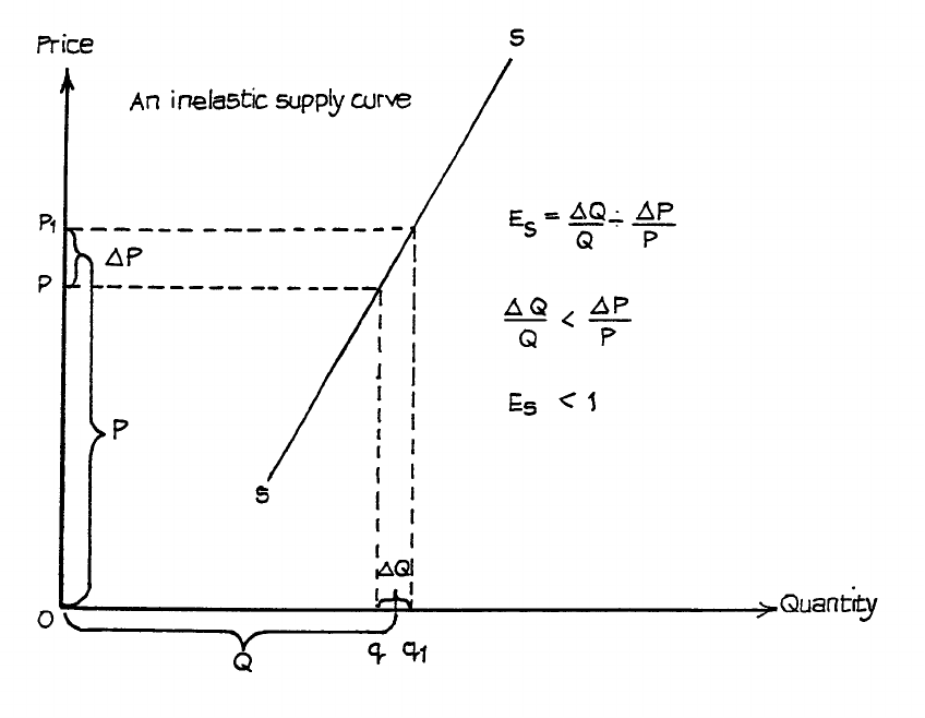
Page 113
Figure 5.14
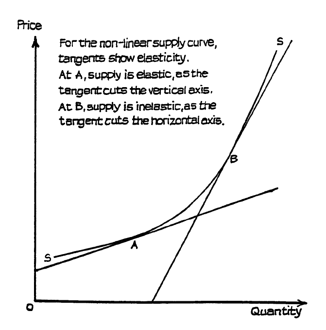
Page 114
Figure 5.15
When the curve is non-linear, the important point is the direction of the tangent to the curve at
the price level under consideration. This is shown in Figure 5.15.
Elasticity of Supply in the Long Run
The main influence on the elasticity of supply is the speed with which producers can respond
to changes in cost, price and profitability. Few firms can alter their production plans
immediately when basic materials, capital and labour have already been committed to them.
As time goes on, however, plans can be changed, workers can be hired or fired, and new
machines bought or old ones scrapped.
The speed and ease with which production plans can be changed depends on the nature of the
production process. As a general rule processes, such as services, which are labour-intensive
can be changed more quickly than those that are capital-intensive. Workers, especially if they
are part-time can have their working hours increased or reduced and the number of workers
employed can be changed, whereas capital-intensive processes, such as motor-vehicle
assembly lines, still have to pay costs of capital even when equipment is no longer used. It
may, therefore, be better to maintain production as long as variable costs are covered by sales
revenue and there is some contribution to unavoidable fixed costs rather than suffer the heavy
losses of a major production change. When, however, the decision has to be made to reduce
production the consequences can be swift and far-reaching, with large numbers of workers
suffering redundancy.
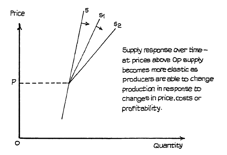
Page 115
We can say, then, that supply will be inelastic in the short run and elastic in the long run.
What constitutes ‘short run’ and ‘long run’ depends on production methods. Nevertheless,
supply is unlikely to be completely inelastic even in the very short term, as some adjustment
is usually possible. Even the motor-assembly track can be speeded up or slowed down, in
response to a managerial decision, in a matter of hours.
The change in elasticity over time is illustrated in Figure 5.16.
Figure 5.16
E. SUPPLY, INDIRECT TAXES AND SUBSIDIES
What are Indirect Taxes and Subsidies?
Governments often influence markets through taxes and subsidies.
• An indirect tax is one that is not levied directly on individuals or organisations but is
applied at some stage in the production or distribution of goods or services. It therefore
affects prices and so is paid indirectly, through price, by consumers and income-earners.
For this reason indirect taxes are often referred to as expenditure taxes.
• Direct taxes are those levied directly on income or wealth as it is created and are paid by
the income- or wealth-earner to the government. The economic implications of direct
taxes are considered later in the course.
At this stage, however, it should be clear to you that anything that influences market price will
have consequences for both supply and demand, with the result that the final consequences of
a tax may not be what the government intended.
Sometimes, of course, the tax may be imposed with the deliberate intention of influencing
supply or demand, but more often it is levied as just another way to raise the revenue that
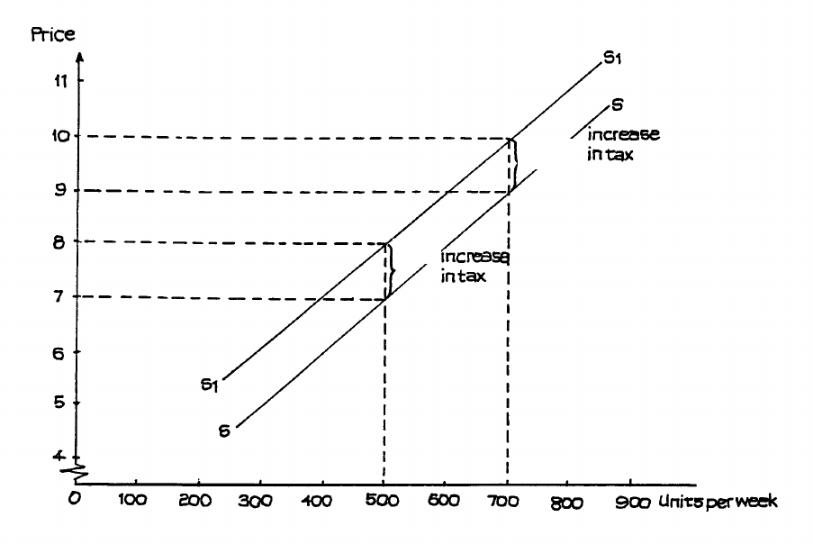
Page 116
governments imagine they need, and they seek to have as little effect as possible on the
production system. In practice, any tax must have an impact, as we shall see.
A subsidy can be seen as a reverse or negative tax. It is a payment to a producer or
distributor, so that its effect is to increase supply. To judge the effects of a subsidy, therefore,
simply reverse the arguments presented in relation to the tax - but remember, of course, that,
in order to pay a subsidy, the government has to have revenue, and its main source of revenue
is tax. Generally, then, a subsidy paid to A means that B and C have to be taxed. The harmful
effects of the tax may outweigh any beneficial effect of the subsidy.
Effect on Supply
The effect on supply of an indirect tax being imposed is illustrated in Figure 5.17. This
shows a supply curve SS, indicating that production can range from 200 units per week at a
price of RWF4 to 800 units at a price of RWF10.
Suppose a new tax is imposed at RWF1 per unit. To supply 500 units per week, producers
wanted a price of RWF7 per unit. After the imposition of the tax, the producers still want to
receive RWF7, but to get this, the price has to rise to RWF8 to include the RWF1 per unit that
now has to be paid to the government. Similarly, to keep production at 700 units per week,
the price has to rise from RWF9 to RWF10 per unit.
Imposition of the tax thus moves the supply curve to the left (SS to S1S1). The vertical
distance between the curves represents the amount of the tax.
Figure 5.17
Of course, a subsidy paid to the producer moves the supply curve to the right because the
argument is exactly reversed.
RWF
RWF 1
RWF 1
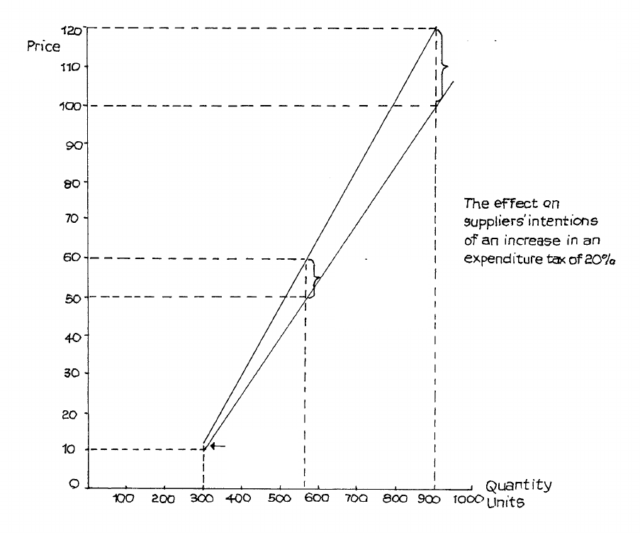
Page 117
In Figure 5.17 the after-tax supply curve S1S1 is parallel to the before-tax curve of SS. This
suggests that the tax or tax increase is “flat rate”, i.e. the same at all price levels. In practice
indirect taxes such as VAT depend on value and are sometimes known as ad valorem taxes.
Usually we would expect the tax to be expressed as a percentage of value or price, and its
amount will therefore increase as price rises. In such cases the gap between the two supply
curves will increase at the higher prices as illustrated in Figure 5.18.
Although suppliers will be seeking to recover the full amount of any additional expenditure
tax from buyers there is no guarantee they will succeed in raising the price sufficiently to
achieve this. The extent to which they can recover the tax or have to absorb it in their total
costs through the more efficient use of their production resources depends largely on the
strength of any price resistance shown by buyers. If buyers cease to buy the product at the
increased price suppliers must reconsider their position. The possible consequences of this
interaction between suppliers and buyers are examined in Study Unit 6.
Figure 5.18
The effect on suppliers’ intentions of an increase in an expenditure tax of 20%.
RWF
RWF20 increase in tax
RWF10
increase in
tax
RWF2
increase

Page 118
BLANK
Page 119
Study Unit 6
Markets and Prices
Contents
__________________________________________________________________
A. Nature of Markets
The “Economic Good”
Market Area
Communications and Transport
Conditions of Supply and Demand
__________________________________________________________________
B. Functions of Markets
Information
Establishing Price
__________________________________________________________________
C. Prices in Unregulated Markets
Definition of Unregulated Market
Equilibrium Price
Changes in Intentions - Shifts in the Curves
_________________________________________________________________
D. Price Regulation
Reasons
Effects of Price Controls
_________________________________________________________________
E. Market Defects - The Case for a Public Sector
Defects in Market Allocation
The Case for a Public Sector and its Boundaries
__________________________________________________________________
F. Price Changes and Indirect Taxes and Subsidies
Effect of Tax on Price
Subsidies
Government Use of Indirect Taxes
__________________________________________________________________
Page 120
A. NATURE OF MARKETS
In economics, a market is an area within which the forces of demand and supply for a
particular “economic good” can communicate and interact, so that the good can be transferred
from suppliers to buyers.
This definition contains a number of important elements which have to be considered
whenever we analyse a particular market or compare one market with another. Let us look at
these elements.
The “Economic Good”
A “good” is any benefit which accords utility to people, and to obtain which they are prepared
to sacrifice scarce resources. The term “utility” is chosen because it avoids the idea that there
has to be any particular virtue in the “good”. If people want something and are prepared to
make some sacrifice of their resources (usually represented by money) to obtain it, then we
assume they gain utility from it, even if it does them actual harm. Thus, economists may
analyse the markets for tobacco or heroin.
The “good” can be a physical object, such as a motor car, or a service. It can be a consumer,
or intermediate, or capital good, or a factor of production. In this course, we are concerned
chiefly with consumer and production factor markets.
We must be careful to give a precise definition of any market we are considering. The total
market for motor cars contains a number of subsidiary markets - e.g. for sports cars or saloon
cars. We must always distinguish the market for the whole class of product from that for a
particular brand or other sub-division. Thus, the market for the Toyota Corolla is distinct
from the market for small cars - which, in turn, is distinct from that for private cars and from
the market for personal transport as a whole.
Confusion sometimes arises when we are concerned with the price elasticity of demand for a
product. The class or product may be price inelastic, whereas a particular brand may be price
elastic. For example, petrol in general may be price inelastic, but the price of K’s petrol can
be price elastic. The motorist has to have petrol, but he may have the choice of a number of
filling stations offering a variety of petrol brands at different prices, and he may also be
prepared to go a few miles out of his way to obtain the cheapest brand of petrol.
Market Area
We need to examine the market area when considering the conditions of a particular market.
The area is that within which communication takes place, and not simply where final
negotiation is arranged. A sale of antiques or fine paintings may take place in a small room
anywhere in the world but, beforehand, catalogues may have been sent to dealers throughout
the world, and many foreign buyers may be represented by their agents when the sale or
auction actually takes place. In contrast, a small retail shop may be concerned with a market
area restricted to a few streets or a single housing estate. The goods it sells may be available
in other shops serving different market areas nearby.
Page 121
Communications and Transport
The extent of the market is really determined by the efficiency of communications and the
ability to transport the goods from seller to buyer. X does not really have a choice between
goods A and B if he does not know that B exists, or if he has no means of comparing price or
quality. Thus, if I am buying tomatoes on one side of the town, I cannot really compare them
with those on sale on the other side of the town, even if someone tells me that they are several
pence cheaper. I need to be sure that they are products of similar quality.
Some markets have developed very precise descriptive terms. The use of these terms, for
example, in some of the basic commodity exchanges, enables buyers and sellers to know
exactly what quality goods are being traded.
There can be an effective market only if it is possible to transfer the product from seller to
buyer. Any barrier to transfer will limit the market area.
Conditions of Supply and Demand
There can be a market only if there are suppliers able to deliver the goods at the time agreed,
and buyers with the necessary resources to acquire them.
The good does not necessarily have to be in existence at the time it is traded, as long as there
is a guarantee that it will be available when and where agreed. The ability of certain
commodity markets to trade in crops not yet grown, or metals not yet mined, is well known;
but a manufacturer can also agree to sell goods not yet made, and a few authors can even sell
books not yet written! However, both buyer and seller must have a clear idea of the product
that is to be delivered. The more precise the definition of a product, the easier it is to sell in
this way.
The desire to buy must also be realistic. Many of us would like to possess an ocean-going
cruiser or a private aeroplane; but few of us, unfortunately, have the resources to acquire and
operate them.
B. FUNCTIONS OF MARKETS
A market has other purposes, apart from providing the means whereby a good is transferred
from supplier to buyer.
Information
The market serves to convey information about the conditions of supply and demand. I may
go to a furniture store, not just to buy a piece of furniture but to see what furniture is available
and at what price. The better the communication system within the market, the more
information I can gain about what can be bought - and the more chance I have of achieving
full utility from my purchase.
This communication function works both ways. The market also informs actual and potential
suppliers about the strength and pattern of demand - about what people want to acquire and
Page 122
what level of price they are prepared to pay. Suppliers need this information in order to plan
production.
The problem from the supplier’s point of view is often that the information comes too late.
He has to make supply decisions before accurate information is available. The supplier wants
to know today what market conditions are going to be like tomorrow. The impossibility of
achieving accurate forecasts all the time is one of the main sources of business risk.
Establishing Price
Arising out of the two-way communication function is a further most important function -
that of establishing the price at which the buyer is willing to buy and the supplier willing to
supply. How this may be achieved is the subject of much of the rest of this study unit.
It is such an important function of the market that some large firms ensure that certain
markets continue to operate only because they need a reliable mechanism for price-setting.
The large manufacturing companies do not really need to buy metal on the London Metal
Exchange - they can obtain all they need direct from suppliers. But they do need to know the
conditions of demand and supply in the main areas where metal is bought and sold. By
keeping the metal exchange in operation, they obtain this information, which provides a
price-setting mechanism and so helps to reduce some of the uncertainties which they have to
face in obtaining essential materials.
C. PRICES IN UNREGULATED MARKETS
Definition of Unregulated Market
The term “unregulated” here means not subject to any price-setting regulation. An
unregulated market can be subject to detailed regulations regarding the conditions of payment
and transfer and the procedures for settling disputes. These, however, assist rather than
impede the free communication of buying and supplying intentions, and allow them to
interact in order to establish a market price. An unregulated market is, thus, one in which the
forces of supply and demand are free to interact, without any form of outside price control.
We tend to think of regulation in terms of control by the State or its agencies, but a market
can, of course, be controlled in other ways. Certain local art and antiques auctions are
reputed to have been controlled by rings of dealers who agree not to bid against each other
and to share purchases among themselves after the auction. This is not an unregulated
market! The prices paid for goods at such an auction are not “market” prices because they do
not reflect the true conditions of demand.
Equilibrium Price
The equilibrium price is the one at which the intentions of suppliers are just matched by the
intentions of buyers, i.e. where the amount of the good demanded is just equal to the amount
provided. In this state there is no pressure from either supply or demand to move away from
this price, so the market forces are in a state of rest - in equilibrium.
Page 123
We have examined the concepts of supply and demand schedules and “curves”. If we put
supply and demand schedules and curves together, we can arrive at the equilibrium price, i.e.
the “market” price.
Suppose we have the supply and demand schedules for the product “Whizzo” as set out in
Table 6.1 and illustrated in Figure 6.1.
Price per kilo Quantity (kilos per week)
RWF
Producers willing to supply
Consumers willing to buy
1,500
200
700
2,000
300
675
2,500
400
650
3,000
500
625
3,500
600
600
4,000
700
575
4,500
800
550
5,000
900
525
Table 6.1: Supply and Demand Schedules for “Whizzo”
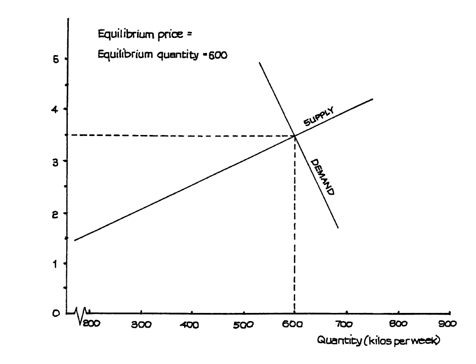
Page 124
Figure 6.1
We can see from the schedules and the graph that it is only at price RWF3,500 (600 kilos per
week) that the intentions of producers and buyers are the same. At any higher price,
producers will be supplying more than buyers are willing to buy. At any lower price,
producers will not be supplying enough “Whizzo” to meet demand. RWF3,500 is the
equilibrium price, and 600 kilos per week the equilibrium quantity. As long as neither set of
intentions changes, there is no incentive for any movement away from this price and quantity,
once it is achieved.
Changes in Intentions - Shifts in the Curves
We can show the concept of equilibrium price and quantity in a general graphical model, as in
Figure 6.2. Here, equilibrium price is Op and equilibrium quantity Oq - the price and
quantity level where the supply and demand curves intersect. We can develop this approach
to analyse the result of movements in the supply and demand curves.
RWF ’000
per kilo
RWF3,500
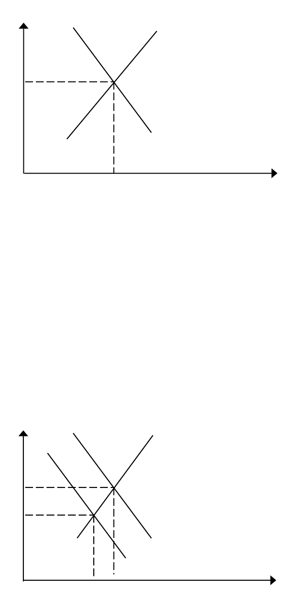
Page 125
Figure 6.2
(a) Change in Either Demand or Supply
Look at Figure 6.3. Here there is a shift in buyers’ intentions, caused perhaps by a
change in taste, supported by an increase in advertising. The result is a movement of the
demand curve from DD to D1D1.
In this model, supply intentions remain unchanged. The result is an increase in the
equilibrium price and quantity from Op, Oq to Op1, Oq1.
We can use the same technique to illustrate the effect of a shift in suppliers’ intentions.
This is shown in Figure 6.4, where supply falls from SS to S1S1. Demand intentions
remain unchanged (DD) and the equilibrium price and quantity move from Op, Oq to
Op1, Oq1.
Price rises and quantity traded in this market falls.
Figure 6.3
Quantity
Price
D
S
P
D
S
O
q
q1
q
Price Price
Quantity
P
P1
D
D
1
D
S
D1
S
q
1
q
O
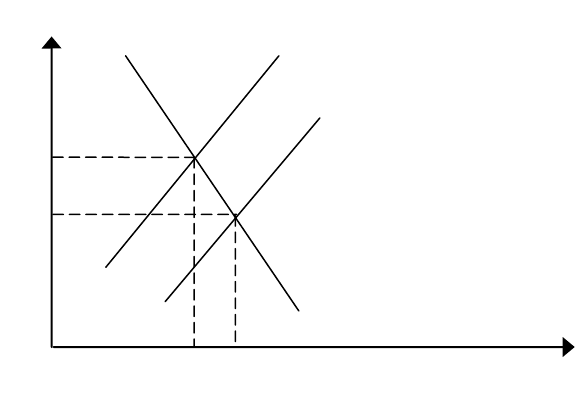
Page 126
Figure 6.4
(b) Change in Both Demand and Supply
So far, we have considered only a possible shift in demand or supply. In practice, of
course, a movement in one is likely to influence the other through the effect on price and
quantity.
Suppose there is a major increase in demand, represented by a movement of the demand
curve in Figure 6.5, from DD to D1D1. This shift, if supply remains unchanged at SS,
results in an increase in equilibrium price from Op to Op1, and in quantity from Oq to
Oq1.
Now suppose that this increase in quantity makes it worthwhile for one or more
producers to develop new production methods, so that the good can be mass-produced at
a lower unit cost. The result, after a time interval, is to shift the supply curve from SS to
St+ 1 St + 1. Here the t + 1 indicates a change in time-period.
The new supply schedule, combined with the increased demand, produces a fresh
equilibrium price and quantity at Opt + 1, Oqt + 1. We have the apparently unusual result of
an increase in demand resulting in a reduction in market price. Note, however, that this
can happen only when given some rather special assumptions about the stage of a
product’s development and the possibility for change in supply conditions.
Price
Quantity
P
P
1
S1
S
1
D
D
S
S
q
1
q
O

Page 127
Figure 6.5
Normally, we expect an increase in demand to raise equilibrium price and quantity. This is
the direct effect. The later reduction in price can result only from a shift in the supply curve,
indicating a completely new set of supply conditions.
A somewhat similar process can be initiated by a change in technology allowing mass
production at a reduced price. Here, there is first a shift outwards in the supply curve.
Demand then rises, but not enough to stop the price from falling. Consider the market for
pocket calculators in this light.
qt+1
q1
q
Price
Quantity
P
t+1
P
P1
O
D
D
D1
D1
S
S
t+1
S
S
t+1
Page 128
D. PRICE REGULATION
Reasons
If price and quantity will always move to an equilibrium provided economic markets are left
alone, we must ask why governments and other agencies should ever wish to intervene. In
practice, there are several reasons, of which the following are among the most common:
(a) Social Unacceptability
If the price resulting from an unregulated market were considered to be socially
unacceptable, as causing hardship or conflict in the community, attempts might be made
to control it. This could happen in a period of food shortage caused by war and/or
climatic disaster, and also if there were a shortage of housing in urban areas sufficient to
cause hardship and increase risks of disease, crime and other social evils.
(b) Incomes of Producers
Attempts might be made to maintain high prices if it were desired to raise the income of
producers and their employees. This is one of the motives of the European Union’s
Common Agricultural Policy (CAP).
(c) Stability of Supply
Some markets are notoriously unstable because of unplanned variations in supply, caused
by weather and other circumstances beyond the control of producers. In these cases,
attempts may be made to control prices to ensure greater stability in the market.
Effects of Price Controls
If prices are controlled without any attempt also to control demand and/or supply, the result
can be the opposite of that intended. This is illustrated in Figure 6.6.
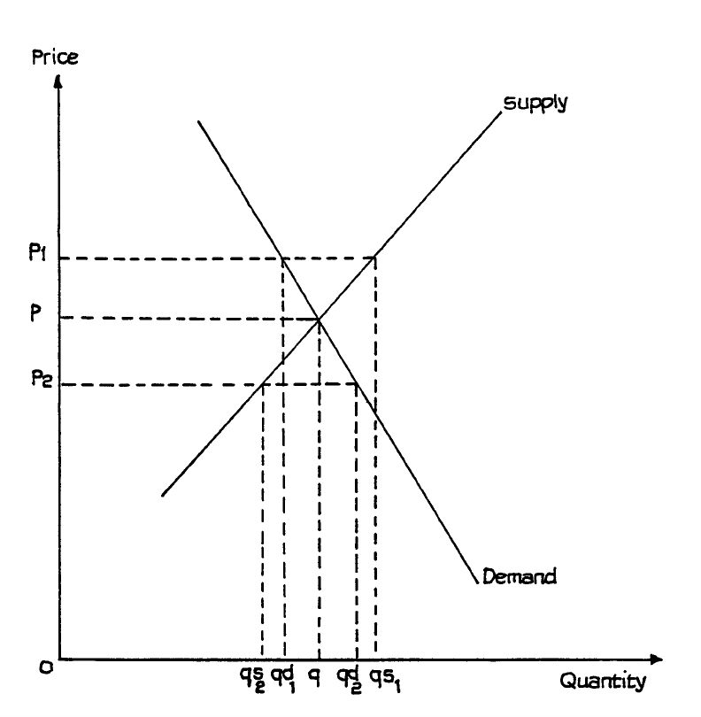
Page 129
Figure 6.6
Looking at the diagram, if price is fixed at p1, quantity supplied (qs1) is more than that
demanded (qd1), and there is surplus production.
If price is fixed at p2, quantity demanded (qd2) is more than that supplied (qs2), and there is a
shortage.
Only at price p will quantity supplied = quantity demanded.
Here, we see that any attempt to fix prices at a level other than the market equilibrium price
of p will produce either surplus production (fixed price p1 > p) or a shortage (fixed price p2 <
p).
We are forced to the conclusion that, on their own, price controls are ineffective.
Governments and other bodies must identify the real problem and seek to solve that. For
example, if the problem is lack of adequate supply (food or housing shortage), then the
government must either increase supply, e.g. by making additional payments, called subsidies,
to suppliers, or by entering the market as producers or importers, or, if these remedies are
Page 130
impossible, it must ration the available supply among consumers in a way that the community
regards as acceptable.
Such measures may be effective, at least for a time, though they may be expensive to
administer and control. The government, or other body, must decide whether the social
benefits to be gained from market regulation justify the cost and opportunity costs of the
resources used in maintaining the regulations. Care must also be taken to ensure that the
regulations themselves do not discourage suppliers to the extent that the basic objects of the
policies are defeated. The heavy bureaucracy created by many schemes in the so-called
planned or socialist economies often significantly discourages total production. If the
problem is excess supply, then the government may seek either to stimulate demand, e.g. by
reducing prices through the payment of subsidies, or to reduce supply by encouraging or
paying producers to leave the market, as in the case of European Union measures to reduce
European milk and wine supplies.
The most difficult problems often involve unplanned fluctuations of supply, when the plans of
regulatory bodies can be upset by unusually good - or bad - crops owing to the weather. If
there are fairly regular cycles of over- and under-production, and demand is reasonably
constant, and if it is possible to store the crops, then the government can apply a mixture of
controls over prices and production combined with purchases of over-production to keep in
store for release in periods of under-production. However, it is found that the guaranteed
prices that usually form part of such policies lead inevitably to steady increases in production,
so that the government finds itself storing quantities of goods that it has little hope of ever
releasing for resale, except at very low prices to people in other parts of the world. It may
even have to give away some of the surplus produce. Such policies then become a heavy
burden on taxpayers and lead to hostility from the community.
It is clear that governments which embark on market-intervention policies may, and often do,
find that they become involved in increasingly difficult and expensive measures that do very
little to solve the problems they were meant to eliminate.
Page 131
E. MARKET DEFECTS - THE CASE FOR A PUBLIC SECTOR
Defects in Market Allocation
In very many cases, unregulated markets and the price system are effective and efficient ways
of allocating resources and, as we saw in the previous section, some forms of well-meaning
government intervention can actually make worthy social objectives more difficult to achieve.
Nevertheless, this does not mean that unregulated markets are always perfect. The existence
of some defects is widely accepted and among the main problems are:
(a) Inequalities of Income
One of the virtues claimed for the unregulated market is that it makes the consumer
sovereign and that resource allocation responds to demand pressures. However, if we
imagine that consumers influence allocation by votes cast when they buy or refrain from
buying goods and services, we have to admit that some consumers have more votes than
others and large numbers have very few votes. Markets respond quickly to those groups
which have the most purchasing power. This does not always ensure that resources are
allocated in ways that meet the social expectations of the community.
It has always been difficult to ensure that the poorest sections of the community are
adequately housed. Normal commercial suppliers of housing are unwilling to meet this
demand because the people concerned cannot afford to pay the full “economic costs” of
housing, i.e. it is not usually possible to make a profit from providing housing for the
poor. It is much more profitable to provide second homes for the wealthy. Not only does
this offend against many people’s ideas of social justice, but the housing problem
rebounds against the community, for which it causes extra costs because inadequate
housing leads to poor health, disease, crime and a wide range of social problems that
become a charge on the taxpayers. Only the State can intervene to improve housing for
the poor. It cannot do so simply by holding down rents. It has to promote supply either
by setting up State suppliers or by subsidising private suppliers so that supply becomes
profitable.
(b) Market Power of Some Large Suppliers
Consumers may not always be as powerful as introductory economic theory suggests.
Later we will learn about markets dominated by large firms. If such firms become very
powerful, they can influence both supply and demand through controlling the goods
allowed into the market and by heavy advertising. Governments of most large market-
economy nations are often accused of failing to take action to check the sale of tobacco
and alcohol - both of which are potentially dangerous to health and society - because of
the power of the tobacco and alcohol producing companies. Even more notorious is the
extremely powerful “gun lobby” in the USA.
(c) Deficiencies in the Supply of Public Goods
The market economy operates on the principle of self-interest. Consumers wish to
maximise their own utility; producers their profit. In most cases this works to the public
benefit but not always. If it is in no one’s interest to provide a community or public
good, it will not be provided without the intervention of the political machinery of the
State. Public sewers, public roads and transport, police and social services, even fire
Page 132
services, fall into this class. The community clearly needs adequate services but left to
the market only the wealthy would attempt to purchase their own, and the community as
a whole would be subject to the risk of contagious diseases, unchecked crime and fires.
The Case for a Public Sector and its Boundaries
In noting the defects of the market economy as a means of allocating resources we have, in
effect, made a case for a public sector within which the State, through its political structures,
makes good the gaps and deficiencies of the unregulated market. The State can ensure that
there is a minimum standard of housing for those with low incomes, build roads and
establish communication systems. It can build sewerage systems and a system of piped, clean
water, provide police and fire services and a health and education service to ensure that all
who are sick obtain medical care regardless of income and all children achieve a minimum
level of education essential for survival in the modern world.
In communities with high living standards the question then arises as to how far State
provision should go in the provision of public goods which at some stage tend to become
private goods.
Let us take a closer look at two particular, high-profile issues.
(a) Education
Most would accept the need for all to receive a basic education, but this does not
necessarily mean that all who wish to do so should have the right to free education to
post-graduate level. Since there is evidence that, on average (but not, of course, for all
individuals) there is a correlation between income level and length of time spent in full-
time education, then education beyond the minimum represents a personal capital
investment and many would argue that such education should be paid for by those who
will benefit from it. Counter arguments are that the community benefits from the
contribution of its most highly skilled and educated members (e.g. brain surgeons) and
should, therefore, pay to obtain the maximum potential from its scarce human resources,
and also that those who earn high incomes normally pay the most taxes and thus pay
eventually for the education they received. There is no clear right or wrong answer to
this debate but you can see that the precise boundaries between the public and private
sector in the supply of goods such as education are not clear-cut and the matter is
arguable.
(b) Health Care
Another area of public controversy is the provision of health care. The community
clearly needs a health service if only to defend itself against dangerous diseases which
could quickly become plagues if large numbers of people could not afford treatment.
Most people’s ideas of social justice would accept that a person stricken by accident or
sickness should receive treatment regardless of income. However, should this mean that
all forms of treatment should be available for all regardless of income? Should the
diseases of greed and over-indulgence be given the same care as those of poverty and
ignorance? If people can afford to pay for additional treatment or for more comfortable
treatment, or non-urgent treatment at times that suit them rather than at times that suit a
bureaucratic administration, is there any reason why they should not do so? No one
Page 133
passes moral judgement on those who choose to spend their income on exotic holidays
rather than a fortnight at a local resort, yet many pass such judgement on those who
prefer to pay for a private room when they are in hospital instead of sharing a public
ward.
Clearly many of the arguments surrounding health care involve emotionally charged
value judgements resulting from past social injustices and history, but there are also
serious economic considerations involved. The economist is concerned with the
allocation of scarce resources and we have to recognise that resources devoted to health
care are scarce. The march of technology and medical science has made possible cures
and treatments more widespread. Open heart and transplant surgery require a massive
investment in resources but benefit only a relatively few people. The proportion of older
people is greater (life Expectancy has increased by approximately 48% since 2004) and
the demands they make for health care are proportionally much greater also. Not even
the most wealthy and advanced nation can provide all the resources that would be
required to give immediate treatment to all those wanting it. Difficult allocation
decisions have to be made and are made daily.
On the other hand it can be argued that a private health system which permits scarce
resources to be allocated on the basis of ability to pay, or by virtue of employment in a
company that provides health insurance as part of its remuneration, is diverting resources
from areas of greater personal or social need. One person suffers pain so that a
consultant can earn a private income treating a less urgent patient in a private hospital.
On the other hand it can be argued that the private health service brings in resources that
would otherwise not be available. The consultant is willing to work for a relatively low
level of pay from the National Health System because he or she can have the additional
income from private patients. Without this, the best surgeons would possibly go to
countries where earnings were higher. Private hospitals relieve the public health system
of many patients and reduce its need for expensive capital equipment. The debate can
again continue with no clear right or wrong.
The basic problem is really one of allocation of scarce resources and the public versus
private health service is only part of a much larger economic and social issue which
concerns to whom, how and on what basis resources should be allocated for health care.
How should the community decide what proportion of available scarce resources should
be devoted to the technically brilliant feats of surgery which bring acclaim to surgeons
and enable them to attend conferences in exotic countries and how much to the
unglamorous, humdrum work of caring for the mentally ill for whom there is no hope of
cure and little chance of international laurels for the carer? The unregulated market will
not provide an answer, nor will a medical service subject to all the usual human vanities
and frailties. The answer must eventually come through the political machinery of the
community and the quality of the answer will reflect the health of that machinery.
Similar issues can be applied to virtually every other public sector and public utility service
and you should give some thought to the allocation problems inherent in, say, police, fire,
water, and housing services.
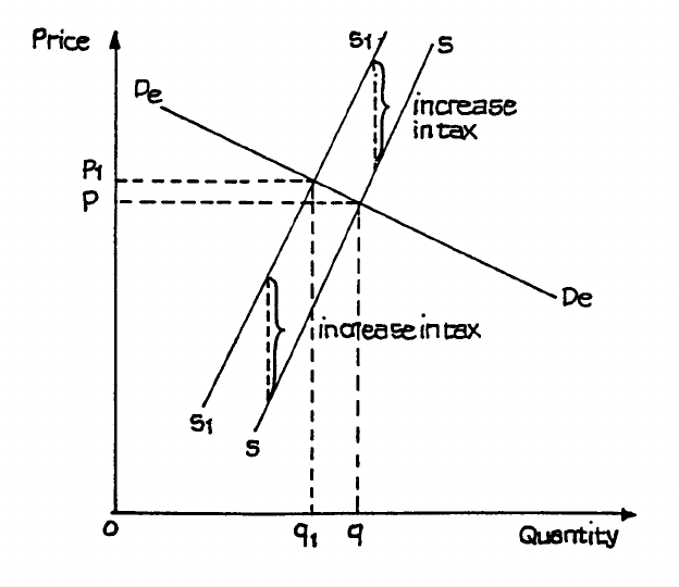
Page 134
Figure 6.7
F. PRICE CHANGES AND INDIRECT TAXES AND SUBSIDIES
Effect of Tax on Price
In Study Unit 5 we saw how the supply curve was likely to shift as a result of a change in an
indirect tax or subsidy. For the likely effect on market price, however, it is also necessary to
take account of the conditions of demand since it is likely that the producer’s efforts to recoup
the tax by adding this to the price will leave the quantity demanded in the market unchanged.
Look now at Figure 6.7. Here we show the movement of the supply curve from SS to S1S1
(resulting from the increase in tax) and the demand curve DeDe. The equilibrium price moves
up (from Op to Op1) but by an amount less than the increase in tax. The amount supplied to
the market falls from Oq to Oq1 and the output/quantity fall is greater than the price rise.
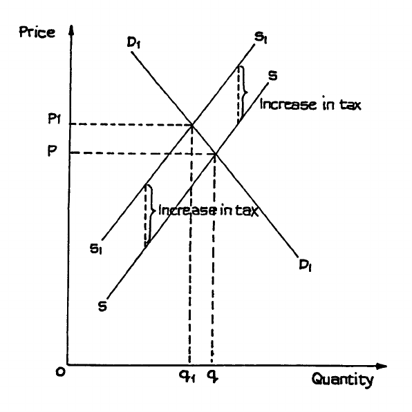
Page 135
Figure 6.8
Now look at Figure 6.8. Here we have the shift in supply curve SS to S1S1 and a demand
curve D1D1. Again we have an increase in equilibrium price (Op to Op1) and a reduction in
quantity supplied (Oq to Oq1). This time, however, the reduction in quantity is less than the
increase in price.
Why the difference in the two situations? You will have noticed that the curve D1D1 is much
steeper than DeDe. This reflects the fact that demand in Figure 6.7 is more price elastic than
demand in Figure 6.8. The two illustrations show that the more price elastic the demand for a
product is, the smaller will be the market-price increase following an increase in indirect tax,
and the greater will be the cutback in supply to the market.
This, after all, is really common sense. Price elasticity indicates the degree of responsiveness
of quantity demanded to any change in price.
Subsidies
The effect of a subsidy will be the exact reverse of that of the tax. Instead of the movement of
the supply curve from SS to S1S1 there is an increase in supply at all prices, i.e. as from S1S1
to SS, and there will be a reduction in market price, as from Op1 to Op. Such a reduction is
likely to have been the main government objective in arranging the subsidy, particularly if the
good is a “socially worthy” one such as a basic food in a time of shortage, housing, or a
service such as education or health care.
Page 136
Remember also that the new supply curve need not be exactly parallel to the original before
the tax or subsidy change. If the tax or subsidy increases with value, i.e. is an ad valorem tax
or subsidy, the gap between the curves will increase as price rises, as illustrated in Figure
5.17.
Government Use of Indirect Taxes
If the government increases indirect tax on goods which are price elastic, it will not receive
much extra tax but it will depress demand. If it imposes the tax on goods which are price
inelastic, it will not have much effect on output but the government will collect more tax
revenue.
If you think back to when we discussed the “income effect” you will realise that the effect of
the tax may go further. Suppose there is a general increase in indirect tax on all goods. Some
will be demand price inelastic, and their pricing will increase without much reduction in the
amount supplied and bought. The buyers are paying more for nearly the same quantity of
goods. This means they have less income to spend on other goods - they will have to cut
purchases of goods which are price elastic.
The unfortunate producers of price-elastic goods will suffer a double blow. They will suffer a
drop in demand from the tax increase and not be able to increase price by anything like the
full amount of the tax, and they will suffer a further drop in demand because consumers’
discretionary incomes have fallen.
We have so far assumed that these taxes would be used either to increase government
revenues or to reduce consumer demand if the government believed that excess demand was
causing inflation. There is, however, another aspect of government policy that is not
beginning to appear: this is the control of pollution, which is now recognised as a significant
problem.
As indirect tax on expenditure could be used as in instrument to reduce demand, and hence
the production or use of something that was believed to be a source of pollution. An example
would be an additional tax on petrol to discourage the use of motor vehicles. However, as the
demand for petrol is price inelastic then the tax will not have much effect on vehicle use but
will reduce consumer incomes available for spending on other goods. One of the main
reasons why demand for petrol for car use is price inelastic is because of the lack of
satisfactory substitutes. As motor vehicle ownership has increased, the demand for, and
supply of, public transport has fallen; and as public transport provision falls and its price rises
so even more people are induced to use their own private cars.
We conclude, therefore, that a ‘pollution tax’ on petrol would fail in its objective unless the
government also made provision for, and probably subsidised, alternative public transport, at
least in urban areas where cars are used for travel to work and for relatively short journeys. If
the government also wished to discourage car use for longer journeys it would need to
provide alternatives, probably in the form of subsidised public transport. A tax is a very blunt
instrument and a government wishing to influence consumer behaviour needs to take many
aspects into account. It is not sufficient simply to increase the price of the good whose use it
Page 137
wishes to discourage. Reverting to our general discussion of the effects of taxes on prices,
notice that we have not taken into account differing elasticities of supply. This is because
supply reactions will take place over a period of time. If suppliers can react by cutting back
supply fairly quickly, then there will be further effects on market price. You can examine
these for yourself by changing the supply curve to make it more elastic in Figures 6.7 and 6.8.

Page 138
BLANK

Page 139
Study Unit 7
Market Structures and Competition
Contents
A. Meaning and Importance of Competition
B. Perfect Competition
Definition
Conditions for Perfect Competition
Movement towards Equilibrium in Perfectly Competitive Markets
Views on Perfect Competition
Profit Maximisation as a Result of Perfect Competition
C. Monopoly
Definition
Sources of Monopoly
The Monopoly Model
Comment
D. Monopolistic Competition
Main Features
General Model
Comment
E. Oligopoly
Price Competition
Price Stickiness
Kinked Demand Curve
Limitations of the Kinked Demand Curve Model
Price Leadership
F. Profit Maximisation and Alternative Objectives for the Firm
Page 140
A. MEANING AND IMPORTANCE OF COMPETITION
‘Competition’ is one of those simple words which are common in everyday speech and which
we all assume we understand but which, when we really try and explain, start to present
difficult problems. Ask yourself what benefits you think you get from competition as a
consumer. Suppose you think in terms of being able to buy from different suppliers, of being
able to choose from a variety of different but broadly similar goods - for example choosing
shoes of different styles, sizes, quality and price ranges - and perhaps of having some power
as a consumer to bargain over price, or knowing that some suppliers will charge lower prices
than others. Notice that the word that recurs constantly when most of us think about
competition is choice. You and I, as consumers, value the ability to choose between a range
of goods, different prices and different standards of quality and service.
Because of the buyers’ ability to choose and apply pressure on prices, we expect competition
to oblige producers and distributors to use their resources efficiently and keep production and
distribution costs low. Competition is usually thought to be a very powerful force to ensure
production efficiency.
Competition is thus widely believed to be a desirable feature of markets. Most of the major
modern market economies have legislation and institutions concerned with preserving or
increasing competition.
Economists have generally been in favour of competition as a force likely to increase the
efficient use of scarce resources, and they have developed a concept of perfect competition
which we shall examine in this study unit. More recently, however, they have recognised that
traditional views of competition have limitations and that the pressures on business firms are
more complex than have sometimes been believed in the past. There is also a recognition that
increased competition can sometimes have consequences that are not beneficial to consumers
or which are not socially very desirable.
For example, competing firms are likely to seek to attract the largest number of buyers and
may do this by providing those goods and services for which there is the greatest demand.
Consequently, consider the following possibilities:
• Four or five multiple stores all offering similar styles and sizes of children’s clothes, with
little to offer buyers wanting different styles or the less common sizes.
• Rival buses, some nearly empty, jockeying for custom in the streets of populous cities but
little or no transport to outlying rural areas.
• Twelve or more insurance offices all offering cut-price insurance but with policies
containing conditions that are likely to allow the companies to avoid meeting claims for
losses that policy holders thought had been fully covered.
These examples - and you can probably think of others - suggest that competition can lead to
less genuine choice for consumers or can lead to a reduction in the quality of services
provided. This quality reduction can be very damaging in the financial services sector:
Page 141
competitive banking does not appear to have improved relationships between the major banks
and their customers.
We must, therefore, be careful in our assessment of the benefits of competition and be
prepared to be critical when examining some of the traditional economic models of
competitive markets. These models have been developed in the belief that the degree of
competition in a market is likely to influence the behaviour and performance of firms
operating in it. In this study unit we look at some of the best known models, and these
provide an essential starting point for understanding the often complex markets existing in
modern economies.
Page 142
B. PERFECT COMPETITION
Definition
Our first theoretical model covers the situation where the economic market operates in its
purest or most perfect form. Perfect competition is the state of affairs existing in a market
totally free from imperfections in the communication and interaction of the economic forces
of supply and demand.
Some writers like to make a distinction between perfect or ideal markets and perfect
competition, in addition to the distinction between the market as an area and competition as a
condition found in that area. They suggest that the conditions for perfect competition are
satisfied when the individual firm is a “price-taker”, i.e. when it can sell all that it can
produce at the market price, which by itself it cannot alter, and when buyers are indifferent as
to which seller’s product they buy at that price. Such a very limited set of requirements
would be satisfied when firms in an industry were subject to a regulated price set by a
government or some other regulatory body which had powers to buy goods un-saleable in the
market. This would certainly not be a perfect market.
For true perfect competition to exist, it seems more realistic to stipulate that sellers must be
free to enter and leave the market, so that total supply can change and bring about the
equilibrium position. Just to establish a market price through some form of price regulation
would not produce the same result, unless the regulating body is very sensitive to demand
shifts, and production plans can be adapted quickly.
It seems, then, that full operation of perfect competition can be achieved only in a perfect
economic market, and to put too much emphasis on differences between the two does not
really help very much in our analysis of the main market forces.
Conditions for Perfect Competition
These can be summarised as follows:
(a) Goods Must Be Homogeneous
This means that, in the perception of the buyer, all units of the goods offered by all
suppliers are equally acceptable. The buyer is indifferent as to which unit he receives, as
long as it conforms to any description adopted by, and understood in, the market.
Notice that it is the perception of the buyer that is important. Suppose two large retail
stores make an arrangement with a manufacturer to be supplied with canned coffee in
plain tins. The manufacturer supplies coffee of the same type and quality to each retailer
in the plain cans quite impartially. However, each store adds its own label to the cans
and sells the coffee under completely different brand names and at slightly different
prices. The products are physically the same, but they are not homogeneous, because the
public perceives them as different and competing products.
Page 143
(b) Perfect Transport and Communications
All consumers in the market must have the same information. Suppliers must have
access to the same information about production factors and the technical conditions of
production. No producer is in a more favoured situation than any other.
(c) Price Established Only by Market Forces
No producer and no buyer is able to influence the price by his own actions, nor by actions
agreed with other producers or buyers. There is no degree of monopoly power in the
market.
(d) Economic Motives Only
The actions of suppliers and buyers are influenced only by economic motives. If buyers
or sellers are influenced by a desire to support a charity or a political party the market
will not be purely economic, however worthy the social motives.
Economic rationality in a market economy assumes an underlying self-interest and a
desire to maximise benefits that can be gained from available scarce resources. For the
consumer this means maximising utility, as defined in Study Unit 2, while for producers
it is usually interpreted as wishing to maximise profit - an objective examined later.
(e) No Barriers Limiting Market Entry and Exit
Suppliers and buyers must be free to enter and leave the market as they choose and as
they are guided by considerations of profit and utility. This is a very important element
in any competitive market and in some modern models of market behaviour, notably that
of contestable markets, it is the most important consideration.
Barriers to market entry and exit may be “natural”, i.e. arising out of the nature of the
goods or the production process, or “artificial”, i.e. arising out of market regulations.
Natural barriers are highest when production requires large amounts of highly
specialised capital, e.g. oil exploration and extraction or motor vehicle assembly. Only
firms with access to very large amounts of finance can enter these markets and, once this
capital has been acquired, the firms are committed to staying in the market, since exit
would usually involve very large financial losses. Natural barriers are low when little
specialised capital or skill is needed to commence production.
When natural barriers are low, established producers may seek to protect themselves
from new entry by building artificial barriers, such as membership of a trade or
professional association, entry to which may require a long period of apprenticeship or
education or high membership fees. It is not unknown for established traders to prevent
new entry illegally by the use of force.
The lower the barriers, both natural and artificial, the more contestable the market, and
the theory of contestable markets suggests that contestability is a powerful force
determining the behaviour of suppliers in a market. If producers know that they can
easily be challenged by new competitors they will behave as if they were subject to
competition because they will not wish to provide incentives for new firms to come into
the market. Such incentives would include supernormal profit or the existence of buyers
who were dissatisfied with existing goods, standards of service or prices.
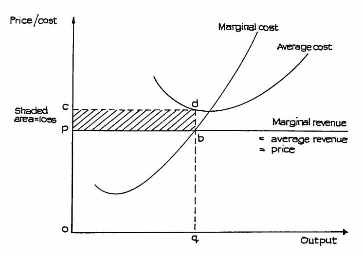
Page 144
Consequently we would expect a perfectly contestable market to exhibit most if not all
the characteristics of perfect competition.
Movement towards Equilibrium in Perfectly Competitive Markets
We can now examine the behaviour of firms operating under conditions of perfect
competition.
If we assume that the firm is experiencing diminishing marginal returns and can sell all it can
produce at the market price, over which it has no control, then it will have average and
marginal cost curves and an average revenue curve as shown in Figure 7.1. Since all units of
the good are sold at the same price whatever the firm’s sales level, price will equal average
revenue and will also be the same as marginal revenue.
Suppose the price resulting from the interaction of supply and demand in the market as a
whole is Op; then there is no level of output at which the firm can produce at a profit.
At all levels of output price, average revenue is below the average cost curve. However, the
profit-maximising condition of marginal cost = marginal revenue is also the loss-minimising
condition, so the best output for the firm to choose is at Oq where marginal cost equals
marginal revenue. At this output level, average cost at Oc is higher than average revenue at
Op, so the firm suffers a loss equal to the shaded area cdbp.
Given the conditions for perfect competition, if this is the situation faced by one firm, it is the
situation of all firms subject to the same market information and technology. Firms cannot
continue indefinitely suffering losses. Some will withdraw from the market (remember that
unrestricted entry and exit is another condition of this market) because they are less able to
withstand losses or they have other markets they can enter.
Figure 7.1
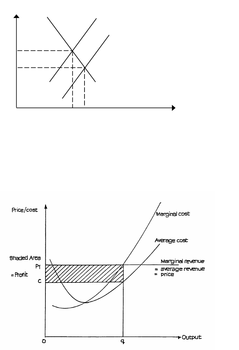
Page 145
As supply declines, the total market supply curve moves to the left, as shown in Figure 7.2.
Figure 7.2
The market equilibrium price then rises - assuming that demand remains unchanged.
Supposing the equilibrium price moves up from Op to Op1, this produces the situation for the
individual firm illustrated by Figure 7.3.
Figure 7.3
Price
Output
P
P
1
D
S
1
D
S
S1
S
qm
qm1
O
If firms suffer losses at price Op
1
some withdraw from the market.
Market supply falls from Oqm to
Oqm1 and equilibrium price rises
from Op to Op1 as supply shifts
from SS to S1S1.
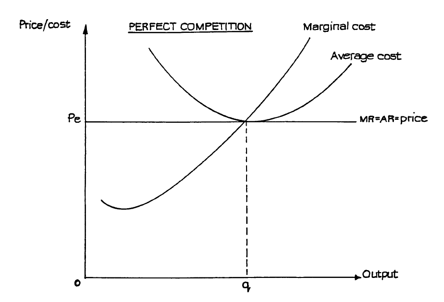
Page 146
Now we see that the average revenue at Op1 is higher than average cost at Oc, and the firm is
enjoying profits, represented by the shaded area. Notice that, once again, the most profitable
output to aim at is at Oq, where marginal cost is just equal to marginal revenue.
Now, given our earlier assumptions, all firms are making profits. If we have defined cost to
include a normal return to all production factors (including some return to enterprise in the
form of a minimum profit to keep firms in the market and provide necessary capital
investment) then this shaded area profit is an additional or abnormal profit, resulting only
from the special market opportunities.
Owing to perfect communication and free entry, new firms will enter the market to take
advantage of these profits. Supply will now increase - the supply curve will move to the right
and equilibrium price will fall.
Suppose it falls to a position between Op and Op1, say to Ope where price/average revenue is
just equal to average cost. Now the individual firm is in the position illustrated in Figure 7.4.
Here, there is neither abnormal profit nor loss. We assume that the firm’s costs include an
element of normal profit, which can be defined as a fair return to the firm’s enterprise, or
sometimes as that amount of profit which is sufficient to keep firms operating in that market.
This normal profit is included, therefore, in the average cost curve. There is no incentive for
firms to move into or out of the market; there is no reason why supply should shift - and, as
long as demand remains unchanged, there is no reason for any movement in this equilibrium
balance.
Figure 7.4
Page 147
It is on the basis of this kind of argument that textbooks and examiners sometimes make
much of the distinction between short-run equilibrium in perfect competition where
abnormal profits or losses can be experienced, and long-run equilibrium where only
“normal” profits (included in the average total cost curve) are possible. However, we should
stress that these are really only partial equilibrium positions relating to supply alone. The
model says nothing about influences on demand which is often far from stable. A shift in
demand will be quickly reflected in a shift in supply to readjust output to the new market
price. Consequently, in markets where demand is inherently unstable - as in the Stock and
Commodity Exchanges - long-run equilibrium may never be reached as suppliers are
constantly adapting to the shifting market environment.
Views on Perfect Competition
Economists often favour perfect competition on the following grounds:
(a) The elimination of abnormal profit, as shown in Figure 7.4.
(b) Efficient use of resources. Notice that, in equilibrium, the bringing together of price and
marginal cost and the elimination of abnormal profit means that producers will produce
when the average cost curve is at its lowest point (where marginal cost equals average
cost). There is then a tendency to encourage producers to reduce average costs as much
as possible. This is equivalent to making the most efficient use of resources.
(c) Price is equal to marginal cost. Price is the money value of the utility gained by the last
or marginal consumer, i.e. marginal utility. When marginal cost = marginal utility, as in
perfect competition, the cost of producing the last unit is just equal to the value of the
utility given by that unit to its consumer. If this were true in all cases, then the total cost
of production would equal the total value of utility received. This would be the best
possible use of all resources, it is suggested.
Not everyone accepts these arguments, and you should read this section in conjunction with
the discussion of monopoly, later.
One of the arguments against perfect competition is that it prevents producers from making
the profit necessary to provide funds for investment and research, to find better ways of
producing goods. Another argument is that competition can be wasteful, as resources are
doing the same things. If there were fewer competing firms, total costs could be reduced and
some resources freed to produce something else.
Firms dislike perfect competition because, as indicated earlier, prices are unstable. If
communications are good, then supply can adapt very quickly to price changes caused by
changes in demand. The result is that prices are constantly adapting to new equilibrium
positions - as with the Stock Exchange, which is still the common textbook example of a
market which is close to perfect competition. In the Stock Exchange, prices change daily, and
even hourly.
Manufacturers cannot tolerate swiftly-moving prices like this - they could survive in such a
market only if they could keep changing the prices paid for production factors, including the
wages paid to workers. Trade unions have sought to achieve stable jobs - and, preferably,
Page 148
rising wages. Producers then want stable - and, preferably, rising - prices. Those economists
who argue for perfect competition in the consumer interest, and then for stable wages and
secure employment, are being illogical. These two conditions cannot exist together.
Perfect competition may or may not, therefore, be ideal from a purely economic viewpoint. It
is certainly far from ideal from a social standpoint.
Profit Maximisation as a Result of Perfect Competition
Notice that the only output enabling the firm to survive in the equilibrium condition
illustrated in Figure 7.4 is where marginal cost equals marginal revenue. The removal of
abnormal profit ensures that the average cost curve is at a tangent to the average revenue
curve, and as this is horizontal, then the average cost curve must be at a tangent at its lowest
point, i.e. where average cost equals marginal cost.
This is what is meant by saying profit maximisation is a survival condition resulting from
perfect competition. Only by achieving this profit-maximising output can the individual firm
avoid losses. Whether it achieves this intentionally or by trial and error does not matter;
failure to achieve it means eventual failure to exist in the market.
C. MONOPOLY
Definition
Monopoly is the opposite extreme to perfect competition. It exists when there is only one
supplier for a particular product and there are no close substitutes for that product.
Again, we have to be careful how we define the product. Historically almost all monopolies
are subject to destruction by the onward march of technology.
Sources of Monopoly
Monopoly can arise in three ways: by operation of the law, by possession of a unique feature,
or by the achievement of market control.
(a) Operation of Law
This is a very old source of monopoly power. Kings used to sell monopolies in Europe to
raise money, i.e. they sold people the right to be sole suppliers of a necessary product,
such as salt, in a given area. The monopolist could rely on the support of the King’s
officers to protect his monopoly and the profits he could make more than covered the fee
he had to pay for his position.
Today, some countries may grant a company the right to be sole supplier of a product or
service in return for some measure of State inspection and control over profits and
prices. Some important public utilities, e.g. Electrogaz, are legally companies in the
private sector but are subject to government influence as a shareholder, and regulation by
separate bodies. Note Electrogaz has been taken back into Government “owenership”
and is EWSA
Page 149
A more limited monopoly power is granted under patent and copyright laws, which are
similar in most countries. The idea of a patent is that the inventor of a new idea shares
his knowledge with the State for the public benefit, in return for a monopoly control over
the use of his idea for a limited number of years. If rival suppliers are unable to develop
a competing product without breaking the patent, this form of monopoly can be very
valuable - take, for example, the monopoly enjoyed for some years by the Polaroid
instant film-developing process.
(b) Possession of a Unique Feature
Individuals have monopoly control over the supply of their own skills, and this may be a
source of considerable profit. The top footballers, tennis players and entertainers are
monopolists of this type. When the skill lies in producing something written or recorded,
then the monopoly position is protected by copyright laws - which modern technology
has made more difficult to enforce, however.
(c) Market Control
It is difficult to achieve total monopoly over supply without the protection of the law,
although it is not unknown - especially in the production of some intermediate products.
For a number of years, all the valves for pneumatic tyres on motor vehicles were
produced by one manufacturer. Such a monopoly rarely lasts very long. When a large
rival decides to challenge the monopolist, there is little that can be done to prevent this.
The Monopoly Model
The model has been developed to explain the outcome of a monopoly not subject to any
special legal protection or control. It assumes that the firm is pursuing a profit-maximising
objective, and that it is able to make abnormal profits.
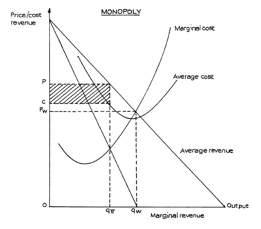
Page 150
Figure 7.5
A monopolist’s output is the total market supply, and the demand for its product is the total
market demand. The firm will thus face a downward-sloping demand curve. If we assume
that it is not practising price discrimination, then this curve will be the price/average revenue
curve. The graphical model is shown in Figure 7.5.
The profit-maximising monopolist will produce at output Oq
π
, where marginal cost equals
marginal revenue, and will charge price Op. Abnormal profit is represented by the shaded
area. Oc is the average cost, so Op
−
Oc is the average profit earned on each unit of product
sold.
If the firm were to set price to equal marginal cost, which is the position desirable from the
consumer viewpoint, it would produce output Oqw and charge the lower price Opw. This is
why the profit-maximising monopolist is said to restrict output and increase price in
comparison with a firm operating in a competitive market.
Comment
There is much evidence that large firms with considerable market power may not maximise
profits but may pursue quite different objectives, such as growth or sales revenue
Page 151
maximisation. The average cost curve was drawn on the basis that abnormal profit was being
made. There is nothing in the model itself that says that the average cost curve must be this
shape and in this position. We can move it up or down without affecting the other curves, and
so alter the profit quite legitimately.
In short, the model proves nothing. It simply illustrates the assumptions made. Notice that,
if we drop the profit-maximising requirement, we can allow the firm to increase output and
reduce price, and so come closer to the consumer-benefiting output level of Oqw. This would
also reduce average cost and allow the firm to make more efficient use of its resources.
In answer to the charge that monopoly is against the public interest because it restricts output
and raises price, the following arguments can be put forward:
(a) The monopolist’ size and ability to produce for the whole market enables it to achieve
economies of scale, so that costs are actually lower than they would be under perfect
competition.
(b) The monopolist employs professional managers who make more efficient use of
available resources than small owner/managers, who often lack managerial skill.
(c) The monopolist does not maximise profits but is content with just a satisfactory level of
profit.
(d) Some element of abnormal or monopoly profit (normal profit is considered to be
included in the firm’s costs as for perfect competition) is desirable, so that the firm:
(i) can spend money on research and gather funds for further capital investment;
(ii) has the incentive to take risks and innovate and sometimes suffer losses that would
cripple smaller firms.
The position where a monopolist is actually able to charge lower prices than would be
possible under perfect competition is illustrated in Figure 7.6. Here, for simplicity, constant
average total costs have been assumed and the monopolist’s cost curve is below that of small
firms by reason of economies of scale and improved technology. Assuming that the
monopolist seeks to maximise profits, the appropriate price will be Pm, still higher than the
perfectly competitive price of Pc. However, this could be reduced if the monopolist had some
other objective such as maximising growth or revenue. The revenue-maximising price (Pr),
i.e. the price applicable to producing at the quantity level where marginal revenue is 0, and
therefore total revenue is at its maximum, is lower than the perfectly competitive price of Pc.
Notice that, unlike the firm under perfect competition, the monopolist can charge a range of
prices, depending upon the firm’s objectives, and still make a profit.
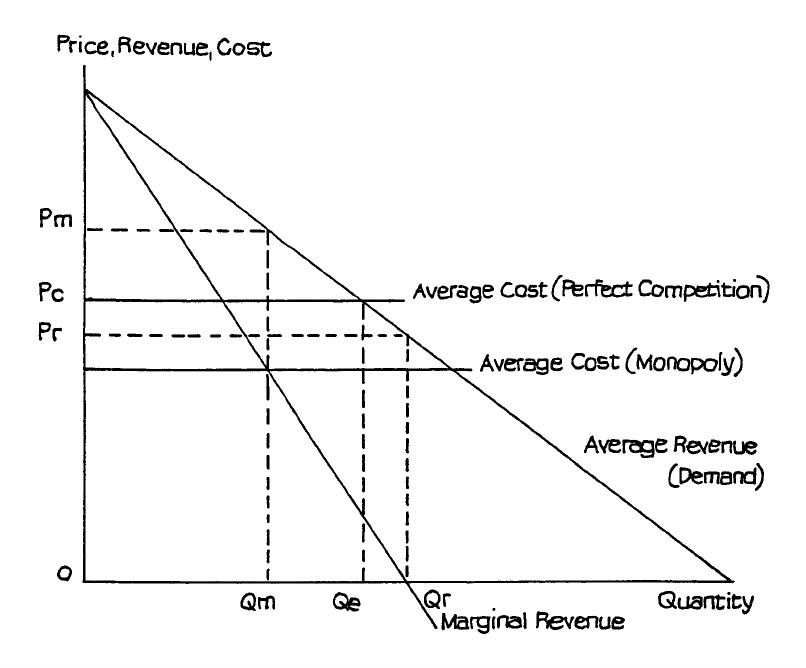
Page 152
Figure 7.6: Price and Output Under Perfect Competition and Monopoly
The argument really boils down to a question of performance. Does the monopolist behave
against the community interest or does it achieve levels of efficiency beyond the capacity of
small firms operating in highly competitive markets? There is no clear answer. As the
extreme cases of monopoly are fairly rare in practice, examination is usually made of markets
which approach monopoly conditions.
If the demand curve faced by the monopolist shifts, this will alter the marginal revenue curve
and consequently the profit-maximising output and price. However, we cannot assume that
the demand curve will simply move outwards parallel to the old one. It is possible that its
slope may change (become steeper or less steep). Consequently, while normally we would
expect an increase in demand at all prices to lead to an increase in monopoly price (assuming
costs remained unchanged), we cannot be absolutely sure of this. Try experimenting with
differently sloped average revenue curves. Remember that the marginal revenue must bisect
(cut into two equal halves) the horizontal distance between the average revenue curve and the
revenue (vertical) axis. You will find that there are changes that could produce a reduction in
the profit-maximising price!
Page 153
D. MONOPOLISTIC COMPETITION
Main Features
Monopolistic competition still retains many of the features of perfect competition -
unrestricted entry to and exit from the market, good (but not perfect) communication and
transport conditions, motivation by economic considerations only, and the perception by
buyers that the products of the various firms are good substitutes for each other.
It is in this last point that monopolistic competition differs from perfect competition.
Although the products are considered to be good substitutes, they are not homogeneous.
Buyers do express preference for one seller’s product as opposed to another’s.
Sellers seek to increase this preference by differentiating their product through branding
(giving it distinguishing features) and especially by advertising. The greater the degree of
preference they can establish, the stronger the brand loyalty and the greater the freedom
gained by the supplier from needing to follow the market price for that class of product.
Success brings an increased degree of market power and a reduction in price elasticity of
demand.
General Model
In the general model of monopolistic competition, however, we assume that the individual
firm is not able to achieve a high degree of price inelasticity, so that the demand curve for the
individual product has only a fairly gentle slope, i.e. there is still a high degree of
substitutability between competing brands. This prevents the individual firm from making
monopoly profits. It is still closely governed by the market price for the class of product. The
result is shown in Figure 7.7.
Features of this model are outlined below.
(a) There is no abnormal or monopoly profit, i.e. average cost equals price/average revenue
at Op and, as for perfect competition and monopoly, it includes an element of normal
profit.
(b) At the profit-maximising output of Oq, average cost is still falling to its minimum at Oc,
where average cost is equal to marginal cost - the output level where the rising marginal
cost curve cuts the bottom of the average cost curve.
(c) Price (at Op) is above marginal cost (Om) at the profit-maximising output Oq.
Price is thus higher and output lower than would be the case if price were to be equal to
marginal cost, as in perfect competition. The lack of monopoly profit is the result of
competition and the ability of firms to enter and leave the market.
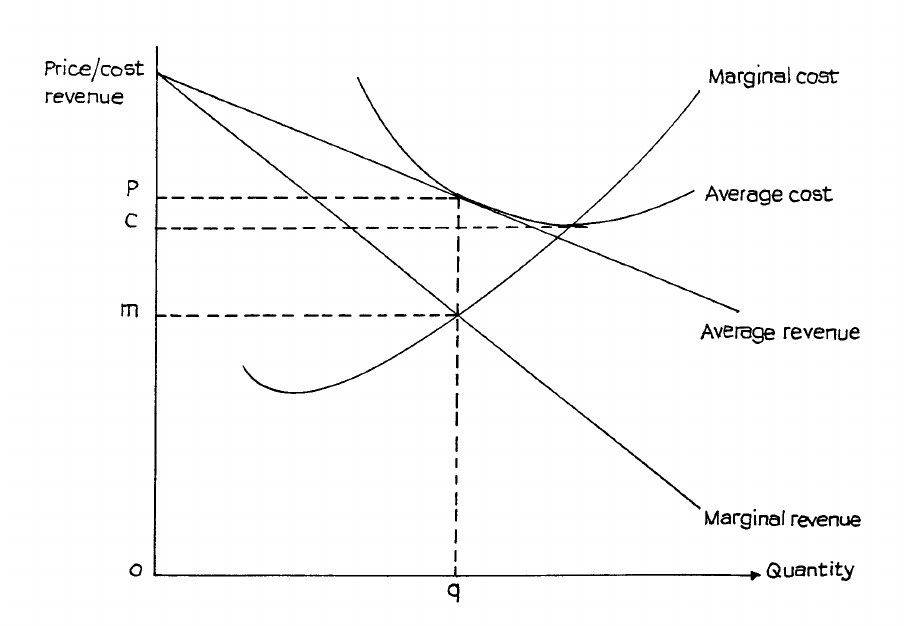
Page 154
Figure 7.7: Monopolistic Competition
Comment
It can be argued that this market structure is not really in the best interests of either consumers
or business firms, for the following reasons:
(a) Price is higher and output lower than would be the case with perfect competition.
(b) The firm is not making the best use of its resources, since average cost is still falling at
output Oq, as we saw a moment ago.
(c) Profits are confined to the normal minimum required to keep firms in the market - the
amount included in our definition of costs for the purposes of these market models. They
cannot achieve the profits needed for investment and research or the high output levels
necessary for economies of scale.
It is also argued, however, that consumers are prepared to accept these additional prices and
costs in return for the benefits they receive through greater choice of product - the ability to
choose between competing brands and competing suppliers. This competition may also lead
to improvements in product quality and design as well as services to the consumer.
We can expect firms operating in such market conditions to seek to increase their monopoly
power and make their product-demand curves less elastic. They will do this by brand
advertising, by securing favourable treatment from distribution organisations or through
technical improvements in their products. They may be able to keep an advantage by
securing patent protection or keeping processes secret from their competitors.
Page 155
E. OLIGOPOLY
Oligopoly is the market structure where supply is controlled by a few firms which are large in
relation to the market size. Very often the firms are also large by any standards, and are likely
to be oligopolists in several markets.
Oligopoly is now commonly found in the advanced industrial countries and a great deal of
attention is paid to it. There is, however, no single model which can be held to apply under
all circumstances.
Price Competition
One influence that is thought to be important is the extent to which the products are in price
competition with each other. If there is little price competition and if consumers are not
thought to choose brands on the basis of comparative price (i.e. if cross elasticity of demand
is low) then each oligopolist has a high degree of monopoly control over the demand for his
own product.
This will, of course, depend chiefly upon whether the products are regarded by consumers as
homogeneous or whether they consider each brand to be distinct and different. It is unlikely
that consumers will find much to choose between, say, various brands of white loaves of
bread. Cross elasticity of demand between the brands is thus likely to be high when the bread
is on sale in similar distribution outlets. If there are price differences, customers will choose
according to price.
In these circumstances, suppliers may seek to operate in different sections of the market, e.g.
through different supermarket chains. They may also seek to differentiate their products
through such devices as flavour or by developing novelty shapes or other related products.
A full study of oligopoly is likely to embrace problems of prices and non-price competition,
and even the question of how far firms may collude together to limit the extent of competition
between established firms and to protect themselves against possible newcomers to the
market.
Price Stickiness
Efforts have been made to produce models based on traditional assumptions of profit
maximisation. One such model seeks to explain the observed tendency that the prices of
some goods in oligopolistic markets remain steady in spite of fluctuations in the prices of
basic commodities. This “stickiness” is apparent in more normal, less inflationary times.
This particular feature of an oligopolistic market for a product still regarded as fairly
homogeneous (in spite of brand advertising) has given rise to the model known usually as the
kinked demand curve.
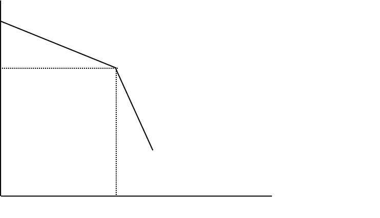
Page 156
Kinked Demand Curve
Suppose the current and “sticky” price of a product is RWF1 per unit. This is the price that
customers have come to expect. If one oligopolist supplier tries to increase the price, rival
producers will be reluctant to follow. They keep their prices the same and gain market share
at the expense of the price-raiser. If, however, the oligopolist reduces the price, the other
suppliers are obliged to reduce their prices also to prevent his encroaching on their market
share.
Thus there is a kink around the price of RWF1 in the demand (unit price or average revenue)
curve faced by the individual oligopolist. At higher prices the curve is more elastic, due to
the loss of market share, than at lower prices where all market shares stay the same. You can
see the general shape of such a kinked curve in Figure 7.8.
Figure 7.8
Price
per
unit
Quantity
Rwf
q
O
At price RWF1 the oligopolist has
difficulty changing price. At higher
prices he loses market share. At
lower prices all oligopolists in the
market keep the same share but lose
revenue.
Page 157
Now consider a possible table of revenues resulting from this condition.
Price per Unit
(RWF ‘000)
Quantity
(units per time
period)
Total Revenue (TR)
RWF ‘000
Marginal Revenue
(Change in TR)
(Rwf)
1.40
0
0
1,300
1.30
10
13.00
1,100
1.20
20
24.00
900
1.10
30
33.00
700
1.00
40
40.00
(600 or 200)
0
0.80
50
40.00
−400
0.60
60
36.00
0
−80
0.40
70
28.00
−1,200
0.20
80
16.00
−1,600
0
90
0
The kink in the average revenue curve, shown in Figure 7.9, occurs at the price of RWF1,000
and the quantity level of 40 units. At prices above RWF1,000, demand falls off at the rate of
ten units for each RWF100 rise in price. At prices below RWF1,000, however, demand falls
by only five units for each RWF100 rise in price, i.e. the unit price has to fall RWF200 to
enable the oligopolist to gain a quantity increase of ten units.
The change in the slope of the average revenue (price) curve results in a similar change in the
slope of the marginal revenue curve and you can see that there are two possible marginal
revenues at the quantity level of 40 units. The higher (RWF600) results from the continuation
downwards of the upper part of the curve, whilst the lower (RWF200) results from the
upward continuation of the lower part of the curve. This is clearer on the graph but you
should be able to work out the same results from the table. Remember the marginal revenue
levels in the table belong to the midpoints of the quantity changes. The lower curve is
changing at the rate of RWF400 for each ten units; the upper curve is changing at the rate of
RWF200 for each ten units.
Limitations of the Kinked Demand Curve Model
The implication of this model is that short-term fluctuations of variable and hence marginal
costs will not lead the profit-maximising oligopolist to change his price or output. You can
see in Figure 7.9 that the quantity level at which profits are maximised, i.e. where MC1 and
MC2 = MR is 45, at which level the market clearing price is RWF100. Marginal cost can
fluctuate anywhere between MC1 and MC2 without altering the profit maximising position.
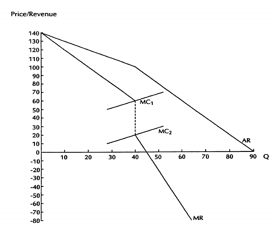
Page 158
Figure 7.9
Remember, however, that this model depends on an assumption of profit-maximising
behaviour for the oligopolist and a high degree of substitution between products. This
produces the reactions from competing oligopolists which we have described (i.e. refusal to
follow a price increase but matching a price reduction). It is not a general model of oligopoly
and does not tell us how the “sticky” price is arrived at in the first place. There are too many
behavioural assumptions for the model to be entirely satisfactory.
The model does not hold up during periods of severe price inflation, when we would expect
firms to follow their rivals’ price rises but not any price reductions which they will not expect
to be maintained because of rising costs.
Price Leadership
Another tendency, which does hold during inflation, is for all oligopolists in a market to
follow the price movements of one firm, the price leader. Such leaders can be:
• The least-cost firm, which can oblige competitors with higher costs to follow its prices,
even though they cannot maximise their own profits at the levels it sets.
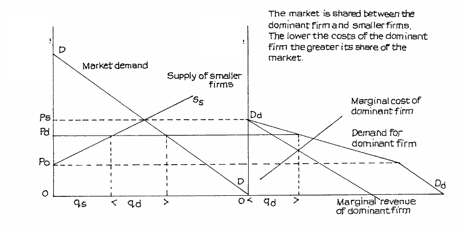
Page 159
• A firm which is typical of others in the market and which becomes a barometer of market
conditions. If this firm feels that a price change is necessary, then it is probable that
others will feel the same.
• The largest and the dominant firm in the market. The most common model of this
situation assumes that this firm, because of its size and the economies of scale it can
achieve, is able to achieve lower costs than the others. The lower its costs compared with
the other firms’ costs the greater will be its market share and, consequently, its
dominance in the market. This model is illustrated in Figure 7.10.
Figure 7.10
The market is shared between the dominant firm and smaller firms. The lower the costs of
the dominant firm the greater its share of the market.
The dominant firm model makes the following assumptions:
(a) The dominant firm is aware of the total market demand curve and the cost conditions and
hence the supply curve for the smaller firms in the market.
(b) The objective of the dominant firm is to maximise profits.
In Figure 7.10 the demand curve DD is the demand curve for the market and SsSs is the
supply curve for the smaller firms. At price Po these firms are unwilling to supply to the
market; it is their minimum price. At price Ps the smaller firms are able and willing to supply
the full market demand at that price.
This knowledge allows the dominant firm to estimate its own demand curve, which is made
up of market demand at each price less the amount which the smaller firms are able to supply.
Thus the demand for the dominant firm’s product is nil at price Ps but it is the same as market
demand at prices Po and below. Between these two prices the dominant firm is able to supply
the balance between market demand and supply from the smaller firms.
Price
Revenue
Cost
RWF
Price
Revenue
Cost RWF
Page 160
On the assumption of profit maximisation the dominant firm will wish to supply quantity qd
which is the quantity at which its marginal cost is equal to its marginal revenue. At this
quantity level the dominant firm’s market clearing and profit maximising price is Pd. If it
charges this price the other firms will have to follow, and market demand at this price is
shared on the basis of qd to the dominant firm and qs to the smaller firms.
Notice that if you raise the dominant firm’s marginal cost curve you will reduce qd and
increase qs. However, if you lower this curve you will increase the market share going to the
dominant firm, which is thus able to maintain its dominance as long as it is able to keep its
costs lower than those of the smaller firm. We may assume it is able to achieve this through
economies of scale, a higher level of technical knowledge and managerial skill, and by its
superior power to secure low prices in the factor markets.
F. PROFIT MAXIMISATION AND ALTERNATIVE OBJECTIVES
FOR THE FIRM
In the discussions of perfect competition and monopoly, we noted that whereas under perfect
competition long-term survival depended on the firm maximising its profits, whether or not
this was its conscious objective, under monopoly the firm could survive without actually
maximising profits. As long as it made a satisfactory profit it was able to pursue other
objectives. We now develop this point more fully.
Any firm which possesses a substantial degree of market power as a producer and which is
large in relation to the total size of the market in which it operates, will have a product
demand curve which is downward sloping and, if it is successful, is also likely to be able to
make profits above the minimum needed to keep it in the market. Its position may, therefore,
be represented by a model similar to that usually used for monopoly as in Figure 7.11.
This model assumes that the firm does not practise price discrimination, so that its product
demand curve is also its average revenue curve. Assuming that its market power allows it to
make profits above the minimum, there will be a substantial range of output levels and prices
between which it can make profits. This, in Figure 7.11, is the range between output level A
(price PA) which is the lower break-even point where the falling average cost just equals
average revenue, and output level C (price PC) which is the higher break-even point where the
rising average cost just equals average revenue.
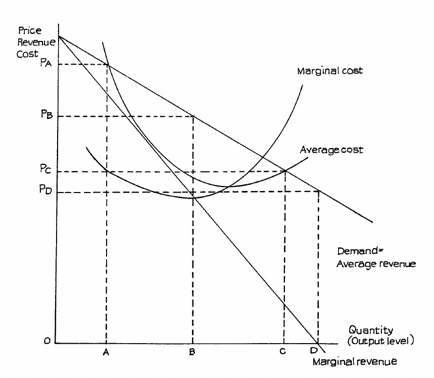
Page 161
Figure 7.11
The firm in this situation can pursue objectives other than profit maximisation as long as it
operates within this profit range, but, as the model suggests, the range can be very wide.
During the past half century there have been many economists who have argued that large
firms, especially oligopolies, do not maximise profits. Unfortunately there has been no
universal agreement over what objective or objectives they do pursue instead. A number of
alternative theories of the firm have been developed and each of these is based on different
assumptions about firms’ behaviour. For convenience we can identify two broad groups of
theories - those that replace profit maximisation by an assumption that firms seek to
maximise something else, and those that abandon any idea of maximisation in the belief that
firms seek to pursue several objectives at the same time and cannot, therefore, hope to
optimise any one.
(a) Alternative Maximising Theories
An American economist, Baumol, suggested that firms seek to maximise sales revenue,
subject to making a minimum profit which was defined as that level of profit needed to
retain the support of the firm’s shareholders and the financial markets. In Figure 7.11 the
revenue-maximising output level is at D, where marginal revenue is O (at the top of the
Page 162
total revenue curve), but in this model quantity D lies beyond the second break-even
point of C, so the firm could not reach D without suffering a loss. If it were to try to
maximise revenue subject to achieving minimum profit, it would have to produce at an
output level somewhere between B and C and charge a price between PA and PB.
A British economist, Marris, has argued that firms seek to maximise their rate of growth
(expansion) subject to preserving their share values at a level where the firm can hope to
be reasonably safe from the fear of being taken over. If the firm grows too fast, its profit
rate tends to fall and this depresses the share value and brings the risk of take-over. Too
slow a rate of growth is also likely to bring the firm to the notice of take-over raiders, so
the firm has to balance the desire for growth with the need to maintain profits.
There are similarities in the Baumol and Marris theories. Both agree that the firm’s
objectives are really established by its professional managers, who are free to control the
firm as long as they keep the shareholders satisfied with their dividends and the financial
markets satisfied with their profits. Profit remains important - no one doubts that in a
market economy - but it is not maximised to the exclusion of other aims that meet
managerial ambitions. Managers like to operate in large firms because size brings
prestige, high salaries and a range of other benefits, so these are pursued, to some extent
at the expense of the profits belonging to shareholders. In the Baumol theory, revenue
was seen largely as a way of measuring growth. The Marris argument is slightly more
complex and stresses growth more directly.
Another American economist, Williamson, developed another kind of maximisation but
quite cleverly combined this with the idea that the firm pursued several objectives at the
same time. Again agreeing with the idea that managers were the real controllers of the
firm, Williamson argued that they sought to maximise managerial utility and that this
utility was a combination of the pursuit of profit, growth, measured by the number of
people employed, and managerial “perks” (all the various expenses, benefits, etc. that
movement up the business managerial ladder tends to bring).
(b) Satisficing Theories
The rather ugly word “satisficing” has been coined to express the idea that firms pursue
several different objectives at once. Whereas no one objective can be achieved to
complete satisfaction, the firm aims to pursue each to a degree of tolerable semi-
satisfaction, i.e. it “satisfices” without fully satisfying. The idea was first given clear
expression by the American economist, Simon, in an influential book, Administrative
Behaviour. Simon argued that, in practice, firms could not hope, even if they wished, to
maximise anything but rather reacted to problems as they arose and aimed to keep all
those involved in the firm reasonably satisfied so that the firm could continue to exist.
Following the reasoning of Simon, this idea was developed into a more formal
Behavioural Theory of the Firm by two more American economists, Cyert and March, in
a book with that title. In this theory the firm is seen as a coalition between shareholders,
managers and customers, all of whose support is needed to hold the coalition together.
To do so the firm has to pursue multiple objectives, such as profit, sales growth, market
share and products to satisfy customers as well as the needs of production managers, but
no one objective can be pursued to the exclusion of the others. The firm has to develop a
Page 163
set of behavioural principles to enable it to hold the coalition together and guide
managerial decision-making.
Various other attempts have been made to explain business behaviour but there is no general
agreement as to whether the traditional assumption of profit maximisation should be
abandoned and, if so, what should replace it. The alternative theories sometimes seem to
describe actual business behaviour more realistically, especially in relation to large
oligopolists. Firms do pursue growth, often at the expense of profits, take-over battles are
commonplace and the salaries and prestige of top business managers appear to bear little
relationship to the profitability of the companies they manage.
On the other hand, an economic theory of the firm should be concerned not only with how
firms actually do behave but also how they should behave, if the economic goals of technical
and allocative efficiency are to be achieved. Unfortunately, the alternative theories appear to
suggest that if firms operate as they predict, they are likely to be less efficient in the full
economic sense than if they pursue profit maximisation - the desire to make the largest
achievable profit consistent with market conditions. One thing that has to be remembered
always is that profit maximisation does not mean making very large and anti-social profits,
but simply the largest profit possible under prevailing market conditions. Profit maximisation
under perfect competition suggests lower profits than satisficing behaviour in an oligopolist
market. A market economy appears to operate more efficiently when firms seek to maximise
profit. Consequently, most economists continue to work with profit-maximising models,
whilst fully recognising that firms do frequently depart from profit-maximising behaviour in
practice.

Page 164
BLANK

Page 165
Study Unit 8
Further Aspects of Markets and Prices; Factor Markets
Contents
A. Market Structures and Economic Welfare
Elements of Economic Welfare
Competitive Markets and Economic Welfare
B. Price Discrimination
First Degree Discrimination
Second Degree Discrimination
Third Degree Discrimination
Using Spare Capacity
C. Factor Markets
Determining Factor Prices
Professionalism
Alternative Uses of Factors
Supply of Factors
Factors Influencing Labour Supply
Methods Used by Trade Unions
Wage Differentials
Functions of Factor Markets
Business Demand for Factors
D. Economic Rent
Meaning of Economic Rent
Economic Rent in the Market
Economic Rent and the Individual
Quasi-Rent
Page 166
A. MARKET STRUCTURES AND ECONOMIC WELFARE
In Study Unit 7 we examined the main forms of market structure - perfect competition,
monopolistic competition, oligopoly and monopoly. At the start of our examination we noted
that it has long been a common belief among many economists that the structure of a market
influences the conduct of firms operating in it and that this conduct in turn influences their
performances. The main areas of conduct likely to be affected by the competitive conditions
of the market are those of:
- price setting
- advertising and marketing
- attitudes to innovation and investment
- quality standards
- customer care.
Conduct in these areas is likely to affect the firm’s performance in relation to profit and the
efficiency with which it uses scarce resources.
Elements of Economic Welfare
By ‘economic welfare’ we mean the use of scarce resources to bring the greatest benefit to
the largest possible number of people in the community. Welfare is said to be maximised
when resources are used and production distributed in such a way that it is impossible to
make one person better off without making another person worse off.
Achievement of a high level of welfare clearly requires the efficient use of resources and it is
usual to identify two kinds of efficiency - technical or production efficiency and allocative
efficiency.
• Production or technical efficiency arises when producers are able to increase the
quantity of goods and services from a given quantity of production factors. This kind of
efficiency can be measured without too much difficulty. For example, we can calculate
how many motor cars one firm can produce from a set quantity of capital and labour and
compare this figure with the number of similar vehicles produced from the same amount
of capital and labour by a rival producer.
• Allocative efficiency relates to the distribution of production to meet the expressed
wants of the community. It is of no great benefit to the community to become more
technically efficient in the production of motor cars if there is already a surplus of these
but a severe shortage of other goods, say homes to live in. A production system would
achieve allocative efficiency if it were able to eliminate both surpluses and shortages.
The measurement and achievement of allocative efficiency presents rather more
problems than technical efficiency given the basic economic problem of unlimited wants
and scarce resources. If there are never going to be enough resources to satisfy everyone
there will always be some who feel that there are not enough of certain goods or services
and others who consider that resources could be better used on the forms of production
they consider to be of most importance.
Page 167
The greatest difficulties in determining allocative priorities are usually experienced in the
public sector, where the relationship between receiving the utility or benefit of a service is
separated from paying the price (meeting the factor costs) of providing that service.
Arguments about the relative importance of, say, providing more nursery education as
opposed to extending care for the elderly, tend to assume that the costs of both will be paid by
some third group, usually anonymous or simply referred to as “the taxpayer” or “the
government”. In this way pressure groups desiring more of their own favoured benefit avoid
the difficult matter of opportunity cost.
The difficulties still exist in the market economy, or the private sector of the mixed economy,
but they become focused on the question of willingness and ability to pay for the options
available.
In an earlier study unit we suggested that a consumer’s marginal utility for a good would be
equal to the price that consumer was willing to pay for the good. If we accept this then the
good’s market demand curve can be regarded as the aggregate of all the marginal utilities of
the consumers willing to pay any price for the good. Each point on the curve represents the
utility of the marginal buyer at that point - the buyer who is prepared to pay that price but not
a higher price. A lower price brings in additional buyers whose marginal utilities are now
equal to that reduced price. Looked at in this way the market demand curve becomes a
marginal social valuation curve - i.e. the value to the marginal user at each level of
production.
On the supply side of the market the marginal cost curve represents the cost of producing
each additional unit of the good. This cost depends on the prices of the inputs in the factor
markets and these factor prices are influenced by the community’s valuation of other possible
uses for the same factors. We may thus see the marginal cost curve as the community’s
marginal social cost curve.
This view of market demand and supply is illustrated in Figure 8.1, where we see that if
production of this particular good rises above qo its marginal social cost is greater than its
value to the community. If production is lower the community would gain from increased
production because its marginal value is higher than its marginal social cost. Only at the
production level qo are these social costs and values equal.
The implication for achieving allocative efficiency is that the prices for goods should just
equal their marginal costs. If the whole production system could be organised in such a way
that market prices for all goods and services were just equal to their marginal costs the
community could be achieving the highest possible level of allocative efficiency.
This kind of argument is the basis for the belief expressed in many economics textbooks that
the equality of price and marginal cost is an ideal to be pursued in the interests of increasing
efficiency and raising the level of economic welfare. However, it ignores a number of
important issues, in particular:
• Those goods which are clearly valued by society but which are not paid for directly by
their immediate users. These include the examples of education and care of the elderly.
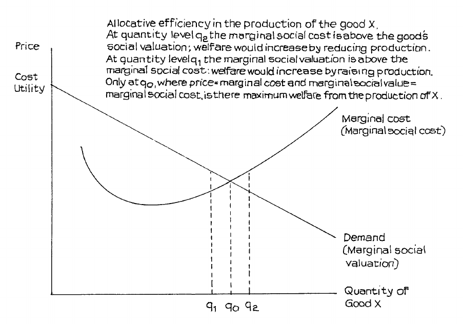
Page 168
Few very young children have incomes of their own and relatively few of the elderly in
need of care have incomes able to meet the marginal costs of its provision.
• Income inequalities that exist in most market economies. As a result of these inequalities
we cannot really guarantee that all market demand curves are true representations of the
marginal social valuation curves of many goods on which the community as a whole is
likely to place a high value. Housing is an issue which presents difficulties for many
societies. An economic system which produces massive inequalities in housing
provision cannot really claim to have achieved a high level of allocative efficiency
whatever the relationship between house market prices and marginal costs.
Figure 8.1: Allocative Efficiency in the Production of the Good X
Competitive Markets and Economic Welfare
One of the problems that economists have sought to solve is the question of which type of
market is most likely to increase production and allocative efficiency and, therefore, raise the
level of economic welfare.
In traditional microeconomics perfect competition has often been favoured on the grounds
that in the so-called long run equilibrium for the firm under perfect competition the following
desirable objectives are achieved:
- Abnormal profit is eliminated
- Price is equal to marginal cost
- Firms are obliged to produce at quantity levels where average costs are at their lowest.
Page 169
However, it is possible to raise a number of serious objections to this view of perfect
competition.
• Long-run equilibrium can only be achieved if demand remains constant over a reasonably
long period. If demand fluctuates, as it frequently does in competitive markets, the
market is extremely unstable. Firms face constantly fluctuating prices and have to plan
production under conditions of considerable uncertainty. This leads to instability in
factor (including labour) prices.
• Market instability and low profit levels make it difficult to undertake technical research.
Consequently firms tend to remain small and the level of technology low. Although
firms may be forced to minimise production costs these may be at levels significantly
higher than could be achieved if they were able to gain economies of large-scale
production and develop more advanced production technology. Resources are not,
therefore, used to their maximum potential efficiency.
• As pointed out earlier, goods that are homogeneous offer no choice to consumers and
choice is an element in consumer utility.
If, then, there are doubts about the real efficiency of perfect competition, how do the other
market structures compare?
Monopolistic competition does offer choice but it suffers from most of the potential defects
of perfect competition. Monopoly offers potential gains from economies of scale, the
avoidance of resource duplication when competing firms produce similar goods and try to sell
to the same customers, and profits are available for technical development. However, the
absence of competition removes many of the pressures that force managers to be efficient and
profits may be distributed to senior managers and shareholders rather than used for research
and development. Monopoly power can lead to less rather than more efficiency in all its
aspects.
Oligopoly is usually classed with monopoly in its effects on efficiency and oligopolists are
often accused of collusive behaviour in order to create partial monopolies for their own
benefit. There have been many examples of collusive behaviour and abuse of market power
but some modern studies have shown that apparent oligopolies can sometimes be highly
competitive and the possibilities for potential compensation can produce some of the benefits
of competition with less wasteful duplication of resources.
Clearly there are no simple solutions to the problems of increasing efficiency.

Page 170
B. PRICE DISCRIMINATION
So far, all our discussions of equilibrium and market price have assumed that suppliers will
charge the same price to all consumers at any one time-period within any given supply range.
Thus, if the market price is RWF5 per kilo, this will be the price paid by Mr A Van Rooyen
and by the Gold Plate Corporation. Suppliers do not discriminate between customers but
charge all the same price.
However, in practice, there is often price discrimination between buyers. Economists have
identified the following three types of price discrimination.
First Degree Discrimination
This is the most extreme form. Suppliers seek to charge each individual customer a price
equal to his marginal utility, i.e. they will try to charge the highest price that each customer is
prepared to pay. This is often called “haggling”. Private houses (other than new houses) and
second-hand cars are usually sold in this way. In many countries, most goods are sold by
haggling - a practice which has also been termed “perfect price discrimination”. If successful,
such total price discrimination will achieve the highest possible revenue - as is illustrated in
Figure 8.2.
Figure 8.2: Total or Perfect Price Discrimination
This, of course, is a seller’s ideal which is almost impossible to achieve. Moreover, there are
costs involved. Haggling is time-consuming and possible only when there are relatively few
customers in relation to the time available for selling. When the number of customers rises,
the cost of haggling exceeds the extra revenue gained, and sellers usually move towards a
RWF9
RWF4
Page 171
fixed-price system - especially when unskilled assistants have to be employed. Haggling is
profitable only when the seller is more skilled than the buyer! There is also the danger that
those who paid RWF8 will meet those who paid RWF4, feel cheated and refuse to buy any
more. Some degree of monopoly power is desirable for successful long-term, total price
discrimination.
Second Degree Discrimination
This is the term sometimes applied where a selected number of large customers are charged
prices lower than could be justified on the grounds of any large-scale economies achieved. If
a customer buys in bulk, then some price reduction is normal because the unit costs of selling,
administration and transport are all likely to be lower. It is not price discrimination when
such cost savings are shared with the customer. Nor is it price discrimination when customers
are given incentives to adopt cost-cutting practices, e.g. to pay quickly before being sent
accounts, or as soon as accounts are submitted; to order regularly, thus saving selling
expenses; or to take orders at times and in quantities suited to the sellers’ needs.
Price discrimination implies a price reduction to particular customers, made simply to obtain
an order that would not otherwise be given, or to encourage loyalty from a customer whom
the seller would not wish to lose.
A case of second degree price discrimination is illustrated in Figure 8.3. Notice here that the
average revenue does not match any price actually charged to any customer. Again, there is
the danger that customers paying the higher price will learn of the practice and become
alienated towards the supplier. Some degree of monopoly power is, clearly, desirable from
the seller’s point of view. There is also a danger that the low-price buyer will re-sell to other
customers at an intermediate price, though monopoly power would make this practice short-
lived.
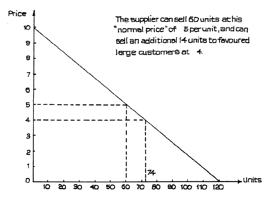
Page 172
Figure 8.3: Second Degree Price Discrimination
Third Degree Discrimination
This is the term used to describe the situation where two or more separate markets can be
identified and segregated. This is illustrated in Figures 8.4 and 8.5.
Here, there are two separate markets. Market A is made up of customers willing to pay up to
RWF16 per unit. Market B customers will pay only up to RWF10. In this particular case, the
maximum market size in each is the same, at 500 units. At all prices, we see that demand is
more price elastic in market B than in A. The curve in B is less steep, indicating that
customers are more price conscious and demand reacts more to any change in price.
The curve for the combined market is the addition of A and B. At prices above RWF10 it
reflects A’s curve only, but at lower prices it is the sum of the two separate curves.
We can adapt Figure 8.4 to show how the firm can gain from price discrimination. Figure 8.5
adds a marginal cost curve and marginal revenue curves to the diagram. If the firm charges
the same price in both markets and does not discriminate, then its profit-maximising price,
where marginal revenue = marginal cost, is RWF8. At this price, total sales are 350 units, and
total revenue is RWF8 × 350 = RWF2,800.
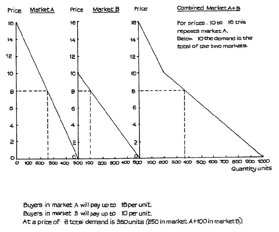
Page 173
Figure 8.4
Suppose the firm can charge different prices in each market without any alteration in costs.
The marginal cost remains unchanged, and this is indicated by the horizontal MC line just
below 4 on the vertical axis. If it charges profit-maximising prices in each market, it will
seek to equate this marginal cost with the marginal revenue (MR) in each of the markets A
and B. This produces a price in A of RWF9.60, at which price 200 units are sold, and a price
of RWF7 in market B with sales in B of 150 units.
Total quantity sold remains unchanged at 350 units. 50 units are lost in A but 50 are gained in
B. Total revenue, however, rises to RWF2,970, made up of 200 units at RWF9.60 plus 150
units at RWF7. Because costs remain unchanged, the additional revenue must mean that
profits rise. Notice that the rise in price in market A, where demand is more inelastic, is
greater than the fall in price in market B, so that the revenue gained from the practice of
discrimination is greater than the amount of revenue lost.
We can say, then, that, in order to gain from price discrimination in two different markets,
price elasticity of demand at the relevant price range must be different. At the same time,
price discrimination can be operated successfully only if the two markets can be kept
completely separate. Sometimes, small differences may be made, to make it appear that the
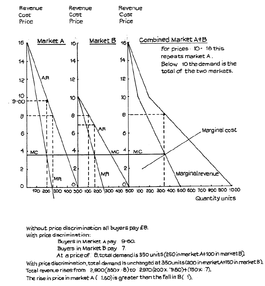
Page 174
two markets are different - e.g. the difference between first- and second-class rail travel. This
represents price discrimination if the difference in fares is greater than any cost difference
caused by the difference in service, standard of comfort, etc. (normally, it is). There are also
similar class differences in air travel. Services markets are often easier to separate than goods
- largely because they cannot be stored and re-sold.
Monopoly power is not necessary for price discrimination in services, though it helps if all
suppliers adopt similar practices, which then gain public acceptability more easily.
Figure 8.5
Page 175
Using Spare Capacity
A rather different practice which is sometimes described as price discrimination is that of
making use of spare capacity at a price which covers variable costs and makes some
contribution to fixed costs. Thus, a manufacturer may accept an order below his normal
price, if his machines and labour would otherwise not be fully used. Any price will increase
profit, provided it is more than the marginal costs of meeting the order, and does not lead to
pressure for reduced prices from other customers.
In the same way, a coach service may offer cheaper fares on scheduled services on certain
days of the week, when otherwise coaches would be running with many empty seats. The
“standby” air fare, whereby the airline offers a low price in order to fill a seat which would
otherwise remain empty is based on the same principle. However, if these measures become
too popular, they defeat their purpose. Demand is simply transferred from one time-period to
another, rather than increased, and total revenue is reduced. It is often found, therefore, that
such special price arrangements can be offered only for limited periods; otherwise all prices
are reduced and profits transformed into losses.
The object of any form of price discrimination is to increase revenue more than any increase
in cost that may be incurred. Price discrimination which increases quantity demanded
without any increase in profit is a failure. A reduction in quantity supplied or a change in the
pattern of demand without change in total quantity supplied could also be justified if this
resulted in a reduction in costs greater than any reduction in revenue. However, price
discrimination normally leads to some increase in cost so that a greater increase in revenue
would normally be needed for the practice to result in a profit rise.
Page 176
C. FACTOR MARKETS
In order to produce any goods or services, the business organisation has to acquire production
factors. We have already seen that the payments made to production factors make up the
costs of the business. The price that has to be paid to obtain factors forms the costs of
production. We must now examine some aspects of how factor prices are determined.
Determining Factor Prices
Just as the products of business organisations are sold in markets at prices which, subject to
any market imperfections, are the result of the interaction of the forces of supply and demand,
so also are the production factors.
There are factor markets, just as there are product markets - only, in factor markets the
business organisations are the buyers, and they provide the demand. The sellers are the factor
owners, e.g. the owners of land or capital and people who supply their own labour. In cases
where trade unions have a very high degree of control over the people who may work in an
occupation and the terms and conditions under which they may be employed, the union could
be considered to be the supplier, and a number of economic models are based on this
assumption.
The factor markets, therefore, are those for land, finance for capital investment and labour.
The markets for basic natural resources, such as metals, and the basic commodities required
for production or for foods, are also normally regarded as being very close to factor markets.
The factor, land, is often seen as including the resources of the land which are required for
production to take place.
Most of the structural features used to classify markets as described earlier, i.e. perfect
competition, monopoly, etc., can also be applied to factor markets. At the same time,
however, there are some special features which apply to factor markets, and we need to take
these into account.
Professionalism
The buyers and sellers of factors tend to be more expert than consumers, especially in
distinguishing differences in quality. In the consumer field, it is possible to create differences
in essentially identical articles by branding, pricing, and advertising, so that buyers can be
persuaded to pay more for certain goods in the belief that they are buying superior quality. In
the factor markets, this still takes place but to a lesser extent. In markets for basic materials,
careful systems of grading usually apply as for example on the London Metal Exchange for
Tin ore cassiterite.
The actual buying and selling tends to become a specialised function in a factor market, so
that the broker or skilled agent is important. Tin is bought and sold in the London Metal
Exchange by brokers who have to be members of specialist associations. The skilled agent
operating as a consultant has not gained an important place in the labour market, but is
beginning to be more common in the field of management selection.
Page 177
Alternative Uses of Factors
Factors are simply means to an end - the desired end being the production of consumer or
capital goods, or the giving of a service. As it is the end which is important, rather than the
means, there will usually be a variety of ways in which factors can be combined in order to
produce a particular final product (the “production function”). In a market operating through
the price system, the aim is to find the cheapest combination which will produce a given level
and quality of output.
Firms which wish to achieve this combination will be influenced by changes in factor prices
and by new inventions.
(a) Changes in Factor Prices
If copper becomes more expensive, it might be possible to use aluminium as a substitute.
If labour becomes more expensive because of pay rises or employment taxes, more
extensive use may be made of capital in the form of labour-saving machinery. If land is
very expensive, a firm may use a computer and highly-skilled staff to control stocks, so
that less land is devoted to the storage of material. Capital and labour will thus replace
land if their total additional cost is lower than that of the land saved.
(b) Inventions
New discoveries change the production function. We are familiar with the developments
which have helped to replace manual labour by capital in the form of earth-moving
equipment, office machinery, computers, and electronically-controlled factory machines.
In addition, modern developments in transport and communications, the building of new
roads, and the extension of electric and gas power has given firms greater freedom in the
choice of location, so that there is now a greater amount of land available for industrial
use. The principle of substitution is not new but it is the key to the understanding of
factor markets.
Supply of Factors
Factors of production are supplied in return for money incomes - wages, salaries, rent, fees,
profits and interest are all incomes to factors. As a general rule, we can say that more will be
supplied at a higher price (assuming that people wish to maximise their incomes).
Although supply will tend to increase in response to a price rise, this may not happen
immediately. It may be very difficult, or even impossible, to increase supply in the very short
run. The supply for skilled labour, in particular, is often very inelastic in the short run, so
that, in a complex industrial economy where the time element is of great importance to
employers, an increase in demand may produce a steep rise in wages.
The supply of factors to particular markets should be distinguished from the supply of factors
to all markets, i.e. to the economy as a whole. Total supply may be unchanged but the
distribution of supply may vary as conditions in particular markets become more - or less -
favourable to the owners of the factors.
Page 178
The total supply of factors to the economy as a whole is governed by rather different
considerations.
(a) Supply of Land
For most countries, land, of course, is fixed in supply with only relatively small increases
possible from reclaiming land from the sea, mountains or jungle, and in some cases this
can have environmental consequences of serious concern for the future. The productivity
of land in some countries can be improved with irrigation and its industrial-commercial
potentialities transformed with improved communications.
(b) Supply of Capital
Capital is a more mobile factor; huge amounts of it are moved around the world by the
large multinational companies. The total quantity of productive capital can also be
increased by improvements in the financial, especially the banking, structure of a nation.
If people are able to keep their savings safely in bank deposits instead of in gold tooth
fillings, there can be a significant increase in a country’s total supply of capital that can
be used in business development. In many developing countries there is a high degree of
political instability so that people with spare capital tend to keep it in more stable form,
such as gold or diamonds, where it can be evacuated quickly to a different country.
Increased political stability in these countries can bring a swift increase in total capital
available for business development in the domestic economy.
The supply of capital to a developed market economy is also subject to political as well
as economic influences. The total amount of capital produced by an economy depends
on the wealth created by its economic activity and by the proportion of that wealth that is
saved rather than consumed. In the absence of exchange controls, the domestic supply
will be increased by inflows of capital from residents in foreign countries and reduced by
outflows from residents in the home country. To encourage capital to come into the
country rather than flow out, governments can manipulate interest rates so that
investment becomes more profitable in the country than elsewhere. However, other
countries may be pursuing similar policies and high interest rates have other, more
damaging economic consequences so governments have only limited control over them.
International investors will tend to keep their capital in those countries which offer the
highest rewards, taking into account safety and security and the maintenance of
purchasing power in world markets.
(c) Supply of Labour
Labour is also a mobile factor but its mobility between countries is almost always
restricted by State controls. The rather chilling term “economic refugee” has been coined
to describe people who wish to follow the normal market practice of moving to where the
rewards are greater, often away from areas where they are very poor, but are prevented
from doing so by governments whose approval of unregulated markets stops well short of
any action thought likely to cause domestic social tension.
(i) The supply of labour to the economy as a whole depends, in the first place, on the
size and structure of the total population and on the proportion of the population that
is of “working age” (between minimum school leaving age and the “normal” age of
retirement). The size of the total population is influenced by rates of birth, death,
Page 179
immigration and emigration. In most developed countries both birth and death rates
have been falling, so that the population has been growing at a slow rate compared
with earlier periods but has also been growing older. The total effect is to increase
the proportion of population of working age. Most governments now try to control
immigration and to admit only people with either scarce skills or capital. Although
emigration is not usually controlled in developed countries it is, of course,
influenced by immigration controls in other areas.
(ii) The proportion of people of working age who actually work or seek work (nowadays
described as the workforce) depends on the proportion of:
• young people electing to stay in full-time education beyond the minimum school
leaving age.
• older people electing - or forced - to take retirement before the “normal” retiring
age
• females electing to remain in, or rejoin the workforce instead of working full-
time in the home.
(iii) This apparently clear-cut structure is becoming increasingly blurred by such
tendencies as: more gradual movement from education to work as students finance
their studies by working part-time; more gradual retirement as older people move
from full- to part-time employment before retiring completely from the workforce;
increasing numbers of people taking time out of the workforce to gain additional
qualifications; and the considerable growth of part-time female employment.
(iv) Although economists like to keep supply and demand firmly distinct as separate
forces, the demand for labour does affect supply because the knowledge that there is
a low and shrinking demand for unskilled labour will influence many young people
to stay in full-time education to improve their chances of obtaining jobs, while the
fear of future redundancy is likely to influence older people to accept any financial
inducements offered to them to take early retirement. Redundancy or threat of
redundancy of a husband or partner may provide a further inducement for many
women to return to the workforce or move from part-time to full-time employment.
(v) Much has been written about the reasons for the increase in the proportion of women
in the workforce, an increase that has taken place in most industrial countries. It is
often overlooked that women are expected to work, as hard, if not harder, than men
in most agrarian economies! The reasons include changes in demand for labour,
from heavy manual to light manual and mental work, changes in social attitudes,
changes in family size and the technology of birth control, and the mechanisation of
work in the home. Whatever the reasons, there is no doubting the proportional
increase in females in the workforce that has taken place throughout most of the
developed world and in many newly industrialised countries. This increase has had
very great social as well as economic effects and has also influenced the institutions
of labour markets. In general, though with some important exceptions, female
workers tend to be less controlled by trade unions than men in the older industrial
occupations.
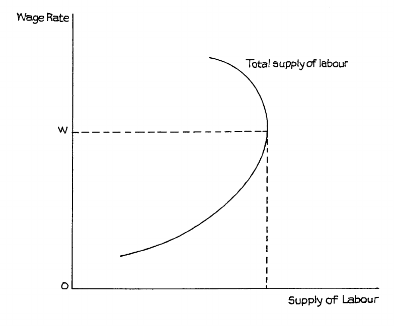
Page 180
Figure 8.6
(vi) Like any other economic good, the supply of labour is influenced by price - the wage
rate. Clearly this has a major impact on the supply of labour to particular
occupations and industries. Other things being equal (which they rarely are) people
generally prefer to work in the more highly-paid sectors of employment. However,
the impact of the general wage rate on the total supply of labour is less certain.
People work to obtain income. They also need free time, given the general term
“leisure”, in order to enjoy that income. Consequently, there is always something of
a conflict between the need to work to gain income and the desire for leisure. High
income and little leisure can be as unsatisfactory as a great deal of leisure and little
income. The widely accepted view among economists is that people can be expected
to wish to work more as wage rates rise from low levels, but that there comes a point
when the desire for leisure becomes more powerful than the desire for more income
and the response to any further rise in the wage rate is to work less. There is much
evidence to suggest that people have a target level of income according to their view
of what constitutes a satisfactory living standard, and once that target is reached,
they prefer to have increased time of their own. The target can, of course, change as
the purchasing power of money and people’s expectations and ambitions change.
However, the implication of this view of people’s attitudes to work, income and
leisure is that the supply of labour curve is likely to slope backwards at the higher
wage levels, as illustrated in Figure 8.6. When the wage rate reaches Ow, the
preference for leisure becomes more powerful than the desire for additional income,
so the total supply of labour starts to fall when wages rise above this level.
Page 181
(vii) There is also firm evidence that this shaped supply of labour curve appears to apply
to men more than to women. It seems that, at current wage levels, the supply of
female labour continues to rise with the level of wages. A number of explanations
have been offered for this difference between the attitudes of men and women.
These include:
• Where families cannot help, many women incur expense in securing child care
and house cleaning services when they decide to remain in or return to the
workforce. Only those women whose incomes from working exceed the cost of
working can afford to work. As wage rates rise, more women fall into this
group.
• Household income often depends on the combined incomes of a man and
woman in the household. At low wage levels, reliance is chiefly on the man’s
income, but as wage rates rise, the man may decide to take more “leisure” in
order to help with the family and home so that the woman can return to work.
• The general desire of women to work has been so strong during the past two or
three decades for a mixture of financial and non-financial reasons, that it has
resulted in a continued increase in female employment during the time that
wage levels have been rising. Statistically it is difficult to separate the wage
from the non-wage influences when there is this strong trend in one direction.
The supply-side pressures have been matched by the employers’ demand for
part-time female workers as one way to bring greater flexibility into the
workforce in a period when socially and politically inspired employment
protection legislation has been making it more rigid in spite of increased
competition and insecurity in product markets.
Factors Influencing Labour Supply
(a) Society, Laws and Customs
(b) Labour Immobility. (i.e. restrictions on labour movement)
(i) between regions and countries (= geographic immobility)
(ii) between jobs (i.e. occupational immobility)
caused by – union barriers, professional barriers, lack of information on job
opportunities, housing shortages (expense, non-monetary considerations (friends,
social life), ability, linguistic and cultural differences.)
(c) Barriers of entry to certain professions/trades (e.g. professional qualifications, long
apprenticeship)
(d) Lack of freely-available information about jobs and wages.
(e) Trade Union influence on labour supply and wages.
Trade unions can have a significant influence on wage levels.
The Bargaining Theory of Wages: is that wage levels are set by negotiation between unions
and management by a process of Collective Bargaining.
Page 182
The role of unions is to raise the real wage of the work force by:
(a) Erect and maintain barriers to entry into jobs so as to ensure high earnings for existing
members.
(b) Monopolise the supply of labour in the industry.
However, unions cannot go on raising the real wages of the work force unless labour
increases its productivity (output per worker) so as to offset the increase in its costs.
Methods Used By Trade Unions
1. Negotiations with employers (generally annual).
2. Official Strikes.
3. Picketing
4. Work to Rule or Go-Slow or overtime ban.
5. Selective Strike Action.
6. Unofficial Strikes.
7. National Wage Agreements - i.e. wage agreements negotiated at a national level
between trade union and employers’ federations. This sets a minimum or “normal” wage
level or wage rise firms can then negotiate around that “norm” with their own employees.
8. Minimum Wages – minimum legal wage that all workers must receive. It is used to
protect the incomes of the lower paid and thus is used as a means of relieving poverty. There
are arguments made for and against minimum wage legislation. The main argument against it
is that it reduces employment as some firms cannot afford to pay the higher wage. Another is
that it does little to reduce poverty among those who do not work as it only benefits those in
employment.
Sources of Unions Depends on:
(i) The union’s size, financial resources and negotiating skills.
(ii) The sensitivity of its workers' occupations (e.g. electricity worker’s strike can have a
huge impact).
(iii) A union’s ability to control the supply of labour (closed-shop helps).
(iv) Economic viability of the industry.
(v) General Economic Conditions.
(vi) A union’s relationship with the government.
(vii) Technological progress
(ix) Restrictive wage legislation.
(x) Market Conditions.
(xi) Labour Productivity Improvements.
Wage Differentials
Page 183
These are differences in the rate of pay between one type of job and another.
Wage Differentials depend on:
(a) Restrictions on supply of certain types of labour (e.g. because of professional `
qualifications, rare abilities, danger).
(b) Higher demand for certain types of labour.
(c) Higher revenue for certain occupations.
(d) Union Strength in different occupations.
Skilled workers tend to be paid more than unskilled because:
(a) They are more productive (i.e. have a higher Product of Labour).
(b) They are scarcer (i.e. demand is less relative to supply, so their supply curve is further to
the left).
(c) Supply of skilled workers is relatively INELASTIC because of barriers to entry
(professional qualifications) and because availability of people with suitable talent is
restricted.
Wages differentials could be eroded by
(a) Strike action.
(b) Minimum wage legislation.
(c) Income controls
(d) Increased productivity by unskilled workers.
(e) Training incentives.
Functions of Factor Markets
The factor market performs two functions, as follows:
(a) Rationing: the supply of factors is rationed between the users so that the greatest supply
is given to those best able to use the factor efficiently, as shown by their ability to pay the
highest price for the factor.
(b) Distribution: factors are directed to those areas of production where they are most
valuable. These will be areas which are best able to pay high rewards. This ability to
pay will result from the fact that these are areas where demand for consumer products is
highest. Thus, the distribution of factors is determined by the demand for consumer and
investment goods and services.
In the modern mixed economy, however, markets are seldom perfect, and we have to
recognise that non-economic motives are sometimes important. We also have to recognise
the importance of government influence. We shall see that some types of labour and land are
largely outside the price system, although they are rarely altogether unaffected by it.
Page 184
Business Demand for Factors
The demand for production factors is what is often called a “derived demand”. This is
because the firm will employ factors only as long as they contribute to the profits of the
organisation. A factor is wanted because it is necessary for the production of the firm’s
product, and the firm’s profit comes from selling its product.
In general, therefore, the higher the demand for the firm’s product, the greater will be its
ability to make profits, and the more factors it will want to employ.
However, the demand for factors may not rise in direct proportion to any rise in the demand
for the product, because the firm will try to make more efficient use of the factors it already
has, before it employs more. Thus, a 10% rise in the demand for the product is likely to lead
to a less than 10% increase in factor demand. In a period of very rapid technological advance
there might have to be a very great increase in product demand indeed to produce any really
significant increase in total factor demand. In particular, developments in electronics and
what may be termed “micro-technology” mean that the demand for space or land is not likely
to increase in anything like the same proportion as production increases. Many machines
have become smaller, as well as more efficient. Micro-computers take up much less space
than mainframe computers.
The main interest of economists, however, tends to be concentrated on the relative demand
for capital and labour - machines and people - because these are to a very large extent
substitutes for each other and, of course, the employment or unemployment of people has
very important social implications. The firm’s desire to employ machines or people, and the
proportions in which they are employed, depends on the extent to which they can contribute
to production. If, for example, a machine can produce twice as much as a man, for the same
yearly cost, then the employer will prefer to employ the machine, other things being equal. If
we recognise this simple fact, then we can see that the demand for labour in relation to the
demand for capital (machinery) will depend on:
(a) The productivity of both labour and capital - i.e. the amount that each can add to total
production per unit; and
(b) the unit price of both labour and capital.
If the firm is seeking to maximise profits, then it will try to aim at the condition where the
additional product contributed by the last RWF spent on labour will be exactly equal to the
additional product contributed by the last RWF spent on capital (equipment/machines, etc.).
If this is not the position, then the firm can increase its efficiency and profitability by
switching from labour to capital, or vice versa, according to which offers the greater increase
in production for each RWF of additional expenditure. If the extra production per RWF of
labour is two units and the extra achieved by spending another RWF on capital is four units,
then clearly the firm will gain by spending fewer RWFs on labour, and more RWFs on capital.
We can express precisely this idea more formally in the equation.

Page 185
MPP
P
MPP
P
L
L
K
K
=
where MPPL = the marginal physical product of labour
MPPK = the marginal physical product of capital
PL = the unit price of labour
PK = the unit price of capital
The marginal physical product of a factor is the addition to the total product achieved by
employing one more unit of the factor - in the reduction in total product suffered by
employing one less unit of the factor.
Factor markets are not perfect, and a firm’s ability to achieve this condition is likely to be
constrained by a number of influences, including labour law, trade union power, and the fact
that there are what are called indivisibilities in the employment of factors. For example, if
one worker is needed to look after three machines, the firm cannot employ 1
2
3
workers if it
wishes to use five machines. It is likely to need two workers but will then have excess labour
capacity, and will have a strong incentive to increase its product sales in order to justify
acquiring the sixth machine which will add nothing to labour costs.
However, even if the firm is unlikely to be able to achieve the profit-maximising ideal
employment of factors, this analysis shows us which employment trends are likely to follow
certain relative changes in productivity and prices of labour and capital.
If technological advances produce more productive and cheaper machines, and trade unions
achieve higher real wages and “improved working conditions” - which often means reduced
labour productivity - then we cannot be surprised if, after a time, business demand for capital
rises while demand for labour falls, and there is a rise in worker unemployment.
Page 186
D. ECONOMIC RENT
Meaning of Economic Rent
It is a feature of all markets, but especially true of factor markets, that the market price is
determined briefly by conditions at the margin. In the absence of price discrimination, all
buyers pay the price which reflects the utility of the marginal or last buyer. Similarly, all
workers in a firm are usually paid the same wage as that paid to the last one employed in that
category. If the last worker to be employed was paid more than the others, then all the others
could leave and seek re-employment at that marginal rate. The same principle applies to other
factors of production. If we accept this, then we can see that, at any given time, most factors
will be employed at a rate that is above the lowest rate which would bring them into the
market. If, for example, worker A joins a firm at a wage of RWF100 per week and if, in the
course of time, the firm expands and takes on more workers and, to attract more workers it
has to raise the wage to, say, RWF120, then the worker who joined the firm for RWF100 is
getting RWF20 more than the amount at which he would still be prepared to be employed in
that work. (Inflation is, of course, ignored here, and we assume that money values are
constant over time.) The extra RWF20 is the result of the operation of the market and of the
interplay of the economic forces of supply and demand. As such, it is termed economic rent.
The term may seem confusing as applied to workers, but the concept was originally worked
out in respect of land - hence “rent”. At the time, people were blaming the rising prices of
food on greedy landlords who were demanding increased rents for their land. Some
economists of the day pointed out that it was the rising demand for food from a growing and
increasingly urban population that was pushing up food prices and bringing into production
more land at increased rents. Because the poorer marginal land was able to command higher
rents, the rents of other productive land also rose, even though their use did not change. The
owners of the land which had always been in use gained an economic rent over and above the
rent at which they would still have farmed their land.
Economic Rent in the Market
The idea of economic rent applies to all factors in the market as a whole, and is only zero for
the marginal factor just attracted into the market at the current rate. The diagram in Figure
8.7 is often used to illustrate this. From it we see that the market equilibrium wage is Ow,
and this is the wage paid to all workers in that market. Notice that the supply of labour curve
reflects the probability that there is a minimum wage below which no one is prepared to work
in that market. Ow is the wage needed to attract into the market the marginal worker at OL.
All other workers would be prepared to enter the market at a lower wage - this being
illustrated by the existence of a supply-of-labour curve. The amount at which each worker is
prepared to enter or remain in the market is likely to be determined by the next-best wage he
could obtain elsewhere, and is thus known as the “transfer earnings” (earnings received on
transfer to the next-best market).
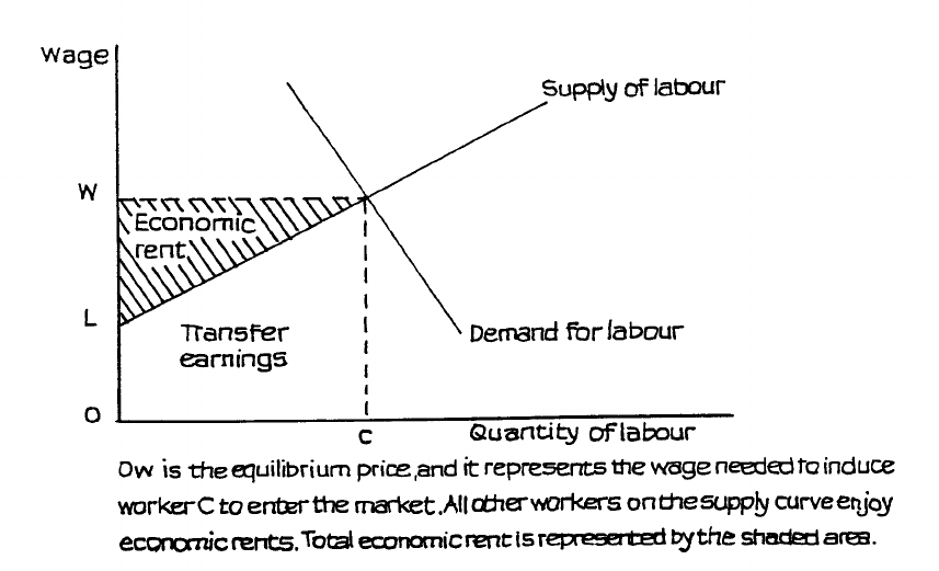
Page 187
Figure 8.7
Thus, all workers in the market and receiving wage Ow, other than the marginal worker, are
receiving part transfer earnings and part economic rent. The total amount of economic rent in
the market is represented by the shaded area. The area below the supply curve up to quantity
OL is total transfer earnings.
Economic Rent and the Individual
The position of the individual worker (or other factor) in the market is illustrated in Figure
8.8. Here again, the market equilibrium wage resulting from the interaction of demand and
supply is Ow. Worker “a” receives the market wage Ow but his position on the supply curve
indicates that he would enter or remain in the market at the lower wage of OWa.
Thus, the amount W-Wa represents the proportion of his total wage that is economic rent. His
next-best earnings are Ow.
The concept is important in the analysis of wages, because it suggests that workers whose
wage contains a high element of economic rent are very vulnerable to changes in market
conditions that would reduce the equilibrium wage. That money wages have not fallen in the
industrial nations for most of the past half century does not mean that they cannot fall - or,
indeed, should not fall, under certain conditions.
What has happened in recent years is that demand has fallen in many labour markets, and this
has affected real wages, i.e. money wages adjusted to take account of changes in the
purchasing power of money. This readjustment has not only reduced the amount of economic
rent in those markets, but has also forced those workers who have had to leave the market to
discover that their transfer earnings were much lower than their previous wage. Those

Page 188
workers who have sought to obtain work at a level close to their old wage, instead of
accepting it at their transfer earnings rate, have usually remained unemployed.
Worker a would still be employed at wage Wa, but he receives the market
equilibrium wage W. So W-Wa represents economic rent.
Figure 8.8
The implication for the individual worker is very clear. The greater the element of economic
rent in the current wage, the greater the degree of vulnerability to any change in market
conditions. The worker least likely to suffer is the one with the least economic rent and the
highest level of transfer earnings. Thus, workers with several marketable skills, those able to
retrain to meet demand in new markets, are the ones with the lowest economic rent, and they
have the least to fear from economic change.
Quasi-Rent
The term quasi-rent is sometimes used to describe a form of economic rent for a factor the
supply of which is temporarily highly inelastic or completely fixed. The use of “quasi”
indicates that, in the long run, supply is not fixed.
Take the case of a sport which becomes popular very quickly. The few people who are star
performers at the time of the popularity surge, suddenly become well known and in great
demand for competitions and “appearances”. Their earnings rise very quickly but contain a
high rent element. These high earnings attract to the sport talented people who had not
previously considered a serious career in it. The standard of performances increases, as does
the number of star performers. Only those with most exceptional talent are now able to earn
very high incomes. Others, who would have been stars by the standards of a few years earlier,
can earn little more than an average income.
W
Economic
rent
Wa
Transfer
earnings
a
O
Supply of labour
Demand for labour
Quantity of labour
Wage
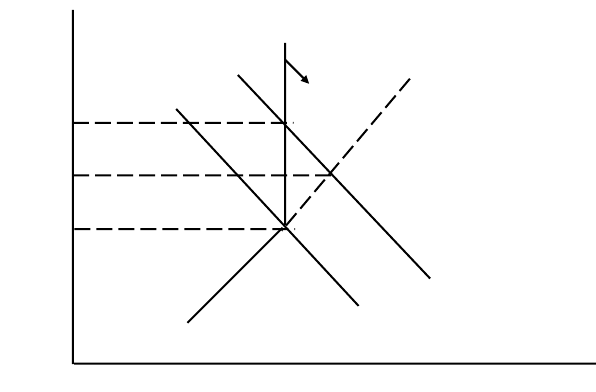
Page 189
The situation is illustrated in Figure 8.9. As people respond to the increased earnings
possibilities, the supply curve swings to the right at this higher earnings level, and the extent
of economic rent is reduced, as shown in the model.
Supply totally inelastic in the short term and, following a rise in demand DD to
D1D1, the wage rises from Owo to Ow1. There is economic rent of W1-Wo. In
time, and in response to the increased rewards, supply rises and the economic
rent element falls bringing down the wage to Ow2.
Figure 8.9
Wage
D
1
D
W
1
D1
D
W
0
W2
O
Increased supply
Supply
Quantity

Page 190
BLANK

Page 191
Study Unit 9
National Income
Contents
A. From Micro to Macro Economics
B. Measuring Economic Activity
GDP and GNP
National Income
C. Interpreting the Figures
Real and Nominal Income
International Comparisons
Page 192
A. FROM MICRO TO MACRO ECONOMICS
The microeconomic analysis of previous units was concerned with particular markets and the
strategies of economic agents in these markets. The focus was on the behaviour of the firm,
the consumer, the worker, the determination of price in a competitive market, etc.
Macroeconomic analysis focuses on the performance of the economy as a whole, rather than
the microeconomic features within it. The level of production in the whole economy; the
level of employment/unemployment in the economy; the average price level of the whole
economy; trade between the economy and the rest of the world; these are all macroeconomic
issues. Because the focus is on the economy as a whole, the variables of interest are often
aggregates of microeconomic variable. For example, in microeconomics we might be
concerned with consumers’ expenditure on a particular product whereas in macroeconomics,
we might be concerned with total consumers’ expenditure in the economy.
Governments play a major role in modern economies. The policies adopted by governments
are often guided by macroeconomic analysis. If, for no other reason, it is important that the
analysis is reliable.

Page 193
B. MEASURING ECONOMIC ACTIVITY
There are three related measures of economic activity for an economy:
Gross Domestic Product (GDP)
Gross National Product (GNP)
Net National Product (or National Income)
GDP is the value, in money terms, of the total output of final goods and services produced in
an economy over a period of (usually) one year. Final goods include both consumer goods
and capital goods. There are three alternative methods of calculating this value, the income
method, the output method and the expenditure method.
(i) The Output Approach: measures the sales value of the total output of final goods
produced by firms. (This gives you National Product, NP)
(ii) The Outcome Approach: adds up the total income received by the factors of production
for their use in producing the output (i.e. wages, profit and rent and interest). (This gives
you National Income, NI.)
(iii) The Expenditure Approach: measures National Expenditure by calculating the total
spending on final consumption goods and on investment.
Table 9.1 gives a simplified illustration of how these measurements are calculated.
Producer Farms Mills Bakeries Retail
Output
Wheat
Flour
Bread
Bread
Value of Output (Gross)
RWF100m
RWF140m
RWF180m
RWF200m
Value Added (Factor
incomes)
RWF100m
RWF 40m
RWF 40m
RWF 20m
Table 9.1 Stages of Production
Table 9.1 illustrates hypothetical figures for stages of production, the final product being
bread. The farms supply the mills with wheat; the mills supply the bakeries with flour, the
bakeries supply the retailer with bread which is then sold to the final consumer.
To simplify the analysis, it is assumed in Table 9.1 that there are no bought in inputs into the
farms and therefore the RWF100m worth of wheat represents the net output of the farms. The
only bought in input for the mills is the RWF100m of wheat, for the bakeries the RWF140m
of flour and for the retail trade the RWF180m of bread.
The value of final output for the whole process is the RWF200m worth of bread sold by the
retail trade, and it is this figure we wish to add to the GDP of the economy. The wheat, flour
and wholesale bread are all intermediate products and care should be taken not to double
count these items. The value added at each stage is the difference between the value of output
and the value of bought in inputs. The value added can also be thought of as the gross
n

Page 194
earnings available to be paid as income (wages, profit, interest, rent) to the factors of
production employed at that stage.
The three methods of measurement are all seeking to establish the contribution to GDP of
RWF200m. The expenditure method focuses on the RWF200m that is spent purchasing the
bread; the income method focuses on the sum of the gross factor incomes generated in all
sectors (RWF200m); the output method focuses on the sum of the value added of all sectors
(RWF200m).
Because the three methods are merely different ways of measuring the same quantity the
following identity must be true:
National Income = National Output = National Expenditure
In reality, national income accounting is not as straightforward as the above example
suggests. A modern economy is made up of many sectors with large, medium and small scale
enterprises along with many self-employed traders. Monitoring all this economic activity is a
difficult task. Furthermore, governments usually wish to measure economic activity so that
the incomes earned can be taxed. The requirement to pay tax on income can operate as a
disincentive to declare income resulting in a black economy (undeclared economic activity).
Because of this, there may be a tendency for the official figures to understate the true level of
economic activity. The higher the rates of tax in a country, the larger the black economy is
likely to be.
Various problems need to be avoided if an accurate measure of GDP is to be achieved:
Problems with National Income calculation
(i) With its estimation
(ii) With its use.
Estimation Problems
(a) What Goods/Services to Include
General principle: take into account only those products which change hands for
money but there are distortions which reduce its accuracy e.g.:
(i) Unpaid services (e.g. housewives duties, washing own car, etc.) are not included but
the same services, when paid, for are.
(ii) Many farmers consume part of their own produce with no money changing hands
and many households live in their own houses, imputed value must be applied to
these factors.
(iii) Many durable goods give services over time but this is hard to calculate so they are
included at the price they were bought at.
(iv) There are many government services – healthcare, education, police and defence
forces – provided ‘free’, these services are included at cost.
Page 195
(v) Externalities are not measured or included (e.g. pollution).
(b) The danger of double counting.
This can lead to incorrect estimates e.g.:
(i) Incomes such as social security are received without any contribution to production,
These are TRANSFER PAYMENTS from the taxpayer to the welfare recipient and
are therefore not included.
(ii) The production of a final good includes a number of intermediate stages. It would
be double-counting to include the value of the good in these preceding stages and
then include it again in the value of the final good.
To avoid this problem;
* only include the value of the final product.
Or * add the value added from each stage of production.
(iii) A rise in the value of stocks should not be counted as it does not represent any
growth in real output.
(c) Inadequate Information
The sources of information used may be inconsistently measured, subject to
numerous revisions, change over time, differ between countries, e.g. income tax
returns are likely to be underestimates.
The censuses of production, distribution, population, etc are taken infrequently so
comparisons are hard.
Basically – statistics have many biases and inaccuracies built into them.
Problems with using national income
4 Main uses
(i) To describe the structure of the national economy (i.e. to measure the total
wealth in the economy), to assist government planning.
But
Problem: Unless data is complete, Accurate and Up-to-date (which it rarely
is) using NI as a policy guide may lead to perverse results
(opposite of those aimed for).
(ii) To measure living standards (NI per capita)
Must adjust NI for the number of people in the economy (i.e. the number it must
be shared between.
So only NI per capita (i.e. per head) is valid as a measure of living standards.
Page 196
But
Problem: Even the number of heads (capita) may be inaccurate.
Disparities in the distribution of income (the way income is shared out among
the population) may mean that an average measure of NI gives a distorted
picture of the economy.
Average living standards may be overestimated because “bads” are not costed in
(i.e. negative), or underestimated because public sector activity is only included
at cost and unpaid activities are not included at all.
(iii) Comparisons over time (Change in NI per capita at constant prices)
These are only valid if the data have been collected/prepared on the same basis
over time.
Problems: Changes in: income distribution, the price level (i.e.
inflation), service-intensity, quality of goods, contribution of the
public sector, share of investment, share of defence spending.
Can make comparisons over time inexact.
(iv) Comparisons between countries
Much the same problems as for comparisons over time but also:
Exchange rates, different tastes and needs and different levels of development
are problems.
(d) When using the expenditure method it is necessary to adjust for the value of imports
and exports. Domestic expenditure will include expenditure on imports, while
foreigners will be buying domestically produced goods or services that are exported.
The value of exports should be added to GDP while the value of imports should be
subtracted.
(e) Another problem arises as a result of indirect taxes. If the bread in Table 9.1 was
subject to 10% value added tax, consumers expenditure would be RWF220m but
factor incomes would still be only RWF200m. The tax is a transfer payment to the
government. To calculate GDP at factor cost from GDP at market prices it is
necessary to subtract indirect taxes and add any government subsidies to producers.
GDP and GNP
To get from GDP to GNP it is necessary to adjust for net factor incomes from abroad (NFIA).
Economic activity in one country can be generating income for residents of another country
due to repatriated profits from foreign investment. GDP measures the income generated in a
particular country, no matter who has a claim to that income. GNP measures the income
being earned by the residents of a country irrespective of where the income is generated.
GNP = GDP + NFIA (9.1)
Creditor countries (those accumulating net foreign assets) are net exporters of capital and
consequently have positive NFIA. For creditor countries GNP exceeds GDP. Debtor

Page 197
countries (those accumulating net foreign liabilities) are net recipients of inward investment
and consequently have negative NFIA with the result that GNP is less than GDP.
National Income
To get from Gross National Product to Net National Product (NNP), it is necessary to adjust
for the depreciation of the national stock of capital. Part of the capital stock will be used up
in the production of goods and services. NNP is calculated by subtracting an allowance for
depreciation from GNP:
NNP = GNP – Depreciation
(9.2)
When Net National Product is calculated on a factor cost basis this figure is accepted as the
National Income figure.
Millions
A National Income 2010
Personal consumption 85214
Public sector current expenditure 28503
Gross domestic fixed capital formation 25293
Change in stock -2264
Exports 145902
Imports -121037
Statistical discrepancy -1015
GDP at market price 160596
Net factor incomes from abroad -28363
GNP or GNY at Market prices 132233
Subsidies 1719
Taxes -359
GNP/income at factor cost 133592
GNP at factor cost less depreciation gives Net National Product at factor cost.
International comparisons: The link below gives international comparisons of GNP per head.
http://data.worldbank.org/indicator/NY.GNP.PCAP.CD
Table 9.2

Page 198
C. INTERPRETING THE FIGURES
National income figures are designed to measure the extent of economic activity in an
economy. The level of economic activity in turn determines the material living standards of
the society. The figures give an indication of how living standards in a particular country (1)
are changing over time and (2) compare on an international scale.
It must be remembered that the figures are exclusively concerned with material living
standards and say nothing about the quality of life in a country. Living standards may be
rising but some people may feel that the quality of life (however measured) is declining.
When measuring living standards the appropriate measure is per capita GNP which is arrived
at by dividing GNP by the population:
GNP per capita = Population
Product National Gross
Living standards therefore depend not only on the income being earned by the members of a
society (GNP) but also on the size of the population that the income must support. If a
country has a growing population, then GNP must be rising faster if living standards are to
improve.
Real and Nominal Income
When comparing living standards over time, it is important to distinguish between real
income and nominal income. The distinction is important when there is inflation in an
economy as the change in nominal income will exaggerate the change in living standards.
Table 9.3 gives hypothetical figures for an economy.
Year 1993 1994 1995
GNP (RWFm) (current market prices)
Price Index – Inflation
GNP (RWFm) (constant prices)
30,000
100
30,000
33,000
105
31,429
36,300
112
32,411
Table 9.3 Real Income and National Income
The figures indicate that GNP (in nominal terms) has been growing at 10% p.a. However, the
inflation index indicates that prices have risen by 5% from 1993 to 1994 and by 12% overall
from 1993 to 1995. Nominal income is arrived at by multiplying output (quantities) by the
prevailing prices, but if prices are rising, nominal GNP will tend to be rising whether or not
real output is rising. To get a measure of the change in real output it is necessary to express
the GNP figures at constant prices by removing the effects of inflation. The constant price
figures are arrived at by deflating the market price figures with the appropriate GNP deflator
which is 100/price index. For example, the real GNP figure of 31,429 for 1994 is arrived at
by multiplying 33,000 by 100/105. It can be seen that the economy has expanded in real
terms (constant prices) by 4.76% (93/94) and 3.12% (94/95).

Page 199
Even if real per capita income is growing over time, it is important to be aware of certain
facts:
It is only an average and, therefore, says nothing about the distribution of income or
changes in the distribution of income over time. In other words, growing per capita
income is not incompatible with increasing poverty among some sections of society.
It says nothing about the number of hours worked. Clearly it would be preferable if
rising real income was achieved with a shorter working week rather than with a longer
one.
It fails to take account of any negative (or positive) externalities in production such as
pollution
It is a measure of output whether or not the output adds to welfare. If congestion on
the roads means journeys are taking longer and more petrol is being consumed as a
result, this will add to GNP while hardly improving welfare.
It fails to include welfare increasing activities that do not involve market transactions.
Unpaid domestic work and DIY activities are obvious examples.
International Comparisons
Special problems arise when making international comparisons of living standards. Firstly, a
common standard of measurement is required which means that the national incomes of
different countries must be expressed in a common currency. Secondly, if economies differ
significantly in their structure, comparing GNP figures may not be comparing like with like.
Problems may arise if:
exchange rates fail to reflect purchasing power parities and
the scope of market transactions differ significantly between countries
To illustrate the first problem, we will use the following hypothetical figures for Rwanda and
Kenya.
GNP per capita
Rwanda: RWF161,000 Kenya: KES 52,700
Exchange rate
RWF7 = KES1
On the basis of this (convenient) exchange rate per capita income in Rwanda could be
expressed as KES23,000 or the Kenyan figure could be expressed as RWF368,900. Can we
conclude that living standards are 129% higher in Kenya? This conclusion is only valid if we
assume that the purchasing power of RWF 7 in Rwanda is equivalent to the purchasing power
of KES 1 in Kenya. In other words, we need to assume that similar products have the same
real prices in both countries. In practice however, exchange rates can be extremely volatile,
particularly in the short term. We must conclude that prevailing exchange rates do not
necessarily reflect purchasing power parities (Section 14C)
The second problem stems from the fact that national income accounting focuses on
marketable production rather than production in general. We have seen that unpaid domestic
Page 200
work and DIY activities are excluded from the figures. But for less developed economies
much of their economic activity may be of this kind due to the fact that market relationships
are less developed. Much of the economic activity, such as subsistence farming, takes place
outside of market relationships. International comparisons based on GNP figures have greater
validity when comparing countries at similar stages of economic development and with
similar accounting standards.
Because of the problems involved in international comparisons via GNP figures comparisons
are often made in alternative ways. The number of doctors per 1000 of population;
pupil/teacher ratios in schools; the number of telephones or TVs per household, etc. can be
used to make comparisons of living standards between countries.
Factors Affecting the Potential Size of the National Income
(a) National Resources.
(b) Nature of the Labour force (% of population, skill).
(c) Amount of capital investment.
(d) Whether factors of production are combined efficiently.
(e) Innovation and technology.
(f) Political Stability.
(g) Availability of Foreign Loans.
(h) Terms of trade (i.e. amount of another country’s goods which can be got for home-grown
goods).

Page 201
Study Unit 10
The Determination of National Income
Contents
A. Keynes and Aggregate Demand
B. Two Sector Model
Consumption and Savings Functions
Investment Function
Aggregate Demand and Equilibrium Income
C. Underemployment Equilibrium
D. The Multiplier Effect
E. The Paradox of Thrift
Page 202
A. KEYNES AND AGGREGATE DEMAND
In the previous chapter, we were concerned with the measurement of economic activity. In
this and subsequent chapters, we will be developing a system of macro-economic analysis to
help us investigate why the level of economic activity is what it is. It is often the case that
GDP is significantly lower than it might be. High levels of unemployment imply that
economies could be producing more. What are the causes of high levels of unemployment?
What conditions are necessary for economies to be operating at their full-employment level of
output?
The starting point for macroeconomic analysis is usually the work of John Maynard Keynes.
Keynes wished to understand why economies tended to progress in a cycle of booms and
slumps (the business cycle) and why they occasionally experienced prolonged recessions.
The boom periods were characterised by high and rising levels of output and employment
while the slumps were characterised by rising unemployment and falling output.
Keynes put forward a simple but persuasive explanation regarding the determination of output
and employment in the economy. The level of output firms will be willing to produce, he
argued, is determined by the aggregate demand (AD) for goods and services in the economy.
The level of output firms are willing to produce will, in turn, determine the level of
employment. The level of aggregate demand drives the economy.
AD output employment
If total demand in the economy were to rise, firms would wish to produce more and therefore
they would be offering more employment. If total demand were to fall, firms would have
accumulating unsold stocks leading them to cut production and employment. If we wish to
know why the levels of output and employment tend to fluctuate, according to Keynes, the
explanation is to be found in fluctuations in the level of aggregate demand.
Aggregate demand is concerned with the total level of desired (or planned) expenditure in the
economy and has four components originating from four different sources.
Households: consumption expenditure (C);
Firms: capital and inventory investment expenditure (I);
Government: current and capital expenditure (G);
Foreign sector: the excess of exports over imports (X – M).
AD = C + I + G + (X – M) [10.1]
Though similar to the accounting identity for GDP (see Study unit 9), aggregate demand is
not the same thing as GDP. The components of aggregate demand in the above identity relate
to desired levels of expenditure whereas the components in the accounting identity for GDP
relate to realised outcomes. Planned and realised outcomes may not necessarily coincide,
only doing so when the economy is in equilibrium.
Page 203
To understand why aggregate demand might fluctuate, we need to understand why the
components (C, I, G, X & M) might fluctuate. When we know this we can bring the
components together to construct a theoretical model of the economy. It is important to
realise that the model can take a simple form initially but be made more complex by relaxing
or changing the assumptions underlying the model. The simplest model is that of a two-
sector closed economy. This focuses on the interaction between domestic households and
firms while ignoring the impact of government and the foreign sector. By adding a
government to the model we have a closed economy with government. By adding the foreign
sector we move to an open economy model. While simple models can be accused of lacking
realism, they are essential for developing the analysis by enabling us to isolate and focus on
key macroeconomic relationships.
B. TWO SECTOR MODEL
Consumption and Savings Functions
It is convenient to think of households and firms as being completely distinct. Households
derive their incomes (wages, rent, interest, profit) from the factor services they provide to
firms. If we assume that all the profit earned by firms is distributed then gross factor incomes
is equal to GDP.
Households have a simple choice with regard to the income they receive; they can either
spend it or save it. If total income is denoted with a Y, total household spending with a C and
total household savings with an S, we have:
Y = C + S [10.2]
The consumption function is concerned with all factors that may influence the level of
consumption expenditure. The savings function is concerned with all factors that influence
the level of savings. The single most important influence on the level of household
consumption expenditure (C) is the level of household income (Y). It is assumed that as Y
rises C will also rise, but not by the same amount. As Y rises, household savings (S) will also
rise, therefore;
∆Y = ∆C + ∆S [10.3]
where ∆C and ∆S are both positively related to ∆Y.
The proportion of any change in income that is spent is known as the marginal propensity to
consume (MPC) while the proportion that is saved is known as the marginal propensity to
save (MPS).

Page 204
Example:
Household income rises by RWF100m and as a result consumption expenditure rises by
RWF80m and savings rise by RWF20m.
MPC =
8.0
100
80 ==
∆
∆
Y
C
MPS =
2.0
100
20 ==
∆
∆
Y
S
It also follows that:
MPC + MPS = 1 [10.4]
The proportion of any given level of income that is spent is known as the average propensity
to consume (APC) while the proportion that is saved is known as the average propensity to
save (also known as the savings ratio):
APC + APS =
Y
S
Y
C+
= 1 [10.5]
The general shape of the consumption function and the savings function are as illustrated in
Figure 10.1. The diagrams indicate that both consumption expenditure and savings rise as
income rises. The slope of the savings function at any point is the MPS. By assumption the
slopes are positive but less than one. The APC at any point on the consumption function is
simply the level of consumption over the corresponding level of income (e.g. APC at point a
is c0/y0). The APS at any point on the savings function is the level of savings over the
corresponding level of income (e.g. APC at point b is s0/y0).
Other factors that are likely to influence the level of income spent or saved include:
the market rate of interest (i);
household wealth.
Rising interest rates will make saving more attractive and, by implication, consumption
expenditure less attractive. If interest rates rise, the proportion of income spent (APC) will
fall while the proportion saved (APS) will rise and vice versa.
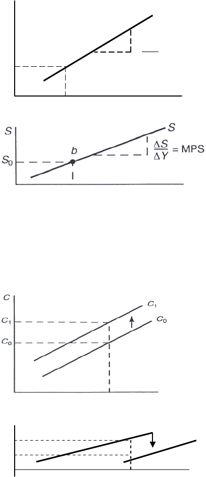
Page 205
C
C
MPC=
∆
∆
Y
C
C0 a
Yo y
(a)
Yo y
(b)
Figure 10.1: Consumption and savings functions
Increases in household wealth, e.g. an increase in the value of the housing stock, will mean
that households will be less likely to save and more likely to spend and vice versa. Any
changes, other than changes in household income, that cause C or S to change can be
illustrated by a shift in the consumption and savings functions.
Yo y
S So
So S1
S1
Yo y
Figure 10.2: Changes in the average propensities to consume and save
Assume either a fall in interest rates or an increase in household wealth causes households to
spend more (save less) of their income. The effect is illustrated in Figure 10.2. Prior to the
change c0 is being spent and s0 is being saved from y0. After the change, c1 is being spent and
s1 is being saved from y0. Note – the APC has risen (c0/y0 c1/y0) while the APS has fallen
(s0/y0 s1/y0).
Page 206
Investment Function
The investment expenditure of firms (I) is the second component of aggregate demand in the
two-sector model. Investment expenditure is defined as expenditure on output that is not for
consumption in the current period. Capital investment is expenditure on plant and equipment
while inventory investment is expenditure leading to increased stock levels. It is quite
possible that firms could be engaging in unplanned inventory investment if, due to falling
sales, there is an undesired accumulation of unsold stocks. This unplanned investment
expenditure is included in GDP but is not included in aggregate demand. Changes in stock
levels are the signal to firms to change their level of output and employment. If stock levels
are falling due to rising demand, firms will tend to expand production whereas if stock levels
are rising due to falling demand production is likely to be reduced.
Factors likely to influence the desired level of investment expenditure are:
interest rates;
business confidence;
the rate of change of income and expenditure.
The desired level of investment expenditure will be negatively related to changes in interest
rates. Also the more confident firms are about future market conditions, the more willing
they will be to invest in the present period. The accelerator theory suggests that the rate of
change of income and expenditure has an important influence on the level of investment
expenditure. Whatever the present level of income happens to be, the above factors may be
exerting a positive or negative influence on the desired level of investment expenditure. It is
assumed, unless otherwise stated, that the current desired level of investment expenditure is
not influenced by the current level of income. This assumption is illustrated in Figure 10.3.
The horizontal investment function (I0) implies that the current level of income (Y) is not a
factor influencing the desired level of investment expenditure. If there is an increase in the
desired level of investment expenditure due to, say, a fall in interest rates, the investment
schedule in Figure 10.3 will shift upwards and vice versa. From the point of view of the
simple circular flow model of the economy investment expenditure is regarded as
exogenously determined, i.e. it is not determined by variables which are themselves
determined within the model.

Page 207
Figure 10.3: Investment function
Aggregate Demand and Equilibrium Income
The aggregate demand schedule for the two sector economy can be arrived at simply by
adding the desired level of investment expenditure (I) to the desired level of consumption
expenditure (C). This is illustrated in Figure 10.4.
As income rises aggregate demand (C + 1) rises due to the positive relationship between Y
and C. The C + I line will have the same slope (MPC) as the consumption function and it is
arrived at by simply adding the investment function of Figure 10.3 to the consumption
function of Figure 10.1(a).
The level of output in the Keynesian circular flow model is determined by firms simply
adjusting their production levels to satisfy the level of aggregate demand in the economy. If
the aggregate demand for goods and services exceeds the current output of goods and services
( C + I > Y) then firms will expand production. If, on the other hand, aggregate demand is less
than current output ( C + I < Y) firms adjust by cutting production. The equilibrium level of
output is where aggregate demand is equal to the current level of output:
Y=C+I
[10.6]
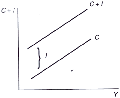
Page 208
Figure 10.4: Aggregate demand
Equation (10.6) represents the equilibrium condition for a two-sector model of the economy.
In equilibrium the realised outcomes (GDP measures) are equal to the planned measures (AD
measures).
An alternative way of thinking of equilibrium is to focus on injections and withdrawals.
Withdrawals from the circular flow are incomes earned but not passed on as expenditure on
domestically produced goods and services. Injections into the circular flow are expenditures
on domestically produced goods and services which are exogenously determined (coming
from outside the system). In the two-sector model, savings represent a withdrawal while
investment expenditure represents an injection. The income expenditure equilibrium (y = C +
I) can be reformulated in terms of injections and withdrawals. We know that y = C + S.
Substituting C + S for y in the equilibrium condition gives:
C+S = C+I or
S = I
[10.7]
Equation [10.7] tells us that the economy is in equilibrium when the level of injections
(investment expenditure) is equal to the level of withdrawals (savings). Both equilibrium
conditions are illustrated in Figure 10.5.
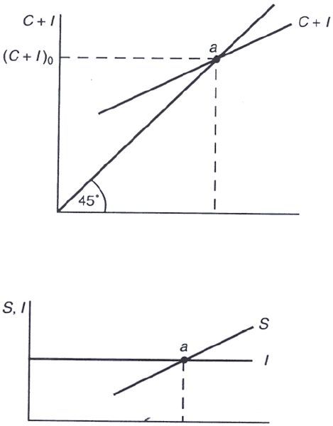
Page 209
Yo Y
(a)
Yo Y
(b)
Figure 10.5: Equilibrium in the two-sector model
In Figure 10.5(a) the 45° line corresponds to the equation C + I = Y. Therefore any point on
the 45° line satisfies the equilibrium condition for the economy. However the actual aggregate
demand function for the economy (C + I) has a slope less than one ( = MPC) and therefore
must intersect the 45° line. The point of intersection (a) represents the equilibrium for the
economy with an equilibrium output of y o corresponding to the level of aggregate demand
(C + I) 0. At output levels less than y 0 aggregate demand exceeds output so the economy will
expand. At output levels greater than y 0 aggregate demand is less than output so the
economy will contract.
Figure 10.5(a) is referred to as an 'income/expenditure' diagram. Figure 10.5(b) represents the
corresponding 'injections/withdrawals diagram '. These diagrams represent alternative ways of
illustrating the equilibrium output of the economy which in both cases is y0. At output levels
below y0 in Figure 10.5(b) injections exceed withdrawals causing the economy to expand
whereas at output levels above y0 withdrawals exceed injections causing the economy to
contract.
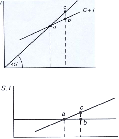
Page 210
C. UNDEREMPLOYMENT EQUILIBRIUM
The point that Keynes was concerned to emphasise was that the equilibrium level of income
was not necessarily the full employment level of income. It was possible for the economy to
be in equilibrium but with high levels of unemployment (an underemployment equilibrium).
This situation is illustrated in Figure 10.6.
C+I
Yo Yf y
Yo Yf y
Figure 10.6: Deflationary gap
The equilibrium level of output is Yo, but Yf is the required level of output if full
employment is to be achieved. This economy is experiencing a deflationary gap. i.e. too little
expenditure. The deflationary gap, indicates the amount of new expenditure that needs to be
injected into the economy and is equal to the distance bc in both diagrams. .
The problem as Keynes saw it can be appreciated if we focus on the savings investment
equilibrium (S = I). Decisions regarding the level of savings are being made by households
while decisions regarding the level of investment are being made separately by firms. There
was no reason to assume that these decisions would coincide at a full employment
equilibrium. The point is illustrated in Figure 10.7.
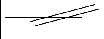
Page 211
S, 1 S1
S0
a I
Y1 Yf y
Figure 10.7: Underemployment equilibrium
Let's assume that, starting at a full employment equilibrium (a), households decide to save
more (spend less), causing the savings function to shift from So to S1. Unless firms spend
more on investment, output will fall from Yf to yY1. But, according to Keynes, firms would
be unlikely to increase investment at a time when demand and therefore sales were falling.
Therefore the economy will move to an underemployment equilibrium at Y1. The classical
economists believed that the increased savings represented an increase in loanable funds
which would cause interest rates to fall and thus stimulate investment. Keynes, however, was
more concerned with the blow to business confidence resulting from falling consumer
demand.
The nature of the underemployment equilibrium illustrated in Figure 10.7 is of interest. Y1 is
the equilibrium level of income following the increase in savings. However it is not like a
micro-economics equilibrium where markets clear as a result of the equality between supply
and demand. At Y1 in Figure 10.7 there is involuntary unemployment and therefore labour
markets cannot be clearing. More workers are seeking employment than are being offered
jobs.
Keynes argued that there was a need for the government to intervene in the economy to
ensure that the level of aggregate demand was sufficient to generate full employment.
However, sticking with our two-sector model which has no government, the only way
aggregate demand can rise is if households decide to save less of their income (an
autonomous increase in consumption expenditure) or if firms decide to raise investment
expenditure. Either of these will result in an upward shift in the aggregate demand function.
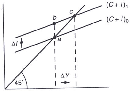
Page 212
C+I
Yo Y1 y
Figure 10.8: Increasing aggregate demand
Figure 10.8 illustrates with reference to an increase in investment expenditure. Assume the
initial equilibrium Yo is an underemployment equilibrium. An exogenously determined
change in investment expenditure shifts the aggregate demand function from (C + I)o to (C +
I)1 – we are not concerned to explain the cause of this change but merely to trace the effect
of it. The initial effect is for the economy to shift from point a to point b. However point b is
not an equilibrium point (AD > Y0)' the economy expands to the new equilibrium at point c
with income equal to Y1. Certain features of this movement from Y0 to Y1 should be noted:
In the simple circular flow model it is assumed that prices do not change. This fix
price assumption means that the economy's GDP expands in real terms (Section 9C)
as a result of the increase in aggregate demand:
.There are exogenous and induced changes in expenditure occurring. The increase in
investment expenditure (exogenous) causes income to rise but this rise in income
causes further induced changes in consumption expenditure (the movement from b to
c).
.Because of the exogenous and induced changes in expenditure the final change in
income (AY) is greater than the initial change in investment expenditure (A1). This is
known as the multiplier effect.

Page 213
D. THE MULTIPLIER EFFECT
The Multiplier is the ratio of the total increase in national income to the initial increase.
i.e.
Or it is a measure of the effect on total National Income of a unit change in some part of
aggregate demand i.e. investments or government spending or exports.
An Initial increase in expenditure has a snowball effect, leading to more and more spending in
the economy leading of a larger increase in National Income.
E.g. using the simple multiplier ( )
Where the MPS is the marginal propensity to save and MPC is the marginal propensity to
consume.
If investment increases by 100,000 and MPC = 0.25, by how much does National Income
increase?
Answer: = = =
National Income increases by 100,000 x = RWF133,000
De-multiplier: When there is a reduction in investments or government spending or
exports, there is a bigger reduction in total national income because of the reverse multiplier.
Factors which affect MPS and MPC will affect the multiplier.
E.g: the age distribution of the population,
The income distribution of the population,
Expectations of the future.
Importance of the Multiplier
It is important because it means that an increase in one component of aggregate demand will
increase national income by more than the initial increase.
So, if the government can boost spending initially (e.g. by increasing government spending or
giving investment or export grants, or lowering interest rates) it can set off a general
expansionary process.
Multiplier =
Total Increase in National Income
Initial increase in National Income
1
MPS
__
1
1 - MPC
____
1
MP
________
_______
1
1 – 0.25
1
0.75
____
1
0.75
____

Page 214
In an open economy (i.e. one which trades with other countries) and where there is
government intervention the multiplier becomes:
i.e. the multiplier effect is smaller the bigger are the withdrawals from the circular flow..
E.g. – if MPS = 10%, MPM = 45% and MPT = 25%
The “Simple” multiplier = = 10.
But the open economy multiplier = = 1.25
Limitations of the Multiplier
1. If there is full employment, any increase in demand will be inflationary. (But can use the
“de-multiplier” effect here).
2. If the withdrawals (i.e. leakages) from the circular flow, savings, taxation or imports, are
high the multiplier will be very small so “pump priming” will have little effect.
3. There may be a long-term lapse before the benefits of the multiplier take effect. (So it is
no good as a short-term solution to unemployment or inflation).
4. The consumption function in modern times is volatile therefore the effects of the
multiplier are also unpredictable.
5. If the government tries to increase spending it can lead to other problems in the economy.
The extra spending must be financed. If the government raises taxes, the multiplier will
be lower and people may work less hard. If it borrows the money it can lead to high
national debt problems and cause interest rates to rise.
The Accelerator Principal
This states that if the RATE of increase in consumer goods is rising, there must be an even
faster rate of increase in investment by firms, so as to boost production capacity enough to
meet the higher demand.
[There is also a “decelerator” effect where when National Income is falling the percentage
drop in investment is even faster than the rate of fall in consumption.]
The accelerator principle means that;
(a) National Income remains high only as long as investments are high, and
____
Open Economy Multiplier =
___________________
1
MPS + MPT + MPM
1
0.1
1
0.1 + 0.45 + 0.25
_________________
Page 215
(b) investment is high only so long as income and consumption are RISING.
So, as National Income approaches its peak level (boom) as determined by available capacity,
NEW investment will fall towards zero, reducing aggregate demand and hence National
Income.
This decelerator effect will be compounded by the de-multiplier and national income will fall
sharply.
Investment and the Business Cycle
An investment: committing resources (i.e. factors) to a long-term project with a view to
earning a satisfactory return over the period of the project.
The six main factors that influence the volume of investment are:
1. The expected return from investments
An investment involves the acquisition of more buildings, machinery, plant and
equipment (i.e. NET investments)
Firms should go on adding to their capital so long as the marginal efficiency of capital
(MEC) exceeds the marginal cost of the extra capital (i.e. the interest rate).
In other words, the expected rate of return must at least equal the required rate of return
(i.e. the MC of investment).
2. Risk, Confidence and expectations about future prospects.
Investment projects are long-term ventures; it takes several years to reap the full return.
So there is a risk to investment because the future is uncertain.
If confidence is high (i.e. there are good expectations about the future) investment will
increase. The bigger the risk or perceived risk the lower will be investment.
Risk is bigger with a new market or a new product.
3. New technology boosts investments because:
(a) it can reduce the unit costs of production (by enabling the factors of production to be
more productive.) This increases profitability and supply will increase as firms
invest more to achieve lower costs and remain competitive.
(b) new technology leads to new types of goods which stimulate consumer demand and
firms will invest more to meet this extra demand.
4. The Accelerator principle/changes in income.
5. Government Grants and Subsidies.
Governments can encourage investment by giving grants and subsidies.
Government Grants are generally “regional” i.e. aimed at areas of high unemployment or
“export related” to encourage firms to export or “innovative” to boost R & D. In terms of
Agriculture, grants may be aimed at food production to make the country less reliant on
imports.

Page 216
They often effect decisions on where to invest rather than whether or not to invest.
6. Interest Rates
Profits from an investment are earned over several years i.e. the life of the investment.
Firms invest money now to earn profits in the future so there is an opportunity cost of
having your capital tied up.
The opportunity cost is the interest cost. It is calculated using Discounting Cash Flow
(DCF) Analysis – Net Present Value (NPV).
If NPV is positive the benefits of the investment are greater than the cost so the
investment is worth undertaking.
(PV puts a current value on future flows of income.)
PV depends on three things;
(a) Interest Rates.
(b) Riskiness of the investment.
(c) Inflation.
NPV = + + ..... - Cost
i.e.
R = Expected Return; r = Rate of Interest; C = Cost of the investment Outlay
E.g (i) The asset costs RWF2,000
(ii) The firm can raise finance at annual interest rate of 10%.
(iii) Asset’s lifespan is 5 years.
(iv) Net return on asset is RWF1,000 pa.
1.1 = 1 + 10% (10% = = 0.1 so 1 + 10% = 1.1)
NPV = + + + + - 2,000
= (909 + 826 + 750 + 683 + 621) - 2,000
= RWF3,798 the gross value of the Asset (GPV)
- RWF2,000 - cost________________________
+ RWF1789 = NPV
The investment is worthwhile
Investment spending is volatile, much more so than consumption and can therefore cause
big increases or falls in National Income.
Return in 1 year
(1 + interest rate)
_____________
_____________
Return in year 2
(1 + interest rate)2
Return in year n
(1 + interest rate)n
_____________
NPV = + + + ...... + - C
R1
(1 + r)
___
_
R2
(1 + r)2
R3
(1 + r)3
____
____
Rn
(1 + r)n
____
____
10
100
______
1,000
(1 .1)
1,000
(1 .1)2
1,000
(1.1)3
1,000
(1.1)
4
1,000
(1.1)5
______
______
______
______
Page 217
Business Cycles
These are the continual sequence of rapid growth in national income, followed by a slow-
down in growth and then a fall in national income (recession) which eventually changes back
to growth and so on.
A trade cycle or business cycle has four phases (period of the cycle seven years)
Characteristics
1. Depression (a) Heavy Unemployment
(b) Low consumer demand
(c) Over Capacity (unused capacity in production)
(d) Prices stable, or even falling
(e) Business Profits Low
(f) Business Confidence in the future Low
2. Recovery (a) Investment picks up.
(b) Employment rises
(c) Consumer spending rises
(d) Profits rise
(e) Business Confidence Grows
(f) Prices stable, or slowly rising
3. Boom (a) Consumer Spending Rising fast
(b) Output capacity reached: labour shortages occur
(c) Output can only be increased by new labour-saving
investment (technology).
(d) Investment spending high.
(e) Increases in demand now stimulate price rises.
(f) Business Profits high
4. Recession (a) Consumption falls off
(b) Many investments suddenly become unprofitable and
new investments falls
(c) Production falls
(d) Employment falls
(e) Profits fall, some businesses fail
(f) Recession can turn into severe depression
Explanation of Business Cycles
1. Pre Keynesian Theories
Different steps in the cycle:
(a) Recovery
(i) Investment begins to rise because;
• interest rates have fallen
• cost of factors have fallen
Page 218
• new technologies
• expectations
(ii) Once investments start to rise, more labour will be employed (to make the
capital equipment that is being invested in). This increases income, leading to
higher consumer spending and therefore still more investment which again
boosts demand, etc.
The increase in demand eventually pushes up prices.
(iii) Eventually the upswing flattens out – because of over-investment during the
boom. This surplus capacity eventually leads to redundancies and this
unemployment causes a fall in income and consumption.
(iv) The accelerator principle increases this cyclical effect.
2. Keynes’ theory: Multiplier – Accelerator Theory
The combination of the multiplier and accelerator explain the upswings and downswings
in the business cycle.
The Paradox of Thrift
This illustrates the workings of a “de-multiplier” in a situation where savings and investments
are temporarily out of balance.
All income that is saved is not necessarily invested – some savings are held as money (i.e.
cash or near cash).
(a) If this is so a rise in savings will cause a fall in consumption which may cause
businesspeople to reduce investment.
(b) This fall in investment, through the multiplier, causes greater reductions in national
income.
(c) The fall in National income, means households have smaller incomes and so save less.
Paradox of Thrift: Greater savings without greater investment end with smaller incomes
and smaller savings.
Policies on Investment – Government and the Trade Cycle
The government can try to influence the trade cycle – moderate the upswings and
downswings – using management.
(a) Encourage new investment (grants and subsidies) or itself invests
(b) Increase Government spending by borrowing or reduce taxes.
(c) Encourage exports with subsidies and discourage imports (tariffs, quotas etc.)
If demand is too strong, government policies would be the opposite.
Page 219
Government can influence investment by:
(a) Controlling interest rates
(b) Grants and subsidies to encourage investment
(c) Boost business confidence – announcing and achieving policy objectives for growth and
development.
(d) Encourage technological progress, Research and development.
(e) Control the money supply to change consumption
(f) Direct Government Spending
(g) Keeping tax low.
Importance of Investment
(i) Public sector investment has valuable spin-offs – better infrastructure,
telecommunications etc.
(ii) Investment represents consumption foregone now to increase the capacity to produce and
consume in the future – it shapes the future growth and development of nations.
(iii) It is vital determinant of the economies long-term growth rate.
Financing of Investment
Private sector Investment
(a) Retained profits
(b) New share issues
(c) Borrowing
Public Sector Investment
(a) higher taxation
(b) Borrowing
(c) Bond issues
Note public sector investment can “crowd out” private investment.
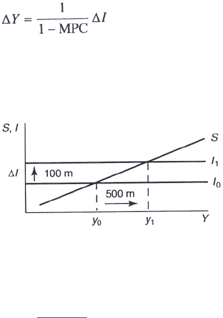
Page 220
It can be shown that for Figure 10.8 :
[10.8]
where 1/1- MPC is the multiplier. The multiplier effect is easily illustrated using the savings-
investment diagram. In Figure 10.9 the initial equilibrium is yo. The MPC is assumed to be
0.8.
Figure 10.9: Multiplier effect
(i.e. MPS = 0.2). Investment expenditure rises by RWFl00m. The value of the multiplier is 5
(i.e. 1/1- 0.8). The final change in income is RWF500m.
Note as income rises from Yo to Y1 there is an induced increase in savings. Income rises
until the new level of savings is equal to the higher level of investment. The multiplier effect
results from successive (but diminishing) rounds of expenditure following the initial increase
in expenditure. Initially investment expenditure rises by RWF100m causing incomes to rise
by the same amount. However because MPC = 0.8, RWF80m of this increased income will
be spent causing incomes to rise by an additional RWF80m. RWF64m of this additional
change will be spent. ..and so on.
∆Y=
1
x RWF100m = RWF500m
1 – 0.8
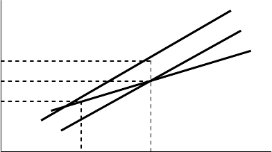
Page 221
E. THE PARADOX OF THRIFT
The paradox of thrift relates to the possibility of households intending to save more (or less)
but actually ending up saving less (or more). In Figure 10.10 it is assumed that the level of
investment expenditure is positively related to the level of income (as illustrated by the
upward slope).
S, 1
S1
S0
b I
S1
S0 a
S2 c
Y1 Yo y
Figure 10.10: Paradox of thrift
The initial equilibrium is at point a with income level of y0 and s0 being saved. Households
decide (for whatever reason) to save more and therefore spend less of their incomes. This is
indicated by the upward shift in the savings function from S0 to S1. Because the increase in
savings represents a fall in aggregate demand, the equilibrium level of income falls from y0 to
y1 (point c represents the new equilibrium). Although the savings ratio has increased, the
overall level of savings has fallen due to the fall in the level of income. Households had
intended saving an amount s1 from y0 but end up saving an amount s2 from y1, i.e. the level of
savings has fallen despite the original intention to increase savings.

Page 222
BLANK

Page 223
Study Unit 11
Government in the Circular Flow
Contents
A. Government Policies and Objectives
B. Closed Economy Model
Equilibrium in the Closed Economy
C. Active Fiscal Policy
D. Open Economy Model
Aggregate Demand in an Open Economy
E. Limitations of the Simple Keynesian Model
Page 224
A. GOVERNMENT POLICIES AND OBJECTIVES
Governments play a major role in all modern economies. Public procurements – government
expenditure on defence, education, health, transport, etc. – represent a major claim on the
economic resources of society. Government expenditure is therefore an important component
of aggregate demand in the economy.
Governments also pursue broader policy objectives. Although the priorities can shift
depending on circumstances, the following are the well established objectives of
macroeconomic policy:
Full employment;
Low inflation;
Economic growth;
Satisfactory balance of payments;
Redistribution of income in society.
The problem for governments is that these objectives are not always mutually consistent.
Conflicts can emerge, for example, in trying simultaneously to achieve full employment and
low inflation, or in trying to achieve economic growth while having generous policies for
redistributing income from rich to poor. Priorities will have to be established and a trade-off
between objectives may be necessary.
To achieve their macroeconomic objectives governments must formulate appropriate policies.
Macroeconomic policies tend to be classified under two broad headings:
Fiscal policy: using the powers of taxation and government expenditure to achieve
objectives.
Monetary policy: using interest rates and the money supply to achieve objectives.
In the context of the simple Keynesian circular flow model, the focus is on the use of fiscal
policy to achieve the full employment objective. Being a fixed price model, it is clearly
inadequate for analysing issues concerning inflation.
B. CLOSED ECONOMY MODEL
By including a government in the model we need to take account of an additional withdrawal
from and injection into the circular flow of income and expenditure:
Taxation (T) represents a withdrawal from the circular flow. It represents income
earned which is passed to the government rather than passed on as expenditure on
domestically produced goods and services.
Government Expenditure (G) represents an injection of expenditure into the circular
flow.
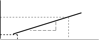
Page 225
The fiscal policy being pursued by the government will be reflected in the annual budget.
With regard to the impact of the budget on aggregate demand there are three possible
scenarios:
Balanced budget: (G = T) - injections equal withdrawals implying a neutral effect on
aggregate demand;
Budget deficit: (G > T) – injections exceed withdrawals causing aggregate demand to
increase (‘expansionary budget’);
Budget surplus: (G < T) – withdrawals exceed injections causing aggregate demand to
decrease (‘contractionary budget’).
A budget deficit will force the government to seek additional (besides taxation) sources of
finance. Typically a budget deficit can be expected to result in a public sector borrowing
requirement (PSBR). Annual borrowing in turn contributes to the national debt, which is
simply all outstanding (unredeemed) public sector debt. A budget surplus may be used for
public sector debt repayment (PSDR) which represents a reduction in the national debt.
In practice governments have additional sources of finance besides taxation and borrowing.
These include the proceeds of privatisation or the profits of state sector enterprises. However
these sources are either one-off or relatively insignificant and will be ignored in the following
analysis.
There are three components of aggregate demand (AD) in the closed economy:
AD = C + I + G [11.1]
Government expenditure (G) is exogenously determined in that its level cannot be explained
by reference to the economic variables of the model. The level of G depends on the
ideological make-up of the government which may be sympathetic to relatively high or
relatively low levels of public expenditure.
Because taxation exists, it is necessary to distinguish between the gross factor incomes of
households (Y) and the disposable income of households (Yd). Disposable income is what
remains after taxes have been deducted:
Yd = Y – T [11.2]
T
T
125
∆T
25 ∆Y
100 500 y
Figure 11.1: Tax function
If we assume for simplicity that all taxes are direct, i.e. taken directly from gross income, then
the level of taxation (T) depends on two things: the rate of tax and the level of income (Y).
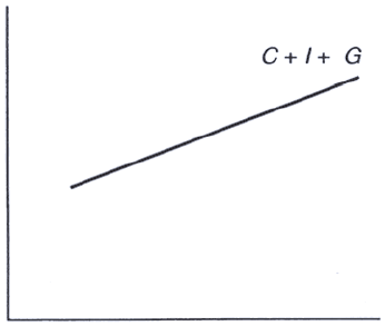
Page 226
Taxation is therefore endogenously determined. Given the rate of tax the amount of tax is
determined by the level of income. As income rises the level of tax rises and vice versa.
Figure 11.1 illustrates a simple tax function.
As gross incomes rise tax revenue increases. The marginal rate of tax (MRT) which is the rate
of tax on an additional RWF1 earned, is indicated by the slope of the line (A T / A Y). If we
assume a simple tax function of the form T = 0.25Y then for Y= RWF100, T= RWF25 and
for Y= RWF500, T= 125, etc. The proportion of any change in income that is taken by the
government in tax (AT/AY) is sometimes referred to as the marginal propensity to tax (MPT).
Households must now decide how much of their disposable incomes (rather than gross
incomes) to spend or save. A given marginal propensity to consume from disposable income
(MPC) will mean a lower marginal propensity to consume from gross income (MPCg).
Example
Assume:
All income is taxed at a rate of 25% (MRT = 0.25)
Households spend 80% of any additional disposable income (MPC = 0.8) and save
20% (MPS = 0.2). Then
T = O.25Y
Yd = Y-T = Y-O.25Y = O.75Y
∆C = O.8∆Yd
= O.8(0.75)∆Y = O.6∆Y
i.e. given a 25% marginal tax rate, a marginal propensity to consume from disposable income
of 0.8 implies a marginal propensity to consume from gross income of 0.6.
The aggregate demand function for the closed economy can be illustrated as in Figure 11.2.
Aggregate demand at any given level of income is arrived at by simply adding the relevant
levels of C, I and G. Both I and G are assumed to be independent of
C+ 1+ G
y
Figure 11.2: Aggregate demand function for a closed economy

Page 227
the level of income whereas C is positively related to it. The slope of the aggregate demand
function is ∆C/∆Y (i.e. MPCg). The slope of the line in Figure 11.2 is flatter than that in
Figure 10.1 (a) due to the inclusion of taxation. It follows that the multiplier effect is
weakened by the inclusion of taxation. The formula for the multiplier (k) is now:
k = gMPC1
1
MRT) - (1 MPC - 1
1
−
=
[11.3]
Example
Using the figures from the previous example:
k = 06 -1
1
0.25) - (1 0.8 - 1
1
= = 2.5
Quite simply the greater the scope for withdrawals from the circular flow the lower the
proportion of any change in gross income that is passed on as expenditure thus reducing the
multiplier effect.
Equilibrium in the Closed Economy
The equilibrium condition for the closed economy is:
Y=C+I+G
[11.4]
When the sum of the desired levels of expenditure in the economy ( C + I + G) is equal to the
value of output (Y) being produced in the economy, there will be no tendency for economic
expansion or contraction. The equilibrium can be illustrated using an income expenditure
diagram as in Figure 11.3.
The equilibrium level of income is determined at the point where the aggregate demand
function intersects the 45° line. This is at point a in Figure 11.3 with an equilibrium income
of Yo.
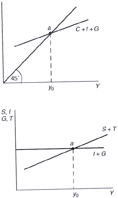
Page 228
An alternative formulation of the equilibrium condition is in terms of injections and
withdrawals. S+T=I+G [11.5]
C +1 +G
Figure 11.3: Equilibrium in a closed economy (income/expenditure diagram)
Figure 11.4: Equilibrium in the injections/withdrawals diagram
As both withdrawals (S ,T) are positively related to the level of income and both injections
(I,G) are independent of the level of income (exogenous) this equilibrium condition can be
illustrated as in Figure 11.4.
The equilibrium level of income (Yo) is determined at the point of intersection of the
injections and withdrawals functions (point a).
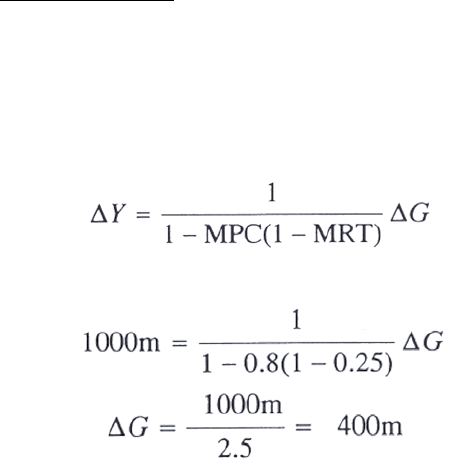
Page 229
C. ACTIVE FISCAL POLICY
As we have seen, Keynes was pessimistic about the capacity of an unregulated free market
economy to generate a full employment equilibrium. The Keynesian analysis was developed
in the period between the two World Wars, a period of global economic and political
instability. The depression of the early 1930s was characterised by mass unemployment in
Europe and in the USA. Not a time when one's confidence in the free market system was
likely to be strengthened.
Because governments must raise taxes to finance expenditure on such things as defence,
education, etc., a fiscal policy of some sort is unavoidable. However the traditional policy of
governments was to pursue 'fiscal rectitude'. This meant keeping taxation and therefore
government expenditure as low as possible while balancing the budget. What Keynes argued
was that governments should have an active fiscal policy with a view to influencing the
overall level of aggregate demand in the economy. If the economy was experiencing a
deflationary gap the government should either raise government expenditure or lower taxes or
some combination of both. Figure 11.5 illustrates an economy which is initially in an
underemployment equilibrium (point a).
By increasing expenditure by an amount equal to AG the government can shift the aggregate
demand function from ( C + I + G)o to ( C + I + G) I. A new equilibrium is achieved at point
b which is a full employment equilibrium. Note because of the multiplier effect the
government does not have to raise G by the required increase in Y
∆Y =
MRT)(1 MPC1
1
−−
∆G [11.6]
Example
Assume the government needs to raise the level of output by RWF1000m (∆Y= RWF1000m)
to achieve full employment. The MPC = 0.8 and the MRT = 0.25.

Page 230
C+ 1+ G
Yo Yf y
Figure 11.5: Fiscal expansion: increased government expenditure
C+ 1+ G
Yo Y1 y
Figure 11.6: Fiscal expansion: reduction in taxation
Therefore if the government increases expenditure (∆G) by RWF400m income will rise by
RWF1000m.
If instead of increasing government expenditure the government reduced taxes it could
stimulate household expenditure (C) by raising household disposable income (Yd). However
C will not initially increase by the full reduction in taxation as only some proportion (the
MPC) will be spent while some proportion (the MPS) is saved. The initial increase in
consumption will be equal to MPC times ∆T. Figure 11.6 illustrates fiscal expansion by way
of a tax reduction.
In Figure 11.6 AC = MPC ∆T. The multiplier effect resulting from a reduction in taxation
will be less than the multiplier effect for an increase in government expenditure:
[11.7]
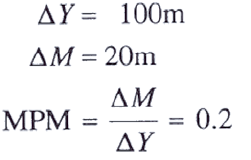
Page 231
Equation [11.7] gives the multiplier effect of a lump sum change in taxes (∆7). Because the
taxation multiplier [11.7] is less than the government expenditure multiplier (11.6) it is
possible to achieve a balanced budget multiplier effect. If government raises taxation and
expenditure by an equal amount, the increase in taxes will reduce income by a smaller amount
than the increase in expenditure will raise it. The overall effect, therefore, will be positive.
The net effect is the result of the government spending income that households had in fact
been saving.
D. OPEN ECONOMY MODEL
In an open economy we must take account of international trade. Exports are domestically
produced goods the demand for which originates abroad. Foreign expenditure on the
economy's exports (X) represents an injection of income and expenditure into the domestic
economy. Imports are foreign produced goods the demand for which originates in the
domestic economy. Domestic expenditure on imports (M) represents income earned which is
not passed on as expenditure on domestic production and is therefore a withdrawal from the
circular flow.
The value of imports will depend on:
The level of domestic income (Y) - as income rises more will be spent. It is assumed that
some of this additional expenditure will go on imports The marginal propensity to import
(MPM) is the proportion of any change in income that is spent on imports
Example
The real exchange rate (Section 14A) -the competitiveness of domestic goods and
services relative to foreign ones will influence consumers' purchases. Competitiveness
depends on the nominal exchange rate (Section 14A) and domestic prices relative to
foreign prices.
The value of exports will depend on:
The level of world income - if income and expenditure are rising in the economies of
trading partners this will lead to an increase in demand for exports (for example if the
Kenyan economy is booming this will stimulate demand for Rwandan exports).
The real exchange rate - if domestically produced goods and services lose
competitiveness on world markets, exports will be adversely affected and vice versa.
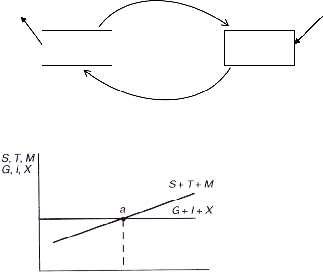
Page 232
In the completed circular flow model there are three injections (G, I, X) and three
withdrawals (S, T, M) as illustrated in Figure 11.7. All the injections are exogenously
determined, i.e. their levels are determined by factors not included in the model. The
withdrawals are endogenously determined as the level of domestic income (Y) has a
positive influence on all of their levels.
Consumption expenditure (C)
S+T+M G + I + X
Factor incomes (Y)
Figure 11.7: The circular flow of income and expenditure
Yo y
Figure 11.8: Open economy equilibrium: (injections and withdrawals)
The economy will be in equilibrium with no tendency for output to expand or contract when
the sum of injections equals the sum of withdrawals:
S+T+M=G+I+X [11.8]
This equilibrium condition can be illustrated in an injections/withdrawals diagram as in
Figure 11.8.
The economy is in equilibrium at point a where the injections line intersects the withdrawals
line with income Yo.
Aggregate Demand in an Open Economy
The aggregate demand for domestically produced goods and services in an open economy is:
AD = C+I+G+ (X-M) [11.9]
Domestic
Households
Domestic
Firms
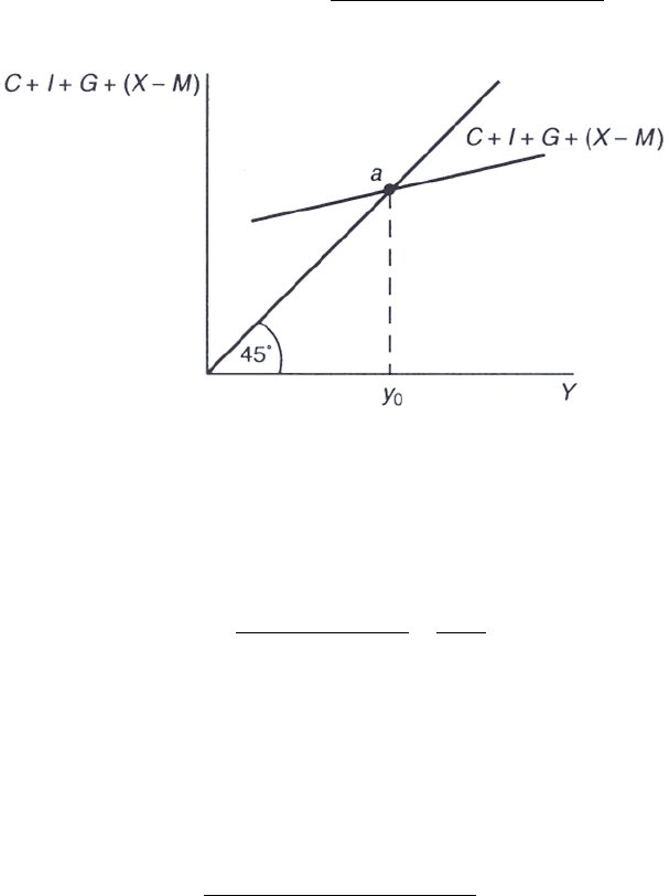
Page 233
The equilibrium condition is that total desired expenditure be equal to the value of domestic
output: Y = C+I+G+(X-M) [11.10]
This equilibrium condition is an alternative formulation of Equation [11.8] and is illustrated
in Figure 11.9.
Equilibrium is at point a with income at Yo. The aggregate demand function in Figure 11.9
has a slope which is flatter than that of Figure 11.2. This is because imports are positively
related to the level of domestic income (i.e. endogenously determined) and are included in the
function with a negative sign. It follows that the multiplier effect is weakened when we move
from a closed to an open economy.
The formula for the open economy multiplier is:
k =
MPMMRT)(1 MPC1
1
+−−
Figure 11.9: Open economy equilibrium: income/expenditure diagram
Example
MPC = 0.8
MRT = 0.25
MPM = 0.2
k = 06 -1
1
0.2 (0.75) 0.8 - 1
1
=
+ = 1.67
Clearly the multiplier effect, resulting from any injection of demand into the economy, will be
weaker the higher is the MPM. Figure 11.10 illustrates the multiplier effect with respect to a
change in government expenditure (∆G). Note, the relationship between ∆G and ∆Y depends
on the open economy multiplier.
∆Y = MPMMRT)(1 MPC1
1
+−− = ∆G
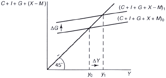
Page 234
We can conclude that fiscal policy in an open economy will have less effect on economic
activity than in a closed economy. The higher the MPM, the smaller the multiplier and the
less impact policy will have.
Figure 11.10: Multiplier effect in an open economy
E. LIMITATIONS OF THE SIMPLE KEYNESIAN MODEL
The simple Keynesian model of income determination, developed in this and the previous
chapter, explains the level of economic activity by reference to the level of aggregate demand.
If there is unemployment in the economy government can remove it by raising aggregate
demand by means of fiscal policy. All economic models simplify reality with a view to
clarifying key relationships. All resort to the ceteris paribus assumption in order to make
conditional predictions. For example, ‘if aggregate demand is raised, all else being equal, the
result will be increased economic activity’ is the conditional prediction of the simple
Keynesian model.
Models can be criticised if the assumptions are wrong or key economic relationships are
being left out so that either way the predictions are unreliable. The main weakness of a
simple circular flow model is the absence of a monetary system. It focuses on production to
supply markets for goods and services but has nothing to say about money. Because
monetary issues are outside the scope of the model, it lacks the capacity to explain the
following:
The Crowding Out Effect:
An increase in government expenditure may lead to a fall in private sector expenditure
(‘crowding out’). For example, assume the government is pursuing an expansionary fiscal
policy and is borrowing funds in the capital markets to finance a budget deficit. If this has the
effect of raising interest rates then private sector investment expenditure and consumption
expenditure are likely to fall. The crowding out effect calls into question the government’s
ability to control the level of aggregate demand.
Page 235
Stagflation:
This is a situation where unemployment and inflation are simultaneously rising. The simple
model has a ‘fix price’ assumption. We can interpret this to mean that, if unemployment
exists and aggregate demand rises, real output rather than the price level will rise. If,
however, the economy is fully employed and aggregate demand continues to rise, then as
output cannot rise, inflation will occur. In the simple model, inflation can only be due to too
much demand in the economy. It follows that simultaneously rising inflation and
unemployment are precluded by the model. Stagflation was a widespread problem in the
global economy in the 1970s and was a major factor leading to a loss of confidence in
Keynesian economics.
Other problems include.
The Nature of Unemployment:
The Keynesian model has a one-dimensional view of the cause of unemployment. The model
explains unemployment by reference to the level of aggregate demand. If the latter is too low,
unemployment will be the result. However, unemployment may have a number of causes. If
so, simply increasing aggregate demand may not be an adequate policy.
Openness of Modern Economies:
We have seen that fiscal policy may be relatively ineffective with regard to influencing
economic activity if there is a high marginal propensity to import. Modern economies are
much more open than was the case when Keynes was developing his analysis. Clearly small
open economies (particularly with high marginal rates of tax) will have relatively weak
multiplier effects and therefore fiscal policy as prescribed by Keynes will be correspondingly
weakened.

Page 236
BLANK

Page 237
Study Unit 12
Money, Banking and Taxation
Contents
A. Money in Modern Economies
B. Credit Creation and the Money Supply
C. The Central Bank
D. Monetary Policy
Controlling the Reserve Asset Ratio
Open Market Operations (OMO)
Interest Rates
Alternative Instruments of Control
E. The Demand for Money
F. Determination of the Rate of Interest
_
G. The Quantity Theory of Money
_
H. Taxation
______________________________________________________________________
Page 238
A. MONEY IN MODERN ECONOMIES
Money plays a crucial role in modern economies. Without money, trade would be based on
barter. In a barter economy, trade requires a double-coincidence of wants – if you have eggs
but want cheese you must find somebody who has cheese but wants eggs. With barter the
activities of selling and buying cannot be separated. The existence of money facilitates trade,
division of labour and therefore economic development.
Money is usually defined by reference to the principal functions it performs:
A medium of exchange (exchange function)
Money is used as payment for goods and services. Its existence separates the
activities of buying and selling and thereby removes the need for a double-coincidence
of wants when trading.
A store of value (asset function)
To be acceptable as a medium of exchange, money must act as a store of value.
Money must be a means of storing purchasing power.
A unit of account
To act as a medium of exchange, money must also act as a unit of account. It must be
possible to measure the value of goods and services in terms of money. Without
money, national income accounting would be practically impossible.
A standard of deferred payments
By acting as a unit of account over time, money facilitates the generalised use of credit
in modern economies.
Anything that is generally acceptable as payment for goods and services can act as a medium
of exchange. Traditionally, money had an intrinsic value, e.g. gold. In modern economies
paper money has no intrinsic value and depends crucially on the confidence of the public
(confidence in its purchasing power) for its effectiveness. Traditionally the confidence of the
public was based on the convertibility of legal tender into gold at a particular rate (gold
standard). It would be rare for a modern government to guarantee convertibility.
Payment for goods and services in the modern economy is typically by means of legal tender
or bank balances. People will accept payment by cheque (claims on bank balances) but only
if they are confident it is convertible into legal tender.
The two important components of money in a modern economy are therefore legal tender and
bank balances.
Different measures of the amount of money in the economy can be got by drawing
distinctions between cash in circulation and in bank tills, or between different types of bank
deposit.
M0: cash in circulation + cash in bank tills + operational deposits of commercial banks
held at Central Bank.
Page 239
M1: cash in circulation + private sector current account deposits (sight deposits) in
commercial banks.
M3: 0M1 + private sector deposit accounts (time deposits) in commercial banks
M0 is known as the monetary base. M1 is a narrow definition of money whereas M3
is a broad definition of money. Alternative definitions can be got by including foreign
currency deposits or building society deposits, etc.
It can be seen from Table 12.1 that cash is not the dominant form of money in modern
economies. For the broad definition (M3) cash can be a very small proportion, bank deposits
being by far the largest component (90% or more).
Table 4: Monetary aggregate developments at the end of the
period (in billions of RWF, unless otherwise indicated)
2006 2007
Net external assets 284.70
351.50
Net domestic assets 0.90
23.40
Domestic credit 93.40
115.80
Net Credit to Government -69.20
-80.90
Autonomous agencies -2.00
-1.30
Public companies 2.40
1.80
Private sector 162.20
196.10
Other net items -92.50
-92.30
BROAD MONEY 285.70
374.90
Currency in circulation 54.70
67.40
Deposits 231.00
307.50
Of which: Sight deposits 103.10
160.60
Time deposits 69.00
78.30
Currency deposits 58.80
68.60
Source: NBR, Research Department
Table 12.1: From REVIEW OF MONETARY POLICY AND FINANCIAL SECTOR DEVELOPMENTS IN 2007
AND MONETARY POLICY GUIDELINE FOR 2008 : National Bank of Rwanda
Inflation
Inflation erodes the “real” value of money (i.e. the purchasing power of money)
Measure of inflation (in many countries) it is The Consumer Price Index (CPI)
The CPI is a monthly index of the value of a fixed basket of goods which includes
mortgages/loans to buy houses.

Page 240
Inflation prevents money from performing its functions properly
1. Means of exchange
When inflation is very high (hyperinflation) people no longer want to use money.
2. Unit of account
When there is inflation money is no longer a stable unit of account because the prices of
different products rise by different percentages so relative price and values change.
3. Standard for Deferred Payment
In a period of inflation debtors gain at the expense of creditors.
(i) That is an unfair/arbitrary change.
(ii) It makes people/banks reluctant to lend and increases the interest rate.
(iii) Long-term contracts are hard to negotiate.
4. Store of Wealth
Inflation erodes the “real” value of money and leads to people holding their wealth in
other asset e.g. property, art.
B. CREDIT CREATION AND THE MONEY SUPPLY
Commercial banks are profit-seeking institutions. To make profits, banks must provide loans
to creditworthy borrowers. Banks are financial intermediaries, receiving funds from some
groups and advancing funds to other groups.
Deposits Loans
(Liabilities) (Assets)
Modern commercial banking operates on the principle of fractional reserve banking. The
bank only keeps a fraction of its deposit liabilities in liquid form, the greater proportion being
advanced as interest earning loans. The bank knows from experience that not all depositors
are likely to seek to withdraw all their deposits at any given time. Therefore, only a fraction
of liabilities need be held in reserve to meet day-to-day obligations. The fraction of deposit
liabilities held in reserve by the bank is known as the Reserve Asset Ratio (RAR). Note:
there is a conflict here between the pursuit of profit and the need to maintain adequate
liquidity. Excessive reserves suggest that the bank should increase loans in pursuit of profit.
However, if reserves are too low, the bank faces the danger of being incapable of meeting its
liabilities. Prudent management requires having sufficient liquidity (cash and liquid assets) to
meet liabilities as they arise.
Fractional reserve banking leads to the creation of money by profit-seeking commercial
banks.
Example:
Assume a commercial bank, operating with a 10% RAR receives a cash deposit of
RWF1,000. The immediate effect is for the banks liabilities (RWF1,000 deposit) and assets
(RWF1,000 in cash) to increase by the same amount. However, the RWF1,000 cash will not
generate profit for the bank. Given the RAR of 10%, the profit maximising strategy is to
keep RWF100 in reserve and lend RWF900 resulting in the following assets and liabilities:
Commercial
Banks

Page 241
Liabilities Assets
Deposits: RWF1,000 Reserves: RWF100 Loans: RWF900
Somebody has borrowed RWF900, presumably with a view to spending it. If we assume for
simplicity that there is only one (multi-branch) bank in the economy and all receipts are
deposited in this bank, then, when the RWF900 is spent it will find its way back into the
bank. This new deposit of RWF900 enables the bank to create further loans of RWF810
resulting in the following assets and liabilities:
Liabilities Assets
Deposits: RWF1900 Reserves: RWF190 Loans: RWF1710
When the RWF810 is spent and re-deposited in the bank a further loan of RWF729 is
possible.
Liabilities Assets
Deposits: RWF2710 Reserves: RWF271 Loans: RWF2439
Given our simplifying assumptions and the profit-maximising strategy of the bank, further
loans, receipts and deposits will occur. However, the figures are getting smaller at each
successive stage and will eventually peter out. The total effect on the bank’s balance sheet
will be as follows:
Liabilities Assets
Deposits: RWF10,000 Reserves: RWF1000 Loans: RWF9000
Ultimately, the initial increase in liquid reserves (RWF1000 cash deposit) has enabled the
bank to advance loans of RWF9000.
It can be seen from the final figures that:
Total assets = Total liabilities = RWF10,000
RAR = sLiabilitieDeposit
Assets Reserve
=
%10
000,10
1000 =
RWF
Deposit Liabilities = Reserve Assets
RAR
1 = RWF1000
RWF10,000
0.1
1=
The last relationship can be expressed in terms of changes to highlight the credit creation
process. Letting D stand for deposit liabilities and RA for reserve assets:
∆D = ∆RA
RAR
1
[12.1e]
Equation 12.1 tells us that there will be a change in deposit liabilities (∆D) equal to a multiple
(1/RAR) of any change in reserve assets (∆RA). The credit multiplier is simply the inverse of
the RAR (i.e. 1/RAR). The credit multiplier effect will increase as the RAR decreases and
vice versa.
Page 242
Example:
A bank operates with an RAR of 20%. There is an increase in cash deposits of RWF1000.
The total effect on the money supply is RWF1000 (1/0.2) = RWF5000. The initial cash
deposit of RWF1000 has led to an expansion of bank loans of RWF4000. Here the credit
multiplier is 5 (= 1/0.2).
It is important to realise that as bank deposits expand, all measures of money (except MO) are
expanding.
If we allow for a multibank system, the previous analysis is still valid and equation 12.1e still
holds, provided all banks operate with the same RAR.
In conclusion, bank deposits are the largest component of money in a modern economy. The
pursuit of profit will lead banks to provide loans to the public. This process of credit
creation leads to an expansion of the money supply in the economy.
Functions of Commercial Banks
1. Providing a payments mechanism – clearing system source of notes and coin for the
public.
2. Place to store wealth.
3. Source of loans and overdrafts.
4. Acting as a financial intermediary.
5. Exchange for foreign currency.
6. Advise and assist customers.
7. Help exporters and importers.
8. Leasing.
9. Debt factoring.
10. Insurance broker.
11. Sell own insurance (subsidiary companies).
12. Sell Pensions.
13. Share registration service.
14. Unit trust business.
Liquidity, Profitability and Security.
The 3 conflicting aims of banks.
Profitability : must be achieved to satisfy the banks’ shareholders.
Liquid assets represent ***2% of total assets;
near-liquid assets represent 25% - loans, bills, gilt-edged securities, CD’s.
The biggest profits come from lending at higher rates of interest:
(i) long-term lending is usually at higher interest rates than short term lending.
(ii) Higher risk lending also command higher interest rates.
Liquidity : a bank must have some liquid assets.
(i) notes and coin to meet demands for cash withdrawals.
Page 243
(ii) a bank account to settle debts with other banks (done via transfers between banks from
“operational deposits” held with the central bank, The National Bank of Rwanda – NBR.)
(iii) “near-liquid” assets (i.e. quickly changeable into liquid assets) to cover “extra” surges in
demand for cash.
(iv) to meet NBR regulations.
Security : banks must be stable and secure, or no one will deposit money with them. So
banks must lend wisely with a strong likelihood that the loans will be repaid in full, on time
with interest. Often banks get security against a loan (E.g. mortgage backed, assets or life
assurance***)
These 3 aspects of bank-lending – profitability, liquidity and security – are evident in a
commercial banks asset structure. They also hold property and equipment.
These 3 aspects have to be considered when taking deposits or making loans but they can
work against each other.
The biggest returns are earned on long-term, illiquid assets (i.e. long-term and overdraft) and
on risky loans.
C. THE CENTRAL BANK
In modern economies central banks (indicated with a capital ‘B’) are invariably public sector
institutions. The degree of autonomy enjoyed by the Bank may differ from country to country
but ultimately they are all answerable in some measure to the government. Central Banks are
primarily regulators rather than profit-maximising institutions.
Typically, the following functions are performed by a Central Bank:
Sole issuer of legal tender;
Banker to the clearing banks – the banks keep their operational deposits at the
Bank. If one bank is writing a cheque payable to another, it will be drawn on these
deposits;
Banker to the government – the government keeps its accounts at the Bank;
Supervision of financial system – maintain public confidence in the system by
ensuring that banks behave prudently;
Lender of last resort – if banks are incapable of meeting their liabilities due to a
temporary shortage of liquidity, the Bank is usually willing to lend money to banks
and, thereby, underwrite public confidence in the financial system. (Note, this
function gives rise to a moral hazard dilemma. If the Bank is always prepared to bail
out the banks, then they will have less incentive to behave prudently);
Borrows money on behalf of government – issues short term and longer term
government securities. (This in turn gives rise to a need to manage the national debt.
The Bank may or may not be responsible for managing the national debt);

Page 244
Instrument of government monetary policy – controls the amount of money in the
economy, the level of interest rates and the exchange rate of the currency.
D. MONETARY POLICY
Too much money in the economy can lead to inflation which undermines the value of the
currency. The Central Bank may have a statutory obligation to protect the value of the
currency irrespective of government policies (the German Model).
Controlling the amount of legal tender in the economy seems a simple task for any Central
Bank given that they are the sole issuer. In practice, the control of the money supply is
concerned with the creation of bank deposits by commercial banks. We have seen (Section
12B) that there is a definite relationship between bank deposits, bank liquidity (reserve assets)
and the RAR
in the form: ∆D = ∆RA
RAR
1
It is easy to see that, if the Bank wishes to control ∆D, then controlling the amount of reserve
assets available to the banks and/or controlling the reserve asset ratio can be effective.
Controlling the Reserve Asset Ratio
The Bank has the power to insist that banks keep a given proportion of their liabilities in the
form of liquid reserves. On the other hand, the Bank may leave it to banks to decide their
own ‘prudential rate’. If the Bank wishes to restrict the capacity of the banks to create
deposits, it could insist on a high minimum reserve asset ratio. The higher the RAR, the
smaller is the credit multiplier. For example, an RAR of 10% gives a credit multiplier of 10
whereas an RAR of 20% gives a credit multiplier of 5. A high RAR will mean that, for any
given level of reserve assets, there will be less bank deposits and therefore less money in the
economy.
Open Market Operations (OMO)
OMO is the practice of buying or selling government securities by the Bank with a view to
influencing commercial bank liquidity. For effectiveness, these sales or purchases must be
carefully targeted. If the Bank sells government securities to the non-bank private sector,
these securities will be paid for by the public by the writing of cheques payable to the Bank to
be drawn on accounts in the banks. The banks when honouring these cheques will be
required to transfer funds to the Bank resulting in a loss of commercial bank liquidity. For a
given RAR, this will result over time in a multiple contraction of commercial bank deposits.
An expansionary OMO would entail the Bank buying back securities from the non-bank
private sector resulting in an increase in commercial bank liquidity.
An obvious problem with OMO is that it disregards the level of the national debt. If long-
term securities are being sold by the Bank, then the national debt is rising and vice versa. In
practice governments tend to be concerned to control the level of the national debt in which
Page 245
case the casual issuing of government securities to control the money supply would be
inappropriate.
Interest Rates
The process of credit creation, banks lending money, presupposes the existence of willing
borrowers. The willingness to borrow will in turn depend on the rate of interest charged. The
Bank has the power to influence interest rates and thereby the desired level of borrowing in
the economy.
In a modern economy, there is a structure of inter-related interest rates rather than a single
rate. The rate charged to a borrower will depend on two factors: (i) the duration of the loan
and (ii) the degree of risk attached to the borrower.
The length of the loan and the risk will both have a positive effect on the rate of interest
charged.
Short-term rates (up to one year loans) are determined in the money markets whereas longer
term rates are determined in the capital markets. The money markets are dominated by
financial institutions (including the Bank) borrowing/lending among themselves. The Bank
has a determining influence on rates charges in the money markets. The rate at which the
Bank is willing to lend money to the money markets determines short-term interest rates and
ultimately the whole structure of interest rates in the economy. By raising this Bank rate, the
Bank raised the cost of borrowing funds for the commercial banks. This in turn will mean
higher rates for those wishing to borrow from commercial banks. The overall effect will be to
reduce the amount of borrowing and therefore the expansion of the money supply.
Alternative Instruments of Control
The Bank may resort to alternative means of controlling credit creation. One way is by means
of special deposits. This is where the Bank reduces the liquidity of the commercial banks by
requiring them to deposit funds in special accounts at the Bank. These funds are not eligible
to act as reserve assets. Another way is by means of moral persuasion. The Bank indicates to
the banks that it wishes them to curtail lending. Whether or not the banks comply will
depend on how the banks expect the Bank to respond to non-compliance.
Page 246
E. THE DEMAND FOR MONEY
The demand for money is concerned with the willingness of people to hold non interest-
earning cash. Besides being a medium of exchange, money functions as a store of value –
this is referred to as the asset function of money (Section 12A). However, money may be a
relatively poor store of value. During periods of inflation money loses its value. Even
without inflation if interest-earning assets exist as an alternative why hold non-interest
earning cash. There is an opportunity cost involved in holding money measured in terms of
the interest foregone if interest-earning assets were held instead of cash. Holding money is
not costless and therefore needs to be justified.
To hold money is to express a preference for liquidity rather than less liquid interest-earning
assets. The Keynesian approach to money demand is known as the theory of liquidity
preference. The simplest approach is to assume a choice between holding non interest-
earning cash or interest-earning assets such as government bonds. However, the important
point is the trade-off that exists between liquidity and the expected rate of return on less
liquid interest-earning assets.
Keynes advanced three motives for holding cash:
The transactions motive;
The precautionary motive;
The speculative motive.
The transactions motive stems from the fact that peoples’ income and expenditure are not
perfectly synchronised. For many people income is received periodically in a lump sum
whereas expenditure is a continuous flow. People will tend to hold cash to meet ongoing
expenditures. As the level of expenditure of an individual will be positively linked to the
level of income, it is reasonable to assume that the desired level of cash balances for
transactions purposes will be positively linked to the level of income.
Other factors may also have an influence on the desired level of transactions balances. If
interest rates are very high, then people may wish to economise on cash holdings. Also the
pattern of payments will be a factor: a person paid weekly will hold less cash on average than
the same person paid monthly. For example, a worker paid RWF100 per week will have
average cash holdings of RWF50 whereas that worker paid RWF400 every four weeks will
have average cash holdings of RWF200.
The precautionary motive for holding cash balances stems from the unpredictability of some
transactions. People will hold cash balances just in case a need arises. As with transactions
balances, the level of precautionary balances is likely to be primarily influenced by the level
of income.

Page 247
The speculative motive stems from the desire to avoid capital losses. Keynes suggested that
there would be a tendency to switch out of interest-earning assets and into cash if there was a
danger of incurring capital losses on these assets. The key to this analysis is the relationship
between market rates of interest and the market value of fixed interest securities.
Governments borrow by issuing (‘gilt-edged’) securities. Assume a government bond with a
‘coupon rate’ of 10% and a nominal value of RWF1000. For simplicity, we will assume that
the bond has no redemption date (non-redeemable fixed interest securities are known as
perpetuities):
The government has borrowed RWF1000 at 10% annual interest. The bond is effectively an
IOU and ownership of this bond entitles the holder to an annual income of RWF100 into an
indefinite future. If market rates of interest fall to 5% then it would require RWF2000 to
generate an annual income of RWF100. If market rates of interest were to rise to 20%, it
would require only RWF500 to generate an annual income of RWF100. It can be seen,
therefore, that the market value of fixed interest securities will move inversely with market
rates of interest.
If an investor expects market rates of interest to rise (i.e. bond prices to fall), it would make
sense to sell bonds for cash rather than incur the expected capital losses. One obvious
problem with this analysis is that any buyer of the bond must have different expectations from
the seller regarding future interest rates, i.e. they wouldn’t willingly buy the bond at a price
that implied future losses. If everybody in the bond market has the same expectations, then
this will be reflected in existing market prices for bonds. In this case there will be nothing to
be gained from selling bonds (unless the market underestimates the future rise in interest
rates).
If we assume that different investors in the bond market have different expectations regarding
future interest rates then speculative buying and selling of bonds will occur. Note: if bonds
are being sold, cash is being acquired because cash is regarded as less of a risk. These cash
balances are the speculative balances. If we further assume that the higher interest rates are
the more likely, investors are to expect a fall and the lower they are the greater the expectation
of a rise. Then at high rates (fall anticipated) bond prices will be expected to rise so that
holding bonds rather than cash makes sense. At low rates (rise anticipated) bond prices will
be expected to fall so that holding cash rather than bonds makes sense.
The speculative demand for money developed by Keynes implies an inverse relationship
between the rate of interest and the desired level of speculative money balances. It is likely
that transactions and precautionary balances will also be reduced when interest rates are high.
The overall result is a demand for money balances that is inversely related to the rate of
interest but positively related to the level of income in the economy.
Nominal value : RWF1000
Annual interest : RWF 100
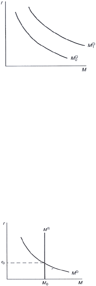
Page 248
Figure 12.1: The demand for money
In Figure 12.1 each money demand curve is drawn for a different level of income. Both are
downward sloping, reflecting the inverse relationship between the rate of interest and desired
money balances. As income rises the demand for money rises, which is reflected in the
outward shifting demand curve (M0 → M1).
F. DETERMINATION OF THE RATE OF INTEREST
It can be assumed that the money supply in the economy is determined by the Bank’s
monetary policy. This can be illustrated by a vertical supply of money at whatever quantity
the Bank decides. Figure 12.2. brings the supply of and demand for money together .
Figure 12.2: The equilibrium rate of interest
The equilibrium rate of interest will be determined at the point of intersection of the money
supply and money demand curves. If the bank decides on a money supply of M o and if the
demand for money in the economy is as represented by MD, then the equilibrium rate of
interest in the economy is ro (Figure 12.2).
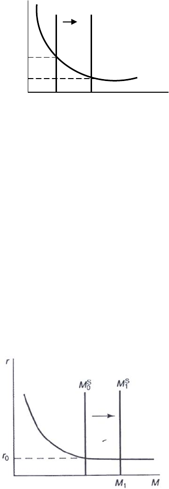
Page 249
If the Bank decides on expansionary or contractionary monetary policy then, by implication, it
is choosing lower or higher interest rates.
R MS0 MS1
R0
R1 MD
M0 M1 M
Figure 12.3: Monetary policy and interest rates
Figure 12.3 illustrates how an expansionary monetary policy (e.g. Bank buys government
bonds) leads to a shift of the money supply from M o to M 1. As a result - interest rates fall
from r o to r 1 and bond prices rise. A contractionary monetary policy (e.g. selling
government bonds) would lead to a leftward-shifting money supply a rise in interest rates and
therefore a fall in bond prices. A tight monetary policy implies high interest rates whereas a
loose monetary policy implies low interest rates.
Keynes suggested the possibility of a liquidity trap. At very low rates of interest the
opportunity cost (interest forgone) of holding cash will be insignificant. If at a very low rate a
change is more likely to mean an upward change then holding speculative cash balances
rather than bonds would appear to make sense. At very low rates of interest therefore there
may be a potentially limitless level of desired cash holdings. This can be illustrated by a
perfectly elastic (horizontal) segment of the money demand curve at very low rates of interest
as in Figure 12.4.
Figure 12.4: Liquidity trap
At r0, there is a perfectly elastic demand for money. If the economy is in a liquidity trap, then
expanding the money supply (M20 → Ms1) will have no effect on the equilibrium rate of
interest which remains at r0. Governments might use an expansionary monetary policy to
stimulate economic activity. An expansionary monetary policy means lower interest rates
which should stimulate investment and consumption expenditure. However, if the economy
is in a liquidity trap as in Figure 12.4, an expansionary monetary policy will not lead to low
Page 250
interest rates and therefore have no effect. Keynesians have traditionally recommended the
use of fiscal policy rather than monetary policy as the appropriate method of influencing
aggregate demand.
G. THE QUANTITY THEORY OF MONEY
The quantity theory of money (QTM) is a theory about how much money supply is needed to
enable the economy to function. In particular, it is concerned with the impact of a changing
money supply on prices. The money value of expenditure in an economy depends on the
price of goods and services and the quantity of goods and services purchased. If we let Y
stand for the annual quantity of final goods and services purchased and P for the average price
of these goods and services then PY is the money value of expenditure on final output.
The money value of expenditure can also be thought of as the amount of money in circulation
multiplied by the number of times this money is spent. Letting M stand for the quantity of
money and V for the number of times this money is spent annually, then MV is also the
money value of expenditure.
These four variables, M, V, P and Y can be defined in such a way as to give us the equation of
exchange:
MV = PY [12.2]
The equation of exchange is in fact an identity as V is simply defined as PY/M. V is referred
to as the income velocity of circulation of money. Velocity of circulation measures the
number of times money changes hands
For example, if P = RWF2; Y = 10,000 units of output and M = RWF4000
RWF4000 (v) = RWF2 x 10,000 => V = 5
The Quantity Theory of money makes certain assumptions:
(a) The level of output Y clearly has an upper limit determined by available resources of land
labour and capital. If we start with the simplifying assumption that the economy is fully
employed, then Y can be treated as fixed at its upper limit, indicated by Y*.
Page 251
(b) The velocity of circulation, V, depends on how effectively the existing stock of money is
being used. This depends on the pattern of payments in the economy and to some extent
on the level of interest rates. We saw (Section 12E) that a worker being paid weekly
would have lower average cash balances than a worker being paid monthly and that at
higher rates of interest there is an incentive to hold less cash. The lower cash holdings
are for any given level of nominal GDP, the higher the velocity of circulation needs to be.
For simplicity, we will assume that these factors are all constant so that velocity can be
treated as a fixed value. Given these assumptions and denoting the constant V with V*,
we have:
MV* = PY* [12.3]
Equation [12.3] gives us a simple quantity theory of money. As the Left Hand Side of the
equation must equal the Right Hand Side, a rise in M must result in a proportional increase in
P. The QTM predicts that an increase in the money supply will cause inflation. As the
quantity of money increases, the value of money (its purchasing power) falls.
The simplicity of the Quantity Theory of Money is part of its appeal. However, in its simple
form, it is open to a number of criticisms:
The assumption that Y is fixed at the full employment level may be inappropriate. If
there is unemployment in the economy, then an expansionary monetary policy may
lead to an increase in real output.
There is much evidence to suggest that V is subject to significant variability. That
being so, the simple link between M and P may be more complex than the simple
QTM suggests.
Logically, it is possible to reverse causation. The QTM assumes that changes in M
cause changes in P. What if changes in P cause changes in M? Cost-Push
explanations of inflation would tend to argue that the money supply adapts to
accommodate changes in prices.
How is M to be measured? We saw (Section 12A) that there are different measures of
money depending on how it is defined. Which measure of M is appropriate for the
QTM? Central Banks are sometimes unsure which measure of money to target.
The link between M and P is not as the simple QTM would imply. However, few economists
would deny that a rising money supply, particularly if it is rising faster than real output, must
eventually cause inflation. The closer the economy is to full employment, the more prone to
inflation it is likely to be.
The Four Functions of Money
1. Means of exchange (facilitates trade).
2. Unit of account (standard measure of value).
3. Standard of deferred payment (helps establish a value for “future” payments)
Page 252
To provide an acceptable standard of deferred payment, money must maintain its value
over time. Inflation erodes the value of money.
With inflation: -
• Creditors gain at the expense of debtors (bad for long-term contracts)
• Those on fixed incomes lose out.
4. Store of value.
Money is a liquid store of value, i.e. a liquid asset.
It is liquid because it can be converted into cash or used to buy goods.
(a) Without delay
(b) Without significant penalty or loss of face value (i.e. without loss of capital value of
interest)
Commodity Money: Money made from a valuable commodity (gold etc.)
Non-commodity Money: Money whose value is greater than inherent value (token money),
e.g. banknotes and coins, bank accounts and cheques).
Non-commodity money is:
More divisible,
More portable
Easier to transfer
Narrow Money: very liquid money balances
Broad Money: Less liquid financial assets but still relatively liquid.
H. TAXATION
Functions of Taxation
(a) To raise revenue – to pay for goods and services and for the upkeep for government
administration
(b) To discourage bad habits – e.g. tax on cigarettes, alcohol.
(c) To make private firms/people pay for externalities – e.g. pollution.
(d) To redistribute wealth – tax the better off and pay for social welfare and old age pensions.
(e) To protect domestic industries from foreign competition – import taxes and export
subsidies (reverse taxes).
(f) To stabilise National income – taxation reduces the effect of the multiplier so it dampens
swings in the trade cycle.
(g) To target particular sections of the economy – e.g. taxes on wealth, capital, income,
goods can be used with relative precision to affect specific sectors.
Page 253
Qualities of a Good Tax System
1. Based on the system ability to pay.
2. The tax should be certain and understood by all.
3. Payment should be related to how and when people receive and spend their income (e.g.
PAYE deducted when wages are paid, VAT is charged when goods are bought).
4. Cost of collection should be small relative to its yield.
5. Should be easily adjustable. E.g. the rates
6. Should not harm initiative
7. Evasion should be difficult.
8. It should be fair.
Three ways of Levying Taxation.
1. Regressive Tax - Takes a higher proportion from the poorer person’s salary than the
rich person e.g. VAT TV Licence and road tax.
2. Proportional Tax - Takes the same proportion of income in tax from all levels of
income earners.
3. Progressive Tax - Takes a higher proportion of income in tax as income rises, e.g. the
entire system of income tax, those on higher income pay a higher marginal rate of tax.
Progressive Tax
Advantages
1. They are levied according to ability to pay.
2. They help the government redistribute wealth from rich to poor.
3. Progressive income and wealth taxes (i.e. direct taxes) help to counteract regressive
indirect taxes (VAT etc).
4. The progressivity of direct taxes can be adjusted so that its not penalty high on the rich.
Page 254
Disadvantages
1. (a) If progressive taxes are too harsh they can be a disincentive to initiative and effort,
e.g. deter working harder, but the evidence on this argument is unclear, sometimes
taxes force people to work harder to maintain their incomes despite the tax.
(b) Higher corporate (company) taxes may reduce investment, research and
development, expansion.
(c) High direct taxes may cause a loss (i.e. emigration) of more skilled workforce
abroad.
2. High taxes may encourage:
(a) Tax avoidance (legal) e.g. non-taxable perks.
(b) Tax evasion (illegal)
(c) Transfer of wealth abroad to tax havens, etc.
Proportional Taxation
Advantage
1. It is seen to be fair
Disadvantages
1. It’s expensive, needs a large administration to calculate proportional tax liabilities.
2. The necessary tax rules are complex.
3. It does not help with wealth redistribution.
Regressive Tax
Advantage
1. Relatively easy to administer and collect usually.
Disadvantages
1. It is not equitable, the less well off pay a higher percentage of their income.
Types of Tax
Direct Tax paid direct by a person or firm to the revenue authority, e.g. income tax,
corporation tax, capital gains tax.
They tend to be progressive or proportional.
Advantages
1. Fair and equitable, levied by ability to pay.
2. They tend to be stabilisers, take more money out of the system at boom times when
incomes and wealth are higher.
3. They are hard to pass on and so are less inflationary than indirect taxes.
4. Such taxes are clear to the people who have to pay.
Page 255
Disadvantages
1. Direct taxes can cause distortions, especially to incentives to work.
2. When levied at a high rate it can affect occupational and geographic mobility.
(a) High taxes in areas of good employment or in good/well paid industries may deter
people moving into these areas.
(b) High marginal rates, by narrowing differentials in the after tax pay of skilled and
unskilled labour, may reduce the incentive to train and cause a shortage of skilled
labour.
(c) High marginal rates may encourage tax avoidance, i.e. finding legal loop holes.
(d) A direct tax on profits is likely to be disincentive to risk-taking and enterprise and
will reduce the ability to invest, by reducing after-tax profits and therefore retained
earnings.
Indirect Tax collected from an intermediary who passes the tax onto consumers in the price
of goods, e.g. VAT and custom duties on imports.
Indirect taxes tend to be regressive and avoidable, can stop buying the good.
Advantages
1. Harder to evade than indirect taxes.
2. Can be used to encourage or discourage the production or consumption of particular
goods.
3. It is a flexible instrument of economic policy – the rates can be changed quickly and
easily and can take effect immediately.
Disadvantages
1. These taxes are “hidden” from the tax payer.
2. They can be inflationary, increase the selling price.
3. They tend to be regressive.
4. They are not impartial, distortions in consumption patterns, e.g. they tend to penalise
smokers, drinkers and car drivers most.

Page 256
BLANK

Page 257
Study Unit 13
International Trade
Contents
A. International Trade
___________________________________________________________________
B. Balance of Payments
The Current Account
The Capital Account
Disequilibrium
C. The Terms of Trade
D. Inter-industry and Intra-industry Trade
E. Free Trade and Protection
F. Impact of a Tariff
Page 258
A. INTERNATIONAL TRADE
How can free trade lead to an increase in economic welfare?
Countries trade with each other so that their inhabitants can enjoy a higher standard of living.
Very few (if any) countries attempt to supply all their own economic needs. Factor
endowments, climate, skills and knowledge vary greatly from one country to another. Thus,
complete economic self-sufficiency at an acceptable standard of living is impossible, or at
least very difficult, for a number of reasons:
(a) Size of Population: Small population limits opportunities for large-scale production.
For a “small” country to take advantage of significant economies of scale it must be able
to export its goods so as to gain access to larger markets and import other goods which it
would be uneconomic to produce domestically.
(b) Nature of soil and climate: Some countries have unsuitable soil and climate to
produce certain goods so these goods must be imported.
(c) Resources: Some countries have limited supplies of mineral and energy resources and
so have to import large amounts of oil, coal, steel, etc.
(d) Skills and Technology and Capital: Some countries lack the necessary human,
technological and capital resources to produce certain goods, thus either these resources
or the final goods themselves must be imported.
The rationale for free trade follows from the reasons outlined above. The main reasons
being:
(i) Efficiency is encouraged: Trade intensifies competition which puts pressure on firms to
be more efficient.
(ii) Economies of scale/size: Industries where significant economies of scale apply might
not be feasible if production had to be confined to the level of demand within national
frontiers. This is especially true of small economies such as Rwanda’s where those
wishing to expand often have to look to export markets.
(iii) Exports earn foreign currency: Which helps countries pay for their import bills for
essential commodities like oil and raw materials. It is important that export revenues
should, as far as possible, pay for imports since any Balance of Payments (BoP) current
account deficit not met by capital inflows must be financed by running down foreign
exchange or by foreign borrowing – neither of which courses of action is desirable over
the long term.
(iv) Exports are an injection into the economy: Greater exports means greater
production and therefore increased employment potential. By causing a magnified
increase in national income (via the multiplier) increased exports also boost economic
growth.
(v) A healthy export trade creates confidence and encourages investment: The opening
up of export markets gives businessmen and investors’ confidence to expand their
activities/increase investment since they are no longer confined to the home market.

Page 259
Furthermore, in times of national economic recession, economic recovery may depend on
the expansion of exports.
(vi) Imports are often essential to industrial and commercial life: Raw material and
energy imports which are incorporated into finished products boost the economy, since
without these essential imports production of some goods could not take place.
Moreover, while imports are detrimental to domestic employment in so far as they
complete with home produced goods, they also create employment by supplying essential
raw materials and in the import/ export, distribution, transport, sales and retail sectors.
(vii) Consumption possibilities are increased: Trade extends the consumption possibilities
of a country beyond its own production frontier.
(viii)The Law and comparative advantage/costs: Perhaps, the main justification for free trade
is this law which states: a country should concentrate on production of those goods in
which it is relatively more efficient and obtain its other requirements by trading. A
country has a comparative advantage in production of a given commodity if the
opportunity cost, i.e. the amount of the other good which must be sacrificed to produce
one unit of the good in question, of the good is lower in that country. Thus, it will be
mutually beneficial for countries to trade so long as there is some difference in their
relative efficiencies in the production of the commodities.
The Law of Comparative Advantages in More Detail.
Each country has a different factor endowment and different skills, knowledge and
experience. Thus, the cost of producing goods – in terms of resources used (i.e. opportunity
cost) – will vary from one country to another. Free trade increases economic welfare by
enabling countries to take advantage of international specialisation to their mutual benefit.
For Example:
Production of Wheat
per man (units)
Production of Cloth
per man (units)
Cost of one unit of Wheat
(in units of cloth)
Cost of one unit of Cloth
(in units of Wheat)
UK 10 2 2
10
5
USA 15 8 8
15
15
8
This schedule indicates that a person in the UK can produce 10 units of wheat or 2 units of
cloth. The opportunity cost of wheat (i.e. its cost in terms of amount of cloth foregone) is 1/5
in the UK and 8/15 in the USA.
It is clear that the USA has an absolute advantage in both goods, i.e. it can produce goods
more efficiently (i.e. at lower opportunity cost) than the UK. But even in this situation, both
countries can gain if each country specialises in the product in which they have a comparative
or relative advantage.
The USA has a comparative advantage in the production of cloth since if it produces 1 unit of
cloth it forgoes the possibility of producing 15/8 (17/8) units of wheat whereas the UK to
Page 260
produce 1 unit of cloth would have to forgo 5 units of wheat, (i.e. the USA has a smaller
opportunity cost for cloth).
The UK has a comparative advantage in the production of wheat, since it produces 1 unit of
wheat it forgoes 1/5 of a unit of cloth while the USA to produce 1 unit of wheat would have to
sacrifice 8/15 of a unit of cloth.
(8/15 > 1/5 therefore opportunity cost of wheat is smaller in UK).
To illustrate the gains to be made from trade consider the following:
If the USA and the UK follow the law of comparative advantage and the USA specialises in
cloth while the UK specialises in wheat then the total gain in production will be:
Cloth
Wheat
USA’s Output
UK’s Output
+1
-1
-
15/8
+5
Net Gain
Nil
+31/8
Wheat
Cloth
USA’s Output
UK’s Output
+1
-1
-
1/5
+8/15
Net Gain
Nil
+1/3
By reallocating resources the total output has increased by 31/8 units of wheat and 1/3 unit of
cloth.
Naturally, the reallocation that would take place in reality would be much greater than one
unit and hence the gains would be very significant.
Note: the principle of Comparative Advantage can be extended from the above 2
commodity-2 country example to apply to the real world where many countries trade in
numerous commodities.
However, there are a number of problems (i.e. buts) to the practical application of the law.
These are:
(a) Whether trade will be beneficial will depend on the terms of trade – i.e. the rate at which
products exchange on world markets as well as on the opportunity costs ratio. From the
example given above for specialisation and trade to be advantageous to both countries
the terms of trade must lie between:
15/8 and 5 (units of wheat) for cloth, and
1/5 and 8/15 (units of cloth) for wheat
Why? Well, to explain the cloth terms of trade – it costs the UK 5 units of wheat to
produce 1 unit of cloth so if the UK can get a unit of cloth for any figure less than 5 units
of wheat it will be better off. Likewise, it costs the USA 15/8 units of wheat to produce 1
unit of cloth so if the USA can get more than 15/8 units of wheat for a unit of cloth it’s
better off.
[ USA specialises in cloth]
[ UK specialises in Wheat]

Page 261
The precise rate at which the exchange takes place will depend on the relative bargaining
strengths of both sides.
(b) If transport costs are very high they will greatly reduce and may even eliminate the gains
from specialisation and trade.
(c) The benefits of trade may not be evenly distributed.
(d) There may not be perfect factor mobility – workers laid off in the industry which is
comparatively disadvantaged may not be able to take up employment in the industry
that’s expanding.
(e) There may not be constant returns to scale – i.e. 2 men need not necessarily produce
twice as much as one man (though that is what is assumed in the example given above).
In fact diminishing returns may set in when output exceeds a certain level.
(f) It may be very difficult to discover where the advantages lie (i.e. with which countries).
Relative costs are very hard to work out and much trade is carried out simply to obtain
more variety, maybe actually against the strict theory of comparative advantage.
Protectionism
Despite the advantages of free trade, protectionism – i.e. restriction or prevention of imports –
occurs to some extent in some countries.
It may take one or a combination of the following forms:
(i) Quotas – restriction on the amount of particular products which can be imported.
Advantages: the size of the quota is flexible and can quickly be changed ( or );
government and domestic firms know the maximum level of imports in advance and can
take decisions accordingly; can be of use in restricting imports in the face of BoP current
account deficit.
Disadvantages: Yields no revenue to the government; tends to establish monopolies of
larger importers and reduce competition thereby increasing prices and maybe reducing
quality; they tend to require frequent changes which cause uncertainty; with many
different distribution channels it’s difficult to establish when the last unit of the quota has
been imported.
(ii) Tariffs – taxes on imports, usually calculated as a percentage of the price of the good at
time of importation.
Advantages: raises revenue for the government; discourage imports (by raising the price
of foreign products) and therefore is of help in times of BoP current account deficit.
Disadvantages: hinders the trading process by adding to the administrative burden; by
raising the price of imports it may cause/exacerbate inflation and eventually increase
export prices; the effectiveness of tariffs depends on the elasticity of demand for imports
– if inelastic, dearer imports merely raise the total import bill (because quantity will not
fall much.)
(iii) Embargos – total loan on the importation of a commodity. Generally used only in
extreme circumstances e.g. UK embargo on importation of Irish Cattle due to outbreak of
Foot and Mouth in Ireland.
Page 262
(iv) Exchange controls
Why restrict free trade if it is beneficial?
(a) The infant industry argument – an industry may need some protection against
“mature” competitors in the early stages of its development. However, it is frequently
the case that infant industries protected in this manner never develop to optimal
efficiency and so cannot survive when protection is withdrawn.
(b) To maintain domestic employment during a recession – if there is low domestic
demand, a country may introduce import restrictions so as to reserve the domestic market
for domestic producers and thus protect national employment.
(c) To allow non-viable industries to decline gradually – in this way the economic
and social costs will be reduced.
(d) To prevent “Dumping” – i.e. the sale of goods on the domestic market at prices
lower than the costs of production in their origin, i.e. to protect domestic producers
against unfair competition.
(e) Strategic reasons – e.g. protection of agriculture, since a country without its own
food supplies would be very vulnerable in times of war or economic recession.
(f) BoP deficit – if imports constantly exceed exports there is a great temptation to
introduce protective measures (but this does not solve the underlying problems).
(g) Protection against low wage economies – since they have a big cost advantage.
(h) Political Purposes – e.g. anti-apartheid sanctions against South Africa.
(i) To raise revenue for the government – through tariffs.
If a country imposes restrictions on its imports in order to protect certain of its industries then
it will lose some of the advantages of international specialisation and its real income per head
will fall. It can be assumed that the industries which the restriction are designed to protect are
industries in which the country no longer has a comparative advantage and waste will occur
in continuing to use resources in these industries instead of transferring them to areas where
the country has a comparative advantage.
Import restrictions will mean higher prices and a reduction in variety of product for
everybody but some groups will benefit in other ways. Firms in protected industries will now
remain in business and make increased profits. Employment in these industries will be
maintained and perhaps increased as production is increased to fill the gap left by import
restriction. Similarly industries which supply the protected industries will benefit if the
object of the restrictions is to favour an “infant industry” or to diversify the economy, and
these objectives are achieved, then benefit will accrue to the country as a whole and to the
particular groups concerned.
The benefits gained above will be far outweighed by the costs imposed on the rest of the
country by way of less output at a higher cost. Higher prices in the protected industries will
mean a reduction in the demand for the products of other industries. Export demand will fall
as foreign countries suffer a fall in income due to the reduction in their exports to the country
imposing the restrictions. Foreign countries will suffer losses in the same way as the country
Page 263
imposing the restrictions and may, themselves, retaliate in a similar way making the losses
even more severe.
It has so far been assumed that the country’s objective in imposing restrictions was the
maximisation of economic welfare but the country may have other objectives in mind. These
might include a desire for self-sufficiency in some products for strategic or defence reasons,
or the wish to preserve some particular, maybe traditional, way of life. To the extent that
import restrictions achieve these objectives they will presumably benefit all, but the economic
costs will be as indicated as above.
B. BALANCE OF PAYMENTS
The balance of payments accounts represent a record of all transactions between residents and
firms located in one country and the rest of the world. Depending on the nature of the
transaction, the details will be recorded in either of two accounts: the current account or the
capital account.
Please see diagram below showing detailed breakdown of Rwandan Balance of Payments (World
Bank Indicators).
WORLD BANK INDICATORS - RWANDA - BALANCE OF PAYMENTS
Previous Jan ‘07
Last Jan ‘08
Changes in net reserves (BoP; US dollar) in Rwanda
-105216849.9
-55552810.7
Communications; computer; etc. (% of service exports; BoP) in Rwanda
43.2
35.2
Current account balance (BoP; US dollar) in Rwanda
-146637069.2
-252075161.3
Current account balance (% of GDP) in Rwanda
-3.9
-5.4
Current transfers; receipts (BoP; US dollar) in Rwanda
435390653.5
558457028.0
Exports of goods and services (BoP; US dollar) in Rwanda
363310377.9
664761740.2
Exports of goods; services and income (BoP; US dollar) in Rwanda
411303209.1
693024253.3
Exports of goods; services; income and workers' remittances (BoP; US dollar) in Rwanda
439584024.0
756331656.7
Foreign direct investment; net (BoP; US dollar) in Rwanda
80088879.3
103350000.0
Foreign direct investment; net inflows (BoP; US dollar) in Rwanda
67142879.3
103350000.0
Foreign direct investment; net inflows in reporting economy (DRS; US dollar) in Rwanda
67142879.3
103350000.0
Foreign direct investment; net inflows (% of GDP) in Rwanda
1.8
2.2
Foreign direct investment; net outflows (% of GDP) in Rwanda
-0.4
Goods exports (BoP; US dollar) in Rwanda
184177641.6
256562540.1
Goods imports (BoP; US dollar) in Rwanda
636598971.9
879777869.2
Grants; excluding technical cooperation (US dollar) in Rwanda
536490000.0
739440000.0
Imports of goods and services (BoP; US dollar) in Rwanda
908610772.0
1401254650.2
Imports of goods; services and income (BoP; US dollar) in Rwanda
971414733.0
1463532133.4
Income payments (BoP; US dollar) in Rwanda
62803961.1
62277483.2
Income receipts (BoP; US dollar) in Rwanda
47992831.2
28262513.2
Insurance and financial services (% of service exports; BoP) in Rwanda
0.5
1.4
Insurance and financial services (% of service imports; BoP) in Rwanda
0.6
0.5
Net capital account (BoP; US dollar) in Rwanda
160947697.5
210060000.0
Net current transfers (BoP; US dollar) in Rwanda
413474454.7
518432718.8
Net errors and omissions; adjusted (BoP; US dollar) in Rwanda
3887553.5
-5396856.0
Page 264
Net income (BoP; US dollar) in Rwanda
-14811129.8
-34014970.1
Net trade in goods and services (BoP; US dollar) in Rwanda
-545300394.1
-736492910.0
Net trade in goods (BoP; US dollar) in Rwanda
-452421330.3
-623215329.1
Portfolio equity; net inflows (BoP; US dollar) in Rwanda
0.0
0.0
Portfolio investment; equity (DRS; US dollar) in Rwanda
0.0
0.0
Portfolio investment; excluding LCFAR (BoP; US dollar) in Rwanda
-18790000.0
Profit remittances on FDI (US dollar) in Rwanda
9346339.4
15360000.0
Royalty and license fees; receipts (BoP; US dollar) in Rwanda
61941751.8
Service exports (BoP; US dollar) in Rwanda
179132736.3
408199200.1
Service imports (BoP; US dollar) in Rwanda
272011800.1
521476781.0
Technical cooperation grants (US dollar) in Rwanda
73750000.0
93060000.0
Total reserves in months of imports in Rwanda
6.8
4.9
Total reserves (includes gold; US dollar) in Rwanda
552791214.6
596280757.8
Total reserves minus gold (US dollar) in Rwanda
552791214.6
596280757.8
Total reserves (% of total external debt) in Rwanda
94.6
90.0
Trade in services (% of GDP) in Rwanda
12.1
19.7
Transport services (% of service exports; BoP) in Rwanda
20.0
13.8
Transport services (% of service imports; BoP) in Rwanda
31.5
54.5
Travel services (% of service exports; BoP) in Rwanda
36.3
49.6
Travel services (% of service imports; BoP) in Rwanda
25.4
13.4
Workers' remittances and compensation of employees; paid (US dollar) in Rwanda
68118995.7
70182067.9
Workers' remittances and compensation of employees; received (% of GDP) in Rwanda
1.4
1.4
Workers' remittances and compensation of employees; received (US dollar) in Rwanda
51270439.2
67797401.4
Workers' remittances; receipts (BoP; US dollar) in Rwanda
28280814.9
63307403.4
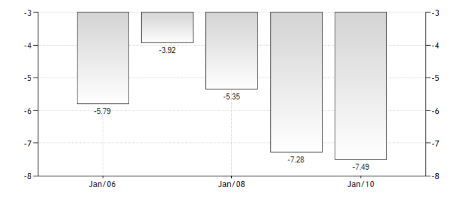
Page 265
The Current Account
The current account records current income from and current payments to the rest of the
world. The transactions concerned may be related to visible trade; invisible trade; profit,
interest and dividend flow; or international transfers. Transactions leading to income received
by the host country are entered with a plus sign whereas transactions requiring payments
abroad are entered with a minus sign.
Visible trade – or merchandise trade – is concerned with trade in tangible items such as food,
manufactures, etc. Exports are entered with a plus sign while imports are entered with a
minus sign. Invisible trade relates to trade in services such as transport, financial and other
services and also includes income and expenditure relating to tourism. Profit, interest and
dividend flows result from the foreign ownership of assets. Domestic owners of foreign
assets receive property income from abroad whereas foreign owners of domestic assets
receive property income from the host country. International transfers relate to transactions
such as foreign aid; private transfers such as remittances from emigrant workers, etc. It is not
uncommon for all items, other than visible trade, to be collectively referred to as invisibles.
The Current account balance (% of GDP) in Rwanda was last reported at -7.49 in 2010,
according to a World Bank report released in 2011. The Current account balance (% of GDP)
in Rwanda was -7.28 in 2009, according to a World Bank report, published in 2010. The
Current account balance (% of GDP) in Rwanda was reported at -5.35 in 2008, according to
the World Bank.
The sum of current incomes and payments, both visible and invisible, gives the current
account balance. A surplus on current account, representing an excess of foreign earnings
over foreign expenses, suggests that a country is ‘paying its way in the world’. A deficit
would indicate that the country concerned was either incurring net foreign liabilities or using
up foreign assets to finance the deficit.
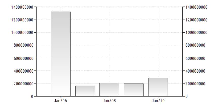
Page 266
The Capital Account
The capital account records changes in overseas assets and liabilities. When a foreign
multinational invests in the domestic economy, the multinational acquires an asset.
However, the economy acquires a liability in the sense that there will be a subsequent outflow
of repatriated profits to provide a return on this inward investment. The reason why the
inward investment is desirable, of course, is the fact that typically the investment will
generate enough earnings not only to finance repatriated profits, but also to provide incomes
for domestic employees. When a multinational invests in a foreign country, foreign assets are
being acquired which should lead to an inflow of property income on the current account at a
later date.
Net capital account (BoP; US dollar) in Rwanda
The Net capital account (BoP; US dollar) in Rwanda was last reported at 285,635,385 in
2010, according to a World Bank report released in 2011. The Net capital account (BoP; US
dollar) in Rwanda was 200,000,000 in 2009, according to a World Bank report, published in
2010. The Net capital account (BoP; US dollar) in Rwanda was reported at 210,060,000 in
2008, according to the World Bank. Net capital account includes government debt
forgiveness, investment grants in cash or in kind by a government entity, and taxes on capital
transfers. Also included are migrants' capital transfers and debt forgiveness and investment
grants by nongovernmental entities. Data are in current U.S. dollars.
Inward capital flows – i.e. those generating liabilities for the home economy – are entered
with a plus sign whereas outward flows – i.e. those generating overseas assets – are entered
with a minus sign. These capital flows are referred to as foreign direct investments (FDI) if
they finance the acquisition of real assets (such as factories) or as portfolio investments if they
finance the purchase of financial assets (such as government bonds, bank deposits, etc). Also
included is foreign borrowing (+ sign) or lending (- sign) by domestic private sector financial
institutions. Official capital flows refer to government borrowing (+ sign) or lending (- sign)

Page 267
and to changes in official reserves at the Central Bank (increases with a – sign, reductions
with a + sign).
All capital inflows are recorded with a plus sign whereas capital outflows are recorded with a
minus sign. However, it is the minus entries that represent an increase in the economy’s
overseas assets or a reduction in overseas liabilities.
It is important to note that the Balance of Payments, taken in total, must exactly balance. All
transactions should lead to a double-entry of equivalent values but with opposite signs. For
example, if a Rwandan exporter of merchandise to Kenya invoices in RWF to the value of
RWF10m, then the Kenyan importer must spend the Kenyan Shillings (KES) equivalent to
purchase RWF10m to settle the account. That means somebody else must be selling
RWF10m to buy KES. The exporter’s transaction leads to a + RWF10m entry on the current
account whereas the seller of the RWF10m is causing an entry of –RWF10m on either the
current or capital account (depending on why KES are being purchased). Therefore the
surplus on the current account should be exactly matched by a deficit on capital account of an
equal amount. As the figures are never 100% accurate a balancing item is typically required
to balance the accounts.
Disequilibrium
The balance of payments, taken overall, must balance. However, subsections of the accounts
may not be in balance. For example, a deficit on current account typically represents an
excess of current expenditures over current earnings. This deficit must be financed somehow,
and the financing of it will be reflected in a surplus on the capital account. This in turn means
an increase in foreign liabilities or a decline in foreign assets. The excess is being financed
whether by using up official foreign reserves or foreign borrowing or some other capital
inflow.
A balance of payments deficit is generally interpreted to mean a reduction in the official
reserves held at the Central Bank. This reduction may be caused by a current account deficit
which is not being financed by private sector capital inflows, or alternatively despite a surplus
on current account a larger outflow of private sector capital is occurring. A balance of
payments surplus is indicated by an increase in official reserves.
C. THE TERMS OF TRADE
The terms of trade are concerned with the rate at which one country’s goods exchange for
those of other countries. Changes in the terms of trade indicate whether a country must
export more or less in order to purchase a given volume of imports. A terms of trade index
(TOT) can be calculated as:
TOT =
pricesimport of average weighted
pricesexport of average weighted
x 100
The index is a trade-weighted one, i.e. the various prices are weighted according to the
relative importance of that product regarding the total value of imports or exports. The prices
Page 268
are dominated in a single currency and the index is typically set equal to 100 in a base year
(the year in which the weightings are established).
An improvement in the terms of trade is indicated by an increase in the index, an adverse
change by a reduction. An ‘improvement’ means that less needs to be exported to purchase a
given volume of imports (or more imports for a given volume of exports). An improvement
can result from:
An increase in export prices;
A reduction in import prices;
An increase in the nominal exchange rate (Section 14A).
An improvement in the terms of trade does not necessarily benefit the balance of payments or
employment. For example, an increase in domestic prices means fewer goods need be
exported to purchase a given volume of imports. However, it may now be more difficult to
sell these goods with the result that the value of exports may fall. A fall in the price of an
important import (such as oil) typically represents an unambiguous improvement in the terms
of trade.
D. INTER-INDUSTRY AND INTRA-INDUSTRY TRADE
What is the source of comparative advantage? Why do countries differ in their abilities to
produce goods and services? David Ricardo (1722 – 1823), who first formulated the theory
of comparative advantage, suggested that differences in labour productivity between countries
were the reason for differences in relative costs between countries. Access to different levels
of technology could explain differences in labour productivity.
Two Swedish economists (Heckscher and Ohlin) developed this analysis further and argued
that even countries with access to similar technologies could have different relative costs due
to differences in their overall endowment of factors of production. Countries would tend to
specialise in producing those products requiring the factors in which they were favourably
endowed. For example, countries with a relative abundance of labour would tend to
specialise in labour intensive products whereas countries with a relative abundance of capital
would tend to specialise in capital intensive products. Differences in natural resources would
also play their part in determining relative costs between countries.
The important point about the above analysis is the focus on the differences between
countries. Given the differences in factor endowments different countries would tend to
specialise in different products. This type of specialisation is the basis for inter-industry
trade. This is where countries export different products from the ones they import. For
example, the Rwandan economy exports tea and coffee and cassiterite and iron ore, all raw
materials but imports manufactured goods.
The ability of the theory of comparative advantage to explain the pattern of international trade
has been diminished by the growth of intra-industry trade. This is where countries import and

Page 269
export similar products. For example, many economies both import and export motorcars;
Ireland imports and exports whiskey1, etc. By emphasising the differences between countries
the theory of comparative advantage fails to explain intra-industry trade which has much to
do with similarities between countries.
Intra-industry trade is based on product differentiation. Countries will import and export
variations, usually branded versions, of a basic product. Thus Germany exports BMWs while
importing Citroens, etc. The growth of intra-industry trade is linked to an increasing demand
for greater consumer choice and the existence of economies of scale in production. With
rising prosperity in a country, consumers tend to want greater choice regarding the goods they
purchase. If this greater choice was to be catered for exclusively by home producers, there
would be a tendency for a larger number of relatively small producers to emerge. However,
where there is relatively free international trade, producers can cater for similar market
segments in different countries and exploit any economies of scale that might exist. We
would therefore expect intra-industry trade to be more important, the more integrated
economies are and the more similar they are in terms of living standards. Not surprisingly,
intra-industry trade is the dominant feature of the growing trade in consumer goods between
the member-states of the EU.
E. FREE TRADE AND PROTECTION
There are gains from international specialisation and trade. International specialisation can be
expected to result in a more efficient use of global resources. This in turn implies improved
living standards for consumers in the countries concerned. However, it is commonplace for
governments to have commercial policies which include a range of barriers to free
international trade. For example:
Tariffs – a tax on imports having the effect of raising the price of the imports on the
domestic market.
Quotas – an upper limit on the quantity of a product that it is permissible to import.
Non-tariff barriers -
Export subsidies – enables exporters to sell in foreign markets at prices that do not
reflect the true relative cost.
Trade barriers are designed primarily to protect domestic producers from foreign competition.
A range of arguments has been put forward in support of protectionist measures:
Unemployment – there can be major adjustment costs if domestic industries are forced
to adjust to foreign competition. This can be particularly so when there is a significant
shift in comparative advantage from one country or region to another. For example,
1 Whiskey in Ireland and USA and Whisky in Scotland and Canada
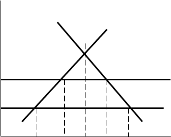
Page 270
the growing competitiveness of China and many SE Asian economies in manufactured
goods poses major problems for European economies.
Infant industries – some industries may require protection from superior foreign
competitors if they are to develop and prosper. Particularly where efficiency is based
on economies of scale, protectionist measures may enable an industry to develop on
the home market and become internationally competitive in the longer term.
Strategic industries – the government, for political reasons, may consider it
undesirable to be over-dependent on foreign suppliers of certain products such as food
or armaments.
To improve the balance of payments.
Free international trade can result in gainers and losers and therefore have important
implications for the distribution of income in society. Despite long-term benefits there may be
significant short-term costs. Governments must decide, usually under pressure from local
interests, where the balance of advantage lies. However, there is no economic case for the
permanent protection of inefficient domestic industries. Inefficiencies in one sector
inevitably translate into higher costs in other sectors either by way of higher input prices or
less demand or both. The result is living standards lower than they might otherwise be.
F. IMPACT OF A TARIFF
The effect of the imposition of a tariff can be illustrated as in Figure 13.3.
P
S
P0
P1 b c Stw
Pw e f Sw
a d D
q1 q3 q0 q4 q2 Q
Figure 13.3: Impact of a tariff
The S and D curves represent domestic supply and demand conditions. If we assume that the
country can import as much as it wishes at the prevailing world price (known as the 'small
country assumption'), this can be illustrated with a perfectly elastic supply curve (Sw) drawn
at the world price (pw). If the country’s commercial policy is to keep out imports completely,
the domestic price will be po with domestic production at qo. If the country adopts a policy of
free trade, the domestic price will fall to the world price pw, domestic production falls to q1,
consumption expands to q2, with q2 – q1 being imported.
Page 271
Assume, starting from a position of free trade, the country imposes a per unit tariff (t) on
imports. This can be illustrated by an upward shift of the world supply curve by an amount
equal to the tariff (Sw → Stw). The effect of the tariff is to benefit domestic producers at the
expense of domestic consumers and foreign producers. The domestic price rises to p1, which
is the world price plus the tariff (pw + t). Domestic production expands from q1 to q3, but
domestic consumption falls from q2 to q4. Imports, which were q2 – q1, fall to q4 – q3. The
government’s tariff revenue from these imports is q4 – q3 times t (indicated by the shaded area
abcd).
Consumers’ surplus has fallen by pwp1cf as a result of the tariff. This has been converted into
increased profits for domestic producers (pwp1be), tariff revenue for the government (abcd)
and payment for the higher costs of domestic producers (eba). The triangle dcf represents a
deadweight loss (i.e. a loss with no corresponding gain).

Page 272
BLANK

Page 273
Study Unit 14
Exchange Rates
Contents
A. Nominal, Effective and Real Exchange Rates
B. Determination of the Nominal Exchange Rate
C. Purchasing Power Parity
D. Fixed and Floating Exchange Rates
Managed Float
Arguments in Favour of and Against Fixed Exchange Rate Regimes
Arguments in Favour of and Against Free Floating Rates
______________________________________________________________________
E. Exchange Rates and the Balance of Payments
F. Monetary and Fiscal Policy with Fixed and Floating Exchange Rates

Page 274
A. NOMINAL, EFFECTIVE AND REAL EXCHANGE RATES
An exchange rate is simply the price of one currency in terms of another. For example,
suppose that, however unlikely it might be, RWF1 = $1.50 or RWF1 = Euro 2.50, etc. These
are examples of the nominal exchange rate (NER) and clearly there are as many NERs as
there are currencies. The NERs of significance for the economy are those with the country’s
important trading partners.
It is possible that one currency is gaining value against some currencies but losing value
against others. The effective exchange rate (EER) is an index which attempts to measure the
overall change in the value of one currency against a range of other currencies.
Example:
Assume the RWF/$ rate changes from RWF1 = $1.50 to RWF1 = $1.35, (a –10%
depreciation of RWF), while the RWF/Euro rate changes from RWF1 = Euro2.50 to RWF1 =
Euro2.75, (a +10% appreciation of RWF). For simplicity assume that 75% of the country’s
trade is with Germany and 25% with the USA. The change against the Euro will have a
greater impact on the economy than the change against the $ and will, therefore, receive a
correspondingly greater weighting:
(+10% x 0.75) – (10% x 0.25) = +5%
The EER has a base year value equal to 100 and is adjusted in the light of trade weighted
changes in relevant NERs. For the above example, the EER would increase, say, from 100 to
105, indicating an overall appreciation of 5%.
The real exchange rate (RER) is an index which measures changes in the international
competitiveness of a country’s goods and services.
Example:
Price of bottle of Rwandan Beer = RWF10
Price of bottle of Kenyan Beer = RWF10
EER RWF / KES Rate RWF1 = KES1
The competitiveness of the Rwandan Beer will be affected if either the NER changes or if the
domestic price of either beer changes. For example, if the price of Rwandan Beer increases,
then it will lose competitiveness unless the value of the RWF falls against KES. The RER
incorporates changes in both relative prices and NERs and can be calculated as the ratio of
domestic prices (Pd) to foreign prices (Pf) the latter converted to domestic currency terms:
RER =
EER x P
P
f
d
An appreciation of RER, due to domestic prices rising faster relative to foreign prices or an
appreciation of the EER (resulting in cheaper foreign goods) implies a loss of
competitiveness.
Page 275
B. DETERMINATION OF THE NOMINAL EXCHANGE RATE
The NER is a price and, like any price, the value will be determined by buyers and sellers in a
market, in this case the foreign exchange markets. These are highly competitive markets,
resembling perfectly competitive ones in some respects. For example, homogeneous
products; a large number of financial institutions dealing; well-informed dealers using
advanced communications systems.
Only money is being traded and, therefore, the seller of one currency is of necessity the buyer
of another. By focusing on just two currencies, a particular NER can be isolated and the
analysis simplified. If we take just the Franc (RWF) and the Dollar (USD) then sellers of
RWF by definition are buyers of USD and vice versa. Anything causing increased demand
for USD (i.e. increased sales of RWF) will cause the RWF to depreciate against the USD (i.e.
the USD to appreciate against the RWF). For example, if the exchange rate changes from
RWF1 = USD2.50 to RWF1 = USD2.60, the RWF has appreciated while the USD has
depreciated.
By isolating the motives for buying a foreign currency, we can better understand the forces of
supply and demand at work. Americans wish to buy RWF for a number of reasons including
the following:
To finance the purchase of Rwandan goods and services (Cassiterite, coffee, tourism,
etc.);
To invest in Rwanda: (a) in real assets (FDI) and (b) in financial assets (portfolio
investments);
The American Central Bank may wish to influence the RWF/USD exchange rate.
The first above represents a current account transaction while the other two are capital
account transactions (Section 13A). The willingness of foreigners to buy a country’s exports
will depend on how competitive they are in terms of price and quality. All else being equal, a
successful trading nation can expect to have a strong currency. Inward investment in real
assets will depend on the long-term prospects for the economy to generate an acceptable rate
of return to prospective foreign investors. Investments in financial assets on the other hand
will be influenced by relative interest rates and the shorter term prospect of capital gains or
losses. If interest rates rise in Rwanda relative to America, all else being equal, this will
attract funds into the Rwandan financial system and vice versa. If the franc is expected to lose
value in the future this will result in increased selling (note the self-fulfilling expectation) and
vice versa.
Portfolio investments are highly liquid and can have a destabilising effect on money markets.
Sudden or short-term fluctuations in the value of a currency are not caused by current account
transactions or by long term capital flows (FDI). Sudden (and sometimes dramatic) changes
are caused by changes in interest rates or changing confidence in the future value of the
currency..
The traditional analysis of exchange rate determination focuses initially on current account
transactions, in particular the supply and demand for currencies to finance international trade.
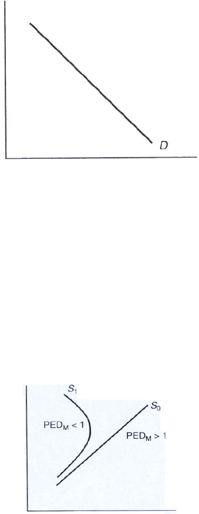
Page 276
When the RWF is strong relative to the USD, Rwandan goods will be more expensive in
America for any given Rwandan price level. By implication the Americans will want fewer
RWF to buy Rwandan exports when the RWF has a high rate against the USD. This can be
illustrated (Figure 14.1) by a downward-sloping demand curve for RWF. At higher exchange
rates fewer RWF are bought by Americans with a view to buying Rwandan goods and
services.
USD price of RWF
RWF
Figure 14.1: Demand for RWF
The demand curve in Figure 14.1 will shift if there are changes in such things as the
popularity of Rwandan goods, Rwandan interest rates relative to foreign rates, expectations
regarding the future exchange rate, the Rwandan price level, etc.
The supply of RWF, for current account transactions is equivalent to the demand for USD to
import American goods and services into Rwanda. As the exchange rate of the RWF rises,
American goods are cheaper in Rwanda for any given price level in America. So, more
American goods will be bought in Rwanda if RWF has a high exchange rate. However it does
not follow that more RWF are necessarily being spent on these extra imports which require
fewer RWF to buy them. Only if the price-elasticity of demand for American imports
(PEDm) is elastic will more RWF be actually spent buying the extra American goods.
USD price of RWF
RWF
Figure 14.2: Supply of RWF
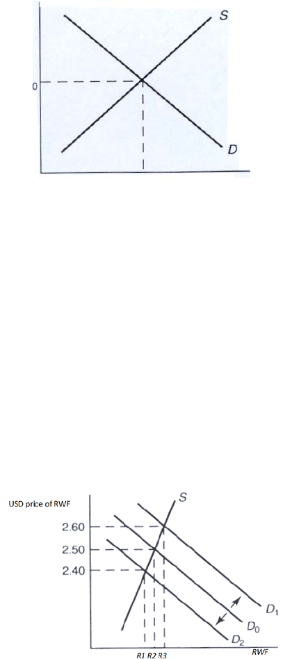
Page 277
Assuming this is the case (PEDm > 1), we can represent the supply of RWF to buy American
goods with an upward-sloping supply curve. If demand were price-inelastic there would be a
backward-bending supply curve as illustrated in Figure 14.2.
If the demand for American imports remains price elastic in Rwanda the supply curve of
RWF will remain upward sloping (So), if demand becomes price-inelastic the supply curve
bends backwards (S I).
By bringing the supply and the demand curves together the analysis of the determination of
the NER can be based on straight forward supply and demand analysis. Figure 14.3 illustrates
this (assuming PEDm > I).
USD price of RWF
RWF
Figure 14.3: The equilibrium exchange rate
The equilibrium RWF/OM exchange rate (eo) is determined at the intersection of the supply
and demand for RWF. RWF0 represents the equilibrium quantity of RWF traded for the
given period.
If the demand curve in Figure 14.3 shifts outward (rising Rwandan interest rates attracting an
inflow of funds for example) the equilibrium value of RWF will rise and vice versa. If the
supply curve shifts outward (rising American interest rates causing an outflow of funds for
example) the equilibrium exchange rate falls and vice versa as illustrated in Figure 14.4.
An increase in the demand for RWF shifts the demand curve from Do to Dl. The value of the
RWF increases from, say, USD2.50 to USD2.60. A fall in demand (Do ~ D2) causes the
exchange rate to fall from USD2.50 to, for example, USD2.40.
Figure 14.4: Changes in the equilibrium value of RWF
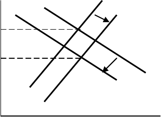
Page 278
C. PURCHASING POWER PARITY
Purchasing power parity (PPP) is a theory of the long-run determination of the exchange
rate. According to PPP changes in relative prices between countries will be the most
important influence on the NER in the long run. PPP predicts that countries with relatively
high inflation rates will experience a decline in the exchange rate of their currency.
Using the example of the Rwandan and Kenyan beers (Section 14A), assume 100% inflation
in Rwanda leads to a doubling of the price of Rwandan Beer i.e. from RWF10 to RWF20. At
the original NER (1RWF1 = RWF1) the Rwandan Beer loses competitiveness and beer
drinkers in both Rwanda and Kenya switch to Kenyan beer.
The switch to Kenyan beer will mean an increased demand for KES in Rwanda, and
(assuming demand in Kenya for the Rwandan product is price-elastic) a fall in demand for
RWF from importers of Rwandan Beer. Figure 14.5 illustrates these effects.
A switch in purchases from Rwandan to Kenyan products implies an increased supply of
RWF to the foreign exchange market to buy more KES (So ~ S I). Assuming demand for
Rwandan goods in Kenya is price-elastic there is less demand for RWF as a result of
Rwandan inflation (Do--+ DI). The equilibrium value of the RWF falls from e0 to e1.
RWF price of RWF
S0
S1
e0
e1
D0
D1
RWF
Figure 14.5: Operation of purchasing power parity
PPP predicts that the value of the RWF will fall by an amount necessary to restore the
competitiveness of Rwandan products (i.e. a new NER of RWF1 = RWF0.50 in our simple
example). If we generalise, the prediction is that the NER’s will adjust so that, in the longer
term, the RER remains constant. What this means is that similar products should cost the
same in different currencies. According to PPP, it is current account transactions that
determine the exchange rate in the long run even if capital account transactions lead to short-
term fluctuations.
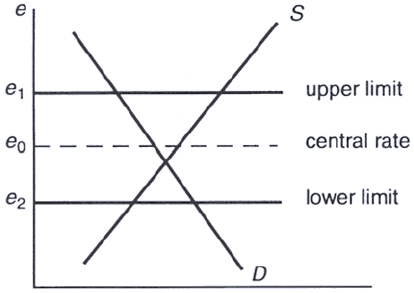
Page 279
D. FIXED AND FLOATING EXCHANGE RATES
In pursuit of their macro-economic objectives (Section 11A) governments must decide on an
appropriate policy for the exchange rate. Three alternative policies (or exchange rate
regimes) are typically available:
free floating
fixed
managed float
A free floating system is where the government allows the exchange rate to be determined by
free market forces. The currency may appreciate or depreciate depending on the relative
strength of supply and demand in the foreign exchange market.
The level of the exchange rate has an important bearing on the ability of a country to trade.
Fluctuations in the exchange rate can be damaging for the economy. Because of this,
governments may intervene to influence the exchange rate through a variety of fixed
exchange rate systems.
Strictly speaking, a fixed exchange rate would require currencies to be locked together at a
particular rate.
However governments may enter into fixed exchange rate agreements whereby upper and
lower limits to the exchange rate are fixed, rather than a particular rate. The post-war Bretton
Woods agreement and the Exchange Rate Mechanism in the EU are examples. Three rates
need to be determined, a central rate plus upper and lower limits which determine the band
within which the actual market rate is permitted to fluctuate (Figure 14.6).
Provided the free market exchange rate remains within the upper (e1) and lower (e2) limits
there is no need for central banks to intervene. The objective is to limit the extent of variation
allowable rather than fix the rates at a particular level. The tighter the bands the greater the
degree of certainty for those involved in international trade but the greater the likelihood the
central bank will need to intervene.
Figure 14.6: Fixed exchange rate
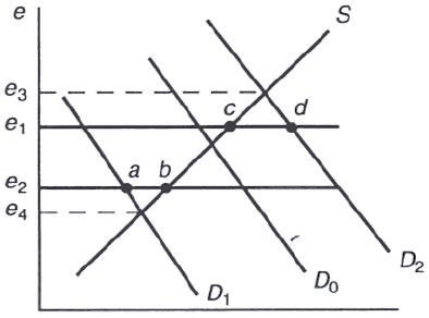
Page 280
Figure 14.7: Intervention in a fixed exchange rate system
If the equilibrium rate moves outside the band the Central Bank must intervene (Figure 14.7).
The shift of the demand curve from D0 to D1 will result in an exchange rate of e4 which is
below the permissible lower limit of e2. The Central Bank is obliged to intervene before the
lower limit is breached. The Bank will be required to use its foreign reserves to buy its own
currency. The distance ab indicates the excess supply of the currency at the lower limit e2
and is the minimum quantity of RWF that needs to be purchased- An alternative (or
complementary) policy is for the Bank to raise domestic interest rates with a view to shifting
the demand curve for the currency upward so that the point of intersection is once again
within the permitted band- Were the demand curve to shift outward from Do to D2 the free
market rate rises to e3 which is above the upper limit of el- To prevent this the Bank must
increase the supply of its own currency to the market by an amount at least equal to cd, the
extent of the excess demand at e1 - The Bank's official reserves will be rising as it purchases
foreign currency - Alternatively (or as a complement) the Bank could reduce domestic
interest rates with a view to shifting the supply and demand curves downwards so that the
point of intersection is within the permitted band-
Operating a fixed exchange rate system imposes certain constraints on a Central Bank:
An adequate stock of foreign currency reserves must be maintained for intervention
purposes.
Monetary policy (Section 12D) must be subordinated to the exchange rate regime.
Interest rates may need to be adjusted to strengthen (or weaken) the currency as
circumstances require.
Problems arise when long-term trends - trade patterns, inflation rates etc. - create the need to
realign currencies. In Figure 14.8, for example, if the shift from D0 to D1 reflects a longer
term trend rather than a temporary shift a devaluation of the currency will be necessary.
If e3 represents the long-run equilibrium rate then the currency has become overvalued with
respect to the original band. The shift from D0 to D1, if permanent, is causing a continuous
fall in the Bank's foreign currency reserves (ab per period) as it intervenes to prevent the rate
falling below e2. Furthermore, a policy of high domestic interest rates will be the appropriate
monetary policy to adopt.
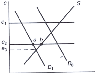
Page 281
Figure 14.8: Devaluation as an option
As foreign reserves are finite and high interest rates will undermine domestic economic
activity, the government will be forced to devalue the currency. Devaluation means choosing
a lower central rate and, therefore, a new lower band which will remove the pressure on the
Bank’s foreign reserves and domestic interest rates.
If one country is undertaking devaluation, then it follows that at least one other country must
be pursuing ‘revaluation’. This requires choosing a higher band because the currency has
become undervalued with respect to the original band. The ultimate freedom to devalue
down or revalue up has given rise to the term ‘adjustable peg’ to describe these systems.
Effectively, they are designed to remove short-term fluctuations rather than prevent longer
term adjustments in exchange rates.
Managed Float
A managed float (sometimes referred to as a ‘dirty float’) is a policy whereby a Central Bank
unilaterally intervenes in the money markets to influence the exchange rate. It is not part of
an international agreement requiring it to do so as in the case of fixed exchange rate systems.
The government typically sets the target for the exchange rate which the Bank pursues.
Arguments in Favour of Fixed Exchange Rate Regimes
By creating a degree of certainty regarding the exchange rate, they reduce the costs
and risks associated with international trade, and therefore can be expected to promote
international trade.
Participating countries will be required to pursue prudent macroeconomic policies that
keep inflation low or face the need for frequent devaluations.
A degree of order is achieved, particularly if the alternative is countries unilaterally
seeking competitive advantage through artificially low exchange rates.
Arguments against Fixed Exchange Rate Regimes
The need for stocks of foreign currency reserves can be wasteful of scarce resources.
Periodic realignments when currencies need to be devalued can cause currency crises.
Page 282
Speculators have a one way bet. If the evidence points to the need to devalue a
currency, speculators can borrow that currency simply with a view to selling it on the
foreign exchange markets. This increases the pressure on the authorities to devalue
after which the speculators can switch back into the (now devalued) currency to repay
liabilities while leaving a profit.
Arguments in Favour of Free Floating Rates
The exchange rate continuously adjusts to bring the balance of payments into
equilibrium. This follows from the fact that the Central Bank simply refuses to use
reserves to intervene.
Savings on official reserves.
Greater freedom to pursue other macroeconomic objectives. For example, interest
rates can be set to meet the internal needs of the economy rather than support the
(perhaps overvalued) exchange rate.
A flexible exchange rate can operate as a shock-absorber for an economy. For
example, it is much easier for an economy to restore its international competitiveness
by allowing the NER to fall than by reducing its internal price level (See Section
14E).
Arguments Against Free Floating Rates
Free floating rates can be extremely volatile. This increases the risks and therefore
costs (in terms of hedging) involved in international trade.
Because the costs involved rise, firms will be less likely to engage in international
trade.
E. EXCHANGE RATES AND THE BALANCE OF PAYMENTS
We have seen (Section 13A) that balance of payments disequilibrium typically means a loss
of official reserves resulting from a deficit elsewhere in the accounts. This deficit may be due
to private outflows on the capital account. However, a ‘fundamental disequilibrium’ can be
interpreted as a large and persistent deficit on the current account. The country is ‘not paying
its way in the world’ resulting in falling reserves, perhaps official borrowing and very likely
high interest rates in an attempt to attract capital inflows.
With flexible exchange rates, this fundamental disequilibrium cannot occur. Quite simply, if
the Central Bank is not intervening, reserves cannot be falling. The exchange rate will adjust
to equate the supply and demand for the currency for current account and capital account
transactions. A fundamental disequilibrium occurs when the Central Bank refuses to allow
the necessary adjustment in the exchange rate.
A current account deficit is removed by reducing the value of imports relative to exports. In
the absence of devaluation, the following policies might be adopted:
Page 283
Deflate the economy;
Import controls;
Buy domestic campaigns.
The first implies the use of monetary and/or fiscal policy to cut the overall level of aggregate
demand in the economy. While this will lead to falling demand for imports, the demand for
goods in general will fall with a likely increase in unemployment.
The second strategy, while it may be effective, invites retaliation. It is also likely to
contravene international commitments such as the World Trade Organisation (formerly
GAAT) agreements.
Even the third strategy may contravene international commitments given to the EAC.
By devaluing the currency, the government makes imported goods more expensive while
exports become less expensive. The impact on the current account will depend on how
domestic demand for imports and foreign demand for exports respond. This in turn depends
on the price elasticity of demand for imports and exports.
The Marshall Lerner condition
This states that if the sum of the price elasticities of demand for imports and exports is greater
than one (PEDm + PEDx > 1) in absolute terms then devaluation will improve the balance of
trade.
There is some evidence that the Marshall Lerner condition is likely to hold in the longer term
but perhaps not in the shorter term. International trade flows may be the result of contracts
that cannot be quickly changed. Furthermore, it may take time for consumers in one country
to adapt to changes in another country's prices. If so the demand for imports and exports may
be relatively inelastic in the short term.
If the sum of the elasticities is less than one in the short term but greater than one in the
longer term, devaluation will initially have a worsening effect on the balance of payments
followed by an improvement. This is the j-curve effect illustrated in Figure 14.9.
Starting at point a with a trade deficit the government devalues the currency. The short-term
effect is for the trade balance to worsen by going further into deficit but to improve over time.
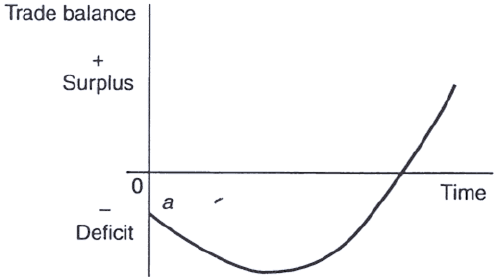
Page 284
Figure 14.9: J-curve
F. MONETARY AND FISCAL POLICY WITH FIXED AND FLOATING
EXCHANGE RATES
Fixed exchange rate systems have a cost in terms of monetary independence. We have seen
that the level of domestic interest rates will have to complement the exchange rate policy.
Furthermore the domestic money supply will respond to surpluses and deficits on the balance
of payments whereas with flexible exchange rates domestic money supply is internally
controlled.
Assume fixed exchange rates and a balance of payments surplus reflected in rising official
reserves. The surplus is the result of the Central Bank selling the domestic currency (i.e.
buying foreign currency) to prevent the exchange rate rising. However, the increase in
foreign reserves at the Central Bank will be matched by an increase in the liquidity of the
banking system as the Bank is supplying domestic currency to the foreign exchange market.
A balance of payments deficit would cause the domestic money supply to contract as the
Bank would be buying domestic currency with foreign currency reserves.
It is possible for the Bank to counteract this balance of payments effect on the domestic
money supply. Open market operations (Section 12D) can be used as a means of sterilisation.
When there is a balance of payments surplus which would otherwise cause the money supply
to expand, the Bank could sell government bonds which would reverse the expansionary
effect of the surplus. With a balance of payments deficit, the appropriate sterilisation would
be to purchase government bonds.
Monetary policy designed to influence the domestic economy becomes ineffective with fixed
exchange rates when there is free capital mobility. Assume the government attempts to
stimulate the domestic economy via an expansionary monetary policy. The domestic money
supply expands causing domestic interest rates to fall. However, with free capital mobility
the fall in interest rates will cause an outflow on the capital account as investors seek higher
returns abroad. This outflow will cause the exchange rate to fall. To prevent the exchange
rate falling, the Central Bank must buy its own currency and/or raise domestic interest rates,
i.e. put the monetary policy into reverse.
Page 285
Fiscal policy will be more effective under fixed exchange rates. Assume an expansionary
fiscal policy whereby the level of taxation is cut. Increased spending leads to an expansion of
the economy. As incomes rise, there will be rising demand for money balances (Section 12E)
causing domestic interest rates to rise. This in turn will lead to an inflow of capital which
will cause the exchange rate to rise. However, the Central Bank must now intervene to
prevent the exchange rate rising. It does so by selling the domestic currency and/or lowering
domestic interest rates either of which implies an increase in the domestic money supply.
This expansionary monetary policy reinforces the initial fiscal policy.
The above analysis implicitly assumes that output rather than the price level increases with
fiscal expansion. If the domestic price level were to rise then exports would fall and imports
rise, in which case the previous analysis would require some modification.
With flexible exchange rates, the effectiveness of policy is reversed; monetary policy is
effective whereas fiscal policy is not. We have seen that fiscal expansion exerts upward
pressure on interest rates whereas monetary expansion implies lower interest rates. With free
capital mobility and rising interest rates, capital inflows will cause the exchange rate to rise
with the result that exports fall while imports rise. These effects of the rising exchange rate
will reverse any expansionary effect of the fiscal policy. However, the lower interest rates
following monetary expansion result in a lower exchange rate due to capital outflows. This
stimulates exports and curtails imports, both of which reinforce the effects of monetary
expansion.

Page 286
BLANK

Page 287
Study Unit 15
The Economics of European Integration
Contents
_____________________________________________________________________
A. Economic Integration
B. Trade Creation and Trade Diversion Effects of a Customs Union
C. The Single Market Programme
Page 288
A. ECONOMIC INTEGRATION
All countries must devise a commercial policy which will govern their trading relationships
with other countries. At an early stage in their economic development, countries might
pursue a policy of self-sufficiency with a view to cultivating home industries. However, there
are gains from specialisation and international trade (Section 13B) and there are few countries
willing to forego these gains in the longer term.
Countries can enter into a variety of trading relationships including the following:
Preferential tariffs: countries reduce tariffs for certain products from certain countries;
Free trade area: participating countries agree to abolish tariffs and quotas with a view
to liberalising merchandise trade;
Customs union: participating countries agree to free trade among themselves but also
they agree to common commercial policies regarding non-members;
Single market: as well as the elimination of tariffs and quotas, members agree to the
abolition of a range of non-tariff barriers (NTB’s); allow free factor mobility and
adopt a common set of rules regarding competition, etc;
Economic and Monetary Union (EMU): members agree to a single currency (or at
least irrevocable locked exchange rates), a single Central Bank operating a common
monetary policy and harmonisation of fiscal policies where appropriate.
The European Union (EU) was always more than merely a set of economic relationships
between members. Since its inception in 1957, the EU (then called EEC) has had a strong
political dimension. ‘Federalists’ wish to see the EU evolve into a modern superstate with
power residing in European institutions such as the European Parliament and European Court
of Justice. Others (‘confederalists’) prefer to see the EU remain as basically a set of
agreements between sovereign governments. These want power to be exercised on an inter-
governmental basis and exercised through a Council of Ministers representing national
interests.
From an economics perspective however, the EU can conveniently be viewed as having
evolved from the stage of customs union, is currently in the single market phase and planning
to proceed to the EMU phase.
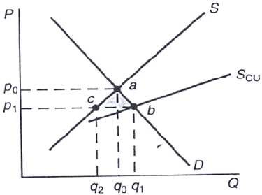
Page 289
B. TRADE CREATION AND TRADE DIVERSION EFFECTS OF A
CUSTOMS UNION
Up until the mid 1980s the economic relationship between members of the EU was largely
that of a customs union with the addition of a Common Agricultural Policy financed through
(a rather meagre) centralised budget.
When analysing the effects of a customs union it is important to realise that a customs union
requires the harmonisation of two sets of tariffs: abolition of internal tariffs but the adoption
of common external tariffs. The abolition of internal tariffs can be expected to have a trade-
creation effect. However adopting a common external tariff can have a trade-diversion effect
in certain circumstances.
Trade-creation occurs when a change in tariffs enables consumers to buy cheaper products
from more efficient producers. Trade-creation benefits consumers and efficient producers at
the expense of inefficient producers.
Trade-diversion occurs when a change in tariffs requires consumers to purchase higher cost
products from less efficient producers. Trade-diversion benefits inefficient producers at the
expense of consumers and efficient producers. This trade-diversion effect can occur if, when
harmonising external tariffs, a country ends up with a relatively higher tariff on a product
from a non-member that it was previously trading with. Figure 15.1 illustrates the trade-
creation effect of a customs union.
Assume to begin with that a country prevents the importation of a particular product. If so the
equilibrium in the domestic market will be determined at the intersection of the domestic
supply (S) and domestic demand (D). This is at point a in Figure 15.1. with an equilibrium
price of po and an equilibrium quantity of qo. Assume now that this country forms a customs
union with one or more other countries. If the removal of trade barriers leads to foreign
suppliers entering the domestic market, supply to the domestic market will expand. This
effect is illustrated by the customs union supply curve (Scu). The new equilibrium will be at
point b with an equilibrium price of p 1 and quantity of q 1.
Figure 15.1: Trade creation effect of a customs union
The giving to foreign suppliers freedom of entry to the home market has led to increased
domestic consumption (q 0 → q 1) at a lower price (p 0 → p1). However at the lower price
domestic producers will only supply q 2. Less efficient domestic producers have been
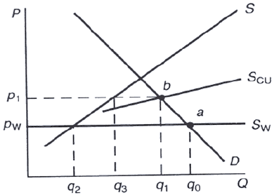
Page 290
squeezed out of the market resulting in a fall in domestic production (q 0 → q 2). The country
is importing q 1 - q 2 from foreign suppliers and this represents the trade-creation effect.
Consumers' surplus has increased by p 1P 0 ab while there is a loss of profits to domestic firms
of p 1P 0 ac . The result is a net welfare gain equal to the shaded triangle cab.
Figure 15.2: Trade diversion effect of a customs union
Figure 15.2 illustrates a trade-diversion effect resulting from a customs union. Sw represents
the world supply of a product to an economy at a world price of p w. If we assume that
initially the country imposes no barriers to the importation of this product the equilibrium will
be at point a with a price of p w and domestic consumption at q 0. Of this, q 2 is supplied by
domestic producers and q 0 - q 2 is imported.
If we assume that the country now enters a customs union which entails prohibitive tariff
barriers for this product to non-members the relevant supply curve is now S cu. There is a
new equilibrium at point b with price p 1 and quantity q 1. Inefficient customs union
producers are now benefiting at the expense of consumers and more efficient world suppliers.
Imports from efficient world producers (qo – q2) cease. Less efficient domestic producers
increase production ( q 2 → q 3) .The country now imports q 1 - q 3 from less efficient
producers in other members of the customs union. Consumer’s surplus falls by pwP1ba.
The Common Agricultural Policy traditionally meant high prices for EU farmers and high
tariffs on imported foods. There would therefore have been significant trade-diversion effects
on joining the EU for countries such as the UK who were major importers of food from non-
members. As the Republic of Ireland's trade with non-members was relatively small at the
time of joining, trade-diversion effects were not likely to have been significant.
The net welfare effect of membership of a customs union will be influenced by the extent of
trade-creation and trade-diversion effects. However, additional economic gains are likely to
arise from the removal of internal tariffs in the form of greater efficiency due to the increased
competition and also economies of scale resulting from larger markets.
Page 291
C. THE SINGLE MARKET PROGRAMME
In 1987 the member states of the EU ratified the Single European Act (SEA). The SEA
represented significant reform of the way in which the EU conducted its political and
economic affairs. The economic dimension of the SEA was a commitment to a single market
programme (SMP). Member states were given a five year adjustment period so that the single
market could be in place by the end of 1992.
The background to the SMP was accumulating evidence that the EU was being outperformed
economically by its major international competitors, i.e. the USA and Japan. In a range of
areas such as job-creation, unemployment, international competitiveness (particularly in
modern hi-tech sectors), investment in research and development, innovation, etc. the relative
performance of the EU was an increasing cause for concern.
The poor performance was put down to the fragmentation of the EU economy. The EU
represented a collection of distinct national economies that still retained a wide range of non-
tariff barriers (NTB’s) to trade rather than a single integrated European economy. These
NTB’s had a distorting effect on intra-community trade and in many cases, prevented cross-
border trade altogether. The EU had succeeded in removing tariffs and quotas on
merchandise trade but the NTB’s remained a major obstacle to intra-community trade and
competition.
The NTB’s come under four broad headings:
Physical barriers – delays at border crossings resulting from the monitoring of ‘imports’ and
‘exports’ – excessive paperwork associated with cross-border trade.
Technical barriers – different countries having different national standards regarding health
and safety, etc. with the result that goods satisfying the requirements of one member country
might not be permitted into another member country.
Fiscal barriers – indirect taxes influence retail prices. Different rates of tax have a distorting
effect on trade particularly in border regions.
National preferences in public procurements – government contracts (roads, schools,
hospitals, defence, etc.) represent approximately 15% of economic activity in the EU. The
practice of governments was to give preference to local firms when awarding these contracts
which effectively precluded cross-border competition.
The SMP is based on the four freedoms – free movement of goods, services, labour and
capital. Firms supplying goods or services in one part of the single market should be free to
supply the same in any other part. Workers from any part of the EU should be free to seek
employment in any other part and on equal terms with local workers. There should be no
restriction on investors from one member state transferring funds to any other member state.
The SMP has meant the abolition of border checks on goods (and within the Schengen group
of countries on the movement of people). In the absence of the total harmonisation of
standards, there should be mutual recognition so that goods or services satisfying the
Page 292
requirements of one member state should have unrestricted access to others. Policies for the
approximation of indirect taxes have been agreed (despite the fact that national governments
are extremely reluctant to give up their independence regarding general taxation). There is
now a system of compulsory competitive tendering for public contracts with legal redress for
firms who feel they are being discriminated against on the basis of nationality.
New competition rules have been devised with a view to creating a level playing field for
firms competing in the single market. In particular, national governments are no longer free
to subsidise domestic firms, nor are they free to restrict access to domestic markets. For
example, the Irish government is no longer free to subsidise Aer Lingus, nor could it prevent
BUPA entering the health insurance market to compete against the VHI and it was to open up
the whole telecommunications sector to foreign competition by the year 2000.
The SMP is designed to create a more competitive economy in the EU. Greater efficiency
should result from:
more competitive pressure as barriers to entry are removed from national markets;
improved resource allocation through freer play of comparative advantage;
exploitation of economies of scale as firms gain access to larger markets;
restructuring as firms adopt pan-European rather than national strategies;
product innovation and process innovation resulting from greater competitive
pressure.
The Cecchini Report published by the European Commission (1988) attempted to quantify
the expected gains from the removal of the NTB’s (which were referred to as the costs of
non-Europe).
Stage 1 gains would come through quickly as the removal of physical and technical barriers
gave consumers greater choice by enabling firms to operate in wider markets. Cecchini
estimated these static gains as being of the order of 2½% of (EU) GDP.
Stage 2 gains were longer term gains as industry adapted to the new more competitive
environment. Restructuring would take place as domestic monopolies were forced to
compete and firms in general sought to exploit the new opportunities. Cecchini estimated
stage 2 gains as being of the order of 3% of (EU) GDP.
Stage 3 gains were macroeconomic benefits which were envisaged for the longer term.
Improvements in economic conditions (more jobs, rising GDP) would relax the pressure on
national budgets enabling governments to further stimulate their economies through fiscal
measures. The best case scenario was an overall increase in GDP of 7% with increased
employment of 5m.
The SMP has resulted in increased competition in many sectors of the EU economy.
However, the results do not yet add up to the expectations in the Cecchini Report. A number
of explanations can be advanced for the relatively poor outcome:
Page 293
Failure by governments to fully implement SMP measures particularly in the areas of
state subsidies and public procurements.
An unfavourable macroeconomic background to SMP. Tight monetary policy
resulting in high interest rates in the EU in the early phase followed by tight fiscal
policies designed to satisfy EMU requirements.
It is also possible that the Cecchini analysis is, at least partially, flawed:
Overemphasis on the scope for exploiting economies of scale in the single market.
Critics argue that economies of scope, i.e. the ability of firms to produce a flexible
product mix, is of increasing importance.
Failure to highlight issues other than NTB’s which may be greater sources of
inefficiency. For example, the lack of flexibility in EU labour markets or the failure
of managers to adopt advanced managerial techniques.
National preferences on the part of consumers indicates that fragmentation is at least
partially the result of demand-side rather than supply-side factors.
Whatever the longer term impact of the SMP, it is clear that it represents a major transfer of
power from national governments to the European Commission in the economic sphere.
Governments will inevitably have to adapt their industrial strategies and may be required to
harmonise them in some respects. For example, as the SMP refuses to distinguish between
private sector and state sector enterprises for the purposes of competition policy and as
governments are restricted regarding subsidies, there is a developing trend to privatise state
enterprises. In the longer term, the ability of governments and regional development agencies
to offer special incentives in a competitive effort to attract FDI may be open to question.

Page 294
BLANK

Page 295
Study Unit 16
Growth Strategies of Firms
Contents
A. Horizontal Growth
__________________________________________________________________________
B. Vertical Growth
__________________________________________________________________________
C. Diversified Growth
__________________________________________________________________________
D. Growth by Mergers
__________________________________________________________________________
E. Economies of Scope
__________________________________________________________________________
F. Profit Maximisation Objective when management is separate from ownership
___________________________________________________________________________
G. Alternative Theories of the Firm
__________________________________________________________________________
H. Principal – Agent Theory
__________________________________________________________________________
Page 296
A. HORIZONTAL GROWTH
Horizontal growth can be achieved through horizontal integration which is the development
into activities which are competitive with, or complimentary to, a company’s present
activities. Many companies have realised that there are opportunities in other markets for the
exploitation of its own competencies e.g. maybe to displace the current provider as a new
entrant. Horizontal integration can occur at any stage within the value chain.
Advantages and Disadvantages of Horizontal Integration
Advantages - (A) Increases market power over the next or the previous link in the
process
- (B) Enables greater economies of scale to occur
Disadvantages - (A) May restrict customer choice
- (B) Unequal market influence may increase costs overall by the
exercise of monopoly power and this may attract the attention of
the Monopolies/Competition Commission
B. VERTICAL GROWTH
Vertical growth can be achieved through vertical integration which is the extension of a
firm’s competitive ability within the same industry. It involves expanding the company’s
range of activities backwards into sources of supply and / or forwards towards end users of
the final product. A company can achieve vertical integration through two methods;
- it can start its operations in the other stages in the industry’s activity
- it can acquire a company already performing these activities
Backward Integration
This process generates cost savings only when the volume needed is big enough to maximise
a specific supplier’s economies of scale without any negative impact on the existing quality
standard. Backward integration can also benefit the company by diminishing the uncertainty
of depending on suppliers of crucial components or support services. It can also lessen a
company’s vulnerable position when dealing with powerful suppliers that raise prices at every
opportunity. If the firm concerned is low on a key supplier’s priority list it can find itself
waiting on shipments every time supplies get tight. If this occurs, the firm’s reputation will
suffer through poor production and customer relations activities (where applicable) and
backward integration may be a suitable strategic solution.
Page 297
Forward Integration
The requirement for forward integration follows much the same concept as above. In many
industries, sales agents, wholesalers etc. have no affiliation to any one company’s brand and
tend to push what earns them the biggest profits. Poor sales and distribution channels can give
rise to high inventory costs and underutilisation of capacity. A company that encounters the
above may find it beneficial to integrate forward into wholesaling / retailing in order to have
outlets fully committed to representing its products. This can lead into the activity of selling
directly to end users which produces important cost savings which has an impact on
permitting lower selling prices.
Strategic disadvantages of Vertical Integration
There are serious considerations that need to be evaluated before pursuing a strategy of
vertical integration. Issues that need to be considered include some of the following;
(1) Capital investment in the industry is increased but this increases business risk
especially where this investment could have been used for more worthwhile
projects
(2) Integrating forward or backward locks a firm into relying on sources of supply /
channels of distribution which can have a negative impact on supplier / end user
flexibility
(3) Balancing capacity, especially at each stage of the value chain, is a very vexing
issue
(4) Forward or backward integration requires very different skills and business
capabilities. Companies have to be aware that what they thought would add value
to their core businesses may not necessarily work out that way
Advantages and Disadvantages of Vertical Growth
A strategy of vertical growth depends on;
(1) Whether it can improve the performance of critical activities that reduce costs
(2) Its impact on investment costs, flexibility and response times
(3) Its ability to create competitive advantage
Page 298
C. DIVERSIFIED GROWTH
A diversification strategy depends upon a company’s growth opportunities in its present
industry and it also depends on the available opportunities to utilise its resources and
capabilities in other market areas.
Diversified growth can de done through one of two ways;
(1) Related markets – through vertical integration strategies
(2) Unrelated markets – this is where the relevant company acts as a ‘holding
company’ by operating in areas where its detailed knowledge of the key factors for
success is limited. This type of diversification can be operated successfully where
the use of tight but clear financial controls is suitably managed.
Three Tests required for justification of a diversification strategy
Strategists, in order to ensure an increase in shareholder value, must use the following three
tests;
(1) The attractiveness test – the industry chosen must be attractive enough to have
consistent good returns on investment. This largely depends upon the presence of
favourable competitive and market conditions
(2) The cost-of-entry test – the cost to enter the specific industry must not be so high
as to erode the potential for good profitability. The more attractive it is the more
expensive it can be to get into
(3) The better-off test – the diversifying company must bring some potential for
competitive advantage to the new business it enters. If this is achieved there is also
opportunity for added profitability and share holder value
Diversification Strategies
Once the decision is made to diversify, a choice must be made whether to diversify into a
related or unrelated business / businesses. The following are six diversification related
strategies;
(1) Strategies for entering new industries – acquisition, start-up and joint venture
(2) Related diversification strategies
(3) Unrelated diversification strategies
Page 299
(4) Divestiture and liquidation strategies – if a company is considered for divestiture,
it would suggest that it no longer fits or is an attractive investment
(5) Corporate turnaround, retrenchment and restructuring strategies
(6) Multinational diversification strategies – an example of this is where a
multinational company can benefit from its competitive advantage by transferring
its expertise in a core technology to other lines of business able to benefit from its
capabilities e.g. Honda – from piston rings to motorcycles to cars, hedge trimmers
etc.
The first three are ways to diversify and the last three are strategies that strengthen the
positions and performances of companies that have already diversified.
D. GROWTH BY MERGERS
Mergers are similar to acquisitions in the sense of two companies combining. However,
mergers usually arise because neither company has the ability to acquire the other on its own.
This has the potential benefit of being more friendly but requires special handling if the
benefits are to be realised.
Motives for mergers
These include some of the following;
(1) It allows the company to enter new product or / and market areas especially where
the process of internal development is slow. This is especially true in many e-
commerce businesses
(2) The competitive situation may influence a company to adopt a merger strategy
compared to being a new company entering the market. Competitive reaction is
reduced if the former strategy is adopted
(3) De-regulation is a driving force for many mergers which reduces the
fragmentation of the market
(4) Financial motives that enhance opportunities are also a factor
(5) A lack of resources or competencies to compete successfully may be acquired that
will offer better economies of scale or economies of scope
Problems with Mergers
It is important to note that approx. 70% of mergers end up with lower returns to shareholders
of both organisations. One of the main reasons for this is due to issues associated with
Page 300
cultural fit. This is where a ‘clash of cultures’ may arise because the organisational routines
are so different in each organisation. Cultural fit can be even more problematic with cross-
border mergers due to the complication and combination of different national cultures.
E. ECONOMIES OF SCOPE
Economies of scope exist whenever it is less costly for two or more companies to be operated
under centralised management than to function as separate independent companies. Most
economies of scope fall into one of four categories;
(1) Technology Fits – when there is potential for sharing common technology. This
allows for more effective performance of technology-related activities
(2) Operating Fits – opportunities exist on this category due to the combination of
activities or transfer skills / capabilities in procurement, conducting R & D,
improving production processes etc.
(3) Distribution and Customer-Related Fits – when the value chains of different
businesses overlap to such an extent that the products are used by the same
customers, opportunities exist for cost savings in such areas as using a single sales
force for all products instead of separate sales forces for each product line etc.
(4) Managerial Fits – benefits in this category can be obtained when managerial
knowledge in one line of business can be transferred to another line
Sources of Inter-firm Economies of Scope that can motivate strategic alliances
(1) Exploiting economies of scale
(2) Learning from competitors
(3) Managing risk and sharing costs
(4) Low-cost entry into new markets
(5) Managing uncertainty
Page 301
F. PROFIT MAXIMISATION OBJECTIVE WHEN MANAGEMENT IS
SEPARATE FROM OWNERSHIP
The traditional theory of the firm assumes that its sole objective is to maximise profit. The
managerial theories make the assumption that where ownership (shareholders / stockholders)
and control (management) of the company are separated, the objective that guides the firm
will be the one that management sets. This is generally done through the process of
maximising sales revenue or growth. Some commentators, like Marris, argue that growth is a
separate objective from profit. Growth may also be a means of securing greater stability for
the firm.
Profit Maximisation vs. Wealth Maximisation
Maximisation of profits is generally regarded as the proper objective of the firm, but it is not
as inclusive a goal as that of maximising shareholder wealth. For example, total profits are
not as important as earnings per share. A firm could always raise total profits by issuing stock
and using the proceeds to invest in Treasury bills / Bonds. Even maximisation of earnings per
share, however, is not a fully appropriate objective, partly because it does not specify the
timing or duration of expected returns. Is the investment project that will produce
RWF60,000,000 return 3 years from now more valuable than the project that will produce
annual returns of RWF20,000,000 in each of the next 3 years? An answer to this question
depends upon the time value of money to the firm and to investors at the margin. Few
existing stockholders would think favourably of a project that promised its first return in 50
years. We must take into account the time pattern of returns in our analysis.
G. ALTERNATIVE THEORIES OF THE FIRM
Firms are in business for a simple reason - to make money. Traditional economic theory
suggests that firms make their decisions on supply and output on the basis of profit
maximisation. However, many economists and managerial scientists question that the sole
aim of a firm is the maximisation of profits.
The most serious examination on the theory of the firm comes from those who question
whether firms even make an effort to maximise their profits. A firm (especially a large
conglomerate) is not a single decision-maker but a collection of people within it. This implies
that in order to understand the decision-making process within firms, we have to analyse who
controls the firm and what their interests and motivations are.
The fact that most large companies are not run by their owners is often brought forward to
support this claim. A large corporation typically is owned by thousands of shareholders /
stockholders, most of whom have nothing to do with the business decisions. Those decisions
are made by a professional management team, appointed by a salaried board of directors.
Page 302
In most cases these managers will not own stock in the company which may lead to strongly
differing goals of owners and managers. When managers’ salaries stay unaffected by higher
profits they may pursue other goals to raise their personal profile.
This behaviour strikes the astute observer regularly when, for example, reading or watching
the financial media. Managers often mention the rises in sales or the growth of their company
rather then the profits. Some economists like Begg (1996) argued that managers have an
incentive to promote growth as usually these same managers of larger companies generally
obtain higher salaries.
H. PRINCIPAL – AGENT THEORY
The principal – agent theory is the theory of devising compensation rules that induce an agent
to act in the best interests of a principal. Agents, whether they are managers or workers,
pursue their own goals and often impose costs on a principal.
Principal-agent problem - the central dilemma investigated by principal agent theorists is
how to get the agent to act in the best interests of the principal when the agent has an
informational advantage over the principal and has different interests from the principal.
Sappington (1991) provides a discussion of principal-agent incentive problems;
(A) Privatisation as a solution to the principal-agent problem.
Principals must balance agency costs against costs of debt financing and other costs
associated with not separating ownership from control. The issue of privatisation of
government services hinges not only on the relative production costs in the public vs.
private sector, but also on agency / transaction costs. This is made more complicated
by the fact that there are many forms of separation of ownership / sovereignty from
control, including many forms of contracting out, which can carry high agency costs.
Indeed, contractors may be in-house governmental agents, not representing
privatization at all.
Agency costs are a type of transaction cost, reflecting the fact that without incurring costs, it is
impossible for principals to ensure agents will act in the principals' interest. Agency costs
include the costs of investigating and selecting appropriate agents, gaining information to set
performance standards, monitoring agents and residual losses. Agency costs have policy
implications.
Information costs in contract management - in addition to recognising that
contract management involves agency costs, one may also observe that the
informational advantage of the contractor regarding performance means that the
contractor may be able to impose high agency costs by resisting the principal's
effort to gain information. The more difficult for the principal to gain information
on performance outcomes, the more likely that contracts will be framed instead in
terms of contractor behaviour
Page 303
(A) Goal incongruity - between principal and agent increases the incentive of
the agent to withhold information from the principal (Simonsen and Hill,
1998).
(B) Agent risk aversion - some agents are more risk-averse than others,
perhaps due to organisational culture issues. Risk-averse agents are more
prone to withhold information from principals, increasing agency costs.
(C) Interdependence can also make processes and procedures more complex
and uncertain, in turn increasing agency costs of obtaining performance
information.
(D) Communication costs. The agent may not follow the intent of the principal
when there has been insufficient investment of time and personnel, and
investment in communications channels, by the principal, resulting in lack
of clarity and / or consistency of messages from the principal (Goggin et
al, 1990).