THE INSTITUTE OF CAT L2.3 MANAGEMENT ACCOUNTING Study Manual
User Manual:
Open the PDF directly: View PDF ![]() .
.
Page Count: 454 [warning: Documents this large are best viewed by clicking the View PDF Link!]
- Study Unit Title Page
- Some More Terminology 30
- 4 Materials and Stock Control 51
- 5 Labour 91
- Methods of Remuneration 93
- 7 Job Costing/Batch Costing 155
- 9 Process Costing 1 183
- Application and General Principles 184
- 17 Cost Book Keeping 429
- INTRODUCTION TO the COURSE
- A. NATURE AND FUNCTIONS OF COST ACCOUNTING
- b. COST ACCOUNTING COMPARED WITH FINANCIAL ACCOUNTING
- c. THE ROLE OF COST ACCOUNTING IN A MANAGEMENT INFORMATION SYSTEM
- B. BASIC COSTING METHODS
- C. COST CENTRES AND COST UNITS
- D. SUPERIMPOSED PRINCIPLES AND TECHNIQUES
- E. SOME MORE TERMINOLOGY
- F. DIFFERENCE BETWEEN ABSORPTION AND MARGINAL COSTING SYSTEMS
- A. Introduction
- A. INTRODUCTION AND DEFINITIONS
- B. ACCOUNTING FOR MATERIALS
- C. OUTLINE OF PROCEDURES
- Ordering Stock
- Receiving Stock
- Issuing Stock
- Storing Stock
- Stock Levels
- D. ORGANISATION AND DOCUMENTATION OF PURCHASING
- F. PROCEDURE IN THE ACCOUNTS DEPARTMENT
- G. THE STOREKEEPER AND STORES ISSUES
- H. STOCK LEVELS
- I. ECONOMIC ORDER QUANTITY
- J. STOCK TURNOVER
- K. ACCOUNTING RECORDS REQUIRED FOR MATERIALS
- L. STOCKTAKING
- M. THE PRICING OF MATERIAL ISSUES
- N. OBSOLETE, DORMANT AND SLOW-MOVING STOCK
- A. METHODS OF REMUNERATION
- B. TIME RATES
- C. INCENTIVE SCHEMES
- D. PIECE-RATEs
- E. DIFFERENTIAL PIECE-RATE SYSTEMS
- F. PREMIUM BONUS SCHEMES
- G. GROUP BONUS SCHEMES
- H. PERFORMANCE-RELATED PAY
- I. PROFIT SHARING AND CO-PARTNERSHIP
- J. NON-MONETARY INCENTIVES
- K. MEASUREMENT OF THE EFFICIENCY OF LABOUR
- L. LABOUR TURNOVER
- M. RECORDING LABOUR COSTS
- Time Recording Methods
- N. INDIRECT LABOUR
- O. TREATMENT OF OVERTIME
- P. SUMMARY
- A. EXAMPLES OF EXPENSES
- B. NOTIONAL EXPENSES
- C. CAPITAL EQUIPMENT
- D. INTRODUCTION TO OVERHEAD COSTS
- E. OVERHEAD ALLOTMENT
- Dept 1
- Dept 2
- Service Centre
- General Overhead Cost Centre
- F. OVERHEAD ABSORPTION
- G. THE USE OF PREDETERMINED ABSORPTION RATES
- H. TREATMENT OF ADMINISTRATION OVERHEAD
- I. TREATMENT OF SELLING AND DISTRIBUTION OVERHEAD
- J. ACTIVITY-BASED COSTING
- A. INTRODUCTION
- B. FACTORY JOB COSTING
- A. APPLICATION AND GENERAL PRINCIPLES
- B. BUILDING UP PROCESS COSTS
- C. Examples of Process Costing
- Example 1: Demonstration of Process Accounts and Stock Accounts When the Value of Opening and Closing Work-in-Progress is Given
- Example 2: Introduction to “Equivalent Units” - Work-in-Progress at End of Period Only
- Example 3: Work-in-Progress at Both Beginning and End of the Period: FIFO Method
- Example 4: Work-in-Progress at Both Beginning and End of Period: Average Method
- Essential Differences Using FIFO and Average Methods
- Example 5: Alternative Layout Where a Process Other Than the First is Involved - The layout is shown below.
- D. Losses in process costing – normal losses and abnormal losses
- A. OPERATING COSTING
- B. PROCESS COSTING INVOLVING BOTH LOSSES AND WORK-IN-PROGRESS
- A. INTRODUCTION
- B. LIMITATION OF ABSORPTION COSTING
- C. FIXED, VARIABLE AND SEMI-VARIABLE COSTS
- D. DEFINITION OF MARGINAL COST
- E. THE MARGINAL COST EQUATION: TERMINOLOGY OF MARGINAL COSTING
- F. USES OF MARGINAL COSTING
- G. ARGUMENTS AGAINST MARGINAL COSTING
- I. worked example
- J. when production is constant but sales fluctuate
- K. when sales are constant but production fluctuates
- L. marginal and absorption costing compared
- A. BREAK-EVEN ANALYSIS
- B. BREAK-EVEN CHART
- C. THE PROFIT VOLUME GRAPH
- D. USE OF THE PROFIT VOLUME GRAPH FOR MORE THAN ONE PRODUCT
- E. THE PROFIT/VOLUME OR CONTRIBUTION/SALES RATIO
- F. MARGINAL PROFIT AND LOSS ACCOUNT
- It should be clear that over several periods taken together such that stock at the beginning of the first period and at the end of the last period was nil, the absorption and marginal costing methods would give the same total profit, but the amount of...
- A. INTRODUCTION
- Relevant costs for decision making purposes are:
- Maximum sales demand (units) 120 160 110
- a. introduction
- b. types of standard cost and system
- c. setting standards
- d. types of variance
- e. the standard hour
- f. measures of capacity
- g. limitations of standard costing
- H. purpose of variance analysis
- I. MEANING and possible causeS OF variances
- Scheme of Analysis: Absorption Costing
- Variance Calculations
- (a) Direct Materials
- (b) Direct Labour
- (c) Variable Overheads
- (i) Variable Overhead Expenditure Variance
- (ii) Variable Overhead Efficiency Variance
- (d) Fixed Overheads
- (i) Fixed Overhead Expenditure Variance
- (ii) Fixed Overhead Volume Variance
- (iii) Fixed Overhead Capacity Variance
- (iv) Fixed Overhead Efficiency Variance
- (e) Sales Variances
- (i) Sales Margin Price Variance
- (ii) Sales Margin Volume Variance
- Summary of Variances
- Analysing Variances: Marginal Costing
- Comparing Variances Resulting Under Absorption and Marginal Costing
- J. relationships between variances and investigation of their causes
- K. planning and revision variances
- L. worked example
- a. definitions
- B. advantages of budgetary control systems
- C. types of budget
- D. preparation of budgets
- E. Control mechanism
- f. Flexible budgets
- G. Behavioural implications
- h. Budgeting and long-term objectives
- I. Public Sector Budgets
- a. FUNCTIONAl budgets
- B. master budgets
- C. cash budget
- D. flexible budgets
- E. zero-base budgeting (zbb)
- F. Budgetary control and standard costing - behavioural considerations
- A. COST ACCOUNTING SYSTEMS
- B. INTEGRATED OR INTEGRAL SYSTEMS
- KEY Management Accounting TERMS

CAT
Certified Accounting Technicians Examination
Stage: Level L2.3
Subject Title: Management Accounting
Study Manual

BLANK

F2.1 MANAGEMENT ACCOUNTING
Page 1
© CPA Ireland
All rights reserved.
The text of this publication, or any part thereof, may not be reproduced or transmitted in any
form or by any means, electronic or mechanical, including photocopying, recording, storage
in an information retrieval system, or otherwise, without prior permission of the publisher.
Whilst every effort has been made to ensure that the contents of this book are accurate, no
responsibility for loss occasioned to any person acting or refraining from action as a result of
any material in this publication can be accepted by the publisher or authors. In addition to
this, the authors and publishers accept no legal responsibility or liability for any errors or
omissions in relation to the contents of this book.
INSTITUTE OF
CERTIFIED PUBLIC ACCOUNTANTS
OF
RWANDA
LEVEL 2
L2.3 MANAGEMENT ACCOUNTING
First Edition 2012
This study manual has been fully revised and
updated in accordance with the current
syllabus. It has been developed in
consultation with experienced lecturers.

F2.1 MANAGEMENT ACCOUNTING
Page 2
BLANK

F2.1 MANAGEMENT ACCOUNTING
Page 3
Contents
Study Unit Title Page
Introduction to Your Course 9
1 Introduction to Cost Accounting
13
Nature and Functions of Cost Accounting 14
Cost Accounting Compared with Financial Accounting 16
The Role of Cost Accounting in a Management Information System 17
2 Principles of Costing 19
The Elements of Cost 20
Basic Costing Methods 25
Cost Centres and Cost Units 26
Superimposed Principles and Techniques 28
Some More Terminology 30
Difference Between Absorption and Marginal Costing Systems 30
3 Cost Behaviour Patterns 35
Introduction 36
Fixed Costs 36
Variable Costs 37
Semi-Variable Costs 38
Step Costs 38
The Linear Assumption of Cost Behaviour 44
Accountant’s v’s Economist Model 45
Factors Affecting the Activity Level 45
Cost Behaviour and Decision Making 46
Cost Variability and Inflation 46
4 Materials and Stock Control 51
Introduction and Definitions 53
Accounting for Materials 54
Outline of Procedures 55
Organisation and Documentation of Purchasing 59
Receiving Department 65
Procedure in the Accounts Department 67
The Storekeeper and Stores Issues 69
Stock Levels 71
Economic Order Quantity 73
Stock Turnover 76
Accounting Records Required for Materials 76
Stocktaking 77
The Pricing of Material Issues 81
Obsolete, Dormant and Slow-Moving Stock 87
Just-In-Time (JIT) 88

F2.1 MANAGEMENT ACCOUNTING
Page 4
Contents
Study Unit Title Page
5 Labour 91
Methods of Remuneration 93
Time Rates 94
Incentive Schemes 97
Straight Piece-Rate Systems 99
Differential Piece-Rate Systems 100
Premium Bonus Schemes 101
Group Bonus Schemes 103
Performance-Related Pay 104
Profit Sharing and Co-Partnership 105
Non-Monetary Incentives 107
Measurement of the Efficiency of Labour 108
Labour Turnover 109
Recording Labour Costs 111
Indirect Labour 112
Treatment of Overtime 114
Summary 115
6 Overheads and Activity Based Costing
117
Examples of Expenses 118
Notional Expenses 118
Capital Equipment 120
Introduction to Overhead Costs 121
Overhead Allotment 125
Overhead Absorption 132
The Use of Predetermined Absorption Rates 138
Treatment of Administration Overhead 141
Treatment of Selling and Distribution Overhead 141
Activity-Based Costing 143
7 Job Costing/Batch Costing
155
Introduction 156
Factory Job Costing 157
Introduction to Batch Costing 170
Calculation of Cost per Unit 171
Production Line Information 171
Batch Production vs Continuous Production 171
Example 172
Economic Batch Quantity 173

F2.1 MANAGEMENT ACCOUNTING
Page 5
Contents
Study Unit Title Page
8 Service Costing 175
Introduction 176
Service Cost Units 176
Cost Collection & Cost Sheets 177
Internal Service Activities 177
Examples 178
9 Process Costing 1 183
Application and General Principles 184
Elements of Process Costing 185
Examples of Process Costing 186
Losses in Process Costing 201
10 Process Costing 2 207
Operating Costing 208
Process Costing Involving Both Losses and Work-in-Progress 212
11 Marginal v Absorption Costing 223
Introduction 224
Limitation of Absorption Costing 224
Fixed, Variable and Semi-Variable Costs 227
Definition of Marginal Cost 229
The Marginal Cost Equation: Terminology of Marginal Costing 229
Uses of Marginal Costing 231
Arguments Against Marginal Costing 236
Assumptions of Marginal Costing 237
Worked Example 238
When Production is Constant but Sales Fluctuate 242
When Sales are Constant but Production Fluctuates 247
Marginal and Absorption Costing Compared 250
12 Breakeven Analysis 257
Break-Even Analysis 258
Break-Even Chart 262
The Profit Volume Graph 270
Use of the Profit Volume Graph for More Than One Product 272
The Profit/Volume or Contribution/Sales Ratio 277
Marginal Profit and Loss Account 282

F2.1 MANAGEMENT ACCOUNTING
Page 6
Contents
Study Unit Title Page
13 Decision Making 289
Introduction 290
The Practical Use of Relevant Costs 291
Market Vulnerability Analysis 304
Continue/Close Down Decisions 305
Marginal Costing in Decision Making 306
Decision Making Involving a Single Limiting Factor 313
14 Standard Costing and Variance Analysis 319
Introduction 321
Types of Standard Cost and System 322
Setting Standards 323
Types of Variance 330
The Standard Hour 331
Measures of Capacity 332
Limitations of Standard Costing 334
Purpose of Variance Analysis 334
Meaning and Possible Causes of Variances 335
Relationships Between Variances and Investigation of Causes 351
Planning and Revision Variances 358
Worked Example 360
15 Budgets - Planning and Control 363
Definitions 364
Advantages of Budgetary Control Systems 367
Types of Budget 368
Preparation of Budgets 369
Control Mechanism 375
Flexible Budgets 379
Behavioural Implications 381
Budgeting and Long-term Objectives 382
Public Sector Budgets 382
16 Preparation, Techniques and Considerations of Budget 387
Functional Budgets 388
Master Budgets 389
Cash Budget 400
Flexible Budgets 408
Zero-base Budgeting (ZBB) 420
Budgetary Control and Standard Costing – Behavioural Considerations 425
F2.1 MANAGEMENT ACCOUNTING
Page 7
Contents
Study Unit Title Page
17 Cost Book Keeping 429
Cost Accounting Systems 430
Integrated or Integral Systems 431
Glossary Key Terms 441

F2.1 MANAGEMENT ACCOUNTING
Page 8
BLANK
F2.1 MANAGEMENT ACCOUNTING
Page 9
INTRODUCTION TO THE COURSE
Stage: Level 2
Subject Title: L2.3 Management Accounting
Aim
The aim of this subject is to ensure that students develop a knowledge and understanding of
the various cost accounting principles, concepts and techniques appropriate for planning,
decision-making and control and the ability to apply these techniques in the generation of
management accounting reports.
Learning Outcomes
On successful completion of this subject, students should be able to:
• Explain the relative strengths and weaknesses of alternative cost accumulation
methods and discuss the value of management accounting information.
• Calculate unit costs applying overhead using both absorption costing and activity
based costing principles.
• Apportion and allocate costs to units of production in job, batch and process costing
systems, for the purpose of stock valuation and profit measurement.
• Identify and explain cost behaviour patterns and apply cost-volume profit analysis.
• Define and use relevant costs in a range of decision-making situations.
• Prepare and present budgets for planning, control and decision-making.
• Compute, interpret and investigate variances.
• Demonstrate communication skills including the ability to present quantitative and
qualitative information, together with analysis, argument and commentary, in a form
appropriate to the intended audience.
F2.1 MANAGEMENT ACCOUNTING
Page 10
Syllabus:
1. The Role of the Management Accountant
• The nature and scope of management accounting.
• The relationship between management accounting and financial accounting.
• Cost classifications.
• The role of the Management Accountant in a modern business environment including
the recognition of possible ethical issues that may arise.
2. Cost Accumulation Systems
• Accounting for materials: stock valuation approaches (FIFO; LIFO and AVCO);
EOQ; JIT concepts.
• Accounting for labour: remuneration methods; incentive schemes; productivity,
labour turnover and labour performance reports.
• Accounting for Overheads: absorption costing and activity based costing (ABC)
approaches to overheads.
3. Costing Methods
• Job and batch costing.
• Process costing for single products and the use of equivalent units calculations under
both FIFO and Weighted Average accounting systems.
• Process costing ledger accounts including normal and abnormal loss/gain.
• The role of costing in non-manufacturing sectors.
• Marginal costing and the importance of contribution for decision-making.
• Comparison of marginal costing and absorption costing approaches.
4. Information for Decision Making
• Cost behaviour patterns and identification of fixed/variable elements in a cost using
High/Low method.
• Break-even analysis and the importance of contribution.
• Break-even chart preparation and interpretation.
• Calculation of break-even point, margin of safety and target profit.
• Limitations of Cost Volume Profit Analysis.
• Relevant costing principles including committed, sunk and opportunity costs.
• Relevant costs in decision-making.
• Decision making with a single limiting factor/constraint.
• Qualitative factors relevant to specific decisions.
F2.1 MANAGEMENT ACCOUNTING
Page 11
5. Information for Planning and Control
• The role of budgeting including alternative budgeting systems (Fixed, flexible,
incremental and Zero Based Budgeting (ZBB)).
• Behavioural and motivational issues in the budgetary process.
• Functional and subsidiary budgets.
• Standard costing: role and procedures for standard setting including different types of
standards.
• Variance analysis: the calculation and interpretation of basic sales/cost variances.
Reconciliation reports. The inter-relationship and possible causes of variances. (Fixed
overhead capacity and efficiency variances are not examinable.)

F2.1 MANAGEMENT ACCOUNTING
Page 12
BLANK

F2.1 MANAGEMENT ACCOUNTING
Page 13
Study Unit 1
Introduction to Cost Accounting
Contents
A. Nature and Functions of Cost Accounting
B. Cost Accounting Compared with Financial Accounting
C. The Role of Cost Accounting in a Management Information System
F2.1 MANAGEMENT ACCOUNTING
Page 14
A. NATURE AND FUNCTIONS OF COST ACCOUNTING
What Is “Cost Accounting”?
The Chartered Institute of Management Accountants, in its publication, “Terminology of
Management and Financial Accountancy”, defines cost accounting as:
“.... that part of management accounting which establishes budgets and standard costs,
and the actual costs of operations, processes, departments or products and the analysis of
variances, profitability or social use of funds.”
This involves participation in and with management to ensure that there is effective:
• Formulation of plans to meet objectives (long-term planning)
• Formulation of short-term operation plans (budgeting/profit planning)
• Corrective action to bring future actual transactions into line (financial control)
• Recording of actual transactions.
What Cost Accounting Provides for the Organisation
(a) Additional Financial Information
When cost accounting was first used, its main purpose was to provide additional
information concerning the financial operations of an organisation. For the majority of
firms, this is still considered as its main purpose. It usually implies historical costing and
the production of regular detailed statements and statistics.
(b) Control Information
A more modern concept of cost accounting is that its purpose is to assist management by
providing them with control information.
This usually demands more from the cost accountant. He or she will still produce
statistical statements, but will be required to analyse and interpret these statements.
Comparisons will be made with “budgets” and “standards”, and the cost accountant will
probably use the exception system of reporting, advising management only where action
is required.
F2.1 MANAGEMENT ACCOUNTING
Page 15
(c) Management Tool
Cost accounting has often been likened to a tool in the hands of management. Consider
what this means:
(i) It must be the right tool. The cost accountant, in consultation with management,
must agree what information is required and when; the cost of providing it will also
have to be taken into consideration. The question must also be asked, is complete
accuracy necessary? Will an approximation within given limits be of more value, if
it can be provided swiftly?
Any system of costing must be tailored to suit the organisation which it serves. In
many cases simple historical cost accounting will be sufficient; in others a more
sophisticated system may be necessary.
(ii) The tool must be capable of doing the job. The cost accountant must ensure that the
facts and figures produced provide management with the information they require,
in an easily assimilated form.
Do not forget that manufacturing conditions and markets will change over the years,
and the cost accounting system may need to be adapted to suit changing needs. A
new system may need to be designed and introduced.
(iii) It is management who use the tool, and the extent of its success will depend upon the
degree of efficiency with which it is used.
Objects of a Cost Accounting System
Different firms will use cost accounting for different purposes. Nevertheless, every system
will involve some of the objectives listed below.
(a) Cost Control
This will be assisted by:
(i) Finding out the cost of each product (or service), process and department - costs
must be ascertained in phase with manufacturing activity, enabling remedial action
to be taken quickly when it is required.
(ii) Comparing the costs with budget, standard or past performance figures to indicate
the degree of efficiency attained.
(iii) Analysing the variances from budget and identifying the person or department
responsible so that prompt, remedial action may be taken.
(iv) Disclosing to what extent production facilities are used and indicating the amount
and cost of idle and waiting time.
F2.1 MANAGEMENT ACCOUNTING
Page 16
(v) Presenting the information suitably to management, in such a form as to guide them
in taking any necessary action.
(b) Advice to Management in the Formulation of Policy
This will include:
(i) Provision of information to assist in the regulation of production and the systematic
control of the organisation.
(ii) Provision of special investigations and reports. These might deal with such matters
as:
− Whether to manufacture a part or to sub-contract another firm.
− The advisability of installing new machinery.
− The effect of increased or reduced production volumes on profitability.
(c) Advice on the Effects of Management Policy
This will be disclosed through reports (both regular reports and those following special
investigations).
(d) Estimating and Price Fixing
Figures will be provided from standards or past results as the basis for future estimates.
Cost is an important factor in price fixing, but it is not the only one. Demand and
competitive activity are also crucial. Therefore a firm’s profitability may depend largely
on its ability to control costs in ways described in (a) above.
B. COST ACCOUNTING COMPARED WITH FINANCIAL
ACCOUNTING
You will be familiar already with the end-products of financial accounting, namely the
balance sheet and the profit and loss account. These are valuable documents for
management, the first giving the position of a company or firm at a specific time, the second
showing the results of the company’s operations over a specific period of time. The books of
account from which the profit and loss account and balance sheet are derived are also of
value, since they provide a record of every transaction.
Despite the value of the financial accounts, it was their inadequacy which gave rise to the
introduction of costing and the development of costing techniques. The financial accounts
show primarily external transactions (sales, purchases, borrowing, etc.) and the profit for the
organisation as a whole. Management requires detailed knowledge of the cost of each
product or unit, of each department or process to show how the profit was built up and the
F2.1 MANAGEMENT ACCOUNTING
Page 17
relative profitability of each section of the business. Cost accounting has now become an
essential factor of every business.
It is of interest that in recent years “integrated accounts” (see later in this study unit) have
grown in popularity. Integrated accounts are merely the combining of the financial and cost
accounts into one set of books. We seem to have come full circle, from the separation of the
financial and cost accounts, through the development of costing, to the joining together of the
two systems into one integral system. Of course, in many businesses increasing
computerisation has assisted this development.
C. THE ROLE OF COST ACCOUNTING IN A
MANAGEMENT INFORMATION SYSTEM
Product Analysis
Only the very simplest form of organisation does not need a cost accounting system, and even
in this case some “cost accounting” would be done, but the simplicity of the business renders
a special system unnecessary.
In a more complex organisation, results can be analysed in depth. The cost of each process or
operation which goes to make up the final product can be ascertained, as can the cost of the
various “service” departments (stores, tool room, power house, etc.).
Investigating Costs
The cost accountant would not be satisfied merely to ascertain the figures, however. Perhaps
costs can be reduced, and/or revenues, and/or production increased.
The cost accountant will consult the sales manager. It may be that increases in price will
result in a decrease in sales. Moreover, financial considerations are not the only ones to be
borne in mind.
By pursuing such enquiries, the cost accountant is achieving the second function of costing,
that is, cost control. It should be stated here that it is not the cost accountant’s job to make
executive decisions, but merely to express the management’s policy in terms of money, and
to indicate where efficiency may be increased.
Guiding Management Policy
A most important side to the cost accountant’s work is providing information to management
at all levels. His or her job is to advise management of the financial effects of alternative
policies. He or she is an adviser only; it is for the manager to make policy decisions. Thus
the cost accounting system will justify itself only when the information it produces is used by
management. (Management accountants are part of “Management” and make use of both
cost accounting information and financial accounting information for their involvement in
management decisions.)
F2.1 MANAGEMENT ACCOUNTING
Page 18
Non-Financial Considerations
Clearly therefore, before management can make decisions, they require information on which
to arrive at the decisions and cost accounting information is one part of the required
information. Other matters need to be considered which are frequently of a non-financial
nature, however. These might include:
(a) position in the market;
(b) environmental considerations;
(c) legal constraints;
(d) staff qualifications and training needs

F2.1 MANAGEMENT ACCOUNTING
Page 19
Study Unit 2
Principles of Costing
Contents
_______________________________________________________________
A. The Elements of Cost
_______________________________________________________________
B. Basic Costing Methods
_______________________________________________________________
C. Cost Centres and Cost Units
_______________________________________________________________
D. Superimposed Principles and Techniques
_______________________________________________________________
E. Some More Terminology
_______________________________________________________________
F. Difference Between Absorption and Marginal Costing Systems
_______________________________________________________________
F2.1 MANAGEMENT ACCOUNTING
Page 20
A. THE ELEMENTS OF COST
The expenditure we are considering in our cost accounting is, of course, the same expenditure
(subject to certain considerations which will be mentioned) as that which is dealt with in the
financial accounts. It is merely that we are looking at it in a different way. Whereas the
financial accounts are normally concerned only with the nature of the expense, e.g. whether it
is wages, lighting and heating, etc., the cost accounts are concerned with the purpose of the
expense, e.g. whether the wages are in respect of, say, manufacturing or distribution, and if
manufacturing, whether they are in respect of labour directly or indirectly concerned with the
product, and so on.
Make sure that you clearly UNDERSTAND, and then REMEMBER, the following
classifications.
Labour, Materials and Expenses
All expenditure can be classified into three main groups - labour, materials and expenses.
Each of the expenses may be subdivided into one of two categories:
(a) Items directly applicable to the product, i.e. direct.
(b) Items which cannot be directly applied to the product, i.e. indirect.
The total of indirect materials, indirect labour and indirect expenses is called overhead.
Fixed and Variable Costs
There is a further subdivision of costs which we may briefly note here (and about which I
will say more later), and that is between fixed costs and variable costs. Fixed costs are those
which remain constant (in total) over a wide range of output levels, while variable costs are
those which vary (in total) more or less according to the level of output. This division is of
great significance, and we shall be dealing with it later. Observe, now, that by its very nature
“prime cost” consists of variable items only, while the various overhead categories may
contain some of each kind.
(a) Examples of fixed costs: rent, rates, insurance, depreciation of buildings, management
salaries.
(b) Examples of variable costs: raw materials, commission on sales, piece-work earnings.
F2.1 MANAGEMENT ACCOUNTING
Page 21
Definitions
Here are some definitions in this connection, which you must understand clearly:
(a) Direct Labour Cost
This is the cost of remuneration for employees’ efforts applied directly to a product or
saleable service which can be identified separately in product costs.
Examples of direct labour, as defined above, would include the costs of employing
bricklayers, machine operators, bakers, miners, bus drivers. There is no doubt as to
where you would charge these labour costs. Doubt would arise, however, with a truck
driver’s wage in a factory. His wage cannot be charged direct to any product, as he is
helping many departments and operators. Therefore, his wage would have to be
classified as indirect. In a few exceptional circumstances it may be established that the
truck driver is employed only to transport materials for the manufacture of one product.
If this were the case, his wage could be charged direct to the product, and he would be
as much a direct worker as the operator who is using the materials.
(b) Direct Materials Cost
This is the cost of materials entering into and becoming constituent elements of a
product or saleable service and which can be identified separately in product cost. The
following materials fall within this definition:
(i) All materials specially purchased for a particular job, order or process.
(ii) All materials requisitioned from the stores for particular production orders.
(iii) Components or parts produced or purchased and requisitioned from the finished
goods store.
(iv) Material passed from one operation to another.
We must consider here the term “raw material”. In many cases the raw material of one
industry or process is the finished product of another. Thus leather in the form of hides
constitutes the finished product of a tannery but the raw material of a footwear factory;
while carded wool, the product of the carding process, becomes the raw material of the
hardening section.
(c) Direct Expenses
These are costs, other than materials or labour, which are incurred for a specific product
or saleable service.
Direct expenses are not encountered as often as direct materials or labour costs. An
example would be electric power to a machine, provided that the power is metered and
the exact consumption by the machine is known. We can then charge the cost of power
direct to the job. More often, however, we will know only the electricity bill for the
whole factory, so this will be an indirect expense.
F2.1 MANAGEMENT ACCOUNTING
Page 22
Another example of a direct expense is a royalty payment to the inventor of a product.
(d) Prime Cost
This is the total cost of direct wages, direct material and direct expenses.
(e) Overhead
Overhead is the total cost of indirect labour, indirect materials and indirect expenses.
Examples of indirect materials include oils, cotton waste and grease. Examples of
indirect labour include the costs of employing maintenance workers, oilers, cleaners
and supervisors. Examples of indirect expenses include lighting, rent and
depreciation.
Overheads may be divided into four main groups:
(i) works or factory expense;
(ii) administration expense;
(iii) selling expense;
(iv) distribution expense.
An Example from the Confectionery Industry
The cost of production of most commodities is made up mainly of the cost of the raw
materials of which they are manufactured and the cost of labour which is employed making
them, i.e. wages.

F2.1 MANAGEMENT ACCOUNTING
Page 23
RWF RWF RWF
To Direct Materials Consumed:
(1) Flour
Opening Stock 2,080
Purchases 5,720
7,800
Less:
Closing Stock 990
Part-Finished Goods 300 1,290 6,510
(2) Gelatine
Opening Stock 1,720
Purchases 3,180
4,900
Less:
Closing Stock 55
Part-Finished Goods 60 115 4,785
(3) Sugar and Other Materials
Opening Stock 5,040
Purchases 10,920
15,960
Less:
Closing Stock 4,985
Part-Finished Goods 360 5,345 10,615
COST OF RAW MATERIALS USED 21,910
To Direct Labour 3,720
To Direct Expense -
PRIME COST 25,630
To Factory Overhead 6,650
FACTORY COST (COST OF PRODUCTION) RWF32,280
F2.1 MANAGEMENT ACCOUNTING
Page 24
To this total of factory cost will be added administration, selling and distribution expenses, to
arrive at a figure of total cost, to which will be added profit to give the selling price. (This
method of costing is known as Absorption Costing - see later.)
The example given above is of a “process” industry in which the product passes from one
process to the next. Unless production is shut down completely at the end of each accounting
period, which would be most uneconomical, there will at all times be some product “in the
pipeline” at various stages of completion which will be credited against the charges for the
period in question and become the opening charge for the subsequent period. These opening
and closing adjustments are always necessary.
An Example from the Photographic Industry
Let us now consider a business which manufactures cameras, where the amount of labour
involved in manufacture is small compared with the amount of precision machinery which is
necessary for the manufacture of efficient apparatus. In such an industry, costs arising from
the depreciation and obsolescence of machinery may be of much greater importance
compared with the cost of materials and labour than they were in the case of the
confectionery manufacturing company. These charges which are related only indirectly to
output are said to constitute indirect expenditure, as against materials and labour and other
similar items which constitute direct expenditure.
In addition to depreciation, all the charges incurred in the general offices (such as salaries of
managers, rent and rates) together with the expenses involved in marketing the product (such
as advertising and carriage) must be included in the indirect expenses. You will appreciate,
therefore, that in order to give a reflection of the cost of production for each unit of output,
accounts must be prepared to show the allocation of these indirect expenses as well as the
direct expenses (provided it is intended to follow Absorption Costing methods rather than
Marginal Costing - see later).
F2.1 MANAGEMENT ACCOUNTING
Page 25
B. BASIC COSTING METHODS
The basic costing method employed by an organisation must be devised to suit the methods
by which goods are manufactured or services are provided. The choice is between specific
order costing, service/function costing and continuous operation/ process costing.
Specific Order Costing
This costing method is applicable where the work consists of separate contracts, jobs or
batches, each of which is authorised by a special order or contract.
The subdivisions of specific order costing are:
(a) Job Costing
This applies where work is undertaken to a customer’s special requirements. Each
“job” is of comparatively short duration. Throughout the manufacturing process, each
job is distinct from all other jobs. Examples of industries using job costing are:
building maintenance, certain types of engineering (e.g. manufacture of special purpose
machines) and printing.
(b) Batch Costing
This is a form of specific order costing which applies where similar articles are
manufactured in batches, either for sale, or for use within the undertaking. In most
cases the costing is similar to job costing.
(c) Contract Costing
This applies when work of long duration is undertaken to customers’ special
requirements, e.g. builders, civil engineers, etc.
In job costing, costs of each job (or batch) can be separately identified.
Continuous Operation/Process Costing
This is the basic costing method applicable where goods or services are produced by a
sequence of continuous or repetitive operations or processes to which costs are charged
before being averaged over the units produced during the period. This procedure is widely
used, for example, in the chemicals industry.
Service/Function Costing
This is the method used for specific services or functions, e.g. canteens, maintenance and
personnel. These may be referred to as service centres, departments or functions.
F2.1 MANAGEMENT ACCOUNTING
Page 26
C. COST CENTRES AND COST UNITS
Cost Centre
A cost centre is a location, function or item of equipment in respect of which costs may be
ascertained and related to cost units for control purposes. A cost centre may be a productive
department, an individual machine, a service department such as stores serving the productive
departments, etc.
Cost Unit
This is a quantitative unit of product or service in relation to which costs are ascertained. For
instance, in paint manufacture, costs would be ascertained “per litre of paint”. The litre of
paint is therefore the cost unit.
Examples of cost units in other activities are:
Accounting Account maintained
Brewing Barrel of beer racked
Brickmaking 1,000 bricks
Building industry Complete job or contract
Cable manufacture 1,000 yards (or m) of cable
Canteen Employee or meal served
Chemicals industry Per gram, kg, etc. depending on relative quantity
produced
Power station Kilowatt/hours
Gravel or sand pits Cubic yard/metre extracted
Hospitals Per patient-day, or per bed-week
Invoicing Per 100 or 1,000 invoices
Liquids Gallon, litre
Maintenance Operating hour or value of asset
Metal plating Square foot/metre
Police service Per 1,000 population or per constable-day
Printing Ream or 1,000 copies
Public transport Miles run, passenger-mile, 100-seat mile or fare-stage
Purchasing Per order placed, or value of materials
Sales order department Per enquiry, or value of sales made
Sales representative Per call or value of sales made
School Per pupil-day or per examination passed
Steam 1,000 lbs steam raised
Storage Tonne of material, gallon or litre of liquid, value of
materials
Street cleaning 1,000 population, or mile of road
Street lighting Lamp or mile of road
Timber 1,000 cu. ft, board-foot, etc.
F2.1 MANAGEMENT ACCOUNTING
Page 27
Typing Space, line typed or standard document typed
Water supply 1,000 population or 1,000 gallons produced
Window cleaning per window or 100 sq. yds
Profit Centre
A profit centre is a location or function in respect of which both expenditure and income may
be attributable. A profit centre may be a division of the business or a specific function within
the organisation. In order that true profitability may be assessed, it is necessary to install
procedures to transfer-charge all relevant costs and revenue to the profit centre. Ideally, the
net costs of all central operating areas should be allocated, on an agreed basis, to profit
centres.
The development of the profit centre concept means that profit centres have come to act as a
focal point for the collation of cost centres and the provision of useful high-level management
information.
Examples of profit centres in the financial services industry are:
− UK clearing banking
− Merchant banking
− Credit card operations
− Corporate banking
− International banking.
F2.1 MANAGEMENT ACCOUNTING
Page 28
D. SUPERIMPOSED PRINCIPLES AND TECHNIQUES
Whichever costing method is in use (a choice which will be largely dictated by the
production method), there is a choice of principles and techniques which may be adopted in
presenting information to management. These are introduced briefly here, and we will study
some of them in detail later.
Absorption Costing
This principle involves all costs, including the costs of selling and administration, being
allotted to cost units. Total overheads are “absorbed”, via the method thought most
appropriate.
Marginal Costing
This is a principle whereby variable costs only are charged to cost units, and the fixed cost
attributable to the relevant period is written off in full against the “contribution” for that
period, contribution being the difference between total sales value and total variable costs. At
this stage therefore, remember when using marginal costing, do NOT attempt to apportion
fixed costs to individual cost units.
Actual Cost Ascertainment
This is the ascertainment of costs in retrospect, after they have been incurred. It is also
known as historical costing.
Variance Accounting
This is a technique whereby the planned activities of an undertaking are quantified in
budgets, standard costs, standard selling prices and standard profit margins. These are then
compared with the actual results, and note is taken of the differences, i.e. the “variances”, for
subsequent examination.
Differential Costing
This is a technique used in the preparation of “ad hoc” information, in which only cost and
income differences between alternative courses of action are taken into consideration. In
other words, any costs which would be incurred whatever decision were taken, are ignored.
Incremental Costing
This is another technique used in the preparation of “ad hoc” information. Here
consideration is given to a range of graduated or stepped changes in the level or nature of
F2.1 MANAGEMENT ACCOUNTING
Page 29
activity, and the additional costs and revenues likely to result from each degree of change are
presented.
Uniform Costing
This is the use by several undertakings of the same costing system (i.e. the same basic
method, specific order costing or operation costing, and the same superimposed principles
and techniques, e.g. absorption costing rather than marginal costing). Uniform costing
enables the results of the various organisations concerned to be compared. In many
industries, a trade association advises member firms on costing methods, and collects data
from them, which is then circulated to member firms so that they can see how they compare
with other firms in the industry. Strict anonymity is, of course, maintained.
To recapitulate at this stage, a reminder of the total cost structure, within the context of
Absorption Costing, can be represented as follows:
Direct Labour Prime
Direct Materials Cost Works, Factory
Direct Expenses or Production
Cost
Factory Overheads Total
Cost
Admin. Overheads
Selling Overheads Selling
Distribution Overheads Price
Profit
Figure 3
F2.1 MANAGEMENT ACCOUNTING
Page 30
E. SOME MORE TERMINOLOGY
Controllable and Uncontrollable Costs
Sometimes reference is made to costs being either “controllable” or “uncontrollable”. As we
have seen already, costs are charged or allocated to cost centres. Each cost centre has an
officer in control. Costs are said to be “controllable” when the costs charged can be
influenced by the actions of this person in charge. Where they cannot, they are of course
“uncontrollable” costs. Sometimes controllable costs are referred to as “managed costs”.
Avoidable and Unavoidable Costs
“Avoidable costs” are the specific costs of part of an organisation which would be avoided if
that part or sector/activity did not exist. Another term for this is “relevant costs”. It follows,
therefore, that “unavoidable costs” are those that are unaffected by a particular decision. As
they are in fact irrelevant to the decision, they are also known as “irrelevant costs”.
F. DIFFERENCE BETWEEN ABSORPTION AND
MARGINAL COSTING SYSTEMS
We have already looked at the broad divisions between Absorption and Marginal Costing
systems but we have not yet considered them in detail. This we will do later in the course. In
the meantime, let us consider a case which may indicate more clearly the difference.

F2.1 MANAGEMENT ACCOUNTING
Page 31
A company manufactures three products, A, B and C, and in the year makes a profit of
RWF70,000, as follows:
RWF
Total Sales 600,000
Variable Labour 160,000
Variable Material 240,000
Variable Overhead 30,000
Fixed Overhead 100,000
Net Profit 70,000
It is decided to analyse these figures between Products A, B and C. The company uses
absorption costing and apportions (or spreads) fixed overhead in proportion to the sales value
of Products A, B and C. (We have not yet covered the methods of getting a proportion of
overhead costs into costs; this follows later in the course.)
The figures now become:
Total A B C
RWF RWF RWF RWF
Sales 600,000 250,000 200,000 150,000
Variable Labour 160,000 70,000 45,000 45,000
Variable Material 240,000 100,000 60,000 80,000
Variable Overhead 30,000 15,000 10,000 5,000
Fixed Overhead 100,000 41,666 33,334 25,000
Net Profit 70,000 23,334 51,666 (5,000)
Management considers the situation. It decides to stop manufacturing C, since it is producing
a net loss of RWF5,000. Sales of A and B cannot be increased because of market conditions.
However, as a result of dropping C, fixed overheads will reduce to RWF90,000. The staff
formerly employed on the production of C were temporary and have been sacked.
Management congratulates itself and looks forward to an improved net profit situation.

F2.1 MANAGEMENT ACCOUNTING
Page 32
To their dismay the following results arise:
Total A B
RWF RWF RWF
Sales 450,000 250,000 200,000
Variable Labour 115,000 70,000 45,000
Variable Material 160,000 100,000 60,000
Variable Overhead 25,000 15,000 10,000
Fixed Overhead 90,000 50,000 40,000
Net Profit 60,000 15,000 45,000
Despite their efforts, profits are actually reduced by RWF10,000!
The reason for this should be fairly obvious. If we consider the situation in terms of financial
accounting, we have lost RWF20,000 gross profit which C produced (RWF150,000 sales less
RWF130,000 cost of sales) which in turn could have been available to cover, in part, the
expenses of the company. This is basically the approach followed by marginal costing.
Instead of referring to “gross profit”, the term “contribution” is used, that is, the contribution
made towards covering overheads or fixed costs.
If a marginal costing approach had been taken to the initial figures for Products A, B and C,
these would have read as follows:
Total A B C
RWF RWF RWF RWF
Sales 600,000 250,000 200,000 150,000
Variable Labour 160,000 70,000 45,000 45,000
Variable Material 240,000 100,000 60,000 80,000
Variable Overhead 30,000 15,000 10,000 5,000
430,000 185,000 115,000 130,000
Sales less
Variable Costs
(CONTRIBUTION) 170,000 65,000 85,000 20,000
Fixed Overhead 100,000
Net Profit 70,000
F2.1 MANAGEMENT ACCOUNTING
Page 33
Note, no attempt has been made to spread the fixed overhead cost of RWF100,000 between
Products A, B and C. Provided the total contribution is greater than fixed overhead, a net
profit will result. Obviously, if the contribution in total can be increased (by increased sales
prices or variable costs reductions) a higher net profit will result.
In this case we have studied, it is in fact the very spreading of fixed overhead costs between
Products A, B and C which lead management to think that C was making an overall loss. For
some particular reason, it was decided to allocate fixed overheads to Products A, B and C in
direct proportion to their sales value. Suppose instead it had been decided to allocate them in
direct proportion to the variable overheads incurred by A, B and C. This would have resulted
in fixed overhead of RWF50,000 being allocated to A, RWF33,334 to B and RWF16,666 to
C, with the result that the overall net profit of RWF70,000 would have been split between A
RWF15,000, B RWF51,666 and C RWF3,334. In this case, the management might not have
been tempted to cancel C!
Clearly, the basis on which fixed overheads are allocated is most important in the decision
areas of sales levels, production levels, etc. Advocates of marginal costing consider that, at
best, such allocation of fixed overheads is fairly arbitrary and can only confuse, so it is better
not to attempt it.
We will return to this later in the course but at this point it must be stated that absorption
costing is still widely practised and indeed in some areas is ideal for the needs which exist.
In monopolistic situations, in local and in central government, it can be, and is, used
extensively. In such circumstances cost management often centres on comparisons of total
cost in one period of time with another period of time. Provided the same method of
allocating fixed overheads is used in the periods being compared, then such cost comparisons
are still valid, particularly as the information is required for comparison purposes only and
not for changes in levels of production/services decisions.

F2.1 MANAGEMENT ACCOUNTING
Page 34
BLANK

F2.1 MANAGEMENT ACCOUNTING
Page 35
Study Unit 3
Cost Behaviour Patterns
Contents
A. Introduction
B. Fixed Costs
C. Variable Costs
D. Semi-Variable Costs
E. Step Costs
F. The Linear Assumption of Cost Behaviour
G. Accountants vs Economist Model
H. Factors Affecting the Activity Level
_______________________________________________________________
I. Cost Behaviour and Decision Making
_______________________________________________________________
J. Cost Variability and Inflation
F2.1 MANAGEMENT ACCOUNTING
Page 36
A. INTRODUCTION
As we saw earlier in this study unit, costs can be divided either into direct and indirect costs,
or variable and fixed costs.
Direct costs are variable, that is the total cost varies in direct proportion to output. If, for
instance, it requires RWF10 worth of material to make one item it will require RWF20 worth
to make two items and RWF100 worth to make ten items and so on.
Overhead costs, however, may be either fixed, variable or semi-variable.
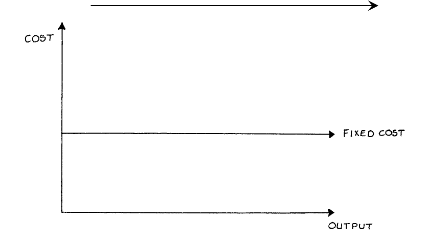
B. FIXED COST
A fixed cost is one which can vary with the passage of time but, within limits, tends to
remain fixed irrespective of the variations in the level of output. All fixed costs are overhead.
Examples of fixed overhead are: executive salaries, rent, rates and depreciation.
A graph showing the relationship of total fixed cost to output appears in Figure 4.
Figure 4
Please note the words “within limits” in the above description of fixed costs. Sometimes this
is referred to as the “relevant range”, that is the range of activity level within which fixed
costs (and variable costs) behave in a linear fashion.
F2.1 MANAGEMENT ACCOUNTING
Page 37
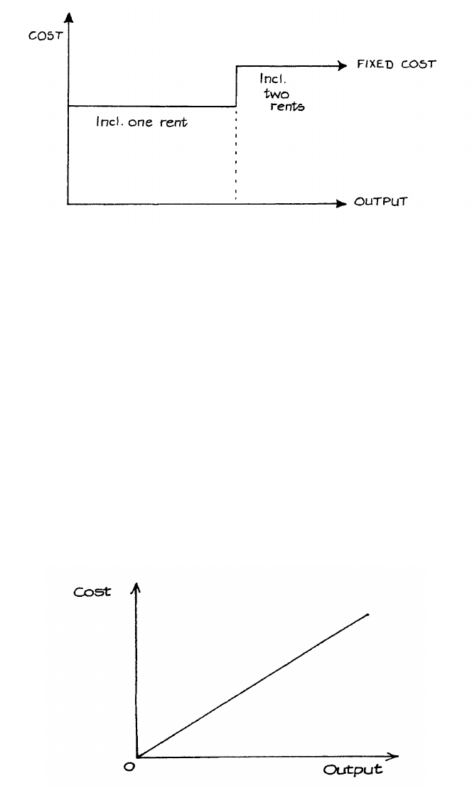
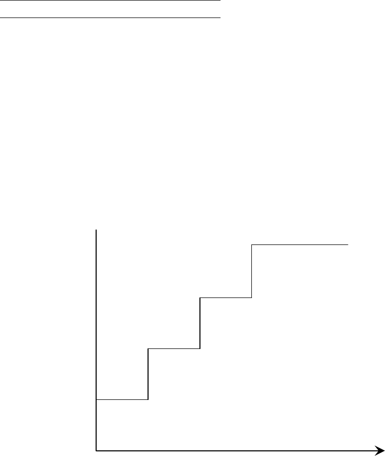
Suppose an organisation rents a factory. The yearly rent is the same no matter what the
output of the factory is. If business expands sufficiently, however, it may be that a second
factory is required and a large increase in rent will follow. Fixed costs would then be as in
Figure 5.
Figure 5
A cost with this type of graph is known as a step function cost for obvious reasons.
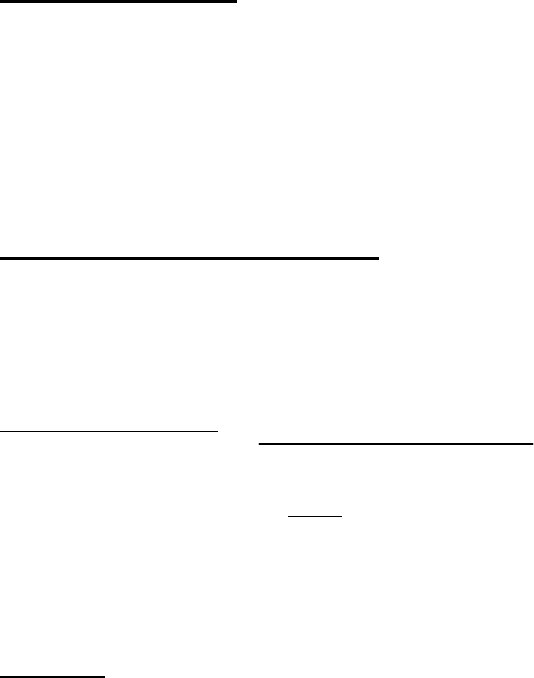
C. VARIABLE COST
This is a cost which tends to follow (in the short term) the level of activity in a business.
As already stated, direct costs are by their nature variable. Examples of variable overhead
are: repairs and maintenance of machinery; electric power used in the factory;
consumable stores used in the factory.
The graph of a variable cost is shown in Figure 6.
Figure 6
F2.1 MANAGEMENT ACCOUNTING
Page 38
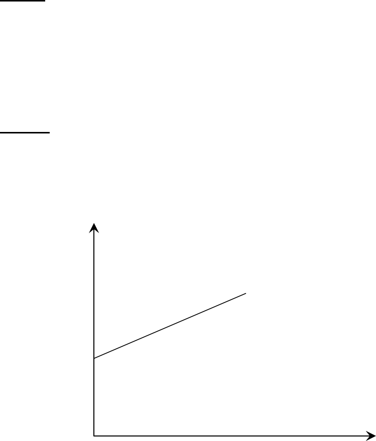
D. SEMI-VARIABLE (OR SEMI-FIXED) COST
This is a cost containing both fixed and variable elements, and which is thus partly affected
by fluctuations in the level of activity.
For examination purposes, semi-variable costs usually have to be separated into their fixed
and variable components. This can be done if data is given for two different levels of output.
Example
At output 2,000 units, costs are RWF12,000.
At output 3,000 units, costs are RWF17,000.
Therefore for an extra 1,000 units of output, an extra RWF5,000 costs have been incurred.
This is entirely a variable cost, so the variable component of cost is RWF5 per unit.
Therefore at the 2,000 units level, the total variable cost will be RWF10,000. Since the total
cost at this level is RWF12,000, the fixed component must be RWF2,000. You can check
that a fixed component of RWF2,000 and a variable component of RWF5 per unit gives the
right total cost for 3,000 units.
E. STEP COST
RWF
Total Cost
F2.1 MANAGEMENT ACCOUNTING
Page 39
Level of Activity
Example: Rent can be a step cost in certain situations where accommodation requirements
increase as output levels get higher.
A Step Cost
Many items of cost are a fixed cost in nature within certain levels of activity.
Semi-Variable Costs
This is a cost containing both fixed and variable components and which is thus partly affected
by fluctuations in the level of activity (CIMA official DFN).
Example: Running a Car
• Fixed Cost is Road Tax and insurance.
• Variable cost is petrol, repairs, oil, tyres-all of these depend on the number of miles
travelled throughout the year.
RWF
Total Cost
Level of Activity
A method of splitting semi-variable costs is the High – Low method.
F2.1 MANAGEMENT ACCOUNTING
Page 40
High – Low method
Firstly, examine records of cost from previous period. Then pick a period with the highest
activity level and the period with the lowest level of activity.
• Total Cost of high activity level minus total cost of low activity level will equal variable
cost of difference in activity levels.
• Fixed Costs are determined by substitution
Example of High - Low Method
Highest level 10,000 units, cost of RWF4,000
Lowest Level activity level 2,000 units cost of RWF1,600
Variable Cost Element: (RWF4,000 - RWF1,600)
10,000 units – 2,000 units
= 2,400
8,000
∴ = RWF 0.30 per unit
Fixed Cost (under high level figure)
RWF4,000 – (10,000 x RWF 0.30)
= RWF1,000
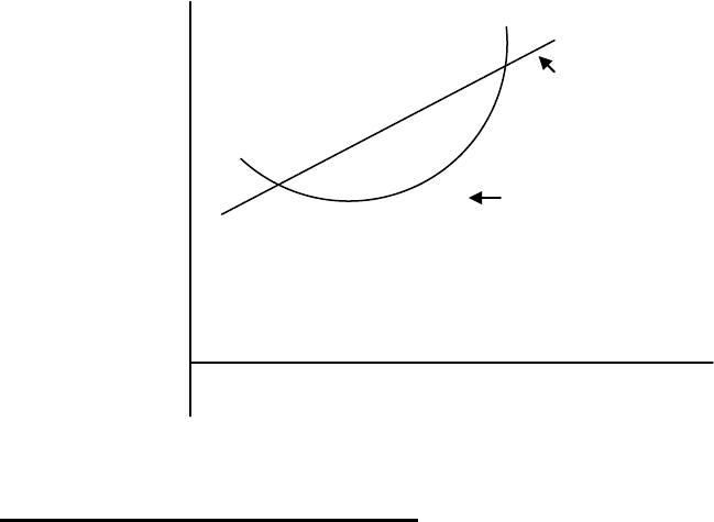
Scattergraphs
Information about two variables that are considered to be related in some way can be plotted
on a scattergraph. This is simply a graph on which historical data can be plotted. For cost
behaviour analysis, the scattergraph would be used to record cost against output level for a
large number of recorded “pairs” of data.
Then by plotting cost level against activity level on a scattergraph, the shape of the resulting
figure might indicate whether or not a relationship exists.
In such a scattergraph, the y axis represents cost and the x axis represents the output or
activity level.
One advantage of the scattergraph is that it is possible to see quite easily if the points indicate
that a relationship exists between the variables, i.e. to see if any correlation exists between
them.
F2.1 MANAGEMENT ACCOUNTING
Page 41
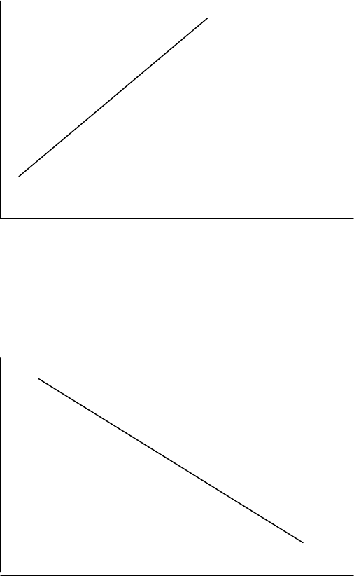
Positive correlation exists where the values of the variables increase together (for example,
when the volume of output increases, total costs increase).
Negative correlation exists where one variable increases and the other decreases in value
Some illustrations:
1. Weight and height in humans
Weight
Positive Linear Correlation
x x x
x x
x
x x
x x
x x
Height
2. Sales of Scarves and temperature
Sales x x x Negative Linear Correlation
x x x
x x x
x x x
x x x
x x x
Temperature

F2.1 MANAGEMENT ACCOUNTING
Page 42
3. Sugar Imports and Mining Production
Imports
x x x
x x x x x
x x x x x No Correlation
x x x x x x
x x x x x x x x
x x x x x x
x x x
x x x x
Mining Production
A scattergraph can be used to make an estimate of fixed and variable costs, by drawing a
“line of best fit” through the band of points on the scattergraph, which best represents all the
plotted points.
The above diagrams contain the line of best fit. These lines have been drawn using
judgement. This is a major disadvantage, as drawing the line “by eye”. If there is a large
amount of scatter, different people may draw different lines.
Thus, as a technique, it is only suitable where the amount of scatter is small or where the
degree of accuracy of the prediction is not critical.
However, it does have an advantage over the high-low method in that all points on the graph
are considered, not just the high and low point.
Regression Analysis
This is a technically superior way to identify the “slope” of the line. It is also known as
“Least Squares Regression”. This statistical method is used to predict a linear relationship
between two variables. It uses all past data (not just the high and low points) to calculate the
line of best fit.
The equation of the regression line of y on x is of the form:
y = a + bx
F2.1 MANAGEMENT ACCOUNTING
Page 43
In other words, if we are trying to predict the cost (y) from an activity (x), it is necessary to
calculate the values of a and b from given pairs of data for x and y. The following formulae
are used:
a = Σy - bΣx
n n
b = nΣxy - ΣxΣy
nΣx2 – (Σx)2
where “n” is the number of pairs of x and y values. (The symbol “Σ” means
‘the sum of’)
Thus, in order to calculate “a”, it is necessary to calculate “b” first.
Example
The following is the output of a factory and the cost of production over the last 5 months:
Output (‘000 units)
Cost (RWF’000)
January
20
82
February
16
70
March
24
90
April
22
85
May
18
73
(i) Determine a formula to show the expected level of costs for any given volume of
output
(ii) Prepare a budget for total costs if output is 27,000 units
Solution:
Let x = output
Let y = costs
n = 5 (5 pairs of x & y values)
Construct a table as follows: (in ‘000)
x
y
xy
x2
y2
20
82
1,640
400
6,724
16
70
1,120
256
4,900
24
90
2,160
576
8,100
22
85
1,870
484
7,225
18
73
1,314
324
5,329
Σx = 100
Σy = 400
Σxy = 8,104
Σx2 = 2,040
Σy2 = 32,278

F2.1 MANAGEMENT ACCOUNTING
Page 44
b = nΣxy - ΣxΣy = 5(8,104) – (100)(400)
nΣx2 – (Σx)2 5(2,040) – (100)2
b = 2.60
a = Σy - bΣx = 400 – 2.6(100)
n n 5 5
a = 28 (or 28,000)
Thus, the formula for any given level of output is:
y = RWF28,000 + RWF2.60x
where
y = total cost (in RWF’000)
x = output (in ‘000 units)
If output is 27,000 units, then total cost (y) will be:
y = RWF28,000 + RWF2.60(27,000)
y = RWF98,200
F. THE LINEAR ASSUMPTION OF COST BEHAVIOUR
1. Cost are assumed to be either fixed, variable or semi-variable within a normal range of
output.
2. Fixed and variable costs can be estimated with degrees of probable accuracy. Certain
methods maybe used to access this (High-Low method).
3. Costs will rise in a straight line/linear fashion as the activity increases.
F2.1 MANAGEMENT ACCOUNTING
Page 45
G. ACCOUNTANTS - V’S – ECONOMIST MODEL
RWF
Total Cost
Activity
Assumptions of Above Diagram
The accountants state that the linear assumption of cost behaviour is linear because:
1. The linear cost (straight line) is only used in practice within normal ranges of output
‘Relevant Range of Activity’.
The term ‘Relevant Range’ is used to refer to the output range at which the firm expects
to be operating in the future.
2. It is easier to understand than Economists’ cost line.
3. The fixed and variable costs are easier to use.
4. The relevant range and the costs estimated by the economists and the accountants will
not be very different.
H. FACTORS AFFECTING THE ACTIVITY LEVEL
1. The economic environment.
2. The individual firm – its staff, their motivation and industrial relations.
3. The ability and talent of management.
4. The workforce (unskilled, semi-skilled and highly skilled).
5. The capacity of machines.
6. The availability of raw material.
Economists Cost Lines Curvilinear
Accountants Cost Line is Linear (Straight)
F2.1 MANAGEMENT ACCOUNTING
Page 46
I. COST BEHAVIOUR AND DECISION MAKING
Factors to Consider:
1. Future plans for the company.
2. Current competition to the company.
3. Should the selling price of a single unit be reduced in order to attract more customers.
4. Should sale staff be on a fixed salary or on a basic wage with bonus/commission.
5. Is a new machine required for current year.
6. Will the company make the product internally or buy it.
For all of the above factors, management must estimate costs at all levels and evaluate
different courses of action. Management must take all eventualities into account when
making decisions for the company.
Example of things management would need to know is fixed costs do not generally change as
a result of a decision unless the company have to rent an additional building for a new job
etc.
J. COST VARIABILITY AND INFLATION
Care must be taken in interpreting cost data over a period of time if there is inflation. It may
appear that costs have risen relative to output, but this may be purely because of inflation
rather than because the amount of resources used has increased.
If a cost index, such as the Retail Price Index, is available the effects of inflation can be
eliminated and the true cost behaviour pattern revealed.
It is essential for the index selected to be relevant to the company; if one of the many Central
Statistical Office indices is not appropriate, it may be possible for the company to construct
one from its own data.
F2.1 MANAGEMENT ACCOUNTING
Page 47
Consider the following example, which deals with the relationship between production output
and the total costs of a single-product company, taken over a period of four years:
Year Output Total Costs
(tonnes) RWF
1 2,700 10,400
2 3,100 11,760
3 3,700 14,880
4 4,400 20,700
Suppose that we have the above information, together with the cost indices as follows:
Year Cost Index
1 100
2 105
3 120
4 150
5 175 (estimated)
If our estimated output for Year 5 is 5,000 tonnes, how may we calculate the estimated total
costs?
First, we have to convert the costs of the four years’ production to Year 1 cost levels, by
applying the indices as follows:
Conversion Cost at
Year Actual Cost Factor Year 1 Level
RWF RWF
1 10,400 1 10,400
2 11,760 100/105 11,200
3 14,880 100/120 12,400
4 20,700 100/150 13,800
F2.1 MANAGEMENT ACCOUNTING
Page 48
Secondly, we must split the adjusted costs into their fixed and variable elements. This is
done by examining the difference or movement between any two years, for example:
Production Adjusted Cost
Year 1 2,700 tonnes RWF10,400
Year 4 4,400 tonnes RWF13,800
We observe that an increase of 1,700 tonnes gives a rise in costs of RWF3,400. The variable
cost is therefore RWF2 per tonne.
Now by deducting the variable cost from the adjusted cost in any year, we can ascertain the
level of fixed cost. For example, in Year 4, the variable cost @ RWF2 per tonne would be
4,400 × RWF2 = RWF8,800. If we deduct this figure from the total adjusted cost
RWF13,800, we are left with the fixed cost total of RWF13,800 – RWF8,800 = RWF5,000.
This fixed cost is, of course, expressed in terms of Year 1 cost level. In real terms, the fixed
costs (those costs which do not vary with changes in volume) will increase over the four years
in proportion to the cost index.
We now see that the yearly total costs, adjusted to Year 1 cost levels, may be split into the
fixed and variable elements as follows:
Production Fixed Variable Total
Year (tonnes) RWF @ RWF2 tonne RWF
1 2,700 5,000 5,400 10,400
2 3,100 5,000 6,200 11,200
3 3,700 5,000 7,400 12,400
4 4,400 5,000 8,800 13,800
5 (est’d) 5,000 5,000 10,000 15,000
Finally, by applying the cost index for each year to the total costs at Year 1 cost levels, we
may complete our forecast:
F2.1 MANAGEMENT ACCOUNTING
Page 49
Total Cost at
Year Year 1 Levels Cost Index Actual Cost
RWF RWF
1 10,400 100 10,400
2 11,200 105 11,760
3 12,400 120 14,880
4 13,800 150 20,700
5 (est’d) 15,000 175 26,250
Limitations
This forecast of RWF26,250 for the total costs in Year 5 is, of course, subject to many
limitations. The method of calculation assumes that all costs are either absolutely fixed or are
variable in direct proportion to the volume of production. In practice, as we have seen, it is
usually found that “fixed” costs will tend to rise slightly in steps, while the variable costs will
usually rise less steeply at the higher levels of output, because of the economies of scale.
Also, our forecast will only be as accurate as our forecast of the cost index for Year 5. This is
as difficult to predict as the Retail Price Index, which is influenced by changes in the price of
each item in the “shopping basket”.
The analysis of cost behaviour in this way is thus useful as a guide to management, provided
we remember that:
(a) It assumes a linear (or “straight line”) relationship between volume and cost.
(b) Costs will be influenced by many other factors, such as new production methods or new
plant.
(c) Inflation will have a varying effect on different items of cost.
This subject of cost behaviour is fundamental to many aspects of cost accounting.

F2.1 MANAGEMENT ACCOUNTING
Page 50
BLANK

F2.1 MANAGEMENT ACCOUNTING
Page 51
Study Unit 4
Materials and Stock Control
Contents
A. Introduction and Definitions
B. Accounting for Materials
C. Outline of Procedures
D. Organisation and Documentation of Purchasing
E. Receiving Department
F. Procedure in the Accounts Department
G. The Storekeeper and Stores Issues
H. Stock Levels
I. Economic Order Quantity
J. Stock Turnover
K. Accounting Records Required for Materials

F2.1 MANAGEMENT ACCOUNTING
Page 52
Contents (continued)
L. Stocktaking
M. The Pricing of Material Issues
N. Obsolete, Dormant and Slow-Moving Stock
_______________________________________________________________
O. Just-In-Time (JIT)
_______________________________________________________________
F2.1 MANAGEMENT ACCOUNTING
Page 53
A. INTRODUCTION AND DEFINITIONS
You have so far in your studies learned how cost accounting differs from financial
accounting, how we can set up double entry cost accounts, how expenditure can be
categorised into cost elements, and the nature of these cost elements, and we have touched on
the two accounting techniques of absorption costing and marginal costing.
We are now going to examine the first element of cost - material. Before we do so, however,
you should study carefully the following definitions of the various kinds of materials stock:
(a) Raw Materials
This is unprocessed stock awaiting conversion into saleable products. Remember that
the finished product of one process or industry is often the raw material of the next
process or another industry.
(b) Bulk Materials
These are materials not in unit form, i.e. they cannot be counted but must be measured
by weight, volume, bars, tubes or sheets. Such materials are not suitable for the work
in hand without any change in form.
(c) Part-Finished Stock
This is work-in-progress which has not reached the stage of completion as a part or
component.
(d) Finished Goods
These are manufactured goods, ready for sale or despatch, e.g. to a customer or agent.
They may also be known as manufactured stock or completed stock, and represent
work-in-progress which has been completed and transferred physically, and by entry in
the accounts, from the manufacturing department to the warehouse.
(e) Finished Parts
These are items or component parts which are in store and are awaiting either final
assembly or sale as spares.
(f) Scrap Material
This is discarded material which has some recovery value and which is usually either
disposed of without further treatment (other than reclamation and handling), or
reintroduced into the production process in place of raw material.
(g) Indirect Materials
These are materials which cannot be identified as part of the product, e.g. material for
the machine which makes the product.
(h) Consumable Stores
This term refers to certain direct materials, such as lubricants, waste, cleaning
materials, etc.
F2.1 MANAGEMENT ACCOUNTING
Page 54
B. ACCOUNTING FOR MATERIALS
Accounting for materials is every bit as important as accounting for cash.
Waste
Adequate control is necessary to guard against the many forms of waste which occur, such as
carelessness, pilfering, breakages, breaking bulk materials into small lots, overstocking, etc.
Overstocking
This causes loss by wasting space and congesting the stores; physical deterioration through
evaporation, shrinkage, damp or rust; obsolescence, so that space is wasted by out-of-date
material; and loss of interest on capital needlessly locked up.
Inefficient purchasing may result in direct financial loss by buying in the wrong markets or at
the wrong time, and in indirect loss by holding up the work on account of the failure to secure
deliveries at the required time.
Advantages of Accounting for Materials
The advantages of stores (material) accounting may be summarised briefly as follows:
(a) A check on the honesty of staff is provided.
(b) Differences are detected, investigated and prevented in the future.
(c) Production is not held up for lack of materials.
(d) Overstocking is avoided.
(e) Systematic buying is facilitated.
(f) Obsolete stocks are detected and dealt with.
(g) Wastage due to various causes can be measured.
(h) In the event of a fire which damages materials in stores but not the relative records, or
of a burglary, there is evidence available to produce to the insurance company in
connection with the amount of the claim.
F2.1 MANAGEMENT ACCOUNTING
Page 55
C. OUTLINE OF PROCEDURES
We shall now briefly outline the procedures necessary in the purchase, receipt, storage, issue
and transfer of materials.
Stock Control
Ordering Stock
Receiving Stock
Issuing Stock
Stock Levels
Storing Stock
F2.1 MANAGEMENT ACCOUNTING
Page 56
Buying
(a) Requests for the purchase of materials should always be made to the purchasing officer,
who can co-ordinate the requirements of several departments.
(b) The purchasing officer should maintain records so that the best possible terms can be
obtained for the goods required. (This will usually mean best possible price, but
occasionally it may be necessary to accept a higher price, for instance to obtain speedier
delivery.)
(c) Official order forms should be issued by the purchasing department and copies should
be raised as follows:
(i) To supplier.
(ii) To goods inward area to facilitate checking on arrival of goods.
(iii) Copy retained to check supplier’s invoice when it arrives.
(iv) Additional copies may be raised according to the requirements of the business, but the
number should be kept to a minimum.
Receipt
All goods should be introduced into the organisation through a designated and controlled
area. The material should be inspected by a competent official, who should prepare, in
duplicate, a goods received note. One of these forms should be passed to the purchasing
department for comparison with the copy of the order form and the invoice when it comes to
hand. The second copy will be passed to the storeman, who will enter details on the bin card
when receiving the goods. (Bin cards are more fully described in the next study unit.)
It is common for a firm supplying goods to require a signature of an authorised official of the
recipient organisation. Such procedures obviously improve the internal controls within the
supplier but often the recipient is acknowledging that he has received the goods, in full, in
good condition. In many cases the necessary testing and checking will take some time so it is
usual to sign the delivery note and add the word “unexamined”. This provides satisfactory
evidence to the supplier that a delivery was made, without preventing the recipient from
taking action should some of the goods be missing or defective.
It is essential that the goods are thoroughly checked as soon as possible after receipt and that
the supplier is advised of any problems at the earliest opportunity. Normally all contact on
such matters will be made by the buyer, who will make use of other technical expertise
within the organisation as necessary.
Depending upon the nature of the product, it is sometimes possible to undertake sample
checking of quantity or quality. In some circumstances it may be necessary to undertake a
full testing procedure, on a strictly limited basis, often to the point of actually destroying the
component. Again, depending upon the nature of the product, the purchaser may have made
it a condition of his order that, if the specified sample fails his acceptance test, he will be
F2.1 MANAGEMENT ACCOUNTING
Page 57
entitled to reject the whole batch. Such procedures are often used by multiple retailers,
especially in the clothing industry.
If the materials are not in good condition, the purchasing department must be informed
immediately, so that the supplier can be contacted. Often, a goods rejected note is prepared
to maintain a formal record and to prevent inadvertent payment of the invoice.
Storage
The point at which goods are stored should be functionally designed and have adequate
security. Each storage area should allow easy handling of, and access to, each commodity
stored. The sites of stores in an organisation should be carefully planned in relation to cost
reduction. Having one centralised store will reduce accommodation costs and wages but will
result in more internal transportation and longer lead-times for production departments to get
hold of materials.
Issue
The main transactions affecting a system of material control arise from the issue of materials
from storage. All materials are issued on an authorisation known as a “stores requisition”.
This form, usually issued by the production planning department, is the authority for the
storeman to pass out goods from his care into the production flow. The storeman receives a
departmental signature for the goods, and enters details on the appropriate bin card.
The requisitions, bearing the number of the cost unit or department for which the goods are to
be used, are passed to the cost department, where they will be priced. Following normal
double entry principles, we must credit the material accounts and debit the job or process
accounts with the value of materials used.
Flowchart
The following flowchart (Figure 11) illustrates the movement of goods and paperwork as
described above.
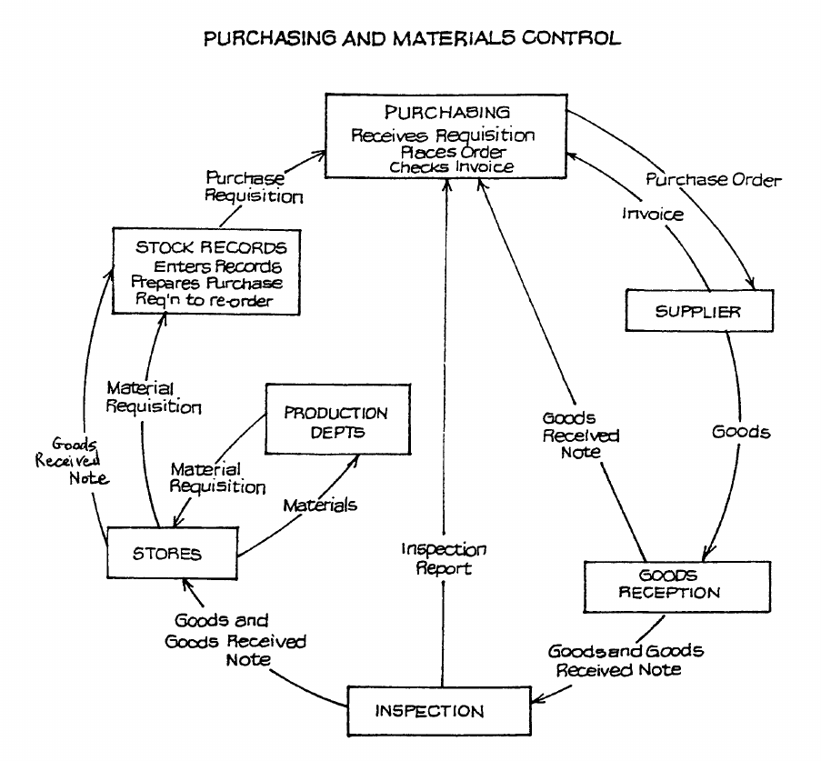
F2.1 MANAGEMENT ACCOUNTING
Page 58
Figure 11
F2.1 MANAGEMENT ACCOUNTING
Page 59
D. ORGANISATION AND DOCUMENTATION OF
PURCHASING
The Objects of a Purchasing System
(a) To obtain the right quality of materials.
(b) To obtain the right quantity of materials.
(c) To obtain delivery in such a manner as to co-ordinate the receipt of stocks with the
production programme or sales requirements.
(d) To pay the minimum price for the materials purchased, consistent with (a) to (c).
(e) To carry the minimum stocks without causing loss of production through shortage of
materials.
Main Documents
• Purchase Requisition Form
• Purchase Order Form
• Specification of Materials
• Goods Received Note
• Goods Rejected Note
The Purchase Requisition
The form used to advise the purchasing department of the factory requirements and also to
authorise the purchasing department to make the necessary purchase is the purchase
requisition (illustrated in Figure 12).
F2.1 MANAGEMENT ACCOUNTING
Page 60
ABC CO. LTD
PURCHASE REQUISITION
To Purchasing Department Serial No. 1
FROM DEPT. ...................... CHARGE A/C NO. ...................... Date ............... 20 ..
Material Symbol Quantity Description Delivery
or Code No.
Required
of Material
Requirements
E
F
G
H
Purchase Date Ordered Supplier Authorised by:
Order No.
A
B
C
D
Figure 12
The purchase requisition is completed as follows:
(a) Spaces A, B and C are filled in by the purchasing department.
(b) The signature in space D is that of one of the officials who are authorised to sign the
requisition.
(c) Spaces E, F, G are filled in by the storekeeper.
(d) A space may also be provided for the insertion by the purchasing department of the
price per unit of the material and the total value of the order, to enable a control to be
maintained of purchase commitments.
(e) A copy of the purchase requisition will be retained by the person or department
originating it.
(f) In space E the stock code number is entered.
F2.1 MANAGEMENT ACCOUNTING
Page 61
(g) The “Quantity Required” (space F) is regulated by the maximum and minimum stocks,
which are fixed by the management. The maximum stock is the amount above which
the storekeeper may not allow the stock in hand to rise, and the minimum stock is the
amount below which the stock in hand should not fall.
In space F the unit of quantity (i.e. lbs, tons, etc.) must be stated clearly, to avoid any
possible under- or over-ordering. It may be of advantage to have a separate space for
“Unit of Quantity”. To save re-handling on delivery, it is essential to indicate the form
in which the goods are to be delivered, e.g. in cartons of 100 units or pallets holding 1
gross of packets, etc.
(h) In space H the delivery instructions should include the unloading bay or direct to place
or usage, etc. Date required by may also be inserted.
Normally, three copies of the purchase requisition will be prepared and routed, as follows:
(1) To the purchasing department.
(2) To the planning department for information purposes, or this copy may be held by the
authorising executive.
(3) Retained by the issuing department.
A list of officials with power to authorise requisitions should be compiled and properly
authorised requisitions only should be accepted by the purchasing department. Most
requisitions will come from the storekeeper, when stocks of standard materials need
replenishing. Requisitions may also be initiated by:
• Production control department, for materials to be issued direct to jobs.
• Plant engineer, for materials required for capital projects or maintenance.
• Heads of administrative departments, for indirect materials not kept as standard stock.
F2.1 MANAGEMENT ACCOUNTING
Page 62
The Purchase Order
An official form, known as a purchase order, must be sent out for every order, to show the
supplier that the order is an official one on behalf of the firm, and so that the receiving system
can function efficiently. In the case of new or non-standard materials, issue of the order will
be preceded by a tendering procedure so that the best supplier can be selected.
The purchase order normally incorporates the purchaser’s terms and conditions of purchase;
acceptance of the order is deemed to imply acceptance under the purchaser’s terms. This is
an important consideration regarding the ultimate acceptance of the goods and any
subsequent claims made for defective goods. A significant amount of a purchasing officer’s
time can often be taken up in agreeing whose terms are applicable to a particular order.
PURCHASE ORDER
ABC CO. LTD & ADDRESS Order No. .................
To: .................................................
Please quote this No. on your Invoice
.................................................
.................................................
Date ..........................
Please supply in accordance with the instructions given on the back of this order.
Our Code Quantity Particulars Rate Amount
Your quotation
No. ............................
Terms:
Signed
for ABC Co. Ltd
.............................
Figure 13
F2.1 MANAGEMENT ACCOUNTING
Page 63
Copies of the purchase order will generally be distributed as follows:
(1) To the supplier.
(2) To the receiving department.
(3) To the accounting department.
(4) To the department which issued the purchase requisition.
(5) Retained by the purchasing department.
F2.1 MANAGEMENT ACCOUNTING
Page 64
Specification of Materials
ABC CO. LTD
SPECIFICATION OF MATERIALS
Inward Order No. No.
Details Date
Delivery Note Date
Item Code For use of Storekeeper
No.
Details
Quantity
(if stock
Remarks Purchase
Material)
Req. No.
1
2
3
4
5
6
7
8
9
10
Compiled by Drawing Office Ref.:
Checked by Planning Office Ref.:
Figure 14
A specification of materials (also known as a bill of materials) is a form which shows all the
materials and items which will be required for a particular order; this is prepared by the
drawing office.
On receipt of such specification, the storekeeper will be able to foresee the requirements of
the particular job concerned, and will make sure that he has the necessary materials in stock.
If he is short of any of them, he will prepare a stock purchase requisition, and will inform the
planning department so that any readjustment of plans necessitated by a shortage of material
may be made.
F2.1 MANAGEMENT ACCOUNTING
Page 65
E. RECEIVING DEPARTMENT
Duties
(a) Receiving and signing for goods from suppliers.
(b) Unloading the goods. (The department will have a copy of the purchase order, so that
arrangements can be made in advance for any special apparatus required.)
(c) Checking the contents as to quantity and condition and conformity with the purchase
order.
(d) Taking the necessary steps to have the goods tested or inspected.
(e) Notifying the stores department or the requisitioning department of the receipt of
goods.
(f) Delivering the goods to the appropriate point of storage or usage.
Goods Inwards Book and Goods Received Note
A goods inwards book may be kept to record all receipts from suppliers. Often goods cannot
be checked immediately on unloading, and recording the receipt of the goods in the goods
inwards book will ensure adequate control of the goods. The particulars usually recorded in
the goods inwards book are:
• Date received
• Supplier and carrier
• Very brief description of the goods
• Reference to the goods received note when compiled.
The next step is the preparation of the goods received note (see below).
Spaces A to G on the form shown (Figure 15) will be filled in at the goods receiving
department. It will then be sent with the goods to the stores department, where the goods will
be unpacked and their quality and condition inspected. If he is satisfied, the inspector will
then sign in the space H and the document will be forwarded to the purchasing department.
If the inspector is dissatisfied with the goods, he will issue a goods rejected slip and send this
to the purchasing department.
F2.1 MANAGEMENT ACCOUNTING
Page 66
ABC CO. LTD
GOODS RECEIVED NOTE
Supplier: No. 1
.......................... G .............................
...........................................................
........................................................... Date Received ................... 19 .........
Code No.
Quantity
Received Description of Material
Remarks
A B C
Purchase
Order No. Carrier
Received by:
Inspected by:
D E F H
Figure 15
Space may be provided on the goods received note for the insertion of a goods rejected slip
number and the bin or location number where the goods are finally placed by the storekeeper.
Space may also be provided for the number and type of containers and for reference to a
separate report, e.g. inspection, shortage, damage report.
Rejected Goods
When goods are found to be defective or otherwise not in accordance with the order, they
will be rejected. When goods are rejected, a routine similar to the following should be
adopted:
(a) A goods rejected note, similar to that shown in Figure 16 should be prepared in
triplicate.
(b) One copy of this note should be sent to the purchasing department, which will then
arrange with the supplier to obtain credit and arrange for the replacement of the rejected
goods.
(c) The second copy should be sent to the planning department, which may have to modify
its plans regarding work with the material concerned.
F2.1 MANAGEMENT ACCOUNTING
Page 67
(d) The third copy is filed in the stores.
GOODS REJECTED NOTE
No.: ..................................
Supplier: ............................................ Examined by: ..................................
Order No.: ......................................... Date ...............................................
Code
Specification
No.
Remarks
Steps
Taken
Signature
(Purch. Dept)
Figure 16
F. PROCEDURE IN THE ACCOUNTS DEPARTMENT
Now let us look at what is happening on the financial accounting side of the business.
Checking the Invoices
The supplier’s invoice will arrive some time after the goods.
It will be necessary to devise carefully a system to check against errors on invoices. A
suitable system is where each invoice is, on receipt, entered into an invoice register and
numbered. It is then impressed with a rubber stamp, designed as shown in Figure 17.
Spaces (b) and (c) will be filled in by the purchasing department; the requisite numbers are
obtained by reference to the copy order book, in which the number of goods received note
will have been entered. If each invoice is entered and registered under a serial number, this
number being entered in the copy order book, there should be no possibility of passing a
F2.1 MANAGEMENT ACCOUNTING
Page 68
duplicate invoice. The register of invoices may be compiled in the purchasing department,
the serial number being entered into space (a). The person who is responsible for checking
calculations will initial in space (d).
INVOICE STAMP
Register No.
(a)
Order No. (b)
G.R. Note No.
(c)
Calculations Checked (d)
Checked with Order (e)
Prices Checked (f)
Allocation (g)
Bought Journal Forward
(h)
Stores Ledger
Forward
Job Ledger
(j)
Passed for Payment (k)
Figure 17
In large businesses, where hundreds or thousands of invoices are handled daily, the
calculations may be checked by a special department.
Spaces (e) and (f) will be initialled by a member of the purchasing department, reference
being made to the signature on the goods received note for confirmation that the goods are of
the required quality and quantity.
The account to which the purchase is to be charged, e.g. whether it is ordinary stock material
or whether it is material purchased for a specific job which has to be charged to the cost
account for that job, will be entered in space (g). The folio of the entry in either the stores
ledger (for standard materials) or the job ledger (for orders in connection with special jobs)
will be entered in space (j).
The invoices will then be passed to the accounts office, where they will be entered in the
purchase journal for posting to the bought ledger and the bought ledger control account. The
purchase journal folio will be entered in space (h).
Finally, the invoice will be passed for payment by the authorised official, who signs in space
(k).
F2.1 MANAGEMENT ACCOUNTING
Page 69
G. THE STOREKEEPER AND STORES ISSUES
Duties of the Storekeeper
The storekeeper has considerable responsibility.
The following is a list of his duties:
(a) To receive materials into the store.
(b) To keep all items in store neatly packed in their own containers and in the position
allotted to them.
(c) To issue materials against a duly signed stores requisition.
(d) To see that no unauthorised person is allowed to enter the store. Normally, the only
persons allowed access to the stores, apart from the storekeeper himself, are his
assistants, stock-takers and auditors.
(e) In some cases the responsibility for checking the quantity of goods in each container or
bin will rest with the storekeeper.
(f) To issue a stock requisition whenever the reorder level is reached (see later).
(g) To maintain records of receipts and issues.
(h) To report on any slow-moving and obsolete stocks.
The General Routine for Stores Issues
In no circumstances should materials be issued from store without the presentation of a
materials or stores requisition signed by an authorised person (see Figure 18). Only by
strict enforcement of this rule is it possible to guard against the misuse of materials and the
pilfering of stores.
F2.1 MANAGEMENT ACCOUNTING
Page 70
ABC CO. LTD Serial No. .......................
STORES REQUISITION
Please supply to ............................. Dept Date ................... 20 .......
Job No. ...................
Code
No.
Description
of Material
Quantity
Required Issued Price
Amount
Stores
Ledger
Signed: Issued by: Received by: Cost Office Ref.:
......................... ............................ ............................ ................................
Foreman
Figure 18
The price and amount will be entered by the cost office after the document has been recorded
by the stores.
The routine in connection with the above requisition is as follows:
(a) When any material is required for a job in a department, the foreman makes out a stores
(or materials) requisition. He signs this and it is taken to the storekeeper. Note that
frequently the requisitions for a particular job are made out by the planning or progress
department from the bill of materials and passed to the foreman only when he is ready
to start the job. It is also sometimes required that the requisition number should be
entered on the bill of materials.
(b) The storekeeper then issues the materials and signs the requisition, which is also signed
by the person receiving the goods.
(c) The requisitions are forwarded regularly to the cost office, where the issues are priced
(see later).
Materials Returned to Stores
Any unused materials normally should be returned to stores together with a stores return note,
sometimes referred to as a stores credit note. This document gives similar details to the
F2.1 MANAGEMENT ACCOUNTING
Page 71
stores requisition but is usually printed in a distinguishing colour, e.g. red. The routine in
connection with the returns note is similar to that with the requisition.
Sundry Transfers of Materials
If goods are transferred from one cost unit to another after leaving the stores, it is necessary
to charge the receiving cost unit with the value of materials concerned and to credit the cost
unit originally charged. This is achieved by raising a materials transfer slip, which bears a
description of the goods transferred, the references of both cost units and the signatures of
both supervisors concerned.
Transfers should be made only if the goods are immediately required by another department
and if it is clearly more efficient (because of location) to make a direct transfer. Otherwise all
unused materials should be returned to the stores, as described above, for reissue.
H. STOCK LEVELS
In order to ensure that the flow of production is not impaired by the lack of materials and also
that excessive capital is not tied up in stocks, it is necessary to ensure that the level of stock
held always lies between certain limits.
Maximum Quantity
This represents the greatest amount of an item of stock which should be carried if the best use
is to be made of working capital.
In determining the maximum stock level, the following are among the factors considered:
(a) Capital tied up in stocks.
(b) Capital available.
(c) Cost of storage (including rent, insurance, labour costs).
(d) Storage space available.
(e) Consumption rate.
(f) Economic purchasing quantities (see later).
(g) Market conditions and prices, seasonal considerations.
(h) Nature of material - possible deterioration or obsolescence.
Minimum Quantity
This represents the level below which the stock should not normally be allowed to fall if the
requirements of production are to be met.

F2.1 MANAGEMENT ACCOUNTING
Page 72
The minimum level is determined by the rate of consumption of materials and the time taken
between placing an order and receiving the material.
Reorder Level
It is necessary to set a point at which an order must be placed. This point is known as the
reorder level. It will be higher than the minimum level, to cover use during the period before
the order is received.
Reorder Quantity
The reorder quantity is the quantity which should be ordered at the time the reorder level is
reached. It will depend on the discounts available from suppliers for bulk ordering, the cost
of placing an order and the cost of storage (see later).
Formulae
• Reorder level = Maximum consumption × Maximum reorder period.
• Minimum stock = Reorder level – (Normal consumption × Normal reorder period).
• Maximum stock = Reorder level + Reorder quantity – (Minimum consumption ×
Minimum reorder period).
• Average stock = Minimum stock + ½ Reorder quantity.
These levels should be reviewed periodically to ensure that they reflect current conditions.
Example
Component A is used as follows:
Normal usage 50 per week
Minimum usage 25 per week
Maximum usage 75 per week
Reorder quantity 300
Reorder period 4-6 weeks
Calculate the reorder level, the minimum and maximum levels, and the average stock level.

F2.1 MANAGEMENT ACCOUNTING
Page 73
Solution
Reorder level = Maximum consumption × Maximum reorder period
= 75 × 6
= 450
Minimum level = Reorder level – (Normal consumption × Normal reorder period)
= 450 – 50 × 5
= 200
Maximum level = Reorder level + Reorder quantity – (Minimum consumption ×
Minimum reorder period)
= 450 + 300 – (25 × 4)
= 650
Average level = Minimum stock + one half Reorder quantity
= 200 + (300 ÷ 2)
= 350.
I. ECONOMIC ORDER QUANTITY
Formula
There is a formula which tells a company the optimum batch size in which to purchase goods.
The formula is:
Q = 2C D
C
2
1
Where:
Q is the economic order quantity;
D is the annual demand for the product;
C2 is the fixed cost of placing an order, i.e. delivery charges, clerical time in placing
order, checking invoice, etc., which do not vary with the size of the order; if the
goods are produced internally it will include fixed production costs incurred
specifically in producing the batch, e.g. tool setting;
C1 is the annual cost of holding one unit of stock.
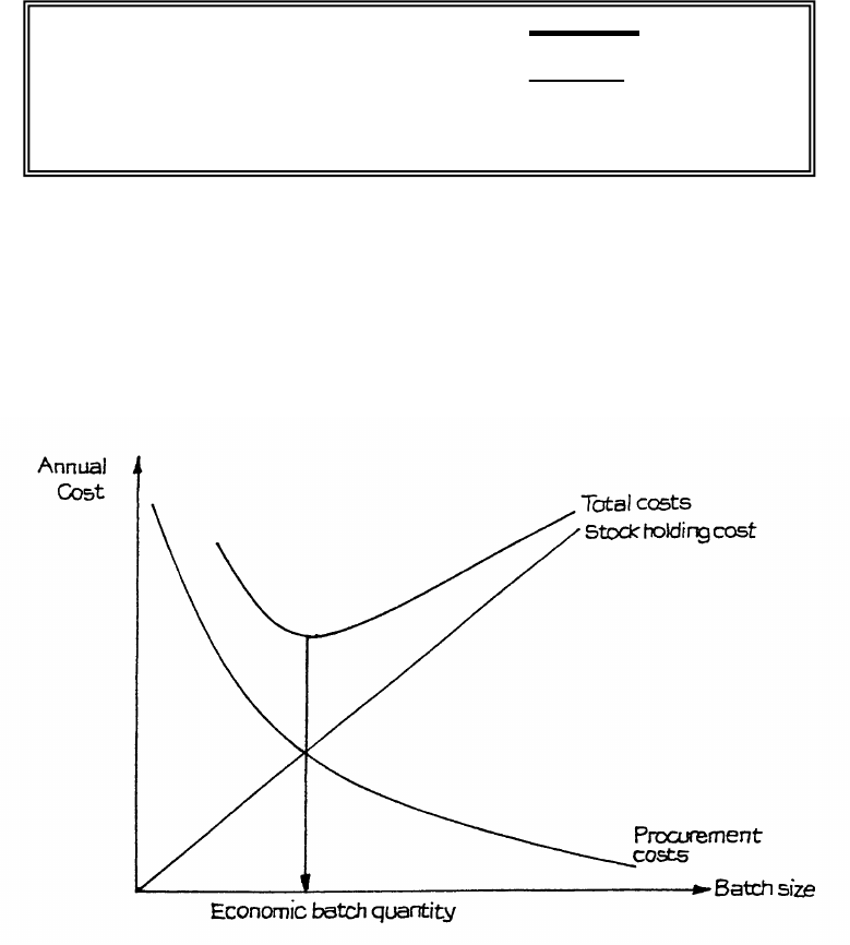
F2.1 MANAGEMENT ACCOUNTING
Page 74
You should notice that the model is rather limited: the unit cost is assumed to be constant.
There is no provision for quantity discounts which might make it more attractive to purchase
larger quantities.
Or
Formula:
Where:
D = Demand
C = Cost of Ordering
C = Cost of holding
Figure 19
The position of the economic batch quantity can be illustrated graphically (see Figure 19).
Obviously, the larger the batches which are bought, the fewer batches there need to be to
cover the annual demand. Therefore, the total fixed cost (S × number of batches) decreases
as the batch size increases. Conversely, buying larger batches will increase the average stock
held, and therefore increase the total stockholding cost. The economic batch quantity is at the
point where total costs are minimised.
√
2 D C
o
H
C
o
H
F2.1 MANAGEMENT ACCOUNTING
Page 75
Example
A company uses 4,000 components, type “A”, in a year. The cost of placing an order is
RWF20. The stockholding cost is RWF4 per item per year. Stocks are replenished when the
stock level falls to 50 units; orders placed are received the same day. Calculate the economic
order quantity.
Solution
Using the formula Q =
2DS
H
Then, Q =
2 4,000 20
4
× ×
=
40 000,
= 200
∴ orders should be placed for batches of 200 units at a time.
Explanation
The correctness of the formula can be demonstrated by using the data of the above example
and “testing” different order sizes.
A Order size 100 160 200 250
B Number of orders p.a. 40 25 20 16
C Total ordering cost B × RWF20RWF800 RWF500 RWF400 RWF320
D Average stock 50 + (½ × A) 100 130 150 175
E Stock holding cost D × RWF4 RWF400 RWF520 RWF600 RWF700
F Total cost C + E RWF1,200 RWF1,020 RWF1,000 RWF1,020
∴ 200 is the economic order quantity.

F2.1 MANAGEMENT ACCOUNTING
Page 76
J. STOCK TURNOVER
This term expresses the number of times stock is sold or used within a given period. Usually
it is expressed as a ratio:
Cost of sales for a specific period
Average value of sto
ck held
(Average value of stock held is (Opening value + Closing value) ÷ 2.)
Example:
Cost of stock sold in Year 1 RWF600,000
Opening stock RWF30,000
Closing stock RWF20,000
Stock turnover =
000,25
000,600
RWF
RWF
= 24 times per year.
K. ACCOUNTING RECORDS REQUIRED FOR
MATERIALS
Bin Cards
Bin cards are prime entry records of the quantities of stock, kept on an in/out/balance basis,
held in designated storage areas.
These records are maintained at the physical point of storage and usually show only
quantities, not costs, of items held. The storekeeper is responsible for keeping the bin cards
up-to-date.
The bin card records receipts, issues and the balance remaining in stock. The receipts side
will show entries from goods received notes and returned to stores notes and the issues
portion shows the goods passed to production as per stores requisition slips. The balance on
hand shown on the card should equal the physical number of items in stock.

F2.1 MANAGEMENT ACCOUNTING
Page 77
The bin card may also show the materials allocated, i.e. reserved for a particular cost unit but
not yet issued; and free stock, which is the balance on order and on hand less the allocated
stock. This is because the reorder level is sometimes set in terms of the free stock level.
Stores Ledger Accounts
These accounts are maintained in a stores ledger held in the cost office, an account being
opened for each item held in stock. The entries mirror the transactions shown on the bin
cards, but show the values as well as quantities. The physical separation of the bin cards and
stores ledger accounts and the fact that different staff are involved helps prevent fraud or
pilfering of materials. Having a dual record also helps to detect clerical error.
L. STOCKTAKING
This is a process whereby stocks (which may comprise direct and indirect materials, work-in-
progress and finished goods) are physically counted and are then valued item by item.
Perpetual Inventory and Continuous Stocktaking
When the stores balances are recorded after every issue or receipt of materials, a perpetual
inventory is in operation. This can be combined with a continuous stocktaking system
whereby a few items are actually counted every day. The physical quantity in stock is then
compared with the balance shown in the records.
The advantages of this system are as follows:
(a) The temporary dislocation of work caused by end-of-period stocktaking is avoided.
(b) The daily checking of items can be so arranged that all items are checked at least twice
a year, and fast-moving or valuable lines can be checked more frequently. Checking
should be carried out by non-stores staff, and advance notice should not be given of
which items are to be checked each day.
(c) Explanations of differences between physical stock and records can be made more easily
and perhaps measures can be taken to prevent a recurrence.
Such differences might be due to:
(i) Evaporation;
(ii) Absorption of moisture;
(iii) Losses in breaking bulk;
unavoidable differences.

F2.1 MANAGEMENT ACCOUNTING
Page 78
(iv) Unavoidable approximation in measuring issues;
(v) Pilferage;
(vi) Poor storage conditions or handling,
causing damage;
(vii) Careless measurement.
(d) There is a reinforcement of the need for honesty on the part of the staff.
(e) The annual accounts can be prepared earlier, as the book value of the stores is
acceptable for balance sheet purposes. The stock value can also be used to prepare
monthly accounts.
(f) The opportunity can be taken to check that maximum stock levels are not being
exceeded so that the disadvantages of excessive stocks are more easily avoided.
The perpetual inventory routine needs to be thoroughly documented within the organisation,
and active measures taken to ensure that laid-down procedures are followed. This is
necessary not only to gain the greatest internal advantage of this approach, but also in order
that the auditors may be convinced of the validity of the stock figures. To this end the
auditors will generally spend a lot of time satisfying themselves that the system is working
correctly, especially in the early years after its implementation.
Methods of Stocktaking
(a) Individual Count
Where items are individual and of the same generic group, it is necessary to count the
number of each type held in stock.
As a general rule this is only carried out when items are of reasonable size; where nuts,
bolts or nails are concerned, it is usual to weigh the items or estimate the amount by
experience. The individual count method is very slow and laborious if there are a large
number of items involved. This method can be greatly speeded up if stock is stored in
standard quantities or bundles, so that it merely becomes a question of counting the
number of bundles.
avoidable differences
.
F2.1 MANAGEMENT ACCOUNTING
Page 79
(b) Measurement of Liquids
The method by which the liquid is stored and used will very largely determine the way
in which the physical stocktaking should be carried out. If liquid is delivered in bulk
and drawn off for use automatically, it is usual for meters to be installed which give the
usage for a period and the volume remaining in storage. The tolerance of accuracy is
normally very small and, subject to practical experience, it is usual to accept the
reading on the meters for purposes of stocktaking. Electronic measuring devices are
extremely accurate and can be relied on to provide a high degree of accuracy.
In certain cases usage may be measured by a type of meter which does not record
deliveries or stock remaining, e.g. a petrol pump of the older type. A theoretical stock
value will be continuously maintained, but the contents of the tank will be compared
with this at regular intervals. A dip-stick will normally be used for this purpose. This
method of measurement relies on the fact that one dip-stick is maintained for each size
of tank, and the degree of accuracy will depend on the calibration of the stick.
(c) Measurement by Calculation
There are many materials which are solids but cannot be counted individually, e.g. coal,
flour or sugar. The amount of such items can be calculated by ascertaining the cubic
space taken up measured, for example, in cubic feet; so that by using the known weight
of the commodity per cubic foot, the total weight can be obtained for pricing.
(d) Measurement by Technical Estimate
Where goods are incapable of being counted or measured by scientific means, it may be
necessary to resort to technical estimates.
Organisation of Annual Stocktaking
Many large organisations, which are not working on a perpetual inventory system, will
arrange for the physical stocks to be counted before the year end. This is a satisfactory
arrangement provided suitable systems are in place to monitor stock movements between the
date of the physical check and the financial year end. The auditors must be advised in
advance if this route is to be followed and it must be emphasised how important it is to have
in place procedures to monitor stock movement and to ensure that they are being correctly
followed.
With an annual stocktake (rather than a continuous system) the greatest problem is that of
getting the full procedure carried out in the time allowed. The deadline allowed for the
completion of stock figures is some time before the completion of the annual accounts. As
the physical count cannot take place before the close of the last day’s business, the time
available is short and the work to be done considerable.
(a) Preparatory Work
F2.1 MANAGEMENT ACCOUNTING
Page 80
Time will be saved at the stocktaking if preparatory work can be carried out prior to
commencement of stocktaking. Jobs which can be done are: the typing of forms, the
entering of static information such as description and in certain cases price, the
grouping of forms by departments and the issue of stocktaking forms at least one week
in advance of the date of action.
One week before stocktaking, therefore, a responsible official can check that the correct
forms have been issued to the various sections and departments and have been
completed in respect of date, heading and all static information. This will eliminate one
of the common bottle-necks caused by people complaining that they did not receive the
correct forms or did not receive any forms at all.
Careful design of forms can also save time at the actual stocktaking. They should be on
stout card so that they are not damaged in the stores, logically laid out so that the
person completing them can work from left to right, and should ask only for relevant
information.
(b) Physical Counting and Measurement
This should be carried out by non-stores staff (but the stores staff should be on hand to
assist by showing the stocktakers the location of each item). The stocktakers should
only be required physically to measure the stock and enter this on forms on which the
description of each item has already been entered: all other entries to be made can be
done in the cost office. The auditors should normally be invited to attend the physical
count, although their appearance will depend upon the materiality of the stock figure.
(c) Valuation
Having ascertained the quantity of stock, this has to be converted to a value in RWF.
We will consider this later.
(d) Checking
On completion of the calculation and the checking, it should be the specific
responsibility of the official in charge of stocktaking to ensure that all stock sheets
issued have been returned fully completed.
Any additional sheets relating to new types of stock should be specially studied, so that
at the following stocktaking the appropriate preparatory work can be carried out.
All sections should then be merged into a stock summary, taking care to ensure a full
audit trail back from the final stock value to the individual items of stock.
(e) Conclusion
If the suggestions on form design and organisation of staff are carried out, accurate
physical stock figures can be obtained. Nevertheless, an annual stocktaking is a major
undertaking needing a lot of work.
F2.1 MANAGEMENT ACCOUNTING
Page 81
M. THE PRICING OF MATERIAL ISSUES
Problem of Pricing
In times of changing prices, firms have to decide on how they will price the materials issued
to production, when they are trying to arrive at overall production costs. Should it be the
price they actually paid for the material, or the current price of the same type of material
(which could well be higher)?
There are several different methods of pricing material issues, which we shall now discuss.
At Market Price Ruling at the Date of Issue
When quoting for business, it may be necessary to include materials on the basis of their
market price at the time, even though they may have been bought some time earlier at a
higher price; for, if a firm gives a high quotation in an attempt to recover the full cost of the
materials, it may lose the business altogether to a competitor whose quotation is based on the
current market price.
Conversely, if a manufacturer has, through good fortune or foresight, acquired considerable
stocks of a material at a price below that currently ruling and he acquires business which will
use those materials, he will want to take advantage of this good buying by placing a quote
which includes the current market value of the materials. (The manufacturer will not always
get away with this! In particular, if he is a contractor for a government department he will be
obliged to charge for the materials at cost.)
The use of market prices therefore gives credit for good buying and the reverse for bad
buying. The difficulty is to establish the current market price and, as this does not line up
with the actual cost of the materials, it is necessary to operate an adjustment account to take
care of the differences.
At Inflated Cost
This method is used to cover the unavoidable wastage which may occur in certain
circumstances. The changes which often take place in this wastage render the method
inaccurate and an adjustment account will have to be opened.
At Cost Price
Issue of materials is usually carried out on this basis, and clearly it is not necessary to use an
adjustment account. There are several conventions by which materials can be issued at cost
price; the most usual are described below.
F2.1 MANAGEMENT ACCOUNTING
Page 82
(a) FIFO - First In, First Out
This is a method pricing material issues using the oldest purchase price first, i.e. the
oldest items in stock shown by the stock records are issued first.
If the transactions involved are numerous, this method involves a great deal of clerical
effort, and it is therefore best used for slow-moving stock where the value is high and
the price does not fluctuate a great deal. In times of rising prices, the valuation of
issues tends to be low. On the other hand, the value placed on the closing stock will
reflect current prices, since if the first stock to come in is deemed to be the first issued,
it is the latest stock which remains.
Advantages of FIFO
1. Probably represents what is really happening within the stores.
2. Easy to use.
3. Easy to explain to managers.
4. The closing stock value should be near market value.
Disadvantages of FIFO
1. Can be difficult to operate.
2. Issues of stock can be at a lower cost than market price, especially in a period of
inflation.
F2.1 MANAGEMENT ACCOUNTING
Page 83
Example
Receipts Issues Balance
Units Rate Amount Units Rate Amount Units Amount
RWF
RWF
RWF
RWF
RWF
Jan. 1
12
1.00
12.00
12
12.00
" 10
10
1.05
10.50
22
22.50
" 11
5
1.00
5.00
17
17.50
" 26
(7
1.00
7.00
(1
1.05
1.05
9
9.45
" 30
10
1.10
11.00
19
20.45
Feb. 4
5
1.05
5.25
14
15.20
" 10
(4
1.05
4.20
(2
1.10
2.20
8
8.80
" 11
10
1.05
10.50
18
19.30
" 15
(8
1.10
8.80
(1
1.05
1.05
9
9.45
Stock balance made up of 9 units @ RWF1.05 = RWF9.45.
FIFO may be inequitable in that two jobs on the same day may be charged different
rates for the same material.
(b) LIFO - Last In, First Out
This is a method of pricing material issues using the last purchase price first.
Date
8
6
9
F2.1 MANAGEMENT ACCOUNTING
Page 84
When this method is in operation, stores issued are charged at the prices of the latest
items in the stock from which the materials are drawn. In times of inflation, therefore,
the cost of the present high-priced material is charged to production as it is incurred. On
the other hand, closing stocks will be conservatively valued. Like FIFO, the method can
be cumbersome to operate and possibly inequitable.
Advantages of LIFO
1. Fairly accurate method of accounting for inflation.
2. Helps decision making.
3. Stock that is issued is close to market value of stock.
Disadvantages of LIFO
1. Can be difficult to operate.
2. Difficult to explain to managers.
3. Variations in prices.
4. Closing stocks become undervalued when compared to market value.
F2.1 MANAGEMENT ACCOUNTING
Page 85
Example
Receipts Issues Balance
Units
Rate
Amount
Units
Rate
Amount
Units
Amount
RWF
RWF
RWF
RWF
RWF
Jan. 1
12
1.00
12.00
12
12.00
" 10
10
1.05
10.50
22
22.50
" 11
5
1.05
5.25
17
17.25
" 26
(5
1.05
5.25
(3
1.00
3.00
9
9.00
" 30
10
1.10
11.00
19
20.00
Feb. 4
5
1.05
5.50
14
14.50
" 10
(5
1.10
5.50
(1
1.00
1.00
8
8.00
" 11
10
1.05
10.50
18
18.50
" 15
9
1.05
9.45
9
9.05
Balance of stock 1 @ RWF1.05 = RWF1.05
= RWF9.05
8 @ RWF1.00 = RWF8.00
Both FIFO and LIFO can produce anomalies - two jobs which receive materials on the
same day may be charged differently because one batch of purchases has been exhausted
Date
8
6
F2.1 MANAGEMENT ACCOUNTING
Page 86
(c) Weighted Average Price
Under this method, the price at which stores are issued is calculated by dividing the
total cost of the materials in stock from which the material to be priced could have been
drawn, by the total quantity of material in that stock.
This method has the advantage of spreading the cost more evenly. It can be used to
advantage where the price of materials fluctuates rapidly and is a useful method for
computerised accounting.
However, like the LIFO and FIFO methods, it may involve a lot of clerical work.
Should there be an extremely high or low price, it is reflected in the costs for a long
time afterwards.
A simplification is to use a periodic weighted average, calculating the average net after
each receipt but retrospectively once a month (say). If this method were used in the
previous example, the average for January would be RWF1.0469 (32 units received at
RWF33.50) and this would be used for both issues in January. The balance on hand at
the beginning of February would then be valued at RWF19.89 (19 units at
RWF1.0469), so the retrospective weighted average for February would be RWF1.0479
((RWF19.89 plus RWF10.50) divided by 29).
A further simplification is to use a simple average, i.e. adding up the prices without
weighting for quantity and dividing by the number of prices. Again this may be
calculated on the continuous or periodic system.
Using the continuous system, the simple average for the 1 January to 10 January
consignments would be RWF1.025 ((RWF1 plus RWF1.05) divided by 2). This
method should only be used when there is little fluctuation in prices, but it can be a
useful time-saving short-cut.
Advantages of Weighted Average Price
1. Any fluctuations in price are smoothed out.
2. Decision making is made easier using this method.
3. Easier to operate.
Disadvantages of Weighted Average Price
1. Prices and closing stock values can be lower than the market value.
2. When using this system, actual price can run into several decimal places.
F2.1 MANAGEMENT ACCOUNTING
Page 87
(d) Standard Price
This is the method adopted when a standard costing system is in operation. Purchases
are posted to the stock account at the predetermined standard price and issues are priced
at standard price. The difference between the actual cost of purchases and their value at
standard price, called the “price variance”, is posted to a separate account.
(e) Replacement Price
Under this method, stores are issued at the current replacement price. Using standard
manual record cards it is not possible to maintain details of the value of goods in stock,
although the physical balance is maintained and may be multiplied by the current
replacement price to arrive at a replacement cost stock figure. This stock figure would
need to be adjusted subsequently, before it could be used in the financial accounts of
the company.
Good records are essential, as the replacement price at the time of each issue must be
known and this is only likely to be realistic in a fully computerised environment. The
system has the advantage that all issues are made at current economic value, but this in
itself will lead to the generation of sundry profits and losses on stock holdings.
N. OBSOLETE, DORMANT AND SLOW-MOVING STOCK
Obsolete Stock
Obsolete stock can be a serious matter. All stock represents cash and should be turned into
products and sold to bring the money back in again.
Obsolete stock is dead cash. All possible steps must be taken to prevent stock from
becoming obsolete by the co-ordination of the efforts of all concerned. For example, the
design department may agree to a modification being held back until existing stocks have
been used; or the sales department may have a big “push” on an item which is shortly to be
dropped, so as to clear out stocks.
Yet some obsolescence is unavoidable. It is a good thing to keep a separate section of the
stores, to which any stocks declared obsolete should be transferred immediately.
Thought must be given as to whether there will be a demand for spares for old models still in
existence and, if so, some parts must be set aside for this purpose.
The remaining problem then is the one of finding the best possible market for the remainder.
The buying department is usually in the best position to do this.
F2.1 MANAGEMENT ACCOUNTING
Page 88
Remember, it is not only the cost of the materials which is tied up, but storage space, labour,
etc.
Dormant and Slow-Moving Stock
In addition to obsolete stock there is the problem of dormant stock, and of slow-moving
stock. Dormant stock means an item which has not moved for a considerable period. It is not
obsolete because it has not been replaced by a new item, and in the future it is expected to
move again.
Slow-moving stock may consist of items which are only issued at long intervals. Obviously
an item like this will not be featured as a stock receipt until, after a long interval, it drops to
reorder level. At that time, either the storekeeper will mark the reorder requisition “SM” so
that the matter will be investigated, or, in the case of an automatic system, the item will be
printed out by the computer as an exception for special study.
O. JUST-IN-TIME (JIT)
Traditionally organisations in the West have used a “push” production flow system. This
system has the following stages:
1. Buy raw materials and place them in stock
2. Produce goods based on sales forecasts
3. Requisition goods from stock and make products according to the production schedule
4. Place finished goods into finished goods store
5. Sell to customers from finished goods when customers request products
However, Japanese companies, most notably Toyota, developed a different system, known as
Just-In-Time or Stockless Production. This system is not a “push” system but a “pull” system.
A product is not made until the customer requests it and components are not made until they
are required by the next production stage. In a full JIT system, virtually no stock is held; that
is no raw material stock and no finished goods stock, but there will usually be a small amount
of work-in-progress.
JIT stock management methods seek to eliminate any waste that arises in the manufacturing
process as a result of using stock. JIT purchasing methods apply the JIT principle to
deliveries of material from suppliers. With JIT production methods, stock levels of raw
materials, work-in-progress and finished goods are reduced to a minimum or eliminated
altogether by improved work-flow planning and closer relationships with suppliers.
F2.1 MANAGEMENT ACCOUNTING
Page 89
Advantages of JIT
JIT stock management methods seek to eliminate waste at all stages of the manufacturing
process by minimising or eliminating stock, defects, breakdowns and production delays. This
is achieved by improved workflow planning, emphasising quality control and firm contracts
between buyer and supplier.
One advantage of JIT stock management methods is a stronger relationship between buyer
and supplier. This offers security to the supplier, who benefits from regular orders, continuing
future business and more certain production planning. The buyer benefits from lower stock
holding costs, lower investment in stock and work-in-progress and the transfer of stock
management problems to the supplier. The buyer may also benefit from bulk purchase
discounts or lower purchase costs.
The emphasis on quality control in the production process reduces scrap, re-working and set-
up costs, while improved production design can reduce or even eliminate unnecessary
material movements. The result is a smooth flow of material and work through the production
system, with no queues or idle time.
Disadvantages of JIT
A JIT stock management system may not run as smoothly in practice as theory may suggest,
since there may be little room for manoeuvre in the event of unforeseen delays. For example,
there is little room for error on delivery times.
The buyer is also dependent on the supplier for maintaining the quality of delivered materials
and components. If delivered quality is not up to the required standard, expensive downtime
or a production standstill may arise, although the buyer can protect against this by including
guarantees and penalties in the suppliers contract. If the supplier increases prices, the buyer
may find that it is not easy to find an alternative supplier who can meet his needs at short
notice.

F2.1 MANAGEMENT ACCOUNTING
Page 90
BLANK

F2.1 MANAGEMENT ACCOUNTING
Page 91
Study Unit 5
Labour
Contents
A. Methods of Remuneration
B. Time Rates
C. Incentive Schemes
D. Straight Piece-Rate Systems
E. Differential Piece-Rate Systems
F. Premium Bonus Schemes
G. Group Bonus Schemes
H. Performance-Related Pay
I. Profit Sharing and Co-Partnership
J. Non-Monetary Incentives
K. Measurement of the Efficiency of Labour

F2.1 MANAGEMENT ACCOUNTING
Page 92
Contents (Continued) Page
L. Labour Turnover
M. Recording Labour Costs
_______________________________________________________________
N. Indirect Labour
O. Treatment of Overtime
_______________________________________________________________
P. Summary
F2.1 MANAGEMENT ACCOUNTING
Page 93
A. METHODS OF REMUNERATION
Fixing Wage Rates
Wage rates may be fixed by individual agreement between employer and employee, or more
commonly by collective bargaining between trade unions and employers’ associations.
An employer may pay wages on an hourly basis, per piece, or may adopt one of the various
bonus methods of payment, but the general principle of a wages policy is to obtain the
maximum production per RWF of wages paid while maintaining an acceptable quality of
production, within the limits of “social justice” (i.e. employees should receive a “fair day’s
wages”).
In deciding on the method of remuneration to use, attention must be paid to the following
factors:
(a) The relative importance of quantity and quality, and the cost of spoilage.
(b) The degree of specialisation and standardisation of the product.
(c) The degree to which automatic or semi-automatic machines are used.
Main Methods
Workers may be paid by time of attendance or by results. The latter method provides an
incentive to increase production. “Payment by results” covers:
(a) Piece Rates:
These may be:
− Straight piece rates
− Piece rates with guaranteed minimum
− Differential piece rates.
(b) Bonus Schemes:
These can be any of the following:
− Bonus schemes for direct workers individually
− Bonus schemes for direct workers in groups
− Bonus schemes for indirect workers
− Bonus schemes for staff.
(c) Performance-Related Pay
(d) Indirect Monetary Incentives:

F2.1 MANAGEMENT ACCOUNTING
Page 94
These may take the form of:
− Co-partnership schemes
− Profit-sharing schemes
− Allowances and expenses of various kinds.
(e) Non-Monetary Incentives:
These are further inducements to increase output. They include security of
employment, prospects of promotion and the satisfaction that a job gives to an
employee (i.e. craft work as opposed to repetitive production).
B. TIME RATES
At Ordinary Levels
This system is the most common method of wage payment in Britain. It is a system of
paying workers for the time worked rather than for work produced. It may be in the form of
an hourly rate, or shift or weekly rate for an agreed number of hours. We must examine the
circumstances in which it is most favoured, and its advantages and disadvantages.
(a) Where the System Can be Favoured
(i) Where the work done is very difficult to measure, e.g. when a service is rendered
- nurses, policemen, probation officers, lift attendants, teachers - or when the
work cannot be standardised, e.g. the majority of clerical operators or
administrative work.
(ii) When workers are learning, e.g. apprentices.
(iii) Where the speed of the machine, operation, or process governs the speed at which
the operator can work, e.g. assembly lines, chemical plants, and process industries
such as bottle or paper making.
(iv) When quality of production is of prime importance and would be endangered by
encouraging an operator to work faster.
(v) When safety is likely to be endangered if the operation is speeded up, e.g. lorry
driver.
(vi) When it is found that good employer/employee relations exist and a satisfactory
output is being achieved. The introduction of an incentive scheme may disrupt
the good employer/employee relations, causing discontent and possibly lower
production.
(vii) When work is so unstandardised that the expense and difficulty involved in
measuring the work done, etc. would be so great as to outweigh any advantages
accruing from an incentive scheme.
F2.1 MANAGEMENT ACCOUNTING
Page 95
(b) Advantages
(i) The system is simple to understand and simple to operate, saving on clerical
labour in number and quality of staff.
(ii) Wages are stable, an advantage rated very highly by many workers.
(c) Disadvantages
(i) The system provides no direct incentive to the worker to increase output or to
produce better quality work.
(ii) It tends towards higher production costs because the workers tend to work at an
accepted minimum rate.
(iii) It requires close supervision, and in times of full employment the worker’s output
is greatly dependent on his goodwill and conscientious attitude, since there is no
fear of dismissal.
(d) Effect of Variations in Output
Any gain or loss arising from variations in the operators’ efficiency will be borne by the
employer. Thus, if the daily wage of each of four operators is RWF40:
If A produces 20 units his labour cost per unit is RWF2, i.e. RWF40 divided by 20
units.
If B produces 40 units his labour cost per unit is RWF1, i.e. RWF40 divided by 40
units.
If C produces 80 units his labour cost per unit is RWF0.50, i.e. RWF40 divided by 80
units.
If D produces 100 units his labour cost per unit is RWF0.40, i.e. RWF40 divided by
100 units.
Clearly, labour cost per unit falls with increased production. This is illustrated in
Figure 20.
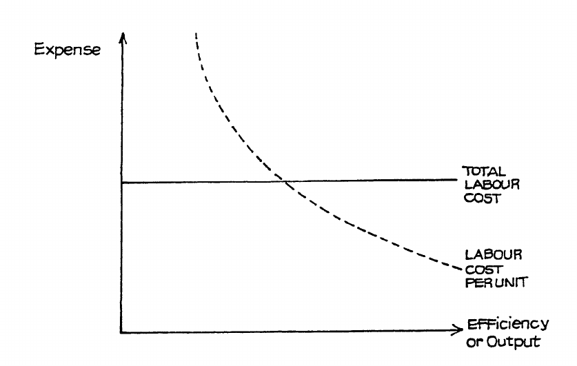
F2.1 MANAGEMENT ACCOUNTING
Page 96
Figure 20
High Wage Plan
(a) Significant Points
(i) An appreciably higher than average wage is paid compared with other factories in
the area.
(ii) A higher standard of output, both in quality and quantity, is set.
(iii) As a vacancy attracts a larger number of applicants, the employer can secure the
services of better workers, who will be willing to maintain the higher standard in
order to retain their jobs and the higher wages.
(b) Advantages
(i) It is simple to understand and operate.
(ii) Wages are stable.
(iii) It overcomes the lack of incentive of ordinary time rates.
(iv) Output increases, and as a result, the cost per unit falls, compensating the
employer for the increase in wages.
(c) Disadvantages
(i) As with ordinary time rates, this system still does not provide incentive for
exceptional effort and ability.
(ii) It requires close supervision.
F2.1 MANAGEMENT ACCOUNTING
Page 97
Graduated Time Rates
These are time rates adjusted for particular reasons, e.g. changes in the cost of living,
additional rates for merit, loyalty, etc.
C. INCENTIVE SCHEMES
General Principles
There are some general principles which should apply to all incentive schemes:
(a) The reward should be as nearly related to effort as possible, both in amount and in time
of payment.
(b) The scheme should be fair to both employer and employee.
(c) There should be mutual agreement to ensure that the basis of the scheme is fully
understood, covers all reasonable points, and is not capable of being misinterpreted.
(d) The scheme should be strong and positive; it should have clearly defined, worthwhile
and attainable objectives.
(e) There should be no limits placed upon the amount of additional earnings.
(f) The incentives should not be affected by matters outside the employees’ control.
(g) The incentive should be reasonably permanent, not merely a device to be used by the
employer when business is good and dropped when it is not.
(h) The rates for payment by results should be fixed only after the job has been properly
assessed.
(j) Piece rates or time allowances, once fixed, should remain, unless conditions or methods
change.
(k) The standard of performance set must be reasonably attainable by the average
employee and it should be possible to demonstrate that this is so.
(l) The scheme should be simple, capable of being understood by the workers so that they
can make their own calculations, and easy to operate with the minimum of clerical
work.
(m) A properly prepared incentive scheme should assist supervision and help to reduce the
cost of it.
(n) The scheme should be in conformity with any national, local or trade agreement.

F2.1 MANAGEMENT ACCOUNTING
Page 98
Reasons for Having an Incentive Scheme
Before we discuss various incentive schemes, it would be useful if we considered the
difference such a scheme of remuneration might make to certain firms.
Firms with high fixed overheads will want to increase output as much as possible, because by
increasing output they can spread the fixed overheads over a larger number of units, thus
reducing the fixed cost per unit - assuming, as we have already seen, that absorption costing
is in operation.
Under some incentive schemes the labour cost per unit will rise, but by increasing the output,
the total cost per unit will fall (again employing absorption costing).
Example
Under an
Under an
Under a Guaranteed
Incentive
Increased
Fixed Wage
Scheme
Incentive
A B C D
(a) No. of units produced
150,000
200,000
250,000
300,000
(b) Total fixed cost
RWF500,000
RWF500,000
RWF500,000
RWF500,000
(c) Fixed cost per unit
(b)
(a)
RWF3.33
RWF2.50
RWF2.00
RWF1.67
(d) Total wages cost
RWF100,000
RWF100,000
RWF120,000
RWF160,000
(e) Wages cost per unit
(d)
(a)
RWF0.67 RWF0.50 RWF0.48 RWF0.53
(f) Material cost per unit
RWF1.00
RWF1.00
RWF1.00
RWF1.00
(g) Total cost per unit
(c) + (e) + (f)
RWF5.00
RWF4.00
RWF3.48
RWF3.20
F2.1 MANAGEMENT ACCOUNTING
Page 99
You will note that the increased production in B has caused the fixed cost per unit and labour
cost per unit to fall considerably. In C the fixed cost per unit has again fallen, but because the
incentive scheme is in operation the labour cost per unit has hardly fallen at all. Because an
increased incentive is operating in D, the wages cost per unit has risen, but this is more than
compensated for by the reduction in fixed cost per unit.
D. PIECE-RATES
Advantages of Piece Rates
(a) Time wasted by employees is not paid for, although much depends on the cause of the
idle time and on the agreement in force in the particular industry.
(b) Each worker is paid on his merits, and thus individual effort is encouraged.
(c) The increase in production through the workers being induced to work faster causes a
decrease in the fixed expenses chargeable to each unit (in an absorption costing
context).
(d) The employer knows in advance the exact direct labour cost of each job; this
information is invaluable when tendering for work.
(e) The workers tend to be more careful with tools and equipment when they know that any
mishap to these will reduce their own earning powers.
Disadvantages
(a) Difficulty may be encountered in fixing an equitable rate
(b) Slow workers may feel discontented as they will receive a lower wage than the faster
worker. Trade unions are often opposed to piece work on this ground and also on the
ground that the greater speed of production due to piece work may reduce employment
opportunities in the long run.
(c) Excessive waste of material may be caused through the workers attempting to work
quickly. Scrapped work will not be paid for, but the employer will lose to the extent of
the overheads involved and the cost of the material spoilt, particularly if any of the
unsatisfactory work has been allowed to continue in production and has passed through
subsequent operations. It would be advantageous to introduce a penalty for spoiled
work but this would be very difficult.
(d) Unless some differential or bonus system is introduced, there is no extra reward for
exceptional effort, e.g. a worker is paid the same per unit for producing one unit or 50
units. Conversely, no fine is levied for slow production and although only a small wage
is earned, the overhead expenses per unit will increase.
F2.1 MANAGEMENT ACCOUNTING
Page 100
(e) Payment may be irregular, because of numerous factors, e.g. sickness, breakdown of
machinery, shortage of raw materials, and bad weather.
In many industries, however, there are now agreements providing for the payment of a
guaranteed minimum week when causes outside the control of the workers operate to
disturb or prevent normal production.
(f) If the proportion of overhead to labour cost is very low, then there is little advantage to
be gained.
(g) It is stated that over-production may result from speedy work, although it should be
possible, with an efficient planning and production control (or progress) department, to
ensure that only the required amounts of any commodity are produced.
(h) The risk of accidents may be increased.
(j) Piece rates may encourage individuals to work purely for themselves and there may be
a lack of co-operation in the department.
(k) There may be a tendency towards absenteeism and bad time-keeping, especially when
workers feel they have earned “enough”.
E. DIFFERENTIAL PIECE-RATE SYSTEMS
The principle behind differential piece-rate systems is to introduce an additional incentive, at
the point when most workers feel it is not worthwhile putting any more extra effort into their
work - in other words, to encourage them to put in that extra effort.
For example, let us consider lifting potatoes. If there are 12 potato plants in each row, it will
not be difficult to dig up one row in one day, but if we are only being paid RWF2 per row it
will not give us much of a day’s wage. If we dig up 20 rows this will give us a wage of
RWF40, 21 rows a wage of RWF42 and so on. You will probably agree that to dig another
row after the twenty-first is going to involve considerable effort - much more effort than the
first row. Under a straight piece-work system, we are still paid RWF2 for the first or the
twenty-first row.
MR. Taylor realised that the straight piece-work system gave no additional incentive to
workers for outstanding effort. He introduced the differential piece-work system, under
which a worker receives an additional bonus after he reaches a certain level of output. Thus,
in our example of potato lifting, Taylor might have introduced a rate of RWF3 per row once
the work has reached 25 rows. Once the figure of 25 has been reached, the RWF3 per row
will be paid for all the rows dug (not just for those after 25), thus giving a very strong
incentive to the worker to reach and pass the 25 figure.
Differential piece-rate systems are suitable when there are relatively high fixed costs in
comparison with direct wages; the aim is continuous maximum production.
F2.1 MANAGEMENT ACCOUNTING
Page 101
F. PREMIUM BONUS SCHEMES
The main systems using the premium bonus principle are Halsey or Halsey-Weir and Rowan
systems. These are important and most examination questions on incentive schemes will he
based on them
In premium bonus systems a time allowance and not a piece rate is made for a job. The
bonus arising from greater production is shared between employer and employee. Compare
this with straight piece work where all the gains or losses arising from labour efficiency or
inefficiency are borne by the employee, while the reverse is true with guaranteed time rates,
when all gains or losses arising from labour efficiency are borne by the employer
Basic Features
The following points apply to premium bonus schemes:
(a) Basic time rate is guaranteed.
(b) The hourly rate of employees increases, but at a lower rate than production.
(c) A low task is set, e.g. 70% of standard. The result is that employees begin earning
bonus at a relatively low level of output, encouraging them to increase efforts.
Advantages and Disadvantages
(a) Advantages
(i) (c) above is probably the most important - it encourages workers and even
learners to increase efforts.
(ii) There is a guaranteed basic wage.
(iii) The system is reasonably simple to understand.
(iv) The employer benefits by sharing in the saving of time, which may encourage
him to install time-saving machinery and improve methods.
(v) The system is suitable where it is impossible to measure production standards
with a high degree of accuracy.
(vi) The system can be operated after very little time study and investigation.
Obviously, the more elaborate the preparation the more accurate will be the rate
setting, but this will increase the overhead costs. Being able to operate the system
almost at once can be a very important advantage.
(b) Disadvantages
(i) Employees often object to sharing the savings in time and it is difficult to explain
or to justify the principle to the workers.
(ii) Incentive is not nearly as strong as for straight piece work.

F2.1 MANAGEMENT ACCOUNTING
Page 102
(iii) Direct labour costs increase at low levels of output when compared with a straight
piece-work system and even when compared with a guaranteed day-wage system.
Halsey System, or Halsey-Weir System
This is a premium bonus scheme with a time-rate guarantee. Standard time is allowed for the
job, and if this time or longer is taken, time rate is paid. If less time is taken the worker is
paid a fixed percentage of the saving in time. In practice the bonus percentage varies
between 30% and 70% of time saved; the usual proportion is 50%.
To apply this on a 50% basis, look at the following example.
Earnings are: Time rate × (Time taken + 1/2 Time saved).
Assume: Time rate RWF4 per hour
Time allowed 50 hours
Time taken 40 hours
Earnings will be: RWF4 × (40 hours + 1/2 × 10 hours)
= 45 × RWF4 = RWF180
or 45 hours’ pay for 40 hours’ work.
To find the effective hourly rate, divide the amount earned by the time (number of hours)
taken to earn it.
Rowan System
This is also a premium bonus scheme. A standard time is allowed for a job and a bonus paid
for the time saved. The bonus is paid as a percentage addition to the time rate, equal to the
percentage of time saved to standard time.
There are two methods of calculation:
(a) Time wages + (% Hours saved × Time wages).

F2.1 MANAGEMENT ACCOUNTING
Page 103
(b)
Time taken + Time taken Time saved
Time allowed
×
× Time rate per hour
Assume: Time rate RWF4 per hour
Time allowed 50 hours
Time taken 40 hours
Earnings would be RWF160 + (20% × RWF160) = RWF192.
You will notice that, under the Rowan system, the worker is paid more than under the Halsey
system at levels of production just over standard; but the Halsey system gives the worker a
much higher incentive at high levels of efficiency.
G. GROUP BONUS SCHEMES
General Principles
Incentive bonus schemes can be applied to the group as well as to individuals. The bonus is
calculated for the group and shared among them on an agreed basis.
(a) Use
Group bonus schemes are usually introduced where particular circumstances apply:
(i) Where there is a desire to encourage an “esprit de corps” in the factory.
(ii) Where it is impossible to measure an individual’s output, as in many automated
processes. The output is dependent on the group.
(iii) Where individual bonus schemes are causing jealousy among workers and
possibly a reduction in co-operative effort.
(b) Advantages
(i) The great advantage is that the group bonus scheme promotes team work. The
bonus is paid to all workers, i.e. not only direct workers but foremen, inspectors,
internal transport workers, tool-men, etc.
F2.1 MANAGEMENT ACCOUNTING
Page 104
(ii) It may encourage poorer workers to work harder, following the lead of better
workers. Poorer workers may feel that they cannot let their team-mates down and
may therefore put extra effort into their work
(iii) Group bonus schemes are usually simple and fairly cheap to operate compared
with individual schemes.
(iv) Mutual supervision is often exercised by the group members.
(c) Disadvantages
(i) Many employers contend that total output tends to fall because good workers
have not the same incentive to work as efficiently.
(ii) The incentive may be lessened as wages tend to be more constant than in
individual schemes.
Bonus Schemes for Indirect Workers
These usually take the form of, say, a proportion of the average bonus of a related group of
direct workmen, or of a shop.
Staff Incentive Schemes
These are not common but may take many forms.
A bonus for a foreman may be related to the output of his department, or the total hours saved
in his department.
The grading of clerical staff may persuade people to work to attain a higher grade and thus
increase earnings. In some cases work measurement may be made the basis (see later). This
applies particularly to machine operators such as typists and data processing input operators.
H. PERFORMANCE-RELATED PAY
In recent years many organisations have introduced remuneration systems in which the wage
and salary levels are based upon the performance of individual employees. These systems
are aimed at rewarding employees according to their performance, ensuring that those
employees who perform the best receive the highest rewards. Incentives are also built into
the remuneration system that motivate employees to improve their performance at work.
Examples of performance-related pay are:
(a) Sales personnel who are paid a commission on sales.
F2.1 MANAGEMENT ACCOUNTING
Page 105
(b) Branch managers whose pay is based upon the profits earned by each branch.
I. PROFIT SHARING AND CO-PARTNERSHIP
Profit sharing and co-partnership are not synonymous; you should be able to define each one.
Definitions
(a) Profit Sharing
The definition of profit sharing, as agreed at an international congress in 1889, is that
“an employer agrees with his employees that they shall receive in partial remuneration
of their labour, and in addition to their wages, a share, fixed beforehand, in the profits
realised by the undertaking”.
Be careful to note that the share in the profits is fixed beforehand and is not a bonus
granted at the discretion of the employer, although the agreed formula will usually
define the limits which will permit a profit share.
(b) Co-Partnership
Co-partnership gives the workers an opportunity to share in the profits, capital and
control of the undertaking.
Thus, the worker will participate in the profits of the firm in addition to standard wages.
He should be able to accumulate his share of profits in the capital of the company and,
if these are in the form of shares with voting rights, he will automatically share in the
control of the undertaking. A share in the control of the undertaking may also be
secured by forming a co-partnership committee of workers, which will have some
influence in the management of the firm.
Methods
There is a great variety of methods used in schemes for profit sharing and co-partnership.
Circumstances differ among firms and consideration will be given to the following points:
(a) Capital employed and the division of profit between capital and labour.
(b) Labour employed and to what extent labour influences output and cost of production
Once the amount of profit to be divided among the workers has been decided upon we have a
problem, namely how is this money to be divided among the workers? A straight percentage
F2.1 MANAGEMENT ACCOUNTING
Page 106
of wages would not compensate for loyalty, long service, etc. On the other hand, a person
employed for a few months has not contributed fully to the profits.
This brings us to the question of qualification for participation in the scheme, e.g. at age 21 or
after one or two years’ service are possible qualifications. It is important that the
qualifications are decided before the scheme begins - and agreed with those who hope to
participate in it.
Advantages and Disadvantages
(a) Advantages
(i) The most important advantage is that the scheme can be designed to reduce
labour turnover, e.g. double bonus may be paid after five years’ service or there
may be a system of increasing bonuses after every four years’ service.
(ii) It does help to build up a team spirit. The status of the worker is raised,
particularly with co-partnership, when workers may have a little influence in
management decisions through their share voting rights.
(iii) It is said to stimulate interest in the work and increase efficiency; for instance, the
employee may feel it is worthwhile making more suggestions.
(iv) It is said to increase productivity.
(b) Disadvantages
(i) There is considerable difficulty in deciding on a basis for apportioning the profits
as indicated above.
(ii) Profits fluctuate; therefore bonuses will fluctuate and may sometimes be zero.
(iii) Workers in fact have little say in management policy. Although policy decisions
may be best for the firm in the long term, they may not be for immediate profits.
(iv) Trade unions have been against such schemes, arguing that they weaken the trade
unions, and that share ownership is “an extension of the capitalist society”.
(v) The poor workers share equally with good workers.
(vi) The scheme provides no direct incentive because rewards are too long deferred,
i.e. paid once, or possibly twice, per annum.
(vii) Employees may not trust the figures given by management.
(viii) The amount of profit is not controlled solely by the workers, efforts, and this
makes them suspicious of the scheme. For example, suppose the workers work at
the same level of efficiency in two successive years, but because the buying
department makes a highly profitable purchase, the first-year profits and bonuses
are high. In the second year there could be a trade depression and profits and
bonuses will probably be non-existent.
F2.1 MANAGEMENT ACCOUNTING
Page 107
(ix) Workers share in the profits of good years but do not suffer the losses of bad
years.
J. NON-MONETARY INCENTIVES
Purpose
Financial incentives aim mainly at immediate results, while the object of non-monetary
incentives is, in general, to build up output over a long-term period, by the following
methods:
(a) Encouraging loyalty in the firm and reducing labour turnover.
(b) Improving the employees’ health, thus reducing absences through illness and
increasing efficiency because the workforce is physically fitter.
(c) Building up a happy and contented staff, thus reducing absenteeism and increasing
output through more willing co-operation.
(d) Making prospects with the firm attractive so that it can select the best workers when
a vacancy arises.
(e) Building up good industrial relations, thereby reducing strikes.
(f) Giving the worker a sense of purpose and a feeling of security through the interest
shown by management in providing the various amenities.
Various Aspects
It is impossible to list all non-monetary incentives but you should consider the following:
(a) Health:
− Medical unit in the factory staffed by trained nursing and first-aid staff and
possibly a doctor.
− Safety officer.
− Provision for private medical treatment.
(b) Canteen:
− Subsidised meals, ensuring that workers have at least one substantial meal per
day.
(c) Social:
− Sport as well as dancing and social gatherings.
F2.1 MANAGEMENT ACCOUNTING
Page 108
(d) Education:
− Day-release facilities or provision for full-time sandwich courses.
− Prizes and/or increments in salary for examination successes.
− Training in all branches of the firm so that employees have the experience when
there is a possibility of internal promotion.
K. MEASUREMENT OF THE EFFICIENCY OF LABOUR
Efficiency Ratio
The efficiency (productivity) ratio is defined as:
Standard hours of output × 100%
Actual hours to produce output
Example
The standard time which should be taken to produce one unit is two hours. In a 40-hour
week, one employee produces 19 units and another 22 units.
Their efficiency ratios are respectively:
19 2
40
×
× 100 =
38
40
× 100 = 95%
and
22 2
40
×
× 100 =
44
40
× 100 = 110%
This ratio could be employed for the whole factory rather than for individual workers.
Trends could then be observed and any decrease in efficiency investigated.
Output per Man/Hour
This is an alternative method of measuring overall efficiency, where total output is divided by
the number of hours taken to produce it.

F2.1 MANAGEMENT ACCOUNTING
Page 109
The method of calculating “man-hours” may or may not include both direct and indirect
workers. It is probably better, from the point of view of controlling labour costs, to include
both.
Trends in this statistic need careful interpretation. For instance, if further mechanisation is
introduced, output per man/hour should increase. (The efficiency ratio would automatically
take account of such changes because the standard hours allowance would be adjusted on any
change in methods.)
An alternative to “output per man/hour” would be “output per RWF100 of labour cost”. This
takes account of wages increases: if a pay rise is awarded, output must increase if the “output
per RWF100” statistic is not to decrease.
Ratio of Direct to Indirect Labour
Provided the degree of mechanisation does not change, management should control the
proportion of indirect labour. If the ratio shows that indirect labour forms an increasing
proportion, this points to administrative inefficiency. On the other hand, too low a proportion
of indirect labour may mean that direct workers are not receiving the back-up services they
need.
Care needs to be taken in interpreting this measure, however, as clearly the proportion of
direct workers will fall with increasing mechanisation. There is thus no “ideal” ratio which
can be quoted.
L. LABOUR TURNOVER
We mentioned in the previous study unit that the various incentive schemes can help to
reduce labour turnover. Now we will study this topic in more detail.
Measuring Labour Turnover
The most common measure of labour turnover is:
Number of leavers replaced
Average workforce
× 100%
Thus, if a reduction in the workforce were planned, e.g. by offering early retirement, the
people retiring early would not enter into the turnover statistics. In measuring labour
turnover, management is concerned to control the cost of having to replace those employees
who leave.

F2.1 MANAGEMENT ACCOUNTING
Page 110
Cost of Labour Turnover
The cost of labour turnover can be high. It includes the following:
(a) Personnel Department
Under this heading come all the costs associated with recruitment: advertising,
interviewing, interviewees’ expenses, etc.
(b) Training New Recruits and Losses Resulting
Every new recruit must have some training. Training costs money, i.e. the time of
another operator who has to show the new beginners how to do the job; or the time of a
supervisor or training school.
Even after training, the beginner will be unable for some time to do a full day’s work
equivalent to that of a skilled operator with years of experience. The result is that the
machines used by the new recruit are underemployed, causing further loss.
The new recruit is also likely to cause more scrap and possibly break tools and
equipment more readily than a skilled operator. He or she is also more liable to
accidents, causing further loss.
Reasons for Turnover
A certain amount of labour turnover is inevitable - employees retire or die, thus giving
younger staff opportunities for promotion. However, as has been pointed out, labour turnover
is costly and so should be controlled. Every effort should be made to find out why workers
leave and, where defects are found, to put them right.
Where labour turnover is high and workers are being regularly lost to other firms in the same
locality, the following factors require careful consideration:
(a) Methods of wage remuneration, e.g. is skill being adequately rewarded? Does average
remuneration compare well with other local firms? Can workers reach an adequate rate
of earnings without a high proportion of overtime working?
(b) Have the employees confidence in the future long-term prospects of employment within
the organisation?
(c) Is there any antagonism on the part of the employees, owing to inefficient
management?
(d) Are there sufficient general incentives to encourage employees to stay within the
organisation, e.g. long service awards, pensions, canteen facilities, joint consultation,
sports and recreational facilities, etc?
Suggested Remedies
(a) Personnel Department
If recruitment procedures are good, labour turnover will be reduced because the right
people will be given the right jobs.
F2.1 MANAGEMENT ACCOUNTING
Page 111
The personnel department can also help reduce labour turnover by developing and
maintaining good employee/employer relations. Joint consultation may be developed.
Clearly wage rates will be an important issue, as will opportunities for training and
promotion.
(b) General Welfare
Good employee/employer relations may be developed by the personnel department but
certain services will also go a long way towards maintaining such relationships and
improving morale. The most important of these include the provision of sports
facilities, e.g. sports field, tennis court, , etc; canteen facilities with, possibly,
subsidised meals; adequate first-aid facilities with possibly a medical centre run by a
doctor (depending on the size of the firm); pension scheme - a very powerful factor in
reducing labour turnover among employees.. Part of the expense of providing these
facilities must be set against the cost of labour turnover, although some of these
services will also tend to reduce absenteeism and sickness.
M. RECORDING LABOUR COSTS
The calculation of wages and payroll normally requires two sets of documentation in respect
of each employee, i.e. a time record and a work summary record. By evaluating each record
separately and then comparing the respective payable hours, we can be sure that a full
analysis has been made for cost purposes.
Time Recording
The recording of gate times, i.e. the arrival of each employee at the works in the morning and
his or her departure in the evening, is very important. A number of methods are in use,
depending on the number of employees involved, and you must know the outline of these
methods. If you work in a large factory with the latest machinery you may feel that some of
these methods are old fashioned, but in cost accounting it is important to bear in mind that
circumstances in different concerns vary considerably and what may be old fashioned and
cumbersome in a large works may be the most convenient way of dealing with a small
factory of 20 or 30 employees. You must remember that the costing methods to be used in
any business must be the most suitable for that business, and not necessarily those which
have proved successful elsewhere.
More attention is being paid nowadays to effective clocking systems. The sellers of the many
types of clock claim, quite justifiably, that an installation which includes a time clock, other
clocks and a “hooter”, all synchronised, more than pays for itself in a short time by reason of
the extra production resulting from more prompt starts, precisely-timed tea breaks, etc. These
systems are usually obtainable on a rental basis, which includes full maintenance, at a
reasonable cost.
F2.1 MANAGEMENT ACCOUNTING
Page 112
Try to inspect some different types of machine and system; make sure that you are fully
aware of the method adopted by your own employer.
Time Recording Methods
Time Book
Here, employees on arrival write their names in a book which is ruled off at the time for
starting, late arrivals signing below the line, or alternatively the names are placed in
alphabetical order and each employee enters his or her time of arrival.
Check or Disc Method
Here, numbered metal discs are hung up outside the office. On arrival, each employee
removes a disc bearing his or her own number and places it, either in a receptacle, or on
another board, also numbered.
Note that the time book and disc methods record only the fact of early arrival or lateness and
not the extent of this, but they both have the advantage of being simple to operate.
N. INDIRECT LABOUR
In all works, some staff will be employed on servicing work, e.g. plant maintenance. Where
an employee is continuously engaged on the same type of service or indirect labour, a record
of his or her work may not be required since the total wages may be charged to the one
expense account. Where an employee undertakes various kinds of indirect work, however, it
may be necessary to keep some record of the manner in which he or she spends his or her
time, so that the labour costs may be allocated to the correct accounts in the cost ledger. A
time-sheet similar to that shown in Figure 27 may be used.
(From Study Unit 2 you will recall that direct labour is where the employee’s efforts are
applied directly to a product or saleable service which can be identified separately in a
product cost.)
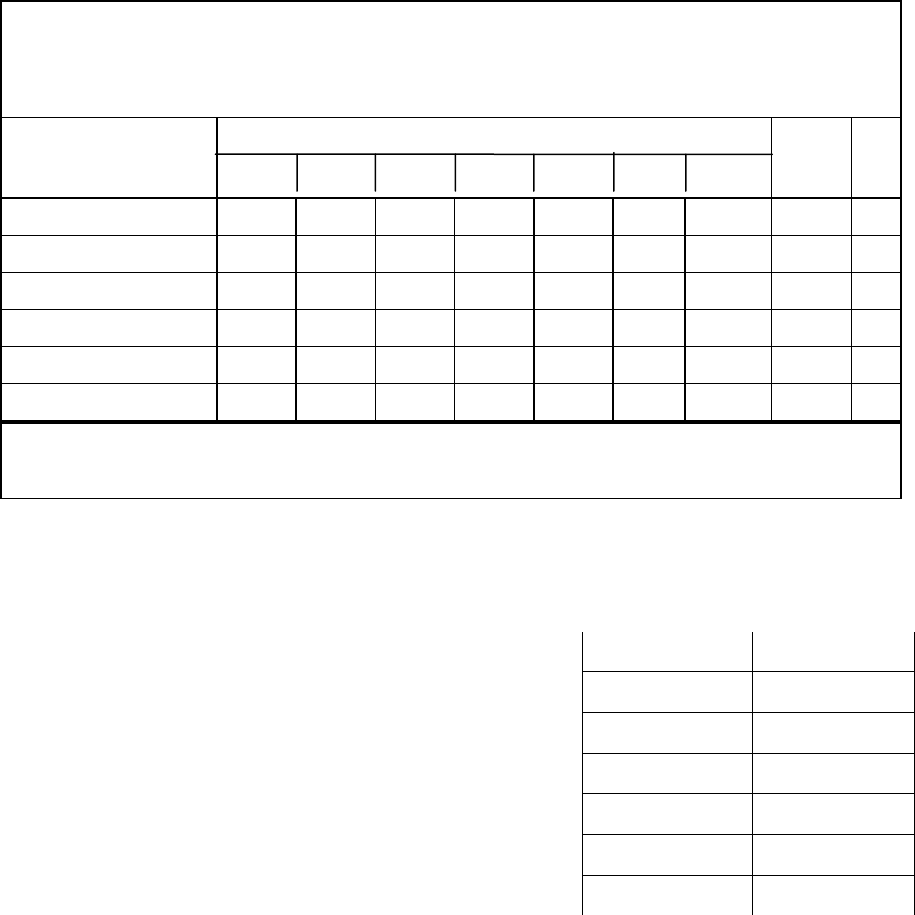
F2.1 MANAGEMENT ACCOUNTING
Page 113
Name:
Clock No.: Rate per Hour
Nature of Work
Hours
Th. Fri. Sat. Mon. Tues. Wed. Total
RWF
Machinery Repairs
Dept A
" B
" C
Machine Cleaning
" Oiling
Sig. ..........................................................
Figure 27: Indirect Labour Record
Examples of Direct and Indirect Labour
Direct
Indirect
Wages of Support Staff
Bonuses
Basic Pay of Indirect Workers
Basic Pay of Direct Workers
Cost of Idle Time
Overtime at Request of Customer Order
F2.1 MANAGEMENT ACCOUNTING
Page 114
O. TREATMENT OF OVERTIME
It is not within the scope of a cost accountant’s duties to decide whether or not overtime
working should be authorised, but he or she must record the cost of such working, analyse the
cause and report the facts to management. Clearly, when a department has had idle time
during normal working hours and has worked overtime, this situation should be referred to
higher management.
There should be a separate column on the pay sheets for overtime so that it is possible to
obtain the total overtime cost quickly.
For employees who are required to work “unsocial hours” it is now common practice to make
shift premium payments as an additional incentive. These are a particular feature of
operations that have to be run on a 24-hour, 365 days of the year basis and, eventually, they
tend to lose their free incentive advantage, once the employee has become used to receiving
them on a regular basis.
The underlying principle for charging overtime is: charge the cost to the cost unit causing the
expense. This may be illustrated as follows:
(a) Job Cost
Charge to individual jobs if customer wishes delivery date to be brought forward and
overtime has to be worked to do so.
(b) General Overhead
This category of overhead account is charged with overtime if general pressure of
business has caused occasional overtime working. It would be unfair to make an extra
charge to those jobs which just happened to be done in the evening.
(c) Direct Labour Cost
On the other hand, if overtime is worked regularly and consistently because of a
shortage of direct workers, it is really part of the normal direct labour cost and should
be treated accordingly. An average hourly rate would be calculated based on the
number of hours at standard rate and the number of hours at premium rates, and all jobs
would be charged with labour at this average rate.
(d) Departmental Overhead
(i) If inefficiency within a particular department has caused overtime then that
departmental overhead account should be charged with the cost.
(ii) If overtime has been worked in Department B because Department A was
inefficient, the cost of overtime in Department B should be charged to the
departmental overhead of Department A.
F2.1 MANAGEMENT ACCOUNTING
Page 115
P. SUMMARY
The information given in this study unit covers a broad spectrum of the recording systems
used. It must be emphasised that each industry has its own problems in recording both
attendance times and work-on-the-job times and that the solutions adopted are likely to be
unique. Great care needs to be taken to ensure that enough data is collected to meet central
requirements without making the procedure so onerous that it becomes inefficient.

F2.1 MANAGEMENT ACCOUNTING
Page 116
BLANK

F2.1 MANAGEMENT ACCOUNTING
Page 117
Study Unit 6
Overheads and Activity Based Costing
Contents
A. Examples of Expenses
B. Notional Expenses
C. Capital Equipment
D. Introduction to Overhead Costs
E. Overhead Allotment
F. Overhead Absorption
G. The Use of Predetermined Absorption Rates
H. Treatment of Administration Overhead
I. Treatment of Selling and Distribution Overhead
J. Activity-Based Costing

F2.1 MANAGEMENT ACCOUNTING
Page 118
A. EXAMPLES OF EXPENSES
So far we have examined two of the components of cost, namely labour and material costs.
The third cost element is expenses, which comprises all items not falling within the other two
categories. Examples therefore include rent, rates, telephone charges, power, royalties
payable to an inventor, depreciation of equipment, etc.
Direct and Indirect Expenses
We saw with both material and labour that such costs could be direct or indirect. For
instance, the wages of a skilled carpenter in a furniture factory are a direct cost, but the wages
of a foreman or of a clerk in the cost office are normally indirect. The distinction is that the
carpenter’s wages can be identified with particular products, whereas the others cannot.
The same distinction applies in the case of expenses, although there are in fact very few
examples of direct expenses. Royalties payable to the inventor of a product are clearly a
direct expense. Another example would be the running cost of a machine used entirely for
one particular product; in practice, however, most machines are used for a variety of products
so their associated costs are indirect expenses.
B. NOTIONAL EXPENSES
Rent
If a business rents its factory, the rent payable is, of course, an expense. Often, even if the
premises are owned and no rent is paid, a notional charge in lieu of rent is included in the cost
accounts. This allows for the fact that the real cost of premises is not only the depreciation of
those premises but also the interest on the capital which is tied up (which a landlord would
allow for in fixing the rent). This permits direct comparison of costs of production between
different sites.
F2.1 MANAGEMENT ACCOUNTING
Page 119
Interest on Capital
It may similarly be argued that the expenses in the cost accounts should include a notional
charge for interest on capital in respect of all manufacturing equipment (regardless of
whether money was in fact borrowed to purchase that equipment). Arguments for and
against this approach are as follows:
(a) In Favour of Including Interest on Capital
(i) Just as wages are the reward for labour, interest is the reward for capital.
Therefore an economist would argue that interest, as well as wages and other
costs, ought to be taken into account in calculating profit.
(ii) False conclusions may be drawn from comparisons if interest is not taken into
account. If one manufacturer makes his own sub-assemblies while another buys
them ready-made, interest on the additional capital which the first manufacturer
has tied up must be taken into account in deciding which of them has taken the
more economical option.
(iii) Interest takes account of the time factor, which is of prime importance in
production.
(b) Against Including Interest on Capital
(i) Interest payments depend on the manner in which the business is financed. One
manufacturer may provide his own capital, while another may decide to raise
loans. The manner of financing does not affect the manufacturing cost but only
the way in which the ultimate profit is distributed (whether used to pay interest on
loans or available for the owner).
(ii) How should interest be calculated? Should the cost of fixed assets alone be used,
or should capital tied up in stocks also be taken into account? What rate of
interest should be used? Problems arise when comparisons are required between
firms in the same industry and in many cases production costs may be widely
different.
(iii) Inclusion will complicate the cost accounts and, if interest is included in stock
valuations in the cost accounts, an adjustment would be required in order to arrive
at stock valuations for the financial accounts.
The arguments against often outweigh the arguments in favour of inclusion of this interest as
an expense. However, when pricing a large order which the manufacturer will have to
finance for a long period before receiving payment, it is reasonable to include an amount to
cover interest on capital.
F2.1 MANAGEMENT ACCOUNTING
Page 120
C. CAPITAL EQUIPMENT
Depreciation
Depreciation is charged in order to apportion the capital cost of a fixed asset over its working
life. Depreciation is often a major part of the total overhead expense, so it is worth looking in
some detail at the methods which are used to calculate it.
There are at least two methods of calculating an annual depreciation charge in common use:
i.e. the straight line method, whereby the capital cost of the machine, less any estimated
residual value at the end of its life, is spread equally over the estimated number of years of
life; and the reducing balance method, in which a percentage of the remaining book value
of the machine is written off each year, so that the charge declines as the asset gets older.
In costing, we want to arrive at a level of annual charge for depreciation and find a means of
apportioning it (along with other costs) to the individual products or jobs. This is done by:
(a) Estimating the number of hours to be worked by the machine per year and dividing the
annual depreciation by this estimated number of hours, to arrive at a machine-hour rate.
(b) Estimating the number of hours to be worked by the machine throughout its life, and
dividing the capital cost, less any estimated residual value, by this number of hours, to
arrive at a machine-hour rate.
(c) Calculating a combined charge for depreciation and repairs, by dividing the capital cost
less residual value plus the total expected repair bill over the asset’s life, by the
estimated number of hours of use. The advantage of this method is that the cost
charged in each year of the asset’s life is the same - the rate does not rise with the
higher repair bills which will arise in the asset’s later years. However, this method may
be impractical, since it is difficult to estimate the total repair bill.
A better approach here is to use the reducing balance method. Indeed, some would
argue that this is one advantage of using the reducing balance method. Consider the
case of a company with only one large machine. It can use either the straight line or the
reducing balance method for depreciation. It is known that with each year of usage,
repair and maintenance costs will increase.
F2.1 MANAGEMENT ACCOUNTING
Page 121
Machine Cost: RWF200,000
Straight Line 10% Reducing Balance 10%
Dep. Rep./Maint. Total Dep. Rep./Maint. Total
RWF RWF RWF RWF RWF RWF
Yr 1 20,000 0 20,000 20,000 0 20,000
2 20,000 2,100 22,100 18,000 2,100 20,100
3 20,000 3,500 23,500 16,200 3,500 19,700
4 20,000 5,600 25,600 14,580 5,600 20,180
5 20,000 7,080 27,080 13,122 7,080 20,202
You will note that in these circumstances straight line depreciation plus repairs and
maintenance will rise each year, whereas reducing balance depreciation plus repairs and
maintenance will have a tendency towards equality each year. (The figures in the
example have been chosen to illustrate this clearly.)
D. INTRODUCTION TO OVERHEAD COSTS
Definition
An overhead cost is defined in the CIMA Terminology as:
“The total cost of indirect materials, indirect labour, and indirect expenses”.
This means those items of material, wages or expense which, because of their general nature,
cannot be charged direct to a particular job or process but have to be spread in some way over
the various jobs or processes.
Identification of Overhead Costs
In considering what is a direct charge and what is an indirect charge, i.e. overhead, regard
must be paid to the type of industry, the method of production and the organisation of the
firm concerned. For instance, in a general machine shop making a variety of products, the
foreman’s wages would be an indirect or overhead charge, as there is no obvious method of
identifying the cost of the foreman’s wages with a particular job; on a building site, the
foreman’s wages would be a direct expense, as they can only relate to the contract in hand.
The Changing Problem of Overhead Costs
50 years ago most labour was manual, and such overhead expense as existed was a
comparatively small proportion of total cost; today the position has changed radically. Direct
F2.1 MANAGEMENT ACCOUNTING
Page 122
labour, as such, becomes an increasingly small proportion of total cost, and overhead
expenses very much larger. This tendency will undoubtedly continue as mechanisation and
automation develop; and the cost accountant must always move with the times, developing
and rearranging information to suit requirements.
We said earlier that a costing system must suit the business; it must suit not only the kind of
business but also the stage of development of the business. A costing system which was
suitable for a car manufacturer 20 years ago is probably not suitable now - because of the
changing relationship between direct labour and overheads and the enhanced information
demands to manage the business.
With automation becoming increasingly important, there is a tendency for overheads to
increase and for prime costs to decrease. The installation of new machines will increase the
depreciation charges and such items as service labour, while fewer workers will be needed to
operate them (direct labour).
Classification by Function
There are three main classifications of overhead: production, administration and selling, and
distribution overhead. These headings are associated with the three main functions of the
business organisation and we should, as a first step, attempt to classify overhead expenditure
into the appropriate categories. Clearly, there are certain items of cost which appertain to all
three, such as electricity, rent and rates, and it will be necessary to break these individual
charges down to the shares appropriate to the main headings.
(a) Production Overhead
Before any business can start producing goods, it must have a building, which has to be
heated, lit, ventilated and provided with energy to operate the machines. The building
must be kept clean and will need repair and redecoration from time to time, and in
addition rent and rates will have to be paid. The products will have to be designed and
production must be planned, supervised and checked. Records have to be kept, wages
calculated, some form of stores must be operated and materials must be conveyed from
point to point within the building.
These functions, and others, are not directly concerned with actual production, but are
nonetheless essential and may be looked upon as services to the actual job of
production. It is the cost of providing these services which constitutes the production
overhead.
F2.1 MANAGEMENT ACCOUNTING
Page 123
Specific examples of this type of overhead are as follows:
(i) Rent and rates of factories and land.
(ii) Insurance and depreciation of plant and machinery, and buildings.
(iii) Salaries of the technical staff.
(iv) Repairs and maintenance of plant and machinery.
(v) Consumable stores used in the factory.
(vi) Holidays, paid sick leave and idle time of factory employees.
(vii) Factory heating and lighting.
(viii) Internal transport expenses.
(The above is not intended to be an exhaustive list.)
(b) Selling and Distribution Overhead
The dividing line between production overhead and selling and distribution overhead
comes when the finished goods are delivered to the finished goods store.
Examples of selling and distribution overhead are:
− Salesmen’s salaries
− Salesmen’s expenses
− Salesmen’s commission
− Advertising
− Samples
− Depreciation of delivery vehicles
− Carriage outwards
− Vehicle drivers’ wages
− Warehouse charges
(c) Administration Overhead
Examples are:
− Office repairs
− Office salaries
− Depreciation of office machinery
− Office heating and lighting
− Postal charges
− Stationery
− Share of rates.

F2.1 MANAGEMENT ACCOUNTING
Page 124
Collection of Overhead
All expenditure as it is incurred is allocated its appropriate code number and is accumulated
against each cost centre. (Remember the definition of “cost centre” given in Study Unit 2.)
This will comprise wages and payments which are incurred at irregular intervals. For
example, rates may be paid either half-yearly or yearly and it is, therefore, possible that
during a shorter period of, for instance, three months, either no expenditure will be incurred,
or, alternatively, a whole year’s expenditure may be included.
We must, therefore, prepare a periodical “expense summary”, which ascertains the total
expenditure to be charged to costs of production in respect of each cost centre. It is necessary
to improve the simple figures of payments made, by providing for expenditure incurred but
not yet paid and for expenditure paid in advance.
Example
Electricity bill of RWF800 per annum paid quarterly in arrears on 28 February (RWF250),
31 May (RWF200), 31 August (RWF100) and 30 November (RWF250).
Rates paid in advance at RWF2,500 (payable 1 April for full year).
As at 30 September the accounts will show:
(a) Electricity payments RWF550
(b) Rates RWF2,500
An apportionment would give:
(a) Electricity
12
9
× RWF800 = RWF600 ∴ financial accrual RWF50.
(b) Rates
12
6
× RWF2,500 = RWF1,250 ∴ financial prepayment = RWF1,250.
F2.1 MANAGEMENT ACCOUNTING
Page 125
E. OVERHEAD ALLOTMENT
Allocation and Apportionment
You should learn the following CIMA definitions of cost allocation and cost apportionment:
(a) Cost Allocation
“The charging of discrete identifiable items of cost to cost centres or cost units.”
(b) Cost Apportionment
“The division of costs among two or more cost centres in proportion to the estimated
benefit received, using a proxy, e.g. square feet.”
As an example of cost allocation, repairs to the building housing the raw materials store could
be allocated directly to the stores department cost centre.
Those items which cannot be allocated must be apportioned. As the definition implies, there
is no single correct way to apportion costs. We have to use the most logical basis possible
with the data at our disposal.
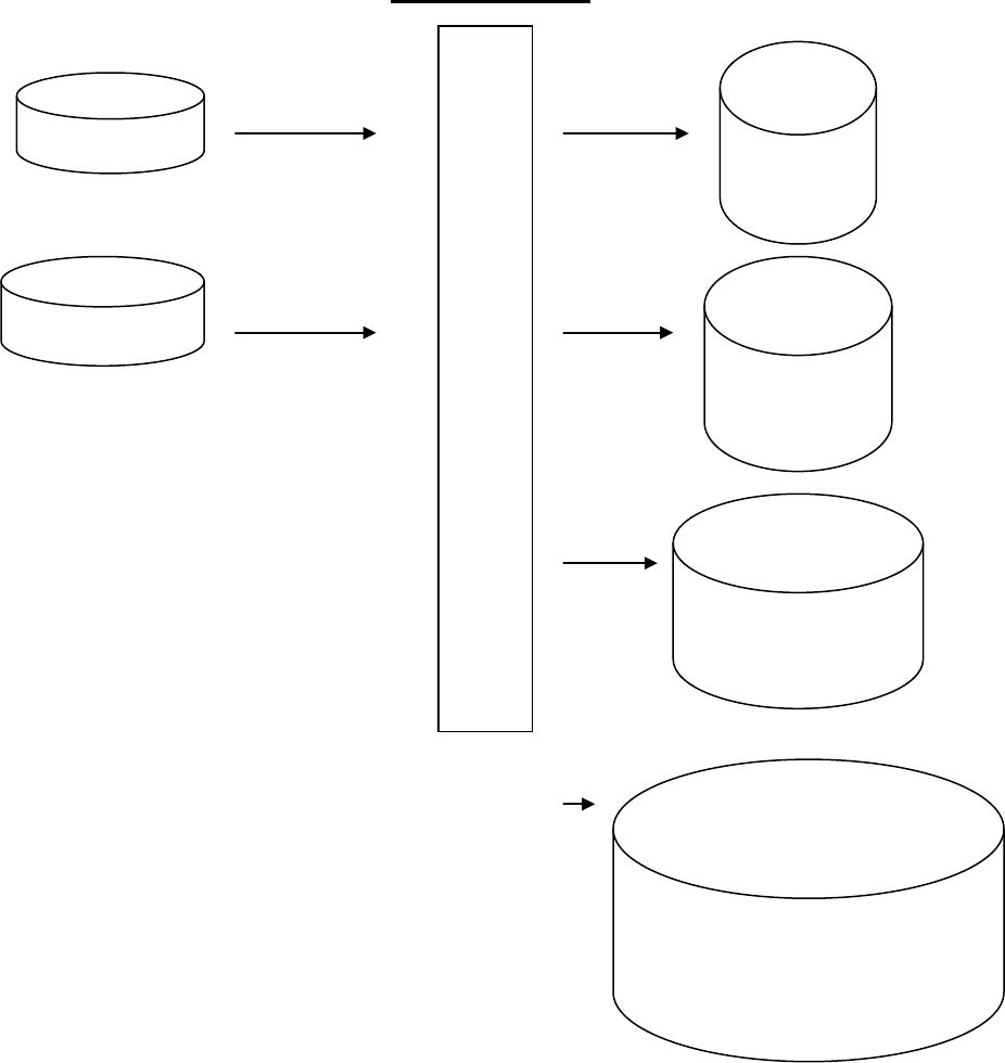
F2.1 MANAGEMENT ACCOUNTING
Page 126
Cost Allocation
Direct Costs
Dept 2
Dept 1
Service Centre
General Overhead Cost
Centre
C
O
S
T
A
L
L
O
C
A
T
I
O
N
Indirect Costs
F2.1 MANAGEMENT ACCOUNTING
Page 127
Cost Apportionment
You will find the following methods of cost apportionment among those used in practice:
(a) Capital Value of Cost Centre
Where cost is increased by reference to the capital value of the cost centre it should be
apportioned in the same way, e.g. fire insurance premium charged by reference to
capital value.
(b) Cost Centre Labour Cost
Where the cost depends on the extent of labour cost of the centre, such as in the case of
employers’ liability insurance premiums, this should also form the basis for the
apportionment of the premium paid.
(c) Cost Centre Area
Where cost depends on the floor area, it should be apportioned in the same way, e.g.
rent and rates.
(d) Cost Centre Cubic Capacity
Where cost is incurred in phase with cubic capacity, it should be spread back on this
basis, e.g. lighting.
(e) Number of Employees at Cost Centre
The cost of providing a canteen service is generally proportional to the numbers
employed, so it is reasonable to apportion it by reference to the number of employees at
each cost centre.
(f) Technical Estimate
The chief engineer of a factory is in a position to estimate how the cost of certain
expenses should be apportioned between the various cost centres of the factory.
Examples of this type of expense are as follows:
(i) Light
The wattage used in each department can be calculated and the cost of lighting
apportioned to each cost centre accordingly.
(ii) Power
The horsepower of machines in each cost centre can be established and the cost of
power apportioned on this basis.
(g) Proportionate to Materials Issued
The expenses of operating the stores department, and “normal” stores losses, may be
apportioned by this method, measuring materials by value, weight or volume, as
appropriate.
(h) Proportionate to Production Hours
There are many items of expenditure which can be apportioned on this basis, although
the figures are usually available only where a fairly comprehensive costing system is in
operation. Either labour hours or machine hours may be used. Items which may be
apportioned on this basis are:
(i) Overtime wages (where not allocated direct).
(ii) Machine maintenance (where not chargeable direct).
F2.1 MANAGEMENT ACCOUNTING
Page 128
Examples
Example 1
Here is an example of overhead allotment.
A company has two production departments, X and Y and three service departments, stores,
maintenance and production control.
The data to be used in apportioning costs is:
Stores
Maintenance
Production
Control
X
Y
Total
Area in sq. m.
300
400
100
3000
4200
8000
Number of
employees
4
12
30
200
300
546
Value of
equipment
(RWF000s)
-
8
-
20
12
40
Electricity
(000 units)
-
20
-
320
210
550
Number of
Extraction
points
1
2
-
14
23
40

F2.1 MANAGEMENT ACCOUNTING
Page 129
We have now arrived at an estimate of the overhead appropriate to each department or cost
centre. However, we really need to express all overhead costs as being appropriate to one or
other of the two production departments, for instance, so that we can include in the price of
our products an element to cover overhead - for it is only in this way that costs incurred will
be recovered. Although costs have been incurred by the service departments, they have
really in the end been incurred for the production departments. The next step is therefore to
re-apportion the costs of the service departments. We do this in a similar way to that used in
the original apportionment.
Additional data is provided: the total number of material requisitions was 1,750, of which
175 were for maintenance department, 1,000 for Department X and 575 for Department Y.
This data will be used to apportion the cost of the stores department to these three
departments. Maintenance costs will be directly allocated to production control and
Departments X and Y. (In practice, a record may be kept of the number of maintenance
hours needed in each department to provide data for cost apportionment.) Production control
costs will be apportioned between Departments X and Y according to the number of
employees in those departments (already given)
Item
Apportionment
Basis
Total
Cost
Stores
Maintenance
Production
Control
X
Y
RWF
RWF
RWF
RWF
RWF
RWF
Rent
Area
800
30
40
10
300
420
Indirect
material
Allocation
174
11
25
44
31
63
Indirect labour
Allocation
5,463
287
671
1,660
1,040
1,805
Factory
administration
Number of
employees
2,184
16
48
120
800
1,200
Machine
depreciation
Value
440
-
88
-
220
132
Power
Electricity
550
-
20
-
320
210
Heat and light
Area
80
3
4
1
30
42
Machine
insurance
Value
40
-
8
-
20
12
Fumes
extraction
plant
Number of
extraction points
120
3
6
-
42
69
9,851
350
910
1,835
2,803
3,953

F2.1 MANAGEMENT ACCOUNTING
Page 130
Item
Basis of
Apportionment
Stores
Maintenance
Production
Control
X
Y
RWF
RWF
RWF
RWF
RWF
Cost b/f from
previous table
350
910
1,835
2,803
3,953
Stores Department
costs re-apportioned
No. of
requisitions
-350
35
-
200
115
Maintenance
Department
costs allocated
Allocation
-
-945
126
263
556
Production control
costs re-apportioned
Number of
employees
-
-
-1,961
784
1,177
TOTAL
Nil
Nil
Nil
4,050
5,801
Note that when a department’s costs are re-apportioned, the cost is credited to that
department.
Having completed the re-apportionment, you will see that the total of overhead now
attributed to Departments X and Y is, of course, equal to the original total of overhead. This
is something you should always check in doing examination questions of this type.
Examiners have been known to include direct costs in the list of costs, to trap the unwary, e.g.
costs such as direct material and production wages. If you are asked to allocate overheads,
ignore direct costs.
In the above example, some of the stores department’s cost was incurred on behalf of the
maintenance department, but not the other way round. When service departments serve each
other as well as the production departments (sometimes called reciprocal services), we must
use repeated distribution to apportion their costs to the production cost centres. An
example follows.
Example 2
A manufacturing company has two production departments (machining and assembly) and
two service departments (tooling and maintenance).
The expenses of the service departments are dealt with as follows:

F2.1 MANAGEMENT ACCOUNTING
Page 131
Tooling 70% to Machining
20% to Assembly
10% to Maintenance
Maintenance 50% to Machining
30% to Assembly
20% to Tooling
Overhead incurred during the month was:
Machining Assembly Tooling Maintenance
RWF RWF RWF RWF
Indirect Material 4,600 5,200 1,800 600
Indirect Labour 6,100 1,200 2,700 1,600
Miscellaneous 700 900 500 300
We are required to apportion all costs to the production departments.
The first stage is to find the total of all the costs incurred. We can then apportion the costs of
each service department in turn until our objective is achieved.
Machining Assembly Tooling Maintenance
RWF RWF RWF RWF
Total 11,400 7,300 5,000 2,500
Service department costs redistributed:
Tooling 3,500 1,000 (5,000) 500
Maintenance 1,500 900 600 (3,000)
Tooling 420 120 (600) 60
Maintenance 30 18 12 (60)
Tooling 9 3 (12) -
RWF16,859 RWF9,341 NIL NIL
(In the above exercise, brackets are used instead of minus signs.)

F2.1 MANAGEMENT ACCOUNTING
Page 132
F. OVERHEAD ABSORPTION
Introduction
Overhead absorption is the allotment of overhead to cost units by means of rates separately
calculated for each cost centre.
In other words, when we talk about the amount of overhead absorbed by a product, we mean
the proportion of the total overhead which we estimate is appropriate to that product.
If all items produced by a department were identical, there would be no problem. We should
simply take the total overhead incurred by each productive department (determined by the
methods already described) and divide it by the number of products made, to arrive at an
overhead rate for the product. In practice, it is rarely as simple as that, for units are not
identical.
The following are methods of overhead absorption found in practice.
Percentage on Prime Cost
This system is still, unfortunately, in widespread use where costing is fragmentary, and it
must not be dismissed until you are quite clear why it is inadequate.
Imagine, a manufacturer asked to make a million pairs of army boots. If the boots cost him
RWF1 to make they would be sold to the government for RWF1.10, so he would have an
income of RWF0.10 per pair to meet general overheads and profits. If, however, he was a
very inefficient manufacturer, so that his boots cost him RWF2 per pair to make, they would
be sold to the government for RWF2.20 and he would have a sum of RWF0.20 to meet
overheads and profits. He had thus a very direct incentive to inefficiency and it is probably
true to say that the need to remedy this abuse was one of the powerful factors contributing to
the development of the cost accounting profession.
The only thing that can be said in favour of this percentage on prime cost is that it is simple
and requires little clerical work, but it would only be approximately true when materials used
on every job were equal in price, wages were uniform throughout (both for skilled and
unskilled labour) and any equipment used was employed equally on all jobs. As these
conditions virtually never apply, the system should virtually never be used.
Formula:
period for thecost Prime
period for the Overhead
× 100
= Percentage of prime cost
F2.1 MANAGEMENT ACCOUNTING
Page 133
Percentage on Direct Wages
This is a slight improvement on “percentage on prime cost”, because fluctuations due to the
varying prices of direct materials are eliminated and, furthermore, there are a few items of
expenditure which can, in fact, be reasonably absorbed on the basis of direct wages. It is still
very unsatisfactory in general, however, and the criticisms against it may be summarised as
follows:
(a) The ratio of wages cost to total hours spent on production may vary considerably where
on one job skilled men are using expensive machines, and on others a large number of
unskilled men are employed without much equipment.
(b) The slower, and therefore usually the more inefficient, worker attracts a larger burden of
overheads.
(c) Where piece rates are used, the overhead recovered per piece will be constant, although
much of this may have been done quickly by expert workers and the other part slowly by
beginners.
Formula:
Overhead for the period
Wages for the period
× 100
= Wages percentage rate
Points in its favour are:
• It is simple and easy to calculate, especially where the costing system is rough and
ready.
• More consideration is given to the time factor.
Percentage on Direct Material
This method has the worst features of the previous two. Only rarely is it found in practice
that overhead is proportionate to material used.
Formula:
Overhead for the period
Direct materials used
× 100
= Material percentage rate
F2.1 MANAGEMENT ACCOUNTING
Page 134
Absorption on Basis of Time
Anyone who has had any experience of costing will have concluded that much overhead
expenditure is, above all else, subject to the time factor in its relation to output. If one article
takes twice as long to go through the factory as another, it should attract to itself twice the
charge for lighting the factory as the other product, and this is only one example which you
can probably multiply many times out of your own experience. It is generally true, therefore,
that by far the most valuable method of apportioning overhead is on a time basis, and this is
usually of one of two kinds, a direct labour-hour rate and a machine-hour rate.
Occasionally a combination of both these will be in operation and a composite rate per
production hour may be used.
(a) Direct Labour-Hour Rate
Where this system is used, the number of hours of direct labour worked at a production
centre is estimated, and the number divided into the total figure shown in the expense
summary for that production centre (or costing department) for the corresponding
period. The resultant figure gives an amount to be added to the direct cost of the output
for every hour of the direct labour used throughout.
Hours may be either the number of hours expected to be worked, or the number of
hours which would relate to working at normal capacity.
This is a very satisfactory method, particularly where a production centre uses little
elaborate or expensive machinery, and when it may reasonably be said that every hour
of direct labour absorbs the same amount of expense. You must remember, however,
that separate direct labour-hour rates should be calculated for each production centre
and that holidays should be excluded, as should overtime hours, except when this is a
regular recurring feature.

F2.1 MANAGEMENT ACCOUNTING
Page 135
The advantages of this system are as follows:
(i) The result is not invalidated by use of skilled and unskilled labour.
(ii) Proper provision is made to deal with fast and slow workers who are paid piece
rates.
(iii) The figure of labour hours is a more useful guide to the management than the
value of wages paid, because fluctuations due to varying overtime rates and
wages increases are avoided.
Formula:
Overhead for the period
Direct labour hours worked or budgeted to be worked in the period
= Direct labour-hour rate
(b) Machine-Hour Rate
Where machinery rather than labour is the dominant feature of a production centre, a
rate of overhead per hour of machine time should be substituted for a rate per direct
labour hour.
The “machine-hour rate” is defined as:
“A rate calculated by dividing the budgeted or estimated overhead or labour, and the
overhead cost, attributable to a machine or group of similar machines by the
appropriate number of machine hours.
The hours may be the number of hours for which the machine or group is expected
to be operated, the number of hours which would relate to normal working for the
factory, or full capacity.”
To find this machine-hour rate, it is necessary to estimate the number of hours of
operation of the machine or machines in the cost centre during the period under
consideration. Allowance must be made for idle time and for cleaning and setting-up
time. The total expense is then divided by the number of working machine hours.

F2.1 MANAGEMENT ACCOUNTING
Page 136
As an example, let us return to Example 1 in Section E of this study unit. After the
service department’s costs had been re-apportioned, the costs attributed to the
production departments X and Y were RWF4,050 and RWF5,801 respectively.
Now suppose that Department X has five identical machines working 162 hours each
during the period under consideration.
Department Y is not automated and has 20 direct workers, each working 160 hours
during the period.
The total number of machine hours worked in Department X is 5 × 162 = 810 hours.
Therefore the machine-hour rate is:
RWF
4 050
810
,
= RWF5 per machine hour
The total number of direct labour hours worked in Department Y is 20 × 160 = 3,200
hours. Therefore the labour-hour rate is:
RWF
5 801
3 200
,
, = RWF1.81 per direct labour hour
Suppose that the manufacture of an article takes four machine hours in Department X.
It is then passed to Department Y for hand-finishing, which takes six hours. Then the
amount of overhead absorbed by this article is:
RWF4 × 5 (Department X) + RWF6 × 1.81 (Department Y)
= RWF30.86
In determining the total cost of the article, this sum would be added to the cost of the
direct materials, direct labour and direct expenses incurred.
In the illustration above, only one hourly rate has been calculated for each department.
In practice, fixed and variable overhead will, if possible, be kept separate, and a
separate absorption rate calculated for each.
F2.1 MANAGEMENT ACCOUNTING
Page 137
(c) Machine-Hour Rate Where Machines Are Not Identical
In the above illustration the department operated identical machines. Where the
machines are not identical, however, it is necessary to calculate the rate for each
machine separately. You can apply the following principles:
(i) Some expenditure can be directly allocated to the particular machine, e.g. power,
cost of repairs, depreciation.
(ii) Overhead chargeable to the production centre in which the machine is located,
and not to the individual machine, e.g. rent, rates, heating, is apportioned on the
basis of area occupied.
Example
Using the data below, you are required to calculate a machine-hour absorption rate for
multi-drilling machine no. 5.
Relating specifically to machine no. 5
Original cost: RWF13,300
Estimate life span: 10 years
Estimated scrap value after 10 years: RWF300
Floor space occupied: 250 square metres
Number of operators: 2
Estimated running hours: 1,800 per annum
Estimated cost of repairs: RWF240 per annum
Estimated cost of power: RWF1,000 per annum
Relating to the department in which machine no. 5 is situated
Floor area: 5,000 square metres
Number of operators: 60
Rent: RWF4,400 per annum
Supervision: RWF3,600 per annum
Solution
In addition to the costs specifically relating to machine no. 5, the following apportioned
costs must be taken into account:
(i) Rent - on the basis of floor area occupied.
(ii) Supervision - on the basis of number of operators for machine no. 5 compared
with the number employed in the whole department.

F2.1 MANAGEMENT ACCOUNTING
Page 138
Therefore the total costs appropriate to machine no. 5 are as follows:
RWF per annum
Depreciation: RWF
10
RWF300 300,13 −
1,300
Rent (
1
20
of department’s cost) 220
Supervision ( 1
30
of department’s cost) 120
Repairs 240
Power 1,000
Total RWF2,880 per annum
Therefore the machine-hour rate is:
RWF
2 880
1 800
,
,
= RWF1.60 per machine hour
G. THE USE OF PREDETERMINED ABSORPTION RATES
Introduction
In the examples considered so far, we have been dealing with a known total of overhead
which we have allocated or apportioned to cost centres and hence to cost units. In practice,
of course, costs are being incurred while production is taking place, so that total costs are not
known until the end of the period. But management needs timely information on product
costs as they are being incurred. To overcome this problem, predetermined overhead rates
are used. These are based on estimated overheads and estimated production levels. Each job
then absorbs overhead at the predetermined rate.
Overhead Adjustment Account
At the end of each period it is necessary to compare the overhead which has been absorbed
with that actually incurred. Almost certainly there will be differences. Overhead will have
been over-absorbed if the production level was greater than anticipated, or if overhead costs
were lower than anticipated. Conversely, overhead will have been under-absorbed if the
production level was lower than anticipated or overhead costs were greater.
F2.1 MANAGEMENT ACCOUNTING
Page 139
The overhead over- or under-absorbed each month is transferred to an overhead adjustment
account, and at the end of the year the net amount over- or under-absorbed is transferred to
profit and loss account. This method is preferable to the alternative of carrying forward a
balance on the overhead account each month, although this alternative method is acceptable if
the under- or over-absorption is caused purely by seasonal fluctuations where an average
annual rate of overhead absorption is in use. In this case, there will be under-absorption in
some periods and over-absorption in other periods because of the seasonal factors, but the net
effect over a year will be nil. Nevertheless, since a cost accountant will rarely be in a
position to say that all under- or over-absorption is due to seasonable factors, it is still
considered preferable to operate an overhead adjustment account.
Example
In a period in which 1,600 direct labour hours are expected to be worked, fixed overheads are
expected to be RWF20,000. In fact only 1,550 direct labour hours are worked and the actual
overhead incurred is RWF19,750.
The predetermined rate for absorption of overhead is RWF12.50 per direct labour hour
600,1
000,20
RWF
. Thus, for instance, a job which took 20 hours to complete would absorb
RWF250 fixed overhead.
Because 1,550 direct labour hours are worked, the amount of overhead which has been
absorbed by the end of the period is 1,550 × RWF12.50 = RWF19,375.
Comparing this with the actual overhead incurred, we see that overhead has been under-
absorbed by RWF375.
Extracts from the relevant accounts are shown below:
OVERHEAD CONTROL
RWF
RWF
Incurred
19,750
Work-in-progress - absorbed
overhead
19,375
Overhead adjustment - under-
absorbed overhead
375
RWF19,750
RWF19,750
F2.1 MANAGEMENT ACCOUNTING
Page 140
WORK-IN-PROGRESS
RWF
RWF
Direct material
Transferred to finished
Direct labour
goods stock
Overhead absorbed
19,375
OVERHEAD ADJUSTMENT
RWF
RWF
Overhead control - under-
Profit and loss
375
absorbed overhead
375
RWF375
RWF375
Analysis of Under-/Over-Absorbed Overhead
In the last section we arrived at a figure of RWF375 for under-absorbed overhead. It would
be useful to management to know the reasons for this under-absorption.
From the above workings, we know that the amount of overhead absorbed is RWF19,375.
Had the expected number of hours been worked, overhead absorbed would have been
RWF20,000.
Therefore, because of the shortfall in hours worked, there is under-absorption of RWF625.
However, this is offset by RWF250 because the overhead bill of RWF19,750 is less than
expected.
To summarise: RWF
Under-absorption owing to shortfall in hours 625
Over-absorption owing to lower total cost 250
Net under-absorption RWF375
“Blanket” Overhead Absorption Rates
Overhead absorption rates should preferably be calculated separately for each department.
However, a “blanket” rate for the whole factory may be acceptable in the following
circumstances:

F2.1 MANAGEMENT ACCOUNTING
Page 141
(a) Where only one product is manufactured.
(b) Where there are several products but they use approximately equal amounts of the
services of all departments.
(c) Where overhead forms a small proportion of total cost, and the extra work involved in
calculating departmental absorption rates would not be worthwhile.
H. TREATMENT OF ADMINISTRATION OVERHEAD
It is not generally worthwhile to attempt to be too scientific in apportioning administration
costs to products. For pricing purposes, the inclusion of an agreed percentage on production
costs will generally be adequate. For other purposes, there is no need to absorb
administration costs into product costs: instead they can be treated as period costs to be
written off in the profit and loss account.
I. TREATMENT OF SELLING AND DISTRIBUTION
OVERHEAD
Variable Elements
Some elements of selling and distribution overhead vary directly with the quantities sold - for
instance, commission of so much per unit paid to a salesman. Such items can be charged
directly to the product concerned in addition to the production cost.
Fixed Elements
Other items are incurred whether products are sold or not - for instance, rent of showrooms,
salaries of salesmen. Such items may be treated as period costs and written off in the profit
and loss account or may be absorbed in one of three ways:
(a) Percentage on Sales Value
Selling overheads for year RWF250,000
Estimated sales value for year RWF2,500,000
Absorption rate =
Cost
Activity
× 100 =
250 000
2 500 000
,
, ,
× 100 or 10%

F2.1 MANAGEMENT ACCOUNTING
Page 142
In this case, we add 10% of the sales value of the cost unit to the cost to cover selling
overheads.
This method is useful when prices are standardised and the proportions of each type of
article sold are constant.
(b) Rate per Article
Selling overheads for year RWF250,000
Number of articles to be produced 1,000,000
Absorption rate =
Cost
Activity
or
250 000
1 000 000
,
, ,
or RWF0.25 per article
For each article produced, 0.25rwf is added to the cost.
The method is particularly applicable where a restricted range of articles is produced,
but it can be used for an extended range by evaluating different sizes using a points
system.
(c) Percentage of
Selling overheads for the year RWF250,000
Estimated production cost of sales for year RWF2,000,000
Absorption rate =
Cost
Activity
× 100 =
250 000
2 000 000
,
, ,
× 100 = 12½%
12½% of production cost of each unit is calculated and added to that cost.
Care must be taken in applying this method. For instance, suppose a company makes
two products, A and B. A costs twice as much as B to produce. Therefore, a
percentage on production cost basis would charge A with twice as much selling and
distribution overhead as B. However, it may very well be that there is a ready market
F2.1 MANAGEMENT ACCOUNTING
Page 143
for A, so there is no need to advertise it, whereas B is in competition with others and
the company spends RWF10,000 on advertising B. It is therefore clearly incorrect to
charge A with twice the overhead which is charged to B. Indeed, the advertising cost
should have been charged directly to B. The method is, however, acceptable if the
costs involved are small, or if there is a limited range of products and those costs which
do not vary with the cost of production can be charged direct.
J. ACTIVITY-BASED COSTING
What is Activity-Based Costing?
The two traditional costing methods are absorption costing and marginal costing, as we have
seen. Absorption costing allocates and apportions all overheads to products. In order to do
this, companies must allocate and apportion service overheads to the main production
departments. Direct labour and/or machine-hour rates are then derived, which are used to
calculate the overheads attributable to each product. The approach was developed in the
early part of the 20th century and assumes that overheads directly relate to the level of
production. This is not always the case under current production methods, as factors such as
sales mix, complexity, range and production techniques all influence overhead costs. The
method of apportionment can also seem arbitrary and the resulting product costs are
sometimes difficult to interpret.
Marginal costing, on the other hand, makes no attempt to apportion overheads and a
product’s marginal cost only includes direct material, direct labour and directly attributable
overheads. Sales less marginal cost establishes the company’s contribution, which should be
managed in such a way that it covers all fixed overheads and generates the required level of
profit. Critics of this approach point to the danger of not apportioning all overheads to
products and the possibility that these costs will not be recovered in selling prices. As a
result, the company may drift into loss and eventually go out of business.
Absorption costing requires a lot of time and energy put into the basis of overhead allocation
and apportionment but often the factors leading to the generation of these costs are obscured.
Marginal costing tends to ignore these fixed overheads and relies on budgets to control cost
levels. Activity-based costing provides an alternative approach to the treatment of fixed
overheads. It focuses on the activities that generate overheads and the factors, or cost
drivers, that cause costs to change. These cost drivers are at the heart of ABC and are used
to determine the basis of overheads attributable to each product. Attention is focused on each
activity and the factors that cause cost levels to change. In consequence, the nature of each
cost will be better understood and increased control and better decisions should result.
F2.1 MANAGEMENT ACCOUNTING
Page 144
Terms used in Activity-Based Costing
⇒ Activity: Discrete services or related tasks which are carried out repeatedly.
⇒ Cost Driver: The factor or event which causes a cost to occur.
⇒ Cost Pool: All the costs incurred when an activity takes place.
• Professors Kaplan and Cooper of Harvard University created the idea of activity based
costing. It was designed to deal with the problem of allocating costs to output where
such costs are not related to volume of production.
• In the traditional methods overheads are apportioned to output using a basis such as
machine hours.
• For every cost driver the cost per unit of activity is calculated and this is then used to
divide costs into individual cost units.
Examples of: Activities & Cost Drivers Used
− Purchasing Dept
− No. of Invoices
− Accounting Dept Costs
− No. of Accounting Reports
− Set up Costs
− No. of Manufacturing Set Ups
− Engineering Dept. Costs
− No. of Production Orders
Advantages of Activity-Based Costing (ABC)
• Better basis for cost apportionment.
• Overheads are traced to the product.
• ABC brings attention to cost behaviour and helps in the reduction of costs.
• ABC provides a useful means of getting financial and non financial data.
• More realistic product costs.
• Forces managers to consider the drivers of cost in their business.
Disadvantages of Activity-Based Costing
• Difficulty in picking cost drivers.
• Very time consuming.
• The problem of common costs.
• A full ABC systems having numerous cost pools and cost drivers is more complex and
more expensive to operate.
The stages involved in ABC are:
(a) Identify the activities that cause overheads to be incurred.
(b) Change the accounting system so that costs are collected by activity rather than by cost
centre.

F2.1 MANAGEMENT ACCOUNTING
Page 145
(c) Identify the factors that cause each activity’s costs to change. These factors are the cost
drivers.
(d) Establish the volume of each cost driver.
(e) Calculate the cost driver rates by dividing the activity’s cost by the volume of its cost
driver.
(f) Establish the volume of each cost driver required by each product.
(g) Calculate overheads attributable to each product by multiplying (f) by (e).
ABC concentrates on the activities which are essential in order that services are provided or
goods produced. All related costs are charged to the activity and each activity is itself
necessary for the final product to be produced. Examples could be:
• Personnel department costs
• Material handling
• Spare parts administration.
These activities are known as “cost drivers” (defined as “an activity that generates cost”).
Having separated expenses into these cost drivers, then the most appropriate method of
allocation is determined for each cost driver and used. For example, the total cost of the
personnel department might well be allocated on the basis of numbers of personnel in each
cost centre, etc.
By having different activity costs, each having different methods of allocation, it is argued
that the allocation/apportionment task is refined and, being less arbitrary, more correctly
reflects “true cost”.
The following example will illustrate how this works.

F2.1 MANAGEMENT ACCOUNTING
Page 146
Worked Example
One of the findings of companies that have used ABC is that high-volume production tends
to be over-costed, whilst low-volume, small-batch work is often under-costed. This probably
results from the additional overheads associated with short production runs not being
adequately reflected in the company’s costing system. Our example will therefore consider
two products. Product X is manufactured in long production runs, whilst Product Y has more
components, greater variety and is manufactured in small batches.
Product X
Product Y
Monthly production
5,000
6,000
Direct material costs
RWF
RWF
Department A
4.00
5.00
Department B
4.00
4.00
Department C
2.00
3.00
RWF10.00
RWF12.00
Direct labour costs
RWF5.00
RWF7.00
Machine-hours
Hrs
Hrs
Department A
0.50
0.60
Department B
0.50
0.90
Department C
0.25
0.50
Overheads
RWF
Production Department A
20,000
Production Department B
15,000
Production Department C
10,000
Purchasing
6,000
Production control
5,000
Tool-setting
12,000
Maintenance
3,000
Quality control
4,000

F2.1 MANAGEMENT ACCOUNTING
Page 147
Product Costs Calculated Using Absorption Costing
The first step is to apportion the service department overheads to the production departments.
In this example we will use the following basis of apportionment:
RWF
Purchasing
6,000
Direct material costs
Production control
5,000
Direct material costs
Tool-setting
12,000
Direct material costs
Maintenance
3,000
Machine-hours
Quality control
4,000
Machine-hours
The monthly material costs and machine-hours can be calculated from the previous data, and
are presented on the following page.
Dept A
Dept B
Dept C
Total
Machine-hours
Product X
2,500
2,500
1,250
6,250
Product Y
3,600
5,400
3,000
12,000
6,100
7,900
4,250
18,250
Departmental % of total
33.4%
43.3%
23.3%
100.0%
Direct Material
Product X
20,000
20,000
10,000
50,000
Product Y
30,000
24,000
18,000
72,000
50,000
44,000
28,000
122,000
Departmental % of total
41%
36%
23%
100%

F2.1 MANAGEMENT ACCOUNTING
Page 148
The overhead analysis sheet apportioning service department overheads to production
departments can now be prepared:
Overheads
Department
RWF000
Basis
A
B
C
Production Department A
20
20.0
Production Department B
15
15.0
Production Department C
10
10.0
Purchasing
6
Material
2.4
2.2
1.4
Production control
5
Material
2.1
1.8
1.1
Tool-setting
12
Material
4.9
4.3
2.8
Maintenance
3
M/C
hours
1.0
1.3
0.7
Quality control
4
M/C
hours
1.3
1.7
1.0
75
31.7
26.3
17.0
The machine-hour rates are therefore:
Cost
RWF
Machine-hours
Rate
RWF
Dept A
31,700
6,100
5.20
Dept B
26,300
7,900
3.33
Dept C
17,000
4,250
4.00
Overheads apportioned to each product under a traditional product costing system can be
calculated by multiplying the product’s machine-hours by the appropriate departmental rate.
The answer to these calculations is presented next.
Product X
RWF
Product Y
RWF
Dept A
2.60
3.12
Dept B
1.67
3.00
Dept C
1.00
2.00
5.27
8.12
This example has been simplified but is not untypical of systems found in practice.
Overheads are apportioned to products based on a machine-hour rate, which in this example
does not take into account the fact that Product Y is manufactured in small batches requiring
additional tool-setting, production control and quality control effort.
F2.1 MANAGEMENT ACCOUNTING
Page 149
Product Costs Calculated Using ABC
An activity-based costing method would regard these costs as activities that can be
controlled, and seek to identify the cost drivers that determine the cost levels. These cost
drivers may not necessarily be the number of items produced and in this example we will
assume they are as follows:
Activity
Cost Driver
Purchasing
Number of orders
Production control
Number of components produced
Tool-setting
Number of tool changes
Maintenance
Machine-hours
Quality control
Number of components inspected
Production Department A
Machine-hours
Production Department B
Machine-hours
Production Department C
Machine-hours
In order to keep this example simple, it is assumed that the production department overheads
are directly related to machine-hours worked. In practice it would be possible to divide each
department into a number of different activities, each with its own cost driver.
The additional information required to calculate activity-based costs is:
Product X
Product Y
Total
Number of orders
300
900
1,200
Components produced
15,000
48,000
63,000
Components inspected
2,000
11,000
13,000
Machine-hours
6,250
12,000
18,250
Tool changes
10
60
70

F2.1 MANAGEMENT ACCOUNTING
Page 150
The cost driver rates are calculated below:
Overheads
RWF
Cost Driver
Volume
Rate
Production Department A
20,000
6,100
3.28 per m/c hr
Production Department B
15,000
7,900
1.90 " " "
Production Department C
10,000
4,250
2.35 " " "
Purchasing
6,000
1,200
5.00 per order
Production control
5,000
63,000
0.08 per part
Tool-setting
12,000
70
171.43 per change
Maintenance
3,000
18,250
0.16 per m/c hr
Quality control
4,000
13,000
0.31 per
inspection
The overhead rate per product under activity-based costing becomes:
Product X
Product Y
Rate
RWF
Volume
Overhead
RWF
Volume
Overhead
RWF
Dept A
3.28
2,500
8,200
3,600
11,808
Dept B
1.90
2,500
4,750
5,400
10,260
Dept C
2.35
1,250
2,938
3,000
7,050
Purchasing
5.00
300
1,500
900
4,500
Production control
0.08
15,000
1,200
48,000
3,840
Tool-setting
171.43
10
1,714
60
10,286
Maintenance
0.16
6,250
1,000
12,000
1,920
Quality control
0.31
2,000
620
11,000
3,410
21,922
53,074
Quantity produced
5,000
6,000
OVERHEAD PER
PRODUCT
RWF4.38
RWF8.85
Product Y’s cost is greater than that obtained from the traditional absorption costing method
and reflects the additional costs involved in its manufacture.
Further Considerations
The ABC approach to ascertaining cost of production was introduced as an important
innovation in management accounting in the 20th century. It is a further development in
relating overhead expenses to production.
F2.1 MANAGEMENT ACCOUNTING
Page 151
Over recent years, rapid changes in methods of production have resulted in direct labour costs
per unit of output being reduced. More expenditure is now indirect overhead not directly
related to units of production.
In marginal costing the only variable activity considered is volume of sales. It is established
that, at a certain level of production and sales, a breakeven point will be reached; the
contribution per unit thereafter is related to profit. In the case of absorption costing, overhead
costs are absorbed in the most logical way by units of production. Allocation and absorption
is achieved arbitrarily but as logically as possible. As overheads have become a greater
proportion of total production cost, any arbitrariness in how they are charged to products
becomes more significant.
In activity-based costing the overheads are considered to be related to the use made by
production of the facilities (cost drivers) responsible for incurring them. This is considered a
more logical way to obtain accurate information on the cost of production. The advocates of
ABC consider the following points in promoting this approach:
• It provides more accurate product costs, which should enable the management to make
decisions on pricing, most profitable product mix etc. in a more logical manner.
• It is argued that production resources are more efficiently utilised.
• It extends the variable cost approach to short-term and long-term costs and volume
changes. This is because these costs are related to the activities and not only to volume
of production.
• Costs are considered in more detail as to whether they add value to production or not.
In this way management can achieve better cost control.
• The management will have better understanding of the economics of production and of
activities performed by the company.
Although ABC is a better approach in relating overheads to production, it is still an arbitrary
method. It is in a sense an extension of absorption costing, as ABC product costs are full
absorption costs. ABC can be applied to all costs incurred in an organisation, not only
production costs. It is being used increasingly in service organisations such as hotels, schools
and hospitals.
ABC in Service Industries
The nature of the ‘product’ in service industries means that the cost structure typically differs
from manufacturing industries. Direct costs tend to be a smaller proportion of total cost,
because the direct material content of a service is usually small. The direct labour content of
a service can, however, be significant.

F2.1 MANAGEMENT ACCOUNTING
Page 152
The impetus for the application of ABC in service industries is mainly a desire for more
understanding of the costs of providing services, as an aid to decision-making and cost
control. There may be a tendency in service industries to view all costs as overheads, bearing
no direct relationship to the level of service provided. This results in cost control being
aimed at the inputs to the process rather than the outputs, so it will be relatively ineffective.
The application of ABC in service industries requires clear specification of what services are
provided, so that the activities driven by and underpinning the services can be specified.
Examples of cost units used in service industries could include:
Business
Cost unit
Healthcare (hospitals)
(a) Bed occupied (b) Out-
patient
Hotel & catering
Room/cover
Professional services (accountants, architects,
lawyers)
Chargeable hour
Education
(a) Enrolled student (b)
Successful student
(c) School meal
These cost units could be refined to reflect significant differences in the activities and drivers
relating to them. One hospital changed its cost unit on adopting an ABC approach. The
initial unit was a patient-day, but analysis of the activities necessary to provide a patient-day
revealed a range of activities falling into two broad categories: those relating to the nursing
care a patient received, and those relating to bed occupancy. The latter category, such as the
provision of ward cleaning services and patients’ meals was mainly driven by the number of
beds, and these activities were largely independent of the specific types of patient occupying
the beds. The nursing care activities, however, were driven by the medical needs of
particular types of patient. On the change of cost unit, every ward’s head nurse rated each
patient and arrived at a level of ‘acuity’ on a five-point scale. The ‘acuity’ rating was the
driver for the cost of nursing activity, and was used both in charging patients for their
hospital stay, and in preparing a flexible budget for nursing costs in each ward.
The solution in this instance of the hospital is compatible with the approach of a traditional
costing system - it equates to a manufacturing company changing from a plant-wide
absorption rate to cost-centre absorption rates. However, this does not indicate a general
compatibility between the traditional and the ABC approach in service industries.
A key factor in the ABC approach is the recognition of cost at levels other than the unit
level. The cost of making a bed available is largely a facility-level cost, while the cost of
providing nursing care to patients at a particular sickness level is a unit-level cost, i.e. it will
increase as the number of patients with this level of sickness increases. ABC and traditional
costing result in the greatest differences when cost drivers are batch- and product-related,
rather than unit- and facility-related.
F2.1 MANAGEMENT ACCOUNTING
Page 153
In some service industries, e.g. public relations, the specific output may be difficult to
identify and quantify. Where there are multiple outputs, identifying support activities with
particular outputs may be even more difficult. Even strong advocates of ABC acknowledge
that the costs of applying it in such circumstances may well outweigh the benefits. For
example, a hotel may incur significant costs in tending its gardens and maintaining communal
areas. Allocating these facility-sustaining common costs to particular ‘products’, such as
overnight stays, must be largely arbitrary.
However, ABC can be very suitable for the service sector in identifying customer
profitability rather than ‘product cost’. Customer focus is vital in service industries -
customers may make very different demands even when using the same ‘product’. In some
cases common costs may be more easily identified with customers than products; e.g. a hotel
swimming pool may be used more by families than by business people, even though both
types of guest are being provided with overnight accommodation. An ABC analysis of
customer profitability in service industries may yield valuable information to assist
management in, for example, price-setting.

F2.1 MANAGEMENT ACCOUNTING
Page 154
BLANK

F2.1 MANAGEMENT ACCOUNTING
Page 155
Study Unit 7
Job Costing/Batch Costing
Contents
A. Introduction
B. Factory Job Costing
C. Introduction to Batch Costing
D. Calculation of Cost per Unit
E. Product Line Information
F. Batch Production Versus Continuous Production
G. Example
H. Economic Batch Quantity
F2.1 MANAGEMENT ACCOUNTING
Page 156
A. INTRODUCTION
In management accounting systems, costs are usually accumulated to meet both external
management needs and external reporting requirements.
Examples of these are: -
Internal Management Needs: – Pricing decisions
Determining Product Range
Performance of departments
External Reporting Requirements – Inventory Valuation.
The method of accumulating the cost data depends on the type of product or service the
company offers.
Job costing is a method of costing used when cost units can be separately identified and need
to be costed individually.
It’s essential features are: -
(a) Each job can be accurately identified.
(b) Direct costs are charged directly to each job.
Typical application of job costing can be seen in the engineering, shipbuilding, construction
and printing industries.
F2.1 MANAGEMENT ACCOUNTING
Page 157
The classification can be further broken down depending on the duration of the job and the
number of individual units to be produced. The main types of job costing and their principal
features are: -
“Factory” Sub Costing
-
Comparatively short duration.
-
Usually carried out in factory, e.g. furniture, machinery
Batch Costing
-
Similar to above but with larger number of units
produced, e.g. production of component parts for bulk
orders.
The job to which costs are assigned is the Batch of units
produced.
Contract Costing
-
The duration is usually greater than 1 year. Typical use
would be in the construction field, e.g. housing, roads,
bridges, etc.
While these three costing situations may be regarded as very distinct from one another they
all possess the characteristics of job costing.
B. FACTORY JOB COSTING
Although reference has been made to manufacturing industries the costing technique can
apply to the service industries such as vehicle repair, costing of audits and research projects.
Below is a brief outline of the practical procedures involved in the setting up of a job.
(a) A prospective customer approaches the supplier requesting a tender for goods to be
supplied.
(b) The supplier agrees precise details of items to be supplied, e.g. quantity, quality, size,
colour, delivery date, and any special requirements.
(c) The suppliers estimating department prepares a price for the job.
This will include direct costs, appropriate overheads and where appropriate the cost of
any additional equipment required specially for the job.
(d) Finally, the suppliers profit margin is added to give the quoted selling price.
The following is a typical job costing: -

F2.1 MANAGEMENT ACCOUNTING
Page 158
Job No. 1234
As newly appointed chief cost clerk, you find that the selling price of Job No. 1234 has
been calculated on the following basis:
RWF
Materials
12.09
Direct wages (22 hours @ RWF0.25 per hour)
5.50
(Dept A – 10 hours
Dept B – 4 hours
Dept C – 8 hours)
17.59
Plus 33⅓% on prime cost
5.86
RWF23.45
An analysis of the previous year’s Profit and Loss Account shows the following:
RWF
RWF
Materials used
77,500
Sales
135,000
Direct wages -
Dept A
5,000
Dept B
6,000
Dept C
4,000
15,000
Factory
overhead:
Dept A
2,500
Dept B
4,000
Dept C
1,000
7,500
Gross profit c/d
35,000
RWF135,000
RWF135,000
Selling costs
30,000
Net profit
5,000
Gross Profit
b/d
35,000
RWF35,000
RWF35,000

F2.1 MANAGEMENT ACCOUNTING
Page 159
REQUIREMENT:
(i) Draw up a job cost sheet.
(ii) Add to the total job cost 10% for profit and give the final selling price.
Work to the nearest cent.
Job No. 1234 – Solution
Job Cost Sheet
(i)
RWF
RWF
Materials used
12.09
Department A
Direct wages 10 hrs @ RWF0.25
2.50
Departmental overhead 50% of wages
1.25
3.75
Department B
Direct wages 4 hrs @ RWF0.25
1.00
Departmental overhead 66⅔% of wages
0.66
1.66
Department C
Direct wages 8 hrs @ RWF0.25
2.00
Departmental overhead 25% of wages
0.50
2.50
FACTORY COST
20.00
Selling overhead 30% on factory cost
6.00
TOTAL COST
RWF26.00
(ii)
Total cost
RWF26.00
Add: 10% profit margin
2.60
SELLING PRICE
RWF28.60

F2.1 MANAGEMENT ACCOUNTING
Page 160
Notes:
(i) Generally the principal types of material would be listed.
(ii) Dept. A overhead calculated as a rate per hour as follows:
Total Overhead
=
2,500
= 50%
Total Wages
5,000
(iii)
Dept. B overhead =
4,000
= 66⅔%
6,000
(iv)
Dept. C overhead =
1,000
= 25%
4,000
(v)
Selling overhead (calculated as a %
of cost of sales) =
Total selling cost
Total factory costs
=
30,000
= 30%
100,000
(e) If accepted, the job is allocated a unique job number, a material requisition is sent to
stores and a purchase requisition prepared for any special materials or equipment
required. A job card is raised setting out the stages of work to be performed and an
advice is sent to personnel if specialised labour is required.
(f) At the appropriate time the job will be “loaded” onto the factory floor. In an efficient
organisation this will be timed to ensure that the delivery date is met and storage costs
(for the completed product) are minimised.
Treatment of Overheads:
Direct costs can be charged to the job on an “actual” or “standard” basis depending on the
sophistication of the system in use.
Overheads can be divided into fixed and variable and must be applied to the specific jobs
using an acceptable basis. Such a basis may be direct labour hours, or direct labour cost
(depending on the accuracy required and the cost of the clerical work involved to produce the
information).

F2.1 MANAGEMENT ACCOUNTING
Page 161
Annualized Rates:
Overheads are usually grouped for a period of 1 year and a rate calculated, e.g.:
Variable costs for year
60,000
Fixed costs of year
90,000
Total costs for year
150,000
Expected direct labour hours
50,000
Hours
Predetermined O/H rate per hour
3.00
Per hour
i.e.
RWF150,000
=
Numerator (Budget O/H)
50,000
Hhs
Denominator (Budget Activity)
The average for one year is taken to: -
1. Overcome the effect of seasonal or calendar variations in overhead costs for the month,
e.g. heating, air conditioning, i.e. reasons relating to the numerator – overheads.
2. Overcome the effect of fluctuating monthly production on unit costs, i.e. denominator
reasons.
Under/Over Applied Overheads:
Accounting for total factory overhead costs involves: -
(a)
Actual overhead cost
incurred,
i.e. the overhead cost incurred on the accruals
accounting basis. This is debited to the Factory
Overhead Control. Corresponding credits are made to
Stores Control, Accrued Wages, Accounts Payable,
etc.
(b)
Overhead cost applied, i.e.
The overhead actually applied to jobs in the period.
This is
debited to W.I.P. Control and credited to
Factory Overhead applied. It is computed by
multiplying the recovery rate by the number of units of
the recover base appropriate to the job rate per hour
(RWF3) x 400 Direct labour hours spent on the job =
RWF1,200.
The difference between these accounts will represent overheads under/over applied to the
jobs completed and in progress at the year end. Strictly speaking, this difference should be
prorated over: -

F2.1 MANAGEMENT ACCOUNTING
Page 162
Cost of Sales (if sold)
Finished Goods (in stock at y/e)
WIP (uncompleted items) e.g.
Example:
Factory O/H Incurred
RWF11,000
Factory O/H Applied
RWF10,000
Direct
Costs
O/H’s
Applied
Total
Cost
Cost of sales
30,000
9,000
39,000
Finished Goods
8,000
750
8,750
W.I.P.
2,000
250
2,250
40,000
10,000
50,000
Proration of Under Applied O/H:
Proration of RWF1,000
under applied overhead
on the basis of: -
O/H
Total Costs
Overhead
Applied
Total
Cost
RWF
%
RWF
%
(1)
(2)
Cost of Sales
9,000
90
39,000
78
900
780
Finished Goods
750
7.5
8,750
17.5
75
175
W.I.P.
250
2.5
2,250
4.5
25
45
10,000
100
50,000
100
1,000
1,000
Column (1) represents the correct treatment whereas Column (2) represents a simpler (less
correct) alternative. If the under/over applied O/H is small in relation to total production
costs the effect of using the simpler apportionment (Column (ii)) will not be material.
The journal entry to effect this adjustment would be: -
Dr
Cost of Sales
7,800

F2.1 MANAGEMENT ACCOUNTING
Page 163
Finished Goods
1,750
W.I.P.
450
Cr
Factory Overhead Applied
10,000
RWF10,000
RWF10,000
Adjustment required to prorate under applied overhead over relevant accounts.
Interim Financial Statements:
The above procedure is used at the year-end. For the extraction of monthly/quarterly
accounts any under/over applied overhead can be
(a) Written off to profit and loss account.
(b) Carried forward as an asset/liability to the next month.
Treatment (a) is preferred because it evens out the effect of:
(a) Operating at different levels of activity
(b) Seasonal Costs.
However, “unplanned” or unanticipated under/over applied O/H’s should be prorated in the
period they occur because they were not expected and do not form part of the expected
annual overheads.
e.g.
Regular Ltd
Budgeted factory overhead cost
RWF440,000
Budgeted direct labour hours
200,000
Hrs
Actual factory overhead costs
RWF494,000
Actual direct labour hours
210,000
Hrs
Location of Production
Cost of Sales
62½%
Finished Goods
25%
W.I.P.
12½%
100%

F2.1 MANAGEMENT ACCOUNTING
Page 164
REQUIREMENT:
Compute:
(a) Predetermined Overhead Rate
(b) Applied factory O/H Cost
(c) Under/Over Applied O/H
(d) Proration of Above
Answer:
(a)
Predetermined O/H Rate
=
Budget Factory O/H
RWF440,000
= RWF2.20 per hr
Budget D.L. Hrs
200,000
Hrs
(b)
Applied factory O/H Cost
=
Actual D.L.
Hrs
Predetermined Rate
210,000
Hrs
x RWF2.20
=
RWF462,000
(c)
Under Applied O/H
=
Actual O/H
-
Applied O/H
=
RWF494,000
-
RWF462,000
=
RWF32,000
(d)
Proration of Under Applied O/H
Applied
O/H
Under
Applied
O/H
Total
O/H
RWF
%
RWF
%
RWF
%
Cost of Sales
288,750
62.5
20,000
62.5
308,750
62.5
Finished
Goods
115,500
25.0
8,000
25.0
123,500
25.0
W.I.P.
57,750
12.5
4,000
12.5
61,750
12.5
RWF462,000
100
RWF32,000
100
RWF494,000
100

F2.1 MANAGEMENT ACCOUNTING
Page 165
Batch Costing:
Batch costing is a method of costing used when a number of identical items pass through a
process or a factory as a distinct and identifiable batch.
It differs from Job Costing in that in job costing the number of items in the job is usually low
whereas in Batch Costing the number of identical items is large. However, many of the
principles used in job costing can be applied. The costs are broken down into cost per unit
only when the batch is completed or taken to a stage where common processing stops, e.g.
different types of metallic painting or different packaging.
Batch Size:
An important aspect of batch processing is determining the most economical batch size. This
allows a balance to be struck between set up costs and stock holding costs that will minimise
the overall cost per unit of items in the batch.
The calculation of the Economic Batch Quantity (EBQ) is similar to that for the Economic
Order Quantity (EOQ) in purchasing, but in this case the order costs are replaced by set up
costs and the purchase price is replaced by a production cost.
Briefly the calculation of the EBQ is as follows: -
The main factors in determining the EBQ are: -
C
=
Set up costs for machinery required to produce the batch
P
=
Unit production cost for each item produced in the production
D
=
Demand for the unit per annum
I
=
Stock holding costs expressed as a % of the cost of items in stock
If batch (E) with n units is produced the cost will be: -
En
=
Set up Costs + Production Costs + Stock Holding costs
=
CD
+ P +
n
ip
n
2

F2.1 MANAGEMENT ACCOUNTING
Page 166
Using Calculus:
dE
= -
CD
ip
= 0
dn
n2
2
n2 =
2CD
ip
n
=
√
2CD
ip
Where n = EBQ
Example:
Demand P.A.
2,400
Units
Set up Costs
RWF120
Production Cost
RWF6
p.u.
Stock Holding Costs
6%
EBQ =
√
2 x 120 x 2,400
0.06 x 6
=
√
576,000
=
√
1,600,000
0.36
=
1,265 units
This formula assumes that production runs take place instantaneously. In reality if the
production run is such that a time period exists between the completion of the first and the
last unit then due to the continuing demand for the product the stock levels will never reach
their full quota n (ignoring stock) because by the time the batch n is completed and put into
stock some of the items will have already been sold.

F2.1 MANAGEMENT ACCOUNTING
Page 167
This reduces the stock holding costs and allows the EBQ to increase slightly.
The stock holding costs in the equation are reduced from:
ip ti ip (1 -
D
)
R
Where R
=
Rate of Production
Thus where R is large – in effect instantaneous production the formula is: -
EBQ =
√
2CD
ip
But where R is lower the formula is: -
EBQ =
√
2CD
Ip (1 –
D
)
R
Per the example given the effect is: -
R
=
4,800
p.a.
=
2D
EBQ
=
1,789
=
9,600
p.a.
=
4D
=
1,461
=
24,000
p.a.
=
10D
=
1,333
=
240,000
p.a.
=
100D
=
1,271
=
Very large
=
1,265
If R = D then EBQ = infinity, i.e. continuous processing
If R < D then production unable to meet demand.
Other problems:
Problems may arise where batches of dissimilar products are brought together for common
processing.

F2.1 MANAGEMENT ACCOUNTING
Page 168
e.g. Baking in an oven
Loading and unloading time and oven costs must be apportioned to the batches on an
equitable basis. If such costs are small in relation to unit costs then they can be treated as
general overhead.
Unfinished batches must be valued at the end of each accounting period. This problem is
dealt with under Process Costing.
Accounting For Batch Costs:
Batch costing has the attributes of job costing in so far as costs are assembled for each batch.
In addition to materials and to operating labour and overhead costs this would include set-up
costs.
Having determined the total cost it is then necessary to apply this cost to the individual units
produced. This is done by the same averaging method used in process costing situations, i.e.:
-
Batch costs
= Batch Cost per Unit
Total Batch Output
In determining total batch output one often has the problem that units in progress, (at the time
of determination of batch output) are at intermediate stages of completion. This is dealt with
by treating such units as equivalent whole units depending on the stage of completion, e.g.
200 units 50% complete are treated as 100 equivalent whole units. This concept belongs to
process costing in which it is extensively used.
The following is an example of batch costing embracing incomplete work-in-progress.
Example: QUESTION
BATCH NO. 647
At the end of an accounting period Batch No. 647 had been charged with RWF1,000
materials, RWF500 labour and RWF500 overheads. 1,000 units had been put into work, and
the normal wastage is 5%. By the end of the accounting period 450 good units had been
transferred to finished stock and 400 units were capable of completion. It was estimated that
for these uncompleted units 75% of material cost had been incurred, 50% of the labour
applied and 50% of the overheads absorbed. Units were only rejected on final inspection
when completed. Calculate the cost of the finished units and of the work in progress, and
show the summarised Batch Account No. 647 to nearest RWF.
F2.1 MANAGEMENT ACCOUNTING
Page 169
Batch No. 647
Statement of Production
Equivalent Production (Units)
Input
Output
Output
Materials
Labour
Overhead
Units
Units
Units
%
Units
%
Units
%
1,000
Normal wastage
50
-
-
-
-
-
-
Abnormal wastage
100
100
100
100
100
100
100
Finished production
450
450
100
450
100
450
100
Work-in-Progress
400
300
75
200
50
200
50
1,000
1,000
Equivalent Production
850
750
750
COMPUTATION OF UNIT COST
AND
STATEMENT OF EVALUATION
Materials
Labour
Overhead
Total
Total Cost
RWF1,000
RWF500
RWF500
RWF2,000
Equivalent Produciton (units)
850
750
750
Unit Cost
RWF1.1764
RWF0.6
RWF0.6
Abnormal waste
100
117.6
66.7
66.7
251.0
Finished Production
450
529.4
300.0
300.0
1,129.4
Work-in-Progress
Materials
300
Labour & Overhead
200
353.0
133.3
133.3
619.6
RWF1,000
RWF500
RWF500
RWF2,000
F2.1 MANAGEMENT ACCOUNTING
Page 170
BATCH NO. 647 ACCOUNT
Units
RWF
Units
RWF
Units
Introduced
1,000
--
Normal loss
50
--
Materials
1,000
Abnormal loss
100
251.0
Labour
500
Finished
Production
450
1,129.4
Overhead
500
Work-in-Progress
400
619.6
1,000
RWF2,000
1,000
RWF2,000
(Note: Since the units represented by the abnormal loss were only rejected on final
inspection after completion, they must bear 100% of material, labour and overhead cost.)
C. INTRODUCTION TO BATCH COSTING
The CIMA Terminology defines a batch as a “group of similar units which maintains its
identity throughout one or more stages of production and is treated as a cost unit”.
It is a form of specific order costing in which costs are attributed to batches of products. A
batch is very similar in nature to job costing, the only real difference being that a number of
items are being costed together as a single unit, instead of a single item or service.
Having calculated the cost of the batch, the cost per item of that batch can be determined by
dividing the total cost by the number of items produced.
Batch costing can be applied in many situations, including, for example:
• Where customers order a quantity of identical items;
• Where a batch of similar items are produced and held in stock awaiting customers
orders
• Where an internal manufacturing order is raised for a batch of identical parts, for
example components to be used in production
Examples include a batch of bakery where items are cooked in batches or a batch of identical
teddy bears produced by a toy factory.
F2.1 MANAGEMENT ACCOUNTING
Page 171
D. CALCULATION OF COST PER UNIT
As mentioned, the procedure is similar to job costing. The batch is treated as the job and the
costs for the batch are collected on the job card which is then subsequently used to value
work in progress.
A cost sheet (or computer file) will be used to record the direct and indirect costs incurred by
(or allocated to) the production of the batch. This cost sheet is called a batch cost sheet. When
the products (or components) are finished, the batch cost sheet is closed and the products will
be transferred to stores or charged to sales at the average cost of the batch.
E. PRODUCT LINE INFORMATION
Batch costing is usually used where a wide variety of products are held in stock. The cost
accountant will be called upon to provide detailed information on product costs for the
following areas:
Production Planning / Control
Scheduling to maintain stock levels and to meet fluctuations in demand could pose a major
problem. It would require continuous information to be ascertained on set-up costs, stock
movements and machine utilisation. (Note the Economic Batch Quantity can be calculated to
assist in production scheduling – see section F below).
Pricing
Management will require regular analyses of product costs and profits. This information will
assist in directing sales effort and help to determine sales policy.
Research
Cost information will be required in the development of new products / improving operations.
F. BATCH PRODUCTION VERSUS CONTINUOUS
PRODUCTION
Many organisations operate a continuous production line or series of lines which individually
perform tasks, the combined result of which is the finished product.
These organisations do not manufacture to the requirements of a specific customer, per se,
but they might employ a version of batch costing to attach a cost to their product. In these
circumstances, the costs are ascertained for a batch and an average cost per unit is calculated.
The difference, however, is in determining the batch. Often, this is done by reference to time
(for example an accounting period).
Batch production differs from a continuous production line because with continuous
production, the same product is made all the time (or for long periods of time) without
interruption. However, Batch production consists of a sequence of production runs, with a
different product made in each batch. The costs of setting up the production line for a new
F2.1 MANAGEMENT ACCOUNTING
Page 172
batch and cleaning up after a batch has been produced can be significant. Batch set-up costs
are charged to individual batches where they can be identified and recorded.
G. EXAMPLE
Bookillbo Limited manufactures embroidered school uniforms.
The following details are available from the company’s budget:
Cost Centre
Estimated
Overheads
Estimated Level of
Activity
Cutting and sewing
RWF93,000
37,200 machine hours
Embroidering and
packing
RWF64,000
16,000 direct labour hours
Administration, selling and distribution overhead is absorbed into batch costs at a rate of 8%
of total production cost. Selling prices are set to achieve a margin of 15%.
An order for 45 school jumpers has been produced for St. Archibald’s Boys School. Details
of this batch are as follows:
Direct Materials
RWF113.90
Direct Labour:
Cutting and sewing: 0.5 hours @ RWF9/hr
Embroidering and packing: 29 labour hours @ RWF11/hr
RWF4.50
RWF319.00
Machine hours worked in cutting and sewing
2
Fee paid to designer of logo for crest on school jumper
RWF140.00
REQUIREMENT:
Calculate the selling price per school jumper

F2.1 MANAGEMENT ACCOUNTING
Page 173
Solution:
RWF RWF
Direct material 113.90
Direct labour:
Cutting and sewing 4.50
Embroidering and packing 319.00
323.50
Design costs 140.00
Prime cost 577.40
Production Overhead:
Cutting and sewing: 2 mach. hrs x RWF2.50 (w1) 5.00
Embroidering and packing: 29 lab. hrs x RWF4 (w1) 116.00
121.00
Total Production Cost 698.40
Administration etc. (RWF698.40 x 8%) 55.87
Total Cost 754.27
Profit margin (RWF754.27 x 15/85) 133.11
Total selling price of batch 887.38
Selling price per school jumper RWF887.38 / 45 RWF19.72
Working 1
Calculation of overhead absorption rates:
Cutting and sewing: RWF93,000 / 37,200 machine hrs = RWF2.50 / mach. hr
Embroidering and packing: RWF64,000 / 16,000 labour hrs = RWF4.00 / lab. hr
H. ECONOMIC BATCH QUANTITY
When an organisation manufactures its own stock items in batches, it will order a fresh
supply of the item as a batch quantity. The Economic Batch Quantity (EBQ) represents the
quantity that minimises the aggregate total of the costs of stockholding and the cost of setting
up the batch for manufacture.
It is similar in concept to the Economic Order Quantity (EOQ), when ordering goods from an
external supplier. However, there is an important difference. When stock is manufactured
internally in a batch, units of the stock item can start to be delivered into stores before the
batch production run has been completed.
The first units of the batch will therefore be delivered into stores before the final units have
been manufactured and these units can be used immediately.
The average stock level is therefore not Q/2, because this is the average stock level when the
maximum stock level is Q. With internal batch production, the maximum stock level is:
F2.1 MANAGEMENT ACCOUNTING
Page 174
Q(1 – D/R)
Where:
D = the rate of demand for the stock item
R = the rate at which the stock item can be manufactured
The Economic Batch Quantity is therefore:
EBQ = 2COD
CH(1 – D/R)
Where:
CO = Fixed Costs per batch
D = Expected annual sales problem
CH = Holding Cost per stock unit per annum
R = Replenishment Rate
Example
A company uses 60,000 widgets every year. It manufactures these widgets internally and can
produce them at a rate of 240,000 units each year. The cost of holding a widget in stock for
one year is 4 and the cost of ordering and setting up a batch production run for the widgets is
RWF2,025.
What is the Economic Batch Quantity?
Solution
2 x 2,025 x 60,000
4(1 – 60,000 / 240,000)
EBQ = 9,000 units

F2.1 MANAGEMENT ACCOUNTING
Page 175
Study Unit 8
Service Costing
Contents
A. Introduction
_______________________________________________________________
B. Service Cost Units
_______________________________________________________________
C. Cost Collection and Cost Sheets
_______________________________________________________________
D. Internal Service Activities
_______________________________________________________________
E. Examples
_______________________________________________________________
F2.1 MANAGEMENT ACCOUNTING
Page 176
A. INTRODUCTION
Service costing is defined as “cost accounting for services or functions, for example
canteens, maintenance and HR. These may be referred to as service centres, departments or
functions”.
Service industries are different to manufacturing in that their outputs are intangible. However,
service outputs still have a production cost and the organisation must be able to determine
these costs in order to run the business efficiently.
It is important to note that no new costing principles are involved when moving from one
type of business to another. But it must be decided what are the relevant cost units and how
the elements of cost in materials, wages and other expenses may be analysed and classified in
order to ascertain the cost of these cost units.
B. SERVICE COST UNITS
One of the biggest problems in service industries is identifying a cost unit that represents an
appropriate measure of the service provided. A composite cost unit is often used. The nature
of the service provided should determine the cost unit used.
Examples of these composite cost units are given below:
Service
Cost Unit
Hospital
Patient days
Accountancy Services
Chargeable man-hours
Electricity generation
Kilowatt hours
Restaurant
Meals served
Transport company
Passenger miles
Carriers
Ton-miles
In addition, some service organisations may use a number of different cost units the measure
the various kinds of service that it provides. For example, a hotel provides a variety of
services, each of which may be measured separately as follows:
Service
Cost Unit
Accommodation
Occupied bed nights or Guest days
Restaurant
Meals served
Function facilities
Time based (e.g. hours)

F2.1 MANAGEMENT ACCOUNTING
Page 177
C. COST COLLECTION AND COST SHEETS
Having decided the cost unit to be used, it is important that the appropriate statistical
information is gathered and recorded properly. Cost Sheets record the costs of each service
that is provided.
At regular intervals, these cost sheets are prepared by the cost accountant to provide
information to management. The cost sheet would, typically, include the following for both
the current period and the aggregate year to date:
(i) Cost information
(ii) Cost units statistics
(iii) Cost per unit. This is the average cost per unit and can be calculated as follows:
Total costs per period .
No. of service units supplied in period
(iv) Perhaps some non-cost statistics may also be provided which may be useful to
management, for example, average miles per gallon of fuel
The data from these cost sheets are then used to provide cost reports. These reports are a
summary of the totals for the period and may be further analysed into fixed and variable
costs.
D. INTERNAL SERVICE ACTIVITIES
Most modern organisations have internal services departments, such as HR, stores,
maintenance, canteen etc. It is not unusual for these departments to involve significant costs.
The cost of these departments must be calculated, principally for two main reasons.
(a) To control costs in the service department. This enables management to compare the
cost against a target (budget) and also to compare actual costs against previous period
costs for the department.
(b) To control costs of the user department and prevent the unnecessary use of services. If
the cost of services is charged to the user departments so that the charges reflect the use
made of the departments of the services, the overhead cost of user departments will be
established more accurately and may discourage excessive use of the service if that cost
is significant.
F2.1 MANAGEMENT ACCOUNTING
Page 178
E. EXAMPLES
1. Sunshine Hotel
The following information is provided for the month of June for the rooms department of
the Sunshine Hotel.
Twin Bed Rooms
Single Bed
Rooms
Number of rooms in hotel
260
70
Number of rooms available to let
240
40
Average number of rooms occupied daily
200
30
In addition the following information is available:
Number of guests in the period 6,450
Average length of stay 2 days
Total revenue in period RWF774,000
Number of employees 200
Payroll costs for the period RWF100,000
Items laundered in period 15,000
Cost of cleaning supplies in period RWF5,000
Total cost of laundering RWF22,500
Listed daily rate for twin-bed room RWF110
Listed daily rate for single room RWF70
The hotel calculates a number of statistics, including the following:
Statistic
Measurement Method
Room Occupancy
Total number of rooms occupied as a percentage of rooms
available to let
Bed Occupancy
Total number of beds occupied as a percentage of beds
available
Average Guest rate
Total revenue divided by number of guests
Revenue Utilisation
Actual revenue as a percentage of maximum revenue from
available rooms
Average cost per
occupied bed
Total cost divided by number of beds occupied
REQUIREMENT:
Prepare a table containing the following statistics, calculated to one decimal place:
(i) room occupancy (%)
(ii) bed occupancy (%)
(iii) average guest rate (RWF)
(iv) revenue utilisation (%)
(v) cost of cleaning supplies per occupied room per day (RWF)
(vi) average cost per occupied bed per day (RWF)

F2.1 MANAGEMENT ACCOUNTING
Page 179
Solution
(i) room occupancy= Total number of rooms occupied x 100
Rooms available to let
= 200 + 30 x 100
240 + 40
= 82.1%
(ii) bed occupancy = Total number of beds occupied x 100
Total number of beds available
= 6,450 guests x 2 days per guest
((240 x 2) + (40 x 1)) x 30 days
= 82.7%
(iii) average guest rate = Total revenue
No. of guests
= RWF774,000
6,450
= RWF120
(iv) revenue utilisation = actual revenue . x 100
maximum revenue from available rooms
= RWF774,000 . x 100
((240 x RWF110) + (40 x RWF70)) x 30 days
= 88.4%
(v) Cost of cleaning supplies per occupied room per day
= RWF5,000 .
(200 + 30) x 30 days
= RWF0.72

F2.1 MANAGEMENT ACCOUNTING
Page 180
(vi) Average cost per occupied bed per day
= Total Cost .
Number of beds occupied
= RWF100,000 + RWF5,000 + RWF22,500
6,450 x 2
= RWF9.90
2. DLN Limited is a transport company which operates a regular delivery service from its
warehouse in Kigali to a destination near Bukavul. The total annual mileage covered
(including 100 outward and return journeys) being 18,000 miles per 10-ton vehicle.
For the outward journey, the vehicle is always fully loaded and in addition there is a
regular demand for return loads of 400 tons per vehicle per annum. The standard charge
to customers is 24 rwf per ton/mile. The costs of operating this service are as follows:
Vehicle fixed charges RWF5,400 per annum
Drivers’ wages, including normal overtime RWF10,260 per annum
Vehicle running costs RWF 0.33 per mile
The company is willing to pay a bonus to drivers of up to 30% of any additional profit
for obtaining additional return loads.
REQUIREMENT:
(a) What annual profit would be earned per vehicle without any additional return
loads?
(b) What annual bonus would be payable to a driver who consistently obtained an
additional 5-ton return load?
(c) What annual bonus would be payable if the additional 5-ton return load involved
a detour of 20 miles (on which no income would be earned) and a RWF2
additional overtime pay on each occasion?

F2.1 MANAGEMENT ACCOUNTING
Page 181
Solution
(a) Annual Profit per vehicle under existing conditions:
Annual cost per vehicle: RWF
Fixed charges 5,400
Drivers wages 10,260
Running Costs (18,000 miles x 33rwf / mile) 5,940
21,600
Income: Ton / miles
100 outward journeys
(9,000 miles x 10 tons) 90,000
Return journey
(9,000 mile / 100 journeys)
= 90 mile x 400 tons 36,000
___________
126,000 x RWF24 = 30,240
___________
Annual profit per vehicle 8,640
___________
(b) Annual bonus on regular route RWF
5 tons x 9,000 miles = 45,000 ton / miles x RWF 10,800
Bonus at 30% 3,240
(c) Annual bonus on detour route RWF RWF
Additional income per above 10,800
Less:
20 mile x 100 journeys
= 2,000 miles x RWF33 660
Overtime
100 journeys x RWF2 200
860
__________
Net additional income 9,940
__________
Bonus at 30% 2,982

F2.1 MANAGEMENT ACCOUNTING
Page 182
BLANK

F2.1 MANAGEMENT ACCOUNTING
Page 183
Study Unit 9
Process Costing 1
Contents
A. Application and General Principles
B. Elements of Process Costings
C. Examples of Process Costing
D. Losses in Process Costing

F2.1 MANAGEMENT ACCOUNTING
Page 184
A. APPLICATION AND GENERAL PRINCIPLES
Application
Until now we have been considering organisations with a cost unit which can be segregated,
and have direct expenses wholly attributed to it. Other types of organisation produce output
in which a unit cannot be easily separated, so that the output requires to be treated in bulk. It
is then necessary to use the technique known as process costing.
Process costing is applicable in the chemical, paint, carpet, food processing and textiles
industries.
General Method
The method is essentially one of averaging, whereby the total costs of production are
accumulated under the headings of processes in the manufacturing routine, and output figures
are collected in respect of the various processes. The total process cost is divided by the total
output of the process, so that an average unit cost of manufacturing is arrived at for each
process.
Where there are several processes involved in the production routine, it is usual to cost each
process and to build up the final total average cost, step by step. The output of one process
may be the raw material of a subsequent one, thus making it necessary to establish the
process cost at each stage of the manufacturing operation.
The way to do this is to regard each process carried out as a cost centre, and to collect
information regarding the usage of materials, costs of labour and direct expenses exclusively
attributable to individual processes. Each process will be charged with its share of overhead
expenses and the procedure of building up cost rates per process or cost centre is carried out
in accordance with the rules given previously.
Need to Record Losses and Good Production
We have said that an average cost per unit is obtained for each process. This average cost is
arrived at by dividing the cost of each process by the number of “good” units of production
obtained from it. Hence it is necessary to set up a recording scheme to find the number of
units produced by each process. Since it is unlikely that all material entering a process will
emerge in the form of good production, the recording scheme should provide records of
losses from each process in addition to records of good production achieved.
F2.1 MANAGEMENT ACCOUNTING
Page 185
B. BUILDING UP PROCESS COSTS
Material
The method of charging material usage will depend on the factory layout and organisation. If
there is only one input of raw material at the stage of the initial process, the problem is
simplified and material usage can be computed from the stores requisitions. In a case such as
this, the output of the first process becomes the raw material of the second, and so on.
If further raw material is required at a subsequent process, it may be convenient to establish
raw material stores adjacent to the point of usage.
In many cases material may be used which is of low value, e.g. nails, and the volume of
paperwork required to record each issue would be prohibitive. In such cases the method of
charging would be to issue the anticipated usage for a costing period at one time, the issue
being held for use at the point of manufacture. A physical stock-taking at the end of the
period would establish actual usage of material, which could be compared with the theoretical
usage expected for the output achieved. With all such items the requirement is to maintain
some degree of physical control rather than accurate cost allocation.
Labour
Accounting for labour where process costing is in operation is normally straightforward
because fixed teams of operatives are associated with individual processes, and the
interchange of labour between processes is not normal from the point of view of efficiency.
It is often as simple as collating names on the pay sheets to establish the wages cost for a
process. Where process labour is interchangeable, labour charges per process may be
established by issuing job cards to employees to record the time spent on each process.
Direct Expenses
All expenses wholly and exclusively incurred for one particular process will be given the
proper process number and attributed to the cost centre on this basis.
Overhead
The indirect material, labour and expenses not chargeable to one particular process must be
borne eventually by production. Absorption rates are used as before, and it is necessary that
we establish rates in advance for each cost centre. This means that the total overhead
expenses of the business must be estimated and apportioned to the processes in terms of the
rules which we have already explained. As we have seen, it is necessary to assess the output
F2.1 MANAGEMENT ACCOUNTING
Page 186
expected at each cost centre. Then the absorption rates for the cost centres can be calculated
by dividing the costs associated with them by the estimated output per cost centre.
In this way we establish a relationship between overhead cost and activity. At the close of
each period the actual activity achieved by the cost centre is multiplied by the predetermined
rate to give the charge for overheads. However, where marginal costing techniques are being
followed (see later study units), overhead costs are not included but are dealt with in total as
is fundamental to marginal costing.
Conversion Costs
These are the costs of converting material input into semi-finished or finished products, i.e.
additional direct materials, direct wages, direct expenses and absorbed production overhead.
They do not include the costs of original new material inputs. The term “conversion
costs” is often referred to in examination questions on process costing and you should
understand what the term means.
C. EXAMPLES OF PROCESS COSTING
• Value of opening and closing WIP
• Equivalent units
• FIFO method
• Average method
The techniques used in process costing can be demonstrated with the aid of a series of
examples. You should follow them through carefully, making sure that you understand each
stage and can follow the double entries in the accounts.
Example 1: Demonstration of Process Accounts and Stock Accounts When the
Value of Opening and Closing Work-in-Progress is Given
In this example an organisation produces an item which requires two processes, and it is
normal for stocks of goods completed by Process I to be held for some time before being
used in Process II. It is therefore necessary to open process stock accounts. (In future
examples we shall assume that output from one process is used immediately in the next
process, making it unnecessary to keep stock accounts.)
F2.1 MANAGEMENT ACCOUNTING
Page 187
The following information has been collected for costing period no. 3.
Process I
Process II
Direct materials used
RWF2,000
RWF1,400
Direct labour cost
RWF2,000
RWF2,100
Production overhead
RWF1,150
Opening Stocks: Process I 1,000 units valued at
RWF0.50 each
Finished
Goods
1,111
units valued at
RWF0.90 each
Opening Work-In-Progress: Process I 1,400 units valued at
RWF0.25 each
Process II
644
units valued at
RWF0.155 each
Closing Work-In-Progress: Process I 600 units valued at
RWF0.25 each
Process II
200
units valued at
RWF0.50 each
Closing Stocks: Process I 1,600 units valued at
RWF0.50 each
Process II
555
units valued at
RWF0.90 each
Units completed during Period 3: Process I 9,600 units
Process II
9,444
units
Sales 10,000 units at RWF1.10 each
Production overhead is absorbed at the rate of RWF0.50 per machine hour for Process I and
RWF0.25 per machine hour for Process II.
Machine hours worked during Period 3:
Process I
1,200
Process II
2,000
Process II used 9,000 units of Process 1
output
F2.1 MANAGEMENT ACCOUNTING
Page 188
Solution
(*The asterisked items are those which are found as the balancing figure on the account.)
PROCESS I ACCOUNT
Units
Unit
Cost
Total
Cost
Units
Unit
Cost
Total
Cost
RWF
RWF
RWF
RWF
Opening WIP
1,400
0.25
350
Process I stock
9,600
0.50*
4,800*
Material
8,800*
2,000
WIP c/d
600
0.25
150
Labour
2,000
Overhead
(1,200 × 0.5)
600
10,200
4,950
10,200
4,950
WIP b/d
600
0.25
150
Notice that both the “Units” and the “Total Cost” columns must balance.
PROCESS I STOCK ACCOUNT
Units
Unit
Cost
Total
Cost
Units
Unit
Cost
Total
Cost
RWF
RWF
RWF
RWF
Balance b/f
1,000
0.50
500
Process II
9,000
0.50
4,500
Process I
9,600
4,800
Balance c/f
1,600
0.50
800
10,600
0.50
5,300
10,600
0.50
5,300
Balance b/f
1,600
0.50
800
As the opening stock had the same value as the units transferred from Process I during the
period (50rwf per unit), there is no problem over valuing the 9,000 units issued to Process II.
If the unit costs had been different, either the FIFO method or the averaging method would
have been used to value the units issued to Process II, and the closing stock.
F2.1 MANAGEMENT ACCOUNTING
Page 189
PROCESS II ACCOUNT
Units
Unit
Cost
Total
Cost
Units
Unit
Cost
Total
Cost
RWF
RWF
RWF
RWF
Opening WIP
644
0.155
100
Finished stock
9,444
0.90*
8,500*
Process I
WIP c/d
200
0.50
100
stock
9,000
0.50
4,500
Material
1,400
Labour
2,100
Overhead
(2,000 × 0.25)
500
9,644
8,600
9,644
8,600
WIP b/d
200
0.50
100
FINISHED STOCK ACCOUNT
Units
Unit
Cost
Total
Cost
Units
Unit
Cost
Total
Cost
RWF
RWF
RWF
RWF
Balance b/f
1,111
0.90
1,000
Profit & loss a/c
Process II
9,444
0.90
8,500
Cost of sales
10,000
0.90
9,000
Balance c/f
555
0.90
500
10,555
0.90
9,500
10,555
0.90
9,500
Balance b/f
555
0.90
500
PRODUCTION OVERHEAD ACCOUNT
RWF
RWF
Actual expenditure
1,150
Absorbed: Process I
600
Absorbed: Process II
500
Profit and loss a/c:
under-absorbed overhead
50
1,150
1,150
F2.1 MANAGEMENT ACCOUNTING
Page 190
PROFIT AND LOSS ACCOUNT
RWF
RWF
Cost of sales
9,000
Sales
11,000
Production/overhead
Under-absorbed
50
Profit
1,950
11,000
11,000
Example 2: Introduction to “Equivalent Units” - Work-in-Progress at End of
Period Only
In Process I the costs incurred during January were:
RWF
Materials 2,000
Labour 2,700
Overhead 1,600
RWF6,300
F2.1 MANAGEMENT ACCOUNTING
Page 191
There was no opening work-in-progress. 1,100 units were introduced into the process. 700
were completed during January and the remaining 400 were:
75% complete as to materials,
50% complete as to labour,
25% complete as to overhead.
Calculate: cost per unit, total value of finished production, value of closing work-in-
progress.
Draw up the process account.
Solution
Note: “Equivalent units” or “effective units” are a notional quantity of completed units
substituted for an actual quantity of incomplete physical units in progress, when the
aggregate work content of the incomplete units is deemed to be equivalent to that of
the substituted quantity of completed units.
The idea of equivalent units is that 200 units half-complete are equivalent to 100 units fully-
complete, in terms of cost. In the above example we have different degrees of completion for
the different elements of cost. The meaning is that the units comprising the closing WIP have
had 75% of the required material incorporated in them; this has taken 50% of the labour
processing time necessary to complete a full unit and the overhead content is put at 25% of
that for a full unit (e.g. the units concerned have had 25% of the necessary machine time).
The layout shown on the next page is recommended for all questions where percentage
completion is given.
Since there is no mention of overhead absorption rates in this question, we assume that
overhead is charged to production as it is actually incurred, rather than by the use of
predetermined absorption rate.
F2.1 MANAGEMENT ACCOUNTING
Page 192
CALCULATION OF EQUIVALENT UNITS AND COST PER UNIT
Material Labour Overhead
% Com-
pletion
Equiv-
alent
Units
% Com-
pletion
Equiv-
alent
Units
% Com-
pletion
Equiv-
alent
Units
Completed units
(700) transferred
to next process
100
700
100
700
100
700
WIP c/d (400)
75
300
50
200
25
100
A Total equivalent
units
1,000
900
800
B Costs incurred
RWF
2,000
2,700
1,600
Cost per
equivalent unit
(B/A)
2
3
2
Valuations
Total cost per equivalent unit = RWF7 (RWF2 + RWF3 + RWF2)
Value of finished production = RWF7 × 700 = RWF4,900
Value of closing WIP (ascertained by reference to no. of equivalent units for each category of
cost):
RWF
Material 300 × RWF2 = 600
Labour 200 × RWF3 = 600
Overhead 100 × RWF2 = 200
RWF1,400
F2.1 MANAGEMENT ACCOUNTING
Page 193
PROCESS I ACCOUNT
Units RWF Units RWF
Material
1,100
2,000
Process II
700
4,900
Labour
2,700
WIP c/d
400
1,400
Overhead
1,600
1,100
6,300
1,100
6,300
WIP b/d
400
1,400
Example 3: Work-in-Progress at Both Beginning and End of the Period: FIFO
Method
Process No. 2 had opening work-in-progress of 200 units valued at RWF1,692, completed as
to:
Previous process 100%
Added materials 80%
Labour 60%
Overhead 75%
During the month a further 2,200 units were received from the previous process, valued at
RWF4 per unit (total RWF8,800).
The following costs were incurred:
RWF
Materials added 5,060
Labour 5,450
Overhead absorbed 3,906
At the end of the month 400 units were still in process, completed as to:
Materials added 90%
Labour 75%
Overhead 80%
Calculate the division of costs incurred during the month between: completion of opening
work-in-progress, units started and completed during the month, and closing work-in-
progress, and draw up the process account.
F2.1 MANAGEMENT ACCOUNTING
Page 194
Solution
The implication in this question, where we are told the percentage completion of the opening
work-in-progress (and can therefore see how much work remains to be done on it this month
in order to complete it), and are asked to show the cost of completing the opening work-in-
progress, is that FIFO is to be used. That is, we are to assume, for costing purposes, that the
opening work-in-progress is completed first, before any new units are worked on. (It does
not matter whether or not that is what happens in practice: it is a reasonable assumption to
make for costing purposes.)
The method is very similar to that illustrated in Example 2. Because of our FIFO assumption,
we can say that the output from Process 2 must be:
200 units - opening work-in-progress, now complete
1,800 units - started and finished this period.
CALCULATION OF EQUIVALENT UNITS AND COST PER EQUIVALENT UNIT
(PROCESS 2)
Material
Labour
Overhead
% Com-
pletion
Equiv-
alent
Units
% Com-
pletion
Equiv-
alent
Units
% Com-
pletion
Equiv-
alent
Units
Completion of
opening WIP (200)
20
40
40
80
25
50
Units started and
finished this
month (1,800)
100
1,800
100
1,800
100
1,800
Closing WIP (400)
90
360
75
300
80
320
a Total equivalent
units
2,200
2,180
2,170
b Costs incurred this
month RWF
5,060
5,450
3,906
Cost per equiv.
unit (b/a) RWF
2.3
2.5
1.8

F2.1 MANAGEMENT ACCOUNTING
Page 195
Division of this month’s costs
(1) Completion of opening WIP:
RWF
Material added 40 × RWF2.3 = 92
Labour 80 × RWF2.5 = 200
Overhead 50 × RWF1.8 = 90
RWF382
(2) Units fully processed this period:
Total cost per unit = RWF2.3 + RWF2.5 + RWF1.8 = RWF6.60
∴ cost of 1,800 units = 1,800 × RWF6.60 = RWF11,880
(3) Closing WIP:
RWF
Material added 360 × RWF2.3 = 828
Labour 300 × RWF2.5 = 750
Overhead 320 × RWF1.8 = 576
RWF2,154
Valuation of Closing WIP
RWF
Process 2 costs incurred on closing WIP
(from above) 2,154
Add: Cost b/f from Process I (400 @ RWF4) 1,600
Total value of closing WIP 3,754
Calculation of Cost Transferred to Process 3
RWF
Opening valuation of opening WIP 1,692
Add: cost of completing opening WIP (from above) 382
Total cost of the first 200 units of output 2,074
Cost of the remaining 1,800 units:
Cost b/f from Process I (1,800 × 4) 7,200
Processing cost this month (from above) 11,880
Total cost of output RWF21,154
F2.1 MANAGEMENT ACCOUNTING
Page 196
PROCESS 2 ACCOUNT
Units RWF Units RWF
WIP b/f
200
1,692
Transferred to
Transferred from
Process 3
2,000
21,154
Process 1
2,200
8,800
WIP c/f
400
3,754
Materials added
5,060
Labour
5,450
Overhead
3,906
2,400
24,908
2,400
24,908
Example 4: Work-in-Progress at Both Beginning and End of Period:
Average Method
At the beginning of March the work-in-progress in Process I was 7,000 units, valued as
follows:
RWF
Materials 29,600
Labour 7,600
Overhead 6,000
43,200
During March a further 32,000 units were introduced and additional costs during the month
were:
RWF
Materials 110,800
Labour 33,650
Overhead 31,950
176,400

F2.1 MANAGEMENT ACCOUNTING
Page 197
At the end of the month 30,000 units had been fully processed and passed to the next process
and 9,000 units remained in Process I, completed as follows:
Material 100% complete
Labour 33
1
3
% complete
Overhead 33
1
3
% complete
Make the necessary calculations and draw up the process account.
Solution
In this example it is impossible to use the FIFO method just described, because we do not
know how much work remains to be done to complete the opening WIP.
The average method is therefore used, in which the costs incurred in previous months on the
opening WIP and the costs incurred in March are averaged over the total number of units
processed (30,000).
F2.1 MANAGEMENT ACCOUNTING
Page 198
CALCULATION OF EQUIVALENT UNITS AND COST PER EQUIVALENT UNIT
Material Labour Overhead
% Com-
pletion
Equiv-
Alent
Units
% Com-
pletion
Equiv-
alent
Units
% Com-
pletion
Equiv-
alent
Units
Units transferred
to next process
(30,000)
100
30,000
100
30,000
100
30,000
Closing WIP
(9,000)
100
9,000
33
13
3,000
33
13
3,000
A Total equiv. units 39,000 33,000 33,000
Costs incurred in
previous periods
(value of opening
WIP) RWF
29,600
7,600
6,000
Costs incurred
in March RWF
110,800
33,650
31,950
B Total cost RWF 140,400 41,250 37,950
Cost per
equivalent
unit (B/A) RWF
3.60
1.25
1.15
Cost of units transferred to next process
Total cost per equivalent unit = RWF3.60 + RWF1.25 + RWF1.15 = RWF6
Cost of completed units = 30,000 × RWF6 = RWF180,000
Valuation of closing work-in-progress
RWF
Material 9,000 × 3.60 = 32,400
Labour 3,000 × 1.25 = 3,750
Overhead 3,000 × 1.15 = 3,450
39,600
F2.1 MANAGEMENT ACCOUNTING
Page 199
PROCESS I ACCOUNT
Units RWF Units RWF
WIP b/f
7,000
43,200
Transferred
Materials
32,000
110,800
to Process II
30,000
180,000
Labour
33,650
WIP c/f
9,000
39,600
Overhead
31,950
39,000
219,600
39,000
219,600
WIP b/f 9,000 39,600
Essential Differences Using FIFO and Average Methods
It is important to understand the essential differences between the FIFO and average methods,
and when each may be used. Although the average method may appear somewhat easier, in
examinations you are recommended to use FIFO whenever possible, i.e. when the percentage
completion is given for both opening and closing WIP.
In practice FIFO is used when the costs do not fluctuate significantly from month to month,
and the average method is used where there are larger fluctuations.
The essential differences you will see between the two methods are:
(a) The equivalent units calculation under FIFO shows percentage of work required to
complete opening WIP, whereas under the average method, opening WIP and units
fully processed (started and finished) this period are grouped together.
(b) Under FIFO only one cost (the cost incurred this period) is used to work out the cost
per equivalent unit. The value of opening WIP is not brought in until later. In the
average method the value of opening WIP is added to the cost incurred this period.
(c) In Example 3, we were looking at Process 2 and consequently had a cost brought
forward from Process 1. By leaving this element until the very end of the calculations,
no difficulties were encountered. This element is slightly more difficult to introduce in
the average method. The best way is to have a four-column instead of a three-column
layout for the calculation of equivalent units, treating the units transferred from the
previous process as “Material 1” and the material introduced in the present process as
“Material 2”. All units, whether fully complete at the end of the period or closing WIP,
are of course 100% complete in respect of “Material 1”.
F2.1 MANAGEMENT ACCOUNTING
Page 200
This technique can also be applied to the FIFO method, and is illustrated by the following
alternative solution to Example 3 (using the FIFO method).
Example 5: Alternative Layout Where a Process Other Than the First
is Involved - The layout is shown below.
CALCULATION OF EQUIVALENT UNITS AND COST PER EQUIVALENT UNIT
“Material 1”
(Transfer from
Process 1)
Materials
Added
Labour
Overhead
%
Equiv.
Units
%
Equiv.
Units
%
Equiv.
Units
%
Equiv.
Units
Completion of
opening WIP
(200)
-
-
20
40
40
80
25
50
Units started and
finished this
period (1,800)
100
1,800
100
1,800
100
1,800
100
1,800
Units started this
period and in
process at close
(400)
100
400
90
360
75
300
80
320
A Total equivalent
units
2,200
2,200
2,180
2,170
B Costs introduced
this month RWF
8,800
5,060
5,450
3,906
Cost per
equivalent unit
RWF
4
2.3
2.5
1.8

F2.1 MANAGEMENT ACCOUNTING
Page 201
Division of Costs
(a) Completion of opening WIP - as before.
(b) Units fully processed this period:
RWF
Process 1 Cost 1,800 × 4 = 7,200
Process 2 Cost 1,800 × 6.60 = 11,880
19,080
(c) Closing WIP - as before.
D. LOSSES IN PROCESS COSTING – NORMAL LOSSES
AND ABNORMAL LOSSES
Losses - The Terminology
You should familiarise yourself with the following CIMA terminology. Make sure you
understand the difference between scrap and waste.
(a) Scrap
Discarded material which has some recovery value and which is usually either disposed
of without further treatment (other than reclamation and handling), or re-introduced
into the production process in place of raw material.
(b) Waste
Discarded substances having no value.
Normal Loss
All loss, theoretically, is avoidable, and it can be said that inefficiency exists wherever waste
occurs. However, no factory ever completes its manufacturing programme without
producing some loss, so loss up to a certain level must be expected and regarded as normal.
Every effort must be made to reduce it to an absolute minimum by the proper use of
materials, machines, methods and effective controls.
The normal loss in processes is usually readily recognisable, and can be expressed as a
percentage of the total input of material. The cost of normal loss is borne by the process,
less any incoming credit in respect of the sale of loss. Where there is no sale value of the
normal loss, then of course in the examples which follow, normal loss value would be nil.
F2.1 MANAGEMENT ACCOUNTING
Page 202
Example
Cost of process RWF2,000
Number of units entering process 1,000
Percentage of input regarded as normal loss 10%
Value of loss per unit 25rwf
The process account will be written as follows:
PROCESS ACCOUNT
Units RWF Units RWF
Input in units
1,000
Normal loss
100
25
Cost of process
2,000
Cost of normal
Output
900
1,975
1,000
RWF2,000
1,000
RWF2,000
Calculations:
(a) Normal loss - 10% of input = 100 units
(b) Credit value of (a) above, 100 units at 25rwf per unit = RWF25
(c) Cost of normal output per unit =
900
25 000,
2−rwf
= RWF2.19
From this example you can see that the cost of normal loss is written into the cost of good
production, but that credit is given for scrap value, if any.
Abnormal Loss or Gain
If losses are greater than normal, there is said to be an abnormal loss, while if losses are less
than normal there is an abnormal gain. Normal loss is treated in exactly the same manner as
above, i.e. its scrap value is credited to the process account and the cost per unit of normal
output is found. Abnormal losses or gains are valued at the same value as good production
and transferred to abnormal loss or gain account and thence to profit and loss account, after
making any adjustments for the income from the sale of abnormal loss. This procedure
highlights any abnormalities so that any necessary explanations may be incorporated in the
periodic management accounts, thus facilitating the taking of corrective action.
Examples
Example 1
Total cost of process = RWF7,385
No. of units input = 700
F2.1 MANAGEMENT ACCOUNTING
Page 203
Normal loss = 5% of input
Actual loss = 40 units
Scrapped units are sold at RWF2 each
Show the process account, abnormal loss account and scrap account.
Solution
Workings
Normal loss: 5% of 700 = 35 units
Scrap value of normal loss = 35 × RWF2 = RWF70
Actual loss = 40 units
∴ Abnormal loss = 5 units
Normal output expected = 700 – 35 = 665 units
Cost per unit of normal output =
665
70) 385,7( −rwf
(allowing credit for scrap value of normal loss)
= RWF11 per unit
i.e. abnormal loss and good production are each valued at RWF11/unit.
∴ Cost of abnormal loss = 5 × RWF11 = RWF55
∴ Cost of good production = 660 × RWF11 = RWF7,260
PROCESS I ACCOUNT
Units
RWF
Units
RWF
Input
700
7,385
Normal loss
(scrap value)
35
70
Process II
660
7,260
Abnormal loss
5
55
700
7,385
700
7,385
NORMAL LOSS ACCOUNT
Units RWF Units RWF
Process I a/c
35
70
Scrap a/c
35
70
F2.1 MANAGEMENT ACCOUNTING
Page 204
ABNORMAL LOSS ACCOUNT
Units RWF Units RWF
Note (a)
Scrap a/c
5
10 (b)
Process I a/c
5
55
Profit & loss a/c
-
45 (c)
5
55
5
55
SCRAP ACCOUNT
Units RWF Units RWF
Note (d)
Normal loss a/c
35
70
Cash
40
80 Note (e)
Note (b)
Abnormal loss
a/c
5
10
40
80
40
80
Notes on Abnormal Loss Account and Scrap Account
(a) This is the double entry of the “abnormal loss” appearing in the process account.
(b) These are the two halves of a double entry and represent the scrap value of abnormal
loss
(5 units @ RWF2).
(c) This is the loss to be transferred to profit and loss account, arising from the abnormal
loss. It is found as the balancing figure on the account.
(d) This is the double entry of the normal loss entry in the process account.
(e) This is the cash which would be received from sale of both normal and abnormal loss
(40 units @ RWF2).
Example 2
Same data as Example 1 except that the actual loss is 30 units.
Solution
Calculation of cost per unit of normal output - as before (RWF11 per unit).
Actual loss = 30 units; normal loss = 35 units
F2.1 MANAGEMENT ACCOUNTING
Page 205
Abnormal gain = 5 units
Abnormal gain and good production are each valued at RWF11 per unit.
Value of abnormal gain = 5 × RWF11 = RWF55
Cost of good production = 670 × RWF11 = RWF7,370
In the process account, the abnormal gain must appear on the opposite side of the account to
the losses. (It is like having an extra input to the process.)
PROCESS I ACCOUNT
Units RWF Units RWF
Input
700
7,385
Normal loss -
Abnormal loss
5
55
(scrap value)
35
70
Process II
660
7,260
705
7,440
705
7,440
NORMAL LOSS ACCOUNT
Units
RWF
Units
RWF
Process I a/c
35
70
Abnormal gain a/c
5
10
Scrap a/c
30
60 Note
(b)
35
70
35
70
ABNORMAL GAIN ACCOUNT Note (a)
Units RWF Units RWF
Normal loss a/c
5
10
Process I a/c
5
55
Profit & loss a/c
45
5
55
5
55
SCRAP ACCOUNT
Units RWF Units RWF
Normal loss a/c
30
60
Cash
30
60
F2.1 MANAGEMENT ACCOUNTING
Page 206
Notes on the Abnormal Gain Account, Normal Loss Account and Scrap
Account
(a) The entries made in the abnormal gain account are as follows:
Credit the abnormal gain account with the difference between the actual output and
normal output at full cost.
Debit the abnormal gain account with the variance in units at their scrap value, e.g. 5
units at RWF2 each = RWF10. These units and value are then credited to the normal
loss account to reduce the normal loss to the actual loss.
Debit the abnormal gain account with the difference in value between the abnormal
gain at full cost and the foregone scrap value of the gain, i.e. RWF55 – 10 = RWF45.
This amount is credited to the profit and loss account.
If an abnormal gain arises, remember to make the above accounting entries in the order
shown.
(b) This entry is transferred to the scrap account and represents the actual loss in units at
their scrap value, e.g. 30 units at RWF2 each = RWF60.

F2.1 MANAGEMENT ACCOUNTING
Page 207
Study Unit 10
Process Costing 2
Contents
A. Operating Costing
B. Process Costing Involving Both Losses and Work-in-Progress

F2.1 MANAGEMENT ACCOUNTING
Page 208
A. OPERATING COSTING
The Method Described
Those organisations which provide a service to their customers use this method to establish
the costs of their service. The service is regarded in the same way as the process is regarded
in process costing and is the cost centre to which cost is attributed. If several types of service
are provided, there will be a series of cost centres and it will be necessary to evolve a
technique of apportioning overheads with a view to building up an overhead absorption rate
system.
The direct costs associated with each service will be collected under the service heading, and
overheads will be charged to them by use of the predetermined overhead absorption rates.
Costs of services are therefore built up in the same way as the costs of processes are found in
an orthodox process costing system. The main difference between ordinary process costing
and operating costing is the selection of the unit of activity whereby unit costs are arrived
at.
Units of Operating Costing
As we can see by reference to transport organisations, buses, railways, airlines, carriers, etc.,
there are several possible units of division. We could calculate the cost per mile of running,
per passenger carried or per ton of freight moved. Each of these possibilities has some merit,
but it is usual to combine the two main factors - the distances travelled and the weights or
numbers of goods or passengers carried over these distances.
We therefore establish the total cost of a service during a period, and evaluate the activity
relating to that service in terms of ton-miles or passenger-miles for the same period. Dividing
the total service cost by the total activity will give the unit cost of each ton-mile or passenger-
mile, i.e. the cost of moving one ton (or one passenger) a distance of one mile.
The necessary data is available from the drivers’ logbooks, which would specify loads
carried, mileage travelled, pick-up points and delivery points. Additional control is available
by analysing the vehicle’s tachograph.

F2.1 MANAGEMENT ACCOUNTING
Page 209
Example
A vehicle leaves its depot carrying a load of 10 tons, travels 4 miles to A, at which point it
offloads 6 tons, travels 6 miles to B, uplifts 2 tons and offloads 4 tons, proceeds 5 miles to C
and offloads entirely. The vehicle returns empty by the same route to its depot.
From To Miles Tons Ton-Miles
Depot A 4 10 40
A B 6 4 24
B C 5 2 10
C Depot 15 0 0
74
The total cost of this operating trip will be divided by 74 to ascertain the cost per ton-mile of
the journey.
Use of Operating Costing
A list of types of organisation which would be likely to use this method of costing is given
below, with a note of the different units for which costs may be ascertained.
Organisation Cost Unit
Road Transport Running hour
Ton carried
Mile
Passenger-mile
Ton-mile
Railways Engine-mile
Ton-mile
Passenger-mile
Wagon-mile
Gas Production 1,000 cubic ft produced
1,000 cubic ft sold
Ton of coal carbonised
Electricity Production 1,000 units generated
1,000 units sold
Hospitals Available bed-day
Occupied bed-day

F2.1 MANAGEMENT ACCOUNTING
Page 210
Example
The following information relates to the running of a hotel, for one year.
RWF
Rent and rates 420,000
Maintenance 130,000
Insurance 165,000
Lighting and heating 93,000
Postage, stationery and other overheads 137,000
Wages and salaries 170,000
Food 225,000
Total operating cost 1,340,000
Number of rooms: 65 doubles
30 singles
Average number of nights’ letting per annum per room: 250
REQUIREMENT:
(a) Calculate the costs per single room and per double room.
(b) Calculate the cost per person per nightly stay.

F2.1 MANAGEMENT ACCOUNTING
Page 211
Solution
Costs should be apportioned on the basis of the number of beds.
(a) Cost per Room
RWF
Total operating costs 1,340,000
Number of beds 65 × 2 = 130
30
160
Cost per bed per annum
160
000,340,1rwf
= RWF8,375
Cost per room
doubles RWF8,375 × 2 = RWF16,750
singles RWF 8,375
(b) Cost per Person per Nightly Stay
This can be found by dividing the cost per bed by the average number of lettings per
annum.
250
375,8rwf
= RWF33.50

F2.1 MANAGEMENT ACCOUNTING
Page 212
B. PROCESS COSTING INVOLVING BOTH LOSSES AND
WORK-IN-PROGRESS
To further explain process costing and to help your overall understanding, here are some
examples of process costing where both work-in-progress and abnormal loss/gains are
involved.
Example 1
Process No. 1
Opening work-in-progress: 300 units valued at RWF1,380
Degree of completion: materials 80%, labour 60%
overheads 40%.
During the month 4,300 units were introduced and costs incurred were:
RWF
Materials 11,885
Labour 9,400
Overheads 7,540
RWF28,825
Normal loss = 10%, actual loss = 500 units.
Losses are ascertained by inspection at the end of the process.
Scrapped units can be sold for RWF1 each.
Closing work-in-progress 500 units;
Degree of completion: materials 75%, labour 50%, overheads 40%.
Carry out the necessary calculations and draw up the Process 1 account, abnormal loss/gain
account and scrap account.
Solution
Since the percentage completion is given for both opening and closing work-in-progress, the
FIFO method is the appropriate one.
The comment that losses are ascertained by inspection at the end of the process means that
we do not simply take 10% of input - the closing work-in-progress must be excluded since,
not being finished, it will not form part of the inspection.
F2.1 MANAGEMENT ACCOUNTING
Page 213
Opening WIP 300
Add units introduced 4,300
4,600
Less closing WIP 500
Units available for
inspection 4,100
Normal loss 10% 410 Total loss = 500 units, i.e.
Expected good units 3,690 abnormal loss = 90 units
Abnormal loss 90
Actual output 3,600
This output of 3,600 units consists of the opening 300 units WIP, now completed, and a
further 3,300 units started and finished this period.
Cost per Equivalent Unit
Material
Labour
Overhead
%
Equiv.
Units
%
Equiv.
Units
%
Equiv.
Units
Completion of
opening WIP (300)
20
60
40
120
60
180
Units started and finished this
period
(3,300)
100
3,300
100
3,300
100
3,300
Abnormal loss (90)
100
90
100
90
100
90
Closing WIP (500)
75
375
50
250
40
200
A Total equivalent units 3,825 3,760 3,770
Cost RWF
11,885
9,400
7,540
Less scrap value of
normal loss RWF
410
-
-
B
Net cost
11,475
9,400
7,540
Cost per equivalent unit
B RWF
3
2.5
2
A
Note that normal loss does not appear in the equivalent units calculation (except for the credit
for scrap value).
Cost of completing opening WIP
RWF

F2.1 MANAGEMENT ACCOUNTING
Page 214
Material (60 × RWF3) 180
Labour (120 × RWF2.50) 300
Overhead (180 × RWF2) 360
840
Cost of units fully processed this period
Cost per equivalent unit = RWF3 + RWF2.50 + RWF2 = RWF7.50
∴ of fully processed units = 3,300 × RWF7.50 = RWF24,750
Cost transferred to next process
RWF
Cost of units fully processed this period 24,750
Cost of completing opening WIP 840
Add opening value of WIP 1,380
Transferred to Process 2 RWF26,970
Cost of abnormal loss
90 units @ RWF7.50 = RWF675
Value of closing WIP
RWF
Material (375 x RWF3) 1,125
Labour (250 x RWF2.50) 625
Overhead (200 x RWF2) 400
RWF2,150
F2.1 MANAGEMENT ACCOUNTING
Page 215
PROCESS I ACCOUNT
Units RWF Units RWF
WIP b/d
300
1,380
Process 2
3,600
26,970
Material
4,300
11,885
Abnormal loss
90
675
Labour
9,400
Normal loss -
Overheads
7,540
scrap value
410
410
WIP c/d
500
2,150
4,600
30,205
4,600
30,205
WIP b/d
500
2,150
ABNORMAL LOSS ACCOUNT
Units RWF Units RWF
Process 1
90
675
Scrap
90
90
Profit and loss
585
90
675
90
675
NORMAL LOSS ACCOUNT
Units
RWF
Units
RWF
Process 1 A/c
410
410
Scrap A/c
410
410
SCRAP ACCOUNT
Units RWF Units RWF
Abnormal loss
90
90
Cash
500
500
Normal loss
410
410
500
500
500
500

F2.1 MANAGEMENT ACCOUNTING
Page 216
Example 2
Process No. 1
Opening work-in-progress 1,500 units valued at RWF4,120.
Degree of completion: materials 70%, labour and overheads 60%.
During the month 10,300 units were introduced and costs incurred were:
RWF
Materials 13,945
Labour 13,250
Overheads 8,800
RWF35,995
Normal loss = 10%. Losses are ascertained by inspection at the end of the process.
Scrapped units are sold for 40rwf each.
At the end of the month, 9,200 units had been passed to the next process and 1,800 units were
still in process, complete as follows:
Materials 60%, labour and overheads 40%.
Make the necessary calculations and prepare the process account.
Solution
Opening WIP 1,500
Units introduced 10,300
11,800
Less closing WIP 1,800
Units available for 10,000 Normal loss 10% = 1,000 units
inspection Expected output = 9,000 units
Units passed to next 9,200 1,500 units opening WIP
process 7,700 units started and finished this period
Actual loss 800 Abnormal gain 200 units
F2.1 MANAGEMENT ACCOUNTING
Page 217
Calculation of Equivalent Units and
Cost per Equivalent Unit
Material Labour and Overheads
%
Equiv.
Units
%
Equiv.
Units
Completion of opening WIP
(1,500)
30
450
40
600
Units started and finished this
period (7,700)
100
7,700
100
7,700
Abnormal gain (200)
100
(200)
100
(200)
Closing WIP (1,800)
60
1,080
40
720
A
Total equivalent units
9,030
8,820
Cost RWF
13,945
22,050
Less scrap value of normal loss
RWF
400
-
B
Net cost RWF
13,545
22,050
Cost per equiv. unit (B ÷ A)
RWF
1.5
2.5
F2.1 MANAGEMENT ACCOUNTING
Page 218
Cost of completing opening WIP
RWF
Material (450 × RWF1.50) 675
Labour and overhead (600 × RWF2.50) 1,500
2,175
Cost of units started and finished this period
Total cost per unit = RWF4
Cost of fully processed units = 7,700 × RWF4 = RWF30,800
Cost transferred to next process
RWF
Cost of units fully processed this period 30,800
Cost of completing opening WIP 2,175
Add opening value of WIP 4,120
Cost transferred to next process 37,095
Cost of closing WIP
Material (1,080 × RWF1.50) 1,620
Labour and overhead (720 × RWF2.50) 1,800
3,420
Value of abnormal gain
200 units @ RWF4 = RWF800
PROCESS 1 ACCOUNT
Units RWF Units RWF
WIP b/f
1,500
4,120
Normal loss -
Material
10,300
13,945
scrap value
1,000
400
Labour
13,250
Process 2
9,200
37,095
Overhead
8,800
WIP c/f
1,800
3,420
Abnormal gain
200
800
12,000
40,915
12,000
40,915
F2.1 MANAGEMENT ACCOUNTING
Page 219
ABNORMAL GAIN ACCOUNT
Units RWF Units RWF
Normal loss
200
80
Process 1
200
800
Profit and loss
720
200
800
200
800
NORMAL LOSS ACCOUNT
Units RWF Units RWF
Process 1 a/c
1,000
400
Abnormal gain a/c
200
80
Scrap a/c
800
320
1,000
400
1,000
400
SCRAP ACCOUNT
Units
RWF
Units
RWF
Normal loss a/c
800
320
Cash
800
320
Further Complications
Further complications might arise, for instance, units being rejected part-way through a
process instead of at the end. This is covered in the next example.
Example
1,000 units of material, at a cost of RWF9,000, are input to Process 1. Normal loss is 10% of
input. Normal loss is discovered at the end of the process and has no scrap value. During
Period 2, labour costs of RWF3,750 and overhead costs of RWF4,000 were incurred. Due to
a fault on one of the machines, there was an exceptional amount of faulty work, i.e. 250 units.
These were discovered half-way through processing. The material content of these units was
salvaged and will be re-input to the process in the next period. 150 other units were lost at
the end of processing.
Prepare the process account.
F2.1 MANAGEMENT ACCOUNTING
Page 220
Solution
Material Labour/Overhead
% %
Completion Completion
Fully processed
units (600) 100 600 100 600
Abnormal loss (250) 100 250 50 125
Abnormal loss (50) 100 50 100 50
Total equivalent units 900 775
Material Labour/Overhead
RWF RWF
Costs: period 2 9,000 7,750
Cost per equivalent unit 10 10
Cost of abnormal loss:
loss half-way through 2,500 1,250
loss at end 500 500
RWF4,750
PROCESS ACCOUNT
Units RWF Units RWF
Input
1,000
9,000
Normal loss
100
Nil
Labour
3,750
Abnormal loss
300
4,750
Overhead
4,000
Finished goods
600
12,000
1,000
16,750
1,000
16,750
F2.1 MANAGEMENT ACCOUNTING
Page 221
ABNORMAL LOSS ACCOUNT
Units RWF Units RWF
Process account
300
4,750
Process account
next period
(material
salvaged 250
@ RWF9)
250
2,250
Waste
50
Nil
P& L
2,500
300
4,750
300
4,750
NORMAL LOSS ACCOUNT
Units
RWF
Units
RWF
Process a/c
100
Nil
Waste
100
Nil

F2.1 MANAGEMENT ACCOUNTING
Page 222
BLANK

F2.1 MANAGEMENT ACCOUNTING
Page 223
Study Unit 11
Marginal v Absorption Costing
Contents
A. Introduction
B. Limitation of Absorption Costing
C. Fixed, Variable and Semi-Variable Costs
D. Definition of Marginal Cost
E. The Marginal Cost Equation: Terminology of Marginal Costing
F. Uses of Marginal Costing
G. Arguments Against Marginal Costing
H. Assumptions of Marginal Costing
I. Worked Example
J. When Production is Constant but Sales Fluctuate
K. When Sales are Constant but Production Fluctuates
L. Marginal and Absorption Costing Compared

F2.1 MANAGEMENT ACCOUNTING
Page 224
A. INTRODUCTION
In previous study units we have considered only costing systems that arrange for all costs to
be included in or absorbed into individual costs, i.e. absorption costing. This approach aims
at identifying the total cost of an activity or a unit of production, and is frequently applied to
job costing and process costing.
Marginal costing makes no attempt to apportion fixed costs to individual cost units. This
means that in calculating the profit for a period using marginal costing, the unit cost of sales
would be equal to the marginal or variable cost, which would be deducted from selling price
to give contribution. All fixed costs would be written off in the period in which they are
incurred, i.e. they would be deducted from total contribution, to give the profit for the period.
In contrast to marginal costing, in absorption costing (sometimes known as total absorption
costing or full costing) all production costs are absorbed into cost units, including a share of
fixed production overhead. This means that in a situation where stock is carried forward to
future periods, with absorption costing a certain amount of fixed production overhead would
also be carried forward, and therefore the reported profit figure would be different from that
obtained with marginal costing.
B. LIMITATION OF ABSORPTION COSTING
Let us consider the following scenario. B Bloggs & Co., a small company, manufactures
three products - A, B and C. It follows the principle of absorption costing, allocating both its
factory overheads and its selling overheads on what it considers to be a correct basis. After
six months, the following profit statement was produced.
Profit Statement - Total Cost Basis
Element of Cost Total Cost Product A Product B Product C
RWF RWF RWF RWF
Direct wages 12,000 3,000 4,000 5,000
Direct material 14,000 6,000 6,000 2,000
Factory overheads
Variable 1,500 600 600 300
Fixed 3,000 1,000 1,000 1,000
Selling overheads
Variable 3,000 2,000 700 300
Fixed 4,500 1,500 1,500 1,500
Total cost 38,000 14,100 13,800 10,100

F2.1 MANAGEMENT ACCOUNTING
Page 225
Sales value 48,000 21,000 18,000 9,000
Profit/(Loss) 10,000 6,900 4,200 (1,100)
As a result of this situation, the decision is taken to stop production of Product C since it is a
loss-making product. As it is a small company, it is easy to dispense with the services of the
workforce producing Product C since they are largely part-timers. Production will
concentrate on making Products A and B only. No increase in sales of A and B is possible in
the next six months and fixed costs are not capable of being reduced. However, management
looks forward to a better second half of the year with levels and standards of production
being maintained. They assume their second half-yearly profits to be RWF11,100
(RWF10,000 + RWF1,100).
The second half of the year profit statement shows:
Profit Statement - Total Cost Basis
Element of Cost Total Cost Product A Product B
RWF RWF RWF
Direct wages 7,000 3,000 4,000
Direct material 12,000 6,000 6,000
Factory overheads
Variable 1,200 600 600
Fixed 3,000 1,500 1,500
Selling overheads
Variable 2,700 2,000 700
Fixed 4,500 2,250 2,250
Total cost 30,400 15,350 15,050
Sales value 39,000 21,000 18,000
Profit/(Loss) 8,600 5,650 2,950
The peril of using absorption costing! Management realised eventually by studying these
figures that while they had “saved” the loss on Product C of RWF1,100, Products A and B
had to bear the RWF2,500 fixed costs which previously had been borne by Product C, hence
the profits from A and B were RWF2,500 less in total. Therefore + RWF1,100 –
RWF2,500 = – RWF1,400. Hence the profit dropped by RWF1,400 from RWF10,000 to
RWF8,600.
It will be clear that however “correct” the basis on which fixed costs are allocated, it is
nevertheless arbitrary. Consider the situation in the first six months if, instead of allocating

F2.1 MANAGEMENT ACCOUNTING
Page 226
the fixed factory and selling overheads equally between Products A, B and C, they had been
allocated in the ratio 3 : 2 : 1 (for some good reason). The profit statement for the first six
months would have been:
Profit Statement - Total Cost Basis
Element of Cost Total Cost Product A Product B Product C
RWF RWF RWF RWF
Direct wages 12,000 3,000 4,000 5,000
Direct material 14,000 6,000 6,000 2,000
Factory overheads
Variable 1,500 600 600 300
Fixed 3,000 1,500 1,000 500
Selling overheads
Variable 3,000 2,000 700 300
Fixed 4,500 2,250 1,500 750
Total cost 38,000 15,350 13,800 8,850
Sales value 48,000 21,000 18,000 9,000
Profit/(Loss) 10,000 5,650 4,200 150
Perhaps management might not then have considered taking corrective action to improve the
situation!
It is the allocation of fixed costs which can cause wrong management decisions to be made in
situations such as this.
Marginal costing takes an alternative approach by making no attempt to apportion fixed costs
over different products. It is assumed that, within limits, fixed costs genuinely are fixed and
are therefore not affected by the volume of production. In attempting to make rational
management decisions by comparing alternative production strategies, it is often useful to
remove the complication of fixed costs, as misleading results may be produced if production
levels are different from those budgeted.
You should note that the terms marginal cost/variable cost/direct cost are generally regarded
as interchangeable and also that the strict economic definition of marginal cost relates to the
cost of producing a single additional unit.
F2.1 MANAGEMENT ACCOUNTING
Page 227
C. FIXED, VARIABLE AND SEMI-VARIABLE COSTS
Before going any further, it is necessary to recall the definitions of fixed, variable and semi-
variable cost given in an earlier study unit.
Fixed Cost (See diagram in Study Unit 3: Cost behaviour Patterns )
A fixed cost is one which tends to remain fixed regardless of the level of production.
Examples are rent, rates, salary of the production manager. It should be clear that any
expense classified as “fixed” is only fixed for a certain time period and only within certain
levels of production.
For instance, the uniform business rate is likely to increase once a year or once every few
years, so clearly rates are not fixed for ever. However, within the year, they are fixed
regardless of the level of production at the factory. If, though, production increased so
greatly that it was necessary to acquire a new factory, clearly there would be additional rates
to pay. Therefore a fixed cost can only be regarded as fixed over a certain period of time and
only within certain levels of production.
Variable Cost
This is a cost which tends to follow (in the short term) the level of activity. Consider a
selling expense such as travellers’ commission. If the organisation makes no sales, no
payment or expense will arise; but as sales begin to rise from zero the cost of commission
will increase according to the level of sales achieved. This is an example of variable cost.
Semi-Variable Cost (See diagram in Study Unit 3: Cost behaviour
Patterns )
Between these two extremes, one of which reacts in complete sympathy with production
activity, while the other is not affected by activity, there is another type of overhead which is
partly fixed and partly variable. It is known as a semi-fixed or semi-variable cost, that is to
say, a cost containing both fixed and variable elements, and which is thus partly affected by
fluctuations in the level of activity. An example is the charge for electricity, which consists
of a standing charge per quarter (the fixed element) and a charge per unit of usage (the
variable element). Any semi-variable cost can be separated into fixed and variable
components, as follows.
High-Low Method
The total cost for two different levels of output is:
Output (units) 40,000 50,000
Total cost RWF320,000 RWF360,000

F2.1 MANAGEMENT ACCOUNTING
Page 228
The increase in total cost for the increase in output is first calculated. This is a variable cost.
High Output Low Output Increase (Variable Cost)
Units 50,000 40,000 10,000
Total cost RWF360,000 RWF320,000 RWF40,000 i.e. RWF4 per unit
The total cost can now be divided into its fixed and variable elements by examining either
level of output.
At 40,000 units RWF
Total cost 320,000
Variable cost 40,000 × RWF4 160,000
Fixed cost is 160,000
The variable cost per unit is calculated by dividing the increase in total cost by the increase in
output:
000,10
000,40RWF
= RWF4
Note: Total cost = Fixed cost + Variable cost.

F2.1 MANAGEMENT ACCOUNTING
Page 229
D. DEFINITION OF MARGINAL COST
The Chartered Institute of Management Accountants defines marginal cost as: "The variable
cost of one unit of a product or a service; i.e. a cost which would be avoided if the unit was
not produced or provided."
From the above descriptions of fixed, variable and semi-variable cost, it should be clear to
you that producing one item less does not avoid any fixed cost or any of the fixed element of
semi-variable costs.
A statement of cost on a marginal basis will therefore contain only the variable cost, built up
as follows:
Cost per unit
RWF RWF
Direct material x
Direct labour x
Direct expenses x
Prime cost x
Add: Variable overheads:
Factory x
Selling x x
Marginal cost x
E. THE MARGINAL COST EQUATION: TERMINOLOGY
OF MARGINAL COSTING
When the total variable (or marginal) cost of a number of products is deducted from the total
sales revenue, the amount that is left over is called the contribution. Since fixed costs have
not yet been taken into account, this contribution has to cover fixed costs and then any
amount remaining is profit. (That is why it is called the contribution - it is a contribution
towards fixed costs and then profit.) We can write this symbolically as S – V = F + P.
This is the basic equation of marginal costing. (Sales revenue – Variable cost = Fixed cost
+ Profit.)

F2.1 MANAGEMENT ACCOUNTING
Page 230
The term “contribution” is defined as the difference between sales value and the variable cost
of those sales, expressed either in absolute terms or as a contribution per unit.
Contribution is not profit, it is sales less variable cost.
RWF
Sales x
Less Variable Costs x
= Contribution x
We can also talk about the contribution per unit of a product: this is simply the selling
price minus the variable (marginal) cost. It should be clear to you that under marginal
costing we cannot talk about the profit from any one product, since fixed costs are only
considered in total and are not apportioned to the individual products. However, a number of
decisions can be made by looking at the contribution - clearly if a company maximises its
contribution it is also maximising its profit, provided fixed costs are truly fixed.
A profit statement for the three products, A, B and C in our first example in this study unit,
built up on a marginal costing basis, would have been:
Total Product Product Product
A B C
Sales 48,000 21,000 18,000 9,000
Direct wages 12,000 3,000 4,000 5,000
Direct material 14,000 6,000 6,000 2,000
Variable overhead
Factory 1,500 600 600 300
Selling 3,000 2,000 700 300
Marginal cost 30,500 11,600 11,300 7,600
Contribution 17,500 9,400 6,700 1,400
Fixed overhead
(Factory & Selling) 7,500
Profit 10,000
F2.1 MANAGEMENT ACCOUNTING
Page 231
With this layout of the profit statement, management would have been able to determine that
Product C, whilst not the best product to produce, nevertheless made a contribution towards
covering fixed costs of RWF1,400. Note that it is this lost contribution of RWF1,400 which
reduced the profit figure from RWF10,000 to RWF8,600 in the first example.
At this point it is worth considering what is the best product to produce. By calculating the
contribution per RWF of sales for each of the three products, we can rank them as to their
relative ability to cover fixed costs and generate profits:
• Product A provides RWF9,400 contribution from RWF21,000 sales, i.e. RWF0.4476 per
RWF1 of sales.
• Product B provides RWF6,700 contribution from RWF18,000 sales, i.e. RWF0.3722 per
RWF1 of sales.
• Product C provides RWF1,400 contribution from RWF9,000 sales, i.e. RWF0.1556 per
RWF1 of sales.
Clearly the ranking is A - B - C and with no production or sales limitations, total production
and sales of A would maximise contribution and therefore profit.
F. USES OF MARGINAL COSTING
Deciding on a Selling Price
Marginal costing is useful when a company has carried out some market research to ascertain
the likely sales of a product at different selling prices.
Example 1
The variable costs of Product A are RWF10 per unit. The company has undertaken market
research which indicates that the likely sales at each of a number of possible selling prices
would be:
Selling price RWF12 RWF15 RWF20
Sales (thousands) 20 10 4.5
The company wishes to know which selling price it should adopt.
Solution
Selling Price
F2.1 MANAGEMENT ACCOUNTING
Page 232
RWF12 RWF15 RWF20
(a) Contribution per unit
(Selling price – Variable cost) RWF2 RWF5 RWF10
(b) Sales (thousands) 20 10 4.5
Total contribution (a) × (b) RWF40,000 RWF50,000 RWF45,000
Clearly the company should sell the product at RWF15 each as this maximises the
contribution it will make.
Example 2
DPS Ltd is experiencing a recession in trade. As a result, the Board of Directors is very
anxious to obtain all possible business.
A request for a quotation is received from RLY and Co. for a special type of machine. The
costing department of DPS Ltd has estimated the following costs for the machine:
Direct material cost RWF30
Direct labour cost RWF25 (100 hours)
Overhead costs:
Variable - RWF0.50 per direct labour hour; Fixed – RWF1 per direct labour hour.
Special jigs and other equipment required to produce the machine are estimated to cost
RWF100. There is no possibility of further use for these in the future.
You are required to calculate the lowest price which should be quoted for the order.

F2.1 MANAGEMENT ACCOUNTING
Page 233
Solution
Quotation for Machine for RLY & Co.
RWF
Direct material 30
Direct labour 100 hours 25
Direct expense (special equipment) 100
155
Variable overhead costs:
100 hours @ 50RWF per direct labour hour 50
Marginal cost RWF205
The marginal cost of the machine is, therefore, RWF205. This represents the lowest possible
price and it may be quoted when the factory is being operated even though not covering fixed
costs, e.g. as a policy of keeping workers employed.
Normally an addition would be made to the RWF205, thus allowing some contribution to be
made towards reducing fixed costs. If working at normal capacity, the fixed cost content of
the job would be found by multiplying the number of direct labour hours by the rate per hour,
i.e.
100 hours × RWF1 = RWF100.
In the circumstances envisaged, the company may perhaps attempt to recover half the fixed
costs, i.e. RWF50, thus making a total price of RWF255. However, this figure is purely
hypothetical in that the percentage of total fixed costs to be taken is determined by reference
to the degree of urgency involved. If there is no possibility of further orders then a low
contribution should be included to ensure that DPS Ltd’s price is competitive, giving them a
good chance of winning the order. On the other hand, if there is a reasonable possibility of
further orders, a higher recovery of fixed overhead should be attempted.
Deciding Whether to Accept an Additional Contract
In times when it is short of work, a firm can accept additional work provided that the sales
revenue is more than the marginal cost of that work and any additional fixed costs incurred.
This is because, although the new work might not show a profit on an absorption full cost
basis (where it was given a share of the total fixed costs), it will provide an additional
contribution and so reduce any overall loss (or increase overall profit). In the long term, of
course, a firm will not survive unless it covers all its fixed costs.

F2.1 MANAGEMENT ACCOUNTING
Page 234
Example 1
A company manufactures articles for RWF6 each (variable cost) and normally sells them at
RWF10 each. Fixed costs are RWF10,000 per month. The firm is currently short of work - it
is only selling 2,000 units a month. It has the chance of an additional contract for 500 units a
month for four months if it will accept a reduced selling price of RWF8 per unit. Fixed costs
will not be increased if the contract is accepted. Advise the company whether or not to
accept the contract.
Solution
The contribution per unit on the additional contract would be RWF2 (RWF8 – RWF6).
Since this is positive (i.e. selling price is greater than marginal cost) the contract should be
accepted (but see below).
Demonstration that this will reduce the loss
On present sales of 2,000 units the contribution is RWF4 per unit (RWF10 – RWF6).
Total contribution is 2,000 × RWF4 =RWF8,000 (per month)
Fixed costs RWF10,000 " "
Loss RWF 2,000 " "
If the new contract is accepted, the additional contribution is 500 × RWF2 = RWF1,000
per month. Therefore the loss is reduced by RWF1,000, to RWF1,000.
Note: Since the contract is for four months, the company would have to take into account the
likelihood of sales at the normal selling price picking up within that time. Obviously, if sales
are likely to pick up, the company would prefer full price sales rather than being tied to a
reduced price contract. But if sales are unlikely to improve, the reduced price contract is
better than nothing!
Example 2
A company manufactures articles at a variable cost of RWF5 each, which it usually sells for
RWF10 each. It has the chance of an additional contract for 600 articles at RWF9 each but is
unsure whether to accept, as fixed costs would be increased by RWF1,500.
What is your advice?

F2.1 MANAGEMENT ACCOUNTING
Page 235
Solution
Contribution per unit on the extra sales = RWF4
Total additional contribution = 600 × RWF4 =RWF2,400
Additional fixed costs incurred RWF1,500
Additional profit RWF 900
Therefore the company should accept the contract.
Setting a Selling Price for Additional Work
In the long run, of course, a company must set selling prices which ensure that all its costs are
covered. However, in the short term, it will accept work at lower prices than normal, rather
than lose the work altogether, if it is short of work. Marginal costing can be used to
determine the minimum price which should be charged for such additional work.
Example
A company manufactures articles at a marginal cost of RWF12 each, which it sells for
RWF20. It has been approached by a charity who would purchase 2,000 articles if a mutually
acceptable reduced price could be negotiated. Fixed costs are expected to increase by
RWF6,000 if the extra 2,000 articles are produced. What is the minimum price which the
company should quote for the contract?
Solution
The contribution from the extra 2,000 articles must at least cover the extra fixed costs
incurred, i.e.
extra contribution needed is RWF6,000 minimum.
∴ extra contribution needed per unit is RWF
6 000
2 000
,
, minimum
= RWF3 minimum.
∴ minimum price to be quoted is marginal cost + RWF3 = RWF15 each.
∴ minimum price for whole order is 2,000 × RWF15 = RWF30,000.
F2.1 MANAGEMENT ACCOUNTING
Page 236
Deciding Whether to Cease Production of Unprofitable Items
Our very first example in this study unit, B Bloggs & Co., is an example of this use of
marginal costing.
G. ARGUMENTS AGAINST MARGINAL COSTING
The above examples have illustrated situations where marginal costing must be used for
better decision-making. There are, however, some arguments against marginal costing.
Inadequate Sales Mixture
A company which is short of work will accept reduced-price work provided the selling price
covers marginal cost and any additional fixed costs incurred. This was illustrated in Section
F of this study unit. Indeed, in the short term, a firm might even accept work at a price below
marginal cost, if it wanted to avoid laying off workers. However, if a company takes on too
much reduced-price work, it will be unable to take on more profitable work which becomes
available at a later date. Therefore, the indiscriminate use of marginal costing techniques can
lead to an inadequate sales mixture, with the firm being unable to concentrate on its most
profitable product.
Price-Fixing Policy
We have studied an example where marginal costing was used to establish a short-term price
(see Section F of this study unit). However, as already pointed out, such a method could not
be used for fixing long-term prices.
Where a total cost system is in operation, selling prices can be fixed by finding the total cost
of each product and adding on a percentage to give the desired level of profit. If marginal
costing is used, however, the percentage added on has to cover fixed costs as well as profit,
and this makes the selling price very difficult to calculate.
This is a serious objection to marginal costing for those businesses which do one-off jobs to
customers' specifications, and where a price must be worked out for each order individually.
For businesses which have a ready market for their product, however, the objection is not
quite as serious. This is because in practice few companies are entirely free to determine
their own selling price. It is in part determined for them by the extent of the competition and
what the market will bear. They will lose sales if they charge much more than their
competitors and/or more than people are willing to pay. Therefore many businesses must
take the selling price as given, and concentrate on keeping their costs down in order to make
a profit.
F2.1 MANAGEMENT ACCOUNTING
Page 237
Stock Valuation
When marginal costing is used, valuations of the closing stock of finished goods or work-in-
progress exclude any element of fixed cost. This is contrary to the IAS International
Accounting Standard No. 2 which says that these stock valuations should include a fair share
of production overheads.
H. ASSUMPTIONS OF MARGINAL COSTING
(i) Fixed expenses will remain unchanged over the relevant period. In the short term it
may be valid but over the longer term unforeseen circumstances may arise which will
require additional fixed expenses being incurred (e.g. renting of additional premises).
This can create stepped fixed expenses with multiple break even points.
(ii) Selling price will remain constant. A drop in demand may lead to a reduction in the
selling price to maintain a reasonable share of the market. Some goods may be sold
below normal selling price to attract customers who will then buy more profitable
goods (loss leaders).
(iii) The contribution percentage will remain constant. This ignores economy of scale
which enables variable costs to be reduced. It also assumes that materials will be
available at the same price during the relevant period. The recent fluctuations in the
price of fuel due to political instability and regional conflicts are a very good example
of circumstances, which can completely invalidate break even assumptions.
(iv) Only one product is sold. For multiple products break even analysis is very
complicated and assumptions are made that the ratio of sales of the different products
will remain constant. An average contribution is calculated. This assumption may
prove to be inaccurate over an extended period of time.
(v) Expenses can be categorised into variable and fixed. There are a number of grey areas
and different firms will treat some expenses as variable whereas others may treat them
as fixed.
F2.1 MANAGEMENT ACCOUNTING
Page 238
I. WORKED EXAMPLE
You will be aware of both types of costing, so we can usefully start by refreshing your
memory with a practical exercise. Try the following.
Question
Using the information given below, prepare profit statements for the months of March and
April using:
(a) Marginal costing
(b) Absorption costing
Per unit:
RWF
Sales price
50
Direct material cost
18
Direct wages
4
Variable production overhead
3
Per month:
Fixed production overhead
99,000
Fixed selling expenses
14,000
Fixed administration expenses
26,000
Variable selling expenses 10% of sales value
Normal capacity was 11,000 units per month.
March units
April units
Sales
10,000
12,000
Production
12,000
10,000

F2.1 MANAGEMENT ACCOUNTING
Page 239
Answer
The valuation of units of production and stock will be different with each of the methods:
(a) Marginal Costing
All units will be valued at the variable production cost of RWF25:
RWF
Direct material cost
18
Direct wages
4
Variable production overhead
3
Total variable production cost
25
PROFIT STATEMENTS FOR MARCH AND APRIL USING MARGINAL COSTING
March
April
Units
RWF000
Units
RWF000
Sales @ RWF50
10,000
500
12,000
600
Less Cost of sales:
Opening stock @ RWF25
-
-
2,000
50
Variable cost of production @
RWF25
12,000
300
10,000
250
12,000
300
12,000
300
Less Closing stock @ RWF25
2,000
50
-
-
10,000
250
12,000
300
Variable selling expenses
50
60
Total variable cost of sales
300
360
RWF000
RWF000
Contribution
200
240
Less Fixed costs:
Production overhead
99
99
Selling expenses
14
14
Administration expenses
26
139
26
139
Net profit
61
101

F2.1 MANAGEMENT ACCOUNTING
Page 240
Total net profit for March and April = RWF162,000
(b) Absorption Costing
The valuation of units of production and stock will include a share of the fixed
production overhead for the month.
SSAP 9 Stocks and Long-term Contracts states that the allocation of overheads in the
valuation of stocks must be based on the company’s normal level of activity. The cost of
unused capacity (i.e. under-absorbed overheads) should be written off in the current year.
In this example, therefore, the rate for absorption of fixed production overheads should
be based on an activity level of 11,000 units per month.
∴ Fixed production overhead absorption rate:
000,11
000,99rwf
= RWF9 per unit
∴ Full production cost for one unit, to be used in stock valuations:
RWF per unit
Variable cost
25 (as before)
Fixed production cost
9
34
F2.1 MANAGEMENT ACCOUNTING
Page 241
PROFIT STATEMENTS FOR MARCH AND APRIL USING ABSORPTION
COSTING
March
April
Units
RWF000
Units
RWF000
Sales @ RWF50
10,000
500
12,000
600
Less Cost of sales:
Opening stock @ RWF34
-
-
2,000
68
Production cost absorbed @
RWF34
12,000
408
10,000
340
12,000
408
12,000
408
Less Closing stock @ RWF34
2,000
68
-
-
10,000
340
12,000
408
Gross profit
160
192
Adjustment for over/(under)
absorption of overheads (Note 1)
9
(9)
169
183
RWF000
RWF000
Less
Variable selling expenses
50
60
Fixed selling expenses
14
14
Fixed administration
expenses
26
90
26
100
Net profit
79
83
Total net profit for March and April = RWF162,000
F2.1 MANAGEMENT ACCOUNTING
Page 242
Note 1: Calculation of over/(under) absorption of fixed production
overheads
Production
(units)
Overhead
absorbed
per unit
Total
overhead
absorbed
Overhead
incurred
Over/(under
) absorption
March
12,000
RWF9
RWF108,000
RWF99,000
RWF9,000
April
10,000
RWF9
RWF90,000
RWF99,000
(RWF9,000)
Notice that the net profits for March and April together are the same using both methods,
RWF162,000. This is because all of the stock is sold by the end of April, and therefore all
costs have been charged against sales.
The net profit figure for March is RWF18,000 higher using absorption costing, due to
RWF18,000 of fixed production overhead being carried forward in stock, to be charged
against the sales revenue for April. (Stock = 2,000 units × RWF9 = RWF18,000.)
Having reminded yourself of the technique, you can now go on to look at a problem that the
examiner might set. In which circumstances would you use marginal costing; in which
absorption costing?
J. WHEN PRODUCTION IS CONSTANT BUT SALES
FLUCTUATE
Absorption costing is usually considered more suitable in these circumstances.
Example
MC Ltd manufacture and sell a single product. Cost and revenue details of the product are as
follows:
Per unit:
RWF
Sales price
20
Variable cost of production
6
Per month:
Fixed production overhead
5,000
F2.1 MANAGEMENT ACCOUNTING
Page 243
Fixed selling and administration
overhead
3,000
It is MC’s policy to maintain a constant production output at the normal capacity of 1,000
units per month, despite fluctuations in monthly sales levels. Sales achieved for the months
of January to April were as follows:
Units
January
400
February
500
March
1,400
April
1,700
You are asked to prepare profit statements for January to April using:
• Marginal costing
• Absorption costing
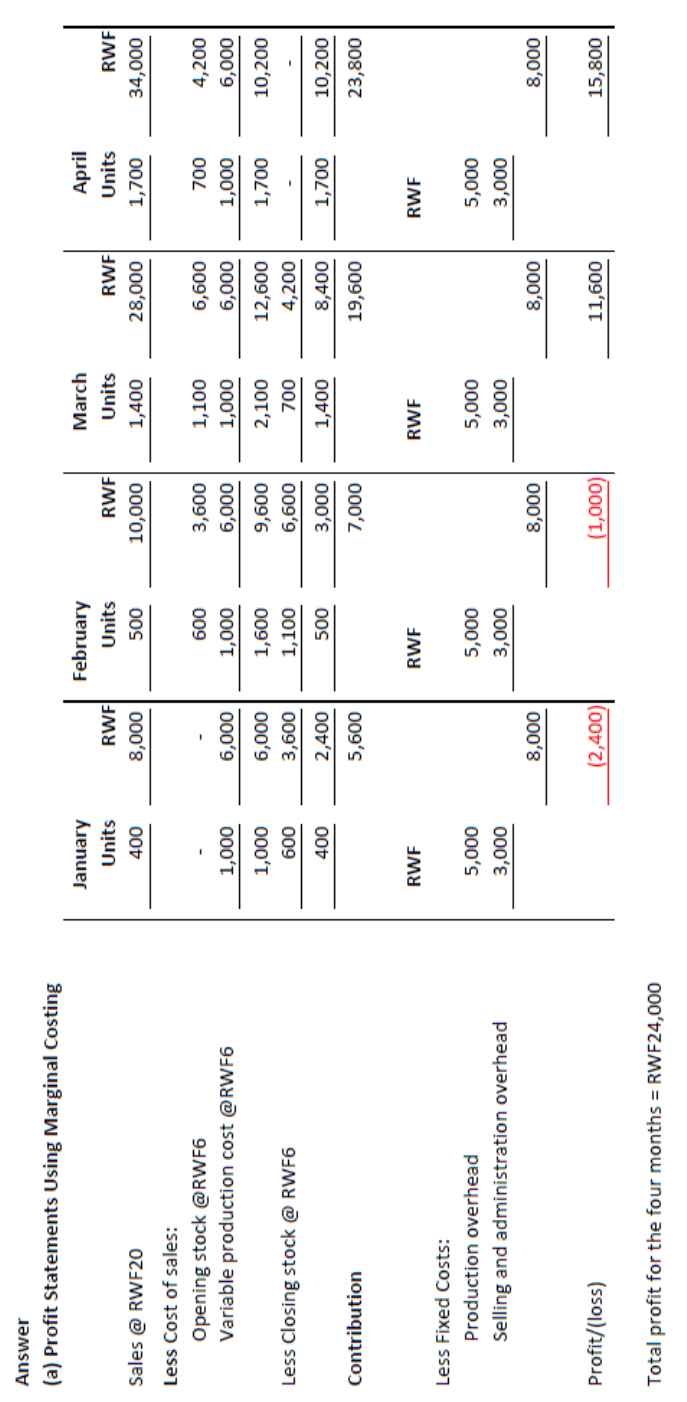
F2.1 MANAGEMENT ACCOUNTING
Page 244
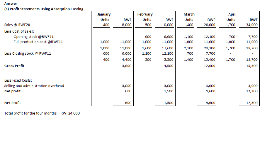
F2.1 MANAGEMENT ACCOUNTING
Page 245
(b) Fixed production overhead absorption rate =
000,1
000,5rwf
= units
= RWF5 per unit
∴ Full production cost = RWF5 + RWF6 variable cost per
unit
= RWF11 per unit
Note that there will be no over- or under-absorption of fixed production overheads,
because the production for every month is equal to the normal capacity of 1,000 units.
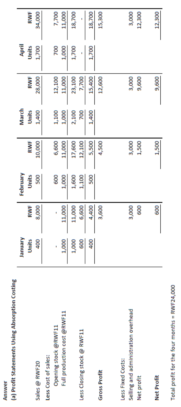
F2.1 MANAGEMENT ACCOUNTING
Page 246
F2.1 MANAGEMENT ACCOUNTING
Page 247
You can see, therefore, that when production is constant but sales fluctuate each month,
absorption costing will cause fewer profit fluctuations than marginal costing. Managers
could have been caused unnecessary concern if marginal costing had been used because of
the losses which this method would show in January and February. With absorption costing,
the fixed production overheads were carried forward in stock to be matched against the
relevant revenue when it arose in March and April.
Be prepared to explain to an examiner why a particular method should be used.
K. WHEN SALES ARE CONSTANT BUT PRODUCTION
FLUCTUATES
This is not very likely to occur in practice, but in this situation marginal costing would show
a constant level of profit linked to the constant sales.
Example
Consider again the previous example of MC Ltd, and prepare profit statements using (a)
marginal costing and (b) absorption costing for January to April, based on the same cost data,
and the following activity levels:
Sales Units
Production Units
January
1,000
1,900
February
1,000
1,000
March
1,000
600
April
1,000
500
Note: 1,000 units per month is still considered to be normal capacity.
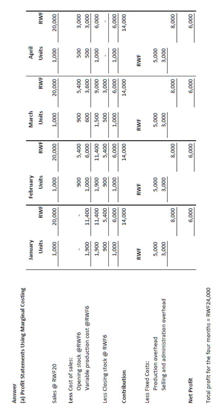
F2.1 MANAGEMENT ACCOUNTING
Page 248
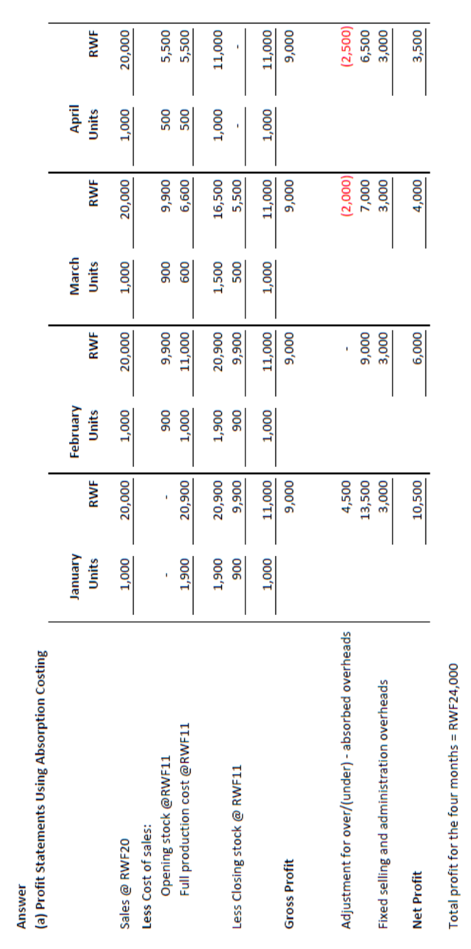
F2.1 MANAGEMENT ACCOUNTING
Page 249
F2.1 MANAGEMENT ACCOUNTING
Page 250
Calculation of over/(under)-absorption of fixed production overheads
Production
(units)
Overhead
absorbed
per unit
RWF
Total
overhead
absorbed
RWF
Overhead
incurred
RWF
Over/(under
) absorption
RWF
January
1,900
5
9,500
5,000
4,500
February
1,000
5
5,000
5,000
-
March
600
5
3,000
5,000
(2,000)
April
500
5
2,500
5,000
(2,500)
L. MARGINAL AND ABSORPTION COSTING COMPARED
Most management accounting theorists agree that marginal costing is more useful in
decision-making, where a choice has to be made between alternatives. Marginal costing
would provide information about differential costs, which would be most relevant to the
situation.
However, a choice has to be made between marginal and absorption costing in the routine
internal cost accounting system. There is no straightforward answer as to which system
should be used. The system designer must consider all the advantages and disadvantages and
what is required from the system, before making a decision.
Remember these points if you are given a scenario in the examination and need to decide on
the best option.
Arguments in Favour of Absorption (Full) Costing
(a) When production is constant but sales fluctuate, absorption costing will cause fewer
profit fluctuations than marginal costing in periods when stocks are being built up to
match future increased sales demand (see the example in Section C).
(b) No output could be achieved without incurring fixed production costs, and it is
therefore logical to include them in stock valuations.
(c) If managers continually use marginal cost pricing, there is a danger that they may lose
sight of the need to cover fixed costs. Absorption costing values all production at full
cost, so that managers are always aware of fixed costs.
(d) SSAP 9 Stocks and Long-term Contracts states that in order to match costs and
revenues, the cost of stock should include all costs incurred in bringing the stock to its
present condition. These costs should include all related production overheads, even if

F2.1 MANAGEMENT ACCOUNTING
Page 251
they accrue on a time basis (i.e. do not fluctuate with the level of activity - fixed
overheads).
Arguments in Favour of Marginal Costing
(a) When sales are constant but production fluctuates, marginal costing will give a more
logical, constant profit picture.
(b) Since fixed costs accrue on a time basis, it is logical to charge them against sales in the
period in which they are incurred. The recommendations of SSAP 9 are for external
profit reporting purposes, but the internal costing system simply has to meet the
information needs of managers. The marginal costing system will also give a better
indication of the actual cash flow of the business.
(c) Under- or over-absorption of overheads is not a problem with marginal costing, and
managers are never working under a false impression of profit being made, which could
be totally altered by an adjustment for under- or over-absorbed overheads in absorption
costing.
Further Points
It is important to remember that the difference between absorption and marginal costing
arises from the treatment of the fixed costs of production. As direct material cost and direct
labour cost will always vary with production, it is the overhead cost which creates the
difficulties.
In absorption costing all the overheads are absorbed using various logical bases. It is
essential to prepare an overhead summary prior to a period, dividing anticipated overheads
into production and service departments. The overheads allocated or apportioned to service
departments are then apportioned to production using the most logical basis; an absorption
rate is calculated on the basis of whether the production departments are labour, machines or
material intensive.
In marginal costing, direct cost of production is calculated by adding direct material cost,
direct labour cost and overheads which can be related to one unit of production. By
deducting this marginal cost of production (cost to produce one extra unit) from the sales
revenue, a contribution towards fixed overheads from each unit of production is calculated.
Total fixed overheads divided by contribution per unit establishes the breakeven point. This
is where all fixed overheads are recovered and the business starts making contribution
towards profit.
Limitations of absorption costing:
• In absorption costing the main difficulty arises in dividing overhead expenses between
production and service departments. If they relate to one department they can be easily
allocated; but if they need to be apportioned between departments then the most logical
basis of apportionment has to be established.

F2.1 MANAGEMENT ACCOUNTING
Page 252
• The cost of production is calculated after the production has taken place. The profit or
loss is therefore calculated after the event, reducing any opportunity for the
management to take action to control the cost in order to improve profitability.
• Because the absorption rate is calculated on the basis of anticipated production, and the
overheads themselves are estimated, at the end of the period there will always be over-
or under-absorption of overheads as actual production or actual overheads will be more
or less than the estimate.
• Absorption costing does not assist management by giving accurate information that
helps in preparing quotations for future contracts or in establishing a correct selling
price. This is because the overheads in the following period may be different and they
may change in their variability.
Limitations of marginal costing:
• The main difficulty in marginal or direct costing is to establish variability of overhead
expenses. In reality most overheads are semi-variable. They are neither strictly
variable with production nor strictly fixed for any level of production. Their variability
can be calculated by techniques such as scattergraphs etc. Therefore the basic
argument in favour of marginal costing is flawed.
• In the case of a business producing more than one product, it is difficult to calculate
breakeven points for each product. The best we can achieve is usually to calculate an
overall breakeven point based on level of activity or total sales revenue. This again
reduces the usefulness of marginal costing.
Absorption costing is useful to management because it is easy to operate. Once the basis of
apportionment and rates of absorption are agreed, adjustments can be made annually to bring
them in line with the current situation. Marginal costing is very useful to management in
making decisions, e.g. on make or buy, levels of production, pricing of products.
In conclusion, both methods can and should be used by management - absorption costing for
the benefits it gives in cost accumulation and cost control, and marginal costing to assist in
managerial decisions.
Example 2
The following information relates to product J for quarter three, which has just ended:
Production
(units)
Sales
(units)
Fixed
Overheads
RWF000
Variable Costs
RWF000
Budget
40,000
38,000
300
1,800

F2.1 MANAGEMENT ACCOUNTING
Page 253
Actual
46,000
42,000
318
2,070
The selling price of product J was RWF72 per unit.
The fixed overheads were absorbed at a predetermined rate per unit.
At the beginning of quarter three there was an opening stock of product J of 2,000 units
valued at RWF25 per unit variable costs and RWF5 per unit fixed overheads.
REQUIREMENT:
(a) (i) Calculate the fixed overhead absorption rate per unit for the last quarter, and
Present profit statements using FIFO (first in, first out) using:
(ii) Absorption costing, and
(iii) Marginal costing, and
(iv) Reconcile and explain the difference between the profits or losses.
(b) Using the same data, present similar statements to those required in part (a), using the
AVECO (average cost) method of valuation, reconcile the profit or loss figures, and
comment briefly on the variations between the profits or losses in (a) and (b).
Answer
(a) (i) Fixed overhead absorption rate per unit:
Budgeted fixed overheads
Budgeted production
000,40
000,300rwf
= RWF7.5
(ii) Absorption Costing (FIFO) Profit Statement
RWF000
RWF000
Sales (42000 × RWF72)
3,024
Less Cost of sales:
Opening stock (2,000 × RWF30)
60
Add Production (46,000 × RWF52.5)
(W1)
2,415
2,475
Less Closing stock (6,000 × RWF52.5)
315
2,160
864
Add Over-absorption
(W2)
27
F2.1 MANAGEMENT ACCOUNTING
Page 254
Profit
891
Workings
Per unit
RWF
(1) Variable cost 45
000,40
000,800,1rwf
Fixed overhead
7.5
52.5
(2) Fixed overhead absorbed
46,000 ×RWF7.5 =
345,000
Less Actual
318,000
RWF27,000

F2.1 MANAGEMENT ACCOUNTING
Page 255
(iii) Marginal Costing (FIFO) Profit
Statement
RWF000
RWF000
Sales
3,024
Less Cost of sales
Opening stock (2,000 × RWF25)
50
Add Production (46,000 × RWF45)
(W1)
2,070
2,120
Less Closing stock (6,000 × RWF45)
270
1,850
Contribution
1,174
Less Fixed overheads (actual)
318
Profit
856
(iv) Reconciliation
Profit
Absorption
891
Marginal
856
35
Fixed overheads in closing stock
(6,000 × RWF7.50)
45
Less Opening stock (2,000 × RWF7.50)
10
35
The difference is due to fixed overheads being carried forward in stock valuations. The
figures under absorption give a higher profit because more of the fixed overheads are
carried forward into the next accounting period than were brought forward from the
previous one. The fixed overhead absorption rate depends on estimates of both
production units and fixed overheads, and actual figures may vary. The over-
absorption of fixed overheads is adjusted for at the end of the period.
Under marginal costing fixed overheads are treated as period costs and not carried
forward in stock valuations; under- or over-absorption does not arise. Marginal
costing, by taking only the variable costs, shows how much contribution is being made,
and is regarded as giving more useful figures for decision-making.
F2.1 MANAGEMENT ACCOUNTING
Page 256
(b) Absorption Costing (AVECO) Profit Statement
RWF000
RWF000
Sales
3,024
Less Cost of sales
Opening stock plus production (48,000 ×
RWF51.56)
2,475
Less Closing stock (6,000 × RWF51.56)
309
2,166
858
Plus Over-absorption
27
Profit
885
Marginal Costing (AVECO) Profit Statement
RWF000
RWF000
Sales
3,024
Less Cost of sales
Opening stock plus production
(48,000 at RWF44.17)
2,120
Less Closing Stock (6,000 × RWF44.17)
265
1,855
Contribution
1,169
Less Fixed overheads
318
Profit
851
Reconciliation:
Difference in profits
34
Absorption closing stock
309
Less Marginal closing stock
265
44
Less Fixed costs in absorption opening stock
10
34
The variations in the profits in (a) and (b) of RWF6,000 and RWF5,000 respectively are
caused by using different methods of valuation (FIFO and AVECO). The valuation
method can affect profit/loss for both absorption and marginal approaches, and could
lead to much wider variations than here.

F2.1 MANAGEMENT ACCOUNTING
Page 257
Study Unit 12
Break Even Analysis
Contents
A. Break-Even Analysis
B. Break-Even Chart
C. The Profit Volume Graph
D. Use of the Profit Volume Graph for More Than One Product
E. The Profit/Volume or Contribution/Sales Ratio
F. Marginal Profit and Loss Account
______________________________________________________________

F2.1 MANAGEMENT ACCOUNTING
Page 258
A. BREAK-EVEN ANALYSIS
For any business there is a certain level of sales at which there is neither a profit nor a loss,
i.e. the total income and the total costs are equal. This point is known as the break-even
point. It is very easy to calculate, and it can also be found by drawing a graph called a break-
even chart.
Calculation of Break-Even Point – Example
As shown in the last unit, you must be able to layout a marginal cost statement before doing
Break Even formulas.
Marginal Cost Statement
Sales
x
- Variable Cost
(x)
= Contribution
x
- Fixed Costs
(x)
= Profit/Loss
xx
Let us assume that the organising committee of a dinner have set the selling price at
RWF8.40 per ticket. They have agreed with a firm of caterers that the meal would be
supplied at a cost of RWF5.40 per person. The other main items of expense to be considered
are the costs of the premises and orchestra which will amount to RWF80 and RWF100
respectively. The variable cost in this example is the cost of catering, and the fixed costs are
the amounts for premises and orchestra.
The first step in the calculations is to establish the amount of contribution per ticket.
Contribution
RWF
Price of ticket (sales value) 8.40
Less Catering cost (marginal cost) 5.40
Contribution 3.00
Now that this has been established, we can evaluate the fixed expenses involved.
F2.1 MANAGEMENT ACCOUNTING
Page 259
Fixed Costs
RWF
Hire of premises 80
Orchestra fee 100
Total fixed expenses RWF180
The organisers know that for each ticket they sell, they will obtain a contribution of RWF3
towards the fixed costs of RWF180. Clearly it is only necessary to divide RWF180 by
RWF3 to establish the number of contributions which are needed to break even on the
function. The break-even point is therefore 60, i.e. if 60 tickets are sold there will be neither
a profit nor a loss on the function. Any tickets sold in excess of 60 will provide a profit of
RWF3 each.
Formulae
The general formula for finding the break-even point in volume is:
Fixed costs
Contribution per unit
(this is, of course, exactly what we did in the example).
If the break-even point is required in terms of sales value, rather than sales volume, the
formula that should be used is as follows:
Break-even point =
Fixed costs
C/ s ratio
The C/s ratio is
Contribution
Sales
× 100.
For example, the contribution earned by selling one unit of Product A at a selling price of
RWF10 is RWF4.
C/s ratio =
10
4
RWF
RWF
× 100 = 40%
In our example of the dinner-dance, the break-even point in revenue would be:
40.8
3
180
rwf
rwf
= RWF504
F2.1 MANAGEMENT ACCOUNTING
Page 260
The committee would know that all costs (both variable and fixed) would be exactly covered
by revenue when sales revenue earned equals RWF504. At this point no profit nor loss
would be received.
Suppose the committee were organising the dinner in order to raise money for charity, and
they had decided in advance that the function would be cancelled unless at least RWF120
profit would be made. They would obviously want to know how many tickets they would
have to sell to achieve this target.
Now, the RWF3 contribution from each ticket has to cover not only the fixed costs of
RWF180, but also the desired profit of RWF120, making a total of RWF300. Clearly they
will have to sell 100 tickets (RWF300 divided by RWF3).
To state this in general terms:
Volume of sales needed to achieve a given profit =
Fixed costs + Desired profit
Contribution per unit
Suppose the committee actually sold 110 tickets. Then they have sold 50 more than the
number needed to break even. We say they have a margin of safety of 50 units, or of
RWF420 (50 × RWF8.40), i.e.
Margin of safety = Sales achieved – Sales needed to break even.
The margin of safety is defined as the excess of normal or actual sales over sales at break-
even point.
It may be expressed in terms of sales volume or sales revenue.
Margin of safety is very often expressed in percentage terms:
Sales achieved Sales needed to break even
Sales achieved
−
× 100%
i.e. the dinner committee have a percentage margin of safety of 50/110 × 100% = 45%.
F2.1 MANAGEMENT ACCOUNTING
Page 261
The significance of margin of safety is that it indicates the amount by which sales could fall
before a firm would cease to make a profit. Thus, if a firm expects to sell 2,000 units, and
calculates that this would give it a margin of safety of 10%, then it will still make a profit if
its sales are at least 1,800 units (2,000 – 10% of 2,000), but if its forecasts are more than
10% out, then it will make a loss.
The profit for a given level of output is given by the formula:
(Output × Contribution per unit) – Fixed costs.
It should not, however, be necessary for you to memorise this formula, since when you have
understood the basic principles of marginal costing, you should be able to work out the profit
from first principles.
Consider again our example of the dinner. What would be the profit if they sold (a) 200
tickets (b) RWF840 worth of tickets?
(a) We already know that the contribution per ticket is RWF3.
Therefore, if they sell 200 tickets, total contribution is 200 × RWF3 = RWF600.
Out of this, the fixed costs of RWF180 must be covered: anything remaining is profit.
Therefore profit = RWF420. (Check: 200 tickets is 140 more than the number needed
to break even. The first 60 tickets sold cover the fixed costs; the remaining 140 show a
profit of RWF3 per unit. Therefore profit = 140 × RWF3 = RWF420, as before.)

F2.1 MANAGEMENT ACCOUNTING
Page 262
(b) RWF840 worth of tickets is 100 tickets, since they are RWF8.40 each.
RWF
Total contribution on 100 tickets = 300
Less fixed costs 180
Profit RWF120
B. BREAK-EVEN CHART
Information Required
(a) Sales Revenue
When we are drawing a break-even chart for a single product, it is a simple matter to
calculate the total sales revenue which would be received at various outputs.
As an example let us take the following figures:
Output (units) Sales revenue (RWF)
0 0
2,500 10,000
5,000 20,000
7,500 30,000
10,000 40,000
(b) Fixed Costs
We must establish which elements of cost are fixed in nature. The fixed element of any
semi-variable costs must also be taken into account.
Let us assume that the fixed expenses total RWF8,000.
(c) Variable Costs
The variable elements of cost must be assessed at varying levels of output.
Output (units) Variable costs (RWF)
0 0
2,500 5,000
5,000 10,000
7,500 15,000
10,000 20,000

F2.1 MANAGEMENT ACCOUNTING
Page 263
Plotting the Graph
The graph is drawn with level of output (or sales value) represented along the horizontal axis
and costs/revenues up the vertical axis. The following are the stages in the construction of
the graph:
(a) Plot the sales line from the above figures.
(b) Plot the fixed expenses line. This line will be parallel to the horizontal axis.
(c) Plot the total expenses line. This is done by adding the fixed expenses of RWF8,000 to
each of the variable costs above.
(d) The break-even point (often abbreviated to BEP) is represented by the meeting of the
sales revenue line and the total cost line. If a vertical line is drawn from this point to
meet the horizontal axis, the break-even point in terms of units of output will be found.
The graph is illustrated in Figure 1.
Note that, although we have information available for four levels of output besides zero, one
level is sufficient to draw the chart, provided we can assume that sales and costs will lie on
straight lines. We can plot the single revenue point and join it to the origin (the point where
there is no output and therefore no revenue). We can plot the single cost point and join it to
the point where output is zero and total cost = fixed cost.
In this case, the break-even point is at 4,000 units, or a revenue of RWF16,000 (sales are at
RWF4 per unit).
This can be checked by calculation:
Sales revenue = RWF4 per unit
Variable costs = RWF2 per unit
∴ Contribution = RWF2 per unit
Fixed costs = RWF8,000
Break-even point =
Fixed costs
Contribution per unit
= 4,000 units.
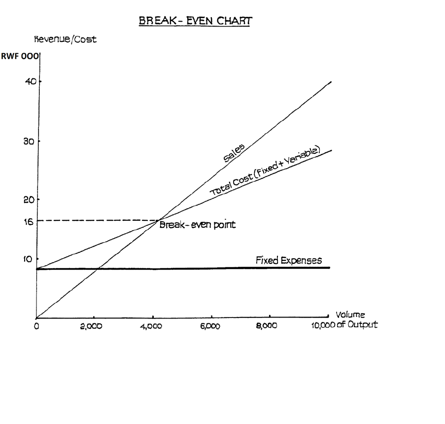
F2.1 MANAGEMENT ACCOUNTING
Page 264
Figure 1
Break-even Chart for More Than One Product
Because we were looking at one product only in the above example, we were able to plot
“volume of output” and straight lines were obtained for both sales revenue and costs. If we
wish to take into account more than one product, it is necessary to plot “level of activity”
instead of volume of output. This would be expressed as a percentage of the normal level of
activity, and would take into account the mix of products at different levels of activity.
Even so, the break-even chart is not a very satisfactory form of presentation when we are
concerned with more than one product: a better graph, the profit-volume graph, is discussed
in the next study unit. The problem with the break-even chart is that we should find that,
because of the different mixes of products at the different activity levels, the points plotted
for sales revenue and variable costs would not lie on a straight line.
F2.1 MANAGEMENT ACCOUNTING
Page 265
Assumptions and Limitations of Break-Even Charts
Apart from the above point about the difficulty of dealing with more than one product, you
should bear the following points in mind:
(a) Break-even charts are only accurate within fairly narrow levels of output. This is
because if there were to be a substantial change in the level of output, the proportion of
fixed costs could change.
(b) Even with only one product, the income line may not be straight. A straight line
implies that the manufacturer can sell any volume he likes at the same price. This may
well be untrue: if he wishes to sell more units he might have to reduce the price.
Whether this increases or decreases his total income depends on the elasticity of
demand for the product. Therefore the sales line may curve upwards or downwards,
but in practice is unlikely to be straight.
(c) Similarly, we have assumed that variable costs have a straight line relationship with
level of output, i.e. variable costs vary directly with output. This might not be true. For
instance, the effect of diminishing returns might cause variable costs to increase beyond
a certain level of output.
(d) Break-even charts only hold good for a limited time-span. Nevertheless, within these
limitations a break-even chart can be a very useful tool. Managers who are not well-
versed in accountancy find it easier to understand a break-even chart than a calculation
showing the break-even point.
General Points on the Interpretation of Break-Even Charts
The skeleton break-even chart (Figure 2) illustrates the following points:
(a) Margin of Safety
The margin of safety - i.e. the extent by which sales could fall before a loss was
incurred - is easily read from the graph.
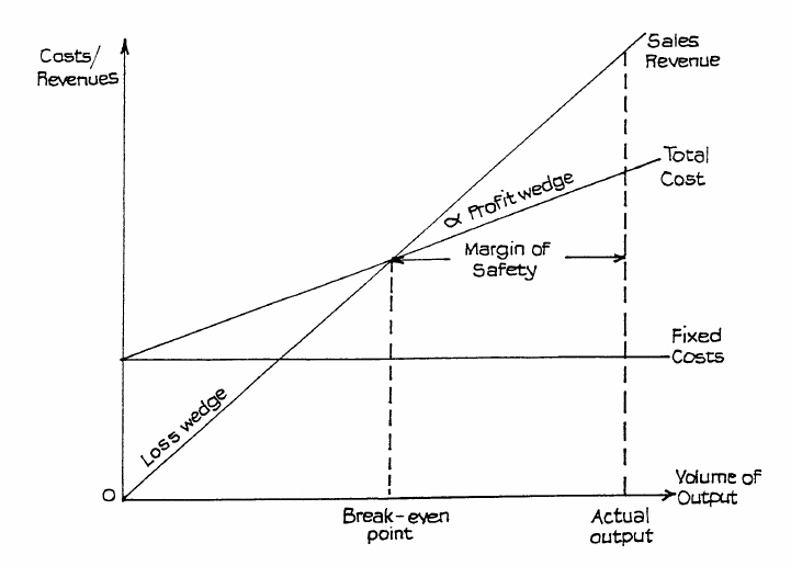
F2.1 MANAGEMENT ACCOUNTING
Page 266
Figure 2
(b) Angle of Incidence
The angle a marked on the chart is referred to as the angle of incidence. This shows the
rate at which profits increase once the break-even point is passed. A large angle of
incidence means a high rate of earning (equally it means that if sales fell below break-
even point, the loss would increase rapidly). This is also illustrated by the size of the
profit and loss wedges.
Changes in Cost Structure
If costs increase, the break-even point will be reached at a higher level of sales. The break-
even chart (Figure 3) illustrates the effect of changes.
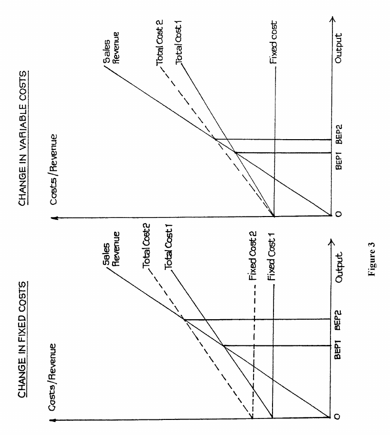
F2.1 MANAGEMENT ACCOUNTING
Page 267
Example
A long-distance coach company expects 80,000 tickets to be sold on a particular route in a
three-month period at a price of RWF30 each. Fixed overhead for the period is budgeted at
RWF412,500 and expected net profit is RWF247,500.
REQUIREMENT:
Calculate:
(a) the contribution/sales ratio;
(b) the total contribution;

F2.1 MANAGEMENT ACCOUNTING
Page 268
(c) the contribution per ticket;
(d) the additional profit arising from selling a further 1,250 tickets;
(e) the additional sales required to earn the same profit as that shown above if the price per
ticket is reduced to RWF27.75.
Solution
(a) The contribution must first be calculated.
Fixed costs + Profit: RWF412,500 + RWF247,500 = RWF660,000.
Contribution/sales ratio
=
RWF30 tickets000,80
000,660
×
rwf
× 100 = 27.5%
(b) Total contribution = RWF660,000.
(c) Contribution per ticket: this is the total contribution divided by the number of tickets to
be sold
80,000
660,000 RWF
= RWF8.25
(d) Additional profit arising from selling a further 1,250 tickets: as the company is already
trading at above its break-even point, any additional contribution earned by additional
sales will be profit.
The additional profit is 1,250 × RWF8.25 = RWF10,312.50
(e) The additional sales required to produce a profit of RWF247,500 if the selling price per
ticket is reduced to RWF27.75 is calculated as follows:
Target contribution RWF660,000
Selling price per ticket RWF30
No. of tickets sold 80,000
Revised position
Target contribution RWF660,000
Selling price per ticket RWF27.75
Fixed costs remain the same. Therefore the reduction in selling price reduces
contribution by the same amount:
RWF30 – RWF27.75 = RWF2.25. This reduces contribution per ticket from RWF8.25
to RWF6.00.

F2.1 MANAGEMENT ACCOUNTING
Page 269
To earn a target profit of RWF660,000, sales must now be
6
000,660
rwf
rwf
= 110,000.
This means that an additional number of 30,000 (110,000 – 80,000) tickets must be
sold.
Contribution Break-Even Chart
An alternative form of break-even chart is one which shows the contribution earned. Instead
of starting by measuring the fixed costs from the base line, the variable costs are taken. The
fixed costs are then shown above the variable costs.
Example
Variable costs RWF2 per unit
Fixed costs RWF80,000
Maximum sales RWF200,000
Selling price per unit RWF20
REQUIREMENT:
Prepare a contribution break-even chart. (See Figure 4)
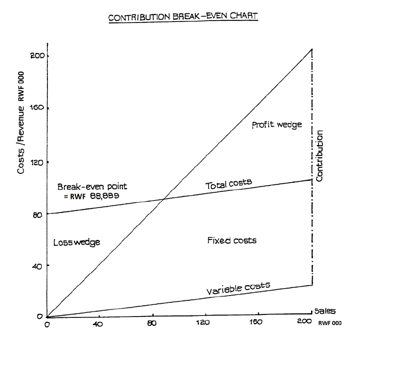
F2.1 MANAGEMENT ACCOUNTING
Page 270
Figure 4
C. THE PROFIT VOLUME GRAPH
The profit volume graph provides an alternative presentation to the break-even chart
discussed in the previous study unit. It may be more easily understood by managers who are
not used to accountancy or statistics.
In this graph, sales revenue is plotted on the horizontal axis, against profit/loss on the vertical
axis. It is therefore necessary to work out the profit before starting to plot the graph. This is
done using the marginal costing equation.
Sales revenue – Variable cost = Fixed cost + Profit
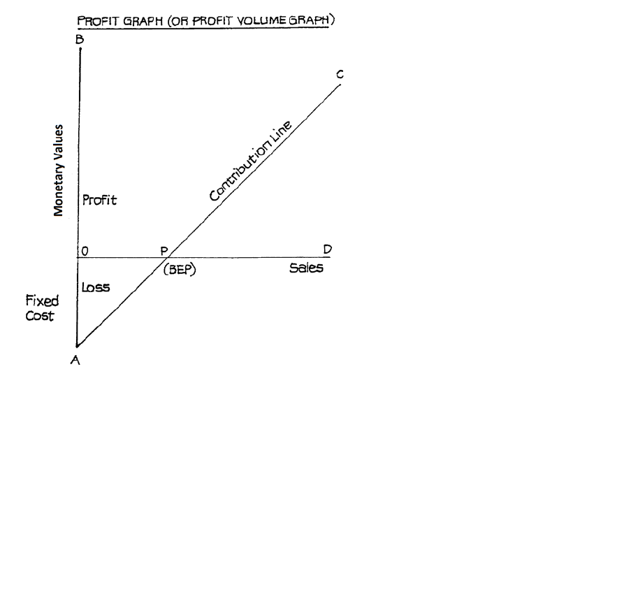
F2.1 MANAGEMENT ACCOUNTING
Page 271
or Profit = Sales revenue – Variable cost × Fixed cost
or Profit = Contribution per unit × No. of units – Fixed cost
The general form of the graph is illustrated in Figure 6.
Figure 6
The distance AO on the graph represents the amount of fixed cost, since when no sales are
made there will be a loss equal to the fixed cost.

F2.1 MANAGEMENT ACCOUNTING
Page 272
D. USE OF THE PROFIT VOLUME GRAPH FOR MORE
THAN ONE PRODUCT
In order to draw a profit volume graph for several products it is necessary to calculate:
(a) Sales revenue for each product and cumulative sales revenue.
(b) Contribution for each product, cumulative contribution and hence profit.
The graph is easiest to draw and interpret if the products are taken in order, starting with the
most profitable and working back to the least profitable, “profitability” in this context being
measured by the relationship which contribution bears to sales revenue.
Example
The Works Director of XY Ltd, a company manufacturing and marketing a number of
different products, considers that the profit could be increased by restricting the number of
products. He wishes to eliminate production of the two lines which contribute
proportionately least, and he is satisfied that the output and sale of the remaining products
would be increased proportionately so that the total value of sales is unaffected.
He asks you to help him by preparing from the following data a suitable graph which would
indicate the products which should be eliminated, and would assist him in presenting his
point of view to his colleagues on the Board.
Product Variable Cost Profit Sales
RWF RWF RWF
A 11,000 3,000 (Loss) 12,000
B 18,000 3,000 22,000
C 17,000 500 20,000
D 21,500 9,500 44,000
E 6,000 8,000 23,000
F 8,000 2,000 (Loss) 10,000
131,000
Fixed expenses are at a level of RWF33,500.

F2.1 MANAGEMENT ACCOUNTING
Page 273
Solution
The first step is to establish the contribution made towards fixed expenses by the individual
products. The second is to calculate the contribution as a percentage of sales revenue. At
this stage we will be able to eliminate the least profitable lines.
Product Sales Variable Contribution Contribution as
Cost Percentage of
Sales Revenue
RWF RWF RWF %
A 12,000 11,000 1,000 8.3
B 22,000 18,000 4,000 18.2
C 20,000 17,000 3,000 15.0
D 44,000 21,500 22,500 51.1
E 23,000 6,000 17,000 74.0
F 10,000 8,000 2,000 20.0
It is clear that A and C are proportionately the two least profitable products, and should be
eliminated.
Since the question states that the total value of sales will remain the same, we must gross up
the sales of the remaining items.
Product Former Sales Share of Increase Revised Sales
RWF RWF RWF
E 23,000 7,440 30,440
D 44,000 14,220 58,220
F 10,000 3,230 13,230
B 22,000 7,110 29,110
RWF99,000 RWF32,000 RWF131,000

F2.1 MANAGEMENT ACCOUNTING
Page 274
We must now calculate revised contributions for each product.
Product Sales Percentage Revised Contribution
Contribution
RWF % RWF
E 30,440 74 22,500
D 58,220 51 29,750
F 13,230 20 2,650
B 29,110 18.2 5,300
The method of obtaining the points to be plotted is as follows:
Present Basis
Product Sales Contribution Profit
(Contribution Less
Fixed Costs)
RWF RWF RWF
E 23,000 17,000 –16,500
D 44,000 22,500
67,000 39,500 + 6,000
F 10,000 2,000
77,000 41,500 + 8,000
B 22,000 4,000
99,000 45,500 +12,000
C 20,000 3,000
119,000 48,500 +15,000
A 12,000 1,000
RWF131,000 RWF49,500 +16,000

F2.1 MANAGEMENT ACCOUNTING
Page 275
Revised Basis
Product Sales Contribution Profit
(Contribution Less
Fixed Costs)
RWF RWF RWF
E 30,440 22,500 –11,000
D 58,220 29,750
88,660 52,250 +18,750
F 13,230 2,650
101,890 54,900 +21,400
B 29,110 5,300
RWF131,000 RWF60,200 +26,700
The graph is shown in Figure 7. (on the page 301)
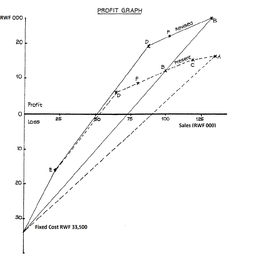
F2.1 MANAGEMENT ACCOUNTING
Page 276
Figure 7
From the graph we can read:
(a) Revised profit is RWF26,700.
(b) Present profit is RWF16,000.
(c) Revised BEP is RWF72,900.
(d) Present BEP is RWF88,700.

F2.1 MANAGEMENT ACCOUNTING
Page 277
E. THE PROFIT/VOLUME OR CONTRIBUTION/SALES
RATIO
Calculation
In the calculations for the profit graph in the previous example, we made use of the ratio
“contribution: sales” (expressed as a percentage). This ratio has historically been referred to
as the “profit: volume ratio”. This is not a very sensible name, because it does not describe
what the ratio actually is. In fact, examiners now call it by the more descriptive name of
“contribution : sales ratio” (C/S ratio) but you should watch out for the alternative
terminology P/V ratio in older textbooks.
The ratio may be calculated as either:
Selling price per unit Variable cost per unit
Selling price per unit
−
or
Total sales revenue Total variable cost
Total sales revenue
−
Alternatively, it may be calculated when variable costs are not known, provided the sales
revenue and profit figures are known for two different levels of output.
Example
Calculate the contribution: sales (C/S) ratio from the following information:
Sales Figures Profit Figures
RWF RWF
Activity Level I 3,500 625
Activity Level II 3,000 500
The calculation of the ratio is as follows:
(a) Variation in profits: Level I - Level II is RWF625 – RWF500 = RWF125.
(b) Variation in sales: Level I - Level II is RWF3,500 – RWF3,000 = RWF500.
This means that for additional sales of RWF500 there is an additional profit of
RWF125.

F2.1 MANAGEMENT ACCOUNTING
Page 278
(c) Contribution: sales ratio
(a)
(b)
or
125
500
= 0.25
This figure can be checked by drawing up profit statements for the two activity levels,
bearing in mind that if the ratio is 0.25, i.e. contribution is 0.25 per RWF of sales, then
variable costs will be 0.75 per RWF of sales. We must also remember that fixed cost =
contribution – profit, and that the fixed cost will by definition be the same at each of the two
activity levels.
Level I Level II
RWF RWF
Sales 3,500 3,000
Less marginal cost (0.75 per RWF1) 2,625 2,250
Contribution 875 750
Less fixed expenses 250 250
Profits 625 500
Use of Ratio
(a) Profit at Different Levels of Sales
Using the data in the last example, what would be the profit on RWF2,000 sales?
What sales level would be required to produce a profit of RWF1,000?
(i) Sales of RWF2,000
a. Sales as above RWF2,000
b. C/S percentage as calculated 25%
c. Contribution on RWF2,000 sales,
25% of RWF2,000 RWF500
d. Fixed expenses as calculated RWF250
e. Profit on RWF2,000 sales (c. – d.) RWF250
(ii) Profit Requirement of RWF1,000
a. Profit requirement as above RWF1,000
b. Fixed expenses as calculated RWF250
c. Total contribution required
(a. + b.) RWF1,250
d. C/S percentage as calculated 25%
e. Sales required RWF1,250 ×
100
25
RWF5,000

F2.1 MANAGEMENT ACCOUNTING
Page 279
(b) Calculation of Break-Even Point
We saw earlier that the formula for calculating the break-even point in sales value is:
Fixed Cost
C/ s ratio
This gives the breakdown point in terms of sales value.
Using the same data again, break-even point will be
250
025.
= 250 ×
100
25
= 1,000
i.e. the break-even point occurs when sales are RWF1,000.
Typical Examination Question
(a) Define and illustrate by means of simple arithmetical examples:
(i) Contribution/sales ratio;
(ii) Margin of safety.
(b) Demonstrate the relationship between a firm's contribution/sales ratio, its percentage
margin of safety, and its profit/sales ratio.
(c) What is the significance of a firm's margin of safety?
(d) The following details relate to Product X:
RWF RWF
Selling price 120
Costs:
Material 60
Labour 15
Variable overhead 5
Fixed overhead 10 90
Profit RWF30
During the forthcoming year it is expected that material costs will increase by 10%,
wages by 33
13
% and other costs by 20%.
You are required to calculate the percentage increase in the selling price of X which
would maintain the firm's contribution/sales ratio.

F2.1 MANAGEMENT ACCOUNTING
Page 280
Solution
(a) (i) The contribution/sales ratio is the contribution that is sales revenue - variable
cost, expressed as a proportion of sales.
For example, if selling price = RWF100 and variable cost/unit = RWF75, the
contribution/unit is RWF25 and the C/S ratio 0.25 or 25%.
(ii) The margin of safety is the difference between a firm’s actual or expected sales,
and the sales which would be needed to break even. It may be expressed as a
percentage of the actual sales.
For example, using the data above and supposing fixed costs to be RWF2,500, the
sales volume required to break even would be 100 units (
2 500
25
,
).
If the firm’s actual sales were 200 units, its margin of safety would be 100 units
or
100
200
× 100% = 50%.
(b) A firm’s profit/sales ratio can be obtained by applying its percentage margin of safety
to its C/S ratio. This is illustrated using the above data:
RWF
Actual sales (200 units @ RWF100) 20,000
Marginal cost of sales (200 @ RWF75) 15,000
Contribution (= 25% of revenue) 5,000
Less fixed costs 2,500
Profit (= 12½% of revenue) 2,500
Contribution/sales ratio × percentage margin of safety
= 25% × 50% = 12½%
which is the profit/sales ratio, as required.
(c) A firm’s margin of safety shows its ability to withstand adverse trading conditions: for
instance, in the above example the firm can afford for sales to drop by up to 50% before
it will be in real difficulties.

F2.1 MANAGEMENT ACCOUNTING
Page 281
(d) Present Increase Expected
Costs Costs
RWF % RWF
Material 60 10 66
Labour 15 33
13
20
Variable overhead 5 20 6
Marginal cost 80 92
Since current sales revenue is RWF120 per unit, the current C/S ratio is 40/120 or
33
13
%. The variable cost: sales ratio is 66
23
%.
If the C/S ratio is to remain the same, the variable cost : sales ratio will also remain the
same,
i.e. 66
23
% of the new selling price is RWF92.
Therefore the new selling price must be RWF138
(
92
66 23
× 100).
RWF
Check: Selling price 138
Less variable cost 92
Contribution RWF46 which is
13
of sales revenue, as
required.
The two most important points to notice about this part of the question are:
(i) The examiner gave the fixed cost per unit as a “red herring”. In marginal costing
we are only interested in the fixed costs in total; fixed cost per unit is relevant
only to absorption costing. As it transpired, in this question we did not need any
information at all about fixed costs.
(ii) The variable (marginal) cost to sales ratio and the contribution to sales ratio are
complementary ratios, i.e. when expressed as percentages they add up to 100%,
and if one of them remains constant, then so does the other.
F2.1 MANAGEMENT ACCOUNTING
Page 282
F. MARGINAL PROFIT AND LOSS ACCOUNT
Advantages
In the orthodox trading and profit and loss account, the opening and closing stocks are
debited and credited respectively, and the valuations placed upon them include a share of
production fixed overheads. Accountants who believe in using marginal costing take the
view that all fixed costs should be written off in the period in which they are incurred and that
there can be no justification for carrying part of one period’s costs forward to the next period
in closing stock. They argue that fixed costs are incurred on a time basis, regardless of the
level of production or sales in any period. They claim, therefore, that a closing stock
valuation which excludes any element of cost is more “accurate”. The exclusion of fixed
costs does ensure that the writing off of fixed costs is not deferred until a later period. The
main advantage of the marginal form of profit and loss account is, therefore, that the profit
will not be affected simply because of a significant change in the stock figures: profit is
clearly related to the level of sales.
Example of Layout
Total Product A Product B
Sales revenue xxxx xxx xxx
Less Variable costs of goods sold:
Direct material xxx xx xx
Direct labour xxx xx xx
Variable overheads xxx xx xx
Total variable cost xxx xxx xxx
Contribution xxx xxx xxx
Less Fixed costs xxx
RWFxxx
Layout When Some Fixed Costs Can Be Allocated
If some of the fixed costs can be directly associated with a particular product or department,
then clearly these costs should be shown separately and not grouped with the general fixed
costs. This is best illustrated by an example.

F2.1 MANAGEMENT ACCOUNTING
Page 283
Example
A company manufactures goods in three separate factories. The projected figures for the next
year are as follows:
Edinburgh York Gloucester
RWF RWF RWF
Sales 440,000 400,000 700,000
Branch expenses:
Salaries 42,000 38,000 62,000
Advertising 8,000 15,000 10,000
Other 10,000 8,000 11,000
There is a central office in London which is estimated to cost RWF154,000.
Variable costs amount to 75% of sales for each factory.
The marginal profit and loss account for this company would appear as follows:
Edinburgh York Gloucester Total
RWF RWF RWF RWF
Sales 440,000 400,000 700,000 1,540,000
Less variable cost of sales330,000 300,000 525,000 1,155,000
Gross contribution 110,000 100,000 175,000 385,000
Less branch fixed costs 60,000 61,000 83,000 204,000
Contribution to
central expenses and profit50,000 39,000 92,000 181,000
Less central expenses 154,000
Profit RWF27,000

F2.1 MANAGEMENT ACCOUNTING
Page 284
Comparison of Absorption and Marginal Costing Methods
Example
The Melody Radio Co. Ltd which manufactures the “Melody” radio receiver, commenced
trading on 1 April last. The company’s budget for each four-week period is as follows:
RWF RWF
Sales - 20,000 receivers 400,000
Manufacturing cost of goods sold:
Variable costs 240,000
Fixed overhead 60,000 300,000
Gross profit 100,000
Selling and distribution costs (fixed) 20,000
Net profit RWF80,000
The following data relates to the first two trading periods:
Period 1 Period 2
Production 24,000 18,000
Sales 18,000 21,000
REQUIREMENT:
(a) Prepare operating statements for each of the two periods:
(i) Where fixed manufacturing overhead is absorbed into product costs at the
budgeted rate and selling and distribution costs are treated as period costs.
(ii) Where all fixed costs are treated as period costs.
You may assume that the selling price, fixed costs, and unit variable costs for the two
periods are in line with budget.
(b) Comment upon the results revealed by your statements.

F2.1 MANAGEMENT ACCOUNTING
Page 285
Solution
Workings
Variable costs = RWF
240 000
20 000
,
,
= RWF12 per unit.
Fixed overhead absorption rate = RWF
60 000
20 000
,
,
= RWF3 per unit.
Selling price = RWF
400 000
20 000
,
,
= RWF20 per unit.
Stock figures
Period 1 Period 2
Units Units
Opening stock 0 6,000
+ Production 24,000 18,000
24,000 24,000
– Sales 18,000 21,000
Closing stock 6,000 3,000
Fixed overheads are fully absorbed by production of 20,000 units.
In Period 1, fixed overheads will be over-absorbed by 4,000 × RWF3 = RWF12,000.
In Period 2, fixed overheads will be under-absorbed by 2,000 × RWF3 = RWF6,000.
The wording of the question is taken to mean that closing stock should be valued at the
budgeted rate (RWF15 per unit) and under- or over-absorption written off in the relevant
period.
The alternative would be, taking Period 1 as an example, to value closing stock as:
Variable cost: 6,000 × RWF12 =RWF72,000
Fixed cost: ¼ of RWF60,000 =RWF15,000 (since closing stock is ¼ of the period’s
production)

F2.1 MANAGEMENT ACCOUNTING
Page 286
RWF87,000
(i) Absorbing Fixed Manufacturing Overhead at the Budgeted Rate
Period 1 Period 2
RWF RWF RWF RWF
Sales 360,000 420,000
Opening stock (@ RWF15/unit) 90,000
Production (@ RWF15/unit) 360,000 270,000
360,000 360,000
Less closing stock (@ RWF15/unit) 90,000 45,000
270,000 315,000
Fixed manufacturing
overhead over- absorbed (12,000)
Fixed manufacturing
overhead under- absorbed ________ 6,000
Total manufacturing
cost of goods sold 258,000 321,000
Gross profit 102,000 99,000
Less selling and
distribution costs 20,000 20,000
Net profit 82,000 79,000

F2.1 MANAGEMENT ACCOUNTING
Page 287
(ii) All Fixed Costs Treated as Period Costs (Marginal Costing)
Period 1 Period 2
RWF RWF RWF RWF
Sales 360,000 420,000
Opening stock (@ RWF12 per unit) - 72,000
Production (@ RWF12 per unit) 288,000 216,000
288,000 288,000
Closing stock (@ RWF12 per unit) 72,000 36,000
Marginal cost of sales 216,000 252,000
Contribution 144,000 168,000
Fixed manufacturing cost 60,000 60,000
Gross profit 84,000 108,000
Selling and distribution cost 20,000 20,000
Net profit 64,000 88,000
(b) Comments
The marginal costing statement relates profit clearly to sales: when sales rise, profit
rises. The absorption costing statement shows a lower profit in Period 2, despite the
rise in sales, because of the change in the stock position.
The profits under the two methods may be reconciled as follows:
Period 1 Closing stock valuation - absorption costing - RWF90,000
Closing stock valuation - marginal costing - RWF72,000
Difference in closing stock valuation = difference in profit
between the two methods RWF18,000
Period 2 Fall in stock during period = 3,000 units
Valuation - absorption costing - 3,000 @ RWF15 = RWF45,000

F2.1 MANAGEMENT ACCOUNTING
Page 288
Valuation - marginal costing - 3,000 @ RWF12 = RWF36,000
Difference = difference in profit between the two methods
RWF9,000
Taking the two periods together
Total profit – absorption costing RWF161,000
Total profit – marginal costing RWF152,000
Difference = difference in Period 2 closing stock valuation
RWF 9,000
It should be clear that over several periods taken together such that stock at the beginning
of the first period and at the end of the last period was nil, the absorption and marginal
costing methods would give the same total profit, but the amount of profit in each
individual period would be different under the two methods.

F2.1 MANAGEMENT ACCOUNTING
Page 289
Study Unit 13
Decision Making
Contents
A. Introduction
B. The Practical Use of Relevant Costs
C. Market Vulnerability Analysis
D. Continue/Close Down Decisions
E. Marginal Costing in Decision Making
_______________________________________________________________
F. Decision Making Involving A Single Limiting Factor
_______________________________________________________________
F2.1 MANAGEMENT ACCOUNTING
Page 290
A. INTRODUCTION
Accountants have an important role in the preparation of relevant data for decision making
purposes.
For decision making purposes information is required which is relevant to the particular
decision under consideration. In all decisions there must be a “status quo” (or position the
decision making entity will be in if no decision is taken) and an alternative position (or
several alternative positions) which will result as a direct consequence of the decision to be
taken. Relevant information is that which relates to the differences between the basic, or
status quo outcome and the alternatives. Therefore the decision should be appraised by
making a comparison of the financial effects between the two sets of outcomes. Information
concerning events which are common to all outcomes possibilities may be ignored as such
events are not decision variables. The decision variables are not to be measured by the
historic costs utilised in regular management accounting reports as the historic costs relate to
past transactions and not, therefore, decision variables for the purpose of any current
decision. Past transactions are common to all future or current actions and as such are events
which are common to all outcomes hence they may be ignored. Relevant information
concerns future incremental (or avoidable) costs and revenues (as these can be altered by the
current decisions) as well as current opportunity values of existing assets.
Hence the figures incorporated in regularly produced management accounting reports are
generally based on past actions and are not to be used for decision making which is
concerned with current and future alternative actions. However, frequently, the figures used
in the regularly produced statements will be a good first approximation for the values which
should be attributed to the relevant decision variables – but this cannot be relied upon to be
always the case.
Relevant costs for decision making purposes are:
(i) Opportunity costs of existing assets or past expenditure.
Assets currently held as a result of past expenditure bestow benefits to the owner. It is
not the past expenditure which bestows the benefits but the current ownership of the
asset and benefits can be measured only by considering the uses to which the asset can
be put. Hence for decision making purposes the historic cost is irrelevant as it is the
measurement of a past transaction and it does not measure the current benefit derivable
from the asset. If a current asset is used for one purpose then its alternative use will be
foregone – for the purposes of deciding whether it is worthwhile to forego this
alternative use then the benefits which would be derived from that use should be
attributed to the asset as its opportunity cost. Opportunity cost is therefore the net
revenue which avoidable as a result of the decision.
F2.1 MANAGEMENT ACCOUNTING
Page 291
(ii) Incremental, attributable future costs.
Future costs may be relevant but the essential point is that the future costs be avoidable
as a result of the decision. If accepting a decision incurs (or saves) a cost and rejecting
the decision does incur (or saves) a cost and rejecting the decision does incur (or save)
that cost then the cost is a decision variable. However care must be taken to ensure that
only truly avoidable costs are included as relevant, and all truly avoidable costs are
treated as relevant – apportioned fixed overhead is not relevant but actual changes in
total fixed overhead are relevant to the decision which would cause the change.
These are the types of cost which are relevant for decision making but the actual application
of the concept depends upon the precise decision to be made. There is no such thing as the
costs for decision purposes which can be applied to an asset on a regular basis – there are
instead a variety of relevant costs depending upon the nature of the decision to be made.
Thus figures used in routinely produced statements are not useful for decision making
purposes as relevant information is situation dependant.
B. THE PRACTICAL USE OF RELEVANT COSTS
There are a number of specific areas where accountants can use the concept of relevant costs
and these will be illustrated now: -
(a) Make or buy decisions
(b) Joint product decision i.e. sell or reprocess
(c) Special orders
(d) Key factor decisions
(e) Addition/discontinuance of products
(f) Pricing
(g) Continue/close down decisions
(a) Make or Buy Decisions
A common type of decision is a make-buy decision in which the decision maker
chooses between buying an item or manufacturing it e.g. should a furniture
manufacturer buy in seat cushions or should they try and manufacture them themselves.
The decision may not simply be for tangible products but could be a service facility e.g.
sub contract out computer services of use own personnel. Regardless of the type of

F2.1 MANAGEMENT ACCOUNTING
Page 292
make-buy decisions the analytical process is the same. Managers attempt to isolate the
costs relevant to the decision at hand.
To illustrate let us assume, KA Tractors Limited manufacture a line of garden tractors.
Currently the company purchases sub-assemblies for RWF80 a unit which is expected
to rise to RWF90 next year. The company is currently operating at 70% capacity and
has the ability to manufacture the sub-assemblies itself. This would incur additional
leasing costs of RWF25,000 per annum. Current requirements are 5,000 units.
The current costs of manufacturing are as below: -
RWF
Direct material
25
Direct labour
30
Variable overhead
20
Additional fixed overhead
5
Allocated fixed overhead
12
Total manufacturing cost
92
X 5,000 =
RWF460,000
Purchase alternative
90
X 5,000 =
RWF450,000
2
RWF10,000
Manufacturing appears to cost RWF2 more per unit. However the figures contain costs
which are not relevant to the decision i.e. allocated fixed overhead RWF12 which will
be incurred whether manufactured or purchased. These SUNK COSTS should be
disregarded because they are already committed and the decision will not alter them.
The relevant cost is only RWF92 - RWF12 = RWF80 and the company can save
RWF10 a unit by manufacturing.
However let us assume that the company is operating at full capacity and therefore by
producing the sub assemblies it will have to forego the use of the space for alternative
production. This alternative may be to produce engine blocks selling at a contribution
(i.e. Sales less variable cost of manufacturing) of RWF15 per unit. The decision will
therefore be altered so it is better to earn a contribution of RWF15 rather than save
RWF10 and thus the company should sub-contract out. The alternative income of the
engine blocks are known as the OPPORTUNITY COSTS of the manufacturing
decision.

F2.1 MANAGEMENT ACCOUNTING
Page 293
(b) Joint Product Decision I.E. Sell Or Reprocess
In general joint product decisions can be categorised as those affecting single products
and those affecting the entire group. Allocated joint costs are not relevant to the former
decision but are to the latter.
Let us examine AG. Brewing Limited which produces 2 joint products lager and beer
and we use 2 of the most common methods of joint cost allocation i.e. physical units
and gross profit methods. The schedule of total product costs is as follows: -
Physical Units Method
Product
Sales
Price
RWF
Production
Joint
Costs
RWF
Post
Split off
Costs
RWF
Total Cost
RWF
Per unit
cost
RWF
Lager
20
50,000
(G)
(5/6)
625,000
180,000
805,000
16.1
Beer
50
10,000
(G)
(1/6)
125,000
120,000
245,000
24.5
60,000
(G)
750,000
300,000
1,050,000
Gross Profit Method
Product
Sales
Price
RWF
Production
Joint
Costs
RWF
Post
Split off
Costs
RWF
Total Cost
RWF
Per unit
cost
RWF
Lager
20
50,000
(G)
(82/120)
520,000
180,000
700,000
14
Beer
50
10,000
(G)
(38/120)
230,000
120,000
350,000
35
60,000
(G)
750,000
300,000
1,050,000
We can now assume a competitor SUPERBEER comes on to the market at RWF32.50.
What decision do we make as the physical units methods says we should continue in
production whereas the gross profit method leaves us with a closure decision as the cost
of RWF35 exceed revenue by RWF2.50 per unit. Which is correct?

F2.1 MANAGEMENT ACCOUNTING
Page 294
The answer lies in disregarding the joint costs as they are SUNK and are committed
anyway. The relevant cost is the costs incurred after split off of RWF120,000 or
RWF12 per gallon produced and compare this with the additional (incremental) income
generated of RWF32.5 therefore the company should continue production. A
contribution of RWF20.5 is earned towards recovering the joint costs which represents
increased profit of RWF205,000 from the alternative of discontinuing the line.
Taking this further let us assume that lager can be sold for RWF10 a gallon without
processing beyond the split off point. Revenue falls by RWF10 and costs by RWF3.60
(RWF180,000 ÷ 50,000 gallons). Since loss in revenue exceeds costs saved by
RWF6.40 the decision must be to continue the product to completion as there would be
an overall fall of RWF320,000 in the years profits.
However if instead we can assume that Beer can be sold for RWF27.50 at split off or at
RWF32.50 on full completion then the fall in income at split off is only RWF5 a gallon
compared with cost savings of RWF12 (RWF120,000 ÷ 10,000 gallons). A net saving
of RWF7 a gallon would result increasing profits by RWF70,000.
Joint costs become relevant when an alternative is to discontinue production of all the
joint products in the group. For example the company may have a target gross profit on
its joint products of say 25% then the following are the relevant costs: -
RWF
Joint Costs
750,000
Post split-off costs
300,000
Target gross profit (25% x RWF1,325,000)
331,250
1,381,250
*Sales
1,325,000
Shortfall
(56,250)
*Lager
50,000 gallons at RWF20 =
RWF1,000,000
Beer
10,000 gallons at RWF32.5 (competitor) =
RWF325,000
RWF1,325,000

F2.1 MANAGEMENT ACCOUNTING
Page 295
(c) Special Orders
Often a company is faced with a decision to take on special orders or “one off” orders
which have different characteristics than on going orders. Each order should therefore
be evaluated based on costs relevant to the situation.
Let us assume the CL Toy Co is currently operating at only 60% capacity. A national
toy company approaches the company with a proposal that the firm should produce
200,000 assorted toys at RWF7 each (normal price RWF10).
The firms accountant produces the following information: -
RWF
Direct materials
2
Direct labour
3
Variable selling and distribution costs
1
Manufacturing overhead allocated
2
8
It would appear that the company would lose RWF1 for each toy sold but
manufacturing overhead is already “sunk” therefore it cannot be relevant to the decision
being taken. The additional costs are only RWF6 and therefore each unit sold will
make a positive RWF1 contribution towards recovery of fixed overheads and towards
profits.
However it would be wrong simply to judge the special order on its quantitative merits
along. There are a number of side effects which should be carefully considered in
conjunction with the above?
(i) Will acceptance result in further orders from this customer and if I charge this
price of RWF7 am I stuck to it?
(ii) What effect will this reduced price have on other customers. Will they demand
price decreases or are they likely to turn elsewhere for their business?
(iii) By accepting the special order could I be losing out on other more profitable work
elsewhere?
(iv) How long will this spare capacity last?
These are just a few of the problems created by this decision and these may very well in
the end outweigh the financial advantages computed as per above.

F2.1 MANAGEMENT ACCOUNTING
Page 296
(d) Key Factor Decisions
Contribution Per Key Factors
Sometimes a decision has to be made on whether to produce one product or another.
This happens when a multi-product plant is operating at capacity and a decision has to
be made as to which orders to accept i.e. the production capacity is the limiting factor.
The contribution approach supplies the data for a proper decision, because the decision
is determined by the product that makes the largest total contribution to profit. The
objective is to maximise total profits which depend on getting the highest contribution
margin per unit of the constraining factor.
A company has two products:
Product A
Product B
Selling Price
10
15
Variable Expense
7
9
Contribution Margin
3
6
P/V ratio
30%
40%
B seems more profitable than A.
But if there are only 1000 hours of capacity available and that:
A - takes ⅓ hours to produce and
B - takes 1 hour to produce
It follows
A
B
Units per hour
3
1
Contribution Margin per hour
9
6
Product A should be produced because it contributes the greater contribution per hour.
We can prove this by calculating the profits under both decisions: -

F2.1 MANAGEMENT ACCOUNTING
Page 297
Product A
1000
Hours maximum capacity
1000
Hours maximum capacity
⅓
Hours required for each unit
1
Hour required for each unit
∴ 3000
Total production
∴ 1000
Total production possible
RWF3
Unit contribution
RWF6
Unit contribution
∴
RWF9000
Total contribution
∴
RWF6000
Total contribution
A is clearly the better product to produce despite the fact that each unit is only earning
half that of product B. However, the important factor is that product A takes ⅓ of the
time to produce as B and therefore with a limiting factor of 1000 hours this outweighs
any contribution/unit disadvantage.
Constraining Factor is Labour
1 Unit of A takes 2 hours to produce and a unit of B takes 3 hours
A
B
Direct material
.25
.15
Direct labour at .05 per hour
.10
.15
Variable overhead at .03 per hour
.06
.09
.41
.39
Contribution
.59
.81
Selling Price
1.00
1.20
P/V ratio
59%
67%
Contribution per hour
.30
.27
∴ Product A becomes more important when labour is the constraining factor.
Very often where labour is the constraining factor one is asked to indicate possible
methods of providing the estimated missing productive capacity which would include
the following:
(a) Recruit and train additional personnel.
(b) Resort to employing existing labour on an overtime basis. During the overtime
periods, a premium would be paid which would have to be more than offset by
the additional contribution. Also to be considered is whether fixed costs and

F2.1 MANAGEMENT ACCOUNTING
Page 298
variable overhead will change as a result of the extended use of personnel and
facilities. In addition, the effect of the overtime on labour efficiency should be
considered.
(c) The production might be contracted out to another manufacturer. In this case the
main factor would be the external contract price which would have to be included
in the contribution analysis.
(d) Install a second shift.
(e) Addition/Discontinuance Of Products
The various reasons for adding or discontinuing products to a company’s range are
usually to increase profits or reduce the losses. Provided that no fixed investment is
required then the incremental analysis should provide a solution.
Let us assume that the firm has spare capacity. An opportunity arises for regular
turnover of 10,000 units/month of a new product “x” at a price of RWF1 each. No
investment is required. If we assume material and labour to cost 75rwf per unit,
additional fixed overheads to cost RWF1,500 per annum then provided there are no
better alternatives available the project should go ahead: -
RWF
RWF
Sales
10,000
Variable costs
7,500
Additional fixed costs
1,500
9,000
Increased contribution
RWF1,000
If facilities were not idle and there were other possibilities then in addition to the above
costs OPPORTUNITY COSTS should be considered.
In relation to the decision to discontinue a product the only relevant costs are those
which are AVOIDABLE as a result of the decisions. For example a product
profitability report could well look as follows: -
RWF
RWF
Sales
2,500
Variable costs
2,000
Fixed costs
700
2,700
Net Loss
RWF(200)

F2.1 MANAGEMENT ACCOUNTING
Page 299
It would appear that the product should be discontinued but we may find that we can
only reduce our fixed overheads by say RWF400 in which case the cost savings are
RWF2,400 only which would be less than the RWF2,500 revenue lost. It is therefore
essential to analyse expenses to identify how much could be avoided if the product
were dropped and ascertain whether any other costs would be incurred e.g. redundancy
costs.
(f) Pricing
Pricing Decisions: Long Run And Short Run
Pricing a product is one of the most difficult areas for management decision. There are
basically two aspects of the problem: -
(a) Long-run pricing policy and
(b) Short-run pricing policy.
(a) Long-run pricing policy
The objective in the long run of a company is to maximise profit. Basically this
boils down to maximising the difference between: -
(ii) Total Revenue = units x price and
(iii) Total costs = (units x variable costs) + fixed costs.
In many firms today the pricing policy is quite often simply to add a margin to
total cost giving a sales figure. This COST PLUS PRICING can be seriously in
error for it fails to take into account the effect of that decision on sales volume. It
may be possible to reduce prices and increase profits if the volume is sufficiently
elastic in relation to price changes or it may not affect volume and therefore
decrease profits. Sufficient to stress that pricing policies should not be reviewed
in isolation.
When comparing the effect on unit sales of varying prices what is critical is the
contribution margin since fixed costs are unaffected by volume changes. The aim
of contribution pricing is to maximise contribution and therefore profits at the
same time.

F2.1 MANAGEMENT ACCOUNTING
Page 300
Example
CP Limited prices products at cost plus 50%. Its cost structure and current
activity level are as follows: -
Volume
(units)
Capacity
Usage
Per Unit
RWF
Total
RWF
Variable costs
6,000
60%
5
30,000
Fixed costs
50,000
Total cost
80,000
Mark-up (50%)
40,000
Sales
6,000
60%
RWF20
RWF120,000
Market research indicates that a 10% price reduction would increase sales volume
by 25%. A contribution approach to the pricing problem clearly shows that profit
is higher after the price change than before.
Volume
Per Unit
Total
Before
After
Before
After
Before
After
(units)
(units)
RWF
RWF
RWF
RWF
Sales
6,000
7,500
20
18
120,000
135,000
Capacity
usage
60%
75%
Variable
costs
6,000
7,500
5
5
30,000
37,500
Contribution
6,000
7,500
15
13
90,000
97,500
Fixed costs
50,000
50,000
Operating profit
RWF40,000
RWF47,500
However, there are a number of dangers inherent in this approach: -
(i) Fixed costs are only fixed within the RELEVANT RANGE OF
ACTIVITY. Once outside this range then we must take account of the
impact of the pricing decision on fixed costs. (Example below illustrates
this point in a short run context.)
(ii) In the long run all costs will vary.
These two dangers should lead to caution in using a rigid classification of costs.

F2.1 MANAGEMENT ACCOUNTING
Page 301
(iii) By concentrating on contribution management could lose sight of the long
term problem of covering fixed costs. This often happens when
management allow a short run price which slightly exceeds marginal cost to
become the long run price. (See (c) Special Orders above).
(b) Short run pricing policy
In the short term a company can accept orders at a price above marginal cost but
below normal full cost provided there is surplus capacity available in the factory
and that it does not displace other more profitable work or affect the relationship
that the company has with its present customers who may well ask for price
reductions as well. This type of marginal cost pricing is used in the public sector
a great deal e.g. railway cheap fares in off-peak periods, electricity cheaper off
peak usage etc.
Let us now look at an example dealing with varying levels of activity.
Example:
AY Limited is a manufacturing company. At present it is operating at 60% level
of activity at which level its sales (at RWF20 per unit) are RWF120,000.
Variable costs are RWF5.00 per units.
Fixed costs amount to RWF50,000 but it is estimated that to achieve 80% - 90%
activity level would cause fixed costs to increase by RWF10,000.
The sales manager of the company has proposed that the price of the product
should be reduced by 25% so as to reach a wider sales market. As a result the
board of directors require a statement showing:
(i) The operating profit of the company at activity levels of 60%, 70%, 80%
and 90% assuming:
(a) No change in price is effected
(b) A reduction in selling price of 25% is effected and
(ii) The percentage increase on present output which will be required to
maintain the present profit if the company reduces the selling price.

F2.1 MANAGEMENT ACCOUNTING
Page 302
Solution
(i) Statement of Operating Profit
(a)
(b)
Present Policy
New Policy
RWF
RWF
Selling Price per unit
20
15
Variable costs per unit
5
5
Contribution cost per unit
15
10
Activity level
60%
70%
80%
90%
60%
70%
80%
90%
Sales units
6,000
7,000
8,000
9,000
6,000
7,000
8,000
9,000
Contribution
(RWF)
90,000
105,000
120,000
135,000
60,000
70,000
80,000
90,000
Fixed Costs
(RWF)
50,000
50,000
60,000
60,000
50,000
50,000
60,000
60,000
Operating Profit
(RWF)
40,000
55,000
60,000
75,000
10,000
20,000
20,000
30,000
(ii) Increase in Production Required:
To maintain the present profit level, one must ascertain the change in
contribution i.e. at 60%
Contribution at selling price of RWF20
=
90,000
Contribution at selling price of RWF15
=
60,000
Change
30,000
To offset this falling contribution production must be increased by:
30,000
or 50%
60,000
The production would have to be increased by 3,000 units. Unfortunately,
this represents 90% activity level at which level (in fact any level above
80%) fixed costs are increased by RWF10,000 thus reducing profit by the
same amount. Therefore, to maintain its existing profit level, the company
must cover this extra RWF10,000 by increased contribution from extra
units produced.

F2.1 MANAGEMENT ACCOUNTING
Page 303
i.e.
Increased Fixed Costs
=
10,000
= 1,000 units
Contribution per unit
10
Thus in order to maintain its existing profit level the company must produce
an extra 4,000 units to offset the effect of its reduced selling price i.e.
6,000 + 4,000 units
=
10,000 @ New Contribution =
100,000
Less Fixed Costs
60,000
Net Profit
40,000
The above example illustrates how marginal costing may be used to simplify
complicated pricing and production decisions, by concentrating on the effect on
contribution but at the same time care must be taken that all “relevant” costs are taken
into consideration e.g. the increase in fixed costs of RWF10,000 is a “relevant” cost for
this decision.
The conclusion should not be reached that all variable costs are relevant and that all fixed
costs are irrelevant. This approach over-simplifies the problem as all costs become variable
in the long run.
Certain costs may be variable but because of the nature of the decision to be made become
irrelevant. Furthermore fixed costs are often affected by a decision. For example the
decision to buy (or not to buy) a second car is usually influenced by the fixed costs that go
with the second car.
If the length of time under consideration is long enough no cost is fixed. Yet decisions often
have to be made in conditions where the length of time is short enough for costs to be fixed.
Fixed costs should therefore, be considered when they are expected to be altered either
immediately or in the future by the decision at hand.

F2.1 MANAGEMENT ACCOUNTING
Page 304
C. MARKET VULNERABILITY ANALYSIS
Price Competition and Volume Shortfalls
A simple examination of a firm’s cost structure will show how vulnerable it is to market
changes in the downward direction.
In particular a businessman with a high variable cost is vulnerable to price competition from
competitors who have a low variable cost per unit. They will still be generating a
contribution at a price below his variable cost, so that he must sell each unit at a gross loss to
compete.
However in conditions of low demand for the product where the price is maintained (i.e.
where price reductions will not generate increased demand) the business with the low
variable costs and high fixed costs will fare worse. This is because volume shortfalls at a
high contribution per unit have a greater impact on profit than at a low contribution per unit.
The business with the low variable cost will usually have high fixed costs with the result that
volume shortfalls quickly give rise to losses.
Example
Two businesses, A Limited and B Limited, sell the same type of product in the same type of
market. Their budgeted Profit and Loss Accounts for the year ending 31st December 19X6
are as follows:
A Limited
B Limited
RWF
RWF
RWF
RWF
Sales (10,000 units)
150,000
150,000
Less:
Variable costs
120,000
60,000
Fixed costs
15,000
135,000
75,000
135,000
Net Profit
RWF15,000
RWF15,000
When one considers: -
(a) The break-even points of each business:
(b) The minimum selling price each business can sustain without incurring a gross loss.
(c) The profit (loss) of each business in the event of sales falling to 5,000 units per annum.
These points as to price and volume vulnerability are clearly illustrated.

F2.1 MANAGEMENT ACCOUNTING
Page 305
D. CONTINUE/CLOSE DOWN DECISIONS
A similar decision to the addition/discontinuance of products is the decision whether to
continue or close down a department/business. Again the relevant costs in the decision are
the AVOIDABLE COSTS.
Let us examine a simple department store with 3 departments whose results are as follows:
Total
Groceries
Hardware
Furniture
RWF
RWF
RWF
RWF
Sales
490,000
100,000
180,000
210,000
Variable costs
332,000
80,000
126,000
126,000
Contribution
158,000
20,000
(20%)
54,000
(30%)
84,000
(40%)
Fixed costs
76,000
21,000
20,000
35,000
82,000
(1,000)
34,000
49,000
At first glance we should close down the grocery departments as there is a loss of RWF1,000.
However this assumes that all RWF21,000 of fixed costs will be save. This is unlikely as
there are a number of COMMON COSTS which have been apportioned to all 3 products.
As well as that there are a number of other considerations: -
(i) Will I have customers for my other two departments if I close groceries down i.e.
groceries are a loss leader.
(ii) Are there alternatives for other new departments which might make a larger
contribution.
(iii) Could I expand on hardware and furniture in the space now occupied by groceries and
earn a higher contribution.
Let us assume that after further analysis of the fixed costs we discover that of the RWF21,000
fixed costs, RWF6,000 are unavoidable. Thus the decision to close down the grocery
department would result in a net revenue loss of RWF5,000 (100,000 – 95,000). However,
taking this further we could assume that the idle space now left, could be used by the
expanding hardware department when sales could increase of RWF150,000 which at a
contribution of 30% should result in RWF45,000 additional contribution. In order to do this,
however, additional capital investment of RWF10,000 is essential together with an additional
member of staff costing RWF6,000. The net effect of all this is to increase contribution from
the original by RWF24,000 as follows:

F2.1 MANAGEMENT ACCOUNTING
Page 306
Original
Close Groceries
Extend
Hardware
Difference
RWF
RWF
RWF
Sales
490,000
540,000
50,000
Variable costs
332,000
357,000
(25,000)
Contribution
158,000
183,000
25,000
Fixed costs
76,000
77,000
(1,000)
82,000
106,000
24,000
E. MARGINAL COSTING IN DECISION MAKING
Question 1
You are consulted by XYZ and Company Ltd to advise on the sales policy which they should
adopt. The following information is available from the system of total costing in operation
for the year end 30 June.
Product Classifications
A B C D
RWF RWF RWF RWF
Expense Element
Material costs 2,000 4,000 1,000 3,000
Labour costs 1,000 1,500 500 1,250
Fuel and power costs 300 500 100 200
Direct expenses 400 800 700 500
Sales Levels 10,000 14,000 6,000 12,000
You evaluate the cost structure of the expense elements and find it to be as follows:
Material costs - 100% variable
Labour costs - 20% fixed
Fuel and power costs - 10% fixed
Direct expenses - 10% variable

F2.1 MANAGEMENT ACCOUNTING
Page 307
The overhead expenses are established at the following figures, and your assessment of the
cost structure is also shown:
Factory overheads - 10% variable RWF6,500
Admin. overheads - 80% fixed RWF2,000
Sales overheads - 60% fixed RWF10,000
The administration overheads should be spread equally between factory and sales overheads.
The variable sales overheads are directly related to sales value, and the factory overheads of a
variable nature are related to direct labour costs.
Prepare a statement which shows management in the clearest possible fashion which product
is most profitable, and also a statement to show the effect of two proposals made by the sales
manager:
(a) That the sale of C can be increased by 10% if a better grade of material is used. This
will increase the variable material cost by 5% per unit.
(b) That A and D are similar in market appeal, and if A were eliminated the sales of D
would rise by 50%.
Solution XYZ & CO. LTD
Profit Statement - Year End 30 June
A B C D Total
RWF RWF RWF RWF RWF
Direct material - 100% 2,000 4,000 1,000 3,000 10,000
" labour - 80% 800 1,200 400 1,000 3,400
" fuel and power - 90% 270 450 90 180 990
" expenses - 10% 40 80 70 50 240
3,110 5,730 1,560 4,230 14,630
Add Variable works cost
25% on direct labour 200 300 100 250 850
Variable selling
cost 10% on sales
value 1,000 1,400 600 1,200 4,200
Marginal cost 4,310 7,430 2,260 5,680 19,680
Sales value 10,000 14,000 6,000 12,000 42,000
Contribution 5,690 6,570 3,740 6,320 22,320

F2.1 MANAGEMENT ACCOUNTING
Page 308
Less fixed expenses 16,570
Net profit for half year RWF5,750
Calculations
(a) Statement of Fixed Expenses
RWF
Labour costs - 20% 850
Fuel and power - 10% 110
Salaries and expenses - 90% 2,160
Works overheads - 90% 5,850
Admin. overheads - 80% 1,600
Selling overheads - 60% 6,000
RWF16,570
(b) Calculations of Overhead Absorption Rates
(i) Direct labour costs - variable RWF3,400
(ii) Variable factory overheads - 10% RWF650
Share of admin. variable
overheads - 50% of 20% RWF200 RWF850
(iii) Overhead absorption rate =
Cost
Activity
× 100 =
850 100
3,400
×
= 25% on direct labour
(iv) Total sales value RWF42,000
(v) Variable selling overheads
- 40% RWF4,000
Share of admin. variable
overheads - 50% of 20% RWF200 RWF4,200
(vi) Overhead absorption rate =
Cost
Activity
× 100 =
4,200
42,000
× 100 = 10% on sales value

F2.1 MANAGEMENT ACCOUNTING
Page 309
Revised Profit Statement
Giving Effect to Sales Manager’s Proposals
B C D Total
RWF RWF RWF RWF
Direct materials 4,000 1,155 4,500 9,655
" labour 1,200 440 1,500 3,140
" fuel and power 450 99 270 819
" expenses 80 77 75 232
5,730 1,771 6,345 13,846
Add Variable works cost 300 110 375 785
Variable selling cost 1,400 660 1,800 3,860
Marginal cost 7,430 2,541 8,520 18,491
Sales value 14,000 6,600 18,000 38,600
Contribution 6,570 4,059 9,480 20,109
Less Fixed expenses 16,570
Revised net profit RWF3,539
F2.1 MANAGEMENT ACCOUNTING
Page 310
Conclusion
The suggestion that the grade of material used in Product C should be improved is worth
pursuing, since the contribution made by that product will be increased.
However, the suggestion that Product A be dropped is not worthwhile, since the extra
contribution gained by Product D does not compensate for the contribution lost on Product A.
Question 2
The XL Co. Ltd manufactures four products, “Mainline”, “Trimline”, “Exline” and
“Superline”. The costs and revenues are as follows:
XL CO. LTD.
Mainline
Trimline
Exline
Superline
RWF
RWF
RWF
RWF
Revenue for year
10,000
15,000
30,000
15,000
* Variable costs
5,000
6,000
20,000
9,000
Fixed costs
6,000
4,000
5,000
8,000
Total costs
11,000
10,000
25,000
17,000
PROFIT
LOSS
RWF(1,000)
RWF5,000
RWF5,000
RWF(2,000)
* Note that variable costs include prime costs and variable overhead costs.
The directors are considering whether or not to eliminate the products on which losses are
being incurred and concentrate only on the products earning profits. The sales of these latter
products, they are advised, are unlikely to increase and this fact makes the problem more
difficult.
You, as management accountant, are required to present the information in the most
appropriate manner and advise the board of directors on the best course to follow.
F2.1 MANAGEMENT ACCOUNTING
Page 311
Answer
(a) Marginal Profit and Loss Statement
Product Sales Value Marginal Cost Contribution
RWF
RWF
RWF
Mainline
10,000
5,000
5,000
Trimline
15,000
6,000
9,000
Exline
30,000
20,000
10,000
Superline
15,000
9,000
6,000
70,000
40,000
30,000
Less Fixed costs
23,000
Net Profit
RWF7,000
(b) Position when Trimline and Exline Only are Produced
Product
Sales Value
Marginal Cost
Contribution
RWF
RWF
RWF
Trimline
15,000
6,000
9,000
Exline
30,000
20,000
10,000
45,000
26,000
19,000
Less Fixed costs
23,000
Loss
RWF4,000
Clearly the position portrayed (RWF4,000 loss) shows that the elimination of Mainline and
Superline will result in a loss instead of a profit.
F2.1 MANAGEMENT ACCOUNTING
Page 312
(c) Position when Superline Only is Eliminated
Product Sales Value Marginal Cost Contribution
RWF
RWF
RWF
Mainline
10,000
5,000
5,000
Trimline
15,000
6,000
9,000
Exline
30,000
20,000
10,000
55,000
31,000
24,000
Less Fixed costs
23,000
Profit
RWF1,000
(d) Position when Mainline Only is Eliminated
Product Sales Value Marginal Cost Contribution
RWF
RWF
RWF
Trimline
15,000
6,000
9,000
Exline
30,000
20,000
10,000
Superline
15,000
9,000
6,000
60,000
35,000
25,000
Less Fixed costs
23,000
Profit
RWF2,000
(e) Recommendations
(i) If sales volumes of the four products cannot be increased, then all four should be
produced as at present. In this way the total possible net profit of RWF7,000 per
annum is earned.
(ii) “Mainline” makes a contribution of RWF5,000, so it is worth continuing.
(iii) “Superline” makes a contribution of RWF6,000, so that too is worth continuing.
(iv) If apportionments of fixed overheads are felt to be essential, then a more accurate
basis for the calculation may have to be found.
(v) A market research investigation into the potentialities of the products is
recommended. Possibly a sales campaign may allow larger volumes to be
produced which, in turn, would result in a larger total contribution.

F2.1 MANAGEMENT ACCOUNTING
Page 313
F. DECISION MAKING INVOLVING A SINGLE LIMITING
FACTOR
“A limiting factor is any factor that is in scarce supply and that prevents the organisation
from expanding its activities further, i.e. it limits the organisation’s activities”
For many organisations, the limiting factor is sales because they simply cannot sell as many
units as they would like. Therefore, their ability to expand is restricted or limited.
But other factors may also be limited (and this is especially the case in the short term). For
example, machine capacity, raw materials or the supply of skilled labour may be limited for
the period (or until some remedial action resolves the situation)
If an organisation is facing a situation involving a single limiting factor (i.e. where only one
resource is in short supply), then it must ensure that a production plan is established that
maximises the organisation’s profit using the available capacity of this resource.
Assuming that fixed costs remain constant, this is the same as saying that that the
contribution must be maximised from the use of the scarce resource. The profit of an
organisation in this situation will be maximised by maximising the contribution per unit of
the limiting factor. This is the decision rule that must be followed.
Example 1
NT Ltd manufactures three products; X, Y and Z. All three products use two materials A and
B. Due to adverse weather conditions and poor growth yield, the supplier of the materials has
informed NT that the supply of A and B will be limited to the following quantities for the
next period:
Material A 1,030 kg
Material B 1,220 kg
No other source of supply can be found for the next period.
Information relating to the three products manufactured by NT Ltd is as follows:
X Y Z
Quantity of material used per unit manufactured:
Material A (kg) 2 1 4
Material B (kg) 5 3 7
Maximum sales demand (units) 120 160 110
Contribution per unit sold (RWF) 15.00 12.00 17.50
Because the products are perishable, no finished goods stocks are held
F2.1 MANAGEMENT ACCOUNTING
Page 314
REQUIREMENT:
(a) Recommend a production mix that will maximise the profits of NT Ltd for the
forthcoming period
(b) NT Ltd has a valued customer to whom they wish to guarantee the supply of 50 units of
each product next period. Would this alter your recommendation?
Solution
(a) The first step is to check whether the supply of each material is adequate or whether
either or both of them represent a limiting factor.
X Y Z Total
MAXIMUM SALES DEMAND (UNITS) 120 160 110
Material A required per unit (kg) 2 1 4
Total Material A required (kg) 240 160 440 840
Material B requires per unit (kg) 5 3 7
Total Material B required (kg) 600 480 770 1,850
It can be seen that there will be sufficient material A to satisfy the maximum demand
for the products but material B will be a limiting factor.
Thus, we employ the decision rule mentioned earlier, i.e. maximise the contribution per
unit of limiting factor. Rank material B in this order and then allocate according to this
ranking.
X Y Z
Contribution per unit sold RWF15 RWF12 RWF17.50
Material B per unit (kg) 5 3 7
Contribution per kg of material B RWF3 RWF4 RWF2.50
Ranking 2 1 3
Therefore, NT Ltd. should produce as much of Product Y as possible. Then, when
maximum demand for Y has been met, produce Product X and finally, with any
material B leftover, produce product Z.

F2.1 MANAGEMENT ACCOUNTING
Page 315
The optimal production plan for the next period will be:
Recommended Material B Total
Product Production Utilised Contribution
(units) (kg) (RWF)
Y 160 480 1,920
X 120 600 1,800
1,080 3,720
Z 20* 140(balance) 350
1,220 4,070
* After satisfying the demand for X and Y, 140 kg of Material B will be available for
the production of Product Z. Since Product Z requires 7 kg of Material B per unit, a
maximum 20 units of Product Z can be produced.
(b) The recommended production plan in part (a) does not include sufficient Product Z to
satisfy the requirements of 50 units for the valued customer. Some of the material
allocated to Product X (second in the ranking) must be allocated to Product Z. The
recommended production plan will now be as follows:
Recommended Material B Total
Product Production Utilised Contribution
(units) (kg) (RWF)
Y 160 480 1,920
X 78* 390(balance) 1,170
870 3,090
Z 50 350 875
1,220 3,965
* since the original production plan did not meet the needs of the valued customer, it
will be necessary to divert resources so that sufficient Product Z will be produced.
Then the maximum amount of Product Y will be produced (first in the ranking) and the
remainder of Material B will be used to produce Product X
It can be seen that the total contribution will be lower than the production plan in part
(a). But the altered plan makes the best use of the available material B within the
restriction of market requirements. Failure to meet the requirements of the valued
customer might lead to loss of future business as this customer may take their business
elsewhere.
Example 2

F2.1 MANAGEMENT ACCOUNTING
Page 316
ELG Ltd. manufactures three products A, B and C. The products are all finished on the same
machine. This is the only mechanised part of the process. During the next period, the
production manager is planning an essential major maintenance overhaul of the machine.
This will restrict the available machine hours to 4,200 hours for the next period.
Data for the three products is:
A B C
RWF per unit RWF per unit RWF per
unit
Selling price 90 51 63.00
Variable Cost 39 18 27.00
Fixed Production Cost 30 24 18.00
Other fixed cost 6 3 10.50
Profit 15 6 7.50
Maximum demand (units per period) 750 420 390
No stocks are held.
Fixed production costs are absorbed using a machine hour rate of RWF6 per machine hour.
REQUIREMENT:
Determine the production plan that will maximise profit for the forthcoming period.
F2.1 MANAGEMENT ACCOUNTING
Page 317
Solution
Firstly, calculate how many machine hours are required for each product:
A B C
Total
Fixed production costs per
unit at RWF6 per hour RWF30 RWF24 RWF18
Machine hours per unit 5 4 3
Maximum demand (units) 750 420 390
Maximum hours required 3,750 1,680 1,170 6,600
Since 6,600 machine hours are required and only 4,200 are available, machine hours are a
limiting factor. To maximise profit for the period, it is necessary to maximise the
contribution per unit of scarce resource. In other words, maximise the contribution per hour
of machine time
(Note: Do not allocate hours according to profit per hour or profit per product)
Now, calculate the contribution per machine hour from each of the products:
A B C
RWF RWF RWF
Selling price per unit 90 51 63
Variable cost per unit 39 18 27
Contribution per unit 51 33 36
Machine hours per unit 5 4 3
Contribution per hour RWF10.20 RWF8.25 RWF12.00
Ranking 2 3 1
The available hours can be allocated according to this ranking.
Product Units to be produced Machine Hours
C 390 (maximum demand) 1,170
A 606 (balance)* 3,030
4,200
* After producing the maximum number of Product C, there will be 3,030 machine hours left
available. Product A is the second ranking product, requiring 5 machine hours per unit.
Therefore, only 606 can be produced in the available time. This is less than the maximum
market demand of 750 units. Consequently, no units of Product B will be produced as there is
no machine time available.

F2.1 MANAGEMENT ACCOUNTING
Page 318
BLANK

F2.1 MANAGEMENT ACCOUNTING
Page 319
Study Unit 14
Standard Costing and Variance Analysis
Contents
A. Introduction
B. Types of Standard Cost and System
C. Setting Standards
D. Types of Variance
E. The Standard Hour
F. Measures of Capacity
G. Limitations of Standard Costing
_______________________________________________________________
H. Purpose of Variance Analysis
_______________________________________________________________
I. Meaning and Possible Causes of Variances
_______________________________________________________________
J. Relationships Between Variances and Investigation of their Causes
_______________________________________________________________
K. Planning and Revision Variances
_______________________________________________________________

F2.1 MANAGEMENT ACCOUNTING
Page 320
Standard Costing and Variance Analysis
Contents (Continued)
L. Worked Example

F2.1 MANAGEMENT ACCOUNTING
Page 321
A. INTRODUCTION
Planning and Control
One of the principal objects of any management accounting system should be to assist in the
planning and control of operations. The techniques of budgetary control and standard costing
can help management carry out this vital function.
In this study unit and the next we will be looking at the objectives and methods of standard
costing; these will help you understand its purpose, the methods by which standards are set,
the procedures for calculating variances, and the interpretation of variances. In subsequent
study units we will look in detail at budgetary control.
Budgetary Control and Standard Costing Compared
Whereas budgetary control is concerned with the overall plans of the organisation and
assignment of responsibilities for control over revenues and expenditure, standard costing is
concerned with the establishment of detailed performance levels, together with the related
costs and revenues per unit and in total for the planned activities of the organisation.
Both budgetary control and standard costing have certain features in common:
• The setting of targets or standards
• The recording of actual results
• The comparison of actual results with standards (or budgeted)
• The computation of variances and their analysis
These all assist in defining the ‘gatekeeper’ role of the management accountant.
Definitions
The Chartered Institute of Management Accountants, in its terminology, gives the following
definitions:
(a) Standard Costing
A technique which uses standards for costs and revenues for the purpose of control
through variance analysis.
F2.1 MANAGEMENT ACCOUNTING
Page 322
(b) Standard Cost
A predetermined calculation of how much costs should be under specified working
conditions. It is built up from an assessment of the value of cost elements and
correlates technical specifications and the quantification of materials, labour and other
costs to the prices and/or wage rates expected to apply during the period in which the
standard cost is intended to be used. Its main purposes are to provide bases for control,
through variance accounting, for the valuation of stock and work in progress and, in
some cases, for fixing selling prices.
Value and Use of Standards
We can see from these definitions that standards are compiled prior to production taking
place, and that they relate to specific assessments of physical quantities and cost. They are,
in fact, yardsticks against which actual quantities and costs or revenues can be measured. If
circumstances or conditions change, then a revision of standards will be required - so the
standards in use reflect the current specifications. The standards may also be subject to
annual or periodic updating.
B. TYPES OF STANDARD COST AND SYSTEM
• Ideal Standard Costs
These are based on ideal conditions - i.e. 100% efficiency is expected from workers,
machinery and management: it is only in an automatic and very efficiently run factory
that ideal standard costs are likely to be achieved.
• Attainable Standards
These are based on attainable conditions, and they are more realistic than ideal
standard costs. Provided that all the factors of production are made as efficient as
possible before the standards are set, the standard costs are likely to be of great
practical value. They represent, to workers and management, realistic figures, capable
of achievement. The variances really do mean increased or reduced efficiency.
• Basic Standard Costs
These are a special type of standard cost. The idea is to select a ‘base year’, and then
set the standards (ideal or attainable at that time). The standard costs then remain in
force for a number of years without being revised.
Their main advantage is that trends in costs over a number of years can be seen quite
easily. Another advantage is that the actual value of stocks is known - and so there is
no problem of converting standard costs to actual costs for use in final accounts. This
assumes, of course, that it is desirable to use the actual cost of the stocks. There is a
F2.1 MANAGEMENT ACCOUNTING
Page 323
tendency to advocate the use of the standard costs for stock valuation and, if this view
is taken, there is no disadvantage in using ordinary standard costs.
The chief weakness of basic standards is that they do not allow the efficiency achieved
to be measured.
• Current Standard Costs
These are standard costs which represent current conditions - i.e. they are kept up-to-
date. Ideal standards and attainable standards are current standard costs, which are
changed when conditions change (normally once a year).
C. SETTING STANDARDS
• Direct Materials
• Direct Labour
• Variable Overheads
• Fixed overheads
• Sales Variances
Essential Prerequisites
(a) Before manufacturing costs can be predetermined, the following factors must be stated:
(i) The volume of output.
(ii) The relevant, clearly-defined, conditions of working (grade of materials, etc.).
(iii) The predetermined level of efficiency.
Each element of cost - material, labour and overhead - must be taken in turn, and the
standard cost for each product determined. The object must be to ascertain what the
costs should be, not what they will be.
(b) Before any attempt is made to set the standards, all functions entering into production
should be examined and made efficient. Only then will it be possible to have standard
costs which represent true measures of efficiency.
(c) The following have then to be predetermined:
(i) Standard Quantities
F2.1 MANAGEMENT ACCOUNTING
Page 324
Due allowance should be made for normal losses or wastage. Abnormal losses
should be excluded from the standards, as these are not true costs.
(ii) Standard Prices or Rates
The aim should be to estimate the trend of prices or rates, and then predetermine
these having full regard to expected increases or reductions.
(iii) Standard Quality or Grade of Materials, Workers or Services
Unless the appropriate grade of material or worker is clearly defined when the
standards are set, there will be great difficulty in measuring accurately any
variance which may arise. A lower-grade material may mean an adverse material
usage variance and a favourable material price variance - the one tending, to some
extent, to cancel out the other. This sort of situation is bound to arise, unless
materials are standardised and the appropriate grade for a product strictly defined:
all variances are, in some way, related to each other.
Application of Standard Costing
Standard costing is applied most successfully to continuous or repetitive operations, where
large volumes of a standard product are produced. The application of standard costing
principles to job costing systems is more difficult, as products will vary - each one may be
unique. As the products themselves are not standardised, the emphasis will be on the
machines and operations concerned. Standard feeds and speeds for machines may be
developed, as well as output for handwork operations. These standards will then be applied
to the specifications for individual products.
Setting Standard Costs for Direct Materials
The product is analysed into its detailed material requirements, and all the materials are
listed on a form called a standard material specification.
(a) Material Quantities
Determination of material quantities may be accomplished by one of the following
methods:
(i) Referring to past records - e.g. stores records kept when historical costing was
adopted.
(ii) Making a model of the product, noting all significant facts when the test runs are
carried out.
(iii) Establishing the relationship between the size or weight of the product and the
material content, thereby calculating the standard quantity - in the case of screws,
for example, the weight of the screws will indicate the metal content, and a
standard quantity can then be fixed.
F2.1 MANAGEMENT ACCOUNTING
Page 325
Great care must be exercised in calculating a reasonable allowance to cover
unavoidable material wastage - owing to cutting, for example.
(b) Material Prices
Standard prices for materials will be set by the purchasing officer and the accountant.
The actual practice adopted can vary from company to company. Some companies set
standards based on what is expected to be the average price ruling during the budget
year. This has the effect of over-costing products during the first half of the year, and
under-costing them during the second half. These differences are called variances; we
will cover their calculation in the next study unit.
An alternative approach is to set standard prices based on actual prices ruling on the
first day of the new financial year. This can be completed before the year begins, as
suppliers generally notify price increases in advance. As standards are based on actual
prices at the beginning of the year, it is necessary to calculate a budget for material
price variances which is the company’s estimate of the impact inflation will have on
material prices.
This approach has the advantage that costs are based on actual prices and not on
forward estimates which may or may not be accurate. The standard cost represents the
actual cost on the first day of the year and can be used with confidence by the
marketing team. As the year progresses the actual material prices will be compared
with these standard prices and the financial impact on the company calculated. By
comparing actual prices with the prices ruling on the first day of the year, it is possible
to get an accurate assessment of the rate of inflation applicable to material purchases.
This information will be compared with the forecast rate of inflation built into the
company’s budget, and can be used to assess the need for selling price adjustments or
other corrective actions.
(c) Standard Cost
The standard cost is obtained as follows:
Standard quantity
×
Standard price
This will be done for each type of material, and the totals added together to arrive at the
standard material cost for the product.
Setting Standard Costs for Direct Labour
An analysis of the operations required to manufacture each product will be essential before
the standards are set. The correct grade of worker for each operation must also be
established.
F2.1 MANAGEMENT ACCOUNTING
Page 326
(a) Standard Time for Each Operation
The standard time for each operation will be set by one of the following methods:
(i) Referring to past records, and then adjusting to allow for any changes in
conditions.
(ii) Use of time-studies based on work study. Each element of an operation is
timed, and then a total standard is determined by adding together all the element
times and adding on allowances for relaxation, interruption, etc.
(iii) Employment of synthetic time-studies. This is really a combination of (a) and
(b). Detailed records are built up by the use of the time-studies, and then, from
these records, the appropriate elemental times are selected to arrive at the total
standard time for any operation which has not been timed.
(b) Standard Wage Rates
As with material prices, the actual practice adopted will vary from company to
company. Some companies base their standards on what they expect to be the average
rate during the budget year. This means that they have to anticipate wage increases and
changes in methods. An alternative approach is to base standard labour costs on the
rates and methods applicable on the first day of the financial year, and then forecast
variances based on projected wage increases and changes in methods. In this way the
standard labour cost for each product represents the actual cost on the first day of the
financial year, and provides similar advantages to those which we outlined in the
previous section on material prices.
When an incentive method of payment is in operation, setting the standard rate may be
relatively simple. For example, for a piece-rate system, the standard rate will be the
fixed rate per piece. To avoid having too many rates, average rates may be used.
To summarise, the standard cost for direct labour is:
Standard direct labour-hour
×
Standard direct labour rate
Setting Standard Costs for Overheads - Variable
- Fixed
Overhead costs are often the most difficult costs to predetermine.
(a) Preliminary Classification
One of the first steps will be to divide such costs into the following three classes:
F2.1 MANAGEMENT ACCOUNTING
Page 327
• Fixed overhead costs
• Variable overhead costs
• Semi-variable overhead costs
(i) Fixed Overhead Costs
In this class, the total remains the same irrespective of output, and they are often
known as policy costs. Top management determines the extent of the fixed costs
when formulating policy.
(ii) Variable Overhead Costs
In this class, the total increases with increased output, and reduces with decreased
output, since variable overhead costs are fixed at so much per unit of output or
standard hour. For example, the rate may be RWF0.35 per unit - so, for each
additional unit of output to be produced, a further RWF0.35 must be included in
the budget.
(iii) Semi-variable Overhead Costs
These are partly fixed and partly variable, and they have to be divided into two
parts - thus showing quite clearly the fixed element and the variable element.
Once the division has been made, predetermination of the costs is greatly
facilitated. The two methods used for separating fixed and variable costs are both
statistical techniques:
• Use of a regression chart
• Use of the method of least squares
(b) Determination of Standard Amounts
This may be done by using past records or by using a form of time-study, when work
can be divided into work units. For example, it may be possible to estimate the
requirements so far as factory cleaners are concerned by fixing a time per square yard
of floor for sweeping, washing, or other appropriate tasks.
The volume of output must be predetermined, especially so that total variable costs for
each type of expense may be calculated. Particular attention must be paid to the
allowances to be made for normal time losses (labour absenteeism, waiting for material,
tools, etc.) and also the abnormal time losses owing to a falling-off in the volume of
sales. It has been suggested that up to 20%, or even more, may have to be deducted to
arrive at a ‘normal capacity to manufacture’, and a further 20% or thereabouts
deducted to arrive at a figure to cover losses of sales (known as the ‘normal capacity to
produce and sell’). In the latter case, the long-term (say, six or seven years) figures are
taken, and then a net yearly average is calculated.
F2.1 MANAGEMENT ACCOUNTING
Page 328
(c) Preparation of Budgets for Factory Overheads
Once the appropriate capacity has been selected and the costs have been classified into
fixed or variable, the factory budgets can be prepared. Usually they are prepared
departmentally - i.e. a separate budget for each cost centre or department. The hourly
rate (machine-hour or direct labour-hour) is then calculated for each cost centre, and
applied on the appropriate standard cost card.
For each volume of output, it is possible to have a cost equation, which may take the
following form:
(Variable Units to)
Total for each class of expenses = Fixed costs + (cost per unit × be made)
The ‘units to be made’ may be expressed in terms of physical units or in standard hours.
The variable cost per unit will have been ascertained from the direct material and
labour content, together with variable overheads. Once the variable cost per unit has
been calculated, the budget may be built up stage by stage, by entering each expense,
and then its amount.
Note in particular the fact that in practice two types of budget are in use:
(i) Fixed Budget
This shows the output and costs for one volume of output only; it thus represents
a rigid plan.
(ii) Flexible Budget
A number of outputs will be shown, together with the cost for each type of
expense. The fixed costs will be the same for all volumes of output, whereas the
variable costs will increase with increases in activity.
Standard Product Costs
Standard product costs are compiled for each product made. This is done by bringing
together the standard product materials specifications, the standard operations, the
performance standards, and the standard rates. A standard product cost card is shown in
Figure 5.1.
Machine Time or Operator Time
So far, the standard rates for labour and overheads have been expressed in terms of operator
time. However, in some circumstances the direct process time is relevant to the machine-
hour, rather than the labour-hour. In these cases, labour and overhead are expressed in terms
of a machine-hour rate.
F2.1 MANAGEMENT ACCOUNTING
Page 329
STANDARD PRODUCT COST
Product Group: Supershields Part No. - S12
UNIT - PER PART
Standard materials
spec.
Std Qty
Std Price
Cost
Work-in-progress
lb
RWF
RWF
RWF
EN 2.A.1.25 steel
Scrap and swarf*
30.0
(12.0)
0.04
0.004
1.200
(0.048)
1.200
(0.048)
Standard mtls cost
18.0
1.1520
1.1520
Standard operations
Std time
Std m/c
hr rate
Cost
Std hrs
RWF
RWF
Press out on 70 ton
Press
0.01
1.32
0.0132
1.1652
Turn on capstan
0.04
1.26
0.0504
1.2156
Braze
0.02
1.22
0.0244
1.2400
Pack
0.05
1.20
0.0600
1.3000
Works std cost
1.3000
Admin. overhead -
10% of wks std
costs
0.1300
Selling overhead -
3% of wks std
cost
0.0390
Total std cost
1.4690
Std selling price
1.60
Std gross margin
(on wks std
cost)
18.75%
0.30
(*Brackets denote a minus figure.)
Figure 5.1: Standard Product Cost Card
F2.1 MANAGEMENT ACCOUNTING
Page 330
Computerised Systems
The standard-setting process is enhanced if the company has invested in computerised
Material Requirements Planning (MRP) systems which require a detailed breakdown of every
component and sub-component used in the finished product. These systems are used in the
production planning and purchasing functions, and allow companies to ‘explode’ the forecast
production programme into a detailed list of all the material and components required to
manufacture it. This requirement can then be compared with the company’s stock positions
so that order quantities can be calculated. It is therefore relatively easy to add the standard
cost of each component to the computer system, which then enables the computer to calculate
the standard cost of each product. The purchasing system is often linked into MRP systems
and as a result it is also possible to update standard costs to actual costs.
D. TYPES OF VARIANCE
The difference between a standard cost (or budgeted cost) and an actual cost is known as a
variance.
Favourable and Adverse Variance
Variances may be favourable or adverse. If actual cost exceeds standard or budgeted cost,
then the variance is adverse. On the other hand, if actual cost is less than standard or
budgeted cost, then the variance is favourable. Note that overhead volume variance is an
exception to this general statement. An adverse variance is usually shown in brackets.
Classification According to Cost Element
To make the variances as informative as possible, they are analysed according to each
element of cost - i.e. material, labour and overhead. A further analysis is then made, under
each heading (material, etc.), according to price and quantity.
We will be discussing further subdivisions of some of these variances later.
F2.1 MANAGEMENT ACCOUNTING
Page 331
E. THE STANDARD HOUR
CIMA Definition
Perhaps the most satisfactory way of explaining this expression is to consider the definition
put forward in the CIMA terminology. This defines the standard hour/minute as:
The quantity of work achievable at standard performance, expressed in terms of a
standard unit of work in a standard period of time.
Measure of Output Achieved
From this definition, you can see that a standard hour refers to a measurement of output,
and not to the physical passage of time. If an operative works harder than envisaged by the
standards, he may produce 1.25 standard hours within the physical time of 60 minutes; and,
conversely, if he works more slowly than standard he may only produce 0.75 standard hours
in 60 minutes.
In assessing output, the time passage will be 60 minutes and the number of units produced in
that time will be recorded to establish the output of a standard hour. Suppose a factory
produces rulers, and in 60 minutes it is observed that an operative can produce 400 rulers,
then 1 standard hour’s output will be assessed at 400 rulers. Further, suppose that, in the
course of an 8-hour day, the output of an operative was 3,600 rulers; on the basis of the
agreement the output would be assessed at 9 standard hours.
Note: 9 standard hours have been produced in 8 clock hours. This distinction between
standard hours and clock hours is vital to the statistics of standard costing.
Example
AB & Co. Ltd produces cars of differing engine capacity, the output being assessed in
standard hours as shown overleaf:
Engine Capacity
Standard Hours
Per Unit
1,000
20
1,500
32
2,000
40
2,600
50

F2.1 MANAGEMENT ACCOUNTING
Page 332
The output statement for a week could then be shown in the following way:
AB & CO. LTD
OUTPUT - WEEK NO. 14
Product
(Engine
Capacity)
Standard
Hours
per Unit
No. of
Cars
Produced
Output in
Standard
Hours
1,000 20 120 2,400
1,500
32
140
4,480
2,000
40
30
1,200
2,600
50
25
1,250
9,330
Obviously, when there are changes in methods of production, output comparisons week by
week will not be valid. The figures produced above are not affected by changes in rates of
pay or any change in the value of money.
The standard overhead cost is expressed as:
Standard hours
×
Standard overhead rate
F. MEASURES OF CAPACITY
CIMA Definitions
The CIMA terminology includes three measures of capacity:
(a) Full Capacity
Production volume expressed in standard hours that could be achieved if sales orders,
supplies and workforce were available for all installed workplaces.
(b) Practical Capacity
Full capacity less an allowance for known unavoidable volume losses.

F2.1 MANAGEMENT ACCOUNTING
Page 333
(c) Budgeted Capacity
Standard hours planned for the period, taking into account budgeted sales, supplies and
workforce availability.
Level of Activity Ratios
Using the above measures as a starting point, various ratios can be developed to show the
level of activity attained, and the efficiency of production. The CIMA terminology refers to
three ratios: idle capacity, production volume and efficiency.
You can see that full capacity refers to an ideal situation, where there are no losses of any
kind. Practical capacity reflects an attainable level of performance, while budgeted capacity
takes into account anticipated conditions in relation to sales, production and labour facilities
which will be available.
Let’s assume the following data for an accounting period:
(a) Practical capacity expressed in standard hours 10,000
(b) Budgeted capacity in standard hours assuming 80% efficiency 8,000
(c) Standard hours produced 7,000
(d) Actual hours worked 8,500
The following ratios can be produced:
(i) Idle capacity ratio
( ) ( )
( )
, ,
,
a b
a
−=−=
10 000 8 000
10 000 20 per cent
(ii) Production volume ratio
( )
( )
,
,.
c
b= =
7 000
8 000 875 per cent
(iii) Efficiency ratio
8,500 X 100 = 85%
10,000
F2.1 MANAGEMENT ACCOUNTING
Page 334
G. LIMITATIONS OF STANDARD COSTING
There are criticisms of the appropriateness of standard costing in the modern industrial
environment. The main ones include:
• Standard costing was developed when the business environment was more stable and
operating conditions were less prone to change. Stable conditions cannot be assumed
in today’s dynamic environment.
• Performance to standard used to be considered satisfactory, but constant improvement
must now be aimed for in order to remain competitive.
• The emphasis on labour variances is no longer appropriate with increasingly automated
production methods.
A business’s decision to use standard costing must depend on its effectiveness in helping
managers make correct decisions. Standard costing may be useful even where the final
output is not standardised. It may be possible to identify various standard components and
activities for which standards can be set and used effectively in planning and control. Also,
the use of demanding performance levels in standard costs may help to encourage continuous
improvement.
Remember that if comparison between actual and standard cost is to be meaningful, standards
must be valid and relevant, so it is important for standard cost to be kept as up-to-date as
possible. Frequent updating of standards may be required to ensure that they fairly
represent the latest methods and operations, and the latest prices which must be paid for the
resources being used.
H. PURPOSE OF VARIANCE ANALYSIS
Guide to Management Action
Having established quantity standards for sales, materials and direct labour with the relevant
standard sales and cost values, actual operational results are compared with the standard
allowances. The differences between the money values for the actual and standard results are
known as variances. These variances are intended as a guide to the management, to identify
the causes of discrepancies between actual and standard performance and to provide a basis
for corrective action and decision-making.
Follow-up Procedures
It is important that follow-up procedures are established to investigate the causes of
significant variances - otherwise the full benefits of standard costing will not be realised.
F2.1 MANAGEMENT ACCOUNTING
Page 335
I. MEANING AND POSSIBLE CAUSES OF VARIANCES
In studying the analysis of variances, you should not only understand the techniques of the
calculations but also the meaning and possible causes of variances.
Scheme of Analysis: Absorption Costing
Variances are calculated for
• Sales
• Direct wages
• Direct materials
• Variable overheads
• Fixed overheads
In each case, the variances are classified according to their nature - whether price, efficiency
or volume - each type of variance having its own title. The analysis of variable and fixed
overheads will depend upon whether absorption or marginal costing methods are used. In the
following calculations, absorption costing principles are adopted. The forms of analysis
used when marginal (variable) costing methods are employed will be given later. The chart
in Figure 6.1 shows the main variances produced under absorption costing methods.
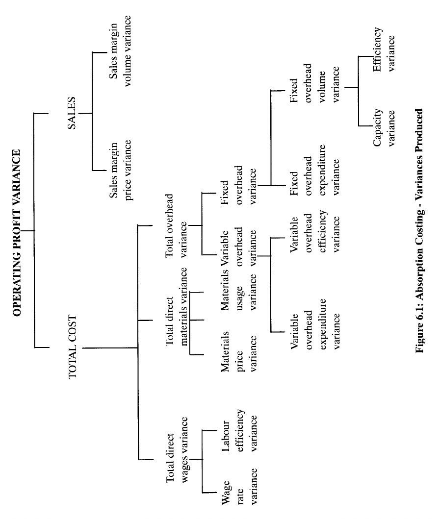
F2.1 MANAGEMENT ACCOUNTING
Page 336

F2.1 MANAGEMENT ACCOUNTING
Page 337
The variances can be summarised as follows:
Sales
- Sales margin price variance
Sales margin volume variance
Direct wages
- Wage rate variance
Labour efficiency variance
Direct materials
- Materials price variance
Materials usage variance
Variable overheads
- Variable overheads expenditure variance
Variable overheads efficiency variance
Fixed overheads
- Fixed overheads expenditure variance
Fixed overheads volume variance, divided into:
- Capacity variance
- Efficiency variance
There are also other sub-variances for sales, direct materials and direct wages.

F2.1 MANAGEMENT ACCOUNTING
Page 338
Variance Calculations
In our calculations we shall assume that an organisation has the following estimated (or
budgeted) and actual results:
Budgeted Results
RWF
RWF
Sales (10,000 units at RWF20 per unit)
200,000
Costs
Direct materials (10,000 kg at RWF4 per kg)
40,000
Direct wages (20,000 hours at RWF3 per hour)
60,000
Variance overheads (20,000 hours at RWF2 per
hour)
40,000
Fixed overheads
20,000
160,000
Net profit
RWF40,000

F2.1 MANAGEMENT ACCOUNTING
Page 339
Actual Results
RWF
RWF
Sales (9,500 units)
185,000
Direct materials (9,800 kg)
38,500
Direct wages (19,400 hours)
56,000
Variable overheads
37,500
Fixed overheads
19,500
151,500
Net profit
RWF33,500
The standard selling price and costs per unit can be calculated from the budgeted figures as
follows:
Per Unit
RWF
Selling price
20
Direct materials (1 kg at RWF4)
4
Direct wages (2 hours at RWF3)
6
Variable overheads (2 hours at RWF2)
4
Fixed overheads (2 hours at RWF1)
2
16
Standard net profit per unit
4
(a) Direct Materials
The standard cost for direct materials is made up of two parts:
• Standard quantity
• Standard price
F2.1 MANAGEMENT ACCOUNTING
Page 340
Where the actual quantity differs from the standard quantity, there will be a usage
variance. Where the actual price differs from the standard price, there will be a price
variance.
(i) Direct Materials Price Variance
The formula for calculating the materials price variance is:
(Actual quantity × Actual price) − (Actual quantity × Standard price)
This may be abbreviated to:
(AQ × AP) − (AQ × SP) = (AP − SP) × AQ
Using the figures given, the price variance may be calculated:
AQ × AP AQ × SP
9,800 × RWF4
RWF38,500 RWF39,200
Price variance: RWF38,500 − RWF39,200 = RWF700 (we ignore the minus
sign, but must decide whether the variance is favourable or not - see below).
The AQ × AP calculation had already been given, RWF38,500, so that no
additional calculations were required. Questions may sometimes be set where it
is necessary to multiply the actual quantity used by the actual price.
Having calculated that there is a variance of RWF700, we must now determine
whether it is favourable or adverse. Had the company paid the standard price
for the material, the cost would have been greater than the actual amount paid.
So there is a favourable (F) variance in this case.
The variance could also have been calculated by using the following formula:
AQ × (AP − SP)
The actual price per kg is: RWF38,500 ÷ 9,800 = RWF3.93
The formula then becomes:
9,800 × (RWF3.93 − RWF4) = RWF686 (difference owing to rounding)
Reasons for the Variance
An essential part of variance analysis is to look at the possible reasons for, or
possible causes of, the variances. The materials price variance can be attributed
to the purchasing department. Where the actual purchase prices are below
standard prices, the difference may arise from special purchase terms, discounts, a
general reduction in prices, or the purchase of lower-quality materials.
F2.1 MANAGEMENT ACCOUNTING
Page 341
Where the purchase prices are above standard, the cause may be a general rise in
prices, a change in materials specifications, or the purchase of smaller quantities
from more than one supplier, with a loss of discounts or less favourable terms.
(ii) Direct Materials Usage Variance
The formula for calculating this variance is:
(Actual quantity × Standard price) − (Standard quantity × Standard price)
This may be abbreviated to:
(AQ × SP) − (SQ × SP) = (AQ − SQ) × SP
The calculation from our data is
AQ × SP SQ × SP
9,800 kg × RWF4 = RWF39,200 9,500 kg × RWF4 = RWF38,000
Usage variance = RWF1,200 (adverse)
The variance is adverse, because there was an excess usage of 300 kg of material
which, at the standard price of RWF4 per kg, caused a variance of RWF1,200.
Note that, in calculating the standard quantity of material, the amount is based on
the actual units sold - not the budgeted quantity, otherwise the variance would
not be meaningful. This procedure of adjusting the budget figures is usually
known as flexing the budget.
Reasons for the Variance
The material usage variance is primarily the responsibility of the factory foreman
or supervisor. It may be caused by faulty machinery; loss or pilferage; excess
wastage; lower quality of materials; faulty handling; or changes in inspection or
quality standards.
A summary of the direct material cost variances is:
RWF
RWF
Actual cost
38,500
Price variance (favourable)
700
Usage variance (adverse)
(1,200)
(500)
Standard cost RWF38,000
(b) Direct Labour
The direct labour standard cost is made up of direct labour hours multiplied by the
standard direct labour wage rate. Both the actual labour hours and actual wage rates
F2.1 MANAGEMENT ACCOUNTING
Page 342
may differ from the standards, and it is necessary to separate these two differences in
order to analyse any variation between standard costs and actual costs. As shown in
Figure 6.1, the two variances are direct wage rate variance and direct labour efficiency
variance.
(i) Wage Rate Variance
This is equivalent to the materials price variance, as it reflects the difference in
the price or rate paid for direct labour hours.
The formula is:
(Actual hours × Actual rate) − (Actual hours × Standard rate)
or (AH × AR) − (AH × SR) = (AR − SR) × AH
Using our data, the calculation is:
(AH × AR) − (AH × SR)
19,400 hrs × RWF3
RWF56,000 − RWF58,200
Wage rate variance = RWF2,200 (favourable)
The variance is favourable, since the actual cost is below the standard cost for the
actual hours worked.
Reasons for the Variance
The wage rate variance can be caused by changes in wage rates not provided for
in the standards, or the use of a different class or grade of labour from that
specified in the standards. Unscheduled overtime premiums or shiftwork rates
may also account for variations in labour rates. Where wage rates have changed
since the standards were prepared, the variance will not be within the control of
managers. Where a different grade of labour is used from that specified, the
manager or foreman may be held responsible, and the matter would require
further investigation.
(ii) Direct Labour Efficiency Variance
The standard hours for direct labour were produced on the assumption of a given
level of output or performance. These hours multiplied by the standard direct
labour hourly rate give the standard cost per unit.
The formula for the labour efficiency variance is:
(Actual hours × Standard rate) − (Standard hours × Standard rate)
or (AH × SR) − (SH × SR) = (AH − SH) × SR
Using our data, the relevant calculations are:

F2.1 MANAGEMENT ACCOUNTING
Page 343
AH × SR SH × SR
19,400 hrs × RWF3 - 19,000 × RWF3
RWF58,200 - RWF57,000
Labour efficiency variance = RWF1,200 (adverse)
Note that the actual sales of 9,500 units were below the budgeted amount of
10,000 units. In order to make a relevant comparison between actual and
standard hours, the standard must be based on the equivalent standard time for
9,500 units:
9,500 × 2 hours = 19,000 hours
Reasons for the Variance
The responsibility for the labour efficiency variance will, generally, rest with the
supervisor or factory foreman. It may arise through the use of a different
machine or machines from those specified; machine breakdown; lack of
maintenance of plant; the use of defective or sub-standard materials; the use of
different grades of labour from those specified; changes in operating
arrangements or inspection standards; or faulty rate-setting. Delays in production
can also arise from lack of instructions or bad organisation.
The labour cost variances can be summarised as follows:
RWF
RWF
Actual cost
56,000
Wage rate variance (favourable)
2,200
Labour efficiency variance (adverse)
(1,200)
1,000
Standard cost RWF57,000
(c) Variable Overheads
These overheads are related to volume of production or sales. Variable production
overheads may be related to machine or direct labour hours, or as a percentage of costs,
depending upon which is most appropriate. From our data, it is clear that the variable
overheads have been calculated in relation to direct labour hours.
The analysis of variable overhead variances follows the pattern already illustrated for
direct materials and direct labour costs. In this case the variances are the expenditure
and the efficiency variance.
F2.1 MANAGEMENT ACCOUNTING
Page 344
(i) Variable Overhead Expenditure Variance
The formula is:
(Actual variable overhead) − (Actual hours × Standard rate)
or AVO − (AH × SR)
The figures from our data are:
AVO AH × SR
19,400 × RWF2
RWF37,500 RWF38,800 = RWF1,300
(favourable)
The actual overhead incurred is below the standard cost of the hours worked.
Reasons for the Variance
The variance indicates that the total of the individual items making up the
variable cost is below the standard cost of those items for the number of hours
worked. It will be necessary to examine each item in detail in order to show the
causes of the difference. The costs covered under this heading will be the
variable elements of indirect wages, indirect materials and indirect expenses. It
will also be necessary to establish which managers or executives are responsible
for the control of these costs.
(ii) Variable Overhead Efficiency Variance
The formula is:
(Actual hours × Standard rate) − (Standard hours × Standard rate)
or (AH × SR) − (SH × SR) = (AH − SH) × SR
Using the figures from our data:
AH × SR SH × SR
19,400 × RWF2 19,000 × RWF2
RWF38,800 RWF38,000 = RWF800
(adverse)
As with the calculation for labour costs, the standard hours are based upon actual
output.
Reasons for the Variance
The variable overhead efficiency variance follows the same pattern as that for the
calculation for direct labour efficiency and therefore the same causes will apply.
Summary of variable overhead variances:
F2.1 MANAGEMENT ACCOUNTING
Page 345
RWF
RWF
Actual variable cost
37,500
Expenditure variance (favourable)
1,300
Efficiency variance (adverse)
(800)
500
Standard cost RWF38,000
(d) Fixed Overheads
We are assuming that the company uses absorption costing methods. As you will
remember, under absorption costing methods fixed overheads are allocated to products
for the purpose of calculating unit costs and stock values. We have already established
that the standard cost for fixed overheads is RWF1 per hour, and this will be used for
the purpose of calculating overhead variances.
(i) Fixed Overhead Expenditure Variance
As the fixed overheads are unaffected by changes in volume within certain
ranges, the budget figure can be used for the purpose of comparison with the
actual overhead incurred.
The formula is:
Actual fixed overhead − Budgeted fixed overhead
(AFO) (BFO)
The relevant figures from our data are:
AFO BFO
RWF19,500 RWF20,000 = RWF500 (favourable)
Reasons for the Variance
The favourable variance in this calculation indicates that the total cost of the
items making up the fixed overheads is below the budgeted cost. As with the
variable overheads, the individual items must be examined to identify where the
savings have been made - or, in the case of an adverse variance, where
overspending has occurred. In the case of fixed overheads, it is likely that a
number of the items will be outside the control of production managers or
supervisory staff.
(ii) Fixed Overhead Volume Variance
This variance shows the effect on the absorption of fixed overhead costs resulting
from changes in the volume of production.
F2.1 MANAGEMENT ACCOUNTING
Page 346
The formula is:
Budgeted fixed overhead − (Standard hours × Standard rate)
(BFO) (SH × SR)
Using our data:
(BFO) SH × SR
19,000 × RWF1
RWF20,000 RWF19,000 = RWF1,000 (adverse)
This variance indicates the value of fixed overhead under- or over-absorbed by
reason of a higher or lower number of hours than anticipated in the budget. In
this case the variance is adverse, because the number of actual hours recorded
was 1,000 below the budget figure, resulting in a shortfall of RWF1,000 in
recovery of overheads.
The fixed overhead volume variance can be further sub-analysed into two main
causes: capacity and efficiency.
(iii) Fixed Overhead Capacity Variance
In this case the budgeted fixed overhead cost is compared with the actual hours
worked at the standard fixed overhead rate per hour:
BFO -
(Actual hours × Standard rate)
(AH × SR)
19,400 × RWF1
RWF20,000
RWF19,400 = RWF600 (adverse)
This variance indicates that the factory was under-employed to the extent of 600
hours during the period, and investigations would be required to find the cause. It
would be necessary to find whether the cause was external (through falling
demand), or internal (through bad management or production delays or
difficulties).
(iv) Fixed Overhead Efficiency Variance
The second subvariance arising from the volume variance is related to efficiency.
We have seen, in calculating the labour and variable overhead efficiency
variances, how the variance is derived. The same procedure applies in the case of
fixed overheads.
F2.1 MANAGEMENT ACCOUNTING
Page 347
The formula is:
(Actual hours × Standard rate) − (Standard hours × Standard rate)
(AH × SR) (SH × SR)
RWF19,400 RWF19,000 = RWF400 (adverse)
The efficiency variance arises from the same causes as the other efficiency
variances. The usefulness of attaching an hourly value to fixed overheads is
sometimes doubted, since these costs are sunk costs, and have little relevance to
the level of efficiency obtained. The variance merely indicates the value of fixed
overheads under- or over-absorbed through a change in the level of efficiency.
We can now summarise the fixed overhead variances as follows:
RWF
RWF
Actual fixed overhead cost
19,500
Expenditure variance (favourable)
500
Capacity variance (adverse)
(600)
Efficiency variance (adverse)
(400)
(500)
Standard fixed overhead cost RWF19,000
(e) Sales Variances
Under absorption costing methods, the sales variances are based on profit margins.
The two main variances are the sales margin price variance and sales margin volume
variance.
(i) Sales Margin Price Variance
This variance is intended to show the difference in profit arising from changes in
the standard selling price. In our data, actual sales were 9,500 units, which
resulted in a sales value of RWF185,000. Had the units been sold at the standard
selling price of RWF20, the sales value would have been 9,500 × RWF20 =
RWF190,000. The loss of profit arising from the variation in selling prices is
RWF5,000. This variance is adverse, since selling prices were below the
standard price. Expressed as a formula this becomes:
[(Actual quantity × Actual selling price) − Standard cost] −
[(Actual quantity × Standard selling price) − Standard cost]
F2.1 MANAGEMENT ACCOUNTING
Page 348
= [(AQ × ASP) − SC]
−
[(AQ × SSP) − SC]
RWF185,000 − RWF152,000 RWF190,000 − RWF152,000
= RWF33,000 = RWF38,000 = RWF5,000
(adverse)
The standard cost of RWF152,000 represents 9,500 units at RWF16.
Reason for the Variance
This variance, together with the sales margin volume variance, is the
responsibility of the sales department. The change in selling prices may have
resulted from sales at specially discounted prices or from allowances for quantity
purchases. The company might operate in an industry in which prices are
determined by market leaders, and it may be forced to follow the market trends.
The sales department must also check that price concessions given by its sales
staff are justified, and take care that any major price reductions are authorised by
senior staff.
(ii) Sales Margin Volume Variance
This variance shows the profit or loss arising from changes in sales volume.
The formula is:
(Actual quantity × Standard margin) − (Budgeted quantity × Standard margin)
(AQ × SM) (BQ × SM)
9,500 × RWF4 10,000 × RWF4
RWF38,000 RWF40,000 = RWF2,000
(adverse)
The result shows that there is a loss of profit of RWF2,000, because 500 fewer
units were sold than were budgeted.
Reasons for the Variance
This variance may be caused by internal factors (through failure to achieve sales
targets set in the budget) or sales targets for representatives may have been set too
optimistically and not be attainable in practice. External factors might include a
general depression in the industry concerned, or the entry of new competitors.
F2.1 MANAGEMENT ACCOUNTING
Page 349
Summary of Variances
It is now possible to summarise the variances, to show the reconciliation between the
budgeted profit of RWF40,000 and the actual profit of RWF33,500 in our original data:
SUMMARY OF VARIANCES
Adverse
RWF
Favourable
RWF RWF
Budgeted profit
40,000
Variances
Sales:
Price
5,000
Volume
2,000
Direct materials:
Price
700
Usage
1,200
Direct wages:
Wage rate
2,200
Labour efficiency
1,200
Variable overheads:
Expenditure
1,300
Efficiency
800
Fixed overheads:
Expenditure
500
Capacity
600
Efficiency
400
Net adverse variance (6,500)
Actual profit RWF33,500

F2.1 MANAGEMENT ACCOUNTING
Page 350
Analysing Variances: Marginal Costing
The variance analysis has so far been based on a system of absorption costing. Under a
variable or marginal costing system, there would be only one variance for fixed overheads -
the expenditure variance - as, in this method of costing, all fixed overheads would be
charged to the accounting period concerned, and no allocations would be made to production
units. The fixed overhead variances for capacity and efficiency would not apply but it would
become part of the sales margin volume variance.
Comparing Variances Resulting Under Absorption and Marginal
Costing
We can now tabulate our data to give comparison of variances resulting under each system:
Absorption Costing
Variable Costing
Adverse
RWF
Favourable
RWF
Adverse
RWF
Favourable
RWF
Fixed overheads:
Expenditure
500
500
Capacity
600
-
Efficiency
400
-
Sales:
Sales volume
2,000
3,000
3,000
500
3,000
500
You can see that, under marginal costing, the sales margin volume variance reflects the
amount of contribution lost through the deficiency in sales - not the loss of net profit. The
contribution is RWF6 per unit, and 500 fewer units were sold than were budgeted - giving a
variance of RWF3,000. The variances for materials, wages and variable overheads will be
identical under both absorption and marginal costing methods.
F2.1 MANAGEMENT ACCOUNTING
Page 351
J. RELATIONSHIPS BETWEEN VARIANCES AND
INVESTIGATION OF THEIR CAUSES
Interrelationship of Variances
Variances may be interrelated through some connecting factor. Frequently, a favourable
variance for one cost factor may result in an adverse variance for another. Lower-quality
materials may be purchased, giving a favourable materials price variance. However, this
possibly results in production delays or difficulties - giving an adverse variance for labour
efficiency. A lower, less skilled, grade of labour may be used at a lower rate of pay -
producing a favourable direct wage rate variance. This may result in extended production
times - giving an adverse labour efficiency variance. Similarly, a greater volume of sales
may be achieved by selling at lower prices than standard - giving a favourable sales volume
variance but an adverse sales price variance. These (and other) linking causes should be
considered in analysing standard costing variances, so that individual variances are not
considered in isolation.
Significant Variances
As we have already noted, the full benefits of standard costing will not be realised unless
variances are analysed and investigated, and corrective action taken where shown to be
necessary.
Not every variance will justify the time and expense of investigation, and some consideration
must be given to determining what are to be regarded as significant variances. Minor
variations, either in terms of money value or as percentages of the amounts involved, need
not call for investigation. It will be necessary to decide for each element of cost the control
limits within which variances can be allowed to occur without investigation. Upper and
lower control limits may be set, and only when variances are outside these limits will
investigation be required.
(a) Materials Price, Mix and Yield Variances
In process industries it is common for two or more materials to be mixed together to
produce a new material. There will be a standard specification for the proportion of
each material to be used - a standard mix, or mixture - which will also specify the
allowance for normal wastage from a given input of material. This specification will
usually be a standard batch of mixture, according to the normal quantity of input, to
produce a given volume of output. This type of operation can lead to variances arising
from variations in the mix of materials or the amount of wastage incurred, and the yield
obtained from a given input. The material usage variances can therefore be analysed to
show the causes arising from these two factors.

F2.1 MANAGEMENT ACCOUNTING
Page 352
Example
A company mixes three chemicals together to produce a new material for further
processing. The standard specification is:
Input per batch
material
1,000 kg Quantity
(kg)
Price per kg
RWF
A
500
1.00
B
300
3.00
C
200
5.00
The standard output per batch is 900 kg.
During an accounting period in which five batches of the mix were processed, the
following results were recorded:
Input
Quantity
(kg)
Price per kg
RWF
A
2,500
1.20
B
1,600
2.80
C
900
5.20
5,000
Output for the period: 4,320 kg
There are three variances - price, mix and yield.
The price variance is already familiar to us.
The mix variance represents the gain or loss arising from departures from the standard
percentages or proportions in which materials are mixed.
The yield variance represents the gain or loss arising from greater or smaller wastage
than that specified in the standard.
The steps in the analysis are:
(i) Calculate the actual cost of input.
(ii) Calculate the standard cost of the actual input.
(iii) Restate the total input quantity in the standard proportions specified.
F2.1 MANAGEMENT ACCOUNTING
Page 353
(iv) Calculate the standard input required for the actual output, and multiply by
the standard cost to give the standard cost of the actual output.
The calculations are as follows:
F2.1 MANAGEMENT ACCOUNTING
Page 354
The variances are:
(a) − (b) materials price variance: RWF12,160 − RWF11,800
= (RWF360) (adverse)
(b) − (c) materials mix variance: RWF11,800 − RWF12,000
= RWF200 (favourable)
(c) − (d) materials yield variance: RWF12,000 − RWF11,520
= RWF(480) (adverse)
Summary:
RWF
RWF
Actual cost
12,160
Materials price variance
(360)
Materials mix variance
200
Materials yield variance
(480)
Net variance
(640)
Standard cost of actual output
RWF11,520
Interpretation of Variances:
(i) Materials Price Variance
As we described earlier, this variance shows the gain or loss where purchase
prices differ from standard.
(ii) Materials Mix Variance
This variance shows the gain or loss arising from a change in the input mixture.
Our actual mixture used more of the cheaper materials A and B and less of
material C - giving a favourable mix variance when the same mix is stated in
standard proportions. Enquiries would be needed to find the reason for the
change in mix - shortage of the required materials or human error in preparing the
batch mixes.
(iii) Materials Yield Variance
This variance shows the gain or loss arising from excess or lower than standard
wastage allowances. 4,800 kg should have been used to produce the output of
4,320 - bearing in mind that the standard loss is 10 per cent of input. The excess
usage might have been caused by using the cheaper materials in the batch
mixtures. The variance of RWF480 represents the standard cost of the excess 200
kg, valued at standard prices.
(b) Sales Variances
In the same way as the materials usage mix can be subdivided, so the sales volume
variance can be further analysed into mix and volume variances, where more than one
product is sold. These additional variances show the gains or losses arising from a
change in the composition of sales. Different products are likely to have different
profit margins - therefore, although gross sales figures may be above budget levels, the

F2.1 MANAGEMENT ACCOUNTING
Page 355
profitability of sales may not be as high as budgeted if more units are sold of a less
profitable product.
Example
Out of Style Ltd has the following budgeted and actual sales for an accounting period:
Budget
Product
Units
Selling Price
per Unit
RWF
Standard Cost
per Unit
RWF
Standard Profit
per Unit
RWF
A
5,000
10.00
8.00
2.00
B
2,000
30.00
20.00
10.00
C
3,000
15.00
6.00
9.00
10,000
Actual
Product
Units
Selling Price
per Unit
RWF
Standard Cost
per Unit
RWF
Actual Profit
per Unit
RWF
A
6,000
11.00
8.00
3.00
B
3,000
28.00
20.00
8.00
C
2,000
13.00
6.00
7.00
11,000
F2.1 MANAGEMENT ACCOUNTING
Page 356

F2.1 MANAGEMENT ACCOUNTING
Page 357
Variances:
Sales price margin variance
(a) − (b) = RWF56,000
−
RWF60,000 = (RWF4,000) (adverse)
Sales mix margin variance
(b) − (c) = RWF60,000 − RWF62,700 = (RWF2,700) (adverse)
Sales volume margin variance
(c) − (d) = RWF62,700 − RWF57,000 = RWF5,700 (favourable)
Summary:
RWF
RWF
Actual profit
56,000
Sales price margin variance
(4,000)
Sales mix margin variance
(2,700)
Sales volume margin variance
5,700
Net adverse variance
(1,000)
Budgeted profit
RWF55,000
Interpretation of Variances:
(i) Sales Price Margin Variance
This variance, as we explained earlier, shows the profit or loss arising from
changes in selling prices. This is a responsibility of the sales department.
(ii) Sales Mix Margin Variance
This variance shows the variation in profit arising from a different composition of
sales from the budgeted amounts. It may be caused by falling demand for some
products and rising demand for others. Some products may be more easily sold,
and salespeople have concentrated on products which have a more rapid turnover
but possibly less profit. Our adverse variance has been shown because more
products with lower profit margins have been sold than budgeted, and
investigations would be required to find the cause. The advent of new
competition can be a factor.
(iii) Sales Volume Margin Variance
This variance indicates the loss or gain in profit through sales quantities being
above or below budget levels. The causes for this variance have been previously
outlined.
F2.1 MANAGEMENT ACCOUNTING
Page 358
(c) Costing Method in Use
In answering examination questions on the subject of sales variances, take care to find
whether answers should be based on standard contributions or standard profit
margins - depending upon whether marginal or absorption costing methods are to be
used.
K. PLANNING AND REVISION VARIANCES
Outdated Standards
Standards may become outdated because of changes in market prices, wage rates, selling
prices or other causes. In many organisations the standards will be revised only once a year,
so that any changes which take place during the year will give rise to variances.
Material Price Change
At the time of setting a standard price for a particular material, a price of RWF5 per kg may
appear to be realistic but, owing to factors outside the control of the organisation, the price
may rise to RWF6 per kg. The rise of RWF1 will be uncontrollable so far as the purchasing
department is concerned. But the purchasing department may sometimes be able to secure
materials on slightly more favourable terms than the general rise in prices. Two variances
can then be calculated:
(a) A planning revision variance, reflecting the general rise in prices
(b) A price variance arising from the purchasing department’s efficiency in purchasing
above or below the current market price.
Example
Standard price of material
RWF10.00 per kg
Current market price
RWF13.00 per kg
Quantity purchased
10,000 kg
Price paid
RWF12.80 per kg
F2.1 MANAGEMENT ACCOUNTING
Page 359
The variances may be calculated as follows:
Actual
Quantity
Actual
Price
Actual
Cost
Current
Price
Current
Cost
Standard
Price
Standard
Price
RWF RWF RWF RWF RWF RWF
10,000 12.80 128,000 130,000 130.00 10.00 100,000
Variances:
Price variance
RWF128,000 − RWF130,000 = RWF2,000 (favourable)
Planning revision variance
RWF130,000 − RWF100,000 = RWF30,000 (adverse)
Interpretation of variances:
(a) The price variance, in this case, shows the purchasing department’s efficiency in
purchasing supplies below the current market price.
(b) The planning revision variance shows the effect of price changes which have arisen
since the standards were prepared, and it is uncontrollable so far as the purchasing
department is concerned.
Similar variances can be prepared for wage rate variances or other cost or sales factors where
changes in wage rates or other changes have occurred after the standards have been prepared.
Revision Variances
Various changes may occur during the period when standards are in operation, so the
standard cost of production may change.
• Temporary changes - if the changes that take place during production are of a
temporary nature, usual variance analysis will indicate the influence on the standard
cost of production. Management action should follow to correct the situation.
• Permanent changes - if the changes are in material used, grade of labour used, or in
methods of production and are of a permanent nature, the standards themselves will
need to be revised. Under such circumstances revision variances could be calculated
for a short period of time. On revising the whole structure of standard costs and
variance analysis, say at the end of a year, any permanent changes will be incorporated.
Generally, temporary changes tend to be controllable requiring management action, whilst
permanent changes are often outside the control of the management.
F2.1 MANAGEMENT ACCOUNTING
Page 360
L. WORKED EXAMPLE
Examination questions frequently require the computation of variances, and much
examination time can be wasted if you do not fully understand the methods of calculating,
presenting and reconciling variances. You should work through the following question
carefully, before comparing your answer with the one given.
Question
X Ltd had the following budgeted and actual results for a recent accounting period:
Budgeted:
RWF
RWF
Sales (2,000 units)
50,000
Costs
Direct materials (4,000 kg @ RWF3)
12,000
Direct wages (4,000 hours @ RWF4)
16,000
Variable overheads (4,000 hours @ RWF1)
4,000
Fixed overheads
2,000
34,000
Net profit
16,000
Actual:
Sales (1,900 units)
47,000
Costs
Direct materials (3,900 kg)
11,500
Direct wages (3,700 hours)
15,500
Variable overheads
3,900
Fixed overheads
2,100
33,000
Net profit
14,000
The company uses variable (marginal) costing methods.
REQUIREMENT:
Prepare all variances for the period, and a statement reconciling the budgeted and actual
profits.
F2.1 MANAGEMENT ACCOUNTING
Page 361
Answer
Variance Analysis
Direct materials:
AQ × AP
AQ × SP
SQ × AP
3,900 × RWF3
3,800 × RWF3
RWF11,500
RWF11,700
RWF11,400
(a)
(b)
(c)
Materials price variance: (a) − (b) RWF200 (favourable)
Materials usage variance: (b) − (c) (RWF300) (adverse)
Direct wages:
AH × AR
AH × SR
SH × SR
3,700 × RWF4
3,800 × RWF4
RWF15,500
RWF14,800
RWF15,200
(a)
(b)
(c)
Direct wages rate variance: (a) − (b) (RWF700) (adverse)
Labour efficiency variance: (b) − (c) RWF400 (favourable)
Variable overheads:
AO
AH × SR
SH × SR
3,700 × RWF1
3,800 × RWF1
RWF3,900
RWF3,700
RWF3,800
(a)
(b)
(c)
Variable overhead expenditure variance: (a) − (b) (RWF200) (adverse)
Variable overhead efficiency variance: (b) − (c) RWF100
(favourable)
Fixed overheads:
AO
SO
RWF2,100
RWF2,000
Fixed overhead variance: (RWF100) (adverse)

F2.1 MANAGEMENT ACCOUNTING
Page 362
Sales variances:
AQ × AP
AQ × SP
1,900 × RWF25
RWF47,000
RWF47,500
Sales price margin variance: (RWF500) (adverse)
Act. Sales − std con
Budgeted sales − std con. RWF50,000 −
RWF32,000
RWF17,100
RWF18,000
Sales volume margin variance: (RWF900) (adverse)
Reconciliation of Budgeted and Actual Profit
Adverse
RWF
Favourable
RWF RWF
Budgeted profit
16,000
Variances
Sales:
Sales price
500
Sales volume
900
Direct materials:
Price
200
Usage
300
Direct wages:
Wage rate
700
Labour efficiency
400
Variable overheads:
Expenditure
200
Efficiency
100
Fixed overheads
100
2,700 700
Net adverse variance 2,000
Actual net profit 14,000

F2.1 MANAGEMENT ACCOUNTING
Page 363
Study Unit 15
Budgets – Planning and Control
Contents
A. Definitions
B. Advantages of Budgetary Control Systems
C. Types of Budget
D. Preparation of Budgets
E. Control Mechanism
F. Flexible Budgets
G. Behavioural Implications
H. Budgeting and Long-term Objectives
I. Public Sector Budgets
F2.1 MANAGEMENT ACCOUNTING
Page 364
A. DEFINITIONS
Budget (A plan in money)
A budget is defined as:
“A plan quantified in monetary terms, prepared and approved prior to a defined period
of time, usually showing planned income to be generated and/or expenditure to be
incurred during that period and the capital to be employed to attain a given objective.”
A budget is therefore an agreed plan which evaluates in financial terms the various targets
set by a company’s management. It includes a forecast profit and loss account, balance sheet,
accounting ratios and cash flow statements which are often analysed by individual months to
facilitate control.
Budgets are normally constructed within the broader framework of a company’s long-term
strategic plan covering the next five to ten years. This strategic plan sets out the company’s
long-term objectives, whilst the budget details the actions that must be taken during the
following year to ensure that its short and long-term goals are achieved.
Budgetary Control
A definition of budgetary control is:
“The establishment of budgets relating the responsibilities of executives to the
requirements of a policy, and the continuous comparison of actual with budgeted results,
either to secure by individual action the objective of that policy or to provide a basis for
its revision.”
Companies aim to achieve objectives by constantly comparing actual performance against
budget. Differences between actual performance and budget are called variances. An
adverse variance reduces profit and a favourable variance improves profitability.
Budgetary control therefore allows management to review variances to identify aspects of the
business that are performing better or worse than expected. In this way a company will be
able to monitor its sales performance, expenditure levels, capital expenditure projects, cash
flow, and asset and liability levels. Corrective action will be taken to reduce the impact of
adverse trends.
Financial budgets are prepared in the same format as the company’s profit and loss, balance
sheet and cash flow statements. In this way it is easy to compare actual and budgeted results
and calculate variances.
F2.1 MANAGEMENT ACCOUNTING
Page 365
Here is a typical statement comparing actual and budgeted results:
PROFIT AND LOSS ACCOUNT - MAY
MONTH YEAR TO DATE
Description
Budget
Actual
Variance
Budget
Actual
Variance
R
W
F
%
R
W
F
%
RWF
R
W
F
%
R
W
F
%
RWF
Sales
Tickets
Catering
Souvenirs
Other
Total
Gross Profit
Tickets
Catering
Souvenirs
Other
Total
Overheads
Staff costs
Rent & local authority tax
Electricity
Gas
Cleaning
Repairs
Renewals
Advertising
Entertainment
Commissions
Laundry
Motor expenses
Total overheads
NET PROFIT

F2.1 MANAGEMENT ACCOUNTING
Page 366
You can see that this statement details the month’s performance together with that for the
year to date. It covers the whole company; in order to obtain even greater control it is
necessary to prepare operating statements evaluating the contribution from each area of the
business. These additional statements usually cover the activities of individual managers to
identify which of them are failing to achieve their targets. A typical operating statement is as
follows:
OPERATING STATEMENT
Maintenance Department
Month of May . . . .
Month
Cumulative
Description
Budget
Actual
Variance
Budget
Actual
Varianc
e
RWF
RWF
RWF
RWF
RWF
RWF
Salaries
16,000
15,500
500
70,000
67,000
3,000
Wages
51,000
53,000
(2,000)
250,000
255,000
(5,000)
Indirect materials
2,000
1,900
100
10,000
12,000
(2,000)
Maintenance
6,000
6,000
-
24,000
23,900
100
Electricity
8,000
10,000
(2,000)
40,000
39,000
1,000
Gas
6,500
7,000
(500)
26,500
28,000
(1,500)
Total 89,500 93,400 (3,900) 420,500 424,900 (4,400)
This statement includes all expenditure under the control of the maintenance manager. It
details expenditure for the month of May and the cumulative position for the year to date.
The statement identifies the month’s main areas of overspend as wages, electricity and gas.
For the year to date the main problem areas are wages, indirect materials and gas.
Under a system of budgetary control the maintenance manager will be asked to prepare a
report explaining all variances and the action being taken to bring the department back onto
budget. These actions will be monitored in the following months to ensure that the corrective
measures have been taken.
F2.1 MANAGEMENT ACCOUNTING
Page 367
B. ADVANTAGES OF BUDGETARY CONTROL SYSTEMS
Agreed Targets
Budgets establish targets for each aspect of a company’s operations. These targets are set in
conjunction with each manager. In this way managers are committed to achieving their
budgets. This commitment also acts as a motivator.
Problems Identified
Budgets systematically examine all aspects of the business and identify factors that may
prevent a company achieving its objectives.
Problems are identified well in advance, which in turn allows a company to take the
necessary corrective action to alleviate the difficulty. For example, a budget may indicate
that the company will run short of cash during the winter period because of the seasonal
nature of the service being provided. By anticipating this position the company should be
able to take corrective action or arrange additional financing.
Scope for Improvement Identified
Budgets will identify all those areas that can be improved, thereby increasing efficiency and
profitability.
Positive plans for improving efficiency can be formulated and built into the agreed budget.
In this way a company can ensure that its plans for improvement are actually implemented.
Improved Co-ordination
All managers will be given an outline of the company’s objectives for the following year.
Each manager will then be asked to formulate their own plans so as to ensure that the
company’s overall objectives are achieved.
All the managers’ plans will be combined and evaluated so that a total budget for the
company can be prepared. During this process the company will ensure that each individual
plan fits in with the company’s overall objectives.
Control
It is essential for a company to achieve, if not exceed, its budget.
Achievement of budget will be aided by the use of a budgetary control system which
constantly monitors actual performance against the budget. All variances will be monitored
F2.1 MANAGEMENT ACCOUNTING
Page 368
and positive action taken in order to correct those areas of the business that are failing
to perform.
Raising Finance
Any provider of finance will want to satisfy itself that the company is being managed
correctly and that a loan will be repaid and interest commitments honoured.
The fact that a company has established a system of budgetary control will help to
demonstrate that it is being managed correctly. The budget will also show that the company
is able to meet all its commitments.
C. TYPES OF BUDGET
There are a number of different types of budget covering all aspects of a company’s
operations. These can be summarised into the following categories.
Operating Budgets
Master budgets cover the overall plan of action for the whole organisation and normally
include a budgeted profit and loss account and balance sheet.
The master budget is analysed into subsidiary budgets which detail responsibility for
generating sales and controlling costs. Detailed schedules are also prepared showing the
build-up of the figures included in the various budget documents.
Capital Budgets
These budgets detail all the projects on which capital expenditure will be incurred during the
following year, and when the expenditure is likely to be incurred. Capital expenditure is
money spent on the acquisition of fixed assets such as buildings, motor cars and equipment.
The capital budget enables the fixed asset section of the balance sheet to be completed and
provides information for the cash budget.
Cash Budgets
This budget analyses the cash flow implications of each of the above budgets. It is prepared
on a monthly basis and includes details of all cash receipts and payments. The cash budget
will also include the receipt of finance from loans and other sources together with forecast
repayments.
F2.1 MANAGEMENT ACCOUNTING
Page 369
D. PREPARATION OF BUDGETS
Timetable
Each company prepares its budgets at a specific time of the year. The process is very time-
consuming and allowance must be made for:
• Each manager to prepare his estimates
• The accumulation of the managers’ estimates so that a provisional budget can be built
up for the whole company
• The provisional budget to be reviewed and any changes to be agreed
A large company with a January to December financial year will therefore probably
commence its budget preparation in August of the preceding year. This will allow 4-5
months for the work to be completed. If it is to be completed successfully, it is essential that
a timetable is prepared detailing what information is required and the dates by which it must
be submitted. The preparation of budgets is a major project and it must be managed
correctly.
Organisation
As we have just said, the preparation of budgets is a very important task which is given a
high level of visibility within the company. The overall co-ordination of the budgeting
process is therefore handled at a high level.
Budgeting may be the responsibility of the Finance Director, who will have responsibility for
bringing together the directors and managers’ initial estimates. The Finance Director will
specify the information that is required and the dates by which it is required. S/he will also
circulate a set of economic assumptions so that all directors and managers are preparing their
forecasts against the same economic background.
The Financial Director will eliminate most of the obvious inconsistencies from the initial
estimates and submit a preliminary budget to the Chairman of the company and its Board of
Directors. The Board will consider the overall framework of this preliminary budget so as to
ensure that the budget is acceptable and that it gives the desired results.
The Board must also ensure that the budget is realistic and achievable. If the Board does not
accept any part of the budget then it will be referred back to the relevant managers for further
consideration.
Some companies set up a budget committee to co-ordinate the budgeting process. This
committee carries out similar functions to those we described earlier, but will involve more of
the company’s senior directors and managers. This committee will probably be chaired by
the Chairman of the company.
F2.1 MANAGEMENT ACCOUNTING
Page 370
The final budget must be accepted by the Board of Directors. It will then form the agreed
plan for the following year against which performance will be monitored and controlled.
Profit and Loss Account
(a) Limiting Factors
A company’s financial performance will be constrained by what are known as limiting
factors, which may include:
• Demand for products
• Supply of skilled labour
• Supply of key components
• Capacity or space
Each of these constraints limit the company’s ability to generate sales and profits.
Sales cannot exceed the demand for products, and production cannot exceed the limits
imposed by labour and material availability and capacity.
It is essential that a company recognises the fact that it may have a limiting factor, as
this will govern the overall shape of its budget.
(b) Sales
Sales budgets are normally prepared by the company’s marketing department. The
sales budget of a small company may be set by its managing director working in
conjunction with his sales team. The sales budget will take into account the following
factors:
• What is the sales trend for each product/service? Are sales increasing or
decreasing and why?
• Will any new product/service be launched and when?
• Will any of the existing products/services be phased out?
• What price increases can be obtained during the year?
• What is the advertising and promotional budget likely to be?
• What will be the pattern of sales throughout the period covered by the budget?
• What will the company’s competitors be doing?
− Are they introducing new products?
− What is their pricing policy?
− Are they being aggressive in order to gain market share?
− What is their advertising expenditure likely to be?
− Are there any new competitors entering the market?
F2.1 MANAGEMENT ACCOUNTING
Page 371
(c) Cost of Sales
Having established a preliminary sales budget, it is necessary to calculate the cost of
sales. Most companies know how much each of their products cost to produce. These
costs must be updated to allow for the forecast level of price increases and proposed
changes to specifications or methods.
(d) Labour Costs
Labour costs will be calculated by multiplying the number of people required to
complete the budget by their rates of pay. Full allowance will have to be made for any
planned wage increases.
(e) Overheads
The sales budget will be circulated to all managers with responsibility for controlling
costs. These documents will enable each manager to understand the proposed scale of
the company’s operations. Each manager will consider the items of expenditure that he
must incur in order to ensure that the company can achieve its sales targets.
Each manager will already understand the cost of running his area and from this
information he should be able to estimate the cost levels required for the budget year.
By accumulating all the managers’ individual estimates it is possible for the company
to build up a total cost budget.
(f) Profit before Tax
Sales − Cost of sales − Overheads = Profit before tax
(g) Taxation
From the budgeted level of profit, the company will be able to calculate the level of
corporation tax payable.
(h) Dividends
Dividends will be budgeted based on the forecast level of profits and the company’s
overall financial policy.
(j) Retained Earnings
Profit before tax − Tax − Dividends = Retained earnings
Retained earnings will be added to the balance sheet reserves.
The preceding data will be converted into a budgeted profit and loss account which should be
analysed to individual months and prepared in the same format as the company’s
management accounts.
F2.1 MANAGEMENT ACCOUNTING
Page 372
There will also be detailed operating statements which allocate costs to individual managers.
These statements are also prepared on a monthly basis so that actual expenditure can be
compared with budget.
Balance Sheet
Having completed a budgeted profit and loss account, it is then necessary to complete a
budgeted balance sheet.
(a) Fixed Assets
(i) Capital Budgets
Each manager will be asked to submit details of his capital expenditure
requirements, together with a brief summary of the reasons why the expenditure
is necessary. A more detailed appraisal will be required before the expenditure is
actually committed.
The capital budget will include items such as:
− New buildings
− Machinery and equipment
− Office equipment
− Computers
− Commercial vehicles
− Motor cars
The sum total of all the managers’ capital expenditure requirements will form a
provisional capital budget.
(ii) Disposals
Fixed assets may be sold or dismantled during the year. These will be listed and
an estimate made of any sales proceeds that may arise.
If a company sells a fixed asset for more than its net book value then a profit will
be made. A loss will result if an asset is sold for less than its net book value.
(iii) Depreciation
The first step in completing budgeted depreciation is to calculate the charge for
the year on the assets already owned by the company. This will require the
company to examine each of its assets and calculate the depreciation charge.
All companies are required to keep a fixed asset register, which includes details
of all their fixed assets. Many companies have computerised their fixed asset
registers, which considerably improves the speed with which this part of the
budgeting process can be completed.

F2.1 MANAGEMENT ACCOUNTING
Page 373
A company must also calculate the depreciation charge on the projects included
in its capital budget. A total depreciation charge can then be derived.
(iv) Net Book Value
We can now see how a company can complete the fixed assets section of its
budgeted balance sheet. Here is an example:
Cost
Depreciation
Net Book Value
RWF
RWF
RWF
Balances as at 1
Jan
125,000
(35,000)
90,000
Asset disposals
(7,000)
6,000
(1,000)
Depreciation for
year
(12,000)
(12,000)
Additions
55,000
(2,000)
53,000
Balances as at 31
Dec
173,000 (43,000) 130,000
(b) Working Capital
(i) Stocks
Companies calculate stock turnover ratios in order to monitor their stock control
function. The formula for calculating stock turnover is:
Stock turnover =
stock Average
sales ofCost
Companies strive for a high stock turnover, which means they are carrying low
stocks and managing the function effectively. It is therefore possible to target
improved performance by setting a higher stock turnover target for the
following year, which can be converted into a stock valuation by adopting the
following formula:
Budgeted average stock =
overStock turn
sales ofcost Budgeted
(ii) Debtors
A company will also calculate debtors’ ratios in order to monitor the effectiveness
of its credit control function. From these ratios it will establish target ratios
which can be used to calculate budgeted debtors in a similar way to the above
stock calculation.
Debtors ratio =
days 365
sales Creditors
Debtors ×
Budgeted debtors =
365
salesCredit ratio Debtors ×

F2.1 MANAGEMENT ACCOUNTING
Page 374
(iii) Cash in Hand and at Bank
In practice the budgeting process will use cash as the balancing figure in the
balance sheet. This approach may seem strange but, if you think about it, you
will see that a company’s cash position will be the result of everything else that
the company does.
(iv) Creditors
Creditors will be calculated in a very similar way to the above debtors
calculation. A target creditors ratio will be determined, which will then be
applied to the purchases figure derived from other parts of the budgeting process.
Creditors ratio =
days 365
purchasesCredit
Creditors ×
Budgeted creditors =
365
purchasesCredit ratio Creditors ×
(v) Bank Overdraft
The cash budgeting process may indicate that a bank overdraft will be required.
(c) Share Capital
The value of a company’s share capital will only change if new shares are issued. This
decision will be taken at the highest level within a company.
(d) Reserves
The opening balance on reserves will be known. The final figure will be the opening
balance plus or minus the value of retained earnings taken from the budgeted profit and
loss account.
(e) Loans
The opening position will be known. The final figure will be the opening position plus
the value of any new loans less the value of loans repaid.
All the preceding data will be presented in the budgeted balance sheet in the same format as
the company adopts for its monthly accounts. This statement will also be prepared on a
monthly basis to facilitate comparison with actual results.
Budget Review
The company has now completed provisional profit and loss, capital, cash and balance sheet
budgets.
The provisional budget will be considered by the Board of Directors. The Board must satisfy
itself that the budget is achievable and consistent with the company’s overall strategy. If the
Board accepts the budget it will become the standard by which the company will be
F2.1 MANAGEMENT ACCOUNTING
Page 375
monitored throughout the following year. If the Board does not accept part of the budget
then it will be referred back to management for further work.
In large groups of companies, the budget will also have to be approved by the Board of the
company’s holding company.
E. CONTROL MECHANISM
The budget will detail all aspects of the company’s operations. The company will prepare
monthly profit and loss accounts, operating statements, cash flow statements and balance
sheets. Each of the figures in these documents will be compared with the budget. Variances
will be calculated (the differences between actual and budgeted results). Excessive costs and
inadequate sales will be highlighted and positive action will be required in order to ensure
that the company corrects any adverse variances.
Management by Exception
When a system of budgetary control is in operation, the principle of management by
exception can be applied, i.e. when presenting information on actual results to management,
attention should be given mainly to those areas where there is a deviation from budget.
Regular Presentation of Information
The accounting function should be organised to produce the actual figures for comparison
with the budgets at the earliest possible point of time. The accounts headings should be the
same as the budget headings, so that the minimum processing work is necessary on the
figures.
The expense involved in collecting the cost figures must be borne in mind. A balance should
be struck between keeping costs to the minimum and obtaining the maximum amount of
useful information.
The budget committee should be in possession of the comparison between actual and budget
expenses within two to three weeks from the close of an accounting period. Each period
should be examined in detail by the budget committee, and managerial action taken where
necessary.
Prompt presentation of information is important because any adverse trends will probably be
continuing while data is being collected and analysed. If action is to be taken to contain the
F2.1 MANAGEMENT ACCOUNTING
Page 376
results for the succeeding period, it must be taken quickly, so the time required to collect and
analyse the data must be minimised.
Variance Interpretation
Any variances shown by the budget statements should be interpreted by the budget officer.
He should give his view on whether the variance is regarded as controllable or non-
controllable.
This part of the operation is most important. The skill and experience of the budget officer
will be of the greatest value to management, who wish to know not only the extent of any
deviation from plan, but more importantly, the reasons for it and any action being taken to
correct it.
Note that the purpose of such information is not to punish any individual for not keeping to
his budget (though it may sometimes be necessary to point out that results are unacceptable)
but rather to obtain information that will assist management to ensure that future budgets are
accurate and that greater effort is made to achieve them. The budget may also need to be
updated in the light of results achieved to date, by preparing a re-forecast.
Remember that one possible cause of variances is poor initial forecasting and budgeting.
Techniques should be kept under constant review and improved over time in the light of
experience.
SALES/
PRODUCTION
COMPARATOR
CHIEF
EXECUTIVE/
BUDGET
COMMITTEE
Actual profit
Budget
Compare actual
profit with budget
Take corrective
action: alter
output, sales
effort etc. and
re-budget
Variance

F2.1 MANAGEMENT ACCOUNTING
Page 377
Figure 7.1: Budgetary Control System
Example
The principles involved in presenting information, and a suggested layout, are illustrated in
the following example.
PQ Co. is operating a budgetary control system. The overhead costs for service department
X are as follows:
Flexible Budget for Dept X - January
Units of service:
10,000
12,000
14,000
RWF
RWF
RWF
Cleaning
300
340
380
Consumable stores
200
230
260
Depreciation
180
200
220
Insurance
150
200
250
Light and fans
200
230
260
Power
240
260
280
Repairs
160
190
220
Wages – indirect
700
740
780
2,130
2,390
2,650
For January the units supplied were 13,000 and the costs incurred were:
RWF
Cleaning 370
Consumable stores 250
Depreciation 210
Insurance 230
Light and fans 250
Power 270
Repairs 210
Wages - indirect 750
You are required to draft an operating statement showing the variances from each type of
expense. Complete the statement by showing possible reasons for the variances.
Answer
The costs (budgeted and actual) should be compared for the actual level of activity
achieved. Accordingly, on the operating statement shown below, the actual activity of
13,000 units forms the basis of the calculation of the budgeted costs. The variability of the
F2.1 MANAGEMENT ACCOUNTING
Page 378
costs can be seen quite clearly from the flexible budget (see next section). Thus, for
example, cleaning costs increase by RWF40 for 2,000 units of service or, in other words,
RWF20 for 1,000 units. Therefore, to find the cost for 13,000 units it is necessary to take the
cost for 12,000 units (RWF340) and add the cost for 1,000 units (RWF20), making a total of
RWF360.
OPERATING STATEMENT
X Department Month: January
Output: 13,000 units
Types of
Expense Activity Achieved
13,000 units
Variances Reasons for Variances
Actual Budgeted Fav. Adverse
RWF RWF RWF RWF
Cleaning
370
360
10
Maintenance work has
brought extra cleaning
Consumable
stores 250 245 5 Extra materials consumed -
maintenance
Depreciation 210 210 - -
Insurance 230 225 5 Increased premium
Light and fans 250 245 5 Extremely hot - extra cooler
used
Power 270 270 - -
Repairs
210
205
5
Large machine major
breakdown
Wages - indirect 750 760 10 Overtime anticipated not
worked
2,540
2,520
This example is very simple, but the same principles apply with more difficult problems. The
basis for the calculation of activity may be the volume of sales or production.
In problems in examinations it is not always clear what level of activity has been achieved -
this may have to be calculated from details of sales, stocks and other information.

F2.1 MANAGEMENT ACCOUNTING
Page 379
Profit Variance
Management will be especially interested in why profit was different from budget (not just
costs). The following presentation may be adopted to compare budgeted and actual profit:
RWF
Budget profit x
Plus/minus variance due to sales )
volume/selling prices ) x
x
Plus/minus cost variance x
Actual profit x
F. FLEXIBLE BUDGETS
Many companies use budgeting simply to compare actual performance with the budget that
was set during the previous financial year. This directs attention towards achieving the
agreed financial targets. The budget is fixed and all variances are reported.
However, as we saw in the previous section, if sales are greater than budget then it can be
expected that cost of sales and variable overheads will also be higher. It is possible to
compare actual results with what is therefore known as a flexible budget. A flexible budget
is defined as:
“A budget which, by recognising the difference in behaviour between fixed and variable
costs in relation to fluctuations in output, turnover, or other variable factors such as
number of employees, is designed to change appropriately with such fluctuations.”
Let’s take a look at another simple example:
Budget
Actual
Sales (units)
1,000
1,100
RWF
RWF
Selling price
10
10
Material cost each
3
4
Labour cost each
2
2
Variable overhead each
1
1
Fixed overheads
2,000
2,000

F2.1 MANAGEMENT ACCOUNTING
Page 380
Comparison with the original (or fixed) budget would give the following variances:
Budget
Actual
Variance
RWF
RWF
RWF
Sales
10,000
11,000
1,000
Material cost
3,000
4,400
(1,400)
Labour cost
2,000
2,200
(200)
Variable overhead
1,000
1,100
(100)
Fixed overheads
2,000
2,000
-
Profit
2,000
1,300
(700)
In this statement there are adverse labour and variable overhead variances even though their
actual cost per product is exactly the same as budget. The only genuine adverse variance is
material, where the actual cost per product is RWF1 per product greater than the budget.
This would be better highlighted by preparing a flexible budget which shows the expected
level of costs for the actual level of sales at budgeted selling prices. This would result in the
following statement of variances which more accurately reflects the control variances and
highlights only the overspend in material costs of RWF1,100:
Flexed Budget
Actual
Variance
RWF
RWF
RWF
Sales
11,000
11,000
-
Material cost
3,300
4,400
(1,100)
Labour cost
2,200
2,200
-
Variable overhead
1,100
1,100
-
Fixed overheads
2,000
2,000
-
Profit
2,400
1,300
(1,100)
We will be looking at flexible budgeting in further detail later.

F2.1 MANAGEMENT ACCOUNTING
Page 381
G. BEHAVIOURAL IMPLICATIONS
Budgetary control is a very powerful tool which highlights all departures from the agreed
budget. It is therefore vitally important that all managers are involved in the budget-setting
process so that they feel committed to achieving their targets. It also needs to be recognised
that managers will play the ‘budget game’ and endeavour to ensure they have achievable
targets. It is quite common to find that the company’s first budget estimates show it plunging
into massive losses. Sales and marketing staff have been cautious with their sales estimates
and views on price increases, whilst line managers have been unduly pessimistic about costs
and endeavour to secure the maximum capital budget so that they can implement all their
projects.
It takes time to tease out their genuine expectations, and this process must be handled very
carefully in order to avoid the appearance of imposing budgetary targets on managers. The
eventual target should be realistic but stretching - so as to provide a challenge to the people
involved.
Having constructed the budget, it is also important to recognise that some managers may
attempt to bend the system so that adverse variances are not reported in their area. It is not
unknown for managers to put incorrect codes on their purchase orders so that costs are shown
in another manager’s operating statement, or reported elsewhere on their own. Naturally this
does nothing to help define better budgets in the following years.
It is also essential that the basis of the budget-setting process is understood. In practice it is
often based on the company’s current position and then updated for changes expected in the
forthcoming year. This can lead to established inefficiencies being built into next year’s
targets. An alternative approach is called zero-based budgeting, which challenges the
accepted way of doing things and attempts to construct budgets based on the way operations
would be established if they were being set up for the first time. The budget must obviously
start from the company’s current position, but this type of analysis should encourage the
company to progress towards a better way of structuring its activities.
We will cover zero-based budgeting in detail later.
F2.1 MANAGEMENT ACCOUNTING
Page 382
H. BUDGETING AND LONG-TERM OBJECTIVES
Budgetary control is important, but the correct balance needs to be maintained between the
company’s short and long-term goals. Budgetary control tends to highlight short-term
financial objectives, and this highlighting is sometimes reinforced by management incentive
schemes geared to achieving budget. Great care must therefore be exercised to ensure that
decisions are not taken which protect short-term profitability at the expense of the long-term
position of the company. For example, research and development costs can be cut without
any immediate impact on the company; however, it is likely to have a major impact on the
company’s long-term position.
I. PUBLIC SECTOR BUDGETS
Preparation of the Budget
This section details specific steps in the budget preparation process, as it’s one of the core
functions of the Chief Budget Manager. The budget preparation process is coordinated by the
National Budget Department at MINECOFIN and all the budget related documents are posted
at their website http://www.minecofin.gov.rw/ministry/directorates/nb.
The First Budget Call Circular
The budget preparation call circular is triggered by the issuance of the First Budget Call
Circular (BCC). The BCC is issued in accordance with Article 28 of OBL, and provides
information to guide the Chief Budget Managers in the preparation of the budget. The 1st
BCC is normally issued in October and it is important that Chief Budget Managers start using
it from October.
The 1st BCC is not intended to seek budget submissions from budget agencies but is rather
aimed at giving advance information to facilitate timely coordination and effective planning
within the sectors to allow formulation of policy based budgets within individual budget
agencies at a later stage. The 1st BCC is aimed at inducing discussions at the sector level on
priority activities to be funded through the Government budget for the following financial
year. These priorities should be reflected in joint sector review report and should be the basis
for submission of the budget requests in response to the 2nd BCC, normally issued in early
December.
The Second Budget Call Circular
As indicated above, the 1st BCC issued in October is meant to provide advance information
to budget agencies to better prepare and make informed plans and budgets. The 2nd Budget
Call Circular is issued in early December requiring budget agencies to prepare detailed
budget submissions for the following financial year. The 2nd BCC, which is also prepared by
National Budget Department, includes:
(a) The total indicative resource envelope derived from the macro-fiscal framework
consistent with the broad policy objectives. The indicative ceilings are issued at high level at
line ministries, provinces and other high level government institutions. This is to allow
coordination and prioritization of activities at the high level of Government programmes. The
F2.1 MANAGEMENT ACCOUNTING
Page 383
parent institutions (Ministries and other high level institutions) that have been allocated
ceilings are required to immediately undertake consultative process with all affiliated
agencies to agree on individual agency ceilings that shall be the basis for the detailed budget
estimates to be entered in the budget system (SmartFMS).
(b) Budget submission formats (Annexes) to be submitted by each budget agency to assist in
preparation of the Finance Law (including externally and internally financed projects,
internally generated revenues, earmarked transfers to districts, Agency MTEFs, Strategic
Issues Papers (SIPs).
Strategic Issues Papers (SIPs)
The Strategic Issues Papers (SIPs) and Agency MTEFs are prepared by line ministries after
consultation with their affiliated agencies, projects and districts. At this stage, information is
gathered regarding projects support and sector budget support.
The SIPs and agency MTEFs are submitted to MINECOFIN and analyzed by NBD. Budget
consultations are then held between line ministries and MINECOFIN (in March) to agree on
final ceilings to submit to Cabinet & Parliament.
As indicated above, budget preparation is one of the most important responsibilities for a
Chief Budget Manager. Chief Budget Managers should ensure that the contents of the
guidelines are strictly adhered to and all issues therein are addressed in their draft budget
estimates.
Submission and approval of budgets
The procedures for preparation, presentation and approval of budgets are provided for under
Chapter III Articles 28-45.
It should be noted that no budget should be provided for urgent and unforeseen expenditures
with a budget of a central government agency as provided in article 31 of the OBL. Such a
budget is only provided under the budget of Ministry of Finance and Economic Planning.
However, each district may provide for such expenditure in its own budget as provided under
article 32 of the law.
Article 35: Expenditure estimates shall be prepared by budget Agencies, based on the
available resources and the guidelines issued by the Minister. Each budget Agency shall have
a separate budgetary line (vote) in the budget. Expenditure estimates of each budget Agency
are organized in a programmatic, economic and functional classification, in line with
international classification standards.
Article 6 of the OBL obliges government institutions to reflect all the revenues including
grants and all expenditures within their budgets. Chief Budget Managers should ensure
during budget preparation that this requirement is respected.
In order to meet the constitutional obligation as per Article 79 to submit the draft budget
estimates and MTEF to parliament before commencement of the budget session, the draft
estimates of Budget Agencies should reach MINECOFIN not later than January 28th, in hard
copies and electronically through SmartFMS. This gives NBD time to analyse the budgets
and conduct Budget Hearings for all Sector Ministries. In months 8-9 (February/March), the
detailed draft budget is prepared by MINECOFIN along with accompanying Budget
Framework Paper (BFP).
F2.1 MANAGEMENT ACCOUNTING
Page 384
The BFP sets out the macroeconomic context of the draft budget as well as the key policy
choices underlying the proposed resource allocation. The BFP is discussed by Cabinet and
recommendations are incorporated. The BFP and draft Budget is discussed with donors at the
second Joint Budget Support Review. It is at this point that Development Partners make firm
commitments for the coming year.
In accordance with article 79 of the Constitution of the Republic of Rwanda of June 4, 2003
as amended to date, the Cabinet shall submit the draft budget to the Chamber of Deputies
before the beginning of the budget session. This is further elaborated in Article 42 of OBL.
The Minister presents the draft estimates and BFP to Parliament in the 10th month of the
financial year (April).
The Parliamentary Committee on Budget and State Property in collaboration with other
sectoral committees scrutinizes the BFP and the draft budget estimates and submits a report
to plenary containing recommendations to the Executive for improvement of the BFP and
draft budget estimates. This report is normally submitted before the end of May and becomes
the basis for revising the BFP and preparing the draft Finance Law.
After the approval of the draft finance law by Cabinet around the first week of June, the draft
finance is submitted to Parliament and is officially laid before the Parliament by the Minister
of Finance and Economic Planning during the second week of June. The budget is ordinarily
voted and approved by Parliament before commencement of the next fiscal year.
Preparation and approval of Local Government Budgets
The Intergovernmental Fiscal Relations Unit (IGFR) in MINECOFIN acts as the coordinating
unit between the district and national budget cycle.
Districts carry out their own review of last year’s performance which is discussed at the Joint
Action Forum in month 2 (August). During budget preparation, districts participate in
consultations with line ministries on Earmarked Transfers. MINECOFIN (IGFR) sends out
the District Budget Call Circular for Districts to prepare their budgets. Following the
finalization of the BFP at the national level, districts prepare their detailed budget based on
final resource envelopes agreed at Districts’ Joint Action Forum and transfers from Central
Government communicated by the Ministry of Finance and Economic Planning.
As required under article 43 of the OBL, the draft budgets of local administrative entities
shall be submitted to the executive committee of such an entity for further analysis before
submission to the local council of such an entity for examination and approval. When the
draft budget of local administrative entities has been approved by Council, they shall make it
public to the general meeting of the residents convened by the Executive Committee of the
local administrative entity, in each sector.
Revised Budget
Article 45 of OBL provides for revision of budget after six months of implementing the
budget. The proposed changes shall be consistent with the approved medium-term strategies
and budget framework; and if they are different from the approved budget framework, the
reasons thereof shall be notified to the Parliament or to the local Council of such an entity.
Accordingly, the Chief Budget Managers are required to monitor closely the implementation
of their budget by keeping a close eye on issues that might require revision after six months
of implementing the budget. These should be the issues that cannot be handled through
F2.1 MANAGEMENT ACCOUNTING
Page 385
budget re-allocation like information on project funds that has just been communicated by the
donor, under- spending of a project that might require some adjustment in the procurement
plan and thus budget revision etc.
Requests for budget revision should be communicated to the Ministry of Finance and
Economic Planning by the first week of December to have an informed decision of whether a
budget revision is warranted or not by the end of December.

F2.1 MANAGEMENT ACCOUNTING
Page 386
BLANK

F2.1 MANAGEMENT ACCOUNTING
Page 387
Study Unit 16
Preparation Techniques and Considerations of Budgets
Contents
A. Functional Budgets
B. Master Budgets
C. Cash Budget
D. Flexible Budgets
E. Zero-base Budgeting (ZBB)
F. Budgetary Control and Standard Costing - Behavioural
Considerations
F2.1 MANAGEMENT ACCOUNTING
Page 388
A. FUNCTIONAL BUDGETS
Sample Data
VT Ltd produces two products - X and Y. The products pass through two departments -
Department 1 and Department 2. The following standards have been prepared for direct
materials and direct wages:
Product
X Y
Material A 5 kg 8 kg
Material B 4 kg 9 kg
Direct labour:
Department 1 3 hours 2 hours
Department 2 2 hours 4 hours
The standard costs for direct material and direct labour are:
RWF per kg
Material A 2.00
Material B 1.20
Direct wages: RWF per hr
Department 1 3.00
Department 2 3.50
Standard selling prices are:
Product RWF per unit
X 50.00
Y 80.00
The budgeted sales for each product for the coming year are:
Product Units
X 8,000
Y 10,000
The company plans to increase the stocks of finished goods, so that the closing stock of
product X will be 2,000 units and the closing stock of product Y will be 3,000 units.
Opening stocks of finished goods are:
Product Units
F2.1 MANAGEMENT ACCOUNTING
Page 389
X 1,000
Y 2,000
Finished goods are valued at variable production cost.
Opening stocks of direct material are:
Material kg
A 12,000
B 15,000
The required closing stocks of materials are: material A 19,000 kg; material B 15,000 kg.
Dept 1 Dept 2
per direct per direct
labour-hour labour-hour
RWF RWF
Light, fans, power 0.20 0.20
Consumable stores, indirect materials 0.40 0.30
Indirect wages 0.30 0.50
Repairs and maintenance 0.20 0.30
Standard variable selling and distribution expenses are:
Product X Product Y
per RWF of per RWF of
sales value sales value
(%) (%)
Commission 5 5
Carriage, packing, transport 4 2.5
Telephone, postage, stationery 2 2

F2.1 MANAGEMENT ACCOUNTING
Page 390
Fixed production, selling and distribution, and administration overheads are budgeted to be as
follows:
Production Selling and
Distributio
n
Administratio
n
RWF
RWF
RWF
Salaries:
Dept 1
10,000
Dept 2
12,000
Selling and distribution:
Product X
20,000
Product Y
30,000
Administration
22,000
Depreciation:
Dept 1
20,000
Dept 2
22,000
Selling and distribution:
Product X
5,000
Product Y
6,000
Administration
6,000
Stationery, postage, telephone:
Dept 1
1,100
Dept 2
1,200
Selling and dist. product X
800
product Y
1,000
Administration
2,500
Sundry expenses:
Dept 1
1,400
Dept 2
1,300
Selling and dist. product X
1,200
product Y
1,500
Administration
1,500

F2.1 MANAGEMENT ACCOUNTING
Page 391
The company’s balance sheet at the beginning of the year was:
BALANCE SHEET
RWF
RWF
Fixed assets at cost
1,000,000
Less: accumulated depreciation
200,000
800,000
Current Assets
Stock: material
42,000
finished goods
145,100
Debtors
150,000
Cash
40,000
377,100
Current Liabilities
Creditors
110,000
Net current assets
267,100
1,067,100
Represented by:
Share capital
800,000
Reserves
267,100
1,067,100
The budgeted cash flows per quarter are:
Quarter
(1)
(2)
(3)
(4)
RWF
RWF
RWF
RWF
Debtors
250,000
200,000
300,000
300,000
Creditors
110,000
100,000
100,000
122,000
Wages
90,000
90,000
92,000
92,000
Expenses
83,000
84,000
87,000
88,000

F2.1 MANAGEMENT ACCOUNTING
Page 392
You are required to prepare the following budgets:
– Sales
– Production
– Materials purchases
– Direct materials cost
– Direct labour cost
– Production overheads
– Selling and distribution overheads
– Administration overheads
– Trading and profit and loss account
– Balance sheet at year-end
– Cash
Sales Budget
The sales budget will frequently be the starting point of the budget, and it is in our example.
The sales figures will usually determine the production requirements - subject, as in this
case, to any required adjustment to the stocks of finished goods. The sales budget will be
derived from salespeople’s reports, market research, or other intelligence or information
bearing on future sales levels and demand for the company’s products. The sales budget
would be analysed according to the regions or territories involved, with monthly budget
figures for territories, salespeople and products, so that sales representatives would have
specific targets against which actual performances could be measured.
The total sales budget in terms of units and values for the two products will be:
Product
Units
Unit Price
Sales Value
RWF
RWF
X
8,000
50.00
400,000
Y
10,000
80.00
800,000
1,200,000
Production Budget
The purpose of this budget is to show the required production for the coming year, so that
production scheduling can be completed in advance and individual machine loading
schedules can be prepared. This will enable the production department to assess the budgeted
usage of plant, the labour requirements and the extent of any under- or over-capacity. As
with the sales budget, the total annual requirements must be analysed into monthly figures.

F2.1 MANAGEMENT ACCOUNTING
Page 393
The total budget for the year is:
Product
X Y
units units
Sales 8,000 10,000
Plus closing stock required 2,000 _3,000
10,000 13,000
Less opening stock 1,000 2,000
Production requirement 9,000 11,000
Materials Purchase Budget
This budget sets out the purchasing requirements for each type of material used by the
organisation, so that the purchasing department can place orders for deliveries, to take place
in accordance with production requirements - the essential need being that production should
not be held up for lack of materials. Purchase orders should be placed, and deliveries phased,
according to the production schedules, care being taken that no excessive stocks are carried.
The standard for the products will also specify the quality of material required, so that the
purchasing department will be responsible for obtaining the materials required, of the
standard quality.
As with other budgets, the purchasing budget should show the monthly quantities to be
purchased, allowing for any lead time in suppliers’ deliveries.
Materials
A B
kg kg
Production: Product X 45,000 36,000
Product Y 88,000 99,000
133,000 135,000
Plus required closing stock 19,000 15,000
152,000 150,000
Less opening stock 12,000 15,000
Purchases required 140,000 135,000
F2.1 MANAGEMENT ACCOUNTING
Page 394
Direct Materials Cost Budget
The figures for this budget flow from the materials purchases budget, and they show the
financial implications of the planned purchases, for purposes of financial control and cash
flow requirements.
Material A Material B
Purchases required 140,000 kg 135,000 kg
Price per kg RWF2.00 RWF1.20
Cost of purchases RWF280,000 RWF162,000
Note that the quantities for production represent the number of production units in the
production budget multiplied by the kg per unit.
Direct Labour Cost Budget
This budget shows the number of direct labour-hours required to fulfil the production
requirements and the monetary value of those hours. Departmental figures are given, so that
departmental supervisors are made aware of the labour-hours and costs over which they are
expected to exercise control. Periodic reports would be made to supervisors, showing the
output achieved and the relevant standard hours and costs for that output (and, where
necessary, the reports required on any significant variances from the standards).
F2.1 MANAGEMENT ACCOUNTING
Page 395
Direct labour-hours: PRODUCT
X
Y
Departmen
t
Units
Hours
per unit
Total
hours
Units
Hours
per unit
Total
hours
Combined
totals
1
9,000
3
27,000
11,000
2
22,000
49,000
2
9,000
2
18,000
11,000
4
44,000
62,000
Direct labour costs:
Department Hours Rate
RWF RWF
1 49,000 3.00 147,000
2 62,000 3.50 217,000
111,000 364,000

F2.1 MANAGEMENT ACCOUNTING
Page 396
Production Overhead Budget
The variable and fixed overheads are shown by department. The departmental supervisors
will be expected to exercise control over those items for which they are responsible, and
monthly reports, highlighting the variances from budget, will be provided to assist them. The
variable overheads are expressed as amounts per direct labour-hour - but these could also be
shown in relation to some other factor, such as machine time, units of production, materials to
be consumed, or other relevant factors. In practice a combination of these factors might be
used.
Variable overheads:
Department 1
Department 2
(Dir. lab-hours 49,000)
(Dir. lab-hours 62,000)
Per hour
Per hour
RWF
RWF
RWF
RWF
Light, heat, power
0.20
9,800
0.20
12,400
Consumable stores, indirect
materials
0.40
19,600
0.30
18,600
Indirect wages
0.30
14,700
0.50
31,000
Repairs, maintenance
0.20
9,800
0.30
18,600
53,900
80,600
Fixed overheads:
Dept 1
Dept 2
RWF
RWF
Salaries
10,000
12,000
Depreciation
20,000
22,000
Stationery, postage, telephone
1,100
1,200
Sundry expenses
1,400
1,300
32,500
36,500
Selling and Distribution Overheads Budget
As with other overhead budgets, the object of this budget is to identify the overheads to be
controlled by the management - in this case the sales management. Further analyses of the
overheads would be required to show the budgeted costs on a monthly basis, and by regions
and representatives where appropriate.

F2.1 MANAGEMENT ACCOUNTING
Page 397
Variable overheads:
Product
X
Y
Sales
RWF400,000
RWF800,000
% of sales
RWF
% of sales
RWF
Commission
5
20,000
5
40,000
Carriage, packing, despatch
4
16,000
2.5
20,000
Telephone, postage, stationery
2
8,000
2
16,000
44,000
76,000
Fixed overheads:
Salaries
20,000
30,000
Depreciation
5,000
6,000
Stationery, postage, telephone
800
1,000
Sundry
1,200
1,500
27,000
38,500
Administration Overheads Budget
The administration overheads are likely to be mainly of a fixed character, and not affected by
production or sales levels, except where there are wide fluctuations. These overheads will
cover the general administration and accounting services of the organisation, and they will be
the responsibility of the chief executive concerned. Separate budgets for the accounting,
company secretarial and other departments will be required in larger organisations. The
budgets will be prepared after detailed studies have been made of the level of service required
to provide the necessary accounting, secretarial and other administrative services needed.
Where a complete review is required, an organisation and methods study may be
undertaken. Monthly reports will show actual and budgeted results, as with other functions,
and variances shown for further investigation. (The costs in this problem have been assumed
to be entirely fixed.)
RWF
Salaries 22,000
Depreciation 6,000
Stationery, postage, telephone 2,500
Sundry expenses 1,500
32,000
F2.1 MANAGEMENT ACCOUNTING
Page 398
B. MASTER BUDGETS
(This is not examinable for Formation 2; however it is useful for information purposes)
Budgeted Trading and Profit and Loss Account
This account is part of the master budget as it brings together all the functional and
subsidiary budgets and it shows the expected trading profit or loss based on the sales and
cost budgets previously prepared. In the light of these results, the management may decide
to recommend changes to the sales and cost figures, to bring the expected results into line
with a required return on capital or gross and net profit percentages related to sales. Once the
final figures have been approved, the budgeted trading and profit figures become the target
for the company as a whole. Using the figures arising from the previous budgets, the
budgeted trading and profit and loss account would be as follows:
VT LTD
BUDGETED TRADING AND PROFIT AND LOSS ACCOUNT
FOR THE YEAR ENDED . . . .
RWF
RWF
Sales
1,200,000
Opening stock of materials
42,000
Purchases
442,000
484,000
Less Closing stock of materials
56,000
428,000
Direct wages
364,000
Variable production overheads
134,500
926,500
Opening stock of finished goods
145,000
1,071,500
Less Closing stock of finished goods
236,000
835,500
Gross profit
364,500
Overhead Expenses
Variable selling and distribution overhead
120,000

F2.1 MANAGEMENT ACCOUNTING
Page 399
Fixed overheads:
Production
27,000
Selling and distribution
54,500
Administration
26,000
Depreciation:
Production
42,000
Selling and distribution
11,000
Administration
6,000
286,500
Net profit
78,000
Budgeted Balance Sheet
This also forms part of the master budget, and it shows the expected overall financial
position resulting from the budgets. It enables assessments to be made of the return on
capital and ratios of profitability and liquidity - for example, the current asset/current liability
position, credit collection periods, and other financial ratios. This may also be part of a
review process in which some revisions may be required before final approval is given.

F2.1 MANAGEMENT ACCOUNTING
Page 400
VT LTD
BUDGETED BALANCE SHEET AS AT . . . .
RWF
RWF
Fixed assets at cost
1,000,000
Less: accumulated depreciation
259,000
741,000
Current Assets
Stock of materials
56,000
Stock of finished goods
236,000
Debtors
300,000
592,000
Current Liabilities
Creditors
120,000
Bank overdraft
48,000
168,000
Net current assets
424,000
1,165,000
Represented by:
Share capital
800,000
Reserves
365,000
1,165,000
C. CASH BUDGET
This budget enables management to see the timing of projected cash flows and the net cash
flow position for each period. Monthly cash flow figures would be provided to show the
anticipated cash position at each point. In the light of this budget, it may be necessary to
make arrangements for overdraft facilities for short-term needs or investment of surplus
funds. In very large organisations the management of funds may require constant attention to
ensure that effective use is made of all available funds. Also separate cash budgets may be
required for operational cash flows and financing cash flows. The operational cash flows
F2.1 MANAGEMENT ACCOUNTING
Page 401
relate to trading operations, and financing cash flows to longer-term financing with related
interest charges.
Construction of Cash Budgets
It is very important that you understand how to construct a cash budget (this topic forms a
frequent examination question).
Cash budget detail the cash effect of all transactions included in a company’s budgeted profit
and loss account and balance sheet. There are two methods of preparing them. One method
calculates receipts and payments, whilst the other looks at the change in the opening and
closing balance sheet positions.
We will examine a budget covering a three-month period. We will ignore the effect of VAT.
Example
Cashflow Ltd’s budgeted profit and loss account and balance sheets are as follows:
BUDGETED PROFIT AND LOSS ACCOUNT
January February March
RWF
RWF
RWF
RWF
RWF
RWF
Sales
80,000
70,000
90,000
Opening stock
7,000
13,000
11,000
Purchases
30,000
19,000
30,000
37,000
32,000
41,000
Closing stock
(13,000)
(11,000)
(14,000)
Cost of sales
(24,000)
(21,000)
(27,000)
Gross profit
56,000
49,000
63,000
Overheads
Wages and salaries
10,000
10,000
10,000
Depreciation
4,000
4,000
4,000
Other overheads
20,000
(34,000)
18,000
(32,000)
22,000
(36,000)
Net profit
22,000
17,000
27,000
F2.1 MANAGEMENT ACCOUNTING
Page 402
BUDGETED BALANCE SHEETS
As at 1 Jan As at 31 Mar
RWF
RWF
RWF
RWF
Fixed Assets
Cost
175,000
200,000
Depreciation
(20,000)
(32,000)
Net book value
155,000
168,000
Current Assets
Stock
7,000
14,000
Debtors
100,000
90,000
Cash
10,000
117,000
81,000
185,000
Current Liabilities
Trade creditors
(50,000)
(52,000)
Taxation
(24,000)
-
Dividends
(7,000)
(81,000)
-
(52,000)
Capital employed
191,000
301,000
Financed by:
Share capital
100,000
150,000
Reserves
25,000
91,000
Shareholders’ funds
125,000
241,000
Loans
66,000
60,000
191,000
301,000
F2.1 MANAGEMENT ACCOUNTING
Page 403
Additional Notes:
• All sales and purchases are made on one month’s credit.
• Wages and salaries are paid in the same month as the expense is incurred.
• The increase in the value of fixed assets results from the purchase of equipment costing
RWF25,000. The cash payment was made in March.
• The debtor balance as at 1 Jan will be received in January.
• The trade creditor balance as at 1 Jan will be paid in January.
• The balance sheet taxation figure shown as part of current liabilities relates to a tax
provision made on a previous year’s profits. The tax is due for payment in February.
• The balance sheet dividends figure shown as part of current liabilities relates to a
proposed dividend payable on the previous year’s profits. This dividend is payable in
March.
• The increase in share capital results from the issue of new shares. Cash to the value of
RWF25,000 is receivable in February with the balance due in March.
• A RWF6,000 loan repayment is to be made in January.
F2.1 MANAGEMENT ACCOUNTING
Page 404
(a) Receipts and Payments Method
The cash budget prepared on the receipts and payments basis is presented below:
CASH BUDGET
January February March
RWF
RWF
RWF
Receipts
Cash from sales
100,000
80,000
70,000
Issue of shares
______
25,000
25,000
Total receipts
100,000
105,000
95,000
Payments
Purchases
(50,000)
(30,000)
(19,000)
Wages and salaries
(10,000)
(10,000)
(10,000)
Other overheads
-
(20,000)
(18,000)
Purchase of fixed assets
-
-
(25,000)
Taxation
-
(24,000)
-
Dividends
-
-
(7,000)
Loan repayment
(6,000)
-
-
Total payments
(66,000)
(84,000)
(79,000)
Net cash flow for month 34,000 21,000 16,000
Opening cash position
10,000
44,000
65,000
Cash inflow
34,000
21,000
16,000
Closing cash position
44,000
65,000
81,000
F2.1 MANAGEMENT ACCOUNTING
Page 405
Explanatory notes on preparation of cash budget:
(i) Sales
All sales are made on one month’s credit. This means that January’s sales will be
paid for in February, February’s sales will be paid for in March and March’s sales
will be paid for in April.
Cash from March’s sales will be received in April, which is not covered by the
cash budget. At the end of March, RWF90,000 is owed to the company which
will be shown as debtors in March’s balance sheet.
(ii) Purchases
The company obtains one month’s credit on all its purchases. January’s
purchases will be paid for in February. February’s purchases will be paid for in
March and March’s purchases will be paid for in April.
At the end of March the company owes its suppliers RWF30,000, which will be
shown as part of creditors in March’s balance sheet.
(iii) Wages and Salaries
Wages are paid out in the same month as the expense is incurred.
(iv) Depreciation
Depreciation covers the reduction in value of a company’s fixed assets.
Depreciation is not a cash payment. It is an accounting provision which
reduces profits and the value of assets in the balance sheet.
Cash flow statements are concerned only with cash payments and cash receipts.
As depreciation does not affect cash, it will not appear in a budgeted cash flow
statement.
(v) Other Overheads
Other overheads are bought on one month’s credit. The cost, included in
January’s profit and loss account, is included in February’s cash flow, and so on.
At the end of March the company owes its suppliers RWF22,000 which will be
shown as part of creditors together with the RWF30,000 owed for its other
purchases.
(vi) Cash Balances
The opening cash position in January is taken from the balance sheet as at 1 Jan.
The closing cash position for January becomes the opening cash position in
February. February’s closing cash position becomes the opening cash position in
March.

F2.1 MANAGEMENT ACCOUNTING
Page 406
(b) Comparison of Opening and Closing Balance Sheets Method
It is also possible to prepare a cash budget by examining the opening and closing
balance sheet positions.
Completion of the cash budget on a receipts and payments basis will identify the level
of debtors and creditors. The debtors figure will represent sales made on credit for
which payment has not been received. The creditors figure will represent purchases
made on credit that have not yet been paid for. The statement will also establish the
cash or bank overdraft position.
As an alternative, it is possible to calculate debtors and creditors by using target ratios
or other information that will always be given to you in an examination question.
Cash Flow Statement
You should be aware from your financial accounting studies that, from a budgeted balance
sheet and profit and loss account, it is possible to prepare a cash flow statement. The layout
of this type of statement is presented below. The information in this statement is taken from
Cashflow Ltd’s accounts detailed earlier.
CASH FLOW STATEMENT
RWF
RWF
Operating profit
66,000
Add back depreciation
12,000
Changes in working capital:
Stocks
(7,000)
Debtors
10,000
Creditors
2,000
Cash flow from operating activities
83,000
Taxation
(24,000)
Capital expenditure
(25,000)
Dividends
(7,000)
Sources of new finance:
Share capital
50,000
Loan repayments
(6,000)
Cash inflow (represented by a change in the cash balance)
71,000
F2.1 MANAGEMENT ACCOUNTING
Page 407
This type of statement starts with a company’s profits. It then adds back the amount of
depreciation included in the profit and loss account as this does not involve a payment of
cash. Operating profit is then further adjusted for changes in the working capital position:
• An increase in stocks will reduce cash.
• A reduction in debtors means that the company has received a greater value of cash
than it has invoiced out in the form of credit sales. This will benefit a company’s cash
position.
• An increase in the value of creditors means that the company has paid less to its
suppliers than it has been allowed in credit. This will improve the cash position.
The effect of raising new share capital will benefit cash and the payment of tax and
dividends and repayment of a loan will obviously reduce the cash balance.
The final figure in the statement is the company’s net cash flow for the period, which is
represented by a change in the company’s cash position. The opening cash position was
RWF10,000 and the closing balance was RWF81,000. The company must therefore have
generated a positive cash flow of RWF71,000.
The advantage of this type of statement is that it clearly identifies those areas of the business
that must be controlled in order effectively to manage its cash resource:
− Profit must be maximised.
− Capital expenditure must be controlled. Investment should lead to improved levels of
profitability.
− Stock must be kept to a minimum.
− Debtors must be kept to a minimum.
− Creditors must be controlled so that the maximum benefit is obtained from this form of
finance.
We will look at cash flow statements again in a later study unit.
F2.1 MANAGEMENT ACCOUNTING
Page 408
Benefits of Cash Budgets
The preparation of cash budgets will also generate the following benefits:
(a) Cash budgeting highlights the impact that all other decisions have on a company’s
financial resource.
(b) Cash may be a limiting factor and restrict a company’s plans. The preparation of a
cash budget will indicate if this is the case.
(c) Budgeting will identify any cash problems that may occur during the period covered
by the budget. Advance warning will enable a company to take corrective action.
(d) Cash budgets are very useful documents when talking to banks and other financial
institutions. These organisations want to see that a company is controlling its cash,
and that it will be in a position to meet its obligations as they fall due.
D. FLEXIBLE BUDGETS
Use of Flexible Budgets
Fixed budgets are used to plan the activity of the organisation. Cost control begins by
comparing actual expenditure with budget. Remember, though, that if the level of activity
differs from that expected, some costs will change, and the individual manager cannot be
expected to control the whole of that change. If activity is greater than budgeted, some costs
will rise; if activity is less than budgeted, some costs will fall. The question is whether the
manager has kept costs within the level to be expected, given the activity level.
A flexible budget, as we mentioned in an earlier study unit, is one which - by recognising the
difference in behaviour between fixed and variable costs in relation to fluctuations in output,
turnover, or other variable factors, such as number of employees - is designed to change
appropriately with such fluctuations. It is the flexible budget which is used for control
purposes, not the fixed budget we have discussed so far.
Cost Behaviour
In order to understand flexible budgets, we must recall our earlier definitions of fixed and
variable costs:
(a) Fixed Cost
This is a cost which accrues in relation to the passage of time and which, within certain
output and turnover limits, tends to be unaffected by fluctuations in the level of activity.
Examples are rent, , insurance and executive salaries.
F2.1 MANAGEMENT ACCOUNTING
Page 409
(b) Variable Cost
This is a cost which, in the short term, tends to follow the level of activity. Examples
are all direct costs, sales commission and packaging costs.
(c) Semi-variable Cost
This is a cost containing both fixed and variable elements, which is, therefore, partly
affected by fluctuations in the volume of output or turnover. There are two main
methods of predicting semi-variable costs at various levels of output or turnover:
(i) Separation of Fixed and Variable Elements
Provided the cost is known for two different levels of output/turnover, the fixed
and variable elements can be separated, and the level of cost at any other level of
output/turnover predicted. If more than two items of data are available, the
highest and lowest are selected (the high and low point method).
Example
At output levels of 1,000 units, 1,200 units, 1,500 units and 1,800 units costs are
RWF2,000, RWF2,200, RWF2,500 and RWF2,800 respectively. Taking the low
and high points (1,000 units and 1,800 units), an extra 800 units of output causes
an extra RWF800 of cost: the variable element of the cost must be RWF1 per
unit. Therefore, considering the total cost for RWF1,000 units, the fixed element
of cost must be RWF1,000.
(ii) Graphical Method for ‘Curve Expenses’
The calculation made in (i) is an oversimplification of the situation that is found
in practice in respect of semi-variable costs: it was assumed that, after a certain
initial expense, incremental costs varied in direct proportion to output - in other
words, that the graph of the cost looked like that in Figure 10.1:
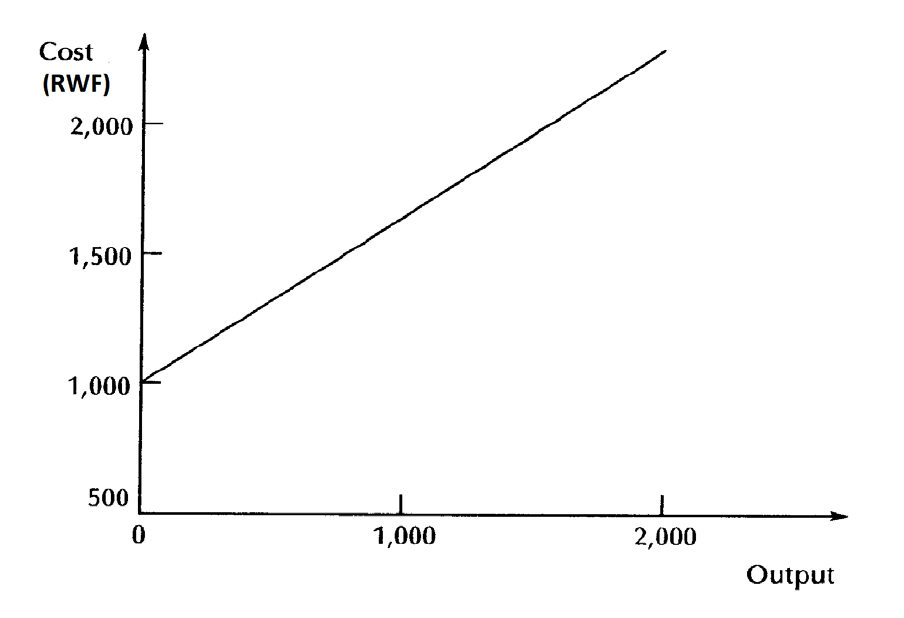
F2.1 MANAGEMENT ACCOUNTING
Page 410
Figure 10.1: Cost Varying in Direct Proportion to Output
In practice, the graph of semi-variable expenses appears as a curve. The
following procedure should be adopted:
a. Find the expense level for various levels of activity.
b. Plot these levels of cost on a graph.
c. Draw a line of best fit, so that the cost for any other activity level can be
found by interpolation.
To obtain the graph in Figure 10.2, investigation has been carried out at activity
levels of 10%, 30%, 50%, 70%, 90% and 100% of the budgeted level, and the
values plotted. The line of best fit has then been drawn between them.
It has been assumed that an activity of 64% has been achieved, and the broken
line projected to find the cost which should be associated with this activity level -
i.e. RWF5,000.
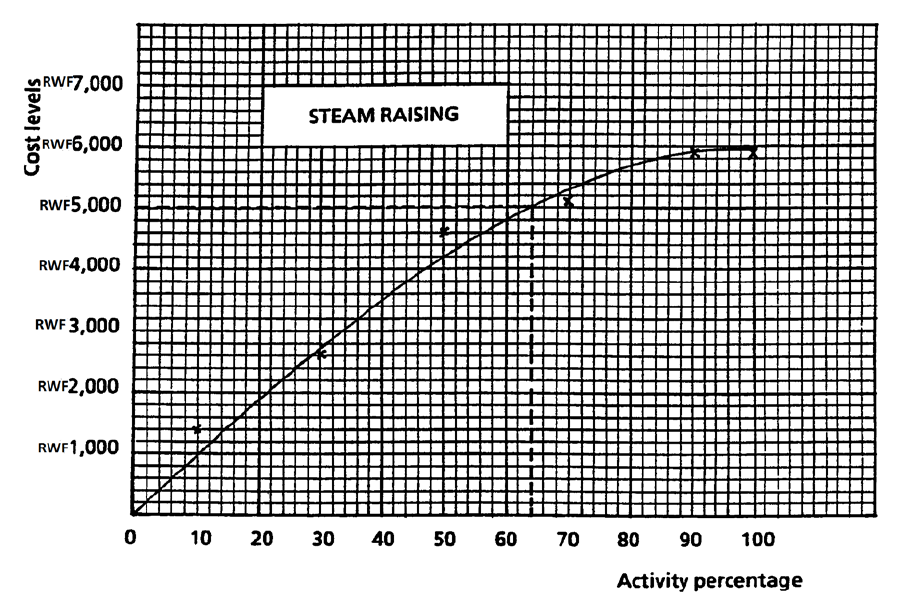
F2.1 MANAGEMENT ACCOUNTING
Page 411
Figure 10.2: Activity Level and Cost
(d) Discretionary Cost
This is a fourth category of cost, which may be incurred or not, at the manager’s
discretion. It is not directly necessary to achieving production or sales, even though the
expenditure may be desirable. Examples are research and development expenditure.
Discretionary costs such as this are a prime target for cost reduction when funds are
scarce, precisely because they are not related to current production or sales levels. This
might be a very short-sighted policy - nevertheless, it is useful to have these costs
separately identified in the budget.
(e) Controllable Costs or Managed Costs
As we know, the emphasis in budgeting is on responsibility for costs (budgetary control
is one form of responsibility accounting). The aim must be to give each manager
information about those costs he can control, and not to overburden him with
information about other costs. A controllable cost is one chargeable to a budget or cost
centre which can be influenced by the actions of the person in control of the centre.
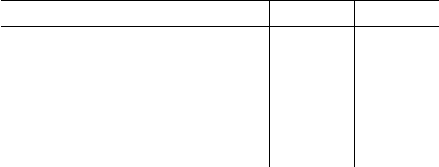
F2.1 MANAGEMENT ACCOUNTING
Page 412
Given a long enough time-period, all costs are ultimately controllable by someone in
the organisation (e.g. a decision could be taken to move to a new location, if factory
rent became too high). Controllable costs may, however, be controllable only to a
limited extent. Fixed costs are generally controllable only given a reasonably long
time-span. Variable costs may be controlled by ensuring that there is no wastage but
they will still, of course, rise more or less in proportion to output.
Preparation of Flexible Budgets
Example 1
The fixed budget for budget centre A is shown below. This is the budget based on the
expected level of output, and it will therefore be the budget used to plan the resources
needed in that department. Note that the activity level is given in standard hours. Remember
that the standard hour is a measure of output, not of time: it is the quantity of output or
amount of work which should be performed in 1 hour. This concept is used because it
enables us to compare different types of work. Instead of saying ‘400 units of X which take 2
hours per unit plus 200 units of Y which takes 1 hour per unit’ we can simply say ‘1,000
standard hours’.
BUDGET CENTRE A
Budget - Period 3 Activity 1,000 std hrs
Fixed Variable Total
RWF RWF RWF
Process labour 2,000 2,000
Indirect labour 50 85 135
Fuel and power 450 800 1,250
Consumable stores 5 15 20
3,405
From the above figures, we can evaluate a level of expense which is appropriate to any level
of output, within fairly broad limits. The figures have been set as the total allowance of
expense which is expected to be incurred at an output level of 1,000 standard hours. Should,
however, the output not be as envisaged, the allowance of cost can be varied to compensate
for the change in level of activity. This adjustment is known as flexing a budget for
activity.
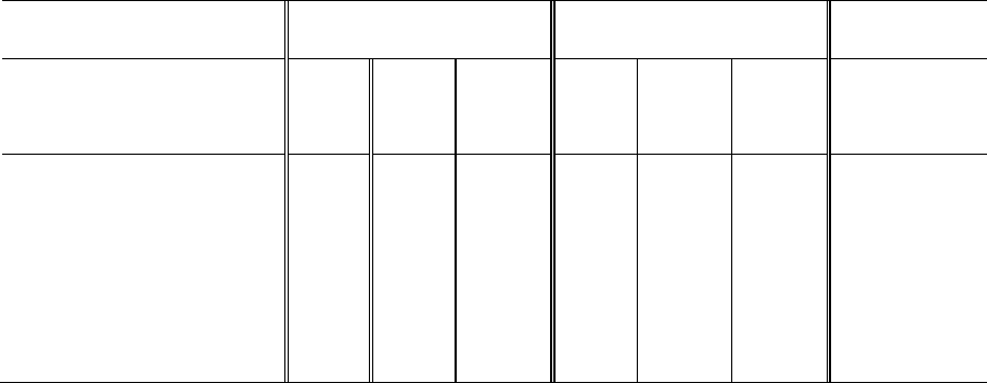
F2.1 MANAGEMENT ACCOUNTING
Page 413
We would expect that if 1,000 standard hours were produced, the cost incurred would be
RWF3,405. If the level of output changes for some reason, the level of cost usually changes.
We will assume that the levels of output attained were 750 standard hours in period 4 and
1,200 standard hours in
period 5. The budgets would be flexed to compensate for the changes which have taken
place in the actual output compared with those anticipated.
BUDGET CENTRE A
Budget - Period 4 Actual output 750 std hrs
Budgeted output 1,000 std hrs
Production volume ratio 75%
Basic Budget Flexed Budget Actual
F V Total F V Total
RWF
RWF
RWF
RWF
RWF
RWF
RWF
Process labour - 2,000 2,000 - 1,500 1,500 1,509
Indirect labour 50 85 135 50 64 114 126
Fuel and power 450 800 1,250 450 600 1,050 986
Consumable stores 5 15 20 5 11 16 19
In this instance, the fixed expenses are deemed to have remained the same but the basic
budget variable figures have been allowed at only 75% of the full budget. We thus attempt to
show that activity has had its effect on cost. For example, we expected that only RWF1,500
would be expended on process labour for the output achieved but, in fact, we spent
RWF1,509, and we exceeded the allowed cost by RWF9.
Now consider the effect on the budget in period 5 of having gained a greater output than that
envisaged originally:

F2.1 MANAGEMENT ACCOUNTING
Page 414
BUDGET CENTRE A
Budget - Period 5 Actual output 1,200 std hrs
Budgeted output 1,000 std hrs
Production volume ratio 120%
Basic Budget
Flexed Budget
Actual
F
V
Total
F
V
Total
RWF
RWF
RWF
RWF
RWF
RWF
RWF
Process labour
-
2,000
2,000
-
2,400
2,400
2,348
Indirect labour
50
85
135
50
102
152
193
Fuel and power
450
800
1,250
450
960
1,410
1,504
Consumable stores
5
15
20
5
18
23
19
Here we have used a factor of 120% as applied to the variable elements of the basic budget.
For fuel and power we observe that the fixed element has remained constant, but we have
assumed that the variable element of RWF800, having risen in sympathy with the level of
output, will have gone up by 20%, to RWF960. The flexed budget figure for fuel and power
thus becomes RWF1,410, compared with the basic budget figure of RWF1,250.
It is clearly more reasonable to compare the actual cost of fuel and power for the period - i.e.
RWF1,504 - with the flexed budget rather than with the basic budget. This explains the
entire purpose of flexible budgeting, insofar as it attempts to provide a value comparison
between the actual figure of cost and the budget figure.
Comment: Budget centre A involved a production budget. The flexing for activity was
therefore carried out according to different levels of output. The definition of flexible
budgets given earlier referred to fluctuations in output, turnover, or other factors. Obviously,
the selling costs budget will be flexed according to turnover (i.e. number of units sold) rather
than to output levels, while the canteen will be flexed according to number of employees.
Now work out the following problem for yourself before checking with the answer.
Example 2
From the following selected data of a department the normal and expected workload of which
is 3,000 hours per month:
(a) Compile a flexible budget for 2,000, 2,800 and 3,600 hours of work.
(b) Compile a fixed budget.
(c) Calculate the departmental hourly overhead rate for the total of the following items:
F2.1 MANAGEMENT ACCOUNTING
Page 415
Expense Heading
Behaviour of Expense
Supervision
RWF250 up to 2,000 hours
An extra RWF60 for steps of 400 hours above 2,000
A further RWF30 from 3,600 hours upward
Depreciation
RWF400 up to 3,000 hours
RWF550 above 3,000 hours and up to 4,200 hours
Consumable supplies
RWF12 per 100 hours
Heat and fans
RWF45 from 1,200 to 2,000 hours inclusive
RWF55 above 2,000 hours and RWF60 above 3,000
hours
Power
RWF15 per 100 hours up to 3,200
RWF12 per 100 hours for hours above 3,200
Cleaning
RWF30 up to 2,800 hours
RWF40 above 2,800 hours
Repairs
RWF75 up to 1,600 hours
Additional RWF25 for steps of 400 hours up to 3,200
hours
Additional RWF40 above 3,200 hours
Indirect wages
RWF20 per 100 hours
Rent
RWF180
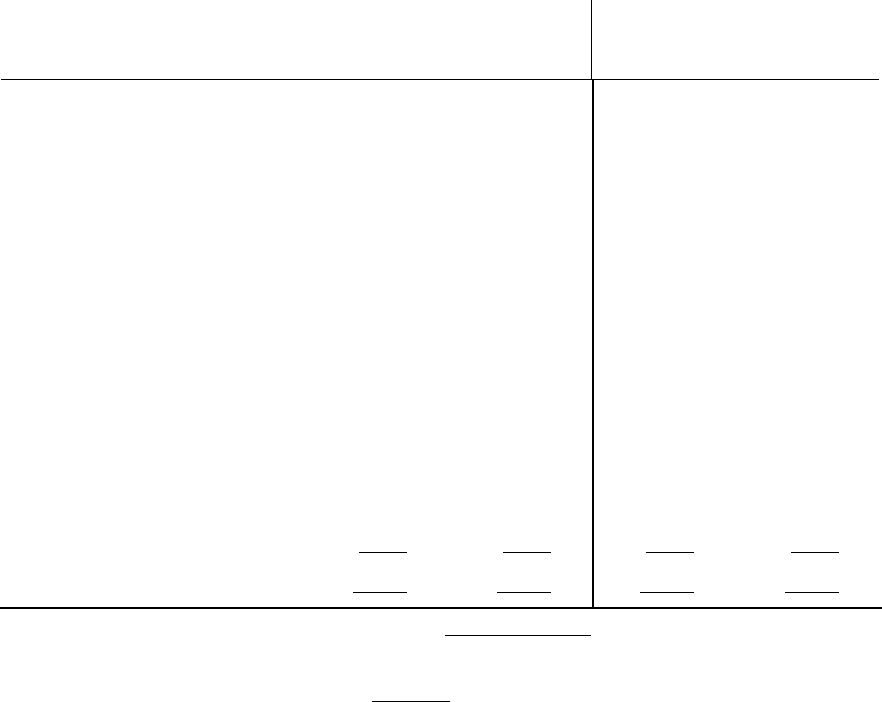
F2.1 MANAGEMENT ACCOUNTING
Page 416
Answer
(a) Flexible Budget per
Month (b) Fixed Budget per
Month
Hours of work 2,000 2,800 3,600 3,000
RWF
RWF
RWF
RWF
Expense:
Supervision
250
370
490
430
Depreciation
400
400
550
400
Consumable supplies
240
336
432
360
Heat and fans
45
55
60
55
Power
300
420
528
450
Cleaning
30
30
40
40
Repairs
100
150
215
175
Indirect wages
400
560
720
600
Rent
180
180
180
180
1,945
2,501
3,215
2,690
(c) Departmental hourly overhead rate =
hours Budgeted
expense Budgeted
=
000,3
690,2rwf
= RWF0.8966
F2.1 MANAGEMENT ACCOUNTING
Page 417
Notes:
(a) Supervision
This is a semi-variable expense, and it rises only when extra hours are worked - e.g.
when the number of employees increases, or when the firm increases the number of
supervisors. The allowance for 2,001 hours to 2,400 hours would be RWF310, and
between 2,801 and 3,200 the allowance would be RWF430.
Following this line of reasoning, up to and including 3,600 hours would have an
allowance of RWF490. Anything above 3,600 would have a budget of RWF580 - i.e.
including the extra RWF30.
(b) Depreciation
This is normally a fixed expense - but fixed only within certain ranges of production
activity. Remember that no expense is fixed over a long period or over a wide range of
production activities.
(c) Consumable Supplies
This is a variable expense in this example - it rises or falls in a direct ratio to the
number of hours worked.
(d) Heat and fans
This is a semi-variable expense; probably the figures are based on past experience or a
technical estimate.
(e) Power
This is a variable expense but, at certain levels of activity, power is supplied at a
cheaper rate.
(f) Cleaning
This is a semi-variable expense.
(g) Repairs
Again, a semi-variable expense. Presumably, when the number of hours worked
increases, more repairs will be required - but not in a direct ratio to the increase in
hours.
(h) Indirect Wages
These are, in this case, a variable expense.
F2.1 MANAGEMENT ACCOUNTING
Page 418
(j) Rent
Here, this is a fixed expense.
(k) Calculation of Departmental Hourly Overhead Rate
It is most important to realise that this rate is always calculated from the fixed budget -
not from a flexible budget. This is because the rate has to be applied throughout the
budget period as it proceeds, and the actual level of output is not known until the end of
the period, so that we would not know which flexible budget to choose. Remember that
the fixed budget is used for planning purposes, the flexible budget for control.
The difference between the flexible budget at a certain level of activity and the actual cost
incurred is, as we know, termed a variance. This may be either favourable or adverse.
Example 3
The flexible budget for the transport department of a manufacturing company contains the
following extract:
Flexible Budget for Four-weekly Period
Ton-miles to be run 80,000 100,000 120,000
Costs:
RWF
RWF
RWF
Depreciation
240
240
240
Insurance and road tax
80
80
80
Maintenance materials
160
190
190
Maintenance wages
120
120
160
Replacement of tyres
40
50
60
Rent
110
110
110
Supervision
130
130
130
Drivers’ expenses
200
400
600
1,080
1,320
1,570
In the four-weekly period No.7, the budgeted activity was 100,000 ton-miles but the actual
activity was 90,000 ton-miles. The actual expenditure during that period was:

F2.1 MANAGEMENT ACCOUNTING
Page 419
Costs:
RWF
Depreciation
240
Insurance and road tax
80
Maintenance materials
165
Maintenance wages
115
Replacement of tyres
35
Rent
110
Supervision
130
Drivers’ expenses
315
1,190
Prepare a tabulation of the variances from budget in relation to period No.7.
Answer
Budgeted
Activity
Flexed
Budget
Actual
Expense
Expense Variance
Ton-miles 100,000 90,000 90,000
Expense: RWF RWF RWF RWF
Depreciation (F)
240
240
240
-
Insurance and road tax (F)
80
80
80
-
Maintenance materials (S−V)
190
190
165
25 saving
Maintenance wages (S−V)
120
120
115
5 saving
Replacement of tyres (V)
50
45
35
10 saving
Rent (F)
110
110
110
-
Supervision (F)
130
130
130
-
Drivers’ expenses (V)
400
300
315
15 overspending
1,320
1,215
1,190
25 saving
Maintenance materials may cause a little difficulty. There is no indication in the problem at
what level of activity the rise from RWF160 to RWF190 takes place. From the information
given, it could be taken as 80,000 ton-miles or 99,999 ton-miles. You will have to make a
decision on which to take - but remember that the level of activity taken in the solution is
80,001 ton-miles and, above this level, the budgeted expense will be RWF190.
F2.1 MANAGEMENT ACCOUNTING
Page 420
E. ZERO-BASE BUDGETING (ZBB)
Basic Approach
Some aspects of the budget are easy to quantify. For example, if the required output is
known then the materials budget can be calculated from known data - material usage per unit
of output, wastage, planned stock changes, expected losses, etc. However, many aspects of
the budget cannot be so easily quantified - the outcome of indirect and service areas cannot
easily be related to sales and production targets. In these areas, traditionally, an incremental
approach to budgeting has been adopted. Typically, the manager starts from his current head
count and activities and estimates how much more (or, in times of hardship, less) he needs.
The advantages of this approach are:
• It is based on known factors (current expenditure).
• It is probably the least time-consuming approach to budgeting.
But:
• It encourages an easy-going, ‘live and let live’ approach.
• Considerable inertia is built into the company’s procedures. Change will be difficult to
manage.
• Existing services are accepted as necessary without question, whereas a critical eye
might see worthwhile savings.
It was to combat the disadvantages of traditional budgeting that zero base budgeting (ZBB)
was introduced. ZBB is an attempt to eliminate unnecessary expenditure being retained in
budgets. It rejects the common approach of setting budgets by taking last year’s expenditure
as the starting point for this year’s budget, and instead requires that the budget be built up
from scratch. In this way activities are rejustified each year. The CIMA defines ZBB as:
“A method of budgeting whereby all activities are re-evaluated each time a budget is
formulated.
Each functional budget starts with the assumption that the function does not exist and is
at zero cost. Increments of cost are compared with increments of benefit, culminating in
the planned maximum benefit for a given budgeted cost.”
The way in which ZBB is implemented will vary from one organisation to another, but the
following steps may be taken:
• The organisation is divided into decision units, each representing a readily identifiable
part of the business, such as a function, division, department or section.
F2.1 MANAGEMENT ACCOUNTING
Page 421
• Managers will be required to prepare decision packages, i.e. documents defining the
objectives, targets and resources which will be needed. It may also be necessary to
prepare alternative budgets based on different levels of production or service.
• Where different levels of budgets are set for decision units, a grading of priorities will
be required in order to assist in the final choice of packages and allocation of available
resources.
The technique is most useful when applied to service and support functions such as research
and development and administration, where there is considerable discretion as to the level of
expenditure, and it has been used in non-profit-making organisations such as local
government. When funds are scarce, such a technique is the only way of introducing new
projects, as otherwise existing projects always have first claim on the scarce resources.
Expenditure may be committed (the minimum essential to meet statutory requirements, for
example for safety, or to ensure operations continue). It may also be engineered (changing
with activity levels) or discretionary (depending on management, e.g. conference costs).
ZBB exercises are very time-consuming and costly and some organisations would only carry
out a full ZBB approach, say every three to five years, and would use previous years’ costs
and revenues as a starting point in the intervening years. There may also be communication
problems in explaining ZBB to managers, and lack of co-operation as managers see ZBB as a
threat to their ‘empires’ and status.
How the System Works
Where ZBB differs from the traditional approach is that managers must scrutinise very
carefully from scratch their future requirements In other words, in principle it ignores all
previous expenditure and performance associated with the company’s activities, and looks
afresh at these activities with a view to possible cost reduction, elimination of an activity,
new ways of achieving objectives, or redistribution of resources.
A company operating ZBB demands full co-operation and participation from its managers in
producing their respective assessments of requirements. They are made fully responsible for
their decisions. The process requires each manager to justify his total budget (and,
subsequently, justify the use of resources).
(a) Decision Packages
The system requires a manager to prepare decision packages for all activities (e.g.
projects, job functions) within his responsibility, and these packages must clearly lay
out the minimum level of performance essential, and any additional costs and additional
benefits linked with these costs. Decision packages must be produced where it is
considered that there may be alternative approaches (buy-in or sub-contract, for
F2.1 MANAGEMENT ACCOUNTING
Page 422
example) and finally an indication (cost effect) of not continuing with any particular
activity. Decision packages represent units of intended activity.
Examples of activities within the management accountant’s responsibility could be:
material control unit; payroll purchase ledger; sales ledger; data processing unit. The
manager of each of these areas would be required to produce decision packages on the
basis just outlined.
(b) Ranking and Evaluation
Having produced batches of decision packages, the manager would then rank them in
order of importance, after carrying out a cost/benefit analysis for each package. All
packages would then be forwarded to top management, who would compare and
evaluate the relative organisational needs, and fund accordingly - taking due note of
high and low priority packages. Their considerations would extend to those decision
packages which might cover redundant or duplicated activities.
(c) Need for Educated Managers
In using ZBB there is a strong inference that managers are well informed in the area of
information collecting and evaluation. They must, further, be trained in cost/benefit
analysis, in order to rank the decision packages. This is a potential weakness - not in
the system of ZBB itself, but in the means of producing it.
(d) Comparison with Traditional Budgeting
Whereas traditional budgeting paints with a very broad brush, assuming that all
activities will continue during the budget year, ZBB paints with a thin brush, providing
very fine economic detail (and, thus, fine control of individual activities and operations
within the organisation). Because the funding of activities is considered in detail by
means of decision packages, company resources are carefully directed and monitored.
F2.1 MANAGEMENT ACCOUNTING
Page 423
Implications and Value of ZBB
• ZBB, in principle, starts from scratch but, in practice, it would start from a minimum
cost level for each activity, and build up decision packages by changing the inputs.
This contrasts with traditional budgeting which assumes all activities are necessary
and continuing - there is very little ‘weeding out’.
• Managers are made aware of the corporate effect of their departments’ operations.
• ZBB allows questions to be asked before committing funds, and not afterwards, as in
traditional budgeting.
• Inefficient, redundant or obsolete operations are identified before the budget is
finalised.
• Greater managerial detail is available to the top management.
• Low and middle managers are made fully aware of the smallest details of the many
activities for which they are responsible.
• Managerial education must be at a very high level, with its attendant high training
cost.
Question
A manufacturing company intends to introduce zero-based budgeting in respect of its service
departments.
(a) Explain how zero-based budgeting differs from incremental budgeting and explain the
role of committed, engineered and discretionary costs in the operation of zero-based
budgeting.
(b) Give specific examples of committed, engineered and discretionary costs in the
operation of zero-based budgeting.
Answer
(a) Incremental budgeting uses the budget of the previous year as a starting point and
adjustments are made for volume, price changes and efficiency. The basic structure of
the budget is regarded as acceptable as it stands.
Zero-based budgets place the onus on the departmental manager to justify all proposed
expenditure. Nothing is accepted as being necessary expenditure. Each department
will need to consider possible options for the year, which will be ranked and used to
decide total budgets within the overall master budget of the organisation.
The role of a committed cost in zero-based budgeting is to set the minimum level of
expenditure necessary for statutory requirements to be met or for business operations to
take place.
F2.1 MANAGEMENT ACCOUNTING
Page 424
An engineered cost is one that is incurred in proportion to activity. These differ under
each level of activity projected under zero-based budgeting.
Discretionary costs are those which management decide whether to incur or not. They
will be assessed on a cost/benefit analysis and accepted or discarded depending on the
result.
(b) The following are examples of each kind of costs. You may have suggested others
relevant to your organisation.
Committed:
− Anti-pollution measures required by law
− A minimum level of maintenance and repair costs
− Requirement of a limited company to prepare annual accounts backed by
adequate accounting records; cost of audit
Engineered:
− Machine guards for each machine used
− Routine replacement of laser printer cartridges
− Costs of invoicing per order/statement per customer
Discretionary:
− Updating conferences; attendance expenditure
− Expenditure on management accounting function
F2.1 MANAGEMENT ACCOUNTING
Page 425
F. BUDGETARY CONTROL AND STANDARD COSTING -
BEHAVIOURAL CONSIDERATIONS
Throughout our studies on budgetary control and standard costing, the emphasis has been on
the economic aspect. There is, however, another - and very important - side to the concept,
and this is the effect on the human beings who will operate - and be judged by - the budgetary
system.
It was only in the 1980s that the results of years of study of interpersonal relationships
percolated into the field of management accountancy. It is now recognised that failure to
consider the effect of cost control on the people could result in a lowering of morale,
reducing motivation and company loyalty. The effect of this would be a reduction in profits
or cost-saving.
• Control Aspects of Budgeting
In preparing budgets in the first instance, managers should be consulted in respect of
their anticipation of costs which are controlled by them. It is true that an overall
objective is set by the higher levels of management, but the actual achievement of that
objective is left for the lower levels of management to plan.
Control is achieved by continuous comparison between actual and budgeted results.
Instead of using the term ‘variances’, as used in standard costing, it may be better to
call them differences.
These differences could be related to how well managers are performing their
functions. It is necessary to relate the differences in results to performance indicators.
The ultimate purpose of preparing budgets and calculating variances (differences)
between actual and budgeted results is to initiate managerial action. In the case of
controllable variances, speedy authoritative action would result in stemming adverse
variances or encouraging favourable variances. In the case of non-controllable
variances, caused by external factors, swift management action to search for
alternatives would be necessary.
• Levels of Management Information
It is necessary to consider the frequency of comparative information made available to
management at different levels. Lower levels of management require information
speedily, for example weekly, to stem adverse movements, while higher levels of
management, to prevent unnecessary paperwork, could receive summarised
information, for example on a monthly basis.
F2.1 MANAGEMENT ACCOUNTING
Page 426
The information given to management should be in units easily understood by the level
to which it is directed. The lower levels may be more interested in labour or machine-
hours or kg materials used, while higher levels would require the information in
monetary values.
• Motivation and Co-operation
Any system of cost control, to be fully effective, must provide for motivation and
incentive. If this requirement is not satisfied, managers will approach their
responsibilities in a very cautious and conservative manner. Praise should be
forthcoming if budgets are bettered: unfortunately, it is losses and adverse variances
which attract attention and investigation.
Personal goals and ambitions are strongly linked with organisational goals; these
personal goals may include a desire for a higher social standing and a betterment of the
individual’s status. To satisfy the goals of both the organisation and the individual,
there must be goal congruence. Without this mutual understanding, the economic
atmosphere of the organisation will be much less healthy.
The success of a budget procedure depends, at all times, on people. They must work
within the system in an understanding and co-operative manner. This can be achieved
only by individuals who have a total involvement at all stages of the budgetary
procedure, and who share in its favourable as well as its adverse revelations.
• Results of Goal Antagonism
Some of the most damaging and negative results of non-motivation created by a
budgetary control system are:
(a) Suspicion of being manipulated by the budget system: it is seen as a pressure
device.
(b) Competition between cost centres may arise and thus diminish the unifying
effect of budgetary control.
(c) A discouraging atmosphere will be created by failure to commend favourable
results, and by criticism of adverse results.
• Other Effects on Management Behaviour
The way standard costing and budgetary control systems are used can influence
management behaviour in a number of other ways:
(a) Standard costing and budgetary control systems concentrate on the short term. It
must be recognised that managers may therefore be placed in a situation whereby
they make decisions that satisfy the short-term control systems but damage the
future position of the business. For example, a manager may decide to reduce his
F2.1 MANAGEMENT ACCOUNTING
Page 427
research and development costs in order to stay within budget. This may satisfy
the short-term objectives but will clearly have long-term implications for the
business.
(b) Standard costing and budgetary systems sometimes include in operating
statements a number of costs over which the manager has no control. This
approach can be counter-productive and demotivating as a manager cannot be
held responsible for costs that he cannot control.
(c) Unless constant vigilance is maintained it will be possible for managers to incur
expenditure but have it charged to another manager’s cost centre. This practice
can result in conflict within the business which can cause a great deal of harm.
(d) Managers may feel that they have fully to spend their budgets so as to justify their
original predictions and in so doing avoid having their following year’s budget
reduced. This approach may cause waste within the business.

F2.1 MANAGEMENT ACCOUNTING
Page 428
BLANK

F2.1 MANAGEMENT ACCOUNTING
Page 429
Study Unit 17
Cost Book-Keeping
Contents
A. Cost Accounting Systems
B. Integrated or Integral Systems
F2.1 MANAGEMENT ACCOUNTING
Page 430
A. COST ACCOUNTING SYSTEMS
The Principle of Double Entry
In some businesses, the cost accounts may consist of little more than statistical memoranda,
but in a business of any size or complexity, it is preferable for the cost accounts to be kept on
a double entry basis, as this will provide more detailed information and a check on the
arithmetical accuracy of the entries.
While double entry cost accounts are generally to be preferred, you must remember that the
system has to suit the business and not the reverse. An elaborate system should not be
introduced merely for the sake of theory; the purpose of cost accounting is to provide
management with information.
We shall assume that you are familiar with the elements of double entry book-keeping, and
the arguments which show the necessity of keeping the financial accounts on a proper double
entry basis. The same arguments apply to the cost accounts. As in financial accounts, the
golden rule applies - “for every credit there is a debit” - and if you keep to this you will not
go far wrong.
Main Classification
Accounting systems which are used for costs may be classified as follows:
(a) Interlocking Systems
In these systems two separate ledgers are kept, one for costing figures (the cost ledger)
and one for financial figures (the financial ledger). Most figures in the cost ledger will
have been extracted from the financial ledger. For example, materials entering the
store, which will be recorded in the cost ledger, will already appear in the purchases
account in the financial ledger. This is why the systems are described as
“interlocking”. Since both ledgers describe the transactions of the business during the
same period, they must be capable of reconciliation.
(b) Integrated or Integral Systems
In these systems one ledger is kept, in which both the financial and cost data are
recorded.
F2.1 MANAGEMENT ACCOUNTING
Page 431
B. INTEGRATED OR INTEGRAL SYSTEMS
Description
Integrated accounts are a set of accounting records which provide financial and cost accounts
using a common input of data for all accounting purposes.
An integrated accounting system avoids the need to open a cost ledger control account and to
reconcile the cost and financial accounts.
Figure 2 shows the accounting flow within an integrated system. If you compare this
flowchart with Figure 1 you will see that they are very similar. In the integrated system the
debtors, creditors, bank and fixed assets accounts have replaced the cost ledger control
account.
In the interlocking system these accounts were, of course, part of the financial ledger, and the
cost ledger control account was the means of interlocking the two ledgers, transferring items
from the financial to the cost ledger. The integrated system is more straightforward as this
intermediate step is eliminated.
If you now compare the integrated system with what you learned about the financial ledger in
your Accounting Framework course, you will notice that the integrated system has dispensed
with the purchases account. The figure of purchases is derived from the creditors control
account and posted straight to the stores control account.
Worked Example
In view of what we have said about integrated systems, you may be surprised that separate
cost and financial profit and loss accounts are asked for. The cost profit and loss account is
not in fact part of the double entry system. It is a memorandum account only, prepared to
show what the profit would be without the effect of purely financial items. Company policy
determines whether two accounts are prepared or whether one is considered adequate.

F2.1 MANAGEMENT ACCOUNTING
Page 432
Question
ABC Ltd started the year with the following trial balance:
RWF
RWF
Capital
100,000
Fixed Assets
30,000
Debtors
10,000
Stores
20,000
Work-in-Progress
20,000
Finished Goods
30,000
Creditors
20,000
Bank
10,000
120,000
120,000
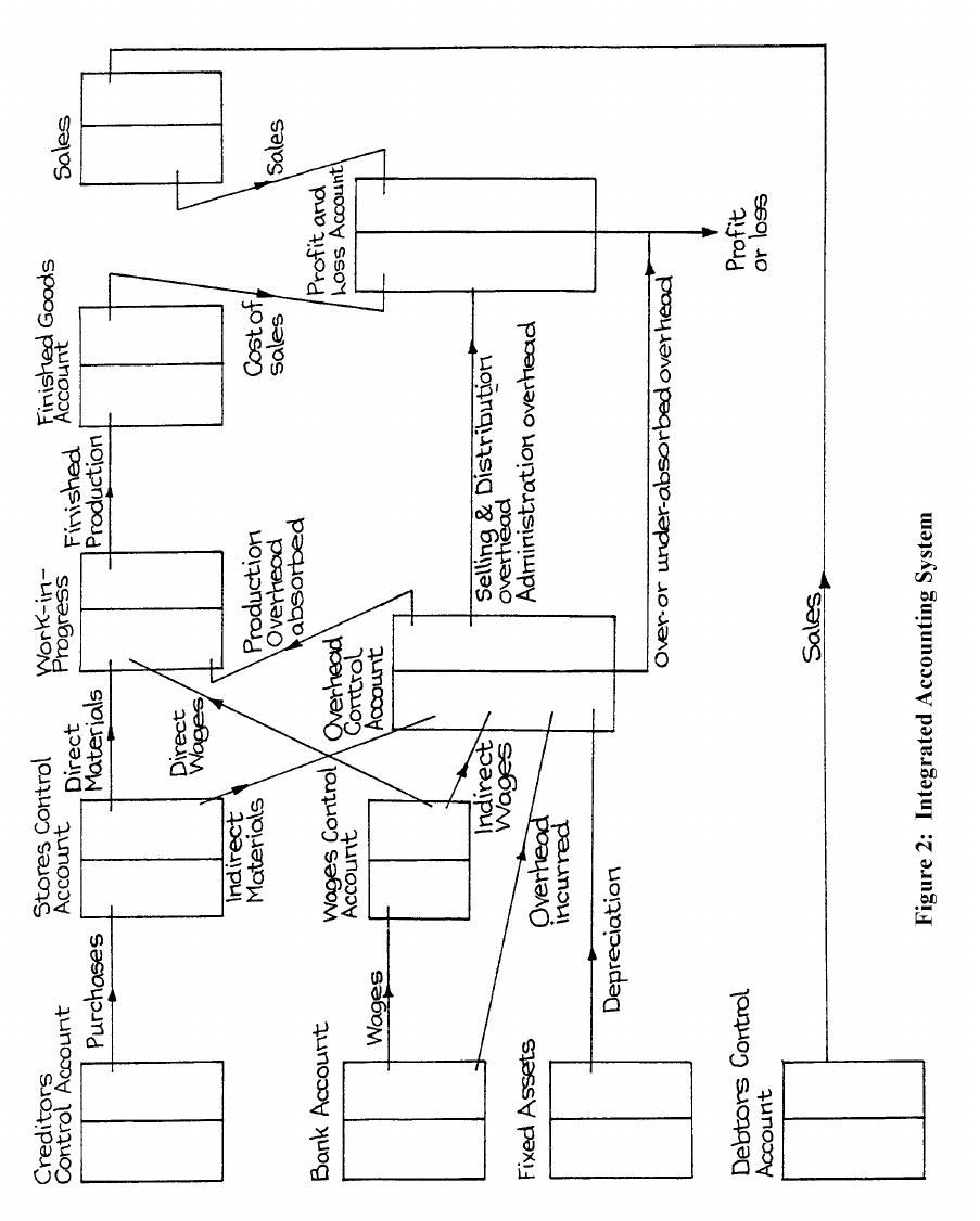
F2.1 MANAGEMENT ACCOUNTING
Page 433

F2.1 MANAGEMENT ACCOUNTING
Page 434
During January the following transactions took place:
RWF
Raw materials purchased on credit
20,000
Sales on credit
25,000
General operating expenses (cash)
10,000
Wages
10,000
Discounts allowed
1,500
Discounts received
1,000
Creditors paid
15,000
Payments by debtors
20,000
Issues from Raw Material Store
30,000
Issues from Finished Goods Store
20,000
Finished production entering Finished Goods Store
40,000
Depreciation was taken as 1% for the month on fixed assets.
Prepare:
(a) All ledger accounts;
(b) Cost profit and loss account;
(c) Financial profit and loss account;
(d) Trial balance as at the month end.
Answer
* The asterisked items are the balancing figures in the accounts.
CAPITAL
20..
RWF
Balance b/f
100,000
F2.1 MANAGEMENT ACCOUNTING
Page 435
DEBTORS
20..
RWF
20..
RWF
Balance b/f
10,000
Bank
20,000
Sales
25,000
Discounts Allowed
1,500
Balance c/f
13,500*
35,000
35,000
Balance b/f
13,500
WORK-IN-PROGRESS
20..
RWF
20..
RWF
Balance c/f
20,000
Finished Goods
40,000
Stores
30,000
Balance c/f
30,300*
Bank (Wages)
10,000
Overhead Control
10,300
70,300
70,300
Balance b/f
30,300
CREDITORS
20..
RWF
20..
RWF
Bank
15,000
Balance b/f
20,000
Discounts Received
1,000
Stores
20,000
* Balance c/f
24,000
40,000
40,000
Balance b/f
24,000
F2.1 MANAGEMENT ACCOUNTING
Page 436
BANK
20..
RWF
20..
RWF
Balance b/f
10,000
Work-in-Progress (Wages)
10,000
Debtors
20,000
Overhead Control
10,000
* Balance c/f
5,000
15,000
35,000
35,000
Balance b/f
5,000
FIXED ASSETS
20..
RWF
20..
RWF
Balance
30,000
STORES CONTROL ACCOUNT
20..
RWF
20..
RWF
Balance b/f
20,000
Work-in-Progress
30,000
Creditors (Materials Purchased)
20,000
Balance c/f
10,000*
40,000
40,000
Balance b/f
10,000
FINISHED GOODS
20..
RWF
20..
RWF
Balance c/f
30,000
Cost of Sales
20,000
Work-in-Progress
40,000
Balance c/f
50,000*
70,000
70,000
Balance b/f
50,000
F2.1 MANAGEMENT ACCOUNTING
Page 437
PROVISIONS FOR DEPRECIATION
20..
RWF
20..
RWF
Balance c/f
300
Overhead Control
300
300
300
Balance b/f
300
OVERHEAD CONTROL
20..
RWF
20..
RWF
Bank
10,000
Work-in-Progress
10,300
Provision for Depreciation
300
10,300
10,300
COST OF SALES
20..
RWF
20..
RWF
Finished Goods
20,000
Profit and Loss
20,000
20,000
20,000
SALES
20..
RWF
20..
RWF
Profit and Loss
25,000
Debtors
25,000
25,000
25,000
DISCOUNTS ALLOWED
20..
RWF
20..
RWF
Debtors
1,500
Profit and Loss
1,500
1,500
1,500

F2.1 MANAGEMENT ACCOUNTING
Page 438
DISCOUNTS RECEIVED
20..
RWF
20..
RWF
Profit and Loss
1,000
Creditors
1,000
1,000
1,000
COST PROFIT AND LOSS ACCOUNT (MEMORANDUM ONLY)
20..
RWF
20..
RWF
Cost of Sales
20,000
Sales
25,000
Profit
5,000
25,000
25,000
FINANCIAL PROFIT AND LOSS ACCOUNT
20..
RWF
20..
RWF
Cost of Sales
20,000
Sales
25,000
Discounts Allowed
1,500
Discounts Received
1,000
Profit c/f
4,500
26,000
26,000

F2.1 MANAGEMENT ACCOUNTING
Page 439
TRIAL BALANCE AS AT 31 JANUARY
Dr
Cr
RWF
RWF
Capital
100,000
Profit
4,500
Fixed Assets
30,000
Provision for Depreciation
300
Stores
10,000
Debtors
13,500
Work-in-Progress
30,300
Finished Goods
50,000
Creditors
24,000
Bank
5,000
133,800
133,800
Make sure that you understand all the entries used in this answer; once you have studied it
carefully, you should attempt the exercise of posting the entries given in the question.
Advantages of Integrated Accounting Systems
Provided that integrated accounting can be fitted conveniently into the organisation, there are
five distinct advantages:
(a) Savings in accounting costs can be made.
(b) There is no need for reconciliation of cost and financial accounts.
(c) Better use can be made of accounting information, since all the facts are known.
Together with this is the better co-operation which should ensue from the cost and
financial accounting staff also being “integrated”.
(d) Single data capture greatly simplifies automated linkages between the process control
systems, accounting systems and the overall management information systems.
F2.1 MANAGEMENT ACCOUNTING
Page 440
(e) When introducing computerised systems, it is not sensible to use two separate ledgers,
with all the attendant control problems. Computer systems are best at handling large
volumes of data and exercising overall control, but problems often arise when control
level interfaces are necessary such as when two or more ledgers are maintained. To
overcome these problems the purchase and sales ledger areas of a computerised
accounting system are usually kept apart from the nominal ledger and are physically
defined as separate modules by the software supplier
If the accounts are not computerised, the work has to be sub-divided and, historically,
this was why separate ledgers evolved for the cost and financial accounts.
F2.1 MANAGEMENT ACCOUNTING
Page 441
GLOSSARY OF
MANAGEMENT ACCOUNTING
TERMS
A-Z
F2.1 MANAGEMENT ACCOUNTING
Page 442
KEY MANAGEMENT ACCOUNTING TERMS
This glossary contains a number of Management Accounting terms which you might
encounter. It is not intended to be comprehensive; for further explanations of these terms and
of terms not included here, you should refer to the main body of this book.
Abnormal Gains The gain resulting when actual loss is less than the normal or expected
loss.
Abnormal Loss The loss resulting when actual loss is greater than the normal or
expected loss.
Absorption Overhead Overhead charged to products or services by means of
absorption rates. (CIMA Official Terminology)
Absorption Costing The procedure which charges fixed as well as variable overhead to cost
units. (CIMA Official Terminology)
Absorption Rate A rate charged to a cost unit intended to account for the overhead at a
predetermined level of activity. (CIMA Official Terminology)
Account Classification Method A simple cost estimation technique involving the
classification of costs as fixed, variable or semi variable.
Activity Based Costing (ABC) Cost attribution to cost units on the basis of benefit
received from indirect activities e.g. ordering, setting-up, assuring
quality. (CIMA Official Terminology)
Administrative Expenses Cost of management, and of secretarial, accounting and
administrative services, which cannot be related to the separate
production, marketing or research and development functions. (CIMA
Official Terminology)
Attainable Standard A standard which can be attained if a standard unit of work is carried
out efficiently, a machine properly operated or a material properly
used. Allowances are made for normal losses, waste and machine
downtime. (CIMA) Official Terminology)
F2.1 MANAGEMENT ACCOUNTING
Page 443
Avoidable Costs The specific costs of an activity or sector of a business which would be
avoided if that activity or sector did not exist. (CIMA Official
Terminology)
Basic Standard A long term standard which remains unchanged over the years and is
used to show trends.
Batch A group of similar articles which maintains its identity throughout one
or more stages of production and is treated as a cost unit. (CIMA
Official Terminology)
Batch Costing A form of specific order costing; the attribution of costs to batches.
(CIMA Official Terminology)
Bill of Materials A specification of the materials and parts required to make a product.
(CIMA Official Terminology)
Breakeven Chart A chart which indicates approximate profit or loss at different levels of
sales volume within a limited range. (CIMA Official Terminology)
Breakeven Point The level of activity at which there is neither profit nor loss. (CIMA
Official Terminology)
Breakeven (cost-volume profit (CVP)) analysis The study of the interrelationships
between costs, volume and profit at various levels of activity.
Budget A plan expressed in money. It is prepared and approved prior to the
budget period and may show income, expenditure, and the capital to be
employed. May be drawn up showing incremental effects on former
budgeted or actual figures, or be complied by zero-based budgeting.
(CIMA Official Terminology)
Budget Committee Ideally comprises representatives from every part of the organisation
and oversees the budgeting process by co-ordinating and allocating
responsibility for budget preparation, timetabling, providing
information to assist in budget preparation and monitoring the
budgeting and planning process by comparing actual and budgeted
results.
F2.1 MANAGEMENT ACCOUNTING
Page 444
Budget Manual A detailed set of documents that provide information and guidelines
about the budgetary process.
Budget Period The period for which a budget is prepared and used, which may then
be sub-divided into control periods. (CIMA Official Terminology)
Budgeted Capacity Standard Hours planned for the period, taking into account budgeted
sales, supplies, workforce availability and efficiency expected.
By-product Output of some value produced incidentally in manufacturing
something else (main product). See joint products. (CIMA Official
Terminology)
Cash Buget A statement in which estimated future cash receipts and payments are
tabulated in such a way as to show the forecast cash balance of a
business at defined intervals.
Classification The arrangement of items in logical groups having regard to their
nature (subjective classification) or purpose (objective classification).
(CIMA Official Terminology)
Code A system of symbols designed to be applied to a classified set of items
to give a brief accurate reference, facilitating entry, collation and
analysis. (CIMA Official Terminology)
Committed Cost The future cash outflow that will be incurred regardless of whatever
decision is taken now about alternative opportunities.
Computer-aided design/computer aided manufacturing (CAD CAM) system
Computer based techniques which allow interactive design and
testing of a manufacturing component on a visual display unit and
permits the programming and control of production equipment in the
manufacturing task.
Continuous Operation Costing See process costing.
Contract Costing A form of specific order costing; attribution of costs to individual
contracts. (CIMA Official Terminology)
F2.1 MANAGEMENT ACCOUNTING
Page 445
Contribution/profit volume (P/V) chart Chart showing the impact on profit of changes in
turnover. (CIMA Official Terminology)
Controllable Cost A cost which can be influenced by its budget holder. (CIMA Official
Terminology)
Cost Accounting The establishment of budgets, standard costs and actual costs of
operations, processes, activities or products; and the analysis of
variances, profitability or the social use of funds. (CIMA Official
Terminology)
Cost Accumulation The collection of cost data in some organised way through an
accounting system.
Cost behaviour The way in which costs of output are affected by fluctuations in the
level of activity. (CIMA Official Terminology)
Cost Centre A production or service location, function, activity or item of
equipment whose costs may be attributed to cost units. (CIMA Official
Terminology)
Cost Department The department responsible for keeping cost accounting records.
Cost Driver An activity which generates cost. (Particularly related to activity based
costing). (CIMA Official Terminology)
Cost Pool A group of costs that are associated with the same activity or cost
driver.
Cost Unit A unit of product or service in relation to which costs are ascertained.
(CIMA Official Terminology)
Cost-volume-profit (CVP) analysis See breakeven analysis.
Current Standard A standard based on current working conditions (current wastage,
current inefficiencies).
F2.1 MANAGEMENT ACCOUNTING
Page 446
Database Frequently a much-abused term. In its strict sense a database is a file
of data structured in such a way that it may serve a number of
applications without its structure being dictated by any one of those
applications, the concept being that programs are written around the
database rather than files being structured to meet the needs of specific
programs. The term is also rather loosely applied to simple file
management software. (CIMA Official Terminology)
Differential/Incremental Cost The difference in total cost between alternatives;
calculated to assist decision-making. (CIMA Official Terminology)
Direct Cost Expenditure which can be economically identified with a specific
saleable cost unit. (CIMA Official Terminology)
Dual Value See shadow price.
Departmental/functional budget A budget of income and/or expenditure applicable to a
particular function. A function may refer to a department or a process.
Exponential Smoothing A method of short term forecasting which involves the
automatic weighting of past data with weights that decrease
exponentially with time so that the most current values receive the
greatest weighting and the older observations receive a decreasing
weighting.
Equivalent Units Notional whole units representing uncompleted work. Used to
apportion costs between work in progress and completed output.
(CIMA Official Terminology)
Feasible Area/Region The area on a graphical model of a linear programming
problem in which all of the constraints are satisfied.
Feedback A component of a control system which measures differences between
planned and actual results and modifies subsequent actions to achieve
the required results. (CIMA Official Terminology)
Feedforward Control Control based on comparing original targets or actual results
with a forecast of future results.
F2.1 MANAGEMENT ACCOUNTING
Page 447
First-in, First-out (FIFO) Process Costing Method A process costing method that
sharply distinguishes between the work done on opening work in
progress and the work done on work introduced into the process during
the period.
Fixed Budget A budget which does not include any provision for the event that actual
volumes of production may differ from those budgeted.
Fixed Cost/Fixed Overhead/Period Cost The cost which is incurred for a period, and
which, within certain output and turnover limits, tends to be unaffected
by fluctuations in the levels of activity (output or turnover). Examples
are rent, rates, insurance and executive salaries. (CIMA Official
Terminology)
Fixed Overhead See Fixed Cost
Flexible Budget A budget which be recognising different cost behaviour patterns, is
designed to change as volume of output changes. (CIMA Official
Terminology)
Flexible Manufacturing System An integrated production system that uses computer-
controlled robots to produce immense varieties of a product at a low
cost; flexibility is promoted through rapid changeover times.
Forecasting The identification of factors and quantification of their effect on an
entity, as a basis for planning. (CIMA Official Terminology)
Full Capacity Output (expressed in standard hours) that could be achieved if sales
order, supplies and workforce were available for all installed
workplaces. (CIMA Official Terminology)
Full Cost Plus Pricing Method of determining the sales price by calculating the full
cost of the product and adding a percentage mark-up for profit.
Function Costing See Service Costing
Functional Budget See Departmental Budget
F2.1 MANAGEMENT ACCOUNTING
Page 448
Functional Classification of Costs A group of costs that were all incurred for the
same basic purpose.
High-low Method A technique for determining the fixed and variable components of a
total cost that uses actual observations of total cost at the highest and
lowest levels of activity and calculates the change in both activity and
cost.
Historical Cost The actual cost of acquiring assets, goods and services. (CIMA Official
Terminology)
Ideal Standard A standard which can be attained under the most favourable conditions,
with no allowance for normal losses, waste and machine downtime.
Also known as potential standard. (CIMA Official Terminology)
Imputed Cost Cost recognised in a particular situation that is not regularly recognised
bu usual accounting procedures.
Incremental Cost See Differential Cost
Industrial Engineering Approach Cost estimation approach which analyses the
relationships between inputs and outputs in physical terms and then
transforms the physical measures into standard or budgeted costs.
Integrated Accounts A set of accounting records which provides financial and cost accounts
using a common input of data for all accounting purposes. (CIMA
Official Terminology)
Interlocking Accounts/Non-Integrated Accounts A system in which the cost accounts
using a common input of data for all accounting purposes. (CIMA
Official Terminology)
Internal Opportunity Cost The shadow price of a scarce source.
Key Factor See Limiting Factor
Job A customer order or task of relatively short duration. (CIMA Official
Terminology)
F2.1 MANAGEMENT ACCOUNTING
Page 449
Job Costing A form of specific order costing; the attribution of cost to jobs. (CIMA
Official Terminology)
Joint Products Two or more products separated in processing, each having sufficiently
high saleable value to merit recognition as a main product. (CIMA
Official Terminology)
Just-in-Time (JIT) A technique for the organisation of work flows, to allow rapid, high
quality, flexible production whilst minimising manufacturing waste
and stock levels. (CIMA Official Terminology)
Least Squares Method (of regression analysis) Method of finding the line of best fit.
Limiting Factor/Key Factor Anything which limits the activity of an entity. An entity seeks
to optimise the benefit it obtains from the limiting factor. (CIMA
Official Terminology)
Line of Best Fit Represents the best linear relationship between two variables.
Linear Programming The use of a series of linear equations to construct a
mathematical model. The objective is to obtain an optimal solution to
a complex operational problem, given a number of alternative values of
stated variables and quantitative constraints as to their use. (CIMA
Official Terminology)
Mark-up Pricing See Marginal Cost Plus Pricing
Marginal Cost Plus Pricing/Mark-up Pricing Method of determining the sales price by
adding a profit margin onto either marginal cost of production or
marginal cost of sales.
Marginal Costing The accounting system in which variable costs are charged to cost units
and fixed costs of the period are written off in full against the aggregate
contribution. Its special value is in decision-making. The objective is
to obtain an optimal solution to a complex operational problem, given a
number of alternative values of stated variables and quantitive
constraints as to their use. (CIMA Official Terminology)
F2.1 MANAGEMENT ACCOUNTING
Page 450
Master Budget The set of budgeted profit and loss account, budgeted balance sheet
and cash budget.
Minimum Pricing Price charged that just covers both the incremental costs of production
and selling an item and the opportunity costs of the resources
consumed in making and selling it.
Mixed Cost See Semi-Variable Cost
Moving Averages A technique involving the calculation of consecutive averages over
time to establish the trend of a time series.
Non-Integrated Accounts See Inter-Locking Accounts
Normal Loss The loss expected during the normal course of operations, for
unavoidable reasons.
Notional Cost The value of a benefit where no actual cost incurred. (CIMA Official
Terminology)
Objective Function The mathematical equation which states the maximisation or
minimisation objective of a linear programming problem.
Operating Statement A regular report for management of actual cost, and revenue, as
appropriate. Usually compares actual with budget and shows
variances. (CIMA Official Terminology)
Opportunity Cost The value of a benefit sacrificed in favour of an alternative course of
action. (CIMA Official Terminology)
Overhead Absorption Rate A means of attributing overhead to a product or service based,
for example, on direct labour hours, direct hour cost or machine hours.
(CIMA Official Terminology)
Overhead/Indirect Cost Expenditure o labour, materials or services which cannot be
economically identified with a specific saleable cost unit. (CIMA
Official Terminology)
F2.1 MANAGEMENT ACCOUNTING
Page 451
Period Cost See Fixed Cost
Semi-Fixed Cost See Semi Variable Cost
Semi-Variable Cost/Semi-Fixed Cost/Mixed Cost A cost containing both fixed and variable
components and which is thus partly affected by fluctuations in the
level of activity. (CIMA Official Terminology)
Standard Costing A control technique which compares standard cost and revenues with
actual results to obtain variances which are used to stimulate improved
performance. (CIMA Official Terminology)
Step Cost A cost which is fixed in nature but only within certain levels of
activity.
Time Series Analysis The analysis of a series of figures or values recorded over time.
Uncontrollable Cost A cost that cannot be affected by management within a given time
period.
Under or Over-Absorbed overhead The difference between overhead incurred and
overhead absorbed in a given period. In a standard costing system, it is
the sum of variable production overhead total variance and fixed
production overhead variance. (CIMA Official Terminology)
User Cost The incremental cost of using machinery.
Variable Cost Cost which tends to vary with the level of activity. (CIMA Official
Terminology)
Variance Difference between planned, budgeted, or standard cost and actual
cost; and similarly for revenue. Not to be confused with statistical
variance which measures the dispersion of a statistical population.
F2.1 MANAGEMENT ACCOUNTING
Page 452
Variance Analysis The analysis of performance by means of variances. Used to promote
management action at the earliest possible stages.
Weighted Average Process Costing Method A process costing method that adds the
cost of all work done in the current period to the cost of work done in
the preceding period on the current period’s opening work in process
and divides the total by the equivalent units of work done to date.
Zero Based Budgeting A method of budgeting whereby all activities are re-evaluated
each time a budget is set. Discrete levels of each activity are valued
and a combination chosen to match funds available.
