COMCOT User Manual V1.7
COMCOT%20User%20Manual%20v1.7
COMCOT%20User%20Manual%20v1.7
COMCOT%20User%20Manual%20v1.7
COMCOT%20User%20Manual%20v1.7
User Manual:
Open the PDF directly: View PDF ![]() .
.
Page Count: 65
USER MANUAL FOR COMCOT VERSION 1.7
(FIRST DRAFT)
by
Xiaoming Wang
Febury 2009
ACKNOWLEDGEMENTS
COMCOT version 1.7 was developed by Xiaoming Wang at Institute of Geological &
Nuclear Science, New Zealand. Part of work and all its earlier versions were accom-
plished by Xiaoming Wang, Y.-S. Cho, S.-B. Woo and other members in the Wave Group
led by Professor P. L.-F. Liu at Cornell University, USA.
This document serves as an improvement and appendix to Computer programs for
tsunami propagation and inundation, edited by Liu, P. L.-F., Woo, S.-B. and Cho, Y.-S.
(1998), Cornell University.
The author takes no responsibilties on any type of actual or potential damages or
losses caused by using the entire or any part of this code.
2
TABLE OF CONTENTS
Acknowledgements............................... 2
TableofContents ................................ 3
ListofTables .................................. 5
ListofFigures.................................. 6
1 Introduction 1
1.1 Features.................................. 2
1.2 BriefHistory ............................... 3
2 Governing Equations and Numerical Methods 5
2.1 GoverningEquations ........................... 5
2.2 NumericalMethod ............................ 7
2.3 Nested Grid Configuration . . . . . . . . . . . . . . . . . . . . . . . . 12
2.4 Moving Boundary Scheme . . . . . . . . . . . . . . . . . . . . . . . . 16
2.5 Dispersion Improvement . . . . . . . . . . . . . . . . . . . . . . . . . 19
3 Tsunami Generation 21
3.1 Sea Floor Disturbances . . . . . . . . . . . . . . . . . . . . . . . . . . 21
3.1.1 Instantaneous Deformation - Elastic Fault Model . . . . . . . . 22
3.1.2 Transient Seafloor Motion . . . . . . . . . . . . . . . . . . . . 24
3.2 Water Surface Disturbances . . . . . . . . . . . . . . . . . . . . . . . . 25
4 Parameter Configuration, Input and Output Data 28
4.1 ControlFiles ............................... 28
4.1.1 General Information . . . . . . . . . . . . . . . . . . . . . . . 28
4.1.2 Parameters for Fault Model . . . . . . . . . . . . . . . . . . . . 31
4.1.3 Parameters for Wave Maker . . . . . . . . . . . . . . . . . . . 33
4.1.4 Parameters for Landslides/Transient Floor Motion . . . . . . . 34
4.1.5 Parameters for All Grid Levels . . . . . . . . . . . . . . . . . . 35
4.2 InputData................................. 40
4.2.1 Bathymetric/Topographical Data . . . . . . . . . . . . . . . . . 40
4.2.2 Seafloor Deformation Data . . . . . . . . . . . . . . . . . . . . 41
4.2.3 Transient Sea Floor Motion Data . . . . . . . . . . . . . . . . . 43
4.2.4 Bottom Friction Coefficients................... 45
4.2.5 Time History Input for Wave Maker . . . . . . . . . . . . . . . 45
4.2.6 Numerical Tidal Gauge Locations . . . . . . . . . . . . . . . . 45
4.3 OutputData................................ 46
4.3.1 Time Sequence Data . . . . . . . . . . . . . . . . . . . . . . . 46
4.3.2 Water Surface Elevation/Volume Fluxes . . . . . . . . . . . . . 46
4.3.3 Initial Condition . . . . . . . . . . . . . . . . . . . . . . . . . 48
4.3.4 Seafloor Deformation . . . . . . . . . . . . . . . . . . . . . . . 48
4.3.5 Maximum Water Surface Elevation/Depression . . . . . . . . . 49
3
4.3.6 Time History Records . . . . . . . . . . . . . . . . . . . . . . 50
4.3.7 Hot Start/Automatic Data Backup . . . . . . . . . . . . . . . . 51
A Flow Chart of COMCOT 53
B Oblique Stereographic Projection 54
C MatLab Scripts for Data Processing 57
4
LIST OF TABLES
3.1 Parameters for Elastic Fault Plane Model . . . . . . . . . . . . . . . . 22
4.1 Fortran scripts to write Water surface/Volume flux data into a data file . 47
4.2 Fortran scripts to write Initial Condition into a data file . . . . . . . . . 48
4.3 Fortran scripts to write Seafloor Deformation into a data file . . . . . . 49
4.4 Fortran scripts to write Max/Min Water Surface Fluctuations into a data
file .................................... 50
4.5 Fortran scripts to write snapshots for hot start . . . . . . . . . . . . . . 51
5

LIST OF FIGURES
2.1 Sketch of Staggered Grid Setup in COMCOT. . . . . . . . . . . . . . . 8
2.2 Sketch of Nested Grid Setup . . . . . . . . . . . . . . . . . . . . . . . 13
2.3 Detailed view of Nested Grid Setup. Left panel: grid nesting at lower-
left corner of sub-level grid region; Right panel: grid nesting at upper-
right corner of sub-level grid region. . . . . . . . . . . . . . . . . . . . 13
2.4 Detailed Time Marching Scheme of Nested Grid Setup. . . . . . . . . 16
2.5 A sketch of moving boundary scheme. . . . . . . . . . . . . . . . . . 18
3.1 Sketch of a Fault Plane and Fault parameter definitions. . . . . . . . . 26
3.2 Sketch of Transient Sea Floor Motion). . . . . . . . . . . . . . . . . . 27
4.1 General Parameter Section in COMCOT.CT L ............. 29
4.2 Fault Parameter Section in COMCOT.CT L ............... 31
4.3 Wave Maker Parameter Section in COMCOT.CT L ........... 33
4.4 Parameters for 1st-level grid in COMCOT.CT L ............. 36
4.5 Parameters for sub-level grids in COMCOT.CTL ............ 39
4.6 Example of Bathymetry Data File (XYZ format) . . . . . . . . . . . . 40
4.7 Example of Seafloor Deformation Data File (XYZ Format) . . . . . . . 42
4.8 Example of Landslide Data File (XYT Format) . . . . . . . . . . . . . 44
4.9 Example of Tidal Gauge Location File ts location.dat ......... 46
A.1 Flow Chart of COMCOT. . . . . . . . . . . . . . . . . . . . . . . . . 53
6
CHAPTER 1
INTRODUCTION
Tsunami is a typical long wave in the ocean, generated by seafloor or water surface dis-
turbances over a sufficiently large area. It has been observed and recorded since ancient
times, especially in Japan and the Mediterranean areas. The earliest recorded tsunami
occurred in 2,000 B.C. offthe coast of Syria (Lander and Lockridge, 1989). In recent
years, the most devastating tsunami was triggered by the 2004 Sumatra earthquake off
the coast of Indonesia and caused tremendous property loss and over 225,000 casual-
ties in the surrounding countries of Indian Ocean, especially in Indonesia, Sri Lanka,
Thailand and India.
For the tsunami hazard mitigation, it is very important to construct inundation maps
along those coastlines vulnerable to tsunami flooding. These maps should be developed
based on the historical tsunami events and hypothetical scenarios. To produce realistic
and reliable inundation estimates, it is essential to use a numerical model that calculates
accurately the tsunami propagation from a source region to the coastal areas of concern
and the subsequent tsunami run-up and inundation.
In many events, the wavelength of a tsunami is usually long compared to the wa-
ter depth, the dispersion effect, measured by µ=h0/l0, can be practically neglected if
h0/l0is smaller than 1/20. In this scenario, shallow water equations are adequate for
studying tsunami evolutions. Numerical models based on shallow water equations are
generally very efficient in simulating transoceanic tsunamis due to the use of explicit
numerical schemes and no need to solve higher-order derivatives associated with non-
linearity and frequency dispersion. COMCOT is one of the models based on Shallow
Water Equations.
1
COMCOT (Cornell Multi-grid Coupled Tsunami model) adopts explicit staggered
leap-frog finite difference schemes to solve Shallow Water Equations in both Spheri-
cal and Cartesian Coordinates. A nested grid system, dynamically coupled up to 12
levels (which will be also referred to as layers) with different grid resolution, can be
implemented in the model to fulfill the need for tsunami simulations in different scales.
Nested grid system means in a region of one grid size, there is one or more regions with
smaller grid sizes situated in, which eventually, forms a hierarchy of grids, or grid levels.
The region with largest grid size is called 1st-level grid and all the grid regions directly
nested in the 1st level grid, are called 2nd-level grids, so on and so forth. In one grid
region, up to 12 sub-level grid regions can be defined. It should be noted that in one grid
region, a uniform grid size (4x=4y) is adopted in COMCOT. Spherical or Cartesian
coordinate system, as well as either linear or nonlinear version of governing equations
can be chosen for each region. The water surface displacement is assumed the same as
the deformation of the sea floor as long as the uplift motion is much faster than the wave
propagation; otherwise, submarine landslide model should be used to include transient
effect. For a given earthquake, the displacement of seafloor is determined from a linear
elastic dislocation theory (Mansinha and Smylie, 1971; Okada, 1985).
For theoretical background and detailed derivations, please refer to Liu et al. (1998),
Computer programs for tsunami propagation and inundation, Cornell University.
1.1 Features
COMCOT is capable of efficiently studying the entire life-span of a tsunami, including
its generation, propagation, runup and inundation. Multiple tsunami-generating mech-
anisms can be implemented in COMCOT, including instal or transient faulting, land-
2
slides, water surface disturbances or wave maker. Both linear and nonlinear Shallow
Water Equations are available in spherical or Cartesian coordinate system for numer-
ical studies at different scales. Nested grid configuration balances the efficiency and
accuracy in which larger grid size can be used in the open sea for studying tsunami
propagation and finer grids can be adopted for coastal regions of interest. Some features
are briefly listed below:
♦Explicit Leap-Frog finite difference scheme to solve linear and nonlinear shallow
water equations in spherical and cartesian coordinates;
♦Nested grid configuration
♦Multiple tsunami-generating mechanisms, including instant faulting ( Mansinha
and Smylie (1971) and Okada (1985)), transient floor motion (e.g., landslides or tran-
sient faulting), water surface disturbance and wave maker;
♦Implementation of constant or variable bottom roughness;
♦Dispersion-improved numerical scheme;
♦Flexible input/output options
1.2 Brief History
COMCOT originated from the creation of Yongsik Cho and S.N. Seo (version 1.0)
based on the theoretical and numerical work of Shuto (1991); ?and Imamura et al.
(1988). Moving boundary scheme was introduced and validated against experimental
studies (Liu et al., 1995). Dr. Seung-Buhm Woo introduced a user interface (i.e., pa-
rameter file) and develop a general grid matching algorithm (1999) and finally formed
3
version 1.4. Many achievements were made with COMCOT during this period, such as
the successful simulations of 1960 Chile Tsunami (Liu et al., 1994) and 1986 Taiwan
Hua-lien tsunami, involving the modelling of tsunami generation, propagation, runup
and inundation. The coming of Fortran 90 gave a new power to the programming of
COMCOT. With the helps of many others, especially Tom Logan (ARSC), Steven Lantz
(Cornell University) and Philip L.-F. Liu (Cornell University), further improvements and
modifications were introduced by Xiaoming Wang (2003-), which yielded version 1.5
and 1.6. And subroutines dealing with nonlinear equations were also optimized to get
a better efficiency by Tom Logan (ARSC, 2003). One of the significant progresses is
the migration from Fortran 77 to Fortran 90, allowing dynamic allocation of arrays.
The structure of COMCOT was re-organized and a new user interface and parameter
modules was introduced, making the code much neat and more expandable. Most of
subroutines were rewritten during this time and more tsunami-generating mechanism
were implemented. A new grid-nesting algorithm was developed to allow more effi-
cient and flexible grid setup. Numerical simulations performed on this version include
2002 Hua-lien tsunami, 2003 Algerian tsunami, 2004 and 2005 Indian Ocean tsunamis
and 2006 Java tsunami. For the 2004 Giant Tsunami, both runup and inundation were
extensively studied in several regions.
In version 1.7, the solver kernel is re-packaged with a more efficient interface. More
data formats are supported. Moreover, the grid-matching becomes much easier. Once
the region of sub-level grids is defined (by coordinates of lower-left and upper-right cor-
ners), the grid-matching is done automatically by COMCOT. In addition, a dispersion-
improved algorithm is also added into the solver so that COMCOT will be able to sim-
ulate linear/weakly nonlinear dispersive waves, but still keep a high computational effi-
ciency.
4
CHAPTER 2
GOVERNING EQUATIONS AND NUMERICAL METHODS
2.1 Governing Equations
Linear and nonlinear shallow water equations in both Spherical and Cartesian Coordi-
nates are implemented in COMCOT. For tsunamis in deep ocean, tsunami amplitude
is much smaller than the water depth and linear shallow water equations in Spherical
Coordinates can be applied.
∂η
∂t+1
Rcos ϕ(∂P
∂ψ +∂
∂ϕ(cos ϕQ))=−∂h
∂t(2.1)
∂P
∂t+gh
Rcos ϕ
∂η
∂ψ −f Q =0 (2.2)
∂Q
∂t+gh
R
∂η
∂ϕ +f P =0 (2.3)
where ηis the water surface elevation; (P,Q) denote the volume fluxes in X(West-
East) direction and Y(South-North) direction, respectively; (ϕ, ψ) denote the latitude
and longitude of the Earth; Ris the radius of the Earth; gis the gravitational acceleration
and his the water depth. And the term −∂h
∂treflects the effect of transient seafloor motion,
can be used to model landslide-generated tsunamis. frepresents the Coriolis force
coefficient due to the rotation of the Earth and
f= Ω sin ϕ(2.4)
and Ωis the rotation rate of the Earth.
When a simulation involving a relatively small region in which the Earth rotation
effect is not prominent, shallow water equations in Cartesian Coordinates are preferred.
The follow linear shallow water equations in Cartesian Coordinates are also imple-
5

mented in COMCOT.
∂η
∂t+(∂P
∂x+∂Q
∂y)=−∂h
∂t(2.5)
∂P
∂t+gh∂η
∂x−f Q =0 (2.6)
∂Q
∂t+gh∂η
∂y+f P =0 (2.7)
where (P,Q) denote the volume fluxes in X(West-East) direction and Y(South-North)
direction, respectively, and both are products of velocity and water depth, i.e., P=hu
and Q=hv.
Since as the tsunami propagates over a continental shelf and approaches a coastal
area, linear shallow water equations are no longer valid. The wave length of the incident
tsunami becomes shorter and the amplitude becomes larger as the leading wave of a
tsunami propagates into shallow water. Therefore, the nonlinear convective inertia force
and bottom friction terms become increasingly important, while the significance of the
Coriolis force and the frequency dispersion terms diminishes. The nonlinear shallow
water equations including bottom friction effects are adequate to describe the flow mo-
tion in the coastal zone (Kajiura and Shuto, 1990; Liu et al., 1994). Furthermore, along
the shoreline, where the water depth becomes zero, a special treatment is required to
properly track shoreline movements.
In COMCOT, the following nonlinear shallow water equations are implemented in
Spherical Coordinates as
∂η
∂t+1
Rcos ϕ(∂P
∂ψ +∂
∂ϕ(cos ϕQ))=−∂h
∂t(2.8)
∂P
∂t+1
Rcos ϕ
∂
∂ψ (P2
H)+1
R
∂
∂ϕ PQ
H+gH
Rcos ϕ
∂η
∂ψ −f Q +Fx=0 (2.9)
∂Q
∂t+1
Rcos ϕ
∂
∂ψ PQ
H+1
R
∂
∂ϕ (Q2
H)+gH
R
∂η
∂ϕ +f P +Fy=0 (2.10)
6

and in Cartesian Coordinates as
∂η
∂t+(∂P
∂x+∂Q
∂y)=−∂h
∂t(2.11)
∂P
∂t+∂
∂x(P2
H)+∂
∂yPQ
H+gH∂η
∂x+Fx=0 (2.12)
∂Q
∂t+∂
∂xPQ
H+∂
∂y(Q2
H)+gH∂η
∂y+Fy=0 (2.13)
in which His the total water depth and H=η+h;Fxand Fyrepresents the bottom
friction in Xand Ydirections, respectively. And these two terms are evaluated via
Manning’s formula
Fx=gn2
H7/3P(P2+Q2)1/2(2.14)
Fx=gn2
H7/3Q(P2+Q2)1/2(2.15)
where nis the Manning’s roughness coefficient.
2.2 Numerical Method
Explicit leap-frog finite difference method is adopted to solve both linear and nonlinear
shallow water equations (Cho, 1995). The evaluation of water surface elevation, η, and
volume fluxes, Pand Q, are staggered in time and space. Figure 2.1 shows a grid
system in which the water surface displacement ηis evaluated at the center of a grid cell
and volume fluxes Pand Q(product of velocity and water depth) are evaluated at edge
centers (i.e., (i+1/2,j) and (i,j+1/2)) of the grid cell.
The numerical scheme has a truncation error of O(4x2,4y2,4t2). The explicit leap-
frog finite difference scheme for linear shallow water equations can be expressed as
ηn+1/2
i,j−ηn−1/2
i,j
4t+(1
Rcos ϕ)i,j
Pn
i+1/2,j−Pn
i−1/2,j
4ψ(2.16)
7
Figure 2.1: Sketch of Staggered Grid Setup in COMCOT.
+(1
Rcos ϕ)i,j
(cos ϕi,j+1/2)Qn
i,j+1/2−(cos ϕi,j−1/2)Qn
i,j−1/2
4ϕ=−hn+1/2
i,j−hn−1/2
i,j
4t(2.17)
Pn+1
i+1/2,j−Pn
i+1/2,j
4t+(gh
Rcos ϕ)i+1/2,j
ηn+1/2
i+1,j−ηn+1/2
i,j
4ψ−f Qn
i+1/2,j=0 (2.18)
Qn+1
i,j+1/2−Qn
i,j+1/2
4t+(gh
R)i,j+1/2
ηn+1/2
i,j+1−ηn+1/2
i,j
4ϕ+f Qn
i,j+1/2=0 (2.19)
in Spherical Coordinates for a large scale simulation and
ηn+1/2
i,j−ηn−1/2
i,j
4t+Pn
i+1/2,j−Pn
i−1/2,j
4x+Qn
i,j+1/2−Qn
i,j−1/2
4y=−hn+1/2
i,j−hn−1/2
i,j
4t(2.20)
Pn+1
i+1/2,j−Pn
i+1/2,j
4t+ghi+1/2,j
ηn+1/2
i+1,j−ηn+1/2
i,j
4x=0 (2.21)
Qn+1
i,j+1/2−Qn
i,j+1/2
4t+ghi,j+1/2
ηn+1/2
i,j+1−ηn+1/2
i,j
4y=0 (2.22)
in Cartesian Coordinates for a small scale simulation.
From the continuity equation, the proposed leap-frog scheme calculates the free sur-
8

face elevation at the (i,j)−th grid point on the (n+1/2) −th time step. These computa-
tions are fully explicit and require information on the volume flux components and the
free surface displacement from the previous time step. The volume flux components are
not evaluated at the same location as that for the free surface displacement. Figure ??
shows a grid system in which the free surface displacement, η, is calculated at the center
of a grid cell (i,j) and the volume flux components, Pand Q, are obtained at the centers
of four edges of the grid cell, i.e., Pi−1/2,j,Pi+1/2,j,Qi,j−1/2and Qi,j+1/2. The momentum
equations, ?? and ??, are then used to calculate the volume flux components, Pi+1/2,jand
Qi,j+1/2. Note that the calculations for the free surface displacement and the volume flux
components are also staggered in time.
The nonlinear shallow water equations are discretized by using the same leap-frog
finite difference scheme as the linear shallow water equations. The nonlinear convection
terms are discretized with an upwind scheme. In general, the upwind scheme is condi-
tionally stable and introduces some numerical dissipation. But if the velocity gradient
in the fluid field is not too large and if the stability condition, which is pgh4t/4x<1
is satisfied, upwind formulation is preferred for solving advective terms since, at each
time step, only a small computational effort is required. The free surface elevation is
evaluated at time levels t=(n−1/2)4tand t=(n+1/2)4thowever the volume flux
components are calculated at time levels t=n4tand t=(n+1)4t.
The nonlinear convective terms in the momentum equations in Cartesian coordinate
system are discretized by using an upwind scheme and given as
∂
∂x(P2
H)=1
4x
λ11
(Pn
i+3/2,j)2
Hn
i+3/2,j
+λ12
(Pn
i+1/2,j)2
Hn
i+1/2,j
+λ13
(Pn
i−1/2,j)2
Hn
i−1/2,j
(2.23)
∂
∂yPQ
H=1
4y
λ21
(PQ)n
i+1/2,j+1
Hn
i+1/2,j+1
+λ22
(PQ)n
i+1/2,j
Hn
i+1/2,j
+λ23
(PQ)n
i+1/2,j−1
Hn
i+1/2,j−1
(2.24)
∂
∂xPQ
H=1
4x
λ31
(PQ)n
i+1,j+1/2
Hn
i+1,j+1/2
+λ32
(PQ)n
i,j+1/2
Hn
i,j+1/2
+λ33
(PQ)n
i−1,j+1/2
Hn
i−1,j+1/2
(2.25)
9

∂
∂y(Q2
H)=1
4y
λ41
(Qn
i,j+3/2)2
Hn
i,j+3/2
+λ42
(Qn
i,j+1/2)2
Hn
i,j+1/2
+λ43
(Qn
i,j−1/2)2
Hn
i,j−1/2
(2.26)
in which the coefficient, λ, are determined from
λ11 =0, λ12 =1, λ13 =−1,i f Pn
i+1/2,j≥0
λ11 =1, λ12 =−1, λ13 =0,i f Pn
i+1/2,j<0(2.27)
λ21 =0, λ22 =1, λ23 =−1,i f Qn
i+1/2,j≥0
λ21 =1, λ22 =−1, λ23 =0,i f Qn
i+1/2,j<0(2.28)
λ31 =0, λ32 =1, λ33 =−1,i f Pn
i,j+1/2≥0
λ31 =1, λ32 =−1, λ33 =0,i f Pn
i,j+1/2<0(2.29)
λ41 =0, λ42 =1, λ43 =−1,i f Qn
i,j+1/2≥0
λ41 =1, λ42 =−1, λ43 =0,i f Qn
i,j+1/2<0(2.30)
Since the upwind scheme is employed, the discretized momentum equations are
only first-order in accuracy in terms of spatial grid sizes. Bottom frictional terms are
discretized as
Fx=νx(Pn+1
i+1/2,j+Pn
i+1/2,j) (2.31)
Fy=νy(Qn+1
i,j+1/2+Qn
i,j+1/2) (2.32)
where νxand νyare given by
νx=1
2
gn2
(Hn
i+1/2,j)7/3[(Pn
i+1/2,j)2+(Qn
i+1/2,j)2]1/2(2.33)
νy=1
2
gn2
(Hn
i,j+1/2)7/3[(Pn
i,j+1/2)2+(Qn
i,j+1/2)2]1/2(2.34)
for the Manning’s formula. Finally, the finite difference forms for the continuity and
momentum equations in Cartesian Coordinates are written as
ηn+1/2
i,j=ηn−1/2
i,j−rx(Pn
i+1/2,j−Pn
i−1/2,j)−ry(Qn
i,j+1/2−Qn
i,j−1/2) (2.35)
10

Pn+1
i+1/2,j=1
1+νx4tn(1 −νx4t)Pn
i+1/2,j−rxgHn+1/2
i+1/2,j(ηn+1/2
i+1,j−ηn+1/2
i,j)o
−rx
1+νx4t
λ11
(Pn
i+3/2,j)2
Hn
i+3/2,j
+λ12
(Pn
i+1/2,j)2
Hn
i+1/2,j
+λ13
(Pn
i−1/2,j)2
Hn
i−1/2,j
−rx
1+νx4t
λ21
(PQ)n
i+1/2,j+1
Hn
i+1/2,j+1
+λ22
(PQ)n
i+1/2,j
Hn
i+1/2,j
+λ23
(PQ)n
i+1/2,j−1
Hn
i+1/2,j−1
(2.36)
Qn+1
i,j+1/2=1
1+νy4tn(1 −νy4t)Qn
i,j+1/2−rygHn+1/2
i,j+1/2(ηn+1/2
i,j+1−ηn+1/2
i,j)o
−ry
1+νy4t
λ31
(PQ)n
i+1,j+1/2
Hn
i+1,j+1/2
+λ32
(PQ)n
i,j+1/2
Hn
i,j+1/2
+λ33
(PQ)n
i−1,j+1/2
Hn
i−1,j+1/2
−ry
1+νy4t
λ41
(Qn
i,j+3/2)2
Hn
i,j+3/2
+λ42
(Qn
i,j+1/2)2
Hn
i,j+1/2
+λ43
(Qn
i,j−1/2)2
Hn
i,j−1/2
(2.37)
in which rx=4t/4xand ry=4t/4y. Following approximations have been used to
derive the above finite difference equations.
Hn+1/2
i+1/2,j=1
2(Hn+1/2
i,j+Hn+1/2
i+1,j) (2.38)
Hn+1/2
i,j+1/2=1
2(Hn+1/2
i,j+Hn+1/2
i,j+1) (2.39)
Hn
i+1/2,j=1
4(Hn−1/2
i,j+Hn+1/2
i,j+Hn−1/2
i+1,j+Hn+1/2
i+1,j) (2.40)
Hn
i,j+1/2=1
4(Hn−1/2
i,j+Hn+1/2
i,j+Hn−1/2
i,j+1+Hn+1/2
i,j+1) (2.41)
Pn
i,j+1/2=1
4(Pn
i−1/2,j+Hn
i−1/2,j+1+Pn
i+1/2,j+Pn
i+1/2,j+1) (2.42)
Qn
i+1/2,j=1
4(Qn
i,j−1/2+Qn
i+1,j−1/2+Qn
i,j+1/2+Qn
i+1,j+1/2) (2.43)
In spherical coordinates, the nonlinear shallow water equations are discretized as
ηn+1/2
i,j=ηn−1/2
i,j−1
Rcos ϕi,j
4t
4ψ(Pn
i+1/2,j−Pn
i−1/2,j)
−1
R
4t
4ϕ(Qn
i,j+1/2−Qn
i,j−1/2) (2.44)
Pn+1
i+1/2,j=fx
(1 −νx4t)Pn
i+1/2,j−(gH
Rcos ϕ)n+1/2
i+1/2,j
4t
4ψ(ηn+1/2
i+1,j−ηn+1/2
i,j)
−fx
Rcos ϕi,j
4t
4ψ
λ11
(Pn
i+3/2,j)2
Hn
i+3/2,j
+λ12
(Pn
i+1/2,j)2
Hn
i+1/2,j
+λ13
(Pn
i−1/2,j)2
Hn
i−1/2,j
11

−fx
R
4t
4ϕ
λ21
(PQ)n
i+1/2,j+1
Hn
i+1/2,j+1
+λ22
(PQ)n
i+1/2,j
Hn
i+1/2,j
+λ23
(PQ)n
i+1/2,j−1
Hn
i+1/2,j−1
(2.45)
Qn+1
i,j+1/2=fy
(1 −νy4t)Qn
i,j+1/2−gHn+1/2
i,j+1/2
R
4t
4ψ(ηn+1/2
i,j+1−ηn+1/2
i,j)
−fy
Rcos ϕi,j+1/2
4t
4ψ
λ31
(PQ)n
i+1,j+1/2
Hn
i+1,j+1/2
+λ32
(PQ)n
i,j+1/2
Hn
i,j+1/2
+λ33
(PQ)n
i−1,j+1/2
Hn
i−1,j+1/2
−fy
R
4t
4ϕ
λ41
(Qn
i,j+3/2)2
Hn
i,j+3/2
+λ42
(Qn
i,j+1/2)2
Hn
i,j+1/2
+λ43
(Qn
i,j−1/2)2
Hn
i,j−1/2
(2.46)
in which fx=1
1+νx4tand fy=1
1+νy4t. Other variables are the same as defined before.
2.3 Nested Grid Configuration
As we know during the shoaling of waves, their length will become much smaller than
in deep ocean. Finer grids will be necessary to resolve wave profiles in shallow water
regions. Therefore, when the water depth varies within the computational domain, it
might be desirable that different grid size and time step size be employed in different
sub-regions. The nested grid configuration allows to obtain detailed information in the
coastal region. Finer grids should be used only in specific regions of interests.
In COMCOT, either the linear or nonlinear shallow water equations with either
spherical or cartesian coordinate system can be assigned to a specific sub-level region.
These sub-level grid regions are dynamically connected. The any ratio of grid size be-
tween two directly nested grid layers can be used, however it should be an integer.
Here we briefly describe the technique for exchanging information between two
nested grid layers of different grid sizes. As shown in Figure 2.2 and 2.3, a smaller grid
system is nested in a larger grid system with the ratio of 1 : 3. The arrows represent
the volume fluxes, Pand Q, across each grid cell, while squares and dots indicate the
12
Figure 2.2: Sketch of Nested Grid Setup
Figure 2.3: Detailed view of Nested Grid Setup. Left panel: grid nesting at lower-
left corner of sub-level grid region; Right panel: grid nesting at upper-
right corner of sub-level grid region.
locations where the free surface displacement is evaluated.
At a certain time level, volume fluxes in both large and small grid systems are de-
termined from the momentum equations, with the exception of volume fluxes for the
smaller grid system along the boundaries between two grid regions. These data are de-
13
termined by interpolating the neighboring volume fluxes from the large grid system. The
free surface displacement at the next time level for the small grid system can be calcu-
lated from the continuity equation. Usually the time step size for the smaller grid system
is also smaller than that used in the larger grid system to sastify the CFL (Courant-
Friedrichs-Lewy) condition. Therefore, the volume fluxes along the boundary of the
small grid system at the next time level must be obtained by interpolating the neighbor-
ing volume fluxes obtained from the large grid system over a larger time interval. After
the free surface displacements in the small grid system are calculated up tot he next time
level of the large grid system, the free surface displacements in the large grid system are
updated by solving the continuity equation.
Let us describe these procedure step by step. Suppose all flux values in the inner
and the outer region are known at time level t=n4tand we need to solve the inner and
the outer region values at the next time step t=(n+1)4t. Since the outer grid region
and the inner grid region adopt different grid sizes, the time step sizes for each region
are different due to the requirement of stability. In COMCOT, the ratio of time step size
between the outer grid region and inner grid region varies, depending on the maximum
water depth in each region. And for simplicity, also assume that the time step of the
inner region is one half of that of the outer region (see Figure 2.4).
*Get the free surface elevation at t=(n+1/2)4tin the outer region by solving
continuity equation.
*To solve the continuity equation in the inner region, however, we need to have the
flux information along the connected boundary at t=n4t. So the flux values in the outer
grids at the connected boundary are linearly interpolated and then those interpolated
values are assigned to the fluxes in the inner at the boundary.
14
*Get the free surface elevation at t=(n+1/4)4tin the inner grid region by solving
continuity equation.
*Get the flux values at t=(n+1/2)4tin the inner grid region by solving momentum
equation.
*To get the free surface elevation at t=(n+3/4)4tin the inner grid region, we
should have the flux information along the connected boundary at t=(n+1/2)4t. To
get these information we can do the in the following way. First, since we already know
the free surface elevation at t=(n+1/2)4tand flux at t=n4tin the outer region, we can
get the flux in the outer region along the connected boundary at t=(n+14t) by solving
linear momentum equation locally. Second, these flux values at t=(n+1)4tare linearly
interpolated along the connected boundary. And to get the value at t=(n+1/2)4t, outer
flux values at t=n4tand t=(n+1)4tare also linearly interpolated. Those spatially and
timely interpolated flux values are assigned to the flux in the inner grid at the boundary.
*Get the free surface elevation at t=(n+3/4)4tin the inner grid region by solving
continuity equation.
*To transfer the information from the inner grid region to the outer region, the free
surface elevation in the inner grid region is spatially averaged over the grid size of the
outer region. These averaged elevation values at t=(n+3/4)4tare then time averaged
with those at t=(n+1/4)4tin the inner region. These spatially and timely averaged
elevation values in the inner grid region update the elevation values at t=(n+1/2)4tin
the outer region.
*Get the flux values at t=(n+1)4tin the inner region by solving momentum
equation;
15
*Get the flux values at t=(n+1)4tin the outer region by solving momentum
equation.
The above scheme of time and space evoluation for nested grids is illustrated in
Figure 2.4 for 1-D problem. This nested grid scheme has been validated and applied to
Figure 2.4: Detailed Time Marching Scheme of Nested Grid Setup.
several numerical, experimental and practical studies (Liu et al., 1994, 1995; Cho, 1995;
Liu et al., 1998; Wang and Liu, 2005, 2007).
2.4 Moving Boundary Scheme
In carrying out numerical computations, the computational domain is divided into finite
difference grids. Initially, the free surface displacement is zero everywhere, as are the
volume fluxes. When the grid point is on dry land, the ’water depth’, h, takes a negative
value and gives the elevation of the land measured from the Mean Water Level (MWL).
Figure 2.5 shows a schematic sketch of the moving boundary treatment used in the
16
study (Cho, 1995; Liu et al., 1995). The MWL represents the mean water level and Hf
denotes the flooding depth in Figure 2.5. In a land (dry) cell the total depth, H=h+η,
has a negative value. On the other hand, the wet cell has a positive Hvalue. The
continuity equation in conjunction with boundary conditions along offshore boundaries
is used to find free surface displacements at the next time step in the entire computational
domain, including the dry (land) cells. The free surface displacement at a dry land grid
remains zero because the volume fluxes are zero at the neighboring grid points (See
figure 2.5). At a shoreline grid, the total depth, H, is updated. A numerical algorithm
is needed to determine if the total water depth is high enough to flood the neighboring
dry (land) cells and hence to move the shoreline. The momentum equations are used to
update the volume fluxes in the wet cells only.
To illustrate the moving boundary algorithm, the one-dimensional case is used as an
example. As shown in Figure 2.5, the real bathymetry has been replaced by a staircase
representation. The total depth, H, is calculated and recorded at grid points i−1, iand
i+1, while the volume flux is computed at grid points i−1/2, i+1/2 and i+3/2. As
shown in Figure 2.5), the i−th cell is a wet cell in which the total depth is positive and
the (i+1) −th cell is dry (land) cell in which the total depth is negative and the volume
fluxes are zero. The shoreline is somewhere between the i−th cell and (i+1) −th
grid points. Then, the volume flux at the (i−1/2) −th grid point is assigned to be zero.
Therefore, the shoreline does not move to the onshore direction. When the water surface
is rising as shown in Figure 2.5, however, the volume flux at the (i+1/2) −th grid point
is no longer zero. The shoreline may move one grid point to the onshore direction. After
the total depth has been updated from the continuity equation, the following algorithm
is used to determine whether or not the shoreline should be moved. If Hi>0, possible
cases can be summarized as
17
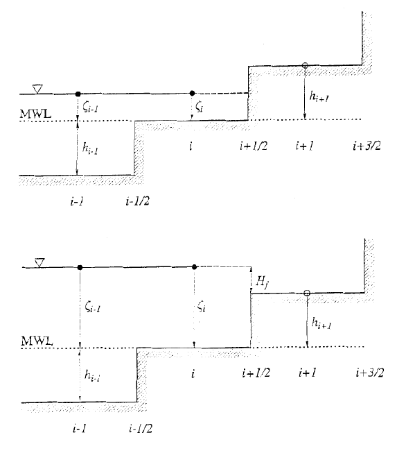
Figure 2.5: A sketch of moving boundary scheme.
* If Hi+1≤0 and hi+1+ηi≤0, then the shoreline remains between grid points iand
i+1 and the volume flux Pi+1/2remains zero;
* If Hi+1≤0 and hi+1+ηi>0, then the shoreline moves to between grid points i+1
and i+2 and the volume flux Pi+1/2may have a nonzero value, while Pi+3/2is assigned
to be zero. The flooding depth is Hf=hi+1+ηi;
* If Hi+1>0, then the shoreline moves to between grid points i+1 and i+2. The
volume flux Pi+1/2may have a nonzero value while Pi+3/2has a zero value. The flooding
depth is Hf=max(hi+1+ηi,hi+1+ηi+1).
In the above cases, the time-step index has been omitted for simplicity. The algo-
18
rithm is developed for a two-dimensional problem and the corresponding ydirection
algorithm has the same procedure as that for the xdirection.
To save computing time, the regions that represent permanent dry (land) can be ex-
cluded from the computation by installing a depth criterion. In COMCOT, grid cells
with land elevation greater than 50.0 meters, will not be included in the computation.
Moreover, when His very small, the associated bottom friction term become very large
and, accordingly, a lower bound of the water depth is used to avoid the difficulty. The fi-
nite difference approximation for the continuity equation correctly accounts for positive
and zero values of the total depth on each side of a computational grid. The treatment
of flooding and ebbing grid cells guarantees mass conservation while accounting for the
flooding and ebbing of land. The occurrence of a zero value for the total depth Hon one
side of a cell implies zero mass flux until Hbecomes positive. A grid cell is considered
a dry cell only if the total water depths at all sides are zero or negative. This moving
boundary scheme has been validated and applied to several experimental and practical
studies (Liu et al., 1994, 1995; Cho, 1995; Wang and Liu, 2007).
2.5 Dispersion Improvement
For most tsunami events, length scales of tsunamis are much larger than water depth over
which they propagate. Therefore, physical frequency dispersion effect can be neglected
and Shallow Water Equations are adequate enough to describe tsunami waves without
considering dispersion. However, the wavelength of a tsunami may not be large enough
compared to water depth so that the dispersion effect can be neglected. Moveover, the
dispersion effect is also accumulated over distance. Thus, in some conditions, the dis-
persion effect should be considered in a simulation. Physically, Boussinesq Equation
19

models or 3-D Navier-Stokes equation models are required to account for the dispersion
effects. But considering the scale of a tsunami simulation and computational cost of
these models, Boussinesq Equation models or 3-D Navier-Stokes equation models are
not a preferable choice. As we know, numerical dispersion is an inherent phenomena
in discretizing shallow water equation with explicit leap-frog finite difference scheme.
Imamura et al. (1988) proposed a method to mimic physical dispersion by using this
type of numerical dispersion for linear shallow water equation models over constant
water depth. By choosing grid size according to the following relationship,
4x=p4h2+gh(4t)2(2.47)
in which his water depth; gis gravitational acceleration and 4tis the size of time
step, then physical dispersion can be recovered. Cho (1995) improved the method to
correct the accuracy in diagonal directions. Yoon (2002) further improve the scheme to
describe the dispersion effect over a slowly varying bathymetry. Later on, Wang (2008)
extended the idea to weakly nonlinear weakly dispersive waves over a slowly varying
bathymetry so that the numerical dispersion in the shallow water equation model can be
used to recover the dispersion relationship of traditional Boussinesq equations.
Please refer to Wang (2008) for more details.
20
CHAPTER 3
TSUNAMI GENERATION
Tsunamis are generated by large-area disturbances on seafloor, such as submarine earth-
quakes, landslides or volcanic eruptions, or on water surface such as meteorite im-
pacts. Multiple tsunami generation mechanisms can be implemented in COMCOT, in-
cluding instantaneous seafloor rupture computed via fault models, e.g., Okada (1985)
and Mansinha and Smylie (1971), transient floor motions (e.g., transient ruptures, land-
slides), customized profiles of water surface displacements and wave makers.
3.1 Sea Floor Disturbances
Depending on the duration of the seafloor motion relative to the wave period of tsunamis,
the seafloor disturbances can be classified into two categories. If the duration of a floor
motion is much shorter the tsunami wave period being generated, the motion can be as-
sumed instantaneous (i.e., a sudden uplift of seafloor), then the displacement of seafloor
can be estimated via fault models (Mansinha and Smylie, 1971; Okada, 1985) and the
water surface is assumed to exactly follow the uplift the seafloor since water over this
large rupture area can not be drained out within such short duration. However, if the
duration of the floor rupture motion is comparable to tsunami wave period, the rupture
should be considered as a transient process and this transient process should be modelled
in tsunami simulations.
21

3.1.1 Instantaneous Deformation - Elastic Fault Model
For instantaneous seafloor rupture, the seafloor displacement caused by an earthquake
event is computed via elastic finite fault plane theory proposed originally by Mansinha
and Smylie (1971) and then improved by Okada (1985). Both models are available in
COMCOT. The theory assumes a rectangular fault plane being buried in semi-infinite
elastic half plane. This plane is an idealized representation of the interface between two
colliding tectonic plates where violent relative motion (i.e., dislocation) occurs during an
earthquake event (see Figure 3.1). The dislocation (or slip motion) occurring on the fault
plane will then deform the surface of the semi-infinite medium, which is considered as
the seafloor displacement during the earthquake event. To compute the deformation, the
following fault parameters are necessary. The definition of these parameters can be seen
Table 3.1: Parameters for Elastic Fault Plane Model
Parameters Unit
Epicenter (Lat, Lon) Degrees
Focal depth Meters
Length of Fault Plane Meters
Width of Fault Plane Meters
Dislocation (slip ) Meters
Strike direction (θ) Degrees
Dip angle (δ) Degrees
Rake (slip) angle (λ) Degrees
in Figure 3.1. In elastic fault plane theory, fault plane is where violent relative motion
occurs in an earthquake event. Specifically, fault plane is assumed as an rectangular
area of plate interface on foot block and the top and bottom edges of the fault plane are
parallel to the mean Earth surface. The orientation and position of this fault plane are
22
prescribed by its center location (ϕ0, ψ0), strike direction and dip angle. The center of the
fault plane is called focus and is the location where rupture starts during an earthquake
event. Its projection on the mean surface of the Earth is called epicenter.Focal depth is
defined as the vertical distance between the focus and the epicenter. Strike direction is
defined as the facing direction when someone stands on the top edge of a fault plane with
foot block on his left-hand side and the fault plane on his right-hand side. Then strike
angle,θ, is the angle measuring clockwise from the local north to the strike direction.
Dip angle,δ, is the angle between the mean Earth surface and the fault plane, measured
from the mean Earth surface down to the fault plane. The size of the fault plane is
described by its length and width. The length of a fault plane, L, is defined as the
length of its top edge or bottom edge (the edges parallel to the strike direction) and
the width of the fault plane, W, refers to the length of one of the other two edges. The
above parameters describe the size, location and orientation of a fault plane. The rupture
occurring on this fault plane is described by slip direction (i.e., rake) and dislocation
(amount of slip motion). Slip Direction (rake) describes to which direction the hanging
block moves relative to the foot block on the fault plane. Strike angle,λ, is the angle
measured counter-clock-wise from strike direction to slip direction on the fault plane.
Dislocation (slip amount)is the distance of motion of hanging block relative to the foot
block along the strike direction on the fault plane.
With the fault parameters defined above, the seafloor deformation can be calculated
via elastic finite fault plane theory. The detailed procedure of this calculation can be
found in the papers by Mansinha and Smylie (1971) and Okada (1985).
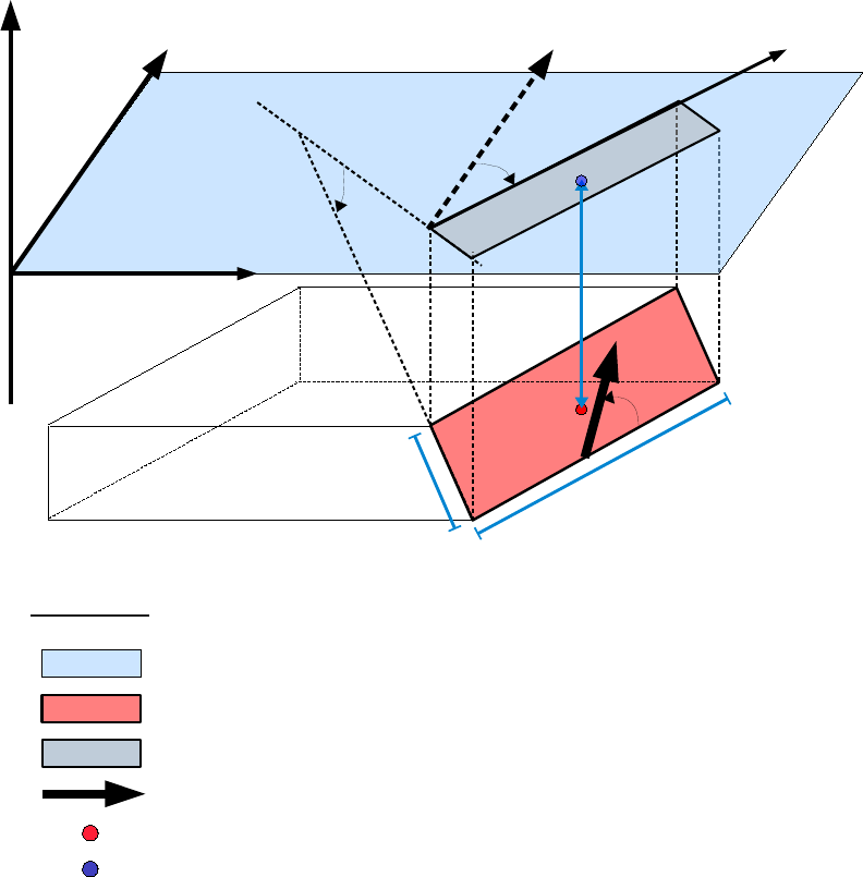
Since the floor displacement is evaluated over a plane, special handling is required
to map it onto the mean Earth Surface (i.e., Ellipsoidal surface). Oblique Stereo-
graphic Projection (Snyder, 1987) is implemented in COMCOT to map the surface of
23

an Ellipsoid (the Earthquake) onto a plane by taking the epicenter as where the plane
is tangential to the Earth surface. For this projection in COMCOT, the Earth is de-
scribed by WGS84 Datum (i.e., semi-major axis a=6378137.0mand semi-minor axis
b=6356752.3142mwith scaling factor k0=0.9996). With this projection method, each
location (ϕ, λ) on the Earth surface (Ellipsoidal surface), corresponds to a point (x,y) on
the plane tangential to the Earth surface at the epicenter (ϕ0, λ0), whose displacement
can be computed via either Mansinha and Smylie’s method or Okada’s approach.
3.1.2 Transient Seafloor Motion
Different from the instant deformation in which the duration of rupturing process can
be neglected, for a transient seafloor motion, the duration cannot be omitted and should
be considered in numerical simulations. This type of transient seafloor motion could
be the seafloor rupture caused by an earthquake event or submarine landslides. The
inclusion of temporal variation of water depth (or, more exactly, the motion of seafloor)
in Equations (2.1)-(2.13) allows to simulate such type of transient bottom floor motion
as long as long wave assumption is satisfied. This transident seafloor motion model has
been applied to study the transient rupture process of the 2004 Indian Ocean tsunami
(Wang and Liu, 2006).
To simulate tsunamis generated by transient seafloor motion with COMCOT, varia-
tion of water depth in terms of time should be prepared before a simulation starts. The in-
put data file contains a sequence of snapshots of instantaneous seafloor positions relative
to its original position. This snapshot data is then used to evaluate the term ∂h
∂tin Equa-
tions (2.1)-(2.13). Figure 3.2 shows how water depth changes during a landslide event.
Three snapshots are presented in the sketch. The variations of seafloor in this event are
24
described by its position relative to its original location. For example, in snapshot t=t2,
the seafloor variations at x=x1,x2,x3 are given as 4h(x1,t2) =h(x1,t0) −h(x1,t2),
4h(x2,t2) =h(x2,t0) −h(x2,t2) and 4h(x3,t2) =h(x3,t0) −h(x3,t2), respectively. If
4h>0, it means seafloor is being uplifted; if 4h<0, the seafloor is being subsided.
3.2 Water Surface Disturbances
In addition to generating tsunamis via seafloor motions, in COMCOT, tsunamis can also
be generated from a customized initial water surface displacement. When using this
mechanism to generate a tsunami, a data file needs to be prepared which contains the
the profile of water surface displacement measured from the mean surface level. This
displacement will become the source of a tsunami.
25
h
UPWARD
0
NORTHING
EASTING
LEGEND
FAULT PLANE (A RECTANGULAR SURFACE ON FOOT BLOCK)
PROJECTION OF FAULT PLANE ON MEAN EARTH SURFACE
DIP ANGLE OF FAULT PLANE
EPICENTER (PROJECTION OF FOCUS ON EARTH SURFACE)
FOCUS OF AN EARTHQUAKE (CENTER OF FAULT PLANE)
SLIP DIRECTION ON FAULT PLANE (RELATIVE TO FOOT BLOCK)
SLIP DIRECTION ON FAULT PLANE (RAKE ANGLE)
STRIKE ANGLE
h
FOCAL DEPTH
NORTHING
STRIKE DIRECTION
MEAN EARTH SURFACE
MEAN EARTH SURFACE
L
W
W
LLENGTH OF FAULT PLANE
WIDTH OF FAULT PLANE
FOOT BLOCK
Figure 3.1: Sketch of a Fault Plane and Fault parameter definitions.
26
MEAN SEA LEVEL
WATER
SEA BED
WATER
SEA BED
WATER
SEA BED
t = t0
t = t1
t = t2
h(x2,t1)
LEGEND
WATER
SEA BED
SLIDING MATERIALS
ORIGINAL SEA FLOOR (BEFORE LANDSLIDE)
h(x2,t0)
h(x2,t2)
h(x1,t0)
X0 x1 x2
h(x3,t0)
h(x1,t1)
h(x1,t2)
x3
h(x3,t1)
h(x3,t2)
X
0 x1 x2 x3
X
0 x1 x2 x3
Figure 3.2: Sketch of Transient Sea Floor Motion).
27

CHAPTER 4
PARAMETER CONFIGURATION, INPUT AND OUTPUT DATA
The user should prepare the topographic information and focal parameters for the spe-
cific tsunami simulation. The detailed information on preparing these files, as well as a
further explanation of the items in input files is given in the follows sections.
4.1 Control Files
COMCOT.CTL defines all the parameters required for tsunami simulations with
COMCOT. If multiple fault planes are implemented, an additional control file,
FAULT MULTI.CTL, is also required to configure parameters for additional fault
planes. These two parameter control files can be edited or viewed with any TXT-editing
applications, such as WordPad,UltraEdit and etc. It should be noted the structure of
these two files CANNOT be altered or changed except for the VALUE FIELD portion.
Otherwise, COMCOT cannot read these two files properly.
In general, COMCOT.CTL contains 5 parameter sections, which provides control on
the parameters for the simulation, fault model, wave maker, landslides and grid setup.
Each section will be explained in detail in the following sections.
4.1.1 General Information
The first section (see Figure 4.1) in COMCOT.CTL provides the control on the gen-
eral aspects of a numerical simulation, such as the total runtime, initial and boundary
conditions. For each line, parameter value should be specified after ’:’.
28
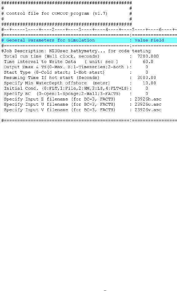
Figure 4.1: General Parameter Section in COMCOT.CTL
Total run time defines the total physical duration to be simulated, which should be
given in seconds.
Time interval to Write Data defines the time interval (in seconds) to output data
(including water surface elevation, and volume flux if specified).
Output Zmax &TS is used to control the output of maximum water surface elevation
and time history records at given locations. 0 – The maximum water surface elevation
and depression will be output every hour; 1 – The the time history records will be output
at up to 9999 locations given in the data file ts location.dat; 2 – Both the maximum
water surface elevation and the time history records will be output.
Start Type is used to specify the starting type of a simulation. 0 – Start a simulation
from the very beginning, t=0s; 1 – Start a simulation from a resuming time step where
data are previously saved.
Resuming Time If hot start specified the moment when a simulation starts from if
29

hot start is used or, the moment when a snapshot will be saved for a later restart if cold
start is selected.
Specify Min WaterDepth offshore is used to define the where is the shoreline. For
example, if a value 10.0 is assigned here, the water depth shallower than 10.0 meters
will be treated as land region and a vertical wall boundary is set along the 10.0−meter
water depth contour. To specify the true shoreline, 0.0 should be given here which will
be used for runup and inundation calculation.
Initial Cond. (0:FLT,1:File,2:WM,3:LS,4:FLT+LS) is used to define the initial
conditions. 0 – use fault model to calculate the seafloor deformation and fault pa-
rameters should be given at fault parameter section in COMCOT.CTL; If multiple
fault planes are implemented, parameters for additional fault planes should be given
in FAULT MULTI.CTL; 1 – use customized the profile in an external data file as initial
condition and the file name and format are specified at Fault Parameter section; 2 – use
incident wave maker to generate waves; 3 – use landslide model to generate tsunamis
and landslide parameters are defined at Landslide section in COMCOT.CTL; 4 – use
both fault model and landslide model to generate tsunamis.
Specify BC (0-Open;1-Sponge;2-Wall;3-FACTS) is used to define boundary con-
ditions of the numerical domain. 0 – open boundary (i.e., radiation boundary); 1
– use sponge layer (absorbing boundary); 2 – use vertical wall boundary; 3 – use
FACTS data as input boundary condition for far-field tsunami sources and use COM-
COT to calculate nearshore properties. The input boundary conditions are obtained
from the data files given at Specify Input Z filename,Specify Input U filename and
Specify Input V filename.
30
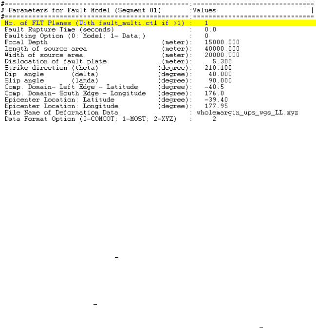
4.1.2 Parameters for Fault Model
If in the line Initial Cond. (0:FLT,1:File,2:WM,3:LS,4:FLT+LS) in General Param-
eter Section, 0 or 4 is selected, fault parameters should be given in the section
Parameters for Fault Model in COMCOT.CTL. These fault parameters will be used
to calculate seafloor deformation during an earthquake event. Then, it is assumed that
the water surface just mimics the seafloor deformation.
Figure 4.2: Fault Parameter Section in COMCOT.CTL
Fault parameters for a specific earthquake:
No. of FLT Planes (Use fault multi.ctl if ¡ 1) defines how many fault planes will
be implemented to create seafloor deformation. If the number is larger than 1, an ad-
ditional control file, FAULT MULTI.CTL will be required to specify parameters for
additional fault planes. The definitions of parameters in FAULT MULTI.CTL are the
same as this section.
Fault Rupture Time (seconds) defines when this fault plane will rupture. 0.0
means the fault is rupturing at the beginning of the simulation.
Faulting Option (0: Model; 1- Data;) specifies if the seafloor deformation is cre-
31
ated via fault model (e.g., Okada, 1985) or imported from an external data file. 0 – use
fault model with the fault parameters given in this section to calculate seafloor deforma-
tion; 1 – use an external data file which contains the seafloor deformation as the initial
condition. The file name and format are given in the last two lines of this section.
Focal Depth is the distance measured vertically from the top edge of a fault plane
to the mean earth surface.
Length of source area is the length of the rectangular fault plane and
Width of source area is the width of the rectangular fault plane.
Dislocation of fault plate defines the relative dislocation between foot block and
hanging block on the fault plane.
Strike direction defines the strike angle (θ) of the fault plane, measured from the
north to the fault line, with the fault plane on the right-hand side.
Dip angle is the angle (δ) between the mean earth surface and the fault plane.
Slip angle is the angle (λ) measured counter clock wise from the fault line to the
direction of relative motion of hanging block on the fault plane.
Comp. Domain- Left Edge - Latitude is the latitude of the lower-left (i.e., south-
east) corner grid in the 1st-level grid, layer01.
Comp. Domain- South Edge - Longitude is the longitude of the lower-left (i.e.,
southeast) corner grid in the 1st-level grid, layer01.
Epicenter Location: Latitude and Epicenter Location: Longitude specify the
latitude and longitude of the epicenter of an earthquake.
32
File Name of Deformation Data specifies the file name of the seafloor deformation
data if 1 is chosen at the line Faulting Option (0: Model; 1- Data;). And the data for-
mat should be given at the line Data Format Option (0-COMCOT; 1-MOST; 2-XYZ).
3 ASCII formats are supported by COMCOT. 0 – use the old COMCOT format (ver-
sion1.6 or earlier); 1 – use the MOST format and 2 – use the XYZ format. Latitude of
the epicenter of an earthquake.
By default, COMCOT will output the initial condition (initial water surface eleva-
tion) in a file named ini sur f ace.dat.
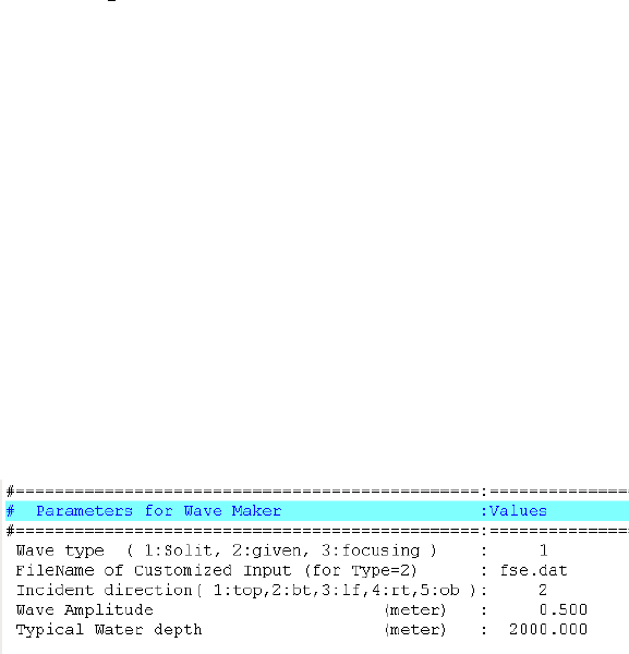
4.1.3 Parameters for Wave Maker
If in the line Initial Cond. (0:FLT,1:File,2:WM,3:LS,4:FLT+LS) in General Param-
eter Section, ”2” is selected, parameters for wave maker should be given in the section
Parameters for Wave Maker in COMCOT.CTL. Either solitary waves or a customized
time history profile can be sent into the numerical domain (1st-level grid, layer01)
through any of the four boundaries.
Figure 4.3: Wave Maker Parameter Section in COMCOT.CTL
Wave type ( 1: Solitary, 2:given profile ) is used to determine the incident wave
type: 1 – Send Solitary wave into the numerical domain, layer01; 2 – Input a wave
profile defined in a time history file through one boundary whose should be given after
33
FileName of Customized Input (for Type=2); 3 – generate a focusing solitary wave.
When using this option, incident wave through a boundary will converge to a specified
location (”focus”). Two additional parameters will be asked for when the program starts:
x and y coordinates of the focus in layer01.
Incident direction( 1:top,2:bt,3:lf,4:rt,5:ob ) defines which boundary the wave is
sent through. 1 – waves come from the top boundary of the domain; 2 – waves come
from the bottom boundary of the domain; 3 – waves come from the left boundary of the
domain; 4 – waves come from the right boundary of the domain; 5 – Oblique incident
wave. When using this option, an oblique wave will be sent into the numerical domain
through boundaries. The oblique angle will be required after the program starts. The
angle ranges is measured from the northward (upward) to the incident direction, ranging
from 0.0 to 360..
Characteristic Wave Amplitude specifies the wave amplitude of the incident wave
(only effective when solitary wave is sent in).
Typical Water depth specifies the characteristic water depth, which is effective for
both wave types. This value is used to calculate volume flux associated with incident
waves based on shallow water wave theory.
4.1.4 Parameters for Landslides/Transient Floor Motion
If in the line Initial Cond. (0:FLT,1:File,2:WM,3:LS,4:FLT+LS) in General Pa-
rameter Section, 3 or 4 is selected, parameters for submarine landslide model
(or other submarine transient seafloor motions) should be given in the section
Parameters for Transient Sea Floor Motion in COMCOT.CTL. Compared to the di-
34

mension of the simulated region (i.e., layer01), transient seafloor motions (e.g., transient
fault rupture, landslides), generally, occur within a small confined area, which is defined
by the coordinates of its left (west), right (east), bottom (south) and top (north) margins.
X Coord. of Left/West Edge of Landlide Area specifies X coordinate of grids on
the left/west margin of the landslide region.
x Coord. of Right/East Edge of Landlide Area specifies X coordinate of grids on
the right/east margin of the landslide region.
Y Coord. of Bottom/South Edge of Landlide Area specifies Y coordinate of grids
on the bottom/south margin of the landslide region.
Y Coord. of Top/North Edge of Landlide Area specifies Y coordinate of grids on
the top/north margin of the landslide region. It should be noted that the units/coordinates
used here should be the same as those of 1st-level grid. For example, if the 1st-level grid,
layer01, adopts Spherical Coordinates (Latitude/Longitude), then the values defining the
landslide region should also be latitude/longitude in Spherical Coordinates.
File Name of SeaFloor Motion Data specifies the filename of seafloor motion data.
This data file contains a time sequence of snapshots of variation of the seafloor relative
to its original location.
4.1.5 Parameters for All Grid Levels
Parameters for 1st-Level Grid
In COMCOT.CTL, parameter section for grids of all levels follows the parameter sec-
tion of landslide model. The section, Parameters for 1st-level grid – layer 01, con-
35
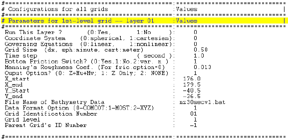
tains configurations for the 1st-level grid (the largest grid region), layer01.
Figure 4.4: Parameters for 1st-level grid in COMCOT.CTL
The meaning of each entry is illustrated as follows.
Run This Layer? is used to determine if this grid level is included in the numerical
simulation. 0 – this grid level will be include; 1 – this grid level will not be included in
the simulation.
Coordinate System specifies which coordinates will be used for this grid level. 0 –
use Spherical Coordinates; 1 – use Cartesian Coordinates.
Governing Equations determines which type of governing equations will be used
for this grid level. 0 – use linear shallow water equations; 1 – use nonlinear shallow
water equations. If runup and inundation are going to be calculated, nonlinear shallow
water equations must be chosen.
Grid Size specifies the grid size (4x) adopted for this grid level. If spherical co-
ordinate system is adopted, the grid size should be given in arc minutes; if cartesian
coordinate system is adopted, the grid size should be given in meters.
Time Step determines the time step (4t) used for the numerical simulation. The
36

time step chosen should guarantee that Courant condition is satisfied, which means
4t<4x
pghmax
(4.1)
where gis the gravitational acceleration and hmax is the maximum water depth within
the region of this grid level. If Courant condition is not satisfied for a given time step
(4t), COMCOT will automatically adjust it to make Courant condition being satisfied.
Inside the code, the maximum time step size 4tallowed is fixed as 0.54x/pghmax.
Bottom Friction Switch? is used to determine if bottom friction is considered in
the numerical simulation. 0 – bottom friction will be included and a constant bot-
tom friction coefficient will be applied (Manning’s n) and the roughness is given at
Manning’s Roughness Coef.; 1 – bottom friction will not be considered; 2 – bot-
tom friction will be included and variable Manning’s roughness coefficient will be
applied. The variable roughness coefficients need to be given in a data file named
f ric coe f layerXX.dat in which XX represents the grid ID of this grid level.
Ouput Option? (0: Z+Hu+Hv; 1: Z Only; 2: NONE) is used to control the out-
put of free surface elevation and volume fluxes. 0 – both water surface elevation and
volume fluxes (i.e., product of water depth and velocity) will be output; 1 – only water
surface elevation not be output. 2 – both water surface elevation and volume fluxes will
not be output.
In COMCOT, a grid region (i.e., a rectangular area) is defined by the coordinates
of its lower-left /south-west corner (X Start,Y Start) and upper-right/north-east corner
(X End,Y End).
X Start specifies X coordinate of the left/west margin of the grid region.
X End specifies X coordinate of the right/east margin of the grid region.
37

Y Start specifies Y coordinate of the bottom/south margin of the grid region.
Y End specifies Y coordinate of the top/north margin of the grid region.
Together with the given grid size, the water depth/land elevation at every grid will
be extracted from the input bathymetry/topography data file whose name is given af-
ter File Name of Bathymetry Data.File Name of Bathymetry Data specifies the file-
name of bathymetry data for this grid level. This data file contains the gridded bathy-
metric/topographic data for this grid level.
Data Format Option is used to determine which type of data format is adopted for
bathymetry data file. 0 – use old COMCOT data format (version 1.6 or earlier); 1 –
use MOST format; 2 – use XYZ format (3-column data containing x, y and bathymetry
information); 3 – use ETOPO bathymetry data. XYZ format is suggested.
Grid Identification Number is used to assign an ID to this grid level. This is the
only identification number used to distinguish this grid from the others. It is not sug-
gested to change the value here.
Grid Level is used to determine the level of this grid in the hierarchy of nested grid
setup. For the largest grid layer (the 1st level), the grid level is 1.
Parent Grid’s ID Number is used to specify which grid layer is the parent grid of
this grid layer. The parent grid means the grid layer where the current grid is directly
nested in. For the 1st-level grid, the parent grid ID should be specified as -1 (or 0) since
it has no parent grid.
38
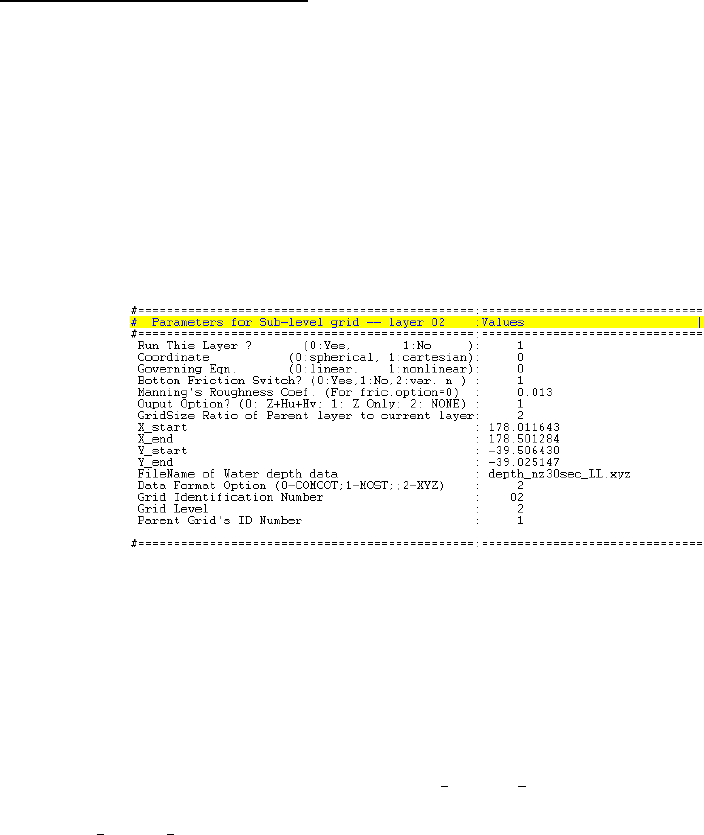
Parameters for sub-level grids
The parameter configurations for sub-level grids are very similar to that of the 1st-level
grid. But, there is no need to specify the grid size (4x) and time step (4t) for sub-level
grids. However, the grid size ratio of its parent grid to this grid level should be given
after GridSize Ratio of Parent layer to current layer. The grid size ratio can be any
integer larger than or equal to 1. However, a ration less than 10 is suggested.
Figure 4.5: Parameters for sub-level grids in COMCOT.CT L
In COMCOT, a sub-level grid region (i.e., a rectangular area) is defined by the coor-
dinates of its lower-left /south-west corner (X Start,Y Start) and upper-right/north-east
corner (X End,Y End). This four values should be given in the same coordinates as
that used in its parent grid layer. If the current grid layer adopts Cartesian coordinates
(UTM) and its parent grid layer adopts Spherical Coordinates (latitude/longitude), then
the coordinates of these two corners should be given in laitutde/longitude. In COMCOT,
a sub-level grid layer using Cartesian coordinates can be nested inside a grid layer using
Spherical coordinates. However, the reverse nesting is not supported.
39
4.2 Input Data
4.2.1 Bathymetric/Topographical Data
4 ASCII formats of bathymetry data are supported in COMCOT v1.7, the old COMCOT-
formatted data (for version 1.6 or earlier), MOST-formatted data and XYZ format data
and ETOPO bathymetry data. However, XYZ format is suggested whose format will
be detailed here. The bathymetry data file should be in ASCII format and written in 3
columns. The first column contains information of X coordinates (rightward, pointing to
the east), and second column contains information of Y coordinates (upward, pointing to
the North) and the third column contains the data of water depth (positive for bathymetry
data and negative for topographical data), see Figure 4.6.
Figure 4.6: Example of Bathymetry Data File (XYZ format)
The format of ETOPO data is the same as that of XYZ 3-column data. The only
difference is the sign of data. In ETOPO data, the value of water depth is given as
a negative number and the land elevation is given as a positive number. The ETOPO
40
bathymetry data (either ETOPO1 or ETOPO2) can be directly used in COMCOT v1.7.
COMCOT will change the sign after the ETOPO data is loaded in.
The bathymetry data must be gridded and the gridded data (a nx ×ny matrix) should
be written row by row or column by column from the left/west (i=1) to the right/east
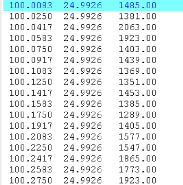
(i=nx) from the bottom/south ( j=1) to the top/north ( j=nx) where iand jrepresent
the x,ygrid index of bathymetry/topography grids and nx and ny are the total number
of grids in Xand Ydirection. The xcoordinates must increase monotonically and y
coordinates should increase or decrease monotonically. It should be noted that for each
grid layer the gridded bathymetry/topography data should adopt the same coordinate
system as specified for this grid layer. And the area of bathymetry/topography data
should be larger than or equal to the region defined by X S tart,X End,Y S tart and
Y End in the parameter section for this grid layer.
If a grid layer adopts Cartesian coordinate system, however, its parent grid layer
uses Spherical Coordinate system, X S tart,X End,Y S tart and Y End of this grid
layer should given with spherical coordinates (latitude, longitude). But, the bathymetry
data file of this grid layer should be prepared with cartesian coordinates (UTM). The
position of this grid layer is determined by X S tart,X End,Y S tart and Y End which
are given in longitude and latitude. The key to remember is the position of a sub-level
grid layer is also defined in the same coordinates as its parent grid layer.
4.2.2 Seafloor Deformation Data
Similar to bathymetry/topography data file, 3 ASCII formats of seafloor deformation
data are also supported in COMCOT v1.7, the old COMCOT-formatted data (for version
1.6 or earlier), MOST-formatted data and XYZ format data. However, XYZ format is
41
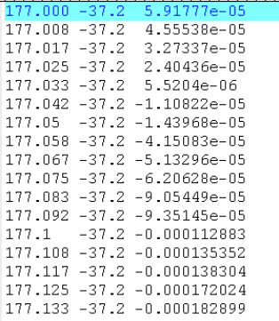
also suggested. The seafloor deformation data file should be in ASCII format and written
in 3 columns. The format is the same as that of XYZ-format bathymetry data file. The
first column contains information of X coordinates (rightward, pointing to the east), and
second column contains information of Y coordinates (upward, pointing to the North)
and the third column contains the data of water depth (positive for bathymetry data and
negative for topographical data), see Figure 4.7.
Figure 4.7: Example of Seafloor Deformation Data File (XYZ Format)
The deformation data should be gridded and written row by row from the left/west
(i=1) to the right/east (i=nx) from the bottom/south ( j=1) to the top/north ( j=nx)
where iand jrepresent the x,ygrid index of bathymetry/topography grids and nx and ny
are the total number of grids in Xand Ydirection. It should be noted that the deformation
data should use the same coordinate system as the 1st-level grid. The area of deformation
data should fall inside the region defined by the 1st-level grid.
42
4.2.3 Transient Sea Floor Motion Data
To generate tsunamis by landslides or any other type of transient seafloor motion, a
data file is required to provide information on seafloor motion. This data file contains a
sequence of snapshots of seafloor variations in terms of time.
If, for example, the landslide area has a grid dimension of nx and ny where nx and
ny stand for the total number of grids in Xand Ydirection, respectively, and in total,
nt snapshots are created to trace the variation of seafloor position in time, the variation
of seafloor can be represented as 4h(i,j,k), where i=1,nx,j=1,ny and k=1,nt.
4h(i,j,k) describes the variation of the seafloor position against its origin at (i,j) at time
level k. And 4h(i,j,k) can be obtained from
4h(i,j,k)=h(i,j,k)−h0(i,j) (4.2)
in which h(i,j,k) denotes the instantaneous water depth at (i,j) at time level kand
h0(i,j) represents the original position of seafloor.
Figure 3.2 gives a simply example of seafloor variation during a landslide event.
3 snapshots are presented to show the positions of seafloor during a landslide event.
Snapshot at t=t0 shows the original position of sea floor before landslide and snapshots
at t=t1 and t=2 indicate the intermediate and final stage of seafloor position. Then
the variation of seafloor can be described by these 3 snapshots. For example, at x=
x1, 3 snapshots of seafloor variation are 4h(x1,t0), 4h(x1,t1) and 4h(x1,t2) where
4h(x1,t0) =h(x1,t0) −h(x1,t0), 4h(x1,t1) =h(x1,t0) −h(x1,t1) and 4h(x1,t2) =
h(x1,t0)−h(x1,t2), respectively. If 4h>0, it indicates that the seafloor is being uplifted;
if 4h<0, it means the seafloor is being subsided.
After the snapshot data of seafloor variation is determined, the input data file for
this transient seafloor motion can be written in the following format. The first line of
43
the data file contains 3 integers specifying the grid dimension, nx and ny, and the total
number of snapshots, nt. Then, it follows by the Xcoordinates of gridded data (from
lines 2 to nx +1), Ycoordinates of gridded data (from lines nx +2 to nx +ny +1) and
the times at which the snapshots are created (from lines nx +ny +2 to nx +ny +nt +1).
After the coordinates and time information, it is the section for snapshot data. All the nt
snapshots of seafloor variation are written into a single column one by one from t=t1
to t=tnt. For each snapshot, e.g., 4h(nx,ny,t1), the data should be written row by row
from the left/west (i=1) to the right/east (i=nx) from the bottom/south (j=1) to
the top/north (j=nx) where iand jrepresent the x,ygrid index of gridded snapshot
data. It should be noted that the landslide snapshot data should use the same coordinate
system as the 1st-level grid. The landslide area should fall inside the region defined by
the 1st-level grid. However, the grid and time resolutions are not necessarily the same
as those of the 1st-level grid layer. Interpolation will be carried out inside COMCOT. A
sample data file is shown in Figure ??.
Figure 4.8: Example of Landslide Data File (XYT Format)
Two file formats are supported: the old COMCOT format (for version 1.6) and the
new XYT format. The new format is suggested for version 1.7.
44

4.2.4 Bottom Friction Coefficients
If at the grid parameter section, 2 is chosen after Bottom Friction Switch? for one grid
layer, a gridded Manning’s roughness n(varying in space) should be prepared for this
grid layer before simulation starts. The roughness coefficient data file has the same
format as that of bathymetric/topographical data. The grid size is not necessarily the
same as that of the grid layer, but the area covered should be slightly larger than or
at least equal to the grid layer. The file name of roughness coefficients should be like
f ric coe f layerXX.dat in which XX represents the grid ID of this grid layer.
4.2.5 Time History Input for Wave Maker
A time history input of water surface elevation is required if the wave maker is im-
plemented and the option 2is chosen for Wave type ( 1: Solitary, 2:given profile ).
The data file should be written in ASCII format and the file name need to be given
at the line FileName of Customized Input (for Type=2). The data file contains two
data columns. The first column contains the time sequence, t=tk(k=1,· · · ,nt),
and the second column contains the water surface elevation, η=ηk(k=1,nt), corre-
sponding to the time sequence. The units should be seconds for time and meters for the
water surface elevation.
4.2.6 Numerical Tidal Gauge Locations
If in the control file COMCOT.CTL,Output Zmax & TS is set to 1 or 2, the the time
history records will be output at up to 9999 numerical tidal gauge location. A data file,
textb f ts location.dat, is required to specify these tidal gauge locations. The data file
45
contains two data columns. The first data column defines the Xcoordinates of tidal
gauges and the second column defines the Ycoordinates of tidal gauges. In Figure 4.9,
locations of four tidal gauges are specified.
Figure 4.9: Example of Tidal Gauge Location File ts location.dat
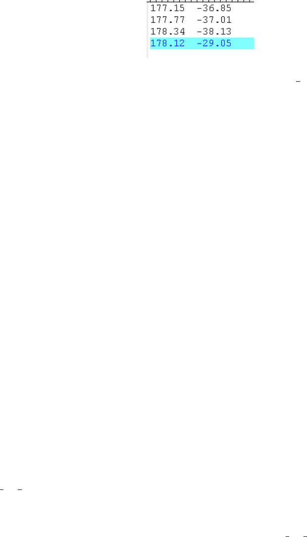
4.3 Output Data
4.3.1 Time Sequence Data
A data file, named time.dat, will always be output for a simulation. The data file con-
tains only one data column, which is the wall-clock time corresponding to each time
step during the entire simulation. This output file can be used together with the time
history output at specified tidal gauges to create time history plots.
4.3.2 Water Surface Elevation/Volume Fluxes
Generally, only the free surface elevation will be output in data files named in the form
z ID xxxxxx.dat, where zstands for free surface elevation, two digits ID denote the cor-
responding grid identification number and the six digits, xxxxxx, corresponds to the time
step number when the data is output. Therefore, the data file z ID xxxxxx.dat stores the
46

free surface elevation at all grid points in the grid layer. For example, z01 001234.dat
stores the free surface elevation at all the grid points of layer01 at time step 1234. It
should be mentioned that the total number of time steps required for a simulation and
also time step number for data output are also calculated based on the time step (4t)
of layer01. For example, if 0.5stime step is used for layer01, the number of time
steps, 1234, corresponds to a physical time t=1234 ×0.5=617.0s. However, if
the switch Output Volume Flux is set to 0 for this layer, two additional data files,
m ID xxxxxx.dat and n ID xxxxxx.dat will be created, storing volume flux data in x
direction and ydirection, respectively, at all the grid points in this grid layer at time step
number xxxxxx. The following scripts will be able to read the data in a output data file
”F AB dddddd.dat” into a predefined matrix B(nx,ny)
Table 4.1: Fortran scripts to write Water surface/Volume flux data into a data file
open (IO-UNIT,file=’z ID xxxxxx.dat’,status=’unknown’)
do i=1, ny
read (IO-UNIT, ’(15f9.3)’) (B(i, j), i=1, nx)
enddo
close(IO-UNIT)
In Table4.1, zdenotes water surface elevation, for volume flux, zshould be replaced
by mfor volume flux in Xdirection or nfor volume flux in Ydirection; ID represents
Identification Number of a grid layer and xxxxxx stands for the number of time steps
at which the data is written. In addition, if the switch Output Volume Flux is set to 2,
neither water surface elevation nor volume fluxes will be out.
To obtain the velocity components (u,v) at a grid, divide the volume flux components
by the total water depth (η+h) where ηrepresents the water surface fluctuation.
47

4.3.3 Initial Condition
At the beginning of a simulation starts, the initial water surface displacement will be
written into a data file named ini sur face.dat. This data file is written via the following
FORTRAN code.
Table 4.2: Fortran scripts to write Initial Condition into a data file
open (IO-UNIT,file=’ini surface.dat’,status=’unknown’)
do i=1, ny
write (IO-UNIT, ’(15f8.3)’) (deform(i, j), i=1, nx)
enddo
close(IO-UNIT)
In Table 4.2, de f orm(i,j) denotes initial water surface fluctuation at grid (i,j); nx
and ny denotes the total number of grids in Xand Ydirections, respectively.
4.3.4 Seafloor Deformation
If multiple fault planes are implemented,i.e., in COMCOT.CTL,Initial Cond. (0:FLT,1:File,2:WM,3:LS,4:FLT+LS)
is set to 0 or 4 and No. of FLT Planes (Use fault multi.ctl if ¿1) is larger than 1, the
seafloor deformation generated by each fault plane will be output in data files named
de f orm segXX.dat where xx denotes the numbering of fault planes, starting from 01 up
to 99. This type of data file is written via the following FORTRAN code.
In Table 4.3, de f orm(i,j) denotes seafloor deformation at grid (i,j) generated by
fault plane xx;nx and ny denotes the total number of grids in Xand Ydirections, re-
spectively.
48

Table 4.3: Fortran scripts to write Seafloor Deformation into a data file
open (IO-UNIT,file=’deform segXX.dat’,status=’unknown’)
do i=1, ny
write (IO-UNIT, ’(15f8.3)’) (deform(i, j), i=1, nx)
enddo
close(IO-UNIT)
4.3.5 Maximum Water Surface Elevation/Depression
If inCOMCOT.CTL,Output Zmax & TS is set to 0 or 2, the maximum water surface
elevation/depression will be output every hour and at the end of a simulation. Every
one hour during the simulation, two data files will be created for each grid layer, named
etamax layerID XXXXhrs.dat and etamin layerID XXXXhrs.dat, in which ID de-
notes the two-digit identification number of each grid layer and the 4-digit XXXX repre-
sents the number of wall-clock hours elapsing since the tsunami event occurs. The data
file etamax layerID XXXXhrs.dat contains the maximum water surface elevation at
every grid for each grid layer included in the simulation in the past XXXX hours and
etamin layerID XXXXhrs.dat contains the maximum water surface depression at ev-
ery grid for each grid layer included in the simulation in the past XXXX hours. For
example, etamax layer01 0001hrs.dat stores the maximum water surface elevation at
all the grid points of layer01 within the past 1.0 hours and etamin layer01 0001hrs.dat
stores the maximum water surface depression at all the grid points of layer01 within the
past 1.0 hours. The data file, for example, etamax layer01 0001hrs.dat, is written via
the following FORTRAN code.
In Table4.4, ηmax denotes the maximum water surface elevation of grid layer 01; nx
and ny are the total numbers of grids in Xand Ydirections. At the end of the simulation,
49

Table 4.4: Fortran scripts to write Max/Min Water Surface Fluctuations into a data
file
open (IO-UNIT,file=’etamax layer01 0001.dat’,status=’unknown’)
do i=1, ny
read (IO-UNIT, ’(15f9.4)’) (ηmax(i, j), i=1, nx)
enddo
close(IO-UNIT)
two data files, etamax layer01.dat and etamin layer01.dat, will also be created storing
the maximum water surface elevation/depression within the entire simulated duration. It
should be mentioned that this type of maximum water surface elevation/depression data
files will be created for every grid layer included in the numerical simulation.
4.3.6 Time History Records
If in the control file COMCOT.CTL,Output Zmax & TS is set to 1 or 2, the the
time history records will be output at up to 9999 locations given in the data file
ts location.dat. A series of data files will be created with the names in the for-
mat like ts recordxxxx.dat in which xxxx represents the position of a tidal gauge
in the data file ts location.dat. For example, if in total 4 tidal gauges are de-
fined in ts location.dat, then four data files, ts record001.dat,ts record0002.dat,
ts record0003.dat and ts record0004.dat, will be created corresponding to the four
tidal gauges, numbering from top to bottom, in ts location.dat.
50

4.3.7 Hot Start/Automatic Data Backup
By default, COMCOT will automatically create a resuming snapshot during a sim-
ulation for later hot start. The resuming snapshot will be created at the mo-
ment specified at Resuming Time If hot start in COMCOT.CTL. The simulation
can restart from this save snapshot. For this snapshot, three data files will
be created which are z1 layerID XXXXXX.dat,m1 layerID XXXXXX.dat and
n1 layerID XXXXXX.dat. In the file names, ID denotes the 2-digit identification
number of a grid layer and XXXXXX denotes the corresponding 6-digit time step
number. For example, if Resuming Time If hot start is set to 1000.0 in a simu-
lation including only one grid layer, 01 and the time step 4t=1.5, at time step
number NINT(1000.0/4t)=667 (NINT means the nearest integer), the following
three data files will be created: z1 layer01 000667.dat,m1 layer01 000667.dat and
n1 layerlayer01 000667.dat. The data in these data files are all written in the follow-
ing format (FORTRAN script) in Table4.5.
Table 4.5: Fortran scripts to write snapshots for hot start
open (IO-UNIT,file=’F1 layer01 000667.dat’,status=’unknown’)
do i=1, ny
read (IO-UNIT, ’(10f12.5)’) (F(i, j), i=1, nx)
enddo
close(IO-UNIT)
In Table4.5, Fdenotes one of z,mand n;nx and ny are the total numbers of grids in
Xand Ydirections.
This function is designed for a special purpose. In some cases, grid regions of inter-
est are far away from a source region and it will take a long time for the leading wave
51
of a tsunami to arrive at these regions. The time for the leading wave travelling from
the source region to right before entering the small grid regions can be estimated based
on water depth and phase speed. Then, this time is specified as the resuming time for a
later restart Resuming Time If hot start in COMCOT.CTL. At the first step, cold start
can be performed with all sub-level grids turned off. After the simulation passes through
that specified time, stop the program, modify COMCOT.CTL to turn on all the sub-level
grids required, change Start Type to Hot Start and rerun the simulation. For this time,
the simulation will start from the specified time with all sub-level grids. Time will be
saved. When using the hot start function, if the snapshot data are not there, COMCOT
will assume the surface displacements and fluxes everywhere are zeros at that moment
and continues the simulation.
52
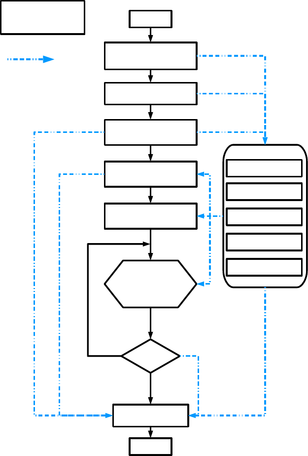
APPENDIX A
FLOW CHART OF COMCOT
START
READ
CONFIGURATION
READ
BATHYMETRY
DETERMINE DX, DT
GRID-MATCHING
SETUP I.C.
SETUP B.C.
SWE
SOLVER
t < T_END
OUTPUT
END
FAULT MODEL
LANDSLIDE
SURFACE PROF.
INPUT B.C.
NO
YES
WAVE MAKER
BATHYMETRY DATA FOR ALL GRID LAYERS
INITIAL WATER SURFACE DISPLACEMENT
Z, Hu, Hv
FLOOR DEFORMATION
SELECT
n=n+1
t=n*dt
n=1
COMCOT
FLOW CHART
DATA FLOW
Figure A.1: Flow Chart of COMCOT.
53

APPENDIX B
OBLIQUE STEREOGRAPHIC PROJECTION
For elastic fault plane theories (e.g., Mansinha and Smylie (1971), Okada (1985)),
the displacement is computed over a semi-infinite half plane, special handling is re-
quired to map it onto the mean Earth Surface (i.e., Ellipsoidal surface). Oblique Stere-
ographic Projection (Snyder, 1987) is implemented in COMCOT to map the surface of
an Ellipsoid (the Earthquake) onto a plane by taking the epicenter as where the plane
is tangential to the Earth surface. For this projection in COMCOT, the Earth is de-
scribed by WGS84 Datum (i.e., semi-major axis a=6378137.0mand semi-minor axis
b=6356752.3142mwith scaling factor k0=0.9996). Given the geodetic origin of the
projection at the tangent point (ϕ0,λ0), i.e., the latitude and longitude of the epicenter,
the parameters defining the conformal sphere are:
R=ρ0ν0(B.1)
n=r1+e2cos4ϕ0
1−e2(B.2)
c=(n+sin ϕ0)(1 −sin Φ0)
(n−sin ϕ0)(1 +sin Φ0)(B.3)
where
ρ0=a0(1 −e2)
(1 −e2sin2ϕ0)3/2
ν0=a
1−e2sin2ϕ0
e=p1−b2/a2
sin Φ = w1−1
w1+1
w1=(S1·S2)n
S1=1+sin ϕ0
1−sin ϕ0
S2=1−esin ϕ0
1+esin ϕ0
54

in which Ris the radius of the conformal sphere; eis the eccentricity of the Earth.
The conformal latitude and longitude (Φ0,Λ0) of the origin are computed from
Φ0=arcsin (w2−1
w2+1)
Λ0=λ0
where S1and S2are as above and w2=c(S1·Se
2)n=cw1.
Then, for any point with geodetic coordinates (ϕ, λ), the equivalent conformal lati-
tude and longitude (χ, Λ) are computed from
Λ = n(λ−Λ0)+ Λ0(B.4)
Φ = arcsin (w−1
w+1)(B.5)
where
w=c(SaSe
b)n
Sa=1+sin ϕ
1−sin ϕ
Sb=1−sin ϕ
1+sin ϕ
Then for any geodetic location (ϕ, λ), its projection on the plane tangential to the
Earthquake surface at (ϕ0, λ0) can be expressed as
x=2Rk0cos Φsin(Λ−Λ0)/β (B.6)
y=2Rk0{sin Φcos Φ0−cos Φsin Φ0cos(Λ−Λ0)}/β (B.7)
in which xand yare two axes of the Cartesian coordinates on the plane with its origin at
the tangential point (ϕ0, λ0); xaxis points to the north and yaxis points to the east and
β=1+sin Φsin Φ0+cos Φcos Φ0cos(Λ−Λ0).
55
With the above method, for each location (ϕ, λ) on the Earth surface (Ellipsoidal
surface), it corresponds to a point (x,y) on the plane tangential to the Earth surface at
the epicenter (ϕ0, λ0), whose displacement can be computed via either Mansinha and
Smylie’s method or Okada’s approach.
56
APPENDIX C
MATLAB SCRIPTS FOR DATA PROCESSING
57
BIBLIOGRAPHY
Y.-S. Cho. Numerical simulations of tsunami and runup. PhD thesis, Cornell University,
1995.
F. Imamura, N. Shuto, and C. Goto. Numerical simulation of the transoceanic propa-
gation of tsunamis. paper presented at the Sixth Congress of the Asian and Pacific
Regional Division, Int. Assoc. Hydraul. Res., Kyoto, Japan, 1988.
K. Kajiura and N. Shuto. Numerical modeling of free-surface flows that are two-
dimensional in plan. In Tsunami in The Sea, number 9 Part B, pages 395–420. John
Wiley and Sons, Inc., 1990.
J.F. Lander and P.A. Lockridge. United States Tsunamis. U.S. Department of Com-
merce, 1989.
P. L.-F. Liu, Y.-S. Cho, S. B. Yoon, and S. N. Seo. Numerical simulations of the 1960
chilean tsunami propagation and inundation at hilo, hawaii. In Recent Development
in Tsunami Research, pages 99–115. Kluwer Academic Publishers, 1994.
P. L.-F. Liu, S-B. Woo, and Y-S Cho. Computer programs for tsunami propagation and
inundation. Technical report, Cornell University, 1998.
P.L.-F. Liu, Y-S. Cho, M.J. Briggs, C.E. Synolakis, and U. Kanoglu. Run-up of solitary
waves on a circular island. J. Fluid Mech, 302:259–285, 1995.
L. Mansinha and D. E. Smylie. The displacement fields of inclined faults. Bull. Seism.
Soc. Am., 61:1433–1440, 1971.
M. Okada. Surface deformation due to shear and tensile faults in a half-space. Bull.
Seism. Soc. Am., 75(4):1135–1154, 1985.
58
N. Shuto. Numerical simulation of tsunamis - its present and near future. Natural
Hazards, 4:171–191, 1991.
J. P. Snyder. Map projects - a working manual. U.S. Geological Survey Professional
Paper 1395, page 383, 1987.
X. Wang. Numerical modelling of surface and internal waves over shallow and inter-
mediate water. PhD thesis, Cornell University, 2008.
X. Wang and P. L.-F. Liu. A numerical investigation of boumerdes-zemmouri (algeria)
earthquake and tsunami. CMES, 10(2):171–184, 2005.
X. Wang and P. L.-F. Liu. An analysis of 2004 sumatra earthquake fault plane mecha-
nisms and indian ocean tsunami. J. Hydraulic Res., 44(2):147–154, 2006.
X. Wang and P. L.-F. Liu. Numerical simulations of the 2004 indian ocean tsunamis -
coastal effects. Journal of Earthquake and Tsunami, 1(3):273–297, 2007.
S. B. Yoon. Propagation of distant tsunamis over slowly varying topography. J. Geophys.
Res., 101(C10):3140–, 2002.
59
