Paper CPA F1.1 BUSINESS MATHEMATICS & QUANTITATIVE METHODS Revision Guide

User Manual:

Open the PDF directly: View PDF .
Page Count: 46

CONTENTS

LOSSARY

CPA

Certified Public Accountant Examination

Stage: Foundation F1.1

Subject Title: Business Mathematics &

Quantitative Methods

Revision Guide

LOSSARY

INSIDE COVER - BLANK

Page 2

CONTENTS

Title

Page

Study Techniques

Examination Techniques

Assessment Strategy

Learning Resources

Sample Questions and Solutions

Page 3

BLANK

Page 4

STUDY TECHNIQUE

What is the best way to manage my time?

• Identify all available free time between now and the examinations.

• Prepare a revision timetable with a list of “must do” activities.

• Remember to take a break (approx 10 minutes) after periods of

intense study.

What areas should I revise?

• Rank your competence from Low to Medium to High for each topic.

• Allocate the least amount of time to topics ranked as high.

• Allocate between 25% - 50% of time for medium competence.

• Allocate up to 50% of time for low competence.

How do I prevent myself veering off-track?

• Introduce variety to your revision schedule.

• Change from one subject to another during the course of the day.

• Stick to your revision timetable to avoid spending too much time on one topic.

Are study groups a good idea?

• Yes, great learning happens in groups.

• Organise a study group with 4 – 6 people.

• Invite classmates of different strengths so that you can learn from one another.

• Share your notes to identify any gaps.

Page 5

EXAMINATION TECHNIQUES

INTRODUCTION

Solving and dealing with problems is an essential part of learning, thinking and intelligence.

A career in accounting will require you to deal with many problems.

In order to prepare you for this important task, professional accounting bodies are placing

greater emphasis on problem solving as part of their examination process.

In exams, some problems we face are relatively straightforward, and you will be able to deal

with them directly and quickly. However, some issues are more complex and you will need to

work around the problem before you can either solve it or deal with it in some other way.

The purpose of this article is to help students to deal with problems in an exam setting. To

achieve this, the remaining parts of the article contain the following sections:

• Preliminary issues

• An approach to dealing with and solving problems

• Conclusion.

Preliminaries

The first problem that you must deal with is your reaction to exam questions.

When presented with an exam paper, most students will quickly read through the questions

and then many will … PANIC!

Assuming that you have done a reasonable amount of work beforehand, you shouldn’t be

overly concerned about this reaction. It is both natural and essential. It is natural to panic in

stressful situations because that is how the brain is programmed.

Archaeologists have estimated that humans have inhabited earth for over 200,000 years. For

most of this time, we have been hunters, gatherers and protectors.

In order to survive on this planet we had to be good at spotting unusual items, because any

strange occurrence in our immediate vicinity probably meant the presence of danger. The

brain’s natural reaction to sensing any extraordinary item is to prepare the body for ‘fight or

flight’. Unfortunately, neither reaction is appropriate in an exam setting.

The good news is that if you have spotted something unusual in the exam question, you have

completed the first step in dealing with the problem: its identification. Students may wish to

use various relaxation techniques in order to control the effects of the brain’s extreme

reaction to the unforeseen items that will occur in all examination questions.

Page 6

However, you should also be reassured that once you have identified the unusual item, you

can now prepare yourself for dealing with this, and other problems, contained in the exam

paper.

A Suggested Approach for Solving and Dealing with Problems in Exams.

The main stages in the suggested approach are:

1. Identify the Problem

2. Define the Problem

3. Find and Implement a Solution

4. Review

1. Identify the Problem

As discussed in the previous section, there is a natural tendency to panic when faced with

unusual items. We suggest the following approach for the preliminary stage of solving and

dealing with problems in exams:

Scan through the exam question

You should expect to find problem areas and that your body will react to these items.

PANIC!!

Remember that this is both natural and essential.

Pause

Take deep breaths or whatever it takes to help your mind and body to calm down.

Try not to exhale too loudly – you will only distract other students!

Do something practical

Look at the question requirements.

Note the items that are essential and are worth the most marks.

Start your solution by neatly putting in the question number and labelling each part of your

answer in accordance with the stated requirements.

Actively reread the question

Underline (or highlight) important items that refer to the question requirements. Tick or

otherwise indicate the issues that you are familiar with. Put a circle around unusual items that

will require further consideration.

Page 7

2. Define the Problem

Having dealt with the preliminary issues outlined above, you have already made a good start

by identifying the problem areas. Before you attempt to solve the problem, you should make

sure that the problem is properly defined. This may take only a few seconds, but will be time

well spent. In order to make sure that the problem is properly defined you should refer back

to the question requirements. This is worth repeating: Every year, Examiner Reports note that

students fail to pass exams because they do not answer the question asked. Examiners have a

marking scheme and they can only award marks for solutions that deal with the issues as

stipulated in the question requirements. Anything else is a waste of time. After you have re-

read the question requirements ask yourself these questions in relation to the problem areas

that you have identified:

Is this item essential in order to answer the question?

Remember that occasionally, examiners will put ‘red herrings’ (irrelevant issues) into the

question in order to test your knowledge of a topic.

What’s it worth?

Figure out approximately how many marks the problem item is worth. This will help you to

allocate the appropriate amount of time to this issue.

Can I break it down into smaller parts?

In many cases, significant problems can be broken down into its component parts. Some parts

of the problem might be easy to solve.

Can I ignore this item (at least temporarily)?

Obviously, you don’t want to do this very often, but it can be a useful strategy for problems

that cannot be solved immediately.

Note that if you leave something out, you should leave space in the solution to put in the

answer at a later stage. There are a number of possible advantages to be gained from this

approach:

1) It will allow you to make progress and complete other parts of the question that you are

familiar with. This means that you will gain marks rather than fretting over something

that your mind is not ready to deal with yet.

2) As you are working on the tasks that you are familiar with, your mind will relax and you

may remember how to deal with the problem area.

3) When you complete parts of the answer, it may become apparent how to fill in the

missing pieces of information. Many accounting questions are like jigsaw puzzles: when

Page 8

you put in some of the parts that fit together, it is easier to see where the missing pieces

should go and what they look like.

3. Find and Implement a Solution

In many cases, after identifying and defining the problem, it will be easy to deal with the

issue and to move on to the next part of the question. However, for complex problems that

are worth significant marks, you will have to spend more time working on the issue in order

to deal with the problem. When this happens, you should follow these steps:

Map out the problem

Depending on your preferred learning style, you can do this in a variety of ways including

diagrams, tables, pictures, sentences, bullet points or any combination of methods. It is best

to do this in a working on a separate page (not on the exam paper) because some of this work

will earn marks. Neat and clearly referenced workings will illustrate to the examiner that you

have a systematic approach to answering the question.

Summarise what you know about the problem

Make sure that this is brief and that it relates to the question requirements. Put this

information into the working where you have mapped out the problem. Be succinct and

relevant. The information can be based on data contained in the question and your own

knowledge and experience. Don’t spend too long at this stage, but complete your workings as

neatly as possible because this will maximise the marks you will be awarded.

Consider alternative solutions

Review your workings and compare this information to the question requirements. Complete

as much of the solution as you can. Make sure it is in the format as stipulated in the question

requirements. Consider different ways of solving the problem and try to eliminate at least one

alternative.

Implement a solution

Go with your instinct and write in your solution. Leave extra space on the page for a change

of mind and/or supplementary information. Make sure the solution refers to your workings

that have been numbered.

4. Review

After dealing with each problem and question, you should spend a short while reviewing your

solution. The temptation is to rush onto the next question, but a few moments spent in

Page 9

reviewing your solution can help you to gain many marks. There are three questions to ask

yourself here:

Have I met the question requirements?

Yes, we have mentioned this already. Examiner Reports over the years advise that failure to

follow the instructions provided in the question requirements is a significant factor in causing

students to lose marks. For instance, easy marks can be gained by putting your answer in the

correct format. This could be in the form of a report or memo or whatever is asked in the

question. Likewise, look carefully at the time period requested. The standard accounting

period is 12 months, but occasionally examiners will specify a different accounting period.

Is my solution reasonable?

Look at the figures in your solution. How do they compare relative to the size of the figures

provided in the question?

For example, if Revenue were 750,000 and your Net Profit figure was more than 1 million,

then clearly this is worth checking.

If there were some extraordinary events it is possible for this to be correct, but more than

likely, you have misread a figure from your calculator. Likewise, the depreciation expense

should be a fraction of the value of the fixed assets.

What have I learned?

Very often in exams, different parts of the solution are interlinked. An answer from one of

your workings can frequently be used in another part of the solution. The method used to

figure out an answer may also be applicable to other parts of your solution.

Conclusion

In order to pass your exams you will have to solve many problems. The first problem to

overcome is your reaction to unusual items. You must expect problems to arise in exams and

be prepared to deal with them in a systematic manner. John Foster Dulles, a former US

Secretary of State noted that: The measure of success is not whether you have a tough

problem to deal with, but whether it is the same problem you had last year. We hope that, by

applying the principles outlined in this article, you will be successful in your examinations

and that you can move on to solve and deal with new problems.

Page 10

Stage: Foundation 1

Subject Title: F1.1 Business Mathematics and Quantitative

Methods

Examination Duration: 3 Hours

Assessment Strategy

Examination Approach

This subject deals with the collection and organisation of key business facts into meaningful

data and the presentation and analysis of this data into useful information. Questions are

framed in a business context, with each question having a number of sub-sections. The first

sub-section may require quantitative analysis, while others may require qualitative analysis,

that is, to provide an interpretation of the quantitative data.

Examination Format

The examination is unseen, closed

book and 3 hours’ in duration.

Students are required to answer 5

questions out of 6.

Marks Allocation

Each question carries 20 marks The

total for the paper is 100 marks.

Learning Resources

Core Texts

Curwin and Slater / Quantitative Methods for

Business Decisions, 6th Edition / Cengage

(2008) ISBN 1844805743

Clare Morris / Quantitative Approaches in

Business Studies, 7th Edition / Pearson

Education (2010) ISBN 027379417

Donald Waters / Quantitative Methods for

Business, 4th Edition / Pearson Education

(2007) ISBN 0273694588.

For greater depth on statistics, the following is

recommended:

W.M. Harper / Statistics, 6th Edition / Pearson

Education / ISBN 0273634267.

Manuals

Institute of Certified Public Accountants of Rwanda – F1.1 Business Mathematics &

Quantitative Methods

Page 11

Supplementary Texts and

Journals

Les Oakshott / Essential Quantitative Methods for

Business, Management and Finance, 4th Edition/

/Palgrave (2009)/ ISBN 9780230218185.

Lucy T. / Quantitative Techniques 6th ed. /

Continuum Publications (2002) / ISBN

0826458548.

Wisniewski M. / Quantitative Methods for

Decision Makers 5th ed / Pearson 2009 / ISBN

9780273712077 / ISBN 0273712071.

Buglear J. / Quantitative Methods for Business

Elsevier (2004) / ISBN 0750658983.

Buglear J. / Stats Means Business / Butterworth

Heinemann (2001) / ISBN 0750653647.

Soper J. / Mathematics for Economics and

Business / Blackwell (2004) / ISBN

1405111275.

Useful Websites

(as at date of publication)

http://www.icparwanda.com/services.php

http://ubalt.edu/ntsbarsh/Businessstat/

opre504.htm - Professor Hossein Arsham’s,

(FOR, FRSS, FWIF), Statistical Thinking for

Managerial Decisions.

Page 12

REVISION QUESTIONS AND

SOLUTIONS

Stage: Foundation F1.1

Subject Title: Business Mathematics

& Quantitative

Page 13

QUESTION 1

Two companies have provided tenders for the replacement of production machines for DIY Ltd.

Machine 1 will cost

RWF

25,000 and Machine 2 will cost

RWF

20,000. The financial

accountant estimates that the other cash flows for the machines over their four year lifetime

will be:

Cash inflows (

RWF

)

Year 1 Year 2 Year 3 Year 4

Machine 1 18,000 22,000 12,000 8,500

Machine 2 10,000 12,000 16,000 17,000

Cash outflows (

RWF

)

Year 1 Year 2 Year 3 Year 4

Machine 9,000 12,000 3,000 3,000

Machine 2 7,000 10,000 3,500 3,500

The loan rate charged by the bank is 14%. You may assume that the chosen machine is paid

for upon delivery on site (purchased now) and the other cash flows will occur at the end of

the year.

REQUIRED:

(a) Set out the net cash flows for each machine. (4 Marks)

(b) Derive the Net Present Value for each machine. (6 Marks)

(d) The supplier of Machine 1 has now offered to modify its payment terms. Instead of

requiring an initial payment of

RWF

25,000, they will accept an initial payment of

RWF

15,000 with the balance of

RWF

10,000 payable in year 1. Which machine would

you now advise the company to purchase? Support your answer with relevant calculations.

(6 Marks)

[Total: 20 Marks]

Page 14

Page 15

QUESTION 2

To demonstrate that it is providing loans to small companies, the GV bank provided the

following data. This data summarises the number and level of loans to companies in both Kigali

and Butare.

Loans (

RWF

000s) Number of Companies

Kigali Butare

24 < 28 8 19

28 < 32 41 36

32 < 36 77 47

36 < 40 90 58

40 < 44 58 27

44 < 48 26 13

REQUIRED:

(a) Compare the mean loan and standard deviation for both Kigali and Butare.

(10 marks)

(b) Derive the co-efficient of variation for both regions. (6 marks)

(4 marks)

[Total: 20 Marks]

QUESTION 3

The local supermarket recently received a consignment of cereals from the national distributor.

The management accountant believed that the consignment is incorrectly packed and randomly

selected 49 bags to be sampled. The mean weight was found to be 42.4kgs with a standard

deviation of 4kgs. According to the distributor, the bags should have had a mean weight of

40kgs.

REQUIRED:

(a) Calculate the range of weights with a 95% confidence level. (10 Marks)

(b) Test if the population mean is greater than 40kg with a 95% confidence level.

(10 marks)

[Total: 20 Marks]

Page 16

QUESTION 4

The SME company wishes to establish a relationship between the costs of production and

the output of the company. The following data, on units of output and total costs, has been

collected over the last eight quarters:

Quarter Output (units) Cost

RWF

10,000

20,000

40,000

25,000

30,000

40,000

50,000

45,000

32,000

39,000

58,000

44,000

52,000

61,000

70,000

64,000

REQUIRED:

(a) Using linear regression analysis, derive the relationship between the variables. (10 Marks)

(b) Interpret the equation in terms of both fixed and variable costs of production. (6 Marks)

[Total: 20 Marks]

QUESTION 5

(a) Your company is purchasing a Systems 102 shredder for

RWF

12,000. Estimate the

equal annual payments, if the machine is being purchased with a 5 year loan compounded

annually at 14%. (6 Marks)

(b) You wish to purchase a forklift for your business. Your bank quotes you an annual

percentage rate (APR) of interest of 15% on a loan of

RWF

20,000 over 4 years.

Calculate the total interest paid. Assume that the interest is paid at the end of each year.

(6 Marks)

normally distributed with a mean value of

RWF

3,000 and a standard deviation of

RWF

500. You consider that 5% of the accounts are ‘doubtful’. In this context you are

asked to determine the probability that, if an account is randomly chosen, its value will be

between

RWF

3,200 and

RWF

3,500.

Page 17

(8 Marks)

[Total: 20 Marks]

QUESTION 6

“Time series data can be used as a basis for estimating both trend and seasonal variation.

Such estimates can then be used as a basis for forecasting.”

In this context:

(a) Outline the structure of a time series including trend, seasonal, cyclical and irregular

components.

(8 Marks)

(b) Describe the moving average method for smoothing a time series. (6 Marks)

[Total: 20 Marks]

QUESTION 7

CPAR Consultants Ltd. is undertaking an analysis of a proposal by Superior Products Ltd. The

company is investing in a moulding machine at a cost of

RWF

125

000

The machine will last

for 5 years and will be sold for scrap at the end of year 6 for

RWF

000

The machine will

require regular annual maintenance. At the end of year 1 this will amount to

RWF

500 and

will increase by 20% each year until the end of year 4. The revenue produced by the

machine is estimated at

RWF

000 at the end of year 1 and this will increase by 10% at the

end of each year over the life of the machine.

As a consultant with CPAR you are required to:

(i) Tabulate the net cash flows for the machine. (8 Marks)

(ii) Establish the Internal Rate of Return (IRR) on the investment. (8 Marks)

(iii) Interpret your result if the overdraft rate provided by the bank is 15%. (4 Marks)

[Total: 20 Ma

]

Page 18

QUESTION 8

DIB Ltd. has two divisions with employees doing similar types of work. The data below gives

the distribution of earnings of a sample of employees from the two divisions.

Earnings/week

RWF

Number of e

Division

400 – 420

420 – 440

440 – 460

460 – 480

480 – 500

500 – 520

As the management accountant to the company you are asked to:

(i) Calculate the average earnings and standard deviation for employees of both divisions

(12 Marks)

(ii) Determine if there is any significant difference between the earnings in both divisions.

Test at the 1% significance level. (8 Marks)

[Total: 20 Ma

]

QUESTION 9

Fado Ltd is a training company which pays a Government allowance to trainees during various

stages of training. A recent notice by the Office of the Comptroller General has indicated that the

company will be subject to an audit in the near future. You have compiled the following data

from the company records.

Monthly

Allowance

Number of

260-280

280-300

300-320

320-340

340-360

360-380

380-400

400-420

Page 19

In order to prepare for the audit you have been requested by the financial controller to prepare

a report for the Board. As part of your report you are requested to:

(i)

Present the data in a histogram.

(8 Marks)

(ii)

Derive the modal and median allowances paid to trainees.

(8 Marks)

(iii)

Explain your results.

(4 Marks)

[Total: 20 Ma

ks]

QUESTION 10

A company is negotiating with Superior Products Ltd for the supply of batteries for its torches.

Superior Products needs to plan its production to meet the needs of the torch company. It uses the

companyʼs quarterly sales figures over the past three years to forecast future demand.

2007

2008

2009

350

450

550

285

420

530

197

325

415

390

460

615

Using this data:

(i) Derive the trend line equation using linear regression analysis (10 Marks)

(ii) Illustrate the data on a diagram and forecast the demand for the four quarters of 2010

(10 Marks)

[Total: 20 Ma

ks]

QUESTION 11

As an independent financial adviser you are presented with the following problems from

clients

(i) The SPP Credit Union has launched a new saving scheme for investors. If your client

invests

RWF

000 now and

RWF

000 at the end of each year for the next 3 years,

he will receive 10% in year 1 and 15% in years 2 and 3. Advise your client of the sum

receivable at the end of year 3 and the overall return on the investment. (6 Marks)

(ii) Mr P. Orr has been offered an encashment value of

RWF

000 now by the Bank of

Kigali on his endowment mortgage. However, he estimates that it will mature to

RWF

500 in 5 years time applying an interest rate of 4%. Advise Mr P.Orr on the

best option. (6 Marks)

(iii) “Paulʼs”, the local builderʼs provider, consults you regarding the weights of concrete

provided to construction sites. He believes that the quantities supplied exceed the required

Page 20

amounts. He wants to ensure that only 5% of any orders of concrete exceed the standard

order weight of 1,000kg. The specification of the automatic weighing machine states that

orders weigh with a standard deviation of

10kg. Advise Paul on the level that the machines average should be set to, assuming a

normal distribution. Provide a diagram to support your advice. (8 Marks)

[Total: 20 Ma

]

QUESTION 12

You are frequently asked by the financial director to make presentations to the management

team on modern business concepts. Discuss the following for inclusion in your next

presentation:

(i)

Structure of a time series.

(5 Marks)

(ii)

Investment Appraisal.

(5 Marks)

(iii)

Network Analysis.

(5 Marks)

(iv)

Measures of dispersion.

(5 Marks)

[Total: 20 Ma

ks]

Page 21

SUGGESTED SOLUTIONS

SOLUTION 1

(a) and (b) Cash flows are set out in the table below.

Machine 1

Year

Cash Inflows

Cash Outflows

Net Cash Flows

Discount Factor

Present Value

-1

-2

(1) - (2)

-14%

---------

-25,000

1.000

-25,000

18,000

- 9,000

-9,000

0.877

7,893

22,000

-12,000

10,000

0.769

7,690

12,000

-3,000

9,000

0.675

6,075

8,500

-3,000

5,500

0.592

3,256

Net Present Value

(86)

Machine

Year

Cash

Inflows

(1)

Cash Outflows

(2)

Net Cash Flows

(1) - (2)

Discount Factor

(14%)

Present Value

---------

(20,000)

1.000

(20,000)

10,000

(7,000)

3,000

0.877

2,631

12,000

(10,000)

2,000

0.769

1,538

16,000

(3,500)

12,500

0.675

8,438

17,000

(3,500)

13,500

0.592

7,992

Net Present Value

2 Marks

599

3 Marks

Page 22

c) The Net Present Value for machine 1 is a net loss of

RWF

86 while machine 2

provides a positive Net Present Value of

RWF

599. On this basis machine 2 is more

financially attractive and should be selected by the company.

However, the difference between the NPV for both machines is small. Machine 1 has larger

cash inflows during the early years while machine 2 has larger cash inflows during the latter

years. The basic difference between the two proposals is the initial cost. A more appropriate

analysis is to derive the internal rate of return which will provide a % return of both proposals

which can be compared with the rate provided by the bank. (4 Marks)

d) Based on the offer of phased payments for Machine 1, the revised Net Present Value

for Machine 1 is a positive

RWF

1,144. Although Machine 2 also provides a positive Net

Present Value of

RWF

599, it is less positive than Machine 1. On this basis Machine 1 is the

more financially attractive and should be selected by the company. (4 Marks)

Year

Cash Inflows

Cash Outflows

Net Cash Flows

Discount Factor

Present Value

-1

-2

(1) - (2)

-14%

---------

-15,000

18,000

-19,000

-1,000

0.877

-877

22,000

-12,000

10,000

0.769

7,690

12,000

-3,000

9,000

0.675

6,075

8,500

-3,000

5,500

0.592

3,256

Net Present Value

1,144

(2 Marks)

[Total: 20 Marks]

SOLUTION 2

(a) The mean loans and standard deviations are calculated below.

Kigali Region

Lower Upper Midpoint No companies fx (x-x)

f(x-x)

Boundary

(x)

(f)

208

-11.03

973.29

1230

- 7.03

2026.26

Page 23

2618

- 2.03

156.31

3420

0.97

84.68

2436

4.97

1432.60

1196

8.97

2091.96

∑

300

6765.10

Mean, ͞x = ∑fx = 11,108 =

RWF

37.03 (2 marks)

∑f 300

Standard deviation, σ = √ ∑f(x - x)2 = √6765.1 = √ 22.55 = 4.75 (3 marks)

∑f 300

Butare Region.

Lower Upper Midpoint No companies Fx (x-x) f(x-x)

Boundary

(x)

(f)

494

-9.54

1729.22

1080

- 5.54

1104.89

1598

- 1.54

111.47

2204

2.46

350.99

1134

6.46

1126.75

598

10.46

1422.35

∑

200

7108

5845.67

Mean, ͞x = ∑fx = 7,108 =

RWF

35.54 (2 marks)

∑f 200

Standard deviation, σ = √ ∑f(x - ͞x)2 = √5845.7 = √ 29.22 = 5.40 (3 marks)

∑f 200

(b) Co-efficient of variation. This measures the relative dispersion between distributions and is

derived from σ .

Using this co-efficient gives:

Kigali: 4.75 x 100 = 12.83%; Butare:

5.40

x 100 = 15.19%

37.03

(3 marks)

35.54

(3 marks)

between the distributions is not wide. This calculation is more appropriate where there is

substantial difference between the means of the distributions. The co-efficient is a measure that

enables us to quantify the relative dispersion. (4 marks)

[Total: 20 Marks]

Page 24

SOLUTION 3

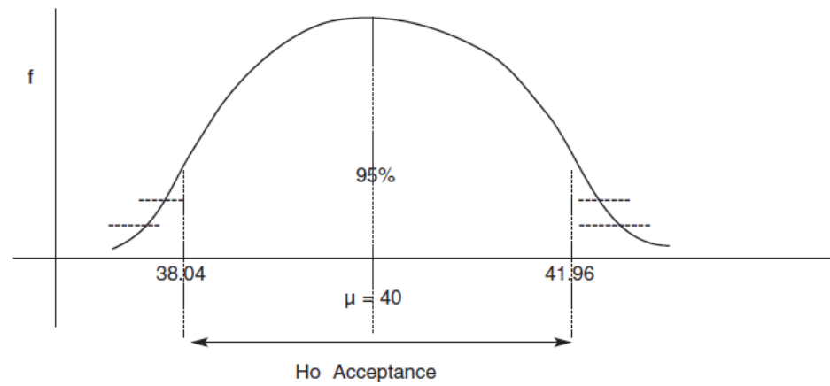
(a) Establish the hypothesis that the population mean weight, µ, is 40kgs, that is, the Null

Hypothesis (Ho). This means that we are assuming that there is no difference between the mean

and the sample mean and that any difference can be ascribed to chance. The Alternative

Hypothesis (H1) can be stated that the population mean does not equal 40kg.

Ho: µ = 40kg

H1: µ ≠ 40kg (2 marks)

If Ho is found to be true H1 is rejected while if Ho is found to be false, H1 is accepted. With a

95% confidence level the sample mean must lie within ± 1.96 standard errors (the acceptance

zone), so that, if Ho is true, 95% of the means of all samples must be within the range µ ±

1.96sx where sx is the standard error, that is, sx = σ/√n. (2 marks)

Therefore, sx = 4/√49 = 0.57.

The range is 40 ± 1.96 x 0.57, that is, 38.88kgs to 41.12kgs (2 marks)

or the z-score [(x – µ)/sx = (42.4 -40)/0.57 = 4.21] must fall outside ± 1.96

As the sample mean of 42.4kg falls outside the acceptance zone the null hypothesis is rejected

and H1 is accepted, that is, µ ≠ 40kg. The difference between the population and sample

means is significant at the 5% level. (4 marks)

(b) In this test it is necessary to test if the population mean is greater than the assumed

value of 40kgs, that is,

Ho: µ = 40kgs; H1: µ > 40kgs. (4 marks)

This is a one tailed test where the number of standard errors at the 5% level is 1.65. Since the

calculated z score is 4.21 and is outside the 5% value the Null Hypothesis is rejected.

(2 marks)

It can therefore be stated that the population mean is greater than 40kgs. (2 marks)

The analysis is shown in the diagram for a two tailed test.

Page 25

(2 marks)

[Total: 20 Marks]

Page 26

SOLUTION 4

To determine the relationship between the variables, and the regression line Y = a + bX, we

solve the following equations

∑Y = na + b∑X

∑XY = a∑X + b∑X2 or substitute the above values into the following (2 Marks)

b = ∑XY - ∑X x ∑Y

∑X2 - (∑X)

a = ∑Y - b∑X

n n

X (000’s) Y (000’s) XY X

10 32 320 100

20 39 750 400

40 58 2320 1600

25 44 1100 625

30 52 1560 900

40 61 2440 1600

50 70 3500 2500

45 64 2880 2025

260 420 14900 9750

Quarter

Output (units)

Total Cost RWF

10,000

32,000

20,000

39,000

40,000

58,000

25,000

44,000

30,000

52,000

40,000

61,000

50,000

70,000

45,000

64,000

Page 27

Therefore, b = 14900 - 260 x 420/8 = 14900 - 13650

9500 - (260)/8 9750 - 8450

= 1250/1300

= 0.9615 (2 Marks)

a = 420/8 - 0.9615 x 260/8

= 52.5 - 31.25

= 21.25 (2 Marks)

Y = 21,250 + 0.962X (4 Marks)

Page 28

(b) Total Cost = Fixed cost + Variable cost per unit of production. (2 marks)

In the above equation the fixed cost is

RWF

21,250; this cost is independent of the

level of production. X represents the variable cost of production i.e. for each unit increase in

production the costs increases by a factor of 0.962. At some stage during the production

process the variable cost profile will intersect the fixed cost to give the breakeven value. The

sum of the fixed and variable costs gives the total cost profile. (4 marks)

costs are:

Y = RWF21,250 + 0.962X 1,250

(2 marks)

= RWF21,250 + 0.962 (55,000) = RWF52,910

This projection is outside the boundaries of the relationship and the accuracy is predicated on

the principle that the linear relationship will continue. On the assumption that the linearity of

the relationship continues, the extrapolated figure can be accepted as being relatively accurate.

(2 marks)

[Total: 20 Marks]

SOLUTION 5

(a) In this case we are talking about an amortisation annuity over the 5 years, that is, the

amount borrowed (

RWF

12,000) is equal to the present value of the annual payments (say

A) over the 5 years at the interest rate of 14%.

RWF

12,000 = A + A + A + A + A

1.14 (1.14)2 (1.14)3 (1.14)4 (1.14)5

(3 Marks)

= A (0.8772 + 0.7695 + 0.6749 + 0.5921 + 0.5194)

= A (3.4331)

Therefore, A =

RWF

12,000 =

RWF

3,495. (3 Marks)

3.4331

Page 29

(b) The interest will be compounded over the four years. The compound interest is

derived as follows (the total cost at the end of four years less the initial cost equals the interest

paid)

CI = P(1 + i)t - P, where I = 15%, P =

RWF

20,000, t = 4. (3 Marks)

Therefore, CI = 20,000(1 + 0.15)4 - 20,000

= 20,000 x 1.749 - 20,000

= 34,980 - 20,000 = RWF14,980

(3 Marks)

RWF

3,200 is given by

Z = (3200 - 3000)/500

= 0.4

The probability is 0.3446 from the Normal distribution tables. (3 Marks)

Probability of more than

RWF

3500 is given by

Z = (3500 - 3000)/500

= 1.00

The probability is 0.1587 from the Normal distribution tables. (3 Marks)

Therefore, probability is within the range 3200 to 3500, that is, 0.3446 – 0.1587, i.e. 0.1859.

(2 Marks)

[Total: 20 Marks]

Page 30

SOLUTION 6

(a) Structure of a time series.

A time is a set of results for a particular variable of interest taken over a period of time. There are

four separate elements to consider

- Trend component: in a set of time series data the measurements are taken at regular

intervals. However, there may be random fluctuations in the data but in some cases the

data will show a shift to lower or higher values over the time period in question. This

movement is called the trend and is usually the result of some long term factors such as

changes in expenditure, output, etc. There may be various trend patterns such as increasing

linear trends, decreasing linear trend, non-linear trend or no trend.

(2 Marks)

- Cyclical component: a time series may show a trend of some sort but may also show a

cyclical pattern of alternative sequences of observation above and below the trend line.

This moves from the medium to longer term around the trend line. Any pattern of this

type which lasts longer than a year is called a cyclical element for the time series. This is

generally a very common occurrence. (2 Marks)

- Seasonal component: there may be a pattern of variability in regular cycles within a year.

The element of the time series which represents variability due to seasonal influences

is called the seasonal element. It normally refers to movements over a one year period

but it can also refer to any repeating pattern of less than one-year’s duration (2 Marks)

- Irregular component: this is the element which cannot be explained by the trend,

cyclical and/or seasonal elements and is entirely unpredictable. It represents the random

variability in the time series, caused by unanticipated and non-recurring factors which

are unpredictable. It gives a dramatic and unexpected departure from trend. (2 Marks)

(b) Use of the moving average method for smoothing.

Smoothing methods are used to smooth out the irregular element of time series where there are

no significant trends, cyclical or seasonal pattern.

Moving average: this method involves using the average of the most recent data values to

forecast the next period. The number of data values used can be selected in order to minimise

the forecasting error. To find the moving average, the simple average for a specified number

of items of data is found. For example, with quarterly data a simple average for four items of

data can be calculated and then move that average along. This is done by recalculating the

average having dropped the initial item of data and adding a subsequent item of data. This

gives the four quarter moving total. The moving totals fall in between the actual quarterly

data, that is, the first moving total falls between quarters 2 and 3. The respective four quarter

Page 31

moving totals are divided by 4 to find the four quarter moving average. The data is centred by

summing respective pairs of data and dividing by two. This smooths the data so that the trend

line can be derived. In this way moving averages are used to ‘smooth out’ fluctuations in the

data and obtain a trend line. This is the moving average trend which can be plotted to show

the direction. Since the trend does not vary significantly in short time periods the trend can

be projected to forecast future events.

However, there are limitations to the use of moving averages. Equal weighting is given to each

of the values used in the moving average calculation whereas the most recent data is more

relevant to current conditions. The moving average takes no account of data outside the period

of average so full use is not made of all the data. The use of the unadjusted moving average as a

forecast can cause misleading results when there is an underlying seasonal variation.

(6 Marks)

Forecasting from the time series lies in our knowledge of the behaviour of trend. Since the trend

does not vary significantly in short time periods, the trend can be projected to forecast future

events. A time series can be used to forecast where there are no significant trends, cyclical

or seasonal elements using the moving averages method as set out above. Using moving

averages, to get an accurate projection of trend without plotting the values, it is necessary to

derive the average rate of change of the trend. This can be done by deducting the first value

of the trend from the last trend value, taking the average (less one) and adding to the last

trend value. This can be done for a number of values to forecast for a number of periods into

the future. This is the moving average trend which can be plotted to show the direction. The trend

can be projected forward. However, the further the trend is projected the greater is the

possibility of inaccuracy.

However, if there are both trend and seasonal elements in the series there are other methods

which may be used. The first stage in such a forecasting technique is to calculate the seasonal

factors by smoothing out the time series using the moving averages method. If the seasonal

factors are quarterly then the moving average is calculate on groups of four data points. When

seasonal elements are involved it is necessary to work out the centred moving averages which

are averages of the moving averages. Dividing the original observation by the equivalent

centred moving average gives a seasonal factor for each observation. This is done for all

quarters.

If the time series shows a long term linear trend, linear regression may be used. A linear

regression equation linking dependent and independent variables can be derived but this

assumes that we have a linear trend and that the future will be like the past. (6 Marks)

[Total: 20 Marks]

Page 32

SOLUTION 7

1. (i) Cash Flows for the proposal.

Year

Cost

RWF

Cost

RWF

Net Ca

Flows

RWF

0 125,000

(125,000)

(1,500) 30,000 28,500

(1,800) 33,000 31,200

(2,160) 36,300 34,140

(2,592) 39,930 37,338

43,923 43,923

6 5

000

(2 Marks) (2 Marks) (2 Marks) (2 Marks)

(ii) Calculation of the Internal Rate of Return. To calculate the IRR it is necessary to derive present

values. Taking discount values at 14% and 20% the following table is developed.

Net Cash

RWF

Discount

@ 12%

RWF

Discount

@ 18%

RWF

0 (125,000) 1

000 (125,000) 1

000 (125,000)

1 28,500 0

893 25,450.5 0

847 24,139.5

2 31,200 0

797 24,866.4 0

718 22,401.6

3 34,140 0

712 24,307.7 0

609 20,791.3

4 37,338 0

636 23,747.0 0

516 19,266.4

5 43,923 0.567 24,904.3 0.437 19,194.4

6 5

000 0.507 2,535.0 0

370 1,850.0

NPV

810.9

(17,356)

(2 Marks) (2

Marks)

The IRR can be derived by calculation or graphically. Using the formula

N1I2 - N2I1 , where discount rate I1 gives NPV N1 and discount rate I2 gives NPV N2

N1 - N2

N1 =

RWF

810

I1 = 12%; N2 = (

RWF

356)

I2 = 18%

Page 33

IRR = 810.9 x 0.18 - (17,356) x 0.12 = 2,229 = 12.3%

810.9 - (17,356) 18,167

(4 Marks)

Page 34

(iii) Interpretation of the result. The value of 12.2% can be interpreted as the rate of

return that the project will earn. On face value the NPV is positive at 12% and this

represents a positive result. However, if the cost of capital to the company, represented by

the rate of interest charged by the bank of 15%, is greater than this value, the project is not

viable. However, there are mechanisms for deriving the real cost of capital to the company

based on its equity and funds which may not be representative of the bank rates. The

decision of the company in this case is that the project, as a stand alone investment, will not

contribute the required return. (4 Marks)

[Total: 20 Ma

]

SOLUTION 8

(i) The average earnings and standard deviations for employees in both divisions.

Division 1

Lower

Bound

Upper

Bound

Mid

point

(

)

400

420

440

460

480

500

420

440

460

480

500

520

410

430

450

470

490

510

600

750

800

250

100

1,849,100

3,698,000

7,087,500

8,836,000

6,002,500

2,601,000

∑

141

65,010

30,074,100

Mean = x = ∑fx = 65,010 =

RWF

461

1 (3 Marks)

∑f 141

Standard Deviation

σ = √ ∑ fx 2 – {∑ fx}2 = √ 3,074,100 – 212,578

∑ f {∑ f } 141

= √ 731 = RWF26.71 (3 Marks)

Division 2

Lower

Bound

Upper

Bound

Mid point (

)

400

420

440

460

480

500

420

440

460

480

500

520

410

430

450

470

490

510

920

900

500

200

600

850

017

200

547

000

125

000

254

000

604

000

9103

500

Page 35

∑

227

105,970

49,650,700

Mean = x = ∑fx = 105,970 =

RWF

466

8 (3 Marks)

∑f 227

Standard Deviation.

σ = √ ∑ fx2 – {∑ fx}2 = √ 49,650,700 – 217,928

∑ f {∑ f } 227

= √ 797 =

RWF

23 (3 Marks)

Summary

Division

Mean

RWF

461

RWF

466

Std Deviation

RWF

Number 141 227

(ii) In order to test if there is a difference in the earnings between both divisions a hypothesis

can be used. In this case we are testing for the difference of means in a similar way as confidence

intervals for the difference of means. The difference between the sample estimates is first

calculated and the values given by the null hypothesis, transform the difference to a number of

standard errors, then compare with a critical value consistent with the alternative hypothesis. In

this way we are comparing if the two sample means have come from the same population,

i.e. Null Hypothesis, Ho: µ1 = µ2 and the alternative hypothesis

H1: µ1 ≠ µ2 (4 Marks)

This is a two sided test. In this particular test we are assuming H0 to be correct.

The Z statistic is X1 - X2 , that is, the difference in means divided by the standard error

√S

12 +

N1 N2

X1 - X2 = 461.1 - 466.8 = - 5.7

= 26

= 5.06;

= 28

23 = 3.51;

N1 141 N2 227

Z = -5.7 = - 1.94 (4 Marks)

√8.57

Z, at 1% significance level, is 2.58.

Since the calculated value is less than this level we accept the null hypothesis – the samples do

not provide evidence that there is a difference in the long-run earnings of employees.

Page 36

[Total: 20 Ma

]

Page 37

SOLUTION 9

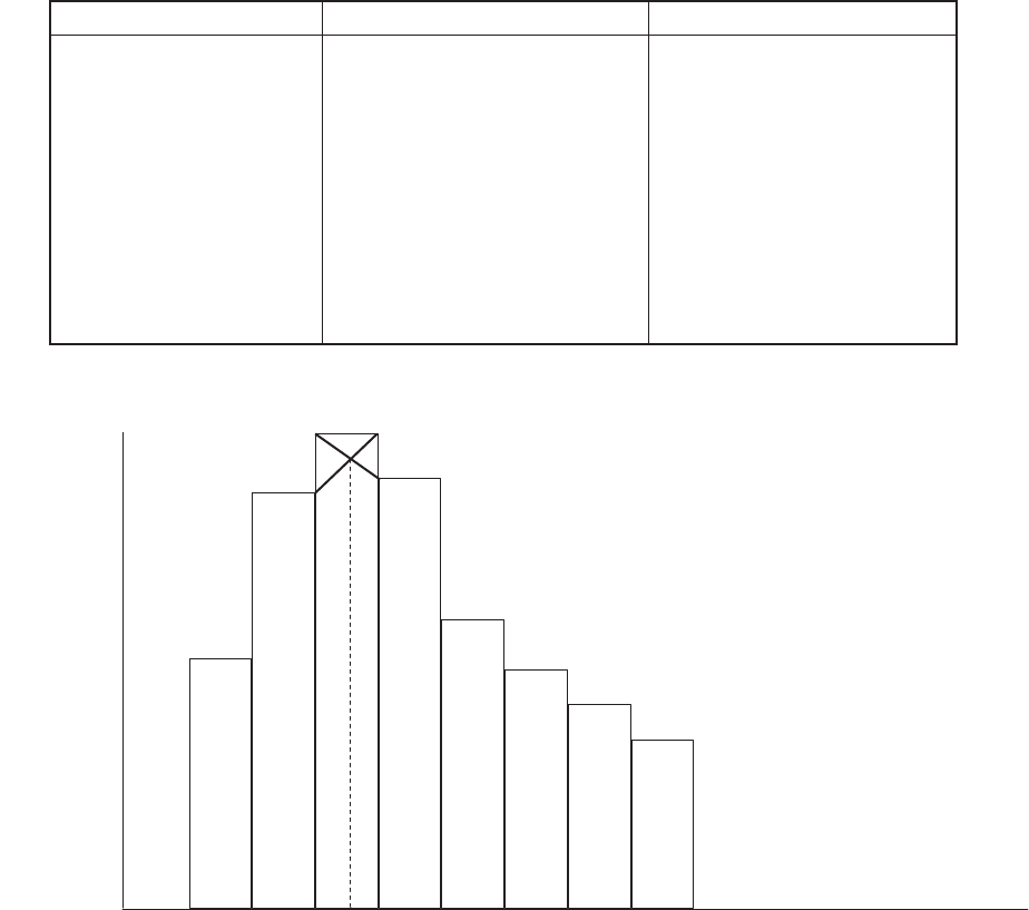
(i) Histogram of the data.

Monthly Allowance rwf

Number of Trainees (f)

Cumulative Frequency

260-280

280-300

300-320

320-340

340-360

360-380

380-400

400-420

Frequency

0 260 280 300 320 340 360 380 400 420 Weekly allowance

RWF

(8 Marks)

The modal value of the allowance is approximately

RWF310,

found from the histogram.

(ii) The Median.

The median is the value of the 40.5 trainee in group 320 – 340.

From the formula the median value = 320 + (40.5 – 38)/15 x 20 =

RWF

323

(6 Marks)

(iii) Comparison of the mode and median.

The mode is the greatest frequency of the distribution and is in the range

RWF320

RWF340.

The accurate value is derived from the histogram above.

Page 38

The median represents 50% of the data above and below the mid point. It means that 50% of

the trainees are receiving more than

RWF

323

23 and 50% less than

RWF

323

(8 Marks)

Page 39

SOLUTION 10

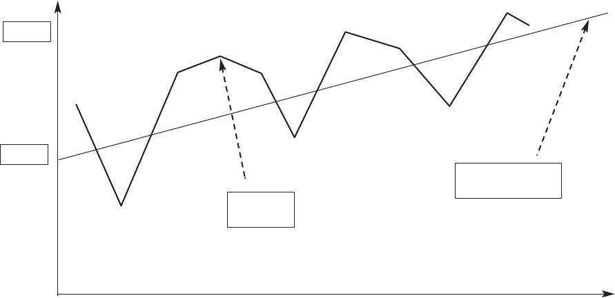
(i) The trend for this data can be developed using either a moving average technique or linear

regression analysis. A four quarter centred moving average could be derived allowing us to

decompose the data to isolate the trend by means of either additive or multiplicative models. In the

present case it may be substantially easier to develop the trend by means of linear regression without

smoothing the data, that is,

y = a + bx where

a = Σy - bΣx

n n

b = Σxy - (ΣxΣy)/n,

Σx2 - (Σx)2/n

Quarter

Sales

∑

350

295

197

390

450

420

325

460

550

530

415

615

997

100

121

144

650

350

590

591

1,560

2,250

2,520

2,275

3,680

4,950

5,300

4,565

7,380

011

(5 Marks)

Inserting values gives

b = 36,011 - (78 x 4997)/12

650 - 55

= 3530.5 = 24.69

143

a = 4997 - 24.69 x 78 = 416.4 - 160.5 = 255.9

12 12

Therefore, y = 255.9 + 24.69x. (5 Marks)

Page 40

(ii) Plotting a graph of the points and projecting the data for 2010. (5 Marks)

Y Sales

600

300

Time

Series

Regression

Line

0 4 8 12 16

uar

ers

The projected points for the four quarters of 2010 are calculated from the regression line for

quar

ers

13,14,15,16.

For x = 13, y (Sales) = 576,870

For x = 14, y (Sales) = 601,560

For x = 15, y (Sales) = 626, 250

For x = 16, y (Sales) = 650,940

(5 Marks)

(Total: 20 Ma

ks)

Page 41

SOLUTION 11

(i) Initial Sum invested:

RWF

000

At end year 1

+10%

RWF

1,000

RWF

5,000

RWF

000

At end year 2

+15%

RWF

2,400

RWF

5,000

RWF

400

At end year 3

+15%

RWF

3,510

RWF

5,000

RWF

910 ---- Sum Receivable (3 Marks)

Return on investment: (

RWF

910 -

RWF

000) x 100 = 27.64%

RWF

000

(3 Marks)

(ii) Discounting

RWF

500 to present values at 4% gives 13,500 = 13,500

1.045 1.2166

= R

096

Since this value is greater than

RWF

000

the option to receive

RWF

500 in 5 years is

the best option. (6 Marks)

(iii) Standard deviation = 10kg; Mean = ?; x = 1000kg.

Converting these values to the standard Normal Distribution z = x - µ

For 5% (0.05), z = 1.645

Therefore, 1.645 = 1000 - µ

µ = 1000 - 1.645 x 10

= 983

55kg

To ensure that only 5% of the orders are overweight the machine should be set to 983.55kg.

(4 Marks)

Page 42

Diagram (4 Marks)

100 kg

Area

= 0.05

gives z

= 1.645

[Total: 20 Ma

]

Page 43

SOLUTION 12

An explanation of the terms is provided below.

(i)

Structure

of a time series. A time series is a set of results for a particular variable

taken over a period of time. There are four separate elements in the structure

- Trend: In many cases the data exhibits a shift either to lower or higher values over

the time period in question. This movement is called the trend and is usually the result

of some long-term factors such as changes in expenditure, sales, demographic factors, etc.

There may be many trend patterns – increasing linear trend, decreasing linear trend, non-

linear trend or no trend.

Cyclical:

A time series may display a trend of some form but may also show a cyclical

pattern of alternative sequences of observation above and below the trend line. Any regular

pattern which lasts longer than a year is the cyclical element of the time series. This is a

common occurrence represented by the retail sector of business.

- Seasonal: although the cyclical patter may be displayed over a number of years, there

may be a pattern of variability within one-year periods. The element of the time series which

represents variability due to seasonal influences is the seasonal element. While it normally

refers to patterns over a one-year period, it can also refer to any repeating pattern of less

than one-yearʼs duration.

- Irregular element: this is the element which cannot be explained by the trend, the

cyclical or seasonal elements. It represents the random variability in the time-series, caused

by unanticipated and non-recurring factors which are unpredictable. There are particular

methods used to smooth out the irregular element of time series where there are no

significant trends, cyclical or seasonal patterns such as moving averages or exponential

smoothing. (5 Marks)

(ii)

Investment Appraisal

Many use many quantitative techniques as an aid to

decision making. One of the most important applications is concerned with investment

decisions. Managers often have to make choices between alternative decisions, they need to

consider future costs and revenues and the importance of incremental changes in costs and

revenues. It is also critical to consider the time value of money because of time scales

involved. The managerʼs decision to invest is based on three important factors – the

estimate of the future based on forecasts of costs, revenues, inflation, and interest rates; the

alternatives available for investment: techniques to support the decision must be used; the

business attitude to risk: because of the uncertainty of the future and project uncertainty,

additional techniques must be used. A number of these techniques used in investment

appraisal are, the accounting rate of return; payback; discounted cash flow, such as net

present value and internal rate of return.

The accounting rate of return is the ratio of the average annual profits, after depreciation, to

the capital involved. Variations of this exist but it has some drawbacks – it does not allow

for the timing of cash flows and profit has subjective elements. Payback is a popular

technique which is defined as the period which it takes for the projects net cash flows to

recover the original investment. Payback favours quick return projects

Page 44

– the project with the shortest payback period is accepted. However, it does not measure

overall investment worth since it does not consider cash flows after the payback period or

the timing of cash flows. Net Present Value uses discounting principles and involves

calculating the present value of expected cash inflows and outflows and establishing

whether the present value of the net cash flows is positive. The internal rate of return is the

discount rate which gives zero NPV. If the calculated IRR is greater than the companyʼs

cost of capital the investment is accepted. However these two techniques do not necessarily

rank investment proposals in the same order of attractiveness. But the IRR technique is used

extensively in investment appraisal decisions. (5 Marks)

(iii) Network

Analysis

This deals with a range of techniques used to aid managers in the

planning and control of projects. These techniques show the inter-relationship of the

various jobs to be done to complete the project and clearly identify the critical parts of the

project. They provide planning and control information on the time, cost and resources

required. These techniques are of particular value where projects are large and contain many

related and interdependent activities, where many types of facilities, high capital

investments and a large number of staff are involved, where projects have to be completed

within target time and costs.

Path analysis. To develop the technique it is necessary to know the activities involved,

their logical relationship, an estimate of the time the activity is expected to take. It may be

necessary to have a range of estimates of times, costs, resources and probabilities. Once the

logic of the activities has been agreed and an outline network drawn, it can be completed by

inserting the activity duration times. These times may be estimated by using probabilities

(developing the expected time) or using basic time estimates. A basic feature of the analysis

is the calculation of the project duration which is the duration of the critical path. This is the

path through the network which gives the shortest time in which the whole project can be

completed. It is the chain of activities with the longest duration times. In a network there

may be more than one critical path. The activities along the critical path are vital activities

which must be completed on time otherwise the project will be delayed. If it is required to

reduce the overall project duration then the time of one or more of the activities on the

critical path must be reduced.

A further important feature of the analysis deals with the process of cost scheduling. This

implies that by using more resources the duration could be reduced but at the expense of

higher costs. The costs associated with delivery of the project, as designed, is the ʻnormalʼ

cost. It is possible to reduce the activities by means of extra wages, overtime, additional

facility costs which are higher than normal and are called crash costs. This is an element of

least cost scheduling which finds the least cost method of reducing the overall project

duration, time period by time period. (5 Marks)

(iv) Measures of

dispersion.

Measures of dispersion represent a measure of the extent of

spread of data around the mean or average of the data. The simplest measure of

dispersion is to take the absolute difference between the highest and lowest value of the

raw data – ʻthe rangeʼ. The interquartile range is the absolute difference between the upper

and lower quartiles of a distribution. These measures of dispersion involve comparing two

different points on the frequency distribution such as the maximum and minimum points

(the range) or the upper and lower quartiles. However, other measures of dispersion which

compare all the points on the frequency distributions are more important. The ʻmean

Page 45

deviationʼ, that is, the average of the absolute deviations from the arithmetic mean, may be

used. However, if is the basis for the most common measures of dispersion – the variance

and the standard deviation. The variance is derived by squaring all the deviations from the

arithmetic mean. Rather than use squared units, it is more realistic to express solutions to

problems in terms of single units. The standard deviation takes the square root of the

variance. The standard deviation is then the square root of the average of the squared

deviation from the mean and is the most commonly used measure to explain the dispersion

of data. These various methods can be used for both grouped and ungrouped data. (5 Marks)

Paper CPA F1.1 BUSINESS MATHEMATICS & QUANTITATIVE METHODS Revision Guide

Navigation menu

Versions of this User Manual:

Views

Navigation