Barclays Capital Research Note CPI User Guide 2004

CPI%20Barclays%20User%20Guide%202004

User Manual:

Open the PDF directly: View PDF .
Page Count: 122 [warning: Documents this large are best viewed by clicking the View PDF Link!]

Barclays Capital Research Barclays Capital Research

Global Inflation-Linked Products

A User’s Guide

January 2004

Barclays Capital

5 The North Colonnade

London E14 4BB

For further information on any aspect of our Global Inflation-Linked business please contact:

Tim Peat

Global Inflation-Linked Product Coordinator

+44 (0)20 7773 9555

tim.peat@barcap.com

Strategy Contacts

Alan James

Global Inflation-Linked Strategist

+44 (0)20 7773 2238

alan.james@barcap.com

Gemma Wright

US Treasury Strategist

+1 212 412 2516

gemma.wright@barcap.com

Michael Oman

Inflation-Linked Strategist

+44 (0)20 7773 9106

michael.oman@barcap.com

John Richards

Japan Strategist

+81 (3)3276 1546

john.richards@barcap.com

Jacques Delpla

French Inflation-Linked Strategist

+33 144 58 3226

jacques.delpla@ barcap.com

Leon Myburgh

Africa Strategist

+27 11 772 7222

leon.myburgh@barcap.com

Index Contact

John Williams

Head of Index Products

+44 (0)20 7773 2419

john.williams@barcap.com

Matt Cocup

Index Products

+44 (0)20 7773 6172

matt.cocup@barcap.com

Economics Contacts

Julian Callow

Chief European Economist

+44 (0)20 7773 1369

julian.callow@barcap.com

David Hillier

Chief UK Economist

+44 (0)20 7773 4307

david.hillier@barcap.com

Henry Willmore

Head of US Economics

+1 212 412 6858

henry.willmore@barcap.com

Guide Contributors

Tim Bond

Global Head of Interest Rates Strategy

+44 (0)20 7773 2242

tim.bond@barcap.com

Sreekala Kochugovindan

Quantitative Strategist

+44 (0)20 7773 2234

sreekala.kochugovindan@barcap.com

Amita Shrivastava

US Economist

+1 212 412 3002

amita.shrivastava@barcap.com

This publication has been prepared by Barclays Capital ('Barclays Capital') - the investment banking division of Barclays Bank PLC. This publication

is provided to you for information purposes only. Prices shown in this publication are indicative and Barclays Capital is not offering to buy or sell

or soliciting offers to buy or sell any financial instrument. The information contained in this publication has been obtained from sources that

Barclays Capital believes are reliable but we do not represent or warrant that it is accurate or complete. The views in this publication are those of

Barclays Capital and are subject to change, and Barclays Capital has no obligation to update its opinions or the information in this publication.

Barclays Capital and its affiliates and their respective officers, directors, partners and employees, including persons involved in the preparation or

issuance of this document, may from time to time act as manager, co-manager or underwriter of a public offering or otherwise, in the capacity of

principal or agent, deal in, hold or act as market-makers or advisors, brokers or commercial and/or investment bankers in relation to the securi-

ties or related derivatives which are the subject of this publication.

Neither Barclays Capital, nor any affiliate, nor any of their respective officers, directors, partners, or employees accepts any liability whatsoever for

any direct or consequential loss arising from any use of this publication or its contents. The securities discussed in this publication may not be

suitable for all investors. Barclays Capital recommends that investors independently evaluate each issuer, security or instrument discussed in this

publication, and consult any independent advisors they believe necessary. The value of and income from any investment may fluctuate from day

to day as a result of changes in relevant economic markets (including changes in market liquidity). The information in this publication is not

intended to predict actual results, which may differ substantially from those reflected.

This communication is being made available in the UK and Europe to persons who are investment professionals as that term is defined in Article

19 of the Financial Services and Markets Act 2000 (Financial Promotion Order) 2001. It is directed at persons who have professional experience in

matters relating to investments. The investments to which it relates are available only to such persons and will be entered into only with such

persons. Barclays Capital - the investment banking division of Barclays Bank PLC, authorised and regulated by the Financial Services Authority

('FSA') and member of the London Stock Exchange.

BARCLAYS CAPITAL INC. IS DISTRIBUTING THIS MATERIAL IN THE UNITED STATES AND, IN CONNECTION THEREWITH, ACCEPTS RESPONSIBILITY

FOR ITS CONTENTS. ANY U.S. PERSON WISHING TO EFFECT A TRANSACTION IN ANY SECURITY DISCUSSED HEREIN SHOULD DO SO ONLY BY

CONTACTING A REPRESENTATIVE OF BARCLAYS CAPITAL INC. IN THE U.S., 200 Park Avenue, New York, New York 10166.

Non-U.S. persons should contact and execute transactions through a Barclays Bank PLC branch or affiliate in their home jurisdiction unless local

regulations permit otherwise.

permission of Barclays Capital. Barclays Bank PLC is registered in England No. 1026167. Registered office 54 Lombard Street, London EC3P 3AH.

Additional information regarding this publication will be furnished upon request.

EU2187

www.barcap.com/inflation

EU2187 Cover Inflation Linked V1_spine.qxd 19/01/2004 17:14 Page 1

Barclays Capital Global Rates Strategy 1

Table of Contents

Foreword 3

Introduction 4

Why Have Inflation-Linked Products Taken Off in a Low-Inflationary World? 5

Why Issue or Pay Inflation? 7

The Markets 13

United States 14

UK 20

France 31

Italy 36

Sweden 37

Canada 41

Australia 44

Barclays Inflation-Linked Bond Indices 47

South Africa 50

Japan 52

Greece 54

Iceland 55

Israel 56

New Zealand 57

Mexico 58

Inflation-Linked Derivatives 59

Non-Government Issuance 65

Inflation-Linked Product in the Investment Universe 69

The Fisher Equation – Nominal Bond Comparisons and the Risk Premium 70

The Duration of Inflation-Linked Bonds and the Concept of Beta 73

Linkers in a Portfolio Context 77

Comparing Real Bonds With Equities 83

Comparing Linkers to Other Real Assets 87

2 Global Rates Strategy Barclays Capital

Value Analysis 91

Fundamental Factors Behind Real Yields 92

Breakeven Trades and Forwards 101

Seasonality and Inflation-Linked Bonds 105

Deflation Protection: The Par “Floor” 108

Real and Nominal Curve Slopes 111

Inter-market Valuations and Trading 113

Appendices 115

Example Swap Structures 116

Real Yields 119

Breakeven Inflation 120

The Barclays Capital Global Inflation-Linked Bond Index 121

Key Information Sources 122

Summary Sovereign Table 124

Barclays Capital Global Rates Strategy 3

Foreword

In the 15 months since we published the first edition of our User’s Guide for inflation-

linked bonds there have been a variety of dramatic developments in the "linker"

marketplace. The size of the global inflation-linked government bond market has more

than doubled. Bond market trading volumes have increased markedly. But the most

exciting development has been the explosion of activity in the field of inflation-linked

derivatives. Linkers are now indubitably established as an asset class in their own right.

We at Barclays Capital continue to extol the virtues of linkers. Given the scale of the

development of the asset class, it is clear that they are attracting ever more attention and

focus from investors and borrowers alike. We continue to commit unrivalled resources in

terms of distribution, liquidity provision, market research, web-based analytical tools and

index provision and are proud to offer the most complete coverage of the product.

In this guide we offer a comprehensive review of the major markets and discuss in

depth all of the major topics relevant to linkers. This includes discussion on the

changing nature of the inflation products universe. As well as being a comprehensive

reference across a broad range of markets, this guide includes studies on topics

affecting investment decisions in linkers, ranging from the macro long-run

determinants of real yields to considerations for short-term trading strategies.

We trust you will enjoy making use of this publication and find its contents informative,

interesting and thought provoking. Above all, however, we hope it will further excite

your interest in the world of "linkers".

Tim Peat

Managing Director

Global Inflation-Linked Product Co-ordinator

4 Global Rates Strategy Barclays Capital

Introduction

Alan James

Inflation linked products are not new but they are going through a period of very rapid

development. Since our previous User’s Guide was published in September 2002 not

only has the size of the linker bond market more than doubled but the size of the

inflation derivatives market has increased by at least 10 times. The asset class has come

a very long way indeed since 1780, when the State of Massachusetts issued its first

bond linked to a basket of commodities.

Inflation-linked bonds were issued by a number of countries after 1945, including Israel,

Argentina, Brazil and Iceland. However, the modern market is generally accepted to have

been born in 1981, when the first index-linked gilts were issued in the UK. The other large

markets adopted somewhat different calculations to those used by the first mover, mostly

copying the more straightforward model first employed by Canada in 1991.

In this publication we will focus on the development of the markets that make up the

Barclays Global Inflation Bond Index, of which more detail later in this publication. In

chronological order, the markets are the UK (1981), Australia (1985), Canada (1991),

Sweden (1994), the US (1997), France (1998) and Italy (2003). In this guide we have

arranged them by order of size. We will also give some consideration to larger markets

outside of this classification, as well as focus on the rapidly developing inflation swaps

markets in the euro area, UK and US.

While calculations vary to a greater or lesser extent between countries, in this

publication we try and outline the simple differences between them as well as providing

the rigorous detail as required. Government inflation-linked bonds tend to have a

similar structure, where principal and income are adjusted for changes in the relevant

consumer price index between issue date and cash flow payment date, subject to an

indexation lag. Many recent corporate issues have had different inflation-linked

structures though, while the growth of the inflation derivatives market has meant that

whatever cash flow style is desired can now be created.

Throughout the guide we will refer to bonds as “inflation-linked”, “inflation-indexed”,

“index-linked”, “real return bonds”, “inflation bonds” or the short-form nickname

“linkers”. These terms will be used interchangeably, with nothing meant by the choice

of one rather than another.

Barclays Capital Global Rates Strategy 5

Why Have Inflation-Linked Products

Taken Off in a Low-Inflationary World?

Alan James

To some, it may seem perverse that inflation-linked products have blossomed during a

period in which global inflation has been at or near 50-year lows. Arguably, however,

the two are inherently linked. As the population of the post-industrial world ages,

demand for products with known real cash flows grows sharply. At the same time, in

the very long term, an aging population is likely to be deflationary. There is only one

reason to save, and therefore sacrifice current spending, and that is in order that savers

and their dependents can enjoy future consumption. The saver is predominantly, if not

wholly, interested in the future real worth of savings, not their nominal future price. As

workers approach retirement, they tend to focus increasingly on maintaining future

purchasing power, rather than taking risks to accumulate. Meanwhile, as the population

ages, inflation becomes more and more politically unacceptable, as there is an

increasing focus on the diminution of purchasing power from price rises.

We may be at a significant inflexion point in terms of anti-inflation policy. The acceptance

that deflation is just as much of a social evil as inflation has already changed global policy

makers’ stance. However, it may be that the efforts to avoid deflation also suggest that

the political pressure for central banks to contain inflation has temporarily reduced. It is

so long since any of the world’s richest nations had a significant inflationary problem that

central bankers are being encouraged to take a more balanced view with regards to the

trade-off between inflation risks and growth. Only hindsight will tell us whether this

change in emphasis is a good thing or not, but it does mean that the uncertainty over

price levels in the next 10 years may be somewhat higher than in the past 10. Inflation-

linked markets are behaving as though this is the case.

It should not be forgotten that even in a stable low-inflationary environment, in the

long term there remains a considerable uncertainty about the real value of nominal

bond returns. $100 now would have the purchasing power of $74 in 30 years’ time if

inflation averaged 1% but only $48 if inflation averaged 2.5%, more than 50% less.

While there is always an element of basis risk for an individual, as their own

consumption basket will not be the same as the relevant inflation index, no other

financial asset can give close to the real value certainty of inflation-linked products. If

saving is ultimately about deferred consumption, then for an investor the question

should not be why hold inflation-linked bonds, but why hold anything else. Other riskier

assets need to prove why they offer an attractive alternative.

Demographic pressures are such that it is quite conceivable for the inflation-linked

market to continue growing at its current rate. A quick reference to the growth in

computer processing power serves as a reminder of just how explosive a sustained

trend in which the size of the bond market doubles every 18 months could be. Whether

or not this trend, “Moore’s Law”, really can apply to linkers for a sustained period is

debatable, but a structural reallocation of pension assets could easily see the trend

continue for several years. For instance, if US pension funds were to allocate the same

percentage of their assets to linkers as have UK pension funds, this allocation would be

larger than the current global market ($600bn). Even UK pension funds have offset less

than only a quarter of their total inflation-linked liabilities with inflation-linked bonds.

Japanese pension funds have a higher percentage of their liabilities with inflation

linkages and are further along the demographic transition but are only just starting to

address this exposure. It may well be that the potential for supply rather than demand

6 Global Rates Strategy Barclays Capital

becomes the limiting factor. It appears likely, however, that the inflation-linked sector

could soon grow too large to be ignored.

Inflation uncertainty should be as much of a concern to borrowers as investors. As the

sector develops, it will become increasingly possible to choose whether to hedge-out

inflation risk. The advantages of the asset class are such that a stage of self-reinforcing

growth has now been reached. The drawbacks of the inflation-linked market are

becoming increasingly eroded due to the positive network externalities of familiarity

and liquidity. Clearly, this honeymoon phase cannot continue forever, but in the same

way the market now thinks of futures or interest rate swaps, the time may soon come

when the market can no longer imagine a world without inflation-linked bonds.

Barclays Capital Global Rates Strategy 7

Why Issue or Pay Inflation?

Alan James

The most natural issuers of inflation-linked bonds (and indeed structural payers of

inflation using swaps) are governments. Over time many of the traditional arguments in

favour of issuance have developed, with a significant change in emphasis as markets

have matured. We consider these before going on to look at more recent arguments in

favour of government supply. Fundamentally, the reasoning behind most corporate

structural paying/issuing is not that different than for governments, though corporates

may also have shorter-term value and cash flow considerations.

Traditional Reasons for Inflation-Indexed Bonds

Exploiting Excessive Market Inflation Expectations

A government may have more faith in the institutional arrangements in place to

maintain an anti-inflationary bias than investors. This was a major factor influencing

the UK’s decision to issue linkers in 1981: aggressive monetary and fiscal tightening had

been implemented to bring inflation under control at the time but investors remained

unconvinced that there would be a significant long-term reduction. By issuing inflation-

linked bonds, the UK Treasury thus saved an enormous amount of money when

inflation fell sharply and stayed low, ultimately bringing inflationary expectations down

too. Ex-post, some were critical about the underperformance of linkers versus

conventionals in this phase, but such criticism was unjustified. Nominal bonds had

enjoyed a windfall gain due to what was, for the market, unexpectedly low inflation.

In many countries this factor is notably less important than it has been in the past. In

most developed economies, with independent and transparent monetary policies, the

gap between market and government expectations of inflation is likely to be small. This

is not to say there are not times when there may be divergences of expectations that

encourage issuance, but the mismatch is unlikely to be the primary concern. For more

recently developing countries with less established monetary and fiscal institutions and

capital markets, there may still be occasions where governments perceive the markets’

expectations of price increases are substantially too high, particularly when institutional

changes have just been made.

Positive Credibility Feedback

A closely related benefit of inflation-linked bond issuance is that it can create a positive

credibility feedback. If a government really has taken steps to bring down long-term

inflation then it is in its interests to issue inflation-linked bonds while inflation

expectations remain high. The market may be more willing to believe in the

institutional changes made to bring down inflation if the government is seen to be

putting its money where its mouth is. The longer the expected lifespan of a particular

government, the more the strategy may be beneficial. This is another argument that is

not particularly relevant for developed economies with totally independent monetary

policies, but may be significant for transitional economies that have undergone periods

of high inflation.

8 Global Rates Strategy Barclays Capital

Saving a Risk Premium

A popular early argument for inflation-linked issuance was that if government inflation-

linked bonds really were risk-free financial assets, then a government could save an

inflation risk premium by issuing them in place of nominal debt. If investors are primarily

interested in maintaining the future real value of their savings, they should be prepared to

pay an insurance premium for the privilege of owning the risk-free inflation hedge. In

practice, it is debatable to what extent such a premium has been seen in the major

markets. We will discuss the risk premium factor in more detail later in this publication,

but this consideration tends to gain increasing emphasis when monetary policy credibility

comes under pressure. Early in the development of some of the major markets, it has

appeared that there have been negative inflation risk premia, or at least positive effects

were more than offset by negatives, eg, liquidity. The significant increase in government

supply in 2003 could arguably be explained largely by an increasing willingness by

investors to pay inflation risk premia compared to nominal bonds, but it is very hard to

differentiate between inflation expectations and risk premia.

Social Benefits

The existence of inflation-linked bonds may provide benefits to society beyond the

funding considerations. The ability to easily discern market expectations of inflation

may be of benefit to both policy setters. In particular, if it helps avoid inflationary

monetary and fiscal policy errors then it may be socially beneficial. Independent central

banks pay close heed to developments in market implied inflationary expectations if the

relevant markets are seen to be relatively undistorted, though it is often hard to tell at

the time if this is the case. One of the major reasons put forward within Japan for it to

start issuing inflation bonds was that the implied inflation rate that this would produce

would be a useful policy gauge. Experience elsewhere suggests it will take several years

at least before there is sufficient liquidity and acceptance of the asset class for the

implied inflation to be reliable enough a guide to be a benefit.

Some baseline expectation of inflation from linkers may also be useful for economic

agents in making decisions. The existence of inflation bonds could theoretically act to

reduce inflation uncertainty. This could encourage more savings, either directly into

inflation-linked bonds, or indirectly into assets for which there is a clearer real value if

there are inflation-linked assets for comparison. Putting a price on such benefits is all

but impossible, but there seem few clear differences in behaviour between economic

agents in similar countries with and without inflation bond markets.

Cash Flow Benefits

In nominal terms, a standard inflation-linked bond has smaller cash flows upfront than

as the price level rises. In effect, an inflation bond is, at least in nominal terms, a

discount instrument if inflation is expected over the life of the issue. This benefit may

be a factor worth considering for transitional countries that have short-term cash

constraints but ultimately sound finances. Otherwise it is a relatively weak argument on

its own, indeed almost irrelevant in most countries where governments are required to

account for inflation as it accretes in linkers.

Barclays Capital Global Rates Strategy 9

Inflation-Linked Issuing: Risk Related Reasons

The Appropriate Nature of Liabilities

The future expenditures and revenues of a government are almost all essentially real

flows. Its major future “asset” is its entitlement to a future (real) stream of tax revenues,

which will reflect both inflation and real economic activity. Having at least a portion of

liabilities linked to inflation should offer risk reduction benefits to the government

borrower, matching its future debt servicing costs with its revenues. The more that

revenues tend to grow faster than expenditures as prices rise, the more there is an

incentive to issue inflation-linked bonds. While ex post the costs of inflation-linked

bonds may be higher to issuers than nominal bonds would have been if there is higher

than expected inflation, the government is better placed to cover this cost.

Cyclical Benefits

The UK DMO put particular emphasis on the fact that inflation and the budgetary

situation of the government are likely to be correlated. When growth is strong, there is

little pressure on public finances but inflation is likely to be higher. Equally when

growth is weak, prices are unlikely to be rising quickly. Servicing linker costs rather than

that in nominal debt should thus tend to be a fiscal stabiliser. The fiscal impact of a

deflationary downturn on a country with a significant stock of inflation-linked bonds

ought to be less severe than a country with only nominal debt. Other than a stagflation

scenario, the main risk to this hypothesis is late in the economic cycle, when after a

strong growth period inflationary pressures may continue to grow even as output is

already falling away. Equally, issuing at the start of an economic upswing may well be

optimum timing, for it is likely that during such a phase inflation risk premia are likely

to be high until policy acts to contain inflationary pressure. It is also a time when

funding needs are high and it is advantageous to extend the average life of the debt

portfolio – ideal circumstances for issuing inflation-linked bonds.

Risk Diversification

Even governments with no natural preference for either real or nominal liabilities

should regard it as appropriate to have some inflation-linked liabilities within their debt

unless they assign no probability to lower future inflation than the market expects. A

government is better off having a balanced liability portfolio in the face of economic

uncertainty. This diversification benefit can mean that it is in a government’s interest to

issue inflation-linked bonds even when implicit inflation is lower than the government

thinks inflation will actually turn out. The fact that it is usually easier to sell longer-

dated real return bonds than nominal issues also leads to a benefit from reducing the

exposure to short-term cash flow pressures.

Maximising Investor Reach

There is clearly potential for a government that issues inflation bonds to reach investors

who would not buy nominal government bonds, and also to tap new money that would

not have been allocated into nominal debt. The largest issuers in recent years, including

the US Treasury, have stressed this point. Traditionally, US pension funds hold very few

government bonds, for instance, but they are more natural buyers of inflation-linked

bonds. Recently, pension funds appear to have started a reallocation into TIPS from

equities, despite not buying any significant amount of nominal Treasuries. Similarly in

the euro area, where there is competition between government issuers like nowhere

10 Global Rates Strategy Barclays Capital

else, the ability to reach an additional set of investors is a highly regarded prize. A

broader investor base not only cheapens funding on average, but it also reduces the

reliance on particular sources of funds, again reducing systemic risk.

Drawbacks of Inflation-Linked Issuance or Paying

One persistent criticism of governments issuing inflation-linked bonds is that any form

of inflation indexation is insidious and pernicious. If bonds are linked to inflation then

there will be increased pressure for other items to be linked to inflation too. Inflation is

an economic evil that widespread indexation could make less painful for individuals. If

people cease to care about inflation then it is more likely to increase until it reaches

levels that are once again painful. This line of reasoning has been particularly prevalent

in Germany, where before 2003 it was illegal for any debt to be indexed. It was a major

reason cited for Germany’s decision not to issue in 2004 even when the majority of the

officials and politicians were calling for it.

While there is some evidence to support the risks of creeping inflation from widespread

indexation, and countries such as Israel and Iceland have tried to wean themselves off

indexation as a consequence, this is a long way from saying that it is the fault of

inflation-linked bonds. There is no reason why bonds cannot be linked to inflation

without general indexation elsewhere. It should be relatively easy for a government to

keep financial funding and other price setting at arm’s length.

There is an argument that if there is a substantial risk premium to inflation but the

implied inflation rate in the market is used as a basis for agents’ behaviour when setting

prices and wages then there may be an inflationary bias created that is a negative social

externality. On the other hand, if there is a significant inflation risk premium then the

lower fiscal pressure that the government issuing inflation bonds brings ought to in

itself be deflationary. The more inflation-linked debt that a country issues, the less

incentive it has to reflate the economy and reduce the real value of the debt stock.

Inflation-linked instruments are often criticised for being opaque and hard to calculate.

It is true that mathematically they are harder to quantify than nominal instruments, but

conceptually there should be less uncertainty for a product for which the value of the

real cash flows is known in advance.

Criticism of inflation products being less liquid than their nominal equivalents is fair,

although the liquidity gap has been closing recently. The reason for the lower liquidity

has a lot to do with the product better matching long-term needs than nominals. Partly,

the lower liquidity is the price of success for meeting specific needs so well, which

means that much less day-to-day trading is needed. While liquidity is lower, a less

frequent need to trade means that the relative cost of turnover is not that high.

Why Should Corporates Pay or Issue in Inflation?

Many of the benefits discussed above can apply to corporates as well as governments.

Corporate balance sheets are full of real assets, so offsetting these with real liabilities is

appealing. Large company cash flows also tend to have a considerable inflation element

to them – for instance, supermarkets’ sales will be similar to the inflation basket and so

their prices will rise in a similar vein. Some utilities and public infrastructure projects may

have more direct inflation linked revenues, which it is strongly in their interest to hedge.

Barclays Capital Global Rates Strategy 11

Just as having inflation exposure within a government debt portfolio acts as a fiscal

stabiliser, having it within the portfolio of a corporate can tend to act as a revenue

stabiliser. This is particularly the case for industries with strong cyclical cash flows, even

if they do not have a long-term liability matching benefit.

The benefits of extending investor reach by issuing inflation-linked bonds are probably

more important for corporate issuers than governments. Companies can take

advantage of issuing into specific pockets of demands, and then use inflation

derivatives to align this with their liability needs, or if they have no desire for inflation

exposure then swap out the exposure entirely.

Barclays Capital Global Rates Strategy 13

The Markets

14 Global Rates Strategy Barclays Capital

United States

Gemma Wright, Amita Shrivastava

Development of the Market

The US Treasury introduced inflation-linked debt in early 1997 in an attempt to

broaden the investor base for US government debt and to reduce the Treasury’s long-

term debt servicing costs with the issuance of a real return bond. Initially, a 5-, 10- and

30-year bond were issued annually but with a growing budget surplus, the Treasury

reduced its issuance commensurate with reductions in the nominal calendar until only

an annual 10-year note, with just one reopening auction, existed in 2001. The return to

burgeoning budget deficits in 2002, along with a maturing market and increased

investor demand, has induced an expansion to quarterly 10-year note auctions in 2004.

The Treasury announced it was considering an expansion of issuance to include

additional maturity points along the yield curve in October 2003. As of the end of 2003,

the US Treasury Inflation-Indexed market is the largest globally and constitutes 48% of

the Barclays Global Inflation-Linked Index. Moreover, the bonds represent an alternative

asset class within diversified fixed income and equity portfolios.

The US Inflation-Indexed bond was patterned after the Canadian model with

contemporaneous inflation uplift to both the principal and coupon. The real bonds are

adjusted daily although the inflation accretion on the principal value is paid at maturity.

The semi-annual coupon is paid on the inflation-adjusted principal. Additionally, the

Treasury adopted a “deflation” floor to protect the principal value in the event of

deflation. The floor essentially guarantees the holder of the inflation-linked bond the

greater of the inflation-adjusted principal or par value at maturity. While officially US

linkers are called Treasury Inflation-Indexed Securities (TIIS), they are commonly

referred to as TIPS (Treasury Inflation Protected Securities). This acronym was used in

initial consultation papers and has proved too popular a moniker to dislodge.

The TIIS are indexed against the Consumer Price All Urban Non-Seasonally Adjusted

Index, which is released monthly as part of the Bureau of Labor Statistics Consumer

Price Index Report. One reason for choosing this particular index was to provide a

contemporaneous measure of inflation, which would represent the broadest market

basket. Indeed, this particular index is used in the compilation of the Cost of Living

Adjustment (COLA) that is figured each year for pensions and labour contracts. Thus, it

is not surprising that it was the preferred selection of the October 1992 33rd Report by

the Committee on Government Operations entitled “Fighting Inflation and Reducing the

Deficit: The Role of Index-linked Bonds”, which endorsed the use of inflation-linked debt

by the government. Clearly, by adopting this particular index, the Treasury attempted

to attract the broadest investor participation for the new product.

Currently, central banks, investment managers, corporate, insurance, pension,

endowments and hedge funds participate in the US TIPS market. The US Federal

Reserve’s System Open Market Account, which is used to provide or reduce liquidity in

the US banking system, owns approximately 9% of the issuance outstanding.

With the cash inflation-linked market in the US fairly developed at its 7-year anniversary,

the inflation-derivative market has begun to expand. During the last quarter of 2003, we

estimate that approximately $1.23bn of inflation swaps were transacted. Moreover, the

Chicago Mercantile Exchange has announced its intention to launch an inflation contract

patterned off of the Eurodollar series in February 2004. Initially, the CME has indicated

that the inflation series will constitute quarterly contracts out to a three-year maturity.

See the inflation derivatives section for more details.

Barclays Capital Global Rates Strategy 15

The Linking Index

As mentioned above, the TIIS are indexed against the non-seasonally adjusted US City

Average All Items Consumer Price Index for all Urban Consumers (CPI-U). The CPI-U

measures price changes for urban consumers of a fixed basket of goods and services of

constant quality and quantity. The index was first introduced in 1978 and currently

reflects the buying behavior of 80% of the population. Prices are collected from 85 urban

areas, which include 21,000 retail and service establishments. Rents data are gathered

from 40,000 landlords and tenants as well as 20,000 homeowner occupants. Prices are

collected for over 200 categories, which are classified under eight major groups.

The basket of goods and services and the item weights are determined from the Consumer

Expenditure Survey (CEX). Since the CPI is a fixed-weight index, the implicit weights remain

the same from month to month. A related concept is the relative importance of an item.

Relative importance in essence means that if the price of a particular item rises more than

the average price increase of items in the basket then the relative importance of that item

increases. To illustrate, crude oil price, as measured by WTI-C, has risen from $19.7 per

barrel in January 2002 to $31.1 per barrel in November 2003. The relative importance of

energy has risen from 6.2% to 6.7% during the same time period. The table below

highlights the relative importance of the eight major categories.

Figure 1: Relative Importance of CPI Components

Education and

Communication

5.8%

Recreation

6.0%

Other Goods and

Services

4.3%

Transportation

17.1%

Medical Care

5.8%

Housing

40.9%

Food and

Beverages

15.8%

Apparel

4.4%

Source: Bureau of Labor Statistics, Haver Analytics.

We use a multivariate model to forecast core inflation, which in the long term is

unbiased versus the linking NSA headline CPI index. We began by examining the

independent predictive power of a wide range of variables including money supply,

industrial materials prices, trade-weighted dollar etc. The final forecasting model

includes lagged values of six key variables – core inflation, OFHEO House Price Index,

Commodity Research Bureau’s raw industrial materials index, gold prices, rental

vacancy rate and unemployment rate. We use year-over-year changes in the first four

variables and changes in the levels of rental vacancy rate and the unemployment rate.

All the variables are lagged by a year except the rental vacancy rate, which exhibits a

longer lag of two years.

As Figure 1 shows, the housing component of the CPI is 41%, mainly a shelter component

but also including utility costs, household furnishings etc. A large part of the shelter

component is owner’s equivalent rent (about 22% weight in the overall index). The House

Price Index and the rental vacancy rate are useful in capturing the trends in the shelter

16 Global Rates Strategy Barclays Capital

component. In the long run, house prices track the shelter component pretty closely.

However, in the short run the two series can diverge. Our analysis shows that the rental

vacancy rate captures the short-term dynamics causing the divergences.

Tax

On August 25, 1999, the Internal Revenue Service published “Final regulations”

covering the tax treatment of inflation-indexed instruments. Investors should consider

the entire document, but a key paragraph is detailed below:

“The final regulations provide rules for the treatment of certain debt instruments that

are indexed for inflation and deflation, including Treasury Inflation-Indexed Securities.

The final regulations generally require holders and issuers of inflation-indexed debt

instruments to account for interest and original issue discount (OID) using constant

yield principles. In addition, the final regulations generally require holders and issuers of

inflation- indexed debt instruments to account for inflation and deflation by making

current adjustments to their OID accruals.”

Thus, the inflation escalation of principal in the US is taxable as income annually, even

though the Treasury will be making inflation payment at maturity. This creates a

phantom inflation tax, which for non-tax exempt investors such as insurance companies

and individual investors may make ownership in TIPS unattractive. To ameliorate this

problem, Treasury in 1998 issued a Series I Savings Bond program targeted to

individual investors. These bonds are tax exempt for 30 years.

Rules and regulations governing the tax treatment of TIPS can be found at the following

link: ftp://ftp.publicdebt.treas.gov/gsrintax.pdf.

Calculations and Definitions

A TIPS issue’s quoted price is a real price. Settlement values and cash flows are arrived

at using the following formulas:

Each day has its own distinct Reference Index. The first day of each month has a

Reference Index equal to the CPI index of three calendar months earlier. For example,

for September 1, 2003, the CPI for June 2003 applies, while for October 1, 2003, the CPI

for July 2003 applies. Reference Indices for intervening days are calculated by a linear

interpolation on a standard Treasury Actual/Actual day count accrual basis.

)(

)1(

323 --- -´

+= mmm ICPICP

ICPIndex

where:

CPI m-2 = is the price index for month m-2

CPI m-3 = is the price index for month m-3

D m = is the number of days in month m

m = is the month in which settlement takes place

t = is the day of the month on which settlement takes place

This formula is used to calculate a CPI Reference Index for the official original issue

date, or “Base Reference Index”. This need not be the first settlement date of a new

issue of a bond but is the reference index for the initial accrual date of a given bond.

Barclays Capital Global Rates Strategy 17

For settlement date or cash flow payment date, t, a Reference CPI is then calculated.

Both that Reference Index and the Base Index are truncated to six decimal places, and

then rounded to five decimal places for a final value. These two indices provide an Index

Ratio for the value date:

Index Ratio = Reference CPIt /Reference CPIBase

For settlement amounts, real accrued interest is calculated as for ordinary Treasuries.

Clean price and accrued are each multiplied by the Index Ratio to arrive at a cash

settlement amount. For coupons paid, the (real) semi-annual coupon rate is multiplied

by the Index Ratio, and likewise for the par redemption amount (with the cash value

subject to the par floor).

iStrips

TIPS became strippable instruments after the complications involved in achieving

coupon fungibility for those TIPS paying interest on the same day were overcome. All

TIPS issues are now eligible for stripping and Barclays Capital has been an innovator in

this area, first stripping TIPS in November 2000.

The US Federal Register sets forth basic conventions for stripping and future settlement

prices of zero coupon inflation instruments. The complete formulas may be found at

the following link for CFR 356.36 Appendix B. The link for this register is as follows:

http://www.access.gpo.gov/nara/cfr/waisidx_02/31cfr356_02.html.

Principal Component

There will only be one principal component (corpus) per TIPS issue. The par amount is

the original face value of the bond to be stripped, in $1,000 increments. The principal

component retains one of the key attractions to TIPS. Holders of the principal on

maturity will receive the inflation-adjusted principal value or the par amount,

whichever is greater.

Figure 2: Example X

TIPS 3.875% 1/15/09

P = $1,000,000 par amount

CPI – U = Base CPI on Issue Date = 164.0

If on January 15, 2009, the CPI-U is equal to 201.7601, then an owner of the principal

component will receive

(201.7601/164.0) * 1,000,000 = $1,230,244.51

If, however, the 2009 CPI-U is less than the current CPI-U, the inflation-adjusted

principal will be less than par and the investor will, accordingly, receive the $1,000,000.

Interest Component

The interest component (coupon) from a particular TIPS issue is transferred at an

adjusted value, which is established using the CPI reference value for its original issue

(dated) date. With an inflation adjustment made to an investor at maturity, coupons

paid on the same day by different TIPS are now fungible. All such components with the

18 Global Rates Strategy Barclays Capital

same maturity date have the same CUSIP number, regardless of the underlying security

from which the interest payments were stripped.

The US Treasury, in the Federal Register, sets the stripped interest component and its

adjusted payment valuation. The Treasury established that the adjusted valuation (AV)

calculation would be as follows:

Figure 3: Example X

TIPS 3.875% 1/15/09

C = quoted coupon

P = $1,000,000 par amount

CPI = 164.00 Base CPI on Issue (dated) Date

AV = adjusted value

AV = ((C/2) *P) *(100/CPI))

or ((.03875/2) * 1000000) * (100/164) = $11,814.02

At maturity, the amount payable on a coupon strip is made via the following formula:

Figure 4: Example X

AP= amount payable at maturity

RVCPI = reference value for CPI at maturity date

AP = AV *(RVCPI/100)

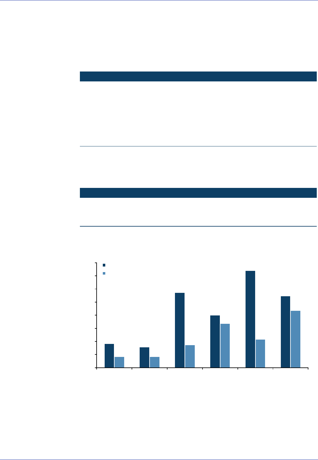
Figure 5: Historical Performance and Risk

10%

12%

14%

16%

1998 1999 2000 2001 2002 2003

TIIS Return

TIIS Ann. Monthly St. Dev

Source: Barclays Capital.

Barclays Capital Global Rates Strategy 19

Figure 6: Risk and Return vs US Treasuries and Equities

-2

-1

1998 1999 2000 2001 2002 2003

Equity Return/Risk

IL Return/Risk

Conventionals Return/Risk

Source: Barclays Capital.

20 Global Rates Strategy Barclays Capital

Mike Oman

The first Index-Linked Gilt, the 2% Sep 1996, was auctioned by the UK Treasury on 27

March 1981, and launched the modern linker market as we see it today. Since that first

auction for £1bn in face value, a constant commitment to the asset class from both the

Treasury and the investor base has seen the market grow to a current £85bn by market

capitalisation and £39bn in face value, representing 25% of the total gilt market. 15

bonds in total have been issued, with 10 bonds (colloquially referred to as “stocks”)

currently outstanding on the real yield curve. Maturities are relatively evenly spaced

from 2004 to 2035.

The creation of a linker market was formally recommended by the “Committee to

Review the Functioning of Financial Institutions (1977-80)” (known as the Wilson

Committee, after its Chair Sir Harold Wilson); however, indexation of debt was not a

new idea in the UK – the UK Government’s National Savings department had been

issuing inflation-linked savings certificates for retail investors since 1975, and Keynes

recommended the move as early as 1924.

The erosion of asset values by inflation was a significant risk faced by investors at the

time of the first auction. In the 10 years prior, annual RPI (Retail Price Index), the index

to which all UK linkers are linked, had reached as high as 26% and as low as 6%,

creating considerable uncertainty as to the future purchasing power of savings. The risk

premium built into conventional gilt yields was also high in order to reflect this degree

of uncertainty making government borrowing costs historically high. In the same way

that inflation protection had been designed to encourage participation in the National

Savings Scheme it was wisely argued that linking gilts to RPI would attract disaffected

investors. At a time of tepid nominal economic growth when most assets had returned

less than inflation, the guaranteed positive “real” 2% coupon offered by the Sep ’96 was

appealing, and particularly so to the actuarial community, which at the time must have

doubted the ability of competing assets to provide the real return required to meet

pension liabilities. Indeed, for the first year, investment in this asset class was restricted

to pension funds.

Of course it could not have been known that three years before the maturity of the

second UK linker, issued also in 1981 as a 25 yr bond, there would be more concern

over deflation than inflation, and so it is wrong to view the Treasury’s move as

opportunistic; however, if there was any difference of opinion between issuer and

investor as to the likely success of efforts to curb inflation, it was certainly the Treasury

that made best use of the “credibility gap”. The first linkers were issued at a breakeven

spread of around 9% RPI, an expected inflation accrual cost considerably higher than

has been realised; within two years of the inception of the market, RPI dropped below

5%, and with the exception of the late 80s boom and oil price shock, has remained

below 5% to date.

Issuance of indexed debt contributes to the credibility of a government’s anti-

inflationary rhetoric, as the incentive to debase the real value of the outstanding debt is

diminished. However, the handing over of monetary policy to an independent Monetary

Policy Committee in 1997, with an explicit inflation target of 2.5% RPIX (RPI excluding

mortgage payments) is the overriding explanation for the low level of UK breakevens

and RPI since the mid to late nineties. Given that the early attraction of linkers was

borne out of the worry over high and unstable inflation, a period of low and relatively

stable inflation might be expected to bring a significant reduction in demand for the

product. This has not been the case. The market continues to grow at a strong pace,

Barclays Capital Global Rates Strategy 21

with the linker market now representing around 25% of all overall gilts, and liquidity is

improving at accelerating pace as Figure 7 illustrates. Pension fund buying has been

instrumental to the continued demand for UK linkers, and particularly at the long-end

as it is the asset that most accurately matches the real liability to be met, a point that

will be discussed further later on.

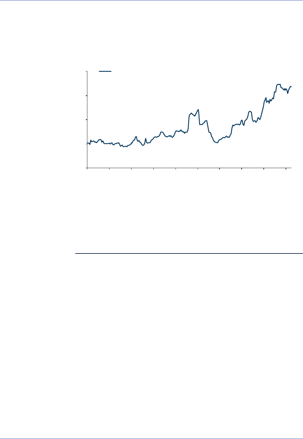
Figure 7: Market Liquidity is Improving Rapidly

Apr 99 Oct 99 Apr 00 Oct 00 Apr 01 Oct 01 Apr 02 Oct 02 Apr 03 Oct 03

13 week ma turnover £bn

Source: Barclays Capital.

Lastly, no introduction to the UK linker market would be complete without a mention of

the one-off innovation of an index-linked convertible gilt, nicknamed the “Maggie Mays”.

The 2% Index-Linked 1999 was convertible into a nominal bond (10.25% 1999) at three

future conversion dates. At a time when inflation remained volatile, and with the term to

option expiry spanning a general election whose outcome was uncertain, seldom has so

much optionality been sold so cheaply. The bonds were all (or almost all) converted.

The Choice of Linking Index

Index-linked gilts are linked to the “Retail Prices Index (All Items)”, or RPI, with an

eight-month lag. The inflation rate calculated from this index is often described as

“headline” inflation, as a short-form name distinguishing it from the so-called

“underlying” measure RPIX, which excludes mortgage interest payments and was until

very recently the Monetary Policy Committee’s inflation target.

In the UK, and elsewhere, a host of different indices were considered, including wages

(the average earnings series) and the GDP deflator. Wage indexation was appealing for

practical reasons, because defined benefit pensions are linked to salaries, and for “social

inclusivity” reasons. It was thought socially desirable for retirees to share in the real

income growth enjoyed by those in work, rather than see real income divergence

between workers and pensioners as time passes.

The GDP deflator’s attraction stems from it being perhaps the broadest possible

measure of inflation, but the appeal of this is eclipsed by its shortcomings. A linking

index needs to be transparent, widely and easily understood, robust, timely and not

prone to revision. Here, the GDP deflator falls down on most counts and problems also

emerge with using wage and salary indices. RPI or CPI measures become the obvious

choices. RPI was seen to be the preferred representation of consumer price inflation

and remains the appropriate choice because pensions in payment liabilities are linked

22 Global Rates Strategy Barclays Capital

RPI

to LPI, a capped and floored RPI series, giving RPI the edge over CPI in terms of

minimising the basis between the asset and the liabilities of the principal sources of

demand, pension and life assurance companies. We discuss this in more detail in the

important issues sections.

In the UK, RPI raw data is collected in the middle of each month, with the new index for

that month published in the middle of the following month. Weights are recalculated

annually, with re-weighting done in January.

For a full description of the RPI, see the National Statistics publication “The Retail Price

Index Technical Manual. 1998 edition”.

www.statistics.gov.uk/downloads/theme_economy/RPI_TECHNICAL_MANUAL.pdf

How Do They Work?

As with many things in life, once shown the easy way to do something one wonders why

it was ever done differently before. UK linkers are a good example of such a situation, as

their construction would seem unintuitive and unnecessarily awkward having

experienced the Canadian model that most other linker markets have sensibly adopted.

Instead of trading in real space, with settlement amounts uplifted or downsized to reflect

and compensate for the inflation experienced in the meantime (the Canadian model), UK

linkers trade in clean price cash terms (not real) with the traded price incorporating

inflation accretion. In a positive inflation environment, such as we have had since the

beginning of the market, the clean price will therefore tend to drift higher. The oldest

linker still outstanding, the IL 06 currently trades at more than £260 per £100 face value,

and is little changed in terms of yield from when it was issued in 1981.

To trade in nominal space, it is necessary to know the inflated value of the next coupon

to allow for accrued interest to be calculated, and as a result indexation has to be done

with an eight-month lag (a coupon’s cash value will need to be known six months

before it is due, and it will take some time to gather and publish the price information

for the final month). Accrued interest is then calculated in the usual way for gilts.

For example, the eight-month lag means that the principal value of the 2% IL 2006,

issued in July 1981 and redeeming in July 2006, will actually be uplifted by the

percentage increase in the RPI between November 1980 and November 2005. Investors

should note that the RPI was re-based in January 1987 from 394.5 to 100. So investors

“lose” the inflation for the last eight months of a bonds life, but “gain” the inflation for

the eight months prior to the bonds issue. This term mismatch is not a particularly big

problem in the relatively stable inflation era we enjoy, but the history shows that the

impact has at times had a large bearing on the return that was realised.

The cash value of semi-annual coupons are calculated as follows:

Coupon paid =

Where:

C = is the quoted annual coupon

RPIt = is the RPI for month t

m = is the payment month

Barclays Capital Global Rates Strategy 23

i = is issue month

The coupon arrived at, now in money terms, is truncated to two decimal places for the

two oldest existing linkers (2006 and 2011), and truncated to four decimal places for all

others bar one. The exception is the new 2035 issue, which uses natural rounding to 6

decimal places. Accrued interest is calculated on the money value (not real value) of the

coupon to be paid on an actual/actual basis.

Similarly, the cash value of the redemption amount is:

Redemption value =

Where: r is the redemption month

Unlike some other linker markets, there is no minimum redemption floor of 100 in the

event of deflation over the entire life of a bond.

Yield Calculations

To derive yield metrics from a nominal price, it is necessary to know all of the cash

flows that are owed; however, clearly in the case of a UK linker (given that the RPIs that

define the coupon payments beyond the next one are not yet known), the cash flows

are also uncertain, preventing a nominal yield calculation. The market circumvents this

problem by convention and assumptions that may seem a little strange to the

newcomer. To arrive at what is termed a “gross redemption yield” (GRY), or “money

yield”, it is assumed that RPI grows at an assumed rate beyond the last known value,

and the convention for that assumption is currently an annual 3%. An unknown RPI for

month t is given by:

Equation 1

1)1( fRPIRPI tt +=

where f is the RPI assumption. Coupon payments and the redemption value are mapped

out according to this RPI assumption and then an internal rate of return, the money

yield, can be calculated for any given dirty price. Once a money yield figure is found,

the assumption is removed to give the “real yield” according to the following

calculation, which is the convention:

Equation 2

()

æ+

where real yield is g, money yield is y and the inflation assumption is f.

The linker market and the conventional market are, of course, competing assets, and

the relative pricing in theory should depend upon the outlook for RPI. Effectively, what

the market does is price the assumed nominal cash flows so that the money yield that

they would generate is:

100

RPI

24 Global Rates Strategy Barclays Capital

Equation 3

()

beiNYy -+= 03.0

where NY is the comparable conventional gilt yield and bei is the market’s assessment

of the appropriate breakeven inflation rate. This only loosely holds, for reasons to be

explained below, but it may help the intuition behind the way the market is priced. So if

exactly zero inflation was expected, a projected set of cash flows that is built on the

assumption of 3% inflation will have to be priced such that the yield they would

generate is 3% above that of the conventional gilt for the two markets to be at fair

relative value from an inflation expectations perspective. If it was expected that 3%

inflation would on average prevail for the life of a linker, a projected set of cash flows

that assumes that rate will have to be priced such that their money yield is equal to the

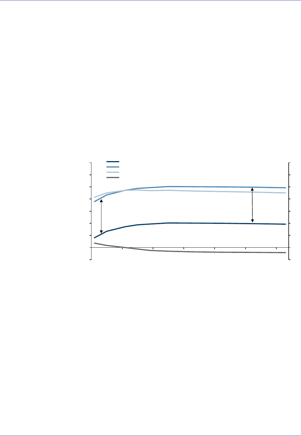
nominal yield of the conventional. Figure 8 shows the curves in December 2003, and

demonstrates this simple relationship, the breakeven on the IL09 very close to 3%, and

the point at which the money yield and gilt curve have no spread.

Figure 8: The Relationship Between Money Yield, Gilt Yield, Breakevens

and the Assumption

-1

2004 2009 2014 2019 2024 2029 2034

-1

Real Curve

Money Yield Curve

Gilt Curve

Breakeven minus inflation assumption

Source: Barclays Capital.

The calculation process is a little clunky, and has an influence on the real yield number

in its own right, and unfortunately in a variable fashion. As discussed, the inflation

assumption takes a bearing on all cash flows except the first (which is known), but then,

according to Equation 2 in the Yield Calculation section, 3% is removed from the overall

money yield, or in effect removed from all the cash flows, including the first. If the

inflation rate of the six months of RPIs that define the inflation accrual of the first

coupon is commensurate to 3% annualised, there is no problem, because the inflation

rate put into the nominal cash flows of the money yield calculation is exactly that which

is taken out, leaving just the unbiased real yield. This is not often the case, although

recently RPI has been running at close to 3%, making it more likely. If the inflation rate

for the next coupon accrual is much lower than the assumption, too much yield is

stripped out by the equation than is justified, and the number produced understates the

real yield, and of course vice versa. If the real yield is understated, the breakeven is

overstated. This is an important point to note when comparing the relative value of

linkers to fundamentals and to other markets where the breakeven rates do not have

this variable distortion.

Barclays Capital Global Rates Strategy 25

The extent of the distortion is determined by the degree to which known inflation in the

last eight months differs from the assumption, the absolute level of real yields, and by

the maturity of the bond considered. It will be greater for shorter bonds as the eight

months for which the yield is over- or understated represents a greater portion of cash

flows than for longer maturities. The choice of assumption is therefore very important

as Figure 9 demonstrates. The current convention of 3% is fairly appropriate for our

expectations for RPI, limiting the likely distortion. Prior to 1998, there was not really a

convention as such, but the Bank of England used to compute real yields for its own

analytics based on a 5% inflation assumption (although a secondary series based on a

10% inflation assumption was also computed). To solve the problem as to how to

calculate settlement proceeds in the unusual event that market participants conducted

trades on a yield basis, formulae were put together. These arrangements imposed a

formal adoption of 3% as the assumption, agreed by the GEMMs.

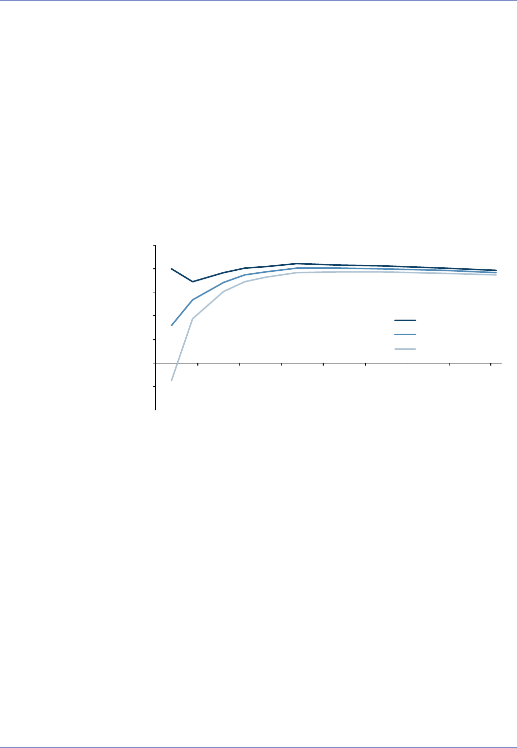
Figure 9: The Real Yield Curve on 15 Dec 03 with Various Inflation

Assumptions

-1.0

-0.5

0.0

0.5

1.0

1.5

2.0

2.5

2003 2007 2011 2015 2019 2023 2027 2031 2035

With 1% RPI assumption

With 3% RPI assumption

With 5% RPI assumption

Source: Barclays Capital.

Furthermore, an RPI release will cause the real yield curve to shift, all other things being

equal, as the RPI level from which the 3% assumption is applied thereafter will have

shifted (unless the change to the index is at an annualised rate of 3%, or 0.247% in that

month, which would leave the RPI schedule unchanged, but is very unlikely), which of

course means that the money yield for the given price will be different, and so will the

real yield. Real yield time series will therefore have monthly discontinuities, a factor that

must be borne in mind when trying to analyse yield histories.

The conclusion is that the calculation methodologies and conventions of UK linkers are

not ideal, to say the least, from the perspective of analysis of relative or absolute value.

However, there is no perfect solution because indexation will always have to be done

with a lag. The Canadian model is affected adversely by the lag too, but the problem is

somewhat hidden and emerges in a slightly different form. Newly published CPI data is

only incorporated in the price of the bond with a delay, which encourages a focus on

“good carry months”, when index increases are large, and “bad carry months”, when

they are small or negative. Roughly speaking, at the start of good carry months, “true”

real yields are effectively understated – there is known favourable future price

information that isn’t captured by the yield. And the degree of understatement will

increase for shorter-dated maturities.

26 Global Rates Strategy Barclays Capital

DMO’s Real Yield Formula

The Debt Management Office’s “Formulae for calculating gilt prices from yields”, 15 January

2002 update, gives a closed solution real yield formula. The yield formula, expressed

algebraically, is daunting. For practical purposes, it is often much less cumbersome to

calculate these yields numerically on a spreadsheet, rather than algebraically.

The real yield formula below covers bonds with two or more remaining cash flows.

The term “quasi-coupon date”, in the notes that follow the formula, means the

theoretical cash flow dates determined by the redemption date – they are quasi dates

because weekends and holidays may mean the true payment dates differ.

Any errors of duplication are ours and we have also trimmed and altered the wording of the

explanatory notes. Readers should refer to the above official publication to see complete

details, including the treatment of linkers with less than two cash flows remaining.

nwauuww

acw

uwddP

é-

++= 100)()1(

)1(2

)( 1

21 , for 1³n

Where:

P = The “dirty” price (ie, including accrued) per £100 face.

d1 = Cash flow due on the next quasi-coupon date per £100 face (may be zero in the case

of a long first coupon period or in the case of settlement in the ex-dividend period;

or may be greater or less than c/2 during long or short first coupon periods).

d2 = Cash flow due on the next but one quasi-coupon date per £100 face (may be

greater or less than c/2 times the RPI Ratio during long first coupon periods).

c = (Real) coupon per £100 face.

r = No. days from settlement date to next quasi-coupon date.

s = No. days in coupon run containing settlement date.

g = Semi-annual real yield.

w =

f = Assumed inflation rate (3% is the current convention).

n = No. of coupon periods from next quasi-coupon date to redemption.

RPIB = The Base RPI for the bond - that for the month eight months prior to issue

date.

RPIL = Latest published RPI

k = No. of months from the month whose RPI determines the next coupon to the

month of the latest RPI

a =

03.1

1÷

RPIB

RPIL

Barclays Capital Global Rates Strategy 27

Market Conventions and Practice

In 1988, auctions were replaced by taps (ad hoc sales of small amounts) for primary

issuance of linkers, reverting to auctions in November 1998. Auctions are single-price,

rather than the multiple-price auctions used for nominal gilts, and have been smaller in

size than for nominals. The approach has been to repeatedly re-open existing linker

issues at each auction – the 2% 2035 issue was the first new bond for 10 years.

In 1998, the DMO removed the obligation for all gilt-edged market makers (GEMMs) to

make prices in linkers, introducing a smaller grouping of index-linked market makers

(IG GEMMs). The framework under which the DMO interacts with the market is quite

involved, so readers should refer to the latest version of “Official Operations in the Gilt-

Edged Market” on the DMO’s website for a full understanding. The pertinent elements

to look at for linkers include auction methodology, circumstances when the DMO might

consider using taps and linker switch auctions (and how they would work), the DMO’s

“Shop Window” facility, and so on.

The repo market in linkers co-exists alongside an old-style stock-lending system. Issues

seldom stray far from general collateral rates. Index-linked gilts are not strippable, and

there is no index-linked futures contract. There is a sterling inflation derivatives market,

which is discussed in the derivatives section of this guide.

Government funding plans are laid out annually in a “Gilt Remit” within the Treasury’s

“Debt and Reserves Management Report”. This generally coincides with the Budget,

just ahead of the beginning of the new fiscal year in April. The remit contains an

estimate of the total size of linker sales, by market value, to be carried out in the new

fiscal year. In recent years, this has been subject to a minimum of £2.5bn, which will

remain in place until further notice. We are also told planned auction dates, and are

often given guidance as to how plans might be altered in the event of changes to the

health of public finances. Formal remit revisions can happen at any time, but two key

times are, firstly, early in the new fiscal year once the prior year’s finances are known,

and secondly, when the Autumn Pre-Budget Statement is announced.

The DMO has (twice) consulted on the possibility of adopting the Canadian model for

future new issues of index-linked gilts. Opinion was divided in the latest consultation

round, and the authorities felt there was insufficient support to justify the change.

Taxation

What we outline here is our general understanding of UK tax principles as they apply to

index-linked bonds. It should not be construed as tax advice, which we do not give. It

may be incorrect, or out of date, and it is certainly an incomplete synopsis. No action

should be taken without proper advice from a qualified tax expert.

For index-linked gilts, institutional investors that are taxed are treated in the following

way. An inflation tax relief is granted based on the inflation experienced between tax

year-ends. This relief is deducted from the total return (calculated on a mark-to-market

basis or an accrual basis, according to the an election made by the investor), and the

difference is taxed. This means that index-linked enjoy a material tax advantage over

nominal gilts – the intent and effect is that investors are only taxed on their real return,

not on inflation compensation.

This is essentially, but not precisely, the same as saying that the inflation increase in

principal is not taxable. There are two reasons why it is not the same. Firstly, if an

28 Global Rates Strategy Barclays Capital

investor tax year-end is, say, December, the relief will be based on the RPI change from

December to December, without a lag, whereas indexation occurs with an eight-month

lag. Secondly, The starting value at the beginning of any tax year is unlikely to be

exactly indexed par.

This tax treatment covers most taxed investors, but there are exceptions. It is also

worth saying that most index-linked gilts are held by pension funds, or within the

pension business lines of life assurance companies, which do not pay tax, so this is not

relevant for them. This also means that tax is not a material influence on the market.

Corporate index-linked do not enjoy this inflation relief. The inflation uplift is taxable –

ie, no inflation credit is applied. However, certain issuers might be able to obtain an

exemption from this tax. The UK's Inland Revenue decided that since corporate issuers

are allowed to offset the inflation uplift against taxable income, in the year that it

accretes, then corporate linker investors should not receive inflation relief. As we have

said, this is not an issue for pension funds who are the main holders.

Private individuals who hold UK index-linked gilts only pay tax on income accrued over the

course of the financial year, so they do get all gains – inflation-linked or otherwise – tax

free. This also means that losses, in the event of a falling RPI, are not allowable against tax.

Important Issues 1 – Institutional Investment

The sterling securities markets are dominated by long-term institutional investors,

namely pension funds and life assurance companies. The latest balance sheet numbers

for mid-2003 suggest that of the £85bn index-linked outstanding by market value, life

companies held £23.8bn and pension funds held £51.7bn. Collectively, those two sets of

institutions hold almost 90% of the linker market, a fairly typical proportion for the last

five years of data. We would suspect that private holders’ interest – for tax-efficiency

reasons – is shorter on the curve, so the institutional holdings of Over 5 yr linkers is

proportionally higher still. We would also suggest that life company holdings are in

effect pensions assets, matching real annuity obligations and pension fund obligations

that have been “bought-out”

Barclays Capital has written at length about pension fund investment and regulation. For

a good overview, we would direct interest to our last two annual Equity Gilt Studies. The

majority of UK private pension liabilities are still of a defined benefit, or final salary, type.

There are three broad classes of pensions liability: active (those in work and contributing

to a scheme), deferred (those no longer contributing but not yet retired), and pensioners.

Active liabilities rise with salaries, while, under the Pensions Act 1995, deferred and

pensions-in-payment liabilities must rise by something called the Limited Price Index

(LPI), or RPI with a 5% cap and a 0% floor. These schemes are very mature, with the

majority of liabilities now LPI-linked, so the appropriateness of index-linked becomes

obvious, and there is a growing non-government market in LPI bonds and swaps. The

Government's White Paper, Action on Occupational Pensions, published in June 2003,

announced that pension rights accrued from 6 April 2005 in an occupational pension

scheme will have to increase once in payment annually in line with the RPI up to 2.5%

rather than the 5% cap that currently applies to pension rights accrued since April 1997.

In the same White Paper it was confirmed that the MFR (Minimum Funding

Requirement) rules for defined benefit pensions were to be replaced by a scheme-

specific approach. The MFR was not short of critics, with it accused of inflexibility, and

adversely affecting investment decisions, encouraging schemes to invest in only a

narrow range of asset types irrespective of specific circumstances such that investment

Barclays Capital Global Rates Strategy 29

value was lost. It served to ensure that gilts, including linkers were in strong demand

particularly in the long-end and so its replacement is not seen as a positive for the

market; however, it does not alter the essential nature of the liabilities, which are

inflation-linked. The new accounting framework, FRS17, and the past few years of

market experience, also highlight the risks UK pension funds have been running by

holding very high equity weightings against very mature liabilities. Also, as more

defined benefit schemes mature, the need for UK pension funds to migrate to greater

bond weightings (particularly index-linked) seems inescapable.

Important Issues 2 – Index Issues

The wordings of different linker prospectuses differ, but essentially all issues, save for

the newest 2035 bond, enjoy “comfort language”, giving some protection against

adverse RPI measurement changes. In the event of changes to the coverage or

calculation of the RPI, which the Bank of England (acting as “index trustee”) deem

“materially detrimental”, then investors will be given the right to sell bonds back to the

government at indexed par (par, adjusted for inflation), although that is not of great

comfort at present as all stocks under this protection are trading above indexed par. For

UKTI2 1/35 (issued 11 July 2002) and any subsequent new issues that fall under the

DMO’s regime, the choice of index it is at the Chancellor’s discretion (with the proviso

that there is consultation with a body with “recognised expertise in the construction of

price indices”), a choice which will be “conclusive and binding”.

This is always a concern, having seen the US Bureau of Labor Statistics make

methodological changes that materially reduce reported inflation, and given the

knowledge that UK RPI inflation is materially higher than UK CPI (formerly referred to as

HICP) inflation. The Office of National Statistics is undergoing a “Three Year Research

Programme on RPI Methodology”, which has already made an impact albeit small. In

October 2003, it was announced that the personal computer series of RPI would be

subject to “hedonic pricing adjustment for quality changes”, in a similar fashion to

many of the series in US CPI. The ONS estimate that this will reduce RPI by 0.05% per

year, is small but illustrative of the changes that can be made to the detriment of linker

returns. Now that UK CPI is the focus of monetary policy, it is possible that there will be

less pressure to tweak the RPI construction methodology, most likely in ways such as

described above that will reduce the rate, as its public usage has been reduced, but

there are no guarantees.

There was never a serious worry that the move to CPI for monetary policy would be

accompanied by a sudden change in the basis for linkers to the same measure, as it simply

would not be tolerated. This would leave investors holding an asset that accretes at a

systematically lower rate, and the Treasury understands the need to act in good faith

towards holders of a quarter of its outstanding marketable debt. In December 2003, the

DMO stated that it was unlikely to recommend that new bonds have a CPI basis as the

investor base (pension funds and insurance funds) have most of their liabilities linked to

RPI, and hence the demand for CPI basis would not be as strong and offer less value to the

Treasury from a funding cost perspective. Maybe so, for now, but there is of course the

possibility that the liabilities of the investor base may at some stage adopt a CPI basis

instead, although this has been downplayed. Such a migration would reduce the value of

pension entitlements for members and in an instant dramatically cut the deficit of the

private pensions system, which would free up balance sheet capital, enabling greater

investment and growth. The monetary policy switch might be seen as a convenient

justification for this, and if it were to happen it would suddenly be in the interests of the

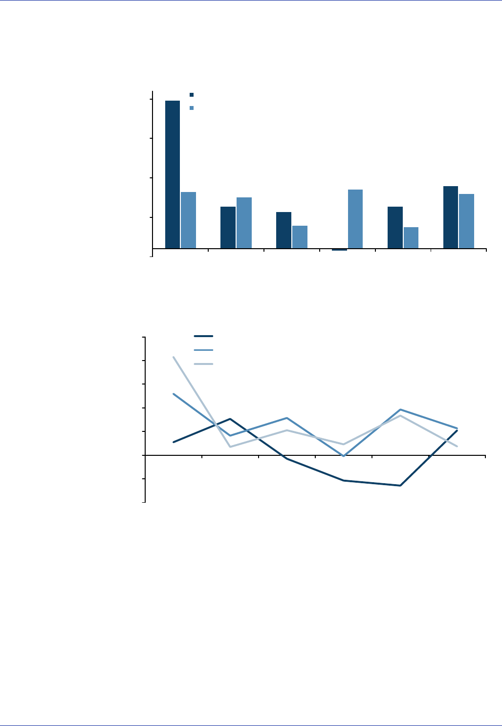
30 Global Rates Strategy Barclays Capital

Treasury to issue linkers with a CPI basis. These developments, if they happen at all, are

most probably many years away, so not an immediate concern, but it is important to keep

one eye on developments in the pensions sector.

Figure 10: Historical Performance and Risk

-1%

14%

19%

1998 1999 2000 2001 2002 2003

UKIL Return

UKIL Ann. Monthly St. Dev

Source: Barclays Capital.

Figure 11: Risk and Return vs UK Nominals and Equities

-2

-1

1998 1999 2000 2001 2002 2003

Equity Return/Risk

IL Return/Risk

Conventionals Return/Risk

Source: Barclays Capital.

Barclays Capital Global Rates Strategy 31

France

Alan James

France first announced its intention to issue inflation-linked bonds on 3 December

1997. The legislation to enable the launch of the new asset class was passed on 3 July

1998. On 15 September 1998 the 3% OATi Jul 2009 was syndicated. Subsequently, this

bond has been reopened at auction on more than a dozen occasions and remains an

on-the-run issue. The market was widely consulted on the main characteristics of the

new bond, including the choice of inflation index to which it would be linked. It was

decided that the bonds would adopt the Canadian methodology that was fast becoming

the preferred global structure, but including a principal floor as the US had done. The

inflation index was agreed as INSEE’s official measure of French national CPI, excluding

tobacco. The CPI section below discusses this decision in more detail. The timing of the

first issue just ahead of the start of the euro area was not coincidence. This monetary

union was expected to intensify competition for financing in nominal bonds, and the

hope was that France would gain a first-mover advantage by being the first euro area

country to issue inflation-linked bonds.

A second linker, the 3.4% OATi Jul 2029, was launched a year later in September 1999,

again linked to French national CPI ex-tobacco. The same issuance route was followed,

with an initial syndication and occasional reopenings. Growth in the outstanding market

value of these two bonds was slow but steady. There was some disappointment that the

instruments did not seem to be capturing the imagination of investors in eurozone

countries outside of France. In October 2001, France addressed this issue head-on by

launching the 3% OAT¤i Jul 2012. This new issue was linked to the non-seasonally-

adjusted Euro Area Harmonised Index of Consumer Prices (HICP), excluding tobacco.

Again this bond was launched via syndication, but with its size boosted by some direct

exchanges out of the OATi09. There were some fears ahead of this issue that the launch

of a second inflation-linked product may harm the liquidity of existing OATi bonds, but in

fact the move gave a new lease of life to the sector as a whole. Not only did turnover in

the new issue quickly grow but interest in the existing issues was heightened too.

France has responded to an increase in interest and demand in the sector with a

significant increase in the pace of supply. It has issued new bonds each year while

auctioning existing issues with increasing frequency. The OAT¤i Jul 2032 was

syndicated in 2002, including some exchanges out of the OATi29. The OATi Jul 2013

was the first issue to be launched via auction in 2003. Demand growth in 2003 was so

rapid that despite frequent reopenings, this new issue was relatively hard to find, and

traded close to zero in repo for several months, even after more of the bond was

created specifically for lending. Interest in French CPI-linked bonds was further boosted

by the decision to partially link “Livret A” public savings rates to inflation from August

2004. The Agence France Trésor (AFT) decided to revert to a syndication method to

launch its new OAT¤i Jul 2020 at the start of 2004.

The Linking Indices for OATi and OAT¤i Issues

There was considerable debate ahead of the initial launch of French inflation-linked

bonds as to whether to link the first issue to French inflation or to that of the then

forthcoming euro area. The arguments for the domestic index included the likelihood

that national inflation would be a better liability match for the government. However,

international appeal would clearly be broader for a euro index. In 1998, the final

decision almost certainly came down to practicalities. At the time, the disadvantages of

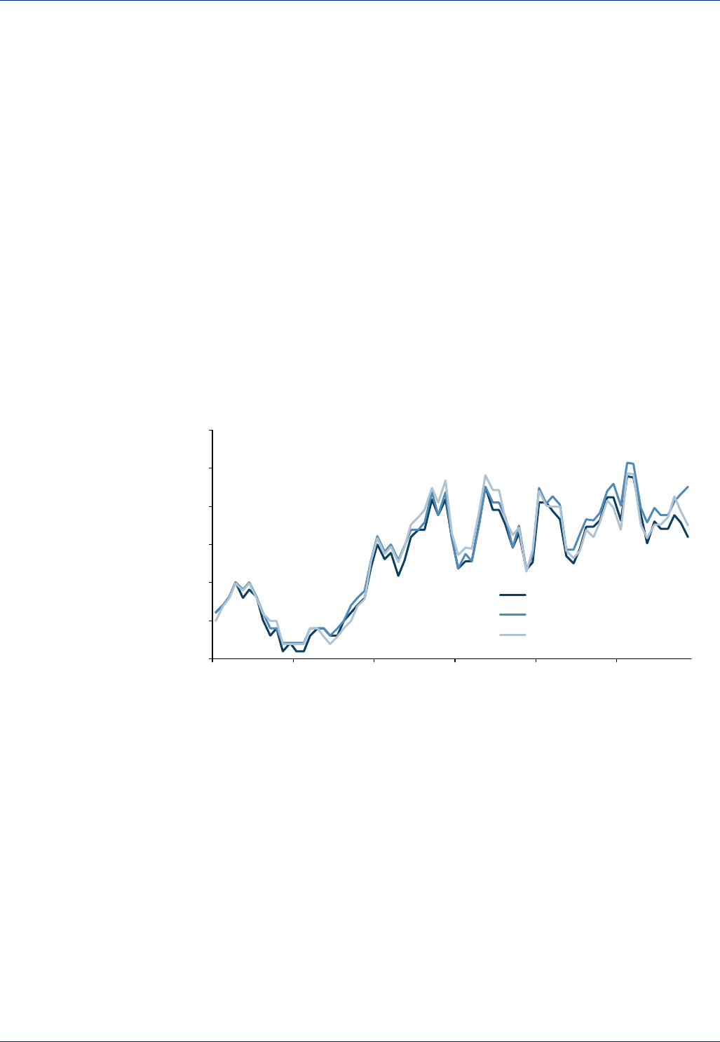
32 Global Rates Strategy Barclays Capital

Eurostat’s European Harmonised Index of Consumer Prices for the EMU area were

material as it was a relatively new, untested index with no track record. Full index

coverage was not yet complete in some countries and this left an index in flux and an

associated fear of revision risk.

The hope when the first OATi was launched was that French inflation would be

regarded as a good proxy for European inflation, particularly in the longer term, and

this would encourage strong demand from other euro area countries. After all, in this

sense, what is important is the long-term correlation of inflation rates – it is not

necessary for the inflation levels to be the same for these bonds to be appropriate

hedging instruments. Tobacco’s exclusion was a legal matter. More substantive and

difficult legislation would have had to be introduced to change it, as all other

government contractual arrangements in France with an inflation element (minimum

wages, social benefits, etc) use the ex-tobacco series. The series used is the final non

seasonally-adjusted CPI ex-tobacco index, which is usually released around the 22nd of

each month. The unrevised index is used, though if the series is rebased all reference

calculations are adjusted accordingly. Note that INSEE does issue a preliminary inflation

series earlier in the month, but this is merely a useful guide: the official index is only

released with the final monthly CPI readings.

Figure 12: French Inflation

0.0

0.5

1.0

1.5

2.0

2.5

3.0

Jan 98 Jan 99 Jan 00 Jan 01 Jan 02 Jan 03

French CPI ex-tobacco

French CPI

French HICP ex-tobacco

Source: AFT, Thomson Financial.

Eurostat’s HICP ex-tobacco for the euro-area (HICPx) is now a relatively well-

established index, which has left most of its early teething problems behind. ¤i bonds

accrue inflation based on the first release of the euro HICPx, not counting any

subsequent revisions. Due to the euro HICPx series being made up of the indices from

(currently) 12 different countries it is liable to more frequent revisions than that in the

French series. In particular, every five years Germany consistently revises its inflation

series when it rebases them. These revisions usually restate inflation estimates upwards,

biasing down slightly the accrual actually paid. The monthly data is usually released just

after mid-month, except in February when re-weightings of individual country data for

the January indices delay release until close to month end. A guide for the forthcoming

monthly data comes from the flash estimate of headline inflation (there is no estimate

for HICPx), which comes at the turn of each month after Germany and Italy have

released provisional inflation estimates.

Barclays Capital Global Rates Strategy 33

Figure 13: Euro Inflation

0.0

0.5

1.0

1.5

2.0

2.5

3.0

3.5

Jan 98 Jan 99 Jan 00 Jan 01 Jan 02 Jan 03

HICPx revised

HICPx unrevised

HICP

Source: AFT, Thomson Financial.

Consumption levels of the different euro area countries are used to weight the index. As

new countries enter the monetary union they are included in the price index calculations.

New entrants to the euro area from the relatively high price level countries of Northern

Europe would potentially have a slight depressing effect on euro HICPx. On the other

hand, if poorer EU accession countries were to join, this would tend to bias the price index

higher, even though the weights for these countries would not be that large.

The calculation methods for the French CPI ex-tobacco and euro HICPx calculations are

relatively similar. Both use geometric aggregation at the lowest strata sub-indices, and

have long been innovative in the use of hedonic techniques for quality adjustments. It is

generally felt that any inflation ‘overstatement’ in either French or euro HICPx inflation

is very limited, so there would appear to be little or no threat of inflation being shaved

by purely methodological changes. See later in this publication for more discussion of

trends between different inflation indices, and particularly between French CPI ex-

tobacco and euro HICPx.

Calculations

The quoted prices of inflation-linked bonds are in real terms. Settlement values and

cash flows then adjust for accrued inflation using the following process (identical to

that laid out previously for the US, except coupons are paid annually):

Each day has its own distinct Reference Index. The first day of each month has a

Reference Index equal to the price index of three calendar months earlier, eg, that for 1

February 2004 is the price index for November 2003 and that for 1 March 2004 is the

price index for December 2003. Reference Indices for intervening days are calculated by

straight-line interpolation on a standard Actual/Actual accrual rate. For example on 8

February 2004 the Reference Index will be 7/29 times the Dec ’03 inflation index plus

22/29 times the Nov ’03 value.

This same process is used to calculate a Reference Index for the first inflation accrual

date of the bond, or “Base Reference Index”. The date for this base is a year before the

first coupon, to ensure a full first coupon. For any given day, whether the settlement

date of a trade or cash flow payment date, the Index Ratio is then calculated by dividing

the Reference Index for that day by the Base Reference Index. For settlement amounts,

34 Global Rates Strategy Barclays Capital

real accrued interest is calculated as for ordinary OATs. Clean price and accrued are

each multiplied by the Index Ratio to arrive at a cash settlement amount. For coupons

paid, the (real) annual coupon rate is multiplied by the Index Ratio, and likewise for the

par redemption amount (with the cash value subject to a par floor).

The AFT publishes all Reference Indices and Reference Index Ratios after new data

becomes available. See the AFT website: http://www.aft.gouv.fr/oat/us/. Depending on

the time of the month compared to when data is released, this will include references to

the end of the current month or the month after. If the price index is rebased then the

Base Reference Index is adjusted accordingly to leave inflation accrual unaffected.

Linkers are taxed in very much the same way as other French government bonds,

ie, the inflation accrual is taxable for domestics while there is no withholding tax

payable for international investors. Retail investors can pay all withholding tax at

maturity or sale. Institutional investors pay tax both on interest received and annually

on inflation as it accrues.

Issuance Patterns

The AFT has steadily increased linker issuance since the product was launched. It is

committed to a minimum of 10% of its total bond issuance to be in inflation-linked bonds

but if demand is sufficient it may issue significantly more than this. ¤16bn was issued in

2003. While 80% of this was in OATi bonds the AFT indicated that is was issuing the new

OAT¤i20 to rebalance supply between the two types of bonds. With regards to further

new bonds the AFT may choose to use either syndication or an auction for the initial

tranche, but subsequent supply has always come via auctions. In previous years, issuance

was somewhat opportunistic, sometimes with several months between auctions or two

auctions in a month if demand was strong. From 2004 there will be supply every month

that nominal bonds are also being auctioned, ie, all but August and November. Previously,

auctions could take place on the same day as any conventional bond auction but the AFT

has stated that due to the greater maturity of the index-linked bond market, auctions will

take place exclusively on the same day as short maturity BTAN conventional bonds, which

is almost always the third Thursday of the month.

Figure 14: Historical Performance and Risk

10%

12%

1999 2000 2001 2002 2003

OATi/¤i Return

OATi/¤i Ann. Monthly St. Dev

Source: Barclays Capital.

Barclays Capital Global Rates Strategy 35

Figure 15: Risk and Return vs French Nominals and Equities

-2

-1

1999 2000 2001 2002 2003

Equity Return/Risk

IL Return/Risk

Conventionals Return/Risk

Source: Barclays Capital.

36 Global Rates Strategy Barclays Capital

Italy

Alan James

Italy announced its intention to issue its first inflation-linked BTP on 5 September 2003

and syndicated a ¤7bn 5 yr bond within just five days. The speed of the ground-

breaking transaction took many in the market by surprise but acceptance of the issue

came quickly, enabling a syndicated reopening in October to bring the bond over

¤10bn. The BTP¤i 1.65% Sep 2008 followed an almost identical model to French OAT¤i

bonds, except that it pays semi-annual coupons as conventional BTP bonds do. The

bond was initially priced using an interpolated spread to the nominal BTP curve, but a

maturity matched conventional bond was auctioned the week after the launch, enabling

straightforward trading of the breakeven inflation spread.

The choice of maturity for the first BTP¤i was determined by heavy domestic retail

demand for inflation-linked notes. The Public Debt Division of the Italian Department of

the Treasury had noted that a considerable amount of swapped 5 yr MTN notes with

inflation-linked coupons had been sold in Italy. It also recognised that without a 5 yr

point on the OAT¤i curve, it was relatively difficult for issuers to hedge their inflation

exposure. Thus, Italy hoped that the bond would be bought for hedging purposes by

those with inflation derivative exposure as well as directly through retail channels. This

is discussed in more detail in the later derivatives and non-government inflation-linked

issuance sections. More than 220 investors bought the initial syndication, with the

majority placed into Italy. Much of the remainder went to the UK and US, a combination

of derivative houses and long established international inflation-linked investors, with

relatively little going to other euro area countries. The reopening syndication redressed

this imbalance, with almost 40% being allocated to French investors.

For 2004, Italy confirmed a commitment to complete the euro real interest rate curve

with issuance at medium and long maturities. It indicated that the liquidity of new

benchmarks will be assured by syndications or auctions. Linker supply is likely to

remain solely in euro inflation-linked bonds, at least in 2004. Coupled with larger

funding needs than France, this leaves Italy as likely to be the heaviest issuer of euro

inflation-linked bonds. On the other hand, with new Italian agency Infrastructure

announcing issuance of Italian inflation-linked bonds, there is a possibility that the

Treasury itself follows suit if demand is seen to be sufficient.

As with a conventional BTP, a BTP¤i pays its coupon every six months but its yield is

quoted on an annual basis. Calculations work in exactly the same way, with inflation

accrual calculated on a daily interpolated basis between the inflation data from three

and two months previously. BTP¤i bonds are eligible to be stripped. The linking index is

the same as for OAT¤i bonds, the Euro Area Harmonised Index of Consumer Prices ex-

tobacco. Italy chose the same index as France mainly for market convenience, as it is

the index most widely used in inflation swaps and MTN bonds as well as OATis.

Domestic Italian indexation has often excluded tobacco in the past though. In

particular, “TFR” severance pay is linked to Italian FOI inflation ex-tobacco (at 1.5% plus

75% of inflation).

BTP¤i bonds follow the same tax rules as conventional BTPs. This means that domestic

entities will be taxed on inflation uplift as well as real returns. International investors are

exempted from paying withholding tax as long as they are within countries that Italy

does not define as tax havens and send in the necessary initial documents that are on

the Treasury website. At the time of writing, countries excluded from the “white list” of

tax exempt countries include Switzerland as well as offshore tax havens, though it is

possible that this will change.

Barclays Capital Global Rates Strategy 37

Sweden

Alan James

The Swedish Government first issued inflation-linked bonds in 1994. According to the

Swedish National Debt Office (SNDO), this was to supply those investors who

demanded a large inflation premium when buying nominal bonds but who were not in

need of the liquidity available in benchmark bonds. Sweden saw that its pension sector

ought to have a significant demand for inflation and that the asset class would create

cheaper funding in the long run for the government and diversify the risk of the

government debt portfolio. It should also be noted that the Swedish krona had devalued

sharply in the year preceding the programme’s inception, raising the value of

outstanding foreign currency debt. Thus, the SNDO needed an alternative source of

funding at a time when inflation expectations were relatively high. Inflation-linked

bonds were arguably the most suitable choice for further borrowing.

The first to be linked to Swedish CPI (non-seasonally adjusted) was a 20-year bond with

a zero-coupon structure (3001, 0% 2014). A selection of the eight Primary Dealers in

the nominal market took responsibility to quote two-way prices for the new bond. The

Debt Office held five common price auctions from April to June 1994, which saw a face

value of SEK16bn being offered to the market. In practice, though, only SEK6.7bn was

allotted in this initial phase, as many in the market held out for higher real yields.

In 1995, the SNDO launched its second inflation-linked bond, another zero but with a

shorter maturity of 10 years (3002, 0% 2004). At this time, the SNDO decided to

replace the common price auctions with multiple price auctions. Moreover, the SNDO

opened a non-competitive facility for small volumes in the auctions, so that small

investors could enter the market. In February 1996, the SNDO launched two new bonds,

a 5-year zero-coupon bond (3003, 0% 2001) and a 12-year coupon bond (3101, 4%

2008). In June 1996, the 24-year coupon bond (3102, 4% 2020) was launched. With the

curve established, the market grew quickly until 1998. Subsequently, growth slowed,

not unexpectedly given that the programme was maturing, so that the SNDO felt less

obliged to pump the market with supply just for the sake of liquidity. Limited funding

needs led to a richening of longer nominal bonds, narrowing spreads to linkers and

leaving further issuance as relatively unattractive for the government, albeit with actual

inflation also falling sharply, the SNDO benefited from their previous issuance. While a

new retail 30-year bond was issued in June 1998, this bond was not fully developed.

In April 1999, the SNDO launched two new linkers, a new 30-year bond (3104, 3.5%

2028) and a 16-year bond (3105, 3.5% 2015). These two bonds were the first to be

issued with an inflation floor, meaning that the new bonds had a similar structure to US

Treasury Inflation-indexed bonds. The format of issuing inflation-linked bonds was

changed, this time back to bid price auctions. The primary dealers were permitted to

switch linkers directly with the SNDO on a daily basis, in order to enhance the liquidity

of the market.

Since 1999, there has been a clear commitment to enhance liquidity into coupon bonds,

with switch auctions away from the older zero-coupon issues. Auctions became

monthly in 2000. In 2002, following a buyback of the 0% 2004 bond, new issuance was

accelerated. Auctions were commonly spread over two days, with up to three bonds

issued per month. To become more responsive to demand, auctions were made variable

in size, with a target minimum size but also a maximum size to which the auction could

be expanded if demand was strong.

38 Global Rates Strategy Barclays Capital

For 2004 issuance frequencies have been increased to twice monthly, to encourage

secondary market liquidity further. The use of flexible auction sizes is likely to be scaled

back given the greater flexibility that fortnightly auctions afford and the perceived

maturing of the global asset class and hence investors. The SNDO continues to target

annual issuance levels of around SEK15bn, but will respond if demand growth continues

as in 2003. The benchmark 2015, 2020 and 2028 bonds will all be eligible for

reopening. While a quarter of Swedish domestic bonds by value are already inflation

linked, this percentage is set to rise further in coming years as Sweden has accepted the

benefits of a large percentage of linkers within their debt profile. The SNDO is also

already addressing how it will run down the 2008 bond as it nears maturity, but

switching into longer issues will not commence before 2005.

The Swedish Consumer Price Index (CPI)

The Swedish Consumer Price Index is compiled monthly and is a good proxy for the

consumption patterns of the entire country. The weights and sample of items are

revised at the beginning of each year. The weights for the major groups are based on

the Swedish National Accounts statistics. The index uses regular prices paid by the

public. Value-Added Tax is included in the prices and subsidies are excluded. The price

collection is done around the middle of the month and the index is published in the

middle of the following month. Prices are collected from a random sample of 600 retail

stores, restaurants, etc.

The Consumer Price Index is chain weighted with yearly links (each link with December

of the preceding year, the weights being revised for each link). The links for the months

January to December are computed with weights based on the value of private

consumption during the preceding year recalculated to December prices of that year.

For the month of December, a revised link, the long-term link, is also calculated. The

weights for this link are based on the value of private consumption during the year,

recalculated to the price level in December of the previous year. The long-term link may

differ from the short-term link due to better information on the price development. The

index number of the Consumer Price Index is calculated for every month, from the two

types of links. The short-term link is chained back, through the long-term link in each

preceding year. This method of re-weighting can lead to significant changes in the CPI

index between December and January releases that do not correspond to price changes

in that period.

Seasonality in Swedish inflation is larger than in most other markets, creating relatively

volatile carry. With the vast majority of electricity in Sweden coming from hydro-

electric power, headline CPI inflation is unusually sensitive to the weather, particularly

very cold winters or extended dry spells. While there is not a long-term structural bias

between CPI and the domestic HICP measure, housing costs are included in CPI but not

HICP (with a 7% weight). This leaves a medium-term bias towards higher CPI than the

standardised European inflation measure in a hiking cycle. The SNDO made clear before

the last euro referendum that there would be no changing of the measurement index

for domestic inflation-linked bonds even if Sweden were to adopt the euro. Monetary

policy of the Swedish Riksbank is based on underlying inflation (UND1X) rather than the

headline CPI measure, to exclude mortgage interest payments and energy prices. A 2%

annual rate is targeted, with symmetrical tolerance of 1%.

Barclays Capital Global Rates Strategy 39

Figure 16: Swedish Inflation

-2.0

-1.0

0.0

1.0

2.0

3.0

4.0

Jan 98 Jan 99 Jan 00 Jan 01 Jan 02 Jan 03

CPI

HICP

UND1X

Source: Thomson Financial.

Calculations

Calculations for Swedish linkers are slightly different to and more complex than the

Canadian model. Bonds are usually quoted in terms of real yields. Unlike countries

following the Canadian model, when prices are quoted they are not expressed in real

terms but include inflation uplift. Inflation accrual is calculated in a very similar way,

though, with a three-month lag between the inflation release and the reference value for

the first of the month. However, day count conventions are different, as there is linear

interpolation but assuming 30-day months. Hence, for a reference day, d of the month is:

d =

[]

()

332

29,1

---

ttt CPICPICPI

dofMinimum

This factor matters for daily valuations but is unimportant for coupon calculations as all

coupon bonds pay on the first of December anyway. Interest also accrues on a

European 30/360 basis. Unlike in other countries, there is not individual base index for

each bond to calculate the inflation uplift ratio. Instead, set base index points are used.

For most of the bonds, the start point was 1 January 1994, while it was 1 January 1999

for the two most recent issues. In practical terms, this meant that bonds were issued

with notable inflation accrual already in their price, but this only matters in real yield

terms if a bond has a deflation floor. Only the two most recent bonds, the SV3104, 3.5%

2028 and the SV3105, 3.5% 2015 have deflation floors on the principal and there was

almost no lag to their deflation base.

For settlement purposes, there are separate rounding conventions for zero coupon and

coupon paying issues. For zero coupon bonds there is no rounding in the calculation,

but the settlement price is rounded to the nearest krona. Coupon bonds are rounded

once, with the clean nominal price (ie, after inflation accrual) rounded to three decimal

places before adding on accrued interest. The settlement price is then rounded to the

nearest krona.

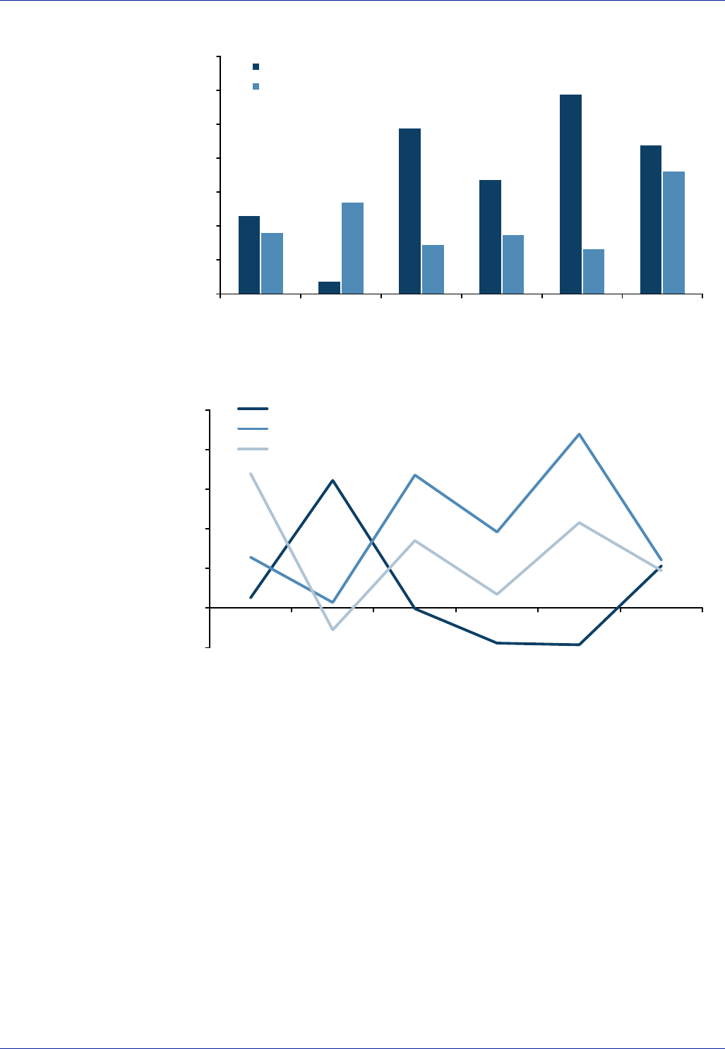
40 Global Rates Strategy Barclays Capital

Figure 17: Historical Performance and Risk

10%

12%

14%

1998 1999 2000 2001 2002 2003

SGIL Return

SGIL Ann. Monthly St. Dev

Source: Barclays Capital.

Figure 18: Risk and Return vs Swedish Nominals and Equities

-1

1998 1999 2000 2001 2002 2003

Equity Return/Risk

IL Return/Risk

Conventionals Return/Risk

Source: Barclays Capital.

Barclays Capital Global Rates Strategy 41

Canada

Gemma Wright, Amita Shrivastava

The Canadian Government issued its first Real Return bond (RRB) in December 1991.

The initial issue, the 4.25% 2021, was a 30-year maturity and is now the shortest RRB

bond on the curve. Thus far, the Treasury has decided to issue new bonds at four year

intervals; the 4.25% 2026 being issued in 1995, the 4% 2031 in 1999 and the 3.0% 2036

in 2003. Given its maturity profile, the Canadian inflation-linked bond market has

largely been in the realm of pension funds, but from time to time international investors

have taken advantage of real yield differentials versus other more heavily traded

international markets such as the UK and US.

The Bank of Canada (BOC) acts on behalf of the Department of Finance for the purpose

of managing the financing programme. The BOC currently operates under a quarterly

funding schedule with one 30-year RRB auction every three months. This is similar to

both the UK and US who also operate under a quarterly funding schedule. Over the past

five years the Canadian Government’s fiscal situation has improved significantly

although a sequence of budget surpluses has had an insignificant impact on the

issuance of inflation-linked bonds. At present the Bank of Canada issues in the region of

C$300mn RRBs every quarter.

The Linking Index

Canadian RRBs are indexed against the Not Seasonally Adjusted All Items Consumer

Price Index. It includes all Canadian families and individuals living in urban or rural

private households. Information on consumer expenditures is gathered through the

Survey of Household Spending and the Food Expenditure Survey, which use random

samples of Canadian households. The index measures price changes using the cost of a

fixed basket of commodities through time. The basket consists of about 600 goods and

services including transportation, clothing, housing, food and recreation. The CPI index

reflects pure price movements only as the basket includes goods and services of

identical or equivalent quantity and quality over time.

The index is weighted to reflect typical spending patterns. The weights are determined

based on family expenditure surveys that are conducted periodically. The current

weights are based on the 2001 survey. As the figure below shows, the index comprises

eight major components. The component with the highest weight is the shelter

component, which includes both owner-occupied and rented accommodation. The CPI

includes consumer items only and excludes personal income taxes, consumer savings

and investments etc. The index uses geometric means at the first-stage aggregation of

collected price data, making quality adjustments where possible. The fixed basket price

index is an arithmetic average of price relatives for all single commodities contained in

the basket. The index attempts to capture innovations in final prices, which include any

changes in the Goods and Services Tax as well as provincial retail sales taxes.

42 Global Rates Strategy Barclays Capital

Figure 19: CPI Weights for Major Components

Clothing and

footwear

5.8%

Houshold

operations and

furnishings

10.7% Alcoholic beverages

and tobacco prodcts

3.2%

Health and Personal

Care

4.5%

Recreation,

education and

reading

12.1%

Shelter

28.5%

Food

16.3%

Transportation

18.8%

Source: Statistics Canada (Reflects 2001 basket at 2001 prices).

The Canadian Model

The Canadian Treasury was an innovator; with a simplified approach to the indexation

of inflation for real return bonds. The change in the indexation process was quite

dramatic with the inflation lag reduced to three months from the eight months used by

the UK. This enabled a more contemporaneous measure of inflation and allowed the

market to trade in real space without an embedded inflation assumption. The crucial

change in structure was the use of an Index Ratio to inflate both principal and coupon

for a given settlement date. This change eliminated the effect of real yields changing

when the inflation index is published. As discussed in the UK section, index-linked gilts

use an inflation assumption to calculate real yields – in 1991 5% and now 3%. UK real

yields vary every time there is an inflation release different from this assumption.

This new methodology became know as the “Canadian model”, and has been generally

followed by all subsequent major issuers. The change in methodology allowed for

simpler valuation and has assisted in the relative value analysis of the product versus

conventional bonds as well cross currency real yields. More recently the concepts of

forward real yields and forward breakevens have become determining factors in the

relative valuation of international markets that have adopted this calculation method.

Calculation Methodology

A reference CPI value is calculated for every day based upon the CPI values for three

months and two months prior to the month containing the settlement date. The

reference CPI for the first of each month is the index value of three months previously.

The reference CPI for any day during the month is calculated by linear interpolation.

Reference CPI for day ‘d’:

()

332

)1(

---

ttt CPICPICPI

d = day of the month eg, 1st implies d=1

m = number of days in that month

The indexation factor is the reference CPI for the settlement date divided by the

reference CPI for the base date. Coupons are accrued on an Actual/Actual basis and

paid semi-annually. The gross settlement price is calculated as follows:

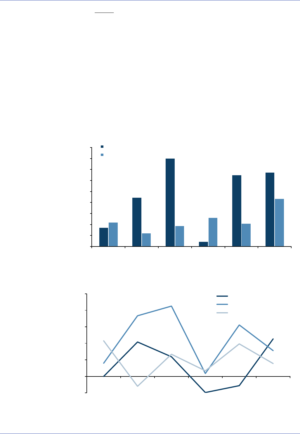
Barclays Capital Global Rates Strategy 43

))((

base

CPI

cp +

p = clean price of the bond

c = real accrued

CPIt = Reference CPI at time t

CPIbase = Base CPI

Real Return bonds are taxable for residents but are not subject to withholding tax for

non-residents. For residents, RRBs’ income received and accrued is taxed in a given year

while the inflation accretion on the principal is also taxed. Capital gains are not taxed

until realised. For non-residents the Canadian Treasury is not ordinarily required to

withhold tax from interest or principal paid on RRBs. However, the Treasury’s website

provides more detail on these conditions http://www.fin.gc.ca/invest/taxtreat-e.html.

Figure 20: Historical Performance and Risk

10%

12%

14%

16%

18%

1998 1999 2000 2001 2002 2003

RRB Return

RRB Ann. Monthly St. Dev

Source: Barclays Capital.

Figure 21: Risk and Return vs Canadian Nominals and Equities

-1

1998 1999 2000 2001 2002 2003

Equity Return/Risk

IL Return/Risk

Conventionals Return/Risk

Source: Barclays Capital.

44 Global Rates Strategy Barclays Capital

Australia

Mike Oman

The Australian Government first issued Capital Indexed Bonds (CIBs) in 1985 and they

currently account for just over 11% of the face value of the Commonwealth Government

debt, with an outstanding face value of A$6.55bn ($4.82bn). The Australian Treasury

announced the suspension of the Treasury Indexed Bond programme with the publication

of the budget on 13 May 2003. This announcement followed a 12-month period of

analysis and market consultation that sought to determine whether the Commonwealth

Government Securities (CGS) market was a viable going concern given the sharp fall in

the Commonwealth Government’s financing requirement in the past years. This may

come as a surprise to those readers whose national governments are wrestling with

deepening budget deficits. The fiscal position of the Australian Government has remained

resilient throughout the latest global economic downturn, generating persistent budget

surpluses. Net debt has fallen from 19.1% of GDP in 1995-96 to an estimated 3.7% of GDP

in 2003-04, and is projected to be zero by the end of 2006. There is already a concern

over the disproportionately large role the banks have within financial markets, and so it

was argued that the CGS market should be maintained. An interest rate market

completely dominated by banks and corporate paper would be vulnerable to economic

shocks, and pose a serious threat to financial stability and the accessibility of refinancing

capital for corporates, so the decision was taken to support government debt liquidity,

and structured in such a way that it supports the 3-year and 10-year Treasury bond

futures contracts. Rather disappointingly, there was not room for a continuation of the

Treasury Indexed Bond Programme.

There are four issues with maturities of 2005, 2010, 2015 and 2020. Each bond has a

real coupon rate of 4% pa, with payments made quarterly. All four CIBs are linked to the

“Weighted Average of Eight Capital Cities: All-Groups Index”, otherwise known as the

Australian CPI. The index is maintained and published by the Australian Bureau of

Statistics on a quarterly basis. Upon any change to the CPI index that is considered

detrimental to the product, the prospectus for CIBs allows for the re-purchase of the

bonds at market prices deemed appropriate by the Treasurer.

The interest on Australian linkers is accrued on an actual/actual basis, while the bonds

are quoted on a yield basis. The coupon payment is determined by the Kt term in the

equation shown below. As is the case with other international linkers, both income and

capital are indexed against inflation. Australian CIBs are similar to UK index-linked in

that the next coupon amount is always known on or before the current coupon

payment date. To quote the prospectus: “The amount of inflation indexation in any

given coupon period is equal to the average percentage change in the Consumer Price

Index over two quarters ending in the quarter which is two quarters prior to that in

which the next interest payment falls”. This basically means that the bonds have a six-

month indexation lag compared to eight months in the UK. Australian linkers trade ex-

dividend for seven days prior to the payment date; the UK, Swedish and South African

markets also have ex-dividend periods. Australian linkers, like other markets, contain an

embedded put at maturity that protects against deflation over the life of the bond.

Unlike other markets that offer an inflation floor, Capital Indexed Bonds protect both

coupon and principal against deflation over the life of the bond (for further details

please refer to Treasury prospectus).

Barclays Capital will continue to include the current stock of Australian Treasury Indexed

Bonds in the Global Inflation-Linked Bond Index. Naturally their share of the index will fall

sharply throughout the period in which the programme remains suspended.

Barclays Capital Global Rates Strategy 45

The Australian CPI

The last review of the Consumer Price Index was completed in September 1998. The

Australian Bureau of Statistics decided that the CPI would be modified from a measure

of the change in living costs of employee households to a general measure of price

inflation for the household sector. As a result, the population covered was expanded

from wage and salary earner households to include all metropolitan households.

Weights were revised to reflect new expenditure patterns and the expanded population

coverage. The Australian CPI index is a geometric index that allows for substitution

between similar products and adjusts for quality changes within each expenditure

group with weights held constant to reflect the latest Household Expenditure survey

(HES). As with other inflation indices, the CPI is most useful as an indicator of price

movements, not as a precise measure of individual household experiences.

Taxation

Income from Treasury Indexed Bonds derived by way of interest or discount or through

capital accruals throughout the life of the bonds is taxed according to the laws of the

Commonwealth and States. Non-residents should note that payment of interest will be

subject to Australian interest withholding tax unless specific exemption applies.

Calculations

The settlement price for A$100 face value of Australian inflation-linked bonds is given

by the following formula:

Price =

[]

100

100)(

Kvaxgv

æ+

where

400

yield real quoted

= xdisstock i.e.,coupon next receivenot lholder wil if 0,

datepayment next at coupon receive lholder wil if 1,

é+= -100

KK tt

Kt is the nominal cash value of A$100 principal at the next interest payment date

irrespective of whether the bond is ex-dividend or not. Kt-1 is the cash value at the

previous payment date but if there has been no previous payment date Kt-1 is equal to

A$100. Kt and Kt-1 are rounded to two decimal places.

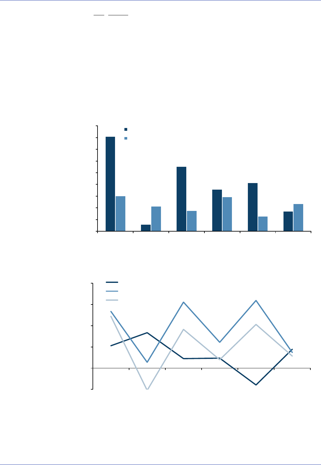
46 Global Rates Strategy Barclays Capital

é-=

100

CPI

where CPIt is the CPI for the quarter which is two quarters previous to the quarter in

which the coupon is paid. CPIt-2 is the CPI two quarters prior to CPIt.

f = number of days from the settlement date to the next interest payment date.

d = number of days from previous to next interest due date.

g = fixed quarterly interest payment (annual rate divided by 4).

n = number of full quarters between next interest payment date and maturity date.

Figure 22: Historical Performance and Risk

10%

12%

14%

16%

18%

1998 1999 2000 2001 2002 2003

ACGIL Return

ACGIL Ann. Monthly St. Dev

Source: Barclays Capital.

Figure 23: Risk and Return Versus Australian Nominals and Equities

-1

1998 1999 2000 2001 2002 2003

Equity Return/Risk

IL Return/Risk

Conventionals Return/Risk

Source: Barclays Capital.

Barclays Capital Global Rates Strategy 47

Barclays Inflation-Linked Bond Indices

John Williams

The Barclays family of inflation-linked bond indices has been created to provide

investors with accurate benchmarks for performance measurement, as well as offering

discrete building blocks for market analysis and portfolio construction. The indices

provide an accurate, comprehensive depiction of the performance and fundamental

characteristics of the world’s major inflation-linked bond markets.

A broad range of indices is available. As well as an index for each of the major inflation-

linked markets both sovereign and non-sovereign, various combinations of market are

also available as standard or on request. The indices include only capital indexed bonds

with a remaining maturity of one year or more. The index methodology is based on the

EFFAS standard with strict adherence to stated rules and a monthly rebalancing cycle.

Global Inflation-Linked Bond Index

Barclays Capital launched its first inflation-linked bond index in October 1997 – the

Global Inflation-Linked Bond Index. It measures the performance of the major

government inflation-linked bond markets. The index is designed to include only those

markets in which a global government linker fund is likely to invest. This makes

investability a key criterion for inclusion in the index.

In order to ensure that the index includes only the more liquid and investable bonds, it

has strict market eligibility rules. For a market to be eligible it must have a US dollar

face value of $1bn or more and a foreign currency long-term debt rating of AA-/Aa3 or

better. Individual securities must have a US dollar face value of $100mn or more. These

rules have been effective in including only the more liquid markets.

Markets currently included in the index (in the order they began) are the UK, Australia,

Canada, Sweden, the US, France and Italy. The index is published daily on the Barclays

Research and Indices websites, on Bloomberg and DataStream and is featured every month

in the Global Inflation-Linked Monthly and other Barclays Capital Research publications.

Figure 24: Global Index Structure

World Government Index

France Govt

EMU HICP Linked

Australia

Govt

Canada

Govt

Sweden

Govt

Italy

Govt

EMU

HICP

Linked

France

Govt

EMU

HICP

Linked

France

Govt

FRCPI

Linked

Source: Barclays Capital.

48 Global Rates Strategy Barclays Capital

As can be seen in Figure 24, the index has a high degree of granularity. Sub-indices are

defined for each country and where appropriate by country and linking index; so, for

example, there are indices for France Govt, France Govt FRCPI-Linked and France Govt

EMU HICP-Linked. The same principal is applied across countries so that inflation-linked

assets can be tracked by country, by linking index or both. Detailed information is also

available at bond level including price, yield, total return index and breakeven inflation.

As more and more international linker funds are launched it is necessary to be able to

analyse returns in a range of different currencies. As well as local currency returns, hedged

and un-hedged return series are available in AUD, CAD, CHF, GBP, EUR, JPY and USD.

The growth of inflation-linked bond markets in the early 2000s encouraged us to

launch three additional linker indices:

Sterling Inflation-Linked Bond Index

Demand for long dated inflation-linked assets from the UK pension industry led to

spectacular growth in the sterling corporate inflation-linked bond market. We launched

the Barclays Sterling Inflation-Linked Bond Index in January 2001 with a base date of 31

December 1999. The index combines bonds from the Gilt and Non-Gilt Inflation-Linked

bond markets with a cut-off of £100mn face value. The Non-Gilt portion of the index is

further divided by rating and by sector.

Figure 25: Sterling Index Structure

Sterling Inflation-Linked Bond Index

(All Maturity, 1-5Yrs, 5-15yrs, >15yrs)

UK Govt

All

1-5yrs

5-15Yrs

>15yrs

Rating Indices

AAA

BBB

Sector Indices

Agency/Supra

Corporate

Utility

Insurance Wrapped

Non-Govt

(All, 1-5yrs, 5-15yrs, >15yrs)

Source: Barclays Capital.

Euro Inflation-Linked Bond Index

The latest addition to the Barclays inflation-linked bond index line-up is our euro index

launched in May 2003. It combines euro government and non-government inflation-

linked bonds and is set fair to capture the evolution of the linker market in the euro-

zone. Bonds are eligible for this index if they are linked to the inflation of any EMU

member country or the harmonised EMU HICP, are denominated in euros, have a face

value of ¤500mn or more and are issued by an EMU member government or a quasi-

government issuer.

At the time of writing, the majority of non-government capital indexed bonds issued in

euros are from quasi-government bodies. Corporate issuance has been chiefly in the

form of inflation-linked Medium Term Notes, which are not eligible for inclusion in the

Barclays Capital Global Rates Strategy 49

indices. As the market matures and corporate issuers begin to issue capital indexed

bonds, we would hope to broaden the rules to include these issues into the index, and at

the same time introduce new sector and rating categories.

Figure 26: Euro Index Structure

CPI Indices

FRCPI

EMU HICP

...

Country

Indices

France

Greece

Italy

...

Government

Euro Inflation-Linked Bond Index

CPI Indices

FRCPI

EMU HICP

...

Sector/

Rating

Indices

tba

Non Government CPI Indices

FRCPI

EMU HICP

...

Source: Barclays Capital

South Africa Inflation-Linked Bond Index

The South African Treasury announced its intention to issue inflation-linked bonds in

March 2000. By the autumn of 2002, the market had grown rapidly and asset managers

were crying out for a suitable benchmark. After discussions with leading South African

asset managers and the South African Treasury, we launched the Barclays South Africa

Government Inflation-Linked Bond Index. This index includes all South African domestic

Government inflation-linked bonds of ZAR400mn or more.

Customised Benchmarks

Many users of indices have investment aims that cannot easily be replicated using

standard benchmark indices. This is particularly true of global bond portfolios where

the desired country and currency allocations seldom reflect market capitalisation.

Because of the breadth of coverage of the Barclays inflation-linked index family and the

market expertise backing up the index, we are able to offer a degree of customisation

unavailable elsewhere. Please contact the author for more details.

For more details on inflation-linked bond indices please refer to the Barclays Inflation-Linked Bond Indices Guide.

50 Global Rates Strategy Barclays Capital

South Africa

Leon Myburgh

South Africa’s economy has shown continual improvements in its credit profile and is

increasingly being differentiated from emerging economies. However, the rand has

been subject to periods of significant volatility. As South Africa has an open economy,

currency movements play an important role in setting price levels. Therefore, we would

expect a significant real and inflation risk premium to have embedded itself in long-

term nominal bond yields. However, similar to other international linker markets, there

is little evidence of a significant inflation risk premium at this stage of the market’s

development. During 2002, the inversion of the breakeven inflation curve, driven by

pricing distortions in the conventional bond curve, became extreme, implying a

negative inflation-risk premium. Since then, most of this pricing anomaly has been

reversed but the breakeven curve is still downward sloping. This anomaly will probably

continue to reduce with the issuance of more long-term nominal debt, removing the

structural shortage of long-term assets.

The bonds carry an explicit principal deflation floor, “if the capital value of the bonds on the

redemption date is less than the principal amount, then the issuer shall pay the bondholders

an additional amount equal to the difference”. The bonds are quoted on a real yield basis

with inflation indexation calculated under a slightly augmented Canadian methodology. For

the first day of any calendar month (settlement day), the CPI from four months prior is the

reference CPI for that date. This means that South African linkers have a lag that is a month

longer than those seen in Canada, France, Sweden and the US.

Market Development

In the budget delivered on 23 February 2000, the Minister of Finance stated the

Department of Finance (now known as the National Treasury) intended to issue

inflation-linked debt in the first quarter of 2000. This followed extensive research

carried out by the Department over the preceding years. At the time, it cited confidence

that CPI would decline over the medium term and therefore the introduction of this

instrument would reduce the costs of servicing debt in real terms, allowing more room

for social expenditure. It was emphasised that the introduction of this instrument

indicated the government’s commitment to keeping inflation under control.

The first auction took place on a uniform yield basis on 15 March 2000. The auction

was oversubscribed 1.7 times but the Treasury decided to set the cut-off yield at 6.50%

and issued only R495mn of the R1.0bn on offer. The next auction was held on 7

September 2000 where the R250mn on offer was oversubscribed 3.7 times and all the

bonds were issued. Since then, ILB auctions have become a regular feature in the

government’s funding programme, with auctions being held nearly every month.

The first issue had a maturity of 2013, commonly known as the R189; a second bond

was issued in May 2001 with a 2023 maturity (R197), followed by a 2008 maturity

(R198) in 2002. In 2003, the government issued the R202 with a maturity of 2033.

CPI and CPIX

Government inflation-linked bonds are linked to the headline non-seasonally adjusted

Consumer Price Index (CPI) for metropolitan areas as published by Stats SA. The official

inflation target for the Monetary Policy Committee is CPI excluding interest rates on

mortgage bonds (CPIX) for metropolitan and other urban areas.

Barclays Capital Global Rates Strategy 51

Every five years, Stats SA conducts a Survey of Income and Expenditure of Households

and this information is weighted according to the Population Census figures in order to

represent all households in South Africa. This survey is used to identify the goods and

services bought by a typical consumer or household and which should be included in

the basket of goods and services used to monitor price changes. From this survey,

weights are determined for specific products in the basket. The weight of each product

stays the same for the five-year period until the results of the next Survey of Income

and Expenditure of Households becomes available.

Prices of goods and services included in the CPI are collected in the first seven days of

the month. While most prices are collected monthly, some are collected quarterly, six

monthly, or annually. The collection of prices depends on the frequency on which these

prices tend to change.

Calculations

Each day has its own distinct Reference Index. The first day of each month has a

Reference Index equal to the CPI index of four calendar months earlier, eg, that for 1

February 2004 is the CPI for October 2003 and that for 1 March 2004 is the CPI for

November 2003. This lag is one month longer than many other markets. Reference

Indices for intervening days are calculated by straight-line interpolation.

This formula is used to calculate a Reference CPI Index for the official original issue date,

or “Base Reference Index”. For settlement date or cash flow payment date, t, a Reference

CPI is then calculated. Both the Reference Index and the Base Index are rounded to 15

decimal places. These two indices provide an Index Ratio for the value date:

Index RatioDate = Reference CPIt /Reference CPIBase

For settlement amounts, real accrued interest is calculated as for ordinary South

African bonds. Dirty price and accrued are each multiplied by the Index Ratio to arrive

at a cash settlement amount. For coupons paid, the (real) semi-annual coupon rate is

multiplied by the Index Ratio, and likewise for the par redemption amount (with the

cash value subject to the par floor).

Taxation

South African CPI linked bonds fall under section 24J of the Income Tax Act, 1962.

Interest on bonds is taxed on a yield to maturity basis. Both coupon payments and the

difference between the acquisition cost and the nominal value of the bond are defined

as interest and is taxable for income tax purposes. Inflation-linked bonds are basically

treated like floating rate instruments. The tax liability is determined annually taking

into account any adjustments to the principal amount and the coupon payments as a

result of changes in the CPI.

South African inflation-linked bonds pay interest on a semi-annual basis. There is a

“books closed” period, which occurs two weeks prior to the interest payment date,

therefore the bonds trade ex-coupon for significantly longer than other markets such as

Australia, Sweden and the UK. During 2004, the “books closed” period for all domestic

government bonds will be reduced to a standard 10-day period.

52 Global Rates Strategy Barclays Capital

Japan

John Richards

The Japanese Government is scheduled to issue its first inflation-linked bond on

4 March 2004. The Ministry of Finance will approach the first auction very cautiously.

Early indications are that the initial size will be only JPY100bn, but in FY 04 issuance will

expand to at least JPY600bn, according to MoF’s announced issuance plan. Longer term,

Japan faces an exceptionally heavy government-borrowing schedule and MoF will need

to tap all sources of funds. In this environment, sharp increases in inflation-linked bond

issuance are likely if the security meets with even modest initial success. The initial

bond will have a 10 yr maturity and will be launched via a single price auction. If there

are subsequent reopenings, these will be via variable price auctions.

While it is possible to question the need for an inflation-linked bond in a deflationary

environment such as Japan’s, our preliminary modelling indicates that, as a relatively

low-volatility instrument whose yield will be comparable to those currently available in

the 5-year to 10-year maturity spectrum of the JGB market, it will have a place in many

bond portfolios. As deflation recedes in Japan, the potential importance of inflation-

linked bonds increases significantly, particularly with pension liabilities in Japan having

a greater inflation-linked element than many in other countries.

The initial issue’s specifications have not been finalised and MoF reserves the right to

make changes until just prior to issuance, but preliminary specifications are available

from MoF and we believe that there will be no material changes in them prior to the

first issue in March. The issue is generally based on what has come to be known as the

Canadian model, but three features are worth noting. (1) The security will not have a

floor to protect buyers in the event of deflation. Apparently MoF hopes to use the new

bond to provide an independent gauge of inflationary-deflationary expectations. (2)

Inflation will be measured by “core” CPI, (CPI excluding perishables). (3) Reflecting

unresolved tax issues, initial selling restrictions will limit holders to “designated financial

institutions” which are not subject to Japanese withholding taxes. Individuals and

corporations cannot own inflation-linked bonds directly.

The Linking Index

JGB inflation bonds will be linked to nationwide core CPI, a measure that excludes

perishables – the volatile fresh foods component of the overall CPI. The index is

compiled by the Ministry of Public Management, Home Affairs, Posts and

Telecommunications and is published monthly, usually on the last Friday of each

month. The data lags by one month, ie, January data is published at the end of February.

Calculations

Calculations for Japanese linkers are almost identical to those in Canada, with semi-

annual coupons and no deflation floor. Principal and coupons both accrue inflation

based on the ratio of the daily reference CPI value to the base reference value at

issuance. The only substantive difference is that inflation accrual is based around the

10th of the month rather than the first. As coupons pay on the 10th too, this means

that they use a reference CPI that is exactly the inflation value for three months earlier.

Settlement for a new bond will also be on the 10th of the launch month so that the base

reference CPI will be fixed using the index number for three months prior. At other

Barclays Capital Global Rates Strategy 53

times in month the inflation reference value is calculated via linear interpolation

between the reference for the previous and next 10th of the month.

no. of days from

10th day of month

“m-1” till today

(calculation day)

Reference

CPI on

month “m”

and day “n”,

where n<10

Reference

CPI on 10th

day of

month “m-

1”

no. of days in

month “m-1”

Reference CPI on10th

day of month “m” –

Reference CPI on 10th

day of month “m-1”

n-10

Reference

CPI on

month “m”

and day “n”,

where n>10

Reference

CPI on 10th

day of

month “m”

no. of days in month

“m”

Reference CPI on10th

day of month “m+1”–

Reference CPI on 10th

day of month “m”

While still under review here is the provisional tax treatment for the new bonds.

Income tax is payable coupon payments. The increase in the inflation-adjusted

principal, if any, at the redemption date is considered to be an interest payment and as

such taxable. No tax is applied when the principal falls in value due to the decline in

prices. The tax treatment when a bond is sold is less clear, and this is the main reason

that the initial bond may only be bought by “designated financial institutions” which

are not subject to Japanese withholding taxes. Japanese linkers will not be included in

the Barclays Capital Global Inflation-Linked Bond Index until this holding restriction is

relaxed, but in the meantime will be a stand-alone Japanese Inflation-Linked Index.

54 Global Rates Strategy Barclays Capital

Greece

Alan James

The GGB¤i 2.9% Jul 2025 was launched in March 2003. The bond was announced on 7

March and priced on 18 March, for ¤1.25bn, using an interpolated OAT¤i real yield

curve. Technically this issue is not eligible to be reopened via auctions, though future

bonds may be. The bond was not syndicated again in 2003 and so made up less than

5% of total funding for the year. Greece committed to reopening the bond via

syndication in Q1 04.

The GGB¤i 2.9% Jul 2025 is not eligible for the Barclays Capital Global Inflation-linked Bond

Index until Greece is upgraded to AA- by Standard & Poor’s and Aa3 by Moody’s. Currently

both agencies rate Greece one notch too low. It is in the euro inflation bond index.

The GGB¤i25 has exactly the same calculation conventions as French OAT¤i bonds,

with its inflation accrual linked to the eurostat euro area HICP ex-tobacco index. It even

has the same coupon payment date, 25 July. At initial launch it was issued with accrued

interest and inflation to ensure a full first coupon payment. This means its base

reference index for inflation accrual is from 25 July 2002.

Barclays Capital Global Rates Strategy 55

Iceland

Mike Oman

Indexed government bonds have been issued regularly since 1964 in Iceland, making it

one of the oldest inflation-linked markets. Indexation for financial products first

emerged in earnest in 1955 with the introduction of partially indexed state housing

loans to individuals, a concept that spread to other types of borrowing and eventually

to government borrowing in the 1960s. Icelandic linkers have taken a variety of forms

and used different linking indices, originally the Building Cost Index. The linking index

has evolved to become the Icelandic CPI (which since 1995 has not included the

Building Cost Index and used to be called the CTI).

The majority of the Icelandic domestic bond market is index linked and there are

currently three types of linkers: Housing Authority bonds (IBN, annuities), Housing

Bonds (IBH, callable annuities) and Treasury bonds with a face value of around

ISK450bn ($6.4bn). Only 10% of the indexed bond market capitalisation is sovereign,

explaining why Iceland does not qualify for inclusion in the Barclays Capital Global

Inflation-linked Bond Index. Sovereign backed housing agency paper accounts for the

remainder and this majority share is set to increase further in the coming years.

Maximum housing bond mortgages were upped as of 1 January 2004, encouraging

increased housing bond issuance, which should be compounded by recent trends

towards growing housing market activity and sustained house price appreciation. By

contrast, the redemption and buyback programme for 2004 of the National Debt

Management Agency on behalf of the National Treasury, includes only ISK15bn of

Treasury bonds (RIKS linkers and RIKB which are non-indexed) in 2004 implying zero

net Treasury issuance.

As of 1 July 2004, issuance of both housing (IBH) and housing authority bonds (IBN) will

be discontinued in their current form, to be replaced by new Housing Financing Fund

(HFF) Bonds eliminating entirely the callable feature of the IBHs. HFF Bonds are to be

issued in only a few series of annuity bonds, but with quarterly not annual coupons. The

new series will be open during their entire term, which will be up to 50 years. Holders of

(IBH) and (IBN) will be offered to switch in stages following the establishment of the

new HFF Bond series. The intention of the HFF is that the new housing financing

arrangements will mean greater efficiency on the bond market and improve access to

foreign investors, resulting in lower real interest rates in Iceland. We expect that total

HFF bond issuance will be in the region of ISK60bn-70bn in 2004, and that there will be

four new HFF Bond series, which may take more than a year to fully establish.

Bond market turnover in general has expanded sizeably, and housing bond turnover

especially, with volumes rising by an average of 25% pa since 1998, and 150% of

market capitalisation being a typical annual trading volume.

56 Global Rates Strategy Barclays Capital

Israel

Mike Oman

Israeli government bonds were first linked to CPI in 1955, following a spate of

devaluations that made dollar indexation no longer desirable. The share of indexation

rose in the 1970s and 1980s along with the increase in inflation from single digit levels

in the 1960s to a range of 10-40% throughout most of the 1970s and a range of 100-

450% from 1979 to mid-1985. Indexation in Israel is so widespread that the word

“interest” in the vernacular refers to real interest, with compensation for inflation being

referred to by other terminology.

On maturity the bondholder receives the par value multiplied by the change in CPI since

issue, or some fraction of the change in the CPI for partially indexed bonds. Modern

Israeli linkers coupons are also indexed, and there is no deflation floor.

The tradable Israeli domestic debt (60% of the total debt) is comprised of non-linked,

CPI-linked, and US dollar-linked debt. In the past, the tradable domestic debt was

almost entirely linked to the CPI or to the US dollar. In 1993, the share of CPI linked debt

was 87% of the total domestic tradable debt, and the share of the debt linked to the

dollar was about 11% of the total domestic tradable debt. Now approximately $25bn of

CPI linked debt is outstanding, which is 49% of tradable debt and 21% of all

government debt. Israel’s rating is too low to qualify for inclusion in the Barclays Capital

Global Inflation-Linked Bond Index.

The stated aim of developing a full non-indexed yield curve to rival international

competitors and to achieve more balance for the government debt portfolio pushes CPI

linked issuance lower down on the list of priorities and hence its share should fall. The

success of the government, aided by external support to suppress inflation expectations

reduces the inflation premium and therefore its attractiveness to the government from

a funding cost perspective. CPI dropped from in excess of 20% in 1989 to zero in 2000.

Furthermore, the demand for non-indexed debt relative to indexed debt, as measured

by auction cover, has been considerably higher in recent years. Since 1999 on average

only 24% of the tradable debt issued has been CPI linked, although it is rising.

Foreign participation in the Israeli government bond market increased dramatically in

the 2002-2003 period. However, this trend is yet to filter from the non-indexed sector

into the CPI indexed sector, and still represents only a very small percentage.

Figure 27: CPI linked Share of Tradable Debt is in Decline

10%

20%

30%

40%

50%

60%

70%

80%

90%

100%

1993 1994 1995 1996 1997 1998 1999 2000 2001 2002 2003

CPI Indexed USD Indexed Non-indexed

Source: Israeli Ministry of Finance.

Barclays Capital Global Rates Strategy 57

New Zealand

Mike Oman

New Zealand has only one index-linked government bond outstanding, 4.5% 15

February 2016 with a face value of NZ$1.5bn, representing 5% of the government bond

market. Inflation-indexed bonds have not been issued since 1999, as it has not been

seen as cost-effective to do so. They had been auctioned through a uniform price

system in order to reduce the potential winner's curse problem, which is viewed “to be

greater for a less liquid instrument that is more difficult to price”. The bond does not

qualify for the Barclays Capital Global Inflation-Linked Bond Index as it was below

US$1bn face value after its last reopening in 1999.

In the 1990s the NZ DMO commissioned studies to quantify the risk characteristics of

the assets in the government's balance sheet, from which to draw conclusions regarding

the appropriate liability structure. It emerged that government assets were sensitive to

real rates, implying a case for issuing some inflation-indexed debt, and encouraging a

restart to the government indexed debt programme in 1995, which began in 1983,

when New Zealand’s other two government linkers, Jun ’99 and Sep ’01, were launched.

These were semi-annual, and inflation uplift calculations precluded negative indexation

for coupon and principal: a type of inflation floor. Inflation adjusted savings bonds

(retail, non-marketable) pre-dated the government bond programme and were popular

due to the inflation uplift on the principal being tax free.

The current outstanding linker is denominated in New Zealand dollars with a fixed

coupon paid quarterly in arrears. The index to be used for calculating the “Indexed

Component” is the All Groups Consumer Price Index (“CPI”) as measured and published

quarterly by Statistics New Zealand. The mechanics of this remaining linker are identical

to Australian linkers: indexation is based on the average percentage change in the

Consumer Price Index (CPI) over the two quarters ending the quarter, which is two

quarters before the one in which the next interest payment falls (for example, if the

next interest payment is in February, the index ratio is based on the average movement

in the CPI over the two quarters ended in the preceding September quarter). The floor

and tax-free indexation features of the older bonds do not apply. They may be stripped

into separate coupon and principal components in accordance with the NZ DMO’s rules.

A reduction in the volatility of NZ CPI and the poor initial response to the 2016 issue

leaves the less liquid linker product an unappealing source of finance for the

government from a funding cost perspective. The NZ DMO intends to focus its issuance

strategy on building liquid benchmarks of around NZ$3bn spread evenly across the

curve (tending to alternate between new short and long issues). With an annual funding

need of less than NZ$3bn at the time of writing, there is little reason to expect a

relaunch of linker issuance in the near future. However, as the global linker market

matures and is traded on a more global footing, the liquidity concern is likely to

diminish, and the demand for diversification of linker portfolios may reverse the view

that linker issuance is simply not cost effective.

58 Global Rates Strategy Barclays Capital

Mexico

Mike Oman

Mexico has had an indexed linked market since the 1970s in the shape of Oil price

linked Nafinsa bonds, but it was not until 1989 that the first government NCPI bonds

known as Ajustabonos were issued as part of a programme of financial reforms to

tackle the problems of high and unstable inflation. Udibonos replaced Ajustabonos,

which the Ministry of Finance stopped issuing in January 1995. The last of the

Ajustabonos matured in 1999. Udibonos are coupon bonds with cash flows

denominated in UDI, which is effectively the Mexican peso adjusted for CPI inflation

based at 1 UDI =1 MXN on 4 April 1995, thereby providing the inflation linkage. The

uplifted face value at the end of 2003 was equivalent to $7bn, but the sovereign rating

is too low for the market to be included in our global government index.

The average maturity of government securities in the domestic market continues to rise,

as exemplified by the progressive lengthening of the maturities of new Udibonos from

two or three to five years in the late 1990s, and now to 10 years (the first 10-year is the

6.5% Jan ’11 issued first in January 2001). However, domestic debt still has a relatively

short maturity mainly due to the lack of appetite for long-term exposure to Mexican peso

government debt. While maturities have lengthened, the number of bonds outstanding

has fallen, from 22 in August 1998 to just seven in January 2004. Udibonos are auctioned

once every six weeks, usually UDI400mn in size, at the time of writing.

Barclays Capital Global Rates Strategy 59

Inflation-Linked Derivatives

Alan James

Inflation-linked derivatives, and in particular inflation swaps, are not a new

phenomenon. Barclays Capital has been trading sterling inflation swaps for more than

10 years. US inflation swap trades were conducted in 1997, followed in 1998 by trades

in French and euro inflation, as well as inflation of several other European countries that

still have no bond market. However, it was not until 2002 that the market really began

to flourish. Now there are markets in inflation swaps for all of the indices with

established bond markets. The most active markets in descending order of absolute size

are: euro HICP ex-tobacco (HICPx); UK RPI; French CPI ex-tobacco; US CPI; euro headline

HICP; and Italian CPI ex-tobacco.

The major benefit of inflation derivatives compared to inflation-linked bonds is flexibility.

Structures can be made that fulfil the specific needs of corporates, institutions or

governments. The cost of entry for payers of inflation is much lower than it is for issuing

bonds. While by far the most transactions are conducted in inflation swaps, inflation

floors, caps and swaptions are also traded when there is particular demand. So too are

hybrid structures, for instance incorporating an equity–related component.

How the Inflation-Linked Swaps Market Evolved

The inflation-linked swaps market in the 1990s developed in a not dissimilar way to the

interest rate swaps market in the 1980s, albeit growing at a slower pace initially. The UK

market developed first, due to the existence of a curve of tradable linkers with similar

features to the swap market. This meant that banks could develop unmatched inflation

swap books and hedge their risk using linkers. Ironically there is now much more

matching in the UK market than in the euro area or US, with banks effectively acting as

intermediaries between payer and receiver. In most inflation-linked swap markets

managing the bond-swap spread risk as well as reset risks, repo spreads, etc has

become the main focus of risk managing an IL swap book.

In the UK IL swap market, the main drivers are the usual payers and receivers of

inflation, namely corporate debt issuers versus pension fund and insurance company

investors. Among natural payers, until recently, utility companies with inflation-linked

revenues have tended to issue inflation-linked bonds rather than pay. It was the

development of the Private Finance Initiative (PFI) in the UK that really encouraged the

growth of the inflation swaps market. In PFI projects a central or local government

entity guarantees an annuity flow (typically over 20-30 years) to the private sector.

They are usually associated with infrastructure projects such as roads, railroads, and

bridges, or health, education, or defence building projects. It is mainly health sector

projects that have guaranteed cash flows linked to UKRPI. The project companies fund

their initial costs in the form of bond issues, which are usually credit wrapped to give

AAA ratings, or through bank lending. For smaller initiatives in particular it made sense

to fund in nominal markets and hedge the inflation exposure via paying inflation swaps.

Inflation-linked flow from this source was significant from the mid 1999s onwards, and

over time has become increasingly skewed towards paying in inflation swaps.

IL swaps have essentially performed a supporting role for the underlying IL bond

market, providing payers and receivers with cheaper and more efficient routes to

60 Global Rates Strategy Barclays Capital

execution than in the bond market or meeting needs that the bond market is unable to

satisfy. In mid 2000, a large number of AAA issuers (IBRD, EBRD, EIB, NIB, RFF, CDC, and

others) entered the IL issuance market in the UK with almost all of the investor demand

coming from the UK pension and insurance sectors. These new issues were all swapped

(ie, the issuers were all getting Libor funding and hedging out the inflation-linked

flows), with banks such as Barclays hedging. Such opportunistic issuing is no longer a

factor due to the relative richening of inflation swaps, but it helped invigorate the

market and would return if valuations were to alter.

In 2003 there were increasing difficulties with many traditional buyers of inflation-

linked bonds being too full of the name of the credit wrapping institutions, the

healthcare sector and to a lesser extent utilities. This led to a relative underperformance

of corporate inflation-linked bonds relative to index-linked gilts and inflation swaps. In

the second half of 2003 there was almost no corporate issuance, but paying increased

significantly. It has also led to a significant increase in the number of pension funds and

insurers who have extended their mandate to enable them to receive inflation.

The UK market has developed without the screen-based pricing by brokers that has

characterised the growth of the euro and US markets. Now the market has developed

there are significant flows in the five-year sector, but the average maturity of

transactions is considerably longer than elsewhere, with most trades still at 15yr+. The

majority of transactions, at least weighted by value, involve direct establishment of a

swap involving a real money receiver. As such they are transacted via individual banks,

usually with as little evidence as possible of flow presented to the market at the time.

This makes quantifying turnover or the absolute size of the market extremely difficult,

but we estimate turnover in 2003 of at least £6bn. In comparison turnover in the index-

linked gilt market was £150bn. On the other hand most of the flow was one way, and

gilt linker issuance was itself only £6bn. When there have been unbalanced swap flows

they have certainly had a major impact on linker real yields.

Euro Area

The French CPI ex-tobacco swaps market developed alongside the bond market,

although the first trades were struck just before the OATi09 was actually launched. As

the curve developed with the launch of the OATi29 and French agency issuance,

principally CADES, hedging risk became feasible. Some real money investors started

matching cash flows as the market developed. However, the depth of the market really

started to pick-up alongside trading in euro inflation swaps, and there has been active

basis trading between the two. The market developed rapidly as brokers started to

show prices to banks in generic zero coupon swaps. Recently inter-dealer broker prices

have become generally viewable in both French CPI and euro HICPx.

The French CPI swaps market was given a considerable boost by the decision to link the

Livret A public sector savings rate to inflation from August 2004 (the rate will be half

the three-month money rate and half annual French CPI ex-tobacco plus 25 bp). This

leaves an exposure to inflation for the manager of these savings schemes of around

¤45bn. As the manager is likely to be restricted in the percentage of any bond it can

hold, this leaves the swap market as the obvious route to hedge the exposure. Not many

of the liabilities need to be hedged for the impact on swaps to be large. In addition, the

change to the official rate may encourage commercial banks to offer their own

accounts linked to French CPI, and this too is likely to create swap flow.

Euro HICP ex-tobacco has quickly developed into the largest inflation swaps market,

with monthly turnover rising over ¤4bn in late 2003. Euro inflation had been quoted

from the start of the euro area in the same way as inflation in euro area countries

Barclays Capital Global Rates Strategy 61

outside France was quoted, despite the lack of a bond market. Some equity-related

retail notes with an inflation element, particularly from the Italian Post Office in early

2001, encouraged the market to trade. Until the launch of the OAT¤i12 in October

2001, euro inflation was generally traded as the headline HICP series but during 2002

the market shifted towards the same HICPx index as the bond. Tobacco basis has

developed into a relatively active sub branch though, as there have been some large

swapped MTN notes linked to headline HICP.

While increasing turnover in the inflation bond market certainty encouraged activity in

inflation swaps too, the real driver was retail demand for structured inflation notes,

initially only from Italy. Structured notes have been a feature of the Italian market for

several years, initially based on nominal interest rates. As rates fell, so cash flows were no

longer sufficiently attractive for retail interest, equity linked notes became common.

Some of these contained real elements in addition to the equity component. The decline

in equity markets reduced demand for equity-linked notes, leaving an opportunity for

inflation-linked MTNs. The next section considers this sector in more detail, but it is

sufficient to say that ¤10bn structured MTNs in 2003, many hedged out through broker

screens, have been more than enough to establish the market. The market for Italian

(FOI) inflation ex-tobacco has also grown out of this retail MTN demand.

The launch of the BTP¤i08 is closely linked with the maturing of the euro inflation

swaps market. The bond itself came about due to the Italian retail demand, with the

Italian treasury keen both to tap the demand directly but also to take advantage of non-

hedged exposure in the sector, as the shortest OAT¤i had a 2012 maturity while most

MTN supply was at 5yr. It achieved both to some extent, enabling a record ¤7bn initial

issue. Subsequent cheapening of the bond versus swaps encouraged a significant new

development: asset swapping of the bond by portfolio asset swappers, who were able to

lock in Euribor plus levels. Similar asset swapping was also seen in the OATi09, which

had underperformed French CPI due to Livret A pressures. This encouraged banks to

trade inflation swaps and bonds together, bringing inflation-linked asset swaps up to

10yr, very much in line with those seen in nominal bonds and significantly enhancing

the depth in both markets.

Until Autumn 2003, the market for US CPI was very much “by appointment only”, at

which point the developments elsewhere became too large to ignore. Swapped US CPI-

linked MTNs were already being sold in Europe. While there were a number of swapped

issues in 1997, there has been almost no supply and very little growth in swaps since.

This time around, with brokers willing to show quotes on a similar basis to those in the

euro HICPx, the market established itself quickly. The announcement by the Chicago

Mercantile Exchange that it would start quoting an inflation future in 2004 further

underpinned the market, as did the Treasury’s comment that it was considering adding

new maturity TIPS. Volumes totalled around $300mn in the first three quarters of 2003,

whereas broker volumes in November were more than $550mn and, even in December,

growth did not slow. It grew up as a market with very few payers, but as this left implied

asset swaps on TIPS significantly cheaper than in nominal Treasuries, banks have been

happy to build up exposure knowing that portfolio managers already familiar with

inflation products would be happy to asset swap TIPS if swaps were to richen further.

62 Global Rates Strategy Barclays Capital

Types of Inflation-Linked Derivatives

There are a variety of different types of inflation swaps, but the most commonly quoted

rates are for zero swaps. The counterparties exchange just one cash flow at the

maturity of the swap. The final payment depends on the ratio of the price index now

(given the usual market lag) compared to the price index at expiry. The price is quoted

as a pure breakeven annualised inflation rate. While not directly comparable with

conventions in the bond or interest rate swaps market they are an intuitively easy

structure that is relatively easy to calculate and visualise, hence the general acceptance

by inter-dealer brokers and banks. A combination of various zero rates can be used to

build many different structures.

There is no inflation floor in a standard zero swap. There are slight differences between

quoting conventions in French CPI and euro HICPx. French CPI swaps quote based on

the daily interpolated reference value, consistent with that in the OATi market. Euro

HICPx usually quote off the actual monthly inflation index, leaving a discontinuity when

the month changes. This often leads to two (or even three) months being quoted at the

same time on different screens. The UK market trades monthly, with a lag of two

months to the active trading month. The US market is most commonly quoted using

the monthly data too, though attempts have been made to follow the daily TIPS

inflation reference. It is somewhat surprising that the euro market developed with

monthly fixing given the convention in France. It was probably due to a combination of

it starting before the ¤i bond market, participants following a similar convention to that

in the then more developed UK market, and greater consistency with year-on-year

inflation swaps.

The alternative regularly quoted inflation swaps rates to zero coupons are year-on-year

inflation swaps. In 2003 these were very commonly traded euro structures due to the MTN

market. Typically these reset yearly, with the inflation leg paying on the year-year inflation

rate for the given month (often plus a fixed percentage), usually based on a three-month

lag from the current month. The conventional leg will most commonly be based on six-

month LIBOR, though other floating maturities and purely fixed-rate terms have also been

transacted. Year-on-year inflation swap rates are quoted without inflation floors.

Inflation swaps with cash flows equivalent to those in government bonds have generally

been transacted versus bonds themselves, ie, as asset swaps. In the UK the structure of

the corporate and government inflation bond markets are the same and as there is no

deflation floor, so the creation of equivalent derivatives is relatively straightforward.

Elsewhere asset swapping of accreting bonds needs to include deflation floors.

Deflation floors are the most commonly traded inflation derivatives after swaps. They

trade both in year-on-year as well as longer terms where they usually offset bond

repayments. Floors at other year-on-year inflation rates have also traded in both euro

HICPx and US CPI, most commonly 1%, as this is an inflation floor that many MTNs have

used. Inflation caps are much more unusual. The only significant instances of caps have

been in the UK, usually in conjunction with floors as part of Limited Price Indexation

(LPI) hedging by pension funds. LPI liabilities grow with RPI but are floored at 0%

inflation and capped at 5%. Almost all UK cap trades have thus been conducted at 5%,

albeit with the LPI cap falling to 2.5% for accruals after April 2005 this may change.

To date inflation swaptions that have traded have been deal related, for instance when

an issuer knows that it will issue but is unsure of size. This is a sector that may well

develop once inflation futures trade actively, but so far difficulty in hedging inflation

forwards has meant swaptions are limited to the short term, where carry is known.

Barclays Capital Global Rates Strategy 63

Inflation Futures

The Chicago Mercantile Exchange (CME) announced a US CPI future in October 2003,

launching it at the start of February 2004. There have been previous unsuccessful

attempts to develop inflation futures markets, including a CBOT TIPS future, which

faltered due to the difficulty in forward trading in inflation bonds. A true inflation

forward requires an inflation assumption as well as a nominal repo rate. The new future

avoids this problem by trading the inflation index directly. Indeed as its liquidity

develops it should make forward inflation bond real yield trading possible as the short

term inflation element can be hedged using the future. If this contract is successful it is

not likely to be long before inflation futures also develop in euro HICP.

The design of the CME CPI futures contract mimics the structure of the extremely liquid

Eurodollar futures contract. Specifically, the contracts list on a quarterly cycle and cash

settle to the three-month change in the non-seasonally adjusted CPI-U (the same index

to which TIPS are tied), annualised and converted to a “price” by subtracting the result

from 100%. Like Eurodollars they cash settle, with each contract having a notional size

of $1mn and a $25 DV01. They trade electronically with half ticks allowed. The month

involved is the CPI index number during the contract month ie, the reading for the

previous month, compared to the index three months before this. For example, the

September ’03 contract, if it had existed, would have settled at a price of:

100 - [(Aug CPI/May CPI) - 1] * 400

= 100 - [(184.6 / 183.5) - 1] * 400

= 97.60, which implies an annualised rate of 2.398%.

There is no cap to the future’s price level. For instance, the December ’03 future would

have settled at 100.215, ie, 100 - [(184.5 / 184.6) - 1] * 400. With inflation quoted

quarterly this series can exhibit notable seasonality. In this particular case the impact of

seasonality is to push the future 43¢ higher than would have been the case had the

seasonally adjusted index been used. The largest seasonality is for the June future: a

future for June 2003 would have been 87¢ lower than for an equivalent future based on

the seasonally adjusted series. The Mar ’03 and Sep ’03 distortions were both 22¢

higher than if they had been seasonally adjusted (ie, 0.1 index point).

The development of the CPI future ought to underpin development of shorter dated US

inflation swaps and structured inflation notes, filling the gap on the curve to the TII07.

They may also serve to accelerate the active arbitraging between the bond markets and

US CPI swaps that has already been seen in Europe.

64 Global Rates Strategy Barclays Capital

Figure 28: Provisional Contract Specifications

Reference Index

Contract based on Consumer Price Index, US city average for all

urban consumers, all items, not seasonally adjusted (CPI). The

“Reference Index” is calculated as 100 less the annualised % change

in CPI over past three months or

100 – [400 x ( (CPI t ¸ CPI t-3) -1 ) ]

eg, the most recent CPIt = 190 while the CPI of three months prior is

188. The Reference Index (RI) may be calculated as 95.74

95.74 = 100 – [400 x ((190 ¸ 188) – 1) ]

Note that the RI may be quoted at values either greater than or less

than 100.

Contract Size Contract valued at $2,500 x Reference Index (RI)

Minimum Price Fluctuation or Tick 0.5 bp or 0.005%, which equates

to a value of $12.50 (= $2,500 x 0.005)

Contract Months “March Quarterly Cycle” of March, June, September and December

Trading Hours Offered exclusively on the GLOBEX® electronic trading platform

during the hours of 7.20am to 2pm Mondays through Fridays

Position Limits 5,000 contracts

Final Settlement Date

Final settlement shall occur no later than the first business day of the

calendar month subsequent to the contract month. Thus, the last

possible settlement date for a March contract shall be the first

business day of April. While CPI release dates are known, and will be

publicised by the exchange, well in advance, the CPI is released on a

non-regular schedule. Effectively, settlement shall occur on the date

of the CPI release during the contract month, after which time the

contract price is fixed and contracts shall be marked to the Final

Settlement Price and settled in cash.

Final Settlement Price

The most recent CPI release for a given month shall constitute the

CPI used for the purposes of calculating the Final Settlement Price.

Note that the base of the Reference Index may be revised

subsequent to its initial release and the Exchange shall use such

revised figure in the calculation of the Final Settlement Price.

Source: CME.

Barclays Capital Global Rates Strategy 65

Non-Government Issuance

Alan James

Sterling

While there was some corporate issuance of inflation-linked bonds in the mid 1980s,

particularly from building societies, this was limited in size. The first corporate issue

large enough for the Barclays Capital Sterling Inflation-Linked Bond Index, ie, £100mn

or more, was an asset-backed issue by Anglia Water in 1990. Utility issuance has been a

fairly regular feature of the market ever since. Many regulated utilities have a degree of

RPI-based pricing restrictions and hence a clear inflation-linked revenue link. Water

companies in particular have issued (and more recently paid) in inflation. The largest

single name issuer is National Grid Transco Plc, which has gas and electricity prices

linked to RPI, though some of its issues have a credit wrapped guarantee and so are

AAA. In total at the end of 2003 it had three bonds in the index, worth £1.2bn, plus two

smaller issues. Another issuer who has partially funded via inflation-linked, due to the

nature of its cash flows, is supermarket chain Tesco Plc, which sells a broad range of

products covering roughly half the make-up of the RPI.

The largest source of non-gilt issuance in recent years has come from Private Finance

Initiative (PFI) related deals. PFI deals involve a private company building infrastructure

and then getting paid an income stream over time until the asset comes under the

ownership of the relevant authority. Almost all of these issues have been wrapped with

credit guarantees to enable AAA ratings. Most hospital-related projects involve RPI-linked

cash flows that will be paid to the financier once the hospital is operational and hence are

ideally suited to funding via inflation-linked issuance. Thus, this kind of issuer has been

numerous, though other large PFI infrastructure projects have also involved partial

financing via inflation linked. Many hospital bonds are amortising after a number of years,

usually close to the time when the building project is expected to be complete and cash

flows to be paid. As discussed in the derivatives section, PFI inflation-linked flows have

increasingly been seen in swaps rather than in inflation-linked bond issuance.

As mentioned in the derivatives section there was significant swapped supranational

and agency from mid 2000. There has been little recently, as funding levels have been

unattractive for asset swapped deals. Apart from at ultra long dates where there are no

equivalent government issues, it appears unlikely that there will be much opportunistic

issuance in the near future. Limited EIB issuance may continue as matched finance for

PFI projects. EIB is the largest single AAA issuer of sterling non-gilt inflation-linked. EIB

bonds larger than £100mn had market value of £640mn at the end of 2003, while there

were also a few smaller bonds.

At the end of 2003 the market value of the Non-Gilt Barclays Capital Sterling Inflation-

Linked Bond Index was £8.4bn. Of this, the largest sub-section was AAA wrapped deals,

mainly PFI, worth £3.4bn. Utilities were worth £2.1bn (excluding wrapped deals).

Agency and supranationals were worth £1.9bn. The largest bond in this subsection is a

£500mn 2051 amortising issue for the Channel Tunnel Rail Link, which, due to a

government guarantee, is classed as an agency bond. Other corporates made up £0.9bn

of the total. Supply remains heavily skewed to the long end, though there is occasional

10 yr supply. More than 85% of the index, £7.3bn, remained in the over-15 yr maturity

bucket at the end of 2003.

66 Global Rates Strategy Barclays Capital

Euro

Government Style Bonds

At least until 2004, the only major non-government issuers of inflation-linked bonds

with the same accreting format have been French government-related entities. By far

the larger issuer of these agencies and EPICS has been CADES: Caisse d’Amortissement

de la Dette Sociale. This sovereign agency was created in 1996 as a vehicle to

consolidate and service the debts of the French social security funds. Currently the

agency manages social security debts from up to 1998, but in 2005 this will be

extended. The increase in liabilities is likely to be offset with further issuance. At

present the agency is scheduled to be wound up in January 2014, limiting the scope for

longer-dated issuance. Given the nature of its cash flows, mainly the dedicated CRDS

tax that grows in line with French household disposable income, all its linker supply has

been in French CPI linked bonds.

There were three CADESi benchmark bonds outstanding at the end of 2003, with a

market value of ¤9.3bn, around one third of its total debt. The CADESi 3.15% Jul ’13

was the first bond to be issued in March 1999. By the end of 2003 it was the smallest

and least liquid of the three bonds, not having been reopened since it reached ¤2.3bn

face value in May 2001. The 3.8% Jul ’06 was launched in January 2000. As the shortest

French linker it has particular niche appeal and by the end of 2003 had been syndicated

10 times, bringing it to ¤3.7bn face value. The 3.4% Jul ’11 was first issued in Jun ’02

and had a face value of ¤2.55bn into 2004.

Calculations for CADESi bonds are identical to OATis except that initial inflation accrual

was started before the issue date of the bonds, to give a full first coupon. In practice

CADESi bonds have traded very much like OATis, albeit with lower liquidity, and have

helped define the curve. In December 2003 the agency Jul ’13 consistently traded 1 bp

over the maturity matched OATi.

Apart from CADES, the only other non-government issuers with government style

bonds large enough to qualify for the Barclays Capital Euro Inflation-Linked Index, ie,

over ¤500mn, are Caisse Nationale des Autoroutes (CNA) and Réseau Ferré de France

(RFF) though several other agencies have also issued in smaller size. CNA is a public

agency administered by CDC, which grants loans to toll road companies. Its ¤600mn

3.9% 2016 French CPI linked bond was issued in Jul ’01 and is only a small part of its

funding. RFF is the EPIC that owns French rail infrastructure. It issued an ¤800mn 2.45%

Feb23 linked to euro HICPx in February 2003.

The first major agency issuer is set to be Infrastructure of Italy. The bond will be the

first benchmark issue in a government style format linked to Italian inflation

(specifically FOI inflation ex-tobacco). This new Italian development agency will have

partially inflation-linked cash flows from its projects, such as high-speed railway lines. A

government style bond is appropriate for companies with such cash flows, as their

exposure to inflation grows over time. The potential for this style of issuance to develop

may come from similar sources to the UK. In particular the use of PFI style financing is

growing across Europe. If the cash flows that authorities are willing to pay for such

funding are not explicitly inflation linked, the likely supply from this source is relatively

limited compared to the flows seen in the UK though. Also, as the depth of the

derivatives market grows it is more likely to be cheaper and easier for smaller natural

payers of inflation to do so in swaps rather than by issuing.

Barclays Capital Global Rates Strategy 67

Inflation Structured Notes

Almost all euro (and dollar) denominated MTN inflation bond issuance to date has been

swapped, and hence is a function of specific demand. As discussed in the derivatives

section, the majority of demand for structured MTN bonds with inflation-linked

coupons has come from Italy. Most of this supply came considerably richer compared

to inflation swaps than government debt. Bonds with yearly coupons linked to inflation

and no principal uplift have less inflation protection embedded in them than accreting

government style bonds. Arguably there is a degree of inflation protection illusion with

which such bonds have been valued. The widely dispersed nature of this issuance,

¤10bn in 2003, means that while there are several issues over ¤500mn, liquidity is very

limited. Issuance is unlikely to grow much from the 2003 rate unless prices become

more competitive to bring in a broader investor base.

The typical structure of an Italian retail MTN bond has been to have a fixed coupon for

the first year and then a coupon paying the year-on-year inflation rate plus a spread.

Usually there has been a floor on the coupon, most commonly at zero inflation. In terms

of maturity, this kind of note has been issued between 3 and 15 yr maturities, with the

heaviest supply in 5 yr. The linking inflation index has most commonly been euro HICPx,

but euro HICP headline, Italian FOI ex-tobacco and US CPI linked notes have also been

issued. There has also been supply in France of CPI ex-tobacco paper.

The heaviest supply of MTN notes has been bank issues but there have also been several

opportunistic AAA issuers. The largest single issuer of MTN coupon inflation bonds in

2003 was Banca Intesa Spa, with more than ¤3bn notes including large 5 yr bonds

linked to euro headline HICP and Italian FOI inflation. A broad range of Italian banks,

and several international banks with Italian retail distribution were involved in issuing.

EIB issued just over ¤1bn euro-denominated inflation linked notes in 2003 and other

opportunistic top-rated issuers included Austria, KfW and IBRD.

Barclays Capital Global Rates Strategy 69

Inflation-Linked Product in the

Investment Universe

70 Global Rates Strategy Barclays Capital

The Fisher Equation – Nominal Bond

Comparisons and the Risk Premium

Alan James

The Fisher equation, which was formulated by Irving Fisher in the inter-war years

before the start of inflation-linked bond markets, states that a nominal bond yield is

made up of three components – inflationary expectations, a required real yield that

investors demand over and above those inflationary expectations, and a “risk

premium”. The risk premium reflects the assumption that investors want additional

compensation for accepting undesirable inflation risk when holding nominal bonds.

The presence of inflation-linked bonds allows the substitution of actual real yields for

“required real yields” in the formula, to give:

(1+n) = (1+r) (1+f) (1+p)

Where: n = yield on nominal bond

r = real yield in index-linked bond

f = inflationary expectations

p = risk premium

If inflation and interest rates are relatively low then this can be approximated with an

additive form:

n = r + f + p

This has lead to the market “shortcut”:

n = r + bei

Where: bei = “breakeven inflation”

Breakeven Inflation

In principle, “breakeven inflation” is the rate of inflation that will equate the returns on

an inflation-linked bond and a “comparator” nominal bond issue of the same term. In

theory, calculating it by simply subtracting a real yield from a nominal yield is a crude

form of a properly compounded calculation, particularly when bond market

conventions are semi-annual and what you should want is an annual measure of

inflation. More accurate “Fisher breakevens” have been quoted in the past, particularly

in the UK, but more recently market convention has moved decisively towards simple

spreads.

The Fisher breakeven for a market with an annual yield convention would be:

()

bei

While for a semi-annual market:

()

æ+

bei

Barclays Capital Global Rates Strategy 71

Historically, breakeven inflation in the UK was calculated in a slightly more complicated

way. Because UK real yields require an inflation assumption – 3% is the market

convention – there is an inconsistency between the breakeven inflation rate and the

inflation assumption used. The market tended to use the last formula above to arrive at

a “first cut” BEI, then it uses that BEI rate as the new inflation assumption to calculate a

new real yield. This is done iteratively until the assumed inflation rate and the BEI rate

converge on a “final cut” BEI.

The approximation with simple spreads is not that extreme if yields are relatively low.

For instance, for an annual bond with a real yield at 2% and a nominal yield at 4%, the

distortion is only 4 bp. After all, there are other difficulties involved which have to be

accepted – invariably there is a term mismatch between linker and comparator, there is

reinvestment risk, and there is the fact that, because of the indexation lag, the real yield

is not “pure”. In many markets there is not even unanimity over which nominal bond to

use as a comparator. Interpolated breakeven spreads are sometimes used, particularly

in France. A truer measure of breakeven inflation would be achieved if we were lucky

enough to have zero coupon linkers with no lag and a zero coupon nominal of identical

term. Zero rates quoted for inflation swaps come closest to this ideal, but even here

there is the indexation imperfection.

The Risk Premium

Finding the inflation risk premium has always been an academic “holy grail”. Beware

those that claim to have found it, because the path is fraught with difficulties. We do

not question the logic that investors might be prepared to pay a risk-premium for

inflation protection. That is powerful, as is the argument that the premium should be a

function of inflation uncertainty, which in turn, is likely to be correlated with the recent

experience of inflation volatility. But these things get us no closer to attaching a value

to the premium.

The problem is that true inflationary expectations are not observable. We cannot

disaggregate breakeven inflation into inflationary expectations and the risk premium.

We might have an economists’ “consensus” for this year’s or next year’s inflation

(which is usually just an average), but there is no guarantee that the economists’

consensus is either up-to-the-minute or in agreement with the market’s consensus. And

we certainly don’t have good current data for long-term inflationary expectations.

Even if the start of an inflation futures strip gives some indication of a market expected

rate, it can all too easily be distorted away from true expectations. At best, any market-

implied breakeven inflation rate can only show the market clearing expected inflation

rather than of the average investors. It should represent the inflation expectation plus

risk premium of marginal investors, but different investors will have different ideas

about expected inflation and acceptable risk premia. Over time, the preferences of

different marginal investors will be captured.

For an inflation bond market, even considering breakeven inflation rates as

representative of the expectations and risk premia of marginal investors is overly

simplistic, though it has often been used as the starting point for academic studies.

Issuers as well as investors have reaction functions based on their expectations and risk

preferences. As governments can issue either nominal or inflation bonds, the ratio is

dependent upon their views even if it can be accepted that their total funding needs are

exogenously determined. Arguably, medium term it is more likely to be the reaction

function of a government issuer than any given investor that determines the market

clearing level given the relative sizes.

72 Global Rates Strategy Barclays Capital

In practice many inflation-linked bond markets appear to have had negative inflation

risk premia in the relatively early stages of their development; in other words,

breakeven inflation levels were below what was commonly perceived to be expected

future inflation. It is quite possible to reason how this could occur, even without

considering factors such as liquidity that may skew preferences towards nominal debt.

If a government values the portfolio diversification of increasing the amount of its debt

in inflation linked, it may be willing to pay a premium to issue the debt in order to gain

the diversification benefit. In addition, the issuer may be willing to accept relatively

cheaper issuance in the early stages of a programme in order to establish it in the hope

of more attractive funding levels in the future. It may thus issue at a breakeven rate

below the level that it expects inflation to be. Even while many investors may be willing

to pay a risk premium in this environment, if supply in the short term is greater than

that sought by such investors, the market clearing breakeven level may still be lower

than consensus inflation expectations.

An additional computational bias tends to understate inflation expectations using bond

breakeven inflation. Convexity means that forward bond curves understate true

expectations of the future path of rates. As the value of convexity is a function of

volatility and real yields are generally less volatile than nominal yields, there is less

convexity effect on the real curve than the nominal curve. Hence the yield on a long

dated nominal bond is biased down by more due to convexity than that of a similar

maturity inflation bond. The breakeven inflation implied by the yield spread is thus

somewhat lower. In practical terms the impact at shorter maturities is minimal, but for

30 yr breakevens it is a factor that should not be ignored.

Despite the problems of convexity, the shape of the breakeven inflation curve may give

some indication of whether there is an inflation risk premium in the market and how it

changes over time. In particular, the breakeven slope beyond 5 years in a liquid market

may be a reasonable guide to developments in risk premia, as there is unlikely to be a

strong prior in the market about inflation trends after the current economic cycle. The

slope of the forward breakeven curve beyond 5 yrs would be a purer measure, but to

construct this for bonds is a relatively complex process that in practice can create more

distortions than it solves due to the need to fit multiple curves. Eventually the

development of inflation futures and swaps is likely to lead to less biased proxies for the

behaviour of market inflation risk premia, but the best that can be hoped for is to catch

sight of the grail rather than to hold it.

Barclays Capital Global Rates Strategy 73

The Duration of Inflation-Linked Bonds

and the Concept of Beta

Alan James

“Forty-two!’ yelled Loonquawl. ‘Is that all you’ve got to show for seven and a half million

years’ work?”

“I checked it very thoroughly,’ said the computer, ‘and that quite definitely is the answer. I

think the problem, to be quite honest with you, is that you’ve never actually known what

the question is”

‘The Hitch Hikers Guide to the Galaxy’

Douglas Adams

“How do I measure the modified duration of linkers?” sounds like a straightforward

question, but the answer is not one that is generally welcome. It is simple to calculate a

modified duration with respect to changes in real yields, but on its own such a number

is not particularly relevant when comparing it versus the duration of nominal bonds. It

is trivial to calculate the sensitivity of real yields to changes in actual inflation. In order

to achieve equivalency with the duration of a nominal bond, sensitivity to expected

inflation and the covariance between the real yield and inflationary components would

be needed. This cannot be calculated and may be relatively unstable, but the reasoning

can be gleaned from the most simplified form of the Fisher equation:

Nominal yield (y) = Real yield (r) + Breakeven inflation (bei).

Consider the variances of both sides of this equation:

Variance (y) = Variance (r) + Variance (bei) + {2 x Covariance (r,bei)}

This formula shows that, provided the covariance between the real yield and bei is not

sharply negative, real yields will be less volatile than nominal yields. In other words the

yield sensitivity, or “beta”, of an inflation-linked bond to a change in the equivalent

nominal yield will usually be less than one. If this beta was always a stable number then it

would be easy to calculate the equivalent nominal duration for an inflation bond. Equally

though, if it was that easy then there would be no additional value to inflation-linked

bonds as a diversified asset class. As the table below shows, the long-term average

covariance between real yields and breakevens has been low. There have been phases

where it has been significantly positive and others where it has been reasonably negative.

The only mathematically correct way to report duration for a mixed portfolio of

nominals and linkers, in a way that adds some useful information, is to drop the

standard duration figure and instead show two new numbers: duration with respect to

real yield and duration with respect to inflationary expectations. These are the two

main partial derivatives of the Fisher equation. On the other hand, using yield beta as a

shorthand way of converting real yield duration into nominal space is useful as long its

limitations are remembered.

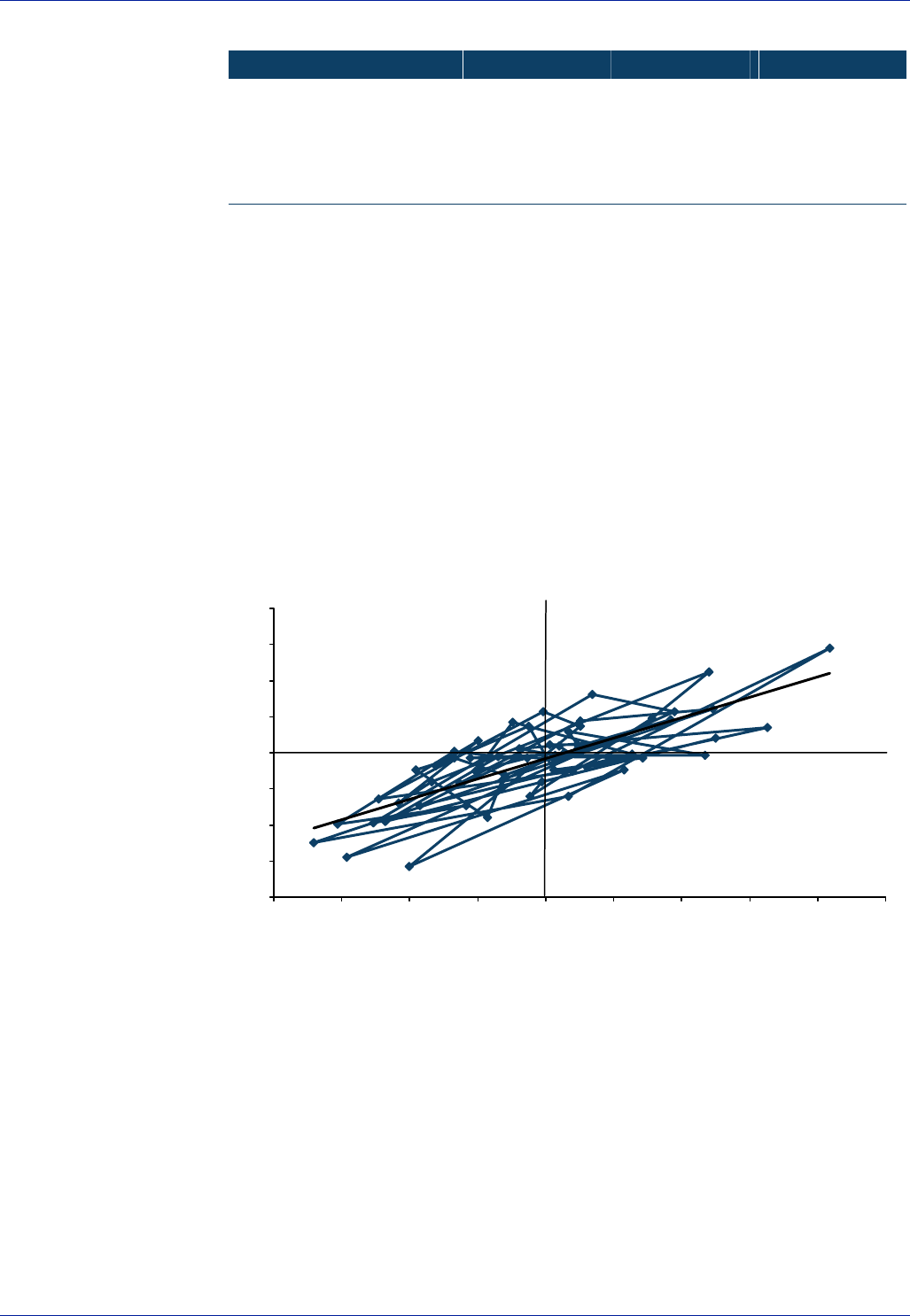
74 Global Rates Strategy Barclays Capital

Figure 29: Volatility Composition in US, France and UK

US France UK

Variance of Nominal Yield 10.1 5.6 5.7

Of Which:

Variance of Real Yield 5.2 2.7 3.0

Variance of Breakeven Inflation 4.0 2.8 3.2

2 × Covariance (RY, BEI) 0.9 0.1 -0.5

Notes: Figures based on monthly changes for the years 1999 to 2003. Inflation bonds used are the TII08,

OATi09 and UKTI09, respectively. Variances are in non-annualised basis points.

Source: Barclays Capital.

The table above shows that, on average, in the very long term, real yields have been

around half as volatile as nominal yields. This would suggest that the yield betas in all

three markets have averaged close to 0.5. However, even the measurement of beta can

be disputed. The analysis here uses monthly yield change data. If instead the level of

nominal and real yields is used then the corresponding yield betas are between 0.8 and

0.9 for the three countries. In other words while month-on-month real yields are much

less volatile than nominal yields, over the long term the trend that they follow is not

that much less erratic than in nominal yields. Neither method is ideal. The former is less

statistically biased, but equally trend data may contain important information that you

do not want to ignore.

Figure 30: Long-term Beta on TII08 Based on Monthly Yield Changes

beta 0.56

y = 0.56x - 0.03

R2 = 0.61

-0.8

-0.6

-0.4

-0.2

0.0

0.2

0.4

0.6

0.8

-0.8 -0.6 -0.4 -0.2 0 0.2 0.4 0.6 0.8 1

Change in nominal yield

Change in real yield

Source: Barclays Capital.

Barclays Capital Global Rates Strategy 75

Figure 31: Long-term Beta on TII08 Based on Monthly Yield Levels

beta 0.83

y = 0.83x - 0.95

R2 = 0.94

0.0

0.5

1.0

1.5

2.0

2.5

3.0

3.5

4.0

4.5

5.0

2.0 2.5 3.0 3.5 4.0 4.5 5.0 5.5 6.0 6.5 7.0

Nominal yield

Real yield

Source: Barclays Capital.

In the shorter term, the difference between the level and change measures of beta are

rarely as large as in the example above due to the trending nature of the variables being

less powerful, but there can still be a notable difference. In practice, the majority of the

market uses level-based betas, so in the absence of a strong theoretical preference

either way we generally do the same. Within longer-term portfolio analysis we prefer to

consider return volatility analysis, which has the additional benefit of including inflation

carry data directly. For the five years from 1999 to 2003 the monthly return beta is 0.55

for the Barclays Capital US index, 0.58 for the Euro government index and 0.77 for the

UK government index.

As yield betas are generally less than one, a breakeven inflation trade, ie, with equal

notional dv01 weights on the nominal and real legs, is usually a directional trade. The

most notable exception was the period November 2002 to April 2003 when, unusually,

the betas in all the major markets were above one, due to portfolio reallocation from

equities to real bonds leaving them tending to outperform on bullish fixed-income days.

In a rallying market, a breakeven trade usually underperforms absent carry

considerations, as nominal yields are more volatile. Beta weighting of the trade, ie,

dividing the simple dv01 of the real leg by its yield beta, is an attempt to remove

directionality. However, it is only an effective means of doing this if the beta continues

to trade as it has done historically though, which is far from certain.

76 Global Rates Strategy Barclays Capital

Figure 32: Yield Beta Regimes for the TIIJan12 Since Launch

Nov02-Apr03

y = 1.47x - 3.59

R2 = 0.83

Apr03-Sep03

y = 0.55x - 0.12

R2 = 0.91

Oct03-Dec03

y = 0.59x - 0.54

R2 = 0.38

Jan02-Nov02

y = 0.72x - 0.49

R2 = 0.90

1.0

1.5

2.0

2.5

3.0

3.5

4.0

2.5 3.0 3.5 4.0 4.5 5.0 5.5

Real Yield

Nominal Yield

Source: Barclays Capital.

As the chart above shows, in practice inflation bonds have tended to trend within

relatively tight yield beta regimes versus nominal bonds. Typically these periods extend

for a number of months, though some have lasted as long as two years. When such

trading regimes break there is usually a relatively quick transition phase, of no more

than a month, followed by a new regime in which the beta is quite different from that in

the previous regime. Since September 2003, both the European and US markets appear

to have moved into a different phase though, with no equilibrium beta regime

establishing itself. This may be a sign of uncertainty in the market during a phase of

portfolio reallocation. However, we see a significant chance that there has been a more

fundamental shift as liquidity in the market has improved. Instead of inflation bonds

being traded as a spread product to nominal bonds they now appear to behave more

like an independent asset class. While fundamental longer-term beta relationships are

likely to hold, it may just be that medium-term trading regimes are a thing of the past.

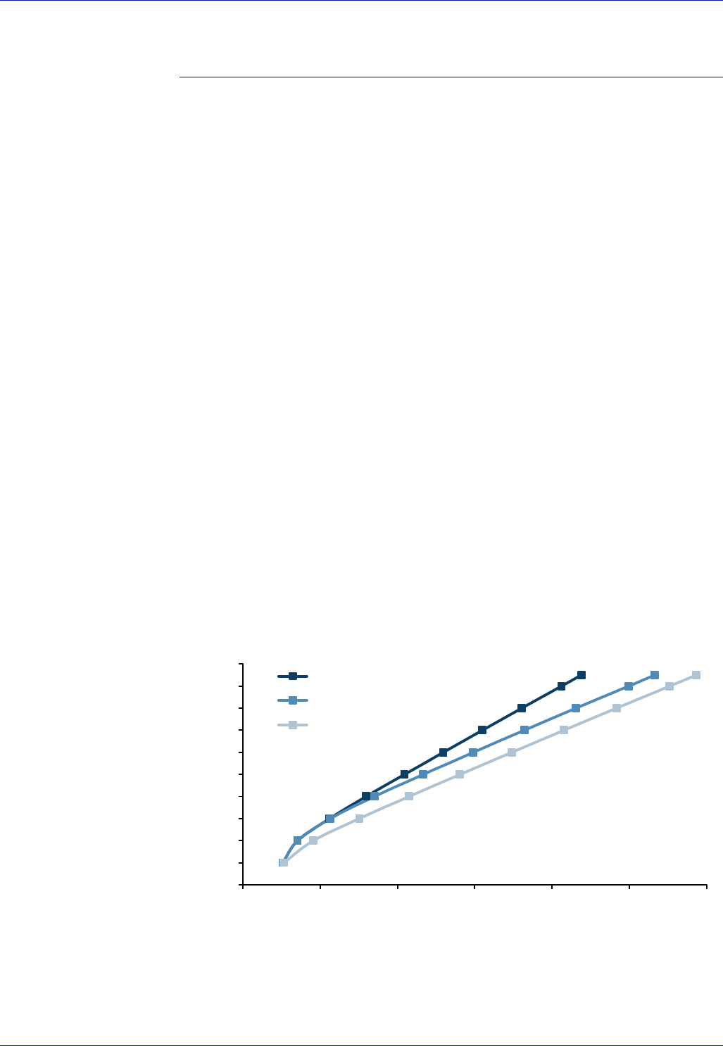
Barclays Capital Global Rates Strategy 77

Linkers in a Portfolio Context

Mike Oman

Much has been made of the enhancements that can be made to the risk and return

characteristics of a fixed income/equities portfolio by the inclusion of linkers from a

theoretical point of view. The theoretical argument effectively relies on the beta

relationship between real and nominal yields. Using the Fisher equation as a starting

point, a nominal bond yield can be broken down into a real return, which is reward for

saving, or compensation for lending rather than investing, inflation compensation and a

risk premium, as discussed previously in this guide. Ignoring the risk premium element

for the moment, assuming some degree of covariance between expected inflation and

nominal rates, as is reasonable, the beta between real and nominal yields will be less

than 1: a proportion of the variability in nominal yields is accounted for by variability in

breakevens, leaving real yields comparatively more stable, and giving real bonds less

price and return volatility. The attractiveness of an asset for a portfolio is usually

measured in terms of the risk and return play-off, and so if the theory holds in reality,

linkers should have a good chance of being the fixed income asset of choice over the

more volatile nominal bonds. We have put this to the test in the US TIPS market and the

UK index-linked gilt market.

The US TIPS market is now seven years old, giving enough data to confidently perform

a risk-return analysis. In that time, we have witnessed some strong economic growth,

some quarters of negative growth, an equity market boom and an equity market slump,

reassuring that the sample period does not bring an inhibiting bias to the results of the

analysis, although admittedly the Fed Funds target rate is considerably lower now than

it has been at any time in the period sample period; so from a monetary policy

perspective perhaps, not a complete cycle, but fairly close. The analysis that follows

uses the complete data set for the broadest TIPS index and the Barclays Capital “US

Breakeven Index”, an index of Treasuries that closely matches the maturity and the

weights of the TIPS index to enable a fair contest.

Figure 33: TIPS Enhance the Efficient Portfolio Frontier (1997-2003)

3.5%

4.0%

4.5%

5.0%

5.5%

6.0%

6.5%

7.0%

7.5%

8.0%

8.5%

0% 1% 2% 3% 4% 5% 6%

Risk

Return

TIPS, Treasuries, S&P, T-Bills unconstrained

Max 20% TIPS

No TIPS

Source: Barclays Capital.

Also competing for weight in the optimal portfolio are T-Bills and the S&P 500. We

have determined the portfolio weightings of these four assets that give the lowest

possible standard deviation of return for a range of return outcomes. When put

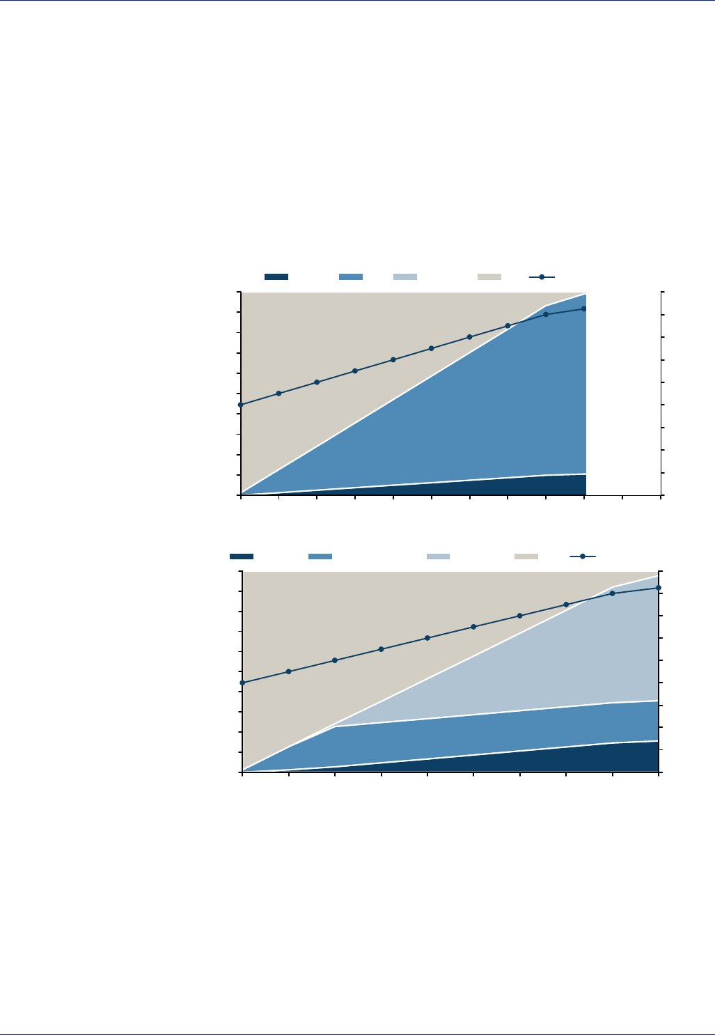
78 Global Rates Strategy Barclays Capital

together, this gives the efficient frontier, and as illustrated by the difference between

the lightest and the darkest frontiers in Figure 33, inclusion of TIPS in a portfolio

enhances the range of available risk-return play-offs.

The breakdown of the asset weightings that would have delivered the optimal risk-

returns characteristics reveals that Treasuries do not get a look in, squeezed out by TIPS

for any specified rate of return. Bills dominate at low return levels due to their

extremely low volatility, with 100% weight in bills to generate the 4% return. However,

beyond risk free returns, the history suggests that a combination of TIPS and equities

should be added to give the optimal mix. The maximum return available in this time

period of 8.25% annualised is achieved at lowest risk with 89% TIPS and 11% S&P 500.

Figure 34: Optimal Asset Split Shows that TIPS Overshadow Treasuries

10%

20%

30%

40%

50%

60%

70%

80%

90%

100%

0.5% 0.7% 1.1% 1.6% 2.1% 2.6% 3.0% 3.6% 4.1% 4.3% 5.0% 5.3%

Risk

Asset spilt of efficient portfolio

S&P 500 TIPS Treasuries Bills Return (RHS)

10%

20%

30%

40%

50%

60%

70%

80%

90%

100%

0.5% 0.7% 1.1% 1.7% 2.3% 3.0% 3.6% 4.2% 4.9% 5.3%

Risk

Asset split of efficient portfolio

S&P 500 TIPS (Max. 20%) Treasuries Bills Return (RHS)

Source: Barclays Capital.

Clearly, given that the TIPS market is 20 times smaller than the Treasury market, it is

not realistic to look at an unconstrained portfolio. The second graph above shows the

weightings that emerge as optimal given the constraint that the maximum TIPS

weighting is 20%. It can be seen that it is necessary to take higher risk than previously

to achieve the same level of return: 5.33% Std Dev for an 8.25% annual return, versus

the 4.38% minimum standard deviation for the same return when an unlimited

proportion of TIPS was allowed.

Barclays Capital Global Rates Strategy 79

Figure 35: Cumulative Nominal Returns in the Period, %

100

120

Apr 97 Apr 98 Apr 99 Apr 00 Apr 01 Apr 02 Apr 03

Bills

S&P 500

TIPS

Treasuries

Source: Barclays Capital.

Looking at the nominal returns cumulatively in the period the portfolio weights make a

great deal of sense. When first launched, inflation expectations as measured by the

breakeven inflation levels were higher than the inflation that emerged, partly due to a

relatively high inflation environment at the time (in the region of 3% Y/Y) and partly

because the scarcity premium that TIPS yields incorporated allowed for relatively high

breakevens. This “first mover’s disadvantage” has been seen in many of the inflation

markets across the world; the initial buyers of linkers will be either those who are most

inflation risk-averse (so those for whom inflation-protection is most precious), or those

who have the highest inflation expectations. Hence, in the early years, TIPS

underperformed Treasuries, but scarcity has since subsided and, if anything, inflation

expectations have at times become too low, so cumulative returns have almost caught

up. Return volatility has been considerably lower, as the theory predicts, and

consequently from a mean-variance perspective the history suggests that TIPS are the

fixed income assets of choice.

UK linkers certainly suffered from the “first-mover disadvantage”. The high and volatile

inflation environment that existed in the UK in the early 1980s was arguably the main

reason why the market began, as investors were in all probability tired of seeing the

purchasing power of their gilt investments dwindle. Early investors were hit by the

double-whammy of the unwinding of the scarcity premium and a dramatic success on

the part of monetary policy makers to curb inflation expectations. The second UK

linker, the IL06, was sold in 1981 at a breakeven of around 9%. RPI has been between

1% and 4% for 10 years. As a result, long-term mean-variance analysis of the UK

market has often shown only a very limited role for UK IL gilts to play in a portfolio of

sterling assets if any at all, and only at low return levels, in line with the general benefits

of diversification (even gold, ex-lending income, the subject of “zero-coupon perpetual”

jibes will feature in the efficient frontier for this reason).

Figure 36 shows rolling 5 yr risk versus return for the FTSE linker index and the FTSE

conventional gilt index. It suggests that pre-1998 in particular, linkers underperformed gilts,

but also suffered from higher return volatility, the worst possible combination of attributes.

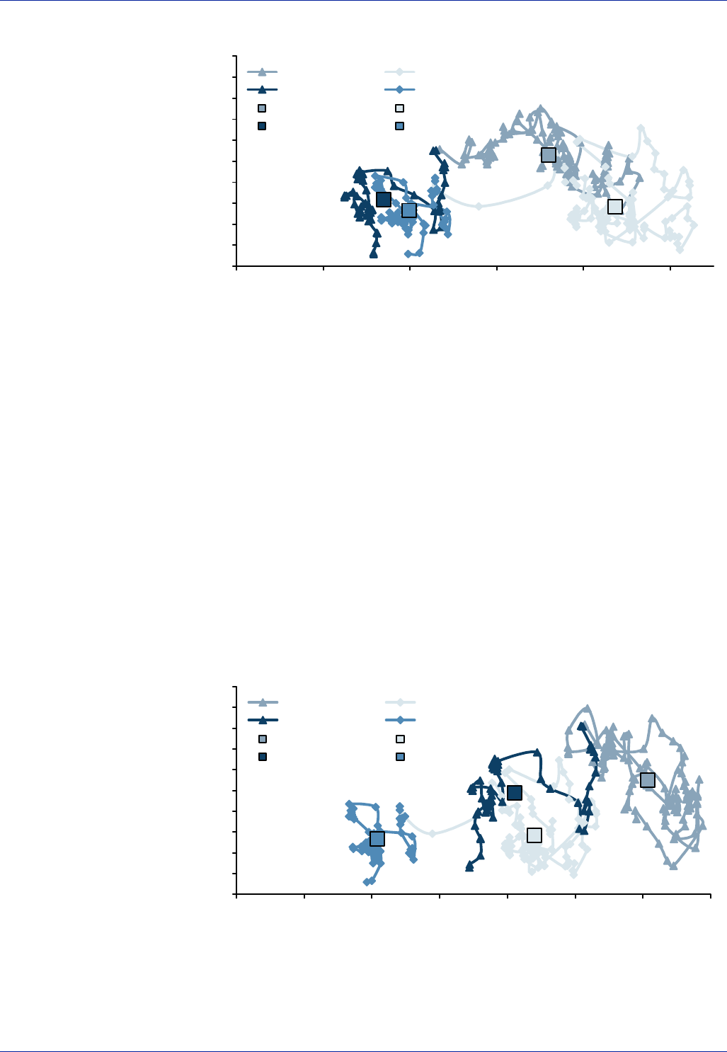
80 Global Rates Strategy Barclays Capital

Figure 36: UKILGs Riskier and Offer Lower Returns Than Conventionals?

10%

11%

12%

13%

14%

15%

16%

3% 4% 5% 6% 7% 8%

Risk

Return

Conv. Gilts 83-98 IL Gilts 83-98

Conv. Gilts 98-03 IL Gilts 98-03

Conv. Ave. 83-98 IL Ave. 83-98

Conv. Ave. 98-03 IL Ave. 98-03

Source: Barclays Capital.

It may seem strange that in the early period linkers suffered higher volatility considering

that much of the fall in nominal yields that occurred can be attributed to falling inflation

expectations (therefore you would expect a low beta and real yields to be less volatile

than conventional yields) and damning for the theoretical claim that linkers are superior

assets for a portfolio. This is a common result but a misleading guide to portfolio

optimisation due to the make-up of the indices used. The first ultra-long dated

conventional was not launched until the mid-80s whereas the shorter-end of the curve

was already highly populated giving the broad conventional index much lower duration

during that earlier period and hence much lower return volatility in response to the

strong down move in yields observed. Arguably a fairer method is to look at a portfolio of

conventional gilts that closely matches the maturity profile and weightings of the linker

index used such as the Barclays Capital Breakeven Index for UK gilts, just as was done for

the TIPS analysis. In this way, it is only the characteristics of the asset class rather than the

specific universe of available assets that is being compared.

Figure 37: A Fairer Comparison Illustrates the Stability of Linker Returns

10%

11%

12%

13%

14%

15%

16%

3% 4% 5% 6% 7% 8% 9% 10%

Risk

Return

Conv. Gilts 83-98 IL Gilts 83-98

Conv. Gilts 98-03 IL Gilts 98-03

Conv. Ave. 83-98 IL Ave. 83-98

Conv. Ave. 98-03 IL Ave. 98-03

Source: Barclays Capital.

As Figure 37 shows, the theoretical prediction for the relative volatility of returns is

borne out when the comparison is fairer from a duration perspective. The poor returns

performance as a result of falling inflation expectations is again evident. If efficient

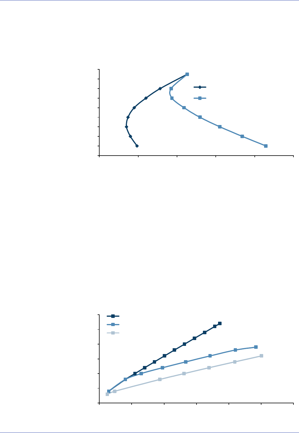
Barclays Capital Global Rates Strategy 81

frontier analysis is tackled using histories of these more comparable indices during the

time that RPI inflation and breakevens stabilised below 5% (1994-2004), it is clear that

UK linkers significantly reduced the volatility of a portfolio’s returns. In that time period,

the returns of the three assets included in the portfolios in Figure 38 were broadly

similar, giving only a slim portfolio frontier, but the principle is clear.

Figure 38: UKILGs Enter the Efficient Portfolio Since Inflation Stabilisation

7.0%

7.2%

7.4%

7.6%

7.8%

8.0%

8.2%

8.4%

8.6%

8.8%

4% 5% 6% 7% 8% 9%

Risk

Return

FTSE 100, UK linkers, UK conventional gilts

FTSE 100, UK conventional gilts, No linkers

Source: Barclays Capital.

The important point is that should the MPC be capable of keeping inflation stable in the

low single digits and positive, the severe underperformance of UK linkers in the 1980s

should not return, and there is no reason to suggest that the relatively lower volatility

characteristic of the asset should not continue, in which case UK linkers should

consolidate their position in the efficient portfolio in coming years.

The European linker market is younger than the US market and has grown considerably

more slowly to date, leaving much less in the way of history to study. However,

preliminary indications, as shown in Figure 39, would suggest that the portfolio

enhancement potential of linkers is as strong as the theory would predict. The

European portfolio includes 3-month money, the Eurotop300 index, OATis and OAT¤Is,

and the breakeven index of French nominal bond comparators. The resemblance to the

result from the US market is striking.

Figure 39: Euro Linkers Show Early Promise

3.2%

3.7%

4.2%

4.7%

5.2%

5.7%

6.2%

0% 1% 2% 3% 4% 5% 6%

Risk

Return

OATi/¤i, Nominals, Eurotop 300, 3m Money unconstrained

Max 20% OATi/¤I

No OATi/¤I

Source: Barclays Capital.

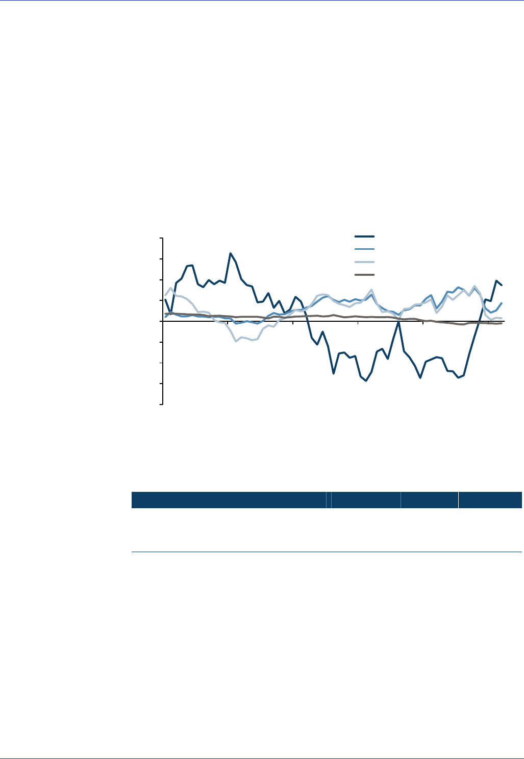
82 Global Rates Strategy Barclays Capital

So far, this analysis has only considered returns in nominal space, as is the norm for

optimal portfolio analysis. Given the nature of the product this guide covers, a mention

of real return volatility is warranted. For the pension fund community, given that it is

real liabilities that need to be matched, the risk-return characteristics of the universe of

assets in real space are arguably what matter. Evidence from the US markets supports

the idea that the volatility advantage that TIPS have over Treasuries and equities is even

greater when considering real returns instead of nominal returns, in this case using the

CPI nsa as the deflator. Bills or money market instruments tend to dominate efficient

portfolios at the lower return ranges due to their extremely low volatility, but it is this

asset class that suffers the most in this respect – real volatility being almost 90% higher

than in nominal terms although still by far the lowest. The conclusion is that TIPS

should therefore demand an even greater weighting in the efficient real portfolio.

Figure 40: TIPS Real 12m Returns Have Been Seldom Negative and

Relatively Stable Versus the Competing Assets

-40%

-30%

-20%

-10%

10%

20%

30%

40%

Sep 98 Sep 99 Sep 00 Sep 01 Sep 02 Sep 03

S&P 500 Real 12m Returns

TIPS 12m Real Returns

Treasuries 12m Real Returns

Bills 12m Real Returns

Source: Barclays Capital.

Figure 41: TIPS is the Only US Asset to Have Lower Real Vol Than

Nominal Vol

1997-2003 S&P TIPS Treasuries Bills

Nominal return volatility % 17.45 4.86 6.98 0.53

Real return volatility % 17.50 4.77 7.00 0.98

Difference (%) 0.27% -1.78% 0.24% 87.18%

Source: Barclays Capital.

Barclays Capital Global Rates Strategy 83

Comparing Real Bonds With Equities

Sreekala Kochugovindan

Historically, equities have been considered to be the asset class most able to counter

inflation risk. A frequently recommended trade for an inflationary period is to switch

out of nominal bonds into equities as robust economic growth is expected to be

accompanied by rallying stock markets. However, recent experience of increased

volatility and the sharp downturn in the aftermath of the speculative bubble serves as a

reminder of the risks attached to using stocks as an inflation hedge. The 25% decline in

the real total return of UK stocks during 2002 placed investors such as pension funds

with long-term real liabilities under intense pressure. In this article we compare

inflation-linked bonds with equities.

The Yield Gap

The most commonly used method of comparing the relative value of equities to bonds

is to examine the yield gap. The standard Fisher equation discussed previously, which

relates the nominal bonds to inflation-linked bonds, has an analogue relating equity

dividend yields to real yields:

dy = dividend yield on an equity index

r = redemption yield for the index-linked government bond index

E(rdg) = markets expected growth rate for equity dividends

erp = the markets expected return for equities (Equity Risk Premium)

dy = r + E(rdg) – erp

Rearranging the equation we have:

r – dy = E(rdg) - erp

So the yield gap between equities and bonds is equal to the gap between expected real

dividend growth rate and the risk premium demanded by investors in order to hold

equities. Alternatively, we can relate real yields to equity earnings yields and gain the

following relationship:

r – ey = E(reg) - erp

Where

ey = Equity earnings yield

E(reg) = expected real equity earnings growth

Just as the inflation risk premium is avoided in the nominal versus real bond Fisher

equation when the formula is reduced to:

Nominal yield – real yield = breakeven inflation,

In the equity/real yield relationship the analogue is:

Dividend yield gap = breakeven future real dividend growth

Equity yield gap = breakeven future real earnings growth

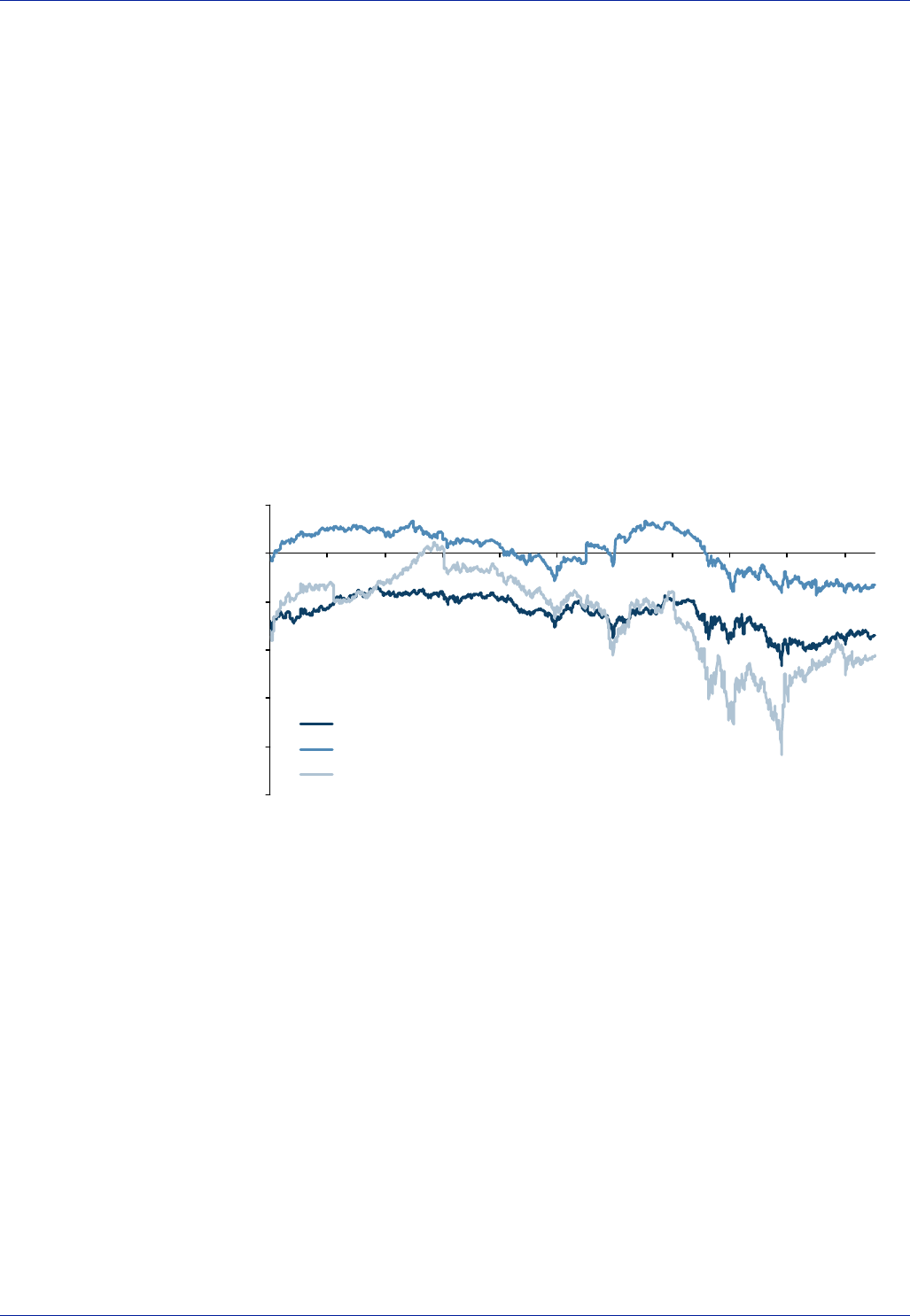
84 Global Rates Strategy Barclays Capital

So it is possible to remove the equity risk premium from the equation just as the

inflation risk premium was removed from the Fisher equation.

The dividend yield gap between the FTSE All share and IL All Maturity reached -2.3% in

March 2003, the highest level in 20 years, indicating the cheapest valuation of equities

versus index-linked bonds in two decades. Since then, the yield gap has retraced to

-1.14%, which can still be regarded as an historically high level. The high yield gap in

March 2003 possibly reflected deflationary fears and the expectation that corporate

profits and hence dividends would remain subdued or even worsen. As these

deflationary fears dissipated, the market yield gap began to edge back towards zero.

As indicated above, the real yield gap can also be expressed in terms of the earnings

yield instead of the dividend yield. The earnings yield is considered to be a more reliable

indicator given that the relevance of the dividend yield diminished during the 1990s as

more and more companies chose to return cash to shareholders via buybacks rather

than paying out bigger dividends. The chart below plots the history of the real yield gap

in the UK, the US and France. In each country, equities appear cheap relative to index-

linked bonds compared to the historic average.

Figure 42: Real Yield Gap

-10

-8

-6

-4

-2

Sep 98 Mar 99 Sep 99 Mar 00 Sep 00 Mar 01 Sep 01 Mar 02 Sep 02 Mar 03 Sep 03

UK Yield Gap

US yield gap

Fr Yield Gap

Source: Barclays Capital.

Do Equities Provide an Adequate Inflation Hedge?

Equities are considered to be a real asset because the investor receives a dividend

payment plus the capital appreciation of the equity. During a period of robust

economic growth, companies’ profits are likely to strengthen, as both the output of the

company and the prices the company is able to charge rise. Rising profits result in

higher stock valuation and at the aggregate level, nominal equity returns are likely to be

greater if inflation is higher. The nominal bond, on the other hand, provides the investor

with a regular coupon payment fixed for the life of the bond regardless of any changes

in the rate of inflation.

In the case of real assets, we would expect a strong positive correlation between the asset

value and inflation. Using over 100 years of historical data for the UK and US, we can

calculate the 20-year rolling correlation between inflation and equity total returns to test

how well equities perform under different inflation scenarios. The charts display the

correlations of inflation with both real total returns and nominal total returns. The

striking feature in both charts is that the correlations are actually negative for most of the

century, suggesting that equity performance deteriorates as inflation rises, even when

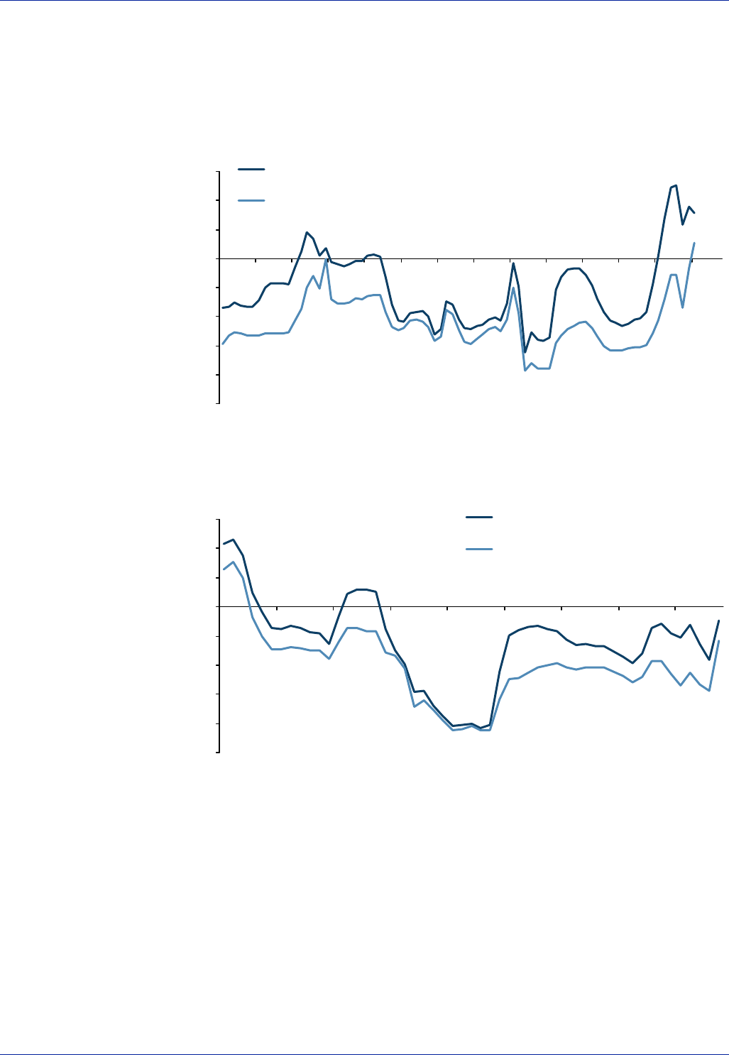
Barclays Capital Global Rates Strategy 85

returns are measured in nominal terms. In the case of the UK, real returns were

negatively correlated until 1996, after which they became positively correlated. US stocks

on the other hand only exhibit a negative relationship after WW2. Focusing on the 1970s,

a decade characterised by excessive levels of inflation, the correlation becomes even more

negative as equities posted one of the worst performances of the century.

Figure 43: Rolling Correlation between UK Equity Total Returns and RPI

-1.0

-0.8

-0.6

-0.4

-0.2

0.0

0.2

0.4

0.6

1924 1930 1936 1942 1948 1954 1960 1966 1972 1978 1984 1990 1996 2002

Correlation between 5 year annualised

nominal returns & Inflation

Correlation between 5 year annualised real

returns and inflation

Source: Barclays Capital.

Figure 44: Rolling Correlation between US Equity Total Returns and CPI

-1.0

-0.8

-0.6

-0.4

-0.2

0.0

0.2

0.4

0.6

1950 1956 1962 1968 1974 1980 1986 1992 1998

Correlation between 5 year annualised

nominal returns & Inflation

Correlation between 5 year annualised real

returns and inflation

Source: Barclays Capital.

Figure 45 compares the real total returns of the different asset classes over time. The

table focuses on the UK market as it possesses the most mature index-linked bond

market. The first three columns display the annual returns for the individual years while

the last three columns display the annualised return over 10 years, 20 years and 50

years. Data for index-linked bonds is only available for 20 years so long-term

comparisons are not possible here; however the table does illustrate the weak

performance of equities during a period of stable inflation (2002) and during periods of

high inflation. The OPEC crisis at the end of 1973 induced the worst equity bear market

of the 20th century with real total returns falling 58% in 1974. The 20 and 50 year

annualised returns show strong results for equities, suggesting that equities may act as

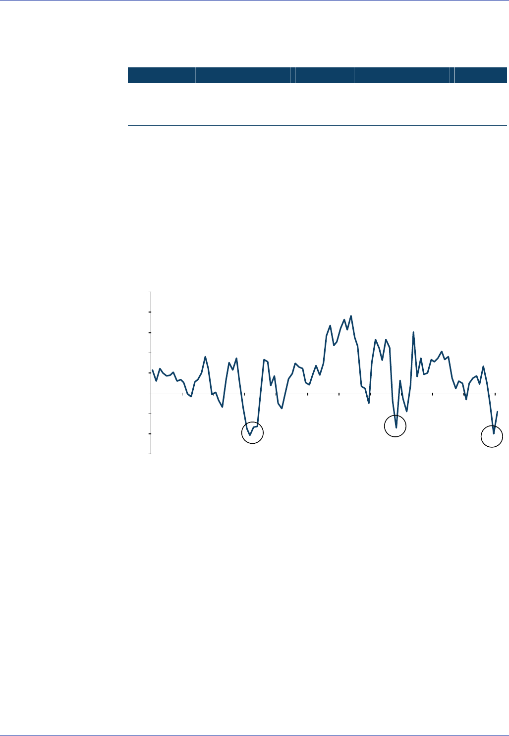
86 Global Rates Strategy Barclays Capital

a good inflation hedge over the long run, but the short-term fluctuations could be

enough to endanger those pension funds which may need to meet their real liabilities.

Figure 45: UK Real Total Returns

Last 2002 1979 1974 10 Years 20 Years 50 Years

Equities -24.5 -4.9 -58.0 3.2 8.0 6.9

Gilts 6.7 -11.0 -29.0 4.6 6.1 1.6

Index-Linked 5.1 3.7 3.9

Source: Barclays Capital.

The chart below illustrates the equity risk premium defined as the difference between

the total return of equities and nominal gilts. The chart again serves to illustrate the

underperformance of equities during three distinct inflation periods: 1) deflation during

the 1930s; 2) high inflation during the 1970s; 3) low and stable inflation in recent years.

These three periods are highlighted in the chart below and shows that relative equity

underperformance is possible under all three scenarios.

Figure 46: UK Equity Risk Premium: Excess Return of Equities Relative to

Gilts (5-year Annualised Returns)

-15

-10

-5

1904 1913 1922 1931 1940 1949 1958 1967 1976 1985 1994 2003

Source: Barclays Capital.

Conclusion

Equities have traditionally been considered to provide a good hedge against inflation.

Although this seems true in the very long run, the higher level of short-term volatility

poses dangers for investors with real liabilities. Index-linked bonds on the other hand

provide a real yield determined in advance, which provides the investor with greater

inflation protection. Combined with the fact that they are a separate asset class, they

possess lower volatility of returns and a low level of correlation with other assets,

linkers provide attractive properties with a balanced portfolio even for those without

explicit real liabilities.

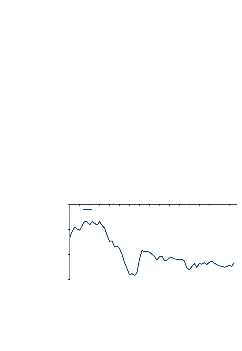
Barclays Capital Global Rates Strategy 87

Comparing Linkers to Other Real Assets

Sreekala Kochugovindan

The analysis adapted for equities in the previous article can also be applied to other real

assets. In this article we consider the relative performance of commercial property and

commodities with index-linked government bonds.

Beginning with the yield gap, the Fisher equation analogue for property can be defined

as follows:

ry = rental yield on property

= Rental income (net of annual outgoings)/(Market value + Purchaser’s Costs)

r = redemption yield for the index-linked government bond index

r – ry = Breakeven rental income growth

Figure 47 plots the gap between the UK All Maturities index-linked government bond

yield and the rental yield of UK commercial property as provided by the Investment

Property Databank (we focus on commercial property only as institutional investor

portfolios mainly include commercial rather than residential property). The average

rental yield for the past 10 years stands at 7.5% compared to the average real yield of

2.9% and the equity earnings yield of 4.9%. The consistently high relative level of

commercial rental yield implies that the risk premia associated with property is even

greater than that of equities. This could be due to a number of reasons including poor

liquidity, tenant default risk and maintenance costs. In the aftermath of the property

market crash of the early 1990s, rental yields rose to as high as 9% in 1993 from 5.2%

in 1989. Since then, rental yields have remained at relatively high levels, fluctuating

between 6% and 8%.

Figure 47: UK Real Yields vs Rental Yields

-6

-5

-4

-3

-2

-1

87 88 89 90 91 92 93 94 95 96 97 98 99 00 01 02 03

Real yield - Rental yield

Source: Datastream, IPD.

Total Return Comparisons

Figure 48 plots the total returns of the IPD commercial property total return index and

the Goldman Sachs Commodity total returns index. Annual commercial property total

returns slumped 15% in 1990 despite an inflation rate of 10%. Shifts in both supply and

demand were responsible as the property boom of the late 1980s brought with it a

88 Global Rates Strategy Barclays Capital

stream of leveraged developers which increased the stock of office buildings, while the

recessionary slump in demand induced excess supply and tumbling property returns.

Figure 48: Real Annual Total Returns – Commercial Property and

Commodities

-60%

-40%

-20%

20%

40%

60%

80%

88 89 90 91 92 93 94 95 96 97 98 99 00 01 02 03

-20%

-15%

-10%

-5%

10%

15%

20%

25%

30%

Commodity returns (LHS)

Property Returns (RHS)

Source: Datastream, IPD.

Commodities are frequently perceived as a reliable inflation hedge and examining the

past 15 years of data we find that there is a positive correlation between commodity

returns and the annual rate of inflation. While the property market slumped during

1990 and 1991, commodities real returns were as high as 29%. However, as highlighted

in the chart above, these returns were highly volatile, swinging from 29% to -2% in the

final two quarters of 1990.

The All Commodities index has proven to be the most volatile of all the real asset

classes. Gold and precious metals are often cited as lower volatility inflation hedged

assets. Figure 49 below plots the Goldman Sachs All Commodity total returns and

the Precious Metals sub-index total returns. The precious metals sub-index contains

83.14% Gold, 8.62% Silver and 8.24% Platinum. Although the volatility of the

precious metals index is significantly lower, it is interesting to note that during the

high inflation years of the late 1980s and early 1990s, the annual total returns are

predominantly negative. In addition to this, precious metals are still more volatile

than index-linked bonds.

Barclays Capital Global Rates Strategy 89

Figure 49: Real Annual Total Returns – All Commodity Returns and

Precious Metals Sub Index

-50%

-30%

-10%

10%

30%

50%

70%

88 89 90 91 92 93 94 95 96 97 98 99 00 01 02 03

All commodity returns

Precious metals returns

Source: Datastream.

As was the case for equities as a real asset, it seems that property and commodities

provide a fair degree of inflation protection in the long run. However, these asset

classes possess greater volatility than index-linked bonds and are therefore more prone

to short-term fluctuations, posing considerable risks for investors with real liabilities.

Barclays Capital Global Rates Strategy 91

Value Analysis

92 Global Rates Strategy Barclays Capital

Fundamental Factors Behind Real Yields

Tim Bond

The topic of real bond yields is a notorious analytical quagmire. Macroeconomic theory

provides a generous list of potential variables that should influence real yields. These

factors include monetary policy settings, trend productivity and GDP growth rates,

demographics, fiscal positions and investor risk appetites. To some extent, all these

factors have a discernable impact on real yield movements. However, the empirical

estimation of the size of these responses is, in practice, difficult to accomplish. Three main

problems dog such exercises. Firstly, the historical database of true real yields is limited by

the relative juvenility of the index-linked markets. Secondly, the construction of longer

time series for real yields is an uncertain process, largely due to ambiguity over the choice

of the appropriate deflator and the paucity of reliable information on long-term inflation

expectations. Thirdly and perhaps most importantly, many of the potential explanatory

variables for real yields tend to be endogenous to the business cycle. Thus, the apparently

weak observable correlations between fiscal positions and real yield levels may be partly

due to the obvious point that the majority of government borrowing fluctuations are

attributable to the business cycle. During recessions, the fiscal position tends to

deteriorate, theoretically placing upward pressure on real yields, yet monetary policy is

usually eased at the same time, placing downward pressure on real yields. Conversely, risk

appetites and productivity growth are positively correlated with the business cycle,

obscuring the degree of causation for changes in real yields. Additionally, the scale of real

yield responses to their presumed driving factors is geographically varied. With these

caveats established, the following is an attempt to highlight some of relationships

between real yields and their theoretical causative factors.

Monetary Policy

Within the framework of a short- to medium-term investment horizon, actual and

expected monetary policy settings are the most important influence on real yields.

Inasmuch as medium-term yields are the sum of the expected short-term rates, the

theoretical underpinnings for the markedly high correlations between short rates and

long-term real yields are strong. Indeed, since the difference between nominal yields

and real yields – breakeven inflation – represents the marketplace’s verdict on the

success of monetary settings, it is unsurprising to find that nominal yields have greater

freedom of manoeuvre relative to official rates than is demonstrated by real yields. The

volatility of long nominal yields relative to actual and expected official rates lies in

inflation expectations, not in real yields.

Figure 50 demonstrates this proposition. It displays the results of a 2 variable regression

model for daily 10-year TIPs yields, in which the explanatory variables are the Fed funds

rate and 1 year forward 3-month Libor. With an R-squared of 0.90 and a standard error

of 23 bp, it is clear that the bulk of short-term fluctuations in real yield result from

shifts in the actual and expected short rate structure.

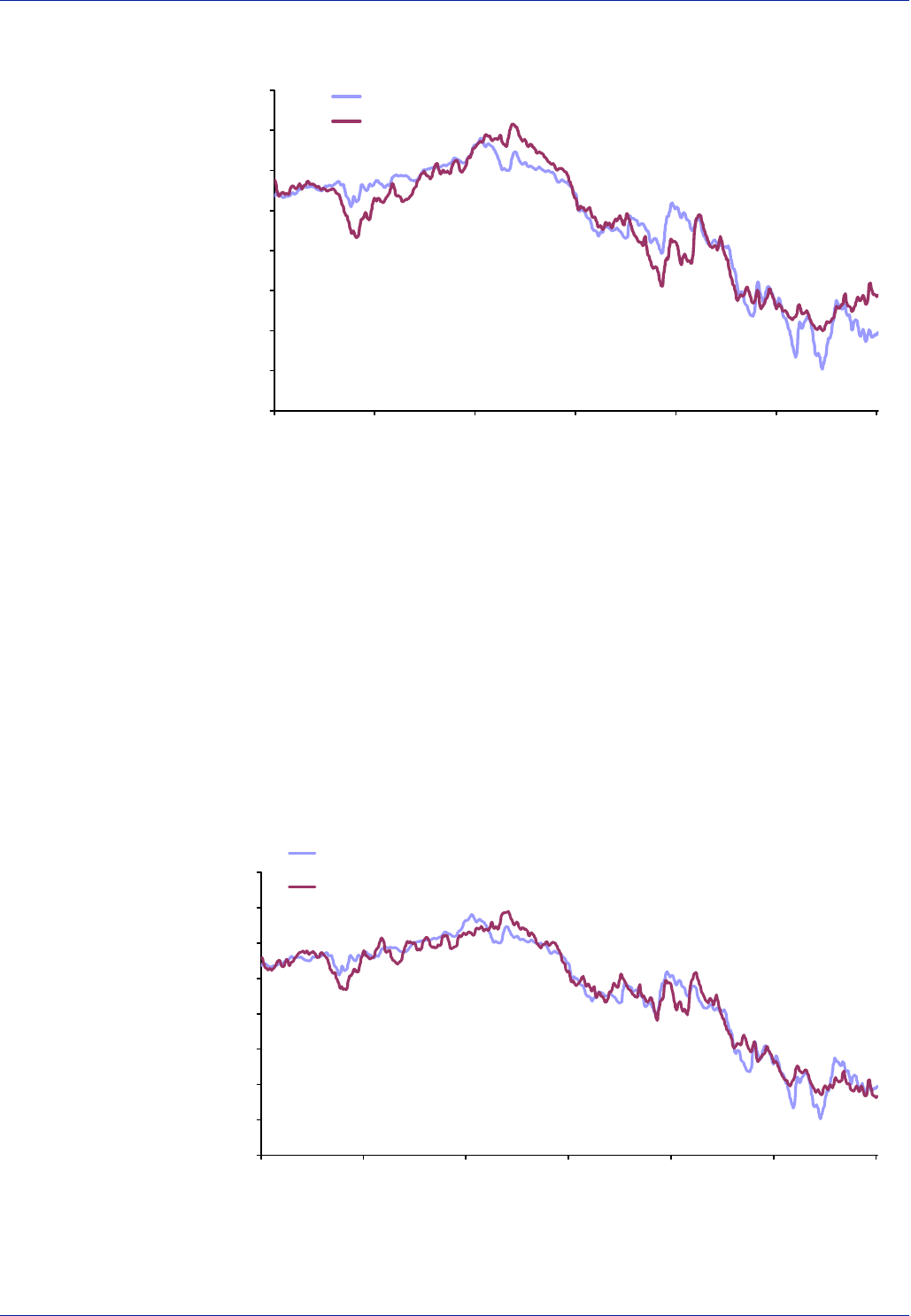
Barclays Capital Global Rates Strategy 93

Figure 50: US 10 yr TIPs Yields, Actual And Modelled from Fed Funds and

1 yr Forward 3-month Libor

1.5

2.5

3.5

4.5

01/01/98 01/01/99 01/01/00 01/01/01 01/01/02 01/01/03 01/01/04

Actual

Model

Source Barclays Capital.

We would note in passing, with reference to previous studies of US real yields, that the

calibration of this model could be further improved with the inclusion of a raw material

price variable. With the addition of the Economist All Industrials Commodity Index, the

R-squared rises to 0.96 and the standard error drops to 15 bp. The improvement is due

to the strong positive correlation between inflation expectations and commodity prices.

Rising commodity prices increase inflation expectations, in turn increasing the demand

for inflation protection, reducing TIPs yields. The coefficient for the raw materials in the

regression is negative. Eventually, incipient inflationary pressures heralded by rising raw

material prices would be expected to raise the anticipated (and actual) Fed Funds rate,

pushing real yields upwards. In the absence of such expectations, counter-intuitively, a

rise in inflationary expectations tends to lower real yields.

Figure 51: US 10-year TIPs Yields, Actual and Modelled from Fed Funds

rate, 1 year Forward 3-month Libor and the Economist Industrials Index

1.5

2.5

3.5

4.5

01/01/98 01/01/99 01/01/00 01/01/01 01/01/02 01/01/03 01/01/04

Actual

Model

Source Barclays Capital.

The link between official short rates and the level of long real yields suggests that a

Taylor Rule approach to the modelling of real yields might be appropriate. Such a line

of analysis is indeed successful in the US, although the short lifespan of the TIPs market

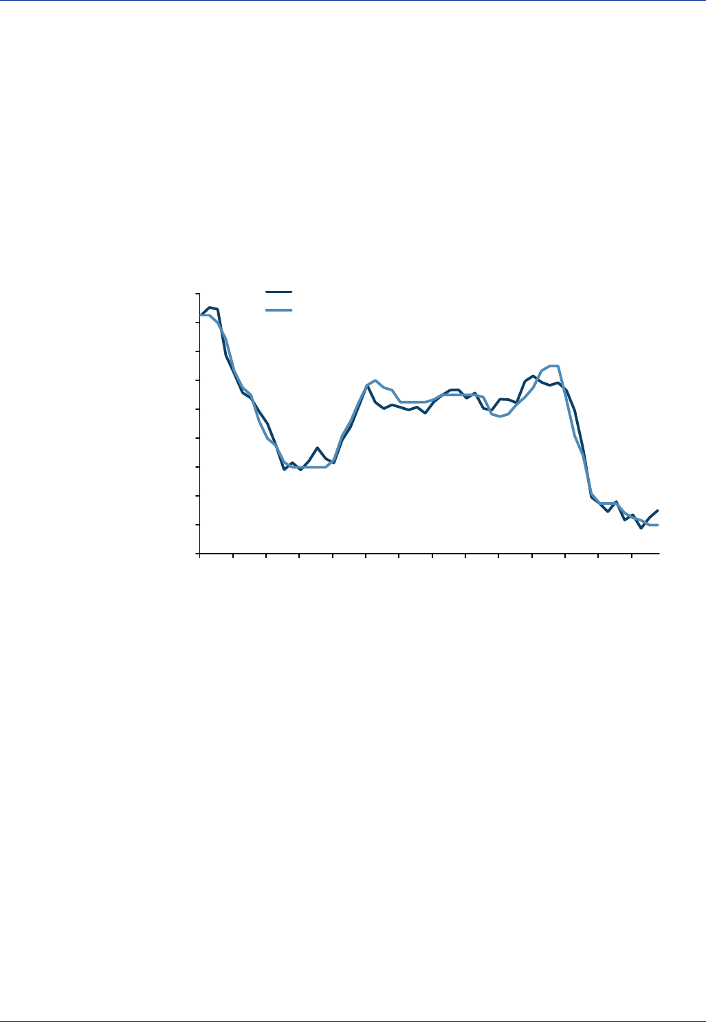
94 Global Rates Strategy Barclays Capital

does not provide sufficient history to prove this point conclusively. The Federal

Reserve’s triple mandate is to control inflation, while maintaining employment levels

and ensuring financial market stability. Adapting the Taylor Rule to encompass these

three objectives, we have constructed a 4 variable equation for the Funds Rate,

consisting of the core consumption deflator, the unemployment “gap”, the trade-

weighted dollar and low grade corporate bond yield spreads (proxying for financial

market stability). The unemployment “gap” is the difference between current

unemployment and the moving average of the historic unemployment rate at which

unit labour cost growth is zero. This measure is designed to represent the slack – or lack

of slack – in the labour market. The model successfully captures the bulk of the FOMC’s

decisions over the past decade.

Figure 52: Fed Fund Rate Actual and Modelled from Core Inflation,

Unemployment Gap, Trade-weighted Dollar and Corporate Bond Spreads

1990 1991 1992 1993 1994 1995 1996 1997 1998 1999 2000 2001 2002 2003

Model

Fed Funds

Source Barclays Capital.

Unsurprisingly, given the positive coincident correlation between TIPs yields and Fed

policy, these same variables have strong explanatory power for real yields. In Figure 53

below, we apply the adapted Taylor rule to explain 10-year nominal yields deflated by

10-year inflation expectations. The match is not perfect, but the r-squared of 0.75

suggests that some of the main influences on real yields are indeed being captured. The

implication is that for investment purposes, the process of forecasting real yield

movements over the medium term should follow similar parameters to those employed

when forecasting movements in official short rates.

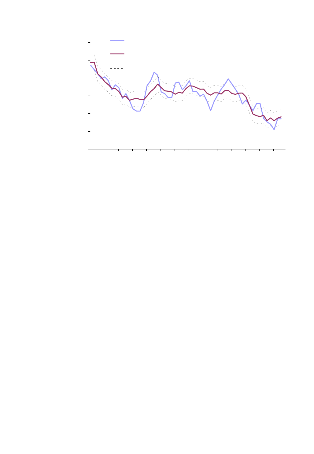
Barclays Capital Global Rates Strategy 95

Figure 53: 10-year US Treasury Yields Deflated by 10-year Consensus

Inflation Expectations, Actual and Modelled from Core Inflation, the

Unemployment Gap and Corporate Bond Spreads

Jun-

10 yr yields minus 10 yr

expected inflation

Model

standard error

Source Barclays Capital.

A similar analysis is slightly less effective in the UK. A clear positive link between actual

and anticipated monetary settings and longer-term real yields is certainly visible, but

the relationship is less robust. The r-squared of a regression of base rates, 1-year

forward 3-month Libor and a constant 10-year linker yield is 0.67, even for monthly

data, as opposed to 0.90 for daily data when the same exercise is conducted in the US

market. However, when a further fiscal variable is introduced, the PSNCR/GDP ratio, the

model improves noticeably, the r-squared rising to 0.80 and the standard error falling

10 bp. We use the one-year forward PSNCR/GDP ratio in the equation, on the

assumption that information regarding impending deficit/GDP ratios is readily

forecasted and consequently available to market participants far ahead of time. In

particular, the introduction of the fiscal variable corrects the model’s overestimation of

real yields during the 1999-2000 period. During those years, real yields stayed

remarkably low, despite monetary tightening. Anecdotally, the anomaly was explained

by the strong demand for long linker assets meeting a shrinking supply generated by

budget surpluses. The results of this model suggest that this anecdotal explanation was

indeed correct. The exercise informs us that a 1% change in the deficit/GDP ratio

changes longer-term real yields by 13 bp, a result that is within the admittedly wide

boundaries established in academic surveys of the impact of fiscal positions on long-

term interest rates.

96 Global Rates Strategy Barclays Capital

Figure 54: UK 10-year Constant Maturity Linker Yields, Actual and

Modelled From Base Rates and 1-year Forward 3-month Libor, With and

Without Fiscal Variable

1.5

2.5

3.5

4.5

5.5

1986 1987 1988 1989 1990 1991 1992 1993 1994 1995 1996 1997 1998 1999 2000 2001 2002 2003

UK 10 year real yields

Modelled from 1 year forward 3

month money and the defict /

GDP ratio

modelled from base rates and

forwards

Source Barclays Capital ONS.

Demographics

Shifts in the age distribution of populations have a pronounced effect on long-term

trends in financial asset yields. The theoretical justifications for this influence can be

found in the life-cycle theory of savings, in the relationship between the dimensions of

the working age population and structural fiscal pressures and in the pertinence of the

average age of the working population to productivity and inflation trends. Figure 55

and Figure 56 below illustrate the results of our models for US and UK nominal long-

term government bond yields, in which the explanatory variables are age buckets of the

respective populations, expressed as percentages of the total population. In the UK, we

use the 25-44 year cohort, which has a negative correlation to yields, together with the

15-24 and 65-75 year cohorts, which show a positive correlation to yields. In the US

model, we have confined the exercise to two variables, the 35-54 year cohort and the

65 yr plus cohort, the correlations being similar to those displayed in the UK model.

These results conform to the theoretical expectations that when the workforce of peak

productive and savings age is expanding, a downward pressure on financial asset yields

should be visible, while the converse applies when the dependent population undergoes

a relative expansion. Interestingly, the coefficients for the working age populations are

similar in both countries, at minus 0.5 for the UK 25-54 year age group and at minus

0.7% for the 35-54 year cohort in the US, per 1% of the total population. In the UK

figure, we have also provided an out-of-sample result, in which the regression was

stopped in 1990.

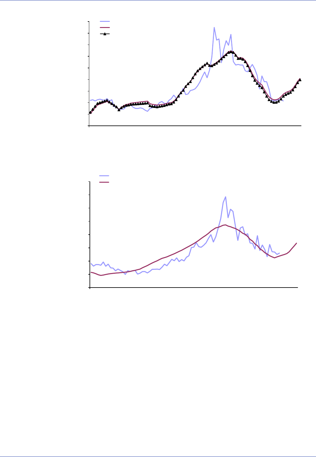
Barclays Capital Global Rates Strategy 97

Figure 55: UK Long Gilt Yields Actual and Modelled From Demographics

1922 1932 1942 1952 1962 1972 1982 1992 2002

Yield

Model

out of sample from 1990

Source Barclays Capital.

Figure 56: US long Treasury Yields Actual and Modelled From

Demographics

1926 1936 1946 1956 1966 1976 1986 1996 2006

actual

Model

Source Barclays Capital.

The models above are of nominal yields because we lack a reliable long-term dataset for

real yields. However, movements in medium and long Linker yields in the UK display an

average quarterly correlation of 90%, 1985-to-date, while even on a daily basis, US

linker yields show an 83% average coincident correlation with US nominal yields.

Therefore, it is reasonable to suppose that the broad impact of demographic shifts on

nominal yields exhibited above is mirrored by a comparable effect on real yields.

While the demographic explanation for long-run changes in real yields and the

monetary policy explanation for short-run changes are apparently two irreconcilable

approaches to the subject, in practice we can square this analytical circle. Somewhat

surprisingly, long-run trends in T-bill yields – which can be assumed to approximate to

official short-term interest rates – appear to be influenced by demographic trends. In

Figure 57 and Figure 58 we perform a similar analysis to Figure 55 and Figure 56,

substituting 1-year nominal T-bill yields in the UK and US for long government yields.

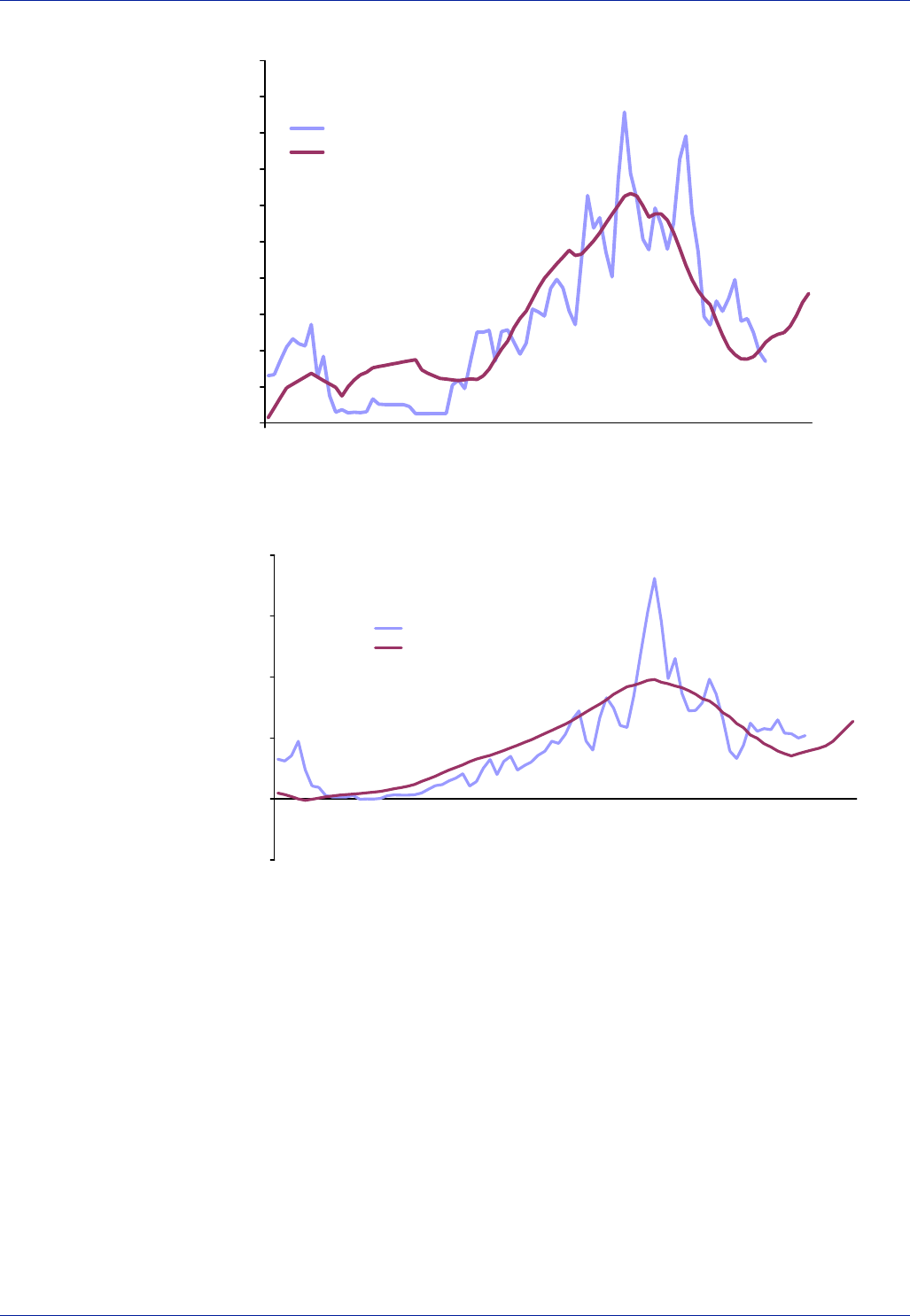
98 Global Rates Strategy Barclays Capital

Figure 57: UK T-bill Yields Modelled from Demographics

1922 1932 1942 1952 1962 1972 1982 1992 2002

1yr Bill UK Yield

Model

Source Barclays Capital.

Figure 58: US T-bill Yields Modelled From Demographics

-5.00

0.00

5.00

10.00

15.00

20.00

1926 1936 1946 1956 1966 1976 1986 1996 2006

Actual 12 month US T-bill

Model

Source Barclays Capital.

The reasoning behind this apparently eccentric finding is actually straightforward.

Fluctuations in the supply of workers, particularly workers of peak productivity age, will

influence inflation rates, in turn influencing monetary policy. Shortages of workers

relative to dependents will tend to foster wage inflation cycles – as these demographic

models correctly predicted would occur in the 1970s. A preponderance of savers over

dependents will also tend to keep the cost of capital lower than otherwise. Such an

environment would tend to be friendly for investment, suggesting little possibility of

inflationary bottlenecks on the supply side and indeed some risk of a deflationary over-

expansion of the supply-side. This occurred in Japan and would probably have occurred

in the US, had the boom run on for a few years and had the investment frenzy not been

so narrowly focussed on information technology.

Overall, fluctuations in the ratio of savers to dependents will influence the price of

capital and hence, at a second remove the inflationary potential of the supply-side of

the economy. The fluctuation of the worker-dependent ratio, which is much the same

Barclays Capital Global Rates Strategy 99

thing as the saver-dependent ratio, also directly influences the inflationary potential of

the supply side via the economy’s associated propensity for wage inflation.

Demographic shifts that tend to constrict the supply of savings – thus pressing real

yield higher – will also tend to render the economy more prone to inflation, thereby

pressing official short-term rates higher. We could also add that at least in theory,

changes in the worker/saver-to-dependent ratio will influence the structural fiscal

position for governments. A shortage of workers will tend to increase government

borrowing, the opposite also applying. Very broad trends in the US deficit/GDP ratio,

when adjusted for the distortion caused by WW2, follow the patterns mapped out by

the fluctuations in these demographic factors.

As is visible in all the demographic models exhibited above, the decade ahead is

characterised by upwards pressure on interest rates and real yields. This is due to the

steady increase in the retirement of the baby-boomers and the consequent decline in the

size of the worker and saver cohort, relative to the retired. This process can be expected

to expand structural government deficit positions, render the economic environment

more biased to wage inflation (because workers will be in short supply) and press up the

cost of capital (because high savers will also be in short supply). The process appears

inexorable. The argument that savings can be funnelled from Asia to the US and Europe

to counteract these pressures is incorrect. The Asian economies are confronted by similar

– or worse – demographic trends albeit slightly lagged outside of Japan.

This outlook questions the received wisdom that the demographic profile of pension fund

liabilities requires an increased weighting in bonds at the expense of other assets. Such

recommendations are predicated on a partial assessment of the influence of ageing

societies on the structure of pension liabilities and fail to incorporate the effects that the

same demographic shifts will exert on asset markets and inflation. On the basis that an

ageing population profile is likely to swell structural budget deficits, increase interest

rates and raise latent wage-inflation risks, the switch into bonds at the current juncture of

an inflexion point in the demographic trend might not be an optimal strategy.

Fiscal Influences

The influence of the fiscal variable on term interest rates is particularly hard to

estimate, largely because government finances, the interest rates cycle and the business

cycle are endogenous. However, there is a broad academic consensus regarding the

existence of causation between government finances and interest rates, although

estimates of the effects of a 1% (of GDP) deterioration in the fiscal position range from

9 bp to 86 bp (OECD Economics Working Paper No.367, 2003). A recent contribution to

the discussion from Thomas Laubach, of the Federal Reserve (New Evidence on the

Interest Rate Effects of Budget Deficits and Debt – Fed working paper May 2003)

partially evades the problem of endogenous variables by studying the impact of

changes of long-term expected budget deficits on long-term forward real rates.

Laubach found that a 1% shift in the projected budget deficit alters long-term real rates

by roughly 25 bp. Our own version of this analysis (The Global Inflation-Linked Monthly

– September 2003) found a comparable effect of 35 bp, when the CBO’ 5-year deficit-

GDP forecast, the current deficit ratio and the Dow Jones dividend yield ratio (to proxy

for investor risk appetites) were the explanatory variables for the 5-year forward 10-

year Treasury yield deflated by 10-year consensus inflation expectations.

An alternative approach might be to examine the impact of fiscal fundamentals on the

yield of government bonds relative to other interest rates. It is now widely recognised

that the main determinant of swap spreads is the supply of government bonds relative

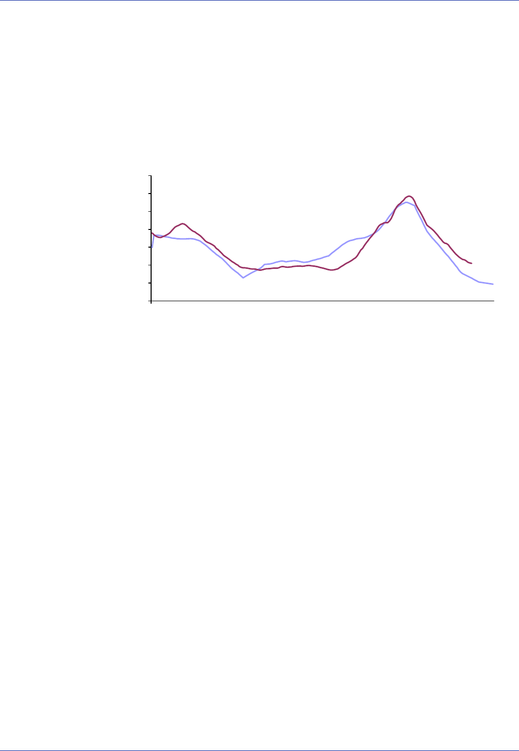
100 Global Rates Strategy Barclays Capital

to the broader debt markets. Most models for swap spreads therefore incorporate a

fiscal variable. Since swap rates can be expected to react to cyclical fundamentals,

including inflation, in a similar fashion to government yields, the spread of government

bonds against swaps might be seen as a pure measure of the impact of budgetary

fundamentals on real yields. In Figure 59, we model a moving average of 10-year US

swap spreads from the projected deficit/GDP ratio. The exercise confirms that fiscal

fundamentals are the main determinant of the yield of government bonds relative to

the non-government curve.

Figure 59: US 10-year Swap Spread, Modelled from Projected

Deficit/GDP Ratio

0.2

0.4

0.6

0.8

1.2

1.4

1989 1990 1991 1992 1993 1994 1995 1996 1997 1998 1999 2000 2001 2002 2003 2004

Source Barclays Capital.

In summary, the multi-decade trend in real yields can be seen as a product of long-run

shifts in the demographics. On a shorter-term investment horizon, the main

determinant of the level real yields is the business cycle and the central bank short-term

rate. However, the sensitivity of long real yields to short-term rates is geographically

varied. There is abundant evidence for a connection between deficit/GDP ratios and the

level of real yields, with the spread between government debt and the Libor curve

determined by the fiscal position. There is also some evidence that investor risk

appetites are negatively correlated with real yields.

Barclays Capital Global Rates Strategy 101

Breakeven Trades and Forwards

Mike Oman

The concept of the breakeven trade is very simple as, in essence, it is a simple spread

trade, although the carry aspect is more volatile in the inflation-linked world. The profile

of the investor base and the maturity of markets have been crucial factors in determining

the nature of breakeven trading. For example, the UK market is dominated by pension

fund investors who are focused largely on real returns rather than breakevens. Thus

valuation, and therefore the progress of a breakeven trade, will be influenced more by a

bond’s relative value on the real curve and the absolute level of real rates than by the

fundamental value of expected inflation, the inflation risk premium and current inflation

accretion. European and US markets trade more as spread product, with the spread

influenced more by the current inflation accretion and the expectations of future

inflation. Increasing globalisation may encourage an increase in breakeven trading, as

international trading is often done in breakevens to avoid currency hedging issues.

A pure breakeven inflation trade involves equal PV01 weights for a linker and its

nominal comparator. This position profits on any widening of the 1:1 yield spread

between the two but tends to be directional, with the linker usually underperforming in

a rally. Instead of a true breakeven trade, a spread trade using a yield beta weighting

attempt to take out this directionality. The nature of such a trade is somewhat different

as it ceases to be a self-funded position and hence has different carry characteristics.

Breakeven Carry

The carry aspect of a breakeven trade is more complicated and interesting than for a

regular spread trade, and this is because the rate of inflation accretion varies through

time, tracking month-on-month inflation readings with a lag. In the context of the

generic Canadian model, the rate of inflation accretion varies month by month and is

determined by the month-on-month increase in the relevant index for the months 2

and 3 months prior to the time considered. So, for example, if it is 1 January, the

amount by which the inflated settlement proceeds are scaled up each day in the coming

month to compensate for inflation is determined by the following formula:

tCPI

CPI

hDaysInMont

In this case the two CPI index levels are for the preceding November and October. If

November CPI was 0.4% higher than that for October (eg, 227.3 versus 226.4) a bond

with settlement value of 114.466 on one day will have a settlement value of 114.481 the

next purely due to inflation accrual, a 1.5 cent increase in one day which when

considered over a 31-day month is a 0.4% accretion rate per month. This is the

compensation for inflation, and when considered in direct competition to nominal

bonds, is the trade-off made for receiving a real yield instead of a nominal yield. In

annualised terms, 0.4% M/M inflation equates to an annual inflation rate of 4.9%. If the

difference between real yield and nominal yield at that maturity (the breakeven) is less

than 4.9% (so less than 0.4% in monthly terms), it will be beneficial, all else being equal,

to buy the inflation-linked bond and sell the nominal comparator bond for that month.

This is what we would term positive breakeven carry. It is the expected net carry to

holding the breakeven position for that month, and when expressed in terms of basis

points indicates by how much the breakeven would have to fall in the month for the

position to lose money overall (ie, to what extent carry “protects” the trade).

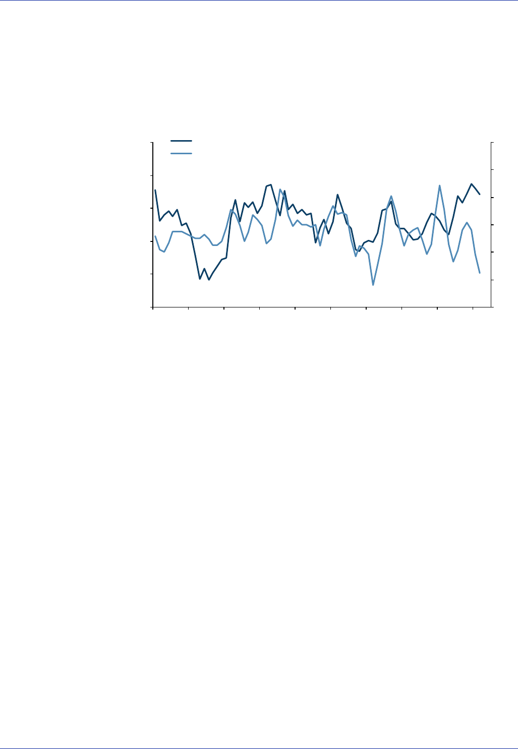
102 Global Rates Strategy Barclays Capital

This has implications for breakeven trades that play-out in very obvious and significant

fashion in the Canadian style linker markets (it will affect the UK market in the same

way but due to the longer-term nature of indexation in the UK the effect plays out more

slowly). Higher-than-anticipated inflation announcements promise improved carry in

the coming month and therefore trigger accounts to enter breakeven positions or

unwind short breakeven positions in the run-up to the next month. The impact on

breakevens is illustrated very clearly in Figure 60.

Figure 60: Inflation Accretion is a Major Driver of Breakeven Trades

0.5

1.0

1.5

2.0

2.5

3.0

Dec 97 Aug 98 Apr 99 Dec 99 Aug 00 Apr 01 Dec 01 Aug 02 Apr 03 Dec 03

-2%

-1%

10yr TIPS Breakeven

3m annualised inflation accretion (RHS)

Source: Barclays Capital.

Trades that are motivated purely to reap good breakeven carry are classic candidates

for beta weighted spread trades, which attempt to reduce the volatility of P/L and

remove the directionality of breakeven trades. Directional moves are not necessary for

such a trade to work as intended, and it must be borne in mind that beta itself may be

influenced by the existence of positive or negative breakeven carry. The reaction might

be to increase the weighting of the linker side beyond that implied by current beta to

take advantage of the expected outperformance of real rates due to the carry.

Alternatively, in a rallying nominal market beta might be expected to rise in a positive

carry period, and in a sell-off beta might be expected to fall. Trying to remove

directionality from such carry trades can thus be more of an art than a science.

None of the modern inflation-linked markets use seasonally adjusted inflation indices

for indexation in order that the degree of subjectivity with regard to the cash flows of

the product is minimised. Consequently, the pattern of month-on-month inflation

accretion is subject to seasonal influences, making certain times of the year, particularly

from January to April in the US and February to May in Europe, good breakeven carry

periods. The next section discusses these trends.

Translation of carry into basis points makes analysis of the effects of inflation accretion

much easier to analyse, particularly when determining which parts of the curve will be

relatively more or less affected. Any given monthly move in an inflation index will have

a larger effect on the shorter bonds because they have a smaller PV01, so the given

percentage accretion of principal translates to a greater move in basis point terms.

Large month-on-month increases will give a bias towards breakeven curve flattening

and large month-on-month decreases will bias towards steepening.

The most useful way to project and compare the impact of inflation accretion on the

returns to various breakeven positions is to calculate the forward yield, firstly under the

known accrual for the next month or so, and secondly according to one’s forecast for

inflation in the future. Higher inflation accretion will produce higher forward real yields.

Barclays Capital Global Rates Strategy 103

When subtracted from the forward yield of the nominal comparator at the given

horizon, what we term a “forward breakeven” is found. In the case where inflation

accretion (once annualised, as done in the example given above) exceeds the spot

breakeven inflation (and after a small adjustment to capture the difference in funding

costs of the two positions, detailed below), the forward breakeven will tend to be lower

than the spot breakeven. The difference between forward and spot breakeven is what

we term breakeven carry, or breakeven “protection” (specifically spot minus forward

breakeven). A positive breakeven protection indicates positive carry to the breakeven

trade considered, and is therefore an important relative value metric.

Forward Real Yield and Forward Breakevens –

Calculations

Forward real yield in this context is calculated using a similar methodology to the

forward pricing of a nominal bond, the only difference being that we incorporate an

estimate of the index ratio for a given horizon date (the reference CPI for the particular

date in the future divided by the base index for the bond concerned). It is a cash and

carry forward pricing methodology.

Methodology for calculating forward real yields under the Canadian method:

ttt APGP +=

where:

GPt = real price + real accrued

then

ttt IRGPMV *=

where

IR = Index ratio

MVt= Market (Cash) Value

We then invest the cash proceeds at a rate, r, for the next, d days, giving a forward

breakeven cash amount of MVf

From this forward cash amount we subtract the reinvested value of any coupons

received and then divide this by the expected index ratio at the forward date. By doing

this we arrive at our forward real gross price and subtracting the forward real accrued

gives the forward real price of the bond.

(

)

ff A

ARMV

FP -

IR f=forward index ratio

ARf =coupon received (reinvested)

Af = forward real accrued

This real forward price, when put through the usual yield from price formula, but this

time at the forward horizon date, gives the forward real yield. Now that we have an

104 Global Rates Strategy Barclays Capital

estimate of the forward real yield we can now simply calculate the forward yield of the

comparator bond and then arrive at a forward breakeven inflation rate, which we can

then compare to the spot and/or to a long run chart of breakeven inflation.

The forward analysis is, in effect, a cost analysis of the breakeven trade. Given the

seasonality in inflation, the cost of entering breakeven trades can vary significantly and

may explain why spot breakeven inflation spreads appear cheap or expensive to their

long-run average. Another useful aspect of this analysis is that we can gauge what our

inflation forecasts imply about the shape of the real yield and breakeven inflation curve

over varying horizons. When the forwards are mapped out across a curve, we may be

able to form a stronger opinion about which sector is the best for breakeven inflation

trades or alternatively for curve flattening or steepening trades. Figure 61 demonstrates

the 1-month negative carry versus financing (forward real yield lower than spot real

yield) that the shorter-dated TIPS struggled against in December 2003, and the

negative breakeven protection forecast over all time horizons for all TIPS at that time.

This information is published for the major markets every day in the Barclays Capital

Daily Inflation-Linked Report. Breakevens subsequently dropped and the breakeven

curve steepened.

Figure 61: Real Yield Carry and Breakeven Protection as of 1 December 2003

Carry bp Breakeven Protection bp

1mth 3mth 6mth 12mth 1mth 3mth 6mth 12mth

2007 -4.2 -7.9 23.7 45.8 -9.7 -23.4 -8.2 -15.3

2008 -2.4 -3.7 22.4 43.2 -7.6 -18.4 -7.5 -14.2

2009 -1.5 -1.4 21.4 41.1 -6.2 -14.8 -5.8 -10.1

2010 -0.9 -0.2 20.1 38.5 -5.8 -13.9 -7.6 -14.3

2011 -0.6 0.4 18.4 35.0 -5.0 -12.2 -7.1 -13.6

Jan-12 -0.4 0.8 17.0 32.3 -4.6 -11.2 -7.1 -13.5

Jul-12 -0.3 0.9 16.3 30.9 -4.3 -10.5 -6.8 -12.9

2013 -0.2 1.0 14.6 27.6 -4.0 -9.7 -7.0 -13.3

2028 0.1 1.1 8.4 15.7 -2.7 -6.8 -7.3 -13.9

2029 0.1 1.1 8.3 15.4 -2.6 -6.6 -7.0 -13.4

2032 0.0 0.9 7.2 13.3 -2.5 -6.3 -7.1 -13.5

Repo Assumed 0.97 1.05 1.14 1.47

Source: Barclays Capital.

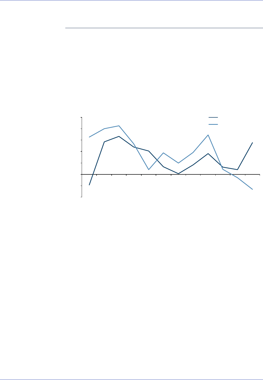
Barclays Capital Global Rates Strategy 105

Seasonality and Inflation-Linked Bonds

Gemma Wright, Alan James

All major inflation-linked markets use non-seasonally adjusted series, due to the lack of

consistency and transparency in seasonal adjustment methodologies. The adaptation of

the Canadian model by most sovereign issuers of inflation-linked debt has helped embed

the use of a contemporaneous measure of inflation in the bulk of outstanding inflation-

linked debt. Not smoothing for the fluctuations of volatile items, such as food and energy

leaves a fairly predictable pattern of behaviour for each consumer price index. Moreover,

given that the relatively short three-month lag between the month for indexation and

actual impact of inflation accrual, it is not surprising to find that breakeven inflation

spreads are highly sensitive to the cyclical bias inherent in each index.

Figure 62: Average Monthly Change in the US and EMU CPI Indices

-0.2%

-0.1%

0.0%

0.1%

0.2%

0.3%

0.4%

0.5%

Jan Feb March April May June July Aug Sept Oct Nov Dec

EMU HICP ex-tobacco

US CPI U NSA

Source: Bureau of Labor Statistics, Ecowin.

Each CPI has its own behavioural pattern, driven in part by timing differentials for the

introduction of price increases/decreases in items such as the price of oil, rents, auto

prices, and food. As the chart above demonstrates there are often similarities between

seasonal patterns in the US and Europe, though euro-area inflation is less volatile. US

price levels have the strongest tendency to rise in the first four months of the year and

European prices from February to May. There is a consistently sharp divergence in

behaviour for December and January, due mainly to different seasonal discounting plus

extreme December spikes in German holiday prices.

The behaviour of the underlying price indices leaves an indelible mark on the behaviour

of the breakeven inflation spreads. In the US we find a relatively strong relationship

between the behaviour of the 2007 TIIS breakeven inflation spread and the monthly

change in the CPI-U NSA. Statistically the link is stronger for the month inflation is

released rather than the month it is taken, but both are significant. This allows for a

better timing of a tactical overweight/underweight in inflation-linked bonds. Moreover,

the behaviour of breakeven inflation spreads surrounding periods of higher/lower

inflation accretion have historically impacted the slope of the real curve.

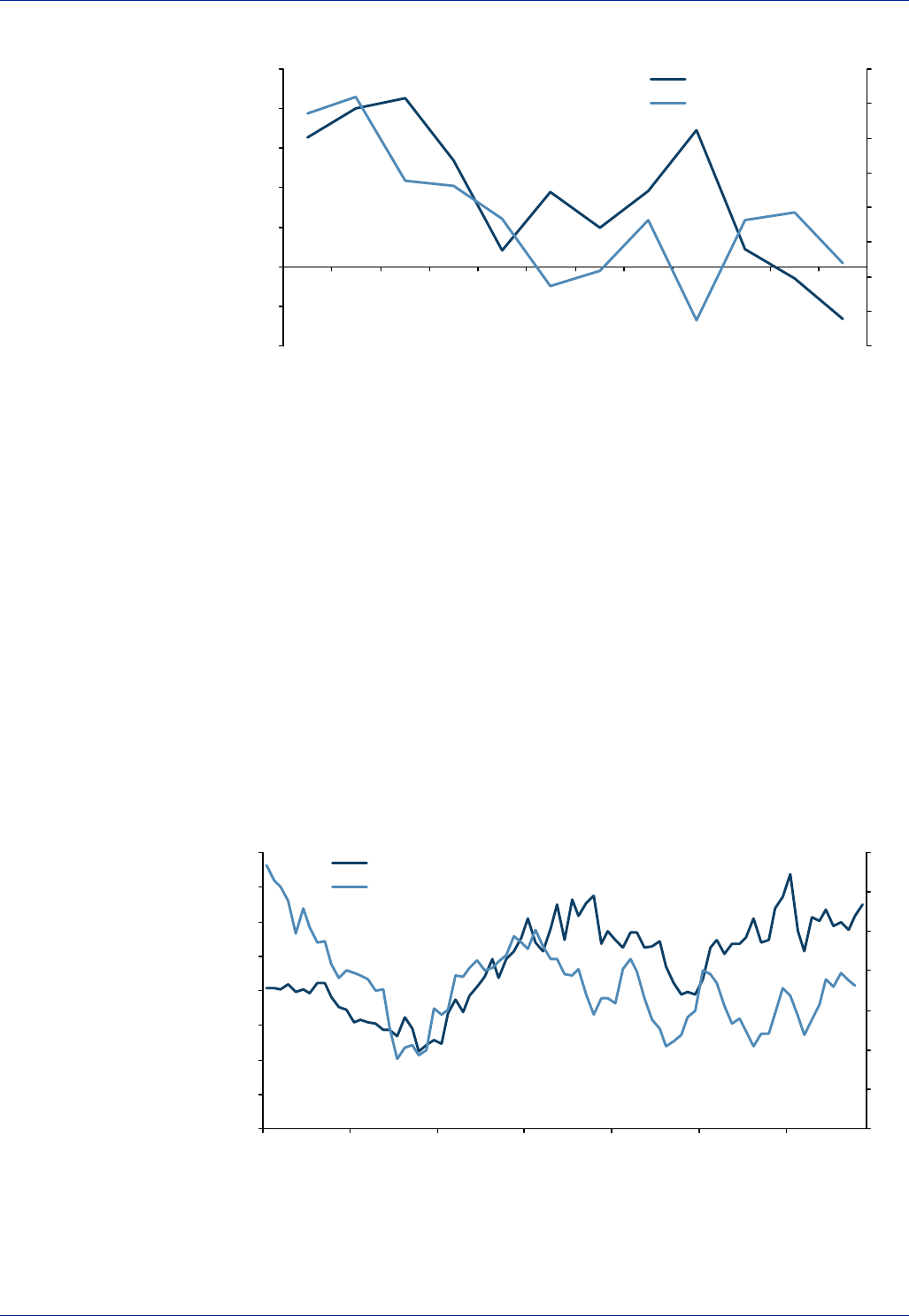
106 Global Rates Strategy Barclays Capital

Figure 63: Average Change 1997-2003 Between BEI 2007 and CPI-U NSA

-0.2%

-0.1%

0.0%

0.1%

0.2%

0.3%

0.4%

0.5%

Jan Feb March April May June July Aug Sept Oct Nov Dec

-20

-15

-10

-5

US CPI NSA (lhs)

BP change in 2007 BEI (rhs)

Source: Barclays Capital, Bureau of Labor Statistics.

In the past seven years there have been three extended periods in which the breakeven

inflation spread behaviour varied from the underlying inflation index. In the first five

months of 1998 and 2003 and the final seven months of 1999, the breakeven inflation

spreads were greatly influenced by atypical seasonal changes in energy prices. As we

can see from the graph in Figure 64, energy price movements as measured by West

Texas Intermediate (WTI) oil prices closely track changes to the BEI spreads. However,

the correlation for the past seven years is a modest 24%, driven in part by these three

aberrant periods. The correlation rises, not surprisingly as we exclude the 1998-99

period. From 2001-03, monthly changes in WTI and BEI spreads saw a 35% correlation

driven in large part by the hefty 63% correlation in 2003. This significant correlation

was driven in large part to large spikes in the price of crude oil in advance of the onset

of war with Iraq. Shifting inflation expectations did much to widen BEI spreads (see

Figure 65) sooner than normal and quick profit-taking as energy prices sold off

collapsed BEI spreads in spite of a period of still favourable inflation accretion.

Figure 64: WTI Oil Price and 2007 TIIS BEI

Feb 97 Feb 98 Feb 99 Feb 00 Feb 01 Feb 02 Feb 03

0.0

0.5

1.0

1.5

2.0

2.5

3.0

3.5

WTIC (lhs)

2007 BEI (rhs)

Source: Haver Analytics, Barclays Capital.

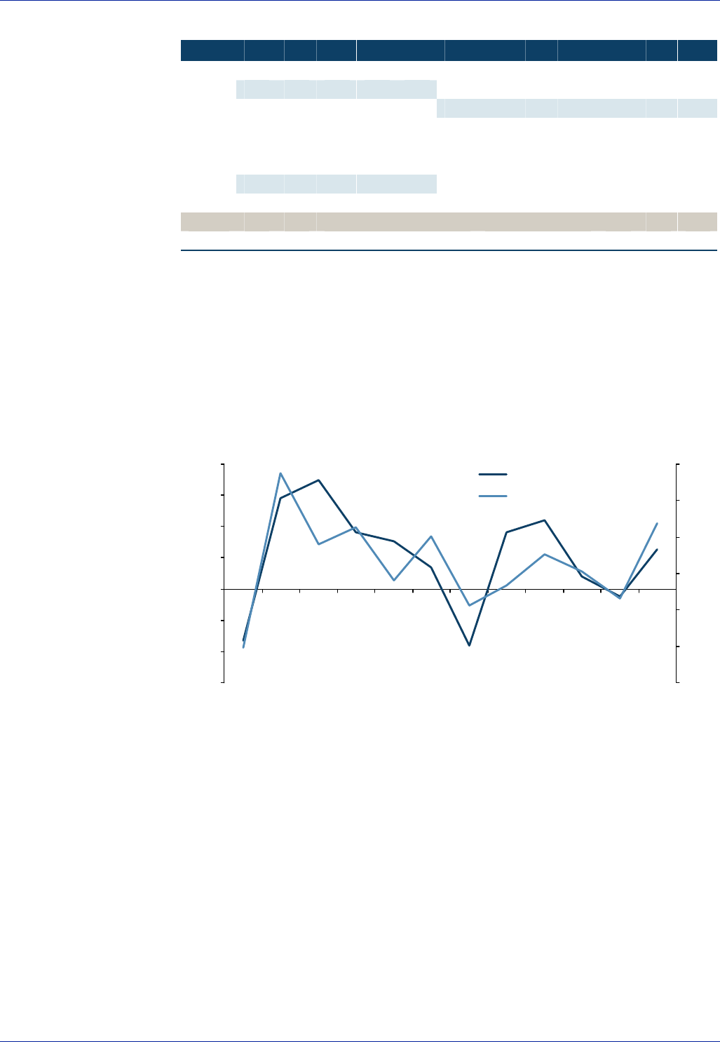
Barclays Capital Global Rates Strategy 107

Figure 65: Seasonality of 2007 BEI

Jan Feb Mar Apr May Jun Jul Aug Sep Oct Nov Dec

1997 12.4 -19.3 -7.0 -18.5 -41.9 32.8 -23.7 -20.0 1.7 -28.4

1998 -18.6 10.8 -4.3 -1.9 -5.4 -15.3 2.9 -48.9 -40.6 14.7 3.0 -11.7

1999 6.3 53.0 -8.8 6.9 43.0 -2.0 11.8 9.4 -12.0 2.2 8.9 7.7

2000 24.0 -7.8 -8.5 23.6 -19.8 -17.0 0.4 -19.2 -1.1 6.8 -31.4 -26.0

2001 20.8 -0.4 -5.7 43.5 13.5 -16.5 -34.7 -25.9 -12.0 -22.7 6.3 8.5

2002 23.1 7.9 50.8 -5.1 -10.8 -29.7 -22.1 7.1 -16.7 -18.4 16.1 -0.5

2003 25.2 32.0 -9.1 -25.5 -25.0 19.5 19.0 32.0 -8.6 17.6 -10.5 -5.6

Average 13.5 15.9 3.8 3.2 -1.6 -11.3 -9.2 -1.8 -16.4 -2.8 -0.8 -8.0

Up Leg (Jan – May) Down Leg (Jun – Dec)

Average change in BEI 34.8 -50.4

Source: Barclays Capital.

The sample period is too short to draw any similar inferences from analysis in OAT¤i

bonds, but the chart below shows the performance for the OATi09 breakeven versus the

change in French CPI. Here the statistical fit is much closer than in the US and the move in

breakeven inflation and the actual inflation index data are coincident, suggesting a more

forward-looking market. Ironically the European market appears more responsive to

pricing seasonal biases than the US, despite seasonality being a less important factor.

Figure 66: Average Change between BEI 2009 OATi and French CPI

-0.3%

-0.2%

-0.1%

0.0%

0.1%

0.2%

0.3%

0.4%

Jan Feb March April May June July Aug Sept Oct Nov Dec

-0.15

-0.10

-0.05

0.00

0.05

0.10

0.15

French CPI ex tobacco (lhs)

Avg Change in BEI in bp (rhs)

Source: Barclays Capital.

The lesson learned from these aberrant patterns is to utilise the underlying inflation

indices as a starting point for assessment of the potential seasonality for breakeven

inflation spreads. Be aware though that the volatile energy sector can have a more

instantaneous impact on inflation and breakevens.

108 Global Rates Strategy Barclays Capital

Deflation Protection: The Par “Floor”

Alan James

US, French, Italian, Australian, South African and some Swedish inflation bonds have a

floor on the final principal payment of par. If the linking price index falls over the entire

life of the bond, its principal repayment is the par value of the issue rather than the par

value multiplied by the index ratio. This is an automatically activated embedded option

within the bond that is often not fully considered when pricing. The main reason that

Japan chose not to include deflation protection in its new JGBi bonds is that pricing the

value of this option in a country where prices had been drifting downwards for five

years would have been a major component of its overall value. This would mean that

the real yield and breakeven values would be relatively hard to interpret, as these

calculations do not adjust for the presence of the floor.

Investors who are only concerned about real returns have little need for a deflation

floor for inflation bonds. The floor actually means that real returns would be skewed

higher if prices fall and the par put is exercised. In the real world though, investors in

inflation-linked bonds do care about nominal returns as well, hence the guarantee that

the nominal principal will be at least repaid is reassuring. The presence of the floor

skews the long run real return difference between nominal and real bond. As inflation

rises, the real returns of linkers improve compared to nominal bonds at the same rate.

On the other hand, once the floor is triggered, linkers perform only marginally worse

than nominal bonds if deflation intensifies as only the coupon element of the linker

return suffers compared to the conventional.

Australia was the first country to offer nominal return floors on linkers in 1985, but it

went a step further than just offering a par put on the principal. Coupon payments are

also floored at par, albeit if prices do subsequently rise then future coupon payments

remain at par until the excess paid out has been offset. The original proposal for US

TIPS was to only floor the nominal value of all cash flows paid out over the life of a

bond. The idea of deflation protection was sufficiently well received, and the value of

the option perceived to be so small by the Treasury, that the floor was eventually only

the principal and almost all other countries since have followed suit.

Some of the factors in pricing the value of the deflation floor, and indeed other inflation

derivatives, are common to standard options. The obvious starting point is to ask how

far in or out of the money the option is. For a new bond, the option is typically at the

money (or very close if there is some inflation accrual at launch, eg, in France). For

older bonds that have already seen their index ratio rise above its starting value, the

floor clearly becomes less and less important. For instance, at the end of 2003 the TII07

had an index ratio of 116.7. The value of the floor on this bond was thus virtually

worthless, as deflation would have to be greater than 5% a year for it to come into

effect. However, in order to attempt to model the valuation of the option, assumptions

have to be made about the distribution of inflation.

Assessing the time value of an inflation option is trickier than for an interest rate

option. While the value of even a European interest rate option clearly increases the

longer it has to expiry, this is not necessarily the case with an inflation option. If the

mean for inflation is positive, then the probability of cumulative deflation falls the

longer the time period. Statistically, this bias is offset somewhat by the observed fact

that annual inflation tends to be autocorrelated. In other words there is much more

likely to be deflation in a given year if there was deflation the previous year. Provided

the change in the rate of inflation is not also autocorrelated, and in practice this

appears justified, the positive mean tends to decrease the value of the option as the

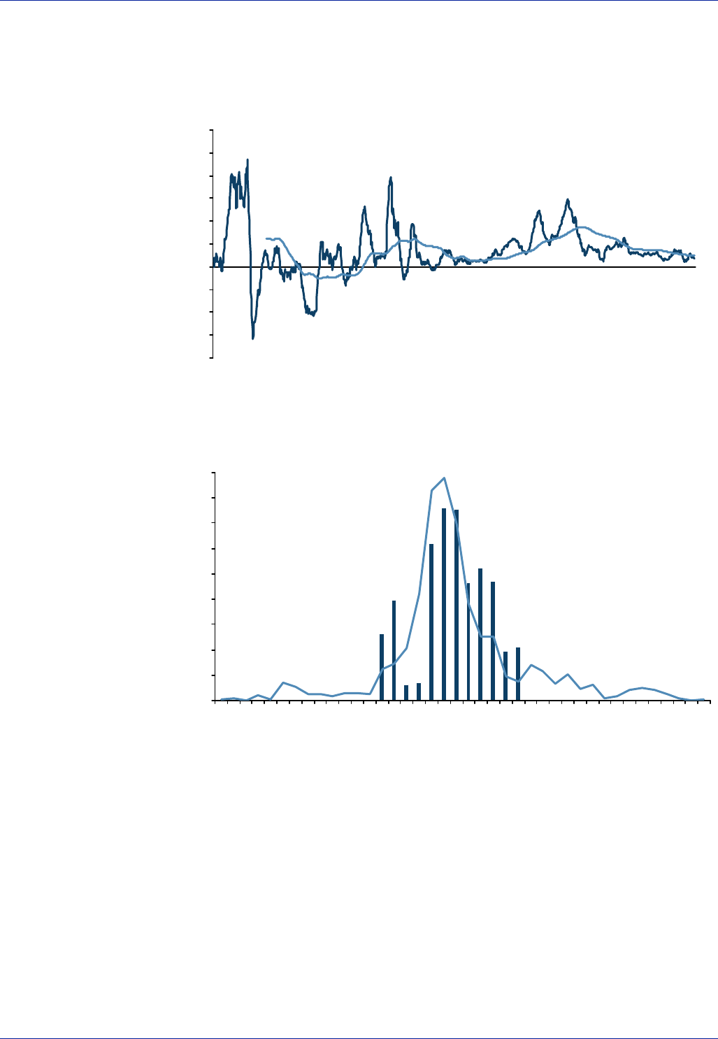
Barclays Capital Global Rates Strategy 109

time to maturity extends. The charts below for US CPI clearly show that the level of

inflation does tend to trend and that, had linkers existed, 10-year par floors would have

been exercised through the 1930s but at no other time.

Figure 67: US CPI Annual Inflation and 10 yr Average Inflation

-20

-15

-10

-5

1914 1924 1934 1944 1954 1964 1974 1984 1994 2004

Inflation

10yr average

inflation

Source: Bureau of Labor Statistics.

Figure 68: Distribution of US CPI Annual and 10 yr Average Inflation

100

120

140

160

180

-15 -11 -7 -3 1 5 9 13 17 21

Annual infaltion

10yr average inflation

Source: Bureau of Labor Statistics, Barclays Capital.

In practical terms, even assuming a fat-tailed distribution function for inflation for a

new 10 yr bond, given recent volatilities the value of the floor only starts to be a

significant element of the pricing if the mean expected inflation, best approximated by

the breakeven inflation spread, is below 1.5%. Aggressive assumptions have to be made

about the trending nature of inflation for the fair value of the embedded option to be

above 2 bp. Statistically, it is hard to justify such assumptions, and economic policy

goals in most markets do not justify them either. The explicit commitment by the

FOMC in 2003 to pursue an active policy to avoid the risk of deflation ought to have

reduced the value of the par floor option. Ironically, the change in stance actually

increased focus on the existence of the floor, leading to the TII13 auction in July 2003

being the first issue where the option value was actively considered in pricing the roll.

In the case of an economy with an endemically lower inflation mean than the existing

major inflation-linked markets, such as Japan, the pricing of the floor becomes more

110 Global Rates Strategy Barclays Capital

important. Below 1% breakeven levels for an issue with no significant inflation accrual,

the option value increases exponentially, distorting the meaning of the real yield and

breakeven numbers as considered using Canadian model conventions. With a floor in

place, the breakeven inflation as normally measured can never go significantly negative

assuming negligible real coupons (a realistic assumption for such a new linker in a

deflationary country). Against this greater complexity should be weighed the signal

that not having a floor may send to the markets about the commitment of the country

to avoid deflation. Take for instance the example of Switzerland, which despite press

speculation in Q4 03 had not issued inflation-linked bonds at the time of writing.

Realised inflation and inflation expectations are notably lower than in the existing

markets with floors, but the Swiss National Bank is committed to avoiding measured

deflation. As a small open economy (unlike Japan), this is a credible commitment, given

that the authorities have the ability to print money and use it to push the currency

weaker. This credibility could be weakened somewhat if inflation-linked bonds were

issued with no par floor. This could influence expectations and thus the likelihood of the

SNB actually having to act.

Given Japan’s decision not to employ a deflation floor, and with Western central banks

having sought to stock up their arsenals with weapons to avoid sustained deflation, the

importance of deflation floors at present seems relatively limited for government

bonds. The best indication of how pricing models might develop if deflation does

become an increasing likelihood in the future is to look at how pricing models have

developed for pricing of floors for inflation derivatives and MTN bonds. The likelihood

of a zero floor being exercised on a coupon paying a function of the year-on-year

inflation rate is the same for one year as for a par floor, but the value of this option

increases with the length of the bond. Also floors have been traded at levels above zero,

most commonly 1%. As the depth of the inflation derivative market grows, the models

employed for pricing floors (and indeed caps) are likely to develop.

Many of the models for shorter-term deflation or low inflation floors try to combine the

statistical properties of inflation with central bank reaction functions. They attempt to

use the pricing of interest rate options to indicate the value of inflation options. The

more explicit central bank intentions with respect to low inflation and the risk of

deflation in 2003 have encouraged this approach to develop. For instance, since if euro

inflation drops below 1% ECB rates are likely to be cut from 2%, an interest rate option

with a floor of 1.5% may be a good indicator of the value of a similar maturity 1%

inflation floor. Similarly, the skew of further out-of-the-money interest rate options

may give a good indication of a zero-inflation floor. To date there has been little written

about the use of such modelling. Given the unpredictability of central bank reaction

functions, the degree to which the two types of options have moved together is quite

surprising, and seems to suggest that the street uses out-of-the-money interest rate

options in an attempt to hedge their inflation floor exposure.

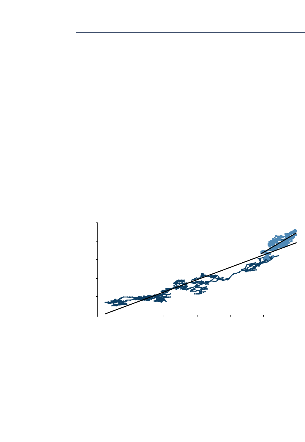
Barclays Capital Global Rates Strategy 111

Real and Nominal Curve Slopes

Alan James

In most markets, real and nominal yield curve shapes are surprisingly poorly correlated

except in the very long run when they trend in similar directions. Real yield curves are

on average less volatile than their nominal counterparts, but not by that much. In

France, for instance, the real curve on average has moved by 80% as much as the

nominal curve. This suggests that an increasing inflation risk premium with maturity is

not that large a component of the nominal slope. It is an important structural factor but

in the short term can easily be drowned out by other more immediate concerns. In both

the US and UK, over the long term, real curves on average have moved about two-thirds

as much as nominal curves.

Nominal and real yield curves in the US are weakly correlated in the short term but in

the long term tend to move in the same direction. For instance, since issuance in 1998,

the slope between the TII08 and TII28 is 93% explained by the corresponding spread in

nominal bonds. However, considering the whole sample over shorter-term 100-day

periods the average explanatory power is only 30%. There is never a more closely

correlated sub period than the overall sample. In the second half of 2002 and in 2003,

real yield curves were actually more volatile than nominal curves. It is notable that

trends in 5s10s curve slopes in recent years have followed those in the overall curve

very closely, even when stripping out carry factors, despite the relative illiquidity in

bond TIPS.

Figure 69: Slope of TII08 and TII28 vs Nominal Equivalents

1998-2003

y = 0.66x - 0.20

R2 = 0.93

2003

y = 1.04x - 0.88

R2 = 0.63

-0.5

0.0

0.5

1.0

1.5

2.0

-0.5 0.0 0.5 1.0 1.5 2.0 2.5

nominal slope

real slope

Source: Barclays Capital.

Surprisingly, the UK nominal and real yield curves have had a closer relationship in

recent years than in other markets. Previously there was almost no correlation in the

MFR-dominated period, i.e. until 2001, when the real yield curve was very static while

the inversion of the nominal curve was acute but unstable. Even though more market

participants focus on real yields as opposed to breakevens compared to other countries,

recently institutional pressures on nominal and real yield curves have been similar.

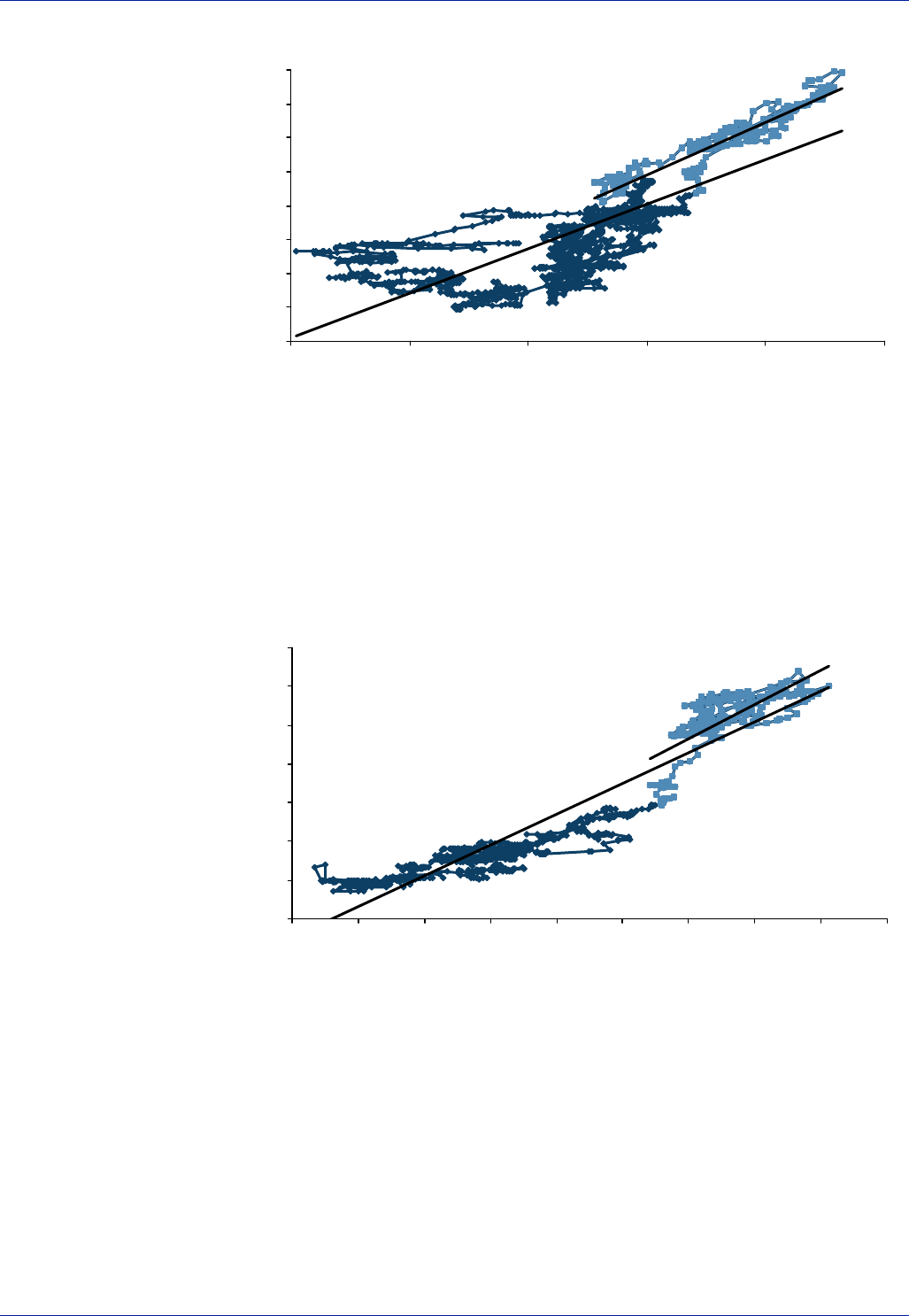
112 Global Rates Strategy Barclays Capital

Figure 70: Slope of IL09 and IL30 vs Nominal Equivalents

1997-2003

y = 0.66x + 0.01

R2 = 0.64

2003

y = 0.77x + 0.18

R2 = 0.87

-0.8

-0.6

-0.4

-0.2

0.0

0.2

0.4

0.6

0.8

-1.2 -0.8 -0.4 0.0 0.4 0.8

nominal slope

real slope

Source: Barclays Capital.

As seen in other markets, the real curve slope in OATis follows a similar longer-term

trend to the nominal market, but the day-to-day interrelationships are not strong. As is

the case with TIPS, attempting to strip out the trend bias by considering shorter sub-

periods leaves the explanatory power of movements in the nominal curve explaining

well below half of the movements in the real curve slope.

Figure 71: Slope of OATi09 and OATi29 vs Nominal Equivalents

1999-2003

y = 0.80x - 0.30

R2 = 0.89

2003

y = 0.89x - 0.34

R2 = 0.57

-0.2

0.0

0.2

0.4

0.6

0.8

1.0

1.2

0.0 0.2 0.4 0.6 0.8 1.0 1.2 1.4 1.6 1.8

nominal slope

real slope

Source: Barclays Capital

Somewhat surprisingly, in 2003 the day-to-day correlations between nominal and real

curves increased at the same time as traditional beta correlations waned. Considering

daily changes of the two slopes for the year, almost half of movements in real yield curves

can be explained by movements in the nominal curve, twice the previous correlation. We

suspect this may be indicative of a change in the institutional investor behaviour at the

long end. Long nominal bonds and inflation bonds appear to have been bought at the

same time, with pension fund reallocations away from the equity market.

Barclays Capital Global Rates Strategy 113

Inter-market Valuations and Trading

Alan James

The risks to cross-market inflation trading are relatively high but it is quite common for

attractive trading opportunities to develop, both short term and structural. Clearly, real

yield spreads between markets in different currencies can be volatile, but in practice

relative breakevens can move just as much. Despite this, compared to domestic trading,

far more cross currency positions are relative breakeven inflation trades than real yield

spread trades. The advantage of breakeven positions is that it they are basically

currency hedged. Given the relative volatilities of real yields compared to currencies, an

unhedged trade would mainly involve currency exposure. Theoretically this is less the

case in real yields than in nominals, as currency moves tend to alter inflationary

pressures and perceptions. In practice, there is only marginally less volatility than an

unhedged nominal position in the long run and often no benefit at all shorter term.

Short-term trades are relatively hard to cover in a forum such as this. Suffice to say that

many day-to-day opportunities develop due to global linker markets often moving with

similar trends but with some moving more quickly than others. For instance, if euro

breakevens widen notably before New York opening, it is relatively rare for TIPS to be

marked richer at the start of the day, leaving the potential for an in-and-out position. The

UK market tends to be stickier than the US and often follows with a slight lag (two or three

days) if there are major moves. Only slightly longer-term cross-market trades are those

driven by supply and index effects. Due to the relatively high level of issuance in inflation-

linked bonds compared to the float of existing issues, which is caused by the high

percentage of issues locked away by buy-and-hold investors, the markets are quite sensitive

to such changes. Cross-market trading is often an effective way of exploiting these trends.

The most common medium-term cross-market trades are those primarily motivated by

carry considerations. These may be based on known carry that has yet to be accrued in

the reference inflation indices or based on inflation expectations. Such positions are

usually expressed in breakeven spreads unless nominal yield expectations work the

same way as the real yield carry. Longer-term hedged cross-currency real yield trades

can enable yield exposure in markets which have relative punitive carry in nominal

markets, as the higher inflation accrual offsets the worse nominal carry that comes

from higher policy rates and a flatter curve.

Longer-term structural positioning may be based on the different shapes of real yield or

breakeven curves or absolute spread levels. In such long-term positions it is important to

consider the mechanics of the relative inflation indices. Most obviously, is there a

calculation bias between the different methodologies? This is most clearly the case when

considering trades involving the UK, as the arithmetically calculated RPI is biased to be

higher than geometrically weighted CPI measures elsewhere. This alone is worth about 50

bp more compared to other countries given the sub-component volatility of recent years.

The existence of standardised HICP measures across Europe makes it relatively easy to

consider the relative inflation index biases in these countries. Only the UK has a clear

calculation bias but there are other biases due to different inclusions and weightings for

trending variables. The UK includes house price depreciation but currently HICP

measures do not. As house prices tend to grow faster than prices (in the long term

tracking wage growth more closely) this again biases the RPI higher by 20 bp+. HICP has

a narrower definition of health costs than some countries. This tends to bias national

whole economy indices higher over time versus equivalent HICP measures due to the

long-term trend for healthcare prices to rise faster than general inflation. On the other

hand, Italian FOI inflation excludes pensioners, so has the opposite bias, worth on

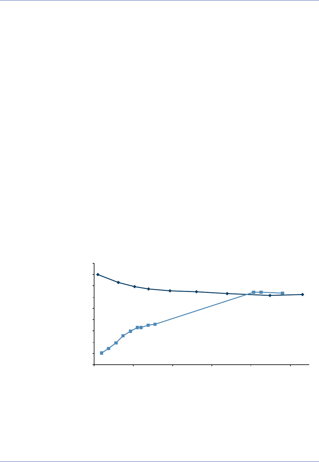
114 Global Rates Strategy Barclays Capital

average 15 bp per annum. Whether or not tobacco is included in an index produces a

similar bias, given the long tendency for this tax to rise. At the start of 2004, euro

tobacco basis traded at 15 bp for five years.

One offshoot from the difference in inflation baskets that is often overlooked is that some

price indices are more cyclical than others. The clearest case of this comes if mortgage

interest costs are included in the price index, unlike in HICPs, as rate hikes can often feed

through more quickly than the disinflationary impact of the hike. Again, the UK stands

out on this count, not only due to the high percentage of mortgage interest costs in the

RPI but also high base rate sensitivity as most mortgages are variable rate. Swedish CPI is

biased up slightly in a hiking cycle, but the impact comes through more slowly than in the

UK due to longer-term fixed rates. The US has a de facto link between both policy and

mortgage rates and CPI through the imputed rent aspect that tended to have a

sometimes overlooked deflationary impact on US CPI in 2003.

For 2004 and 2005, UK RPI inflation is set to be considerably higher than that accruing for

either European or US inflation-linked bonds. The computational bias is added to by the

direct impact of house prices, rate hikes and council tax. As of November 2003, the UK had

the lowest headline CPI of inflation-linked issuers, at 1.3%, but RPI was 2.5%. Given this

medium-term bias, is larger than the longer-term effect, it is understandable that UK

breakeven inflation curve is downward sloping at shorter maturities, but it is more

surprising that it is downward sloping all the way along the curve. This is in sharp contrast

to the French and US breakeven curves. Despite the 70-80 bp long-term bias in favour of UK

linkers, US long-end breakevens rose above those in the UK in late 2003. This left a

structural position holding UK long-end breakevens versus the opposite in the US as an

attractive opportunity, likely on average to offer significant positive carry for a considerable

period. On the other hand, it is the kind of position that can move around day-to-day by

relatively large amounts, making it an uncomfortable mark-to-market position.

Figure 72: UK and US Breakeven Curves as of 13 January 2004

1.5

1.7

1.9

2.1

2.3

2.5

2.7

2.9

3.1

3.3

2006 2011 2016 2022 2027 2033

US breakeven curve

UK breakeven curve

Source: Barclays Capital.

Barclays Capital Global Rates Strategy 115

Appendices

116 Global Rates Strategy Barclays Capital

Example Swap Structures

Figure 73: HICPx Zero Coupon vs Compounded Fixed

Amount: ¤50,000,000

Start Date: [TBD]

End Date: [TBD]

Bank Receives: Inflation, at maturity:

notional*([HICPx(m-3)/HICPx(s-3)]-1)

Where s = month of start date, m= month of maturity date, HICPx

is the Euro HICP Ex-tobacco index value

Bank Pays: Fixed rate, at maturity:

notional* [(1+X%)T-1] ;

Where T= tenor in years, X= quoted fixed rate

Note: The same structure trades for US CPI-U nsa with two-month lag.

Figure 74: OATei-style vs Euribor or Fixed

Amount: ¤50,000,000

Start Date: [TBD]

End Date: [TBD]

Bank Pays: 6m Euribor flat, Semi-annual Act/360

Fixed Rate, Annual 30/360

Bank Receives: Real Coupon of X%:

X% * [HICP(p - 3)/HICP(s - 3)] * Dayfrac * Notional, Annual

30/360

Additionally, at maturity:

Notional * Max {0%, [HICP(m - 3)/HICP(s - 3) - 1]}

Where p = payment date, s = start date, and m = maturity date

HICP (base) = HICP(s – 3)

We use the standard 3 month lag for indexation

Note: The cash flows match those of the bond; TIPS-style will be semi-annual; BTP ¤i style will be semi-annual,

but quoted annually.

Barclays Capital Global Rates Strategy 117

Figure 75: Zero Coupon Only vs upfront or Euribor-Spread

Amount: ¤50,000,000 (for example)

Start Date: [TBD]

End Date: [TBD]

Bank Receives: Upfront premium OR 6m Euribor - Spread, Semi-annual Act/360

Bank Pays: At Maturity:

Notional *[ Max {0%, [HICP(m - 3)/HICP(s - 3) - 1]} + X%}]

Where s = start date, and m = maturity date

HICP (base) = HICP(s – 3) = HICP(Type in Month and Year)= Type

in Value

We use the standard 3-month lag for indexation

Figure 76: Real Coupon (Only) vs Euribor or Fixed

Amount: ¤50,000,000

Start Date: [TBD]

End Date: [TBD]

Bank Pays: 6m Euribor flat, Semi-annual Act/360

Fixed Rate, Annual 30/360

Bank Receives: Real Coupon of X%:

X% * [HICP(p - 3)/HICP(s - 3)] * Dayfrac * Notional, Annual

30/360

Where p = payment date, s = start date, and m = maturity date

HICP (base) = HICP(s – 3)

We use the standard 3-month lag for indexation

118 Global Rates Strategy Barclays Capital

Figure 77: Real Annuity vs Compounded Fixed

Amount: ¤5,000,000

Start Date: [TBD]

End Date: [TBD]

Bank Pays: Compounded Fixed Annual Payments each year t:

Notional * (1 + X%)^t

Bank Receives: Real Annuity paid annually:

Notional * [HICP(p - 3)/HICP(s - 3)]

Where p = payment date, s = start date

HICP (base) = HICP(s – 3)

We use the standard 3 month lag for indexation

Figure 78: Year-on-year Inflation Plus Spread vs Euribor Flat

Amount: ¤50,000,000

Start Date: [TBD]

End Date: [TBD]

Bank Pays: Fixed Rate

Annual 30/360

Bank Receives: Year-on-year inflation plus spread:

{Max[0%, [HICP(p - 3)/HICP(p - 15) - 1]] + X%} * Dayfrac *

Notional, Annual 30/360

Max {0%, [HICP(p - 3)/HICP(p - 15) - 1] + X%} * Dayfrac *

Notional, Annual 30/360

(keep one of the two alternatives: 0% floored inflation rate or 0%

floored total coupon)

Where p = payment date

HICP (base) = HICP(s – 3)

We use the standard 3-month lag for indexation

Barclays Capital Global Rates Strategy 119

Real Yields

Figure 79: Australia 10 yr Real Yield

2.6

2.8

3.0

3.2

3.4

3.6

3.8

4.0

4.2

Jan 98 Oct 98 Jul 99 Apr 00 Jan 01 Nov 01 Aug 02 May 03

Figure 80: Canada 10 yr Real Yield

2.5

2.7

2.9

3.1

3.3

3.5

3.7

3.9

4.1

4.3

Jan 98 Oct 98 Jul 99 Apr 00 Jan 01 Nov 01 Aug 02 May 03

Figure 81: France 10 yr Real Yield

1.6

2.0

2.4

2.8

3.2

3.6

4.0

Sep 98 Jun 99 Mar 00 Jan 01 Oct 01 Jul 02 Apr 03

Figure 82: Sweden 10 yr Real Yield

2.1

2.5

2.9

3.3

3.7

4.1

4.5

Jan 98 Oct 98 Jul 99 Apr 00 Jan 01 Nov 01 Aug 02 May 03

Figure 83: UK 10 yr Real Yield

1.3

1.8

2.3

2.8

3.3

Jan 98 Oct 98 Jul 99 Apr 00 Jan 01 Nov 01 Aug 02 May 03

Figure 84: US 10 yr Real Yield

1.4

1.9

2.4

2.9

3.4

3.9

4.4

Jan 98 Oct 98 Jul 99 Apr 00 Jan 01 Nov 01 Aug 02 May 03

Source: Barclays Capital.

120 Global Rates Strategy Barclays Capital

Breakeven Inflation

Break Even Inflation Current Inflation 10yr Rolling Inflation

Figure 85: Australia 10 yr BEI vs Actual Inflation

-1

Jan 98 Oct 98 Jul 99 Apr 00 Jan 01 Nov 01 Aug 02 May 03

Figure 86: Canada 10 yr BEI vs Actual Inflation

Jan 98 Oct 98 Jul 99 Apr 00 Jan 01 Nov 01 Aug 02 May 03

Figure 87: France 10 yr BEI vs Actual Inflation

0.0

0.5

1.0

1.5

2.0

2.5

3.0

Sep 98 Jun 99 Mar 00 Jan 01 Oct 01 Jul 02 Apr 03

Figure 88: Sweden 10 yr BEI vs Actual Inflation

-2

-1

Jan 98 Oct 98 Jul 99 Apr 00 Jan 01 Nov 01 Aug 02 May 03

Figure 89: UK 10 yr BEI vs Actual Inflation

Jan 98 Oct 98 Jul 99 Apr 00 Jan 01 Nov 01 Aug 02 May 03

Figure 90: US 10 yr BEI vs Actual Inflation

Jan 98 Oct 98 Jul 99 Apr 00 Jan 01 Nov 01 Aug 02 May 03

Source: Barclays Capital.

Barclays Capital Global Rates Strategy 121

The Barclays Capital Global Inflation-Linked

Bond Index

Figure 91: Constituents as of End 2003

Country Issuing Coupon Maturity Real Yield Mod Duration

Market Value

(US$ Billions) Weight

Australia 4 20 Aug 05 3.33 1.55 0.9 0.18

Australia 4 20 Aug 10 3.39 5.74 1.5 0.31

Australia 4 20 Aug 15 3.46 9.22 2.2 0.45

Australia 4 20 Aug 20 3.53 12.1 2.4 0.49

Canada 4.25 01 Dec 21 2.72 13.04 6.1 1.26

Canada 4.25 01 Dec 26 2.76 15.53 6.0 1.25

Canada 4 01 Dec 31 2.78 17.91 6.3 1.30

Canada 3 01 Dec 36 2.79 21.06 0.9 0.19

Italy 1.65 15 Sep 08 1.54 4.48 13.0 2.71

France OATei 3 25 Jul 12 2.01 7.54 15.7 3.28

France OATei 3.15 25 Jul 32 2.52 19.34 7.5 1.57

France OATi 3 25 Jul 09 1.66 5.1 20.3 4.24

France OATi 2.5 25 Jul 13 2.1 8.45 13.8 2.87

France OATi 3.4 25 Jul 29 2.5 17.67 6.8 1.42

Sweden 4 01 Dec 08 2.34 4.49 5.0 1.04

Sweden 0 01 Apr 14 2.72 10.1 2.2 0.47

Sweden 3.5 01 Dec 15 2.72 9.85 7.2 1.50

Sweden 4 01 Dec 20 2.81 12.72 5.1 1.06

Sweden 3.5 01 Dec 28 2.85 17.16 5.3 1.10

UK 2 19 Jul 06 1.24 2.46 9.7 2.02

UK 2.5 20 May 09 1.65 5.02 13.2 2.76

UK 2.5 23 Aug 11 1.82 6.9 19.8 4.13

UK 2.5 16 Aug 13 1.9 8.49 21.5 4.47

UK 2.5 26 Jul 16 1.96 10.7 25.5 5.32

UK 2.5 16 Apr 20 1.98 13.4 21.3 4.44

UK 2.5 17 Jul 24 1.98 16.07 20.8 4.34

UK 4.125 22 Jul 30 1.94 17.83 11.1 2.31

UK 2 26 Jan 35 1.9 22.97 6.1 1.26

US 3.375 15 Jan 07 0.59 2.87 20.2 4.21

US 3.625 15 Jan 08 0.95 3.73 21.6 4.50

US 3.875 15 Jan 09 1.22 4.55 20.6 4.29

US 4.25 15 Jan 10 1.43 5.31 14.7 3.07

US 3.5 15 Jan 11 1.63 6.21 13.3 2.78

US 3.375 15 Jan 12 1.78 7.01 7.1 1.48

US 3 15 Jul 12 1.85 7.48 26.1 5.45

US 1.875 15 Jul 13 1.96 8.61 20.2 4.20

US 3.625 15 Apr 28 2.34 16.94 23.9 4.98

US 3.875 15 Apr 29 2.33 17.21 28.6 5.95

US 3.375 15 Apr 32 2.25 19.19 6.5 1.35

Note: Real Yield and Modified Duration are Semi-annual.

Source: Barclays Capital.

122 Global Rates Strategy Barclays Capital

Key Information Sources

Barclays Capital Links

http://www.barcap.com Barclays Capital

http://www.barcap.com/inflation Barclays Capital Inflation-Linked House Site

http://www.barcap.com/indices Barclays Capital Indices

http://www.barcap.com/linkers Barclays Capital Inflation-Linked Analytics

http://www.barcap.com/research Barclays Capital Research

Bloomberg Pages

BCIL Barclays Capital Inflation-Linked Menu

BCAP1 Barclays Capital TIPS Prices

BCAP2 Barclays Capital i-strip Prices

BXEI Barclays Capital Euro Inflation-Linked Prices

BXGL Barclays Capital UK Index Linked Prices

BCSA Barclays Capital South Africa

Issuer Links

http://www.aofm.gov.au Australian Office of Financial Management

http://www.bankofcanada.ca Bank of Canada

http://www.aft.gouv.fr Agence France Tresor (AFT)

http://www.dt.tesoro.it/english-ve/public-deb Public Debt Division, Italian Treasury

http://www.mof.go.jp Japanese Ministry of Finance

http://www.treasury.gov.za South African National Treasury

http://www.rgk.se The Swedish National Debt Office

http://www.dmo.gov.uk UK Debt Management Office

http://www.treas.gov US Treasury

http://www.publicdebt.treas.gov US Bureau of the Public Debt

Useful Links

http://www.federalreserve.gov US Federal Reserve

http://www.boj.or.jp/ Bank of Japan

http://www.euro.ecb.int European Central Bank

http://www.bankofengland.co.uk The Bank of England

http://www.riksbank.com Riksbank

http://www.rba.gov.au Reserve Bank of Australia

124 Global Rates Strategy Barclays Capital

Summary Sovereign Table

Figure 92: Markets Overview

US UK France Italy Sweden Canada Australia South Africa Japan

Generic name

Treasury Inflation

Indexed Securities,

TIIS, TIPS

United Kingdom

Index-Linked

Gilts

OAT¤I, OATi BTP¤I

Swedish

Government

Index-Linked

Canadian Real

Return Bonds

Australian Capital

Indexed Bonds

South Africa Index-

Linked JGBi

No.Bonds

Outstanding* 11 10 6 1 6 4 4 4

Market Value

Outstanding bn* $ 202.800 bn £ 85.089 bn ¤ 50.866 bn ¤ 10.305 bn SEK 178.223 bn CAD 24.787 bn AUD 9.137 bn ZAR 37.734 bn

Market Value

Outstanding $ bn* $ 202.800 bn $ 151.647 bn $ 64.16 bn $ 12.998 bn $ 24.769 bn $ 19.181 bn $ 6.884 bn $ 5.653 bn

First IssueDate January 97 March 81 September 98 September 03 April 94 December 91 July 85 March 00 March 04

Linking Index CPI All urban nsa UK RPI French CPI ex-tobacco

Euro HICP ex-tobacco

Euro HICP

ex-tobacco Swedish CPI nsa CPI All Items nsa All groups CPI South Africa CPI nsa Japanese CPI ex-

perishables

Linking index

Bloomberg Ticker CPURNSA index UKRPI index FRCPXTBM index,

CPTFEMU index CPTFEMU index SWCPI index CACPI index AUCPI index SACPI index JCPNGENF index

Indexation Lag 2-3 months 8 months 2-3 months 2-3 months 2-3 months 2-3 months 6 months 3-4 months 2-3 months

Floor? Par Floor No Floor Par Floor Par Floor 2 with par floor,

4 without No Floor Coupon and Principal

Par Floor Par Floor No Floor

Coupon Frequency Semi-annual Semi-annual Annual Semi-annual Annual or

zero coupon Semi-annual Quarterly Semi-annual Semi-annual

Tax treatment

of uplift taxable annually not taxed taxable annually taxable annually taxable annually taxable annually taxable annually taxable annually Unknown

Strippable? Yes No No Yes No No No No Unknown

Note: * As of 31 December 2003.

Source: Barclays Capital.