CPLEX Users Manual User's
User Manual:
Open the PDF directly: View PDF ![]() .
.
Page Count: 586 [warning: Documents this large are best viewed by clicking the View PDF Link!]
- Contents
- Meet CPLEX
- Part 1. Languages and APIs
- Chapter 1. Concert Technology for C++ users
- Chapter 2. Concert Technology for Java users
- Architecture of a CPLEX Java application
- Creating a Java application with Concert Technology
- Modeling an optimization problem with Concert Technology in the Java API
- Solving the model
- Accessing solution information
- Choosing an optimizer
- Controlling CPLEX optimizers
- More solution information
- Advanced modeling with IloLPMatrix
- Modeling by column
- Example: optimizing the diet problem in Java
- Modifying the model
- Chapter 3. Concert Technology for .NET users
- Prerequisites
- Describe
- Step 1: Describe the problem
- Step 2: Open the file
- Model
- Step 3: Create the model
- Step 4: Create an array to store the variables
- Step 5: Specify by row or by column
- Build by Rows
- Step 6: Set up rows
- Step 7: Create the variables: build and populate by rows
- Step 8: Add objective
- Step 9: Add nutritional constraints
- Build by Columns
- Step 10: Set up columns
- Step 11: Add empty objective function and constraints
- Step 12: Create variables
- Solve
- Step 13: Solve
- Step 14: Display the solution
- Step 15: End application
- Good programming practices
- Step 16: Read the command line (data from user)
- Step 17: Show correct use of command line
- Step 18: Enclose the application in try catch statements
- Example: optimizing the diet problem in C#.NET
- Example: copying a model
- Chapter 4. Callable Library
- Architecture of the Callable Library
- Using the Callable Library in an application
- CPLEX programming practices
- Overview
- Variable names and calling conventions
- Data types
- Ownership of problem data
- Problem size and memory allocation issues
- Status and return values
- Symbolic constants
- Parameter routines
- Null arguments
- Referencing ranges of objects
- Character strings
- Checking and debugging problem data
- Callbacks
- Portability
- FORTRAN interface
- C++ interface
- Managing parameters from the Callable Library
- Example: optimizing the diet problem in the Callable Library
- Using surplus arguments for array allocations
- Example: using query routines lpex7.c
- Chapter 5. CPLEX for Python users
- Why Python?
- Meet the Python API
- Modifying and querying problem data in the Python API
- Using polymorphism in the Python API
- Example: generating a histogram
- Querying solution information in the Python API
- Examining variables with nonzero values in a solution
- Displaying high precision nonzero values of a solution
- Managing CPLEX parameters in the Python API
- Using callbacks in the Python API
- Example: displaying solutions with increased precision from the Python API
- Example: examining the simplex tableau in the Python API
- Example: solving a sequence of related problems in the Python API
- Example: complex termination criteria in a callback
- Part 2. Programming considerations
- Chapter 6. Developing CPLEX applications
- Chapter 7. Modeling assistance in CPLEX
- Chapter 8. Managing input and output
- Chapter 9. Timing interface
- Chapter 10. Tuning tool
- Part 3. Continuous optimization
- Chapter 11. Solving LPs: simplex optimizers
- Chapter 12. Solving LPs: barrier optimizer
- Introducing the barrier optimizer
- Barrier simplex crossover
- Differences between barrier and simplex optimizers
- Using the barrier optimizer
- Special options in the Interactive Optimizer
- Controlling crossover
- Using SOL file format
- Interpreting the barrier log file
- Accessing and managing the log file of the barrier optimizer
- Sample log file from the barrier optimizer
- Sample log file from the augmented system solver
- Preprocessing in the log file
- Nonzeros in lower triangle of A*A' in the log file
- Ordering-algorithm time in the log file
- Cholesky factor in the log file
- Iteration progress in the log file
- Infeasibility ratio in the log file
- Understanding solution quality from the barrier LP optimizer
- Tuning barrier optimizer performance
- Overcoming numeric difficulties
- Diagnosing infeasibility reported by barrier optimizer
- Chapter 13. Solving network-flow problems
- Choosing an optimizer: network considerations
- Formulating a network problem
- Example: network optimizer in the Interactive Optimizer
- Solving problems with the network optimizer
- Example: using the network optimizer with the Callable Library netex1.c
- Solving network-flow problems as LP problems
- Example: network to LP transformation netex2.c
- Chapter 14. Solving problems with a quadratic objective (QP)
- Chapter 15. Solving problems with quadratic constraints (QCP)
- Identifying a quadratically constrained program (QCP)
- Detecting the problem type of a QCP or SOCP
- Changing problem type in a QCP
- Changing quadratic constraints
- Solving with quadratic constraints
- Numeric difficulties and quadratic constraints
- Accessing dual values and reduced costs of QCP solutions
- Accessing dual values and reduced costs of SOCP solutions
- Examples: SOCP
- Examples: QCP
- Part 4. Discrete optimization
- Chapter 16. Solving mixed integer programming problems (MIP)
- Stating a MIP problem
- Preliminary issues
- Using the mixed integer optimizer
- Tuning performance features of the mixed integer optimizer
- Branch & cut or dynamic search?
- Introducing performance features of the MIP optimizer
- Applying cutoff values
- Applying tolerance parameters
- Applying heuristics
- When an integer solution is found: the incumbent
- Controlling strategies: diving and backtracking
- Selecting nodes
- Selecting variables
- Changing branching direction
- Solving subproblems
- Using node files
- Probing
- Cuts
- What are cuts?
- Boolean Quadric Polytope (BQP) cuts
- Clique cuts
- Cover cuts
- Disjunctive cuts
- Flow cover cuts
- Flow path cuts
- Gomory fractional cuts
- Generalized upper bound (GUB) cover cuts
- Implied bound cuts: global and local
- Lift-and-project cuts
- Mixed integer rounding (MIR) cuts
- Multi-commodity flow (MCF) cuts
- Reformulation Linearization Technique (RLT) cuts
- Zero-half cuts
- Adding cuts and re-optimizing
- Counting cuts
- Parameters affecting cuts
- Heuristics
- Preprocessing: presolver and aggregator
- Starting from a solution: MIP starts
- Issuing priority orders
- Using the MIP solution
- Progress reports: interpreting the node log
- Troubleshooting MIP performance problems
- Introducing troubleshooting for MIP performance
- Too much time at node 0
- Trouble finding more than one feasible solution
- Large number of unhelpful cuts
- Lack of movement in the best node
- Time wasted on overly tight optimality criteria
- MIP kappa: detecting and coping with ill-conditioned MIP models
- Slightly infeasible integer variables
- Running out of memory
- Difficulty solving subproblems: overcoming degeneracy
- Unsatisfactory optimization of subproblems
- Examples: optimizing a simple MIP problem
- Example: reading a MIP problem from a file
- Chapter 17. Solving mixed integer programming problems with quadratic terms
- Chapter 18. Benders algorithm
- Chapter 19. Solution pool: generating and keeping multiple solutions
- What is the solution pool?
- Example: simple facility location problem
- Filling the solution pool
- Accumulating incumbents in the solution pool
- Populating the solution pool
- Choosing whether to accumulate or populate
- Enumerating all solutions
- Impact of change on the solution pool
- Examining the solution pool
- Accessing a solution in the solution pool
- Using solutions from the solution pool
- Deleting solutions from the solution pool
- The incumbent and the solution pool
- Parameters of the solution pool
- Filtering the solution pool
- Chapter 20. Using special ordered sets (SOS)
- Chapter 21. Using semi-continuous variables: a rates example
- Chapter 22. Using piecewise linear functions in optimization: a transport example
- What is a piecewise linear function?
- Syntax of piecewise linear functions
- Discontinuous piecewise linear functions
- Isolated points in piecewise linear functions
- Using IloPiecewiseLinear in expressions
- Describing the problem
- Developing a model
- Solving the problem
- Displaying a solution
- Ending the application
- Complete program: transport.cpp
- Chapter 23. Indicator constraints in optimization
- Chapter 24. Logical constraints in optimization
- Chapter 25. Using logical constraints: Food Manufacture 2
- Chapter 26. Using column generation: a cutting stock example
- Chapter 27. Early tardy scheduling
- Part 5. Parallel optimization
- Chapter 28. Multithreaded parallel optimizers
- What are multithreaded parallel optimizers?
- Threads
- Determinism of results
- Using parallel optimizers in the Interactive Optimizer
- Using parallel optimizers in the Component Libraries
- Using the parallel barrier optimizer
- Concurrent optimizer in parallel
- Determinism, parallelism, and optimization limits
- Parallel MIP optimizer
- Clock settings and time measurement
- Chapter 29. Remote object for distributed parallel optimization
- CPLEX remote object for distributed parallel optimization
- Application layout for the remote object
- Programming paradigm in C for the CPLEX remote object
- More about CPXXopenCPLEXremote
- Programming in C++ with the CPLEX remote object
- Programming in Java with the CPLEX remote object
- Transport types for the remote object
- Contrasting local and remote environments and libraries
- Multicast: invoking the same methods on a group of objects
- Asynchronous execution
- User functions to run user-defined code on the remote machine
- Serializing for the remote object
- Sending status messages to the master
- Example: distributed concurrent MIP
- Code running on the master
- Creating and initializing a remote object
- Dispatching problem data to remote objects
- Destroying remote objects
- Setting parameters in remote objects
- Solving a problem with remote objects
- Fetching the results of distributed concurrent MIP optimization
- Processing status updates and receiving informational messages
- Setting up status updates on the remote machines: user functions
- Code running on the remote worker machines
- Deploying an application of the CPLEX remote object
- Example: parallel optimization of a Benders decomposition
- Chapter 30. Solving a MIP with distributed parallel optimization
- Distributed optimization of MIPs: the algorithm
- Special characteristics of distributed branch and bound
- Technical limits of distributed branch and bound
- VMC file for specifying parameters, ramp up options, and environment variables in distributed parallel optimization
- Before you begin
- Distributed parallel MIP in the Interactive Optimizer
- Using Open MPI with distributed parallel MIP
- Using MPICH with distributed parallel MIP
- Using a process transport protocol with distributed parallel MIP
- Using TCP/IP as the transport protocol with distributed parallel MIP
- Example: Callable Library (C API)
- Example: C++ API
- Example: Java API
- Example: Python API
- Using multiple processes as workers on a single machine
- Part 6. Infeasibility and unboundedness
- Chapter 31. Preprocessing and feasibility
- Chapter 32. Managing unboundedness
- Chapter 33. Diagnosing infeasibility by refining conflicts
- What is a conflict?
- What a conflict is not
- How to invoke the conflict refiner
- How a conflict differs from an IIS
- Meet the conflict refiner in the Interactive Optimizer
- Interpreting conflict
- More about the conflict refiner
- Refining a conflict in a MIP start
- Using the conflict refiner in an application
- Comparing a conflict application to Interactive Optimizer
- Chapter 34. Repairing infeasibilities with FeasOpt
- Part 7. Advanced programming techniques
- Chapter 35. User-cut and lazy-constraint pools
- What are user cuts and lazy constraints?
- What are pools of user cuts or lazy constraints?
- Differences between user cuts and lazy constraints
- Identifying candidate constraints for lazy constraint pool
- Limitations on user-cut pools
- Adding user cuts and lazy constraints
- Deleting user cuts and lazy constraints
- Chapter 36. Using goals
- Chapter 37. Using optimization callbacks
- What are callbacks?
- Informational callbacks
- Query or diagnostic callbacks
- Control callbacks
- Implementing callbacks with Concert Technology
- Example: deriving the simplex callback ilolpex4.cpp
- Implementing callbacks in the Callable Library
- Example: using callbacks lpex4.c
- Example: controlling cuts iloadmipex5.cpp
- Interaction between callbacks and parallel optimizers
- Return values for callbacks
- Terminating without callbacks
- Chapter 38. Goals and callbacks: a comparison
- Chapter 39. Advanced presolve routines
- Chapter 40. Advanced MIP control interface
- Part 8. Appendixes
- Acknowledgment of use: dtoa routine of the gdtoa package
- Further acknowledgments: AMPL
- Index
IBM ILOG CPLEX Optimization Studio
CPLEX User’s Manual
Version 12 Release 7
IBM
IBM ILOG CPLEX Optimization Studio
CPLEX User’s Manual
Version 12 Release 7
IBM

Copyright notice
Describes general use restrictions and trademarks related to this document and the software described in this document.
© Copyright IBM Corp. 1987, 2016
US Government Users Restricted Rights - Use, duplication or disclosure restricted by GSA ADP Schedule Contract with
IBM Corp.
Trademarks
IBM, the IBM logo, and ibm.com are trademarks or registered trademarks of International Business Machines Corp.,
registered in many jurisdictions worldwide. Other product and service names might be trademarks of IBM or other
companies. A current list of IBM trademarks is available on the Web at "Copyright and trademark information" at
www.ibm.com/legal/copytrade.shtml.
Adobe, the Adobe logo, PostScript, and the PostScript logo are either registered trademarks or trademarks of Adobe
Systems Incorporated in the United States, and/or other countries.
Linux is a registered trademark of Linus Torvalds in the United States, other countries, or both.
UNIX is a registered trademark of The Open Group in the United States and other countries.
Microsoft, Windows, Windows NT, and the Windows logo are trademarks of Microsoft Corporation in the United States,
other countries, or both.
Java and all Java-based trademarks and logos are trademarks or registered trademarks of Oracle and/or its affiliates.
Other company, product, or service names may be trademarks or service marks of others.
Additional registered trademarks, copyrights, licenses
IBM ILOG CPLEX states these additional registered trademarks, copyrights, and acknowledgements.
Python is a registered trademark of the Python Software Foundation.
MATLAB is a registered trademark of The MathWorks, Inc.
OpenMPI is distributed by The Open MPI Project under the New BSD license and copyright 2004 - 2012.
MPICH2 is copyright 2002 by the University of Chicago and Argonne National Laboratory.
© Copyright IBM Corporation 1987, 2016.
US Government Users Restricted Rights – Use, duplication or disclosure restricted by GSA ADP Schedule Contract
with IBM Corp.

Contents
Meet CPLEX ............ xiii
What is CPLEX? ............ xiii
What does CPLEX do? .......... xiii
What you need to know .......... xv
Examples online............. xv
Notation in this manual.......... xvii
Related documentation .......... xviii
Online services ............. xx
Further reading ............. xx
Part 1. Languages and APIs ..... 1
Chapter 1. Concert Technology for C++
users ................ 3
Overview ............... 3
Architecture of a CPLEX C++ application..... 3
Compiling and linking ........... 4
Creating a C++ application with Concert Technology 4
Modeling an optimization problem with Concert
Technology ............... 5
Overview .............. 5
Creating the environment: IloEnv ...... 5
Defining variables and expressions: IloNumVar.. 6
Declaring the objective: IloObjective ..... 7
Adding constraints: IloConstraint and IloRange.. 7
Formulating a problem: IloModel ...... 7
Managing data ............ 8
Solving the model ............ 9
Overview .............. 9
Extracting a model ........... 10
Invoking a solver ........... 11
Choosing an optimizer.......... 11
Controlling the optimizers ........ 13
Accessing solution information ........ 14
Accessing solution status ......... 15
Querying solution data ......... 15
Accessing basis information ........ 16
Performing sensitivity analysis ....... 16
Analyzing infeasible problems ....... 16
Assessing solution quality ........ 17
Modifying a model ............ 18
Overview .............. 18
Deleting and removing modeling objects ... 18
Changing variable type ......... 19
Handling errors ............. 20
Example: optimizing the diet problem in C++ ... 21
Overview .............. 21
Problem representation ......... 22
Application description ......... 23
Creating multi-dimensional arrays with IloArray 23
Using arrays for input or output ...... 24
Solving the model with IloCplex ...... 25
Complete program ........... 26
Chapter 2. Concert Technology for
Java users ............. 27
Architecture of a CPLEX Java application .... 27
Overview .............. 27
Compiling and linking a Java application ... 28
Creating a Java application with Concert Technology 28
Modeling an optimization problem with Concert
Technology in the Java API ......... 29
Overview .............. 29
Using IloModeler ........... 31
The active model ........... 33
Building the model ........... 34
Solving the model ............ 35
Accessing solution information ........ 36
Choosing an optimizer .......... 37
Overview .............. 37
What does CPLEX solve? ......... 37
Solving a single continuous model...... 38
Solving subsequent continuous relaxations in a
MIP ................ 39
Controlling CPLEX optimizers ........ 39
Overview .............. 40
Parameters ............. 40
Priority orders and branching directions.... 41
More solution information ......... 41
Overview .............. 41
Writing solution files .......... 41
Dual solution information ........ 42
Basis information ........... 42
Infeasible solution information ....... 42
Solution quality ............ 43
Advanced modeling with IloLPMatrix ..... 43
Modeling by column ........... 44
What is modeling by column? ....... 44
Procedure for Modeling by Column ..... 45
Example: optimizing the diet problem in Java ... 45
Modifying the model ........... 47
Chapter 3. Concert Technology for
.NET users ............. 49
Prerequisites .............. 49
Describe ............... 49
Step 1: Describe the problem ........ 50
Step 2: Open the file ........... 50
Model ................ 51
Step 3: Create the model .......... 51
Step 4: Create an array to store the variables ... 51
Step 5: Specify by row or by column ...... 52
Build by Rows ............. 52
Step 6: Set up rows ............ 52
Step 7: Create the variables: build and populate by
rows................. 52
Step 8: Add objective ........... 52
Step 9: Add nutritional constraints....... 53
Build by Columns ............ 53
© Copyright IBM Corp. 1987, 2016 iii

Step 10: Set up columns .......... 53
Step 11: Add empty objective function and
constraints............... 53
Step 12: Create variables .......... 54
Solve ................ 54
Step 13: Solve ............. 54
Step 14: Display the solution ........ 54
Step 15: End application .......... 55
Good programming practices ........ 55
Step 16: Read the command line (data from user).. 55
Step 17: Show correct use of command line.... 55
Step 18: Enclose the application in try catch
statements ............... 56
Example: optimizing the diet problem in C#.NET.. 56
Example: copying a model ......... 56
Chapter 4. Callable Library ...... 59
Architecture of the Callable Library ...... 59
Overview .............. 59
Compiling and linking ......... 60
Using the Callable Library in an application ... 60
Overview .............. 60
Initialize the CPLEX environment ...... 60
Instantiate the problem as an object ..... 61
Put data in the problem object ....... 61
Optimize the problem .......... 62
Change the problem object ........ 62
Destroy the problem object ........ 62
Release the CPLEX environment ...... 62
CPLEX programming practices ........ 62
Overview .............. 63
Variable names and calling conventions .... 63
Data types.............. 64
Ownership of problem data ........ 64
Problem size and memory allocation issues... 64
Status and return values ......... 65
Symbolic constants ........... 65
Parameter routines ........... 65
Null arguments ............ 66
Referencing ranges of objects ....... 66
Character strings ........... 67
Checking and debugging problem data .... 67
Callbacks .............. 68
Portability .............. 69
FORTRAN interface .......... 70
C++ interface ............. 71
Managing parameters from the Callable Library .. 71
Example: optimizing the diet problem in the
Callable Library ............. 73
Overview .............. 73
Problem representation ......... 73
Program description .......... 74
Solving the model with CPXlpopt ...... 75
Complete program ........... 75
Using surplus arguments for array allocations ... 75
Example: using query routines lpex7.c ..... 77
Chapter 5. CPLEX for Python users .. 79
Why Python?.............. 79
Meet the Python API ........... 80
Modifying and querying problem data in the
Python API .............. 80
Using polymorphism in the Python API ..... 80
Example: generating a histogram ....... 81
Querying solution information in the Python API . 82
Examining variables with nonzero values in a
solution ............... 83
Displaying high precision nonzero values of a
solution ............... 83
Managing CPLEX parameters in the Python API .. 84
Using callbacks in the Python API ....... 84
Example: displaying solutions with increased
precision from the Python API ........ 85
Example: examining the simplex tableau in the
Python API .............. 86
Example: solving a sequence of related problems in
the Python API ............. 86
Example: complex termination criteria in a callback 86
Part 2.
Programming considerations ... 89
Chapter 6. Developing CPLEX
applications ............ 91
Tips for successful application development ... 91
Prototype the model .......... 91
Identify routines to use ......... 91
Test interactively ........... 91
Assemble data efficiently ......... 92
Test data .............. 92
Test and debug the model ........ 92
Choose an optimizer .......... 93
Program with a view toward maintenance and
modifications ............. 93
Using the Interactive Optimizer for debugging .. 96
Eliminating common programming errors .... 97
Turn on the data check parameter ...... 97
Check your include files ......... 97
Clean house and try again ........ 98
Read your messages .......... 98
Check return values .......... 98
Beware of numbering conventions...... 98
Make local variables temporarily global .... 98
Solve the problem you intended ...... 99
Special considerations for FORTRAN ..... 99
Tell us ............... 99
Chapter 7. Modeling assistance in
CPLEX .............. 101
Chapter 8. Managing input and output 103
Platform limits on files .......... 103
Representing very large models: 64-bit API ... 103
Selecting an encoding .......... 108
Understanding file formats ......... 109
Overview.............. 109
Working with LP files ......... 109
Working with MPS files ......... 110
Legacy file formats .......... 111
iv CPLEX User’s Manual

Using Concert XML extensions ....... 112
Using Concert csvReader ......... 112
Managing log files............ 113
Overview.............. 113
Creating, renaming, relocating log files .... 113
Closing log files ........... 113
Controlling message channels ........ 114
Overview.............. 114
Output channels in the Interactive Optimizer 114
Callable Library routines for message channels 115
Example: Callable Library message channels .. 116
Concert Technology message channels .... 117
Chapter 9. Timing interface ..... 119
Determinism and the timing interface ..... 119
Using the timing interface ......... 120
Using the timing interface in callbacks ..... 121
Chapter 10. Tuning tool ....... 123
Meet the tuning tool ........... 123
Overview: scope of the tuning tool ..... 123
If CPLEX solves your problem to optimality .. 123
If CPLEX finds solutions but does not prove
optimality ............. 124
Tuning and time limits ......... 124
Tuning time limits and determinism ..... 125
Tuning results ............ 126
Invoking the tuning tool.......... 126
Examples: time limits on tuning in the Interactive
Optimizer .............. 127
Fixing parameters and tuning multiple models in
the Interactive Optimizer ......... 128
Invoking the tuning tool in the Interactive
Optimizer ............. 129
Fixed parameters to respect ....... 129
Files of models to tune ......... 129
Tuning models in the Callable Library (C API) .. 130
Callbacks for tuning ........... 131
Terminating a tuning session ........ 131
Part 3. Continuous optimization 133
Chapter 11. Solving LPs: simplex
optimizers............. 135
Introducing the primal and dual optimizers ... 135
Choosing an optimizer for your LP problem ... 135
Overview of LP optimizers ........ 135
Automatic selection of an optimizer ..... 136
Dual simplex optimizer ......... 137
Primal simplex optimizer ........ 137
Network optimizer .......... 137
Barrier optimizer ........... 138
Sifting optimizer ........... 138
Concurrent optimizer.......... 138
Parameter settings and optimizer choice ... 139
Tuning LP performance .......... 139
Introducing performance tuning for LP models 139
Preprocessing ............ 139
Starting from an advanced basis ...... 141
Simplex parameters .......... 143
Diagnosing performance problems ...... 146
Lack of memory ........... 146
Ill conditioning ............ 147
Numeric difficulties .......... 148
Diagnosing LP infeasibility ......... 152
Infeasibility reported by LP optimizers .... 153
Coping with an ill-conditioned problem or
handling unscaled infeasibilities ...... 153
Interpreting solution quality ....... 154
Finding a conflict ........... 157
Repairing infeasibility: FeasOpt ...... 157
Accessing slack variables and solution values .. 157
Examples: using a starting basis in LP optimization 158
Overview.............. 158
Example ilolpex6.cpp.......... 159
Example lpex6.c ........... 159
Chapter 12. Solving LPs: barrier
optimizer ............. 161
Introducing the barrier optimizer....... 161
Barrier simplex crossover ......... 162
Differences between barrier and simplex optimizers 162
Using the barrier optimizer......... 163
Special options in the Interactive Optimizer ... 164
Controlling crossover........... 164
Using SOL file format .......... 164
Interpreting the barrier log file ....... 164
Accessing and managing the log file of the
barrier optimizer ........... 164
Sample log file from the barrier optimizer ... 165
Sample log file from the augmented system
solver ............... 166
Preprocessing in the log file ....... 167
Nonzeros in lower triangle of A*A' in the log
file ................ 167
Ordering-algorithm time in the log file .... 167
Cholesky factor in the log file ....... 167
Iteration progress in the log file ...... 168
Infeasibility ratio in the log file ...... 168
Understanding solution quality from the barrier LP
optimizer............... 169
Tuning barrier optimizer performance ..... 170
Overview of parameters for tuning the barrier
optimizer.............. 170
Memory emphasis: letting the optimizer use
disk for storage............ 171
Preprocessing ............ 172
Detecting and eliminating dense columns ... 173
Choosing an ordering algorithm ...... 173
Using a starting-point heuristic ...... 174
Overcoming numeric difficulties ....... 175
Default behavior of the barrier optimizer with
respect to numeric difficulty ....... 175
Numerical emphasis settings ....... 175
Difficulties in the quality of solution..... 175
Difficulties during optimization ...... 177
Difficulties with unbounded problems .... 178
Diagnosing infeasibility reported by barrier
optimizer............... 179
Contents v

Chapter 13. Solving network-flow
problems ............. 181
Choosing an optimizer: network considerations 181
Formulating a network problem ....... 181
Example: network optimizer in the Interactive
Optimizer .............. 182
Network flow problem description ..... 182
Understanding the network log file ..... 183
Tuning performance of the network optimizer 184
Solving problems with the network optimizer .. 184
Invoking the network optimizer ...... 184
Network extraction .......... 185
Preprocessing and the network optimizer ... 185
Example: using the network optimizer with the
Callable Library netex1.c ......... 185
Solving network-flow problems as LP problems 187
Example: network to LP transformation netex2.c 188
Chapter 14. Solving problems with a
quadratic objective (QP) ...... 189
Distinguishing between convex and nonconvex
QPs ................ 189
Entering QPs ............. 191
Matrix view ............. 191
Algebraic view ............ 191
Examples for entering QPs ........ 191
Reformulating QPs to save memory ..... 192
Saving QP problems ........... 193
Changing problem type in QPs ....... 193
Changing quadratic terms ......... 194
Optimizing QPs ............ 195
Diagnosing QP infeasibility......... 196
Examples: creating a QP, optimizing, finding a
solution ............... 197
Problem description of a quadratic program .. 197
Example: iloqpex1.cpp ......... 197
Example: QPex1.java .......... 198
Example: qpex1.c ........... 198
Example: reading a QP from a file qpex2.c ... 199
Chapter 15. Solving problems with
quadratic constraints (QCP) ..... 201
Identifying a quadratically constrained program
(QCP) ................ 201
Characteristics of a quadratically constrained
program .............. 201
Convexity ............. 201
Semi-definiteness ........... 203
Second order cone programming (SOCP) and
non PSD .............. 203
Representing SOCP as Lagrangian ..... 204
Detecting the problem type of a QCP or SOCP .. 206
Overview.............. 206
Concert Technology and QCP problem type .. 206
Callable Library and QCP problem type ... 206
Interactive Optimizer and QCP problem type 207
File formats and QCP problem type ..... 207
Changing problem type in a QCP ...... 210
Changing quadratic constraints ....... 211
Solving with quadratic constraints ...... 212
Numeric difficulties and quadratic constraints .. 212
Accessing dual values and reduced costs of QCP
solutions ............... 212
Accessing dual values and reduced costs of SOCP
solutions ............... 215
Examples: SOCP ............ 217
Examples: QCP............. 217
Part 4. Discrete optimization ... 219
Chapter 16. Solving mixed integer
programming problems (MIP) .... 221
Stating a MIP problem .......... 221
Preliminary issues ............ 222
Entering MIP problems ......... 222
Displaying MIP problems ........ 223
Changing problem type in MIPs ...... 223
Changing variable type ......... 225
Using the mixed integer optimizer ...... 225
Invoking the optimizer for a MIP model. ... 225
Emphasizing feasibility and optimality .... 226
Terminating MIP optimization....... 227
Tuning performance features of the mixed integer
optimizer............... 229
Branch & cut or dynamic search? ..... 229
Introducing performance features of the MIP
optimizer.............. 229
Applying cutoff values ......... 230
Applying tolerance parameters ...... 230
Applying heuristics .......... 230
When an integer solution is found: the
incumbent ............. 230
Controlling strategies: diving and backtracking 231
Selecting nodes............ 231
Selecting variables........... 232
Changing branching direction ....... 234
Solving subproblems .......... 234
Using node files ........... 235
Probing .............. 235
Cuts ................ 236
What are cuts? ............ 236
Boolean Quadric Polytope (BQP) cuts .... 236
Clique cuts ............. 237
Cover cuts ............. 237
Disjunctive cuts ........... 237
Flow cover cuts ........... 237
Flow path cuts ............ 238
Gomory fractional cuts ......... 238
Generalized upper bound (GUB) cover cuts .. 238
Implied bound cuts: global and local .... 238
Lift-and-project cuts .......... 239
Mixed integer rounding (MIR) cuts ..... 239
Multi-commodity flow (MCF) cuts ..... 240
Reformulation Linearization Technique (RLT)
cuts ............... 240
Zero-half cuts ............ 241
Adding cuts and re-optimizing ...... 242
Counting cuts ............ 242
Parameters affecting cuts ........ 242
Heuristics .............. 244
vi CPLEX User’s Manual
What are heuristics? .......... 244
Node heuristic ............ 244
Relaxation induced neighborhood search (RINS)
heuristic .............. 244
Solution polishing ........... 245
Feasibility pump ........... 250
Preprocessing: presolver and aggregator .... 251
Starting from a solution: MIP starts ...... 253
Issuing priority orders .......... 257
Using the MIP solution .......... 258
Accessing a MIP solution as values in an array 258
Writing integer solutions to a file ...... 259
Displaying a MIP solution in the Interactive
Optimizer ............. 259
Accessing information about the MIP solution 259
Analyzing MIP solution quality ...... 260
Working with the fixed MIP problem .... 261
Progress reports: interpreting the node log ... 261
Troubleshooting MIP performance problems ... 267
Introducing troubleshooting for MIP
performance............. 267
Too much time at node 0 ........ 267
Trouble finding more than one feasible solution 268
Large number of unhelpful cuts ...... 268
Lack of movement in the best node ..... 269
Time wasted on overly tight optimality criteria 269
MIP kappa: detecting and coping with
ill-conditioned MIP models........ 270
Slightly infeasible integer variables ..... 272
Running out of memory......... 273
Difficulty solving subproblems: overcoming
degeneracy ............. 276
Unsatisfactory optimization of subproblems .. 277
Examples: optimizing a simple MIP problem ... 278
ilomipex1.cpp ............ 279
MIPex1.java ............. 279
MIPex1.cs and MIPex1.vb ........ 279
mipex1.c .............. 279
Example: reading a MIP problem from a file ... 279
ilomipex2.cpp ............ 279
mipex2.c .............. 280
Chapter 17. Solving mixed integer
programming problems with quadratic
terms ............... 281
MIQP: mixed integer programs with quadratic
terms in the objective function........ 281
MIQCP: mixed integer programs with quadratic
terms in the constraints .......... 283
Features of the MIP optimizer for MIQCP ... 284
Chapter 18. Benders algorithm .... 287
Parameter for Benders algorithm ....... 287
API for Benders algorithm ......... 287
Examples of Benders algorithm ....... 289
Benders decomposition: CPLEX default..... 289
Annotated decomposition for Benders algorithm 290
Annotating a model for CPLEX ....... 290
Annotations for Callable Library (C API) users 292
Annotations for C++ API users ...... 293
Annotations for Java API users ...... 293
Annotations for .NET API users ...... 294
Annotations for Python API users ..... 295
Further reading about Benders algorithm .... 295
Chapter 19. Solution pool: generating
and keeping multiple solutions.... 297
What is the solution pool? ......... 297
Example: simple facility location problem .... 297
Filling the solution pool .......... 299
Accumulating incumbents in the solution pool .. 299
Populating the solution pool ........ 300
What is populating the solution pool? .... 300
Invoking the populate procedure ...... 300
Algorithm of the populate procedure .... 300
Example: calling populate ........ 301
Stopping criteria for the populate procedure .. 303
Stored solutions, populate limit, and pool
capacity .............. 304
Choosing whether to accumulate or populate... 304
What’s the difference between accumulating and
populating? ............. 304
Advanced use: interaction of MIP optimization
and populate ............ 305
Example: using populate after MIP optimization 305
Enumerating all solutions ......... 306
How to enumerate all solutions ...... 306
Limitations due to continuous variables and
finite precision ............ 307
Limitations due to unbounded MIP models .. 307
Limitations due to numeric difficulties .... 307
Impact of change on the solution pool ..... 308
Changes between MIP optimization and
populate .............. 308
Persistence of solutions in the solution pool .. 308
Model changes and the solution pool .... 308
Examining the solution pool ........ 309
Accessing a solution in the solution pool .... 310
Using solutions from the solution pool ..... 311
Deleting solutions from the solution pool .... 312
The incumbent and the solution pool ..... 312
Parameters of the solution pool ....... 313
Which parameters control the solution pool? 313
Example: quality control through the solution
pool gap parameter .......... 313
Example: few or many solutions through
intensity parameter .......... 314
Example: diverse solutions through replacement
parameter ............. 315
Filtering the solution pool ......... 315
What are filters of the solution pool? .... 315
Diversity filters............ 316
Range filters............. 317
Filter files ............. 318
Example: controlling properties of solutions
with filters ............. 319
Incumbent callback as a filter ....... 319
Contents vii

Chapter 20. Using special ordered
sets (SOS)............. 321
What is a special ordered set (SOS)?...... 321
Example: SOS Type 1 for sizing a warehouse ... 321
Declaring SOS members .......... 322
Example: using SOS and priority ....... 322
ilomipex3.cpp ............ 322
mipex3.c .............. 323
Chapter 21. Using semi-continuous
variables: a rates example ...... 325
What are semi-continuous variables? ..... 325
Describing the problem .......... 325
Representing the problem ......... 326
Building a model ............ 326
Solving the problem ........... 327
Ending the application .......... 327
Complete program ........... 327
Chapter 22. Using piecewise linear
functions in optimization: a transport
example.............. 329
What is a piecewise linear function?...... 329
Syntax of piecewise linear functions ...... 330
Discontinuous piecewise linear functions .... 331
Isolated points in piecewise linear functions ... 333
Using IloPiecewiseLinear in expressions .... 333
Describing the problem .......... 333
Problem statement........... 333
Variable shipping costs ......... 334
Model with varying costs ........ 335
Developing a model ........... 335
Creating the environment and model .... 335
Representing the data ......... 336
Adding constraints .......... 336
Checking convexity and concavity ..... 336
Adding an objective .......... 337
Solving the problem ........... 337
Displaying a solution........... 337
Ending the application .......... 338
Complete program: transport.cpp....... 338
Chapter 23. Indicator constraints in
optimization ............ 339
What is an indicator constraint? ....... 339
Example: fixnet.c ............ 340
Indicator constraints in the Interactive Optimizer 340
What are indicator variables? ........ 340
Restrictions on indicator constraints ...... 340
Best practices with indicator constraints .... 341
Chapter 24. Logical constraints in
optimization ............ 343
What are logical constraints? ........ 343
What can be extracted from a model with logical
constraints? .............. 343
Overview.............. 343
Logical constraints in the C++ API ..... 344
Logical constraints in the Java API ..... 345
Logical constraints in the .NET API ..... 345
Which nonlinear expressions can be extracted? .. 345
Logical constraints for counting ....... 346
Logical constraints as binary variables ..... 346
How are logical constraints extracted? ..... 347
Chapter 25. Using logical constraints:
Food Manufacture 2 ........ 349
Introducing the example.......... 349
Describing the problem .......... 349
Representing the data .......... 350
Developing the model .......... 352
Formulating logical constraints ....... 353
Solving the problem ........... 353
Chapter 26. Using column generation:
a cutting stock example ....... 355
What is column generation? ........ 355
Column-wise models in Concert Technology ... 355
Describing the problem .......... 356
Representing the data .......... 357
Developing the model: building and modifying 358
The master model and column generator in this
application. ............. 358
Adding extractable objects: both ways .... 358
Adding columns to a model ....... 359
Changing the type of a variable ...... 360
Cut optimization model ......... 360
Pattern generator model......... 360
Changing the objective function ....... 361
Solving the problem: using more than one
algorithm............... 361
Ending the program ........... 362
Complete program ........... 362
Chapter 27. Early tardy scheduling 363
Describing the problem .......... 363
Understanding the data file ........ 363
Reading the data ............ 364
Creating variables ............ 364
Stating precedence constraints ........ 364
Stating resource constraints......... 365
Representing the piecewise linear cost function .. 365
Transforming the problem ......... 366
Solving the problem ........... 366
Part 5. Parallel optimization .... 369
Chapter 28. Multithreaded parallel
optimizers............. 371
What are multithreaded parallel optimizers? ... 371
Threads ............... 371
Thread safety ............ 371
Threads parameter .......... 372
Threads and performance considerations ... 373
Determinism of results .......... 373
Using parallel optimizers in the Interactive
Optimizer .............. 374
viii CPLEX User’s Manual

Using parallel optimizers in the Component
Libraries ............... 375
Using the parallel barrier optimizer ...... 376
Concurrent optimizer in parallel ....... 376
Determinism, parallelism, and optimization limits 377
Parallel MIP optimizer .......... 378
Introducing parallel MIP optimization .... 378
Root relaxation and parallel MIP processing .. 378
Memory considerations and the parallel MIP
optimizer.............. 379
Output from the parallel MIP optimizer ... 379
Clock settings and time measurement ..... 381
Chapter 29. Remote object for
distributed parallel optimization ... 383
CPLEX remote object for distributed parallel
optimization.............. 383
Application layout for the remote object .... 384
Programming paradigm in C for the CPLEX
remote object ............. 385
More about CPXXopenCPLEXremote ..... 388
Programming in C++ with the CPLEX remote
object ................ 389
Programming in Java with the CPLEX remote
object ................ 389
Transport types for the remote object ..... 389
Transport types for the remote object: local .. 390
Transport types for the remote object: process 390
Transport types for the remote object: MPI .. 391
Transport types for the remote object: TCP/IP 392
Contrasting local and remote environments and
libraries ............... 393
Multicast: invoking the same methods on a group
of objects ............... 393
Asynchronous execution.......... 396
Asynchronous execution in the Callable Library
(C API) .............. 396
Asynchronous execution in the C++ API ... 398
Asynchronous execution in the Java API ... 400
User functions to run user-defined code on the
remote machine ............ 401
Serializing for the remote object ....... 403
Sending status messages to the master ..... 404
Example: distributed concurrent MIP ..... 405
Code running on the master ....... 406
Creating and initializing a remote object ... 406
Dispatching problem data to remote objects .. 407
Destroying remote objects ........ 409
Setting parameters in remote objects..... 409
Solving a problem with remote objects .... 410
Fetching the results of distributed concurrent
MIP optimization ........... 412
Processing status updates and receiving
informational messages ......... 413
Setting up status updates on the remote
machines: user functions ........ 414
Code running on the remote worker machines 414
Deploying an application of the CPLEX remote
object ................ 415
Using a makefile for an application of the
CPLEX remote object .......... 415
Contrasting remote and local issues ..... 416
Example: parallel optimization of a Benders
decomposition ............. 416
Chapter 30. Solving a MIP with
distributed parallel optimization ... 419
Distributed optimization of MIPs: the algorithm 419
Special characteristics of distributed branch and
bound ................ 420
Technical limits of distributed branch and bound 421
VMC file for specifying parameters, ramp up
options, and environment variables in distributed
parallel optimization ........... 422
Before you begin ............ 424
Distributed parallel MIP in the Interactive
Optimizer .............. 425
Using Open MPI with distributed parallel MIP .. 426
Using MPICH with distributed parallel MIP ... 428
Using a process transport protocol with distributed
parallel MIP .............. 430
Using TCP/IP as the transport protocol with
distributed parallel MIP .......... 431
Example: Callable Library (C API) ...... 432
Example: C++ API............ 434
Example: Java API............ 435
Example: Python API........... 437
Using multiple processes as workers on a single
machine ............... 438
Part 6. Infeasibility and
unboundedness ......... 441
Chapter 31. Preprocessing and
feasibility ............. 443
Issues of infeasibility and unboundedness .... 443
Early reports of infeasibility based on
preprocessing reductions ......... 443
Chapter 32. Managing unboundedness 447
What is unboundedness? ......... 447
Avoiding unboundedness in a model ..... 447
Diagnosing unboundedness ........ 448
Chapter 33. Diagnosing infeasibility
by refining conflicts ........ 451
What is a conflict?............ 451
What a conflict is not........... 451
How to invoke the conflict refiner ...... 451
How a conflict differs from an IIS ...... 452
Meet the conflict refiner in the Interactive
Optimizer .............. 453
Limits of the conflict refiner in the Interactive
Optimizer ............. 453
A model for the conflict refiner ...... 453
Optimizing the example ......... 454
Interpreting the results and detecting conflict 454
Displaying a conflict in the Interactive
Optimizer ............. 455
Interpreting conflict ........... 455
Contents ix

Understanding the conflict in the model ... 455
Deleting a constraint .......... 456
Understanding a conflict report ...... 456
Summing equality constraints ....... 457
Changing a bound........... 457
Adding a constraint .......... 457
Changing bounds on cost ........ 458
Relaxing a constraint .......... 459
More about the conflict refiner ....... 459
Refining a conflict in a MIP start ....... 461
Using the conflict refiner in an application ... 462
Example: modifying ilomipex2.cpp ..... 462
What belongs in an application to refine conflict 463
Comparing a conflict application to Interactive
Optimizer .............. 463
Preferences in the conflict refiner ...... 463
Groups in the conflict refiner ....... 464
Chapter 34. Repairing infeasibilities
with FeasOpt ........... 465
What is FeasOpt? ............ 465
Invoking FeasOpt ............ 465
Specifying preferences .......... 466
Interpreting output from FeasOpt ...... 466
Example: FeasOpt in Concert Technology .... 467
Part 7. Advanced programming
techniques ............ 473
Chapter 35. User-cut and
lazy-constraint pools ........ 475
What are user cuts and lazy constraints? .... 475
What are pools of user cuts or lazy constraints? 475
Differences between user cuts and lazy constraints 476
Identifying candidate constraints for lazy constraint
pool ................ 477
Limitations on user-cut pools ........ 478
Adding user cuts and lazy constraints ..... 478
Using the Component Libraries to add user cuts
or lazy constraints........... 478
Using the Interactive Optimizer to add user cuts
or lazy constraints........... 479
Reading and writing LP files ....... 479
Reading and writing SAV files....... 480
Reading and writing MPS files ...... 480
Deleting user cuts and lazy constraints ..... 481
Chapter 36. Using goals ....... 483
Branch & cut with goals .......... 483
What is a goal?............ 483
Overview of goals in the search ...... 483
How goals are implemented in branch & cut 484
About the method execute in a goal ..... 484
Special goals in branch & cut ........ 484
Or goal .............. 485
And goal .............. 485
Fail goal .............. 485
Local cut goal ............ 485
Null goal .............. 486
Branch as CPLEX goal ......... 486
Solution goal ............ 486
Aggregating goals ............ 487
Example: goals in branch & cut ....... 487
The goal stack ............. 489
Memory management and goals ....... 490
Cuts and goals ............. 491
Injecting heuristic solutions......... 493
Controlling goal-defined search ....... 494
Example: using node evaluators in a node selection
strategy ............... 496
Search limits.............. 497
Chapter 37. Using optimization
callbacks ............. 499
What are callbacks? ........... 499
Informational callbacks .......... 500
What is an informational callback? ..... 500
Reference documents about informational
callbacks .............. 501
Where to find examples of informational
callbacks .............. 501
Informational callbacks and distributed MIP:
some special considerations ....... 502
What informational callbacks can return ... 503
Query or diagnostic callbacks ........ 504
What are query or diagnostic callbacks? ... 504
Where query callbacks are called ...... 504
Query callbacks and dynamic search .... 506
Query callbacks and parallel search ..... 506
Control callbacks ............ 506
What are control callbacks?........ 506
What control callbacks do ........ 507
Control callbacks and dynamic search .... 508
Control callbacks and parallel search .... 509
Implementing callbacks with Concert Technology 509
How callback classes are organized ..... 509
Writing callback classes by hand ...... 510
Writing callbacks with macros in C++ .... 511
Callback interface ........... 512
The continuous callback ......... 513
Example: deriving the simplex callback
ilolpex4.cpp .............. 513
Implementing callbacks in the Callable Library .. 514
Callable Library callback facilities ..... 514
Setting callbacks ........... 515
Callbacks for continuous and discrete problems 515
Example: using callbacks lpex4.c ....... 515
Example: controlling cuts iloadmipex5.cpp ... 516
Interaction between callbacks and parallel
optimizers .............. 520
Return values for callbacks ......... 521
Terminating without callbacks ........ 521
Chapter 38. Goals and callbacks: a
comparison ............ 523
Overview............... 523
xCPLEX User’s Manual

Chapter 39. Advanced presolve
routines.............. 525
Introduction to presolve .......... 525
A proposed example ........... 526
Restricting presolve reductions ....... 526
When to alert presolve to modifications ... 527
Adding constraints to the first solution .... 527
Primal and dual considerations in presolve
reductions ............. 527
Cuts and presolve reductions ....... 528
Infeasibility or unboundedness in presolve
reductions ............. 528
Protected variables in presolve reductions ... 529
Manual control of presolve ......... 529
Modifying a problem........... 531
Chapter 40. Advanced MIP control
interface ............. 533
Introducing the advanced MIP control interface 533
Introducing MIP control callbacks ...... 533
What are MIP control callbacks? ...... 533
Thread safety and MIP control callbacks ... 534
Presolve and MIP control callbacks ..... 534
Heuristic callback ............ 535
Cut callback .............. 536
Branch selection callback ......... 537
Incumbent callback ........... 538
Node selection callback .......... 539
Solve callback ............. 539
Part 8. Appendixes ........ 541
Acknowledgment of use: dtoa routine
of the gdtoa package ........ 543
Further acknowledgments: AMPL... 545
Index ............... 547
Contents xi
xii CPLEX User’s Manual

Meet CPLEX
Introduces CPLEX, explains what it does, suggests prerequisites, and offers advice
for using this documentation with it.
What is CPLEX?
Describes CPLEX Component Libraries.
IBM ILOG CPLEX offers C, C++, Java, .NET, and Python libraries that solve linear
programming (LP) and related problems. Specifically, it solves linearly or
quadratically constrained optimization problems where the objective to be
optimized can be expressed as a linear function or a convex quadratic function.
The variables in the model may be declared as continuous or further constrained
to take only integer values.
CPLEX comes in these forms to meet a wide range of users' needs:
vThe CPLEX Interactive Optimizer is an executable program that can read a
problem interactively or from files in certain standard formats, solve the
problem, and deliver the solution interactively or into text files. The program
consists of the file cplex.exe on Windows platforms or cplex on UNIX
platforms.
vConcert Technology is a set of libraries offering an API that includes modeling
facilities to allow a programmer to embed CPLEX optimizers in C++, Java, or
.NET applications. The library is provided in these files: ilocplexXXX.lib,
concert.lib, and cplexXXX.jar, where XXX represents a version number. This
convention of specifying the version number in the name of the library makes it
possible for you to maintain more than one version, if necessary. The library is
also provided in these files on Microsoft Windows platforms: cplexXXX.dll and
concertXXX.dll The library is also provided in these files on UNIX platforms:
libilocplex.a, libconcert.a, and cplex.jar. In all those cases, Concert
Technology makes use of the Callable Library (described next).
vThe CPLEX Callable Library is a C library that allows the programmer to embed
CPLEX optimizers in applications written in C, Visual Basic, Fortran or any
other language that can call C functions. The library is provided as a DLL on
Windows platforms and in a library (that is, with file extensions .a , .so , or .sl
) on UNIX platforms.
In this manual, the phrase CPLEX Component Libraries is used to refer equally to
any of these libraries. While all libraries are callable, the term Callable Library as
used here refers specifically to the C library.
What does CPLEX do?
Defines the scope of CPLEX.
CPLEX is a tool for solving, first of all, linear optimization problems. Such
problems are conventionally written like this:
Minimize (or
maximize)
c1x1+ c 2x2+ . . . + c nxn
subject to a11 x1+ a 12 x2+ . . . + a 1n xn~ b 1
© Copyright IBM Corp. 1987, 2016 xiii
a21 x1+ a 22 x2+ . . . + a 2n xn~ b 2
. . .
am1 x1+ a m2 x2+ . . . + a mn xn~ b m
with these bounds l1≤x1≤u1, ... ln≤xn≤un
where the relation ~ may be greater than or equal to, less than or equal to, or
simply equal to, and the upper bounds uiand lower bounds limay be positive
infinity, negative infinity, or any real number.
When a linear optimization problem is stated in that conventional form, its
coefficients and values are customarily referred to by these terms:
objective function
coefficients
c1, . . . , c n
constraint coefficients a11 , . . . , a mn
righthand side b1, . . . , b m
upper bounds u1, . . . , u n
lower bounds l1, . . . , l n
variables or
unknowns
x1, . . . , x n
In the most basic linear optimization problem, the variables of the objective
function are continuous in the mathematical sense, with no gaps between real
values. To solve such linear programming problems, CPLEX implements
optimizers based on the simplex algorithms (both primal and dual simplex) as well
as primal-dual logarithmic barrier algorithms and a sifting algorithm. These
alternatives are explained more fully in Chapter 11, “Solving LPs: simplex
optimizers,” on page 135.
CPLEX can also handle certain problems in which the objective function is not
linear but quadratic. Such problems are known as quadratic programs or QPs.
Chapter 14, “Solving problems with a quadratic objective (QP),” on page 189,
covers those kinds of problems.
CPLEX also solves certain kinds of quadratically constrained problems. Such
problems are known as quadratically constrained programs or QCPs. Chapter 15,
“Solving problems with quadratic constraints (QCP),” on page 201, tells you more
about the kinds of quadratically constrained problems that CPLEX solves,
including the special case of second order cone programming (SOCP) problems.
CPLEX is also a tool for solving mathematical programming problems in which
some or all of the variables must assume integer values in the solution. Such
problems are known as mixed integer programs or MIPs because they may
combine continuous and discrete (for example, integer) variables in the objective
function and constraints. MIPs with linear objectives are referred to as mixed integer
linear programs or MILPs, and MIPs with quadratic objective terms are referred to
as mixed integer quadratic programs or MIQPs. Likewise, MIPs that are also
quadratically constrained in the sense of QCP are known as mixed integer
quadratically constrained programs or MIQCPs.
Within the category of mixed integer programs, there are two kinds of discrete
integer variables: if the integer values of the discrete variables must be either 0
(zero) or 1 (one), then they are known as binary; if the integer values are not
restricted in that way, they are known as general integer variables. This manual
xiv CPLEX User’s Manual

explains more about the mixed integer optimizer in Chapter 16, “Solving mixed
integer programming problems (MIP),” on page 221.
CPLEX also offers a network optimizer aimed at a special class of linear problem
with network structures. CPLEX can optimize such problems as ordinary linear
programs, but if CPLEX can extract all or part of the problem as a network, then it
will apply its more efficient network optimizer to that part of your problem and
use the partial solution it finds there to construct an advanced starting point to
optimize the rest of the problem. Chapter 13, “Solving network-flow problems,” on
page 181 offers more detail about how the CPLEX network optimizer works.
What you need to know
Suggests prerequisites for using CPLEX.
The manual assumes that you are familiar with CPLEX from reading Getting
Started with CPLEX and from following the tutorials there. Before you begin using
CPLEX, it is a good idea to read Getting Started with CPLEX and to try the tutorials
in it. It is available in the standard distribution of the product.
In order to use CPLEX effectively, you need to be familiar with your operating
system, whether UNIX or Windows.
This manual assumes that you are familiar with the concepts of mathematical
programming, particularly linear programming. In case those concepts are new to
you, the bibliography in “Further reading” on page xx in this preface indicates
references to help you there.
This manual also assumes you already know how to create and manage files. In
addition, if you are building an application that uses the Component Libraries, this
manual assumes that you know how to compile, link, and execute programs
written in a high-level language. The Callable Library is written in the C
programming language, while Concert Technology is written in C++, Java, and
.NET. This manual also assumes that you already know how to program in the
appropriate language and that you will consult a programming guide when you
have questions in that area.
Examples online
Describes examples delivered with the product.
For the examples explained in the manual, you will find the complete code for the
solution in the examples subdirectory of the standard distribution of CPLEX, so
that you can see exactly how CPLEX fits into your own applications. Table 1 lists
the examples in this manual and indicates where to find them.
Table 1. Examples
Example Source File In This Manual
dietary optimization:
building a model by rows
(constraints) or by columns
(variables), solving with
IloCplex in C++
ilodiet.cpp “Example: optimizing the
diet problem in C++” on
page 21
Meet CPLEX xv

Table 1. Examples (continued)
Example Source File In This Manual
dietary optimization:
building a model by rows
(constraints) or by columns
(variables), solving with
IloCplex in Java
Diet.java “Example: optimizing the
diet problem in Java” on
page 45
dietary optimization:
building a model by rows
(constraints) or by columns
(variables), solving with
Cplex in C#.NET
Diet.cs “Example: optimizing the
diet problem in C#.NET” on
page 56
dietary optimization:
building a model by rows
(constraints) or by columns
(variables), solving with the
Callable Library
diet.c “Example: optimizing the
diet problem in the Callable
Library” on page 73
linear programming: starting
from an advanced basis ilolpex6.cpp
lpex6.c
“Example ilolpex6.cpp” on
page 159
“Example lpex6.c” on page
159
network optimization: using
the Callable Library
netex1.c “Example: using the network
optimizer with the Callable
Library netex1.c” on page
185
network optimization:
relaxing a network flow to
an LP
netex2.c “Example: network to LP
transformation netex2.c” on
page 188
quadratic programming:
maximizing a QP iloqpex1.cpp
QPex1.java
qpex1.c
“Example: iloqpex1.cpp” on
page 197
“Example: QPex1.java” on
page 198
“Example: qpex1.c” on page
198
quadratic programming:
reading a QP from a
formatted file
qpex2.c “Example: reading a QP from
a file qpex2.c” on page 199
quadratically constrained
programming: QCP qcpex1.c
iloqcpex1.cpp
QCPex1.java
“Examples: QCP” on page
217
second order cone
programming: SOCP socpex1.c
ilosocpex1.cpp
SocpEx1.java
“Examples: SOCP” on page
217
xvi CPLEX User’s Manual

Table 1. Examples (continued)
Example Source File In This Manual
mixed integer programming:
optimizing a basic MIP ilomipex1.cpp
mipex1.c
“Examples: optimizing a
simple MIP problem” on
page 278
mixed integer programming:
reading a MIP from a
formatted file
ilomipex2.cpp
mipex2.c
“Example: reading a MIP
problem from a file” on page
279
mixed integer programming:
using special ordered sets
(SOS) and priority orders
ilomipex3.cpp
mipex3.c
“Example: using SOS and
priority” on page 322
cutting stock: using column
generation
cutstock.cpp “What is column
generation?” on page 355
transport: piecewise-linear
optimization
transport.cpp “Complete program:
transport.cpp” on page 338
food manufacturing 2: using
logical constraints
foodmanufac.cpp Chapter 25, “Using logical
constraints:
Food Manufacture 2,” on
page 349
early tardy scheduling etsp.cpp Chapter 27, “Early tardy
scheduling,” on page 363
input and output: using the
message handler
lpex5.c “Example: Callable Library
message channels” on page
116
using query routines lpex7.c “Example: using query
routines lpex7.c” on page 77
using callbacks ilolpex4.cpp
lpex4.c
iloadmipex5.cpp
“Example: deriving the
simplex callback
ilolpex4.cpp” on page 513
“Example: using callbacks
lpex4.c” on page 515
“Example: controlling cuts
iloadmipex5.cpp” on page
516
using the tuning tool tuneset.c “Meet the tuning tool” on
page 123 and “Examples:
time limits on tuning in the
Interactive Optimizer” on
page 127
mixed integer programming:
solution pool
location.lp “Example: simple facility
location problem” on page
297
Notation in this manual
Documents notation in this manual.
Like the reference manuals, this manual uses the following conventions:
vImportant ideas are italicized the first time they appear.
Meet CPLEX xvii

vThe names of C routines and parameters in the CPLEX Callable Library begin
with CPX ; the names of C++ and Java classes in CPLEX Concert Technology
begin with Ilo; and both appear in this typeface, for example:
CPXcopyobjnames or IloCplex.
vThe names of .NET classes and interfaces are the same as the corresponding
entity in Java, except the name is not prefixed by Ilo . Names of .NET methods
are the same as Java methods, except the .NET name is capitalized (that is,
uppercase) to conform to Microsoft naming conventions.
vWhere use of a specific language (C++, Java, C, C#, and so on) is unimportant
and the effect on the optimization algorithms is emphasized, the names of
CPLEX parameters are given as their Concert Technology variant. The CPLEX
Parameters Reference Manual documents the correspondence of these names to the
Callable Library and the Interactive Optimizer.
vText that is entered at the keyboard or displayed on the screen and commands
and their options available through the Interactive Optimizer appear in this
typeface, for example, set preprocessing aggregator n .
vValues that you must supply (for example, the value to set a parameter) also
appear in the same typeface as the command but modified to indicate you must
supply an appropriate value; for example, set simplex refactor ispecifies that
you must supply a value for i.
vMatrices are denoted in two ways:
– In printable material where superscripts and bold type are available, the
product of A and its transpose is denoted like this: AAT. The superscript T
indicates the matrix transpose.
– In computer-generated samples, such as log files, where only ASCII characters
are available, the product of A and its transpose are denoted like this: A*A’.
The asterisk (*) indicates matrix multiplication, and the prime (') indicates the
matrix transpose.
Related documentation
Describes other available documentation of the product.
The online information files are distributed with the CPLEX libraries.
The complete documentation set for CPLEX consists of the following material:
vGetting Started: It is a good idea for new users of CPLEX to start with that
manual. It introduces CPLEX through the Interactive Optimizer, and contains
tutorials for CPLEX Concert Technology for C++, Java, and .NET applications as
well as the CPLEX Callable Library.
Getting Started is supplied in HTML and as an Eclipse plugin for use in IBM
Help System based on Eclipse.
vUser’s Manual: This manual explains the topics covered in the Getting Started
manual in greater depth, with individual chapters about:
– LP (Linear Programming) problems;
– Network-flow problems;
– QP (Quadratic Programming) problems;
– QCP (Quadratically Constrained Programming), including the special case of
second order cone programming (SOCP) problems, and
– MIP (Mixed Integer Programming) problems.
There is also detailed information about:
– tuning performance,
xviii CPLEX User’s Manual
– managing input and output,
– generating and keeping multiple solutions in the solution pool,
– using query routines,
– using callbacks, and
– using parallel optimizers.
The CPLEX User’s Manual is supplied in HTML and as an Eclipse plugin for
use in the IBM Help System based on Eclipse.
vOverview of the API offers you navigational links into the HTML reference
manual organized into categories of tasks you may want to perform in your
applications. Each category includes a table linking to the corresponding C
routine, C++ class or method, and Java interface, class, or method to accomplish
the task. There are also indications about the name of the corresponding .NET
method.
vCallable Library Reference Manual: This manual supplies detailed definitions
of the routines, macros, and functions in the CPLEX C application programming
interface (API). It is available online as HTML and as an Eclipse plugin for use
in the IBM Help System based on Eclipse.
As part of that online manual, you can also access other reference material:
– CPLEX Error Code Symbols documents error codes by name in Error Code
Symbols in the CPLEX Callable Library (C API) . You can also access error
codes by number in Error Codes by Number in the CPLEX Callable Library
(C API).
– CPLEX Solution Quality Symbols documents solution quality codes by name
in Solution Quality Symbols the CPLEX Callable Library (C API) .
– CPLEX Solution Status Symbols documents solution status codes by name in
Solution Status Symbols in the CPLEX Callable Library (C API) . CPLEX
Solution Status Codes documents solution status codes by number in Solution
Status Codes by Number in the CPLEX Callable Library (C API).
vCPLEX C++ API Reference Manual: This manual supplies detailed definitions
of the classes, macros, and functions in the CPLEX C++ application
programming interface (API). It is available online as HTML and as an Eclipse
plugin for use in the IBM Help System based on Eclipse.
vCPLEX Java API Reference Manual: This manual supplies detailed definitions
of the Concert Technology interfaces and CPLEX Java classes. It is available
online as HTML and as an Eclipse plugin for use in the IBM Help System based
on Eclipse.
vCPLEX .NET Reference Manual: This manual documents the .NET API of
Concert Technology for CPLEX. It is available online as HTML and as an Eclipse
plugin for use in the IBM Help System based on Eclipse.
vCPLEX Python API Reference Manual: This manual documents the Python API
of CPLEX. It is available online as HTML and as an Eclipse plugin for use in the
IBM Help System based on Eclipse.
vCPLEX Parameters Reference Manual: This manual lists the parameters of
CPLEX with their names in the Callable Library, in Concert Technology, and in
the Interactive Optimizer. It also shows their default settings with explanations
of the effect of other settings. Normally, the default settings of CPLEX solve a
wide range of mathematical programming problems without intervention on
your part, but these parameters are available for fine tuning in special cases.
vCPLEX File Formats Reference Manual: This manual documents the file formats
recognized and supported by CPLEX.
Meet CPLEX xix

vCPLEX Interactive Optimizer Commands: This manual lists the commands of
the Interactive Optimizer, along with their options and links to examples of their
use in the CPLEX User’s Manual.
Online services
Describes the optimization forum.
CPLEX supports an online forum for discussion of topics in optimization,
mathematical programming, and CPLEX. These forums are accessible through the
Internet at http://www.ibm.com/developerworks/forums.
Further reading
Recommends further reading about related topics.
In case you want to know more about optimization and mathematical or linear
programming, here is a brief selection of printed resources:
Williams, H. P. Model Building in Mathematical Programming, fourth edition.
New York: John Wiley & Sons, 1999. This textbook includes many examples of how
to design mathematical models, including linear programming formulations. (How
you formulate your model is at least as important as what CPLEX does with it.) It
also offers a description of the branch & bound algorithm. In fact, Williams’s book
inspired some of the models delivered with CPLEX.
Chvatal, Vasek, Linear Programming, New York: W.H. Freeman and Company,
1983. This standard textbook for undergraduate students introduces both theory
and practice of linear programming.
Wolsey, Laurence A., Integer Programming, New York: John Wiley & Sons, 1998.
This book explains branch and cut, including cutting planes, in detail.
Nemhauser, George L. and Laurence A. Wolsey, Integer and Combinatorial
Optimization, New York: John Wiley & Sons, 1999. A reprint of the 1988 edition,
this book is a widely cited and comprehensive reference about integer
programming.
Gill, Philip E., Walter Murray, and Margaret H. Wright, Practical Optimization.
New York: Academic Press, 1982 reprint edition. This book covers, among other
topics, quadratic programming.
For more information about ill-conditioning and numerical difficulties, see also
these references:
vHigham, Nicholas J., Accuracy and Stability of Numerical Algorithms, Society
for Industrial and Applied Mathematics (SIAM), 2002.
vDuff, Iain S., A. M. Erisman, John Ker Reid, Direct Methods for Sparse Matrices
Clarendon Press, 1989.
vGill, Philip E., Walter Murray, Margaret H. Wright, Practical Optimization,
Academic Press, 1981.
vGolub, Gene Howard, Charles F. Van Loan, Matrix Computations, The Johns
Hopkins University Press, 1983.
xx CPLEX User’s Manual

Part 1. Languages and APIs
This part of the manual collects topics about each of the application programming
interfaces (APIs) available for IBM ILOG CPLEX. It is not necessary to read each
of these topics thoroughly. In fact, most users will concentrate only on the topic
about the API that they plan to use, whether C, C++, Java, or .NET.
© Copyright IBM Corp. 1987, 2016 1
2CPLEX User’s Manual

Chapter 1. Concert Technology for C++ users
Explores the features CPLEX offers to users of C++ to solve mathematical
programming problems.
Overview
Highlights the design, architecture, modeling facilities for C++ users of CPLEX.
This topic explains the design of the library, explains modeling techniques, and
offers an example of programming with Concert Technology in C++. It also
provides information about controlling parameters in a C++ application. It shows
how to write C++ applications using CPLEX Concert Technology for C++ users. It
also includes information about compiling and linking your applications.
Architecture of a CPLEX C++ application
Describes the architecture of a conventional CPLEX application in C++.
Figure 1 on page 4 shows a program using CPLEX Concert Technology to solve
optimization problems. The optimization part of the user’s application program is
captured in a set of interacting C++ objects that the application creates and
controls. These objects can be divided into two categories:
vModeling objects are used to define the optimization problem. Generally an
application creates several modeling objects to specify the optimization
problems. Those objects are grouped into an IloModel object representing the
complete optimization problem.
vSolving objects in an instance of IloCplex are used to solve models created with
the modeling objects. An instance of IloCplex reads a model and extracts its
data to the appropriate representation for the CPLEX optimizers. Then the
IloCplex object is ready to solve the model it extracted. After it solves a model,
it can be queried for solution information.
© Copyright IBM Corp. 1987, 2016 3
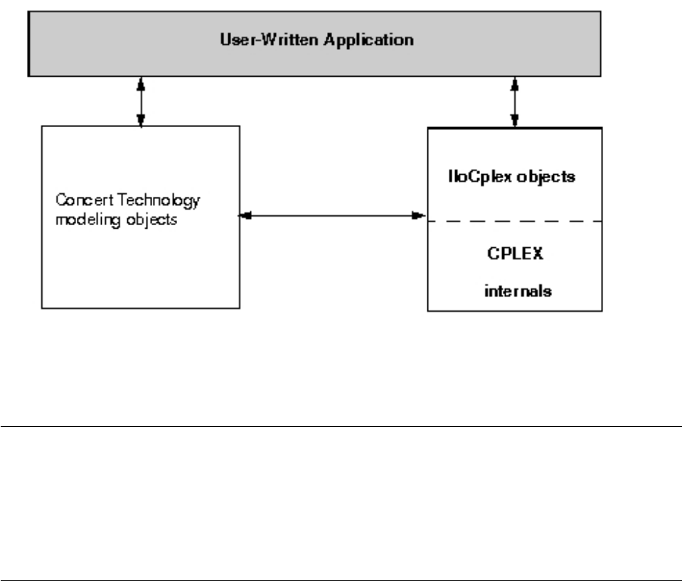
Compiling and linking
Tells where to find instructions to compile and link a C++ application using
CPLEX.
Compilation and linking instructions are provided with the files that come in the
standard distribution of CPLEX for your computer platform. Check the
readme.html file for details.
Creating a C++ application with Concert Technology
Outlines steps to create a C++ application with CPLEX.
About this task
These are the steps most applications are likely to entail.
Procedure
1. First, create a model of your problem with the modeling facilities of Concert
Technology. “Modeling an optimization problem with Concert Technology” on
page 5 offers an introduction to creating a model.
2. When the model is ready to be solved, hand it over to CPLEX for solving.
“Solving the model” on page 9 explains how to do so. It includes a survey of
the IloCplex interface for controlling the optimization. Individual controls are
discussed in the chapters explaining the individual optimizers.
3. After CPLEX solves the model, “Accessing solution information” on page 14,
shows you how to access and interpret results from the optimization.
Figure 1. A view of Concert Technology for C++ users
4CPLEX User’s Manual

4. After analyzing the results, you may want to make changes to the model and
study their effect. “Modifying a model” on page 18 explains how to make
changes and how CPLEX deals with them.
5. “Handling errors” on page 20, discusses the error handling and debugging
support provided by Concert Technology and CPLEX.
6. “Example: optimizing the diet problem in C++” on page 21 presents a
complete program.
Results
Not covered in this chapter are advanced features, such as the use of goals or
callbacks for querying data about an ongoing optimization and for controlling the
optimization itself. Goals, callbacks, and other advanced features are discussed in
Part 7, “Advanced programming techniques,” on page 473.
Modeling an optimization problem with Concert Technology
Introduces classes of the C++ API of Concert Technology for modeling
optimization problems to be solved by IloCplex.
Overview
Highlights the C++ classes for models in CPLEX.
A Concert Technology model consists of a set of C++ objects. Each variable, each
constraint, each special ordered set (SOS), and the objective function in a model are
all represented by objects of the appropriate Concert Technology class. These
objects are known as modeling objects. They are summarized in the table Table 2
on page 9.
Creating the environment: IloEnv
Describes the C++ class IloEnv.
Before you create modeling objects, you must construct an object of the class
IloEnv . This object known as the environment. It is constructed with the
statement:
IloEnv env;
That statement is usually the first Concert Technology statement in an application.
At the end, you must close the environment by calling:
env.end();
That statement is usually the last Concert Technology statement in an application.
The end method must be called because, like most Concert Technology classes, the
class IloEnv is a handle class. That is, an IloEnv object is really only a pointer to
an implementation object. Implementation objects are destroyed by calling the end
method. Failure to call the end method can result in memory leaks.
Users familiar with the CPLEX Callable Library are cautioned not to confuse the
Concert Technology environment object with the CPLEX environment object of
type CPXENVptr, used to set CPLEX parameters. Such an object is not needed with
Concert Technology, as parameters are handled directly by each instance of the
class IloCplex. In other words, the environment in Concert Technology always
refers to the object of class IloEnv required for all other Concert Technology
objects.
Chapter 1. Concert Technology for C++ users 5
Defining variables and expressions: IloNumVar
Describes the C++ class IloNumVar.
Probably the first modeling class you will need is IloNumVar . Objects of this class
represent decision variables in a model. They are defined by the lower and upper
bound for the variable, and a type which can be one of ILOFLOAT , ILOINT , or
ILOBOOL for continuous, integer, or Boolean variables, respectively. The following
constructor creates an integer variable with bounds -1 and 10:
IloNumVar myIntVar(env, -1, 10, ILOINT);
The class IloNumVar provides methods that allow querying of the data needed to
specify a variable. However, only bounds can be modified. Concert Technology
provides a modeling object class IloConversion to change the type of a variable.
This conversion allows you to use the same variable with different types in
different models.
Variables are usually used to build up expressions, which in turn are used to
define the objective or constraints of the optimization problem. An expression can
be explicitly written, as in
1*x[1] + 2*x[2] + 3*x[3]
where xis assumed to be an array of variables (IloNumVarArray ). Expressions can
also be created piece by piece, with a loop:
IloExpr expr(env);
for (int i = 0; i < x.getSize(); ++i)
expr += data[i] * x[i];
Whenever possible, build your expressions in terms of data that is either integer or
double-precision (64-bit) floating point. Single-precision (32-bit) floating point data
should be avoided, as it can result in unnecessarily ill conditioned problems. For
more information, refer to “Numeric difficulties” on page 148.
While Concert Technology supports very general expressions, only linear,
quadratic, piecewise-linear, and logical expressions can be used in models to be
solved with IloCplex . For more about each of those possibilities, see these topics:
vChapter 11, “Solving LPs: simplex optimizers,” on page 135 and Chapter 12,
“Solving LPs: barrier optimizer,” on page 161 both discuss linear expressions.
vChapter 14, “Solving problems with a quadratic objective (QP),” on page 189
discusses quadratic expressions in an objective function.
vChapter 15, “Solving problems with quadratic constraints (QCP),” on page 201
discusses quadratic expressions in quadratically constrained programming
problems (QCPs), including the special case of second order cone programming
(SOCP) problems.
vChapter 22, “Using piecewise linear functions in optimization: a transport
example,” on page 329 introduces piecewise-linear expressions through a
transportation example.
vChapter 24, “Logical constraints in optimization,” on page 343 introduces logical
constraints handled by CPLEX. Topics following it offer examples.
When you have finished using an expression (that is, you created a constraint with
it) you need to delete it by calling its method end , for example:
expr.end();
6CPLEX User’s Manual
Declaring the objective: IloObjective
Describes the C++ class IloObjective.
Objects of class IloObjective represent objective functions in optimization models.
IloCplex may only handle models with at most one objective function, though the
modeling API provided by Concert Technology does not impose this restriction. An
objective function is specified by creating an instance of IloObjective . For
example:
IloObjective obj(env,
1*x[1] + 2*x[2] + 3*x[3],
IloObjective::Minimize);
defines the objective to minimize the expression 1*x[1] + 2*x[2] + 3*x[3].
Adding constraints: IloConstraint and IloRange
Describes the C++ classes for constraints and ranges.
Similarly, objects of the class IloConstraint represents constraints in your model.
Most constraints will belong to the subclass IloRange , derived from
IloConstraint, and thus inherit its constructors and methods. IloRange represent
constraints of the form lower bound ≤expression ≤upper bound . In other
words, an instance of IloRange is a convenient way to express a ranged constraint,
that is, a constraint with explicit upper or lower bounds. Any floating-point value
or +IloInfinity or -IloInfinity can be used for the bounds. For example:
IloRange r1(env, 3.0, x[1] + x[2], 3.0);
defines the constraint x[1] + x[2] == 3.0 .
Formulating a problem: IloModel
Describes the C++ class IloModel.
To formulate a full optimization problem, you need to create the objects that are
part of it and add them to an instance of IloModel, the class that represents
optimization problems. For example, these lines:
IloModel model(env);
model.add(obj);
model.add(r1);
define a model consisting of the objective obj , constraint r1 , and all the variables
they use. Notice that variables need not be added to a model explicitly, as they are
implicitly considered if any of the other modeling objects in the model use them.
(However, you may explicitly add variables to a model, for example, if you
consider a variable a part of the problem even though it does not appear in a
constraint or objective function.)
For convenience, Concert Technology provides the functions IloMinimize and
IloMaximize to define minimization and maximization objective functions. Also,
operators <=, == , and >= are overloaded to create IloRange constraints. These
features allow you to rewrite that example in a compact and readable way, like
this:
IloModel model(env);
model.add(IloMinimize(env, 1*x[1] + 2*x[2] + 3*x[3]);
model.add(x[1] + x[2] == 3.0);
Chapter 1. Concert Technology for C++ users 7
With this notation, you need not create the C++ variables obj and r1 explicitly (as
originally in the example). Instead, they are expressed through the variables in this
second example.
The class IloModel is itself a class of modeling objects. Thus, one model can be
added to another. A possible use of this feature is to capture different scenarios in
different models, all of which are extensions of a core model. The core model could
be represented as an IloModel object itself and added to the IloModel objects that
represent the individual scenarios.
Managing data
Describes C++ classes to manage data.
Usually the data of an optimization problem must be collected before or during the
creation of the Concert Technology representation of the model. Though, in
principle, modeling does not depend on how the data is generated and
represented, this task may be facilitated by the array classes or set classes, such
asIloNumSet, provided by Concert Technology.
For example, objects of class IloNumArray can be used to store numeric data in
arrays. Elements of the class IloNumArray can be accessed like elements of standard
C++ arrays, but the class also offers a wealth of additional features. For example,
Concert Technology arrays are extensible; in other words, they transparently adapt
to the required size when new elements are added using the method add .
Conversely, elements can be removed from anywhere in the array with the method
remove . Concert Technology arrays also provide debugging support when
compiled in debug mode by using assert statements to make sure that no element
beyond the array bounds is accessed. Input and output operators (that is,
operator << and operator >>) are provided for arrays. For example, the code:
IloNumArray data(env, 3, 1.0, 2.0, 3.0);
cout << data << endl;
produces the following output:
[1.0, 2.0, 3.0]
When you have finished using an array and want to reclaim its memory, call the
method end; for example, data.end. When the environment ends, all memory of
arrays belonging to the same environment is returned to the system as well. Thus,
in practice you do not need to call end on an array (or any other Concert
Technology object) just before calling env.end.
The constructor for arrays specifies that an array of size 3 with elements 1.0, 2.0,
and 3.0 is constructed. This output format can be read back in with, for example:
cin >> data;
The “Example: optimizing the diet problem in C++” on page 21 takes advantage of
this function and reads the problem data from a file.
Finally, Concert Technology provides the template class IloArray<X> to create array
classes for your own type X. This technique can be used to generate
multidimensional arrays. All the functions mentioned here are supported for
IloArray classes except for input/output, which depends on the input and output
operator being defined for type X.
8CPLEX User’s Manual

Solving the model
Describes facilities for solving a model in the C++ API.
Overview
Introduces the C++ class IloCplex.
CPLEX generally does not need to be involved while you create your model.
However, after the model is set up, it is time to create your cplex object, that is, an
instance of the class IloCplex, to be used to solve the model. IloCplex is a class
derived from IloAlgorithm. There are other Concert Technology algorithm classes,
also derived from IloAlgorithm, as documented in the CPLEX C++ API Reference
Manual. Some models might also be solved by using other algorithms, such as the
class IloCP for constraint programming, or by using a hybrid algorithm consisting
of both CP Optimizer and CPLEX. Some models, on the other hand, cannot be
solved with CPLEX.
The makeup of the model determines whether or not CPLEX can solve it. More
precisely, in order to be handled by IloCplex objects, a model may only consist of
modeling objects of the classes listed in Table 2.
Instances of IloConstraint extracted by CPLEX can be created in a variety of
ways. Most often, they can be generated by means of overloaded C++ operators,
such as == , <= , or >= , in the form expression1 operator expression2 . Instances
of both IloConstraint and IloRange generated in that way may be built from
either linear or quadratic expressions. Constraints and ranges may also include
piecewise linear terms. (Other sections of this manual, not specific to C++, show
you how to use quadratic expressions: Chapter 14, “Solving problems with a
quadratic objective (QP),” on page 189 and Chapter 15, “Solving problems with
quadratic constraints (QCP),” on page 201. Likewise, Chapter 22, “Using piecewise
linear functions in optimization: a transport example,” on page 329 shows you how
to apply piecewise linear terms in a C++ application.)
For more detail about solving problems with IloCplex , see the following sections
of this manual.
Table 2. Concert Technology modeling objects in C++
To model: Use:
numeric variables objects of the class IloNumVar , as long as
they are not constructed with a list of
feasible values
semi-continuous variables objects of the class IloSemiContVar
linear objective function an object of the class IloObjective with
linear or piecewise linear expressions
quadratic objective function an object of the class IloObjective with
quadratic expressions
Chapter 1. Concert Technology for C++ users 9

Table 2. Concert Technology modeling objects in C++ (continued)
To model: Use:
linear constraints objects of the class IloRange
(lower bound <= expression <= upper
bound)
or
objects of the class IloConstraint
(expr1 relation expr2)
involving strictly linear or piecewise linear
expressions
quadratic constraints objects of the class IloConstraint that
contain quadratic expressions as well as
linear expressions or piecewise linear
expressions
logical constraints objects of the class IloConstraint or
generated ranges with linear or piecewise
linear expressions
variable type-conversions objects of the class IloConversion
special ordered sets of type 1 objects of the class IloSOS1
special ordered sets of type 2 objects of class IloSOS2
For an explanation of quadratic constraints, see Chapter 15, “Solving problems
with quadratic constraints (QCP),” on page 201.
For more information about quadratic objective functions, see Chapter 14, “Solving
problems with a quadratic objective (QP),” on page 189.
For examples of piecewise linear constraints, see Chapter 22, “Using piecewise
linear functions in optimization: a transport example,” on page 329.
For more about logical constraints, see Chapter 24, “Logical constraints in
optimization,” on page 343. This topic introduces the idea of generated ranges.
For a description of special ordered sets, see Chapter 20, “Using special ordered
sets (SOS),” on page 321.
Extracting a model
Describes the method that extracts a model for an algorithm in the C++ API.
This manual defines only one optimization model and uses only one instance of
IloCplex at a time to solve the model. Consequently, this manual talks about these
as the model and the cplex object. However, in Concert Technology, an arbitrary
number of models and algorithm-objects can be created. The cplex object can be
created by the constructor:
IloCplex cplex(env);
To use CPLEX to solve the model, the model must first be extracted to cplex by a
call like this:
10 CPLEX User’s Manual
cplex.extract(model);
This method copies the data from the model into the appropriate efficient data
structures, which CPLEX uses for solving the problem. It does so by extracting
each of the modeling objects added to the model and each of the objects referenced
by them. For every extracted modeling object, corresponding data structures are
created internally in the cplex object. For readers familiar with the sparse matrix
representation used internally by CPLEX, a variable becomes a column and a
constraint becomes a row. As discussed later, these data structures are
synchronized with the modeling objects even if the modeling objects are modified.
If you consider a variable to be part of your model, even though it is not (initially)
used in any constraint, you should add this variable explicitly to the model. This
practice makes sure that the variable will be extracted. This practice may also be
important if you query solution information for the variable, since solution
information is available only for modeling objects that are known to CPLEX
because they have been extracted from a model.
If you feel uncertain about whether or not an object will be extracted, you can add
it to the model to be sure. Even if an object is added multiple times, it will be
extracted only once and thus will not slow the solution process down.
Since the sequence of creating the cplex object and extracting the model to it is
such a common one, IloCplex provides the shortcut:
IloCplex cplex(model);
This shortcut is completely equivalent to separate calls and makes sure that the
environment used for the cplex object will be the same as that used for the model
when it is extracted, as required by Concert Technology. The shortcut uses the
environment from the model to construct the cplex object before extraction.
Invoking a solver
Describes the method that invokes a solver in the C++ API.
After the model is extracted to the cplex object, you are ready to solve it by calling
solve();
For most problems this is all that is needed for solving the model. Nonetheless,
CPLEX offers a variety of controls that allow you to tailor the solution process for
your specific needs.
Choosing an optimizer
Describes the optimizers available in the C++ API.
Solving the extracted model with CPLEX involves solving one or a series of
continuous relaxations:
vOnly one continuous relaxation needs to be solved if the extracted model is
continuous itself, that is, if it does not contain integer variables, Boolean
variables, semi-continuous or semi-integer variables, logical constraints, special
ordered sets (SOS), or piecewise linear functions. Chapter 11, “Solving LPs:
simplex optimizers,” on page 135 and Chapter 12, “Solving LPs: barrier
optimizer,” on page 161 discuss the algorithms available for solving LPs.
Similarly, Chapter 14, “Solving problems with a quadratic objective (QP),” on
page 189, discusses the algorithms available for solving QPs. Chapter 15,
Chapter 1. Concert Technology for C++ users 11
“Solving problems with quadratic constraints (QCP),” on page 201 re-introduces
the barrier optimizer in the context of quadratically constrained programming
problems (QCPs). Chapter 22, “Using piecewise linear functions in optimization:
a transport example,” on page 329 introduces piecewise-linear functions through
a transportation example. Chapter 24, “Logical constraints in optimization,” on
page 343 introduces logical constraints, and chapters following it offer examples.
vIn all other cases, the extracted problem that CPLEX sees is indeed a MIP and,
in general, a series of continuous relaxations needs to be solved. The method
cplex.isMIP returns IloTrue in such a case. Chapter 16, “Solving mixed integer
programming problems (MIP),” on page 221 discusses the algorithms applied.
The optimizer option used for solving the first continuous relaxation (whether it is
the only one or just the first in a series of problems) is controlled by the root
algorithm parameter:
cplex.setParam(IloCplex::RootAlg, alg);
where alg is a member of the nested enumeration IloCplex_Algorithm.
As a nested enumeration, the fully qualified names that must be used in the
program are IloCplex::Primal, IloCplex::Dual, and so on. Table 3 displays the
meaning of the optimizer options defined by IloCplex::Algorithm.
Tip:
The choice Sifting is not available for QP models. Only the Barrier option is
available for QCP models. Table 4 summarizes these options.
Table 3. Optimizer options in IloCplex::Algorithm
Optimizer Purpose
AutoAlg let CPLEX decide which algorithm to use
Primal use the primal simplex algorithm
Dual use the dual simplex algorithm
Network use the primal network simplex algorithm on
an embedded network followed by the dual
simplex algorithm for LPs and the primal
simplex algorithm for QPs on the entire
problem
Barrier use the barrier algorithm. The type of
crossover performed after the barrier
algorithm is set by the parameter
IloCplex::BarCrossAlg .
Sifting use the sifting algorithm
Concurrent use multiple algorithms concurrently on a
multiprocessor system
Table 4. Algorithm available at root by problem type
Value Algorithm Type LP?
MILP?
QP?
MIQP?
QCP?
MIQCP?
0 IloCplex::AutoAlgyes yes yes
1 IloCplex::Primal yes yes not available
2 IloCplex::Dual yes yes not available
3 IloCplex::Networkyes yes not available
12 CPLEX User’s Manual
Table 4. Algorithm available at root by problem type (continued)
Value Algorithm Type LP?
MILP?
QP?
MIQP?
QCP?
MIQCP?
4 IloCplex::Barrieryes yes yes
5IloCplex::Siftingyes not available not available
6IloCplex::Concurrentyes yes not available
If the extracted model requires the solution of more than one continuous
relaxation, the algorithm for solving the first one at the root is controlled by the
RootAlg parameter. The algorithm at all other nodes except the root is controlled
by the NodeAlg parameter:
cplex.setParam(IloCplex::NodeAlg, alg)
Table 5 summarizes the options available at nodes.
Table 5. Algorithm types for NodeAlg
Value Algorithm Type MILP? MIQP? MIQCP?
0 IloCplex::Auto yes yes yes
1 IloCplex::Primal yes yes not available
2 IloCplex::Dual yes yes not available
3 IloCplex::Networkyes not available not available
4 IloCplex::Barrieryes yes yes
5IloCplex::Siftingyes not available not available
Controlling the optimizers
Describes parameters that control the optimizers in the C++ API.
Though CPLEX defaults will prove sufficient to solve most problems, CPLEX offers
a variety of parameters to control various algorithmic choices. CPLEX parameters
can assume values of type bool, num, int, and string. IloCplex provides four
categories of parameters that are listed in the nested enumeration types:
vIloCplex_BoolParam
vIloCplex_IntParam
vIloCplex_NumParam
vIloCplex_StringParam
To access the current value of a parameter that interests you from Concert
Technology, use the method getParam. To access the default value of a parameter,
use the method getDefault. Use the methods getMin and getMax to access the
minimum and maximum values of num and int type parameters.
Some integer parameters are tied to nested enumerations that define symbolic
constants for the values the parameter may assume. The table Table 6 on page 14
summarizes those parameters and their enumeration types.
Chapter 1. Concert Technology for C++ users 13
Table 6. Nested enumerations for integer parameters
This Enumeration: Is Used for This Parameter:
IloCplex::Algorithm IloCplex::RootAlg
IloCplex::Algorithm IloCplex::NodeAlg
IloCplex::MIPEmphasisType IloCplex::MIPEmphasis
IloCplex::VariableSelect IloCplex::VarSel
IloCplex::NodeSelect IloCplex::NodeSel
IloCplex::PrimalPricing IloCplex::PPriInd
IloCplex::DualPricing IloCplex::DPriInd
IloCplex::BranchDirection IloCplex::BrDir
There are, of course, routines in Concert Technology to set these parameters. Use
the following methods to set the values of CPLEX parameters:
vsetParam(BoolParam, value);
vsetParam(IntParam, value);
vsetParam(NumParam, value);
vsetParam(StringParam, value);
For example, the numeric parameter IloCplex::EpOpt controlling the optimality
tolerance for the simplex algorithms can be set to 0.0001 by this call:
setParam(IloCplex::EpOpt, 0.0001);
The CPLEX Parameters Reference Manual documents the type of each parameter
(bool, int, num, string) along with the Concert Technology enumeration value,
symbolic constant, and reference number representing the parameter.
The method setDefaults resets all parameters (except the log file) to their default
values, including the CPLEX callback functions. This routine resets the callback
functions to NULL.
When you are solving a MIP, CPLEX provides additional controls of the solution
process. Priority orders and branching directions can be used to control the
branching in a static way. These controls are discussed in “Heuristics” on page 244.
These controls are static in the sense that they allow you to control the solution
process based on data that does not change during the solution and can thus be set
up before you solve the model.
Dynamic control of the solution process of MIPs is provided through goals or
control callbacks. They are discussed in Chapter 36, “Using goals,” on page 483,
and in Chapter 37, “Using optimization callbacks,” on page 499. Goals and
callbacks allow you to control the solution process based on information that is
generated during the solution process. Chapter 38, “Goals and callbacks: a
comparison,” on page 523 contrasts the advantages of each approach.
Accessing solution information
Describes available information about solution feasibility, solution variables, basis
information, and solution quality.
14 CPLEX User’s Manual

Accessing solution status
Describes the status of a solution.
Calling solve returns a Boolean value that specifies whether or not a feasible
solution (but not necessarily the optimal one) has been found. To obtain more of
the information about the model that CPLEX found during the call to the solve
method, call the method getStatus. It returns a member of the nested enumeration
IloAlgorithm_Status. The fully qualified names of those symbols have the
IloAlgorithm prefix. The table Table 7 shows what each return status means for the
extracted model.
Table 7. Algorithm status and information about the model
Return Status Extracted Model
Feasible has been proven to be feasible. A feasible
solution can be queried.
Optimal has been solved to optimality. The optimal
solution can be queried.
Infeasible has been proven to be infeasible.
Unbounded has been proven to be unbounded. The
notion of unboundedness adopted by
IloCplex does not include that the model
has been proven to be feasible. Instead, what
has been proven is that if there is a feasible
solution with objective value x*, there exists
a feasible solution with objective value x*-1
for a minimization problem, or x*+1 for a
maximization problem.
InfeasibleOrUnbounded has been proven to be infeasible or
unbounded.
Unknown has not been able to be processed far
enough to prove anything about the model.
A common reason may be that a time limit
was hit.
Error has not been able to be processed or an error
occurred during the optimization.
As you see, these statuses indicate information about the model that the CPLEX
optimizer was able to prove during the most recent call to the method solve.
In addition, the CPLEX optimizer provides information about how it terminated.
For example, it may have terminated with only a feasible but not optimal solution
because it hit a limit or because a user callback terminated the optimization.
Further information is accessible by calling solution query routines, such as the
method getCplexStatus, which returns a member of the nested enumeration type
IloCplex::CplexStatus, or methods cplex.isPrimalFeasible or
cplex.isDualFeasible.
For more information about those status codes, see the CPLEX Reference Manual.
Querying solution data
Describes methods available in the C++ API to query data about the solution after
optimization.
Chapter 1. Concert Technology for C++ users 15
If getValue returns IloTrue , a feasible solution has been found and solution values
for model variables are available to be queried. For example, the solution value for
the numeric variable var1 can be accessed like this:
IloNum x1 = getValue(var1);
However, querying solution values variable by variable may result in ugly code.
Here, the use of Concert Technology arrays provides a much more compact way of
accessing the solution values. Assuming your variables are stored in an array of
numeric variables (IloNumVarArray) named var , use lines like these to access the
solution values for all variables in var simultaneously:
IloNumArray x(env); getValues(x, var);
Value x[i] contains the solution value for variable var[i].
Solution data is not restricted to the solution values of variables. It also includes
values of slack variables in constraints (whether the constraints are linear or
quadratic) and the objective value. If the extracted model does not contain an
objective object, IloCplex assumes a 0 expression objective. The objective value is
returned by calling method getObjValue. Slack values are accessed with the
methods getSlack and getSlacks, which take a linear constraint, a quadratic
constraint, or an array of constraints as a parameter.
For LPs and QPs, solution data includes information such as dual variables and
reduced cost. Such information can be queried with the methods, getDual,
getDuals, getReducedCost, and getReducedCosts.
Accessing basis information
Describes methods in the C++ API to retrieve basis information.
When you solve LPs or QPs with either the simplex algorithm or the barrier
optimizer with crossover enabled, basis information is available as well. You can
consult basis information by means of the method getStatuses which returns basis
status information for variables and constraints.
Such information is encoded by the nested enumeration IloCplex::BasisStatus.
Performing sensitivity analysis
Describes methods in the C++ API to analyze infeasible problems.
The availability of a basis for an LP allows you to perform sensitivity analysis for
your model, if the model is an LP. Such analysis tells you by how much you can
modify your model without affecting the solution you found. The modifications
supported by the sensitivity analysis function include bound changes, changes of
the right hand side vector and changes of the objective function. They are analyzed
by the methods getBoundSA, getRHSSA, and getObjSA, respectively.
Analyzing infeasible problems
Describes methods in the C++ API to analyze infeasible models.
An important feature of CPLEX is that even if no feasible solution has been found,
(that is, if solve returns IloFalse), some information about the problem can be
16 CPLEX User’s Manual
queried. All the methods discussed so far may successfully return information
about the current (infeasible) solution which CPLEX maintains.
Unfortunately, there is no simple comprehensive rule about whether or not current
solution information can be queried because, by default, CPLEX uses a presolve
procedure to simplify the model. If, for example, the model is proven to be
infeasible during the presolve, no current solution is generated by the optimizer. If,
in contrast, infeasibility is proven by the optimizer, current solution information is
available to be queried. The status returned by getCplexStatus may help you
decide which case you are facing, but it is probably safer and easier to include the
methods for querying solution within try/catch statements.
When an LP has been proven to be infeasible, CPLEX provides assistance for
investigating the cause of the infeasibility. In one approach, known as FeasOpt,
CPLEX accepts an infeasible model and selectively relaxes bounds and constraints
to find a minimal set of changes that would make the model feasible. It then
reports these suggested changes and the solution they would produce for you to
decide whether to apply them in your model. For more about this approach, see
“Repairing infeasibility: FeasOpt” on page 157.
In another approach, CPLEX can detect a conflict among the constraints and
bounds of an infeasible model and refine the conflict to report to you a minimal
conflict to repair yourself. For more about this approach, see Chapter 33,
“Diagnosing infeasibility by refining conflicts,” on page 451.
For more about these and other ways of overcoming infeasibility, see “Diagnosing
LP infeasibility” on page 152.
Assessing solution quality
Describes methods in the C++ API to assess quality of a solution.
The CPLEX optimizer uses finite precision arithmetic to compute solutions. To
compensate for numeric errors due to this convention, tolerances are used by
which the computed solution is allowed to violate feasibility or optimality
conditions. Thus the solution computed by the solve method may in fact slightly
violate the bounds specified in the model, for example. You can call the method
getQuality, like this: IloNum violation = cplex.getQuality(q); where q is one of
the symbols of the embedded enumeration IloCplex::Quality such as
MaxPrimalInfeas. That method queries the maximum bound violation among all
variables and slacks.
If you are also interested in the variable or constraint where the maximum
violation occurs, call the same method with these arguments instead:
IloRange maxrange;
IloNumVar maxvar;
IloNum violation = cplex.getQuality(IloCplex::MaxPrimalInfeas, &maxrange, &maxvar);
CPLEX copies the variable or constraint handle in which the maximum violation
occurs to maxvar or maxrange , and then CPLEX makes the other handle an empty
one. The maximum primal infeasibility is only one example of a wealth of quality
measures. The full list is defined by the nested enumeration IloCplex::Quality. Each
of these measures of quality can be used as an argument for the methods
getQuality, though some measures are not available for all choices of all options of
all optimizers. A list of solution qualities appears in the CPLEX Reference Manual of
the Callable Library and C++ API, as the group optim.cplex.solutionquality .
Chapter 1. Concert Technology for C++ users 17

Modifying a model
Describes methods in the C++ API to modify a model.
Overview
Outlines different ways to modify a model for CPLEX in a C++ application.
In some applications, you may want to solve another model or a modification of
your original model, in order, for example, to analyze a scenario or to make
adaptations based on the solution of the first model. To do this, you do not have to
start a new model from scratch, but instead you can take an existing model and
change it to your needs. To do so, call the modification methods of the individual
modeling objects.
When an extracted model is modified, the modification is tracked in the cplex
object through notification. Whenever a modification method is called, cplexobjects
that have extracted the model are notified about it. The cplex objects then track the
modification in their internal data structures.
Not only does CPLEX track all modifications of the model it has extracted, but also
it tries to maintain as much solution information from a previous invocation of
solve as is possible and reasonable.
You have already encountered what is perhaps the most important modification
method, that is, the method IloModel::add for adding modeling objects to a model.
Conversely, you may call IloModel::remove to remove a modeling object from a
model.
Objective functions can be modified by changing their sense and by editing their
expression, or by changing their expression completely.
Similarly, the bounds of constraints and their expressions can be modified.
For a complete list of supported modifications, see the documentation of the
individual modeling objects in the reference manual.
Deleting and removing modeling objects
Describes the effects of deleting modeling objects in the C++ API.
A special type of modification is that of deleting a modeling object by calling its
end method. Consider, for example, the deletion of a variable. What happens if the
variable you delete has been used in constraints or in the objective function, or has
been extracted to CPLEX? If you call its end method, Concert Technology carefully
removes the deleted variable from all other modeling objects and algorithms that
may keep a reference to the variable in question. This convention applies to any
modeling object to be removed. However, user-defined handles to the removed
variable are not managed by Concert Technology. Instead, it is up to the user to
make sure that these handles are not used after the deletion of the modeling object.
The only operation allowed then is the assignment operator.
Concert Technology also provides a way to remove a modeling object from all
other modeling objects and algorithms exactly the same way as when deleting it,
yet without deleting the modeling object: call the method
18 CPLEX User’s Manual
IloExtractable::removeFromAll. This method may be helpful to temporarily
remove a variable (or even an array of objects) from your model while keeping the
option to add it back later.
Tip: The method removeFromAll is inherited by classes derived from the class
IloExtractable, such classes as IloObjective, IloConstraint, or IloModel and others.
It is important to understand the difference between calling end and calling
model.remove(obj) for an object obj. In the case of a call to remove, obj is not
necessarily removed from the problem that CPLEX maintains. Whether or not
anything appears to happen depends on whether the removed object is referenced
by yet another extracted modeling object. For example, when you add a modeling
object, such as a ranged constraint, to a model, all the variables used by that
modeling object implicitly become part of the model as well. However, when you
remove that modeling object (for example, that ranged constraint), those variables
are not implicitly removed because they may be referenced by other elements
(such as the objective function or a basis, for example). In other words,
model.add(rngct) followed later by model.remove(rngct) does not leave the model
unchanged: the model still contains the variables in rngct, even if they do not
actually appear in other constraints. CPLEX does not check whether they appear in
other constraints or not when it applies remove. For that reason, variables can be
explicitly removed from a model only by a call to its end member function.
Usually when a constraint is removed from the extracted model, the constraint is
also removed from CPLEX as well, unless it was added to the model more than
once.
Consider the case where a variable is removed from CPLEX after one of the end or
remove operations. If the cplex object contains a simplex basis, by default the status
for that variable is removed from the basis as well. If the variable happens to be
basic, the operation corrupts the basis. If this is not what you want, CPLEX
provides a delete mode that first pivots the variable out of the basis before
removing it. The resulting basis is not guaranteed to be feasible or optimal, but it
will still constitute a valid basis. To select this mode, call the method:
setDeleteMode(IloCplex::FixBasis);
Similarly, when removing a constraint with the FixBasis delete mode, CPLEX will
pivot the corresponding slack or artificial variable into the basis before removing it,
to make sure of maintaining a valid basis. In either case, if no valid basis was
available in the first place, no pivot operation is performed. To set the delete mode
back to its default setting, call:
setDeleteMode (IloCplex::LeaveBasis);
Changing variable type
Describes IloConversion, the class of the C++ API to change the type of a variable.
The type of a variable cannot be changed by calling modification methods. Instead,
Concert Technology provides the modeling class IloConversion , the objects of
which allow you to override the type of a variable in a model. This design allows
you to use the same variable in different models with different types. Consider for
example model1 containing integer variable x. You then create model2 , as a copy
of model1 , that treats xas a continuous variable, with the following code:
Chapter 1. Concert Technology for C++ users 19

IloModel model2(env);
model2.add(model1);
model2.add(IloConversion(env, x, ILOFLOAT));
A conversion object, that is, an instance of IloConversion , can specify a type only
for a variable that is in a model. Converting the type more than once is an error,
because there is no rule about which would have precedence. However, this
convention is not too restrictive, since you can remove the conversion from a
model and add a new one. To remove a conversion from a model, use the method
IloExtractable::end . To add a new one, use the methodIloModel::add . For a
sample of code using these methods in this procedure, see the documentation of
the class IloConversion in the CPLEX C++ API Reference Manual.
Handling errors
Describes error handling in the C++ API.
In Concert Technology two kinds of errors are distinguished:
vProgramming errors, such as:
– accessing empty handle objects;
– mixing modeling objects from different environments;
– accessing Concert Technology array elements beyond an array’s size; and
– passing arrays of incompatible size to functions.
Such errors are usually an oversight of the programmer. After they are
recognized and fixed there is usually no danger of corrupting an application.
In a production application, it is not necessary to handle these kinds of errors.
In Concert Technology such error conditions are handled using assert
statements. If compiled without -DNDEBUG , the error check is performed and
the code aborts with an error message indicating which assertion failed. A
production application should then be compiled with the -DNDEBUG compiler
option, which removes all the checking. In other words, no CPU cycles are
consumed for checking the assertions.
vRuntime errors, such as memory exhaustion.
A correct program assumes that such failures can occur and therefore must be
treated, even in a production application. In Concert Technology, if such an error
condition occurs, an exception is thrown.
All exceptions thrown by Concert Technology classes (including IloCplex) are
derived from IloException. Exceptions thrown by algorithm classes such as
IloCplex are derived from its child class IloAlgorithm::Exception. The most
common exceptions thrown by CPLEX are derived from IloCplex_Exception, a
child class of IloAlgorithm::Exception .
Objects of the exception class IloCplex::Exception correspond to the error codes
generated by the CPLEX Callable Library. You query the error code from a caught
exception by calling the method:
IloInt getStatus () const;
You query the error message by calling the method:
const char* IloException::getMessage() const;
20 CPLEX User’s Manual

That method is a virtual method inherited from the base class IloException. If you
want to access only the message for printing to a channel or output stream, it is
more convenient to use the overloaded output operator (operator<< ) provided by
Concert Technology for IloException.
In addition to exceptions corresponding to error codes from the C Callable Library,
a cplex object may throw exceptions pertaining only to IloCplex. For example, the
exception MultipleObjException is thrown if a model is extracted containing more
than one objective function. Such additional exception classes are derived from
class IloCplex_Exception; objects can be recognized by a negative status code
returned when calling method getStatus .
In contrast to most other Concert Technology classes, exception classes are not
handle classes. Thus, the correct type of an exception is lost if it is caught by value
rather than by reference (that is, using catch(IloException& e) {...} ). This is one
reason that catching IloException objects by reference is a good idea, as
demonstrated in all examples. See, for example, ilodiet.cpp . Some derived
exceptions may carry information that would be lost if caught by value. So if you
output an exception caught by reference, you may get a more precise message than
when outputting the same exception caught by value.
There is a second reason for catching exceptions by reference. Some exceptions
contain arrays to communicate the reason for the failure to the calling function. If
this information were lost by calling the exception by value, method end could not
be called for such arrays and their memory would be leaked (until env.end is
called). After catching an exception by reference, calling the exception’s method
end will free all the memory that may be used by arrays (or expressions) of the
actual exception that was thrown.
In summary, the preferred way of catching an exception is this:
catch (IloException& e) {
...
e.end();
}
where IloException may be substituted for the desired Concert Technology
exception class.
Example: optimizing the diet problem in C++
Shows an example of the C++ API.
Overview
Outlines how to solve the diet problem with CPLEX in a C++ application.
The optimization problem solved in this example is to compose a diet from a set of
foods, so that the nutritional requirements are satisfied and the total cost is
minimized. “Problem representation” on page 22 describes the problem.
The example ilodiet.cpp illustrates these procedures:
v“Creating a model row by row” on page 22;
v“Creating a model column by column” on page 23.
Chapter 1. Concert Technology for C++ users 21
To continue this example, “Application description” on page 23 outlines the
structure of the application. The following sections explain more about data
structures useful in this application.
Notes about the application are available in “Complete program” on page 26.
Problem representation
Describes how the problem is represented in the application.
The problem contains a set of foods, which are the modeling variables; a set of
nutritional requirements to be satisfied, which are the constraints; and an objective
of minimizing the total cost of the food. There are two ways of looking at this
problem:
vThe problem can be modeled by rows, by entering the variables first and then
adding the constraints on the variables and the objective function.
vThe problem can be modeled by columns, by constructing a series of empty
constraints and then inserting the variables into the constraints and the objective
function.
Concert Technology is equally suited for both kinds of modeling; in fact, you can
even mix both approaches in the same program. If a new food product is created,
you can create a new variable for it regardless of how the model was originally
built. Similarly, if a new nutrient is discovered, you can add a new constraint for it.
Creating a model row by row
You walk into the store and compile a list of foods that are offered. For each food,
you store the price per unit and the amount in stock. For some foods that you
particularly like, you also set a minimum amount you would like to use in your
diet. Then, for each of the foods, you create a modeling variable to represent the
quantity to be purchased for your diet.
Now you get a nutrition book and look up which nutrients are known and
relevant for you. For each nutrient, you note the minimum and maximum amounts
that should be found in your diet. Also, you go through the list of foods and
decide how much a food item will contribute for each nutrient. This gives you one
constraint per nutrient, which can naturally be represented as a range constraint in
pseudo-code like this:
nutrMin[i] <= sum_j (nutrPer[i][j] * Buy[j]) <= nutrMax[i]
where irepresents the number of the nutrient under consideration, nutrMin[i]
and nutrMax[i] the minimum and maximum amount of nutrient iand
nutrPer[i][j] the amount of nutrient iin food j.
Finally, you specify your objective function in pseudo-code like this:
minimize sum_j (cost[j] * Buy[j])
The loop in the example combines those two ideas and looks like this:
mod.add(IloMinimize(env, IloScalProd(Buy,foodCost)));
for (i = 0; i < m; i++) {
IloExpr expr(env);
for (j = 0; j < n; j++) {
expr += Buy[j] * nutrPer[i][j];
}
mod.add(nutrMin[i] <= expr <= nutrMax[i]);
expr.end();
22 CPLEX User’s Manual
This way of creating the model appears in the function buildModelByRow , in the
example ilodiet.cpp .
Creating a model column by column
You start with the nutrition book where you compile the list of nutrients that you
want to make sure are properly represented in your diet. For each of the nutrients,
you create an empty constraint:
nutrMin[i] ≤... ≤nutrMax[i]
where ... is left to be filled in after you walk into the store. Also, you set up the
objective function to minimize the cost. Constraint iis referred to as range[i] and
to the objective as cost .
Now you walk into the store and, for each food, you check the price and
nutritional content. With this data you create a variable representing the amount
you want to buy of the food type and install the variable in the objective function
and constraints. That is, you create the following column in pseudo code, like this:
cost(foodCost[j]) "+" "sum_i" (range[i](nutrPer[i][j]))
where the notation +and sum indicate in pseudo code that you add the new
variable jto the objective cost and constraints range[i]. The value in parentheses
is the linear coefficient that is used for the new variable. This notation is similar to
the syntax actually used in Concert Technology, as demonstrated in the function
buildModelByColumn , in the example ilodiet.cpp .
for (j = 0; j < n; j++) {
IloNumColumn col = cost(foodCost[j]);
for (i = 0; i < m; i++) {
col += range[i](nutrPer[i][j]);
}
Buy.add(IloNumVar(col, foodMin[j], foodMax[j], type));
col.end();
}
Application description
Describes the architecture of the application.
In ilodiet.cpp , the main part of the application starts by declaring the
environment and terminates by calling the method end for that environment. The
code in between is encapsulated in a try block that catches all Concert Technology
exceptions and prints them to the C++ error stream cerr . All other exceptions are
caught as well, and a simple error message is issued. The first action of the
program is to evaluate command-line options and call the function usage in cases
of misuse.
Note:
In such cases, an exception is thrown. This practice makes sure that env.end is
called before the program is terminated.
Creating multi-dimensional arrays with IloArray
Describes data handling in the application.
All data defining the problem are read from a file. The nutrients per food are
stored in a two-dimensional array, IloNumArray2 .
Chapter 1. Concert Technology for C++ users 23
Using arrays for input or output
Describes input and out in the application.
If all goes well, the input file is opened in the file ifstream . After that, the arrays
for storing the problem data are created by declaring the appropriate variables.
Then the arrays are filled by using the input operator with the data file. The data
is checked for consistency and, if it fails, the program is aborted, again by
throwing an exception.
After the problem data has been read and verified, it is time to build the model. To
do so, construct the model object with this declaration:
IloModel mod(env);
The array Buy is created to store the modeling variables. Since the environment is
not passed to the constructor of Buy , an empty handle is constructed. So at this
point the variable Buy cannot be used.
Depending on the command-line option, either buildMethodByRow or
buildMethodByColumn is called. Both create the model of the diet problem from the
input data and return an array of modeling variables as an instance of the class
IloNumVarArray . At that point, Buy is assigned to an initialized handle containing
all the modeling variables and can be used afterwards.
Building the model by row
The model is created by rows using the function buildModelByRow . It first gets the
environment from the model object passed to it. Then the modeling variables Buy
are created. Instead of calling the constructor for the variables individually for each
variable, create the full array of variables, with the array of lower and upper
bounds and the variable type as parameter. In this array, variable Buy[i] is created
such that it has lower bound foodMin[i] , upper bound foodMax[i] , and type
indicated by type .
The statement:
mod.add(IloMinimize(env, IloScalProd(Buy, foodCost)));
creates the objective function and adds it to the model. The IloScalProd function
creates the expression ∑j (Buy[j] * foodCost[j]) which is then passed to the
function IloMinimize . That function creates and returns the actual IloObjective
object, which is added to the model with the call mod.add .
The following loop creates the constraints of the problem one by one and adds
them to the model. First the expression ∑j (Buy[j] * nutrPer[i][j]) is created by
building a Concert Technology expression. An expression variable expr of type
IloExpr is created, and linear terms are added to it by using operator+= in a loop.
The expression is used with the overloaded operator<= to construct a range
constraint (an IloRange object) which is added to the model:
mod.add(nutrMin[i] <= expr <= nutrMax[i]);
After an expression has been used for creating a constraint, it is deleted by a call to
expr.end .
Finally, the array of modeling variables Buy is returned.
24 CPLEX User’s Manual
Building the model by column
The function buildModelByColumn implements the creation of the model by
columns. It begins by creating the array of modeling variables Buy of size 0. This is
later populated when the columns of the problem are created and eventually
returned.
The statement:
IloObjective cost = IloAdd(mod, IloMinimize(env));
creates a minimization objective function object with 0 expressions and adds it to
the model. The objective object is created with the function IloMinimize . The
template function IloAdd is used to add the objective as an object to the model and
to return an objective object with the same type, so that the objective can be stored
in the variable cost . The method IloModel::add returns the modeling object as an
IloExtractable , which cannot be assigned to a variable of a derived class such as
IloObjective . Similarly, an array of range constraints with 0 (zero) expressions is
created, added to the model, and stored in the array range .
In the following loop, the variables of the model are created one by one in
columns; thus, the new variables are immediately installed in the model. An
IloNumColumn object col is created and initialized to define how each new variable
will be appended to the existing objective and constraints.
The IloNumColumn object col is initialized to contain the objective coefficient for the
new variable. This is created with cost(foodCost[j]) , that is using the overloaded
operator() for IloObjective . Next, an IloNumColumn object is created for every
constraint, representing the coefficient the new variable has in that constraint.
Again these IloNumColumn objects are created with the overloaded operator() , this
time of IloRange . The IloNumColumn objects are merged together to an aggregate
IloNumColumn object using operator += . The coefficient for row iis created with
range[i](nutrPer[i][j]) , which calls the overloaded operator() for IloRange
objects.
When a column is completely constructed, a new variable is created for it and
added to the array of modeling variables Buy . The construction of the variable is
performed by the constructor:
IloNumVar(col, foodMin[j], foodMax[j], type)
which creates the new variable with lower bound foodMin[j] , upper bound
foodMax[j] and type type , and adds it to the existing objective and ranges with
the coefficients specified in column col . After creating the variable for this
column, the IloColumn object is deleted by calling col.end .
Solving the model with IloCplex
Shows how to solve the example.
After the model has been populated, it is time to create the cplex object and
extract the model to it by calling:
IloCplex(mod);
It is then ready to solve the model, but for demonstration purposes the extracted
model will first be written to the file diet.lp . Doing so can help you debug your
Chapter 1. Concert Technology for C++ users 25
model, as the file contains exactly what CPLEX sees. If it does not match what you
expected, it will probably help you locate the code that generated the wrong part.
The model is then solved by calling method solve. Finally, the solution status and
solution vector are output to the output channel cplex.out . By default this
channel is initialized to cout. All logging during optimization is also output to this
channel. To turn off logging, you would set the out stream of cplex to a null
stream by calling cplex.setOut(env.getNullStream()).
Complete program
Refers to the online sample.
The complete program ilodiet.cpp is available online in the standard distribution
at yourCPLEXinstallation /examples/src .
Note:
vAll the definitions needed for a CPLEX Concert Technology application in C++
are imported by including the file <ilcplex/ilocplex.h> .
vThe line ILOSTLBEGIN is a macro that is needed for portability. Microsoft Visual
C++ code varies, depending on whether you use the STL or not. This macro
allows you to switch between both types of code without the need to otherwise
change your source code.
vThe function usage is called in case the program is executed with incorrect
command line arguments.
26 CPLEX User’s Manual

Chapter 2. Concert Technology for Java users
Explores the features CPLEX offers to Java users to solve mathematical
programming problems.
Architecture of a CPLEX Java application
Describes the architecture of a Java application in Concert Technology.
Overview
Offers an overview of the architecture.
A user-written application of IBM ILOG CPLEX in Java first creates an IloCplex
object. It then uses the Concert Technology modeling interface implemented by
IloCplex to create the variables, the constraints, and the objective function of the
model to be solved. For example, every variable in a model is represented by an
object that implements the Concert Technology variable interface IloNumVar. The
user code accesses the variable only through its Concert Technology interface.
Similarly, all other modeling objects are accessed only through their respective
Concert Technology interfaces from the user-written application, while the actual
objects are maintained in the CPLEX database.
Figure 2 on page 28 illustrates how an application uses Concert Technology,
IloCplex, and the CPLEX internals. The Java interfaces, represented by the dashed
outline, do not actually consume memory. The CPLEX internals include the
computing environment, its communication channels, and your problem objects.
A user-written Java application and CPLEX internals use separate memory heaps.
Java supports two different command-line options of interest in this respect:
v-Xms sets the initial heap size for the Java-part of the application;
v-Xmx sets the maximum heap size for the Java part of the application.
For applications where more memory is needed, you must carefully assess whether
the Java application needs to increase or decrease its memory heap. In some cases,
the Java application needs more memory to create the model to be solved. If so,
use the -Xmx option to increase the maximum heap size. Keep in mind that
allocating more space in the heap to the Java application makes less memory
available to the CPLEX internals, so increase the maximum heap size only as
needed. Otherwise, the Java application will use too much memory, imposing an
unnecessary limitation on the memory available to the CPLEX internals.
In cases where insufficient memory is available for CPLEX internals, there are
remedies to consider with respect to the heap:
vmake sure the maximum heap size has not been set to a value larger than
needed;
vconsider reducing the default maximum heap size if the Java application can
operate with less memory.
For users familiar with object-oriented design patterns, this design is that of a
factory, where IloCplex is a factory for modeling objects. The advantage of such a
design is that code which creates a model using the Concert Technology modeling
© Copyright IBM Corp. 1987, 2016 27
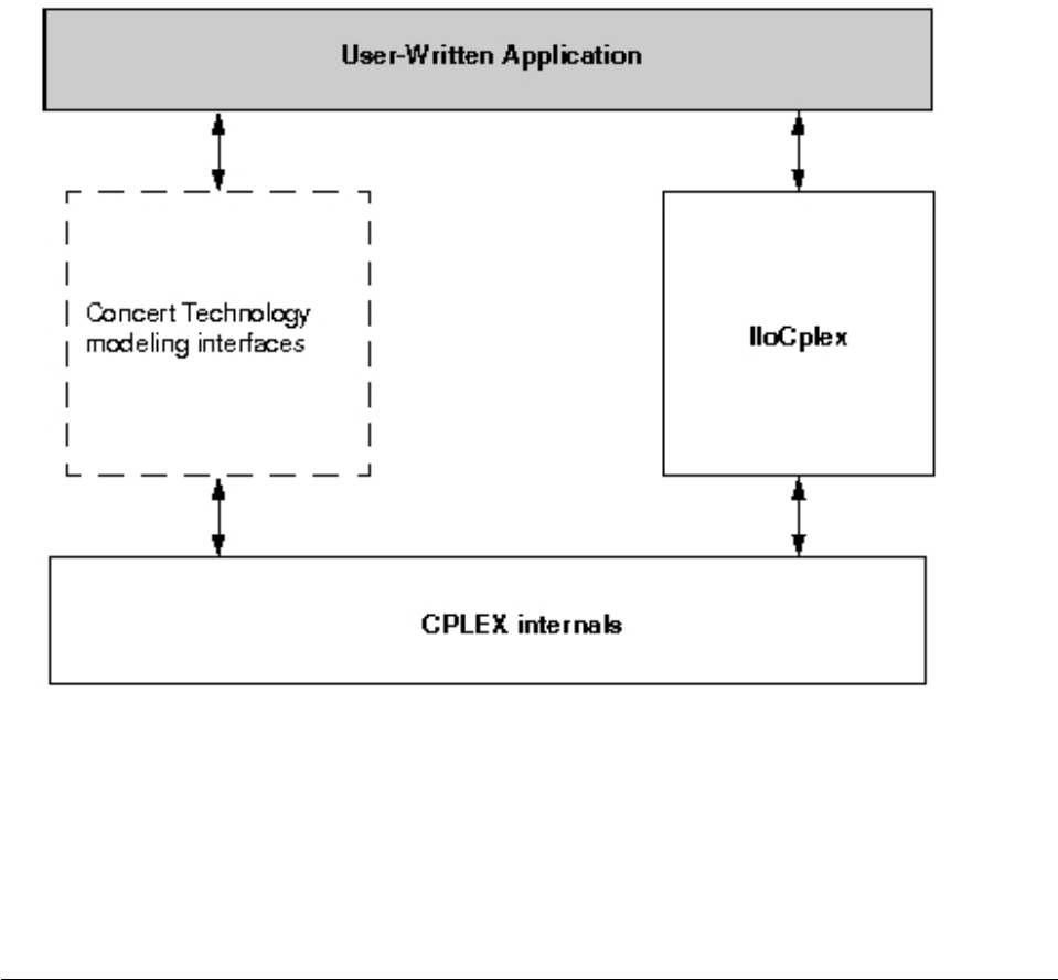
interface can be used not only with IloCplex, but also with any other factory class,
for instance IloSolver. This allows you to try different optimization technologies
for solving your model.
Compiling and linking a Java application
Tells where to find the compilation and linking instructions specific to the Java
API.
Compilation and linking instructions are provided with the files that come in the
standard distribution of CPLEX for your computer platform. Check the file
readme.html for details.
Creating a Java application with Concert Technology
Introduces the components of an application in the Java API of Concert Technology
and covers the steps most Java applications are likely to follow.
First, create a model of your problem with the modeling facilities of Concert
Technology. “Modeling an optimization problem with Concert Technology in the
Java API” on page 29 offers an introduction to creating a model. “Building the
model” on page 34 goes into more detail.
When the model is ready to be solved, hand it over to CPLEX for solving. “Solving
the model” on page 35 explains how to do so. It includes a survey of the IloCplex
interface for controlling the optimization. Individual controls are discussed in the
chapters explaining the individual optimizers.
Figure 2. A view of Concert Technology for Java users
28 CPLEX User’s Manual

“Accessing solution information” on page 36 shows you how to access and
interpret results from the optimization after solving the model.
After analyzing the results, you may want to make changes to the model and
study their effect. “Modifying the model” on page 47 explains how to make
changes and how CPLEX deals with them in the context of the diet problem.
“Example: optimizing the diet problem in Java” on page 45 presents a complete
program.
Not covered in this chapter are advanced features, such as the use of goals or
callbacks to query data about an ongoing optimization and for controlling the
optimization itself. Goals, callbacks, and other advanced features are discussed in
Part 7, “Advanced programming techniques,” on page 473.
Modeling an optimization problem with Concert Technology in the
Java API
Describes classes in the Java API to model an optimization problem.
Overview
Introduces classes to support models for CPLEX in Java applications.
An optimization problem is represented by a set of interconnected modeling
objects in an instance of IloCplex or IloCplexModeler. Modeling objects in Concert
Technology are objects of type IloNumVar and its extensions, or IloAddable and its
extensions. Since these are Java interfaces and not classes, objects of these types
cannot be created explicitly. Rather, modeling objects are created using methods of
an instance of IloModeler or one of its extensions, such as IloMPModeler or
IloCPModeler.
Note:
The class IloCplex extends IloCplexModeler. All the modeling methods in IloCplex
derive from IloCplexModeler. IloCplex implements the solving methods.
The class IloCplexModeler, which implements IloMPModeler, makes it possible for
a user to build models in a Java application as pure Java objects, without using the
class IloCplex.
In particular, a model built with IloCplexModeler using no instance of IloCplex
does not require loading of the CPLEX.dll nor any shared library.
Furthermore, IloCplexModeler is serializable. For example, a user may develop a
pure Java application that builds a model with IloCplexModeler and sends the
model and modeling objects off to an optimization server that uses IloCplex.
The example CplexServer.java shows you how to write an optimization server that
accepts pure Java model taking advantage of the class IloCplexModeler in a native
J2EE client application.
This discussion concentrates on IloModeler and IloMPModeler because the classes
IloCplex and IloCplexModeler implement these interfaces and thus inherit their
methods. To create a new modeling object, you must first create the IloModeler
Chapter 2. Concert Technology for Java users 29

which will be used to create the modeling object. For the discussion here, the
model will be an instance of IloCplex, and it is created like this:
IloCplex cplex = new IloCplex();
Since class IloCplex implements IloMPModeler (and thus its parent interface
IloModeler ) all methods from IloMPModeler and IloModeler can be used for
building a model. IloModeler defines the methods to:
vcreate modeling variables of type integer, floating-point, or Boolean;
vconstruct simple expressions using modeling variables;
vcreate objective functions; and
vcreate ranged constraints, that is, constraints of the form:
lowerbound ≤expression ≤upperbound
Models that consist only of such constructs can be built and solved with any
optimizer implementing the IloModeler interface, including IloCplex, which
implements the IloMPModeler extension.
The IloMPModeler interface extends IloModeler by adding functionality specific to
mathematical programming applications. This functionality includes these
additional modeling object types:
vsemi-continuous variables;
vspecial ordered sets; and
vpiecewise linear functions.
It also includes these modeling features to support specific needs:
vchange of type for previously declared variables;
vmodeling by column; and
vgeneral manipulations of model entities.
Table 8 summarizes those observations about the interfaces of CPLEX with Concert
Technology for Java users.
Table 8. Modeling classes of CPLEX with Concert Technology for Java users
To Model This Use an Object of This Class or Interface
variable IloNumVar and its extensions IloIntVar and
IloSemiContVar
range constraint IloRange with (piecewise) linear or quadratic
expressions
other relational constraint IloConstraint of the form expr1 relation
expr2, where both expressions are linear or
quadratic and may optionally contain
piecewise linear terms.
LP matrix IloLPMatrix
linear or quadratic objective IloObjective with (piecewise) linear or
quadratic expressions
variable type-conversion IloConversion
special ordered set IloSOS1 or IloSOS2
logical constraints IloOr, IloAnd, and methods such as not
30 CPLEX User’s Manual
For an explanation of quadratic constraints, see Chapter 15, “Solving problems
with quadratic constraints (QCP),” on page 201. For more information about
quadratic objective functions, see Chapter 14, “Solving problems with a
quadratic objective (QP),” on page 189. For examples of piecewise linear
constraints, see Chapter 22, “Using piecewise linear functions in optimization: a
transport example,” on page 329. For a description of special ordered sets, see
Chapter 20, “Using special ordered sets (SOS),” on page 321. For more about
logical constraints, see Chapter 24, “Logical constraints in optimization,” on page
343.
Using IloModeler
Describes the class IloModeler in the Java API.
IloModeler defines an interface for building optimization models. This interface
defines methods for constructing variable, constraint, and objective function
objects.
Variables in a model
A modeling variable in Concert Technology is represented by an object of type
IloNumVar or one of its extensions. You can choose from a variety of methods
defined in IloModeler and IloMPModeler to create one or multiple modeling
variable objects. An example of the method is:
IloNumVar x = cplex.numVar(lb, ub, IloNumVarType.Float, "xname");
This constructor method allows you to set all the attributes of a variable: its lower
and upper bounds, its type, and its name. Names are optional in the sense that
null strings are considered to be valid as well.
The other constructor methods for variables are provided mainly for ease of use.
For example, because names are not frequently assigned to variables, all variable
constructors come in pairs, where one variant requires a name string as the last
parameter and the other one does not (defaulting to a null string).
Integer variables can be created by the intVar methods, and do not require the
type IloNumVarType.Int to be passed, as this is implied by the method name. The
bound parameters are also specified more consistently as integers. These methods
return objects of type IloIntVar, an extension of interface IloNumVar that allows
you to query and set bounds consistently using integers, rather than doubles as
used for IloNumVar .
Frequently, integer variables with 0/1 bounds are used as decision variables. To
help create such variables, the boolVar methods are provided. In the Boolean type,
0(zero) and 1(one) are implied, so these methods do not need to accept any
bound values.
For all these constructive methods, there are also equivalent methods for creating a
complete array of modeling variables at one time. These methods are called
numVarArray, intVarArray, and boolVarArray .
Chapter 2. Concert Technology for Java users 31
Expressions
Modeling variables are typically used in expressions that define constraints or
objective functions. Expressions are represented by objects of type IloNumExpr.
They are built using methods such as sum, prod, diff, negative, and square. For
example, the expression
x1 + 2*x2
where x1 and x2 are IloNumVar objects, is constructed by this call:
IloNumExpr expr = cplex.sum(x1, cplex.prod(2.0, x2));
It follows that a single variable is a special case of an expression, since IloNumVar
is an extension of IloNumExpr.
The special case of linear expressions is represented by objects of type
IloLinearNumExpr. Such expressions can be edited, especially convenient when
linear expressions are being built in a loop, like this:
IloLinearNumExpr lin = cplex.linearNumExpr();
for (int i = 0; i < num; ++i)
lin.addTerm(value[i], variable[i]);
The special case of the scalar product of an array of values with an array of
variables is directly supported through the method scalProd. Thus that loop can be
rewritten as:
IloLinearNumExpr lin = cplex.scalProd(value, variable);
It is recommended that you build expressions in terms of data that is either integer
or double-precision (64-bit) floating-point. Single-precision (32 bit) floating-point
data should be avoided as it can result in unnecessarily ill-conditioned problems.
For more information, refer to “Numeric difficulties” on page 148.
Ranged constraints
Ranged constraints are constraints of the form: lb ≤expression ≤ub and are
represented in Concert Technology by objects of type IloRange. The most general
constructor is:
IloRange rng = cplex.range(lb, expr, ub, name);
where lb and ub are double values, expr is of type IloNumExpr, and name is a
string.
By choosing the range bounds appropriately, ranged constraints can be used to
model any of the more commonly found constraints of the form:
expr relation rhs
where relation is the relation =, ≤, or ≥. The following table shows how to choose lb
and ub for modeling these relations:
relation lb ub method
= rhs rhs eq
≤-Double.MAX_VALUE rhs le
≥rhs Double.MAX_VALUE ge
32 CPLEX User’s Manual
The last column contains the method provided with IloModeler to use directly to
create the appropriate ranged constraint, when you specify the expression and
righthand side (RHS). For example, the constraint expr ≤1.0 is created by the call:
IloRange le = cplex.le(expr, 1.0);
Again, all constructors for ranged constraints come in pairs, one constructor with
and one without an argument for the name.
The objective function
The objective function in Concert Technology is represented byan object of type
IloObjective. Such objects are defined by an optimization sense, an expression,
and an optional name. The objective expression is represented by an IloNumExpr.
The objective sense is represented by an object of class IloObjectiveSense and can
take two values, IloObjectiveSense.Maximize or IloObjectiveSense.Minimize. The
most general constructor for an objective function object is:
where sense is of type IloObjectiveSense, expr is of type IloNumExpr, and name is
a string.
For convenience, the methods maximize and minimize are provided to create a
maximization or minimization objective respectively, without using an
IloObjectiveSense parameter. Names for objective function objects are optional, so
all constructor methods come in pairs, one with and one without the name
parameter.
The active model
Describes the active model in the Java API.
Modeling objects, constraints and objective functions are created as explained in
“Using IloModeler” on page 31; then these components must be added to the
active model. The active model is the model implemented by the IloCplex object
itself. In fact, IloModeler is an extension of the IloModel interface defining the
model API. Thus, IloCplex implements IloModel, or in other words, an IloCplex
object is a model. The model implemented by the IloCplex object itself is referred
to as the active model of the IloCplex object, or if there is no possibility of
confusion between several optimizers, simply as the active model.
A model is just a set of modeling objects of type IloAddable such as IloObjective
and IloRange. Objects of classes implementing this interface can be added to an
instance of IloModel. Other IloAddable objects usable with IloCplex are
IloLPMatrix, IloConversion, IloSOS1, and IloSOS2. These will be covered in the
IloMPModeler section.
Variables cannot be added to a model because IloNumVar is not an extension of
IloAddable. All variables used by other modeling objects (IloAddable objects) that
have been added to a model are implicitly part of this optimization model. The
explicit addition of a variable to a model can thus be avoided.
During modeling, a typical sequence of operations is to create a modeling object
and immediately add it to the active model. To facilitate this, for most constructors
with a name such as ConstructorName, there is also a method add ConstructorName
which immediately adds the newly constructed modeling object to the active
model. For example, the call:
IloObjective obj = cplex.addMaximize(expr);
Chapter 2. Concert Technology for Java users 33
is equivalent to:
IloObjective obj = cplex.add(cplex.maximize(expr));
Not only do the add ConstrucorName -methods simplify the program, they are also
more efficient than the two equivalent calls because an intermediate copy can be
avoided.
Building the model
Uses the diet example to demonstrate building a model for CPLEX in Java.
All the building blocks are now in place to implement a method that creates a
model. The diet problem consists of finding the least expensive diet using a set of
foods such that all nutritional requirements are satisfied. The example in this
chapter builds the specific diet model, chooses an optimizing algorithm, and shows
how to access more detailed information about the solution.
The example includes a set of foods, where food jhas a unit cost of foodCost[j].
The minimum and maximum amount of food jwhich can be used in the diet is
designated foodMin[j] and foodMax[j], respectively. Each food jalso has a
nutritional value nutrPerFood[i][j] for all possible nutrients i. The nutritional
requirement states that in the diet the amount of every nutrient iconsumed must
be within the bounds nutrMin[i] and nutrMax[i].
Mathematically, this problem can be modeled using a variable Buy[j] for each food
jindicating the amount of food jto buy for the diet. Then the objective is:
minimize ∑j (Buy[j] * foodCost[j])
The nutritional requirements mean that the following conditions must be observed;
that is, for all i:
nutriMin[i] ≤∑i nutrPerFood[i][j] * Buy[j] ≤nutriMax[i]
Finally, every food must be within its bounds; that is, for all j:
foodMin[j] ≤Buy[j] ≤foodMax[j]
With what you have learned so far, you can implement a method that creates such
a model.
static void buildModelByRow(IloModeler model,
Data data,
IloNumVar[] Buy,
IloNumVarType type)
throws IloException {
int nFoods = data.nFoods;
int nNutrs = data.nNutrs;
for (int j = 0; j < nFoods; j++) {
Buy[j] = model.numVar(data.foodMin[j], data.foodMax[j], type);
}
model.addMinimize(model.scalProd(data.foodCost, Buy));
for (int i = 0; i < nNutrs; i++) {
model.addRange(data.nutrMin[i],
model.scalProd(data.nutrPerFood[i], Buy),
data.nutrMax[i]);
}
}
The function accepts several arguments. The argument model is used for two
purposes:
34 CPLEX User’s Manual

vcreating other modeling objects, and
vrepresenting the model being created.
The argument data contains the data for the model to be built. The argument Buy
is an array, initialized to length data.nFoods, containing the model's variables.
Finally, the argument type is used to specify the type of the variables being
created.
The function starts by creating the modeling variables, one by one, and storing
them in the array Buy. Each variable jis initialized to have bounds
data.foodMin[j] and data.foodMax[j] and to be of type type.
The variables are first used to construct the objective function expression with the
method model.scalProd(foodCost, Buy). This expression is immediately used to
create the minimization objective which is directly added to the active model by
addMinimize.
In the loop that follows, the nutritional constraints are added. For each nutrient i
the expression representing the amount of nutrient in a diet with food levels Buy is
computed using model.scalProd(nutrPerFood[i], Buy). This amount of nutrient
must be within the ranged constraint bounds nutrMin[i] and nutrMax[i]. This
constraint is created and added to the active model with addRange.
Note that function buildModelByRow uses the interface IloModeler rather than
IloCplex. This convention allows the function to be called without change in
another implementation of IloModeler, such as IloCP.
Solving the model
Describes the class IloCplex in the Java API.
After you have created an optimization problem in your active model, you solve it
by means of the IloCplex object. For an object named cplex, for example, you
solve by calling the method like this:
cplex.solve();
The solve method returns a Boolean value specifying whether or not a feasible
solution was found and can be queried. However, when true is returned, the
solution that was found may not be the optimal one; for example, the optimization
may have terminated prematurely because it reached an iteration limit.
Additional information about a possible solution available in the IloCplex object
can be queried with the method getStatus returning an IloCplex.Status object.
Possible statuses are summarized in Table 9.
Table 9. Solution status
Return Status Active Model
Error It has not been possible to process the active
model, or an error occurred during the
optimization.
Unknown It has not been possible to process the active
model far enough to prove anything about
it. A common reason may be that a time
limit was reached.
Chapter 2. Concert Technology for Java users 35
Table 9. Solution status (continued)
Return Status Active Model
Feasible A feasible solution for the model has been
proven to exist.
Bounded It has been proven that the active model has
a finite bound in the direction of
optimization. However, this does not imply
the existence of a feasible solution.
Optimal The active model has been solved to
optimality. The optimal solution can be
queried.
Infeasible The active model has been proven to possess
no feasible solution.
Unbounded The active model has been proven to be
unbounded. The notion of unboundedness
adopted by IloCplex is technically that of
dual infeasibility; this does not include the
notion that the model has been proven to be
feasible. Instead, what has been proven is
that if there is a feasible solution with
objective value z*, there exists a feasible
solution with objective value z*-1 for a
minimization problem, or z*+1 for a
maximization problem.
InfeasibleOrUnbounded The active model has been proven to be
infeasible or unbounded.
For example, an Optimal status indicates that an optimal solution has been found
and can be queried, whereas an Infeasible status indicates that the active model
has been proven to be infeasible. See the online CPLEX Java API Reference Manual
for more information about these statuses.
More detailed information about the status of the optimizer can be queried with
method getCplexStatus returning an object corresponding to CPLEX status codes.
Again the online CPLEX Java API Reference Manual contains further information
about this.
Accessing solution information
Describes the information available in the Java API about a solution.
If a solution has been found with the solve method, you access it and then query
it using a variety of methods. The objective function can be accessed by the call:
double objval = cplex.getObjValue();
The values of individual modeling variables for the solution are accessed by the
methods IloCplex.getValue, for example:
double x1 = cplex.getValue(var1);
Frequently, solution values for an array of variables are needed. Rather than your
having to implement a loop to query the solution values variable by variable, use
the method IloCplex.getValues to do so with only one function call, like this:
double[] x = cplex.getValues(vars);
36 CPLEX User’s Manual

Similarly,you query slack values for the constraints in the active model by means
of the methods IloCplex.getSlack or IloCplex.getSlacks .
These ideas apply to solvingand printing the solution to the diet problem as well.
IloCplex cplex = new IloCplex();
IloNumVar[] Buy = new IloNumVar[nFoods];
if ( byColumn ) buildModelByColumn(cplex, data, Buy, varType);
else buildModelByRow (cplex, data, Buy, varType);
// Solve model
if ( cplex.solve() ) {
System.out.println();
System.out.println(“Solution status = “+ cplex.getStatus());
System.out.println();
System.out.println(“cost = “+ cplex.getObjValue());
for (int i = 0; i < nFoods; i++) {
System.out.println(“Buy”+i+“=“+
cplex.getValue(Buy[i]));
}
System.out.println();
}
These lines of code start by creating a new IloCplex object and passing it, along
with the raw data in another object, either to the method buildModelByColumn or to
the method buildModelByRow. The array of variables returned by it is saved as the
array Buy. Then the method solve optimizes the active model and, upon success,
the application prints solution information.
Choosing an optimizer
Describes algorithms implemented in the Java API for solving optimization
problems.
Overview
Introduces the Java methods that solve a problem in CPLEX.
The algorithm implemented in the solve methods can be controlled and if
necessary tailored to the particular needs of the model. The most important control
you exercise is your selection of the optimizer.
What does CPLEX solve?
Explains what is solved in terms of problem types.
Given an active model, CPLEX solves one continuous relaxation or a series of
continuous relaxations.
vA single LP is solved if IloCplex.isMIP, IloCplex.isQO, and IloCplex.isQC
return false. This is the case if the active model does not include:
– integer variables, Boolean variables, or semi-continuous variables;
– special ordered sets (SOS);
– piecewise linear functions among the constraints; or
– quadratic terms in the objective function or among the constraints.
IloCplex provides several optimizing algorithms to solve LPs. For more about
those optimizers, see Chapter 11, “Solving LPs: simplex optimizers,” on page
135
Chapter 2. Concert Technology for Java users 37
135, Chapter 12, “Solving LPs: barrier optimizer,” on page 161, and
Chapter 13, “Solving network-flow problems,” on page 181 in this manual.
vA single QP is solved if both IloCplex.isMIP and IloCplex.isQC return false
and IloCplex.isQO returns true. This is the case if the active model contains a
quadratic (and positive semi-definite) objective but does not contain:
– integer variables, Boolean variables, or semi-continuous variables;
– quadratic terms among the constraints;
– special ordered sets; or
– piecewise linear functions among the constraints.
As in the case of LPs, IloCplex provides several optimizing algorithms to
solve QPs. For more about identifying this kind of problem, see Chapter 14,
“Solving problems with a quadratic objective (QP),” on page 189.
vA single QCP is solved if IloCplex.isMIP returns false and IloCplex.isQC
returns true, indicating that it detected a quadratically constrained program
(QCP). This is the case if the active model contains one or more quadratic (and
positive semi-definite) constraints but does not contain:
– integer variables, Boolean variables, or semi-continuous variables;
– special ordered sets; or
– piecewise linear functions.
IloCplex solves QCP models using the barrier optimizer. For more about this
kind of problem, see Chapter 15, “Solving problems with quadratic
constraints (QCP),” on page 201, where the special case of second order cone
programming (SOCP) problems is also discussed.
In short, an LP model has a linear objective function and linear constraints; a QP
model has a quadratic objective function and linear constraints; a QCP includes
quadratic constraints, and it may have a linear or quadratic objective function. A
problem that can be represented as LP, QP, or QCP is also known collectively as a
continuous model or a continuous relaxation.
A series of relaxations is solved if the active model is a MIP, which can be
recognized by IloCplex.isMIP returning true. This is the case if the model contains
any of the objects excluded for single continuous models. If a MIP contains a
purely linear objective function, (that is, IloCplex.isQO returns false ), the
problem is more precisely called an MILP. If it includes a positive semidefinite
quadratic term in the objective, it is called an MIQP. If it includes a constraint that
contains a positive semidefinite quadratic term, it is called an MIQCP. MIPs are
solved using branch & cut search, explained in more detail in Chapter 16, “Solving
mixed integer programming problems (MIP),” on page 221.
Solving a single continuous model
Shows how to choose the optimizer to solve a single continuous model.
To choose the optimizer to solve a single continuous model, or the first continuous
relaxation in a series, use
IloCplex.setParam(IloCplex.IntParam.RootAlg, alg)
where alg is an integer specifying the algorithm type. Table 10 on page 39 shows
you the available types of algorithms.
38 CPLEX User’s Manual
Table 10. Algorithm types for RootAlg
alg Algorithm Type LP? QP? QCP?
0 IloCplex.Algorithm.Auto yes yes yes
1 IloCplex.Algorithm.Primal yes yes not available
2 IloCplex.Algorithm.Dual yes yes not available
3 IloCplex.Algorithm.Network yes yes not available
4 IloCplex.Algorithm.Barrier yes yes yes
5IloCplex.Algorithm.Sifting yes not available not available
6IloCplex.Algorithm.Concurrent yes yes not available
You are not obliged to set this parameter. In fact, if you do not explicitly call
IloCplex.setParam(IloCplex.IntParam.RootAlg, alg), CPLEX will use the default:
IloCplex.Algorithm.Auto. In contrast, any invalid setting, such as a value other
than those of the enumeration, will produce an error message.
The IloCplex.Algorithm.Sifting algorithm is not available for QP. IloCplex will
default to the IloCplex.Algorithm.Auto setting when the parameter
IloCplex.IntParam.RootAlg is set to IloCplex.Algorithm.Sifting for a QP.
Only the settings IloCplex.Algorithm.Auto and IloCplex.Algorithm.Barrier are
available for a QCP.
Solving subsequent continuous relaxations in a MIP
Shows how to choose the optimizer to solve a series of relaxations.
Parameter IloCplex.IntParam.RootAlg also controls the algorithm used for solving
the first continuous relaxation when solving a MIP. The algorithm for solving all
subsequent continuous relaxations is then controlled by the parameter
IloCplex.IntParam.NodeAlg .
In other words, use the root algorithm parameter to choose the optimizer for
solving at the root, and use the node algorithm parameter to choose the optimizer
for solving at the subsequent nodes of the problem.
The algorithm choices appear in Table 11
Table 11. Algorithm types for NodeAlg
alg Algorithm Type MILP? MIQP? MIQCP?
0 IloCplex.Algorithm.Auto yes yes yes
1 IloCplex.Algorithm.Primal yes yes not available
2 IloCplex.Algorithm.Dual yes yes not available
3 IloCplex.Algorithm.Network yes not available not available
4 IloCplex.Algorithm.Barrier yes yes yes
5IloCplex.Algorithm.Sifting yes not available not available
Controlling CPLEX optimizers
Describes the features that control optimizers in the Java API.
Chapter 2. Concert Technology for Java users 39
Overview
Introduces the methods to invoke CPLEX parameters in a Java application.
Though CPLEX defaults will prove sufficient to solve most problems, CPLEX offers
a variety of other parameters to control various algorithmic choices. CPLEX
parameters can take values of type boolean, int, double, and string. The
parameters are accessed via parameter names defined in classes
IloCplex.BooleanParam, IloCplex.IntParam, IloCplex.DoubleParam, and
IloCplex.StringParam corresponding to the parameter type.
Parameters
Introduces parameters as a means to control optimizers in the Java API.
Parameters are manipulated by means of IloCplex.setParam.
For example:
cplex.setParam(IloCplex.BooleanParam.PreInd, false);
sets the Boolean parameter PreInd to false, instructing CPLEX not to apply
presolve before solving the problem.
Integer parameters often indicate a choice from a numbered list of possibilities,
rather than a quantity. For example, the class IloCplex.PrimalPricing defines
constants with the integer parameters shown in Table 12 for better maintainability
of the code.
Table 12. Constants in IloCplex.PrimalPricing
Integer Parameter Constant in class IloCplex.PrimalPricing
0 IloCplex.PrimalPricing.Auto
1 IloCplex.PrimalPricing.Devex
2 IloCplex.PrimalPricing.Steep
3 IloCplex.PrimalPricing.SteepQStart
4 IloCplex.PrimalPricing.Full
Thus, the suggested method for setting steepest-edge pricing for use with the
primal simplex algorithm looks like this:
cplex.setParam(IloCplex.IntParam.PPriInd,
IloCplex.PrimalPricing.Steep);
Table 13 gives an overview of the classes defining constants for parameters.
Table 13. Classes with parameters defined by integers.
Class For use with parameters:
IloCplex.Algorithm IloCplex.IntParam.RootAlg
IloCplex.IntParam.NodeAlg
IloCplex.MIPEmphasis IloCplex.IntParam.MIPEmphasis
IloCplex.VariableSelect IloCplex.IntParam.VarSel
IloCplex.NodeSelect IloCplex.IntParam.NodeSel
IloCplex.DualPricing IloCplex.IntParam.DPriInd
IloCplex.PrimalPricing IloCplex.IntParam.PPriInd
40 CPLEX User’s Manual

Parameters can be queried with method IloCplex.getParam and reset to their
default settings with method IloCplex.setDefaults. The minimum and maximum
value to which an integer or double parameter can be set is queried with methods
IloCplex.getMin and IloCplex.getMax, respectively. The default value of a
parameter is obtained with IloCplex.getDefault .
Priority orders and branching directions
Introduces methods in the Java API to specify priority orders and branching
directions.
When CPLEX is solving a MIP, another important way for you to control the
solution process is by providing priority orders and branching directions for
variables.
The methods for doing so are these:
vIloCplex.setDirection,
vIloCplex.setDirections,
vIloCplex.setPriority, and
vIloCplex.setPriorities.
Priority orders and branch directions allow you to control the branching performed
during branch & cut in a static way.
Dynamic control of the solution process of MIPs is provided through goals or
control callbacks. Goals are discussed for C++ in Chapter 36, “Using goals,” on
page 483. Control callbacks are discussed in Chapter 37, “Using optimization
callbacks,” on page 499. (Java goals and callbacks are similar to the C++ goals and
callbacks.) Goals and callbacks allow you to control the solution process when
solving MIPs based on information generated during the solution process itself.
Chapter 38, “Goals and callbacks: a comparison,” on page 523 contrasts the
advantages of both.
More solution information
Describes additional information available from a solution.
Overview
Introduces methods in Java to access information about a solution in CPLEX.
Depending on the model being solved and the algorithm being used, more
solution information is generated in addition to the objective value and solution
values for variables and slacks.
Writing solution files
Describes methods of the Java API to write solution files.
The class IloCplex offers a variety of ways to write information about a solution
that it has found.
After solving, you can call the method IloCplex.writeMIPstart to write a MIP
solution suitable for a restart. The file it writes is in MST format. That format is
documented by MST file format: MIP starts in the CPLEX File Formats Reference
Manual.
Chapter 2. Concert Technology for Java users 41
The method IloCplex.exportModel writes the active model to a file. The format of
the file depends on the file extension in the name of the file that your application
passes as an argument to this method. A model exported in this way to a file can
be read back into CPLEX by means of the method IloCplex.importModel. Both
these methods are documented more fully in the reference manual of the Java API.
Dual solution information
Describes methods of the Java API to access dual solution information.
When solving an LP or QP, all the algorithms also compute dual solution
information that your application can then query. (However, no dual information is
available for QCP models.) You can access reduced costs by calling the method
IloCplex.getReducedCost or IloCplex.getReducedCosts. Similarly, you can access
dual solution values for the ranged constraints of the active model by using the
methods IloCplex.getDual or IloCplex.getDuals.
Basis information
Describes methods of the Java API to access basis information.
When solving an LP using all but IloCplex.Algorithm.Barrier without crossover,
or when solving a QP with a Simplex optimizer, basis information is available as
well. Basis information can be queried for the variables and ranged constraints of
the active model using method IloCplex.getBasisStatus. This method returns
basis statuses for the variables or constraints using objects of type
IloCplex.BasisStatus, with possible values:
IloCplex.BasisStatus.Basic ,
IloCplex.BasisStatus.AtLower ,
IloCplex.BasisStatus.AtUpper, and
IloCplex.BasisStatus.FreeOrSuperbasic .
The availability of a basis for an LP allows you to perform sensitivity analysis for
your model. Such analysis tells you by how much you can modify your model
without affecting the solution you found. The modifications supported by the
sensitivity analysis function include variable bound changes, changes to the
bounds of ranged constraints, and changes to the objective function. They are
analyzed by methods IloCplex.getBoundSA, IloCplex.getRangeSA,
IloCplex.getRHSSA and IloCplex.getObjSA, respectively.
Infeasible solution information
Describes methods of the Java API to access information about an infeasible
solution.
An important feature of CPLEX is that even if no feasible solution has been found,
(that is, if cplex.solve returns false), some information about the problem can
still be queried. All the methods discussed so far may successfully return
information about the current (infeasible) solution that CPLEX maintains.
Unfortunately, there is no simple comprehensive rule about whether or not current
solution information can be queried. This is because by default, CPLEX uses a
presolve procedure to simplify the model. If, for example, the model is proven to
42 CPLEX User’s Manual

be infeasible during the presolve, no current solution is generated by the optimizer.
If, in contrast, infeasibility is only proven by the optimizer, current solution
information is available to be queried. The status returned by calling
cplex.getCplexStatus may help you decide which case you are facing, but it is
probably safer and easier to include the methods for querying the solution within
try / catch statements.
The method IloCplex.isPrimalFeasible can be called to learn whether a primal
feasible solution has been found and can be queried. Similarly, the method
IloCplex.isDualFeasible can be called to learn whether a dual feasible solution
has been found and can be queried.
When an LP has been proven to be infeasible, CPLEX provides assistance for
investigating the cause of the infeasibility through two different approaches: the
conflict refiner and FeasOpt.
One approach, invoked by the method IloCplex.refineConflict, computes a
minimal set of conflicting constraints and bounds and reports them to you for you
to take action to remove the conflict from your infeasible model. For more about
this approach, see Chapter 33, “Diagnosing infeasibility by refining conflicts,” on
page 451.
Another approach to consider is the method IloCplex.feasOpt to explore whether
there are modifications you can make that would render your model feasible.
“Repairing infeasibility: FeasOpt” on page 157 explains that feature of CPLEX more
fully, with examples of its use.
Solution quality
Describes methods of the Java API to access information about the quality of a
solution.
The CPLEX optimizer uses finite precision arithmetic to compute solutions. To
compensate for numeric errors due to this, tolerances are used by which the
computed solution is allowed to violate feasibility or optimality conditions. Thus
the solution computed by the solve method may in fact slightly violate the bounds
specified in the active model.
IloCplex provides the method getQuality to allow you to analyze the quality of
the solution. Several quality measures are defined in class IloCplex.QualityType.
For example, to query the maximal bound violation of variables or slacks of the
solution found by cplex.solve, call getQuality, like this:
IloCplex.QualityType inf = cplex.getQuality(IloCplex.QualityType.MaxPrimalInfeas);
double maxinfeas = inf.getValue();
The variable or constraint for which this maximum infeasibility occurs can be
queried by inf.getNumVar or inf.getRange, one of which returns null. Not all
quality measures are available for solutions generated by different optimizers. See
the CPLEX Java API Reference Manual for further details.
Advanced modeling with IloLPMatrix
Explains the concept of matrix modeling as implemented by the class IloLPMatrix
in the Java API.
Introduces the Java class supporting matrix-oriented modeling in CPLEX.
Chapter 2. Concert Technology for Java users 43

So far the constraints have been considered only individually as ranged constraints
of type IloRange ; this approach is known as modeling by rows. However,
mathematically the models that can be solved with IloCplex are frequently
represented as:
Minimize (or Maximize) f(x)
such that L ≤Ax ≤U
with these bounds L ≤x≤U
where A is a sparse matrix. A sparse matrix is one in which a significant portion of
the coefficients are zero, so algorithms and data structures can be designed to take
advantage of it by storing and working with the substantially smaller subset of
nonzero coefficients.
Objects of type IloLPMatrix are provided for use with IloCplex to express
constraint matrices rather than individual constraints. An IloLPMatrix object
allows you to view a set of ranged constraints and the variables used by them as a
matrix, that is, as: L≤Ax ≤U
Every row of an IloLPMatrix object corresponds to an IloRange constraint, and
every column of an IloLPMatrix object corresponds to a modeling variable (an
instance of IloNumVar ).
An IloLPMatrix object is created with the method LPMatrix defined in
IloMPModeler like this:
IloLPMatrix lp = cplex.LPMatrix();
(or cplex.addLPMatrix to add it immediately to the active model). The rows and
columns are then added to it by specifying the nonzero matrix coefficients.
Alternatively, you can add complete IloRange and IloNumVar objects to it to create
new rows and columns. When adding ranged constraints, columns will be
implicitly added for all the variables in the constraint expression that do not
already correspond to a column of the IloLPMatrix. The IloLPMatrix object will
make sure of consistency between the mapping of rows to constraints and columns
to variables. For example, if a ranged constraint that uses variables not yet part of
the IloLPMatrix is added to the IloLPMatrix, new columns will automatically be
added and associated to those variables.
See the online CPLEX Java API Reference Manual for more information about
IloLPMatrix methods.
Modeling by column
Introduces modeling by columns as implemented in the Java API.
What is modeling by column?
Explains modeling by column.
The concept of modeling by column modeling comes from the matrix view of
mathematical programming problems. Starting from a (degenerate) constraint
matrix with all its rows but no columns, you populate it by adding columns to it.
The columns of the constraint matrix correspond to variables.
Modeling by column in CPLEX is not limited to IloLPMatrix, but can be
approached through IloObjective and IloRange objects as well. In short, for
CPLEX, modeling by column can be more generally understood as using columns
44 CPLEX User’s Manual

to hold a place for new variables to install in modeling objects, such as an objective
or row. The variables are created as explained in “Procedure for Modeling by
Column.”
Procedure for Modeling by Column
Tells how to model by columns in the Java API.
Start by creating a description of how to install a new variable into existing
modeling objects. Such a description is represented by IloColumn objects.
Individual IloColumn objects define how to install a new variable in one existing
modeling object and are created with one of the IloMPModeler.column methods.
Several IloColumn objects can be linked together (with the IloCplex.and method)
to install a new variable in all modeling objects in which it is to appear. For
example:
IloColumn col = cplex.column(obj, 1.0).and(cplex.column(rng, 2.0));
can be used to create a new variable and install it in the objective function
represented by obj with a linear coefficient of 1.0 and in the ranged constraint rng
with a linear coefficient of 2.0 .
After you have created the proper column object, use it to create a new variable by
passing it as the first parameter to the variable constructor. The newly created
variable will be immediately installed in existing modeling objects as defined by
the IloColumn object that has been used. So this line:
IloNumVar var = cplex.numVar(col, 0.0, 1.0);
creates a new variable with bounds 0.0 and 1.0 and immediately installs it in the
objective obj with linear coefficient 1.0 and in the ranged constraint rng with
linear coefficient 2.0 .
All constructor methods for variables come in pairs, one with and one without a
first IloColumn parameter. Methods for constructing arrays of variables are also
provided for modeling by column. These methods take an IloColumnArray object
as a parameter that defines how each individual new variable is to be installed in
existing modeling objects.
Example: optimizing the diet problem in Java
Describes an application to solve the diet problem in the Java API.
The problem solved in this example is to minimize the cost of a diet that satisfies
certain nutritional constraints. You might also want to compare this approach
through the Java API of CPLEX with similar applications in other programming
languages:
v“Example: optimizing the diet problem in C++” on page 21
v“Example: optimizing the diet problem in C#.NET” on page 56
v“Example: optimizing the diet problem in the Callable Library” on page 73
This example was chosen because it is simple enough to be viewed from a row as
well as from a column perspective. Both ways are shown in the example. In this
example, either perspective can be viewed as natural. Only one approach will seem
natural for many models, but there is no general way of deciding which is more
appropriate (rows or columns) in a particular case.
Chapter 2. Concert Technology for Java users 45
The example accepts a filename and two options -c and -i as command line
arguments. Option -i allows you to create a MIP model where the quantities of
foods to purchase must be integers. Option -c can be used to build the model by
columns.
The example starts by evaluating the command line arguments and reading the
input data file. The input data of the diet problem is read from a file using an
object of the embedded class Diet.Data. Its constructor requires a file name as an
argument. Using the class InputDataReader, it reads the data from that file. This
class is distributed with the examples, but will not be considered here as it does
not use CPLEX or Concert Technology in any special way.
After the data has been read, the IloCplex modeler/optimizer is created.
IloCplex cplex = new IloCplex();
IloNumVar[] Buy = new IloNumVar[nFoods];
if ( byColumn ) buildModelByColumn(cplex, data, Buy, varType);
else buildModelByRow (cplex, data, Buy, varType);
The array IloNumVar[] Buy is also created where the modeling variables will be
stored by buildModelByRow or buildModelByColumn .
You have already seen a method very similar to buildModelByRow. This function is
called when byColumn is false, which is the case when the example is executed
without the -c command line option; otherwise, buildModelByColumn is called.
Note that unlike buildModelByRow, this method requires IloMPModeler rather than
IloModeler as an argument since modeling by column is not available with
IloModeler .
First, the function creates an empty minimization objective and empty ranged
constraints, and adds them to the active model.
IloObjective cost = model.addMinimize();
IloRange[] constraint = new IloRange[nNutrs];
for (int i = 0; i < nNutrs; i++) {
constraint[i] = model.addRange(data.nutrMin[i], data.nutrMax[i]);
}
Empty means that they use a 0expression. After that the variables are created one
by one, and installed in the objective and constraints modeling by column. For
each variable, a column object must be created. Start by creating a column object
for the objective by calling:
IloColumn col = model.column(cost, data.foodCost[j]);
The column is then expanded to include the coefficients for all the constraints
using col.and with the column objects that are created for each constraint, as in
the following loop:
for (int i = 0; i < nNutrs; i++) {
col = col.and(model.column(constraint[i], data.nutrPerFood[i][j]));
}
When the full column object has been constructed it is finally used to create and
install the new variable like this:
Buy[j] = model.numVar(col, data.foodMin[j], data.foodMax[j], type);
After the model has been created, solving it and querying the solution is
straightforward. What remains to be pointed out is the exception handling. In case
46 CPLEX User’s Manual

of an error, CPLEX throws an exception of type IloException or one of its
subclasses. Thus the entire CPLEX program is enclosed in try/catch statements.
The InputDataReader can throw exceptions of type java.io.IOException or
InputDataReader.InputDataReaderException.
Since none of these three possible exceptions is handled elsewhere, the main
function ends by catching them and issuing appropriate error messages.
The call to the method cplex.end frees the memory that CPLEX uses.
The entire source code listing for the example is available as Diet.java in the
standard distribution at yourCPLEXinstallation /examples/src.
Modifying the model
Describes modification of a model in the Java API.
An important feature of CPLEX is that you can modify a previously created model
to consider different scenarios. Furthermore, depending on the optimization model
and algorithm used, CPLEX will save as much information from a previous
solution as possible when optimizing a modified model.
The most important modification method is IloModel.add, for adding modeling
objects to the active model. Conversely, you can use IloModel.remove to remove a
modeling object from a model, if you have previously added that object.
When you add a modeling object such as a ranged constraint to a model, all the
variables used by that modeling object implicitly become part of the model as well.
However, when you remove a modeling object, no variables are implicitly removed
from the model. Instead, variables can only be explicitly removed from a model by
calling IloMPModeler.delete. (The interface IloMPModeler derives from the class
IloModel, among others. It is implemented by the class IloCplex.) This call will
cause the specified variables to be deleted from the model, and thus from all
modeling objects in the model that are using these variables. In other words,
deleting variables from a model may implicitly modify other modeling objects in
that model.
The API of specific modeling objects may provide modification methods. For
example, you can change variable bounds by using the methods IloNumVar.setLB
and IloNumVar.setUB. Similarly, you can change the bounds of ranged constraints
by using IloRange.setLB and IloRange.setUB.
Because not all the optimizers that implement the IloModeler interface support the
ability to modify a model, modification methods are implemented in IloMPModeler.
These methods are for manipulating the linear expressions in ranged constraints
and objective functions used with IloCplex. The methods
IloMPModeler.setLinearCoef, IloMPModeler.setLinearCoefs, and
IloMPModeler.addToExpr apply in this situation.
The type of a variable cannot be changed. However, it can be overwritten for a
particular model by adding an IloConversion object, which allows you to specify
new types for variables within that model. When CPLEX finds a conversion object
in the active model, it uses the variable types specified in the conversion object
instead of the original type specified for the optimization. For example, in a model
Chapter 2. Concert Technology for Java users 47
containing the following lines, CPLEX will only generate solutions where variable
xis an integer (within tolerances), yet the type returned by x.getType will remain
IloNumVarType.Float.
IloNumVar x = cplex.numVar(0.0, 1.0);
cplex.add(cplex.conversion(x, IloNumVarType.Int));
A variable can be used only in at most one conversion object, or the model will no
longer be unambiguously defined. This convention does not imply that the type of
a variable can be changed only once and never again after that. Instead, you can
remove the conversion object and add a new one to implement consecutive
variable type changes. To remove the conversion object, use the method
IloModel.remove .
48 CPLEX User’s Manual

Chapter 3. Concert Technology for .NET users
Explores the features that CPLEX offers to users of C#.NET through Concert
Technology.
Prerequisites
Prepares the reader for this tutorial.
This tutorial walks you through an application based on the widely published diet
problem.
The .NET API can be used from any programming language in the .NET
framework. This tutorial concentrates on an example using C#.NET. There are also
examples of VB.NET (Visual Basic in the .NET framework) delivered with IBM
ILOG CPLEX in yourCPLEXhome \examples\src. Because of their .NET framework,
those VB.NET examples differ from the traditional Visual Basic examples that may
already be familiar to some CPLEX users.
Note:
This topic consists of a tutorial based on a procedure-based learning strategy. The
tutorial is built around a sample problem, available in a file that can be opened in
an integrated development environment, such as Microsoft Visual Studio. As you
follow the steps in the tutorial, you can examine the code and apply concepts
explained in the tutorials. Then you compile and execute the code to analyze the
results. Ideally, as you work through the tutorial, you are sitting in front of your
computer with Concert Technology for .NET users and CPLEX already installed
and available in your integrated development environment.
For hints about checking your installation of CPLEX and Concert Technology for
.NET users, see the online manual Getting Started. It is also a good idea to try the
tutorial for .NET users in that manual before beginning this one.
Describe
States the aim of the tutorial and describes the finished application.
The aim of this tutorial is to build a simple application with CPLEX and Concert
Technology for .NET users. The tutorial is based on the well known diet problem:
to minimize the cost of a daily diet that satisfies certain nutritional constraints. The
conventional statement of the problem assumes data indicating the cost and
nutritional value of each available food.
The finished application accepts a filename and two options -c and -i as
command line arguments. Option -i allows you to create a MIP model where the
quantities of foods to purchase must be integers (for example, 10 carrots).
Otherwise, the application searches for a solution expressed in continuous
variables (for example, 1.7 kilos of carrots). Option -c can be used to build the
model by columns. Otherwise, the application builds the model by rows.
© Copyright IBM Corp. 1987, 2016 49

The finished application starts by evaluating the command line arguments and
reading the input data file. The input data for this example is the same data as for
the corresponding C++ and Java examples in this manual. The data is available in
the standard distribution at:
yourCPLEXhome \examples\data\diet.dat
Step 1: Describe the problem
Suggests questions to ask when you describe the problem.
Write a natural language description of the problem and answer these questions:
vWhat is known about this problem?
vWhat are the unknown pieces of information (the decision variables) in this
problem?
vWhat are the limitations (the constraints) on the decision variables?
vWhat is the purpose (the objective) of solving this problem?
What is known?
The amount of nutrition provided by a given quantity of a given food.
The cost per unit of food.
The upper and lower bounds on the foods to be purchased for the diet
What are the unknowns?
The quantities of foods to buy.
What are the constraints?
The food bought to consume must satisfy basic nutritional requirements.
The amount of each food purchased must not exceed what is available.
What is the objective?
Minimize the cost of food to buy
Step 2: Open the file
Tells where to find lessons for this tutorial.
Open the file yourCPLEXhome \examples\src\tutorials\Dietlesson.cs in your
integrated development environment, such as Microsoft Visual Studio. Then go to
the comment Step 2 in Dietlesson.cs, and add the following lines to declare a
class, a key element of this application.
public class Diet {
internal class Data {
internal int nFoods;
internal int nNutrs;
internal double[] foodCost;
internal double[] foodMin;
internal double[] foodMax;
internal double[] nutrMin;
50 CPLEX User’s Manual

internal double[] nutrMax;
internal double[][] nutrPerFood;
internal Data(string filename) {
InputDataReader reader = new InputDataReader(filename);
foodCost = reader.ReadDoubleArray();
foodMin = reader.ReadDoubleArray();
foodMax = reader.ReadDoubleArray();
nutrMin = reader.ReadDoubleArray();
nutrMax = reader.ReadDoubleArray();
nutrPerFood = reader.ReadDoubleArrayArray();
nFoods = foodMax.Length;
nNutrs = nutrMax.Length;
if ( nFoods != foodMin.Length ||
nFoods != foodMax.Length )
throw new ILOG.CONCERT.Exception("inconsistent data in file "
+ filename);
if ( nNutrs != nutrMin.Length ||
nNutrs != nutrPerFood.Length )
throw new ILOG.CONCERT.Exception("inconsistent data in file "
+ filename);
for (int i = 0; i < nNutrs; ++i) {
if ( nutrPerFood[i].Length != nFoods )
throw new ILOG.CONCERT.Exception("inconsistent data in file "
+ filename);
}
}
}
The input data of the diet problem is read from a file into an object of the nested
class Diet.Data. Its constructor requires a file name as an argument. Using an
object of the class InputDataReader, your application reads the data from that file.
Model
Describes the modeling step of this tutorial.
This example was chosen because it is simple enough to be viewed by rows as
well as by columns. Both ways are implemented in the finished application. In this
example, either perspective can be viewed as natural. Only one approach will seem
natural for many models, but there is no general way of deciding which is more
appropriate (rows or columns) in a particular case.
Step 3: Create the model
Shows lines to create the model in a .NET application of CPLEX.
Go to the comment Step 3 in Dietlesson.cs, and add this statement to create the
Cplex model for your application.
Cplex cplex = new Cplex();
Step 4: Create an array to store the variables
Shows lines to create an array in a .NET application of CPLEX.
Go to the comment Step 4 in Dietlesson.cs, and add this statement to create the
array of numeric variables that will appear in the solution.
INumVar[] Buy = new INumVar[nFoods];
Chapter 3. Concert Technology for .NET users 51

At this point, only the array has been created, not the variables themselves. The
variables will be created later as continuous or discrete, depending on user input.
These numeric variables represent the unknowns: how much of each food to buy.
Step 5: Specify by row or by column
Shows lines to add to accept arguments in a .NET application of CPLEX.
Go to the comment Step 5 in Dietlesson.cs, and add the following lines to specify
whether to build the problem by rows or by columns.
if ( byColumn ) BuildModelByColumn(cplex, data, Buy, varType);
else BuildModelByRow (cplex, data, Buy, varType);
The finished application interprets an option entered through the command line by
the user to apply this conditional statement.
Build by Rows
Introduces reason for a static method in this example.
The finished application is capable of building a model by rows or by columns,
according to an option entered through the command line by the user. The next
steps in this tutorial show you how to add a static method to your application.
This method builds a model by rows.
Step 6: Set up rows
Shows lines to declare a static method in a .NET application of CPLEX.
Go to the comment Step 6 in Dietlesson.cs, and add the following lines to set up
your application to build the model by rows.
internal static void BuildModelByRow(IModeler model,
Data data,
INumVar[] Buy,
NumVarType type) {
int nFoods = data.nFoods;
int nNutrs = data.nNutrs;
Those lines begin the static method to build a model by rows. The next steps in
this tutorial show you the heart of that method.
Step 7: Create the variables: build and populate by rows
Shows lines to create variables for this example.
Go to the comment Step 7 in Dietlesson.cs , and add the following lines to create
a loop that creates the variables of the problem with the bounds specified by the
input data.
for (int j = 0; j < nFoods; j++) {
Buy[j] = model.NumVar(data.foodMin[j], data.foodMax[j], type);
}
Step 8: Add objective
Shows lines to add an objective to this example.
52 CPLEX User’s Manual

Go to the comment Step 8 in Dietlesson.cs, and add this statement to add the
objective to the model.
model.AddMinimize(model.ScalProd(data.foodCost, Buy));
The objective function indicates that you want to minimize the cost of the diet
computed as the sum of the amount of each food to buy Buy[i] times the unit
price of that food data.foodCost[i].
Step 9: Add nutritional constraints
Shows lines to add constraints to this example.
Go to the comment Step 9 in Dietlesson.cs, and add the following lines to add
the ranged nutritional constraints to the model.
for (int i = 0; i < nNutrs; i++) {
model.AddRange(data.nutrMin[i],
model.ScalProd(data.nutrPerFood[i], Buy),
data.nutrMax[i]);
}
}
Build by Columns
Introduces the need for a static method in the example.
As noted in “Build by Rows” on page 52, the finished application is capable of
building a model by rows or by columns, according to an option entered through
the command line by the user. The next steps in this tutorial show you how to add
a static method to your application to build a model by columns.
Step 10: Set up columns
Shows lines to build the model by columns.
Go to the comment Step 10 in Dietlesson.cs, and add the following lines to set up
your application to build the problem by columns.
internal static void BuildModelByColumn(IMPModeler model,
Data data,
INumVar[] Buy,
NumVarType type) {
int nFoods = data.nFoods;
int nNutrs = data.nNutrs;
Those lines begin a static method that the next steps will complete.
Step 11: Add empty objective function and constraints
Shows lines to add objective function and constraints in a model built by columns.
Go to the comment Step 11 in Dietlesson.cs, and add the following lines to create
empty columns that will hold the objective and ranged constraints of your
problem.
Chapter 3. Concert Technology for .NET users 53

IObjective cost = model.AddMinimize();
IRange[] constraint = new IRange[nNutrs];
for (int i = 0; i < nNutrs; i++) {
constraint[i] = model.AddRange(data.nutrMin[i], data.nutrMax[i]);
}
Step 12: Create variables
Shows lines to create variables in a model built by columns.
Go to the comment Step 12 in Dietlesson.cs, and add the following lines to create
each of the variables.
for (int j = 0; j < nFoods; j++) {
Column col = model.Column(cost, data.foodCost[j]);
for (int i = 0; i < nNutrs; i++) {
col = col.And(model.Column(constraint[i],
data.nutrPerFood[i][j]));
}
Buy[j] = model.NumVar(col, data.foodMin[j], data.foodMax[j], type);
}
}
For each food j, a column object col is first created to represent how the new
variable for that food is to be added to the objective function and constraints. Then
that column object is used to construct the variable Buy[j] that represents the
amount of food jto be purchased for the diet. At this time, the new variable will
be installed in the objective function and constraints as defined by the column
object col.
Solve
Describes steps in the tutorial to solve the problem.
After you have added lines to your application to build a model, you are ready for
the next steps: adding lines for solving and displaying the solution.
Step 13: Solve
Shows line to invoke the solver in this example.
Go to the comment Step 13 in Dietlesson.cs, and add this statement to solve the
problem.
if ( cplex.Solve() ) {
Step 14: Display the solution
Shows lines to display the solution in this example.
Go to the comment Step 14 in Dietlesson.cs, and add the following lines to
display the solution.
System.Console.WriteLine();
System.Console.WriteLine("Solution status = "
+ cplex.GetStatus());
System.Console.WriteLine();
54 CPLEX User’s Manual

System.Console.WriteLine(" cost = " + cplex.ObjValue);
for (int i = 0; i < nFoods; i++) {
System.Console.WriteLine(" Buy"
+ i
+ " = "
+ cplex.GetValue(Buy[i]));
}
System.Console.WriteLine();
}
Step 15: End application
Shows a line to end the application for this example.
Go to the comment Step 15 in Dietlesson.cs, and add this statement.
cplex.End();
Good programming practices
Describes good programming practices to include in the application.
The next steps of this tutorial show you how to add features to your application.
Step 16: Read the command line (data from user)
Shows lines to read data entered by a user of this example.
Go to the comment Step 16 in Dietlesson.cs, and add the following lines to read
the data entered by the user at the command line.
for (int i = 0; i < args.Length; i++) {
if ( args[i].ToCharArray()[0] == ’-’) {
switch (args[i].ToCharArray()[1]) {
case ’c’:
byColumn = true;
break;
case ’i’:
varType = NumVarType.Int;
break;
default:
Usage();
return;
}
}
else {
filename = args[i];
break;
}
}
Data data = new Data(filename);
Step 17: Show correct use of command line
Shows lines that prompt user about correct usage.
Go to the comment Step 17 in Dietlesson.cs, and add the following lines to show
the user how to use the command correctly (in case of inappropriate input from a
user).
Chapter 3. Concert Technology for .NET users 55

internal static void Usage() {
System.Console.WriteLine(" ");
System.Console.WriteLine("usage: Diet [options] <data file>");
System.Console.WriteLine("options: -c build model by column");
System.Console.WriteLine(" -i use integer variables");
System.Console.WriteLine(" ");
}
Step 18: Enclose the application in try catch statements
Shows lines to enclose this application in try catch statements.
Go to the comment Step 18 in Dietlesson.cs, and add the following lines to
enclose your application in a try and catch statement in case of anomalies during
execution.
}
catch (ILOG.CONCERT.Exception ex) {
System.Console.WriteLine("Concert Error: " + ex);
}
catch (InputDataReader.InputDataReaderException ex) {
System.Console.WriteLine("Data Error: " + ex);
}
catch (System.IO.IOException ex) {
System.Console.WriteLine("IO Error: " + ex);
}
}
The try part of that try and catch statement is already available in your original
copy of Dietlesson.cs. When you finish the steps of this tutorial, you will have a
complete application ready to compile and execute.
Example: optimizing the diet problem in C#.NET
Tells where to find complete application, project, lessons for the tutorial.
You can see the complete program online at:
yourCPLEXhome\examples\src\Diet.cs
There is a project for this example, suitable for use in an integrated development
environment, such as Microsoft Visual Studio, at:
yourCPLEXhome\examples\system\ format \Diet.csproj
The empty lesson, suitable for interactively following this tutorial, is available at:
yourCPLEXhome\examples\tutorials\Dietlesson.cs
Example: copying a model
Shows how to copy a model, emphasizing special considerations about copying
elements of the model explicitly.
If you want to copy an existing model in a .NET application of CPLEX, you might
consider using the method MakeClone of the interface IModel. However, that
interface method must be implemented to copy any elements (such as an objective
function, rows (constraints), or columns (variables)) that you have added to the
original model as you built up the original model and populated it.
56 CPLEX User’s Manual
The following example is a variation of the example LPex2.cs, showing how to
copy the original model and add the elements explicitly to clone the entire model.
using ILOG.Concert;
using ILOG.CPLEX;
using System.Collections;
public class LPex2
{
public static void Main(string[] args)
{
try
{
Cplex cplex_orig = new Cplex();
cplex_orig.ImportModel("C:\\test\\bip2.lp");
IEnumerator matrixEnum = cplex_orig.GetLPMatrixEnumerator();
matrixEnum.MoveNext();
ILPMatrix lp = (ILPMatrix)matrixEnum.Current;
CloneManager cm = new SimpleCloneManager(cplex_orig);
Cplex cplex = new Cplex();
IObjective obj = (IObjective)cplex_orig.GetObjective().MakeClone(cm);
cplex.Add(obj);
for(int r=0;r < lp.Ranges.Length;r++){
System.Console.WriteLine(lp.Ranges[r].ToString());
IRange temp = (IRange)lp.Ranges[r].MakeClone(cm);
cplex.Add(temp);
}
if (cplex.Solve())
{System.Console.WriteLine("Model Feasible");
System.Console.WriteLine("Solution status = " + cplex.GetStatus());
System.Console.WriteLine("Solution value = " + cplex.ObjValue);
double[] x = cplex.GetValues(lp);
for (int j = 0; j < x.Length; ++j)
System.Console.WriteLine("Variable Name:" + lp.GetNumVar(j).Name + ";
Value = " + x[j]+";
LB="+lp.GetNumVar(j).LB+";
UB="+lp.GetNumVar(j).UB+";
Type="+lp.GetNumVar(j).Type.ToString());
}
else
{
System.Console.WriteLine("Solution status = " + cplex.GetStatus());
}
}
catch (ILOG.Concert.Exception e)
{
System.Console.WriteLine("Concert exception caught: " + e);
}
}
}
That example imports a model into a CPLEX object. In your application, you need
to change the class and location of the LP file to fit your actual situation.
Chapter 3. Concert Technology for .NET users 57
58 CPLEX User’s Manual
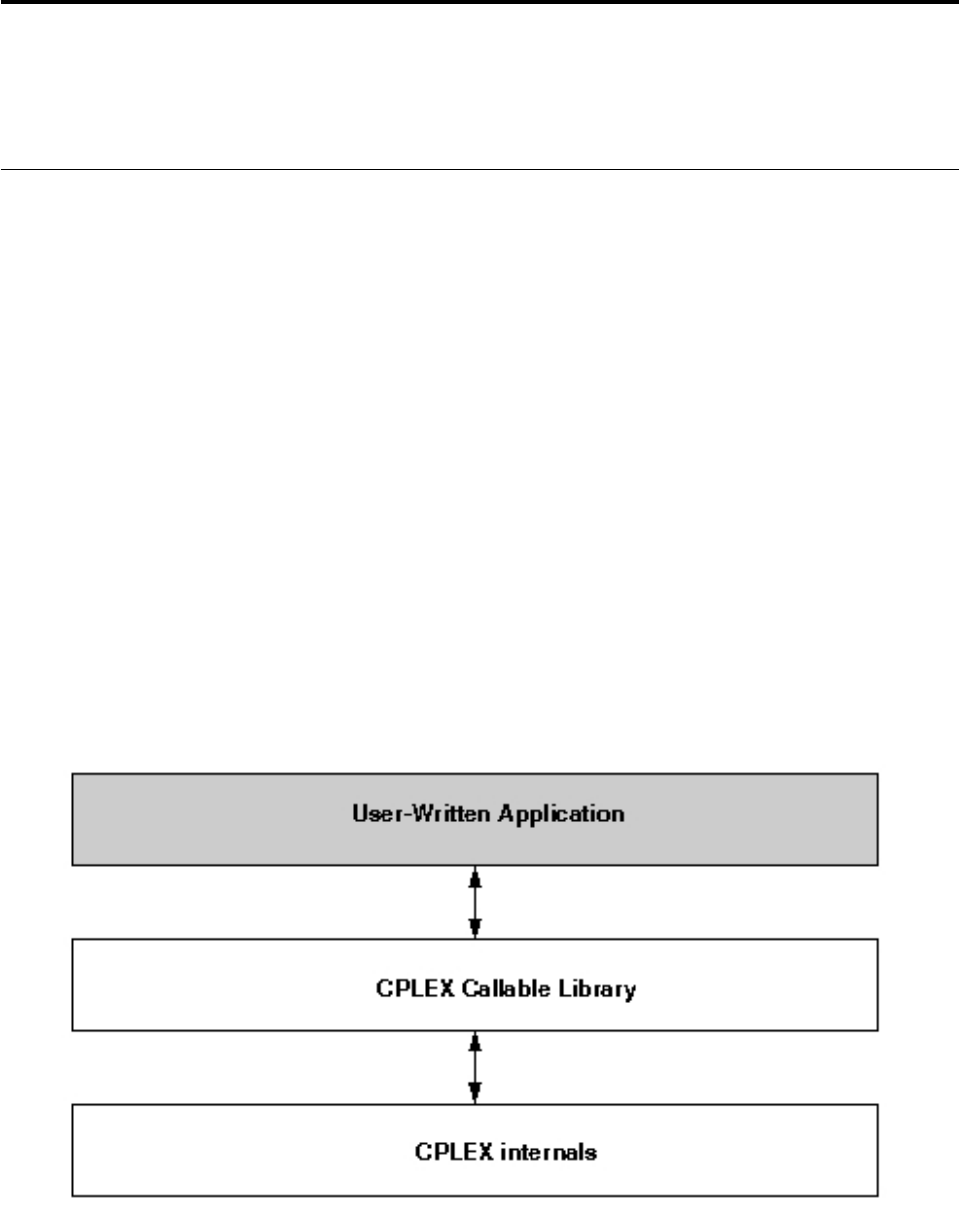
Chapter 4. Callable Library
Shows how to write C applications using the Callable Library.
Architecture of the Callable Library
Describes the architecture of the Callable Library C API.
Overview
Offers general remarks and a diagram of the architecture of a Callable Library
application.
IBM ILOG CPLEX includes a callable C library that makes it possible to develop
applications to optimize, to modify, and to interpret the results of mathematical
programming problems whether linear, mixed integer, or convex quadratic ones.
You can use the Callable Library to write applications that conform to many
modern computer programming paradigms, such as client-server applications
within distributed environments, multithreaded applications running on multiple
processors, applications linked to database managers, or applications using flexible
graphic user interface builders, just to name a few.
The Callable Library together with the CPLEX database make up the CPLEX core,
as you see in Figure 3. The CPLEX database includes the computing environment,
its communication channels, and your problem objects. You will associate the core
with your application by calling library routines.
The Callable Library itself contains routines organized into several categories:
Figure 3. A view of the Callable Library
© Copyright IBM Corp. 1987, 2016 59

vproblem modification routines let you define a problem and change it after you
have created it within the CPLEX database;
voptimization routines enable you to optimize a problem and generate results;
vutility routines handle application programming issues;
vproblem query routines access information about a problem after you have
created it;
vfile reading and writing routines move information from the file system of your
operating system into your application, or from your application into the file
system;
vparameter routines enable you to query, set, or modify parameter values
maintained by CPLEX.
Compiling and linking
Tells where to find information about compiling and linking with the C API.
Compilation and linking instructions are provided with the files that come in the
standard distribution of CPLEX for your computer platform. Check the
readme.html file for details.
Using the Callable Library in an application
Describes an application of the C API.
Overview
Outlines steps to include in a Callable Library application.
This topic tells you how to use the Callable Library in your own applications.
Briefly, you must initialize the CPLEX environment, instantiate a problem object,
and fill it with data. Then your application calls one of the CPLEX optimizers to
optimize your problem. Optionally, your application can also modify the problem
object and re-optimize it. CPLEX is designed to support this sequence of
operations—modification and re-optimization of linear, quadratic, or mixed integer
programming problems (LPs, QPs, or MIPs) efficiently by reusing the current
feasible solution (basis or incumbent) of a problem as its starting point (when
applicable). After it finishes using CPLEX, your application must free the problem
object and release the CPLEX environment it has been using. The following
sections explain these steps in greater detail.
Initialize the CPLEX environment
Tells how to initialize the environment in the C API.
To initialize a CPLEX environment, you must use the routine CPXopenCPLEX.
This routine returns a C pointer to the CPLEX environment that it creates. Your
application then passes this C pointer to other CPLEX routines (except CPXmsg). As
a developer, you decide for yourself whether the variable containing this pointer
should be global or local in your application. This routine is time consuming, so
you should call the CPXopenCPLEX routine only once, or as infrequently as possible,
in a program that solves a sequence of problems.
A multithreaded application needs multiple CPLEX environments. Consequently,
CPLEX allows more than one environment to exist at a time.
60 CPLEX User’s Manual
Note:
An attempt to use a problem object in any environment other than the
environment (or a child of that environment) where the problem object was created
will raise an error.
Instantiate the problem as an object
Tells how to instantiate a problem object in the C API.
After you have initialized a CPLEX environment, your next step is to instantiate
(that is, create and initialize) a problem object by calling CPXcreateprob. This
routine returns a C pointer to the problem object. Your application then passes this
pointer to other routines of the Callable Library.
Most applications will use only one problem object, though CPLEX allows you to
create multiple problem objects within a given CPLEX environment.
Put data in the problem object
Tells how to populate a problem object with data in the C API.
When you instantiate a problem object, it is originally empty. In other words, it has
no constraints, no variables, and no coefficient matrix. CPLEX offers you several
alternative ways to put data into an empty problem object (that is, to populate
your problem object).
vYou can make a sequence of calls, in any convenient order, to these routines:
– CPXaddcols
– CPXaddqconstr
– CPXaddrows
– CPXchgcoeflist
– CPXcopyctype
– CPXcopyqsep
– CPXcopyquad
– CPXnewcols
– CPXnewrows
vIf data already exist in MPS, SAV, or LP format in a file, you can call
CPXreadcopyprob to read that file and copy the data into the problem object.
Mathematical Programming System (MPS) is an industry-standard format for
organizing data in mathematical programming problems. LP and SAV file
formats are CPLEX-specific formats for expressing linear programming problems
as equations or inequalities. “Understanding file formats” on page 109 explains
these formats briefly. They are documented in the reference manual CPLEX File
Formats.
vYou can assemble arrays of data and then call CPXcopylp to copy the data into
the problem object.
Whenever possible, compute your problem data in double precision (64 bit).
Computers are finite-precision machines, and truncating your data to single
precision (32 bit) can result in unnecessarily ill-conditioned problems For more
information, refer to “Numeric difficulties” on page 148.
Chapter 4. Callable Library 61

Optimize the problem
Tells how to optimize a problem in the C API.
Call one of the CPLEX optimizers to solve the problem object that you have
instantiated and populated. “Choosing an optimizer for your LP problem” on page
135 explains in greater detail how to choose an appropriate optimizer for your
problem.
Change the problem object
Tells how to modify a problem in the C API.
In analyzing a given mathematical program, you may make changes in a model
and study their effect. As you make such changes, you must keep CPLEX informed
about the modifications so that CPLEX can efficiently re-optimize your changed
problem. Always use the problem modification routines from the Callable Library
to make such changes and thus keep CPLEX informed. In other words, do not
change a problem by altering the original data arrays and calling CPXcopylp again.
That tempting strategy usually will not make the best use of CPLEX. Instead,
modify your problem by means of the problem modification routines.
Use the routines whose names begin with CPXchg to modify existing objects in the
model, or use the routines CPXaddcols, CPXaddqconstr, CPXaddrows, CPXnewcols, and
CPXnewrows to add new constraints and new variables to the model.
For example, let’s say a user has already solved a given LP problem and then
changes the upper bound on a variable by means of an appropriate call to the
Callable Library routine CPXchgbds. CPLEX will then begin any further
optimization from the previous optimal basis. If that basis is still optimal with
respect to the new bound, then CPLEX will return that information without even
needing to refactor the basis.
Destroy the problem object
Tells when to destroy a problem object in the C API.
Use the routine CPXfreeprob to destroy a problem object when your application no
longer needs it. Doing so will free all memory required to solve that problem
instance.
Release the CPLEX environment
Tells how to end an application of the C API.
After all the calls from your application to the Callable Library are complete, you
must release the CPLEX environment by calling the routine CPXcloseCPLEX. This
routine tells CPLEX that:
vall application calls to the Callable Library are complete;
vCPLEX should release any memory allocated by CPLEX for this environment.
CPLEX programming practices
Lists some of the programming practices the CPLEX team observes in developing
and maintaining the Callable Library (C API).
62 CPLEX User’s Manual
Overview
Introduces general characteristics of variables and routines in the Callable Library.
The Callable Library supports modern programming practices. It uses no external
variables. Indeed, no global nor static variables are used in the library so that the
Callable Library is fully re-entrant and thread-safe. The names of all library
routines begin with the three-character prefix CPX to prevent namespace conflicts
with your own routines or with other libraries. Also to avoid clutter in the
namespace, there is a minimal number of routines for setting and querying
parameters.
Tip:
Thread-safety concerns reading as well as writing data. That is, if two threads
attempt to read or write to the same location, trouble may occur.
Variable names and calling conventions
Describes the coding practices of the C API with respect to variable names and
calling conventions.
Routines in the Callable Library obey the C programming convention of call by
value (as opposed to call by reference, for example, in FORTRAN and BASIC). If a
routine in the Callable Library needs the address of a variable in order to change
the value of the variable, then that fact is documented in the Callable Library
Reference Manual by the suffix _p in the argument name in the synopsis of the
routine. In C, you create such values by means of the &operator to take the
address of a variable and to pass this address to the Callable Library routine.
For example, let’s look at the synopses for two routines, CPXgetobjval and CPXgetx,
as they are documented in the Callable Library Reference Manual to clarify this
calling convention. Here is the synopsis of the routine CPXgetobjval:
int CPXgetobjval (CPXCENVptr env, CPXCLPptr lp, double *objval_p);
In that routine, the third argument is a pointer to a variable of type double . To call
this routine from C, declare:
double objval;
Then call CPXgetobjval in this way:
status = CPXgetobjval (env, lp, &objval);
In contrast, here is the synopsis of the routine CPXgetx
int CPXgetx (CPXENV env, CPXLPptr lp, double *x, int begin, int end);
You call it by creating a double-precision array by means of either one of two
methods. The first method dynamically allocates the array, like this:
double *x = NULL;
x = (double *) malloc (100*sizeof(double));
The second method declares the array as a local variable, like this:
double x[100];
Then to see the optimal values for columns 5 through 104, for example, you could
write this:
status = CPXgetx (env, lp, x, 5, 104);
Chapter 4. Callable Library 63

The parameter objval_p in the synopsis of CPXgetobjval and the parameter xin
the synopsis of CPXgetx are both of type (double *). However, the suffix _p in the
parameter objval_p indicates that you should use an address of a single variable in
one call, while the lack of _p in xindicates that you should pass an array in the
other.
For guidance about how to pass values to CPLEX routines from application
languages such as FORTRAN or BASIC that conventionally call by reference, see
“Call by reference” on page 71 in this manual, and consult the documentation for
those languages.
Data types
Describes the data types available in the C API.
In the Callable Library, CPLEX defines a few special data types for specific CPLEX
objects, as you see in the table Table 14. The types starting with CPXC represent the
corresponding pointers to constant (const) objects.
Table 14. Special data types in the Callable Library.
Data type Is a pointer to Declaration Set by calling
CPXENVptr
CPXCENVptr
CPLEX environment CPXENVptr env; CPXopenCPLEX
CPXLPptr CPXCLPptr problem object CPXLPptr lp; CPXcreateprob
CPXNETptr
CPXCNETptr
problem object CPXNETptr net; CPXNETcreateprob
CPXCHANNELptr message channel CPXCHANNELptr
channel;
CPXgetchannels
When any of these special variables are set to a value returned by an appropriate
routine, that value can be passed directly to other CPLEX routines that require
such arguments. The actual internal type of these variables is a memory address
(that is, a pointer); this address uniquely identifies the corresponding object. If you
are programming in a language other than C, you should choose an appropriate
integer type or pointer type to hold the values of these variables.
Ownership of problem data
Describes ownership conventions in the C API with respect to data.
The Callable Library does not take ownership of user memory. All arguments are
copied from your user-defined arrays into CPLEX-allocated memory. CPLEX
manages all problem-related memory. After you call a routine that copies data into
a CPLEX problem object, you can free or reuse the memory you allocated as
arguments to the copying routine.
Problem size and memory allocation issues
Describes conventions of the C API with respect to size of problem and memory
allocation.
As indicated in “Change the problem object” on page 62, after you have created a
problem object by calling CPXcreateprob, you can modify the problem in various
ways through calls to routines from the Callable Library. There is no need for you
to allocate extra space in anticipation of future problem modifications. Any limit on
64 CPLEX User’s Manual
problem size is set by system resources and the underlying implementation of the
system function malloc, not by artificial limits in CPLEX.
As you modify a problem object through calls to modification routines from the
Callable Library, CPLEX automatically handles memory allocations to
accommodate the increasing size of the problem. In other words, you do not have
to keep track of the problem size nor make corresponding memory allocations
yourself as long as you are using library modification routines such as CPXaddrows
or CPXaddcols.
Status and return values
Describes coding conventions of the C API with respect to status and return
values.
Most routines in the Callable Library return an integer value, 0(zero) indicating
success of the call. A nonzero return value indicates a failure. Each failure value is
unique and documented in the Callable Library Reference Manual. However, some
routines are exceptions to this general rule.
The Callable Library routine CPXopenCPLEX returns a pointer to a CPLEX
environment. In case of failure, it returns a NULL pointer. The argument *status_p
(that is, one of its arguments) is set to 0if the routine is successful; in case of
failure, that argument is set to a nonzero value that indicates the reason for the
failure.
The Callable Library routine CPXcreateprob returns a pointer to a CPLEX problem
object and sets its argument *status_p to 0 (zero) to report success. In case of
failure, it returns a NULL pointer and sets *status_p to a nonzero value specifying
the reason for the failure.
Some query routines in the Callable Library return a nonzero value when they are
successful. For example, CPXgetnumcols returns the number of columns in the
constraint matrix (that is, the number of variables in the problem object). However,
most query routines return 0(zero) reporting success of the query and entail one
or more arguments (such as a buffer or character string) to contain the results of
the query. For example, CPXgetrowname returns the name of a row in its name
argument.
It is extremely important that your application check the status (whether the status
is indicated by the return value or by an argument) of the routine that it calls
before it proceeds.
Symbolic constants
Describes coding conventions about symbolic constants in the C API.
Most CPLEX routines return or require values that are defined as symbolic
constants in the header file (that is, the include file) cplex.h. This practice of using
symbolic constants, rather than hard-coded numeric values, is highly recommend.
Symbolic names improve the readability of calling applications. Moreover, if
numeric values happen to change in subsequent releases of the product, the
symbolic names will remain the same, thus making applications easier to maintain.
Parameter routines
Describes routines of the C API to control CPLEX parameters.
Chapter 4. Callable Library 65
You can set many parameters in the CPLEX environment to control its operation.
The values of these parameters may be integer, double, or character strings, so
there are sets of routines for accessing and setting them. Table 15 shows you the
names and purpose of these routines. Each of these routines accepts the same first
argument: a pointer to the CPLEX environment (that is, the pointer returned by
CPXopenCPLEX). The second argument of each of those parameter routines is the
parameter number, a symbolic constant defined in the header file, cplex.h.
“Managing parameters from the Callable Library” on page 71 offers more details
about parameter settings.
Table 15. Callable Library routines for parameters in the CPLEX environment.
Type Change value Access current value Access default, max,
min
integer CPXsetintparam CPXgetintparam CPXinfointparam
double CPXsetdblparam CPXgetdblparam CPXinfodblparam
string CPXsetstrparam CPXgetstrparam CPXinfostrparam
Null arguments
Describes coding conventions of the C API with respect to null arguments.
Certain CPLEX routines that accept optional arguments allow you to pass a NULL
pointer in place of the optional argument. The documentation of those routines in
the Callable Library Reference Manual shows explicitly whether NULL pointer
arguments are acceptable. (Passing NULL arguments is an effective way to avoid
allocating unnecessary arrays.)
Referencing ranges of objects
Describes coding conventions of the C API with respect to indexing arrays and
numbering other objects.
Consistent with standard C programming practices, in CPLEX an array containing
kitems will contain these items in locations 0(zero) through k-1.
References to rows and columns
A linear program with mrows and ncolumns will have its rows indexed from 0to
m-1, and its columns from 0to n-1.
Within the linear programming data structure, the rows and columns that
represent constraints and variables are referenced by an index number. Each row
and column may optionally have an associated name. If you add or delete rows,
the index numbers usually change:
vfor deletions, CPLEX decrements each reference index above the deletion point;
and
vfor additions, CPLEX makes all additions at the end of the existing range.
However, CPLEX updates the names so that each row or column index will
correspond to the correct row or column name. Double checking names against
index numbers is the only sure way to reveal which changes may have been made
to matrix indices in such a context. The routines CPXgetrowindex and
CPXgetcolindex translate names to indices.
66 CPLEX User’s Manual
References to other objects
Similar conventions (numbering from 0to k-1) apply to other objects supported by
the Callable Library (C API). Examples include modeling objects, such as special
ordered sets (SOS), indicator constraints, and quadratic constraints, as well as
optimization objects, such as MIP starts. If an application creates ksuch objects, the
objects will be indexed in the range 0to k-1. For deletions, CPLEX decrements
each reference index above the deletion point; for additions, CPLEX puts all the
added elements at the end of the existing range.
Character strings
Describes coding conventions of the C API with respect to character strings.
You can pass character strings as parameters to various CPLEX routines, for
example, as row or column names. The Interactive Optimizer truncates output
strings 255 characters. Routines from the Callable Library truncate strings at 255
characters in output text files (such as MPS or LP text files) but not in binary SAV
files. Routines from the Callable Library also truncate strings at 255 characters in
names that occur in messages. Routines of the Callable Library that produce log
files, such as the simplex iteration log file or the MIP node log file, truncate at 16
characters. Input, such as names read from LP and MPS files or typed interactively
by the enter command, are truncated to 255 characters. However, it is not
recommended that you rely on this truncation because unexpected behavior may
result.
A string passed to CPLEX by your application as an argument of a Callable
Library routine must be terminated by the NUL character. In other words, CPLEX
recognizes NUL as the termination of a string that it accepts as an argument. This
programming convention in C has implications for your choice of encoding. If you
change the encoding of CPLEX from its default encoding ISO-8859-1 (also known
as Latin-1) to a multi-byte encoding such as UTF-32, where a NULL byte can exist in
the multi-byte representation of a character, then you must take care that a NULL
byte within the multi-byte representation of a character does not unintentionally
terminate a string passed to CPLEX as an argument. For an extended explanation
of this point plus an example of how this situation can produce unintended results,
see the topic “Selecting an encoding” on page 108, especially Example: hazardous
encodings.
Checking and debugging problem data
Describes routines to verify problem data and diagnose bugs in an application of
the C API.
If you inadvertently make an error entering problem data, the problem object will
not correspond to your intentions. One possible result may be a segmentation fault
or other disruption of your application. In other cases, CPLEX may solve a
different model from the one you intended, and that situation may or may not
result in error messages from CPLEX.
Using the data checking parameter
To help you detect this kind of error, you can set the data consistency checking and
modeling assistance parameter CPX_PARAM_DATACHECK(int) to the value CPX_ON to
activate additional checking of array arguments for CPXcopyData, CPXreadData, and
CPXchgData routines (where Data varies). The additional checks include:
vinvalid sense /ctype /sostype values
Chapter 4. Callable Library 67
vindices out of range, for example, rowind ≥numrows
vduplicate entries
vmatbeg or sosbeg array with decreasing values
vNANs in double arrays
vNULLs in name arrays
This additional checking may entail overhead (time and memory). When the
parameter is set to CPX_OFF, only simple checks are performed, for example,
checking for the existence of the environment.
Using diagnostic routines for debugging
CPLEX also provides diagnostic routines to look for common errors in the
definition of problem data. In the standard distribution of CPLEX, the file check.c
contains the source code for these routines:
vCPXcheckcopylp
vCPXcheckcopylpwnames
vCPXcheckcopyqpsep
vCPXcheckcopyquad
vCPXcheckcopyaddrows
vCPXcheckaddcols
vCPXcheckchgcoeflist
vCPXcheckvals
vCPXcheckcopyctype
vCPXcheckcopysos
vCPXcheckcopynet
Each of those routines performs a series of diagnostic tests of the problem data and
issues warnings or error messages whenever it detects a potential error. To use
them, you must compile and link the file check.c. After compiling and linking that
file, you will be able to step through the source code of these routines with a
debugger to help isolate problems.
If you have observed anomalies in your application, you can exploit this diagnostic
capability by calling the appropriate routines just before a change or copy routine.
The diagnostic routine can then detect errors in the problem data that could
subsequently cause inexplicable behavior.
Those checking routines send all messages to one of the standard CPLEX message
channels. You capture that output by setting a parameter (that is, the messages to
screen switch CPX_PARAM_SCRIND) if you want messages directed to your screen or
by calling the routine CPXsetlogfile if you want to direct messages to a log file.
Callbacks
Describes coding conventions of the C API with respect to callbacks.
The Callable Library supports callbacks so that you can define functions that will
be called at crucial points in your application:
vduring the presolve process;
vonce per iteration in a linear programming or quadratic programming routine;
and
68 CPLEX User’s Manual
vat various points, such as before node processing, in a mixed integer
optimization.
In addition, callback functions can call CPXgetcallbackinfo to retrieve information
about the progress of an optimization algorithm. They can also return a value to
indicate whether to terminate an optimization. CPXgetcallbackinfo and certain
other callback-specific routines are the only ones of the Callable Library that a
user-defined callback may call. (Of course, calls to routines not in the Callable
Library are permitted.)
Chapter 37, “Using optimization callbacks,” on page 499 explores callback facilities
in greater detail, and Chapter 40, “Advanced MIP control interface,” on page 533
discusses control callbacks in particular.
Portability
Describes coding conventions of the C API to make portable applications.
CPLEX contains a number of features to help you create Callable Library
applications that can be easily ported between UNIX and Windows platforms.
CPXPUBLIC
All Callable Library routines except CPXmsg have the word CPXPUBLIC as part of
their prototype. On UNIX platforms, this has no effect. On Win32 platforms, the
CPXPUBLIC designation tells the compiler that all of the CPLEX functions are
compiled with the Microsoft __stdcall calling convention. The exception CPXmsg
cannot be called by __stdcall because it takes a variable number of arguments.
Consequently, CPXmsg is declared as CPXPUBVARARGS; that calling convention is
defined as __cdecl for Win32 systems.
Function pointers
All Callable Library routines that require pointers to functions expect the passed-in
pointers to be declared as CPXPUBLIC. Consequently, when your application uses
such routines as CPXaddfuncdest , CPXsetlpcallbackfunc, and
CPXsetmipcallbackfunc, it must declare the user-written callback functions with the
CPXPUBLIC designation. For UNIX systems, this has no effect. For Win32 systems,
this will cause the callback functions to be declared with the __stdcall calling
convention. For examples of function pointers and callbacks, see “Example: using
callbacks lpex4.c” on page 515 and “Example: Callable Library message channels”
on page 116.
CPXCHARptr, CPXCCHARptr, and CPXVOIDptr
The types CPXCHARptr , CPXCCHARptr, and CPXVOIDptr are used in the header file
cplex.h to avoid the complicated syntax of using the CPXPUBLIC designation on
functions that return char* , const char* , or void* .
File pointers
File pointer arguments for Callable Library routines should be declared with the
type CPXFILEptr . On UNIX platforms, this practice is equivalent to using the file
pointer type. On Win32 platforms, the file pointers declared this way will
correspond to the environment of the CPLEX DLL. Any file pointer passed to a
Callable Library routine should be obtained with a call to CPXfopen and closed
Chapter 4. Callable Library 69
with CPXfclose. Callable Library routines with file pointer arguments include
CPXsetlogfile, CPXaddfpdest , CPXdelfpdest , and CPXfputs . “Callable Library
routines for message channels” on page 115 discusses most of those routines.
String functions
CPXmsgstr in the Callable Library makes it easier to work with strings. This routine
is helpful when you are writing applications in a language, such as Visual Basic,
that does not allow you to de-reference a pointer.
FORTRAN interface
Describes coding conventions of the C API to support interface with a FORTRAN
application.
The Callable Library can be interfaced with FORTRAN applications. Although they
are no longer distributed with the product, you can download examples of a
FORTRAN application from the technotes of the product support web site. At the
portal of your product, search for CPLEX and FORTRAN to locate relevant
technotes, such as "Calling CPLEX from FORTRAN" or "Calling CPLEX C API
from Fortran using Open Watcom"
Those examples were compiled with CPLEX versions 7.0 and earlier on a
particular platform. Since C-to-FORTRAN interfaces vary across platforms
(operating system, hardware, compilers, etc.), you may need to modify the
examples for your own system.
Whether you need intermediate routines for the interface depends on your
operating system. As a first step in building such an interface, it is a good idea to
study your system documentation about C-to-FORTRAN interfaces. In that context,
this section lists a few considerations particular to CPLEX in building a FORTRAN
interface.
Case-sensitivity
As you know, FORTRAN is a case-insensitive language, whereas routines in the
Callable Library have names with mixed case. Most FORTRAN compilers have an
option, such as the option -U on UNIX systems, that treats symbols in a
case-sensitive way. It is a good idea to use this option in any file that calls Callable
Library routines.
On some operating systems, certain intrinsic FORTRAN functions must be in all
upper case (that is, capital letters) for the compiler to accept those functions.
Underscore
On some systems, all FORTRAN external symbols are created with an underscore
character (that is, _) added to the end of the symbol name. Some systems have an
option to turn off this feature. If you are able to turn off those postpended
underscores, you may not need other “glue” routines.
Six-character identifiers
FORTRAN 77 allows identifiers that are unique only up to six characters.
However, in practice, most FORTRAN compilers allow you to exceed this limit.
Since routines in the Callable Library have names greater than six characters, you
70 CPLEX User’s Manual

need to verify whether your FORTRAN compiler enforces this limit or allows
longer identifiers.
Call by reference
By default, FORTRAN passes arguments by reference; that is, the address of a
variable is passed to a routine, not its value. In contrast, many routines of the
Callable Library require arguments passed by value. To accommodate those
routines, most FORTRAN compilers have the VMS FORTRAN extension %VAL() .
This operator used in calls to external functions or subroutines causes its argument
to be passed by value (rather than by the default FORTRAN convention of passed
by reference). For example, with that extension, you can call the routine CPXprimopt
with this FORTRAN statement:
status = CPXprimopt (%val(env), %val(lp))
Pointers
Certain CPLEX routines return a pointer to memory. In FORTRAN 77, such a
pointer cannot be de-referenced; however, you can store its value in an appropriate
integer type, and you can then pass it to other CPLEX routines. On most 32-bit
operating systems, the default integer type of four bytes is sufficient to hold
pointer variables. On 64-bit operating systems, a variable of type INTEGER*8 may be
needed. Consult your system documentation to learn the appropriate integer type
to hold variables that are C pointers.
Strings
When you pass strings to routines of the Callable Library, they expect C strings;
that is, strings terminated by an ASCII NULL character, denoted \0 in C.
Consequently, when you pass a FORTRAN string, you must add a terminating
NULL character; you do so by means of the FORTRAN intrinsic function CHAR(0) .
C++ interface
Describes conventions of the C API for interface with C++ applications.
The CPLEX header file, cplex.h , includes the extern C statements necessary for
use with C++. If you wish to call the CPLEX C interface from a C++ application,
rather than using Concert Technology, you can include cplex.h in your C++
source.
Managing parameters from the Callable Library
Introduces routines to manage parameters of CPLEX from the C API.
Some CPLEX parameters assume values of type double; others assume values of
type int; others are strings (that is, C-type char*). Consequently, in the Callable
Library, there are sets of routines (one for int, one for double, one for char*) to
access and to change parameters that control the CPLEX environment and guide
optimization.
For example, the routine CPXinfointparam shows you the default, the maximum,
and the minimum values of a given parameter of type int , whereas the routine
CPXinfodblparam shows you the default, the maximum, and the minimum values
of a given parameter of type double , and the routine CPXinfostrparam shows you
Chapter 4. Callable Library 71
the default value of a given string parameter. Those three Callable Library routines
observe the same conventions: they return 0(zero) from a successful call and a
nonzero value in case of error.
The routines CPXinfointparam and CPXinfodblparam expect five arguments:
va pointer to the environment; that is, a pointer of type CPXENVptr returned by
CPXopenCPLEX;
van indication of the parameter to check; this argument may be a symbolic
constant, such as the clock type for computation time parameter
CPX_PARAM_CLOCKTYPE, or a reference number, such as 1006; the symbolic
constants and reference numbers of all CPLEX parameters are documented in
the Parameters Reference Manual and they are defined in the include file cplex.h .
va pointer to a variable to hold the default value of the parameter;
va pointer to a variable to hold the minimum value of the parameter;
va pointer to a variable to hold the maximum value of the parameter.
The routine CPXinfostrparam differs slightly in that it does not expect pointers to
variables to hold the minimum and maximum values as those concepts do not
apply to a string parameter.
To access the current value of a parameter that interests you from the Callable
Library, use the routine CPXgetintparam for parameters of type int ,
CPXgetdblparam for parameters of type double , and CPXgetstrparam for string
parameters. These routines also expect arguments to indicate the environment, the
parameter you want to check, and a pointer to a variable to hold that current
value.
No doubt you have noticed in other chapters of this manual that you can set
parameters from the Callable Library. There are, of course, routines in the Callable
Library to set such parameters: one sets parameters of type int ; another sets
parameters of type double ; another sets string parameters.
vCPXsetintparam accepts arguments to indicate:
– the environment; that is, a pointer of type CPXENVptr returned by
CPXopenCPLEX;
– the parameter to set; this routine sets parameters of type int ;
– the value you want the parameter to assume.
vCPXsetdblparam accepts arguments to indicate:
– the environment; that is, a pointer of type CPXENVptr returned by
CPXopenCPLEX;
– the parameter to set; this routine sets parameters of type double ;
– the value you want the parameter to assume.
vCPXsetstrparam accepts arguments to indicate:
– the environment; that is, a pointer of type CPXENVptr returned by
CPXopenCPLEX;
– the parameter to set; this routine sets parameters of type const char* ;
– the value you want the parameter to assume.
The Parameters Reference Manual documents the type of each parameter (int,
double, char*) along with the symbolic constant and reference number representing
the parameter.
72 CPLEX User’s Manual

The routine CPXsetdefaults resets all parameters (except the log file) to their
default values, including the CPLEX callback functions. This routine resets the
callback functions to NULL. Like other Callable Library routines to manage
parameters, this one accepts an argument specifying the environment, and it
returns 0for success or a nonzero value in case of error.
Example: optimizing the diet problem in the Callable Library
Walks through an example applying the C API.
Overview
Describes the problem in the example.
The optimization problem solved in this example is to compose a diet from a set of
foods, so that the nutritional requirements are satisfied and the total cost is
minimized. The example diet.c illustrates these points.
Problem representation
Describes how to represent the problem by means of the C API.
The problem contains a set of foods, which are the modeling variables; a set of
nutritional requirements to be satisfied, which are the constraints; and an objective
of minimizing the total cost of the food. There are two ways to look at this
problem:
vThe problem can be modeled in a row-wise fashion, by entering the variables
first and then adding the constraints on the variables and the objective function.
vThe problem can be modeled in a column-wise fashion, by constructing a series
of empty constraints and then inserting the variables into the constraints and the
objective function.
The diet problem is equally suited for both kinds of modeling. In fact you can even
mix both approaches in the same program: If a new food product is introduced,
you can create a new variable for it, regardless of how the model was originally
built. Similarly, is a new nutrient is discovered, you can add a new constraint for
it.
Creating a model row by row
You walk into the store and compile a list of foods that are offered. For each food,
you store the price per unit and the amount they have in stock. For some foods
that you particularly like, you also set a minimum amount you would like to use
in your diet. Then for each of the foods you create a modeling variable to represent
the quantity to be purchased for your diet.
Now you get a medical book and look up which nutrients are known and relevant
for you. For each nutrient, you note the minimum and maximum amount that
should be found in your diet. Also, you go through the list of foods and decide
how much a food item will contribute for each nutrient. This gives you one
constraint per nutrient, which can naturally be represented as a range constraint
nutrmin[i] ≤∑j(nutrper[i][j] * buy[j]) ≤nutrmax[i]
Chapter 4. Callable Library 73
where irepresents the index of the nutrient under consideration, nutrmin[i] and
nutrmax[i] the minimum and maximum amount of nutrient iand nutrper[i][j]
the amount of nutrient iin food j. Finally, you specify your objective function to
minimize, like this:
cost = ∑j(cost[j] * buy[j])
This way to create the model is shown in function populatebyrow in example
diet.c .
Creating a model column by column
You start with the medical book where you compile the list of nutrients that you
want to make sure are properly represented in your diet. For each of the nutrients,
you create an empty constraint:
nutrmin[i] ≤... ≤nutrmax[i]
where ... is left to be filled after you walk into your store. You also set up the
objective function to minimize the cost. Constraint iis referred to as rng[i] and
the objective is referred to as cost .
Now you walk into the store and, for each food, you check its price and nutritional
content. With this data you create a variable representing the amount you want to
buy of the food type and install it in the objective function and constraints. That is
you create the following column:
IloObjective obj = cplex.objective(sense, expr, name);
cplex.setParam(IloCplex.IntParam.PPriInd,
IloCplex.PrimalPricing.Steep);
IloColumn col = cplex.column(obj, 1.0).and(cplex.column(rng, 2.0));
cost(foodCost[j]) "+" "sum_i" (rng[i](nutrper[i][j]))
where the notation "+" and "sum " indicates that you “add” the new variable jto
the objective cost and constraints rng[i] . The value in parentheses is the linear
coefficient that is used for the new variable.
Here’s another way to visualize a column, such as column j in this example:
foodCost[j]
nutrper[0][j]
nutrper[1][j]
...
nutrper[m-1][j]
Program description
Describes the architecture of an application from the C API solving the diet
problem.
All definitions needed for a Callable Library application are imported when your
application includes the file <ilcplex/cplex.h> at the beginning of the application.
After a number of lines that establish the calling sequences for the routines that are
to be used, the main function of the application begins by checking for correct
command line arguments, printing a usage reminder and exiting in case of errors.
Next, the data defining the problem are read from a file specified in the command
line at run time. The details of this are handled in the routine readdata. In this file,
cost, lower bound, and upper bound are specified for each type of food; then
74 CPLEX User’s Manual

minimum and maximum levels of several nutrients needed in the diet are
specified; finally, a table giving levels of each nutrient found in each unit of food is
given. The result of a successful call to this routine is two variables nfoods and
nnutr containing the number of foods and nutrients in the data file, arrays cost,
lb, ub containing the information about the foods, arrays nutrmin, nutrmax
containing nutritional requirements for the proposed diet, and array nutrper
containing the nutritional value of the foods.
Preparations to build and solve the model with CPLEX begin with the call to
CPXopenCPLEX. This establishes a CPLEX environment to contain the LP problem.
After calls to set parameters, one to control the output that comes to the user's
terminal, and another to turn on data checking for debugging purposes, a problem
object is initialized through the call to CPXcreateprob. This call returns a pointer to
an empty problem object, which now can be populated with data.
Two alternative approaches to filling this problem object are implemented in this
program, populatebyrow and populatebycolumn, and which one is executed is set at
run time by an argument on the command line. The routine populatebyrow
operates by first defining all the columns through a call to CPXnewcols and then
repeatedly calls CPXaddrows to enter the data of the constraints. The routine
populatebycolumn takes the complementary approach of establishing all the rows
first with a call to CPXnewrows and then sequentially adds the column data by calls
to CPXaddcols.
Solving the model with CPXlpopt
Shows the routine used to solve the problem.
The model is at this point ready to be solved, and this is accomplished through the
call to CPXlpopt, which by default uses the dual simplex optimizer.
After this, the program finishes by making a call to CPXsolution to obtain the
values for each variable in this optimal solution, printing these values, and writing
the problem to a disk file (for possible evaluation by the user) via the call to
CPXwriteprob. It then terminates after freeing all the arrays that have been
allocated along the way.
Complete program
Tells where to find the C implementation of the diet problem online.
The complete program, diet.c , appears online in the standard distribution at
yourCPLEXinstallation /examples/src .
Using surplus arguments for array allocations
Describes coding conventions of the C API to manage surplus arguments and array
allocations.
Most of the query routines in the Callable Library require your application to
allocate memory for one or more arrays that will contain the results of the query.
In many cases, your application—the calling program—does not know the size of
these arrays in advance. For example, in a call to CPXgetcolsrequesting the matrix
data for a range of columns, your application needs to pass the arrays cmatind and
cmatval for CPLEX to populate with matrix coefficients and row indices. However,
unless your application has carefully kept track of the number of nonzeros in each
Chapter 4. Callable Library 75
column throughout the problem specification and, if applicable, throughout its
modification, the actual length of these arrays remains unknown.
Fortunately, the query routines in the Callable Library contain a surplus_p
argument that, when used in conjunction with the array length arguments, enables
you first to call the query routine to discover the length of the required array.
Then, when the length is known, your application can properly allocate these
arrays. Afterwards, your application makes a second call to the query routine with
the correct array lengths to obtain the requested data.
For example, consider an application that needs to call CPXgetcols to access a
range of columns. Here is the list of arguments for CPXgetcols.
CPXgetcols (CPXENVptr env,
CPXLPptr lp,
int *nzcnt_p,
int *cmatbeg,
int *cmatind,
double *cmatval,
int cmatspace,
int *surplus_p,
int begin,
int end);
The arrays cmatind and cmatval require one element for each nonzero matrix
coefficient in the requested range of columns. The required length of these arrays,
specified in cmatspace , remains unknown at the time of the query. Your
application—the calling program—can discover the length of these arrays by first
calling CPXgetcols with a value of 0for cmatspace . This call will return an error
status of CPXERR_NEGATIVE_SURPLUS indicating a shortfall of the array length
specified in cmatspace (in this case, 0); it will also return the actual number of
matrix nonzeros in the requested range of columns. CPXgetcols deposits this
shortfall as a negative number in the integer pointed to by surplus_p . Your
application can then negate this shortfall and allocate the arrays cmatind and
cmatval sufficiently long to contain all the requested matrix elements.
The following sample of code illustrates this procedure. The first call to CPXgetcols
passes a value of 0(zero) for cmatspace in order to obtain the shortfall in cmatsz .
The sample then uses the shortfall to allocate the arrays cmatind and cmatval
properly; then it calls CPXgetcols again to obtain the actual matrix coefficients and
row indices.
status = CPXgetcols (env, lp, &nzcnt, cmatbeg, NULL, NULL,
0, &cmatsz, 0, numcols - 1);
if ( status != CPXERR_NEGATIVE_SURPLUS ) {
if ( status != 0 ) {
CPXmsg (cpxerror,
"CPXgetcols for surplus failed, status = %d\n", status);
goto TERMINATE;
}
CPXmsg (cpxwarning,
"All columns in range [%d, %d] are empty.\n",
0, (numcols - 1));
}
cmatsz = -cmatsz;
cmatind = (int *) malloc ((unsigned) (1 + cmatsz)*sizeof(int));
cmatval = (double *) malloc ((unsigned) (1 + cmatsz)*sizeof(double));
if ( cmatind == NULL || cmatval == NULL ) {
CPXmsg (cpxerror, "CPXgetcol mallocs failed\n");
status = 1;
goto TERMINATE;
}
76 CPLEX User’s Manual

status = CPXgetcols (env, lp, &nzcnt, cmatbeg, cmatind, cmatval,
cmatsz, &surplus, 0, numcols - 1);
if ( status ) {
CPXmsg (cpxerror, "CPXgetcols failed, status = %d\n", status);
goto TERMINATE;
}
That sample code (or your application) does not need to set the length of the array
cmatbeg . The array cmatbeg has one element for each column in the requested
range. Since this length is known ahead of time, your application does not need to
call a query routine to calculate it. More generally, query routines use surplus
arguments in this way only for the length of any array required to store problem
data of unknown length. Problem data in this category include nonzero matrix
entries, row and column names, other problem data names, special ordered sets
(SOS), priority orders, and MIP start information.
Example: using query routines lpex7.c
Shows how to use query routines of the C API in an example.
This example uses the Callable Library query routine CPXgetcolname to get the
column names from a problem object. To do so, it applies the programming pattern
just outlined in “Using surplus arguments for array allocations” on page 75. It
derives from the example lpex2.c from the manual Getting Started. This
query-routine example differs from that simpler example in several ways:
vThe example calls CPXgetcolname twice after optimization: the first call discovers
how much space to allocate to hold the names; the second call gets the names
and stores them in the arrays cur_colname and cur_colnamestore.
vWhen the example prints its answer, it uses the names as stored in cur_colname.
If no names exist there, the example creates generic names.
This example assumes that the current problem has been read from a file by
CPXreadcopyprob. You can adapt the example to use other query routines to get
information about any problem read from a file.
The complete program lpex7.c appears online in the standard distribution at
yourCPLEXinstallation/examples/src.
Chapter 4. Callable Library 77
78 CPLEX User’s Manual

Chapter 5. CPLEX for Python users
Explores the features that CPLEX offers to users of Python to solve mathematical
programming problems.
Before you begin working with the Python API of CPLEX, consider the topic
Setting up the Python API of CPLEX and the tutorial Python tutorial, both in
Getting Started with CPLEX.
Why Python?
Introduces the Python API of CPLEX.
The Python application programming interface (API) of CPLEX supports the full
functionality of CPLEX. Like other APIs, it enables a user to design models and
solve problems in these disciplines:
vlinear programming (LP),
vmixed integer programming (MIP),
vquadratic programming (QP),
vquadratically constrained programming (QCP),
vsecond-order cone programming (SOCP),
vmixed integer quadratic programming (MIQP),
vmixed integer quadratically constrained programming (MIQCP).
Python itself is a freely available, open-source, cross-platform scripting language
with a gentle learning curve. It enjoys a growing user-base in both industry and
academia.
As a scripting language, it offers an easy approach for newcomers to CPLEX. For
more experienced programmers, it promises good performance and ease of
development in full-fledged optimization applications.
Python supports procedural, functional, and object-oriented coding paradigms.
Because of its automatic memory management, Python applications do not require
clean-up code, as C or C++ applications do. Thanks to its dynamic typing, Python
applications do not need variable declarations, making Python applications easy to
maintain or extend as modeling conditions change.
As an interpreted language, Python applications do not require the usual steps of
compilation and linking like other APIs. In addition, many mature libraries
supporting graphic user interfaces, database queries, visualization, statistical
analysis, scientific computing, and so forth, are readily available for Python
applications.
With those advantages of Python in general, you can use the Python API of CPLEX
in a variety of ways. For example, you can use it to write scripts and applications
that call CPLEX. Because of its interpreter, you can also use the Python API
interactively. Like the Interactive Optimizer, the Python API of CPLEX supports
important features of CPLEX, such as:
vImproving performance with the Chapter 10, “Tuning tool,” on page 123
© Copyright IBM Corp. 1987, 2016 79

vChapter 34, “Repairing infeasibilities with FeasOpt,” on page 465
vChapter 33, “Diagnosing infeasibility by refining conflicts,” on page 451
An alternative to the Interactive Optimizer, it offers features not available there,
such as callbacks and programming loops. For an example of callback
programming with the Python API, see “Using callbacks in the Python API” on
page 84. For a sample programming loop, see “Example: solving a sequence of
related problems in the Python API” on page 86
Meet the Python API
Introduces methods of the class Cplex.
In the Python API of CPLEX, the class Cplex encapsulates an optimization problem
and provides methods to create and modify the model, to solve the problem, and
to query the solution. The class Cplex also offers methods to read data, write
results, or populate a model. Also within this class, there are groups of methods
that facilitate your management of variables, linear constraints, and the objective
function of your model as well as your analysis of the solution. For samples of
these methods at work, see the examples diet.py and rates.py distributed with
the product.
Modifying and querying problem data in the Python API
Shows how to modify and query data by index or by name.
You can use either object names or indices as handles to modify and query
problem data. For example, assume that you have already created c, an instance of
the class Cplex, and that it contains ten variables in this session of Python. Then
the following line adds a new variable to that model and sets the upper bound of
the new variable as 1.0.
>>> c.variables.add(names = ["new_var"], ub = [1.0])
Afterwards, the following lines in the same session query that new variable by its
name and return its index and upper bound, like this:
>>> c.variables.get_index("new_var")
10
>>> c.variables.get_upper_bounds("new_var")
1.0
Likewise, you can query the new variable by its index to return its upper bound.
>>> c.variables.get_upper_bounds(10)
1.0
In fact, you can modify the upper bound of that variable, accessing it either by its
name or by its index, as you see in the following lines of the same session:
>>> c.variables.set_upper_bounds("new_var", 2.0)
>>> c.variables.get_upper_bounds(10)
2.0
>>> c.variables.set_upper_bounds(10, 3.0)
>>> c.variables.get_upper_bounds("new_var")
3.0
Using polymorphism in the Python API
Illustrates polymorphism in the Python API.
80 CPLEX User’s Manual

In the Python API of CPLEX, the methods available to modify problem data are
two-way polymorphic. That is, objects of a given type can appear as and be used
like objects of another type. For example, to modify a single piece of data, you can
call the method with a handle, such as the name or index of the variable, and the
new data, like this:
>>> c.variables.set_upper_bounds("var0", 2.0)
>>> c.variables.get_upper_bounds("var0")
2.0
Likewise, to modify multiple pieces of data, you can call the method with a list of
pairs of handles and data, like this:
>>> c.variables.set_upper_bounds([("var0", 3.0), ("var1", 4.0)])
>>> c.variables.get_upper_bounds("var0")
3.0
>>> c.variables.get_upper_bounds("var1")
4.0
Methods available to query problem data are four-way polymorphic. You can call
them with a single handle, with two handles, with a list of handles, or with no
handle at all. For example, the following line queries the upper bound of a given
variable by name; that is, the method uses one argument.
>>> c.variables.get_upper_bounds("new_var")
3.0
The following example queries an inclusive range of data by calling the method
with two handles (the first and last index) to return the upper bounds of all the
variables in that range of indices.
>>> c.variables.get_upper_bounds(0, 3)
[1.0, 2.0, 1.0, 1.0]
As a third example of polymorphism, consider the following query by an arbitrary
list of handles comprising two indices and a name. The method returns the upper
bound of all those variables, whether they were called by index or by name.
>>> c.variables.get_upper_bounds([0, 1, "new_var"])
[1.0, 2.0, 3.0]
Indeed, you can query data by calling a method with no arguments at all. For
example, the following line shows a query that returns a list equal in length to the
number of variables.
>>> c.variables.get_upper_bounds()
[1.0, 2.0, 1.0, 1.0, . . ., 3.0]
Example: generating a histogram
Illustrates reporting with histograms from the Python API.
The Python API also generates formatted reports that include histograms. These
reports are available either interactively in a Python session or programmatically in
a Python application.
To generate a histogram, use methods of the class Cplex. If you are interested in a
histogram based on the rows (constraints) of your model, consider the method
get_histogram of the LinearConstraintInterface. Similarly, if you are interested in
a histogram based on the columns (variables) of your model, consider the method
get_histogram of the VariablesInterface.
Chapter 5. CPLEX for Python users 81

The method __str__ of the histogram object returns a string displaying the number
of rows or columns with nonzeros in human readable form. The data member
orientation of the histogram object specifies either columns (indicating that the
histogram reflects the nonzero counts for the variables of the linear constraint
matrix) or rows (indicating that the histogram reflects the nonzero counts for the
constraints of the model).
Additionally, you can query the histogram object about the number of rows or
columns with a given nonzero count. That is, how many rows have N nonzeros?
Or, how many columns have K nonzeros? Here is a sample interactive session
querying nonzero columns and generating a histogram of them:
>>> import cplex
>>> c = cplex.Cplex("ind.lp")
>>> histogram = c.variables.get_histogram()
>>> print histogram
Nonzero Count: 1 2 3
Number of Columns: 1 6 36
>>> histogram[2]
6
>>> histogram[0:4]
[0, 1, 6, 36]
Continuing in the same session, the following lines use the histogram to report
more elaborate information about nonzeros in that problem:
>>> maxh = max(histogram)
>>> for i, count in histogram:
>>> if histogram[i] == maxh:
>>> print "most common nz count is", maxh, "appearing", count, "times"
most common nz count is 3 appearing 36 times
Querying solution information in the Python API
Introduces methods to query the quality of solutions in the Python API.
To query the quality of a solution in a Python session or from a Python
application, use a method of the solution object (such as get_integer quality or
get_float_quality) and supply the identifier of the quality of interest, like this:
c.solution.get_integer_quality(quality_ID)
c.solution.get_float_quality(quality_ID)
Tip:
The argument you supply to those methods may be the identifier of a single
quality or it may be a list of identifiers of qualities.
The same approach works for querying the quality of a solution in the solution
pool, but of course you invoke methods of the solution pool object in that case,
like this:
c.solution.pool.get_integer_quality(soln, quality_ID)
c.solution.pool.get_float_quality(soln, quality_ID)
Rather than retrieving information about the quality of a solution one metric at a
time, you can extract the most commonly used metrics with a single line of code.
To do so, use the methods Cplex.solution.get_quality_metrics or
Cplex.solution.pool.get_quality_metrics. You can display the objects returned
by these methods interactively, or you can use those returned objects to query
individual solution metrics.
82 CPLEX User’s Manual

For example, to report information about the incumbent solution in a Python
session, adapt this approach to your specific problem:
>>> c = cplex.Cplex("problem.lp")
>>> c.solve()
>>> print c.solution.get_quality_metrics()
For information about the quality of a solution in the solution pool, you specify
the solution of interest either by its index or by its name in the solution pool, like
this:
>>> print c.solution.pool.get_quality_metrics(soln)
The object returned by this method get_quality_metrics has many data members
that you can inspect individually. For the names and the conditions under which
they are defined, see the documentation of the class QualityMetrics in the
reference manual of the Python API.
Examining variables with nonzero values in a solution
Documents ways to examine nonzero variables in a solution: for-loop, lambda
expression, function.
To examine the nonzero values of variables in a solution, the Python API of CPLEX
offers several alternatives.
vYou can enter a for-loop interactively to print the solution, like this:
>>> for i, x in enumerate(c.solution.get_values()):
... if (x!=0): #leading spaces for indention
... print "Solution value of ", c.variables.get_names(i), \
... " is ", x
Solution value of Open(1) is 1.0
Solution value of Open(2) is 1.0 ...
vYou can enter a lambda expression interactively to print the solution, like this:
>>> print zip([1,2],[3,4]); # built-in function zip
[(1, 3), (2, 4)]
>>> print filter(lambda x:x[1]!=0,
zip(c.variables.get_names(),c.solution.get_values()))
[(’Open(1)’, 1.0), (’Open(2)’, 1.0), ...
vYou can write a reusable function to print the solution, like this:
>>> def display_solution_nonzero_values (c):
... for i, x in enumerate(c.solution.get_values()):
... if (x!=0):
... print "Solution value of ",c.variables.get_names(i),\
... " is ", x
>>> display_solution_nonzero_values(c)
Solution value of Open(1) is 1.0
Solution value of Open(2) is 1.0 ...
Displaying high precision nonzero values of a solution
Offers an example of a function to display nonzero values of a solution at high
precision in Python.
The Python API of CPLEX also supports display at high precision of nonzero
values in a solution. To take advantage of this feature in your Python applications
of CPLEX, you can define your own function, like this:
>>> def display_solution_nonzero_values_highprecision(c):
... for i, x in enumerate(c.solution.get_values()):
... if (x!=0):
... print "Solution value of ",c.variables.get_names(i),\
Chapter 5. CPLEX for Python users 83

... " is ", " %+18.16e" % x
...
>>> display_solution_nonzero_values_highprecision(c)
Solution value of Open(1) is +1.0000000000000000e+000
Solution value of Open(2) is +1.0000000000000000e+000
Solution value of Open(3) is +1.7865900324417692e+002...
Managing CPLEX parameters in the Python API
Documents CPLEX parameters in the Python API.
CPLEX normally performs well on a wide variety of problems at default settings.
However, the product offers a number of parameters that you can adjust to meet
specific needs of your problem. These CPLEX parameters are documented in the
reference manual, Parameters of CPLEX. That manual shows the name of each
parameter in the Python, C, C++, Java, and .NET APIs, as well as the name in the
Interactive Optimizer. The documentation of a parameter specifies values that the
parameter can take and outlines conditions under which changing the default
value of a parameter may be useful in a given problem.
Tip:
For users familiar with the hierarchy of parameters in the Interactive Optimizer or
CPLEX MATLAB toolbox, the parameters of the Python API are organized in the
same way.
As an example of a CPLEX parameter in use, here is a typical Python session that
first sets a time limit of five minutes (that is, three hundred seconds) for
performance tuning and then accesses the value that was just set. The example
illustrates the naming pattern and calling convention of CPLEX parameters in the
Python API.
>>> c = cplex.Cplex()
>>> c.parameters.tuning.timelimit.set(300.0)
>>> c.parameters.tuning.timelimit.get()
300.0
Parameters that accept symbolic names have a member, values, comprising
descriptive names. For example, the following line sets the barrier optimizer as the
method for solving continuous models (LPs).
>>> c.parameters.lpmethod.set(c.parameters.lpmethod.values.barrier)
As objects of the Python API, parameters have methods to access their minimum,
maximum, and default values, as the following lines illustrate.
>>> c.parameters.simplex.tolerances.markowitz.min()
0.0001
>>> c.parameters.simplex.tolerances.markowitz.default()
0.01
>>> c.parameters.simplex.tolerances.markowitz.max()
0.99999000000000005
>>> c.parameters.simplex.tolerances.markowitz.set(2.0)
Traceback ... cplex.exceptions.CplexError: Invalid argument
Using callbacks in the Python API
Introduces callbacks in the Python API.
84 CPLEX User’s Manual

Callbacks allow user-written Python functions to supplement the algorithms
CPLEX applies to solve optimization problems. Like other APIs of CPLEX, the
Python API supports user-written callbacks for many purposes, such as:
vcomplex termination criteria;
valternative branching rules;
vuser-defined cutting planes;
vadditional criteria for feasibility of new incumbents;
vand many other possibilities.
In the Python API, the callback classes are defined in the module callbacks of the
package cplex. They occupy a hierarchy of classes similar to that of the other
object-oriented APIs, such as C++ or Java.
callbacks.PresolveCallback
callbacks.SimplexCallback
callbacks.BarrierCallback
callbacks.CrossoverCallback
callbacks.TuningCallback
callbacks.MIPInfoCallback
callbacks.MIPCallback
callbacks.BranchCallback
callbacks.UserCutCallback
callbacks.LazyConstraintCallback
callbacks.HeuristicCallback
callbacks.SolveCallback
callbacks.IncumbentCallback
callbacks.NodeCallback
The topic Chapter 37, “Using optimization callbacks,” on page 499 offers general
guidance about writing and using your own callbacks.
Example: displaying solutions with increased precision from the
Python API
Illustrates how to format output from a Python session using CPLEX.
This example shows how to read a problem from a file, myprob.lp, in LP format.
(For more information about LP, the linear programming format, see that topic in
the reference manual, File formats supported by CPLEX.) The example prints the
solution in double precision. It also displays nonzero reduced costs with the names
of the associated variables.
>>> c = cplex.Cplex("myprob.lp")
>>> c.solve()
[. . . CPLEX log . . .]
>>> # print the solution vector in double precision
>>> for val in c.solution.get_values():
... print " %+18.16e" % val
...
+2.5000000000000000e+000
+1.7865900324417692e+002
+1.9999999999999999e-001
>>> # print the nonzero reduced costs and their variable names
>>> for i, dj in enumerate(c.solution.get_reduced_costs()):
... if dj != 0.:
... print "red. cost of ", c.variables.get_names(i), " is ", dj
...
red. cost of x1 is 3.04
Chapter 5. CPLEX for Python users 85

Example: examining the simplex tableau in the Python API
Illustrates how to examine a typical simplex tableau.
This example reads a problem from a file, myprob.mps, formatted in MPS. (For
more information about the math programming standard format MPS, see that
topic in the reference manual, File formats supported by CPLEX.) After setting a
limit on the number of iterations, and selecting primal simplex as the optimizer, it
then loops through the simplex iterations as CPLEX solves the problem, printing
rows (constraints).
>>> c = cplex.Cplex("myprob.mps")
>>> c.parameters.simplex.limits.iterations.set(1)
>>> c.parameters.lpmethod.set(c.parameters.lpmethod.values.primal)
>>> # this while loop will print the tableau after each
>>> # simplex iteration
>>> while c.solution.get_status() != c.solution.status.optimal:
... c.solve()
... print " CURRENT TABLEAU "
... for tableau_row in c.solution.advanced.binvarow():
... print tableau_row
... print
...
You can print only selected rows of the tableau by passing the names of rows or
the indices of rows to the method binvarow. Another method, binvacol, returns
columns of a tableau. The methods binvrow and binvcol return the inverted basis
matrix.
Example: solving a sequence of related problems in the Python API
Illustrates how to solve a sequence of related problems in a loop.
Consider, for example, a sequence of related problems. The sequence begins with a
model read from a formatted file, myprob.mps. (For more information about the
math programming standard format MPS, see that topic in the reference manual,
File formats supported by CPLEX.) Successive problems in the sequence reset the
lower bound of the variable x0 and solve the model again with the new lower
bound. The example prints the CPLEX log for each solution in a sequence of files
named lb_set_to_0.log, lb_set_to_1.log, and so forth.
>>> c = cplex.Cplex("myprob.mps")
>>> for i in range(10):
... c.set_results_stream("lb_set_to_" + str(i) + ".log")
... c.variables.set_lower_bounds("x0", 1.0 * i)
... c.solve()
... if c.solution.get_status() == c.solution.status.infeasible:
... break
...
Example: complex termination criteria in a callback
Illustrates how to use a callback to set complex criteria for termination in the
Python API.
This example uses the class of informational MIP callbacks, MIPInfoCallback, to set
multiple criteria for termination of a Python application.
Tip:
86 CPLEX User’s Manual
For simple, straight forward termination of CPLEX (for example, in response to
control-C entered by a user), a callback is not necessary. Instead, use the method
terminate of the Cplex object.
The class MIPInfoCallback can also query the incumbent solution vector, slacks on
linear constraints, slacks on quadratic constraints, and other measures of progress.
>>> class StopCriterion(cplex.callbacks.MIPInfoCallback):
... def __call__(self):
... if self.get_num_nodes() > 1000:
... if self.get_MIP_relative_gap() < 0.1:
... self.terminate()
... return
... else: # we've processed fewer than 1000 nodes
... if self.get_MIP_relative_gap() < 0.001:
... self.terminate()
... return
>>> c = cplex.Cplex("myprob.mps")
>>> c.register_callback(StopCriterion)
>>> c.solve()
[. . . CPLEX log . . .]
>>> c.solution.MIP.get_mip_relative_gap()
0.093
>>> c.solution.progress.get_num_nodes_processed()
223
Chapter 5. CPLEX for Python users 87
88 CPLEX User’s Manual

Part 2. Programming considerations
This part of the manual documents concepts that are valid as you develop an
application, regardless of the programming language that you choose. It highlights
software engineering practices implemented in IBM ILOG CPLEX, practices that
will enable you to develop effective applications to exploit it efficiently.
© Copyright IBM Corp. 1987, 2016 89
90 CPLEX User’s Manual

Chapter 6. Developing CPLEX applications
Offers suggestions for improving application development and debugging
completed applications.
Tips for successful application development
In the previous chapters, you saw briefly the minimal steps to use the Component
Libraries in an application. This section offers guidelines for successfully
developing an application that exploits the IBM ILOG CPLEX Component Libraries
according to those steps. These guidelines aim to help you minimize development
time and maximize application performance.
Prototype the model
Describes use of prototypes.
Begin by creating a small-scale version of the model for your problem. This
prototype model can serve as a test-bed for your application and a point of
reference during development.
Identify routines to use
Describes purpose of decomposition.
If you decompose your application into manageable components, you can more
easily identify the tools you will need to complete the application. Part of this
decomposition consists of deciding which methods or routines from the CPLEX
Component Libraries your application will call. Such a decomposition will assist
you in testing for completeness; it may also help you isolate troublesome areas of
the application during development; and it will aid you in measuring how much
work is already done and how much remains.
Test interactively
Introduces Interactive Optimizer as debugger.
The Interactive Optimizer in CPLEX (introduced in the manual Getting Started)
offers a reliable means to test the CPLEX component of your application
interactively, particularly if you have prototyped your model. Interactive testing
through the Interactive Optimizer can also help you identify precisely which
methods or routines from the Component Libraries your application needs.
Additionally, interactive testing early in development may also uncover any flaws
in procedural logic before they entail costly coding efforts.
Most importantly, optimization commands in the Interactive Optimizer perform
exactly like optimization routines in the Component Libraries. For an LP, the
optimize command in the Interactive Optimizer works the same way as the
cplex.solve and CPXlpopt routines in the CPLEX Component Libraries.
Consequently, any discrepancy between the Interactive Optimizer and the
Component Libraries routines with respect to the solutions found, memory used,
or time taken indicates a problem in the logic of the application calling the
routines.
© Copyright IBM Corp. 1987, 2016 91
Assemble data efficiently
Describes populating the problem with data.
As indicated in previous topics, CPLEX offers several ways of putting data into
your problem or (more formally) populating the problem object. You must decide
which approach is best adapted to your application, based on your knowledge of
the problem data and application specifications. These considerations may enter
into your decision:
vIf your Callable Library application builds the arrays of the problem in memory
and then calls CPXcopylp, it avoids time-consuming reads from disk files.
vIn the Callable Library, using the routines CPXnewcols, CPXnewrows, CPXaddcols,
CPXaddrows, and CPXchgcoeflist may help you build modular code that will be
more easily modified and maintained than code that assembles all problem data
in one step.
vAn application that reads an MPS or LP file may reduce the coding effort but,
on the other hand, may increase runtime and disk space requirements.
Keep in mind that if an application using the CPLEX Component Libraries reads
an MPS or LP file, then some other program must generate that formatted file. The
data structures used to generate the file can almost certainly be used directly to
build the problem-populating arrays for CPXcopylp or CPXaddrows, a choice
resulting in less coding and a faster, more efficient application.
In short, formatted files are useful for prototyping your application. For production
purposes, assembly of data arrays in memory may be a better enhancement.
Test data
Presents a data checking tool.
CPLEX provides a parameter to check the correctness of data used in problem
creation and problem modification methods: the data consistency checking and
modeling assistance (DataCheck or CPX_PARAM_DATACHECK). When this parameter is
set, CPLEX will perform extra checks to confirm that array arguments contain
valid values, such as indices within range, no duplicate entries, valid row sense
indicators and valid numeric values. These checks can be very useful during
development, but are probably too costly for deployed applications. The checks are
similar to but not as extensive as those performed by the CPXcheck Data functions
provided for the C API. When the parameter is not set (the default), only simple
error checks are performed, for example, checking for the existence of the
environment.
Test and debug the model
Introduces the preprocessor, conflict refiner, and FeasOpt as testing and debugging
tools.
The optimizers available in CPLEX work on primarily on models for which
bounded feasible solutions exist. For unbounded or infeasible models, that is, for
models for which no bounded, feasible solution exists, CPLEX offers tools to
enable you to test and debug the model.
“Early reports of infeasibility based on preprocessing reductions” on page 443
explains how to interpret reports from the preprocessor that your model is
infeasible or unbounded. It also describes how to use a parameter to further your
analysis of those preprocessor reports.
92 CPLEX User’s Manual
Chapter 33, “Diagnosing infeasibility by refining conflicts,” on page 451 explains
the conflict refiner, a tool that can help you diagnose incompatibilities among
constraints within your model or MIP start.
Chapter 34, “Repairing infeasibilities with FeasOpt,” on page 465 introduces a tool
that attempts to repair infeasibility in a model by modifying the model according
to preferences that you express.
Choose an optimizer
Describes optimizer choice in terms of problem type.
After you have instantiated and populated a problem object, you solve it by calling
one of the optimizers available in the CPLEX Component Libraries. Your choice of
optimizer depends on the type of problem:
vUse the primal simplex, dual simplex, or primal-dual barrier optimizers to solve
linear and quadratic programs.
vUse the barrier optimizer to solve quadratically constrained programming
problems.
vThe network optimizer is appropriate for solving linear and quadratic programs
with large embedded networks.
vUse the MIP optimizer if the problem contains discrete components (binary,
integer, or semi-continuous variables, piecewise linear objective, or SOS sets).
In CPLEX, there are many possible parameter settings for each optimizer.
Generally, the default parameter settings are best for linear programming and
quadratic programming problems, but Chapter 11, “Solving LPs: simplex
optimizers,” on page 135 and Chapter 14, “Solving problems with a
quadratic objective (QP),” on page 189 offer more detail about improving
performance with respect to these problems. Integer programming problems are
more sensitive to specific parameter settings, so you may need to experiment with
them, as suggested in Chapter 16, “Solving mixed integer programming problems
(MIP),” on page 221.
In either case, the Interactive Optimizer in CPLEX lets you try different parameter
settings and different optimizers to decide the best optimization procedure for
your particular application. From what you learn by experimenting with
commands in the Interactive Optimizer, you can more readily choose which
method or routine from the Component Libraries to call in your application.
Program with a view toward maintenance and modifications
Suggests practices to facilitate maintenance and modification of applications.
Good programming practices save development time and make an application
easier to understand and modify. “Tips for successful application development” on
page 91 outlines programming conventions followed in developing CPLEX. In
addition, the following programming practices are recommended.
Comment your code
Comments, written in mixed upper- and lower-case, will prove useful to you at a
later date when you stare at code written months ago and try to figure out what it
does. They will also prove useful to CPLEX team, should you need to send CPLEX
your application for customer support.
Chapter 6. Developing CPLEX applications 93
Write readable code
Follow conventional formatting practices so that your code will be easier to read,
both for you and for others. Use fewer than 80 characters per line. Put each
statement on a separate line. Use white space (for example, space, blank lines, tabs)
to distinguish logical blocks of code. Display compound loops with clearly
indented bodies. Display if statements like combs; that is, align if and else in the
same column and then indent the corresponding block. Likewise, it is a good idea
to indent the body of compound statements, loops, and other structures distinctly
from their corresponding headers and closing brackets. Use uniform indentation
(for example, three to five spaces). Put at least one space before and after each
relational operator, as well as before and after each binary plus (+) and minus (-).
Use space as you do in normal a natural language, such as English.
Avoid side-effects
It is good idea to minimize side-effects by avoiding expressions that produce
internal effects. In C, for example, try to avoid expressions of this form:
a = c + (d = e*f); /* A BAD IDEA */
where the expression assigns the values of dand a.
Don’t change argument values
A user-defined function should not change the values of its arguments. Do not use
an argument to a function on the lefthand side of an assignment statement in that
function. Since C and C++ pass arguments by value, treat the arguments strictly as
values; do not change them inside a function.
Declare the type of return values
Always declare the return type of functions explicitly. Though C has a “historical
tradition” of making the default return type of all functions int , it is a good idea
to declare explicitly the return type of functions that return a value, and to use
void for procedures that do not return a value.
Manage the flow of your code
Use only one return statement in any function. Limit your use of break statements
to the inside of switch statements. In C, do not use continue statements and limit
your use of goto statements to exit conditions that branch to the end of a function.
Handle error conditions in C++ with a try /catch block and in C with a goto
statement that transfers control to the end of the function so that your functions
have only one exit point.
In other words, control the flow of your functions so that each block has one entry
point and one exit point. This “one way in, one way out” rule makes code easier to
read and debug.
Localize variables
Avoid global variables at all costs. Code that exploits global variables invariably
produces side-effects which in turn make the code harder to debug. Global
variables also set up peculiar reactions that make it difficult to include your code
successfully within other applications. Also global variables preclude
multithreading unless you invoke locking techniques. As an alternative to global
94 CPLEX User’s Manual
variables, pass arguments down from one function to another.
Name your constants
Scalars (both numbers and characters) that remain constant throughout your
application should be named. For example, if your application includes a value
such as 1000, create a constant with the #define statement to name it. If the value
ever changes in the future, its occurrences will be easy to find and modify as a
named constant.
Choose clarity first, efficiency later
Code first for clarity. Get your code working accurately first so that you maintain a
good understanding of what it is doing. Then, after it works correctly, look for
opportunities to improve performance.
Debug effectively
“Using diagnostic routines for debugging” on page 68, contains tips and guidelines
for debugging an application that uses the CPLEX Callable Library. In that context,
a symbolic debugger as well as other widely available development tools are quite
helpful to produce error-free code.
Test correctness, test performance
Even a program that has been carefully debugged so that it runs correctly may still
contain errors or “features” that inhibit its performance with respect to execution
speed, memory use, and so forth. Just as the CPLEX Interactive Optimizer can aid
in your tests for correctness, it can also help you improve performance. It uses the
same routines as the Component Libraries; consequently, it requires the same
amount of time to solve a problem created by a Concert or Callable Library
application.
Use one of these methods, specifying a file type of SAV, to create a binary
representation of the problem object from your application in a SAV file.
vIloCplex::exportModel in the C++ API
vIloCplex.exportModel in the Java API
vCplex.ExportModel in the .NET API
vCPXwriteprob in the Callable Library (C API)
vcplex.model.write(“my_model.sav”)in the Python API
Then read that representation into the Interactive Optimizer, and solve it there.
If your application sets parameters, use the same settings in the Interactive
Optimizer.
If you find that your application takes significantly longer to solve the problem
than does the Interactive Optimizer, then you can probably improve the
performance of your application. In such a case, look closely at issues like memory
fragmentation, unnecessary compiler options, inappropriate linker options, and
programming practices that slow the application without causing incorrect results
(such as operations within a loop that should be outside the loop).
Chapter 6. Developing CPLEX applications 95

Using the Interactive Optimizer for debugging
Describes Interactive Optimizer more fully as debugger.
The CPLEX Interactive Optimizer distributed with the Component Libraries offers
a way to see what is going on within the CPLEX part of your application when
you observe peculiar behavior in your optimization application. The commands of
the Interactive Optimizer correspond exactly to routines of the Component
Libraries, so anomalies due to the CPLEX-part of your application will manifest
themselves in the Interactive Optimizer as well, and contrariwise, if the Interactive
Optimizer behaves appropriately on your problem, you can be reasonably sure that
routines you call in your application from the Component Libraries work in the
same appropriate way.
With respect to parameter settings, you can write a parameter file with the file
extension .prm from your application by means of one of these methods:
vIloCplex::writeParam in the C++ API
vIloCplex.writeParam in the Java API
vCplex.WriteParam in the .NET API
vCPXwriteparam in the Callable Library
vwrite file .prm in the Interactive Optimizer
The Interactive Optimizer can read a .prm file and then set parameters exactly as
they are in your application.
In the other direction, you can use the display command in the Interactive
Optimizer to show the nondefault parameter settings; you can then save those
settings in a .prm file for re-use later. See the topic Saving a parameter specification
file in the reference manual of the Interactive Optimizer for more detail about
using a parameter file in this way.
To use the Interactive Optimizer for debugging, you first need to write a version of
the problem from the application into a formatted file that can then be loaded into
the Interactive Optimizer. To do so, insert a call to the method exportModel or to
the routine CPXwriteprob into your application. Use that call to create a file,
whether an LP, SAV, or MPS formatted problem file. (“Understanding file formats”
on page 109 briefly describes these file formats.) Then read that file into the
Interactive Optimizer and optimize the problem there.
Note that MPS, LP and SAV files have differences that influence how to interpret
the results of the Interactive Optimizer for debugging. SAV files contain the exact
binary representation of the problem as it appears in your program, while MPS
and LP files are text files containing possibly less precision for numeric data. And,
unless every variable appears on the objective function, CPLEX will probably order
the variables differently when it reads the problem from an LP file than from an
MPS or SAV file. With this in mind, SAV files are the most useful for debugging
using the Interactive Optimizer, followed by MPS files, then finally LP files, in
terms of the change in behavior you might see by use of explicit files. On the other
hand, LP files are often quite helpful when you want to examine the problem,
more so than as input for the Interactive Optimizer. Furthermore, try solving both
the SAV and MPS files of the same problem using the Interactive Optimizer.
Different results may provide additional insight into the source of the difficulty. In
particular, use the following guidelines with respect to reproducing your program’s
behavior in the Interactive Optimizer.
96 CPLEX User’s Manual

1. If you can reproduce the behavior with a SAV file, but not with an MPS file,
this suggests corruption or errors in the problem data arrays. Use the DataCheck
parameter or diagnostic routines in the source file check.c to track down the
problem.
2. If you can reproduce the behavior in neither the SAV file nor the MPS file, the
most likely cause of the problem is that your program has some sort of
memory error. Memory debugging tools such as Purify will usually find such
problems quickly.
3. When solving a problem in MPS or LP format, if the Interactive Optimizer
issues a message about a segmentation fault or similar ungraceful interruption
and exits, contact CPLEX customer support to arrange for transferring the
problem file. The Interactive Optimizer should never exit with a system
interrupt when solving a problem from a text file, even if the program that
created the file has errors. Such cases are extremely rare.
If the peculiar behavior that you observed in your application persists in the
Interactive Optimizer, then you must examine the LP or MPS or SAV problem file
to discover whether the problem file actually defines the problem you intended. If
it does not define the problem you intended to optimize, then the problem is being
passed incorrectly from your application to CPLEX, so you need to look at that
part of your application.
Make sure the problem statistics and matrix coefficients indicated by the
Interactive Optimizer match the ones for the intended model in your application.
Use the Interactive Optimizer command display problem stats to verify that the
size of the problem, the sense of the constraints, and the types of variables match
your expectations. For example, if your model is supposed to contain only general
integer variables, but the Interactive Optimizer indicates the presence of binary
variables, check the type variable passed to the constructor of the variable (Concert
Technology) or check the specification of the ctype array and the routine
CPXcopyctype (Callable Library). You can also examine the matrix, objective, and
righthand side coefficients in an LP or MPS file to see if they are consistent with
the values you expect in the model.
Eliminating common programming errors
Serves as a checklist to eliminate common pitfalls from an application.
Turn on the data check parameter
Suggests a parameter to improve quality of data.
Whenever an application behaves unexpectedly, consider turning on the CPLEX
data consistency checking and modeling assistance (DataCheck or
CPX_PARAM_DATACHECK). When this parameter is turned on, CPLEX performs
additional checking to verify whether arguments that are arrays actually contain
valid data, such as indices within range, no duplicate entries, valid row sense
indicators, and valid numeric values. Though these checks are probably too costly
for deployed applications, they can be very useful during development.
Check your include files
Identifies essential include file (header file).
Chapter 6. Developing CPLEX applications 97
Make sure that the header file ilocplex.h (Concert Technology) or cplex.h
(Callable Library) is included at the top of your application source file. If that file
is not included, then compile-time, linking, or runtime errors may occur.
Clean house and try again
Suggests recovery strategy.
Remove all object files, recompile, and relink your application.
Read your messages
Introduces warning and error messages.
CPLEX detects many different kinds of errors and generates exception, warnings,
or error messages about them.
To query exceptions in Concert Technology, use the methods:
IloInt getStatus () const; const char* IloException::getMessage() const;
To view warnings and error messages in the Callable Library, you must direct
them either to your screen or to a log file.
vTo direct all messages to your screen, use the routine CPXsetintparam to set the
messages to screen switch CPX_PARAM_SCRIND.
vTo direct all messages to a log file, use the routine CPXsetlogfile.
Check return values
Explains purpose of return values.
Most methods and routines of the Component Libraries return a value that
indicates whether the routine failed, where it failed, and why it failed. This return
value can help you isolate the point in your application where an error occurs.
If a return value indicates failure, always check whether sufficient memory is
available.
Beware of numbering conventions
Describes indexing and numbering conventions.
If you delete a portion of a problem, CPLEX changes not only the dimensions but
also the indices of the problem. If your application continues to use the former
dimensions and indices, errors will occur. Therefore, in parts of your application
that delete portions of the problem, look carefully at how dimensions and indices
are represented.
Make local variables temporarily global
Describes investigation of the heap through global variables.
If you are having difficulty tracking down the source of an anomaly in the heap,
try making certain local variables temporarily global. This debugging trick may
prove useful after your application reads in a problem file or modifies a problem
object. If application behavior changes when you change a local variable to global,
then you may get from it a better idea of the source of the anomaly.
98 CPLEX User’s Manual
Solve the problem you intended
Recommends interactive debugging and diagnostic routines.
Your application may inadvertently alter the problem and thus produce
unexpected results. To check whether your application is solving the problem you
intended, use the Interactive Optimizer, as in “Using the Interactive Optimizer for
debugging” on page 96, and the diagnostic routines, as in “Using diagnostic
routines for debugging” on page 68.
You should not ignore any CPLEX warning message in this situation either, so read
your messages, as in “Read your messages” on page 98.
If you are working in the Interactive Optimizer, you can use the command
display problem stats to check the problem dimensions.
Special considerations for FORTRAN
Describes FORTRAN conventions for indexing, numbering.
Check row and column indices. FORTRAN conventionally numbers from one (1),
whereas C, C++, Java, and other languages number from zero (0). This difference
in numbering conventions can lead to unexpected results with regard to row and
column indices when your application modifies a problem or exercises query
routines.
It is important that you use the FORTRAN declaration IMPLICIT NONE to help you
detect any unintended type conversions, because such inadvertent conversions
frequently lead to strange application behavior.
Tell us
Tells where to report problems.
Finally, if your problem remains unsolved by CPLEX, or if you believe you have
discovered a bug in CPLEX, the team would appreciate hearing from you about it,
through IBM customer support or the IBM ILOG CPLEX users’ forum.
Chapter 6. Developing CPLEX applications 99
100 CPLEX User’s Manual

Chapter 7. Modeling assistance in CPLEX
CPLEX can assist you as you develop your model.
CPLEX offers assistance to help you to identify and to eliminate troublesome
elements from your model. Turn on modeling assistance by setting the data
consistency checking and modeling assistance parameter to the value
CPX_DATACHECK_ASSIST (2). After this data-checking parameter is turned on at
this level, CPLEX modeling assistance prints warnings (in the warning log or on
the warning channel, depending on your settings for messages). The warnings are
about potential problems in your model. For example, modeling assistance will
report bounds, coefficients, and righthand side (RHS) values that are
inappropriately large or small.
Modeling assistance can report kappa (also known as the condition number, a
statistical evaluation of bases or models) for both linear programs (LP) and mixed
integer programs (MIP). This information can help you identify ill conditioning in
your model. For more about kappa and how to interpret it, see the topics “Ill
conditioning” on page 147 and “MIP kappa: detecting and coping with
ill-conditioned MIP models” on page 270 in the CPLEX User's Manual.
Modeling assistance uses symbols that are prefixed by the name CPXMI_ (for
Modeling Information) to report possibly troublesome elements of your model. For
more detail about these symbols that report information gathered about your
model, see Modeling information in the CPLEX Callable Library (C API) in the
reference manual of the Callable Library (C API), regardless of the API you are
using.
When CPLEX solves a model with the data consistency checking and modeling
assistance parameter set to the value 2, CPLEX examines features of the model that
can impede performance or produce numerical instability (even if the features are
otherwise valid). When CPLEX detects such detrimental or unstable features as it
solves your model, it issues a warning and suggests possible improvements. For
example, the following warnings are typical of such situations:
CPLEX Warning 1040: Detected a big coefficient for a binary
variable in a constraint. In constraint c171832, variable
x490416 has a coefficient 1000.21 times larger than second
largest. Consider turning constraint into an indicator.
CPLEX Warning 1041: Detected big-M constraint that could be
turned into an indicator. In constraint c8095, variable x354
has a bigM of 1000 and could be turned into indicator.
CPLEX Warning 1042: Detected a variable bound constraint with
large coefficients. Constraint c8101, links binary variable
x934 with variable x2642 and the ratio between the two is
1e+06. Consider turning constraint into an indicator for
better performance and numerical stability.
© Copyright IBM Corp. 1987, 2016 101
102 CPLEX User’s Manual

Chapter 8. Managing input and output
Describes input to and output from CPLEX.
Platform limits on files
Provides background for managing input and output for CPLEX.
Note:
There are platforms that limit the size of files that they can read. For example, a
32-bit operating system typically has a smaller addressable memory than a
comparable 64-bit operating system and consequently limits the size of a file there.
If you have created a problem file on one platform, and you find that you are
unable to read the problem on another platform, consider whether the platform
where you are trying to read the file suffers from such a limit on file size. IBM
ILOG CPLEX may be unable to open your problem file due to the size of the file
being greater than the platform limit.
Representing very large models: 64-bit API
CPLEX supports 64-bit integers, a feature allowing you to enter models in which
the number of nonzero coefficients is very large.
In legacy applications of CPLEX, the practical number of nonzero coefficients in a
model was no more than 2,100,000,000, regardless of whether the operating system
supported 32 or 64 bits. With this 64-bit API, models with as many as 9e18 nonzero
coefficients (approximately 9,223,372,036,800,000,000) are limited only by the
memory available on your computer. CPLEX also offers other, correspondingly
large 64-bit integer counters for the number of iterations, number of nodes
processed, indices of nodes, number of aggregations, and so forth.
Tip: The number 9,223,372,036,800,000,000 represents nine quintillion, two hundred
twenty-three quadrillion, three hundred seventy-two trillion, thirty-six billion, eight
hundred million in American English, roughly the upper range of signed integers
on a 64-bit operating system.
For clarity in this topic, “32-bit API” refers to the legacy interface of the Callable
Library (C API) of previous versions of CPLEX. Likewise, “64-bit API” refers to the
implementation of this feature supporting very large models in the C, C++, Java,
.NET, and Python APIs.
Extended parameters for very large models in the 64-bit API
Certain parameters of CPLEX control very large integers, such as integers relating
to the number of nodes explored during the search for a solution, the number of
nonzero coefficients in a model, the number of iterations during optimization, and
so forth. These parameters are designated by their type CPX_PARAMTYPE_LONG.
Code that you write using this symbol takes advantage fully of the address space
on your platform, whether your platform is 32-bit or 64-bit.
© Copyright IBM Corp. 1987, 2016 103

Table 16 lists those parameters extended on all platforms. Table 17 lists the
parameters that depend on your declaration as 32-bit or 64-bit of the symbol
CPXNNZ (the number of nonzeros); the compile-time value of this symbol
depends on your port, that is, your combination of compiler and operating system.
Table 16. Parameters accepting CPX_PARAMTYPE_LONG on all platforms
Concert APIs Callable Library Python API Link to manual
ItLim CPX_PARAM_ITLIM simplex.limits.iterations simplex maximum iteration
limit
SiftItLim CPX_PARAM_SIFTITLIM sifting.iterations upper limit on sifting iterations
BarItLim CPX_PARAM_BARITLIM barrier.limits.iterations barrier iteration limit
BarMaxCor CPX_PARAM_BARMAXCOR barrier.limits.corrections barrier maximum correction
limit
BBInterval CPX_PARAM_BBINTERVAL mip.strategy.bbinterval MIP strategy best bound
interval
CutPass CPX_PARAM_CUTPASS mip.limits.cutpasses number of cutting plane passes
FracPass CPX_PARAM_FRACPASS mip.limits.gomorypass pass limit for generating
Gomory fractional cuts
HeurFreq CPX_PARAM_HEURFREQ mip.strategy.heuristicfreq MIP heuristic frequency
MIPInterval CPX_PARAM_MIPINTERVAL mip.interval MIP node log interval
NodeLim CPX_PARAM_NODELIM mip.limits.nodes MIP node limit
IntSolLim CPX_PARAM_INTSOLLIM mip.limits.solutions MIP integer solution limit
StrongItLim CPX_PARAM_STRONGITLIM mip.limits.strongit MIP strong branching iterations
limit
RINSHeur CPX_PARAM_RINSHEUR mip.strategy.rinsheur RINS heuristic frequency
SubMIPNodeLimCPX_PARAM_SUBMIPNODELIMmip.limits.submipnodelim limit on nodes explored when a
subMIP is being solved
RepairTries CPX_PARAM_REPAIRTRIES mip.limits.repairtries number of attempts to repair
infeasible MIP start
PolishAfterNode CPX_PARAM_POLISHAFTERNODEmip.polishing.nodes nodes to process before starting
to polish a feasible solution
PolishAfterIntSol CPX_PARAM_POLISHAFTERINTSOLmip.polishing.solutions MIP integer solutions to find
before starting to polish a
feasible solution
NetItLim CPX_PARAM_NETITLIM (not available) network simplex iteration limit
Table 17. Port-dependent parameters
Concert APIs Callable Library Python API Links to manual
NzReadLim CPX_PARAM_NZREADLIM read.nonzeros nonzero element read limit
AggFill CPX_PARAM_AGGFILL preprocessing.fill preprocessing aggregator fill
QPNzReadLim CPX_PARAM_QPNZREADLIM read.qpnonzeros QP Q-matrix nonzero read limit
Callable Library (C API) and very large models
In the CPLEX Callable Library (C API), the legacy 32-bit API is still available, as
well as its familiar include file cplex.h. Each of the routines in the 32-bit API is
duplicated by a corresponding routine, prefixed by CPXX (for CPLEX extended) and
declared in a separate header file, cplexx.h.
104 CPLEX User’s Manual
For example, the existing 32-bit routine CPXsolution declared in cplex.h has a
corresponding 64-bit routine CPXXsolution declared in cplexx.h. Another include
file, cpxconst.h, declares the common constants that routines declared in either
cplex.h or cplexx.h require; both cplex.h and cplexx.h implicitly include
cpxconst.h.
Example: querying number of nonzeros in a model
When you query the number of nonzero coefficients in a model by means of the
64-bit routine CPXXgetnumnz, the routine returns a value of type CPXNNZ. This
symbol, defined in cplexx.h, depends on the current setting of CPX_APIMODEL.
Code written with this interface takes best advantage of the address space
available on your platform, whether 32-bit or 64-bit. In contrast, when you query
the number of nonzero coefficients in a model by means of the 32-bit routine
CPXgetnumnz, the routine returns a value of type int. This query routine will not
fail with very large models, but silent truncation can occur if the return value is in
fact of type LONG and the result cannot be represented by a 32-bit integer.
Using the 64-bit API in a Callable Library application
To take advantage of the 64-bit API of CPLEX in your applications of the Callable
Library (C API), you simply include the header file cplexx.h, which implicitly
includes cpxconst.h; then use routines declared in these header files; that is,
routines prefixed by CPXX in your application.
The file cplexx.h declares a variety of symbols (typedefs and macros):
vCPXINT is the signed 32-bit integer type.
vCPXLONG is the signed 64-bit integer type.
vCPX_BIGINT is the maximum value for CPXINT. In particular, it specifies the
upper limit for CPLEX parameters of type CPXINT.
vCPX_BIGLONG is the maximum value for CPXLONG. In particular, it specifies
the upper limit for CPLEX parameters of type CPX_PARAMTYPE_LONG; that
is, those parameters accepting CPXLONG as a value.
However, the API does not oblige you to use those types directly. Instead, the API
introduces types that are more descriptive of how the corresponding typed data is
applied.
vCPXSIZE represent the size in bytes (not characters) of names associated with
the model, its variables, and its constraints. Technically, CPXSIZE is a signed
integer type of the same width as size_t. It is defined in cpxconst.h, which in
turn is included by cplex.h and cplexx.h appropriately.
vCPXCNT represents counters. CPXCNT specifies the integer type that cplexx.h
uses to pass potentially large counters, such as number of nodes, number of
iterations, and so forth, to the CPLEX Callable Library (C API) or to read such
data from the library. The type of CPXCNT is 64-bit integer by default.
vCPXDIM represents dimensions. CPXDIM specifies the integer type that
cplexx.h uses to pass dimensions of a model, such as row indices, column
counts, and so forth, to the CPLEX Callable Library (C API) or to read such data
from the library. The type of CPXDIM is 32-bit integer by default.
vCPXNNZ represents the number of nonzero coefficients. CPXNNZ specifies the
integer type that cplexx.h uses to pass the number of nonzero coefficients to the
CPLEX Callable Library (C API) or to read such data from it. By default, the
type CPXNNZ is CPXINT on 32-bit architecture and CPXLONG on 64-bit
architecture. However, you can override the default definition of CPXNNZ by
Chapter 8. Managing input and output 105
defining CPX_APIMODEL. In other words, the actual type of CPXNNZ depends
on the current setting of CPX_APIMODEL.
vCPX_APIMODEL specifies to the CPLEX Callable Library (C API) whether to
anticipate a small (fewer than two billion nonzero coefficients) or a large model.
CPLEX then chooses the types of counters for dimensions, number of rows,
number of columns, number of nonzero coefficients, buffer sizes, lengths of
names, and other counters appropriately. Normally, by default, CPLEX discerns
these types from your operating system and automatically chooses appropriately.
However, if you need to control bit-length of integers explicitly, use values of
this symbol in your application to specify a large or small model.
Tip: CPX_APIMODEL affects only the API, not the library. Internally, the library
always uses 32-bit nonzero counters on 32-bit ports and 64-bit nonzero counters on
64-bit ports. CPX_APIMODEL allows you to specify which types to use when your
application interacts with the library. If the data types requested by
CPX_APIMODEL are different from the types used internally, then the library will
perform appropriate transformations.
Adapting legacy applications in the Callable Library (C API)
If you want to adapt your existing Callable Library (C API) applications to take
advantage of 64-bit counters, for example, to solve models with more than two
billion nonzero coefficients, and you want to do so in a way that is portable in
future applications, use those symbols (typedefs and macros) in your application to
support such portability.
Parameters of this 64-bit type can still be controlled through the 32-bit API as long
as the values do not exceed INT_MAX. If you set a LONG parameter by means of
the 32-bit API to a value greater than or equal to CPX_BIGINT as a representation
of infinity, then CPLEX will quietly transform this symbol into CPX_BIGLONG, the
value that denotes infinity (approximately 9e+18).
To use parameters that accept values greater than INT_MAX in your legacy
application of the 32-bit API, use these corresponding routines from the 64-bit API
instead:
vCPXXsetlongparam
vCPXXgetlongparam
vCPXXinfolongparam
In the Callable Library (C API), you can still invoke these existing 32-bit routines
on all parameter types.
vCPXsetintparam
vCPXgetintparam
vCPXinfointparam
That invocation of the existing 32-bit routines (CPXsetintparam, CPXgetintparam,
CPXinfointparam) will not fail, but silent truncation can occur if the parameter is
in fact of type LONG and the result cannot be represented by a 32-bit number.
In contrast, these 32-bit routines treat parameters of type
CPX_PARAMTYPE_LONG correctly:
vCPXsetlongparam
vCPXgetlongparam
106 CPLEX User’s Manual
vCPXinfolongparam
You can, if necessary, (in legacy applications, for example) also invoke these
routines for long parameters on parameters of type CPX_PARAMTYPE_INT. These
long parameter routines work correctly there. This practice of invoking the long
routines for long parameters on parameters of type CPX_PARAMTYPE_INT is not
recommended, but the practice is allowed for convenience with respect to
parameters in Table 17 on page 104. For parameters in that table, this practice
(allowed but not recommended) treats each parameter in a way that does not
depend on the actual port (combination of compiler and operating system) in use.
C++ API and large integer parameters
In the C++ API of CPLEX, the parameters listed in Table 16 on page 104 and
Table 17 on page 104 have migrated from the legacy enumeration
IloCplex::IntParam to the recommended enumeration IloCplex::LongParam. The
parameters listed in the table of port-dependent parameters are managed correctly
and transparently by the C++ API. That is, the user does not need to worry about
the actual type of the parameter. Existing code still compiles without change.
However, CPLEX silently truncates a long parameter value when it is obliged to
assign the value to a variable of type int. Consequently, you should carefully
check your code in this respect and migrate legacy applications as appropriate to
the 64-bit API.
Java API and large integer parameters
In the Java API of CPLEX, the parameters listed in Table 16 on page 104 and
Table 17 on page 104 have migrated from the legacy class IloCplex.IntParam to the
recommended class IloCplex.LongParam. Existing code still compiles without
change. However, CPLEX silently truncates a long parameter value when it is
obliged to assign the value to a variable of type int. Consequently, it is a good
idea to migrate from those legacy members to new members as appropriate in
your legacy applications. For example, if your legacy application uses a very large
value for any of the parameters listed in those two tables, then you should migrate
to the longer type of value for that parameter.
.NET API and large integer parameters
In the .NET API of CPLEX, the parameters listed in Table 16 on page 104 and
Table 17 on page 104 have migrated from the legacy class Cplex.IntParam to the
recommended class Cplex.LongParam. Existing code still compiles without change.
However, CPLEX silently truncates a long parameter value when it is obliged to
assign the value to a variable of type int. Consequently, it is a good idea to
migrate from those legacy members to new members as appropriate in your legacy
applications. For example, if your legacy application uses a very large value for
any of the parameters listed in those two tables, then you should migrate to the
longer type of value for that parameter.
Python API and large integer parameters
In the Python API of CPLEX, the parameters listed in Table 16 on page 104 and
Table 17 on page 104 are managed appropriately and transparently without change
in your legacy applications. For new applications of the Python API, use the 64-bit
API for future portability and correct treatment of large integers.
Chapter 8. Managing input and output 107

Selecting an encoding
Explains special considerations about encoding, also known as code pages.
CPLEX offers parameters that specify the encoding (also known as the code page)
for CPLEX to use in the representation of data, whether as input or output. For
details about these encoding parameters, see also the documentation of the API
string encoding switch and the file encoding switch in the CPLEX Parameters
Reference Manual.
Tip:
These encoding parameters have no effect on IBM CPLEX Optimizer for z/OS,
where only EBCDIC IBM-1047 encoding is available.
However, the user must append the option swaplfnl to the encoding name, like
this:
"IBM1047,swaplfnl"
in order to avoid anomalies due to a difference in the way that the IBM Java
Virtual Machine and Runtime Environment interprets newline characters, and the
way International Components for Unicode (ICU) interprets newline characters.
Default encoding
By default, CPLEX uses the encoding ISO-8859-1 (also known as Latin-1). The
familiar encoding known as ASCII is a subset of ISO-8859-1. In fact, ISO-8859-1
supports a wide variety of character sets, so this default is a reasonable choice for
many users.
Multi-byte encoding
However, the encoding ISO-8859-1 cannot represent multi-byte character sets, such
as Chinese, Japanese, Korean, Indian, or Vietnamese characters, for example. If you
want to represent a character set that requires multiple bytes per character, then a
better choice than the default is the encoding UTF-8. UTF-8 is a multi-byte
character encoding that can represent every character in the Unicode character set;
that is, it is sufficiently comprehensive for many purposes. It is compatible with
ASCII. It does not require byte-order marks (also known as BOM) nor specification
of big-end or little-end byte-order. It does not include multi-byte characters that
contain a NULL byte in their multi-byte encoding. In short, it is a serviceable if
bulky encoding for many users whose needs reach beyond ASCII or Latin-1.
If you choose another multi-byte encoding, such as UTF-32 or UTF-16, for example,
rather than UTF-8, be sure to specify the encoding fully by including the byte
order, like this: UTF-32LE or UTF-32BE.
Also take care if you choose another multi-byte encoding, such as UTF-16 or
UTF-32, instead of UTF-8: CPLEX routines such as CPXmsg do not work well with
those encodings because those encodings include characters that contain a NULL
byte in their multi-byte representation. The presence of these NULL bytes can lead to
unfortunate coincidences in representation and thus unintended renderings of
characters.
Example: hazardous encodings
108 CPLEX User’s Manual

To get an idea of the hazards of such encodings, imagine a situation in which a
user creates a model as a file in a favorite editor with the encoding cp424, an
extension of ASCII to support Hebrew characters. The unsuspecting user names
the model gimel (a single Hebrew character, not reproduced here). In this model,
the user names each variable with a distinct, single Hebrew character. The user,
aware that the encoding used in the editor is not the default file encoding in
CPLEX, carefully sets the CPLEX file encoding parameter to the value cp424 before
reading the file into CPLEX. Unfortunately, our unlucky user then relies on the
default value ISO-8859-1 of the API encoding parameter of CPLEX to write the
problem to disk. Since the Hebrew character gimel (the name of the model) cannot
be represented in the Latin-1 code page, a silent substitution of the ISO08859-1
substitute character (hex value 0x1a) occurs. Equally calamitous, all the variables in
the model appear to have the same name, {0x1a, 0x00}, because some
representations in the encoding cp424 unfortunately coincide with other character
representations in the default API encoding ISO-8859-1, though this coincidence
does not appear to the software to be an error.
Advice
To avoid hazardous situations such as that example, the documentation of relevant
features of CPLEX call your attention to the current value of the parameters API
string encoding switch and file encoding switch. The documentation also urges
caution about your choice of an encoding that allows a NULL byte in the
representation of characters. The documentation also notes that your choice of
encoding must be a superset of ASCII. The documentation of the encoding
parameters also point out that when you change either of them from its default
setting, you must verify that your change is consistent with the value of the other
encoding parameter.
Understanding file formats
Explains programming considerations about widely used file formats.
Overview
Introduces the reference manual about file formats supported by CPLEX.
The CPLEX File Formats Reference Manual documents the file formats that CPLEX
supports more fully. The following topics cover programming considerations about
widely used file formats.
Working with LP files
Describes programming considerations for working with LP file format.
LP files are row-oriented so you can look at a problem as you enter it in a
naturally and intuitively algebraic way. However, CPLEX represents a problem
internally in a column-ordered format. This difference between the way CPLEX
accepts a problem in LP format and the way it stores the problem internally may
have an impact on memory use and on the order in which variables are displayed
on screen or in files.
Variable order and LP files
As CPLEX reads an LP format file by rows, it adds columns as it encounters them
in a row. This convention will have an impact on the order in which variables are
named and displayed. For example, consider this problem:
Chapter 8. Managing input and output 109
Maximize 2x2 + 3x3
subject to
-x1 + x2 + x3 ≤20
x1 - 3x2 + x3 ≤30
with these bounds
0≤x1 ≤40
0≤x2 ≤infinity
0≤x3 ≤infinity
Since CPLEX reads the objective function as the first row, the two columns
appearing there will become the first two variables. When the problem is displayed
or rewritten into another LP file, the variables there will appear in a different order
within each row. In this example, if you execute the command
display problem all, you see this:
Maximize
obj: 2 x2 + 3 x3
Subject To
c1: x2 + x3 - x1 <= 20
c2: - 3 x2 + x3 + x1 <= 30
Bounds
0 <= x1 <= 40
All other variables are >= 0.
That is, x1 appears at the end of each constraint in which it has a nonzero
coefficient. Also, while re-ordering like this does not affect the optimal objective
function value of the problem, if there exist alternate optimal solutions at this
value, then the different order of the variables could result in a change in the
solution path of the algorithm, and there may be noticeable variation in the
solution values of the individual variables.
Working with MPS files
Describes programming considerations for working with MPS file format.
The CPLEX MPS file reader is highly compatible with files created by other
modeling systems that respect the MPS format. There is generally no need to
modify existing problem files to use them with CPLEX. However, there are
CPLEX-specific conventions that may be useful for you to know. This section
explains those conventions, and the CPLEX File Formats Reference Manual
documents the MPS format more fully.
Free rows in MPS files
In an MPS file, CPLEX selects the first free row or N-type row as the objective
function, and it discards all subsequent free rows unless it is instructed otherwise
by an OBJNAME section in the file. To retain free rows in an MPS file, reformulate
them as equality rows with an additional free variable. For example, replace the
free row x+yby the equality row x+y-s=0where sis free. Generally, the
CPLEX presolver will remove rows like that before optimization so they will have
no impact on performance.
Ranged rows in MPS files
To handle ranged rows, CPLEX introduces a temporary range variable, creates
appropriate bounds for this variable, and changes the sense of the row to an
equality (that is, MPS type EQ). The added range variables will have the same
110 CPLEX User’s Manual
name as the ranged row with the characters Rg prefixed. When CPLEX generates
solution reports, it removes these temporary range variables from the constraint
matrix.
Extra rim vectors in MPS files
The MPS format allows multiple righthand sides (RHSs), multiple bounds, and
multiple range vectors. It also allows extra free rows. Together, these features are
known as extra rim vectors. By default, the CPLEX MPS reader selects the first
RHS, bound, and range definitions that it finds. The first free row (that is, N-type
row) becomes the objective function, and the remaining free rows are discarded.
The extra rim data are also discarded.
Naming conventions in MPS files
CPLEX accepts any noncontrol-character within a name. However, CPLEX
recognizes blanks (that is, spaces) as delimiters, so you must avoid them in names.
You should also avoid $(dollar sign) and *(asterisk) as characters in names
because they normally indicate a comment within a data record.
Error checking in MPS files
Fairly common problems in MPS files include split vectors, unnamed columns, and
duplicated names. CPLEX checks for these conditions and reports them. If repeated
rows or columns occur in an MPS file, CPLEX reports an error and stops reading
the file. You can then edit the MPS file to correct the source of the problem.
Saving modified MPS files
You may often want to save a modified MPS file for later use. To that end, CPLEX
writes out a problem exactly as it appears in memory. All your revisions of that
problem will appear in the new file. One potential area for confusion occurs when
a maximization problem is saved. Since MPS conventionally represents all
problems as minimizations, CPLEX reverses the sign of the objective-function
coefficients when it writes a maximization problem to an MPS file. When you read
and optimize this new problem, the values of the variables will be valid for the
original model. However, since the problem has been converted from a
maximization to the equivalent minimization, the objective, dual, and reduced-cost
values will have reversed signs.
Legacy file formats
Describes programming considerations about legacy file formats.
MPS, Mathematical Programming System, an industry-standard format based on
ASCII-text has historically been restricted to a fixed format in which data fields
were limited to eight characters and specific fields had to appear in specific
columns on specific lines. CPLEX supports extensions to MPS that allow more
descriptive names (that is, more than eight characters), greater accuracy for
numeric data, and greater flexibility in data positions.
Most MPS files in fixed format conform to the CPLEX extensions and thus can be
read by the CPLEX MPS reader without error. However, the CPLEX MPS reader
will not accept the following conventions:
vblank space within a name;
vblank lines;
Chapter 8. Managing input and output 111

vmissing fields (such as bound names and righthand side names);
vextraneous, uncommented characters;
vblanks in lieu of repeated name fields, such as bound vector names and
righthand side names.
Using Concert XML extensions
Describes facilities for serialization of models and solutions.
Concert Technology for C++ users offers a suite of classes for serializing CPLEX
models (that is, instances of IloModel ) and solutions (that is, instances of
IloSolution ) through XML. The CPLEX C++ API Reference Manual documents the
XML serialization API in the group optim.concert.xml. That group includes these
classes:
vIloXmlContext allows you to serialize an instance of IloModel or IloSolution .
This class offers methods for reading and writing a model, a solution, or both a
model and a solution together. There are examples of how to use this class in the
reference manual.
vIloXmlInfo offers methods that enable you to validate the XML serialization of
elements, such as numeric arrays, integer arrays, variables, and other
extractables from your model or solution.
vIloXmlReader creates a reader in an environment (that is, in an instance of
IloEnv ). This class offers methods to check runtime type information (RTTI), to
recognize hierarchic relations between objects, and to access attributes of objects
in your model or solution.
vIloXmlWriter creates a writer in an environment (that is, in an instance of
IloEnv ). This class offers methods to access elements and to convert their types
as needed in order to serialize elements of your model or solution.
Note:
There is a fundamental difference between writing an XML file of a model and
writing an LP/MPS/SAV file of the same extracted model. If the model contains
piecewise linear elements (PWL), or other nonlinear features, the XML file will
represent the model as such. In contrast, the LP/MPS/SAV file will represent only
the transformed model. That transformed model obscures these nonlinear features
because of the automatic transformation that took place.
Using Concert csvReader
Describes facilities for reading comma separated values (CSV).
CSV is a file format consisting of lines of comma-separated values in ordinary
ASCII text. Concert Technology for C++ users provides classes adapted to reading
data into your application from a CSV file. The constructors and methods of these
classes are documented more fully in the Concert Technology C++ Reference Manual.
vIloCsvReader
An object of this class is capable of reading data from a CSV file and passing the
data to your application. There are methods in this class for recognizing the first
line of the file as a header, for indicating whether or not to cache the data, for
counting columns, for counting lines, for accessing lines by number or by name,
for designating special characters, for indicating separators, and so forth.
vIloCsvLine
112 CPLEX User’s Manual

An object of this class represents a line of a CSV file. The constructors and
methods of this class enable you to designate special characters, such as a
decimal point, separator, line ending, and so forth.
vIloCsvReader::Iterator
An object of this embedded class is an iterator capable of accessing data in a
CSV file line by line. This iterator is useful, for example, in programming loops
of your application, such as while -statements.
Managing log files
Describes facilities for working with log files.
Overview
Introduces log files from CPLEX.
As CPLEX is working, it can record messages to a log file. By default, the
Interactive Optimizer creates the log file in the directory where it is running, and it
names the file cplex.log . If such a file already exists, CPLEX adds a line
indicating the current time and date and then appends new information to the end
of the existing file. That is, it does not overwrite the file, and it distinguishes
different sessions within the log file. By default, there is no log file for Component
Library applications.
You can locate the log file where you like, and you can rename it. Some users, for
example, like to create a specifically named log file for each session. Also you can
close the log file in case you do not want CPLEX to record messages to its default
log file.
Creating, renaming, relocating log files
Describes methods for creating, renaming, and relocating log files.
vIn the Interactive Optimizer, use the command set logfile filename ,
substituting the name you prefer for the log file. In other words, use this
command to rename or relocate the default log file.
vFrom the Callable Library, first use the routine CPXfopen to open the target file;
then use the routine CPXsetlogfile. The Callable Library Reference Manual
documents both routines.
vFrom Concert, use the setOut method to send logging output to the specified
output stream.
vFrom the Python API, use the methods set_results_stream and set_log_stream
to send logging output to the specified file-like objects.
Closing log files
Describes facilities for closing log files.
vIf you do not want CPLEX to record messages in a log file, then you can close
the log file from the Interactive Optimizer with the command set logfile *.
vBy default, routines from the Callable Library do not write to a log file.
However, if you want to close a log file that you created by a call to
CPXsetlogfile, call CPXsetlogfile again, and this time, pass a NULL pointer as its
second argument.
vFrom Concert, use the setOut method with env.getNullStream as argument,
where env is an IloEnv object, to stop sending logging output to an output
stream.
Chapter 8. Managing input and output 113

vFrom the Python API, use the methods set_results_stream and set_log_stream
with the argument None to stop CPLEX from sending logged output to an output
stream.
Controlling message channels
Describes message channels.
Overview
Introduces message channels for CPLEX.
In both the Interactive Optimizer and the Callable Library, there are message
channels that enable you to direct output from your application as you prefer. In
the Interactive Optimizer, these channels are defined by the command
set output channel with its options as listed in Table 18.
In the Python API, the class Cplex provides the methods set_results_stream,
set_warning_stream, set_error_stream, and set_log_stream to control output
channels.
In the Callable Library, there are routines for managing message channels, in
addition to parameters that you can set. In the C++ and Java APIs, the class
IloCplex inherits methods from the Concert Technology class IloAlgorithm ,
methods that enable you to control input and output channels.
The following sections offer more details about these ideas:
v“Output channels in the Interactive Optimizer”;
v“Callable Library routines for message channels” on page 115;
v“Example: Callable Library message channels” on page 116;
v“Concert Technology message channels” on page 117.
Output channels in the Interactive Optimizer
Describes control for message channels in Interactive Optimizer.
Besides the log-file parameter, the Interactive Optimizer offers you output-channel
parameters to give you finer control over when and where messages appear.
Output-channel parameters indicate whether output should or should not appear
on screen in the Interactive Optimizer. They also allow you to designate log files
for message channels. The output-channel parameters do not affect the log-file
parameter, so it is customary to use the command set logfile before the
command set output channel value1 value2.
In the output-channel command, you can specify a channel to be one of dialog,
errors, logonly, results, or warnings. The table Table 18 summarizes the
information carried over each channel.
Table 18. Options for the output channel command
Channel Information
dialog messages related to interactive use; for
example, prompts, help messages, greetings
errors messages to inform user that operation
could not be performed and why
114 CPLEX User’s Manual

Table 18. Options for the output channel command (continued)
Channel Information
logonly message to record only in file (not on screen)
for example, multiline messages
results information explicitly requested by user;
state, change, progress information
warnings messages to inform user request was
performed but unexpected condition may
result
The option value2 lets you specify a file name to redirect output from a channel.
Also in that command, value1 allows you to turn on or off output to the screen.
When value1 is y, output is directed to the screen; when its value is n, output is
not directed to the screen. The table Table 19 summarizes which channels direct
output to the screen by default. If a channel directs output to the screen by default,
you can leave value1 blank to get the same effect as set output channel y.
Table 19. Channels directing output to the screen or to a file
Channel Default value 1 Meaning
dialog y blank directs output to
screen but not to a file
errors y blank directs output to
screen and to a file
logonly n blank directs output only to
a file, not to screen
results y blank directs output to
screen and to a file
warnings y blank directs output to
screen and to a file
Callable Library routines for message channels
Describes routines to control message channels in the C API.
The Callable Library (C API) defines several message channels for flexible control
over message output:
vcpxresults for messages containing status and progress information;
vcpxerror for messages issued when a task cannot be completed;
vcpxwarning for messages issued when a nonfatal difficulty is encountered; or
when an action taken may have side-effects; or when an assumption made may
have side-effects;
vcpxlog for messages containing information that would not conventionally be
displayed on screen but could be useful in a log file. In other words, this
message channel displays information that is not displayed elsewhere, such
information as branching information in the MIP log or basis-change information
in the Simplex log. Because this information complements the information
printed through the channel declared by cpxresults, this channel is most useful
when the output destinations for the cpxlog channel are also connected to the
channel declared by cpxresults.
Chapter 8. Managing input and output 115
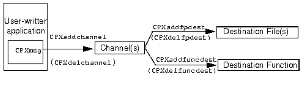
Output messages flow through message channels to destinations. Message
channels are associated with destinations through their destination list. Messages
from routines of the CPLEX Callable Library are assigned internally to one of those
predefined channels. Those default channels are C pointers to CPLEX objects; they
are initialized by CPXopenCPLEX; they are not global variables. Your application
accesses these objects by calling the routine CPXgetchannels. You can use these
predefined message channels for your own application messages. You can also
define new channels.
An application using routines from the CPLEX Callable Library produces no
output messages unless the application specifies message handling instructions
through one or more calls to the message handling routines of the Callable Library.
In other words, the destination list of each channel is initially empty.
Messages from multiple channels may be sent to one destination. All predefined
CPLEX channels can be directed to a single file by a call to CPXsetlogfile.
Similarly, all predefined CPLEX channels except cpxlog can be directed to the
screen by the messages to screen switch CPX_PARAM_SCRIND. For a finer level of
control, or to define destinations for application-specific messages, use the
following message handling routines, all documented in the Callable Library
Reference Manual:
vCPXmsg writes a message to a predefined channel;
vCPXflushchannel flushes a channel to its associated destination;
vCPXdisconnectchannel flushes a channel and clears its destination list;
vCPXaddfpdest adds a destination file to the list of destinations associated with a
channel;
vCPXdelfpdest deletes a destination from the destination list of a channel;
vCPXaddfuncdest adds a destination function to a channel;
vCPXdelfuncdest deletes a destination function to a channel;
After channel destinations are established, messages can be sent to multiple
destinations by a single call to a message-handling routine.
Example: Callable Library message channels
Demonstrates control of message channels in the C API.
This example shows you how to use the CPLEX message handler from the Callable
Library. It captures all messages generated by CPLEX and displays them on screen
Figure 4. CPLEX message handling routines
116 CPLEX User’s Manual
along with a label indicating which channel sent the message. It also creates a user
channel to receive output generated by the program itself. The user channel
accepts user-generated messages, displays them on screen with a label, and records
them in a file without the label.
The complete program lpex5.c appears online in the standard distribution at
yourCPLEXinstallation /examples/src. This example derives from lpex1.c, a
program in Getting Started. There are a few differences between the two examples:
vIn this example, the function ourmsgfunc (rather than the C functions printf or
fprintf(stderr, . . .)) manages all output. The program itself or CPXmsg from
the CPLEX Callable Library calls ourmsgfunc. In fact, CPXmsg is a replacement for
printf, allowing a message to appear in more than one place, for example, both
on screen and in a file.
Only after you initialize the CPLEX environment by calling CPXopenCPLEX can
you call CPXmsg. And only after you call CPXgetchannels can you use the default
CPLEX channels. Therefore, calls to ourmsgfunc print directly any messages that
occur before the program gets the address of cpxerror (a channel). After a call to
CPXgetchannels gets the address of cpxerror, and after a call to CPXaddfuncdest
associates the message function ourmsgfunc with cpxerror, then error messages
are generated by calls to CPXmsg.
After the TERMINATE: label, any error must be generated with care in case the
error message function has not been set up properly. Thus, ourmsgfunc is also
called directly to generate any error messages there.
vThe Callable Library routine CPXfopen opens the file lpex5.msg to accept solution
information. A call to the Callable Library routine CPXaddfpdest associates that
file with that channel. Solution information is also displayed on screen since
ourmsgfunc is associated with that new channel, too. Thus in the loops near the
end of main , when the solution is printed, only one call to CPXmsg suffices to put
the output both on screen and into the file.
vAlthough CPXcloseCPLEX will automatically delete file- and function-destinations
for channels, it is a good practice to call CPXdelfpdest and CPXdelfuncdest at the
end of your programs.
Concert Technology message channels
Describes control of message channels in Concert Technology C++ API.
In the C++ API of Concert Technology, the class IloEnv initializes output streams
for general information, for error messages, and for warnings. The class
IloAlgorithm supports these communication streams, and the class IloCplex
inherits its methods. For general output, there is the method IloAlgorithm ::out.
For warnings and nonfatal conditions, there is the method IloAlgorithm::warning.
For errors, there is the method IloAlgorithm::error.
By default, an instance of IloEnv defines the output stream referenced by the
method out as the system cout in the C++ API, but you can use the method setOut
to redefine it as you prefer. For example, to suppress output to the screen in a C++
application, use this method with this argument:
setOut(IloEnv::getNullStream)
Likewise, you can use the methods IloAlgorithm::setWarning and setError to
redefine those channels as you prefer.
Chapter 8. Managing input and output 117
118 CPLEX User’s Manual

Chapter 9. Timing interface
Introduces the timing interface available in CPLEX.
Determinism and the timing interface
Defines determinism in the context of the timing interface for accessing time
stamps.
Determinism means that repeated solving of the same model with the same
parameter settings, including limits, on the same computing platform will follow
exactly the same solution path, yielding the same level of performance and the
same values in the solution.
In contrast to determinism, the concept of opportunism implies taking advantage
of opportunities to improve performance even though these advantages in
performance may result in a different path to the solution or possibly even in
different results.
System time (such as CPU time measured in seconds or wall clock time measured
in seconds) is not deterministic; in other words, it may vary from one run to
another. For example, the load of other applications on a system can impact
performance and thus influence system time. Consequently, two consecutive runs
even with the same time limit may yield results that are not deterministic.
For situations where the user requires deterministic results, CPLEX offers a choice
between deterministic and opportunistic algorithms. For a comparison and contrast
of determinism and opportunism in the context of parallel algorithms, for example,
see the topic “Determinism of results” on page 373.
CPLEX also offers the user a choice between time limits measured in seconds (that
is, dependent on system time) and time limits measured deterministically. The
options of system time measured in seconds and deterministic time measured in
ticks (on the one hand) or parallelism and opportunism (on the other) are
orthogonal to one another. That is, you can set a system time limit on a
deterministic parallel algorithm, but of course then the termination criterion will
not be deterministic because it depends on nondeterministic system time measured
in seconds. You can likewise set a deterministic time limit on an opportunistic
parallel optimization. In that case, the termination criterion, indeed, the entire run
will not be deterministic because of the opportunism of the parallel optimization.
In other words, you can mix and match these options, but you must give careful
consideration to the effect you want to achieve in doing so.
You can even set both a deterministic and a system time limit simultaneously. In
such a case, CPLEX stops the optimization as soon as it reaches one of the limits
(similar to what happens when you set both a MIP gap and a node limit in a MIP
optimization).
Tip: If you want a fully deterministic optimization, then you need to apply a
deterministic algorithm, and you must not use a wall-clock time limit nor a CPU
time limit.
© Copyright IBM Corp. 1987, 2016 119

For more detail about time limits measured in seconds, see the documentation of
the parameter optimizer time limit in seconds (CPX_PARAM_TILIM, TiLim). For
more detail about deterministic time limits, see the documentation of the
parameter deterministic time limit (CPX_PARAM_DETTILIM, DetTiLim).
Using the timing interface
Describes the timing interface for accessing general purpose time stamps.
There are methods and routines in IBM ILOG CPLEX that provide a time stamp to
enable you to measure computational time. These methods and routines are
adapted for use either with opportunistic search or with the default deterministic
search. Some of the methods and routines measure time in seconds of wall-clock
time; others measure time in deterministic ticks. An application can invoke one of
these methods or routines at the beginning and end of an operation, and then
compare the two time stamps to compute elapsed time (either in seconds or in
deterministic ticks, depending on the respective method or routine that you chose).
vIn Concert Technology
– In the C++ API, IloCplex::getCplexTime returns a time stamp that
applications may use to calculate elapsed time in seconds.
IloCplex::getDetTime returns a time stamp in deterministic ticks.
– In the Java API, IloCplex.getCplexTime returns a time stamp that
applications may use to calculate elapsed time in seconds.
IloCplex.getDetTime returns a time stamp in deterministic ticks.
– In the .NET API, the property Cplex.CplexTime accesses a time stamp that
applications may use to calculate elapsed time in seconds. The property
Cplex.DetTime accesses a time stamp in deterministic ticks.
vIn the Callable Library, CPXXgettime returns a time stamp that applications may
use to calculate elapsed time in seconds. CPXXgetdettime returns a time stamp in
deterministic ticks.
vIn the Python API, the method Cplex.get_time returns a time stamp to measure
elapsed time in seconds, and the method Cplex.get_dettime returns a time stamp
to measure elapsed time in deterministic ticks.
Timestamps for callbacks
In addition, other methods and routines return a time stamp adapted to use in
callbacks. Again, there are methods and routines available either for measuring
time in seconds or for measuring time in deterministic ticks. For more information
about these callback methods and routines, see “Using the timing interface in
callbacks” on page 121.
Examples of the timing interface
For a sample of these timing features, see these examples among those distributed
with the product in yourCPLEXinstallation/examples:
vilomipex4.cpp in C++ in Concert Technology
vMIPex4.java in Java in Concert Technology
vMIPex4.cs in C#.NET in Concert Technology
vMIPex4.vb in Visual Basic.NET in Concert Technology
vxmipex4.c in C in the Callable Library
120 CPLEX User’s Manual

Using the timing interface in callbacks
Describes the timing interface for accessing time stamps from callbacks.
In addition to the general purpose methods and routines that provide a time stamp
to enable you to measure computational time in your applications of IBM ILOG
CPLEX, there are methods and routines specifically for use in callbacks. Like the
general purpose methods and routines for time stamps, these callback methods
and routines are adapted for use either with the default opportunistic search or
with the deterministic search. An application can invoke one of these methods or
routines at the beginning and end of an operation, and then compare the two time
stamps to compute elapsed time (either in seconds or in deterministic ticks,
respectively).
vIn Concert Technology
– In the C++ API, CallbackI::getStartTime returns a time stamp in seconds at
the beginning of optimization. CallbackI::getStartDetTime returns a time
stamp in deterministic ticks at the beginning of optimization.
CallbackI::getEndTime returns a time stamp specifying in seconds when
CPLEX will reach a time limit. CallbackI::getEndDetTime returns a time
stamp specifying in deterministic ticks when CPLEX will reach a time limit.
CallbackI::getCplexTime returns the current time stamp in seconds.
CallbackI::getDetTime returns the current time stamp in deterministic ticks.
– In the Java API, CpxCallback.getStartTime returns a time stamp in seconds at
the beginning of optimization. CpxCallback.getStartDetTime returns a time
stamp in deterministic ticks at the beginning of optimization.
CpxCallback.getEndTime returns a time stamp specifying in seconds when
CPLEX will reach a time limit. CpxCallback.getEndDetTime returns a time
stamp specifying in deterministic ticks when CPLEX will reach a time limit.
– In the .NET API, the property Cplex.Callback.StartTime accesses a time
stamp in seconds at the beginning of optimization.
Cplex.Callback.StartDetTime accesses a time stamp in deterministic ticks at
the beginning of optimization. Cplex.Callback.EndTime accesses a time stamp
specifying in seconds when CPLEX will reach a time limit.
Cplex.Callback.EndDetTime accesses a time stamp specifying in deterministic
ticks when CPLEX will reach a time limit.
With those values, you can compute the time in seconds since the start of the
optimization: getCplexTime - getStartTime. Likewise, you can compute the
remaining time in seconds until CPLEX reaches the time limit: getEndTime -
getCplexTime. Analogously, you can compute the time in deterministic ticks
since the start of the optimization: getDetTime - getStartDetTime. Similarly, you
can compute the remaining time in deterministic ticks until CPLEX reaches the
time limit: getDetEndTime - getDetTime.
vIn the Callable Library, CPX_CALLBACK_INFO_STARTTIME and
CPX_CALLBACK_INFO_ENDTIME are symbolic values that CPXgetcallbackinfo can
supply in its argument whichinfo. Those values are time stamps of the point in
time when optimization started and terminated (if optimization does not finish
before that point). In other words, those symbols are useful in measuring time in
seconds through information callbacks.
Likewise, CPX_CALLBACK_INFO_STARTDETTIME and CPX_CALLBACK_INFO_ENDDETTIME
are also symbolic values that CPXgetcallbackinfo can supply in its argument
whichinfo. Those values are time stamps of the point in time measured in
deterministic ticks when optimization started and terminated (if optimization
does not finish before that point). In other words, those symbols are useful in
measuring time in deterministic ticks through information callbacks.
Chapter 9. Timing interface 121
vIn the Python API, these methods are available for measuring time in callbacks.
– Callback.get_start_time
– Callback.get_start_dettime
– Callback.get_end_time
– Callback.get_end_dettime
– Callback.get_dettime
122 CPLEX User’s Manual

Chapter 10. Tuning tool
The tuning tool, a utility to aid you in improving the performance of your
optimization applications, analyzes a model or a group of models and suggests a
suite of parameter settings for you to use that provide better performance than the
default parameter settings for your model or group of models. This topic
documents the tuning tool of IBM ILOG CPLEX.
Meet the tuning tool
Introduces the tuning tool.
Overview: scope of the tuning tool
Defines the scope of the tuning tool.
The tuning tool looks at parameters to improve solving time, either in seconds of
system time or in deterministic ticks. If your model suffers from numeric
instability, the tuning tool will not attempt to correct that problem. Furthermore, if
there is insufficient memory to accommodate optimization of your model, the
tuning tool will not correct that problem either. In short, the tuning tool does not
magically eliminate all performance bottlenecks. However, if you understand the
performance issues of your model, the tuning tool can help you discern parameter
settings that lead to faster solving time.
The recommended practice with the tuning tool is to solve your model first with
default parameter settings and to consider the results before invoking the tuning
tool. Your analysis of those results directs you toward the next step. The following
topics sketch typical scenarios for working effectively with the tuning tool and
outline what to expect from the tuning tool.
If CPLEX solves your problem to optimality
Distinguishes problems solved to optimality.
If CPLEX solves your problem to optimality, you may still want to apply the
tuning tool to discover whether you can solve the model faster. In such a case,
bear in mind that the tuning tool performs several optimization runs as it goes
about its work. These optimization runs may take six to eight times longer than
the default run that produced your optimal results. If that projected time (six to
eight times longer than the initial default run) seems too long for your purpose,
then consider setting a general time limit or consider setting a specific tuning time
limit per problem, per optimization. As you set such time limits, keep in mind that
you can set time limits in terms of system time seconds or deterministic ticks. (For
information about these contrasting ways of measuring time, see the topic
Chapter 9, “Timing interface,” on page 119.)
To set a general time limit, either use the optimizer time limit in seconds
parameter (TiLim, CPX_PARAM_TILIM) to set a limit in seconds of system time, or use
the deterministic time limit parameter (DetTiLim, CPX_PARAM_DETTILIM) to set a
deterministic time limit in terms of deterministic ticks.
To set a specific tuning time limit per problem, per optimization, either use the
tuning time limit in seconds parameter (TuningTiLim, CPX_PARAM_TUNINGTILIM) to
© Copyright IBM Corp. 1987, 2016 123
set a limit in seconds of system time, or use the deterministic tuning time limit
parameter (TuningDetTiLim, CPX_PARAM_TUNINGDETTILIM) to set a deterministic time
limit in terms of deterministic ticks.
“Examples: time limits on tuning in the Interactive Optimizer” on page 127
illustrates this approach through time limits more fully.
If CPLEX finds solutions but does not prove optimality
Distinguishes problems with solutions not proven optimal.
In the case where CPLEX finds solutions for your model but does not prove
optimality in your initial run before invoking the tuning tool, you will likely want
to set the time limit per model. See “Tuning and time limits” for more about that
idea.
In situations where CPLEX does not solve your model to optimality for a reason
other than a time limit, you should address that reason before you apply the
tuning tool.
For example, if your initial run results in an out-of-memory error, consider setting
the memory emphasis parameter (memory reduction switch: MemoryEmphasis,
CPX_PARAM_MEMORYEMPHASIS). Then create a file in which you specify a fixed setting
of that parameter for the tuning tool to respect. Pass that file to the tuning tool
with your model. “Fixing parameters and tuning multiple models in the Interactive
Optimizer” on page 128 illustrates this approach.
Tuning and time limits
Introduces parameters to set time limits on tuning.
The tuning process is affected by four time limit parameters, and these parameters
interact with one another.
voptimizer time limit in seconds: TiLim, CPX_PARAM_TILIM
vdeterministic time limit: DetTiLim, CPX_PARAM_DETTILIM
vtuning time limit in seconds: TuningTiLim, CPX_PARAM_TUNINGTILIM
vdeterministic tuning time limit: TuningDetTiLim, CPX_PARAM_TUNINGDETTILIM
For the tuning process, the overall time limit in seconds of system time is set with
the general time limit parameter (optimizer time limit in seconds: TiLim,
CPX_PARAM_TILIM).
The overall time limit in deterministic ticks is set with the deterministic time limit
parameter (deterministic time limit: DetTiLim, CPX_PARAM_DETTILIM).
Tuning consists of a series of optimizations of each of the problems to be tuned.
You can specify a time limit on each of these optimizations, either in terms of
seconds of system time or in terms of deterministic ticks. To set a time limit in
seconds on each optimization of a tuning run, use the tuning time limit parameter
(tuning time limit in seconds: TuningTiLim, CPX_PARAM_TUNINGTILIM). To set a time
limit in deterministic ticks on each optimization of a tuning run, use the
deterministic tuning time limit parameter (deterministic tuning time limit:
TuningDetTiLim, CPX_PARAM_TUNINGDETTILIM). In either case, the default value of the
tuning parameter is set to a value much smaller than the default value of the
overall time limit, so as to avoid runs of unlimited length. These two tuning-timing
parameters govern complete optimizations started within the tuning tool. The
124 CPLEX User’s Manual
tuning tool may also launch shorter and partial optimizations; in such cases, it uses
these tuning-timing parameters as guidance to compute shorter time limits.
Tip: You can set both the overall time limit in seconds (TiLim) and the overall
deterministic time limit (DetTiLim) to a finite value (less than 1e+75), and the entire
tuning session will terminate if CPLEX reaches either of those limits. In contrast,
you cannot set both the per-problem, per-optimization time limit in seconds
(TuningTiLim) and the deterministic per-problem, per-optimization time limit
(TuningDetTiLim) parameters to a finite value (less than 1e+75). At least one of
those two must be set to 1e+75 (infinity).
The per-problem, per-optimization time limit can also be set by means of the
general time limit parameter (optimizer time limit in seconds TiLim,
CPX_PARAM_TILIM) or the deterministic time limit parameter (deterministic time
limit DetTiLim, CPX_PARAM_DETTILIM) in a fixed parameter set. “Fixing parameters
and tuning multiple models in the Interactive Optimizer” on page 128 explains
more about that approach. If you are using a time limit in your usual (non-tuning)
runs of the models, you may want to set the per-problem, per-optimization time
limit in this way.
Tuning time limits and determinism
Documents the effect of tuning time limits on determinism.
Values of the tuning time-limit parameters impact whether or not CPLEX conducts
the tuning session in deterministic mode.
vtuning time limit in seconds: TuningTiLim, CPX_PARAM_TUNINGTILIM
vdeterministic tuning time limit: TuningDetTiLim, CPX_PARAM_TUNINGDETTILIM
In the following discussion, 1e+75 corresponds to infinity on most platforms.
Check your platform-specific declarations to be sure.
If TuningTiLim < 1e+75, and TuningDetTiLim = 1e+75, then the tuning result will be
nondeterministic, as CPLEX uses a system time limit for individual tuning runs.
If TuningTiLim = 1e+75, and TuningDetTiLim < 1e+75, then the tuning result will be
deterministic, as CPLEX uses a deterministic time limit for individual tuning runs.
If TuningTiLim = 1e+75, and TuningDetTiLim = 1e+75 (the default values of these
parameters), then the tuning result will be deterministic, as CPLEX uses a default
deterministic time limit of ten million (1e+7) ticks for individual tuning runs. In
other words, the default setting of these two parameters is identical to setting
TuningDetTiLim = 1e+7.
Of course, if you apply a finite overall system time limit (TiLim, CPX_PARAM_TILIM),
and the tuning process reaches that finite system time limit, then the tuning results
are not deterministic. (This principle is the same for optimization in deterministic
mode reaching a time limit: results are not deterministic then either.)
The overall system time limit (TiLim, CPX_PARAM_TILIM), the overall deterministic
time limit (DetTiLim, CPX_PARAM_DETTILIM), the tuning time limit in seconds
(TuningTiLim, CPX_PARAM_TUNINGTILIM), and the deterministic tuning time limit in
ticks (TuningDetTiLim, CPX_PARAM_TUNINGDETTILIM) are unrelated to the parallel
mode switch (ParallelMode, CPX_PARAM_PARALLELMODE). If the parallel mode switch
Chapter 10. Tuning tool 125

is set as opportunistic, for example, through a tuning parameter file, then the
results of tuning will be nondeterministic, even if TuningTiLim is set to infinity
(1e+75).
In order to achieve truly deterministic, repeatable tuning results, all of the
following conditions must hold:
vThe parallel mode switch (ParallelMode, CPX_PARAM_PARALLELMODE) must be at its
default value, 0 (zero) or set to its deterministic value 1 (one).
vThe optimizer time limit in seconds (TiLim, CPX_PARAM_TILIM) must be set to
infinity (1e+75 on most platforms), its default value.
vThe tuning time limit in seconds (TuningTiLim, CPX_PARAM_TUNINGTILIM) must be
set to infinity (1e+75 on most platforms), its default value.
In other words, if you are using default values of all CPLEX parameters, a tuning
session will yield deterministic results.
Tuning results
Describes typical results of a tuning session.
The tuning tool selects the best suite of parameter settings based on the
performance times of the several optimizations of the model or models. Whether
your tuning results are deterministic depends on considerations outlined in the
topics “Tuning and time limits” on page 124 and “Tuning time limits and
determinism” on page 125.
Invoking the tuning tool
Describes methods and routines to invoke the tuning tool.
The tuning tool is available in all components of CPLEX: Concert Technology,
Callable Library, and Interactive Optimizer.
In Concert Technology, you invoke the tuning tool through these methods:
vtuneParam in the C++ API; see also the example ilotuneset.cpp ;
vtuneParam in the Java API; see also the example TuneSet.java ;
vCplex.TuneParam in the .NET API; see also the example TuneSet.cs or
TuneSet.vb .
The tool is also part of the Callable Library (C API) through separate routines for
tuning a single model or a group of models. For more detail about the C routine
for tuning a single model or a group of models, see “Tuning models in the Callable
Library (C API)” on page 130. For a sample application, see examples/src/cplex/
tuneset.c .
In the Interactive Optimizer, you can tune one model or a group of models with
the tune command. See the “Examples: time limits on tuning in the Interactive
Optimizer” on page 127, as well as the topic “Fixing parameters and tuning
multiple models in the Interactive Optimizer” on page 128.
You can specify whether you want the least worst performance or the best average
performance across a set of models with the tuning measure parameter, (tuning
measure: TuningMeasure, CPX_PARAM_TUNINGMEASURE), documented in the CPLEX
Parameters Reference Manual.
126 CPLEX User’s Manual

When you are tuning a single model, you can ask CPLEX to permute the model
and re-tune to get more robust results, as explained in the documentation of the
repeat tuning parameter (tuning repeater: TuningRepeat, CPX_PARAM_TUNINGREPEAT).
You can also set a time limit specific to tuning per problem and per optimization
run, as explained in the topic “Tuning and time limits” on page 124. The example
in “Examples: time limits on tuning in the Interactive Optimizer.” shows how to
set such a time limit.
Examples: time limits on tuning in the Interactive Optimizer
Shows the effect of both deterministic and nondeterministic time limits on the
tuning tool in the Interactive Optimizer.
Both overall system time limits (in seconds) and overall deterministic time limits
(in ticks) have an impact on tuning. Likewise, both overall time limits and
per-problem, per-optimization time limits also govern tuning. These examples in
the Interactive Optimizer illustrate key points about time limits and tuning.
First example: overall time limit and per-problem time limit in
seconds
As a first example, suppose that you want to spend an overall amount of time
tuning the parameter settings for a given model, say, 1000 seconds. Also suppose
that you want CPLEX to make multiple attempts within that overall time limit to
tune the parameter settings for your model. Suppose further that you want to set a
time limit on each of those attempts, say, 200 seconds per attempt.
In the Interactive Optimizer, first enter your model into a session (for example, by
reading a formatted file), like this:
read model.mps
Then set the overall time limit through the environment with this command:
set timelimit 1000
That command makes 1000 seconds available as a resource in the environment.
The command effectively sets the overall time limit (optimizer time limit in
seconds: TiLim, CPX_PARAM_TILIM).
Then set the tuning time limit, like this:
set tune timelimit 200
This series of commands tells CPLEX to tune the parameters of your model,
making multiple attempts of 200 seconds each (set by the tuning time limit in
seconds: TuningTiLim, CPX_PARAM_TUNINGTILIM), within an overall time limit of 1000
seconds (set by the optimizer time limit in seconds: TiLim, CPX_PARAM_TILIM) .
Tip: Remember that system time limits in seconds lead to nondeterministic results
in tuning, as explained in the topics “Tuning and time limits” on page 124 and
“Tuning time limits and determinism” on page 125. If your application requires
deterministic results, use deterministic time limits instead, as illustrated in the next
example.
Chapter 10. Tuning tool 127

Second example: overall deterministic time limit and per-problem
deterministic time limit in ticks
As a second example, suppose that you want to spend an overall amount of time
deterministically tuning the parameter settings for a given model, say, 1000000
ticks. Also suppose that you want CPLEX to make multiple attempts within that
overall time limit to tune the parameter settings for your model. Suppose further
that you want to set a time limit on each of those attempts, say, 200 ticks per
attempt.
In the Interactive Optimizer, as in the previous example, first enter your model
into a session (for example, by reading a formatted file), like this:
read model.mps
Then set the overall deterministic time limit through the environment with this
command:
set dettimelimit 1000000
That command makes 1000000 ticks available as a resource in the environment.
The command effectively sets the overall deterministic time limit (deterministic
time limit: DetTiLim, CPX_PARAM_DETTILIM).
Then set the deterministic tuning time limit, like this:
set tune dettimelimit 200000
This series of commands tells CPLEX to tune the parameters of your model
deterministically, making multiple attempts of 200000 ticks each (set by the
deterministic tuning time limit: TuningDetTiLim, CPX_PARAM_TUNINGDETTILIM),
within an overall time limit of 1000000 ticks (set by the deterministic time limit:
DetTiLim, CPX_PARAM_DETTILIM).
Tip: You can use both overall time limits (both system in seconds and
deterministic in ticks) together; that is, you can set both TiLim and DetTiLim
simultaneously, as explained in the topic “Tuning and time limits” on page 124.
However, you must not mix a per-problem, per-optimization tuning time limit in
seconds with a deterministic per-problem, per-optimization tuning time limit in
ticks. That is, do not mix TuningTiLim, CPX_PARAM_TUNINGTILIM with
TuningDetTiLim, CPX_PARAM_TUNINGDETTILIM, again as explained in “Tuning and
time limits” on page 124.
Default behavior
At default settings, these four time limits are set to infinity (that is, 1e+75 on most
platforms). These default settings are equivalent to setting the deterministic tuning
time limit TuningDetTiLim, CPX_PARAM_TUNINGDETTILIM to 1e+7.
Fixing parameters and tuning multiple models in the Interactive
Optimizer
Shows options of the tuning tool command in the Interactive Optimizer.
128 CPLEX User’s Manual
Invoking the tuning tool in the Interactive Optimizer
Shows commands to invoke the tuning tool in the Interactive Optimizer.
The command to invoke the tuning tool in the Interactive Optimizer is: tools tune
Optionally, that command may take one or two arguments, in either order, like
this:
tools tune paramfile.prm modelfile
or
tools tune modelfile paramfile.prm
The following sections explain those optional arguments.
Fixed parameters to respect
Describes facilities in Interactive Optimizer to exclude parameters from
consideration by the tuning tool.
If you supply an optional file name with the extension.prm , that file contains the
formatted list of parameters and their values that you do not want CPLEX to tune.
That is, you want CPLEX to respect those parameter settings. If you do not supply
a parameter file to the tune command, then all parameters are subject to tuning.
For example, if you have a model that you know has numerical issues, and you
have already determined that you want to set the numerical emphasis parameter
yourself, then a PRM file suitable for tuning your model would contain the
following heading and parameter setting:
CPLEX Parameter File Version 12.7.0.0
CPXPARAM_Emphasis_MIP 1
Tip:
A PRM file must have a correctly formatted header to let CPLEX know which
version to expect.
An easy way to generate a PRM file with a correct heading and fixed parameter
settings is to read your model, set the parameters you wish, and write a PRM file
from the Interactive Optimizer, with this command:
write filename .prm
Files of models to tune
Describes facility in the Interactive Optimizer to tune multiple models
simultaneously.
If you supply an optional file name, such as modelfile, that file contains a list of
files, one file name per line. Each file contains a model to tune. Each file must
specify its type, such as .mps, .lp, or .sav, as the extension in the file name.
Optionally, those cited files may be compressed, as specified by the extension .gz
or .bz2. Here is an example of the contents of such a file, specifying three
compressed files of type .mps available in the current working directory:
Chapter 10. Tuning tool 129

p0033.mps.gz
p0548.mps.gz
p2756.mps.gz
For models not in the current working directory, you can specify a path to them
with the usual syntax for your platform.
CPLEX will uncompress the model files, read them according to their type of
format, and apply the tuning tool to that suite of files. If you do not specify a list
of models to tune, then CPLEX tunes the model currently in the Interactive
Optimizer.
Tuning models in the Callable Library (C API)
Describes the tuning tool in the C API.
The routine CPXtuneparam tunes one existing model, and the routine
CPXtuneparamprobset tunes a group of models, specified by an array of file names.
Both these routines are applicable to models of one of these types: LP, QP, and
MIP. (Neither applies to networks. Neither applies to quadratically constrained
programs (QCP).) Advanced bases in .sav files are ignored by these routines.
Acceptable file formats for these routines are:
v.mps
v.lp
v.sav
Parameter settings in the environment control the resources for the tuning tool; the
parameter settings passed in the arguments of these routines are used by CPLEX
as a starting point for tuning. You can specify parameters and corresponding
values for CPLEX to use as a starting point. Bear in mind that the parameters you
specify at nondefault settings will be fixed during the tuning. That is, the tuning
tool will not attempt to modify them. In other words, when you set a parameter as
a starting point, you eliminate it from consideration by the tuning tool.
Callbacks (except the tuning callback) are ignored by these tuning routines in the
Callable Library (C API).
The tuning tool checks the termination signal (that is, the variable set by the
routine CPXsetterminate) and terminates the tuning process in compliance with
that termination signal. Tuning also respects time limits set in the environment.
The result of either tuning routine is an environment containing the parameter
settings recommended by tuning. You can query these values or write them to a
formatted PRM file with the usual routines.
After tuning, the return value of either routine specifies 0 (zero) when tuning
completed successfully and nonzero when it has not done so. A tuning status is
also returned as an argument to these routines. The possible nonzero values of the
tuning status argument are these:
vCPX_TUNE_ABORT specifies that abort occurred through CPXsetterminate.
vCPX_TUNE_TILIM specifies that tuning reached the time limit specified in the
environment by the overall optimizer time limit parameter CPX_PARAM_TILIM .
vCPX_TUNE_DETTILIM specifies that tuning reached the deterministic time limit
specified by the deterministic time limit parameter CPX_PARAM_DETTILIM.
130 CPLEX User’s Manual

Tuning will set any parameters which have been chosen even if there is an early
termination.
Callbacks for tuning
Describes callbacks available to the tuning tool.
A tuning callback is a user-written function that CPLEX calls before each trial run
during a tuning session. A tuning callback allows you to follow the progress of
tuning. It reports information that enables you to estimate how much more time
tuning needs to achieve results useful in your model.
To use a tuning callback in a tuning session, you must first write the callback
function, and then pass it to CPLEX. CPLEX will then execute your tuning callback
before it begins a trial run.
vIn Concert Technology, you must implement your user-written function as an
instance of the tuning callback class.
– IloCplex::TuningCallbackI in the C++ API
– IloCplex.TuningCallback in the Java API
– Cplex.TuningCallback in the .NET API
For details about writing your tuning callback, see Chapter 37, “Using
optimization callbacks,” on page 499, especially “Implementing callbacks with
Concert Technology” on page 509
vIn the Callable Library (C API), use the routine CPXsettuningcallbackfunc . For
more about how to write a callback, see also “Implementing callbacks in the
Callable Library” on page 514.
Terminating a tuning session
Describes facilities to end a tuning session.
To terminate a tuning session, you can use one of the following means:
vIn the C++ API, pass an instance of the class IloCplex::Aborter to an instance
of IloCplex. Then call the method IloCplex::Aborter::abort to terminate the
tuning session.
vIn the Java API, pass an instance of the class IloCplex.Aborter to an instance of
IloCplex. Then call the method IloCplex.Aborter.abort to terminate the tuning
session.
vIn the .NET API, pass an instance of the class Cplex.Aborter to an instance of
Cplex . Then call the method Cplex.Aborter.Abort to terminate the tuning
session.
vIn the Callable Library (C API), call the routine CPXsetterminate to set a pointer
to the termination signal. Initially, the value of the termination signal should be
zero. When your application sets the termination signal to a nonzero value, then
CPLEX will terminate the tuning session.
Chapter 10. Tuning tool 131
132 CPLEX User’s Manual

Part 3. Continuous optimization
This part focuses on algorithmic considerations about the optimizers of IBM ILOG
CPLEX that solve problems formulated in terms of continuous variables. While
ILOG CPLEX is delivered with default settings that enable you to solve many
problems without changing parameters, this part also documents features that you
can customize for your application.
© Copyright IBM Corp. 1987, 2016 133
134 CPLEX User’s Manual

Chapter 11. Solving LPs: simplex optimizers
Documents the primal and dual simplex optimizers.
Introducing the primal and dual optimizers
Places the primal and dual optimizers in context.
The preceding topics have focused on the details of writing applications that
model optimization problems and access the solutions to those problems, with
minimal attention to the optimizer that solves them, because most models are
solved well by the default optimizers provided by IBM ILOG CPLEX. For instances
where a user wants to exert more direct influence over the solution process,
CPLEX provides a number of features that may be of interest.
This topic and the following one tell you more about solving linear programs with
the LP optimizers of CPLEX. This topic emphasizes primal and dual simplex
optimizers.
Choosing an optimizer for your LP problem
Explains considerations of choosing an optimizer for LP models.
Overview of LP optimizers
Introduces parameters to select LP optimizers.
CPLEX offers several different optimizers for linear programming problems. Each
of these optimizers is available whether you call CPLEX from within your own
application using Concert Technology or the Callable Library, or you use the
Interactive Optimizer.
The choice of LP optimizer in CPLEX can be specified using the algorithm for
continuous linear problems parameter, named RootAlg in the C++, Java, and .NET
APIs, CPX_PARAM_LPMETHOD in the Callable Library, and lpmethod in the Interactive
Optimizer. In Concert Technology, the LP method is controlled by the RootAlg
parameter (which also controls related aspects of QP and MIP solutions, as
explained in the corresponding chapters of this manual). In this chapter, this
parameter will be referred to uniformly as LPMethod.
The LPMethod parameter sets which optimizer will be used when you solve a
model in one of the following ways:
vcplex.solve (Concert Technology)
vCPXlpopt (Callable Library)
voptimize (Interactive Optimizer)
The choices for LPMethod are summarized in Table 20 on page 136.
© Copyright IBM Corp. 1987, 2016 135
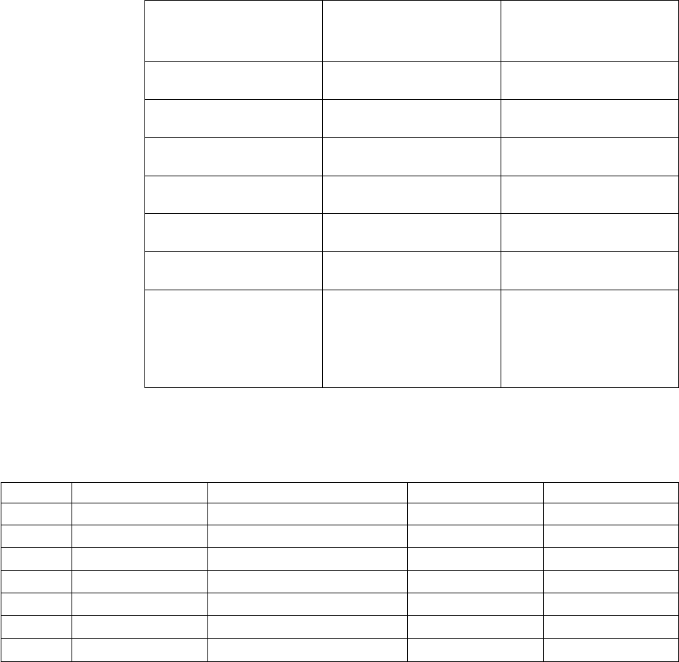
Table 20. Settings of the LPMethod parameter for choosing an optimizer
Setting of
LPMethod
Meaning See Section
0 Default Setting “Automatic selection of an
optimizer”
1 Primal Simplex “Primal simplex optimizer”
on page 137
2 Dual Simplex “Dual simplex optimizer” on
page 137
3 Network Simplex “Network optimizer” on
page 137
4 Barrier “Barrier optimizer” on page
138
5 Sifting “Sifting optimizer” on page
138
6Concurrent Dual, Barrier,
and Primal in opportunistic
parallel mode; Concurrent
Dual and Barrier in
deterministic parallel mode
“Concurrent optimizer” on
page 138
The symbolic names for these settings in an application are summarized in
Table 21.
Table 21. Symbolic names for LP solution methods
Concert C++ Concert Java Concert.NET Callable Library
0 IloCplex::AutoAlg IloCplex.Algorithm.Auto Cplex.Auto CPX_ALG_AUTOMATIC
1 IloCplex::Primal IloCplex.Algorithm.Primal Cplex.Primal CPX_ALG_PRIMAL
2 IloCplex::Dual IloCplex.Algorithm.Dual Cplex.Dual CPX_ALG_DUAL
3 IloCplex::Network IloCplex.Algorithm.Network Cplex.Network CPX_ALG_NET
4 IloCplex::Barrier IloCplex.Algorithm.Barrier Cplex.Barrier CPX_ALG_BARRIER
5 IloCplex::Sifting IloCplex.Algorithm.Sifting Cplex.Sifting CPX_ALG_SIFTING
6 IloCplex::Concurrent IloCplex.Algorithm.Concurrent Cplex.Concurrent CPX_ALG_CONCURRENT
Automatic selection of an optimizer
Describes conditions for automatic selection of an optimizer.
The default Automatic setting of the LP method lets CPLEX decide which
algorithm to use to optimize your problem. Most models are solved well with this
setting, and this is the recommended option except when you have a compelling
reason to tune performance for a particular class of model.
On a serial computer, or on a parallel computer where only one thread will be
invoked, the automatic setting will in most cases choose the dual simplex
optimizer. An exception to this rule is when an advanced basis is present that is
ascertained to be primal feasible; in that case, primal simplex will be called.
136 CPLEX User’s Manual
On a computer where parallel threads are available to CPLEX, the automatic
setting typically results in the concurrent optimizer being called in either
deterministic, or opportunistic parallel mode. However, exceptions to this general
rule occur when CPLEX analyzes characteristics of your model plus your
parameter settings, and determines from that analysis that running different
algorithms concurrently may not improve performance on that model with those
parameter settings. Here are a few examples (the list is not exhaustive) of
situations where CPLEX can draw the conclusion that performance will not be
improved by concurrent optimization with different algorithms:
vThe presence of an advanced basis
vThe model is so small that the overhead costs of setting up concurrent
optimization exceed possible performance gains
vThe memory emphasis parameter memory reduction switch has been enabled.
In such cases, CPLEX invokes simplex optimizers.
Dual simplex optimizer
Describes conditions favoring the dual simplex optimizer.
If you are familiar with linear programming theory, then you recall that a linear
programming problem can be stated in primal or dual form, and an optimal
solution (if one exists) of the dual has a direct relationship to an optimal solution
of the primal model. CPLEX dual simplex optimizer makes use of this relationship,
but still reports the solution in terms of the primal model. The dual simplex
method is the first choice for optimizing a linear programming problem, especially
for primal-degenerate problems with little variability in the righthand side
coefficients but significant variability in the cost coefficients.
Primal simplex optimizer
Describes conditions favoring the primal simplex optimizer.
CPLEX primal simplex optimizer also can effectively solve a wide variety of linear
programming problems with its default parameter settings. The primal simplex
method is not the obvious choice for a first try at optimizing a linear programming
problem. However, this method will sometimes work better on problems where the
number of variables exceeds the number of constraints significantly, or on
problems that exhibit little variability in the cost coefficients. Few problems exhibit
poor numeric performance in both primal and dual form. Consequently, if you
have a problem where numeric difficulties occur when you use the dual simplex
optimizer, then consider using the primal simplex optimizer instead.
Network optimizer
Describes conditions favoring the network optimizer.
If a major part of your problem is structured as a network, then the CPLEX
network optimizer may have a positive impact on performance. The CPLEX
network optimizer recognizes a special class of linear programming problems with
network structure. It uses highly efficient network algorithms on that part of the
problem to find a solution from which it then constructs an advanced basis for the
rest of your problem. From this advanced basis, CPLEX then iterates to find a
solution to the full problem. Chapter 13, “Solving network-flow problems,” on
page 181 explores this optimizer in greater detail.
Chapter 11. Solving LPs: simplex optimizers 137
Barrier optimizer
Describes conditions favoring the barrier optimizer.
The barrier optimizer offers an approach particularly efficient on large, sparse
problems (for example, more than 100 000 rows or columns, and no more than
perhaps a dozen nonzeros per column) and sometimes on other models as well.
The barrier optimizer is sufficiently different in nature from the other optimizers
that it is discussed in detail in Chapter 12, “Solving LPs: barrier optimizer,” on
page 161.
Sifting optimizer
Describes conditions favoring the sifting optimizer.
Sifting was developed to exploit the characteristics of models with large aspect
ratios (that is, a large ratio of the number of columns to the number of rows). In
particular, the method is well suited to large aspect ratio models where an optimal
solution can be expected to place most variables at their lower bounds. The sifting
algorithm can be thought of as an extension to the familiar simplex method. It
starts by solving a subproblem (known as the working problem) consisting of all
rows but only a small subset of the full set of columns, by assuming an arbitrary
value (such as its lower bound) for the solution value of each of the remaining
columns. This solution is then used to re-evaluate the reduced costs of the
remaining columns. Any columns whose reduced costs violate the optimality
criterion become candidates to be added to the working problem for the next
major sifting iteration. When no candidates are present, the solution of the working
problem is optimal for the full problem, and sifting terminates.
The choice of optimizer to solve the working problem is governed by the SiftAlg
parameter. You can set this parameter to any of the values accepted by the
LPMethod parameter, except for Concurrent and of course Sifting itself. At the
default SiftAlg setting, CPLEX chooses the optimizer automatically, typically
switching between barrier and primal simplex as the optimization proceeds. It is
recommended that you not turn off the barrier crossover step (that is, do not set
the parameter BarCrossAlg to -1) when you use the sifting optimizer, so that this
switching can be carried out as needed.
Tip:
If you invoke concurrent optimization on a linear program (LP), the concurrent
optimzer checks the aspect ratio of the model. If the concurrent optimizer finds a
large aspect ratio, and if ten or more threads are available to CPLEX, then the
concurrent optimizer also invokes sifting on the LP model. For more information
about concurrent optimization, see the topic “Concurrent optimizer.”
Concurrent optimizer
Describes conditions favoring the concurrent optimizer.
The concurrent optimizer launches distinct optimizers in multiple threads. When
the concurrent optimizer is launched on a single-threaded platform, it calls the
dual simplex optimizer. In other words, choosing the concurrent optimizer makes
sense only on a multiprocessor computer where threads are enabled. For more
information about the concurrent optimizer, see Chapter 28, “Multithreaded
parallel optimizers,” on page 371, especially “Concurrent optimizer in parallel” on
page 376.
138 CPLEX User’s Manual

Tip: Crossover in concurrent optimization is incompatible with an LP callback due
to considerations about thread-safety.
Parameter settings and optimizer choice
Describes special considerations about parameters and choice of optimizer.
When you are using parameter settings other than the default, consider the
algorithms that these settings will affect. Some parameters, such as the time limit,
will affect all the algorithms invoked by the concurrent optimizer. Others, such as
the refactoring frequency, will affect both the primal and dual simplex algorithms.
And some parameters, such as the primal gradient, dual gradient, or barrier
convergence tolerance, affect only a single algorithm.
Tuning LP performance
Documents tactics for tuning performance on LP models.
Introducing performance tuning for LP models
Outlines general facilities for performance tuning on LP models.
Each of the optimizers available in CPLEX is designed to solve most linear
programming problems under its default parameter settings. However,
characteristics of your particular problem may make performance tuning
advantageous.
As a first step in tuning performance, try the different CPLEX optimizers, as
recommended in “Choosing an optimizer for your LP problem” on page 135.
To help you decide whether default settings of parameters are best for your model,
or whether other parameter settings may improve performance, the tuning tool is
available. Chapter 10, “Tuning tool,” on page 123 explains more about this utility
and offers you examples of its use.
The following sections suggest other features of CPLEX to consider in tuning the
performance of your application.
Preprocessing
Documents preprocessing at default parameter settings in LP optimizers.
At default settings, CPLEX preprocesses problems by simplifying constraints,
reducing problem size, and eliminating redundancy. Its presolver tries to reduce
the size of a problem by making inferences about the nature of any optimal
solution to the problem. Its aggregator tries to eliminate variables and rows
through substitution. For most models, preprocessing is beneficial to the total
solution speed, and CPLEX reports the model's solution in terms of the user's
original formulation, making the exact nature of any reductions immaterial.
Dual formulation in presolve
A useful preprocessing feature for performance tuning, one that is not always
activated by default, can be to convert the problem to its dual formulation. The
nature of the dual formulation is rooted in linear programming theory, beyond the
scope of this manual, but for the purposes of this preprocessing feature it is
Chapter 11. Solving LPs: simplex optimizers 139

sufficient to think of the roles of the rows and columns of the model's constraint
matrix as being switched. Thus the feature is especially applicable to models that
have many more rows than columns.
You can direct the preprocessor to form the dual by setting the PreDual parameter
to 1(one).
Conversely, to entirely inhibit the dual formulation for the barrier optimizer, you
can set the PreDual parameter to -1 . The default, automatic, setting is 0.
It is worth emphasizing, to those familiar with linear programming theory, that the
decision to solve the dual formulation of your model, via this preprocessing
parameter, is not the same as the choice between using the dual simplex method or
the primal simplex method to perform the optimization. Although these two
concepts (dual formulation and dual simplex optimizer) have theoretical
foundations in common, it is valid to consider, for example, solving the dual
formulation of your model with the dual simplex method; this would not simply
result in the same computational path as solving the primal formulation with the
primal simplex method. However, with that distinction as background, it may be
worth knowing that when CPLEX generates the dual formulation, and a simplex
optimizer is to be used, CPLEX will in most cases automatically select the opposite
simplex optimizer to the one it would have selected for the primal formulation.
Thus, if you set the PreDual parameter to 1 (one), and also select LPMethod 1
(which normally invokes the primal simplex optimizer), the dual simplex optimizer
will be used in solving the dual formulation. Because solution status and the other
results of an optimization are the same regardless of these settings, no additional
steps need to be taken by the user to use and interpret the solution; but
examination of solution logs might prove confusing if this behavior is not taken
into account.
Dependency checking in presolve
The CPLEX preprocessor offers a dependency checker which strengthens problem
reduction by detecting redundant constraints. Such reductions are usually most
effective with the barrier optimizer, but these reductions can be applied to all types
of problems: LP, QP, QCP, MIP, MIQP, MIQCP. Table 22 shows you the possible
settings of the dependency switch, the parameter that controls dependency
checking, and indicates their effects.
Table 22. Dependency checking parameter DepInd or CPX_PARAM_DEPIND
Setting Effect
-1 automatic: let CPLEX choose when to use
dependency checking
0 turn off dependency checking (default)
1 turn on only at the beginning of
preprocessing
2 turn on only at the end of preprocessing
3 turn on at beginning and at end of
preprocessing
Final factor after presolve
When presolve makes changes to the model prior to optimization, a reverse
operation (uncrush) occurs at termination to restore the full model with its
140 CPLEX User’s Manual
solution. With default settings, the simplex optimizers will perform a final basis
factorization on the full model before terminating. If you turn on the memory
emphasis parameter (memory reduction switch: MemoryEmphasis (bool),
CPX_PARAM_MEMORYEMPHASIS (int)) to conserve memory, the final factorization after
uncrushing will be skipped; on large models this can save some time, but
computations that require a factorized basis after optimization (for example the
computation of the condition number Kappa) may be unavailable depending on
the operations presolve performed.
Factorization can easily be performed later by a call to a simplex optimizer with
the parameter AdvInd set to a value greater than or equal to one.
Memory use and presolve
To reduce memory use, presolve may compress the arrays used for storage of the
original model. This compression can make more memory available for the
optimizer that the user has called. To conserve memory, you can also turn on the
memory emphasis parameter (memory reduction switch: MemoryEmphasis (bool),
CPX_PARAM_MEMORYEMPHASIS (int)) .
Controlling passes in preprocessing
In rare instances, a user may wish to specify the number of analysis passes that the
presolver or the aggregator makes through the problem. The parameters PrePass
and AggInd , respectively, control these two preprocessing features; the default,
automatic , setting of -1 lets CPLEX decide the number of passes to make, while a
setting of 0directs CPLEX not to use that preprocessing feature, and a positive
integer limits the number of passes to that value. At the automatic setting, CPLEX
applies the aggregator just once when it is solving the LP model; for some
problems, it may be worthwhile to increase the AggInd setting. The behavior under
the PrePass default is less easy to predict, but if the output log indicates it is
performing excessive analysis, you may wish to try a limit of five passes or some
other modest value.
Aggregator fill in preprocessing
Another parameter, which affects only the aggregator, is AggFill. Occasionally the
substitutions made by the aggregator will increase matrix density and thus make
each iteration too expensive to be advantageous. In such cases, try lowering
AggFill from its default value of 10. CPLEX may make fewer substitutions as a
consequence, and the resulting problem will be less dense.
Turning off preprocessing
Finally, if for some reason you wish to turn CPLEX preprocessing entirely off, set
the parameter PreInd to 0 (zero).
Starting from an advanced basis
Documents effect of an advanced basis on LP optimizers.
Another performance improvement to consider, unless you are using the barrier
optimizer, is starting from an advanced basis. If you can start a simplex optimizer
from an advanced basis, then there is the potential for the optimizer to perform
significantly fewer iterations, particularly when your current problem is similar to
a problem that you have solved previously. Even when problems are different,
Chapter 11. Solving LPs: simplex optimizers 141
starting from an advanced basis may possibly help performance. For example, if
your current problem is composed of several smaller problems, an optimal basis
from one of the component problems may significantly speed up solution of the
other components or even of the full problem.
Note that if you are solving a sequence of LP models all within one run, by
entering a model, solving it, modifying the model, and solving it again, then with
default settings the advanced basis will be used for the last of these steps
automatically.
In cases where models are solved in separate application calls, and thus the basis
will not be available in memory, you can communicate the final basis from one run
to the start of the next by first saving the basis to a file before the end of the first
run.
To save the basis to a file:
vWhen you are using the Component Libraries, use the method cplex.writeBasis
or the Callable Library routine CPXmbasewrite , after the call to the optimizer.
vIn the Interactive Optimizer, use the write command with the file type bas ,
after optimization.
Then to read an advanced basis from this file later:
vWhen you are using the Component Libraries, use the method cplex.readBasis
or the routine CPXreadcopybase .
vIn the Interactive Optimizer, use the read command with the file type bas .
Tip:
A basis file, also known as a BAS file, is a formatted text file conforming to the
MPS standard. It relies on each variable (column) and each constraint (row) having
a name. If those names do not exist, names will be created automatically and
added during write operations of a basis file. If you anticipate the need to read
and write basis files, it is a good idea to assign a name yourself to every variable
and constraint when you create your model.
Make sure that the advanced start parameter, AdvInd , is set to either 1 (its default
value) or 2, and not 0 (zero), before calling the optimization routine that is to make
use of an advanced basis.
The two nonzero settings for AdvInd differ in this way:
vAdvInd =1 causes preprocessing to be skipped;
vAdvInd =2 invokes preprocessing on both the problem and the advanced basis.
If you anticipate the advanced basis to be a close match for your problem, so that
relatively few iterations will be needed, or if you are unsure, then the default
setting of 1 is a good choice because it avoids some overhead processing. If you
anticipate that the simplex optimizer will require many iterations even with the
advanced basis, or if the model is large and preprocessing typically removes much
from the model, then the setting of 2 may give you a faster solution by giving you
the advantages of preprocessing. However, in such cases, you might also consider
not using the advanced basis, by setting this parameter to 0 instead, on the
grounds that the basis may not be giving you a helpful starting point after all.
142 CPLEX User’s Manual

Simplex parameters
Documents parameters settings that may improve performance of LP optimizers.
After you have chosen the right optimizer and, if appropriate, you have started
from an advanced basis, you may want to experiment with different parameter
settings to improve performance. This section documents parameters that are most
likely to affect performance of the simplex linear optimizers. (The barrier optimizer
is different enough from the simplex optimizers that it is discussed elsewhere, in
Chapter 12, “Solving LPs: barrier optimizer,” on page 161). The simplex tuning
suggestions appear in the following topics:
v“Pricing algorithm and gradient parameters”
v“Scaling” on page 144
v“Crash” on page 145
v“Memory management and problem growth” on page 146
Pricing algorithm and gradient parameters
The parameters in Table 23 set the pricing algorithms that CPLEX uses.
Consequently, these are the algorithmic parameters most likely to affect simplex
linear programming performance. The default setting of these gradient parameters
chooses the pricing algorithms that are best for most problems. When you are
selecting alternate pricing algorithms, look at these values as guides:
voverall solution time;
vnumber of Phase I iterations (that is, iterations before CPLEX arrives at an initial
feasible solution);
vtotal number of iterations.
CPLEX records those values in the log file as it works. (By default, CPLEX creates
the log file in the directory where it is executing, and it names the log file
cplex.log. “Managing log files” on page 113 tells you how to rename and relocate
this log file.)
If the number of iterations required to solve your problem is approximately the
same as the number of rows, then you are doing well. If the number of iterations is
three times greater than the number of rows (or more), then it may very well be
possible to improve performance by changing the parameter that sets the pricing
algorithm, DPriInd for the dual simplex optimizer or PPriInd for the primal
simplex optimizer.
The symbolic names for the acceptable values for these parameters appear in
Table 23 and Table 24 on page 144. The default value in both cases is 0(zero).
Table 23. DPriInd parameter settings for dual simplex pricing algorithm
Description Concert Callable Library
0set automatically DPriIndAuto CPX_DPRIIND_AUTO
1standard dual pricing DPriIndFull CPX_DPRIIND_FULL
2steepest-edge pricing DPriIndSteep CPX_DPRIIND_STEEP
3steepest-edge in slack
space
DPriIndFullSteep CPX_DPRIIND_FULLSTEEP
4steepest-edge, unit
initial norms
DPriIndSteepQStart CPX_DPRIIND_STEEPQSTART
5devex pricing DPriIndDevex CPX_DPRIIND_DEVEX
Chapter 11. Solving LPs: simplex optimizers 143

Table 24. PPriInd parameter settings for primal simplex pricing algorithm
Description Concert Callable Library
-1 reduced-cost pricing PPriIndPartial CPX_PPRIIND_PARTIAL
0 hybrid reduced-cost and
devex
PPriIndAuto CPX_PPRIIND_AUTO
1 devex pricing PPriIndDevex CPX_PPRIIND_DEVEX
2 steepest-edge pricing PPriIndSteep CPX_PPRIIND_STEEP
3 steepest-edge, slack
initial norms
PPriIndSteepQStart CPX_PPRIIND_STEEPQSTART
4 full pricing PriIndFull CPX_PPRIIND_FULL
For the dual simplex pricing parameter, the default value selects steepest-edge
pricing. That is, the default (0 or CPX_DPRIIND_AUTO) automatically selects 2 or
CPX_DPRIIND_STEEP.
For the primal simplex pricing parameter, reduced-cost pricing (-1 ) is less
computationally expensive, so you may prefer it for small or relatively easy
problems. Try reduced-cost pricing, and watch for faster solution times. Also if
your problem is dense (say, 20-30 nonzeros per column), reduced-cost pricing may
be advantageous.
In contrast, if you have a more difficult problem taking many iterations to
complete Phase I and arrive at an initial solution, then you should consider devex
pricing (1). Devex pricing benefits more from CPLEX linear algebra enhancements
than does partial pricing, so it may be an attractive alternative to partial pricing in
some problems. However, if your problem has many columns and relatively few
rows, devex pricing is not likely to help much. In such a case, the number of
calculations required per iteration will usually be disadvantageous.
If you observe that devex pricing helps, then you might also consider
steepest-edge pricing (2). Steepest-edge pricing is computationally more expensive
than reduced-cost pricing, but it may produce the best results on difficult
problems. One way of reducing the computational intensity of steepest-edge
pricing is to choose steepest-edge pricing with initial slack norms (3).
Scaling
Poorly conditioned problems (that is, problems in which even minor changes in
data result in major changes in solutions) may benefit from an alternative scaling
method. Scaling attempts to rectify poorly conditioned problems by multiplying
rows or columns by constants without changing the fundamental sense of the
problem. If you observe that your problem has difficulty staying feasible during its
solution, then you should consider an alternative scaling method.
Use the scaling parameter (scale parameter: ScaInd, CPX_PARAM_SCAIND) to set
scaling appropriate for your model. Table 25 summarizes available values for this
parameter.
Table 25. ScaInd parameter settings for scaling methods
ScaInd Value Meaning
-1 no scaling
144 CPLEX User’s Manual
Table 25. ScaInd parameter settings for scaling methods (continued)
ScaInd Value Meaning
0equilibration scaling (default)
1aggressive scaling
Refactoring frequency
CPLEX dynamically decides the frequency at which the basis of a problem is
refactored in order to maximize the speed of iterations. On very large problems,
CPLEX refactors the basis matrix infrequently. Very rarely should you consider
increasing the number of iterations between refactoring. The refactoring interval is
controlled by the ReInv parameter. The default value of 0(zero) means CPLEX will
decide dynamically; any positive integer specifies the user's chosen factoring
frequency.
Crash
It is possible to control the way CPLEX builds an initial (crash) basis through the
CraInd parameter.
In the dual simplex optimizer, the CraInd parameter sets whether CPLEX
aggressively uses primal variables instead of slack variables while it still tries to
preserve as much dual feasibility as possible. If its value is 1(one), it specifies the
default starting basis; if its value is 0(zero) or -1, it specifies an aggressive starting
basis. These settings are summarized in Table 26.
Table 26. CraInd parameter settings for the dual simplex optimizer
CraInd Setting Meaning for Dual Simplex Optimizer
1Use default starting basis guided by
coefficients
0Use an aggressive starting basis ignoring
coefficients
-1 Use an aggressive starting basis contrary to
coefficients
In the primal simplex optimizer, the CraInd setting sets how CPLEX uses the
coefficients of the objective function to select the starting basis. If its value is 1
(one), CPLEX uses the coefficients to guide its selection; if its value is 0(zero),
CPLEX ignores the coefficients; if its value is -1, CPLEX does the opposite of what
the coefficients normally suggest. These settings are summarized in Table 27.
Table 27. CraInd parameter settings for the primal simplex optimizer
CraInd Setting Meaning for Primal Simplex Optimizer
1Use coefficients of objective function to
select basis
0Ignore coefficients of objective function
-1 Select basis contrary to one indicated by
coefficients of objective function
Chapter 11. Solving LPs: simplex optimizers 145

Memory management and problem growth
CPLEX automatically handles memory allocations to accommodate the changing
size of a problem object as you modify it. And it manages (using a cache) most
changes to prevent inefficiency when the changes will require memory
re-allocations.
Diagnosing performance problems
While some linear programming models offer opportunities for performance
tuning, others, unfortunately, entail outright performance problems that require
diagnosis and correction. This section indicates how to diagnose and correct such
performance problems as lack of memory or numeric difficulties.
Lack of memory
Documents CPLEX behavior in limited memory for LP models.
To sustain computational speed, CPLEX should use only available physical
memory, rather than virtual memory or paged memory. Even if your problem data
fit in memory, CPLEX will need still more memory to optimize the problem. When
CPLEX recognizes that only limited memory is available, it automatically makes
algorithmic adjustments to compensate. These adjustments almost always reduce
optimization speed. If you detect when these automatic adjustments occur, then
you can decide when you need to add additional memory to your computer to
sustain computational speed for your particular problem.
An alternative to obtaining more memory is to conserve memory that is available.
The memory emphasis parameter (memory reduction switch) can help you in this
respect.
vC++ Name MemoryEmphasis (bool) in Concert Technology
vC Name CPX_PARAM_MEMORYEMPHASIS (int) in the Callable Library
vemphasis memory in the Interactive Optimizer
If you set the memory emphasis parameter to its optional value of 1 (one), then
CPLEX adopts memory conservation tactics at the beginning of optimization rather
than only after the shortage becomes apparent. These tactics may still have a
noticeable impact on solution speed because these tactics change the emphasis
from speed to memory utilization, but they could give an improvement over the
default in the case where memory is insufficient.
The following sections offer further guidance about memory conservation if
memory emphasis alone does not do enough for your problem.
Warning messages
In certain cases, CPLEX issues a warning message when it cannot perform an
operation, but it continues to work on the problem. Other CPLEX messages warn
that CPLEX is compressing the problem to conserve memory. These warnings
mean that CPLEX finds insufficient memory available, so it is following an
alternate—less desirable—path to a solution. If you provide more memory, CPLEX
will return to the best path toward a solution.
146 CPLEX User’s Manual
Paging virtual memory
If you observe paging of memory to disk, then your application is incurring a
performance penalty. If you increase available memory in such a case, performance
will speed up dramatically.
Refactoring frequency and memory requirements
The CPLEX primal and dual simplex optimizers refactor the problem basis at a
rate set by the ReInv parameter.
The longer CPLEX works between refactoring, the greater the amount of memory
it needs for each iteration. Consequently, one way of conserving memory is to
decrease the interval between refactoring. In fact, if little memory is available to it,
CPLEX will automatically decrease the refactoring interval in order to use less
memory at each iteration.
Since refactoring is an expensive operation, decreasing the refactoring interval (that
is, factoring more often) will generally slow performance. You can tell whether
performance is being degraded in this way by checking the iteration log file.
In an extreme case, lack of memory may force CPLEX to refactor at every iteration,
and the impact on performance will be dramatic. If you provide more memory in
such a situation, the benefit will be tremendous.
Preprocessing and memory requirements
By default, CPLEX automatically preprocesses your problem before optimizing,
and this preprocessing requires memory. If memory is extremely tight, consider
turning off preprocessing, by setting the PreInd parameter to 0 (zero). But doing
this foregoes the potential performance benefit of preprocessing, and should be
considered only as a last resort.
Ill conditioning
Introduces CPLEX behavior with respect to ill conditioning in LP models.
A mathematical model is said to be ill-conditioned when a small change in the
input results in a surprisingly large change in the computed solution.
Even if you do not explicitly change the data in your model, finite precision
computers can introduce changes in the data for a variety of reasons.
vMost numbers (for example, 1/3, 5/12) cannot be represented exactly in finite
precision.
vDifferent chips employ different floating point representations.
vDifferent compilers can use the same floating point representation differently.
Consequently, an ill-conditioned linear system can yield much different results on
different machines.
Not all kinds of ill-conditioning are easily measured. However, there are
conventions to measure ill-conditioning in square linear systems of equations.
These conventions calculate a value, known as the condition number or kappa,
based on measurable qualities of the solution of the square linear system. (For
Chapter 11. Solving LPs: simplex optimizers 147
more information about ill-conditioning and how it is conventionally calculated,
consult the references recommended in the topic “Further reading” on page xx in
the preface of this manual.)
Experts in the field say that a square linear system is ill-conditioned if the
condition number kappa is large. A square linear system is well conditioned if the
condition number kappa is small. Whether the condition number kappa is large or
small depends on the computer, the data, and the algorithmic tolerances. In
particular, ill conditioning can occur when the round off error associated with
finite precision is large enough to influence algorithmic decisions. In other words,
the basic question about both ill-conditioning and numerical difficulties is whether
the tolerances of the optimizer can misdirect it to make decisions about the model
based on round-off error of the computer. Algorithmic decisions based on
computer round-off error are likely to cause inconsistent results in optimization.
Numeric difficulties
Documents CPLEX behavior with respect to numeric difficulties in LP models.
CPLEX is designed to handle the numeric difficulties of linear programming
automatically. In this context, numeric difficulties mean such phenomena as:
vrepeated occurrence of singularities;
vlittle or no progress toward reaching the optimal objective function value;
vlittle or no progress in scaled infeasibility;
vrepeated problem perturbations; and
vrepeated occurrences of the solution becoming infeasible.
While CPLEX will usually achieve an optimal solution in spite of these difficulties,
you can help it do so more efficiently. This section characterizes situations in which
you can help.
Some problems will not be solvable even after you take the measures suggested
here. For example, problems can be so poorly conditioned that their optimal
solutions are beyond the numeric precision of your computer.
Numerical emphasis settings
The numerical precision emphasis parameter controls the degree of numerical
caution used during optimization of a model.
vC++ Name NumericalEmphasis in Concert Technology
vC Name CPX_PARAM_NUMERICALEMPHASIS in the Callable Library
vemphasis numerical in the Interactive Optimizer
At its default setting, CPLEX employs ordinary caution in dealing with the
numerical properties of the computations it must perform. Under the optional
setting, CPLEX uses extreme caution.
This emphasis parameter is different in style from the various tolerance parameters
in CPLEX. The purpose of the emphasis parameter is to relieve the user of the
need to analyze which tolerances or other algorithmic controls to try. Instead, the
user tells CPLEX that the model about to be solved is known to be susceptible to
unstable numerical behavior and lets CPLEX make the decisions about how best to
proceed.
148 CPLEX User’s Manual
There may be a trade-off between solution speed and numerical caution. You
should not be surprised if your model solves less rapidly at the optional setting of
this parameter, because each iteration may potentially be noticeably slower than at
the default. On the other hand, if the numerical difficulty has been causing the
optimizer to proceed less directly to the optimal solution, it is possible that the
optional setting will reduce the number of iterations, thus leading to faster
solution. When the user chooses an emphasis on extreme numerical caution,
solution speed is in effect treated as no longer the primary emphasis.
Numerically sensitive data
There is no absolute link between the form of data in a model and the numeric
difficulty the problem poses. Nevertheless, certain choices in how you present the
data to CPLEX can have an adverse effect.
Placing large upper bounds (say, in the neighborhood of 1e9 to 1e12) on individual
variables can cause difficulty during Presolve. If you intend for such large bounds
to mean “no bound is really in effect” it is better to simply not include such
bounds in the first place.
Large coefficients anywhere in the model can likewise cause trouble at various
points in the solution process. Even if the coefficients are of more modest size, a
wide variation (say, six or more orders of magnitude) in coefficients found in the
objective function or right hand side, or in any given row or column of the matrix,
can cause difficulty either in Presolve when it makes substitutions, or in the
optimizer routines, particularly the barrier optimizer, as convergence is
approached.
A related source of difficulty is the form of rounding when fractions are
represented as decimals; expressing 1/3 as .33333333 on a computer that in
principle computes values to about 16 digits can introduce an apparent “exact”
value that will be treated as given but may not represent what you intend. This
difficulty is compounded if similar or related values are represented a little
differently elsewhere in the model.
For example, consider the constraint 1/3 x1 + 2/3 x2 = 1. In perfect arithmetic, it
is equivalent to x1 + 2 x2 = 3. However, if you express the fractional form with
decimal data values, some truncation is unavoidable. If you happen to include the
truncated decimal form of the constraint in the same model with some
differently-truncated form or even the exact-integer data form, an unexpected
result could easily occur. Consider the following problem formulation:
Maximize
obj: x1 + x2
Subject To
c1: 0.333333 x1 + 0.666667 x2 = 1
c2: x1 + 2 x2 = 3
End
With default numeric tolerances, this will deliver an optimal solution of x1=1.0
and x2=1.0 , giving an objective function value of 2.0 . Now, see what happens
when using slightly more accurate data (in terms of the fractional values that are
clearly intended to be expressed):
Chapter 11. Solving LPs: simplex optimizers 149
Maximize
obj: x1 + x2
Subject To
c1: 0.333333333 x1 + 0.666666667 x2 = 1
c2: x1 + 2 x2 = 3
End
The solution to this problem has x1=3.0 and x2=0.0, giving an optimal objective
function value of 3.0 , a result qualitatively different from that of the first model.
Since this latter result is the same as would be obtained by removing constraint c1
from the model entirely, this is a more satisfactory result. Moreover, the numeric
stability of the optimal basis (as indicated by the condition number, discussed in
the next section), is vastly improved.
The result of the extra precision of the input data is a model that is less likely to be
sensitive to rounding error or other effects of solving problems on finite-precision
computers, or in extreme cases will be more likely to produce an answer in
keeping with the intended model. The first example, above, is an instance where
the data truncation has fundamentally distorted the problem being solved. Even if
the exact-integer data form of the constraint is not present with the decimal form,
the truncated decimal form no longer exactly represents the intended meaning and,
in conjunction with other constraints in your model, could give unintended
answers that are "accurate" in the context of the specific data being fed to the
optimizer.
Be particularly wary of data in your model that has been computed (within your
program, or transmitted to your program from another via an input file) using
single-precision (32-bit) arithmetic. For example, in C, this situation would arise
from using type float instead of double. Such data will be accurate only to about 8
decimal digits, so that (for example) if you print the data, you might see values
like 0.3333333432674408 instead of 0.3333333333333333. CPLEX uses
double-precision (64-bit) arithmetic in its computations, and truncated
single-precision data carries the risk that it will convey a different meaning than
the user intends.
The underlying principle behind all the cautions in this section is that information
contained in the data needs to reflect actual meaning or the optimizer may reach
unstable solutions or encounter algorithmic difficulties.
Measuring problem sensitivity with basis condition number
kappa
Ill-conditioned matrices are sensitive to minute changes in problem data. That is, in
such problems, small changes in data can lead to very large changes in the
reported problem solution. CPLEX provides a basis condition number to measure
the sensitivity of a linear system to the problem data. You might also think of the
basis condition number as the number of places in precision that can be lost.
For example, if the basis condition number at optimality is 1e+13, then a change in
a single matrix coefficient in the thirteenth place (counting from the right) may
dramatically alter the solution. Furthermore, since many computers provide about
16 places of accuracy in double precision, only three accurate places are left in such
a solution. Even if an answer is obtained, perhaps only the first three significant
digits are reliable.
Specifically, condition numbers on the order of 1e+7 indicate virtually no chance of
ill conditioning. Condition numbers on the order of 1e+8 to 1e+9 indicate only a
150 CPLEX User’s Manual
slight chance of ill conditioning, and only if the model is also poorly scaled or has
some other numerical problems. Condition numbers on the order of 1e+10 to 1e+13
have some potential for ill conditioning. Nonetheless, because the condition
number provides an upper bound on the sensitivity to change, CPLEX usually
solves models with condition numbers in this range with little or no trouble.
However, when the order of magnitude of the condition number exceeds 1e+13,
numerical problems are more likely to occur.
More generally, for a given order of magnitude for the feasibility and optimality
tolerances, dividing the feasibility tolerance by the machine precision specifies the
lower threshold for the condition number at which point the potential for
numerical difficulties begins. For example, with the default feasibility of CPLEX
and optimality tolerances of 1e-6 and machine precision of 1e-16, 1e+10 is the
smallest condition number for which algorithmic decisions might be made based
on round-off error. This calculation explains why, with default parameter settings,
condition numbers of 1e+10 define the lower threshold at which point ill
conditioning may occur.
Because of this effective loss of precision for matrices with high basis condition
numbers, CPLEX may be unable to select an optimal basis. In other words, a high
basis condition number can make it impossible to find a solution.
vIn the Interactive Optimizer, use the command display solution kappa in order
to see the basis condition number of a resident basis matrix.
vIn Concert Technology, use the method:
IloCplex::getQuality(IloCplex::Kappa) (C++)
IloCplex.getQuality(IloCplex.QualityType.Kappa) (Java)
Cplex.GetQuality(Cplex.QualityType.Kappa) (.NET)
vIn the Callable Library, use the routineCPXgetdblquality to access the condition
number in the double-precision variable dvalue, like this:
status = CPXgetdblquality(env, lp, &dvalue, CPX_KAPPA);
Repeated singularities
Whenever CPLEX encounters a singularity, it removes a column from the current
basis and proceeds with its work. CPLEX reports such actions to the log file (by
default) and to the screen (if you are working in the Interactive Optimizer or if the
messages to screen switch CPX_PARAM_SCRIND is set to 1(one)). After it finds an
optimal solution under these conditions, CPLEX will then re-include the discarded
column to be sure that no better solution is available. If no better objective value
can be obtained, then the problem has been solved. Otherwise, CPLEX continues
its work until it reaches optimality.
Occasionally, new singularities occur, or the same singularities recur. CPLEX
observes a limit on the number of singularities it tolerates. The parameter SingLim
specifies this limit. By default, the limit is ten. After encountering this many
singularities, CPLEX will save in memory the best factorable basis found so far
and stop its solution process. You may want to save this basis to a file for later use.
To save the best factorable basis found so far in the Interactive Optimizer, use the
write command with the file type bas. When using the Component Libraries, use
the method cplex.writeBasis or the routine CPXwriteprob.
Chapter 11. Solving LPs: simplex optimizers 151

If CPLEX encounters repeated singularities in your problem, you may want to try
alternative scaling on the problem (rather than simply increasing CPLEX tolerance
for singularities). “Scaling” on page 144 explains how to try alternative scaling.
If alternate scaling does not help, another tactic to try is to increase the Markowitz
tolerance. The Markowitz tolerance controls the kinds of pivots permitted. If you
set it near its maximum value of 0.99999 , it may make iterations slower but more
numerically stable. “Inability to stay feasible” shows how to change the Markowitz
tolerance.
If none of these ideas help, you may need to alter the model of your problem.
Consider removing the offending variables manually from your model, and review
the model to find other ways to represent the functions of those variables.
Stalling due to degeneracy
Highly degenerate linear programs tend to stall optimization progress in the
primal and dual simplex optimizers. When stalling occurs with the primal simplex
optimizer, CPLEX automatically perturbs the variable bounds; when stalling occurs
with the dual simplex optimizer, CPLEX perturbs the objective function.
In either case, perturbation creates a different but closely related problem. After
CPLEX has solved the perturbed problem, it removes the perturbation by resetting
problem data to their original values.
If CPLEX automatically perturbs your problem early in the solution process, you
should consider starting the solution process yourself with a perturbation. (Starting
in this way will save the time that would be wasted if you first allowed
optimization to stall and then let CPLEX perturb the problem automatically.)
To start perturbation yourself, set the parameter PerInd to 1instead of its default
value of 0(zero). The perturbation constant, EpPer, is usually appropriate at its
default value of 1e-6, but can be set to any value 1e-8 or larger.
If you observe that your problem has been perturbed more than once, then the
perturbed problem may differ too greatly from your original problem. In such a
case, consider reducing the value of the perturbation constant perturbation
constant (EpPer in Concert Technology, CPX_PARAM_EPPER in the Callable Library).
Inability to stay feasible
If a problem repeatedly becomes infeasible in Phase II (that is, after CPLEX has
achieved a feasible solution), then numeric difficulties may be occurring. It may
help to increase the Markowitz tolerance in such a case. By default, the value of
the parameter EpMrk is 0.01, and suitable values range from 0.0001 to 0.99999.
Sometimes slow progress in Phase I (the period when CPLEX calculates the first
feasible solution) is due to similar numeric difficulties, less obvious because
feasibility is not gained and lost. In the progress reported in the log file, an
increase in the printed sum of infeasibilities may be a symptom of this case. If so,
it may be worthwhile to set a higher Markowitz tolerance, just as in the more
obvious case of numeric difficulties in Phase II.
Diagnosing LP infeasibility
Documents ways to diagnose sources of infeasibility in LP models.
152 CPLEX User’s Manual
Infeasibility reported by LP optimizers
Documents facilities for diagnosing sources of infeasibility in LP models.
CPLEX reports statistics about any problem that it optimizes. For infeasible
solutions, it reports values that you can analyze to discover where your problem
formulation proved infeasible. In certain situations, you can then alter your
problem formulation or change CPLEX parameters to achieve a satisfactory
solution.
vWhen the CPLEX primal simplex optimizer terminates with an infeasible basic
solution, it calculates dual variables and reduced costs relative to the Phase I
objective function; that is, relative to the infeasibility function. The Phase I
objective function depends on the current basis. Consequently, if you use the
primal simplex optimizer with various parameter settings, an infeasible problem
will produce different objective values and different solutions.
vIn the case of the dual simplex optimizer, termination with a status of
infeasibility occurs only during Phase II. Therefore, all solution values are
relative to the problem's natural (primal) formulation, including the values
related to the objective function, such as the dual variables and reduced costs.
As with the primal simplex optimizer, the basis in which the detection of
infeasibility occurred may not be unique.
CPLEX provides tools to help you analyze the source of the infeasibility in your
model. Those tools include the conflict refiner and FeasOpt:
vThe conflict refiner is invoked by the routine CPXrefineconflict in the Callable
Library or by the method refineConflict in Concert Technology. It finds a set of
conflicting constraints and bounds in a model and refines the set to be minimal
in a sense that you declare. It then reports its findings for you to take action to
repair that conflict in your infeasible model. For more about this feature, see
Chapter 33, “Diagnosing infeasibility by refining conflicts,” on page 451.
vFeasOpt is implemented in the Callable Library by the routine CPXfeasopt and
in Concert Technology by the method feasOpt. For more about this feature, see
“Repairing infeasibility: FeasOpt” on page 157.
With the help of those tools, you may be able to modify your problem to avoid
infeasibility.
Coping with an ill-conditioned problem or handling unscaled
infeasibilities
Describes the effect of scaling on infeasible LP models.
By default, CPLEX scales a problem before attempting to solve it. After it finds an
optimal solution, it then checks for any violations of optimality or feasibility in the
original, unscaled problem. If there is a violation of reduced cost (indicating
nonoptimality) or of a bound (indicating infeasibility), CPLEX reports both the
maximum scaled and unscaled feasibility violations.
Unscaled infeasibilities are rare, but they may occur when a problem is
ill-conditioned. For example, a problem containing a row in which the coefficients
have vastly different magnitude is ill-conditioned in this sense and may result in
unscaled infeasibilities.
It may be possible to produce a better solution anyway in spite of unscaled
infeasibilities, or it may be necessary for you to revise the coefficients. To decide
which way to go, consider these steps in such a case:
Chapter 11. Solving LPs: simplex optimizers 153
1. Use the command display solution quality in the Interactive Optimizer to
locate the infeasibilities.
This command will provide the magnitude of the unscaled infeasibilities. If the
unscaled infeasibilities just barely exceed the CPLEX feasibility tolerance, the
solution may be acceptable. Or, by reducing the feasibility tolerance and
continuing the optimization, you may be able to reduce the unscaled
infeasibilities to an acceptable level. To examine solution quality from an
application, use the routine CPXgetdblquality or the methods
IloCplex::getQuality, IloCplex.getQuality, Cplex.GetQuality.
2. Examine the coefficient matrix for poorly scaled rows and columns.
3. Evaluate whether you can change unnecessarily large or small coefficients.
4. Consider alternate scalings.
5. Consider the parameter settings.
Consider setting the scale parameter (CPX_PARAM_SCAIND, ScaInd) to 1 (one), or
consider setting the Markowitz tolerance (CPX_PARAM_EPMRK, EpMrk) to .90.
Alternatively, consider turning on the numerical precision
emphasis(CPX_PARAM_NUMERICALEMPHASIS, NumericalEmphasis).
Any of these nondefault parameter settings can improve the accuracy of
computed solutions on poorly scaled or ill-conditioned models. While these
settings may increase the time per iteration and thus slow down performance,
in many cases a corresponding reduction in iteration count due to the more
precise calculations compensates for any potential increase in runtime.
You may also be able to re-optimize the problem successfully after you reduce
optimality tolerance, as explained in “Maximum reduced-cost infeasibility” on
page 156, or after you reduce feasibility tolerance, as explained in “Maximum
bound infeasibility: identifying largest bound violation” on page 156. When you
change these tolerances, CPLEX may produce a better solution to your problem,
but lowering these tolerances sometimes produces erratic behavior or an unstable
optimal basis.
Tip:
If you restart CPLEX from a previously optimal or infeasible solution and use
reduced tolerance without making any other change to the problem, the previous
solution status remains valid. Consequently, no iterations will occur because
parameter settings (such as this reduced tolerance) are part of the environment in
which CPLEX operates, rather than part of a solution to one of possibly multiple
models in that environment. In other words, changing parameters does not alter
the solution status, but changing the model does. You can make CPLEX restart the
optimization using new tolerances by making a superfluous change in the model,
for example, by resetting the bound on a variable to its existing value.
Check the basis condition number, as explained in “Measuring problem sensitivity
with basis condition number kappa” on page 150. If the condition number is fairly
low (for example, as little as 1e5 or less), then you can be confident about the
solution. If the condition number is high, or if reducing tolerance does not help,
then you must revise the model because the current model may be too
ill-conditioned to produce a numerically reliable result.
Interpreting solution quality
Documents facilities for evaluating solution quality in LP models.
154 CPLEX User’s Manual
Infeasibility and unboundedness in linear programs are closely related. (For more
about that idea, see the topics in Part 6, “Infeasibility and unboundedness,” on
page 441.) When the linear program CPLEX solves is infeasible, the associated dual
linear program has an unbounded ray. Similarly, when the dual linear program is
infeasible, the primal linear program has an unbounded ray. This relationship is
important for proper interpretation of infeasible solution output.
The treatment of models that are unbounded involves a few subtleties. Specifically,
a declaration of unboundedness means that CPLEX has detected that the model
has an unbounded ray. Given any feasible solution x with objective z, a multiple of
the unbounded ray can be added to x to give a feasible solution with objective z-1
(or z+1 for maximization models). Thus, if a feasible solution exists, then the
optimal objective is unbounded. Note that CPLEX has not necessarily concluded
that a feasible solution exists. To see whether CPLEX has also concluded that the
model has a feasible solution, use one of these routines or methods:
vin Concert Technology:
– isPrimalFeasible or isDualFeasible in the C++ API;
– IloCplex.isPrimalFeasible or isDualFeasible in the Java API;
– Cplex.IsPrimalFeasible or IsDualFeasible in the .NET API.
vCPXsolninfo in the Callable Library.
By default, individual infeasibilities are written to a log file but not displayed on
the screen. To display the infeasibilities on your screen, in Concert Technology, use
methods of the environment to direct the output stream to a log file; in the
Interactive Optimizer, use the command set output logonly y cplex.log.
For C++ applications, see “Accessing solution information” on page 14, and for
Java applications, see “Accessing solution information” on page 36. Those sections
highlight the application programming details of how to retrieve statistics about
the quality of a solution.
Regardless of whether a solution is infeasible or optimal, the command
display solution quality in the Interactive Optimizer displays the bound and
reduced-cost infeasibilities for both the scaled and unscaled problem. In fact, it
displays the following summary statistics for both the scaled and unscaled
problem:
vmaximum bound infeasibility, that is, the largest bound violation;
vmaximum reduced-cost infeasibility;
vmaximum row residual;
vmaximum dual residual;
vmaximum absolute value of a variable, a slack variable, a dual variable, and a
reduced cost.
When the simplex optimizer detects infeasibility in the primal or dual linear
program (LP), parts of the solution it provides are relative to the Phase I linear
program it solved to conclude infeasibility. In other words, the result you see in
such a case is not the solution values computed relative to the original objective or
original righthand side vector. Keep this distinction in mind when you interpret
solution quality; otherwise, you may be surprised by the results. In particular,
when CPLEX detects that a linear program is infeasible using the primal simplex
method, the reduced costs and dual variables provided in the solution are relative
to the objective of the Phase I linear program it solved. Similarly, when CPLEX
detects that a linear program is unbounded because the dual simplex method
Chapter 11. Solving LPs: simplex optimizers 155
detected dual infeasibility, the primal and slack variables provided in the solution
are relative to the Phase I linear program created for the dual simplex optimizer.
The following sections discuss these summary statistics in greater detail.
Maximum bound infeasibility: identifying largest bound violation
The maximum bound infeasibility identifies the largest bound violation. This
information may help you discover the cause of infeasibility in your problem. If
the largest bound violation exceeds the feasibility tolerance of your problem by
only a small amount, then you may be able to get a feasible solution to the
problem by increasing the feasibility tolerance parameter (EpRHS in Concert
Technology, CPX_PARAM_EPRHS in the Callable Library). Its range is between 1e-9
and 0.1. Its default value is 1e-6.
Maximum reduced-cost infeasibility
The maximum reduced-cost infeasibility identifies a value for the optimality
tolerance that would cause CPLEX to perform additional iterations. It refers to the
infeasibility in the dual slack associated with reduced costs. Whether CPLEX
terminated with an optimal or infeasible solution, if the maximum reduced-cost
infeasibility is only slightly smaller in absolute value than the optimality tolerance,
then solving the problem with a smaller optimality tolerance may result in an
improvement in the objective function.
To change the optimality tolerance, set the optimality tolerance parameter (EpOpt in
Concert Technology, CPX_PARAM_EPOPT in the Callable Library). Its range is between
1e-9 and 0.1. Its default value is 1e-6.
Maximum row residual
The maximum row residual identifies the maximum constraint violation. CPLEX
simplex optimizers control these residuals only indirectly by applying numerically
sound methods to solve the given linear system. When CPLEX terminates with an
infeasible solution, all infeasibilities will appear as bound violations on structural
or slack variables, not constraint violations. That is, the row residuals compare the
righthand side of the constraint with the lefthand side (including slacks) for the
computed solution. The maximum row residual may help you decide whether a
model of your problem is poorly scaled, or whether the final basis (whether it is
optimal or infeasible) is ill-conditioned.
Maximum dual residual
The maximum dual residual indicates the numeric accuracy of the reduced costs in
the current solution. By construction, in exact arithmetic, the dual residual of a
basic solution is always 0 (zero). A nonzero value is thus the effect of roundoff
error due to finite-precision arithmetic in the computation of the dual solution
vector. Thus, a significant nonzero value indicates ill conditioning.
Maximum absolute values: detecting ill-conditioned problems
When you are trying to decide whether your problem is ill-conditioned, you also
need to consider the following maximum absolute values, all available in the
infeasibility analysis that CPLEX provides you:
vvariables;
156 CPLEX User’s Manual

vslack variables;
vdual variables;
vreduced costs (that is, dual slack variables).
When using the Component Libraries, use the method getQuality or the routine
CPXgetdblquality to access the information provided by the command
display solution quality in the Interactive Optimizer.
If you discover from this analysis that your model is indeed ill-conditioned, then
you need to reformulate it. “Coping with an ill-conditioned problem or handling
unscaled infeasibilities” on page 153 outlines steps to follow in this situation.
Finding a conflict
Introduces the conflict refiner as a tool for diagnosing sources of infeasibility in a
LP models.
If CPLEX reports that your problem is infeasible, then you can invoke tools of
CPLEX to help you analyze the source of the infeasibility. These diagnostic tools
compute a set of conflicting constraints and column bounds that would be feasible
if one of them (a constraint or variable) were removed. Such a set is known as a
conflict. For more about detecting conflicts, see Chapter 33, “Diagnosing
infeasibility by refining conflicts,” on page 451.
Repairing infeasibility: FeasOpt
Introduces FeasOpt as a tool for repairing infeasibility in LP models.
Previous sections focused on how to diagnose the causes of infeasibility. However,
you may want to go beyond diagnosis to perform automatic correction of your
model and then proceed with delivering a solution. One approach for doing so is
to build your model with explicit slack variables and other modeling constructs, so
that an infeasible outcome is never a possibility. Such techniques for formulating a
model are beyond the scope of this discussion, but you should consider them if
you want the greatest possible flexibility in your application.
In contrast, an automated approach offered in CPLEX is known as FeasOpt (for
feasible optimization). FeasOpt attempts to repair an infeasibility by modifying the
model according to preferences set by the user. For more about this approach, see
Chapter 34, “Repairing infeasibilities with FeasOpt,” on page 465
Accessing slack variables and solution values
Documents the conventions that CPLEX observes with respect to slack variables
and solution values.
In most use cases, you can regard the values of slack variables returned by
solution routines in CPLEX as the righthand side (RHS) of the corresponding
constraint minus the value of the linear (or quadratic) expression in the lefthand
side (LHS), regardless of the sense of the constraint.
Ranged rows with finite lower and upper bounds have slack values consisting of
the value of the linear expression minus the lower bound.
The slack variable values adhere to those conventions regardless of the application
programming interface (API) in use.
Chapter 11. Solving LPs: simplex optimizers 157
However, a few use cases require additional information. For all APIs, the proper
interpretation of the dual variables returned by the routine CPXXgetpi as reduced
costs on slack variables depends on the internal representation inside CPLEX of
those slacks. In that context, CPLEX follows these conventions:
vFor less-than-or-equal-to (≤) constraints, CPLEX adds a nonnegative slack.
vFor equality (==) constraints, CPLEX adds an artificial variable with lower and
upper bounds of 0 (zero).
vFor greater-than-or-equal-to (≥) constraints, CPLEX subtracts a nonnegative
surplus value.
The artificial variable associated with an equality constraint takes on a value of 0
(zero) in the case of a feasible basis solution.
Thus, for greater-than-or-equal-to (≥) constraints, the reduced cost on the slack is
simply the associated dual variable value, whereas for all other constraints, the
reduced cost on the slack is the negative of the dual value.
Formally, CPLEX transforms the problem to standard form, like this:
min c’x, such that Ax + Es = b, l ≤x≤u, 0 ≤s≤r
by adding slack and artificial variables in the following way (depending on the
sense of each constraint). In the table, E is a diagonal matrix, and e_i is a unit
vector with 1 (one) in position i.
Table 28. How CPLEX adds slack in standard form
sense E_i r_i
== e_i 0 (zero)
≤e_i infinity
≥-e_i infinity
range -e_i absolute value of range
This practice of CPLEX adding slack or artificial variables depending on the sense
of a constraint is also relevant to users of the Callable Library (C API) advanced
linear programming routines to access parts of the so-called simplex tableau. First
of all, slacks are handled implicitly and are not part of the constraint matrix of
structural variables passed to CPLEX via routines such as CPXXcopylp, CPXXaddrows,
or CPXXaddcols. Therefore, advanced routines, such as CPXXbinvarow or
CPXXbinvacol, generate simplex row and column tableau information only for
structural variables. To access the tableau row elements associated with the slack
variables, you must first call CPXXbinvrow to obtain the associated row of the basis
inverse; then you must negate the elements associated with the ≥constraints.
Likewise, to access the tableau columns for slack variables, you must first call
CPXXbinvcol for the appropriate slack variable; then you must negate those tableau
column elements if the slack corresponds to a ≥constraint.
Examples: using a starting basis in LP optimization
Shows examples of starting from an advanced basis for LP optimization.
Overview
Introduces an example starting from an advanced basis.
158 CPLEX User’s Manual
Here is an approach mentioned in the section “Tuning LP performance” on page
139, which is to start with an advanced basis. The following small example in C++
and in C demonstrates an approach to setting a starting basis by hand. “Example
ilolpex6.cpp” is from Concert Technology in the C++ API. “Example lpex6.c” is
from the Callable Library in C.
Example ilolpex6.cpp
Shows an example of starting from in advanced basis in the C++ API.
The example, ilolpex6.cpp, resembles one you may have studied in the Getting
Started manual, ilolpex1.cpp. This example differs from that one in these ways:
vArrays are constructed using the populatebycolumn method, and thus no
command line arguments are needed to select a construction method.
vIn the main routine, the arrays cstat and rstat set the status of the initial basis.
vAfter the problem data has been copied into the problem object, the basis is
copied by a call to cplex.setBasisStatuses.
vAfter the problem has been optimized, the iteration count is printed. For the
given data and basis, the basis is optimal, so no iterations are required to
optimize the problem.
The main program starts by declaring the environment and terminates by calling
method end for the environment. The code in between is encapsulated in a try
block that catches all Concert Technology exceptions and prints them to the C++
error stream cerr. All other exceptions are caught as well, and a simple error
message is issued. Next the model object and the cplex object are constructed. The
function populatebycolumn builds the problem object and, as noted earlier,
cplex.setBasisStatuses copies the advanced starting basis.
The call to cplex.solve optimizes the problem, and the subsequent print of the
iteration count demonstrates that the advanced basis took effect. In fact, this basis
is immediately detected as optimal, resulting in zero iterations being performed, in
contrast to the behavior seen in the example program ilolpex1.cpp where the
same model is solved without the use of an advanced basis.
The complete program ilolpex6.cpp appears online in the standard distribution at
yourCPLEXinstallation /examples/src.
Example lpex6.c
Shows an example of starting from an advanced basis in the C API.
The example, lpex6.c, resembles one you may have studied in the Getting Started
manual, lpex1.c. This example differs from that one in these ways:
vIn the main routine, the arrays cstat and rstat set the status of the initial basis.
vAfter the problem data has been copied into the problem object, the basis is
copied by a call to CPXcopybase .
vAfter the problem has been optimized, the iteration count is printed. For the
given data and basis, the basis is optimal, so no iterations are required to
optimize the problem.
The application begins with declarations of arrays to store the solution of the
problem. Then, before it calls any other CPLEX routine, the application invokes the
Callable Library routine CPXopenCPLEX to initialize the CPLEX environment. After
the environment has been initialized, the application calls other Callable Library
Chapter 11. Solving LPs: simplex optimizers 159
routines, such as CPXsetintparam with the argument CPX_PARAM_SCRIND to direct
output to the screen and most importantly, CPXcreateprob to create the problem
object. The routine populatebycolumn builds the problem object, and as noted
earlier, CPXcopybase copies the advanced starting basis.
Before the application ends, it calls CPXfreeprob to free space allocated to the
problem object and CPXcloseCPLEX to free the environment.
The complete program lpex6.c appears online in the standard distribution at
yourCPLEXinstallation /examples/src.
160 CPLEX User’s Manual

Chapter 12. Solving LPs: barrier optimizer
Documents solving linear programming problems by means of the CPLEX barrier
optimizer.
Introducing the barrier optimizer
Describes the type of problem the barrier optimizer solves and characterizes its
approach.
The IBM ILOG CPLEX barrier optimizer is well suited to large, sparse problems.
An alternative to the simplex optimizers, which are also suitable to problems in
which the matrix representation is dense, the barrier optimizer exploits a
primal-dual logarithmic barrier algorithm to generate a sequence of strictly positive
primal and dual solutions to a problem. As with the simplex optimizers, it is not
really necessary to understand the internal workings of barrier in order to obtain
its performance benefits. However, for the interested reader, here is an outline of
how it works.
CPLEX finds the primal solutions, conventionally denoted (x, s), from the primal
formulation:
Minimize cTx
subject to Ax = b
with these bounds x + s = u and x ≥l
where A is the constraint matrix, including slack and surplus variables; u is the
upper and l the lower bounds on the variables.
Simultaneously, CPLEX automatically finds the dual solutions, conventionally
denoted (y, z, w) from the corresponding dual formulation:
Maximize bTy - uTw + lTz
subject to ATy - w + z = c
with these bounds w ≥0 and z ≥0
All possible solutions maintain strictly positive primal solutions (x - l, s) and
strictly positive reduced costs (z, w) so that the value 0 (zero) forms a barrier for
primal and dual variables within the algorithm.
CPLEX measures progress by considering the primal feasibility, dual feasibility, and
duality gap at each iteration. To measure feasibility, CPLEX considers the accuracy
with which the primal constraints (Ax = b, x + s = u) and dual constraints
(ATy + z - w = c) are satisfied. The optimizer stops when it finds feasible primal
and dual solutions that are complementary. A complementary solution is one
where the sums of the products (xj-lj)zjand (uj- xj)zjare within some tolerance
of 0 (zero). Since each (xj-lj), (uj- xj), and zjis strictly positive, the sum can be
near zero only if each of the individual products is near zero. The sum of these
products is known as the complementarity of the problem.
© Copyright IBM Corp. 1987, 2016 161

On each iteration of the barrier optimizer, CPLEX computes a matrix based on AAT
and then computes a Cholesky factor of it. This factored matrix has the same
number of nonzeros on each iteration. The number of nonzeros in this matrix is
influenced by the barrier ordering parameter.
The CPLEX barrier optimizer is appropriate and often advantageous for large
problems, for example, those with more than 100 000 rows or columns. It is not
always the best choice, though, for sparse models with more than 100 000 rows. It
is effective on problems with staircase structures or banded structures in the
constraint matrix. It is also effective on problems with a small number of nonzeros
per column (perhaps no more than a dozen nonzero values per column).
In short, denseness or sparsity are not the deciding issues when you are deciding
whether to use the barrier optimizer. In fact, its performance is most dependent on
these characteristics:
vthe number of floating-point operations required to compute the Cholesky
factor;
vthe presence of dense columns, that is, columns with a relatively high number of
nonzero entries.
To decide whether to use the barrier optimizer on a given problem, you should
look at both these characteristics, not simply at denseness, sparseness, or problem
size. (How to check those characteristics is explained later in this chapter in
“Cholesky factor in the log file” on page 167, and “Nonzeros in lower triangle of
A*A' in the log file” on page 167).
Barrier simplex crossover
Describes considerations about basis solutions and the barrier optimizer.
Since many users prefer basic solutions because they can be used to restart simplex
optimization, the CPLEX barrier optimizer includes basis crossover algorithms. By
default, the barrier optimizer automatically invokes a primal crossover when the
barrier algorithm terminates (unless termination occurs abnormally because of
insufficient memory or numeric difficulties). Optionally, you can also execute
barrier optimization with a dual crossover or with no crossover at all. The section
“Controlling crossover” on page 164 explains how to control crossover in the
Interactive Optimizer.
Differences between barrier and simplex optimizers
Contrasts barrier optimizer with simplex optimizers.
The barrier optimizer and the simplex optimizers (primal and dual) are
fundamentally different approaches to solving linear programming problems. The
key differences between them have these implications:
vSimplex and barrier optimizers differ with respect to the nature of solutions.
Barrier solutions tend to be midface solutions. In cases where multiple optima
exist, barrier solutions tend to place the variables at values between their
bounds, whereas in basic solutions from a simplex technique, the values of the
variables are more likely to be at either their upper or their lower bound. While
objective values will be the same, the nature of the solutions can be very
different.
vBy default, the barrier optimizer uses crossover to produce a basis. However,
you may choose to run the barrier optimizer without crossover. In such a case,
162 CPLEX User’s Manual
the fact that barrier without crossover does not produce a basic solution has
consequences. Without a basis, you will not be able to optimize the same or
similar problems repeatedly using advanced start information. You will also not
be able to obtain range information for performing sensitivity analysis.
vSimplex and barrier optimizers have different numeric properties, sensitivity,
and behavior. For example, the barrier optimizer is sensitive to the presence of
unbounded optimal faces, whereas the simplex optimizers are not. As a result,
problems that are numerically difficult for one method may be easier to solve by
the other. In these cases, concurrent optimization, as documented in “Concurrent
optimizer in parallel” on page 376, may be helpful.
vSimplex and barrier optimizers have different memory requirements. Depending
on the size of the Cholesky factor, the barrier optimizer can require significantly
more memory than the simplex optimizers.
vSimplex and barrier optimizers work well on different types of problems. The
barrier optimizer works well on problems where the AATremains sparse. Also,
highly degenerate problems that pose difficulties for the primal or dual simplex
optimizers may be solved quickly by the barrier optimizer. In contrast, the
simplex optimizers will probably perform better on problems where the AAT
and the resulting Cholesky factor are relatively dense, though it is sometimes
difficult to predict from the dimensions of the model when this will be the case.
Again, concurrent optimization, as documented in “Concurrent optimizer in
parallel” on page 376, may be helpful.
Using the barrier optimizer
Documents parameters and methods associated with the barrier optimizer.
As you have read in “Introducing the barrier optimizer” on page 161, the CPLEX
barrier optimizer finds primal and dual solutions from the primal and dual
formulations of a model, but you do not have to reformulate the problem yourself.
The CPLEX barrier optimizer automatically creates the primal and dual
formulations of the problem for you after you enter or read in the problem.
Specify that you want to use the barrier optimizer by setting the parameter
LPMethod to one of the values in Table 29.
Table 29. Settings of LPMethod to invoke the barrier optimizer
Setting Context
IloCplex::Barrier Concert Technology for C++ users
IloCplex.Algorithm.Barrier Concert Technology for Java users
Cplex.Algorithm.Barrier Concert Technology for .NET users
CPX_ALG_BARRIER Callable Library
4Interactive Optimizer
And then you call the solution routine just as for any other CPLEX optimizer, as
you see in Table 30.
Table 30. Calling the barrier optimizer
Call Context
cplex.solve Concert Technology for C++ users
cplex.solve Concert Technology for Java users
Chapter 12. Solving LPs: barrier optimizer 163

Table 30. Calling the barrier optimizer (continued)
Call Context
Cplex.Solve Concert Technology for .NET users
CPXlpopt Callable Library
optimize Interactive Optimizer
Special options in the Interactive Optimizer
Describes where to find further options of the barrier optimizer in the Interactive
Optimizer.
In addition to the parameters available for other CPLEX LP optimizers, there are
also parameters to control the CPLEX barrier optimizer. In the Interactive
Optimizer, to see a list of the parameters specific to the CPLEX barrier optimizer,
use the command set barrier.
Controlling crossover
Documents parameters controlling barrier crossover.
The nature of the crossover step that follows barrier is controlled by the parameter
barrier crossover algorithm (CPX_PARAM_BARCROSSALG, BarCrossAlg). That topic in
the Parameters Reference Manual explains the possible options of the barrier
crossover parameter. At its default Automatic setting, CPLEX invokes an
appropriate crossover step based on the problem type and the number of threads
available.
To turn off the crossover step that normally follows barrier optimization, use the
parameter solution type for LP and QP (CPX_PARAM_SOLUTIONTYPE, SolutionType)
documented in the Parameters Reference Manual. When you use the solution type
parameter to tell CPLEX to seek a nonbasic solution, in barrier optimization, you
effectively eliminate barrier crossover.
Using SOL file format
Describes content of SOL file with respect to the barrier optimizer and crossover.
When you use the CPLEX barrier optimizer with no crossover, you can save the
primal and dual variable values and their associated reduced cost and dual values
in a SOL-format file (that is, a solution file with the extension .sol). You can then
read that solution file into CPLEX before you initiate a crossover at a later time.
After you read a solution file into CPLEX, all three optimizers (primal simplex,
dual simplex, and barrier simplex) automatically invoke crossover. See the CPLEX
File Formats Reference Manual, especially SOL file format: solution files, for more
about solution files.
Interpreting the barrier log file
Describes the log file generated by the barrier optimizer.
Accessing and managing the log file of the barrier optimizer
Describes routines and methods to access and manage the log file of the barrier
optimizer.
164 CPLEX User’s Manual
Like the CPLEX simplex optimizers, the barrier optimizer records information
about its progress in a log file as it works. Some users find it helpful to keep a new
log file for each session. By default, CPLEX records information in a file named
cplex.log.
vIn Concert Technology, use the method setOut of IloCplex to designate a log file
for a predefined channel.
vIn the Callable Library, use the routine CPXsetlogfile with arguments to
indicate the log file.
vIn the Interactive Optimizer, use the command set logfile filename to change
the name of the log file.
You can control the level of information that CPLEX records about barrier
optimization by setting the BarDisplay parameter. Those settings appear in
Table 31.
Table 31. BarDisplay parameter settings.
BarDisplay Values Meaning
0 no display
1 display normal information (default)
2 display detailed (diagnostic) output
Sample log file from the barrier optimizer
Shows a typical log file from the barrier optimizer.
Here is an example of a log file for a barrier optimization (without crossover):
Tried aggregator 1 time.
LP Presolve eliminated 6 rows and 17 columns.
Aggregator did 15 substitutions.
Reduced LP has 6 rows, 10 columns, and 27 nonzeros.
Presolve time = 0.00 sec. (0.03 ticks)
Parallel mode: using up to 2 threads for barrier.
Number of nonzeros in lower triangle of A*A’= 12
Using Approximate Minimum Degree ordering
Total time for automatic ordering = 0.00 sec. (0.00 ticks)
Summary statistics for Cholesky factor:
Threads = 2
Rows in Factor = 6
Integer space required = 6
Total nonzeros in factor = 21
Total FP ops to factor = 91
Itn Primal Obj Dual Obj Prim Inf Upper Inf Dual Inf Inf Ratio
0 -1.2012130e+02 -7.0480000e+02 3.27e+02 2.33e+01 3.30e+01 1.00e+00
1 -8.8861518e+01 -2.4268915e+02 1.38e+01 9.88e-01 8.51e+00 2.34e-01
2 -3.3075574e+02 -3.1493139e+02 2.24e+00 1.60e-01 3.75e+00 1.78e-01
3 -4.3398457e+02 -5.1934808e+02 1.19e+00 8.49e-02 4.70e-01 4.21e-01
4 -4.6344180e+02 -4.7285137e+02 1.98e-02 1.41e-03 7.57e-02 2.51e+00
5 -4.6469974e+02 -4.6476244e+02 1.40e-04 9.99e-06 5.34e-04 1.52e+02
6 -4.6475314e+02 -4.6475314e+02 1.40e-08 9.99e-10 5.34e-08 1.53e+06
7 -4.6475314e+02 -4.6475314e+02 2.06e-12 1.04e-13 5.35e-12 1.53e+10
Barrier time = 0.00 sec. (0.03 ticks)
Parallel mode: deterministic, using up to 2 threads for concurrent optimization.
Dual crossover.
Dual: Fixed no variables.
Primal: Fixing 1 variable.
0 PMoves: Infeasibility 0.00000000e+00 Objective -4.64753143e+02
Primal: Pushed 0, exchanged 1.
Reinitializing dual norms . . .
Chapter 12. Solving LPs: barrier optimizer 165
Dual simplex solved model.
Total crossover time = 0.01 sec. (0.02 ticks)
Total time on 2 threads = 0.02 sec. (0.09 ticks)
Dual simplex - Optimal: Objective = -4.6475314286e+02
Solution time = 0.02 sec. Iterations = 0 (0)
Deterministic time = 0.09 ticks (5.58 ticks/sec)
Sample log file from the augmented system solver
Shows a typical log file from the augmented system solver.
Consider this model of a nonconvex quadratic program (QP) in LP file format.
Minimize
OBJ.FUNC: [ 2 x * y ] / 2
Subject To
R1:x-y<=1
R2: x - y > = -1
R3:x+y<=1
R4: x + y > = -1
Bounds
x free
y free
End
The objective function of that model includes a quadratic term that is not positive
semi-definite. In such a case, CPLEX can apply an augmented system solver in the
barrier optimizer.
In particular, if you apply the optimality target parameter with a value of 2, then
CPLEX searches for a solution that satisfies first-order optimality conditions, but is
not necessarily globally optimal.
Here is an example of a log file from the augmented system solver on that model:
Number of nonzeros in lower triangle of Q = 1
Using Approximate Minimum Degree ordering
Total time for automatic ordering = 0.02 sec. (0.00 ticks)
Summary statistics for factor of Q:
Rows in Factor = 2
Integer space required = 2
Total nonzeros in factor = 3
Total FP ops to factor = 5
Note: Q in objective is not positive semi-definite.
Tried aggregator 1 time.
No QP presolve or aggregator reductions.
Presolve time = 0.02 sec. (0.00 ticks)
Summary statistics for factor of Augmented system:
Rows in Factor = 6
Integer space required = 0
Total nonzeros in factor = 21
Total FP ops to factor = 91
Itn Primal Obj Dual Obj Prim Inf Dual Inf Comple
0 1.2325952e-032 -1.2325952e-032 3.33e-016 4.00e+000 1.00e+000
1 -1.3681779e-033 -3.9837078e-014 2.22e-016 2.00e-003 5.00e-004
2 -8.6025148e-023 -4.0000199e-014 4.44e-016 1.00e-006 2.50e-007
3 -5.6343179e-022 -3.9999999e-014 1.11e-016 5.47e-010 1.25e-010
Barrier time = 0.03 sec. (0.03 ticks)
Total time on 8 threads = 0.03 sec. (0.03 ticks)
Barrier - Satisfies first-order optimality conditions: Objective = -5.634317873
166 CPLEX User’s Manual
4e-022
Solution time = 0.03 sec. Iterations = 3
Deterministic time = 0.03 ticks (0.93 ticks/sec)
Preprocessing in the log file
Identifies the preprocessing report in a log file from the barrier optimizer.
The opening lines of that log file record information about preprocessing by the
CPLEX presolver and aggregator. After those preprocessing statistics, the next line
records the number of nonzeros in the lower triangle of a particular matrix, AAT,
denoted A*A' in the log file.
Nonzeros in lower triangle of A*A' in the log file
Explains report of nonzeros in the log file of the barrier optimizer.
The number of nonzeros in the lower triangle of AATgives an early indication of
how long each barrier iteration will take in terms of a relative measure of time.
The larger this number, the more time each barrier iteration requires. If this
number is close to 50% of the square of the number of rows of the reduced LP,
then the problem may contain dense columns that are not being detected. In that
case, examine the histogram of column counts; then consider setting the barrier
column-nonzeros parameter to a value that enables CPLEX to treat more columns
as being dense.
In the Interactive Optimizer, you can examine the histogram of column counts with
the command display problem histogram. For example, that command executed
on the model logged in “Sample log file from the barrier optimizer” on page 165
produces these row and column reports:
Row counts (excluding fixed variables):
Nonzero Count: 1 2 3 4 5 6 7 9
Number of Rows: 2 16 1 1 4 1 1 1
Column counts (excluding fixed variables):
Nonzero Count: 1 2 4
Number of Columns: 1 21 10
Ordering-algorithm time in the log file
Describes the report of the time used by ordering algorithm of the barrier
optimizer.
After the number of nonzeros in the lower triangle of AAT, CPLEX records the
time required by the ordering algorithm. (The CPLEX barrier optimizer offers you
a choice of several ordering algorithms, explained in “Choosing an ordering
algorithm” on page 173.) This section in the log file indicates which ordering
algorithm the default Automatic setting chose.
Cholesky factor in the log file
Identifies the report of the Cholesky factor in the log file of the barrier optimizer.
After the time required by the ordering algorithm, CPLEX records information
about the Cholesky factor. CPLEX computes this matrix on each iteration. The
number of rows in the Cholesky factor represents the number after preprocessing.
The next line of information about the Cholesky factor—integer space
Chapter 12. Solving LPs: barrier optimizer 167
required—indicates the amount of memory needed to store the sparsity pattern of
the factored matrix. If this number is low, then the factor can be computed more
quickly than when the number is high.
Information about the Cholesky factor continues with the number of nonzeros in
the factored matrix. The difference between this number and the number of
nonzeros in AATindicates the fill-level of the Cholesky factor.
The final line of information indicates how many floating-point operations are
required to compute the Cholesky factor. This number is the best predictor of the
relative time that will be required to perform each iteration of the barrier
optimizer.
Iteration progress in the log file
Identifies iteration progress in the log file of the barrier optimizer.
After the information about the Cholesky factor, the log file records progress at
each iteration. It records both primal and dual objectives (as Primal Obj and
Dual Obj) per iteration.
It also records absolute infeasibilities per iteration. Internally, the CPLEX barrier
optimizer treats inequality constraints as equality constraints with added slack and
surplus variables. Consequently, primal constraints in a problem are written as
Ax = b and x + s = u, and the dual constraints are written as ATy + z - w = c.
As a result, in the log file, the infeasibilities represent norms, as summarized in
Table 32.
Table 32. Infeasibilities and norms in the log file of a barrier optimization
Infeasibility In log file Norm
primal Prim Inf |b - Ax|
upper Upper Inf |u - (x + s)|
dual Dual Inf |c - yA - z + w|
If solution values are large in absolute value, then the infeasibilities may appear
inordinately large because they are recorded in the log file in absolute terms. The
optimizer uses relative infeasibilities as termination criteria.
Infeasibility ratio in the log file
Identifies the infeasibility ratio reported in the log file of the barrier optimizer.
If you are using one of the barrier infeasibility algorithms available in the CPLEX
barrier optimizer (that is, if you have set BarAlg to either 1 or 2, as discussed later
in this chapter), then CPLEX records a column of output titled Inf Ratio, the
infeasibility ratio. This ratio, always positive, is a measure of progress for that
particular algorithm. In a problem with an optimal solution, you will see this ratio
increase to a large number. In contrast, in a problem that is infeasible or
unbounded, this ratio will decrease to a very small number. (The infeasibility ratio
is not available in the standard barrier algorithm, that is, when the value of BarAlg
is set to 3.)
168 CPLEX User’s Manual

Understanding solution quality from the barrier LP optimizer
Documents the information available about the quality of a solution found by the
barrier optimizer.
When CPLEX successfully solves a problem with the CPLEX barrier optimizer, it
reports the optimal objective value and solution time in a log file, as it does for
other LP optimizers.
Because barrier solutions (prior to crossover) are not basic solutions, certain
solution statistics associated with basic solutions are not available for a strictly
barrier solution. For example, reduced costs and dual values are available for
strictly barrier LP solutions, but range information about them is not.
To help you evaluate the quality of a barrier solution more readily, CPLEX offers a
special display of information about barrier solution quality. To display this
information in the Interactive Optimizer, use the command
display solution quality after optimization. When using the Component
Libraries, use the method cplex.getQuality or use the routines CPXgetintquality
for integer information and CPXgetdblquality for double-valued information.
Table 33 lists the items CPLEX displays and explains their meaning. In the solution
quality display, the term pi refers to dual solution values, that is, the y values in
the conventional barrier problem-formulation. The term rc refers to reduced cost,
that is, the difference z - w in the conventional barrier problem-formulation. Other
terms are best understood in the context of primal and dual LP formulations.
Normalized errors, for example, represent the accuracy of satisfying the constraints
while considering the quantities used to compute Ax on each row and yTA on each
column. In the primal case, for each row, consider the nonzero coefficients and the
xj values used to compute Ax. If these numbers are large in absolute value, then it
is acceptable to have a larger absolute error in the primal constraint.
Similar reasoning applies to the dual constraint.
If CPLEX returned an optimal solution, but the primal error seems high to you, the
primal normalized error should be low, since it takes into account the scaling of
the problem and solution.
After a simplex optimization—whether primal, dual, or network—or after a
crossover, the display command will display information related to the quality of
the simplex solution.
Table 33. Barrier solution quality display .
Item Meaning
primal objective primal objective value cTx
dual objective dual objective value bTy - uTw + lTz
duality gap difference between primal and dual
objectives
complementarity sum of column and row complementarity
column complementarity (total) sum of |(xj- lj)vzj| + |(uj- xj)vwj|
column complementarity (max) maximum of |(xj- lj)vzj| and
|(uj- xj)vwj| over all variables
Chapter 12. Solving LPs: barrier optimizer 169

Table 33. Barrier solution quality display (continued).
Item Meaning
row complementarity (total) sum of |slacki vyi|
row complementarity (max) maximum of |slacki vyi|
primal norm |x| (total) sum of absolute values of all primal
variables
primal norm |x| (max) maximum of absolute values of all primal
variables
dual norm |rc| (total) sum of absolute values of all reduced costs
dual norm |rc| (max) maximum of absolute values of all reduced
costs
primal error (Ax = b) (total, max) total and maximum error in satisfying
primal equality constraints
dual error (A’pi +rc = c) (total, max) total and maximum error in satisfying dual
equality constraints
primal x bound error (total, max) total and maximum error in satisfying
primal lower and upper bound constraints
primal slack bound error (total, max) total and maximum violation in slack
variables
dual pi bound error (total, max) total and maximum violation with respect to
zero of dual variables on inequality rows
dual rc bound error (total, max) total and maximum violation with respect to
zero of reduced costs
primal normalized error (Ax = b) (max) accuracy of primal constraints
dual normalized error (A'pi + rc = c) (max) accuracy of dual constraints
Tuning barrier optimizer performance
Describes facilities for tuning performance of the barrier optimizer.
Overview of parameters for tuning the barrier optimizer
Introduces performance parameters of the barrier optimizer.
Naturally, the default parameter settings for the CPLEX barrier optimizer work
best on most problems. However, you can tune several algorithmic parameters to
improve performance or to overcome numeric difficulties.
To help you decide whether default settings of parameters are best for your model,
or whether other parameter settings may improve performance, the tuning tool is
available. Chapter 10, “Tuning tool,” on page 123 explains more about this utility
and shows you examples of its use.
Parameters for performance and numeric difficulties
The following sections document parameters particularly relevant to performance
and numeric difficulties in the barrier optimizer:
v“Memory emphasis: letting the optimizer use disk for storage” on page 171
v“Preprocessing” on page 172;
v“Detecting and eliminating dense columns” on page 173;
170 CPLEX User’s Manual
v“Choosing an ordering algorithm” on page 173;
v“Using a starting-point heuristic” on page 174.
Parameters for termination
In addition, several parameters set termination criteria. With them, you control
when CPLEX stops optimization.
Parameters to control convergence
You can also control convergence tolerance (another factor that influences
performance). Convergence tolerance specifies how nearly optimal a solution
CPLEX must find: tight convergence tolerance means CPLEX must keep working
until it finds a solution very close to the optimal one; loose tolerance means
CPLEX can return a solution within a greater range of the optimal one and thus
stop calculating sooner.
Cholesky factor and parameter changes
Performance of the CPLEX barrier optimizer is most highly dependent on the
number of floating-point operations required to compute the Cholesky factor at
each iteration. When you adjust barrier parameters, always check their impact on
this number. At default output settings, this number is reported at the beginning of
each barrier optimization in the log file, as explained in “Cholesky factor in the log
file” on page 167.
Dense columns and performance considerations
Another important performance issue is the presence of dense columns. A dense
column means that a given variable appears in a relatively large number of rows.
You can check column density as suggested in “Nonzeros in lower triangle of A*A'
in the log file” on page 167. “Detecting and eliminating dense columns” on page
173 also says more about column density.
Managing parameter changes for the barrier optimizer
In adjusting parameters, you may need to experiment to find beneficial settings
because the precise effect of parametric changes will depend on the nature of your
LP problem as well as your platform (hardware, operating system, compiler, etc.).
After you have found satisfactory parametric settings, keep them in a parameter
specification file for re-use, as explained in Saving a parameter specification file in
the reference manual CPLEX Interactive Optimizer Commands.
Memory emphasis: letting the optimizer use disk for storage
Describes effect of the memory emphasis parameter on the performance of the
barrier optimizer.
At default settings, the CPLEX barrier optimizer will do all of its work in central
memory (also variously referred to as RAM, core, or physical memory). For models
too large to solve in the central memory on your computer, or in cases where you
simply do not want to use this much memory, it is possible to instruct the barrier
optimizer to use disk for part of the working storage it needs, specifically the
Cholesky factorization. Since access to disk is slower than access to central
memory, there may be some lost performance by this choice on models that could
be solved entirely in central memory, but the out-of-core feature in the barrier
Chapter 12. Solving LPs: barrier optimizer 171
optimizer is designed to make this trade-off as efficient as possible. It generally
will be far more effective than relying on the virtual memory (that is, the swap
space) of your operating system.
To activate the out-of-core feature, set the memory emphasis parameter (memory
reduction switch) to 1 (one) instead of its default value of 0 (zero).
vMemoryEmphasis in Concert Technology
vCPX_PARAM_MEMORYEMPHASIS in the Callable Library
vemphasis memory in the Interactive Optimizer
This memory emphasis feature will also invoke other memory conservation tactics,
such as compression of the data within presolve.
Memory emphasis uses some working memory in RAM to store the portion of the
factor on which it is currently performing computation. You can improve
performance by allocating more working memory by means of the working
memory parameter (memory available for working storage).
vWorkMem in Concert Technology
vCPX_PARAM_WORKMEM in the Callable Library
vworkmem in the Interactive Optimizer
More working memory allows the optimizer to transfer less data to and from disk.
In fact, the Cholesky factor matrix will not be written to disk at all if its size does
not exceed the value of the working memory parameter. The default for this
parameter is 128 megabytes.
When the barrier optimizer operates with memory emphasis, the location of disk
storage is controlled by the working directory parameter (directory for working
files).
vWorkDir in Concert Technology
vCPX_PARAM_WORKDIR in the Callable Library
vworkdir in the Interactive Optimizer
For example, to use the directory /tmp/mywork, set the working directory parameter
to the string /tmp/mywork. The value of the working directory parameter should be
specified as the name of a directory that already exists, and CPLEX will create its
working directory as a subdirectory there. At the end of barrier optimization,
CPLEX will automatically delete any working directories it created, leaving the
directory specified by the working directory parameter intact.
Preprocessing
Describes the effect of preprocessing on the performance of the barrier optimizer.
For best performance of the CPLEX barrier optimizer, preprocessing should almost
always be on. That is, use the default setting where the presolver and aggregator
are active. While they may use more memory, they also reduce the problem, and
problem reduction is crucial to barrier optimizer performance. In fact, reduction is
so important that even when you turn off preprocessing, CPLEX still applies
minimal presolving before barrier optimization.
For problems that contain linearly dependent rows, it is a good idea to turn on the
preprocessing dependency parameter. (By default, it is off.) This dependency
checker may add some preprocessing time, but it can detect and remove linearly
172 CPLEX User’s Manual

dependent rows to improve overall performance. Table 34 shows you the possible
settings of the dependency switch, the parameter that controls dependency
checking, and indicates their effects.
Table 34. Dependency checking parameter DepInd or CPX_PARAM_DEPIND
Setting Effect
-1 automatic: let CPLEX choose when to use
dependency checking
0 turn off dependency checking
1 turn on only at the beginning of
preprocessing
2 turn on only at the end of preprocessing
3 turn on at beginning and at end of
preprocessing
These reductions can be applied to all types of problems: LP, QP, QCP, MIP,
including MIQP and MIQCP.
Detecting and eliminating dense columns
Explains the effect of dense columns in the model on performance of the barrier
optimizer.
Dense columns can significantly degrade the performance of the barrier optimizer.
A dense column is one in which a given variable appears in many rows. So that
you can detect dense columns, the Interactive Optimizer contains a display feature
that shows a histogram of the number of nonzeros in the columns of your model,
display problem histogram c .
“Nonzeros in lower triangle of A*A' in the log file” on page 167 explains how to
examine a log file from the barrier optimizer in order to tell which columns CPLEX
detects as dense at its current settings.
In fact, when a few dense columns are present in a problem, it is often effective to
reformulate the problem to remove those dense columns from the model.
Otherwise, you can control whether CPLEX perceives columns as dense by setting
the column nonzeros parameter. At its default setting, CPLEX calculates an
appropriate value for this parameter automatically. However, if your problem
contains one (or a few) dense columns that remain undetected at the default
setting (according to the log file), you can adjust this parameter yourself to help
CPLEX detect it (or them). For example, in a large problem in which one column
contains forty entries while the other columns contain less than five entries, you
may benefit by setting the column nonzeros parameter to 30. This setting allows
CPLEX to recognize that column as dense and thus invoke techniques to handle it.
To set the dense column threshold, set the parameter BarColNz to a positive integer.
The default value of 0(zero) means that CPLEX will set the threshold.
Choosing an ordering algorithm
Describes performance considerations with respect to the ordering algorithm of the
barrier optimizer.
Chapter 12. Solving LPs: barrier optimizer 173
CPLEX offers several different algorithms in the CPLEX barrier optimizer for
ordering the rows of a matrix:
vautomatic, the default, indicated by the value 0;
vapproximate minimum degree (AMD), indicated by the value 1;
vapproximate minimum fill (AMF) indicated by the value 2;
vnested dissection (ND) indicated by the value 3.
The log file, as explained in “Ordering-algorithm time in the log file” on page 167,
records the time spent by the ordering algorithm in a barrier optimization, so you
can experiment with different ordering algorithms and compare their performance
on your problem.
Automatic ordering, the default option, will usually be the best choice. This option
attempts to choose the most effective of the available ordering methods, and it
usually results in the best order. It may require more time than the other settings.
The ordering time is usually small relative to the total solution time, and a better
order can lead to a smaller total solution time. In other words, a change in this
parameter is unlikely to improve performance very much.
The AMD algorithm provides good quality order within moderate ordering time.
AMF usually provides better order than AMD (usually 5-10% smaller factors) but it
requires somewhat more time (10-20% more). ND often produces significantly
better order than AMD or AMF. Ten-fold reductions in runtimes of the CPLEX
barrier optimizer have been observed with it on some problems. However, ND
sometimes produces worse order, and it requires much more time.
To select an ordering algorithm, set the parameter BarOrder to a value 0, 1, 2, or 3.
Using a starting-point heuristic
Describes impact of starting-point heuristics on performance of the barrier
algorithm.
CPLEX supports several different heuristics to compute the starting point for the
CPLEX barrier optimizer. The starting-point heuristic is specified by the
BarStartAlg parameter, and Table 35 summarizes the possible settings and their
meanings.
Table 35. BarStartAlg parameter settings for starting-point heuristics
Setting Heuristic
1dual is 0 (default)
2estimate dual
3average primal estimate, dual 0
4average primal estimate, estimate dual
For most problems the default works well. However, if you are using the dual
preprocessing option (setting the parameter PreDual to 1) then one of the other
heuristics for computing a starting point may perform better than the default.
vIn the Interactive Optimizer, use the command set barrier startalg i,
substituting a value for i.
vWhen using the Component Libraries, set the barrier starting point algorithm
parameter IloCplex::BarStartAlg or CPX_PARAM_BARSTARTALG.
174 CPLEX User’s Manual

Overcoming numeric difficulties
Documents ways to cope with numeric difficulties in the barrier optimizer.
Default behavior of the barrier optimizer with respect to
numeric difficulty
Describes the context of crossover by barrier optimizer.
As noted in “Differences between barrier and simplex optimizers” on page 162, the
algorithms in the barrier optimizer have very different numeric properties from
those in the simplex optimizer. While the barrier optimizer is often extremely fast,
particularly on very large problems, numeric difficulties occasionally arise with it
in certain classes of problems. For that reason, it is a good idea to run simplex
optimizers in conjunction with the barrier optimizer to verify solutions. At its
default settings, the CPLEX barrier optimizer always crosses over after a barrier
solution to a simplex optimizer, so this verification occurs automatically.
Numerical emphasis settings
Documents purpose of numerical emphasis parameter for barrier optimizer.
Before you try tactics that apply to specific symptoms, as described in the
following sections, a useful CPLEX parameter to try is the numerical precision
emphasis parameter.
vNumericalEmphasis in Concert Technology
vCPX_PARAM_NUMERICALEMPHASIS in the Callable Library
vemphasis numerical in the Interactive Optimizer
Unlike the following suggestions, which deal with knowledge of the way the
barrier optimizer works or with details of your specific model, this parameter is
intended as a way to tell CPLEX to exercise more than the usual caution in its
computations. When you set it to its nondefault value specifying extreme
numerical caution, various tactics are invoked internally to try to avoid loss of
numerical accuracy in the steps of the barrier algorithm.
Be aware that the nondefault setting may result in slower solution times than
usual. The effect of this setting is to shift the emphasis away from fastest solution
time and toward numerical caution. On the other hand, if numerical difficulty is
causing the barrier algorithm to perform excessive numbers of iterations due to
loss of significant digits, it is possible that the setting of extreme numerical caution
could actually result in somewhat faster solution times. Overall, it is difficult to
project the impact on speed when using this setting.
The purpose of this parameter setting is not to generate "more accurate solutions"
particularly where the input data is in some sense unsatisfactory or inaccurate. The
numerical caution is applied during the steps taken by the barrier algorithm
during its convergence toward the optimum, to help it do its job better. On some
models, it may turn out that solution quality measures are improved (Ax-b
residuals, variable-bound violations, dual values, and so forth) when CPLEX
exercises numerical caution, but this would be a secondary outcome from better
convergence.
Difficulties in the quality of solution
Suggests strategies with the barrier optimizer to overcome poor quality solutions.
Chapter 12. Solving LPs: barrier optimizer 175
“Understanding solution quality from the barrier LP optimizer” on page 169 lists
the items that CPLEX displays about the quality of a barrier solution. If the CPLEX
barrier optimizer terminates its work with a solution that does not meet your
quality requirements, you can adjust parameters that influence the quality of a
solution. Those adjustments affect the choice of barrier algorithm, the limit on
barrier corrections, and the choice of starting-point heuristic—topics introduced in
“Tuning barrier optimizer performance” on page 170 and recapitulated here in the
following subsections.
Change the barrier algorithm
The CPLEX barrier optimizer implements the algorithms listed in Table 36. The
selection of barrier algorithm is controlled by the BarAlg parameter. The default
option invokes option 3for LPs and QPs, option 1for QCPs, and option 1for
MIPs where the CPLEX barrier optimizer is used on the subproblems. Naturally,
the default is the fastest for most problems, but it may not work well on LP or QP
problems that are primal infeasible or dual infeasible. Options 1and 2in the
CPLEX barrier optimizer implement a barrier algorithm that also detects
infeasibility. (They differ from each other in how they compute a starting point.)
Though they are slower than the default option, in a problem demonstrating
numeric difficulties, they may eliminate the numeric difficulties and thus improve
the quality of the solution.
Table 36. BarAlg parameter settings for barrier optimizer
BarAlg Setting Meaning
0default
1algorithm starts with infeasibility estimate
2algorithm starts with infeasibility constant
3standard barrier algorithm
Change the limit on barrier corrections
The default barrier algorithm in the CPLEX barrier optimizer computes an estimate
of the maximum number of centering corrections that CPLEX should make on each
iteration. You can see this computed value by setting barrier display level two, as
explained in “Interpreting the barrier log file” on page 164, and checking the value
of the parameter to limit corrections. (Its default value is -1.) If you see that the
current value is 0(zero), then you should experiment with greater settings. Setting
the parameter BarMaxCor to a value greater than 0(zero) may improve numeric
performance, but there may also be an increase in computation time.
Choose a different starting-point heuristic
As explained in “Using a starting-point heuristic” on page 174, the default
starting-point heuristic works well for most problems suitable to barrier
optimization. But for a model that is exhibiting numeric difficulty it is possible that
setting the BarStartAlg to select a different starting point will make a difference.
However, if you are preprocessing your problem as dual (for example, in the
Interactive Optimizer you issued the command set preprocessing dual), then a
different starting-point heuristic may perform better than the default. To change
the starting-point heuristic, see Table 35 on page 174.
176 CPLEX User’s Manual
Difficulties during optimization
Suggests strategies for overcoming difficulties during optimization with the barrier
optimizer.
Numeric difficulties can degrade performance of the CPLEX barrier optimizer or
even prevent convergence toward a solution. There are several possible sources of
numeric difficulties:
velimination of too many dense columns may cause numeric instability;
vtight convergence tolerance may aggravate small numeric inconsistencies in a
problem;
vunbounded optimal faces may remain undetected and thus prevent convergence.
The following subsections offer guidance about overcoming those difficulties.
Numeric instability due to elimination of too many dense
columns
“Detecting and eliminating dense columns” on page 173 explains how to change
parameters to encourage CPLEX to detect and eliminate as many dense columns as
possible. However, in some problems, if CPLEX removes too many dense columns,
it may cause numeric instability.
You can check how many dense columns CPLEX removes by looking at the
preprocessing statistics at the beginning of the log file. For example, the following
log file shows that CPLEX removed 2249 columns, of which nine were dense.
Selected objective sense: MINIMIZE
Selected objective name: obj
Selected RHS name: rhs
Selected bound name: bnd
Problem ’XXX.mps’read.
Read time = 0.03 sec. (0.69 ticks)
Tried aggregator 1 time.
LP Presolve eliminated 2200 rows and 2249 columns.
Aggregator did 8 substitutions.
Reduced LP has 171 rows, 182 columns, and 1077 nonzeros.
Presolve time = 0.02 sec. (0.46 ticks)
***NOTE: Found 9 dense columns.
Number of nonzeros in lower triangle of A*A’= 6071
Using Approximate Minimum Degree ordering
Total time for automatic ordering = 0.00 sec. (0.23 ticks)
Summary statistics for Cholesky factor:
Rows in Factor = 180
Integer space required = 313
Total nonzeros in factor = 7286
Total FP ops to factor = 416448
If you observe that the removal of too many dense columns results in numeric
instability in your problem, then increase the column nonzeros parameter,
BarColNz.
The default value of the column nonzeros parameter is 0(zero); that value tells
CPLEX to calculate the parameter automatically.
Chapter 12. Solving LPs: barrier optimizer 177
To see the current value of the column nonzeros parameter (either one you have
set or one CPLEX has automatically calculated) you need to look at the level two
display, by setting the BarDisplay parameter to 2.
If you decide that the current value of the column nonzeros parameter is
inappropriate for your problem and thus tells CPLEX to remove too many dense
columns, then you can increase the parameter BarColNz to keep the number of
dense columns removed low.
Small numeric inconsistencies and tight convergence tolerance
If your problem contains small numeric inconsistencies, it may be difficult for the
CPLEX barrier optimizer to achieve a satisfactory solution at the default setting of
the complementarity convergence tolerance. In such a case, you should increase the
convergence tolerance parameter (BarEpComp for LP or QP models, BarQCPEpComp
for QCP models).
Unbounded variables and unbounded optimal faces
An unbounded optimal face occurs in a model that contains a sequence of optimal
solutions, all with the same value for the objective function and unbounded
variable values. The CPLEX barrier optimizer will fail to terminate normally if an
undetected unbounded optimal face exists.
Normally, the CPLEX barrier optimizer uses its barrier growth parameter,
BarGrowth , to detect such conditions. If this parameter is increased beyond its
default value, the CPLEX barrier optimizer will be less likely to detect that the
problem has an unbounded optimal face and more likely to encounter numeric
difficulties.
Consequently, you should change the barrier growth parameter only if you find
that the CPLEX barrier optimizer is terminating its work before it finds the true
optimum because it has falsely detected an unbounded face.
Difficulties with unbounded problems
Suggests strategies to overcome unbounded problems with the barrier optimizer.
CPLEX detects unbounded problems in either of two ways:
veither it finds a solution with small complementarity that is not feasible for
either the primal or the dual formulation of the problem;
vor the iterations tend toward infinity with the objective value becoming very
large in absolute value.
The CPLEX barrier optimizer stops when the absolute value of either the primal or
dual objective exceeds the objective range parameter, BarObjRng.
If you increase the value of BarObjRng, then the CPLEX barrier optimizer will
iterate more times before it decides that the current problem suffers from an
unbounded objective value.
If you know that your problem has large objective values, consider increasing
BarObjRng.
Also if you know that your problem has large objective values, consider changing
the barrier algorithm by resetting the BarAlg parameter.
178 CPLEX User’s Manual

Diagnosing infeasibility reported by barrier optimizer
Explains information about an infeasible solution from the barrier optimizer and its
implications in diagnosing sources of infeasibility.
When the CPLEX barrier optimizer terminates and reports an infeasible solution,
all the usual solution information is available. However, the solution values,
reduced costs, and dual variables reported then do not correspond to a basis;
hence, that information does not have the same meaning as the corresponding
output from the CPLEX simplex optimizers.
Actually, since the CPLEX barrier optimizer works in a single phase, all reduced
costs and dual variables are calculated in terms of the original objective function.
If the CPLEX barrier optimizer reports to you that a problem is infeasible, one
approach to overcoming the infeasibility is to invoke FeasOpt or the conflict
refiner. See Chapter 34, “Repairing infeasibilities with FeasOpt,” on page 465 and
Chapter 33, “Diagnosing infeasibility by refining conflicts,” on page 451 for an
explanation of these tools.
If the CPLEX barrier optimizer reports to you that a problem is infeasible, but you
still need a basic solution for the problem, use the primal simplex optimizer.
CPLEX will then use the solution provided by the barrier optimizer to find a
starting basis for the primal simplex optimizer. When the primal simplex optimizer
finishes its work, you will have an infeasible basic solution for further infeasibility
analysis.
If the default algorithm in the CPLEX barrier optimizer discovers that your
problem is primal infeasible or dual infeasible, then try the alternate algorithms in
the barrier optimizer. These algorithms, though slower than the default, are better
at detecting primal and dual infeasibility.
To select one of the barrier infeasibility algorithms, set the BarAlg parameter to
either 1or 2.
Chapter 12. Solving LPs: barrier optimizer 179
180 CPLEX User’s Manual

Chapter 13. Solving network-flow problems
Documents the CPLEX network optimizer.
Choosing an optimizer: network considerations
Describes conditions under which the network optimizer is appropriate.
As explained in “Using the Callable Library in an application” on page 60, to
exploit IBM ILOG CPLEX in your own application, you must first create a CPLEX
environment, instantiate a problem object, and populate the problem object with
data. As your next step, you call a CPLEX optimizer.
If part of your problem is structured as a network, then you may want to consider
calling the CPLEX network optimizer. This optimizer may have a positive impact
on performance. There are two alternative ways of calling the network optimizer:
vIf your problem is an LP where a large part is a network structure, you may call
the network optimizer for the populated LP object.
vIf your entire problem consists of a network flow, you should consider creating a
network object instead of an LP object. Then populate it, and solve it with the
network optimizer. This alternative generally yields the best performance
because it does not incur the overhead of LP data structures. This option is
available only for the Callable library.
How much performance improvement you observe between using only a simplex
optimizer versus using the network optimizer followed by either of the simplex
optimizers depends on the number and nature of the other constraints in your
problem. On a pure network problem, performance has been measured as 10–100
times faster with the network optimizer. However, if the network component of
your problem is small relative to its other parts, then using the solution of the
network part of the problem as a starting point for the remainder may or may not
improve performance, compared to running the primal or dual simplex optimizer.
Only experiments with your own problem can tell.
Formulating a network problem
Defines the characteristics of a network flow model.
A network-flow problem finds the minimal-cost flow through a network, where a
network consists of a set N of nodes and a set A of arcs connecting the nodes. An
arc a in the set A is an ordered pair (i, j) where i and j are nodes in the set N; node
i is called the tail or the from- node and node j is called the head or the to-node of
the arc a. Not all the pairs of nodes in a set N are necessarily connected by arcs in
the set A. More than one arc may connect a pair of nodes; in other words,
a1 = (i, j) and a2 = (i, j) may be two different arcs in A, both connecting the
nodes i and j in N.
Each arc amay be associated with four values:
vxais the flow value, that is, the amount passing through the arc afrom its tail
(or from-node) to its head (or to-node). The flow values are the modeling
variables of a network-flow problem. Negative values are allowed; a negative
flow value indicates that there is flow from the head to the tail.
© Copyright IBM Corp. 1987, 2016 181
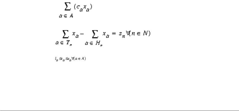
vla, the lower bound, sets the minimum flow allowed through the arc a. By
default, the lower bound on an arc is 0 (zero).
vua, the upper bound, sets the maximum flow allowed through the arc a. By
default, the upper bound on an arc is positive infinity.
vca, the objective value, specifies the contribution to the objective function of one
unit of flow through the arc.
Each node nis associated with one value:
vsnis the supply value at node n.
By convention, a node with strictly positive supply value (that is, sn> 0) is called
a supply node or a source, and a node with strictly negative supply value (that is, s
n< 0) is called a demand node or a sink. A node where sn= 0 is called a
transshipment node. The sum of all supplies must match the sum of all demands; if
not, then the network flow problem is infeasible.
Tnis the set of arcs whose tails are node n; Hnis the set of arcs whose heads are
node n. The usual form of a network problem looks like this:
Minimize (or maximize)
subject to
with these bounds
That is, for each node, the net flow entering and leaving the node must equal its
supply value, and all flow values must be within their bounds. The solution of a
network-flow problem is an assignment of flow values to arcs (that is, the
modeling variables) to satisfy the problem formulation. A flow that satisfies the
constraints and bounds is feasible.
Example: network optimizer in the Interactive Optimizer
Demonstrates an example of the network optimizer in the Interactive Optimizer.
Network flow problem description
Describes a sample network flow problem for the network optimizer.
This example is based on a network where the aim is to minimize cost and where
the flow through the network has both cost and capacity. Figure 5 on page 183
shows you the nodes and arcs of this network. The nodes are labeled by their
identifying node number from 1 through 8. The number inside a node indicates its
supply value; 0 (zero) is assumed where no number is given. The arcs are labeled 1
through 14. The lower bound l, upper bound u, and objective value cof each arc
are displayed in parentheses (l, u, c) beside each arc. In this example, node 1
and node 5 are sources, representing a positive net flow, whereas node 4 and
182 CPLEX User’s Manual
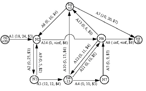
node 8 are sinks, representing negative net flow.
The example in Figure 5 corresponds to the results of running the netex1.c. If you
run that application, it will produce a file named netex1.net which can be read
into the Interactive Optimizer with the command read netex1.net. After you read
the problem into the Interactive Optimizer, you can solve it with the command
netopt or the command optimize.
Understanding the network log file
Describes a typical log file, corresponding to the example, from the network
optimizer.
As CPLEX solves the problem, it produces a log like the following lines:
Iteration log . . .
Iteration: 0 Infeasibility = 48.000000 (150)
Network - Optimal: Objective = 2.6900000000e+002
Solution time = 0.01 sec. Iterations = 9 (9)
Deterministic time = 0.00 ticks (0.97 ticks/sec)
This network log file differs slightly from the log files produced by other CPLEX
optimizers: it contains values enclosed in parentheses that represent modified
objective function values.
As long as the network optimizer has not yet found a feasible solution, it is in
Phase I. In Phase I, the network optimizer uses modified objective coefficients that
penalize infeasibility. At its default settings, the CPLEX network optimizer displays
the value of the objective function calculated in terms of these modified objective
coefficients in parentheses in the network log file.
You can control the amount of information recorded in the network log file, just as
you control the amount of information in other CPLEX log files. To record no
information at all in the log file, use the command set network display 0. To
display the current objective value in parentheses relative to the actual unmodified
objective coefficients, use the command set network display 1. To see the display
mentioned earlier in this section, leave the network display parameter at its default
value, 2. (If you have changed the default value, you can reset it with the
command set network display 2.)
Figure 5. A directed network with arc-capacity, flow-cost, sinks, and sources
Chapter 13. Solving network-flow problems 183

Tuning performance of the network optimizer
Suggests strategies for improving performance of the network optimizer.
The default values of parameters controlling the network optimizer are generally
the best choices for effective performance. However, the following sections indicate
parameters that you may want to experiment with in your particular problem.
Controlling tolerance
You control the feasibility tolerance for the network optimizer through the
parameter NetEpRHS. Likewise, you control the optimality tolerance for the network
optimizer through the parameter NetEpOpt.
Selecting a pricing algorithm for the network optimizer
On the rare occasions when the network optimizer seems to take too long to find a
solution, you may want to change the pricing algorithm to try to speed up
computation. The pricing algorithm for the network optimizer is controlled by
parameter NetPPriInd. All the choices use variations of partial reduced-cost
pricing.
Limiting iterations in the network optimizer
Use the parameter NetItLim if you want to limit the number of iterations that the
network optimizer performs.
Solving problems with the network optimizer
Explains invocation and activity of the network optimizer.
Invoking the network optimizer
Describes invocation of the network optimizer.
You instruct CPLEX to apply the network optimizer for solving the LP at hand by
setting the algorithm for continuous linear problems parameter:
vsetting CPX_PARAM_LPMETHOD to CPX_ALG_NET in the Callable Library
vor setting RootAlg to Network in Concert Technology
When you do so, CPLEX performs a sequence of steps. It first searches for a part
of the LP that conforms to network structure. Such a part is known as an
embedded network. It then uses the network optimizer to solve that embedded
network. Next, it uses the resulting basis to construct a starting basis for the full
LP problem. Finally, it solves the LP problem with a simplex optimizer.
You can also use the network optimizer when solving QPs (that is, problems with
a positive semi-definite quadratic term in the objective function), but not when
solving quadratically constrained problems. To do so using the Callable Library,
you set the algorithm for continuous quadratic optimization parameter
CPX_PARAM_QPMETHOD to CPX_ALG_NET. For Concert Technology, you set the RootAlg
parameter to Network. When CPLEX uses the network optimizer to solve a QP, it
first ignores the quadratic term and uses the network optimizer to solve the
resulting LP. CPLEX then uses the resulting basis to start a simplex algorithm on
the QP model with the original quadratic objective.
184 CPLEX User’s Manual

Network extraction
Documents how the network optimizer extracts a problem.
The CPLEX network extractor searches an LP constraint matrix for a submatrix
with the following characteristics:
vthe coefficients of the submatrix are all 0 (zero), 1 (one), or -1 (minus one);
veach variable appears in at most two rows with at most one coefficient of +1 and
at most one coefficient of -1.
CPLEX can perform different levels of extraction. The level it performs depends on
the NetFind parameter.
vWhen the NetFind parameter is set to 1(one), CPLEX extracts only the obvious
network; it uses no scaling; it scans rows in their natural order; it stops
extraction as soon as no more rows can be added to the network found so far.
vWhen the NetFind parameter is set to 2, the default setting, CPLEX also uses
reflection scaling (that is, it multiplies rows by -1) in an attempt to extract a
larger network.
vWhen the NetFind parameter is set to 3, CPLEX uses general scaling, rescaling
both rows and columns, in an attempt to extract a larger network.
In terms of total solution time expended, it may or may not be advantageous to
extract the largest possible network. Characteristics of your problem will qualify
the tradeoff between network size and the number of simplex iterations required to
finish solving the model after solving the embedded network.
Even if your problem does not conform precisely to network conventions, the
network optimizer may still be advantageous to use. When it is possible to
transform the original statement of a linear program into network conventions by
these algebraic operations:
vchanging the signs of coefficients,
vmultiplying constraints by constants,
vrescaling columns,
vadding or eliminating redundant relations,
then CPLEX will carry out such transformations automatically if you set the
NetFind parameter appropriately.
Preprocessing and the network optimizer
Explains possible impact of the preprocessor on network flow models.
If your LP problem includes network structures, there is a possibility that CPLEX
preprocessing may eliminate those structures from your model. For that reason,
you should consider turning off preprocessing before you invoke the network
optimizer on a problem.
Example: using the network optimizer with the Callable Library
netex1.c
Demonstrates an example of the network optimizer in the C API.
Chapter 13. Solving network-flow problems 185
In the standard distribution of CPLEX, the file netex1.c contains code that creates,
solves, and displays the solution of the network-flow problem illustrated in
Figure 5 on page 183.
Briefly, the main function initializes the CPLEX environment and creates the
problem object; it also calls the optimizer to solve the problem and retrieves the
solution.
In detail, main first calls the Callable Library routine CPXopenCPLEX. As explained in
“Initialize the CPLEX environment” on page 60, CPXopenCPLEX must always be the
first CPLEX routine called in a Callable Library application. Those routines create
the CPLEX environment and return a pointer (called env) to it. This pointer will be
passed to every Callable Library routine. If this initialization routine fails, env will
be NULL and the error code indicating the reason for the failure will be written to
status. That error code can be transformed into a string by the Callable Library
routine CPXgeterrorstring.
After main initializes the CPLEX environment, it uses the Callable Library routine
CPXsetintparam to turn on the CPLEX messages to screen switch parameter
CPX_PARAM_SCRIND so that CPLEX output appears on screen. If this parameter is
turned off, CPLEX does not produce viewable output, neither on screen, nor in a
log file. It is a good idea to turn this parameter on when you are debugging your
application.
The Callable Library routine CPXNETcreateprob creates an empty problem object,
that is, a minimum-cost network-flow problem with no arcs and no nodes.
The function buildNetwork populates the problem object; that is, it loads the
problem data into the problem object. Pointer variables in the example are
initialized as NULL so that you can check whether they point to valid data (a good
programming practice). The most important calls in this function are to the
Callable Library routines, CPXNETaddnodes, which adds nodes with the specified
supply values to the network problem, and CPXNETaddarcs, which adds the arcs
connecting the nodes with the specified objective values and bounds. In this
example, both routines are called with their last argument NULL indicating that no
names are assigned to the network nodes and arcs. If you want to name arcs and
nodes in your problem, pass an array of strings instead.
The function buildNetwork also includes a few routines that are not strictly
necessary to this example, but illustrate concepts you may find useful in other
applications. To delete a node and all arcs dependent on that node, it uses the
Callable Library routine CPXNETdelnodes. To change the objective sense to
minimization, it uses the Callable Library routine CPXNETchgobjsen.
Look again at main , where it actually calls the network optimizer with the Callable
Library routine, CPXNETprimopt. If CPXNETprimopt returns a nonzero value, then
an error has occurred; otherwise, the optimization was successful. Before retrieving
that solution, it is necessary to allocate arrays to hold it. Then use CPXNETsolution
to copy the solution into those arrays. After displaying the solution on screen,
write the network problem into a file, netex1.net in the NET file format.
The TERMINATE: label is used as a place for the program to exit if any type of error
occurs. Therefore, code following this label cleans up: it frees the memory that has
been allocated for the solution data; it frees the network object by calling
CPXNETfreeprob; and it frees the CPLEX environment by calling CPXcloseCPLEX.
All freeing should be done only if the data is actually available. The Callable
186 CPLEX User’s Manual

Library routine CPXcloseCPLEX should always be the last CPLEX routine called in a
Callable Library application. In other words, all CPLEX objects that have been
allocated should be freed before the call to CPXcloseCPLEX .
The complete program netex1.c appears online in the standard distribution at
yourCPLEXinstallation /examples/src.
Solving network-flow problems as LP problems
Explains the conversion between a network flow model and a conventional LP
model.
A network-flow model is an LP model with special structure. The CPLEX network
optimizer is a highly efficient implementation of the primal simplex technique
adapted to take advantage of this special structure. In particular, no basis factoring
occurs. However, it is possible to solve network models using any of the CPLEX
LP optimizers if first, you convert the network data structures to those of an LP
model. To convert the network data structures to LP data structures, in the
Interactive Optimizer, use the command change problem lp ; from the Callable
Library, use the routine CPXcopynettolp.
The LP formulation of our example from Figure 5 on page 183 looks like this:
Minimize
3a1 + 3a2 + 4a3 + 3a4 + 5a5 + 6a6 + 7a7 + 4a8 + 2a9 + 6a10+ 5a11+ 4a12+ 3a13+ 6a14
subject to
a1 = 20
-a1 + a2 - a8 - a9 + a14 = 0
- a2 + a3 + a9 = 0
- a3 + a4 + a10 + a11 - a12 = -15
a7 + a8 - a10 - a13 = 5
- a5 + a6 - a11 + a12 + a13 - a14 = 0
- a4 + a5 = 0
- a6 - a7 = -10
with these bounds
18 ≤a1 ≤24 0 ≤a2 ≤25 a3 = 12
0≤a4 ≤10 0 ≤a5 ≤9 a6 free
0≤a7 ≤20 0 ≤a8 ≤10 0 ≤a9 ≤5
0≤a10 ≤15 0 ≤a11 ≤10 0 ≤a12 ≤11
0≤a13 ≤6 0 ≤a14
In that formulation, in each column there is exactly one coefficient equal to 1 (one),
exactly one coefficient equal to -1, and all other coefficients are 0 (zero).
Since a network-flow problem corresponds in this way to an LP problem, you can
indeed solve a network-flow problem by means of a CPLEX LP optimizer as well.
If you read a network-flow problem into the Interactive Optimizer, you can
transform it into its LP formulation with the command change problem lp. After
this change, you can apply any of the LP optimizers to this problem.
When you change a network-flow problem into an LP problem, the basis
information that is available in the network-flow problem is passed along to the LP
formulation. In fact, if you have already solved the network-flow problem to
Chapter 13. Solving network-flow problems 187

optimality, then if you call the primal or dual simplex optimizers (for example,
with the Interactive Optimizer command primopt or tranopt), that simplex
optimizer will perform no iterations.
Generally, you can also use the same basis from a basis file for both the LP and the
network optimizers. However, there is one exception: in order to use an LP basis
with the network optimizer, at least one slack variable or one artificial variable
needs to be basic. “Starting from an advanced basis” on page 141 explains more
about this topic in the context of LP optimizers.
If you have already read the LP formulation of a problem into the Interactive
Optimizer, you can transform it into a network with the command
change problem network. Given any LP problem and this command, CPLEX will
try to find the largest network embedded in the LP problem and transform it into
a network-flow problem. However, as it does so, it discards all rows and columns
that are not part of the embedded network. At the same time, CPLEX passes along
as much basis information as possible to the network optimizer.
Example: network to LP transformation netex2.c
Demonstrates an example of converting a network flow model to its LP model in
the C API.
This example shows how to transform a network-flow problem into its
corresponding LP formulation. That example also indicates why you might want to
make such a change. The example reads a network-flow problem from a file
(rather than populating the problem object by adding rows and columns as in
netex1.c ). You can find the data of this example in the file examples/data/
infnet.net . After reading the data from that file, the example then attempts to
solve the problem by calling the Callable Library routine CPXNETprimopt. If it
detects that the problem is infeasible, it then invokes the conflict refiner to analyze
the problem and possibly indicate the cause of the infeasibility.
The complete program netex2.c appears online in the standard distribution at
yourCPLEXinstallation /examples/src.
188 CPLEX User’s Manual

Chapter 14. Solving problems with a quadratic objective (QP)
Describes solving quadratic programming problems (QPs) with CPLEX.
CPLEX solves quadratic programs; that is, a model in which the constraints are
linear, but the objective function can contain one or more quadratic terms. These
problems are also known as QP. When such problems are convex, CPLEX normally
solves them efficiently in polynomial time. Nonconvex QPs, however, are known to
be quite hard. In theoretical terms, they are characterized as NP-hard. CPLEX
applies various approaches to those problems, such approaches as barrier
algorithms or branch and bound algorithms. Notably, in the branch and bound
approach, there is no theoretical guarantee about the complexity of such a problem.
Consequently, solution of such a problem (that is, a nonconvex QP) can take many
orders of magnitude longer than the solution of a convex QP of comparable
dimensions. The following topics address the question of how to distinguish such
problems and describe the facilities that CPLEX offers to solve them.
Distinguishing between convex and nonconvex QPs
Explains how to determine the convexity of a quadratic program.
Conventionally, a quadratic program (QP) is formulated this way:
Minimize 1/2 xTQx + cTx
subject to Ax ~ b
with these bounds l ≤x≤u
where the relation ~ may be any combination of equal to, less than or equal to,
greater than or equal to, or range constraints. As in other problem formulations, l
indicates lower and u upper bounds. Q is a matrix of objective function
coefficients. That is, the elements Qjj are the coefficients of the quadratic terms xj2,
and the elements Qij and Qji are summed together to be the coefficient of the term
xixj.
IBM ILOG CPLEX distinguishes between two kinds of Q matrices:
vIn a separable problem, only the diagonal terms of the matrix are defined; all
off-diagonal terms of the matrix are zero.
vIn a nonseparable problem, at least one off-diagonal term of the matrix is nonzero.
CPLEX can solve minimization problems having a convex quadratic objective
function. Equivalently, it can solve maximization problems having a concave
quadratic objective function. All linear objective functions satisfy this property for
both minimization and maximization. However, you cannot always assume this
property in the case of a quadratic objective function.
CPLEX can also compute points that satisfy first-order optimality conditions of
models with arbitrary quadratic objective functions. These models include
minimization problems with a concave objective function, maximization problems
with a convex objective function, and either minimization or maximization
© Copyright IBM Corp. 1987, 2016 189
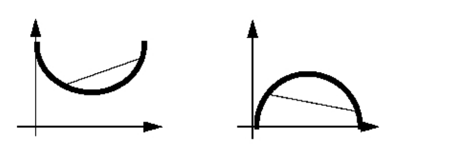
problems with objective functions that are neither convex nor concave. Such points
may not be the globally optimal solution to the model.
Intuitively, recall that any point on the line between two arbitrary points of a
convex function will be above that function. In more formal terms, a continuous
segment (that is, a straight line) connecting two arbitrary points on the graph of
the objective function will not go below the objective of a minimization problem,
and equivalently, the straight line will not go above the objective of a
maximization problem. The image Figure 6 illustrates this intuitive idea for an
objective function in one variable. It is possible for a quadratic function in more
than one variable to be neither convex nor concave.
In formal terms, the question of whether a quadratic objective function is convex
or concave is equivalent to whether the matrix Q is positive semi-definite or
negative semi-definite. For convex QPs, Q must be positive semi-definite; that is,
xTQx ≥0 for every vector x, whether or not x is feasible. For concave
maximization problems, the requirement is that Q must be negative semi-definite;
that is, xTQx ≤0 for every vector x. It is conventional to use the same term,
positive semi-definite, abbreviated PSD, for both cases, on the assumption that a
maximization problem with a negative semi-definite Q can be transformed into an
equivalent PSD.
For a separable function, to determine the convexity of a problem, it is sufficient to
check whether the individual diagonal elements of the matrix Q are of the correct
sign. For the nonseparable case, it may be less easy to decide in advance the
convexity of Q. However, CPLEX detects this property during the early stages of
optimization.
By default, CPLEX terminates if the quadratic objective term in a QP is found to be
non PSD. In such a case, in order to instruct CPLEX not to terminate, you must set
the optimality target parameter. The value that you set for that parameter depends
on the type of results that you expect. If you would like CPLEX to compute a
point that satisfies first-order optimality conditions (that is, a local optimum), then
you set the parameter to the value CPX_SOLUTIONTARGET_FIRSTORDER. If you
would like CPLEX to find a global optimum, then you set the parameter to the
value CPX_SOLUTIONTARGET_OPTIMALGLOBAL.
For a more complete explanation of quadratic programming generally, a textbook,
such as one of those listed in “Further reading” on page xx of the preface of this
manual, may be helpful.
Figure 6. Minimize a convex objective function, maximize a concave objective function
190 CPLEX User’s Manual

Entering QPs
Documents the two views of quadratic objective functions supported by CPLEX: a
matrix view and an algebraic view.
Matrix view
Describes the matrix view of a quadratic program.
In the matrix view, commonly found in textbook presentations of QP, the objective
function is defined as 1/2 xTQx + cTx, where Q must be symmetric. This view is
supported by the MPS file format and the Callable Library routines, where
information about the quadratic objective function is specified by providing the
matrix Q. Thus, by definition, the factor of 1/2 must be explicit when you enter a
model using the matrix view, as it will be implicitly assumed by the optimization
routines.
Similarly, symmetry of the Q matrix data is required; the MPS reader will return
an error status code if the file contains unequal off-diagonal components, such as a
nonzero value for one and zero (or omitted) for the other.
This symmetry restriction applies to quadratic programming input formats rather
than the quadratic programming problem itself. For models with an asymmetric Q
matrix, either express the quadratic terms algebraically, as described in “Algebraic
view,” or provide as input (Q + Q' )/2 instead of Q. This latter approach relies on
the identity Q= (Q + Q')/2 + (Q - Q')/2 combined with the fact that (Q - Q')/2
contributes 0 (zero) to the quadratic objective.
Algebraic view
Describes the algebraic view of a quadratic program.
In the algebraic view, a quadratic objective function is specified as an expressions
of the form:
c1*x1 + ... + cn*xn + q11*x1*x1 + q12*x1*x2 + ... + qnn*xn*xn
This view is supported by the LP format, when you enter a quadratic objective
function in the Interactive Optimizer, and by Concert Technology. When you enter
a quadratic objective with the algebraic view, neither symmetry considerations nor
any implicit factors need to be considered, and indeed attempting to specify both
of the off-diagonal elements for one of the quadratic terms may result in double
the intended value of the coefficient.
Examples for entering QPs
Demonstrates ways to enter the objective function of a quadratic program.
CPLEX LP format requires the factor of 1/2 to be specified explicitly in the file.
Minimize
obj: [ 100 x1 ^2 - 200 x1 * x2 + 100 x2 ^2]/2
MPS format for this same objective function contains the following block.
QMATRIX
x1 x1 100
x1 x2 -100
x2 x1 -100
x2 x2 100
Chapter 14. Solving problems with a quadratic objective (QP) 191
A C++ Concert program having such an objective function might include the
following code.
model.add(IloMinimize(env, 0.5 * (100*x[0]*x[0] +
100*x[1]*x[1] -
200*x[0]*x[1])));
Or since the algebraic view is supported, the factor of one-half could be simplified
as in the following equivalent expression:
model.add(IloMinimize(env, (50*x[0]*x[0] +
50*x[1]*x[1] -
100*x[0]*x[1])));
A similar Java program using Concert might express it this way:
IloNumExpr x00 = model.prod(100, x[0], x[0]);
IloNumExpr x11 = model.prod(100, x[1], x[1]);
IloNumExpr x01 = model.prod(-200, x[0], x[1]);
IloNumExpr Q = model.prod(0.5, model.sum(x00, x11, x01));
model.add(model.minimize(Q));
Again, the user may choose to simplify that expression algebraically if that suits
the purposes of the application better.
Finally, a Callable Library application in C might construct the quadratic objective
function in a way similar to the following lines:
zqmatbeg[0] = 0; zqmatbeg[1] = 2;
zqmatcnt[0] = 2; zqmatcnt[1] = 2;
zqmatind[0] = 0; zqmatind[2] = 0;
zqmatval[0] = 100.0; zqmatval[2] = -100.0;
zqmatind[1] = 1; zqmatind[3] = 1;
zqmatval[1] =-100.0; zqmatval[3] = 100.0;
CPXcopyquad (env, lp, qmatbeg, qmatcnt, qmatind, qmatval);
To re-emphasize the point about the factor of 1/2 in any of these methods: if that
objective function is evaluated with a solution of x1 = 1.000000 and x2 =
3.000000, the result is 200, not 400.
Reformulating QPs to save memory
Describes an alternative formulation of a quadratic program that may save
memory.
When the Qmatrix is very dense or extremely large in dimension, excessive
memory may be needed to solve the problem as conventionally formulated.
However, you may be able to use an alternative formulation to avoid such
bottlenecks. Specifically, if you can express Qas FF', (where Fis another matrix,
not necessarily square, having fewer nonzeros than Q, and F' is its transpose) then
you can reformulate the QP like this:
min c’x+y’y
Ax ~b
y - Fx = 0
l <= x <= u
y free
In the reformulation, y is a vector of free variables, one variable for each column of
F.
192 CPLEX User’s Manual

Portfolio optimization models in particular benefit from this reformulation. In the
most common portfolio models, Qis a covariance matrix of asset returns, while F
is the matrix of the deviations of the asset returns from their mean used to
compute the covariances. In that reformulation, the number of columns of F
corresponds to the number of time periods for which returns are measured.
In general, while the number of rows in Fmust match the dimension of the square
matrix Q, the number of columns of Fmay be fewer. So, even if Qis dense and F
is also dense, you still may reduce the memory requirements to solve the model if
Fhas more rows than columns.
Furthermore, if Fis a sparser matrix than Q, this alternative formulation may
improve performance even if Fhas more columns than Q.
Saving QP problems
Recommends appropriate file formats to save a quadratic program.
After you enter a QP problem, whether interactively or by reading a formatted file,
you can then save the problem in a formatted file. The formats available to you are
LP, MPS, and SAV. (These formats are documented in the reference manual, File
formats supported by CPLEX.) When you save a QP problem in one of these
formats, the quadratic information will also be recorded in the formatted file.
Changing problem type in QPs
Explains special considerations about the change of the problem type of a
quadratic program.
Situations in which you must change the problem type of your model arise, for
example, when you remove quadratic terms from the objective function of a QP or
when you add a quadratic term to the objective function of a linear program (LP).
This topic highlights whether and how to change problem type according to the
CPLEX component that you use (Concert Technology, Python API, Callable Library,
Interactive Optimizer).
Concert Technology (that is, applications written in the C++, Java, or .NET API of
CPLEX) treats all models as capable of containing quadratic coefficients in the
objective function. These coefficients can therefore be added or deleted at will.
When extracting a model with a quadratic objective function, CPLEX will
automatically detect it as a QP and make the required adjustments to data
structures. Likewise, in the Python API, CPLEX treats all models as capable of
containing quadratic coefficients in the objective function.
However, the other ways of using CPLEX (the Callable Library and the Interactive
Optimizer) require an explicit problem type to distinguish a linear program (LP)
from a QP. The following sections discuss the topic for these users.
When you enter a problem, CPLEX discovers the problem type from the available
information. When read from a file (LP, MPS, or SAV format, for example), or
entered interactively, a continuous optimization problem is usually treated as being
of type QP if quadratic coefficients are present in the objective function and no
quadratic terms are present among the constraints. (Quadratic terms among the
constraints may make a problem of type QCP. For more about that type, see
Chapter 15, “Solving problems with quadratic constraints (QCP),” on page 201.)
Otherwise, the problem type is usually LP. The issue of problem types that support
Chapter 14. Solving problems with a quadratic objective (QP) 193

integer restrictions in conjunction with quadratic variables is discussed in
Chapter 16, “Solving mixed integer programming problems (MIP),” on page 221.
If you enter a problem that lacks any quadratic coefficients, its problem type is
initially LP. If you then wish to modify the problem to contain quadratic
coefficients in the objective function, you do this by first changing the problem
type to QP. Conversely, if you have entered a QP model and wish to remove all the
quadratic coefficients from the objective function and thus convert the model to an
LP, you must also change the problem type to LP. Note that deleting each of the
quadratic coefficients individually still leaves the problem type as QP, although in
most instances the distinction between this problem and its LP or QP counterpart
is somewhat arbitrary in terms of the steps to solve it.
When using the Interactive Optimizer, you use the command change problem with
one of the following options:
vlp indicates that you want CPLEX to treat the problem as an LP. This change in
Problem Type removes from your problem all the quadratic information, if there
is any present.
vqp indicates that you want CPLEX to treat the problem as a QP. This change in
Problem Type creates in your problem an empty quadratic matrix, if there is not
one already present, for the objective function, ready for populating via the
change qpterm command.
From the Callable Library, use the routine CPXchgprobtype to change the problem
type to either CPXPROB_LP for the LP case or CPXPROB_QP for the QP case for the
same purposes.
Changing quadratic terms
Defines quadratic algebraic term and quadratic matrix.
CPLEX distinguishes between a quadratic algebraic term and a quadratic matrix
coefficient. The quadratic algebraic terms are the coefficients that appear in the
algebraic expression defined as part of the CPLEX LP format. The quadratic matrix
coefficients appear in Q. The quadratic coefficient of an off-diagonal term must be
distributed within the Q matrix, and it is always one-half the value of the
quadratic algebraic term.
To clarify that terminology, consider this example:
Minimize a + b + 1/2(a2+ 4ab + 7b2)
subject to a + b ≥10
with these bounds a ≥0 and b ≥0
The off-diagonal quadratic algebraic term in that example is 4, so the quadratic
matrix Q is
vIn a QP, you can change the quadratic matrix coefficients in the Interactive
Optimizer by using the command change qpterm .
194 CPLEX User’s Manual

vFrom the Callable Library, use the routine CPXchgqpcoef to change quadratic
matrix coefficients.
vConcert Technology does not support direct editing of expressions other than
linear expressions. Consequently, to change a quadratic objective function, you
need to create an expression with the modified quadratic objective and use the
setExpr method of IloObjective to install it.
Changing an off-diagonal element changes the corresponding symmetric element
as well. In other words, if a call to CPXchgqpcoef changes Qij to a value, it also
changes Qji to that same value.
To change the off-diagonal quadratic term from 4 to 6, for example, use this
sequence of commands in the Interactive Optimizer:
CPLEX> change qpterm
Change which quadratic term [’variable’ ’variable’]: a b
Present quadratic term of variable ’a’, variable ’b’is 4.000000.
Change quadratic term of variable ’a’, variable ’b’to what: 6.0
Quadratic term of variable ’a’, variable ’b’changed to 6.000000.
From the Callable Library, the CPXchgqpcoef call to change the off-diagonal term
from 4to 6would change both of the off-diagonal matrix coefficients from 2to 3.
Thus, the indices would be 0and 1, and the new matrix coefficient value would be
3.
If you have entered a linear problem without any quadratic terms in the
Interactive Optimizer, and you want to create quadratic terms, you must first
change the problem type to QP. To do so, use the command change problem qp.
This command will create an empty quadratic matrix with Q = 0.
By changing quadratic terms, you may affect the convexity of the objective
function. If you change a quadratic term so that the resulting matrix is no longer
convex in the case of a minimization problem or concave in the case of a
maximization problem, you must set the optimality target parameter
(CPX_PARAM_OPTIMALITYTARGET, OptimalityTarget) to ask CPLEX to return either a
solution that satisfies first-order optimality conditions or a globally optimal
solution.
Optimizing QPs
Describes how to invoke an optimizer for a quadratic program and explains the
appropriate choice of optimizer.
CPLEX allows you to solve your QP models through a simple interface, by calling
the default optimizer.
vIn the Interactive Optimizer, use the command optimize.
vFrom the Callable Library, use the routine CPXqpopt.
vIn Concert Technology applications, use the method solve.
With default settings, this will result in CPLEX invoking the barrier optimizer to
solve a continuous QP.
Tip: For nonconvex QP problems, particularly for those that are non PSD, consider
changing the default value of optimality target to search for either a locally or
globally optimal solution. When instructed to look for a globally optimal solution,
CPLEX uses a branch-and-bound algorithm. In such cases, the algorithms and
Chapter 14. Solving problems with a quadratic objective (QP) 195

options documented in Chapter 16, “Solving mixed integer programming problems
(MIP),” on page 221 and in Chapter 17, “Solving mixed integer programming
problems with quadratic terms,” on page 281 apply.
For users who wish to tune the performance of their applications, CPLEX offers
two simplex optimizers to try for solving convex QPs: dual simplex and primal
simplex. (However, dual simplex and primal simplex cannot be used to solve
nonconvex QPs.) You can also use the network optimizer; this approach first solves
the model as an LP network (temporarily ignoring the quadratic term in the
objective function) and takes this solution as a starting point for the primal simplex
QP optimizer. This choice of QP optimizer is controlled by the root algorithm
parameter (QPMETHOD in the Interactive Optimizer and in the Callable Library).
The table Table 37 shows you the possible settings.
Table 37. RootAlg parameter settings for QPs.
Root algorithm value Optimizer
0 Automatic (default)
1 Primal Simplex
2 Dual Simplex
3 Network Simplex
4 Barrier
5 Sifting
6 Concurrent
Many of the optimizer tuning decisions for LP apply in the QP case; and
parameters that control barrier and simplex optimizers in the LP case can be set for
the QP case, although in some instances to differing effect. Most models are solved
fastest by default parameter settings. In case your model is not solved satisfactorily
by default settings, consider the advice offered in the topic Chapter 12, “Solving
LPs: barrier optimizer,” on page 161, especially “Tuning barrier optimizer
performance” on page 170 as well as in the topic Chapter 11, “Solving LPs: simplex
optimizers,” on page 135, especially “Tuning LP performance” on page 139.
Just as for the LP case, each of the available QP optimizers automatically
preprocesses your model, conducting presolution problem analysis and reductions
appropriate for a QP.
The barrier optimizer for QP supports crossover for convex QPs, but unlike other
LP optimizers, its crossover step is off by default for QPs. The QP simplex
optimizers return basic solutions, and these bases can be used for purposes of
restarting sequences of optimizations, for example. As a result, application writers
who wish to allow end users control over the choice of QP optimizer need to be
aware of this fundamental difference and to program carefully. For most purposes,
the nonbasic barrier solution for convex QPs is entirely satisfactory, in that all such
solutions fully satisfy the standard optimality and feasibility conditions of
optimization theory.
Diagnosing QP infeasibility
Explains infeasibility in the context of a quadratic program.
Diagnosis of an infeasible QP problem can be carried out by the conflict refiner.
See Chapter 33, “Diagnosing infeasibility by refining conflicts,” on page 451.
196 CPLEX User’s Manual

Note that it is possible for the outcome of that analysis to be a confirmation that
your model (viewed as an LP) is feasible after all. This is typically a symptom that
your QP model is numerically unstable or ill-conditioned. Unlike the simplex
optimizers for LP, the QP optimizers are primal-dual in nature, and one result of
that is the scaling of the objective function interacts directly with the scaling of the
constraints.
Just as our recommendation regarding numeric difficulties on LP models (see
“Numeric difficulties” on page 148) is for coefficients in the constraint matrix not
to vary by more than about six orders of magnitude, for QP this recommendation
expands to include the quadratic elements of the objective function coefficients as
well. Fortunately, in most instances, it is straightforward to scale your objective
function, by multiplying or dividing all the coefficients (linear and quadratic) by a
constant factor, which changes the unit of measurement for the objective but does
not alter the meaning of the variables or the sense of the problem as a whole. If
your objective function itself contains a wide variation of coefficient magnitudes,
you may also want to consider scaling the individual columns to achieve a closer
range.
Examples: creating a QP, optimizing, finding a solution
Demonstrates creation, optimization, and solution of a quadratic program.
Problem description of a quadratic program
Describes the model used in the examples of a quadratic program.
This example shows you how to build and solve a QP. The problem being created
and solved is:
Maximize
x1+ 2x2+ 3x3- 0.5(33x12
+ 22x22+ 11x32- 12x1x2
- 23x2x3)
subject to
-x1+ x2+ x3≤20
x1- 3x2+ x3≤30
with these bounds
0≤x1≤40
0≤x2≤+∞
0≤x3≤+∞
The following sections solve this model in the various APIs available in CPLEX:
v“Example: iloqpex1.cpp”
v“Example: QPex1.java” on page 198
v“Example: qpex1.c” on page 198
Example: iloqpex1.cpp
Demonstrates the solution of a quadratic program in the C++ API.
This example is almost identical to ilolpex1.cpp with only function populatebyrow
to create the model. Also, this function differs only in the creation of the objective
from its ilolpex1.cpp counterpart. Here the objective function is created and
added to the model like this:
model.add(IloMaximize(env, x[0] + 2 * x[1] + 3 * x[2]
- 0.5 * (33*x[0]*x[0] + 22*x[1]*x[1] + 11*x[2]*x[2]
- 12*x[0]*x[1] - 23*x[1]*x[2]) ));
Chapter 14. Solving problems with a quadratic objective (QP) 197
In general, any expression built of basic operations +, -, *, /constant, and
brackets [] that amounts to a quadratic and optional linear term can be used for
building a QP objective function. If the expressions of the objective or any
constraint of the model contains IloPiecewiseLinear, then when a quadratic
objective is specified the model becomes an MIQP problem. (Piecewise-linearity is
not the only characteristic that renders a model MIQP. See also, for example, the
features in Chapter 24, “Logical constraints in optimization,” on page 343, where
automatic transformation with logical constraints can render a problem MIQP.)
The complete program iloqpex1.cpp appears online in the standard distribution at
yourCPLEXinstallation/examples/src .
Example: QPex1.java
Demonstrates the solution of a quadratic program in the Java API.
This example is almost identical to LPex1.java using only the function
populatebyrow to create the model. Also, this function differs only in the creation
of the objective from its LPex1.java counterpart. Here the objective function is
created and added to the model like this:
// Q = 0.5 ( 33*x0*x0 + 22*x1*x1 + 11*x2*x2 - 12*x0*x1 - 23*x1*x2 )
IloNumExpr x00 = model.prod( 33, x[0], x[0]);
IloNumExpr x11 = model.prod( 22, x[1], x[1]);
IloNumExpr x22 = model.prod( 11, x[2], x[2]);
IloNumExpr x01 = model.prod(-12, x[0], x[1]);
IloNumExpr x12 = model.prod(-23, x[1], x[2]);
IloNumExpr Q = model.prod(0.5, model.sum(x00, x11, x22, x01, x12));
double[] objvals = {1.0, 2.0, 3.0};
model.add(model.maximize(model.diff(model.scalProd(x, objvals), Q)));
A quadratic objective may be built with square, prod, or sum methods. Inclusion of
IloPiecewiseLinear will change the model from a QP to a MIQP.
Example: qpex1.c
Demonstrates the solution of a quadratic program in the C API.
This example shows you how to optimize a QP with routines from the CPLEX
Callable Library when the problem data is stored in a file. The example derives
from lpex1.c discussed in Getting Started. The Concert forms of this example,
iloqpex1.cpp and QPex1.java , are included online in the standard distribution.
Instead of calling CPXlpopt to find a solution as for the linear programming
problem in lpex1.c, this example calls CPXqpopt to optimize this quadratic
programming problem.
Like other applications based on the CPLEX Callable Library, this one begins with
calls to CPXopenCPLEX to initialize the CPLEX environment and to CPXcreateprob to
create the problem object. Before it ends, it frees the problem object with a call to
CPXfreeprob , and it frees the environment with a call to CPXcloseCPLEX.
In the routine setproblemdata , there are parameters for qmatbeg, qmatcnt, qmatind,
and qmatval to fill the quadratic coefficient matrix. The Callable Library routine
CPXcopyquad copies this data into the problem object created by the Callable
Library routine CPXcreateprob.
198 CPLEX User’s Manual

In this example, the problem is a maximization, so the objective sense is specified
as CPX_MAX .
The off-diagonal terms in the matrix Q are one-half the value of the terms x1x2, and
x2x3as they appear in the algebraic form of the example.
Instead of calling CPXlpopt to find a solution as for the linear programming
problem in lpex1.c, this example calls CPXqpopt to optimize this quadratic
programming problem.
Example: reading a QP from a file qpex2.c
Demonstrates reading data for a quadratic program from a file and solving in the
C API.
This example shows you how to optimize a QP with routines from the CPLEX
Callable Library when the problem data is stored in a file. The example derives
from lpex2.c discussed in Getting Started. The Concert forms of this example,
iloqpex2.cpp and QPex2.java , are included online in the standard distribution.
Instead of calling CPXlpopt to find a solution as for the linear programming
problem in lpeq2.c, this example calls CPXqpopt to optimize this quadratic
programming problem.
Like other applications based on the CPLEX Callable Library, this one begins with
calls to CPXopenCPLEX to initialize the CPLEX environment and to CPXcreateprob to
create the problem object. Before it ends, it frees the problem object with a call to
CPXfreeprob, and it frees the environment with a call to CPXcloseCPLEX.
The complete program, qpex2.c, appears online in the standard distribution at
yourCPLEXinstallation/examples/src.
Chapter 14. Solving problems with a quadratic objective (QP) 199
200 CPLEX User’s Manual

Chapter 15. Solving problems with quadratic constraints
(QCP)
Documents the solution of quadratically constrained programming problems (QCPs),
including the special case of second order cone programming problems (SOCPs).
Identifying a quadratically constrained program (QCP)
Defines the types of quadratically constrained programs that CPLEX solves.
Characteristics of a quadratically constrained program
Describes the characteristics of a quadratically constrained program.
The distinguishing characteristic of QCP is that quadratic terms may appear in one
or more constraints of the problem. The objective function of such a problem may
or may not contain quadratic terms as well. Thus, the most general formulation of
a QCP is:
Minimize 1/2xTQx + cTx
subject to Ax ~ b
and aiTx+ xTQix≤rifor i=1,...,q
with these bounds l ≤x≤u
As in a quadratic objective function, convexity plays an important role in quadratic
constraints. The constraints must each define a convex region. To make sure of
convexity, IBM ILOG CPLEX requires that each Qimatrix be positive semi-definite
(PSD) or that the constraint can be transformed into a second order cone. The
following sections offer more information about these concepts.
Convexity
Defines convexity in the context of a quadratically constrained program.
The inequality x2+ y2≤1is convex. To give you an intuitive idea about convexity,
Figure 7 on page 202 graphs that inequality and shades the area that it defines as a
constraint. If you consider aand bas arbitrary values in the domain of the
constraint, you see that any continuous line segment between them is contained
entirely in the domain.
© Copyright IBM Corp. 1987, 2016 201
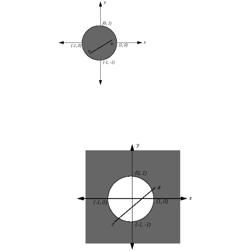
The inequality x2+ y2≥1is not convex; it is concave. Figure 8 graphs that
inequality and shades the area that it defines as a constraint. If you consider cand
das arbitrary values in the domain of this constraint, then you see that there may
be continuous line segments that join the two values in the domain but pass
outside the domain of the constraint to do so.
It might be less obvious at first glance that the equality x2+ y2= 1 is not convex
either. As you see in the figure titled Figure 9 on page 203, there may be a
continuous line segment that joins two arbitrary points, such as eand f, in the
domain but the line segment may pass outside the domain. Another way to see
this idea is to note that an equality constraint is algebraically equivalent to the
intersection of two inequality constraints of opposite sense, and you have already
seen that at least one of those quadratic inequalities will not be convex. Thus, the
equality is not convex either.
Figure 7. x2+ y2≤1 is convex
Figure 8. x2+ y2≥1 is not convex
202 CPLEX User’s Manual
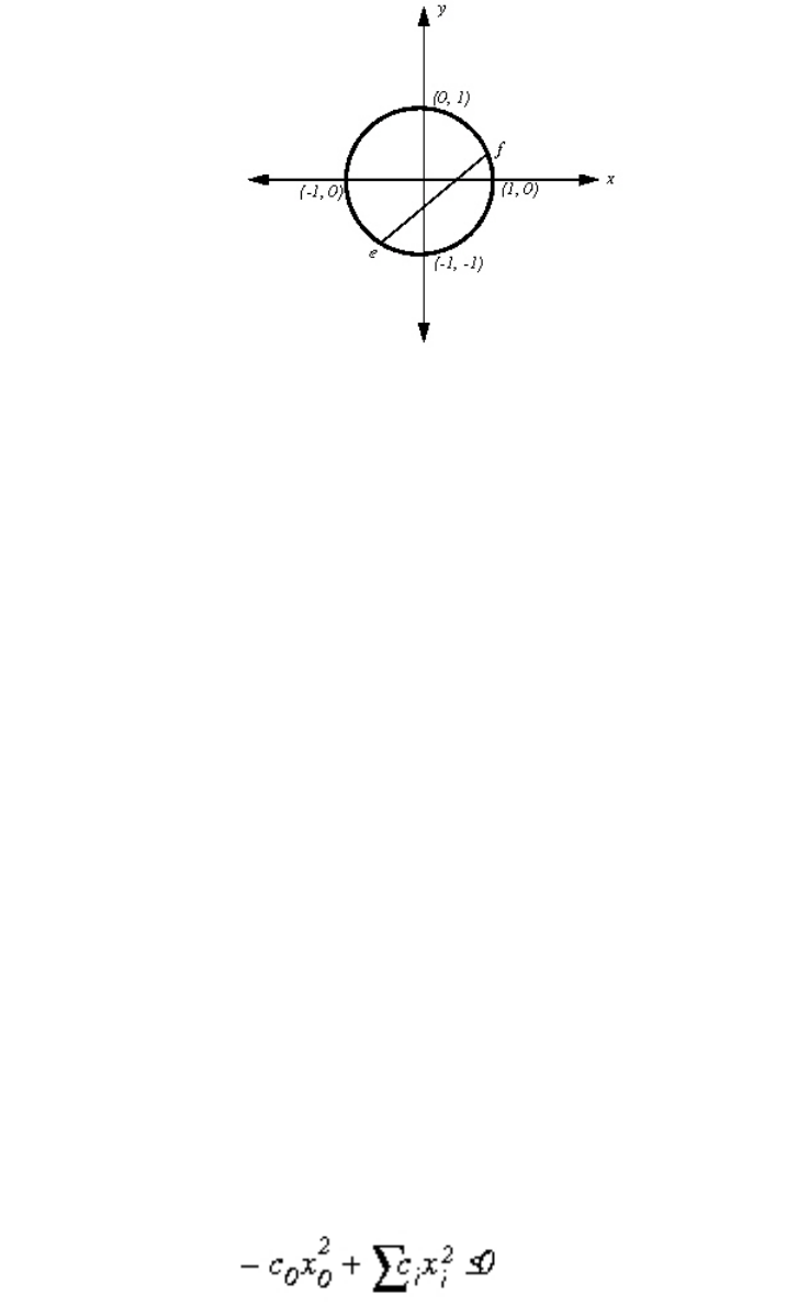
Semi-definiteness
Defines semi-definiteness in the context of a quadratically constrained program.
“Identifying a quadratically constrained program (QCP)” on page 201 explained
that the quadratic matrix in each constraint must be positive semi-definite (PSD),
thus providing convexity. A matrix Qiis PSD if xTQix≥0 for every vector x,
whether or not x is feasible. Other issues pertaining to positive semi-definiteness
are discussed in the context of a quadratic objective function in “Distinguishing
between convex and nonconvex QPs” on page 189.
When you call the barrier optimizer, your quadratic constraints will be checked for
the necessary PSD property, and an error status 5002 will be returned if any of
them violate it.
Second order cone programming (SOCP) and non PSD
Relates convexity and positive semi-definiteness to second order cone
programming.
There is one exception to the PSD requirement; that is, there is an additional form
of quadratic constraint which is accepted but is not covered by the general
formulation in “Identifying a quadratically constrained program (QCP)” on page
201. Technically, the class of quadratically constrained problems that the barrier
optimizer solves is a Second-Order Cone Program (SOCP). CPLEX, through its
preprocessing feature, carries out the translation to SOCP for you, transparently,
returning the solution in terms of your original formulation. A constraint will be
accepted for solution by the barrier optimizer if it can be transformed to the
following convex second-order cone constraint:
CPLEX automatically transforms quadratic constraints of these types into second
order cone constraints:
x’Qx <= y² where y >= 0 and Q is PSD
x’Qx <= yz where y >= 0 , z >= 0, and Q is PSD
Figure 9. x2+ y2= 1 is not convex
Chapter 15. Solving problems with quadratic constraints (QCP) 203
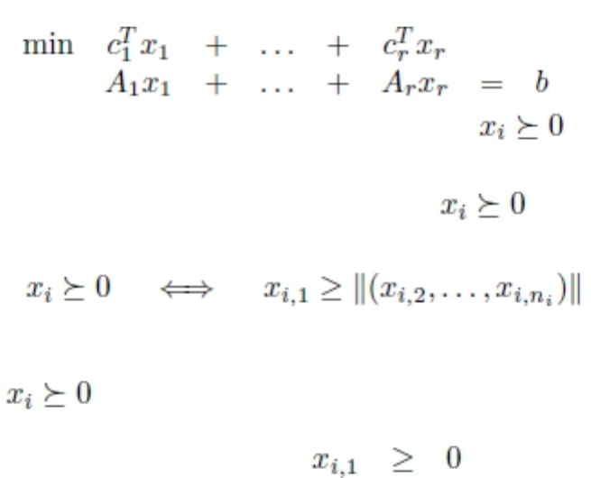
Note:
When Q is the identity matrix, that formulation is known as a rotated cone. CPLEX
automatically translates those formulations as well and solves the rotated cone
program for you transparently.
For further background about second order cone programming, see also the topic
“Examples: SOCP” on page 217. For suggestions about accessing dual values and
reduced costs of SOCP models, see the topic “Accessing dual values and reduced
costs of SOCP solutions” on page 215. Those topics cite the Lagrangian
representation of second order cone programs and second order cone constraints.
Representing SOCP as Lagrangian
Recalls mathematical principles useful in creating and manipulating second order
cone programs.
Second order cone programs (SOCPs) are special in the sense that any
quadratically constrained program (QCP) can be transformed into an equivalent
second order cone program. CPLEX makes use of this fact to solve a wider range
of quadratically constrained models. Furthermore, CPLEX uses this equivalence to
return more information, such as dual values and reduced costs, about the model
and its solution, even about SOCPs.
To understand how best to use CPLEX routines and methods when you solve
SOCPs, recall how second order cone programs mathematically represent a model
that includes second order cone constraints. A second order cone program is an
optimization problem in this standard form, where the xiare pair-wise disjoint
vectors of variables such that xi= (xi,1 , . . . , xi,in):
A second order cone constraint for a variable vector
is defined like
this, where the double bars represent the Euclidean norm of the vector:
Also recall that if ni= 1, then the following second order cone constraint:
reduces to the following inequality:
204 CPLEX User’s Manual
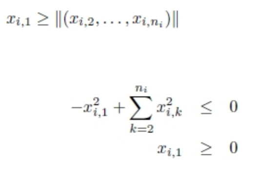
In other words, a second order cone constraint, such as this inequality:
(where the double bars specify a Euclidean norm) is equivalent to these two
constraints:
With those facts about the standard form of a second order cone constraint in
mind, you can specify the objective function and the linear constraints of a second
order cone program (SOCP) just as you would specify them in a similar linear
program (LP); then, in addition, you specify those two equivalent constraints for
each of the second order cone constraints in your model.
To clarify that procedure for specifying SOCPs, consider the following model:
min x1 + x2 + x3 + x4 + x5 + x6
x1 + x2 + x5 = 8
x3 + x5 + x6 = 10
(x1, x2, x3) ≥0 (x4, x5) ≥0 (x6) ≥0
In that model, there are two ordinary linear constraints:
x1 + x2 + x5 = 8
x3 + x5 + x6 = 10
At first glance, there appear to be three second order cones (SOC) to consider:
(x1, x2, x3) ≥0
(x4, x5) ≥0
(x6) ≥0
According to the procedure, you must specify two equivalent constraints for each
second order cone constraint in the model. For the first SOC, consider x1 greater
than or equal to the Euclidean norm of x2 and x3. This consideration leads to the
following pair of constraints.
-x12+ x22+ x33≤0
x1 ≥0
Likewise, according to the procedure, consider the second SOC.
(x4, x5) ≥0
That second consideration leads to the following pair of constraints.
-x42+ x52≤0
x4 ≥0
The third SOC consists of only one variable, so according to the procedure, it leads
only to the lower bound of 0 (zero) on x6.
Consequently, that model looks like this in conventional LP format:
Chapter 15. Solving problems with quadratic constraints (QCP) 205

Minimize
obj: x1 + x2 + x3 + x4 + x5 + x6
Subject To
c1: x1 + x2 + x5 = 8
c2: x3 + x5 + x6 = 10
q1: [ -x1^2 + x2^2 + x3^2 ] <= 0
q2: [ -x4^2 + x5^2 ] <= 0
Bounds
0 <= x1
x2 Free
x3 Free
0 <= x4
x5 Free
0 <= x6
End
For more detail about the syntax of LP format, see LP file format: algebraic
representation in the reference manual File formats supported by CPLEX.
Detecting the problem type of a QCP or SOCP
Documents the criteria that CPLEX components use to detect the problem type of a
quadratically constrained program.
Overview
Offers general considerations about QCP problem type in each API of CPLEX.
The various components of CPLEX (the object-oriented APIs of Concert
Technology, the C API of the Callable Library, and the Interactive Optimizer) give
more or less weight to the idea of problem type. The following topics discuss the
issues of problem type for each of those components with respect to QCPs and
SOCPs.
Tip:
FeasOpt, as documented in Chapter 34, “Repairing infeasibilities with FeasOpt,” on
page 465, does NOT apply to QCP problems.
Concert Technology and QCP problem type
Documents the role of the quadratic constraints in Concert Technology
applications.
Concert Technology treats all models as capable of containing quadratic
constraints. In other words, applications written in Concert Technology are capable
of handling quadratic constraints. These constraints can be added or deleted at will
in your application, just as other constraints are. When extracting a model with a
quadratic constraint, CPLEX automatically detects it as a QCP and makes the
required adjustments to its internal data structures.
Callable Library and QCP problem type
Documents the role of quadratic constraints in the C API.
When routines of the Callable Library read a problem from a file, they are capable
of detecting quadratic constraints. If they detect a quadratic constraint in the model
they read, Callable Library routines automatically set the problem type as QCP. If
there are no quadratic constraints, then Callable Library routines consider whether
there are any quadratic coefficients in the objective function. If there is a quadratic
206 CPLEX User’s Manual
term in the objective function, then Callable Library routines automatically set the
problem type as QP, as explained in “Changing problem type in QPs” on page 193.
Interactive Optimizer and QCP problem type
Documents the role of quadratic constraints in the Interactive Optimizer.
In the Interactive Optimizer, a problem containing a quadratic constraint, as
denoted by square brackets, is automatically identified as QCP when the problem
is read from a file or entered interactively.
File formats and QCP problem type
Describes the file formats that accommodate quadratic constraints.
CPLEX supports the definition of quadratic constraints in SAV files with the .sav
file extension, in LP files with the .lp file extension, and in MPS files with the .mps
file extension. In LP files, you state your quadratic constraints in the subject to
section of the file. For more detail about representing QCP models in MPS file
format, see the CPLEX File Formats Reference Manual, especially the topic
Quadratically constrained programs (QCP) in MPS files. Here is a sample of a file
including quadratic constraints in MPS format.
NAME p0033_qc1.lp.gz
ROWS
N R100
L R118
L R119
L R120
L R121
L R122
L R123
L R124
L R125
L R126
L R127
L R128
L ZBESTROW
L QC1
L QC2
L QC3
L QC4
COLUMNS
MARK0000 ’MARKER’ ’INTORG’
C157 R100 171
C157 R122 -300
C157 R123 -300
C158 R100 171
C158 R126 -300
C158 R127 -300
C159 R100 171
C159 R119 300
C159 R120 -300
C159 R123 -300
C159 QC1 1
C160 R100 171
C160 R119 300
C160 R120 -300
C160 R121 -300
C161 R100 163
C161 R119 285
C161 R120 -285
C161 R124 -285
C161 R125 -285
Chapter 15. Solving problems with quadratic constraints (QCP) 207
C162 R100 162
C162 R119 285
C162 R120 -285
C162 R122 -285
C162 R123 -285
C163 R100 163
C163 R128 -285
C164 R100 69
C164 R119 265
C164 R120 -265
C164 R124 -265
C164 R125 -265
C165 R100 69
C165 R119 265
C165 R120 -265
C165 R122 -265
C165 R123 -265
C166 R100 183
C166 R118 -230
C167 R100 183
C167 R124 -230
C167 R125 -230
C168 R100 183
C168 R119 230
C168 R120 -230
C168 R125 -230
C169 R100 183
C169 R119 230
C169 R120 -230
C169 R123 -230
C170 R100 49
C170 R119 190
C170 R120 -190
C170 R122 -190
C170 R123 -190
C171 R100 183
C172 R100 258
C172 R118 -200
C173 R100 517
C173 R118 -400
C174 R100 250
C174 R126 -200
C174 R127 -200
C175 R100 500
C175 R126 -400
C175 R127 -400
C176 R100 250
C176 R127 -200
C177 R100 500
C177 R127 -400
C178 R100 159
C178 R119 200
C178 R120 -200
C178 R124 -200
C178 R125 -200
C179 R100 318
C179 R119 400
C179 R120 -400
C179 R124 -400
C179 R125 -400
C180 R100 159
C180 R119 200
C180 R120 -200
C180 R125 -200
C181 R100 318
C181 R119 400
208 CPLEX User’s Manual
C181 R120 -400
C181 R125 -400
C182 R100 159
C182 R119 200
C182 R120 -200
C182 R122 -200
C182 R123 -200
C183 R100 318
C183 R119 400
C183 R120 -400
C183 R122 -400
C183 R123 -400
C184 R100 159
C184 R119 200
C184 R120 -200
C184 R123 -200
C185 R100 318
C185 R119 400
C185 R120 -400
C185 R123 -400
C186 R100 114
C186 R119 200
C186 R120 -200
C186 R121 -200
C187 R100 228
C187 R119 400
C187 R120 -400
C187 R121 -400
C188 R100 159
C188 R128 -200
C189 R100 318
C189 R128 -400
MARK0001 ’MARKER’ ’INTEND’
RHS rhs R118 -5
rhs R119 2700
rhs R120 -2600
rhs R121 -100
rhs R122 -900
rhs R123 -1656
rhs R124 -335
rhs R125 -1026
rhs R126 -5
rhs R127 -500
rhs R128 -270
rhs QC1 1
rhs QC2 2
rhs QC3 1
rhs QC4 1
BOUNDS
UP bnd C157 1
UP bnd C158 1
UP bnd C159 1
UP bnd C160 1
UP bnd C161 1
UP bnd C162 1
UP bnd C163 1
UP bnd C164 1
UP bnd C165 1
UP bnd C166 1
UP bnd C167 1
UP bnd C168 1
UP bnd C169 1
UP bnd C170 1
UP bnd C171 1
UP bnd C172 1
UP bnd C173 1
Chapter 15. Solving problems with quadratic constraints (QCP) 209

UP bnd C174 1
UP bnd C175 1
UP bnd C176 1
UP bnd C177 1
UP bnd C178 1
UP bnd C179 1
UP bnd C180 1
UP bnd C181 1
UP bnd C182 1
UP bnd C183 1
UP bnd C184 1
UP bnd C185 1
UP bnd C186 1
UP bnd C187 1
UP bnd C188 1
UP bnd C189 1
QMATRIX
C158 C158 1
C158 C189 0.5
C189 C158 0.5
C189 C189 1
QCMATRIX QC1
C157 C157 1
C157 C158 0.5
C158 C157 0.5
C158 C158 1
C159 C159 1
C160 C160 1
QCMATRIX QC2
C161 C161 2
C162 C162 2
C163 C163 1
QCMATRIX QC3
C164 C164 1
C165 C165 1
QCMATRIX QC4
C166 C166 1
C167 C167 1
C168 C168 1
C169 C169 1
C171 C171 1
ENDATA
Changing problem type in a QCP
Explains considerations about changing the problem type in a quadratically
constrained program, according to CPLEX components.
By default, every model in Concert Technology is the most general problem type
possible. Consequently, it is not necessary to declare the problem type nor to
change the problem type, even if you add quadratic constraints to the model or
remove them from it.
In contrast, both the Callable Library and the Interactive Optimizer need for you
to specify a change in problem type explicitly if you remove the quadratic
constraints that make your model a QCP.
In both the Callable Library and Interactive Optimizer, if you want to remove the
quadratic constraints in order to solve the problem as an LP or a QP, then you
must change the problem type, just as you would, for example, if you removed the
quadratic coefficients from a quadratic objective function.
210 CPLEX User’s Manual

From the Callable Library, use the routine CPXchgprobtype to change the problem
type to CPXPROB_LP if you remove the quadratic constraints from your model in
order to solve it as an LP. Contrariwise, if you want to add quadratic constraints to
an LP or a QP model and then solve it as a QCP, use the routine CPXchgprobtype to
change the problem type to CPXPROB_QCP.
When using the Interactive Optimizer, you apply the command change problem
with one of the following options:
vlp specifies that you want CPLEX to treat the problem as an LP. This change in
the problem type removes all the quadratic information from your problem, if
there is any present.
vqp specifies that you want CPLEX to treat the problem as a QP (that is, a
problem with a quadratic objective). This choice removes the quadratic
constraints, if there were any in the model.
vqcp specifies that you want CPLEX to treat the problem as a QCP.
Changing quadratic constraints
Explains special considerations about modifying a constraint containing a quadratic
term.
To modify a quadratic constraint in your model, you must first delete the old
quadratic constraint and then add the new one.
In Concert Technology, you add constraints (whether or not they are quadratic) by
means of the method add of the class IloModel , as explained about C++
applications in “Adding constraints: IloConstraint and IloRange” on page 7 and
about Java applications in “The active model” on page 33. To add constraints to a
model in the .NET framework, see Chapter 3, “Concert Technology for
.NET users,” on page 49.
Also in Concert Technology, you can remove constraints (again, whether or not
they are quadratic) by means of the method remove of the class IloModel , as
explained about C++ applications in “Deleting and removing modeling objects” on
page 18 and about Java applications in “Modifying the model” on page 47.
The Callable Library has a separate set of routines for creating and modifying
quadratic constraints; do not use the routines that create or modify linear
constraints.
In the Callable Library, you add a quadratic constraint by means of the routine
CPXaddqconstr. You remove and delete quadratic constraints by means of the
routine CPXdelqconstr. Don’t forget to change the problem type, as explained in
“Changing problem type in a QCP” on page 210. If you want to change a
quadratic constraint, first delete it by calling CPXdelqconstrs and then add the new
constraint using CPXaddqconstr.
In the Interactive Optimizer, if you want to change a quadratic constraint, you
must delete the constraint (change delete qconstraints) and add the new
constraint. Again, if you change a quadratic constraint to a linear constraint, you
must also change the problem type, as explained in “Changing problem type in a
QCP” on page 210.
Chapter 15. Solving problems with quadratic constraints (QCP) 211

Solving with quadratic constraints
Documents the routine or method to solve a quadratically constrained program.
CPLEX allows you to solve your QCP models (that is, problems with quadratic
constraints) through a simple interface, by calling the default optimizer.
vIn Concert Technology applications, use the solve method of IloCplex.
vFrom the Callable Library, use the routine CPXbaropt.
vIn the Interactive Optimizer, use the command optimize.
With default settings, each of these approaches will result in the barrier optimizer
being called to solve a continuous QCP.
The barrier optimizer is the only optimizer available to solve QCPs.
However, in a mixed integer quadratically constrained programming (MIQCP)
problem, you can specify whether CPLEX solves a QCP relaxation or LP relaxation
of the subproblems. The MIQCP strategy switch parameter (MIQCPStrat,
CPX_PARAM_MIQCPSTRAT) lets you specify which type of relaxation to solve.
Numeric difficulties and quadratic constraints
Describes the symptoms of numeric difficulties in a quadratically constrained
program.
A word of warning: numeric difficulties are likely to be more acute for QCP than
for LP or QP. Symptoms include:
vlack of convergence to an optimal solution;
vviolation of constraints.
Consequently, you will need to scale your variables carefully so that units of
measure are roughly comparable among them.
Accessing dual values and reduced costs of QCP solutions
Outlines a procedure for accessing dual values and reduced costs from QCP
solutions.
The CPLEX routines and methods that query dual values and reduced costs in
linear programs (LPs) also access dual values and reduced costs for quadratically
constrained programs, that is, QCP models. In order to use these routines and
methods effectively in your applications to solve SOCPs, recall these points about
Lagrangian functions and QCPs.
First, recall the conventional statement of a quadratically constrained program:
212 CPLEX User’s Manual
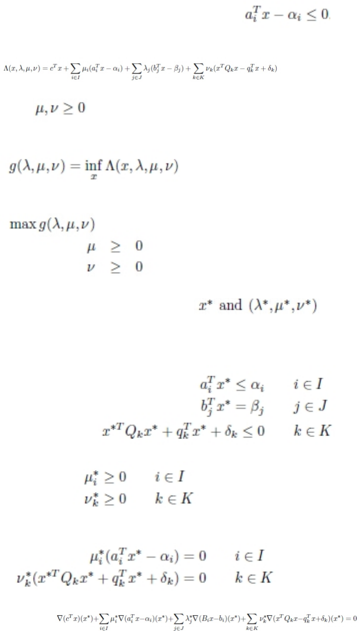
In that general statement, assume that the bounds of the model are expressed in
the matrix as a subset of the constraints in I, like this:
Now recall the same model stated in Lagrangian terms:
where:
The Lagrangian dual is expressed generally like this:
Consequently, the Lagrangian dual of this conventional QCP model looks like this:
Also recall that a primal-dual solution pair
that is an optimal solution to those Lagrangian statements of the primal and dual
QCP model must also satisfy the Karush-Kuhn-Tucker (KKT) conditions:
primal feasibility
dual feasibility
complementary slackness
stationarity
Chapter 15. Solving problems with quadratic constraints (QCP) 213
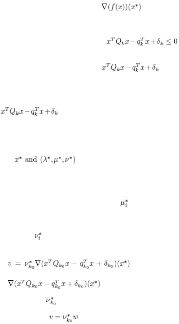
In those statements of the KKT conditions,
denotes the derivative of f(x) evaluated at x*.
For a quadratic constraint expressed like this:
a difficulty arises in the stationarity condition for quadratically constrained
programs (QCPs) because the derivative of:
can be undefined at x*. In such a case, KKT conditions cannot be formulated and
satisfied.
The point at which the derivative of a quadratic constraint such as:
is likely to be undefined is at the top of the cone representing that constraint.
Whether x*is at the top of the cone or not is determined by numeric tolerances.
Because such tolerances depend greatly on the model at hand, CPLEX does not
make this decision about x*for you. Instead, CPLEX offers an application
programming interface (API) for you to query the values of a primal-dual solution
pair:
For example, in the Callable Library (C API) these routines are available for this
purpose:
vCPXXgetx queries the values x*.
vCPXXgetpi queries the dual values of a range of constraints in a (linear or)
quadratically constrained problem (QCP); that is:
vCPXXgetdj queries the reduced costs for a range of variables in a (linear or)
quadratically constrained problem (QCP); that is, it accesses the dual multipliers
for bound constraints on the specified variables.
vThe values:
cannot be accessed directly. However, for a quadratic constraint k0in the set K,
CPXXgetqconstrdslack returns the slack vector of the dual problem:
If the derivative exists at x*, you can compute wlike this:
and thus obtain:
from the relation:
Tip:
214 CPLEX User’s Manual
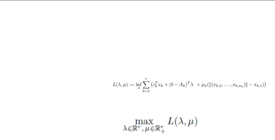
The routine CPXXgetqconstrdslack (or CPXgetqconstrdslack) returns the dual slack
for a single quadratic constraint. You can get the full dual slack vector by summing
up the results of CPXgetdj and CPXgetqconstrdslack (the latter for all quadratic
constraints).
For a demonstration of the procedure outlined here to access dual values and
reduced costs of a QCP model, see these examples distributed with the product:
vIn the Callable Library (C API), see the examples xqcpdual.c and qcpdual.c.
vIn the C++ API, see the example iloqcpdual.cpp.
vIn the Java API, see the example QCPDual.java.
vIn the C#.NET API, see the example QCPDual.cs.
vIn the Python API, see the example qcpdual.py.
vIn the MATLAB connector, see the example qcpdual.m.
For reference documentation of these routines and methods, see the reference
manual of your preferred application programming interface (API):
vCallable Library (C API)
– CPXXgetqconstrdslack and CPXgetqconstrdslack
vC++ API
– IloCplex::getQCDSlack
vJava API
– IloCplex.getQCDSlack
v.NET API
– Cplex.GetQCDSlack
vPython API
– SolutionInterface.get_quadratic_dualslack
vMATLAB connector new fields in the Cplex.Solution structure
– qcpdslack
Accessing dual values and reduced costs of SOCP solutions
Outlines a procedure for accessing dual values and reduced costs from SOCP
solutions.
The CPLEX routines and methods that query dual values and reduced costs in
linear programs (LPs) also access dual values and reduced costs for second order
cone programs, that is, SOCP models. In order to use these routines and methods
effectively in your applications to solve SOCPs, recall these points about
Lagrangian functions and SOCPs. First of all, the Lagrangian primal of the second
order cone program that you saw in “Representing SOCP as Lagrangian” on page
204 looks like this:
Similarly, the Lagrangian dual of the second order cone program of that same
model looks like this:
Chapter 15. Solving problems with quadratic constraints (QCP) 215
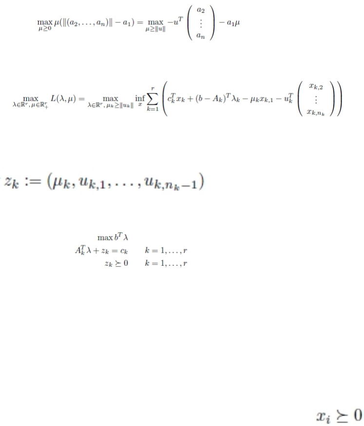
In fact, you probably recall that for any vector (a1, a2, ... an), the following equality
holds:
With that equivalence in mind, you can rewrite the sample problem like this:
Given that restatement of the original SOCP in Lagrangian terms, you can set the
derivative (with respect to x) to zero, and define the vector zklike this:
Then the dual of the same model looks like this:
After you solve a primal second order cone program in the form shown here, you
can query values of λ(lambda) of the corresponding dual of the SOCP model. To
query those values, use these routines and methods:
vIn the Callable Library (C API), use CPXXgetpi.
vIn the C++ API, use the methods IloCplex::getDuals.
vIn the Java API, use the methods IloCplex.getDuals.
vIn the .NET API, use the methods Cplex.GetDuals.
vIn the Python API, use the methods SolutionInterface.get_dual_values.
To query the dual multipliers µkfor the second order cone constraints:
first query the zvector, that is, the dual slack vector. Then use the idea that µk=
zk1.
vIn the Callable Library (C API), you can obtain the zvector by summing
CPXXgetdj and CPXXgetqconstrdslack.
vIn the C++ API, sum the results of both IloCplex::getReducedCosts and
IloCplex::getQCDSlack.
vIn the Java API, sum the results of both IloCplex.getReducedCosts and
IloCplex.getQCDSlack.
vIn the .NET API, sum the results of both Cplex.GetReducedCosts and
Cplex.GetQCDSlack.
vIn the Python API, sum the results of both cplex.solution.get_reduced_costs and
cplex.solution.get_quadratic_dualslack.
Tip:
216 CPLEX User’s Manual

A pure SOCP does not have bound constraints, so CPXXgetdj returns the zero
vector. However, by definition, the dual slack vector is the sum of CPXXgetdj and
CPXXgetqconstrdslack where CPXXgetqconstrdslack is for each quadratic
constraint.
(That observation applies to the equivalent methods in other APIs as well.)
Examples: querying dual values and reduced costs of a SOCP
The following examples show you how to apply that procedure to query the dual
values and reduced costs of a problem stated as a second order cone program
(SOCP). Each of the examples defines a function checkkkt, which reads the dual
values λ, queries the values of z, constructs µ, then tests that these vectors satisfy
the Karush-Kuhn-Tucker conditions for the model in the example.
vAmong the examples of the Callable Library (C API), see socpex1.c and
xsocpex1.c.
vAmong the examples of the C++ API, see ilosocpex1.cpp.
vAmong the examples of the Java API, see SocpEx1.java.
vAmong the examples of the .NET API, see SocpEx1.cs and SocpEx1.vb.
vAmong the examples of the Python API, see socpex1.py.
vAmong the examples of the MATLAB connector, see socpex1.m.
Examples: SOCP
Lists examples of SOCP.
The following examples, distributed with the product, show how to create and
populate that SOCP model and then how to access dual values and reduced costs
for the SOCP model in each API:
vIn the Callable Library (C API), see socpex1.c and xsocpex1.c.
vIn the C++ API, see ilosocpex1.cpp.
vIn the Java API, see SocpEx1.java.
vIn the .NET API, see SocpEx1.cs and SocpEx1.vb.
vIn the Python API, see socpex1.py.
vIn the MATLAB connector, see socpex1.m.
Examples: QCP
Tells where to find sample applications solving a quadratically constrained
program.
For examples of QCPs, see these variations of the same problem in yourCPLEXhome
/examples/src:
vqcpex1.c
viloqcpex1.cpp
vQCPex1.java
vQCPex1.cs
Chapter 15. Solving problems with quadratic constraints (QCP) 217
218 CPLEX User’s Manual

Part 4. Discrete optimization
This part focuses on algorithmic considerations about the optimizers of IBM ILOG
CPLEX that solve problems formulated in terms of discrete variables, such as
integer, Boolean, piecewise-linear, or semi-continuous variables. While default
settings of ILOG CPLEX enable you to solve many problems without changing
parameters, this part also documents features that enable you to tune performance.
© Copyright IBM Corp. 1987, 2016 219
220 CPLEX User’s Manual

Chapter 16. Solving mixed integer programming problems
(MIP)
Documents the solution of mixed integer programs (MIPs) with the CPLEX mixed
integer optimizer; that is, solving models in which one or more variables must take
integer solution values.
Stating a MIP problem
Defines the kind of problems that the mixed integer optimizer solves.
A mixed integer programming (MIP) problem may contain both integer and
continuous variables. If the problem contains an objective function with no
quadratic term, (a linear objective), then the problem is termed a Mixed Integer Linear
Program (MILP).
Tip:
The all zero objective function associated with a feasibility problem is also a linear
objective.
If there is a quadratic term in the objective function, the problem is termed a Mixed
Integer Quadratic Program (MIQP). If the model has any constraints containing a
quadratic term, regardless of the objective function, the problem is termed a Mixed
Integer Quadratically Constrained Program (MIQCP).
In IBM ILOG CPLEX documentation, if the discussion pertains specifically to the
MILP, MIQP, or MIQCP case, then that term is used. For the majority of topics that
pertain equally to MILP, MIQP, and MIQCP, the comprehensive term MIP is used.
Integer variables may be restricted to the values 0 (zero) and 1 (one), in which case
they are referred to as binary variables. Or they may take on any integer values, in
which case they are referred to as general integer variables. A variable of any MIP
that may take either the value 0 (zero) or a value between a lower and an upper
bound is referred to as semi-continuous. A semi-continuous variable that is restricted
to integer values is referred to as semi-integer. Chapter 21, “Using semi-continuous
variables: a rates example,” on page 325 says a bit more about semi-continuous
variables later in this manual. Special Ordered Sets (SOS) are discussed in
Chapter 20, “Using special ordered sets (SOS),” on page 321. Continuous variables
in a MIP problem are those which are not restricted in any of these ways, and are
thus permitted to take any solution value within their (possibly infinite) lower and
upper bounds.
In CPLEX documentation, the comprehensive term integer variable means any of the
various types just mentioned except for continuous or SOS. The presence or
absence of a quadratic term in the objective function or among the constraints for a
given variable has no bearing on its being classified as continuous or integer.
The following formulation illustrates a mixed integer programming problem,
which is solved in the example program ilomipex1.cpp or mipex1.c , discussed
later in this chapter:
© Copyright IBM Corp. 1987, 2016 221
Maximize x1 + 2x2 + 3x3 + x4
subject
to
- x1 + x2 + x3 + 10x4 ≤20
x1 - 3x2 + x3 ≤30
x2 - 3.5x4 = 0
with
these
bounds
0≤x1 ≤40
0≤x2 ≤+∞
0≤x3 ≤+∞
2≤x4 ≤3
x4 integer
Preliminary issues
When you are optimizing a MIP, there are a few preliminary issues that you need
to consider to get the most out of CPLEX. The following sections cover such topics
as entering variable types, displaying MIPs in the Interactive Optimizer, detecting
the problem type, and switching to the fixed form of your problem.
Entering MIP problems
Describes special considerations for entering a MIP or reading a MIP from a file,
You enter MIPs into CPLEX as explained in each of the topics about the APIs of
CPLEX, with this additional consideration: you need to specify which variables are
binary, general integer, semi-continuous, and semi-integer, and which are contained
in special ordered sets (SOS).
Concert Technology users specify this information by passing the value of a type
to the appropriate constructor when creating the variable, as summarized in
Table 38.
Table 38. Specifying type of variable for a MIP in Concert Technology.
Type of Variable C++ API Java API .NET API
binary IloNumVar::Type::ILOBOOL IloNumVarType.Bool NumVarType.Bool
integer IloNumVar::Type::ILOINT IloNumVarType.Int NumVarType.Int
semi-continuous IloSemiContVar::Type::ILONUM IloNumVarType.Float NumVarType.Float
semi-integer IloSemiContVar::Type::ILOINT IloNumVarType.Int NumVarType.Int
Callable Library users specify this information through the routine CPXcopyctype.
In the Interactive Optimizer, to specify binary integers in the context of the enter
command, type binaries on a separate line, followed by the designated binary
variables. To specify general integers, type generals on a separate line, followed by
the designated general variables. To specify semi-continuous variables, type
semi-continuous on a separate line, followed by the designated variables.
Semi-integer variables are specified as both general integer and semi-continuous.
The order of these three sections (generals, semi-continuous, semi-integer as both)
does not matter. To enter the general integer variable of the “Stating a MIP
problem” on page 221, you type this:
generals
x4
222 CPLEX User’s Manual

You may also read MIP data in from a formatted file, just as you do for linear
programming problems. “Understanding file formats” on page 109 in this manual
lists the file formats briefly, and the reference manual File formats supported by
CPLEXdocuments file formats, such as MPS, LP, and others.
vTo read MIP problem data into the Interactive Optimizer, use the read
command with an option to indicate the file type.
vTo read MIP problem data into your application, use the importModel method
in Concert Technology or use CPXreadcopyprob in the Callable Library.
Displaying MIP problems
Describes options for displaying a MIP model.
Table 39 summarizes display options in the Interactive Optimizer that are specific
to MIP problems.
Table 39. Interactive Optimizer display options for MIP problems.
Interactive command Purpose
display problem binaries lists variables restricted to binary values
display problem generals lists variables restricted to integer values
display problem semi-continuous lists variables of type semi-continuous and
semi-integer
display problem integers lists all of the above
display problem sos lists the names of variables in one or more
Special Ordered Sets
display problem stats lists LP statistics plus:
vnumber of binary variables, if present;
vnumber of general variables, if present;
vand number of SOSs, if present.
In Concert Technology, use one of the accessors supplied with the appropriate
object class, such as IloSOS2::getVariables .
From the Callable Library, use the routines CPXgetctype and CPXgetsos to access
this information.
Changing problem type in MIPs
Describes means of changing the type of a MIP model; also specifies how CPLEX
determines the type of a MIP model.
Concert Technology applications treat all models as capable of containing integer
variables, and thus these variable declarations may be added or deleted at will.
When extracting a model with integer variables, CPLEX in Concert Technology
will automatically detect the model as a MIP and make the required adjustments to
internal data structures.
However, the other ways of using CPLEX, the Callable Library and the Interactive
Optimizer, require an explicit declaration of a problem type to distinguish
Chapter 16. Solving mixed integer programming problems (MIP) 223

continuous LPs, QPs, and QCPs from MIPs. Techniques to declare the problem
type with the Callable Library and the Interactive Optimizer are discussed in this
topic.
When you enter a problem, CPLEX detects the problem type from the available
information. If the problem is read from a file (LP, MPS, or SAV format, for example),
or entered interactively, the problem type is discovered according to Table 40.
Table 40. Definitions of problem types
Problem
Type
No Integer
Variables
Has Integer
Variables
No Quadratic
Terms in the
Objective
Function
Has
Quadratic
Terms in the
Objective
Function
Has
Quadratic
Terms in
Constraints
lp X X
qp X X
qcp X possibly X
milp X X
miqp X X
miqcp X possibly X
However, if you enter a problem with no integer variables, so that its problem type
is initially lp, qp, or qcp, and you then wish to modify the problem to contain
integer variables, this modification is accomplished by first changing the problem
type to milp, miqp, or miqcp . Conversely, if you have entered an MILP, MIQP, or
MIQCP model and wish to remove all the integer declarations and thus convert
the model to a continuous formulation, you can change the problem type to lp, qp,
or qcp. Note that deleting each of the integer variable declarations individually still
leaves the problem type as milp, miqp, or miqcp, although in most instances the
distinction between this problem and its continuous counterpart is somewhat
arbitrary in terms of the steps that will be taken to solve it.
Thus, when using the Interactive Optimizer, you use the command change
problem with one of the following options:
vmilp, miqp, or miqcp
specifying that you want CPLEX to treat the problem as an MILP, MIQP, or
MIQCP, respectively. This change in problem type makes the model ready for
declaration of the integer variables via subsequent change type commands. If
you change the problem to be an MIQP or MIQCP and there are not already
quadratic terms in the objective function or among the constraints, the
Interactive Optimizer creates an empty quadratic matrix, ready for populating
via the change qpterm command.
vlp, qcp, or qp
specifying that you want all integer declarations removed from the variables in
the problem. If you choose the qp or qcpproblem type and there are not already
quadratic terms in the objective function or among the constraints, the
Interactive Optimizer creates an empty quadratic matrix, ready for populating
via the change qpterm command.
From the Callable Library, use the routine CPXchgprobtype to change the problem
type to CPXPROB_MILP, CPXPROB_MIQP, or CPXPROB_MIQCP for the MILP, MIQP, and
MIQCP case respectively, and then assign integer declarations to the variables
224 CPLEX User’s Manual

through the CPXcopyctype function. Conversely, remove all integer declarations
from the problem by using CPXchgprobtype with problem type CPXPROB_LP,
CPXPROB_QP, or CPXPROB_QCP.
At the end of a MIP optimization, the optimal values for the variables are directly
available. However, you may wish to obtain information about the LP, QP, or QCP
associated with this optimal solution (for example, to know the reduced costs for
the continuous variables of the problem at this solution). To do this, you must
change the problem to be of type Fixed, either fixed_milp for the MILP case or
fixed_miqp for the MIQP case. The fixed MIP is the continuous problem in which
the integer variables are fixed at the values they attained in the best integer
solution. After changing the problem type, you can then call any of the continuous
optimizers to re-optimize, and then display solution information for the continuous
form of the problem. If you then wish to change the problem type back to the
associated milp or miqp, you can do so without loss of information in the model.
Changing variable type
Describes special considerations about changing the type of a variable in a MIP
model.
In the Interactive Optimizer, the command change type adds (or removes) the
restriction on a variable that it must be an integer. When you enter the command
change type , the system prompts you to enter the variable that you want to
change, and then it prompts you to enter the type (cfor continuous, bfor binary, i
for general integer, sfor semi-continuous, nfor semi-integer).
You can change a variable to binary even if its bounds are not 0 (zero) and 1 (one).
However, in such a case, the optimizer will change the bounds to be 0 and 1.
If you change the type of a variable to be semi-continuous or semi-integer, be sure
to create both a lower bound and an upper bound for it. These variable types
specify that at an optimal solution the value for the variable must be either exactly
zero or else be between the lower and upper bounds (and further subject to the
restriction that the value be an integer, in the case of semi-integer variables).
A problem may be changed to a mixed integer problem, even if all its variables are
continuous.
Note:
It is not required to specify explicit bounds on general integer variables. However,
if during the branch-and-cut algorithm a variable exceeds 2,100,000,000 in
magnitude of its solution, an error termination will occur. In practice, it is wise to
limit integer variables to values far smaller than the stated limit, or numeric
difficulties may occur; trying to enforce the difference between 1,000,000 and
1,000,001 on a finite precision computer might work but could be difficult due to
round-off.
Using the mixed integer optimizer
Describes features of the MIP optimizer.
Invoking the optimizer for a MIP model.
Describes invocation of the optimizer for a MIP model.
Chapter 16. Solving mixed integer programming problems (MIP) 225
The CPLEX mixed integer optimizer solves MIP models using a very general and
robust algorithm based on branch & cut. While MIP models have the potential to
be much more difficult than their continuous LP, QCP, and QP counterparts, it is
also the case that large MIP models are routinely solved in many production
applications. A great deal of algorithmic development effort has been devoted to
establishing default CPLEX parameter settings that achieve good performance on a
wide variety of MIP models. Therefore, it is recommended to try solving your
model by first calling the mixed integer optimizer in its most straightforward form.
To invoke the mixed integer optimizer, use one of these approaches:
vIn the Interactive Optimizer, use the mipopt command.
vIn Concert Technology, with the method solve.
vIn the Callable Library, use the routineCPXmipopt.
Emphasizing feasibility and optimality
Describes the context of the MIP emphasis parameter.
The following topic, “Tuning performance features of the mixed integer optimizer”
on page 229, goes into great detail about the algorithmic features, controlled by
parameter settings, that are available in CPLEX to achieve performance tuning on
difficult MIP models. However, there is an important parameter, MIPEmphasis or
CPX_PARAM_MIPEMPHASIS, that is oriented less toward the user understanding the
algorithm being used to solve the model, and more toward the user telling the
algorithm something about the underlying aim of the optimization being run. That
parameter is discussed here.
Optimizing a MIP model involves:
1. finding a succession of improving integer feasible solutions (that is, solutions
satisfying the linear and quadratic constraints and the integrality conditions);
while
2. also working toward a proof that no better feasible solution exists and is
undiscovered.
For most models, a balance between these two sometimes-competing aims works
well, and this is another way of stating the philosophy behind the default
MIPEmphasis setting: it balances optimality and integer feasibility.
At this default MIPEmphasis setting of 0(that is, MIPEmphasisBalanced in Concert
Technology or CPX_MIPEMPHASIS_BALANCED in the Callable Library), CPLEX uses
tactics intended to find a proven optimal solution quickly, for models of a broad
range of difficulty. That is, considerable analysis of the model is performed before
branching ever begins, in the expectation that the investment will result in a faster
total run time, yet not every possible analysis is performed. And then branching is
performed in a manner that seeks to find good quality feasible solutions, without
sacrificing too much time that could be spent proving the optimality of any
solution that has already been found.
In many situations, the user may want a greater emphasis on feasibility and less
emphasis on analysis and proof of optimality. For example, a restrictive time limit
(set by the user with the TiLim parameter) may be in force due to a real-time
application deployment, where a model is of sufficient difficulty that a proof of
optimality is unlikely, and the user wants to have simply as good a solution as is
practicable when the time limit is reached. The MIPEmphasis setting of 1
(MIPEmphasisFeasibility in Concert Technology or CPX_MIPEMPHASIS_FEASIBILITY
226 CPLEX User’s Manual
in the Callable Library) directs CPLEX to adopt this emphasis. Less computational
effort is applied at the outset toward the analyses that aid in the eventual proof of
optimality, and more effort is spent in immediately beginning computations that
search for early (and then improved) feasible solutions. It is likely on most models
that an eventual proof of optimality would take longer by setting MIPEmphasis to 1
, but since the user has given CPLEX the additional information that this proof is
of less importance than usual, the user's needs will actually be met more
effectively.
Another choice for MIPEmphasis is 2(MIPEmphasisOptimality in Concert Technology
or, in the Callable Library, CPX_MIPEMPHASIS_OPTIMALITY). This setting results in a
greater emphasis on optimality than on feasibility. The search for feasible solutions
is not ignored completely, but the balance is shifted toward moving the Best Bound
(described in the following paragraph) more rapidly, at the likely expense of
feasible solutions being found less rapidly, and improved feasible solutions less
frequently, than with the default emphasis.
The fourth choice for MIPEmphasis, 3(MIPEmphasisBestBound in Concert Technology
or, in the Callable Library, CPX_MIPEMPHASIS_BESTBOUND) works exclusively at
moving the Best Bound. The Best Bound represents the objective function value at
which an integer feasible solution could still potentially exist. As possibilities are
eliminated, this Best Bound value will move in the opposite direction to that of
any improving series of integer feasible solutions. The process of moving the Best
Bound will eventually result in the optimal feasible solution being discovered, at
which point the optimization is complete, and feasible solutions may be discovered
along the way anyway, due to branches that happen to locate feasible solutions
that do not match the Best Bound. A great deal of analysis may be performed on
the model, beyond what is done with the default emphasis. Therefore, it is
recommended to use this setting only on models that are difficult for the default
emphasis, and for which you do not care about interim feasible solutions that may
or may not be optimal.
The final choice for MIPEmphasis is 4 (CPX_MIPEMPHASIS_HIDDENFEAS). It applies
considerable additional effort toward finding high quality feasible solutions that
are difficult to locate, and for this reason the eventual proof of optimality may take
longer than with default settings. This choice is intended for use on difficult
models where a proof of optimality is unlikely, and where emphasis 1 (one) does
not deliver solutions of an appropriately high quality.
To make clear a point that has been alluded to so far: every choice of MIPEmphasis
results in the search algorithm proceeding in a manner that eventually will find
and prove an optimal solution, or will prove that no integer feasible solution
exists. The choice of emphasis only guides CPLEX to produce feasible solutions in
a way that is in keeping with the user's particular purposes, but the accuracy and
completeness of the algorithm is not sacrificed in the process.
The MIPEmphasis parameter may be set in conjunction with any other CPLEX
parameters (discussed at length in the next section). For example, if you wish to
set an upward branching strategy via the BrDir parameter, this will be honored by
any setting of MIPEmphasis. Of course, certain combinations of MIPEmphasis with
other parameters may be counter-productive, such as turning off all cuts with
emphasis 3, but the user has the option if that is what is wanted.
Terminating MIP optimization
Describes termination conditions of the MIP optimizer.
Chapter 16. Solving mixed integer programming problems (MIP) 227

CPLEX terminates MIP optimization under a variety of circumstances. First,
CPLEX declares integer optimality and terminates when it finds an integer solution
and all parts of the search space have been processed. Optimality in this case is
relative to whatever tolerances and optimality criteria you have set. For example,
CPLEX considers any user-supplied cutoff value (such as CutLo or CutUp) as well
as the objective difference parameter (ObjDif) when it treats nodes during
branch & cut. Thus these settings indirectly affect termination.
An important termination criterion that the user can set explicitly is the MIP gap
tolerance. In fact, there are two such tolerances: a relative MIP gap tolerance that is
commonly used, and an absolute MIP gap tolerance that is appropriate in cases
where the expected optimal objective function is quite small in magnitude. The
default value of the relative MIP gap tolerance is 1e-4; the default value of the
absolute MIP gap tolerance is 1e-6. These default values indicate to CPLEX to stop
when an integer feasible solution has been proved to be within 0.01% of optimality.
On a difficult model with input data obtained with only approximate accuracy,
where a proved optimum is thought to be unlikely within a reasonable amount of
computation time, a user might choose a larger relative MIP gap to allow early
termination; for example, a relative MIP gap of 0.05 (corresponding to 5%).
Conversely, in a model where the objective function amounts to billions of dollars
and the data are accurate to a degree that further processing is worthwhile, a
tighter relative MIP Gap (even 0.0) may be advantageous to avoid any chance of
missing the best possible solution.
CPLEX also terminates optimization when it reaches any limit that you have set.
You can set limits on time, number of nodes, size of tree memory, and number of
integer solutions. Table 41 summarizes those parameters and their purpose.
Table 41. Parameters to limit MIP optimization
To set a limit on Use this parameter
Concert
Technology Callable Library
Interactive
Optimizer
elapsed time optimizer time limit
in seconds
TiLim CPX_PARAM_TILIM timelimit
elapsed
deterministic time
deterministic time
limit
DetTiLim CPX_PARAM_DETTILIM dettimelimit
number of nodes MIP node limit NodeLim CPX_PARAM_NODELIM mip limits nodes
size of tree tree memory limit TreLim CPX_PARAM_TRELIM mip limits
treememory
number of integer
solutions
MIP integer
solution-file switch
and prefix
IntSolLim CPX_PARAM_INTSOLLIM mip limits
solutions
relative MIP gap
tolerance
relative MIP gap
tolerance
EpGap CPX_PARAM_EPGAP mip tolerances
mipgap
absolute MIP gap
tolerance
absolute MIP gap
tolerance
EpAGap CPX_PARAM_EPAGAP mip tolerances
absmipgap
CPLEX also terminates when an error occurs, such as when CPLEX runs out of
memory or when a subproblem cannot be solved. If an error is due to failure to
solve a subproblem, an additional line appears in the node log file to indicate the
reason for that failure. For suggestions about overcoming such errors, see
“Troubleshooting MIP performance problems” on page 267.
228 CPLEX User’s Manual

Tuning performance features of the mixed integer optimizer
Describes features for tuning performance of the MIP optimizer.
Branch & cut or dynamic search?
Describes the search facilities of the MIP optimizer.
In addition to a robust branch & cut algorithm, CPLEX also offers a dynamic search
algorithm. The dynamic search algorithm consists of the same building blocks as
branch & cut: LP relaxation, branching, cuts, and heuristics. The following sections
of the manual describe performance and tuning in relation to branch and cut. The
parameters mentioned in this context have a similar effect in the dynamic search
algorithm as in conventional branch and cut. In fact, the generic description in
relation to branch & cut suffices conceptually for both branch and cut and
dynamic search, even though their implementations differ.
CPLEX offers the MIP search parameter (MIP dynamic search switch: MIPSearch,
CPX_PARAM_MIPSEARCH) for you to control whether it pursues dynamic search or
conventional branch & cut in solving your problem. At its default setting, this
parameter specifies that CPLEX should choose which algorithm to apply on the
basis of characteristics it finds in your model. Other settings allow you to specify
which search to pursue.
Because many parameter settings directly affect the branch & cut and dynamic
search algorithms, here is a general description of how branch & cut is
implemented within CPLEX.
In the branch & cut algorithm, CPLEX solves a series of continuous subproblems.
To manage those subproblems efficiently, CPLEX builds a tree in which each
subproblem is a node. The root of the tree is the continuous relaxation of the original
MIP problem.
If the solution to the relaxation has one or more fractional variables, CPLEX will
try to find cuts. Cuts are constraints that cut away areas of the feasible region of
the relaxation that contain fractional solutions. CPLEX can generate several types
of cuts. (“Cuts” on page 236 tells you more about that topic.)
If the solution to the relaxation still has one or more fractional-valued integer
variables after CPLEX tries to add cuts, then CPLEX branches on a fractional
variable to generate two new subproblems, each with more restrictive bounds on
the branching variable. For example, with binary variables, one node will fix the
variable at 0 (zero), the other, at 1 (one).
The subproblems may result in an all-integer solution, in an infeasible solution, or
another fractional solution. If the solution is fractional, CPLEX repeats the process.
Introducing performance features of the MIP optimizer
Describes performance features generally.
The CPLEX Mixed Integer Optimizer contains a wealth of features intended to aid
in the solution of challenging MIP models. While default strategies are provided
that solve the majority of models without user involvement, there exist difficult
models that benefit from attention to performance tuning.
Chapter 16. Solving mixed integer programming problems (MIP) 229
To help you decide whether default settings of parameters are best for your model,
or whether other parameter settings may improve performance, the tuning tool is
available. Chapter 10, “Tuning tool,” on page 123 explains more about this utility
and directs you to examples of its use.
This section discusses the CPLEX features and parameters that are the most likely
to offer help with difficult models.
Applying cutoff values
Describes conditions in which CPLEX applies a cutoff value.
CPLEX cuts off nodes when the value of the objective function associated with the
subproblem at that node is worse than the cutoff value.
You set the cutoff value by means of the CutUp parameter (for a minimization
problem) or the CutLo parameter (for a maximization problem), to indicate to
CPLEX that integer feasible solutions worse than this cutoff value should be
discarded. The default value of the lower cutoff is -1e+75; the default value of the
upper cutoff is 1e+75. The defaults, in effect, mean that no cutoff is to be supplied.
You can supply any number that you find appropriate for your problem. It is
never required that you supply a cutoff, and in fact for most applications is it not
done.
Applying tolerance parameters
Describes conditions in which CPLEX applies tolerances.
CPLEX will use the value of the best integer solution found so far, as modified by
the tolerance parameters ObjDif (absolute objective function difference) or
RelObjDif (relative objective function difference) as the cutoff. Again, it is not
typical that users set these parameters, but they are available if you find them
useful. Use care in changing these tolerances: if either of them is nonzero, you may
miss the optimal solution by as much as that amount. For example, in a model
where the true minimum is 100 and the absolute cutoff is set to 5, if a feasible
solution of say, 103 is found at some point, the cutoff will discard all nodes with a
solution worse than 98, and thus the solution of 100 would be overlooked.
Applying heuristics
Describes conditions in which CPLEX applies heuristics.
Periodically during the branch & cut algorithm, CPLEX may apply a heuristic that
attempts to compute an integer solution from available information, such as the
solution to the relaxation at the current node. This activity does not replace the
branching steps, but sometimes is able inexpensively to locate a new feasible
solution sooner than by branching, and a solution found in this way is treated in
the same way as any other feasible solution. At intervals in the tree, new cuts
beyond those computed at the root node may also be added to the problem.
When an integer solution is found: the incumbent
Describes CPLEX handling of an incumbent value.
After CPLEX finds an integer solution, it does the following:
vIt makes that integer solution the incumbent solution and that node the
incumbent node.
230 CPLEX User’s Manual

vIt makes the value of the objective function at that node (modified by the
objective difference parameter) the new cutoff value.
vIt prunes from the tree all subproblems for which the value of the objective
function is no better than the incumbent.
Controlling strategies: diving and backtracking
Describes parameters to control search strategies
You control the path that CPLEX traverses in the tree through several parameters,
as summarized in Table 42.
Table 42. Parameters for controlling branch & cut strategy.
Interactive
Optimizer Command
Concert Technology
IloCPLEX Method
Callable Library
Routine Parameter Reference
set mip strategy
backtrack
setParam (BtTol , n) CPXsetdblparam (env,
CPX_PARAM_BTTOL , n)
backtracking
tolerance
set mip strategy
nodeselect
setParam(NodeSel ,
i)
CPXsetintparam (env,
CPX_PARAM_NODESEL ,
i)
MIP node selection
strategy
set mip strategy
variableselect
setParam(VarSel , i) CPXsetintparam(env,
CPX_PARAM_VARSEL ,
i)
MIP variable
selection strategy
set mip strategy
bbinterval
setParam(BBInterval
, i)
CPXsetintparam(env,
CPX_PARAM_BBINTERVAL
, i)
MIP strategy best
bound interval
set mip strategy
branch
setParam(BrDir , i) CPXsetintparam(env,
CPX_PARAM_BRDIR , i)
MIP branching
direction
During the branch & cut algorithm, CPLEX may choose to continue from the
present node and dive deeper into the tree, or it may backtrack (that is, begin a
new dive from elsewhere in the tree). The value of the backtrack tolerance
parameter, BtTol or CPX_PARAM_BTTOL, influences this decision, in terms of the
relative degradation of the objective function caused by the branches taken so far
in this dive. Setting that parameter to a value near 0.0 increases the likelihood that
a backtrack will occur, while the default value near 1.0 makes it more likely that
the present dive will continue to a resolution (fathoming either via a cutoff or an
infeasible combination of branches or the discovery of a new incumbent integer
feasible solution). See the CPLEX Parameters Reference Manual for more details
about how this parameter influences the computation that makes the decision to
backtrack.
Selecting nodes
Describes options of the parameter to control selection of strategies applied at
nodes and their effect on the search.
When CPLEX backtracks, there usually remain large numbers of unexplored nodes
from which to begin a new dive. The node selection parameter sets this choice.
(For documentation of the node selection parameter, see MIP node selection
strategy in the CPLEX Parameters Reference Manual.)
Chapter 16. Solving mixed integer programming problems (MIP) 231

Table 43. Node selection parameter settings for node search type
Value of the parameter Symbolic Value Node Search Type
1 (Default) CPX_NODESEL_BESTBOUND Best Bound search, which
means that the node with the
best objective function will
be selected, generally near
the top of the tree.
2 CPX_NODESEL_BESTEST Best Estimate search,
whereby CPLEX will use an
estimate of a given node's
progress toward integer
feasibility relative to its
degradation of the objective
function. This setting can be
useful in cases where there is
difficulty in finding feasible
solutions or in cases where a
proof of optimality is not
crucial.
3 CPX_NODESEL_BESTEST_ALT A variation on the Best
Estimate search.
0 CPX_NODESEL_DFS Depth First search will be
conducted. In many cases
this amounts to a brute force
strategy for solving the
combinatorial problem,
gaining a small amount of
tactical efficiency due to a
variety of reasons, and it is
rare that it offers any
advantage over other
settings.
In instances where Best Estimate node selection (NodeSel = 2or 3) is in effect, the
parameter known as MIP strategy best bound interval (BBinterval or
CPX_PARAM_BBINTERVAL) sets the frequency at which CPLEX uses Best Bound upon
backtracking. The default value of 7works well, but you can set it to 0(zero) to
make sure that Best Estimate is used every time backtracking occurs.
Selecting variables
Describes trade-offs around variable selection and options of the parameter to
control selection of the next variable.
After a node has been selected, the variable selection parameter influences which
variable is chosen for branching at that node. (For documentation of that
parameter, see MIP variable selection strategy in the CPLEX Parameters Reference
Manual.)
When CPLEX selects a branching variable during execution of the branch and cut
algorithm, there is a trade-off between more informed selections that require more
computational effort and less informed selections that are computationally cheaper.
More computationally intensive selection procedures can reduce the node count,
but also reduce the rate of node throughput. Less intensive procedures can increase
the node count, but that improved node throughput can yield an improvement in
232 CPLEX User’s Manual
overall performance. If you can properly assess these trade-offs for your model,
you can achieve faster performance than the default variable selection strategy in
CPLEX.
The key here is the concept of strong branching, which can be computationally
expensive, but which can yield valuable information about branching. The idea
behind strong branching at a node relaxation (root node or child node) is the
selection of a subset of the integer-restricted variables with fractional values in the
node relaxation solution. For each variable in this subset, CPLEX explores both the
up and down branches by running a modest number of simplex iterations; CPLEX
then uses the results to assess the benefit of branching up or down on that
variable.
Setting the MIP variable selection strategy parameter to 3 does this at every node.
The default of the MIP variable selection strategy parameter (which is typically 2)
computes strong branching data at the root node in order to calculate pseudo costs
for each variable. These pseudo costs really help with subsequent branching, but
their calculation can be expensive. Setting the parameter to 4 computes much less
expensive pseudo reduced costs. This choice can save time, particularly at the root
node when you have asked CPLEX to perform an optimization with limited total
run time.
Recent versions of CPLEX perform powerful computations when processing the
root node, and consequently many models solve to optimality (or close to
optimality) at the root node. If most of the time is spent at the root node, CPLEX
has little time left then for branching, so the benefit of more informed branching
decisions at the child node probably may not be worth the cost of those root node
calculations.
Note that this situation will not always be the case, though.
Sometimes, strong branching calculations at the root yield variable fixings. For
example, if CPLEX quickly discovers that the up branch on a binary variable is
infeasible, CPLEX can immediately fix that variable to 0 (zero). These variable
fixings yielded by strong branching calculations can make heuristics more effective,
or can yield other performance improvements.
So, do not always set the MIP variable selection strategy parameter to 4 with
models that run for only a few nodes. But, for models where CPLEX seems to
spend a lot time at the root node, consider setting the parameter to 4 to see
whether that helps.
Similarly, for models where root node processing time is brief, node relaxations
solve quickly, and lack of progress toward the best node is an issue, consider the
more computationally expensive setting of 3 for the MIP variable selection strategy
parameter. This setting instructs CPLEX to perform strong branching calculations
at the child nodes as well as at the root node.
The following table summarizes the settings for this parameter.
Chapter 16. Solving mixed integer programming problems (MIP) 233

Table 44. VarSel parameter settings for choice of branching variable
VarSel Setting Symbolic Value Branching Variable Choice
-1 CPX_VARSEL_MININFEAS Branch strictly at the nearest
integer value which is closest
to the fractional variable.
1 CPX_VARSEL_MAXINFEAS Branch strictly at the nearest
integer value which is
furthest from the fractional
variable.
0 (Default) CPX_VARSEL_DEFAULT CPLEX automatically decides
each branch direction.
2 CPX_VARSEL_PSEUDO Use pseudo costs, which
derives an estimate about the
effect of each proposed
branch from duality
information.
3 CPX_VARSEL_STRONG Use strong branching, which
invests considerable effort in
analyzing potential branches
in the hope of drastically
reducing the number of
nodes that will be explored.
4 CPX_VARSEL_PSEUDOREDUCED Use pseudo reduced costs,
which is a computationally
less intensive form of pseudo
costs.
Changing branching direction
Describes options of the parameter to change branching direction and its effect on
search.
After a variable has been selected for branching, the branching direction parameter
influences the direction, up or down, of the branch on that variable to be explored
first. (For documentation of that parameter, see MIP branching direction in the
CPLEX Parameters Reference Manual.)
Table 45. BrDir parameter settings for choice of branching direction
BrDir Setting Symbolic Value Branching Direction Choice
-1 CPX_BRANCH_DOWN Branch downward
0 (Default) CPX_BRANCH_GLOBAL CPLEX automatically decides
each branch direction.
1 CPX_BRANCH_UP Branch upward
Priority orders complement the behavior of these parameters. They are introduced
in “Issuing priority orders” on page 257. They offer a mechanism by which you
supply problem-specific directives about the order in which to branch on variables.
In a priority order, you can also provide preferred branching directions for specific
variables.
Solving subproblems
Describes the parameters to control solution of subproblems.
234 CPLEX User’s Manual
CPLEX allows you to distinguish the algorithm applied to the initial relaxation of
your problem from the algorithm applied to other continuous subproblems of a
MIP. This distinction between initial relaxation and the other MIP subproblems
may be useful when you have special information about the nature of your model.
In this context, "other MIP subproblems" includes nodes of the branch & cut tree,
problems re-solved after cutting plane passes, problems solved by node heuristics,
and so forth.
The algorithm for initial MIP relaxation parameter (RootAlg, CPX_PARAM_STARTALG)
enables you to specify which algorithm for CPLEX to apply to the initial
relaxation.
The MIP subproblem algorithm parameter (NodeAlg, CPX_PARAM_SUBALG) lets you
specify the algorithm applied to other continuous subproblems.
For more detail about situations in which you may find these parameters helpful,
see “Unsatisfactory optimization of subproblems” on page 277.
Using node files
Describes a storage feature for nodes of the search.
On difficult models that generate a great number of nodes in the tree, the amount
of available memory for node storage can become a limiting factor. Storage of node
files can be an effective technique which uses disk space to augment RAM, at little
or no penalty in terms of solution speed.
The node-file storage-feature enables you to store some parts of the branch & cut
tree in files while the branch & cut algorithm is being applied. If you use this
feature, CPLEX will be able to explore more nodes within a smaller amount of
computer memory. This feature includes several options to reduce the use of
physical memory, and it entails a very small increase in runtime. Node-file storage
as managed by CPLEX itself offers a much better option in terms of memory use
and performance time than relying on swap space as managed by your operating
system in this context.
For more about the parameters controlling node files, see “Use node files for
storage” on page 274.
Probing
Describes probing, a technique that fixes binary variables and analyzes the
implications.
The probing feature can help in many different ways on difficult models. Probing
is a technique that looks at the logical implications of fixing each binary variable to
0 (zero) or 1 (one). It is performed after preprocessing and before the solution of
the root relaxation. Probing can be expensive, so this parameter should be used
selectively. On models that are in some sense easy, the extra time spent probing
may not reduce the overall time enough to be worthwhile. On difficult models,
probing may incur very large runtime costs at the beginning and yet pay off with
shorter overall runtime. When you are tuning performance, it is usually because
the model is difficult, and then probing is worth trying.
At the default setting of the probing parameter (0 (zero)), CPLEX will
automatically decide an appropriate level of probing. Setting the probing
Chapter 16. Solving mixed integer programming problems (MIP) 235

parameter to 1, 2, or 3, results in increasing levels of probing performed beyond
the default level. A setting of -1 results in no probing being performed.
To activate an increasing level of probing use the MIP probing level parameter:
vIn the Interactive Optimizer, use the command set mip strategy probe i.
vIn Concert Technology, set the integer parameter Probe.
vIn the Callable Library, set the integer parameter CPX_PARAM_PROBE.
Cuts
Describes types of cuts available in the MIP optimizer as performance features.
What are cuts?
Defines cuts.
Cuts are constraints added to a model to restrict (cut away) noninteger solutions
that would otherwise be solutions of the continuous relaxation. The addition of
cuts usually reduces the number of branches needed to solve a MIP.
In the following descriptions of cuts, the term node includes the root node (that is,
the root relaxation). Cuts are most frequently seen at the root node, but they may
be added by CPLEX at other nodes as conditions warrant.
CPLEX can generate both global cuts and local cuts. A global cut is a cut that is
valid for all nodes of the branch-and-bound tree, even if that global cut was found
during the analysis of a particular node. In contrast, a local cut is a cut that is valid
only for a specific node and for all of its descendant nodes.
Here are descriptions of the cuts implemented in CPLEX. These types of cuts are
all separated as global cuts with the sole exception of implied bound cuts. Implied
bound cuts can be separated as global cuts or as local cuts as conditions warrant.
v“Boolean Quadric Polytope (BQP) cuts”
v“Clique cuts” on page 237
v“Cover cuts” on page 237
v“Disjunctive cuts” on page 237
v“Flow cover cuts” on page 237
v“Flow path cuts” on page 238
v“Gomory fractional cuts” on page 238
v“Generalized upper bound (GUB) cover cuts” on page 238
v“Implied bound cuts: global and local” on page 238
v“Lift-and-project cuts” on page 239
v“Mixed integer rounding (MIR) cuts” on page 239
v“Multi-commodity flow (MCF) cuts” on page 240
v“Reformulation Linearization Technique (RLT) cuts” on page 240
v“Zero-half cuts” on page 241
Boolean Quadric Polytope (BQP) cuts
Defines a Boolean Quadric Polytope (BQP) cut.
Boolean Quadric Polytope cuts, also known as BQP cuts, exploit a cutting plane
technique to solve continuous global quadratic programs (QP) or mixed integer
236 CPLEX User’s Manual
quadratic programs (MIQP) more efficiently. This technique is based on the
observation that every valid linear cut for the mixed integer set defined by:
A = { (x, X) : x in {0,1}, X_ij = x_i x_j if i is different from j, X_ii = 0 }
is also a valid inequality for the continuous set defined by:
B = { (x, X) : 0 <= x <= 1, X_ij = x_i x_j if i is different from j, X_ii = 0 }
CPLEX makes use of such cuts to solve nonconvex quadratic programs (QP) and
nonconvex mixed integer quadratic programs (MIQP) to global optimality.
CPLEX does not apply BQP cuts to mixed integer linear programs (MILP).
Background
In his article The Boolean Quadric Polytope: Some characteristics, facets, and relatives
published in Mathematical Programming, volume 45, pages 139–172, 1989,
Manfred Padberg defined a Boolean Quadric Polytope QPnin n(n+1)/2 dimensions
as resulting from the linearization of the given quadratic form Q.
Samuel Burer and Adam N. Letchford provided a theoretical basis for BQP cuts in
their article On non-convex quadratic programming with box constraints published in
2009 by the Society for Industrial and Applied Mathematics in the SIAM Journal
on Optimization, volume 20, issue 2, pages 1073-1089.
Clique cuts
Defines a clique cut.
A clique is a relationship among a group of binary variables such that at most one
variable in the group can be positive in any integer feasible solution. Before
optimization starts, CPLEX constructs a graph representing these relationships and
finds maximal cliques in the graph.
Cover cuts
Defines a cover cut.
If a constraint takes the form of a knapsack constraint (that is, a sum of binary
variables with nonnegative coefficients less than or equal to a nonnegative
righthand side), then there is a minimal cover associated with the constraint. A
minimal cover is a subset of the variables of the inequality such that if all the subset
variables were set to one, the knapsack constraint would be violated, but if any
one subset variable were excluded, the constraint would be satisfied. CPLEX can
generate a constraint corresponding to this condition, and this cut is called a cover
cut.
Disjunctive cuts
Defines disjunctive cuts.
A MIP problem can be divided into two subproblems with disjunctive feasible
regions of their LP relaxations by branching on an integer variable. Disjunctive cuts
are inequalities valid for the feasible regions of LP relaxations of the subproblems,
but not valid for the feasible region of LP relaxation of the MIP problem.
Flow cover cuts
Defines flow cover cuts.
Chapter 16. Solving mixed integer programming problems (MIP) 237
Flow covers are generated from constraints that contain continuous variables, where
the continuous variables have variable upper bounds that are zero or positive
depending on the setting of associated binary variables. The idea of a flow cover
comes from considering the constraint containing the continuous variables as
defining a single node in a network where the continuous variables are in-flows
and out-flows. The flows will be on or off depending on the settings of the
associated binary variables for the variable upper bounds. The flows and the
demand at the single node imply a knapsack constraint. That knapsack constraint
is then used to generate a cover cut on the flows (that is, on the continuous
variables and their variable upper bounds).
Flow path cuts
Defines flow path cuts.
Flow path cuts are generated by considering a set of constraints containing the
continuous variables that define a path structure in a network, where the
constraints are nodes and the continuous variables are in-flows and out-flows. The
flows will be on or off depending on the settings of the associated binary variables.
Gomory fractional cuts
Defines Gomory fractional cuts.
Gomory fractional cuts are generated by applying integer rounding on a pivot row
in the optimal LP tableau for a (basic) integer variable with a fractional solution
value.
Generalized upper bound (GUB) cover cuts
Defines GUB cover cuts.
A GUB constraint for a set of binary variables is a sum of variables less than or
equal to one. If the variables in a GUB constraint are also members of a knapsack
constraint, then the minimal cover can be selected with the additional
consideration that at most one of the members of the GUB constraint can be one in
a solution. This additional restriction makes the GUB cover cuts stronger (that is,
more restrictive) than ordinary cover cuts.
Implied bound cuts: global and local
Defines both global and local implied bound cuts.
In some models, binary variables imply bounds on nonbinary variables (that is,
general integer variables and continuous variables). CPLEX generates cuts to reflect
these relationships. In fact, CPLEX can generate two different types of implied
bound cuts:
vCPLEX generates global implied bound cuts by using globally valid bounds on
the continuous variables in the model. For a parameter to control this activity,
see the documentation of the MIP globally valid implied bound cuts switch in
the CPLEX Parameters Reference Manual.
vCPLEX generates local implied bound cuts by using locally valid bounds on the
continuous variables of the subproblem (that is, the branch-and-bound node)
under consideration. For a parameter to control this activity, see the
documentation of the MIP locally valid implied bound cuts switch in the CPLEX
Parameters Reference Manual.
238 CPLEX User’s Manual
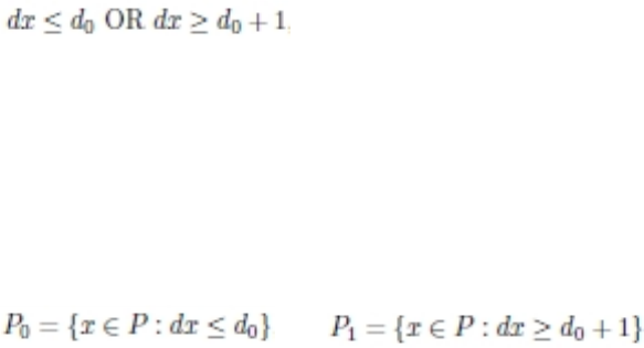
Lift-and-project cuts
Defines lift-and-project cuts.
Lift and project cuts are split cuts separated by fixing the (split) disjunction in
advance.
A MIP problem can be divided into two subproblems by branching on an integer
variable or on any combination of integer variables of the MIP. Those two
subproblems suggest two disjoint LP relaxations. A lift-and-project cut is a linear
inequality satisfied by the two LP relaxations defined by branching on a given
integer variable or combination of integer variables. (That inequality, however,
need not be valid for the LP relaxation of the original problem.)
More formally, a valid split disjunction for a MIP problem looks like this:
where dis a vector of coprime integer values, d0is an integer, and djis equal to 0
(zero) for all continuous variables x. In other words, the disjunction is defined only
on the integer-constrained variables of the MIP.
Given the polyhedron Pcorresponding to the LP relaxation of the MIP, and given a
valid split disjunction for that MIP, all the MIP feasible solutions are contained in
one of the two disjoint polyhedra defined by Pintersecting the split disjunction.
That is, the MIP feasible solutions are here:
OR
A lift-and-project cut is an inequality that is valid for the union of P0and P1,
though not valid for P.
Lift and project cuts as implemented in CPLEX can also be helpful in solving
mixed integer quadratically constrained programs (MIQCP) under certain
conditions.
For a more thorough exploration of the theory supporting lift and project cuts, see
the reports of these researchers:
vEgon Balas, Sebastian Ceria, and Gerard Cornuejols: "A lift-and-project cutting
plane algorithm for mixed-integer programs" in Mathematical Programming
volume 58, pages 295-324, 1993
vEgon Balas, Sebastian Ceria, and Gerard Cornuejols: "Mixed 0-1 programming by
lift-and-project in a branch-and-cut framework" in Management Science volume
42, pages 1229-1246, 1996
vPierre Bonami: "On optimizing over lift-and-project closures" in Mathematical
Programming Computation volume 4, pages 151–179, 2012
Mixed integer rounding (MIR) cuts
Defines MIR cuts.
MIR cuts are generated by applying integer rounding on the coefficients of integer
variables and the righthand side of a constraint.
Chapter 16. Solving mixed integer programming problems (MIP) 239
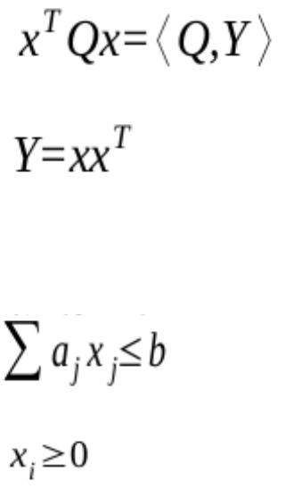
Multi-commodity flow (MCF) cuts
Defines multi-commodity flow cuts.
Many real-world models include network structures. CPLEX is able to recognize
some of these network structures automatically and to produce special cutting
planes that usually help to solve such models.
The structure that is addressed by this separator is called a multi-commodity flow
network with arc capacities.
When such a structure is present, CPLEX generates cuts that state that the
capacities installed on arcs pointing into a component of the network must be at
least as large as the total flow demand of the component that can not be satisfied
by flow sources within the component.
Reformulation Linearization Technique (RLT) cuts
Defines a Reformulation Linearization Technique (RLT) cut.
Reformulation Linearization Technique cuts, also known as RLT cuts, exploit a
cutting plane technique to solve certain nonconvex continuous quadratic programs
(QP) or mixed integer quadratic programs (MIQP) to global optimality.
Consider a conventional linearization of a possibly nonconvex QP:
where
.
As the first step in applying the reformulation linearization technique to this
nonconvex model, multiply each valid constraint by a different variable. That is,
consider a valid constraint, such as:
Now consider another variable, such as:
Now consider their product. This step produces:
240 CPLEX User’s Manual
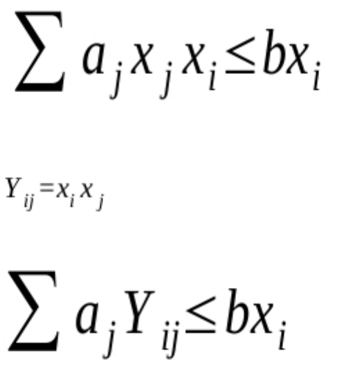
Next, use the relaxation variables
to linearize that product:
The result is a cut. Moreover, this technique also works for equations with free
variables.
For more detail about this subject, see the book A Reformulation-Linearization
Technique for Solving Discrete and Continuous Nonconvex Problems by Hanif
D. Sherali and W. P. Adams, published in 1999 by Springer. For a discussion of
mixed integer quadratic programs (MIQP) generally, see the article by Christian
Bliek, Pierre Bonami, and Andrea Lodi, "Solving Mixed-Integer Quadratic
Programming problems with IBM-CPLEX: a progress report" published in the
Proceedings of the Twenty-Sixth RAMP Symposium of the Research Association
of Mathematical Programming, held in Tokyo in 2014.
Zero-half cuts
Defines zero-half cuts and offers an example.
Zero-half cuts are based on the observation that when the lefthand side of an
inequality consists of integral variables and integral coefficients, then the righthand
side can be rounded down to produce a zero-half cut. Zero-half cuts are also
known as 0-1/2 cuts. To understand how zero-half cuts are generated, consider
these two constraints over five integer variables with integer coefficients:
x1 + 2x2 + x3 + 3x4 <= 8
x1 + 3x3 + x4 + 2x5 <= 5
Now consider the sum of those two constraints:
2x1 + 2x2 + 4x3 + 4x4 + 2x5 <= 13
Divide that constraint by 2:
x1 + x2 + 2x3 + 2x4 + x5 <= 6.5
Round down the righthand side to get the zero-half cut:
Chapter 16. Solving mixed integer programming problems (MIP) 241

x1 + x2 + 2x3 + 2x4 + x5 <= 6
Adding cuts and re-optimizing
Describes conditions under which CPLEX adds cuts.
Each time CPLEX adds a cut, the subproblem is re-optimized. CPLEX repeats the
process of adding cuts at a node until it finds no further effective cuts. It then
selects the branching variable for the subproblem.
Counting cuts
Describes methods and routines to calculate how many cuts have been added.
Cuts may be added to a problem during MIP optimization. After MIP optimization
terminates, to know the number of cuts that were added during optimization,
implement one of the following techniques in your application:
vFor Concert Technology, use the method:
– IloCplex::getNcuts in the C++ API;
– IloCplex.getNcuts in the Java API;
– Cplex.GetNcuts in the .NET API.
vFor Callable Library, use the routine CPXgetnumcuts.
Tip:
After MIP optimization terminates, those techniques count the number of cuts that
were added during the optimization. In order to count cuts while optimization is
on going, consider methods from the query callbacks, such as
IloCplex::MIPCallback::getNzeroHalfCut, which counts the number of zero-half
cuts, for example. For more detail, see “Query or diagnostic callbacks” on page
504, which tells where to find examples of their use and where to find
documentation of such methods in the reference manuals of the APIs.
Parameters affecting cuts
Summarizes parameters controlling cuts.
Parameters control the way each class of cuts is used. Those parameters are listed
in the table Parameters for controlling cuts.
Table 46. Parameters for controlling cuts
Cut Type Interactive
Command Concert Technology Callable Library Parameter
Reference
Boolean Quadric
Polytope (BQP)
set mip cuts bqp MIP.Cuts.BQP CPXPARAM_MIP_Cuts_BQP Boolean Quadric
Polytope cuts
Clique set mip cuts
cliques
MIP.Cuts.Cliques CPXPARAM_MIP_Cuts_Cliques MIP cliques switch
Cover set mip cuts
covers
MIP.Cuts.Covers CPXPARAM_MIP_Cuts_Covers MIP covers switch
Disjunctive set mip cuts
disjunctive
MIP.Cuts.DisjunctiveCPXPARAM_MIP_Cuts_DisjunctiveMIP disjunctive
cuts switch
Flow Cover set mip cuts
flowcovers
MIP.Cuts.FlowCovers CPXPARAM_MIP_Cuts_FlowCovers MIP flow cover cuts
switch
Flow Path set mip cuts
pathcut
MIP.Cuts.PathCut CPXPARAM_MIP_Cuts_PathCut MIP flow path cut
switch
242 CPLEX User’s Manual

Table 46. Parameters for controlling cuts (continued)
Cut Type Interactive
Command Concert Technology Callable Library Parameter
Reference
Gomory set mip cuts
gomory
MIP.Cuts.Gomory CPXPARAM_MIP_Cuts_Gomory MIP Gomory
fractional cuts
switch
GUB Cover set mip cuts
gubcovers
MIP.Cuts.GUBCovers CPXPARAM_MIP_Cuts_GUBCovers MIP GUB cuts
switch
Globally Valid
Implied Bound
set mip cuts
implied
MIP.Cuts.Implied CPXPARAM_MIP_Cuts_Implied MIP globally valid
implied bound cuts
switch
Locally Valid
Implied Bound
set mip cuts
localimplied
MIP.Cuts.LocalImpliedCPXPARAM_MIP_Cuts_LocalImpliedMIP locally valid
implied bound cuts
switch
Lift and Project set mip cuts
liftproj
MIP.Cuts.LiftProj CPXPARAM_MIP_Cuts_LiftProj Lift-and-project cuts
switch for MIP and
MIQCP
Mixed Integer
Rounding (MIR)
set mip cuts
mircut
MIP.Cuts.MIRCut CPXPARAM_MIP_Cuts_MIRCut MIP MIR (mixed
integer rounding)
cut switch
Multi-commodity
Flow
set mip cuts
mcfcut
MIP.Cuts.MCFCut CPXPARAM_MIP_Cut_MCFCut MCF cut switch
Reformulation
Linearization
Technique (RLT)
set mip cuts rlt MIP.Cuts.RLT CPXPARAM_MIP_Cuts_RLT Reformulation
Linearization
Technique (RLT)
cuts
Zero-Half set mip cuts
zerohalfcut
MIP.Cuts.ZeroHalfCutCPXPARAM_MIP_Cuts_ZeroHalfCutMIP zero-half cuts
switch
The default value of each of those parameters is 0(zero). By default, CPLEX
automatically decides how often (if at all) it should try to generate that class of cut.
A setting of -1 specifies that no cuts of the class should be generated; a setting of 1
specifies that cuts of the class should be generated moderately; and a setting of 2
specifies that cuts of the class should be generated aggressively. For clique cuts,
cover cuts, disjunctive cuts, local implied bound cuts, as well as lift and project
cuts, a setting of 3 is permitted. This setting specifies that this type of cut should
be generated very aggressively.
In the Interactive Optimizer, the command set mip cuts all i applies the value i
to all types of cut parameters. That is, you can set them all simultaneously.
The cut factor row-multiplier limit (CutsFactor, CPXPARAM_MIP_Limits_CutsFactor)
parameter controls the number of cuts CPLEX adds to the model.
The constraint aggregation limit for cut generation (AggForCut,
CPXPARAM_MIP_Limits_AggForCut) parameter controls the number of constraints
allowed to be aggregated for generating MIR and flow cover cuts.
The pass limit for generating Gomory fractional cuts (GomoryPass,
CPXPARAM_MIP_Limits_GomoryPass) parameter controls the number of passes for
generating Gomory fractional cuts. This parameter will not have any effect if the
parameter for set mip cuts gomory has a nondefault value.
Chapter 16. Solving mixed integer programming problems (MIP) 243

The candidate limit for generating Gomory fractional cuts (GomoryCand,
CPXPARAM_MIP_Limits_GomoryCand) parameter controls the number of variable
candidates to be considered for generating Gomory fractional cuts.
The number of cutting plane passes parameter (CutPass,
CPXPARAM_MIP_Limits_CutPass) sets the upper limit on the number of cutting plane
passes that CPLEX performs when it solves the root node of a MIP model. The
value -1 (that is, negative one) disables cut separation and may be a more
convenient way for you to turn off all cuts than for you to set them individually.
Heuristics
Introduces heuristics in performance features.
What are heuristics?
Defines a heuristic and describes conditions under which CPLEX applies heuristics
in MIP optimization.
In CPLEX, a heuristic is a procedure that tries to produce good or approximate
solutions to a problem quickly but which lacks theoretical guarantees. In the
context of solving a MIP, a heuristic is a method that may produce one or more
solutions, satisfying all constraints and all integrality conditions, but lacking an
indication of whether it has found the best solution possible.
Being integrated into branch & cut, these heuristic solutions gain the same
advantages toward a proof of optimality as any solution produced by branching,
and in many instances, they can speed the final proof of optimality, or they can
provide a suboptimal but high-quality solution in a shorter amount of time than by
branching alone. With default parameter settings, CPLEX automatically invokes the
heuristics when they seem likely to be beneficial.
CPLEX provides families of heuristics to find integer solutions at nodes (including
the root node) during the branch-and-cut procedure. These families of heuristics
are documented in the following topics.
Node heuristic
Describes the heuristic applied at nodes by the MIP optimizer.
The node heuristic employs techniques to try to construct a feasible solution from
the current (fractional) branch-and-cut node. This feature is controlled by the
parameter HeurFreq . At its default value of 0 (zero), CPLEX dynamically sets the
frequency with which the heuristic is invoked. The setting -1 turns the feature off.
A positive value specifies the frequency (in node count) with which the heuristic
will be called. For example, if the HeurFreq parameter is set to 20, then the node
heuristic will be applied at node 0, node 20, node 40, and so on.
Relaxation induced neighborhood search (RINS) heuristic
Describes RINS as a heuristic of the MIP optimizer.
Relaxation induced neighborhood search (RINS) is a heuristic that explores a
neighborhood of the current incumbent solution to try to find a new, improved
incumbent. The neighborhood depends on the current incumbent solution, as well
as on the the current fractional solution of a branch-and-cut node. The
244 CPLEX User’s Manual
neighborhood is formulated and explored as another MIP (known as the subMIP).
The subMIP optimization is truncated by limiting the number of nodes explored in
the search tree.
Two parameters apply specifically to RINS: RINSHeur and SubMIPNodeLim.
RINSHeur controls how often RINS is invoked, in a manner analogous to the way
that HeurFreq works. A setting of 100, for example, means that RINS is invoked
every 100th node in the tree, while -1 turns it off. The default setting is 0 (zero),
which means that CPLEX decides when to apply it; with this automatic setting,
RINS is applied very much less frequently than the node heuristic is applied
because RINS typically consumes more time. Also, with the default setting, RINS is
turned entirely off if the node heuristic has been turned off via a HeurFreq setting
of -1; with any other RINSHeur setting than 0 (zero), the HeurFreq setting does not
affect RINS frequency.
SubMIPNodeLim restricts the number of nodes searched in the subMIP during
application of the relaxation induced neighborhood search (RINS) heuristic. Its
default is 500 is satisfactory in most situations, but you can set this parameter to
any positive integer if you need to tune performance for your problem.
For more about this heuristic, see the article published by Emilie Danna, Edward
Rothberg, Claude Le Pape in 2005, titled Exploring relaxation induced neighborhoods to
improve MIP solutions in the journal Mathematical Programming in volume 102,
issue 1, pages 71–90.
Solution polishing
Describes solution polishing as a heuristic of the MIP optimizer.
Solution polishing can yield better solutions in situations where good solutions
are otherwise hard to find. More time-intensive than other heuristics, solution
polishing is actually a variety of branch and cut that works after an initial solution
is available. In fact, it requires a solution to be available for polishing, either a
solution produced by branch and cut, or a MIP start supplied by a user.
Because of the high cost entailed by solution polishing, it is not called throughout
branch and cut like other heuristics. Instead, solution polishing works in a second
phase after a first phase of conventional branch and cut. As an additional step after
branch and cut, solution polishing can improve the best known solution.
As a kind of branch-and-cut algorithm itself, solution polishing focuses solely on
finding better solutions. Consequently, it may not prove optimality, even if the
optimal solution has indeed been found.
Stopping criteria for solution polishing
Solution polishing obeys the same stopping criteria as branch and cut.
vThe absolute gap tolerance is a stopping criterion for polishing. For more
general information about it, see absolute MIP gap tolerance in the CPLEX
Parameters Reference Manual.
–EpAGap in Concert Technology
–CPX_PARAM_EPAGAP in the Callable Library
–mip tolerances absmipgap in the Interactive Optimizer
Chapter 16. Solving mixed integer programming problems (MIP) 245
vThe relative gap tolerance is a stopping criterion for polishing. For more general
information about it, see relative MIP gap tolerance in the CPLEX Parameters
Reference Manual.
–EpGap in Concert Technology
–CPX_PARAM_EPGAP in the Callable Library
–mip tolerances mipgap in the Interactive Optimizer
vThe optimizer time limit is a stopping criterion for polishing. For more general
information about it, see optimizer time limit in seconds in the CPLEX
Parameters Reference Manual.
–TiLim in Concert Technology
–CPX_PARAM_TILIM in the Callable Library
–timelimit in the Interactive Optimizer
vThe node limit is a stopping criterion for polishing. For more general
information about it, see MIP node limit in the CPLEX Parameters Reference
Manual.
–NodeLim in Concert Technology
–CPX_PARAM_NODELIM in the Callable Library
–mip limits nodes in the Interactive Optimizer
vThe integer solution limit is a stopping criterion for polishing. For more general
information about it, see MIP integer solution-file switch and prefix in the
CPLEX Parameters Reference Manual.
–IntSolLim in Concert Technology
–CPX_PARAM_INTSOLLIM in the Callable Library
–mip limits solutions in the Interactive Optimizer
Those criteria apply to the overall optimization, that is, branch and cut plus
solution polishing. For example, if you set the optimizer time limit in seconds
(TiLim, CPX_PARAM_TILIM) to 100 seconds, then CPLEX spends at most 100 seconds
in total for branch and cut plus solution polishing.
Starting conditions for solution polishing
You control when CPLEX switches from branch and cut to solution polishing with
these parameters:
vThe absolute MIP gap before starting to polish a feasible solution
–PolishAfterEpAGap in Concert Technology
–CPX_PARAM_POLISHAFTEREPAGAP in the Callable Library
–mip polishafter absmipgap in the Interactive Optimizer
vThe relative MIP gap before starting to polish a feasible solution
–PolishAfterEpGap in Concert Technology
–CPX_PARAM_POLISHAFTEREPGAP in the Callable Library
–mip polishafter mipgap in the Interactive Optimizer
vThe number of MIP integer solutions to find before starting to polish a feasible
solution
–PolishAfterIntSol in Concert Technology
–CPX_PARAM_POLISHAFTERINTSOL in the Callable Library
–mip polishafter solutions in the Interactive Optimizer
vThe number of nodes to process before starting to polish a feasible solution
–PolishAfterNode in Concert Technology
246 CPLEX User’s Manual
–CPX_PARAM_POLISHAFTERNODE in the Callable Library
–mip polishafter nodes in the Interactive Optimizer
vThe amount (in seconds) of time before starting to polish a feasible solution
–PolishAfterTime in Concert Technology
–CPX_PARAM_POLISHAFTERTIME in the Callable Library
–mip polishafter time in the Interactive Optimizer
With each of those parameters, a user tells CPLEX when to switch from branch
and cut to solution polishing. CPLEX is able to switch after it has found a feasible
solution and put into place the MIP structures needed for solution polishing.
When these two conditions are met (feasible solution and structures in place),
CPLEX stops branch and cut then switches to solution polishing whenever the first
of these starting conditions is met:
vwhen CPLEX achieves a specified absolute MIP gap;
vwhen CPLEX achieves a specified relative MIP gap;
vwhen CPLEX finds a specified number of integer feasible solutions;
vwhen CPLEX processes a specified number of nodes;
vwhen CPLEX has spent a specified amount of time in optimization.
Other parameters governing solution polishing
Like the RINS heuristic, solution polishing explores neighborhoods of previously
found solutions by solving subMIPs. Consequently, the subMIP node limit also
controls aspects of the work that solution polishing performs. See the limit on
nodes explored when a subMIP is being solved in the CPLEX Parameters Reference
Manual.
vSubMIPNodeLim in Concert Technology
vCPX_PARAM_SUBMIPNODELIM in the Callable Library
vmip limits submipnodelim in the Interactive Optimizer
Solution polishing operates in a second phase, after a first phase of the usual
branch and cut, but it operates within the same branch-and-cut framework.
Consequently, the same parameters that govern branch and cut also govern
solution polishing.
For example, if multiple threads are available in your application, solution
polishing can exploit them to work in parallel. See global thread count in the
CPLEX Parameters Reference Manual.
vThreads in Concert Technology
vCPX_PARAM_THREADS in the Callable Library
vthreads in the Interactive Optimizer
Similarly, your choice of opportunistic or deterministic parallel mode for MIP
optimization also governs solution polishing. For more detail about choosing
opportunistic or deterministic parallel mode, see parallel mode switch in the
CPLEX Parameters Reference Manual.
vParallelMode in Concert Technology
vCPX_PARAM_PARALLELMODE in the Callable Library
vparallel in the Interactive Optimizer
Chapter 16. Solving mixed integer programming problems (MIP) 247
Callbacks and solution polishing
Callbacks are valid and work during solution polishing. However, nodes are
processed much more slowly during solution polishing because of the more
expensive work carried out at each node. Consequently, callbacks may be called
less often during solution polishing.
Finding a first solution to improve by polishing
A typical use of solution polishing is first, to find a preliminary solution with
branch and cut, then to improve it with solution polishing.
To create conditions where you can find a first solution and then improve it by
means of polishing, follow these steps:
1. Set to 1 (one) the number of MIP integer solutions to find before starting to
polish a feasible solution.
vPolishAfterIntSol in Concert Technology
vCPX_PARAM_POLISHAFTERINTSOL in the Callable Library
vmip polishafter solutions in the Interactive Optimizer
2. Set the optimizer time limit in seconds to a positive value, such as 200 seconds,
to specify the total time for CPLEX to spend in branch and cut plus polishing.
3. Call the optimizer.
Improving a MIP start with polishing
Similarly, polishing can improve a MIP start.
To create conditions to improve a MIP start with polishing, follow these steps:
1. Set to 0 (zero) the time before starting to polish a feasible solution.
2. Set the optimizer time limit in seconds to a positive number of seconds.
vTiLim in Concert Technology
vCPX_PARAM_TILIM in the Callable Library
vtimelimit in the Interactive Optimizer
3. Verify that the advanced start switch remains at its default value of 1 (one) so
that polishing will proceed from the MIP start.
vAdvInd in Concert Technology
vCPX_PARAM_ADVIND in the Callable Library
vadvance in the Interactive Optimizer
4. Specify the MIP start, for example, by reading it from a file or adding it to the
model, as explained in “Establishing starting values in a MIP start” on page
254.
5. Call the optimizer.
With those settings, CPLEX switches to polishing as soon as all MIP structures
needed for polishing are in place. It does not completely solve the root node with
those settings. In particular, it does not generate cuts under these conditions.
If CPLEX is unable to process the MIP start into a solution, then solution polishing
does not begin until after branch and cut finds a solution.
248 CPLEX User’s Manual
In contrast, if you want to solve the root node, and if the MIP start has been
processed into a solution, you must change that step 1 before applying the other
steps:
1. Set the starting condition for polishing by means of this parameter, the number
of nodes to process before starting to polish a feasible solution, set to 1 (one).
vPolishAfterNode in Concert Technology
vCPX_PARAM_POLISHAFTERNODE in the Callable Library
vmip polishafter nodes in the Interactive Optimizer
2. Set the optimizer time limit in seconds to a positive number of seconds.
3. Verify that the advanced start switch remains at its default value of 1 (one).
4. Specify the MIP start, for example, by reading it from a file or adding it to the
model, as explained in “Establishing starting values in a MIP start” on page
254.
5. Call the optimizer.
If your model and application are such that processing the root node takes too
much time, try the recommendations in these other topics:
v“Large number of unhelpful cuts” on page 268
v“Too much time at node 0” on page 267
In the rare event that solution polishing is unable to improve a MIP start that you
provide, polishing may be more successful if you disable some combination of
dual reductions, nonlinear reductions, or symmetry reductions during
preprocessing.
For details about the parameters to disable those features, see the CPLEX Parameter
Reference Manual, especially these topics:
vthe presolve switch: PreInd, CPX_PARAM_PREIND
vthe linear reduction switch: PreLinear, CPX_PARAM_PRELINEAR
vthe symmetry breaking parameter: Symmetry, CPX_PARAM_SYMMETRY
Controlling solution polishing with time as a criterion
As an example to illustrate how to manage time spent polishing a feasible solution,
suppose the user wants to solve a problem by spending 100 seconds in branch and
cut plus 200 seconds in polishing.
1. Set the optimizer time limit in seconds to 300.0 seconds. This parameter
controls the total time spent in branch and cut plus solution polishing.
vTiLim in Concert Technology
vCPX_PARAM_TILIM in the Callable Library
vtimelimit in the Interactive Optimizer
2. Set to 100 seconds the amount of time before starting to polish a feasible
solution as the starting condition for polishing. This parameter controls the
amount of time CPLEX spends in branch and cut before CPLEX switches to
solution polishing.
vPolishAfterTime in Concert Technology
vCPX_PARAM_POLISHAFTERTIME in the Callable Library
vmip polishafter time in the Interactive Optimizer
3. Call the optimizer.
Chapter 16. Solving mixed integer programming problems (MIP) 249
Under those conditions, if CPLEX finds a feasible solution within the first 100
seconds of branch and cut, then it switches to solution polishing after exactly 100
seconds. However, if CPLEX does not find a feasible solution within the first 100
seconds, then it continues branch and cut until it finds a first feasible solution and
switches to solution polishing afterward.
Those settings guarantee that CPLEX spends at most 300 seconds on the model
and that CPLEX applies polishing only if it finds a feasible solution within that
time.
Controlling solution polishing with a gap as a criterion
CPLEX also allows you to control when polishing starts and when polishing ends
with a gap as a criterion. The gap may be relative or absolute. For example,
suppose you want to apply branch and cut until achieving a 10% relative gap and
then you want to switch to solution polishing until achieving a 2% relative gap.
To apply branch and cut until achieving a 10% gap and then to switch to solution
polishing until achieving a 2% gap, follow these steps:
1. Set the relative MIP gap tolerance to 2%. This parameter determines when
overall optimization stops.
vEpGap in Concert Technology
vCPX_PARAM_EPGAP in the Callable Library
vmip tolerances mipgap in the Interactive Optimizer
2. Set to 10% the relative MIP gap before starting to polish a feasible solution.
This parameter sets the starting condition for polishing. It controls when
CPLEX switches from branch and cut to solution polishing.
3. Set the optimizer time limit in seconds to a positive value (for example, 200
seconds) to specify the total time spent in branch and cut plus polishing. For
difficult problems, this step is a precaution to guarantee that CPLEX terminates
even if the targeted gap cannot be achieved.
vTiLim in Concert Technology
vCPX_PARAM_TILIM in the Callable Library
vtimelimit 200.0 in the Interactive Optimizer
4. Call the optimizer.
For more about solution polishing
For technical detail about how solution polishing works, see the article by Edward
Rothberg, An evolutionary algorithm for polishing mixed integer programming solutions,
published in INFORMS Journal on Computing, volume 19, issue 4, pages 534–541
(2007).
Feasibility pump
Describes the feasibility pump as a heuristic of the MIP optimizer.
The feasibility pump is a heuristic that finds an initial feasible solution even in
certain very hard mixed integer programming problems (MIPs). In CPLEX, you
control this heuristic by means of a parameter, feasibility pump switch, that
specifies how the feasibility pump looks for a feasible solution.
vFBHeur in Concert Technology
vCPX_PARAM_FPHEUR in the Callable Library
250 CPLEX User’s Manual

vmip strategy fpheur in the Interactive Optimizer
Various settings of this parameter turn off the feasibility pump entirely, allow
CPLEX to determine whether to apply the feasibility pump, emphasize finding any
feasible solution, or emphasize finding a feasible solution with a good objective
value. For more detail about this parameter and its settings, see feasibility pump
switch in the Parameters Reference Manual.
For a theoretical and practical explanation of the feasibility pump heuristic, see
research reported by Fischetti, Glover, and Lodi (2003, 2005), by Bertacco, Fischetti,
and Lodi (2005), and by Achterberg and Berthold (2005, 2007).
Preprocessing: presolver and aggregator
Describes preprocessing in the MIP optimizer.
When you invoke the MIP optimizer, whether through the Interactive Optimizer
command mipopt, through a call to the Concert Technology IloCplex method
solve , or through the Callable Library routine CPXmipopt , CPLEX by default
automatically preprocesses your problem. Table 47 summarizes the preprocessing
parameters. In preprocessing, CPLEX applies its presolver and aggregator one or
more times to reduce the size of the integer program in order to strengthen the
initial linear relaxation and to decrease the overall size of the mixed integer
program.
Table 47. Parameters to control MIP preprocessing.
Interactive
Command
Concert
Technology
Parameter
Callable Library Parameter Comment Parameter
Reference
set preprocessing
aggregator
AggInd CPX_PARAM_AGGIND on by default preprocessing
aggregator
application limit
set preprocessing
presolve
PreInd CPX_PARAM_PREIND on by default presolve switch
set preprocessing
boundstrength
BndStrenInd CPX_PARAM_BNDSTRENIND presolve must be
on
bound
strengthening
switch
set preprocessing
coeffreduce
CoeRedInd CPX_PARAM_COEREDIND presolve must be
on
coefficient
reduction setting
set preprocessing
relax
RelaxPreInd CPX_PARAM_RELAXPREIND applies to
relaxation
relaxed LP presolve
switch
set preprocessing
reduce
Reduce CPX_PARAM_REDUCE all on by default primal and dual
reduction type
set preprocessing
numpass
PrePass CPX_PARAM_PREPASS automatic by
default
limit on the number
of presolve passes
made
set preprocessing
repeat
RepeatPresolve CPX_PARAM_REPEATPRESOLVE automatic by
default
MIP repeat presolve
switch
These and other parameters also control the behavior of preprocessing of the
continuous subproblem (LP, QP, or QCP) solved during a MIP optimization. See
Chapter 16. Solving mixed integer programming problems (MIP) 251

“Preprocessing” on page 139 for further details about these parameters in that
context. The following discussion pertains to these parameters specifically in MIP
preprocessing.
While preprocessing, CPLEX attempts to strengthen bounds on variables. This
bound strengthening may take a long time. In such cases, you may want to turn
off bound strengthening.
CPLEX attempts to reduce coefficients of constraints during preprocessing.
Coefficient reduction usually strengthens the continuous relaxation and reduces the
number of nodes in the branch & cut tree, but not always. Sometimes, it increases
the amount of time needed to solve the linear relaxations at each node, possibly
enough time to offset the benefit of fewer nodes. Two levels of coefficient reduction
are available, so it is worthwhile to experiment with these preprocessing options to
see whether they are beneficial to your problem.
The RelaxPreInd parameter controls whether an additional round of presolve is
applied before CPLEX solves the continuous subproblem at the root relaxation.
Often the root relaxation is the single most time-consuming subproblem solved
during branch and cut. Certain additional presolve reductions are possible when
MIP restrictions are not present, and on difficult models this extra step will often
pay off in faster root-solve times. Even when there is no appreciable benefit, there
is usually no harm either. However, the RelaxPreInd parameter is available if you
want to explore whether skipping the additional presolve step will improve overall
solution speed, for example, if you are solving a long sequence of very easy
models and need maximum speed on each one.
It is possible to apply preprocessing a second time, after cuts and other analyses
have been performed and before branching begins. If your models tend to require
a lot of branching, this technique is sometimes useful in further tightening the
formulation. Use the MIP repeat presolve switch (RepeatPresolve,
CPX_PARAM_REPEATPRESOLVE) parameter to invoke this additional step. Its default
value of -1 means that CPLEX makes the decision internally whether to repeat
presolve; 0 (zero) turns off this feature unconditionally, while positive values allow
you control over which aspects of the preprocessed model are re-examined during
preprocessing and whether additional cuts are then permitted. Table 48
summarizes the possible values of this parameter.
Table 48. Values of RepeatPresolve parameter.
Value Effect
-1 Automatic (default)
0 Turn off repeat presolve
1 Repeat presolve without cuts
2 Repeat presolve with cuts
3 Repeat presolve with cuts and allow new
root cuts
CPLEX preprocesses a MIP by default. However, if you use a basis to start LP
optimization of the root relaxation, CPLEX will proceed with that starting basis
without preprocessing it. Frequently the strategic benefits of MIP presolve
outweigh the tactical advantage of using a starting basis for the root node, so use
caution when considering the advantages of a starting basis.
252 CPLEX User’s Manual

Starting from a solution: MIP starts
Documents advanced starts; also known as warm starts or MIP starts.
When you are solving a mixed integer programming problem (MIP), you can
supply hints to help CPLEX find an initial solution. These hints consist of pairs of
variables and values, known as a MIP start, an advanced start, or a warm start. A
MIP start might come from a different problem you have previously solved or
from your knowledge of the problem, for example. You can also provide CPLEX
with one or more MIP starts, that is, multiple MIP starts.
A MIP start may be a feasible solution of the model, but it need not be; it may
even be infeasible or incomplete. If you are interested in debugging an infeasible
MIP start, that is, if you want to discover why CPLEX regards the model inferred
from the pairs of variables and values in a MIP start as infeasible, consider using
the conflict refiner on that model inferred from that MIP start, as explained in
“Refining a conflict in a MIP start” on page 461.
What are the characteristics of a MIP start?
A MIP start may include continuous variables and discrete variables of various
types, such as integer variables, binary variables, semi-continuous variables,
semi-integer variables, or variables appearing in special ordered sets. For more
information about each of those types, see these topics in this manual:
vChapter 21, “Using semi-continuous variables: a rates example,” on page 325
vChapter 35, “User-cut and lazy-constraint pools,” on page 475
vChapter 23, “Indicator constraints in optimization,” on page 339 or Chapter 24,
“Logical constraints in optimization,” on page 343
vChapter 20, “Using special ordered sets (SOS),” on page 321
You may specify values for any combination of discrete and continuous variables.
CPLEX decides how to construct a starting point from these variable-value pairs
depending on the specified values and on the specified effort level. For more detail
about effort level, see “MIP starts and effort level” on page 255.
Managing a MIP start with the advanced start switch
After a MIP start has been established for your model, you control its use by the
advanced start switch (AdvInd in Concert Technology; CPX_PARAM_ADVIND in the
Callable Library). At the default setting of 1 (one) , the MIP start values that you
specify are used. If you set AdvInd to the value 0 (zero), then the MIP start will not
be used. If you set this parameter to 2, CPLEX retains the current incumbent (if
there is one), re-applies presolve, and starts a new search from a new root. Setting
2 can be particularly useful for solving fixed MIP models, where a start vector but
no corresponding basis is available. For more about a fixed MIP, see Working with
the fixed MIP problem.
Using a MIP start
When you provide a MIP start as data, CPLEX processes it before starting branch
and cut during an optimization. If one or more of the MIP starts define a solution,
CPLEX installs the best of these solutions as the incumbent solution. Having an
incumbent from the very beginning of branch and cut allows CPLEX to eliminate
portions of the search space and thus may result in smaller branch-and-cut trees.
Chapter 16. Solving mixed integer programming problems (MIP) 253
Having an incumbent also allows CPLEX to use heuristics which require an
incumbent, such as relaxation induced neighborhood search (RINS heuristic) or
solution polishing.
You may invoke relaxation induced neighborhood search on a starting solution. See
“Relaxation induced neighborhood search (RINS) heuristic” on page 244 in this
manual for more about that topic.
Alternatively, you may invoke solution polishing to improve a solution known to
CPLEX. See “Solution polishing” on page 245, also in this manual, for more about
that way of proceeding.
Establishing starting values in a MIP start
You can establish MIP starting values by using the method addMIPStart in a
Concert Technology application, or by using CPXaddmipstarts in a Callable
Library application.
For use in the Interactive Optimizer, or as an alternative approach in a Concert
Technology or Callable Library application, you can establish MIP starting values
in a formatted file and then read the file.
To read a MIP start from a formatted file, use one of these:
vthe method readMIPStart in Concert Technology
vthe routine CPXreadcopymipstarts in the Callable Library
vthe command read in the Interactive Optimizer
You can establish MIP starting values from a file in either MST or SOL format.
MST and SOL share the same underlying XML format. MST format is documented
in MST file format: MIP starts in the CPLEX File Formats Reference Manual. SOL
format is documented in SOL file format: solution files also in the CPLEX File
Formats Reference Manual.
Creating a file for a MIP start
At the end of a MIP optimization, when a feasible (not necessarily optimal)
solution is still in memory, you can create an MST file for later use as starting
values to another MIP problem.
vfrom Concert Technology with the method writeMIPStarts
vfrom the Callable Library with the routine CPXwritemipstarts
vfrom the Interactive Optimizer with the write command
Tip:
Make sure that the name of each variable is consistent between the original model
and your target model when you use this approach.
When you tell CPLEX to write a MIP start to a formatted file, you can also specify
a degree of detail to record there, such as only values of discrete variables, values
of all variables, and so forth. The write level for MST, SOL files is a parameter
(WriteLevel, CPX_PARAM_WRITELEVEL), documented in the CPLEX Parameter Reference
Manual, to manage the level of detail.
254 CPLEX User’s Manual
When CPLEX reads from such a file, it processes all the MIP starts. They will be
processed at the next MIP optimization. Immediately after an optimization, the first
MIP start is the MIP start corresponding to the incumbent solution, so if you write
a file with multiple MIP starts, the first MIP start will be that corresponding to the
incumbent.
Because processing a large number of MIP starts may be costly, CPLEX allows you
to associate an individual effort level with each MIP start. The effort level tells
CPLEX how to expend its effort in processing that MIP start. For more detail about
effort level, see “MIP starts and effort level.”
MIP starts and effort level
You may want CPLEX to process multiple MIP starts differently, expending more
effort on some than on others. Moreover, you may want to limit the effort CPLEX
applies to MIP starts when it transforms each MIP start into a feasible solution,
especially if there are many of them. In that context, you can specify a level of
effort that CPLEX should expend for each MIP start to transform it into a feasible
solution.
You specify the level of effort as an argument to the method or routine that adds a
MIP start to a model or that modifies a MIP start. When CPLEX writes MIP starts
to a file, such as a file in MST format, CPLEX records the level of effort the user
specified for each MIP start. If you have not specified an effort level, CPLEX
assigns a default effort level.
Here are the levels of effort and their effect:
vLevel 1: CPX_MIPSTART_CHECKFEAS CPLEX checks feasibility of the
corresponding MIP start. This level requires you to provide values for all
variables in the problem, both discrete and continuous. If any values are
missing, CPLEX does not process this MIP start.
vLevel 2: CPX_MIPSTART_SOLVEFIXED CPLEX solves the fixed LP problem
specified by the MIP start. This effort level requires you to provide values for all
discrete variables. If values for any discrete variables are missing, CPLEX does
not process the MIP start.
vLevel 3: CPX_MIPSTART_SOLVEMIP CPLEX solves a subMIP. You must specify
the value of at least one discrete variable at this effort level.
vLevel 4: CPX_MIPSTART_REPAIR CPLEX attempts to repair the MIP start if it is
infeasible, according to the parameter that sets the number of attempts to repair
infeasible MIP start (RepairTries, CPX_PARAM_REPAIRTRIES). You must specify the
value of at least one discrete variable at this effort level, too.
vLevel 5: CPX_MIPSTART_NOCHECK CPLEX does not delay processing to
perform the usual checks. CPLEX checks only whether the MIP start is a
complete solution; if the MIP start is not a complete solution, CPLEX rejects it. If
the MIP start is a complete solution, CPLEX performs no further checks. At this
level, CPLEX does not delay processing to check whether any constraints in the
MIP start were designated as lazy constraints in the model, for example. If the
solution defined by the MIP start is infeasible, behavior is undefined, as a
consequence of this lack of checking.
You may specify a different level of effort for each MIP start, for example, differing
levels of effort for the incumbent, for a MIP start corresponding to a solution in the
solution pool, for a MIP start supplied by the user. By default, CPLEX expends
effort at level 4 for the first MIP start and at level 1 (one) for other MIP starts. You
may change that level of effort; you do so by means of an argument to the method
Chapter 16. Solving mixed integer programming problems (MIP) 255
or routine when you add a MIP start to a model or when you modify the MIP
start.
MIP starts and repair tries
If the values specified in your MIP start do not lead directly to an integer-feasible
solution, CPLEX applies a heuristic to try to repair the MIP start. The number of
times that CPLEX attempts to repair a MIP start is controlled by a parameter, the
number of attempts to repair infeasible MIP start (RepairTries in Concert
Technology, CPX_PARAM_REPAIRTRIES in the Callable Library). If this process
succeeds, the solution will be treated as an integer solution of the current problem.
MIP starts and the solution pool
If you are solving a sequence of problems, for example, by modifying and
re-solving the model, CPLEX creates a MIP start corresponding to the incumbent
and to each member of the solution pool. You may add other MIP starts which you
have computed. CPLEX then automatically processes all of these MIP starts, unless
you have turned off MIP starts by setting that parameter to 0 (zero). For
documentation of the MIP start parameter (AdvInd, CPX_PARAM_ADVIND) see
advanced start switch in the CPLEX Parameters Reference Manual.
MIP starts and the Interactive Optimizer
To write a particular MIP start to a file from the Interactive Optimizer, use the
write command supplying the file name, the file extension for MST formatted files,
and the identifier of the MIP start, like this:
write filename.mst id
The identifier of the MIP start may be its name or its index number. In the
Interactive Optimizer, MIP starts are named by default like this: m1, m2, m3, and so
forth (that is, m followed by a number). The index number of a MIP start ranges
from 1 (one) through the number of existing MIP starts for the current problem.
To write all existing MIP starts from the current session of the Interactive
Optimizer to a formatted file, use this command:
write filename.mst all
To delete a MIP start from the current session of the Interactive Optimizer, use this
command, where id is the name or index of the MIP start to delete:
change delete mipstart id
To delete a range of MIP starts, supply one the conventional options for a range in
the Interactive Optimizer, using hyphen or wild card star, like these examples:
change delete mipstart 5-7
change delete mipstart *
MIP starts in the C++ API
Use the method IloCplex::addMIPStart to add a MIP start to your model. This
method is not incremental. In other words, successive calls of this method do not
add more values to an existing MIP start. Instead, successive calls of the method
override any existing MIP start. That is, each call of this method creates a new MIP
start.
256 CPLEX User’s Manual

Furthermore, this method works only on one-dimensional arrays. If you want to
create a MIP start from a multidimensional array, you first must flatten the
multidimensional array by copying the variables into a one-dimensional array
before you call this method. Here is a sample, assuming a matrix of dimensions m
by n, with the starting value x[i][j] in start[i][j], that you can adapt to your
own application.
IloNumVarArray startVar(env);
IloNumArray startVal(env);
for (int i = 0; i < m; ++i)
for (int j = 0; j < n; ++j) {
startVar.add(x[i][j]);
startVal.add(start[i][j]);
}
cplex.addMIPStart(startVar, startVal);
startVal.end();
startVar.end();
MIP starts in the Java API
Use the method IloCplex.addMIPStart to add a MIP start to your model. This
method is not incremental. In other words, successive calls of this method do not
add more values to an existing MIP start. Instead, successive calls of the method
override any existing MIP start. That is, each call of this method creates a new MIP
start.
Furthermore, this method works only on one-dimensional arrays. If you want to
create a MIP start from a multidimensional array, you first must flatten the
multidimensional array by copying the variables into a one-dimensional array
before you call this method. Here is a sample, assuming a matrix of dimensions m
by n, with the starting value x[i][j] in start[i][j], that you can adapt to your
own application.
IloNumVar[] startVar = new IloNumVar[m * n];
double[] startVal = new double[m * n];
for (int i = 0, idx = 0; i < m; ++i)
for (int j = 0; j < n; ++j) {
startVar[idx] = x[i][j];
startVal[idx] = start[i][j];
++idx;
}
cplex.addMIPStart(startVar, startVal);
startVar = null;
startVal = null;
Issuing priority orders
Describes priority order to control MIP optimization.
In the search, CPLEX makes decisions about which variable to branch on at a
node. You can control the order in which CPLEX branches on variables by issuing
a priority order. A priority order assigns a branching priority to some or all of the
integer variables in a model. CPLEX performs branches on variables with a higher
assigned priority number before variables with a lower priority; variables not
assigned an explicit priority value by the user are treated as having a priority
value of 0. Note that CPLEX will branch only on variables that take a fractional
solution value at a given node. Thus a variable with a high priority number might
still not be branched upon until late in the tree, if at all, and indeed if the presolve
or the aggregator feature of the CPLEX Preprocessor removes a given variable then
branching on that variable would never occur regardless of a high priority order
assigned to it by the user.
Chapter 16. Solving mixed integer programming problems (MIP) 257
Problems that use integer variables to represent different types of decisions should
assign higher priority to those that must be decided first. For example, if some
variables in a model activate processes, and others use those activated processes,
then the first group of variables should be assigned higher priority than the second
group. In that way, you can use priority to achieve better solutions.
Setting priority based on the magnitude of objective coefficients is also sometimes
helpful.
You can specify priority for any variable, though the priority is used only if the
variable is a general integer variable, a binary integer variable, a semi-continuous
variable, a semi-integer variable, or a member of a special ordered set. To specify
priority, use one of the following routines or methods:
vFrom the Callable Library, use CPXcopyorder to copy a priority order and apply
it, or CPXreadcopyorder to read the copy order from a file in ORD format. That
format is documented in the CPLEX File Formats Reference Manual.
vFrom Concert Technology, use the method setPriority to set the priority of a
given variable or setPriorities to set priorities for an array of variables. Use
the method readOrder to read priorities from a file in ORD format and apply
them.
CPLEX can generate a priority order automatically, based on problem-data
characteristics. This facility can be activated by setting the MIPOrdType parameter to
one of the values in Table 49.
Table 49. Parameter settings for branching priority order
Value Branching priority order
0no automatic priority order will be
generated (default)
1decreasing cost coefficients among the
variables
2 increasing bound range among the variables
3increasing cost per matrix coefficient count
among the variables
If you explicitly read a file of priority orders, its settings will override any generic
priority order you may have set by this parameter.
The parameter MIPOrdInd, when set to 0 (zero), allows you to direct CPLEX to
ignore a priority order that was previously read from a file. The default setting for
this parameter means that CPLEX applies a priority order, if one has been read in.
Using the MIP solution
Describes access to the solution of a MIP optimization.
The following topics discuss the optimal solution or the best feasible solution, if
no optimum has been proved. For information about managing the entire pool of
feasible solutions, see Chapter 19, “Solution pool: generating and keeping multiple
solutions,” on page 297.
Accessing a MIP solution as values in an array
Describes access to the solution of a MIP optimization as values in an array.
258 CPLEX User’s Manual
After you have solved a MIP, you will usually want to make use of the solution in
some way. If you are interested only in the values of the variables at the optimum,
then you can perform some simple steps to get that information:
vIn Concert Technology, the method getValues accesses this information.
vIn the Callable Library, use the routine CPXgetx.
After your program has placed the solution values into arrays in this way, it can
print the values to the screen, write the values to a file, perform computations
using the values, and so forth.
Writing integer solutions to a file
Specifies the parameter to create a file for integer solutions of a MIP.
You can also tell CPLEX the name of a file where you want CPLEX to write integer
solutions to your MIP. To do so, use the parameter MIP integer solution-file switch
and prefix documented in the CPLEX Parameters Reference Manual.
Such a file can be useful, for example, to collect incumbents in your CPLEX
application.
Displaying a MIP solution in the Interactive Optimizer
To display the solution of a MIP optimization in the Interactive Optimizer.
In the Interactive Optimizer, you can print the nonzero solution values to the
screen with the command display solution variables. A copy of this information
goes to the log file, named cplex.log by default. Thus one way to print your
solution to a file is to rename the log file temporarily. For example, the following
series of commands in the Interactive Optimizer will place the solution values of
all variables whose values are not zero into a file named solution.asc:
set logfile solution.asc
display solution variables
set logfile cplex.log
Accessing information about the MIP solution
Describes access to information about the solution of a MIP optimization.
Further solution information, such as the optimal values of the slack variables for
the constraints, can be written to a file in the SOL format. See the description of
this file format in the CPLEX File Formats Reference Manual in SOL file format:
solution files.
For any of the MIP problem types, the following additional solution information is
available in the Interactive Optimizer through options of the display command
after optimization has produced a solution:
vobjective function value for the best integer solution, if one exists;
vbest bound, that is, best objective function value among remaining subproblems;
vsolution quality;
vprimal values for the best integer solution, if one has been found;
vslack values for best integer solution, if one has been found.
If you request other solution information than these items for a MIP, an error
status will be issued. For example, in the Interactive Optimizer, you would get the
following message:
Chapter 16. Solving mixed integer programming problems (MIP) 259
Not available for mixed integer problems
use CHANGE PROBLEM to change the problem type
Such post-solution information does not have the same meaning in a mixed integer
program (MIP) as in a linear program (LP) because of the special nature of the
integer variables in the MIP. The reduced costs, dual values, and sensitivity ranges
give you information about the effect of making small changes in problem data so
long as feasibility is maintained. Integer variables, however, lose feasibility if a
small change is made in their value, so this post-solution information cannot be
used to evaluate changes in problem data in the usual way of continuous models.
Analyzing MIP solution quality
Describes analysis of the quality of a solution of a MIP optimization.
CPLEX can also display information about the quality of a MIP solution. Here is a
sample, typical of such quality information.
MILP objective -2.1989035553e+06
MILP solution norm |x| (Total, Max) 1.95445e+10 1.68134e+08
MILP solution error (Ax=b) (Total, Max) 3.90105e+05 8.14760e+03
MILP x bound error (Total, Max) 0.00000e+00 0.00000e+00
MILP x integrality error (Total, Max) 1.96296e-06 9.81482e-07
MILP slack bound error (Total, Max) 8.27493e-08 2.95847e-09
Because a MIP solution lacks an associated unique basis matrix, no measures of
dual variable solution quality or reduced cost solution quality are available for a
MIP solution. However, as you see in that sample, CPLEX provides norms of
primal variable values, bound violations, and associated residuals in much the
same way as for LP solutions. For more detail about those qualities, see the topic
“Interpreting solution quality” on page 154
Furthermore, the integrality error declares the maximum amount by which the
solution value of a variable restricted to be integral has violated its integrality
restriction. By default, CPLEX uses a default value of integrality tolerance of 1e-05.
(You can adjust this value by means of the integrality tolerance parameter.)
The MILP slack bound error recomputes the slack or artificial variable values
based on the structural variable values in the solution. The MILP slack bound error
corresponds to the slack values that would be obtained from all the slack values in
the basis of the fixed LP associated with the MILP solution. Any resulting violation
of the bounds of these slack variables that exceeds the feasibility tolerance
indicates potential for better solution quality if you address ill-conditioning in the
model.
The slack bound error differs from the primal residual solution error Ax - b.
Specifically, the slack bound error involves recomputing the slacks; in contrast, the
primal residual solution error computes residuals based on the structural and
slack values obtained from the node relaxation or heuristic from which the final
integer solution was computed. These two metrics (slack bound error and primal
residual solution error), along with the integrality error, are the most important
measures of MIP solution quality.
As an example of analyzing the quality of a solution, consider this model:
10000x + y >= 10000
x >= 1
y >= 0
x,y integer
260 CPLEX User’s Manual

For the solution x = 1 - 1e-10, y = 0, the integrality error is 1e-10. The MIP slack
bound violation is obtained by comparing the lefthand side of the solution
value, 10000*(1-1e-10), to the righthand side of 10000. The difference implies a
value of -1e-6 for the surplus variable on the constraint, a slack bound violation of
1e-6. In other words, constraint coefficients larger than one can magnify a bound
violation for a structural variable into a larger slack bound violation.
Working with the fixed MIP problem
Documents working with a fixed MIP.
Integer variables often represent major structural decisions in a model, and many
continuous variables of the model may be related to these major decisions. With
that observation in mind, if you take the integer variable solution values as given,
then you can obtain useful post-solution information that applies only to the
continuous variables, in the usual way. This observation about the information
available only for continuous variables in a MIP is the idea behind the so-called
"fixed MIP" problem. The fixed MIP is a form of the MIP problem where all of the
discrete variables are placed at values corresponding to the MIP solution; that is,
the discrete variables are fixed in the sense of set at a given value. Thus a fixed
MIP is a continuous problem though not strictly a relaxation of the MIP.
If you wish to access dual information in such a problem, first optimize your MILP
problem to create the fixed MILP problem; then re-optimize it, like this:
vIn Concert Technology, call the method solveFixed . (There is no explicit
problem type in Concert Technology, so there is no need to change the problem
type as in other components.)
vIn the Callable Library, call the routine CPXchgprobtype with the argument
CPXPROB_FIXEDMILP as the problem type and then call CPXlpopt .
vIn the Interactive Optimizer, use these commands to change the problem type
and re-optimize:
– change problem fixed_milp
– optimize
As explained in “Managing a MIP start with the advanced start switch” on page
253, setting 2 of the advanced start switch (AdvInd in Concert Technology;
CPX_PARAM_ADVIND in the Callable Library) can be particularly useful for solving
fixed MIP models, where a start vector but no corresponding basis is available.
Progress reports: interpreting the node log
Describes the progress reports issued in the node log during MIP optimization.
As explained in other topics, when CPLEX optimizes mixed integer programs, it
builds a tree with the linear relaxation of the original MIP at the root and
subproblems to optimize at the nodes of the tree. CPLEX reports its progress in
optimizing the original problem in a node log file as it traverses this tree.
You control how information in the log file is recorded and displayed, through two
CPLEX parameters. The MIPDisplay parameter controls the general nature of the
output that goes to the node log. The table Table 50 on page 262 summarizes its
possible values and their effects.
Chapter 16. Solving mixed integer programming problems (MIP) 261

Table 50. Values of the MIP display parameter
Value Effect
0No display until optimal solution has been found
1Display integer feasible solutions
2Display integer feasible solutions plus an entry for every n-th node;
default
3Display integer feasible solutions, every n-th node entry, number of cuts
added, and information about the processing of each successful MIP start
4Display integer feasible solutions, every n-th node entry, number of cuts
added, information about the processing of each successful MIP start, and
information about the LP subproblem at root
5Display integer feasible solutions, every n-th node entry, number of cuts
added, information about the processing of each successful MIP start, and
information about the LP subproblem at root and at nodes
The MIP node log interval parameter (MIPInterval, CPX_PARAM_MIPINTERVAL)
controls how frequently node log lines are printed. Its default is 100; it can be set
to any positive integer value, as documented in the CPLEX Parameters Reference
Manual. CPLEX records a line in the node log for every node with an integer
solution if the parameter controlling MIP node log display information
(MIPDisplay, CPX_PARAM_MIPDISPLAY) is set to 1 (one) or higher. Likewise, if the
MIPDisplay is set to 2 or higher, then for any node whose number is a multiple of
the MIPInterval value, a line is recorded in the node log for every node with an
integer solution.
Here is an example of a log file from the Interactive Optimizer, where the
MIPInterval parameter has been set to 10:
Tried aggregator 1 time.
Presolve time = 0.00 sec. (0.00 ticks)
MIP emphasis: balance optimality and feasibility.
MIP search method: dynamic search.
Parallel mode: none, using 1 thread.
Root relaxation solution time = 0.00 sec (0.00 ticks)
Nodes Cuts/
Node Left Objective IInf Best Integer Best Bound ItCnt Gap
* 0+ 0 0.0000 3261.8212 8 ---
* 0+ 0 3148.0000 3261.8212 8 3.62%
0 0 3254.5370 7 3148.0000 Cuts: 5 14 3.38%
0 0 3246.0185 7 3148.0000 Cuts: 3 24 3.11%
* 0+ 0 3158.0000 3246.0185 24 2.79%
0 0 3245.3465 9 3158.0000 Cuts: 5 27 2.77%
0 0 3243.4477 9 3158.0000 Cuts: 5 32 2.71%
0 0 3242.9809 10 3158.0000 Covers: 3 36 2.69%
0 0 3242.8397 11 3158.0000 Covers: 1 37 2.69%
0 0 3242.7428 11 3158.0000 Cuts: 3 39 2.68%
0 2 3242.7428 11 3158.0000 3242.7428 39 2.68%
10 11 3199.1875 2 3158.0000 3215.1261 73 1.81%
* 20+ 11 3168.0000 3215.1261 89 1.49%
20 13 3179.0028 5 3168.0000 3215.1261 89 1.49%
30 15 3179.9091 3 3168.0000 3197.5227 113 0.93%
* 39 3 integral 0 3186.0000 3197.3990 126 0.36%
40 3 3193.7500 1 3186.0000 3197.3990 128 0.36%
Cover cuts applied: 9
Zero-half cuts applied: 2
Gomory fractional cuts applied: 1
262 CPLEX User’s Manual
Solution pool: 5 solutions saved.
MIP-Integer optimal solution: Objective = 3.1860000000e+03
Solution time = 0.01 sec. (0.00 ticks) Iterations = 131 Nodes = 44
In that example, CPLEX found the optimal objective function value of
3.1860000000e+03 after exploring 44 nodes and performing 131 (dual simplex)
iterations, and CPLEX found an integral LP solution, designated by the star (*) and
the word integral at node 39. That log reports a heuristic solution, designated by
a star (*) and a plus (+) after the node number, at the root and at node 20. The MIP
interval parameter was set at 10, so every tenth node was logged, in addition to
the node where an integer solution was found.
As you can see in that example, CPLEX logs an asterisk (*) in the left-most
column for any node where it finds an integer-feasible solution (that is, a new
incumbent). In the next column, it logs the node number. It next logs the number
of nodes left to explore.
In the next column, Objective, CPLEX either records the objective value at the
node or a reason to fathom the node. (A node is fathomed if the solution of a
subproblem at the node is infeasible; or if the value of the objective function at the
node is worse than the cutoff value for branch & cut; or if the linear programming
relaxation at the node supplies an integer solution.) This column is left blank for
lines that report that CPLEX found a new incumbent by primal heuristics. A plus
(+) after the node number distinguishes such lines.
In the column labeled IInf, CPLEX records the number of integer-infeasible
variables and special ordered sets. If no solution has been found, the column titled
Best Integer is blank; otherwise, it records the objective value of the best integer
solution found so far.
The column labeled Cuts/Best Bound records the best objective function value
achievable. If the word Cuts appears in this column, it means various cuts were
generated; if a particular name of a cut appears, then only that kind of cut was
generated.
The column labeled ItCnt records the cumulative iteration count of the algorithm
solving the subproblems. Until a solution has been found, the column labeled Gap
is blank. If a solution has been found, the relative gap value is printed: when it is
less than 999.99 , the value is printed; otherwise, hyphens are printed. The gap is
computed as:
(best integer - best node) * objsen / (abs (best integer) + 1e-10)
Consequently, the printed gap value may not always move smoothly. In particular,
there may be sharp improvements whenever a new best integer solution is found.
Moreover, if the populate procedure of the solution pool is invoked, the printed
gap value may become negative after the optimal solution has been found and
proven optimal.
CPLEX also logs its addition of cuts to a model. In the previous sample node log
file, CPLEX reports that it added a variety of cuts (cover cuts, zero-half cuts,
Gomory fractional cuts).
CPLEX also logs the number of clique inequalities in the clique table at the
beginning of optimization. Cuts generated at intermediate nodes are not logged
Chapter 16. Solving mixed integer programming problems (MIP) 263
individually unless they happen to be generated at a node logged for other
reasons. CPLEX logs the number of applied cuts of all classes at the end.
CPLEX also shows, in the node log file, each instance of a successful application of
the node heuristic. The previous sample node log file shows that a heuristic found
a solution at node 20. The + denotes an incumbent generated by the heuristic.
Periodically, if the MIP display parameter is 2or greater, CPLEX records the
cumulative time spent since the beginning of the current MIP optimization and the
amount of memory used by branch & cut. (Periodically means that time and
memory information appear either every 20 nodes or ten times the MIP interval
parameter, whichever is greater.)
The Interactive Optimizer prints an additional summary line in the log if
optimization stops before it is complete. This summary line shows the best MIP
bound, that is, the best objective value among all the remaining node subproblems.
The following example shows you lines from a node log file where an integer
solution has not yet been found, and the best remaining objective value
is 2973.9912281.
MIP-Node limit, no integer solution.
Current MIP best bound = 2.9739912281e+03 (gap is infinite)
Solution time = 0.01 sec. (0.00 ticks) Iterations = 68 Nodes = 7 (7)
“Stating a MIP problem” on page 221 presents a typical MIP problem. Here is the
node log file for that problem with the default setting of the MIP display
parameter and two threads:
Selected objective sense: MINIMIZE
Selected objective name: obj
Selected RHS name: rhs
Selected bound name: bnd
Problem ’samples.mps’read.
Read time = 0.03 sec. (0.00 ticks)
Tried aggregator 2 times.
Aggregator did 1 substitutions.
Reduced MIP has 2 rows, 3 columns, and 6 nonzeros.
Reduced MIP has 0 binaries, 1 generals, 0 SOSs, and 0 indicators.
Presolve time = 0.03 sec. (0.01 ticks)
Found incumbent of value -34.000000 after 0.05 sec. (0.02 ticks)
Probing time = 0.00 sec. (0.00 ticks)
Tried aggregator 1 time.
Presolve time = 0.00 sec. (0.00 ticks)
Probing time = 0.00 sec. (0.00 ticks)
MIP emphasis: balance optimality and feasibility.
MIP search method: dynamic search.
Parallel mode: deterministic, using up to 2 threads.
Root relaxation solution time = 0.03 sec. (0.00 ticks)
Nodes Cuts/
Node Left Objective IInf Best Integer Best Bound ItCnt Gap
* 0+ 0 -34.0000 -163.0000 3 379.41%
0 0 -125.2083 1 -34.0000 -125.2083 3 268.26%
* 0+ 0 -122.5000 -125.2083 3 2.21%
0 0 cutoff -122.5000 3 0.00%
Elapsed time = 0.11 sec. (0.04 ticks, tree = 0.00 MB, solutions = 2)
Root node processing (before b&c):
Real time = 0.06 sec. (0.02 ticks)
Parallel b&c, 2 threads:
Real time = 0.00 sec. (0.00 ticks)
Sync time (average) = 0.00 sec.
264 CPLEX User’s Manual
Wait time (average) = 0.00 sec.
------------
Total (root+branch&cut) = 0.06 sec. (0.02 ticks)
Solution pool: 2 solutions saved.
MIP - Integer optimal solution: Objective = -1.2250000000e+02
Solution time = 0.13 sec. Iterations = 3 Nodes = 0
Deterministic time = 0.04 ticks (0.35 ticks/sec)
These additional items appear only in the node log file (not on screen) in
conventional branch & cut:
vVariable records the name of the variable where CPLEX branched to create this
node. If the branch was due to a special ordered set, the name listed here will be
the right-most variable in the left subset.
vBspecifies the branching direction:
– Dmeans the variables was restricted to a lower value;
– Umeans the variable was restricted to a higher value;
– Lmeans the left subset of the special ordered set was restricted to 0 (zero);
– Rmeans the right subset of the special ordered set was restricted to 0 (zero);
– Ameans that constraints were added or more than one variable was
restricted;
– Nmeans that cuts added to the node LP resulted in an integer feasible
solution; no branching was required;
– NodeID specifies the node identifier.
vParent specifies the NodeID of the parent.
vDepth tells the depth of this node in the branch & cut tree.
Those additional items are not applicable in dynamic search. Here is a sample
session in the Interactive Optimizer showing the log file typical in dynamic search.
In this log file, you see activity at the root node, a variety of cuts added to the
model, and accumulation of solutions in the solution pool.
Selected objective sense: MINIMIZE
Selected objective name: total_costs
Selected RHS name: rhs
Selected bound name: bnd
Problem ’anothersample.mps’read.
Read time = 0.01 sec. (0.23 ticks)
Tried aggregator 2 times.
Aggregator did 24 substitutions.
Reduced MIP has 455 rows, 818 columns, and 2043 nonzeros.
Reduced MIP has 397 binaries, 0 generals, 0 SOSs, and 0 indicators.
Presolve time = 0.02 sec. (1.54 ticks)
Probing time = 0.00 sec. (0.56 ticks)
Cover probing fixed 0 vars, tightened 5 bounds.
Tried aggregator 1 time.
MIP Presolve modified 5 coefficients.
Reduced MIP has 455 rows, 818 columns, and 2043 nonzeros.
Reduced MIP has 397 binaries, 0 generals, 0 SOSs, and 0 indicators.
Presolve time = 0.01 sec. (1.20 ticks)
Probing time = 0.00 sec. (0.56 ticks)
Clique table members: 29.
MIP emphasis: balance optimality and feasibility.
MIP search method: dynamic search.
Parallel mode: deterministic, using up to 2 threads.
Root relaxation solution time = 0.01 sec. (1.64 ticks)
Nodes Cuts/
Chapter 16. Solving mixed integer programming problems (MIP) 265
Node Left Objective IInf Best Integer Best Bound ItCnt Gap
0 0 983.1674 24 983.1674 125
0 0 1032.1317 35 Cuts: 82 216
0 0 1062.8654 43 Cuts: 105 304
0 0 1075.9744 52 Cuts: 65 388
* 0+ 0 1264.0000 1075.9744 486 14.88%
0 0 1081.5806 58 1264.0000 Cuts: 66 486 14.43%
0 0 1086.2299 51 1264.0000 Cuts: 52 546 14.06%
0 0 1088.8063 52 1264.0000 Cuts: 34 596 13.86%
* 0+ 0 1240.0000 1088.8063 637 12.19%
0 0 1090.8727 53 1240.0000 Cuts: 40 637 12.03%
0 0 1091.5433 53 1240.0000 Cuts: 35 667 11.97%
0 0 1091.8490 56 1240.0000 Cuts: 17 694 11.95%
0 0 1092.0247 52 1240.0000 Cuts: 13 707 11.93%
0 0 1092.1376 55 1240.0000 Cuts: 13 719 11.92%
0 0 1092.5211 58 1240.0000 Cuts: 9 741 11.89%
* 0+ 0 1197.0000 1092.5211 760 8.73%
0 0 1092.6120 55 1197.0000 Cuts: 14 760 8.72%
* 0+ 0 1173.0000 1092.6120 760 6.85%
* 0+ 0 1172.0000 1092.6120 760 6.77%
* 0+ 0 1160.0000 1092.6120 760 5.81%
0 2 1092.6120 55 1160.0000 1092.6120 760 5.81%
Elapsed time = 4.68 sec. (996.95 ticks, tree = 0.01 MB, solutions = 6)
181 99 1123.4828 28 1160.0000 1107.0342 9274 4.57%
376 221 1150.4582 33 1160.0000 1112.6850 17065 4.08%
581 325 1133.1086 24 1160.0000 1120.3812 25477 3.42%
822 465 1137.1711 39 1160.0000 1123.6613 33378 3.13%
1006 561 1135.3554 32 1160.0000 1126.4741 41813 2.89%
1288 690 1137.5743 36 1160.0000 1129.7101 48613 2.61%
1545 768 cutoff 1160.0000 1131.9613 56928 2.42%
1840 901 1156.9766 22 1160.0000 1134.5757 64644 2.19%
2078 982 1153.6714 25 1160.0000 1136.2144 72322 2.05%
3108 1102 1154.4286 1 1160.0000 1144.4474 105611 1.34%
Elapsed time = 11.03 sec. (4111.73 ticks, tree = 1.43 MB, solutions = 6)
* 3112 1101 integral 0 1158.0000 1144.4474 105704 1.17%
3380 946 1109.1909 49 1158.0000 1146.4790 114211 0.99%
4335 368 cutoff 1158.0000 1146.4790 147638 0.99%
GUB cover cuts applied: 3
Cover cuts applied: 12
Implied bound cuts applied: 32
Flow cuts applied: 67
Mixed integer rounding cuts applied: 54
Flow path cuts applied: 4
Zero-half cuts applied: 6
Multi commodity flow cuts applied: 8
Gomory fractional cuts applied: 5
Root node processing (before b&c):
Real time = 4.63 sec. (991.49 ticks)
Parallel b&c, 2 threads:
Real time = 16.83 sec. (5417.26 ticks)
Sync time (average) = 0.01 sec.
Wait time (average) = 0.00 sec.
------------
Total (root+branch&cut) = 21.46 sec. (6408.75 ticks)
Solution pool: 7 solutions saved.
MIP - Integer optimal solution: Objective = 1.1580000000e+03
Solution time = 21.51 sec. Iterations = 164313 Nodes = 5078
Deterministic time = 6413.71 ticks (298.22 ticks/sec)
266 CPLEX User’s Manual

Troubleshooting MIP performance problems
Describes symptoms of performance problems in MIP optimization and
recommends remedies.
Introducing troubleshooting for MIP performance
Describes the background of MIP performance problems.
Even the most sophisticated methods currently available to solve pure integer and
mixed integer programming problems require noticeably more computation than
the methods for similarly sized continuous problems. Many relatively small integer
programming models still take enormous amounts of computing time to solve.
Indeed, some such models have never yet been solved. In the face of these
practical obstacles to a solution, proper formulation of the model is crucial to
successful solution of pure integer or mixed integer programs.
For help in formulating a model of your own integer or mixed integer problem,
you may want to consult H.P. Williams’s textbook about practical model building
(referenced in “Further reading” on page xx in the preface of this manual).
Also you may want to develop a better understanding of the branch & cut
algorithm. For that purpose, Williams’s book offers a good introduction, and
Nemhauser and Wolsey’s book (also referenced in “Further reading” on page xx in
the preface of this manual) goes into greater depth about branch & cut as well as
other techniques implemented in the CPLEX MIP optimizer.
“Tuning performance features of the mixed integer optimizer” on page 229 in this
chapter has already discussed several specific features that are important for
performance tuning of difficult models. Here are more specific performance
symptoms and the remedies that can be tried.
Too much time at node 0
Describes remedies for excessive time spent to solve root relaxation.
If you observe that a very long time passes before the search begins processing
nodes, it may be that the root relaxation problem itself is taking a long time. The
standard screen display will print a line saying "Root relaxation solution time =
" after this root solve is complete, and a large solution time would be an indicator
of an opportunity for tuning. If you set the MIPDisplay parameter to 4, you may
get a further indication of the difficulties this root solve has run into. Tuning
techniques found in Chapter 11, “Solving LPs: simplex optimizers,” on page 135,
Chapter 14, “Solving problems with a quadratic objective (QP),” on page 189, and
Chapter 15, “Solving problems with quadratic constraints (QCP),” on page 201 are
applicable to tuning the root solve of a MIP model, too. In particular, it is worth
considering setting the RootAlg parameter to a nondefault setting, such as the
barrier optimizer, to see if a simple change in algorithm will speed up this step
sufficiently.
For some problems, CPLEX will spend a significant amount of time performing
computation at node 0, apart from solving the continuous LP, QP, or QCP root
relaxation. While this investment of time normally saves in the overall
branch & cut, it does not always do so. Time spent at node 0 can be reduced by
two parameters.
Chapter 16. Solving mixed integer programming problems (MIP) 267
First, you can try turning off the node heuristic by setting the parameter HeurFreq
to -1 . Second, try a less expensive variable selection strategy by setting the
parameter VarSel to 4, pseudo reduced costs.
It is worth noting that setting the MIPEmphasis parameter to 1, resulting in an
emphasis on feasibility instead of optimality, often also speeds up the processing of
the root node. If your purposes are compatible with this emphasis, consider using
it.
Trouble finding more than one feasible solution
Describes remedies for failure to find more than one feasible solution.
For some models, CPLEX finds an integer feasible solution early in the process and
then does not find a better one for quite a while. One possibility, of course, is that
the first feasible solution is optimal and will eventually be proven optimal. In that
case, there are no better solutions.
One possible approach to finding more feasible solutions is to increase the
frequency of the node heuristic, by setting the parameter MIP heuristic frequency
(HeurFreq, CPX_PARAM_HEURFREQ) to a value such as 10, 5, or even 1. This heuristic
can be expensive, so exercise caution when setting this parameter to values less
than 10.
Another approach to finding more feasible solutions is to try a node selection
strategy alternative. Setting the parameter MIP node selection strategy (NodeSel ,
CPX_PARAM_NODESEL) to 2invokes a best-estimate search, which sometimes does a
better job of locating good quality feasible solutions than the default node selection
strategy.
The settings 1 (one) and 4 of the MIP emphasis switch (MIPEmphasis,
CPX_PARAM_MIPEMPHASIS) both address the issue of finding feasible solutions. These
parameter settings are also worth considering for this symptom of difficulty
finding more than one feasible solution.
Solution polishing also helps you find additional solutions. A good strategy in this
respect is to let branch and cut find the first feasible solution and then let solution
polishing improve it. For instructions to apply this strategy, see Finding a first
solution to improve by polishing.
Large number of unhelpful cuts
Describes remedies for too much time spent to generate cuts.
While the cuts added by CPLEX reduce the time required to solve most problems,
on occasion they can have the opposite effect. If you notice, for example, that
CPLEX adds a large number of cuts at the root, but the objective value does not
change significantly, then you may want to experiment with turning off cuts
selectively (that is, by type of cut) or completely.
To turn off cuts selectively, use the cut parameters summarized in Table 46 on page
242, with a value of -1 (minus one). For example, in the Interactive Optimizer, the
following command turns off only cover cuts:
set mip cuts covers -1
To limit types of cuts generated, consider the type of cut limit parameter
(EachCutLim, CPX_PARAM_EACHCUTLIM).
268 CPLEX User’s Manual
To limit the number of passes that CPLEX executes to generate cuts, consider the
number of cutting plane passes parameter (CutPass, CPX_PARAM_CUTPASS).
To turn off all cuts, set the cut pass parameter to -1 (minus one). For example, in
the Interactive Optimizer, use the following command to turn off all generation of
all cuts:
set mip cuts all -1
Lack of movement in the best node
Describes conditions in which strong branching may help.
For some models, the Best Node value in the node log changes very slowly or not
at all. The time required to solve such models can sometimes be reduced by the
variable selection strategy known as strong branching. Strong branching explores a
set of candidate branching-variables in-depth, performing a limited number of
simplex iterations to estimate the effect of branching up or down on each.
Important:
Strong branching consumes significantly more computation time per node than the
default variable selection strategy.
To activate strong branching, set the variable selection parameter to a value of 3.
For documentation of that parameter, see MIP variable selection strategy in the
CPLEX Parameters Reference Manual.
On rare occasions, it can be helpful to modify strong branching limits. If you
modify the limit on the size of the candidate list, then strong branching will
explore a larger (or smaller) set of candidates. If you modify the limit on strong
branching iteration, then strong branching will perform more (or fewer) simplex
iterations per candidate.
These limits are controlled by the parameters StrongCandLim and StrongItLim,
respectively.
Other parameters to consider trying, in the case of slow movement of the Best
Node value, are nondefault levels for Probe (try the aggressive setting of 3first,
and then reduce it if the probing step itself takes excessive time for your
purposes), and MIPEmphasis set to a value of 3.
Time wasted on overly tight optimality criteria
Describes the effect of optimality tolerance on performance.
Sometimes CPLEX finds a good integer solution early, but must examine many
additional nodes to prove that the solution is optimal. You can speed up the
process in such a case if you are willing to change the optimality tolerance. CPLEX
supports two kinds of tolerance:
vRelative optimality tolerance guarantees that a solution lies within a certain
percentage of the optimal solution. Relative optimality tolerance is regulated by
the parameter CPX_PARAM_EPGAP, EpGap.
vAbsolute optimality tolerance guarantees that a solution lies within a certain
absolute range of the optimal solution. Absolute optimality tolerance is regulated
by the parameter CPX_PARAM_EPAGAP, EpAGap.
Chapter 16. Solving mixed integer programming problems (MIP) 269
The default relative optimality tolerance is 0.0001. At this tolerance, the final
integer solution is guaranteed to be within 0.01% of the optimal value. Of course,
many formulations of integer or mixed integer programs do not require such tight
tolerance, so requiring CPLEX to seek integer solutions that meet this tolerance in
those cases is wasted computation. If you can accept greater optimality tolerance in
your model, then you should change the parameter EpGap.
If, however, you know that the objective values of your problem are near zero,
then you should change the absolute gap because percentages of very small
numbers are less useful as optimality tolerance. Change the parameter EpAGap in
this case.
To speed up the proof of optimality, you can set objective difference parameters,
both relative and absolute. Setting these parameters helps when there are many
integer solutions with similar objective values. For example, setting the ObjDif
parameter to 100.0 makes CPLEX skip any potential solution with its objective
value within 100.0 units of the best integer solution so far. Or, setting the
RelObjDif to 0.01 would mean that CPLEX would skip any potential new solution
that is not at least 1% better than the incumbent solution. Naturally, since this
objective difference setting may make CPLEX skip an interval where the true
integer optimum may be found, the objective difference setting weakens the
guarantee of optimality.
Cutoff parameters can also be helpful in restricting the search for optimality, for
example, when you already know solutions that have an objective value worse
than a given value, or when you know that there are solutions within a certain
distance of the initial relaxation of your problem. In such a case, you can readily
set the upper cutoff parameter for minimization problems and the lower cutoff
parameter for maximization problems. Set the parameters CutUp and CutLo ,
respectively, to establish a cutoff value.
When you set a MIP cutoff value, CPLEX searches with the same solution strategy
as though it had already found an integer solution, using a node selection strategy
that differs from the one it uses before a first solution has been found.
MIP kappa: detecting and coping with ill-conditioned MIP
models
Recommends techniques to detect ill conditioning in your MIP model.
To help you evaluate ill-conditioning and numerical difficulties in your model,
CPLEX offers an optional report of the condition number, that is, MIP kappa
statistics based on the simplex solutions of node relaxations during MIP
optimization. To generate such a report, set the MIP kappa
computation(CPX_PARAM_MIPKAPPASTATS, MIPKappaStats) documented in the
Parameter Reference Manual.
When you set that parameter to report kappa statistics about your model, CPLEX
tells you whether it encountered suspicious, unstable, or ill-posed bases while
solving your model. For a definition of the range of condition numbers for
suspicious, unstable, and ill-posed bases, see the documentation of these symbols
in the reference manuals of the APIs:
vCPX_KAPPA_SUSPICIOUS or KappaSuspicious reports the percentage of numerically
suspicious simplex bases (condition number kappa between 1e+7 and 1e+10)
among simplex bases encountered during a MIP solve.
270 CPLEX User’s Manual
vCPX_KAPPA_UNSTABLE or KappaUnstable reports the percentage of numerically
unstable simplex bases (condition number kappa between 1e+10 and 1e+14)
among simplex bases encountered during a MIP solve.
vCPX_KAPPA_ILLPOSED or KappaIllposed reports the percentage of numerically
ill-posed simplex bases (condition number greater than 1e+14) among simplex
bases encountered during a MIP solve.
Here is a sample from a log file showing results when the parameter
CPX_PARAM_MIPKAPPASTATS=2 tells CPLEX to compute MIP kappa for all LP
subproblems:
MILP objective -2.1989035553e+06
MILP solution norm |x| (Total, Max) 1.95445e+10 1.68134e+08
MILP solution error (Ax=b) (Total, Max) 3.90105e+05 8.14760e+03
MILP x bound error (Total, Max) 0.00000e+00 0.00000e+00
MILP x integrality error (Total, Max) 1.96296e-06 9.81482e-07
MILP slack bound error (Total, Max) 8.27493e-08 2.95847e-09
Branch-and-cut subproblem optimization:
Max condition number: 1.9347e+12
Percentage (number) of stable bases: 0.00% (0)
Percentage (number) of suspicious bases: 99.97% (16518157)
Percentage (number) of unstable bases: 0.03% (5044)
Percentage (number) of ill-posed bases: 0.00% (0)
Attention level: 0.010089
In such a report, the attention level estimates the probability of numerical
difficulties for the given sample of condition numbers. When the attention level is
0 (zero), CPLEX encountered only stable bases while solving the model. When the
attention level is strictly greater than 0 (zero), CPLEX encountered at least one
basis that is not stable. The maximum value of attention level is 1 (one), reporting
that all the bases are ill-posed.
You should reconsider your model if CPLEX reports any ill-posed bases or more
than 5% unstable bases.
In a report like that sample, consider the solution norm values. If the report shows
large solution norm values, check the lower order decimal places for round off
error. If the round off error exceeds the tolerances set for this optimization, you can
encounter inconsistent results and other numerical difficulties.
For example, that sample report of solution quality shows that the maximum
individual x value is on the order of 1e+8. Conventional machine precision is
1e-16; that is, there are 16 digits of accuracy; that is, values beyond the eighth
decimal place are likely to arise from round-off error. CPLEX uses default
tolerances for feasibility and optimality of 1e-6 implying that the solution in the
sample report is sound. However, for the particular model in that sample report, it
would not be a good idea to reduce the CPLEX feasibility and optimality
tolerances to 1e-8 or less.
Also consider the solution error in the report. The solution error is a vector of
residuals on the constraints; that is:
b - Ax
The Max solution error is the maximum individual absolute residual element in
that vector. The Total solution error is the sum of the absolute values of all
elements in that vector. In that sample report, both the maximum and total
solution error are quite significant.
Chapter 16. Solving mixed integer programming problems (MIP) 271
Acceptable residual levels depend on the magnitude of the numerical values in
the problem. In other words, whether residuals are too great or not depends on
your model and data. For most models, one would expect residuals no larger than
the feasibility tolerance used to solve the model. In this case (as reported in that
sample), the residuals are much larger. In fact, the residuals are so much larger that
they warrant investigation.
To detect the source of the large residuals and to assess their importance, start by
looking for constraints with large right hand side values where a modest relative
violation in the constraint results in a large absolute violation. Then, examine the
nonzero matrix and associated variable values for such constraints. This procedure
suggests the cause of the large residuals. Possible remedies include rescaling
constraints with extremely large coefficients or reformulating parts of the model to
reduce large solution values.
Even a small percentage of ill-posed bases in the MIP kappa statistics is cause for
concern about the model. Likewise, a significant percentage of unstable bases raises
concern about the model. For practical suggestions about how to address such
concerns, see the popular CPLEX Tech Note Diagnosing ill conditioning at your IBM
Support Portal: http://www-304.ibm.com/support/docview.wss?uid=swg21399993
Slightly infeasible integer variables
Describes remedies for slightly infeasible integer variables.
On some models, the integer solution returned by CPLEX at default settings may
contain solution values for the discrete variables that violate integrality by a small
amount. The integrality tolerance parameter (EpInt, CPX_PARAM_EPINT) has a default
value of 1e-5, which means that any discrete variable that violates integrality by no
more than this amount will not be branched upon for resolution. For most model
formulations, this situation is satisfactory and avoids branching that may be
essentially meaningless, only consuming additional computing time.
However, some formulations combine discrete and continuous variables, for
example, involving constraint coefficients over a million in magnitude, where even
a small integrality violation can be magnified elsewhere in the model. In such
situations, you may attempt to address this variation by tightening the simplex
feasibility tolerance (EpRHS, CPX_PARAM_EPRHS) from its default value to its
minimum; also tighten EpInt to a similar value, and re-run the MIP optimization
from the beginning.
Tip:
If you restart CPLEX from a previously optimal or infeasible solution and use
reduced tolerance without making any other change to the problem, the previous
solution status remains valid. Consequently, no iterations will occur because
parameter settings (such as this reduced tolerance) are part of the environment in
which CPLEX operates, rather than part of a solution to one of possibly multiple
models in that environment. In other words, changing parameters does not alter
the solution status, but changing the model does. You can make CPLEX restart the
optimization using new tolerances by making a superfluous change in the model,
for example, by resetting the bound on a variable to its existing value.
If this adjustment is insufficient to give satisfactory results, you can also try setting
EpInt all the way to zero, preferably in conjunction with a tightened EpRHS setting.
This very tight integrality tolerance directs CPLEX to attempt to branch on any
272 CPLEX User’s Manual
integer infeasibility, no matter how small. Numeric round-off due to floating-point
arithmetic on any computer may make it impossible to achieve this tolerance, but
in practice, the setting achieves its aim in many models and reduces the integrality
violations in many others. In cases where the integrality violation even after
branching remains above EpInt or is above 1e-10 when EpInt has been set to a
value smaller than that, a solution status returned will be
CPX_STAT_OPTIMAL_INFEAS instead of the usual CPX_STAT_OPTIMAL. In most cases a
solution with status CPX_STAT_OPTIMAL_INFEAS will be satisfactory, and reflects only
round-off error after presolve uncrush, but extra care in using the solution may be
advisable in numerically sensitive formulations.
If these suggestions are not appropriate for your problem, another alternative to
consider is reformulation of your model with indicator constraints. Chapter 23,
“Indicator constraints in optimization,” on page 339 offers more information about
that alternative.
Running out of memory
Describes remedies for limited memory.
A very common difficulty with MIPs is running out of memory. This problem
almost always occurs when the branch & cut tree becomes so large that
insufficient memory remains to solve a continuous LP, QP, or QCP subproblem. (In
the rare case that the dimensions of a very large model are themselves the main
contributor to memory consumption, you can try adjusting the memory emphasis
parameter, as described in “Lack of memory” on page 146.) As memory gets tight,
you may observe warning messages from CPLEX as it attempts various operations
in spite of limited memory. In such a situation, if CPLEX does not find a solution
shortly, it terminates the process with an error message.
The information about a tree that CPLEX accumulates in memory can be
substantial. In particular, CPLEX saves a basis for every unexplored node.
Furthermore, when CPLEX uses the best bound or best estimate strategies of node
selection, the list of unexplored nodes itself can become very long for large or
difficult problems. How large the unexplored node list can be depends on the
actual amount of memory available, the size of the problem, and algorithm
selected.
A less frequent cause of memory consumption is the generation of cutting planes.
Gomory fractional cuts, and, in rare instances, Mixed Integer Rounding cuts, are
the ones most likely to be dense and thus use significant memory at default
automatic settings. You can try turning off these cuts, or any of the cuts you see
listed as being generated for your model (in the cuts summary at the end of the
node log), or simply all cuts, through the use of parameter settings discussed in
the section on cuts in this manual; doing this carries the risk that this will make
the model harder to solve and only delay the eventual exhaustion of available
memory during branching. Since generation of cutting planes is not a frequent
cause of memory consumption, apply these recommendations only as a last resort,
after trying to resolve the problem with less drastic measures.
Certainly, if you increase the amount of available memory, you extend the
problem-solving capability of CPLEX. Unfortunately, when a problem fails because
of insufficient memory, it is difficult to project how much further the process
needed to go and how much more memory is needed to solve the problem. For
these reasons, the following suggestions aim at avoiding memory failure whenever
possible and recovering gracefully otherwise.
Chapter 16. Solving mixed integer programming problems (MIP) 273
Reset the tree memory parameter
To avoid a failure due to running out of memory, set the working memory
parameter, WorkMem, to a value significantly lower than the available memory on
your computer (in megabytes), to instruct CPLEX to begin compressing the storage
of nodes before it consumes all of available memory. See the related topic “Use
node files for storage,” for other choices of what should happen when WorkMem is
exceeded. That topic explains how to tell CPLEX that it should use disk for
working storage.
Because the storage of nodes can require a lot of space, it may also be advisable to
set a tree limit on the size of the entire tree being stored so that not all of your disk
will be filled up with working storage. The call to the MIP optimizer will be
stopped after the size of the tree exceeds the value of TreLim, the tree limit
parameter. At default settings, the limit is infinity (1e+75), but you can set it to a
lower value (in megabytes).
Use node files for storage
As noted in “Using node files” on page 235, CPLEX offers a node-file
storage-feature to store some parts of the branch & cut tree in files as it progresses
through its search. This feature allows CPLEX to explore more nodes within a
smaller amount of computer memory. It also includes several options to reduce the
use of physical memory. Importantly, it entails only a very small increase in
runtime. In terms of performance, node-file storage offers a much better option
than relying on generic swap space managed by your operating system.
This feature is especially helpful when you are using steepest-edge pricing as the
subproblem simplex pricing strategy because pricing information itself consumes a
great deal of memory.
Note:
Try node files whenever the MIP optimizer terminates with the condition "out of
memory" and the node count is greater than zero. The message in such a situation
looks like the following sample output.
Clique cuts applied: 30
CPLEX Error 1001: Out of memory.
Consider using CPLEX node files to reduce memory usage.
MIP-Error termination, integer feasible: Objective = 5.6297000000e+04
Current MIP best bound = 5.5731783224e+04 (gap = 565.217, 1.00%)
Several parameters control the use of node files. They are:
vmemory available for working storage: WorkMem in Concert Technology or
CPX_PARAM_WORKMEM in the Callable Library
vnode storage file switch: NodeFileInd in Concert Technology or
CPX_PARAM_NODEFILEIND in the Callable Library
vtree memory limit: TreLim in Concert Technology or CPX_PARAM_TRELIM in the
Callable Library
vdirectory for working files WorkDir in Concert Technology or CPX_PARAM_WORKDIR
in the Callable Library
CPLEX uses node file storage most effectively when the amount of working
memory is reasonably large so that it does not have to create node files too
frequently. The default value of the WorkMem parameter is 2048 megabytes (that is, 2
274 CPLEX User’s Manual

gigabytes). Setting it to higher values, even on a machine with very large memory,
can be expected to result in only marginally improved efficiency. However, if your
machine has less than 2 gigabytes of RAM, it is advisable to reduce this setting by
at least 128 MB to avoid defeating the purpose of node files, a situation that would
occur if your application inadvertently triggers the swap space of your operating
system.
When tree storage size exceeds the limit defined by WorkMem, and if the
tree-memory limit has not been exceeded, then what happens next is decided by
the setting of the node storage file switch (NodeFileInd in Concert Technology or
CPX_PARAM_NODEFILEIND in the Callable Library). If that parameter is set to zero,
then optimization proceeds with the tree stored in memory until CPLEX reaches
the tree memory limit (TreLim in Concert Technology or CPX_PARAM_TRELIM in the
Callable Library). If the node file indicator is set to 1(the default), then a fast
compression algorithm is used on the nodes to try to conserve memory, without
resorting to writing the node files to disk. If the parameter is set to 2, then node
files are written to disk. If the parameter is set to 3, then nodes are both
compressed (as in option 1) and written to disk (as in option 2). Table 51
summarizes these different options.
Table 51. Parameter values for node file storage
Value Meaning Comments
0no node files optimization continues
1node file in memory and
compressed
optimization continues
(default)
2node file on disk files created in temporary
directory
3node file on disk and
compressed
files created in temporary
directory
Among the memory conservation tactics employed by CPLEX when the memory
emphasis parameter has been set, the maximum setting for the node file indicator
is automatically chosen, so that node-file storage will go to disk. You may still
wish to adjust the working memory or tree limit parameters to fit the capabilities
of your computer.
In cases where node files are written to disk, CPLEX will create a temporary
subdirectory under the directory specified by the directory for working files
parameter (WorkDir in Concert Technology or CPX_PARAM_WORKDIR in the Callable
Library). The directory named by this parameter must exist before CPLEX attempts
to create node files. By default, the value of this parameter is “.”, which means the
current working directory.
CPLEX creates the temporary directory by means of system calls. If the system
environment variable is set (on Windows platforms, the environment variable TMP;
on UNIX platforms, the environment variable TMPDIR), then the system ignores the
CPLEX node-file directory parameter and creates the temporary node-file directory
in the location indicated by its system environment variable. Furthermore, if the
directory specified in the CPLEX node-file directory parameter is invalid (for
example, if it contains illegal characters, or if the directory does not allow write
access), then the system chooses a location according to its own logic.
The temporary directory created for node file storage will have a name prefixed by
cpx. The files within it will also have names prefixed by cpx.
Chapter 16. Solving mixed integer programming problems (MIP) 275
CPLEX automatically removes the files and their temporary directory when it frees
the branch & cut tree:
vin the Interactive Optimizer,
– at problem modification;
– at normal termination;
vfrom Concert Technology,
– when you call env.end
– when you modify the extracted model
vfrom the Callable Library,
– when you call a problem modification routine;
– when you call CPXfreeprob .
If a program terminates abnormally, the files are not removed.
Node files could grow very large. Use the tree memory limit parameter (TreLim,
CPX_PARAM_TRELIM) to limit the size of the tree so that it does not exceed available
disk space, when you choose settings 2 or 3 in the node storage file switch
(NodeFileInd, CPX_PARAM_NODEFILEIND). It is usually better to let CPLEX terminate
the run gracefully, with whatever current feasible solution has been found, than to
trigger an error message or even a program abort.
When CPLEX uses node-file storage, the sequence of nodes processed may differ
from the sequence in which nodes are processed without node-file storage. Nodes
in node-file storage are not accessible to user-written callback routines.
Change algorithms
The best approach to reduce memory use is to modify the solution process. Here
are some ways to do so:
vSwitch the node selection strategy to best estimate, or more drastically to
depth-first, as explained in Table 43 on page 232. Depth-first search rarely
generates a long, memory-consuming list of unexplored nodes since CPLEX
dives deeply into the tree instead of jumping around. A narrowly focused
search, like depth-first, also often results in faster processing times for individual
nodes. However, overall solution time is generally much worse than with
best-bound node selection because each branch is searched exhaustively to its
deepest level before it is fathomed in favor of better branches.
vAnother memory-conserving strategy is to use strong branching for variable
selection; that is, set the MIP variable selection strategy parameter (VarSel,
CPX_PARAM_VARSEL) to the value 3. Strong branching requires substantial
computational effort at each node to decide the best branching variable. As a
result, it generates fewer nodes and thus makes less overall demand on memory.
Often, strong branching is faster as well.
Difficulty solving subproblems: overcoming degeneracy
Describes ways to overcome degeneracy as a source of difficulty in solving
subproblems.
There are classes of MIPs that produce very difficult subproblems, for example, if
the subproblems are dual degenerate. In such a case, a different optimizer, such as
the primal simplex or the barrier optimizer, may be better suited to your problem
than the default dual simplex optimizer for subproblems. These alternatives are
discussed in “Unsatisfactory optimization of subproblems” on page 277. You may
276 CPLEX User’s Manual
also consider a stronger dual simplex pricing algorithm, such as dual steepest-edge
pricing (that is, the parameter DPriInd or CPX_PARAM_DPRIIND set to the value 2).
If the subproblems are dual degenerate, then consider using the primal simplex
optimizer for the subproblems. You make this change by setting the MIP
subproblem algorithm parameter (NodeAlg, CPX_PARAM_SUBALG) to 1 (one).
A different option is to solve as few subproblems of the original model as possible
by switching to solution polishing after you find a first feasible solution. This
strategy is appropriate if obtaining good integer solutions is more important than
obtaining a proof of optimality. For details about how to apply solution polishing,
see “Solution polishing” on page 245.
Unsatisfactory optimization of subproblems
Describes ways to overcome unsatisfactory optimization of difficult subproblems.
In some problems, you can improve performance by evaluating how the
continuous LP or QP subproblems are solved at the nodes in the search space, and
then possibly modifying the choice of algorithm to solve them.
QCP subproblems are solved only by the barrier optimizer. However, MIQCP
models are not always solved by a sequence of QCP subproblems. The MIQCP
strategy switch (MIQCPStrat, CPX_PARAM_MIQCPSTRAT) allows you to control what
kinds of subproblems are solved in a mixed integer quadratically constrained
programming model. Consequently, the following suggestions may also help that
class of problem as well.
You can control which algorithm CPLEX applies to the root relaxation of your
problem separately from your control of which algorithm CPLEX applies to other
subproblems. The following sections explain those parameters more fully.
RootAlg parameter and difficult subproblems
The RootAlg algorithm parameter indicates the algorithm for CPLEX to use on the
initial subproblem. In a typical MIP, that initial subproblem is usually the linear
relaxation of the original MIP. By default, CPLEX starts the initial subproblem with
the dual simplex optimizer. You may have information about your problem that
suggests that another optimizer could be more efficient. Table 52 summarizes the
values available for the RootAlg parameter.
To set the algorithm for initial MIP relaxation parameter:
vIn the Interactive Optimizer, use the command
set mip strategy startalgorithm with the value to indicate the optimizer you
want.
vIn Concert Technology, use the IloCplex method setParam with the parameter
RootAlg and the appropriate algorithm enumeration value.
vIn the Callable Library, use the routine CPXsetinparam with the parameter
CPX_PARAM_STARTALG, and the appropriate symbolic constant.
Table 52. Parameter settings for RootAlg and NodeAlg.
Concert Technology
Enumeration
Callable Library
Symbolic Constant
Setting Calls this Optimizer
Auto CPX_ALG_AUTO 0 automatic
Primal CPX_ALG_PRIMAL 1 primal simplex
Chapter 16. Solving mixed integer programming problems (MIP) 277

Table 52. Parameter settings for RootAlg and NodeAlg (continued).
Concert Technology
Enumeration
Callable Library
Symbolic Constant
Setting Calls this Optimizer
Dual CPX_ALG_DUAL 2 dual simplex
(default)
Network CPX_ALG_HYBNETOPT 3 network simplex
Barrier CPX_ALG_BARRIER 4 barrier with
crossover
Sifting CPX_ALG_SIFTING 5 sifting
Concurrent CPX_ALG_CONCURRENT 6 concurrent: allowed
at root, but not at
nodes
NodeAlg parameter and difficult subproblems
The NodeAlg parameter indicates the algorithm for CPLEX to use on node
relaxations other than the root node. By default, CPLEX applies the dual simplex
optimizer to subproblems, and unlike the RootAlg parameter it is extremely
unusual for this to not be the most desirable choice, but again, you may have
information about your problem that tells you another optimizer could be more
efficient. The values and symbolic constants are the same for the NodeAlg
parameter as for the RootAlg parameter in Table 52 on page 277.
To set the MIP subproblem algorithm parameter:
vIn Concert Technology, use the IloCplex method setParam with the parameter
NodeAlg and the appropriate algorithm enumeration value.
vIn the Callable Library, use the routine CPXsetintparam with the parameter
CPX_PARAM_SUBALG, and the appropriate symbolic constant.
vIn the Interactive Optimizer, use the command set mip strategy subalgorithm
with the value to indicate the optimizer you want.
Note:
Only simplex and barrier optimizers can solve problems of type QP (quadratic
term in the objective function).
Only the barrier optimizer can solve problems of type QCP (quadratic terms
among the constraints).
Solution polishing and difficult subproblems
When subproblems are not solved satisfactorily, another option is to solve as few
subproblems of the original model as possible by switching to solution polishing as
soon as a first feasible solution is found. This strategy is helpful when finding a
good integer solution is more important than proving optimality. For more
information about this strategy, see “Solution polishing” on page 245 in this
manual.
Examples: optimizing a simple MIP problem
Introduces samples that demonstrate how to optimize a MIP with the CPLEX
Component Libraries.
278 CPLEX User’s Manual

ilomipex1.cpp
Shows how to optimize a MIP model in the C++ API.
The example derives from ilolpex8.cpp. Here are the differences between that
linear program and this mixed integer program:
vThe problem to solve is slightly different. It appears in “Stating a MIP problem”
on page 221.
vThe routine populatebyrow added the variables, objective, and constraints to the
model created by the method IloModel model(env).
MIPex1.java
Shows how to optimize a MIP model in the Java API.
Also available among the examples distributed with the product is a Java
implementation of the same MIP.
MIPex1.cs and MIPex1.vb
Shows how to optimize a MIP model in the .NET API.
Also available among the examples distributed with the product are a C#.NET and
a Visual Basic.NET implementation of the same MIP.
mipex1.c
Shows how to optimize a MIP model in the C API.
The example derives from lpex8.c. Here are the differences between that linear
program and this mixed integer program:
vThe problem to solve is slightly different. It appears in “Stating a MIP problem”
on page 221.
vThe routine setproblemdata has an argument, ctype, to set the types of the
variables to indicate which ones must assume integer values. The routine
CPXcopyctype associates this data with the problem that CPXcreateprob creates.
vThe example calls CPXmipopt to optimize the problem, rather than CPXlpopt.
vThe example calls the routines CPXgetstat, CPXgetobjval, CPXgetx, and
CPXgetslack (instead of CPXsolution ) to get a solution.
You do not get dual variables this way. If you want dual variables, you must do
the following:
– Use CPXchgprobtype to change the problem type to a fixed problem
(CPXPROB_FIXEDMILP).
– Then call CPXprimopt to optimize that problem.
– Then use CPXsolution to get a solution to the fixed problem.
Example: reading a MIP problem from a file
Introduces samples that show to solve a MIP with the Component Libraries when
the problem data is stored in a file.
ilomipex2.cpp
Shows how to read data from a file and solve a MIP model in the C++ API.
Chapter 16. Solving mixed integer programming problems (MIP) 279
This example derives from ilolpex2.cpp, an LP example explained in the manual
Getting Started. That LP example differs from this MIP example in these ways:
vThis example solves only MIPs, so it calls only IloCplex::solve, and its
command line does not require the user to indicate an optimizer.
vThis example does not generate or print a basis.
Like other applications based on CPLEX Concert Technology, this one uses env, an
instance of IloEnv, to initialize the Concert Technology environment and
IloModel model(env) to create a problem object. Before the application ends, it calls
env.end to free the environment.
mipex2.c
Shows how to read data from a file and solve a MIP model in the C API.
The example derives from lpex2.c, an LP example explained in the manual Getting
Started. That LP example differs from this MIP example in these ways:
vThis example solves only MIPs, so it calls only CPXmipopt, and its command line
does not require the user to specify an optimizer.
vThis example does not generate or print a basis.
Like other applications based on the Callable Library, this one calls CPXopenCPLEX
to initialize the CPLEX environment; it sets the screen-indicator parameter to direct
output to the screen and calls CPXcreateprob to create a problem object. Before it
ends, it calls CPXfreeprob to free the space allocated to the problem object and
CPXcloseCPLEX to free the environment.
280 CPLEX User’s Manual

Chapter 17. Solving mixed integer programming problems
with quadratic terms
Documents the solution of mixed integer programs that include quadratic terms in
the objective (MIQP) or among the constraints (MIQCP). That is, CPLEX uses the
mixed integer optimizer to solve models in which one or more variables must take
integer solution values and in which there can be quadratic terms in the objective
function and possibly among the coefficients of the constraints.
MIQP: mixed integer programs with quadratic terms in the objective
function
Distinguishes types of mixed integer programs according to quadratic terms in the
objective function or constraints of the model.
As introduced in the topic “Stating a MIP problem” on page 221, a mixed integer
programming (MIP) problem can contain both integer and continuous variables. If
the problem contains an objective function with no quadratic term, (a linear
objective), then the problem is termed a Mixed Integer Linear Program (MILP).
However, if there is a quadratic term in the objective function, the problem is
termed a Mixed Integer Quadratic Program (MIQP).
If the model has any constraints containing a quadratic term, regardless of the
objective function, the problem is termed a Mixed Integer Quadratically Constrained
Program (MIQCP). For more information about solving a MIQCP, see the topic
“MIQCP: mixed integer programs with quadratic terms in the constraints” on page
283.
This topic explores MIQP further and documents the features of CPLEX that solve
MIQP problems. For a more formal survey of these ideas, see the article by
Christian Bliek, Pierre Bonami, and Andrea Lodi, "Solving Mixed-Integer Quadratic
Programming problems with IBM-CPLEX: a progress report" published in the
Proceedings of the Twenty-Sixth RAMP Symposium of the Research Association
of Mathematical Programming, held in Tokyo in 2014.
Convex and nonconvex MIQP
The topic “Distinguishing between convex and nonconvex QPs” on page 189
clarified the difference between convex and nonconvex quadratic programs (QP).
That same distinction is relevant to MIQP problems as well. By default, CPLEX can
solve MIQPs where the restriction of the problem to its continuous and general
integer variables is a convex quadratic program (QP). If this assumption is not
satisfied, CPLEX will return the error CPXERR_Q_NOT_POS_DEF.
To change this default behavior and thus possibly solve a nonconvex MIQP,
CPLEX offers the parameter optimality target. This parameter can instruct CPLEX
to search for a globally or locally optimal solution.
© Copyright IBM Corp. 1987, 2016 281
Globally optimal solutions to nonconvex models
To instruct CPLEX to search for a globally optimal solution regardless of the
convexity or nonconvexity of the objective function, you first set the value of this
parameter to 3 (CPX_OPTIMALITYTARGET_OPTIMALGLOBAL). Then you
optimize your problem as usual. For example, in the Interactive Optimizer, you
invoke the command optimize. In an application of the Callable Library (C API),
the user invokes CPXXmipopt and CPXmipopt. Likewise, in other APIs, the user
invokes the appropriate method to optimize.
For an example of setting this parameter and optimizing to find a globally optimal
solution, consider one of these samples delivered with the product:
vxglobalmiqpex1.c in the Callable Library (C API) 64-bit
vglobalmiqpex1.c in the Callable Library (C API) 32-bit
viloglobalqpex1.cpp in the C++ API
vGlobalQPex1.java in the Java API
vGlobalQPex1.cs in the C#.NET API
vglobalqpex1.py in the Python API
vGlobalQPex1.vb in the Visual Basic.NET API
vglobalqpex1.m in the MATLAB connector
When your application is solving a nonconvex MIQP, you can also control how
CPLEX applies BQP cuts, based on the Boolean Quadric Polytope of your model.
For more detail about BQP cuts, see Boolean Quadric Polytope cuts in the CPLEX
Parameters Reference Manual. The topic “Boolean Quadric Polytope (BQP) cuts” on
page 236 in the CPLEX User's Manual offers a brief definition of BQP cuts and a
bibliographic reference about Boolean Quadric Polytopes for further reading.
Likewise, when you are solving a nonconvex MIQP, you can also control how
CPLEX applies RLT cuts, based on the reformulation linearization technique. For
documentation of the parameter to control RLT cuts, see Reformulation
Linearization Technique (RLT) cuts in the CPLEX Parameters Reference Manual. For a
brief definition of RLT cuts, see the topic “Reformulation Linearization Technique
(RLT) cuts” on page 240 in the CPLEX User's Manual.
Locally optimal solutions and first order optimality
Similarly, you can instruct CPLEX to search for a locally optimal solution,
satisfying first-order optimality conditions, by setting the solution target type to
the value 2 (CPX_OPTIMALITYTARGET_FIRSTORDER). Then optimize as usual.
Relaxation of nonconvex MIQP
Perhaps you are familiar with the idea that to solve a MILP, CPLEX relaxes the
original problem within bounds and solves the relaxation. Similarly, when you
instruct CPLEX to solve a nonconvex MIQP to global optimality, CPLEX uses a
variety of techniques (as discussed in the theoretical literature) to relax and solve
the original problem. However, in the case of a nonconvex MIQP, it is possible that
a given relaxation of the original problem is not bounded. In such a case, CPLEX
terminates optimization and returns the status
CPXMIP_ABORT_RELAXATION_UNBOUNDED.
282 CPLEX User’s Manual

MIQCP: mixed integer programs with quadratic terms in the
constraints
Distinguishes types of mixed integer quadratically constrained programs according
to quadratic terms in the constraints of the model.
As introduced in the topic “Stating a MIP problem” on page 221, a mixed integer
programming (MIP) problem can contain both integer and continuous variables. If
the problem contains an objective function with no quadratic term, (a linear
objective), and all the constraints are linear, then the problem is termed a Mixed
Integer Linear Program (MILP).
If there is a quadratic term in the objective function and all the constraints in the
model are linear, the problem is termed a Mixed Integer Quadratic Program (MIQP).
(For more information about solving a MIQP, see the topic “MIQP: mixed integer
programs with quadratic terms in the objective function” on page 281.) If the
model has any constraints containing a quadratic term, regardless of the objective
function, the problem is termed a Mixed Integer Quadratically Constrained Program
(MIQCP).
This topic explores MIQCP further and specifies the features of MIQCP problems
that CPLEX solves.
The topics “Characteristics of a quadratically constrained program” on page 201
and “Convexity” on page 201 clarify the difference between convex and nonconvex
quadratically constrained programs (QCP). That same distinction is relevant to
MIQCP problems as well.
By default, CPLEX can solve a mixed integer quadratically constrained program
(MIQCP) satisfying certain conditions on the objective function and on the
constraints.
Conditions on the objective function
vThe objective function is linear.
vOr, the objective function contains quadratic terms and is convex. The
observations in “Distinguishing between convex and nonconvex QPs” on page
189 apply here.
vOr, the objective function contains only quadratic terms that are the product of
binary variables; in this case, the objective function is not necessarily convex.
Conditions on the constraints
Each constraint in the MIQCP model must statisfy at least one of the following
conditions:
vThe constraints that contain a quadratic term can be represented as second order
cone programs (SOCP). The topics “Characteristics of a quadratically constrained
program” on page 201 and “Convexity” on page 201 are also relevant here.
vThe quadratic term in a constraint involves only multiplication of binary
variables.
If these assumptions about the objective and about the constraints are not satisfied,
CPLEX will return the error CPXERR_Q_NOT_POS_DEF.
Chapter 17. Solving mixed integer programming problems with quadratic terms 283
Features of the MIP optimizer for MIQCP
Specifies features of the MIP optimizer that are relevant to mixed integer
quadratically constrained programs (MIQCP).
Solving a mixed integer quadratically constrained program (MIQCP) can introduce
special considerations with respect to the branch and bound search. Some MIQCP
models lend themselves to solution as a second order cone program. In other
MIQCP models, outer approximation can be a useful strategy. Special
considerations about cuts can also apply to some MIQCP models.
SOCP branch and bound or outer approximation?
CPLEX solves most MIQCP models roughly in the same way as it solves other
mixed integer programs (MIP). However, CPLEX offers algorithmic options
adapted to the nonlinearity of the quadratic constraints in a MIQCP model. Indeed,
CPLEX offers two main search strategies to solve a MIQCP model.
vOne strategy exploits a branch and bound search tree based on the continuous
QCP solver. For more information about the QCP solver, see Chapter 15,
“Solving problems with quadratic constraints (QCP),” on page 201.
vAnother strategy exploits outer approximation relying on the continuous LP
solver to build a search tree.
To choose between these two strategies, the user sets the MIQCP strategy switch,
as documented in the reference manual Parameters of CPLEX.
In the branch and bound strategy based on the QCP solver, CPLEX develops a
search tree and solves the continuous relaxation of the model by the SOCP solver
at each node of the tree. That is, at each node of the tree, all quadratic constraints
are satisfied.
In the outer approximation strategy, CPLEX builds a linear approximation of the
model by using first order approximations of the quadratic constraints. These
linear approximations are refined throughout the algorithm to yield an optimal
solution that satisfies all the quadratic constraints of the model. The linear
approximation cuts are known as cone linearizations.
By default, CPLEX tries to choose the best of the two strategies. However, you may
have knowledge of your model that implies that one of the two strategies is more
appropriate. In that case, you can choose the strategy manually to yield better
results.
Usually, the branch and bound strategy based on the QCP solver has the
advantage of obtaining tighter bounds at the nodes; these tighter bounds at the
nodes can cost much more time to process each node.
In contrast, the outer approximation strategy based on the LP solver has the
advantage of processing nodes faster, but the relaxations in this strategy can be
weaker.
On some numerically challenging models, one strategy can be more robust than
the other.
284 CPLEX User’s Manual
Cuts and MIQCP
All the cuts available in CPLEX to solve a mixed integer program (MIP) are also
available to solve a MIQCP. For more about MIP cuts, see “Cuts” on page 236 in
this manual.
Cone cuts are separated automatically, depending on the strategy used to solve
MIQCPs.
“Lift-and-project cuts” on page 239 can be useful in solving some MIQCP models.
See documentation of the parameter Lift-and-project cuts switch for MIP and
MIQCP in the CPLEX Parameters Reference Manual.
Chapter 17. Solving mixed integer programming problems with quadratic terms 285
286 CPLEX User’s Manual

Chapter 18. Benders algorithm
CPLEX implements Benders algorithm.
Given a formulation of a problem, CPLEX can decompose the model into a single
master and (possibly multiple) subproblems. To do so, CPLEX makes use of
annotations that you supply for your model. This approach can be applied to
mixed-integer linear programs (MILP). For certain types of problems, this approach
can offer significant performance improvements.
Parameter for Benders algorithm
Benders strategy parameter specifies how CPLEX applies Benders algorithm to
your problem.
The parameter, Benders strategy, specifies to CPLEX how you want to apply
Benders algorithm as a strategy to solve your model. By default, if you did not
annotate your model to specify a decomposition, CPLEX executes conventional
branch and bound. If you annotated your model, CPLEX attempts to refine your
decomposition and applies Benders algorithm. With this parameter, you can direct
CPLEX to decompose your model and to apply its implementation of Benders
algorithm in one of these alternative ways:
v1 USER: CPLEX attempts to decompose your model strictly according to your
annotations.
v2 WORKERS: CPLEX decomposes your model by using your annotations as
hints and refining the decomposition where it can.
– CPLEX initially decomposes your model according to your annotations.
– CPLEX then attempts to refine that decomposition by further decomposing
the specified subproblems.
This approach can be useful if you annotate certain variables to go into master,
and all others to go into a single subproblem, which CPLEX can then decompose
further for you.
v3 FULL: CPLEX automatically decomposes your model, ignoring any
annotations you may have supplied.
– CPLEX puts all integer variables into the master.
– CPLEX puts all continuous variables into a subproblem.
– CPLEX further decomposes that subproblem, if possible.
If you want CPLEX to apply a Benders strategy to the solution of your problem,
but you do not specify cpxBendersPartition annotations yourself, see the topic
“Benders decomposition: CPLEX default” on page 289 for an explanation of default
CPLEX decomposition.
API for Benders algorithm
CPLEX implements Benders algorithm in all its application programming interfaces
(API).
© Copyright IBM Corp. 1987, 2016 287
CPLEX offers an application programming interface for Benders algorithm, a
cut-generating linear program (CGLP) in C, C++, Java, .NET, and Python. The
Interactive Optimizer also supports Benders algorithm.
Callable Library (C API) for Benders
The routine CPXXbendersopt and CPXbendersopt implements Benders algorithm
in CPLEX as a means to solve a linear program (LP) or mixed integer program
(MIP) as a decomposed model consisting of master and workers defined by a
partition of the original model.
Corresponding asynchronous, join, and multicast routines enable your applications
to apply Benders algorithm with remote objects to solve a decomposition of master
and workers in parallel. See Remote Object (Benders algorithm) in the CPLEX
Callable Library (C API) in the Callable Library (C API) Reference Manual for
documentation of these routines.
Symbolic constants in the Callable Library (C API) support the parameter Benders
strategy. See the documentation of that parameter in the CPLEX Parameters
Reference Manual for more detail about the effect of these symbolic constants:
vCPX_BENDERSSTRATEGY_OFF
vCPX_BENDERSSTRATEGY_AUTO
vCPX_BENDERSSTRATEGY_USER
vCPX_BENDERSSTRATEGY_WORKERS
vCPX_BENDERSSTRATEGY_FULL
C++ API for Benders
To use Benders features of CPLEX in your C++ application, optionally annotate
your model; then set the parameter Benders strategy accordingly, and invoke
optimization with IloCplex::solve.
The enumeration BendersStrategyType includes the following values to support
your choice of Benders strategy in your C++ Application:
vBendersOff
vBendersAuto
vBendersUser
vBendersWorkers
vBendersFull
See the documentation of the parameter Benders strategy for more detail about the
effect of those values.
Java API for Benders
To use Benders features in your Java application, optionally annotate your model;
then set the parameter Benders strategy accordingly, and invoke optimization with
IloCplex.solve.
The class BendersStrategy includes the following values to support your choice of
Benders strategy in your Java Application:
vOff
vAuto
288 CPLEX User’s Manual

vUser
vWorkers
vFull
Use those values to set the Benders strategy parameter. See the documentation of
the parameter Benders strategy for more detail about the effect of those values.
.NET API for Benders
To use Benders features in your .NET application, optionally annotate your model;
then set the parameter Benders strategy accordingly, and invoke optimization with
Cplex.Solve.
Python API for Benders
To use Benders features in your Python application, optionally annotate your
model; then set the parameter Benders strategy accordingly, and invoke
optimization with cplex.solve.
Interactive Optimizer commands for Benders
In the Interactive Optimizer, follow these steps:
1. Read in your model as usual. Optionally, read your annotations from a
formatted .ann file.(For more about ANN files, see ANN: annotations for
modeling elements in the reference manual File formats supported by CPLEX.)
2. By means of the Benders strategy parameter, specify the Benders strategy that
you prefer. For example, if you supply annotations for CPLEX to use, type the
command:
set benders strategy 2
or if you reply on CPLEX to decompose your model, type the command:
set benders strategy 3
3. Invoke the usual optimization command.
Examples of Benders algorithm
CPLEX provides examples that implement Benders algorithm.
CPLEX offers examples of Benders algorithm in all APIs.
vIn the Callable Library (C API), see benders.c or xbenders.c.
vIn the C++ API, see ilobenders.cpp.
vIn the Java API, see Benders.java.
vIn the .NET API, see Benders.cs.
vIn the Python API, see benders.py.
Benders decomposition: CPLEX default
CPLEX implements a default Benders decomposition in certain situations.
If you want CPLEX to apply a Benders strategy to the solution of your problem,
but you do not specify cpxBendersPartition annotations yourself, CPLEX puts all
integer variables in master and continuous variables into subproblems. If there are
Chapter 18. Benders algorithm 289

no integer variables in your model, or if there are no continuous variables in your
model, CPLEX raises an error stating that it cannot automatically decompose the
model to apply a Benders strategy.
Annotated decomposition for Benders algorithm
CPLEX applies your annotations when it decomposes a model.
As the topic Chapter 18, “Benders algorithm,” on page 287 explains, CPLEX can
decompose a model into a single master and (possibly multiple) subproblems. To
do so, CPLEX uses annotations that you supply for your model. How CPLEX uses
those annotations depends on your settings of the parameter, Benders strategy.
If you want to specify a decomposition to CPLEX, you use the annotations feature
of CPLEX. First, you create a new annotation cpxBendersPartition of type long.
Next, you use cpxBendersPartition to annotate some or all of the variables in your
model. These annotations specify to CPLEX whether certain variables belong to the
master or to one of the subproblems assigned to workers (where the subproblems
are numbered from 1 (one) to N, the number of subproblems).
vIf you annotate a given variable with the value 0 (zero), CPLEX assigns that
variable to the master.
vIf you do not annotate a given variable, CPLEX assumes the default value
annotation.
vIf you annotate a given variable with the value i, where i is greater than or equal
to 1 (one), CPLEX assigns that variable to subproblem i.
vIf you annotate a given variable with a value strictly less than zero, CPLEX
raises an error CPXERR_NO_DECOMPOSITION.
CPLEX also produces an error CPXERR_BAD_DECOMPOSITION if the annotated
decomposition does not yield disjoint subproblems. For example, if your
annotations specify that two (or more) variables belong in different subproblems,
yet your model specifies that these variables participate in the same constraint,
then these variables are linked. Consequently, the subproblems where these
variables appear according to your annotations are not disjoint with respect to the
partition.
Tip: It is a good idea to verify that the N subproblems plus master actually define
a decomposition of the original model into disjoint subproblems. That is, make
sure you have a complete partition for your decomposition. In fact,
If you want CPLEX to apply a Benders strategy to the solution of your problem,
but you do not specify cpxBendersPartition annotations yourself, see the topic
“Benders decomposition: CPLEX default” on page 289 for an explanation of default
CPLEX decomposition.
Annotating a model for CPLEX
Annotation of a model specifies to CPLEX how to decompose your model.
If you want to specify a decomposition of your model to CPLEX, you use
annotations. In fact, CPLEX offers an application programming interface (API) for
the purpose of annotating the objects of a model. An annotation specifies a key
and value pair, where keys are strings, and values can be either long or double.
You can associate an annotation with each element (such as the objective, variables,
rows, columns, and so forth) of your model. CPLEX can take advantage of these
290 CPLEX User’s Manual
annotations as it solves your model. For example, these annotations make it
possible for you to specify to CPLEX the blocks of a partition of the variables to
apply Benders algorithm.
To annotate your model, you first create a new annotation cpxBendersPartition of
type long. Conventionally, the key cpxBendersPartition and the value 0 (zero)
together designate elements in the master of a Benders decomposition, while other
values designate subproblems of the partition. You can specify a default value
annotation yourself.
Next, you use cpxBendersPartition to annotate some or all of the variables in your
model. These annotations specify to CPLEX whether certain variables belong to the
master or to one of the subproblems assigned to workers (where the subproblems
are numbered from 1 (one) to N, the number of subproblems).
vIf you annotate a given variable with the value 0 (zero), CPLEX assigns that
variable to the master.
vIf you do not annotate a given variable, CPLEX assumes the default value
annotation.
vIf you annotate a given variable with the value i, where i is greater than or equal
to 1 (one), CPLEX assigns that variable to subproblem i.
vIf you annotate a given variable with a value strictly less than zero, CPLEX
raises an error CPXERR_NO_DECOMPOSITION.
Tip: It is a good idea to verify that the N subproblems plus master actually define
a decomposition of the original model into disjoint subproblems. That is, make
sure you have a complete partition for your decomposition. In fact,
CPLEX also produces an error CPXERR_BAD_DECOMPOSITION if the annotated
decomposition does not yield disjoint subproblems. For example, if your
annotations specify that two (or more) variables belong in different subproblems,
yet your model specifies that these variables participate in the same constraint,
then these variables are linked. Consequently, the subproblems where these
variables appear according to your annotations are not disjoint with respect to the
partition.
If you want CPLEX to apply a Benders strategy to the solution of your problem,
but you do not specify cpxBendersPartition annotations yourself, see the topic
“Benders decomposition: CPLEX default” on page 289 for an explanation of default
CPLEX decomposition.
Besides the application programming interface (API) to support annotations,
CPLEX also offers a file format, ANN or .ann, to support annotations of modeling
objects. CPLEX can read annotations from such a formatted file and apply those
annotations to your model. CPLEX can also collect annotations from a model and
write those annotations to such a formatted file.
In the standard distribution of the product, see the file annotation.xsd for the
XML schema supporting annotations.
For more detail about the API for annotations, see the topic about the API of
interest to you in your CPLEX application:
vSee the topic “Annotations for Callable Library (C API) users” on page 292 for a
list of routines supporting annotations in the Callable Library (C API).
Chapter 18. Benders algorithm 291
vSee the topic “Annotations for C++ API users” on page 293 for a list of classes
and methods supporting annotations in the C++ API.
vSee the topic “Annotations for Java API users” on page 293 for a list of classes
and methods supporting annotations in the Java API.
vSee the topic “Annotations for .NET API users” on page 294 for a list of classes
and methods supporting annotations in the .NET API.
vSee the topic “Annotations for Python API users” on page 295 for a list of
classes and methods supporting annotations in the Python API.
Annotations for Callable Library (C API) users
CPLEX supports annotations for Benders decomposition in the Callable Library (C
API).
In the Callable Library (C API), CPLEX offers these routines to support annotation
of your model:
vCPXXdelannotation and CPXdelannotation deletes any annotations known to
CPLEX from your model.
vCPXXgetannotationname and CPXgetannotationname retrieves the name of the
annotation designated by its index.
vCPXXgetannotationtype and CPXgetannotationtype accesses the type of the
annotation designated by its index.
vCPXXgetdblannotationdefval and CPXgetdblannotationdefval accesses the
default value of an annotation.
vCPXXgetdblannotations and CPXgetdblannotations accesses the values of the
annotations of a range of modeling objects in a model.
vCPXXgetlongannotationdefval and CPXgetlongannotationdefval accesses the
default value of an annotation.
vCPXXgetlongannotations and CPXgetlongannotations accesses the values of the
annotations of a range of modeling objects in a model.
vCPXXgetnumannotations and CPXgetnumannotations accesses the number of
annotations of a model.
vCPXXnewdblannotation and CPXnewdblannotation creates an annotation with
the specified name for annotating modeling objects with data of type dbl.
vCPXXnewlongannotation and CPXnewlongannotation creates an annotation with
the specified name for annotating modeling objects with data of type long.
vCPXXreadcopyannotations and CPXreadcopyannotations reads a file in the .ann
file format and copies the information of all the annotations contained in that
file into a CPLEX problem object. That is, this routine annotates a model with
data from a formatted file of annotations.
vCPXXsetdblannotations and CPXsetdblannotations sets the annotation values for
a set of modeling objects in the CPLEX problem object.
vCPXXsetlongannotations and CPXsetlongannotations sets the annotation values
for a set of modeling objects in the CPLEX problem object.
vCPXXwriteannotations and CPXwriteannotations writes all the annotations of a
model to a specified file.
vCPXXwritebendersannotation and CPXwritebendersannotation collects the
annotations that CPLEX automatically generated for your model and writes
those annotations to a formatted file.
292 CPLEX User’s Manual
Annotations for C++ API users
CPLEX supports annotations for Benders decomposition in the C++ API.
In the C++ API, CPLEX offers features to support annotation of your model. These
classes support annotations:
vIloCplex::NumAnnotation
vIloCplex::LongAnnotation
These methods of IloCplex support annotations:
vdelAnnotation
vfindLongAnnotation
vfindNumAnnotation
vgetAnnotation
vgetDefaultValue
vgetName
vhasLongAnnotation
vhasNumAnnotation
vnewLongAnnotation
vnewNumAnnotation
vnumLongAnnotations
vnumNumAnnotations
vreadAnnotations
vsetAnnotation
vwriteBendersAnnotation
vwriteBendersAnnotations
Tip: If you load an annotation file for a problem that contains indicator constraints,
CPLEX resets any annotation for an indicator constraint to the default value of that
annotation.
Annotations for Java API users
CPLEX offers support for annotations in the Java API.
Also in the Java API, CPLEX offers features to support annotation of your model.
These classes support annotations:
vIloCplex.Annotation
vIloCplex.LongAnnotation
These methods of IloCplex support annotations:
vnewLongAnnotation(String name)
vnewLongAnnotation(String name, long defval)
vfindLongAnnotation(String name)
vfindLongAnnotation(int num)
vgetAnnotationName(LongAnnotation annotation)
vgetNumLongAnnotations()
vdelAnnotation(LongAnnotation annotation)
vhasLongAnnotation(String name)
vgetDefaultValue (LongAnnotation annotation)
Chapter 18. Benders algorithm 293
vgetAnnotation (LongAnnotation annotation, IloNumVar var)
vgetAnnotation (LongAnnotation annotation, IloIntVar var)
vgetAnnotation (LongAnnotation annotation, IloObjective obj)
vgetAnnotation (LongAnnotation annotation, IloConstraint con)
vgetAnnotation (LongAnnotation annotation, IloAddable[] items)
vsetAnnotation(LongAnnotation annotation, IloNumVar var, long value)
vsetAnnotation(LongAnnotation annotation, IloObjective obj, long value)
vsetAnnotation(LongAnnotation annotation, IloConstraint con, long value)
vsetAnnotation(LongAnnotation annotation, IloAddable[] items, long[] values)
vwriteAnnotations(String filename)
vreadAnnotations(String filename)
vwriteBendersAnnotation(String filename)
Annotations for .NET API users
CPLEX offers features to support annotations of your model for Benders
decomposition in the .NET API.
In the .NET API, CPLEX offers features to support annotation of your model.
These classes to support annotations:
vCplex.Annotation
vCplex.LongAnnotation
These methods of the class Cplex support annotations:
vNewLongAnnotation(String name)
vNewLongAnnotation(String name, long defval)
vFindLongAnnotation(String name)
vFindLongAnnotation(int num)
vGetAnnotationName(LongAnnotation annotation)
vGetNumLongAnnotations()
vDelAnnotation(LongAnnotation annotation)
vHasLongAnnotation(String name)
vGetDefaultValue (LongAnnotation annotation)
vGetAnnotation (LongAnnotation annotation, IloNumVar var)
vGetAnnotation (LongAnnotation annotation, IloIntVar var)
vGetAnnotation (LongAnnotation annotation, IloObjective obj)
vGetAnnotation (LongAnnotation annotation, IloConstraint con)
vGetAnnotation (LongAnnotation annotation, IloAddable[] items)
vSetAnnotation(LongAnnotation annotation, IloNumVar var, long value)
vSetAnnotation(LongAnnotation annotation, IloObjective obj, long value)
vSetAnnotation(LongAnnotation annotation, IloConstraint con, long value)
vSetAnnotation(LongAnnotation annotation, IloAddable[] items, long[] values)
vWriteAnnotations(String filename)
vReadAnnotations(String filename)
vWriteBendersAnnotation(String filename)
294 CPLEX User’s Manual

Annotations for Python API users
CPLEX supports annotations for Benders decomposition in the Python API.
These classes support annotations in the Python API of CPLEX:
vAnnotationType
vAnnotationObjectType
vAnnotationInterface
There are also methods for adding, accessing, and modifying annotations of a
model.
vcplex.annotations.add adds a new annotation to a model.
vcplex.annotations.get_num returns the number of annotations of a model.
vcplex.annotations.delete deletes the annotation from an element of a model.
vcplex.annotations.get_names returns the names of a set of annotations.
vcplex.annotations.get_types returns the type of a set of annotations.
vcplex.annotations.get_default_values returns the default value of a set of
annotations.
vcplex.annotations.set_values sets annotations for a specified object type.
vcplex.annotations.get_values returns the annotations for a specified object
type.
vcplex.annotations.read reads annotations from a file.
vcplex.annotations.write writes annotations to a file.
vcplex.write_benders_annotation writes to a file any annotations that CPLEX
automatically generated.
For detailed documentation and examples of methods in these classes, see the
entries for these classes in the reference manual of the Python API of CPLEX
V12.7.0 or more recent, particularly doc strings in src/python/2.x/cplex/
_internal/_anno.py.
Further reading about Benders algorithm
Directs a reader to more sources about Benders algorithm.
The popular acceptance of the original paper suggesting a decomposition or
partitioning of a model to support solution of mixed integer programs gave rise to
"Benders algorithm" as the name.
J. Benders. Partitioning procedures for solving mixed-variables programming problems in
Numerische Mathematik, volume 4, issue 1, pages 238–252, 1962
Other researchers developed the theory of cut-generating linear programs (CGLP)
to further this practice.
M. Fischetti, D. Salvagnin, A. Zanette.A note on the selection of Benders’ cuts in
Mathematical Programming, series B, volume 124, pages 175-182, 2010
Still others applied the practice to practical operations research. This technical
report describes Benders algorithm in "modern" terms and offers implementation
hints.
Chapter 18. Benders algorithm 295
M. Fischetti, I. Ljubic, M. Sinnl. Benders decomposition without separability: a
computational study for capacitated facility location problems in Technical Report
University of Padova, 2016
296 CPLEX User’s Manual

Chapter 19. Solution pool: generating and keeping multiple
solutions
Introduces the solution pool for storing multiple solutions to a mixed integer
programming problem (MIP) and explains techniques for generating and managing
those solutions.
What is the solution pool?
Defines the solution pool for storing multiple solutions of a MIP model.
The solution pool allows you to generate and store multiple solutions to a mixed
integer programming (MIP) model. This feature uses an extension of the IBM ILOG
CPLEX branch-and-cut algorithm to generate multiple solutions in addition to the
optimal solution.
For example, some constraints may be difficult to formulate efficiently as linear
expressions, or the objective may be difficult to quantify exactly. In such cases,
obtaining multiple solutions will help you choose one which best fits all your
criteria, including the criteria that could not be expressed easily in a conventional
MIP model.
Furthermore, you can use the solution pool and tools associated with it to explore
and evaluate alternative solutions in a variety of ways:
vYou can collect solutions within a given percentage of the optimal solution. To
do so, apply the solution pool gap parameters (relative or absolute), as explained
in “Parameters of the solution pool” on page 313.
vYou can collect a set of diverse solutions. To do so, use the solution pool
replacement strategy parameter (SolnPoolReplace, CPX_PARAM_SOLNPOOLREPLACE)
to set the solution pool replacement strategy to CPX_SOLNPOOL_DIV , as explained
in the documentation of that parameter in the CPLEX Parameters Reference
Manual. In order to control the diversity of solutions even more finely, apply a
diversity filter, as explained in “Diversity filters” on page 316.
vIn an advanced application of this feature, you can collect solutions with specific
properties. To do so, see “Filtering the solution pool” on page 315
vYou can collect all solutions or all optimal solutions to a MIP model. To do so,
see “Enumerating all solutions” on page 306.
Tip:
The solution pool distinguishes solutions by the values of their discrete variables
only. For more explanation of this point, see “Limitations due to continuous
variables and finite precision” on page 307
Example: simple facility location problem
Describes a model used in documentation of the solution pool.
A simple version of a facility location problem appears throughout this sequence of
topics to show how the solution pool and the tools associated with it work. Here's
a description of the problem: a company is considering opening as many as four
© Copyright IBM Corp. 1987, 2016 297
warehouses in order to serve nine different regions. The goal is to minimize the
sum of fixed costs associated with opening warehouses (constraint c2) as well as
the various transportation costs incurred to ship goods from the warehouses to the
regions (constraint c3).
Whether or not to open a warehouse is represented by binary variable xi , for i=1
to 4.
Whether or not to ship goods from warehouse ito region jis represented by
binary variable yji , for j=1 to 9 and i=1 to 4.
Each region needs a specified amount of goods, and each warehouse can store only
a limited quantity of goods (constraints c4 to c7). In addition, each region must be
served by exactly one warehouse (constraints c8 to c16). Constraints c17 to c52
complete the model by stating that warehouse imust be open in order for goods
to be shipped from warehouse ito any region j.
The model for this simple facility location problem is available online in the
formatted LP file yourCPLEXhome/examples/data/location.lp . In standard form,
a model for the simple facility location problem looks like this:
Minimize
obj: cost
Subject To
c1: - cost + fixed + transport = 0
c2: - fixed + 130 x1 + 150 x2 + 170 x3 + 180 x4 = 0
c3: - transport
+ 10 y11 + 30 y12 + 25 y13 + 55 y14
+ 10 y21 + 25 y22 + 25 y23 + 45 y24
+ 20 y31 + 23 y32 + 30 y33 + 40 y34
+ 25 y41 + 10 y42 + 26 y43 + 40 y44
+ 28 y51 + 12 y52 + 20 y53 + 29 y54
+ 36 y61 + 19 y62 + 16 y63 + 22 y64
+ 40 y71 + 39 y72 + 22 y73 + 27 y74
+ 75 y81 + 65 y82 + 55 y83 + 35 y84
+ 34 y91 + 43 y92 + 41 y93 + 62 y94 = 0
c4: 10 y11 + 10 y21 + 12 y31 + 15 y41 + 15 y51 + 15 y61 + 20 y71 + 25 y81 + 30 y91 - 90 x1 <= 0
c5: 10 y12 + 10 y22 + 12 y32 + 15 y42 + 15 y52 + 15 y62 + 20 y72 + 25 y82 + 30 y92 - 110 x2 <= 0
c6: 10 y13 + 10 y23 + 12 y33 + 15 y43 + 15 y53 + 15 y63 + 20 y73 + 25 y83 + 30 y93 - 130 x3 <= 0
c7: 10 y14 + 10 y24 + 12 y34 + 15 y44 + 15 y54 + 15 y64 + 20 y74 + 25 y84 + 30 y94 - 150 x4 <= 0
c8: y11 + y12 + y13 + y14 = 1
c9: y21 + y22 + y23 + y24 = 1
c10: y31 + y32 + y33 + y34 = 1
c11: y41 + y42 + y43 + y44 = 1
c12: y51 + y52 + y53 + y54 = 1
c13: y61 + y62 + y63 + y64 = 1
c14: y71 + y72 + y73 + y74 = 1
c15: y81 + y82 + y83 + y84 = 1
c16: y91 + y92 + y93 + y94 = 1
c17: x1 - y11 >= 0
c18: x1 - y21 >= 0
c19: x1 - y31 >= 0
c20: x1 - y41 >= 0
c21: x1 - y51 >= 0
c22: x1 - y61 >= 0
c23: x1 - y71 >= 0
c24: x1 - y81 >= 0
c25: x1 - y91 >= 0
c26: x2 - y12 >= 0
c27: x2 - y22 >= 0
c28: x2 - y32 >= 0
c29: x2 - y42 >= 0
c30: x2 - y52 >= 0
298 CPLEX User’s Manual

c31: x2 - y62 >= 0
c32: x2 - y72 >= 0
c33: x2 - y82 >= 0
c34: x2 - y92 >= 0
c35: x3 - y13 >= 0
c36: x3 - y23 >= 0
c37: x3 - y33 >= 0
c38: x3 - y43 >= 0
c39: x3 - y53 >= 0
c40: x3 - y63 >= 0
c41: x3 - y73 >= 0
c42: x3 - y83 >= 0
c43: x3 - y93 >= 0
c44: x4 - y14 >= 0
c45: x4 - y24 >= 0
c46: x4 - y34 >= 0
c47: x4 - y44 >= 0
c48: x4 - y54 >= 0
c49: x4 - y64 >= 0
c50: x4 - y74 >= 0
c51: x4 - y84 >= 0
c52: x4 - y94 >= 0
Binaries
x1 x2 x3 x4
y11 y12 y13 y14 y21 y22 y23 y24 y31 y32 y33 y34
y41 y42 y43 y44 y51 y52 y53 y54 y61 y62 y63 y64
y71 y72 y73 y74 y81 y82 y83 y84 y91 y92 y93 y94
Filling the solution pool
Describes ways to fill the solution pool.
There are two ways to fill the solution pool associated with a model:
vYou can accumulate successive incumbents, as explained in “Accumulating
incumbents in the solution pool.”
vYou can generate alternative solutions, as explained in “Populating the solution
pool” on page 300.
The difference between those ways is explained in “Choosing whether to
accumulate or populate” on page 304.
Other details about filling and managing the solution pool are explained in
“Deleting solutions from the solution pool” on page 312 and “Model changes and
the solution pool” on page 308.
Accumulating incumbents in the solution pool
Describes accumulation of incumbents in the solution pool.
MIP optimization automatically adds incumbents to the solution pool as they are
discovered when you call it in one of these conventional ways:
vIn Concert Technology, you invoke MIP optimization by means of one of these
methods:
– IloCplex::solve in the C++ API.
– IloCplex.solve in the Java API.
– Cplex.Solve in the .NET API.
vIn the Callable Library (C API), you invoke the MIP optimizer by means of the
routine CPXmipopt .
Chapter 19. Solution pool: generating and keeping multiple solutions 299

vIn the Interactive Optimizer, you invoke the command mipopt.
Tip: The solution pool does not accumulate incumbents from FeasOpt. Nor does
Benders optimization add incumbents to the solution pool.
For example, if you read the model of “Example: simple facility location problem”
on page 297 into the Interactive Optimizer and invoke the usual command mipopt ,
MIP optimization finds solutions that it stores in the solution pool, and the log
looks something like this (allowing for variation in the MIP path):
Solution pool: 4 solutions saved.
MIP - Integer optimal solution: Objective = 4.9900000000e+02
Solution time = 0.12 sec. Iterations = 197 Nodes = 33
Populating the solution pool
Explains populate, the fundamental procedure of the solution pool.
What is populating the solution pool?
Introduces the populate procedure of the solution pool.
CPLEX also provides a procedure specifically to generate multiple solutions. You
can invoke this procedure either as an alternative to the usual MIP optimizer or as
a successor to the MIP optimizer. You can also invoke this procedure many times
in a row in order to explore the solution space differently. In particular, you may
invoke this procedure multiple times to find additional solutions, especially if the
first solutions found are not satisfactory.
The following topics tell you more about the populate procedure.
Invoking the populate procedure
Describes how to invoke the populate procedure of the solution pool.
The populate procedure is available in all application programming interfaces
(APIs) of CPLEX.
vIn Concert Technology, you invoke this procedure by means of the method:
– IloCplex::populate in the C++ API.
– IloCplex.populate in the Java API.
– Cplex.Populate in the .NET API.
vIn the Callable Library (C API), you invoke this procedure by means of the
routine CPXpopulate.
vIn the Interactive Optimizer, you invoke this procedure by means of the
command populate.
For examples of populating the solution pool in an application, see
yourCPLEXhome/examples/src/populate.c and ilopopulate.cpp as well as
Populate.java and Populate.cs.
Algorithm of the populate procedure
Describes the algorithm of the populate procedure.
Briefly, the algorithm that populates the solution pool works in two phases.
300 CPLEX User’s Manual
In the first phase, it solves the model to optimality (or some stopping criterion set
by the user), but it retains nodes that might contain useful, even if not necessarily
optimal integer feasible solutions—nodes that would be pruned by the optimality
based branch-and-cut algorithm of CPLEX. In other words, it retains nodes that
have a feasible relaxation but an objective value worse than the cutoff value, as
well as nodes that have an integer feasible relaxation solution without all the
integer restricted variables having fixed bounds.
In the second phase, it generates multiple solutions by using the information
computed and stored in the first phase and by continuing to explore the tree.
Specifically, it branches on the additional nodes retained in the first phase and
continues to explore the subtrees associated with these nodes.
The amount of preparation in the first phase and the intensity of exploration in the
second phase are controlled by the solution pool intensity parameter:
vSolnPoolIntensity in Concert Technology;
vCPX_PARAM_SOLNPOOLINTENSITY in the Callable Library;
vmip pool intensity in the Interactive Optimizer.
After a model has been read (or created), the first call to populate will carry out
both the first and second phase. In the general case, subsequent calls to populate
will re-use stored information and proceed with the continuation of the second
phase. The first phase will be re-computed if:
vthe value of the pool intensity parameter has increased between successive calls
of populate;
vany filters have been deleted.
The details of the algorithm that populates the solution pool are published in the
paper titled "Generating Multiple Solutions for Mixed Integer Programming
Problems," by Emilie Danna, Mary Fenelon, Zonghao Gu, and Roland Wunderling,
in the Proceedings of the Twelfth Conference on Integer Programming and
Combinatorial Optimization (IPCO 2007), LNCS 4513, pages 280 - 294.
Example: calling populate
Shows an example of the populate procedure in the Interactive Optimizer.
You can generate multiple solutions with populate. To see this effect in the
Interactive Optimizer, first read the example cited in “Example: simple facility
location problem” on page 297, like this:
read location.lp
populate
At default settings in the Interactive Optimizer, you will see results such as these:
Populate: phase I
Tried aggregator 1 time.
MIP Presolve eliminated 3 rows and 3 columns.
MIP Presolve modified 47 coefficients.
Reduced MIP has 49 rows, 40 columns, and 148 nonzeros.
Presolve time = 0.01 sec.
Clique table members: 45.
MIP emphasis: balance optimality and feasibility.
Root relaxation solution time = 0.04 sec.
Nodes Cuts/
Node Left Objective IInf Best Integer Best Node ItCnt Gap
0 0 452.1107 27 452.1107 51
Chapter 19. Solution pool: generating and keeping multiple solutions 301
* 0+ 0 549.0000 452.1107 51 17.65%
0 0 468.2224 23 549.0000 Cuts: 17 64 14.71%
* 0+ 0 512.0000 468.2224 64 8.55%
0 0 470.5942 23 512.0000 Cuts: 2 68 8.09%
0 0 470.6800 20 512.0000 Cuts: 3 70 8.07%
0 2 470.6800 20 512.0000 470.6800 70 8.07%
* 10 6 integral 0 499.0000 479.9271 129 3.82%
Cover cuts applied: 2
Zero-half cuts applied: 2
Gomory fractional cuts applied: 1
Populate: phase II
MIP emphasis: balance optimality and feasibility.
100 26 infeasible 499.0000 500.0000 234 -0.20%
Cover cuts applied: 2
Zero-half cuts applied: 2
Gomory fractional cuts applied: 1
Solution pool: 20 solutions saved.
Populate - Populate solution limit exceeded, integer optimal: Objective = 4.9900000000e+02
Solution time = 0.54 sec. Iterations = 261 Nodes = 193 (34)
In that log, you see that the procedure executed its first and second phases. It
reports parameter settings, such as MIP emphasis, like other optimization logs. It
also reports how many solutions it found. It stops when it reaches the populate
limit. (In this example, the populate limit rests at its default, 20 solutions.)
Interestingly, the gap printed in that log becomes negative in the second phase of
populate. At the end of the first phase of populate, the model was solved to
optimality; the best node value and the best integer value coincided and were
equal to the optimal objective value; the gap was zero. Early in the second phase,
the best integer value remained equal to the optimal objective value, but as
populate progressed, nodes were explored and fathomed. At some point, all nodes
with a relaxation value equal to the optimal objective value were fathomed. This
fathoming explains why the best node value increased above the optimal objective
value (for a minimization problem, such as this example) as the search space was
explored in the second phase. Recall that the gap value is computed as:
(bestInteger-bestBound)*objSense/(abs(bestInteger)+1e-10)
Consequently, the gap can become negative. A negative gap value ( -g% ) indicates
that the search space explored by populate does not contain any more solutions
that are less than g% worse than the optimal objective value.
You can invoke the populate procedure multiple times. In successive invocations, it
will re-use information it has accumulated in previous invocations. For example, if
you then immediately invoke populate a second time on this model, it re-uses the
information it gathered in the previous invocation to resume its second phase, like
this:
CPLEX> populate
Populate: phase II
MIP emphasis: balance optimality and feasibility.
200 32 infeasible 499.0000 512.0000 268 -2.61%
300 38 infeasible 499.0000 514.0000 282 -3.01%
400 44 516.0000 1 499.0000 516.0000 295 -3.41%
500 48 518.0000 1 499.0000 518.0000 312 -3.81%
Cover cuts applied: 2
Zero-half cuts applied: 2
302 CPLEX User’s Manual
Gomory fractional cuts applied: 1
Solution pool: 40 solutions saved.
Populate - Populate solution limit exceeded, integer optimal: Objective = 4.9900000000e+02
Solution time = 0.23 sec. Iterations = 320 Nodes = 532 (53)
In this second invocation, populate does not disturb the twenty solutions already
accumulated in the solution pool, and it continues to search for another twenty
solutions before stopping at its default limit again.
The status line of both invocations of populate indicates that the optimal solution
of the model has been found. Nevertheless, populate continues to produce
solutions: optimality is not the stopping criterion for populating the solution pool.
For more detail about stopping criteria, see “Stopping criteria for the populate
procedure.”
Stopping criteria for the populate procedure
Defines stopping criteria of the populate procedure.
Optimality is not a stopping criterion for the populate procedure. Even if the
optimality gap is zero, this procedure will still try to find alternative solutions. The
stopping criteria for populating the solution pool are these:
vPopulate limit. This parameter controls how many solutions are generated before
the populate procedure stops. Its default value is 20. Consequently, the
procedure stopped after generating 20 solutions in the example with model
location.lp in “Example: calling populate” on page 301.
maximum number of solutions generated for solution pool by populate
–PopulateLim in Concert Technology
–CPX_PARAM_POPULATELIM in the Callable Library (C API)
–mip limits populate in the Interactive Optimizer
Note:
The parameter to limit the number of integer solutions in a MIP (MIP integer
solution-file switch and prefix: IntSolLim in Concert Technology,
CPX_PARAM_INTSOLLIM in the Callable Library, or mip limits solutions in the
Interactive Optimizer) does not apply to the populate procedure; if you want
to limit the populate procedure, apply the populate limit parameter
(PopulateLim, CPX_PARAM_POPULATELIM) instead.
voptimizer time limit in seconds, as in a standard MIP optimization.
–TiLim in Concert Technology
–CPX_PARAM_TILIM in the Callable Library (C API)
–timelimit in the Interactive Optimizer
vMIP node limit, as in a standard MIP optimization.
–NodeLim in Concert Technology
–CPX_PARAM_NODELIM in the Callable Library (C API)
–mip limit nodes in the Interactive Optimizer
vIn the absence of other stopping criteria, the populate procedure stops when it
cannot enumerate any more solutions.
In particular, if you specify an objective tolerance with the relative or absolute
solution pool gap parameters, populate stops if it cannot enumerate any more
solutions within the specified objective tolerance.
Chapter 19. Solution pool: generating and keeping multiple solutions 303

However, there may exist additional solutions that are feasible, and if you have
specified an objective tolerance, those feasible solutions may also satisfy this
additional criterion. Depending on the solution pool intensity parameter,
populate may or may not enumerate all possible solutions. Consequently,
populate may stop when it has enumerated only a subset of the solutions
satisfying your criteria.
Stored solutions, populate limit, and pool capacity
Distinguishes between the solution pool capacity and the populate limit.
It may be helpful to distinguish between criteria that govern the algorithm
underlying populate (the procedure that generates solutions to store in the solution
pool) and criteria that control how CPLEX manages those stored solutions.
By default, CPLEX stores all solutions generated by populate in the solution pool.
However, the user may not be interested in examining every generated solution.
For that reason, the user may set a maximum number of solutions kept in solution
pool using the solution pool capacity parameter: SolnPoolCapacity,
CPX_PARAM_SOLNPOOLCAPACITY to specify a finite maximum number of solutions to
store in the solution pool. Only solutions stored in the pool are available for
examination when populate terminates.
As explained in the topic “Stopping criteria for the populate procedure” on page
303, the populate limit provides a stopping criterion for populate. In other words,
it is a criterion that governs the algorithm. In contrast, the solution pool capacity
(SolnPoolCapacity, CPX_PARAM_SOLNPOOLCAPACITY) does not control the algorithm
associated with populate at all. Instead, the solution pool capacity, along with the
solution pool replacement strategy parameter (SolnPoolReplace,
CPX_PARAM_SOLNPOOLREPLACE), controls how CPLEX manages the solutions
generated by populate.
Choosing whether to accumulate or populate
Explains differences between accumulating incumbents and generating multiple
solutions in the solution pool.
What’s the difference between accumulating and populating?
Contrasts the populate procedure with MIP optimization.
Both MIP optimization and populate generate a series of solutions, but the two
procedures differ in their aims. The aim of MIP optimization is optimality: after a
solution has been found, MIP optimization prunes nodes unless they yield
solutions of improving objective value, and the procedure will stop when
optimality has been proven. In contrast, the aim of populate is to generate as many
solutions as possible: after a solution has been found, populate may generate
solutions of both improving and degrading objective value because it has retained
nodes that may contain such solutions. It will stop only when it cannot generate
any additional solutions or because other stopping criteria intervene.
In order to decide which procedure is better for your application, you should first
try the MIP optimizer. If the solutions produced are sufficient for your application,
then the MIP optimizer is the appropriate choice. If not, then you should try
populate to generate more solutions and to have more control over the properties
of the generated solutions.
304 CPLEX User’s Manual
Advanced use: interaction of MIP optimization and populate
Explains when to invoke the populate procedure.
Should you call MIP optimization and then populate, or should you call populate
alone?
You can call populate after you call the MIP optimizer, or you can call populate on
its own after you read or create a model. In order to decide which to do, you need
to know more about the two procedures.
Recall that the algorithm underlying populate works in two phases. If you call the
MIP optimizer after the model is read, it will gather and store information about
the search as it solves the model. In practice, its activity constitutes the first phase
of the populate algorithm. In the general case, if you then call populate, populate
will re-use the information stored by the MIP optimizer and carry out only the
second phase.
In contrast, if you call populate immediately after the model is read, populate will
perform both the first phase and the second phase.
If you specify a nondefault setting of the pool intensity parameter, then calling the
MIP optimizer and afterwards calling populate will give the same results in terms
of performance and solutions generated as calling populate alone. (The exception
to this generalization occurs when the pool intensity parameter is set at its default
value, 0 (zero) that is, automatic. For details about that case, see the documentation
of the solution pool intensity parameter.)
Calling populate alone is simpler than calling populate after MIP optimization.
However, if you want more control over the details of the two phases (for
example, if you want to specify different stopping criteria for each phase), then
you need to call MIP optimization followed by populate, instead of calling
populate alone. The risk associated with this approach is that populate might not
be able to reuse the information about the tree from the previous MIP
optimization; in that case, populate will start from scratch; that is, it again
performs the first phase, followed by the second phase. In particular, this repetition
of the first phase will happen if you increase the pool intensity parameter between
the call to MIP optimization and the call to populate.
More information about this topic can be found in the documentation about the
solution pool intensity parameter (SolnPoolIntensity,
CPX_PARAM_SOLNPOOLINTENSITY) in the CPLEX Parameters Reference Manual.
In short, if you want the simplicity of a black box, call populate alone; if you need
more control, call MIP optimization, then populate.
Example: using populate after MIP optimization
Illustrates contrast between MIP optimization and the populate procedure.
After invoking MIP Optimization, you can generate additional solutions with
populate. You can use this possibility to get a few additional solutions quickly if
the solutions obtained during MIP Optimization are not satisfactory. However, as
explained in “Advanced use: interaction of MIP optimization and populate,” the
sequence MIP Optimization followed by populate is especially useful to control the
parameters and the stopping criteria of each phase of populate.
Chapter 19. Solution pool: generating and keeping multiple solutions 305

Consider again the model in “Example: simple facility location problem” on page
297. Suppose that the transportations costs are subject to fluctuations, and
consequently it does not make sense to spend time optimizing the model exactly to
optimality. You can set the MIP gap tolerance (absolute MIP gap tolerance: EpAGap,
CPX_PARAM_EPAGAP; relative MIP gap tolerance EpGap, CPX_PARAM_EPGAP) to a value
higher than the default (in this example: 5%) so that the MIP optimization, which
constitutes the first phase of populate, stops earlier. Then, populate will go
immediately into the second phase, so it can start producing solutions sooner.
The commands to reproduce this situation looks like this in the Interactive
Optimizer:
read location.lp
set mip pool intensity 2
set mip tolerances mipgap 0.05
mipopt
populate
MIP optimization (as executed by mipopt in the Interactive Optimizer) shows these
results:
Solution pool: 3 solutions saved.
MIP - Integer optimal, tolerance (0.05/1e-06): Objective = 4.9900000000e+02
Current MIP best bound = 4.7976250000e+02 (gap = 19.2375, 3.86%)
Solution time = 0.05 sec. Iterations = 135 Nodes = 11 (6)
Populate (following mipopt in the Interactive Optimizer) shows results like these:
Solution pool: 23 solutions saved.
Populate - Populate solution limit exceeded, integer feasible:
Objective = 4.9900000000e+02
Current MIP best bound = 4.9278787879e+02 (gap = 6.21212, 1.24%)
Solution time = 0.05 sec. Iterations = 271 Nodes = 261 (53)
In this example, the solution pool intensity (SolnPoolIntensity,
CPX_PARAM_SOLNPOOLINTENSITY) is set to 2 because the default automatic value of
this parameter for the sequence MIP optimization followed by populate is not the
fastest possible setting for generating a large number of solutions. If you use this
sequence of commands to control precisely the behavior of the optimizer in the
first and second phase of populate, it is a good idea to reset the pool intensity
parameter yourself, rather than relying on its default value.
Enumerating all solutions
Describes difficulties of enumerating all solutions.
How to enumerate all solutions
Tells how to enumerate all solutions of a MIP model.
About this task
You can also enumerate all solutions that are valid for a specific criterion. For
example, if you want to enumerate all alternative optimal solutions, do the
following steps:
Procedure
1. Set the absolute gap for solution pool parameter (SolnPoolAGap,
CPX_PARAM_SOLNPOOLAGAP) to 0.0 (zero).
306 CPLEX User’s Manual
2. Set the solution pool intensity parameter to 4 (SolnPoolIntensity,
CPX_PARAM_SOLNPOOLINTENSITY).
3. Set the maximum number of solutions generated for solution pool by populate
(PopulateLim, CPX_PARAM_POPULATELIM) to a value sufficiently large for your
model; for example, 2 100 000 000.
4. Call populate.
Results
Beware, however, that, even for small models, the number of possible solutions is
likely to be huge. Consequently, enumerating all of them will take time and
consume a large quantity of memory.
In the Interactive Optimizer, for example, to write all the solutions to a file named
mySolutions.sol in the SOL file format, execute that procedure and then use the
following command:
write mySolutions.sol all
In addition, when you attempt to enumerate all solutions, some restrictions apply,
as explained in the following sections.
v“Limitations due to continuous variables and finite precision”
v“Limitations due to unbounded MIP models”
v“Limitations due to numeric difficulties”
Limitations due to continuous variables and finite precision
Describes limitations due to finite precision arithmetic.
There may be an infinite number of possible values for a continuous variable, and
it is not practical to enumerate all of them on a finite-precision computer.
Therefore, populate gives only one solution for each set of discrete variables, even
though there may exist several solutions that have the same values for all discrete
variables but different values for continuous variables.
Limitations due to unbounded MIP models
Describes limitations due to unbounded MIP models.
Likewise, for the same reason, populate does not generate all possible solutions for
unbounded MIP models. As soon as the proof of unboundedness is obtained,
populate stops.
Limitations due to numeric difficulties
Describes limitations due to numeric difficulties.
CPLEX uses numerical methods of finite-precision arithmetic. Consequently, the
feasibility of a solution depends on the value given to tolerances. Two parameters
define the tolerances that assess the feasibility of a MIP solution:
vthe integrality tolerance (EpInt, CPX_PARAM_EPINT);
vthe feasibility tolerance (EpRHS, CPX_PARAM_EPRHS).
A solution may be considered feasible for one pair of values for these two
parameters, and infeasible for a different pair. This phenomenon is especially
noticeable in models with numeric difficulties, for example, in models with Big M
coefficients.
Chapter 19. Solution pool: generating and keeping multiple solutions 307

Since the definition of a feasible MIP solution is subject to tolerances, the total
number of solutions to a MIP model may vary, depending on the approach used to
enumerate solutions, and on precisely which tolerances are used. In most models,
this tolerance issue is not problematic for CPLEX. But, in the presence of numeric
difficulties, CPLEX may create solutions that are slightly infeasible or integer
infeasible, and therefore create more solutions than expected.
You can find more details about the topic of numeric difficulties in the CPLEX
User’s Manual in “Numeric difficulties” on page 148 and “Slightly infeasible integer
variables” on page 272.
Impact of change on the solution pool
Describes changes to a model or its context that may have an impact on the
solution pool and the solutions stored there.
Changes between MIP optimization and populate
Describes changes to a MIP model between optimization and populate.
What might users do between a call of MIP optimization and a call of populate or
between successive calls of populate?
Users can continue to call populate until they have a pool of solutions they are
satisfied with. Between calls, users may examine solutions. If the solutions are
satisfactory, users can stop calling populate. If the solutions are not satisfactory,
then users can make changes to improve the solution pool. Changes that have an
impact on the solutions that populate generates and stores include these:
vchanging parameter settings;
vadding filters;
vremoving filters;
vchanging characteristics of filters.
Changes of the model itself, such as altering the objective function, are treated
differently. For details, see “Model changes and the solution pool.”
Persistence of solutions in the solution pool
Describes conditions under which solutions persist in the solution pool.
Successive calls to MIP optimization or populate create solutions that are stored in
the solution pool. Each call to MIP optimization or populate applies to all solutions
in the pool. In particular, CPLEX may replace solutions in the pool obtained during
previous invocations of MIP optimization or populate if the pool is at its capacity
and CPLEX finds new solutions satisfying the replacement criteria.
If you want to keep all solutions produced through all calls to MIP optimization or
populate, then you must query the solution pool before calling MIP optimization
or populate again and store the solutions in user-defined arrays.
Model changes and the solution pool
Describes model changes and their impact on feasibility of solutions in the solution
pool.
308 CPLEX User’s Manual

When a user modifies a model, for example, by adding constraints or changing the
coefficients of the objective function, the existing solutions already in the solution
pool may or may not be feasible in terms of the changed model. Therefore,
immediately after changing a model, the user cannot access the solution pool. In
fact, if the user attempts to query the solution pool after changing a model, the
solution pool query routines and methods return an error: CPXERR_NO_SOLNPOOL .
However, the MIP starts constructed from the solutions in the solution pool before
the changes to the model may still exist if those MIP starts have not been modified
or deleted. If those unmodified MIP starts still exist, they are accessible through
these methods and routines:
vwriteMIPStart in the C++ API;
vwriteMIPStart in the Java API;
vCplex.WriteMIPStart in the .NET API;
vCPXgetmipstarts and CPXwritemipstarts in the Callable Library (C API).
Moreover, if the advanced start switch (AdvInd, CPX_PARAM_ADVIND) is set to a value
greater than zero, then after the user changes a model, the next call to MIP
optimization or populate tries to process MIP starts corresponding to members of
the solution pool to derive solutions for the newly changed model.
Examining the solution pool
Describes access to generic information about the solution pool.
In the Interactive Optimizer, the command display solution pool produces a
synopsis about the solution pool, such as the following lines.
CPLEX> display solution pool
Solution pool: 29 solutions saved.
Mean objective = 5.7372413793e+002
Also in the Interactive Optimizer, the command display solution list shows the
objective value of solutions in the pool, along with the percentage of discrete
variables that take a value different from the incumbent. To display all solutions in
the pool, use display solution list * . Alternatively, you can specify the indices
of the solutions to display, for example: display solution list 2-4 .
The information displayed by both of these commands in the Interactive Optimizer
is available through methods or routines in Concert Technology and the Callable
Library, as shown in Table 53 on page 310.
Table 53 on page 310 summarizes methods, routines, and commands that access
aggregated information about the solution pool itself, such information as the
number of solutions in the pool, the number of solutions that have been replaced,
and the arithmetic mean of the objective value of solutions in the pool.
Solutions are replaced, according to the replacement policy, when the pool reaches
its maximum capacity. Its maximum capacity is specified by the solution pool
capacity parameter (maximum number of solutions kept in solution pool:
SolnPoolCapacity, CPX_PARAM_SOLNPOOLCAPACITY) not by the parameter that limits
populate (maximum number of solutions generated for solution pool by populate:
PopulateLimit, CPX_PARAM_POPULATELIM).
In the presence of an objective tolerance specific to the solution pool, as specified
either by the relative gap for solution pool parameter (SolnPoolGap,
Chapter 19. Solution pool: generating and keeping multiple solutions 309

CPX_PARAM_SOLNPOOLGAP) or by the absolute gap for solution pool parameter
(SolnPoolAGap, CPX_PARAM_SOLNPOOLAGAP), solutions that are generated but then
deleted because of the improvement in the best integer value are also counted as
replaced.
Table 53. Accessing information about the solution pool
Purpose Concert Technology Callable Library Interactive Optimizer
Number of solutions getSolnPoolNsolns CPXgetsolnpoolnumsolns display solution
pool
Number replaced getSolnPoolNreplaced CPXgetsolnpoolnumreplaced display solution
pool
Arithmetic mean of
objective values
getSolnPoolMeanObjValue CPXgetsolnpoolmeanobjval display solution
pool
Accessing a solution in the solution pool
Describes access to a particular solution in the solution pool.
If you want to examine all the solutions available in the solution pool, your
application should loop from 0 (zero) to N-1 (that is, one less than the number of
solutions in the pool). Index 0 (zero) conventionally refers to the current incumbent
solution.
To learn the number of solutions in the pool for such a loop, use one of the
following methods or routines.
vIn Concert Technology,
– In the C++ API, use the method IloCplex::getSolnPoolNsolns.
– In the Java API, use the method IloCplex.getSolnPoolNsolns.
– In the .NET API, use the method Cplex.GetSolnPoolNsolns.
vIn the Callable Library, use the routine CPXgetsolnpoolnumsolns.
Table 54 summarizes the methods, routines, or commands that access information
about a given solution in the solution pool.
Table 54. Accessing solution information in the solution pool
Purpose Concert Technology Callable Library Interactive Optimizer
Objective value getObjValue CPXgetsolnpoolobjval display solution
member i obj
Value of variable getValues CPXgetsolnpoolx display solution
member i var
Slack in linear
constraints
getSlacks CPXgetsolnpoolslack display solution
member i slacks
Slack in quadratic
constraints
getSlacks CPXgetsolnpoolqconstrslack display solution
member i qcslacks
Quality getQuality CPXgetsolnpoolintquality
or
CPXgetsolnpooldblquality
display solution
member i quality
Difference between
solutions
(see Notes) (see Notes) display solution
difference i j
310 CPLEX User’s Manual

Note:
In the Interactive Optimizer, the command
display solution difference 1 2
compares the first and second solution. Likewise, the command
display solution difference 0 2
compares the incumbent and the second solution.
There is no exact equivalent of this difference command in Concert Technology or
the Callable Library. In those APIs, first access the solution vector (for example, in
the C++ API by means of the method getValues or in the C API by means of the
routine CPXgetsolnpoolx) and then write your own comparison.
For a sample of these methods or routines, see the example in yourCPLEXhome
/examples :
vilopopulate.cpp
vPopulate.java
vPopulate.cs or Populate.vb
vpopulate.c
Using solutions from the solution pool
Describes routines and methods to exploit solutions from the solution pool.
The solutions in the solution pool are available for use in applications or further
optimizations. For example, you can write a particular solution from the solution
pool to a solution file in SOL format.
vIn Concert Technology
– In the C++ API, use IloCplex::writeSolution.
– In the Java API, use IloCplex.writeSolution.
– In the .NET API, use Cplex.WriteSolution.
vIn the Callable library, use the routine CPXsolwritesolnpool .
vIn the Interactive Optimizer, use this command, where irepresents the index of
the solution in the solution pool: write filename .sol i
You can also write all the solutions from the solution pool into a single SOL file.
vIn Concert Technology
– In the C++ API, use IloCplex::writeSolutions.
– In the Java API, use IloCplex.writeSolutions.
– In the .NET API, use Cplex.WriteSolutions.
vIn the Callable library, use the routine CPXsolwritesolnpoolall.
vIn the Interactive Optimizer, use this command: write filename .sol all
Similarly, you can use a solution from the solution pool to change the fixed
problem of your MIP model. Only these two types are supported for this change:
vCPXPROB_FIXEDMILP
vCPXPROB_FIXEDMIQP
Chapter 19. Solution pool: generating and keeping multiple solutions 311

vIn Concert Technology
– In the C++ API, use IloCplex::solveFixed.
– In the Java API, use IloCplex.solveFixed.
– In the .NET API, use Cplex.SolveFixed.
vIn the Callable Library (C API), use the routine CPXchgprobtypesolnpool.
vIn the Interactive Optimizer, the following command changes the fixed problem
to that of the solution at index iin the pool: change problem fixed i
The parameter write level for MST, SOL files (WriteLevel, CPX_PARAM_WRITELEVEL),
documented in the CPLEX Parameters Reference Manual, enables you to specify
various levels of information, such as values for only discrete variables, values for
all variables, and so forth, for CPLEX to record about a solution when it writes the
solution to a formatted file.
Deleting solutions from the solution pool
Describes routines and methods to delete solutions from the solution pool.
When the advanced start switch (AdvInd, CPX_PARAM_ADVIND) is set to 0 (zero) and a
new optimization is started, either by MIP optimization or by populate, all
solutions in the solution pool are deleted automatically.
You can also delete solutions yourself from the pool.
vIn Concert Technology, use the methods:
– delSolnPoolSolns in the C++ API.
– delSolnPoolSolns in the Java API.
– Cplex.DelSolnPoolSolns in the .NET API.
vIn the Callable Library (C API) use the routine CPXdelsolnpoolsolns to delete
solutions from the solution pool.
vIn the Interactive Optimizer, use this command, where ispecifies the index of
the solution to be deleted: change delete solutions i
The incumbent and the solution pool
Describes access to the incumbent from the solution pool.
A copy of the incumbent solution (that is, the best integer solution found relative
to the objective function) is always added to the pool, as long as the pool capacity
is at least one, regardless of its evaluation with respect to any filters and regardless
of the replacement criterion governing the solution pool. This copy of the
incumbent solution will be the first member of the solution pool, that is, the
solution with index 0 (zero). The incumbent is accessible through queries that use
the symbolic value identifying the incumbent.
vIn the C++ API, use the value IloCplex::IncumbentId as an argument to such
methods as IloCplex::getValues, getSlack, getSlacks, getQuality, getObjValue.
vIn the Java API, use the value IloCplex.IncumbentId as an argument to such
methods as IloCplex.getValues, getSlack, getSlacks, getQuality, getObjValue.
vIn the .NET API, use the value Cplex.IncumbentId as an argument to such
methods as Cplex.GetValues, GetSlack, GetSlacks, GetQuality, GetObjValue.
vIn the Callable Library (C API), use the symbolic value CPX_INCUMBENT_ID as an
argument to such routines as,CPXgetsolnpoolx, CPXgetsolnpoolobjval,
312 CPLEX User’s Manual

CPXgetsolnpoolslack, CPXgetsolnpoolqconstrslack, CPXgetsolnpooldblquality,
CPXgetsolnpoolintquality, CPXgetsolnpoolsolnname, CPXsolwritesolnpool,
CPXchgprobtypesolnpool.
vIn the Interactive Optimizer use the command:
display solution member 0
or
display solution member incumbent
That is, you can display the incumbent solution by index number or by name.
Parameters of the solution pool
Describes parameters to control the solution pool.
Which parameters control the solution pool?
Lists parameters to control the solution pool.
CPLEX provides parameters to control the solution pool. The table titled Table 55
summarizes these parameters. CPLEX Parameters Reference Manual documents each
of these parameters in greater detail.
Table 55. Parameters for the solution pool
Purpose Concert parameter Callable Library parameter Interactive
Optimizer
Parameter
Reference
Intensity SolnPoolIntensity CPX_PARAM_SOLNPOOLINTENSITY mip pool intensity solution pool
intensity
Limit on populate
(number of
solutions generated)
PopulateLim CPX_PARAM_POPULATELIM mip limits
populate
maximum number
of solutions
generated for
solution pool by
populate
Maximum capacity
(number of
solutions stored)
SolnPoolCapacity CPX_PARAM_SOLNPOOLCAPACITY mip pool capacity maximum number
of solutions kept in
solution pool
Replacement
strategy
SolnPoolReplace CPX_PARAM_SOLNPOOLREPLACE mip pool replace solution pool
replacement
strategy
Relative objective
gap
SolnPoolGap CPX_PARAM_SOLNPOOLGAP mip pool relgap relative gap for
solution pool
Absolute objective
gap
SolnPoolAGap CPX_PARAM_SOLNPOOLAGAP mip pool absgap absolute gap for
solution pool
The MIP node limit parameter (NodeLim, CPX_PARAM_NODELIM) and optimizer time
limit in seconds parameter (TiLim, CPX_PARAM_TILIM) also have an effect on the
solution pool, just as they influence MIP optimization generally. For more detail
about these parameters, see their entries in the CPLEX Parameters Reference Manual.
Example: quality control through the solution pool gap
parameter
Illustrates quality control through the solution pool gap parameter.
Chapter 19. Solution pool: generating and keeping multiple solutions 313
In many cases, solutions are interesting only if their objective value is close to the
optimal objective value of the model. In that context, you can control the quality of
solutions generated and saved in the solution pool with the absolute gap for
solution pool parameter (SolnPoolAGap, CPX_PARAM_SOLNPOOLAGAP) and the relative
gap for solution pool parameter (SolnPoolGap, CPX_PARAM_SOLNPOOLGAP).
To demonstrate this idea, consider again the example cited in “Example: simple
facility location problem” on page 297. In order to obtain solutions that are less
than 10% worse than the optimal objective value, specify the solution pool relative
gap parameter in the Interactive Optimizer like this:
read location.lp
set mip pool relgap 0.1
populate
Then display the objective value of each solution in the Interactive Optimizer with
this command:
display solution list *
Afterwards, you see that all solutions in the pool are of a cost less than or equal to
548; that is, within 10% of the optimal objective value of 499.
Example: few or many solutions through intensity parameter
Illustrates effect of the intensity parameter on the solution pool.
Use the solution pool intensity parameter (SolnPoolIntensity,
CPX_PARAM_SOLNPOOLINTENSITY) to balance the number of solutions generated and
the amount of time or memory consumed. Lower intensity values generate fewer
solutions, whereas higher intensity values generate more solutions.
If you need many solutions, but do not want to impair performance too greatly,
the value 2 (moderate) is a good choice for most models.
For example, the following session in the Interactive Optimizer reads a model in
LP format of the “Example: simple facility location problem” on page 297.The
session then effectively removes the stopping criterion of the populate limit
parameter by setting it very high.
read location.lp
set mip limits populate 10000
set mip pool intensity 2
set mip pool relgap 0.1
populate
You can see from the log that setting the pool intensity to 2 yields results faster
than when populate is called after MIP optimization at the default value of
solution pool intensity.
If you set the solution pool intensity parameter to 3 (aggressive) or 4 (very
aggressive), then an even larger number of solutions will be produced.
At solution pool intensity 2, a large number of solutions are produced (in this case,
196 solutions, though the precise number of solutions may vary on your platform).
If you set solution pool intensity at 3 instead, populate will generate a greater
number of solutions (in this case, 208 solutions).
314 CPLEX User’s Manual

Likewise, if you set solution pool intensity at 4 instead, a very great number of
solutions will be produced and stored in the solution pool, as this setting
exhaustively enumerates solutions.
In this small example, the settings 3 and 4 happen to produce the same number of
solutions (208), but in general it will not be the case that the two settings have the
same effect.
Example: diverse solutions through replacement parameter
Illustrates effect on diversity of the replacement parameter of the solution pool.
It is often impractical to manage a very large number of solutions, and in those
situations, a smaller set of solutions with different characteristics proves more
useful. You can achieve this aim in two steps:
1. Set the solution pool capacity parameter (maximum number of solutions kept
in solution pool SolnPoolCapacity, CPX_PARAM_SOLNPOOLCAPACITY) to a
manageable number, rather than its default value, which is quite large.
2. Set the solution pool replacement strategy (SolnPoolReplace,
CPX_PARAM_SOLNPOOLREPLACE) to 2: replace least diverse solutions.
These settings make sure that pool capacity will not increase as solutions are
added. Instead, solutions will be replaced in the pool according to their diversity if
the number of solutions generated exceeds the limited capacity of the pool.
As an example of this idea of using the replacement strategy parameter to control
diversity of solutions in the solution pool, consider the following session in the
Interactive Optimizer, again reading the model in “Example: simple facility
location problem” on page 297, setting parameters, and calling populate.
read location.lp
set mip pool intensity 2
set mip pool relgap 0.1
set mip pool replace 2
set mip pool capacity 10
set mip limits populate 10000
set time 1
populate
Logically, the pool contains only ten solutions now (its capacity) even though more
solutions have been generated. The number of solutions that have been generated
but are not retained in the pool is reported in the log by the number of solutions
replaced.
If you apply a time limit of 10 seconds instead of 1 (one), many more solutions
will be generated. That greater number of solutions also leads to greater diversity
among the solutions retained in the pool.
Filtering the solution pool
Documents filters of the solution pool. Filters offer a means of controlling
properties of the solutions you generate and store.
What are filters of the solution pool?
Defines filtering of the solution pool.
Chapter 19. Solution pool: generating and keeping multiple solutions 315
Filtering allows you to control properties of the solutions generated and stored in
the solution pool. CPLEX provides two predefined ways to filter solutions.
vIf you want to filter solutions based on their difference as compared to a
reference solution, use a diversity filter, as explained in “Diversity filters.”
vIf you want to filter solutions based on their validity in an additional linear
constraint, use a range filter, as explained in “Range filters” on page 317.
Those two ways are practical for most purposes. However, if you require finer
control of which solutions to keep and which to eliminate, use an incumbent
callback, as explained in “Incumbent callback as a filter” on page 319.
Adding or deleting filters does not affect the solutions already in the pool; new
filters are applied only at the next call of MIP optimization or the populate
procedure.
CPLEX assigns an index number to a filter when the filter is added to the solution
pool. You can access a filter through this index number. Diversity filters and range
filters share the same sequence of indices.
To count the number of filters associated with the solution pool, use one of these
methods, routines, or commands:
vIn Concert Technology
– getNfilters in the C++ API;
– IloCplex.getNFilters in the Java API;
– Cplex.GetNFilters in the .NET API.
vCPXgetsolnpoolnumfilters in the Callable Library (C API );
vIn the Interactive Optimizer, use the following command to display names of
solution pool filters:
display auxiliary filters
To access a filter, use one of these methods, routines, or commands:
vConcert Technology offers a method to access each characteristic of a filter; for
example, getFilterType , getFilterIndex , getFilterVars , and so forth.
vCPXgetsolnpoolrngfilter or CPXgetsolnpooldivfilter in the C API;
To delete a filter, use one of these methods, routines, or commands:
vIn Concert Technology
– In the C++ API, use the method IloCplex::delFilter.
– In the Java API, use the method IloCplex.delFilter.
– In the .NET API, use the method Cplex.DelFilter.
vIn the Callable Library (C API), use CPXdelsolnpoolfilters.
vIn the Interactive Optimizer, use the command
change delete filter
.
Diversity filters
Describes diversity filters of the solution pool.
Adiversity filter allows you generate solutions that are similar to (or different from)
a set of reference values that you specify for a set of binary variables. In particular,
316 CPLEX User’s Manual
you can use a diversity filter to generate more solutions that are similar to an
existing solution or to an existing partial solution. Several diversity filters can be
used simultaneously, for example, to generate solutions that share the
characteristics of several different solutions.
To create a diversity filter, use one of these methods, routines, or commands.
vIn Concert Technology
– In the C++ API, use the method IloCplex::addDiversityFilter to add a
diversity filter to the invoking IloCplex object.
– In the Java API, use the method IloCplex.addDiversityFilter to add a
diversity filter to the invoking IloCplex object.
– In the .NET API, use the method Cplex.AddDiversityFilter to add a
diversity filter to the invoking Cplex object.
vIn the Callable Library (C API), use the routine CPXaddsolnpooldivfilter,
passing the reference values, variables of interest, and weights as arguments; or,
use your favorite text editor to create a file formatted according to the
specifications in FLT file format: filter files for the solution pool, and then install
the contents of that file with the routine CPXreadcopysolnpoolfilters.
vIn the Interactive Optimizer, use your favorite text editor to create a file
formatted according to the specifications in FLT file format: filter files for the
solution pool; then install the contents of that formatted file with the command:
read filename flt
For greater detail about the characteristics of diversity filters and reference sets, see
the documentation of those methods and routine in the Reference Manuals of the
APIs. For an example of a filter in use, see “Example: controlling properties of
solutions with filters” on page 319.
Range filters
Describes range filters of the solution pool.
A range filter allows you to generate solutions that obey a new constraint, specified
as a linear expression within a range.
The difference between adding a range filter and adding a linear constraint directly
to the model is that you can add range filters without losing information
computed in previous invocations of MIP optimization or populate and stored in
the search space. In contrast, if you change the model directly by adding
constraints, the next call of optimize or populate will discard previous information
and restart from scratch on the changed model.
Range filters can be used to express diversity constraints that are more complex
than the standard form implemented by diversity filters. In particular, range filters
also apply to general integer variables, semi-integer variables, continuous variables,
and semi-continuous variables, not just to binary variables.
To create a range filter, use one of the following methods, routines, or commands.
vIn Concert Technology
– In the C++ API, use the method IloCplex::addRangeFilter to add the range
filter to the invoking instance of IloCplex.
– In the Java API, use the method IloCplex.addRangeFilter to add the range
filter to the invoking instance of IloCplex.
Chapter 19. Solution pool: generating and keeping multiple solutions 317
– In the .NET API, use the method Cplex.AddRangeFilter to add the range filter
to the invoking instance of Cplex.
vIn the Callable Library (C API), use the routine CPXaddsolnpoolrngfilter,
passing a linear constraint and range as arguments; or, use your favorite text
editor to create a file formatted according to the specifications in FLT file format:
filter files for the solution pool, and then install the contents of that file with the
routine CPXreadcopysolnpoolfilters.
vIn the Interactive Optimizer, use your favorite text editor to create a file
formatted according to the specifications in FLT file format: filter files for the
solution pool; then install the contents of that formatted file with the command:
read filename.flt
For more detail about the characteristics of range filters, see the documentation of
those methods and routine in the Reference Manuals of the APIs. For an example of
a filter in use, see “Example: controlling properties of solutions with filters” on
page 319.
Filter files
Describes filter files for the solution pool.
You can store filters in a file, known as a filter file, distinguished by the file
extension .flt . The same filter file can contain several filters, including both
diversity filters and range filters. For documentation of the format of a filter file,
see FLT file format: filter files for the solution pool in the CPLEX File Formats
Reference Manual.
To create filters, use your favorite text editor to create a file formatted according to
the specifications in FLT file format: filter files for the solution pool.
To install filters declared in a filter file, use one of these methods, routines, or
commands:
vIn Concert Technology, use the methods:
– IloCplex::readFilters
– IloCplex.readFilters
– Cplex.ReadFilters
vIn the Callable Library (C API), use the routine CPXreadcopysolnpoolfilters to
add diversity or range filters.
vIn the Interactive Optimizer, use the read command to import a filter file.
To write existing filters to a formatted file (for example, for re-use later), use these
methods, routines, or commands:
vIn Concert Technology, use the methods:
– writeFilters in the C++ API;
– writeFilters in the Java API;
– Cplex.WriteFilters in the .NET API.
vIn the Callable Library (C API), use the routine CPXfltwrite.
vIn the Interactive Optimizer, use the write command with the file type option
flt to create a filter file of the filters currently associated with the solution pool.
For example, the following command creates a file named filename.flt
containing the filters associated with the solution pool: write filename flt
318 CPLEX User’s Manual
Example: controlling properties of solutions with filters
Illustrates filters in use in the solution pool.
The model in “Example: simple facility location problem” on page 297 has two
categories of variables. The xvariables specifying the facilities to open are of a
higher decision level than the yvariables deciding how the goods are shipped
from facilities to regions. Suppose, for example, that you want to populate the
solution pool with solutions that differ by which facilities are opened, without
specifying any specific criteria for the shipping decisions. The replacement strategy
(shown in “Example: diverse solutions through replacement parameter” on page
315) does not allow you to specify a customized diversity measure that takes into
account only a subset of the variables. However, this diversity measure expressed
only over the x variables can be enforced through a diversity filter.
Suppose further that facilities 1 and 2 are open. Let a solution keeping those two
facilities open be the reference; that is, the reference value for x1 is 1 (one), for x2
is 1 (one), for x3 is 0 (zero), for x4 is 0 (zero). Then use a diversity filter to
stipulate that any solution added to the solution pool must differ from the
reference by decisions to open or close at least two other facilities. The following
filter file enforces this diversity by giving each x variable a weight of 1.0 and
specifying a minimum diversity of 2 and unlimited maximum diversity (that is,
infinity). In other words, this diversity filter makes sure that solutions satisfy the
following constraint:
2 <= 1.0 * |x1 - 1| + 1.0 * |x2 - 1| + 1.0 * |x3 - 0| + 1.0 * |x4 - 0|<= infinity
The yvariables are not specified in the filter; hence, they are not taken into account
in the diversification.
NAME location
DIVFILTER f1 2 inf
x1 1.0 1
x2 1.0 1
x3 1.0 0
x4 1.0 0
ENDATA
Range filters also enforce additional constraints. Suppose, for example, that you
want to limit transportation costs to less than fixed costs. The following range filter
enforces this restriction by expressing the linear constraint:
-infinity <= 1.0 * transport - 1.0 * fixed <=0
NAME location
RNGFILTER f2 -inf 0
transport 1.0
fixed -1.0
ENDATA
Incumbent callback as a filter
Describes the incumbent callback as a filter for the solution pool.
If you need to enforce more complex constraints on solutions (if you need to
enforce nonlinear constraints, for example), you can use the incumbent callback in
Concert Technology or the Callable Library. During the populate procedure, the
incumbent callback is called each time a new solution is found, even if the new
solution does not improve the objective value of the incumbent. The incumbent
callback allows your application to accept or reject the new solution based on your
own criteria.
Chapter 19. Solution pool: generating and keeping multiple solutions 319
Bear in mind that the incumbent callback disables dynamic search. At default
parameter settings, the incumbent callback, as a control callback, also disables
deterministic parallel MIP optimization though you can override this default
behavior by setting the parallel mode switch (ParallelMode,
CPX_PARAM_PARALLELMODE) yourself. For more about dynamic search, see
“Branch & cut or dynamic search?” on page 229. For more about parallel MIP
optimization, see “Parallel MIP optimizer” on page 378.
To create an incumbent callback, use the following methods or routine:
vIn Concert Technology:
– In the C++ API, derive a subclass of IloCplex::IncumbentCallbackI, the
implementation class documented in the reference manual. Use your
user-defined subclass according to the instructions in the parent class
IloCplex::CallbackI.
– In the Java API, implement a subclass of IloCplex.IncumbentCallback. Use it
as documented in the parent class IloCplex.Callback.
– In the .NET API, implement a subclass of Cplex.IncumbentCallback. Use it as
documented in the parent class Cplex.Callback.
vIn the Callable Library (C API), use the routine CPXXsetincumbentcallbackfunc.
Callbacks typically demand a profound understanding of the algorithms used by
CPLEX. Thus they incur a higher risk of incorrect behavior in your application,
behavior that can be difficult to debug. For more information, see Chapter 37,
“Using optimization callbacks,” on page 499 and Chapter 40, “Advanced MIP
control interface,” on page 533.
320 CPLEX User’s Manual

Chapter 20. Using special ordered sets (SOS)
Describes special ordered sets (SOSs) in a model as a way to specify integrality
conditions.
What is a special ordered set (SOS)?
Defines a special ordered set, explains its purpose, and describes its effect.
A special ordered set (SOS) is an additional way to specify integrality conditions in
a model. In particular, a special ordered set is a way to restrict the number of
nonzero solution values among a specified set of variables in a model. There are
various types of SOS:
vSOS Type 1 is a set of variables where at most one variable may be nonzero.
vSOS Type 2 is a set of variables where at most two variables may be nonzero. If
two variables are nonzero, they must be adjacent in the set.
The members of a special ordered set (SOS) individually may be continuous or
discrete variables in any combination. However, even when all the members are
themselves continuous, a model containing one or more special ordered sets (SOSs)
becomes a discrete optimization problem requiring the mixed integer optimizer for
its solution.
IBM ILOG CPLEX uses special branching strategies to take advantage of SOSs. For
many classes of problems, these branching strategies can significantly improve
performance. These special branching strategies depend upon the order among the
variables in the set. The order is specified by assigning weights to each variable.
The order of the variables in the model (such as in the MPS or LP format data file,
or the column index in a Callable Library application) is not used in SOS
branching. If there is no ordered relationship among the variables (such that
weights cannot be specified or would not be meaningful), other formulations
should be used instead of a special ordered set.
Example: SOS Type 1 for sizing a warehouse
Illustrates special ordered sets in a warehouse example.
To give you a feel for how SOSs can be useful, here’s an example of an SOS
Type 1 used to choose the size of a warehouse. Assume for this example that a
warehouse of 10000, 20000, 40000, or 50000 square feet can be built. Define binary
variables for the four sizes, say, x1, x2, x4, and x5. Connect these variables by a
constraint defining another variable to denote available square feet, like this:
z - 10000x1 - 20000x2 - 40000x4 - 50000x5 = 0.
Those four variables are members of a special ordered set. Only one size can be
chosen for the warehouse; that is, at most one of the x variables can be nonzero in
the solution. And, there is an order relationship among the x variables (namely, the
sizes) that can be used as weights. Then the weights of the set members are 10000,
20000, 40000, and 50000.
Assume furthermore that there is a known fractional (that is, noninteger) solution
of x1 = 0.1, x5 = 0.9. These values indicate that other parts of the model have
© Copyright IBM Corp. 1987, 2016 321

imposed the requirement of 46000 square feet since 0.1*10000 + 0.9*50000 = 46000.
In SOS parlance, the weighted average of the set is (0.1*10000 + 0.9*50000)/
(0.1 + 0.9) = 46000.
Split the set before the variable with weight exceeding the weighted average. In
this case, split the set like this: x1, x2, and x4 will be in one subset; x5 in the other.
Now branch. One branch restricts x1, x2, x4 to 0 (zero). This branch results in x5
being set to 1 (one).
The other branch, where x5 is set to 0 (zero), results in an infeasible solution, so it
is removed from further consideration.
If a warehouse must be built, then the additional constraint is needed that
x1 + x2 + x4 + x5 = 1. The implicit constraint for an SOS Type 1 is less than or
equal to one. The continuous relaxation may more closely resemble the MIP if that
constraint is added.
Declaring SOS members
Describes routines and methods for declaring a special ordered set.
CPLEX offers you several ways to declare an SOS in a problem:
vUse features of Concert Technology.
– In the C++ API, use the classes IloSOS1 , IloSOS2.
– In the Java API, use the interfaces IloSOS1 or IloSOS2 , or use the methods
IloCplex.addSOS1 or addSOS2.
– In the .NET API, use the interfaces ISOS1 or ISOS2 , or use the methods
CplexModeler.AddSOS1 or CplexModeler.AddSOS2.
vUse routines from the Callable Library, such as CPXaddsos or CPXcopysos.
vUse SOS declarations within an LP file (that is, one in LP format with the file
extension .lp ). Conventions for declaring SOS information in LP files are
documented in the CPLEX File Format Reference Manual.
vUse SOS declarations within an MPS file (that is, one in MPS format with the
file extension .mps ). If you already have MPS files with SOS information, you
may prefer this option, but keep in mind that this way of declaring an SOS
supports the fewest number of digits of precision in the data. Conventions for
declaring SOS information in MPS files are documented in the CPLEX File
Format Reference Manual.
Members of an SOS should be given unique weights that in turn define the order
of the variables in the set. (These unique weights are also called reference row
values.) Each of those ways of declaring SOS members allows you to specify
weights.
The SOS example, “Example: SOS Type 1 for sizing a warehouse” on page 321,
used the coefficients of the warehouse capacity constraint to assign weights.
Example: using SOS and priority
Illustrates how to integrate priority orders with a special ordered set.
ilomipex3.cpp
Illustrates priority orders and a special ordered set in the C++ API.
322 CPLEX User’s Manual
This example derives from ilomipex1.cpp . The differences between that simpler
MIP example and this one are:
vThe problem solved is slightly different so the output is interesting. The actual
SOS and priority order that the example implements are arbitrary; they do not
necessarily represent good data for this problem.
vThe routine setPriorities sets the priority order.
mipex3.c
Illustrates priority orders and a special ordered set in the C API.
This example derives from mipex1.c. The differences between that simpler MIP
example and this one are:
vThe problem solved is slightly different so the output is interesting. The actual
SOS and priority order that the example implements are arbitrary; they do not
necessarily represent good data for this problem.
vThe CPLEX preprocessing parameters for the presolver and aggregator are
turned off to make the output interesting. Generally, this is not required nor
recommended.
vThe routine setsosandorder sets the SOS and priority order:
– It calls CPXcopysos to copy the SOS into the problem object.
– It calls CPXcopyorder to copy the priority order into the problem object.
– It writes the priority order to files by calling CPXordwrite.
vThe routine CPXwriteprob writes the problem with the constraints and SOSs to
disk before the example copies the SOS and priority order to verify that the base
problem was copied correctly.
Chapter 20. Using special ordered sets (SOS) 323
324 CPLEX User’s Manual

Chapter 21. Using semi-continuous variables: a rates example
Demonstrates semi-continuous variables in Concert Technology in an example of
managing production in a power plant.
What are semi-continuous variables?
Defines semi-continuous variables.
A semi-continuous variable is a variable that by default can take the value 0 (zero)
or any value between its semi-continuous lower bound (sclb) and its upper bound
(ub). The semi-continuous lower bound (sclb) must be finite. The upper bound (ub)
need not be finite. The semi-continuous lower bound (sclb) must be greater than or
equal to 0 (zero). An attempt to use a negative value for the semi-continuous lower
bound (sclb) will result in that bound being treated as 0 (zero).
In Concert Technology, semi-continuous variables are represented by the class
IloSemiContVar. To create a semi-continuous variable, you use the constructor from
that class to specify the environment, the semi-continuous lower bound, and the
upper bound of the variable, like this:
IloSemiContVar mySCV(env, 1.0, 3.0);
That statement creates a semi-continuous variable with a semi-continuous lower
bound of 1.0 and an upper bound of 3.0. The method
IloSemiContVar::getSemiContinuousLB returns the semi-continuous lower bound of
the invoking variable, and the method IloSemiContVar::getUB returns the upper
bound. That class, its constructors, and its methods are documented in the CPLEX
C++ API Reference Manual.
In that manual, you will see that IloSemiContVar derives from IloNumVar, the
Concert Technology class for numeric variables. Like other numeric variables,
semi-continuous variables assume floating-point values by default (type ILOFLOAT).
However, you can designate a semi-continuous variable as integer (type ILOINT). In
that case, it is a semi-integer variable.
For details about the feasible region of a semi-continuous or semi-integer variable,
see the documentation of IloSemiContVar in the CPLEX C++ API Reference Manual.
In the Callable Library, semi-continuous variables can be entered with type
CPX_SEMICONT or CPX_SEMIINT via the routine CPXcopyctype. In that case, the lower
bound of 0 (zero) is implied; the semi-continuous lower bound is defined by the
corresponding entry in the array of lower bounds; and likewise, the
semi-continuous upper bound is defined by the corresponding entry in the array of
upper bounds of the problem.
Semi-continuous variables can be specified in MPS and LP files. “Stating a MIP
problem” on page 221 tells you how to specify variables as semi-continuous.
Describing the problem
Describes a power plant to illustrate a model with semi-continuous variables.
© Copyright IBM Corp. 1987, 2016 325

With this background about semi-continuous variables, consider an example using
them. Assume that you are managing a power plant of several generators. Each of
the generators may be on or off (producing or not producing power). When a
generator is on, it produces power between its minimum and maximum level, and
each generator has its own minimum and maximum levels. The cost for producing
a unit of output differs for each generator as well. The aim of the problem is to
satisfy demand for power while minimizing cost in the best way possible.
Representing the problem
Identifies salient features of the model with semi-continuous variables.
As input for this example, you need such data as the minimum and maximum
output level for each generator. The application will use Concert Technology arrays
minArray and maxArray for that data. It will read data from a file into these arrays,
and then learn their length (that is, the number of generators available) by calling
the method getSize.
The application also needs to know the cost per unit of output for each generator.
Again, a Concert Technology array, cost, serves that purpose as the application
reads data in from a file with the operator >>.
The application also needs to know the demand for power, represented as a
numeric variable, demand.
Building a model
Describes the application to solve a model with semi-continuous variables.
After the application creates an environment and a model in that environment, it is
ready to populate the model with extractable objects pertinent to the problem.
It represents the production level of each generator as a semi-continuous variable.
In that way, with the value 0 (zero), the application can accommodate whether the
generator is on or off; with the semi-continuous lower bound of each variable, it
can indicate the minimum level of output from each generator; and indicate the
maximum level of output for each generator by the upper bound of its
semi-continuous variable. The following lines create the array production of
semi-continuous variables (one for each generator), like this:
IloNumVarArray production(env);
for (IloInt j = 0; j < generators; ++j)
production.add(IloSemiContVar(env, minArray[j], maxArray[j]));
The application adds an objective to the model to minimize production costs in
this way:
mdl.add(IloMinimize(env, IloScalProd(cost, production)));
It also adds a constraint to the model: it must meet demand.
mdl.add(IloSum(production) >= demand);
With that model, now the application is ready to create an algorithm (in this case,
an instance of IloCplex ) and extract the model.
326 CPLEX User’s Manual

Solving the problem
Describes activity in the application.
To solve the problem, create the algorithm, extract the model, and solve.
if (cplex.solve()) {
Ending the application
Describes memory management in the application.
As in all C++ CPLEX applications, this program ends with a call to IloEnv::end to
de-allocate the model and algorithm after they are no longer in use.
env.end();
Complete program
Identifies location of the sample application in the C++ API and other APIs as
well.
You can see the entire program online in the standard distribution of CPLEX at
yourCPLEXinstallation/examples/src/rates.cpp.
You will also find Rates.java in yourCPLEXinstallation /examples/src/. If your
installation includes the .NET API of CPLEX, then you will also find the C#.NET
implementation of this example in Rates.cs and the VB.NET implementation in
Rates.vb.
Chapter 21. Using semi-continuous variables: a rates example 327
328 CPLEX User’s Manual
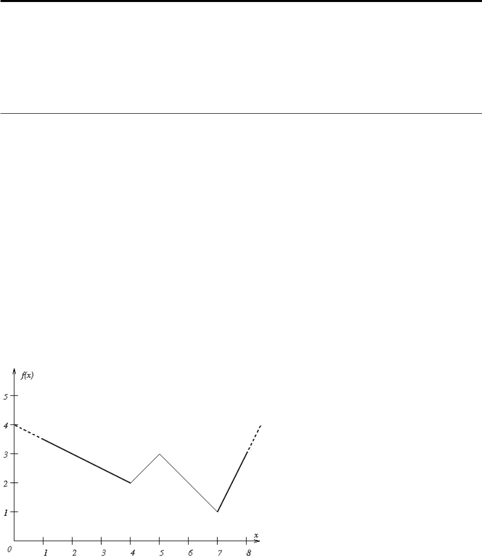
Chapter 22. Using piecewise linear functions in optimization:
a transport example
Demonstrates the use of piecewise linear functions to solve a transportation
problem.
What is a piecewise linear function?
Defines a piecewise linear function.
Some problems are most naturally represented by constraints over functions that
are not purely linear but consist of linear segments. Such functions are also known
as piecewise linear. In this topic, a transportation example shows you various ways
of stating and solving problems that lend themselves to a piecewise linear model.
Before plunging into the problem itself, this section defines a few terms appearing
in this discussion.
From a geometric point of view, Figure 10 shows a conventional piecewise linear
function f(x) . This particular function consists of four segments. If you consider
the function over four separate intervals, (-∞, 4) and [4, 5) and [5, 7) and [7,
∞), you see that f(x) is linear in each of those separate intervals. For that reason,
it is said to be piecewise linear. Within each of those segments, the slope of the
linear function is clearly constant, though it is different between segments. The
points where the slope of the function changes are known as breakpoints. The
piecewise linear function in Figure 10 has three breakpoints.
Piecewise linear functions are often used to represent or to approximate nonlinear
unary functions (that is, nonlinear functions of one variable). For example,
piecewise linear functions frequently represent situations where costs vary with
respect to quantity or gains vary over time.
Figure 10. A piecewise linear function with breakpoints
© Copyright IBM Corp. 1987, 2016 329

Syntax of piecewise linear functions
Describes the syntax to represent a piecewise linear function.
To define a piecewise linear function in Concert Technology, you need these
components:
vthe independent variable of the piecewise linear function;
vthe breakpoints of the piecewise linear function;
vthe slope of each segment (that is, the rate of increase or decrease of the function
between two breakpoints);
vthe geometric coordinates of at least one point of the function.
In other words, for a piecewise linear function of nbreakpoints, you need to know
n+1 slopes.
Typically, the breakpoints of a piecewise linear function are specified as an array of
numeric values. For example, the breakpoints of the function f(x) as it appears in
Figure 10 on page 329 are specified in this way, where the first argument, env ,
specifies the environment, the second argument specifies the number of
breakpoints under consideration, and the remaining arguments specify the
x-coordinate of the breakpoints:
IloNumArray (env, 3, 4., 5., 7.)
The slopes of its segments are indicated as an array of numeric values as well. For
example, the slopes of f(x) are specified in this way, where the first argument
again specifies the environment, the second argument specifies the number of
slopes given, and the remaining arguments specify the slope of the segments:
IloNumArray (env, 4, -0.5, 1., -1., 2.)
The geometric coordinates of at least one point of the function, (x, f(x)) must
also be specified; for example, (4, 2) . Then in Concert Technology, those
elements are brought together in an instance of the class IloPiecewiseLinear in
this way:
IloPiecewiseLinear(x,
IloNumArray(env, 3, 4., 5., 7.),
IloNumArray(env, 4, -0.5, 1., -1., 2.),
4, 2)
Another way to specify a piecewise linear function is to give the slope of the first
segment, two arrays for the coordinates of the breakpoints, and the slope of the
last segment. In this approach, the example f(x) from Figure 10 on page 329 looks
like this:
IloPiecewiseLinear(x, -0.5, IloNumArray(env, 3, 4., 5., 7.),
IloNumArray(env, 3, 2., 3., 1.), 2);
Note:
It may help you understand the signatures of these functions to recall the familiar
Cartesian representation of a line or segment in two dimensions, x and y:
y = ax + b
where a represents the slope of the line or segment and b represents the height at
which the line theoretically crosses the y-axis at the point (0, b).
330 CPLEX User’s Manual

Discontinuous piecewise linear functions
Defines a discontinuous piecewise linear function.
Thus far, you have seen a piecewise linear function where the segments are
continuous. Intuitively, in a continuous piecewise linear function, the endpoint of
one segment has the same coordinates as the initial point of the next segment, as
in Figure 10 on page 329. One way of defining a continuous piecewise linear
function is by specifying its breakpoints and the slope of each segment. Those
specification breakpoints are also known as the anchors of their segments.
There are piecewise linear functions, however, where the endpoint of one segment
and the initial point of the next segment may have the same xcoordinate but differ
in the value of f(x). Such a difference is known as a step in the piecewise linear
function, and such a function is known as discontinuous. Figure 11 on page 332
shows a discontinuous piecewise linear function with two steps.
Tip:
When the anchor of a segment resides at a step, then the discontinuous piecewise
linear function is not uniquely defined by specifying its breakpoints and the slopes
of its segments. In contrast, as long as the anchor point resides elsewhere, rather
than at a step, one can specify a discontinuous piecewise linear function by its
breakpoints and slopes as one specifies a continuous piecewise linear function.
Syntactically, a step is represented in this way:
vThe x-coordinate of the breakpoint where the step occurs is repeated in the array
of the breakpoint.
vThe value of the first point of a step in the array of slopes is the height of the
step. This value replaces the undefined slope of the vertical line associated with
the discontinuous step.
vThe value of the second point of the step in the array of slopes is the slope of
the function after the step.
Concert Technology also supports discontinuous piecewise linear functions
specified by the x-coordinate of the breakpoints and their associated function
values, along with the slopes of the first and last segments. This additional
information uniquely defines the function. At a step, the value of the x-coordinate
appears twice in the breakpoint array of the specification. The function values
associated with the bottom and top of the step appear in the corresponding entries
of the values array.
By convention, a breakpoint belongs in both segments associated with the step. For
example, in Figure 11 on page 332, at the breakpoint x=3 , the points (3,1) and
(3,3) are both admissible. Similarly, when x = 5 , the points (5,4) and (5,5) are
both admissible.
However, isolated points, as explained in “Isolated points in piecewise linear
functions” on page 333, are not allowed, neither in continuous nor in
discontinuous piecewise linear functions. In fact, only one step is allowed at a
given point.
Chapter 22. Using piecewise linear functions in optimization: a transport example 331
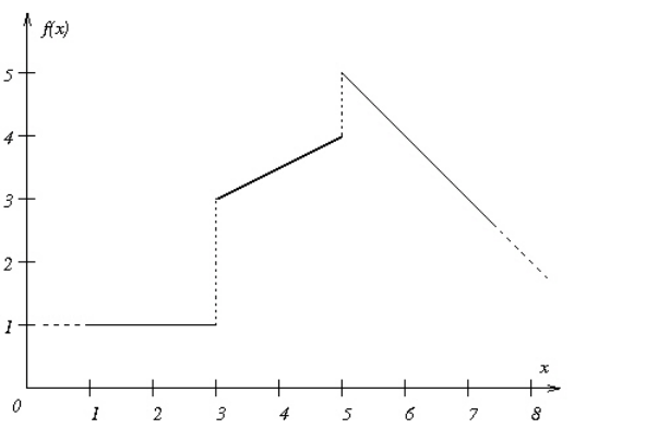
In Concert Technology, a discontinuous piecewise linear function is represented by
the overloaded functionIloPiecewiseLinear. For example, the function in Figure 11
is declared in this way, with the discontinuous step values (2 and 1) highlighted:
IloPiecewiseLinear(x,
IloNumArray(env, 4, 3. ,3. ,5. ,5.),
IloNumArray(env, 5, 0., 2., 0.5, 1., -1.),
0, 1);
The anchor point of (0,1) specified as the last two arguments does not reside at a
discontinuity in that example.
Similarly, one can specify the same discontinuous piecewise linear function using
breakpoints and values by providing the slope of the segment preceding the first
break point, arrays of the breakpoints and associated function values, and the slope
of the segment following the last breakpoint, like this:
IloPiecewiseLinear(x, 0.,
IloNumArray(env, 4, 3. ,3. ,5. ,5.),
IloNumArray(env, 4, 1., 3., 4., 5.),
-1.);
Note:
It may help to understand the signature of the function in this example to recall
that in Cartesian coordinates, the slope of a horizontal line (that is, a line or
segment parallel to the x-axis) is 0 (zero), and the slope of a vertical line (that is, a
line or segment parallel to the y-axis) is undefined in the conventional
representation:
y = ax + b
In the signature of the function, the undefined slope of the vertical segment at the
point of discontinuity is represented as the height of the step.
Figure 11. A discontinuous piecewise linear function with steps
332 CPLEX User’s Manual

Isolated points in piecewise linear functions
Defines an isolated point in a piecewise linear function.
When you specify the same point more than twice as you declare a piecewise
linear function, you inadvertently create an isolated point. IBM ILOG CPLEX does
not support isolated points. When it encounters an isolated point in the declaration
of a piecewise linear function, CPLEX issues a warning and ignores the isolated
point. An isolated point may appear as a visible point in the graph of a
discontinuous piecewise linear function. For example, the point (3, 2) would be
an isolated point in Figure 11 on page 332 and consequently ignored by CPLEX.
Isolated points may also be less conspicuously visible; for example, if the height of
a step in a discontinuous piecewise linear function is 0 (zero), the isolated point
overlaps with an endpoint of two other segments, and consequently, the isolated
point will be ignored by CPLEX.
Using IloPiecewiseLinear in expressions
Describes a piecewise linear function as an expression.
Whether it represents a continuous or a discontinuous piecewise linear function, an
instance of IloPiecewiseLinear behaves like a floating-point expression. That is,
you may use it in a term of a linear expression or in a constraint added to a model
(an instance of IloModel).
Describing the problem
Demonstrates a problem for which piecewise linear functions are suitable.
Problem statement
Describes a model using piecewise linear functions.
Assume that a company must ship cars from factories to showrooms. Each factory
can supply a fixed number of cars, and each showroom needs a fixed number of
cars. There is a cost for shipping a car from a given factory to a given showroom.
The objective is to minimize the total shipping cost while satisfying the demands
and respecting supply.
In concrete terms, assume there are three factories and four showrooms. Here is
the quantity that each factory can supply:
supply0 = 1000
supply1 = 850
supply2 = 1250
Each showroom has a fixed demand:
demand0 = 900
demand1 = 1200
demand2 = 600
demand3 = 400
Let nbSupply be the number of factories and nbDemand be the number of
showrooms. Let x ij be the number of cars shipped from factory ito showroom j
. The model is composed of nbDemand + nbSupply constraints that force all demands
to be satisfied and all supplies to be shipped. Thus far, a model for our problem
looks like this:
Chapter 22. Using piecewise linear functions in optimization: a transport example 333
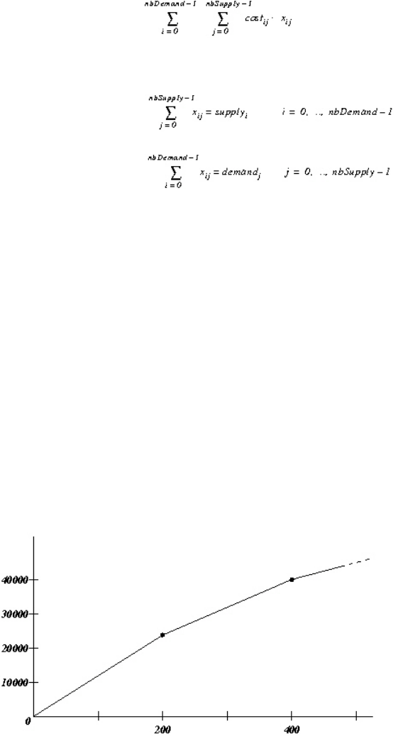
Minimize
subject to
Variable shipping costs
Distinguishes convex from concave piecewise linear functions.
Now consider the costs of shipping from a given factory to a given showroom.
Assume that for every pair (factory, showroom), there are different rates, varying
according to the quantity shipped. To illustrate the difference between convex and
concave piecewise linear functions, in fact, this example assumes that there are two
different tables of rates for shipping cars from factories to showrooms. The first
table of rates looks like this:
va rate of 120 per car for quantities between 0 and 200;
va rate of 80 per car for quantities between 200 and 400;
va rate of 50 per car for quantities higher than 400.
These costs that vary according to quantity define the piecewise linear function
represented in Figure 12. As you see, the slopes of the segments of that function
are decreasing, so that function is concave.
Also assume that there is a second table of rates for shipping cars from factories to
showrooms. The second table of rates looks like this:
va rate of 30 per car for quantities between 0 and 200;
va rate of 80 per car for quantities between 200 and 400;
va rate of 130 per car for quantities higher than 400.
Figure 12. A concave piecewise linear cost function
334 CPLEX User’s Manual
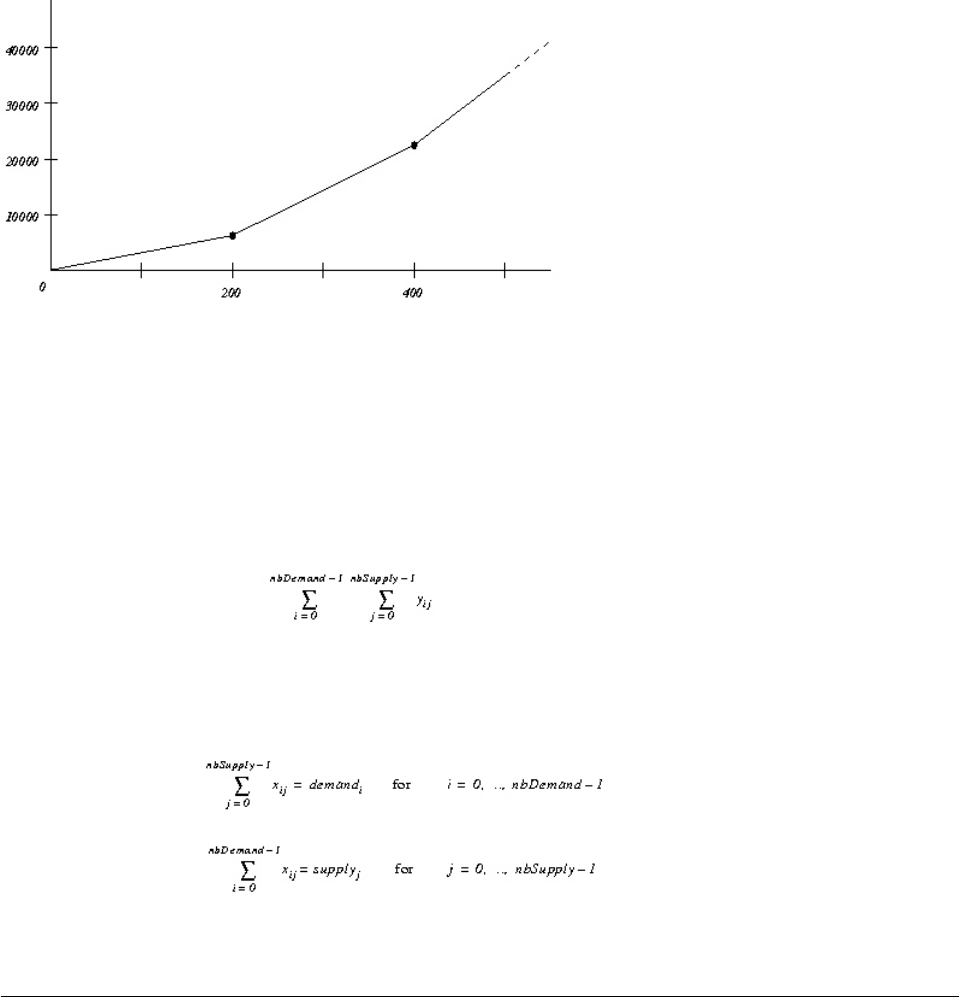
The costs in this second table of rates that vary according to the quantity of cars
shipped define a piecewise linear function, too. It appears in Figure 13. The slopes
of the segments in this second piecewise linear function are increasing, so this
function is convex.
Model with varying costs
Describes syntax to represent varying costs in the model.
With this additional consideration about costs varying according to quantity, our
model now looks like this:
Minimize
subject to
yij =,(x ij )for i = 0, ..., nbDemand-1 and j = 0, ..., nbSupply-1
With this problem in mind, consider how to represent the data and model in
Concert Technology.
Developing a model
Describes an application using piecewise linear functions.
Creating the environment and model
Describes creation of the environment and model in the application.
Figure 13. A convex piecewise linear cost function
Chapter 22. Using piecewise linear functions in optimization: a transport example 335
As in other examples in this manual, this application begins by creating an
environment, an instance of IloEnv.
IloEnv env;
Within that environment, a model for this problem is created as an instance of
IloModel.
IloModel model(env);
Then constraints and an objective are added to the model. The following sections
sketch these steps.
Representing the data
Describes populating the model with data.
As in other examples, the template class IloArray appears in a type definition to
create matrices for this problem, like this:
typedef IloArray<IloNumArray> NumMatrix;
typedef IloArray<IloNumVarArray> NumVarMatrix;
Those two-dimensional arrays (that is, arrays of arrays) are now available in the
application to represent the demands from the showrooms and the supplies
available from the factories.
IloInt nbDemand = 4;
IloInt nbSupply = 3;
IloNumArray supply(env, nbSupply, 1000., 850., 1250.);
IloNumArray demand(env, nbDemand, 900., 1200., 600., 400.);
NumVarMatrix x(env, nbSupply);
NumVarMatrix y(env, nbSupply);
for(i = 0; i < nbSupply; i++){
x[i] = IloNumVarArray(env, nbDemand, 0, IloInfinity, ILOFLOAT);
y[i] = IloNumVarArray(env, nbDemand, 0, IloInfinity, ILOFLOAT);
}
Adding constraints
Describes adding constraints in the application.
According to the description of the problem, the supply of cars from the factories
must meet the demand of the showrooms. At the same time, it is important not to
ship cars that are not in demand; in terms of this model, the demand should meet
the supply as well. Those ideas are represented as constraints added to the model,
like this:
for(i = 0; i < nbSupply; i++) { // supply must meet demand
model.add(IloSum(x[i]) == supply[i]);
}
for(j = 0; j < nbDemand; j++) { // demand must meet supply
IloExpr v(env);
for(i = 0; i < nbSupply; i++)
v += x[i][j];
model.add(v == demand[j]);
v.end();
}
Checking convexity and concavity
Describes data checking in the application to detect convexity and concavity.
336 CPLEX User’s Manual

To illustrate the ideas of convex and concave piecewise linear functions, two tables
of costs that vary according to the quantity of cars shipped were introduced in the
problem description. To accommodate those two tables in the model, the following
lines are added.
if (convex) {
for(i = 0; i < nbSupply; i++){
for(j = 0; j < nbDemand; j++){
model.add(y[i][j] == IloPiecewiseLinear(x[i][j],
IloNumArray(env, 2, 200.0, 400.0),
IloNumArray(env, 3, 30.0, 80.0, 130.0),
0.0, 0.0));
}
}
}else{
for(i = 0; i < nbSupply; i++){
for(j = 0; j < nbDemand; j++){
model.add(y[i][j] == IloPiecewiseLinear(x[i][j],
IloNumArray(env, 2, 200.0, 400.0),
IloNumArray(env, 3, 120.0, 80.0, 50.0),
0.0, 0.0));
}
}
}
Adding an objective
Describes adding an objective function to the application.
The objective is to minimize costs of supplying cars from factories to showrooms,
It is added to the model in these lines:
IloExpr obj(env);
for(i = 0; i < nbSupply; i++){
obj += IloSum(y[i]);
}
model.add(IloMinimize(env, obj));
obj.end();
Solving the problem
Describes activity in the application.
The following lines create an algorithm (an instance of IloCplex ) in an
environment (an instance of IloEnv ) and extract the model (an instance of
IloModel ) for that algorithm to find a solution.
IloCplex cplex(env);
cplex.extract(model);
cplex.exportModel("transport.lp");
cplex.solve();
Displaying a solution
Describes display of the solution from the application.
To display the solution, use the methods of IloEnv and IloCplex.
env.out() << ’’ - Solution: ’’ << endl;
for(i = 0; i < nbSupply; i++){
env.out() << ’’ ’’ << i << ’’:’’;
for(j = 0; j < nbDemand; j++){
env.out() << cplex.getValue(x[i][j]) << ’’\t’’;
}
Chapter 22. Using piecewise linear functions in optimization: a transport example 337

env.out() << endl;
}
env.out() << ’’ Cost = ’’ << cplex.getObjValue() << endl;
Ending the application
Describes memory management in the application.
As in other C++ examples in this manual, the application ends with a call to the
method IloEnv::end to clean up the memory allocated for the environment and
algorithm.
env.end();
Complete program: transport.cpp
Tells where the sample application in C++ is located and where to find variations
in other APIs.
You can see the complete program online in the standard distribution of CPLEX at
yourCPLEXinstallation/examples/src/transport.cpp.
You will also find Transport.java in yourCPLEXinstallation /examples/src/. If your
installation includes the .NET API of CPLEX, then you will also find the C#.NET
implementation of this example in Transport.cs. Likewise, you will find
transport.py implementing this problem and using piecewise linear constraints in
Python.
338 CPLEX User’s Manual

Chapter 23. Indicator constraints in optimization
Introduces indicator constraints and emphasizes their advantages over Big M
formulations.
What is an indicator constraint?
Defines indicator constraints.
An indicator constraint is a way for a user of the Callable Library (C API) or
Python API to express relationships among variables by identifying a binary
variable to control whether or not a specified linear constraint is active. This
feature is also available in the Interactive Optimizer, as explained in “Indicator
constraints in the Interactive Optimizer” on page 340.
Formulations using indicator constraints can be more numerically robust and
accurate than conventional formulations involving so-called Big M data if the Big
M formulations use artificial data to turn on or turn off enforcement of a
constraint. Such Big M formulations often exhibit trickle flow, and sometimes they
behave in unstable ways. Replacement of such formulations with indicator
constraints enables CPLEX either to branch explicitly on the indicator constraint, or
to use MIP preprocessing to derive a tighter value of Big M that makes the
formulation more stable.
In Concert Technology applications, CPLEX automatically uses indicator
constraints for you when it encounters a constraint within an expression and when
it encounters expressions which can be linearized, including the following:
vIloAnd or Cplex.And
vIloOr or Cplex.Or
vIloNot or Cplex.Not
vIloIfThen or Cplex.IfThen
vusing a constraint as a binary variable itself
You may recognize those expressions as logical constraints. For more information
about logical constraints in the object-oriented application programming interfaces,
see the topic Chapter 24, “Logical constraints in optimization,” on page 343 in this
manual.
In Callable Library applications, you can invoke the routine CPXaddindcontr
yourself to introduce indicator constraints in your model. To remove an indicator
constraint that you have added, use the routine CPXdelindconstr.
In the Python API, you can introduce an indicator constraint in your model by
means of the method indicator_constraints.add.
Further reading
IBM Tech Note: Difference between using indicator constraints and a big-M
formulation
Paul Rubin's comprehensive blog about the perils of Big M
© Copyright IBM Corp. 1987, 2016 339

Example: fixnet.c
Illustrates indicator constraints in an application of the C API.
For an example of indicator constraints in use, see fixnet.c among the examples
distributed with the product. This example shows a model of a fixed-charge
problem using indicator constraints.
Indicator constraints in the Interactive Optimizer
Contrasts indicator constraints with a Big M formulation in the Interactive
Optimizer.
In the Interactive Optimizer, you can include indicator constraints among the
usual linear constraints in LP-file format. You can also use the commands enter
and add with indicator constraints. For example, you could declare y as a binary
variable and enter the following:
constr01: y = 0 -> x1 + x2 + x3 = 0
In plain English, that indicator constraint states that if yis 0 (zero), then x1 + x2 +
x3 must be 0 (zero). Likewise, if x1 + x2 + x3 is not 0 (zero), then ymust be 1
(one).
That formulation of an indicator constraint is recommended instead of the
following Big M formulation:
constr01: x1 + x2 + x3 - 1e+9 y <= 0 // not recommended
That Big M formulation relies on the xvalues summing to less than the Big M
value (in this case, one billion). Such an assumption may cause numeric instability
or undesirable solutions in certain circumstances, whereas a model with the
indicator constraint, by contrast, introduces no new assumptions about upper
bounds. In that respect, the use of indicator constraints instead of a Big M
formulation offers a more numerically stable model, closer to the mathematical
programming issues of the problem, and thus more likely to produce useful
solutions of the problem.
What are indicator variables?
Defines an indicator variable and directs you to an example.
The binary variable introduced in an indicator constraint is known as an indicator
variable. Usually, an indicator variable will also appear in the objective function or
in other constraints. For example, in fixnet.c, the indicator variables fappear in
the objective function to represent the cost of building an arc. In fact, an indicator
variable introduced in one indicator constraint may appear again in another,
subsequent indicator constraint.
Restrictions on indicator constraints
Describes limitations on indicator constraints.
There are a few restrictions regarding indicator constraints:
vThe constraint must be linear; a quadratic constraint is not allowed to have an
indicator constraint.
vA lazy constraint cannot have an indicator constraint.
340 CPLEX User’s Manual

vA user-defined cut cannot have an indicator constraint.
vOnly z=0 (zero) or z=1 (one) is allowed for the indicator variable because the
indicator constraint implies that the indicator variable is binary.
CPLEX does not impose any arbitrary limit on the number of indicator constraints
or indicator variables that you introduce, but there may be practical limits due to
resources available on your platform.
Best practices with indicator constraints
Suggests best practices with respect to indicator constraints.
The following points summarize best practices with indicator constraints in
Callable Library applications:
vAvoid Big M values if at all possible. If you choose to introduce Big M values in
your model anyway, use the smallest possible value of Big M because Big M
values create numerical difficulties and can introduce trickle-flow problems in
node LP solutions.
vUse indicator constraints instead of Big M when Big M values in the formulation
cannot be reduced.
vDo not introduce indicator constraints if Big M can be eliminated from your
model.
vDo not introduce indicator constraints if Big M is eliminated by preprocessing.
Check the presolved model to determine whether Big M has been eliminated
from your model by preprocessing. In that case, do not introduce indicator
constraints for that Big M.
vIf valid upper bounds on continuous variables are available, use them. Bounds
strengthen LP relaxations. Bounds are used in a MIP for fixing and so forth.
Chapter 23. Indicator constraints in optimization 341
342 CPLEX User’s Manual

Chapter 24. Logical constraints in optimization
Describes logical constraints in CPLEX with Concert Technology.
What are logical constraints?
Defines logical constraints.
For IBM ILOG CPLEX, a logical constraint combines linear constraints by means of
logical operators, such as logical-and, logical-or, negation (that is, not), conditional
statements (that is, if ... then ...) to express complex relations between linear
constraints. CPLEX can also handle certain logical expressions appearing within a
linear constraint. One such logical expression is the minimum of a set of variables.
Another such logical expression is the absolute value of a variable. There’s more
about logical expressions in “Which nonlinear expressions can be extracted?” on
page 345.
Formulations using logical constraints can be more numerically robust and
accurate than conventional formulations involving so-called Big M data if the Big
M formulations use artificial data to express the constraint. Such Big M
formulations often exhibit trickle flow, and sometimes they behave in unstable
ways. Replacement of such formulations with logical constraints enables CPLEX®
either to branch more directly on the logical constraint, or to use MIP
preprocessing to derive a tighter value of Big M that makes the formulation more
stable.
Concert Technology can automatically translate logical constraints into their
transformed equivalent that the discrete (that is, MIP) or continuous (LP)
optimizers of CPLEX can process efficiently in the C++, Java, or .NET APIs.
In the Callable Library, indicator constraints provide a similar facility. For more
about that idea, see Chapter 23, “Indicator constraints in optimization,” on page
339 in this manual.
What can be extracted from a model with logical constraints?
Documents the logical constraints available in each API.
Overview
Introduces logical constraints in the context of extraction.
Concert Technology offers classes for you to design a model of your problem, of
course. You can then invoke an algorithm to extract information from your model
to solve the problem. In this context, an algorithm is an instance of a class such as
IloCplex, documented in the CPLEX Reference Manuals of the C++ and Java APIs,
or of the class CPLEX, documented in the CPLEX Reference Manual of the .NET API.
For more about this idea of extraction generally, see topics in Part 1, “Languages
and APIs,” on page 1, or see the concept of Extraction in the CPLEX Reference
Manual of the C++ API.
© Copyright IBM Corp. 1987, 2016 343
When your model contains certain logical operators and conditional statements,
Concert Technology extracts them as logical constraints appropriately. Much the
same logical constraints are available in these APIs of CPLEX.
v“Logical constraints in the C++ API”
v“Logical constraints in the Java API” on page 345
v“Logical constraints in the .NET API” on page 345
For similar facilities in the Callable Library, see Chapter 23, “Indicator constraints
in optimization,” on page 339.
Logical constraints in the C++ API
Describes logical constraints in the C++ API.
In C++ applications, the class IloCplex can extract modeling objects to solve a
wide variety of MIPs, as you see in “Solving the model” on page 9, summarized in
the table in “Overview” on page 9. In fact, the C++ class IloCplex can extract
logical constraints as well as some logical expressions. The logical constraints that
IloCplex can extract are these:
vIloAnd
vIloOr
vIloNot
vIloIfThen
vIloDiff
v== that is, the equivalence relation
Among those extractable objects, IloAnd IloOr , IloNot , and IloDiff can also be
represented in your application by means of the overloaded C++ operators:
v|| (for IloOr )
v&& (for IloAnd )
v!(for IloNot )
v!= that is, the exclusive-or relation (for IloDiff )
All those extractable objects accept as their arguments other linear constraints or
logical constraints, so you can combine linear constraints with logical constraints in
complicated expressions in your application.
For example, to express the idea that two jobs with starting times x1 and x2 and
with duration d1 and d2 must not overlap, you can either use overloaded C++
operators, like this:
model.add((x1 >= x2 + d2) || (x2 >= x1 + d1));
or you can express the same idea, like this:
IloOr or(env)
or.add(x1 >= x2 + d2);
or.add(x2 >= x1 + d1);
model.add(or);
Since IloCplex can also extract logical constraints embedded in other logical
constraints, you can also write logical constraints like this:
IloIfThen(env, (x >= y && x >= z), IloNot(x <= 300 || y >= 700))
where x, y, and zare variables in your application.
344 CPLEX User’s Manual

Logical constraints in the Java API
Describes logical constraints in the Java API.
Of course, because the Java programming language does not support the
overloading of operators as C++ does, overloaded logical operators are not
supported in the Java API of Concert Technology. However, the Java class
IloCplexModeler offers logical modeling facilities through methods, such as:
vIloCplexModeler.and
vIloCplexModeler.or
vIloCplexModeler.not
vIloCplexModeler.ifThen
Moreover, like their C++ counterparts, those extractable Java objects accept as their
arguments other linear constraints or logical constraints, so you can combine linear
constraints with logical constraints in complicated expressions in your Java
application.
Logical constraints in the .NET API
Describes logical constraints in the .NET API.
Similarly, the .NET API of Concert Technology supports logical constraints, though
not operator overloading. The .NET class Cplex offers these overloaded logical
methods:
vCplex.And
vCplex.Or
vCplex.Not
vCplex.IfThen
Again, those extractable .NET objects accept other linear constraints or logical
constraints as their arguments, thus making it possible for you to combine linear
constraints with logical constraints in expressions in your .NET applications.
Which nonlinear expressions can be extracted?
Describes certain nonlinear expressions as logical constraints.
Some expressions are easily recognized as nonlinear, for example, a function such
as x2+ y2≤1. However, other nonlinearities are less obvious, such as absolute
value as a function. In a very real sense, MIP is a class of nonlinearly constrained
problems because the integrality restriction destroys the property of convexity
which any linear constraints otherwise might possess. Because of that
characteristic, certain (although not all) nonlinearities are capable of being
converted to a MIP formulation, and thus can be solved by CPLEX. In fact,
IloCplex can extract the following nonlinear expressions in a C++ application:
vIloMin the minimum of an array of numeric expressions or over a numeric
expression and a constant in C++
vIloMax the maximum of an array of numeric expressions or over a numeric
expression and a constant in C++
vIloAbs the absolute value of a numeric expression
vIloPiecewiseLinear the piecewise linear combination of a numeric expression,
vA linear constraint can appear as a term in a logical constraint.
Chapter 24. Logical constraints in optimization 345

For example, given these variables and arrays:
IloIntVarArray x(env, 5, 0, 1000);
IloNumVar y(env, -1000, 5000);
IloNumVar z(env, -1000, 1000);
IloCplex in a C++ application recognizes the following constraint as valid and
extracts it:
IloMin(x) >= IloAbs(y)
In fact, ranges containing logical expressions can, in turn, appear in logical
constraints. For example, the following constraint is valid and extractable by
IloCplex:
IloIfThen(env, (IloAbs(y) <= 100), (z <= 300));
It is important to note here that only linear constraints can appear as arguments of
logical constraints extracted by CPLEX. That is, quadratic constraints are not
handled in logical constraints. Similarly, quadratic terms can not appear as
arguments of logical expressions such as IloMin, IloMax, IloAbs, and
IloPiecewiseLinear.
Logical constraints for counting
Describes cardinality (counting) as a logical constraint.
In many cases it is even unnecessary to allocate binary variables explicitly in order
to gain the benefit of linear constraints within logical expressions. For example,
optimizing how many items appear in a solution is often an issue in practical
problems. Questions of counting (how many?) can be represented formally as
cardinality constraints.
Suppose that your application includes three variables, each representing a
quantity of one of three products, and assume further that a good solution to the
problem means that the quantity of at least two of the three products must be
greater than 20. Then you can represent that idea in your application, like this:
IloNumVarArray x(env, 3, 0, 1000);
model.add((x[0] >= 20) + (x[1] >= 20) + (x[2] >= 20) >= 2);
Logical constraints as binary variables
Describes logical constraints as terms in expressions.
Linear or logical constraints can appear as terms in numeric expressions. A linear
constraint appearing as a term in a numeric expression behaves like a binary value.
For example, given xand yas variables, you can write the following lines to get
the truth value of x≥yin a binary value:
IloIntVar b(env, 0, 1);
model.add(b == (x >= y));
It is important to note here that only linear constraints can appear as arguments of
logical constraints extracted by IloCplex. That is, quadratic constraints are not
handled in logical constraints. Similarly, quadratic terms cannot appear as
arguments of logical expressions such as IloMin, IloMax, IloAbs, and
IloPiecewiseLinear.
346 CPLEX User’s Manual

How are logical constraints extracted?
Describes extraction of logical constraints as indicators.
Logical constraints are transformed automatically into equivalent linear
formulations when they are extracted by a CPLEX algorithm. This transformation
involves automatic creation by CPLEX of new variables and constraints. The
transformation entails indicators as discussed in Chapter 23, “Indicator constraints
in optimization,” on page 339.
Chapter 24. Logical constraints in optimization 347
348 CPLEX User’s Manual

Chapter 25. Using logical constraints: Food Manufacture 2
Demonstrates logical constraints in a sample application.
Introducing the example
Introduces an example from food manufacturing to illustrate logical constraints.
Chapter 24, “Logical constraints in optimization,” on page 343 introduced features
of IBM ILOG CPLEX that transform parts of your problem automatically for you.
This topic shows you some of those features in use in a C++ application. The
example is based on the formulation by H.P. Williams of a standard industrial
problem in food manufacturing. The aim of the problem is to blend a number of
oils cost effectively in monthly batches. In this form of the problem, formulated by
Williams as food manufacturing 2 in his book Model Building in Mathematical
Programming, the number of ingredients in a blend must be limited, and extra
conditions are added to govern which oils can be blended.
Describing the problem
Describes the problem verbally.
The problem is to plan the blending of five kinds of oil, organized in two
categories (two kinds of vegetable oils and three kinds of non vegetable oils) into
batches of blended products over six months.
Some of the oil is already available in storage. There is an initial stock of oil of 500
tons of each raw type when planning begins. An equal stock should exist in
storage at the end of the plan. Up to 1000 tons of each type of raw oil can be
stored each month for later use. The price for storage of raw oils is 5 monetary
units per ton. Refined oil cannot be stored. The blended product cannot be stored
either.
The rest of the oil (that is, any not available in storage) must be bought in
quantities to meet the blending requirements. The price of each kind of oil varies
over the six-month period.
The two categories of oil cannot be refined on the same production line. There is a
limit on how much oil of each category (vegetable or non vegetable) can be refined
in a given month:
vNot more than 200 tons of vegetable oil can be refined per month.
vNot more than 250 tons of non vegetable oil can be refined per month.
There are constraints on the blending of oils:
vThe product cannot blend more than three oils.
vWhen a given type of oil is blended into the product, at least 20 tons of that
type must be used.
vIf either vegetable oil 1 (v1) or vegetable oil 2 (v2) is blended in the product,
then non vegetable oil 3 (o3) must also be blended in that product.
© Copyright IBM Corp. 1987, 2016 349

The final product (refined and blended) sells for a known price: 150 monetary
units per ton.
The aim of the six-month plan is to maximize profit by lowering production and
storage costs.
Representing the data
Raises questions pertinent to a sound representation of the data of the problem.
To represent the problem accurately, there are several questions to consider:
vWhat is known about the problem?
vWhat are the unknowns of the problem?
vWhat are the constraints of the problem?
vWhat is the objective of the problem?
What is known?
In this particular example, the planning period is six months, and there are five
kinds of oil to be blended. Those details are represented as constants, like this:
const IloInt nbMonths = 6;
const IloInt nbProducts = 5;
The five kinds of oil (vegetable and non vegetable) are represented by an
enumeration, like this:
typedef enum { v1, v2, o1, o2, o3 } Product;
The varying price of the five kinds of oil over the six-month planning period is
represented in a numeric matrix, like this:
NumMatrix cost(env, nbMonths);
cost[0]=IloNumArray(env, nbProducts, 110.0, 120.0, 130.0, 110.0, 115.0);
cost[1]=IloNumArray(env, nbProducts, 130.0, 130.0, 110.0, 90.0, 115.0);
cost[2]=IloNumArray(env, nbProducts, 110.0, 140.0, 130.0, 100.0, 95.0);
cost[3]=IloNumArray(env, nbProducts, 120.0, 110.0, 120.0, 120.0, 125.0);
cost[4]=IloNumArray(env, nbProducts, 100.0, 120.0, 150.0, 110.0, 105.0);
cost[5]=IloNumArray(env, nbProducts, 90.0, 100.0, 140.0, 80.0, 135.0);
That matrix could equally well be filled by data read from a file in a large-scale
application.
What is unknown?
The variables of the problem can be represented in arrays:
vHow much blended, refined oil to produce per month?
vHow much raw oil to use per month?
vHow much raw oil to buy per month?
vHow much raw oil to store per month?
like this:
IloNumVarArray produce(env, nbMonths, 0, IloInfinity);
NumVarMatrix use(env, nbMonths);
NumVarMatrix buy(env, nbMonths);
NumVarMatrix store(env, nbMonths);
IloInt i, p;
for (i = 0; i < nbMonths; i++) {
350 CPLEX User’s Manual
use[i] = IloNumVarArray(env, nbProducts, 0, IloInfinity);
buy[i] = IloNumVarArray(env, nbProducts, 0, IloInfinity);
store[i] = IloNumVarArray(env, nbProducts, 0, 1000);
}
In those lines, the type NumVarMatrix is defined as:
typedef IloArray<IloNumVarArray> NumVarMatrix ;
Notice that how much to use and buy is initially unknown, and thus has an
infinite upper bound, whereas the amount of oil that can be stored is limited, as
you know from the description of the problem. Consequently, one of the
constraints is expressed here as the upper bound of 1000 on the amount of oil by
type that can be stored per month.
What are the constraints?
As you know from “Describing the problem” on page 349, there are various
constraints in this problem.
For each type of oil, there must be 500 tons in storage at the end of the plan. That
idea can be expressed like this:
for (p = 0; p < nbProducts; p++) {
store[nbMonths-1][p].setBounds(500, 500);
}
The constraints on production in each month can all be expressed as statements in
a for-loop:
vNot more than 200 tons of vegetable oil can be refined.
model.add(use[i][v1] + use[i][v2] <= 200);
vNot more than 250 tons of non-vegetable oil can be refined.
model.add(use[i][o1] + use[i][o2] + use[i][o3] <= 250);
vA blend cannot use more than three oils; or equivalently, of the five oils, two
cannot be used in a given blend.
model.add((use[i][v1] == 0) +
(use[i][v2] == 0) +
(use[i][o1] == 0) +
(use[i][o2] == 0) +
(use[i][o3] == 0) >= 2);
vBlends composed of vegetable oil 1 (v1) or vegetable oil 2 (v2) must also include
non vegetable oil 3 (o3).
model.add(IloIfThen(env, (use[i][v1] >= 20) || (use[i][v2] >= 20),
use[i][o3] >= 20));
vThe constraint that if an oil is used at all in a blend, at least 20 tons of it must be
used is expressed like this:
for (p = 0; p < nbProducts; p++)
model.add((use[i][p] == 0) || (use[i][p] >= 20));
Note:
Alternatively, you could use semi-continuous variables.
vThe fact that a limited amount of raw oil can be stored for later use is expressed
like this:
if (i == 0) {
for (IloInt p = 0; p < nbProducts; p++)
model.add(500 + buy[i][p] == use[i][p] + store[i][p]);
Chapter 25. Using logical constraints: Food Manufacture 2 351

}
else {
for (IloInt p = 0; p < nbProducts; p++)
model.add(store[i-1][p] + buy[i][p] ==
use[i][p] + store[i][p]);
}
What is the objective?
On a monthly basis, the profit can be represented as the sale price per ton (150)
multiplied by the amount produced minus the cost of production and storage, like
this, where profit is defined as IloExpr profit(env);:
profit += 150 * produce[i] - IloScalProd(cost[i],
buy[i]) - 5 * IloSum(store[i]);
Developing the model
Describes creation of the model for the problem.
First, create the model, like this:
IloModel model(env);
Then use a for-loop to add the constraints for each month (from “Representing the
data” on page 350: What are the constraints?), like this:
IloExpr profit(env);
for (i = 0; i < nbMonths; i++) {
model.add(use[i][v1] + use[i][v2] <= 200);
model.add(use[i][o1] + use[i][o2] + use[i][o3] <= 250);
model.add(3 * produce[i] <=
8.8 * use[i][v1] + 6.1 * use[i][v2] +
2 * use[i][o1] + 4.2 * use[i][o2] + 5 * use[i][o3]);
model.add(8.8 * use[i][v1] + 6.1 * use[i][v2] +
2 * use[i][o1] + 4.2 * use[i][o2] + 5 * use[i][o3]
<= 6 * produce[i]);
model.add(produce[i] == IloSum(use[i]));
if (i == 0) {
for (IloInt p = 0; p < nbProducts; p++)
model.add(500 + buy[i][p] == use[i][p] + store[i][p]);
}
else {
for (IloInt p = 0; p < nbProducts; p++)
model.add(store[i-1][p] + buy[i][p] == use[i][p] + store[i][p]);
}
profit += 150 * produce[i]
- IloScalProd(cost[i], buy[i])
- 5 * IloSum(store[i]);
model.add((use[i][v1] == 0) + (use[i][v2] == 0) + (use[i][o1] == 0) +
(use[i][o2] == 0) + (use[i][o3] == 0) >= 2);
for (p = 0; p < nbProducts; p++)
model.add((use[i][p] == 0) || (use[i][p] >= 20));
model.add(IloIfThen(env, (use[i][v1] >= 20) || (use[i][v2] >= 20),
use[i][o3] >= 20));
}
To consolidate the monthly objectives, add the overall objective to the model, like
this:
model.add(IloMaximize(env, profit));
352 CPLEX User’s Manual

Formulating logical constraints
Contrasts conventional formulation of constraints with more efficient logical
constraints.
You have already seen how to represent the logical constraints of this problem in
“Representing the data” on page 350: What are the constraints? However, they
deserve a second glance because they illustrate an important point about logical
constraints and their automatic transformation in CPLEX.
// Logical constraints
// The food cannot use more than 3 oils
// (or at least two oils must not be used)
model.add((use[i][v1] == 0) + (use[i][v2] == 0) + (use[i][o1] == 0) +
(use[i][o2] == 0) + (use[i][o3] == 0) >= 2);
// When an oil is used, the quantity must be at least 20 tons
for (p = 0; p < nbProducts; p++)
model.add((use[i][p] == 0) || (use[i][p] >= 20));
// If products v1 or v2 are used, then product o3 is also used
model.add(IloIfThen(env, (use[i][v1] >= 20) || (use[i][v2] >= 20),
use[i][o3] >= 20));
Consider, for example, the constraint that the blended product cannot use more
than three oils in a batch. Given that constraint, many programmers might
naturally write the following statement (or something similar) in C++:
model.add ( (use[i][v1] != 0)
+ (use[i][v2] != 0)
+ (use[i][o1] != 0)
+ (use[i][o2] != 0)
+ (use[i][o3] != 0)
<= 3);
That statement expresses the same constraint without changing the set of solutions
to the problem. However, the formulations are different and can lead to different
running times and different amounts of memory used for the search tree. In other
words, given a logical English expression, there may be more than one logical
constraint for expressing it, and the different logical constraints may perform
differently in terms of computing time and memory.
Chapter 24, “Logical constraints in optimization,” on page 343 introduced
overloaded logical operators that you can use to combine linear, semi-continuous,
or piecewise linear constraints in CPLEX. In this example, notice the overloaded
logical operators == , >= , || that appear in these logical constraints.
Solving the problem
Describes activity in the application, display of the solution, and memory
management.
The following statement solves the problem to optimality:
if (cplex.solve()) {
These lines (the action of the if-statement) display the solution:
cout << " Maximum profit = " << cplex.getObjValue() << endl;
for (IloInt i = 0; i < nbMonths; i++) {
IloInt p;
cout << " Month " << i << " " << endl;
cout << " . buy ";
for (p = 0; p < nbProducts; p++) {
cout << cplex.getValue(buy[i][p]) << "\t ";
Chapter 25. Using logical constraints: Food Manufacture 2 353
}
cout << endl;
cout << " . use ";
for (p = 0; p < nbProducts; p++) {
cout << cplex.getValue(use[i][p]) << "\t ";
}
cout << endl;
cout << " . store ";
for (p = 0; p < nbProducts; p++) {
cout << cplex.getValue(store[i][p]) << "\t ";
}
cout << endl;
}
}
else {
cout << " No solution found" << endl;
Like other C++ applications using CPLEX with Concert Technology, this one ends
with a call to free the memory used by the environment.
env.end();
354 CPLEX User’s Manual

Chapter 26. Using column generation: a cutting stock
example
Uses an example of cutting stock to demonstrate the technique of column
generation in Concert Technology.
What is column generation?
Defines column generation.
In colloquial terms, column generation is a way of beginning with a small,
manageable part of a problem (specifically, a few of the variables), solving that
part, analyzing that partial solution to discover the next part of the problem
(specifically, one or more variables) to add to the model, and then resolving the
enlarged model. Column generation repeats that process until it achieves a
satisfactory solution to the whole of the problem.
In formal terms, column generation is a way of solving a linear programming
problem that adds columns (corresponding to constrained variables) during the
pricing phase of the simplex method of solving the problem. In gross terms,
generating a column in the primal simplex formulation of a linear programming
problem corresponds to adding a constraint in its dual formulation. In the dual
formulation of a given linear programming problem, you might think of column
generation as a cutting plane method.
In that context, many researchers have observed that column generation is a very
powerful technique for solving a wide range of industrial problems to optimality
or to near optimality. Ford and Fulkerson, for example, suggested column
generation in the context of a multi-commodity network flow problem as early as
1958 in the journal of Management Science. By 1960, Dantzig and Wolfe had
adapted it to linear programming problems with a decomposable structure.
Gilmore and Gomory then demonstrated its effectiveness in a cutting stock
problem. More recently, vehicle routing, crew scheduling, and other
integer-constrained problems have motivated further research into column
generation.
Column generation rests on the fact that in the simplex method, the solver does
not need access to all the variables of the problem simultaneously. In fact, a solver
can begin work with only the basis (a particular subset of the constrained
variables) and then use reduced cost to decide which other variables to access as
needed.
Column-wise models in Concert Technology
Describes features of Concert Technology to support column generation.
Concert Technology offers facilities for exploiting column generation. In particular,
you can design the model of your problem (one or more instances of the class
IloModel) in terms of columns (instances of IloNumVar, IloNumVarArray,
IloNumColumn, or IloNumColumnArray). For example, instances of IloNumColumn
represent columns, and you can use the operator()in the classes IloObjective and
IloRange to create terms in column expressions. In practice, the column serves as a
© Copyright IBM Corp. 1987, 2016 355
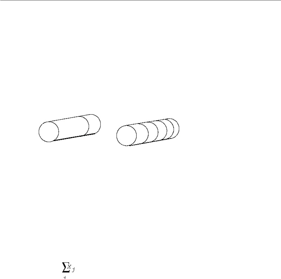
place holder for a variable in other extractable objects (such as a range constraint
or an objective) when your application needs to declare or use those other
extractable objects before it can actually know the value of a variable appearing in
them.
Furthermore, an instance of IloCplex provides a way to solve the master linear
problem, while other Concert Technology algorithms (that is, instances of IloCP, of
IloCplex itself, or of other subclasses of IloAlgorithm, for example) lend
themselves to other parts of the problem by specifying which variables to consider
next (and thus which columns to generate).
In the CPLEX C++ API Reference Manual, the concept Column-Wise Modeling
provides more detail about this topic and offers simple examples of its use.
Describing the problem
Describes a problem to illustrate column generation.
The cutting stock problem in this chapter is sometimes known in math
programming terms as a knapsack problem with reduced cost in the objective
function.
Generally, a cutting stock problem begins with a supply of rolls of material of fixed
length (the stock). Strips are cut from these rolls. All the strips cut from one roll are
known together as a pattern. The point of this example is to use as few rolls of
stock as possible to satisfy some specified demand of strips. By convention, it is
assumed that only one pattern is laid out across the stock; consequently, only one
dimension—the width—of each roll of stock is important.
Even with that simplifying assumption, the fact that there can be so many different
patterns makes a naive model of this problem (where a user declares one variable
for every possible pattern) impractical. Such a model introduces too many
symmetries. Fortunately, for any given customer order, a limited number of
patterns will suffice, so many of the possible patterns can be disregarded, and the
application can focus on finding the relevant ones.
Here is a conventional statement of a cutting stock problem in terms of the
unknown Xj, the number of times that pattern j will be used, and Aij, the number
of items i of each pattern j needed to satisfy demand di:
Minimize:
subject to:
Figure 14. Two different patterns from a roll of stock
356 CPLEX User’s Manual
greater than or equal to diwith:
Solving this model with all columns present from the beginning is practically
impossible. In fact, even with only 10 types of items with a size roughly 1/10 of
the width of the roll, there would exist roughly 10^10 kinds of patterns, and hence
that many decision variables. Such a formulation might not even fit in memory on
a reasonably large computer. Moreover, most of those patterns would obviously
not be interesting in a solution. These considerations make column generation an
interesting approach for this problem.
To solve a cutting stock problem by column generation, start with a subproblem.
Choose one pattern, lay it out on the stock, and cut as many items as possible,
subject to the constraints of demand for that item and the width of the stock. This
procedure will surely work in that it produces some answer (a feasible solution) to
the problem, but it will not necessarily produce a satisfactory answer in this way
since it probably uses too many rolls.
To move closer to a satisfactory solution, the application can then generate other
columns. That is, other decision variables (other Xj) will be chosen to add to the
model. Those decision variables are chosen on the basis of their favorable reduced
cost with the help of a subproblem. This subproblem is defined to identify the
coefficients of a new column of the master problem with minimal reduced cost.
With πas the vector of the dual variables of the current solution of the master
problem, the subproblem is defined like this:
Minimize:
subject to:
That is, the subproblem data consists of W as the width of a roll of stock, Wias the
width of strip i that can be used in a pattern cut from the roll. The entries Aiare
the modeling variables of the subproblem. They specify the number of times the
i-th strip is used in the pattern. Their solution values will be the coefficients of the
new column to be added to the master model if a solution with a negative
objective function is found for the subproblem. Consequently, the variables Aimust
be nonnegative integers.
Representing the data
Describes environment, model, and data in the application.
Chapter 26. Using column generation: a cutting stock example 357

As usual in a Concert Technology application, an environment, an instance of
IloEnv, is created first to organize the data and build the model of the problem.
The data defining this problem includes the width of a roll of stock. This value is
read from a file and represented by a numeric value, rollWidth. The widths of the
ordered strips are also read from a file and put into an array of numeric values,
size. Finally, the number of rolls ordered of each width is read from a file and put
into an array of numeric values, amount.
Developing the model: building and modifying
Describes column generation in this application with generalizations about other
applications.
The master model and column generator in this application.
Outlines the design of master model and column generator with emphasis on
modifications during model building.
In this problem, an initial model cutOpt is built first to represent the master model.
Later, through its modifications, another model patGen is built to generate the new
columns. That is, patGen represents the subproblem.
The first model cutOpt, an instance of IloModel, is declared like this:
IloModel cutOpt (env);
As a model for this problem is built, there will be opportunities to demonstrate to
you how to modify a model by adding extractable objects, adding columns,
changing coefficients in an objective function, and changing the type of a variable.
When you modify a model by means of the methods of extractable objects, Concert
Technology notifies the algorithms (instances of subclasses of IloAlgorithm, such
as IloCplex or IloCP) about the modification. (For more about that idea, see the
concept of Notification in the CPLEX C++ API Reference Manual.)
When IloCplex, for example, is notified about a change in an extractable object
that it has extracted, it maintains as much of the current solution information as it
can accurately and reasonably. Other parts of the CPLEX User’s Manual offer more
detail about how the algorithm responds to modifications in the model.
Adding extractable objects: both ways
Describes alternative ways to add columns to the model.
In a Concert Technology application, there are two ways of adding extractable
objects to a model: by means of a template function (IloAdd) or by means of a
method of the model (IloModel::add). In this example, you see both ways.
Using a template to add objects
When an objective is added to the model, the application needs to keep a handle
to the objective RollsUsed because it is needed when the application generates
columns. For that purpose, the application relies on the template function IloAdd,
like this:
IloObjective RollsUsed = IloAdd(cutOpt, IloMinimize(env));
Apart from the fact that it preserves type information, that single line is equivalent
to these lines:
358 CPLEX User’s Manual
IloObjective RollsUsed = IloMinimize(env);
cutOpt.add(RollsUsed);
Likewise, the application adds an array of constraints to the model. These
constraints are needed later in column generation as well, so the application again
uses IloAdd again to add the array Fill to the model.
IloRangeArray Fill = IloAdd(cutOpt,
IloRangeArray(env, amount, IloInfinity));
That statement creates amount.getSize range constraints. Constraint Fill[i]has a
lower bound of amount[i]and an upper bound of IloInfinity.
Using a method to add objects
It is also possible to add objects to your model by means of the method
IloModel::add. This example uses that approach for the submodel in this line:
patGen.add(IloScalProd(size, Use) <= rollWidth);
Adding columns to a model
Shows how to add generated columns to a master model.
Procedure
1. Create a column expression defining the new column.
2. Create a variable using that column expression and add the variable to the
model.
Results
For example, in this problem, RollsUsed is an instance of IloObjective. The
statement RollsUsed(1) creates a term in a column expression defining how to add
a new variable as a linear term with a coefficient of 1 (one) to the expression
RollsUsed .
The terms of a column expression are connected to one another by the overloaded
operator + .
The master model is initialized with one variable for each size. Each such variable
represents the pattern of cutting a roll into as many strips of that size as possible.
These variables are stored as they are created in the array Cut by the following
loop:
IloInt nWdth = size.getSize();
for (j = 0; j < nWdth; j++)
Cut.add(IloNumVar(RollsUsed(1) + Fill(1)(int(rollWidth / size[j]))));
Consequently, the variable Cut[j] will have an objective coefficient of 1 (one) and
only one other nonzero coefficient (rollWidth/size[j]) for constraint Fill[j].
Later, in the column generation loop, new variables will be added. Those variables
will have coefficients defined by the solution vectors of the subproblem stored in
the array newPatt.
According to that two-step procedure for adding a column to a model, the
following lines create the column with coefficient 1 (one) for the objective
RollsUsed and with coefficient newPatt[i] for constraint Fill[i]; they also create
the new variable with bounds at 0 (zero) and at MAXCUT.
Chapter 26. Using column generation: a cutting stock example 359
IloNumColumn col = RollsUsed(1);
for (IloInt i = 0; i < Fill.getSize(); ++i)
col += Fill[i](newPatt[i]);
IloNumVar var(col, 0, MAXCUT);
(However, those lines do not appear in the example at hand.) Concert Technology
offers a shortcut in the operator() for an array of range constraints. Those lines of
code can be condensed into the following line:
IloNumVar var(RollsUsed(1) + Fill(newPatt), 0, MAXCUT);
In other words, Fill(newPatt) returns the column expression that the loop would
create. You see a similar shortcut in the example.
Changing the type of a variable
Describes modifying the type of variables in the master model to support
integrality constraints.
After the column-generation phase terminates, an integer solution to the master
problem must be found. To do so, the type of the variables must be changed from
continuous to integer.
With Concert Technology, in order to change the type of a variable in a model, you
actually create an extractable object (an instance of IloConversion) and add that
object to the model.
In the example, when the application needs to change the elements of Cut (an
array of numeric variables) from their default type of ILOFLOAT to integer (type
ILOINT), it creates an instance of IloConversion for the array Cut, and adds the
conversion to the model, cutOpt, like this:
cutOpt.add(IloConversion(env, Cut, ILOINT));
Cut optimization model
Describes the initial model in the application.
Here is a summary of the initial model cutOpt :
IloModel cutOpt (env);
IloObjective RollsUsed = IloAdd(cutOpt, IloMinimize(env));
IloRangeArray Fill = IloAdd(cutOpt,
IloRangeArray(env, amount, IloInfinity));
IloNumVarArray Cut(env);
IloInt nWdth = size.getSize();
for (j = 0; j < nWdth; j++)
Cut.add(IloNumVar(RollsUsed(1) + Fill[j](int(rollWidth / size[j]))));
Pattern generator model
Describes the column generator in the application.
The submodel of the cutting stock problem is represented by the model patGen in
this example. This pattern generator patGen (in contrast to cutOpt) is defined by
the integer variables in the array Use. That array appears in the only constraint
added to patGen: a scalar product making sure that the patterns used do not
exceed the width of rolls. The application also adds a rudimentary objective
function to patGen. This objective initially consists of only the constant 1 (one). The
360 CPLEX User’s Manual

rest of the objective function depends on the solution found with the initial model
cutOpt. The application will build that objective function as that information is
computed. Here, in short, is patGen:
IloModel patGen (env);
IloObjective ReducedCost = IloAdd(patGen, IloMinimize(env, 1));
IloNumVarArray Use(env, nWdth, 0, IloInfinity, ILOINT);
patGen.add(IloScalProd(size, Use) <= rollWidth);
Changing the objective function
Describes modification of the objective function in the application.
After the dual solution vector of the master model is available, the objective
function of the subproblem is adjusted by a call to the method
IloObjective::setLinearCoefs, like this:
ReducedCost.setLinearCoefs(Use, price);
Solving the problem: using more than one algorithm
Uses two instances of the algorithm to solve two models (master and column
generator).
This example does not solve the problem to optimality. It only generates a good
feasible solution. It does so by first solving a continuous relaxation of the
column-generation problem. In other words, the application drops the requirement
for integrality of the variables while the columns are generated. After all columns
have been generated for the continuous relaxation, the application keeps the
variables generated so far, changes their type to integer, and solves the resulting
integer problem.
As you’ve seen, this example manages two models of the problem, cutOpt and
patGen. Likewise, it uses two algorithms (that is, two instances of IloCplex) to
solve them.
Here’s how to create the first algorithm cutSolver and extract the initial model
cutOpt:
IloCplex cutSolver(cutOpt);
And here is how to create the second algorithm and extract the model patGen:
IloCplex patSolver(patGen);
The heart of the example is here, in the column generation and optimization over
current patterns:
IloNumArray price(env, nWdth);
IloNumArray newPatt(env, nWdth);
for (;;) {
/// OPTIMIZE OVER CURRENT PATTERNS ///
cutSolver.solve();
report1 (cutSolver, Cut, Fill);
/// FIND AND ADD A NEW PATTERN ///
for (i = 0; i < nWdth; i++)
price[i] = -cutSolver.getDual(Fill[i]);
ReducedCost.setLinearCoefs(Use, price);
Chapter 26. Using column generation: a cutting stock example 361

patSolver.solve();
report2 (patSolver, Use, ReducedCost);
if (patSolver.getValue(ReducedCost) > -RC_EPS) break;
patSolver.getValues(newPatt, Use);
Cut.add( IloNumVar(RollsUsed(1) + Fill(newPatt)) );
}
cutOpt.add(IloConversion(env, Cut, ILOINT));
cutSolver.solve();
Those lines solve the current subproblem cutOpt by calling cutSolver.solve. Then
they copy the values of the negative dual solution into the array price. They use
that array to set objective coefficients in the model patGen. Then they solve the
right pattern generation problem.
If the objective value of the subproblem is nonnegative within the tolerance RC_EPS,
then the application has proved that the current solution of the model cutOpt is
optimal within the given optimality tolerance (RC_EPS). Otherwise, the application
copies the solution of the current pattern generation problem into the array
newPatt and uses that new pattern to build the next column to add to the model
cutOpt. Then it repeats the procedure.
Ending the program
Ends the application with memory management in the C++ API.
As in other C++ Concert Technology applications, this program ends with a call of
IloEnv::end to de-allocate the models and algorithms after they are no longer in
use.
env.end();
Complete program
Tells where to find the sample application in the C++ API and other variations in
other APIs.
You can see the entire program online in the standard distribution of IBM ILOG
CPLEX at yourCPLEXinstallation/examples/src/cutstock.cpp.
You will also find CutStock.java in yourCPLEXinstallation/examples/src/. If your
installation includes the .NET API of CPLEX, then you will also find the C#.NET
implementation of this example in CutStock.cs and the VB.NET implementation in
CutStock.vb.
362 CPLEX User’s Manual

Chapter 27. Early tardy scheduling
Solves a scheduling problem by applying logical constraints, piecewise linear
functions, and aggressive MIP emphasis.
Describing the problem
Describes the problem to solve in the application.
The problem is to schedule a number of jobs over a group of resources. In this
context, a job is a set of activities that must be carried out, one after another. Each
resource can process only one single activity at a time.
For each job, there is a due date, that is, the ideal date to finish this job by
finishing the last activity of this job. If the job is finished earlier than the due date,
there will be a cost proportional to the earliness. Symmetrically, if the job is
finished later than the due date, there will be a cost proportional to the tardiness.
As “just in time” inventory management becomes more and more important,
problems like this occur more frequently in industrial settings.
Understanding the data file
Describes the data of the problem.
The data for this problem are available online with your installation of the product
in the file yourCPLEXhome /examples/data/etsp.dat.
The data of this example consists of arrays and arrays of arrays (that is, matrices).
One array of arrays represents the resources required for each activity of a job. For
example, job0 entails eight activities, and those eight activities require the
following ordered list of resources:
1, 3, 4, 1, 2, 4, 2, 4
A second array of arrays represents the duration required for each activity of a job.
For job0, the following ordered list represents the duration of each activity:
41, 32, 72, 65, 53, 35, 53, 2
In other words, job0 requires resource1 for a duration of 41 time units; then job0
requires resource3 for 32 time units, and so forth.
There is also an array representing the due date of each job. That is, array[i]
specifies the due date of jobi.
To represent the penalty for the early completion of each job, there is an array of
penalties.
Likewise, to represent the penalty for late completion of each job, there is an array
of penalties for tardiness.
© Copyright IBM Corp. 1987, 2016 363

Reading the data
Shows how to read data from a file to fill matrices in the model.
The first part of this application reads data from a file and fills matrices:
IloEnv env;
IntMatrix activityOnAResource(env);
NumMatrix duration(env);
IloNumArray jobDueDate(env);
IloNumArray jobEarlinessCost(env);
IloNumArray jobTardinessCost(env);
f >> activityOnAResource;
f >> duration;
f >> jobDueDate;
f >> jobEarlinessCost;
f >> jobTardinessCost;
IloInt nbJob = jobDueDate.getSize();
IloInt nbResource = activityOnAResource.getSize();
Each line in the data file corresponds to an array in the matrix and thus represents
all the information about activities for a given job.
For each job, other arrays contain further information from the data file:
vjobDueDate contains the due date for each job;
vjobEarlinessCost contains the penalty for being too early for each job;
vjobTardinessCost contains the penalty for being too late for each job.
The matrix activityOnAResource contains the sets of activities that must be
scheduled on the same resource. This information will be used to state resource
constraints.
Creating variables
Identifies unknowns of the problem.
The unknowns of the problem are the starting dates of the various activities. To
represent these dates with Concert Technology modeling objects, the application
creates a matrix of numeric variables (that is, instances of IloNumVar) with bounds
between 0 and Horizon , where Horizon is the maximum starting date for an
activity that does not exclude interesting solutions of the problem. In this example,
it is set arbitrarily at 10000. The type NumVarMatrix is defined as
typedef IloArray<IloNumVarArray> NumVarMatrix;
NumVarMatrix s(env, nbJob);
for(j = 0; j < nbJob; j++){
s[j] = IloNumVarArray(env, nbResource, 0.0, Horizon);
}
Stating precedence constraints
Shows syntax of precedence constraints for this model.
In each job, activities must be processed one after the other. This order is enforced
by the precedence constraints, which look like this:
364 CPLEX User’s Manual

for(j = 0; j < nbJob; j++){
for(i = 1; i < nbResource; i++){
model.add(s[j][i] >= s[j][i-1] + duration[j][i-1]);
}
}
Stating resource constraints
Shows syntax of resource constraints for this model.
Each resource can process one activity at a time. To avoid having two (or more)
activities that share the same resource overlap with each other, disjunctive
constraints are added to the model. Disjunctive constraints look like this:
s1 >= s2 + d2 or s2 >= s1 + d1
where sis the starting date of an activity and dis its duration.
If nactivities need to be processed on the same resource then about (n*n)/2
disjunctions need to be stated and added to the model, like this:
for(i = 0; i < nbResource; i++) {
IloInt end = nbJob - 1;
for(j = 0; j < end; j++){
IloInt a = activityOnAResource[i][j];
for(IloInt k = j + 1; k < nbJob; k++){
IloInt b = activityOnAResource[i][k];
model.add(s[j][a] >= s[k][b] + duration[k][b]
||
s[k][b] >= s[j][a] + duration[j][a]);
}
}
}
Representing the piecewise linear cost function
Shows the earliness-tardiness cost function as a piecewise linear function.
The earliness-tardiness cost function is the sum of piecewise linear functions
having two segments, as you see in Figure 15 on page 366. The function takes as
an argument the completion date of the last activity of a job (in other words, the
starting date plus the duration). In that two-segment function, the slope of the first
segment is (-1) times the earliness cost, and the slope of the second segment is the
tardiness cost. Moreover, at the due date, the cost is zero. Consequently, the
function can be represented as a piecewise linear function with one breakpoint and
two slopes, like this:
IloInt last = nbResource - 1;
IloExpr costSum(env);
for(j = 0; j < nbJob; j++) {
costSum += IloPiecewiseLinear(s[j][last] + duration[j][last],
IloNumArray(env, 1, jobDueDate[j]),
IloNumArray(env, 2, -jobEarlinessCost[j], jobTardinessCost[j]),
jobDueDate[j], 0);
}
model.add(IloMinimize(env, costSum));
Chapter 27. Early tardy scheduling 365
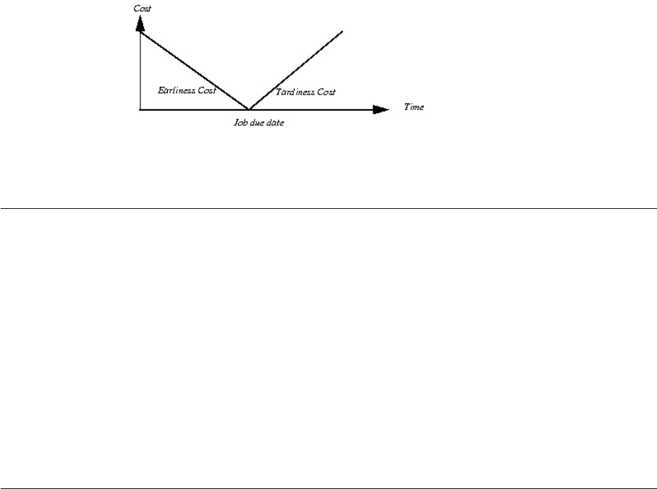
Transforming the problem
Explains what CPLEX extracts.
When IBM ILOG CPLEX extracts disjunctive constraints and piecewise linear
functions, it transforms them to produce a MIP with linear constraints and possibly
SOS constraints over integer or continuous variables. The tightness of the
transformation depends on the bounds set on the variables.
In this example, the Horizon is set to 10000, but if you have information about
your problem that indicates that a good or even optimal solution exists with a
tighter horizon (say, 2000 instead) then the linear formulation of disjunctions will
be tighter with that tighter horizon.
That kind of tightening often leads to a better lower bound at the root node and to
a reduction of the solving time.
Solving the problem
Highlights MIP emphasis and solution polishing parameters; tells where to find the
application.
An emphasis on finding hidden feasible solutions has proven particularly effective
for this problem so this example makes that selection by setting the MIPEmphasis
parameter to 4. For more detail about setting the MIP emphasis parameter to find
hidden feasible solutions, see MIP emphasis switch in the CPLEX Parameters
Reference Manual.
Solution polishing is also useful in this problem. Activate solution polishing by
specifying a positive value for the parameter that controls the amount of time (in
seconds) spent on polishing. For detail about that parameter, see time before
starting to polish a feasible solution in the CPLEX Parameters Reference Manual. For
more detail about invoking solution polishing, see “Solution polishing” on page
245 in this manual.
More generally, to invoke solution polishing and to emphasize finding hidden
feasible solutions both tend to be effective strategies on models where adjusting a
small subset of variables can easily yield better solutions. In other words, in such
problems, local search heuristics are effective. The following types of models are
well suited for these parameter settings of local search heuristics
1. to emphasize finding hidden feasible solutions
2. to invoke solution polishing on the feasible solutions
Figure 15. Earliness and tardiness as piecewise linear cost function
366 CPLEX User’s Manual
vscheduling
vknapsack
vvehicle routing
vset covering
vset packing
vset partitioning
(This list is suggestive, not exhaustive nor exclusive. Other types of problems can
also benefit from this approach as well.)
You can see the entire example online in the standard distribution of CPLEX at
yourCPLEXinstallation/examples/src/etsp.cpp. Implementations of the same model,
using the same features of CPLEX, are available as Etsp.java, Etsp.cs, and
Etsp.vb as well.
Chapter 27. Early tardy scheduling 367
368 CPLEX User’s Manual

Part 5. Parallel optimization
This part documents features of CPLEX for optimization in parallel. It introduces
special considerations about parallel programming with CPLEX. It documents the
remote object for distributed computing with CPLEX applications. It also
documents distributed parallel optimization techniques for mixed integer
programming (MIP). This part of the manual assumes that you are already familiar
with earlier parts of the manual.
© Copyright IBM Corp. 1987, 2016 369
370 CPLEX User’s Manual

Chapter 28. Multithreaded parallel optimizers
Documents the CPLEX multithreaded parallel optimizers.
What are multithreaded parallel optimizers?
Describes the multithreaded parallel optimizers available in CPLEX.
IBM ILOG CPLEX offers multithreaded parallel barrier, parallel MIP, and
concurrent optimizers. These parallel optimizers are implemented to run on
hardware platforms with multiple cores. These multithreaded parallel optimizers
can be called from the Interactive Optimizer and the Component Libraries.
Threads
Documents threads in the context of parallel optimizers.
Thread safety
Summarizes special considerations about thread safety in parallel applications.
When you use callbacks with the CPLEX parallel optimizers, the nature of the
callback can affect the thread safety of the application. You should consider the
performance trade-offs that may occur in such a situation. For example, if the
application invokes a callback that provides significant performance improvements,
but cannot be written in a thread-safe way, you should assess whether running
CPLEX in sequential mode in the presence of the callback yields better
performance than running CPLEX in parallel mode without the callback.
Also, in order to make sure of thread safety, in certain cases CPLEX restricts the
way in which it calls a callback. In particular, when it calls an informational
callback in either deterministic or opportunistic mode, CPLEX makes sure of
thread safety by calling the callback only from the main thread that contains the
relevant global information required by the informational callback.
When CPLEX solves MIPs, each deterministic thread runs independently and
solves a separate subtree, so you may see a significant number of nodes processed
between calls to the callback.
For this reason, if you need to terminate an optimization running in parallel, you
need to assess whether stopping the optimization deterministically or stopping it
as quickly as possible is more important.
With respect to a query callback, the routine CPXsetterminate in the C API or
methods of the class IloCplex::Aborter in the object-oriented APIs yields the
fastest termination but may compromise determinism due to slight variations in
system runtime. In contrast, aborting the optimization by returning a nonzero
status may take longer since the run continues until the next synchronization
point, but the results will be deterministic.
With an informational callback, the two alternatives for terminating the
optimization are both deterministic and do not delay the termination. However,
CPLEX calls informational callbacks less frequently than it calls query callbacks.
© Copyright IBM Corp. 1987, 2016 371

Table 56 summarizes compatibility of callbacks, by type, with thread-safety and
parallel mode. Table 57 summarizes compatibility of callbacks, by type, with
dynamic and conventional MIP search mode.
Table 56. Thread safety of callbacks by parallel mode
Type of callback
Parallel mode:
Deterministic
Parallel mode:
Opportunistic
Additional
information
“Informational
callbacks” on page
500
thread-safe thread-safe
“Query or diagnostic
callbacks” on page
504
thread-safe, but user
must make sure of
determinism
thread-safe “Query callbacks and
parallel search” on
page 506
“Control callbacks”
on page 506
thread limit set to 1
(one) by default;
otherwise,
thread-safe; user
must make sure of
determinism
thread limit set to 1
(one) by default;
otherwise,
thread-safe
“Thread safety and
MIP control
callbacks” on page
534
Table 57. Compatibility of callbacks with MIP search mode
Type of callback
MIP search mode:
Dynamic
MIP search mode:
Conventional
Additional
information
“Informational
callbacks” on page
500
compatible compatible
“Query or diagnostic
callbacks” on page
504
compatible compatible “Query callbacks and
dynamic search” on
page 506
“Control callbacks”
on page 506
incompatible compatible “Control callbacks
and dynamic search”
on page 508
Threads parameter
Describes the effect of the threads parameter in parallel.
You manage the number of threads that CPLEX uses with the global thread count
parameter (Threads, CPX_PARAM_THREADS) documented in the CPLEX Parameters
Reference Manual. At its default setting 0 (zero), the number of threads that CPLEX
actually uses during a parallel optimization is no more than 32 or the number of
CPU cores available on the computer where CPLEX is running (whichever is
smaller).
If you set the threads parameter to a value greater than its default of 0 (zero), then
the number of threads that CPLEX uses equals that value. When you set the
threads parameter to 1 (one), you enforce sequential operation, that is, processing
on one thread only.
The number of threads used by a parallel CPLEX optimizer is separate from and
independent of the number of users. A typical CPLEX installation permits one use,
that is, a single concurrent execution on one computer. By default, CPLEX uses a
number of threads equal to the number of cores or 32 threads (whichever number
372 CPLEX User’s Manual

is smaller). The operating system manages any contention for processors. If
processor contention among multiple executions becomes problematic in your
application, consider setting the CPLEX threads limit parameter to a suitable value
so that the total number of threads used by all executions does not exceed the
number of available cores on your platform.
The number of parallel threads used by a CPLEX optimizer is usually controlled
by CPLEX parameter settings. These settings are discussed in more detail in the
sections that follow.
Threads and performance considerations
Describes performance consideration for threads.
The benefit of applying more threads to optimizing a specific problem varies
depending on the optimizer you use and the characteristics of the problem. You
should experiment to assess performance improvements and degradation when
you apply more or fewer processors.
For example, consider the following results:
Root node processing (before b&c):
Real time = 3.22
Parallel b&c, 2 threads:
Real time = 8.29
Sync time (average) = 2.74
Wait time (average) = 2.48
-------
Total (root+branch&cut) = 11.51 sec.
When the wait time is particularly high, as in that example, consider changing the
parallel mode from deterministic to opportunistic or changing from parallel to
sequential processing. “Determinism of results” explains more about these choices.
Another key consideration in setting optimizer and global thread limits is your
management of overall system load.
Determinism of results
Defines determinism and describes its effect in parallel optimization.
By default, CPLEX employs parallel algorithms only as long as the optimization
remains deterministic. In this context, deterministic means that repeated solving of
the same model with the same parameter settings, including limits, on the same
computing platform will follow exactly the same solution path, yielding the same
level of performance and the same values in the solution.
Tip:
CPLEX real time limits (also known as wall clock time) depend on system time.
System time is not deterministic. In other words, system time may vary from one
run to another. Consequently, two consecutive runs even with the same time limit
may yield results that are not deterministic. In contrast, CPLEX deterministic time
limits do not depend on system time. Consequently, two consecutive runs with the
same deterministic time limit will follow the same solution path.
Two parallel implementations are available in CPLEX: deterministic and
opportunistic. Opportunistic parallel optimization requires less synchronization
Chapter 28. Multithreaded parallel optimizers 373

between threads and thus offers better performance on average. Consequently,
during development of an application, you may find deterministic parallelism
advantageous for the repeatable, invariant solution path and results, whereas after
development, during application deployment, you may prefer opportunistic
parallelism for its performance.
To maintain determinism (that is, an implicit contract of repeatable, invariant
search path and results), CPLEX invokes deterministic parallelism by default for
MIP optimization.
In addition to the threads parameter, you can use the parallel mode switch
(ParallelMode, CPX_PARAM_PARALLELMODE) to control the invocation of opportunistic
algorithms. With its default setting of 0 (zero), only deterministic algorithms are
used, unless the threads parameter is changed to a value strictly greater than one.
To force CPLEX to use deterministic algorithms in all cases, set the parallel mode
parameter to 1 (one).
To allow CPLEX to use opportunistic algorithms in all situations, set the parallel
mode parameter to -1 (minus one).
The presence of a time limit, set by the optimizer time limit in seconds parameter
(TiLim, CPX_PARAM_TILIM) for example, poses problems for reproducibility in any
algorithm that is otherwise deterministic, even in sequential rather than parallel
mode. Subtle variations in runtime on computer architectures can lead to variation
in the measurement of time. (Other limits, such as node limits, are not subject to
this variability.)
Because time limits are so important in many applications, CPLEX will still
attempt to use deterministic mode without regard to whether a time limit is in
effect. While variability will still be much lower than with the opportunistic
setting, the user is advised that complete determinism within time limits can not
be assured.
There are other features of CPLEX that also depend implicitly on computer run
time. Because of this implicit dependence, they too can pose problems for
reproducibility in otherwise deterministic algorithms. Examples include
terminating the optimization, using a termination signal in a callback, or any other
use of a callback where behavior varies according to the order in which the
callbacks are invoked on multiple threads. In fact, the subtle variations in
computer run time can alter the order in which the threads invoke a callback on
consecutive runs.
Using parallel optimizers in the Interactive Optimizer
Describes parallel optimization in the Interactive Optimizer.
For the mixed integer programming (MIP) optimizers of discrete models, the
barrier optimizer for continuous models, and the concurrent optimizers for
continuous models, the following sequence of commands invokes parallel
deterministic optimization at default settings.
1. Start the parallel CPLEX Interactive Optimizer with the command cplex at the
operating system prompt.
2. Enter your problem object, and populate it with data as usual.
374 CPLEX User’s Manual

3. Call the parallel optimizer with the optimize command. The optimizer then
uses the maximum number of available threads in deterministic mode.
Linear programming models (LPs) are solved by default with the dual simplex
algorithm. The dual simplex algorithm does not use multiple threads. In order to
benefit from parallel execution for LP, you need to invoke the barrier or concurrent
optimizers explicitly.
To abandon determinism by means of the parallel mode parameter
1. Start the parallel CPLEX Interactive Optimizer with the command cplex at the
operating system prompt.
2. Enter the command: set parallel -1. The optimizer then uses the maximum
number of available threads in opportunistic mode.
3. Enter your problem object and populate it with data as usual.
4. Optimize.
Using parallel optimizers in the Component Libraries
Describes parallel optimization in the Component Libraries.
When you use one of the Component Libraries, such as the Callable Library, follow
these steps to invoke parallel optimization.
1. Create your CPLEX environment and initialize a problem object in the usual
way. See “Initialize the CPLEX environment” on page 60 and “Instantiate the
problem as an object” on page 61 for details.
2. Enter and populate your problem object in the usual way, as in “Put data in the
problem object” on page 61.
3. If you want to use an opportunistic parallel algorithm, set the parallel mode
switch (ParallelMode, CPX_PARAM_PARALLELMODE) in your application. If you
want to use deterministic mode with fewer than the maximum number of
available threads, set both the parallel mode and the threads parameter in your
application. See “Determinism of results” on page 373 for background about
this step.
4. Call the parallel optimizer with the appropriate method or routine (identified
from the table).
Table 58. Parallel optimizer methods and routines of the Component Libraries
Optimizer Concert IloCplex Method Callable Library
parallel MIP optimizer solve CPXmipopt
parallel barrier optimizer setParam(RootAlg, Barrier)
and then solve
CPXbaropt or CPXhybbaropt
concurrent optimizer setParam(RootAlg,
Concurrent) and then solve CPXsetintparam(env,
CPX_PARAM_LPMETHOD,
CPX_ALG_CONCURRENT)
and then CPXlpopt or
CPXqpopt
Chapter 28. Multithreaded parallel optimizers 375

Using the parallel barrier optimizer
Describes the parallel barrier optimizer.
The CPLEX parallel barrier optimizer achieves significant speedups over its serial
counterpart on a wide variety of classes of problems. (The serial barrier optimizer
is introduced in Chapter 12, “Solving LPs: barrier optimizer,” on page 161, and
explored further in Chapter 14, “Solving problems with a quadratic objective
(QP),” on page 189 and in Chapter 15, “Solving problems with quadratic
constraints (QCP),” on page 201.) Consequently, the parallel barrier optimizer will
be the best continuous choice on a parallel computer more frequently than on a
single-processor. For that reason, you should be careful not to apply performance
data or experience based on serial optimizers when you are choosing which
optimizer to use on a parallel platform.
Concurrent optimizer in parallel
Describes the concurrent optimizer.
On a multiprocessor computer, the concurrent optimizer launches distinct LP and
QP optimizers on multiple threads, terminating as soon as the first optimizer
finishes. The first thread uses the same strategy as the single-processor automatic
setting (0 zero) of the algorithm for continuous linear problems
(CPX_PARAM_LPMETHOD, RootAlg) or algorithm for continuous quadratic optimization
(CPX_PARAM_QPMETHOD, RootAlg) depending on the problem type. If a second thread
is available, the concurrent optimizer runs the barrier optimizer on it.
In the presence of more than three threads (for example, on hardware with four or
more processors), the behavior of the concurrent optimizer depends on whether
the parallel mode is opportunistic or deterministic. If the parallel mode is
opportunistic and a third processor is available, the concurrent optimizer runs all
three optimizers simultaneously: dual simplex, primal simplex, and barrier. All
further available threads are devoted to making the barrier optimization parallel.
In contrast, if the parallel mode is deterministic (the default mode) and more than
two threads are available, then the concurrent optimizer runs the dual simplex and
barrier optimizers simultaneously and applies all additional threads to making the
barrier optimizer parallel.
LP with large aspect ratio
When the concurrent optimizer is invoked on a linear program (LP), it checks the
aspect ratio of the model. If the aspect ratio is large, and if more than 10 (ten)
threads are available to CPLEX, then concurrent optimization also invokes sifting
on the LP. For more information about sifting, see the topic “Sifting optimizer” on
page 138.
Finishing first: basis solution in concurrent optimization
Barrier optimization is not considered complete until the crossover step has been
performed and simplex re-optimization has converged; in other words, regardless
of which optimizer turns out to be the fastest, the concurrent optimizer always
returns a basis solution at optimality.
376 CPLEX User’s Manual

Performance trade-offs in concurrent optimization
The concurrent optimizer requires more memory than any individual optimizer,
and of course it adds system load by consuming more aggregate CPU time than
the fastest individual optimizer would alone. However, the advantages offered in
terms of robust solution of models, and assurance in most cases of the minimum
solution time, will make it attractive in many situations.
Interpreting the log in concurrent optimization
When you invoke concurrent optimization in your application, you may observe a
point in the log when CPLEX®reports a solution of the model by an optimizer, but
no other report of activity appears in the log for a considerable time afterward.
During this apparently inactive period, concurrent optimization deterministically
manages potential race conditions among competing optimizers. Among other
decisions during this period, the concurrent optimizer decides deterministically
from which of those competing optimizers to accept the final solution.
If this apparent wait during the race between concurrent optimizers poses a
problem for your application, there are two alternative remedies available to you:
vUse opportunistic mode, rather than the default deterministic mode. To do so,
change the setting of the parallel mode switch (CPX_PARAM_PARALLELMODE,
ParallelMode) documented in the CPLEX Parameters Reference Manual.
vSet the optimizer that consistently solves your model first as the starting
algorithm in your application.
To do so, set the parameter appropriate for your type of model:
– algorithm for continuous linear problems (CPX_PARAM_LPMETHOD, RootAlg)
documented in the CPLEX Parameters Reference Manual.
– algorithm for continuous quadratic optimization (CPX_PARAM_QPMETHOD,
RootAlg) documented in the CPLEX Parameters Reference Manual.
– algorithm for initial MIP relaxation (CPX_PARAM_STARTALG, RootAlg)
documented in the CPLEX Parameters Reference Manual.
Callbacks and concurrent optimization
Because of considerations about thread safety and predictable behavior, concurrent
optimization should not invoke any callbacks except in the first, main thread.
Determinism, parallelism, and optimization limits
Documents effect of determinism on optimization limits.
CPLEX respects limits that the user sets, such limits as the number of iterations,
the amount of time spent in optimization, and so forth. However, to achieve
deterministic results, CPLEX must impose strict requirements with respect to
synchronization of parallel threads or processes. The stricter synchronization
requirements of deterministic parallel algorithms may cause CPLEX to deviate
slightly from any non default limits on the optimization. For example, with a node
limit of 2000 on four threads, the deterministic parallel MIP algorithm achieves the
two-thousandth node on one thread but must wait for the other three threads to
finish processing their nodes. In consequence, a final node count of up to 2003 is
possible. Similarly, with a finite time limit on the parallel concurrent optimizer, if
the thread for the dual simplex optimizer reaches the time limit first, it must wait
for the other optimizers to finish their next iteration before that thread terminates.
Chapter 28. Multithreaded parallel optimizers 377

Particularly since each barrier method iteration involves computational effort
equivalent to many simplex iterations, this wait for synchronization can yield a
modest deviation from the specified time limit.
Parallel MIP optimizer
Describes the parallel MIP optimizer.
Introducing parallel MIP optimization
Describes parallel MIP optimization in general terms.
By default, CPLEX uses the deterministic parallel MIP optimizer to solve a mixed
integer programming problem. In doing so, it exploits parallel computations while
it solves nodes of the MIP branch & cut tree. It also executes strong branching
computations in parallel. Furthermore, CPLEX also exploits parallelism while
solving the root node.
As explained in “Determinism of results” on page 373, you may find it
advantageous to develop your application in deterministic parallel mode, where
you can rely on the invariance and repeatability of the search path and results to
evaluate the correctness of your model and solutions. After you are convinced of
correctness of your model, there are two different approaches you can take in
deployment of your application. If performance is critical, consider deploying in
opportunistic parallel mode. While faster performance in opportunistic mode
cannot be guaranteed, it does generally out-perform deterministic mode. On the
other hand, if performance is not critical, you may prefer to deploy in deterministic
mode to retain the possibility of reproducing any problems that your end-user may
encounter during deployment. In summary, you need to evaluate for your model
and application which mode is more appropriate.
Root relaxation and parallel MIP processing
Describes special considerations about the root relaxation in parallel MIP
optimization.
In some models, the continuous root relaxation takes significant solution time
before parallel branching begins. These models have potential for additional speed
increases by running the root relaxation step in parallel. If the root problem is an
LP or QP, CPLEX invokes the concurrent optimizer by default. This practice
provides a form of parallelism that assigns the available threads to multiple
optimizers. If the root problem is a QCP, the barrier optimizer alone is used.
You can try a different form of parallelism at the root by selecting the barrier
optimizer specifically with the algorithm for initial MIP relaxation parameter:
vRootAlg in Concert Technology;
vCPX_PARAM_STARTALG in the Callable Library;
vset mip strategy startalgorithm in the Interactive Optimizer.
In such a case, the parallel threads will all be applied to the barrier algorithm.
To help you evaluate how much time is spent at the root node before parallel
processing begins, the log of parallel MIP processing distinguishes time spent
processing the root node before parallel branch and cut begins, like this typical log:
378 CPLEX User’s Manual
Root node processing (before b&c):
Real time = 4.67 sec. (991.49 ticks)
Parallel b&c, 2 threads:
Real time = 17.68 sec. (5417.26 ticks)
Sync time (average) = 0.01
Wait time (average) = 0.00
-------
Total (root+branch&cut) = 22.35 sec. (6408.75 ticks)
The log of sequential MIP optimization also distinguishes time spent processing
the root node before sequential branch and cut begins. If you contrast the
following sample log file of sequential MIP optimization with the previous sample
log file of parallel MIP optimization, you get an idea of the time spent in
synchronization and waiting. This contrast in your own model may help you
estimate how much speed up in performance to anticipate from parallel
optimization.
Root node processing (before b&c):
Real time = 4.25 sec. (971.17 ticks)
Sequential b&c:
Real time = 19.12 sec. (6441.66 ticks)
-------
Total (root+branch&cut) = 23.37 sec. (7412.83 ticks)
Memory considerations and the parallel MIP optimizer
Describes considerations about memory consumption in parallel MIP optimization.
Before the parallel MIP optimizer invokes parallel processing, it makes separate,
internal copies of the initial problem. The individual processors use these copies
during computation, so each of them requires an amount of memory roughly equal
to the size of the presolved model.
Output from the parallel MIP optimizer
Shows a sample log from parallel MIP optimization.
The parallel MIP optimizer generates slightly different output in the node log (see
“Progress reports: interpreting the node log” on page 261) from the sequential MIP
optimizer. The following paragraphs explain those differences.
CPLEX prints a summary of timing statistics specific to the parallel MIP optimizer
at the end of optimization. You can see typical timing statistics in the following
sample run.
Selected objective sense: MINIMIZE
Selected objective name: COST
Selected RHS name: RHS
Selected bound name: BOUND
Problem ’sample.mps’read.
Read time = 0.01 sec. (0.19 ticks)
Tried aggregator 2 times.
MIP Presolve modified 308 coefficients.
Aggregator did 1 substitutions.
Reduced MIP has 477 rows, 877 columns, and 1754 nonzeros.
Reduced MIP has 378 binaries, 0 generals, 0 SOSs, and 0 indicators.
Presolve time = 0.02 sec. (0.96 ticks)
Found incumbent of value 97019.000000 after 0.03 sec. (2.88 ticks)
Probing time = 0.00 sec. (0.09 ticks)
Tried aggregator 1 time.
Presolve time = 0.00 sec. (0.88 ticks)
Probing time = 0.00 sec. (0.09 ticks)
Chapter 28. Multithreaded parallel optimizers 379
Clique table members: 2.
MIP emphasis: balance optimality and feasibility.
MIP search method: dynamic search.
Parallel mode: deterministic, using up to 2 threads.
Root relaxation solution time = 0.00 sec. (0.95 ticks)
Nodes Cuts/
Node Left Objective IInf Best Integer Best Bound ItCnt Gap
* 0+ 0 97019.0000 2.0000 60 100.00%
0 0 3192.0420 12 97019.0000 3192.0420 60 96.71%
* 0+ 0 4505.0000 3192.0420 60 29.14%
0 0 3393.6018 21 4505.0000 Cuts: 38 116 24.67%
0 0 3555.7097 19 4505.0000 Cuts: 46 159 21.07%
0 0 3609.2106 24 4505.0000 Cuts: 38 202 19.88%
* 0+ 0 4448.0000 3609.2106 202 18.86%
* 0+ 0 3990.0000 3609.2106 247 9.54%
0 0 3647.5779 32 3990.0000 Cuts: 43 247 6.57%
0 0 3659.6926 34 3990.0000 Cuts: 39 284 6.57%
0 0 3711.0491 35 3990.0000 Cuts: 25 323 6.57%
0 0 3725.5063 38 3990.0000 Cuts: 30 362 6.57%
0 0 3736.7342 32 3990.0000 Cuts: 26 402 6.35%
0 0 3755.9382 27 3990.0000 Cuts: 25 425 5.87%
0 0 3762.8446 31 3990.0000 Cuts: 29 445 5.69%
0 0 3775.7611 35 3990.0000 Cuts: 27 471 5.37%
0 0 3779.3191 34 3990.0000 Cuts: 25 489 5.28%
0 0 3782.2251 32 3990.0000 Cuts: 29 513 5.21%
* 0+ 0 3985.0000 3782.2251 538 5.09%
0 0 3786.8940 34 3985.0000 Cuts: 12 538 1.67%
0 0 3793.3163 32 3985.0000 Cuts: 18 559 1.67%
* 0+ 0 3983.0000 3918.4040 559 1.62%
0 0 cutoff 3983.0000 3983.0000 559 0.00%
Elapsed time = 0.84 sec. (289.23 ticks, tree = 0.00 MB, solutions = 6)
Cover cuts applied: 3
Flow cuts applied: 23
Mixed integer rounding cuts applied: 34
Gomory fractional cuts applied: 4
Root node processing (before b&c):
Real time = 0.80 sec. (285.32 ticks)
Parallel b&c, 2 threads:
Real time = 0.00 sec. (0.00 ticks)
Sync time (average) = 0.00 sec.
Wait time (average) = 0.00 sec.
------------
Total (root+branch&cut) = 0.80 sec. (285.32 ticks)
Solution pool: 6 solutions saved.
MIP - Integer optimal solution: Objective = 3.9830000000e+03
Solution time = 0.84 sec. Iterations = 559 Nodes = 0
Deterministic time = 289.29 ticks (345.27 ticks/sec)
The sample reports that the processors spent an average of 0.00 of a second of real
time waiting for other processors to provide nodes to be processed. The Sync time
is the average time a processor spends trying to synchronize by accessing globally
shared data. Because only one processor at a time can access such data, the amount
of time spent in synchronization is really crucial: any other processor that tries to
access this region must wait, thus sitting idle, and this idle time is counted
separately from the Wait time.
There is another difference in the way logging occurs in the parallel MIP optimizer.
When this optimizer is called, it makes a number of copies of the problem. These
380 CPLEX User’s Manual

copies are known as clones. The parallel MIP optimizer creates as many clones as
there are threads available to it. When the optimizer exits, these clones and the
memory they used are discarded.
If a log file is active when the clones are created, then CPLEX creates a clone log
file for each clone. The clone log files are named cloneK.log, where Kis the index
of the clone, ranging from 0 (zero) to the number of threads minus one. Since the
clones are created at each call to the parallel MIP optimizer and discarded when it
exits, the clone logs are opened at each call and closed at each exit. (The clone log
files are not removed when the clones themselves are discarded.)
The clone logs contain information normally recorded in the ordinary log file (by
default, cplex.log) but inconvenient to send through the normal log channel. The
information likely to be of most interest to you are special messages, such as error
messages, that result from calls to the LP optimizers called for the subproblems.
Clock settings and time measurement
Describes reporting of time in parallel MIP optimization.
On most platforms, CPLEX offers two ways of measuring time: CPU time and
wall-clock time. Wall-clock time is the default on all platforms.
You can choose the type of clock by setting the clock type for computation time
parameter to a value different from the default 2.
vIn Concert Technology, use the method:
– IloCplex::setParam(ClockType , i)in the C++ API;
– IloCplex.setParam(ClockType, i)in the Java API;
– Cplex.SetParam(ClockType, i)in the .NET API.
vIn the Callable Library, use the routine
CPXsetintparam(env, CPX_PARAM_CLOCKTYPE , i).
vIn the Interactive Optimizer, use the command set clocktype i.
Replace the iwith the value 0 (zero, the automatic setting) to use CPU time for
sequential optimizers and wall-clock time for parallel optimizers; 1 (one) to specify
CPU time; or 2 to specify wall-clock time.
Chapter 28. Multithreaded parallel optimizers 381
382 CPLEX User’s Manual
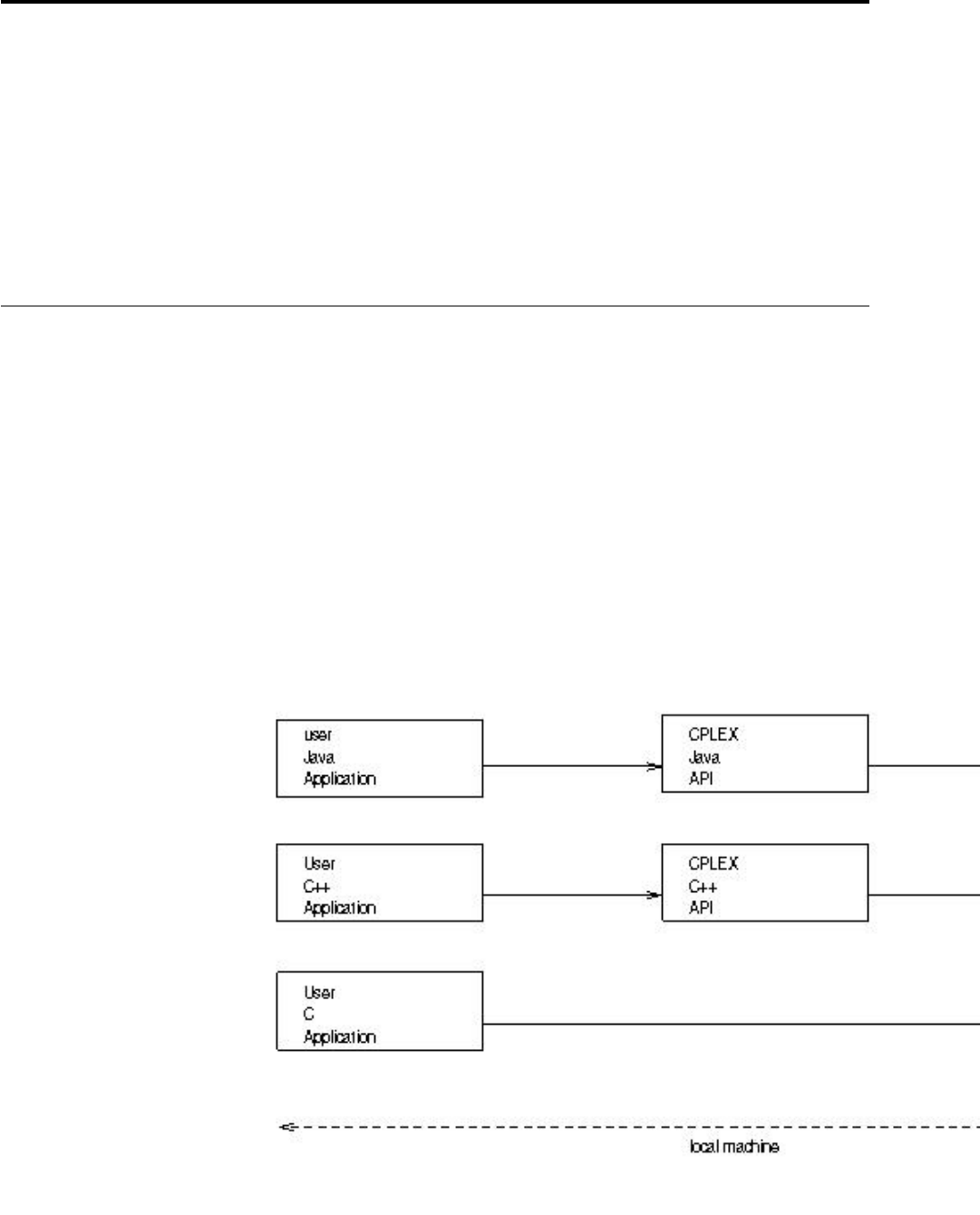
Chapter 29. Remote object for distributed parallel optimization
Introduces the remote object available in CPLEX for distributed parallel
optimization.
CPLEX offers a programming interface to support remote objects that greatly ease
development of distributed parallel applications of CPLEX optimizers. The
following topics document the CPLEX remote object primarily in terms of the
CPLEX Callable Library (C API), but several of these topics emphasize special
considerations for the C++ and Java application programming interfaces (APIs).
CPLEX remote object for distributed parallel optimization
Defines the remote object available in CPLEX for distributed parallel optimization.
IBM ILOG CPLEX offers features that greatly simplify your development of
applications implementing parallel algorithms that use CPLEX on distributed
hardware. Though CPLEX itself does not implement a distributed parallel
algorithm as such, it does provide the CPLEX remote object to facilitate your own
implementation.
IBM developerWorks offers a half-hour video explaining applications and use cases
of the CPLEX remote object. A link to the video appears in Related Links in this
topic.
Consider the conventional layout of applications that use CPLEX locally,
represented in this figure.
© Copyright IBM Corp. 1987, 2016 383
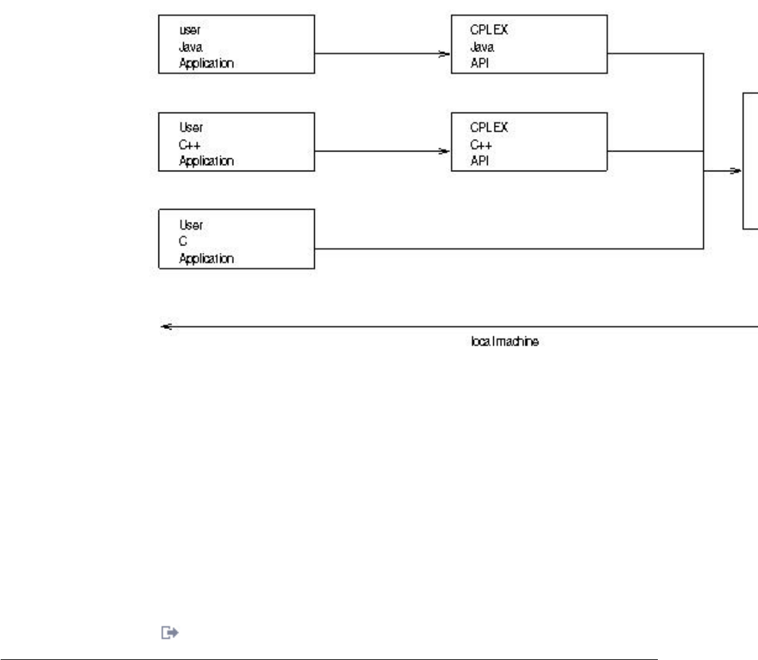
According to that layout, any application using CPLEX eventually invokes routines
of the CPLEX Callable Library (C API). These routines are invoked either directly
(by applications using the C API) or through dedicated application programming
interfaces for applications using C++, Java, C#.NET, VB.NET, Python, or The
MathWorks MATLAB. In other words, when your application uses only the CPLEX
Callable Library, the entire application runs on a local machine.
The introduction of the CPLEX remote object changes the situation slightly to a
layout that looks like the next figure.
According to that figure, on your local machine, your application calls a function
in a remote CPLEX API, instead of calling the CPLEX Callable Library directly.
This remote API implements stubs that forward function calls to an instance of the
CPLEX Callable Library that is actually located on a remote machine. This instance
of the Callable Library on the remote machine is also known as the CPLEX remote
object.
As you can see in that figure, nothing fundamental changes for the user-written
applications based on CPLEX. Such applications simply have to call the
corresponding functions of the remote API (instead of calling the same familiar
routines of the Callable Library locally). The remote API was carefully designed so
that only minimal changes are required when a user switches from a strictly local
application to a distributed application.
Video about CPLEX remote object
applications and use cases of the CPLEX remote object.
Application layout for the remote object
Describes the layout of a distributed application using the remote object.
An application that uses the CPLEX remote object to implement a distributed
parallel algorithm consists of these components:
384 CPLEX User’s Manual

vA master process: This master process controls multiple worker processes.
Because the master process conventionally runs on a local machine, it is also
sometimes referred to as the local application or the local process.
vOne or more worker processes: These processes often run on a remote machine,
so they are also referred to as remote applications or as remote processes, in contrast
to the master.
vOptionally a dynamically loaded library; that is, user-written code that is
loaded into the worker processes and executed there.
All three of these components are conventionally compiled into different executable
files.
The master process is code written entirely by the application developer. It
dynamically links to CPLEX libraries in order to include the code that is required
to connect to the worker processes. The master often runs on a local machine. In a
simple application design, the master process is simply a process that frequently
hands out work as jobs to the worker processes.
A worker process runs on a remote machine. (In fact, workers can run in separate
processes on the local machine as well; more about that idea in other topics.) One
instance of a worker process represents one instance of a remote Callable Library
object. A worker process starts when the cplex binary file is invoked with the
argument -worker=process, -worker=mpi, or -worker=tcpip depending on which
data transport type is needed. The topic “Transport types for the remote object” on
page 389 explains data transport types and their options.
By default, a worker process does not run any user-written code. However, it is
possible to augment or extend a worker process by dynamically loading
user-defined, user-written code into this worker process. To augment or extend a
worker process, a user function instructs the worker process to load a dynamically
loaded object and to execute a predefined function in this object. The idea of a user
function is explained in the topic “User functions to run user-defined code on the
remote machine” on page 401.
Programming paradigm in C for the CPLEX remote object
Describes a programming paradigm in C for the remote object in CPLEX.
Chapter 29. Remote object for distributed parallel optimization 385
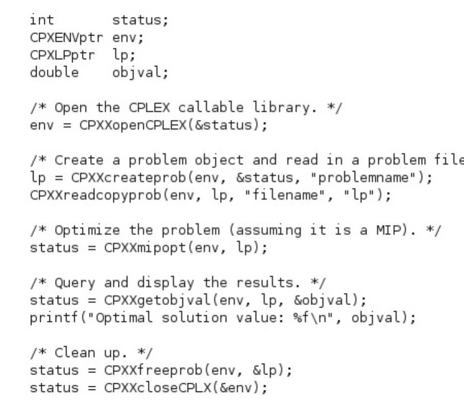
Consider the outline of a simple application that uses the CPLEX Callable Library
(C API). (For the sake of brevity, this outline omits status checking.)
That skeleton code solves the model declared in the file filename on the local
machine. What if you want to run the code on the local machine but perform the
actual solve on a different (remote) machine? In that situation, you can use the
CPLEX remote object. To solve the problem on a remote machine change this line:
env = CPXXopenCPLEX(&status);
to the following line:
env = CPXXopenCPLEXremote(transport, argc, argv, &status);
386 CPLEX User’s Manual
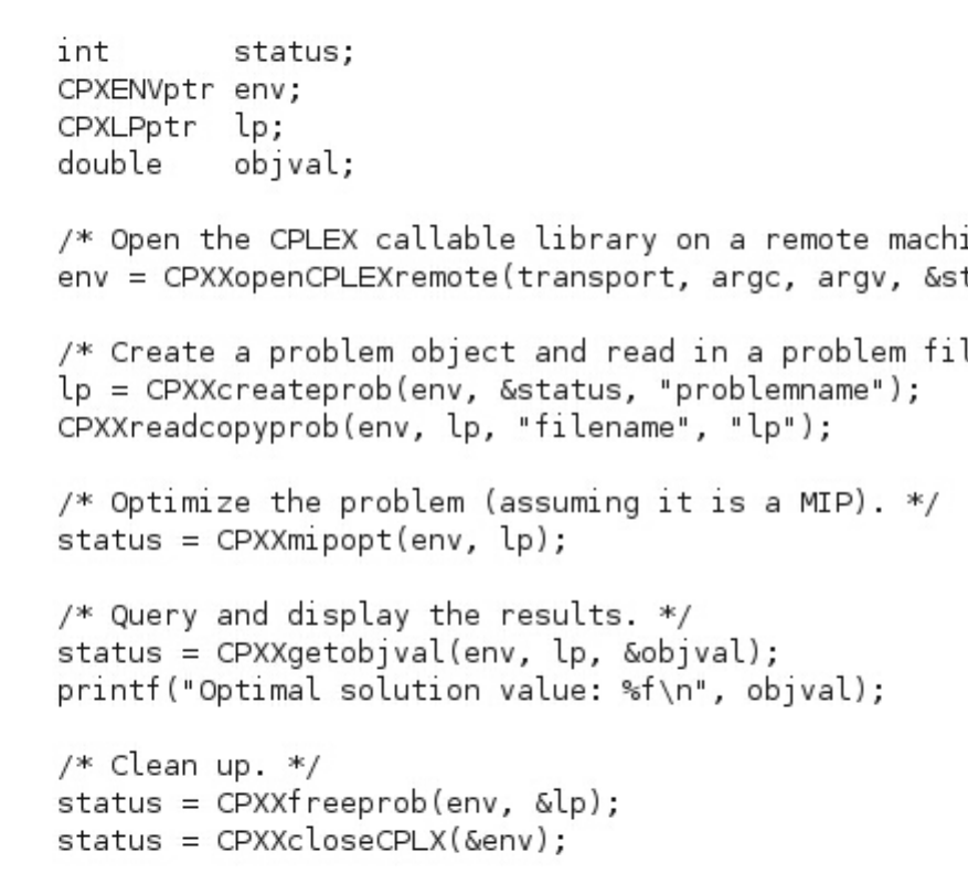
After that change (explained more fully later), your program looks like this:
In that code, the arguments transport, argc, argv define the machine on which
the remote solve takes place. In contrast to the original routine CPXXopenCPLEX,
the remote function CPXXopenCPLEXremote does not open the Callable Library
on the local machine, but rather on the remote machine specified by the
arguments. Like CPXXopenCPLEX, CPXXopenCPLEXremote returns a pointer to
the CPLEX environment, CPXENVptr that acts as a handle to the CPLEX Callable
Library; however, this time, it acts as the handle to a library instantiated on a
remote machine.
As you can see in the modified code snippet, the rest of the code does not need to
know nor care whether the CPXENVptr passed to it references a local or a remote
instance of the library. The implementation of the functions simply takes care to do
the right thing: if the CPXENVptr references a remote library, then the function call
is forwarded to this remote library instance; if the CPXENVptr argument references
a local library, then the call is executed locally.
The arguments transport, argc, argv
Chapter 29. Remote object for distributed parallel optimization 387

The simplest setting of the arguments to CPXXopenCPLEXremote instructs CPLEX
to create a new worker with the process transport on the local machine. It looks
like this:
char const *transport = "processtransport";
char const *argv[] = { "cplex", "-worker=process" };
int const argc = sizeof (argv) / sizeof (*argv);
This simple declaration assumes that the cplex binary file is available to your
application, for example, in your $PATH environment variable. This simple
declaration also assumes that it must start the remote environment in a different
process on the same machine.
A more ambitious declaration (to start the remote environment in a different
process on a different machine) invokes a secure shell, such as ssh, to reach a
remote machine (such as, for example, remote.com), like this:
char const *transport = "processtransport";
char const *argv[] = { "ssh", "remote.com", "cplex", "-worker=process" };
int const argc = sizeof (argv) / sizeof (*argv);
For that more ambitious declaration to work successfully (invoking a secure shell
in a different process on a remote machine), you need to satisfy these
prerequisites:
vThe cplex binary file must be installed on the remote machine, as cited in the
declaration; in this example, the remote machine is cited as remote.com, but
clearly your application must supply a valid name of a remote machine, where a
user account to which your application has login-access has already been set up
for remote access (such as automatic login, secure shell, or other facilities
appropriate to your environment).
vThe location of the cplex binary file must be available in the remote
environment; for example, through the $PATH environment variable on
remote.com.
More about CPXXopenCPLEXremote
Documents the routine supporting the remote object.
CPXXopenCPLEXremote
The routine CPXXopenCPLEXremote instantiates the CPLEX Callable Library on a
remote machine and returns a handle to the remote object that represents the
Callable Library instance. Here is the signature of that routine:
CPXENVptr CPXXopenCPLEXremote(char const *transport,
int argc, char const * const*argv,
int *status_p);
Upon success the routine stores 0 (zero) in status_p and returns a handle to the
remote library instance. In case of error, NULL is returned, and an error code is
stored in status_p.
The transport argument selects the transport type used to communicate with the
remote machine. CPLEX supports various transport types that allow you to use
different communication protocols with remote machines. The arguments argc and
argv are transport-specific arguments. They specify parameters and options that
the selected transport needs to establish the connection to a remote machine. For
more about these arguments, see the topic “Transport types for the remote object”
on page 389.
388 CPLEX User’s Manual

Programming in C++ with the CPLEX remote object
Documents programming in C++ with the remote object in CPLEX.
The CPLEX remote object is also available in the Concert C++ API. The examples
iloparbenders.cpp and iloparmipopt.cpp illustrate how to use the remote object
through the Concert C++ API. As you see in those examples, you use one of these
two constructors in the class IloCplex to instantiate a CPLEX remote object.
IloCplex(IloEnv env, char const *transport, int argc, char const *const *argv);
IloCplex(IloModel model, char const *transport, int argc, char const *const *argv);
The arguments transport, argc, argv are exactly the same arguments as for the
Callable Library (C API) routine CPXXopenCPLEXremote. Those arguments specify
how to connect to the remote object worker.
Internally, those constructors create a remote object master that off-loads all work
to the remote object worker specified by those connection arguments. Function
calls to the remote object worker are transparent; that is, you can not distinguish
between instances of the class IloCplex that were created with a remote object and
those that were not created with a remote object. In fact, you do not need to
distinguish whether an instance of IloCplex was created with a remote object. All
work the same.
Programming in Java with the CPLEX remote object
Documents programming in Java with the remote object in CPLEX.
The CPLEX remote object is also available in the Concert Java API. The example
RemoteParBenders.java illustrates how to use the remote object through the
Concert Java API. As you see in that example, you use this constructor in the class
IloCplex to instantiate a CPLEX remote object.
IloCplex(String transport, String[] args);
The arguments transport and args are exactly the same arguments as for the
Callable Library (C API) routine CPXXopenCPLEXremote. Those arguments specify
how to connect to the remote object worker.
Internally, that constructor creates a remote object master that off-loads all work to
the remote object worker specified by those connection arguments. Function calls
to the remote object worker are transparent; that is, you can not distinguish
between instances of the class IloCplex that were created with a remote object and
those that were not created with a remote object. In fact, you do not need to
distinguish whether an instance of IloCplex was created with a remote object. All
work the same.
Transport types for the remote object
Documents the transport protocols supporting the remote object.
The arguments of CPXXopenCPLEXremote (introduced in the topic “More about
CPXXopenCPLEXremote” on page 388) define communication between the master
and worker(s). The argument transport declares the type of communication (local,
process, mpi, tcp/ip). The arguments argc and argv are specific to the type of
communication declared; they define how to establish communication with the
remote object.
Chapter 29. Remote object for distributed parallel optimization 389
In other words, the transport-type argument in the call to CPXXopenCPLEXremote
specifies which strategy is used to transport data between the local machine
(master) and the remote machine (worker). That is, both the worker and the master
use the transport. CPLEX supports a variety of transport types: local, process,
message passing interface (MPI), Transport Control Protocol/Internet Protocol
(TCP/IP). The following topics document those types.
Transport types for the remote object: local
Documents the local transport protocol supporting the remote object.
If the transport argument to CPXXopenCPLEXremote is NULL or the empty
string, then the arguments argc, argv are ignored, and the call to
CPXXopenCPLEXremote behaves like an ordinary call to CPXXopenCPLEX. That
is, the handle returned is a handle to a local instance of the CPLEX Callable
Library.
Transport types for the remote object: process
Documents the process transport protocol supporting the remote object.
If the transport argument to CPXXopenCPLEXremote is processtransport, then
CPLEX explicitly creates a new process which in turn instantiates the CPLEX
Callable Library. CPLEX communicates with the newly created process using
(named) pipes.
{"-stdio"|"-namedpipes=%s"} [remote shell arguments] cplex "-worker=process" ["-logfile=%s"] ["-libpath=%s"]*
The process transport protocol understands the following arguments:
v-stdio
Uses the stdin and stdout channels of the newly created process for input and
output of messages. This situation implies that the newly created process must
not use these two channels for its own purposes.
v-namedpipes=%s
Uses named pipes created in the specified directory (in contrast to stdio).
v-worker=%s
Specifies the transport type to be used by the worker process. For CPLEX
applications, this argument must always be present, and its value must be set to
process.
v-logfile=%s
Specifies a file to which the process writes log messages. This argument is
optional.
v-libpath=%s
Adds a directory to the list of directories searched when dynamic libraries are
loaded. This argument is optional. This argument can be repeated.
Other arguments are passed without change, exactly as they are, as command-line
arguments to the new process that is started by the transport layer. These
remaining arguments define the command line of the cplex process to be started.
The following examples illustrate that point.
Example 1: Start a process on the local machine using named pipes in the current
directory.
390 CPLEX User’s Manual
char const *args[] = { "-namedpipes=.", "cplex", "-worker=process" };
int status;
CPXENVptr env;
env = CPXXopenCPLEXremote("processtransport", sizeof(args) / sizeof(args[0]),
args, &status);
Example 2: Start a process on the remote machine (remote.com for example) using
named pipes of that process for communication.
char const *args[] = { "-namedpipes=.",
"/usr/bin/ssh", "remote.com", "cplex",
"-worker=process" };
int status;
CPXENVptr env;
env = CPXXopenCPLEXremote("processtransport", sizeof(args) / sizeof(args[0]),
args, &status);
Both those examples assume that the cplex binary file is installed and accessible
according to the environment variable $PATH. If such is not the case, then you need
to specify a full path to the cplex binary file.
In Example 2, the cplex binary file must be installed on the remote machine
(identified in the example as remote.com); and the binary file must be accessible in
the remote $PATH environment variable there.
Example 2 also assumes that a remote login, not requiring a password, has already
been set up and is available to the application.
Transport types for the remote object: MPI
Documents the message passing interface (MPI), a transport protocol supporting
the remote object.
To use the Message Passing Interface (MPI), you must configure MPI to start the
CPLEX executable with the argument -worker=mpi on all machines being used.
Optionally, you can also pass arguments to specify a log file and to extend the
paths searched during dynamic loading of libraries (that is, the libpath
environment variable).
If the transport argument to CPXXopenCPLEXremote is mpitransport, then
CPLEX assumes that it is running in an application of the message passing
interface (MPI) and uses MPI to communicate between processes. The MPI
transport understands the following arguments:
v-remoterank=%d
Specifies the MPI rank of the remote end to which CPLEX connects. The new
remote object instance will be created on the machine identified by this rank.
This argument is required.
v-libpath=%s
Adds a directory to the list of directories searched when dynamic libraries are
loaded. This argument is optional. This argument can be repeated.
v-forcemt
Specifies that CPLEX should use multiple threads in the worker, regardless of
the policy with respect to multiple threads in the MPI library.
v-nothreads
Specifies that CPLEX should use exactly one thread in the worker.
Example: MPI configuration file
Chapter 29. Remote object for distributed parallel optimization 391
Here are the contents of a MPI configuration file for one master with two workers.
-np 1 ./my-master
-np 1 /opt/COS/cplex/bin/cplex -worker=mpi -logfile=server0.log
-np 1 /opt/COS/cplex/bin/cplex -worker=mpi -logfile=server1.log
With that configuration, you must then create two environments on master, like
this:
CPXENVptr env[2];
int i;
for (i = 0; i < 2; ++i) {
int status;
char rank[32];
char const *argv[1] = { rank };
sprintf (rank, "-remoterank=%d", i + 1);
env[i] = CPXXopenCPLEXremote ("mpitransport", 1, argv, &status);
}
Note:
The Message Passing Interface (MPI) transport protocol is available for most (not
all) combinations of machine, operating system, compiler. On combinations for
which the MPI transport is provided, it was tested with OpenMPI V1.6. The
OpenMPI library for testing was configured with the following command-line
argument:
--enable-mpi-thread-multiple
MPI is not available for CPLEX V12.6.0 (nor more recent versions) on Windows
platforms.
Transport types for the remote object: TCP/IP
Documents the TCP/IP transport protocol supporting the remote object.
If the transport argument to CPXXopenCPLEXremote is the value tcpiptransport,
then CPLEX uses a transport that is based on sockets. For this transport, you must
start the worker process explicitly yourself on the worker machine. To start the
worker process, use the following command as part of the arguments passed to
CPXXopenCPLEXremote:
cplex -worker=tcpip -address=address
where address is an internet (IP) address followed by a port number; for example:
127.0.0.1:1234. The worker listens to this address; the master connects to this
address, so the IP address and the port number must be valid in your
environment.
Like the process and MPI transport protocols, the TCP/IP transport protocol also
supports an optional argument to specify directories to search when dynamic
libraries are loaded.
-libpath=%s
This optional argument adds the specified directory to the list of directories
searched when dynamic libraries are loaded. This argument is optional. This
argument can be repeated.
392 CPLEX User’s Manual

After you start the worker process explicitly yourself with that argument, the
worker begins to listen on that specified port for incoming connections from the
master.
The worker also supports an option to redirect output from the worker to a log
file:
-logfile=file
where file specifies the name of the file for logging output.
Contrasting local and remote environments and libraries
Contrasts the environments of local and remote libraries supporting the remote
object.
Although a remote environment of CPLEX behaves very much like a local
environment of CPLEX, there are some important technical differences between the
remote CPLEX library and the local CPLEX library, and these technical differences
influence the way your application implements certain features of CPLEX.
v
The remote library does not support callbacks directly in the remote
environment.
An attempt to install a callback directly in a remote environment raises the error
code CPXERR_UNSUPPORTED_OPERATION.
vThe remote library in a remote environment supports at most one linear
programming (LP) object or network programming (NET) object.
Both of these limitations can be overcome.
vTo overcome the limitation of the remote library not supporting callbacks, you
can write your own user function. Then use your own user function to install
the callback. For an example of this approach, see the sample parmipopt.c.
vTo overcome the limitation of the remote library not supporting more than one
LP or NET object in a remote environment, you can write your own user
function.
Multicast: invoking the same methods on a group of objects
Introduces the idea of multicasting for the remote object.
In certain situations, you need to call the same function on all remote objects, or
possibly on a group of remote objects. Of course, one option is to loop over all the
remote objects in the group, invoking the function for each object individually.
However, if great amounts of data (such as a large matrix) must be transferred as
the arguments of the function, then calling the function repeatedly in a loop
quickly introduces too much overhead. Some transport protocols offer improved
data handling in situations where one knows that the same data must be sent to
multiple machines. In that context, the following paragraphs explain how to send
data to multiple remote objects at the same time, a practice known as multicasting.
Tip:
Chapter 29. Remote object for distributed parallel optimization 393
Multicasting is available in all transport protocols supported by CPLEX. The
performance improvement of multicasting (as compared with a loop over all
remote targets) is more obvious in some transport protocols, such as message
passing interfaces (MPI), than in others.
Multicasting is available in the Callable Library (C API). It is not available in the
C++ API, nor in the Java API.
Creating an environment group
Since each remote object is represented by a pointer to a CPLEX environment
CPXENVptr, there is a reliable correspondence between each remote objects and its
CPLEX environment (env). Consequently, invoking a function on multiple remote
objects has the same effect as invoking that function on a group of environments.
In order to call the same function on a group of environments, you first need to
create such a group. To do so, use the function CPXXcreateenvgroup.
int CPXXcreateenvgroup (CPXENVGROUPptr *group_p, int nenvs,
CPXENVptr const *envs)
This function creates a group from the number of environments nenvs specified in
envs. It stores a pointer to the newly created group in group_p. Each environment
can appear only once in the group. That is, it is an error to include duplicates in
the array of environments. After the group is created, you can invoke other
functions on the group, rather than on individual environments.
The reference manual documents the following functions, which are available for
operations on a group of environments.
vvoid CPXXfreeenvgroup (CPXENVGROUPptr *group_p)
vint CPXXgetenvgroupsize (CPXCENVGROUPptr group)
vCPXENVptr CPXXgetenvgroupenv (CPXCENVGROUPptr group, int idx)
Which routines are available for multicasts?
For every CPLEX Callable Library routine that accepts an environment env and a
pointer to a linear programming problem lp, (such as CPXXfoo(env, lp, ...)),
there is CPXXfoo_multicast(group, ...) available for use with the remote object.
Likewise, for every CPLEX Callable Library routine that accepts only an
environment env (such as, for example, CPXbar(env, ...)), there is a
corresponding multicast routine CPXbar_multicast(group, ...). In both cases,
(whether the routine accepts only an environment, or whether the routine accepts
both an environment and a linear programming problem) the rest of the argument
list of the multicast routine replicates the argument list of the original routine.
In short, not all CPLEX Callable Library routines have a corresponding multicast
function. To support a multicast implementation, a CPLEX routine must satisfy
these criteria:
vNo output arguments except a status return value
vAt most, one problem object as an input argument
vAn environment as an input argument
Example: calling a function on a group of environments
After you have created a group of environments, it is easy to call the same
function on each environment in the group simultaneously. As an example,
394 CPLEX User’s Manual
suppose you want to enable screen output for all the environments in a group. In
other words, you want to turn on the screen indicator parameter
(CPX_PARAM_SCRIND). Of course, it would be inefficient and time-consuming to
loop over the environments like this:
/* inefficient implementation */
for (i = 0; i < NUMENVS; ++i) {
status = CPXXsetintparam (envs[i], CPX_PARAM_SCRIND, CPX_ON);
/* Check status here. */
...
}
Instead, you can invoke a multicast function on the group of environments, like
this:
CPXENVGROUPptr group;
int status;
status = CPXXcreateenvgroup (&group, NUMENVS, envs);
/* Check status here */
...
status = CPXXsetintparam_multicast (group, CPX_PARAM_SCRIND, CPX_ON);
/* Check status here */
...
In other words, instead of calling CPXXsetintparam with a single CPLEX
environment pointer CPXENVptr as argument, you call
CPXXsetintparam_multicast with an environment group as argument. The status
returned by CPXXsetintparam_multicast is 0 (zero) only if the invocation of the
function succeeds on all remote objects in the group.
Problem object and multicasting
Consider for a moment a typical modification of a model, such as deleting rows
from the problem object, and recall the signature of the CPLEX routine for such a
task.
int CPXXdelrows (CPXCENVptr env, CPXLPptr lp, CPXDIM begin, CPXDIM end)
That routine deletes the rows with indices specified by the arguments [begin,
end] from the problem object referenced by lp.
The signature of the multicast version of that routine looks like this:
int CPXdelrows_multicast (CPXENVGROUPptr group, CPXDIM begin, CPXDIM end)
Notice that there is no problem object in the signature of the multicast function. In
fact, the problem object reference would be different for different remote objects
and a meaningful multicast would no longer be possible. To allow multicasts with
functions that have a problem object argument (either a pointer to a CPLEX linear
program CPXLPptr or to a CPLEX network program CPXNETptr) the problem
object argument is implied for multicast functions. In other words, each remote
object holds at most one problem object. When it performs a multicast, CPLEX
assumes that this unique problem object is the argument for the function (if a
problem object is required at all).
This convention implies that when you invoke a multicast function on an
environment group, every environment in the group has a problem object of the
appropriate type. In other words, it is an error to invoke a multicast function on an
environment group in which not every environment has a problem object of the
required type.
Chapter 29. Remote object for distributed parallel optimization 395

Asynchronous execution
Introduces the idea of asynchronous execution for the remote object.
There are situations in which the function that is executed on the remote worker
may consume significant time, but the master can do other things while that
function runs on the remote worker. Consider, for example, an invocation of
CPXXmipopt on the remote worker. CPXXmipopt may take a long time to
complete. Instead of waiting for completion of CPXXmipopt, the master can update
a graphic user interface (GUI), start solutions on other machines, or run any other
application locally. Only when it has nothing else to do should it wait for the
remote call of CPXXmipopt to complete.
The CPLEX remote object supports such a scenario by means of asynchronous
function calls. An asynchronous function starts in the background and returns
immediately. At some later point in time, the master must explicitly wait for the
function to complete, an operation also known as joining.
Asynchronous execution in the Callable Library (C API)
Introduces the idea of asynchronous execution for the remote object in the Callable
Library (C API).
To support asynchronous execution with the remote object, the CPLEX Callable
Library (C API) offers specialized routines.
Starting asynchronous execution
Documents starting asynchronous execution for the remote object.
If a conventional CPLEX routine, such as the imaginary CPXXfoo, can be invoked
asynchronously for the remote object, then there is a corresponding routine
CPXXfoo_async, which is part of the remote library. The arguments of this
asynchronous routine are the input arguments of its conventional analog,
CPXXfoo. Additionally, the asynchronous routine has an output argument of type
CPXASYNCptr, where CPXASYNCptr is a handle to the initiated routine. You can use
this handle to query the status of the asynchronous routine, to kill it, or to wait for
its completion. (The following topics elaborate those possibilities in greater detail.)
Consider, for example, the familiar CPLEX Callable Library routine, CPXXgetx.
int CPXXgetx (CPXCENVptr env, CPXCLPptr lp, double *x, CPXDIM begin, CPXDIM end);
The input arguments to this routine are env, lp, begin, end, so the routine that
initiates an asynchronous call to CPXXgetx has the following signature:
int CPXXgetx_async (CPXCENVptr env, CPXCLPptr lp, CPXDIM begin, CPXDIM end, CPXASYNCptr *handle_p);
A call of CPXXgetx_async triggers a call to CPXXgetx on the remote worker
specified by the argument env and returns immediately. In other words, the
asynchronous routine does not wait for the call of CPXXgetx to complete. If
CPXXgetx_async returns a status of 0 (zero), then in handle_p, it places an opaque
handle that describes the call to CPXXgetx that just started.
Tip: A successful return of the routine CPXXgetx_async does not mean that
CPXXgetx on the remote worker completed and returned successfully. That
preliminary successful return of the asynchronous routine means only that
CPXXgetx started successfully.
396 CPLEX User’s Manual
Indeed, an unsuccessful return of the asynchronous routine CPXXgetx_async does
not mean that CPXXgetx failed on the remote worker. Instead, that unsuccessful
return value of the asynchronous routine means that the routine could not even be
invoked on the remote worker (probably due to problems in the transport layer).
Waiting for asynchronous execution and finishing
Documents waiting and finishing of asynchronous execution for the remote object.
Continuing with the discussion of asynchronous execution of the imaginary routine
CPXXfoo, you recall that after calling CPXXfoo_async, applications on the master
can use the handle returned by CPXXfoo_async. In particular, applications on the
master can use the handle returned by CPXXfoo_async in cooperation with the
routine CPXXfoo_join to wait for completion of execution of CPXXfoo on the
remote worker. The arguments of CPXXfoo_join are the handle returned by
CPXXfoo_async and all output arguments of the routine CPXXfoo.
Consider a specific example. For the conventional routine CPXXgetx, the signature
of the corresponding join routine looks like this:
int CPXXgetx_join (CPXHANDLEptr *handle_p, double *x);
CPXXgetx_join waits for the completion of the call of CPXXgetx on the remote
worker. Then the join routine fetches the result of that call (in this example, the
solution vector) and stores the result in x. The return value of CPXXgetx_join is
usually the return value of CPXXgetx on the remote worker. If a transport or
protocol error occurred while the join routine was waiting for the completion of
CPXXgetx, or if an invalid asynchronous pointer CPXASYNCptr was used, then the
join routine can also return an error code specifying this condition.
Tip: The asynchronous join routine destroys the handle pointed to by handle_p
and also sets *handle_p to NULL. It is an error to use the handle pointed to by
handle_p after the asynchronous join routine returns.
Testing asynchronous execution
Documents testing of asynchronous execution for routines running remotely.
While an asynchronous routine is running on a remote worker, the CPLEX remote
object makes it possible to check whether the routine has completed. If the routine
has completed, then a call to the corresponding asynchronous join routine (such as
the imaginary CPXXfoo_join) completes immediately, demonstrating that the target
on the remote worker has completed execution. Otherwise, the call can block. To
test whether an asynchronous routine is still running on the remote worker, an
application on the master uses an asynchronous test routine, with a signature like
this:
int CPXXasynctest (CPXASYNCptr handle, int *running_p)
In the signature of an asynchronous test routine, the handle argument is the handle
returned by the corresponding asynchronous routine (such as the imaginary
CPXXfoo_async). This handle defines the asynchronous routine. The asynchronous
test will store a true value in the argument running_p if the routine defined by the
handle is still running; otherwise, it stores a value of false.
Tip: There is a corresponding pair of asynchronous routines, CPXXfoo_async and
CPXXfoo_join for every conventional routine of CPLEX that can be executed
asynchronously remotely. However, there is only one asynchronous test routine. It
applies to every conventional routine of CPLEX that can be executed
asynchronously remotely.
Chapter 29. Remote object for distributed parallel optimization 397
Killing asynchronous execution
Documents termination of asynchronous execution on a remote worker.
It is possible to terminate (that is, to kill) an asynchronous routine that has not yet
been joined. To do so, call the asynchronous kill routine.
int CPXXasynckill (CPXASYNCptr handle)
Calling that routine kills the function defined by the argument handle.
Use
There is a corresponding pair of asynchronous routines, CPXXfoo_async and
CPXXfoo_join for every conventional routine of CPLEX that can be executed
asynchronously remotely. However, there is only one asynchronous kill routine. It
applies to every conventional routine of CPLEX that can be executed
asynchronously remotely.
After you call CPXXasynckill, you still need to call the corresponding join routine
(for example, the imaginary CPXXfoo_join) to wait for completion of the killed
routine; that is, to wait for the termination to take effect and to clean up resources.
Semantics
The semantics of terminating or killing an asynchronous routine depend greatly on
the routine that is being terminated. For example, a routine such as CPXXgetx
simply ignores a call to terminate, whereas a routine such as CPXXmipopt stops
the optimization when it is killed. If the routine defined by handle has already
completed, but has not yet been joined, when the asynchronous kill routine is
called, then the completed routine ignores the call to terminate.
Which routines can execute asynchronously?
Distinguishes which routines execute asynchronously for the remote object.
Not all conventional routines of the CPLEX Callable Library support asynchronous
execution. For example, routines such as CPXXgetnumrows do not support
asynchronous execution because they do not return a status. If a routine (for
example, the imaginary CPXXfoo) supports asynchronous execution, then the
CPLEX header files define a corresponding pair of routines, CPXXfoo_async and
CPXXfoo_join.
Some routines support asynchronous invocation, but invoking them
asynchronously may be of questionable value. For example, invoking CPXXgetx
will not give you much advantage. Asynchronous invocation is most useful for
routines that potentially run for a very long time, such routines as CPXXmipopt,
CPXXlpopt, and other optimizers, because if those routines are not invoked
asynchronously, their long running time may block other activity that could
proceed otherwise.
Asynchronous execution in the C++ API
Introduces the idea of asynchronous execution for the remote object in the Concert
C++ API.
In the class IloCplex, several methods support asynchronous execution with the
remote object. These methods typically solve a model. For example, consider the
methods IloCplex::solve, IloCplex::feasOpt, IloCplex::refineConflict and others. For
398 CPLEX User’s Manual
each of those methods, CPLEX provides another overloaded method that accepts
an additional argument (async) of type bool. Furthermore, each of those
overloaded methods returns an instance of IloCplex::AsyncHandle or, more
precisely, one of its derived subclasses.
For example, the class IloCplex::SolveHandle is a subclass of the generic handle
class IloCplex::AsyncHandle. Consequently, for the method IloCplex::solve, the
additional overloaded method to support asynchronous execution with the remote
object offers this signature:
IloCplex::SolveHandle IloCplex::solve(bool async);
When your application invokes that method with the value true for the argument
async, that method starts asynchronous execution of the method solve on the
remote object worker associated with the invoking instance of IloCplex.
Furthermore, the instance of IloCplex::SolveHandle returned by this method
represents the asynchronous solve just started.
The class IloCplex::AsyncHandle offers two important methods: test and kill.
IloCplex::AsyncHandle::test returns a Boolean value specifying whether the
asynchronous solve is still running. IloCplex::AsyncHandle::kill kills the
asynchronous solve.
Also CPLEX offers a static method (join) with several overloaded variations. Use
these methods in your application to join the asynchronous solve. In this context,
to join an asynchronous solve means for your application to wait for its completion
and to query the result. Specifically, AsyncHandle::join discards the Boolean return
value, which specifies the presence of a feasible solution, and SolveHandle::join
returns the Boolean value specifying the presence of a feasible solution.
As an example of this class in use, first consider a conventional synchronous solve,
like this:
bool feasible = cplex.solve();
if ( feasible ) { ... }
else { ... }
To execute the same pseudo-code asynchronously with a CPLEX remote object, your
application includes lines like these:
IloCplex::SolveHandle handle = cplex.solve(true);
while ( handle.test() ) {
// sleep or do something else,
// maybe check for user abort and invoke handle->kill() if solve
// should be aborted.
}
bool feasible = handle.joinSolve();
if ( feasible ) { ... }
else { ... }
The main advantage of an asynchronous execution of solve is that the
asynchronous solve runs in the background of your application, so that your
application can interrupt it or wait for it as you prefer.
Tip: If you fail to join an asynchronous handle, then your application will leak
resources.
If you invoke the method (such as solve, feasOpt, refineConflict or other method)
with the value false for the argument async, then the method is executed
synchronously. That is, the method returns only after the activity has finished. The
Chapter 29. Remote object for distributed parallel optimization 399
method still returns an instance of IloCplex::AsyncHandle. The method
IloCplex::AsyncHandle::test for this handle always returns false; that is, the
activity has already finished. Likewise, the method IloCplex::AsyncHandle::kill for
this handle does nothing because there is no activity to interrupt. However, you
still need to invoke the method join in your application in order to obtain a result
and to free resources.
Tip: Calling the special asynchronous overloaded methods on an instance of the
class IloCplex that is not connected to a CPLEX remote object is an error. That is,
calling the special asynchronous overloaded methods on an instance not created by
one of the two constructors cited at the beginning of this topic throws an
exception.
Asynchronous execution in the Java API
Introduces the idea of asynchronous execution for the remote object in the Concert
Java API of CPLEX.
To support asynchronous execution with the remote object, the Concert Java API
offers several methods in the class IloCplex. These methods typically solve a
model. For example, consider the methods IloCplex.solve, IloCplex.feasOpt,
IloCplex.refineConflict and others. For each of those methods, CPLEX provides
another overloaded method that accepts an additional argument (async) of type
boolean. Furthermore, each of those overloaded methods returns an instance of
IloCplex.AsyncHandle, or more precisely, an instance of one of its derived
subclasses.
For example, the class IloCplex.SolveHandle derives from the generic class
IloCplex.AsyncHandle. Consequently, for the method IloCplex.solve, the additional
overloaded method to support asynchronous execution with the remote object
offers this signature:
IloCplex.SolveHandle IloCplex.solve(boolean async);
When your application invokes that method with the value true for the argument
async, that method starts asynchronous execution of the method solve on the
remote object worker associated with the invoking instance of IloCplex.
Furthermore, the instance of IloCplex.SolveHandle returned by this method
represents the asynchronous solve just started.
The class IloCplex.AsyncHandle offers two important methods: test and kill.
IloCplex.AsyncHandle.test returns a Boolean value specifying whether the
asynchronous solve is still running. IloCplex.AsyncHandle.kill kills the
asynchronous solve.
Also CPLEX offers a static method (join) with several overloaded variations. Use
these methods in your application to join the asynchronous solve. In this context,
to join an asynchronous solve means for your application to wait for its completion
and to query the result. Specifically, AsyncHandle.join discards the Boolean return
value, which specifies the presence of a feasible solution, and SolveHandle.join
returns the Boolean value specifying the presence of a feasible solution.
As an example of this class in use, first consider a conventional synchronous solve,
like this:
boolean feasible = cplex.solve();
if ( feasible ) { ... }
else { ... }
400 CPLEX User’s Manual

To execute the same pseudo-code asynchronously with a CPLEX remote object, your
application includes lines like these:
IloCplex.SolveHandle handle = cplex.solve(true);
while ( handle.test() ) {
// sleep or do something else,
// maybe check for user abort and invoke handle->kill() if solve
// should be aborted.
}
boolean feasible = handle.joinSolve();
if ( feasible ) { ... }
else { ... }
The main advantage of an asynchronous execution of solve is that the
asynchronous solve runs in the background of your application, so that your
application can interrupt it or wait for it as you prefer.
Tip: If you fail to join an asynchronous handle, then your application will leak
resources.
If you invoke the method (such as solve, feasOpt, refineConflict or other method)
with the value false for the argument async, then the method is executed
synchronously. That is, the method returns only after the activity has finished. The
method still returns an instance of IloCplex.AsyncHandle. The method
IloCplex.AsyncHandle.test for this handle always returns false; that is, the activity
has already finished. Likewise, the method IloCplex.AsyncHandle.kill for this
handle does nothing because there is no activity to interrupt. However, you still
need to invoke the method join in your application in order to obtain a result and
to free resources.
Tip: Calling the special asynchronous overloaded methods on an instance of the
class IloCplex that is not connected to a CPLEX remote object is an error. That is,
calling the special asynchronous overloaded methods on an instance not created by
the constructor cited at the beginning of this topic throws an exception.
User functions to run user-defined code on the remote machine
Documents user functions for the remote object.
In the framework of the CPLEX remote object, the worker that runs on the remote
machine is always a predefined binary file (that is, the cplex binary file) started by
the special argument -worker= . . . on the command line.
You can dynamically extend this binary file by means of a user functions. A user
function is a piece of executable code that is compiled into a dynamically loadable
object (that is, a shared library or DLL) and loaded by the worker binary file at
runtime.
Tip: User functions to extend the worker binary file are available from the Callable
Library (C API), the Concert C++ API, and the Concert Java API. However, to
implement a user function on the CPLEX remote object worker, you must use the
Callable Library (C API). In fact, the user function cannot "see" any of the Concert
C++ classes nor any of the Concert Java classes that are used on the master side of
the CPLEX remote object. For examples of how to implement a user function for
the the CPLEX remote object, see the sample iloparmipopt.cpp.
In order to load such an object, use the following command line argument:
Chapter 29. Remote object for distributed parallel optimization 401
-userfunction=object=function
where object is the name of the object file that contains the code to be loaded, and
function is the name of a function called by the worker binary file as soon as object
is loaded. The signature of this function must conform to this pattern:
CPXEXPORT void CPXPUBLIC function (CPXMESSAGEHANDLERptr handler)
Furthermore, the function must be visible to the worker binary file; that is, the
function can not be a static function.
The purpose of function is to register a handler function for user messages with the
message handler that is passed in to function. This user message handler has the
following signature:
int userfunction (CPXENVptr env, int id, CPXLONG inlen,
void const *indata, CPXLONG maxout,
CPXLONG *outlen_p, void *outdata, void *handle)
To register the handler function, use the following routine in the Callable Library
(C API):
int CPXXsetuserfunction (CPXMESSAGEHANDLERptr handler,
CPXUSERFUNCTION *function, void *handle)
In other words, a typical implementation looks like this:
typedef struct { ... } USERHANDLE;
static int CPXPUBLIC userfunction (CPXENVptr env, int id, CPXLONG inlen,
void const *indata, CPXLONG maxout,
CPXLONG *outlen_p, void *outdata, void *handle)
{USERHANDLE *h = handle;
...
}
CPXEXPORT void CPXPUBLIC REGISTER_USERFUNCTION (CPXMESSAGEHANDLERptr handler) {
static USERHANDLE handle;
...
CPXXsetuserfunction (handler, userfunction, &handle);
}
When such an implementation is compiled into libuser.so (or, equivalently,
user.dll), the compiled implementation can be loaded by means of the following
command-line argument:
-userfunction=user=REGISTER_USERFUNCTION
In order to invoke a user-defined function on the remote worker, the master
invokes a function with the following signature in the Callable Library (C API):
int CPXXuserfunction (CPXENVptr env, int id, CPXLONG insize,
void const *indata, CPXLONG outspace,
CPXLONG *outsize_p, void *outdata)
In the Concert C++ API, use the method IloCplex::userfunction.
In the Concert Java API, use the method IloCplex.userfunction.
That invocation triggers the following actions:
1. The items specified by the arguments id, inlen, indata, and outspace are
passed or copied to the remote worker identified by the argument env.
402 CPLEX User’s Manual

2. The remote worker tests whether a user message handler has been installed. If
no such handler has been installed, then the remote worker produces an error.
If a user message handler has been installed, then this handler is invoked with
these arguments:
venv, id, insize, outspace
vvalid outlen_p and outdata (That is, the outdata buffer passed to the handler
is at least outspace bytes long.)
vthe handle argument that was specified when the handler was registered
3. If the user message handler returns successfully, then outlen_p bytes are copied
from outdata to the master into the outsize_p and outdata output arguments
of CPXXuserfunction.
4. CPXXuserfunction returns the value that was returned by the user message
handler on the remote worker.
By means of these conventions, it is possible to extend the worker binary file by
almost any kind of function. For example, consider these possibilities:
vid can be used when you implement more than one user-defined function. The
identifier then specifies what exactly to execute.
vinsize and indata are the serialized input arguments for the function specified
by id.
voutspace specifies the maximum size of the output arguments.
voutsize_p and outdata are the serialized output arguments of the function
specified by id.
When you serialize input and output data in an application of the Callable Library
(C API), the structures CPXSERIALIZERptr and CPXDESERIALIZERptr may be helpful.
You can create those structures by means of the routines CPXXserializercreate and
CPXXdeserializercreate to serialize data independently of machine specifics, such
as byte order. See the reference manual of the CPLEX Callable Library (C API) for
documentation of these structures and routines for more detail, and see also the
topic “Serializing for the remote object” in this manual.
Serializing for the remote object
Documents serialization to support the remote object.
When you implement a user function, it may be advantageous or even necessary
to serialize data into a buffer that can then be passed to your user function. In the
other direction, a buffer obtained from a user function may need to be
de-serialized. To make your application portable, this serialization needs to be
independent of byte-order and other machine-specific details. To facilitate this
serialization and de-serialization, CPLEX Callable Library (C API) provides two
structures: CPXSERIALIZER and CPXDESERIALIZER.
In the Concert C++ API, use the class IloCplex::Serializer to serialize arguments for
user functions. Likewise, use the class IloCplex::Deserializer to de-serialize results
of user functions.
In the Concert Java API, use the class IloCplex.Serializer to serialize arguments for
user functions. Likewise, use the class IloCplex.Deserializer to de-serialize results
of user functions.
The routine CPXXserializercreate creates CPXSERIALIZER, and
CPXXserializerdestroy destroys it.
Chapter 29. Remote object for distributed parallel optimization 403

Likewise, the routine CPXXdeserializercreate creates the structure
CPXDESERIALIZER, and the routine CPXXdeserializerdestroy destroys the
de-serialization structure.
Each structure, CPXSERIALIZER and CPXDESERIALIZER, is a collection of
function pointers. The serializer operates on blocks of memory. It can serialize data
that is common in CPLEX applications, such data as integers and floating-point
numbers (that is, numeric data). Likewise, the de-serializer also operates on blocks
of memory to de-serialize common CPLEX data.
Because pointers in a local process (such as master) are not meaningful to remote
processes (such as the workers, running in different processes, possibly on different
machines), you cannot simply serialize the pointer values of handles to the familiar
CPLEX LP object or network object. Instead, in order to serialize or de-serialize
handles to problem objects, use these special CPLEX routines:
vCPXXstoreNEThandle
vCPXXloadNEThandle
vCPXXstoreLPhandle
vCPXXloadLPhandle
Sending status messages to the master
Documents status messages from the remote object to the local (master) machine.
Informational messages, also known informally as info messages, serve as a means
of sending status information from a worker (that is, a process possibly on a
remote machine) back to the master (that is, the local process). When an info
message is sent from worker to master, the worker simply sends the message; that
is, the worker submits the message and carries on with its work. In other words,
the worker does not check whether the message arrived at the master. Nor does
the worker wait for a response from the master. In fact, info messages are purely
unidirectional; they go only from worker to master.
Info messages are classified according to type:
vbyte
vshort
vint
vlong
vdouble
In order to send an info message in the Callable Library (C API), the worker
invokes the appropriate routine, according to type.
vCPXXsendinfobyte
vCPXXsendinfoshort
vCPXXsendinfoint
vCPXXsendinfolong
vCPXXsendinfodouble
Tip: When you want to send data more complex than an info message from a
worker to master, first serialize the data of the message into memory by means of
the structure CPXSERIALIZER; then send the memory block by means of
CPXXsendinfobyte.
404 CPLEX User’s Manual

You prepare the master to receive messages from workers by registering a handler
function. To register a handler function in the Callable Library (C API), use the
routine CPXXsetinfohandler. The registered handler function is invoked then every
time an info message arrives from any worker.
In addition to its data payload, each info message carries a user-defined tag. These
user-defined tags make it possible for your application to distinguish various
messages, particularly messages from different workers.
See the topic “Processing status updates and receiving informational messages” on
page 413 for sample code using info messages in an example of parallel concurrent
MIP optimization distributed among multiple workers.
Concert C++ API
In the Concert C++ API, your application can also capture info messages sent from
a remote worker. To do so, use the class IloCplex::RemoteInfoHandler in the
following procedure.
1. Subclass IloCplex::RemoteInfoHandler.
2. Implement the pure virtual function IloCplex::RemoteInfoHandler::main
3. Register an instance of the subclass with this instance of IloCplex by calling the
method IloCplex::setRemoteInfoHandler
Use at most only one instance of IloCplex::RemoteInfoHandler. If you attempt to
register a second one, it will overwrite the first one.
Concert Java API
In the Concert Java API, your application can also capture info messages sent from
a remote worker. To do so, use the class IloCplex.RemoteInfoHandler in the
following procedure.
1. Subclass IloCplex.RemoteInfoHandler.
2. Implement the pure virtual function IloCplex.RemoteInfoHandler.main
3. Register an instance of the subclass with this instance of IloCplex by calling the
method IloCplex.setRemoteInfoHandler
Use at most only one instance of IloCplex.RemoteInfoHandler. If you attempt to
register a second one, it will overwrite the first one.
Example: distributed concurrent MIP
Introduces an example of distributed concurrent optimization of a mixed integer
program.
CPLEX offers a completely coded example parmipopt.c showing you how to use
the remote object in an application to solve a distributed concurrent mixed integer
program (MIP). The idea of the example is to solve a given MIP on two machines
known as the workers, using a third machine, known as the master, to track
progress and coordinate results.
One machine works mainly on the primal solution of the MIP. The other machine
works mainly on the dual solution of the MIP. The machine working on the primal
solution of the problem exploits all heuristic parameters, thus trying hard to find
Chapter 29. Remote object for distributed parallel optimization 405
feasible solutions of the problem. The machine working on the dual solution of the
problem exploits all possible cut parameters; that is, it tries hard to improve the
dual bound.
A third machine, known as the master, keeps track of the best primal and dual
bounds found by either of the two worker machines. If the two bounds coincide,
the problem is solved, and the application fetches the optimal solution from the
machine that has the best primal bound.
You can find the entire code (parmipopt.c) among the examples provided with
CPLEX in the subdirectory identifying remote examples. In order to execute that
example, go to the directory corresponding to system and library format of your
installation, and execute the following command:
make -f Makefile.remote remote-run-parmipopt
To run all available examples of the remote object, use the following command:
make -f Makefile.remote remote-run
The following topics highlight the major parts of that application.
Code running on the master
Introduces master code for distributed concurrent optimization of a mixed integer
program.
The code in parmipopt.c that runs on the master machine is compiled only if the
preprocessor macro CPX_REMOTE_CLIENT is defined.
Creating and initializing a remote object
Explains creation and initialization of a remote object on a remote machine in an
example of distributed concurrent optimization of a mixed integer program.
To run concurrent MIP optimization, you must create a remote object on two
remote machines. In this example, localhost serves as the remote machine, but in
general any machine does the job.
406 CPLEX User’s Manual
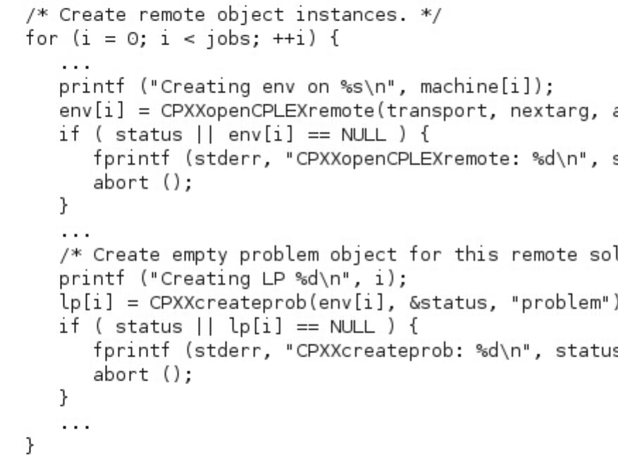
A CPLEX environment pointer CPXENVptr references a remote object instance.
The function CPXXopenCPLEXremote creates such a reference. The following lines
create and initialize the objects needed in this example.
Those lines create a remote object with an empty problem on a remote machine.
Choices such as which machine to use and how to connect to that machine are
specified by arguments of the function CPXXopenCPLEXremote.
vtransport names the data transport protocol used to communicate with the
remote machine. Possible values are mpitransport, processtransport, or
tcpiptransport. (The topic “Transport types for the remote object” on page 389
explains more about those values.)
vnextarg specifies the number of strings in args.
vargs is an array of strings expressing transport-specific configuration options.
Dispatching problem data to remote objects
Documents the dispatch of data to remote objects in an example of distributed
concurrent optimization of a mixed integer program.
This example (parmipopt.c) of distributed concurrent MIP optimization reads the
data of the model from a file. One possibility for dispatching the data from that
original file to the remote objects (in this example, the two workers) is to iterate
over the remote objects and read the data file to each of them. In this example, the
number of remote objects (two) is small, but in general the number of remote
objects can be huge. If the number of remote objects is truly large, iterating over
the individual remote objects and loading the data file into each of them can be
impractical or unrealistic. In contrast, using a multicast to load the data file
simultaneously into all the remote objects is usually faster. In fact, some transport
Chapter 29. Remote object for distributed parallel optimization 407
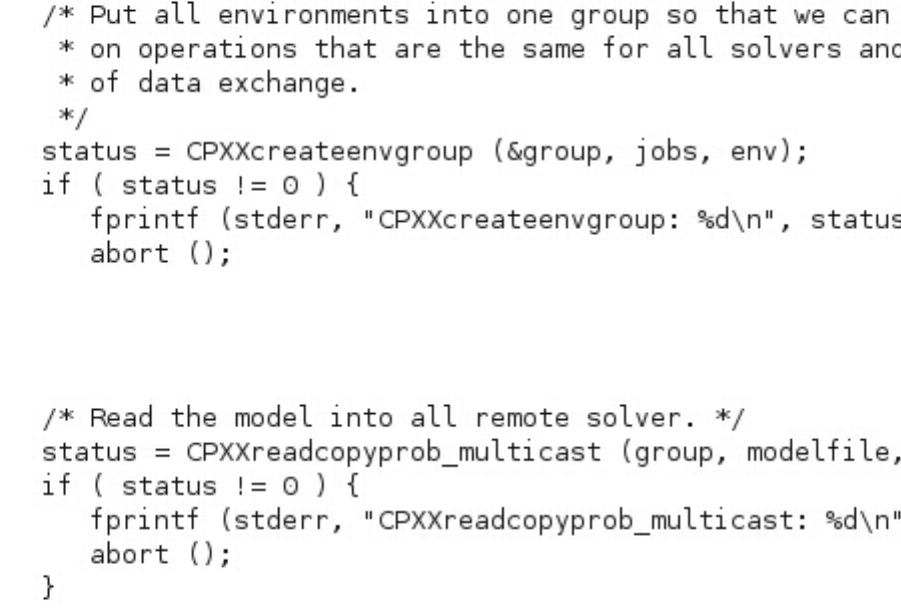
implementations provide special handling of multicasts that can improve
performance dramatically. The message passing interface (MPI) is one such
transport.
To take advantage of a multicast, the following lines of code first create an
environment group. That group contains all the environments of remote objects
that participate in the multicast.
The argument group contains a reference to the newly created group, which
contains all the jobs of all the environments of all the remote objects stored in the
argument env. After that group is created, it is possible to read the data file and
multicast it to all remote objects in the group, as in the following lines of code.
Those lines of code read the file locally into memory and then send this memory
block to all remote objects in the group. The remote objects then parse the memory
block as if it were a file, and thereby each remote object loads the respective
model. After CPXXreadcopyprob_multicast returns, all remote objects in the group
will have loaded the exact same model.
This example also sets the number of threads in each remote object to 1 (one). This
setting reduces machine load in case all "remote" machines are in fact the same
local host.
408 CPLEX User’s Manual
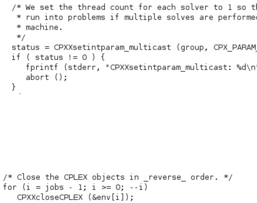
To perform yet another operation (this time, setting the number of threads) in
exactly the same way on every remote object, the example again uses a group and
multicast in the following lines of code.
The following line deletes the group after the group is no longer needed.
CPXXfreeenvgroup (&group);
Destroying remote objects
Destroys remotes objects an example of distributed concurrent optimization of a
mixed integer program.
After the problem is solved, the application must gracefully shut down the remote
objects on the remote machines. This operation occurs in a simple loop, like this:
Tip:
You must destroy the objects in reverse order. For internal technical reasons, you
must respect this reversal. Destroying the objects in any other order can result in
unpredictable behavior.
Setting parameters in remote objects
Shows parameter-setting in an example of distributed concurrent optimization of a
mixed integer program.
The example (parmipopt.c) sets up two contrasting groups of parameters:
primalbound and dualbound. The parameters in primalbound specify values that are
supposed to improve the primal bound of the problem quickly, whereas the
parameters in dualbound specify bounds that are supposed to improve the dual
bound quickly.
In the example, a call of the user-written function applySetting applies these sets of
parameters. This function invokes the Callable Library routines CPXXsetintparam,
CPXXsetlongparam, CPXXsetdblparam on the CPLEX environment pointers
CPXENVptr that reference instances of remote objects. The code in the example is
familiar to users of conventional CPLEX, exactly the same as without the remote
object interface.
Chapter 29. Remote object for distributed parallel optimization 409
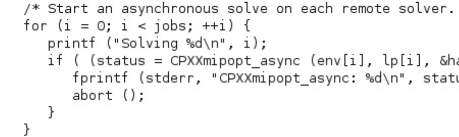
Solving a problem with remote objects
Solves an example of distributed concurrent optimization of a mixed integer
program.
From the perspective of the master, the algorithm that the example parmipopt.c
implements looks like this:
Start the solve on all remote machines
while ( all machines are solving )
display progress message
if ( best known lower and upper bounds are close enough )
stop all machines
stop all machines that are still running
report the results
One way of implementing that algorithm is to use asynchronous function calls on
the remote objects. In contrast to a synchronous function call, an asynchronous
function call does not block until the call completes. Instead, an asynchronous
function returns immediately after triggering the call on the remote object. It
returns a reference to a handle that can be used to check progress of the operation
or to wait for completion of the operation.
To start the solves on all remote objects, the example invokes the asynchronous
version of MIP optimization, like this:
After that call, each machine will have started solving the problem with the
defined parameter settings. The argument handle[i] is a handle to the remote
function call being executed on machine i. To check whether this function is still
running (that is, to verify that the machine is still solving and has not yet found
the optimal solution), the example uses the following line, an asynchronous test:
CPXXasynctest (handle[i], &running);
If the function is still running, that test puts a true value in the argument running;
otherwise, the function puts a false value there. If the value of running is false,
then the function call being tested has solved the problem to optimality. In that
case, the example stops all other machines and reads the optimal solution from the
machine that found it.
In order to stop an ongoing solve on a remote object that has not yet finished, the
example uses an asynchronous kill, like this:
CPXXasynckill (handle[j]);
That line stops the function call defined by handle[j].
410 CPLEX User’s Manual
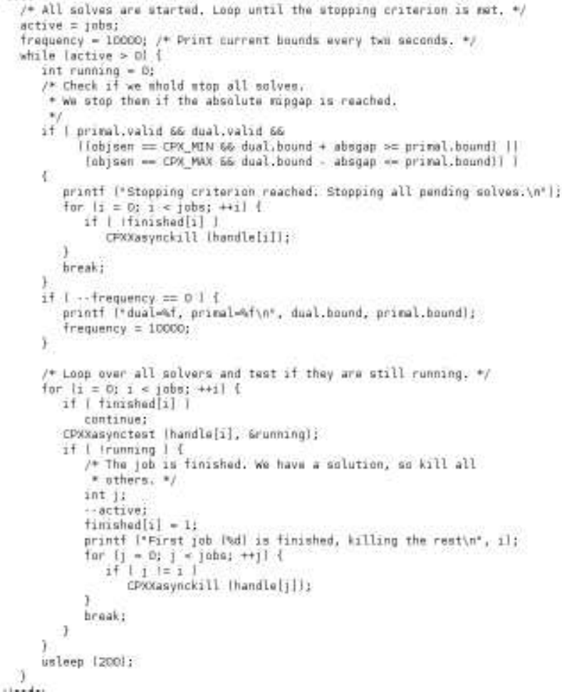
Here is the entire loop on the master:
In the first part of the loop, this example checks whether the best known lower
and upper bounds are close enough. Interestingly, the bounds may come from
different machines. If the bounds are close enough, then the optimal solution has
been found and optimality has been proven. In that case, the example can abort
the solve on all remote objects.
In the second part of the loop, the example checks whether any remote solve has
already finished. If so, then the example stops the solve on all other machines and
exits from the loop.
Since the loop implements a polling mechanism, the example implements a small
delay (usleep(200)) so as to not poll frantically.
Chapter 29. Remote object for distributed parallel optimization 411
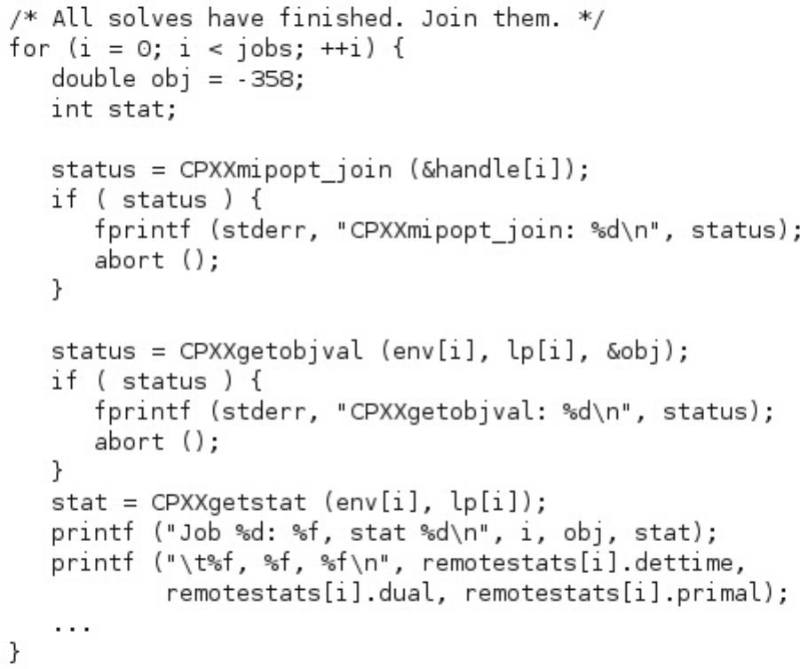
In order to clean up resources properly, the example must join all the
asynchronous solves that were triggered, regardless of whether they completed or
were killed prematurely. After the example has successfully joined the
asynchronous call of CPXXmipopt, the results of this function call are available,
and the example can query the objective function value and algorithm status for
each remote object, like this:
Fetching the results of distributed concurrent MIP
optimization
Fetches remote results in an example of distributed concurrent optimization of a
mixed integer program.
In order to access the x vector of the optimal solution, the example (parmipopt.c)
simply keeps track of the remote object that reported the best feasible solution. In
fact, the argument bestidx is the index of the remote object that reported the best
412 CPLEX User’s Manual
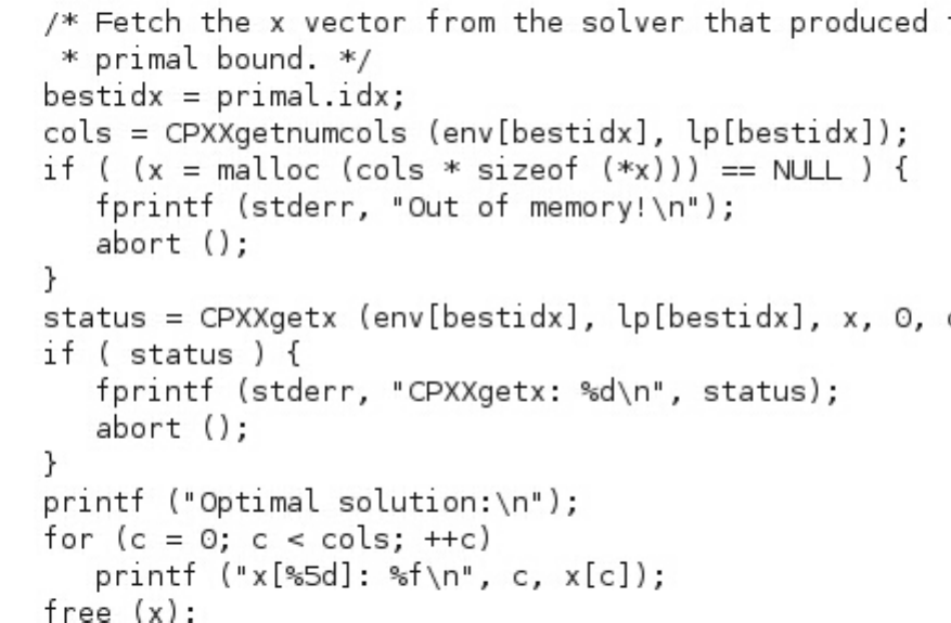
feasible solution. The example then fetches the vector from this object after all
solve calls have finished, like this:
Processing status updates and receiving informational
messages
Master side of messaging in an example of distributed concurrent optimization of a
mixed integer program.
In the example parmipopt.c, the remote worker machines regularly send status
updates to the master machine. To handle status messages (also known as
informational messages or informally, known as info messages) from a remote
object, the example needs to install an information handler (also known informally
as an info handler) in the environment that references the respective remote object.
The following lines of code install such an information handler to manage status
messages.
if ( (status = CPXXsetinfohandler (env[i], infohandler, &remotestats[i])) != 0 ) {
fprintf (stderr, "CPXXsetinfohandler: %d\n", status);
abort ();
}
The argument infohandler is a function with the following signature:
void CPXPUBLIC
infohandler (CPXENVptr xenv, CPXINFOTYPE type, int tag, CPXLONG length,
void const *data, void *handle)
That function is invoked whenever an informational message from a remote object
arrives on the master. The argument xenv is a reference to the remote object from
which the message came. The argument type is the data type of the message. The
argument tag is a user-defined number that identifies the kind of information that
is provided. The arguments length and data are the payload of the message (the
Chapter 29. Remote object for distributed parallel optimization 413

content of which depends on the tag and type arguments). The argument handle is
the third argument that was passed to CPXXsetinfohandler.
The example implements three different kinds of informational messages.
vnew lower bound
This message is sent when a remote object improves on the lower bound. Note
that this is the object-local lower bound, not the overall best lower bound (which
is known only on the master machine).
vnew upper bound
This message is sent when a remote object improves on the upper bound. Note
that this is the object-local upper bound, not the overall best upper bound
(which is known only on the master machine).
vdeterministic time
This message is sent with a high frequency. It gives the current deterministic
time stamp of a remote object.
In the example, these types of messages are managed in a simple switch statement
in the function infohandler by means of updates of global data structures.
Setting up status updates on the remote machines: user
functions
Explains the role of user functions in an example of distributed concurrent
optimization of a mixed integer program.
The example parmipopt.c hooks into a MIP callback on the remote machine in
order to send status updates frequently from the remote machine to the master.
However, the remote object application programming interface (API) does not
explicitly support callbacks, so the example must accomplish the same end by
defining a custom user function for the remote object.
A custom user function is a piece of code that is loaded by the remote object at
runtime. The CPLEX remote API supports this customizing convention by means
of general user functions. On the client side, there is the generic function
CPXXuserfunction.
The argument id is an input argument and specifies which user function to invoke.
The arguments insize and in specify the input arguments for the user function.
When the function is called the first insize bytes of in are copied literally to the
remote object. Upon return of the function, the output provided by the user
function is copied literally from the remote object and stored in outsize_p and out.
The argument outspace gives the size of out, that is, the maximum amount of data
that can be stored there.
The means of getting that piece of code (that is, the custom user function) into the
remote object that actually executes the user-defined function is explained in the
topic “Code running on the remote worker machines.”
Code running on the remote worker machines
Explains an example of distributed concurrent optimization of a mixed integer
program.
414 CPLEX User’s Manual

In an application that sets up a master on a local machine and multiple workers on
remote machines, the binary file running on each worker machine is the cplex
binary file that was started from the master with an appropriate option to
designate the worker and the communication protocol. For example, in
parmipopt.c sample, the command-line option to the cplex binary file looks like
this: -worker=transport where transport specifies the transport communication
protocol.
The command-line of the invocation of the cplex binary file in that example also
includes another option to specify and load a user-defined function. In the example
parmipopt.c, the user function code is compiled whenever the macro
COMPILE_USERFUNCTION is defined. It entails the following functions:
vREGISTER_USERFUNCTION is invoked when the shared object containing the
userfunction code is loaded. It simply registers the function named
userfunction as a CPLEX remote object user function; it does so by means of
CPXXsetuserfunction. (The topic “User functions to run user-defined code on the
remote machine” on page 401 introduces the idea of user functions in general
and outlines their registration.)
vinfocallback is a MIP informational callback. In the example, it is installed by
the function named userfunction. The callback keeps track of the currently best
known primal and dual bounds as well as the current deterministic time.
Whenever a change in a primal or dual bound is observed, an info message (that
is, a status message) with the new bound is sent to the master. Every time the
callback is invoked, it sends an info message with the current deterministic time
to the master. (The topic “Sending status messages to the master” on page 404
introduces the idea of info messages and explains their use in general terms.)
vuserfunction is invoked whenever the master issues a call to CPXXuserfunction.
Depending on the identifier, it performs setup operations (such as registering the
MIP informational callback), or it carries out cleanup operations.
Deploying an application of the CPLEX remote object
Outlines steps to deploy an application of the remote object in CPLEX.
To execute an application of the CPLEX remote object, you must perform these
steps:
1. Build the master process.
2. Build the object that implements the dynamically loadable user function.
3. Deploy both the user-function object and the cplex binary file to the remote
machine.
4. Execute that code.
For simplicity, the following amplification of those steps executes everything on the
same local machine, rather than on a real remote machine. However, later topics
highlight the differences between local and remote execution. Furthermore, the
make files provided with the product explicitly address those differences with
machine-specific settings.
Using a makefile for an application of the CPLEX remote
object
Describes use of a makefile for an application of the remote object in CPLEX.
Chapter 29. Remote object for distributed parallel optimization 415

Sample make files, pre-configured for system-specific library formats, are available
with the product in subdirectories corresponding to the system and library format
of your installation. In order to run the examples available for the remote object,
such as parmipopt.c or parbenders.c, with the process transport as the default
transport, use the following commands, where SYSTEM and LIBFORMAT correspond to
the location on your machine:
cd examples/SYSTEM/LIBFORMAT
make -f Makefile.remote remote-run
To use another transport protocol, apply one of the following commands to specify
another transport instead:
make -f Makefile.remote TRANSPORT=mpi remote-run
or
make -f Makefile.remote TRANSPORT=tcpip remote-run
Contrasting remote and local issues
Contrasts remote and local issues in an application of the remote object in CPLEX.
The simplified example of executing all code on the same, local machine glosses
over a few important points. When you deploy a distributed application using the
CPLEX remote object on multiple machines, you need to keep in mind the
following issues:
vYou need to choose the correct cplex binary file to run on the remote machine.
The binary file to be executed remotely must be compiled for the architecture
and operating system of the remote machine.
vThe same caveat applies to dynamically loadable objects that implement user
functions. The dynamically loadable objects must be built for the architecture
and operating system of the remote machine. If the remote platform (either
architecture or operating system) is different from the development platform,
this discrepancy requires either compiling directly on the remote machine or
cross compiling.
vRoutines such as CPXXreadcopyprob read files on the file system of the master
process and transfer the contents of such files to remote machines. These
routines do not read files from the remote file system.
vRoutines such as CPXXwriteprob write to the file system where the master
process is running. They do not write to the file system where the workers are
running.
Example: parallel optimization of a Benders decomposition
Introduces an example of parallel optimization of a Benders decomposition.
In addition to the sample parmipopt.c demonstrating parallel MIP optimization
using the CPLEX remote object, your CPLEX distribution also includes an example
of parallel optimization of a Benders decomposition: parbenders.c. This example is
available for all ports. There are also make files and Visual Studio projects defined
for this example. One such Visual Studio project (parbenders.process.vcxproj)
demonstrates the example using the process transport protocol; the other project
(parbenders.mpi.vcxproj) demonstrates the message passing interface (MPI)
transport protocol.
To execute that example, you need to prepare the environment.
416 CPLEX User’s Manual
vMake sure that the PATH environment variable includes the directory where the
CPLEX DLL and the remote object DLL are located.
vIf you execute the example with the MPI transport protocol, make sure that the
MPIROOT environment variable specifies the directory where MPI is installed.
To execute the example from the directory corresponding to system and library
format of your installation on GNU/Linux, UNIX, or MacOS operating systems,
use the following command:
make -f Makefile.remote remote-run-parbenders
To execute the example on Windows, prepare your environment as recommended.
Then apply the project in Visual Studio.
Chapter 29. Remote object for distributed parallel optimization 417
418 CPLEX User’s Manual

Chapter 30. Solving a MIP with distributed parallel
optimization
Documents the solution in parallel of a mixed integer program (MIP) in a
distributed environment
Distributed parallel mixed integer programming uses a variation of the well
known branch and bound algorithm to solve a MIP in parallel. In contrast to
conventional branch and bound implemented on platforms with shared memory,
distributed parallel MIP implements a branch and bound algorithm in an
environment of distributed memory, possibly across multiple machines. The
implementation can use more than a single machine to solve a given MIP, thus
making it possible to solve more difficult problems than a shared memory on a
single machine could solve.
Distributed optimization of MIPs: the algorithm
Introduces the algorithm for optimization of a mixed integer program (MIP) in a
distributed computing environment.
The topic Chapter 29, “Remote object for distributed parallel optimization,” on
page 383 introduced the idea of a remote object to support distributed parallel
applications of CPLEX optimizers.
This topic goes further in that direction, introducing the CPLEX algorithm to
support a distributed application designed to solve a mixed integer program (MIP)
in parallel. Specifically, this topic outlines an algorithm that implements a variation
of branch and bound suitable for application across multiple machines (or multiple
nodes of a single machine) to solve a difficult mixed integer program (MIP) in
parallel.
This distributed parallel MIP algorithm runs on a single master associated with
multiple workers. The master and the workers can be physical or virtual machines.
Indeed, in this context, a virtual machine may simply be a process in the operating
system of a machine. Throughout the runtime of this algorithm, the master
coordinates the workers, and the workers perform the "heavy lifting" (that is, the
actual solving of the MIP).
The algorithm begins by presolving the MIP on the master. After presolving, the
algorithm sends the reduced model to each of the workers.
Each of the workers then starts to solve the reduced model. Each worker has its
own parameter settings, possibly different from the parameter settings of other
workers. Each worker solves the reduced model with its own parameter settings
for a limited period of time. This phase is known as ramp up. During ramp up,
each worker conducts its own search, according to its own parameter settings.
Ramp up stops when the master concludes that at least one of the workers has
created a sufficiently large search tree.
At that point, when ramp up stops, the master decides which of the workers
performed best. In other words, the master selects a winner. The parameter settings
© Copyright IBM Corp. 1987, 2016 419

used by the winning worker during ramp up are the basis for the master to
determine which parameter settings to use in the ensuing distributed branch and
bound search.
The search tree on each of the non-winning workers is deleted. The search tree of
the winning worker is distributed over all workers, so that authentic distributed
parallel branch and bound starts from this point. In other words, all workers now
work on the same search tree, with the master coordinating the search in the
distributed tree.
Special characteristics of distributed branch and bound
Distinguishes distributed branch and bound from conventional branch and bound
in shared memory.
The topic “Distributed optimization of MIPs: the algorithm” on page 419 outlined
the algorithm underlying distributed parallel MIP in CPLEX.
This topic continues the description of distributed parallel MIP by distinguishing
the special characteristics of distributed parallel branch and bound from
conventional branch and bound algorithms in shared memory.
Search tree
Distributed parallel branch and bound is similar to conventional, shared-memory
branch and bound. They differ greatly, however, in their management of the search
tree. In a conventional, shared-memory branch and bound, the search tree resides
on a single machine, on disk or in shared memory. In contrast, distributed parallel
branch and bound literally distributes the search tree across a cluster of machines.
In the CPLEX implementation of distributed parallel branch and bound, the master
keeps a number of nodes of the global search tree. If a worker becomes idle, the
master sends some of those nodes to that worker. The worker then starts branch
and bound on those nodes. However, the worker does not simply solve a node,
create some new nodes in doing so, and send them all back to the master. Instead,
the worker considers the search tree node received from the master as a new MIP.
The worker presolves that MIP and finds an optimal solution for that node using
branch and bound. In other words, a worker not only solves a single node; in fact,
the worker solves an entire subtree rooted at that node.
While this distributed parallel branch and bound algorithm is running, the master
can ask a worker to provide some open nodes (that is, unsolved nodes). The
master can then use these nodes to assign work to idle workers. To satisfy such a
request from the master, a worker picks a few open nodes from its current tree.
Because the current tree in a worker is a subtree of the global tree (indeed, it is the
subtree rooted at the node sent to the worker), every node in that subtree is also a
node in the global tree.
Stopping criterion
The distributed parallel branch and bound algorithm stops if all the nodes of the
global search tree have been processed or if it reaches a limit set by the user. Such
limits include a time limit, a limit on the number of nodes processed, a limit on the
number of solutions found, or other similar criteria.
420 CPLEX User’s Manual

Opportunistic distributed parallel MIP
The distributed parallel MIP algorithm supports opportunistic multi-threading.
Specifically, if you set the parallel mode switch to the value -1 (symbolic name
Opportunistic or CPX_PARALLEL_OPPORTUNISTIC), CPLEX will
opportunistically execute the distributed mixed integer programming (MIP)
algorithm in parallel.
The name of the parallel mode switch varies according to the application
programming interface (API) that you choose to use:
vIn the C++ API, use the parameter IloCplex::Param::Parallel
vIn the Java API, use the parameter IloCplex.Param.Parallel
vIn the .NET API, use the parameter Cplex.Param.Parallel
vIn the Callable Library (C API) API, use the parameter CPXPARAM_Parallel
vIn the Python API, use the parameter parameters.parallel
vIn the MATLAB API, use the parameter Cplex.Param.parallel
vIn the Interactive Optimizer, use the command set with the option parallel and
the value -1.
For more information about multi-threading applications, see Chapter 28,
“Multithreaded parallel optimizers,” on page 371 in the CPLEX User's Manual.
Technical limits of distributed branch and bound
Documents limits of distributed branch.
If you are already familiar with solving a mixed integer program (MIP) by means
of conventional CPLEX MIP optimization, there are a few technical differences in
distributed parallel MIP optimization that are worth noting.
No control or query callbacks
Distributed parallel MIP does not support control callbacks. Distributed parallel
MIP does not support query callbacks. However, you can use informational
callbacks with distributed parallel MIP. An informational callback pertains to the
master (not the workers). Furthermore, during rampup, there is no uniquely
defined tree. Consequently, callback information that depends on specifics of a
branch and bound tree does not exist. For more detail about the situations in
which informational callbacks work with distributed parallel MIP, see the
announcement Informational callbacks and distributed MIP. For definitions of
informational, query, and control callbacks, see the topic Chapter 37, “Using
optimization callbacks,” on page 499 in the CPLEX User's Manual. For examples of
informational callbacks, see these samples provided with the product:
vFor users of the Callable Library (C API), see xdistmipex2.c.
vFor users of the C++ API, see ilodistmipex2.cpp.
vFor users of the Java API, see DistMIPEx2.java.
vFor users of the Python API, see distmipex2.py.
vFor users of MATLAB (Cplex class API), see distmipex2.m.
vFor users of the C#.NET API, see DistMIPEx2.cs.
Chapter 30. Solving a MIP with distributed parallel optimization 421

No restarting a run from where it stopped
Distributed parallel MIP always starts from scratch. In contrast, with the
conventional MIP optimizer, you can specify limits, reach them, and restart. For
example, you can specify a limit on the number of nodes to solve and solve your
MIP conventionally with shared memory, stopping when the node limit occurs;
you can then extend the limit on nodes to a greater number and invoke solve
again. With conventional MIP with shared memory, the second solve takes up
where the first solve stopped.
This pattern of stopping and restarting from a previous point is not possible with
distributed parallel MIP. If you attempt that scenario of solving to a node limit,
stopping at the limit, extending the limit to a greater number, and restarting,
distributed parallel MIP simply starts over from scratch (not from the state when it
reached the previous limit).
Mix and match still starts from scratch
Likewise, if you mix calls to conventional MIP with shared memory with calls to
distributed parallel MIP, the call to distributed parallel MIP will always start from
scratch. In fact, if you begin with distributed parallel MIP optimization, let it run
to a limit (such as a time limit, node limit, solutions limit), and then invoke
conventional MIP optimization, even the conventional MIP starts over from
scratch. It does not use any of the information accumulated in the previous
optimization.
VMC file for specifying parameters, ramp up options, and environment
variables in distributed parallel optimization
Documents how to specify CPLEX parameters, ramp up options, and environment
variables in a VMC file for distributed parallel optimization.
A virtual machine configuration (VMC) file is an XML file that specifies the
communication protocol between a master and the workers, as well as the
configuration of each worker (one entry per worker), in a distributed parallel
optimization application. CPLEX accepts VMC files to specify a virtual machine
configuration for distributed parallel optimization.
To assist you in creating such a file yourself, your installation of the product
includes a document type definition (DTD) vmc.dtd and an XML schema
declaration (XSD) vmc.xsd.
Sample VMC files are available in yourCPLEXhome/examples/SYSTEM/FORMAT where
vyourCPLEXhome specifies the folder or directory in your file system where you
installed CPLEX as part of IBM ILOG CPLEX Optimization Studio.
vSYSTEM specifies your combination of computer and operating system.
vFORMAT specifies your compiler.
Setting parameters in a VMC file
To specify parameter settings in a distributed MIP application, use a virtual
machine configuration (VMC) file. By default, workers inherit the parameter
settings of the master, but you can apply different parameter settings for different
workers in the VMC file. You specify CPLEX parameters by name in the <machine>
422 CPLEX User’s Manual
section for a worker in a VMC file. In the event of a conflict between parameter
settings for the master and parameter settings for a worker, the parameter settings
in the VMC file take precedence.
For example, the following line in a VMC file specifies that CPLEX performs
depth-first search in both the ramp up phase and distributed MIP optimization.
<param name="CPX_PARAM_NODESEL" value="0"/>
Setting CPLEX parameters only for ramp up in a VMC file
CPLEX also offers a way of specifying parameters that apply only during ramp up
for distributed parallel optimization. To specify that a given CPLEX parameter
applies only during ramp up, prepend
rampup:
to the name of the CPLEX parameter in the virtual machine configuration (VMC)
file.
For example, look again at the line in a VMC file to specify that CPLEX performs
depth-first search in both the ramp up phase and distributed MIP optimization.
<param name="CPX_PARAM_NODESEL" value="0"/>
In contrast, the following line in a VMC file specifies that CPLEX performs
depth-first search only in the ramp up phase; outside the ramp up phase, CPLEX
applies the default setting for node selection during distributed MIP optimization.
<param name="rampup:CPX_PARAM_NODESEL" value="0"/>
Special ramp up options in a VMC file
CPLEX recognizes special ramp up options in a virtual machine configuration
(VMC) file so that you can give CPLEX useful information about the workers.
v"unlikely_winner"
Some combinations of CPLEX parameter settings can have the effect of the
worker having a very good dual bound, but very few unprocessed search tree
nodes. For example, forcing extremely strong cut generation in a worker can
result in such a situation, making it unlikely for that worker to win the ramp up
competition. In this case CPLEX is likely to delay switching from ramp up to
distributed MIP, even though other workers may have already generated a good
tree (though with a slightly worse dual bound). Therefore, you can mark this
worker as unlikely to be a winner in a reasonable timeframe.
To indicate to CPLEX that you know that the CPLEX parameter settings can
have this side-effect, use the following line in the section declaring the worker in
the virtual machine configuration (VMC) file:
<param name="unlikely_winner" value="1"/>
That line does not exclude the worker from winning; it simply makes CPLEX
take a harder look at the other workers when CPLEX considers when to
terminate the ramp up phase.
v"keeps_all_opt"
You can specify the ramp up option "keeps_all_opt" in the machine section for a
worker in a virtual machine configuration (VMC) file to force CPLEX not to
eliminate any optimal solution during presolve in the ramp up phase. As a
consequence of that ramp up option, CPLEX can merge information from that
worker at the end of ramp up before CPLEX starts the distributed MIP
optimization.
Chapter 30. Solving a MIP with distributed parallel optimization 423

<param name="keeps_all_opt" value="1"/>
When a worker is marked in that way, CPLEX makes sure that presolve does not
eliminate any possible optimal solutions (rather than making sure that at least
one optimal solution remains in the search space).
Why does CPLEX offer this ramp up option? Without this option, CPLEX can
possibly eliminate some optimal solutions in a given worker. Furthermore, the
combined set of optimal solutions eliminated from each of the workers can
(unfortunately, by chance) cover every optimal solution to the problem.
Therefore, CPLEX accepts information from those workers where this option is
set and merges that acceptable information into the information from the worker
that wins the ramp up competition.
Whether to set this ramp up option for a worker or not is a delicately balanced
decision. Setting this option enables CPLEX to merge information from the
worker after ramp up. However, as a consequence of setting this option,
presolve can be less effective in this worker. Not setting this option can make
presolve more effective for this worker (a desirable outcome if this worker wins
the ramp up competition). However, if the worker is not a winner, then some of
the information that the worker gathered can not be merged with the
information from the winning worker.
For example, consider the following straight forward problem:
max x1 + x2
x1 + x2 ≤1
x1, x2 binary
In one worker, CPLEX can fix x2=0 (zero) as a result of presolve. After all, such a
fix still retains the optimal solution (x1=1, x2=0).
In another worker, again as a result of presolve, CPLEX can fix x1=0. After all,
that fix still keeps the optimal solution (x1=0, x2=1).
If information from those two workers in this example were merged without
consideration, then CPLEX concludes unfortunately in the distributed MIP
optimization that (x1=0, x2=0) and thus loses both optimal solutions found by
those two workers (not the results you want, of course).
Environment variables in a VMC file
CPLEX expands an environment variable cited in a VMC file at the time that
CPLEX reads the VMC file. Reference to an environment variable must be of the
form:
$(name)
In particular, CPLEX does not recognize $name nor ${name}. CPLEX interprets the
character sequence $$ as a single $. This convention means that you can produce
verbatim $( by writing $$(.
Before you begin
Consider these general observations before you attempt the following instructions.
The following topics document several ways of using distributed parallel
optimization, that is, the distributed parallel mixed integer programming (MIP)
algorithm implemented in CPLEX. For simplicity and consistency, these topics
assume that the user has a Linux operating system and works in a bash shell.
However, these instructions apply to other operating systems in analogous ways.
424 CPLEX User’s Manual

If you are not using Linux, you may need to adapt the following points in the
instructional topics:
vLD_LIBRARY_PATH: The distributed parallel MIP algorithm implemented in
CPLEX uses dynamically loadable libraries. You have to prepare the runtime
linker so that it can find those libraries when CPLEX requests them. On Linux
this is done by pointing the LD_LIBRARY_PATH environment variable to the
directory that contains the CPLEX dynamically loadable libraries. On other
operating systems this variable may have different names. For example, on
MacOS it is called DYLD_LIBRARY_PATH, on AIX it is called LIBPATH and on
Windows it is PATH.
vShared libraries: On Linux, the names of shared libraries files conventionally
have the suffix .so. On other operating systems, the suffix is different. For
example, on MacOS, the suffix is .dyld. On AIX, the suffix is .a. On Windows,
the suffix is .dll.
vNot all transports (process, MPI, TCP/IP) are available on all platforms.
Consequently, certain features documented in the following topics may be
unavailable on your platform. In particular, there are several platforms on which
the MPI transport is not available.
For simplicity, the instructions in the following topics assume that you have
deployed CPLEX in a directory that is shared over the network by all the machines
involved in your distributed application. This practice (an installation directory
shared across a network) is the conceptually simplest way to deploy CPLEX for
distributed parallel MIP. However, by no means is a "network share" a requirement
to run the CPLEX distributed MIP algorithm. Indeed, it is perfectly fine to deploy
CPLEX to a local directory on each machine involved.
Distributed parallel MIP in the Interactive Optimizer
Shows how to run distributed parallel MIP in the Interactive Optimizer.
In contrast to conventional MIP optimization (with shared memory), distributed
parallel MIP optimization is not a single, stand-alone process in the Interactive
Optimizer. Instead, distributed parallel MIP in the Interactive Optimizer consists of
a suite of distributed processes, each of them potentially running on a different
machine.
While the deployment of the application itself is so different from conventional
MIP, the session in the Interactive Optimizer is quite similar to a conventional
session that optimizes a MIP. A session using distributed parallel MIP generally
looks something like this:
CPLEX> read model.lp
CPLEX> read configuration.vmc
CPLEX> mipopt
CPLEX> display solution variables
The visible difference in that session from a conventional session with shared
memory MIP optimization in the Interactive Optimizer is the command to read a
configuration file:
read configuration.vmc
That command reads a file containing the configuration values for virtual
machines. That configuration tells CPLEX which machines are available for the
distributed parallel algorithm.
Chapter 30. Solving a MIP with distributed parallel optimization 425

A subsequent invocation of mipopt first checks whether a virtual machine
configuration has already been loaded. If not, then the Interactive Optimizer
simply runs conventional MIP optimization with shared memory. However, if a
configuration of virtual machines is present, then the Interactive Optimizer runs
distributed parallel MIP optimization on the machines specified in that
configuration.
For distributed parallel MIP optimization to run correctly, CPLEX must be
deployed on all machines specified in the virtual machine configuration. Your
choice of transport for distributed parallel optimization determines what must be
deployed and how it must be deployed on those machines. The following topics
offer more detail about the implications for what and how of your choice of
transport.
v“Using Open MPI with distributed parallel MIP”
v“Using MPICH with distributed parallel MIP” on page 428
v“Using a process transport protocol with distributed parallel MIP” on page 430
v“Using TCP/IP as the transport protocol with distributed parallel MIP” on page
431
To see the current virtual machine configuration in your Interactive session, use
this command:
display vmc
If you want to stop using distributed parallel optimization in a session of the
Interactive Optimizer (for example, when you want to invoke conventional mipopt
again), then you need to delete the current configuration. To do so, use the
following command:
set distmip config *
Using Open MPI with distributed parallel MIP
Shows how to run distributed parallel MIP with Open MPI transport protocol.
This topic shows how to run distributed parallel MIP optimization with the Open
Message Passing Interface, also known as Open MPI, as the transport protocol to
manage communication between the master and workers.
Prerequisites
vYour CPLEX installation
vA network share or other network file-sharing system, such as Network File
System (NFS), accessible for all the machines, both master and workers, that you
plan to use; for clarification about this prerequisite, see “Before you begin” on
page 424, especially the point about a "network share" not being a hard
requirement.
vYour Open Message Passing Interface (Open MPI) installation in $MPIDIR
MPI is not available for CPLEX V12.6.0 on Windows platforms.
Procedure
1. Find the bin folder or directory of your CPLEX installation.
2. Put the cplex binary file and object files (that is, all files in bin) on the
accessible network share. On many platforms, the object files are designated by
426 CPLEX User’s Manual
the .so file extension. On Windows platforms, these equivalent files are
designated by the .dll file extension. On MacOS, the files are designated by
the .dyld file extension.
For the purpose of this example, all the files from the bin directory of your
CPLEX installation are now in /nfs/CPLEX.
3. Edit the following script to specify your master and workers as well as the
paths to libraries in your installation.
$MPIDIR/bin/mpirun \
-x "LD_LIBRARY_PATH=/nfs/CPLEX:$MPIDIR/lib" \
-tag-output \
-host host1 -host host2 -host host3 \
/nfs/CPLEX/cplex \
-mpi \
-libpath="$MPIDIR/lib" \
-mpilib="$MPIDIR/lib/libmpi.so" \
-mpiapi="openmpi"
In that script, the argument -x "LD_LIBRARY_PATH=/nfs/CPLEX:$MPIDIR/lib"
sets the environment variable so that the runtime linker can easily find the
CPLEX remote object and the MPI libraries. For more information about the
CPLEX remote object, see the topic Chapter 29, “Remote object for distributed
parallel optimization,” on page 383 in the CPLEX User's Manual.
The arguments following -mpi are required only if you have installed more
than one MPI library or if your MPI library is not installed in the standard
location.
That sample script creates an MPI cluster of three machines, with host1 as
master and host2 and host3 as workers.
4. Create a Virtual Machine Configuration file, configuration.vmc, to define the
available workers. Here is a sample of such a file for this example.
<?xml version="1.0"?>
<vmc>
<machine name="host2">
<transport type="MPI">
<rank value="1"/>
</transport>
</machine>
<machine name="host3">
<transport type="MPI">
<rank value="2"/>
</transport>
</machine>
</vmc>
5. On the master (host1 in this example), start a session in the CPLEX Interactive
Optimizer.
6. In your interactive session, execute the command to read the configuration file
that you created.
CPLEX> read configuration.vmc
After that read command, CPLEX is set up for solving distributed parallel MIP
models.
7. Still in your interactive session, enter a model or read it from a file, and then
solve it, like this:
CPLEX> read model.lp
CPLEX> mipopt
8. All the usual commands of the Interactive Optimizer are available to access and
analyze your results.
Chapter 30. Solving a MIP with distributed parallel optimization 427

A convenient short-cut in the Interactive Optimizer
A Virtual Machine Configuration file can contain redundant information.
Consequently, if all the machines in the MPI cluster are available for distributed
parallel MIP optimization, and the master is the process with rank=0 (zero), then
CPLEX can automatically construct a Virtual Machine Configuration from the MPI
environment. Instead of reading a configuration through the command:
CPLEX> read configuration.vmc
you can instead issue the command:
CPLEX> set distmip config mpi
That command creates a Virtual Machine Configuration internally that represents
the full MPI cluster in which CPLEX is running.
Using MPICH with distributed parallel MIP
Shows how to run distributed parallel MIP with MPICH transport protocol.
This topic shows how to run distributed parallel MIP optimization with MPICH, a
portable implementation of the message passing interface, as the transport protocol
to manage communication between the master and workers.
Prerequisites
vYour CPLEX installation
vA network share or other network file-sharing system, such as Network File
System (NFS), accessible for all the machines, both master and workers, that you
plan to use; for clarification about this prerequisite, see “Before you begin” on
page 424, especially the point about a "network share" not being a hard
requirement.
vYour MPICH installation in $MPIDIR
MPI is not available for CPLEX V12.6.0 on Windows platforms.
Procedure
1. Find the bin folder or directory of your CPLEX installation.
2. Put the cplex binary file and object files (that is, all files in bin) on the
accessible network share. On many platforms, the object files are designated by
the .so file extension. On MacOS, the suffix is .dyld. On AIX, the suffix is .a.
On Windows platforms, these equivalent files are designated by the .dll file
extension.
For the purpose of this example, all the files from the bin folder or directory of
your CPLEX installation are now in /nfs/CPLEX/.
3. Edit the following script to specify your master and workers as well as the
paths to libraries in your installation. (The syntax is only slightly different from
the sample script in “Using Open MPI with distributed parallel MIP” on page
426.)
$MPIDIR/bin/mpirun \
-genv LD_LIBRARY_PATH /nfs/CPLEX:$MPIDIR/lib \
-hosts host1,host2,host3 \
--prepend-rank \
/nfs/CPLEX/cplex \
428 CPLEX User’s Manual
-mpi \
-libpath="$MPIDIR/lib" \
-mpilib="$MPIDIR/lib/libmpi.so" \
-mpiapi="mpich"
In that script, the argument -genv LD_LIBRARY_PATH /nfs/CPLEX:$MPIDIR/lib"
sets the environment variable so that the runtime linker can easily find the
CPLEX remote object and the MPICH libraries. For more information about the
CPLEX remote object, see the topic Chapter 29, “Remote object for distributed
parallel optimization,” on page 383 in the CPLEX User's Manual.
The arguments following -mpi are required only if you have installed more
than one MPI library or if your MPI library is not installed in the standard
location.
That sample script creates an MPI cluster of three machines, with host1 as
master and host2 and host3 as workers.
4. Create a Virtual Machine Configuration file, configuration.vmc, to define the
available workers. Here is a sample of such a file for this example.
<?xml version="1.0"?>
<vmc>
<machine name="host2">
<transport type="MPI">
<rank value="1"/>
</transport>
</machine>
<machine name="host3">
<transport type="MPI">
<rank value="2"/>
</transport>
</machine>
</vmc>
5. On the master (host1 in this example), start a session in the CPLEX Interactive
Optimizer.
6. In your interactive session, execute the command to read the configuration file
that you created.
CPLEX> read configuration.vmc
After that read command, CPLEX is set up for solving distributed parallel MIP
models.
7. Still in your interactive session, enter a model or read it from a file, and then
solve it, like this:
CPLEX> read model.lp
CPLEX> mipopt
8. All the usual commands of the Interactive Optimizer are available to access and
analyze your results.
A convenient short-cut in the Interactive Optimizer
A Virtual Machine Configuration file can contain redundant information.
Consequently, if all the machines in the MPI cluster are available for distributed
parallel MIP optimization, and the master is the process with rank=0 (zero), then
CPLEX can automatically construct a Virtual Machine Configuration from the MPI
environment. Instead of reading a configuration through the command:
CPLEX> read configuration.vmc
you can instead issue the command:
CPLEX> set distmip config mpi
Chapter 30. Solving a MIP with distributed parallel optimization 429

That command creates a Virtual Machine Configuration internally that represents
the full MPI cluster in which CPLEX is running.
Using a process transport protocol with distributed parallel MIP
Shows how to run distributed parallel MIP with a process transport protocol.
This topic shows how to run distributed parallel MIP optimization with a process
as the transport protocol to manage communication between the master and
workers. Specifically, this example uses a secure shell (ssh) for the master to
connect to the workers. For simplicity, the example assumes that this secure shell
has been set up to use no password on the remote machines. For more information
about a process transport protocol, compare the topic “Transport types for the
remote object: process” on page 390 about the CPLEX remote object.
Prerequisites
vYour CPLEX installation
vA network share or other network file-sharing system, such as Network File
System (NFS), accessible for all the machines, both master and workers, that you
plan to use; for clarification about this prerequisite, see “Before you begin” on
page 424, especially the point about a "network share" not being a hard
requirement.
Procedure
The procedure for using a process transport protocol for communication is slightly
simpler than for using a message passing transport protocol since you do not need
to declare a message passing cluster. However, the declarations in the Virtual
Machine Configuration file configuration.vmc are more detailed.
1. Find the bin folder or directory of your CPLEX installation.
2. Put the cplex binary file and object files (that is, all files in the bin folder or
directory) on the accessible network share. On many platforms, the object files
are designated by the .so file extension. On Windows platforms, these
equivalent files are designated by the .dll file extension. On MacOS, the suffix
is .dyld. On AIX, the suffix is .a.
For the purpose of this example, all the files from the bin directory of your
CPLEX installation are now in /nfs/CPLEX.
3. Create a Virtual Machine Configuration file, configuration.vmc, to define the
available workers. Here is a sample of such a file for a secure shell as the
process.
<?xml version="1.0"?>
<vmc>
<machine name="host2">
<transport type="process">
<cmdline>
<item value="ssh"/>
<item value="host2"/>
<item value="/nfs/CPLEX/cplex"/>
<item value="-worker=process"/>
<item value="-stdio"/>
<item value="-libpath=/nfs/CPLEX"/>
</cmdline>
</transport>
</machine>
<machine name="host3">
430 CPLEX User’s Manual

<transport type="process">
<cmdline>
<item value="ssh"/>
<item value="host2"/>
<item value="/nfs/CPLEX/cplex"/>
<item value="-worker=process"/>
<item value="-stdio"/>
<item value="-libpath=/nfs/CPLEX"/>
</cmdline>
</transport>
</machine>
</vmc>
4. On the master (host1 in this example), start a session in the CPLEX Interactive
Optimizer.
5. In your interactive session, execute the command to read the configuration file
that you created.
CPLEX> read configuration.vmc
After that read command, CPLEX is set up for solving distributed parallel MIP
models.
6. Still in your interactive session, enter a model or read it from a file, and then
solve it, like this:
CPLEX> read model.lp
CPLEX> mipopt
7. All the usual commands of the Interactive Optimizer are available to access and
analyze your results.
Using TCP/IP as the transport protocol with distributed parallel MIP
Shows how to run distributed parallel MIP with TCP/IP transport protocol.
This topic shows how to run distributed parallel MIP optimization with TCP/IP,
Transmission Control Protocol/Internet Protocol, as the transport protocol to
manage communication between the master and workers. This approach is slightly
more complicated than a process transport or a message passing interface (MPI)
transport because you must start a CPLEX remote object worker, whereas these
remote objects as workers start automatically for the other types of transport. For
more information about using TCP/IP with CPLEX, compare the topic “Transport
types for the remote object: TCP/IP” on page 392.
Prerequisites
vYour CPLEX installation
vA network share or other network file-sharing system, such as Network File
System (NFS), accessible for all the machines, both master and workers, that you
plan to use; for clarification about this prerequisite, see “Before you begin” on
page 424, especially the point about a "network share" not being a hard
requirement.
Procedure
1. Find the bin folder or directory of your CPLEX installation.
2. Put the cplex binary file and object files (that is, all files in bin) on the
accessible network share. On many platforms, the object files are designated by
the .so file extension. On Windows platforms, these equivalent files are
designated by the .dll file extension. On MacOS, the suffix is .dyld. On AIX,
the suffix is .a.
Chapter 30. Solving a MIP with distributed parallel optimization 431

For the purpose of this example, all the files from the bin folder or directory of
your CPLEX installation are now in /nfs/CPLEX.
3. For each host that will serve as a worker, execute the following command:
/nfs/CPLEX/cplex -worker=tcpip -libpath=/nfs/cplex -address=ip:12345
where ip is the name of the host or its IP address and 12345 is the number of
the port where the worker will listen for incoming connections. (You are free to
choose a different port number here.)
That command starts a TCP/IP server to wait for connections from the master.
The TCP/IP server also spawns worker processes as requested. The server does
not terminate itself, however. You must explicitly terminate it; for example, by
pressing CTRL-C when your optimization completes.
4. Create a Virtual Machine Configuration file, configuration.vmc, to define the
available workers. Here is a sample of such a file for TCP/IP.
<?xml version="1.0"?>
<vmc>
<machine name="host2">
<transport type="TCP/IP">
<address host="ip-of-host2" port="12345"/>
</transport>
</machine>
<machine name="host3">
<transport type="TCP/IP">
<address host="ip-of-host3" port="12345"/>
</transport>
</machine>
</vmc>
That sample file defines two workers, one worker on host2 and one worker on
host3. The sample value ip-of-hostN is either the IP address or the name of the
host. The host names and the port numbers must be the same in the
configuration file as those used to start the TCP/IP worker on the
corresponding host.
5. On the master (host1 in this example), start a session in the CPLEX Interactive
Optimizer.
6. In your interactive session, execute the command to read the configuration file
that you created for this TCP/IP example.
CPLEX> read configuration.vmc
After that read command, CPLEX is set up for solving distributed parallel MIP
models.
7. Still in your interactive session, enter a model or read it from a file, and then
solve it, like this:
CPLEX> read model.lp
CPLEX> mipopt
8. All the usual commands of the Interactive Optimizer are available to access and
analyze your results.
Example: Callable Library (C API)
Demonstrates an example of distributed parallel MIP from the Callable Library (C
API).
The implementation of an application to use distributed parallel MIP optimization
in the Callable Library (C API) of CPLEX does not differ greatly from an
application of conventional (shared memory) MIP optimization. The most
significant differences are these points:
432 CPLEX User’s Manual
vYou must load a Virtual Machine Configuration (that is, a configuration.vmc)
before you run distributed parallel MIP optimization.
vInstead of calling CPXXmipopt, your application calls CPXXdistmipopt.
Sample source code
CPLEX offers an example, xdistmipex1.c, that illustrates how to use distributed
parallel MIP. These are the key statements in this code:
env = CPXXopenCPLEX (&status);
status = CPXXreadcopyvmconfig (env, vmconfig);
lp = CPXXcreateprob (env, &status, argv[i]);
status = CPXXreadcopyprob (env, lp, argv[i], NULL);
status = CPXXdistmipopt (env, lp);
As in other applications of the CPLEX Callable Library (C API), the routines
CPXXopenCPLEX, CPXXcreateprob, and CPXXreadcopyprob create a CPLEX
environment and load a problem from a file into a problem object. The routine
CPXXreadcopyvmconfig locad a Virtual Machine Configuration from a file. This
configuration defines which machines the up-coming call of distributed parallel
MIP optimization can use. The routine CPXXdistmipopt invokes distributed
parallel MIP optimization on the problem already loaded and uses the machines
specified in the Virtual Machine Configuration.
Compilation and linking
Compilation of applications that use distributed parallel MIP conforms to the same
conventions as any other Callable Library (C API) application of CPLEX.
Linking on a non-Windows platform, however, is slightly different. If your
application uses distributed parallel MIP, then you must link with
libcplexdistmip.a, part of the CPLEX distribution found in the same place as
libcplex.a. You also must link with libdl.so to enable the application for loading
shared objects. To link with libdl.so, add the option -ldl to the linker command.
Running your application
Running a distributed parallel MIP application is more involved than running a
shared memory application. Your application acts as master while the other
machines specified in your Virtual Machine Configuration act as workers. In order
to run such an application, you must follow these steps:
1. Deploy the workers. That is, copy binaries and shared libraries as explained in
the transport topics:
v“Using Open MPI with distributed parallel MIP” on page 426
v“Using MPICH with distributed parallel MIP” on page 428
v“Using a process transport protocol with distributed parallel MIP” on page
430
v“Using TCP/IP as the transport protocol with distributed parallel MIP” on
page 431
2. Set up your environment so that your application can find the CPLEX shared
libraries. One way to do so is to set an environment variable to point to the
folder or directory that holds the CPLEX shared library.
Chapter 30. Solving a MIP with distributed parallel optimization 433

vOn AIX, set the environment variable LIBPATH.
vOn GNU/Linux, set the environment variable LD_LIBRARY_PATH.
vOn MacOS, set the environment variable DYLD_LIBRARY_PATH.
vOn Windows, set the environment variable PATH.
3. Run your application.
vOn Windows, CPLEX offers a Visual Studio project, that is, a file with the
extension .vcxproj and containing options and values to compile, link, and
run the example xdistmipex1.c. Simply load xdistmipex1.vcxproj and run
the project to execute the code.
vOn other platforms, CPLEX offers a Makefile that compiles, links, and runs
the example xdistmipex1.c. In the following sample commands, replace
these values by appropriate values from your installation.
–COS_INSTALL_DIR is the folder or directory where you installed IBM ILOG
CPLEX Optimization Studio.
–system is the type of your computer platform.
–libformat is the library format.
Then execute the equivalent commands:
cd COS_INSTALL_DIR/cplex/examples/system/libformat
make -f Makefile.distmip dm_execute_c
Example: C++ API
Demonstrates an example of distributed parallel MIP in the C++ API of CPLEX.
You write a distributed parallel MIP application in C++ in much the same way that
you write a conventional (shared memory) application of CPLEX in C++. In that
application, you include an additional step: before you invoke the method
IloCplex::solve, you must load a Virtual Machine Configuration (a
configuration.vmc file, as explained in “Distributed parallel MIP in the Interactive
Optimizer” on page 425.) The presence of the configuration file tells IloCplex::solve
to run distributed parallel MIP instead of conventional (shared memory) MIP
optimization.
Source code
CPLEX offers sample code ilodistmipex1.cpp that shows how to use distributed
parallel MIP. The important statements in that code are these statements:
IloEnv env;
IloModel model(env);
IloCplex cplex(model);
cplex.importModel(model, argv[i]);
cplex.readCopyVMConfig(vmconfig);
cplex.solve();
Those first four statements create an instance of the CPLEX solver and load the
model of a problem into it.
The call to IloCplex::readCopyVMConfig loads a Virtual Machine Configuration
from a file. This configuration specifies which machines the distributed parallel
MIP optimization will use.
434 CPLEX User’s Manual

Finally, the call to IloCplex::solve checks whether the problem is a MIP and
whether a Virtual Machine Configuration has been loaded. If so, CPLEX runs
distributed parallel MIP optimization. Otherwise, it uses one of the conventional
algorithms to solve the loaded model.
Compiling and linking
The conventions to compile applications that use distributed parallel MIP
optimization are precisely the same as the conventions of other CPLEX C++
applications.
On platforms other than Windows, however, the linking is slightly different for an
application of distributed parallel MIP optimization. When your application uses
distributed parallel MIP, you must link with libcplexdistmip.a, a part of the
CPLEX distribution, located in the same place as libcplex.a. You must also link
with libdl.so to enable your application to load shared objects. To link with
libdl.so, you can add the option -ldl to your linker command.
Running your application
Execution of an application using distributed parallel MIP optimization is slightly
more complicated than running a conventional (shared memory) C++ application
of CPLEX. Your application acts as master in distributed parallel MIP while the
other machines specified in the Virtual Machine Configuration act as workers. In
order to run your application, you follow these steps:
1. Deploy the workers. That is, copy the binaries and shared libraries as explained
in “Distributed parallel MIP in the Interactive Optimizer” on page 425.
2. Set up your environment so that your application can find the CPLEX shared
libraries. One way to do so is to set an environment variable to specify the
folder or directory where the CPLEX shared library is located.
vOn AIX, set the environment variable LIBPATH.
vOn GNU/Linux, set the environment variable LD_LIBRARY_PATH.
vOn MacOS, set the environment variable DYLD_LIBRARY_PATH.
vOn Windows, set the environment variable PATH.
3. Run your application.
vOn Windows, CPLEX offers a Visual Studio project, that is, a file with the
extension .vcxproj and containing options and values to compile, link, and
run the example ilodistmipex1.cpp. Simply load ilodistmipex1.vcxproj and
run the project to execute the code.
vOn other platforms, CPLEX offers a Makefile that compiles, links, and runs
the example ilodistmipex1.cpp. In the following sample commands, replace
these values by appropriate values from your installation.
–COS_INSTALL_DIR is the folder or directory where you installed IBM ILOG
CPLEX Optimization Studio.
–system is the type of your computer platform.
–libformat is the library format.
Then execute the equivalent commands:
cd COS_INSTALL_DIR/cplex/examples/system/libformat
make -f Makefile.distmip dm_execute_cpp
Example: Java API
Demonstrates an example of distributed parallel MIP in the Java API of CPLEX.
Chapter 30. Solving a MIP with distributed parallel optimization 435
You write a distributed parallel MIP application in Java in much the same way that
you write a conventional (shared memory) application of CPLEX in Java. In that
application, you include an additional step: before you invoke the method
IloCplex.solve, you must load a Virtual Machine Configuration (a
configuration.vmc file, as explained in “Distributed parallel MIP in the Interactive
Optimizer” on page 425.) The presence of the configuration file tells IloCplex.solve
to run distributed parallel MIP instead of conventional (shared memory) MIP
optimization.
Source code
CPLEX offers sample code DistMIPex1.java that shows how to use distributed
parallel MIP. The important statements in that code are these statements:
cplex = new IloCplex();
cplex.importModel(arg);
cplex.readCopyVMConfig(vmconfig);
cplex.solve();
Those first two statements create an instance of the CPLEX solver and load the
model of a problem into it.
The call to IloCplex.readCopyVMConfig loads a Virtual Machine Configuration
from a file. This configuration specifies which machines the distributed parallel
MIP optimization will use.
Finally, the call to IloCplex.solve checks whether the problem is a MIP and
whether a Virtual Machine Configuration has been loaded. If so, CPLEX runs
distributed parallel MIP optimization. Otherwise, it uses one of the conventional
algorithms to solve the loaded model.
Building the application
Java applications that use distributed parallel MIP build in the same way as
conventional Java applications of CPLEX.
Running your application
Execution of an application using distributed parallel MIP optimization is slightly
more complicated than running a conventional (shared memory) Java application
of CPLEX. Your application acts as master in distributed parallel MIP optimization
while the other machines specified in the Virtual Machine Configuration act as
workers. In order to run your application, you follow these steps:
1. Deploy the workers. That is, copy the binaries and shared libraries as explained
in “Distributed parallel MIP in the Interactive Optimizer” on page 425.
2. Set up your environment so that your application can find the CPLEX shared
libraries. One way to do so is to set an environment variable to specify the
folder or directory where the CPLEX shared library is located.
vOn AIX, set the environment variable LIBPATH.
vOn GNU/Linux, set the environment variable LD_LIBRARY_PATH.
vOn MacOS, set the environment variable DYLD_LIBRARY_PATH.
vOn Windows, set the environment variable PATH.
3. Run your application.
436 CPLEX User’s Manual

On Windows, CPLEX offers a makefile suitable for nmake. On other platforms,
CPLEX offers a Makefile that builds and runs the example DistMIPex1.java. In
the following sample commands, replace these values by appropriate values
from your installation.
vCOS_INSTALL_DIR is the folder or directory where you installed IBM ILOG
CPLEX Optimization Studio.
vsystem is the type of your computer platform.
vlibformat is the library format.
Then execute the equivalent commands:
cd COS_INSTALL_DIR/cplex/examples/system/libformat
make -f Makefile.distmip dm_execute_java
Example: Python API
Demonstrates an example of distributed parallel MIP in the Python API of CPLEX.
You write a distributed parallel MIP application in Python in much the same way
that you write a conventional (shared memory) application of CPLEX in Python. In
that application, you include an additional step: before you invoke the method
solve of the class Cplex, you must load a Virtual Machine Configuration (a
configuration.vmc file, as explained in “Distributed parallel MIP in the Interactive
Optimizer” on page 425.) The presence of the configuration file tells solve to run
distributed parallel MIP instead of conventional (shared memory) MIP
optimization.
Source code
CPLEX offers sample code distmipex1.py that shows how to use distributed
parallel MIP. The important statements in that code are these statements:
cpx = cplex.Cplex()
cpx.read(arg)
cplex.read_copy_vmconfig(vmconfig)
cpx.solve()
Those first two statements create an instance of the CPLEX solver and load the
model of a problem into it.
The call to read_copy_vmconfig loads a Virtual Machine Configuration from a file.
This configuration specifies which machines the distributed parallel MIP
optimization will use.
Finally, the call to solve checks whether the problem is a MIP and whether a
Virtual Machine Configuration has been loaded. If so, CPLEX runs distributed
parallel MIP optimization. Otherwise, it uses one of the conventional algorithms to
solve the loaded model.
Running your application
Execution of an application using distributed parallel MIP optimization is slightly
more complicated than running a conventional (shared memory) Python
application of CPLEX. Your application acts as master in distributed parallel MIP
Chapter 30. Solving a MIP with distributed parallel optimization 437

optimization while the other machines specified in the Virtual Machine
Configuration act as workers. In order to run your application, you follow these
steps:
1. Deploy the workers. That is, copy the binaries and shared libraries as explained
in “Distributed parallel MIP in the Interactive Optimizer” on page 425.
2. Set up your environment so that your application can find the CPLEX shared
libraries. One way to do so is to set an environment variable to specify the
folder or directory where the CPLEX shared library is located.
vOn AIX, set the environment variable LIBPATH.
vOn GNU/Linux, set the environment variable LD_LIBRARY_PATH.
vOn MacOS, set the environment variable DYLD_LIBRARY_PATH.
vOn Windows, set the environment variable PATH.
3. Run your application.
Using multiple processes as workers on a single machine
Explains an application of distributed parallel MIP in multiple processes on a
single machine.
There are situations in which you want to run all code on a single machine. For
example, when you are debugging a complex application, running all code locally
can be beneficial. For the purpose of this example, assume that the local
environment offers 12 cores. In such a case, it can be useful to view that computer
as 12 virtual machines with one core each.
To configure such an environment, you simply add a threads parameter for each
virtual machine in your Virtual Machine Configuration, like this:
<machine>
<transport type=". . .">
. . .
</transport>
<param name="threads" value="1" />
</machine>
That configuration tells CPLEX to use one thread on this particular virtual
machine. The deployment in this case is almost the same as in other cases, with
these differences:
vIf you choose message passing interface (MPI) as the transport protocol, use
"localhost" as the host name for each host.
vIf you choose the process transport, omit the following arguments from the
command line:
– <item value="-stdio" />
– <item value="ssh" />
– <item value="hostname" />
vIf you choose TCP/IP transport protocol, you need to start only one worker on
the local host. All virtual machines declared in the Virtual Machine
Configuration (that is, the configuration.vmc file) should connect to the same
address, such as localhost:12345, for example.
Such a configuration provides interesting opportunities. For example, you can use
a single machine to ramp up an infinite horizon. That practice of ramping up with
an infinite horizon is also known as concurrent MIP optimization. For certain hard
438 CPLEX User’s Manual
models, concurrent MIP optimization or ramping up with an infinite horizon has
been shown to improve performance, even on a single computer with multiple
cores.
Chapter 30. Solving a MIP with distributed parallel optimization 439
440 CPLEX User’s Manual

Part 6. Infeasibility and unboundedness
Documents tools to help you analyze the source of the infeasibility in a model: the
preprocessing reduction parameter for distinguishing infeasibility from
unboundedness, the conflict refiner for detecting minimal sets of mutually
contradictory bounds and constraints, and FeasOpt for repairing infeasibilities.
© Copyright IBM Corp. 1987, 2016 441
442 CPLEX User’s Manual

Chapter 31. Preprocessing and feasibility
Introduces the detection of infeasibilities during preprocessing.
Issues of infeasibility and unboundedness
Outlines issues of infeasibility and unboundedness.
The topics discussed in Part 3, “Continuous optimization,” on page 133 and Part 4,
“Discrete optimization,” on page 219 often contained the implicit assumption that a
bounded feasible solution to your model actually exists. Such may not always be
the case.
The following topics discuss steps to try when the outcome of an optimization is a
declaration that your model is either:
vinfeasible; that is, no solution exists that satisfies all the constraints, bounds,
and integrality restrictions; or
vunbounded; that is, the objective function can be made arbitrarily large.
(A more careful definition of unbounded is provided in “What is
unboundedness?” on page 447.)
Infeasibility and unboundedness are closely related topics in optimization theory.
Consequently, certain of the concepts for one will have direct relation to the other.
As you know, IBM ILOG CPLEX can provide you solution information about the
models that it optimizes. For infeasible outcomes, it reports values that you can
analyze to detect what in your problem formulation caused this result. In certain
situations, you can then alter your problem formulation or change CPLEX
parameters to achieve a satisfactory solution.
Infeasibility can arise from various causes, and it is not possible to automate
procedures to deal with those causes entirely without input or intervention from
the user. For example, in a shipment model, infeasibility could be caused by
insufficient supply, or by an error in demand, and it is likely that the optimizer
will tell the user only that the mismatch exists. The formulator of the model has to
make the ultimate judgment of what the actual error is.
However, there are ways for you to try to narrow down the investigation with
help from CPLEX, for example, through tools such as the conflict refiner,
documented in Chapter 33, “Diagnosing infeasibility by refining conflicts,” on page
451. In certain situations, CPLEX even provides some degree of automatic repair,
for example, with tools such as FeasOpt, documented in Chapter 34, “Repairing
infeasibilities with FeasOpt,” on page 465.
The following topic explains how to interpret reports of infeasibility that occur
before optimization begins, that is, reports that arise from preprocessing.
Early reports of infeasibility based on preprocessing reductions
Explains how to interpret early reports of infeasibility and how to use a parameter
in diagnosis.
© Copyright IBM Corp. 1987, 2016 443
CPLEX preprocessing may declare a model infeasible before the selected
optimization algorithm begins.
This early declaration saves considerable execution time in most cases.
When this declaration is the outcome of preprocessing, it is important to
understand that there are two classes of reductions performed by the preprocessor:
primal and dual reductions.
Reductions that are independent of the objective function are called primal
reductions; those that are independent of the righthand side (RHS) of the
constraints are called dual reductions.
Preprocessing operates on the assumption that the model being solved is expected
by the user to be feasible and that a finite optimal solution exists. If this
assumption is false, then the model is either infeasible or no bounded optimal
solutions exist; that is, it is unbounded.
Since primal reductions are independent of the objective function, they cannot
detect unboundedness; they can detect only infeasibility.
Similarly, dual reductions can detect only unboundedness.
Thus, to aid analysis of an infeasible or unbounded declaration by the
preprocessor, a parameter is provided that the user can set, so that the
optimization can be rerun to make sure that the results reported by the
preprocessor can be interpreted. The CPLEX Parameters Reference Manual documents
this parameter: primal and dual reduction type (CPXPARAM_Reduce).
If a model is declared by the preprocessor to be infeasible or unbounded and the
user believes that it might be infeasible, the parameter can be set to 1 by the user,
and the preprocessor will perform only primal reductions.
If the preprocessor still finds inconsistency in the model, the preprocessor will
declare the model infeasible, instead of infeasible or unbounded.
Similarly, setting the parameter that controls primal and dual reduction type
(CPXPARAM_Reduce) to 2 means that if the preprocessor detects unboundedness in
the model, the model will be declared unambiguously to be unbounded.
Important: For either of those settings (1 or 2) of the parameter that controls
primal and dual reduction type (CPXPARAM_Reduce), you should also set the
advanced start switch (CPXPARAM_Advance) to 0 (zero) so that CPLEX recalculates
the status, rather than returning the current status.
To control the types of reductions performed by the presolver, set the parameter to
one of the following values:
v0 = no primal and dual reductions
v1 = only primal reductions
v2 = only dual reductions
v3 = both primal and dual reductions (default)
These settings of the parameter are intended for diagnostic use, as turning off
reductions will usually have a negative impact on performance of the optimization
algorithms in the normal (feasible and bounded) case.
444 CPLEX User’s Manual
Tip: If CPLEX returns a solution status that specifies that your model is infeasible
or unbounded, you can remove the objective function and re-optimize in order to
check whether the model is feasible. For more about this idea, especially about
unboundedness, see also “Diagnosing unboundedness” on page 448.
Chapter 31. Preprocessing and feasibility 445
446 CPLEX User’s Manual

Chapter 32. Managing unboundedness
Discusses tactics to diagnose the cause of an unbounded outcome in the
optimization of a model and suggests ways to avoid an unbounded outcome.
What is unboundedness?
Defines unboundedness and tells how to access further information about the
problem.
Any class of model, continuous or discrete, linear or quadratic, has the potential to
result in a solution status of unbounded. An unbounded discrete model must have a
continuous relaxation that is also unbounded. Therefore, the discussion here
assumes that you first relax any discrete elements, and thus you deal with an
unbounded continuous optimization problem, when you try to diagnose the cause.
Note:
The reverse of that observation (that an unbounded discrete model necessarily has
an unbounded continuous relaxation) is not necessarily the case: a discrete
optimization model may have an unbounded continuous relaxation and yet have a
bounded optimum.
A declaration of unboundedness means that IBM ILOG CPLEX has detected that
the model has an unbounded ray. That is, for any feasible solution x with objective
z, a multiple of the unbounded ray can be added to x to give a feasible solution
with objective z-1 (or z+1 for maximization models). Thus, if a feasible solution
exists, then the optimal objective is unbounded.
When a model is declared unbounded, CPLEX has not necessarily concluded that a
feasible solution exists. Users can call methods or routines to discover whether
CPLEX has also concluded that the model has a feasible solution.
vIn Concert Technology, call one of these methods:
– isDualFeasible
– isPrimalFeasible
– try/catch the exception
vIn the Callable Library, call the routine CPXsolninfo.
Avoiding unboundedness in a model
Suggests ways to eliminate unboundedness from a model.
Unboundedness can be viewed as an under-constrained condition; such an
outcome may result from a modeler forgetting to include one or more constraints
in the model. Therefore, carefully checking that your problem formulation is
complete is a good first step in diagnosing unboundedness.
The default variable type in CPLEX has a lower bound of 0 (zero) and an upper
bound of infinity. If you declare a variable to be of type Free, its lower bound is
negative infinity instead of 0 (zero). A model can not be unbounded unless one or
more of the variables has either of these infinite bounds. Therefore, one
© Copyright IBM Corp. 1987, 2016 447

straightforward tactic in avoiding unboundedness is to assign finite bounds to
every variable in your model. In other words, if no variable can go on an
unbounded ray to infinity, then your model can not be unbounded.
Other forms of avoiding under-constrained conditions, such as adding a constraint
that limits the sum of all variables, are also possible.
If an unbounded solution is not possible in the physical system you are modeling,
then adding finite lower and upper bounds or adding other constraints may
represent something realistic about the system that is worth expressing in the
model anyway. However, great care should be taken to assign meaningful bounds,
in cases where it is not possible to be certain what the actual bounds should be. If
you happen to select bounds that are tighter than an optimal solution would
obtain, then you can get a solution with a worse value of the objective function
than you want. On the other hand, picking extremely large numbers for bounds
(just to be safe) carries some risk, too: on a finite-precision computer, even a bound
of one billion may introduce numeric instability and cause the optimizer to solve
less rapidly or not to converge to a solution at all, or may result in solutions that
satisfy tolerances but contain small infeasibilities.
Diagnosing unboundedness
Explains typical messages related to unboundedness and suggests ways to access
further information.
If CPLEX returns a solution status that specifies that your model is infeasible or
unbounded, you can remove the objective function and re-optimize in order to
check whether the model is feasible.
You may be able to diagnose the cause of unboundedness by examining the output
from the optimizer that detected the unboundedness. For example, if the
preprocessing at the beginning of optimization made a series of reductions and
then stopped with a message like this:
Primal unbounded due to dual bounds, variable ’x1’.
it makes sense to look at your formulation, paying particular attention to variable
x1 and its interactions. Perhaps x1 never intersects less-than-or-equal-to constraints
with a positive coefficient (or, greater-than-or-equal-to constraints with a negative
coefficient), and by inspection you can see that nothing prevents x1 from going to
infinity.
Similarly, the primal simplex optimizer may terminate with a message like this:
Diverging variable = x2
In such a case, you should focus attention on x2. (The dual simplex and barrier
optimizers work differently than primal; they do not detect unboundedness in this
way.) Unfortunately, the variable which is reported in one of these ways may or
may not be a direct cause of the unboundedness, because of the many algebraic
manipulations performed by the optimizer along the way.
An approach to diagnosis that is related to the technique discussed in “Avoiding
unboundedness in a model” on page 447 is to temporarily assign finite bounds to
all variables. By solving the modified model and discovering which variables have
448 CPLEX User’s Manual
solution values at these artificial bounds, you may be able to trace the cause
through the constraints involving those variables.
Since an unbounded outcome means that an unbounded ray exists, one approach
to diagnosis is to display this ray. In Concert Technology, use the method getRay;
in the Callable Library use the advanced routine CPXgetray. The relationship of
the variables in this ray may give you guidance as to the cause of unboundedness.
If you are familiar with LP theory, then you might consider transforming your
model to the associated dual formulation. This transformation can be
accomplished, for example, by writing out the model in DUA format and then
reading it back in. (See the CPLEX File Formats Reference Manual for a brief
description of DUA as a file format.)
Another way to transform your model to its associated dual formulation is first to
enter your model in the Interactive Optimizer and then to use the following series
of commands to write out the dual formulation of your model to a file in PRE
format.
set preprocessing dual 1 \\ presolve the primal and pass the dual to the optimizer
set preprocessing presolve 0 \\ turn off presolve
set preprocessing reduce 0 \\no primal or dual reductions
write dual.pre
The dual model of an unbounded model will be infeasible. And that means that
you can use the conflict refiner to reduce the infeasible model to a minimal
conflict. (See Chapter 33, “Diagnosing infeasibility by refining conflicts,” on page
451 for more about the conflict refiner.) It is possible that the smaller model will
allow you to identify the source of the (dual) infeasibility more easily than the full
model allows.
Chapter 32. Managing unboundedness 449
450 CPLEX User’s Manual

Chapter 33. Diagnosing infeasibility by refining conflicts
Describes the conflict refiner, a feature for diagnosing the cause of infeasibility in a
model, whether continuous or discrete, whether linear or quadratic.
What is a conflict?
Defines a conflict as a set of mutually contradictory constraints in a model.
A conflict is a set of mutually contradictory constraints and bounds within a model.
Given an infeasible model, IBM ILOG CPLEX can identify conflicting constraints
and bounds within it. CPLEX refines an infeasible model by examining elements
that can be removed from the conflict to arrive at a minimal conflict. A conflict
smaller than the full model may make it easier for the user to analyze the source
of infeasibilities in the original model.
If the model happens to contain multiple independent causes of infeasibility, it
may be necessary for the user to repair one cause and then repeat the process with
a further refinement.
What a conflict is not
Distinguishes conflict refiner from FeasOpt, from data modification, from
infeasibility induced by cutoff values.
Information about the necessary magnitude of change to data values, in order to
gain feasibility, is not available from a conflict. The algorithms for detecting and
refining conflicts do their work by including or removing a constraint or bound in
trial solutions, not by varying the data of those entities. For that kind of insight, or
for an approach to automatic repair of infeasibility, the FeasOpt feature, discussed
in Chapter 34, “Repairing infeasibilities with FeasOpt,” on page 465, is more
appropriate.
CPLEX refines conflicts only among the constraints and bounds in your model. It
disregards the objective function while it is refining a conflict. In particular, if you
have set a MIP cutoff value with the idea that the cutoff value will render your
model infeasible, and then you apply the conflict refiner, you will not achieve the
effect you expect. In such a case, you should add one or more explicit constraints
to enforce the restriction you have in mind. In other words, add constraints rather
than attempt to enforce a restriction through the lower cutoff and upper cutoff
parameters:
vCutLo or CutUp in Concert Technology (not recommended to enforce infeasibility)
vCPX_PARAM_CUTLO or CPX_PARAM_CUTUP in the Callable Library (not recommended
to enforce infeasibility)
vmip tolerance lowercutoff or uppercutoff in the Interactive Optimizer (not
recommended to enforce infeasibility)
How to invoke the conflict refiner
Describes routines and methods to invoke the conflict refiner in CPLEX.
© Copyright IBM Corp. 1987, 2016 451

Table 59 summarizes the methods and routines that invoke the conflict refiner,
depending on the component or API that you choose.
A conflict refiner operating on constraints and domains of variables is also
available in CP Optimizer, the constraint programming engine of IBM ILOG
CPLEX Optimization Studio, in the methods IloCP::refineConflict. For more
information about those methods, see the concept Conflict Refiner in CP Optimizer
as well as the documentation of those methods in the reference manual of the C++
API.
Table 59. Conflict Refiner
API or Component Invoke Conflict Refiner Access Results Save Results
Concert Technology for
C++ Users
IloCplex::refineConflict getConflict writeConflict
Concert Technology for
Java Users
IloCplex.refineConflict getConflict writeConflict
Concert Technology for
.NET Users
Cplex.RefineConflict GetConflict WriteConflict
Callable Library CPXrefineconflict
CPXrefineconflictext
CPXgetconflict
CPXgetconflictext
CPXclpwrite
Interactive Optimizer conflict display conflict all write file.clp
The following sections explain more about these methods and routines.
How a conflict differs from an IIS
Distinguishes a conflict from an irreducibly inconsistent set (IIS).
In some ways a conflict resembles an irreducibly inconsistent set (IIS). Detection of
an IIS among the constraints of a model is a standard methodology in the
published literature; an IIS finder has long been available as a tool within CPLEX.
Both tools (conflict refiner and IIS finder) attempt to identify an infeasible
subproblem of a provably infeasible model.
However, a conflict is more general than an IIS. The IIS finder is applicable only to
continuous LP models, (including those obtained from a continuous QP by
removing the quadratic objective terms). In contrast, the conflict refiner is capable
of doing its work on all continuous and discrete problem types that CPLEX
supports, except for those with explicit second order cone constraints.
Also, you can specify one or more groups of constraints for a conflict; a group will
either be present together in the conflict, or else will not be part of it at all.
You can also assign numeric preference to a constraint or to groups of constraints. In
the case of an infeasible model that has more than one possible conflict, the
preferences you assign will guide the tool toward detecting the conflict you want.
Preferences allow you to specify aspects of the model that may otherwise be
difficult to encode.
While the conflict refiner usually will deliver a smaller set of constraints to
consider than the IIS finder will, the methods are different enough that the reverse
can sometimes be true. The fact that the IIS finder implements a standard
452 CPLEX User’s Manual

methodology may weigh toward its use in some situations. Otherwise, the conflict
refiner can be thought of as usually doing everything the IIS finder can, and often
more. In fact, you might think of the conflict refiner as an extension and
generalization of the IIS finder.
Meet the conflict refiner in the Interactive Optimizer
Introduces the conflict refiner in the Interactive Optimizer.
Limits of the conflict refiner in the Interactive Optimizer
Summarizes the limits of the conflict refiner in the Interactive Optimizer.
You can get acquainted with the conflict refiner in the Interactive Optimizer.
Certain features of the conflict refiner, namely, preferences and groups, are
available only through an application of the Callable Library or Concert
Technology. Those additional features are introduced in “Using the conflict refiner
in an application” on page 462.
A model for the conflict refiner
Describes a model to exercise the conflict refiner in the Interactive Optimizer.
Here’s a simplified resource allocation problem to use as a model in the Interactive
Optimizer. Either you can create a file containing these lines and read the file into
the Interactive Optimizer by means of this command:
read filename
or you can use the enter command, followed by a name for the problem, followed
by these lines:
Minimize
obj: cost
Subject To
c1: - cost + 80 x1 + 60 x2 + 55 x3 + 30 x4 + 25 x5 + 80 x6 + 60 x7 + 35 x8
+ 80 x9 + 55 x10 = 0
c2: x1 + x2 + 0.8 x3 + 0.6 x4 + 0.4 x5 >= 2.1
c3: x6 + 0.9 x7 + 0.5 x8 >= 1.2
c4: x9 + 0.9 x10 >= 0.8
c5: 0.2 x2 + x3 + 0.5 x4 + 0.5 x5 + 0.2 x7 + 0.5 x8 + x10 - service = 0
c6: x1 + x6 + x9 >= 1
c7: x1 + x2 + x3 + x6 + x7 + x9 >= 2
c8: x2 + x3 + x4 + x5 <= 0
c9: x4 + x5 + x8 <= 1
c10: x1 + x10 <= 1
Bounds
service >= 3.2
Binaries
x1 x2 x3 x4 x5 x6 x7 x8 x9 x10
End
This simple model, for example, might represent a project-staffing problem. In that
case, the ten binary variables could represent employees who could be assigned to
duty.
The first constraint defines the cost function. In this example, the objective is to
minimize the cost of salaries. The next three constraints (c2, c3, c4) represent three
nonoverlapping skills that the employees must cover to varying degrees of ability.
The fifth constraint represents some additional quality metric (perhaps hard to
Chapter 33. Diagnosing infeasibility by refining conflicts 453
measure) that most or all of the employees can contribute to. It is called customer
service in this example. That variable has a lower bound to make sure of a certain
predefined minimum level of 3.2.
The remaining constraints represent various work rules that reflect either policy
that must be followed or practical guidance based on experience with this work
force. Constraint c6, for example, dictates that at least one person with managerial
authority be present. Constraint c7 requires at least two senior personnel be
present. Constraint c8 indicates that several people are scheduled for off-site
training during this period. Constraint c9 recognizes that three individuals are not
productive together. Constraint c10 prevents two employees who are married to
each other from working in this group in the same period, since one is a manager.
Optimizing the example
Displays results of optimizing that model in the Interactive Optimizer.
If you apply the optimize command to this example, you will see these results:
Row ’c8’infeasible, all entries at implied bounds.
Presolve time = 0.00 sec.
MIP - Integer infeasible.
Current MIP best bound is infinite.
Solution time = 0.00 sec. Iterations = 0 Nodes = 0
Interpreting the results and detecting conflict
Explains results of the example in the Interactive Optimizer.
The declaration of infeasibility comes from presolve. In fact, presolve has already
performed various reductions by the time it detects the unresolvable infeasibility in
constraint c8. This information by itself is unlikely to provide any useful insights
about the source of the infeasibility, so try the conflict refiner, by entering this
command:
tools conflict
Then you will see results like these:
Refine conflict on 14 members...
Iteration Max Members Min Members
1 11 0
290
370
420
521
622
Minimal conflict: 2 linear constraint(s)
0 lower bound(s)
0 upper bound(s)
Conflict computation time = 0.00 sec. Iterations = 6
The first line of output mentions 14 members; this total represents constraints,
lower bounds, and upper bounds that may be part of the conflict. There are ten
constraints in this model; there are two continuous variables with lower and upper
bounds that represent the other four members to be considered. Because binary
variables are not reasonable candidates for bound analysis, the Interactive
Optimizer treats the bounds of only the variables cost and service as potential
members of the conflict. If you want all bounds to be candidates, you could
instead declare the binary variables to be general integer variables with bounds of
[0,1]. (Making that change in this model would likely result in the conflict refiner
454 CPLEX User’s Manual

suggesting that one of the binary variables should take a negative value.) On some
models, allowing so much latitude in the bounds may cause the conflict refiner to
take far longer to arrive at a minimal conflict.
Displaying a conflict in the Interactive Optimizer
Displays a conflict detected by the conflict refiner in the Interactive Optimizer.
As you can see in the log displayed on the screen, the conflict refiner works to
narrow the choices until it arrives at a conflict containing only two members. Since
the conflict is small in this simplified example, you can see it in its entirety by
entering this command:
display conflict all
Minimize
obj:
Subject To
c2: x1 + x2 + 0.8 x3 + 0.6 x4 + 0.4 x5 >= 2.1
c8: x2 + x3 + x4 + x5 <= 0
Bounds
0 <= x1 <= 1
0 <= x2 <= 1
0 <= x3 <= 1
0 <= x4 <= 1
0 <= x5 <= 1
Binaries
x1 x2 x3 x4 x5
In a larger conflict, you can selectively display constraints or bounds on variables
by using these commands to specify a range of rows or columns:
display conflict constraints
display conflict variables
You can also write the entire conflict to a file in LP-format to browse later by using
the command (where modelname is the name you gave the problem):
write modelname .clp
Interpreting conflict
Interprets the conflict detected by the conflict refiner in the Interactive Optimizer.
Understanding the conflict in the model
Describes the reported conflict in terms of the model in the example.
In those results in “Interpreting the results and detecting conflict” on page 454, you
see that c8, the constraint mentioned by presolve, is indeed a fundamental part of
the infeasibility, as it directly conflicts with one of the skill constraints. In this
example, with so many people away at training, the skill set in c2 cannot be
covered. Perhaps it would be up to the judgment of the modeler or management to
decide whether to relax the skill constraint or to reduce the number of people who
will be away at training during this period, but something must be done for this
model to have a feasible solution.
Chapter 33. Diagnosing infeasibility by refining conflicts 455
Deleting a constraint
Shows the effect of deleting a constraint from a conflict.
For the sake of explanation, assume that a managerial decision is made to cancel
the training in this period. To implement that decision, try entering this command:
change delete constraint c8
Now re-optimize. Unfortunately, even removing c8 does not make it possible to
reach an optimum, as you see from these results of optimization:
Constraints ’c5’and ’c9’are inconsistent.
Presolve time = 0.00 sec.
MIP - Integer infeasible.
Current MIP best bound is infinite.
Solution time = 0.00 sec. Iterations = 0 Nodes = 0
Perhaps presolve has identified a source of infeasibility, but if you run the
conflict command again, you see these results:
Refine conflict on 13 members...
Iteration Max Members Min Members
1 12 0
290
360
440
530
631
732
833
Minimal conflict: 2 linear constraint(s)
1 lower bound(s)
0 upper bound(s)
Conflict computation time = 0.00 sec. Iterations = 8
Now view the entire conflict with this command:
display conflict all
Minimize
obj:
Subject To
c5: 0.2 x2 + x3 + 0.5 x4 + 0.5 x5 + 0.2 x7 + 0.5 x8 + x10 - service = 0
c x4 + x5 + x8 <= 1
sum_eq: 0.2 x2 + x3 + 0.5 x4 + 0.5 x5 + 0.2 x7 + 0.5 x8 + x10 - service = 0
Bounds
0 <= x2 <= 1
0 <= x3 <= 1
0 <= x4 <= 1
0 <= x5 <= 1
0 <= x7 <= 1
0 <= x8 <= 1
0 <= x10 <= 1
service >= 3.2
Binaries
x2 x3 x4 x5 x7 x8 x10
Understanding a conflict report
Explains lower bounds reported in a conflict by the conflict refiner.
The constraints mentioned by presolve are part of the minimal conflict detected by
the conflict refiner. The additional information provided by this conflict is that the
lower bound on service quality could also be considered for modification to
456 CPLEX User’s Manual
achieve feasibility: with only one among employees 4, 5, and 8 permitted, any of
whom contribute 0.5 to the quality metric, the lower bound on service can not be
achieved. Unlike a binary variable, where it would make little sense to adjust
either of its bounds to achieve feasibility, the bounds on a continuous variable like
service may be worth scrutiny.
The other information this Conflict provides is that no change of the upper bound
on service, currently infinity, could aid toward feasibility; perhaps that is already
obvious, but even a finite upper bound would not be part of this conflict (as long
as it is larger than the lower bound of 3.2).
Summing equality constraints
Explains sums of constraints reported in a conflict by the conflict refiner.
Note the additional constraint provided in this conflict: sum_eq. It is a sum of all
the equality constraints in the conflict. In this case, there is only one such
constraint; sometimes when there are more, an imbalance will become quickly
apparent when positive and negative terms cancel.
Changing a bound
Explains the effect of changing a bound reported in a conflict by the conflict
refiner.
Again, for the sake of the example, assume that it is decided after consultation
with management to repair the infeasibility by reducing the minimum on the
service metric, on the grounds that it is a somewhat arbitrary metric anyway. A
minimal conflict does not directly tell you the magnitude of change needed, but in
this case it can be quickly detected by examination of the minimal conflict that a
new lower bound of 2.9 could be achievable; select 2.8, to be safe. Modify the
model by entering this command:
change bound service lower 2.8
and re-optimize. Now at last the model delivers an optimum:
Tried aggregator 1 time.
MIP Presolve eliminated 9 rows and 12 columns.
MIP Presolve modified 16 coefficients.
All rows and columns eliminated.
Presolve time = 0.00 sec.
MIP-Integer optimal solution: Objective = 3.3500000000e+02
Solution time = 0.00 sec. Iterations = 0 Nodes = 0
Displaying the solution indicates that employees {2,3,5,6,7,10} are used in the
optimal solution.
Adding a constraint
Explains the effect of adding a constraint to an infeasible model.
A natural question is why so many employees are needed. Look for an answer by
adding a constraint limiting employees to five or fewer, like this:
add
x1+x2+x3+x4+x5+x6+x7+x8+x9+x10 <= 5
end
optimize
Chapter 33. Diagnosing infeasibility by refining conflicts 457
As you might expect, the output from the optimizer indicates the current solution
is incompatible with this new constraint, and indeed no solution to this what-if
scenario exists at all:
Warning: MIP start values are infeasible.
Retaining MIP start values for possible repair.
Row ’c11’infeasible, all entries at implied bounds.
Presolve time = 0.00 sec.
MIP - Integer infeasible.
Current MIP best bound is infinite.
Solution time = 0.00 sec. Iterations = 0 Nodes = 0
Constraint c11, flagged by presolve, is the newly added constraint, not revealing
very much. To learn more about why c11 causes trouble, run conflict again, and
view the minimal conflict with the following command again:
display conflict all
You will see the following conflict:
Minimize
obj:
Subject To
c2: x1 + x2 + 0.8 x3 + 0.6 x4 + 0.4 x5 >= 2.1
c3: x6 + 0.9 x7 + 0.5 x8 >= 1.2
c4: x9 + 0.9 x10 >= 0.8
c11: x1 + x2 + x3 + x4 + x5 + x6 + x7 + x8 + x9 + x10 <= 5
(omitting the listing of binary variables’bounds)
The constraints in conflict with this new limitation are all of the skill requirements.
When viewed in this light, the inconsistency is easy to spot: one employee is
obviously needed for constraint c4, two are needed for c3, and a simple calculation
reveals that three are needed for c2. Since there is no overlap in the skill sets, five
employees are too few.
Unless management or the formulator of the model is willing to compromise about
the skills, (for example, to relax the righthand side of any of these constraints),
constraint c11 needs to be taken out again, since it is unrealistic to get by with only
five employees:
change delete constraint c11
This change results in a model with an optimal cost of 335, using six employees.
Changing bounds on cost
Explains the effect of changing bounds on cost in the model.
No better cost is possible in this formulation. Still, you may wonder, "Why not?" To
try yet another scenario, instead of limiting the number of employees, try focusing
on the cost by changing the upper bound of the cost to 330, like this:
change bound cost upper 330
optimize
conflict
display conflict all
This series of commands again renders the model infeasible and shows a minimal
conflict:
Subject To
c1: - cost + 80 x1 + 60 x2 + 55 x3 + 30 x4 + 25 x5 + 80 x6 + 60 x7
+ 35 x8 + 80 x9 + 55 x10 = 0
458 CPLEX User’s Manual

c2: x1 + x2 + 0.8 x3 + 0.6 x4 + 0.4 x5 >= 2.1
c3: x6 + 0.9 x7 + 0.5 x8 >= 1.2
c5: 0.2 x2 + x3 + 0.5 x4 + 0.5 x5 + 0.2 x7 + 0.5 x8 + x10 - service
= 0
c9: x4 + x5 + x8 <= 1
Bounds
-Inf <= cost <= 330
service >= 2.9
The upper bound on cost is, of course, expected to be in the conflict, so relaxing it
would merely put the scenario back the way it was. The constraint c1 defines cost,
so unless there is some unexpected latitude in setting salaries, no relief will be
found there. Constraints c2 and c3 represent two skill requirements, previously
judged beyond negotiation, and constraint c5 represents service quality, already
compromised a bit. That rough analysis leaves c9, the requirement not to use three
particular employees together.
Relaxing a constraint
Explains the effect of relaxing a constraint in the model.
How much is it costing to maintain this rule? Consider asking them to work
productively pairwise, if not all three, and relax the upper limit of this constraint,
like this:
change rhs c9 2
optimize
The model is now restored to feasibility, and the new optimum has an overall cost
of 310, a tangible improvement of 25 over the previous optimum, using employees
{2,3,5,6,8,10}; employee 7 has been removed in favor of employee 8. Is that enough
monetary benefit to offset whatever reasons there were for separating employees 4
and 8? That is not a decision that can be made here; but at least this model
provides some quantitative basis toward making that decision. Additionally, a
check of the service variable shows that its solution value is back up to 3.2, a
further benefit from relaxing constraint c9. Perhaps this decision should have been
made sooner, the first time constraint c9 appeared in a conflict.
The solution of 310 could be investigated further by changing the upper bound of
cost to be 305, for example. The conflict resulting from this change consists of the
skills constraint plus the constraint requiring at least one manager on duty. At this
point, the analysis has reached a conclusion, unless management or the model
formulator decides to challenge the policy.
More about the conflict refiner
Describes the behavior of the conflict refiner in greater detail.
Presolve proved the infeasibility of that simplified example in “A model for the
conflict refiner” on page 453. However, a minimal conflict can be refined from an
infeasible model regardless of how the infeasibility was found. The infeasibility
may have been proven by presolve, by the continuous optimizers, or by the mixed
integer optimizer.
A minimal conflict on a nontrivial model can take longer to refine than the
associated optimization algorithm would have taken either to prove the
infeasibility or to solve a similar model instance that was feasible. One reason that
refining a minimal conflict may take longer is that multiple passes (that is,
iterations) are performed; each iteration solves a submodel to decide its feasibility
Chapter 33. Diagnosing infeasibility by refining conflicts 459
status. Another reason is that even if the full model is quickly detected to be
infeasible, the infeasibility of the submodels may be less blatant and thus require
more time to analyze. It can happen that a number of refinement iterations proceed
quickly, and then suddenly no further progress is seen for quite a long time. This
deceptive appearance of lack of progress may be especially noticeable in the case
of mixed integer models, where a proof of infeasibility may become a quite
difficult mathematical problem.
If the user sets a resource limit, such as a time limit, an iteration limit, or node
limit, for example, or if a user interrupts the process interactively, the conflict that
is available at that termination will be the best (that is, the most refined) that was
achievable at that point. Even a nonminimal conflict may be more useful than the
full model for discovering the cause of infeasibility. The status of a bound or
constraint in such a nonminimal conflict may be proved, meaning that the conflict
refiner had sufficient resources to prove participation of bound or constraint in the
conflict, or the status may be possible, meaning that the conflict refiner has not yet
proven whether the bound or constraint is necessarily part of a minimal conflict.
If a model contains more than one cause of infeasibility, then the conflict that is
delivered may not be unique. As you saw in the example, you may repair one
infeasibility only to find that there is another arising. An iterative approach may be
necessary.
When the conflict refiner is allowed to run to completion, a conflict will be
minimal in the sense that removal of any constraint or bound will result in a
feasible subproblem. However, even if there is a single cause of infeasibility, it is
worth realizing that conflicts can often be derived in more than one way, and one
minimal conflict may be smaller (fewer in number of constraints or bounds) than
another. For example, consider this small set of inconsistent constraints:
x + y + z >= 1
x <= 0
y <= 0
z <= 0
x + y + z <= 0
There are multiple minimal conflicts in that small set.
(1)
x + y + z >= 1
x <= 0
y <= 0
z <= 0
(2)
x + y + z >= 1
x + y + z <= 0
Removing any one of the constraints in conflict (1) results in feasibility. Likewise,
removing either of the constraints in conflict (2) also results in feasibility. Either
representation may guide you toward a correct analysis of the infeasibilities in the
model.
Keep in mind also that a conflict may guide you toward multiple ways to repair a
model, some more reasonable than others. For example, if the conflict in a model
using continuous variables to represent percentages looked like this:
x1 + x2 + x3 >= 400
Bounds
0 <= x1 <= 100
0 <= x2 <= 100
0 <= x3 <= 100
460 CPLEX User’s Manual

the infeasibility could be repaired by one change, namely, by increasing the upper
bound of x3 to be 200. However, with the way the variables are defined, this
modification makes little sense. It is more likely that the model contains a subtle
mistake in modeling (if the constraint should include more than three variables, for
example).
When the model passed to the conflict refiner is actually feasible, the conflict
refiner will return this message:
Problem is feasible; no conflict available
An attempt to display or access a conflict when none exists, whether because the
conflict refiner has not yet been invoked or because an error occurred, results in
this error message:
No conflict exists.
The cause of those messages will usually be apparent to a user. However, numeric
instability may cause genuine uncertainty for a user. In an unstable model, one of
the optimizers may return a valid conclusion of infeasibility, based on the numeric
precision allowed by the model, and yet when a trivial modification is made, the
model status changes, and a feasible solution now seems attainable. Because one of
the conventional signs of instability can be this switching back and forth from
feasibility to infeasibility, the user should be alert to this possibility. The conflict
refiner halts and returns an error code if an infeasible model suddenly appears
feasible during its analysis, due to this presumption of numeric instability. The
user should turn attention away from infeasibility analysis at that point, and
toward the sections in this manual such as “Numeric difficulties” on page 148.
Refining a conflict in a MIP start
Describes how a MIP start may be used with the conflict refiner.
The conflict refiner can accept a MIP start. This feature may aid you in debugging
a MIP start that CPLEX rejects. That is, you can use the conflict refiner to analyze a
rejected MIP start and may then be able to repair the MIP start appropriately.
To use the conflict refiner to debug a rejected MIP start, follow these steps:
1. Add the MIP start to the CPLEX object.
2. Call a special version of the conflict refiner, specifying which MIP start to
consider:
vIn Concert Technology
– In the C++ API, use IloCplex::refineMIPStartConflict.
– In the Java API, use IloCplex.refineMIPStartConflict.
– In the .NET API, use Cplex.RefineMIPStartConflict.
vIn the Callable Library, use CPXrefinemipstartconflict or
CPXrefinemipstartconflictext.
vIn the Interactive Optimizer, use the command tools conflict i where i
specifies the index of the MIP start.
When a MIP start is added to the current model, you may specify an effort level to
tell CPLEX how much effort to expend in transforming the MIP start into a feasible
solution. The conflict refiner respects effort levels except level 1 (one): check
feasibility. It does not check feasibility of a MIP start.
Chapter 33. Diagnosing infeasibility by refining conflicts 461

Using the conflict refiner in an application
Describes an application using the conflict refiner in the C++ API.
Example: modifying ilomipex2.cpp
Describes modifications of ilomipex2.cpp to demonstrate the conflict refiner.
Here is an example using the conflict refiner in the C++ API of Concert
Technology. You will modify one of the standard examples ilomipex2.cpp
distributed with the product. Starting from that example, locate this statement in it:
cplex.solve();
Immediately after that statement, insert the following lines to prepare for and
invoke the conflict refiner:
if ( ( cplex.getStatus() == IloAlgorithm::Infeasible ) ||
( cplex.getStatus() == IloAlgorithm::InfeasibleOrUnbounded ) ) {
cout << endl << "No solution - starting Conflict refinement" << endl;
IloConstraintArray infeas(env);
IloNumArray preferences(env);
infeas.add(rng);
infeas.add(sos1); infeas.add(sos2);
if ( lazy.getSize() || cuts.getSize() ) {
cout << "Lazy Constraints and User Cuts ignored" << endl;
}
for (IloInt i = 0; i<var.getSize(); i++) {
if ( var[i].getType() != IloNumVar::Bool ) {
infeas.add(IloBound(var[i], IloBound::Lower));
infeas.add(IloBound(var[i], IloBound::Upper));
}
}
for (IloInt i = 0; i<infeas.getSize(); i++) {
preferences.add(1.0); // user may wish to assign unique preferences
}
if ( cplex.refineConflict(infeas, preferences) ) {
IloCplex::ConflictStatusArray conflict = cplex.getConflict(infeas);
env.getImpl()->useDetailedDisplay(IloTrue);
cout << "Conflict :" << endl;
for (IloInt i = 0; i<infeas.getSize(); i++) {
if ( conflict[i] == IloCplex::ConflictMember)
cout << "Proved : " << infeas[i] << endl;
if ( conflict[i] == IloCplex::ConflictPossibleMember)
cout << "Possible: " << infeas[i] << endl;
}
}
else
cout << "Conflict could not be refined" << endl;
cout << endl;
}
Now run this modified version with the model you have seen in “A model for the
conflict refiner” on page 453. You will see results like these:
No solution - starting Conflict refinement
Refine conflict on 14 members...
Iteration Max Members Min Members
1 11 0
290
462 CPLEX User’s Manual

350
430
520
621
722
Conflict :
Proved : c2( 2.1 <= ( x1 + x2 + 0.8 * x3 + 0.6 * x4 + 0.4 * x5 ) )
Proved : c8( ( x2 + x3 + x4 + x5 ) <= 0)
What belongs in an application to refine conflict
Highlights elements of an application invoking the conflict refiner.
There are a few remarks to make about that modification:
vLazy constraints must not be present in a conflict.
vUser-defined cuts (also known as user cuts) must not be present in a conflict.
These lines check for lazy constraints and user-defined cuts.
if ( lazy.getSize() || cuts.getSize() ) {
cout << "Lazy Constraints and User Cuts ignored" << endl;
}
vSince it makes little sense to modify the bounds of binary (0-1) variables, this
example does not include them in a conflict. This line eliminates binary variables
from consideration:
if ( var[i].getType() != IloNumVar::Bool ) {
Eliminating binary variables from consideration produces behavior consistent
with behavior of the Interactive Optimizer. Doing so is optional. If you prefer for
the conflict refiner to work on the bounds of your binary variables as well, omit
this test, bearing in mind that it may take much longer to refine your model to a
minimal conflict in that case.
vThe method useDetailedDisplay is included to improve readability of the
conflict when it is displayed.
Comparing a conflict application to Interactive Optimizer
Contrasts the conflict refiner in an application and in the Interactive Optimizer to
demonstrate features available only in the Callable Library and Concert
Technology, not in the Interactive Optimizer:
Preferences in the conflict refiner
Highlights preferences in the conflict refiner.
You can assign preference to members of a conflict. In most cases there is no
advantage to assigning unique preferences, but if you know something about your
model that suggests assigning an ordering to certain members, you can do so.
vA preference of -1 means that the member is to be absolutely excluded from the
conflict.
vA preference of 0 (zero) means that the member is always to be included.
vPreferences of positive value represent an ordering by which the conflict refiner
will give preference to the members. A group with a higher preference is more
likely to be included in the conflict. Preferences can thus help guide the
refinement process toward a more desirable minimal conflict.
A group can also be assigned a preference, that is, a value specifying how much the
user wants the group to be part of a conflict. A group with a higher preference is
more likely to be included in the conflict. However, CPLEX makes no guarantee
Chapter 33. Diagnosing infeasibility by refining conflicts 463
when it returns a minimal conflict that other conflicts containing groups with a
greater preference do not exist. For an example of a group, see the topic “Groups
in the conflict refiner” in this manual.
Groups in the conflict refiner
Highlights groups in the conflict refiner.
You can organize constraints and bounds into one or more groups in a conflict. A
group is a set of constraints or bounds that must be considered together; that is, if
one member of a group is designated by the conflict refiner to be a necessary in a
minimal conflict, then the entire group will be part of the conflict.
For example, in the resource allocation problem from “A model for the conflict
refiner” on page 453, management might consider the three skill requirements (c2,
c3, c4) as inseparable. Adjusting the data in any one of them should require a
careful re-evaluation of all three. To achieve that effect in the modified version of
ilomipex2.cpp, replace this line:
infeas.add(rng);
by the following lines to declare a group of the constraints expressing skill
requirements:
infeas.add(rng[0]);
IloAnd skills(env);
skills.add(rng[1]);
skills.add(rng[2]);
skills.add(rng[3]);
infeas.add(skills);
for (IloInt i = 4; i<rng.getSize(); i++) {
infeas.add(rng[i]);
}
(This particular modification is specific to this simplified resource allocation model
and thus would not make sense in some other infeasible model you might run
with the modified ilomipex2.cpp application.)
After that modification, the cost constraint and the constraints indexed 4 through
10 are treated individually (that is, normally) as before. The three constraints
indexed 1 through three are combined into a skills constraint through the IloAnd
operator, and added to the infeasible set.
Individual preferences are not assigned to any of these members in this example,
but you could assign preferences if they express your knowledge of the problem.
See the topic “Preferences in the conflict refiner” on page 463 in this manual for
more general information about using preferences.
After this modification to group the skill constraints, a minimal conflict is reported
like this, with the skill constraints grouped inseparably:
Conflict :
Proved : IloAnd and36 = {
c2( 2.1 <= ( x1 + x2 + 0.8 * x3 + 0.6 * x4 + 0.4 * x5 ) )
c3( 1.2 <= ( x6 + 0.9 * x7 + 0.5 * x8 ) )
c4( 0.8 <= ( x9 + 0.9 * x10 ) ) }
Proved : c8( ( x2 + x3 + x4 + x5 ) <= 0)
464 CPLEX User’s Manual

Chapter 34. Repairing infeasibilities with FeasOpt
Documents FeasOpt, a feature for repairing infeasibility in a model.
What is FeasOpt?
Defines FeasOpt, defines preferences, and describes facilities in FeasOpt.
FeasOpt attempts to repair an infeasibility by modifying the model according to
preferences set by the user. FeasOpt accepts an infeasible model and selectively
relaxes the bounds and constraints in a way that minimizes a weighted penalty
function that you define. FeasOpt supports all types of infeasible models, except
those models with second order cone constraints. In fact, you can apply FeasOpt to
a second order cone program (SOCP) as long as you do not relax the second order
cones in the model.
In essence, FeasOpt is another optimization algorithm (analogous to phase I of the
simplex algorithm). It tries to suggest the least change that would achieve
feasibility. FeasOpt does not actually modify your model. Instead, it suggests a set
of bounds and constraint ranges and produces the solution that would result from
these relaxations. Your application can query this solution. It can also report these
values directly, or it can apply these new values to your model, or you can run
FeasOpt again with different weights perhaps to find a more acceptable relaxation.
The infeasibility on which FeasOpt works must be present explicitly in your model
among its constraints and bounds. In particular, if you have set a MIP cutoff value
with the idea that the cutoff value will render your model infeasible, and then you
apply FeasOpt, you will not achieve the effect you expect. In such a case, you
should add one or more explicit constraints to enforce the restriction you have in
mind. In other words, add constraints rather than attempt to enforce a restriction
through the lower cutoff and upper cutoff parameters:
vCutLo or CutUp in Concert Technology (not recommended to enforce infeasibility)
vCPX_PARAM_CUTLO or CPX_PARAM_CUTUP in the Callable Library (not recommended
to enforce infeasibility)
vmip tolerance lowercutoff or uppercutoff in the Interactive Optimizer (not
recommended to enforce infeasibility)
Invoking FeasOpt
Describes routines and methods to invoke FeasOpt.
Depending on the interface you are using, you invoke FeasOpt in one of the ways
listed in the table Table 60.
Table 60. FeasOpt
API or Component FeasOpt
Concert Technology for C++ users IloCplex::feasOpt
Concert Technology for Java users IloCplex.feasOpt
Concert Technology for .NET users Cplex.FeasOpt
Callable Library CPXfeasopt and CPXfeasoptext
© Copyright IBM Corp. 1987, 2016 465
Table 60. FeasOpt (continued)
API or Component FeasOpt
Interactive Optimizer feasopt { variables | constraints | all }
In Concert Technology, you have a choice of three implementations of FeasOpt,
specifying that you want to allow changes to the bounds on variables, to the
ranges on constraints, or to both.
In the Callable Library, you can allow changes without distinguishing bounds on
variables from ranges over constraints.
In each of the APIs, there is an additional argument where you specify whether
you want merely a feasible solution suggested by the bounds and ranges that
FeasOpt identifies, or an optimized solution that uses these bounds and ranges.
Tip:
FeasOpt does NOT apply to models with explicit second order cone constraints,
unless the preferences indicate that FeasOpt cannot modify those constraints.
FeasOpt does accept convex quadratic constraints.
Specifying preferences
Describes preferences and their effect on bounds and ranges in FeasOpt.
You specify the bounds or ranges that FeasOpt may consider for modification by
assigning positive preferences for each. A negative or zero preference means that the
associated bound or range is not to be modified. One way to construct a weighted
penalty function from these preferences is like this:
where viis the violation and piis the preference.
Thus, the larger the preference, the more likely it will be that a given bound or
range will be modified. However, it is not necessary to specify a unique preference
for each bound or range. In fact, it is conventional to use only the values 0 (zero)
and 1 (one) except when your knowledge of the problem suggests assigning
explicit preferences.
Interpreting output from FeasOpt
Documents typical output from FeasOpt.
The output from FeasOpt consists of two vectors: a conventional solution vector
and another vector of values for infeasible constraints and variables.
Solution vector from FeasOpt
FeasOpt produces a vector of solution values, like the solution vector produced by
the Callable Library routine CPXlpopt or the Concert Technology method solve.
Your application accesses this vector by means of the usual queries to access a
solution vector.
vIn Concert Technology, use one of these methods to access the solution vector
produced by FeasOpt:
466 CPLEX User’s Manual

– In the C++ API, use the method IloCplex::getValues.
– In the Java API, use the method IloCplex.getValues.
– In the .NET API, use the method Cplex.GetValues.
vIn the Callable Library (C API), use the routine CPXsolution.
vIn the Python API, use the method get_values from the class SolutionInterface.
vIn the Interactive Optimizer, use the command display solution.
If the model that your application passed to FeasOpt is infeasible, these solution
values violate at least one constraint or variable bound.
Infeasibility vector from FeasOpt
In addition to that conventional solution vector, FeasOpt also produces a vector of
values that provide useful information about infeasible constraints and variables.
These infeasibility values are 0 (zero) if the constraint or the variable bounds are
satisfied by the relaxed solution. Otherwise, the infeasibility value produced by
FeasOpt is the amount that makes the queried solution valid when that amount is
added to the infeasible constraint or variable bound. For example, for a
less-than-or-equal-to constraint or variable upper bound, that amount is positive.
Likewise, for a greater-than-or-equal-to constraint or variable lower bound, that
amount is negative . For an equality constraint, that amount is also positive when
the row activity exceeds the right hand side (RHS), and negative when the row
activity is less than the right hand side (RHS).
Similarly, these amounts in the infeasibility vector are significant for ranges, such
as ranged rows in the Callable Library (C API) or for instances of the class
IloRange in the C++ API and Java API, or Range in the .NET API. Specifically, a
negative infeasibility value specifies the amount by which the lower bound of the
range must be changed; a positive value specifies the amount by which the upper
bound of the range must be changed.
Example: FeasOpt in Concert Technology
Describes an application to use FeasOpt in the C++ API.
The following examples show you how to use FeasOpt. These fragments of code
are written in Concert Technology for C++ users, but the same principles apply to
the other APIs as well. The examples begin with a model similar to one that you
have seen repeatedly in this manual.
IloEnv env;
try {
IloModel model(env);
IloNumVarArray x(env);
IloRangeArray con(env);
IloNumArray vals(env);
IloNumArray infeas(env);
x.add(IloNumVar(env, 0.0, 40.0));
x.add(IloNumVar(env));
x.add(IloNumVar(env));
model.add(IloMaximize(env, x[0] + 2 * x[1] + 3 * x[2]));
con.add( - x[0] + x[1] + x[2] <= 20);
con.add( x[0] - 3 * x[1] + x[2] <= 30);
con.add( x[0] + x[1] + x[2] >= 150);
model.add(con);
Chapter 34. Repairing infeasibilities with FeasOpt 467
If you extract that model and solve it, by means of the following lines, you find
that it is infeasible.
IloCplex cplex(model);
cplex.exportModel("toto.lp");
cplex.solve();
if ( cplex.getStatus() == IloAlgorithm::Infeasible ||
cplex.getStatus() == IloAlgorithm::InfeasibleOrUnbounded ) {
env.out() << endl << "*** Model is infeasible ***" << endl << endl;
Now the following lines invoke FeasOpt to locate a feasible solution:
// begin feasOpt analysis
cplex.setOut(env.getNullStream());
IloNumArray lb(env);
IloNumArray ub(env);
// first feasOpt call
env.out() << endl << "*** First feasOpt call ***" << endl;
env.out() << "*** Consider all constraints ***" << endl;
int rows = con.getSize();
lb.add(rows, 1.0);
ub.add(rows, 1.0);
if ( cplex.feasOpt(con, lb, ub) ) {
env.out() << endl;
cplex.getInfeasibilities(infeas,con);
env.out() << "*** Suggested bound changes = " << infeas << endl;
env.out() << "*** Feasible objective value would be = "
<< cplex.getObjValue() << endl;
env.out() << "Solution status = " << cplex.getStatus() << endl;
env.out() << "Solution obj value = " << cplex.getObjValue() << endl;
cplex.getValues(vals, x);
env.out() << "Values = " << vals << endl;
env.out() << endl;
}
else {
env.out() << "*** Could not repair the infeasibility" << endl;
throw (-1);
}
The code first turns off logging to the screen by the optimizers, simply to avoid
unnecessary output. It then allocates arrays lb and ub, to contain the preferences as
input. The preference is set to 1.0 for all three constraints in both directions to
indicate that any change to a constraint range is permitted.
Then the code calls FeasOpt. If the FeasOpt call succeeds, then several lines of
output show the results. Here is the output:
*** First feasOpt call ***
*** Consider all constraints ***
*** Suggested bound changes = [50, -0, -0]
*** Feasible objective value would be = 50
Solution status = Infeasible
Solution obj value = 50
Values = [40, 30, 80]
There are several items of note in this output. First, you see that FeasOpt
recommends only the first constraint to be modified, namely, by increasing its
lower bound by 50 units.
468 CPLEX User’s Manual
The solution values of [40, 30, 80] would be feasible in the modified form of the
constraint, but not in the original form. This situation is reflected by the fact that
the solution status has not changed from its value of Infeasible. In other words,
this change to the righthand side (RHS) of the constraint is only a suggestion from
FeasOpt; the model itself has not changed, and the proposed solution is still
infeasible in it.
To get a more concrete idea, assume that this constraint represents a limit on a
supply, and assume further that increasing the supply to 70 is not practical. Now
rerun FeasOpt, not allowing this constraint to be modified, like this:
// second feasOpt call
env.out() << endl << "*** Second feasOpt call ***" << endl;
env.out() << "*** Consider all but first constraint ***" << endl;
lb[0]=ub[0]=0.0;
if ( cplex.feasOpt(con, lb, ub) ) {
env.out() << endl;
cplex.getInfeasibilities(infeas,con);
env.out() << "*** Suggested bound changes = " << infeas << endl;
env.out() << "*** Feasible objective value would be = "
<< cplex.getObjValue() << endl;
env.out() << "Solution status = " << cplex.getStatus() << endl;
env.out() << "Solution obj value = " << cplex.getObjValue() << endl;
cplex.getValues(vals, x);
env.out() << "Values = " << vals << endl;
env.out() << endl;
}
else {
env.out() << "*** Could not repair the infeasibility" << endl;
throw (-1);
}
Those lines disallow any changes to the first constraint by setting lb[0]=ub[0]=0.0.
FeasOpt runs again, and here are the results of this second run:
*** Second feasOpt call ***
*** Consider all but first constraint ***
*** Suggested bound changes = [-0, -0, -50]
*** Feasible objective value would be = 50
Solution status = Infeasible
Solution obj value = 50
Values = [40, 17.5, 42.5]
Notice that the projected maximal objective value is quite different from the first
time, as are the optimal values of the three variables. This solution was completely
unaffected by the previous call to FeasOpt. This solution also is infeasible with
respect to the original model, as you would expect. (If it had been feasible, you
would not have needed FeasOpt in the first place.) The negative suggested bound
change of the third constraint means that FeasOpt suggests decreasing the upper
bound of the third constraint by 50 units, transforming this constraint:
x[0] + x[1] + x[2] >= 150
into
x[0] + x[1] + x[2] >= 100
That second call changed the range of a constraint. Now consider changes to the
bounds.
Chapter 34. Repairing infeasibilities with FeasOpt 469
// third feasOpt call
env.out() << endl << "*** Third feasOpt call ***" << endl;
env.out() << "*** Consider all bounds ***" << endl;
// re-use preferences - they happen to be right dimension
lb[0]=ub[0]=1.0;
lb[1]=ub[1]=1.0;
lb[2]=ub[2]=1.0;
if ( cplex.feasOpt(x, lb, ub) ) {
env.out() << endl;
cplex.getInfeasibilities(infeas,x);
env.out() << "*** Suggested bound changes = " << infeas << endl;
env.out() << "*** Feasible objective value would be = "
<< cplex.getObjValue() << endl;
env.out() << "Solution status = " << cplex.getStatus() << endl;
env.out() << "Solution obj value = " << cplex.getObjValue()<< endl;
cplex.getValues(vals, x);
env.out() << "Values = " << vals << endl;
env.out() << endl;
}
else {
env.out() << "*** Could not repair the infeasibility" << endl;
throw (-1);
}
In those lines, all six bounds (lower and upper bounds of three variables) are
considered for possible modification because a preference of 1.0 is set for each of
them. Here is the result:
*** Third feasOpt call ***
*** Consider all bounds ***
*** Suggested bound changes = [25, 0, 0]
*** Feasible objective value would be = 25
Solution status = Infeasible
Solution obj value = 25
Values = [65, 30, 55]
Those results suggest modifying only one bound, the upper bound on the first
variable. And just as you might expect, the solution value for that first variable is
exactly at its upper bound; there is no incentive in the weighted penalty function
to set the bound any higher than it has to be to achieve feasibility.
Now assume for some reason it is undesirable to let this variable have its bound
modified. The final call to FeasOpt changes the preference to achieve this effect,
like this:
// fourth feasOpt call
env.out() << endl << "*** Fourth feasOpt call ***" << endl;
env.out() << "*** Consider all bounds except first ***" << endl;
lb[0]=ub[0]=0.0;
if ( cplex.feasOpt(x, lb, ub) ) {
env.out() << endl;
cplex.getInfeasibilities(infeas,x);
env.out() << "*** Suggested bound changes = " << infeas << endl;
env.out() << "*** Feasible objective value would be = "
<< cplex.getObjValue() << endl;
env.out() << "Solution status = " << cplex.getStatus() << endl;
env.out() << "Solution obj value = " << cplex.getObjValue() << endl;
cplex.getValues(vals, x);
env.out() << "Values = " << vals << endl;
env.out() << endl;
470 CPLEX User’s Manual
}
else {
env.out() << "*** Could not repair the infeasibility" << endl;
throw (-1);
}
Then after the fourth call of FeasOpt, the output to the screen looks like this:
*** Fourth feasOpt call ***
*** Consider all bounds except first ***
*** Could not repair the infeasibility
Unknown exception caught
This is a correct outcome, and a more nearly complete application should catch
this exception and handle it appropriately. FeasOpt is telling the user here that no
modification to the model is possible within this set of preferences: only the
bounds on the last two variables are permitted to change according to the
preferences expressed by the user, and they are already at [0,+inf], so the upper
bound can not increase, and no negative value for the lower bounds would ever
improve the feasibility of this model.
Not every infeasibility can be repaired, and an application calling FeasOpt will
usually need to take this practicality into account.
Chapter 34. Repairing infeasibilities with FeasOpt 471
472 CPLEX User’s Manual

Part 7. Advanced programming techniques
This part documents advanced programming techniques for users of IBM ILOG
CPLEX. It shows you how to apply query routines to gather information while
CPLEX is working. It demonstrates how to redirect the search with goals or
callbacks. This part also covers user-defined cuts and pools of lazy constraints. It
documents the advanced MIP control interface and the advanced aspects of
preprocessing: presolve and aggregation. It also introduces special considerations
about parallel programming with CPLEX. This part of the manual assumes that
you are already familiar with earlier parts of the manual.
© Copyright IBM Corp. 1987, 2016 473
474 CPLEX User’s Manual
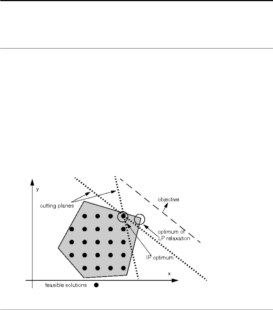
Chapter 35. User-cut and lazy-constraint pools
Documents pools of user-defined cuts and lazy constraints.
What are user cuts and lazy constraints?
Defines user cuts; defines lazy constraints.
In contrast to the cuts that IBM ILOG CPLEX may automatically add while solving
a problem, user cuts are those cuts that a user defines based on information
already implied about the problem by the constraints; user cuts may not be strictly
necessary to the problem, but they tighten the model. Lazy constraints are
constraints that the user knows are unlikely to be violated, and in consequence, the
user wants them applied lazily, that is, only as necessary or not before needed.
User cuts can be grouped together in a pool of user cuts. Likewise, lazy constraints
can also be grouped into a pool of lazy constraints.
Important:
Only linear constraints may be included in a pool of user cuts or lazy constraints.
Neither user cuts nor lazy constraints may contain quadratic terms.
What are pools of user cuts or lazy constraints?
Defines pools of user cuts or lazy constraints.
Sometimes, for a MIP formulation, a user may already know a large set of helpful
cutting planes (user cuts), or can identify a group of constraints that are unlikely to
be violated (lazy constraints). Simply including these cuts or constraints in the
original formulation could make the LP subproblem of a MIP optimization very
large or too expensive to solve. Instead, these situations can be handled in one of
these ways:
Figure 16. Cuts in a typical MIP
© Copyright IBM Corp. 1987, 2016 475

vthrough one of the cut callbacks described in Chapter 40, “Advanced MIP
control interface,” on page 533, or
vby setting up cut pools before MIP optimization begins, as explained in “Adding
user cuts and lazy constraints” on page 478.
The principle in common between these two pools allows the optimization
algorithm to perform its computations on a smaller model than it otherwise might,
in the hope of delivering faster run times. In either case (whether in the case of
pools of user cuts or pools of lazy constraints), the model starts out small, and
then potentially grows as members of the pools are added to the model. Both
kinds of pool may be used together in solving a MIP model, although that would
be an unusual circumstance.
However, there are important distinctions between these two concepts, as
explained in “Differences between user cuts and lazy constraints.”
Differences between user cuts and lazy constraints
Distinguishes user cuts from lazy constraints.
Cuts may resemble ordinary constraints, but are conventionally defined to mean
those which can change the feasible space of the continuous relaxation but do not
rule out any feasible integer solution that the rest of the model permits. A
collection of cuts, therefore, involves an element of freedom: whether or not to
apply them, individually or collectively, during the optimization of a MIP model;
the formulation of the model remains correct whether or not the cuts are included.
This degree of freedom means that if valid and necessary constraints are
mis-identified by the user and passed to CPLEX as user cuts, unpredictable and
possibly incorrect results could occur.
By contrast, lazy constraints represent simply one portion of the constraint set, and
the model would be incomplete (and possibly would deliver incorrect answers) in
their absence. CPLEX always makes sure that lazy constraints are satisfied before
producing any solution to a MIP model. Needed lazy constraints are also kept in
effect after the MIP optimization terminates, for example, when you change the
problem type to fixed-integer and re-optimize with a continuous optimizer.
Another important difference between pools of user cuts and pools of lazy
constraints lies in the timing by which these pools are applied. CPLEX may check
user cuts for violation and apply them at any stage of the optimization.
Conversely, it does not guarantee to check them at the time an integer-feasible
solution candidate has been identified. Lazy constraints are only (and always)
checked when an integer-feasible solution candidate has been identified, and of
course, any of these constraints that turn out to be violated will then be applied to
the full model.
Cuts that are based on optimality and that remove integer feasible solutions
without removing all optimal solutions are known as optimality-based cuts.
Optimality-based cuts do not fit the definition of either a user cut nor a lazy
constraint. For example, symmetry-breaking constraints are sometimes known as
optimality-based cuts because symmetry-breaking constraints can remove integer
feasible solutions without removing all optimal solutions. Symmetry-breaking
constraints are not user cuts in the sense addressed here. Symmetry-breaking
constraints are not necessarily lazy constraints either. However, CPLEX can support
optimality-based cuts as lazy constraints. If you add an optimality-based cut as a
lazy constraint in your model, you can also add it to the user cut pool. This
476 CPLEX User’s Manual

practice of adding an optimality-based cut as a lazy constraint and simultaneously
adding it to the user cut pool makes sure that CPLEX checks the optimality-based
cut at each node relaxation as well as when CPLEX finds an integer feasible
solution.
Another way of comparing these two types of pools is to note that the user
designates constraints as lazy in the strong hope and expectation that they will not
need to be applied, thus saving computation time by their absence from the
working problem. In practice, it is relatively costly (for a variety of reasons) to
apply a lazy constraint after a violation is identified, and so the user should err on
the side of caution when deciding whether a constraint should be marked as lazy.
In contrast, user cuts may be more liberally added to a model because CPLEX is
not obligated to use any of them and can apply its own rules to govern their
efficient use.
CPLEX offers an example that highlights the difference between pools of user cuts
and lazy constraints. The example demonstrates lazy constraint callbacks to
separate integer feasible LP solutions and user cut callbacks to separate fractional
infeasible LP solutions in a Benders decomposition of an asymmetric travelling
salesperson problem.
vIn the Callable Library, see xbendersatsp.c (64-bit) and bendersatsp.c (32-bit).
vIn the C++ API, see ilobendersatsp.cpp.
vIn the Java API, see BendersATSP.java.
vIn the C#.NET API, see BendersATSP.cs.
vIn the VB.NET API, see BendersATSP.vb.
vIn the Python API, see bendersatsp.py.
Identifying candidate constraints for lazy constraint pool
Distinguishes user cuts from lazy constraints.
Here is a procedure for identifying which constraints in your model are good
candidates to be lazy constraints. The procedure entails changing the problem type
more than once.
1. Begin with your mixed integer programming model (MIP).
2. Change its problem type to a linear program (LP).
3. Solve that LP.
4. Identify constraints for which the dual value is 0 (zero). These are the
constraints to make lazy after another change of problem type.
5. Change the LP problem type to a mixed integer linear program problem type
(MILP) so that the identified constraints can be added as lazy constraints.
6. Solve the problem again, this time as a MILP.
Tip: Lazy constraints can be added only to problems of the type MILP; lazy
constraints cannot be added to a problem of the type LP.
Changing problem type
For an introduction to changing a problem type, see the topic “Changing problem
type in MIPs” on page 223.
Adding lazy constraints
Chapter 35. User-cut and lazy-constraint pools 477

For details about adding lazy constraints to a model, see the topic “Adding user
cuts and lazy constraints.”
Limitations on user-cut pools
Describes a limitation on pools with respect to presolve reductions.
Certain considerations apply to user cuts, user-cut pools, and user-cut callbacks.
vIf the linear reduction switch (CPX_PARAM_PRELINEAR, PreLinear) is set to 1 (one),
its default, then nonlinear presolve reductions are allowed. If there are user cuts
in the model as well, then it can happen that a user cut cannot be crushed to the
presolved model, and CPLEX therefore disregards the uncrushed user cut. In
that case, CPLEX displays a log message on the results channel: "Could not
crush NNN user cuts." where NNN is the number of user cuts that CPLEX
could not crush and that CPLEX consequently disregarded.
vFurthermore, the linear reduction switch (CPX_PARAM_PRELINEAR, PreLinear) is set
to 1 (one), its default, and there is a user cut callback, then it can happen that
the user cut generated in the user cut callback cannot be crushed to the
presolved model. This situation means that a call to CPXcutcallbackadd or
CPXcutcallbackaddlocal returns the status CPXERR_PRESLV_CRUSHFORM. This error
is not critical: the message simply tells the user that the cut was discarded
because it could not be crushed to the presolved model; in other words, the cut
could not be represented in terms of presolved problem variables. Since user
cuts are optional (they do not affect the integer-feasible region of the problem),
discarding a user cut does not affect the correctness of the algorithm.
Lazy constraints, lazy constraint pools, and lazy constraint callbacks differ from
their user-cut counterparts in this respect: CPLEX automatically adjusts these
parameters in all APIs to turn off dual reductions when CPLEX detects the
presence of lazy constraints in a model:
vthe linear reduction switch (CPX_PARAM_PRELINEAR, PreLinear)
vthe primal and dual reduction type (CPX_PARAM_REDUCE, Reduce)
Specifically, when CPLEX detects a lazy constraint, it disables dual reductions: if
the parameter was at its default (CPX_PREREDUCE_PRIMALANDDUAL = 3), then CPLEX
changes the value of the parameter to CPX_PREREDUCE_PRIMALONLY = 1 (one); if it
was at CPX_PREREDUCE_DUALONLY = 2, then CPLEX changes the value of the
parameter to CPX_PREREDUCE_NOPRIMALORDUAL = 0 (zero); if it was at
CPX_PREREDUCE_PRIMALONLY = 1(one) or CPX_PREREDUCE_NOPRIMALORDUAL = 0 (zero),
then CPLEX does not change the value of the parameter at all because in that case,
dual reductions have already been turned off.
Adding user cuts and lazy constraints
You can add user cuts or lazy constraints through routines or methods in the
Component Libraries or via LP, SAV, or MPS files, as explained in the following
sections.
Using the Component Libraries to add user cuts or lazy
constraints
Describes routines and methods for adding pools of user cuts or lazy constraints in
the APIs.
The following facilities add user defined cuts to a user cut pool.
478 CPLEX User’s Manual
vThe Callable Library routine CPXaddusercuts
vThe Concert Technology methods:
– addUserCuts in the C++ API
– IloCplex.addUserCuts in the Java API
– Cplex.AddUserCuts in the .NET API
vThe Python API method cplex.linear_constraints.advanced.add_user_cuts
The following facilities will add lazy constraints to a lazy constraint pool.
vThe Callable Library routine is CPXaddlazyconstraints.
vThe Concert Technology methods
– addLazyConstraints in the C++ API
– IloCplex.addLazyConstraints in the Java API
– Cplex.AddLazyConstraints in the .NET API
vThe Python API method
cplex.linear_constraints.advanced.add_lazy_constraints
Using the Interactive Optimizer to add user cuts or lazy
constraints
Describes display and addition of pools of user cuts and lazy constraints in the
Interactive Optimizer.
User cuts and lazy constraints appear when you enter the command display
problem all in the Interactive Optimizer. You can also add user cuts and lazy
constraints to an existing problem with the add command of the Interactive
Optimizer.
Reading and writing LP files
Describes reading and writing pools of user cuts or lazy constraints from LP files.
User cuts and lazy constraints may also be specified in LP-format files, and so may
be read:
vWith the Interactive Optimizer read command
vThrough the routine CPXreadcopyprob of the Callable Library
vThrough the methods of Concert Technology:
– importModel of the C++ API
– IloCplex.importModel of the Java API
– Cplex.ImportModel of the .NET API
When CPLEX writes LP-format files, user cuts and lazy constraints added through
their respective add routines or read from LP format files are included in the
output files along with their names (if any).
General syntax
The general syntax rules for LP format documented in the CPLEX File Formats
Reference Manual apply to user cuts and lazy constraints.
vThe user cuts section or sections must be preceded by the keywords USER CUTS.
vThe lazy constraints section or sections must be preceded by the keywords
LAZY CONSTRAINTS.
Chapter 35. User-cut and lazy-constraint pools 479
These sections, and the ordinary constraints section preceded by the keywords
SUBJECT TO, can appear in any order and can be present multiple times, as long as
they are placed after the objective function section and before any of the keywords
BOUNDS, GENERALS, BINARIES, SEMI-CONTINUOUSor END.
Example
Here is an example of an LP file containing ordinary constraints and lazy
constraints.
Maximize
obj: 12 x1 + 5 x2 + 15 x3 + 10 x4
Subject To
c1: 5 x1 + x2 + 9 x3 + 12 x4 <= 15
Lazy Constraints
l1: 2 x1 + 3 x2 + 4 x3 + x4 <= 10
l2: 3 x1 + 2 x2 + 4 x3 + 10 x4 <= 8
Bounds
0 <= x1 <= 5
0 <= x2 <= 5
0 <= x3 <= 5
0 <= x4 <= 5
Generals
x1 x2 x3 x4
End
CPLEX stores user cuts and lazy constraints in memory separately from ordinary
constraints.
Reading and writing SAV files
Describes reading and writing pools of user cuts or lazy constraints from SAV files.
User cuts and lazy constraints may also be specified SAV-format files, and so may
be read:
vWith the Interactive Optimizer read command
vThrough the routine CPXreadcopyprob of the Callable Library
vThrough the methods of Concert Technology:
– importModel of the C++ API
– IloCplex.importModel of the Java API
– Cplex.ImportModel of the .NET API
When CPLEX writes SAV format files, user cuts and lazy constraints added
through their respective add routines or read from SAV format files are included in
the output files along with their names (if any).
Reading and writing MPS files
Describes reading and writing pools of user cuts or lazy constraints from MPS
files.
CPLEX extends the MPS file format with additional optional sections to
accommodate user defined cuts and lazy constraints. The usual routines of the
Callable Library and methods of Concert Technology to read and write MPS files
also read and write these optional sections. These additional sections follow the
ROWS section of an MPS file in this order:
vROWS
vUSERCUTS
480 CPLEX User’s Manual

vLAZYCONS
The syntax of these additional sections conforms to the syntax of the ROWS section
with this exception: the type R cannot appear in USERCUTS nor in LAZYCONS . For
details about the format of the ROWS section in the MPS file format, see the
CPLEX File Format Reference Manual, especially these sections:
vThe ROWS section
vUser-defined cuts in MPS files
vLazy constraints in MPS files
Here is an example of an MPS file extended to include lazy constraints.
NAME extra.mps
ROWS
N obj
L c2
L c3
LAZYCONS
L c1
COLUMNS
MARK0000 ’MARKER’ ’INTORG’
x1 obj -12
x1 c2 2
x1 c3 3
x1 c1 5
x2 obj -5
x2 c2 3
x2 c3 2
x2 c1 1
x3 obj -15
x3 c2 4
x3 c3 4
x3 c1 9
x4 obj -10
x4 c2 1
x4 c3 10
x4 c1 12
MARK0001 ’MARKER’ ’INTEND’
RHS rhs c2 10
rhs c3 8
rhs c1 15
BOUNDS
UP bnd x1 5
UP bnd x2 5
UP bnd x3 5
UP bnd x4 5
ENDATA
Deleting user cuts and lazy constraints
Describes routines and methods to delete pools of user cuts or lazy constraints.
In the Callable Library, the pools of user cut and lazy constraint are cleared by the
routines CPXfreeusercuts and CPXfreelazyconstraints. Clearing the pools does
not change the MIP solution.
The Concert Technology methods are clearUserCuts and clearLazyConstraints.
Clearing a pool means that the user cuts and lazy constraints in the pool are
removed and are not applied the next time MIP optimization is called, and that the
Chapter 35. User-cut and lazy-constraint pools 481
solution to the MIP (if one exists) is still available. Although any existing solution
is still feasible, it may no longer be optimal because of this change in the
constraints.
482 CPLEX User’s Manual

Chapter 36. Using goals
Documents goals and their role in a branch & cut search.
Branch & cut with goals
Documents the effect of goals in the search.
What is a goal?
Defines a goal in CPLEX.
Goals allow you to take control of the branch & cut search procedure used by IBM
ILOG CPLEX to solve MIP problems. To help you understand how to use goals
with CPLEX, these sections review how this procedure works.
v“Overview of goals in the search”
v“How goals are implemented in branch & cut” on page 484
v“About the method execute in a goal” on page 484
Note:
Goals are implemented by IloCplex::Goal, not IloGoal as in other IBM ILOG
products.
Overview of goals in the search
Describes goals in relation to nodes in the search.
The search procedure manages a search tree consisting of nodes. Every node
represents a subproblem to be solved, and the root node of the tree represents the
entire problem. Nodes are called active if they have not yet been processed.
The tree is first initialized to contain the root node as the only active node. CPLEX
processes active nodes from the tree until either no more active nodes are available
or some limit has been reached. After a node has been processed, it is no longer
active.
When processing a node, CPLEX starts by solving the continuous relaxation of its
subproblem (that is, the subproblem without integrality constraints). If the solution
violates any cuts, CPLEX adds them to the node problem and re-solves. This
procedure is iterated until no more violated cuts are found by CPLEX. If at any
point the relaxation becomes infeasible, the node is pruned, that is, it is removed
from the tree.
To solve the node problem, CPLEX checks whether the solution satisfies the
integrality constraints. If so, and if its objective value is better than that of the
current incumbent, the solution of the node problem is used as the new incumbent.
Otherwise, CPLEX splits the node problem into one or two smaller subproblems,
typically by branching on a variable that violates its integrality constraint. These
subproblems are added to the tree as active nodes and the current node is
deactivated.
© Copyright IBM Corp. 1987, 2016 483

The primary use of goals is to take control of these last steps, namely the
integer-feasibility test and the creation of subproblems. However, as discussed
later, goals also allow you to add local and global cuts.
How goals are implemented in branch & cut
Describes implementation of goals in the search in the C++ API.
Note:
The discussion of the details of using goals will be presented mainly in terms of
the C++ API. The Java and .NET APIs follow the same design and are thus
equivalent at this level of discussion. In cases where a difference between these
APIs needs to be observed, the point will be raised. Where the difference is only in
syntax, the other syntax will be mentioned in parentheses following the C++
syntax.
In C++, goals are implemented in objects of type IloCplex::GoalI (having the
handle class IloCplex::Goal). In Java, goals are implemented in objects of type
IloCplex.Goal (and there are no handle classes). In .NET, goals are implemented
by the class Cplex.Goal. The method IloCplex::GoalI::execute
(IloCplex.Goal.execute) is where the control is implemented. This method is
called by IloCplex after a node relaxation has been solved and all cuts have been
added. Invoking the method execute of a goal is often referred to as executing a
goal. When the method execute is executed, other methods of the class
IloCplex::GoalI (IloCplex.Goal or Cplex.Goal ) can be called to query
information about the current node problem and the solution of its relaxation.
About the method execute in a goal
Describes the execute method of a goal.
Typically, the implementation of the method execute will perform the following
steps:
1. Check feasibility. An interesting possibility here is that the feasibility check may
include more than verifying integrality of the solution. This allows you to
enforce constraints that could not reasonably be expressed using linear
constraints through cuts or branching. In other words, this allows you to use
goals in a way that makes them part of the model to be solved. Such a use is
common in Constraint Programming, but it is less frequently used in
Mathematical Programming. Note, however, that this CP-style application of
goals prevents you from making use of MP-style advanced starting
information, either from a MIP Start file or by restarting a previous
optimization with one that uses goals.
2. Optionally find local or global cuts to be added. Local cuts will be respected
only for the subtree below the current node, whereas global cuts will be
enforced for all nodes from then on.
3. Optionally construct a solution and pass it to CPLEX.
4. Instruct CPLEX how to proceed. Instruct CPLEX how to proceed through the
return value of the method execute; the return value of execute is another goal.
CPLEX simply continues by executing this goal.
Special goals in branch & cut
Describes specialized, predefined goals to control the search.
484 CPLEX User’s Manual
Or goal
Describes the Or goal to create subnodes of the current node.
An Or goal is a goal that creates subnodes of the current node. This function takes
at least 2 and up to 6 goals as arguments. For each of its arguments, the Or goal
will create a subnode in such a way that when that subnode is processed, the
corresponding goal will be executed. After the goal has been executed, the current
node is immediately deactivated.
In the C++ API, an Or goal is returned by IloCplex::GoalI::OrGoal.
In the Java API, an Or goal is returned by the method IloCplex.or.
In the .NET API, an Or goal is returned by the method Cplex.Or.
And goal
Describes the And goal to combine other goals in a fixed order of execution.
An And goal also takes goals as arguments. It returns a goal that will cause CPLEX
to execute all the goals passed as arguments in the order of the arguments.
In the C++ API, an And goal is returned by IloCplex::GoalI::AndGoal.
In the Java API, an And goal is returned by the method IloCplex.and.
In the .NET API, an And goal is returned by the method Cplex.And.
Fail goal
Describes the Fail goal for pruning the search tree.
A Fail goal creates a goal that causes CPLEX to prune the current node. In other
words, it discontinues the search at the node where the goal is executed. CPLEX
will continue with another active node from the tree, if one is available.
In the C++ API, a Fail goal is returned by IloCplex::GoalI::FailGoal.
In the Java API, a Fail goal is returned by the method IloCplex.failGoal.
In the .NET API, a Fail goal is returned by the method Cplex.FailGoal.
Local cut goal
Describes a local cut goal to add a cut to a node.
A local cut goal adds a local cut to the node where the goal is executed.
In the C++ API, the class IloCplex::Goal has constructors that take an instance of
IloRange or an instance of IloRangeArray (IloRange[]) as an argument. When one
of these constructors is used, a local cut goal is created.
To create local cut goals with the Java API, use the method
IloCplex.constraintGoal or if more convenient, one of the methods
IloCplex.leGoal, IloCplex.geGoal, or IloCplex.eqGoal.
Chapter 36. Using goals 485
In the .NET API, use the methods Cplex.ConstraintGoal, Cplex.EqGoal,
Cplex.LeGoal, or Cplex.GeGoal to create a local cut goal.
Null goal
Describes the null goal to stop further branching.
The 0-goal is also known as a null goal or empty goal.
In the C++ API, a null goal is an IloCplex::Goal handle object with a null (0)
implementation pointer.
A null goal can also be returned by the method IloCplex::GoalI::execute.
Use a null goal when you want to instruct CPLEX not to branch any further. For
example, when CPLEX finds a feasible solution, and you want to accept it without
further branching, a null goal is appropriate.
For example, the following sample from the C++ API accepts an integer feasible
solution and stops branching.
if ( isIntegerFeasible() )
return 0;
Branch as CPLEX goal
Describes a branch goal to return control to CPLEX.
Instead of instructing CPLEX not to branch any further (as you can do with a null
goal), it is also possible to tell CPLEX to branch as it normally would; in other
words, to branch as CPLEX. You give CPLEX this instruction by means of a
branching goal. A branching goal tells CPLEX to take over control of the branch &
cut search with its built-in strategies.
The following lines in the C++ API tell CPLEX to continue branching as it would
normally do:
if ( !isIntegerFeasible() )
AndGoal(BranchAsCplexGoal(getEnv()), this);
Solution goal
Describes a goal to inject a solution at a node.
A solution goal is a goal that injects a solution, such as a solution supplied by you
or a solution found by CPLEX during the search.
For example, here is a sample in the C++ API which injects a solution at the
beginning of branch & bound and then uses a branching goal:
if (getNnodes() == 0)
goal = AndGoal(OrGoal(SolutionGoal(goalvar,startVals),
AndGoal(MyBranchGoal(getEnv(), var), goal)),
goal);
elsegoal = AndGoal(MyBranchGoal(getEnv(), var), goal);
return goal;
For more about this kind of special goal, see “Injecting heuristic solutions” on page
493.
486 CPLEX User’s Manual
Aggregating goals
Describes aggregate goals (And, Or).
Since And goals and Or goals take other goals as arguments, goals can be
combined into aggregate goals. In fact, this is how goals are typically used for
specifying a branching strategy. A typical return goal of a user-written execute
method for C++ looks like this:
return AndGoal(OrGoal(var <= IloFloor(val), var >= IloFloor(val)+1), this);
and for Java, it looks like this:
return cplex.and(cplex.or(cplex.leGoal(var, Math.floor(val)),
cplex.geGoal(var, Math.floor(val)+1)), this);
and for C#.NET, it looks like this:
return cplex.And(
cplex.Or(cplex.GeGoal(_vars[bestj], System.Math.Floor(x[bestj])+1),
cplex.LeGoal(_vars[bestj], System.Math.Floor(x[bestj]))),
this);
For the C++ case, note that since this statement would be called from the execute
method of a subclass of IloCplex::GoalI, the full name IloCplex::GoalI::OrGoal
can be abbreviated to OrGoal. Likewise, the full name IloCplex::GoalI::AndGoal
can be abbreviated to AndGoal.
This return statement returns an And goal that first executes the Or goal and then
the current goal itself specified by the this argument. When the Or goal is
executed next, it will create two subnodes. In the first subnode, the first local cut
goal representing
(where
denotes the floor of val) will be executed, thus adding the constraint
for the subtree of this node. Similarly, the second subnode will be created, and
when executing its constraint goal the constraint
var ≥
will be added for the subtree. this is then executed on each of the nodes that have
just been created; the same goal is used for both subtrees. Further details about
how goals are processed are available in “The goal stack” on page 489,
“Controlling goal-defined search” on page 494, and “Search limits” on page 497.
Example: goals in branch & cut
Illustrates goals in a C++ application.
Chapter 36. Using goals 487
Consider the following example to clarify the discussions of goals. This example is
available as ilogoalex1.cpp in the examples/src subdirectory of your CPLEX
distribution. The equivalent Java implementation can be found as GoalEx1.java in
the same location. The C#.NET version is in Goalex1.cs and the VB.NET version is
in Goalex1.vb.
This example shows how to implement and use a goal for controlling the branch
strategy used by CPLEX. As discussed, goals are implemented as subclasses of the
class IloCplex::GoalI (IloCplex.Goal or Cplex.Goal). The C++ implementation of
that example uses the macro
ILOCPLEXGOAL1(MyBranchGoal, IloNumVarArray, vars)
instead. This macro defines two things, class MyBranchGoalI and the function
IloCplex::Goal MyBranchGoal(IloEnv env, IloNumVarArray vars);
The class MyBranchGoalI is defined as a subclass of class IloCplex::GoalI
(IloCplex.Goal orCplex.Goal ) and has a private member IloNumVarArray vars.
The function MyBranchGoal creates an instance of class MyBranchGoalI, initializes
the member vars to the argument vars passed to the function, and returns a
handle to the new goal object. The curly brackets "{ ... }" following the macro
enclose the implementation of the method MyBranchGoalI::execute containing the
actual code of the goal.
The use of the macro is very convenient as the amount of user code is equivalent
to the amount for defining a function, but with a slightly unusual syntax. IloCplex
provides seven such macros that can be used for defining goals with 0 to 6 private
members. If more than 6 members are needed, IloCplex::GoalI (IloCplex.Goal or
Cplex.Goal) must be subclassed by hand.
Since the Java programming language does not provide macros, a subclass of
IloCplex.Goal must always be implemented by hand. In this example, this class is
called MyBranchGoal and there is no helper function for creating an instance of that
class (as the macro does in the case of C++).
The goal is then used for solving the extracted node by calling:
cplex.solve(MyBranchGoal(env, var));
for C++, or for Java:
cplex.solve(new MyBranchGoal(var));
instead of the usual cplex.solve. The rest of the main function contains nothing
new and will not be discussed any further.
In the implementation of the goal, or more precisely its method execute, starts by
declaring and initializing some arrays. These arrays are then used by methods of
class IloCplex::GoalI (IloCplex.Goal or Cplex.Goal) to query information about
the node subproblem and the solution of its relaxation. The method getValues is
used to query the solution values for the variables in vars, the method
getObjCoefs is used to query the linear objective function coefficients for these
variables, and method getFeasibilities is used to query feasibility statuses for
them. The feasibility status of a variable indicates whether IloCplex considers the
current solution value of the variable to be integer feasible or not. IloCplex::GoalI
(IloCplex.Goal or Cplex.Goal) provides a wealth of other query methods. For
details, see the CPLEX Reference Manuals.
488 CPLEX User’s Manual

After you have gathered information about the variables, their objective
coefficients, and their current feasibility statuses, compute the index of an integer
infeasible variable in vars that has the largest objective coefficients among the
variables with largest integer infeasibility. That index is recorded in variable bestj.
Then create a new goal handle object res. By default, this is initialized to an empty
goal. However, if an integer infeasible variable was found among those in vars,
then variable bestj will be ≥0and a nonempty goal will be assigned to res:
res = AndGoal(OrGoal(vars[bestj] >= IloFloor(x[bestj])+1,
vars[bestj] <= IloFloor(x[bestj])),
this);
This goal creates two branches, one for
and one for
and continues branching in both subtrees with the same goal this. Finally, call
method end for all temporary arrays and return goal res.
Since Java objects are garbage collected, there is no need for the variable res.
Instead, depending on the availability of an integer infeasible variable, the null
goal is returned or the returned goal is created in the return statement itself:
return cplex.and(cplex.or(cplex.geGoal(_vars[bestj],
Math.floor(x[bestj]))+1,
cplex.leGoal(_vars[bestj],
Math.floor(x[bestj]))),
this);
The goal stack
Describes the goal stack.
To understand how goals are executed, consider the concept of the goal stack. Every
node has its own goal stack. When cplex.solve(goal) is called, the goal stack of
the root node is simply initialized with goal and then the regular cplex.solve
method is called.
When CPLEX processes a node, it pops the first goal from the node's goal stack
and calls method execute. If a nonempty goal is returned, it is simply pushed back
on the stack. CPLEX keeps doing this until the node becomes inactive or the node's
goal stack becomes empty. When the node stack is empty, CPLEX continues with
its built-in search strategy for the subtree rooted at this node.
In light of the goal stack, here are the different types of goals:
vAs explained in “Or goal” on page 485, the Or goal creates child nodes. CPLEX
first initializes the goal stack of every child node with a copy of the remaining
goal stack of the current node. Then it pushes the goal passed as the argument
to the Or goal on the goal stack of the corresponding node. Finally, the current
node is deactivated, and CPLEX continues search by picking a new active node
from the tree to process.
Chapter 36. Using goals 489

vThe And goal simply pushes the goals passed as arguments onto the goal stack
in reverse order. Thus, when the goals are popped from the stack for execution,
they will be executed in the same order as they were passed as arguments to the
And goal.
vWhen a Fail goal executes, the current node is simply deactivated, and CPLEX
continues on another active node from the tree. In other words, CPLEX
discontinues its search below the current node.
vWhen a local cut goal is executed, its constraints are added to the node problem
as local cuts and the relaxation is re-solved.
vAn empty goal cannot be executed. Thus, empty goals are not pushed onto the
goal stack. If the goal stack is empty, CPLEX continues with the built-in
branching strategy.
With this understanding, consider further what really goes on when a goal returns:
return AndGoal(OrGoal(var <= IloFloor(val), var >= IloFloor(val)+1), this);
The And goal is pushed onto the current node's goal stack, only to be immediately
popped back off of it. When it is executed, it will push this on the goal stack and
then push the Or goal. Thus, the Or goal is the next goal that CPLEX pops and
executes. The Or goal creates two subnodes, and initializes their goal stacks with
copies of the goal stack of the current node. At this point both subnodes will have
this on top of their goal stacks. Next, the Or goal will push a local cut goal for
(where
denotes the floor of val) on the goal stack of the first subnode. Similarly, it pushes
a local cut goal for
var ≥
on the goal stack of the second subnode. Finally, the current node is deactivated
and CPLEX continues its search with a new active node from the tree.
When CPLEX processes one of the subnodes that have been created by the Or goal,
it will pop and execute the first goal from the node's goal stack. As you just saw,
this will be a local cut goal. Thus CPLEX adds the constraint to the node problem
and re-solves the relaxation. Next, this will be popped from the goal stack and
executed. That fact means that the same search strategy as implemented in the
original goal is applied at that node.
Memory management and goals
Describes goals in the context of memory management.
Java and .NET use garbage collection to handle all memory management issues.
Thus the following applies only to the C++ library. Java or .NET users may safely
skip ahead to “Cuts and goals” on page 491.
To conserve memory, in the C++ API, CPLEX only stores active nodes of the tree
and deletes nodes as soon as they become inactive. When deleting nodes, CPLEX
490 CPLEX User’s Manual

also deletes the goal stacks associated with them, including all goals they may still
contain. In other words, CPLEX takes over memory management for goals.
It does so by keeping track of how many references to every goal are in use. As
soon as this number drops to zero (0), the goal is automatically deleted. This
technique is known as reference counting.
CPLEX implements reference counting in the handle class IloCplex::Goal. Every
IloCplex::GoalI object maintains a count of how many IloCplex::Goal handle
objects refer to it. The assignment operator, the constructors, and the destructor of
class IloCplex::Goal are implemented in such a way as to keep the reference
count up-to-date. This convention means that users should always access goals
through handle objects, rather than keeping their own pointers to implementation
objects.
Other than that, nothing special needs to be observed when dealing with goals. In
particular, goals don't have end methods like other handle classes in the C++ API
of Concert Technology. Instead, CPLEX goal objects are automatically deleted when
no more references to them exist.
Local cut goals contain IloRange objects. Since the IloRange object is only applied
when the goal is executed, the method end must not be called for a range
constraint from which a local cut goal is built. The goal will take over memory
management for the constraints and call the method end when the goal itself is
destroyed. Also, an IloRange object can only be used in exactly one local cut goal.
Similarly, method end must not be called for IloRangeArray objects that are passed
to local cut goals. Also such arrays must not contain duplicate elements.
Going back to the example ilogoalex1.cpp, you see that the method end is called
for the temporary arrays x, obj, and feas at the end of the execute method.
Though a bit hidden, two IloRange constraints are constructed for the goal,
corresponding to the arguments of the Or goal. CPLEX takes over memory
management for these two constraints as soon as they are enclosed in a goal. This
takeover happens via the implicit constructor IloCplex::Goal::Goal(IloRange rng)
that is called when the range constraints are passed as arguments to the Or goal.
In summary, the user is responsible for calling end on all Concert Technology
objects created in a goal, except when they have been passed as arguments to a
new goal.
Also, user code in the execute method is not allowed to modify existing Concert
Technology objects in any way. CPLEX uses an optimized memory management
system within goals for dealing with temporary objects. However, this memory
management system cannot be mixed with the default memory management
system used by Concert Technology. Thus, for example, it is illegal to add an
element to array vars in the example, since this array has been created outside of
the goal.
Cuts and goals
Distinguishes local cuts from global cuts and illustrates cuts added by a goal
Goals can also be used to add global cuts. Whereas local cuts are respected only in
a subtree, global cuts are added to the entire problem and are therefore respected
at every node after they have been added.
Chapter 36. Using goals 491
Just as you can add local cuts by means of a local cut goal, as explained in the
topic “Local cut goal” on page 485, you can add a global cut by means of a global
cut goal. A global cut goal is created with the method
IloCplex::GoalI::GlobalCutGoal (IloCplex.globalCutGoal or Cplex.GlobalCutGoal
). This method takes an instance of IloRange or IloRangeArray (IloRange[] ) as its
argument and returns a goal. When the goal executes, it adds the constraints as
global cuts to the problem.
Example ilogoalex2.cpp shows the use of IloCplex::GoalI::GlobalCutGoal for
solving the noswot MILP model. This is a relatively small model from the MIPLIB
3.0 test set, consisting of only 128 variables. Nonetheless, it used to be very hard to
solve without adding special cuts.
Although it is now solvable directly in less than two minutes, the number of nodes
examined is still on the order of 2.5 billion, even for only 128 original variables.
However, cuts can be derived, and the addition of these cuts makes the problem
solvable in under a second with roughly 600 nodes. These cuts are:
x21 - x22 <= 0
x22 - x23 <= 0
x23 - x24 <= 0
2.08*x11 + 2.98*x21 + 3.47*x31 + 2.24*x41 + 2.08*x51 +
0.25*w11 + 0.25*w21 + 0.25*w31 + 0.25*w41 + 0.25*w51 <= 20.25
2.08*x12 + 2.98*x22 + 3.47*x32 + 2.24*x42 + 2.08*x52 +
0.25*w12 + 0.25*w22 + 0.25*w32 + 0.25*w42 + 0.25*w52 <= 20.25
2.08*x13 + 2.98*x23 + 3.47*x33 + 2.24*x43 + 2.08*x53 +
0.25*w13 + 0.25*w23 + 0.25*w33 + 0.25*w43 + 0.25*w53 <= 20.25
2.08*x14 + 2.98*x24 + 3.47*x34 + 2.24*x44 + 2.08*x54 +
0.25*w14 + 0.25*w24 + 0.25*w34 + 0.25*w44 + 0.25*w54 <= 20.25
2.08*x15 + 2.98*x25 + 3.47*x35 + 2.24*x45 + 2.08*x55 +
0.25*w15 + 0.25*w25 + 0.25*w35 + 0.25*w45 + 0.25*w55 <= 16.25
These cuts derive from interpreting the problem as a resource allocation model on
five machines with scheduling horizon constraints and transaction times. The first
three cuts break symmetries among the machines, while the others capture
minimum bounds on transaction costs.
Of course, the best way to solve the noswot model with these cuts is simply to add
them to the model before calling the optimizer. However, for demonstration
purposes here, the cuts are added by means of a goal. The source code of this
example can be found in the examples/src directory of the CPLEX distribution.
The equivalent Java implementation appears as GoalEx2.java in the same location.
Likewise, there is also the C#.NET version in Goalex2.cs and the VB.NET version
in Goalex2.vb .
The goal CutGoal in that example receives a list of "less than" constraints to use as
global cuts and a tolerance value eps. The constraints are passed to the goal as an
array of lhs expressions and an array of corresponding rhs values. Both are
initialized in function makeCuts.
The goal CutGoal checks whether any of the constraints passed to it are violated by
more than the tolerance value. It adds violated constraints as global cuts. Other
than that, it follows the branching strategy CPLEX would use on its own.
The goal starts out by checking whether the solution of the continuous relaxation
of the current node subproblem is integer feasible. This check is done by the
method isIntegerFeasible. If the current solution is integer feasible, a candidate
for a new incumbent has been found, and the goal returns the empty goal to
instruct CPLEX to continue on its own.
492 CPLEX User’s Manual

Otherwise, the goal checks whether any of the constraints passed to it are violated.
It computes the value of every lhs expression for current solution by calling
getValue(lhs[i]). The result is compared to the corresponding righthand side
value rhs[i]. If a violation of more than eps is detected, the constraint is added as
a global cut and the rhs value will be set at IloInfinity to avoid checking it again
unnecessarily.
The global cut goal for lhs[i] ≤rhs[i] is created by the method GlobalCutGoal. It
is then combined with the goal named goal by the method AndGoal, so that the
new global cut goal will be executed first. The resulting goal is stored again in
goal. Before any global cut goals are added, the goal is initialized as:
IloCplex::Goal goal = AndGoal(BranchAsCplexGoal(getEnv()), this);
for C++, or for Java:
cplex.and(cplex.branchAsCplex(), this);
The method BranchAsCplexGoal(getEnv) (cplex.branchAsCplex in the Java API or
Cplex.BranchAsCplex in the .NET API) creates a goal that branches in the same
way as the built-in branch procedure. By adding this goal, the current goal will be
executed for the entire subtree.
Thus the goal returned by CutGoal will add all currently violated constraints as
global cuts one by one. Then it will branch in the way CPLEX would branch
without any goals and execute the CutGoal again in the child nodes.
Injecting heuristic solutions
Defines heuristic solutions and describes the injection of a heuristic solution by a
goal.
At any time in the execution of a goal, you may find that, for example, by slightly
manipulating the current node subproblem solution, you may construct a solution
to your model. Such solutions are called heuristic solutions, and a procedure that
generates them is called a heuristic.
Heuristic solutions can be injected into the branch & cut search by creating a
solution goal with the method IloCplex::GoalI::SolutionGoal
(IloCplex.solutionGoal or Cplex.SolutionGoal). Such a goal can be returned
typically as a subgoal of an And goal much like global cut goals.
When CPLEX executes a solution goal, it does not immediately use the specified
solution as a potential new incumbent. The reason is that with goals, part of the
model may be specified via global cuts or through specialized branching strategies.
Thus the solution needs first to be tested for feasibility with respect to the entire
model, including any part of the model specified through goals.
To test whether an injected solution is feasible, CPLEX first creates a subnode of
the current node. This subnode will of course inherit the goal stack from its parent.
In addition, the solution goal will push local cuts onto the stack of the subnode
such that all variables are fixed to the values of the injected solution.
By processing this subnode as the next node, CPLEX makes sure that either the
solution is feasible with respect to all goals or otherwise it is discarded. Goals that
have been executed so far are either reflected as global cuts or by the local cuts
that are active at the current node. Thus, if the relaxation remains feasible after the
variable fixings have been added, the feasibility of these goals is certain.
Chapter 36. Using goals 493

If at that point the goal stack is not empty, the goals on the goal stack need to be
checked for feasibility as well. Thus by continuing to execute the goals from the
goal stack, CPLEX will either prove feasibility of the solution with respect to the
remaining goals or, in case the relaxation becomes infeasible, decide it really is
infeasible and discard the solution. The rest of the branch & cut search remains
unaffected by all of this.
The benefit of this approach is that your heuristic need not be aware of the entire
model including all its parts that might be implemented via goals. Your heuristic
can still safely be used, as CPLEX will make sure of feasibility for the entire model.
However, there are some performance considerations to observe. If parts of the
model specified with goals are dominant, heuristic solutions you generate might
need to be rejected so frequently that you do not get enough payoff for the work
of running the heuristic. Also, your heuristic should account for the global and
local cuts that have been added at the node where you run your heuristic so that a
solution candidate is not rejected right away and the work wasted.
Controlling goal-defined search
Describes node selection strategy with goals.
So far, you have seen how to control the branching and cut generation of CPLEX
branch & cut search. The remaining missing piece is the node selection strategy.
The node selection strategy sets which of the active nodes in the tree CPLEX
chooses when it selects the next node for processing. CPLEX has several built-in
node selection strategies, selected through the node selection parameter (NodeSel,
CPX_PARAM_NODESEL).
When you use goal-controlled search, you use node evaluators to override the
built-in node selection strategy. You combine a goal with a node evaluator by
calling the method IloCplex::Goal::Apply (IloCplex.apply or Cplex.Apply). This
method returns a new goal that implements the same search strategy as the goal
passed as the argument, but adds the node evaluator to every node in the subtree
defined by the goal. Consequently, nodes may have a list of evaluators attached to
them.
When node evaluators are used, nodes are selected like this:
1. CPLEX starts to choose the node with the built-in strategy as a first candidate.
2. Then CPLEX loops over all remaining active nodes and considers choosing
them instead.
3. If a node has the same evaluator attached to it as the current candidate, the
evaluator is asked whether this node should take precedence over the current
candidate. If the response is positive, the node under investigation becomes the
new candidate, and the test against other nodes continues.
If a node has multiple evaluators attached, they are consulted in the order the
evaluators have been applied. Here is the application order:
vIf the first evaluator prefers one node over the other, the preferred node is used
as candidate and the next node is considered.
vIf the first evaluator does not give preference to one node over the other, the
second evaluator is considered, and so on.
Thus, by adding multiple evaluators, you can build composite node selection
strategies where later evaluators are used for breaking ties in previous evaluations.
494 CPLEX User’s Manual
In the C++ API, node evaluators are implemented as subclasses of class
IloCplex::NodeEvaluatorI. The class IloCplex::NodeEvaluator is the handle class
for node evaluators.
In Java, node evaluators are implemented in objects of type
IloCplex.NodeEvaluator (and there are no handle classes). Likewise, in the .NET
API, node evaluators are implemented in Cplex.NodeEvaluator.
Like goals, node evaluators use reference counting for memory management. As a
result, you should always use the handle objects when dealing with node
evaluators, and there is no method end to be called.
Node evaluators use a two-step process to decide whether one node should take
precedence over another. First, the evaluator computes a value for every node to
which it is attached. This is done by the method evaluate in C++:
IloNum IloCplex::NodeEvaluatorI::evaluate();
and in Java, by the method:
double IloCplex.NodeEvaluator.evaluate();
and in C#.NET:
double Cplex.NodeEvaluator.Evaluate();
This method must be implemented by users who write their own node evaluators.
In the method evaluate, the protected methods of the class
IloCplex::NodeEvaluatorI (IloCplex.NodeEvaluator or Cplex.NodeEvaluator) can
be called to query information about the node being evaluated. The method
evaluate must compute and return an evaluation (that is, a value) that is used
later on, in the second step, to compare two nodes and select one of them. The
evaluate method is called only once for every node, and the result is cached and
reused whenever the node is compared against another node with the evaluator.
The second step consists of comparing the current candidate to another node. This
comparison happens only for evaluators that are shared by the current candidate
and the other node. By default, the candidate is replaced by the other node if its
evaluation value is smaller than that of the candidate. You can alter this behavior
by overwriting the method:
IloBool IloCplex::NodeEvaluatorI::subsume(IloNum candVal, IloNum nodeVal);
or, in the case of Java:
boolean IloCplex.NodeEvaluator.subsume(double candVal, double nodeVal);
or, in the case of C#.NET:
bool Cplex.NodeEvaluator.Subsume(double evalNode, double evalCurrent);
CPLEX calls this method of an evaluator attached to the current candidate if the
node being compared also has the same evaluator attached. The first argument
candVal is the evaluation value the evaluator has previously computed for the
current candidate, and nodeVal is the evaluation value the evaluator has previously
computed for the node being tested. If this method returns IloTrue (true), the
candidate is replaced. Otherwise, the method is called again with reversed
arguments. If it still returns IloFalse (false), both nodes are tied with respect to
that evaluator, and the next evaluator they share is consulted. Otherwise, the
current candidate is kept and tested against the next node.
Chapter 36. Using goals 495

There are two more virtual methods defined for node evaluators that should be
considered when you implement your own node evaluator. The method init is
called immediately before evaluate is called for the first time, thus allowing you to
initialize internal data of the evaluator. When this happens, the evaluator has been
initialized to the first node to be evaluated; thus information about this node can
be queried by the methods of the class IloCplex::NodeEvaluatorI
(IloCplex.NodeEvaluator or Cplex.NodeEvaluator).
Finally, in C++, the method:
IloCplex::NodeEvaluatorI* IloCplex::NodeEvaluatorI::duplicateEvaluator();
must be implemented by the user to return a copy of the invoking node evaluator
object. This method is called by IloCplex to create copies of the evaluator for
parallel branch & cut search.
Example: using node evaluators in a node selection strategy
Illustrates node evaluators in a node selection strategy.
The example ilogoalex3.cpp shows how to use node evaluators to implement a
node selection strategy that chooses the deepest active node in the tree among
those nodes with a maximal sum of integer infeasibilities. The example
ilogoalex3.cpp can be found in the examples/src directory of your distribution.
The equivalent Java implementation can be found in the file Goalex3.java at the
same location. Likewise, the C#.NET example is available in Goalex3.cs.
As this example is an extension of the example ilogoalex1.cpp, this exposition of
it concentrates only on their differences. Also, the example is discussed only in
terms of the C++ implementation; the Java implementation has identical structure
and design and differs only in syntax, as does the .NET as well.
The first difference is the definition of class DepthEvaluatorI as a subclass of
IloCplex::NodeEvaluatorI. It implements the methods evaluate and
duplicateEvaluator. The method evaluate simply returns the negative depth value
queried for the current node by calling method getDepth. Since CPLEX by default
chooses nodes with the lowest evaluation value, this evaluator will favor nodes
deep in the tree. The method duplicateEvaluator simply returns a copy of the
invoking object by calling the (default) copy constructor. Along with the class, the
function DepthEvaluator is also defined to create an instance of class
DepthEvaluatorI and return a handle to it.
Similarly, the class IISumEvaluatorI and function IISumEvaluator are also defined.
The evaluate method returns the negation of the sum of integer infeasibilities of
the node being evaluated. This number is obtained by calling method
getInfeasibilitySum. Thus, this evaluator favors nodes with larger sums of integer
infeasibilities.
This example uses the same search strategy as ilogoalex1.cpp, implemented in
goal MyBranchGoal. However, it applies first the IISumEvaluator to select nodes
with a high integer infeasibility sum; to choose between nodes with the same
integer infeasibility sum, it applies the DepthEvaluator. Application of the
IISumEvaluator is done with:
IloCplex::Goal iiSumGoal = IloCplex::Apply(cplex,
MyBranchGoal(env, var),
IISumEvaluator());
496 CPLEX User’s Manual

The goal created by calling MyBranchGoal is merged with the evaluator created by
calling IISumEvaluator in a new goal iiSumGoal. Similarly, the goal iiSumGoal is
merged with the node evaluator created by calling DepthEvaluator into a new goal
depthGoal:
IloCplex::Goal depthGoal = IloCplex::Apply(cplex,
iiSumGoal,
DepthEvaluator());
Thus, depthGoal represents a goal implementing the branching strategy defined by
MyBranchGoal, but using IISumEvaluator as a primary node selection strategy and
DepthEvaluator as a secondary node selection strategy for breaking ties. This goal
is finally used for the branch & cut search by passing it to the solve method.
Node evaluators are only active while the search is controlled by goals. That is, if
the goal stack becomes empty at a node and CPLEX continues searching with its
built-in search strategy, that search is no longer controlled by any node evaluator.
In order to maintain control over the node selection strategy while using the
CPLEX branch strategy, you can use the goal returned by the method
IloCplex::GoalI::BranchAsCplexGoal (IloCplex.branchAsCplex or
CplexBranchAsCplex). A goal that follows the branching performed by the built-in
strategy of IloCplex can be easily implemented as:
ILOCPLEXGOAL0(DefaultSearchGoal) {
if ( !isIntegerFeasible() )
return AndGoal(BranchAsCplexGoal(getEnv()), this);
return 0;
}
Notice the test for integer feasibility. Without that test, the application would create
an endless loop because when an integer feasible solution has been found, the goal
BranchAsCplex does not change the node at all, and this would continue to be
executed indefinitely.
Search limits
Describes search limits induced by a goal.
As with node evaluators, it is possible to apply search limits to the branch & cut
search controlled by goals. Search limits allow you to limit the search in certain
subtrees; that is, they allow you to discontinue processing nodes when a specified
condition applies. Search limits are implemented in subclasses of the class
IloCplex::SearchLimitI (IloCplex.SearchLimit or Cplex.SearchLimit), and the
procedure for implementing and using them is very similar to that for node
evaluators. See the reference manuals for more details about implementing and
using search limits.
Chapter 36. Using goals 497
498 CPLEX User’s Manual

Chapter 37. Using optimization callbacks
Introduces optimization callbacks.
What are callbacks?
Defines callbacks.
Callbacks allow you to monitor closely and to guide the behavior of CPLEX
optimizers. In particular, callbacks allow user code to be executed regularly during
an optimization or during a tuning session. To use callbacks (either optimization or
tuning callbacks) with CPLEX, you must first write the callback function, and then
pass it to CPLEX. The topic “Callbacks for tuning” on page 131 offers information
about callbacks specific to a tuning session. This part of the manual concentrates
on optimization callbacks, and the topic Chapter 40, “Advanced MIP control
interface,” on page 533 offers further information beyond this introduction to
optimization callbacks. There are three types of optimization callbacks:
informational callbacks, query callbacks, and control callbacks.
Callbacks in the class hierarchy of the APIs
Each of the application programming interfaces (APIs) of CPLEX supports
callbacks. That is, you can write callbacks to use with CPLEX in your preferred
programming language, whether it is C, C++, Java, C#.NET, or Python.
The callback class hierarchy for Java and .NET is exactly the same as the hierarchy
for C++, but the class names differ, in that there is no Iat the end. For example,
the Java implementation class corresponding to the C++ class
IloCplex::OptimizationCallbackI is IloCplex.OptimizationCallback.
The names of callback classes in .NET correspond very closely to those in the C++
and Java APIs. However, the name of a .NET class does not begin with Ilo.
Furthermore, the names of .NET methods are capitalized (that is, they begin with
an uppercase character) according to .NET conventions. For example, the
corresponding callback class in .NET is Cplex.OptimizationCallback.
Similarly, callbacks in Python follow the usual Python naming conventions for
classes, modules, and packages. Thus, the Python name of the callback class
corresponding to the C++ class IloCplex::MIPInfoCallback is
callbacks.MIPInfoCallback.
Callbacks and the CPLEX environment
Depending on the programming language you choose, you may need to pay more
or less attention to the CPLEX environment when you write and use callbacks in
your application.
In Java, .NET, and Python applications, the CPLEX environment is not exposed to
your application, so you need not worry about using the correct environment.
Thus your only concern with respect to the CPLEX environment is that your
callback must not modify the model currently being optimized.
© Copyright IBM Corp. 1987, 2016 499

In contrast, in a C++ application, the environment to use depends on your
purpose.
vIn most cases, use the environment returned by the member function getEnv of
the callback class. The environment returned by getEnv of the callback class in
some cases may be the same environment used in the current optimization. In
such cases, it is valid to use that environment in these particular places.
vIf you create a new problem in a callback, and you want that object to endure
after the optimization, then you should use a new environment that is not
currently used by the optimization.
In an application of the Callable Library (C API), one of the arguments passed to
your callback specifies an environment. Problem objects you create in an
environment will be destroyed as soon as that environment is destroyed.
According to what you want CPLEX to do after optimization, this environment
may or may not be the environment you should use in your callback.
vIn most cases, if at all possible, use the same environment passed to the callback
and no other environment.
vIf you create a problem object in your callback, and you want that problem
object to endure after the optimization routine (such as CPXlpopt, CPXmipopt,
CPXbaropt, or another) terminates, then do not use the environment passed to
the callback function. Instead, create a new environment that is not used in an
optimization function, and use this new environment to create the enduring
problem object of your callback.
Informational callbacks
Documents informational callbacks.
What is an informational callback?
Defines an informational callback.
An informational callback is a user-written routine that enables your application to
access information about the current mixed integer programming (MIP)
optimization without sacrificing performance and without interfering in the search
of the solution space. The algorithms call an informational callback when the
algorithm finds it appropriate; for some algorithms, an informational callback is
called at every node; for other algorithms, an informational callback is called at
convenient points in the progress of the algorithm. The table Table 61 on page 503
summarizes the information that an informational callback can return.
An informational callback can also enable your application to abort (that is, to
terminate) optimization.
Informational callbacks are compatible with MIP dynamic search. For many
models, MIP dynamic search finds feasible and optimal solutions more quickly
than conventional MIP branch & cut.
Informational callbacks are also compatible with all modes of parallel optimization.
Furthermore, CPLEX makes sure that informational callbacks are called in a
thread-safe manner and in a deterministic order. For more information about
deterministic and opportunistic modes of parallel optimization, see the topics
“Determinism of results” on page 373 and “Parallel MIP optimizer” on page 378 in
this manual.
500 CPLEX User’s Manual
Reference documents about informational callbacks
Tells where to find reference documents about informational callbacks.
In Concert Technology, you implement an informational callback as an object of a
class.
vIn the C++ API, an informational callback is an instance of
IloCplex::MIPInfoCallback or one of these derived subclasses:
– IloCplex::DisjunctiveCutInfoCallback
– IloCplex::FlowMIRCutInfoCallback
– IloCplex::FractionalCutInfoCallback
– IloCplex::ProbingInfoCallback
An informational callback is installed in a C++ application by the method
IloCplex::use.
vIn the Java API, an informational callback is an instance of MIPInfoCallback or
one of these derived subclasses:
– IloCplex.DisjunctiveCutInfoCallback
– IloCplex.FlowMIRCutInfoCallback
– IloCplex.FractionalCutInfoCallback
– IloCplex.ProbingInfoCallback
An informational callback is installed in a Java application by the method
IloCplex.use.
vIn the .NET API, an informational callback is an instance of
Cplex.MIPInfoCallback or one of these derived subclasses:
– Cplex.DisjunctiveInfoCallback
– Cplex.FlowMIRCutInfoCallback
– Cplex.FractionalCutInfoCallback
– Cplex.ProbingInfoCallback
An informational callback is installed in a .NET application by the method
Cplex.Use.
In the Python API, the informational callback classes derive from
callbacks.MIPInfoCallback. Informational callbacks are installed in a Python
application by means of the method Cplex.register_callback.
In the Callable Library (C API), use the following routines to install and access an
informational callback:
vCPXsetinfocallbackfunc
vCPXgetinfocallbackfunc
Informational callbacks in a C application may call only the routines
CPXgetcallbackincumbent or CPXgetcallbackinfo.
Where to find examples of informational callbacks
Tells where to find sample applications of informational callbacks.
For examples of how to create and use an informational callback, see the following
samples of code in yourCPLEXhome/examples/src.
vxmipex4.c and mipex4.c
vilomipex4.cpp
Chapter 37. Using optimization callbacks 501
vIloMIPex4.java
vMIPex4.cs
vMIPex4.vb
vmipex4.py
In addition, the following examples show how to use an informational callback in
distributed parallel MIP optimization.
vFor users of the Callable Library (C API), see xdistmipex2.c.
vFor users of the C++ API, see ilodistmipex2.cpp.
vFor users of the Java API, see DistMIPEx2.java.
vFor users of the Python API, see distmipex2.py.
vFor users of MATLAB (Cplex class API), see distmipex2.m.
vFor users of the C#.NET API, see DistMIPEx2.cs.
Informational callbacks and distributed MIP: some special
considerations
Documents special considerations about informational callbacks to support
distributed parallel optimization of mixed integer programs (MIP).
Because of the distributed aspects of an application of distributed parallel MIP
optimization, special considerations apply to informational callbacks in such an
application. For example, when you query certain information by means of
CPXXgetcallbackinfo and CPXgetcallbackinfo in the Callable Library (C API), the
following considerations apply:
vQueries about cut counts, such as CPX_CALLBACK_INFO_COVER_COUNT,
always return 0 (zero).
vQueries about MIP kappa statistics, such as
CPX_CALLBACK_INFO_KAPPA_MAX, result in the error message
CPXERR_NO_KAPPASTATS.
vThe number of threads, as queried by
CPX_CALLBACK_INFO_USER_THREADS, is always 1 (one).
vThe user thread index as identified by
CPX_CALLBACK_INFO_MY_THREAD_NUM is always 0 (zero).
vQueries about the current node count, the number of nodes left, and the
iteration count all return correct values during distributed MIP tree search (that
is, branch and bound) after ramp up terminates. However, during ramp up, the
following queries always return 0 (zero):
– CPX_CALLBACK_INFO_NODE_COUNT
– CPX_CALLBACK_INFO_NODE_COUNT_LONG
– CPX_CALLBACK_INFO_NODES_LEFT
– CPX_CALLBACK_INFO_NODES_LEFT_LONG
– CPX_CALLBACK_INFO_MIP_ITERATIONS
– CPX_CALLBACK_INFO_MIP_ITERATIONS_LONG
vThe informational callback is only called at synchronization points during
distributed MIP optimization; that is, less frequently than in conventional MIP
optimization in shared memory.
Similar considerations apply to analogous queries in other APIs of CPLEX.
502 CPLEX User’s Manual

What informational callbacks can return
Tells what informational callbacks return.
Table 61. Information returned by informational callbacks
Symbolic name Meaning
CPX_CALLBACK_INFO_BEST_INTEGER objective value of the best integer solution
CPX_CALLBACK_INFO_BEST_REMAINING objective value of the best remaining node
CPX_CALLBACK_INFO_CROSSOVER_DEXCH_LONG dual exchange crossover iteration count
CPX_CALLBACK_INFO_CROSSOVER_DPUSH_LONG dual push crossover iteration count
CPX_CALLBACK_INFO_CROSSOVER_PEXCH_LONG primal exchange crossover iteration count
CPX_CALLBACK_INFO_CROSSOVER_PPUSH_LONG primal push crossover iteration count
CPX_CALLBACK_INFO_CUTOFF cutoff information
CPX_CALLBACK_INFO_DISJCUT_PROGRESS progress in disjunctive cuts expressed as a
fraction
CPX_CALLBACK_INFO_ENDDETTIME
time stamp specifying when deterministic
optimization will terminate if optimization
does not finish before that point
CPX_CALLBACK_INFO_ENDTIME
time stamp specifying when opportunistic
optimization will terminate if optimization
does not finish before that point
CPX_CALLBACK_INFO_FLOWMIR_PROGRESS progress in MIR cuts expressed as a fraction
CPX_CALLBACK_INFO_FRACCUT_PROGRESS progress in fractional cuts expressed as a
fraction
CPX_CALLBACK_INFO_ITCOUNT_LONG iteration count (possibly very large)
CPX_CALLBACK_INFO_MIP_FEAS feasibility information
CPX_CALLBACK_INFO_MIP_ITERATIONS how many MIP iterations have occurred
CPX_CALLBACK_INFO_MIP_ITERATIONS_LONG total number of MIP iterations (possibly
very large number of iterations)
CPX_CALLBACK_INFO_MY_THREAD_NUM identifying number of the thread where the
call of the callback occurred
CPX_CALLBACK_INFO_NODE_COUNT how many nodes have been processed
CPX_CALLBACK_INFO_NODE_COUNT_LONG total number of nodes solved (possibly very
large number of nodes)
CPX_CALLBACK_INFO_NODES_LEFT how many nodes remain to be processed
CPX_CALLBACK_INFO_NODES_LEFT_LONG number of remaining nodes (possibly very
large number of nodes)
CPX_CALLBACK_INFO_NODE_NODENUM_LONG node index of the node
CPX_CALLBACK_INFO_NODE_SEQNUM_LONG sequence number of the node
CPX_CALLBACK_INFO_PRESOLVE_AGGSUBST_LONG number of substitutions by aggregator
CPX_CALLBACK_INFO_PRESOLVE_COEFFS_LONG number of coefficients modified by presolve
CPX_CALLBACK_INFO_PROBE_PHASE which phase of probing (0-3)
CPX_CALLBACK_INFO_PROBE_PROGRESS progress in probing expressed as a fraction
CPX_CALLBACK_INFO_STARTDETTIME time stamp, measured in deterministic ticks,
specifying when optimization started
CPX_CALLBACK_INFO_STARTTIME time stamp, measured in wall-clock seconds,
specifying when optimization started
Chapter 37. Using optimization callbacks 503

Query or diagnostic callbacks
Documents query or diagnostic callbacks.
What are query or diagnostic callbacks?
Defines a query or diagnostic callback.
Query or diagnostic callbacks allow you to monitor an ongoing optimization, and
optionally to abort it (that is, to terminate it). Query callbacks access more detailed
information about the current optimization than do informational callbacks. As a
side effect, query or diagnostic callbacks may slow progress. Furthermore, query or
diagnostic callbacks make assumptions about the traversal of a conventional
branch & cut tree; those assumptions about a mixed integer program (MIP) may
be incorrect during dynamic search or during deterministic search in parallel
optimization. For more detail about this point, see the topics “Query callbacks and
dynamic search” on page 506 and “Query callbacks and parallel search” on page
506.
Where query callbacks are called
Tells where query callbacks are called by CPLEX.
Query or diagnostic callbacks are distinguished by the place where they are called
during an optimization. There are nine such places where CPLEX calls a query or
diagnostic callback:
vThe presolve query callback is called regularly during presolve.
– IloCplex::PresolveCallbackI in the C++ API
– IloCplex.PresolveCallback in the Java API
– Cplex.PresolveCallback in the .NET API
– CPXsetlpcallbackfunc in the Callable Library (C API)
– callbacks.PresolveCallback in the Python API
vThe crossover query callback is called regularly during crossover from a barrier
solution to a simplex basis.
– IloCplex::CrossoverCallbackI in the C++ API
– IloCplex.CrossoverCallback in the Java API
– Cplex.CrossoverCallback in the .NET API
– CPXsetlpcallbackfunc in the Callable Library (C API)
– callbacks.CrossoverCallback in the Python API
vThe network query callback is called regularly during the network simplex
algorithm.
– IloCplex::NetworkCallbackI in the C++ API
– IloCplex.NetworkCallback in the Java API
– Cplex.NetworkCallback in the .NET API
– CPXsetnetcallbackfunc in the Callable Library (C API)
– network simplex is not supported in the Python API
vThe barrier query callback is called at each iteration during the barrier
algorithm.
– IloCplex::BarrierCallbackI or IloCplex::ContinuousCallbackI in the C++
API
– IloCplex.BarrierCallback or IloCplex.ContinuousCallback in the Java API
504 CPLEX User’s Manual
– Cplex.BarrierCallback or Cplex.ContinuousCallback in the .NET API
– CPXsetlpcallbackfunc in the Callable Library (C API)
– callbacks.BarrierCallback in the Python API
vThe simplex query callback is called at each iteration during the simplex
algorithm.
– IloCplex::SimplexCallbackI or IloCplex::ContinuousCallbackI in the C++
API
– IloCplex.SimplexCallback or IloCplex.ContinuousCallback in the Java API
– Cplex.SimplexCallback or Cplex.ContinuousCallback in the .NET API
– CPXsetlpcallbackfunc in the Callable Library (C API)
– callbacks.SimplexCallback in the Python API
vThe MIP query callback is called regularly during the branch and cut search.
– IloCplex::MIPCallbackI in the C++ API
– IloCplex.MIPCallback in the Java API
– Cplex.MIPCallback in the .NET API
– CPXsetmipcallbackfunc in the Callable Library (C API)
– callbacks.MIPCallback in the Python API
vThe probing query callback is called regularly during probing.
– IloCplex::ProbingCallbackI in the C++ API
– IloCplex.ProbingCallback in the Java API
– Cplex.ProbingCallback in the .NET API
vThe fractional cut query callback is called regularly during the generation of
fractional cuts.
– IloCplex::FractionalCutCallbackI in the C++ API
– IloCplex.FractionalCutCallback in the Java API
– Cplex.FractionalCutCallback in the .NET API
vThe disjunctive cut query callback is called regularly during the generation of
disjunctive cuts.
– IloCplex::DisjunctiveCutCallbackI in the C++ API
– IloCplex.DisjunctiveCutCallback in the Java API
– Cplex.DisjunctiveCutCallback in the .NET API
vThe flow and mixed integer rounding (MIR) cut query callback is called
regularly during the generation of flow and MIR cuts.
– IloCplex::FlowMIRCutCallbackI in the C++ API
– IloCplex.FlowMIRCutCallback in the Java API
– Cplex.FlowMIRCutCallback in the .NET API
In the C++ API, a query callback is installed by the method use.
In the Java API, a query callback is installed by the method IloCplex.use.
In the .NET API, a query callback is installed by the method Cplex.Use .
In Callable Library applications (C API), a query callback is a user-written function
installed by the routine CPXsetmipcallbackfunc,CPXsetlpcallbackfunc, or
CPXsetnetcallbackfunc.
Chapter 37. Using optimization callbacks 505

In the Python API, a diagnostic or query callback is installed in a Python
application by means of the method Cplex.register_callback.
Query callbacks and dynamic search
Describes query callbacks as incompatible with dynamic search.
Query or diagnostic callbacks are not compatible with dynamic search, a feature
which explores a solution space in a way that departs from a conventional
branch & cut tree.
Normally, CPLEX chooses whether to apply dynamic search or conventional
branch & cut based on characteristics of the model. To benefit from dynamic
search, a MIP must not include query callbacks. In the presence of query or
diagnostic callbacks, CPLEX turns off dynamic search, issues a warning, and
applies conventional branch & cut.
If you want to avoid this warning in an application where query or diagnostic
callbacks are present, you can deliberately turn off dynamic search yourself by
setting the MIP dynamic search switch (MIPSearch, CPX_PARAM_MIPSEARCH) to 1
(one).
Query callbacks and parallel search
Describes query callbacks with respect to parallel search and thread safety.
Query or diagnostic callbacks provide additional information about the
optimization not available from informational callbacks. Query or diagnostic
callbacks are compatible with deterministic parallel search, but , in contrast to
informational callbacks, the order in which CPLEX calls query or diagnostic
callbacks is nondeterministic. Therefore, determinism of the runs is sure only if the
query callback uses output obtained only by specific methods or functions in the
callback API designed to provide information. If the callback examines any
additional information, such as data passed to the callback from the user,
information from system calls, information based on the history of callback
invocations, or other accesses or changes to shared data, determinism of
consecutive runs may be compromised.
In order to make sure of thread safety, CPLEX locks the query callbacks when
they are used with either mode of parallel search.
For more information about deterministic and opportunistic parallel MIP
optimization, see “Determinism of results” on page 373 and “Parallel MIP
optimizer” on page 378.
Control callbacks
Documents control callbacks.
What are control callbacks?
Defines control callbacks.
Control callbacks allow you to control the branch & cut search during the
optimization of MIP problems. Because control callbacks intervene in the search,
the presence of a control callback in an application will cause CPLEX to turn off
506 CPLEX User’s Manual
dynamic search. In other words, dynamic search is turned off and cannot be
enabled in the presence of control callbacks.
By default, parallel MIP solving is also turned off. That is, if control callbacks are
enabled, and if the global thread count (Threads, CPX_PARAM_THREADS) parameter is
at its default value of 0 (zero), then CPLEX uses only a single thread and executes
sequentially; that is, CPLEX does not execute in parallel mode by default under
those conditions. The reason for this default behavior is that CPLEX cannot
guarantee the order of control callback invocation in the presence of user-written
control callbacks that intervene in the search. That is, their invocation is
nondeterministic, even in deterministic parallel mode. Consequently, by default,
CPLEX protects a user from this nondeterministic behavior by turning off parallel
optimization and solving sequentially in the presence of control callbacks.
However, you can enable parallel solving even in the presence of control callbacks
by setting the threads parameter to a nonzero positive value. There are distinct
situations in which you might want to enable parallel solving even in the presence
of control callbacks:
vYou are using only locally available CPLEX data for the decisions in your control
callbacks.
vYou are using opportunistic parallel mode. (That is, you do not require
deterministic behavior.)
The topic “Control callbacks and dynamic search” on page 508 offers more
information about this point.
If you want to take advantage of dynamic search in your application, and you see
a need for a callback to report progress, consider an informational callback instead
of a control callback. The topic “Informational callbacks” on page 500 explains
more about this alternative, which is compatible with dynamic search.
What control callbacks do
Describes what control callbacks do.
If you determine that your application needs to seize control, intervene in the
search, and redirect the optimizer, then the following control callbacks are available
to do so.
vThe node callback allows you to query and optionally overwrite the next node
CPLEX will process during a branch & cut search.
– IloCplex::NodeCallbackI in the C++ API
– IloCplex.NodeCallback in the Java API
– Cplex.NodeCallback in the .NET API
– CPXsetnodecallbackfunc in the Callable Library (C API)
– callbacks.NodeCallback in the Python API
vThe solve callback allows you to specify and configure the optimizer option to
be used for solving the LP at each individual node.
– IloCplex::SolveCallbackI in the C++ API
– IloCplex.SolveCallback in the Java API
– Cplex.SolveCallback in the .NET API
– CPXsetsolvecallbackfunc in the Callable Library (C API)
– callbacks.SolveCallback in the Python API
Chapter 37. Using optimization callbacks 507
vThe user cut callback allows you to add problem-specific user-defined cuts at
each node.
– IloCplex::UserCutCallbackI in the C++ API
– IloCplex.UserCutCallback in the Java API
– Cplex.UserCutCallback in the .NET API
– CPXsetusercutcallbackfunc in the Callable Library (C API)
– callbacks.UserCutCallback in the Python API
vThe lazy constraint callback allows you to add lazy constraints; that is,
constraints that are not evaluated unless they are violated.
–IloCplex::LazyConstraintCallbackI in the C++ API
–IloCplex.LazyConstraintCallback in the Java API
–Cplex.LazyConstraintCallback in the .NET API
–CPXsetlazyconstraintcallbackfunc in the Callable Library (C API)
–callbacks.LazyConstraintCallback in the Python API
vThe heuristic callback allows you to implement a heuristic that tries to generate
a new incumbent from the solution of the LP relaxation at each node.
– IloCplex::HeuristicCallbackI in the C++ API
– IloCplex.HeuristicCallback in the Java API
– Cplex.HeuristicCallback in the .NET API
– CPXsetheuristiccallback in the Callable Library (C API)
–callbacks.HeuristicCallback in the Python API
vThe branch callback allows you to query and optionally overwrite the way
CPLEX will branch at each node.
– IloCplex::BranchCallbackI in the C++ API
– IloCplex.BranchCallback in the Java API
– Cplex.BranchCallback in the .NET API
– CPXsetbranchcallbackfunc in the Callable Library (C API)
–callbacks.BranchCallback in the Python API
vThe incumbent callback allows you to check and optionally reject incumbents
found by CPLEX during the search.
– IloCplex::IncumbentCallbackI in the C++ API
– IloCplex.IncumbentCallback in the Java API
– Cplex.IncumbentCallback in the .NET API
– CPXsetincumbentcallbackfunc in the Callable Library (C API)
–callbacks.IncumbentCallback in the Python API
Control callbacks and dynamic search
Describes control callbacks as incompatible with dynamic search.
Control callbacks are not compatible with dynamic search, a feature which explores
a solution space in a way that departs from a conventional branch & cut tree.
Normally, CPLEX chooses whether to apply dynamic search or conventional
branch & cut based on characteristics of the model. To benefit from dynamic
search, a MIP must not include control callbacks. In the presence of control
callbacks, CPLEX turns off dynamic search, issues a warning, and applies
conventional branch & cut.
508 CPLEX User’s Manual

If you want to avoid this warning in an application where control callbacks are
present, you can deliberately turn off dynamic search yourself by setting the MIP
dynamic search switch (MIPSearch, CPX_PARAM_MIPSEARCH) to 1 (one).
Control callbacks and parallel search
Describes control callbacks as compatible with parallel search.
Parallel search is compatible with control callbacks. However, in those situations,
users must pay particular attention to their callback functions in order to obtain a
deterministic search procedure. For that reason, CPLEX disables parallel search by
default when any callback other than an informational callback is present in the
user’s application.
If you want to enforce parallel behavior in the presence of control callbacks, you
can override the default behavior of CPLEX by means of the global thread count
(CPX_PARAM_THREADS, Threads); set its value to a nonzero positive number greater
than 1 (one).
However, even if you turn on parallel search in this way, the order in which your
callbacks are executed from different threads can be nondeterministic even in
deterministic parallel mode. Your application can safely interact with the CPLEX
environment and with the problem object passed to the callback, but side effects
that your callback produces on other data is nondeterministic. Thus, if you base
the algorithmic decisions inside your control callback on such data, the resulting
algorithm can be nondeterministic, even if you have selected deterministic parallel
mode.
For more information about deterministic and opportunistic parallel MIP
optimization, see “Determinism of results” on page 373 and “Parallel MIP
optimizer” on page 378.
Implementing callbacks with Concert Technology
Documents callbacks in Concert Technology.
How callback classes are organized
Describes the hierarchy of callback classes.
Callbacks are accessed via the IloCplex::Callback handle class in the C++
implementation of IloCplex. An instance of that handle class points to an
implementation object of a subclass of IloCplex::CallbackI. In Java and .NET,
there is no handle class, and a programmer deals only with implementation classes
which are subclasses of IloCplex.Callback or Cplex.Callback. One such
implementation class is provided for each type of callback. The implementation
class provides the functions that can be used for the particular callback as
protected methods.
To reflect the fact that some callbacks share part of their protected API, the callback
classes are organized in a class hierarchy, as documented in the reference manuals
of the APIs. For example, the class hierarchy of C++ callbacks is visible when you
select Tree or Graph in the reference manual of that API. Likewise, the class and
interface hierarchy of Java callbacks is visible when you select Tree in the reference
manual of the Java API. Similarly, you can see the class and interface hierarchy of
.NET callbacks in that reference manual. The reference manual of the Python API
also documents the class hierarchy of callbacks.
Chapter 37. Using optimization callbacks 509
This hierarchy means that, for example, all functions available for the MIP callback
are also available for the probing, fractional cut, flow-and-MIR cut, and disjunctive
cut callbacks. In particular, the function to abort the current optimization is
provided by the class IloCplex::CallbackI (IloCplex.Callback in Java and
Cplex.Callback in .NET and callbacks.Callback in the Python API) and is thus
available to all callbacks (informational, query or diagnostic, and control callbacks).
There are two ways of implementing callbacks for CPLEX: a more complex way
that exposes all the C++ implementation details, and a simplified way that uses
macros to handle the C++ technicalities. Since Java and .NET do not provide
macros, only the more complex way is available for Java or .NET users. This
section first explains the more complex way and discusses the underlying design.
To implement your C or C++ callback quickly without details about the internal
design, proceed directly to “Writing callbacks with macros in C++” on page 511.
Writing callback classes by hand
Describes user’s implementation of a callback class.
To implement your own callback for IloCplex, first select the callback class
corresponding to the callback you want implemented. From it, derive your own
implementation class, and overwrite the virtual method main . This is where you
implement the callback actions, using the protected methods of the callback class
from which you derived your callback or one of its base classes.
Next write a function that creates a new object of your implementation class using
the environment operator new and returning it as an IloCplex::Callback handle
object. Here is an example implementation of such a function:
IloCplex::Callback MyCallback(IloEnv env, IloInt num) {
return (new (env) MyCallbackI(num));
}
It is not customary to write such a function for Java nor for .NET applications;
instead, new is called explicitly for creating a callback object when needed.
After an implementation object of your callback is created (either with the
constructor function in C++ or by directly calling the new operator for Java or
.NET), use it with IloCplex by calling cplex.use with the callback object as an
argument. In C++, to remove a callback that is being used by a cplex object, call
callback.end on the IloCplex::Callback handle callback. In Java or .NET, there is
no way of removing individual callbacks from your IloCplex or Cplex object.
Instead, you remove all callbacks by calling the method IloCplex.clearCallbacks
or CplexClearCallbacks. Since Java and .NET use garbage collection for memory
management, there is nothing equivalent to the end method for callbacks in the
Java or .NET API.
One object of a callback implementation class can be used with only one IloCplex
object at a time. Thus, when you use a callback with more than one cplex object, a
copy of the implementation object is created every time cplex.use is called except
for the first time. In C++, the method IloCplex::use returns a handle to the
callback object that has actually been installed to enable calling end on it.
To construct the copies of the callback objects in C++, class IloCplex::CallbackI
defines another pure virtual method:
virtual IloCplex::CallbackI* IloCplex::CallbackI::duplicateCallback() const
= 0;
510 CPLEX User’s Manual

which must be implemented for your callback class. This method will be called to
create the copies needed for using a callback on different cplex objects or on one
cplex object with a parallel optimizer.
In most cases you can avoid writing callback classes by hand, using supplied
macros that make the process as easy as implementing a function. You must
implement a callback by hand only if the callback manages internal data not
passed as arguments, or if the callback requires eight or more arguments.
Writing callbacks with macros in C++
Describes implementation of a callback class by means of a macro.
This is how to implement a callback using macros. Since macros are not supported
in Java nor in .NET, this technique applies only to C++ applications.
Tip:
These macros make it easier to write callback functions by hiding some of the
implementation details, such as their use of a copy constructor and placement
syntax. Because the macros hide these implementation details, they also introduce
a risk of side effects that you may not anticipate, especially in the context of
multiple threads. On the other hand, in most situations, these macros greatly
simplify implementation of callbacks and may be well suited to your application.
Start by deciding which callback you want to implement and how many
arguments to pass to the callback function. These two pieces of information
determine the macro you need to use.
For example, to implement a simplex callback with one argument, the macro is
ILOSIMPLEXCALLBACK1 . Generally, for every callback type XXX and any number of
arguments nfrom 0to 7, there is a macro called ILOXXXCALLBACKn . The table
Table 62 lists the informational and query callbacks with the corresponding macros
and classes (where n is a placeholder for 0 to 7). The names of macros to write
control callbacks are similar and documented in the reference manual of the
Concert Technology C++ API.
Table 62. Informational and query callback macros
Callback Macro Class
presolve ILOPRESOLVECALLBACKn IloCplex::PresolveCallbackI
continuous ILOCONTINUOUSCALLBACKn IloCplex::ContinuousCallbackI
simplex ILOSIMPLEXCALLBACKn IloCplex::SimplexCallbackI
barrier ILOBARRIERCALLBACKn IloCplex::BarrierCallbackI
crossover ILOCROSSOVERCALLBACKn IloCplex::CrossoverCallbackI
network ILONETWORKCALLBACKn IloCplex::NetworkCallbackI
MIP info ILOMIPINFOCALLBACKn IloCplex::MIPInfoCallbackI
MIP ILOMIPCALLBACKn IloCplex::MIPCallbackI
probing info ILOPROBINGINFOCALLBACKn IloCplex::ProbingCallbackI
probing ILOPROBINGCALLBACKn IloCplex::ProbingCallbackI
fractional cut info ILOFRACTIONALCUTINFOCALLBACKn IloCplex::FractionalCutCallbackI
fractional cut ILOFRACTIONALCUTCALLBACKn IloCplex::FractionalCutCallbackI
disjunctive cut info ILODISJUNCTIVECUTINFOCALLBACKn IloCplex::DisjunctiveCutCallbackI
Chapter 37. Using optimization callbacks 511
Table 62. Informational and query callback macros (continued)
Callback Macro Class
disjunctive cut ILODISJUNCTIVECUTCALLBACKn IloCplex::DisjunctiveCutCallbackI
flow MIR cut info ILOFLOMIRCUTINFOCALLBACKn IloCplex::FlowMIRCutInfoCallbackI
flow MIR cut ILOFLOMIRCUTCALLBACKn IloCplex::FlowMIRCutCallbackI
The protected methods of the corresponding class and its base classes specify the
functions that can be called for implementing your callback. See the Reference
Manual of the C++ API with respect to these classes for details of which functions
can be called.
Here is an example of how to implement a simplex callback with the name
MyCallback that takes one argument:
virtual IloCplex::CallbackI*
IloCplex::CallbackI::duplicateCallback() const = 0;
ILOSIMPLEXCALLBACK1(MyCallback, IloInt, num) {
if ( getNiterations() == num ) abort();
}
This callback terminates the simplex algorithm at the iteration specified by the
number num. It queries the current iteration number by calling the function
getNiterations , a protected method of the class IloCplex::ContinuousCallbackI.
To use this callback with an instance of IloCplex declared as cplex, simply call:
IloCplex::Callback mycallback = cplex.use(MyCallback(env, 10));
The callback that is added to cplex is returned by the method use and stored in
the variable mycallback. This convention allows you to call mycallback.end to
remove the callback from cplex. If you do not intend to access your callback (for
example, in order to delete it before ending the environment), you may safely
leave out the declaration and initialization of the variable mycallback.
Callback interface
Describes the common callback interface.
Two callback classes in the hierarchy need extra attention. The first is the base class
IloCplex::CallbackI in the C++ API (IloCplex.Callback in the Java API or
Cplex.Callback in the .NET API or callbacks.Callback in the Python API). Since
there is no corresponding callback in the Callable Library (C API), this class cannot
be used for implementing user callbacks. Instead, its purpose is to provide an
interface common to all callback functions.
This common interface consists of these methods:
vgetModel, which returns the model that is extracted to the IloCplex object that is
calling the callback;
vgetEnv, which returns the corresponding environment (C++ only),
vabort, which aborts the current optimization.
Further, methods getNrows and getNcols allow you to query the number of rows
and columns of the current cplex LP matrix. These methods can be called from all
callbacks.
512 CPLEX User’s Manual

Note:
For C++ users, no manipulation of the model or, more precisely, no manipulation
of any extracted modeling object is allowed during the execution of a callback. No
modification is allowed of any array or expression not local to the callback
function itself (that is, constructed in the callback and end –ed in the callback). The
only exception is the modification of array elements. For example, x[i] = 0 is
permissible, whereas x.add(0) is not permissible unless xis a local array of the
callback.
The continuous callback
Describes the common interface of callbacks for simplex and barrier optimizers.
The second special callback class is IloCplex::ContinuousCallbackI
(IloCplex.ContinuousCallback in the Java API or CPLEX.ContinuousCallback in the
.NET API or callbacks.ContinuousCallback in the Python API). If you create a
continuous callback and use it with an IloCplex object, it will be used for both the
barrier and the simplex callback. In other words, implementing and using one
Continuous callback is equivalent to writing and using these two callbacks
independently.
Example: deriving the simplex callback ilolpex4.cpp
Illustrates derivation of a simplex callback in the C++ API.
Example ilolpex4.cpp demonstrates the use of the simplex callback to print
logging information at each iteration. It is a modification of example ilolpex1.cpp,
so this discussion concentrates on the differences. The following code:
ILOSIMPLEXCALLBACK0(MyCallback) {
cout << "Iteration " << getNiterations() << ": ";
if ( isFeasible() ) {
cout << "Objective = " << getObjValue() << endl;
}
else {
cout << "Infeasibility measure = " << getInfeasibility() << endl;
}
}
defines the callback MyCallback without arguments with the code enclosed in the
outer {} . In Java, the same callback is defined like this:
static class MyCallback extends IloCplex.ContinuousCallback {
public void main() throws IloException {
System.out.print("Iteration " + getNiterations() + ": ");
if ( isFeasible() )
System.out.println("Objective = " + getObjValue());
else
System.out.println("Infeasibility measure = "
+ getInfeasibility());
}
}
The callback prints the iteration number. Then, depending on whether the current
solution is feasible or not, it prints the objective value or infeasibility measure. The
methods getNiterations, isFeasible, getObjValue, and getInfeasibility are
methods provided in the base class of the
callback, IloCplex::ContinuousCallbackI (IloCplex.ContinuousCallback or
Cplex.ContinuousCallback). See the Reference Manual of the C++ API for the
complete list of methods provided for each callback class.
Chapter 37. Using optimization callbacks 513

Here is the previous sample of code, with the macro ILOSIMPLEXCALLBACK0
expanded:
class MyCallbackI : public IloCplex::SimplexCallbackI {
void main();
IloCplex::CallbackI* duplicateCallback() const {
return (new (getEnv()) MyCallbackI(*this));
}
};
IloCplex::Callback MyCallback(IloEnv env) {
return (IloCplex::Callback(new (env) MyCallbackI()));
}
void MyCallbackI::main() {
cout << "Iteration " << getNiterations() << ": ";
if ( isFeasible() ) {
cout << "Objective = " << getObjValue() << endl;
}
else {
cout << "Infeasibility measure = " << getInfeasibility() << endl;
}
}
The 0(zero) in the macro indicates that no arguments are passed to the constructor
of the callback. For callbacks requiring up to 7 arguments, similar macros are
defined where the 0is replaced by the number of arguments, ranging from 1
through 7. For an example using the cut callback, see “Example: controlling cuts
iloadmipex5.cpp” on page 516. If you need more than 7 arguments, you will need
to derive your callback class yourself without the help of a macro.
After the callback MyCallback is defined, it can be used with the line:
vcplex.use(MyCallback(env)); in C++
vcplex.use(new MyCallback()); in Java
vcplex.Use(new MyCallback()); in .NET
In the case of C++, the function MyCallback creates an instance of the
implementation class MyCallbackI. A handle to this implementation object is
passed to the method IloCplex::use.
If your application defines more than one simplex callback object (possibly with
different subclasses), only the last one passed to CPLEX with the use method is
actually used during simplex. On the other hand, IloCplex can manage one
callback for each callback class at the same time. For example, a simplex callback
and a MIP callback can be used at the same time.
The complete program, ilolpex4.cpp, appears online in the standard distribution
at yourCPLEXinstallation/examples/src. In the same location, there are also samples
in Java (LPex4.java) and in the .NET API (LPex4.cs and LPex4.vb).
Implementing callbacks in the Callable Library
Documents callbacks in the Callable Library C API.
Callable Library callback facilities
Describes features to support callbacks in the C API.
Optimization routines in the Callable Library incorporate a callback facility to
allow your application to transfer control temporarily from CPLEX to the calling
514 CPLEX User’s Manual

application. Using callbacks, your application can implement interrupt capability,
for example, or create displays of optimization progress. After control is transferred
back to a function in the calling application, the calling application can retrieve
specific information about the current optimization from the routine
CPXgetcallbackinfo. Optionally, the calling application can then tell CPLEX to
discontinue optimization.
To implement and use a callback in your application, you must first write the
callback function and then tell CPLEX about it. For more information about the
Callable Library routines for callbacks, see the Callable Library Reference Manual. In
that reference manual, the group optim.cplex.callable.callbacks gives you direct
access to documentation about callback routines.
Setting callbacks
Describes organization of callbacks in the C API.
In the Callable Library, query or diagnostic callbacks are organized into two
groups: LP callbacks (that is, continuous callbacks) and MIP callbacks (that is,
discrete callbacks). For each group, one callback function can be set by the routine
CPXsetlpcallbackfunc and one by CPXsetmipcallbackfunc . You can distinguish
between the actual callbacks by querying the argument wherefrom passed to the
callback function as an argument by CPLEX.
The continuous callback is also called during the solution of problems of type LP,
QP, and QCP.
Callbacks for continuous and discrete problems
Describes when callbacks are invoked and enumerates the arguments of a
user-defined callback in the C API.
CPLEX will evaluate two user-defined callback functions, one during the solution
of continuous problems and one during the solution of discrete problems. CPLEX
calls the continuous callback once per iteration during the solution of an LP, QP, or
QCP problem and periodically during the presolve. CPLEX calls the discrete
callback periodically during the probing phase of MIP preprocessing, periodically
during cut generation, and periodically in the branch & cut process.
Every user-defined callback must have these arguments:
venv, a pointer to the CPLEX environment;
vcbdata, a pointer to CPLEX internal data structures needed by
CPXgetcallbackinfo;
vwherefrom, specifies which optimizer is calling the callback;
vcbhandle, a pointer supplied when your application calls CPXsetlpcallbackfunc
or CPXsetmipcallbackfunc (so that the callback has access to private user data).
The arguments wherefrom and cbdata should be used only in calls to
CPXgetcallbackinfo.
Example: using callbacks lpex4.c
Illustrates callbacks in the C API.
Chapter 37. Using optimization callbacks 515
This example shows you how to use callbacks effectively with routines from the
Callable Library. It is based on lpex1.c, a program from the manual Getting Started.
This example about callbacks differs from that simpler one in several ways:
vTo make the output more interesting, this example optimizes a slightly different
linear program.
vThe CPLEX screen indicator (that is, the messages to screen switch
CPX_PARAM_SCRIND) is not turned on. Only the callback function produces output.
Consequently, this program calls CPXgeterrorstring to retrieve any error
messages and then prints them. After the TERMINATE: label, the program uses
separate status variables so that if an error occurred earlier, its error status will
not be lost or destroyed by freeing the problem object and closing the CPLEX
environment. Table 63 summarizes those status variables.
Table 63. Status variables in lpex4.c.
Variable Represents status returned by this routine
frstatus CPXfreeprob
clstatus CPXcloseCPLEX
vThe function mycallback at the end of the program is called by the optimizer.
This function tests whether the primal simplex optimizer has been called. If so,
then a call to CPXgetcallbackinfo gets the following information:
– iteration count;
– feasibility indicator;
– sum of infeasibilities (if infeasible);
– objective value (if feasible).
The function then prints these values to indicate progress.
vBefore the program calls CPXlpopt, the default optimizer from the Callable
Library, it sets the callback function by calling CPXsetlpcallbackfunc. It unsets
the callback immediately after optimization.
This callback function offers a model for graphic user interfaces that display
optimization progress as well as those GUIs that allow a user to interrupt and stop
optimization. If you want to provide your end-user a facility like that to interrupt
and stop optimization, then you should make mycallback return a nonzero value
to indicate the end-user interrupt.
The complete program lpex4.c appears online in the standard distribution at
yourCPLEXinstallation /examples/src.
Example: controlling cuts iloadmipex5.cpp
Illustrates callbacks to control cuts in the C++ API.
This example shows how to use the cut callback in the context of solving the
noswot model. This is a relatively small model from the MIPLIB 3.0 and MIPLIB
2003 test-sets, consisting only of 128 variables. This model is very hard to solve by
itself. In fact, until the release of CPLEX version 6.5, it appeared to be unsolvable
even after days of computation.
While it is now solvable directly, the computation time is still substantial.
However, cuts can be derived, the addition of which make the problem solvable in
a matter of minutes or seconds. These cuts, expressed as pseudo C++, look like
this:
516 CPLEX User’s Manual
x21 - x22 <= 0
x22 - x23 <= 0
x23 - x24 <= 0
2.08*x11 + 2.98*x21 + 3.47*x31 + 2.24*x41 + 2.08*x51 +
0.25*w11 + 0.25*w21 + 0.25*w31 + 0.25*w41 + 0.25*w51 <= 20.25
2.08*x12 + 2.98*x22 + 3.47*x32 + 2.24*x42 + 2.08*x52 +
0.25*w12 + 0.25*w22 + 0.25*w32 + 0.25*w42 + 0.25*w52 <= 20.25
2.08*x13 + 2.98*x23 + 3.47*x33 + 2.24*x43 + 2.08*x53 +
0.25*w13 + 0.25*w23 + 0.25*w33 + 0.25*w43 + 0.25*w53 <= 20.25
2.08*x14 + 2.98*x24 + 3.47*x34 + 2.24*x44 + 2.08*x54 +
0.25*w14 + 0.25*w24 + 0.25*w34 + 0.25*w44 + 0.25*w54 <= 20.25
2.08*x15 + 2.98*x25 + 3.47*x35 + 2.24*x45 + 2.08*x55 +
0.25*w15 + 0.25*w25 + 0.25*w35 + 0.25*w45 + 0.25*w55 <= 16.25
These cuts derive from an interpretation of the model as a resource allocation
problem on five machines with scheduling, horizon constraints and transaction
times. The first three cuts break symmetries among the machines, while the others
capture minimum bounds on transaction costs. For more information about how
these cuts were found, see the technical research report MIP Theory and Practice:
Closing the Gap.
Of course the best way to solve the noswot model with these cuts is to simply add
the cuts to the model before calling the optimizer. In case you want to copy and
paste those cuts into a model in the Interactive Optimizer, for example, here are
the same cuts expressed in the conventions of the Interactive Optimizer with
uppercase variable names, as in the MPS data file:
X21 - X22 <= 0
X22 - X23 <= 0
X23 - X24 <= 0
2.08 X11 + 2.98 X21 + 3.47 X31 + 2.24 X41 + 2.08 X51 +
0.25 W11 + 0.25 W21 + 0.25 W31 + 0.25 W41 + 0.25 W51 <= 20.25
2.08 X12 + 2.98 X22 + 3.47 X32 + 2.24 X42 + 2.08 X52 +
0.25 W12 + 0.25 W22 + 0.25 W32 + 0.25 W42 + 0.25 W52 <= 20.25
2.08 X13 + 2.98 X23 + 3.47 X33 + 2.24 X43 + 2.08 X53 +
0.25 W13 + 0.25 W23 + 0.25 W33 + 0.25 W43 + 0.25 W53 <= 20.25
2.08 X14 + 2.98 X24 + 3.47 X34 + 2.24 X44 + 2.08 X54 +
0.25 W14 + 0.25 W24 + 0.25 W34 + 0.25 W44 + 0.25 W54 <= 20.25
2.08 X15 + 2.98 X25 + 3.47 X35 + 2.24 X45 + 2.08 X55 +
0.25 W15 + 0.25 W25 + 0.25 W35 + 0.25 W45 + 0.25 W55 <= 16.25
However, for demonstration purposes, this example adds the cuts, using a cut
callback, only when they are violated at a node. This cut callback takes a list of
cuts as an argument and adds individual cuts whenever they are violated by the
current LP solution. Notice that adding cuts does not change the extracted model,
but affects only the internal problem representation of the CPLEX object.
First consider the C++ implementation of the callback. In C++, the callback is
implemented with these lines:
ILOUSERCUTCALLBACK3(CtCallback, IloExprArray, lhs, IloNumArray, rhs, IloNum, eps) {
IloInt n = lhs.getSize();
for (IloInt i = 0; i < n; i++) {
IloNum xrhs = rhs[i];
if ( xrhs < IloInfinity && getValue(lhs[i]) > xrhs + eps ) {
IloRange cut;
try {
cut = (lhs[i] <= xrhs);
add(cut).end();
rhs[i] = IloInfinity;
}
catch (...) {
cut.end();
throw;
Chapter 37. Using optimization callbacks 517
}
}
}
}
This defines the class CtCallbackI as a derived class of
IloCplex::UserCutCallbackI and provides the implementation for its virtual
methods main and duplicateCallback . It also implements a function CtCallback
that creates an instance of CtCallbackI and returns a handle for it, an instance
ofIloCplex::UserCutCallback.
As specified by the 3 in the macro name, the constructor of CtCallbackI takes
three arguments: lhs, rhs, and eps (lefthand side, righthand side, and tolerance).
The constructor stores them as private members to have direct access to them in
the callback function, implemented as the method main. Notice the comma (,)
between the type and the argument object in the macro invocation. Here is how
the macro expands with ellipsis (...) representing the actual implementation
class CtCallbackI : public IloCplex::LazyConstraintCallbackI {
IloExprArray lhs;
IloNumArray rhs;
IloNum eps;
public:
IloCplex::CallbackI* duplicateCallback() const {
return (new(getEnv()) CtCallbackI(*this));
}CtCallbackI(IloEnv env, IloExprArray xx1, IloNumArray xx2, IloNum xx3) :
IloCplex::LazyConstraintCallbackI(env), lhs(xx1), rhs(xx2), eps(xx3) {
}
void main();
};
IloCplex::Callback
CtCallback(IloEnv env, IloExprArray lhs, IloNumArray rhs, IloNum eps) {
return (IloCplex::Callback(new(env) CtCallbackI(env, lhs, rhs, eps)));
}
void CtCallbackI::main() {
...
}
:
Similar macros are provided for other numbers of arguments ranging from 0
through 7 for all callback classes.
The first argument lhs is an array of expressions, and the argument rhs is an array
of values. These arguments are the lefthand side and righthand side values of cuts
of the form lhs ≤rhs to be tested for violation and potentially added. The third
argument eps gives a tolerance by which a cut must at least be violated in order to
be added to the problem being solved.
The implementation of this example cut-callback looks for cuts that are violated by
the current LP solution of the node where the callback is invoked. It loops over the
potential cuts, checking each for violation by querying the value of the lhs
expression with respect to the current solution. This query calls getValue with this
expression as an argument. This value is tested for violation of more than the
tolerance argument eps with the corresponding righthand side value.
Tip:
A numeric tolerance is always a wise thing to consider when dealing with any
nontrivial model, to avoid certain logical inconsistencies that could otherwise occur
518 CPLEX User’s Manual
due to numeric round-off. Here the standard simplex feasibility tolerance serves
this purpose, to make sure there is consistency with the way CPLEX is treating the
rest of the model.
If a violation is detected, the callback creates an IloRange object to represent the
cut: lhs[i] ≤rhs[i]. It is added to the LP by the method add. Adding a cut to
CPLEX, unlike extracting a model, only copies the cut into the CPLEX data
structures, without maintaining a notification link between the two. Thus, after a
cut has been added, it can be deleted by calling its method end. In fact, it should
be deleted, as otherwise the memory used for the cut could not be reclaimed. For
convenience, the method add returns the cut that has been added, and thus the
application can call end directly on the returned IloRange object.
It is important that all resources that have been allocated during a callback are
freed again before leaving the callback, even in the case of an exception. Here
exceptions could be thrown when the cut itself is created or when the application
tries to add it, for example, due to memory exhaustion. Thus, these operations are
enclosed in a try block to catch all exceptions that may occur. In the case of an
exception, the cut is deleted by a call to cut.end and whatever exception was
caught is then re-thrown. Re-throwing the exception can be omitted if you want to
continue the optimization without the cut.
After the cut has been added, the application sets the rhs value at IloInfinity to
avoid checking this cut for violation at the next invocation of the callback. Note
that it did not simply remove the ith element of arrays rhs and lhs, because doing
so is not supported if the cut callback is invoked from a parallel optimizer.
However, changing array elements is allowed.
Also, for the potential use of the callback in parallel, the variable xrhs makes sure
that the same value is used when checking for violation of the cut as when adding
the cut. Otherwise, another thread may have set the rhs value to IloInfinity just
between the two actions, and a useless cut would be added. CPLEX would actually
handle this correctly, as it handles adding the same cut from different threads.
The function makeCuts generates the arrays rhs and lhs to be passed to the cut
callback. It first declares the array of variables to be used for defining the cuts.
Since the environment is not passed to the constructor of that array, an array of
0-variable handles is created. In the following loop, these variable handles are
initialized to the correct variables in the noswot model which are passed to this
function as the argument vars. Variables are identified by querying their names.
After all the variables have been assigned, they are used to create the lhs
expressions and rhs values of the cuts.
The cut callback is created and passed to CPLEX in this line:
cplex.use(CtCallback(env, lhs, rhs, cplex.getParam(IloCplex::EpRHS)));
The function CtCallback constructs an instance of our callback class CtCallbackI
and returns a handle (an instance of IloCplex::Callback) for it. This handle is
directly passed to the function cplex.use.
The Java implementation of the callback is quite similar:
public static class Callback extends IloCplex.UserCutCallback {
double eps = 1.0e-6;
IloRange[] cut;
Callback(IloRange[] cuts) { cut = cuts; }
Chapter 37. Using optimization callbacks 519

public void main() throws IloException {
int num = cut.length;
for (int i = 0; i < num; ++i) {
IloRange thecut = cut[i];
if ( thecut != null ) {
double val = getValue(thecut.getExpr());
if ( thecut.getLB() > val+eps || val-eps > thecut.getUB() ) {
add(thecut);
cut[i] = null;
}
}
}
}
}
Instead of receiving expressions and righthand side values, the application directly
passes an array of IloRange constraints to the callback; the constraints are stored in
cut . The main loops over all cuts and evaluates the constraint expressions at the
current solution by calling getValue(cut[i].getExpr). If this value exceeds the
constraint bounds by more than the tolerance of eps, the cut is added during the
search by a call to add(cut[i]), and cut[i] is set to null in order to avoid
unnecessarily evaluating it again.
As for the C++ implementation, the array of cuts passed to the callback is
initialized in a separate function makeCuts . The callback is then created and used
to with the noswot cuts by calling.
IloCplex provides an easier way to manage such cuts in a case like this, where all
cuts can be easily enumerated before starting the optimization. Calling the
methods cplex.addCut and cplex.addCuts allows you to copy the cuts to IloCplex
before the optimization. Thus, instead of creating and using the callback, a user
could have written:
makeCuts(cuts, vars);
cplex.addUserCuts(cuts);
as shown in the example iloadmipex4.cpp in the distribution. During
branch & cut, CPLEX considers adding individual cuts to its representation of the
model only if they are violated by a node LP solution in about the same way this
example handles them. Whether this approach or adding the cuts directly to the
model gives better performance during the solution of the model depends on the
individual problem.
The complete program iloadmipex5.cpp appears online in the standard distribution
at yourCPLEXinstallation/examples/src. The Java version is found in file
AdMIPex5.java at the same location. The C#.NET implementation is in AdMIPex5.cs,
and the VB.NET implementation is in AdMIPex5.vb.
Interaction between callbacks and parallel optimizers
Describes interaction of callbacks with parallel optimizers.
When you use callback routines, and invoke the parallel implementation of CPLEX
optimizers, you need to be aware that the CPLEX environment passed to the
callback routine corresponds to an individual CPLEX thread rather than to the
original environment created. CPLEX frees this environment when finished with
the thread. This convention does not affect most uses of the callback function.
However, keep in mind that CPLEX associates problem objects, parameter settings,
and message channels with the environment that specifies them. CPLEX therefore
520 CPLEX User’s Manual
frees these items when it removes that environment; if the callback uses routines
like CPXcreateprob, CPXcloneprob, or CPXgetchannels, those objects remain
allocated only as long as the associated environment does. (You should not change
parameters from within a callback.) So, applications that access CPLEX objects in
the callback should use the original environment you created if they need to access
these objects outside the scope of the callback function.
Tip: Using a callback can implicitly cause CPLEX to switch to single-threaded
solves at default parameter settings. See the documentation of global thread count
(CPX_PARAM_THREADS, Threads) in the reference manual Parameters of CPLEX
for further details about this issue.
Return values for callbacks
Documents return values appropriate in user-written callbacks.
A user-written callback should return a nonzero value if the user wants to stop the
optimization and a value of zero otherwise.
For LP, QP, or QCP problems, if the callback returns a nonzero value, the solution
process terminates. If the process was not terminated during the presolve process,
the status returned by the function IloCplex::getStatus or the routines
CPXsolution or CPXgetstat will be CPX_STAT_ABORT_USER, specifying that the
process stopped because the user intervened..
For both LP, QP, QCP, and MIP problems, if the LP/QP/QCP callback returns a
nonzero value during preprocessing, the optimizer will return the value
CPXERR_PRESLV_ABORT, and no solution information will be available.
For MIP problems, if the callback returns a nonzero value, the solution process
terminates, and the status returned by IloCplex::getStatus or CPXgetstat is one
of the values in the table Table 64.
Table 64. Status of nonzero callbacks for MIPs.
Symbolic constant Meaning
CPXMIP_ABORT_FEAS current solution integer feasible
CPXMIP_ABORT_INFEAS no integer feasible solution found
Terminating without callbacks
Describes ways to terminate optimization without a callback.
If you simply want to terminate optimization under circumstances defined by your
application, then you do not necessarily need to write a callback to do so. Instead,
you can invoke termination by these means:
vIn the C++ API, pass an instance of the class IloCplex::Aborter to an instance
of IloCplex . Then call the method IloCplex::Aborter::abort to terminate
optimization.
vIn the Java API, pass an instance of the class IloCplex.Aborter to an instance of
IloCplex . Then call the method IloCplex.Aborter.abort to terminate
optimization.
vIn the .NET API, pass an instance of the class Cplex.Aborter to an instance of
Cplex . Then call the method Cplex.Aborter.Abort to terminate optimization.
Chapter 37. Using optimization callbacks 521
vIn the Callable Library (C API), call the routine CPXsetterminate to set a pointer
to the termination signal. Initially, the value of the termination signal should be
zero. When your application sets the termination signal to a nonzero value, then
CPLEX will terminate optimization.
vIn the Python API, use the method cplex.terminate to terminate optimization.
522 CPLEX User’s Manual

Chapter 38. Goals and callbacks: a comparison
Contrasts goals with callbacks.
Overview
Outlines advantages of goals and callbacks.
Goals and callbacks both provide an API within IBM ILOG CPLEX to allow you to
take control over the branch & cut search for solving MIP models. With one
exception, the same functionality is available in both goals and callbacks. In fact,
the goal API is built on top of callbacks. As a consequence, you can not use
callbacks and goals at the same time. To help you choose which API is more suited
to your needs, this topic examines commonalities and differences between both.
A quick checklist comparing goals and callbacks
Both approaches (goals and callbacks) allow you to control the branch & cut
search used by CPLEX to solve MIP models. The following points distinguish
specific features of this control.
vChecking feasibility
– With goals, you can discontinue the search at a node by returning a Fail goal.
Alternatively, you can continue searching, even though an integer feasible
solution has been found, by returning another nonempty goal.
– With callbacks, you can use method prune of the branch callback to
discontinue the search, and an incumbent callback to accept or reject integer
feasible solutions.
vCreating branches
– With goals, you create branches by using Or goals with local cut goals as
parameters.
– With callbacks, you create branches by using a branch callback.
vAdding local or global cuts
– With goals, you can add global and local cuts by using global and local cut
goals, respectively.
– With callbacks, you need to implement either a cut callback (for global and
local cuts) or a branch callback for branching on local cuts
vInjecting solution candidates
– With goals, you inject solutions by using a solution goal.
– With callbacks, you need to implement a heuristic callback to inject solutions.
vControlling the node selection strategy
– With goals, you control node selection by applying node evaluators to your
search goal.
– With callbacks, you control node selection by using a node callback.
vSupporting advanced starts
– Since goals can enforce constraints, they do not support advanced starting
information. An optimization with goals starts from scratch.
– Since each callback provides a specific functionality, callbacks support
advanced starts.
© Copyright IBM Corp. 1987, 2016 523
Further notes about goals and callbacks
Thus, one of the main differences between goals and callbacks is that with goals,
all functionality is available from the execute method of the goal, whereas with
callbacks, you must implement different callbacks to access different functionality.
With goals, the feasibility test and the resulting branching can be implemented
with a single goal.
The second big difference between goals and callbacks is that with goals you can
easily specify different search strategies in different subtrees. To do this, simply
provide different search goals as a parameter to the Or goal when creating the root
nodes for the subtrees in question. To achieve a similar result with callbacks
requires an implementation that is too complex for a presentation here.
The only functionality that is not supported via goals is that provided by the solve
callback. Because of this, the solve callbacks can be used at the same time as goals.
However, this callback is very rarely used.
In summary, goals can be advantageous if you want to take control over several
steps of the branch & cut search simultaneously, or if you want to specify different
search strategies in different subtrees. On the other hand, if you only need to
control a single aspect of the search (for example, adding cuts) using the
appropriate callback may involve a smaller API and thus be quicker and easier to
understand and implement.
Example contrasting goals and callbacks
As an example, suppose you want to extend a search to satisfy additional
constraints that could not conveniently be added as linear constraints to the model.
With callbacks, you need to use an incumbent callback and a branch callback. The
incumbent callback has to reject an otherwise integer feasible solution if it violates
such an additional constraint. In this case, the branch callback has to follow up
with an appropriate branch to enforce the constraint. The choice of the appropriate
branch may be quite difficult for constraints not modeled with linear expressions,
even though CPLEX supports branching on hyperplanes.
524 CPLEX User’s Manual

Chapter 39. Advanced presolve routines
Documents the advanced presolve routines, available only in the Callable Library
(C API).
Introduction to presolve
Describes presolve with an example contrasting continuous and discrete
optimization.
This discussion of the advanced presolve interface begins with a quick introduction
to presolve. Most of the information in this section will be familiar to people who
are interested in the advanced interface, but everyone is encouraged to read
through it nonetheless.
As most users of IBM ILOG CPLEX know, presolve is a process whereby the
problem input by the user is examined for logical reduction opportunities. The
goal is to reduce the size of the problem passed to the requested optimizer. A
reduction in problem size typically translates to a reduction in total run time (even
including the time spent in presolve itself).
Consider scorpion.mps from NETLIB as an example:
CPLEX> disp pr st
Problem name: scorpion.mps
Constraints : 388 [Less: 48, Greater: 60, Equal: 280]
Variables : 358
Constraint nonzeros: 1426
Objective nonzeros: 282
RHS nonzeros: 76
CPLEX> optimize
Tried aggregator 1 time.
LP Presolve eliminated 138 rows and 82 columns.
Aggregator did 193 substitutions.
Reduced LP has 57 rows, 83 columns, and 327 nonzeros.
Presolve time = 0.00 sec.
Iteration log . . .
Iteration: 1 Dual objective = 317.965093
Dual - Optimal: Objective = 1.8781248227e+03
Solution time = 0.01 sec. Iterations = 54 (0)
CPLEX is presented with a problem with 388 constraints and 358 variables, and
after presolve the dual simplex method is presented with a problem with 57
constraints and 83 variables. Dual simplex solves this problem and passes the
solution back to the presolve routine, which then unpresolves the solution to
produce a solution to the original problem. During this process, presolve builds an
entirely new ‘presolved’ problem and stores enough information to translate a
solution to this problem back to a solution to the original problem. This
information is hidden within the user's problem (in the CPLEX LP problem object,
for Callable Library users) and was inaccessible to the user in CPLEX releases prior
to 7.0.
The presolve process for a mixed integer program is similar, but has a few
important differences. First, the actual presolve reductions differ. Integrality
restrictions allow CPLEX to perform several classes of reductions that are invalid
© Copyright IBM Corp. 1987, 2016 525

for continuous variables. A second difference is that the MIP solution process
involves a series of linear program solutions. In the MIP branch & cut tree, a linear
program is solved at each node. MIP presolve is performed at the beginning of the
optimization and applied a second time to the root relaxation, unless the relaxed
LP presolve switch (RelaxPreInd or CPX_PARAM_RELAXPREIND) is set to 0 (zero), in
which case the presolve is performed only once. All of the node relaxation
solutions use the presolved model. Again, presolve stores the presolved model and
the information required to convert a presolved solution to a solution for the
original problem within the LP problem object. Again, this information was
inaccessible to the user in CPLEX releases prior to version 7.0.
A proposed example
Describes special considerations about presolve.
Now consider an application where the user wants to solve a linear program using
the simplex method, then modify the problem slightly and solve the modified
problem. As an example, let's say a user wants to add a few new constraints to a
problem based on the results of the first solution. The second solution should
ideally start from the basis of the first, since starting from an advanced basis is
usually significantly faster if the problem is only modified slightly.
Unfortunately, this scenario presents several difficulties. First, presolve must
translate the new constraints on the original problem into constraints on the
presolved model. Presolve in releases prior to 7.0 could not do this. In addition,
the new constraints may invalidate earlier presolve reductions, thus rendering the
presolved model useless for the re-optimization. (There is an example in
“Restricting presolve reductions.”) Presolve in releases prior to 7.0 had no way of
disabling such reductions. In the prior releases, a user could either restart the
optimization on the original, unpresolved model or perform a new presolve on the
modified problem. In the former case, the re-optimization does not benefit from the
reduction of the problem size by presolve. In the latter, the second optimization
does not have the benefit of an advanced starting solution.
The advanced presolve interface can potentially make this and many other
sequences of operations more efficient. It provides facilities to restrict the set of
presolve reductions performed so that subsequent problem modifications can be
accommodated. It also provides routines to translate constraints on the original
problem to constraints on the presolved model, so new constraints can be added to
the presolved model. In short, it provides a variety of capabilities.
When processing mixed integer programs, the advanced presolve interface plays a
very different role. The branch & cut process needs to be restarted from scratch
when the problem is even slightly modified, so preserving advanced start
information isn't useful. The main benefit of the advanced presolve interface for
MIPs is that it allows a user to translate decisions made during the branch & cut
process (and based on the presolved model) back to the corresponding constraints
and variables in the original problem. This makes it easier for a user to control the
branch & cut process. Details on the advanced MIP callback interface are provided
in Advanced MIP Control Interface.
Restricting presolve reductions
Describes conditions under which a user might restrict presolve.
526 CPLEX User’s Manual
When to alert presolve to modifications
Describes conditions in which a user alerts presolve to modifications of the model.
As mentioned in “Introduction to presolve” on page 525, some presolve reductions
are invalidated when a problem is modified. The advanced presolve interface
therefore allows a user to tell presolve what sort of modifications will be made in
the future, so presolve can avoid possibly invalid reductions. These considerations
apply only to linear programs. Any modifications of QP or QCP models will
cause CPLEX to discard the presolved model.
Adding constraints to the first solution
Describes the effect of adding constraints after solution.
Consider adding a constraint to a problem after solving it. Imagine that you want
to optimize a linear program:
Primal: Dual:
max -x1 +x2 +x3 min 6y1 +5y2
st x1 +x2 +2x3 ≤6st y1 ≥-1
x2 +x3 ≤5 y1 +y2 ≥1
02y1 +y2 ≥1
x1,x2,x3 ≥0y1,y2,y3 ≥0
Note that the first constraint in the dual (y1 ≥-1) is redundant. Presolve can use
this information about the dual problem (and complementary slackness) to
conclude that variable x1 can be fixed to 0 and removed from the presolved model.
While it may be intuitively obvious from inspection of the primal problem that x1
can be fixed to 0, it is important to note that dual information (redundancy of the
first dual constraint) is used to prove it formally.
Now consider the addition of a new constraint x2 ≤5x1:
Primal: Dual:
max -x1 +x2 +x3 min 6y1 +5y2
st x1 +x2 +2x3 ≤6st y1 - 5y3 ≥-1
x2 +x3 ≤5 y1 +y2 +y3 ≥1
-
5x1
+x2 ≤02y1 +y2 ≥1
x1,x2,x3 ≥0y1,y2,y3 ≥0
Our goal is to add the appropriate constraint to the presolved model and
re-optimize. Note, however, that the dual information presolve used to fix x1 to 0
was changed by the addition of the new constraint. The first constraint in the dual
is no longer guaranteed to be redundant, so the original fixing is no longer valid
(the optimal solution is now x1=1, x2=5, x3=0). As a result, CPLEX is unable to use
the presolved model to re-optimize.
Primal and dual considerations in presolve reductions
Describes modifications that impact primal and dual formulations.
Presolve reductions can be classified into several groups: those that rely on primal
information, those that rely on dual information, and those that rely on both.
Addition of new constraints, modifications to objective coefficients, and tightening
Chapter 39. Advanced presolve routines 527
of variable bounds (a special case of adding new constraints) require the user to
turn off dual reductions. Introduction of new columns, modifications to
righthand-side values, and relaxation of variable bounds (a special case of
modifying righthand-side values) require the user to turn off primal reductions.
These reductions are controlled through the primal and dual reduction type
(CPX_PARAM_REDUCE) parameter. The parameter has four possible settings. The
default value CPX_PREREDUCE_PRIMALANDDUAL (3) indicates that presolve can rely on
primal and dual information. With setting CPX_PREREDUCE_DUALONLY (2), presolve
only uses dual information, with setting CPX_PREREDUCE_PRIMALONLY (1) it only uses
primal information, and with setting CPX_PREREDUCE_NO_PRIMALORDUAL (0) it uses
neither (which is equivalent to turning presolve off).
Setting the primal and dual reduction type (CPX_PARAM_REDUCE) parameter has one
additional effect on the optimization. Normally, the presolved model and the
presolved solution are freed at the end of an optimization call. However, when
CPX_PARAM_REDUCE is set to a value other than its default, CPLEX assumes that the
problem will subsequently be modified and reoptimized. It therefore retains the
presolved model and any presolved solution information (internally to the LP
problem object). If the user has set CPX_PARAM_REDUCE and is finished with problem
modification, the user can call CPXfreepresolve to free the presolved model and
reclaim the associated memory. The presolved model is automatically freed when
the user calls CPXfreeprob on the original problem.
Cuts and presolve reductions
Describes presolve reductions influenced by cuts.
Cutting planes in mixed integer programming are handled somewhat differently
than one might expect. If a user wants to add his or her own cuts during the
branch & cut process (through CPXaddusercuts or CPXcutcallbackadd), it may
appear necessary to turn off dual reductions to accommodate them. (In fact, in this
respect, these cuts differ from lazy constraints discussed in Chapter 35, “User-cut
and lazy-constraint pools,” on page 475.)
However, for reasons that are complex and beyond the scope of this discussion,
dual reductions can be left on. The reasons relate to the fact that valid cuts never
exclude integer feasible solutions, so dual reductions performed for the original
problem are still valid after cutting planes are applied.
However, a small set of reductions does need to be turned off. Recall that presolve
must translate a new constraint on the original problem into a constraint on
variables in the presolved model. Most reductions performed by CPLEX presolve
replace variables with linear expressions of zero or more other variables (plus a
constant). A few do not. These latter reductions make it impossible to perform the
translation to the presolved model. Set the linear reduction switch
CPX_PARAM_PRELINEAR to 0 (zero) to forbid these latter reductions.
Infeasibility or unboundedness in presolve reductions
Describes special considerations of presolve with respect to infeasible or
unbounded models.
Restricting the type of presolve reductions will also allow presolve to conclude
more about infeasible and/or unbounded problems. Under the default setting of
the primal and dual reduction type (CPX_PARAM_REDUCE) parameter, presolve can
only conclude that a problem is infeasible and/or unbounded. If the
528 CPLEX User’s Manual

CPX_PARAM_REDUCE parameter is set to CPX_PREREDUCE_PRIMALONLY (1), presolve can
conclude that a problem is primal infeasible with return status CPXERR_PRESLV_INF .
If CPX_PARAM_REDUCE is set to CPX_PREREDUCE_DUALONLY (2), presolve can conclude
that a problem is primal unbounded (if it is primal feasible) with return status
CPXERR_PRESLV_UNBD .
Note:
This paragraph applies to CPXpresolve, not CPXlpopt.
Protected variables in presolve reductions
Describes the interaction of protected variables and presolve.
A final facility that modifies the set of reductions performed by presolve is the
CPXcopyprotected routine. The user provides as input a list of variables in the
original problem that should survive presolve (that is, should exist in the
presolved model). Presolve will avoid reductions that remove those variables, with
one exception. If a protected variable can be fixed, presolve will still remove it
from the problem. This command is useful in cases where the user wants to
explicitly control some aspect of the branch & cut process (for example, through
the branch callback) using knowledge about those variables.
Manual control of presolve
Describes features to control presolve.
While presolve was a highly automated and transparent procedure in releases of
CPLEX prior to 7.0, releases after 7.0 give the user significant control over when
presolve is performed and what is done with the result. This section discusses
these added control facilities. The routines mentioned here are documented in
detail, including arguments and return values, in the Callable Library Reference
Manual.
The first control function provided by the advanced presolve interface is
CPXpresolve, which manually invokes presolve on the supplied problem. After this
routine is called on a problem, the original problem has a presolved model associated
with it. Subsequent calls to optimization routines (CPXprimopt, CPXdualopt,
CPXbaropt, CPXmipopt) will use this presolved model without repeating the
presolve, provided no operation that discards the presolved model is performed in
the interim. The presolved model is automatically discarded if a problem
modification is performed that is incompatible with the setting of the parameter
CPX_PARAM_REDUCE, documented in primal and dual reduction type. (Further
information about this point appears in “Modifying a problem” on page 531.)
By using the parameter CPX_PARAM_REDUCE to restrict the types of presolve
reductions, CPLEX can make use of the optimal basis of the presolved model. If
you set CPX_PARAM_REDUCE to restrict presolve reductions, then make problem
modifications that don’t invalidate those reductions, CPLEX will automatically use
the optimal basis of the presolved model. On the other hand, if the nature of the
problem modifications is such that you cannot set CPX_PARAM_REDUCE, you can still
perform an advanced start by making the modifications, then calling CPXpresolve
to create the new presolved model, then calling CPXcopystart, passing the original
model and any combination of primal and dual solutions. With nondefault settings
of the parameter CPX_PARAM_REDUCE primal and dual reduction type , CPLEX will
Chapter 39. Advanced presolve routines 529
crush the solutions and use them to construct a starting basis for the presolved
model. If you are continuing with primal simplex, only providing a primal starting
vector will usually perform better.
There are subtleties associated with using CPXcopystart to start an optimization
from an advanced, presolved solution. This routine creates a presolved solution
vector only if the presolved model is already present (either because the user
called CPXpresolve or because the user turned off some presolve reductions
through CPX_PARAM_REDUCE and then solved a problem). The earlier sequence would
not have started from an advanced solution if CPXcopystart had been called before
CPXpresolve. Another important detail about CPXcopystart is that it crushes primal
and/or dual solutions, not bases. It then uses the crushed solutions to choose a
starting basis. If you have a basis, you need to compute optimal primal and dual
solutions (using CPXcopybase and then CPXprimopt), extract them, and then call
CPXcopystart with them to use the corresponding advanced solution. In general,
starting with both a primal and dual solution is preferable to starting with one or
the other. One other thing to note about CPXcopystart is that the primal and dual
slack (slack and dj) arguments are optional. The routine will compute slack values
if none are provided.
You can set the advanced start switch (CPX_PARAM_ADVIND) to 2 in order to use
advanced starting information together with presolve. At this setting, CPLEX will
use starting information provided to it with CPXcopystart or CPXcopybase when it
solves an LP with the primal or dual simplex optimizer in the following way. If no
presolved model is available, presolve is invoked. Then the starting information is
crushed and installed in the presolved model. Finally, the presolved model is
solved from the advanced (crushed) starting point.
Another situation where a user might want to use CPXpresolve is if the user wants
to gather information about the presolve, possibly in preparation for using the
advanced MIP callback routines to control branch & cut. After CPXpresolve has
been called, the user can then call CPXgetprestat to obtain information about the
reductions performed on the problem. This routine provides information, for each
variable in the original problem, about whether the variable was fixed and
removed, aggregated out, removed for some other reason, or is still present in the
reduced model. It also gives information, for each row in the original problem,
about whether it was removed due to redundancy, aggregated out, or is still
present in the reduced model. For those rows and columns that are present in the
reduced model, this function provides a mapping from original row/column
number to row/column number in the reduced model, and vice-versa.
Another situation where a user might want to use CPXpresolve is to work directly
on the presolved model. By calling CPXgetredlp immediately after CPXpresolve, the
user can obtain a pointer to the presolved model. As an example of how this
pointer might be used, the user could call routines CPXcrushx and CPXcrushpi to
presolve primal and dual solution vectors, then call CPXgetredlp to get access to
the presolved model, then use CPXcopystart to copy the presolved solutions into
the presolved model, then optimize the problem, and finally call the routines
CPXuncrushx and CPXuncrushpi (CPXqpuncrushpi for QPs) to unpresolve solutions
from the presolved model, creating solutions for the original problem.
The routine CPXgetredlp provides the user access to internal CPLEX data
structures. The presolved model must not be modified by the user. If the user
wants to manipulate the reduced problem, the user should make a copy of it
(using CPXcloneprob) and manipulate the copy instead.
530 CPLEX User’s Manual

The advanced presolve interface provides another call that is useful when working
directly with the presolved model (either through CPXgetredlp or through the
advanced MIP callbacks). The call to CPXcrushform translates a linear expression in
the original problem into a linear expression in the presolved model. The most
likely use of this routine is to add user cuts to the presolved model during a mixed
integer optimization. The advanced presolve interface also provides the reverse
operation. The routine CPXuncrushform translates a linear expression in the
presolved model into a linear expression in the original problem.
A limited presolve analysis is performed by CPXbasicpresolve and by the Concert
Technology method IloCplex::basicPresolve . This routine detects which rows are
redundant and computes strengthened bounds on the variables. This information
can be used to derive some types of cuts that will tighten the formulation, to aid in
formulation by pointing out redundancies, and to provide upper bounds for
variables. CPXbasicpresolve does not create a presolved model.
The interface allows the user to manually free the memory associated with the
presolved model using the routine CPXfreepresolve. The next optimization call (or
call to CPXpresolve) re-creates the presolved model.
Modifying a problem
Describes conditions in which to modify a model after presolve.
This section briefly discusses the mechanics of modifying a model after presolve
has been performed. This discussion applies only to linear programs; it does not
apply to quadratic programs, quadratically constrained programs, nor mixed
integer programs.
As noted earlier, the user must specify through the parameter CPX_PARAM_REDUCE,
documented in primal and dual reduction type, the types of modifications that are
going to be performed on the model. Recall that if primal reductions are turned
off, the user can add variables, change the righthand-side vector, or loosen variable
bounds without losing the presolved model. These changes are made through the
standard problem modification interface (CPXaddcols, CPXchgrhs, and CPXchgbds).
If dual reductions are turned off, the user can add constraints to the problem,
change the objective function, or tighten variable bounds. Variable bounds are
tightened through the standard interface (CPXchgbds). The addition of constraints or
changes to the objective value must be done through the two routines
CPXpreaddrows and CPXprechgobj. The constraints added by CPXpreaddrows are
equivalent to but sometimes different from those input by the user. The dual
variables associated with the added rows may take different values than those the
user might expect.
If a user makes a problem modification that is not consistent with the setting of
CPX_PARAM_REDUCE, CPLEX discards the presolved model, and presolve is
re-invoked at the next optimization call. Similarly, CPLEX discards the presolved
model if the user modifies a variable or constraint that presolve had previously
removed from the problem. You can use CPXpreaddrows or CPXprechgobj to make
sure that this will not happen. Note that CPXpreaddrows also permits changes to the
bounds of the presolved model. If the nature of the procedure dictates a real need
to modify the variables that presolve removed, you can use the CPXcopyprotected
routine to instruct CPLEX not to remove those variables from the problem.
Chapter 39. Advanced presolve routines 531
Instead of changing the bounds on the presolved model, consider changing the
bounds on the original model. CPLEX will discard the presolved model, but calling
CPXpresolve will cause CPLEX to apply presolve to the modified model, with the
added benefit of reductions based on the latest modifications. Then use CPXcrushx,
CPXcrushpi, and CPXcopystart to provide an advanced start for the problem after
presolve has been applied on the modified problem.
532 CPLEX User’s Manual

Chapter 40. Advanced MIP control interface
Documents the advanced MIP control interface.
Introducing the advanced MIP control interface
Describes the context and prerequisites of the advanced MIP control interface.
In this manual, Chapter 37, “Using optimization callbacks,” on page 499 introduces
callbacks, their purpose, and conventions. Continuing from there, this topic
documents the IBM ILOG CPLEX advanced MIP control interface, describing
control callbacks in greater detail. It assumes that you are already familiar with
that introduction to callbacks in general.
These callbacks allow sophisticated users to control the details of the branch & cut
process. Specifically, users can choose the next node to explore, choose the
branching variable, add their own cutting planes, place additional restrictions on
integer solutions, or insert their own heuristic solutions. These functions are meant
for situations where other tactics to improve performance on a hard MIP problem,
such as nondefault parameter settings or priority orders, have failed. See
“Troubleshooting MIP performance problems” on page 267 for more information
about MIP parameters and priority orders.
Users of the advanced MIP control interface can work with the variables of the
presolved problem or, by following a few simple rules, can instead work with the
variables of the original problem.
Tip:
The advanced MIP control interface relies heavily on the advanced presolve
capabilities. It's a good idea to become familiar with Chapter 39, “Advanced
presolve routines,” on page 525 before reading this topic.
Control callbacks in Concert Technology use the variables of the original model.
These callbacks are fully documented in the reference manual of each application
programming interface (API).
Introducing MIP control callbacks
Documents MIP control callbacks
What are MIP control callbacks?
Describes MIP control callbacks.
As the reader is no doubt familiar, the process of solving a mixed integer
programming problem involves exploring a tree of linear programming relaxations.
CPLEX repeatedly selects a node from the tree, solves the LP relaxation at that
node, attempts to generate cutting planes to cut off the current solution, invokes a
heuristic to try to find an integer feasible solution “close” to the current relaxation
solution, selects a branching variable (an integer variable whose value in the
current relaxation is fractional), and finally places the two nodes that result from
branching up or down on the branching variable back into the tree.
© Copyright IBM Corp. 1987, 2016 533
The CPLEX Mixed Integer Optimizer includes methods for each of those important
steps (node selection, cutting planes, heuristic, branch variable selection, incumbent
replacement). While default CPLEX methods are generally effective, and
parameters are available to choose alternatives if the defaults are not working for a
particular problem, there are rare cases where a user wants to influence or even
override CPLEX methods. CPLEX provides a control callback mechanism to allow
the user to do this. If the user installs a control callback routine, CPLEX calls this
routine during the branch & cut process to allow the user to intervene.
Thread safety and MIP control callbacks
Describes control callbacks in parallel MIP.
When you use a control callback with parallel MIP, you must observe several
points about default parameter settings, thread-safety, and parallelism. This topic
addresses those points.
The presence of a control callback in an application with default parameter settings
turns off parallel MIP. (Informational callbacks do not have this effect of turning off
parallel MIP optimization by default. For more about informational callbacks, see
“Informational callbacks” on page 500.) In order to continue using parallel MIP in
the presence of a control callback, the user must set the global thread count
parameter (Threads, CPX_PARAM_THREADS) to a value strictly greater than one. It is
then the responsibility of the user to implement that control callback in such a way
that the callback is thread-safe.
With respect to determinism, if the user sets the parallel mode switch
(ParallelMode, CPX_PARAM_PARALLELMODE) to 1 (one) thus invoking deterministic
parallel MIP optimization, it is up to the user to make sure that the control
callback does not interfere with the search in any way that would compromise
determinism. In particular, the control callback must be written in such a way that
it does not depend on the order in which callbacks are called, as no fixed order of
calling the callbacks can be guaranteed by parallel CPLEX. To make sure of that
condition, the control callback must use only information queried from CPLEX
itself within the callback as the basis for algorithmic decisions. In other words, no
information that accumulated in an external data structure over several invocations
of the control callback can be used.
Presolve and MIP control callbacks
Describes presolve considerations for MIP control callbacks.
This section addresses an important issue related to presolve that the user of MIP
control callbacks should be aware of.
Most of the decisions made within MIP relate to the variables of the problem. The
heuristic, for example, finds values for all the variables in the problem that
produce a feasible solution. Similarly, branching chooses a variable on which to
branch. When considering user callbacks, the difficulty that arises is that the user is
familiar with the variables in the original problem, while the branch & cut process
is performed on the presolved problem. Many of the variables in the original
problem may have been modified or removed by presolve.
CPLEX provides two options for handling the problem of mapping from the
original problem to the presolved problem. First, in an application of the Callable
Library (C API), the user may work directly with the presolved problem and
presolved solution vectors. This is the default. While this option may at first
534 CPLEX User’s Manual

appear unwieldy, note that the Advanced Presolve Interface allows the user to map
between original variables and presolved variables. The downside to this option is
that the user has to invoke these advanced presolve routines manually.
The second option (available only in applications of the Callable Library (C API),
not in Concert Technology) is to set the MIP callback switch between original
model and reduced, presolved model (CPX_PARAM_MIPCBREDLP) to CPX_OFF (0), thus
requesting that the callback routines work exclusively with original variables.
CPLEX automatically translates the data between original and presolved data.
While the second option is simpler, the first provides more control. These two
options will be revisited at several points in this chapter.
Remember: Callbacks in applications of Concert Technology (that is, the C++, Java,
or .NET APIs) operate only on the original model, not the presolved model. That
is, only the first option, manually invoking advanced presolve methods, is
available and offers more control.
Heuristic callback
Describes the heuristic callback.
This topic introduces the heuristic callback. The first step in using this callback is
to call CPXsetheuristiccallbackfunc, with a pointer to a callback function and
optionally a pointer to user private data as arguments. Among the examples
distributed with the product, there is an advanced example admipex2.c showing
details of how this callback is used. After this routine has been called, CPLEX calls
the user callback function at every viable node in the branch & cut tree. (A node is
viable if its LP relaxation is feasible and its relaxation objective value is better than
that of the best available integer solution.) CPLEX calls the user callback routine
with the solution vector for the current relaxation as input. The callback function
should return a feasible solution vector, if one is found, as output.
The advanced MIP control interface provides several routines that allow the user
callback to gather information that may be useful in finding heuristic solutions.
The routines CPXgetcallbackgloballb and CPXgetcallbackglobalub, for example,
return the tightest known global lower and upper bounds on all the variables in
the problem. No feasible solution whose objective is better than that of the best
known solution can violate these bounds. Similarly, the routines
CPXgetcallbacknodelb and CPXgetcallbacknodeub return variable bounds at this
node. These reflect the bound adjustments made during branching. The routine
CPXgetcallbackincumbent returns the current incumbent - the best known feasible
solution. The routine CPXgetcallbacklp returns a pointer to the MIP problem
(presolved or unpresolved, depending on the MIP callback switch between original
model and reduced, presolved model, CPX_PARAM_MIPCBREDLP). This pointer can be
used to obtain various information about the problem (variable types, etc.), or as
an argument for the advanced presolve interface if the user wants to translate
manually between presolved and unpresolved values. In addition, the callback can
use the cbdata parameter passed to it, along with routine CPXgetcallbacknodelp, to
obtain a pointer to the node relaxation LP. This can be used to access information
about the relaxation (row count, column count, etc.). Note that in both cases, the
user should never use the pointers obtained from these callbacks to modify the
associated problems.
As noted earlier, the CPX_PARAM_MIPCBREDLP parameter influences the arguments to
the user callback routine. If this parameter is set to its default value of CPX_ON (1),
Chapter 40. Advanced MIP control interface 535

the solution vector returned to the callback, and any feasible solutions returned by
the callback, are presolved vectors. They contain one value for each variable in the
presolved problem. The same is true of the various callback support routines
(CPXgetcallbackgloballb, etc.). If the parameter is set to CPX_OFF (0), all these
vectors relate to variables of the original problem. Note that this parameter should
not be changed in the middle of an optimization.
The user should be aware that the branch & cut process works with the presolved
problem, so the code will incur some cost when translating from presolved to
original values. This cost is usually small, but can sometimes be significant.
We should also note that if a user wants to solve linear programs as part of a
heuristic callback, the user must make a copy of the node LP (for example, using
CPXcloneprob ). The user should not modify the CPLEX node LP.
Cut callback
Describes special considerations of the cut callback.
The next example to consider is the user cut callback routine. The user calls
CPXsetusercutcallbackfunc to set a user cut callback. Then CPLEX calls the user's
callback routine at every viable node of the branch & cut tree. See the sample
admipex5.c for a detailed demonstration.
A likely sequence of events after the user cut callback function is called goes like
this. First, the routine calls CPXgetcallbacknodex to get the relaxation solution for
the current node. It possibly also gathers other information about the problem
(through such routines as CPXgetcallbacklp, CPXgetcallbackgloballb, and others).
It then calls a user separation routine to identify violated user cuts. These cuts are
then added to the problem by a call to CPXcutcallbackadd, and the callback
returns. You can add local cuts, that is, cuts that apply to the subtree of which the
current node is the root, by means of the routine CPXcutcallbackaddlocal.
CPLEX supports two rather different types of constraints that might both be
regarded as cuts in some sense.
vThe first type is the conventional MIP cutting plane. A MIP cutting plane is a
constraint that can be derived from other constraints in the problem. Equally
important, a MIP cutting plane does not cut off any integer feasible solutions.
This type is known as a user cut in CPLEX. To add a MIP cutting plane (that is,
a user cut), use the routine CPXsetusercutcallbackfunc.
vThe second type is a lazy constraint that is, a constraint that can not be derived
from other constraints and potentially cuts off integer feasible solutions. In other
words, a lazy constraint changes the feasible region of the model. To add a lazy
constraint, use the routine CPXsetlazyconstraintcallbackfunc.
As with the heuristic callback, the user can choose whether to work with presolved
values or original values of the model. If the user chooses to work with original
values, a few parameters must be modified:
vIf the user adds only cutting planes to the original problem, the user can set the
advanced presolve linear reduction switch (CPX_PARAM_PRELINEAR) to CPX_OFF (0).
This parameter forbids certain presolve reductions that make translation from
original values to presolved values impossible. What happens if the user does
not turn off this parameter? If the user chooses to leave this parameter on, it can
happen that certain user cuts cannot be transformed into the presolved-problem
space; in that case, a call to the routine CPXcutcallbackadd to add such a cut
536 CPLEX User’s Manual

returns the error CPXERR_PRESLV_CRUSHFORM. As user cuts are optional for
solving a MIP problem, the user can safely ignore this error status code.
However, the user must realize that the cut was not added to the LP relaxation
of the problem.
v
If the user adds any lazy constraints, CPLEX detects the lazy constraints and
automatically turns off dual presolve reductions. That is, CPLEX resets two
parameters. CPLEX sets the primal and dual reduction type CPX_PARAM_REDUCE to
the value CPX_PREREDUCE_PRIMALONLY. CPLEX sets the presolve linear reduction
switch CPX_PARAM_PRELINEAR to off. Consequently, the user must think carefully
about whether constraints added through the cut interface are implied by
existing constraints (in which case, these additions are user cuts and thus
nonlinear reductions and dual presolve reductions can be left on) or whether
they are not (in which case, these additions are lazy constraints and thus
nonlinear reductions and dual presolve reductions are forbidden).
Concert Technology users use the class IloCplex::LazyConstraintCallbackI when
adding lazy constraints. CPLEX then automatically turns off dual reductions and
nonlinear reductions.
Concert Technology users use the class IloCplex::UserCutCallbackI when adding
cutting planes. In this case, CPLEX does not adjust parameters because these
parameter changes are not required for user cuts.
One scenario that merits special attention is when the user knows a large set of
cuts because of prior knowledge. Rather than adding them to the original problem
one by one, the user can add them only when they are violated. The CPLEX
advanced MIP control interface provides more than one mechanism for
accomplishing this. The first and probably most obvious at this point is to install a
lazy constraint callback that checks each of them at each node, adding those that
are violated.
Another, perhaps simpler alternative is to add them to a pool of user cuts or lazy
constraints before optimization begins. The topic Chapter 35, “User-cut and
lazy-constraint pools,” on page 475 discusses pools in greater detail.
Branch selection callback
Describes special considerations about the branch selection callback.
The next callback to consider is the branch variable selection callback.
After CPXsetbranchcallbackfunc is called with a pointer to a user callback routine,
the user routine is called whenever CPLEX makes a branching decision. CPLEX
indicates which variable has been chosen for branching and allows the user to
modify that decision. The user may specify the number of children for the current
node (between 0 and 2), and the set of bounds or constraints that are modified for
each child through one of the routines CPXbranchcallbackbranchbds ,
CPXbranchcallbackbranchconstraints , or CPXbranchcallbackbranchgeneral. The
children are explored in the order that they are returned. The branch callback
routine is called for all viable nodes. In particular, it will be called for nodes that
have zero integer infeasibilities; in this case, CPLEX will not have chosen a branch
variable, and the default action will be to discard the node. The user can choose to
branch from this node and in this way impose additional restrictions on integer
solutions.
Chapter 40. Advanced MIP control interface 537

For example, a user branch routine may call CPXgetcallbacknodeintfeas to identify
branching candidates, call CPXgetcallbackpseudocosts to obtain pseudo-cost
information on these variables, call CPXgetcallbackorder to get priority order
information, make a decision based on this and perhaps other information, and
then respond that the current node will have two children, where one has a new
lower bound on the branch variable and the other has a new upper bound on that
variable.
Alternatively, the branch callback routine can be used to sculpt the search tree by
pruning nodes or adjusting variable bounds. Choosing zero children for a node
prunes that node, while choosing one node with a set of new variable bounds
adjusts bounds on those variables for the entire subtree rooted at this node. Note
that the user must be careful when using this routine for anything other than
choosing a different variable to branch on. Pruning a valid node or placing an
invalid bound on a variable can prune the optimal solution.
We should point out one important detail associated with the use of the MIP
callback switch between original model and reduced, presolved
model,CPX_PARAM_MIPCBREDLP, in a branch callback. If this parameter is set to
CPX_OFF (0), the user can choose branch variables (and add bounds) for the original
problem. However, not every fractional variable is actually available for branching.
Recall that some variables are replaced by linear combinations of other variables in
the presolved problem. Since branching involves adding new bounds to specific
variables in the presolved problem, a variable must be present in the presolved
problem for it to be branched on. The user should use the
CPXgetcallbacknodeintfeas routine from the Advanced Presolve Interface to find
branching candidates (those for which CPXgetcallbacknodeintfeas returns
CPX_INTEGER_INFEASIBLE ). The CPXcopyprotected routine can be used to prevent
presolve from removing specific variables from the presolved problem. (In Concert
Technology, this issue is handled for you automatically.) While restricting
branching may appear to limit your ability to solve a problem, in fact a problem
can always be solved to optimality by branching only on the variables of the
presolved problem.
By design, the CPLEX branch callback calculates and provides the branching
decisions that CPLEX would make in case the user does not create any branches in
the callback. Depending on variable selection and other details of your model, the
computation of these candidate branches can be time-consuming. Consequently, if
you know that you will never use the branching candidates suggested by CPLEX,
then you can save time by disabling such features as strong branching.
Incumbent callback
Describes special considerations about the incumbent callback.
The incumbent callback is used to reject integer feasible solutions that do not meet
additional restrictions the user imposes. The user-written callback will be called
each time a new incumbent solution has been found, including when solutions are
provided by the user’s heuristic callback routine. The user callback routine is called
with the new solution as input. Depending on the API, the callback function
changes an argument or invokes a method to indicate whether or not the new
solution should replace the incumbent solution.
Sample code showing how to log the incumbent by means of an informational
callback is available in each API:
vxmipex4.c and mipex4.c in the Callable Library (C API)
538 CPLEX User’s Manual

vilomipex4.cpp in the C++ API
vMIPex4.java in the Java API
vMIPex4.cs in the .NET API
vmipex4.py in the Python API
For the object-oriented callback classes of the C++, Java, and .NET APIs, all
callback information about the model and solution vector pertains to the original,
unpresolved model. For the C API, the MIP callback switch between original
model and reduced, presolved model, CPXPARAM_MIP_Strategy_CallbackReducedLP,
influences the arguments to the user callback routine. If this parameter is set to its
default value of CPX_ON (1), the solution vector that is input to the callback is a
presolved vector. It contains one value for each variable in the presolved problem.
The same is true of the various callback support routines (CPXcallbackglobalub,
and so forth). If the parameter is set to CPX_OFF (0), all these vectors relate to the
variables of the original problem. Note that this parameter should not be changed
in the middle of an optimization.
Tip: In the presence of an incumbent callback, CPLEX does not repeat presolve.
Node selection callback
Describes special considerations about the node selection callback.
The user can influence the order in which nodes are explored by installing a node
selection callback (through CPXsetnodecallbackfunc). When CPLEX chooses the
node to explore next, it will call the user callback routine, with the choice of
CPLEX as an argument. The callback has the option of modifying this choice.
Solve callback
Describes special considerations about the solve callback.
The final callback to consider is the solve callback. By calling
CPXsetsolvecallbackfunc, the user instructs CPLEX to call a user function rather
than the CPLEX choice (dual simplex by default) to solve the linear programming
relaxations at each node of the tree. Advanced example admipex6.c shows how this
callback might be used.
Note:
The most common use of this callback is to craft a customer solution strategy out
of the set of available CPLEX algorithms. For example, a user might create a
hybrid strategy that checks for network status, calling CPXhybnetopt instead of
CPXdualopt when it finds it.
Chapter 40. Advanced MIP control interface 539
540 CPLEX User’s Manual

Part 8. Appendixes
© Copyright IBM Corp. 1987, 2016 541
542 CPLEX User’s Manual

Acknowledgment of use: dtoa routine of the gdtoa package
IBM ILOG CPLEX acknowledges use of the dtoa routine of the gdtoa package.
IBM ILOG CPLEX acknowledges use of the dtoa routine of the gdtoa package,
available at
http://www.netlib.org/fp/.
The author of this software is David M. Gay.
All Rights Reserved.
Copyright (C) 1998, 1999 by Lucent Technologies
Permission to use, copy, modify, and distribute this software and its documentation
for any purpose and without fee is hereby granted, provided that the above
copyright notice appears in all copies and that both that the copyright notice and
this permission notice and warranty disclaimer appear in supporting
documentation, and that the name of Lucent or any of its entities not be used in
advertising or publicity pertaining to distribution of the software without specific,
written prior permission.
LUCENT DISCLAIMS ALL WARRANTIES WITH REGARD TO THIS SOFTWARE,
INCLUDING ALL IMPLIED WARRANTIES OF MERCHANTABILITY AND
FITNESS. IN NO EVENT SHALL LUCENT OR ANY OF ITS ENTITIES BE LIABLE
FOR ANY SPECIAL, INDIRECT OR CONSEQUENTIAL DAMAGES OR ANY
DAMAGES WHATSOEVER RESULTING FROM LOSS OF USE, DATA OR
PROFITS, WHETHER IN AN ACTION OF CONTRACT, NEGLIGENCE OR
OTHER TORTIOUS ACTION, ARISING OUT OF OR IN CONNECTION WITH
THE USE OR PERFORMANCE OF THIS SOFTWARE.
(end of acknowledgment of use of dtoa routine of the gdtoa package)
© Copyright IBM Corp. 1987, 2016 543
544 CPLEX User’s Manual

Further acknowledgments: AMPL
IBM ILOG CPLEX acknowledges use of AMPL Drivers and Solver Library.
Acknowledgement: AMPL Driver for CPLEX
CPLEX acknowledges copyright, authorship, and the disclaimer of warranty for the
AMPL Driver for CPLEX.
Copyright (C) 1997-2001 by Lucent Technologies
The author of this software is David M. Gay.
All Rights Reserved
Permission to use, copy, modify, and distribute this software and its documentation
for any purpose and without fee is hereby granted, provided that the above
copyright notice appear in all copies and that both that the copyright notice and
this permission notice and warranty disclaimer appear in supporting
documentation, and that the name of Lucent or any of its entities not be used in
advertising or publicity pertaining to distribution of the software without specific,
written prior permission.
LUCENT DISCLAIMS ALL WARRANTIES WITH REGARD TO THIS SOFTWARE,
INCLUDING ALL IMPLIED WARRANTIES OF MERCHANTABILITY AND
FITNESS. IN NO EVENT SHALL LUCENT OR ANY OF ITS ENTITIES BE LIABLE
FOR ANY SPECIAL, INDIRECT OR CONSEQUENTIAL DAMAGES OR ANY
DAMAGES WHATSOEVER RESULTING FROM LOSS OF USE, DATA OR
PROFITS, WHETHER IN AN ACTION OF CONTRACT, NEGLIGENCE OR
OTHER TORTIOUS ACTION, ARISING OUT OF OR IN CONNECTION WITH
THE USE OR PERFORMANCE OF THIS SOFTWARE.
(end of acknowledgment for AMPL Driver for CPLEX)
Acknowledgement: AMPL Solver Library
CPLEX acknowledges copyright, authorship, and the disclaimer of warranty for the
AMPL Solver Library.
Copyright (C) 1990, 2001 Lucent Technologies
All Rights Reserved
Permission to use, copy, modify, and distribute this software and its documentation
for any purpose and without fee is hereby granted, provided that the above
copyright notice appear in all copies and that both that the copyright notice and
this permission notice and warranty disclaimer appear in supporting
documentation, and that the name of Lucent or any of its entities not be used in
advertising or publicity pertaining to distribution of the software without specific,
written prior permission.
LUCENT DISCLAIMS ALL WARRANTIES WITH REGARD TO THIS SOFTWARE,
INCLUDING ALL IMPLIED WARRANTIES OF MERCHANTABILITY AND
© Copyright IBM Corp. 1987, 2016 545
FITNESS. IN NO EVENT SHALL LUCENT OR ANY OF ITS ENTITIES BE LIABLE
FOR ANY SPECIAL, INDIRECT OR CONSEQUENTIAL DAMAGES OR ANY
DAMAGES WHATSOEVER RESULTING FROM LOSS OF USE, DATA OR
PROFITS, WHETHER IN AN ACTION OF CONTRACT, NEGLIGENCE OR
OTHER TORTIOUS ACTION, ARISING OUT OF OR IN CONNECTION WITH
THE USE OR PERFORMANCE OF THIS SOFTWARE.
Copyright (C) 2007 David M. Gay
Permission to use, copy, modify, and distribute this software and its documentation
for any purpose and without fee is hereby granted, provided that the above
copyright notice appear in all copies and that both that the copyright notice and
this permission notice and warranty disclaimer appear in supporting
documentation.
The author disclaims all warranties with regard to this software, including all
implied warranties of merchantability and fitness. In no event shall the author be
liable for any special, indirect or consequential damages or any damages
whatsoever resulting from loss of use, data or profits, whether in an action of
contract, negligence or other tortious action, arising out of or in connection with
the use or performance of this software.
Copyright (C) 2011 AMPL Optimization LLC, written by David M. Gay.
Permission to use, copy, modify, and distribute this software and its documentation
for any purpose and without fee is hereby granted, provided that the above
copyright notice appear in all copies and that both that the copyright notice and
this permission notice and warranty disclaimer appear in supporting
documentation.
The author and AMPL Optimization LLC disclaim all warranties with regard to
this software, including all implied warranties of merchantability and fitness. In no
event shall the author be liable for any special, indirect or consequential damages
or any damages whatsoever resulting from loss of use, data or profits, whether in
an action of contract, negligence or other tortious action, arising out of or in
connection with the use or performance of this software.
Copyright (C) 2002 AMPL Optimization LLC
All Rights Reserved
Based largely on suf_sos.c, which bears the following Copyright notice and
disclaimer. AMPL Optimization LLC similarly disclaims all warranties with regard
to this software and grants permission to use, copy, modify, and distribute it and
its documentation.
(end of acknowledgment for AMPL Solver Library)
546 CPLEX User’s Manual

Index
Special characters
.NET API
annotations 294
Benders algorithm 294
A
absolute objective difference
in integrality constraints of a
MIP 230
in MIP performance 269
absolute optimality tolerance
definition 269
gap 269
accessing
artificial variables 157
basis information (C++ API) 16
current parameter value (C API) 71
current parameter value (C++
API) 13
default parameter value (C API) 71
dual values (C++ API) 16
dual values of QCP 212
dual values of SOCP 215
maximum parameter value (C
API) 71
maximum parameter value (Java
API) 40
minimum parameter value (C
API) 71
minimum parameter value (Java
API) 40
nonzero variables (Python API) 83
nonzero variables at high
precision(Python API) 83
objective function value (C++
API) 16
reduced costs (C++ API) 16
reduced costs of QCP 212
reduced costs of SOCP 215
simplex tableau (C API) 157
slack variables 157
solution pool 306, 310
solution quality (C++ API) 17
solution values (C++ API) 16
active model
as instance of IloCplex (Java API) 33
MIP (Java API) 37
active node 483
add method
IloModel C++ class
extensible arrays 8
modifying a model 18
addMinimize method (Java API) 33
advanced basis
example 159
ignored by tuning tool 130
in networks 137
parallel threads and 136
primal feasibility and 136
advanced basis (continued)
reading from file (LP) 141
saving to file (LP) 141
starting from (LP) 141
advanced start
example (LP) 159
AdvInd parameter
MIP start 253
solution polishing and 245
AggCutLim parameter
controlling cuts 242
aggregator
barrier preprocessing 172
simplex and 139
algorithm
choosing in LP (C++ API) 11
controlling in IloCplex (C++ API) 13
pricing 143
type (Java API) 38
using multiple 361
Algorithm.Barrier (Java API) 42
annotating a model 290
annotations
.NET API 294
C++ API 293
Callable Library (C API) 292
definition 290
for Benders algorithm 290
for decomposition of a model 290
Java API 293
Python API 295
application
creating with Concert Technology
(C++ API) 4
development steps (C++ API) 4
arc 181
architecture
C++ API 3
Callable Library (C API) 59
Java API 27
arguments
null pointers (C API) 66
optional (C API) 66
array
constructing (Java API) 45
creating multi-dimensional (C++
API) 23
creating variables in (Java API) 31
extensible (C++ API) 8
using for I/O (C++ API) 24
aspect ratio 138, 376
asynchronous execution
identifying which routines 398
joining and 396
joining and (C API) 396
joining and (C++ API) 398
joining and (Java API) 400
killing 398
remote object and 396, 397, 398
remote object and (C API) 396
remote object and (C++ API) 398
asynchronous execution (continued)
remote object and (Java API) 400
return values 396
starting 396
terminating 398
testing 397
waiting for 397
B
BarAlg
large objective values and 178
log file and 168
settings 176
barrier optimizer
algorithm 161
algorithms and infeasibility 179
barrier display parameter 176
centering corrections 176
column nonzeros parameter and
density 173
column nonzeros parameter and
instability 177
corrections limit 176
crossover 164
growth parameter 178
infeasibility analysis 179
inhibiting dual formulation 139
linear 179
log file 165
numeric difficulties and 177
numerical emphasis and 175
parallel 376
performance tuning 170
preprocessing 172
primal-dual 138
QCP and 203
quadratic 189, 199
quadratic constraints and 203
row-ordering algorithms 174
second-order cone program (SOCP)
and 203
simplex optimizer and 162
solution quality 169
solving LP problems 161
starting-point heuristics 174
threads and 373
unbounded optimal face and 178
unbounded problems 178
uses 161
BarStartAlg parameter
barrier starting algorithm 174
basis
accessing information (C++ API) 16
advanced, primal feasible 136
advanced, role in network 137
advanced, starting from
(example) 159
column generation and 355
condition number 150, 153
crash parameter and 145
© Copyright IBM Corp. 1987, 2016 547
basis (continued)
crossover algorithms 162
current (C API) 60
differences between LP and network
optimizers 187
from basis file 187
infeasibility and 153
maximum row residuals and 156
no factoring in network
optimizer 187
objective in Phase I and 153
optimal, condition number and 150
optimal, numeric stability and 149
parallel threads and advanced
basis 136
preprocessing versus starting
(MIP) 251
previous optimal (C API) 62
refactoring rate 145
removing objects from (C++ API) 18
role in converting LP to network
flow 187
role in converting network-flow to
LP 187
role in network optimizer 184
role in network optimizer to solve
QP 184
saving best so far 151
sensitivity analysis and (Java API) 42
singularities and 151
starting from advanced 526
unexplored nodes in tree (MIP) 273
unstable optimal 153
Benders algorithm 287, 288, 289
.NET API 294
annotated decomposition 290
application programming interface
(API) 288
bibliography 295
C++ API 293
CPLEX default decomposition 289
cut-generating linear program
(CGLP) 287, 295
application programming interface
(API) 288
examples 289
examples 289
further reading 295
introduction 287
Java API 293
parameter 287
strategy 287
Benders decomposition 289, 290
example 416
remote object 416
bibliography xx
column generation 355
ill-conditioning xx
integer programming (IP) xx
linear programming (LP) xx
modeling xx
quadratic programming (QP) xx
Big M 339, 343
Boolean Quadric Polytope (BQP) cuts
definition 236
bound violation (LP) 156
Bounded return status (Java API) 35
branch and bound
distributed MIP 420
branch variable selection callback 537
branch-and-cut algorithm
definition 229
branching direction (Java API) 41
branching, strong 232
breakpoint
discontinuous piecewise linear
and 331
example 329
piecewise linear function and 329
BtTol parameter
backtrack parameter purpose 231
C
C API
asynchronous execution 396
joining 396
remote object 396
C++ API
annotations 293
asynchronous execution 398
Benders algorithm 293
joining 398
remote object 398
call by value (C API) 63
Callable Library
categories of routines 59
core 59
debugging and 96
description xiii
parameters 71
using 59
Callable Library (C API)
annotations 292
callback
branch variable selection 537
concurrent optimizer and 376
concurrent optimizer and (LP) 138
control (definition) 506
control in parallel 509
diagnostic (definition) 504
distributed MIP 502
distributed parallel optimization
and 502
graphic user interface and 516
heuristic 535
incompatible with concurrent
optimizer 138
incompatible with crossover 138
incumbent 538
incumbent as filter in solution
pool 319
informational 502
informational (definition) 500
node selection 539
not in distributed MIP 421
opportunistic parallel mode and 500
resetting to null (C API) 71
resetting to null (C++ API) 13
solve 539
thread safety (MIP) 534
thread safety and 371
time stamps and 121
user cut 536
callback (continued)
using status variables 516
callbacks
environment and 520
parallelism and 520
threads and 520
changing
bounds setLB (Java API) 47
bounds setUB (Java API) 47
limit on barrier corrections 176
maximization to minimization 186
model setLinearCoef (Java API) 47
pricing algorithm 184
problem type
network to LP 187
qp 194
zeroed_qp 194
quadratic coefficients 194
type of variable 360
variable type (C++ API) 19
channel example 116
character string length requirements (C
API) 67
check.c CPLEX file 68
Cholesky factor 171
barrier iteration 161
barrier log file and 167
clique cuts
counting 242
definition 237
cloneK.log 379
clones 379
log files 379
threads and 379
closing
application (C API) 62
application (network) 186
environment (C API) 62
environment (network) 186
log files 113
column
dense 177
density 173
index number (C API) 66
name (C API) 66
nonzeros parameter and density 173
nonzeros parameter and
instability 177
referencing (C API) 66
column generation
basis and 355
cutting plane method and 355
reduced cost and (example) 356
reduced cost to select next
variable 355
columnwise modeling (C API) 74
columnwise modeling (C++ API) 23
columnwise modeling (Java API)
IloMPModeler and 29
objective and 44
ranges and 44
complementarity 161
barrier optimizer and 161
convergence tolerance 178
unbounded models and 178
Component Libraries (definition) xiii
548 CPLEX User’s Manual
Concert Technology
accessing parameter values (C++
API) 13
application development steps (C++
API) 4
creating application (C++ API) 4
description xiii
design (C++ API) 3
error handling (C++ API) 20
solving problem with (C++ API) 3
using (C++ API) 3, 26
writing programs with (C++ API) 3
concurrent MIP optimization 438
concurrent optimization
destroying remote object after 409
distributed 405, 406, 407
fetching remote results 412
LP callback and crossover 138
LP callback incompatible with 138
MIP callback and 414
multi-threading and LP 138
remote messaging 413
remote object and 405, 407
remote object on remote machine 406
remote objects and parameters 409
remote status 413
remote worker side 415
solving remote object 410
status updates and 414
user functions and 414
concurrent optimizer
aspect ratio 376
basis solution and 376
callbacks and 376
crossover and LP callback 138
interpreting log of 376
LP callback incompatible with 138
non-default parameters and 139
parallel modes and 372
parallel processing and 378
parallelism and 376
performance considerations 376
root relaxation and 378
sifting 376
threads and 373
threads and (LP) 138
cone (SOCP) 203
rotated 203
conflict
comparing IIS 452
definition 451
groups in 464
conflict refiner 451
C++ API example 462
Interactive Optimizer example 453
MIP starts and 461
preferences in 463
constraint
adding with user-written
callback 536
convex quadratic 201
creating ranged (Java API) 29
cuts as 236
identifying candidates for lazy 477
indicator 339
lazy 475, 536
logical 343
constraint (continued)
modeling linear (C++ API) 9
quadratic 201
ranged (Java API) 32
removing from basis (C++ API) 18
representing with IloRange (C++
API) 7
violation 156
constructing arrays of variables (Java
API) 45
continuous piecewise linear 331
continuous relaxation (Java API) 37
continuous relaxation (MIP) 229
continuous relaxation subproblem 483
control callback
definition 506
types of 506
conventions
character strings (C API) 67
naming 111
notation xvii
numbering 99, 109
numbering rows, columns 98
convergence tolerance
barrier algorithm and 139
definition 171
effect of tightness 177
performance and 171
converting
error code to string 186
file formats 111
network-flow model to LP 187
network-flow problem to LP 187, 188
convex
quadratic constraints and 201
convex quadratic constraint 201
cover cuts 237
counting 242
defined 237
CPLEX
Component Libraries xiii
core (C API) 59
parameters (C++ API) 13
Cplex.CplexTime 120
Cplex.EndTime 120
cplex.h header file
C API 71
extern statements in 71
in an application 98
macros for pointers in 69
cplex.log file
changing name 165
clone logs 379
default name 113, 143
CPX_CALLBACK_INFO_ENDTIME 120
CPX_INTEGER_INFEASIBLE 537
CPX_PARAM_ADVIND
MIP start 253
presolve and advanced start 529
solution polishing and 245
CPX_PARAM_BARSTARTALG
barrier starting algorithm 174
CPX_PARAM_CLOCKTYPE
example of parameter checking 71
CPX_PARAM_CUTLO
conflict refiner and 451
FeasOpt and 465
CPX_PARAM_CUTUP
conflict refiner and 451
FeasOpt and 465
CPX_PARAM_DATACHECK
entering problem data and 67
CPX_PARAM_DEPIND
barrier 159
CPX_PARAM_EPOPT 156
CPX_PARAM_EPRHS 156
CPX_PARAM_LPMETHOD
choosing LP optimizer 135
network flow 184
CPX_PARAM_MEMORYEMPHASIS
barrier 171
conserving memory 146
final factor after preprocessing 140
presolve and 141
CPX_PARAM_MIPCBREDLP
branch callbacks and 537
callback arguments and 535
heuristic callbacks and 535
incumbent callback and 538
presolved and original problem 534
user defined cuts and 536
CPX_PARAM_NODEFILEIND
effect on storage 274
node files and 274
CPX_PARAM_NUMERICALEMPHASIS
barrier 175
LP 148
CPX_PARAM_POLISHTIME
solution polishing 245
CPX_PARAM_PRELINEAR
advanced MIP control and 536
advanced presolve 528
CPX_PARAM_PROBE
MIP 235
CPX_PARAM_QPMETHOD
network flow and quadratic
objective 184
CPX_PARAM_REDUCE
advanced presolve 527
lazy constraints and 478
lazy constraints and advanced MIP
control 536
optimal basis and 529
presolve and problem
modifications 531
problem modifications and 529
CPX_PARAM_RELAXPREIND
advanced presolve 525
CPX_PARAM_REPAIRTRIES
MIP starts and 253
CPX_PARAM_REPEATPRESOLVE
purpose 251
CPX_PARAM_SCAIND 144
CPX_PARAM_SCRIND
error checking and 68
example lpex6.c 159
example with callbacks 516
managing input and output 115
network flow 186
programming practices and 98
repeated singularities and 151
CPX_PARAM_SCRIND parameter
data checking and 68
reporting repeated singularities 151
Index 549
CPX_PARAM_STARTALG
controlling algorithm in initial
relaxation (MIP) 235
initial subproblem and 277
parallel processing and barrier 378
CPX_PARAM_SUBALG
controlling algorithm at nodes 235
node relaxations and 278
CPX_PARAM_SUBMIPNODELIM
solution polishing and 245
CPX_PARAM_TILIM
solution polishing and 245
CPX_PARAM_TRELIM
effect on storage 274
node files and 274
CPX_PARAM_WORKDIR
barrier 171
node file subdirectory 274
node files and 274
CPX_PARAM_WORKMEM
barrier 171
node files and 274
CPX_PREREDUCE_DUALONLY 527
CPX_PREREDUCE_NO_PRIMALORDUAL 527
CPX_PREREDUCE_PRIMALANDDUAL 527
CPX_PREREDUCE_PRIMALONLY 527
CPX_SEMICONT 325
CPX_SEMIINT 325
CPXaddcols routine
maintainable code and 92
memory management and 64
modifying problems 531
CPXaddfpdest routine
example lpex5.c 116
file pointers and 69
message channels and 115
CPXaddfuncdest routine
example 116
function pointers and (C API) 69
message channels and 115
CPXaddindcontr 339
CPXaddrows routine
example 74
memory allocation and (C API) 64
modularity and 92
CPXaddusercuts 528
CPXbaropt 529
CPXbasicpresolve 529
CPXCENVptr 64
CPXCHANNELptr data type 64
CPXCHARptr data type 69
CPXcheckaddcols routine 68
CPXcheckaddrows routine 68
CPXcheckchgcoeflist routine 68
CPXcheckcopyctype routine 68
CPXcheckcopylp routine 68
CPXcheckcopylpwnames routine 68
CPXcheckcopyqsep routine 68
CPXcheckcopyquad routine 68
CPXcheckcopysos routine 68
CPXcheckvals routine 68
CPXchgbds 531
CPXchgcoeflist routine 92
CPXchgprobtype routine 279
CPXchgqpcoef routine 194
changing quadratic terms 194
example 194
CPXchgrhs 531
CPXcloneprob routine
advanced preprocessing and 529
copying node LPs 535
CPXcloseCPLEX routine
example lpex6.c 159
example mipex2.c 280
example qpex1.c 198
example qpex2.c 199
managing input and output 116
network flow problems 186
purpose 62
CPXCLPptr 64
CPXCNETptr 64
CPXcopybase 529
CPXcopybase routine 159
CPXcopycttype routine 325
CPXcopyctype routine
checking types of variables 96
example mipex1.c 279
specifying types of variables 222
CPXcopylp routine 61, 92
CPXcopynettolp routine 187
CPXcopyorder routine 323
CPXcopyprotected 529, 537
CPXcopyquad routine 198
CPXcopysos routine
example mipex3.c 323
CPXcopystart 529
advanced presolved solution and 529
crushing primal or dual
solutions 529
CPXcreateprob 520
CPXcreateprob routine 199
data types and 64
example lpex6.c 159
example mipex1.c 279
example mipex2.c 280
example qpex1.c 198
problem object (C API) 61
role in application 74
CPXcutcallbackadd 528, 536
CPXdelchannel routine 116
CPXdelfpdest routine 69, 115, 116
CPXdelfuncdest routine 115, 116
CPXdelindconstr 339
CPXdisconnectchannel routine 115
CPXdualopt 529
CPXENVptr data type 64
CPXERR_NEGATIVE_SURPLUS symbolic
constant 75
CPXERR_PRESLV_INF 528
CPXERR_PRESLV_UNBD 528
CPXERR_PRESOLVE_BAD_PARAM 478
cpxerror message channel 115, 116
CPXfclose routine 69
CPXFILEptr data type 69
CPXflushchannel routine 115
CPXfopen routine 69, 113
CPXfputs routine 69
CPXfreepresolve 527
CPXfreeprob 527
CPXfreeprob routine 62, 159, 198, 199,
280
CPXgetcallbackgloballb 535, 536
CPXgetcallbackglobalub 535
CPXgetcallbackincumbent 535
CPXgetcallbackinfo routine 68, 514, 515,
516
CPXgetcallbacklp 535, 536
CPXgetcallbacknodeintfeas 537
CPXgetcallbacknodelb 535
CPXgetcallbacknodelp 535
CPXgetcallbacknodeub 535
CPXgetcallbacknodex 536
CPXgetcallbackorder 537
CPXgetcallbackpseudocosts 537
CPXgetchannels routine 64, 115, 116
CPXgetcolindex routine 66
CPXgetcols routine 75
CPXgetctype routine 223
CPXgetdblparam routine 66, 71
CPXgetdblquality routine 150, 156, 169
CPXgeterrorstring routine 186, 516
CPXgetintparam routine 66, 71
CPXgetintquality routine 169
CPXgetnumcols routine 65
CPXgetobjval routine 279
CPXgetredlp 529
CPXgetrowindex routine 66
CPXgetrowname routine 65
CPXgetslack routine 279
CPXgetsos routine 223
CPXgetstat routine 279, 521
CPXgetstrparam routine 66, 71
CPXgettime 120
CPXgetx routine 63, 279
CPXinfodblparam routine 66, 71
CPXinfointparam routine 66, 71
CPXinfostrparam routine 66, 71
cpxlog message channel 115
CPXlpopt 198, 199
CPXlpopt routine 74, 516
CPXLPptr data type 64
CPXmipopt 529
CPXmipopt routine 279, 280
CPXmsg routine 60, 69, 115, 116
CPXmsgstr routine 70
CPXNETaddarcs routine 186
CPXNETaddnodes routine 186
CPXNETcheckcopynet routine 68
CPXNETchgobjsen routine 186
CPXNETcreateprob routine 64, 186
CPXNETdelnodes routine 186
CPXNETfreeprob routine 186
CPXNETprimopt routine 186, 188
CPXNETptr data type 64
CPXNETsolution routine 186
CPXnewcols routine 74, 92
CPXnewrows routine 92
CPXopenCPLEX routine
data types and 64
example lpex1.c 116
example lpex6.c 159
example netex1.c 186
example qpex1.c 198
example qpex2.c 199
initializing environment 60
managing input and output 115
parameters and 71
role in application 74
CPXordwrite routine 323
CPXPARAM_MIP_Strategy_CallbackReducedLP 538
CPXpreaddrows 531
550 CPLEX User’s Manual
CPXpresolve 529
CPXprimopt 529
CPXprimopt routine 71, 279
CPXPROB_FIXEDMILP symbolic
constant 279
CPXPUBLIC symbolic constant 69
CPXPUBVARARGS symbolic
constant 69
CPXqpopt routine 198, 199
CPXreadcopyprob routine 61
cpxresults message channel 115
CPXsetbranchcallbackfunc 537
CPXsetcutcallbackfunc 536
CPXsetdblparam routine 66, 71
CPXsetdefaults routine 71
CPXsetheuristiccallbackfunc 535
CPXsetintparam routine
arguments of 71
example lpex6.c 159
example netex1.c 186
parameter types and 66
redirecting output to screen 98
selecting root algorithm 277
CPXsetlogfile routine 113, 165
channels and 115
collecting messages 68
file pointers and 69
managing log files 113
CPXsetlpcallbackfunc routine 69, 515,
516
CPXsetmipcallbackfunc routine 69, 515
CPXsetnodecallbackfunc 539
CPXsetsolvecallbackfunc 539
CPXsetstrparam routine 66, 71
CPXsolution routine 74, 279, 521
CPXVOIDptr data type 69
cpxwarning message channel 115
CPXwriteprob 95, 96, 151
SOS example 323
creating
application with Concert Technology
(C++ API) 4
array of variables (Java API) 31
arrays of variables (Java API) 31
Boolean variables (Java API) 31
CPLEX environment 186
log file 113
modeling variables (Java API) 29, 31
network flow problem object 186
new rows (Java API) 44
objective function (Java API) 29
problem object (C API) 61
ranged constraints (Java API) 29
crossover
verifying barrier solutions 175
custom user function
definition 414
cut
Boolean Quadric Polytope (BQP)
definition 236
definition 236
Reformulation Linearization
Technique (RLT) definition 240
cut callback: see user cut callback 536
cut-generating linear program (CGLP)
Benders algorithm 287, 295
Benders algorithm APIs 288
cut-generating linear program (CGLP)
(continued)
Benders algorithm examples 289
Benders strategy 287
CutLo parameter
branch and cut 230
conflict refiner and 451
FeasOpt and 465
cuts 237, 483
adding 242
Boolean Quadric Polytope (BQP)
definition 236
clique 237
counting 242
cover 237
disjunctive 237
dual reductions and 528
flow cover 238
flow path 238
Gomory fractional 238
GUB cover 238
implied bound 238
lift-and-project 239
local or global 484
MCF 240
MIR 239
re-optimizing 242
recorded in MIP node log file 261
Reformulation Linearization
Technique (RLT) definition 240
split 239
what are 236
zero-half (0-1/2) 241
CutsFactor parameter
controlling cuts 242
cutting plane method 355
CutUp parameter
branch and cut 230
conflict refiner and 451
FeasOpt and 465
D
data
entering (C API) 61
data types
special (C API) 64
datacheck parameter
modeling assistance and 101
debugging
Callable Library and 96
diagnostic routines and (C API) 68
heap 98
Interactive Optimizer and 96
return values and 98
definition 221
degeneracy
dual 276
stalling and 152
delete goal stacks 490
deleting
model objects (C++ API) 18
variables (Java API) 47
deleting nodes 490
dense column 173
dense matrix
reformulating QP 192
DepInd parameter
barrier 172
LPs and 140
deployment
contrasting local, remote 416
remote object and 415
destroying
CPLEX environment (C API) 62
nodes 186
problem object (C API) 62
determinism
optimization limits and 377
parallel optimization and 377
timing interface and 119
tuning tool time limit (examples) 127
deterministic search
control callbacks and 509
incumbent callbacks and 319
mixed integer programming (MIP)
and 373
query callbacks and 506
query callbacks in parallel 504
time limits and 373
devex pricing 143
diagnosing
infeasibility (barrier) 179
infeasibility (LP) 153
infeasibility (preprocessor) 444
infeasibility (QP) 196
infeasibility as conflict 451
performance problems (LP) 146
unboundedness 448
diagnostic callback
definition 504
types of 504
diagnostic routine
C API 68
log file and (C API) 68
message channels and (C API) 68
redirecting output from (C API) 68
diet model (Java API) 33
diff method (Java API) 32
dimensions, checking 99
discontinuous piecewise linear 331
breakpoints and 331
segments and 331
disjunctive cuts 237
displaying
barrier information 164
barrier solution quality 169
basis condition 150
bound infeasibilities 155
column-nonzeros parameter 177
infeasibilities on screen 155
messages 116
MIP information periodically 261
network objective values 183
network solution information 186
network solution on screen 186
optimization progress 516
problem dimensions 99
problem statistics 99
reduced-cost infeasibilities 155
simplex solution quality 169
solution quality 153
solutions on screen 116
variables 109
Index 551
distributed concurrent MIP
creating remote object 406
destroying remote objects 409
fetching remote results 412
messaging 413
MIP callback and 414
remote object and 405, 407
remote object and parameters 409
remote object example 406
remote worker and 415
solving remote object 410
user functions and 414
distributed MIP 419, 420, 421, 425, 426,
428
branch and bound 420
C++ API example 434
Callable Library (C API)
example 432
example 432
example C++ API 434
example Java API 436
example Python API 437
Interactive Optimizer 425
configuration 425
distmip config 425
Java API example 436
MPICH transport protocol 428, 430
multiple processes on single
machine 438
no callbacks in 421
no warm starts in 421
Open MPI transport protocol 426
process transport protocol 430
Python API example 437
rampup 419
search tree management and 420
TCP/IP transport protocol 431
distributed optimization
contrasting local, remote
deployment 416
deployment 415
makefile 416
parallel algorithms and 383
programming paradigm 386, 389
remote object for 383
distributed parallel optimization
environment variables 422
informational callbacks and 502
parameters 422
ramp up options 422
virtual machine configuration (VMC)
files 422
diversity filter
accessing 316
counting number of 316
filter file for 318
dual feasibility 161
dual reduction 444
dual residual 155
dual simplex optimizer
perturbing objective function 152
selecting 137
stalling 152
dual variable
solution data (C++ API) 16
duality gap 161
dynamic search
incumbent callbacks and 319
informational callbacks and 500
query callbacks and 504
query callbacks incompatible
with 506
dynamic search algorithm
building blocks of 229
definition 229
MIP performance and 229
E
effort level
incumbent and 255
MIP starts and 255
solution pool and 255
emphasis
memory (barrier) 171
memory (LP) 146
numerical (barrier) 175
numerical (LP) 148
empty goal 486, 489
encoding
multi-byte 108
NULL byte in 108
selecting 108
end method
IloEnv C++ class 5
enter Interactive Optimizer
command 222
entering 222
LPs for barrier optimizer 163
mixed integer programs (MIPs) 222
network arcs 186
network data 186
network data from file 188
network nodes 186
enumerating
solution pool 306
enumeration
Algorithm (C++ API) 11
BasisStatus (C++ API) 16
BoolParam (C++ API) 13
IntParam (C++ API) 13
NumParam (C++ API) 13
Quality (C++ API) 17
Status (C++ API) 15
String Param (C++ API) 13
environment
callbacks and 520
constructing (C++ API) 5
initializing (C API) 60
multithreaded (C API) 60
releasing (C API) 62
threads and 520
environment variables
distributed parallel optimization 422
virtual machine configuration (VMC)
and 422
EpAGap parameter
objective near zero and 269
EpGap parameter
when to change 269
EpOpt parameter 156
EpRHS parameter 156
eq method (Java API) 32
error checking
diagnostic routines for (C API) 68
MPS file format 111
problem dimensions 99
error handling
in Concert Technology (C++ API) 20
querying exceptions 98
Error return status (C++) 15
Error return status (Java API) 35
example
Benders decomposition 416
Column Generation 355
columnwise modeling (C API) 74
columnwise modeling (C++ API) 23
conflict refiner (Interactive
Optimizer) 453
creating multi-dimensional arrays
(C++ API) 23
Cutting Stock 355
dispatching data to remote
object 407
distributed concurrent MIP 405, 406
distributed MIP 432
distributed MIP C++ 434
distributed MIP Java 436
distributed MIP Python 437
FORTRAN 70
lazy constraint callback 476
message handler 116
MIP node log file 261
MIP optimization 279
MIP problem from file 279
MIP with SOS and priority
orders 322
network optimization 182
optimizing QP 197
output channels 116
Piecewise Linear 329
preprocessor macro 406
project staffing 453
reading QP from file 198, 199
remote object 405, 406
remote object on remote machine 406
resource allocation 453
rowwise modeling (C API) 73
rowwise modeling (C++ API) 22
user cut callback 476
using arrays for I/O (C++ API) 24
executing a goal 484
expression
building (C++ API) 6
editable (Java API) 32
in ranged constraints (Java API) 33
linear (C++ API) 6
logical (C++ API) 6
piecewise linear (C++ API) 6
square method (Java API) 32
sum method (Java API) 32
using modeling variables to construct
(Java API) 29
external variables (C API) 63
extra rim vectors 111
F
FailGoal 485
552 CPLEX User’s Manual
feasibility
analysis and barrier optimizer 179
check 484
dual 145, 161
network flows and 181
primal 161
progress toward 152, 181
feasibility tolerance
default 156
largest bound violation and 156
network optimizer and 184
range of 156
reducing 153
Feasible return status (C++) 15
Feasible return status (Java API) 35
feasible solutions
finding hidden (example) 366
FeasOpt 465
definition 465
displaying infeasibilities 467
example 467
invoking 465
output 466
preferences 466
feasOpt method
Java API 42
file format
described 109
example QP problem data (C
API) 198
lazy constraints in LP format 479
lazy constraints in MPS format 480
legacy formats 111
MST and MIP restart 41
solution pool filters 318
virtual machine configuration
(VMC) 425
file reading routines in Callable
Library 59
file writing routines in Callable
Library 59
finding hidden feasible solutions
example 366
relevant problem types 366
flow cover cuts
defined 238
flow path cuts
defined 238
FORTRAN 70, 99
FracCand parameter
controlling cuts 242
FracPass parameter
controlling cuts 242
fractional cuts
defined 238
free row 110
free variable
MPS files and 110
reformulating QPs and 192
G
ge method (Java API) 32
generalized upper bound (GUB) cover
cuts 238
getBasisStatus method
IloCplex Java class 42
getBasisStatuses method
IloCplex C++ class 16
getBoundSA method
IloCplex C++ class 16
getBoundSA method (Java API) 42
getCplexStatus method
IloCplex C++ class 15, 16
getDefault method
IloCplex C++ class 13
getDual method
IloCplex C++ class 16
getDual method (Java API) 42
getDuals method
IloCplex C++ class 16
getDuals method (Java API) 42
getInfeasibilities method
C++ API 467
example 467
used with FeasOpt 467
getMax method
IloCplex C++ class 13
getMax method (Java API) 40
getMin method
IloCplex C++ class 13
getMin method (Java API) 40
getNumVar method
IloCplex class (Java API) 43
getObjSA method
IloCplex C++ class 16
getObjSA method (Java API) 42
getObjValue method
IloCplex C++ class 16
getParam method
IloCplex C++ class 13
getParam method (Java API) 40
getQuality method
IloCplex class 150, 169
getRange method
IloCplex class (Java API) 43
getRangeSA method (Java API) 42
getReducedCost method
IloCplex C++ class 16
getReducedCost method (Java API) 42
getReducedCosts method
IloCplex C++ class 16
getReducedCosts method (Java API) 42
getRHSSA method
IloCplex C++ class 16
getSlack method
IloCplex C++ class 16
getSlacks method
IloCplex C++ class 16
getStatus method
IloCplex C++ class 15
getStatuses method
IloCplex class 159
getValue method
IloCplex C++ class 16
getValues method
IloCplex C++ class 16
global optimum 189
global variables (C API) 63
goal
And-goal 485
empty 486
executing 484
Fail goal 485
goal (continued)
global cuts and 491
Or-goal 485
solution injection by 493
goal stack 489
Gomory fractional cuts
defined 238
graphic user interface (GUI) 516
group 464
definition 464
example in conflict 464
GUB
constraint 238
H
head 181
header file 98
heap, debugging 98
heuristic
callback 535
definition 244
node 244
relaxation induced neighborhood
search (RINS) 244
RINSHeur parameter 244
solutions 493
starting point 174
SubMIPNodeLim and RINS 244
high precision nonzero value (Python
API) 83
histogram
column counts 167
detecting dense columns 173
histogram (Python API) 81
I
ill conditioning
bibliography xx
coping with 153
definition (LP) 147
kappa report (MIP) 270
kappa statistics (MIP) 270
MIP 270
modeling assistance and 101
ill-conditioned
basis 156
factors in 156
maximum dual residual and 156
problem, identifying 153
IloAdd template class (C++ API) 25
IloAddable class (Java API)
active model 33
modeling objects and 29
IloArray template class (C++ API) 8
IloColumn class
and example (Java API) 45
IloColumnArray class (Java API) 45
IloConstraint class (C++ API) 9
IloConversion class (C++ API) 6, 9, 19
IloConversion class (Java API) 47
IloCplex class
getBasisStatus method (Java API) 42
getBasisStatuses method (C++
API) 16
Index 553
IloCplex class (continued)
getBoundSA method (C++ API) 16
getCplexStatus method (C++
API) 15, 16
getDefault method (C++ API) 13
getDual method (C++ API) 16
getDuals method (C++ API) 16
getMax method (C++ API) 13
getMin method (C++ API) 13
getObjSA method (C++ API) 16
getObjValue method (C++ API) 16
getParam method (C++ API) 13
getQuality method 150, 169
getReducedCost method (C++
API) 16
getReducedCosts method (C++
API) 16
getRHSSA method (C++ API) 16
getSlack method (C++ API) 16
getSlacks method (C++ API) 16
getStatus method (C++ API) 15
getStatuses method 159
getValue method (C++ API) 16
getValues method (C++ API) 16
IloMPModeler and (Java API) 29
isDualFeasible method (C++ API) 15
isPrimalFeasible method (C++
API) 15
modeling objects and (Java API) 29
notifying about changes to (C++
API) 18
objects in user application (C++
API) 3
PrimalPricing (Java API) 40
setDefaults method (C++ API) 13
setParam method (C++ API) 13
solve method (C++ API) 15, 16, 17,
18, 25
writeBasis method 151
IloCplex::getCplexTime 120
IloCplex::getEndTime 120
IloCplex.getCplexTime 120
IloCplex.getEndTime 120
IloCplexModeler interface
modeling objects (Java API) 29
IloCPModeler class (Java API) 29
IloEnv class 5
end method (C++ API) 5
IloExpr C++ class 6
IloLPMatrix class (Java API) 44
IloMaximize C++ function 7
IloMinimize C++ function 7, 25
IloModel C++ class 7
IloModel class
add method (C++ API) 8, 18
add method (Java API) 47
remove method (C++ API) 8, 18
remove method (Java API) 47
IloModeler class
basic modeling (Java API) 31
creating modeling objects (Java
API) 29
creating variables (Java API) 31
IloMPModeler class
creating variables (Java API) 31
IloMPModeler class (Java API) 29
delete method 47
IloNumArray C++ class 8
IloNumExpr class
objective and (Java API) 33
ranged constraints and (Java API) 32
variables and (Java API) 32
IloNumVar C++ class 6, 9
IloNumVar class
modeling objects and (Java API) 29
IloNumVarArray C++ class 6
IloNumVarclass
extension of IloNumExpr (Java
API) 32
IloObjective C++ class 9
IloObjective class
addable objects (Java API) 33
as modeling object (C++ API) 9
declaring (C++ API) 7
modeling by column (Java API) 44
setExpr method in QP term 194
IloObjectiveSense class
example (Java API) 33
maximizing (Java API) 33
minimizing (Java API) 33
objective function and (Java API) 33
iloqpex1.cpp example
example
iloqpex1.cpp 197
IloRange class
adding constraints (C++ API) 7
linear constraints and (C++ API) 9
modeling by column (Java API) 44
modeling objects and (Java API) 33
IloSemiContVar class 9
IloSolver as factory (Java API) 27
IloSOS1 C++ class 9
IloSOS2 C++ class 9
implied bound cuts
defined 238
global 238
local 238
include file 98
incumbent
index 0 (zero) in solution pool 310
node 230
solution 230
solution pool and 299
incumbent callback 538
repeated presolve and 538
solution pool and 319
turns off repeated presolve 538
incumbent solution
in solution pool 312
indefinite 189
index number
0 (zero) in solution pool 310
filters for solution pool 316
index number (C API) 66
indicator constraint 343
definition 339
restrictions 340
indicator variable 340
infeasibility
barrier optimizer and 179
conflicts and 451
diagnosing in network flows 188
displaying on screen 155
dual 176, 179
infeasibility (continued)
interpreting results 155
maximum bound 155, 156
maximum reduced-cost 155, 156
network flow 181
network optimizer and 188
norms 168
primal 168, 176, 179
ratio in barrier log file 168
reports 153
scaling and 153
unboundedness and (LP) 155
unscaled 153
Infeasible return status (C++ API) 15
Infeasible return status (Java API) 35
infeasible solution
accessing information (Java API) 42
analyzing (C++ API) 16
InfeasibleOrUnbounded
return status (C++ API) 15
return status (Java API) 35
infinite horizon
ramping up 438
info message
definition 404
tags in 404
informational callback
distributed MIP and 502
distributed parallel optimization
and 502
dynamic search and 500
initializing
CPLEX environment 186
problem object 186
problem object (C API) 61
input operator (C++ API) 8
instantiating
CPLEX environment 186
problem object 186
problem object (C API) 61
integer programming (IP)
bibliography xx
integrality constraints 483
integrality tolerance
MIP 272
parameter 272
Interactive Optimizer
changing problem type (MIP) 223
debugging and 96
description xiii
distributed MIP 425
distmip config 425
experimenting with optimizers 93
improving application
performance 95
testing code in 91
tuning tool 129
tuning tool time limit 127
VMC file format 425
creating 425
deleting 425
displaying 425
isDualFeasible method
IloCplex C++ class 15
isolated point 333
isPrimalFeasible method
IloCplex C++ class 15
554 CPLEX User’s Manual
J
Java API
annotations 293
asynchronous execution 400
Benders algorithm 293
joining 400
remote object 400
Java serialization 29
joining 396
joining (C API) 396
joining (C++ API) 398
joining (Java API) 400
K
kappa
definition (LP) 147
definition (MIP) 270
kappa condition number 150
modeling assistance 101
Karush-Kuhn-Tucker (KKT) conditions
quadratically constrained program
(QCP) 212
knapsack constraint
cover cuts and 237
GUB cover cuts and 238
knapsack model
relevant parameter settings 366
knapsack problem with reduced cost in
objective 356
L
lazy constraint 477, 536
definition 475
Interactive Optimizer and 479
LP file format and 479
MPS file format and 480
pool 475, 481
lazy constraint pool
contrasting user cut pool and 476
example 476
identifying candidates for 477
when CPLEX checks 476
le method
in expressions (Java API) 32
lift-and-project cut 239
limiting
network iterations 184
strong branching candidate list 269
linear expression (C++ API) 6
linear objective function (C++ API) 9
linear programming (LP)
aspect ratio 138, 376
bibliography xx
concurrent optimization and 376
sifting 138
linear relaxation
as initial subproblem in MIP 277
MIP and coefficients at nodes 251
MIP and preprocessing 251
MIP and progress reports 261
local optimum 189
local search heuristics
MIP emphasis parameter and 366
relevant parameter settings 366
local search heuristics (continued)
relevant problem types 366
solution polishing and 366
local transport protocol
remote object and 389, 390
log file
barrier optimizer 165
Cholesky factor in 167
clones and 379
closing 113
contents 143, 169
creating 113
default 113
description 113
diagnostic routines and (C API) 68
iteration 147
naming 113
network 183
parallel MIP optimizer and 379
parameter 113
records infeasibilities 155
records singularities 151
relocating 113
renaming 113
logical constraint 343
example in early tardy
scheduling 363
logical expression (C++ API) 6
LP
barrier optimizer 161
barrier optimizer crossover 164
choosing algorithm (C++ API) 11
network optimizer 181
problem formulation xiii, 161
slack 157
solving 135, 179
LP file format
lazy constraints 479
QPs and 193
row, column order 109
special considerations 109
user cuts 479
M
managing
log file 113
memory (LP) 146
memory (MIP) 273
Markowitz tolerance 151, 152
default 152
increasing to stay feasible 152
maximum value 151
numeric stability and 151
pivots and 151
slow progress in Phase I and 152
maximal cliques
recorded in MIP node log file 261
maximization
concave QPs 189
lower cutoff parameter 269
maximize method
objective functions and (Java API) 33
maximum bound infeasibility 156
maximum reduced-cost infeasibility 156
maximum row residual 156
MCF cuts 240
memory 274
memory emphasis
barrier 171
continuous (LP) 146
memory leaks (C++ API) 5
memory management
MIPs and 273
performance in LP 146
refactoring frequency and 147
memory management (Java API) 27
MemoryEmphasis parameter
barrier 171
conserving memory and 146
final factor after preprocessing 140
presolve and 141
message channel
cpxerror 115
cpxlog 115
cpxresults 115
cpxwarning 115
diagnostic routines and (C API) 68
message handler (example) 116
message passing interface (MPI)
examples 389, 391
remote object and 389, 391
messaging
distributed concurrent MIP 413
minimal covers
recorded in MIP node log file 261
minimization
convex QPs 189
upper cutoff parameter 269
minimize method
objective functions and (Java API) 33
MIP 221, 280, 281
active model (Java API) 37
changing variable type 225
condition number 270
distributed computing and 419, 420,
421, 425, 426, 428, 430, 431, 432, 434,
436, 437, 438
ill conditioning in MIP 270
kappa statistics 270
large residuals 270
memory problems and 273
problem formulation 221, 281, 283
progress reports 261
relaxation algorithm 276
solution quality 270
subproblem algorithm 276
subproblems 276
supplying first integer solution 253
terminating optimization 228
MIP gap tolerance 228
absolute 228
relative 228
MIP start
conflict refiner and 461
effort level 255
interaction with incumbent 253
interaction with solution pool 253
multiple 253
solution pool and 311
supplying first integer solution 253
MIP strategy
strong branching 232
variable selection 232
Index 555
MIPEmphasis
example in early tardy
scheduling 363
MIQCP 281
MIP optimizer and 284
MIQP 281
MIR cuts 239
Mixed Integer Linear Program (MILP)
definition 221, 281, 283
definition (Java API) 37
mixed integer program (MIP)
distributed concurrent 405, 407
fetching remote results 412
lift-and-project cuts 239
remote messaging 413
remote object on remote machine 406
remote worker and 415
user functions and remote
objects 414
mixed integer programming (MIP)
determinism 373
distributed 419
parallel 373
solution pool and 297
threads 373
Mixed Integer Programming (MIP)
concurrent 438
definition 221, 281, 283
distributed computing and 419, 420,
421, 425, 426, 428, 430, 431, 432, 434,
436, 437, 438
features for MIQCP 284
Mixed Integer Quadratic Program (MIQP)
bibliography 240, 281
definition 221, 281
definition (Java API) 37
first-order optimality 281
global optimality 281
local optimality 281
mixed integer quadratically constrained
program (MIQCP)
lift-and-project cuts 239
Mixed Integer Quadratically Constrained
Program (MIQCP) 221
definition 281, 283
optimizer features 284
model
active (Java API) 33
adding columns to 359
adding objects (C++ API) 18
adding submodels (C++ API) 7
changing variable type 360
deleting objects (C++ API) 18
extracting (C++ API) 10
IloMPModeler and (Java API) 29
modifying (Java API) 47
notifying changes to IloCplex object
(C++ API) 18
portfolio optimization 192
reformulating dense QP 192
reformulating large QP 192
removing objects (C++ API) 18
serializing 112
solving (C++ API) 3, 11
solving with IloCplex (C++ API) 25
XML representation of 112
modeling
bibliography xx
columnwise (C API) 74
columnwise (C++ API) 23
objects (C++ API) 3
rowwise (C API) 73
rowwise (C++ API) 22
modeling assistance 101
datacheck parameter 101
ill conditioning 101
kappa condition number 101
numeric difficulties 101
numerical instability 101
warning messages 101
modeling by column (Java API)
IloMPModeler and 29
objective and 44
ranges and 44
modeling variable
creating (Java API) 29
IloNumVar (Java API) 31
modifying
constraints in QCP 211
model (Java API) 47
MPICH
distributed MIP 428, 430
MPS file format
lazy constraints in 480
legacy 111
saving modifications 111
saving QP 193
user cuts in 480
multi-byte encoding 108
multi-commodity flow cuts (MCF) 240
multicast
remote object and 393
multithreaded
optimizers 371
parallel and 371
multithreaded application
needs multiple environments (C
API) 60
N
namespace conflicts (C API) 63
naming
arcs in network flow 186
conventions 111
log file 113
node file 274
nodes in network flow 186
negative method
expressions and (Java API) 32
negative semi-definite objective 189
NetItLim 184
network
converting to LP model 187
embedded 184
infeasibility in 181
modeling variables 181
multi-commodity flow cuts
(MCF) 240
problem formulation 181
network extractor 185
network object 181
network optimizer 137, 181, 185
network optimizer (continued)
preprocessing and 185
problem formulation 181
turn off preprocessing 185
node 483
demand 181
from 181
head 181
sink 181, 182
source 181, 182
supply 181
tail 181
to 181
transshipment 181
viable 535
node file 274
cpx name convention 274
parameters and 274
using with MIP 235
when to use 235, 274
node heuristic 244
node log 261
node problem 483
node selection callback 539
node selection strategy
best estimate 276
depth-first search 276
NodeAlg
controlling algorithm at subproblems
(MIP) 235
NodeAlg parameter
node relaxations and 278
NodeFileInd parameter
effect on storage 274
node files and 274
nonlinear expression
definition 345
nonseparable 189
nonzero value (Python API) 83
nonzeros
variables in solution (Python API) 83
variables in solution and high
precision (Python API) 83
notation in this manual xvii
notifying
changes to IloCplex object (C++
API) 18
NULL byte encoding 108
null goal 486
definition 486
when to use 486
numbering conventions
C 99
FORTRAN 99
row, column order 109
numeric difficulties
barrier growth parameter 178
barrier optimizer and 177
basis condition number and 150
complementarity 178
convergence tolerance 178
definition (LP) 148
dense columns removed 177
infeasibility and 152
modeling assistance and 101
sensitivity 150
unbounded optimal face 178
556 CPLEX User’s Manual
numeric variable (C++ API) 9
numerical emphasis
barrier optimizer and 175
continuous (LP) 148
numerical instability
modeling assistance and 101
NumericalEmphasis parameter
barrier 175
LP 148
O
ObjDif tolerance parameter 230
objective coefficients
crash parameter and 145
modified in log file 183
network flows and 183
priority and 257
objective difference
absolute 230, 269
relative 230, 269
objective function
accessing value of (C++ API) 16
changing sense 186
constructor (Java API) 33
creating (Java API) 29
free row as 110
in log file 183
in MPS file format 111
maximization 111
maximize (C++ API) 7
minimize (C++ API) 7
modeling (Java API) 33
network flows and 181
optimality tolerance and 156
preprocessing and 444
primal reductions and 444
representing with IloObjective (C++
API) 7
sign reversal in 111
objective value
accessing slack in (C++ API) 16
in log file 183
network flows and 181
object range parameter 178
unbounded 178
Open MPI
distributed MIP 426
opportunist mode
MIP in parallel and 373
MIP parallel optimizer and 378
parallel mode parameter 373
opportunistic search
component libraries and 375
control callbacks in parallel 509
informational callbacks and 500
Interactive Optimizer and 374
mixed integer programming (MIP)
and 373
query callbacks and 506
synchronization and 373
thread safety and 534
threads parameter and 373
wait time and 373
Optimal return status (C++ API) 15
Optimal return status (Java API) 35
optimality
basis condition number and 150
cutoff parameters 269
infeasibility ration 168
normalized error and 169
singularities and 151
tolerance 153, 156
relative 269
optimality tolerance
absolute 269
changing relative or absolute 269
gap 269
maximum reduced-cost infeasibility
and 156
network and 184
reducing 153
relative 269
relative, default 269
setting 156
when to change 269
optimality-based cut 476
when CPLEX checks 476
optimization
interrupting 516
stopping 228, 516
optimization limits
determinism and 377
parallel optimization and 377
optimization problem
defining with modeling objects (C++
API) 3
representing with IloModel (C++
API) 7
optimization routines in Callable
Library 59
optimizer
barrier (linear) 161, 179
barrier (quadratic) 189, 199
barrier crossover 164
choosing (Java API) 37, 38
concurrent 376
differences between barrier,
simplex 162
dual simplex 137
MIP 221, 281
distributed 419
MIQCP 281
MIQP 281
multithreaded 371
network 137, 181, 185
parallel 371
primal simplex 137
primal-dual barrier 138
optimizing
cuts 242
OrGoal 489
output
channel parameter 114
debugging and 98
FeasOpt 466
redirecting 114
output operator (C++ API) 8
P
parallel
MIP
distributed 419
multithreaded 371
optimizers 371
threads 372
parallel barrier optimizer 376
parallel distributed optimization 383
parallel MIP optimizer 378
memory considerations 379
output log file 379
parallel mode
thread safety and 371
parallel optimization
control callbacks and 509
distributed 383
Interactive Optimizer and 374
optimization limits and 377
query callbacks and 504, 506
parallel processing
root relaxation 378
selected starting algorithm 378
parallelism
callbacks and 520
threads and 520
parameter
accessing
current value (C API) 71
current value (C++ API) 13
current value (Java API) 40
default value (C API) 71
default value (C++ API) 13
default value (Java API) 40
maximum value (C API) 71
maximum value (C++ API) 13
maximum value (Java API) 40
minimum value (C API) 71
minimum value (C++ API) 13
minimum value (Java API) 40
algorithmic 170
barrier corrections 176
Callable Library and 71
classes of (Java API) 40
gradient 143
log file 113
NetFind network extractor 185
object range 178
optimality cutoff 269
output channel 114
preprocessing dependency 172
routines in Callable Library 59
screen indicator 186
setting
all defaults (C API) 71
all defaults (C++ API) 13
all defaults (Java API) 40
branching direction (Java API) 41
C API 71
C++ API 13
example algorithm (Java API) 38
example steepest edge pricing
(Java API) 40
example turn off presolve (Java
API) 40
Java API 40
priority in MIP (Java API) 41
Index 557
parameter (continued)
setting (continued)
RootAlg (Java API) 38
symbolic constants as (C API) 71
tree memory 274
types of
C API 71
C++ API 13
Java API string 40
Java API StringParam 40
parameters
distributed parallel optimization 422
performance
barrier
centering corrections and 176
characteristics 161
dense columns and 173
memory management and 171
numeric difficulties and 177
preprocessing and 172
row order and 174
tuning 170
convergence tolerance and 171
LP
advanced basis and 141
automatic selection of
optimizer 136
increasing available memory 147
network as model 137
numeric difficulties and 137
parameters for 143
preprocessing and 139
preprocessing and memory 147
refactoring and 147
troubleshooting 146
tuning 139
MIP
default optimizer and 226
feasibility emphasis 226
node files and 274
probing and 235
RINS and 244
subproblems and 276
swap space and 235
troubleshooting 267
tuning 229
negative impact of Reduce
parameter 444
network optimizer
general observations 181
tuning 184
QP
reformulating for 192
tuning 195
SOS
branching strategies and 321
perturbation constant (LP) 152
perturbing
objective function 152
variable bounds 152
piecewise linear 329
continuous 331
definition 329
discontinuous 331
example 329
example in early tardy
scheduling 363
piecewise linear (continued)
expression (C++ API) 6
IloMPModeler and (Java API) 29
isolated point ignored 333
steps 331
PolishTime parameter
solution polishing 245
pool
of cuts 475
of lazy constraints 475
of solutions 297
of user cuts 475
populating problem object (C API) 61
populating problem object (network
optimizer) 186
portability (C API) 69
portfolio optimization model 192
positive semi-definite
objective 189
quadratic constraint 203
second-order cone program (SOCP)
and 203
preference
conflict refiner 463
definition 463
example 463
FeasOpt 466
groups and 464
preprocessing
advanced basis and (LP) 141
barrier and 172
barrier optimizer 172
definition of 139
dense columns removed 177
dependency parameter 172
dual reductions in 444
incumbent callback and 538
lazy constraints and 478
MIPs 251
network optimizer and 185
presolve
repeated 538
primal reductions in 444
repeated presolve 538
second-order cone program (SOCP)
and 203
simplex and 139
starting-point heuristics and 174
turning off 141
presolve 525
barrier preprocessing 172
dependency checking in 140
final factorization after uncrush
in 140
gathering information about 529
incumbent callback and 538
interface 529
lazy constraints and 478
limited 529
process for MIP 525
protecting variables during 529
repeated 538
restricting dual reductions 527
restricting primal reductions 527
simplex and 139
simplex preprocessing 139
turning off (Java API) 40
presolved model
adding constraints to 526
building 525
freeing 527
freeing memory 529
retaining 527
pricing algorithms 184
primal feasibility 161
primal reduction 444
primal simplex optimizer 137
perturbing variable bounds 152
stalling 152
primal variables 145
primal-degenerate problem 137
priority 257
binary variables and 257
integer variables and 257
order 257
parameter to control 257
reading from file 257
semi-continuous variables and 257
semi-integer variables and 257
special ordered set (SOS) and 257
priority order (Java API) 41
Probe parameter
MIP 235
probing parameter 235
problem
analyzing infeasible (C++ API) 16
solving with Concert Technology (C++
API) 3
problem formulation
barrier 161
dual 161, 163
ill-conditioned 153
infeasibility reports 153
linear xiii
network 181
network-flow 181
primal 161, 163
removing dense columns 173
switching from network to LP 187,
188
problem modification routines in Callable
Library 59
problem object
creating (C API) 61
destroying (C API) 62
freeing (C API) 62
initializing (C API) 61
instantiating (C API) 61
network 181
populating 186
populating (C API) 61
problem query routines in Callable
Library 59
problem type
changing from network to LP 187,
188
changing in QCP 210
changing to qp 194
changing to zeroed_qp 194
quadratic programming and 193
quadratically constrained
programming and 206
rotated cone programming and 206
558 CPLEX User’s Manual
problem type (continued)
second order cone programming
and 206
process transport protocol
remote object and 389, 390
prod method in expressions (Java
API) 32
programming paradigm
remote object and 386, 389
pruned node 483
PSD
positive semi-definite in objective
function 189
quadratic constraints and 203
second-order cone program (SOCP) as
exception to 203
Python API
annotations 295
Benders decomposition 295
closing log files 113
creating log files 113
message channels 114
opening log files 113
streams 113
Q
QCP
barrier optimizer and 203
convexity and 201
detecting problem type 206
examples 217
file types and 207
modifying constraints in 211
PSD and 203
QP
example 197, 198, 199
indefinite 189
portfolio optimization 192
problem formulation 189
reformulating large, dense
models 192
solution example 198, 199
solving 189, 199
QP relaxation 196
quadratic
constraints 201
convex constraints 201
quadratic coefficient
changing 194
quadratic objective function (C++ API) 9
quadratic program (QP)
changing problem type 193
nonconvex 240
quadratic programming (QP)
bibliography xx
quadratically constrained program
(QCP) 201
examples: dual values and 212
examples: reduced costs and 212
Karush-Kuhn-Tucker (KKT) conditions
and 212
Lagrangian of 212
query callback
dynamic search incompatible
with 506
parallel search and 506
query callback (continued)
thread safety and 506
R
ramp up
distributed parallel optimization 422
options 422
virtual machine configuration (VMC)
files 422
ramping up
infinite horizon 438
rampup 419
range filter
example 319
ranged constraint
creating (Java API) 29
definition (Java API) 32
name of (Java API) 32
ranged row 110
reading
MIP problem data 279
MIP problem data from file 222
network data from file 188
QP problem data from file 198, 199
start values from MST file 253
redirecting
diagnostic routines (C API) 68
log file output 114
oputput 98
screen output 114
Reduce parameter
lazy constraints and 478
reduced cost
accessing (C++ API) 16
accessing (Java API) 42
choosing variables in column
generation 356
column generation and 355
pricing (LP) 143
reduction
dual 444
primal 444
refactoring frequency
dual simplex algorithm and 139
primal simplex algorithm and 139
reference counting 490
reference row values 322
refineConflict
Java API 42
reflection scaling 185
Reformulation Linearization Technique
(RLT) cuts
definition 240
relative objective difference 230, 269
relative optimality tolerance
default (MIP) 269
definition 269
relaxation
algorithm applied to 276
of MIP problem 229
QP 196
solving MIPs (Java API) 37
relaxation induced neighborhood search
(RINS) 244
RelaxPreInd parameter
advanced presolve 525
RelObjDif tolerance parameter 230
relocating log file 113
remote object
application layout 384
asynchronous execution 396, 397, 398
asynchronous execution (C API) 396
asynchronous execution (C++
API) 398
asynchronous execution (Java
API) 400
callbacks and 393
contrasting local, remote
deployment 416
creation 406
definition 383
deployment 415
destroying 409
distributed concurrent MIP 405, 407,
409, 410
distributed concurrent MIP
example 406
distributed optimization and 383
example: Benders decomposition 416
functions for 388
initialization 406
libraries and 393
limitations 393
makefile 416
MIP callback and 414
multicast 393
parallel algorithms and 383
parallel optimization and 383
parameters in 409
programming paradigm 386, 389
serialization and 403
sockets and 392
starting asynchronous execution 396
status messages 404
transport types 389, 390, 391, 392
user functions (C API) 401
user functions (C++ API) 401
user functions (Java API) 401
user functions and 393, 414
remote results
distributed concurrent MIP 412
remote worker
distributed concurrent MIP 415
remove method
IloModel C++ class 8, 18
renaming
log file 113
RepairTries parameter
MIP starts and 253
RepeatPresolve parameter
purpose 251
reporting (Python API) 82
residual
dual 155
maximum dual 156
maximum row 156
row 155
residual, large (MIP) 270
return status
Bounded (Java API) 35
Error (C++) 15
Error (Java API) 35
Feasible (C++) 15
Index 559
return status (continued)
Feasible (Java API) 35
Infeasible (C++) 15
Infeasible (Java API) 35
InfeasibleOrUnbounded (C++
API) 15
InfeasibleOrUnbounded (Java
API) 35
Optimal (C++ API) 15
Optimal (Java API) 35
Unbounded (C++ API) 15
Unbounded (Java API) 35
Unknown (C++ API) 15
Unknown (Java API) 35
return value
C API 65
debugging with 98
routines to access parameters (C
API) 71
righthand side (RHS)
file formats for 111
rim vectors 111
RINSHeur parameter 244
root relaxation
parallel processing 378
RootAlg parameter
controlling initial relaxation
algorithm 235
initial subproblem and 277
network flow 184
network flow and quadratic
objective 184
parallel processing and barrier 378
rotated cone 203
row
index number (C API) 66
name (C API) 66
referencing (C API) 66
residual 155
row-ordering algorithms 174
approximate minimum degree
(AMD) 174
approximate minimum fill
(AMF) 174
automatic 174
nested dissection (ND) 174
rowwise modeling
C API 73
C++ API 22
S
SAV file format 193
lazy constraints 480
user cuts 480
saving
best factorable basis 151
ScaInd parameter 144
scaled problem statistics 155
scaling
alternative methods of 144
definition 144
feasibility and 153
in network extraction 185
infeasibility and 153
maximum row residual and 156
numeric difficulties and QP 196
scaling (continued)
objective function in QP 196
singularities and 151
scheduling model
relevant parameter settings 366
search limit 497
search tree 483
distributed MIP and 420
second order cone constraint
definition 204, 217
second order cone program
definition 204, 217
Lagrangian equivalents 204, 217
second order cone program (SOCP)
examples: dual values and 215
examples: reduced costs and 215
Lagrangian of 215
second order cone programming
(SOCP) 201
second-order cone program (SOCP)
formulation 203
semi-continuous variable
C++ API 9
example 326
Java API 29
priority and 257
semi-definite
negative and objective 189
positive and constraints 203
positive and objective 189
semi-integer variable 325
priority and 257
sensitivity analysis (C++ API) 16
sensitivity analysis (Java API) 42
separable 189
sequential search
Interactive Optimizer and 374
serialization 29
remote object and 403
serializing 112
set covering
relevant parameter settings 366
set packing
relevant parameter settings 366
set partitioning
relevant parameter settings 366
setDefaults method
IloCplex C++ class 13
setExpr method
IloObjective class 194
setOut method 113
setParam method
IloCplex C++ class 13
setting
algorithm in LP (C++ API) 11
all default parameters (C API) 71
all default parameters (C++ API) 13
callbacks to null (C API) 71
callbacks to null (C++ API) 13
parameters (C API) 71
parameters in C++ API 13
sifting 138
simplex
column generation and 355
dual 137
feasibility tolerance in MIP 272
optimizer 162
simplex (continued)
pricing phase and 355
primal 137
simplex tableau
accessing (C API) 157
singularity 151
slack
accessing bound violations in (C++
API) 17
accessing in constraints in active
model (Java API) 36
accessing slack variables in constraints
(C++ API) 16
accessing slack variables in objective
(C++ API) 16
as indicator of ill-conditioning 156
as reduced cost in infeasibility
analysis 156
example CPXgetslack 279
in primal formulation (barrier) 161
in summary statistics 155
infeasibilities as bound violations
and 156
infeasibility in dual associated with
reduced costs 156
maximum bound violation and (Java
API) 43
meaning in infeasible primal or dual
LP 155
pivoted in when constraint is removed
(C++ API) 18
reducing computation of steepest edge
pricing 143
role in inequality constraints
(barrier) 168
role in infeasibility analysis 156
solution values and 157
using primal variables instead 145
variable needed in basis
(network) 187
variables and primal variables
(dual) 145
SOCP
background 204, 217
detecting problem type 206
examples 204, 217
SOCP second-order cone program 203
solution
accessing quality information (C++
API) 17
accessing values of (C++ API) 16
alternative (MIP) 297
basic infeasible primal 153
basis 162
complementary 161
differences between barrier,
simplex 162
example QP 198, 199
feasible in MIPs 253
finding hidden feasible 366
incumbent 230
infeasible basis 179
midface 162
nonbasis 162
pool (MIP) 297
quality 159, 169, 176
serializing 112
560 CPLEX User’s Manual
solution (continued)
slack variables and 157
supplying first integer in MIPs 253
using advanced presolved 529
verifying 175
XML representation of 112
solution polishing
example 366
example in early tardy
scheduling 363
relevant problem types 366
subproblems and 278
solution pool
accessing incumbent in 310
accessing solutions in 306
changing fixed problem and 311
definition 297
enumerating all solutions 306
fixed problem and 311
incumbent in 299
incumbent solution in 312
index 0 (zero) 312
MIP start and 311
replaced solutions 309
stopping criteria 303
writing all solutions 306
writing MIP start file 311
solution quality
ill conditioning and (LP) 147
incumbent (Python API) 82
LP unboundedness and
infeasibility 155
MIP 270
solution pool (Python API) 82
solve callback 539
solve method
IloCplex C++ class 15, 16, 17, 18, 25
solving
diet problem (Java API) 36
model (C++ API) 11
single LP (Java API) 38
subsequent LPs or QPs in a MIP (Java
API) 39
sparse matrix
IloLPMatrix and (Java API) 44
special ordered set (SOS)
role in model (Java API) 29
type 1 (C++ API) 9
type 2 (C++ API) 9
using 321
weights in 322
split cut 239
stalling 152
starting algorithm
callbacks and 523
goals and 523
parallel processing 378
static variables (C API) 63
status message
master 404
remote object and 404
tags in 404
status variables, using 516
steepest-edge pricing 143, 274
step in piecewise linear function 331
stopping criterion
callbacks and 516
stopping criterion (continued)
optimization (MIP) 228
solution pools and 303
string function 70
strong branching 232, 269
SubMIPNodeLim parameter
RINS and 244
solution polishing and 245
subproblem
definition (MIP) 235
summary statistics 155
suppressing output to the screen 117
surplus argument (C API) 75
symbolic constants (C API) 65, 71
symmetry-breaking constraint 476
when CPLEX checks 476
T
tail 181
TCP/IP
distributed MIP 431
terminating
because of singularities 151
MIP optimization 228
network optimizer iterations 184
without callbacks 521
termination criterion
multiple (Python API) 86
simple (Python API) 86
thread safety
callbacks and 371
concurrent optimization and
(LP) 138
crossover and (LP) 138
LP callback and 138
parallel mode and 371
thread-safe (C API) 63
threads 372
callbacks and 520
clones 379
environment and 520
parallel optimizers 371
parallelism and 520
TiLim parameter
solution polishing and 245
time limit
concurrent optimizer and 139
deterministic search and 373
effects all algorithms invoked by
concurrent optimizer 139
possible reason for Unknown return
status (C++ API) 15
possible reason for Unknown return
status (Java API) 35
TiLim parameter (MIP) 226
tuning tool examples 127
time stamp 120
callbacks and 121
determinism and 119
timing interface 120
callbacks and 121
determinism and 119
tolerance
absolute objective difference and 230
absolute optimality 269
tolerance (continued)
complementarity convergence, default
of 178
complementary solution and 161
convergence and barrier
algorithm 139
convergence and numeric
inconsistencies 177
convergence and performance 171
cut callbacks and 516
cut callbacks and (example) 516
cuts in goals and 491
default numeric (example LP) 149
feasibility (network) 184
feasibility and largest bound
violation 156
feasibility default 156
feasibility range 156
feasibility, reducing 153
integrality
example (Java API) 47
Markowitz 151
Markowitz and numeric
difficulty 152
Markowitz, increasing to stay
feasible 152
optimality 156
optimality (network) 184
optimality, reducing 153
relative objective difference and 230
relative optimality 269
relative optimality default 269
role of (C++ API) 17
role of (Java API) 43
simplex optimality (example C++
API) 13
termination and 228
violated constraints in goals and 491
warning about absolute and relative
objective difference 230
when reducing does not help 153
Transport Control Protocol/Internet
Protocol (TCP/IP)
remote object and 389, 392
transport protocol 389, 390, 391, 392
local 389, 390
message passing interface (MPI) 389,
391
process 389, 390
Transport Control Protocol/Internet
Protocol (TCP/IP) 389, 392
transport types 389, 390, 391, 392
local 389, 390
message passing interface (MPI) 389,
391
process 389, 390
TreLim parameter
effect on storage 274
node files and 274
tuning tool 123
type
changing for variable (Java API) 29
conversion (Java API) 47
Index 561
U
unbounded optimal face
barrier optimizer 162
detecting 178
Unbounded return status (C++ API) 15
Unbounded return status (Java API) 35
unboundedness
dual infeasibility and 155
infeasibility and 155
infeasibility and (LP) 155
optimal objective and 155
unbounded ray and 447
Unknown return status (C++ API) 15
Unknown return status (Java API) 35
unscaled problem statistics 155
user cut
definition 475
Interactive Optimizer and 479
MPS file format and 480
pool 475, 481
user cut callback 536
user cut pool
contrasting lazy constraint pool
and 476
example 476
when CPLEX checks 476
user function
callbacks and 393
definition 401, 414
LP objects in remote
environments 393
NET objects in remote
environments 393
remote environments and 393
remote object and (C API) 401
remote object and (C++ API) 401
remote object and (Java API) 401
utility routines in Callable Library 59
V
variable
accessing dual (C++ API) 16
changing type (C++ API) 6, 19
changing type of 360
constructing arrays of (Java API) 45
creating modeling (Java API) 29
deleting (Java API) 47
external (C API) 63
global (C API) 63
in expressions (C++ API) 6
modeling (Java API) 31
not addable (Java API) 33
numeric (C++ API) 9
order 109
removing from basis (C++ API) 18
representing with IloNumVar (C++
API) 6
semi-continuous (C++ API) 9
semi-continuous (example) 326
semi-continuous (Java API) 29
semi-integer 325
static (C API) 63
type 222
variable selection strategy
strong branching and best node
progress 269
strong branching and conservation of
memory 276
strong branching trade-offs 232
variable type change (Java API) 29
vectors, rim 111
vehicle routing
relevant parameter settings 366
violation
bound 156
constraint 156
virtual machine configuration (VMC)
configuring workers 422
environment variables 422
file format 425
parameters 422
ramp up options 422
W
warm start
not in distributed MIP 421
warning messages
modeling assistance and 101
WorkDir parameter
barrier 171
node file subdirectory 274
node files and 274
working directory
barrier 171
working memory
barrier 171
WorkMem 274
WorkMem parameter
barrier 171
node files and 274
writeBasis method
IloCplex class 151
writing
solutions of solution pool in
Interactive Optimizer 306
X
XML
Concert Technology and 112
serializing model, solution 112
Z
zero-half cut 241
562 CPLEX User’s Manual
IBM®
Printed in USA
