SapRefer3.vp CSi Refer
User Manual: CSiRefer
Open the PDF directly: View PDF ![]() .
.
Page Count: 556 [warning: Documents this large are best viewed by clicking the View PDF Link!]
- Table of Contents
- Chapter I Introduction 1
- Chapter II Objects and Elements 7
- Chapter III Coordinate Systems 11
- Chapter IV Joints and Degrees of Freedom 21
- Overview 22
- Modeling Considerations 23
- Local Coordinate System 24
- Advanced Local Coordinate System 24
- Degrees of Freedom 30
- Restraint Supports 34
- Spring Supports 36
- Nonlinear Supports 37
- Distributed Supports 38
- Joint Reactions 39
- Base Reactions 39
- Masses 40
- Force Load 42
- Ground Displacement Load 42
- Generalized Displacements 45
- Degree of Freedom Output 46
- Assembled Joint Mass Output 47
- Displacement Output 47
- Force Output 48
- Element Joint Force Output 48
- Chapter V Constraints and Welds 49
- Chapter VI Material Properties 69
- Overview 70
- Local Coordinate System 70
- Stresses and Strains 71
- Isotropic Materials 73
- Uniaxial Materials 74
- Orthotropic Materials 75
- Anisotropic Materials 75
- Temperature-Dependent Properties 76
- Element Material Temperature 77
- Mass Density 77
- Weight Density 78
- Material Damping 78
- Nonlinear Material Behavior 80
- Hysteresis Models 85
- Modified Darwin-Pecknold Concrete Model 100
- Time-dependent Properties 101
- Design-Type 102
- Chapter VII The Frame Element 105
- Overview 106
- Joint Connectivity 107
- Degrees of Freedom 108
- Local Coordinate System 108
- Advanced Local Coordinate System 110
- Section Properties 114
- Property Modifiers 123
- Insertion Points 125
- End Offsets 127
- End Releases 131
- Nonlinear Properties 133
- Mass 134
- Self-Weight Load 134
- Gravity Load 135
- Concentrated Span Load 135
- Distributed Span Load 137
- Temperature Load 140
- Strain Load 141
- Deformation Load 141
- Target-Force Load 142
- Internal Force Output 142
- Stress Output 144
- Chapter VIII Hinge Properties 147
- Chapter IX The Cable Element 165
- Overview 166
- Joint Connectivity 167
- Undeformed Length 167
- Shape Calculator 168
- Degrees of Freedom 170
- Local Coordinate System 170
- Section Properties 171
- Mass 172
- Self-Weight Load 172
- Gravity Load 173
- Distributed Span Load 173
- Temperature Load 174
- Strain and Deformation Load 174
- Target-Force Load 174
- Nonlinear Analysis 175
- Element Output 175
- Chapter X The Shell Element 177
- Overview 178
- Joint Connectivity 180
- Edge Constraints 183
- Degrees of Freedom 184
- Local Coordinate System 185
- Advanced Local Coordinate System 186
- Section Properties 190
- Property Modifiers 201
- Joint Offsets and Thickness Overwrites 203
- Mass 206
- Self-Weight Load 206
- Gravity Load 207
- Uniform Load 207
- Surface Pressure Load 208
- Temperature Load 209
- Strain Load 210
- Internal Force and Stress Output 210
- Chapter XI The Plane Element 215
- Chapter XII The Asolid Element 225
- Chapter XIII The Solid Element 237
- Overview 238
- Joint Connectivity 238
- Degrees of Freedom 240
- Local Coordinate System 240
- Advanced Local Coordinate System 240
- Stresses and Strains 246
- Solid Properties 246
- Mass 248
- Self-Weight Load 248
- Gravity Load 249
- Surface Pressure Load 249
- Pore Pressure Load 249
- Temperature Load 250
- Stress Output 250
- Chapter XIV The Link/Support Element—Basic 251
- Overview 252
- Joint Connectivity 253
- Zero-Length Elements 253
- Degrees of Freedom 254
- Local Coordinate System 254
- Advanced Local Coordinate System 256
- Internal Deformations 260
- Link/Support Properties 263
- Coupled Linear Property 270
- Fixed Degrees of Freedom 270
- Mass 271
- Self-Weight Load 272
- Gravity Load 272
- Internal Force and Deformation Output 273
- Chapter XV The Link/Support Element—Advanced 275
- Overview 276
- Nonlinear Link/Support Properties 276
- Linear Effective Stiffness 277
- Linear Effective Damping 278
- Exponential Maxwell Damper Property 279
- Bilinear Maxwell Damper Property 281
- Friction-Spring Damper Property 282
- Gap Property 286
- Hook Property 286
- Wen Plasticity Property 287
- Multi-Linear Elastic Property 289
- Multi-Linear Plastic Property 289
- Hysteretic (Rubber) Isolator Property 291
- Friction-Pendulum Isolator Property 292
- Double-Acting Friction-Pendulum Isolator Property 297
- Triple-Pendulum Isolator Property 299
- Nonlinear Deformation Loads 304
- Frequency-Dependent Link/Support Properties 306
- Chapter XVI The Tendon Object 309
- Overview 310
- Geometry 310
- Discretization 311
- Tendons Modeled as Loads or Elements 311
- Connectivity 311
- Degrees of Freedom 312
- Local Coordinate Systems 313
- Section Properties 314
- Tension/Compression Limits 315
- Mass 316
- Prestress Load 316
- Self-Weight Load 317
- Gravity Load 318
- Temperature Load 318
- Strain Load 318
- Deformation Load 319
- Target-Force Load 319
- Internal Force Output 320
- Chapter XVII Load Patterns 321
- Overview 322
- Load Patterns, Load Cases, and Load Combinations 323
- Defining Load Patterns 323
- Coordinate Systems and Load Components 324
- Force Load 325
- Ground Displacement Load 325
- Self-Weight Load 325
- Gravity Load 326
- Concentrated Span Load 327
- Distributed Span Load 327
- Tendon Prestress Load 327
- Uniform Load 328
- Surface Pressure Load 328
- Pore Pressure Load 328
- Temperature Load 330
- Strain Load 331
- Deformation Load 331
- Target-Force Load 331
- Rotate Load 332
- Joint Patterns 332
- Mass Source 334
- Acceleration Loads 338
- Chapter XVIII Load Cases 341
- Overview 342
- Load Cases 343
- Types of Analysis 343
- Sequence of Analysis 344
- Running Load Cases 345
- Linear and Nonlinear Load Cases 346
- Linear Static Analysis 347
- Multi-Step Static Analysis 348
- Linear Buckling Analysis 349
- Functions 350
- Load Combinations (Combos) 351
- Global Energy Response 357
- Equation Solvers 361
- Environment Variables to Control Analysis 362
- Accessing the Assembled Stiffness and Mass Matrices 363
- Chapter XIX Modal Analysis 365
- Chapter XX Response-Spectrum Analysis 383
- Chapter XXI Linear Time-History Analysis 397
- Chapter XXII Geometric Nonlinearity 409
- Chapter XXIII Nonlinear Static Analysis 425
- Chapter XXIV Nonlinear Time-History Analysis 447
- Chapter XXV Frequency-Domain Analyses 465
- Chapter XXVI Moving-Load Analysis 477
- Overview for CSiBridge 478
- Moving-Load Analysis in SAP2000 479
- Bridge Modeler 480
- Moving-Load Analysis Procedure 481
- Lanes 482
- Influence Lines and Surfaces 485
- Vehicle Live Loads 487
- General Vehicle 495
- Vehicle Response Components 498
- Standard Vehicles 500
- Vehicle Classes 508
- Moving-Load Load Cases 509
- Moving Load Response Control 519
- Step-By-Step Analysis 521
- Computational Considerations 524
- Chapter XXVII References 527

CSI Analysis Reference Manual

CSI Anal y sis Reference Manual
For SAP2000®, ETABS®, SAFE®
and CSiBridge®
ISO# GEN062708M1 Rev.15
Berke ley, Cal i for nia, USA July 2016
COPYRIGHT
Copy right © Com put ers & Struc tures, Inc., 1978-2016
All rights re served.
The CSI Logo®, SAP2000®, ETABS®, SAFE®, CSiBridge®, and SAPFire® are
reg is tered trade marks of Com put ers & Struc tures, Inc. Model-AliveTM and Watch
& LearnTM are trade marks of Com put ers & Struc tures, Inc. Win dows® is a reg is -
tered trade mark of the Microsoft Cor po ra tion. Adobe® and Ac ro bat® are reg is -
tered trade marks of Adobe Sys tems In cor po rated.
The com puter pro grams SAP2000®, ETABS®, SAFE®, and CSiBridge® and all
as so ci ated doc u men ta tion are pro pri etary and copy righted prod ucts. World wide
rights of own er ship rest with Com put ers & Struc tures, Inc. Unlicensed use of these
pro grams or re pro duc tion of doc u men ta tion in any form, with out prior writ ten au -
tho ri za tion from Com put ers & Struc tures, Inc., is ex plic itly pro hib ited. No part of
this pub li ca tion may be re pro duced or dis trib uted in any form or by any means, or
stored in a da ta base or re trieval sys tem, with out the prior ex plicit writ ten per mis -
sion of the pub lisher.
Fur ther in for ma tion and cop ies of this doc u men ta tion may be ob tained from:
Com put ers & Struc tures, Inc.
www.csiamerica.com
info@csiamerica.com (for gen eral in for ma tion)
sup port@csiamerica.com (for tech ni cal sup port)
DISCLAIMER
CON SID ER ABLE TIME, EF FORT AND EX PENSE HAVE GONE
INTO THE DE VEL OP MENT AND TEST ING OF THIS SOFT WARE.
HOW EVER, THE USER AC CEPTS AND UN DER STANDS THAT
NO WAR RANTY IS EX PRESSED OR IM PLIED BY THE DE VEL -
OP ERS OR THE DIS TRIBU TORS ON THE AC CU RACY OR THE
RE LI ABIL ITY OF THE PRO GRAMS THESE PRODUCTS.
THESE PROD UCTS ARE PRAC TI CAL AND POW ER FUL TOOLS
FOR STRUC TURAL DE SIGN. HOWEVER, THE USER MUST EX -
PLIC ITLY UN DER STAND THE BA SIC AS SUMP TIONS OF THE
SOFT WARE MOD EL ING, ANAL Y SIS, AND DE SIGN AL GO -
RITHMS AND COM PEN SATE FOR THE AS PECTS THAT ARE
NOT ADDRESSED.
THE IN FOR MA TION PRO DUCED BY THE SOFT WARE MUST BE
CHECKED BY A QUAL I FIED AND EX PE RI ENCED EN GI NEER.
THE EN GI NEER MUST IN DE PEND ENTLY VER IFY THE RE -
SULTS AND TAKE PROFESSIONAL RE SPON SI BIL ITY FOR THE
IN FOR MA TION THAT IS USED.
ACKNOWLEDGMENT
Thanks are due to all of the nu mer ous struc tural en gi neers, who over the
years have given valu able feed back that has con trib uted to ward the en -
hance ment of this prod uct to its cur rent state.
Spe cial rec og ni tion is due Dr. Ed ward L. Wil son, Pro fes sor Emeri tus,
Uni ver sity of Cali for nia at Ber keley, who was re spon si ble for the con -
cep tion and de vel op ment of the origi nal SAP se ries of pro grams and
whose con tin ued origi nal ity has pro duced many unique con cepts that
have been im ple mented in this ver sion.

Ta ble of Con tents
Chap ter I In tro duc tion 1
Anal y sis Fea tures .............................2
Struc tural Anal y sis and De sign ......................3
About This Man ual ............................3
Top ics...................................3
Ty po graph i cal Con ven tions .......................4
Bold for Def i ni tions .........................4
Bold for Vari able Data........................4
Ital ics for Math e mat i cal Vari ables ..................4
Ital ics for Em pha sis .........................5
Cap i tal ized Names ..........................5
Bib lio graphic Ref er ences .........................5
Chap ter II Ob jects and El e ments 7
Ob jects ..................................7
Ob jects and El e ments...........................8
Groups ..................................9
Chap ter III Co or di nate Sys tems 11
Over view ................................12
Global Co or di nate Sys tem .......................12
Up ward and Hor i zon tal Di rec tions ...................13
De fin ing Co or di nate Sys tems ......................13
Vec tor Cross Prod uct ........................13
De fin ing the Three Axes Us ing Two Vec tors ...........14
i

Lo cal Co or di nate Sys tems........................14
Al ter nate Co or di nate Sys tems......................16
Cy lin dri cal and Spher i cal Co or di nates .................17
Chap ter IV Joints and De grees of Free dom 21
Over view ................................22
Mod el ing Con sid er ations ........................23
Lo cal Co or di nate Sys tem ........................24
Ad vanced Lo cal Co or di nate Sys tem ..................24
Ref er ence Vec tors .........................25
De fin ing the Axis Ref er ence Vec tor ................26
De fin ing the Plane Ref er ence Vec tor................26
De ter min ing the Lo cal Axes from the Ref er ence Vec tors .....27
Joint Co or di nate An gles ......................28
De grees of Free dom ...........................30
Avail able and Un avail able De grees of Free dom ..........31
Re strained De grees of Free dom ..................32
Con strained De grees of Free dom..................32
Mix ing Re straints and Con straints Not Rec om mended ......32
Ac tive De grees of Free dom ....................33
Null De grees of Free dom......................34
Re straint Sup ports............................34
Spring Sup ports .............................36
Non lin ear Sup ports ...........................37
Dis trib uted Sup ports ..........................38
Joint Re ac tions .............................39
Base Re ac tions .............................39
Masses..................................40
Force Load ...............................42
Ground Dis place ment Load .......................42
Re straint Dis place ments ......................43
Spring Dis place ments .......................44
Link/Sup port Dis place ments ....................45
Gen er al ized Dis place ments .......................45
De gree of Free dom Out put .......................46
As sem bled Joint Mass Out put......................47
Dis place ment Out put ..........................47
Force Out put ..............................48
El e ment Joint Force Out put .......................48
ii
CSI Analysis Reference Manual

Chap ter V Con straints and Welds 49
Over view ................................50
Body Con straint .............................51
Joint Con nec tiv ity .........................51
Lo cal Co or di nate Sys tem......................51
Con straint Equa tions ........................51
Plane Def i ni tion .............................52
Di a phragm Con straint ..........................53
Joint Con nec tiv ity .........................53
Lo cal Co or di nate Sys tem......................53
Con straint Equa tions ........................54
Plate Con straint .............................55
Joint Con nec tiv ity .........................55
Lo cal Co or di nate Sys tem......................55
Con straint Equa tions ........................55
Axis Def i ni tion .............................56
Rod Con straint .............................56
Joint Con nec tiv ity .........................57
Lo cal Co or di nate Sys tem......................57
Con straint Equa tions ........................57
Beam Con straint.............................58
Joint Con nec tiv ity .........................58
Lo cal Co or di nate Sys tem......................59
Con straint Equa tions ........................59
Equal Con straint.............................59
Joint Con nec tiv ity .........................60
Lo cal Co or di nate Sys tem......................60
Se lected De grees of Free dom ...................60
Con straint Equa tions ........................60
Lo cal Con straint .............................61
Joint Con nec tiv ity .........................61
No Lo cal Co or di nate Sys tem ....................62
Se lected De grees of Free dom ...................62
Con straint Equa tions ........................62
Welds ..................................65
Au to matic Mas ter Joints.........................66
Stiff ness, Mass, and Loads .....................66
Lo cal Co or di nate Sys tems .....................67
Con straint Out put ............................67
iii
Table of Contents

Chap ter VI Ma te rial Prop er ties 69
Over view ................................70
Lo cal Co or di nate Sys tem ........................70
Stresses and Strains ...........................71
Iso tro pic Ma te ri als ...........................73
Uni ax ial Ma te ri als ............................74
Orthotropic Ma te ri als ..........................75
Anisotropic Ma te ri als ..........................75
Tem per a ture-De pend ent Prop er ties ...................76
El e ment Ma te rial Tem per a ture .....................77
Mass Den sity ..............................77
Weight Den sity .............................78
Ma te rial Damp ing ............................78
Modal Damp ing ..........................79
Vis cous Pro por tional Damp ing...................80
Hysteretic Pro por tional Damp ing .................80
Non lin ear Ma te rial Be hav ior ......................80
Ten sion and Com pres sion .....................81
Shear ................................81
Hys ter esis..............................82
Ap pli ca tion .............................83
Fric tion and Dilitational An gles ..................84
Hys ter esis Mod els ............................85
Back bone Curve (Ac tion vs. De for ma tion) ............86
Cy clic Be hav ior...........................86
Elas tic Hys ter esis Model ......................88
Ki ne matic Hys ter esis Model ....................88
De grad ing Hys ter esis Model ....................89
Takeda Hys ter esis Model......................93
Pivot Hys ter esis Model .......................94
Con crete Hys ter esis Model .....................95
BRB Hard en ing Hys ter esis Model .................97
Iso tro pic Hys ter esis Model .....................99
Mod i fied Dar win-Pecknold Con crete Model .............100
Time-de pend ent Prop er ties ......................101
Prop er ties .............................101
Time-In te gra tion Con trol .....................102
De sign-Type ..............................102
iv
CSI Analysis Reference Manual

Chap ter VII The Frame El e ment 105
Over view................................106
Joint Con nec tiv ity ...........................107
In ser tion Points ..........................107
De grees of Free dom ..........................108
Lo cal Co or di nate Sys tem .......................108
Lon gi tu di nal Axis 1 ........................109
De fault Ori en ta tion ........................109
Co or di nate An gle .........................110
Ad vanced Lo cal Co or di nate Sys tem..................110
Ref er ence Vec tor .........................112
De ter min ing Trans verse Axes 2 and 3 ..............113
Sec tion Prop er ties ...........................114
Lo cal Co or di nate Sys tem .....................115
Ma te rial Prop er ties ........................115
Geo met ric Prop er ties and Sec tion Stiffnesses...........116
Shape Type ............................116
Au to matic Sec tion Prop erty Cal cu la tion .............118
Sec tion Prop erty Da ta base Files..................118
Sec tion-De signer Sec tions ....................118
Ad di tional Mass and Weight ...................120
Non-pris matic Sec tions ......................120
Prop erty Mod i fi ers ...........................123
Named Prop erty Sets .......................124
In ser tion Points ............................125
Lo cal Axes ............................126
End Off sets...............................127
Clear Length............................129
Rigid-end Fac tor .........................129
Ef fect upon Non-pris matic El e ments ...............130
Ef fect upon In ter nal Force Out put ................130
Ef fect upon End Re leases .....................130
End Re leases ..............................131
Un sta ble End Re leases ......................132
Ef fect of End Off sets .......................132
Named Prop erty Sets .......................132
Non lin ear Prop er ties ..........................133
Ten sion/Com pres sion Lim its ...................133
Plas tic Hinge ...........................134
Mass ..................................134
Self-Weight Load ...........................134
v
Table of Contents

Grav ity Load ..............................135
Con cen trated Span Load ........................135
Dis trib uted Span Load .........................137
Loaded Length ..........................137
Load In ten sity ...........................137
Pro jected Loads ..........................137
Tem per a ture Load ...........................140
Strain Load ...............................141
De for ma tion Load ...........................141
Tar get-Force Load ...........................142
In ter nal Force Out put .........................142
Ef fect of End Off sets .......................144
Stress Out put ..............................144
Chap ter VIII Hinge Prop er ties 147
Over view................................147
Hinge Prop er ties ............................149
Hinge Length ...........................150
Plas tic De for ma tion Curve ....................150
Scal ing the Curve .........................151
Strength Loss ...........................152
Types of P-M2-M3 Hinges ....................153
Iso tro pic P-M2-M3 Hinge.....................153
Para met ric P-M2-M3 Hinge....................156
Fi ber P-M2-M3 Hinge ......................156
Hys ter esis Mod els.........................157
Au to matic, User-De fined, and Gen er ated Prop er ties .........158
Au to matic Hinge Prop er ties ......................159
Anal y sis Mod el ing ...........................161
Com pu ta tional Con sid er ations .....................162
Anal y sis Re sults ............................163
Chap ter IX The Ca ble El e ment 165
Over view................................166
Joint Con nec tiv ity ...........................167
Undeformed Length ..........................167
Shape Cal cu la tor ............................168
Ca ble vs. Frame El e ments.....................169
Num ber of Seg ments .......................170
De grees of Free dom ..........................170
vi
CSI Analysis Reference Manual

Lo cal Co or di nate Sys tem .......................170
Sec tion Prop er ties ...........................171
Ma te rial Prop er ties ........................171
Geo met ric Prop er ties and Sec tion Stiffnesses...........172
Mass ..................................172
Self-Weight Load ...........................172
Grav ity Load ..............................173
Dis trib uted Span Load .........................173
Tem per a ture Load ...........................174
Strain and De for ma tion Load .....................174
Tar get-Force Load ...........................174
Non lin ear Anal y sis...........................175
El e ment Out put ............................175
Chap ter X The Shell El e ment 177
Over view................................178
Ho mo ge neous ...........................179
Lay ered ..............................179
Joint Con nec tiv ity ...........................180
Shape Guide lines .........................180
Edge Con straints ............................183
De grees of Free dom ..........................184
Lo cal Co or di nate Sys tem .......................185
Nor mal Axis 3...........................186
De fault Ori en ta tion ........................186
El e ment Co or di nate An gle ....................186
Ad vanced Lo cal Co or di nate Sys tem..................186
Ref er ence Vec tor .........................188
De ter min ing Tan gen tial Axes 1 and 2 ..............189
Sec tion Prop er ties ...........................190
Area Sec tion Type.........................190
Shell Sec tion Type ........................190
Ho mo ge neous Sec tion Prop er ties .................191
Lay ered Sec tion Prop erty .....................193
Prop erty Mod i fi ers ...........................201
Named Prop erty Sets .......................202
Joint Off sets and Thick ness Overwrites ................203
Joint Off sets ............................203
Ef fect of Joint Off sets on the Lo cal Axes .............204
Thick ness Overwrites .......................205
vii
Table of Contents

Mass ..................................206
Self-Weight Load ...........................206
Grav ity Load ..............................207
Uni form Load .............................207
Sur face Pres sure Load .........................208
Tem per a ture Load ...........................209
Strain Load ...............................210
In ter nal Force and Stress Out put....................210
Chap ter XI The Plane El e ment 215
Over view................................216
Joint Con nec tiv ity ...........................217
De grees of Free dom ..........................217
Lo cal Co or di nate Sys tem .......................217
Stresses and Strains ..........................217
Sec tion Prop er ties ...........................218
Sec tion Type ...........................218
Ma te rial Prop er ties ........................219
Ma te rial An gle ..........................219
Thick ness .............................219
In com pat i ble Bend ing Modes ...................220
Mass ..................................220
Self-Weight Load ...........................221
Grav ity Load ..............................221
Sur face Pres sure Load .........................222
Pore Pres sure Load...........................222
Tem per a ture Load ...........................223
Stress Out put ..............................223
Chap ter XII The Asolid El e ment 225
Over view................................226
Joint Con nec tiv ity ...........................226
De grees of Free dom ..........................227
Lo cal Co or di nate Sys tem .......................227
Stresses and Strains ..........................228
Sec tion Prop er ties ...........................228
Sec tion Type ...........................228
Ma te rial Prop er ties ........................229
Ma te rial An gle ..........................229
viii
CSI Analysis Reference Manual

Axis of Sym me try .........................230
Arc and Thick ness.........................231
In com pat i ble Bend ing Modes ...................232
Mass ..................................232
Self-Weight Load ...........................232
Grav ity Load ..............................233
Sur face Pres sure Load .........................233
Pore Pres sure Load...........................234
Tem per a ture Load ...........................234
Ro tate Load ..............................234
Stress Out put ..............................235
Chap ter XIII The Solid El e ment 237
Over view................................238
Joint Con nec tiv ity ...........................238
De gen er ate Sol ids .........................239
De grees of Free dom ..........................240
Lo cal Co or di nate Sys tem .......................240
Ad vanced Lo cal Co or di nate Sys tem..................240
Ref er ence Vec tors .........................241
De fin ing the Axis Ref er ence Vec tor ...............241
De fin ing the Plane Ref er ence Vec tor ...............242
De ter min ing the Lo cal Axes from the Ref er ence Vec tors ....243
El e ment Co or di nate An gles ....................243
Stresses and Strains ..........................246
Solid Prop er ties ............................246
Ma te rial Prop er ties ........................246
Ma te rial An gles ..........................246
In com pat i ble Bend ing Modes ...................247
Mass ..................................248
Self-Weight Load ...........................248
Grav ity Load ..............................249
Sur face Pres sure Load .........................249
Pore Pres sure Load...........................249
Tem per a ture Load ...........................250
Stress Out put ..............................250
Chap ter XIV The Link/Sup port El e ment—Ba sic 251
Over view................................252
ix
Table of Contents

Joint Con nec tiv ity ...........................253
Con ver sion from One-Joint Ob jects to Two-Joint El e ments ...253
Zero-Length El e ments .........................253
De grees of Free dom ..........................254
Lo cal Co or di nate Sys tem .......................254
Lon gi tu di nal Axis 1 ........................255
De fault Ori en ta tion ........................255
Co or di nate An gle .........................256
Ad vanced Lo cal Co or di nate Sys tem..................256
Axis Ref er ence Vec tor ......................257
Plane Ref er ence Vec tor ......................258
De ter min ing Trans verse Axes 2 and 3 ..............259
In ter nal De for ma tions .........................260
Link/Sup port Prop er ties ........................263
Lo cal Co or di nate Sys tem .....................264
In ter nal Spring Hinges ......................264
Spring Force-De for ma tion Re la tion ships .............266
El e ment In ter nal Forces ......................267
Un cou pled Lin ear Force-De for ma tion Re la tion ships .......267
Types of Lin ear/Non lin ear Prop er ties...............269
Cou pled Lin ear Prop erty........................270
Fixed De grees of Free dom .......................270
Mass ..................................271
Self-Weight Load ...........................272
Grav ity Load ..............................272
In ter nal Force and De for ma tion Out put ................273
Chap ter XV The Link/Sup port El e ment—Ad vanced 275
Over view................................276
Non lin ear Link/Sup port Prop er ties ..................276
Lin ear Ef fec tive Stiff ness .......................277
Spe cial Con sid er ations for Modal Anal y ses ...........277
Lin ear Ef fec tive Damp ing .......................278
Ex po nen tial Maxwell Damper Prop erty ................279
Bilinear Maxwell Damper Prop erty ..................281
Fric tion-Spring Damper Prop erty ...................282
Gap Prop erty ..............................286
Hook Prop erty .............................286
Wen Plas tic ity Prop erty ........................287
Multi-Lin ear Elas tic Prop erty .....................289
x
CSI Analysis Reference Manual

Multi-Lin ear Plas tic Prop erty .....................289
Hysteretic (Rub ber) Iso la tor Prop erty .................291
Fric tion-Pen du lum Iso la tor Prop erty..................292
Ax ial Be hav ior ..........................293
Shear Be hav ior ..........................294
Lin ear Be hav ior ..........................297
Dou ble-Act ing Fric tion-Pen du lum Iso la tor Prop erty .........297
Ax ial Be hav ior ..........................297
Shear Be hav ior ..........................298
Lin ear Be hav ior ..........................299
Tri ple-Pen du lum Iso la tor Prop erty...................299
Ax ial Be hav ior ..........................299
Shear Be hav ior ..........................300
Lin ear Be hav ior ..........................304
Non lin ear De for ma tion Loads .....................304
Fre quency-De pend ent Link/Sup port Prop er ties ............306
Chap ter XVI The Ten don Ob ject 309
Over view................................310
Ge om e try................................310
Discretization .............................311
Ten dons Mod eled as Loads or El e ments................311
Con nec tiv ity ..............................311
De grees of Free dom ..........................312
Lo cal Co or di nate Sys tems .......................313
Base-line Lo cal Co or di nate Sys tem ................313
Nat u ral Lo cal Co or di nate Sys tem .................313
Sec tion Prop er ties ...........................314
Ma te rial Prop er ties ........................314
Geo met ric Prop er ties and Sec tion Stiffnesses...........314
Ten sion/Com pres sion Lim its .....................315
Mass ..................................316
Pre stress Load .............................316
Self-Weight Load ...........................317
Grav ity Load ..............................318
Tem per a ture Load ...........................318
Strain Load ...............................318
De for ma tion Load ...........................319
Tar get-Force Load ...........................319
In ter nal Force Out put .........................320
xi
Table of Contents

Chap ter XVII Load Pat terns 321
Over view................................322
Load Pat terns, Load Cases, and Load Com bi na tions .........323
De fin ing Load Pat terns ........................323
Co or di nate Sys tems and Load Com po nents ..............324
Ef fect upon Large-Dis place ments Anal y sis............324
Force Load ...............................325
Ground Dis place ment Load ......................325
Self-Weight Load ...........................325
Grav ity Load ..............................326
Con cen trated Span Load ........................327
Dis trib uted Span Load .........................327
Ten don Pre stress Load .........................327
Uni form Load .............................328
Sur face Pres sure Load .........................328
Pore Pres sure Load...........................328
Tem per a ture Load ...........................330
Strain Load ...............................331
De for ma tion Load ...........................331
Tar get-Force Load ...........................331
Ro tate Load ..............................332
Joint Pat terns ..............................332
Mass Source ..............................334
Mass from Spec i fied Load Pat terns ................335
Neg a tive Mass...........................336
Mul ti ple Mass Sources ......................336
Au to mated Lat eral Loads .....................338
Ac cel er a tion Loads...........................338
Chap ter XVIII Load Cases 341
Over view................................342
Load Cases ...............................343
Types of Anal y sis ...........................343
Se quence of Anal y sis .........................344
Run ning Load Cases ..........................345
Lin ear and Non lin ear Load Cases ...................346
Lin ear Static Anal y sis .........................347
Multi-Step Static Anal y sis .......................348
xii
CSI Analysis Reference Manual

Lin ear Buck ling Anal y sis .......................349
Func tions................................350
Load Com bi na tions (Com bos) .....................351
Con trib ut ing Cases ........................351
Types of Com bos .........................352
Ex am ples .............................353
Cor re spon dence ..........................354
Ad di tional Con sid er ations.....................357
Global En ergy Re sponse ........................357
Equa tion Solv ers ............................361
En vi ron ment Vari ables to Con trol Anal y sis ..............362
SAPFIRE_NUM_THREADS...................362
SAPFIRE_FILESIZE_MB ....................363
Ac cess ing the As sem bled Stiff ness and Mass Ma tri ces ........363
Chap ter XIX Modal Anal y sis 365
Over view................................365
Eigenvector Anal y sis .........................366
Num ber of Modes .........................367
Fre quency Range .........................368
Au to matic Shift ing ........................369
Con ver gence Tol er ance ......................369
Static-Cor rec tion Modes .....................370
Ritz-Vec tor Anal y sis..........................372
Num ber of Modes .........................373
Start ing Load Vec tors .......................373
Num ber of Gen er a tion Cy cles...................375
Modal Anal y sis Out put ........................375
Pe ri ods and Fre quen cies .....................376
Par tic i pa tion Fac tors .......................376
Par tic i pat ing Mass Ra tios .....................377
Static and Dy namic Load Par tic i pa tion Ra tios ..........378
Chap ter XX Re sponse-Spec trum Anal y sis 383
Over view................................383
Lo cal Co or di nate Sys tem .......................385
Re sponse-Spec trum Func tion .....................385
Damp ing..............................386
Modal Damp ing ............................387
Modal Com bi na tion ..........................388
xiii
Table of Contents

Pe ri odic and Rigid Re sponse ...................388
CQC Method ...........................390
GMC Method ...........................390
SRSS Method ...........................390
Ab so lute Sum Method ......................391
NRC Ten-Per cent Method ....................391
NRC Dou ble-Sum Method ....................391
Di rec tional Com bi na tion ........................391
SRSS Method ...........................391
CQC3 Method ...........................392
Ab so lute Sum Method ......................393
Re sponse-Spec trum Anal y sis Out put .................394
Damp ing and Ac cel er a tions ....................394
Modal Am pli tudes.........................394
Base Re ac tions ..........................395
Chap ter XXI Lin ear Time-His tory Anal y sis 397
Over view................................398
Load ing ................................398
De fin ing the Spa tial Load Vec tors ................399
De fin ing the Time Func tions ...................400
Ini tial Con di tions............................402
Time Steps ...............................402
Modal Time-His tory Anal y sis .....................403
Modal Damp ing ..........................404
Di rect-In te gra tion Time-His tory Anal y sis ...............405
Time In te gra tion Pa ram e ters ...................406
Damp ing..............................406
Chap ter XXII Geo met ric Nonlinearity 409
Over view................................409
Non lin ear Load Cases .........................411
The P-Delta Ef fect ...........................413
P-Delta Forces in the Frame El e ment ...............415
P-Delta Forces in the Link/Sup port El e ment ...........418
Other El e ments ..........................419
Ini tial P-Delta Anal y sis ........................419
Build ing Struc tures ........................420
Ca ble Struc tures ..........................422
Guyed Tow ers...........................422
Large Dis place ments..........................422
xiv
CSI Analysis Reference Manual

Ap pli ca tions ............................423
Ini tial Large-Dis place ment Anal y sis ...............423
Chap ter XXIII Non lin ear Static Anal y sis 425
Over view................................426
Nonlinearity ..............................426
Im por tant Con sid er ations .......................427
Load ing ................................428
Load Ap pli ca tion Con trol .......................428
Load Con trol ...........................429
Dis place ment Con trol .......................429
Ini tial Con di tions............................430
Out put Steps ..............................431
Sav ing Mul ti ple Steps .......................431
Non lin ear So lu tion Con trol ......................433
Max i mum To tal Steps.......................434
Max i mum Null (Zero) Steps ...................434
Event-to-Event Step ping Con trol .................434
Non lin ear It er a tion ........................435
Line Search Op tion ........................436
Static Push over Anal y sis........................437
Staged Con struc tion ..........................439
Stages ...............................439
Chang ing Sec tion Prop er ties ...................442
Out put Steps............................442
Ex am ple ..............................443
Tar get-Force It er a tion .........................444
Chap ter XXIV Non lin ear Time-His tory Anal y sis 447
Over view................................448
Nonlinearity ..............................448
Load ing ................................449
Ini tial Con di tions............................449
Time Steps ...............................450
Non lin ear Modal Time-His tory Anal y sis (FNA) ...........451
Ini tial Con di tions .........................451
Link/Sup port Ef fec tive Stiff ness .................452
Mode Su per po si tion ........................452
Modal Damp ing ..........................454
It er a tive So lu tion .........................455
xv
Table of Contents

Static Pe riod ............................457
Non lin ear Di rect-In te gra tion Time-His tory Anal y sis .........458
Time In te gra tion Pa ram e ters ...................458
Nonlinearity ............................459
Ini tial Con di tions .........................459
Damp ing..............................459
Non lin ear So lu tion Con trol ....................461
Chap ter XXV Fre quency-Do main Anal y ses 465
Over view................................466
Har monic Mo tion ...........................466
Fre quency Do main ...........................467
Damp ing ................................468
Sources of Damp ing........................468
Load ing ................................469
De fin ing the Spa tial Load Vec tors ................470
Fre quency Steps ............................471
Steady-State Anal y sis .........................471
Ex am ple ..............................472
Power-Spec tral-Den sity Anal y sis ...................473
Ex am ple ..............................474
Chap ter XXVI Mov ing-Load Anal y sis 477
Over view for CSiBridge ........................478
Mov ing-Load Anal y sis in SAP2000 ..................479
Bridge Mod eler ............................480
Mov ing-Load Anal y sis Pro ce dure ...................481
Lanes ..................................482
Cen ter line and Di rec tion .....................482
Ec cen tric ity ............................482
Cen trif u gal Ra dius ........................483
Width ...............................483
In te rior and Ex te rior Edges ....................483
Discretization ...........................484
In flu ence Lines and Sur faces .....................485
Ve hi cle Live Loads ..........................487
Dis tri bu tion of Loads .......................487
Axle Loads ............................487
Uni form Loads ..........................487
Min i mum Edge Dis tances .....................487
xvi
CSI Analysis Reference Manual

Di rec tions of Load ing .......................488
Re strict ing a Ve hi cle to the Lane Length .............492
Ap pli ca tion of Loads to the In flu ence Sur face ..........492
Length Ef fects...........................494
Ap pli ca tion of Loads in Multi-Step Anal y sis ...........495
Gen eral Ve hi cle ............................495
Spec i fi ca tion ...........................497
Mov ing the Ve hi cle ........................498
Ve hi cle Re sponse Com po nents ....................498
Su per struc ture (Span) Mo ment ..................498
Neg a tive Su per struc ture (Span) Mo ment .............499
Re ac tions at In te rior Sup ports ..................500
Stan dard Ve hi cles ...........................500
Ve hi cle Classes ............................508
Mov ing-Load Load Cases .......................509
Di rec tions of Load ing .......................510
Ex am ple 1 — AASHTO HS Load ing...............512
Ex am ple 2 — AASHTO HL Load ing...............513
Ex am ple 3 — Caltrans Per mit Load ing ..............514
Ex am ple 4 — Re stricted Caltrans Per mit Load ing ........516
Ex am ple 5 — Eurocode Char ac ter is tic Load Model 1 ......518
Mov ing Load Re sponse Con trol ....................519
Bridge Re sponse Groups .....................519
Cor re spon dence ..........................520
In flu ence Line Tol er ance .....................520
Ex act and Quick Re sponse Cal cu la tion ..............521
Step-By-Step Anal y sis .........................521
Load ing ..............................522
Static Anal y sis...........................522
Time-His tory Anal y sis ......................523
En vel op ing and Load Com bi na tions ...............524
Com pu ta tional Con sid er ations .....................524
Chap ter XXVII Ref er ences 527
xvii
Table of Contents

Chapter I
Introduction
SAP2000, ETABS, SAFE, and CSiBridge are soft ware pack ages from Com put ers
and Struc tures, Inc. for struc tural anal y sis and de sign. Each package is a fully in te -
grated sys tem for mod el ing, an a lyz ing, de sign ing, and op ti miz ing struc tures of a
par tic u lar type:
•SAP2000 for gen eral struc tures, in clud ing sta di ums, tow ers, in dus trial plants,
off shore struc tures, pip ing sys tems, build ings, dams, soils, ma chine parts and
many oth ers
•ETABS for build ing struc tures
•SAFE for floor slabs and base mats
•CSiBridge for bridge structures
At the heart of each of these soft ware pack ages is a com mon anal y sis en gine, re -
ferred to through out this man ual as SAPfire. This en gine is the lat est and most pow -
er ful ver sion of the well-known SAP se ries of struc tural anal y sis pro grams. The
pur pose of this man ual is to de scribe the fea tures of the SAPfire anal y sis en gine.
Through out this man ual ref er ence may be made to the pro gram SAP2000, al though
it of ten ap plies equally to ETABS, SAFE, and CSiBridge. Not all fea tures de -
scribed will ac tu ally be avail able in ev ery level of each pro gram.
1

Analysis Features
The SAPfire anal y sis en gine of fers the fol low ing fea tures:
•Static and dy namic analy sis
•Lin ear and non lin ear analy sis
•Dy namic seis mic analy sis and static push over analysis
•Ve hi cle live- load analy sis for bridges
•Geo met ric nonlinearity, in clud ing P-delta and large-dis place ment ef fects
•Staged (in cre men tal) con struc tion
•Creep, shrink age, and ag ing effects
•Buckling anal y sis
•Steady-state and power-spec tral-den sity analysis
•Frame and shell struc tural ele ments, in clud ing beam- column, truss, mem brane,
and plate be hav ior
•Ca ble and Ten don elements
•Two-di men sional plane and axi sym met ric solid el e ments
•Three-di men sional solid el e ments
•Non lin ear link and sup port el e ments
•Fre quency-de pend ent link and sup port prop er ties
•Mul ti ple co or di nate sys tems
•Many types of con straints
•A wide va ri ety of load ing op tions
•Alpha- numeric la bels
•Large ca pac ity
•Highly ef fi cient and sta ble so lu tion al go rithms
These fea tures, and many more, make CSI prod uct the state-of-the-art for struc tural
anal y sis. Note that not all of these fea tures may be avail able in ev ery level of
SAP2000, ETABS, SAFE, and CSiBridge.
2 Analysis Features
CSI Analysis Reference Manual

Structural Analysis and Design
The fol low ing gen eral steps are re quired to ana lyze and de sign a struc ture us ing
SAP2000, ETABS, SAFE, and CSiBridge:
1. Cre ate or mod ify a model that nu meri cally de fines the ge ome try, prop er ties,
load ing, and analy sis pa rame ters for the struc ture
2. Per form an analy sis of the model
3. Re view the re sults of the analy sis
4. Check and op ti mize the de sign of the struc ture
This is usu ally an it era tive pro cess that may in volve sev eral cy cles of the above se -
quence of steps. All of these steps can be per formed seam lessly us ing the SAP2000,
ETABS, SAFE, and CSiBridge graph i cal user in ter faces.
About This Manual
This man ual de scribes the theo reti cal con cepts be hind the mod el ing and analy sis
fea tures of fered by the SAPfire anal y sis en gine that un der lies the var i ous struc tural
anal y sis and de sign soft ware pack ages from Com put ers and Struc tures, Inc. The
graphi cal user in ter face and the de sign fea tures are de scribed in sepa rate man u als
for each program.
It is im per a tive that you read this man ual and un der stand the as sump tions and pro -
ce dures used by these soft ware packages be fore at tempt ing to use the anal y sis fea -
tures.
Through out this man ual ref er ence may be made to the pro gram SAP2000, al though
it of ten ap plies equally to ETABS, SAFE, and CSiBridge. Not all fea tures de -
scribed will ac tu ally be avail able in ev ery level of each pro gram.
Topics
Each Chap ter of this man ual is di vided into top ics and sub top ics. All Chap ters be -
gin with a list of top ics cov ered. These are di vided into two groups:
•Ba sic top ics — rec om mended read ing for all us ers
Structural Analysis and Design 3
Chapter I Introduction

•Ad vanced top ics — for us ers with spe cial ized needs, and for all us ers as they
be come more fa mil iar with the pro gram.
Fol low ing the list of top ics is an Over view which pro vides a sum mary of the Chap -
ter. Read ing the Over view for every Chap ter will ac quaint you with the full scope
of the pro gram.
Typographical Conventions
Through out this man ual the fol low ing ty po graphic con ven tions are used.
Bold for Definitions
Bold ro man type (e.g., ex am ple) is used when ever a new term or con cept is de -
fined. For ex am ple:
The global co or di nate sys tem is a three- dimensional, right- handed, rec tan gu -
lar co or di nate sys tem.
This sen tence be gins the defi ni tion of the global co or di nate sys tem.
Bold for Variable Data
Bold ro man type (e.g., ex am ple) is used to rep re sent vari able data items for which
you must spec ify val ues when de fin ing a struc tural model and its analy sis. For ex -
am ple:
The Frame ele ment co or di nate an gle, ang, is used to de fine ele ment ori en ta -
tions that are dif fer ent from the de fault ori en ta tion.
Thus you will need to sup ply a nu meric value for the vari able ang if it is dif fer ent
from its de fault value of zero.
Italics for Mathematical Variables
Nor mal italic type (e.g., ex am ple) is used for sca lar mathe mati cal vari ables, and
bold italic type (e.g., ex am ple) is used for vec tors and ma tri ces. If a vari able data
item is used in an equa tion, bold ro man type is used as dis cussed above. For ex am -
ple:
0 £ da < db £ L
4 Typographical Conventions
CSI Analysis Reference Manual

Here da and db are vari ables that you spec ify, and L is a length cal cu lated by the
pro gram.
Italics for Emphasis
Nor mal italic type (e.g., ex am ple) is used to em pha size an im por tant point, or for
the ti tle of a book, man ual, or jour nal.
Capitalized Names
Capi tal ized names (e.g., Ex am ple) are used for cer tain parts of the model and its
analy sis which have spe cial mean ing to SAP2000. Some ex am ples:
Frame ele ment
Dia phragm Con straint
Frame Sec tion
Load Pat tern
Com mon en ti ties, such as “joint” or “ele ment” are not capi tal ized.
Bibliographic References
Ref er ences are in di cated through out this man ual by giv ing the name of the
author(s) and the date of pub li ca tion, us ing pa ren the ses. For ex am ple:
See Wil son and Tet suji (1983).
It has been dem on strated (Wil son, Yuan, and Dick ens, 1982) that …
All bib lio graphic ref er ences are listed in al pha beti cal or der in Chap ter “Ref er -
ences” (page 527).
Bibliographic References 5
Chapter I Introduction

6 Bibliographic References
CSI Analysis Reference Manual

Chapter II
Objects and Elements
The phys i cal struc tural mem bers in a structural model are rep re sented by ob jects.
Using the graph i cal user in ter face, you “draw” the ge om e try of an ob ject, then “as -
sign” prop er ties and loads to the ob ject to com pletely de fine the model of the phys i -
cal mem ber. For anal y sis pur poses, SAP2000 con verts each ob ject into one or more
el e ments.
Basic Topics for All Users
•Objects
•Ob jects and Elements
•Groups
Objects
The fol low ing ob ject types are avail able, listed in or der of geo met ri cal di men sion:
•Point ob jects, of two types:
–Joint ob jects: These are au to mat i cally cre ated at the cor ners or ends of all
other types of ob jects be low, and they can be ex plic itly added to rep re sent
sup ports or to cap ture other lo cal ized be hav ior.
Objects 7

–Grounded (one-joint) link/support ob jects: Used to model spe cial sup -
port be hav ior such as iso la tors, damp ers, gaps, multi-lin ear springs, and
more.
•Line ob jects, of four types
–Frame ob jects: Used to model beams, col umns, braces, and trusses
–Cable ob jects: Used to model slen der ca bles un der self weight and ten sion
–Tendon ob jects: Used to prestressing ten dons within other ob jects
–Con necting (two-joint) link/support ob jects: Used to model spe cial
mem ber be hav ior such as iso la tors, damp ers, gaps, multi-lin ear springs,
and more. Un like frame, ca ble, and ten don ob jects, con nect ing link ob jects
can have zero length.
•Area ob jects: Shell el e ments (plate, mem brane, and full-shell) used to model
walls, floors, and other thin-walled mem bers; as well as two-di men sional sol -
ids (plane-stress, plane-strain, and axisymmetric sol ids).
•Solid ob jects: Used to model three-di men sional sol ids.
As a gen eral rule, the ge om e try of the ob ject should cor re spond to that of the phys i -
cal mem ber. This sim pli fies the vi su al iza tion of the model and helps with the de -
sign pro cess.
Ob jects and Elements
If you have ex pe ri ence us ing tra di tional fi nite el e ment pro grams, in clud ing ear lier
ver sions of SAP2000, ETABS, and SAFE, you are prob a bly used to mesh ing phys -
i cal mod els into smaller fi nite el e ments for anal y sis pur poses. Ob ject-based mod el -
ing largely elim i nates the need for do ing this.
For us ers who are new to fi nite-el e ment mod el ing, the ob ject-based con cept should
seem per fectly nat u ral.
When you run an anal y sis, SAP2000 au to mat i cally con verts your ob ject-based
model into an el e ment-based model that is used for anal y sis. This el e ment-based
model is called the anal y sis model, and it con sists of tra di tional fi nite el e ments and
joints (nodes). Re sults of the anal y sis are re ported back on the ob ject-based model.
You have con trol over how the mesh ing is per formed, such as the de gree of re fine -
ment, and how to han dle the con nec tions be tween in ter sect ing ob jects. You also
have the op tion to man u ally mesh the model, re sult ing in a one-to-one cor re spon -
dence be tween ob jects and el e ments.
CSI Analysis Reference Manual
8 Ob jects and Elements

In this man ual, the term “el e ment” will be used more of ten than “ob ject”, since
what is de scribed herein is the fi nite-el e ment anal y sis por tion of the pro gram that
op er ates on the el e ment-based anal y sis model. However, it should be clear that the
prop er ties de scribed here for el e ments are ac tu ally as signed in the in ter face to the
ob jects, and the con ver sion to anal y sis el e ments is au to matic.
One spe cific case to be aware of is that both one-joint (grounded) link/sup port ob -
jects and two-joint (con nect ing) link/support ob jects are al ways con verted into
two-joint link/support el e ments. For the two-joint ob jects, the con ver sion to el e -
ments is di rect. For the one-joint ob jects, a new joint is cre ated at the same lo ca tion
and is fully re strained. The gen er ated two-joint link/support el e ment is of zero
length, with its orig i nal joint con nected to the struc ture and the new joint con nected
to ground by re straints.
Groups
A group is a named col lec tion of ob jects that you de fine. For each group, you must
pro vide a unique name, then se lect the ob jects that are to be part of the group. You
can in clude ob jects of any type or types in a group. Each ob ject may be part of one
of more groups. All ob jects are al ways part of the built-in group called “ALL”.
Groups are used for many pur poses in the graph i cal user in ter face, in clud ing se lec -
tion, de sign op ti mi za tion, de fin ing sec tion cuts, con trol ling out put, and more. In
this man ual, we are pri mar ily in ter ested in the use of groups for de fin ing staged
con struc tion. See Topic “Staged Con struc tion” (page 79) in Chap ter “Non lin ear
Static Anal y sis” for more in for ma tion.
Groups 9
Chapter II Objects and Elements

10 Groups
CSI Analysis Reference Manual

Chapter III
Coordinate Systems
Each struc ture may use many dif fer ent co or di nate sys tems to de scribe the lo ca tion
of points and the di rec tions of loads, dis place ment, in ter nal forces, and stresses.
Un der stand ing these dif fer ent co or di nate sys tems is cru cial to be ing able to prop -
erly de fine the model and in ter pret the re sults.
Basic Topics for All Users
•Over view
•Global Co or di nate Sys tem
•Up ward and Hori zon tal Di rec tions
•De fin ing Co or di nate Sys tems
•Lo cal Co or di nate Sys tems
Advanced Topics
•Al ter nate Co or di nate Sys tems
•Cy lin dri cal and Spheri cal Co or di nates
11

Overview
Co or di nate sys tems are used to lo cate dif fer ent parts of the struc tural model and to
de fine the di rec tions of loads, dis place ments, in ter nal forces, and stresses.
All co or di nate sys tems in the model are de fined with re spect to a sin gle global co or -
di nate sys tem. Each part of the model (joint, ele ment, or con straint) has its own lo -
cal co or di nate sys tem. In ad di tion, you may cre ate al ter nate co or di nate sys tems that
are used to de fine lo ca tions and di rec tions.
All co or di nate sys tems are three- dimensional, right- handed, rec tan gu lar (Car te -
sian) sys tems. Vec tor cross prod ucts are used to de fine the lo cal and al ter nate co or -
di nate sys tems with re spect to the global sys tem.
SAP2000 al ways as sumes that Z is the ver ti cal axis, with +Z be ing up ward. The up -
ward di rec tion is used to help de fine lo cal co or di nate sys tems, al though lo cal co or -
di nate sys tems them selves do not have an up ward di rec tion.
The lo ca tions of points in a co or di nate sys tem may be speci fied us ing rect an gu lar
or cy lin dri cal co or di nates. Like wise, di rec tions in a co or di nate sys tem may be
speci fied us ing rec tan gu lar, cy lin dri cal, or spheri cal co or di nate di rec tions at a
point.
Global Coordinate System
The global co or di nate sys tem is a three- dimensional, right- handed, rec tan gu lar
co or di nate sys tem. The three axes, de noted X, Y, and Z, are mu tu ally per pen dicu lar
and sat isfy the right- hand rule.
Lo ca tions in the global co or di nate sys tem can be speci fied us ing the vari ables x, y,
and z. A vec tor in the global co or di nate sys tem can be speci fied by giv ing the lo ca -
tions of two points, a pair of an gles, or by speci fy ing a co or di nate di rec tion. Co or -
di nate di rec tions are in di cated us ing the val ues ±X, ±Y, and ±Z. For ex am ple, +X
de fines a vec tor par al lel to and di rected along the posi tive X axis. The sign is re -
quired.
All other co or di nate sys tems in the model are ul ti mately de fined with re spect to the
global co or di nate sys tem, ei ther di rectly or in di rectly. Like wise, all joint co or di -
nates are ul ti mately con verted to global X, Y, and Z co or di nates, re gard less of how
they were speci fied.
12 Overview
CSI Analysis Reference Manual

Upward and Horizontal Directions
SAP2000 al ways as sumes that Z is the ver ti cal axis, with +Z be ing up ward. Lo cal
co or di nate sys tems for joints, ele ments, and ground- acceleration load ing are de -
fined with re spect to this up ward di rec tion. Self- weight load ing al ways acts down -
ward, in the –Z di rec tion.
The X-Y plane is hori zon tal. The pri mary hori zon tal di rec tion is +X. An gles in the
hori zon tal plane are meas ured from the posi tive half of the X axis, with posi tive an -
gles ap pear ing coun ter clock wise when you are look ing down at the X-Y plane.
If you pre fer to work with a dif fer ent up ward di rec tion, you can de fine an al ter nate
co or di nate sys tem for that pur pose.
Defining Coordinate Systems
Each co or di nate sys tem to be de fined must have an ori gin and a set of three,
mutually- perpendicular axes that sat isfy the right- hand rule.
The ori gin is de fined by sim ply speci fy ing three co or di nates in the global co or di -
nate sys tem.
The axes are de fined as vec tors us ing the con cepts of vec tor al ge bra. A fun da men tal
knowl edge of the vec tor cross prod uct op era tion is very help ful in clearly un der -
stand ing how co or di nate sys tem axes are de fined.
Vector Cross Product
A vec tor may be de fined by two points. It has length, di rec tion, and lo ca tion in
space. For the pur poses of de fin ing co or di nate axes, only the di rec tion is im por tant.
Hence any two vec tors that are par al lel and have the same sense (i.e., point ing the
same way) may be con sid ered to be the same vec tor.
Any two vec tors, Vi and Vj, that are not par al lel to each other de fine a plane that is
par al lel to them both. The lo ca tion of this plane is not im por tant here, only its ori en -
ta tion. The cross prod uct of Vi and Vj de fines a third vec tor, Vk, that is per pen dicu lar
to them both, and hence nor mal to the plane. The cross prod uct is writ ten as:
Vk = Vi ´ Vj
Upward and Horizontal Directions 13
Chapter III Coordinate Systems

The length of Vk is not im por tant here. The side of the Vi-Vj plane to which Vk points
is de ter mined by the right- hand rule: The vec tor Vk points to ward you if the acute
an gle (less than 180°) from Vi to Vj ap pears coun ter clock wise.
Thus the sign of the cross prod uct de pends upon the or der of the op er ands:
Vj ´ Vi = – Vi ´ Vj
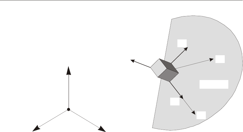
Defining the Three Axes Using Two Vectors
A right- handed co or di nate sys tem R- S-T can be rep re sented by the three mutually-
perpendicular vec tors Vr, Vs, and Vt, re spec tively, that sat isfy the re la tion ship:
Vt = Vr ´ Vs
This co or di nate sys tem can be de fined by speci fy ing two non- parallel vec tors:
•An axis ref er ence vec tor, Va, that is par al lel to axis R
•A plane ref er ence vec tor, Vp, that is par al lel to plane R-S, and points to ward the
positive-S side of the R axis
The axes are then de fined as:
Vr = Va
Vt = Vr ´ Vp
Vs = Vt ´ Vr
Note that Vp can be any con ven ient vec tor par al lel to the R-S plane; it does not have
to be par al lel to the S axis. This is il lus trated in Figure 1 (page 15).
Local Coordinate Systems
Each part (joint, ele ment, or con straint) of the struc tural model has its own lo cal co -
or di nate sys tem used to de fine the prop er ties, loads, and re sponse for that part. The
axes of the lo cal co or di nate sys tems are de noted 1, 2, and 3. In gen eral, the lo cal co -
or di nate sys tems may vary from joint to joint, ele ment to ele ment, and con straint to
con straint.
There is no pre ferred up ward di rec tion for a lo cal co or di nate sys tem. How ever, the
up ward +Z di rec tion is used to de fine the de fault joint and ele ment lo cal co or di nate
sys tems with re spect to the global or any al ter nate co or di nate sys tem.
14 Local Coordinate Systems
CSI Analysis Reference Manual
The joint lo cal 1- 2-3 co or di nate sys tem is nor mally the same as the global X- Y-Z
co or di nate sys tem. How ever, you may de fine any ar bi trary ori en ta tion for a joint
lo cal co or di nate sys tem by speci fy ing two ref er ence vec tors and/or three an gles of
ro ta tion.
For the Frame, Area (Shell, Plane, and Asolid), and Link/Sup port ele ments, one of
the ele ment lo cal axes is de ter mined by the ge ome try of the in di vid ual ele ment.
You may de fine the ori en ta tion of the re main ing two axes by speci fy ing a sin gle
ref er ence vec tor and/or a sin gle an gle of ro ta tion. The ex cep tion to this is one-joint
or zero-length Link/Sup port el e ments, which re quire that you first spec ify the lo -
cal-1 (ax ial) axis.
The Solid el e ment lo cal 1-2-3 co or di nate sys tem is nor mally the same as the global
X-Y-Z co or di nate sys tem. How ever, you may de fine any ar bi trary ori en ta tion for a
solid lo cal co or di nate sys tem by spec i fy ing two ref er ence vec tors and/or three an -
gles of ro ta tion.
The lo cal co or di nate sys tem for a Body, Dia phragm, Plate, Beam, or Rod Con -
straint is nor mally de ter mined auto mati cally from the ge ome try or mass dis tri bu -
tion of the con straint. Op tion ally, you may spec ify one lo cal axis for any Dia -
Local Coordinate Systems 15
Chapter III Coordinate Systems
V is parallel to R axis
a
V is parallel to R-S plane
p
V = V
ra
V = V x V
trp
V = V x V
str
XY
Z
Global
Plane R-S
Vr
Vt
Vs
Va
Vp
Cube is shown for
visualization purposes
Figure 1
Determining an R-S-T Coordinate System from Reference Vectors Va and Vp

phragm, Plate, Beam, or Rod Con straint (but not for the Body Con straint); the re -
main ing two axes are de ter mined auto mati cally.
The lo cal co or di nate sys tem for an Equal Con straint may be ar bi trar ily speci fied;
by de fault it is the global co or di nate sys tem. The Lo cal Con straint does not have its
own lo cal co or di nate sys tem.
For more in for ma tion:
•See Topic “Lo cal Co or di nate Sys tem” (page 24) in Chap ter “Joints and De -
grees of Free dom.”
•See Topic “Lo cal Co or di nate Sys tem” (page 108) in Chap ter “The Frame Ele -
ment.”
•See Topic “Lo cal Co or di nate Sys tem” (page 185) in Chap ter “The Shell Ele -
ment.”
•See Topic “Lo cal Co or di nate Sys tem” (page 217) in Chap ter “The Plane Ele -
ment.”
•See Topic “Lo cal Co or di nate Sys tem” (page 227) in Chap ter “The Aso lid Ele -
ment.”
•See Topic “Lo cal Co or di nate Sys tem” (page 240) in Chap ter “The Solid Ele -
ment.”
•See Topic “Lo cal Co or di nate Sys tem” (page 253) in Chap ter “The Link/Sup -
port El e ment—Basic.”
•See Chap ter “Con straints and Welds (page 49).”
Alternate Coordinate Systems
You may de fine al ter nate co or di nate sys tems that can be used for lo cat ing the
joints; for de fin ing lo cal co or di nate sys tems for joints, ele ments, and con straints;
and as a ref er ence for de fin ing other prop er ties and loads. The axes of the al ter nate
co or di nate sys tems are de noted X, Y, and Z.
The global co or di nate sys tem and all al ter nate sys tems are called fixed co or di nate
sys tems, since they ap ply to the whole struc tural model, not just to in di vid ual parts
as do the lo cal co or di nate sys tems. Each fixed co or di nate sys tem may be used in
rec tan gu lar, cy lin dri cal or spheri cal form.
As so ci ated with each fixed co or di nate sys tem is a grid sys tem used to lo cate ob jects
in the graph i cal user in ter face. Grids have no mean ing in the anal y sis model.
16 Alternate Coordinate Systems
CSI Analysis Reference Manual
Each al ter nate co or di nate sys tem is de fined by spec i fy ing the lo ca tion of the or i gin
and the ori en ta tion of the axes with re spect to the global co or di nate sys tem. You
need:
•The global X, Y, and Z co or di nates of the new or i gin
•The three an gles (in de grees) used to ro tate from the global co or di nate sys tem
to the new sys tem
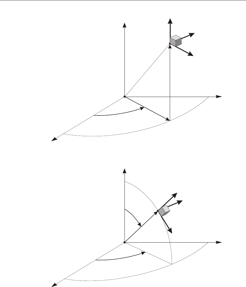
Cylindrical and Spherical Coordinates
The lo ca tion of points in the global or an al ter nate co or di nate sys tem may be speci -
fied us ing po lar co or di nates in stead of rec tan gu lar X- Y-Z co or di nates. Po lar co or -
di nates in clude cy lin dri cal CR- CA- CZ co or di nates and spheri cal SB- SA- SR co or -
di nates. See Figure 2 (page 19) for the defi ni tion of the po lar co or di nate sys tems.
Po lar co or di nate sys tems are al ways de fined with re spect to a rec tan gu lar X- Y-Z
sys tem.
The co or di nates CR, CZ, and SR are lin eal and are speci fied in length units. The co -
or di nates CA, SB, and SA are an gu lar and are speci fied in de grees.
Lo ca tions are speci fied in cy lin dri cal co or di nates us ing the vari ables cr, ca, and cz.
These are re lated to the rec tan gu lar co or di nates as:
crxy=+
22
cay
x
=tan-1
czz=
Lo ca tions are speci fied in spheri cal co or di nates us ing the vari ables sb, sa, and sr.
These are re lated to the rec tan gu lar co or di nates as:
sbxy
z
=tan+
-1
22
say
x
=tan-1
srxyz=++
222
Cylindrical and Spherical Coordinates 17
Chapter III Coordinate Systems

A vec tor in a fixed co or di nate sys tem can be speci fied by giv ing the lo ca tions of
two points or by speci fy ing a co or di nate di rec tion at a sin gle point P. Co or di nate
di rec tions are tan gen tial to the co or di nate curves at point P. A posi tive co or di nate
di rec tion in di cates the di rec tion of in creas ing co or di nate value at that point.
Cy lin dri cal co or di nate di rec tions are in di cated us ing the val ues ±CR, ±CA, and
±CZ. Spheri cal co or di nate di rec tions are in di cated us ing the val ues ±SB, ±SA, and
±SR. The sign is re quired. See Figure 2 (page 19).
The cy lin dri cal and spheri cal co or di nate di rec tions are not con stant but vary with
an gu lar po si tion. The co or di nate di rec tions do not change with the lin eal co or di -
nates. For ex am ple, +SR de fines a vec tor di rected from the ori gin to point P.
Note that the co or di nates Z and CZ are iden ti cal, as are the cor re spond ing co or di -
nate di rec tions. Simi larly, the co or di nates CA and SA and their cor re spond ing co -
or di nate di rec tions are iden ti cal.
18 Cylindrical and Spherical Coordinates
CSI Analysis Reference Manual
Cylindrical and Spherical Coordinates 19
Chapter III Coordinate Systems
Cylindrical
Coordinates
Spherical
Coordinates
X
Y
Z, CZ
ca
cr
cz
P
X
Y
Z
sa
sb
sr
P
+CR
+CA
+CZ
+SB
+SA
+SR
Cubes are shown for
visualization purposes
Figure 2
Cylindrical and Spherical Coordinates and Coordinate Directions

20 Cylindrical and Spherical Coordinates
CSI Analysis Reference Manual

Chapter IV
Joints and Degrees of Freedom
The joints play a fun da men tal role in the analy sis of any struc ture. Joints are the
points of con nec tion be tween the ele ments, and they are the pri mary lo ca tions in
the struc ture at which the dis place ments are known or are to be de ter mined. The
dis place ment com po nents (trans la tions and ro ta tions) at the joints are called the de -
grees of free dom.
This Chap ter de scribes joint prop er ties, de grees of free dom, loads, and out put. Ad -
di tional in for ma tion about joints and de grees of free dom is given in Chap ter “Con -
straints and Welds” (page 49).
Basic Topics for All Users
•Over view
•Mod el ing Con sid era tions
•Lo cal Co or di nate Sys tem
•De grees of Free dom
•Re straint Supports
•Spring Sup ports
•Joint Re ac tions
•Base Reactions
21

•Masses
•Force Load
•De gree of Free dom Out put
•As sem bled Joint Mass Out put
•Dis place ment Out put
•Force Out put
Advanced Topics
•Ad vanced Lo cal Co or di nate Sys tem
•Non lin ear Sup ports
•Dis trib uted Supports
•Ground Dis place ment Load
•Gen er al ized Displacements
•El e ment Joint Force Output
Overview
Joints, also known as nodal points or nodes, are a fun da men tal part of every struc -
tural model. Joints per form a va ri ety of func tions:
•All ele ments are con nected to the struc ture (and hence to each other) at the
joints
•The struc ture is sup ported at the joints us ing Re straints and/or Springs
•Rigid- body be hav ior and sym me try con di tions can be speci fied us ing Con -
straints that ap ply to the joints
•Con cen trated loads may be ap plied at the joints
•Lumped (con cen trated) masses and ro ta tional in er tia may be placed at the
joints
•All loads and masses ap plied to the ele ments are ac tu ally trans ferred to the
joints
•Joints are the pri mary lo ca tions in the struc ture at which the dis place ments are
known (the sup ports) or are to be de ter mined
All of these func tions are dis cussed in this Chap ter ex cept for the Con straints,
which are de scribed in Chap ter “Con straints and Welds” (page 49).
22 Overview
CSI Analysis Reference Manual

Joints in the anal y sis model cor re spond to point ob jects in the struc tural-ob ject
model. Using the SAP2000, ETABS, SAFE, or CSiBridge graph i cal user in ter face,
joints (points) are au to mat i cally cre ated at the ends of each Line ob ject and at the
cor ners of each Area and Solid ob ject. Joints may also be de fined in de pend ently of
any ob ject.
Au to matic mesh ing of ob jects will cre ate ad di tional joints cor re spond ing to any el -
e ments that are cre ated.
Joints may them selves be con sid ered as el e ments. Each joint may have its own lo -
cal co or di nate sys tem for de fin ing the de grees of free dom, re straints, joint prop er -
ties, and loads; and for in ter pret ing joint out put. In most cases, how ever, the global
X-Y-Z co or di nate sys tem is used as the lo cal co or di nate sys tem for all joints in the
model. Joints act in de pend ently of each other un less con nected by other el e ments.
There are six dis place ment de grees of free dom at ev ery joint — three trans la tions
and three ro ta tions. These dis place ment com po nents are aligned along the lo cal co -
or di nate sys tem of each joint.
Joints may be loaded di rectly by con cen trated loads or in di rectly by ground dis -
place ments act ing though Re straints, spring sup ports, or one-joint (grounded)
Link/Sup port objects.
Dis place ments (trans la tions and ro ta tions) are pro duced at every joint. Re ac tion
forces and mo ments act ing at each sup ported joint are also pro duced.
For more in for ma tion, see Chap ter “Con straints and Welds” (page 49).
Modeling Considerations
The lo ca tion of the joints and ele ments is criti cal in de ter min ing the ac cu racy of the
struc tural model. Some of the fac tors that you need to con sider when de fin ing the
ele ments, and hence the joints, for the struc ture are:
•The number of ele ments should be suf fi cient to de scribe the ge ome try of the
struc ture. For straight lines and edges, one ele ment is ade quate. For curves and
curved sur faces, one ele ment should be used for every arc of 15° or less.
•Ele ment bounda ries, and hence joints, should be lo cated at points, lines, and
sur faces of dis con ti nu ity:
–Struc tural bounda ries, e.g., cor ners and edges
–Changes in ma te rial prop er ties
Modeling Considerations 23
Chapter IV Joints and Degrees of Freedom

–Changes in thick ness and other geo met ric prop er ties
–Sup port points (Re straints and Springs)
–Points of ap pli ca tion of con cen trated loads, ex cept that Frame el e ments
may have con cen trated loads ap plied within their spans
•In re gions hav ing large stress gra di ents, i.e., where the stresses are chang ing
rap idly, an Area- or Solid-el e ment mesh should be re fined us ing small ele -
ments and closely- spaced joints. This may re quire chang ing the mesh af ter one
or more pre limi nary analy ses.
•More that one ele ment should be used to model the length of any span for
which dy namic be hav ior is im por tant. This is re quired be cause the mass is al -
ways lumped at the joints, even if it is con trib uted by the ele ments.
Local Coordinate System
Each joint has its own joint lo cal co or di nate sys tem used to de fine the de grees of
free dom, Re straints, prop er ties, and loads at the joint; and for in ter pret ing joint out -
put. The axes of the joint lo cal co or di nate sys tem are de noted 1, 2, and 3. By de fault
these axes are iden ti cal to the global X, Y, and Z axes, re spec tively. Both sys tems
are right- handed co or di nate sys tems.
The de fault lo cal co or di nate sys tem is ade quate for most situa tions. How ever, for
cer tain mod el ing pur poses it may be use ful to use dif fer ent lo cal co or di nate sys -
tems at some or all of the joints. This is de scribed in the next topic.
For more in for ma tion:
•See Topic “Up ward and Hori zon tal Di rec tions” (page 13) in Chap ter “Co or di -
nate Sys tems.”
•See Topic “Ad vanced Lo cal Co or di nate Sys tem” (page 24) in this Chap ter.
Advanced Local Coordinate System
By de fault, the joint lo cal 1- 2-3 co or di nate sys tem is iden ti cal to the global X- Y-Z
co or di nate sys tem, as de scribed in the pre vi ous topic. How ever, it may be nec es -
sary to use dif fer ent lo cal co or di nate sys tems at some or all joints in the fol low ing
cases:
•Skewed Re straints (sup ports) are pres ent
•Con straints are used to im pose ro ta tional sym me try
24 Local Coordinate System
CSI Analysis Reference Manual

•Con straints are used to im pose sym me try about a plane that is not par al lel to a
global co or di nate plane
•The prin ci pal axes for the joint mass (trans la tional or ro ta tional) are not aligned
with the global axes
•Joint dis place ment and force out put is de sired in an other co or di nate sys tem
Joint lo cal co or di nate sys tems need only be de fined for the af fected joints. The
global sys tem is used for all joints for which no lo cal co or di nate sys tem is ex plic itly
speci fied.
A va ri ety of meth ods are avail able to de fine a joint lo cal co or di nate sys tem. These
may be used sepa rately or to gether. Lo cal co or di nate axes may be de fined to be par -
al lel to ar bi trary co or di nate di rec tions in an ar bi trary co or di nate sys tem or to vec -
tors be tween pairs of joints. In ad di tion, the joint lo cal co or di nate sys tem may be
speci fied by a set of three joint co or di nate an gles. These meth ods are de scribed in
the sub top ics that fol low.
For more in for ma tion:
•See Chap ter “Co or di nate Sys tems” (page 11).
•See Topic “Lo cal Co or di nate Sys tem” (page 24) in this Chap ter.
Reference Vectors
To de fine a joint lo cal co or di nate sys tem you must spec ify two ref er ence vec tors
that are par al lel to one of the joint lo cal co or di nate planes. The axis ref er ence vec -
tor, Va, must be par al lel to one of the lo cal axes (I = 1, 2, or 3) in this plane and
have a posi tive pro jec tion upon that axis. The plane ref er ence vec tor, Vp, must
have a posi tive pro jec tion upon the other lo cal axis (j = 1, 2, or 3, but I ¹ j) in this
plane, but need not be par al lel to that axis. Hav ing a posi tive pro jec tion means that
the posi tive di rec tion of the ref er ence vec tor must make an an gle of less than 90°
with the posi tive di rec tion of the lo cal axis.
To gether, the two ref er ence vec tors de fine a lo cal axis, I, and a lo cal plane, i-j.
From this, the pro gram can de ter mine the third lo cal axis, k, us ing vec tor al ge bra.
For ex am ple, you could choose the axis ref er ence vec tor par al lel to lo cal axis 1 and
the plane ref er ence vec tor par al lel to the lo cal 1-2 plane (I = 1, j = 2). Al ter na tively,
you could choose the axis ref er ence vec tor par al lel to lo cal axis 3 and the plane ref -
er ence vec tor par al lel to the lo cal 3-2 plane (I = 3, j = 2). You may choose the plane
that is most con ven ient to de fine us ing the pa rame ter lo cal, which may take on the
Advanced Local Coordinate System 25
Chapter IV Joints and Degrees of Freedom

val ues 12, 13, 21, 23, 31, or 32. The two dig its cor re spond to I and j, re spec tively.
The de fault is value is 31.
Defining the Axis Reference Vector
To de fine the axis ref er ence vec tor for joint j, you must first spec ify or use the de -
fault val ues for:
•A co or di nate di rec tion ax dir (the de fault is +Z)
•A fixed co or di nate sys tem csys (the de fault is zero, in di cat ing the global co or -
di nate sys tem)
You may op tion ally spec ify:
•A pair of joints, ax veca and ax vecb (the de fault for each is zero, in di cat ing
joint j it self). If both are zero, this op tion is not used.
For each joint, the axis ref er ence vec tor is de ter mined as fol lows:
1. A vec tor is found from joint ax veca to joint ax vecb. If this vec tor is of fi nite
length, it is used as the ref er ence vec tor Va
2. Oth er wise, the co or di nate di rec tion ax dir is evalu ated at joint j in fixed co or di -
nate sys tem csys, and is used as the ref er ence vec tor Va
Defining the Plane Reference Vector
To de fine the plane ref er ence vec tor for joint j, you must first spec ify or use the de -
fault val ues for:
•A pri mary co or di nate di rec tion pldirp (the de fault is +X)
•A sec on dary co or di nate di rec tion pldirs (the de fault is +Y). Di rec tions pldirs
and pldirp should not be par al lel to each other un less you are sure that they are
not par al lel to lo cal axis 1
•A fixed co or di nate sys tem csys (the de fault is zero, in di cat ing the global co or -
di nate sys tem). This will be the same co or di nate sys tem that was used to de fine
the axis ref er ence vec tor, as de scribed above
You may op tion ally spec ify:
•A pair of joints, plveca and plvecb (the de fault for each is zero, in di cat ing joint
j it self). If both are zero, this op tion is not used.
26 Advanced Local Coordinate System
CSI Analysis Reference Manual

For each joint, the plane ref er ence vec tor is de ter mined as fol lows:
1. A vec tor is found from joint plveca to joint plvecb. If this vec tor is of fi nite
length and is not par al lel to lo cal axis I, it is used as the ref er ence vec tor Vp
2. Oth er wise, the pri mary co or di nate di rec tion pldirp is evalu ated at joint j in
fixed co or di nate sys tem csys. If this di rec tion is not par al lel to lo cal axis I, it is
used as the ref er ence vec tor Vp
3. Oth er wise, the sec on dary co or di nate di rec tion pldirs is evalu ated at joint j in
fixed co or di nate sys tem csys. If this di rec tion is not par al lel to lo cal axis I, it is
used as the ref er ence vec tor Vp
4. Oth er wise, the method fails and the analy sis ter mi nates. This will never hap pen
if pldirp is not par al lel to pldirs
A vec tor is con sid ered to be par al lel to lo cal axis I if the sine of the an gle be tween
them is less than 10-3.
Determining the Local Axes from the Reference Vectors
The pro gram uses vec tor cross prod ucts to de ter mine the lo cal axes from the ref er -
ence vec tors. The three axes are rep re sented by the three unit vec tors V1, V2 and
V3, re spec tively. The vec tors sat isfy the cross- product re la tion ship:
VVV
123
=´
The lo cal axis Vi is given by the vec tor Va af ter it has been nor mal ized to unit
length.
The re main ing two axes, Vj and Vk, are de fined as fol lows:
•If I and j per mute in a posi tive sense, i.e., lo cal = 12, 23, or 31, then:
VVV
kip
=´ and
VVV
jki
=´
•If I and j per mute in a nega tive sense, i.e., lo cal = 21, 32, or 13, then:
VVV
kpi
=´ and
VVV
jik
=´
An ex am ple show ing the de ter mi na tion of the joint lo cal co or di nate sys tem us ing
ref er ence vec tors is given in Figure 3 (page 28).
Advanced Local Coordinate System 27
Chapter IV Joints and Degrees of Freedom
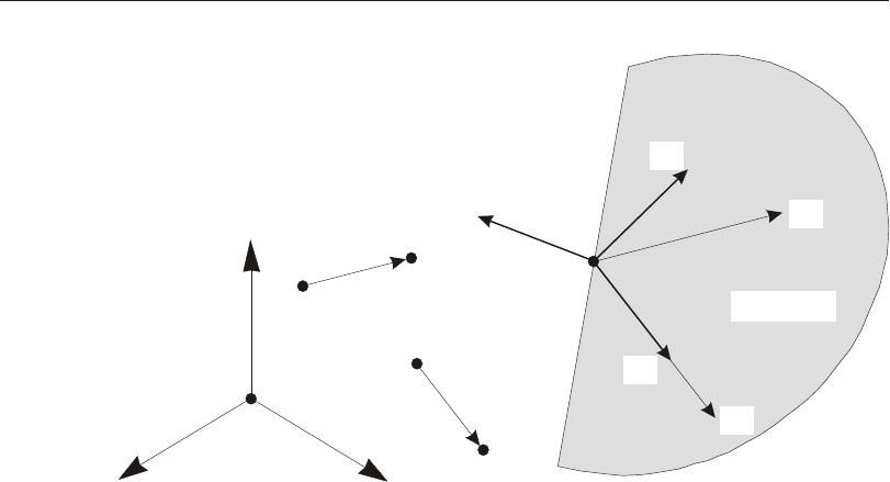
Joint Coordinate Angles
The joint lo cal co or di nate axes de ter mined from the ref er ence vec tors may be fur -
ther modi fied by the use of three joint co or di nate an gles, de noted a, b, and c. In
the case where the de fault ref er ence vec tors are used, the joint co or di nate an gles de -
fine the ori en ta tion of the joint lo cal co or di nate sys tem with re spect to the global
axes.
The joint co or di nate an gles spec ify ro ta tions of the lo cal co or di nate sys tem about
its own cur rent axes. The re sult ing ori en ta tion of the joint lo cal co or di nate sys tem
is ob tained ac cord ing to the fol low ing pro ce dure:
1. The lo cal sys tem is first ro tated about its +3 axis by an gle a
2. The lo cal sys tem is next ro tated about its re sult ing +2 axis by an gle b
3. The lo cal sys tem is lastly ro tated about its re sult ing +1 axis by an gle c
The or der in which the ro ta tions are per formed is im por tant. The use of co or di nate
an gles to ori ent the joint lo cal co or di nate sys tem with re spect to the global sys tem is
shown in Figure 4 (page 29).
28 Advanced Local Coordinate System
CSI Analysis Reference Manual
V is parallel to axveca-axvecb
a
V is parallel to plveca-plvecb
p
V = V
3a
V = V x VAll vectors normalized to unit length.
23p
V = V x V
123
XY
Z
Global
axveca
axvecb
plveca
plvecb
Plane 3-1
j
V3
V2
V1
Va
Vp
Figure 3
Example of the Determination of the Joint Local Coordinate System
Using Reference Vectors for local=31
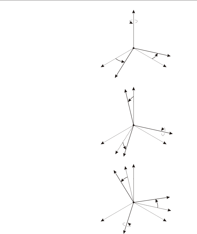
Advanced Local Coordinate System 29
Chapter IV Joints and Degrees of Freedom
a
a
a
b
b
b
c
c
c
Z, 3
Z
Z
X
X
X
1
2
2
2
3
3
1
1
Y
Y
Y
Step 1: Rotation about
local 3 axis by angle a
Step 2: Rotation about new
local 2 axis by angle b
Step 3: Rotation about new
local 1 axis by angle c
Figure 4
Use of Joint Coordinate Angles to Orient the Joint Local Coordinate System

Degrees of Freedom
The de flec tion of the struc tural model is gov erned by the dis place ments of the
joints. Every joint of the struc tural model may have up to six dis place ment com po -
nents:
•The joint may trans late along its three lo cal axes. These trans la tions are de -
noted U1, U2, and U3.
•The joint may ro tate about its three lo cal axes. These ro ta tions are de noted R1,
R2, and R3.
These six dis place ment com po nents are known as the de grees of free dom of the
joint. In the usual case where the joint lo cal co or di nate sys tem is par al lel to the
global sys tem, the de grees of free dom may also be iden ti fied as UX, UY, UZ, RX,
RY and RZ, ac cord ing to which global axes are par al lel to which lo cal axes. The
joint lo cal de grees of free dom are il lus trated in Figure 5 (page 31).
In ad di tion to the regu lar joints that you ex plic itly de fine as part of your struc tural
model, the pro gram auto mati cally cre ates mas ter joints that gov ern the be hav ior of
any Con straints and Welds that you may have de fined. Each mas ter joint has the
same six de grees of free dom as do the regu lar joints. See Chap ter “Con straints and
Welds” (page 49) for more in for ma tion.
Each de gree of free dom in the struc tural model must be one of the fol low ing types:
•Ac tive — the dis place ment is com puted dur ing the analy sis
•Re strained — the dis place ment is speci fied, and the cor re spond ing re ac tion is
com puted dur ing the analy sis
•Con strained — the dis place ment is de ter mined from the dis place ments at other
de grees of free dom
•Null — the dis place ment does not af fect the struc ture and is ig nored by the
analy sis
•Un avail able — the dis place ment has been ex plic itly ex cluded from the analy -
sis
These dif fer ent types of de grees of free dom are de scribed in the fol low ing sub top -
ics.
30 Degrees of Freedom
CSI Analysis Reference Manual
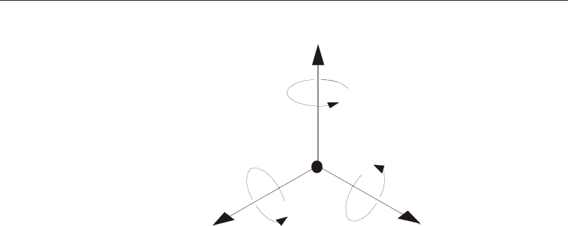
Available and Unavailable Degrees of Freedom
You may ex plic itly spec ify the global de grees of free dom that are avail able to every
joint in the struc tural model. By de fault, all six de grees of free dom are avail able to
every joint. This de fault should gen er ally be used for all three- dimensional struc -
tures.
For cer tain pla nar struc tures, how ever, you may wish to re strict the avail able de -
grees of free dom. For ex am ple, in the X-Y plane: a pla nar truss needs only UX and
UY; a pla nar frame needs only UX, UY, and RZ; and a pla nar grid or flat plate
needs only UZ, RX, and RY.
The de grees of free dom that are not speci fied as be ing avail able are called un avail -
able de grees of free dom. Any stiff ness, loads, mass, Re straints, or Con straints that
are ap plied to the un avail able de grees of free dom are ig nored by the analy sis.
The avail able de grees of free dom are al ways re ferred to the global co or di nate sys -
tem, and they are the same for every joint in the model. If any joint lo cal co or di nate
sys tems are used, they must not cou ple avail able de grees of free dom with the un -
avail able de grees of free dom at any joint. For ex am ple, if the avail able de grees of
free dom are UX, UY, and RZ, then all joint lo cal co or di nate sys tems must have one
lo cal axis par al lel to the global Z axis.
Degrees of Freedom 31
Chapter IV Joints and Degrees of Freedom
Joint
U2
U3
U1
R2
R3
R1
Figure 5
The Six Displacement Degrees of Freedom in the Joint Local Coordinate System

Restrained Degrees of Freedom
If the dis place ment of a joint along any one of its avail able de grees of free dom is
known, such as at a sup port point, that de gree of free dom is re strained. The known
value of the dis place ment may be zero or non- zero, and may be dif fer ent in dif fer -
ent Load Pat terns. The force along the re strained de gree of free dom that is re quired
to im pose the speci fied re straint dis place ment is called the re ac tion, and is de ter -
mined by the analy sis.
Un avail able de grees of free dom are es sen tially re strained. How ever, they are ex -
cluded from the analy sis and no re ac tions are com puted, even if they are non- zero.
See Topic “Re straint Sup ports” (page 34) in this Chap ter for more in for ma tion.
Constrained Degrees of Freedom
Any joint that is part of a Con straint or Weld may have one or more of its avail able
de grees of free dom con strained. The pro gram auto mati cally cre ates a mas ter joint
to gov ern the be hav ior of each Con straint, and a mas ter joint to gov ern the be hav ior
of each set of joints that are con nected to gether by a Weld. The dis place ment of a
con strained de gree of free dom is then com puted as a lin ear com bi na tion of the dis -
place ments along the de grees of free dom at the cor re spond ing mas ter joint.
If a constrained de gree of free dom is also re strained, the re straint will be ap plied to
the con straint as a whole.
See Chap ter “Con straints and Welds” (page 49) for more in for ma tion.
Mixing Restraints and Constraints Not Recommended
It is not rec om mended that re strained de grees of free dom also be con strained, al -
though it is per mit ted. Re ac tions com puted at such de grees of free dom will not in -
clude the con tri bu tions to the re ac tion from joints con nected by con straints.
Ground dis place ment loads ap plied at the con straint will not be ap plied to the joints
con nected by con straint. For better re sults, use springs or grounded (one-joint)
link/sup port ob jects to sup port joints that are also con strained.
Sim i larly, it is not rec om mended, that a given de gree of free dom be in cluded in
more than one con straint, al though it is per mit ted. The anal y sis will at tempt to com -
bine the cou pled con straints, but the re sults may not be as ac cu rate as us ing a sin gle
con straint for all cou pled joints, es pe cially for dy nam ics. For better re sults, in clude
all cou pled joints in a sin gle con straint when ever pos si ble.
32 Degrees of Freedom
CSI Analysis Reference Manual

Note that us ing fixed de grees of free dom in a link/sup port prop erty is the same as
spec i fy ing a con straint. For this rea son, such link/support ob jects should not be
con nected to gether or con nected to con strained joints. In such cases, it is better to
use large (but not too large) stiffnesses rather that fixed de grees of free dom in the
link/support prop erty def i ni tion.
Active Degrees of Freedom
All avail able de grees of free dom that are nei ther con strained nor re strained must be
ei ther ac tive or null. The pro gram will auto mati cally de ter mine the ac tive de grees
of free dom as fol lows:
•If any load or stiff ness is ap plied along any trans la tional de gree of free dom at a
joint, then all avail able trans la tional de grees of free dom at that joint are made
ac tive un less they are con strained or re strained.
•If any load or stiff ness is ap plied along any ro ta tional de gree of free dom at a
joint, then all avail able ro ta tional de grees of free dom at that joint are made ac -
tive un less they are con strained or re strained.
•All de grees of free dom at a mas ter joint that gov ern con strained de grees of
free dom are made ac tive.
A joint that is con nected to any ele ment or to a trans la tional spring will have all of
its trans la tional de grees of free dom ac ti vated. A joint that is con nected to a Frame,
Shell, or Link/Sup port ele ment, or to any ro ta tional spring will have all of its ro ta -
tional de grees of free dom ac ti vated. An ex cep tion is a Frame el e ment with only
truss- type stiff ness, which will not ac ti vate ro ta tional de grees of free dom.
Every ac tive de gree of free dom has an as so ci ated equa tion to be solved. If there are
N ac tive de grees of free dom in the struc ture, there are N equa tions in the sys tem,
and the struc tural stiff ness ma trix is said to be of or der N. The amount of com pu ta -
tional ef fort re quired to per form the analy sis in creases with N.
The load act ing along each ac tive de gree of free dom is known (it may be zero). The
cor re spond ing dis place ment will be de ter mined by the analy sis.
If there are ac tive de grees of free dom in the sys tem at which the stiff ness is known
to be zero, such as the out- of- plane trans la tion in a planar- frame, these must ei ther
be re strained or made un avail able. Oth er wise, the struc ture is un sta ble and the so lu -
tion of the static equa tions will fail.
For more in for ma tion:
•See Topic “Springs” (page 36) in this Chap ter.
Degrees of Freedom 33
Chapter IV Joints and Degrees of Freedom

•See Topic “De grees of Free dom” (page 108) in Chap ter “The Frame Ele ment.”
•See Topic “De grees of Free dom” (page 170) in Chap ter “The Ca ble El e ment.”
•See Topic “De grees of Free dom” (page 181) in Chap ter “The Shell El e ment.”
•See Topic “De grees of Free dom” (page 217) in Chap ter “The Plane Ele ment.”
•See Topic “De grees of Free dom” (page 227) in Chap ter “The Aso lid Ele ment.”
•See Topic “De grees of Free dom” (page 240) in Chap ter “The Solid Ele ment.”
•See Topic “De grees of Free dom” (page 253) in Chap ter “The Link/Sup port El -
e ment—Basic.”
•See Topic “De grees of Free dom” (page 312) in Chap ter “The Ten don Ob ject.”
Null Degrees of Freedom
The avail able de grees of free dom that are not re strained, con strained, or ac tive, are
called the null de grees of free dom. Be cause they have no load or stiff ness, their dis -
place ments and re ac tions are zero, and they have no ef fect on the rest of the struc -
ture. The pro gram auto mati cally ex cludes them from the analy sis.
Joints that have no ele ments con nected to them typi cally have all six de grees of
free dom null. Joints that have only solid- type ele ments (Plane, Aso lid, and Solid)
con nected to them typi cally have the three ro ta tional de grees of free dom null.
Restraint Supports
If the dis place ment of a joint along any of its avail able de grees of free dom has a
known value, ei ther zero (e.g., at sup port points) or non- zero (e.g., due to sup port
set tle ment), a Re straint must be ap plied to that de gree of free dom. The known
value of the dis place ment may dif fer from one Load Pat tern to the next, but the de -
gree of free dom is re strained for all Load Pat terns. In other words, it is not pos si ble
to have the dis place ment known in one Load Pat tern and un known (un re strained) in
an other Load Pat tern.
Re straints should also be ap plied to any avail able de grees of free dom in the sys tem
at which the stiff ness is known to be zero, such as the out- of- plane trans la tion and
in- plane ro ta tions of a planar- frame. Oth er wise, the struc ture is un sta ble and the so -
lu tion of the static equa tions will complain.
Re straints are al ways ap plied to the joint lo cal de grees of free dom U1, U2, U3, R1,
R2, and R3. Ex am ples of Re straints are shown in Figure 6 (page 35).
34 Restraint Supports
CSI Analysis Reference Manual
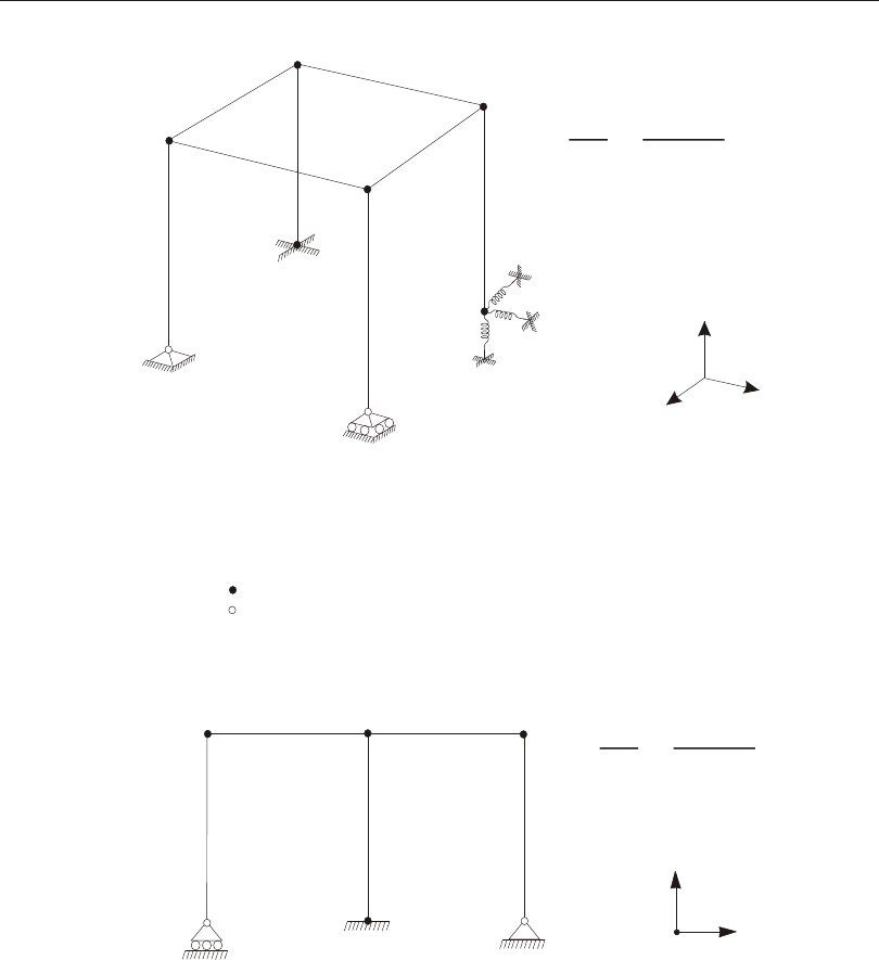
Restraint Supports 35
Chapter IV Joints and Degrees of Freedom
2-D Frame Structure, X-Z plane
3-D Frame Structure
Notes: Joints are indicated with dots:
Solid dots indicate moment continuity
Open dots indicate hinges
All joint local 1-2-3 coordinate systems are
identical to the global X-Y-Z coordinate system
Z
X
Global
Global
Z
XY
Rollers
Hinge
Fixed
Spring
Support
1
2
3
4
5
6
7
8
Hinge
Fixed
Roller
123
456
Joint Restraints
1 U1, U2, U3
2 U3
3 U1, U2, U3, R1, R2, R3
4 None
Joint Restraints
All U2, R1, R3
1 U3
2 U1, U3, R2
3 U1, U3
Figure 6
Examples of Restraints

If a re straint is ap plied to an un avail able de gree of free dom, it is ig nored. The dis -
place ment will be zero, but no re ac tion will be com puted.
In gen eral, you should not ap ply re straints to con strained de grees of free dom. How -
ever, if you do, the anal y sis will at tempt to au to mat i cally re write the con straint
equa tions to ac com mo date the re straint. Re ac tions com puted at such de grees of
free dom will not in clude the con tri bu tions to the re ac tion from joints con nected by
con straints. Ground dis place ment loads ap plied at the con straint will not be ap plied
to the joints con nected by con straint. For better re sults, use springs or grounded
(one-joint) Link/Sup ports to sup port joints that are also con strained.
For more in for ma tion:
•See Topic “De grees of Free dom” (page 30) in this Chap ter.
•See Topic “Re straint Dis place ment Load” (page 42) in this Chap ter.
Spring Supports
Any of the six de grees of free dom at any of the joints in the struc ture can have trans -
la tional or ro ta tional spring sup port con di tions. These springs elas ti cally con nect
the joint to the ground. Spring sup ports along re strained de grees of free dom do not
con trib ute to the stiff ness of the struc ture.
Springs may be speci fied that cou ple the de grees of free dom at a joint. The spring
forces that act on a joint are re lated to the dis place ments of that joint by a 6x6 sym -
met ric ma trix of spring stiff ness co ef fi cients. These forces tend to op pose the dis -
place ments.
Spring stiff ness co ef fi cients may be speci fied in the global co or di nate sys tem, an
Al ter nate Co or di nate Sys tem, or the joint lo cal co or di nate sys tem.
In a joint lo cal co or di nate sys tem, the spring forces and mo ments F1, F2, F3, M1, M2
and M3 at a joint are given by:
(Eqn. 1)
F
F
F
M
M
M
1
2
3
1
2
3
ì
í
ï
ï
ï
î
ï
ï
ï
ü
ý
ï
ï
ï
þ
ï
ï
ï
=-
u1u1u2u1u3u1r1u1r2u1r3
u2u2u3u2r1u2r2u2r3
u3u3r1u3r2u3r3
r1r1r2r1r3
sym.r2r2r3
r3
é
ë
ê
ê
ê
ê
ê
ê
ê
ù
û
ú
ú
ú
ú
ú
ú
ú
ì
í
ï
ï
ï
î
ï
ï
ï
ü
ý
ï
u
u
u
r
r
r
1
2
3
1
2
3
ï
ï
þ
ï
ï
ï
36 Spring Supports
CSI Analysis Reference Manual

where u1, u2, u3, r1, r2 and r3 are the joint dis place ments and ro ta tions, and the terms
u1, u1u2, u2, ... are the speci fied spring stiff ness co ef fi cients.
In any fixed co or di nate sys tem, the spring forces and mo ments Fx, Fy, Fz, Mx, My and
Mz at a joint are given by:
F
F
F
M
M
M
x
y
z
x
y
z
ì
í
ï
ï
ï
î
ï
ï
ï
ü
ý
ï
ï
ï
þ
ï
ï
ï
=-
uxuxuyuxuzuxrxuxryuxrz
uyuyuzuyrxuyryuyrz
uzuzrxuzryuzrz
rxrxryrxrz
sym.ryryrz
rz
é
ë
ê
ê
ê
ê
ê
ê
ê
ù
û
ú
ú
ú
ú
ú
ú
ú
ì
í
ï
ï
ï
î
ï
ï
ï
ü
ý
ï
u
u
u
r
r
r
x
y
z
x
y
z
ï
ï
þ
ï
ï
ï
where ux, uy, uz, rx, ry and rz are the joint dis place ments and ro ta tions, and the terms
ux, uxuy, uy, ... are the speci fied spring stiff ness co ef fi cients.
For springs that do not cou ple the de grees of free dom in a par ticu lar co or di nate sys -
tem, only the six di ago nal terms need to be speci fied since the off- diagonal terms
are all zero. When cou pling is pres ent, all 21 co ef fi cients in the up per tri an gle of the
ma trix must be given; the other 15 terms are then known by sym me try.
If the springs at a joint are speci fied in more than one co or di nate sys tem, stan dard
co or di nate trans for ma tion tech niques are used to con vert the 6x6 spring stiff ness
ma tri ces to the joint lo cal co or di nate sys tem, and the re sult ing stiff ness ma tri ces are
then added to gether on a term- by- term ba sis. The fi nal spring stiff ness ma trix at
each joint in the struc ture should have a de ter mi nant that is zero or posi tive. Oth er -
wise the springs may cause the struc ture to be un sta ble.
The dis place ment of the grounded end of the spring may be speci fied to be zero or
non- zero (e.g., due to sup port set tle ment). This spring dis place ment may vary
from one Load Pat tern to the next.
For more in for ma tion:
•See Topic “De grees of Free dom” (page 30) in this Chap ter.
•See Topic “Spring Dis place ment Load” (page 43) in this Chap ter.
Nonlinear Supports
In cer tain ver sions of the pro gram, you may de fine non lin ear sup ports at the joints
us ing the Link/Sup port el e ment. Non lin ear sup port con di tions that can be mod eled
Nonlinear Supports 37
Chapter IV Joints and Degrees of Freedom

in clude gaps (com pres sion only), multi-lin ear elas tic or plas tic springs, vis cous
damp ers, base iso la tors, and more.
This Link/Sup port can be used in two ways:
•You can add (draw) a one-joint object, in which case it is con sid ered a Sup port
object, and it con nects the joint di rectly to the ground.
•The ob ject can also be drawn with two joints, in which case it is con sid ered a
Link object. You can use a Link ob ject as a sup port if you con nect one end to
the struc ture, and fully re strain the other end.
Both meth ods have the same ef fect. Dur ing anal y sis, one-joint Sup port ob jects are
con verted to two-joint Link el e ments of zero length, and con nected to a gen er ated
joint that is fully re strained.
Mul ti ple Link/Sup port el e ments can be con nected to a sin gle joint, in which case
they act in par al lel. Each Link/Sup port el e ment has its own el e ment lo cal co or di -
nate sys tem that is in de pend ent of the joint lo cal co or di nate sys tem.
Re straints and springs may also ex ist at the joint. Of course, any de gree of free dom
that is re strained will pre vent de for ma tion in the Link/Sup port el e ment in that di -
rec tion.
See Chap ters “The Link/Sup port El e ment – Ba sic” (page 251) and “The Link/Sup -
port El e ment – Ad vanced” (page 275) for more in for ma tion.
Dis trib uted Sup ports
You may as sign dis trib uted spring sup ports along the length of a Frame el e ment, or
over the any face of an area ob ject (Shell, Plane, Asolid) or Solid el e ment. These
springs may be lin ear, multi-lin ear elas tic, or multi-lin ear plas tic. These springs are
con verted to equiv a lent two-joint Link/Sup port el e ments act ing at the joints of the
el e ment, af ter ac count ing for the trib u tary length or area of the el e ment. The gen er -
ated Link/Sup port el e ments are of zero length, with one end con nected to the par ent
ob ject, and the other end con nected to a gen er ated joint that is fully re strained.
Be cause these springs act at the joints, it may be nec es sary to mesh the el e ments to
cap ture lo cal ized ef fects of such dis trib uted sup ports. The best way to do this is
usu ally to use the au to matic in ter nal mesh ing op tions available in the graphical user
interface. This al lows you to change the mesh ing eas ily, while still be ing able to
work with large, sim pler model ob jects.
38 Dis trib uted Sup ports
CSI Analysis Reference Manual

It is not pos si ble to as sign dis trib uted re straint sup ports di rectly. How ever, when
us ing au to matic in ter nal mesh ing, you may op tion ally spec ify that the meshed el e -
ments use the same re straint conditions that are pres ent on the par ent ob ject.
For more in for ma tion, see Top ics “Re straint Sup ports” (page 34), “Spring Sup -
port” (page 36), “Non lin ear Sup ports” (page 37) in this Chap ter, and also Chap ter
“Ob jects and El e ments” (page 7.)
Joint Reactions
The force or mo ment along the de gree of free dom that is re quired to en force any
sup port con di tion is called the re ac tion, and it is de ter mined by the anal y sis. The
re ac tion in cludes the forces (or mo ments) from all sup ports at the joint, in clud ing
re straints, springs, and one-joint Link/Sup port objects. The trib u tary ef fect of any
dis trib uted sup ports is in cluded in the re ac tion.
If a one-joint Link/Sup port ob ject is used, the re ac tion will be re ported at the orig i -
nal joint con nected to the structure, not at the re strained end of the gen er ated
two-joint Link/Sup port el e ment. The re ac tion at the gen er ated joint will be re ported
as zero since it has been trans ferred to the original joint.
For more in for ma tion, see Top ics “Re straint Sup ports” (page 34), “Spring Sup -
port” (page 36), “Non lin ear Sup ports” (page 37), and “Dis trib uted Sup ports” (page
38) in this Chap ter.
Base Reactions
Base Re ac tions are the re sul tant force and mo ment of all the joint re ac tions act ing
on the struc ture, com puted at the global or i gin or at some other lo ca tion that you
choose. This pro duces three force com po nents and three mo ment com po nents. The
base forces are not af fected by the cho sen lo ca tion, but the base mo ments are. For
seis mic anal y sis the hor i zon tal forces are called the base shears, and the mo ments
about the hor i zon tal axes are called the over turn ing mo ments.
Base re ac tions are avail able for all Load Cases and Combos ex cept for Mov -
ing-Load Load Cases. The cen troids (cen ter of ac tion) are also avail able for each
force com po nent of the base re ac tions. Note that these are the cen troids of the re ac -
tions, which may not al ways be the same as the cen troids of the ap plied load caus -
ing the reaction.
For more in for ma tion, see Topic “Joint Reactions” (page 39) in this Chap ter.
Joint Reactions 39
Chapter IV Joints and Degrees of Freedom

Masses
In a dy namic analy sis, the mass of the struc ture is used to com pute in er tial forces.
Nor mally, the mass is ob tained from the ele ments us ing the mass den sity of the ma -
te rial and the vol ume of the ele ment. This auto mati cally pro duces lumped (un cou -
pled) masses at the joints. The ele ment mass val ues are equal for each of the three
trans la tional de grees of free dom. No mass mo ments of in er tia are pro duced for the
ro ta tional de grees of freedom. This ap proach is ade quate for most analy ses.
It is of ten nec es sary to place ad di tional con cen trated masses and/or mass mo ments
of in er tia at the joints. These can be ap plied to any of the six de grees of free dom at
any of the joints in the struc ture.
For com pu ta tional ef fi ciency and so lu tion ac cu racy, SAP2000 al ways uses lumped
masses. This means that there is no mass cou pling be tween de grees of free dom at a
joint or be tween dif fer ent joints. These un cou pled masses are al ways re ferred to the
lo cal co or di nate sys tem of each joint. Mass val ues along re strained de grees of free -
dom are ig nored.
In er tial forces act ing on the joints are re lated to the ac cel era tions at the joints by a
6x6 ma trix of mass val ues. These forces tend to op pose the ac cel era tions. In a joint
lo cal co or di nate sys tem, the in er tia forces and mo ments F1, F2, F3, M1, M2 and M3 at
a joint are given by:
F
F
F
M
M
M
1
2
3
1
2
3
ì
í
ï
ï
ï
î
ï
ï
ï
ü
ý
ï
ï
ï
þ
ï
ï
ï
=-
u100000
u20000
u3000
r100
sym.r20
r3
é
ë
ê
ê
ê
ê
ê
ê
ê
ù
û
ú
ú
ú
ú
ú
ú
ú
&&
&&
&&
&&
&&
u
u
u
r
r
1
2
3
1
2
3
&&
r
ì
í
ï
ï
ï
î
ï
ï
ï
ü
ý
ï
ï
ï
þ
ï
ï
ï
where &&
u1, &&
u2, &&
u3, &&
r1, &&
r2 and &&
r3 are the translational and ro ta tional ac cel er a tions at
the joint, and the terms u1, u2, u3, r1, r2, and r3 are the spec i fied mass val ues.
Un cou pled joint masses may in stead be spec i fied in the global co or di nate sys tem,
in which case they are trans formed to the joint lo cal co or di nate sys tem. Cou pling
terms will be gen er ated dur ing this trans for ma tion in the fol low ing sit u a tion:
•The joint lo cal co or di nate sys tem di rec tions are not par al lel to global co or di -
nate di rec tions, and
•The three translational masses or the three ro ta tional mass mo ments of in er tia
are not equal at a joint.
40 Masses
CSI Analysis Reference Manual
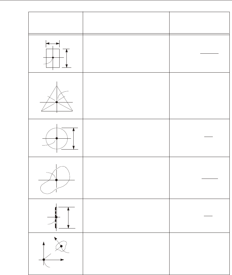
Masses 41
Chapter IV Joints and Degrees of Freedom
Mass Moment of Inertia about vertical axis
(normal to paper) through center of mass
Line mass:
Uniformly distributed mass per unit length
Total mass of line = M (or w/g)
Formula
d
b
c.m.
c.m.
d
c.m.
Y
X
X
Y
Triangular diaphragm:
Uniformly distributed mass per unit area
Total mass of diaphragm = M (or w/g)
General diaphragm:
Total mass of diaphragm = M (or w/g)
Area of diaphragm = A
Moment of inertia of area about X-X = IX
Circular diaphragm:
Uniformly distributed mass per unit area
Total mass of diaphragm = M (or w/g)
Rectangular diaphragm:
Uniformly distributed mass per unit area
Total mass of diaphragm = M (or w/g)
Moment of inertia of area about Y-Y = IY
Shape in
plan
Use general
diaphragm formula
c.m.
X
X
Y
Y
If mass is a point mass, MMI = 0
o
Axis transformation for a mass:
Uniformly distributed mass per unit area
MMI =
cm
MMI =
cm
8
12
2
Md
2
Md
2
MMI = MMI + MD
cm o
d
c.m.
o
D
c.m.
MMIcm =M22
b+d
()
12
MMIcm =M()
A
I+I
XY
Figure 7
Formulae for Mass Moments of Inertia

These cou pling terms will be dis carded by the pro gram, re sult ing in some loss of
ac cu racy. For this rea son, it is rec om mended that you choose joint lo cal co or di nate
sys tems that are aligned with the prin ci pal di rec tions of trans la tional or ro ta tional
mass at a joint, and then spec ify mass val ues in these joint lo cal co or di nates.
Mass val ues must be given in con sis tent mass units (W/g) and mass mo ments of in -
er tia must be in WL2/g units. Here W is weight, L is length, and g is the ac cel era tion
due to grav ity. The net mass val ues at each joint in the struc ture should be zero or
posi tive.
See Figure 7 (page 41) for mass mo ment of in er tia for mu la tions for vari ous pla nar
con figu ra tions.
For more in for ma tion:
•See Topic “De grees of Free dom” (page 30) in this Chap ter.
•See Topic “Mass Source” (page 334) in Chap ter “Load Pat terns”.
•See Chap ter “Static and Dy namic Analy sis” (page 341).
Force Load
The Force Load is used to ap ply con cen trated forces and mo ments at the joints.
Val ues may be speci fied in a fixed co or di nate sys tem (global or al ter nate co or di -
nates) or the joint lo cal co or di nate sys tem. All forces and mo ments at a joint are
trans formed to the joint lo cal co or di nate sys tem and added to gether. The speci fied
val ues are shown in Figure 8 (page 43).
Forces and mo ments ap plied along re strained de grees of free dom add to the cor re -
spond ing re ac tion, but do not oth er wise af fect the struc ture.
For more in for ma tion:
•See Topic “De grees of Free dom” (page 30) in this Chap ter.
•See Chap ter “Load Pat terns” (page 321).
Ground Displacement Load
The Ground Dis place ment Load is used to ap ply spec i fied dis place ments (trans la -
tions and ro ta tions) at the grounded end of joint re straints, joint spring, and
one-joint Link/Sup port objects. Dis place ments may be spec i fied in a fixed co or di -
nate sys tem (global or al ter nate co or di nates) or the joint lo cal co or di nate sys tem.
42 Force Load
CSI Analysis Reference Manual
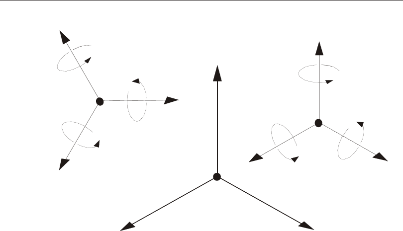
The spec i fied val ues are shown in Figure 8 (page 43). All dis place ments at a joint
are trans formed to the joint lo cal co or di nate sys tem and added to gether.
Re straints may be con sid ered as rigid con nec tions be tween the joint de grees of
free dom and the ground. Springs and one-joint Link/Sup port ob jects may be con -
sid ered as flex i ble con nec tions be tween the joint de grees of free dom and the
ground.
It is very im por tant to un der stand that ground dis place ment load ap plies to the
ground, and does not af fect the struc ture un less the struc ture is sup ported by re -
straints, springs, or one-joint Link/Supports in the di rec tion of load ing!
Restraint Displacements
If a par tic u lar joint de gree of free dom is re strained, the dis place ment of the joint is
equal to the ground dis place ment along that lo cal de gree of free dom. This ap plies
re gard less of whether or not springs are pres ent.
Ground Displacement Load 43
Chapter IV Joints and Degrees of Freedom
Global Coordinates
Joint
uy
uz
ux
ry
rz
rx
Joint Local Coordinates
Joint
u1
u2
u3
r1
r2
r3
Global
Origin
Y
Z
X
Figure 8
Specified Values for Force Load and Ground Displacement Load
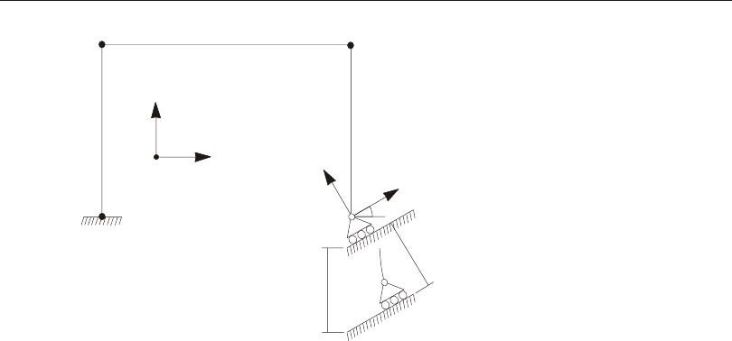
Com po nents of ground dis place ment that are not along re strained de grees of free -
dom do not load the struc ture (ex cept pos si bly through springs and one-joint links).
An ex am ple of this is il lus trated in Figure 9 (page 44).
The ground dis place ment, and hence the joint dis place ment, may vary from one
Load Pat tern to the next. If no ground dis place ment load is spec i fied for a re strained
de gree of free dom, the joint dis place ment is zero for that Load Pat tern.
Spring Displacements
The ground dis place ments at a joint are mul ti plied by the spring stiff ness co ef fi -
cients to ob tain ef fec tive forces and mo ments that are ap plied to the joint. Spring
dis place ments ap plied in a di rec tion with no spring stiff ness re sult in zero ap plied
load. The ground dis place ment, and hence the ap plied forces and mo ments, may
vary from one Load Pat tern to the next.
In a joint lo cal co or di nate sys tem, the ap plied forces and mo ments F1, F2, F3, M1, M2
and M3 at a joint due to ground dis place ments are given by:
44 Ground Displacement Load
CSI Analysis Reference Manual
Z
X
1
3
GLOBAL
30°
U3 = -0.866
UZ = -1.000
The vertical ground settlement, UZ = -1.000,
is specified as the restraint displacement.
The actual restraint displacement that is
imposed on the structure is U3 = -0.866.
The unrestrained displacement, U1, will be
determined by the analysis.
Figure 9
Example of Restraint Displacement Not Aligned with Local Degrees of Freedom

(Eqn. 2)
F
F
F
M
M
M
1
2
3
1
2
3
ì
í
ï
ï
ï
î
ï
ï
ï
ü
ý
ï
ï
ï
þ
ï
ï
ï
=-
u100000
u20000
u3000
r100
sym.r20
r3
é
ë
ê
ê
ê
ê
ê
ê
ê
ù
û
ú
ú
ú
ú
ú
ú
ú
ìu
u
u
r
r
r
g
g
g
g
g
g
1
2
3
1
2
3
í
ï
ï
ï
î
ï
ï
ï
ü
ý
ï
ï
ï
þ
ï
ï
ï
where ug1, ug2, ug3, rg1, rg2 and rg3 are the ground dis place ments and ro ta tions,
and the terms u1, u2, u3, r1, r2, and r3 are the spec i fied spring stiff ness co ef fi -
cients.
The net spring forces and mo ments act ing on the joint are the sum of the forces and
mo ments given in Equa tions (1) and (2); note that these are of op po site sign. At a
re strained de gree of free dom, the joint dis place ment is equal to the ground dis -
place ment, and hence the net spring force is zero.
For more in for ma tion:
•See Topic “Re straints and Re ac tions” (page 34) in this Chap ter.
•See Topic “Springs” (page 36) in this Chap ter.
•See Chap ter “Load Pat terns” (page 321).
Link/Support Displacements
One-joint Link/Sup port ob jects are con verted to zero-length, two-joint Link/Sup -
port el e ments. A re strained joint is gen er ated and the ground dis place ment is ap -
plied as a re straint dis place ment at this gen er ated joint.
The ef fect of the ground dis place ment on the struc ture de pends upon the prop er ties
of the Link/Sup port el e ment con nect ing the re strained joint to the struc ture, sim i lar
to how springs sup ports work, ex cept the Link/Sup port stiff ness may be non lin ear.
Generalized Displacements
A gen er al ized dis place ment is a named dis place ment mea sure that you de fine. It is
sim ply a lin ear com bi na tion of dis place ment de grees of free dom from one or more
joints.
For ex am ple, you could de fine a gen er al ized dis place ment that is the dif fer ence of
the UX dis place ments at two joints on dif fer ent sto ries of a build ing and name it
Generalized Displacements 45
Chapter IV Joints and Degrees of Freedom

“DRIFTX”. You could de fine an other gen er al ized dis place ment that is the sum of
three ro ta tions about the Z axis, each scaled by 1/3, and name it “AVGRZ.”
Gen er al ized dis place ments are pri mar ily used for out put pur poses, ex cept that you
can also use a gen er al ized dis place ment to mon i tor a non lin ear static anal y sis.
To de fine a gen er al ized dis place ment, spec ify the fol low ing:
•A unique name
•The type of dis place ment mea sure
•A list of the joint de grees of free dom and their cor re spond ing scale fac tors that
will be summed to cre ated the gen er al ized displacement
The type of dis place ment mea sure can be one of the fol low ing:
•Translational: The gen er al ized dis place ment scales (with change of units) as
length. Co ef fi cients of con trib ut ing joint trans la tions are unitless. Co ef fi cients
of con trib ut ing joint ro ta tions scale as length.
•Ro ta tional: The gen er al ized dis place ment is unitless (ra di ans). Co ef fi cients of
joint trans la tions scale as in verse length. Co ef fi cients of joint ro ta tions are
unitless.
Be sure to choose your scale fac tors for each con trib ut ing com po nent to ac count for
the type of gen er al ized dis place ment be ing de fined.
Degree of Freedom Output
A ta ble of the types of de grees of free dom pres ent at every joint in the model is
printed in the anal y sis out put (.OUT) file un der the head ing:
DISPLACEMENT DEGREES OF FREEDOM
The de grees of free dom are listed for all of the regu lar joints, as well as for the mas -
ter joints cre ated auto mati cally by the pro gram. For Con straints, the mas ter joints
are iden ti fied by the la bels of their cor re spond ing Con straints. For Welds, the mas -
ter joint for each set of joints that are welded to gether is iden ti fied by the la bel of
one of the welded joints. Joints are printed in alpha- numeric or der of the la bels.
The type of each of the six de grees of free dom at a joint is iden ti fied by the fol low -
ing sym bols:
(A) Ac tive de gree of free dom
(-) Re strained de gree of free dom
46 Degree of Freedom Output
CSI Analysis Reference Manual

(+) Con strained de gree of free dom
( ) Null or un avail able de gree of free dom
The de grees of free dom are al ways re ferred to the lo cal axes of the joint. They are
iden ti fied in the out put as U1, U2, U3, R1, R2, and R3 for all joints. How ever, if all
regu lar joints use the global co or di nate sys tem as the lo cal sys tem (the usual situa -
tion), then the de grees of free dom for the regu lar joints are iden ti fied as UX, UY,
UZ, RX, RY, and RZ.
The types of de grees of free dom are a prop erty of the struc ture and are in de pend ent
of the Load Cases, ex cept when staged con struc tion is per formed.
See Topic “De grees of Free dom” (page 30) in this Chap ter for more in for ma tion.
Assembled Joint Mass Output
You can re quest as sem bled joint masses as part of the anal y sis re sults. The mass at a
given joint in cludes the mass as signed di rectly to that joint as well as a por tion of
the mass from each el e ment con nected to that joint. All mass as signed to the el e -
ments is ap por tioned to the con nected joints, so that this ta ble rep re sents the to tal
mass of the struc ture. The masses are al ways re ferred to the lo cal axes of the joint.
If mul ti ple Mass Sources have been spec i fied, the as sem bled joint mass out put is
pro vided for each Mass Source that was ac tu ally used in the anal y sis.
For more in for ma tion:
•See Topic “Masses” (page 40) in this Chap ter.
•See Topic “Mass Source” (page 334) in Chap ter “Load Pat terns”.
•See Chap ter “Load Cases” (page 341).
Displacement Output
You can re quest joint dis place ments as part of the anal y sis re sults on a case by case
ba sis. For dy namic Load Cases, you can also re quest ve loc i ties and ac cel er a tions.
The out put is al ways re ferred to the lo cal axes of the joint.
•See Topic “De grees of Free dom” (page 30) in this Chap ter.
•See Chap ter “Load Cases” (page 341).
Assembled Joint Mass Output 47
Chapter IV Joints and Degrees of Freedom

Force Output
You can re quest joint sup port forces as part of the anal y sis re sults on a case by case
ba sis. These sup port forces are called re ac tions, and are the sum of all forces from
re straints, springs, or one-joint Link/Sup port ob jects at that joint. The re ac tions at
joints that are not sup ported will be zero.
Note that re ac tions for one-joint Link/Sup port ob jects are not re ported at the orig i -
nal joint, but rather at a gen er ated joint at the same lo ca tion with an iden ti fy ing
label.
The forces and mo ments are al ways re ferred to the lo cal axes of the joint. The val -
ues re ported are al ways the forces and mo ments that act on the joints. Thus a posi -
tive value of joint force or mo ment would tend to cause a posi tive value of joint
trans la tion or ro ta tion along the cor re spond ing de gree of free dom if it were not sup -
ported.
For more in for ma tion:
•See Topic “De grees of Free dom” (page 30) in this Chap ter.
•See Chap ter “Load Cases” (page 341).
Element Joint Force Output
The el e ment joint forces are con cen trated forces and mo ments act ing at the joints
of the el e ment that rep re sent the ef fect of the rest of the struc ture upon the el e ment
and that cause the de for ma tion of the el e ment. The mo ments will al ways be zero for
the solid-type el e ments: Plane, Asolid, and Solid.
A pos i tive value of force or mo ment tends to cause a pos i tive value of trans la tion or
ro ta tion of the el e ment along the cor re spond ing joint de gree of free dom.
El e ment joint forces must not be con fused with in ter nal forces and mo ments which,
like stresses, act within the vol ume of the el e ment.
For a given el e ment, the vec tor of el e ment joint forces, f, is com puted as:
fKur=-
where K is the el e ment stiff ness ma trix, u is the vec tor of el e ment joint dis place -
ments, and r is the vec tor of el e ment ap plied loads as ap por tioned to the joints. The
el e ment joint forces are al ways re ferred to the lo cal axes of the in di vid ual joints.
They are iden ti fied in the out put as F1, F2, F3, M1, M2, and M3.
48 Force Output
CSI Analysis Reference Manual

Chapter V
Constraints and Welds
Con straints are used to en force cer tain types of rigid-body be hav ior, to con nect to -
gether dif fer ent parts of the model, and to im pose cer tain types of sym me try con di -
tions. Welds are used to gen er ate a set of con straints that con nect to gether dif fer ent
parts of the model.
Basic Topics for All Users
•Over view
•Body Con straint
•Plane Def i ni tion
•Di a phragm Con straint
•Plate Con straint
•Axis Def i ni tion
•Rod Con straint
•Beam Con straint
•Equal Con straint
•Welds
49

Advanced Topics
•Lo cal Con straint
•Au to matic Mas ter Joints
•Con straint Out put
Overview
A con straint con sists of a set of two or more con strained joints. The dis place ments
of each pair of joints in the con straint are re lated by con straint equa tions. The types
of be hav ior that can be en forced by con straints are:
•Rigid-body be hav ior, in which the con strained joints trans late and ro tate to -
gether as if con nected by rigid links. The types of rigid be hav ior that can be
mod eled are:
–Rigid Body: fully rigid for all dis place ments
–Rigid Di a phragm: rigid for mem brane be hav ior in a plane
–Rigid Plate: rigid for plate bend ing in a plane
–Rigid Rod: rigid for ex ten sion along an axis
–Rigid Beam: rigid for beam bend ing on an axis
•Equal-dis place ment be hav ior, in which the trans la tions and ro ta tions are equal
at the con strained joints
•Sym me try and anti-sym me try con di tions
The use of con straints re duces the num ber of equa tions in the sys tem to be solved
and will usu ally re sult in in creased com pu ta tional ef fi ciency.
Most con straint types must be de fined with re spect to some fixed co or di nate sys -
tem. The co or di nate sys tem may be the global co or di nate sys tem or an al ter nate co -
or di nate sys tem, or it may be au to mat i cally de ter mined from the lo ca tions of the
con strained joints. The Lo cal Con straint does not use a fixed co or di nate sys tem, but
ref er ences each joint us ing its own joint local coordinate system.
Welds are used to con nect to gether dif fer ent parts of the model that were de fined
sep a rately. Each Weld con sists of a set of joints that may be joined. The pro gram
searches for joints in each Weld that share the same lo ca tion in space and con strains
them to act as a sin gle joint.
50 Overview
CSI Analysis Reference Manual

Body Constraint
A Body Con straint causes all of its con strained joints to move to gether as a
three-di men sional rigid body. By de fault, all de grees of free dom at each con nected
joint par tic i pate. How ever, you can se lect a sub set of the de grees of free dom to be
constrained.
This Con straint can be used to:
•Model rigid con nec tions, such as where sev eral beams and/or col umns frame
to gether
•Con nect to gether dif fer ent parts of the struc tural model that were de fined us ing
sep a rate meshes
•Con nect Frame el e ments that are act ing as ec cen tric stiff en ers to Shell el e ments
Welds can be used to au to mat i cally gen er ate Body Con straints for the pur pose of
con nect ing co in ci dent joints.
See Topic “Welds” (page 64) in this Chap ter for more in for ma tion.
Joint Connectivity
Each Body Con straint con nects a set of two or more joints to gether. The joints may
have any ar bi trary lo ca tion in space.
Local Coordinate System
Each Body Con straint has its own lo cal co or di nate sys tem, the axes of which are
de noted 1, 2, and 3. These cor re spond to the X, Y, and Z axes of a fixed co or di nate
sys tem that you choose.
Constraint Equations
The con straint equa tions re late the dis place ments at any two con strained joints
(sub scripts I and j) in a Body Con straint. These equa tions are ex pressed in terms of
the trans la tions (u1, u2, and u3), the ro ta tions (r1, r2, and r3), and the co or di nates (x1,
x2, and x3), all taken in the Con straint lo cal co or di nate system:
u1j = u1i + r2i Dx3 – r3i Dx2
u2j = u2i + r3i Dx1 - r1i Dx3
Body Constraint 51
Chapter V Constraints and Welds

u3j = u3i + r1i Dx2 - r2i Dx1
r1i = r1j
r2i = r2j
r3i = r3j
where Dx1 = x1j - x1i, Dx2 = x2j - x2i, and Dx3 = x3j - x3i.
If you omit any par tic u lar de gree of free dom, the cor re spond ing con straint equa tion
is not en forced. If you omit a ro ta tional de gree of free dom, the cor re spond ing terms
are re moved from the equa tions for the translational de grees of freedom.
Plane Definition
The con straint equa tions for each Di a phragm or Plate Con straint are writ ten with
re spect to a par tic u lar plane. The lo ca tion of the plane is not im por tant, only its
orientation.
By de fault, the plane is de ter mined au to mat i cally by the pro gram from the spa tial
dis tri bu tion of the con strained joints as follows:
•The cen troid of the con strained joints is de ter mined
•The sec ond mo ments of the lo ca tions of all of the con strained joints about the
cen troid are de ter mined
•The prin ci pal val ues and di rec tions of these sec ond mo ments are found
•The di rec tion of the small est prin ci pal sec ond mo ment is taken as the nor mal to
the con straint plane; if all con strained joints lie in a unique plane, this small est
prin ci pal mo ment will be zero
•If no unique di rec tion can be found, a hor i zon tal (X-Y) plane is as sumed in co -
or di nate sys tem csys; this sit u a tion can oc cur if the joints are co in ci dent or col -
lin ear, or if the spa tial dis tri bu tion is more nearly three-di men sional than
planar.
You may over ride au to matic plane se lec tion by spec i fy ing the fol low ing:
•csys: A fixed co or di nate sys tem (the de fault is zero, in di cat ing the global co or -
di nate system)
•axis: The axis (X, Y, or Z) nor mal to the plane of the con straint, taken in co or -
di nate sys tem csys.
52 Plane Definition
CSI Analysis Reference Manual

This may be use ful, for ex am ple, to spec ify a hor i zon tal plane for a floor with a
small step in it.
Diaphragm Constraint
A Di a phragm Con straint causes all of its con strained joints to move to gether as a
pla nar di a phragm that is rigid against mem brane de for ma tion. Ef fec tively, all con -
strained joints are con nected to each other by links that are rigid in the plane, but do
not af fect out-of-plane (plate) deformation.
This Con straint can be used to:
•Model con crete floors (or con crete-filled decks) in build ing struc tures, which
typ i cally have very high in-plane stiff ness
•Model di a phragms in bridge su per struc tures
The use of the Di a phragm Con straint for build ing struc tures elim i nates the nu mer i -
cal-ac cu racy prob lems cre ated when the large in-plane stiff ness of a floor di a -
phragm is mod eled with mem brane el e ments. It is also very use ful in the lat eral
(hor i zon tal) dy namic anal y sis of build ings, as it re sults in a sig nif i cant re duc tion in
the size of the eigenvalue prob lem to be solved. See Figure 10 (page 54) for an
illustration of a floor diaphragm.
Joint Connectivity
Each Di a phragm Con straint con nects a set of two or more joints to gether. The
joints may have any ar bi trary lo ca tion in space, but for best re sults all joints should
lie in the plane of the con straint. Oth er wise, bend ing mo ments may be gen er ated
that are re strained by the Con straint, which un re al is ti cally stiff ens the struc ture. If
this hap pens, the con straint forces re ported in the anal y sis re sults may not be in
equilibrium.
Local Coordinate System
Each Di a phragm Con straint has its own lo cal co or di nate sys tem, the axes of which
are de noted 1, 2, and 3. Lo cal axis 3 is al ways nor mal to the plane of the con straint.
The pro gram ar bi trarily chooses the ori en ta tion of axes 1 and 2 in the plane. The
ac tual ori en ta tion of the pla nar axes is not im por tant since only the nor mal di rec tion
af fects the con straint equa tions. For more in for ma tion, see Topic “Plane Def i ni -
tion” (page 52) in this Chapter.
Diaphragm Constraint 53
Chapter V Constraints and Welds
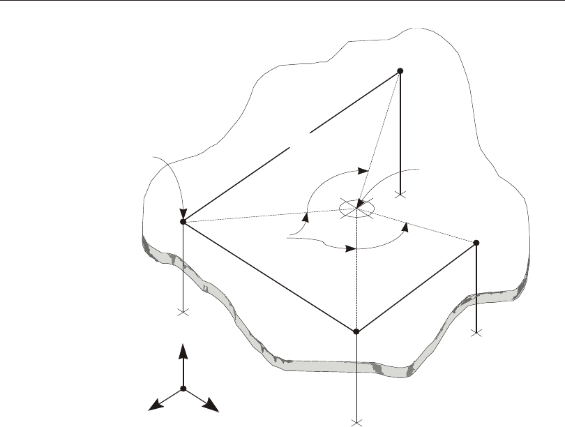
Constraint Equations
The con straint equa tions re late the dis place ments at any two con strained joints
(sub scripts I and j) in a Di a phragm Con straint. These equa tions are ex pressed in
terms of in-plane trans la tions (u1 and u2), the ro ta tion (r3) about the nor mal, and the
in-plane co or di nates (x1 and x2), all taken in the Con straint lo cal coordinate system:
u1j = u1i – r3i Dx2
u2j = u2i + r3i Dx1
r3i = r3j
where Dx1 = x1j - x1i and Dx2 = x2j - x2i.
54 Diaphragm Constraint
CSI Analysis Reference Manual
Z
XY
Constrained
Joint
Constrained
Joint
Constrained
Joint
Constrained
Joint
Global
Column
Beam
Automatic
Master Joint
Rigid Floor Slab
Effective
Rigid Links
Figure 10
Use of the Diaphragm Constraint to Model a Rigid Floor Slab

Plate Constraint
A Plate Con straint causes all of its con strained joints to move to gether as a flat plate
that is rigid against bend ing de for ma tion. Ef fec tively, all con strained joints are
con nected to each other by links that are rigid for out-of-plane bend ing, but do not
af fect in-plane (mem brane) de for ma tion.
This Con straint can be used to:
•Con nect struc tural-type el e ments (Frame and Shell) to solid-type el e ments
(Plane and Solid); the ro ta tion in the struc tural el e ment can be con verted to a
pair of equal and op po site trans la tions in the solid el e ment by the Constraint
•En force the as sump tion that “plane sec tions re main plane” in de tailed mod els
of beam bend ing
Joint Connectivity
Each Plate Con straint con nects a set of two or more joints to gether. The joints may
have any ar bi trary lo ca tion in space. Un like the Di a phragm Con straint, equi lib rium
is not af fected by whether or not all joints lie in the plane of the Plate Constraint.
Local Coordinate System
Each Plate Con straint has its own lo cal co or di nate sys tem, the axes of which are de -
noted 1, 2, and 3. Lo cal axis 3 is al ways nor mal to the plane of the con straint. The
pro gram ar bi trarily chooses the ori en ta tion of axes 1 and 2 in the plane. The ac tual
ori en ta tion of the pla nar axes is not im por tant since only the nor mal di rec tion af -
fects the constraint equations.
For more in for ma tion, see Topic “Plane Def i ni tion” (page 52) in this Chap ter.
Constraint Equations
The con straint equa tions re late the dis place ments at any two con strained joints
(sub scripts I and j) in a Plate Con straint. These equa tions are ex pressed in terms of
the out-of-plane trans la tion (u3), the bend ing ro ta tions (r1 and r2), and the in-plane
co or di nates (x1 and x2), all taken in the Con straint lo cal coordinate system:
u3j = u3i + r1i Dx2 - r2i Dx1
r1i = r1j
Plate Constraint 55
Chapter V Constraints and Welds

r2i = r2j
where Dx1 = x1j - x1i and Dx2 = x2j - x2i.
Axis Definition
The con straint equa tions for each Rod or Beam Con straint are writ ten with re spect
to a par tic u lar axis. The lo ca tion of the axis is not im por tant, only its ori en ta tion.
By de fault, the axis is de ter mined au to mat i cally by the pro gram from the spa tial
dis tri bu tion of the con strained joints as follows:
•The cen troid of the con strained joints is de ter mined
•The sec ond mo ments of the lo ca tions of all of the con strained joints about the
cen troid are de ter mined
•The prin ci pal val ues and di rec tions of these sec ond mo ments are found
•The di rec tion of the larg est prin ci pal sec ond mo ment is taken as the axis of the
con straint; if all con strained joints lie on a unique axis, the two small est prin ci -
pal mo ments will be zero
•If no unique di rec tion can be found, a ver ti cal (Z) axis is as sumed in co or di nate
sys tem csys; this sit u a tion can oc cur if the joints are co in ci dent, or if the spa tial
dis tri bu tion is more nearly pla nar or three-di men sional than linear.
You may over ride au to matic axis se lec tion by spec i fy ing the fol low ing:
•csys: A fixed co or di nate sys tem (the de fault is zero, in di cat ing the global co or -
di nate system)
•axis: The axis (X, Y, or Z) of the con straint, taken in co or di nate sys tem csys.
This may be use ful, for ex am ple, to spec ify a ver ti cal axis for a col umn with a small
off set in it.
Rod Constraint
A Rod Con straint causes all of its con strained joints to move to gether as a straight
rod that is rigid against ax ial de for ma tion. Ef fec tively, all con strained joints main -
tain a fixed dis tance from each other in the di rec tion par al lel to the axis of the rod,
but trans la tions nor mal to the axis and all ro ta tions are unaffected.
This Con straint can be used to:
56 Axis Definition
CSI Analysis Reference Manual

•Pre vent ax ial de for ma tion in Frame el e ments
•Model rigid truss-like links
An ex am ple of the use of the Rod Con straint is in the anal y sis of the two-di men -
sional frame shown in Figure 11 (page 58). If the ax ial de for ma tions in the beams
are neg li gi ble, a sin gle Rod Con straint could be de fined con tain ing the five joints.
In stead of five equa tions, the pro gram would use a sin gle equa tion to de fine the
X-dis place ment of the whole floor. How ever, it should be noted that this will re sult
in the ax ial forces of the beams be ing out put as zero, as the Con straint will cause the
ends of the beams to trans late to gether in the X-di rec tion. In ter pre ta tions of such re -
sults as so ci ated with the use of Constraints should be clearly understood.
Joint Connectivity
Each Rod Con straint con nects a set of two or more joints to gether. The joints may
have any ar bi trary lo ca tion in space, but for best re sults all joints should lie on the
axis of the con straint. Oth er wise, bend ing mo ments may be gen er ated that are re -
strained by the Con straint, which un re al is ti cally stiff ens the struc ture. If this hap -
pens, the con straint forces re ported in the anal y sis re sults may not be in
equilibrium.
Local Coordinate System
Each Rod Con straint has its own lo cal co or di nate sys tem, the axes of which are de -
noted 1, 2, and 3. Lo cal axis 1 is al ways the axis of the con straint. The pro gram ar bi -
trarily chooses the ori en ta tion of the trans verse axes 2 and 3. The ac tual ori en ta tion
of the trans verse axes is not im por tant since only the ax ial di rec tion af fects the
constraint equations.
For more in for ma tion, see Topic “Axis Def i ni tion” (page 56) in this Chap ter.
Constraint Equations
The con straint equa tions re late the dis place ments at any two con strained joints
(sub scripts I and j) in a Rod Con straint. These equa tions are ex pressed only in terms
of the ax ial trans la tion (u1):
u1j = u1i
Rod Constraint 57
Chapter V Constraints and Welds
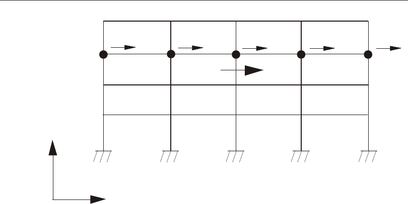
Beam Constraint
A Beam Con straint causes all of its con strained joints to move to gether as a straight
beam that is rigid against bend ing de for ma tion. Ef fec tively, all con strained joints
are con nected to each other by links that are rigid for off-axis bend ing, but do not
af fect trans la tion along or ro ta tion about the axis.
This Con straint can be used to:
•Con nect struc tural-type el e ments (Frame and Shell) to solid-type el e ments
(Plane and Solid); the ro ta tion in the struc tural el e ment can be con verted to a
pair of equal and op po site trans la tions in the solid el e ment by the Constraint
•Pre vent bend ing de for ma tion in Frame el e ments
Joint Connectivity
Each Beam Con straint con nects a set of two or more joints to gether. The joints may
have any ar bi trary lo ca tion in space, but for best re sults all joints should lie on the
axis of the con straint. Oth er wise, tor sional mo ments may be gen er ated that are re -
strained by the Con straint, which un re al is ti cally stiff ens the struc ture. If this hap -
58 Beam Constraint
CSI Analysis Reference Manual
Z
X
X1X2X3X4X5
X
Figure 11
Use of the Rod Constraint to Model Axially Rigid Beams

pens, the con straint forces re ported in the anal y sis re sults may not be in
equilibrium.
Local Coordinate System
Each Beam Con straint has its own lo cal co or di nate sys tem, the axes of which are
de noted 1, 2, and 3. Lo cal axis 1 is al ways the axis of the con straint. The pro gram
ar bi trarily chooses the ori en ta tion of the trans verse axes 2 and 3. The ac tual ori en ta -
tion of the trans verse axes is not im por tant since only the ax ial di rec tion af fects the
constraint equations.
For more in for ma tion, see Topic “Axis Def i ni tion” (page 56) in this Chap ter.
Constraint Equations
The con straint equa tions re late the dis place ments at any two con strained joints
(sub scripts I and j) in a Beam Con straint. These equa tions are ex pressed in terms of
the trans verse trans la tions (u2 and u3), the trans verse ro ta tions (r2 and r3), and the ax -
ial co or di nate (x1), all taken in the Con straint lo cal coordinate system:
u2j = u2i + r3i Dx1
u3j = u3i - r2i Dx1
r2i = r2j
r3i = r3j
where Dx1 = x1j - x1i.
Equal Constraint
An Equal Con straint causes all of its con strained joints to move to gether with the
same dis place ments for each se lected de gree of free dom, taken in the con straint lo -
cal co or di nate sys tem. The other de grees of free dom are unaffected.
The Equal Con straint dif fers from the rigid-body types of Con straints in that there
is no cou pling be tween the ro ta tions and the trans la tions.
This Con straint can be used to par tially con nect to gether dif fer ent parts of the struc -
tural model, such as at ex pan sion joints and hinges
Equal Constraint 59
Chapter V Constraints and Welds

For fully con nect ing meshes, it is better to use the Body Con straint when the con -
strained joints are not in ex actly the same lo ca tion.
Joint Connectivity
Each Equal Con straint con nects a set of two or more joints to gether. The joints may
have any ar bi trary lo ca tion in space, but for best re sults all joints should share the
same lo ca tion in space if used for con nect ing meshes. Oth er wise, mo ments may be
gen er ated that are re strained by the Con straint, which un re al is ti cally stiff ens the
struc ture. If this hap pens, the con straint forces re ported in the anal y sis re sults may
not be in equilibrium.
Local Coordinate System
Each Equal Con straint uses a fixed co or di nate sys tem, csys, that you spec ify. The
de fault for csys is zero, in di cat ing the global co or di nate sys tem. The axes of the
fixed co or di nate sys tem are de noted X, Y, and Z.
Selected Degrees of Freedom
For each Equal Con straint you may spec ify a list, cdofs, of up to six de grees of free -
dom in co or di nate sys tem csys that are to be con strained. The de grees of free dom
are in di cated as UX, UY, UZ, RX, RY, and RZ.
Constraint Equations
The con straint equa tions re late the dis place ments at any two con strained joints
(sub scripts I and j) in an Equal Con straint. These equa tions are ex pressed in terms
of the trans la tions (ux, uy, and uz) and the ro ta tions (rx, ry, and rz), all taken in fixed
co or di nate sys tem csys:
uxj = uxi
uyj = uyi
uzj = uzi
r1i = r1j
r2i = r2j
r3i = r3j
60 Equal Constraint
CSI Analysis Reference Manual

If you omit any of the six de grees of free dom from the con straint def i ni tion, the cor -
re spond ing con straint equa tion is not enforced.
Local Constraint
A Lo cal Con straint causes all of its con strained joints to move to gether with the
same dis place ments for each se lected de gree of free dom, taken in the sep a rate joint
lo cal co or di nate sys tems. The other de grees of free dom are unaffected.
The Lo cal Con straint dif fers from the rigid-body types of Con straints in that there
is no cou pling be tween the ro ta tions and the trans la tions. The Lo cal Con straint is
the same as the Equal Con straint if all con strained joints have the same lo cal co or -
di nate system.
This Con straint can be used to:
•Model sym me try con di tions with re spect to a line or a point
•Model dis place ments con strained by mech a nisms
The be hav ior of this Con straint is de pend ent upon the choice of the lo cal co or di nate
sys tems of the con strained joints.
Joint Connectivity
Each Lo cal Con straint con nects a set of two or more joints to gether. The joints may
have any ar bi trary lo ca tion in space. If the joints do not share the same lo ca tion in
space, mo ments may be gen er ated that are re strained by the Con straint. If this hap -
pens, the con straint forces re ported in the anal y sis re sults may not be in equi lib -
rium. These mo ments are nec es sary to en force the de sired sym me try of the dis -
place ments when the ap plied loads are not sym met ric, or may rep re sent the
constraining action of a mechanism.
For more in for ma tion, see:
•Topic “Force Out put” (page 48) in Chap ter “Joints and De grees of Free dom.”
•Topic “Global Force Bal ance Out put” (page 45) in Chap ter “Joints and De -
grees of Free dom.”
Local Constraint 61
Chapter V Constraints and Welds

No Local Coordinate System
A Lo cal Con straint does not have its own lo cal co or di nate sys tem. The con straint
equa tions are writ ten in terms of con strained joint lo cal co or di nate sys tems, which
may dif fer. The axes of these co or di nate sys tems are de noted 1, 2, and 3.
Selected Degrees of Freedom
For each Lo cal Con straint you may spec ify a list, ldofs, of up to six de grees of free -
dom in the joint lo cal co or di nate sys tems that are to be con strained. The de grees of
free dom are in di cated as U1, U2, U3, R1, R2, and R3.
Constraint Equations
The con straint equa tions re late the dis place ments at any two con strained joints
(sub scripts I and j) in a Lo cal Con straint. These equa tions are ex pressed in terms of
the trans la tions (u1, u2, and u3) and the ro ta tions (r1, r2, and r3), all taken in joint lo cal
co or di nate sys tems. The equa tions used de pend upon the se lected de grees of free -
dom and their signs. Some im por tant cases are described next.
Axisymmetry
Axisymmetry is a type of sym me try about a line. It is best de scribed in terms of a
cy lin dri cal co or di nate sys tem hav ing its Z axis on the line of sym me try. The struc -
ture, load ing, and dis place ments are each said to be axisymmetric about a line if
they do not vary with an gu lar po si tion around the line, i.e., they are in de pend ent of
the angular coordinate CA.
To en force axisymmetry us ing the Lo cal Con straint:
•Model any cy lin dri cal sec tor of the struc ture us ing any axisymmetric mesh of
joints and el e ments
•As sign each joint a lo cal co or di nate sys tem such that lo cal axes 1, 2, and 3 cor -
re spond to the co or di nate di rec tions +CR, +CA, and +CZ, re spec tively
•For each axisymmetric set of joints (i.e., hav ing the same co or di nates CR and
CZ, but dif fer ent CA), de fine a Lo cal Con straint us ing all six de grees of free -
dom: U1, U2, U3, R1, R2, and R3
•Re strain joints that lie on the line of sym me try so that, at most, only ax ial trans -
la tions (U3) and ro ta tions (R3) are per mit ted
The cor re spond ing con straint equa tions are:
62 Local Constraint
CSI Analysis Reference Manual

u1j = u1i
u2j = u2i
u3j = u3i
r1i = r1j
r2i = r2j
r3i = r3j
The nu meric sub scripts re fer to the cor re spond ing joint lo cal co or di nate systems.
Cyclic symmetry
Cy clic sym me try is an other type of sym me try about a line. It is best de scribed in
terms of a cy lin dri cal co or di nate sys tem hav ing its Z axis on the line of sym me try.
The struc ture, load ing, and dis place ments are each said to be cy cli cally sym met ric
about a line if they vary with an gu lar po si tion in a re peated (periodic) fashion.
To en force cy clic sym me try us ing the Lo cal Con straint:
•Model any num ber of ad ja cent, rep re sen ta tive, cy lin dri cal sec tors of the struc -
ture; de note the size of a sin gle sec tor by the an gle q
•As sign each joint a lo cal co or di nate sys tem such that lo cal axes 1, 2, and 3 cor -
re spond to the co or di nate di rec tions +CR, +CA, and +CZ, re spec tively
•For each cy cli cally sym met ric set of joints (i.e., hav ing the same co or di nates
CR and CZ, but with co or di nate CA dif fer ing by mul ti ples of q), de fine a Lo cal
Con straint us ing all six de grees of free dom: U1, U2, U3, R1, R2, and R3.
•Re strain joints that lie on the line of sym me try so that, at most, only ax ial trans -
la tions (U3) and ro ta tions (R3) are per mit ted
The cor re spond ing con straint equa tions are:
u1j = u1i
u2j = u2i
u3j = u3i
r1i = r1j
r2i = r2j
r3i = r3j
Local Constraint 63
Chapter V Constraints and Welds

The nu meric sub scripts re fer to the cor re spond ing joint lo cal co or di nate systems.
For ex am ple, sup pose a struc ture is com posed of six iden ti cal 60° sec tors, iden ti -
cally loaded. If two ad ja cent sec tors were mod eled, each Lo cal Con straint would
ap ply to a set of two joints, ex cept that three joints would be con strained on the
sym me try planes at 0°, 60°, and 120°.
If a sin gle sec tor is mod eled, only joints on the sym me try planes need to be con -
strained.
Symmetry About a Point
Sym me try about a point is best de scribed in terms of a spher i cal co or di nate sys tem
hav ing its Z axis on the line of sym me try. The struc ture, load ing, and dis place ments
are each said to be sym met ric about a point if they do not vary with an gu lar po si tion
about the point, i.e., they are in de pend ent of the an gu lar co or di nates SB and SA.
Ra dial trans la tion is the only dis place ment component that is permissible.
To en force sym me try about a point us ing the Lo cal Con straint:
•Model any spher i cal sec tor of the struc ture us ing any sym met ric mesh of joints
and el e ments
•As sign each joint a lo cal co or di nate sys tem such that lo cal axes 1, 2, and 3 cor -
re spond to the co or di nate di rec tions +SB, +SA, and +SR, re spec tively
•For each sym met ric set of joints (i.e., hav ing the same co or di nate SR, but dif -
fer ent co or di nates SB and SA), de fine a Lo cal Con straint us ing only de gree of
freedom U3
•For all joints, re strain the de grees of free dom U1, U2, R1, R2, and R3
•Fully re strain any joints that lie at the point of sym me try
The cor re spond ing con straint equa tions are:
u3j = u3i
The nu meric sub scripts re fer to the cor re spond ing joint lo cal co or di nate systems.
It is also pos si ble to de fine a case for sym me try about a point that is sim i lar to cy clic
sym me try around a line, e.g., where each octant of the struc ture is iden ti cal.
64 Local Constraint
CSI Analysis Reference Manual
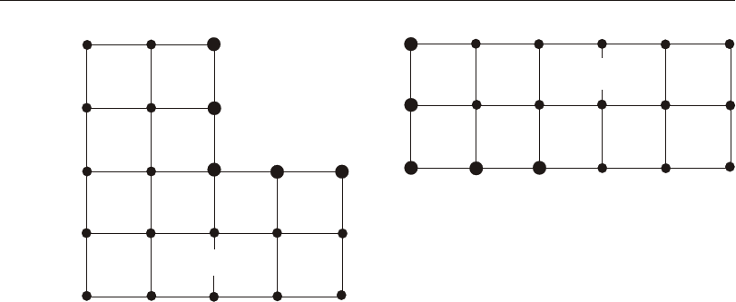
Welds
A Weld can be used to con nect to gether dif fer ent parts of the struc tural model that
were de fined us ing sep a rate meshes. A Weld is not a sin gle Con straint, but rather is
a set of joints from which the pro gram will au to mat i cally gen er ate mul ti ple Body
Con straints to con nect to gether coincident joints.
Joints are con sid ered to be co in ci dent if the dis tance be tween them is less than or
equal to a tol er ance, tol, that you spec ify. Set ting the tol er ance to zero is per mis si -
ble but is not recommended.
One or more Welds may be de fined, each with its own tol er ance. Only the joints
within each Weld will be checked for co in ci dence with each other. In the most
com mon case, a sin gle Weld is de fined that con tains all joints in the model; all co in -
ci dent groups of joints will be welded. How ever, in sit u a tions where struc tural dis -
con ti nu ity is de sired, it may be nec es sary to pre vent the weld ing of some co in ci dent
joints. This may be fa cil i tated by the use of multiple Welds.
Figure 12 (page 65) shows a model de vel oped as two sep a rate meshes, A and B.
Joints 121 through 125 are as so ci ated with mesh A, and Joints 221 through 225 are
as so ci ated with mesh B. Joints 121 through 125 share the same lo ca tion in space as
Joints 221 through 225, re spec tively. These are the in ter fac ing joints be tween the
two meshes. To con nect these two meshes, a sin gle Weld can be de fined con tain ing
all joints, or just joints 121 through 125 and 221 through 225. The pro gram would
Welds 65
Chapter V Constraints and Welds
Mesh B
221
222
223 224
125124
123
122
121
Mesh A
225
Figure 12
Use of a Weld to Connect Separate Meshes at Coincident Joints

gen er ate five Body Con straints, each con tain ing two joints, re sult ing in an
integrated model.
It is per mis si ble to in clude the same joint in more than one Weld. This could re sult
in the joints in dif fer ent Welds be ing con strained to gether if they are co in ci dent
with the com mon joint. For ex am ple, sup pose that Weld 1 con tained joints 1,2, and
3, Weld 2 con tained joints 3, 4, and 5. If joints 1, 3, and 5 were co in ci dent, joints 1
and 3 would be con strained by Weld 1, and joints 3 and 5 would be con strained by
Weld 2. The pro gram would cre ate a sin gle Body Con straint con tain ing joints 1, 3,
and 5. One the other hand, if Weld 2 did not con tain joint 3, the pro gram would only
gen er ate a Body Con straint con tain ing joint 1 and 3 from Weld 1; joint 5 would not
be constrained.
For more in for ma tion, see Topic “Body Con straint” (page 51) in this Chap ter.
Automatic Master Joints
The pro gram au to mat i cally cre ates an in ter nal mas ter joint for each ex plicit Con -
straint, and a mas ter joint for each in ter nal Body Con straint that is gen er ated by a
Weld. Each mas ter joint gov erns the be hav ior of the cor re spond ing con strained
joints. The dis place ment at a con strained de gree of free dom is com puted as a lin ear
com bi na tion of the dis place ments of the master joint.
See Topic “De grees of Free dom” (page 30) in Chap ter “Joints and De grees of Free -
dom” for more in for ma tion.
Stiffness, Mass, and Loads
Joint lo cal co or di nate sys tems, springs, masses, and loads may all be ap plied to
con strained joints. El e ments may also be con nected to con strained joints. The joint
and el e ment stiffnesses, masses and loads from the con strained de grees of free dom
are be au to mat i cally trans ferred to the mas ter joint in a consistent fashion.
The translational stiff ness at the mas ter joint is the sum of the translational
stiffnesses at the con strained joints. The same is true for translational masses and
loads.
The ro ta tional stiff ness at a mas ter joint is the sum of the ro ta tional stiffnesses at the
con strained de grees of free dom, plus the sec ond mo ment of the translational
stiffnesses at the con strained joints for the Body, Di a phragm, Plate, and Beam Con -
straints. The same is true for ro ta tional masses and loads, ex cept that only the first
mo ment of the translational loads is used. The mo ments of the translational
66 Automatic Master Joints
CSI Analysis Reference Manual

stiffnesses, masses, and loads are taken about the cen ter of mass of the con strained
joints. If the joints have no mass, the centroid is used.
Local Coordinate Systems
Each mas ter joint has two lo cal co or di nate sys tems: one for the translational de -
grees of free dom, and one for the ro ta tional de grees of free dom. The axes of each
lo cal sys tem are de noted 1, 2, and 3. For the Lo cal Con straint, these axes cor re -
spond to the lo cal axes of the con strained joints. For other types of Con straints,
these axes are cho sen to be the prin ci pal di rec tions of the translational and ro ta -
tional masses of the mas ter joint. Us ing the prin ci pal di rec tions elim i nates cou pling
be tween the mass com po nents in the master-joint local coordinate system.
For a Di a phragm or Plate Con straint, the lo cal 3 axes of the mas ter joint are al ways
nor mal to the plane of the Con straint. For a Beam or Rod Con straint, the lo cal 1
axes of the mas ter joint are al ways par al lel to the axis of the Constraint.
Constraint Output
For each Body, Di a phragm, Plate, Rod, and Beam Con straint hav ing more than two
con strained joints, the fol low ing in for ma tion about the Con straint and its mas ter
joint is printed in the out put file:
•The translational and ro ta tional lo cal co or di nate sys tems for the mas ter joint
•The to tal mass and mass mo ments of in er tia for the Con straint that have been
ap plied to the mas ter joint
•The cen ter of mass for each of the three translational masses
The de grees of free dom are in di cated as U1, U2, U3, R1, R2, and R3. These are re -
ferred to the two lo cal co or di nate sys tems of the mas ter joint.
Constraint Output 67
Chapter V Constraints and Welds

68 Constraint Output
CSI Analysis Reference Manual

Chapter VI
Material Properties
The Ma te ri als are used to de fine the me chani cal, ther mal, and den sity prop er ties
used by the Frame, Ca ble, Tendon, Shell, Plane, Aso lid, and Solid ele ments.
Basic Topics for All Users
•Over view
•Lo cal Co or di nate Sys tem
•Stresses and Strains
•Iso tro pic Ma te ri als
•Uni ax ial Ma te ri als
•Mass Den sity
•Weight Den sity
•Design- Type In di ca tor
Advanced Topics
•Or tho tropic Ma te ri als
•Ani sotropic Ma te ri als
•Temperature- Dependent Ma te ri als
69

•Ele ment Ma te rial Tem per a ture
•Ma te rial Damp ing
•Non lin ear Ma te rial Be hav ior
•Hysteresis Mod els
•Mod i fied Dar win-Pecknold Con crete Model
•Time-de pend ent Prop er ties
Overview
The Ma te rial prop er ties may be de fined as iso tro pic, or tho tropic or ani sotropic.
How the prop er ties are ac tu ally util ized de pends on the ele ment type. Each Ma te rial
that you de fine may be used by more than one ele ment or ele ment type. For each el -
e ment type, the Ma te ri als are ref er enced in di rectly through the Sec tion prop er ties
ap pro pri ate for that el e ment type.
All elas tic ma te rial prop er ties may be tem pera ture de pend ent. Prop er ties are given
at a se ries of speci fied tem pera tures. Prop er ties at other tem pera tures are ob tained
by lin ear in ter po la tion.
For a given exe cu tion of the pro gram, the prop er ties used by an ele ment are as -
sumed to be con stant re gard less of any tem pera ture changes ex pe ri enced by the
struc ture. Each ele ment may be as signed a ma te rial tem pera ture that de ter mines
the ma te rial prop er ties used for the analy sis.
Time-de pend ent prop er ties in clude creep, shrink age, and age-de pend ent elas tic ity.
These prop er ties can be ac ti vated dur ing a staged-con struc tion anal y sis, and form
the ba sis for sub se quent anal y ses.
Non lin ear stress-strain curves may be de fined for use with fi ber hinges in frame el -
e ments or non lin ear lay ers in shell elements.
Local Coordinate System
Each Ma te rial has its own Ma te rial lo cal co or di nate sys tem used to de fine the
elas tic and ther mal prop er ties. This sys tem is sig nif i cant only for orthotropic and
anisotropic ma te ri als. Iso tro pic ma te ri als are in de pend ent of any par tic u lar
coordinate system.
70 Overview
CSI Analysis Reference Manual
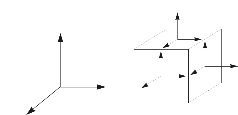
The axes of the Ma te rial lo cal co or di nate sys tem are de noted 1, 2, and 3. By de fault,
the Ma te rial co or di nate sys tem is aligned with the lo cal co or di nate sys tem for each
ele ment. How ever, you may spec ify a set of one or more ma te rial an gles that ro tate
the Ma te rial co or di nate sys tem with re spect to the ele ment sys tem for those ele -
ments that per mit or tho tropic or ani sotropic prop er ties.
For more in for ma tion:
•See Topic “Ma te rial An gle” (page 193) in Chap ter “The Shell El e ment.”
•See Topic “Ma te rial An gle” (page 219) in Chap ter “The Plane Ele ment.”
•See Topic “Ma te rial An gle” (page 229) in Chap ter “The Aso lid Ele ment.”
•See Topic “Ma te rial An gles” (page 246) in Chap ter “The Solid Ele ment.”
Stresses and Strains
The elas tic me chani cal prop er ties re late the be hav ior of the stresses and strains
within the Ma te rial. The stresses are de fined as forces per unit area act ing on an ele -
men tal cube aligned with the ma te rial axes as shown in Figure 13 (page 71). The
stresses s11, s22, and s33 are called the di rect stresses and tend to cause length
Stresses and Strains 71
Chapter VI Material Properties
3
2
1
Material Local
Coordinate System
s11
s33
s13
s13
s12 s12
s23
s23
s22
Stress Components
Figure 13
Definition of Stress Components in the Material Local Coordinate System

change, while s12, s13, and s23 are called the shear stresses and tend to cause an gle
change.
Not all stress com po nents ex ist in every ele ment type. For ex am ple, the stresses
s22,
s33, and s23 are as sumed to be zero in the Frame ele ment, and stress s33 is
taken to be zero in the Shell ele ment.
The di rect strains e11, e22, and e33 meas ure the change in length along the Ma te rial
lo cal 1, 2, and 3 axes, re spec tively, and are de fined as:
e111
1
=du
dx
e222
2
=du
dx
e333
3
=du
dx
where u1, u2, and u3 are the dis place ments and x1, x2, and x3 are the co or di nates in the
Ma te rial 1, 2, and 3 di rec tions, re spec tively.
The en gi neer ing shear strains g12, g13, and g23, meas ure the change in an gle in the
Ma te rial lo cal 1-2, 1-3, and 2-3 planes, re spec tively, and are de fined as:
g121
2
2
1
=+
du
dx
du
dx
g131
3
3
1
=+
du
dx
du
dx
g232
3
3
2
=+
du
dx
du
dx
Note that the en gi neer ing shear strains are equal to twice the ten so rial shear strains
e12, e13, and e23, re spec tively.
Strains can also be caused by a tem pera ture change, DT, that can be spec i fied as a
load on an el e ment. No stresses are caused by a tem pera ture change un less the in -
duced ther mal strains are re strained.
See Cook, Malkus, and Ple sha (1989), or any text book on ele men tary me chan ics.
72 Stresses and Strains
CSI Analysis Reference Manual
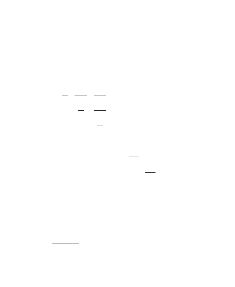
Isotropic Materials
The be hav ior of an iso tro pic ma te rial is in de pend ent of the di rec tion of load ing or
the ori en ta tion of the ma te rial. In ad di tion, shear ing be hav ior is un cou pled from
extensional be hav ior and is not af fected by tem per a ture change. Iso tro pic be hav ior
is usu ally as sumed for steel and con crete, al though this is not al ways the case.
The iso tro pic me chan i cal and ther mal prop er ties re late strain to stress and tem per a -
ture change as fol lows:
(Eqn. 1)
e
e
e
g
g
g
11
22
33
12
13
23
ì
í
ï
ï
ï
î
ï
ï
ï
ü
ý
ï
ï
ï
þ
ï
ï
ï
=
1--
e1
u12
e1
u12
e1
e1
u12
e1
e1
g12
g12
g12
000
1-000
1000
100
sym.10
1
é
ë
ê
ê
ê
ê
ê
ê
ê
ê
ê
ê
ê
ê
ê
ù
û
ú
ú
ú
ú
ú
ú
ú
ú
ú
ú
ú
ú
ú
ì
í
ï
ï
ï
î
ï
ï
ï
ü
s
s
s
s
s
s
11
22
33
12
13
23
ý
ï
ï
ï
þ
ï
ï
ï
+
ì
í
ï
ï
ï
î
ï
ï
ï
ü
ý
ï
ï
ï
þ
ï
ï
ï
a1
a1
a1
0
0
0
DT
where e1 is Young’s modulus of elas tic ity, u12 is Pois son’s ra tio, g12 is the shear
modulus, and a1 is the co ef fi cient of ther mal ex pan sion. This re la tion ship holds re -
gard less of the ori en ta tion of the Ma te rial lo cal 1, 2, and 3 axes.
The shear modulus is not di rectly spec i fied, but in stead is de fined in terms of
Young’s modulus and Pois son’s ra tio as:
g12e1
u12
=+21()
Note that Young’s modulus must be pos i tive, and Pois son’s ra tio must sat isfy the
con di tion:
-<<11
2
u12
Isotropic Materials 73
Chapter VI Material Properties
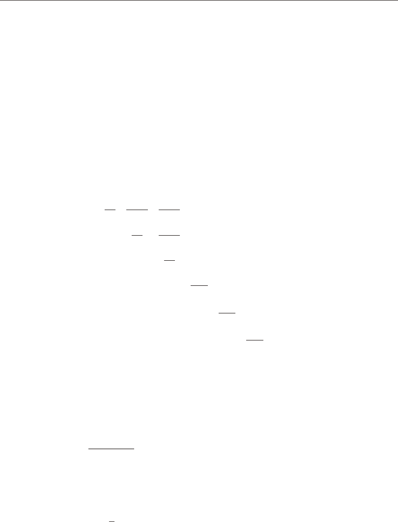
Uniaxial Materials
Uni ax ial ma te ri als are used for mod el ing rebar, ca ble, and ten don be hav ior. These
types of ob jects pri mar ily carry ax ial ten sion and have a pre ferred di rec tion of ac -
tion. Shear ing be hav ior may be con sid ered in cer tain ap pli ca tions, such as for rebar
when used in lay ered shell sections.
Uni ax ial be hav ior can be con sid ered as an iso tro pic ma te rial with stresses
sss
2233230===, re gard less of the strains. This re la tion ship is di rec tional and is
al ways aligned with the Ma te rial lo cal 1 axis.
The uni ax ial me chan i cal and ther mal prop er ties re late strain to stress and tem per a -
ture change as fol lows:
(Eqn. 2)
e
e
e
g
g
g
11
22
33
12
13
23
ì
í
ï
ï
ï
î
ï
ï
ï
ü
ý
ï
ï
ï
þ
ï
ï
ï
=
1--
e1
u12
e1
u12
e1
e1
u12
e1
e1
g12
g12
g12
000
1-000
1000
100
sym.10
1
é
ë
ê
ê
ê
ê
ê
ê
ê
ê
ê
ê
ê
ê
ê
ù
û
ú
ú
ú
ú
ú
ú
ú
ú
ú
ú
ú
ú
ú
ì
í
ï
ï
ï
î
ï
ï
ï
ü
ý
ï
ï
ï
þ
ï
s
s
s
11
12
13
0
0
0
ï
ï
+
ì
í
ï
ï
ï
î
ï
ï
ï
ü
ý
ï
ï
ï
þ
ï
ï
ï
a1
0
0
0
0
0
DT
where e1 is Young’s modulus of elas tic ity, u12 is Pois son’s ra tio, g12 is the shear
modulus, and a1 is the co ef fi cient of ther mal ex pan sion.
When used, the shear modulus is not di rectly spec i fied, but in stead is de fined in
terms of Young’s modulus and Pois son’s ra tio as:
g12e1
u12
=+21()
Note that Young’s modulus must be pos i tive, and Pois son’s ra tio must sat isfy the
con di tion:
-<<11
2
u12
74 Uniaxial Materials
CSI Analysis Reference Manual
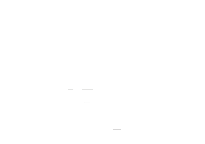
Orthotropic Materials
The be hav ior of an or tho tropic ma te rial can be dif fer ent in each of the three lo cal
co or di nate di rec tions. How ever, like an iso tropic ma te rial, shear ing be hav ior is un -
cou pled from ex ten sional be hav ior and is not af fected by tem pera ture change.
The or tho tropic me chani cal and ther mal prop er ties re late strain to stress and tem -
pera ture change as fol lows:
(Eqn. 3)
e
e
e
g
g
g
11
22
33
12
13
23
ì
í
ï
ï
ï
î
ï
ï
ï
ü
ý
ï
ï
ï
þ
ï
ï
ï
=
1--
e1
u12
e2
u13
e3
e2
u23
e3
e3
g12
g13
g23
000
1-000
1000
100
sym.10
1
é
ë
ê
ê
ê
ê
ê
ê
ê
ê
ê
ê
ê
ê
ê
ù
û
ú
ú
ú
ú
ú
ú
ú
ú
ú
ú
ú
ú
ú
ì
í
ï
ï
ï
î
ï
ï
ï
ü
s
s
s
s
s
s
11
22
33
12
13
23
ý
ï
ï
ï
þ
ï
ï
ï
+
ì
í
ï
ï
ï
î
ï
ï
ï
ü
ý
ï
ï
ï
þ
ï
ï
ï
a1
a2
a3
0
0
0
DT
where e1, e2, and e3 are the moduli of elas tic ity; u12, u13, and u23 are the Pois -
son’s ra tios; g12, g13, and g23 are the shear moduli; and a1, a2, and a3 are the co ef -
fi cients of ther mal ex pan sion.
Note that the elas tic moduli and the shear moduli must be posi tive. The Pois son’s
ra tios may take on any val ues pro vided that the upper- left 3x3 por tion of the stress-
strain ma trix is positive- definite (i.e., has a posi tive de ter mi nant.)
Anisotropic Materials
The be hav ior of an ani sotropic ma te rial can be dif fer ent in each of the three lo cal
co or di nate di rec tions. In ad di tion, shear ing be hav ior can be fully cou pled with ex -
ten sional be hav ior and can be af fected by tem pera ture change.
The ani sotropic me chani cal and ther mal prop er ties re late strain to stress and tem -
pera ture change as fol lows:
Orthotropic Materials 75
Chapter VI Material Properties

(Eqn. 4)
e
e
e
g
g
g
11
22
33
12
13
23
ì
í
ï
ï
ï
î
ï
ï
ï
ü
ý
ï
ï
ï
þ
ï
ï
ï
=
1--
e1
u12
e2
u13
e3
u14
g12
u15
g13
u16
g23
e2
u23
e3
u24
g12
u25
g13
u26
---
1----
g23
e3
u34
g12
u35
g13
u36
g23
g12
u45
g13
u46
g23
1---
1--
sym.1
g13
u56
g23
g23
-
1
é
ë
ê
ê
ê
ê
ê
ê
ê
ê
ê
ê
ê
ê
ê
ù
û
ú
ú
ú
ú
ú
ú
ú
ú
ú
ú
ú
ú
ú
s
s
11
22
s
s
s
s
33
12
13
23
ì
í
ï
ï
ï
î
ï
ï
ï
ü
ý
ï
ï
ï
þ
ï
ï
ï
+
ì
í
ï
ï
a1
a2
a3
a12
a13
a23
ï
î
ï
ï
ï
ü
ý
ï
ï
ï
þ
ï
ï
ï
DT
where e1, e2, and e3 are the moduli of elas tic ity; u12, u13, and u23 are the stan dard
Pois son’s ra tios; u14, u24..., u56 are the shear and cou pling Pois son’s ra tios; g12,
g13, and g23 are the shear moduli; a1, a2, and a3 are the co ef fi cients of ther mal ex -
pan sion; and a12, a13, and a23 are the co ef fi cients of ther mal shear.
Note that the elas tic moduli and the shear moduli must be posi tive. The Pois son’s
ra tios must be cho sen so that the 6x6 stress- strain ma trix is posi tive defi nite. This
means that the de ter mi nant of the ma trix must be posi tive.
These ma te rial prop er ties can be evalu ated di rectly from labo ra tory ex peri ments.
Each col umn of the elas tic ity ma trix rep re sents the six meas ured strains due to the
ap pli ca tion of the ap pro pri ate unit stress. The six ther mal co ef fi cients are the meas -
ured strains due to a unit tem pera ture change.
Temperature-Dependent Properties
All of the me chani cal and ther mal prop er ties given in Equa tions (1) to (4) may de -
pend upon tem pera ture. These prop er ties are given at a se ries of speci fied ma te rial
tem pera tures t. Prop er ties at other tem pera tures are ob tained by lin ear in ter po la tion
be tween the two near est speci fied tem pera tures. Prop er ties at tem pera tures out side
the speci fied range use the prop er ties at the near est speci fied tem pera ture. See
Figure 14 (page 77) for ex am ples.
If the Ma te rial prop er ties are in de pend ent of tem pera ture, you need only spec ify
them at a sin gle, ar bi trary tem pera ture.
76 Temperature-Dependent Properties
CSI Analysis Reference Manual
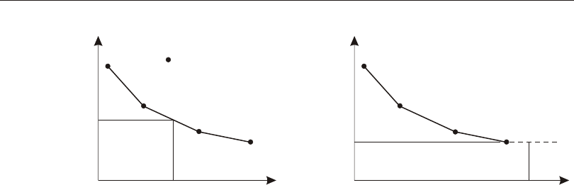
Element Material Temperature
You can as sign each ele ment an ele ment ma te rial tem pera ture. This is the tem -
pera ture at which temperature- dependent ma te rial prop er ties are evalu ated for the
ele ment. The prop er ties at this fixed tem pera ture are used for all analy ses re gard -
less of any tem pera ture changes ex pe ri enced by the ele ment dur ing load ing.
The ele ment ma te rial tem pera ture may be uni form over an ele ment or in ter po lated
from val ues given at the joints. In the lat ter case, a uni form ma te rial tem pera ture is
used that is the av er age of the joint val ues. The de fault ma te rial tem pera ture for any
ele ment is zero.
The prop er ties for a temperature- independent ma te rial are con stant re gard less of
the ele ment ma te rial tem pera tures speci fied.
Mass Density
For each Ma te rial you may spec ify a mass den sity, m, that is used for cal cu lat ing
the mass of the ele ment. The to tal mass of the ele ment is the prod uct of the mass
den sity (mass per unit vol ume) and the vol ume of the ele ment. This mass is ap por -
tioned to each joint of the ele ment. The same mass is ap plied along of the three
trans la tional de grees of free dom. No ro ta tional mass mo ments of in er tia are com -
puted.
Element Material Temperature 77
Chapter VI Material Properties
Interpolated Value
T
E
Tmatt Tmatt
Ematt
Ematt
Extrapolated Value
T
E
indicates specified value e
at temperature t
Figure 14
Determination of Property Ematt at Temperature Tmatt from Function E(T)

Con sis tent mass units must be used. Typi cally the mass den sity is equal to the
weight den sity of the ma te rial di vided by the ac cel era tion due to grav ity, but this is
not re quired.
The mass den sity prop erty is in de pend ent of tem pera ture.
For more in for ma tion:
•See Topic “Mass” (page 134) in Chap ter “The Frame Ele ment.”
•See Topic “Mass” (page 172) in Chap ter “The Ca ble El e ment.”
•See Topic “Mass” (page 206) in Chap ter “The Shell El e ment.”
•See Topic “Mass” (page 220) in Chap ter “The Plane Ele ment.”
•See Topic “Mass” (page 232) in Chap ter “The Aso lid Ele ment.”
•See Topic “Mass” (page 248) in Chap ter “The Solid Ele ment.”
•See Topic “Mass Source” (page 334) in Chap ter “Load Pat terns”.
Weight Density
For each Ma te rial you may spec ify a weight den sity, w, that is used for cal cu lat ing
the self- weight of the ele ment. The to tal weight of the ele ment is the prod uct of the
weight den sity (weight per unit vol ume) and the vol ume of the ele ment. This
weight is ap por tioned to each joint of the ele ment. Self- weight is ac ti vated us ing
Self- weight Load and Grav ity Load.
The weight den sity prop erty is in de pend ent of tem pera ture.
For more in for ma tion:
•See Topic “Self- Weight Load” (page 325) in Chap ter “Load Pat terns.”
•See Topic “Grav ity Load” (page 326) in Chap ter “Load Pat terns.”
Material Damping
You may spec ify ma te rial damp ing to be used in dy namic anal y ses. Dif fer ent types
of damp ing are avail able for dif fer ent types of Load Cases. Ma te rial damp ing is a
prop erty of the ma te rial and af fects all Load Cases of a given type in the same way.
You may spec ify ad di tional damp ing in each Load Case.
78 Weight Density
CSI Analysis Reference Manual

Be cause damp ing has such a sig nif i cant af fect upon dy namic re sponse, you should
use care in de fin ing your damp ing pa ram e ters.
The ma te rial used for cal cu lat ing damp ing is de ter mined for the dif fer ent types of
el e ments as fol lows:
•For frame el e ments, if a ma te rial over write is spec i fied, that ma te rial is used.
Otherwise the ma te rial for the cur rent frame sec tion is used, with non-pris matic
sec tions us ing a sim ple av er age of the damp ing co ef fi cients over all ma te ri als
along the full length of the sec tion.
•For shell el e ments, if a ma te rial over write is spec i fied, that ma te rial is used.
Otherwise the ma te rial for the cur rent shell sec tion is used, with lay ered sec -
tions us ing a thick ness-weighted av er age of the damp ing co ef fi cients over all
ma te rial lay ers in the sec tion.
•For cable, ten don, plane, asolid, and solid el e ments, the ma te rial for the cur rent
sec tion is used.
Ma te rial-based damp ing does not ap ply to link el e ments.
Modal Damping
The ma te rial modal damp ing avail able in SAP2000 is stiff ness weighted, and is
also known as com pos ite modal damp ing. It is used for all re sponse-spec trum and
modal time-his tory anal y ses. For each ma te rial you may spec ify a ma te rial modal
damp ing ra tio, r, where 01£<r. The damp ing ra tio, rij, con trib uted to mode I by el -
e ment j of this ma te rial is given by
rr
K
ij
iji
i
=ff
TK
where fi is mode shape for mode I, Kj is the stiff ness ma trix for el e ment j, and Ki
is the modal stiff ness for mode I given by
Kii
j
ji
=åff
TK
summed over all el e ments, j, in the model.
Material Damping 79
Chapter VI Material Properties

Vis cous Pro por tional Damping
Vis cous pro por tional damp ing is used for di rect-in te gra tion time-his tory anal y ses.
For each ma te rial, you may spec ify a mass co ef fi cient, cM, and a stiff ness co ef fi -
cient, cK. You may spec ify these two co ef fi cients di rectly, or they may be com -
puted by spec i fy ing equiv a lent frac tions of crit i cal modal damp ing at two dif fer ent
pe ri ods or fre quen cies.
The damp ing ma trix for el e ment j of the ma te rial is com puted as:
CMK
jMjKj
cc=+0
where
Mj is the mass of the el e ment, and Kj
0 is the stiff ness of the el e ment. The su -
per script “0” in di cates that for nonlinear el e ments, the ini tial stiff ness is used. This
is the stiff ness of the el e ment at zero ini tial con di tions, re gard less of the cur rent
non lin ear state of the el e ment. The ex cep tion to this rule is that if the cur rent non lin -
ear state has zero stiff ness and zero force or stress (such as for cracked con crete ma -
te rial), then zero damp ing is as sumed. In the case where the ini tial stiff ness is dif -
fer ent in the neg a tive and pos i tive di rec tion of load ing, the larger stiff ness is used.
Hysteretic Pro por tional Damping
Hysteretic pro por tional damp ing is used for steady-state and power-spec tral-den -
sity anal y ses. For each ma te rial, you may spec ify a mass co ef fi cient, dM, and a
stiff ness co ef fi cient, dM. The hysteretic damp ing ma trix for el e ment j of the ma te -
rial is com puted as:
DMK
jMjKj
dd=+0
where Mj is the mass of the el e ment, and Kj
0 is the stiff ness of the el e ment. See the
subtopic “Vis cous Pro por tional Damp ing” above for how the ma te rial stiff ness is
de ter mined for nonlinear el e ments.
Nonlinear Material Behavior
Non lin ear ma te rial be hav ior is avail able in cer tain el e ments us ing a di rec tional ma -
te rial model, in which uncoupled stress-strain be hav ior is mod eled for one or more
stress-strain com po nents. This is a sim ple and prac ti cal en gi neer ing model suit able
for many ap pli ca tions such as beams and col umns, shear walls, bridge decks, tun -
nels, re tain ing walls, and oth ers. You should care fully ex am ine the ap pli ca bil ity of
80 Nonlinear Material Behavior
CSI Analysis Reference Manual

this model be fore us ing it in a gen eral con tin uum model where the gov ern ing
stresses change di rec tion sub stan tially from place to place.
In ad di tion, a two-di men sional con crete model is avail able for use in the lay ered
shell. This model is dis cussed in topic “Mod i fied Dar win-Pecknold Con crete
Model” later in this chap ter. The re main der of this pres ent topic con cerns the di rec -
tional ma te rial model.
Nonlinear ma te rial be hav ior is cur rently not tem per a ture-de pend ent. The be hav ior
spec i fied at the ini tial (most neg a tive) tem per a ture is used for all ma te rial tem per a -
tures.
Ten sion and Compression
For each ma te rial you may spec ify an ax ial stress-strain curve that is used to rep re -
sent the di rect (ten sion-com pres sion) stress-strain be hav ior of the ma te rial along
any ma te rial axis. For Uni ax ial ma te ri als, this rep re sents the re la tion ship be tween
s11 and e11. For Iso tro pic, Orthotropic, and Anisotropic ma te ri als, this curve rep re -
sents the be hav ior along each of the three ma te rial axes, s11-e11, s22-e22, and
s33-e33. The non lin ear stress-strain be hav ior is the same in each di rec tion, even
for Orthotropic, and Anisotropic ma te ri als.
Tension is al ways pos i tive, re gard less of the type of ma te rial (steel, con crete, etc.)
The ten sile and com pres sive sides of the stress-strain be hav ior may be dif fer ent
from each other. For what fol lows, the di rect stress-strain curve may be writ ten as
fol lows:
(Eqn. 5a)
sesee
see
iiii
Tiiii
Ciiii
()(),
(),
=³
£
ì
í
î
0
0
where se
T() rep re sents ten sile be hav ior, and se
C() rep re sents com pres sive be hav -
ior, sub ject to the re stric tions:
(Eqn. 5b)
ses
ses
TT
CC
(),()
(),()
³=
£=
000
000
Shear
A shear stress-strain curve is com puted in ter nally from the di rect stress-strain
curve. The as sump tion is made that shear ing be hav ior can be com puted from ten -
sile and com pres sive be hav ior act ing at 45° to the ma te rial axes us ing Mohr's cir cle
Nonlinear Material Behavior 81
Chapter VI Material Properties

in the plane. For an Isotropic, Orthotropic, or Anisotropic ma te rial, this re sults in
the fol low ing sym met ri cal re la tion ship for shear:
(Eqn. 6a)
sesee
-see
ijij
Sijij
Sijij
()(),
(),
=³
-£
ì
í
î
0
0
where
(Eqn. 6b)
seseseeg
SijTijCijijijij()(()()),,=--=³¹
1
4
1
20
For the case where the di rect stress-strain curve is sym met rical, such as for steel, we
have sese
TC
()()=--, and there fore:
sesee
see
ijij
Tijij
Cijij
()(),
(),
=³
£
ì
í
î
1
2
0
0
To cre ate a ma te rial where the shear ing re la tion ship, se
S(), is pri mary and known,
you can de fine a sym met ri cal di rect stress-strain re la tion ship such that:
sesese
TCS
()()()=--=2
When shear stress is con sid ered for a Uni ax ial ma te rial, the stress is half that for an
Iso tro pic ma te rial. In this way, if you have two uni ax ial ma te ri als at 90° to each
other, the shear be hav ior matches that of an Isotropic ma te rial. Thus for Uni ax ial
ma te ri als:
(Eqn. 6c)
sesee
-see
ijij
Sijij
Sijij
()(),
(),
=³
-£
ì
í
î
1
2
0
0(for Uniaxialmaterial)
Hysteresis
Sev eral hys ter esis mod els are avail able to de fine the non lin ear stress-strain be hav -
ior when load is re versed or cy cled. For the most part, these mod els dif fer in the
amount of en ergy they dis si pate in a given cy cle of de for ma tion, and how the en -
ergy dis si pa tion be hav ior changes with an in creas ing amount of de for ma tion.
De tails are pro vided in Topic “Hys ter esis Mod els" (page 85) in this chap ter.
82 Nonlinear Material Behavior
CSI Analysis Reference Manual

Ap pli ca tion
Non lin ear stress-strain curves are cur rently used in the two ap pli ca tions de scribed
in the following.
Fi ber Hinges
Fi ber hinges are used to de fine the cou pled ax ial force and bi-ax ial bend ing be hav -
ior at lo ca tions along the length of a frame el e ment. The hinges can be de fined man -
u ally, or created au to mat i cally for cer tain types of frame sec tions, in clud ing Sec -
tion-De signer sec tions.
For each fi ber in the cross sec tion at a fi ber hinge, the ma te rial di rect non lin ear
stress-strain curve is used to de fine the ax ial s11 - e11 re la tion ship. Sum ming up the
be hav ior of all the fi bers at a cross sec tion and mul ti ply ing by the hinge length
gives the ax ial force-de for ma tion and bi axial mo ment-ro ta tion re la tion ships.
The s11 - e11 is the same whether the ma te rial is Uni ax ial, Iso tro pic, Orthotropic, or
Anisotropic. Shear be hav ior is not con sid ered in the fi bers. In stead, shear be hav ior
is com puted for the frame sec tion as usual us ing the lin ear shear modulus g12.
For more in for ma tion:
•See Topic “Sec tion De signer Sec tions” (page 134) in Chap ter “The Frame El e -
ment.”
•See Chap ter “Frame Hinge Prop er ties” (page 147).
Lay ered Shell Element
The Shell el e ment with the lay ered sec tion prop erty may con sider lin ear, non lin ear,
or mixed ma te rial be hav ior. For each layer, you se lect a ma te rial, a ma te rial an gle,
and whether each of the in-plane stress-strain re la tion ships are lin ear, non lin ear, or
in ac tive (zero stress). These re la tion ships in clude s11- e11, s22-e22, and s12-e12.
For Uni ax ial ma te ri als, the stress s220= al ways. How ever, shear stiff ness is as -
sumed to be pres ent, but may be set to zero by set ting the shear re la tion ship to be in -
ac tive.
For all ma te ri als, the trans verse nor mal stress s330=. The trans verse shear be hav -
ior is al ways lin ear, us ing the ap pro pri ate shear moduli g13 and g23 from the ma te -
rial ma trix (Eqns. 1–4 above.)
Nonlinear Material Behavior 83
Chapter VI Material Properties

If all three in-plane re la tion ships for a given layer are lin ear, the cor re spond ing lin -
ear ma trix is used (Eqns. 1–4 above), ad justed for the plane-stress con di tion
s330=. Pois son ef fects are in cluded, which may cou ple the two di rect stresses.
If any of the in-plane re la tion ships for a given layer are non lin ear or in ac tive, then
all three re la tion ships be come un cou pled ac cord ing to these rules:
•Pois son’s ra tio is taken to be zero.
•Lin ear di rect stress-strain re la tion ships use stiff ness e1 from the ma te rial ma -
trix (Eqns. 1-4).
•Lin ear shear stress-strain relationships use shear modulus g12 (Eqns. 1-4).
•Non lin ear di rect stress-strain re la tion ships use Eqns. 5 above.
•Non lin ear shear stress-strain re la tion ships use Eqns. 6 above.
•In ac tive stress-strain re la tion ships as sume that the cor re spond ing stress is zero.
The stress-strain be hav ior for a given layer is al ways de fined in the ma te rial co or di -
nate sys tem spec i fied by the ma te rial an gle for that layer. It is par tic u larly im por -
tant to keep this in mind when us ing Uni ax ial ma te ri als, for which s220=.
The above de scrip tion is for the di rec tional ma te rial. In ad di tion, a two-di men -
sional con crete model is avail able for use in the lay ered shell. This model is dis -
cussed in topic “Mod i fied Dar win-Pecknold Con crete Model” later in this chap ter.
For more in for ma tion, see Subtopic “Lay ered Sec tion Prop erty” (page 193) in
Chap ter “The Shell El e ment.”
Friction and Dilitational Angles
For con crete ma te ri als, you can spec ify a fric tion an gle and a dilitational an gle.
These should nor mally be set to zero. The fric tion an gle is an ex per i men tal pa ram e -
ter, and is not rec om mended for nor mal use. The dilitational an gle is a fu ture pa -
ram e ter, and has no ef fect on the model.
The fric tion an gle, f, takes val ues 090£<°f. For the rec om mended value of f=0,
shear be hav ior is as de scribed above. For ex per i men tal use with f>0, the shear
stress is com puted pri mar ily us ing a fric tional model hav ing lin ear stiff ness g12 up
to a lim it ing stress given by:
(Eqn. 7a)
sfs
-ss
12
00
0
£³
<
ì
í
î
tan,
,
84 Nonlinear Material Behavior
CSI Analysis Reference Manual

where s(ss=+
1
21122). Com pres sion is re quired in or der to de velop any shear
strength by this equation. In ad di tion, co he sion is added us ing (Eqn. 6a) above, but
con sid er ing only the con tri bu tion to shear due to ten sion:
(Eqn. 7b)
seseeg
12ST
()(),
121
4121
2120==³
This be hav ior, while in ter est ing, can pres ent com pu ta tional chal lenges un less the
model is well de fined and rea son ably loaded, with suf fi cient duc til ity pro vided us -
ing re in forc ing steel. To re peat: This is an ex per i men tal be hav ior and is not rec om -
mended for nor mal use.
Hys ter esis Models
Hys ter esis is the pro cess of en ergy dis si pa tion through de for ma tion (dis place -
ment), as op posed to vis cos ity which is en ergy dis si pa tion through de for ma tion
rate (ve loc ity). Hys ter esis is typ i cal of sol ids, whereas vis cos ity is typ i cal of flu ids,
al though this dis tinc tion is not rigid.
Hysteretic be hav ior may af fect non lin ear static and non lin ear time-his tory load
cases that ex hibit load re ver sals and cy clic load ing. Monotonic load ing is not af -
fected.
Sev eral dif fer ent hys ter esis mod els are avail able to de scribe the be hav ior of dif fer -
ent types of ma te ri als. For the most part, these dif fer in the amount of en ergy they
dis si pate in a given cy cle of de for ma tion, and how the en ergy dis si pa tion be hav ior
changes with an in creas ing amount of de for ma tion.
Each hys ter esis model may be used for the fol low ing pur poses:
•Ma te rial stress-strain be hav ior, af fect ing frame fi ber hinges and lay ered shells
that use the ma te rial
•Sin gle de gree-of-free dom frame hinges, such as M3 or P hinges. In ter act ing
hinges, such as P-M3 or P-M2-M3, cur rently use the iso tro pic model
•Link/sup port el e ments of type multi-lin ear plas tic ity.
Al though the pres ent chap ter con cerns ma te rial prop er ties, this dis cus sion per tains
equally to all three of these ap pli ca tions.
Hys ter esis Models 85
Chapter VI Material Properties

Back bone Curve (Action vs. Deformation)
For each ma te rial, hinge, or link de gree of free dom, a unaxial ac tion vs. de for ma -
tion curve de fines the non lin ear be hav ior un der monotonic load ing in the pos i tive
and neg a tive di rec tions.
Here ac tion and de for ma tion are an en ergy con ju gate pair as fol lows:
•For ma te ri als, stress vs. strain
•For hinges and multi-lin ear links, force vs. de for ma tion or mo ment vs. ro ta tion,
de pend ing upon the de gree of free dom to which it is ap plied
For each model, the uni ax ial ac tion-de for ma tion curve is given by a set of points
that you de fine. This curve is called the back bone curve, and it can take on al most
any shape, with the fol low ing re stric tions:
•One point must be the or i gin, (0,0)
•At least one point with pos i tive de for ma tion, and one point with neg a tive de -
for ma tion, must be de fined
•The de for ma tions of the spec i fied points must in crease monotonically, with no
two val ues be ing equal
•The ac tion at each point must have the same sign as the de for ma tion (they can
be zero)
•The slope given by the last two points spec i fied on the pos i tive de for ma tion
axis is ex trap o lated to in fi nite pos i tive de for ma tion, or un til it reaches zero
value. Sim i larly, the slope given by the last two points spec i fied on the neg a tive
de for ma tion axis is ex trap o lated to in fi nite neg a tive de for ma tion, or un til it
reaches zero value.
The given curve de fines the ac tion-de for ma tion re la tion ship un der monotonic
load ing. The first slope on ei ther side of the or i gin is elas tic; the re main ing seg -
ments de fine plas tic de for ma tion. If the de for ma tion re verses, it typ i cally fol lows
the two elas tic seg ments be fore be gin ning plas tic de for ma tion in the re verse di rec -
tion, ex cept as de scribed be low.
Cy clic Behavior
Sev eral hys ter esis mod els are avail able in SAP2000, ETABS, and CSiBridge. The
avail able mod els may vary from prod uct to prod uct, and may in clude any or all of
the mod els de scribed be low.
86 Hys ter esis Models
CSI Analysis Reference Manual
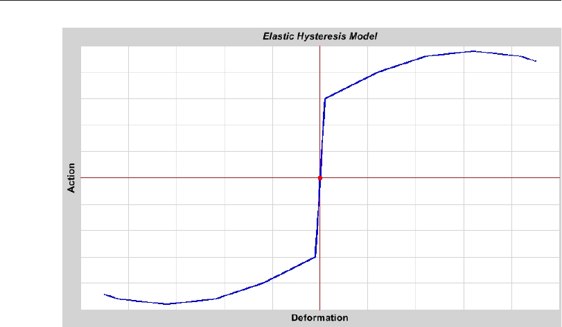
Typ i cal for all mod els, cy clic load ing be haves as fol lows:
•Ini tial load ing in the pos i tive or neg a tive di rec tion fol lows the back bone curve
•Upon re ver sal of de for ma tion, un load ing oc curs along a dif fer ent path, usu ally
steeper than the load ing path. This is of ten par al lel or nearly par al lel to the ini -
tial elas tic slope.
•Af ter the load level is re duced to zero, con tin ued re ver sal of de for ma tion
causes re verse load ing along a path that even tu ally joins the back bone curve on
the op po site side, usu ally at a de for ma tion equal to the max i mum pre vi ous de -
for ma tion in that di rec tion or the op po site di rec tion.
In the de scrip tions be low of cy clic de for ma tion, “load ing” re fers to in creas ing the
mag ni tude of de for ma tion in a given pos i tive or neg a tive di rec tion, and “un load -
ing” re fers to sub se quent re duc tion of the de for ma tion un til the force level reaches
zero. Con tin ued re duc tion of the de for ma tion is “re verse load ing” un til the de for -
ma tion reaches zero, af ter which the de for ma tion in creases again with the same
sign as the load and is “load ing” again. Load ing and un load ing oc cur in the pos i tive
(first and third) quad rants of the ac tion-de for ma tion plot, and re verse load ing oc -
curs in the neg a tive (sec ond and fourth) quad rants.
Hys ter esis Models 87
Chapter VI Material Properties
Figure 15
Elastic Hysteresis Model under Increasing Cyclic Load - No Energy Dissipation
Showing the Backbone Curve Used for All Hysteresis Figures
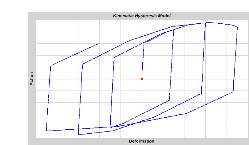
Elas tic Hysteresis Model
The be hav ior is non lin ear but it is elas tic. This means that the ma te rial al ways loads
and un loads along the back bone curve, and no en ergy is dis si pated. This be hav ior is
il lus trated in Figure 15 (page 87). This same back bone curve is used in the fig ures
for all sub se quent mod els, ex cept that the con crete model uses only the pos i tive
por tion of the curve, with the neg a tive por tion be ing de fined separately.
Ki ne matic Hysteresis Model
This model is based upon ki ne matic hard en ing be hav ior that is com monly ob served
in met als, and it is the de fault hys ter esis model for all metal ma te ri als in the pro -
gram. This model dis si pates a sig nif i cant amount of en ergy, and is ap pro pri ate for
duc tile ma te ri als.
Un der the rules of ki ne matic hard en ing, plas tic de for ma tion in one di rec tion
“pulls” the curve for the other di rec tion along with it. Match ing pairs of points are
linked. No ad di tional pa ram e ters are re quired for this model.
88 Hys ter esis Models
CSI Analysis Reference Manual
Figure 16
Kinematic Hysteresis Model under Increasing Cyclic Load

Upon un load ing and re verse load ing, the curve fol lows a path made of seg ments
par al lel to and of the same length as the pre vi ously loaded seg ments and their op po -
site-di rec tion coun ter parts un til it re joins the back bone curve when load ing in the
op po site di rec tion. This be hav ior is shown in Figure 16 (page 88) for cy cles of in -
creas ing de for ma tion.
When you de fine the points on the multi-lin ear curve, you should be aware that
sym met ri cal pairs of points will be linked, even if the curve is not sym met ri cal.
This gives you some con trol over the shape of the hysteretic loop.
The ki ne matic model forms the ba sis for sev eral of the other model de scribed be -
low, in clud ing Takeda, de grad ing, and BRB hard en ing.
De grad ing Hysteresis Model
This model is very sim i lar to the Ki ne matic model, but uses a de grad ing hysteretic
loop that ac counts for de creas ing en ergy dis si pa tion and un load ing stiff ness with
in creas ing plas tic de for ma tion.
Two mea sures are used for plas tic de for ma tion:
•Max i mum plas tic de for ma tion in each the pos i tive and neg a tive di rec tions
•Ac cu mu lated plas tic de for ma tion, which is the ab so lute sum of each in cre ment
of pos i tive or neg a tive plas tic de for ma tion. Plas tic de for ma tion is that which
does not oc cur on the two elas tic seg ments of the ac tion-de for ma tion curve
Ac cu mu lated plas tic de for ma tion can oc cur un der cy clic load ing of con stant am pli -
tude, and can be used to rep re sent fa tigue.
For this model, the fol low ing pa ram e ters are re quired:
•Sep a rately for pos i tive and neg a tive de for ma tions
–Ini tial en ergy fac tor at yield, f0, usu ally 1.0
–En ergy fac tor at mod er ate de for ma tion, f1
–En ergy fac tor at max i mum de for ma tion, f2
–Mod er ate de for ma tion level, x1, as a mul ti ple of the yield de for ma tion
–Max i mum de for ma tion level, x2, as a mul ti ple of the yield de for ma tion
–Ac cu mu lated de for ma tion weight ing fac tor, a
•Stiff ness deg ra da tion weight ing fac tor, s
•Larger-smaller weight ing fac tor, w, usu ally 0.0
Hys ter esis Models 89
Chapter VI Material Properties
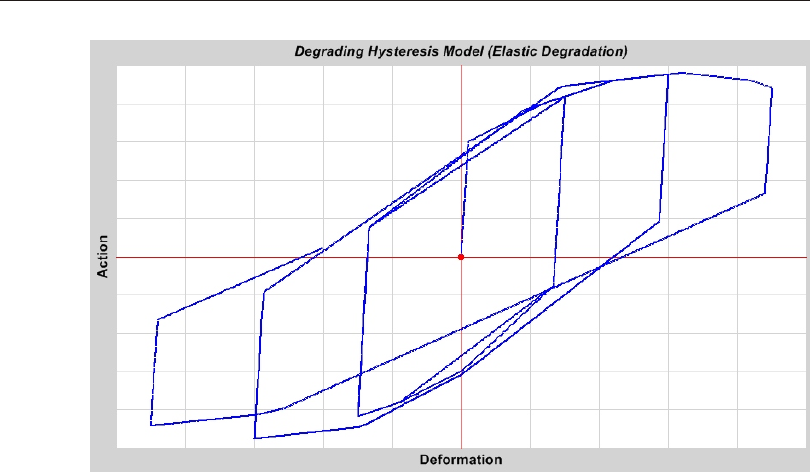
The en ergy fac tors rep re sent the area of a de graded hys ter esis loop di vided by the
en ergy of the non-de graded loop, such as for the ki ne matic model. For ex am ple, an
en ergy fac tor of 0.3 means that a full cy cle of de for ma tion would only dis si pate
30% of the en ergy that the non-de graded ma te rial would. The en ergy fac tors must
sat isfy 1.0 ³ f0 ³ f1 ³ f2 > 0.0. The de for ma tion lev els must sat isfy 1.0 < x1 < x2.
All weight ing fac tors may take any value from 0.0 to 1.0, in clu sive. Be cause the ac -
cu mu lated plas tic de for ma tion is con stantly in creas ing, it is rec om mended that the
weight ing fac tor a gen er ally be small or zero.
For each in cre ment of de for ma tion:
•The ab so lute max i mum pos i tive and neg a tive plas tic de for ma tions that have
oc curred up to this point in the anal y sis are de ter mined, dposmax and dnegmax,
as well as the ac cu mu lated plas tic de for ma tion, dacc.
•A pos i tive plas tic de for ma tion level is cal cu lated as
dadad
pospos
=+-
acc()max
1
where a is the ac cu mu lated weight ing fac tor for pos i tive de for ma tion.
90 Hys ter esis Models
CSI Analysis Reference Manual
Figure 17
Degrading Hysteresis Model under Increasing Cyclic Load
Exhibiting Elastic Degradation (s = 0.0)
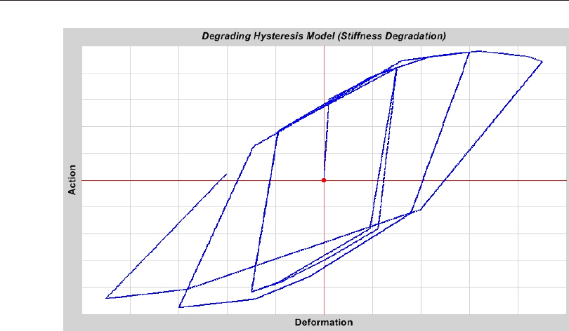
•Com par ing dpos with the pos i tive de for ma tion lev els d1 and d2, ob tained by
mul ti ply ing x1 and x2 with the pos i tive yield de for ma tion, an en ergy fac tor
fpos can be de ter mined by in ter po la tion. If dpos > d2, then fpos = f2.
•Fol low ing the same ap proach, the en ergy fac tor for neg a tive de for ma tion,
fneg, is com puted us ing the cor re spond ing pa ram e ters for neg a tive de for ma -
tion.
•The larger of these two en ergy fac tor is called fmax, and the smaller is fmin.
The fi nal en ergy fac tor is com puted as
fwfwf=+-
maxmin
()1
In the most com mon case, w = 0 and ff=min.
Deg ra da tion does not oc cur dur ing monotonic load ing. How ever, upon load re ver -
sal, the curve for un load ing and re verse load ing is mod i fied ac cord ing to the en ergy
fac tor com puted for the last de for ma tion in cre ment. This is done by squeez ing, or
flat ten ing, the curve to ward the di ag o nal line that con nects the two points of max i -
mum pos i tive and neg a tive de for ma tion.
Hys ter esis Models 91
Chapter VI Material Properties
Figure 18
Degrading Hysteresis Model under Increasing Cyclic Load
Exhibiting Stiffness Degradation (s = 1.0)
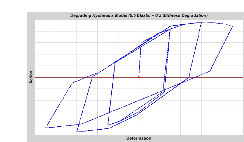
This squeez ing is scaled to achieve the de sired de crease in en ergy dis si pa tion. The
scal ing can oc cur in two di rec tions:
•Par al lel to the elas tic un load ing line, called elas tic deg ra da tion
•Par al lel to the hor i zon tal axis, called stiff ness deg ra da tion
The amount of scal ing in each di rec tion is con trolled by the stiff ness deg ra da tion
weight ing pa ram e ter, s. For s = 0.0, all deg ra da tion is of elas tic type. For s = 1.0, all
deg ra da tion is of stiff ness type. For in ter me di ate val ues, the deg ra da tion is ap por -
tioned ac cord ingly.
While the de for ma tion and in di vid ual en ergy lev els are com puted sep a rately for the
pos i tive and neg a tive di rec tions, the fi nal en ergy level is a sin gle pa ram e ter that af -
fects the shape of the hys ter esis loop in both di rec tions.
Note that if all the en ergy fac tors are equal to 1.0, this model de gen er ates to the ki -
ne matic hys ter esis model.
Fig ures 17, 18, and 19 (pages 90-92) show the shape of the hys ter esis loop for elas -
tic deg ra da tion, stiff ness deg ra da tion, and a mix ture with a stiff ness deg ra da tion
92 Hys ter esis Models
CSI Analysis Reference Manual
Figure 19
Degrading Hysteresis Model under Increasing Cyclic Load
Exhibiting Combined Degradation (s = 0.5)
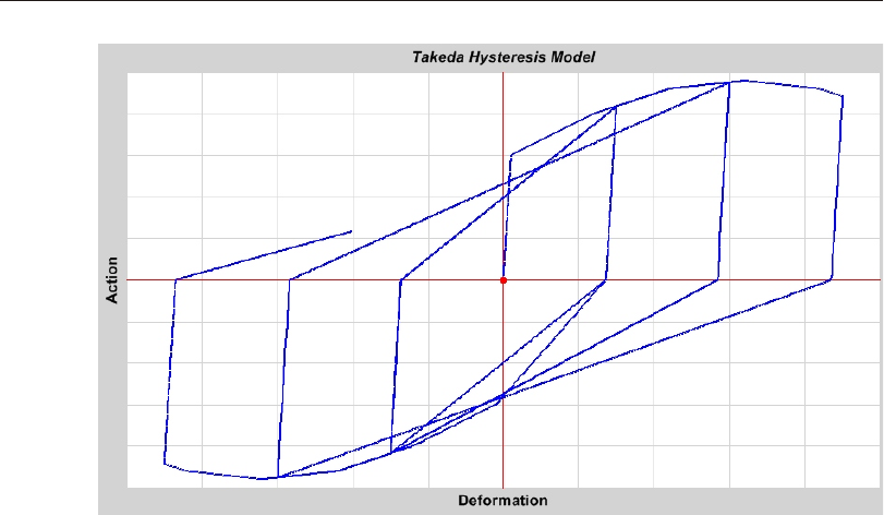
fac tor of s = 0.5. Each of these three cases dis si pates the same amount of en ergy for
a given cy cle of load ing, and less than the en ergy dis si pated for the equiv a lent ki ne -
matic model shown in Figure 16 (page 88).
Takeda Hysteresis Model
This model is very sim i lar to the ki ne matic model, but uses a de grad ing hysteretic
loop based on the Takeda model, as de scribed in Takeda, Sozen, and Niel sen
(1970). This sim ple model re quires no ad di tional pa ram e ters, and is more ap pro pri -
ate for re in forced con crete than for met als. Less en ergy is dis si pated than for the ki -
ne matic model.
Un load ing is along the elas tic seg ments sim i lar to the ki ne matic model. When re -
load ing, the curve fol lows a se cant line to the back bone curve for load ing in the op -
po site di rec tion. The tar get point for this se cant is at the max i mum de for ma tion that
oc curred in that di rec tion un der pre vi ous load cy cles. This re sults in a de creas ing
amount of en ergy dis si pa tion with larger de for ma tions. Un load ing is along the
elas tic seg ments.
This be hav ior is il lus trated in Figure 20 (page 93).
Hys ter esis Models 93
Chapter VI Material Properties
Figure 20
Takeda Hysteresis Model under Increasing Cyclic Load
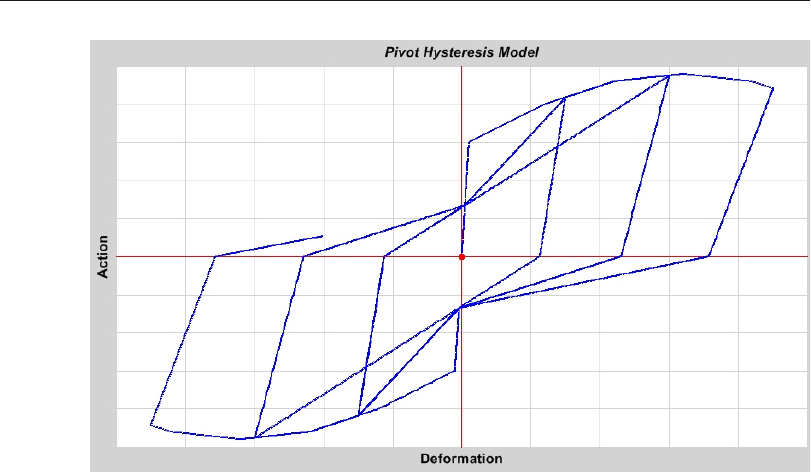
Pivot Hysteresis Model
This model is sim i lar to the Takeda model, but has ad di tional pa ram e ters to con trol
the de grad ing hysteretic loop. It is par tic u larly well suited for re in forced con crete
mem bers, and is based on the ob ser va tion that un load ing and re verse load ing tend
to be di rected to ward spe cific points, called piv ots points, in the ac tion-de for ma tion
plane. The most com mon use of this model is for mo ment-ro ta tion. This model is
fully de scribed in Dowell, Seible, and Wil son (1998). This model is not in tended
for unreinforced con crete. See the sep a rate con crete model be low.
The fol low ing ad di tional pa ram e ters are spec i fied for the Pivot model:
•a1, which lo cates the pivot point for un load ing to zero from pos i tive force. Un -
load ing oc curs to ward a point on the ex ten sion of the pos i tive elas tic line, but at
a neg a tive force value of a1 times the pos i tive yield force.
•a2, which lo cates the pivot point for un load ing to zero from neg a tive force.
Un load ing oc curs to ward a point on the ex ten sion of the neg a tive elas tic line,
but at a pos i tive force value of a2 times the neg a tive yield force.
•b1, which lo cates the pivot point for re verse load ing from zero to ward pos i tive
force. Re load ing oc curs to ward a point on the pos i tive elas tic line at a force
94 Hys ter esis Models
CSI Analysis Reference Manual
Figure 21
Pivot Hysteresis Model under Increasing Cyclic Load
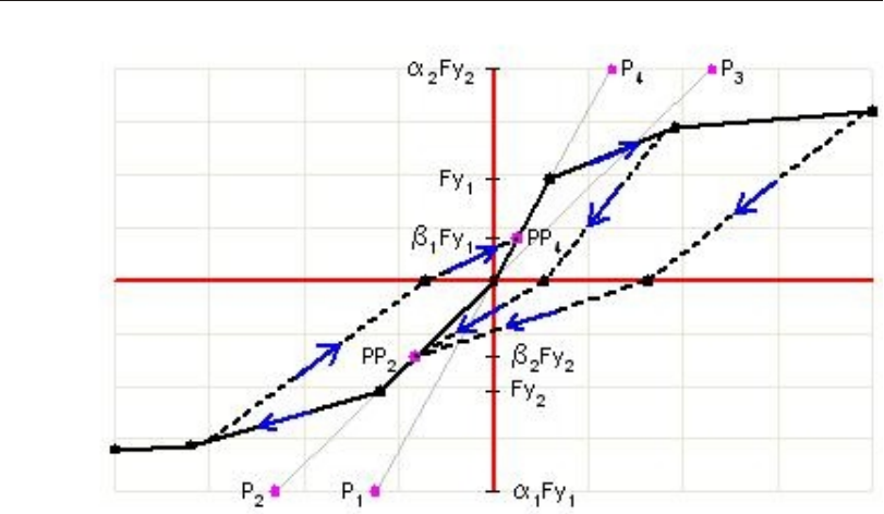
value of b1 times the pos i tive yield force, where 0.0 < b1 £ 1.0. Be yond that
point, load ing oc curs along the se cant to the point of max i mum pre vi ous pos i -
tive de for ma tion on the back bone curve.
•b2, which lo cates the pivot point for re verse load ing from zero to ward neg a tive
force. Re load ing oc curs to ward a point on the neg a tive elas tic line at a force
value of b2 times the neg a tive yield force, where 0.0 < b2 £ 1.0. Be yond that
point, load ing oc curs along the se cant to the point of max i mum pre vi ous neg a -
tive de for ma tion on the back bone curve.
•h, which de ter mines the amount of deg ra da tion of the elas tic slopes af ter plas tic
de for ma tion, where 0.0 < h £ 1.0
These pa ram e ters and the be hav ior are il lus trated in Fig ures 21 and 22 (pages 94
and 95).
Con crete Hysteresis Model
This model is in tended for unreinforced con crete and sim i lar ma te ri als, and is the
de fault model for con crete and ma sonry ma te ri als in the pro gram. Ten sion and
Hys ter esis Models 95
Chapter VI Material Properties
Figure 22
Pivot Hysteresis Model Parameters
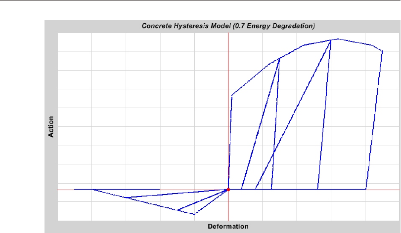
com pres sion be hav ior are in de pend ent and be have dif fer ently. The force-de for ma -
tion (stress-strain) curve is used to de ter mine the sign of com pres sion, which can be
pos i tive or neg a tive. The point hav ing the larg est ab so lute value of stress or force is
con sid ered to be in com pres sion, so that the sign of com pres sion can be ei ther pos i -
tive or neg a tive. Like wise, the con crete model can also be used to rep re sent a ten -
sion-only ma te rial whose be hav ior is sim i lar to con crete in com pres sion.
This model is pri mar ily in tended for ax ial be hav ior, but can be ap plied to any de -
gree of free dom. Re in forced con crete is better mod eled us ing the pivot, de grad ing,
or Takeda mod els.
A non-zero force-de for ma tion curve should al ways be de fined for com pres sion.
The force-de for ma tion curve for ten sion may be all zero, or it may be non-zero pro -
vided that the max i mum force value is of smaller mag ni tude than that for the com -
pres sion side.
A sin gle pa ram e ter, the en ergy deg ra da tion fac tor f, is spec i fied for this model. This
value should sat isfy 0.0 £ f £ 1.0. A value of f = 0.0 is equiv a lent to a clean gap
when un load ing from com pres sion and dis si pates the least amount of en ergy. A
96 Hys ter esis Models
CSI Analysis Reference Manual
Figure 23
Concrete Hysteresis Model under Increasing Cyclic Load
with Compression as Positive and Energy Factor f = 0.7

value of f = 1.0 is dis si pates the most en ergy and could be caused by rub ble fill ing
the gap when un load ing from com pres sion.
Com pres sion be hav ior is mod eled as fol lows:
•Ini tial load ing is along the back bone curve
•Un load ing to zero oc curs along a line nearly par al lel to the com pres sion elas tic
line. The line is ac tu ally di rected to a pivot point on the ex ten sion of the com -
pres sive elas tic line, lo cated so that the un load ing slope at max i mum com pres -
sive force has half the stiff ness of the elas tic load ing line.
•At zero force, re verse load ing to ward ten sion oc curs at zero force.
•Sub se quent load ing in com pres sion oc curs along the pre vi ous un load ing line if
the en ergy fac tor f = 0.0, and along the se cant from the or i gin to the point of
max i mum pre vi ous com pres sive de for ma tion if the en ergy fac tor is 1.0. An in -
ter me di ate se cant from the hor i zon tal axis is used for other val ues of f.
Ten sion be hav ior, if non-zero, is mod eled as fol lows:
•Ini tial load ing is along the back bone curve
•Un load ing oc curs along a se cant line to the or i gin.
•Sub se quent load ing oc curs along the un load ing se cant from the or i gin to the
point of max i mum pre vi ous ten sile de for ma tion.
See Figure 23 (page 96) for an ex am ple of this be hav ior for an en ergy deg ra da tion
fac tor of f = 0.7.
BRB Hard en ing Hysteresis Model
This model is sim i lar to the ki ne matic model, but ac counts for the in creas ing
strength with plas tic de for ma tion that is typ i cal of buck ing-re strained braces, caus -
ing the back bone curve, and hence the hys ter esis loop, to pro gres sively grow in
size. It is in tended pri mar ily for use with ax ial be hav ior, but can be ap plied to any
de gree of free dom.
Two mea sures are used for plas tic de for ma tion:
•Max i mum plas tic de for ma tion in each the pos i tive and neg a tive di rec tions
•Ac cu mu lated plas tic de for ma tion, which is the ab so lute sum of each in cre ment
of pos i tive or neg a tive plas tic de for ma tion. Plas tic de for ma tion is that which
does not oc cur on the two elas tic seg ment of the force-de for ma tion curve
Hys ter esis Models 97
Chapter VI Material Properties
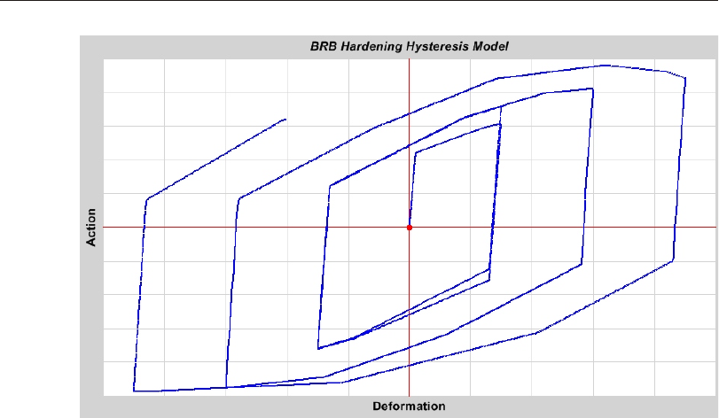
Ac cu mu lated plas tic de for ma tion can oc cur un der cy clic load ing of con stant am pli -
tude.
For this model, the fol low ing pa ram e ters are re quired:
•Sep a rately for ten sion (pos i tive) and com pres sion (neg a tive) de for ma tions
–Hard en ing fac tor at max i mum de for ma tion, h, where h ³ 1.0.
–Max i mum plas tic de for ma tion level at full hard en ing, x2, as a mul ti ple of
yield de for ma tion, where x2 > 1.0
–Max i mum ac cu mu lated plas tic de for ma tion level at full hard en ing, x4, as a
mul ti ple of yield de for ma tion, where x4 > 1.0
–Ac cu mu lated de for ma tion weight ing fac tor, a, where 0.0 £ a £ 1.0.
The hard en ing fac tors scale the size of the back bone curve and hys ter esis loop in
the ac tion (stress/force/mo ment) di rec tion. Be cause the ac cu mu lated plas tic de for -
ma tion is con stantly in creas ing, it is rec om mended that the weight ing fac tor a gen -
er ally be small or zero.
For each in cre ment of de for ma tion:
98 Hys ter esis Models
CSI Analysis Reference Manual
Figure 24
BRB Hardening Hysteresis Model under Increasing Cyclic Load
with Hardening Factor h = 1.5

•The absolute max i mum pos i tive and neg a tive plas tic de for ma tions that have
oc curred up to this point in the anal y sis are determined, dposmax and dnegmax,
as well as the ac cu mu lated plas tic de for ma tion, dacc.
•Com par ing dposmax with the pos i tive de for ma tion level d2, ob tained by mul ti -
ply ing x2 by the pos i tive yield de for ma tion, a hard en ing fac tor hposmax can be
de ter mined by in ter po la tion. If dposmax > d2, then hposmax = h.
•Com par ing dacc with the pos i tive de for ma tion level d4, ob tained by mul ti ply -
ing x4 by the pos i tive yield de for ma tion, a hard en ing fac tor hposacc can be de -
ter mined by in ter po la tion. If dacc > d4, then hposacc = h
•The net hard en ing fac tor due to pos i tive de for ma tion, hpos, is com puted as
hahah
pos pospos
=+-
acc()max
1
•Fol low ing the same ap proach, the hard en ing fac tor due to neg a tive de for ma -
tion, hneg, is com puted us ing the cor re spond ing pa ram e ters for neg a tive de for -
ma tion.
Deg ra da tion does not oc cur dur ing monotonic load ing. How ever, upon load re ver -
sal, the curve for un load ing and re verse load ing in the op po site di rec tion is mod i -
fied ac cord ing to the hard en ing fac tor com puted for the last de for ma tion in cre ment.
This is done by scal ing the ac tion val ues in that di rec tion, in clud ing the back bone
curve for fur ther loading.
Im por tant! Pos i tive de for ma tion and the cor re spond ing hard en ing pa ram e ters only
af fect the neg a tive strength, and vice versa.
Note that if the hard en ing fac tor is equal to 1.0, this model de gen er ates to the ki ne -
matic hys ter esis model.
This be hav ior is il lus trated in Figure 24 (page 98).
Iso tro pic Hysteresis Model
This model is, in a sense, the op po site of the ki ne matic model. Plas tic de for ma tion
in one di rec tion “pushes” the curve for the other di rec tion away from it, so that both
di rec tions in crease in strength si mul ta neously. Un like the BRB hard en ing model,
the back bone curve it self does not in crease in strength, only the un load ing and re -
verse load ing be hav ior. Match ing pairs of points are linked. No ad di tional pa ram e -
ters are re quired for this model.
Un load ing and re verse load ing oc cur along a path par al lel to the elas tic line un til
the mag ni tude of the ac tion in the re verse di rec tion equals that of back bone curve at
Hys ter esis Models 99
Chapter VI Material Properties
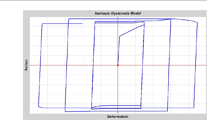
the same amount of de for ma tion in the re verse di rec tion, and then con tin ues along a
hor i zon tal se cant to the back bone curve.
When you de fine the points on the multi-lin ear curve, you should be aware that
sym met ri cal pairs of points will be linked, even if the curve is not sym met ri cal.
This gives you some con trol over the shape of the hysteretic loop.
This model dis si pates the most en ergy of all the mod els. This be hav ior is il lus trated
in Figure 25 (page 100).
Modified Darwin-Pecknold Concrete Model
A two-di men sional non lin ear con crete ma te rial model is avail able for use in the
lay ered shell. This model is based on the Dar win-Pecknold model, with con sid er -
ation of Vecchio-Col lins be hav ior. This model rep re sents the con crete com pres -
sion, crack ing, and shear be hav ior un der both monotonic and cy clic load ing, and
con sid ers the stress-strain com po nents s11-e11, s22-e22, and s33-e33. A state of
plane stress is as sumed.
100 Modified Darwin-Pecknold Concrete Model
CSI Analysis Reference Manual
Figure 25
Isotropic Hysteresis Model under Increasing Cyclic Load

The di rec tion of crack ing can change dur ing the load ing his tory, and the shear
strength is af fected by the ten sion strain in the ma te rial. The ax ial stress-strain
stress-strain curve spec i fied for the ma te rial is sim pli fied to ac count for ini tial stiff -
ness, yield ing, ul ti mate pla teau, and strength loss due to crush ing. Zero ten sile
strength is as sumed.
Hys ter esis is gov erned by the con crete hys ter esis model de scribed in the pre vi ous
topic, with the en ergy dis si pa tion fac tor f = 0.
The lay ered shell al lows this ma te rial to be used for mem brane and/or flex ural be -
hav ior and to be com bined with steel re in force ment placed in ar bi trary di rec tions
and lo ca tions. Trans verse (out-of-plane) shear is as sumed to be elas tic and iso tro pic
us ing the shear stiff ness G13 for both s13-g13 and s23-g23 be hav ior.
See sep a rate Tech ni cal Note “Mod i fied Darwin-Pecknold 2-D Re in forced Con -
crete Material Model” for more in for ma tion, avail able us ing the com mand Help >
Doc u men ta tion.
Time-dependent Properties
For any ma te rial hav ing a de sign type of con crete or tendon, you may spec ify time
de pend ent ma te rial prop er ties that are used for creep, shrink age, and ag ing ef fects
dur ing a staged-con struc tion anal y sis.
For more in for ma tion, see Topic “Staged Con struc tion” (page 439) in Chap ter
“Non lin ear Static Anal y sis.”
Properties
For con crete-type ma te ri als, you may spec ify:
•Ag ing pa ram e ters that de ter mine the change in modulus of elas tic ity with age
•Shrink age pa ram e ters that de ter mine the de crease in di rect strains with time
•Creep pa ram e ters that de ter mine the change in strain with time un der the ac tion
of stress
For tendon-type ma te ri als, re lax ation be hav ior may be spec i fied that de ter mines
the change in strain with time un der the ac tion of stress, sim i lar to creep.
Cur rently these be hav iors can be spec i fied for the CEB-FIP 1990 code (Comite
Euro-In ter na tional Du Beton, 1993) for con crete and ten don ma te ri als, and for con -
Time-dependent Properties 101
Chapter VI Material Properties

crete ma te ri als us ing the fol low ing codes: CEB-FIP 2010, ACI 290R-92, and
user-spec i fied curves.
Time-In te gra tion Control
For each ma te rial, you have the op tion to model the creep be hav ior by full in te gra -
tion or by us ing a Dirichlet se ries approximation.
With full in te gra tion, each in cre ment of stress dur ing the anal y sis be comes part of
the mem ory of the ma te rial. This leads to ac cu rate re sults, but for long anal y ses
with many stress in cre ments, this re quires com puter stor age and ex e cu tion time
that both in crease as the square of the num ber of in cre ments. For larger prob lems,
this can make so lu tion im prac ti cal.
Us ing the Dirichlet se ries ap prox i ma tion (Ketchum, 1986), you can choose a fixed
num ber of se ries terms that are to be stored. Each term is mod i fied by the stress in -
cre ments, but the num ber of terms does not change dur ing the anal y sis. This means
the stor age and ex e cu tion time in crease lin early with the num ber of stress in cre -
ments. Each term in the Dirichlet se ries can be thought of as a spring and dashpot
sys tem with a char ac ter is tic re lax ation time. The pro gram au to mat i cally chooses
these spring-dashpot sys tems based on the num ber of terms you re quest. You
should try dif fer ent num bers of terms and check the anal y sis re sults to make sure
that your choice is ad e quate.
It is rec om mended that you work with a smaller prob lem that is rep re sen ta tive of
your larger model, and com pare var i ous num bers of se ries terms with the full in te -
gra tion so lu tion to de ter mine the ap pro pri ate se ries ap prox i ma tion to use.
Design-Type
You may spec ify a de sign-type for each Ma te rial that in di cates how it is to be
treated for de sign by the SAP2000, ETABS, SAFE, or CSiBridge graph i cal user in -
ter face. The avail able de sign types are:
•Steel: Frame el e ments made of this ma te rial will be de signed ac cord ing to steel
de sign codes
•Con crete: Frame el e ments made of this ma te rial will be de signed ac cord ing to
con crete de sign codes
•Alu mi num: Frame el e ments made of this ma te rial will be de signed ac cord ing
to alu mi num de sign codes
102 Design-Type
CSI Analysis Reference Manual

•Cold-formed: Frame el e ments made of this ma te rial will be de signed ac cord ing
to cold-formed steel de sign codes
•None: Frame el e ments made of this ma te rial will not be de signed
When you choose a de sign type, ad di tional ma te rial prop er ties may be spec i fied
that are used only for de sign; they do not af fect the anal y sis. Con sult the on-line
help and de sign doc u men ta tion for fur ther in for ma tion on these de sign prop er ties.
Design-Type 103
Chapter VI Material Properties

104 Design-Type
CSI Analysis Reference Manual

Chapter VII
The Frame Element
The Frame el e ment is a very pow er ful el e ment that can be used to model beams,
col umns, braces, and trusses in pla nar and three-di men sional struc tures. Nonlinear
ma te rial be hav ior is avail able through the use of Frame Hinges.
Basic Topics for All Users
•Over view
•Joint Con nec tivity
•De grees of Free dom
•Lo cal Co or di nate Sys tem
•Sec tion Prop erties
•In ser tion Point
•End Off sets
•End Re leases
•Mass
•Self- Weight Load
•Con cen trated Span Load
•Dis trib uted Span Load
105

•In ter nal Force Out put
•Stress Output
Advanced Topics
•Ad vanced Lo cal Co or di nate Sys tem
•Prop erty Mod i fiers
•Non lin ear Properties
•Grav ity Load
•Tem pera ture Load
•Strain and De for ma tion Load
•Tar get-Force Load
Overview
The Frame ele ment uses a gen eral, three- dimensional, beam- column for mu la tion
which in cludes the ef fects of bi ax ial bend ing, tor sion, ax ial de for ma tion, and bi ax -
ial shear de for ma tions. See Bathe and Wil son (1976).
Struc tures that can be mod eled with this ele ment in clude:
•Three- dimensional frames
•Three- dimensional trusses
•Pla nar frames
•Pla nar gril lages
•Pla nar trusses
•Cables
A Frame el e ment is mod eled as a straight line con nect ing two points. In the graph i -
cal user in ter face, you can di vide curved ob jects into mul ti ple straight ob jects, sub -
ject to your spec i fi ca tion.
Each el e ment has its own lo cal co or di nate sys tem for de fin ing sec tion prop er ties
and loads, and for in ter pret ing out put.
The el e ment may be pris matic or non-pris matic. The non-pris matic for mu la tion al -
lows the el e ment length to be di vided into any num ber of seg ments over which
prop er ties may vary. The vari a tion of the bend ing stiff ness may be lin ear, par a -
106 Overview
CSI Analysis Reference Manual

bolic, or cu bic over each seg ment of length. The ax ial, shear, tor sional, mass, and
weight prop er ties all vary lin early over each seg ment.
In ser tion points and end off sets are avail able to ac count for the fi nite size of beam
and col umn in ter sec tions. The end off sets may be made par tially or fully rigid to
model the stiff en ing ef fect that can oc cur when the ends of an el e ment are em bed -
ded in beam and col umn in ter sec tions. End re leases are also avail able to model dif -
fer ent fix ity con di tions at the ends of the el e ment.
Each Frame el e ment may be loaded by grav ity (in any di rec tion), mul ti ple con cen -
trated loads, mul ti ple dis trib uted loads, strain and de for ma tion loads, and loads due
to tem per a ture change.
Tar get-force load ing is avail able that iteratively ap plies de for ma tion load to the el -
e ment to achieve a de sired ax ial force.
Ele ment in ter nal forces are pro duced at the ends of each ele ment and at a user-
specified number of equally- spaced out put sta tions along the length of the ele ment.
Ca ble be hav ior is usu ally best mod eled us ing the cat e nary Ca ble el e ment (page
165). How ever, there are cer tain cases where us ing Frame el e ments is nec es sary.
This can be achieved by add ing ap pro pri ate fea tures to a Frame element. You can
re lease the mo ments at the ends of the el e ments, al though we rec om mend that you
re tain small, re al is tic bend ing stiff ness in stead. You can also add non lin ear be hav -
ior as needed, such as the no-com pres sion prop erty, ten sion stiff en ing (p-delta ef -
fects), and large de flec tions. These fea tures re quire non lin ear anal y sis.
Joint Connectivity
A Frame el e ment is rep re sented by a straight line con nect ing two joints, I and j, un -
less mod i fied by in ser tion points as de scribed be low. The two joints must not share
the same lo ca tion in space. The two ends of the el e ment are de noted End I and End
J, re spec tively.
Insertion Point s
Some times the neu tral axis of the el e ment can not be con ve niently lo cated by joints
that con nect to other el e ments in the struc ture. You have the op tion to spec ify in -
ser tion points that lo cate the el e ment with re spect to the joints. The in ser tion
points con sists of a car di nal point spec i fied for the sec tion, plus in de pend ent joint
off sets spec i fied at each end of the el e ment. By de fault the car di nal point is the cen -
troid of the sec tion and the joints off sets are zero.
Joint Connectivity 107
Chapter VII The Frame Element

The two ends of the neu tral axis, con sid er ing the co or di nates of joints I and j plus
the in ser tion points, must not be co in ci dent. It is gen er ally rec om mended that the
off sets due to the in ser tion points be per pen dic u lar to the axis of the el e ment, al -
though this is not re quired.
For more in for ma tion on the in ser tion points, in clud ing how they af fect the lo cal
co or di nate sys tem of the el e ment, see Topic “In ser tion Points” (page 125).
Degrees of Freedom
The Frame el e ment ac ti vates all six de grees of free dom at both of its con nected
joints. If you want to model truss or ca ble el e ments that do not trans mit mo ments at
the ends, you may ei ther:
•Set the geo met ric Sec tion prop er ties j, i33, and i22 all to zero (a is non-zero;
as2 and as3 are ar bi trary), or
•Re lease both bend ing ro ta tions, R2 and R3, at both ends and re lease the tor -
sional ro ta tion, R1, at ei ther end
In ei ther case, the joint off sets and the end off sets must both be zero to avoid mo -
ments at the ends.
For more in for ma tion:
•See Topic “De grees of Free dom” (page 30) in Chap ter “Joints and De grees of
Free dom.”
•See Topic “Sec tion Prop er ties” (page 114) in this Chap ter.
•See Topic “End Off sets” (page 127) in this Chap ter.
•See Topic “End Re leases” (page 131) in this Chap ter.
Local Coordinate System
Each Frame ele ment has its own ele ment lo cal co or di nate sys tem used to de fine
sec tion prop er ties, loads and out put. The axes of this lo cal sys tem are de noted 1, 2
and 3. The first axis is di rected along the length of the el e ment at its centroid; the re -
main ing two axes lie in the plane per pen dicu lar to the ele ment with an ori en ta tion
that you spec ify.
It is im por tant that you clearly un der stand the defi ni tion of the ele ment lo cal 1- 2-3
co or di nate sys tem and its re la tion ship to the global X- Y-Z co or di nate sys tem. Both
108 Degrees of Freedom
CSI Analysis Reference Manual

sys tems are right- handed co or di nate sys tems. It is up to you to de fine lo cal sys tems
which sim plify data in put and in ter pre ta tion of re sults.
In most struc tures the defi ni tion of the ele ment lo cal co or di nate sys tem is ex -
tremely sim ple. The meth ods pro vided, how ever, pro vide suf fi cient power and
flexi bil ity to de scribe the ori en ta tion of Frame ele ments in the most com pli cated
situa tions.
Lo cal axes are first com puted for the el e ment with out con sid er ing the in ser tion
points, i.e., as if the neu tral axis con nects the two joints. These are called the nom i -
nal lo cal axes. If the in ser tion points shift the neu tral axis by a dif fer ent amount at
the two ends, the lo cal axes are then trans formed by pro jecting them onto the neu -
tral axis to de ter mine the ac tual lo cal co or di nate sys tem used for anal y sis.
The dis cus sion be low con sid ers the cal cu la tion of the nom i nal lo cal axes us ing the
joints. The trans for ma tion for the in ser tion points, if needed, is dis cussed later in
Topic “In ser tion Points”.
The sim plest method for com put ing the el e ment lo cal coordinate system, us ing the
de fault ori en ta tion and the Frame ele ment co or di nate an gle, is de scribed in this
topic. Ad di tional meth ods for de fin ing the Frame ele ment lo cal co or di nate sys tem
are de scribed in the next topic.
For more in for ma tion:
•See Chap ter “Co or di nate Sys tems” (page 11) for a de scrip tion of the con cepts
and ter mi nol ogy used in this topic.
•See Topic “Ad vanced Lo cal Co or di nate Sys tem” (page 110) in this Chap ter.
•See Topic “In ser tion Points” (page 125) in this Chapter.
Longitudinal Axis 1
The local axis 1 is al ways the lon gi tu di nal axis of the el e ment, the pos i tive di rec tion
be ing di rected from End I to End J. This axis is al ways lo cated at the cen troid of the
cross sec tion, and con nects joint I to joint j.
Default Orientation
The de fault ori en ta tion of the lo cal 2 and 3 axes is de ter mined by the re la tion ship
be tween the lo cal 1 axis and the global Z axis. The lo cal 1 axis is di rected along the
line be tween the joints I and j with out con sid er ing any off sets:
•The lo cal 1-2 plane is taken to be ver ti cal, i.e., par al lel to the Z axis
Local Coordinate System 109
Chapter VII The Frame Element

•The lo cal 2 axis is taken to have an up ward (+Z) sense un less the ele ment is ver -
ti cal, in which case the lo cal 2 axis is taken to be hori zon tal along the global +X
di rec tion
•The lo cal 3 axis is hori zon tal, i.e., it lies in the X-Y plane
An ele ment is con sid ered to be ver ti cal if the sine of the an gle be tween the lo cal 1
axis and the Z axis is less than 10-3.
The lo cal 2 axis makes the same an gle with the ver ti cal axis as the lo cal 1 axis
makes with the hori zon tal plane. This means that the lo cal 2 axis points ver ti cally
up ward for hori zon tal ele ments.
Coordinate Angle
The Frame ele ment co or di nate an gle, ang, is used to de fine ele ment ori en ta tions
that are dif fer ent from the de fault ori en ta tion. It is the an gle through which the lo cal
2 and 3 axes are ro tated about the posi tive lo cal 1 axis from the de fault ori en ta tion.
The ro ta tion for a posi tive value of ang ap pears coun ter clock wise when the lo cal
+1 axis is point ing to ward you.
For ver ti cal el e ments, ang is the an gle be tween the lo cal 2 axis and the hor i zon tal
+X axis. Oth er wise, ang is the an gle be tween the lo cal 2 axis and the ver ti cal plane
con tain ing the lo cal 1 axis. See Figure 26 (page 111) for ex am ples.
Advanced Local Coordinate System
By de fault, the ele ment lo cal co or di nate sys tem is de fined us ing the ele ment co or -
di nate an gle meas ured with re spect to the global +Z and +X di rec tions, as de scribed
in the pre vi ous topic. In cer tain mod el ing situa tions it may be use ful to have more
con trol over the speci fi ca tion of the lo cal co or di nate sys tem.
This topic de scribes how to de fine the ori en ta tion of the trans verse lo cal 2 and 3
axes with re spect to an ar bi trary ref er ence vec tor when the ele ment co or di nate an -
gle, ang, is zero. If ang is dif fer ent from zero, it is the an gle through which the lo cal
2 and 3 axes are ro tated about the posi tive lo cal 1 axis from the ori en ta tion de ter -
mined by the ref er ence vec tor. The lo cal 1 axis is al ways di rected from end I to end
J of the ele ment.
The dis cus sion be low con sid ers the cal cu la tion of the nom i nal lo cal axes us ing the
joints. The trans for ma tion for the in ser tion points, if needed, is dis cussed later in
Topic “In ser tion Points”.
110 Advanced Local Coordinate System
CSI Analysis Reference Manual
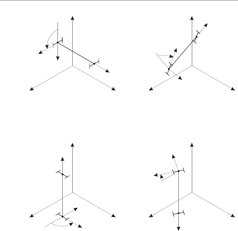
For more in for ma tion:
•See Chap ter “Co or di nate Sys tems” (page 11) for a de scrip tion of the con cepts
and ter mi nol ogy used in this topic.
Advanced Local Coordinate System 111
Chapter VII The Frame Element
Y
Y
Y
Y
Z
Z
Z
Z
X
X
X
X
ang=90°
ang=90°
ang=30°
ang=30°
2
2
2
2
3
3
3
3
1
1
1
1
i
i
i
i
j
j
j
j
Local 1 Axis is Parallel to +Y Axis
Local 2 Axis is Rotated 90° from Z-1 Plane
Local 1 Axis is Parallel to +Z Axis
Local 2 Axis is Rotated 90° from X-1 Plane
Local 1 Axis is Parallel to –Z Axis
Local 2 Axis is Rotated 30° from X-1 Plane
Local 1 Axis is Not Parallel to X, Y, or Z Axes
Local 2 Axis is Rotated 30° from Z-1 Plane
Figure 26
The Frame Element Coordinate Angle with Respect to the Default Orientation

•See Topic “Lo cal Co or di nate Sys tem” (page 108) in this Chap ter.
•See Topic “In ser tion Points” (page 125) in this Chap ter.
Reference Vector
To de fine the trans verse lo cal axes 2 and 3, you spec ify a ref er ence vec tor that is
par al lel to the de sired 1-2 or 1-3 plane. The ref er ence vec tor must have a posi tive
pro jec tion upon the cor re spond ing trans verse lo cal axis (2 or 3, re spec tively). This
means that the posi tive di rec tion of the ref er ence vec tor must make an an gle of less
than 90° with the posi tive di rec tion of the de sired trans verse axis.
To de fine the ref er ence vec tor, you must first spec ify or use the de fault val ues for:
•A pri mary co or di nate di rec tion pldirp (the de fault is +Z)
•A sec on dary co or di nate di rec tion pldirs (the de fault is +X). Di rec tions pldirs
and pldirp should not be par al lel to each other un less you are sure that they are
not par al lel to lo cal axis 1
•A fixed co or di nate sys tem csys (the de fault is zero, in di cat ing the global co or -
di nate sys tem)
•The lo cal plane, lo cal, to be de ter mined by the ref er ence vec tor (the de fault is
12, in di cat ing plane 1-2)
You may op tion ally spec ify:
•A pair of joints, plveca and plvecb (the de fault for each is zero, in di cat ing the
cen ter of the ele ment). If both are zero, this op tion is not used
For each ele ment, the ref er ence vec tor is de ter mined as fol lows:
1. A vec tor is found from joint plveca to joint plvecb. If this vec tor is of fi nite
length and is not par al lel to lo cal axis 1, it is used as the ref er ence vec tor Vp
2. Oth er wise, the pri mary co or di nate di rec tion pldirp is evalu ated at the cen ter of
the ele ment in fixed co or di nate sys tem csys. If this di rec tion is not par al lel to
lo cal axis 1, it is used as the ref er ence vec tor Vp
3. Oth er wise, the sec on dary co or di nate di rec tion pldirs is evalu ated at the cen ter
of the ele ment in fixed co or di nate sys tem csys. If this di rec tion is not par al lel to
lo cal axis 1, it is used as the ref er ence vec tor Vp
4. Oth er wise, the method fails and the analy sis ter mi nates. This will never hap pen
if pldirp is not par al lel to pldirs
112 Advanced Local Coordinate System
CSI Analysis Reference Manual
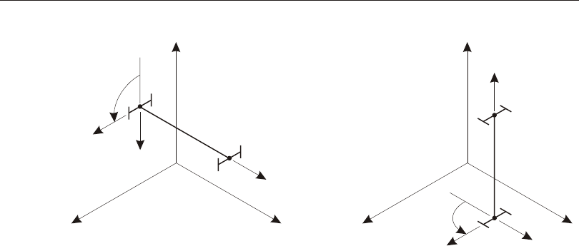
A vec tor is con sid ered to be par al lel to lo cal axis 1 if the sine of the an gle be tween
them is less than 10-3.
The use of the Frame ele ment co or di nate an gle in con junc tion with co or di nate di -
rec tions that de fine the ref er ence vec tor is il lus trated in Figure 27 (page 113). The
use of joints to de fine the ref er ence vec tor is shown in Figure 28 (page 114).
Determining Transverse Axes 2 and 3
The pro gram uses vec tor cross prod ucts to de ter mine the trans verse axes 2 and 3
once the ref er ence vec tor has been speci fied. The three axes are rep re sented by the
three unit vec tors V1, V2 and V3, re spec tively. The vec tors sat isfy the cross- product
re la tion ship:
VVV
123
=´
The trans verse axes 2 and 3 are de fined as fol lows:
•If the ref er ence vec tor is par al lel to the 1-2 plane, then:
VVV
31
=´p and
VVV
231
=´
Advanced Local Coordinate System 113
Chapter VII The Frame Element
X
Y
ZX
Y
Z
ang=90°
ang=90°
2
2
3
3
1
1
i
i
j
j
Local 1 Axis is Not Parallel to pldirp (+Y)
Local 2 Axis is Rotated 90° from Y-1 Plane
Local 1 Axis is Parallel to pldirp (+Y)
Local 2 Axis is Rotated 90° from X-1 Plane
pldirp = +Y
pldirs = –X
local = 12
Figure 27
The Frame Element Coordinate Angle with Respect to Coordinate Directions

•If the ref er ence vec tor is par al lel to the 1-3 plane, then:
VVV
21
=´
p and
VVV
312
=´
In the com mon case where the ref er ence vec tor is per pen dicu lar to axis V1, the
trans verse axis in the se lected plane will be equal to Vp.
Section Properties
A Frame Sec tion is a set of ma te rial and geo met ric prop er ties that de scribe the
cross- section of one or more Frame ele ments. Sec tions are de fined in de pend ently
of the Frame ele ments, and are as signed to the ele ments.
Sec tion prop er ties are of two ba sic types:
•Pris matic — all prop er ties are con stant along the full ele ment length
•Non- prismatic — the prop er ties may vary along the ele ment length
114 Section Properties
CSI Analysis Reference Manual
Y
Z
Joint j
Axis 1
Axis 2
X
Axis 3
Joint i
V (b)
p
V (a)
p
100
101
102
The following two specifications are equivalent:
(a) local=12, plveca=0, plvecb=100
(b) local=13, plveca=101, plvecb=102
Plane 1-3
Plane 1-2
Figure 28
Using Joints to Define the Frame Element Local Coordinate System

Non- prismatic Sec tions are de fined by re fer ring to two or more pre vi ously de fined
pris matic Sec tions.
All of the fol low ing sub top ics, ex cept the last, de scribe the defi ni tion of pris matic
Sec tions. The last sub topic, “Non- prismatic Sec tions”, de scribes how pris matic
Sec tions are used to de fine non- prismatic Sec tions.
Local Coordinate System
Sec tion prop er ties are de fined with re spect to the lo cal co or di nate sys tem of a
Frame ele ment as fol lows:
•The 1 di rec tion is along the axis of the ele ment. It is nor mal to the Sec tion and
goes through the in ter sec tion of the two neu tral axes of the Sec tion.
•The 2 and 3 di rec tions are par al lel to the neu tral axes of the Sec tion. Usu ally the
2 di rec tion is taken along the ma jor di men sion (depth) of the Sec tion, and the 3
di rec tion along its mi nor di men sion (width), but this is not re quired.
See Topic “Lo cal Co or di nate Sys tem” (page 108) in this Chap ter for more in for ma -
tion.
Material Properties
The ma te rial prop er ties for the Sec tion are speci fied by ref er ence to a previously-
defined Ma te rial. Iso tropic ma te rial prop er ties are used, even if the Ma te rial se -
lected was de fined as or tho tropic or ani sotropic. The ma te rial prop er ties used by
the Sec tion are:
•The modu lus of elas tic ity, e1, for ax ial stiff ness and bend ing stiff ness
•The shear modu lus, g12, for tor sional stiff ness and trans verse shear stiff ness
•The co ef fi cient of ther mal ex pan sion, a1, for ax ial ex pan sion and ther mal
bend ing strain
•The mass den sity, m, for com put ing ele ment mass
•The weight den sity, w, for com put ing Self- Weight and Grav ity Loads
The ma te rial prop er ties e1, g12, and a1 are all ob tained at the ma te rial tem pera ture
of each in di vid ual Frame ele ment, and hence may not be unique for a given Sec tion.
See Chap ter “Ma te rial Prop er ties” (page 69) for more in for ma tion.
Section Properties 115
Chapter VII The Frame Element

Geometric Properties and Section Stiffnesses
Six ba sic geo met ric prop er ties are used, to gether with the ma te rial prop er ties, to
gen er ate the stiff nesses of the Sec tion. These are:
•The cross- sectional area, a. The ax ial stiff ness of the Sec tion is given by ae1×;
•The mo ment of in er tia, i33, about the 3 axis for bend ing in the 1-2 plane, and
the mo ment of in er tia, i22, about the 2 axis for bend ing in the 1-3 plane. The
cor re spond ing bend ing stiff nesses of the Sec tion are given by i33e1× and
i22e1×;
•The tor sional con stant, j. The tor sional stiff ness of the Sec tion is given by
jg12×. Note that the tor sional con stant is not the same as the po lar mo ment of
in er tia, ex cept for cir cu lar shapes. See Roark and Young (1975) or Cook and
Young (1985) for more in for ma tion.
•The shear ar eas, as2 and as3, for trans verse shear in the 1-2 and 1-3 planes, re -
spec tively. The cor re spond ing trans verse shear stiff nesses of the Sec tion are
given by as2g12× and as3g12×. For mu lae for cal cu lat ing the shear ar eas of
typi cal sec tions are given in Figure 29 (page 117).
Set ting a, j, i33, or i22 to zero causes the cor re spond ing sec tion stiff ness to be zero.
For ex am ple, a truss mem ber can be mod eled by set ting j = i33 = i22 = 0, and a pla -
nar frame mem ber in the 1-2 plane can be mod eled by set ting j = i22 = 0.
Set ting as2 or as3 to zero causes the cor re spond ing trans verse shear de for ma tion to
be zero. In ef fect, a zero shear area is in ter preted as be ing in fi nite. The trans verse
shear stiff ness is ig nored if the cor re spond ing bend ing stiff ness is zero.
Shape Type
For each Sec tion, the six geo met ric prop er ties (a, j, i33, i22, as2 and as3) may be
speci fied di rectly, com puted from speci fied Sec tion di men sions, or read from a
speci fied prop erty da ta base file. This is de ter mined by the shape type, shape, speci -
fied by the user:
•If shape=GENERAL (gen eral sec tion), the six geo met ric prop er ties must be
ex plic itly spec i fied
•If shape=RECTANGLE, PIPE, BOX/TUBE, I/WIDE FLANGE, or one of
sev eral oth ers of fered by the program, the six geo met ric prop er ties are auto -
mati cally cal cu lated from speci fied Sec tion di men sions as de scribed in “Auto -
matic Sec tion Prop erty Cal cu la tion” be low, or ob tained from a speci fied prop -
erty da ta base file. See “Sec tion Prop erty Da ta base Files” be low.
116 Section Properties
CSI Analysis Reference Manual
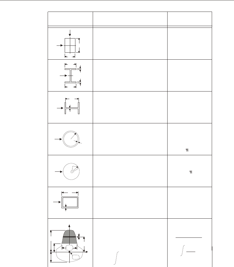
•If shape=SD SEC TION (Sec tion De signer Sec tion), you can cre ate your own
ar bi trary Sec tions us ing the Sec tion De signer util ity within the pro gram, and
Section Properties 117
Chapter VII The Frame Element
tf
tf
bf
bf
Section Description Effective
Shear Area
d
b
Rectangular Section
Shear Forces parallel to the b or d
directions
bd
5/6
Wide Flange Section
Shear Forces parallel to flange
tfbf
5/3
w
Wide Flange Section
Shear Forces parallel to web twd
d
t
r
t
Thin Walled
Circular Tube Section
Shear Forces from any direction
(0.9 - 0.4 s) A
s = (r - t) / r
where
A = (2r - t) t
rSolid Circular Section
Shear Forces from any direction 0.9 r 2
d
t
2td
Q(Y) = n b(n) dn
y
General Section
Shear Forces parallel to
I = moment of inertia of
Ix
2
(y) dy
Q2
b(y)
yb
Y
X
n
dn
y
yb
b(y)
n.a.
Thin Walled
Rectangular Tube Section
Shear Forces parallel to
d-direction
Y-direction
section about X-X
x
yt
yt
yt
Figure 29
Shear Area Formulae

the six geo met ric prop er ties are au to mat i cally cal cu lated. See “Sec tion De -
signer Sec tions” be low.
•If shape=NONPRISMATIC, the Sec tion is in ter po lated along the length of the
el e ment from pre vi ously de fined Sec tions as de scribed in “Nonprismatic Sec -
tion” be low.
Automatic Section Property Calculation
The six geo met ric Sec tion prop er ties can be auto mati cally cal cu lated from speci -
fied di men sions for the sim ple shapes shown in Figure 30 (page 119), and for oth ers
of fered by the program. The re quired di men sions for each shape are shown in the
fig ure.
Note that the di men sion t3 is the depth of the Sec tion in the 2 di rec tion and con trib -
utes pri mar ily to i33.
Section Property Database Files
Geo met ric Sec tion prop er ties may be ob tained from one or more Sec tion prop erty
da ta base files. Several da ta base files are cur rently sup plied with SAP2000,
ETABS, or CSiBridge that provide prop er ties for dif fer ent re gions, codes, and
man u fac tur ers. Their for mat and con tent may be dif fer ent for each prod uct. Ad di -
tional prop erty da ta base files may cre ated by the user or may be avail able from
other sources.
The geo met ric prop er ties are stored in the length units speci fied when the da ta base
file was cre ated. These are auto mati cally con verted to the ap pro pri ate units when
used in a model. Dif fer ent frame sec tions can be ob tained from dif fer ent database
files for the same model.
Sec tion-De signer Sec tions
Sec tion De signer is a sep a rate util ity built into SAP2000, ETABS, and CSiBridge
that can be used to cre ate your own frame sec tion prop er ties. You can build sec tions
of ar bi trary ge om e try and com bi na tions of ma te ri als. The ba sic anal y sis geo met ric
prop er ties (areas, mo ments of in er tia, and tor sional con stant) are com puted and
used for anal y sis. In ad di tion, Sec tion De signer can com pute non lin ear frame hinge
prop er ties.
For more in for ma tion, see the on-line help within Sec tion De signer.
118 Section Properties
CSI Analysis Reference Manual
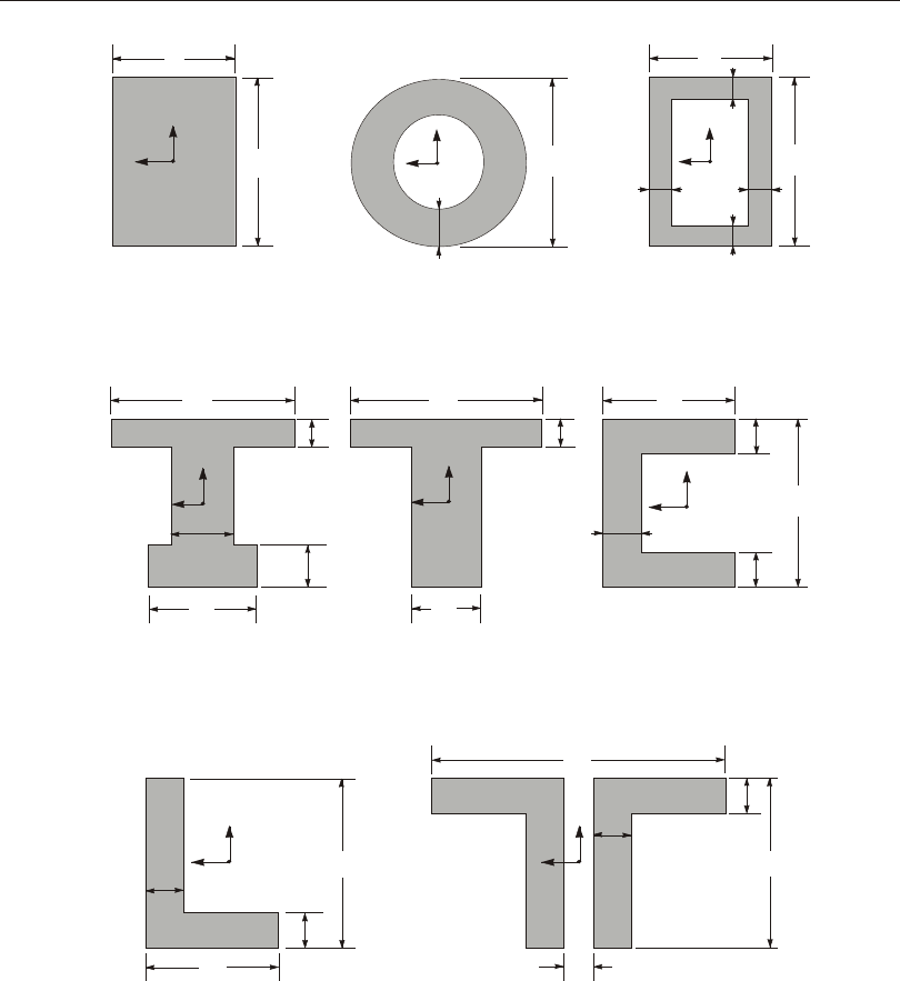
Section Properties 119
Chapter VII The Frame Element
SH = TSH = I SH = C
SH = L SH = 2L
SH = R SH = P SH = B
3
2
t3
tw
t3
t2
tf
tf
tw tw
2
3
t2
t3
3
2
t2t
tfb
tft
t2b
tw
3
22
3t3
tf
tf
tf
t2
tw
t2
tw
dis
tf
2
3
22
33
t2
t2
tf
t3 t3
tw
tw
Figure 30
Automatic Section Property Calculation

Additional Mass and Weight
You may spec ify mass and/or weight for a Sec tion that acts in ad di tion to the mass
and weight of the ma te rial. The ad di tional mass and weight are speci fied per unit of
length us ing the pa rame ters mpl and wpl, re spec tively. They could be used, for ex -
am ple, to rep re sent the ef fects of non struc tural ma te rial that is at tached to a Frame
ele ment.
The ad di tional mass and weight act re gard less of the cross- sectional area of the
Sec tion. The de fault val ues for mpl and wpl are zero for all shape types.
Non-prismatic Sections
Non- prismatic Sec tions may be de fined for which the prop er ties vary along the ele -
ment length. You may spec ify that the ele ment length be di vided into any number
of seg ments; these do not need to be of equal length. Most com mon situa tions can
be mod eled us ing from one to five seg ments.
The varia tion of the bend ing stiff nesses may be lin ear, para bolic, or cu bic over each
seg ment of length. The ax ial, shear, tor sional, mass, and weight prop er ties all vary
line arly over each seg ment. Sec tion prop er ties may change dis con tinu ously from
one seg ment to the next.
See Figure 31 (page 122) for ex am ples of non- prismatic Sec tions.
Segment Lengths
The length of a non- prismatic seg ment may be speci fied as ei ther a vari able length,
vl, or an ab so lute length, l. The de fault is vl = 1.
When a non- prismatic Sec tion is as signed to an ele ment, the ac tual lengths of each
seg ment for that ele ment are de ter mined as fol lows:
•The clear length of the ele ment, Lc, is first cal cu lated as the to tal length mi nus
the end off sets:
LL
c=-+()ioffjoff
See Topic “End Off sets” (page 127) in this Chap ter for more in for ma tion.
•If the sum of the ab so lute lengths of the seg ments ex ceeds the clear length, they
are scaled down pro por tion ately so that the sum equals the clear length. Oth er -
wise the ab so lute lengths are used as speci fied.
•The re main ing length (the clear length mi nus the sum of the ab so lute lengths) is
di vided among the seg ments hav ing vari able lengths in the same pro por tion as
120 Section Properties
CSI Analysis Reference Manual

the speci fied lengths. For ex am ple, for two seg ments with vl = 1 and vl = 2, one
third of the re main ing length would go to the first seg ment, and two thirds to
the sec ond seg ment.
Starting and Ending Sections
The prop er ties for a seg ment are de fined by speci fy ing:
•The la bel, seci, of a pre vi ously de fined pris matic Sec tion that de fines the prop -
er ties at the start of the seg ment, i.e., at the end clos est to joint I.
•The la bel, secj, of a pre vi ously de fined pris matic Sec tion that de fines the prop -
er ties at the end of the seg ment, i.e., at the end clos est to joint j. The start ing and
end ing Sec tions may be the same if the prop er ties are con stant over the length
of the seg ment.
The Ma te rial would nor mally be the same for both the start ing and end ing Sec tions
and only the geo met ric prop er ties would dif fer, but this is not re quired.
Variation of Properties
Non- prismatic Sec tion prop er ties are in ter po lated along the length of each seg ment
from the val ues at the two ends.
The varia tion of the bend ing stiff nesses, i33×e1 and i22×e1, are de fined by speci fy -
ing the pa rame ters eivar33 and eivar22, re spec tively. As sign val ues of 1, 2, or 3 to
these pa rame ters to in di cate varia tion along the length that is lin ear, para bolic, or
cu bic, re spec tively.
Spe cifi cally, the eivar33-th root of the bend ing stiff ness in the 1-2 plane:
eivar33i33e1×
var ies line arly along the length. This usu ally cor re sponds to a lin ear varia tion in
one of the Sec tion di men sions. For ex am ple, re fer ring to Figure 30 (page 119): a
lin ear varia tion in t2 for the rec tan gu lar shape would re quire eivar33=1, a lin ear
varia tion in t3 for the rec tan gu lar shape would re quire eivar33=3, and a lin ear
varia tion in t3 for the I- shape would re quire eivar33=2.
The in ter po la tion of the bend ing stiff ness in the 1-2 plane, i22e1×, is de fined in the
same man ner by the pa rame ter eivar22.
The re main ing prop er ties are as sumed to vary line arly be tween the ends of each
seg ment:
Section Properties 121
Chapter VII The Frame Element
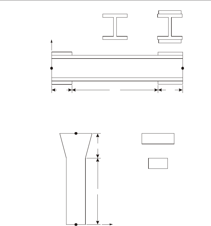
•Stiff nesses: ae1×, jg12×, as2g12×, and as3g12×
•Mass: a×m + mpl
122 Section Properties
CSI Analysis Reference Manual
Axis 2
Axis 2
End I
End I
End J
End J
l=24
seci=B
secj=B
vl=1
seci=A
secj=A
l=30
seci=B
secj=B
vl=1
l=50
seci=A
secj=A
seci=A
secj=B
eivar33=3
Steel Beam with Cover Plates at Ends
Concrete Column with Flare at Top
Section B
Section B
Section A
Section A
Figure 31
Examples of Non-prismatic Sections

•Weight: a×w + wpl
If a shear area is zero at ei ther end, it is taken to be zero along the full seg ment, thus
elim i nat ing all shear de for ma tion in the cor re spond ing bend ing plane for that seg -
ment.
Advanced Location Parameters
Normally the full vari a tion of a non-pris matic sec tion oc curs over the length of a
sin gle frame ob ject. When the ob ject is auto-meshed into mul ti ple frame el e ments,
each el e ment will rep re sent a por tion of the full non-pris matic length.
Sim i larly, if you ex plic itly di vide a non-prismatic frame ob ject into mul ti ple frame
ob jects, it is nec es sary to spec ify for each frame ob ject what por tion of the to tal
nonprismatic vari a tion ap plies to each ob ject. This is done by as sign ing to each ob -
ject:
•The length of the to tal non-pris matic sec tion. This will be the same for each ob -
ject de rived from a sin gle par ent frame ob ject, and will be lon ger than each de -
rived ob ject.
•The rel a tive lo ca tion
For ex am ple, con sider a sin gle non-pris matic frame ob ject of length 8 me ters, di -
vided into four equal-length ob jects. For each de rived ob ject, the as signed
non-pris matic length should be 8 me ters and the rel a tive start ing lo ca tions should
be 0.0, 0.25, 0.5, and 0.75, re spec tively.
Effect upon End Offsets
Prop er ties vary only along the clear length of the ele ment. Sec tion prop er ties within
end off set ioff are con stant us ing the start ing Sec tion of the first seg ment. Sec tion
prop er ties within end off set joff are con stant us ing the end ing Sec tion of the last
seg ment.
See Topic “End Off sets” (page 127) in this Chap ter for more in for ma tion.
Property Modifiers
You may spec ify scale fac tors to mod ify the com puted sec tion prop er ties. These
may be used, for ex am ple, to ac count for crack ing of con crete or for other fac tors
not eas ily de scribed in the ge om e try and ma te rial prop erty val ues. In di vid ual
modifiers are avail able for the fol low ing eight terms:
Property Modifiers 123
Chapter VII The Frame Element

•The ax ial stiff ness ae1×
•The shear stiffnesses as2g12× and as3g12×
•The tor sional stiff ness jg12×
•The bend ing stiffnesses i33e1× and i22e1×
•The sec tion mass a×m + mpl
•The sec tion weight a×w + wpl
You may spec ify multi pli ca tive fac tors in two places:
•As part of the def i ni tion of the sec tion prop erty
•As an as sign ment to in di vid ual el e ments.
If mod i fi ers are as signed to an el e ment and also to the sec tion prop erty used by that
el e ment, then both sets of fac tors mul ti ply the sec tion prop er ties. Mod i fiers can not
be as signed di rectly to a nonprismatic sec tion prop erty, but any mod i fi ers ap plied
to the sec tions con trib ut ing to the nonprismatic sec tion are used.
When per form ing steel frame de sign us ing the Di rect Anal y sis Method of de sign
code AISC 360-05/IBC2006, fur ther prop erty mod i fi ers may be com puted by the
de sign al go rithm for the ax ial and bend ing stiffnesses. In this case, the com puted
mod i fi ers are mul ti plied by those as signed to the el e ment and those spec i fied in the
sec tion prop erty used by that el e ment, so that all three sets of fac tors ap ply.
Named Prop erty Sets
In ad di tion to di rectly as sign ing prop erty mod i fi ers to frame el e ments, you can ap -
ply them to a frame el e ment in a staged-con struc tion Load Case us ing a Named
Prop erty Set of Frame Prop erty Mod i fi ers. A Named Prop erty Set in cludes the
same eight fac tors above that can be as signed to an el e ment.
When a Named Prop erty Set is ap plied to an el e ment in a par tic u lar stage of a Load
Case, it re places only the val ues that are as signed to the el e ment or that had been ap -
plied in a pre vi ous stage; values com puted by the Di rect Anal y sis Method of de sign
are also re placed. How ever, property mod i fi ers spec i fied with the sec tion prop erty
re main in force and are not af fected by the ap pli ca tion of a Named Prop erty Set.
The net ef fect is to use the fac tors spec i fied in the Named Prop erty Set mul ti plied
by the fac tors spec i fied in the sec tion prop erty.
When prop erty mod i fi ers are changed in a staged con struc tion Load Case, they do
not change the re sponse of the struc ture up to that stage, but only af fect sub se quent
re sponse. In other words, the ef fect is in cre men tal. For ex am ple, con sider a can ti le -
124 Property Modifiers
CSI Analysis Reference Manual

ver with only de fault (unity) prop erty mod i fi ers, and a staged con struc tion case as
follows:
•Stage 1: Self-weight load is ap plied, re sult ing in a tip de flec tion of 1.0 and
a sup port mo ment of 1000.
•Stage 2: Named Prop erty Set “A” is ap plied that mul ti plies all stiffnesses
by 2.0, and the mass and weight by 1.0. The tip de flec tion and sup port mo -
ment do not change.
•Stage 3: Self-weight load is ap plied again (incrementally). The re sult ing
tip de flec tion is 1.5 and the sup port mo ment is 2000. Com pared to Stage 1,
the same in cre men tal load is ap plied, but the struc ture is twice as stiff.
• Stage 4: Named Prop erty Set “B” is ap plied that mul ti plies all stiffnesses,
as well as the mass and weight, by 2.0. The tip de flec tion and sup port mo -
ment do not change.
•Stage 5: Self-weight load is ap plied again (incrementally). The re sult ing
tip de flec tion is 2.5 and the sup port mo ment is 4000. Com pared to Stage 1,
twice the in cre men tal load is ap plied, and the struc ture is twice as stiff
In ser tion Points
The lo cal 1 axis of the el e ment runs along the neu tral axis of the sec tion, i.e., at the
cen troid of the sec tion. By de fault this con nects to the joints I and j at the ends of
the el e ment. How ever, it is of ten con ve nient to spec ify an other lo ca tion on the sec -
tion, such as the top of a beam or an out side cor ner of a col umn, to con nect to the
joints.
There is a set of pre-de fined lo ca tions within the sec tion, called car di nal points,
that can be used for this pur pose. The avail able choices are shown in Figure 32
(page 126). The de fault lo ca tion is point 10, the centroid.
You can fur ther off set the car di nal point from the joint by spec i fy ing joint off sets.
The joint off sets to gether with the car di nal point make up the in ser tion point as -
sign ment. The to tal off set from the joint to the cen troid is given as the sum of the
joint off set plus the dis tance from the car di nal point to the cen troid.
This fea ture is use ful, as an ex am ple, for mod el ing beams and col umns when the
beams do not frame into the cen ter of the col umn. Figure 33 (page 128) shows an el -
e va tion and plan view of a com mon fram ing ar range ment where the ex te rior beams
are off set from the col umn cen ter lines to be flush with the ex te rior of the build ing.
In ser tion Points 125
Chapter VII The Frame Element
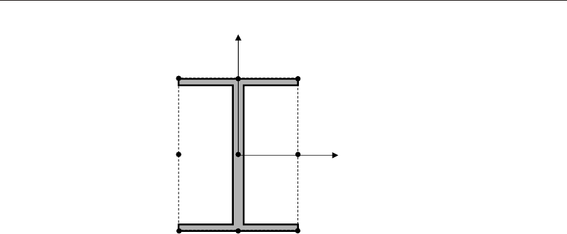
Also shown in this fig ure are the car di nal points for each mem ber and the joint off -
set di men sions.
Off sets along the neu tral axis of the el e ment are usu ally spec i fied us ing end off sets
rather than in ser tion points. See topic “End Off sets” (page 127). End off sets are
treated as part of the length of the el e ment, have el e ment prop er ties and loads, and
may or may not be rigid.
Off sets due to in ser tion points are ex ter nal to the el e ment and do not have any mass
or loads. In ter nally the anal y sis rep re sents the in ser tion point by a fully rigid con -
straint that con nects the neu tral axis to the joints.
Lo cal Axes
The in ser tion points can in ter act sig nif i cantly with the el e ment lo cal co or di nate
sys tem. As de scribed pre vi ously, the nom i nal lo cal axes are com puted for the de -
fault in ser tion points, such that the lo cal 1 axis con nects joints I and j.
The cen troids of the sec tion are then lo cated us ing both the car di nal point and joint
off sets. Joint off sets may be spec i fied us ing the global co or di nate sys tem or the el e -
ment lo cal sys tem. In the latter case, the nom i nal lo cal axes are used for this pur -
pose.
126 In ser tion Points
CSI Analysis Reference Manual
Note: For doubly symmetric members such as
this one, cardinal points 5, 10, and 11 are
the same.
123
4
5
10
11 6
789
1. Bottom left
2. Bottom center
3. Bottom right
4. Middle left
5. Middle center
6. Middle right
7. Top left
8. Top center
9. Top right
10. Centroid
11. Shear center
2 axis
3 axis
Figure 32
Frame Cardinal Points

If the neutral axis of the frame sec tion re mains par al lel to the nominal lo cal 1 axis
(the line con nect ing the two joints), then no fur ther transformation is needed. The
el e ment lo cal axes are the same as the nom i nal axes.
If the neu tral axis has changed direction, then the el e ment lo cal co or di nate sys tem
is com puted as fol lows:
~~
VVV
312
=´ and
~~~
VVV
231
=´
where V1, V2, and V3 and the nom i nal lo cal axes com puted pre vi ously based on the
joints; and ~
V1, ~
V2, and ~
V3 are the trans formed lo cal axes used for anal y sis. If V2 is
ver ti cal, then ~
V3 will al ways be hor i zon tal. Note that the two sys tems are iden ti cal
if ~
VV
11
=, the usual case.
The nom i nal axes are used only for de ter min ing the di rec tion of joint offsets. The
trans formed axes are used for all anal y sis and de sign pur poses, in clud ing load ing
and re sults out put.
For non-pris matic el e ments with non-centroidal car di nal points, the lo cal 1 axis
may not be straight, and as a con se quence the lo cal 2 and 3 axes may change ori en -
ta tion be tween seg ments. This can be ex pected to cause jumps in the ax ial force,
shear, and mo ments. How ever, the change will be a small de vi a tion from the axes
that would have been cal cu lated for an el e ment with no in ser tion points.
End Offsets
Frame ele ments are mod eled as line ele ments con nected at points (joints). How -
ever, ac tual struc tural mem bers have fi nite cross- sectional di men sions. When two
ele ments, such as a beam and col umn, are con nected at a joint there is some over lap
of the cross sec tions. In many struc tures the di men sions of the mem bers are large
and the length of the over lap can be a sig nifi cant frac tion of the to tal length of a
con nect ing ele ment.
You may spec ify two end off sets for each ele ment us ing pa rame ters ioff and joff
cor re spond ing to ends I and J, re spec tively. End off set ioff is the length of over lap
for a given ele ment with other con nect ing ele ments at joint I. It is the dis tance from
the joint to the face of the con nec tion for the given ele ment. A simi lar defi ni tion ap -
plies to end off set joff at joint j. See Figure 34 (page 129).
End Offsets 127
Chapter VII The Frame Element
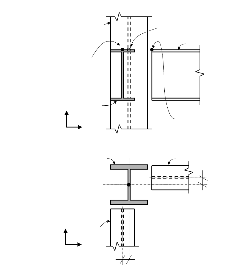
End off sets are auto mati cally cal cu lated by the SAP2000 graphi cal in ter face for
each ele ment based on the maxi mum Sec tion di men sions of all other ele ments that
con nect to that ele ment at a com mon joint.
128 End Offsets
CSI Analysis Reference Manual
Elevation
Cardinal
Point B2
B2
Cardinal
Point C1
B1
C1
Cardinal
Point B1
X
Z
X
Y
Plan
B2C1
B1
2"
2"
Figure 33
Example Showing Joint Offsets and Cardinal Points
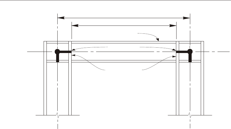
Clear Length
The clear length, de noted Lc, is de fined to be the length be tween the end off sets
(sup port faces) as:
LL
c=-+()ioffjoff
where L is the to tal ele ment length. See Figure 34 (page 129).
If end off sets are speci fied such that the clear length is less than 1% of the to tal ele -
ment length, the pro gram will is sue a warn ing and re duce the end off sets pro por -
tion ately so that the clear length is equal to 1% of the to tal length. Nor mally the end
off sets should be a much smaller pro por tion of the to tal length.
Rigid-end Factor
An analy sis based upon the centerline- to- centerline (joint- to- joint) ge ome try of
Frame ele ments may over es ti mate de flec tions in some struc tures. This is due to the
stiff en ing ef fect caused by over lap ping cross sec tions at a con nec tion. It is more
likely to be sig nifi cant in con crete than in steel struc tures.
End Offsets 129
Chapter VII The Frame Element
End Offsets
Horizontal
Member
Support Face
Total Length L
J
I
C
L
C
L
C
L
ioff joff
Clear Length Lc
Figure 34
Frame Element End Offsets

You may spec ify a rigid- end fac tor for each ele ment us ing pa rame ter rigid, which
gives the frac tion of each end off set that is as sumed to be rigid for bend ing and
shear de for ma tion. The length rigid×ioff, start ing from joint I, is as sumed to be
rigid. Simi larly, the length rigid×joff is rigid at joint j. The flexi ble length Lf of the
ele ment is given by:
LL
f=-+rigidioffjoff()
The rigid- zone off sets never af fect ax ial and tor sional de for ma tion. The full ele -
ment length is as sumed to be flexi ble for these de for ma tions.
The de fault value for rigid is zero. The maxi mum value of unity would in di cate that
the end off sets are fully rigid. You must use en gi neer ing judg ment to se lect the ap -
pro pri ate value for this pa rame ter. It will de pend upon the ge ome try of the con nec -
tion, and may be dif fer ent for the dif fer ent ele ments that frame into the con nec tion.
Typi cally the value for rigid would not ex ceed about 0.5.
Effect upon Non-prismatic Elements
At each end of a non- prismatic ele ment, the Sec tion prop er ties are as sumed to be
con stant within the length of the end off set. Sec tion prop er ties vary only along the
clear length of the ele ment be tween sup port faces. This is not af fected by the value
of the rigid- end fac tor, rigid.
See Sub topic “Non- prismatic Sec tions” (page 120) in this Chap ter for more in for -
ma tion.
Effect upon Internal Force Output
All in ter nal forces and mo ments are out put at the faces of the sup ports and at other
equally- spaced points within the clear length of the ele ment. No out put is pro duced
within the end off set, which in cludes the joint. This is not af fected by the value of
the rigid- end fac tor, rigid.
See Topic “In ter nal Force Out put” (page 144) in this Chap ter for more in for ma tion.
Effect upon End Releases
End re leases are al ways as sumed to be at the sup port faces, i.e., at the ends of the
clear length of the ele ment. If a mo ment or shear re lease is speci fied in ei ther bend -
ing plane at ei ther end of the ele ment, the end off set is as sumed to be rigid for bend -
130 End Offsets
CSI Analysis Reference Manual
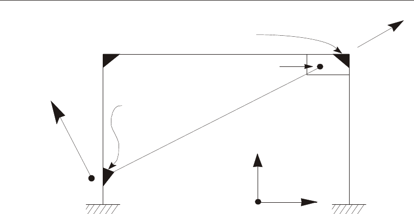
ing and shear in that plane at that end (i.e., it acts as if rigid = 1). This does not af -
fect the val ues of the rigid- end fac tor at the other end or in the other bend ing plane.
See Topic “End Re leases” (page 131) in this Chap ter for more in for ma tion.
End Releases
Nor mally, the three trans la tional and three ro ta tional de grees of free dom at each
end of the Frame ele ment are con tinu ous with those of the joint, and hence with
those of all other ele ments con nected to that joint. How ever, it is pos si ble to re lease
(dis con nect) one or more of the ele ment de grees of free dom from the joint when it
is known that the cor re spond ing ele ment force or mo ment is zero. The re leases are
al ways speci fied in the ele ment lo cal co or di nate sys tem, and do not af fect any other
ele ment con nected to the joint.
In the ex am ple shown in Figure 35 (page 131), the di ago nal ele ment has a mo ment
con nec tion at End I and a pin con nec tion at End J. The other two ele ments con nect -
ing to the joint at End J are con tinu ous. There fore, in or der to model the pin con di -
tion the ro ta tion R3 at End J of the di ago nal ele ment should be re leased. This as -
sures that the mo ment is zero at the pin in the di ago nal ele ment.
End Releases 131
Chapter VII The Frame Element
Axis 3
Axis 2
Axis 1
Continous
Joint
Z
Global
Continous
Joint
Pin Joint
I
J
X
For diagonal element: R3 is released at end J
Figure 35
Frame Element End Releases

Unstable End Releases
Any com bi na tion of end re leases may be speci fied for a Frame ele ment pro vided
that the ele ment re mains sta ble; this as sures that all load ap plied to the ele ment is
trans ferred to the rest of the struc ture. The fol low ing sets of re leases are un sta ble,
ei ther alone or in com bi na tion, and are not per mit ted.
•Re leas ing U1 at both ends;
•Re leas ing U2 at both ends;
•Re leas ing U3 at both ends;
•Re leas ing R1 at both ends;
•Re leas ing R2 at both ends and U3 at ei ther end;
•Re leas ing R3 at both ends and U2 at ei ther end.
Effect of End Offsets
End re leases are al ways ap plied at the sup port faces, i.e., at the ends of the ele ment
clear length. The pres ence of a mo ment or shear re lease will cause the end off set to
be rigid in the cor re spond ing bend ing plane at the cor re spond ing end of the ele -
ment.
See Topic “End Off sets” (page 127) in this Chap ter for more in for ma tion.
Named Prop erty Sets
In ad di tion to di rectly as sign ing end re leases to frame el e ments, you can ap ply them
to a frame el e ment in a staged-con struc tion Load Case us ing a Named Prop erty Set
of Frame Releases. A Named Prop erty Set in cludes the same op tions that can be as -
signed to an el e ment.
When prop erty mod i fi ers are changed in a staged con struc tion Load Case, they do
not change the re sponse of the struc ture up to that stage, but only af fect sub se quent
re sponse. In other words, the ef fect is in cre men tal. For ex am ple, con sider a beam
with as signed mo ment re leases that is added be tween two col umns in a staged con -
struc tion case as fol lows:
•Stage 1: The beam is added to an existing struc ture and self-weight is
applied. Be cause the el e ment has mo ment re leases as signed to it, the beam
is added as sim ply-sup ported and has no fixed-end mo ments. The
mid-span mo ment is 1000.
132 End Releases
CSI Analysis Reference Manual

•Stage 2: Named Prop erty Set “A” is ap plied that has no end re leases. The
mid-span mo ment does not change.
•Stage 3: Self-weight load is ap plied again (incrementally). The re sult ing
mid-span mo ment in creases to 1333, and the end span mo ments are -667
each.
This ex am ple il lus trates the com mon case where beams are ini tially added as sim -
ply-sup ported, then con nected to pro vide fully mo ment con ti nu ity. In an other com -
mon sit u a tion, two in de pend ent staged con struc tion cases can be con sid ered: One
for grav ity load where cer tain mem bers have mo ment re leases, and the other for lat -
eral load where the same mem bers have mo ment con ti nu ity. Each of these cases
can be used as the ba sis for fur ther lin ear or non lin ear Load Cases, and the re sults
con sid ered together for de sign.
Nonlinear Properties
Two types of non lin ear prop er ties are avail able for the Frame/Ca ble el e ment: ten -
sion/com pres sion lim its and plas tic hinges.
When non lin ear prop er ties are pres ent in the el e ment, they only af fect non lin ear
anal y ses. Lin ear anal y ses start ing from zero con di tions (the un stressed state) be -
have as if the non lin ear prop er ties were not pres ent. Lin ear anal y ses us ing the stiff -
ness from the end of a pre vi ous non lin ear anal y sis use the stiff ness of the non lin ear
prop erty as it ex isted at the end of the non lin ear case.
Ten sion/Com pres sion Limits
You may spec ify a max i mum ten sion and/or a max i mum com pres sion that a
frame/ca ble el e ment may take. In the most com mon case, you can de fine a no-com -
pres sion ca ble or brace by spec i fy ing the com pres sion limit to be zero.
If you spec ify a ten sion limit, it must be zero or a pos i tive value. If you spec ify a
com pres sion limit, it must be zero or a neg a tive value. If you spec ify a ten sion and
com pres sion limit of zero, the el e ment will carry no ax ial force.
The ten sion/com pres sion limit be hav ior is elas tic. Any ax ial ex ten sion be yond the
ten sion limit and ax ial short en ing be yond the com pres sion limit will oc cur with
zero ax ial stiff ness. These de for ma tions are re cov ered elastically at zero stiff ness.
Bending, shear, and tor sional be hav ior are not af fected by the ax ial nonlinearity.
Nonlinear Properties 133
Chapter VII The Frame Element

Plas tic Hinge
You may in sert plas tic hinges at any num ber of lo ca tions along the clear length of
the el e ment. De tailed de scrip tion of the be hav ior and use of plas tic hinges is pre -
sented in Chap ter “Frame Hinge Prop erties” (page 147).
Mass
In a dy namic analy sis, the mass of the struc ture is used to com pute in er tial forces.
The mass con trib uted by the Frame ele ment is lumped at the joints I and j. No in er -
tial ef fects are con sid ered within the ele ment it self.
The to tal mass of the ele ment is equal to the in te gral along the length of the mass
den sity, m, mul ti plied by the cross- sectional area, a, plus the ad di tional mass per
unit length, mpl.
For non- prismatic ele ments, the mass var ies line arly over each non- prismatic seg -
ment of the ele ment, and is con stant within the end off sets.
The to tal mass is ap por tioned to the two joints in the same way a sim i larly-dis trib -
uted trans verse load would cause re ac tions at the ends of a sim ply-sup ported beam.
The ef fects of end re leases are ig nored when ap por tion ing mass. The to tal mass is
ap plied to each of the three translational de grees of free dom: UX, UY, and UZ. No
mass mo ments of in er tia are com puted for the ro ta tional de grees of free dom.
For more in for ma tion:
•See Topic “Mass Den sity” (page 77) in Chap ter “Ma te rial Prop er ties.”
•See Topic “Sec tion Prop er ties” (page 114) in this Chap ter for the defi ni tion of
a and mpl.
•See Sub topic “Non- prismatic Sec tions” (page 120) in this Chap ter.
•See Topic “End Off sets” (page 127) in this Chap ter.
•See Topic “Mass Source” (page 334) in Chap ter “Load Pat terns”.
•See Chap ter “Static and Dy namic Analy sis” (page 341).
Self-Weight Load
Self- Weight Load ac ti vates the self- weight of all ele ments in the model. For a
Frame ele ment, the self- weight is a force that is dis trib uted along the length of the
134 Mass
CSI Analysis Reference Manual

ele ment. The mag ni tude of the self- weight is equal to the weight den sity, w, mul ti -
plied by the cross- sectional area, a, plus the ad di tional weight per unit length, wpl.
For non- prismatic ele ments, the self- weight var ies line arly over each non- prismatic
seg ment of the ele ment, and is con stant within the end off sets.
Self- Weight Load al ways acts down ward, in the global –Z di rec tion. You may
scale the self- weight by a sin gle scale fac tor that ap plies equally to all ele ments in
the struc ture.
For more in for ma tion:
•See Topic “Weight Den sity” (page 78) in Chap ter “Ma te rial Prop er ties” for the
defi ni tion of w.
•See Topic “Sec tion Prop er ties” (page 114) in this Chap ter for the defi ni tion of
a and wpl..
•See Sub topic “Non- prismatic Sec tions” (page 120) in this Chap ter.
•See Topic “End Off sets” (page 127) in this Chap ter.
•See Topic “Self- Weight Load” (page 325) in Chap ter “Load Pat terns.”
Gravity Load
Grav ity Load can be ap plied to each Frame ele ment to ac ti vate the self- weight of
the ele ment. Us ing Grav ity Load, the self- weight can be scaled and ap plied in any
di rec tion. Dif fer ent scale fac tors and di rec tions can be ap plied to each ele ment.
If all ele ments are to be loaded equally and in the down ward di rec tion, it is more
con ven ient to use Self- Weight Load.
For more in for ma tion:
•See Topic “Self- Weight Load” (page 134) in this Chap ter for the defi ni tion of
self- weight for the Frame ele ment.
•See Topic “Grav ity Load” (page 326) in Chap ter “Load Pat terns.”
Concentrated Span Load
The Con cen trated Span Load is used to ap ply con cen trated forces and mo ments at
ar bi trary lo ca tions on Frame ele ments. The di rec tion of load ing may be speci fied in
Gravity Load 135
Chapter VII The Frame Element
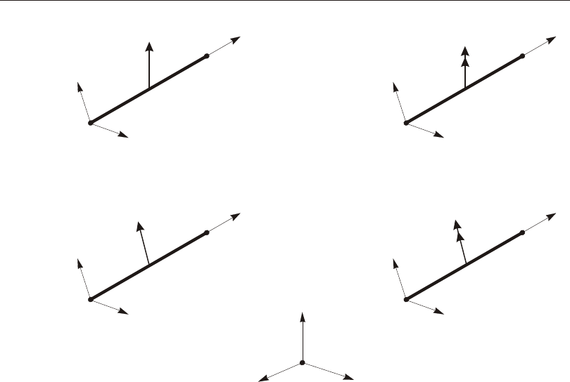
a fixed co or di nate sys tem (global or al ter nate co or di nates) or in the ele ment lo cal
co or di nate sys tem.
The lo ca tion of the load may be speci fied in one of the fol low ing ways:
•Speci fy ing a rela tive dis tance, rd, meas ured from joint I. This must sat isfy
01££rd. The rela tive dis tance is the frac tion of ele ment length;
•Speci fy ing an ab so lute dis tance, d, meas ured from joint I. This must sat isfy
0££dL, where L is the ele ment length.
Any number of con cen trated loads may be ap plied to each ele ment. Loads given in
fixed co or di nates are trans formed to the ele ment lo cal co or di nate sys tem. See
Figure 36 (page 136). Mul ti ple loads that are ap plied at the same lo ca tion are added
to gether.
See Chap ter “Load Pat terns” (page 321) for more in for ma tion.
136 Concentrated Span Load
CSI Analysis Reference Manual
XY
Z
Global
1
2
3
uz
1
2
3
u2
1
2
3
rz
1
2
3
r2
Global Z Force Global Z Moment
Local 2 Force Local 2 Moment
All loads applied
at rd=0.5
Figure 36
Examples of the Definition of Concentrated Span Loads

Distributed Span Load
The Dis trib uted Span Load is used to ap ply dis trib uted forces and mo ments on
Frame ele ments. The load in ten sity may be uni form or trape zoi dal. The di rec tion of
load ing may be speci fied in a fixed co or di nate sys tem (global or al ter nate co or di -
nates) or in the ele ment lo cal co or di nate sys tem.
See Chap ter “Load Pat terns” (page 321) for more in for ma tion.
Loaded Length
Loads may ap ply to full or par tial ele ment lengths. Mul ti ple loads may be ap plied to
a sin gle ele ment. The loaded lengths may over lap, in which case the ap plied loads
are ad di tive.
A loaded length may be speci fied in one of the fol low ing ways:
•Speci fy ing two rela tive dis tances, rda and rdb, meas ured from joint I. They
must sat isfy 01£<£rdardb. The rela tive dis tance is the frac tion of ele ment
length;
•Speci fy ing two ab so lute dis tances, da and db, meas ured from joint I. They
must sat isfy 0£<£dadbL, where L is the ele ment length;
•Speci fy ing no dis tances, which in di cates the full length of the ele ment.
Load Intensity
The load in ten sity is a force or mo ment per unit of length. Ex cept for the case of
pro jected loads de scribed be low, the in ten sity is meas ured per unit of ele ment
length.
For each force or mo ment com po nent to be ap plied, a sin gle load value may be
given if the load is uni formly dis trib uted. Two load val ues are needed if the load in -
ten sity var ies line arly over its range of ap pli ca tion (a trape zoi dal load).
See Figure 37 (page 138) and Figure 38 (page 139).
Projected Loads
A dis trib uted snow or wind load pro duces a load in ten sity (force per unit of ele ment
length) that is pro por tional to the sine of the an gle be tween the ele ment and the di -
rec tion of load ing. This is equiva lent to us ing a fixed load in ten sity that is meas ured
Distributed Span Load 137
Chapter VII The Frame Element
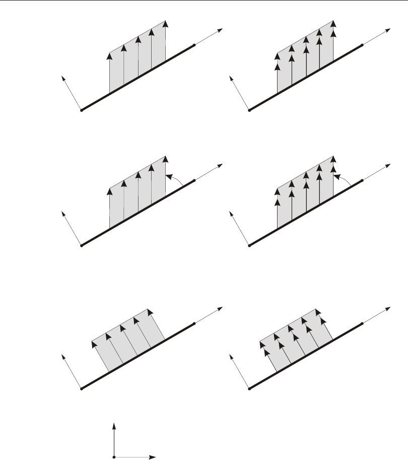
per unit of pro jected ele ment length. The fixed in ten sity would be based upon the
138 Distributed Span Load
CSI Analysis Reference Manual
X
Z
Global
All loads applied from rda=0.25 to rdb=0.75
1
2
1
2
1
2
1
2
1
2
1
2
q
uz rz
rzp
uzp
u2 r2
Y
q
Global Z Force Global Z Moment
Global Z Force on
Projected Length
(To be Scaled by sinq)
Global Z Moment on
Projected Length
(To be Scaled by cosq)
Local 2 Force Local 2 Moment
Figure 37
Examples of the Definition of Distributed Span Loads
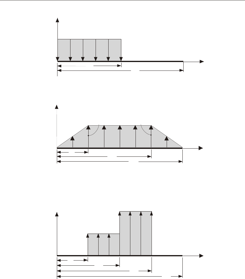
depth of snow or the wind speed; the pro jected ele ment length is meas ured in a
plane per pen dicu lar to the di rec tion of load ing.
Distributed Span Load 139
Chapter VII The Frame Element
AXIS 2
AXIS 1
5
10 20
AXIS 3
AXIS 1
5
5
416
20
AXIS 2
AXIS 1
4
10
16
20
5
10
rda=0.0
rdb=0.5
u2a=–5
u2b=–5
da=4
db=16
u3a=5
u3b=5
da=4
db=10
u2a=5
u2b=5
da=10
db=16
u2a=10
u2b=10
da=0
db=4
u3a=0
u3b=5
da=16
db=20
u3a=5
u3b=0
Figure 38
Examples of Distributed Span Loads

Dis trib uted Span Loads may be speci fied as act ing upon the pro jected length. The
pro gram han dles this by re duc ing the load in ten sity ac cord ing to the an gle, q, be -
tween the ele ment lo cal 1 axis and the di rec tion of load ing. Pro jected force loads
are scaled by sinq, and pro jected mo ment loads are scaled by cosq. The re duced
load in ten si ties are then ap plied per unit of ele ment length.
The scal ing of the mo ment loads is based upon the as sump tion that the mo ment is
caused by a force act ing upon the pro jected ele ment length. The re sult ing mo ment
is al ways per pen dicu lar to the force, thus ac count ing for the use of the co sine in -
stead of the sine of the an gle. The speci fied in ten sity of the mo ment should be com -
puted as the prod uct of the force in ten sity and the per pen dicu lar dis tance from the
ele ment to the force. The ap pro pri ate sign of the mo ment must be given.
Temperature Load
Tem pera ture Load cre ates ther mal strain in the Frame ele ment. This strain is given
by the prod uct of the Ma te rial co ef fi cient of ther mal ex pan sion and the tem pera ture
change of the ele ment. All spec i fied Temperature Loads rep re sent a change in tem -
per a ture from the unstressed state for a lin ear anal y sis, or from the pre vi ous tem per -
a ture in a non lin ear anal y sis.
Three in de pend ent Load Tem pera ture fields may be speci fied:
•Tem pera ture, t, which is con stant over the cross sec tion and pro duces ax ial
strains
•Tem pera ture gra di ent, t2, which is lin ear in the lo cal 2 di rec tion and pro duces
bend ing strains in the 1-2 plane
•Tem pera ture gra di ent, t3, which is lin ear in the lo cal 3 di rec tion and pro duces
bend ing strains in the 1-3 plane
Tem per a ture gra di ents are spec i fied as the change in tem per a ture per unit length.
The tem per a ture gra di ents are pos i tive if the tem per a ture in creases (lin early) in the
pos i tive di rec tion of the el e ment lo cal axis. The gra di ent tem per a tures are zero at
the neu tral axes, hence no ax ial strain is in duced.
Each of the three Load Tem pera ture fields may be con stant along the ele ment
length or lin early in ter po lated from val ues given at the joints by a Joint Pattern.
See Chap ter “Load Pat terns” (page 321) for more in for ma tion.
140 Temperature Load
CSI Analysis Reference Manual

Strain Load
Six types of strain load are avail able, one cor re spond ing to each of the in ter nal
forces and mo ments in a frame el e ment. These are:
•Ax ial strain, e11, rep re sent ing change in length per unit length. Pos i tive strain
in creases the length of an un re strained el e ment, or causes com pres sion in a re -
strained el e ment.
•Shear strains, g12 and g13, rep re sent ing change in an gle per unit length. The an -
gle change is mea sured be tween the cross sec tion and the neu tral axis. Pos i tive
shear strain causes shear de for ma tion in the same di rec tion as would pos i tive
shear forces V2 and V3, re spec tively.
•Tor sional cur va ture, y1, rep re sent ing change in tor sional an gle per unit length.
Pos i tive cur va ture causes de for ma tion in the same di rec tion as would pos i tive
torque T.
•Bend ing cur va tures, y2 and y3, rep re sent ing change in an gle per unit length.
The an gle is mea sured be tween ad ja cent sec tions that re main nor mal to the
neu tral axis. Pos i tive cur va ture causes bend ing de for ma tion in the same di rec -
tion as would pos i tive mo ments M2 and M3, re spec tively.
Each of the Strain Loads may be con stant along the el e ment length or lin early in ter -
po lated from val ues given at the joints by a Joint Pat tern.
In an un re strained el e ment, strain loads cause de for ma tion be tween the two ends of
the el e ment, but in duce no in ter nal forces. This un re strained de for ma tion has the
same sign as would de for ma tion caused by the cor re spond ing (con ju gate) forces
and mo ments act ing on the el e ment. On the other hand, strain load ing in a re -
strained el e ment causes cor re spond ing in ter nal forces that have the op po site sign as
the ap plied strain. Most el e ments in a real struc ture are con nected to fi nite stiff ness,
and so strain load ing would cause both de for ma tion and in ter nal forces. Note that
the ef fects of shear and bend ing strain load ing are cou pled.
For more in for ma tion, see Topic “Internal Force Out put” (page 144) in this chap ter,
and also Chap ter “Load Pat terns” (page 321.)
De for ma tion Load
While Strain Load spec i fies a change in de for ma tion per unit length, De for ma tion
Load spec i fies the to tal de for ma tion be tween the two ends of an un re strained el e -
ment. De for ma tion Load is in ter nally con verted to Strain Load, so you should
Strain Load 141
Chapter VII The Frame Element

choose which ever type of load ing is most con ve niently specified for your par tic u lar
ap pli ca tion.
Cur rently only axial De for ma tion Load is avail able. The spec i fied ax ial de for ma -
tion is con verted to ax ial Strain Load by sim ply di vid ing by the el e ment length. The
com puted strain loads are as sumed to be con stant along the length of the el e ment.
See Chap ter “Load Pat terns” (page 321) for more in for ma tion.
Target-Force Load
Tar get-Force Load is a spe cial type of load ing where you spec ify a de sired ax ial
force, and de for ma tion load is iteratively ap plied to achieve the tar get force. Since
the ax ial force may vary along the length of the element, you must also spec ify the
rel a tive lo ca tion where the de sired force is to oc cur. Tar get-Force load ing is only
used for non lin ear static and staged-con struc tion anal y sis. If ap plied in any other
type of Load Case, it has no ef fect.
Un like all other types of load ing, tar get-force load ing is not in cre men tal. Rather,
you are spec i fy ing the to tal force that you want to be pres ent in the frame el e ment at
the end of the Load Case or con struc tion stage. The ap plied de for ma tion that is cal -
cu lated to achieve that force may be pos i tive, neg a tive, or zero, de pend ing on the
force pres ent in the el e ment at the be gin ning of the anal y sis. When a scale fac tor is
ap plied to a Load Pat tern that con tains Tar get-Force loads, the to tal tar get force is
scaled. The in cre ment of ap plied de for ma tion that is re quired may change by a dif -
fer ent scale fac tor.
See Topic “Tar get-Force Load” (page 331) in Chap ter “Load Pat terns” and Topic
“Tar get-Force It er a tion” (page 444) in Chap ter “Non lin ear Static Anal y sis” for
more in for ma tion.
Internal Force Output
The Frame ele ment in ter nal forces are the forces and mo ments that re sult from in -
te grat ing the stresses over an ele ment cross sec tion. These in ter nal forces are:
•P, the ax ial force
•V2, the shear force in the 1-2 plane
•V3, the shear force in the 1-3 plane
•T, the ax ial torque
142 Target-Force Load
CSI Analysis Reference Manual
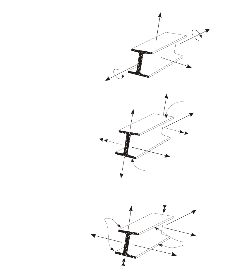
•M2, the bend ing mo ment in the 1-3 plane (about the 2 axis)
•M3, the bend ing mo ment in the 1-2 plane (about the 3 axis)
Internal Force Output 143
Chapter VII The Frame Element
Positive Axial Force and Torque
Positive Moment and Shear
in the 1-2 Plane
Axis 1
Axis 3
Compression Face
Axis 2
M2
Tension Face
Axis 3
M3
V2
Axis 2
Axis 1
Axis 2
P
TAxis 1
Axis 3
T
P
Positive Moment and Shear
in the 1-3 Plane
Tension Face
Compression Face
V2
V3
V3
M3
M2
Figure 39
Frame Element Internal Forces and Moments

These in ter nal forces and mo ments are pres ent at every cross sec tion along the
length of the el e ment, and may be re quested as part of the anal y sis re sults.
The sign con ven tion is il lus trated in Figure 39 (page 143). Posi tive in ter nal forces
and ax ial torque act ing on a posi tive 1 face are ori ented in the posi tive di rec tion of
the ele ment lo cal co or di nate axes. Posi tive in ter nal forces and ax ial torque act ing
on a nega tive face are ori ented in the nega tive di rec tion of the ele ment lo cal co or di -
nate axes. A posi tive 1 face is one whose out ward nor mal (point ing away from ele -
ment) is in the posi tive lo cal 1 di rec tion.
Posi tive bend ing mo ments cause com pres sion at the posi tive 2 and 3 faces and ten -
sion at the nega tive 2 and 3 faces. The posi tive 2 and 3 faces are those faces in the
posi tive lo cal 2 and 3 di rec tions, re spec tively, from the neu tral axis.
Effect of End Offsets
When end off sets are pres ent, in ter nal forces and mo ments are out put at the faces of
the sup ports and at points within the clear length of the ele ment. No out put is pro -
duced within the length of the end off set, which in cludes the joint. Out put will only
be pro duced at joints I or j when the cor re spond ing end off set is zero.
See Topic “End Off sets” (page 127) in this Chap ter for more in for ma tion.
Stress Output
Ax ial stress re sults are avail able for graph i cal dis play and tab u lar out put along with
the in ter nal forces de scribed above. The ax ial stress is de noted S11 and is com puted
at any point in the frame cross sec tion as:
Sxx1123=--
PM3M2
ai33i22
where
•P is the ax ial force, and M2 and M3 are the bend ing mo ments, as de fined in
Topic “In ter nal Force Out put” (page 144)
•a is the cross-sec tional area, and i22 and i33 are the sec tion mo ments of in er -
tia, as de fined in Topic “Sec tion Prop er ties” (page 114)
•x2 and x3 are the co or di nates of the point where the stress is cal cu lated, mea -
sured from the cen troid of the sec tion along the lo cal 2 and 3 axes, re spec -
tively.
144 Stress Output
CSI Analysis Reference Manual

Based on this def i ni tion, ten sile stresses are al ways pos i tive, and com pres sive
stresses are al ways neg a tive, re gard less of the ma te rial.
Stresses are com puted at the same ax ial sta tions as are the in ter nal forces. At each
sta tion, stresses are com puted at se lected stress points over the cross sec tion, with
lo ca tions that de pend upon the shape of the sec tion:
•I-sec tions, T-sec tions, rect an gles, boxes, chan nels, and an gles - at all cor ners
where the max i mum stresses could oc cur
•Cover-plated I sec tions - at the same lo ca tions as for an I-sec tion, plus the ex -
treme cor ners of the cover plates, if pres ent
•Cir cles and pipes - at eight points on the cir cum fer ence
•Sec tion De signer sections - at the stress points de fined when the sec tion was
drawn; if no stress points have been de fined, stress points are as sumed at the
four cor ners of the rect an gu lar bound ing box for the sec tion; this box has di -
men sions t3 x t2
•Gen eral sec tions and all other shapes - at the four cor ners of the rect an gu lar
bound ing box for the sec tion; this box has di men sions t3 x t2
•Nonprismatic sec tions - com puted as above from the in ter po lated shape, if the
shape type is the same at both ends of the frame seg ment; if the shape type is not
the same at both ends, then zero stress is re ported.
•For all shapes ex cept the box and pipe, stresses are also com puted at the cen -
troid of the sec tion
In ad di tion to the value of S11 at each stress point, two ex treme stress values are re -
ported at each station:
•S11Max – the max i mum value over all stress points at that sta tion
•S11Min – the min i mum value over all stress points at that sta tion
Stresses are com puted for all load cases ex cept for mov ing-load cases, for which
zero val ues will be re ported.
The fol low ing as sump tions per tain to the stresses re ported for frame el e ments:
•Stresses are com puted for the base ma te rial of the sec tion. No ac count is made
for the mod u lar ra tio. This usu ally has no ef fect on stresses for any sec tion
types ex cept for some Sec tion De signer shapes.
•Stresses are com puted based on the prop er ties of the sec tion as signed to the
frame el e ment. If the sec tion prop erty is changed dur ing a staged-con struc tion
Stress Output 145
Chapter VII The Frame Element

load case, the calculated stress val ues may not be ap pro pri ate. How ever, the in -
ter nal forces and mo ments are still cor rect.
•If any of the prop er ties a, i22, or i33 is zero, the stress S11 will be re ported as
zero. It is rec om mended to use end re leases rather than set ting the sec tion prop -
er ties to zero.
•Prop erty mod i fi ers that are ap plied to a, i22, or i33 do not change these prop -
erty val ues when used for stress cal cu la tion. In some cases prop erty mod i fi ers
may have an in di rect ef fect upon the stresses if they af fect the cor re spond ing
ax ial force or bend ing mo ments.
The de scrip tion in this topic per tains only to the stress val ues re ported as anal y sis
re sults. Stresses used for frame de sign and bridge de sign are com puted sep a rately,
as ap pro pri ate for the ap pli ca ble ma te rial and de sign procedure.
146 Stress Output
CSI Analysis Reference Manual

Chapter VIII
Hinge Properties
You may in sert plas tic hinges at any num ber of lo ca tions along the clear length of
any Frame el e ment or Ten don ob ject. ETABS also ad mits hinges in ver ti cal
shear-wall el e ments. Each hinge rep re sents con cen trated post-yield be hav ior in one
or more de grees of free dom. Hinges only af fect the be hav ior of the struc ture in non -
lin ear static and non lin ear time-his tory anal y ses.
Advanced Topics
•Over view
•Hinge Properties
•Au to matic, User-De fined, and Gen er ated Properties
•Au to matic Hinge Prop er ties
•Anal y sis Modeling
•Anal y sis Re sults
Overview
Yielding and post-yield ing be hav ior can be mod eled us ing dis crete user-de fined
hinges. Hinges can be as signed to a frame el e ment at any lo ca tion along the clear
Overview 147

length of the el e ment. Un cou pled mo ment, tor sion, ax ial force and shear hinges are
avail able. There are also cou pled P-M2-M3 hinges which yield based on the in ter -
ac tion of ax ial force and bi-ax ial bend ing mo ments at the hinge lo ca tion. Sub sets of
these hinges may in clude P-M2, P-M3, and M2-M3 be hav ior.
Fi ber hinges P-M2-M3 can be de fined, which are a col lec tion of ma te rial points
over the cross sec tion. Each point rep re sents a trib u tary area and has its own
stress-strain curve. Plane sec tions are as sumed to re main planar for the sec tion,
which ties to gether the be hav ior of the ma te rial points. Fi ber hinges are of ten more
re al is tic than force-mo ment hinges, but are more computationally intensive.
More than one type of frame hinge can ex ist at the same lo ca tion, for ex am ple, you
might as sign both an M3 (mo ment) and a V2 (shear) hinge to the same end of a
frame el e ment. Hinge prop er ties can be com puted au to mat i cally from the el e ment
ma te rial and sec tion prop er ties ac cord ing to FEMA-356 (FEMA, 2000) or ACSE
41-13 cri te ria.
For ETABS, hinges can also be as signed to ver ti cal shear walls. These hinges are of
type fi ber P-M3, and al ways act at the cen ter of the shell el e ment. When hinges are
pres ent in a shear wall shell el e ment, the ver ti cal mem brane stress be hav ior is gov -
erned by hinge, while hor i zon tal and shear mem brane stress, as well as out-of-plane
bend ing be hav ior, are gov erned by the prop er ties of the shell el e ment.
Hinges only af fect the be hav ior of the struc ture in non lin ear static and non lin ear
time-his tory anal y ses. Hinge be hav ior does not af fect non lin ear modal time-his tory
(FNA) anal y ses un less the hinges are mod eled as links, as de scribed later in this
chap ter.
Strength loss is per mit ted in the hinge prop er ties, and in fact the FEMA and ASCE
hinges as sume a sud den loss of strength. How ever, you should use this fea ture ju di -
ciously. Sud den strength loss is of ten un re al is tic and can be very dif fi cult to an a -
lyze, es pe cially when elas tic snap-back occurs. We en cour age you to con sider
strength loss only when nec es sary, to use re al is tic neg a tive slopes, and to care fully
eval u ate the re sults.
To help with con ver gence, the pro gram automatically lim its the neg a tive slope of a
hinge to be no stiffer than 10% of the elas tic stiff ness of the Frame el e ment con tain -
ing the hinge. If you need steeper slopes, you can as sign a hinge over write that au -
to mat i cally meshes the frame el e ment around the hinge. By re duc ing the size of the
meshed el e ment, you can in crease the steep ness of the drop-off.
Ev ery thing in this Chap ter ap plies to Ten don objects as well as to Frame el e ments,
al though only the use of ax ial hinges makes sense for Tendons.
CSI Analysis Reference Manual
148 Overview
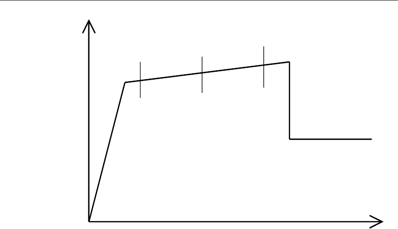
Hinge Properties
A hinge prop erty is a named set of non lin ear prop er ties that can be as signed to
points along the length of one or more Frame el e ments. You may de fine as many
hinge prop er ties as you need.
Force- and mo ment-type hinges are rigid-plas tic. For each force de gree of free dom
(ax ial and shear), you may spec ify the plas tic force-dis place ment be hav ior. For
each mo ment de gree of free dom (bend ing and tor sion) you may spec ify the plas tic
mo ment-ro ta tion be hav ior. Each hinge prop erty may have plas tic prop er ties spec i -
fied for any num ber of the six de grees of free dom. The ax ial force and the two
bend ing mo ments may be cou pled through an in ter ac tion sur face. De grees of free -
dom that are not spec i fied re main elas tic.
Fi ber hinges are elas tic-plas tic and con sist of a set of ma te rial points, each rep re -
sent ing a por tion of the frame cross-sec tion hav ing the same ma te rial. Force-de flec -
tion and mo ment-ro ta tion curves are not spec i fied, but rather are com puted dur ing
the anal y sis from the stress-strain curves of the ma te rial points.
Hinge Properties 149
Chapter VIII Hinge Properties
Displacement
Force
B
C
A
DE
IO LS CP
Figure 40
The A-B-C-D-E curve for Force vs. Displacement
The same type of curve is used for Moment vs. Rotation

Hinge Length
Each plas tic hinge is mod eled as a dis crete point hinge. All plas tic de for ma tion,
whether it be dis place ment or ro ta tion, oc curs within the point hinge. This means
you must as sume a length for the hinge over which the plas tic strain or plas tic cur -
va ture is in te grated.
There is no easy way to choose this length, al though guide lines are given in
FEMA-356 and ASCE 41-13. Typ i cally it is a frac tion of the el e ment length, and is
of ten on the or der of the depth of the sec tion, par tic u larly for mo ment-ro ta tion
hinges.
You can ap prox i mate plas tic ity that is dis trib uted over the length of the el e ment by
in sert ing many hinges. For ex am ple, you could in sert ten hinges at rel a tive lo ca -
tions within the el e ment of 0.05, 0.15, 0.25, ..., 0.95, each with de for ma tion prop er -
ties based on an as sumed hinge length of one-tenth the el e ment length. Of course,
add ing more hinges will add more com pu ta tional cost, so this should only be done
where needed.
For force/mo ment-type hinges, elas tic de for ma tion oc curs along the en tire length
of the Frame el e ment and is not af fected by the pres ence of the hinges. For fi ber
hinges, elas tic be hav ior along the hinge length is de ter mined from the hinge ma te -
rial stress-strain curves, and the elas tic prop er ties of the frame el e ment are ig nored
within the hinge length. For this rea son, the hinge length should not ex ceed the
length of frame el e ment.
Plas tic Deformation Curve
For each force or mo ment de gree of free dom, you de fine a force-dis place ment (mo -
ment-ro ta tion) curve that gives the yield value and the plas tic de for ma tion fol low -
ing yield. This is done in terms of a curve with val ues at five points, A-B-C-D-E, as
shown in Figure 40 (page 149). You may spec ify a sym met ric curve, or one that dif -
fers in the pos i tive and neg a tive di rec tion.
The shape of this curve as shown is in tended for push over anal y sis. You can use
any shape you want. The fol low ing points should be noted:
•Point A is al ways the or i gin.
•Point B rep re sents yield ing. No de for ma tion oc curs in the hinge up to point B,
re gard less of the de for ma tion value spec i fied for point B. The dis place ment
(ro ta tion) at point B will be sub tracted from the de for ma tions at points C, D,
and E. Only the plas tic de for ma tion be yond point B will be ex hib ited by the
hinge.
150 Hinge Properties
CSI Analysis Reference Manual

•Point C rep re sents the ul ti mate ca pac ity for push over anal y sis. How ever, you
may spec ify a pos i tive slope from C to D for other pur poses.
•Point D rep re sents a re sid ual strength for push over anal y sis. How ever, you
may spec ify a pos i tive slope from C to D or D to E for other pur poses.
•Point E rep re sent to tal fail ure. Be yond point E the hinge will drop load down to
point F (not shown) di rectly be low point E on the hor i zon tal axis. If you do not
want your hinge to fail this way, be sure to spec ify a large value for the de for -
ma tion at point E.
You may spec ify ad di tional de for ma tion mea sures at points IO (im me di ate oc cu -
pancy), LS (life safety), and CP (col lapse pre ven tion). These are in for ma tional
mea sures that are re ported in the anal y sis re sults and used for per for mance-based
design. They do not have any ef fect on the be hav ior of the struc ture.
Prior to reach ing point B, all de for ma tion is lin ear and oc curs in the Frame el e ment
it self, not the hinge. Plas tic de for ma tion be yond point B oc curs in the hinge in ad di -
tion to any elas tic de for ma tion that may oc cur in the el e ment.
When the hinge un loads elas ti cally, it does so with out any plas tic de for ma tion, i.e.,
par al lel to slope A-B.
Scaling the Curve
When de fin ing the hinge force-de for ma tion (or mo ment-ro ta tion) curve, you may
en ter the force and de for ma tion val ues di rectly, or you may en ter nor mal ized val ues
and spec ify the scale fac tors that you used to nor mal ized the curve.
In the most com mon case, the curve would be nor mal ized by the yield force (mo -
ment) and yield dis place ment (ro ta tion), so that the nor mal ized val ues en tered for
point B would be (1,1). How ever, you can use any scale fac tors you want. They do
not have to be yield val ues.
Re mem ber that any de for ma tion given from A to B is not used. This means that the
scale fac tor on de for ma tion is actually used to scale the plas tic de for ma tion from B
to C, C to D, and D to E. How ever, it may still be con ve nient to use the yield de for -
ma tion for scal ing.
When au to matic hinge prop er ties are used, the pro gram au to mat i cally uses the
yield val ues for scal ing. These val ues are cal cu lated from the Frame sec tion prop er -
ties. See the next topic for more dis cus sion of au to matic hinge prop er ties.
Hinge Properties 151
Chapter VIII Hinge Properties

Strength Loss
Strength loss is per mit ted in the hinge prop er ties, and in fact the FEMA hinges as -
sume a sud den loss of strength. How ever, you should use this fea ture ju di ciously.
Any loss of strength in one hinge causes load re dis tri bu tion within the struc ture,
pos si bly lead ing to fail ure of an other hinge, and ul ti mately caus ing pro gres sive col -
lapse. This kind of anal y sis can be dif fi cult and time con sum ing. Fur ther more, any
time neg a tive stiffnesses are pres ent in the model, the so lu tion may not be math e -
mat i cally unique, and so may be of ques tion able value.
Sud den strength loss (steep neg a tive stiff ness) is of ten un re al is tic and can be even
more dif fi cult to an a lyze. When an un load ing plas tic hinge is part of a long beam or
col umn, or is in se ries with any flex i ble elas tic subsytem, “elas tic snap-back” can
oc cur. Here the elas tic un load ing de flec tion is larger than, and of op po site sign to,
the plas tic de for ma tion. This re sults in the struc ture de flect ing in the di rec tion op -
po site the ap plied load. SAP2000, ETABS, and CSiBridge have a built-in mech a -
nism to deal with snap-back for cer tain hinges, but this may not al ways be enough
to han dle sev eral si mul ta neous snap-back hinge fail ures.
Con sider care fully what you are try ing to ac com plish with your anal y sis. A well de -
signed struc ture, whether new or retro fit ted, should prob a bly not have strength loss
in any pri mary mem bers. If an anal y sis shows strength loss in a pri mary mem ber,
you may want to mod ify the de sign and then re-an a lyze, rather than try ing to push
the anal y sis past the first fail ure of the pri mary mem bers. Since you need to re-de -
sign any way, what hap pens af ter the first fail ure is not rel e vant, since the be hav ior
will become changed.
To help with con ver gence, the pro gram au to mat i cally lim its the neg a tive slope of a
hinge to be no stiffer than 10% of the elas tic stiff ness of the Frame el e ment con tain -
ing the hinge. By do ing this, snap-back is pre vented within the el e ment, al though it
may still oc cur in the larger struc ture.
If you need steeper slopes, you can as sign a Frame Hinge Overwrite that au to mat i -
cally meshes the Frame ob ject around the hinge. When you as sign this over write,
you can spec ify what frac tion of the Frame ob ject length should be used for the el e -
ment that con tains the hinge. For ex am ple, con sider a Frame ob ject con tain ing one
hinge at each end, and one in the mid dle. If you as sign a Frame Hinge Overwrite
with a rel a tive length of 0.1, the ob ject will be meshed into five el e ments of rel a tive
lengths 0.05, 0.4, 0.1, 0.4, and 0.05. Each hinge is lo cated at the cen ter of an el e -
ment with 0.1 rel a tive length, but be cause two of the hinges fall at the ends of the
object, half of their el e ment lengths are not used. Be cause these el e ments are
shorter than the ob ject, their elas tic stiffnesses are larger, and the pro gram will per -
mit larger neg a tive stiffnesses in the hinges.
152 Hinge Properties
CSI Analysis Reference Manual

By re duc ing the size of the meshed el e ment, you can in crease the steep ness of the
drop-off, al though the slope will never be steeper than you orig i nally spec i fied for
the hinge. Again, we rec om mend grad ual, re al is tic slopes when ever pos si ble, un -
less you truly need to model brit tle be hav ior.
Types of P-M2-M3 Hinges
Nor mally the hinge prop er ties for each of the six de grees of free dom are un cou pled
from each other. How ever, you have the op tion to spec ify cou pled ax ial-force/bi -
axial-mo ment be hav ior. This is called a P-M2-M3 or PMM hinge. Three types are
avail able. In sum mary:
•Iso tro pic P-M2-M3 hinge: This hinge can han dle com plex and un sym met ri cal
PMM sur faces and can in ter po late be tween mul ti ple mo ment-ro ta tion curves.
Two-di men sional sub sets of the hinge are available. It is lim ited to iso tro pic
hys ter esis, which may not be suit able for some structures.
•Para met ric P-M2-M3 hinge: This hinge is lim ited to dou bly sym met ric sec tion
prop er ties and uses a sim ple para met ric def i ni tion of the PMM sur face.
Hysteretic en ergy deg ra da tion can be spec i fied, mak ing it more suit able than
the iso tro pic hinge for ex ten sive cy clic load ing.
•Fi ber P-M2-M3 hinge. This is the most re al is tic hinge, but may re quire the
most computational re sources in terms of anal y sis time and mem ory us age.
Var i ous hys ter esis mod els are avail able and they can be dif fer ent for each ma -
te rial in the hinge.
These hinges are de scribed in more de tail in the fol low ing top ics.
Isotropic P-M2-M3 Hinge
This hinge can han dle com plex and un sym met ri cal PMM sur faces and can in ter po -
late be tween mul ti ple mo ment-ro ta tion curves. It is lim ited to iso tro pic hys ter esis,
which may not be suit able for some struc tures.
Three ad di tional cou pled hinges are avail able as sub sets of the PMM hinge: P-M2,
P-M3, and M2-M3 hinges.
Ten sion is Always Pos i tive!
It is im por tant to note that SAP2000 uses the sign con ven tion where ten sion is al -
ways pos i tive and com pres sion is al ways neg a tive, re gard less of the ma te rial be ing
used. This means that for some ma te ri als (e.g., con crete) the in ter ac tion sur face
may ap pear to be up side down.
Hinge Properties 153
Chapter VIII Hinge Properties

In ter ac tion (Yield) Sur face
For the PMM hinge, you spec ify an in ter ac tion (yield) sur face in three-di men sional
P-M2-M3 space that rep re sents where yielding first oc curs for dif fer ent com bi na -
tions of ax ial force P, mi nor mo ment M2, and ma jor mo ment M3.
The sur face is spec i fied as a set of P-M2-M3 curves, where P is the ax ial force (ten -
sion is pos i tive), and M2 and M3 are the mo ments. For a given curve, these mo -
ments may have a fixed ra tio, but this is not nec es sary. The fol low ing rules ap ply:
•All curves must have the same num ber of points.
•For each curve, the points are or dered from most neg a tive (com pres sive) value
of P to the most pos i tive (ten sile).
•The three val ues P, M2 and M3 for the first point of all curves must be iden ti cal,
and the same is true for the last point of all curves
•When the M2-M3 plane is viewed from above (look ing to ward com pres sion),
the curves should be de fined in a coun ter-clock wise di rec tion
•The sur face must be con vex. This means that the plane tan gent to the sur face at
any point must be wholly out side the sur face. If you de fine a sur face that is not
con vex, the pro gram will au to mat i cally in crease the ra dius of any points which
are “pushed in” so that their tan gent planes are out side the sur face. A warn ing
will be is sued dur ing anal y sis that this has been done.
You can ex plic itly de fine the in ter ac tion sur face, or let the pro gram cal cu late it us -
ing one of the fol low ing formulas:
•Steel, AISC-LRFD Equa tions H1-1a and H1-1b with phi = 1
•Steel, FEMA-356 Equa tion 5-4
•Con crete, ACI 318-02 with phi = 1
You may look at the hinge prop er ties for the gen er ated hinge to see the spe cific sur -
face that was cal cu lated by the pro gram.
Mo ment-Ro ta tion Curves
For PMM hinges you spec ify one or more mo ment/plas tic-ro ta tion curves cor re -
spond ing to dif fer ent val ues of P and mo ment an gle q. The mo ment an gle is mea -
sured in the M2-M3 plane, where 0° is the pos i tive M2 axis, and 90° is the pos i tive
M3 axis.
154 Hinge Properties
CSI Analysis Reference Manual

You may spec ify one or more ax ial loads P and one or more mo ment an gles q. For
each pair (P,q), the mo ment-ro ta tion curve should rep re sent the re sults of the fol -
low ing ex per i ment:
•Ap ply the fixed ax ial load P.
•In crease the mo ments M2 and M3 in a fixed ra tio (cos q, sin q) cor re spond ing
to the mo ment an gle q.
•Mea sure the plas tic ro ta tions Rp2 and Rp3 that oc cur af ter yield.
•Cal cu late the re sul tant mo ment M = M2*cos q + M3*sin q, and the pro jected
plas tic ro ta tion Rp = Rp2*cos q + Rp3*sin q at each mea sure ment increment
•Plot M vs. Rp, and sup ply this data to SAP2000
Note that the mea sured di rec tion of plas tic strain may not be the same as the di rec -
tion of mo ment, but the pro jected value is taken along the di rec tion of the moment.
In ad di tion, there may be mea sured ax ial plas tic strain that is not part of the pro jec -
tion. How ever, dur ing anal y sis the pro gram will re cal cu late the to tal plas tic strain
based on the di rec tion of the nor mal to the in ter ac tion (yield) sur face.
Dur ing anal y sis, once the hinge yields for the first time, i.e., once the val ues of P,
M2 and M3 first reach the in ter ac tion sur face, a net mo ment-ro ta tion curve is in ter -
po lated to the yield point from the given curves. This curve is used for the rest of the
anal y sis for that hinge.
If the val ues of P, M2, and M3 change from the val ues used to in ter po late the curve,
the curve is ad justed to pro vide an energy equiv a lent mo ment-ro ta tion curve. This
means that the area un der the mo ment-ro ta tion curve is held fixed, so that if the re -
sul tant mo ment is smaller, the duc til ity is larger. This is con sis tent with the un der -
ly ing stress strain curves of ax ial “fi bers” in the cross sec tion.
As plas tic de for ma tion oc curs, the yield sur face changes size ac cord ing to the shape
of the M-Rp curve, de pend ing upon the amount of plastic work that is done. You
have the op tion to spec ify whether the sur face should change in size equally in the
P, M2, and M3 di rec tions, or only in the M2 and M3 di rec tions. In the lat ter case,
ax ial de for ma tion be haves as if it is per fectly plastic with no hard en ing or col lapse.
Ax ial col lapse may be more re al is tic in some hinges, but it is computationally dif fi -
cult and may re quire non lin ear di rect-in te gra tion time-his tory anal y sis if the struc -
ture is not sta ble enough the re dis trib ute any dropped grav ity load.
Hinge Properties 155
Chapter VIII Hinge Properties

Parametric P-M2-M3 Hinge
This hinge is lim ited to dou bly sym met ric sec tion prop er ties and uses a sim ple
para met ric def i ni tion of the PMM sur face. Hysteretic en ergy deg ra da tion can be
spec i fied, mak ing it more suit able than the iso tro pic hinge for ex ten sive cy clic
load ing.
Two ver sions of the hinge are avail able, one for steel frame sec tions, and one for re -
in forced-con crete frame sec tions. Cur rently this hinge is only avail able in ETABS,
and will be added to SAP2000 and CSiBridge in sub se quent ver sions.
The de scrip tion and the ory for this hinge for mu la tion are pre sented in the Tech ni cal
Note “Para met ric P-M2-M3 Hinge Model”. This doc u ment can be found in the
Man u als subfolder where the soft ware is in stalled on your com puter. It can be ac -
cessed from in side the soft ware us ing the menu com mand Help > Doc u men ta tion >
Tech ni cal Notes.
De tailed descriptions of the in put val ues needed to de fine the prop er ties for ei ther
the steel or con crete hinge are avail able from the Help fa cil ity within the soft ware.
This can be ac cessed us ing the menu com mand Help > Prod uct Help, or press ing
the F1 key at any time.
Fiber P-M2-M3 Hinge
The Fi ber P-M2-M3 (Fi ber PMM) hinge mod els the ax ial be hav ior of a num ber of
rep re sen ta tive ax ial “fi bers” dis trib uted across the cross sec tion of the frame el e -
ment. Each fi ber has a lo ca tion, a trib u tary area, and a stress-strain curve. The ax ial
stresses are in te grated over the sec tion to com pute the values of P, M2 and M3.
Like wise, the ax ial de for ma tion U1 and the ro ta tions R2 and R3 are used to com -
pute the ax ial strains in each fi ber. Plane sec tions are as sumed to re main pla nar.
You can de fine you own fi ber hinge, ex plic itly spec i fy ing the lo ca tion, area, ma te -
rial and its stress-strain curve for each fi ber, or you can let the pro gram au to mat i -
cally cre ate fi ber hinges for cir cu lar and rect an gu lar frame sec tions.
The Fiber PMM hinge is more “nat u ral” than the Iso tro pic or Para met ric PMM
hinges de scribed above, since it au to mat i cally ac counts for in ter ac tion, chang ing
mo ment-ro ta tion curve, and plas tic ax ial strain. How ever, it is also more
computationally in ten sive, re quir ing more com puter stor age and ex e cu tion time.
You may have to ex per i ment with the num ber of fi bers needed to get an op ti mum
bal ance be tween ac cu racy and computational ef fi ciency.
156 Hinge Properties
CSI Analysis Reference Manual

Strength loss in a fi ber hinge is de ter mined by the strength loss in the un der ly ing
stress-strain curves. Be cause all the fi bers in a cross sec tion do not usu ally fail at the
same time, the over all hinges tend to ex hibit more grad ual strength loss than hinges
with di rectly spec i fied mo ment-ro ta tion curves. This is es pe cially true if rea son able
hinge lengths are used. For this rea son, the pro gram does not au to mat i cally re strict
the neg a tive drop-off slopes of fi ber hinges. How ever, we still rec om mend that you
pay close at ten tion to the mod el ing of strength loss, and mod ify the stress-strain
curves if nec es sary.
For more in for ma tion:
•See Topic “Stress-Strain Curves” (page 80) in Chap ter “Ma te rial Properties.”
•See Topic “Sec tion-De signer Sec tions” (page 118) Chap ter “The Frame El e -
ment.”
Hysteresis Models
The plas tic force-de for ma tion or mo ment-ro ta tion curve de fines the non lin ear be -
hav ior un der monotonic load ing. This curve, com bined with the elas tic be hav ior of
the hinge length in the par ent frame element, is also known as the back bone curve
for the hinge.
Un der load re ver sal or cy clic load ing, the be hav ior will de vi ate from the back bone
curve. Sev eral dif fer ent hys ter esis mod els are avail able to de scribe this be hav ior
for dif fer ent types of ma te ri als. For the most part, these dif fer in the amount of en -
ergy they dis si pate in a given cy cle of de for ma tion, and how the en ergy dis si pa tion
be hav ior changes with an in creas ing amount of de for ma tion.
Hysteresis mod els are de scribed in Topic “Hys ter esis Mod els” (page 85) of Chap -
ter “Ma te rial Prop er ties.”
Hys ter esis mod els are ap pli ca ble to the dif fer ent types of hinges as fol lows:
•Sin gle de gree of free dom hinges: All in elas tic mod els (ki ne matic, de grad ing,
Takeda, pivot, con crete, BRB hard en ing, and iso to pic)
•Cou pled P-M2-M3, P-M2, P-M3, and M2-M3 hinges: Iso tro pic model only
•Fi ber P-M2-M3 hinges: For each ma te rial fi ber, all mod els (elastic, ki ne matic,
de grad ing, Takeda, pivot, con crete, BRB hard en ing, and iso to pic)
Note that all of these mod els are avail able in the cur rent ver sion of ETABS. Some
of the mod els are not yet avail able in SAP2000 and CSiBridge but will be added in
sub se quent ver sions.
Hinge Properties 157
Chapter VIII Hinge Properties

Hysteretic be hav ior may af fect non lin ear static and non lin ear time-his tory load
cases that ex hibit load re ver sals and cy clic load ing. Monotonic load ing is not af -
fected. Note, how ever, that even static push over load cases can pro duce load re ver -
sal in some hinges caused by strength loss in other hinges.
Automatic, User-Defined, and Generated Properties
There are three types of hinge prop er ties in SAP2000:
•Au to matic hinge prop er ties
•User-de fined hinge prop er ties
•Gen er ated hinge prop er ties
Only au to matic hinge prop er ties and user-de fined hinge prop er ties can be as signed
to frame el e ments. When au to matic or user-de fined hinge prop er ties are as signed to
a frame el e ment, the pro gram au to mat i cally cre ates a gen er ated hinge prop erty for
each and ev ery hinge.
The built-in au to matic hinge prop er ties for steel mem bers are based on Ta ble 5-6 in
FEMA-356. The built-in au to matic hinge prop er ties for con crete mem bers are
based on Ta bles 6-7 and 6-8 in FEMA-356, or on Caltrans spec i fi ca tions for con -
crete col umns. Af ter as sign ing au to matic hinge prop er ties to a frame el e ment, the
pro gram gen er ates a hinge prop erty that in cludes spe cific in for ma tion from the
frame sec tion ge om e try, the ma te rial, and the length of the el e ment. You should re -
view the gen er ated prop er ties for their ap pli ca bil ity to your spe cific pro ject.
User-de fined hinge prop er ties can ei ther be based on a hinge prop erty gen er ated
from au to matic prop erty, or they can be fully user-de fined.
A gen er ated prop erty can be con verted to user-de fined, and then mod i fied and
re-as signed to one or more frame el e ments. This way you can let the pro gram do
much of the work for you us ing au to matic prop er ties, but you can still cus tom ize
the hinges to suit your needs. How ever, once you con vert a gen er ated hinge to
user-de fined, it will no lon ger change if you mod ify the el e ment, its sec tion or ma -
te rial.
It is the gen er ated hinge prop er ties that are ac tu ally used in the anal y sis. They can
be viewed, but they can not be mod i fied. Gen er ated hinge prop er ties have an au to -
matic nam ing con ven tion of LabelH#, where La bel is the frame el e ment la bel, H
stands for hinge, and # rep re sents the hinge num ber. The pro gram starts with hinge
num ber 1 and in cre ments the hinge num ber by one for each con sec u tive hinge ap -
plied to the frame el e ment. For ex am ple if a frame el e ment la bel is F23, the gen er -
158 Automatic, User-Defined, and Generated Properties
CSI Analysis Reference Manual

ated hinge prop erty name for the sec ond hinge as signed to the frame el e ment is
F23H2.
The main rea son for the dif fer en ti a tion be tween de fined prop er ties (in this con text,
de fined means both au to matic and user-de fined) and gen er ated prop er ties is that
typ i cally the hinge prop er ties are sec tion de pend ent. Thus it would be nec es sary to
de fine a dif fer ent set of hinge prop er ties for each dif fer ent frame sec tion type in the
model. This could po ten tially mean that you would need to de fine a very large num -
ber of hinge prop er ties. To sim plify this pro cess, the con cept of au to matic prop er -
ties is used in SAP2000. When au to matic prop er ties are used, the pro gram com -
bines its built-in de fault cri te ria with the de fined sec tion prop er ties for each el e -
ment to gen er ate the fi nal hinge prop er ties. The net ef fect of this is that you do sig -
nif i cantly less work de fin ing the hinge prop er ties be cause you don’t have to de fine
each and ev ery hinge.
Automatic Hinge Properties
Au to matic hinge prop er ties are based upon a sim pli fied set of as sump tions that may
not be ap pro pri ate for all struc tures. You may want to use au to matic prop er ties as a
start ing point, and then con vert the cor re spond ing gen er ated hinges to user-de fined
and ex plic itly over write cal cu lated val ues as needed.
Au to matic prop er ties re quire that the pro gram have de tailed knowl edge of the
Frame Sec tion prop erty used by the el e ment that con tains the hinge. For this rea son,
only the fol low ing types of au to matic hinges are avail able:
Con crete Beams in Flex ure
M2 or M3 hinges can be gen er ated us ing FEMA Ta ble 6-7 (I) for the fol low ing
shapes:
•Rect an gle
•Tee
•An gle
•Sec tion De signer
Con crete Col umns in Flex ure
M2, M3, M2-M3, P-M2, P-M3, or P-M2-M3 hinges can be gen er ated us ing
FEMA Ta ble 6-8 (I), for the fol low ing shapes:
Automatic Hinge Properties 159
Chapter VIII Hinge Properties

•Rect an gle
•Cir cle
•Sec tion De signer
or us ing Caltrans spec i fi ca tions, for the fol low ing shapes:
•Sec tion De signer only
Steel Beams in Flex ure
M2 or M3 hinges can be gen er ated us ing FEMA Ta ble 5-6, for the fol low ing
shapes:
–I/Wide-flange only
Steel Col umns in Flex ure
M2, M3, M2-M3, P-M2, P-M3, or P-M2-M3 hinges can be gen er ated us ing
FEMA Ta ble 5-6, for the fol low ing shapes:
•I/Wide-flange
•Box
Steel Braces in Ten sion/Com pres sion
P (ax ial) hinges can be gen er ated us ing FEMA Ta ble 5-6, for the fol low ing
shapes:
•I/Wide-flange
•Box
•Pipe
•Dou ble chan nel
•Dou ble an gle
Fi ber Hinge
P-M2-M3 hinges can be gen er ated for steel or re in forced con crete mem bers us -
ing the un der ly ing stress-strain be hav ior of the ma te rial for the fol low ing
shapes:
•Rect an gle
•Cir cle
160 Automatic Hinge Properties
CSI Analysis Reference Manual

Ad di tional Considerations
You must make sure that all re quired de sign in for ma tion is avail able to the Frame
sec tion as fol lows:
•For con crete Sec tions, the re in forc ing steel must be ex plic itly de fined, or else
the sec tion must have al ready been de signed by the pro gram be fore non lin ear
anal y sis is per formed
•For steel Sec tions, Auto-se lect Sec tions can only be used if they have al ready
been de signed so that a spe cific sec tion has been cho sen be fore non lin ear anal -
y sis is per formed
For more in for ma tion, see the on-line help that is avail able while as sign ing au to -
matic hinges to Frame el e ments in the Graph i cal User In ter face.
Analysis Modeling
Hinges are as signed to a Frame or Shell (shear wall) el e ment to rep re sent the non -
lin ear be hav ior of their par ent el e ment. When the anal y sis model is cre ated, there
are two ways the hinge can be rep re sented:
•Hinge em bed ded in the el e ment
•Hinge as a sep a rate link el e ment
The lat ter method is cur rently only avail able in the ETABS Ul ti mate level, and en -
ables hinge be hav ior to be con sid ered in non lin ear model time-his tory (FNA) load
cases. As a rule, FNA anal y sis runs sig nif i cantly faster than non lin ear di rect-in te -
gra tion time-his tory anal y sis. Nonlinear static anal y sis and nonlinear di rect-in te -
gra tion time his tory anal y sis are avail able for both types of anal y sis mod el ing.
When the hinge is mod eled as a link el e ment, the par ent Frame el e ment is di vided at
the hinge lo ca tion into sep a rate subelements, and a zero-length link el e ment is cre -
ated that con tains the hinge prop erty and con nects the frame subelements. A very
small amount of ax ial mass and ro ta tional in er tia are added at the two con nect ing
joints to im prove FNA it er a tion. A sim i lar in ter nal mod el ing is em ployed for shear
wall el e ments when the hinge is mod eled as a link el e ment.
A sec ond, independent mod el ing op tion is available to as sign au to matic sub di vi -
sion of Frame el e ments at hinge lo ca tions. Us ing this as sign ment, you spec ify a rel -
a tive length that is used when cre at ing the anal y sis model of the hinges for the se -
lected el e ments. The ef fect of this de pends upon how the hinge is mod eled:
Analysis Modeling 161
Chapter VIII Hinge Properties

•For the hinge em bed ded in the el e ment: The Frame ob ject is sub di vided into
sep a rate frame el e ments, with one el e ment con tain ing the hinge that is equal in
length to that spec i fied in the as sign ment.
This has the ad van tage of in tro duc ing more de grees of free dom into the model
that may im prove con ver gence when mul ti ple hinges are fail ing at the same
time, with a pos si ble in crease in com pu ta tion time. In ad di tion, steeper
drop-offs are per mit ted when the hinge curve ex hib its strength loss be cause the
el e ment con tain ing the hinge is shorter, and hence stiffer.
On the other hand, not sub di vid ing the frame el e ment leads to a smaller anal y -
sis model, typ i cally re quir ing less com pu ta tion time and stor age. In addition,
stiff ness pro por tional damp ing for non lin ear di rect-in te gra tion time-his tory
anal y sis is better mod eled in lon ger el e ments.
•For the hinge as a sep a rate link el e ment: The sub di vi sion into two frame el e -
ments and a zero-length link is not changed. However, the elas tic flex i bil ity of
the link is changed to be equal to the length of the frame el e ment spec i fied in
the as sign ment, and the cor re spond ing length of the ad ja cent frame sub-el e -
ments are made rigid.
This has the ad van tage of im prov ing stiff ness-pro por tional damp ing in non lin -
ear di rect-in te gra tion time-his tory anal y sis, and can be rec om mend for this rea -
son. On the other hand, this is not nec es sary for FNA anal y sis.
The de fault rel a tive length for au to matic subdivision is 0.02. Rec om mended val ues
typ i cally range from 0.02 to 0.25.
Com pu ta tional Considerations
The most im por tant ad vice is to only add hinges to the model where non lin ear be -
hav ior is ex pected to have a sig nif i cant ef fect on the anal y sis and design. Add ing
ex tra hinges in creases the time and ef fort it takes to cre ate the model, to run the
analyses, and to in ter pret the re sults.
Start with the sim plest model pos si ble so that you can make many anal y sis runs
quickly. This helps to better un der stand the be hav ior of your struc ture early in the
de sign pro cess and to cor rect mod el ing er rors. Add hinges and complexity grad u -
ally as you de ter mine where nonlinearity is ex pected and/or de sired.
Add ing hinges ev ery where to find the nonlinearity is tempt ing, but this ap proach
usu ally wastes much more time than incrementally grow ing the model.
162 Com pu ta tional Considerations
CSI Analysis Reference Manual

Most mod els with hinges ben e fit from us ing event-to-event step ping for non lin ear
static and non lin ear di rect-in te gra tion time-his tory load cases. This is par tic u larly
true for the para met ric P-M2-M3 hinge. How ever, it may be nec es sary to turn off
event-to-event step ping if the model has a very large num ber of hinges, or if there is
a sig nif i cant amount of other types of nonlinearity in the struc ture. This is best de -
ter mined by run ning anal y ses both with and with out events to see which is most ef -
fi cient.
Most non lin ear time-his tory anal y sis ben e fits from the pres ence of mass at the non -
lin ear de grees-of-free dom. In er tia tends to sta bi lize it er a tion when the non lin ear
be hav ior is chang ing rap idly. This is par tic u larly true for FNA anal y sis. For
ETABS, it is usu ally best to de fine the mass source to in clude ver ti cal mass and to
not lump the mass at the story lev els for mod els that have hinges.
For FNA anal y sis, it is usu ally most ef fi cient to damp out the very high modes.
Some of the Ritz modes needed for FNA anal y sis can be ex pected to be of high fre -
quency. An ex am ple of how to do this would be to de fine the load-case damp ing to
be of type “In ter po lated by Fre quency”. Then spec ify your de sired structure damp -
ing ra tio (say 0.025) for fre quen cies up to 999 Hz, and a damp ing ra tio of 0.99 for
fre quen cies above 1000 Hz. You can ex per i ment with this cut off value to see the ef -
fect on runtime and re sults.
Analysis Results
For each out put step in a non lin ear static or non lin ear di rect-in te gra tion time-his -
tory Load Case, you may re quest anal y sis re sults for the hinges. These re sults in -
clude:
•The forces and/or mo ments car ried by the hinge. De grees of free dom not de -
fined for the hinge will re port zero val ues, even though non-zero val ues are car -
ried rig idly through the hinge.
•The plas tic dis place ments and/or ro ta tions.
•The most ex treme state ex pe ri enced by the hinge in any de gree of free dom.
This state does not in di cate whether it oc curred for pos i tive or neg a tive de for -
ma tion:
–A to B
–B to C
–C to D
–D to E
Analysis Results 163
Chapter VIII Hinge Properties

–> E
•The most ex treme per for mance sta tus ex pe ri enced by the hinge in any de gree
of free dom. This sta tus does not in di cate whether it oc curred for pos i tive or
neg a tive de for ma tion:
–A to B
–B to IO
–IO to LS
–LS to CP
–> CP
When you dis play the de flected shape in the graph i cal user in ter face for a non lin ear
static or non lin ear di rect-in te gra tion time-his tory Load Case, the hinges are plot ted
as col ored dots in di cat ing their most ex treme state or sta tus:
•B to IO
•IO to LS
•LS to CP
•CP to C
•C to D
•D to E
•> E
The col ors used for the dif fer ent states are in di cated on the plot. Hinges that have
not ex pe ri enced any plas tic de for ma tion (A to B) are not shown.
164 Analysis Results
CSI Analysis Reference Manual

Chapter IX
The Cable Element
The Ca ble el e ment is a highly non lin ear el e ment used to model the cat e nary be hav -
ior of slen der ca bles un der their own self-weight. Ten sion-stiff en ing and large-de -
flec tions nonlinearity are in her ently in cluded in the for mu la tion. Non lin ear anal y -
sis is re quired to make use of the Ca ble el e ment. Lin ear anal y ses can be per formed
that use the stiff ness from the end of non lin ear Load Cases.
Advanced Topics
•Over view
•Joint Con nec tiv ity
•Undeformed Length
•Shape Calculator
•De grees of Free dom
•Lo cal Co or di nate Sys tem
•Sec tion Prop er ties
•Prop erty Mod i fi ers
•Mass
•Self-Weight Load
165

•Grav ity Load
•Dis trib uted Span Load
•Tem per a ture Load
•Strain and Deformation Load
•Tar get-Force Load
•Non lin ear Analysis
•El e ment Out put
Overview
The Ca ble el e ment uses an elas tic cat e nary for mu la tion to rep re sent the be hav ior of
a slen der ca ble un der its own self-weight, tem per a ture, and strain load ing. This be -
hav ior is highly non lin ear, and in her ently in cludes tension-stiffening (P-delta) and
large-de flec tion ef fects. Slack and taut be hav ior is au to mat i cally con sid ered.
In the graph i cal user in ter face, you can draw a ca ble ob ject con nect ing any two
points. A shape cal cu la tor is avail able to help you de ter mine the undeformed length
of the ca ble. The undeformed length is extremely crit i cal in de ter min ing the be hav -
ior of the ca ble.
An un loaded, slack ca ble is not sta ble and has no unique po si tion. There fore lin ear
Load Cases that start from zero ini tial con di tions may be mean ing less. In stead, all
lin ear Load Cases should use the stiff ness from the end of a non lin ear static Load
Case in which all ca bles are loaded by their self-weight or other trans verse load. For
cases where no trans verse load is pres ent on a slack Ca ble el e ment, the pro gram
will in ter nally as sume a very small self-weight load in or der to ob tain a unique
shape. How ever, it is better if you ap ply a re al is tic load for this pur pose.
Each Ca ble el e ment may be loaded by grav ity (in any di rec tion), dis trib uted forces,
strain and de for ma tion loads, and loads due to tem per a ture change. To ap ply con -
cen trated loads, a ca ble should be di vided at the point of load ing, and the force ap -
plied to the con nect ing joint.
Tar get-force load ing is avail able that iteratively applies de for ma tion load to the ca -
ble to achieve a de sired ten sion.
El e ment out put in cludes the ax ial force and de flected shape at a user-spec i fied
num ber of equally-spaced out put sta tions along the length of the el e ment.
166 Overview
CSI Analysis Reference Manual

You have the op tion when draw ing a ca ble ob ject in the model to use the cat e nary
el e ment of this chap ter, or to model the ca ble as a se ries of straight frame el e ments.
Us ing frame el e ments al lows you to con sider ma te rial nonlinearity and com pli -
cated load ing, but the cat e nary for mu la tion is better suited to most ap pli ca tions.
Joint Connectivity
A Ca ble el e ment is rep re sented by a curve con nect ing two joints, I and j. The two
joints must not share the same lo ca tion in space. The two ends of the el e ment are
de noted end I and end J, re spec tively.
The shape of the ca ble is de fined by undeformed length of the ca ble and the load
act ing on it, un less it is taut with no trans verse load, in which case it is a straight
line.
Undeformed Length
In the graph i cal user in ter face, you can draw a ca ble ob ject con nect ing any two
points. A shape cal cu la tor is avail able to help you de ter mine the undeformed length
of the ca ble. The re la tion ship be tween the undeformed length and the chord length
(the dis tance be tween the two end joints) is ex tremely crit i cal in de ter min ing the
be hav ior of the ca ble.
In simple terms, when the undeformed length is lon ger that the chord length, the ca -
ble is slack and has sig nif i cant sag. When the undeformed length is shorter than the
chord length, the ca ble is taut and car ries sig nif i cant ten sion with lit tle sag.
When trans verse load acts on the ca ble, there is a tran si tion range where the
undeformed length is close to the chord length. In this re gime, the ten sion and sag
in ter act in a highly non lin ear way with the transverse load.
Tem per a ture, strain, and dis tor tion loads can change the length of the ca ble. The ef -
fect of these changes is sim i lar to chang ing the undeformed length, ex cept that they
do not change the weight of the ca ble. Strain in the ca ble due to any source is cal cu -
lated as the dif fer ence be tween the to tal length and the undeformed length, di vided
by the undeformed length (en gi neer ing strain).
If the undeformed length of a ca ble is shorter than the chord length at the be gin ning
of a non lin ear anal y sis, or when the ca ble is added to the struc ture dur ing staged
con struc tion, ten sion will im me di ately ex ist in the ca ble and it er a tion may be re -
quired to bring the structure into equi lib rium be fore any load is ap plied.
Joint Connectivity 167
Chapter IX The Cable Element

Shape Calculator
The ul ti mate pur pose of the shape cal cu la tor (also called Ca ble Lay out form) in the
graph i cal user in ter face is to help you cal cu late the undeformed length of a ca ble
ob ject. By de fault, the undeformed length is as sumed to be equal to the chord
length be tween the undeformed po si tions of the two end joints.
You may spec ify a ver ti cal load act ing on the ca ble con sist ing of:
•Self-weight (al ways in cluded in the shape cal cu la tor)
•Ad di tional weight per unit of undeformed length of the ca ble
•Ad di tion load per unit hor i zon tal length be tween the two joints
Note that these loads are only used in the shape cal cu la tor. They are not ap plied to
the el e ment dur ing anal y sis. Loads to be used for anal y sis must be as signed to the
el e ments in Load Pat terns.
You may choose one of the fol low ing ways to cal cu late the undeformed length:
•Spec i fy ing the undeformed length, ei ther ab so lute or rel a tive to the chord
length
•Spec i fy ing the max i mum ver ti cal sag, mea sured from the chord to the ca ble
•Spec i fy ing the max i mum low-point sag, mea sured from the joint with the
low est Z el e va tion to the low est point on the ca ble
•Spec i fy ing the con stant hor i zon tal com po nent of ten sion in the ca ble
•Spec i fy ing the ten sion at ei ther end of the ca ble
•Re quest ing the shape which gives the min i mum ten sion at ei ther end of the
ca ble
See Figure 41 (page 169) for a de scrip tion of the ca ble ge om e try.
Note that there does ex ist an undeformed length that yields a min i mum ten sion at
ei ther end of the ca ble. Lon ger ca bles carry more self weight, in creas ing the ten -
sion. Shorter ca bles are tauter, also in creas ing the ten sion. If you in tend to spec ify
the ten sion at ei ther end, it is a good idea first to de ter mine what is the minimum
ten sion, since at tempts to spec ify a lower ten sion will fail. When a larger value of
ten sion is spec i fied, the shorter so lu tion will be re turned.
It is im por tant to note that the shape cal cu lated here may not ac tu ally oc cur dur ing
any Load Case, nor are the ten sions cal cu lated here di rectly im posed upon the ca -
ble. Only the ca ble length is de ter mined. The de formed shape of the ca ble and the
168 Shape Calculator
CSI Analysis Reference Manual
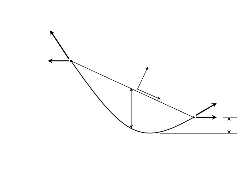
ten sions it car ries will de pend upon the loads ap plied and the be hav ior of the struc -
ture dur ing anal y sis. For ex am ple, the shape cal cu la tor as sumes that the two end
joints re main fixed. How ever, if the ca ble is con nected to a de form ing struc ture, the
chord length and its ori en ta tion may change, yield ing a dif fer ent so lu tion.
Cable vs. Frame Elements
In the shape cal cu la tor, you may spec ify whether the ca ble is to be mod eled with the
cat e nary el e ment of this chap ter, or us ing straight frame el e ments.
If you are in ter ested in highly vari able load ing or ma te rial nonlinearity, us ing frame
el e ments may be ap pro pri ate. Large-de flec tion geo met ri cally non lin ear anal y sis of
the en tire struc ture will be needed to cap ture full ca ble be hav ior. P-delta anal y sis
Shape Calculator 169
Chapter IX The Cable Element
H
H
TI
TJ
EA,w
L0
LC
uMAX
uLOW
I
J
1
2
EA=Stiffness
w=Weightperlength
uMAX=Maximumverticalsag
uLOW=Low-pointsag
H=Horizontalforce
TI=TensionatJointI
TJ=TensionatJointJ
I,J=Joints
L0=Undeformedlength
LC=Chordlength
Figure 41
Cable Element, showing connectivity, local axes, dimensions, properties, and
shape parameters

with com pres sion lim its may be suf fi cient for some ap pli ca tions. For more in for -
ma tion, see Chap ter “The Frame Element” (page 105).
For most ca ble ap pli ca tions, how ever, the cat e nary ca ble el e ment is a better choice,
es pe cially if the ca ble is very slen der, or sig nif i cant sup port move ment is ex pected.
Non lin ear anal y sis is still re quired, but the geo met ric nonlinearity (P-delta and/or
large-de flec tion be hav ior) of the cat e nary el e ment will be con sid ered in ter nally re -
gard less of how the rest of the struc ture is treated.
Number of Segments
In the shape cal cu la tor, you may spec ify the num ber of seg ments into which the ca -
ble ob ject should be bro ken. Each seg ment will be mod eled as a sin gle cat e nary ca -
ble or sin gle frame el e ment.
For the cat e nary el e ment, a sin gle seg ment is usu ally the best choice unless you are
con sid er ing con cen trated loads or in ter me di ate masses for ca ble vi bra tion.
For the frame el e ment, mul ti ple seg ments (usually at least eight, and some times
many more) are re quired to cap ture the shape vari a tion, un less you are mod el ing a
straight stay or brace, in which case a sin gle seg ment may suf fice.
For more in for ma tion, see Chap ter “Ob jects and Elements” (page 7)
Degrees of Freedom
The Ca ble el e ment ac ti vates the three translational de grees of free dom at each of its
con nected joints. Ro ta tional de grees of free dom are not ac ti vated. This el e ment
con trib utes stiff ness to all of these translational de grees of free dom.
For more in for ma tion, see Topic “De grees of Free dom” (page 30) in Chap ter
“Joints and De grees of Free dom.”
Local Coordinate System
Each Ca ble el e ment has its own el e ment lo cal co or di nate sys tem which can be
used to de fine loads act ing on the el e ment. The axes of this lo cal sys tem are de noted
1, 2 and 3. The first axis is di rected along the chord con nect ing the two joints of the
el e ment; the re main ing two axes lie in the plane per pen dic u lar to the chord with an
ori en ta tion that you spec ify. This co or di nate sys tem does not nec es sar ily cor re -
170 Degrees of Freedom
CSI Analysis Reference Manual

spond to the di rec tion of sag of the ca ble, and does not change as the di rec tion of
sag changes dur ing load ing.
The def i ni tion of the ca ble el e ment lo cal co or di nate sys tem is not usu ally im por tant
un less you want to ap ply con cen trated or dis trib uted span loads in the el e ment lo cal
sys tem.
The def i ni tion of the Ca ble lo cal co or di nate sys tem is ex actly the same as for the
Frame el e ment. For more in for ma tion, see Topics “Lo cal Co or di nate Sys tem”
(page 108) and “Ad vanced Lo cal Co or di nate Sys tem” (page 110) in Chap ter “The
Frame El e ment.”
Section Properties
A Cable Sec tion is a set of ma te rial and geo met ric prop er ties that de scribe the
cross-sec tion of one or more Ca ble el e ments. Sec tions are de fined in de pend ently of
the Ca ble el e ments, and are as signed to the el e ments.
Ca ble Sec tions are al ways as sumed to be cir cu lar. You may spec ify either the di am -
e ter or the cross-sec tional area, from which the other value is com puted. Bend ing
mo ments of in er tia, the tor sional con stant, and shear ar eas are also com puted by the
pro gram for a cir cu lar shape.
Material Properties
The ma te rial prop er ties for the Sec tion are spec i fied by ref er ence to a pre vi -
ously-de fined Ma te rial. Iso tro pic ma te rial prop er ties are used, even if the Ma te rial
se lected was de fined as orthotropic or anisotropic. The ma te rial prop er ties used by
the Sec tion are:
•The modulus of elas tic ity, e1, for ax ial stiff ness
•The co ef fi cient of ther mal ex pan sion, a1, for tem per a ture loading
•The mass den sity, m, for com put ing el e ment mass
•The weight den sity, w, for com put ing Self-Weight and Grav ity Loads
The ma te rial prop er ties e1 and a1 are ob tained at the ma te rial tem per a ture of each
in di vid ual Ca ble el e ment, and hence may not be unique for a given Sec tion. See
Chap ter “Ma te rial Prop er ties” (page 69) for more in for ma tion.
Section Properties 171
Chapter IX The Cable Element

Geometric Properties and Section Stiffnesses
For the cat e nary for mu la tion, the sec tion has only ax ial stiff ness, given by ae1×,
where a is the cross-sec tional area and e1 is the modulus of elas tic ity.
Mass
In a dy namic anal y sis, the mass of the struc ture is used to com pute in er tial forces.
The mass con trib uted by the Ca ble el e ment is lumped at the joints I and j. No in er -
tial ef fects are con sid ered within the el e ment it self.
The to tal mass of the el e ment is equal to the undeformed length of the el e ment mul -
ti plied by the mass den sity, m, and by the cross-sec tional area, a. It is ap por tioned
equally to the two joints. The mass is ap plied to each of the three translational de -
grees of free dom: UX, UY, and UZ.
To cap ture dy namics of a ca ble it self, it is nec es sary to di vide the ca ble ob ject into
mul ti ple seg ments. A minimum of four seg ments is rec om mended for this pur pose.
For many struc tures, ca ble vi bra tion is not im por tant, and no sub di vi sion is nec es -
sary.
For more in for ma tion:
•See Topic “Mass Den sity” (page 77) in Chap ter “Ma te rial Prop er ties.”
•See Topic “Sec tion Prop er ties” (page 171) in this Chap ter for the def i ni tion of
a.
•See Topic “Mass Source” (page 334) in Chap ter “Load Pat terns”.
•See Chap ter “Static and Dy namic Anal y sis” (page 341).
Self-Weight Load
Self-Weight Load ac ti vates the self-weight of all el e ments in the model. For a Ca -
ble el e ment, the self-weight is a force that is dis trib uted along the arc length of the
el e ment. The mag ni tude of the self-weight is equal to the weight den sity, w, mul ti -
plied by the cross-sec tional area, a. As the ca ble stretches, the mag ni tude is cor re -
spond ingly re duced, so that the to tal load does not change.
Self-Weight Load al ways acts down ward, in the global –Z di rec tion. You may
scale the self-weight by a sin gle scale fac tor that ap plies equally to all el e ments in
the struc ture.
172 Mass
CSI Analysis Reference Manual

For more in for ma tion:
•See Topic “Weight Den sity” (page 78) in Chap ter “Ma te rial Prop er ties” for the
def i ni tion of w.
•See Topic “Sec tion Prop er ties” (page 171) in this Chap ter for the def i ni tion of
a.
•See Topic “Self-Weight Load” (page 325) in Chap ter “Load Pat terns.”
Gravity Load
Grav ity Load can be ap plied to each Ca ble el e ment to ac ti vate the self-weight of the
el e ment. Us ing Grav ity Load, the self-weight can be scaled and ap plied in any di -
rec tion. Dif fer ent scale fac tors and di rec tions can be ap plied to each el e ment. The
mag ni tude of a unit grav ity load is equal to the weight den sity, w, mul ti plied by the
cross-sec tional area, a. As the ca ble stretches, the mag ni tude is cor re spond ingly re -
duced, so that the to tal load does not change.
If all el e ments are to be loaded equally and in the down ward di rec tion, it is more
con ve nient to use Self-Weight Load.
For more in for ma tion:
•See Topic “Self-Weight Load” (page 134) in this Chap ter for the def i ni tion of
self-weight for the Frame el e ment.
•See Topic “Grav ity Load” (page 326) in Chap ter “Load Pat terns.”
Distributed Span Load
The Dis trib uted Span Load is used to ap ply dis trib uted forces on Ca ble el e ments.
The load in ten sity may be specified as uni form or trap e zoidal. How ever, the load is
ac tu ally ap plied as a uni form load per unit of undeformed length of the ca ble.
The to tal load is cal cu lated and di vided by the undeformed length to de ter mine the
mag ni tude of load to ap ply. As the ca ble stretches, the mag ni tude is cor re spond -
ingly re duced, so that the to tal load does not change.
The di rec tion of load ing may be spec i fied in a fixed co or di nate sys tem (global or
al ter nate co or di nates) or in the el e ment lo cal co or di nate sys tem.
Gravity Load 173
Chapter IX The Cable Element

To model the ef fect of a non-uni form dis trib uted load on a cat e nary ca ble ob ject,
spec ify mul ti ple seg ments for the sin gle ca ble ob ject. The dis trib uted load on the
ob ject will be ap plied as piecewise uni form loads over the seg ments.
For more in for ma tion:
•See Topic “Dis trib uted Span Load” (page 137) in Chap ter “The Frame El e -
ment.”
•See Chap ter “Ob jects and Elements” (page 7) for how a sin gle ca ble ob ject is
meshed into el e ments (seg ments) at anal y sis time.
•See Chap ter “Load Pat terns” (page 321).
Temperature Load
Tem per a ture Load cre ates ax ial ther mal strain in the Ca ble el e ment. This strain is
given by the prod uct of the Ma te rial co ef fi cient of ther mal ex pan sion and the tem -
per a ture change of the el e ment. All spec i fied Tem per a ture Loads rep re sent a
change in tem per a ture from the un stressed state for a lin ear anal y sis, or from the
pre vi ous tem per a ture in a non lin ear anal y sis.
The Load Tem per a ture may be con stant along the el e ment length or in ter po lated
from val ues given at the joints.
See Chap ter “Load Pat terns” (page 321) for more in for ma tion.
Strain and Deformation Load
Ax ial Strain and De for ma tion Load change the length of the ca ble el e ment. De for -
ma tion Load is the to tal change in length, whereas Strain Load is the change in
length per unit of undeformed length. Pos i tive val ues of these loads in crease sag
and tend to re duce ten sion in the ca ble, while neg a tive val ues tighten up the ca ble
and tend to in crease ten sion.
See Chap ter “Load Pat terns” (page 321) for more in for ma tion.
Target-Force Load
Tar get-Force Load is a spe cial type of load ing where you spec ify a de sired ca ble
ten sion, and de for ma tion load is iteratively ap plied to achieve the tar get ten sion.
174 Temperature Load
CSI Analysis Reference Manual

Since the ten sion may vary along the length of the ca ble, you must also spec ify the
rel a tive lo ca tion where the de sired ten sion is to oc cur. Tar get-Force load ing is only
used for non lin ear static and staged-con struc tion anal y sis. If ap plied in any other
type of Load Case, it has no ef fect.
Un like all other types of load ing, tar get-force load ing is not in cre men tal. Rather,
you are spec i fy ing the to tal force that you want to be pres ent in the ca ble el e ment at
the end of the Load Case or con struc tion stage. The ap plied de for ma tion that is cal -
cu lated to achieve that force may be pos i tive, neg a tive, or zero, de pend ing on the
force pres ent in the el e ment at the be gin ning of the anal y sis. When a scale fac tor is
ap plied to a Load Pat tern that con tains Tar get-Force loads, the to tal tar get force is
scaled. The in cre ment of ap plied de for ma tion that is re quired may change by a dif -
fer ent scale fac tor.
See Topic “Tar get-Force Load” (page 331) in Chap ter “Load Pat terns” and Topic
“Tar get-Force It er a tion” (page 444) in Chap ter “Non lin ear Static Anal y sis” for
more in for ma tion.
Nonlinear Analysis
Non lin ear anal y sis is re quired to get mean ing ful re sults with the Ca ble el e ment.
Lin ear anal y ses can be per formed, but they should al ways use the stiff ness from the
end of a non lin ear static Load Case in which all ca bles are loaded by their
self-weight or other trans verse load. For cases where no trans verse load is pres ent
on a slack Ca ble element, the pro gram will in ter nally as sume a very small
self-weight load in or der to ob tain a unique shape. How ever, it is better if you ap ply
a re al is tic load for this pur pose.
Mod els with Ca ble el e ments will usu ally con verge better if you al low a large num -
ber of New ton-Raphson it er a tions in the Load Case, say 25 or more. Con ver gence
be hav ior is gen er ally im proved by us ing fewer seg ments in the ca ble ob ject, and by
ap ply ing larger load in cre ments. Note that this is the op po site be hav ior than can be
ex pected for ca bles mod eled as frames, where us ing more seg ments and smaller
load in cre ments is usu ally ad van ta geous.
Element Output
The cat e nary Ca ble el e ment pro duces ax ial force (ten sion only) and dis place ment
out put along its length.
Nonlinear Analysis 175
Chapter IX The Cable Element

176 Element Output
CSI Analysis Reference Manual

Chapter X
The Shell Element
The Shell el e ment is a type of area ob ject that is used to model mem brane, plate,
and shell be hav ior in pla nar and three-di men sional struc tures. The shell ma te rial
may be ho mo ge neous or lay ered through the thick ness. Ma te rial nonlinearity can
be con sid ered when us ing the lay ered shell.
Basic Topics for All Users
•Over view
•Joint Con nec tiv ity
•Edge Constraints
•De grees of Free dom
•Lo cal Co or di nate Sys tem
•Sec tion Prop er ties
•Mass
•Self-Weight Load
•Uni form Load
•Sur face Pres sure Load
•In ter nal Force and Stress Out put
177

Advanced Topics
•Ad vanced Lo cal Co or di nate Sys tem
•Prop erty Mod i fi ers
•Joint Off sets and Thick ness Overwrites
•Grav ity Load
•Tem pera ture Load
Overview
The Shell ele ment is a three- or four- node for mu la tion that com bines mem brane
and plate- bending be hav ior. The four- joint ele ment does not have to be pla nar.
Each Shell el e ment has its own lo cal co or di nate sys tem for de fin ing Ma te rial prop -
er ties and loads, and for in ter pret ing out put. Tem per a ture-de pend ent, orthotropic
ma te rial prop er ties are al lowed. Each el e ment may be loaded by grav ity and uni -
form loads in any di rec tion; sur face pres sure on the top, bot tom, and side faces; and
loads due to strain and tem per a ture change.
A four-point nu mer i cal in te gra tion for mu la tion is used for the Shell stiff ness.
Stresses and in ter nal forces and mo ments, in the el e ment lo cal co or di nate sys tem,
are eval u ated at the 2-by-2 Gauss in te gra tion points and ex trap o lated to the joints of
the el e ment. An ap prox i mate er ror in the el e ment stresses or in ter nal forces can be
es ti mated from the dif fer ence in val ues cal cu lated from dif fer ent el e ments at tached
to a com mon joint. This will give an in di ca tion of the ac cu racy of a given fi nite-el e -
ment ap prox i ma tion and can then be used as the ba sis for the se lec tion of a new and
more ac cu rate fi nite el e ment mesh.
Struc tures that can be mod eled with this el e ment in clude:
•Floor sys tems
•Wall sys tems
•Bridge decks
•Three-di men sional curved shells, such as tanks and domes
•De tailed mod els of beams, col umns, pipes, and other struc tural mem bers
Two dis tinct for mu la tions are avail able: ho mog e nous and lay ered.
178 Overview
CSI Analysis Reference Manual

Homogeneous
The ho mo ge neous shell com bines in de pend ent membrane and plate be hav ior.
These be hav iors be come cou pled if the el e ment is warped (non-pla nar.) The mem -
brane be hav ior uses an iso para met ric for mu la tion that in cludes trans la tional in-
plane stiff ness com po nents and a “drill ing” ro ta tional stiff ness com po nent in the
di rec tion nor mal to the plane of the ele ment. See Tay lor and Simo (1985) and Ibra -
him be go vic and Wil son (1991). In-plane dis place ments are qua dratic.
Plate-bend ing be hav ior in cludes two-way, out-of-plane, plate ro ta tional stiff ness
com po nents and a translational stiff ness com po nent in the di rec tion nor mal to the
plane of the el e ment. You may choose a thin-plate (Kirchhoff) for mu la tion that ne -
glects trans verse shear ing de for ma tion, or a thick-plate (Mindlin/Reissner) for mu -
la tion which in cludes the ef fects of trans verse shear ing de for ma tion. Out-of-plane
dis place ments are cu bic.
For each ho mo ge neous Shell el e ment in the struc ture, you can choose to model
pure-mem brane, pure-plate, or full-shell be hav ior. It is gen er ally rec om mended
that you use the full shell be hav ior un less the en tire struc ture is pla nar and is ad e -
quately re strained.
Layered
The lay ered shell al lows any num ber of lay ers to be de fined in the thick ness di rec -
tion, each with an in de pend ent lo ca tion, thick ness, be hav ior, and ma te rial. Ma te rial
be hav ior may be non lin ear.
Mem brane de for ma tion within each layer uses a strain-pro jec tion method (Hughes,
2000.) In-plane dis place ments are qua dratic. Un like for the ho mo ge neous shell, the
“drill ing” de grees of free dom are not used, and they should not be loaded. These ro -
ta tions nor mal to the plane of the el e ment are only loosely tied to the rigid-body ro -
ta tion of the el e ment to pre vent in sta bil ity.
For bend ing, a Mindlin/Reissner for mu la tion is used which al ways in cludes tran -
sverse shear de for ma tions. Out-of-plane dis place ments are qua dratic and are con -
sis tent with the in-plane displacements.
The lay ered Shell usu ally rep re sents full-shell be hav ior, al though you can con trol
this on a layer-by-layer basis. Un less the lay er ing is fully sym met ri cal in the thick -
ness di rec tion, mem brane and plate be hav ior will be cou pled.
Overview 179
Chapter X The Shell Element

Joint Connectivity
Each Shell el e ment (and other types of area ob jects/el e ments) may have ei ther of
the fol low ing shapes, as shown in Figure 42 (page 181):
•Quad ri lat eral, de fined by the four joints j1, j2, j3, and j4.
•Tri an gu lar, de fined by the three joints j1, j2, and j3.
The quad ri lat eral for mu la tion is the more ac cu rate of the two. The tri an gu lar ele -
ment is only rec om mended for lo ca tions where the stresses do not change rap idly.
The use of large tri an gu lar el e ments is not rec om mended where in-plane
(membrane) bend ing is sig nif i cant. The use of the quad ri lat eral ele ment for mesh -
ing vari ous geo me tries and tran si tions is il lus trated in Figure 43 (page 182), so that
tri an gu lar el e ments can be avoided altogether.
Edge con straints are also avail able to cre ate tran si tions be tween mis-matched
meshes with out us ing dis torted el e ments. See Subtopic “Edge Con straints” (page
183) for more in for ma tion.
The joints j1 to j4 de fine the cor ners of the ref er ence sur face of the shell el e ment.
For the ho mo ge neous shell this is the mid-sur face of the el e ment; for the lay ered
shell you choose the lo ca tion of this sur face rel a tive to the ma te rial layers.
You may op tion ally as sign joint off sets to the el e ment that shift the ref er ence sur -
face away from the joints. See Topic “Joint Off sets and Thick ness Overwrites”
(page 203) for more in for ma tion.
Shape Guidelines
The lo ca tions of the joints should be cho sen to meet the fol low ing geo met ric con di -
tions:
•The in side an gle at each cor ner must be less than 180°. Best re sults for the
quad ri lat eral will be ob tained when these an gles are near 90°, or at least in the
range of 45° to 135°.
•The as pect ra tio of an ele ment should not be too large. For the tri an gle, this is
the ra tio of the long est side to the short est side. For the quad ri lat eral, this is the
ra tio of the longer dis tance be tween the mid points of op po site sides to the
shorter such dis tance. Best re sults are ob tained for as pect ra tios near unity, or at
least less than four. The as pect ra tio should not ex ceed ten.
180 Joint Connectivity
CSI Analysis Reference Manual
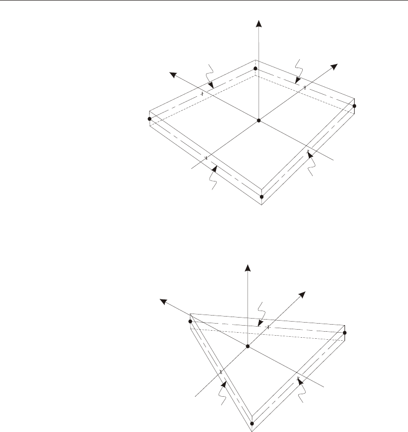
•For the quad ri lat eral, the four joints need not be coplanar. A small amount of
twist in the el e ment is ac counted for by the pro gram. The an gle be tween the
nor mals at the cor ners gives a mea sure of the de gree of twist. The nor mal at a
Joint Connectivity 181
Chapter X The Shell Element
Axis 1
Axis 1
Axis 3
Axis 3
Axis 2
Axis 2
j1
j1
j2
j2
j3
j3
j4
Face 1
Face 1
Face 3
Face 3
Face 4
Face 2
Face 2
Face 6: Top (+3 face)
Face 5: Bottom (–3 face)
Face 6: Top (+3 face)
Face 5: Bottom (–3 face)
Four-node Quadrilateral Shell Element
Three-node Triangular Shell Element
Figure 42
Area Element Joint Connectivity and Face Definitions
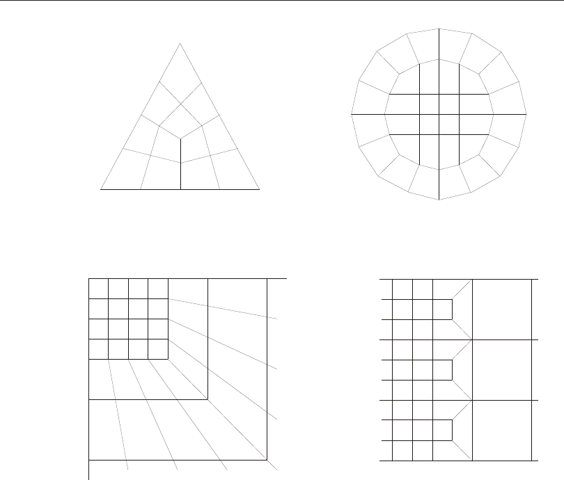
cor ner is per pen dic u lar to the two sides that meet at the cor ner. Best re sults are
ob tained if the larg est an gle be tween any pair of cor ners is less than 30°. This
an gle should not ex ceed 45°.
These con di tions can usu ally be met with ade quate mesh re fine ment. The ac cu racy
of the thick- plate and lay ered for mu la tions is more sen si tive to large as pect ra tios
and mesh dis tor tion than is the thin- plate for mu la tion.
182 Joint Connectivity
CSI Analysis Reference Manual
Triangular Region Circular Region
Infinite Region Mesh Transition
Figure 43
Mesh Examples Using the Quadrilateral Area Element
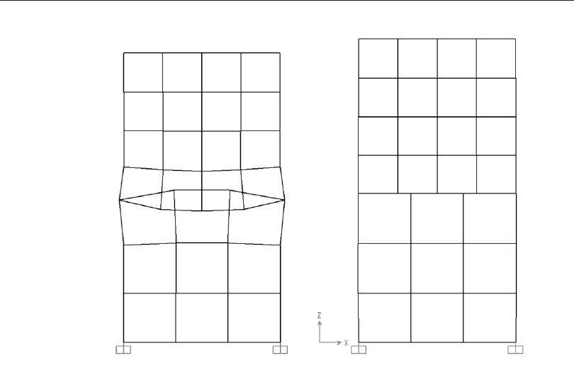
Edge Con straints
You can as sign au to matic edge con straints to any shell el e ment (or any area ob -
jects.) When edge con straints are as signed to an element, the pro gram
automatically con nects all joints that are on the edge of the el e ment to the ad ja cent
cor ner joints of the el e ment. Joints are con sid ered to be on the edge of the el e ment if
they fall within the auto-merge tol er ance set by you in the Graphical User Interface.
Edge con straints can be used to con nect to gether mis-matched shell meshes, but
will also con nect any el e ment that has a joint on the edge of the shell to that shell.
This in clude beams, col umns, re strained joints, link sup ports, etc.
These joints are con nected by flex i ble in ter po la tion con straints. This means that the
dis place ments at the in ter me di ate joints on the edge are in ter po lated from the dis -
place ments of the cor ner joints of the shell. No over all stiff ness is added to the
model; the ef fect is en tirely lo cal to the edge of the el e ment.
Edge Con straints 183
Chapter X The Shell Element
Figure 44
Connecting Meshes with the Edge Constraints: Left Model – No Edge
Constraints; Right Model – Edge Constraints Assigned to All Elements

Figure 44 (page 183) shows an ex am ple of two mis-matched meshes, one con -
nected with edge con straints, and one not. In the con nected mesh on the right, edge
con straints were as signed to all el e ments, al though it was re ally only nec es sary to
do so for the el e ments at the tran si tion. As sign ing edge con straints to el e ments that
do not need them has lit tle ef fect on per for mance and no ef fect on re sults.
The ad van tage of us ing edge con straints in stead of the mesh tran si tions shown in
Figure 43 (page 182) is that edge con straints do not re quire you to cre ate dis torted
el e ments. This can in crease the ac cu racy of the re sults.
It is im por tant to un der stand that near any tran si tion, whether us ing edge con -
straints or not, the ac cu racy of stress re sults is con trolled by the larg est el e ment
size. Fur ther more, the ef fect of the coarser mesh prop a gates into the finer mesh for
a dis tance that is on the or der of the size of the larger el e ments, as gov erned by St.
Venant’s ef fect. For this rea son, be sure to cre ate your mesh tran si tions far enough
away from the ar eas where you need de tailed stress re sults.
Im por tant Note: Edge con straints trans fer load from in ter me di ate joints to cor ner
joints along the edge of a shell. Ap ply ing an edge con straint along an edge that is
co-lin ear with a frame, ca ble, ten don or link ob ject can re sult in load be ing trans -
ferred by the edge con straint in stead of by that ob ject. Us ing edge con straints in
these lo ca tions should be avoided if de tailed re sults in the frame/ca ble/ten don/link
are of in ter est. In par tic u lar, frame de sign re sults could be af fected, and may be
unconservative. Frame/ca ble/ten don/link ob jects with only one joint con nected to
the edge are not af fected, and in fact one of the ad van tages of us ing edge con straints
is to con nect such el e ments to a coarse shell mesh, pro vided that de tailed lo cal
stresses in the shells are not needed. When frame/ca ble/ten don/link ob jects are
co-lin ear with an edge con straint, the over all ef fect of the ob ject on the model is
cap tured, but lo cal re sponse may not be ac cu rate.
Degrees of Freedom
The Shell ele ment al ways ac ti vates all six de grees of free dom at each of its con -
nected joints. When the ele ment is used as a pure mem brane, you must en sure that
re straints or other sup ports are pro vided to the de grees of free dom for nor mal trans -
la tion and bend ing ro ta tions. When the ele ment is used as a pure plate, you must en -
sure that re straints or other sup ports are pro vided to the de grees of free dom for in-
plane trans la tions and the ro ta tion about the nor mal.
The use of the full shell be hav ior (mem brane plus plate) is rec om mended for all
three- dimensional struc tures.
184 Degrees of Freedom
CSI Analysis Reference Manual

Note that the “drill ing” de gree of free dom (ro ta tion about the nor mal) is not used
for the lay ered shell and should not be loaded.
See Topic “De grees of Free dom” (page 30) in Chap ter “Joints and De grees of Free -
dom” for more in for ma tion.
Local Coordinate System
Each Shell el e ment (and other types of area ob jects/el e ments) has its own ele ment
lo cal co or di nate sys tem used to de fine Ma te rial prop er ties, loads and out put. The
axes of this lo cal sys tem are de noted 1, 2 and 3. The first two axes lie in the plane of
the ele ment with an ori en ta tion that you spec ify; the third axis is nor mal.
It is im por tant that you clearly un der stand the defi ni tion of the ele ment lo cal 1- 2-3
co or di nate sys tem and its re la tion ship to the global X- Y-Z co or di nate sys tem. Both
sys tems are right- handed co or di nate sys tems. It is up to you to de fine lo cal sys tems
which sim plify data in put and in ter pre ta tion of re sults.
In most struc tures the defi ni tion of the ele ment lo cal co or di nate sys tem is ex -
tremely sim ple. The meth ods pro vided, how ever, pro vide suf fi cient power and
flexi bil ity to de scribe the ori en ta tion of Shell ele ments in the most com pli cated
situa tions.
Lo cal axes are first com puted for the el e ment with out con sid er ing joint off sets.
These are called the nom i nal lo cal axes. If the joint off sets shift the ref er ence sur -
face by a dif fer ent amount at each joint, the lo cal axes are then trans formed by pro -
ject ing them onto the new nor mal to de ter mine the ac tual lo cal co or di nate sys tem
used for anal y sis.
The dis cus sion be low con sid ers the cal cu la tion of the nom i nal lo cal axes us ing the
joints. The trans for ma tion for the joint offsets, if needed, is dis cussed later in Topic
“Joint Off sets and Thick ness Overwrites” (page 203).
The sim plest method, us ing the de fault ori en ta tion and the Shell ele ment co or di -
nate an gle, is de scribed in this topic. Ad di tional meth ods for de fin ing the Shell ele -
ment lo cal co or di nate sys tem are de scribed in the next topic.
For more in for ma tion:
•See Chap ter “Co or di nate Sys tems” (page 11) for a de scrip tion of the con cepts
and ter mi nol ogy used in this topic.
•See Topic “Ad vanced Lo cal Co or di nate Sys tem” (page 186) in this Chap ter.
Local Coordinate System 185
Chapter X The Shell Element

Normal Axis 3
Lo cal axis 3 is al ways nor mal to the plane of the Shell ele ment. This axis is di rected
to ward you when the path j1-j2-j3 ap pears coun ter clock wise. For quad ri lat eral ele -
ments, the ele ment plane is de fined by the vec tors that con nect the mid points of the
two pairs of op po site sides.
Default Orientation
The de fault ori en ta tion of the lo cal 1 and 2 axes is de ter mined by the re la tion ship
be tween the lo cal 3 axis and the global Z axis:
•The lo cal 3-2 plane is taken to be ver ti cal, i.e., par al lel to the Z axis
•The lo cal 2 axis is taken to have an up ward (+Z) sense un less the ele ment is
hori zon tal, in which case the lo cal 2 axis is taken along the global +Y di rec tion
•The lo cal 1 axis is hori zon tal, i.e., it lies in the X-Y plane
The ele ment is con sid ered to be hori zon tal if the sine of the an gle be tween the lo cal
3 axis and the Z axis is less than 10-3.
The lo cal 2 axis makes the same an gle with the ver ti cal axis as the lo cal 3 axis
makes with the hori zon tal plane. This means that the lo cal 2 axis points ver ti cally
up ward for ver ti cal ele ments.
Element Coordinate Angle
The Shell ele ment co or di nate an gle, ang, is used to de fine ele ment ori en ta tions that
are dif fer ent from the de fault ori en ta tion. It is the an gle through which the lo cal 1
and 2 axes are ro tated about the posi tive lo cal 3 axis from the de fault ori en ta tion.
The ro ta tion for a posi tive value of ang ap pears coun ter clock wise when the lo cal
+3 axis is point ing to ward you.
For hori zon tal ele ments, ang is the an gle be tween the lo cal 2 axis and the hori zon tal
+Y axis. Oth er wise, ang is the an gle be tween the lo cal 2 axis and the ver ti cal plane
con tain ing the lo cal 3 axis. See Figure 45 (page 187) for ex am ples.
Advanced Local Coordinate System
By de fault, the ele ment lo cal co or di nate sys tem is de fined us ing the ele ment co or -
di nate an gle meas ured with re spect to the global +Z and +Y di rec tions, as de scribed
186 Advanced Local Coordinate System
CSI Analysis Reference Manual
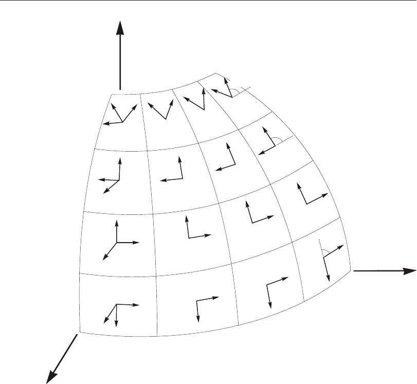
in the pre vi ous topic. In cer tain mod el ing situa tions it may be use ful to have more
con trol over the speci fi ca tion of the lo cal co or di nate sys tem.
This topic de scribes how to de fine the ori en ta tion of the tan gen tial lo cal 1 and 2
axes, with re spect to an ar bi trary ref er ence vec tor when the ele ment co or di nate an -
gle, ang, is zero. If ang is dif fer ent from zero, it is the an gle through which the lo cal
1 and 2 axes are ro tated about the posi tive lo cal 3 axis from the ori en ta tion de ter -
mined by the ref er ence vec tor. The lo cal 3 axis is al ways nor mal to the plane of the
ele ment.
Advanced Local Coordinate System 187
Chapter X The Shell Element
Z
X
Y
45°
90°
–90°
3
For all elements,
Axis 3 points outward,
toward viewer
1
2
1
2
1
2
1
2
3
3
3
Top row: ang = 45°
2nd row: ang = 90°
3rd row: ang = 0°
4th row: ang = –90°
Figure 45
The Area Element Coordinate Angle with Respect to the Default Orientation

For more in for ma tion:
•See Chap ter “Co or di nate Sys tems” (page 11) for a de scrip tion of the con cepts
and ter mi nol ogy used in this topic.
•See Topic “Lo cal Co or di nate Sys tem” (page 185) in this Chap ter.
Reference Vector
To de fine the tan gen tial lo cal axes, you spec ify a ref er ence vec tor that is par al lel to
the de sired 3-1 or 3-2 plane. The ref er ence vec tor must have a posi tive pro jec tion
upon the cor re spond ing tan gen tial lo cal axis (1 or 2, re spec tively). This means that
the posi tive di rec tion of the ref er ence vec tor must make an an gle of less than 90°
with the posi tive di rec tion of the de sired tan gen tial axis.
To de fine the ref er ence vec tor, you must first spec ify or use the de fault val ues for:
•A pri mary co or di nate di rec tion pldirp (the de fault is +Z)
•A sec on dary co or di nate di rec tion pldirs (the de fault is +Y). Di rec tions pldirs
and pldirp should not be par al lel to each other un less you are sure that they are
not par al lel to lo cal axis 3
•A fixed co or di nate sys tem csys (the de fault is zero, in di cat ing the global co or -
di nate sys tem)
•The lo cal plane, lo cal, to be de ter mined by the ref er ence vec tor (the de fault is
32, in di cat ing plane 3-2)
You may op tion ally spec ify:
•A pair of joints, plveca and plvecb (the de fault for each is zero, in di cat ing the
cen ter of the ele ment). If both are zero, this op tion is not used
For each ele ment, the ref er ence vec tor is de ter mined as fol lows:
1. A vec tor is found from joint plveca to joint plvecb. If this vec tor is of fi nite
length and is not par al lel to lo cal axis 3, it is used as the ref er ence vec tor Vp
2. Oth er wise, the pri mary co or di nate di rec tion pldirp is evalu ated at the cen ter of
the ele ment in fixed co or di nate sys tem csys. If this di rec tion is not par al lel to
lo cal axis 3, it is used as the ref er ence vec tor Vp
3. Oth er wise, the sec on dary co or di nate di rec tion pldirs is evalu ated at the cen ter
of the ele ment in fixed co or di nate sys tem csys. If this di rec tion is not par al lel to
lo cal axis 3, it is used as the ref er ence vec tor Vp
188 Advanced Local Coordinate System
CSI Analysis Reference Manual
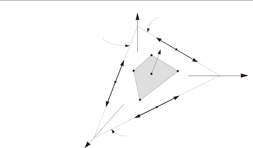
4. Oth er wise, the method fails and the analy sis ter mi nates. This will never hap pen
if pldirp is not par al lel to pldirs
A vec tor is con sid ered to be par al lel to lo cal axis 3 if the sine of the an gle be tween
them is less than 10-3.
The use of the co or di nate di rec tion method is il lus trated in Figure 46 (page 189) for
the case where lo cal = 32.
Determining Tangential Axes 1 and 2
The pro gram uses vec tor cross prod ucts to de ter mine the tan gen tial axes 1 and 2
once the ref er ence vec tor has been speci fied. The three axes are rep re sented by the
three unit vec tors V1, V2 and V3, re spec tively. The vec tors sat isfy the cross- product
re la tion ship:
VVV
123
=´
The tan gen tial axes 1 and 2 are de fined as fol lows:
Advanced Local Coordinate System 189
Chapter X The Shell Element
Intersection of Element
Plane & Global X-Y Plane
Intersection of Element
Plane & Global Y-Z Plane
Intersection of Element
Plane & Global Z-X Plane
j1
j2
j4
j3
X
Y
Z
V3
V pldirp = +X
1
V pldirp = +Z
1
V pldirp = –X
1
pldirp = –Y V1
pldirp = +Y V1
V pldirp = –Z
1
For all cases: local = 32
Figure 46
Area Element Local Coordinate System Using Coordinate Directions

•If the ref er ence vec tor is par al lel to the 3-1 plane, then:
VVV
23
=´p and
VVV
123
=´
•If the ref er ence vec tor is par al lel to the 3-2 plane, then:
VVV
13
=´
p and
VVV
231
=´
In the com mon case where the ref er ence vec tor is par al lel to the plane of the ele -
ment, the tan gen tial axis in the se lected lo cal plane will be equal to Vp.
Section Properties
A Shell Sec tion is a set of ma te rial and geo met ric prop er ties that de scribe the
cross-sec tion of one or more Shell ob jects (el e ments.) A Shell Sec tion prop erty is a
type of Area Sec tion prop erty. Sec tions are de fined in de pend ently of the objects,
and are as signed to the area ob jects.
Area Section Type
When de fin ing an area sec tion, you have a choice of three ba sic el e ment types:
•Shell – the sub ject of this Chap ter, with translational and ro ta tional de grees of
free dom, ca pa ble of sup port ing forces and mo ments
•Plane (stress or strain) – a two-di men sional solid, with translational de grees of
free dom, ca pa ble of sup port ing forces but not mo ments. This el e ment is cov -
ered in Chap ter “The Plane El e ment” (page 215).
•Asolid – axisymmetric solid, with translational de grees of free dom, ca pa ble of
sup port ing forces but not mo ments. This el e ment is cov ered in Chap ter “The
Asolid El e ment” (page 225).
Shell Sec tion Type
For Shell sec tions, you may choose one of the fol low ing types of be hav ior:
•Mem brane
–Pure mem brane be hav ior
–Sup ports only the in-plane forces and the nor mal (drill ing) mo ment
–Lin ear, homogeneous ma te rial.
190 Section Properties
CSI Analysis Reference Manual

•Plate
–Pure plate be hav ior
–Sup ports only the bend ing mo ments and the trans verse force
–Thick- or thin-plate for mu la tion
–Lin ear, homogeneous ma te rial.
•Shell
–Full shell be hav ior, a com bi na tion of mem brane and plate be hav ior
–Sup ports all forces and mo ments
–Thick- or thin-plate for mu la tion
–Lin ear, homogeneous ma te rial.
•Lay ered
–Mul ti ple lay ers, each with a dif fer ent ma te rial, thick ness, be hav ior, and lo -
ca tion
–Pro vides full-shell be hav ior un less all lay ers have only mem brane or only
plate be hav ior
–With full-shell be hav ior, sup ports all forces and mo ments ex cept the “drill -
ing” mo ment
–Thick-plate for mu la tion; may be non lin ear.
It is gen er ally rec om mended that you use the full-shell be hav ior un less the en tire
struc ture is pla nar and is ad e quately re strained.
Homogeneous Section Properties
Ho mo ge neous ma te rial prop er ties are used for the non-lay ered Mem brane, Plate,
and Shell sec tion types. The fol low ing data needs to be spec i fied.
Section Thickness
Each ho mo ge neous Sec tion has a con stant mem brane thick ness and a con stant
bend ing thick ness. The mem brane thick ness, th, is used for cal cu lat ing:
•The mem brane stiff ness for full-shell and pure-mem brane Sec tions
•The el e ment vol ume for the el e ment self-weight and mass cal cu la tions
The bend ing thick ness, thb, is use for cal cu lat ing:
Section Properties 191
Chapter X The Shell Element

•The plate-bend ing and trans verse-shear ing stiffnesses for full-shell and
pure-plate Sec tions
Nor mally these two thick nesses are the same and you only need to spec ify th. How -
ever, for some ap pli ca tions, you may wish to ar ti fi cially change the mem brane or
plate stiff ness. For this pur pose, you may spec ify a value of thb that is dif fer ent
from th. For more de tailed con trol, such as rep re sent ing cor ru gated or orthotropic
con struc tion, the use of prop erty mod i fi ers is better. See Topic “Prop erty
Modifiers” (page 201.)
Thickness Formulation
Two thick ness for mu la tions are avail able, which de ter mine whether or not trans -
verse shear ing de for ma tions are in cluded in the plate-bend ing be hav ior of a plate or
shell el e ment:
•The thick-plate (Mindlin/Reissner) for mu la tion, which in cludes the ef fects of
trans verse shear de for ma tion
•The thin-plate (Kirchhoff) for mu la tion, which ne glects trans verse shear ing de -
for ma tion
Shearing de for ma tions tend to be im por tant when the thick ness is greater than
about one-tenth to one-fifth of the span. They can also be quite sig nif i cant in the vi -
cin ity of bend ing-stress con cen tra tions, such as near sud den changes in thick ness
or sup port con di tions, and near holes or re-en trant cor ners.
Even for thin-plate bend ing prob lems where shear ing de for ma tions are truly neg li -
gi ble, the thick-plate for mu la tion tends to be more ac cu rate, al though some what
stiffer, than the thin-plate for mu la tion. How ever, the ac cu racy of the thick-plate
for mu la tion is more sen si tive to large as pect ra tios and mesh dis tor tion than is the
thin-plate for mu la tion.
It is gen er ally rec om mended that you use the thick-plate for mu la tion un less you are
us ing a dis torted mesh and you know that shear ing de for ma tions will be small, or
un less you are try ing to match a the o ret i cal thin-plate so lu tion.
The thick ness for mu la tion has no ef fect upon mem brane be hav ior, only upon
plate-bend ing be hav ior.
Section Material
The ma te rial prop er ties for each Sec tion are spec i fied by ref er ence to a pre vi -
ously-de fined Ma te rial. The ma te rial may be iso tro pic, uni ax ial, or orthotropic. If
192 Section Properties
CSI Analysis Reference Manual

an anisotropic ma te rial is cho sen, orthotropic prop er ties will be used. The ma te rial
prop er ties used by the Shell Sec tion are:
•The moduli of elas tic ity, e1, e2, and e3
•The shear modulus, g12, g13, and g23
•The Pois son’s ra tios, u12, u13, and u23
•The co ef fi cients of ther mal ex pan sion, a1 and a2
•The mass den sity, m, for com put ing el e ment mass
•The weight den sity, w, for com put ing Self-Weight and Grav ity Loads
The prop er ties e3, u13, and u23 are con densed out of the ma te rial ma trix by as sum -
ing a state of plane stress in the el e ment. The re sult ing, mod i fied val ues of e1, e2,
g12, and u12 are used to com pute the mem brane and plate-bend ing stiffnesses.
The shear moduli, g13 and g23, are used to com pute the trans verse shear ing stiff -
ness if the thick-plate for mu la tion is used. The co ef fi cients of ther mal ex pan sion,
a1 and a2, are used for mem brane ex pan sion and ther mal bend ing strain.
All ma te rial prop er ties (ex cept the den si ties) are obtained at the ma te rial tem per a -
ture of each in di vid ual el e ment.
See Chap ter “Ma te rial Prop er ties” (page 69) for more in for ma tion.
Section Material Angle
The ma te rial lo cal co or di nate sys tem and the el e ment (Shell Sec tion) lo cal co or di -
nate sys tem need not be the same. The lo cal 3 di rec tions al ways co in cide for the
two sys tems, but the ma te rial 1 axis and the el e ment 1 axis may dif fer by the an gle a
as shown in Figure 47 (page 194). This an gle has no ef fect for iso tro pic ma te rial
prop er ties since they are in de pend ent of ori en ta tion.
See Topic “Lo cal Co or di nate Sys tem” (page 70) in Chap ter “Ma te rial Prop er ties”
for more in for ma tion.
Layered Section Property
For the lay ered Sec tion prop erty, you de fine how the sec tion is built-up in the thick -
ness di rec tion. Any num ber of lay ers is al lowed, even a sin gle layer. Lay ers are lo -
cated with re spect to a ref er ence sur face. This ref er ence sur face may be the mid dle
sur face, the neu tral sur face, the top, the bot tom, or any other lo ca tion you choose.
By de fault, the ref er ence sur face con tains the el e ment nodes, al though this can be
changed us ing joint off sets.
Section Properties 193
Chapter X The Shell Element

The thick-plate (Mindlin/Reissner) for mu la tion, which in cludes the ef fects of
trans verse shear de for ma tion, is al ways used for bend ing be hav ior the lay ered
shell.
The fol low ing eight pa ram e ters are spec i fied to de fine each layer, as il lus trated in
Figure 48 (page 195.)
(1) Layer Name
The layer name is ar bi trary, but must be unique within a sin gle Sec tion. How ever,
the same layer name can be used in dif fer ent Sec tions. This can be use ful be cause
re sults for a given layer name can be plot ted si mul ta neously for el e ments hav ing
dif fer ent Sec tions.
(2) Layer Dis tance
Each layer is lo cated by spec i fy ing the dis tance from the ref er ence sur face to the
cen ter of the layer, mea sured in the pos i tive lo cal-3 di rec tion of the el e ment. This
value is called d in the ex am ples be low.
194 Section Properties
CSI Analysis Reference Manual
3 (Element, Material)
a
a
1 (Element)
1 (Material)
2 (Element)
2 (Material)
Figure 47
Shell Section Material Angle
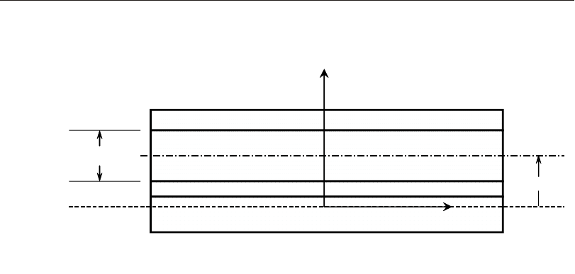
(3) Layer Thick ness
Each layer has a sin gle thick ness, mea sured in the lo cal-3 di rec tion of the el e ment.
For mod el ing rebar or ma te rial fi bers, you can spec ify a very thin “smeared” layer
that has an equiv a lent cross-sec tional area. This value is called th in the ex am ples
be low.
(4) Layer Type
You can choose be tween:
•Mem brane: Strains in the layer (eeg
112212
,,) are com puted only from in-plane
mem brane dis place ments, and stresses in the layer (,,)sss
112212 con trib ute
only to in-plane mem brane forces (,,)FFF
112212.
•Plate: Strains in the layer (eeggg
1122121323
,,,,) are com puted only from
plate-bend ing ro ta tions and trans verse displacements, and stresses in the layer
(sssss
1122121323
,,,,) con trib ute only to plate-bend ing mo ments and trans -
verse shear ing forces (MMMVV
1122121323
,,,,).
•Shell, which com bines mem brane and plate be hav ior: Strains in the layer
(eeggg
1122121323
,,,,) are com puted from all dis place ments and plate-bend -
ing ro ta tions, and stresses in the layer (sssss
1122121323
,,,,) con trib ute to
Section Properties 195
Chapter X The Shell Element
Thickness
Reference
Surface
Distance
Axis1
Axis3
Layer“A”
Layer“B”
Layer“C”
Layer“D”
Figure 48
Four-Layer Shell, Showing the Reference Surface, the Names of the Layers,
and the Distance and Thickness for Layer “C”

all forces and plate-bend ing mo ments
(FFFMMMVV
1122121122121323
,,,,,,,)
.
In most ap pli ca tions, lay ers should use shell be hav ior. See shear-wall mod el ing be -
low for an ex am ple of where you might want to sep a rate membrane and plate be -
hav ior.
Im por tant Note: Mass and weight are com puted only for mem brane and shell lay -
ers, not for plate lay ers. This pre vents dou ble-count ing when in de pend ent mem -
brane and plate lay ers are used for the same ma te rial.
(5) Layer Number of Thickness In te gra tion Points
Ma te rial be hav ior is in te grated (sam pled) at a fi nite num ber of points in the thick -
ness di rec tion of each layer. You may choose one to five points for each layer. The
lo ca tion of these points fol lows stan dard Guass in te gra tion pro ce dures. This value
is called n in the ex am ples be low.
For a sin gle layer of lin ear ma te rial, one point in the thick ness di rec tion is ad e quate
to rep re sent mem brane be hav ior, and two points will cap ture both mem brane and
plate be hav ior. If you have mul ti ple lay ers, you may be able to use a sin gle point for
thin ner lay ers.
Non lin ear be hav ior may re quire more in te gra tion points or more lay ers in or der to
cap ture yield ing near the top and bot tom sur faces. Us ing an ex ces sive num ber of
in te gra tion points can in crease anal y sis time. You may need to ex per i ment to find a
bal ance be tween ac cu racy and com pu ta tional ef fi ciency.
(6) Layer Ma te rial
The ma te rial prop er ties for each layer are spec i fied by ref er ence to a pre vi ously-de -
fined Ma te rial. The ma te rial may be iso tro pic, uni ax ial, or orthotropic. If an
anisotropic ma te rial is cho sen, orthotropic prop er ties will be used. The be hav ior of
the ma te rial de pends on the ma te rial com po nent be hav ior cho sen for the layer, as
de scribed be low.
(7) Layer Ma te rial An gle
For orthotropic and uni ax ial ma te ri als, the ma te rial axes may be ro tated with re -
spect to the el e ment axes. Each layer may have a dif fer ent ma te rial an gle. For ex -
am ple, you can model rebar in two or thogo nal di rec tions as two lay ers of uni ax ial
ma te rial with ma te rial an gles 90° apart. This value is called ang in the ex am ples be -
low. For fur ther in for ma tion, see topic “Sec tion Ma te rial An gle” above (page 193.)
196 Section Properties
CSI Analysis Reference Manual
(8) Layer Material Behavior
Choose be tween “Di rec tional” and “Cou pled”. Di rec tional be hav ior can be ap plied
to all ma te ri als and is de scribed in the re main der of this topic. Cou pled be hav ior is
avail able for con crete ma te ri als only, and uses the mod i fied Dar win-Pecknold be -
hav ior as de scribed in Chap ter “Ma te rial Prop er ties”, Topic “Mod i fied Dar -
win-Pecknold Con crete Model” (page 100).
(9) Layer Material Components
This op tion applies only to “Di rec tional” ma te rial be hav ior. For each of the three
mem brane stress com po nents (,,)sss
112212, you can choose whether the be hav -
ior is lin ear, non lin ear, or in ac tive. For a uni ax ial ma te rial, only the two com po -
nents
(,)ss
1112 are sig nif i cant, since s220= al ways. Ma te rial com po nents are de -
fined in the ma te rial lo cal co or di nate sys tem, which de pends on the ma te rial an gle
and may not be the same for ev ery layer.
If all three com po nents are lin ear (two for the uni ax ial ma te rial), then the lin ear ma -
te rial ma trix is used for the layer, ac cord ing to Equa tions (1) to (4) in Chap ter “Ma -
te rial Prop er ties” (page 69). Note that for anisotropic ma te ri als, the shear cou pling
terms in Equa tion (4) are ne glected so that the be hav ior is the same as given by
Equa tion (3).
If one or more of the three com po nents is non lin ear or in ac tive, then all lin ear com -
po nents use an un cou pled iso tro pic lin ear stress-strain law, all non lin ear com po -
nents use the non lin ear stress-strain re la tion ship, and all in ac tive com po nents as -
sume zero stress. The com po nents be come un cou pled, and be have as if Pois son’s
ra tio is zero. The be hav ior is sum ma rized in the fol low ing ta ble:
Component Linear Nonlinear Inactive
s11se
1111
=×e1Eqns. (5) s110=
s22se
2222
=×e1Eqns. (5) s220=
s12se
1212
=×e1Eqns. (6) s120=
Note that the lin ear equa tion for s12 is for an iso tro pic ma te rial with zero Poisson’s
ra tio. See Chap ter “Ma te rial Prop er ties” (page 69) for Equa tions (5) and (6).
For a uni ax ial ma te rial, s220= and s12 is half the value given in the ta ble above.
Section Properties 197
Chapter X The Shell Element

Trans verse shear be hav ior is al ways lin ear, and is con trolled by the cor re spond ing
mo ment com po nents. For a layer of type Mem brane, the trans verse shear stresses
(,)ss
1323 are both zero. For a layer of type Plate or Shell:
•s130= if s11 is in ac tive, else sg
1313
=×g13
•s230= if s22 is in ac tive, else sg
2323
=×g23
In ter ac tion Be tween Lay ers
Lay ers are de fined in de pend ently, and it is per mis si ble for lay ers to over lap, or for
gaps to ex ist between the lay ers. It is up to you to de cide what is ap pro pri ate.
For ex am ple, when mod el ing a con crete slab, you can choose a sin gle layer to rep -
re sent the full thick ness of con crete, and four lay ers to rep re sent rebar (two near the
top at a 90° an gle to each other, and two sim i lar lay ers at the bot tom.) These rebar
lay ers would be very thin, us ing an equivalent thick ness to rep re sent the cross-sec -
tional area of the steel. Be cause the lay ers are so thin, there is no need to worry
about the fact that the rebar layers over lap the con crete. The amount of ex cess con -
crete that is con tained in the over lapped re gion is very small.
Lay ers are ki ne mat i cally con nected by the Mindlin/Reissner as sump tion that nor -
mals to the ref er ence sur face re main straight af ter de for ma tion. This is the shell
equiv a lent to the beam as sump tion that plane sec tions re main plane.
In te gra tion in the Plane
Force-de flec tion be hav ior is com puted by in te grat ing the stress-strain be hav ior
through the thick ness and over the 1-2 plane of the el e ment. You can spec ify the
num ber of in te gra tion points in the thick ness di rec tion of each layer as de scribed
above.
For each of these thick ness lo ca tions, in te gra tion in the plane is per formed at the
stan dard 2 x 2 Gauss points (co or di nates ±0.577 on a square of size ±1.0). Non lin -
ear be hav ior is sam pled only at these points. This is equiv a lent to hav ing two fi bers,
lo cated ap prox i mately at the ¼ and ¾ points, in each of the lo cal 1 and 2 di rec tions.
Plot ted or tab u lated stresses at lo ca tions other than the four Gauss points are in ter -
po lated or ex trap o lated, and do not nec es sar ily rep re sent the sam pled non lin ear
stresses. For this rea son, stresses at the joints may some times ap pear to ex ceed fail -
ure stresses.
198 Section Properties
CSI Analysis Reference Manual

Example: Non lin ear Shear-Wall, “Realistic” Mod el ing
An im por tant ap pli ca tion for the lay ered shell el e ment is non lin ear shear-wall mod -
el ing, and it will serve as an ex am ple for other ap pli ca tions. Let's con sider an 18
inch (457 mm) thick ver ti cal wall, with two ver ti cal and two hor i zon tal lay ers of
rebar hav ing 3 inch (76 mm) cover from both faces. The two hor i zon tal layers to -
gether pro vide a 1% rebar area ra tio, and the two ver ti cal lay ers to gether pro vide an
area ra tio of 2%.
When mod el ing lin ear be hav ior, it is not usu ally nec es sary to in clude the rebar, but
it is es sen tial for non lin ear be hav ior. In the sim plest case, the en tire wall sec tion
will be con sid ered as non lin ear for both mem brane and bend ing be hav ior, lead ing
to the most “re al is tic”, if not the most prac ti cal model. The re quires a lay ered sec -
tion with five lay ers:
“Re al is tic” Shear-Wall Model
Layer Type Material th d ang ns11s22s12
1Shell Conc 18.00 0. 0°5NNN
2Shell Rebar 0.09 +6. 0°1N-N
3Shell Rebar 0.09 -6. 0°1N-N
4Shell Rebar 0.18 +6. 90°1N-N
5Shell Rebar 0.18 -6. 90°1N-N
For the stress com po nents, “N” in di cates non lin ear, “L” in di cates lin ear, and “-”
in di cates in ac tive. The con crete ma te rial be hav ior may be “Di rec tional” or “Cou -
pled”.
Note that for the rebar, s11 is al ways non lin ear. Ver ti cal rebar is de fined by set ting
the ma te rial an gle to 90°, which aligns it with the shell lo cal-2 axis. Hence the ver ti -
cal rebar stress s11 cor re sponds to shell s22.
Also note that for the rebar, s12 is set to be non lin ear. This al lows the rebar to carry
shear when the con crete cracks. This can taken to rep re sent dowel ac tion, al though
no in for ma tion on ac tual dowel be hav ior is pres ent in the model, so it is only an ap -
prox i ma tion. You must use your en gi neer ing judge ment to de ter mine if this ap -
proach is suit able to your needs. The most con ser va tive ap proach is to set the rebar
stress com po nent s12 to be in ac tive.
Section Properties 199
Chapter X The Shell Element

Example: Non lin ear Shear-Wall, “Practical” Mod el ing
The five-layer model above seems re al is tic, but pres ents many fail ure mech a nisms
that may cloud the en gi neer ing in for ma tion re quired for per for mance-based de -
sign. When ever pos si ble, the sim plest model should be used to meet the en gi neer -
ing goals. Do ing this will make the anal y sis run faster and make the in ter pre ta tion
of re sults eas ier.
With this in mind, a more prac ti cal model is pre sented be low, with only the ver ti cal
mem brane stresses taken to be non lin ear. Such a model may be suit able for taller
shear walls where col umn-like be hav ior gov erns:
“Prac ti cal” Shear-Wall Model
Layer Type Material th d ang ns11s22s12
1Membr Conc 18.00 0. 0°1LNL
2Membr Rebar 0.18 +6. 90°1N--
3Membr Rebar 0.18 -6. 90°1N--
4Plate Conc 16.00 0. 0°2LLL
In this model, only mem brane be hav ior is non lin ear, and only for the ver ti cal stress
com po nent s22. This cor re sponds to rebar stress com po nent s11 when the ma te rial
an gle is 90°. Con crete ma te rial be hav ior is “Di rec tional”.
It is gen er ally not nec es sary to in clude rebar for lin ear be hav ior, so the hor i zon tal
rebar is omit ted, and the rebar shear stress com po nent s12 is set to be in ac tive.
Out-of-plane be hav ior is as sumed to be lin ear, so a sin gle con crete plate layer is
used. The thick ness has been re duced to ac count for crack ing with out ex plicit non -
lin ear mod el ing. Plate bend ing stiff ness is pro por tional to the cube of the thick ness.
Example: In-fill Panel
There are many ways to model an infill panel. Two ap proaches will be pre sented
here, both in tended to rep re sent mem brane shear re sis tance only. The simplest is a
sin gle layer of con crete ma te rial car ry ing only mem brane shear stress, as shown in
the fol low ing model:
200 Section Properties
CSI Analysis Reference Manual
Infill Wall - Sim ple Shear Model
Layer Type Material th d ang ns11s22s12
1Membr Conc 18.00 0. 0°1--N
In the sec ond model, the con crete is as sumed to act as com pres sion struts along the
two di ag o nals. For a square panel, these two struts would act at ma te rial an gles of
±45°, as shown in the fol low ing model:
Infill Wall - Com pres sion Strut Model
Layer Type Material th d ang ns11s22s12
1Membr Conc 18.00 0. 45°1N--
2Membr Conc 18.00 0. -45°1N--
Other pos si bil i ties ex ist. For both mod els, there is no ver ti cal or hor i zon tal mem -
brane stiff ness, and no plate-bend ing stiff ness. There fore, these mod els should only
be used when the el e ment is com pletely sur rounded by frame or other sup port ing
el e ments, and the elements should not be meshed.
Summary
As these ex am ples show, you have con sid er able flex i bil ity to cre ate lay ered shell
sec tions to rep re sent a va ri ety of lin ear and non lin ear be hav ior. The sim plest model
that ac com plishes the en gi neer ing goals should be used. Even when more com pli -
cated mod els may be war ranted, it is rec om mended to start with sim ple, mostly lin -
ear mod els, and in crease the level of com plex ity and nonlinearity as you gain ex pe -
ri ence with your model and its be hav ior.
To as sure a sta ble model, be sure to in clude lay ers that, when com bined, pro vide
both mem brane and plate con tri bu tions to each of the three stress com po nents.
Property Modifiers
You may spec ify scale fac tors to mod ify the com puted sec tion prop er ties. These
may be used, for ex am ple, to ac count for crack ing of con crete, cor ru gated or
orthotropic fab ri ca tion, or for other fac tors not eas ily de scribed in the ge om e try and
Property Modifiers 201
Chapter X The Shell Element

ma te rial prop erty val ues. In di vid ual mod i fi ers are avail able for the fol low ing ten
terms:
•Mem brane stiff ness cor re spond ing to force F11
•Mem brane stiff ness cor re spond ing to force F22
•Mem brane stiff ness cor re spond ing to force F12
•Plate bend ing stiff ness cor re spond ing to mo ment M11
•Plate bend ing stiff ness cor re spond ing to mo ment M22
•Plate bend ing stiff ness cor re spond ing to mo ment M12
•Plate shear stiff ness cor re spond ing to force V12
•Plate shear stiff ness cor re spond ing to force V13
•Mass
•Weight
The stiff ness mod i fi ers af fect only ho mog e nous el e ments, not lay ered el e ments.
The mass and weight mod i fi ers af fect all el e ments.
See Topic “In ter nal Force and Stress Output” (page 210) for the def i ni tion of the
force and mo ment com po nents above.
You may spec ify multi pli ca tive fac tors in two places:
•As part of the def i ni tion of the sec tion prop erty
•As an as sign ment to in di vid ual el e ments.
If mod i fi ers are as signed to an el e ment and also to the sec tion prop erty used by that
el e ment, then both sets of fac tors mul ti ply the sec tion prop er ties.
Named Prop erty Sets
In ad di tion to di rectly as sign ing prop erty mod i fi ers to shell el e ments, you can ap ply
them to a shell el e ment in a staged-con struc tion Load Case us ing a Named Prop erty
Set of Shell Prop erty Mod i fi ers. A Named Prop erty Set in cludes the same ten fac -
tors above that can be as signed to an el e ment.
When a Named Prop erty Set is ap plied to an el e ment in a par tic u lar stage of a Load
Case, it re places only the val ues that are as signed to the el e ment or that had been ap -
plied in a pre vi ous stage; val ues com puted by the Di rect Anal y sis Method of de sign
are also re placed. How ever, prop erty mod i fi ers spec i fied with the sec tion prop erty
re main in force and are not af fected by the ap pli ca tion of a Named Prop erty Set.
202 Property Modifiers
CSI Analysis Reference Manual

The net ef fect is to use the fac tors spec i fied in the Named Prop erty Set mul ti plied
by the fac tors spec i fied in the sec tion prop erty.
When prop erty mod i fi ers are changed in a staged con struc tion Load Case, they do
not change the re sponse of the struc ture up to that stage, but only af fect sub se quent
re sponse. In other words, the ef fect is in cre men tal. For ex am ple, con sider a can ti le -
ver with only de fault (unity) prop erty mod i fi ers, and a staged con struc tion case as
fol lows:
•Stage 1: Self-weight load is ap plied, re sult ing in a tip de flec tion of 1.0 and
a sup port mo ment of 1000.
•Stage 2: Named Prop erty Set “A” is ap plied that mul ti plies all stiffnesses
by 2.0, and the mass and weight by 1.0. The tip de flec tion and sup port mo -
ment do not change.
•Stage 3: Self-weight load is ap plied again (incrementally). The re sult ing
tip de flec tion is 1.5 and the sup port mo ment is 2000. Com pared to Stage 1,
the same in cre men tal load is ap plied, but the struc ture is twice as stiff.
• Stage 4: Named Prop erty Set “B” is ap plied that mul ti plies all stiffnesses,
as well as the mass and weight, by 2.0. The tip de flec tion and sup port mo -
ment do not change.
•Stage 5: Self-weight load is ap plied again (incrementally). The re sult ing
tip de flec tion is 2.5 and the sup port mo ment is 4000. Com pared to Stage 1,
twice the in cre men tal load is ap plied, and the struc ture is twice as stiff
Joint Offsets and Thickness Overwrites
You may op tion ally as sign joint off set and thick ness overwrites to any el e ment.
These are of ten used to gether to align the top or bot tom of the shell el e ment with a
given sur face. See Figure 49 (page 204.)
Joint Off sets
Joint off sets are mea sured from the joint to the ref er ence sur face of the el e ment in
the di rec tion nor mal to the plane of the joints. If the joints de fine a warped sur face,
the plane is de ter mine by the two lines con nect ing op po site mid-sides (i.e., the mid -
dle of j1-j2 to the mid dle of j3-j4, and the mid dle of j1-j3 to the mid dle of j2-j4.) A
pos i tive off set is in the same di rec tion as the pos i tive local-3 axis of the el e ment.
Joint off sets lo cate the ref er ence plane of the el e ment. For ho mo ge neous shells, this
is the mid-sur face of the el e ment. For lay ered shells, the ref er ence sur face is the
Joint Offsets and Thickness Overwrites 203
Chapter X The Shell Element
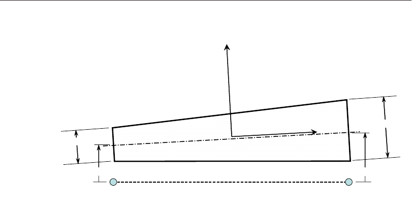
sur face you used to lo cate the lay ers in the sec tion. By chang ing the ref er ence sur -
face in a lay ered sec tion, you can ac com plish the same ef fect as us ing joint off sets
that are equal at the joints. See Topic “Lay ered Sec tion Property” (page 193) for
more in for ma tion.
When you as sign joint off sets to a shell el e ment, you can ex plic itly spec ify the off -
sets at the el e ment joints, or you can ref er ence a Joint Pat tern. Us ing a Joint Pat tern
makes it easy to spec ify con sis tently vary ing off sets over many el e ments. See
Topic “Joint Pat terns” (page 332) in Chap ter “Load Pat terns” for more in for ma tion.
Note that when the neu tral sur face of the el e ment, af ter ap ply ing joint off sets, is no
lon ger in the plane of the joints, mem brane and plate-bend ing be hav ior be come
cou pled. If you ap ply a di a phragm con straint to the joints, this will also con strain
bend ing. Like wise, a plate con straint will con strain mem brane ac tion.
Effect of Joint Offsets on the Lo cal Axes
The in ser tion points can in ter act sig nif i cantly with the el e ment lo cal co or di nate
sys tem. As de scribed pre vi ously, the nom i nal lo cal axes are com puted for zero joint
off sets, such the ref er ence sur face con nects to the joints.
If there are no joint off sets, or the joint off sets are equal at the joints, the off set ref -
er ence plane is par al lel to the orig i nal ref er ence plane of the joints. In this case no
204 Joint Offsets and Thickness Overwrites
CSI Analysis Reference Manual
Thickness1
Axis1
Axis3
Joint 1 Joint 2
Offset 2
Offset 1
Thickness2
ReferenceSurface
Joint Plane
Figure 49
Joint Offsets and Thickness Overwrites for a Homogeneous Shell
Edge View shown Along One Side

fur ther trans for ma tion is nec es sary, and the el e ment lo cal axes are the same as the
nom i nal lo cal axes.
If the joint off sets are not equal, a new lo cal 3 axis (~
V3) is com puted as the nor mal
to the plane de ter mined from the two lines con nect ing the midsides of the ref er ence
sur face af ter ap ply ing the off sets to the joints.
If the nor mal has changed di rec tion, then the el e ment lo cal co or di nate sys tem is
com puted as fol lows:
~~
VVV
123
=´ and
~~~
VVV
231
=´
where V1, V2, and V3 and the nom i nal lo cal axes com puted pre vi ously based on the
joints; and ~
V1, ~
V2, and ~
V3 are the trans formed lo cal axes used for anal y sis. If V2 is
ver ti cal, then ~
V1 will al ways be hor i zon tal. Note that the two sys tems are iden ti cal if
~
VV
33
=, the usual case.
The nom i nal axes are used only for de ter min ing the di rec tion of joint off sets. The
trans formed axes are used for all anal y sis pur poses, in clud ing load ing and re sults
out put.
Thick ness Overwrites
Nor mally the thick ness of the shell el e ment is de fined by the Sec tion Prop erty as -
signed to the el e ment. You have the op tion to over write this thick ness, in clud ing
the abil ity to spec ify a thick ness that var ies over the el e ment.
Cur rently this op tion only af fects ho mo ge neous shells. The thick ness of lay ered
shells is not changed. When thick ness overwrites are as signed to a ho mo ge neous
shell, both the mem brane thick ness, th, and the bend ing thick ness, thb, take the
over writ ten value.
When you as sign thick ness overwrites to a shell el e ment, you can ex plic itly spec ify
the thick nesses at the el e ment joints, or you can ref er ence a Joint Pat tern. Us ing a
Joint Pat tern makes it easy to spec ify con sis tently vary ing thick ness over many el e -
ments. See Topic “Joint Pat terns” (page 332) in Chap ter “Load Pat terns” for more
in for ma tion.
As an ex am ple, sup pose you have a vari able thick ness slab, and you want the top
sur face to lie in a sin gle flat plane. De fine a Joint Pat tern that de fines the thick ness
over the slab. Draw the el e ments so that the joints lie in the top plane. As sign thick -
Joint Offsets and Thickness Overwrites 205
Chapter X The Shell Element

ness overwrites to all the el e ments us ing the Joint Pat tern with a scale fac tor of one,
and as sign the joint off sets us ing the same Joint Pat tern, but with a scale fac tor of
one-half (pos i tive or neg a tive, as needed).
Mass
In a dy namic analy sis, the mass of the struc ture is used to com pute in er tial forces.
The mass con trib uted by the Shell ele ment is lumped at the ele ment joints. No in er -
tial ef fects are con sid ered within the ele ment it self.
The to tal mass of the el e ment is equal to the in te gral over the plane of the el e ment of
the mass den sity, m, mul ti plied by the mem brane thick ness, th, for ho mo ge neous
sec tions, and the sum of the masses of the in di vid ual lay ers for lay ered sec tions.
Note that for lay ered shells, mass is com puted only for mem brane and shell lay ers,
not for plate lay ers. The to tal mass may be scaled by the mass prop erty mod i fier.
The to tal mass is ap por tioned to the joints in a man ner that is pro por tional to the di -
ag o nal terms of the con sis tent mass ma trix. See Cook, Malkus, and Plesha (1989)
for more in for ma tion. The to tal mass is ap plied to each of the three translational de -
grees of free dom: UX, UY, and UZ. No mass mo ments of in er tia are com puted for
the ro ta tional de grees of free dom.
For more in for ma tion:
•See Topic “Mass Den sity” (page 77) in Chap ter “Ma te rial Prop er ties”.
•See Topic “Prop erty Modifiers” (page 201) in this chapter.
•See Topic “Mass Source” (page 334) in Chap ter “Load Pat terns”.
•See Chap ter “Static and Dy namic Analy sis” (page 341).
Self-Weight Load
Self-Weight Load ac ti vates the self-weight of all el e ments in the model. For a Shell
el e ment, the self-weight is a force that is uni formly dis trib uted over the plane of the
el e ment. The mag ni tude of the self-weight is equal to the weight den sity, w, mul ti -
plied by the mem brane thick ness, th, for ho mo ge neous sec tions, and the sum of the
weights of the in di vid ual lay ers for lay ered sec tions. Note that for lay ered shells,
weight is com puted only for mem brane and shell lay ers, not for plate lay ers. The to -
tal weight may be scaled by the weight prop erty mod i fier.
206 Mass
CSI Analysis Reference Manual

Self- Weight Load al ways acts down ward, in the global –Z di rec tion. You may
scale the self- weight by a sin gle scale fac tor that ap plies equally to all ele ments in
the struc ture.
For more in for ma tion:
•See Topic “Weight Den sity” (page 78) in Chap ter “Ma te rial Prop er ties” for the
defi ni tion of w.
•See Topic “Prop erty Mod i fi ers” (page 201) in this chap ter.
•See Topic “Self- Weight Load” (page 325) in Chap ter “Load Pat terns.”
Gravity Load
Grav ity Load can be ap plied to each Shell ele ment to ac ti vate the self- weight of the
ele ment. Us ing Grav ity Load, the self- weight can be scaled and ap plied in any di -
rec tion. Dif fer ent scale fac tors and di rec tions can be ap plied to each ele ment.
If all ele ments are to be loaded equally and in the down ward di rec tion, it is more
con ven ient to use Self- Weight Load.
For more in for ma tion:
•See Topic “Self- Weight Load” (page 191) in this Chap ter for the defi ni tion of
self- weight for the Shell ele ment.
•See Topic “Grav ity Load” (page 326) in Chap ter “Load Pat terns.”
Uniform Load
Uni form Load is used to ap ply uni formly dis trib uted forces to the mid sur faces of
the Shell ele ments. The di rec tion of the load ing may be speci fied in a fixed co or di -
nate sys tem (global or Al ter nate Co or di nates) or in the ele ment lo cal co or di nate
sys tem.
Load in ten si ties are given as forces per unit area. Load in ten si ties speci fied in dif -
fer ent co or di nate sys tems are con verted to the ele ment lo cal co or di nate sys tem and
added to gether. The to tal force act ing on the ele ment in each lo cal di rec tion is given
by the to tal load in ten sity in that di rec tion mul ti plied by the area of the mid-sur face.
This force is ap por tioned to the joints of the ele ment.
Forces given in fixed co or di nates can op tion ally be speci fied to act on the pro jected
area of the mid-sur face, i.e., the area that can be seen along the di rec tion of load ing.
Gravity Load 207
Chapter X The Shell Element
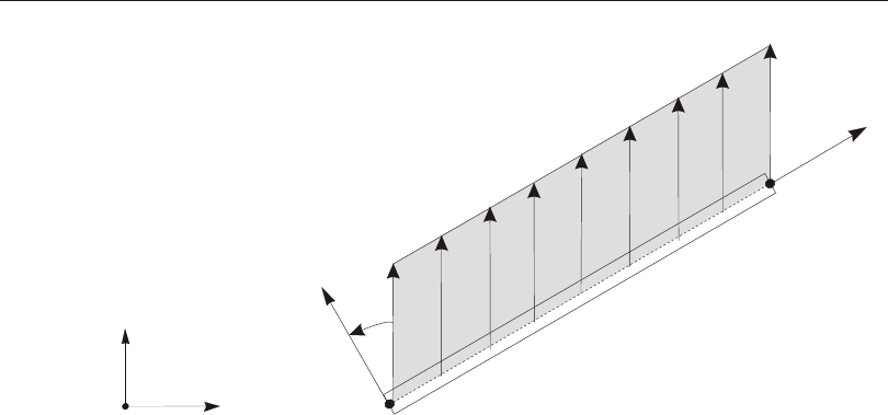
The speci fied load in ten sity is auto mati cally mul ti plied by the co sine of the an gle
be tween the di rec tion of load ing and the nor mal to the ele ment (the lo cal 3 di rec -
tion). This can be used, for ex am ple, to ap ply dis trib uted snow or wind loads. See
Figure 50 (page 208).
See Chap ter “Load Pat terns” (page 321) for more in for ma tion.
Surface Pressure Load
The Sur face Pres sure Load is used to ap ply ex ter nal pres sure loads upon any of the
six faces of the Shell ele ment. The defi ni tion of these faces is shown in Figure 42
(page 181). Sur face pres sure al ways acts nor mal to the face. Posi tive pres sures are
di rected to ward the in te rior of the ele ment.
The pres sure may be con stant over a face or in ter po lated from val ues given at the
joints. The val ues given at the joints are ob tained from Joint Pat terns, and need not
be the same for the dif fer ent faces. Joint Pat terns can be used to eas ily ap ply hy dro -
static pres sures.
The bot tom and top faces are de noted Faces 5 and 6, re spec tively. The top face is
the one visi ble when the +3 axis is di rected to ward you and the path j1-j2-j3 ap -
208 Surface Pressure Load
CSI Analysis Reference Manual
X
Z
Global
1
3
q
uzp
YEdge View of Shell Element
Uniformly distributed force uzp acts on
the projected area of the midsurface.
This is equivalent to force uzp cosq
acting on the full midsurface area.
Figure 50
Example of Uniform Load Acting on the Projected Area of the Mid-surface

pears coun ter clock wise. The pres sure act ing on the bot tom or top face is in te grated
over the plane of the ele ment and ap por tioned to the cor ner joints..
The sides of the el e ment are de noted Faces 1 to 4 (1 to 3 for the tri an gle), count ing
coun ter clock wise from side j1-j2 when viewed from the top. The pres sure act ing
on a side is mul ti plied by the thick ness, th, in te grated along the length of the side,
and ap por tioned to the two joints on that side. the bend ing thick ness, thb, is not
used.
For lay ered shells, the thick ness used for edge loads is mea sured from the bot tom of
the bot tom-most mem brane or shell layer to the top of the top-most mem brane or
shell layer. Gaps be tween lay ers and over lap ping lay ers do not change the thick -
ness used. Plate lay ers are not con sid ered when com put ing the loaded thick ness.
For more in for ma tion:
•See Topic “Thick ness” (page 193) in this Chap ter for the defi ni tion of th.
•See Chap ter “Load Pat terns” (page 321).
Temperature Load
Tem per a ture Load cre ates ther mal strain in the Shell el e ment. This strain is given
by the prod uct of the Ma te rial co ef fi cient of ther mal ex pan sion and the tem per a ture
change of the el e ment. All spec i fied Tem per a ture Loads rep re sent a change in tem -
per a ture from the un stressed state for a lin ear anal y sis, or from the pre vi ous tem per -
a ture in a non lin ear anal y sis.
Two in de pend ent Load Tem pera ture fields may be speci fied:
•Tem pera ture, t, which is con stant through the thick ness and pro duces mem -
brane strains
•Tem pera ture gra di ent, t3, which is lin ear in the thick ness di rec tion and pro -
duces bend ing strains
The tem pera ture gra di ent is speci fied as the change in tem pera ture per unit length.
The tem pera ture gra di ent is posi tive if the tem pera ture in creases (line arly) in the
posi tive di rec tion of the ele ment lo cal 3 axis. The gra di ent tem pera ture is zero at the
mid-sur face, hence no mem brane strain is in duced.
Each of the two Load Tem pera ture fields may be con stant over the plane of the ele -
ment or in ter po lated from val ues given at the joints.
See Chap ter “Load Pat terns” (page 321) for more in for ma tion.
Temperature Load 209
Chapter X The Shell Element

Strain Load
Eight types of strain load are avail able, one cor re spond ing to each of the in ter nal
forces and mo ments in a shell el e ment. These are:
•Mem brane strain loads, e11, e22, and e12, rep re sent ing change in the size and
shape of the el e ment that is uni form through the thick ness. Pos i tive mem brane
strain causes neg a tive cor re spond ing mem brane forces in a re strained el e ment.
•Bend ing strain loads, k11, k22, and k12, rep re sent ing change in the size and
shape of the el e ment that var ies lin early through the thick ness. Pos i tive bend -
ing strain causes neg a tive cor re spond ing bend ing mo ments in a re strained el e -
ment.
•Shear strain loads, g13 and g23, rep re sent ing the change in an gle be tween the
midsurface nor mal and the midsurface. Pos i tive shear strain causes neg a tive
cor re spond ing shear forces in a re strained el e ment. Shear strain load has no ef -
fect on a thin shell or thin plate el e ment, for which shear strain is as sumed to be
zero.
Any of the strain load fields may be con stant over the plane of the el e ment or in ter -
po lated from val ues given at the joints.
In an un re strained el e ment, strain loads cause de for ma tion but in duce no in ter nal
forces. This un re strained de for ma tion has the same sign as would de for ma tion
caused by the cor re spond ing (con ju gate) forces and mo ments act ing on the el e -
ment. On the other hand, strain load ing in a re strained el e ment causes cor re spond -
ing in ter nal forces that have the op po site sign as the ap plied strain. Most el e ments
in a real struc ture are con nected to fi nite stiff ness, and so strain load ing would
cause both de for ma tion and in ter nal forces. Note that the ef fects of shear and bend -
ing strain load ing are cou pled.
For more in for ma tion, see Topic “In ter nal Force and Stress Out put” below, and
also Chap ter “Load Pat terns” (page 321.)
Internal Force and Stress Output
The Shell ele ment in ter nal forces (also called stress re sul tants) are the forces and
mo ments that re sult from in te grat ing the stresses over the ele ment thick ness. For a
ho mo ge neous shell, these in ter nal forces are:
•Mem brane di rect forces:
210 Strain Load
CSI Analysis Reference Manual

(Eqns. 1)
Fdx
112
2
113
=-
+
òth
th
/
/s
Fdx
222
2
223
=-
+
òth
th
/
/s
•Mem brane shear force:
Fdx
122
2
123
=-
+
òth
th
/
/s
•Plate bend ing mo ments:
Mxdx
113
2
2
113
=--
+
òthb
thb
/
/s
Mxdx
222
2
3223
=--
+
òthb
thb
/
/s
•Plate twist ing mo ment:
Mxdx
122
2
3123
=--
+
òthb
thb
/
/s
•Plate trans verse shear forces:
Vdx
132
2
133
=-
+
òthb
thb
/
/s
Vdx
232
2
233
=-
+
òthb
thb
/
/s
where x3 rep re sents the thick ness co or di nate mea sured from the mid-sur face of the
el e ment, th is the mem brane thick ness, and thb is the plate-bend ing thick ness.
For a lay ered shell, the def i ni tions are the same, ex cept that the integrals of the
stresses are now summed over all lay ers, and x3 is al ways mea sured from the ref er -
ence sur face.
It is very im por tant to note that these stress re sul tants are forces and mo ments per
unit of in- plane length. They are pres ent at every point on the mid-sur face of the el -
e ment.
For the thick-plate (Mindlin/Reissner) for mu la tion of the ho mo ge neous shell, and
for the lay ered shell, the shear stresses are com puted di rectly from the shear ing de -
for ma tion. For the thin-plate ho mo ge neous shell, shear ing de for ma tion is as sumed
to be zero, so the trans verse shear forces are com puted in stead from the mo ments
us ing the equi lib rium equa tions:
VdM
dx
dM
dx
1311
1
12
2
=--
Internal Force and Stress Output 211
Chapter X The Shell Element

VdM
dx
dM
dx
23 12
1
22
2
= - -
Where x1 and x2 are in-plane co or di nates par al lel to the lo cal 1 and 2 axes.
The sign con ven tions for the stresses and in ter nal forces are il lus trated in Figure 51
(page 213). Stresses act ing on a posi tive face are ori ented in the posi tive di rec tion
of the ele ment lo cal co or di nate axes. Stresses act ing on a nega tive face are ori ented
in the nega tive di rec tion of the ele ment lo cal co or di nate axes.
A posi tive face is one whose out ward nor mal (point ing away from ele ment) is in the
posi tive lo cal 1 or 2 di rec tion.
Posi tive in ter nal forces cor re spond to a state of posi tive stress that is con stant
through the thick ness. Posi tive in ter nal mo ments cor re spond to a state of stress that
var ies line arly through the thick ness and is posi tive at the bot tom. Thus for a ho mo -
ge neous shell:
(Eqns. 2)
s111111
33
12
=-
FMx
ththb
s222222
33
12
=-
FMx
ththb
s121212
33
12
=-
FMx
ththb
s1313
=V
thb
s2323
=V
thb
s330=
The trans verse shear stresses given here are av er age val ues. The ac tual shear stress
dis tri bu tion is para bolic, be ing zero at the top and bot tom sur faces and tak ing a
maxi mum or mini mum value at the mid-sur face of the ele ment.
The force and mo ment re sul tants are re ported iden ti cally for ho mo ge neous and lay -
ered shells. Stresses are re ported for ho mo ge neous shells at the top and bot tom sur -
faces, and are lin ear in be tween. For the lay ered shell, stresses are re ported in each
layer at the in te gra tion points, and at the top, bot tom, and cen ter of the layer.
The stresses and in ter nal forces are evalu ated at the stan dard 2- by-2 Gauss in te gra -
tion points of the ele ment and ex trapo lated to the joints. Al though they are re ported
212 Internal Force and Stress Output
CSI Analysis Reference Manual
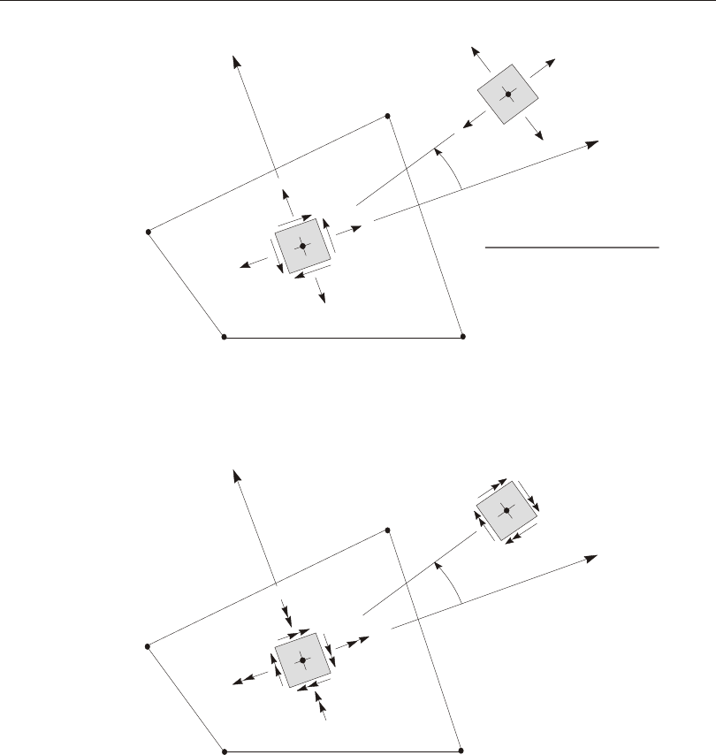
at the joints, the stresses and in ter nal forces ex ist over the whole el e ment. See
Cook, Malkus, and Ple sha (1989) for more in for ma tion.
Internal Force and Stress Output 213
Chapter X The Shell Element
j1
j1
j2
j2
j3
j3
j4
j4
F11
F12
F22
F-MIN
F-MAX
Axis 1
Axis 1
Axis 2
Axis 2
Forces are per unit
of in-plane length
Moments are per unit
of in-plane length
M-MAX
M-MIN
M12
M11
M22
PLATE BENDING AND TWISTING MOMENTS
Transverse Shear (not shown)
Positive transverse shear forces and
stresses acting on positive faces
point toward the viewer
STRESSES AND MEMBRANE FORCES
Stress Sij Has Same Definition as Force Fij
ANGLE
ANGLE
M12
Figure 51
Shell Element Stresses and Internal Resultant Forces and Moments

Prin ci pal val ues and the as so ci ated prin ci pal di rec tions are avail able for Load
Cases and Load Com bi na tions that are sin gle val ued. The an gle given is meas ured
coun ter clock wise (when viewed from the top) from the lo cal 1 axis to the di rec tion
of the maxi mum prin ci pal value.
For more in for ma tion, see Topic “Stresses and Strains” (page 71) in Chap ter “Ma -
te rial Prop er ties”.
214 Internal Force and Stress Output
CSI Analysis Reference Manual

Chapter XI
The Plane Element
The Plane el e ment is used to model plane-stress and plane-strain be hav ior in
two-di men sional sol ids. The Plane el e ment/ob ject is one type of area ob ject. De -
pending on the type of sec tion prop er ties you as sign to an area, the ob ject could also
be used to model shell and axisymmetric solid be hav ior. These types of el e ments
are dis cussed in the pre vi ous and fol low ing Chap ters.
Advanced Topics
•Over view
•Joint Con nec tivity
•De grees of Free dom
•Lo cal Co or di nate Sys tem
•Stresses and Strains
•Sec tion Prop erties
•Mass
•Self- Weight Load
•Grav ity Load
•Sur face Pres sure Load
•Pore Pres sure Load
215

•Tem pera ture Load
•Stress Out put
Overview
The Plane el e ment is a three- or four-node el e ment for mod el ing two-di men sional
sol ids of uni form thick ness. It is based upon an isoparametric for mu la tion that in -
cludes four op tional in com pat i ble bend ing modes. The el e ment should be pla nar; if
it is not, it is for mu lated for the pro jec tion of the el e ment upon an av er age plane
calculated for the el e ment.
The in com pat i ble bend ing modes sig nif i cantly im prove the bend ing be hav ior of
the el e ment if the el e ment ge om e try is of a rect an gu lar form. Im proved be hav ior is
ex hib ited even with non-rect an gu lar ge om e try.
Struc tures that can be mod eled with this el e ment in clude:
•Thin, pla nar struc tures in a state of plane stress
•Long, pris matic struc tures in a state of plane strain
The stresses and strains are as sumed not to vary in the thick ness di rec tion.
For plane-stress, the el e ment has no out-of-plane stiff ness. For plane-strain, the el e -
ment can sup port loads with anti-plane shear stiff ness.
Each Plane el e ment has its own lo cal co or di nate sys tem for de fin ing Ma te rial prop -
er ties and loads, and for in ter pret ing out put. Temperature- dependent, or tho tropic
ma te rial prop er ties are al lowed. Each ele ment may be loaded by grav ity (in any di -
rec tion); sur face pres sure on the side faces; pore pres sure within the ele ment; and
loads due to tem pera ture change.
An 2 x 2 nu mer i cal in te gra tion scheme is used for the Plane. Stresses in the el e ment
lo cal co or di nate sys tem are eval u ated at the in te gra tion points and ex trap o lated to
the joints of the el e ment. An ap prox i mate er ror in the stresses can be es ti mated from
the dif fer ence in val ues cal cu lated from dif fer ent el e ments at tached to a com mon
joint. This will give an in di ca tion of the ac cu racy of the fi nite el e ment ap prox i ma -
tion and can then be used as the ba sis for the se lec tion of a new and more ac cu rate
fi nite el e ment mesh.
216 Overview
CSI Analysis Reference Manual

Joint Connectivity
The joint con nec tiv ity and face def i ni tion is iden ti cal for all area ob jects, i.e., the
Shell, Plane, and Asolid elements. See Topic “Joint Con nec tiv ity” (page 180) in
Chap ter “The Shell El e ment” for more in for ma tion.
The Plane el e ment is in tended to be pla nar. If you de fine a four-node el e ment that is
not pla nar, an av er age plane will be fit through the four joints, and the pro jec tion of
the el e ment onto this plane will be used.
Degrees of Freedom
The Plane ele ment ac ti vates the three trans la tional de grees of free dom at each of its
con nected joints. Ro ta tional de grees of free dom are not ac ti vated.
The plane-stress el e ment con trib utes stiff ness only to the de grees of free dom in the
plane of the ele ment. It is nec es sary to pro vide re straints or other sup ports for the
trans la tional de grees of free dom that are nor mal to this plane; oth er wise, the struc -
ture will be un sta ble.
The plane-strain el e ment mod els anti-plane shear, i.e., shear that is nor mal to the
plane of the el e ment, in ad di tion to the in-plane behavior. Thus stiff ness is cre ated
for all three translational de grees of freedom.
See Topic “De grees of Free dom” (page 30) in Chap ter “Joints and De grees of Free -
dom” for more in for ma tion.
Local Coordinate System
The el e ment lo cal co or di nate sys tem is iden ti cal for all area ob jects, i.e., the Shell,
Plane, and Asolid el e ments. See Topics “Lo cal Co or di nate Sys tem” (page 185) and
“Ad vanced Lo cal Co or di nate Sys tem” (page 186) in Chap ter “The Shell El e ment”
for more in for ma tion.
Stresses and Strains
The Plane ele ment mod els the mid- plane of a struc ture hav ing uni form thick ness,
and whose stresses and strains do not vary in the thick ness di rec tion.
Joint Connectivity 217
Chapter XI The Plane Element

Plane-stress is ap pro pri ate for struc tures that are thin com pared to their pla nar di -
men sions. The thick ness nor mal stress (s33) is as sumed to be zero. The thick ness
nor mal strain (e33) may not be zero due to Pois son ef fects. Trans verse shear
stresses (s12, s13) and shear strains (g12, g13) are as sumed to be zero. Dis place -
ments in the thick ness (lo cal 3) di rec tion have no ef fect on the el e ment.
Plane-strain is ap pro pri ate for struc tures that are thick com pared to their pla nar di -
men sions. The thick ness nor mal strain (e33) is as sumed to be zero. The thick ness
nor mal stress (s33) may not be zero due to Pois son ef fects. Trans verse shear
stresses (s12, s13) and shear strains (g12, g13) are de pend ent upon displacements in
the thick ness (lo cal 3) di rec tion.
See Topic “Stresses and Strains” (page 71) in Chap ter “Ma te rial Prop er ties” for
more in for ma tion.
Section Properties
A Plane Sec tion is a set of ma te rial and geo met ric prop er ties that de scribe the
cross-sec tion of one or more Plane el e ments. Sec tions are de fined in de pend ently of
the Plane el e ments, and are as signed to the area ob jects.
Section Type
When de fin ing an area sec tion, you have a choice of three ba sic el e ment types:
•Plane (stress or strain) – the sub ject of this Chap ter, a two-di men sional solid,
with translational de grees of free dom, ca pa ble of sup port ing forces but not mo -
ments.
•Shell – shell, plate, or mem brane, with translational and ro ta tional de grees of
free dom, ca pa ble of sup port ing forces and mo ments. This el e ment is cov ered in
Chap ter “The Shell El e ment” (page 177).
•Asolid – axisymmetric solid, with translational de grees of free dom, ca pa ble of
sup port ing forces but not mo ments. This el e ment is cov ered in Chap ter “The
Asolid El e ment” (page 225).
For Plane sec tions, you may choose one of the fol low ing sub-types of be hav ior:
•Plane stress
•Plane strain, in clud ing anti-plane shear
218 Section Properties
CSI Analysis Reference Manual

Material Properties
The ma te rial prop er ties for each Plane el e ment are spec i fied by ref er ence to a pre vi -
ously-de fined Ma te rial. Orthotropic prop er ties are used, even if the Ma te rial se -
lected was de fined as anisotropic. The ma te rial prop er ties used by the Plane el e -
ment are:
•The moduli of elas tic ity, e1, e2, and e3
•The shear modu lus, g12
•For plane-strain only, the shear moduli, g13 and g23
•The Pois son’s ra tios, u12, u13 and u23
•The co ef fi cients of ther mal ex pan sion, a1, a2, and a3
•The mass den sity, m, for com put ing el e ment mass
•The weight den sity, w, for com put ing Self-Weight and Grav ity Loads
The prop er ties e3, u13, u23, and a3 are not used for plane stress. They are used to
com pute the thick ness-nor mal stress (s33) in plane strain.
All ma te rial prop er ties (ex cept the den si ties) are ob tained at the ma te rial tem per a -
ture of each in di vid ual el e ment.
See Chap ter “Ma te rial Prop erties” (page 69) for more in for ma tion.
Material Angle
The ma te rial lo cal co or di nate sys tem and the el e ment (Plane Section) lo cal co or di -
nate sys tem need not be the same. The lo cal 3 di rec tions al ways co in cide for the
two sys tems, but the ma te rial 1 axis and the el e ment 1 axis may dif fer by the an gle a
as shown in Figure 52 (page 220). This an gle has no ef fect for iso tro pic ma te rial
prop er ties since they are in de pend ent of ori en ta tion.
See Topic “Lo cal Co or di nate Sys tem” (page 70) in Chap ter “Ma te rial Prop erties”
for more in for ma tion.
Thickness
Each Plane Sec tion has a uni form thick ness, th. This may be the ac tual thick ness,
par tic u larly for plane-stress el e ments; or it may be a rep re sen ta tive por tion, such as
a unit thick ness of an in fi nitely-thick plane-strain el e ment.
Section Properties 219
Chapter XI The Plane Element
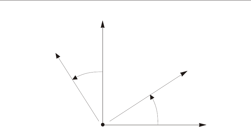
The el e ment thick ness is used for cal cu lat ing the el e ment stiff ness, mass, and loads.
Hence, joint forces com puted from the el e ment are pro por tional to this thick ness.
Incompatible Bending Modes
By de fault each Plane el e ment in cludes four in com pat i ble bend ing modes in its
stiff ness for mu la tion. These in com pat i ble bend ing modes sig nif i cantly im prove
the bend ing be hav ior in the plane of the el e ment if the el e ment ge om e try is of a rect -
an gu lar form. Im proved be hav ior is ex hib ited even with non-rect an gu lar ge om e try.
If an el e ment is se verely dis torted, the in clu sion of the in com pat i ble modes should
be sup pressed. The el e ment then uses the stan dard isoparametric for mu la tion. In -
com pat i ble bend ing modes may also be sup pressed in cases where bend ing is not
im por tant, such as in typ i cal geotechnical prob lems.
Mass
In a dy namic analy sis, the mass of the struc ture is used to com pute in er tial forces.
The mass con trib uted by the Plane ele ment is lumped at the ele ment joints. No in er -
tial ef fects are con sid ered within the ele ment it self.
220 Mass
CSI Analysis Reference Manual
3 (Element, Material)
a
a
1 (Element)
1 (Material)
2 (Element)
2 (Material)
Figure 52
Plane Element Material Angle

The to tal mass of the ele ment is equal to the in te gral over the plane of the ele ment of
the mass den sity, m, mul ti plied by the thick ness, th. The to tal mass is ap por tioned
to the joints in a man ner that is pro por tional to the di ago nal terms of the con sis tent
mass ma trix. See Cook, Malkus, and Ple sha (1989) for more in for ma tion. The to tal
mass is ap plied to each of the three trans la tional de grees of free dom (UX, UY, and
UZ) even when the ele ment con trib utes stiff ness to only two of these de grees of
free dom.
For more in for ma tion:
•See Topic “Mass Den sity” (page 77) in Chap ter “Ma te rial Prop er ties.”
•See Topic “Mass Source” (page 334) in Chap ter “Load Pat terns”.
•See Chap ter “Load Cases” (page 341).
Self-Weight Load
Self- Weight Load ac ti vates the self- weight of all ele ments in the model. For a Plane
ele ment, the self- weight is a force that is uni formly dis trib uted over the plane of the
ele ment. The mag ni tude of the self- weight is equal to the weight den sity, w, mul ti -
plied by the thick ness, th.
Self- Weight Load al ways acts down ward, in the global –Z di rec tion. You may
scale the self- weight by a sin gle scale fac tor that ap plies equally to all ele ments in
the struc ture.
For more in for ma tion:
•See Topic “Weight Den sity” (page 78) in Chap ter “Ma te rial Prop er ties” for the
defi ni tion of w.
•See Topic “Thick ness” (page 219) in this Chap ter for the defi ni tion of th.
•See Topic “Self- Weight Load” (page 325) in Chap ter “Load Pat terns.”
Gravity Load
Grav ity Load can be ap plied to each Plane ele ment to ac ti vate the self- weight of the
ele ment. Us ing Grav ity Load, the self- weight can be scaled and ap plied in any di -
rec tion. Dif fer ent scale fac tors and di rec tions can be ap plied to each ele ment.
If all ele ments are to be loaded equally and in the down ward di rec tion, it is more
con ven ient to use Self- Weight Load.
Self-Weight Load 221
Chapter XI The Plane Element

For more in for ma tion:
•See Topic “Self- Weight Load” (page 221) in this Chap ter for the defi ni tion of
self- weight for the Plane ele ment.
•See Topic “Grav ity Load” (page 326) in Chap ter “Load Pat terns.”
Surface Pressure Load
The Sur face Pres sure Load is used to ap ply ex ter nal pres sure loads upon any of the
three or four side faces of the Plane ele ment. The defi ni tion of these faces is shown
in Figure 42 (page 181). Sur face pres sure al ways acts nor mal to the face. Posi tive
pres sures are di rected to ward the in te rior of the ele ment.
The pres sure may be con stant over a face or in ter po lated from val ues given at the
joints. The val ues given at the joints are ob tained from Joint Pat terns, and need not
be the same for the dif fer ent faces. Joint Pat terns can be used to eas ily ap ply hy dro -
static pres sures.
The pres sure act ing on a side is mul ti plied by the thick ness, th, in te grated along the
length of the side, and ap por tioned to the two or three joints on that side.
See Chap ter “Load Pat terns” (page 321) for more in for ma tion.
Pore Pressure Load
The Pore Pres sure Load is used to model the drag and buoy ancy ef fects of a fluid
within a solid me dium, such as the ef fect of wa ter upon the solid skele ton of a soil.
Sca lar fluid- pressure val ues are given at the ele ment joints by Joint Pat terns, and in -
ter po lated over the ele ment. The to tal force act ing on the ele ment is the in te gral of
the gra di ent of this pres sure field over the plane of the ele ment, mul ti plied by the
thick ness, th. This force is ap por tioned to each of the joints of the ele ment. The
forces are typi cally di rected from re gions of high pres sure to ward re gions of low
pres sure.
See Chap ter “Load Pat terns” (page 321) for more in for ma tion.
222 Surface Pressure Load
CSI Analysis Reference Manual

Temperature Load
The Tem pera ture Load cre ates ther mal strain in the Plane ele ment. This strain is
given by the prod uct of the Ma te rial co ef fi cient of ther mal ex pan sion and the tem -
pera ture change of the ele ment. The tem pera ture change is meas ured from the ele -
ment Ref er ence Tem pera ture to the ele ment Load Tem pera ture. Tem pera ture
changes are as sumed to be con stant through the ele ment thick ness.
See Chap ter “Load Pat terns” (page 321) for more in for ma tion.
Stress Output
The Plane ele ment stresses are evalu ated at the stan dard 2- by-2 Gauss in te gra tion
points of the ele ment and ex trapo lated to the joints. See Cook, Malkus, and Ple sha
(1989) for more in for ma tion.
Prin ci pal val ues and their as so ci ated prin ci pal di rec tions in the ele ment lo cal 1-2
plane are also com puted for sin gle-val ued Load Cases. The an gle given is meas ured
coun ter clock wise (when viewed from the +3 di rec tion) from the lo cal 1 axis to the
di rec tion of the maxi mum prin ci pal value.
For more in for ma tion:
•See Chap ter “Load Pat terns” (page 321).
•See Chap ter “Load Cases” (page 341).
Temperature Load 223
Chapter XI The Plane Element

224 Stress Output
CSI Analysis Reference Manual

Chapter XII
The Asolid Element
The Aso lid ele ment is used to model axi sym met ric sol ids un der axi sym met ric load -
ing.
Advanced Topics
•Over view
•Joint Con nec tivity
•De grees of Free dom
•Lo cal Co or di nate Sys tem
•Stresses and Strains
•Sec tion Prop erties
•Mass
•Self- Weight Load
•Grav ity Load
•Sur face Pres sure Load
•Pore Pres sure Load
•Tem pera ture Load
•Ro tate Load
225

•Stress Out put
Overview
The Asolid el e ment is a three- or four-node el e ment for mod el ing axisymmetric
struc tures un der axisymmetric load ing. It is based upon an isoparametric for mu la -
tion that in cludes four op tional in com pat i ble bend ing modes.
The el e ment mod els a rep re sen ta tive two-di men sional cross sec tion of the three-di -
men sional axisymmetric solid. The axis of sym me try may be lo cated ar bi trarily in
the model. Each el e ment should lie fully in a plane containing the axis of sym me try.
If it does not, it is for mu lated for the pro jec tion of the el e ment upon the plane con -
tain ing the axis of sym me try and the cen ter of the el e ment.
The ge om e try, load ing, dis place ments, stresses, and strains are as sumed not to vary
in the cir cumfer ential di rec tion. Any dis place ments that oc cur in the cir cumfer -
ential di rec tion are treated as axisymmetric torsion.
The use of in com pat i ble bend ing modes sig nif i cantly im proves the in-plane bend -
ing be hav ior of the el e ment if the el e ment ge om e try is of a rect an gu lar form. Im -
proved be hav ior is ex hib ited even with non-rect an gu lar ge om e try.
Each Asolid el e ment has its own lo cal co or di nate sys tem for de fin ing Ma te rial
prop er ties and loads, and for in ter pret ing out put. Tem per a ture-de pend ent,
orthotropic ma te rial prop er ties are al lowed. Each el e ment may be loaded by grav ity
(in any di rec tion); cen trif u gal force; sur face pres sure on the side faces; pore pres -
sure within the el e ment; and loads due to tem per a ture change.
An 2 x 2 nu mer i cal in te gra tion scheme is used for the Asolid. Stresses in the el e -
ment lo cal co or di nate sys tem are eval u ated at the in te gra tion points and ex trap o -
lated to the joints of the el e ment. An ap prox i mate er ror in the stresses can be es ti -
mated from the dif fer ence in val ues cal cu lated from dif fer ent el e ments at tached to a
com mon joint. This will give an in di ca tion of the ac cu racy of the fi nite el e ment ap -
prox i ma tion and can then be used as the ba sis for the se lec tion of a new and more
ac cu rate fi nite el e ment mesh.
Joint Connectivity
The joint con nec tiv ity and face def i ni tion is iden ti cal for all area ob jects, i.e., the
Shell, Plane, and Asolid el e ments. See Topic “Joint Con nec tiv ity” (page 180) in
Chap ter “The Shell El e ment” for more in for ma tion.
226 Overview
CSI Analysis Reference Manual

The Asolid el e ment is in tended to be pla nar and to lie in a plane that con tains the
axis of sym me try. If not, a plane is found that con tains the axis of sym me try and the
center of the el e ment, and the pro jec tion of the el e ment onto this plane will be used.
Joints for a given el e ment may not lie on op po site sides of the axis of sym me try.
They may lie on the axis of sym me try and/or to one side of it.
Degrees of Freedom
The Aso lid ele ment ac ti vates the three trans la tional de grees of free dom at each of
its con nected joints. Ro ta tional de grees of free dom are not ac ti vated.
Stiff ness is cre ated for all three de grees of free dom. De grees of free dom in the
plane rep re sent the radial and ax ial be hav ior. The nor mal trans la tion rep re sents
circumferential tor sion.
See Topic “De grees of Free dom” (page 30) in Chap ter “Joints and De grees of Free -
dom” for more in for ma tion.
Local Coordinate System
The el e ment lo cal co or di nate sys tem is iden ti cal for all area ob jects, i.e., the Shell,
Plane, and Asolid el e ments. See Topics “Lo cal Co or di nate Sys tem” (page 185) and
“Ad vanced Lo cal Co or di nate Sys tem” (page 186) in Chap ter “The Shell El e ment”
for more in for ma tion.
The lo cal 3 axis is nor mal to the plane of the el e ment, and is the neg a tive of the cir -
cumfer ential di rec tion. The 1-2 plane is the same as the ra dial-ax ial plane, al though
the ori en ta tion of the lo cal axes is not re stricted to be par al lel to the ra dial and ax ial
axes.
The ra dial di rec tion runs per pen dic u larly from the axis of sym me try to the cen ter of
the el e ment. The ax ial di rec tion is par al lel to the axis of sym me try, with the pos i tive
sense be ing up ward when look ing along the circumferential (–3) di rec tion with the
ra dial di rec tion point ing to the right.
Degrees of Freedom 227
Chapter XII The Asolid Element

Stresses and Strains
The Aso lid ele ment mod els the mid- plane of a rep re sen ta tive sec tor of an axi sym -
met ric struc ture whose stresses and strains do not vary in the cir cum fer en tial di rec -
tion.
Dis place ments in the lo cal 1-2 plane cause in-plane strains (g11, g22, g12) and
stresses (s11, s22, s12).
Dis place ments in the ra dial di rec tion also cause cir cum fer en tial nor mal strains:
e33=u
r
r
where ur is the ra dial dis place ment, and r is the ra dius at the point in ques tion. The
cir cumfer ential nor mal stress (s33) is com puted as usual from the three nor mal
strains.
Dis place ments in the cir cumfer ential (lo cal 3) di rec tion cause only tor sion, re sult -
ing in cir cumfer ential shear strains (g12, g13) and stresses (s12, s13).
See Topic “Stresses and Strains” (page 71) in Chap ter “Ma te rial Prop erties” for
more in for ma tion.
Section Properties
An Asolid Sec tion is a set of ma te rial and geo met ric prop er ties that de scribe the
cross-sec tion of one or more Asolid el e ments. Sec tions are de fined in de pend ently
of the Asolid el e ments, and are as signed to the area ob jects.
Section Type
When de fin ing an area sec tion, you have a choice of three ba sic el e ment types:
•Asolid – the sub ject of this Chap ter, an axisymmetric solid, with translational
de grees of free dom, ca pa ble of sup port ing forces but not mo ments.
•Plane (stress or strain) – a two-di men sional solid, with translational de grees of
free dom, ca pa ble of sup port ing forces but not mo ments. This el e ment is cov -
ered in Chap ter “The Plane El e ment” (page 215).
228 Stresses and Strains
CSI Analysis Reference Manual

•Shell – shell, plate, or mem brane, with translational and ro ta tional de grees of
free dom, ca pa ble of sup port ing forces and mo ments. This el e ment is cov ered in
Chap ter “The Shell El e ment” (page 177).
Af ter se lect ing an Asolid type of sec tion, you must sup ply the rest of the data de -
scribed be low.
Material Properties
The ma te rial prop er ties for each Asolid el e ment are spec i fied by ref er ence to a pre -
vi ously-de fined Ma te rial. Orthotropic prop er ties are used, even if the Ma te rial se -
lected was de fined as anisotropic. The ma te rial prop er ties used by the Asolid el e -
ment are:
•The moduli of elas tic ity, e1, e2, and e3
•The shear moduli, g12, g13, and g23
•The Pois son’s ra tios, u12, u13 and u23
•The co ef fi cients of ther mal ex pan sion, a1, a2, and a3
•The mass den sity, m, for com put ing el e ment mass
•The weight den sity, w, for com put ing Self-Weight and Grav ity Loads
All ma te rial prop er ties (ex cept the den si ties) are ob tained at the ma te rial tem per a -
ture of each in di vid ual el e ment.
See Chap ter “Ma te rial Prop erties” (page 69) for more in for ma tion.
Material Angle
The ma te rial lo cal co or di nate sys tem and the el e ment (Asolid Sec tion) lo cal co or di -
nate sys tem need not be the same. The lo cal 3 di rec tions al ways co in cide for the
two sys tems, but the ma te rial 1 axis and the el e ment 1 axis may dif fer by the an gle a
as shown in Figure 53 (page 230). This an gle has no ef fect for iso tro pic ma te rial
prop er ties since they are in de pend ent of ori en ta tion.
See Topic “Lo cal Co or di nate Sys tem” (page 70) in Chap ter “Ma te rial Prop erties”
for more in for ma tion.
Section Properties 229
Chapter XII The Asolid Element

Axis of Sym me try
For each Asolid Sec tion, you may se lect an axis of sym me try. This axis is spec i fied
as the Z axis of an al ter nate co or di nate sys tem that you have de fined. All Asolid el -
e ments that use a given Asolid Sec tion will have the same axis of sym me try.
For most mod el ing cases, you will only need a sin gle axis of sym me try. How ever,
if you want to have mul ti ple axes of sym me try in your model, just set up as many al -
ter nate co or di nate sys tems as needed for this pur pose and de fine cor re spond ing
Asolid Sec tion prop er ties.
You should be aware that it is al most im pos si ble to make a sen si ble model that con -
nects Asolid el e ments with other el e ment types, or that con nects to gether Asolid el -
e ments us ing dif fer ent axes of sym me try. The prac ti cal ap pli ca tion of hav ing mul ti -
ple axes of sym me try is to have mul ti ple in de pend ent axisymmetric struc tures in
the same model.
See Topic “Al ter nate Co or di nate Sys tems” (page 16) in Chap ter “Co or di nate Sys -
tems” for more in for ma tion.
230 Section Properties
CSI Analysis Reference Manual
3 (Element, Material)
a
a
1 (Element)
1 (Material)
2 (Element)
2 (Material)
Figure 53
Asolid Element Material Angle
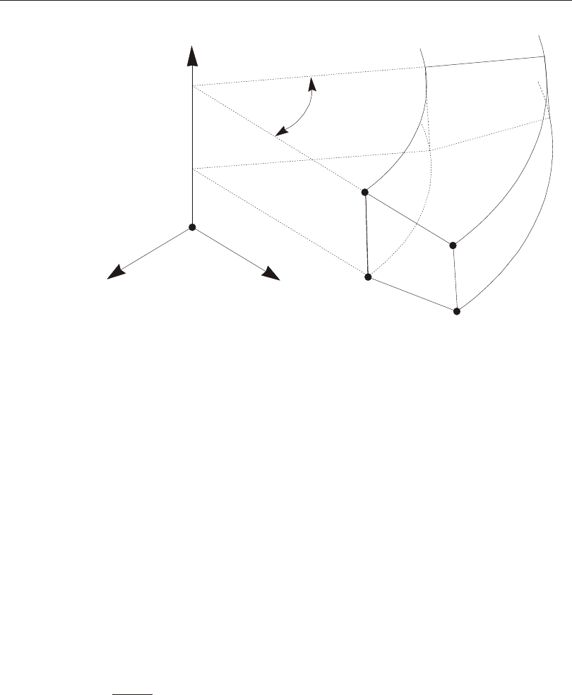
Arc and Thickness
The Asolid el e ment rep re sents a solid that is cre ated by ro tat ing the el e ment’s pla -
nar shape through 360° about the axis of sym me try. How ever, the anal y sis con sid -
ers only a rep re sen ta tive sec tor of the solid. You can spec ify the size of the sec tor,
in de grees, us ing the pa ram e ter arc. For ex am ple, arc=360 mod els the full struc -
ture, and arc=90 mod els one quar ter of it. See Figure 54 (page 231). Set ting arc=0,
the de fault, mod els a one-ra dian sec tor. One ra dian is the same as 180°/p, or ap -
prox i mately 57.3°.
The el e ment “thick ness” (cir cumfer ential ex tent), h, in creases with the ra dial dis -
tance, r, from the axis of sym me try:
hr=×parc
180
Clearly the thick ness var ies over the plane of the el e ment.
The el e ment thick ness is used for cal cu lat ing the el e ment stiff ness, mass, and loads.
Hence, joint forces com puted from the el e ment are pro por tional to arc.
Section Properties 231
Chapter XII The Asolid Element
X, 3 Y, 1
Z, 2
j7
j1
j3
j9
arc
Figure 54
Asolid Element Local Coordinate System and Arc Definition

Incompatible Bending Modes
By de fault each Asolid el e ment in cludes four in com pat i ble bend ing modes in its
stiff ness for mu la tion. These in com pat i ble bend ing modes sig nif i cantly im prove
the bend ing be hav ior in the plane of the el e ment if the el e ment ge om e try is of a rect -
an gu lar form. Im proved be hav ior is ex hib ited even with non-rect an gu lar ge om e try.
If an el e ment is se verely dis torted, the in clu sion of the in com pat i ble modes should
be sup pressed. The el e ment then uses the stan dard isoparametric for mu la tion. In -
com pat i ble bend ing modes may also be sup pressed in cases where bend ing is not
im por tant, such as in typ i cal geotechnical prob lems.
Mass
In a dy namic analy sis, the mass of the struc ture is used to com pute in er tial forces.
The mass con trib uted by the Aso lid ele ment is lumped at the ele ment joints. No in -
er tial ef fects are con sid ered within the ele ment it self.
The to tal mass of the ele ment is equal to the in te gral over the plane of the ele ment of
the prod uct of the mass den sity, m, mul ti plied by the thick ness, h. The to tal mass is
ap por tioned to the joints in a man ner that is pro por tional to the di ago nal terms of
the con sis tent mass ma trix. See Cook, Malkus, and Ple sha (1989) for more in for -
ma tion. The to tal mass is ap plied to each of the three trans la tional de grees of free -
dom (UX, UY, and UZ).
For more in for ma tion:
•See Topic “Mass Den sity” (page 77) in Chap ter “Ma te rial Prop er ties.”
•See Topic “Mass Source” (page 334) in Chap ter “Load Pat terns”.
•See Chap ter “Load Cases” (page 341).
Self-Weight Load
Self- Weight Load ac ti vates the self- weight of all ele ments in the model. For an
Aso lid ele ment, the self- weight is a force that is dis trib uted over the plane of the
ele ment. The mag ni tude of the self- weight is equal to the weight den sity, w, mul ti -
plied by the thick ness, h.
Self- Weight Load al ways acts down ward, in the global –Z di rec tion. If the down -
ward di rec tion cor re sponds to the ra dial or cir cum fer en tial di rec tion of an Aso lid
232 Mass
CSI Analysis Reference Manual

ele ment, the Self- Weight Load for that ele ment will be zero, since self- weight act -
ing in these di rec tions is not axi sym met ric. Non- zero Self- Weight Load will only
ex ist for ele ments whose ax ial di rec tion is ver ti cal.
You may scale the self- weight by a sin gle scale fac tor that ap plies equally to all ele -
ments in the struc ture.
For more in for ma tion:
•See Topic “Weight Den sity” (page 78) in Chap ter “Ma te rial Prop er ties” for the
defi ni tion of w.
•See Subtopic “Arc and Thick ness” (page 231) in this Chap ter for the defi ni tion
of h.
•See Topic “Self- Weight Load” (page 325) in Chap ter “Load Pat terns.”
Gravity Load
Grav ity Load can be ap plied to each Aso lid ele ment to ac ti vate the self- weight of
the ele ment. Us ing Grav ity Load, the self- weight can be scaled and ap plied in any
di rec tion. Dif fer ent scale fac tors and di rec tions can be ap plied to each ele ment.
How ever, only the com po nents of Grav ity load act ing in the ax ial di rec tion of an
Aso lid ele ment will be non- zero. Com po nents in the ra dial or cir cum fer en tial di rec -
tion will be set to zero, since grav ity act ing in these di rec tions is not axi sym met ric.
If all ele ments are to be loaded equally and in the down ward di rec tion, it is more
con ven ient to use Self- Weight Load.
For more in for ma tion:
•See Topic “Self- Weight Load” (page 232) in this Chap ter for the defi ni tion of
self- weight for the Aso lid ele ment.
•See Topic “Grav ity Load” (page 326) in Chap ter “Load Pat terns.”
Surface Pressure Load
The Sur face Pres sure Load is used to ap ply ex ter nal pres sure loads upon any of the
three or four side faces of the Aso lid ele ment. The defi ni tion of these faces is shown
in Figure 42 (page 181). Sur face pres sure al ways acts nor mal to the face. Posi tive
pres sures are di rected to ward the in te rior of the ele ment.
Gravity Load 233
Chapter XII The Asolid Element

The pres sure may be con stant over a face or in ter po lated from val ues given at the
joints. The val ues given at the joints are ob tained from Joint Pat terns, and need not
be the same for the dif fer ent faces. Joint Pat terns can be used to eas ily ap ply hy dro -
static pres sures.
The pres sure act ing on a side is mul ti plied by the thick ness, h, in te grated along the
length of the side, and ap por tioned to the two or three joints on that side.
See Chap ter “Load Pat terns” (page 321) for more in for ma tion.
Pore Pressure Load
The Pore Pres sure Load is used to model the drag and buoy ancy ef fects of a fluid
within a solid me dium, such as the ef fect of wa ter upon the solid skele ton of a soil.
Sca lar fluid- pressure val ues are given at the ele ment joints by Joint Pat terns, and in -
ter po lated over the ele ment. The to tal force act ing on the ele ment is the in te gral of
the gra di ent of this pres sure field, mul ti plied by the thick ness h, over the plane of
the ele ment. This force is ap por tioned to each of the joints of the ele ment. The
forces are typi cally di rected from re gions of high pres sure to ward re gions of low
pres sure.
See Chap ter “Load Pat terns” (page 321) for more in for ma tion.
Temperature Load
The Tem per a ture Load cre ates ther mal strain in the Asolid el e ment. This strain is
given by the prod uct of the Ma te rial co ef fi cient of ther mal ex pan sion and the tem -
per a ture change of the el e ment. All spec i fied Tem per a ture Loads rep re sent a
change in tem per a ture from the un stressed state for a lin ear anal y sis, or from the
pre vi ous tem per a ture in a non lin ear anal y sis. Tem per a ture changes are as sumed to
be con stant through the el e ment thick ness.
See Chap ter “Load Pat terns” (page 321) for more in for ma tion.
Rotate Load
Ro tate Load is used to ap ply cen trifu gal force to Aso lid ele ments. Each ele ment is
as sumed to ro tate about its own axis of sym me try at a con stant an gu lar ve loc ity.
234 Pore Pressure Load
CSI Analysis Reference Manual

The an gu lar ve loc ity cre ates a load on the ele ment that is pro por tional to its mass,
its dis tance from the axis of ro ta tion, and the square of the an gu lar ve loc ity. This
load acts in the posi tive ra dial di rec tion, and is ap por tioned to each joint of the ele -
ment. No Ro tate Load will be pro duced by an ele ment with zero mass den sity.
Since Ro tate Loads as sume a con stant rate of ro ta tion, it does not make sense to use
a Load Pat tern that con tains Ro tate Load in a time- history analy sis un less that Load
Pat tern is ap plied quasi- statically (i.e., with a very slow time varia tion).
For more in for ma tion:
•See Topic “Mass Den sity” (page 77) in Chap ter “Ma te rial Prop er ties.”
•See Chap ter “Load Pat terns” (page 321).
Stress Output
The Asolid el e ment stresses are eval u ated at the stan dard 2-by-2 Gauss in te gra tion
points of the el e ment and ex trap o lated to the joints. See Cook, Malkus, and Plesha
(1989) for more in for ma tion.
Prin ci pal val ues and their as so ci ated prin ci pal di rec tions in the el e ment lo cal 1-2
plane are also com puted for sin gle-val ued Load Cases. The an gle given is mea sured
coun ter clock wise (when viewed from the +3 di rec tion) from the lo cal 1 axis to the
di rec tion of the max i mum prin ci pal value.
For more in for ma tion:
•See Chap ter “Load Pat terns” (page 321).
•See Chap ter “Load Cases” (page 341).
Stress Output 235
Chapter XII The Asolid Element

236 Stress Output
CSI Analysis Reference Manual

Chapter XIII
The Solid Element
The Solid ele ment is used to model three- dimensional solid struc tures.
Advanced Topics
•Over view
•Joint Con nec tivity
•De grees of Free dom
•Lo cal Co or di nate Sys tem
•Ad vanced Lo cal Co or di nate Sys tem
•Stresses and Strains
•Solid Prop erties
•Mass
•Self- Weight Load
•Grav ity Load
•Sur face Pres sure Load
•Pore Pres sure Load
•Tem pera ture Load
•Stress Out put
237

Overview
The Solid ele ment is an eight- node ele ment for mod el ing three- dimensional struc -
tures and sol ids. It is based upon an iso para met ric for mu la tion that in cludes nine
op tional in com pati ble bend ing modes.
The in com pati ble bend ing modes sig nifi cantly im prove the bend ing be hav ior of
the ele ment if the ele ment ge ome try is of a rec tan gu lar form. Im proved be hav ior is
ex hib ited even with non- rectangular ge ome try.
Each Solid el e ment has its own lo cal co or di nate sys tem for de fin ing Ma te rial prop -
er ties and loads, and for in ter pret ing out put. Temperature- dependent, ani sotropic
ma te rial prop er ties are al lowed. Each ele ment may be loaded by grav ity (in any di -
rec tion); sur face pres sure on the faces; pore pres sure within the ele ment; and loads
due to tem pera ture change.
An 2 x 2 x 2 nu meri cal in te gra tion scheme is used for the Solid. Stresses in the ele -
ment lo cal co or di nate sys tem are evalu ated at the in te gra tion points and ex trapo -
lated to the joints of the ele ment. An ap proxi mate er ror in the stresses can be es ti -
mated from the dif fer ence in val ues cal cu lated from dif fer ent ele ments at tached to a
com mon joint. This will give an in di ca tion of the ac cu racy of the fi nite ele ment ap -
proxi ma tion and can then be used as the ba sis for the se lec tion of a new and more
ac cu rate fi nite ele ment mesh.
Joint Connectivity
Each Solid ele ment has six quad ri lat eral faces, with a joint lo cated at each of the
eight cor ners as shown in Figure 55 (page 239). It is im por tant to note the rela tive
po si tion of the eight joints: the paths j1-j2-j3 and j5-j6-j7 should ap pear coun ter -
clock wise when viewed along the di rec tion from j5 to j1. Mathe mati cally stated,
the three vec tors:
•V12, from joints j1 to j2,
•V13 , from joints j1 to j3,
•V15 , from joints j1 to j5,
must form a posi tive tri ple prod uct, that is:
()VVV
1213150´×>
238 Overview
CSI Analysis Reference Manual
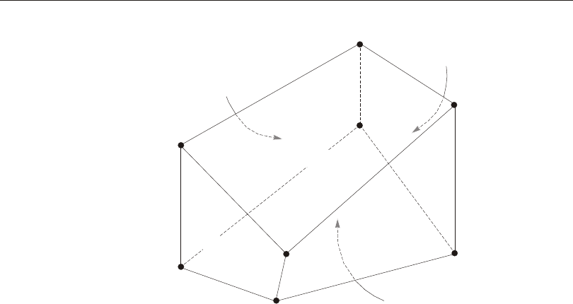
The lo ca tions of the joints should be cho sen to meet the fol low ing geo met ric con di -
tions:
•The in side an gle at each cor ner of the faces must be less than 180°. Best re sults
will be ob tained when these an gles are near 90°, or at least in the range of 45° to
135°.
•The as pect ra tio of an ele ment should not be too large. This is the ra tio of the
long est di men sion of the ele ment to its short est di men sion. Best re sults are ob -
tained for as pect ra tios near unity, or at least less than four. The as pect ra tio
should not ex ceed ten.
These con di tions can usu ally be met with ade quate mesh re fine ment.
De gen er ate Sol ids
De gen er ate sol ids, such as wedges and tet ra he dra, can be cre ated by col laps ing var -
i ous sides of the el e ment. This is done by spec i fy ing the same joint num ber for two
or more of the eight cor ner nodes, so long as the ordering of the nodes re mains the
same. Ex am ples in clude:
Joint Connectivity 239
Chapter XIII The Solid Element
j1
j2
j3
j4
j5
j6
j7
j8
Face 1
Face 2
Face 3
Face 4
Face 5
Face 6
Figure 55
Solid Element Joint Connectivity and Face Definitions

•Wedge (tri an gu lar bottom, tri an gu lar top): j1, j2, j3 = j4, j5, j6, j7 = j8
•Tet ra he dron (triangular bot tom, point top): j1, j2, j3 = j4, j5 = j6 = j7 = j8
•7-node (rectangular bot tom, tri an gu lar top): j1, j2, j3, j4, j5, j6, j7 = j8
•Pyr a mid (rectangular bot tom, point top): j1, j2, j3, j4, j5 = j6 = j7 = j8
Other ex am ples are possible, but these are the rec om mended con fig u ra tions.
Degrees of Freedom
The Solid ele ment ac ti vates the three trans la tional de grees of free dom at each of its
con nected joints. Ro ta tional de grees of free dom are not ac ti vated. This ele ment
con trib utes stiff ness to all of these trans la tional de grees of free dom.
See Topic “De grees of Free dom” (page 30) in Chap ter “Joints and De grees of Free -
dom” for more in for ma tion.
Local Coordinate System
Each Solid ele ment has its own ele ment lo cal co or di nate sys tem used to de fine
Ma te rial prop er ties, loads and out put. The axes of this lo cal sys tem are de noted 1, 2
and 3. By de fault these axes are iden ti cal to the global X, Y, and Z axes, re spec -
tively. Both sys tems are right-handed co or di nate sys tems.
The de fault lo cal co or di nate sys tem is ad e quate for most sit u a tions. How ever, for
cer tain mod el ing pur poses it may be use ful to use el e ment lo cal co or di nate sys tems
that fol low the ge om e try of the struc ture.
For more in for ma tion:
•See Topic “Up ward and Hor i zon tal Di rec tions” (page 13) in Chap ter “Co or di -
nate Sys tems.”
•See Topic “Ad vanced Lo cal Co or di nate Sys tem” (page 240) in this Chap ter.
Advanced Local Coordinate System
By de fault, the element lo cal 1-2-3 co or di nate sys tem is iden ti cal to the global
X-Y-Z co or di nate sys tem, as de scribed in the pre vi ous topic. In cer tain mod el ing
sit u a tions it may be use ful to have more con trol over the spec i fi ca tion of the lo cal
co or di nate sys tem.
240 Degrees of Freedom
CSI Analysis Reference Manual

A va ri ety of meth ods are avail able to de fine a solid-el e ment lo cal co or di nate sys -
tem. These may be used sep a rately or to gether. Lo cal co or di nate axes may be de -
fined to be par al lel to ar bi trary co or di nate di rec tions in an ar bi trary co or di nate sys -
tem or to vec tors be tween pairs of joints. In ad di tion, the lo cal co or di nate sys tem
may be spec i fied by a set of three el e ment co or di nate an gles. These meth ods are de -
scribed in the subtopics that fol low.
For more in for ma tion:
•See Chap ter “Co or di nate Sys tems” (page 11).
•See Topic “Lo cal Co or di nate Sys tem” (page 240) in this Chap ter.
Reference Vectors
To de fine a solid-element lo cal co or di nate sys tem you must spec ify two ref er ence
vec tors that are par al lel to one of the lo cal co or di nate planes. The axis ref er ence
vec tor, Va, must be par al lel to one of the lo cal axes (I = 1, 2, or 3) in this plane and
have a pos i tive pro jec tion upon that axis. The plane ref er ence vec tor, Vp, must
have a pos i tive pro jec tion upon the other lo cal axis (j = 1, 2, or 3, but I ¹ j) in this
plane, but need not be par al lel to that axis. Hav ing a pos i tive pro jec tion means that
the pos i tive di rec tion of the ref er ence vec tor must make an an gle of less than 90°
with the pos i tive di rec tion of the lo cal axis.
To gether, the two ref er ence vec tors de fine a lo cal axis, I, and a lo cal plane, i-j.
From this, the pro gram can de ter mine the third lo cal axis, k, us ing vec tor al ge bra.
For ex am ple, you could choose the axis ref er ence vec tor par al lel to lo cal axis 1 and
the plane ref er ence vec tor par al lel to the lo cal 1-2 plane (I = 1, j = 2). Al ter na tively,
you could choose the axis ref er ence vec tor par al lel to lo cal axis 3 and the plane ref -
er ence vec tor par al lel to the lo cal 3-2 plane (I = 3, j = 2). You may choose the plane
that is most con ve nient to de fine us ing the pa ram e ter lo cal, which may take on the
val ues 12, 13, 21, 23, 31, or 32. The two dig its cor re spond to I and j, re spec tively.
The de fault is value is 31.
Defining the Axis Reference Vector
To de fine the axis ref er ence vec tor, you must first spec ify or use the de fault val ues
for:
•A co or di nate di rec tion axdir (the de fault is +Z)
Advanced Local Coordinate System 241
Chapter XIII The Solid Element

•A fixed co or di nate sys tem csys (the de fault is zero, in di cat ing the global co or -
di nate sys tem)
You may op tion ally spec ify:
•A pair of joints, axveca and axvecb (the de fault for each is zero, in di cat ing the
cen ter of the el e ment). If both are zero, this op tion is not used.
For each element, the axis ref er ence vec tor is de ter mined as fol lows:
1. A vec tor is found from joint axveca to joint axvecb. If this vec tor is of fi nite
length, it is used as the ref er ence vec tor Va
2. Oth er wise, the co or di nate di rec tion axdir is eval u ated at the cen ter of the el e -
ment in fixed co or di nate sys tem csys, and is used as the ref er ence vec tor Va
Defining the Plane Reference Vector
To de fine the plane ref er ence vec tor, you must first spec ify or use the de fault val ues
for:
•A pri mary co or di nate di rec tion pldirp (the de fault is +X)
•A sec ond ary co or di nate di rec tion pldirs (the de fault is +Y). Di rec tions pldirs
and pldirp should not be par al lel to each other un less you are sure that they are
not par al lel to lo cal axis 1
•A fixed co or di nate sys tem csys (the de fault is zero, in di cat ing the global co or -
di nate sys tem). This will be the same co or di nate sys tem that was used to de fine
the axis ref er ence vec tor, as de scribed above
You may op tion ally spec ify:
•A pair of joints, plveca and plvecb (the de fault for each is zero, in di cat ing the
cen ter of the el e ment). If both are zero, this op tion is not used.
For each element, the plane ref er ence vec tor is de ter mined as fol lows:
1. A vec tor is found from joint plveca to joint plvecb. If this vec tor is of fi nite
length and is not par al lel to lo cal axis I, it is used as the ref er ence vec tor Vp
2. Oth er wise, the pri mary co or di nate di rec tion pldirp is eval u ated at the cen ter of
the el e ment in fixed co or di nate sys tem csys. If this di rec tion is not par al lel to
lo cal axis I, it is used as the ref er ence vec tor Vp
242 Advanced Local Coordinate System
CSI Analysis Reference Manual

3. Oth er wise, the sec ond ary co or di nate di rec tion pldirs is eval u ated at the cen ter
of the el e ment in fixed co or di nate sys tem csys. If this di rec tion is not par al lel to
lo cal axis I, it is used as the ref er ence vec tor Vp
4. Oth er wise, the method fails and the anal y sis ter mi nates. This will never hap pen
if pldirp is not par al lel to pldirs
A vec tor is con sid ered to be par al lel to lo cal axis I if the sine of the an gle be tween
them is less than 10-3.
Determining the Local Axes from the Reference Vectors
The pro gram uses vec tor cross prod ucts to de ter mine the lo cal axes from the ref er -
ence vec tors. The three axes are rep re sented by the three unit vec tors V1, V2 and
V3, re spec tively. The vec tors sat isfy the cross-prod uct re la tion ship:
VVV
123
=´
The lo cal axis Vi is given by the vec tor Va af ter it has been nor mal ized to unit
length.
The re main ing two axes, Vj and Vk, are de fined as fol lows:
•If I and j per mute in a pos i tive sense, i.e., lo cal = 12, 23, or 31, then:
VVV
kip
=´ and
VVV
jki
=´
•If I and j per mute in a neg a tive sense, i.e., lo cal = 21, 32, or 13, then:
VVV
kpi
=´ and
VVV
jik
=´
An ex am ple show ing the de ter mi na tion of the element lo cal co or di nate sys tem us -
ing ref er ence vec tors is given in Figure 56 (page 244).
Element Coordinate Angles
The solid-el e ment lo cal co or di nate axes de ter mined from the ref er ence vec tors may
be fur ther mod i fied by the use of three el e ment co or di nate an gles, de noted a, b,
and c. In the case where the de fault ref er ence vec tors are used, the co or di nate an -
gles de fine the ori en ta tion of the el e ment lo cal co or di nate sys tem with re spect to
the global axes.
Advanced Local Coordinate System 243
Chapter XIII The Solid Element

The el e ment co or di nate an gles spec ify ro ta tions of the lo cal co or di nate sys tem
about its own cur rent axes. The re sult ing ori en ta tion of the lo cal co or di nate sys tem
is ob tained ac cord ing to the fol low ing pro ce dure:
1. The lo cal sys tem is first ro tated about its +3 axis by an gle a
2. The lo cal sys tem is next ro tated about its re sult ing +2 axis by an gle b
3. The lo cal sys tem is lastly ro tated about its re sult ing +1 axis by an gle c
The or der in which the ro ta tions are per formed is im por tant. The use of co or di nate
an gles to ori ent the el e ment lo cal co or di nate sys tem with re spect to the global sys -
tem is shown in Figure 4 (page 29).
244 Advanced Local Coordinate System
CSI Analysis Reference Manual
V is parallel to axveca-axvecb
a
V is parallel to plveca-plvecb
p
V = V
3a
V = V x VAll vectors normalized to unit length.
23p
V = V x V
123
XY
Z
Global
axveca
axvecb
plveca
plvecb
Plane 3-1
j
V3
V2
V1
Va
Vp
Figure 56
Example of the Determination of the Solid Element Local Coordinate System
Using Reference Vectors for local=31. Point j is the Center of the Element.

Advanced Local Coordinate System 245
Chapter XIII The Solid Element
a
a
a
b
b
b
c
c
c
Z, 3
Z
Z
X
X
X
1
2
2
2
3
3
1
1
Y
Y
Y
Step 1: Rotation about
local 3 axis by angle a
Step 2: Rotation about new
local 2 axis by angle b
Step 3: Rotation about new
local 1 axis by angle c
Figure 57
Use of Element Coordinate Angles to Orient the
Solid Element Local Coordinate System

Stresses and Strains
The Solid ele ment mod els a gen eral state of stress and strain in a three- dimensional
solid. All six stress and strain com po nents are ac tive for this ele ment.
See Topic “Stresses and Strains” (page 71) in Chap ter “Ma te rial Prop er ties” for
more in for ma tion.
Solid Properties
A Solid Property is a set of ma te rial and geo met ric prop er ties to be used by one or
more Solid el e ments. Solid Prop erties are de fined in de pend ently of the Solid el e -
ments/objects, and are as signed to the el e ments.
Material Properties
The ma te rial prop er ties for each Solid Property are spec i fied by ref er ence to a pre -
vi ously-de fined Ma te rial. Fully anisotropic ma te rial prop er ties are used. The ma te -
rial prop er ties used by the Solid el e ment are:
•The moduli of elas tic ity, e1, e2, and e3
•The shear moduli, g12, g13, and g23
•All of the Pois son’s ra tios, u12, u13, u23, ..., u56
•The co ef fi cients of ther mal ex pan sion, a1, a2, a3, a12, a13, and a23
•The mass den sity, m, used for com put ing el e ment mass
•The weight den sity, w, used for com put ing Self-Weight and Grav ity Loads
All ma te rial prop er ties (ex cept the den si ties) are ob tained at the ma te rial tem per a -
ture of each in di vid ual el e ment.
See Chap ter “Ma te rial Prop erties” (page 69) for more in for ma tion.
Material Angles
The ma te rial lo cal co or di nate sys tem and the el e ment (Property) lo cal co or di nate
sys tem need not be the same. The ma te rial co or di nate sys tem is ori ented with re -
spect to the el e ment co or di nate sys tem us ing the three an gles a, b, and c ac cord ing
to the fol low ing pro ce dure:
•The ma te rial sys tem is first aligned with the el e ment sys tem;
246 Stresses and Strains
CSI Analysis Reference Manual
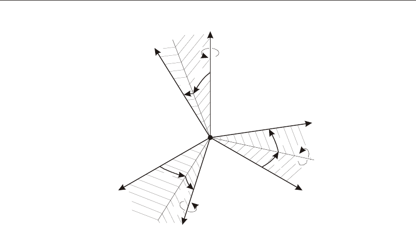
•The ma te rial sys tem is then ro tated about its +3 axis by an gle a;
•The ma te rial sys tem is next ro tated about the re sult ing +2 axis by an gle b;
•The ma te rial sys tem is lastly ro tated about the re sult ing +1 axis by an gle c;
This is shown in Figure 58 (page 247). These an gles have no ef fect for iso tro pic
ma te rial prop er ties since they are in de pend ent of ori en ta tion.
See Topic “Lo cal Co or di nate Sys tem” (page 70) in Chap ter “Ma te rial Prop erties”
for more in for ma tion.
Incompatible Bending Modes
By de fault each Solid ele ment in cludes nine in com pati ble bend ing modes in its
stiff ness for mu la tion. These in com pati ble bend ing modes sig nifi cantly im prove
the bend ing be hav ior of the ele ment if the ele ment ge ome try is of a rec tan gu lar
form. Im proved be hav ior is ex hib ited even with non- rectangular ge ome try.
If an ele ment is se verely dis torted, the in clu sion of the in com pati ble modes should
be sup pressed. The ele ment then uses the stan dard iso para met ric for mu la tion. In -
Solid Properties 247
Chapter XIII The Solid Element
1 (Element)
1 (Material)
2 (Element)
2 (Material)
3 (Element)
3 (Material)
a
a
a
b
b
b
c
c
c
Rotations are performed in the order
a-b-c about the axes shown.
Figure 58
Solid Element Material Angles

com pati ble bend ing modes may also be sup pressed in cases where bend ing is not
im por tant, such as in typi cal geo tech ni cal prob lems.
Mass
In a dy namic analy sis, the mass of the struc ture is used to com pute in er tial forces.
The mass con trib uted by the Solid ele ment is lumped at the ele ment joints. No in er -
tial ef fects are con sid ered within the ele ment it self.
The to tal mass of the ele ment is equal to the in te gral of the mass den sity, m, over the
vol ume of the ele ment. The to tal mass is ap por tioned to the joints in a man ner that is
pro por tional to the di ago nal terms of the con sis tent mass ma trix. See Cook,
Malkus, and Ple sha (1989) for more in for ma tion. The to tal mass is ap plied to each
of the three trans la tional de grees of free dom (UX, UY, and UZ).
For more in for ma tion:
•See Topic “Mass Den sity” (page 77) in Chap ter “Ma te rial Prop er ties.”
•See Topic “Mass Source” (page 334) in Chap ter “Load Pat terns”.
•See Chap ter “Load Cases” (page 341).
Self-Weight Load
Self- Weight Load ac ti vates the self- weight of all ele ments in the model. For a Solid
ele ment, the self- weight is a force that is uni formly dis trib uted over the vol ume of
the ele ment. The mag ni tude of the self- weight is equal to the weight den sity, w.
Self- Weight Load al ways acts down ward, in the global –Z di rec tion. You may
scale the self- weight by a sin gle scale fac tor that ap plies equally to all ele ments in
the struc ture.
For more in for ma tion:
•See Topic “Weight Den sity” (page 78) in Chap ter “Ma te rial Prop er ties” for the
defi ni tion of w.
•See Topic “Self- Weight Load” (page 325) in Chap ter “Load Pat terns.”
248 Mass
CSI Analysis Reference Manual

Gravity Load
Grav ity Load can be ap plied to each Solid ele ment to ac ti vate the self- weight of the
ele ment. Us ing Grav ity Load, the self- weight can be scaled and ap plied in any di -
rec tion. Dif fer ent scale fac tors and di rec tions can be ap plied to each ele ment.
If all ele ments are to be loaded equally and in the down ward di rec tion, it is more
con ven ient to use Self- Weight Load.
For more in for ma tion:
•See Topic “Self- Weight Load” (page 248) in this Chap ter for the defi ni tion of
self- weight for the Solid ele ment.
•See Topic “Grav ity Load” (page 326) in Chap ter “Load Pat terns.”
Surface Pressure Load
The Sur face Pres sure Load is used to ap ply ex ter nal pres sure loads upon any of the
six faces of the Solid ele ment. The defi ni tion of these faces is shown in Figure 55
(page 239). Sur face pres sure al ways acts nor mal to the face. Posi tive pres sures are
di rected to ward the in te rior of the ele ment.
The pres sure may be con stant over a face or in ter po lated from val ues given at the
joints. The val ues given at the joints are ob tained from Joint Pat terns, and need not
be the same for the dif fer ent faces. Joint Pat terns can be used to eas ily ap ply hy dro -
static pres sures.
The pres sure act ing on a given face is in te grated over the area of that face, and the
re sult ing force is ap por tioned to the four cor ner joints of the face.
See Chap ter “Load Pat terns” (page 321) for more in for ma tion.
Pore Pressure Load
The Pore Pres sure Load is used to model the drag and buoy ancy ef fects of a fluid
within a solid me dium, such as the ef fect of wa ter upon the solid skele ton of a soil.
Sca lar fluid- pressure val ues are given at the ele ment joints by Joint Pat terns, and in -
ter po lated over the ele ment. The to tal force act ing on the ele ment is the in te gral of
the gra di ent of this pres sure field over the vol ume of the ele ment. This force is ap -
Gravity Load 249
Chapter XIII The Solid Element

por tioned to each of the joints of the ele ment. The forces are typi cally di rected from
re gions of high pres sure to ward re gions of low pres sure.
See Chap ter “Load Pat terns” (page 321) for more in for ma tion.
Temperature Load
The Tem per a ture Load cre ates ther mal strain in the Solid el e ment. This strain is
given by the prod uct of the Ma te rial co ef fi cient of ther mal ex pan sion and the tem -
per a ture change of the el e ment. All spec i fied Tem per a ture Loads rep re sent a
change in tem per a ture from the un stressed state for a lin ear anal y sis, or from the
pre vi ous tem per a ture in a non lin ear anal y sis.
See Chap ter “Load Pat terns” (page 321) for more in for ma tion.
Stress Output
The Solid ele ment stresses are evalu ated at the stan dard 2 x 2 x 2 Gauss in te gra tion
points of the ele ment and ex trapo lated to the joints. See Cook, Malkus, and Ple sha
(1989) for more in for ma tion.
Prin ci pal val ues and their as so ci ated prin ci pal di rec tions in the ele ment lo cal co or -
di nate sys tem are also com puted for sin gle-val ued Load Cases and Load Com bi na -
tions. Three di rec tion co sines each are given for the di rec tions of the maxi mum and
mini mum prin ci pal stresses. The di rec tion of the mid dle prin ci pal stress is per pen -
dicu lar to the maxi mum and mini mum prin ci pal di rec tions.
For more in for ma tion:
•See Chap ter “Load Pat terns” (page 321).
•See Chap ter “Load Cases” (page 341).
250 Temperature Load
CSI Analysis Reference Manual

Chapter XIV
The Link/Support Element—Basic
The Link el e ment is used to con nect two joints to gether. The Sup port el e ment is
used to con nect one joint to ground. Both el e ment types use the same types of prop -
er ties. Each Link or Sup port el e ment may ex hibit up to three dif fer ent types of be -
hav ior: lin ear, non lin ear, and fre quency-de pend ent, ac cord ing to the types of prop -
er ties as signed to that el e ment and the type of anal y sis be ing per formed.
This Chap ter de scribes the ba sic and gen eral fea tures of the Link and Sup port el e -
ments and their lin ear be hav ior. The next Chap ter de scribes ad vanced be hav ior,
which can be non lin ear or fre quency-de pend ent.
Advanced Topics
•Over view
•Joint Con nec tivity
•Zero- Length Ele ments
•De grees of Free dom
•Lo cal Co or di nate Sys tem
•Ad vanced Lo cal Co or di nate Sys tem
•In ter nal De for ma tions
•Link/Sup port Prop er ties
251

•Cou pled Lin ear Property
•Mass
•Self- Weight Load
•Grav ity Load
•In ter nal Force and De for ma tion Out put
Overview
A Link el e ment is a two-joint con nect ing link. A Sup port el e ment is a one-joint
grounded spring. Prop er ties for both types of el e ment are de fined in the same way.
Each el e ment is as sumed to be com posed of six sep a rate “springs,” one for each of
six deformational de grees-of free dom (ax ial, shear, tor sion, and pure bend ing).
There are two cat e go ries of Link/Support prop er ties that can be de fined: Lin -
ear/Non lin ear, and Fre quency-De pend ent. A Lin ear/Non lin ear prop erty set must
be as signed to each Link or Sup port el e ment. The as sign ment of a Fre -
quency-Dependent prop erty set to a Link or Sup port el e ment is op tional.
All Lin ear/Non lin ear prop erty sets con tain lin ear prop er ties that are used by the el e -
ment for lin ear anal y ses, and for other types of analyses if no other prop er ties are
de fined. Lin ear/Non lin ear prop erty sets may have non lin ear prop er ties that will be
used for all non lin ear anal y ses, and for lin ear anal y ses that con tinue from nonlinear
anal y ses.
Fre quency-de pend ent prop erty sets con tain im ped ance (stiff ness and damp ing)
prop er ties that will be used for all fre quency-de pend ent anal y ses. If a Fre -
quency-De pend ent prop erty has not been as signed to a Link/Sup port el e ment, the
lin ear prop er ties for that el e ment will be used for fre quency-de pend ent anal y ses.
The types of non lin ear be hav ior that can be mod eled with this ele ment in clude:
•Vis coe las tic damp ing
•Gap (com pres sion only) and hook (ten sion only)
•Multi-lin ear uni ax ial elas tic ity
•Uni ax ial plas tic ity (Wen model)
•Multi-lin ear uni ax ial plas tic ity with sev eral types of hysteretic be hav ior: ki ne -
matic, Takeda, and pivot
•Biaxial- plasticity base iso la tor
252 Overview
CSI Analysis Reference Manual

•Friction- pendulum base iso la tor, with or with out up lift pre ven tion. This can
also be used for mod el ing gap-fric tion con tact behavior
Each ele ment has its own lo cal co or di nate sys tem for de fin ing the force-
deformation prop er ties and for in ter pret ing out put.
Each Link/Support el e ment may be loaded by grav ity (in any di rec tion).
Avail able out put in cludes the de for ma tion across the ele ment, and the in ter nal
forces at the joints of the ele ment.
Joint Connectivity
Each Link/Support el e ment may take one of the fol low ing two con fig u ra tions:
•A Link con nect ing two joints, I and j; it is per mis si ble for the two joints to
share the same lo ca tion in space cre at ing a zero-length element
•A Sup port con nect ing a sin gle joint, j, to ground
Con ver sion from One-Joint Objects to Two-Joint Elements
Dur ing anal y sis, all one-joint Link/Sup port ob jects used for mod el ing are ac tu ally
con verted to two-joint Link/Sup port el e ments of zero length. The orig i nal joint, j,
re mains con nected to the struc ture. A new joint , I, is gen er ated at the same lo ca tion
and is fully re strained. Re ac tions are cal cu lated at gen er ated joint I but are re ported
at the orig i nal joint j. Conversely, ground dis place ment loads ap plied at joint j are
trans ferred to joint I.
For the re main der of this chap ter and the next, we will con tinue to re fer to one-joint
el e ments for con ve nience, and to clar ify how the one-joint mod el ing ob jects be -
have.
Zero-Length Elements
The fol low ing types of Link/Support el e ments are con sid ered to be of zero length:
•Single- joint Sup port el e ments
•Two- joint Link el e ments with the dis tance from joint I to joint j be ing less than
or equal to the zero- length tol er ance that you spec ify.
Joint Connectivity 253
Chapter XIV The Link/Support Element—Basic

The length tol er ance is set us ing the Auto Merge Tol er ance in the graph i cal user in -
ter face. Two- joint ele ments hav ing a length greater than the Auto Merge Tol er ance
are con sid ered to be of fi nite length. Whether an ele ment is of zero length or fi nite
length af fects the defi ni tion of the ele ment lo cal co or di nate sys tem, and the in ter nal
mo ments due to shear forces.
Degrees of Freedom
The Link/Support el e ment al ways ac ti vates all six de grees of free dom at each of its
one or two con nected joints. To which joint de grees of free dom the el e ment con -
trib utes stiff ness de pends upon the prop er ties you as sign to the el e ment. You must
en sure that re straints or other sup ports are pro vided to those joint de grees of free -
dom that re ceive no stiff ness.
For more in for ma tion:
•See Topic “De grees of Free dom” (page 30) in Chap ter “Joints and De grees of
Free dom.”
•See Topic “Link/Sup port Prop er ties” (page 263) in this Chap ter.
Local Coordinate System
Each Link/Sup port el e ment has its own el e ment lo cal co or di nate sys tem used to
de fine force-de for ma tion prop er ties and out put. The axes of this lo cal sys tem are
de noted 1, 2 and 3. The first axis is di rected along the length of the el e ment and cor -
re sponds to extensional de for ma tion. The re main ing two axes lie in the plane per -
pen dic u lar to the el e ment and have an ori en ta tion that you spec ify; these di rec tions
cor re spond to shear de for ma tion.
It is im por tant that you clearly un der stand the defi ni tion of the ele ment lo cal 1- 2-3
co or di nate sys tem and its re la tion ship to the global X- Y-Z co or di nate sys tem. Both
sys tems are right- handed co or di nate sys tems. It is up to you to de fine lo cal sys tems
which sim plify data in put and in ter pre ta tion of re sults.
In most struc tures the def i ni tion of the el e ment lo cal co or di nate sys tem is ex -
tremely sim ple. The meth ods pro vided, how ever, pro vide suf fi cient power and
flex i bil ity to de scribe the ori en ta tion of Link/Sup port el e ments in the most com pli -
cated sit u a tions.
254 Degrees of Freedom
CSI Analysis Reference Manual

The sim plest method, us ing the de fault ori en ta tion and the Link/Sup port el e -
ment co or di nate an gle, is de scribed in this topic. Ad di tional meth ods for de fin ing
the Link/Sup port el e ment lo cal co or di nate sys tem are de scribed in the next topic.
For more in for ma tion:
•See Chap ter “Co or di nate Sys tems” (page 11) for a de scrip tion of the con cepts
and ter mi nol ogy used in this topic.
•See Topic “Ad vanced Lo cal Co or di nate Sys tem” (page 256) in this Chap ter.
Longitudinal Axis 1
Lo cal axis 1 is the lon gi tu di nal axis of the ele ment, cor re spond ing to ex ten sional
de for ma tion. This axis is de ter mined as fol lows:
•For ele ments of fi nite length this axis is auto mati cally de fined as the di rec tion
from joint I to joint j
•For zero- length ele ments the lo cal 1 axis de faults to the +Z global co or di nate
di rec tion (up ward)
For the defi ni tion of zero- length ele ments, see Topic “Zero- Length Ele ments”
(page 253) in this Chap ter.
Default Orientation
The de fault ori en ta tion of the lo cal 2 and 3 axes is de ter mined by the re la tion ship
be tween the lo cal 1 axis and the global Z axis. The pro ce dure used here is iden ti cal
to that for the Frame ele ment:
•The lo cal 1-2 plane is taken to be ver ti cal, i.e., par al lel to the Z axis
•The lo cal 2 axis is taken to have an up ward (+Z) sense un less the ele ment is ver -
ti cal, in which case the lo cal 2 axis is taken to be hori zon tal along the global +X
di rec tion
•The lo cal 3 axis is al ways hori zon tal, i.e., it lies in the X-Y plane
An ele ment is con sid ered to be ver ti cal if the sine of the an gle be tween the lo cal 1
axis and the Z axis is less than 10-3.
The lo cal 2 axis makes the same an gle with the ver ti cal axis as the lo cal 1 axis
makes with the hori zon tal plane. This means that the lo cal 2 axis points ver ti cally
up ward for hori zon tal ele ments.
Local Coordinate System 255
Chapter XIV The Link/Support Element—Basic

Coordinate Angle
The Link/Sup port el e ment co or di nate an gle, ang, is used to de fine el e ment ori en ta -
tions that are dif fer ent from the de fault ori en ta tion. It is the an gle through which the
lo cal 2 and 3 axes are ro tated about the pos i tive lo cal 1 axis from the de fault ori en -
ta tion. The ro ta tion for a pos i tive value of ang ap pears coun ter clock wise when the
lo cal +1 axis is point ing to ward you. The pro ce dure used here is iden ti cal to that for
the Frame el e ment.
For ver ti cal ele ments, ang is the an gle be tween the lo cal 2 axis and the hori zon tal
+X axis. Oth er wise, ang is the an gle be tween the lo cal 2 axis and the ver ti cal plane
con tain ing the lo cal 1 axis. See Figure 59 (page 257) for ex am ples.
Advanced Local Coordinate System
By de fault, the ele ment lo cal co or di nate sys tem is de fined us ing the ele ment co or -
di nate an gle meas ured with re spect to the global +Z and +X di rec tions, as de scribed
in the pre vi ous topic. In cer tain mod el ing situa tions it may be use ful to have more
con trol over the speci fi ca tion of the lo cal co or di nate sys tem.
This topic de scribes how to de fine the ori en ta tion of the trans verse lo cal 2 and 3
axes with re spect to an ar bi trary ref er ence vec tor when the ele ment co or di nate an -
gle, ang, is zero. If ang is dif fer ent from zero, it is the an gle through which the lo cal
2 and 3 axes are ro tated about the posi tive lo cal 1 axis from the ori en ta tion de ter -
mined by the ref er ence vec tor.
This topic also de scribes how to change the ori en ta tion of the lo cal 1 axis from the
de fault global +Z di rec tion for zero- length ele ments. The lo cal 1 axis is al ways di -
rected from joint I to joint j for ele ments of fi nite length.
For more in for ma tion:
•See Chap ter “Co or di nate Sys tems” (page 11) for a de scrip tion of the con cepts
and ter mi nol ogy used in this topic.
•See Topic “Lo cal Co or di nate Sys tem” (page 253) in this Chap ter.
256 Advanced Local Coordinate System
CSI Analysis Reference Manual
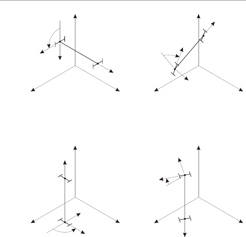
Axis Reference Vector
To de fine the lo cal 1 axis for zero- length ele ments, you spec ify an axis ref er ence
vec tor that is par al lel to and has the same posi tive sense as the de sired lo cal 1 axis.
The axis ref er ence vec tor has no ef fect upon finite- length ele ments.
Advanced Local Coordinate System 257
Chapter XIV The Link/Support Element—Basic
Y
Y
Y
Y
Z
Z
Z
Z
X
X
X
X
ang=90°
ang=90°
ang=30°
ang=30°
2
2
2
2
3
3
3
3
1
1
1
1
i
i
i
i
j
j
j
j
Local 1 Axis is Parallel to +Y Axis
Local 2 Axis is Rotated 90° from Z-1 Plane
Local 1 Axis is Parallel to +Z Axis
Local 2 Axis is Rotated 90° from X-1 Plane
Local 1 Axis is Parallel to –Z Axis
Local 2 Axis is Rotated 30° from X-1 Plane
Local 1 Axis is Not Parallel to X, Y, or Z Axes
Local 2 Axis is Rotated 30° from Z-1 Plane
Figure 59
The Link/Support Element Coordinate Angle with Respect to the Default
Orientation

To de fine the axis ref er ence vec tor, you must first spec ify or use the de fault val ues
for:
•A co or di nate di rec tion ax dir (the de fault is +Z)
•A fixed co or di nate sys tem csys (the de fault is zero, in di cat ing the global co or -
di nate sys tem). This will be the same co or di nate sys tem that is used to de fine
the plane ref er ence vec tor, as de scribed be low
You may op tion ally spec ify:
•A pair of joints, ax veca and ax vecb (the de fault for each is zero, in di cat ing the
cen ter of the ele ment). If both are zero, this op tion is not used
For each ele ment, the axis ref er ence vec tor is de ter mined as fol lows:
1. A vec tor is found from joint ax veca to joint ax vecb. If this vec tor is of fi nite
length, it is used as the ref er ence vec tor Va
2. Oth er wise, the co or di nate di rec tion ax dir is evalu ated at the cen ter of the ele -
ment in fixed co or di nate sys tem csys, and is used as the ref er ence vec tor Va
The cen ter of a zero- length ele ment is taken to be at joint j.
The lo cal 1 axis is given by the vec tor Va af ter it has been nor mal ized to unit length.
Plane Reference Vector
To de fine the trans verse lo cal axes 2 and 3, you spec ify a plane ref er ence vec tor
that is par al lel to the de sired 1-2 or 1-3 plane. The pro ce dure used here is iden ti cal
to that for the Frame ele ment.
The ref er ence vec tor must have a posi tive pro jec tion upon the cor re spond ing trans -
verse lo cal axis (2 or 3, re spec tively). This means that the posi tive di rec tion of the
ref er ence vec tor must make an an gle of less than 90° with the posi tive di rec tion of
the de sired trans verse axis.
To de fine the ref er ence vec tor, you must first spec ify or use the de fault val ues for:
•A pri mary co or di nate di rec tion pldirp (the de fault is +Z)
•A sec on dary co or di nate di rec tion pldirs (the de fault is +X). Di rec tions pldirs
and pldirp should not be par al lel to each other un less you are sure that they are
not par al lel to lo cal axis 1
258 Advanced Local Coordinate System
CSI Analysis Reference Manual

•A fixed co or di nate sys tem csys (the de fault is zero, in di cat ing the global co or -
di nate sys tem). This will be the same co or di nate sys tem that was used to de fine
the axis ref er ence vec tor, as de scribed above
•The lo cal plane, lo cal, to be de ter mined by the ref er ence vec tor (the de fault is
12, in di cat ing plane 1-2)
You may op tion ally spec ify:
•A pair of joints, plveca and plvecb (the de fault for each is zero, in di cat ing the
cen ter of the ele ment). If both are zero, this op tion is not used
For each ele ment, the ref er ence vec tor is de ter mined as fol lows:
1. A vec tor is found from joint plveca to joint plvecb. If this vec tor is of fi nite
length and is not par al lel to lo cal axis 1, it is used as the ref er ence vec tor Vp.
2. Oth er wise, the pri mary co or di nate di rec tion pldirp is evalu ated at the cen ter of
the ele ment in fixed co or di nate sys tem csys. If this di rec tion is not par al lel to
lo cal axis 1, it is used as the ref er ence vec tor Vp.
3. Oth er wise, the sec on dary co or di nate di rec tion pldirs is evalu ated at the cen ter
of the ele ment in fixed co or di nate sys tem csys. If this di rec tion is not par al lel to
lo cal axis 1, it is used as the ref er ence vec tor Vp.
4. Oth er wise, the method fails and the analy sis ter mi nates. This will never hap pen
if pldirp is not par al lel to pldirs
A vec tor is con sid ered to be par al lel to lo cal axis 1 if the sine of the an gle be tween
them is less than 10-3.
The use of the Link/Sup port el e ment co or di nate an gle in con junc tion with co or di -
nate di rec tions that de fine the ref er ence vec tor is il lus trated in Figure 60 (page
260). The use of joints to de fine the ref er ence vec tor is shown in Figure 61 (page
261).
Determining Transverse Axes 2 and 3
The pro gram uses vec tor cross prod ucts to de ter mine the trans verse axes 2 and 3
once the ref er ence vec tor has been speci fied. The three axes are rep re sented by the
three unit vec tors V1, V2 and V3, re spec tively. The vec tors sat isfy the cross- product
re la tion ship:
VVV
123
=´
Advanced Local Coordinate System 259
Chapter XIV The Link/Support Element—Basic
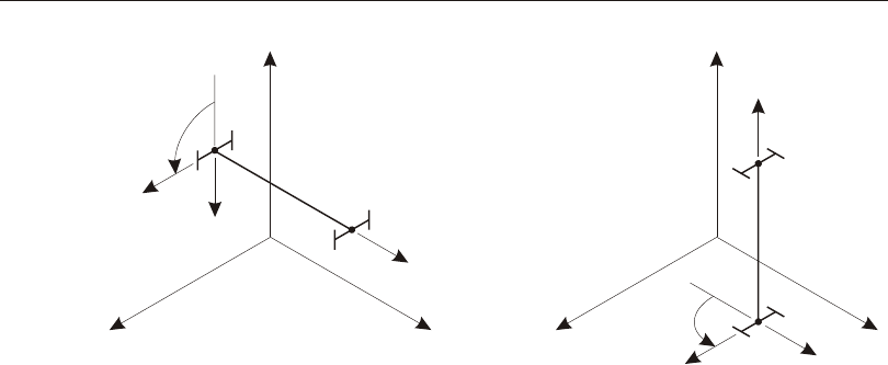
The trans verse axes 2 and 3 are de fined as fol lows:
•If the ref er ence vec tor is par al lel to the 1-2 plane, then:
VVV
31
=´p and
VVV
231
=´
•If the ref er ence vec tor is par al lel to the 1-3 plane, then:
VVV
21
=´
p and
VVV
312
=´
In the com mon case where the ref er ence vec tor is per pen dicu lar to axis V1, the
trans verse axis in the se lected plane will be equal to Vp.
Internal Deformations
Six in de pend ent in ter nal de for ma tions are de fined for the Link/Sup port el e ment.
These are cal cu lated from the rel a tive dis place ments of joint j with re spect to:
•Joint I for a two- joint ele ment
•The ground for a single- joint ele ment
260 Internal Deformations
CSI Analysis Reference Manual
X
Y
ZX
Y
Z
ang=90°
ang=90°
2
2
3
3
1
1
i
i
j
j
Local 1 Axis is Not Parallel to pldirp (+Y)
Local 2 Axis is Rotated 90° from Y-1 Plane
Local 1 Axis is Parallel to pldirp (+Y)
Local 2 Axis is Rotated 90° from X-1 Plane
pldirp = +Y
pldirs = –X
local = 12
Figure 60
The Link/Support Element Coordinate Angle with Respect to Coordinate
Directions
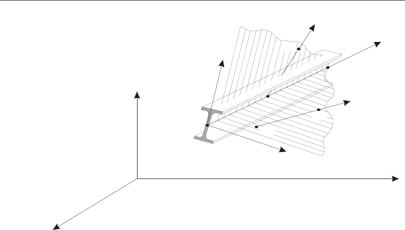
For two- joint Link/Sup port ele ments the in ter nal de for ma tions are de fined as:
•Ax ial: du1 = u1j – u1i
•Shear in the 1-2 plane: du2 = u2j – u2i – dj2 r3j – (L – dj2) r3i
•Shear in the 1-3 plane: du3 = u3j – u3i + dj3 r2j + (L – dj3) r2i
•Tor sion: dr1 = r1j – r1i
•Pure bend ing in the 1-3 plane: dr2 = r2i – r2j
•Pure bend ing in the 1-2 plane: dr3 = r3j – r3i
where:
•u1i, u2i, u3i, r1i, r2i, and r3i are the trans la tions and ro ta tions at joint I
•u1j, u2j, u3j, r1j, r2j, and r3j are the trans la tions and ro ta tions at joint j
•dj2 is the dis tance you spec ify from joint j to the lo ca tion where the shear de -
for ma tion du2 is mea sured (the de fault is zero, mean ing at joint j)
•dj3 is the dis tance you spec ify from joint j to the lo ca tion where the shear de -
for ma tion du3 is mea sured (the de fault is zero, mean ing at joint j)
•L is the length of the ele ment
Internal Deformations 261
Chapter XIV The Link/Support Element—Basic
Y
Z
Joint j
Axis 1
Axis 2
X
Axis 3
Joint i
V (b)
p
V (a)
p
100
101
102
The following two specifications are equivalent:
(a) local=12, plveca=0, plvecb=100
(b) local=13, plveca=101, plvecb=102
Plane 1-3
Plane 1-2
Figure 61
Using Joints to Define the Link/Support Element Local Coordinate System
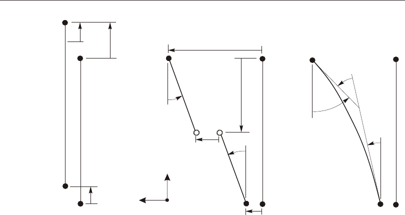
All trans la tions, ro ta tions, and de for ma tions are ex pressed in terms of the ele ment
lo cal co or di nate sys tem.
Note that shear de for ma tion can be caused by ro ta tions as well as trans la tions.
These defi ni tions en sure that all de for ma tions will be zero un der rigid- body mo -
tions of the ele ment.
Im por tant! Note that dj2 is the lo ca tion where pure bend ing be hav ior is mea sured
in the 1-2 plane, in other words, it is where the mo ment due to shear is taken to be
zero. Like wise, dj3 is the lo ca tion where pure bend ing be hav ior is mea sured in the
1-3 plane.
It is im por tant to note that the neg a tives of the ro ta tions r2i and r2j have been used for
the def i ni tion of shear and bend ing de for ma tions in the 1-3 plane. This pro vides
con sis tent def i ni tions for shear and mo ment in both the Link/Sup port and Frame el -
e ments.
Three of these in ter nal de for ma tions are il lus trated in Figure 62 (page 262).
For one- joint grounded- spring ele ments the in ter nal de for ma tions are the same as
above, ex cept that the trans la tions and ro ta tions at joint I are taken to be zero:
262 Internal Deformations
CSI Analysis Reference Manual
2
1
du1
du2
dr3
u1i
u2i
r3i
r3i
r3jr3j
u1ju2j
dj2
Shear Deformation Bending DeformationAxial Deformation
Figure 62
Internal Deformations for a Two-Joint Link Element

•Ax ial: du1 = u1j
•Shear in the 1-2 plane: du2 = u2j – dj2 r3j
•Shear in the 1-3 plane: du3 = u3j + dj3 r2j
•Tor sion: dr1 = r1j
•Pure bend ing in the 1-3 plane: dr2 = – r2j
•Pure bend ing in the 1-2 plane: dr3 = r3j
Link/Support Properties
A Link/Support Prop erty is a set of struc tural prop er ties that can be used to de fine
the be hav ior of one or more Link or Sup port el e ments. Each Link/Support Prop erty
spec i fies the force-de for ma tion re la tion ships for the six in ter nal de for ma tions.
Mass and weight prop er ties may also be spec i fied.
Link/Support Prop er ties are de fined in de pend ently of the Link and Sup port el e -
ments and are ref er enced dur ing the def i ni tion of the el e ments.
There are two cat e go ries of Link/Sup port prop er ties that can be de fined:
•Lin ear/Non lin ear. A Lin ear/Non lin ear prop erty set must be as signed to each
Link or Sup port el e ment.
•Fre quency-De pend ent. The as sign ment of a Fre quency-De pend ent prop erty
set to a Link or Sup port el e ment is op tional.
All Lin ear/Non lin ear prop erty sets con tain lin ear prop er ties that are used by the el e -
ment for lin ear anal y ses, and for other types of anal y ses if no other prop er ties are
de fined. Lin ear/Non lin ear prop erty sets may also have non lin ear prop er ties that
will be used for all non lin ear anal y ses, and for lin ear anal y ses that con tinue from
non lin ear anal y ses.
Fre quency-de pend ent prop erty sets con tain im ped ance (stiff ness and damp ing)
prop er ties that will be used for all fre quency-de pend ent anal y ses. If a Fre -
quency-De pend ent prop erty has not been as signed to a Link/Sup port el e ment, the
lin ear prop er ties for that el e ment will be used for fre quency-de pend ent anal y ses.
This is sum ma rized in the ta ble of Figure 63 (page 264).
Link/Support Properties 263
Chapter XIV The Link/Support Element—Basic

Local Coordinate System
Link/Support Prop er ties are de fined with re spect to the lo cal co or di nate sys tem of
the Link or Sup port el e ment. The lo cal 1 axis is the lon gi tu di nal di rec tion of the el e -
ment and cor re sponds to extensional and tor sional de for ma tions. The lo cal 2 and 3
di rec tions cor re spond to shear and bend ing de for ma tions.
See Topic “Lo cal Co or di nate Sys tem” (page 253) in this Chap ter.
Internal Spring Hinges
Each Link/Support Prop erty is as sumed to be com posed of six in ter nal “springs” or
“Hinges,” one for each of six in ter nal de for ma tions. Each “spring” may ac tu ally
264 Link/Support Properties
CSI Analysis Reference Manual
Load Case
Type
Load Case
Initial
Conditions
Element has
Nonlinear
Properties?
Element has
Freq. Dep.
Properties?
Actual
Property
Used
Linear
Zero Yes or No Yes or No Linear
Nonlinear
Case
No Yes or No Linear
Yes Yes or No Nonlinear
Nonlinear Any
No Yes or No Linear
Yes Yes or No Nonlinear
Frequency
Dependent
Zero Yes or No
No Linear
Yes Freq. Dep.
Nonlinear
Case
No No Linear
Yes No Nonlinear
Yes or No Yes Freq. Dep.
Figure 63
Link/Support Stiffness Properties Actually Used for Different Types of Analysis
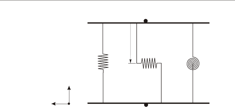
con sist of sev eral com po nents, in clud ing springs and dash pots. The force-
deformation re la tion ships of these springs may be cou pled or in de pend ent of each
other.
Figure 64 (page 265) shows the springs for three of the de for ma tions: ax ial, shear in
the 1-2 plane, and pure- bending in the 1-2 plane. It is im por tant to note that the
shear spring is lo cated a dis tance dj2 from joint j. All shear de for ma tion is as sumed
to oc cur in this spring; the links con nect ing this spring to the joints (or ground) are
rigid in shear. De for ma tion of the shear spring can be caused by ro ta tions as well as
trans la tions at the joints. The force in this spring will pro duce a linearly- varying
mo ment along the length. This mo ment is taken to be zero at the shear spring, which
acts as a mo ment hinge. The mo ment due to shear is in de pend ent of, and ad di tive
to, the con stant mo ment in the ele ment due to the pure- bending spring.
The other three springs that are not shown are for tor sion, shear in the 1-3 plane, and
pure- bending in the 1-3 plane. The shear spring is lo cated a dis tance dj3 from joint
j.
The val ues of dj2 and dj3 may be dif fer ent, al though nor mally they would be the
same for most el e ments.
Link/Support Properties 265
Chapter XIV The Link/Support Element—Basic
Joint j
Joint i
or ground
dj2
Axial Shear Pure
Bending
1
2
Figure 64
Three of the Six Independent Spring Hinges in a Link/Support Element
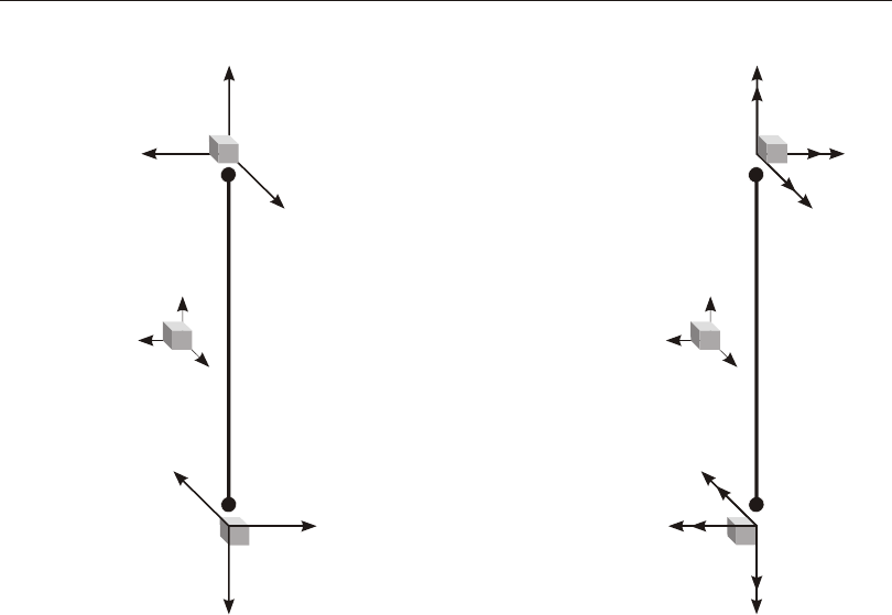
Spring Force-Deformation Relationships
There are six force- deformation re la tion ships that gov ern the be hav ior of the ele -
ment, one for each of the in ter nal springs:
•Ax ial: fu1 vs. du1
•Shear: fu2 vs. du2 , fu3 vs. du3
•Tor sional: fr1 vs. dr1
•Pure bend ing: fr2 vs. dr2 , fr3 vs. dr3
where fu1, fu2, and fu3 are the internal- spring forces; and fr1, fr2, and fr3 are the internal-
spring mo ments.
Each of these re la tion ships may be zero, lin ear only, or lin ear/non lin ear for a given
Link/Support Prop erty. These re la tion ships may be in de pend ent or cou pled. The
266 Link/Support Properties
CSI Analysis Reference Manual
11
PT
PT
22
V2M2
V2M2
33
V3M3
V3M3
i i
j j
Figure 65
Link/Support Element Internal Forces and Moments, Shown Acting at the Joints

forces and mo ments may be re lated to the de for ma tion rates (ve loci ties) as well as
to the de for ma tions.
Element Internal Forces
The Link/Sup port el e ment in ter nal forces, P, V2, V3, and the in ter nal mo ments, T,
M2, M3, have the same mean ing as for the Frame el e ment. These are il lus trated in
Figure 65 (page 266). These can be de fined in terms of the spring forces and mo -
ments as:
•Ax ial: P = fu1
•Shear in the 1-2 plane: V2 = fu2 , M3s = (d – dj2) fu2
•Shear in the 1-3 plane: V3 = fu3 , M2s = (d – dj3) fu3
•Tor sion: T = fr1
•Pure bend ing in the 1-3 plane: M2b = fr2
•Pure bend ing in the 1-2 plane: M3b = fr3
where d is the dis tance from joint j. The to tal bending- moment re sul tants M2 and
M3 com posed of shear and pure- bending parts:
MMM
sb
222=+
MMM
sb
333=+
These in ter nal forces and mo ments are pres ent at every cross sec tion along the
length of the ele ment.
See Topic “In ter nal Force Out put” (page 144) in Chap ter “The Frame Ele ment.”
Uncoupled Linear Force-Deformation Relationships
If each of the in ter nal springs are lin ear and un cou pled, the spring force-
deformation re la tion ships can be ex pressed in ma trix form as:
(Eqn. 1)
f
f
f
f
f
f
k
k
u
u
u
r
r
r
u
u
1
2
3
1
2
3
1
2
00000
00
ì
í
ï
ï
ï
î
ï
ï
ï
ü
ý
ï
ï
ï
þ
ï
ï
ï
=
00
000
00
0
3
1
2
3
1
2
k
k
k
k
d
d
d
u
r
r
r
u
u
u
sym.
é
ë
ê
ê
ê
ê
ê
ê
ê
ù
û
ú
ú
ú
ú
ú
ú
ú
3
1
2
3
d
d
d
r
r
r
ì
í
ï
ï
ï
î
ï
ï
ï
ü
ý
ï
ï
ï
þ
ï
ï
ï
Link/Support Properties 267
Chapter XIV The Link/Support Element—Basic

where ku1, ku2, ku3, kr1, kr2, and kr3 are the lin ear stiff ness co ef fi cients of the in ter nal
springs.
This can be re cast in terms of the ele ment in ter nal forces and dis place ments at joint
j for a one- joint ele ment as:
(Eqn. 2)
P
V
V
T
M
M
k
kk
u
uu
2
3
2
3
00000
000
1
2
ì
í
ï
ï
ï
î
ï
ï
ï
ü
ý
ï
ï
ï
þ
ï
ï
ï
=
-
j
dj22
33
1
2
2
3
3
2
2
00
00
0
kk
k
kk
kk
uu
r
ru
ru
-
+
+
é
ë
ê
ê
êdj3
dj3
dj2
sym.
ê
ê
ê
ê
ù
û
ú
ú
ú
ú
ú
ú
ú
-
ì
í
ï
ï
ï
î
ï
ï
ï
ü
ý
ï
ï
ï
þ
ï
ï
ï
u
u
u
r
r
r
1
2
3
1
2
3j
This re la tion ship also holds for a two- joint ele ment if all dis place ments at joint I are
zero.
Simi lar re la tion ships hold for lin ear damp ing be hav ior, ex cept that the stiff ness
terms are re placed with damp ing co ef fi cients, and the dis place ments are re placed
with the cor re spond ing ve loci ties.
Con sider an ex am ple where the equiva lent shear and bend ing springs are to be
com puted for a pris matic beam with a sec tion bend ing stiff ness of EI in the 1-2
plane. The stiff ness ma trix at joint j for the 1-2 bend ing plane is:
V
M
EI
L
L
LL
u
r
2
3
126
64
32
2
3
ì
í
î
ü
ý
þ=-
-
é
ë
êù
û
úì
í
î
ü
ý
þ
jj
From this it can be de ter mined that the equiva lent shear spring has a stiff ness of
kEI
L
u23
12= lo cated at dj2=L
2, and the equiva lent pure- bending spring has a stiff -
ness of kEI
L
r3=.
For an ele ment that pos sesses a true mo ment hinge in the 1-2 bend ing plane, the
pure- bending stiff ness is zero, and dj2 is the dis tance to the hinge. See Figure 66
(page 269).
268 Link/Support Properties
CSI Analysis Reference Manual
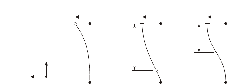
Types of Linear/Nonlinear Properties
The pri mary Linear/Nonlinear Link/Sup port Prop er ties may be of the fol low ing
types:
•Cou pled Linear
•Damper
•Gap
•Hook
•Multi-lin ear Elas tic
•Multi-lin ear Plas tic
•Plas tic (Wen)
•Hysteretic (Rub ber) Iso la tor
•Fric tion-Pen du lum Iso la tor
•Ten sion/Com pres sion Fric tion Pen du lum Isolator
The first type, Cou pled Lin ear, may have fully cou pled lin ear stiff ness and damp -
ing co ef fi cients. This prop erty type is de scribed in Topic “Cou pled Lin ear Prop -
erty” (page 269) in this Chap ter.
All other prop erty types are con sid ered non lin ear. How ever, for each non lin ear
prop erty type you also spec ify a set of un cou pled lin ear stiff ness and damp ing co ef -
Link/Support Properties 269
Chapter XIV The Link/Support Element—Basic
u2ju2ju2j
i
jjj
i
i
dj2=0
dj2
2
1
dj2
Hinge at Joint jHinge near Joint iNo hinge
Figure 66
Location of Shear Spring at a Moment Hinge or Point of Inflection

fi cients that are used in stead of the non lin ear prop er ties for lin ear anal y ses. These
sub sti tute lin ear prop er ties are called “lin ear ef fec tive stiff ness” and “lin ear ef fec -
tive damp ing” prop er ties.
For more in for ma tion:
•See Topic “Cou pled Lin ear Prop erty” (page 269) in this Chap ter.
•See Chap ter “The Link/Sup port El e ment—Advanced” (page 275).
Cou pled Lin ear Prop erty
The Cou pled Lin ear Link/Sup port Prop erty is fully lin ear. It has no non lin ear be -
hav ior. The lin ear be hav ior is used for all lin ear and non lin ear anal y ses. It is also
used for fre quency-de pend ent anal y ses un less fre quency-de pend ent prop er ties
have been as signed to the Link/Sup port el e ment.
The stiff ness ma trix of Eqn. (1) (page 267) may now be fully pop u lated:
(Eqn. 3)
f
f
f
f
f
f
kkk
u
u
u
r
r
r
uuuuu1
2
3
1
2
3
11213
ì
í
ï
ï
ï
î
ï
ï
ï
ü
ý
ï
ï
ï
þ
ï
ï
ï
=
kkk
kkkkk
kkk
ururur
uuuururur
uurur
111213
223212223
3313233
11213
223
3
k
kkk
kk
k
ur
rrrrr
rrr
r
sym.
é
ë
ê
ê
ê
ê
ê
ê
ê
ù
û
ú
ú
ú
ú
ú
ú
ú
ì
í
ï
ï
ï
î
ï
ï
ï
ü
ý
ï
ï
ï
þ
ï
ï
ï
d
d
d
d
d
d
u
u
u
r
r
r
1
2
3
1
2
3
where ku1, ku1u2, ku2, ku1u3, ku2u3, ku3, ..., kr3 are the lin ear stiff ness co ef fi cients of the in -
ter nal springs.
The cor re spond ing ma trix of Eqn. (2) (page 268) can be de vel oped from the re la -
tion ships that give the el e ment in ter nal forces in terms of the spring forces and mo -
ments. See Topic “El e ment In ter nal Forces” (page 267) in this Chap ter.
Sim i larly, the damp ing ma trix is fully pop u lated and has the same form as the stiff -
ness ma trix. Note that the damp ing be hav ior is ac tive for all dy namic anal y ses. This
is in con trast to lin ear ef fec tive damp ing, which is not ac tive for non lin ear anal y ses.
Fixed Degrees of Freedom
It is pos si ble to se lect any num ber or all of the el e ment de for ma tion de grees of free -
dom (DOF) to be fixed, i.e., that their de for ma tion is zero. For a two-joint link, this
270 Cou pled Lin ear Prop erty
CSI Analysis Reference Manual

is equiv a lent to spec i fy ing a joint con straint. For a one-joint link, this is equiv a lent
to spec i fy ing a re straint.
While this fea ture is con ve nient, it should be used with care. There are sev eral im -
por tant con sid er ations that should be kept in mind.
•Link el e ments with fixed DOF should not be con nected to other fixed link el e -
ments or con nected to con strained joints. Oth er wise, this will re sult in joints
that are mul ti ply-con strained, which may be in ac cu rate for dy nam ics.
•For link el e ments with non-zero length, fix ing fewer than all six DOF can lead
to loss of mass cou pling be tween ro ta tional and translational DOF, which can
af fect the dy nam ics of the struc ture if large masses or ro ta tional inertias are
pres ent at the con nected joints.
•When all six DOF are fixed, a full rigid-body con straint is used so that the
translational and ro ta tional in er tia will be accurately han dled, with no loss of
cou pling, pro vided that the link el e ments is not con nected to other con strained
joints or fixed links.
•Link forces are not re ported for fixed DOF.
If forces are needed at fixed DOF, if fixed links are con nected to con strained joints,
or if in er tial cou pling will be lost for non-zero length el e ments, it is rec om mended
that large stiffnesses be used rather than fixed DOF to rep re sent rigid con di tions. It
is im por tant to use stiff ness val ues that are large enough to pre vent sig nif i cant de -
for ma tion, but not so large as to cause nu mer i cal sen si tiv ity in the equa tion so lu -
tion, par tic u larly near nonlinearities in the model. Choose stiff ness val ues that are
about 100 to 10000 times larger than those in con nected el e ments that are ex pected
to un dergo de for ma tion.
Mass
In a dy namic anal y sis, the mass of the struc ture is used to com pute in er tial forces.
The mass con trib uted by the Link or Sup port el e ment is lumped at the joints I and j.
No in er tial ef fects are con sid ered within the el e ment it self.
For each Link/Sup port Property, you may spec ify a to tal trans la tional mass, m.
Half of the mass is as signed to the three trans la tional de grees of free dom at each of
the ele ment’s one or two joints. For single- joint ele ments, half of the mass is as -
sumed to be grounded.
You may ad di tion ally spec ify to tal ro ta tional mass mo ments of in er tia, mr1, mr2,
and mr3, about the three lo cal axes of each ele ment. Half of each mass mo ment of
Mass 271
Chapter XIV The Link/Support Element—Basic

in er tia is as signed to each of the ele ment’s one or two joints. For single- joint ele -
ments, half of each mass mo ment of in er tia is as sumed to be grounded.
The ro ta tional in er tias are de fined in the ele ment lo cal co or di nate sys tem, but will
be trans formed by the pro gram to the lo cal co or di nate sys tems for joint I and j. If
the three in er tias are not equal and ele ment lo cal axes are not par al lel to the joint lo -
cal axes, then cross- coupling in er tia terms will be gen er ated dur ing this trans for ma -
tion. These will be dis carded by the pro gram, re sult ing in some er ror.
It is strongly rec om mended that there be mass cor re spond ing to each non lin ear de -
for ma tion load in or der to gen er ate ap pro pri ate Ritz vec tors for non lin ear modal
time-his tory analy sis. Note that ro ta tional in er tia is needed as well as trans la tional
mass for non lin ear shear de for ma tions if ei ther the ele ment length or dj is non- zero.
For more in for ma tion:
•See Topic “Mass Source” (page 334) in Chap ter “Load Pat terns”.
•See Chap ter “Static and Dy namic Analy sis” (page 341).
•See Topic “Non lin ear De for ma tion Loads” (page 271) in this Chap ter.
Self-Weight Load
Self- Weight Load ac ti vates the self- weight of all ele ments in the model. For each
Link/Sup port Prop erty, a to tal self- weight, w, may be de fined. Half of this weight is
as signed to each joint of each Link/Sup port ele ment us ing that Link/Sup port Prop -
erty. For single- joint ele ments, half of the weight is as sumed to be grounded.
Self- Weight Load al ways acts down ward, in the global –Z di rec tion. You may
scale the self- weight by a sin gle scale fac tor that ap plies equally to all ele ments in
the struc ture.
See Topic “Self- Weight Load” (page 325) in Chap ter “Load Pat terns” for more in -
for ma tion.
Gravity Load
Grav ity Load can be ap plied to each Link/Sup port ele ment to ac ti vate the self-
weight of the ele ment. Us ing Grav ity Load, the self- weight can be scaled and ap -
plied in any di rec tion. Dif fer ent scale fac tors and di rec tions can be ap plied to each
ele ment.
272 Self-Weight Load
CSI Analysis Reference Manual

If all ele ments are to be loaded equally and in the down ward di rec tion, it is more
con ven ient to use Self- Weight Load.
For more in for ma tion:
•See Topic “Self- Weight Load” (page 272) in this Chap ter for the defi ni tion of
self- weight for the Link/Sup port ele ment.
•See Topic “Grav ity Load” (page 326) in Chap ter “Load Pat terns.”
Internal Force and Deformation Output
Link/Sup port ele ment in ter nal forces and de for ma tions can be requested for Load
Cases and Load Com bi na tions.
Re sults for lin ear analy ses are based upon the lin ear effective- stiffness and
effective- damping prop er ties and do not in clude any non lin ear ef fects. Only the re -
sults for non lin ear Load Cases in clude non lin ear be hav ior.
The ele ment in ter nal forces were de fined in Sub topic “Ele ment In ter nal Forces”
(page 267) of this Chap ter. The in ter nal de for ma tions were de fined in Topic “In ter -
nal De for ma tions” (page 260) of this Chap ter.
The ele ment in ter nal forces are la beled P, V2, V3, T, M2, and M3 in the out put. The
in ter nal de for ma tions are la beled U1, U2, U3, R1, R2, and R3 in the out put, cor re -
spond ing to the val ues of du1, du2, du3, dr1, dr2, and dr3.
For more in for ma tion:
•See Chap ter “Load Pat terns” (page 321).
•See Chap ter “Load Cases” (page 341).
Internal Force and Deformation Output 273
Chapter XIV The Link/Support Element—Basic

274 Internal Force and Deformation Output
CSI Analysis Reference Manual

Chapter XV
The Link/Support Element—Advanced
The ba sic, lin ear be hav ior of the Link and Sup port el e ments was de scribed in the
pre vi ous Chap ter. The pres ent Chap ter de scribes the use of the Link and Sup port el -
e ments to model non lin ear be hav ior and fre quency-de pend ent be hav ior.
Advanced Topics
•Over view
•Non lin ear Link/Sup port Prop er ties
•Lin ear Ef fec tive Stiff ness
•Lin ear Ef fec tive Damping
•Ex po nen tial Maxwell Damper Prop erty
•Bilinear Maxwell Damper Prop erty
•Fric tion-Spring Damper Property
•Gap Prop erty
•Hook Prop erty
•Wen Plas tic ity Prop erty
•Multi-Lin ear Elas tic Prop erty
•Multi-Lin ear Plas tic Prop erty
275

•Hysteretic (Rub ber) Iso la tor Prop erty
•Fric tion-Pen du lum Iso la tor Prop erty
•Dou ble-Act ing Fric tion-Pen du lum Iso la tor Prop erty
•Tri ple-Pen du lum Isolator Property
•Non lin ear De for ma tion Loads
•Fre quency-De pend ent Prop er ties
Overview
The ba sic fea tures of the Link and Sup port el e ments were de scribed in the pre vi ous
Chap ter, “The Link/Sup port El e ment—Ba sic” (page 251).
This Chap ter de scribes the var i ous type of non lin ear prop er ties that are avail able,
the con cepts of lin ear ef fec tive stiff ness and damping, the use of nonlinear de for -
ma tion loads for Ritz-vec tor anal y sis, and fre quency-de pend ent prop er ties.
Nonlinear Link/Support Properties
The non lin ear prop er ties for each Link/Sup port Prop erty must be of one of the
var i ous types de scribed be low. The type de ter mines which de grees of free dom may
be non lin ear and the kinds of non lin ear force- deformation re la tion ships avail able
for those de grees of free dom.
Every de gree of free dom may have lin ear effective- stiffness and effective- damping
prop er ties speci fied, as de scribed be low in Sub top ics “Lin ear Ef fec tive Stiff ness”
and “Lin ear Ef fec tive Damp ing.”
Dur ing non lin ear anal y sis, the non lin ear force- deformation re la tion ships are used
at all de grees of free dom for which non lin ear prop er ties were speci fied. For all
other de grees of free dom, the lin ear ef fec tive stiff nesses are used dur ing a non lin ear
anal y sis.
Lin ear anal y ses that start from zero ini tial con di tions will use the lin ear ef fec tive
stiff ness re gard less of whether non lin ear prop er ties were spec i fied or not. Lin ear
anal y ses that use the stiff ness from the end of a pre vi ous non lin ear anal y sis will use
the non lin ear prop er ties. Lin ear ef fec tive damp ing is used for all lin ear anal y ses,
but it is not used for any non lin ear anal y sis.
276 Overview
CSI Analysis Reference Manual

Each non lin ear force- deformation re la tion ship in cludes a stiff ness co ef fi cient, k.
This rep re sents the lin ear stiff ness when the non lin ear ef fect is neg li gi ble, e.g., for
rapid load ing of the Damper; for a closed Gap or Hook; or in the ab sence of yield -
ing or slip ping for the Plas tic1, Iso la tor1, or Iso la tor2 prop er ties. If k is zero, no
non lin ear force can be gen er ated for that de gree of free dom, with the ex cep tion of
the pen du lum force in the Iso la tor2 prop erty.
IM POR TANT! You may some times be tempted to spec ify very large val ues for k,
par ticu larly for Maxwell Dampers, Gap, and Hook prop er ties. Re sist this temp ta -
tion! If you want to limit elas tic de for ma tions in a par ticu lar in ter nal spring, it is
usu ally suf fi cient to use a value of k that is from 102 to 104 times as large as the cor -
re spond ing stiff ness in any con nected ele ments. Larger val ues of k may cause nu -
meri cal dif fi cul ties dur ing so lu tion. See the ad di tional dis cus sion for the Maxwell
Damper properties be low.
Linear Effective Stiffness
For each non lin ear type of Link/Sup port Prop erty, you may spec ify six un cou pled
lin ear ef fec tive-stiff ness co ef fi cients, ke, one for each of the in ter nal springs.
The lin ear ef fec tive stiff ness rep re sents the to tal elas tic stiff ness for the Link/Sup -
port el e ment that is used for all lin ear anal y ses that start from zero ini tial con di -
tions. The ac tual non lin ear prop er ties are ig nored for these types of anal y sis.
If you do not spec ify non lin ear prop er ties for a par tic u lar de gree of free dom, then
the lin ear ef fec tive stiff ness is used for that de gree of free dom for all lin ear and non -
lin ear anal y ses.
The ef fec tive force-de for ma tion re la tion ships for the Link/Sup port Prop er ties are
given by Equa tion 1 above with the ap pro pri ate val ues of ke sub sti tuted for ku1, ku2,
ku3, kr1, kr2, and kr3.
Spe cial Con sid er ations for Modal Analyses
The ef fec tive stiff ness prop er ties are not used for non lin ear de grees of free dom dur -
ing non lin ear time-his tory anal y sis. How ever, non lin ear modal time-his tory (FNA)
anal y ses do make use of the vi bra tion modes that are com puted based on the ef fec -
tive stiff ness if the modal anal y sis it self uses the stiff ness from zero ini tial con di -
tions. Dur ing time in te gra tion the be hav ior of these modes is mod i fied so that the
struc tural re sponse re flects the ac tual stiff ness and other non lin ear pa ram e ters spec -
Linear Effective Stiffness 277
Chapter XV The Link/Support Element—Advanced

i fied. The rate of con ver gence of the non lin ear it er a tion may be im proved by
chang ing the ef fec tive stiff ness.
Fol low ing are some guide lines for se lect ing the lin ear ef fec tive stiff ness. You
should de vi ate from these as nec es sary to achieve your mod el ing and anal y sis
goals. In par tic u lar, you should con sider whether you are more in ter ested in the re -
sults to be ob tained from lin ear anal y ses, or in ob tain ing modes that are used as the
ba sis for non lin ear modal time-his tory anal y ses.
•When car ry ing out anal y ses based on the UBC ‘94 code or sim i lar, the ef fec tive
stiff ness should usu ally be the code-de fined max i mum ef fec tive stiff ness
•For Gap and Hook el e ments the ef fec tive stiff ness should usu ally be zero or k,
de pend ing on whether the el e ment is likely to be open or closed, re spec tively,
in nor mal ser vice
•For Damper el e ments, the ef fec tive stiff ness should usu ally be zero
•For other el e ments, the stiff ness should be be tween zero and k
•If you have cho sen an ar ti fi cially large value for k, be sure to use a much
smaller value for ke to help avoid nu mer i cal prob lems in non lin ear modal
time-his tory anal y ses
In the above, k is the non lin ear stiff ness prop erty for a given de gree of free dom. See
Chap ter “The Link/Sup port El e ment—Basic” (page 251).
Re mem ber that the above con sid er ations do not ap ply for modes cal cu lated us ing
the stiff ness from the end of a non lin ear static or non lin ear di rect-in te gra tion
time-his tory load case. In this case, the ac tual non lin ear stiff ness of the links at the
end of the non lin ear stiff ness load case is used, and the ef fec tive stiff ness is dis re -
garded for non lin ear de grees of free dom.
For more in for ma tion, see Topic “Non lin ear Modal Time-His tory Anal y sis
(FNA)” (page 349) in Chap ter “Non lin ear Time-His tory Anal y sis.”
Linear Effective Damping
For each non lin ear-type of Link/Sup port Prop erty, you may spec ify six un cou pled
lin ear ef fec tive-damp ing co ef fi cients, ce, one for each of the in ter nal springs. By
de fault, each co ef fi cient ce is equal to zero.
The lin ear ef fec tive damp ing rep re sents the to tal vis cous damp ing for the
Link/Sup port el e ment that is used for re sponse-spec trum anal y ses, for lin ear and
pe ri odic time-his tory anal y ses, and for fre quency-de pend ent anal y ses if fre -
278 Linear Effective Damping
CSI Analysis Reference Manual

quency-de pend ent prop er ties have not been as signed to a given Link or Sup port el -
e ment. The ac tual non lin ear prop er ties are ig nored for these types of anal y sis. Ef -
fec tive damp ing can be used to rep re sent en ergy dis si pa tion due to non lin ear damp -
ing, plas tic ity, or fric tion.
The ef fec tive force/de for ma tion-rate re la tion ships for the Link/Sup port Prop er ties
are given by Equa tion 1 above with the ap pro pri ate val ues of ce sub sti tuted for ku1,
ku2, ku3, kr1, kr2, and kr3, and de for ma tion rates sub sti tuted for the cor re spond ing de for -
ma tions.
For re sponse-spec trum and lin ear modal time-his tory anal y sis, the ef fec tive damp -
ing val ues are con verted to modal damp ing ra tios as sum ing pro por tional damp ing,
i.e., the modal cross-cou pling damp ing terms are ig nored. These ef fec tive
modal-damp ing val ues are added to any other modal damp ing that you spec ify di -
rectly. The pro gram will not per mit the to tal damp ing ra tio for any mode to ex ceed
99.995%.
Im por tant Note: Modal cross-cou pling damp ing terms can be very sig nif i cant for
some struc tures. A lin ear anal y sis based on ef fec tive-damp ing prop er ties may
grossly over es ti mate or un der es ti mate the amount of damp ing pres ent in the struc -
ture.
Non lin ear time-his tory anal y sis is strongly rec om mended to de ter mine the ef fect of
added en ergy dis si pa tion de vices. Non lin ear time-his tory anal y sis does not use the
ef fec tive damp ing val ues since it ac counts for en ergy dis si pa tion in the el e ments di -
rectly, and cor rectly ac counts for the ef fects of modal cross-cou pling.
Exponential Maxwell Damper Property
This el e ment is very well suited for mod el ing vis cous damp ers that have a non lin -
ear force-ve loc ity re la tion ship. For sim ple lin ear damp ing, you may in stead want to
use the cou pled lin ear Link Sup port Prop erty. The lin ear prop erty does not re quire
the se ries spring used by the ex po nen tial Maxwell damper, and it does al low you to
con sider a par al lel spring. See Topic “Cou pled Lin ear Prop erty” (page 270) for
more in for ma tion
For the ex po nen tial damper, you can spec ify in de pend ent damp ing prop er ties for
each deformational de gree of free dom. The damp ing prop er ties are based on the
Maxwell model of viscoelasticity (Malvern, 1969) hav ing a ex po nen tial vis cous
damper in se ries with a lin ear spring. See Figure 67 (page 280). If you do not spec -
ify non lin ear prop er ties for a de gree of free dom, that de gree of free dom is lin ear us -
ing the ef fec tive stiff ness, which may be zero.
Exponential Maxwell Damper Property 279
Chapter XV The Link/Support Element—Advanced
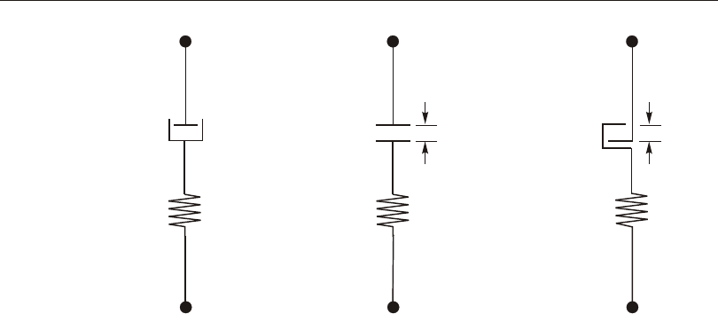
The non lin ear force- deformation re la tion ship is given by:
fdd
kc
==kccexp
&
where k is the spring con stant, c is the damp ing co ef fi cient, cexp is the damp ing ex -
po nent, dk is the de for ma tion across the spring, and &
dc is the de for ma tion rate
across the damper. The damp ing ex po nent must be posi tive; the prac ti cal range is
be tween 0.2 and 2.0.
The spring and damp ing de for ma tions sum to the to tal in ter nal de for ma tion:
ddd
kc
=+
The se ries spring is very im por tant for cap tur ing re al is tic be hav ior of non lin ear
damp ers, es pe cially those with frac tional ex po nents. It rep re sents the elas tic flex i -
bil ity of the damp ing de vice, in clud ing the fluid col umn and the con nect ing mech a -
nisms. It pre vents the damp ing term from pro duc ing un re al is ti cally large vis cous
forces at small ve loc i ties, which can have a very sig nif i cant im pact on over all struc -
tural be hav ior.
You may be tempted to in tro duce a large stiff ness value, k, to rep re sent “pure”
damp ing, but this may re sult in unconservative and un re al is tic be hav ior. It would
be better to get a re al is tic value of the elas tic flex i bil ity from the man u fac turer of
280 Exponential Maxwell Damper Property
CSI Analysis Reference Manual
j
i
k
c
Damper
j
i
k
open
Gap
j
i
k
open
Hook
Figure 67
Maxwell Dampers, Gap, and Hook Property Types,
Shown for Axial Deformations

the de vice and the de tails of the con nec tions, or make an en gi neer ing es ti mate of
the value. For more in for ma tion about the im por tance of the spring con stant, see the
Soft ware Ver i fi ca tion Man ual, where SAP2000 re sults are com pared with ex per i -
ment.
Bilinear Maxwell Damper Property
This el e ment is well suited for mod el ing vis cous damp ers, in clud ing oil damp ers,
that have a bilin ear force-ve loc ity re la tion ship. Such damp ers typ i cally have a re -
lief valve that re duces the damp ing co ef fi cient when a cer tain re lief (or “yield”)
force level is reached. See Kasai (2004) for more in for ma tion.
For the bilinear damper, you can spec ify in de pend ent damp ing prop er ties for each
deformational de gree of free dom. The damp ing prop er ties are based on the
Maxwell model of viscoelasticity (Malvern, 1969) hav ing a bilin ear vis cous
damper in se ries with a lin ear spring. See Figure 67 (page 280). If you do not spec -
ify non lin ear prop er ties for a de gree of free dom, that de gree of free dom is lin ear us -
ing the ef fec tive stiff ness, which may be zero.
The non lin ear force-de for ma tion re la tion ship is given by:
fddd
ddd
kcc
ccc
==£
-³
ì
í
ï
î
kc1c1f1
f1+c2c1f1
&|&|
(&&)|&|
1
ï
where k is the spring con stant, c1 is the damp ing co ef fi cient for force lev els be low
the re lief force, c2 is the damp ing co ef fi cient for force lev els above the re lief force,
f1 is the re lief force, dk is the de for ma tion across the spring, &
dc is the de for ma tion
rate across the damper, and &/dc1=f1c1. The damp ing co ef fi cients must sat isfy the
re la tion ship c1 > c2 ³ 0.
The spring and damp ing de for ma tions sum to the to tal in ter nal de for ma tion:
ddd
kc
=+
The se ries spring is very im por tant for cap tur ing re al is tic be hav ior of non lin ear
damp ers. It rep re sents the elas tic flex i bil ity of the damp ing de vice, in clud ing the
fluid col umn and the con nect ing mech a nisms, which can have a very sig nif i cant
im pact on over all struc tural be hav ior.
You may be tempted to in tro duce a large stiff ness value, k, to rep re sent “pure”
damp ing, but this may re sult in unconservative and un re al is tic be hav ior. It would
Bilinear Maxwell Damper Property 281
Chapter XV The Link/Support Element—Advanced

be better to get a re al is tic value of the elas tic flex i bil ity from the man u fac turer of
the de vice and the de tails of the con nec tions, or make an en gi neer ing es ti mate of
the value. Ex pected val ues for oil damp ers may be on the or der of c1 / k = 0.1 sec -
ond.
The for mu la tion used for this el e ment works best if the time-step size is small com -
pared to the pe riod of ex ci ta tion. This is usu ally not a prob lem for non lin ear modal
(FNA) time-his tory anal y sis, which tends to au to mat i cally use very small time
sub-steps. For non lin ear di rect-in te gra tion time-his tory anal y sis, you should try
dif fer ent time-step sizes un til con sis tent re sults are ob tained. You can ei ther change
the size of the out put time steps or change the max i mum sub-step size (one of the
non lin ear load-case pa ram e ters).
Friction-Spring Damper Property
This el e ment rep re sents a hysteretic damp ing sys tem con sist ing of a stack of al ter -
nat ing in ner and outer me tal lic rings that ex hibit in ter nal fric tion when the stack is
loaded in com pres sion and again when the stack un loads. Each cy cle of load ing and
un load ing dis si pates en ergy hysteretically, mean ing that it is based on dis place -
ment and is in de pend ent of ve loc ity.
Al though the fun da men tal mech a nism is com pres sion of the ring stack, man u fac -
tured de vices may ex hibit ex ter nal damp ing be hav ior in com pres sion, ten sion, or
both. In ad di tion, ki ne matic mech a nisms may be de vised so that the fric tional be -
hav ior can be ap plied to shear or mo ment de grees of free dom. For this rea son, fric -
tion-spring be hav ior may be de fined in de pend ently for any of the six de grees of
free dom of a link el e ment.
A fric tion-spring sys tem un der load ing-slipping ex hib its a lin ear stiff ness k1 that is
a com bi na tion of the elas tic stiff ness to com press the in ner rings and ex pand the
outer rings, plus the fric tional re sis tance. When un load ing-slipping, the sys tem ex -
hib its a smaller lin ear stiff ness k2 that is a com bi na tion of the same elas tic stiff ness
due to ring com pres sion and ex pan sion, but this time with the fric tional re sis tance
act ing in the op po site di rec tion. The elas tic tran si tion be tween load ing and un load -
ing stiff ness is along a much larger elas tic stiff ness k0.
This be hav ior is shown in Figure 68 (page 283). The stiff ness val ues should sat isfy
the fol low ing re la tion ship:
k0 >> k1 > k2 > 0
282 Friction-Spring Damper Property
CSI Analysis Reference Manual
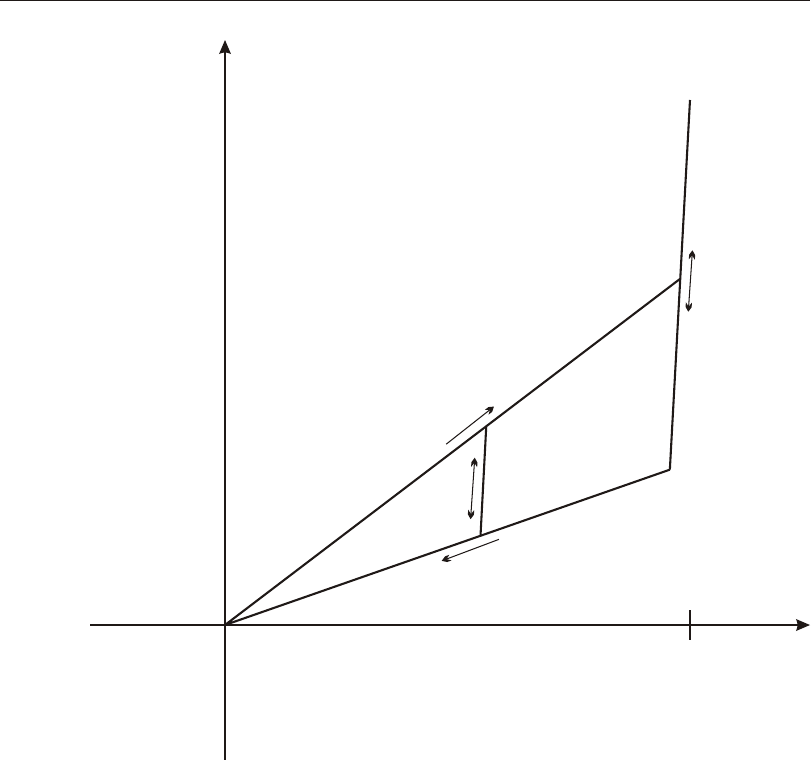
There is usu ally a lim it ing stop dis place ment ds > 0 be yond which the rings can no
lon ger slip. All de for ma tion be yond the stop dis place ment loads and un loads along
the elas tic stiff ness of k0. If you set ds = 0 then no stop dis place ment is ap plied.
A precompression dis place ment dc < 0 may also be spec i fied. This has the ef fect of
in creas ing the ini tial force at which slip ping be gins when load ing to approximately
-×k1dc, and at which slip ping ends when un load ing to approximately -×k2dc, as
shown in Figure 69 (page 284). Load ing and un load ing from zero to these val ues
Friction-Spring Damper Property 283
Chapter XV The Link/Support Element—Advanced
f
dds
k0
k0
k1
k2
Figure 68
Force-Deformation Behavior of a Friction-Spring Damper in Tension
with Stop Displacement but No Precompression
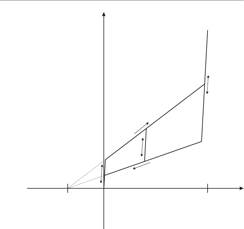
oc curs along the elas tic stiff ness of k0. If you set dc = 0 then no precompression
dis place ment is ap plied, and slip ping be gins and ends at zero force.
The force-de for ma tion re la tion ships shown in Figure 68 and Figure 69 are for ten -
sion (or any pos i tive force or mo ment). Sim i lar be hav ior could be spec i fied in com -
pres sion as well. If ten sion and com pres sion be hav ior are both re quested, the be -
hav ior is sym met ri cal about the or i gin as shown in Figure 70 (page 285). If un sym -
284 Friction-Spring Damper Property
CSI Analysis Reference Manual
f
dds
k0
k0
k0
k1
k2
dc
Figure 69
Force-Deformation Behavior of a Friction-Spring Damper in Tension
with Stop Displacement and Precompression Displacement
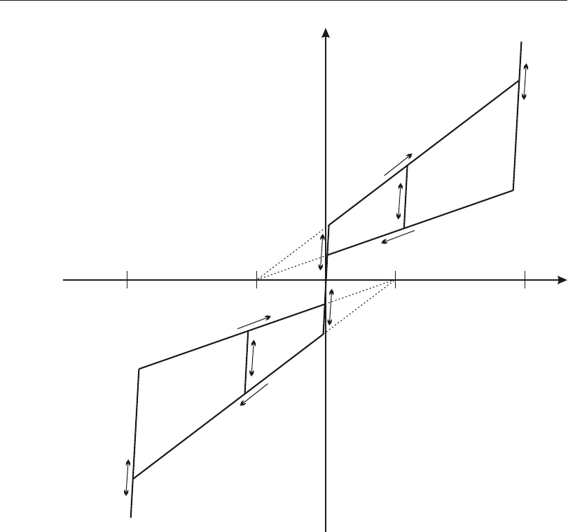
met ri cal be hav ior is de sired, you can use two el e ments in par al lel, one for the ten -
sion be hav ior and one for the com pres sion be hav ior.
Load ing and un load ing can oc cur along the solid lines, but only in the di rec tion of
the ar rows. The dot ted lines in Figure 69 and Figure 70 are shown for ref er ence to
the precompression dis place ment dc. How ever load ing and un load ing can not oc cur
along the dot ted lines.
The non lin ear force-de for ma tion re la tion ship when slipping is given by:
Friction-Spring Damper Property 285
Chapter XV The Link/Support Element—Advanced
f
d
dsdc
-ds -dc
Figure 70
Force-Deformation Behavior of a Friction-Spring Damper in Symmetrical
Tension and Compression

f d= -k1 dc( ) when load ing-slipping, dd
&>0
fd=-k2dc() when un load ing-slipping, dd
&<0
The force-dis place ment re la tion ship is elas tic along a line with stiff ness k0 in the
tran si tions: (1) be tween slid ing while load ing and un load ing, (2) from zero when
dc < 0, and (3) af ter the stop dis place ment ds > 0.
The val ues of k0, k1, k2, ds, and dc should be ob tained from the man u fac turer of
the de vice. The value of k0 should be large com pared to k1 and k2, but not so large
as to cause nu mer i cal sen si tiv ity, which in turn may pro duce in ac cu rate re sults or
non lin ear con ver gence prob lems. A re al is tic value is best, but it should prob a bly be
no more than about 10,000 times larger than k1.
Gap Property
For each de for ma tional de gree of free dom you may spec ify in de pend ent gap
(“compression- only”) prop er ties. See Figure 67 (page 280).
All in ter nal de for ma tions are in de pend ent. The open ing or clos ing of a gap for one
de for ma tion does not af fect the be hav ior of the other de for ma tions.
If you do not spec ify non lin ear prop er ties for a de gree of free dom, that de gree of
free dom is lin ear us ing the ef fec tive stiff ness, which may be zero.
The non lin ear force- deformation re la tion ship is given by:
fdd
=++<
ì
í
î
kopenopen()if
otherwise
0
0
where k is the spring con stant, and open is the ini tial gap open ing, which must be
zero or posi tive.
Hook Property
For each de for ma tional de gree of free dom you may spec ify in de pend ent hook
(“tension- only”) prop er ties. See Figure 67 (page 280).
All in ter nal de for ma tions are in de pend ent. The open ing or clos ing of a hook for one
de for ma tion does not af fect the be hav ior of the other de for ma tions.
286 Gap Property
CSI Analysis Reference Manual
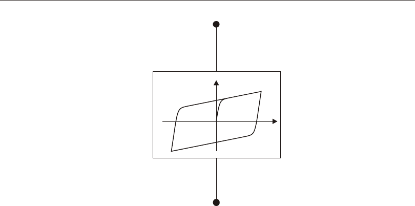
If you do not spec ify non lin ear prop er ties for a de gree of free dom, that de gree of
free dom is lin ear us ing the ef fec tive stiff ness, which may be zero.
The non lin ear force- deformation re la tion ship is given by:
fdd
=-->
ì
í
î
kopenopen()if
otherwise
0
0
where k is the spring con stant, and open is the ini tial hook open ing, which must be
zero or pos i tive.
Wen Plasticity Property
For each de for ma tional de gree of free dom you may spec ify in de pend ent uniaxial-
plasticity prop er ties. The plas tic ity model is based on the hys tere tic be hav ior pro -
posed by Wen (1976). See Figure 71 (page 287).
All in ter nal de for ma tions are in de pend ent. The yield ing at one de gree of free dom
does not af fect the be hav ior of the other de for ma tions.
If you do not spec ify non lin ear prop er ties for a de gree of free dom, that de gree of
free dom is lin ear us ing the ef fec tive stiff ness, which may be zero.
Wen Plasticity Property 287
Chapter XV The Link/Support Element—Advanced
f
d
i
j
k,
yield,
ratio,
exp
Figure 71
Wen Plasticity Property Type for Uniaxial Deformation
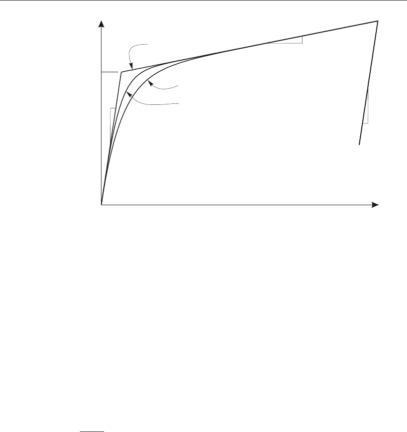
The non lin ear force- deformation re la tion ship is given by:
fdz=+-ratiokratioyield()1
where k is the elas tic spring con stant, yield is the yield force, ra tio is the speci fied
ra tio of post- yield stiff ness to elas tic stiff ness (k), and z is an in ter nal hys tere tic
vari able. This vari able has a range of ||z£1
, with the yield sur face rep re sented by
||z=1
. The ini tial value of z is zero, and it evolves ac cord ing to the dif fer en tial
equa tion:
&
&(||)&
&
zdzdz
d
=->
ì
í
î
k
yield
exp
10if
otherwise
where exp is an ex po nent greater than or equal to unity. Larger val ues of this ex po -
nent in creases the sharp ness of yield ing as shown in Figure 72 (page 288). The
prac ti cal limit for exp is about 20. The equa tion for &
z is equiv a lent to Wen’s model
with A=1
and ab==05..
288 Wen Plasticity Property
CSI Analysis Reference Manual
f
d
yield
exp = 1
exp = 2 k
k
ratio·k
exp ® ¥
Figure 72
Definition of Parameters for the Wen Plasticity Property

Multi-Linear Elastic Property
For each deformational de gree of free dom you may spec ify multi-lin ear elas tic
prop er ties.
All in ter nal de for ma tions are in de pend ent. The de for ma tion in one de gree of free -
dom does not af fect the be hav ior of any other. If you do not spec ify non lin ear prop -
er ties for a de gree of free dom, that de gree of free dom is lin ear us ing the ef fec tive
stiff ness, which may be zero.
The non lin ear force-de for ma tion re la tion ship is given by a multi-lin ear curve that
you de fine by a set of points. The curve can take on al most any shape, with the fol -
low ing re stric tions:
•One point must be the or i gin, (0,0)
•At least one point with pos i tive de for ma tion, and one point with neg a tive de -
for ma tion, must be de fined
•The de for ma tions of the spec i fied points must in crease monotonically, with no
two val ues be ing equal
•The forces (mo ments) can take on any value
The slope given by the last two spec i fied points on the pos i tive de for ma tion axis is
ex trap o lated to in fi nite pos i tive de for ma tion. Sim i larly, the slope given by the last
two spec i fied points on the neg a tive de for ma tion axis is ex trap o lated to in fi nite
neg a tive de for ma tion.
The be hav ior is non lin ear but it is elas tic. This means that the el e ment loads and un -
loads along the same curve, and no en ergy is dis si pated. On the other hand, the
Multi-Lin ear Plas tic Prop erty de fined next does ex hibit hys ter esis and dis si pates
en ergy un der re verse and cy clic load ing.
See also Topic “Hys ter esis Mod els” (page 85) in Chap ter “Ma te rial Prop er ties.”
Multi-Linear Plastic Property
This model is sim i lar to the Multi-Lin ear Elas tic Prop erty de fined above, but the
Plastic prop erty ex hib its dif fer ent load ing and un load ing be hav ior, and thus dis si -
pates en ergy ac cord ing to var i ous hys ter esis mod els that are avail able. For each
deformational de gree of free dom you may spec ify in de pend ent multi-lin ear plas tic -
ity prop er ties.
Multi-Linear Elastic Property 289
Chapter XV The Link/Support Element—Advanced

All in ter nal de for ma tions are in de pend ent. The de for ma tion in one de gree of free -
dom does not af fect the be hav ior of any other. If you do not spec ify non lin ear prop -
er ties for a de gree of free dom, that de gree of free dom is lin ear us ing the ef fec tive
stiff ness, which may be zero.
The non lin ear force-de for ma tion re la tion ship is given by a multi-lin ear curve that
you de fine by a set of points. The curve can take on al most any shape, with the fol -
low ing re stric tions:
•One point must be the or i gin, (0,0)
•At least one point with pos i tive de for ma tion, and one point with neg a tive de -
for ma tion, must be de fined
•The de for ma tions of the spec i fied points must in crease monotonically, with no
two val ues be ing equal
•The forces (mo ments) at a point must have the same sign as the de for ma tion
(they can be zero)
•The slope given by the last two points spec i fied on the pos i tive de for ma tion
axis is ex trap o lated to in fi nite pos i tive de for ma tion, or un til it reaches zero
value. Sim i larly, the slope given by the last two points spec i fied on the neg a tive
de for ma tion axis is ex trap o lated to in fi nite neg a tive de for ma tion, or un til it
reaches zero value.
The given curve de fines the force-de for ma tion (mo ment-ro ta tion) re la tion ship un -
der monotonic load ing. The first slope on ei ther side of the or i gin is elas tic; the re -
main ing seg ments de fine plas tic de for ma tion. If the de for ma tion re verses af ter
plas tic deformation, un load ing oc curs along a dif fer ent, steeper curve be fore be gin -
ning plas tic de for ma tion in the re verse di rec tion.
This pro cess of load ing and un load ing along dif fer ent curves dis si pates en ergy and
is called hys ter esis. Sev eral dif fer ent hys ter esis mod els are avail able to de scribe the
be hav ior of dif fer ent types of ma te ri als. For the most part, these dif fer in the
amount of en ergy they dis si pate in a given cy cle of de for ma tion, and how the en -
ergy dis si pa tion be hav ior changes with an in creas ing amount of de for ma tion.
The avail able hys ter esis mod els for the Multi-Lin ear Plastic Prop erty are de scribed
in Topic “Hys ter esis Mod els” (page 85) in Chap ter “Ma te rial Prop er ties”. These in -
clude ki ne matic, de grad ing, Takeda, pivot, con crete, BRB hard en ing, and iso tro -
pic.
290 Multi-Linear Plastic Property
CSI Analysis Reference Manual
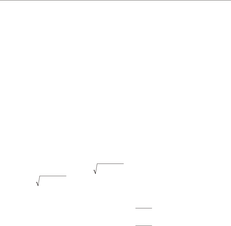
Hysteretic (Rubber) Isolator Property
This is a bi ax ial hys tere tic iso la tor that has cou pled plas tic ity prop er ties for the two
shear de for ma tions, and lin ear effective- stiffness prop er ties for the re main ing four
de for ma tions. The plas tic ity model is based on the hys tere tic be hav ior pro posed by
Wen (1976), and Park, Wen and Ang (1986), and rec om mended for base- isolation
analy sis by Naga ra jaiah, Re in horn and Con stan ti nou (1991). See Figure 73 (page
292).
For each shear de for ma tion de gree of free dom you may in de pend ently spec ify ei -
ther lin ear or non lin ear be hav ior:
•If both shear de grees of free dom are non lin ear, the cou pled force- deformation
re la tion ship is given by:
fdz
uu222
1=+-ratio2k2ratio2yield2()
fdz
uu333
1=+-ratio3k3ratio3yield3()
where k2 and k3 are the elas tic spring con stants, yield2 and yield3 are the yield
forces, ra tio2 and ra tio3 are the ra tios of post- yield stiff nesses to elas tic stiff -
nesses (k2 and k3), and z2 and z3 are in ter nal hys tere tic vari ables. These vari -
ables have a range of zz
2
2
3
21+£, with the yield sur face rep re sented by
zz
2
2
3
21+=. The ini tial val ues of z2 and z3 are zero, and they evolve ac -
cord ing to the dif fer en tial equa tions:
&
&
z
z
az
azz
azz
az
2
3
22
2
223
323
33
2
1
1
ì
í
î
ü
ý
þ=-
-
-
-
é
ë
êù
û
ú
k2
yield2
k3
yield3
&
&
d
d
u
u
2
3
ì
í
ï
ï
î
ï
ï
ü
ý
ï
ï
þ
ï
ï
Where:
adz
u
222
10
0
=>
ì
í
î
if
otherwise
&
adz
u
333
10
0
=>
ì
í
î
if
otherwise
&
These equa tions are equiva lent to those of Park, Wen and Ang (1986) with A=1
and bg==05..
Hysteretic (Rubber) Isolator Property 291
Chapter XV The Link/Support Element—Advanced
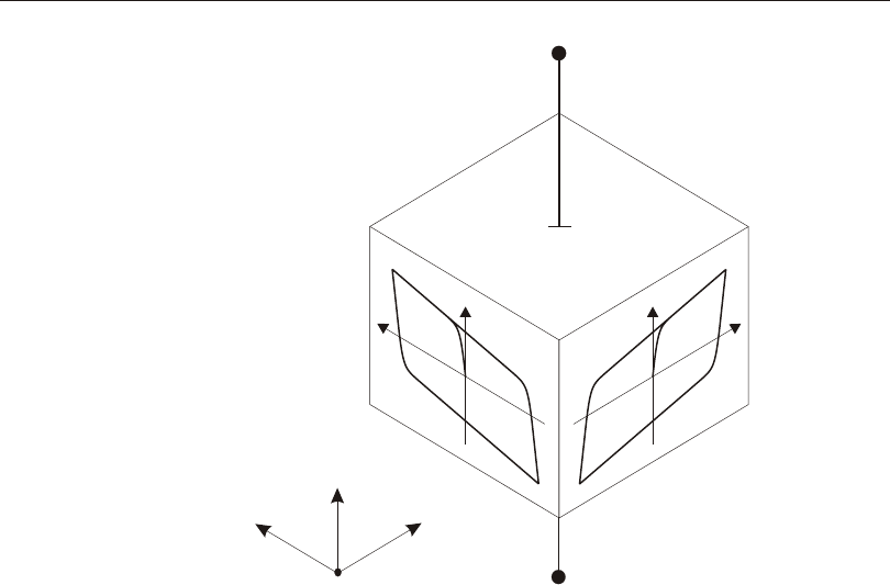
•If only one shear de gree of free dom is non lin ear, the above equa tions re duce to
the uni ax ial plas tic ity be hav ior of the Plas tic1 prop erty with exp=2 for that de -
gree of free dom.
A lin ear spring re la tion ship ap plies to the ax ial de for ma tion, the three mo ment de -
for ma tions, and to any shear de for ma tion with out non lin ear prop er ties. All lin ear
de grees of free dom use the cor re spond ing ef fec tive stiff ness, which may be zero.
Friction-Pendulum Isolator Property
This is a bi ax ial friction- pendulum iso la tor that has cou pled fric tion prop er ties for
the two shear de for ma tions, post- slip stiff ness in the shear di rec tions due the pen -
du lum ra dii of the slip ping sur faces, gap be hav ior in the ax ial di rec tion, and lin ear
effective- stiffness prop er ties for the three mo ment de for ma tions. See Figure 74
(page 293).
292 Friction-Pendulum Isolator Property
CSI Analysis Reference Manual
1
2
3
i
j
fu2
du2
fu3
du3
Figure 73
Hysteretic Isolator Property for Biaxial Shear Deformation
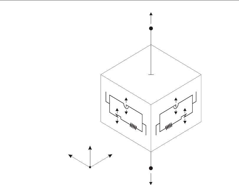
This el e ment can also be used to model gap and fric tion be hav ior be tween con tact -
ing sur faces by set ting the ra dii to zero, in di cat ing a flat surface.
The fric tion model is based on the hys tere tic be hav ior pro posed by Wen (1976),
and Park, Wen and Ang (1986), and rec om mended for base- isolation analy sis by
Naga ra jaiah, Re in horn and Con stan ti nou (1991). The pen du lum be hav ior is as rec -
om mended by Zayas and Low (1990).
The fric tion forces and pen du lum forces are di rectly pro por tional to the com pres -
sive ax ial force in the ele ment. The ele ment can not carry ax ial ten sion.
Ax ial Behavior
The ax ial force, fu1, is al ways non lin ear, and is given by:
Friction-Pendulum Isolator Property 293
Chapter XV The Link/Support Element—Advanced
1
2
3
i
j
P
P
P
P
P
P
Figure 74
Friction-Pendulum Isolator Property for Biaxial Shear Behavior
This element can be used for gap-friction contact problems

f P d d
u
u u
1
1 1 0
0
= = <
ì
í
î
k1 if
otherwise
In or der to gen er ate non lin ear shear force in the el e ment, the stiff ness k1 must be
pos i tive, and hence force P must be neg a tive (com pres sive). A rea son able value for
the stiff ness k1 can be ob tained as the AE/L of the de vice, and should in clude the
flex i bil ity of the con nec tions or sup ports that is not oth er wise in cluded in the
model.
You may ad di tion ally spec ify a damp ing co ef fi cient, c1, for the ax ial de gree of
free dom, in which case the ax ial force be comes:
fPdd
uuu
1110
0
=+<
ì
í
î
c1&if
otherwise
The damp ing force only ex ists when the iso la tor is in com pres sion, re gard less of
the sign of the velocity.
Force fu1 is the to tal ax ial force ex erted by the el e ment on the con nected joints.
How ever, only the stiff ness force P is as sumed to act on the bear ing sur face, caus -
ing shear re sis tance. The damp ing force is ex ter nal.
The pur pose of the damp ing co ef fi cient is to re duce the nu mer i cal chat ter (os cil la -
tion) that can be pres ent in some anal y ses. You can es ti mate the damp ing co ef fi -
cient needed to achieve a cer tain ra tio, r, of crit i cal damp ing (e.g., r = 0.05) from the
for mula
r
m
=c1
k12
where m is the trib u tary mass for the iso la tor, which could be es ti mated from the
self-weight ax ial force di vided by the ac cel er a tion due to grav ity. It is up to you to
ver ify the ap pli ca bil ity of this ap proach for your par tic u lar ap pli ca tion. See the
Soft ware Ver i fi ca tion Man ual for a dis cus sion on the use of this damp ing co ef fi -
cient.
Shear Behavior
For each shear de for ma tion de gree of free dom you may in de pend ently spec ify ei -
ther lin ear or non lin ear be hav ior:
294 Friction-Pendulum Isolator Property
CSI Analysis Reference Manual
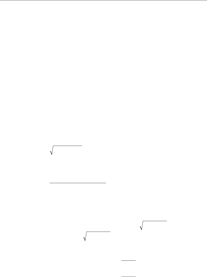
•If both shear de grees of free dom are non lin ear, the fric tion and pen du lum ef -
fects for each shear de for ma tion act in par al lel:
fff
uufup222
=+
fff
uufup333
=+
The fric tional force- deformation re la tion ships are given by:
fPz
ufu222
=-m
fPz
ufu333
=-m
where m2 and m3 are fric tion co ef fi cients, and z2 and z3 are in ter nal hys tere tic
vari ables. The fric tion co ef fi cients are velocity- dependent ac cord ing to:
(Eqn. 1a)
mu
rv
e
2=---
fast2fast2slow2()
mu
rv
e
3=---
fast3fast3slow3()
where slow2 and slow3 are the fric tion co ef fi cients at zero ve loc ity, fast2 and
fast3 are the fric tion co ef fi cients at fast ve loci ties, v is the re sul tant ve loc ity of
slid ing:
(Eqn. 1b)
vdd
uu
=+
&&
2
2
3
2
r is an ef fec tive in verse ve loc ity given by:
(Eqn. 1c)
rdd
v
uu
=+rate2rate3
&&
2
2
3
2
2
and rate2 and rate3 are the in verses of char ac ter is tic slid ing ve loci ties. For a
Teflon- steel in ter face the co ef fi cient of fric tion nor mally in creases with slid ing
ve loc ity (Naga ra jaiah, Re in horn, and Con stan ti nou, 1991).
The in ter nal hys tere tic vari ables have a range of zz
2
2
3
21+£, with the yield
sur face rep re sented by zz
2
2
3
21+=. The ini tial val ues of z2 and z3 are zero,
and they evolve ac cord ing to the dif fer en tial equa tions:
&
&
z
z
az
azz
azz
az
P
2
3
22
2
223
323
33
2
1
1
ì
í
î
ü
ý
þ=-
-
-
-
é
ë
êù
û
ú
k2
m
m
u
u
u
u
d
Pd
2
2
3
3
&
&
k3
ì
í
ï
ï
î
ï
ï
ü
ý
ï
ï
þ
ï
ï
Friction-Pendulum Isolator Property 295
Chapter XV The Link/Support Element—Advanced

where k2 and k3 are the elas tic shear stiff nesses of the slider in the ab sence of
slid ing, and
adz
u
222
10
0
=>
ì
í
î
if
otherwise
&
adz
u
333
10
0
=>
ì
í
î
if
otherwise
&
These equa tions are equiva lent to those of Park, Wen and Ang (1986) with A=1
and bg==05..
This fric tion model per mits some slid ing at all non-zero lev els of shear force;
the amount of slid ing be comes much larger as the shear force ap proaches the
“yield” value of Pm. Slid ing at lower val ues of shear force can be min i mized by
us ing larger val ues of the elas tic shear stiffnesses. How ever, re al is tic val ues of
the shear stiff ness are rec om mended, and can be es ti mated as AG/L of the
locked-up de vice. This should also in clude the flex i bil ity of the con nec tions or
sup ports that is not oth er wise in cluded in the model.
The pen du lum force- deformation re la tion ships are given by:
fPd
upu
22
=-radius2
fPd
upu
33
=-radius3
The spec i fied ra dius should ac tu ally be the ef fec tive pen du lum length, which is
the ra dius of the slid ing sur face mi nus the dis tance from the sur face to the point
of ar tic u la tion of the de vice. This in for ma tion should be ob tained from the
man u fac turer of the de vice.
Nor mally the ra dii in the two shear di rec tions will be equal (spheri cal sur face),
or one ra dius will be zero (cy lin dri cal sur face). How ever, it is per mit ted to
spec ify une qual non- zero ra dii.
A zero ra dius in di cates a flat sur face, and the cor re spond ing per pen dic u lar
shear force is zero. This can be used to model gen eral gap-fric tion be hav ior .
•If only one shear de gree of free dom is non lin ear, the above fric tional equa tions
re duce to:
fPz
f=-m
296 Friction-Pendulum Isolator Property
CSI Analysis Reference Manual

m = - - -
fast fast slow rate
( )
&
ed
&
&( ) &
&
zP
d z d z
d
=- >
ì
í
î
k
m
1 0
2if
otherwise
The above pen du lum equa tion is un changed for the non lin ear de gree of free -
dom.
Linear Be hav ior
A lin ear spring re la tion ship ap plies to the three mo ment de for ma tions, and to any
shear de for ma tion with out non lin ear prop er ties. All lin ear de grees of free dom use
the cor re spond ing ef fec tive stiff ness, which may be zero. The ax ial de gree of free -
dom is al ways non lin ear for non lin ear anal y ses.
Double-Acting Friction-Pendulum Isolator Property
This is a bi axial fric tion-pen du lum iso la tor that sup ports ten sion as well as com -
pres sion, and has uncou pled be hav ior in the two shear di rec tions. The fric tional re -
sis tance can be dif fer ent de pend ing on whether then iso la tor is in ten sion or com -
pres sion. This de vice con sists of two or thogo nal, curved rails that are in ter locked
together. It is in tended to pro vide seis mic iso la tion with up lift pre ven tion, and is
de scribed in de tail by Roussis and Constantinou [2005].
Ax ial Be hav ior
In de pend ent stiffnesses and gap open ings may be spec i fied for ten sion and com -
pres sion. The ax ial force, fu1, is al ways non lin ear, and is given by:
fP
dd
d
u
uu
u
1
11
1
0
==
++<
-
k1copencopenc
k1topent
()()
()
if
if
otherwise
()du10
0
->
ì
í
ï
î
ï
opent
where k1c is the com pres sive stiff ness, k1t is the ten sile stiff ness, openc is the gap
open ing in com pres sion, and opent is the gap open ing in ten sion. Each of the four
val ues may be zero or pos i tive.
You may ad di tion ally spec ify a damp ing co ef fi cient, c1, for the ax ial de gree of
free dom, in which case the ax ial force be comes:
Double-Acting Friction-Pendulum Isolator Property 297
Chapter XV The Link/Support Element—Advanced

f P d
u u1 1
= +c1 &
The damp ing force ex ists whether the iso la tor is in ten sion, com pres sion, or is gap -
ping.
Force fu1 is the to tal ax ial force ex erted by the el e ment on the con nected joints.
How ever, only the stiff ness force P is as sumed to act on the bear ing sur face, caus -
ing shear re sis tance. The damp ing force is ex ter nal. See Topic “Fric tion-Pen du lum
Iso la tor Property” (page 292) for a dis cus sion on the use of this damp ing.
Shear Behavior
For each shear de for ma tion de gree of free dom you may in de pend ently spec ify ei -
ther lin ear or non lin ear be hav ior. The be hav ior in the two shear di rec tions is un cou -
pled, al though they both de pend on the same ax ial force P.
For each non lin ear shear de gree of free dom u2 or u3, you in de pend ently spec ify the
fol low ing pa ram e ters:
•Stiff ness k, rep re sent ing the elas tic be hav ior be fore slid ing be gins. This value
is the same for pos i tive or neg a tive P.
•Fric tion co ef fi cients slowc and fastc for fric tion un der com pres sion at dif fer ent
ve loc i ties, and co ef fi cients slowt and fastt for fric tion un der ten sion at dif fer -
ent ve loc i ties.
•Rate pa ram e ters ratec and ratet for fric tion un der com pres sion and ten sion, re -
spec tively. These are the in verses of char ac ter is tic slid ing ve loc i ties. For a Tef -
lon-steel in ter face the co ef fi cient of fric tion nor mally in creases with slid ing ve -
loc ity (Nagarajaiah, Reinhorn, and Constantinou, 1991).
•Ra dius ra dius, which is the same for ten sion and com pres sion.
Look ing at one shear di rec tion, and con sid er ing ei ther ten sion or com pres sion us -
ing the ap pro pri ate fric tion pa ram e ters, the shear force f is given by:
fff
fp
=+
fPz
f=-m
m=---
fastfastslowrate
()
&
ed
&
&()&
&
zP
dzdz
d
=->
ì
í
î
k
m
10
2if
otherwise
298 Double-Acting Friction-Pendulum Isolator Property
CSI Analysis Reference Manual

f P d
p= - radius
where d is the shear de for ma tion and z is an in ter nal hysteretic vari able. In the
above, the in di ca tors for shear de gree of free dom u2 or u3, as well as for ten sion or
com pres sion, have been dropped.
Linear Be hav ior
A lin ear spring re la tion ship ap plies to the three mo ment de for ma tions, and to any
shear de for ma tion with out non lin ear prop er ties. All lin ear de grees of free dom use
the cor re spond ing ef fec tive stiff ness, which may be zero. The ax ial de gree of free -
dom is al ways non lin ear for non lin ear anal y ses.
Triple-Pendulum Isolator Property
This is a bi axial fric tion-pen du lum iso la tor (or bear ing) that has four spher i cal slid -
ing sur faces, two outer and two in ner, as shown in Figure 75 (page 301). Ki ne matic
con sid er ations cou ple the mo tion of the two in ner slid ers, re sult ing in be hav ior that
can be mod eled as three fric tion-pen du lum iso la tors in se ries. By choos ing dif fer -
ent fric tion co ef fi cients and ra dii for the var i ous slid ing sur faces, the trans verse
(shear) force-de flec tion curve can be tai lored to pro vide dif fer ent re sponse for dif -
fer ent lev els of ex ci ta tion. The prop er ties of the two in ner slid ers are as sumed to be
iden ti cal. The char ac ter is tics and per for mance of this type of iso la tor are de scribed
in Mor gan and Mahin (2008).
Each of the three pendula that act se ries for the tri ple pen du lum uses the same math -
e mat i cal model as de scribed in the topic “Fric tion-Pen du lum Iso la tor Prop erty”
(page 292), with dif fer ences as de scribed be low. The ax ial and mo ment be hav ior
are for the iso la tor as a whole. The shear forces are equal in the three pendula, while
the shear de for ma tions and ve loc i ties are ad di tive.
The fric tion forces and pen du lum forces are di rectly pro por tional to the com pres -
sive ax ial force in the el e ment. The el e ment can not carry ax ial ten sion.
Ax ial Behavior
The ax ial force, fu1, is al ways non lin ear, and is given by:
fPdd
u
uu
1
110
0
==<
ì
í
î
k1if
otherwise
Triple-Pendulum Isolator Property 299
Chapter XV The Link/Support Element—Advanced

In or der to gen er ate non lin ear shear force in the el e ment, the stiff ness k1 must be
pos i tive, and hence force P must be neg a tive (com pres sive).
You may ad di tion ally spec ify a damp ing co ef fi cient, c1, for the ax ial de gree of
free dom, in which case the ax ial force be comes:
fPdd
uuu
1110
0
=+<
ì
í
î
c1&if
otherwise
The damp ing force only ex ists when the iso la tor is in com pres sion.
Force fu1 is the to tal ax ial force ex erted by the el e ment on the con nected joints.
How ever, only the stiff ness force P is as sumed to act on the slid ing surfaces, caus -
ing shear re sis tance. The damp ing force is ex ter nal.
The pur pose of the damp ing co ef fi cient is to re duce the nu mer i cal chat ter (os cil la -
tion) that can be pres ent in some anal y ses. You can es ti mate the damp ing co ef fi -
cient needed to achieve a cer tain ra tio, r, of crit i cal damp ing (e.g., r = 0.05) from the
for mula
r
m
=c1
k12
where m is the trib u tary mass for the iso la tor, which could be es ti mated from the
self-weight ax ial force di vided by the ac cel er a tion due to grav ity. It is up to you to
ver ify the ap pli ca bil ity of this ap proach for your par tic u lar ap pli ca tion. See the
Soft ware Ver i fi ca tion Man ual for a dis cus sion on the use of this damp ing co ef fi -
cient for the fric tion-pen du lum isolator.
Shear Behavior
For each shear de for ma tion de gree of free dom you may in de pend ently spec ify ei -
ther lin ear or non lin ear be hav ior. In the usual case where both the u2 and u3 de grees
of free dom are nonlinear, the be hav ior is iso tro pic and the prop er ties are iden ti cal
in both di rec tions. In other words, the slid ing sur faces are spherical.
The four slid ing sur faces are iden ti fied as:
•In ner Bot tom (in dex 1)
•In ner Top, iden ti cal to In ner Bot tom (in dex 1)
•Outer Bot tom (in dex 2)
•Outer Top (index 3)
300 Triple-Pendulum Isolator Property
CSI Analysis Reference Manual
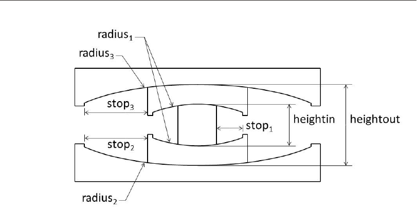
These are shown in Figure 75 (page 301). In the dis cus sion be low, the indices
shown above will be used to iden tify the three pen du lum mechanisms.
For each slid ing sur face, the fol low ing iso tro pic prop er ties are spec i fied:
•stiff, shear stiff ness be fore slid ing, and stiff ness at the stop
•slow, fric tion co ef fi cient at zero ve loc ity
•fast, fric tion co ef fi cient at fast ve loc ity
•rate, in verse of the char ac ter is tic ve loc ity for fric tion
•ra dius, ac tual spher i cal ra dius of the sur face
•stop, trans verse dis place ment per mit ted be fore en coun ter ing a stiff stop
In ad di tion, two heights are spec i fied giv ing the dis tances be tween the slid ing sur -
faces:
•heightin, max i mum dis tance be tween the two in ner sur faces at zero dis place -
ment
•heightout, max i mum dis tance be tween the two outer sur faces at zero dis place -
ment
Triple-Pendulum Isolator Property 301
Chapter XV The Link/Support Element—Advanced
Figure 75
Triple-Pendulum Isolator with Four Sliding Surfaces
The two inner surfaces are always symmetrical

The iso la tor stiff ness at each stage of slid ing is de pend ent upon the ef fec tive
pendulum lengths. For each sur face, the pen du lum length is given by the ra dius mi -
nus the dis tance to the point of ar tic u la tion, a frac tion of the dis tance be tween the
sur faces. Thus:
L1105=-radiusheightin.
L22
=-radiusheightouta
L3 3 1= - -radius heightout( )a
where
a=+
radius
radiusradius
2
23
Dur ing slid ing, the net fric tion co ef fi cient for each sur face is de pend ent upon the
ve loc ity of slid ing on that sur face ac cord ing to the rate-de pend ent friction equa -
tions (Eqns. 1, page 293) given for the fric tion-pen du lum iso la tor.
The monotonic, radial force-de flec tion be hav ior of a typ i cal tri ple-pen du lum iso la -
tor is shown in Figure 76 (page 303). The iso la tor is as sumed to be in com pres sion,
and the plot ted shear force, ~
V, is nor mal ized by the compression load: ~
VVP=,
P<0.
The ac tual be hav ior will de pend on the rel a tive pen du lum lengths, fric tion co ef fi -
cients, and stop dis tances. For the pur pose of the fol low ing dis cus sion, we will as -
sume that the net co ef fi cients for the three sur faces are con stant and or dered such
that mmm
123
££, and that the stop dis tances are large enough as de scribed. The
fol low ing be hav ior is ob served:
•0££uua: The ini tial re sis tance is given by the elas tic stiff ness un til first slid -
ing be gins. This oc curs at a nor mal ized shear force equal to the low est fric tion
co ef fi cient, m1, for the in ner slid ing sur faces.
•uuu
ab
££: The shear stiff ness is now gov erned by the pen du lum lengths of
the two in ner sur faces, both of which are slid ing. This stiff ness is
121
()L.
•uuu
bc
££: When the shear force in creases to the sec ond fric tion co ef fi cient,
m2, slid ing shifts from the in ner-bottom sur face to the outer-bot tom sur face,
and the stiff ness be comes
112
()LL+.
•uuu
cd
££: Sim i larly, at the level of the third fric tion co ef fi cient, m3, slid ing
shifts from the in ner-top sur face to the outer-top sur face, and the stiff ness be -
comes
123
()LL+.
302 Triple-Pendulum Isolator Property
CSI Analysis Reference Manual
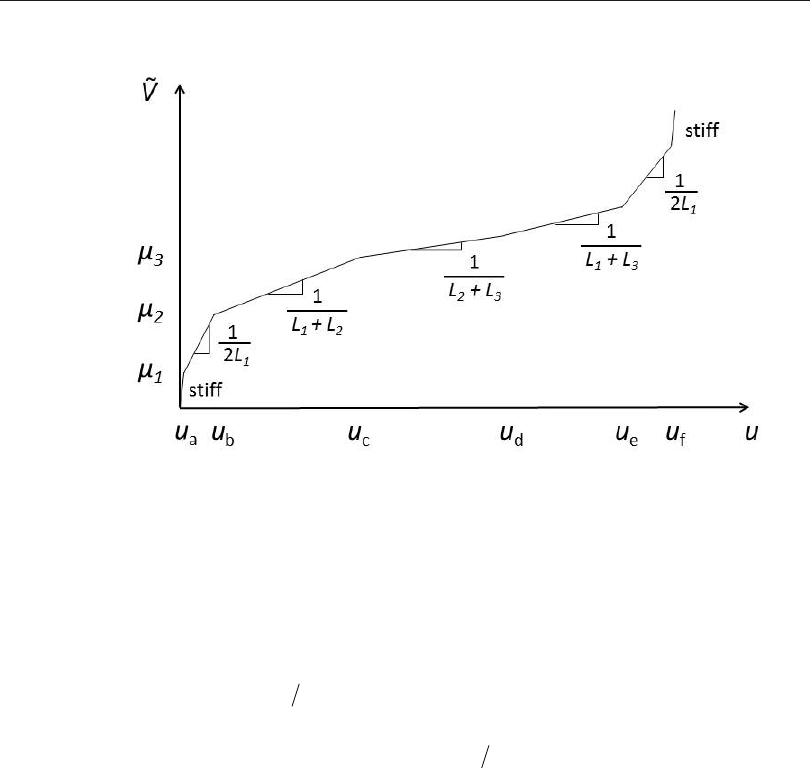
•u u u
d e
£ £ : With in creased slid ing, one of the stops is hit, say for the
outer-bot tom sur face. Slid ing shifts back to the ad ja cent in ner sur face, and the
stiff ness be comes 113
()LL+.
•uuu
ef
££: When the outer-top stop is hit, slid ing shifts back to the ad ja cent
in ner sur face and the stiff ness be comes
121
()L again.
•uuf
>: Af ter both in ner stops are hit, the ini tial elas tic stiff ness is en gaged.
The ac tual be hav ior will de pend on the rel a tive val ues of the pa ram e ters used for
the ac tual iso la tor, the ve loc i ties of slid ing as they af fect the fric tion co ef fi cients,
and the his tory and di rec tion of the mo tion.
The tran si tion to slid ing is not abrupt, but rather oc curs grad u ally as the nor mal ized
shear force ap proaches each fric tion co ef fi cient. This fric tion model per mits some
slid ing at all non-zero lev els of shear force; the amount of slid ing be comes much
larger as the shear force ap proaches the “yield” value of Pm. Slid ing at lower val ues
of shear force can be min i mized by us ing larger val ues of the elas tic shear
stiffnesses, stiff. How ever, re al is tic val ues of the shear stiff ness are rec om mended,
and can be es ti mated as AG/L of the locked-up de vice. This should also in clude the
flex i bil ity of the con nec tions or sup ports that is not oth er wise in cluded in the
Triple-Pendulum Isolator Property 303
Chapter XV The Link/Support Element—Advanced
Figure 76
Normalized Force-Deflection Curve for the Triple-Pendulum Isolator
Typical behavior for monotonic radial loading at slow speed

model. In no case should the stiff ness val ues be more than about 100 to 10000 times
larger than |P/L|, where P is a typ i cal ax ial com pres sion value for the iso la tor, and L
is the pen du lum length. Larger val ues serve no prac ti cal pur pose and make non lin -
ear con ver gence more dif fi cult.
Linear Be hav ior
A lin ear spring re la tion ship ap plies to the three mo ment de for ma tions, and to any
shear de for ma tion with out non lin ear prop er ties. All lin ear de grees of free dom use
the cor re spond ing ef fec tive stiff ness, which may be zero. The ax ial de gree of free -
dom is al ways non lin ear for non lin ear anal y ses.
Nonlinear Deformation Loads
A non lin ear de for ma tion load is a set of forces and/or mo ments on the struc ture
that ac ti vates a non lin ear in ter nal de for ma tion of an Link/Sup port el e ment. A non -
lin ear in ter nal de for ma tion is an Link/Sup port in ter nal de for ma tion for which non -
lin ear prop er ties have been spec i fied.
Non lin ear de for ma tion loads are used as start ing load vec tors for Ritz-vec tor anal y -
sis. Their pur pose is to gen er ate Modes that can ad e quately rep re sent non lin ear be -
hav ior when per form ing non lin ear modal time-his tory anal y ses. A sep a rate non lin -
ear de for ma tion load should be used for each non lin ear in ter nal de for ma tion of
each Link/Sup port el e ment.
When re quest ing a Ritz-vec tor anal y sis, you may spec ify that the pro gram use
built-in non lin ear de for ma tion loads, or you may de fine your own Load Pat terns for
this pur pose. In the lat ter case you may need up to six of these Load Pat terns per
Link/Sup port el e ment in the model.
The built-in non lin ear de for ma tion loads for a sin gle two-joint Link el e ment are
shown in Figure 77 (page 305). Each set of forces and/or mo ments is
self-equilibrating. This tends to lo cal ize the ef fect of the load, usu ally re sult ing in a
better set of Ritz-vec tors. For a sin gle-joint el e ment, only the forces and/or mo -
ments act ing on joint j are needed.
It is strongly rec om mended that mass or mass mo ment of in er tia be pres ent at each
de gree of free dom that is acted upon by a force or mo ment from a non lin ear de for -
ma tion load. This is needed to gen er ate the ap pro pri ate Ritz vec tors.
304 Nonlinear Deformation Loads
CSI Analysis Reference Manual
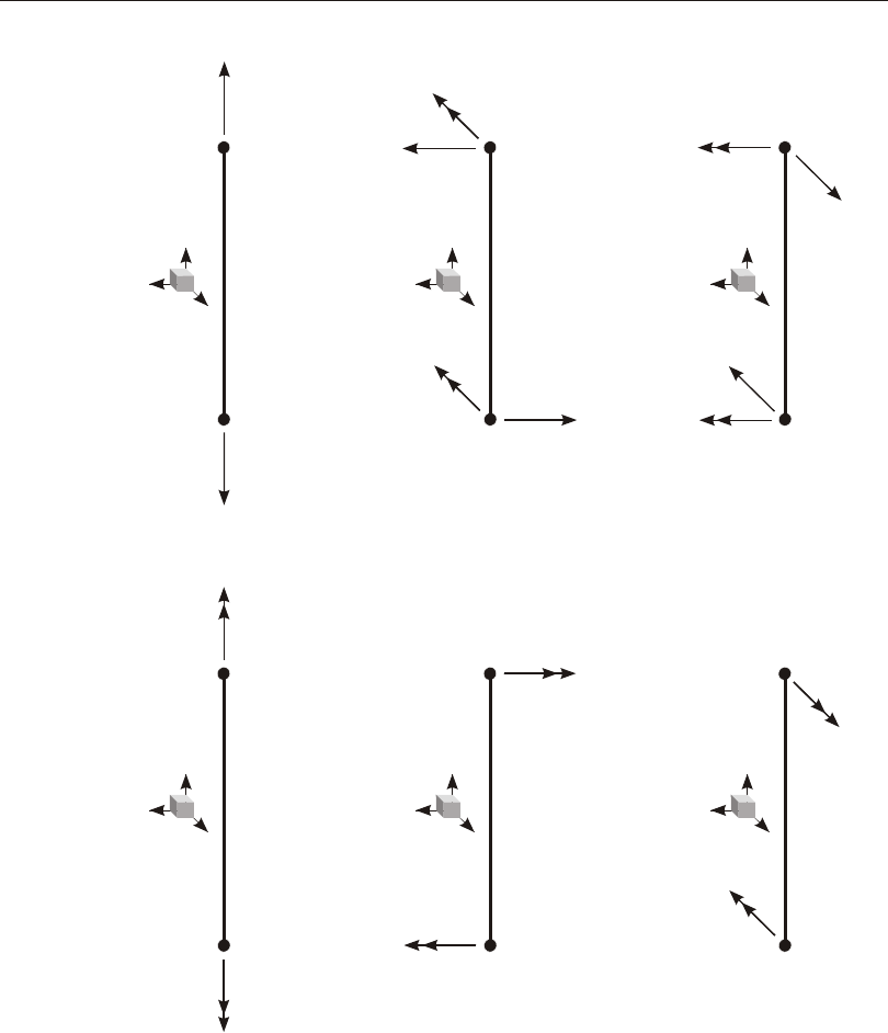
Nonlinear Deformation Loads 305
Chapter XV The Link/Support Element—Advanced
1
1
1
1
1
1
1
1
dj2
1
1
1
1
2
2
2
2
2
2
1
1
1
1
dj3
L–dj3
3
3
3
3
3
3
1
1
L–dj2
i
i
i
i
i
i
j
j
j
j
j
j
Load for
Deformation
dr2
Load for
Deformation
du2
Load for
Deformation
dr3
Load for
Deformation
du3
Load for
Deformation
dr1
Load for
Deformation
du1
L = Element Length
Figure 77
Built-in Nonlinear Deformation Loads for a Two-joint Link Element

For more in for ma tion:
•See Topic “In ter nal De for ma tions” (page 260) in this Chap ter.
•See Topic “Link/Sup port Prop er ties” (page 263) in this Chap ter.
•See Topic “Mass” (page 271) in this Chap ter.
•See Topic “Ritz-Vec tor Anal y sis” (page 349) in Chap ter “Load Cases.”
•See Topic “Non lin ear Modal Time-His tory Anal y sis (FNA)” (page 349) in
Chap ter “Load Cases.”
Frequency-Dependent Link/Support Properties
Each Link or Sup port el e ment can have an optional set of fre quency-de pend ent
prop er ties as signed to it in ad di tion to the lin ear/non lin ear prop erty set that must al -
ways be as signed. Fre quency-de pend ent prop er ties are only used for fre quency-do -
main types of anal y ses, such as Steady-State or Power-Spec tral-Den sity analyses.
Fre quency-de pend ent prop er ties rep re sent the complex im ped ance of the el e ment.
There is a real part that rep re sents the stiff ness and in er tial ef fects, and an imag i nary
part that rep re sents the hysteretic damp ing ef fects. Fre quency-de pend ent prop er -
ties for the six de grees of free dom of the el e ment may be may be cou pled or un cou -
pled cou pled, as given by:
(Eqn. 2)
f
f
f
f
f
f
zzz
u
u
u
r
r
r
uuuuu1
2
3
1
2
3
11213
ì
í
ï
ï
ï
î
ï
ï
ï
ü
ý
ï
ï
ï
þ
ï
ï
ï
=
zzz
zzzzz
zzz
ururur
uuuururur
uurur
111213
223212223
3313233
11213
223
3
z
zzz
zz
z
ur
rrrrr
rrr
r
sym.
é
ë
ê
ê
ê
ê
ê
ê
ê
ù
û
ú
ú
ú
ú
ú
ú
ú
ì
í
ï
ï
ï
î
ï
ï
ï
ü
ý
ï
ï
ï
þ
ï
ï
ï
d
d
d
d
d
d
u
u
u
r
r
r
1
2
3
1
2
3
where zkic
uuu111
=+ is the im ped ance term in the u1
de gree of free dom, and
where
ku1 is the stiff ness/in er tial component, cu1 is the damp ing component, and i
is the square root of –1. The other im ped ance terms are sim i lar.
In Eqn. (2), the force terms on the left-hand side of the equa tion and the dis place -
ment terms on the right-hand side of the equa tions are also com plex. The real parts
of these terms rep re sent the be hav ior at a phase an gle of zero, with time vari a tion
given by the co sine func tion, and the imag i nary parts rep re sent be hav ior at a phase
an gle of 90°, with time vari a tion given by the sine func tion.
306 Frequency-Dependent Link/Support Properties
CSI Analysis Reference Manual

Each of the 21 im ped ance terms may vary with fre quency. You de fine the vari a tion
for each term as a set of points giv ing stiff ness vs. fre quency and damp ing vs. fre -
quency. It is not un usual for the stiff ness term to be neg a tive over part of the range.
A com mon use for fre quency-de pend ent prop er ties would be in Sup port el e ments
that rep re sent the far-field ra di a tion-damp ing ef fect of the soil re gion un der a rigid
foun da tion.
Frequency-Dependent Link/Support Properties 307
Chapter XV The Link/Support Element—Advanced

308 Frequency-Dependent Link/Support Properties
CSI Analysis Reference Manual

Chapter XVI
The Tendon Object
Ten dons are a spe cial type of ob ject that can be em bed ded in side other ob jects
(frames, shells, planes, asolids, and sol ids) to rep re sent the ef fect of prestressing
and post-tensioning. These ten dons at tach to the other ob jects and im pose load
upon them.
Advanced Topics
•Over view
•Ge om e try
•Discretization
•Ten dons Mod eled as Loads or Elements
•Con nec tivity
•De grees of Free dom
•Lo cal Co or di nate Sys tems
•Sec tion Prop er ties
•Non lin ear Properties
•Mass
•Pre stress Load
309

•Self- Weight Load
•Grav ity Load
•Tem per a ture Load
•Strain Load
•De for ma tion Load
•Tar get-Force Load
•In ter nal Force Out put
Overview
Ten dons are a spe cial type of ob ject that can be em bed ded in side other ob jects
(frames, shells, planes, asolids, and sol ids) to rep re sent the ef fect of prestressing
and post-tensioning. These ten dons at tach to the other ob jects through which they
pass and im pose load upon them.
You may spec ify whether the ten dons are to be mod eled as in de pend ent el e ments in
the anal y sis, or just to act upon the rest of the struc ture as loads. Mod el ing as loads
is ad e quate for lin ear anal y ses when you know the losses that will be caused by
elas tic short en ing and time-de pend ent ef fects.
Ten dons should be mod eled as el e ments if you want the pro gram to cal cu late the
losses due to elas tic short en ing and time-de pend ent ef fects, if you want to con sider
nonlinearity in the Tendons, or if you want to know the forces act ing in the Tendons
due to other load ing on the struc ture.
Ten don ob jects share some fea tures with Frame el e ments, which will be cross-ref -
er enced in this Chap ter.
Geometry
Any num ber of ten dons may be de fined. Each ten don is drawn or de fined as a type
of line ob ject be tween two joints, I and j. The two joints must not share the same lo -
ca tion in space. The two ends of the Tendon are de noted end I and end J, re spec -
tively.
The Tendon may have an ar bi trary curved or seg mented shape in three di men sions
be tween those points, and may be off set at the ends from these joints.
310 Overview
CSI Analysis Reference Manual

Discretization
A Tendon may be a long ob ject with com pli cated ge om e try, but it will be au to mat i -
cally discretized into shorter seg ments for pur poses of anal y sis. You must spec ify
the max i mum length of these discretization seg ments dur ing the def i ni tion of the
Ten don. These lengths can af fect how the Ten don loads the struc ture and the ac cu -
racy of the anal y sis re sults. You should choose shorter lengths for Ten dons with
highly curved ge om e try, or Ten dons that pass through parts of the struc ture with
com pli cated ge om e try or changes in prop er ties. If you are not sure what value to
use, try sev eral dif fer ent val ues to see how they af fect the re sults.
Ten dons Mod eled as Loads or Elements
You have a choice for each Tendon how it is to be mod eled for anal y sis:
•As equiv a lent loads that act upon the struc ture
•As in de pend ent el e ments with stiff ness, mass and load ing
Mod el ing as loads is ad e quate for lin ear anal y ses when you know in ad vance the
losses that will be caused by elas tic short en ing and time-de pend ent ef fects.
Ten dons should be mod eled as el e ments if you want the pro gram to cal cu late the
losses due to elas tic short en ing and time-de pend ent ef fects, if you want to con sider
nonlinearity in the Ten dons, or if you want to know the forces act ing in the Ten dons
due to other load ing on the struc ture. The discretized Ten don is in ter nally an a lyzed
as a se ries of equiv a lent short, straight Frame el e ments.
Connectivity
The Ten don is con nected to Frame, Shell, Plane, Asolid, and Solid el e ments
through which it passes along its length. This con nec tion is made au to mat i cally by
the pro gram. See ad di tional de scrip tion be low for parts of the ten don which do not
fall in side an other element.
To de ter mine the el e ments through which the Ten don passes, the pro gram uses the
con cept of a bound ing box:
•For Frame el e ments, the bound ing box is a rect an gu lar prism bounded by the
length of the el e ment and its max i mum cross-sec tional di men sions in the local
2 and 3 di rec tions.
Discretization 311
Chapter XVI The Tendon Object

•For Shell, Plane, and Asolid el e ments, it is the hexahedron bounded by the four
sides of the el e ment and the up per and lower sur faces in the lo cal 3 di rec tion,
with thick ness be ing considered.
•For Solid el e ments, it is the vol ume bounded by the six faces.
By de fault, the Ten don will be checked for con nec tion against all el e ments in the
model. You may re strict this by spec i fy ing a group of ob jects to which the Ten don
may con nect. The Ten don will not con nect to any ob jects that are not in that group.
See Topic “Groups” (page 9) in Chap ter “Ob jects and El e ments” for more in for ma -
tion. Only el e ments from ob jects in this group are con sid ered in the dis cus sion be -
low, where they are called “bound ing el e ments.”
For Ten dons mod eled as loads, if any por tion of the Ten don passes through a
bound ing el e ment, load from that por tion of the ten don within the bound ing el e -
ment is trans ferred to the joints of that el e ment in a stat i cally equiv a lent fash ion.
The load on any por tion of a Ten don that does not fall within a bounding el e ment is
trans ferred to the near est joint that is con nected to a bound ing el e ment.
For Ten dons mod eled as el e ments, if any discretization point (i.e., ei ther end of a
discretization seg ment) falls within a bound ing el e ment, that point is con nected by
an in ter po la tion con straint to all joints of that el e ment. This means that for large
discretizations, the ten don may not ac tu ally be con nected to ev ery el e ment through
which it passes. If the end of the en tire Ten don ob ject does not fall within a bound -
ing el e ment, it is con nected by con straint to the near est joint that is con nected to a
bound ing el e ment. How ever, internal discretization points that do not fall within a
bound ing el e ment will not be con nected to any el e ment (ex cept to ad ja cent ten don
el e ments themselves), so that the ten don will be ex ter nal to the struc ture at those lo -
ca tions.
Degrees of Freedom
The Ten don ob ject has six de grees of free dom along its length. How ever, its ef fect
upon the struc ture de pends upon the el e ments to which it con nects. When con nect -
ing to Frame and Shell el e ments, it may trans mit forces and mo ments to the joints in
those el e ments. When con nect ing to Planes, Asolids, and Sol ids, it only trans mits
forces to the joints.
Even when mod eled as el e ments, a Tendon adds no ad di tional de grees of free dom
to a struc ture, since it is al ways con strained to act with the el e ments that con tain it.
The ex cep tion would be if there is a por tion of the Ten don which is not em bed ded
in any other el e ment and acts as a ex ter nal length of ten don.
312 Degrees of Freedom
CSI Analysis Reference Manual

For more in for ma tion, please see Topic “De grees of Free dom” (page 30) in Chap ter
“Joints and De grees of Free dom.”
Local Coordinate Systems
Each Ten don ob ject has two lo cal co or di nate sys tems:
•Base-line lo cal co or di nate sys tem, which is fixed for the whole ob ject
•Nat u ral lo cal co or di nate sys tem, which var ies along the length of the Ten don
These are de scribed in the following.
Base-line Lo cal Co or di nate System
The Ten don base-line lo cal co or di nate sys tem is used only to de fine the Ten don
nat u ral lo cal co or di nate sys tem.
The axes of base-line sys tem are de noted 1, 2 and 3. The first axis is di rected along
the straight line con nect ing the joints I and j that were used to de fine the Ten don.
The re main ing two axes lie in the plane per pen dic u lar to this axis with an ori en ta -
tion that you spec ify. The base-line lo cal co or di nate sys tem is fixed for the length
of the Ten don, re gard less of the Tendon’s tra jec tory in space.
Base-line lo cal axes are de fined ex actly the same as for a Frame el e ment con nected
to joints I and j, ex cept the Ten don has zero joint off sets. Please see Top ics “Lo cal
Co or di nate Sys tem” (page 108) and “Ad vanced Lo cal Co or di nate Sys tem” (page
110) in Chap ter “The Frame El e ment”.
Natural Local Coordinate System
The Ten don nat u ral lo cal co or di nate sys tem is used to de fine sec tion prop er ties,
loads, and in ter nal force out put. This co or di nate sys tem is de fined with re spect to
the base-line lo cal co or di nate sys tem as fol lows:
•The 1 di rec tion is di rected along the tan gent to the Ten don, in the di rec tion
from end I to end J.
•The 2 di rec tion is par al lel to the 1-2 plane of the base-line lo cal co or di nate sys -
tem.
•The 3 di rec tion is com puted as the cross prod uct of the na tural lo cal 1 and 2 di -
rec tions.
Local Coordinate Systems 313
Chapter XVI The Tendon Object

See Topic “Lo cal Co or di nate Sys tems” (page 312) in this Chap ter for more in for -
ma tion.
Section Properties
A Ten don Sec tion is a set of ma te rial and geo met ric prop er ties that de scribe the
cross-sec tion of one or more Ten don ob jects. Sec tions are de fined in de pend ently of
the Ten dons, and are as signed to the Tendon ob jects.
The cross sec tion shape is al ways cir cu lar. The Sec tion has ax ial, shear, bend ing
and tor sional prop er ties, al though we are pri mar ily in ter ested in only the ax ial be -
hav ior.
Material Properties
The ma te rial prop er ties for the Sec tion are spec i fied by ref er ence to a pre vi -
ously-de fined Ma te rial. Uni ax ial or isotropic ma te rial prop er ties are used, even if
the Ma te rial se lected was de fined as orthotropic or anisotropic. The ma te rial prop -
er ties used by the Sec tion are:
•The modulus of elas tic ity, e1, for ax ial stiff ness and bend ing stiff ness
•The shear modulus, g12, for tor sional stiff ness and trans verse shear stiff ness
•The co ef fi cient of ther mal ex pan sion, a1, for ax ial ex pan sion and ther mal
bend ing strain
•The mass den sity, m, for com put ing el e ment mass
•The weight den sity, w, for com put ing Self-Weight Loads
The ma te rial prop er ties e1, g12, and a1 are all ob tained at the ma te rial tem per a ture
of each in di vid ual Ten don object, and hence may not be unique for a given Sec tion.
See Chap ter “Ma te rial Prop er ties” (page 69) for more in for ma tion.
Geometric Properties and Section Stiffnesses
The cross sec tion shape is al ways cir cu lar. You may spec ify ei ther the di am e ter or
the area, a. The ax ial stiff ness of the Sec tion is given by ae1×.
The re main ing sec tion prop er ties are au to mat i cally cal cu lated for the cir cu lar
shape. These, along with their cor re spond ing Sec tion stiffnesses, are given by:
314 Section Properties
CSI Analysis Reference Manual

•The mo ment of in er tia, i33, about the 3 axis for bend ing in the 1-2 plane, and
the mo ment of in er tia, i22, about the 2 axis for bend ing in the 1-3 plane. The
cor re spond ing bend ing stiffnesses of the Sec tion are given by i33e1× and
i22e1×;
•The tor sional con stant, j. The tor sional stiff ness of the Sec tion is given by
jg12×. For a cir cu lar sec tion, the tor sional con stant is the same as the po lar mo -
ment of in er tia.
•The shear ar eas, as2 and as3, for trans verse shear in the 1-2 and 1-3 planes, re -
spec tively. The cor re spond ing trans verse shear stiffnesses of the Sec tion are
given by as2g12× and as3g12×.
Note that al though six stiff ness val ues are com puted, only the ax ial stiff ness is of
sig nif i cance in a prac ti cal model. The other terms pro vide sta bil ity but have lit tle
in flu ence on the be hav ior of the model.
Ten sion/Com pres sion Limits
You may spec ify a max i mum ten sion and/or a max i mum com pres sion that a Ten -
don may take. In the most com mon case, you would de fine no-com pres sion be hav -
ior by spec i fy ing the com pres sion limit to be zero. Even this may not be needed for
bonded ten dons, which can take some com pres sion.
If you spec ify a ten sion limit, it must be zero or a pos i tive value. If you spec ify a
com pres sion limit, it must be zero or a neg a tive value. If you spec ify a ten sion and
com pres sion limit of zero, the Tendon will carry no ax ial force.
The ten sion/com pres sion limit be hav ior is elas tic. Any ax ial ex ten sion be yond the
ten sion limit or ax ial short en ing be yond the com pres sion limit will oc cur with zero
ax ial stiff ness. These de for ma tions are re cov ered elas ti cally at zero stiff ness.
Im por tant! Ten sion/com pres sion lim its are non lin ear, and only af fect Ten dons
that are mod eled as el e ments, not Ten dons mod eled as loads. Fur ther more, they are
only ef fec tive in a non lin ear analysis.
Lin ear anal y ses start ing from zero con di tions (the un stressed state) be have as if
there were no ten sion/com pres sion lim its. Lin ear anal y ses that use the stiff ness
from the end of a pre vi ous non lin ear anal y sis will have a con stant stiff ness: zero if a
ten sion or com pres sion limit was ex ceeded at the end of the non lin ear case, oth er -
wise the elas tic ma te rial stiff ness of the ten don.
Ten sion/Com pres sion Limits 315
Chapter XVI The Tendon Object

Mass
In a dy namic analy sis, the mass of the struc ture is used to com pute in er tial forces.
When mod eled as el e ments, the mass con trib uted by the Tendon is lumped at each
discretization point along the length of the Tendon. When mod eled as loads, no
mass is con trib uted to the model. This is not usu ally of any sig nif i cance since the
mass of a Ten don is gen er ally small.
The to tal mass of the Tendon is equal to the in te gral along the length of the mass
den sity, m, mul ti plied by the cross- sectional area, a.
For more in for ma tion, see Topic “Mass Source” (page 334) in Chap ter “Load Pat -
terns”.
Prestress Load
Each Tendon pro duces a set of self-equilibrating forces and mo ments that act on the
rest of the struc ture. You may as sign dif fer ent Pre stress loading in dif fer ent Load
Pat terns.
In a given Load Pat tern, the Pre stress Load for any Tendon is de fined by the fol low -
ing pa ram e ters:
•Ten sion in the Tendon, be fore losses.
•Jack ing lo ca tion, ei ther end I or end J, where the tensioning of the Tendon will
oc cur
•Cur va ture co ef fi cient. This spec i fies the frac tion of ten sion loss (due to fric -
tion) per unit of an gle change (in ra di ans) along the length of the Ten don,
measured from the jack ing end.
•Wob ble co ef fi cient. This spec i fies the fraction of ten sion loss (due to fric tion)
per unit of Ten don length, measured from the jack ing end, due to im per fect
straight ness of the ten don.
•An chor age set slip. This spec i fies the length of slip page at the jack ing end of
the Ten don due to the re lease of the jack ing mechanism.
The fol low ing ad di tional load pa ram e ters may be spec i fied that only ap ply when
the Ten don is mod eled as loads:
•Elas tic short en ing stress, due to com pres sive short en ing in the el e ments that
are loaded by the Ten don. This may be due to loads from the Tendon it self or
from other loads act ing on the structure.
316 Mass
CSI Analysis Reference Manual

•Creep stress, due to com pres sive creep strains in the el e ments that are loaded
by the Ten don.
•Shrink age stress, due to com pres sive shrink age strains in the el e ments that are
loaded by the Ten don.
•Steel re lax ation stress, due to ten sile re lax ation strains in the Tendon it self.
For Ten dons mod eled as el e ments, the elas tic short en ing stress is au to mat i cally ac -
counted for in all anal y ses; the time-de pend ent creep, shrink age, and re lax ation
stresses can be ac counted for by per form ing a time-de pend ent staged-con struc tion
anal y sis. See Topic “Staged Con struc tion” (page 439) in Chap ter “Non lin ear Static
Anal y sis” for more in for ma tion.
The ten sion and all of the loss ef fects are con verted to an equiv a lent set of dis trib -
uted and con cen trated forces act ing along the length of the Ten don. These can be
dis played and tab u lated in the graph i cal user in ter face. They are ap plied to the
model as fol lows:
•For Ten dons mod eled as loads, these forces are trans ferred to the joints of the
bound ing el e ments as de scribed ear lier in this chap ter un der Topic “Con nec tiv -
ity”
•For Ten dons mod eled as el e ments, the ten sion at each end of a discretized ten -
don el e ment is con verted to an equiv a lent strain load, -P/(ae1×), where P is the
lo cal ten sion af ter losses, and may vary along the length.
To ac count for com pli cated jack ing pro ce dures, you can spec ify dif fer ent pre stress
loads in dif fer ent Load Pat terns and ap ply them as ap pro pri ate.
Self-Weight Load
Self- Weight Load ac ti vates the self- weight of all ele ments in the model. For a
Tendon object, the self- weight is a force that is dis trib uted along the length of the
ele ment. The mag ni tude of the self- weight is equal to the weight den sity, w, mul ti -
plied by the cross- sectional area, a.
Self- Weight Load al ways acts down ward, in the global –Z di rec tion. You may
scale the self- weight by a sin gle scale fac tor that ap plies equally to all ele ments in
the struc ture.
For more in for ma tion:
•See Topic “Weight Den sity” (page 78) in Chap ter “Ma te rial Prop er ties” for the
defi ni tion of w.
Self-Weight Load 317
Chapter XVI The Tendon Object

•See Topic “Sec tion Prop er ties” (page 314) in this Chap ter for the defi ni tion of
a.
•See Topic “Self- Weight Load” (page 325) in Chap ter “Load Pat terns.”
Gravity Load
Grav ity Load can be ap plied to each Ten don to ac ti vate the self- weight of the
object. Us ing Grav ity Load, the self- weight can be scaled and ap plied in any di rec -
tion. Dif fer ent scale fac tors and di rec tions can be ap plied to each ele ment.
If all ele ments are to be loaded equally and in the down ward di rec tion, it is more
con ven ient to use Self- Weight Load.
For more in for ma tion:
•See Topic “Self- Weight Load” (page 134) in this Chap ter for the defi ni tion of
self- weight for the Frame ele ment.
•See Topic “Grav ity Load” (page 326) in Chap ter “Load Pat terns.”
Temperature Load
Tem per a ture Load cre ates ther mal strain in the Ten don ob ject. This strain is given
by the prod uct of the Ma te rial co ef fi cient of ther mal ex pan sion and the tem per a ture
change of the ob ject. All spec i fied Tem per a ture Loads rep re sent a change in tem -
per a ture from the un stressed state for a lin ear anal y sis, or from the pre vi ous tem per -
a ture in a non lin ear anal y sis.
For any Load Pat tern, you may spec ify a Load Tem per a ture field that is con stant
over the cross sec tion and pro duces ax ial strains. This tem per a ture field may be
con stant along the ele ment length or in ter po lated from val ues given at the joints.
See Chap ter “Load Pat terns” (page 321) for more in for ma tion.
Strain Load
Ax ial strain load rep re sents a change in length per unit length. Pos i tive strain in -
creases the length of an un re strained el e ment, or causes com pres sion in a re strained
el e ment. Strain and tem per a ture load act sim i larly, dif fer ing only by a scale fac tor,
namely the co ef fi cient of ther mal ex pan sion.
318 Gravity Load
CSI Analysis Reference Manual

Strain loads may be con stant along the el e ment length or lin early in ter po lated from
val ues given at the joints by a Joint Pat tern.
For more in for ma tion, see Topic “In ter nal Force Out put” (page 144) in this chap ter,
and also Chap ter “Load Pat terns” (page 321.)
De for ma tion Load
While Strain Load spec i fies a change in de for ma tion per unit length, De for ma tion
Load spec i fies the to tal de for ma tion be tween the two ends of an un re strained el e -
ment. De for ma tion Load is in ter nally con verted to Strain Load, so you should
choose which ever type of load ing is most con ve niently spec i fied for your par tic u lar
ap pli ca tion. The spec i fied ax ial de for ma tion is con verted to ax ial Strain Load by
sim ply di vid ing by the el e ment length. The com puted strain loads are as sumed to
be con stant along the length of the el e ment.
See Chap ter “Load Pat terns” (page 321) for more in for ma tion.
Target-Force Load
Tar get-Force Load is a spe cial type of load ing where you spec ify a de sired ax ial
force, and de for ma tion load is iteratively ap plied to achieve the tar get force. Since
the ax ial force may vary along the length of the el e ment, you must also spec ify the
rel a tive lo ca tion where the de sired force is to oc cur. Tar get-Force load ing is only
used for non lin ear static and staged-con struc tion anal y sis. If ap plied in any other
type of Load Case, it has no ef fect.
Un like all other types of load ing, tar get-force load ing is not in cre men tal. Rather,
you are spec i fy ing the to tal force that you want to be pres ent in the frame el e ment at
the end of the Load Case or con struc tion stage. The ap plied de for ma tion that is cal -
cu lated to achieve that force may be pos i tive, neg a tive, or zero, de pend ing on the
force pres ent in the el e ment at the be gin ning of the anal y sis. When a scale fac tor is
ap plied to a Load Pat tern that con tains Tar get-Force loads, the to tal tar get force is
scaled. The in cre ment of ap plied de for ma tion that is re quired may change by a dif -
fer ent scale fac tor.
See Topic “Tar get-Force Load” (page 331) in Chap ter “Load Pat terns” and Topic
“Tar get-Force It er a tion” (page 444) in Chap ter “Non lin ear Static Anal y sis” for
more in for ma tion.
De for ma tion Load 319
Chapter XVI The Tendon Object

Internal Force Output
The Tendon in ter nal forces are the ax ial forces, P, that re sult from in te grat ing the
ax ial stresses over the ob ject cross sec tion. These in ter nal forces are pres ent at ev -
ery cross sec tion along the length of the Ten don, and may be plot ted or tab u lated as
part of the anal y sis re sults. As is al ways true in SAP2000, ten sion is pos i tive.
Im por tant! In ter nal force out put is only avail able for Ten dons that are mod eled as
el e ments.
320 Internal Force Output
CSI Analysis Reference Manual

Chapter XVII
Load Patterns
A Load Pat tern is a speci fied spa tial dis tri bu tion of forces, dis place ments, tem -
pera tures, and other ef fects that act upon the struc ture. A Load Pat tern by it self does
not cause any re sponse of the struc ture. Load Pat terns must be ap plied in Load
Cases in or der to pro duce re sults.
Basic Topics for All Users
•Over view
•Load Pat terns, Load Cases, and Load Com bi na tions
•De fin ing Load Pat terns
•Co or di nate Sys tems and Load Com po nents
•Force Load
•Re straint Dis place ment Load
•Spring Dis place ment Load
•Self- Weight Load
•Con cen trated Span Load
•Dis trib uted Span Load
•Ten don Pre stress Load
321

•Uni form Load
•Mass Source
•Ac cel er a tion Loads
Advanced Topics
•Grav ity Load
•Sur face Pres sure Load
•Pore Pres sure Load
•Tem pera ture Load
•Strain and De for ma tion Load
•Ro tate Load
•Joint Patterns
Overview
Each Load Pat tern may con sist of an ar bi trary com bi na tion of the avail able load
types:
•Con cen trated forces and mo ments act ing at the joints
•Dis place ments at the grounded ends of joint re straints, joint springs, and
one-joint Link/Sup port elements
•Self- weight and/or grav ity act ing on all ele ment types
•Con cen trated or dis trib uted forces and mo ments act ing on the Frame ele ments
•Dis trib uted forces act ing on the Shell ele ments
•Sur face pres sure act ing on the Shell, Plane, Aso lid, and Solid ele ments
•Pore pres sure act ing on the Plane, Aso lid, and Solid ele ments
•Ther mal ex pan sion act ing on the Frame, Shell, Plane, Aso lid, and Solid ele -
ments
•Prestress load due to Ten dons act ing in Frame, Shell, Plane, Asolid, and Solid
el e ments
•Cen trifu gal forces act ing on Aso lid ele ments
For prac ti cal pur poses, it is usu ally most con ven ient to re strict each Load Pat tern to
a sin gle type of load, us ing Load Cases and Load Com bi na tions to cre ate more
com pli cated com bi na tions.
322 Overview
CSI Analysis Reference Manual

Load Patterns, Load Cases, and Load Combinations
A Load Pat tern is a spec i fied spa tial dis tri bu tion of forces, dis place ments, tem per -
a tures, and other ef fects that act upon the struc ture. A Load Pat tern by it self does
not cause any re sponse of the struc ture.
Load Pat terns must be ap plied in Load Cases in or der to pro duce re sults. A Load
Case de fines how the Load Pat terns are to be ap plied (e.g., stat i cally or dy nam i -
cally), how the struc ture re sponds (e.g., lin early or nonlinearly), and how the anal y -
sis is to be per formed (e.g., mo dally or by di rect-in te gra tion.) A Load Case may ap -
ply a sin gle Load Pat tern or a com bi na tion of Load Patterns.
The re sults of Load Cases can be com bined af ter anal y sis by de fin ing Load Com -
bi na tions, also called Combos. A Load Com bi na tion is a sum or en ve lope of the
re sults from dif fer ent Load Cases. For lin ear prob lems, al ge braic-sum types of
Load Com bi na tions make sense. For non lin ear prob lems, it is usu ally best to com -
bine Load Patterns in the Load Cases, and use Load Com bi na tions only for com put -
ing en ve lopes.
When print ing, plot ting, or dis play ing the re sponse of the struc ture to loads, you
may re quest re sults for Load Cases and Load Com bi na tions, but not di rectly for
Load Pat terns.
When per form ing de sign, only the re sults from Load Com bi na tions are used. Load
Com bi na tions can be au to mat i cally cre ated by the de sign al go rithms, or you can
cre ate your own. If nec es sary, you can de fine Load Com bi na tions that con tain only
a sin gle Load Case.
•See Chap ter “Load Cases” (page 341).
•See Topic “Load Com bi na tions (Combos)” (page 351) in Chap ter “Load
Cases”.
Defining Load Patterns
You can de fine as many Load Pat terns as you want, each with a unique name that
you spec ify. Within each Load Pat tern, any number of joints or ele ments may be
loaded by any number of dif fer ent load types.
Each Load Pat tern has a de sign type, such as DEAD, WIND, or QUAKE. This
iden ti fies the type of load ap plied so that the de sign al go rithms know how to treat
the load when it is ap plied in a Load Case.
Load Patterns, Load Cases, and Load Combinations 323
Chapter XVII Load Patterns

Coordinate Systems and Load Components
Cer tain types of loads, such as tem pera ture and pres sure, are sca lars that are in de -
pend ent of any co or di nate sys tem. Forces and dis place ments, how ever, are vec tors
whose com po nents de pend upon the co or di nate sys tem in which they are speci fied.
Vec tor loads may be speci fied with re spect to any fixed co or di nate sys tem. The
fixed co or di nate sys tem to be used is speci fied as csys. If csys is zero (the de fault),
the global sys tem is used. Oth er wise csys re fers to an Al ter nate Co or di nate Sys tem.
The X, Y, and Z com po nents of a force or trans la tion in a fixed co or di nate sys tem
are speci fied as ux, uy, and uz, re spec tively. The X, Y, and Z com po nents of a mo -
ment or ro ta tion are speci fied as rx, ry, and rz, re spec tively.
Most vec tor loads may also be speci fied with re spect to joint and ele ment lo cal co -
or di nate sys tems. Un like fixed co or di nate sys tems, the lo cal co or di nate sys tems
may vary from joint to joint and ele ment to ele ment.
The 1, 2, and 3 com po nents of a force or trans la tion in a lo cal co or di nate sys tem are
speci fied as u1, u2, and u3, re spec tively. The 1, 2, and 3 com po nents of a mo ment
or ro ta tion are speci fied as r1, r2, and r3, re spec tively.
You may use a dif fer ent co or di nate sys tem, as con ven ient, for each ap pli ca tion of a
given type of load to a par ticu lar joint or ele ment. The pro gram will con vert all
these loads to a sin gle co or di nate sys tem and add them to gether to get the to tal load.
See Chap ter “Co or di nate Sys tems” (page 11) for more in for ma tion.
Ef fect upon Large-Dis place ments Anal y sis
In a large-dis place ments anal y sis, all loads spec i fied in a joint or el e ment lo cal co -
or di nate sys tem will ro tate with that joint or el e ment. All loads spec i fied in a fixed
co or di nate sys tem will not change di rec tion dur ing the anal y sis.
For lin ear anal y ses, and anal y ses con sid er ing only P-delta geo met ric nonlinearity,
the di rec tion of load ing does not change dur ing the anal y sis.
See Chap ter “Geo met ric Nonlinearity” (page 409) for more in for ma tion.
324 Coordinate Systems and Load Components
CSI Analysis Reference Manual

Force Load
Force Load ap plies con cen trated forces and mo ments to the joints. You may spec -
ify com po nents ux, uy, uz, rx, ry, and rz in any fixed co or di nate sys tem csys, and
com po nents u1, u2, u3, r1, r2, and r3 in the joint lo cal co or di nate sys tem. Force
val ues are ad di tive af ter be ing con verted to the joint lo cal co or di nate sys tem.
See Topic “Force Load” (page 42) in Chap ter “Joints and De grees of Free dom” for
more in for ma tion.
Ground Displacement Load
Ground Dis place ment Load ap plies spec i fied ground dis place ments (trans la tions
and ro ta tions) along the sup ported de grees of free dom at the joints. Sup ports in -
clude joint re straints, joint springs, and one-joint Link/Sup port el e ments. You may
spec ify com po nents ux, uy, uz, rx, ry, and rz in any fixed co or di nate sys tem csys,
and com po nents u1, u2, u3, r1, r2, and r3 in the joint lo cal co or di nate sys tem. Dis -
place ment val ues are ad di tive af ter be ing con verted to the joint lo cal co or di nate
sys tem.
See Topic “Ground Dis place ment Load” (page 42) in Chap ter “Joints and De grees
of Free dom” for more in for ma tion.
Self-Weight Load
Self- Weight Load ac ti vates the self- weight of all ele ments in the model. Self-
weight al ways acts down ward, in the global –Z di rec tion. You may scale the self-
weight by a sin gle scale fac tor that ap plies to the whole struc ture. No Self- Weight
Load can be pro duced by an ele ment with zero weight.
For more in for ma tion:
•See Topic “Up ward and Hori zon tal Di rec tions” (page 13) in Chap ter “Co or di -
nate Sys tems.”
•See Topic “Self- Weight Load” (page 134) in Chap ter “The Frame Ele ment.”
•See Topic “Self-Weight Load” (page 172) in Chap ter “The Ca ble El e ment.”
•See Topic “Self-Weight Load” (page 191) in Chap ter “The Shell El e ment.”
•See Topic “Self- Weight Load” (page 221) in Chap ter “The Plane Ele ment.”
•See Topic “Self- Weight Load” (page 232) in Chap ter “The Aso lid Ele ment.”
Force Load 325
Chapter XVII Load Patterns

•See Topic “Self- Weight Load” (page 248) in Chap ter “The Solid Ele ment.”
•See Topic “Self-Weight Load” (page 272) in Chap ter “The Link/Sup port El e -
ment—Ba sic.”
•See Topic “Self-Weight Load” (page 317) in Chap ter “The Tendon Object.”
Gravity Load
Grav ity Load ac ti vates the self-weight of the Frame, Ca ble, Shell, Plane, Asolid,
Solid, and Link/Sup port el e ments. For each el e ment to be loaded, you may spec ify
the grav i ta tional mul ti pli ers ux, uy, and uz in any fixed co or di nate sys tem csys.
Mul ti plier val ues are ad di tive af ter be ing con verted to the global co or di nate sys -
tem.
Each ele ment pro duces a Grav ity Load, hav ing three com po nents in sys tem csys,
equal to its self- weight mul ti plied by the fac tors ux, uy, and uz. This load is ap por -
tioned to each joint of the ele ment. For ex am ple, if uz = –2, twice the self- weight is
ap plied to the struc ture act ing in the nega tive Z di rec tion of sys tem csys. No Grav -
ity Load can be pro duced by an ele ment with zero weight.
The dif fer ence be tween Self- Weight Load and Grav ity Load is:
•Self- Weight Load acts equally on all ele ments of the struc ture and al ways in
the global –Z di rec tion
•Grav ity Load may have a dif fer ent mag ni tude and di rec tion for each ele ment in
the struc ture
Both loads are pro por tional to the self- weight of the in di vid ual ele ments.
For more in for ma tion:
•See Topic “Grav ity Load” (page 135) in Chap ter “The Frame Ele ment.”
•See Topic “Grav ity Load” (page 173) in Chap ter “The Ca ble El e ment.”
•See Topic “Grav ity Load” (page 207) in Chap ter “The Shell El e ment.”
•See Topic “Grav ity Load” (page 221) in Chap ter “The Plane Ele ment.”
•See Topic “Grav ity Load” (page 233) in Chap ter “The Aso lid Ele ment.”
•See Topic “Grav ity Load” (page 249) in Chap ter “The Solid Ele ment.”
•See Topic “Grav ity Load” (page 272) in Chap ter “The Link/Sup port El e -
ment—Ba sic.”
•See Topic “Grav ity Load” (page 318) in Chap ter “The Ten don Object.”
326 Gravity Load
CSI Analysis Reference Manual

Concentrated Span Load
Con cen trated Span Load ap plies con cen trated forces and mo ments at ar bi trary lo -
ca tions on Frame ele ments. You may spec ify com po nents ux, uy, uz, rx, ry, and rz
in any fixed co or di nate sys tem csys, and com po nents u1, u2, u3, r1, r2, and r3 in
the Frame ele ment lo cal co or di nate sys tem. Force val ues are ad di tive af ter be ing
con verted to the Frame ele ment lo cal co or di nate sys tem.
See Topic “Con cen trated Span Load” (page 135) in Chap ter “The Frame Ele ment”
for more in for ma tion.
Distributed Span Load
Dis trib uted Span Load ap plies dis trib uted forces and mo ments at ar bi trary lo ca -
tions on Frame and Ca ble el e ments. You may spec ify com po nents ux, uy, uz, rx,
ry, and rz in any fixed co or di nate sys tem csys, and com po nents u1, u2, u3, r1, r2,
and r3 in the Frame ele ment lo cal co or di nate sys tem. Force val ues are ad di tive af ter
be ing con verted to the Frame ele ment lo cal co or di nate sys tem.
For more in for ma tion, See Topic “Dis trib uted Span Load” (page 137) in Chap ter
“The Frame El e ment”, and Topic “Dis trib uted Span Load” (page 173) in Chap ter
“The Ca ble El e ment”
Tendon Prestress Load
Ten dons are a spe cial type of ob ject that can be em bed ded in side other ob jects
(frames, shells, planes, asolids, and sol ids) to rep re sent the ef fect of prestressing
and post-tensioning. These ten dons at tach to the other ob jects and im pose load
upon them.
You may spec ify whether the ten dons are to be mod eled as in de pend ent el e ments in
the anal y sis, or just to act upon the rest of the struc ture as loads. This af fects the
types of loads that are di rectly im posed upon the struc ture.
See Topic “Pre stress Load” (page 316) in Chap ter “The Ten don Ob ject” for more
in for ma tion.
Concentrated Span Load 327
Chapter XVII Load Patterns

Uniform Load
Uni form Load ap plies uni formly dis trib uted forces to the mid-sur face of Shell ele -
ments. You may spec ify com po nents ux, uy, and uz in any fixed co or di nate sys tem
csys, and com po nents u1, u2, and u3 in the ele ment lo cal co or di nate sys tem. Force
val ues are ad di tive af ter be ing con verted to the ele ment lo cal co or di nate sys tem.
See Topic “Uni form Load” (page 207) in Chap ter “The Shell Ele ment” for more in -
for ma tion.
Surface Pressure Load
Sur face Pres sure Load ap plies an ex ter nal pres sure to any of the outer faces of the
Shell, Plane, Aso lid, and Solid ele ments. The load on each face of an ele ment is
speci fied in de pend ently.
You may spec ify pres sures, p, that are uni form over an ele ment face or in ter po lated
from pres sure val ues given by Joint Pat terns. Hy dro static pres sure fields may eas ily
be speci fied us ing Joint Pat terns. Pres sure val ues are ad di tive.
For more in for ma tion:
•See Topic “Sur face Pres sure Load” (page 208) in Chap ter “The Shell Ele -
ment.”
•See Topic “Sur face Pres sure Load” (page 222) in Chap ter “The Plane Ele -
ment.”
•See Topic “Sur face Pres sure Load” (page 233) in Chap ter “The Aso lid Ele -
ment.”
•See Topic “Sur face Pres sure Load” (page 249) in Chap ter “The Solid Ele -
ment.”
•See Topic “Joint Pat terns” (page 332) in this Chap ter.
Pore Pressure Load
Pore Pres sure Load mod els the drag and buoy ancy ef fects of a fluid within a solid
me dium, such as the ef fect of wa ter upon the solid skele ton of a soil. Pore Pres sure
Load may be used with Shell, Aso lid, and Solid ele ments.
328 Uniform Load
CSI Analysis Reference Manual
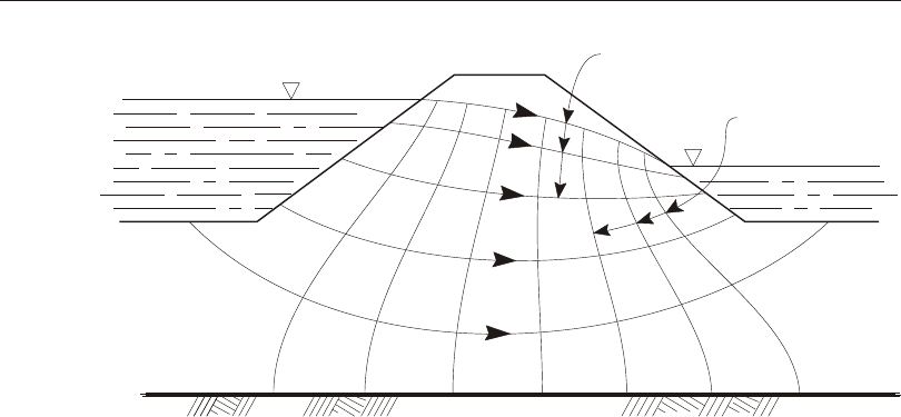
Sca lar fluid- pressure val ues are given at the ele ment joints by Joint Pat terns, and in -
ter po lated over the ele ment. These pres sure val ues may typi cally be ob tained by
flow- net analy sis, such as il lus trated in Figure 78 (page 329). Hy dro static pres sure
fields may eas ily be speci fied us ing Joint Pat terns. Pres sure val ues are ad di tive.
The to tal force act ing on the ele ment is the in te gral of the gra di ent of this pres sure
field over the vol ume of the ele ment. This force is ap por tioned to each of the joints
of the ele ment. The forces are typi cally di rected from re gions of high pres sure to -
ward re gions of low pres sure.
Note that al though pres sures are speci fied, it is the pres sure gra di ent over an ele -
ment that causes the load. Thus a uni form pres sure field over an ele ment will cause
no load. Pres sure dif fer ences be tween ele ments also cause no load. For this rea son,
it is im por tant that the pore- pressure field be con tinu ous over the struc ture.
The dis place ments, stresses, and re ac tions due to Pore Pres sure Load rep re sent the
re sponse of the solid me dium, not that of the com bined fluid and solid struc ture. In
the case of soil, the stresses ob tained are the usual “ef fec tive stresses” of soil me -
chan ics (Ter zaghi and Peck, 1967). Note, how ever, that the to tal soil weight and
mass den sity should be used for the ma te rial prop er ties.
For more in for ma tion:
•See Topic “Pore Pres sure Load” (page 222) in Chap ter “The Plane Ele ment.”
Pore Pressure Load 329
Chapter XVII Load Patterns
Earth Dam Flow Lines
Water Surface
Equipotential
Lines (Constant
Pore Pressure)
Bedrock
Figure 78
Flow-net Analysis of an Earth Dam to Obtain Pore Pressures

•See Topic “Pore Pres sure Load” (page 234) in Chap ter “The Aso lid Ele ment.”
•See Topic “Pore Pres sure Load” (page 249) in Chap ter “The Solid Ele ment.”
•See Topic “Joint Pat terns” (page 332) in this Chap ter.
Temperature Load
Tem per a ture Load cre ates ther mal strains in the Frame, Ca ble, Shell, Plane, Asolid,
and Solid el e ments. These strains are given by the prod uct of the Ma te rial co ef fi -
cients of ther mal ex pan sion and the tem per a ture change of the el e ment. All spec i -
fied Tem per a ture Loads rep re sent a change in tem per a ture from the un stressed state
for a lin ear anal y sis, or from the pre vi ous tem per a ture in a non lin ear anal y sis.
Load Tem pera ture gra di ents may also be speci fied in the two trans verse di rec tions
of the Frame ele ment, and in the thick ness di rec tion of the Shell ele ment. These
gra di ents in duce bend ing strains in the ele ments. Tem pera ture gra di ents are speci -
fied as the linear change in tem pera ture per unit length. Thus to spec ify a given dif -
fer ence in tem per a ture across the depth of a Frame or Shell el e ment, di vide the tem -
per a ture dif fer ence by the cor re spond ing depth, and as sign this value as the tem per -
a ture gra di ent load.
The Load Tem per a tures and gra di ents may be dif fer ent for each Load Pat tern. You
may spec ify tem per a tures and/or gra di ents that are uni form over an el e ment or that
are in ter po lated from val ues given by Joint Pat terns.
For more in for ma tion:
•See Topic “Tem pera ture Load” (page 140) in Chap ter “The Frame Ele ment.”
•See Topic “Tem per a ture Load” (page 174) in Chap ter “The Ca ble El e ment.”
•See Topic “Tem per a ture Load” (page 209) in Chap ter “The Shell El e ment.”
•See Topic “Tem pera ture Load” (page 223) in Chap ter “The Plane Ele ment.”
•See Topic “Tem pera ture Load” (page 234) in Chap ter “The Aso lid Ele ment.”
•See Topic “Tem per a ture Load” (page 250) in Chap ter “The Solid El e ment.”
•See Topic “Tem per a ture Load” (page 318) in Chap ter “The Ten don Object.”
•See Topic “Joint Pat terns” (page 332) in this Chap ter.
330 Temperature Load
CSI Analysis Reference Manual

Strain Load
Strain Load in duces dis trib uted strains in the Frame, Ca ble, and Shell el e ments.
The im posed strains tend to cause de for ma tion in un re strained el e ments, or cre ate
in ter nal forces and stresses in re strained el e ments. The types of strains that are
avail able is dif fer ent for each type of el e ment.
You may spec ify strains that are uni form over an el e ment or that are in ter po lated
from val ues given by Joint Pat terns.
For more in for ma tion:
•See Topic “Strain Load” (page 141) in Chap ter “The Frame El e ment.”
•See Topic “Strain and De for ma tion Load” (page 174) in Chap ter “The Ca ble
El e ment.”
•See Topic “Strain Load” (page 210) in Chap ter “The Frame El e ment.”
•See Topic “Joint Pat terns” (page 332) in this Chap ter.
Deformation Load
De for ma tion Load is an al ter na tive form of Strain Load where the ap plied de for ma -
tion is spec i fied over the whole el e ment rather than on a per-unit-length ba sis. De -
for ma tion Load is only avail able for Frame and Ca ble el e ments. The as sumed dis -
tri bu tion of strain over the el e ment is fixed as de scribed in the top ics ref er enced be -
low. Joint Pat terns are not used.
For more in for ma tion:
•See Topic “De for ma tion Load” (page 141) in Chap ter “The Frame El e ment.”
•See Topic “Strain and De for ma tion Load” (page 174) in Chap ter “The Ca ble
El e ment.”
Target-Force Load
Tar get-Force Load is a spe cial type of load ing where you spec ify a de sired ax ial
force, and de for ma tion load is iteratively ap plied to achieve the tar get force. Since
the ax ial force may vary along the length of the el e ment, you must also spec ify the
rel a tive lo ca tion where the de sired force is to oc cur. Tar get-Force load ing is only
Strain Load 331
Chapter XVII Load Patterns

used for non lin ear static and staged-con struc tion anal y sis. If ap plied in any other
type of Load Case, it has no ef fect.
Un like all other types of load ing, tar get-force load ing is not in cre men tal. Rather,
you are spec i fy ing the to tal force that you want to be pres ent in the frame el e ment at
the end of the Load Case or con struc tion stage. The ap plied de for ma tion that is cal -
cu lated to achieve that force may be pos i tive, neg a tive, or zero, de pend ing on the
force pres ent in the el e ment at the be gin ning of the anal y sis. When a scale fac tor is
ap plied to a Load Pat tern that con tains Tar get-Force loads, the to tal tar get force is
scaled. The in cre ment of ap plied de for ma tion that is re quired may change by a dif -
fer ent scale fac tor.
For more in for ma tion:
•See Topic “Tar get-Force Load” (page 142) in Chap ter “The Frame El e ment.”
•See Topic “Tar get-Force Load” (page 174) in Chap ter “The Ca ble El e ment.”
•See Topic “Tar get-Force It er a tion” (page 444) in Chap ter “Non lin ear Static
Anal y sis” for more in for ma tion.
Rotate Load
Ro tate Load ap plies cen trifu gal force to Aso lid ele ments. You may spec ify an an -
gu lar ve loc ity, r, for each ele ment. The cen trifu gal force is pro por tional to the
square of the an gu lar ve loc ity. The an gu lar ve loci ties are ad di tive. The load on the
ele ment is com puted from the to tal an gu lar ve loc ity.
See Topic “Ro tate Load” (page 234) in Chap ter “The Aso lid Ele ment.”
Joint Patterns
A Joint Pat tern is a named en tity that con sists of a set of sca lar nu meric val ues, one
value for each joint of the struc ture. A Joint Pat tern can be used to de scribe how
pres sures or tem per a tures vary over the struc ture. Joint Pat terns may also be used to
spec ify joint off sets and thick ness over write for Shell el e ments.
Pat terns are most ef fec tive for de scrib ing com pli cated spa tial dis tri bu tions of nu -
meric val ues. Their use is op tional and is not re quired for sim ple prob lems.
Since Pat tern val ues are sca lar quan ti ties, they are in de pend ent of any co or di nate
sys tem. The def i ni tion of a Joint Pat tern by it self causes no ef fect on the struc ture.
CSI Analysis Reference Manual
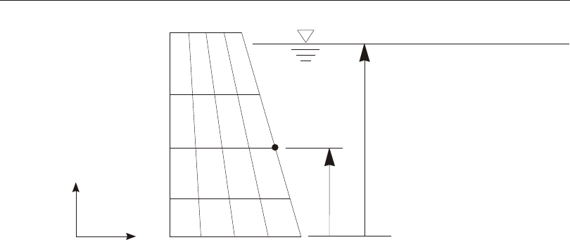
The pat tern must be used in a pres sure, tem per a ture, or other as sign ment that is ap -
plied to the model.
For com pli cated Pat terns, val ues could be gen er ated in a spread sheet pro gram or by
some other means, and brought into the model by im port ing ta bles or by us ing in -
ter ac tive ta ble ed it ing.
In the graph i cal user in ter face, Pat tern val ues can be as signed to se lected joints.
They are spec i fied as a lin ear vari a tion in a given gra di ent di rec tion from zero at a
given da tum point. An op tion is avail able to per mit only pos i tive or only neg a tive
val ues to be de fined. This is use ful for de fin ing hy dro static pres sure dis tri bu tions.
Mul ti ple lin ear vari a tions may be as signed to the same or dif fer ent joints in the
struc ture.
The fol low ing pa ram e ters are needed for a pat tern as sign ment:
•The com po nents of the gra di ent, A, B, and C, in the global co or di nate sys tem
•The value D of the pat tern at the global or i gin
•The choice be tween:
–Set ting neg a tive val ues to zero
–Set ting pos i tive val ues to zero
–Al low all pos i tive and neg a tive val ues (this is the de fault)
Joint Patterns 333
Chapter XVII Load Patterns
Zero Datum = Fluid Surface
z
Fluid weight density = g
Pressure gradient vz = – g
Pressure value v = – g (z – z)
jj
Joint j
zj
Global
X
Z
Figure 79
Example of a Hydrostatic Pressure Pattern

The com po nent A in di cates, for ex am ple, how much the Pat tern value changes per
unit of dis tance par al lel to the global X axis.
The Pat tern value, vj, de fined for a joint j that has co or di nates (xj, yj, zj) is given by:
(Eqn. 1)
vj = A xj + B yj + C zj + D
If you know the co or di nates of the da tum point, x, y, and z, in global co or di nate sys -
tem at which the pat tern value should be zero (say the free sur face of wa ter), then:
(Eqn. 2)
vj = A (xj – x) + B (yj – y) + C (zj – z)
from which we can cal cu late that:
(Eqn. 3)
D = – ( A x + B y + C z )
In most cases, the gra di ent will be par al lel to one of the co or di nate axes, and only
one term in Eqn. 2 is needed.
For ex am ple, con sider a hy dro static pres sure dis tri bu tion caused by wa ter im -
pounded be hind a dam as shown in Figure 79 (page 333). The Z di rec tion is up in
the global co or di nate sys tem. The pres sure gra di ent is sim ply given by the fluid
weight den sity act ing in the down ward di rec tion. There fore, A = 0, B = 0 , and C =
–62.4 lb/ft3 or –9810 N/m3.
The zero-pres sure da tum can be any point on the free sur face of the wa ter. Thus z
should be set to the el e va tion of the free sur face in feet or me ters, as ap pro pri ate,
and D = – C z. For hy dro static pres sure, you would spec ify that neg a tive val ues be
ig nored, so that any joints above the free sur face will be as signed a zero value for
pres sure.
Mass Source
The mass used as in er tia in dy namic analyses or to cal cu late cer tain types of loads
can be con trolled by spec i fy ing the Mass Source. Mul ti ple Mass Sources can be de -
fined so that different load cases can use a dif fer ent mass dis tri bu tions for load ing
and in er tia. Ex am ples could in clude mod el ing a struc ture sup port ing dif fer ent con -
fig u ra tions of equip ment, or ex plic itly con sid er ing the ef fect of dif fer ent ec cen tric i -
ties of the story mass on the mode shapes. How ever, for most mod els only a sin gle
Mass Source is needed, and this is the de fault.
There are three pos si ble con tri bu tions to a Mass Source:
334 Mass Source
CSI Analysis Reference Manual

•El e ment Self Mass — This in cludes the mass from the sec tion prop er ties used
by the el e ments. For the Link/Sup port elements, this mass is ex plic itly de fined
in the sec tion property. For all other el e ments the mass co mes from the ma te rial
prop erty ref er enced by the sec tion prop erty.
•Ad di tional Mass — This in cludes mass as signed to the joints and any ad di -
tional mass as signed to the frame or shell el e ments.
•Spec i fied Load Pat terns — Mass is com puted from the grav ity load as com -
puted from a spec i fied lin ear com bi na tion of load pat terns.
For each de fined Mass Source you may spec ify which of the above con tri bu tions
are to be con sid ered. By de fault, there is only a sin gle Mass Source, and this in -
cludes the El e ment Self Mass and the Ad di tional Mass, with no con tri bu tion from
Specified Load Pat terns.
Mass from Spec i fied Load Pat terns
When de fin ing a Mass Source, you may in clude the mass from a lin ear com bi na tion
of Load Pat terns. For each Load Pat tern in this com bi na tion you spec ify a scale fac -
tor that multiplies the loads. The mass is cal cu lated as fol lows:
•For each in di vid ual joint or el e ment, joint loads are cal cu lated based on the
specified lin ear com bi na tion of load patterns.
•For each joint of this el e ment, the com bined load act ing in the grav ity di rec tion
(neg a tive global Z) is di vided by the grav i ta tional con stant, and then as signed
equally to the translational de grees of free dom at that joint.
•Down ward loads (–Z) cre ate pos i tive mass, and up ward loads (+Z) cre ate neg -
a tive mass.
Im por tant notes:
•Loads are cal cu lated for each el e ment in its orig i nal con fig u ra tion, in de pend ent
of any large-de flec tion anal y sis.
•The mass cal cu lated from loads acts in all three translational di rec tions even
though the load cre at ing the mass acts vertically.
•Self-equilibrating loads, such as tem per a ture, strain, and prestressing, should
not be used for Mass Source.
•Be care ful not to dou ble-count the self-mass by spec i fy ing both El e ment Self
mass and a load pat tern that con tains self-weight.
Mass Source 335
Chapter XVII Load Patterns

Neg a tive Mass
All mass val ues used for anal y sis must be pos i tive or zero. Neg a tive mass is not re -
al is tic and is not al lowed. How ever, you can use neg a tive mass in the mass source if
your in ten tion is to sub tract it from other pos i tive mass.
The con tri bu tions due to El e ment Self Mass and Ad di tional Mass come from ma te -
ri als, link prop er ties, joint mass, line mass, and area mass. Ex cept for joint mass,
these con tri bu tions are al ways pos i tive and are equal for the three translational de -
grees of free dom at each joint. Joint mass can be pos i tive or neg a tive and may be
dif fer ent at each of the six joint de grees of free dom.
The con tri bu tions from Spec i fied Load Pat terns are equal for the three translational
de grees of free dom at each joint. Down ward loads gen er ate pos i tive mass and up -
ward loads gen er ate neg a tive mass.
The net re sult af ter com bin ing all these con tri bu tions for any joint de gree of free -
dom may be pos i tive or neg a tive and will be re ported as such in the “As sem bled
Joint Mass” ta ble. Dur ing equa tion so lu tion, any neg a tive mass val ues that re main
af ter com bin ing the mass for con straints are set to zero and a warn ing is sued in the
anal y sis log file.
Mul ti ple Mass Sources
For most mod els, a sin gle Mass Source is suf fi cient and is de fined as de scribed
above. This will ap ply to all loads calculated from mass and to all dy namic load
cases.
How ever, you have the op tion (when avail able) to spec ify mul ti ple Mass Sources
for use with dif fer ent load cases. Each Mass Source is de fined as de scribed above
by spec i fy ing the three con tri bu tions to the mass. One Mass Source is se lected as
the de fault and this will be used for all Load Cases un less spec i fied oth er wise.
A spec i fied Mass Source can se lected for the fol low ing types of load cases:
•Non lin ear static
•Non lin ear staged-construction
•Non lin ear di rect-integration time-history
If you do not se lect a specified Mass Source for these types of load cases, the Mass
source used will be the de fault Mass Source if the load case starts from zero ini tial
con di tions, or the Mass Source used in the pre vi ous load case if con tin u ing from an -
other one of these same three types of load cases.
336 Mass Source
CSI Analysis Reference Manual

For all other load cases, a sim i lar rule ap plies. The de fault Mass Source will be used
if the load case uses the stiff ness from zero load con di tions. Otherwise, the Mass
Source used will be the same as for the non lin ear static, staged-con struc tion, or di -
rect-in te gra tion time-his tory load case used to cal cu late the stiff ness.
Response-spec trum and modal time-his tory load cases use the Mass Source of their
cor re spond ing modal load case. See Chap ter “Load Cases” (page 341) for more in -
for ma tion, es pe cially Topic “Se quence of Anal y sis” (page 344).
For ex am ple, con sider the case where a re sponse-spec trum anal y sis is to be car ried
out for a tower both with and with out a sig nif i cant equip ment load. You could do
the fol low ing:
•De fine two load pat terns
–DEAD, which in cludes the self-weight of the tower struc ture
–LIVE, which in cludes only the weight of the equip ment
•De fine two mass sources
– MASSDEAD, which in cludes only the load pat tern DEAD with a scale
fac tor of 1.0, and no El e ment Self Mass or Ad di tional Mass
–MASSDEADLIVE, which in cludes both load pat terns DEAD and LIVE,
each with a scale fac tor of 1.0, and no El e ment Self Mass or Ad di tional
Mass
•De fine two non lin ear static load cases
–DEAD, which specifies mass source MASSDEAD
–DEADLIVE, which spec i fies mass source MASSDEADLIVE
•De fine two modal load cases
–MODALDEAD, which uses the stiff ness of load case DEAD
–MODALDEADLIVE, which uses the stiff ness of load case DEADLIVE
•De fine two re sponse-spec trum load cases
–SPECDEAD, which uses the modes of load case MODALDEAD
–DEADLIVE, which uses the modes of load case MODALDEADLIVE
Note that in the above ex am ple the non lin ear static load cases were used only to
spec ify the Mass Source. How ever, in most prac ti cal cases you would also want to
ap ply the cor re spond ing load pat terns as loads and con sider P-delta ef fects, as these
would likely also have an ef fect on the modes.
Note that the re sponse-spec trum cases, in ad di tion to con sid er ing the in er tial ef fect
of the dif fer ent masses on the modes, also ap ply ac cel er a tion loads that are based on
Mass Source 337
Chapter XVII Load Patterns

mass. These loads will au to mat i cally be based on the mass from the same Mass
Source used to cal cu late the modes. See topic “Ac cel er a tion Load” (page 338).
Au to mated Lat eral Loads
Au to mated lat eral loads are avail able as spec i fied in the sep a rate “Au to mated
Lateral Loads Man ual” pro vided with the software. Most of the seis mic loads, and
some wind loads, are cal cu lated based on mass, which in turn is cal cu lated by anal -
y sis from the Mass Source.
When mul ti ple Mass Sources are used, the mass could be dif fer ent be tween load
cases. For this rea son, any given load pat tern that con tains an au to mated lat eral load
based on mass can only be ap plied in load cases that use the same mass source. If
the same load pat tern is ap plied in mul ti ple load cases us ing dif fer ent mass sources,
a warn ing will be is sued when the anal y sis is run and only those load cases us ing
one of the mass sources will be run. In this case, you can de fine duplicate load pat -
terns as needed for use with load cases us ing dif fer ent mass sources.
Some au to mated lat eral loads use a modal pe riod that can be spec i fied by the user or
de ter mined from anal y sis. By de fault, this pe riod will be de ter mined from the first
modal load case that is run, whether or not it uses the same Mass Source as other
load cases that ap ply the load pat tern. For this rea son, when us ing mul ti ple Mass
Sources, it is strongly rec om mended that you re view the modal pe riod used for au -
to mated lat eral loads and spec ify your own value to be used if the cal cu lated value
does not ap ply.
Acceleration Loads
In ad di tion to the Load Pat terns that you de fine, the pro gram au to mat i cally com -
putes three Ac cel er a tion Loads that act on the struc ture due to unit translational ac -
cel er a tions in each of the global di rec tions, and three unit ro ta tional ac cel er a tions
about the global axes at the global or i gin. Ac cel er a tion Loads can be ap plied in a
Load Case just like Load Pat terns.
Ac cel er a tion Loads are de ter mined by d’Alembert’s prin ci pal, and are de noted mx,
my, mz, mrx, mry, and mrz. These loads are used for ap ply ing ground ac cel er a -
tions in re sponse-spec trum (trans la tion only) and time-his tory anal y ses, and can be
used as start ing load vec tors for Ritz-vec tor anal y sis.
These loads are com puted for each joint and el e ment and summed over the whole
struc ture. The translational Ac cel er a tion Loads for the joints are sim ply equal to the
338 Acceleration Loads
CSI Analysis Reference Manual

neg a tive of the joint translational masses in the joint lo cal co or di nate sys tem. These
loads are trans formed to the global co or di nate sys tem.
The translational Ac cel er a tion Loads for all el e ments ex cept for the Asolid are the
same in each di rec tion and are equal to the neg a tive of the el e ment mass. No co or di -
nate trans for ma tions are nec es sary. Ro ta tional ac cel er a tion will gen er ally dif fer
about each axis.
For the Asolid el e ment, the Ac cel er a tion Load in the global di rec tion cor re spond -
ing to the ax ial di rec tion is equal to the neg a tive of the el e ment mass. The Ac cel er a -
tion Loads in the ra dial and cir cumfer ential di rec tions are zero, since trans la tions in
the cor re spond ing global di rec tions are not axisymmetric. Sim i lar con sid er ations
ap ply to the ro ta tional ac cel er a tions.
The Ac cel er a tion Loads can be trans formed into any co or di nate sys tem. In a fixed
co or di nate sys tem (global or Al ter nate), the translational Ac cel er a tion Loads along
the pos i tive X, Y, and Z axes are de noted UX, UY, and UZ, re spec tively; the ro ta -
tional Ac cel er a tion Loads about the X, Y, and Z axes are sim i larly de noted RX,
RY, and RZ.
In a lo cal co or di nate sys tem de fined for a re sponse-spec trum or time-his tory anal y -
sis, the Ac cel er a tion Loads along or about the pos i tive lo cal 1, 2, and 3 axes are de -
noted U1, U2, U3, R1, R2, and R3 re spec tively. Ro ta tional ac cel er a tions will be ap -
plied about the or i gin of the co or di nate sys tem spec i fied with the Ac cel er a tion
Load in the Load Case. Each Ac cel er a tion Load ap plied in a given Load Case can
use a sep a rate co or di nate sys tem.
Al though the ro ta tional ac cel er a tions are ap plied in load cases about the or i gins of
the spec i fied co or di nate sys tems, the modal par tic i pa tion fac tors and the var i ous
modal par tic i pa tion ra tios for the ac cel er a tions RX, RY, and RZ are re ported about
the cen ter of mass for the struc ture:
•For the RX load, this lo ca tion is the y cen troid of the UZ load and the z cen troid
of the UY load.
•For the RY load, this lo ca tion is the z cen troid of the UX load and the x cen troid
of the UZ load.
•For the RZ load, this lo ca tion is the z cen troid of the UY load and the y cen troid
of the UX load.
This makes the ro ta tional par tic i pa tion fac tors and ra tios are more mean ing ful be -
cause they do not in clude any con tri bu tion from the translational ac cel er a tions.
Acceleration Loads 339
Chapter XVII Load Patterns

340 Acceleration Loads
CSI Analysis Reference Manual

Chapter XVIII
Load Cases
A Load Case de fines how the loads are to be ap plied to the struc ture (e.g., stat i cally
or dy nam i cally), how the struc ture re sponds (e.g., lin early or nonlinearly), and how
the anal y sis is to be per formed (e.g., mo dally or by di rect-in te gra tion.)
Basic Topics for All Users
•Over view
•Load Cases
•Types of Anal y sis
•Se quence of Anal y sis
•Run ning Load Cases
•Lin ear and Non lin ear Load Cases
•Lin ear Static Analy sis
•Func tions
•Load Com bi na tions (Combos)
•Global En ergy Response
Advanced Topics
•Multi-Step Static Anal y sis
341

•Lin ear Buckling Anal y sis
•Equa tion Solv ers
•En vi ron ment Vari ables to Con trol Anal y sis
•Ac cess ing the As sem bled Stiff ness and Mass Matrices
Overview
A Load Case de fines how loads are to be ap plied to the struc ture, and how the struc -
tural re sponse is to be cal cu lated. You may de fine as many named Load Cases of
any type that you wish. When you an a lyze the model, you may se lect which cases
are to be run. You may also se lec tively de lete re sults for any Load Case.
Note: Load Pat terns by them selves do not cre ate any re sponse (de flec tions,
stresses, etc.) You must de fine a Load Case to ap ply the load.
There are many dif fer ent types of Load Cases. Most broadly, anal y ses are clas si fied
as lin ear or non lin ear, de pend ing upon how the struc ture re sponds to the load ing.
The re sults of lin ear anal y ses may be superposed, i.e., added to gether af ter anal y sis.
The avail able types of lin ear anal y sis are:
•Static analy sis
•Mo dal analy sis for vi bra tion modes, us ing ei gen vec tors or Ritz vec tors
•Response- spectrum analy sis for seis mic re sponse
•Time- history dy namic re sponse anal y sis
•Buckling-mode analysis
•Moving- load analy sis for bridge and other ve hi cle live loads
•Steady- state anal y sis
•Power-spec tral-den sity analysis
The re sults of non lin ear anal y ses should not nor mally be superposed. In stead, all
loads act ing to gether on the struc ture should be com bined di rectly within the Load
Cases. Non lin ear Load Cases may be chained to gether to rep re sent com plex load -
ing se quences. The avail able types of non lin ear anal y ses are:
•Non lin ear static anal y sis
•Non lin ear time-his tory anal y sis
342 Overview
CSI Analysis Reference Manual

Named Load Com bi na tions can also be de fined to com bine the re sults of Load
Cases. Re sults can be com bined additively or by en vel op ing. Ad di tive Load Com -
bi na tions of non lin ear Load Cases is not usu ally jus ti fied.
Load Cases
Each dif fer ent analy sis per formed is called a Load Case. For each Load Case you
de fine, you need to sup ply the fol low ing type of in for ma tion:
•Case name: This name must be unique across all Load Cases of all types. The
case name is used to re quest anal y sis re sults (dis place ments, stresses, etc.), for
cre at ing Load Com bi na tions, and some times for use by other dependent Load
Cases.
•Anal y sis type: This in di cate the type of anal y sis (static, re sponse-spec trum,
buck ling, etc.), as well as avail able op tions for that type (lin ear, non lin ear,
etc.).
•Pre req ui site load cases: Some load cases may con tinue from a pre vi ous load
case, use the stiff ness from a pre vi ous load case, and/or use the modes from a
pre vi ous load case.
•Loads ap plied: For most types of anal y sis, you spec ify the Load Pat terns that
are to be ap plied to the struc ture.
Ad di tional data may be re quired, de pend ing upon the type of anal y sis be ing de -
fined.
Types of Analysis
There are many dif fer ent types of Load Cases. Most broadly, anal y ses are clas si fied
as lin ear or non lin ear, de pend ing upon how the struc ture re sponds to the load ing.
See Topic “Lin ear and Non lin ear Load Cases” (page 346) in this Chap ter.
The re sults of lin ear anal y ses may be superposed, i.e., added to gether af ter anal y sis.
The avail able types of lin ear anal y sis are:
•Static anal y sis
•Modal anal y sis
•Re sponse-spec trum anal y sis
•Time-his tory anal y sis, by modal su per po si tion or di rect in te gra tion
Load Cases 343
Chapter XVIII Load Cases

•Buckling anal y sis
•Moving-load anal y sis
•Steady-state anal y sis
•Power-spec tral-den sity analysis
The re sults of non lin ear anal y ses should not nor mally be superposed. In stead, all
loads act ing to gether on the struc ture should be com bined di rectly within the Load
Cases. Non lin ear Load Cases may be chained to gether to rep re sent com plex load -
ing se quences. The avail able types of non lin ear anal y ses are:
•Non lin ear static anal y sis
•Non lin ear time-his tory anal y sis, by modal su per po si tion or di rect in te gra tion
Af ter you have de fined a Load Case, you may change its type at any time. When
you do, the pro gram will try to carry over as many pa ram e ters as pos si ble from the
old type to the new type. Pa ram e ters that can not be car ried over will be set to de -
fault val ues, which you can change.
For more in for ma tion:
•See Topic “Lin ear Static Anal y sis” (page 348) in this Chap ter
•See Topic “Buckling Anal y sis” (page 349) in this Chap ter
•See Chap ter “Modal Anal y sis” (page 365)
•See Chap ter “Re sponse-Spec trum Anal y sis” (page 383)
•See Chap ter “Lin ear Time-His tory Anal y sis” (page 397)
•See Chap ter “Non lin ear Static Anal y sis” (page 425)
•See Chap ter “Non lin ear Time-His tory Anal y sis” (page 447)
•See Chap ter “Fre quency-Do main Anal y sis” (page 465)
•See Chap ter “Mov ing-Load Anal y sis” (page 477)
Se quence of Anal y sis
A Load Case may be de pend ent upon other Load Cases in the fol low ing sit u a tions:
•A modal-su per po si tion type of Load Case (re sponse-spec trum or modal
time-his tory) uses the modes cal cu lated in a modal Load Case
•A non lin ear Load Case may con tinue from the state at the end of another non -
lin ear case
344 Se quence of Anal y sis
CSI Analysis Reference Manual

•A lin ear Load Cases may use the stiff ness of the struc ture as com puted at the
end of a non lin ear case
A Load Case which de pends upon an other case is called de pend ent. The case upon
which it de pends is called a pre req ui site case.
When the pro gram per forms anal y sis, it will al ways run the cases in the proper or -
der so that de pend ent cases are run af ter any of their pre req ui site cases.
You can build up one or more se quences of Load Cases that can be as sim ple or as
com pli cated as you need. How ever, each se quence must ul ti mately start with a
Load Case that it self starts from zero and does not have any pre req ui site cases.
Ex am ple
A com mon ex am ple would be to de fine a non lin ear static Load Case with the fol -
low ing main fea tures:
•The name is, say, “PDELTA”
•The type is non lin ear static
•The loads ap plied are Load Pat tern “DEAD” scaled by 1.0 plus Load Pat tern
“LIVE” scaled by 0.25. These rep re sent a typ i cal amount of grav ity load on the
struc ture
•The only nonlinearity con sid ered is the P-delta ef fect of the loading
We are not nec es sar ily in ter ested in the re sponse of Load Case PDELTA, but rather
we will use the stiff ness at the end this case for a se ries of lin ear Load Cases that we
are in ter ested in. These may in clude lin ear static cases for all loads of in ter est (dead,
live, wind, snow, etc.), a modal Load Case, and a re sponse-spec trum Load Case.
Be cause these cases have all been com puted us ing the same stiff ness, their re sults
are su per pos able, mak ing it very sim ple to cre ate any num ber of Load Com bi na -
tions for de sign pur poses.
Running Load Cases
Af ter you have de fined a struc tural model and one or more Load Cases, you must
ex plic itly run the Load Cases to get re sults for dis play, out put, and de sign pur -
poses.
When an anal y sis is run, the pro gram con verts the ob ject-based model to finite el e -
ments, and per forms all cal cu la tions nec es sary to de ter mine the re sponse of the
Running Load Cases 345
Chapter XVIII Load Cases

struc ture to the loads ap plied in the Load Cases. The anal y sis re sults are saved for
each case for sub se quent use.
By de fault, all Load Cases de fined in the model are run each time you per form an
anal y sis. How ever, you can change this be hav ior. For each Load Case, you can set
a flag that in di cates whether or not it will be run the next time you per form an anal y -
sis. This en ables you to de fine as many dif fer ent cases as you need with out hav ing
to run all of them ev ery time. This is par tic u larly use ful if you have non lin ear cases
that may take a long time to run.
If you se lect a case to be run, the pro gram will also run all pre req ui site cases that
have not yet been run, whether you se lect them or not.
You can cre ate new Load Cases with out de let ing the re sults of other cases that have
al ready been run. You can also mod ify ex ist ing Load Cases. How ever, the re sults
for the mod i fied case and all cases that de pend upon it will be de leted.
When an anal y sis is per formed, the cases will be run in an or der that is au to mat i -
cally de ter mined by the pro gram in or der to make sure all pre req ui site cases are run
be fore their de pend ent cases. If any pre req ui site cases fail to com plete, their de -
pend ent cases will not be run. How ever, the pro gram will con tinue to run other
cases that are not de pend ent upon the failed cases.
You should al ways check the anal y sis log (.LOG) file to see sta tis tics, warn ings,
and er ror mes sages that were re ported dur ing the anal y sis. You can also see a sum -
mary of the cases that have been run, and whether or not they com pleted suc cess -
fully, us ing the Anal y sis com mands in the graph i cal user in ter face.
When ever pos si ble, the pro gram will re-use the pre vi ously solved stiff ness ma trix
while run ning Load Cases. Be cause of this, the or der in which the cases are run may
not be the same each time you per form an anal y sis.
See Topic “Se quence of Anal y sis” (page 467) in this Chap ter for more in for ma tion.
Lin ear and Non lin ear Load Cases
Ev ery Load Case is con sid ered to be ei ther lin ear or non lin ear. The dif fer ence be -
tween these two op tions is very sig nif i cant in SAP2000, as de scribed be low.
All Load Case types may be lin ear. Only static anal y sis and time-his tory anal y sis
may be non lin ear.
346 Lin ear and Non lin ear Load Cases
CSI Analysis Reference Manual

Struc tural properties
Lin ear: Struc tural prop er ties (stiff ness, damp ing, etc.) are con stant dur ing the
anal y sis.
Non lin ear: Struc tural prop er ties may vary with time, de for ma tion, and load -
ing. How much nonlinearity ac tu ally oc curs de pends upon the prop er ties you
have de fined, the mag ni tude of the load ing, and the pa ram e ters you have spec i -
fied for the anal y sis.
Initial conditions
Lin ear: The anal y sis starts with zero stress. It does not con tain loads from any
pre vi ous anal y sis, even if it uses the stiff ness from a pre vi ous non lin ear anal y -
sis.
Non lin ear: The anal y sis may con tinue from a pre vi ous non lin ear anal y sis, in
which case it con tains all loads, de for ma tions, stresses, etc., from that pre vi ous
case.
Struc tural response and superposition
Lin ear: All dis place ments, stresses, re ac tions, etc., are di rectly pro por tional to
the mag ni tude of the ap plied loads. The re sults of dif fer ent lin ear anal y ses may
be superposed.
Non lin ear: Be cause the struc tural prop er ties may vary, and be cause of the pos -
si bil ity of non-zero ini tial con di tions, the re sponse may not be pro por tional to
the load ing. There fore, the re sults of dif fer ent non lin ear anal y ses should not
usu ally be superposed.
Linear Static Analysis
The lin ear static analy sis of a struc ture in volves the so lu tion of the sys tem of lin ear
equa tions rep re sented by:
Kur=
where K is the stiff ness ma trix, r is the vec tor of ap plied loads, and u is the vec tor of
re sult ing dis place ments. See Bathe and Wil son (1976).
You may cre ate any num ber of lin ear static Load Cases. For each case you may
spec ify a com bi na tion of one or more Load Pat terns and/or Ac cel er a tion Loads that
Linear Static Analysis 347
Chapter XVIII Load Cases

make up the load vec tor r. Normally, you would spec ify a sin gle Load Pat tern with
a scale fac tor of one.
Ev ery time you de fine a new Load Pat tern, the pro gram au to mat i cally cre ates a cor -
re spond ing lin ear static Load Case of the same name. This Load Case ap plies the
Load Case with a unit scale factor. If you de lete or mod ify the Load Case, the anal y -
sis re sults will not be avail able, even though the Load Case may still ex ist.
For a new model, the pro gram cre ates a de fault Load Pat tern call DEAD which ap -
plies the self weight of the struc ture. The cor re spond ing lin ear static Load Case is
also called DEAD.
For each lin ear static Load Case, you may spec ify that the pro gram use the stiff ness
ma trix of the full struc ture in its un stressed state (the de fault), or the stiff ness of the
struc ture at the end of a non lin ear Load Case. The most com mon rea sons for us ing
the stiff ness at the end of a non lin ear case are:
•To in clude P-delta ef fects from an ini tial P-delta anal y sis
•To in clude ten sion-stiff en ing ef fects in a ca ble struc ture
•To con sider a par tial model that re sults from staged construction
See Chap ter “Non lin ear Static Anal y sis” (page 425) for more in for ma tion.
Multi-Step Static Analysis
Cer tain types of Load Pat terns are multi-stepped, mean ing that they ac tu ally rep re -
sent many sep a rate spa tial load ing pat terns ap plied in se quence. These in clude the
Vehicle-Live and Wave types of Load Pat terns.
You can ap ply multi-stepped Load Pat terns in a Multi-Step Static Load Case. This
type of Load Case will per form a se ries of in de pend ent lin ear anal y ses, one for each
step of the Load Pat tern:
Kur
ii
=
where ri is the load at step I, and ui is the re sult ing so lu tion.
You can ap ply any lin ear com bi na tion of Load Pat terns in the same Load Case,
each with an in de pend ent scale fac tor. These will be summed to gether as fol lows:
all multi-stepped Load Pat terns will be syn chro nized, ap ply ing the load for the
same step num ber at the same time, and all sin gle-stepped Load Pat terns (e.g., dead
load) will be ap plied in ev ery step.
348 Multi-Step Static Analysis
CSI Analysis Reference Manual

The num ber of so lu tion steps for the Load Case will be equal to the larg est num ber
of load steps of any of the ap plied multi-stepped Load Pat terns.
Al though the multi-stepped Load Pat terns rep re sent a time se ries of loads,
Multi-Step Static Anal y sis does not in clude any dy nam i cal ef fects. You can con -
sider dy nam ics by con vert ing the Multi-Step Static Load Case to a Time-His tory
Load Case, which can be lin ear or non lin ear.
Linear Buckling Analysis
Lin ear buck ling anal y sis seeks the in sta bil ity modes of a struc ture due to the P-delta
ef fect un der a specified set of loads. Buckling anal y sis in volves the so lu tion of the
gen er al ized eigenvalue prob lem:
[]KG(r)-=lY0
where K is the stiff ness ma trix, G(r) is the geo met ric (P-delta) stiff ness due to the
load vec tor r, l is the di ag o nal ma trix of eigenvalues, and Y is the ma trix of cor re -
spond ing eigenvectors (mode shapes).
Each eigenvalue-eigenvector pair is called a buckling mode of the struc ture. The
modes are iden ti fied by num bers from 1 to n in the or der in which the modes are
found by the pro gram.
The eigenvalue l is called the buck ling fac tor. It is the scale fac tor that must mul ti -
ply the loads in r to cause buck ling in the given mode. It can also be viewed as a
safety fac tor: if the buck ling fac tor is greater than one, the given loads must be in -
creased to cause buck ling; if it is less than one, the loads must be de creased to pre -
vent buck ling. The buck ling fac tor can also be neg a tive. This in di cates that buck -
ling will oc cur if the loads are re versed.
You may cre ate any num ber of lin ear buck ling Load Cases. For each case you spec -
ify a com bi na tion of one or more Load Pat terns and/or Ac cel er a tion Loads that
make up the load vec tor r. You may also spec ify the num ber of modes to be found
and a con ver gence tol er ance. It is strongly rec om mended that you seek more than
one buck ling mode, since of ten the first few buck ling modes may have very sim i lar
buck ling fac tors. A min i mum of six modes is rec om mended.
It is im por tant to un der stand that buck ling modes de pend upon the load. There is
not one set of buck ling modes for the struc ture in the same way that there is for nat -
u ral vi bra tion modes. You must ex plic itly eval u ate buck ling for each set of loads of
con cern.
Linear Buckling Analysis 349
Chapter XVIII Load Cases

For each lin ear buck ling Load Case, you may spec ify that the pro gram use the stiff -
ness ma trix of the full struc ture in its un stressed state (the de fault), or the stiff ness
of the struc ture at the end of a non lin ear Load Case. The most com mon rea sons for
us ing the stiff ness at the end of a non lin ear case are:
•To in clude P-delta ef fects from an ini tial P-delta anal y sis
•To in clude ten sion-stiff en ing ef fects in a ca ble struc ture
•To con sider a par tial model that re sults from staged con struc tion
See Chap ter “Non lin ear Static Anal y sis” (page 425) for more in for ma tion.
Functions
A Func tion is a se ries of dig it ized abscissa- ordinate pairs that may rep re sent:
•Pseudo- spectral ac cel era tion vs. pe riod for response- spectrum analy sis, or
•Load vs. time for time- history anal y sis
•Load vs. frequency for steady-state anal y sis
•Power den sity (load squared per fre quency) vs. frequency for power-spec -
tral-de nsity analysis
You may de fine any number of Func tions, as sign ing each one a unique la bel. You
may scale the ab scissa and/or or di nate val ues when ever the Func tion is used.
The ab scissa of a Func tion is al ways time, pe riod, or fre quency. The abscissa-
ordinate pairs must be speci fied in or der of in creas ing ab scissa value.
If the in cre ment be tween ab scissa val ues is con stant and the Func tion starts at ab -
scissa zero, you need only spec ify the ab scissa in cre ment, dt, and the suc ces sive
func tion val ues (or di nates) start ing at ab scissa zero. The func tion val ues are spec i -
fied as:
f0, f1, f2, ..., fn
cor re spond ing to ab scis sas:
0, dt, 2 dt, ..., n dt
where n + 1 is the number of val ues given.
If the ab scissa in cre ment is not con stant or the Func tion does not start at ab scissa
zero, you must spec ify the pairs of ab scissa and func tion value as:
CSI Analysis Reference Manual
350 Functions

t0, f0, t1, f1, t2, f2, ..., tn, fn
where n + 1 is the number of pairs of val ues given.
Load Combinations (Combos)
A Load Com bi na tion (Combo) is a named com bi na tion of the re sults from Load
Cases or other Load Combinations. Combo re sults in clude all dis place ments and
forces at the joints and in ter nal forces or stresses in the ele ments.
You may de fine any number of Com bos. To each one of these you as sign a unique
name, that also should not be the same as any Load Case. Com bos can com bine the
re sults of Load Cases and also those of other Com bos, pro vided a cir cu lar de pend -
ency is not cre ated.
By de fault, each Combo pro duces a pair of val ues for each re sponse quan tity: a
maxi mum and a mini mum. These two val ues may be equal for cer tain type of Com -
bos, as dis cussed be low.
Al ter na tively, cor re spon dence may be re quested for tab u lar out put, in which case
mul ti ple pairs of max i mum and min i mum val ues may be pro duced at each out put
lo ca tion for each Combo. This is dis cussed in more de tail in the subtopic “Cor re -
spon dence” be low. The dis cus sion that im me di ately fol lows next con sid ers the de -
fault case where a sin gle max i mum and min i mum value is pro duced for each re -
sponse quan tity.
Con trib ut ing Cases
Each con trib ut ing Load Case or Combo sup plies one or two val ues to the Combo
for each re sponse quan tity:
•Lin ear static cases, in di vid ual modes from Modal or Buckling cases, in di vid ual
steps from multi-stepped Load Cases, and ad di tive Com bos of these types of
re sults pro vide a sin gle value. For the pur poses of de fin ing the Com bos be low,
this sin gle value can be con sid ered to be two equal val ues
•Re sponse-spec trum cases pro vide two val ues: the max i mum value used is the
pos i tive com puted value, and the min i mum value is just the neg a tive of the
max i mum.
•En velopes of re sults from multi-stepped Load Cases pro vide two val ues: a
maxi mum and mini mum.
Load Combinations (Combos) 351
Chapter XVIII Load Cases

•For Mov ing-Load Load Cases, the val ues used are the max i mum and min i mum
val ues ob tained for any ve hi cle load ing of the lanes per mit ted by the pa ram e -
ters of the anal y sis.
For some types of Combos, both val ues are used. For other types of Combos, only
the value with the larger ab so lute value is used.
Each con trib ut ing case is mul ti plied by a scale fac tor, sf, be fore be ing in cluded in a
Combo.
Types of Combos
Five types of Com bos are avail able. For each in di vid ual re sponse quan tity (force,
stress, or dis place ment com po nent) the two Combo val ues are cal cu lated as fol -
lows:
•Ad di tive type: The Combo maxi mum is an al ge braic lin ear com bi na tion of the
maxi mum val ues for each of the con trib ut ing cases. Simi larly, Combo mini -
mum is an al ge braic lin ear com bi na tion of the mini mum val ues for each of the
con trib ut ing cases.
•Ab so lute type: The Combo maxi mum is the sum of the larger ab so lute val ues
for each of the con trib ut ing cases. The Combo mini mum is the nega tive of the
Combo maxi mum.
•SRSS type: The Combo maxi mum is the square root of the sum of the squares
of the larger ab so lute val ues for each of the con trib ut ing cases. The Combo
mini mum is the nega tive of the Combo maxi mum.
•Range type: The Combo max i mum is the sum of the pos i tive max i mum val ues
for each of the con trib ut ing cases (a case with a neg a tive max i mum does not
con trib ute.) Sim i larly, the Combo min i mum is the sum of the neg a tive min i -
mum val ues for each of the con trib ut ing cases (a case with a pos i tive min i mum
does not con trib ute.)
•En ve lope type: The Combo max i mum is the max i mum of all of the max i mum
val ues for each of the con trib ut ing cases. Sim i larly, Combo min i mum is the
min i mum of all of the min i mum val ues for each of the con trib ut ing cases.
Only ad di tive Com bos of sin gle-val ued Load Cases pro duce a sin gle-val ued re sult,
i.e., the max i mum and min i mum val ues are equal. All other Com bos will gen er ally
have dif fer ent max i mum and min i mum val ues.
352 Load Combinations (Combos)
CSI Analysis Reference Manual

Examples
For ex am ple, sup pose that the val ues, af ter scal ing, for the dis place ment at a par tic -
u lar joint are 3.5 for Lin ear Static Load Case LL and are 2.0 for Re sponse-spec trum
case QUAKE. Sup pose that these two cases have been in cluded in an ad di tive-type
Combo called COMB1 and an en ve lope-type Combo called COMB2. The re sults
for the dis place ment at the joint are com puted as fol lows:
•COMB1: The maxi mum is 3.5 + 2.0 = 5.5, and the mini mum is 3.5 – 2.0 = 1.5
•COMB2: The maxi mum is max (3.5, 2.0) = 3.5, and the mini mum is min (3.5, –
2.0) = –2.0
As an other ex am ple, sup pose that Lin ear Static Cases GRAV, WINDX and
WINDY are grav ity load and two per pen dicu lar, trans verse wind loads, re spec -
tively; and that a response- spectrum case named EQ has been per formed. The fol -
low ing four Com bos could be de fined:
•WIND: An SRSS- type Combo of the two wind loads, WINDX and WINDY.
The maxi mum and mini mum re sults pro duced for each re sponse quan tity are
equal and op po site
•GRAVEQ: An additive- type Combo of the grav ity load, GRAV, and the
response- spectrum re sults, EQ. The Combo auto mati cally ac counts for the
posi tive and nega tive senses of the earth quake load
•GRAVWIN: An additive- type Combo of the grav ity load, GRAV, and the
wind load given by Combo WIND, which al ready ac counts for the posi tive and
nega tive senses of the load
•SE VERE: An envelope- type Combo that pro duces the worst case of the two
ad di tive Com bos, GRAVEQ and GRAVWIN
Sup pose that the val ues of ax ial force in a frame ele ment, af ter scal ing, are 10, 5, 3,
and 7 for cases GRAV, WINDX, WINDY, and EQ, re spec tively. The fol low ing re -
sults for ax ial force are ob tained for the Com bos above:
•WIND: maximum , minimum= + = = -5 3 58 58
2 2 . .
•GRAVEQ: maximum , minimum= + = = - =10 7 17 10 7 3
•GRAVWIN: maximum , minimum= + = = - =10 58 158 10 58 42. . . .
•SE VERE: maximum , minimum====max(,.)min(,.)17158173423
Range-type Com bos en able you to per form skip-pat tern load ing very ef fi ciently.
For ex am ple, sup pose you have a four-span con tin u ous beam, and you want to
Load Combinations (Combos) 353
Chapter XVIII Load Cases

know what pat tern of uni form load ing on the var i ous spans cre ates the max i mum
re sponse:
•Cre ate four Load Pat terns, each with uni form load ing on a sin gle span
•Cre ate four cor re spond ing Lin ear Static Load Cases, each ap ply ing a sin gle
Load Pat tern.
•Cre ate a sin gle range Combo, com bin ing the re sults of the four Load Cases
The ef fect of this Combo is the same as en vel op ing all ad di tive com bi na tions of any
sin gle span loaded, any two spans loaded, any three spans loaded, and all four spans
loaded. This range Combo could be added or en vel oped with other Load Cases and
Com bos.
As you can see, us ing Com bos of Com bos gives you con sid er able power and flexi -
bil ity in how you can com bine the re sults of the vari ous Load Cases.
Correspondence
When cor re spon dence is re quested for tab u lar output, the max i mum and min i mum
value is pro duced for each re sponse quan tity as de scribed above, but these are pre -
sented with the val ues of other re lated re sponse quan ti ties at the same lo ca tion that
oc cur at the same time the given max i mum or min i mum is achieved.
For ex am ple, when con sid er ing Frame-el e ment forces, the max i mum value of ax ial
force P at a given out put sta tion is pre sented with the cor re spond ing val ues of V2,
V3, T, M2, and M3 at the same out put sta tion. Six cor re spond ing val ues are also
pre sented for the min i mum value of P, and so on for the max i mum and min i mum
val ues of V2, V3, T, M2, and M3.
With out cor re spon dence, the fol low ing tabular re sults would be pre sented for a
given out put sta tion in a given Combo:
Type PV2 V3 TM2 M3
Max 100 44 5-6 0 1245
Min -50 22 -5 -9 -123 -333
With cor re spon dence, the tab u lar re sults for the same out put sta tion lo ca tion would
be pre sented as:
354 Load Combinations (Combos)
CSI Analysis Reference Manual
Type PV2 V3 TM2 M3
PMax 100 32 -4 -6 -123 -111
PMin -50 24 3-6 0 999
V2Max 81 44 5-7 -65 328
V2Min -30 22 -5 -6 -44 172
V3Max 81 44 5-7 -65 328
V3Min -30 22 -5 -6 -44 172
TMax 50 40 0-6 -69 1033
TMin 87 25 -4 -9 -77 -197
M2Max -20 39 0-8 0 1158
M2Min 27 29 -4 -7 -123 890
M3Max 71 36 5-6 0 1245
M3Min -38 31 -5 -9 -123 -333
In this ex am ple, row PMax pres ents the max i mum value of ax ial force P and the
cor re spond ing val ues of the other frame forces and mo ments that oc cur at the same
time as max i mum P. For a Combo that is the en ve lope of sev eral lin ear static load
cases, this would be the frame forces and mo ments from the con trib ut ing load case
that had the max i mum value of P. For an ad di tive Combo of a dead load case plus a
time-his tory load case, this would be the summed frame forces and mo ments from
that time step in the time-his tory case that, when com bined with dead load, pro -
duces that max i mum value of P. Sim i larly, row PMin is the min i mum value of P
and its cor re spond ing forces and mo ments, and so on for V2Max through M3Min.
The shaded val ues in the ta ble above in di cate the max i mum and min i mum val ues
that would be pre sented in the ta ble with out cor re spon dence. All other val ues in a
given col umn will be within the range of these two val ues.
It is pos si ble, in some cases, that the max i mum or min i mum value of a re sponse
quan tity could oc cur at more than one in stance in a Combo, in which case the cor re -
Load Combinations (Combos) 355
Chapter XVIII Load Cases

spond ing val ues will be pre sented for the first in stance en coun tered. In this case,
the cor re spond ing re sults may not be unique.
Cor re spon dence is avail able for tab u lar out put of the fol low ing quan ti ties in soft -
ware prod ucts that of fer this op tion:
•Joint dis place ments
•Joint re ac tions
•Frame forces, Shell forces
•Shell stresses, Plane stresses, Asolid stresses, Solid stresses
•Link/Support forces and deformations
•El e ment joint forces
•Sec tion Cuts
•Base re ac tions
•Bridge ob ject sec tion forces, Bridge ob ject girder forces (CSiBridge only)
For each of the above, the cor re spon dence is pre sented be tween the var i ous com po -
nents of the same type (e.g., 6 dis place ments, 6 forces, or 6 stresses) at a given lo ca -
tion (joint or out put sta tion). Correspondence is not pre sented be tween com po nents
at dif fer ent lo ca tions or be tween com po nents of dif fer ent types (e.g., dis place ment
and force). The only ex cep tion to this is the Link/Sup port el e ment, where cor re -
spon dence is pre sented be tween the 6 de for ma tion and 12 force com po nents of a
given el e ment. If you want to see the full cor re spond ing state of the struc ture, you
must use step-by-step anal y sis.
Cor re spon dence is avail able for Com bos of types Ad di tive, En ve lope, and Range,
pro vided that the contributing load cases and Com bos also sup port cor re spon -
dence.
Correspondence is not avail able for Com bos of types Ab so lute and SRSS, nor for
Combos that con tain any of the fol low ing types of con trib ut ing load cases and/or
Com bos:
•Re sponse-spec trum load case
•Steady-state load case
•PSD load case
•Mov ing-load case with out correspondence
•Ab so lute Combo
•SRSS Combo
356 Load Combinations (Combos)
CSI Analysis Reference Manual

•A Combo that con tains any of the above
•In ad di tion, cor re spon dence is not avail able for base re ac tions or el e ment joint
forces for any Combo that con tains a mov ing-load case.
Re quest ing cor re spon dence for tab u lar out put does not af fect any other type of dis -
play, de sign, or the Open API functions. Cor re spon dence for de sign pur poses is
con trolled by the De sign Pref er ences. See the var i ous de sign man u als that are in -
cluded with the soft ware for more in for ma tion
Ad di tional Considerations
Mov ing-Load Load Cases should not nor mally be added to gether, in or der to avoid
mul ti ple load ing of the lanes. Ad di tive com bi na tions of Mov ing Loads should only
be de fined within the Mov ing-Load Load Case it self. There fore, it is rec om mended
that only a sin gle Mov ing Load be in cluded in any ad di tive-, ab so lute-, SRSS-, or
range-type Combo, whether ref er enced di rectly as a Mov ing Load or in di rectly
through an other Combo. Mul ti ple Mov ing Loads may be in cluded in any
envelope- type Combo, since they are not added.
Non lin ear Load Cases should not nor mally be added to gether, since non lin ear re -
sults are not usu ally su per pos able. In stead, you should com bine the ap plied loads
within a non lin ear Load Case so that their com bined ef fect can be prop erly an a -
lyzed. This may re quire de fin ing many dif fer ent Load Cases in stead of many dif -
fer ent Combos. Nonlinear Load Cases may be in cluded in an en ve lope-type
Combo, since they are not added.
Global En ergy Re sponse
En ergy re sponse is pro vided for the en tire struc ture for cer tain types of load cases,
in clud ing lin ear and non lin ear modal time-his tory, non lin ear static and staged con -
struc tion, and non lin ear di rect-in te gra tion time his tory (but see Lim i ta tions be low).
En ergy re sponse can be plot ted and pro duced in out put ta bles.
Three ba sic types of en ergy are con sid ered: the work done by ex ter nal agents that
put en ergy into the struc ture, con ser va tive en ergy in the struc ture that can be re cov -
ered, and unconservative en ergy that is dis si pated by the struc ture. Look ing at the
en ergy re sponse can tell you a lot about the be hav ior of the struc ture, but it is most
use ful for de ter min ing the ef fec tive ness of en ergy-dis si pat ing mech a nisms that are
in ten tion ally pro vided as part of the de sign. This can in clude damp ers, iso la tors,
and plas tic hing ing in struc tural mem bers.
Global En ergy Re sponse 357
Chapter XVIII Load Cases

Global Energy Response Components
The fol low ing types of en ergy are re ported for each considred load case:
•In put. This is the work done by ex ter nal agents that put en ergy into the struc -
ture. This in cludes:
–Forces, mo ments, pres sures, self-weight, and sim i lar loads
–Ground ac cel er a tion
–Ground dis place ment
–El e ment strains and dis place ments, in clud ing ther mal and time-de pend ent
strains (but see Lim i ta tions be low).
–P-delta ef fects, such as the work done by ver ti cal forces through lat eral dis -
place ments when P-delta nonlinearity is con sid ered
•Po ten tial. This is a con ser va tive type of en ergy in the struc ture due to elas tic
strain that can be re cov ered when the load ing is re moved. It is of ten de sir able to
limit po ten tial en ergy to the rea son able ex tent pos si ble, since it rep re sents
forces and stresses to be de signed against.
•Ki netic. This is a con ser va tive type of en ergy due to the mo tion of the struc -
ture. It is of ten de sir able to limit ki netic en ergy since this can rep re sent the po -
ten tial for dam age to struc tural and non-struc tural items. Ki netic en ergy is al -
ways zero in a static anal y sis.
•Non lin ear Vis cous Damp ing. This rep re sents the vis cous en ergy dis si pated
by the ve loc ity-based damper el e ments. Non lin ear vis cous damp ing does not
change dur ing non lin ear static and staged con struc tion load cases. The fol low -
ing types of link el e ments can gen er ate this en ergy com po nent dur ing time-his -
tory load cases:
–Lin ear damp ing prop er ties
–Damper – Ex po nen tial
–Damper – Bilinear
–The three Fric tion-Pen du lum Iso la tors (ax ial de gree of free dom only)
•Non lin ear Hysteretic Damp ing. This rep re sents the hysteretic en ergy dis si -
pated by the dis place ment-based damper el e ments and the plas tic de for ma tion
of ma te ri als (in clud ing hinges). Non lin ear hysteretic damp ing can be gen er ated
by the fol low ing el e ments dur ing non lin ear static, staged-con struc tion, and
time-his tory load cases:
–Link el e ments hav ing the fol low ing types of prop er ties:
*Damper – Fric tion Spring
358 Global En ergy Re sponse
CSI Analysis Reference Manual

*Multilinear Plas tic
*Plas tic (Wen)
*Rub ber Iso la tor
*The three Fric tion-Pen du lum Iso la tors (shear de grees of free dom)
–Frame non lin ear hinges of all types
–Lay ered shell el e ments with non lin ear ma te rial prop er ties
•Global Damp ing. This rep re sents the en ergy dis si pated by the struc ture as a
whole. For modal time-his tory load cases, this in cludes the modal damp ing
spec i fied for the load case as well as modal damp ing spec i fied for the ma te ri als,
if any. For non lin ear di rect-in te gra tion time-his tory load cases, this in cludes
stiff ness- and mass-pro por tional damp ing spec i fied for the load case as well as
such damp ing spec i fied for the ma te ri als, if any. Global damp ing is vis cous
(ve loc ity-based) and does not change dur ing non lin ear static and staged-con -
struc tion load cases.
•Er ror. It is ex pected that the sum of the po ten tial, ki netic, and three damp ing
en er gies be equal to the in put en ergy. The en ergy er ror is cal cu lated as the dif -
fer ence be tween the in put en ergy and this sum. There are sev eral rea sons why
this er ror may not be zero, such as:
–Discretization er ror due to larger steps sizes for P-delta or large-dis place -
ment geo met ric nonlinearity. This can be checked by re-run ning the load
case with a smaller step size.
–Round-off er ror in nu mer i cally sen si tive or ill-con di tioned sys tems.
–En ergy that is ex cluded due to the Lim i ta tions listed be low, such as for cer -
tain types of strain load ing.
Re marks
Fol low ing are some gen eral re marks con sid er ing the na ture and use of these global
en ergy re sponse com po nents:
•The in put en ergy can in crease or de crease as the sum of the con ser va tive en -
ergy in creases or de creases. How ever, the three damp ing en er gies rep re sent
work done that is not re cov er able, and these can only in crease the in put en ergy.
•For pur poses of de sign, it is gen er ally pref er a ble that the pri mary en ergy dis si -
pa tion be in the form of non lin ear vis cous and hysteretic damp ing, mean ing
that it co mes from de vices (damp ers, iso la tors, etc.) and hing ing mech a nisms.
Global damp ing rep re sents other ef fects that are not ex plic itly mod eled, such
as from non-struc tural el e ments and the in trin sic na ture of the ma te ri als. If this
Global En ergy Re sponse 359
Chapter XVIII Load Cases

is too large, then it is dif fi cult to know whether or not the de sign in tent is be ing
met.
•When an ob ject is re moved dur ing staged con struc tion, its po ten tial en ergy is
re moved and is also de ducted from the in put en ergy. Any damp ing en ergy pro -
duced by that ob ject is not re moved, as that is al ready as sumed to have been
dis si pated as waste heat.
•If a non lin ear static or staged-con struc tion load case con tin ues from a di rect-in -
te gra tion time-his tory load case, the ve loc ity-based vis cous damp ing en er gies
are held con stant dur ing the static anal y sis. How ever, ki netic en ergy is set to
zero dur ing the static anal y sis and the in put en ergy is cor re spond ingly re duced.
If a non lin ear di rect-in te gra tion time-his tory load case then con tin ues from the
non lin ear static or staged-con struc tion load case, the ve loc ity con tin ues from
the end of the most re cent time-his tory load case in the se quence and the ki netic
en ergy is re com put ed from those ve loc i ties. In ef fect, the non lin ear static or
staged-con struc tion load cases are as sumed to have oc curred in stan ta neously
from the dy nam ics point of view. If this is not de sired, the pre vi ous time-his -
tory load cases should be run long enough to damp out the ve loc i ties.
•The pres ence of en ergy er ror does not in val i date the anal y sis re sults, but can be
an in di ca tion that fur ther in ves ti ga tion is war ranted. See Lim i ta tions be low for
some of the pos si ble rea sons. Note that the en ergy re sponse is cal cu lated from
the ba sic anal y sis re sults (dis place ments, forces, stresses) and does not af fect
these re sults.
Lim i ta tions
Fol low ing are some lim i ta tions of the cur rent implmentation of the global en ergy
re sponse:
•For SAP2000 and CSiBridge, en ergy re sponse is cur rently lim ited to lin ear and
non lin ear modal time-his tory load cases. Non lin ear static, staged-con struc tion,
and di rect-in te gra tion time-his tory load cases are avail able only for ETABS at
the pres ent time.
•Non lin ear modal time-his tory (FNA) load cases only sup port nonlinearity in
link el e ments, hence non lin ear hysteretic damp ing en ergy from frame hinges
and shear walls is only pro duced if the “Model Hinges as Sep a rate Link El e -
ments” op tion is used (see Topic “Anal y sis Mod el ing” in Chap ter “Hinge
Prop er ties”). When us ing the “Model Hinges within El e ments” op tion,
hysteretic damp ing en ergy from frame hinges and shear walls is not con sid -
ered. Hysteretic be hav ior for lay ered shells is not con sid ered for FNA load
cases ei ther way.
360 Global En ergy Re sponse
CSI Analysis Reference Manual

•The in put en ergy and po ten tial en ergy due to span loads within a frame el e ment
may be un der- or over-es ti mated if the in ter nal de flec tion of the beam is sig nif i -
cant com pared to the dis place ments of the two ends. In such cases, sub di vid ing
or mesh ing the frame el e ment may re sult in a dif fer ent and of ten more ac cu rate
in put and po ten tial en ergy due to span loads. This ef fect may be es pe cially pro -
nounced when non lin ear hinges with out hinge overwrites are pres ent in a frame
el e ment with large span loads. Us ing shorter hinge overwrites or the “Model
Hinges as Sep a rate Link El e ments” anal y sis op tion can be used to re solve this
is sue. This is a lim i ta tion on the re ported en ergy re sponse and does not af fect
any force, stress, dis place ment, or de for ma tion re sponse.
•Tem per a ture and strain load ing cre ate self-equilibrating forces act ing at the
joints of the el e ment. The in put en ergy for this type of load ing is cal cu lated as
the work done by these forces act ing through the joint dis place ments. For a
fully re strained el e ment, no in put en ergy would be com puted, and cor re spond -
ingly the po ten tial en ergy will also be re ported as zero. On the other hand, an
un re strained el e ment will re port non-zero work and po ten tial en ergy due to
tem per a ture load ing. Note that the lay ered shell and frame hinges be have op po -
sitely in this re gard. Their en ergy is com puted based on the in ter nal stress state,
and thus they re port non zero in put and po ten tial en ergy due to re strained tem -
per a ture load ing, and zero en ergy for un re strained load ing.
•Hysteretic ma te ri als may some times un der es ti mate the amount of po ten tial en -
ergy pres ent be cause they as sume that un load ing will oc cur along the orig i nal
elas tic stiff ness, when it may ac tu ally oc cur along a re duced stiff ness. As a re -
sult, hysteretic en ergy may show a slight de crease when an el e ment un loads
since some ad di tional po ten tial en ergy is re cov ered. This ef fect is gen er ally in -
sig nif i cant for prac ti cal mod els.
Equa tion Solvers
You can choose from three solv ers avail able for solv ing the stiff ness equa tions:
•Stan dard Solver. This is the slow est of the solv ers for larger prob lems and uses
the most disk space. How ever, it pro vides de tailed warn ing mes sages about in -
sta bil i ties and sen si tiv ity of the stiff ness ma trix.
•Ad vanced Solver. This is the de fault solver. It may be one or two or ders of
mag ni tude faster than the Stan dard solver for larger prob lems, and it also uses
much less disk space. It pro vides lim ited in for ma tion about in sta bil i ties.
•Multi-threaded Solver. This is the faster solver on ma chines with mul ti ple
cores or processors. It runs in memory and does not use any disk space. It pro -
Equa tion Solvers 361
Chapter XVIII Load Cases

vides no in for ma tion on in sta bil i ties. De pend ing on the amount of mem ory
avail able, you may need to use the Ad vanced solver for the larg est prob lems.
Be cause the solv ers per form nu mer i cal op er a tions in a dif fer ent or der, it is pos si ble
that sen si tive prob lems may yield slightly dif fer ent re sults with the dif fer ent solv -
ers due to nu mer i cal roundoff. Parallel pro cess ing can in crease this effect. In ex -
tremely sen si tive, non lin ear, his tory-de pend ent prob lems, the dif fer ences may be
more pro nounced.
All ver i fi ca tion ex am ples have been run and checked us ing all three solv ers. The re -
sults us ing the ad vanced solver are re ported for com par i son in the ver i fi ca tion man -
u als.
The ad vanced solver is based on pro pri etary CSI tech nol ogy. It uses, in part, code
de rived from TAUCS fam ily of solv ers. Please see the copy right no tice at the end
of Chap ter “Ref er ences” (page 533) for more in for ma tion.
En vi ron ment Vari ables to Con trol Analysis
Sev eral en vi ron ment vari ables are avail able to con trol the so lu tion pro cess. These
are rarely needed. If you do use them, they can be set in the Win dows Con trol Panel
or by us ing the SET com mand in a com mand prompt win dow. In gen eral we rec om -
mend not changing these.
Us ing Win dows Con trol Panel, you can add, re move, or change the en vi ron ment
vari ables. By de fault they do not ex ist. Set ting the value to zero or de let ing the en vi -
ron ment vari able will re sult in de fault be hav ior. Changes made in the Con trol Panel
only af fect in stances of SAP2000 or other CSI prod ucts that are started af ter the
change is made. You can not change the be hav ior of an in stance that is al ready
started.
Us ing the com mand prompt, changes made to an en vi ron ment vari able only af fect
in stances of SAP2000 or other CSI prod ucts that are started from within that same
com mand prompt.
SAPFIRE_NUM_THREADS
Cer tain parts of the anal y sis pro cess are parallelized, most no ta bly mov ing-load
anal y sis and the cal cu la tion of cer tain el e ment events, states, and stiff ness ma tri ces.
More par al lel ism will be im ple mented over time in fu ture ver sions. By de fault the
anal y sis uses all the avail able phys i cal cores, which may be half of the hy -
per-threaded cores.
362 En vi ron ment Vari ables to Con trol Analysis
CSI Analysis Reference Manual

You can set SAPFIRE_NUM_THREADS to a pos i tive num ber to re duce the num -
ber of threads if you plan to run mul ti ple in stances of the anal y sis, or want to
change the set tings to ob tain op ti mum per for mance from your ma chine.
The Multi-threaded solver uses its own logic to ob tain op ti mum per for mance.
How ever, SAPFIRE_NUM_THREADS does set the max i mum num ber of threads
to be used. You can over ride this value with the sep a rate en vi ron ment vari able
SAPFIRE_NUM_THREADS_SOLVE. This is rarely needed but could be used to
achieve re pro duc ible re sults in very sen si tive mod els where the nu mer i cal cal cu la -
tions may be af fected by the or der of parallelized op er a tions.
For the most com plete con trol of the Multi-threaded solver, set the en vi ron ment
vari able MKL_DY NAMIC to value FALSE, which forces the solver to use the
spec i fied num ber of threads. By de fault this value is TRUE. We do not gen er ally
rec om mend chang ing the de fault be hav ior, since it may af fect the ef fi ciency of the
solver and other parallelized cal cu la tions. It could also af fect other soft ware prod -
ucts per form ing sci en tific and en gi neer ing com pu ta tion if set in Win dows Con trol
Panel.
SAPFIRE_FILESIZE_MB
By de fault the file-size limit for in ter nal files used dur ing anal y sis is 100 GB, but
this can be changed us ing the en vi ron ment vari able SAPFIRE_FILESIZE_MB to
spec ify an in te ger num ber of mega bytes (MB). The value can rep re sent 1 TB or
more, al though the de fault value will rarely need to be in creased. For most prac ti cal
prob lems, the amount of disk space and other sys tem re sources will con trol the size
of the model and as so ci ated anal y sis files that can be han dled.
On the other hand, you will need to de crease this limit for Win dows FAT32 file sys -
tems that are lim ited to 2 GB. In this case, set SAPFIRE_FILESIZE_MB to 2048 or
less. Most Win dows ma chines use NTFS file sys tems and are not af fected by this
limit. This value may also be needed for files that are in tended to be zipped-up
(com pressed) for stor age or ship ping.
Ac cess ing the As sem bled Stiff ness and Mass Matrices
When us ing the ad vanced equa tion solver, you may re quest that the pro gram pro -
duce the as sem bled stiff ness and mass ma tri ces in the form of text files. This can be
done for a sin gle lin ear static, modal, or buck ling Load Case. To get the stiff ness
and mass ma tri ces for a non lin ear case, de fine a lin ear case that uses the stiff ness
from the fi nal state of the de sired non lin ear case.
Ac cess ing the As sem bled Stiff ness and Mass Matrices 363
Chapter XVIII Load Cases

The as sem bled ma tri ces are pro vided in five text files that have the same name as
the model file, but with the fol low ing ex ten sions and con tents:
•Ex ten sion .TXA: This file in cludes the counts of the num ber of joints and
equa tions in the model, and also de scribes the for mat and con tents of the other
four files.
•Ex ten sion .TXE: This file gives the equa tion num bers for each de gree of free -
dom (DOF) at each joint. Equa tion num bers are pos i tive for ac tive DOF that
are pres ent in the stiff ness and mass ma tri ces, neg a tive for con strained DOF
that are com puted as lin ear com bi na tions of ac tive DOF, and zero for re strained
or null DOF.
•Ex ten sion .TXC: This file de fines the con straint equa tions, and is only pres ent
if there are con straints in the model.
•Ex ten sion .TXK: This file gives the lower half of the sym met ric stiff ness ma -
trix.
•Ex ten sion .TXM: This file gives the lower half of the sym met ric mass ma trix.
Each of the latter four files con tains a sin gle header line that be gins with “Note:”
and de fines the data columns. All sub se quent lines pro vide Tab-de lim ited data for
easy im port into text ed i tors or spread sheet pro grams.
364 Ac cess ing the As sem bled Stiff ness and Mass Matrices
CSI Analysis Reference Manual

Chapter XIX
Modal Anal y sis
Modal anal y sis is used to de ter mine the vi bra tion modes of a struc ture. These
modes are use ful to un der stand the be hav ior of the struc ture. They can also be used
as the ba sis for modal su per po si tion in re sponse-spec trum and modal time-his tory
Load Cases.
Basic Topics for All Users
•Over view
•Ei gen vec tor Analy sis
•Ritz-Vector Analy sis
•Mo dal Analy sis Out put
Overview
A modal anal y sis is de fined by cre at ing a Load Case and set ting its type to
“Modal”. You can de fine mul ti ple modal Load Cases, re sult ing in mul ti ple sets of
modes.
There are two types of modal anal y sis to choose from when de fin ing a modal Load
Case:
Overview 365

•Eigenvector anal y sis de ter mines the un damped free-vi bra tion mode shapes
and fre quen cies of the sys tem. These nat u ral modes pro vide an ex cel lent in -
sight into the be hav ior of the struc ture.
•Ritz-vec tor anal y sis seeks to find modes that are ex cited by a par tic u lar load -
ing. Ritz vec tors can pro vide a better ba sis than do eigenvectors when used for
re sponse-spec trum or time-his tory anal y ses that are based on modal su per po si -
tion
You can re quest that static cor rec tion modes be cal cu lated along with eigenvectors.
They are au to mat i cally in cluded with Ritz vec tors. Static cor rec tion-modes can be
very im por tant for get ting ac cu rate re sponse at stiff sup ports. Their use is gen er -
ally rec om mended.
Modal anal y sis is al ways lin ear. A modal Load Case may be based on the stiff ness
of the full un stressed struc ture, or upon the stiff ness at the end of a non lin ear Load
Case (non lin ear static or non lin ear di rect-in te gra tion time-his tory).
By us ing the stiff ness at the end of a non lin ear case, you can eval u ate the modes un -
der P-delta or geo met ric stiff en ing con di tions, at dif fer ent stages of con struc tion, or
fol low ing a sig nif i cant non lin ear ex cur sion in a large earth quake.
In ad di tion, the mass used for a modal anal y sis can be changed if mul ti ple Mass
Sources have been defined. The Mass Source to be used for a given modal load case
can be spec i fied in the same types of non lin ear Load Cases that can be used to cal -
cu late the stiff ness.
For more in for ma tion:
•See Topic “Mass Source” (page 334) in Chap ter “Load Pat terns”.
•See Chap ter “Load Cases” (page 341).
Eigenvector Analysis
Ei gen vec tor analy sis de ter mines the un damped free- vibration mode shapes and fre -
quen cies of the sys tem. These natu ral Modes pro vide an ex cel lent in sight into the
be hav ior of the struc ture. They can also be used as the ba sis for response- spectrum
or time- history analy ses, al though Ritz vec tors are rec om mended for this pur pose.
Ei gen vec tor analy sis in volves the so lu tion of the gen er al ized ei gen value prob lem:
[]KM-=WF
20
366 Eigenvector Analysis
CSI Analysis Reference Manual

where K is the stiff ness ma trix, M is the di ago nal mass ma trix, W2 is the di ago nal
ma trix of ei gen val ues, and F is the ma trix of cor re spond ing ei gen vec tors (mode
shapes).
Each eigenvalue- eigenvector pair is called a natu ral Vi bra tion Mode of the struc -
ture. The Modes are iden ti fied by num bers from 1 to n in the or der in which the
modes are found by the pro gram.
The ei gen value is the square of the cir cu lar fre quency, w, for that Mode (un less a
fre quency shift is used, see be low). The cy clic fre quency, f, and pe riod, T, of the
Mode are re lated to w by:
Tff==
1
2
andw
p
You may spec ify the number of modes to be found, a con ver gence tol er ance, and
the fre quency range of in ter est. These pa rame ters are de scribed in the fol low ing
sub top ics.
Number of Modes
You may spec ify the max i mum and min i mum num ber of modes to be found.
The pro gram will not cal cu late more than the spec i fied max i mum num ber of
modes. This num ber in cludes any static cor rec tion modes re quested. The pro gram
may com pute fewer modes if there are fewer mass de grees of free dom, all dy namic
par tic i pa tion tar gets have been met, or all modes within the cut off fre quency range
have been found.
The pro gram will not cal cu late fewer than the spec i fied min i mum num ber of
modes, un less there are fewer mass de grees of free dom in the model.
A mass de gree of free dom is any ac tive de gree of free dom that pos sesses trans la -
tional mass or ro ta tional mass mo ment of in er tia. The mass may have been as signed
di rectly to the joint or may come from con nected ele ments.
Only the modes that are ac tu ally found will be avail able for use by any sub se quent
response- spectrum or modal time-his tory Load Cases.
See Topic “De grees of Free dom” (page 30) in Chap ter “Joints and De grees of Free -
dom.”
Eigenvector Analysis 367
Chapter XIX Modal Anal y sis

Frequency Range
You may spec ify a re stricted fre quency range in which to seek the Vi bra tion Modes
by us ing the pa rame ters:
•shift: The cen ter of the cy clic fre quency range, known as the shift fre quency
•cut: The ra dius of the cy clic fre quency range, known as the cut off fre quency
The pro gram will only seek Modes with fre quen cies f that sat isfy:
||f-£shiftcut
The de fault value of cut=0 does not re strict the fre quency range of the Modes.
Modes are found in or der of in creas ing dis tance of fre quency from the shift. This
con tin ues un til the cut off is reached, the re quested number of Modes is found, or
the number of mass de grees of free dom is reached.
A sta ble struc ture will pos sess all posi tive natu ral fre quen cies. When per form ing a
seis mic analy sis and most other dy namic analy ses, the lower- frequency modes are
usu ally of most in ter est. It is then ap pro pri ate to the de fault shift of zero, re sult ing
in the lowest- frequency modes of the struc ture be ing cal cu lated. If the shift is not
zero, response- spectrum and time- history analy ses may be per formed; how ever,
static, moving- load, and p- delta analy ses are not al lowed.
If the dy namic load ing is known to be of high fre quency, such as that caused by vi -
brat ing ma chin ery, it may be most ef fi cient to use a posi tive shift near the cen ter of
the fre quency range of the load ing.
A struc ture that is un sta ble when un loaded will have some modes with zero fre -
quency. These modes may cor re spond to rigid- body mo tion of an in ade quately
sup ported struc ture, or to mecha nisms that may be pres ent within the struc ture. It is
not pos si ble to com pute the static re sponse of such a struc ture. How ever, by us ing a
small nega tive shift, the lowest- frequency vi bra tion modes of the struc ture, in clud -
ing the zero- frequency in sta bil ity modes, can be found. This does re quire some
mass to be pres ent that is ac ti vated by each in sta bil ity mode.
A structure that has buckled under P-delta load will have some modes with zero or
negative frequency. During equation solution, the number of frequencies less than
the shift is determined and printed in the log file. If you are using a zero or negative
shift and the program detects a negative-frequency mode, it will stop the analysis
since the results will be meaningless. If you use a positive shift, the program will
permit negative frequencies to be found; however, subsequent static and dynamic
results are still meaningless.
368 Eigenvector Analysis
CSI Analysis Reference Manual
When us ing a fre quency shift, the stiff ness ma trix is modi fied by sub tract ing from
it the mass ma trix mul ti plied by w0
2, where wp
02=shift. If the shift is very near a
natu ral fre quency of the struc ture, the so lu tion be comes un sta ble and will com plain
dur ing equa tion so lu tion. Run the analysis again using a slightly different shift
frequency.
The cir cu lar fre quency, w, of a Vi bra tion Mode is de ter mined from the shifted ei -
gen value, m, as:
wmw=+0
2
Automatic Shifting
As an op tion, you may re quest that the eigen-solver use au to matic shift ing to speed
up the so lu tion and im prove the ac cu racy of the re sults. This is par tic u larly help ful
when seek ing a large num ber of modes, for very large struc tures, or when there are
a lot of closely spaced modes to be found.
The solver will start with the re quested shift fre quency, shift (de fault zero), and
then suc ces sively then shift to the right (in the pos i tive di rec tion) as needed to im -
prove the rate of con ver gence.
If no cut off fre quency has been spec i fied (cut = 0), au to matic shift ing will only be
to the right, which means that eigenvalues to the left of the ini tial shift may be
missed. This is not usu ally a prob lem for sta ble struc tures start ing with an ini tial
shift of zero.
If a cut off fre quency has been spec i fied (cut > 0), au to matic shift ing will be to the
right un til all eigenvalues be tween shift and shift + cut have been found, then the
au to matic shifting will re turn to the ini tial shift and pro ceed to the left from there.
In ei ther case, au to matic shift ing may not find eigenvalues in the usual or der of in -
creas ing dis tance from the ini tial shift.
Convergence Tolerance
SAP2000 solves for the eigenvalue- eigenvectors pairs us ing an ac cel er ated sub -
space it era tion al go rithm. Dur ing the so lu tion phase, the pro gram prints the ap -
proxi mate ei gen val ues af ter each it era tion. As the ei gen vec tors con verge they are
re moved from the sub space and new ap proxi mate vec tors are in tro duced. For de -
tails of the al go rithm, see Wil son and Tet suji (1983).
Eigenvector Analysis 369
Chapter XIX Modal Anal y sis

You may spec ify the rela tive con ver gence tol er ance, tol, to con trol the so lu tion; the
de fault value is tol = 10-9. The it era tion for a par ticu lar Mode will con tinue un til the
rela tive change in the ei gen value be tween suc ces sive it era tions is less than 2×tol,
that is un til:
1
2
1
1
mm
m
ii
i
+
+
-
½
½
½½
½
½£tol
where m is the ei gen value rela tive to the fre quency shift, and i and i+1
de note suc -
ces sive it era tion num bers.
In the usual case where the fre quency shift is zero, the test for con ver gence be -
comes ap proxi mately the same as:
TT
T
ff
f
ii
i
ii
i
+
+
+
-
½
½
½½
½
½£-
½
½
½½
½
½£
1
1
1
tol tolor
pro vided that the dif fer ence be tween the two it era tions is small.
Note that the er ror in the ei gen vec tors will gen er ally be larger than the er ror in the
ei gen val ues. The rela tive er ror in the global force bal ance for a given Mode gives a
meas ure of the er ror in the ei gen vec tor. This er ror can usu ally be re duced by us ing a
smaller value of tol, at the ex pense of more com pu ta tion time.
Static-Correction Modes
Static cor rec tion-modes can be very im por tant for get ting ac cu rate re sponse at stiff
sup ports. Their use is gen er ally rec om mended.
You may re quest that the pro gram com pute the static-cor rec tion modes for any Ac -
cel er a tion Load or Load Pat tern. A static-cor rec tion mode is the static so lu tion to
that por tion of the spec i fied load that is not rep re sented by the found eigenvectors.
When ap plied to ac cel er a tion loads, static-cor rec tion modes are also known as
miss ing-mass modes or re sid ual-mass modes.
Static-cor rec tion modes are of lit tle in ter est in their own right. They are in tended to
be used as part of a modal ba sis for re sponse-spec trum or modal time-his tory anal y -
sis for high fre quency load ing to which the struc ture re sponds stat i cally. Al though
a static-cor rec tion mode will have a mode shape and fre quency (pe riod) like the
eigenvectors do, it is not a true eigenvector.
370 Eigenvector Analysis
CSI Analysis Reference Manual

You can spec ify for which Load Pat terns and/or Ac cel er a tion Loads you want static
cor rec tion modes cal cu lated, if any. One static-cor rec tion mode will be com puted
for each spec i fied Load un less all eigenvectors that can be ex cited by that Load
have been found. Static-cor rec tion modes count against the max i mum num ber of
modes re quested for the Load Case.
As an ex am ple, consider the translational ac cel er a tion load in the UX di rec tion, mx.
De fine the par tic i pa tion fac tor for mode n as:
fxnnx
=jTm
The static-cor rec tion load for UX translational ac cel er a tion is then:
mm
xxxnn
n
M
f
0
1
=-
=
-
åj
n
The static-cor rec tion mode-shape vec tor, jx0, is the so lu tion to:
Kmjxx00
=
If mx0 is found to be zero, all of the modes nec es sary to rep re sent UX ac cel er a tion
have been found, and no re sid ual-mass mode is needed or will be cal cu lated.
The static-cor rec tion modes for any other ac cel er a tion load or Load Pat tern are de -
fined sim i larly.
Each static-cor rec tion mode is as signed a fre quency that is cal cu lated us ing the
stan dard Ray leigh quo tient method. When static-cor rec tion modes are cal cu lated,
they are used for Re sponse-spec trum and Time-his tory anal y sis just as the
eigenvectors are.
The use of static-cor rec tion modes as sures that the static-load par tic i pa tion ra tio
will be 100% for the se lected ac cel er a tion loads. How ever, static-cor rec tion modes
do not gen er ally re sult in mass-par tic i pa tion ra tios or dy namic-load par tic i pa tion
ra tios of 100%. Only true dy namic modes (eigen or Ritz vec tors) can in crease these
ra tios to 100%.
See Topic “Modal Anal y sis Output” (page 349) in this Chap ter for more in for ma -
tion on modal par tic i pa tion ra tios.
Note that Ritz vec tors, de scribed next, al ways in clude the re sid ual-mass ef fect for
all start ing load vec tors.
Eigenvector Analysis 371
Chapter XIX Modal Anal y sis

Ritz-Vector Analysis
Re search has in di cated that the natu ral free- vibration mode shapes are not the best
ba sis for a mode- superposition analy sis of struc tures sub jected to dy namic loads. It
has been dem on strated (Wil son, Yuan, and Dick ens, 1982) that dy namic analy ses
based on a spe cial set of load- dependent Ritz vec tors yield more ac cu rate re sults
than the use of the same number of natu ral mode shapes. The al go rithm is de tailed
in Wil son (1985).
The rea son the Ritz vec tors yield ex cel lent re sults is that they are gen er ated by tak -
ing into ac count the spa tial dis tri bu tion of the dy namic load ing, whereas the di rect
use of the natu ral mode shapes ne glects this very im por tant in for ma tion.
In addition, the Ritz-vector algorithm automatically includes the advantages of the
proven numerical techniques of static condensation, Guyan reduction, and static
correction due to higher-mode truncation.
The spa tial dis tri bu tion of the dy namic load vec tor serves as a start ing load vec tor
to ini ti ate the pro ce dure. The first Ritz vec tor is the static dis place ment vec tor cor -
re spond ing to the start ing load vec tor. The re main ing vec tors are gen er ated from a
re cur rence re la tion ship in which the mass ma trix is mul ti plied by the pre vi ously ob -
tained Ritz vec tor and used as the load vec tor for the next static so lu tion. Each static
so lu tion is called a gen era tion cy cle.
When the dy namic load is made up of sev eral in de pend ent spa tial dis tri bu tions,
each of these may serve as a start ing load vec tor to gen er ate a set of Ritz vec tors.
Each gen era tion cy cle cre ates as many Ritz vec tors as there are start ing load vec -
tors. If a gen er ated Ritz vec tor is re dun dant or does not ex cite any mass de grees of
free dom, it is dis carded and the cor re spond ing start ing load vec tor is re moved from
all sub se quent gen era tion cy cles.
Stan dard eigen-so lu tion tech niques are used to orthogonalize the set of gen er ated
Ritz vec tors, re sult ing in a fi nal set of Ritz-vec tor Modes. Each Ritz-vec tor Mode
con sists of a mode shape and fre quency. The full set of Ritz-vec tor Modes can be
used as a ba sis to rep re sent the dy namic dis place ment of the struc ture.
When a suf fi cient number of Ritz- vector Modes have been found, some of them
may closely ap proxi mate natu ral mode shapes and fre quen cies. In gen eral, how -
ever, Ritz- vector Modes do not rep re sent the in trin sic char ac ter is tics of the struc -
ture in the same way the natu ral Modes do. The Ritz- vector modes are bi ased by the
start ing load vec tors.
372 Ritz-Vector Analysis
CSI Analysis Reference Manual

You may spec ify the number of Modes to be found, the start ing load vec tors to be
used, and the number of gen era tion cy cles to be per formed for each start ing load
vec tor. These pa rame ters are de scribed in the fol low ing sub top ics.
Number of Modes
You may spec ify the max i mum and min i mum num ber of modes to be found.
The pro gram will not cal cu late more than the spec i fied max i mum num ber of
modes. The pro gram may com pute fewer modes if there are fewer mass de grees of
free dom, all dy namic par tic i pa tion tar gets have been met, or the max i mum num ber
of cy cles has been reached for all loads.
The pro gram will not cal cu late fewer than the spec i fied min i mum num ber of
modes, un less there are fewer mass de grees of free dom in the model.
A mass de gree of free dom is any ac tive de gree of free dom that pos sesses
translational mass or ro ta tional mass mo ment of in er tia. The mass may have been
as signed di rectly to the joint or may come from con nected el e ments.
Only the modes that are ac tu ally found will be avail able for use by any sub se quent
re sponse-spec trum or modal time-his tory Load Cases.
See Topic “De grees of Freedom” (page 30) in Chap ter “Joints and De grees of Free -
dom.”
Starting Load Vectors
You may spec ify any number of start ing load vec tors. Each start ing load vec tor
may be one of the fol low ing:
•An Ac cel era tion Load in the global X, Y, or Z di rec tion
•A Load Pat tern
•A built- in non lin ear de for ma tion load, as de scribed be low
For response- spectrum analy sis, only the Ac cel era tion Loads are needed. For
modal time-his tory analy sis, one start ing load vec tor is needed for each Load Pat -
tern or Ac cel era tion Load that is used in any modal time-history.
If non lin ear modal time-his tory anal y sis is to be per formed, an ad di tional start ing
load vec tor is needed for each in de pend ent non lin ear de for ma tion. You may spec -
ify that the pro gram use the built-in non lin ear de for ma tion loads, or you may de fine
your own Load Pat terns for this pur pose. See Topic “Non lin ear De for ma tion
Ritz-Vector Analysis 373
Chapter XIX Modal Anal y sis

Loads” (page 271) in Chap ter “The Link/Sup port El e ment—Basic” for more in for -
ma tion.
If you de fine your own start ing load vec tors, do the fol low ing for each non lin ear
de for ma tion:
•Ex plic itly de fine a Load Pat tern that con sists of a set of self- equilibrating
forces that ac ti vates the de sired non lin ear de for ma tion
•Spec ify that Load Pat tern as a start ing load vec tor
The number of such Load Pat terns re quired is equal to the number of in de pend ent
non lin ear de for ma tions in the model.
If sev eral Link/Sup port el e ments act to gether, you may be able to use fewer start ing
load vec tors. For ex am ple, sup pose the hor i zon tal mo tion of sev eral base iso la tors
are cou pled with a di a phragm. Only three start ing load vec tors act ing on the di a -
phragm are re quired: two per pen dic u lar hor i zon tal loads and one mo ment about the
ver ti cal axis. In de pend ent Load Cases may still be re quired to rep re sent any ver ti cal
mo tions or ro ta tions about the hor i zon tal axes for these iso la tors.
It is strongly rec om mended that mass (or mass mo ment of in er tia) be pres ent at
every de gree of free dom that is loaded by a start ing load vec tor. This is auto matic
for Ac cel era tion Loads, since the load is caused by mass. If a Load Pat tern or non -
lin ear de for ma tion load acts on a non- mass de gree of free dom, the pro gram is sues a
warn ing. Such start ing load vec tors may gen er ate in ac cu rate Ritz vec tors, or even
no Ritz vec tors at all.
Gen er ally, the more start ing load vec tors used, the more Ritz vec tors must be re -
quested to cover the same fre quency range. Thus in clud ing un nec es sary start ing
load vec tors is not rec om mended.
In each gen era tion cy cle, Ritz vec tors are found in the or der in which the start ing
load vec tors are speci fied. In the last gen era tion cy cle, only as many Ritz vec tors
will be found as re quired to reach the to tal number of Modes, n. For this rea son, the
most im por tant start ing load vec tors should be speci fied first, es pe cially if the
number of start ing load vec tors is not much smaller than the to tal number of Modes.
For more in for ma tion:
•See Topic “Non lin ear Modal Time-His tory Anal y sis (FNA)” (page 149) in
Chap ter “Non lin ear Time-His tory Analysis”.
•See Chap ter “Load Pat terns” (page 321).
374 Ritz-Vector Analysis
CSI Analysis Reference Manual

Number of Generation Cycles
You may spec ify the maxi mum number of gen era tion cy cles, ncyc, to be per formed
for each start ing load vec tor. This en ables you to ob tain more Ritz vec tors for some
start ing load vec tors than oth ers. By de fault, the number of gen era tion cy cles per -
formed for each start ing load vec tor is un lim ited, i.e., un til the to tal number, n, of
re quested Ritz vec tors have been found.
As an ex am ple, sup pose that two lin ear time- history analy ses are to be per formed:
(1) Grav ity load is ap plied quasi- statically to the struc ture us ing Load Pat terns DL
and LL
(2) Seis mic load is ap plied in all three global di rec tions
The start ing load vec tors re quired are the three Ac cel era tion Loads and Load Pat -
terns DL and LL. The first gen era tion cy cle cre ates the static so lu tion for each start -
ing load vec tor. This is all that is re quired for Load Pat terns DL and LL in the first
His tory, hence for these start ing load vec tors ncyc = 1 should be speci fied. Ad di -
tional Modes may be re quired to rep re sent the dy namic re sponse to the seis mic
load ing, hence an un lim ited number of cy cles should be speci fied for these start ing
load vec tors. If 12 Modes are re quested (n = 12), there will be one each for DL and
LL, three each for two of the Ac cel era tion Loads, and four for the Ac cel era tion
Load that was speci fied first as a start ing load vec tor.
Start ing load vec tors cor re spond ing to non lin ear de for ma tion loads may of ten need
only a lim ited number of gen era tion cy cles. Many of these loads af fect only a small
lo cal re gion and ex cite only high- frequency natu ral modes that may re spond
quasi- statically to typi cal seis mic ex ci ta tion. If this is the case, you may be able to
spec ify ncyc = 1 or 2 for these start ing load vec tors. More cy cles may be re quired if
you are par ticu larly in ter ested in the dy namic be hav ior in the lo cal re gion.
You must use your own en gi neer ing judg ment to de ter mine the number of Ritz vec -
tors to be gen er ated for each start ing load vec tor. No sim ple rule can ap ply to all
cases.
Modal Analysis Output
Vari ous prop er ties of the Vi bra tion Modes are avail able as anal y sis re sults. This in -
for ma tion is the same re gard less of whether you use ei gen vec tor or Ritz- vector
analy sis, and is de scribed in the fol low ing sub top ics.
Modal Analysis Output 375
Chapter XIX Modal Anal y sis

Periods and Frequencies
The fol low ing time- properties are printed for each Mode:
•Pe riod, T, in units of time
•Cy clic fre quency, f, in units of cy cles per time; this is the in verse of T
•Cir cu lar fre quency, w, in units of ra di ans per time; w = 2 p f
•Ei gen value, w2, in units of radians- per- time squared
Participation Factors
The mo dal par tici pa tion fac tors are the dot prod ucts of the six Ac cel er a tion Loads
with the modes shapes. The par tici pa tion fac tors for Mode n cor re spond ing to
translational Ac cel er a tion Loads in the global X, Y, and Z di rec tions are given by:
fxnnx
=jTm
fynny
=jTm
fznnz
=jTm
where jn is the mode shape and mx, my, and, mz are the unit translational Ac cel er a -
tion Loads.
Sim i larly, the par tic i pa tion fac tors cor re spond ing to ro ta tional Ac cel er a tion Loads
about the centroidal axes par al lel to the global X, Y, and Z axes are given by:
frxnnrx
=jTm
frynnry
=jTm
frznnrz
=jTm
Here mrx, mry, and, mrz are the unit ro ta tional Ac cel er a tion Loads.
These fac tors are the gen er al ized loads act ing on the Mode due to each of the Ac cel -
era tion Loads. These val ues are called “fac tors” be cause they are re lated to the
mode shape and to a unit ac cel era tion. The modes shapes are each nor mal ized, or
scaled, with re spect to the mass ma trix such that:
jj
nn
TM =1
376 Modal Analysis Output
CSI Analysis Reference Manual

The ac tual mag ni tudes and signs of the par tici pa tion fac tors are not im por tant.
What is im por tant is the rela tive val ues of the six fac tors for a given Mode.
Im por tant: Al though the ro ta tional ac cel er a tions are ap plied in load cases about
the or i gins of the spec i fied co or di nate sys tems, the modal par tic i pa tion fac tors and
the var i ous modal par tic i pa tion ra tios de scribed be low for the ro ta tional ac cel er a -
tions are re ported about the cen ter of mass for the struc ture. This makes the ro ta -
tional par tic i pa tion fac tors and ra tios are more mean ing ful be cause they do not in -
clude any con tri bu tion from the translational ac cel er a tions
For more in for ma tion, See Topic “Ac cel er a tion Loads” (page 338) in Chap ter
“Load Pat terns.”
Participating Mass Ratios
The par tici pat ing mass ra tio for a Mode pro vides a meas ure of how im por tant the
Mode is for com put ing the re sponse to the six Ac cel er a tion Loads in the global co -
or di nate system. Thus it is use ful for de ter min ing the ac cu racy of response-
spectrum analy ses and seis mic time- history analy ses. The par tici pat ing mass ra tio
pro vides no in for ma tion about the ac cu racy of time- history analy ses sub jected to
other loads.
The par tici pat ing mass ra tios for Mode n cor re spond ing to translational Ac cel er a -
tion Loads in the global X, Y, and Z di rec tions are given by:
rf
M
xnxn
x
=()2
rf
M
yn
yn
y
=()2
rf
M
znzn
z
=()2
where fxn, fyn, and fzn are the par tici pa tion fac tors de fined in the pre vi ous sub topic;
and Mx, My, and Mz are the to tal un re strained masses act ing in the global X, Y, and Z
di rec tions.
The par tic i pat ing mass ra tios cor re spond ing to ro ta tional Ac cel er a tion Loads about
centroidal axes par al lel to the global X, Y, and Z di rec tions are given by:
Modal Analysis Output 377
Chapter XIX Modal Anal y sis

rf
M
rxn rxn
rx
=( )2
rf
M
ryn
ryn
ry
=( )2
rf
M
rzn rzn
rz
=( )2
where frxn, fryn, and frzn are the par tic i pa tion fac tors de fined in the pre vi ous subtopic;
and Mrx, Mry, and Mrz are the to tal ro ta tional inertias of the un re strained masses act -
ing about the centroidal axes par al lel to the global X, Y, and Z di rec tions.
The cu mu la tive sums of the par tic i pat ing mass ra tios for all Modes up to Mode n
are printed with the in di vid ual val ues for Mode n. This pro vides a sim ple mea sure
of how many Modes are re quired to achieve a given level of ac cu racy for
ground-ac cel er a tion load ing.
If all ei gen Modes of the struc ture are pres ent, the par tici pat ing mass ra tio for each
of the Ac cel er a tion Loads should gen er ally be unity (100%). How ever, this may
not be the case in the pres ence of Aso lid ele ments or cer tain types of Con straints
where sym me try con di tions pre vent some of the mass from re spond ing to trans la -
tional ac cel era tions.
Static and Dynamic Load Participation Ratios
The static and dy namic load par tici pa tion ra tios pro vide a meas ure of how ade quate
the cal cu lated modes are for rep re sent ing the re sponse to time- history ana lyses.
These two meas ures are printed in the out put file for each of the fol low ing spa tial
load vec tors:
•The three unit Accel era tion Loads
•Three ro ta tional Acceleration loads
•All Load Pat terns spec i fied in the def i ni tion of the modal Load Case
•All non lin ear de for ma tion loads, if they are spec i fied in the def i ni tion of the
modal Load Case
The Load Pat terns and Ac cel er a tion Loads rep re sent spa tial loads that you can ex -
plic itly spec ify in a modal time-his tory analy sis, whereas the last rep re sents loads
that can act im plic itly in a non lin ear modal time-his tory anal y sis.
378 Modal Analysis Output
CSI Analysis Reference Manual

For more in for ma tion:
•See Topic “Non lin ear De for ma tion Loads” (page 271) in Chap ter “The
Link/Sup port Ele ment—Basic.”
•See Chap ter “Load Pat terns” (page 321).
•See Topic “Ac cel er a tion Loads” (page 338) in Chap ter “Load Pat terns.”
•See Topic “Lin ear Modal Time-His tory Anal y sis” (page 403) in Chap ter “Lin -
ear Time-His tory Anal y sis” .
•See Topic “Non lin ear Modal Time-His tory Anal y sis” (page 149) in Chap ter
“Non lin ear Time-His tory Anal y sis”.
Static Load Participation Ratio
The static load par tici pa tion ra tio meas ures how well the cal cu lated modes can rep -
re sent the re sponse to a given static load. This meas ure was first pre sented by Wil -
son (1997). For a given spa tial load vec tor p, the par tici pa tion fac tor for Mode n is
given by
fnn
=jTp
where jn is the mode shape (vec tor) of Mode n. This fac tor is the gen er al ized load
act ing on the Mode due to load p. Note that fn is just the usual par tici pa tion fac tor
when p is one of the six unit Acceleration Loads.
The static par tici pa tion ra tio for this mode is given by
r
f
n
S
n
n
=
æ
è
ç
çö
ø
÷
÷
w
2
up
T
where u is the static so lu tion given by Kup=. This ra tio gives the frac tion of the to -
tal strain en ergy in the ex act static so lu tion that is con tained in Mode n. Note that
the de nomi na tor can also be rep re sented as uKu
T.
Fi nally, the cu mu la tive sum of the static par tici pa tion ra tios for all the cal cu lated
modes is printed in the out put file:
Rr
S
n
S
n
N
n
n
n
N
==
æ
è
ç
ç
ö
ø
÷
÷
=
=
åå
1
2
1
j
w
T
T
p
up
Modal Analysis Output 379
Chapter XIX Modal Anal y sis

where N is the number of modes found. This value gives the frac tion of the to tal
strain en ergy in the ex act static so lu tion that is cap tured by the N modes.
When solv ing for static so lu tions us ing quasi- static time- history analy sis, the value
of RSshould be close to 100% for any ap plied static Loads, and also for all non lin -
ear de for ma tion loads if the analy sis is non lin ear.
Note that when Ritz- vectors are used, the value of RS will al ways be 100% for all
start ing load vec tors. This may not be true when ei gen vec tors are used with out
static cor rec tion modes. In fact, even us ing all pos si ble ei gen vec tors will not give
100% static par tici pa tion if load p acts on any mass less de grees-of-free dom, or if
the sys tem is sensitive or ill-con di tioned. Static-cor rec tion or Ritz modes are highly
rec om mended in these cases.
Dynamic Load Participation Ratio
The dy namic load par tici pa tion ra tio meas ures how well the cal cu lated modes can
rep re sent the re sponse to a given dy namic load. This meas ure was de vel oped for
SAP2000, and it is an ex ten sion of the con cept of par tici pat ing mass ratios. It is as -
sumed that the load acts only on de grees of free dom with mass. Any por tion of load
vec tor p that acts on mass less de grees of free dom can not be rep re sented by this
meas ure and is ig nored in the fol low ing dis cus sion.
For a given spa tial load vec tor p, the par tici pa tion fac tor for Mode n is given by
fnn
=jTp
where jn is the mode shape for Mode n. Note that fn is just the usual par tici pa tion
fac tor when p is one of the six unit Acceleration Loads.
The dy namic par tici pa tion ra tio for this mode is given by
()
rf
n
Dn
=
2
ap
T
where a is the ac cel era tion given by Map=. The ac cel era tion a is easy to cal cu late
since M is di ago nal. The val ues of a and p are taken to be zero at all mass less de -
grees of free dom. Note that the de nomi na tor can also be rep re sented as aMa
T.
Fi nally, the cu mu la tive sum of the dy namic par tici pa tion ra tios for all the cal cu -
lated modes is printed in the out put file:
380 Modal Analysis Output
CSI Analysis Reference Manual

( )
R r
D
n
D
n
Nn
n
N
= =
=
=
åå
1
2
1
jT
T
p
a p
where N is the number of modes found. When p is one of the unit ac cel era tion
loads,
rD is the usual mass par tici pa tion ra tio, and RD is the usual cu mu la tive mass
par tici pa tion ra tio.
When RD is 100%, the cal cu lated modes should be ca pa ble of ex actly rep re sent ing
the so lu tion to any time- varying ap pli ca tion of spa tial load p. If RD is less than
100%, the ac cu racy of the so lu tion will de pend upon the fre quency con tent of the
time- function mul ti ply ing load p. Nor mally it is the high fre quency re sponse that is
not cap tured when RD is less than 100%.
The dy namic load par tic i pa tion ra tio only mea sures how the modes cap ture the spa -
tial char ac ter is tics of p, not its tem po ral char ac ter is tics. For this rea son, RD serves
only as a qual i ta tive guide as to whether enough modes have been com puted. You
must still ex am ine the re sponse to each dif fer ent dy namic load ing with vary ing
num ber of modes to see if enough modes have been used.
Modal Analysis Output 381
Chapter XIX Modal Anal y sis

382 Modal Analysis Output
CSI Analysis Reference Manual

Chapter XX
Response-Spectrum Anal y sis
Re sponse-spec trum anal y sis is a sta tis ti cal type of anal y sis for the de ter mi na tion of
the likely re sponse of a struc ture to seis mic load ing.
Basic Topics for All Users
•Over view
•Lo cal Co or di nate System
•Re sponse-Spec trum Function
•Modal Damping
•Modal Combination
•Di rec tional Combination
•Response- Spectrum Analy sis Out put
Overview
The dy namic equi lib rium equa tions as so ci ated with the re sponse of a struc ture to
ground mo tion are given by:
KuCuMummm()&()&&
()&&()&&()&&
tttututu
xgxygyzgz
++=++()t
Overview 383

where K is the stiff ness ma trix; C is the pro por tional damp ing ma trix; M is the di -
ago nal mass ma trix; u, &
u, and &&
u are the rela tive dis place ments, ve loci ties, and ac cel -
era tions with re spect to the ground; mx, my, and mz are the unit Ac cel era tion Loads;
and &&
ugx, &&
ugy, and &&
ugz are the com po nents of uni form ground ac cel era tion.
Response- spectrum analy sis seeks the likely maxi mum re sponse to these equa tions
rather than the full time his tory. The earth quake ground ac cel era tion in each di rec -
tion is given as a dig it ized response- spectrum curve of pseudo- spectral ac cel era tion
re sponse ver sus pe riod of the struc ture.
Even though ac cel era tions may be speci fied in three di rec tions, only a sin gle, posi -
tive re sult is pro duced for each re sponse quan tity. The re sponse quan ti ties in clude
dis place ments, forces, and stresses. Each com puted re sult rep re sents a sta tis ti cal
meas ure of the likely maxi mum mag ni tude for that re sponse quan tity. The ac tual
re sponse can be ex pected to vary within a range from this posi tive value to its nega -
tive.
No cor re spon dence be tween two dif fer ent re sponse quan ti ties is avail able. No in -
for ma tion is avail able as to when this ex treme value oc curs dur ing the seis mic load -
ing, or as to what the val ues of other re sponse quan ti ties are at that time.
Response- spectrum analy sis is per formed us ing mode su per po si tion (Wil son and
But ton, 1982). Modes may have been com puted us ing ei gen vec tor analy sis or
Ritz- vector analy sis. Ritz vec tors are rec om mended since they give more ac cu rate
re sults for the same number of Modes. You must de fine a Modal Load Case that
com putes the modes, and then re fer to that Modal Load Case in the def i ni tion of the
Re sponse-Spec trum Case.
Response-spec trum can con sider high-fre quency rigid re sponse if re quested and if
ap pro pri ate modes have been com puted. When eigen modes are used, you should
re quest that static cor rec tion vec tors be com puted. This in for ma tion is au to mat i -
cally avail able in Ritz modes gen er ated for ground ac cel er a tion. In ei ther case, you
must be sure to have suf fi cient dynamical modes be low the rigid fre quency of the
ground mo tion.
Any number of response- spectrum Load Cases can be de fined. Each case can dif fer
in the ac cel era tion spec tra ap plied and in the way that re sults are com bined. Dif fer -
ent cases can also be based upon dif fer ent sets of modes com puted in dif fer ent
Modal Load Cases. For ex am ple, this would en able you to con sider the re sponse at
dif fer ent stages of con struc tion, or to com pare the re sults us ing eigenvectors and
Ritz vec tors.
CSI Analysis Reference Manual
384 Overview
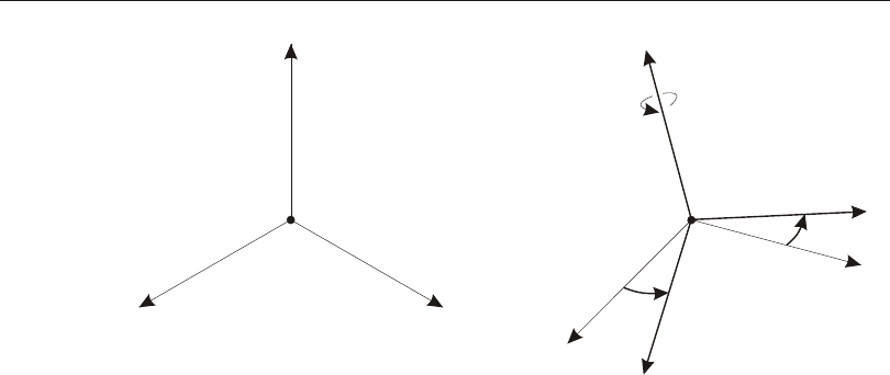
Local Coordinate System
Each Spec has its own response- spectrum lo cal co or di nate sys tem used to de fine
the di rec tions of ground ac cel era tion load ing. The axes of this lo cal sys tem are de -
noted 1, 2, and 3. By de fault these cor re spond to the global X, Y, and Z di rec tions,
re spec tively.
You may change the ori en ta tion of the lo cal co or di nate sys tem by speci fy ing:
•A fixed co or di nate sys tem csys (the de fault is zero, in di cat ing the global co or -
di nate sys tem)
•A co or di nate an gle, ang (the de fault is zero)
The lo cal 3 axis is al ways the same as the Z axis of co or di nate sys tem csys. The lo -
cal 1 and 2 axes co in cide with the X and Y axes of csys if an gle ang is zero. Oth er -
wise, ang is the an gle from the X axis to the lo cal 1 axis, meas ured coun ter clock -
wise when the +Z axis is point ing to ward you. This is il lus trated in Figure 80 (page
385).
Response-Spectrum Function
The re sponse-spec trum curve for a given di rec tion is de fined by dig i tized points of
pseudo-spec tral ac cel er a tion re sponse ver sus pe riod of the struc ture. The shape of
Local Coordinate System 385
Chapter XX Response-Spectrum Anal y sis
ang
ang
ang
Z, 3
Z
X
X
1
2
Y
Y
Global csys
Figure 80
Definition of Response Spectrum Local Coordinate System
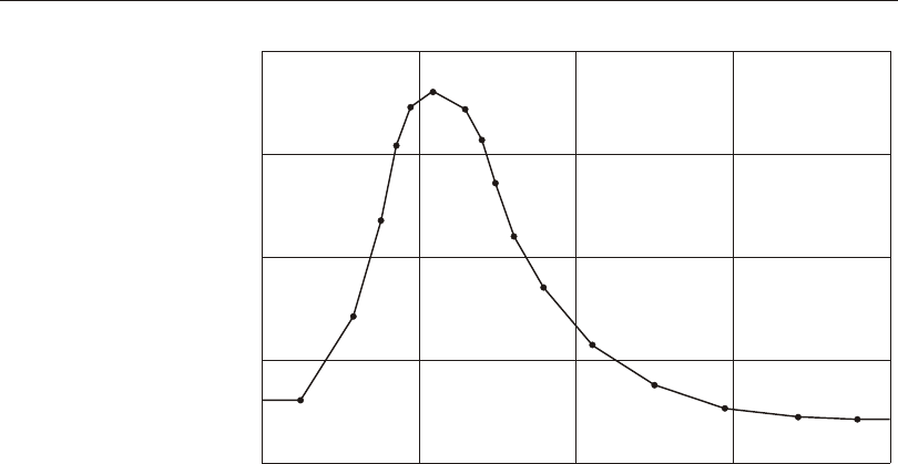
the curve is given by spec i fy ing the name of a Func tion. All val ues for the ab scissa
and or di nate of this Func tion must be zero or pos i tive. See (page 381).
The func tion is as sumed to be nor mal ized with re spect to grav ity. You may spec ify
a scale fac tor sf to mul ti ply the or di nate (pseudo-spec tral ac cel er a tion re sponse) of
the func tion. This should be used to con vert the nor mal ized ac cel er a tion to units
con sis tent with the rest of the model. The scale fac tor it self has ac cel er a tion units
and will be au to mat i cally con verted if you change length units.
If the response- spectrum curve is not de fined over a pe riod range large enough to
cover the Vi bra tion Modes of the struc ture, the curve is ex tended to larger and
smaller pe ri ods us ing a con stant ac cel era tion equal to the value at the near est de -
fined pe riod.
See Topic “Func tions” (page 350) in this Chap ter for more in for ma tion.
Damping
The re sponse-spec trum curve cho sen should re flect the damp ing that is pres ent in
the struc ture be ing mod eled. Note that the damp ing is in her ent in the shape of the
386 Response-Spectrum Function
CSI Analysis Reference Manual
Pseudo-
Spectral
Acceleration
Response
Period (time)
10 2 3 4
10
0
20
30
40
Figure 81
Digitized Response-Spectrum Curve

re sponse-spec trum curve it self. As part of the re sponse-spec trum func tion def i ni -
tion, you must spec ify the damp ing value that was used to gen er ate the re -
sponse-spec trum curve. Dur ing the anal y sis, the re sponse-spec trum curve will au -
to mat i cally be ad justed from this damp ing value to the ac tual damp ing pres ent in
the model.
If zero damp ing is spec i fied for ei ther the re sponse-spec trum func tion or the re -
sponse-spec trum load case, no scal ing will be per formed.
Modal Damping
Damping in the struc ture has two ef fects on re sponse-spec trum anal y sis:
•It mod i fies the shape of the re sponse-spec trum in put curve
•It af fects the amount of statistical cou pling be tween the modes for cer tain
meth ods of re sponse-spec trum modal com bi na tion (e.g., CQC and GMC)
The damp ing in the struc ture is mod eled us ing un cou pled modal damp ing. Each
mode has a damp ing ra tio, damp, which is mea sured as a frac tion of crit i cal damp -
ing and must sat isfy:
01£<damp
Modal damp ing has three dif fer ent sources, which are de scribed in the fol low ing.
Damping from these sources are added to gether. The pro gram au to mat i cally makes
sure that the to tal is less than one.
Modal Damping from the Load Case
For each re sponse-spec trum Load Case, you may spec ify modal damp ing ra tios
that are:
•Con stant for all modes
•Lin early in ter po lated by pe riod or fre quency. You spec ify the damp ing ra tio at
a se ries of fre quency or pe riod points. Be tween spec i fied points the damp ing is
lin early in ter po lated. Out side the spec i fied range, the damp ing ra tio is con stant
at the value given for the clos est spec i fied point.
•Mass and stiff ness pro por tional. This mim ics the pro por tional damp ing used
for di rect-in te gra tion, ex cept that the damp ing value is never al lowed to ex ceed
unity.
Modal Damping 387
Chapter XX Response-Spectrum Anal y sis

In ad di tion, you may op tion ally spec ify damp ing overwrites. These are spe cific
val ues of damp ing to be used for spe cific modes that re place the damp ing ob tained
by one of the meth ods above. The use of damp ing overwrites is rarely nec es sary.
Com pos ite Modal Damping from the Ma te rials
Modal damp ing ra tios, if any, that have been spec i fied for the Ma te rials are con -
verted au to mat i cally to com pos ite modal damp ing. Any cross cou pling be tween the
modes is ig nored. These modal-damp ing val ues will gen er ally be dif fer ent for each
mode, de pend ing upon how much de for ma tion each mode causes in the el e ments
com posed of the dif fer ent Ma te rials.
Ef fec tive Damping from the Link/Support El e ments
Lin ear ef fec tive-damp ing co ef fi cients, if any, that have been spec i fied for
Link/Sup port el e ments in the model are au to mat i cally con verted to modal damp -
ing. Any cross cou pling be tween the modes is ig nored. These ef fec tive
modal-damp ing val ues will gen er ally be dif fer ent for each mode, de pend ing upon
how much de for ma tion each mode causes in the Link/Sup port el e ments.
Modal Combination
For a given di rec tion of ac cel era tion, the maxi mum dis place ments, forces, and
stresses are com puted through out the struc ture for each of the Vi bra tion Modes.
These mo dal val ues for a given re sponse quan tity are com bined to pro duce a sin gle,
posi tive re sult for the given di rec tion of ac cel er a tion. The re sponse has two parts:
pe ri odic and rigid. You can con trol the contribution of these two parts by spec i fy -
ing con trol ling fre quen cies that are properties of the seis mic load ing.
In ad di tion, you can choose the sta tis ti cal method used to com pute the pe ri odic re -
sponse. Modal damp ing, as de scribed in the pre vi ous topic, may af fect the cou pling
be tween the modes, de pend ing upon the method cho sen for pe ri odic modal com bi -
na tion.
Pe riodic and Rigid Response
For all modal com bi na tion meth ods ex cept Ab so lute Sum, there are two parts to the
modal re sponse for a given di rec tion of load ing: pe ri odic and rigid. The dis tinc tion
here is a prop erty of the load ing, not of the struc ture. Two fre quen cies are de fined,
f1 and f2, which de fine the rigid-re sponse con tent of the ground mo tion, where f1 £
f2.
388 Modal Combination
CSI Analysis Reference Manual

For struc tural modes with fre quen cies less than f1 (lon ger pe ri ods), the re sponse is
fully pe ri odic. For struc tural modes with fre quen cies above f2 (shorter pe ri ods), the
re sponse is fully rigid. Be tween fre quen cies f1 and f2, the amount of pe ri odic and
rigid re sponse is in ter po lated, as de scribed by Gupta (1990).
Fre quen cies f1 and f2 are prop er ties of the seis mic in put, not of the struc ture. Gupta
de fines f1 as:
f1=S
S
A
V
max
max
2p
where SAmax is the max i mum spec tral ac cel er a tion and SVmax is the max i mum
spec tral ve loc ity for the ground mo tion con sid ered. The de fault value for f1 is
unity.
Gupta de fines f2 as:
f2f1=+
1
3
2
3fr
where fr is the rigid fre quency of the seis mic in put, i.e., that fre quency above
which the spec tral ac cel er a tion is es sen tially con stant and equal to the value at zero
pe riod (in fi nite fre quency). Oth ers have de fined f2 as:
f2=fr
The fol low ing rules ap ply when spec i fy ing f1 and f2:
•If f2 = 0, no rigid re sponse is cal cu lated and all re sponse is pe ri odic, re gard less
of the value spec i fied for f1.
•Oth er wise, the fol low ing con di tion must be sat is fied: 0 £ f1 £ f2.
•Spec i fy ing f1 = 0 is the same as spec i fy ing f1 = f2.
For any given re sponse quan tity (dis place ment, stress, force, etc.), the pe ri odic re -
sponse, Rp, is com puted by one of the modal com bi na tion meth ods de scribed be -
low. The rigid re sponse, Rr, is al ways com puted as an al ge braic (fully cor re lated)
sum of the re sponse from each mode hav ing fre quency above f2, and an in ter po -
lated por tion of the re sponse from each mode be tween f1 and f2. The to tal re sponse,
R, is com puted by one of the fol low ing two meth ods:
•SRSS, as rec om mended by Gupta (1990) and NRC (2006), which as sumes that
these two parts are statistically in de pend ent:
Modal Combination 389
Chapter XX Response-Spectrum Anal y sis

R R R
p r
= +
2 2
•Ab so lute Sum, for com pat i bil ity with older meth ods:
RRR
pr
=+
Please note that the choice of us ing the SRSS or Ab so lute Sum for com bin ing pe ri -
odic and rigid re sponse is in de pend ent of the pe ri odic modal com bi na tion or the di -
rec tional com bi na tion meth ods de scribed be low.
CQC Method
The Com plete Quad ratic Com bi na tion tech nique for cal cu lat ing the pe ri odic re -
sponse is de scribed by Wil son, Der Kiu re ghian, and Bayo (1981). This is the de -
fault method of mo dal com bi na tion.
The CQC method takes into ac count the sta tis ti cal cou pling be tween closely-
spaced Modes caused by mo dal damp ing. In creas ing the mo dal damp ing in creases
the cou pling be tween closely- spaced modes. If the damp ing is zero for all Modes,
this method de gen er ates to the SRSS method.
GMC Method
The Gen eral Modal Com bi na tion tech nique for cal cu lat ing the pe ri odic re sponse is
the com plete modal com bi na tion pro ce dure de scribed by Equa tion 3.31 in Gupta
(1990). The GMC method takes into ac count the sta tis ti cal cou pling be tween
closely-spaced Modes sim i larly to the CQC method, but uses the Rosenblueth cor -
re la tion co ef fi cient with the time du ra tion of the strong earth quake mo tion set to in -
fin ity. The re sult is es sen tially iden ti cal to the CQC method.
In creas ing the modal damp ing in creases the cou pling be tween closely-spaced
modes. If the damp ing is zero for all Modes, this method de gen er ates to the SRSS
method.
SRSS Method
This method for cal cu lat ing the pe ri odic re sponse com bines the modal re sults by
tak ing the square root of the sum of their squares. This method does not take into
ac count any cou pling of the modes, but rather as sumes that the re sponse of the
modes are all sta tis ti cally in de pend ent. Modal damping does not af fect the re sults.
390 Modal Combination
CSI Analysis Reference Manual

Absolute Sum Method
This method com bines the mo dal re sults by tak ing the sum of their ab so lute val ues.
Essentially all modes are as sumed to be fully cor re lated. This method is usu ally
over-con ser va tive. The dis tinc tion be tween pe ri odic and rigid re sponse is not con -
sid ered for this method. All modes are treated equally. Modal damping does not af -
fect the re sults.
NRC Ten-Percent Method
This tech nique for cal cu lat ing the pe ri odic re sponse is the Ten-Per cent method of
the U.S. Nu clear Reg u la tory Com mis sion Reg u la tory Guide 1.92 (NRC, 2006).
The Ten-Per cent method as sumes full, pos i tive cou pling be tween all modes whose
fre quen cies dif fer from each other by 10% or less of the smaller of the two fre quen -
cies. Modal damp ing does not af fect the cou pling.
NRC Dou ble-Sum Method
This tech nique for cal cu lat ing the pe ri odic re sponse is the Dou ble-Sum method of
the U.S. Nu clear Reg u la tory Com mis sion Reg u la tory Guide 1.92. (NRC, 2006).
The Dou ble-Sum method as sumes a pos i tive cou pling be tween all modes, with cor -
re la tion co ef fi cients that de pend upon damp ing in a fash ion sim i lar to the CQC and
GMC meth ods, and that also de pend upon the du ra tion of the earth quake. You
spec ify this du ra tion as pa ram e ter td as part of the Load Cases def i ni tion.
Directional Combination
For each dis place ment, force, or stress quan tity in the struc ture, the modal com bi -
na tion pro duces a sin gle, pos i tive re sult for each di rec tion of ac cel er a tion. These di -
rec tional val ues for a given re sponse quan tity are com bined to pro duce a sin gle,
pos i tive re sult. Three meth ods are avail able for com bin ing the di rec tional re sponse,
SRSS, CQC3, and Ab so lute Sum.
SRSS Method
This method com bines the re sponse for dif fer ent di rec tions of load ing by tak ing the
square root of the sum of their squares:
Directional Combination 391
Chapter XX Response-Spectrum Anal y sis

R R R R= + +
1
2
2
2
3
2
where R1, R2, and R3 are the modal-com bi na tion val ues for each di rec tion. This
method is in vari ant with re spect to co or di nate sys tem, i.e., the re sults do not de pend
upon your choice of co or di nate sys tem when the given re sponse-spec trum curves
are the same in each di rec tion. This is the de fault method for di rec tional com bi na -
tion, and is closely re lated to the CQC3 method de scribed next.
CQC3 Method
The CQC3 method (Menun and Der Kiureghian, 1998) is an ex ten sion of the SRSS
method of di rec tional com bi na tion. It is ap pli ca ble when the two hor i zon tal spec tra
are iden ti cal in shape but have dif fer ent scale fac tors, as is of ten as sumed. When the
di rec tion of load ing for the two spec tra is not known, it is nec es sary to con sider the
en ve lope of load ing at all pos si ble an gles.
The CQC3 method does this au to mat i cally by cal cu lat ing the crit i cal load ing an gle
for each re sponse quan tity, and re port ing the max i mum re sponse at that an gle. All
that is re quired is to spec ify the same re sponse-spec trum func tion for di rec tions U1
and U2, but with two dif fer ent scale fac tors, and to se lect the CQC3 method for di -
rec tional com bi na tion. The same re sponse will be ob tained no mat ter what value
you spec ify for the load ing an gle, ang, in a given co or di nate sys tem, csys, since all
an gles are en vel oped.
The re sponse to ver ti cal load ing in di rec tion U3, if pres ent, is com bined with the
max i mum hor i zon tal re sponse us ing the SRSS rule. No vari a tion of the ver ti cal di -
rec tion is con sid ered.
If the hor i zon tal spec tra and their scale fac tors are both iden ti cal, the CQC3 method
de gen er ates to the SRSS method.
If dif fer ent spec tra are spec i fied for the two hor i zon tal di rec tions, the CQC3
method may still be se lected and the same cal cu la tions will be performed. How -
ever, the re sults are no lon ger com pletely in de pend ent of load ing an gle, and they
must be re viewed by an en gi neer for their sig nif i cance.
The CQC3 method was orig i nally de fined for pe ri odic re sponse and for the CQC
method of modal com bi na tion. It has been ex tended in SAP2000 to ap ply to all
types of modal com bi na tion, and also to in clude the rigid re sponse, if any. When
the ab so lute modal com bi na tion is used, the CQC3 re sults are not com pletely in de -
pend ent of load ing an gle, but for all qua dratic types of modal com bi na tion, an gu lar
in de pend ence is ob tained. CQC3 can be rec om mended over the SRSS method un -
392 Directional Combination
CSI Analysis Reference Manual

less the di rec tion of load ing is known. Both meth ods are in de pend ent of the choice
of global co or di nate sys tem.
Absolute Sum Method
This method com bines the re sponse for dif fer ent di rec tions of load ing by tak ing the
sum of their ab so lute val ues. A scale fac tor, dirf, is avail able for re duc ing the in ter -
ac tion be tween the dif fer ent di rec tions.
Spec ify dirf = 1 for a sim ple ab so lute sum:
RRRR=++
123
This method is usu ally over-con ser va tive.
Spec ify 0 < dirf < 1 to com bine the di rec tional re sults by the scaled ab so lute sum
method. Here, the di rec tional re sults are com bined by tak ing the max i mum, over all
di rec tions, of the sum of the ab so lute val ues of the re sponse in one di rec tion plus
dirf times the re sponse in the other di rec tions.
For ex am ple, if dirf = 0.3, the spec tral re sponse, R, for a given dis place ment, force,
or stress would be:
RRRR=max(,,)
123
where:
RRRR
1123
03=++.()
RRRR
2213
03=++.()
RRR R
3 3 1 2
03= + +. ( )
and R1, R2, and R3 are the modal-com bi na tion val ues for each di rec tion.
Un like the SRSS and CQC3 meth ods, the absolute sum method can give dif fer ent
re sults de pend ing upon your ar bi trary choice of co or di nate sys tem, even when the
an gle be tween the di rec tion of load ing and the prin ci pal axes of the struc ture is
fixed, and even when the mag ni tude of load ing is the same in two or three di rec -
tions.
Re sults ob tained us ing dirf = 0.3 are com pa ra ble to the SRSS method (for equal in -
put spec tra in each di rec tion), but may be as much as 8% unconservative or 4%
over-con ser va tive, de pend ing upon the co or di nate sys tem. Larger val ues of dirf
tend to pro duce more con ser va tive re sults.
Directional Combination 393
Chapter XX Response-Spectrum Anal y sis

Response-Spectrum Analysis Output
In for ma tion about each re sponse-spec trum Load Case is avail able for dis play,
print ing, and ex port us ing the SAP2000 da ta base tables. This in for ma tion is de -
scribed in the fol low ing subtopics.
Damping and Accelerations
The mo dal damp ing and the ground ac cel era tions act ing in each di rec tion are given
for every Mode.
The damp ing value printed for each Mode is the sum of the spec i fied damp ing for
the Load Case, plus the modal damp ing con trib uted by ef fec tive damp ing in the
Link/Sup port el e ments, if any, and the com pos ite modal damp ing spec i fied in the
Ma te rial Prop erties, if any.
The ac cel era tions printed for each Mode are the ac tual val ues as in ter po lated at the
mo dal pe riod from the response- spectrum curves af ter scal ing by the speci fied
value of sf and mod i fi ca tion for damp ing. The ac cel era tions are al ways re ferred to
the lo cal axes of the response- spectrum analy sis. They are iden ti fied in the out put
as U1, U2, and U3.
Modal Amplitudes
The response- spectrum mo dal am pli tudes give the mul ti pli ers of the mode shapes
that con trib ute to the dis placed shape of the struc ture for each di rec tion of Ac cel -
era tion. For a given Mode and a given di rec tion of ac cel era tion, this is the prod uct
of the mo dal par tici pa tion fac tor and the response- spectrum ac cel era tion, di vided
by the ei gen value, w2, of the Mode.
This am pli tude, mul ti plied by any modal re sponse quan tity (dis place ment, force,
stress, etc.), gives the con tri bu tion of that mode to the value of the same re sponse
quan tity re ported for the re sponse-spec trum load case.
The ac cel era tion di rec tions are al ways re ferred to the lo cal axes of the response-
spectrum analy sis. They are iden ti fied in the out put as U1, U2, and U3.
For more in for ma tion:
•See the pre vi ous Topic “Damp ing and Ac cel era tion” for the defi ni tion of the
response- spectrum ac cel era tions.
394 Response-Spectrum Analysis Output
CSI Analysis Reference Manual

•See Topic “Mo dal Analy sis Out put” (page 349) in Chap ter “Modal Analysis”
for the defi ni tion of the mo dal par tici pa tion fac tors and the ei gen val ues.
Base Reactions
The base re ac tions are the to tal forces and mo ments about the global ori gin re quired
of the sup ports (Re straints, Springs, and one-joint Link/Sup port elements) to re sist
the in er tia forces due to response- spectrum load ing.
These are re ported sep a rately for each in di vid ual Mode and each di rec tion of load -
ing with out any combination. The to tal re sponse-spec trum re ac tions are then re -
ported af ter per form ing mo dal com bi na tion and di rec tional com bi na tion.
The re ac tion forces and mo ments are al ways re ferred to the lo cal axes of the
response- spectrum analy sis. They are iden ti fied in the out put as F1, F2, F3, M1,
M2, and M3.
Im por tant Note: Ac cu rate base re ac tions are best ob tained when static-cor rec tion
modes are in cluded in an eigen anal y sis, or when Ritz vec tors are used. This is par -
tic u larly true when large stiffnesses are used at the sup ports and the model is sen si -
tive or ill-con di tioned.
Response-Spectrum Analysis Output 395
Chapter XX Response-Spectrum Anal y sis

396 Response-Spectrum Analysis Output
CSI Analysis Reference Manual

Chapter XXI
Linear Time-History Anal y sis
Time-his tory anal y sis is a step-by-step anal y sis of the dy nam i cal re sponse of a
struc ture to a spec i fied load ing that may vary with time. The anal y sis may be lin ear
or non lin ear. This Chap ter de scribes time-his tory anal y sis in gen eral, and lin ear
time-his tory anal y sis in par tic u lar. See Chap ter “Non lin ear Time-His tory Anal y -
sis” (page 447) for ad di tional in for ma tion that ap plies only to non lin ear time-his -
tory anal y sis.
Basic Topics for All Users
•Over view
Ad vanced Topics
•Loading
•Ini tial Con di tions
•Time Steps
•Modal Time-His tory Analysis
•Di rect-In te gra tion Time-His tory Anal y sis
397

Overview
Time- history analy sis is used to de ter mine the dy namic re sponse of a struc ture to
ar bi trary load ing. The dy namic equi lib rium equa tions to be solved are given by:
KuCuMur()&()&&
()()tttt++=
where K is the stiff ness ma trix; C is the damp ing ma trix; M is the di ago nal mass
ma trix; u, &
u, and &&
u are the dis place ments, ve loci ties, and ac cel era tions of the struc -
ture; and r is the ap plied load. If the load includes ground acceleration, the
displacements, velocities, and accelerations are relative to this ground motion.
Any number of time- history Load Cases can be de fined. Each time-his tory case can
dif fer in the load ap plied and in the type of analy sis to be per formed.
There are sev eral op tions that de ter mine the type of time-his tory anal y sis to be per -
formed:
•Lin ear vs. Non lin ear.
•Modal vs. Di rect-in te gra tion: These are two dif fer ent so lu tion meth ods, each
with ad van tages and dis ad van tages. Un der ideal cir cum stances, both meth ods
should yield the same re sults to a given prob lem.
•Tran sient vs. Pe ri odic: Tran sient anal y sis con sid ers the ap plied load as a
one-time event, with a be gin ning and end. Pe riodic anal y sis con sid ers the load
to re peat in def i nitely, with all tran sient re sponse damped out.
Pe riodic anal y sis is only avail able for lin ear modal time-his tory anal y sis.
This Chap ter de scribes lin ear anal y sis; non lin ear anal y sis is de scribed in Chap ter
“Non lin ear Time-His tory Anal y sis” (page 447). How ever, you should read the
present Chap ter first.
Loading
The load, r(t), ap plied in a given time-his tory case may be an ar bi trary func tion of
space and time. It can be writ ten as a fi nite sum of spa tial load vec tors, pi, mul ti -
plied by time func tions, ft
i(), as:
(Eqn. 1)
rp()()tft
ii
i
=å
CSI Analysis Reference Manual
398 Overview

The pro gram uses Load Pat terns and/or Ac cel era tion Loads to rep re sent the spa tial
load vec tors. The time func tions can be ar bi trary func tions of time or pe ri odic func -
tions such as those pro duced by wind or sea wave load ing.
If Ac cel era tion Loads are used, the dis place ments, ve loci ties, and ac cel era tions are
all meas ured rela tive to the ground. The time func tions as so ci ated with the Ac cel -
era tion Loads mx, my, and mz are the cor re spond ing com po nents of uni form ground
ac cel era tion, &&
ugx, &&
ugy, and &&
ugz.
Defining the Spatial Load Vectors
To de fine the spa tial load vec tor, pi, for a sin gle term of the load ing sum of Equa tion
1, you may spec ify ei ther:
•The la bel of a Load Pat tern us ing the pa rame ter load, or
•An Ac cel era tion Load us ing the pa rame ters csys, ang, and acc, where:
–csys is a fixed co or di nate sys tem (the de fault is zero, in di cat ing the global
co or di nate sys tem)
–ang is a co or di nate an gle (the de fault is zero)
–acc is the Ac cel era tion Load (U1, U2, or U3) in the ac cel era tion lo cal co or -
di nate sys tem as de fined be low
Each Ac cel era tion Load in the load ing sum may have its own ac cel era tion lo cal co -
or di nate sys tem with lo cal axes de noted 1, 2, and 3. The lo cal 3 axis is al ways the
same as the Z axis of co or di nate sys tem csys. The lo cal 1 and 2 axes co in cide with
the X and Y axes of csys if an gle ang is zero. Oth er wise, ang is the an gle from the X
axis to the lo cal 1 axis, meas ured coun ter clock wise when the +Z axis is point ing to -
ward you. This is il lus trated in Figure 82 (page 400).
The response- spectrum lo cal axes are al ways re ferred to as 1, 2, and 3. The global
Ac cel era tion Loads mx, my, and mz are trans formed to the lo cal co or di nate sys tem
for load ing.
It is gen er ally rec om mended, but not re quired, that the same co or di nate sys tem be
used for all Ac cel era tion Loads ap plied in a given time-his tory case.
Load Pat terns and Ac cel era tion Loads may be mixed in the load ing sum.
For more in for ma tion:
•See Chap ter “Load Pat terns” (page 321).
•See Topic “Ac cel er a tion Loads” (page 338) in Chap ter “Load Pat terns”.
Loading 399
Chapter XXI Linear Time-History Anal y sis
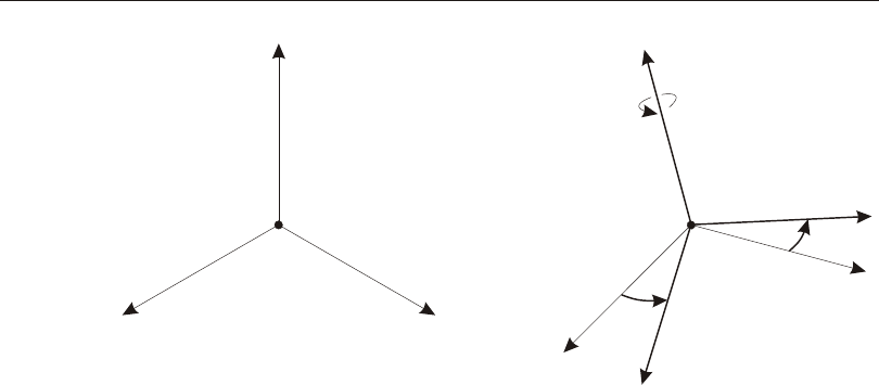
Defining the Time Functions
To de fine the time func tion, fi(t), for a sin gle term of the load ing sum of Equa tion 1,
you may spec ify:
•The la bel of a Func tion, us ing the pa rame ter func, that de fines the shape of the
time varia tion (the de fault is zero, in di cat ing the built- in ramp func tion de fined
be low)
•A scale fac tor, sf, that mul ti plies the or di nate val ues of the Func tion (the de -
fault is unity)
•A time- scale fac tor, tf, that mul ti plies the time (ab scissa) val ues of the Func tion
(the de fault is unity)
•An ar ri val time, at, when the Func tion be gins to act on the struc ture (the de fault
is zero)
The time func tion, fi(t), is re lated to the speci fied Func tion, func(t), by:
fi(t) = sf · func(t)
The analy sis time, t, is re lated to the time scale, t, of the speci fied Func tion by:
t = at + tf · t
400 Loading
CSI Analysis Reference Manual
ang
ang
ang
Z, 3
Z
X
X
1
2
Y
Y
Global csys
Figure 82
Definition of History Acceleration Local Coordinate System
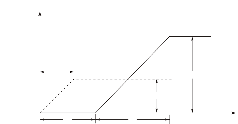
If the ar ri val time is posi tive, the ap pli ca tion of Func tion func is de layed un til af ter
the start of the analy sis. If the ar ri val time is nega tive, that por tion of Func tion func
oc cur ring be fore t = – at / tf is ig nored.
For a Func tion func de fined from ini tial time t0 to fi nal time tn, the value of the
Func tion for all time t < t0 is taken as zero, and the value of the Func tion for all time
t > tn is held con stant at fn, the value at tn.
If no Func tion is speci fied, or func = 0, the built- in ramp func tion is used. This
func tion in creases line arly from zero at t=0 to unity at t=1
and for all time there af -
ter. When com bined with the scal ing pa rame ters, this de fines a func tion that in -
creases line arly from zero at t = at to a value of sf at t = at + tf and for all time there -
af ter, as il lus trated in Figure 83 (page 401). This func tion is most com monly used
to gradu ally ap ply static loads, but can also be used to build up tri an gu lar pulses and
more com pli cated func tions.
See Topic “Func tions” (page 350) in Chap ter “Load Cases” for more in for ma tion.
Loading 401
Chapter XXI Linear Time-History Anal y sis
t
f (t)
i
at tf
sf
1
1
Ramp function after scaling
Built-in ramp function
Figure 83
Built-in Ramp Function before and after Scaling

Ini tial Conditions
The ini tial con di tions de scribe the state of the struc ture at the be gin ning of a
time-his tory case. These in clude:
•Dis place ments and ve loc i ties
•In ter nal forces and stresses
•In ter nal state vari ables for non lin ear elements
•En ergy val ues for the struc ture
•External loads
The ac cel er a tions are not con sid ered ini tial con di tions, but are com puted from the
equi lib rium equa tion.
For lin ear tran sient anal y ses, zero ini tial con di tions are al ways as sumed.
For pe ri odic anal y ses, the pro gram au to mat i cally ad justs the ini tial con di tions at
the start of the anal y sis to be equal to the con di tions at the end of the analysis
If you are us ing the stiff ness from the end of a non lin ear anal y sis, non lin ear el e -
ments (if any) are locked into the state that ex isted at the end of the non lin ear anal y -
sis. For ex am ple, sup pose you per formed a non lin ear anal y sis of a model con tain -
ing ten sion-only frame el e ments (com pres sion limit set to zero), and used the stiff -
ness from this case for a lin ear time-his tory anal y sis. Elements that were in ten sion
at the end of the non lin ear anal y sis would have full ax ial stiff ness in the lin ear
time-his tory analysis, and el e ments that were in com pres sion at the end of the non -
lin ear anal y sis would have zero stiff ness. These stiffnesses would be fixed for the
du ra tion of the lin ear time-his tory anal y sis, regardless of the di rec tion of load ing.
See also Topic “Mass Source” (page 334) in Chap ter “Load Pat terns” for ad di tional
in for ma tion.
Time Steps
Time-his tory anal y sis is per formed at dis crete time steps. You may spec ify the
num ber of out put time steps with pa ram e ter nstep and the size of the time steps
with pa ram e ter dt.
The time span over which the anal y sis is car ried out is given by nstep·dt. For pe ri -
odic anal y sis, the pe riod of the cy clic load ing func tion is as sumed to be equal to this
time span.
402 Ini tial Conditions
CSI Analysis Reference Manual

Re sponses are cal cu lated at the end of each dt time in cre ment, re sult ing in nstep+1
val ues for each out put re sponse quan tity.
Re sponse is also cal cu lated, but not saved, at ev ery time step of the in put time func -
tions in or der to ac cu rately cap ture the full ef fect of the load ing. These time steps
are call load steps. For modal time-his tory anal y sis, this has lit tle ef fect on ef fi -
ciency.
For di rect-in te gra tion time-his tory anal y sis, this may cause the stiff ness ma trix to
be re-solved if the load step size keeps chang ing. For ex am ple, if the out put time
step is 0.01 and the in put time step is 0.005, the pro gram will use a con stant in ter nal
time-step of 0.005. How ever, if the in put time step is 0.075, then the in put and out -
put steps are out of syn chrony, and the loads steps will be: 0.075, 0.025, 0.05, 0.05,
0.025, 0.075, and so on. For this rea son, it is usu ally ad vis able to choose an out put
time step that evenly di vides, or is evenly di vided by, the in put time steps.
Modal Time-His tory Analysis
Modal su per po si tion pro vides a highly ef fi cient and ac cu rate pro ce dure for per -
form ing time-his tory anal y sis. Closed-form in te gra tion of the modal equa tions is
used to com pute the re sponse, as sum ing lin ear vari a tion of the time func tions,
ft
i(), be tween the in put data time points. There fore, nu mer i cal in sta bil ity prob lems
are never en coun tered, and the time in cre ment may be any sam pling value that is
deemed fine enough to cap ture the max i mum re sponse val ues. One-tenth of the
time pe riod of the high est mode is usu ally rec om mended; how ever, a larger value
may give an equally ac cu rate sam pling if the con tri bu tion of the higher modes is
small.
The modes used are com puted in a Modal Load Case that you de fine. They can be
the un damped free-vi bra tion Modes (eigenvectors) or the load-de pend ent Ritz-vec -
tor Modes.
If all of the spa tial load vec tors, pi, are used as start ing load vec tors for Ritz-vec tor
anal y sis, then the Ritz vec tors will al ways pro duce more ac cu rate re sults than if the
same num ber of eigenvectors is used. Since the Ritz-vec tor al go rithm is faster than
the eigenvector al go rithm, the for mer is rec om mended for time-his tory anal y ses.
It is up to you to de ter mine if the Modes cal cu lated by the pro gram are ad e quate to
rep re sent the time-his tory re sponse to the ap plied load. You should check:
•That enough Modes have been com puted
•That the Modes cover an ad e quate fre quency range
Modal Time-His tory Analysis 403
Chapter XXI Linear Time-History Anal y sis

•That the dy namic load (mass) par tic i pa tion mass ra tios are ad e quate for the
Load Pat terns and/or Ac cel er a tion Loads be ing ap plied
•That the modes shapes ad e quately rep re sent all de sired de for ma tions
Im por tant Note: Ac cu rate base re ac tions are best ob tained when static-cor rec tion
modes are in cluded in an eigen anal y sis, or when Ritz vec tors are used. This is par -
tic u larly true when large stiffnesses are used at the sup ports and the model is sen si -
tive or ill-con di tioned. The use of static-cor rec tion modes or Ritz vec tors is gen er -
ally rec om mended for all modal time-his tory analyses.
See Chap ter “Modal Anal y sis” (page 365) for more in for ma tion.
Modal Damping
The damp ing in the struc ture is mod eled us ing un cou pled modal damp ing. Each
mode has a damp ing ra tio, damp, which is mea sured as a frac tion of crit i cal damp -
ing and must sat isfy:
01£<damp
Modal damp ing has three dif fer ent sources, which are de scribed in the fol low ing.
Damping from these sources is added to gether. The pro gram au to mat i cally makes
sure that the to tal is less than one.
Modal Damping from the Load Case
For each lin ear modal time-his tory Load Case, you may spec ify modal damp ing ra -
tios that are:
•Con stant for all modes
•Lin early in ter po lated by pe riod or fre quency. You specify the damp ing ra tio at
a se ries of fre quency or pe riod points. Be tween spec i fied points the damp ing is
lin early in ter po lated. Out side the spec i fied range, the damp ing ra tio is con stant
at the value given for the clos est spec i fied point.
•Mass and stiff ness pro por tional. This mim ics the pro por tional damp ing used
for di rect-in te gra tion, ex cept that the damp ing value is never al lowed to ex ceed
unity.
In ad di tion, you may op tion ally spec ify damp ing overwrites. These are spe cific
val ues of damp ing to be used for spe cific modes that re place the damp ing ob tained
by one of the meth ods above. The use of damp ing overwrites is rarely nec es sary.
404 Modal Time-His tory Analysis
CSI Analysis Reference Manual

Com pos ite Modal Damping from the Ma te rials
Modal damp ing ratios, if any, that have been spec i fied for the Ma te rials are con -
verted au to mat i cally to com pos ite modal damp ing. Any cross cou pling be tween the
modes is ig nored. These modal-damp ing val ues will gen er ally be dif fer ent for each
mode, de pend ing upon how much de for ma tion each mode causes in the el e ments
com posed of the dif fer ent Ma te rials.
Ef fec tive Damping from the Link/Support El e ments
Lin ear ef fec tive-damp ing co ef fi cients, if any, that have been spec i fied for
Link/Sup port el e ments in the model are au to mat i cally con verted to modal damp -
ing. Any cross cou pling be tween the modes is ig nored. These ef fec tive
modal-damp ing val ues will gen er ally be dif fer ent for each mode, de pend ing upon
how much de for ma tion each mode causes in the Link/Sup port el e ments.
Direct-Integration Time-His tory Analysis
Di rect in te gra tion of the full equa tions of mo tion with out the use of modal su per po -
si tion is avail able in SAP2000. While modal su per po si tion is usu ally more ac cu rate
and ef fi cient, di rect-in te gra tion does of fer the fol low ing ad van tages for lin ear prob -
lems:
•Full damp ing that cou ples the modes can be con sid ered
•Im pact and wave prop a ga tion prob lems that might ex cite a large num ber of
modes may be more efficiently solved by di rect in te gra tion
For non lin ear prob lems, di rect in te gra tion also al lows con sid er ation of more types
of nonlinearity that does modal su per po si tion.
Di rect in te gra tion re sults are ex tremely sen si tive to time-step size in a way that is
not true for modal su per po si tion. You should al ways run your di rect-in te gra tion
anal y ses with de creas ing time-step sizes un til the step size is small enough that re -
sults are no lon ger af fected by it.
In par tic u lar, you should check stiff and lo cal ized re sponse quan ti ties. For ex am -
ple, a much smaller time step may be re quired to get ac cu rate re sults for the ax ial
force in a stiff mem ber than for the lat eral dis place ment at the top of a struc ture.
Direct-Integration Time-His tory Analysis 405
Chapter XXI Linear Time-History Anal y sis

Time In te gra tion Pa ram e ters
A va ri ety of com mon meth ods are avail able for per form ing di rect-in te gra tion
time-his tory anal y sis. Since these are well doc u mented in stan dard textbooks, we
will not de scribe them fur ther here, ex cept to sug gest that you use the de fault
“Hilber-Hughes-Tay lor al pha” (HHT) method, un less you have a spe cific pref er -
ence for a dif fer ent method.
The HHT method uses a sin gle pa ram e ter called al pha. This pa ram e ter may take
val ues be tween 0 and -1/3.
For al pha = 0, the method is equiv a lent to the Newmark method with gamma = 0.5
and beta = 0.25, which is the same as the av er age ac cel er a tion method (also called
the trap e zoidal rule.) Using al pha = 0 of fers the high est ac cu racy of the avail able
meth ods, but may per mit ex ces sive vi bra tions in the higher fre quency modes, i.e.,
those modes with pe ri ods of the same or der as or less than the time-step size.
For more neg a tive val ues of al pha, the higher fre quency modes are more se verely
damped. This is not phys i cal damp ing, since it de creases as smaller time-steps are
used. How ever, it is of ten nec es sary to use a neg a tive value of al pha to en cour age a
non lin ear so lu tion to con verge.
For best re sults, use the small est time step prac ti cal, and se lect al pha as close to zero
as pos si ble. Try dif fer ent val ues of al pha and time-step size to be sure that the so lu -
tion is not too de pend ent upon these pa ram e ters.
Damping
In di rect-in te gra tion time-his tory anal y sis, the damp ing in the struc ture is mod eled
us ing a full damp ing ma trix. Un like modal damp ing, this al lows cou pling be tween
the modes to be con sid ered.
Di rect-in te gra tion damp ing has three dif fer ent sources, which are de scribed in the
fol low ing. Damping from these sources is added to gether.
Pro por tional Damping from the Load Case
For each di rect-in te gra tion time-his tory Load Case, you may spec ify pro por tional
damp ing co ef fi cients that ap ply to the struc ture as a whole. The damp ing ma trix is
cal cu lated as a lin ear com bi na tion of the stiff ness ma trix scaled by a co ef fi cient,
cK, and the mass ma trix scaled by a sec ond co ef fi cient, cM.
CSI Analysis Reference Manual
406 Direct-Integration Time-His tory Analysis

You may spec ify these two co ef fi cients di rectly, or they may be com puted by spec -
i fy ing equiv a lent frac tions of crit i cal modal damp ing at two dif fer ent pe ri ods or fre -
quen cies.
For each non lin ear el e ment in the struc ture, the co ef fi cient cK mul ti plies the ini tial
stiff ness ma trix, i.e., the stiff ness of the el e ment at zero ini tial con di tions, re gard -
less of the non lin ear state used to start this anal y sis. The ex cep tion to this rule is that
if the start ing non lin ear state has zero stiff ness and zero force or stress (such as an
open gap or a cracked con crete ma te rial), then zero damp ing is as sumed. In the case
where the ini tial stiff ness is dif fer ent in the neg a tive and pos i tive di rec tion of load -
ing, the larger stiff ness is used.
For ca ble el e ments, the damp ing ma trix is pro por tional to the stiff ness ma trix for an
equiv a lent truss el e ment along the cur rent chord hav ing the same ax ial stiff ness
(AE/L), where L is the undeformed length.
The re sult ing stiff ness-pro por tional damp ing is lin early pro por tional to fre quency.
It is re lated to the de for ma tions within the struc ture. Stiff ness pro por tional damp ing
may ex ces sively damp out high fre quency com po nents.
The re sult ing mass-pro por tional damp ing is lin early pro por tional to pe riod. It is re -
lated to the mo tion of the struc ture, as if the struc ture is mov ing through a vis cous
fluid. Mass pro por tional damp ing may ex ces sively damp out long pe riod com po -
nents.
Proportional Damping from the Ma te rials
You may spec ify stiff ness and mass pro por tional damp ing co ef fi cients for in di vid -
ual ma te ri als. For ex am ple, you may want to use larger co ef fi cients for soil ma te ri -
als than for steel or con crete. The same in ter pre ta tion of these co ef fi cients ap plies
as de scribed above for the Load Case damp ing. Be sure not to dou ble-count the
damp ing by in clud ing the same amount in both the Load Case and the ma te ri als.
Ef fec tive Damping from the Link/Support El e ments
Lin ear ef fec tive-damp ing co ef fi cients, if any, that have been spec i fied for
Link/Sup port el e ments are di rectly in cluded in the damp ing ma trix.
Direct-Integration Time-His tory Analysis 407
Chapter XXI Linear Time-History Anal y sis

408 Direct-Integration Time-His tory Analysis
CSI Analysis Reference Manual

Chapter XXII
Geometric Nonlinearity
SAP2000 is ca pa ble of con sid er ing geo met ric nonlinearity in the form of ei ther
P-delta ef fects or large-dis place ment/ro ta tion ef fects. Strains within the el e ments
are as sumed to be small. Geo met ric nonlinearity can be con sid ered on a
step-by-step ba sis in non lin ear static and di rect-in te gra tion time-his tory anal y sis,
and in cor po rated in the stiff ness ma trix for lin ear anal y ses.
Advanced Topics
•Over view
•Non lin ear Load Cases
•The P-Delta Ef fect
•Ini tial P-Delta Anal y sis
•Large Displacements
Overview
When the load act ing on a struc ture and the re sult ing de flec tions are small enough,
the load-de flec tion re la tion ship for the struc ture is lin ear. For the most part,
SAP2000 anal y ses as sume such lin ear be hav ior. This per mits the pro gram to form
the equi lib rium equa tions us ing the orig i nal (undeformed) ge om e try of the struc -
Overview 409

ture. Strictly speak ing, the equi lib rium equa tions should ac tu ally re fer to the ge om -
e try of the struc ture af ter de for ma tion.
The lin ear equi lib rium equa tions are in de pend ent of the ap plied load and the re sult -
ing de flec tion. Thus the re sults of dif fer ent static and/or dy namic loads can be
superposed (scaled and added), re sult ing in great com pu ta tional ef fi ciency.
If the load on the struc ture and/or the re sult ing de flec tions are large, then the
load-de flec tion be hav ior may be come non lin ear. Sev eral causes of this non lin ear
be hav ior can be iden ti fied:
•P-delta (large-stress) ef fect: when large stresses (or forces and mo ments) are
pres ent within a struc ture, equi lib rium equa tions writ ten for the orig i nal and
the de formed ge om e tries may dif fer sig nif i cantly, even if the de for ma tions are
very small.
•Large-dis place ment ef fect: when a struc ture un der goes large de for ma tion (in
par tic u lar, large strains and ro ta tions), the usual en gi neer ing stress and strain
mea sures no lon ger ap ply, and the equi lib rium equa tions must be writ ten for
the de formed ge om e try. This is true even if the stresses are small.
•Ma te rial nonlinearity: when a ma te rial is strained be yond its pro por tional
limit, the stress-strain re la tion ship is no lon ger lin ear. Plas tic ma te ri als strained
be yond the yield point may ex hibit his tory-de pend ent be hav ior. Ma te rial
nonlinearity may af fect the load-de flec tion be hav ior of a struc ture even when
the equi lib rium equa tions for the orig i nal ge om e try are still valid.
•Other ef fects: Other sources of nonlinearity are also pos si ble, in clud ing non -
lin ear loads, bound ary con di tions and con straints.
The large-stress and large-dis place ment ef fects are both termed geo met ric (or ki ne -
matic) nonlinearity, as dis tin guished from ma te rial nonlinearity. Ki ne matic
nonlinearity may also be re ferred to as sec ond-or der geo met ric ef fects.
This Chap ter deals with the geo met ric nonlinearity ef fects that can be an a lyzed us -
ing SAP2000. For each non lin ear static and non lin ear di rect-in te gra tion time-his -
tory anal y sis, you may choose to con sider:
•No geo met ric nonlinearity
•P-delta ef fects only
•Large dis place ment and P-delta effects
The large dis place ment ef fect in SAP2000 in cludes only the ef fects of large trans la -
tions and ro ta tions. The strains are as sumed to be small in all el e ments.
410 Overview
CSI Analysis Reference Manual

Ma te rial nonlinearity is dis cussed in Chap ters “The Frame Element” (page 105),
“Frame Hinge Properties” (page 147), and “The Link/Sup port Element—Basic”
(page 251). Since small strains are as sumed, ma te rial nonlinearity and geo met ric
nonlinearity ef fects are independent.
Once a non lin ear anal y sis has been per formed, its fi nal stiff ness ma trix can be used
for sub se quent lin ear anal y ses. Any geo met ric nonlinearity con sid ered in the non -
lin ear anal y sis will af fect the lin ear re sults. In par tic u lar, this can be used to in clude
rel a tively con stant P-delta ef fects in build ings or the ten sion-stiff en ing ef fects in
ca ble struc tures into a se ries of su per pos able lin ear anal y ses.
For more in for ma tion:
•See Chap ter “Load Cases” (page 341)
•See Chap ter “Non lin ear Static Anal y sis” (page 425)
•See Chap ter “Non lin ear Time-His tory Anal y sis” (page 447)
Non lin ear Load Cases
For non lin ear static and non lin ear di rect-in te gra tion time-his tory anal y sis, you may
choose the type of geo met ric nonlinearity to consider:
•None: All equi lib rium equa tions are con sid ered in the undeformed con fig u ra -
tion of the struc ture
•P-delta only: The equi lib rium equa tions take into par tial ac count the de formed
con fig u ra tion of the struc ture. Ten sile forces tend to re sist the ro ta tion of el e -
ments and stiffen the struc ture, and com pres sive forces tend to en hance the ro -
ta tion of el e ments and destabilize the struc ture. This may re quire a mod er ate
amount of it er a tion.
•Large dis place ments: All equi lib rium equa tions are writ ten in the de formed
con fig u ra tion of the struc ture. This may re quire a large amount of it er a tion;
New ton-Raphson it er a tions are usu ally most effective. Al though large dis -
place ment and large ro ta tion ef fects are mod eled, all strains are as sumed to be
small. P-delta ef fects are in cluded.
When con tin u ing one non lin ear Load Case from an other, it is rec om mended that
they both have the same geo met ric-nonlinearity set tings.
The large dis place ment op tion should be used for any struc tures un der go ing sig nif -
i cant de for ma tion; and for buck ling anal y sis, par tic u larly for snap-through buck -
ling and post-buck ling be hav ior. Ca bles (mod eled by frame el e ments) and other el -
Non lin ear Load Cases 411
Chapter XXII Geometric Nonlinearity
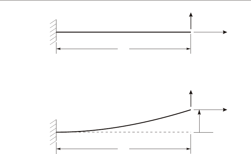
e ments that un dergo sig nif i cant rel a tive ro ta tions within the el e ment should be di -
vided into smaller el e ments to sat isfy the re quire ment that the strains and rel a tive
ro ta tions within an el e ment are small.
For most other struc tures, the P-delta op tion is ad e quate, par tic u larly when ma te rial
nonlinearity dom i nates.
If rea son able, it is rec om mended that the anal y sis be per formed first with out geo -
met ric nonlinearity, add ing P-delta, and pos si bly large-dis place ment ef fects later.
Geo met ric nonlinearity is not avail able for non lin ear modal time-his tory (FNA)
anal y ses, ex cept for the fixed ef fects that may have been in cluded in the stiff ness
ma trix used to gen er ate the modes.
Note that the cat e nary Ca ble el e ment does not re quire P-delta or Large Dis place -
ments to ex hibit its in ter nal geo met ric nonlinearity. The choice should be de ter -
mined by the rest of the struc ture.
412 Non lin ear Load Cases
CSI Analysis Reference Manual
Original Configuration
Deformed Configuration
L
L
P
P
D
F
F
Figure 84
Geometry for Cantilever Beam Example

The P-Delta Effect
The P-Delta ef fect re fers spe cif i cally to the non lin ear geo met ric ef fect of a large
ten sile or com pres sive di rect stress upon trans verse bend ing and shear be hav ior. A
com pres sive stress tends to make a struc tural mem ber more flex i ble in trans verse
bend ing and shear, whereas a ten sile stress tends to stiffen the mem ber against
trans verse de for ma tion.
This op tion is par tic u larly use ful for con sid er ing the ef fect of grav ity loads upon
the lat eral stiff ness of build ing struc tures, as re quired by cer tain de sign codes (ACI
2002; AISC 2003). It can also be used for the anal y sis of some ca ble struc tures,
such as sus pen sion bridges, ca ble-stayed bridges, and guyed tow ers. Other ap pli ca -
tions are pos si ble.
The ba sic con cepts be hind the P- Delta ef fect are il lus trated in the fol low ing ex am -
ple. Con sider a can ti le ver beam sub ject to an ax ial load P and a trans verse tip load F
as shown in Figure 84 (page 412). The in ter nal ax ial force through out the mem ber
is also equal to P.
If equi lib rium is ex am ined in the origi nal con figu ra tion (us ing the un de formed ge -
ome try), the mo ment at the base is MFL=, and de creases line arly to zero at the
loaded end. If, in stead, equi lib rium is con sid ered in the de formed con figu ra tion,
there is an ad di tional mo ment caused by the ax ial force P act ing on the trans verse
tip dis place ment, D. The mo ment no longer var ies line arly along the length; the
varia tion de pends in stead upon the de flected shape. The mo ment at the base is now
MFLP=-D. The mo ment dia grams for vari ous cases are shown in Figure
85 (page 414).
Note that only the trans verse de flec tion is con sid ered in the de formed con figu ra -
tion. Any change in mo ment due to a change in length of the mem ber is ne glected
here.
If the beam is in ten sion, the mo ment at the base and through out the mem ber is re -
duced, hence the trans verse bend ing de flec tion, D, is also re duced. Thus the mem -
ber is ef fec tively stiffer against the trans verse load F.
Con versely, if the beam is in com pres sion, the mo ment through out the mem ber,
and hence the trans verse bend ing de flec tion, D, are now in creased. The mem ber is
ef fec tively more flexi ble against the load F.
If the com pres sive force is large enough, the trans verse stiff ness goes to zero and
hence the de flec tion D tends to in fin ity; the struc ture is said to have buck led. The
The P-Delta Effect 413
Chapter XXII Geometric Nonlinearity
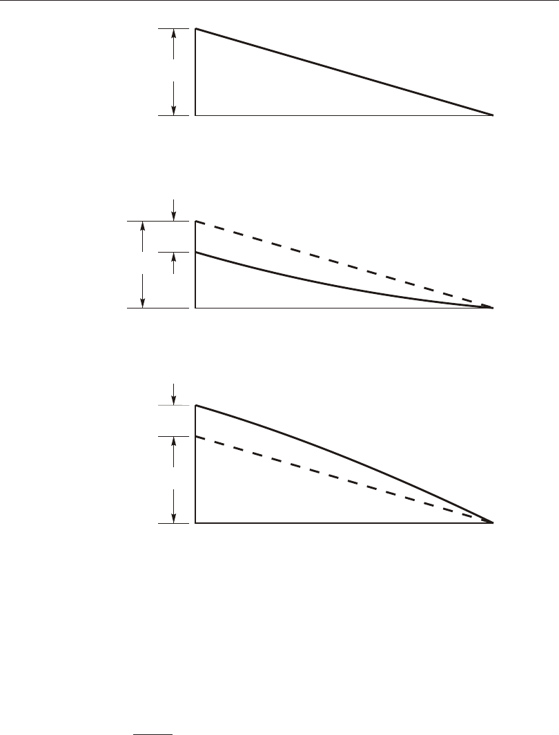
theo reti cal value of P at which this oc curs is called the Euler buck ling load for the
beam; it is de noted by Pcr and is given by the for mula
PEI
L
cr=-p2
2
4
414 The P-Delta Effect
CSI Analysis Reference Manual
Moment in Original Configuration without P-Delta
Moment for Tensile Load P with P-Delta
FL
FL
FL
PD
PD
Moment for Compressive Load P with P-Delta
Figure 85
Moment Diagrams for Cantilever Beam Examples

where EI is the bend ing stiff ness of the beam sec tion.
The ex act P- Delta ef fect of the ax ial load upon the trans verse de flec tion and stiff -
ness is a rather com pli cated func tion of the ra tio of the force P to the buck ling load
Pcr. The true de flected shape of the beam, and hence the ef fect upon the mo ment
dia gram, is de scribed by cu bic func tions un der zero ax ial load, hy per bolic func -
tions un der ten sion, and trigo no met ric func tions un der com pres sion.
The P- Delta ef fect can be pres ent in any other beam con figu ra tion, such as simply-
supported, fixed- fixed, etc. The P- Delta ef fect may ap ply lo cally to in di vid ual
mem bers, or glob ally to the struc tural sys tem as a whole.
The key fea ture is that a large ax ial force, act ing upon a small trans verse de flec tion,
pro duces a sig nifi cant mo ment that af fects the be hav ior of the mem ber or struc ture.
If the de flec tion is small, then the mo ment pro duced is pro por tional to the de flec -
tion.
P-Delta Forces in the Frame Element
The im ple men ta tion of the P-Delta ef fect in the Frame el e ment is de scribed in the
fol low ing subtopics.
Cubic Deflected Shape
The P-Delta ef fect is in te grated along the length of each Frame el e ment, tak ing into
ac count the de flec tion within the el e ment. For this pur pose the trans verse de flected
shape is as sumed to be cu bic for bend ing and lin ear for shear be tween the rigid ends
of the el e ment. The length of the rigid ends is the prod uct of the rigid-end fac tor and
the end off sets, and is usu ally zero. See Topic “End Off sets” (page 127) in Chap ter
“The Frame El e ment” for more in for ma tion.
The true de flected shape may dif fer some what from this as sumed cu bic/lin ear de -
flec tion in the fol low ing sit u a tions:
•The el e ment has non-pris matic Sec tion prop er ties. In this case the P-Delta de -
flected shape is com puted as if the el e ment were pris matic us ing the av er age of
the prop er ties over the length of the el e ment
•Loads are act ing along the length of the el e ment. In this case the P-Delta de -
flected shape is com puted us ing the equiv a lent fixed-end forces ap plied to the
ends of the el e ment.
The P-Delta Effect 415
Chapter XXII Geometric Nonlinearity

•A large P-force is act ing on the el e ment. The true de flected shape is ac tu ally de -
scribed by trig o no met ric func tions un der large com pres sion, and by hy per bolic
func tions un der large ten sion.
The as sumed cu bic shape is usu ally a good ap prox i ma tion to these shapes ex cept
un der a com pres sive P-force near the buck ling load with cer tain end re straints. Ex -
cel lent re sults, how ever, can be ob tained by di vid ing any struc tural mem ber into
two or more Frame el e ments. See the Soft ware Ver i fi ca tion Man ual for more de tail.
Computed P-Delta Axial Forces
The P-Delta ax ial force in each Frame el e ment is de ter mined from the ax ial dis -
place ments com puted in the element. For mean ing ful re sults, it is im por tant to use
re al is tic val ues for the ax ial stiff ness of these el e ments. The ax ial stiff ness is de ter -
mined from the Sec tion prop er ties that de fine the cross-sec tional area and the
modu lus of elas tic ity. Using val ues that are too small may un der es ti mate the
P-Delta ef fect. Using val ues that are too large may make the P-Delta force in the el -
e ment very sen si tive to the it er a tion pro cess.
El e ments that have an ax ial force re lease, or that are con strained against ax ial de -
for ma tion by a Con straint, will have a zero P-Delta ax ial force and hence no
P-Delta ef fect.
The P-Delta ax ial force also in cludes loads that act within the el e ment it self. These
may in clude Self-Weight and Grav ity Loads, Con cen trated and Dis trib uted Span
Loads, Pre stress Load, and Tem per a ture Load.
The P-Delta ax ial force is as sumed to be con stant over the length of each Frame el e -
ment. If the P-Delta load com bi na tion in cludes loads that cause the ax ial force to
vary, then the av er age ax ial force is used for com put ing the P-Delta ef fect. If the
dif fer ence in ax ial force be tween the two ends of an el e ment is small com pared to
the av er age ax ial force, then this ap prox i ma tion is usu ally rea son able. This would
nor mally be the case for the col umns in a build ing struc ture. If the dif fer ence is
large, then the el e ment should be di vided into many smaller Frame el e ments wher -
ever the P-Delta ef fect is im por tant. An ex am ple of the lat ter case could be a flag -
pole un der self-weight.
For more in for ma tion:
•See Topic “Sec tion Prop erties” (page 114) in Chap ter “The Frame El e ment.”
•See Topic “End Re leases” (page 131) in Chap ter “The Frame El e ment.”
•See Chap ter “Con straints and Welds” (page 49).
416 The P-Delta Effect
CSI Analysis Reference Manual

Prestress
When Pre stress Load is in cluded in the P-Delta load com bi na tion, the com bined
ten sion in the prestressing ca bles tends to stiffen the Frame el e ments against trans -
verse de flec tions. This is true re gard less of any ax ial end re leases. Ax ial com pres -
sion of the Frame el e ment due to Pre stress Load may re duce this stiff en ing ef fect,
per haps to zero.
See Topic “Pre stress Load” (page 138) in Chap ter “The Frame El e ment” for more
in for ma tion.
Directly Specified P-delta Axial Forces
You may di rectly spec ify P-delta forces known to be act ing on Frame el e ments.
This is an old-fash ioned fea ture that can be used to model ca ble struc tures where
the ten sions are large and well-known. No it er a tive anal y sis is re quired to in clude
the ef fect of di rectly spec i fied P-Delta ax ial forces.
Use of this fea ture is not usu ally rec om mended! The pro gram does not check if the
forces you spec ify are in equi lib rium with any other part of the struc ture. The di -
rectly spec i fied forces ap ply in all anal y ses and are in ad di tion to any P-delta af -
fects cal cu lated in a non lin ear anal y sis.
We rec om mend in stead that you per form a non lin ear anal y sis in clud ing P-delta or
large-dis place ment ef fects.
If you use di rectly spec i fied P-delta forces, you should treat them as if they were a
sec tion prop erty that al ways af fects the be hav ior of the el e ment.
You can as sign di rectly specified P-Delta force to any Frame el e ment us ing the fol -
low ing pa ram e ters:
•The P-Delta ax ial force, p
•A fixed co or di nate sys tem, csys (the de fault is zero, in di cat ing the global co or -
di nate sys tem)
•The pro jec tion, px, of the P-Delta ax ial force upon the X axis of csys
•The pro jec tion, py, of the P-Delta ax ial force upon the Y axis of csys
•The pro jec tion, pz, of the P-Delta ax ial force upon the Z axis of csys
Normally only one of the pa ram e ters p, px, py, or pz should be given for each
Frame el e ment. If you do choose to spec ify more than one value, they are ad di tive:
The P-Delta Effect 417
Chapter XXII Geometric Nonlinearity

Pc c c
x y z
0= + + +ppx py pz
where P0 is the P-Delta ax ial force, and cx, cy, and cz are the co sines of the an gles be -
tween the lo cal 1 axis of the Frame el e ment and the X, Y, and Z axes of co or di nate
sys tem csys, re spec tively. To avoid di vi sion by zero, you may not spec ify the pro -
jec tion upon any axis of csys that is per pen dic u lar to the lo cal 1 axis of the el e ment.
The use of the P-delta ax ial force pro jec tions is con ve nient, for ex am ple, when
spec i fy ing the ten sion in the main ca ble of a sus pen sion bridge, since the hor i zon tal
com po nent of the ten sion is usu ally the same for all el e ments.
It is im por tant when di rectly spec i fy ing P-Delta ax ial forces that you in clude all
sig nif i cant forces in the struc ture. The pro gram does not check for equi lib rium of
the spec i fied P-Delta ax ial forces. In a sus pen sion bridge, for ex am ple, the ca ble
ten sion is sup ported at the an chor ages, and it is usu ally suf fi cient to con sider the
P-Delta ef fect only in the main ca ble (and pos si bly the tow ers). On the other hand,
the ca ble ten sion in a ca ble-stayed bridge is taken up by the deck and tower, and it is
usu ally nec es sary to con sider the P-Delta ef fect in all three com po nents.
P-Delta Forces in the Link/Support Element
P-delta ef fects can only be con sid ered in a Link/Sup port el e ment if there is stiff ness
in the ax ial (U1) de gree of free dom to gen er ate an ax ial force. A trans verse dis -
place ment in the U2 or U3 di rec tion cre ates a mo ment equal to the ax ial force (P)
times the amount of the de flec tion (delta).
The to tal P-delta mo ment is dis trib uted to the joints as the sum of:
•A pair of equal and op po site shear forces at the two ends that cause a mo ment
due to the length of the el e ment
•A mo ment at End I
•A mo ment at End J
The shear forces act in the same di rec tion as the shear dis place ment (delta), and the
mo ments act about the re spec tively per pen dic u lar bend ing axes.
For each di rec tion of shear dis place ment, you can spec ify three cor re spond ing
frac tions that in di cate how the to tal P-delta mo ment is to be dis trib uted be tween the
three mo ments above. These frac tions must sum to one.
418 The P-Delta Effect
CSI Analysis Reference Manual

For any el e ment that has zero length, the frac tion spec i fied for the shear forces will
be ig nored, and the re main ing two frac tions scaled up so that they sum to one. If
both of these frac tions are zero, they will be set to 0.5.
You must con sider the phys i cal char ac ter is tics of the de vice be ing mod eled by a
Link/Sup port el e ment in or der to de ter mine what frac tions to spec ify. Long brace
or link ob jects would nor mally use the shear force. Short stubby iso la tors would
nor mally use mo ments only. A fric tion-pen du lum iso la tor would nor mally take all
the mo ment on the dish side rather than on the slider side.
Other Elements
For el e ment types other than the Frame and Link/Sup port, the stresses in the each
el e ment are first de ter mined from the dis place ments com puted in the pre vi ous it er -
a tion. These stresses are then in te grated over the el e ment, with re spect to the de riv -
a tives of the isoparametric shape func tions for that el e ment, to com pute a stan dard
geo met ric stiff ness ma trix that rep re sents the P-delta ef fect. This is added to the
orig i nal elas tic stiff ness ma trix of the el e ment. This for mu la tion pro duces only
forces, no mo ments, at each joint in the el e ment.
Shell el e ments that are mod el ing only plate bend ing will not pro duce any P-delta
ef fects, since no in-plane stresses will be de vel oped.
Ini tial P-Delta Analysis
For many ap pli ca tions, it is ad e quate to con sider the P-delta ef fect on the struc ture
un der one set of loads (usu ally grav ity), and to con sider all other anal y ses as lin ear
us ing the stiff ness ma trix de vel oped for this one set of P-delta loads. This en ables
all anal y sis re sults to be superposed for the pur poses of de sign.
To do this, de fine a non lin ear static Load Case that has, at least, the fol low ing fea -
tures:
•Set the name to, say, “PDELTA”
•Start from zero ini tial con di tions
•Apply the Load Pat terns that will cause the P-delta ef fect; of ten this will be
dead load and a frac tion of live load
•For geo met ric nonlinearity, choose P-delta ef fects
Other pa ram e ters in clude the num ber of saved steps, the num ber of it er a tions al -
lowed per step, and the con ver gence tol er ance. If the P-delta ef fect is rea son ably
Ini tial P-Delta Analysis 419
Chapter XXII Geometric Nonlinearity

small, the de fault val ues are ad e quate. We are not con sid er ing staged con struc tion
here, al though that could be added.
We will re fer to this non lin ear static case as the ini tial P-delta case. You can then
de fine or mod ify other lin ear Load Cases so that they use the stiff ness from case
PDELTA:
•Linear static cases
•A modal Load Cases, say called “PDMODES”
•Lin ear di rect-in te gra tion time-his tory cases
•Mov ing-Load Load Cases
Other lin ear Load Cases can be de fined that are based on the modes from case
PDMODES:
•Re sponse-spec trum cases
•Modal time-his tory cases
Re sults from all of these cases are su per pos able, since they are lin ear and are based
upon the same stiff ness ma trix.
You may also want to de fine a buck ling Load Case that ap plies the same loads as
does case PDELTA, and that starts from zero con di tions (not from case PDELTA).
The re sult ing buck ling fac tors will give you an in di ca tion of how far from buck ling
are the loads that cause the P-delta ef fect.
Be low are some ad di tional guide lines re gard ing prac ti cal use of the P-Delta anal y -
sis op tion. See also the Soft ware Ver i fi ca tion Man ual for ex am ple prob lems.
Building Structures
For most build ing struc tures, es pe cially tall build ings, the P-Delta ef fect of most
con cern oc curs in the col umns due to grav ity load, in clud ing dead and live load.
The col umn ax ial forces are com pres sive, mak ing the struc ture more flex i ble
against lat eral loads.
Build ing codes (ACI 2002; AISC 2003) nor mally rec og nize two types of P-Delta
ef fects: the first due to the over all sway of the struc ture and the sec ond due to the
de for ma tion of the mem ber be tween its ends. The for mer ef fect is of ten sig nif i cant;
it can be ac counted for fairly ac cu rately by con sid er ing the to tal ver ti cal load at a
story level, which is due to grav ity loads and is un af fected by any lat eral loads. The
lat ter ef fect is sig nif i cant only in very slen der col umns or col umns bent in sin gle
420 Ini tial P-Delta Analysis
CSI Analysis Reference Manual

cur va ture (not the usual case); this re quires con sid er ation of ax ial forces in the
mem bers due to both grav ity and lat eral loads.
SAP2000 can an a lyze both of these P-Delta ef fects. How ever, it is rec om mended
that the for mer ef fect be ac counted for in the SAP2000 anal y sis, and the lat ter ef fect
be ac counted for in de sign by us ing the ap pli ca ble build ing-code mo ment-mag ni fi -
ca tion fac tors (White and Hajjar 1991). This is how the SAP2000 de sign pro ces sors
for steel frames and con crete frames are set up.
The P-Delta ef fect due to the sway of the struc ture can be ac counted for ac cu rately
and ef fi ciently, even if each col umn is mod eled by a sin gle Frame el e ment, by us ing
the fac tored dead and live loads in the ini tial P-delta Load Case. The it er a tive
P-Delta anal y sis should con verge rap idly, usu ally re quir ing few it er a tions.
As an ex am ple, sup pose that the build ing code re quires the fol low ing load com bi -
na tions to be con sid ered for de sign:
(1) 1.4 dead load
(2) 1.2 dead load + 1.6 live load
(3) 1.2 dead load + 0.5 live load + 1.3 wind load
(4) 1.2 dead load + 0.5 live load – 1.3 wind load
(5) 0.9 dead load + 1.3 wind load
(6) 0.9 dead load + 1.3 wind load
For this case, the P-Delta ef fect due to over all sway of the struc ture can usu ally be
ac counted for, con ser va tively, by spec i fy ing the load com bi na tion in the ini tial
P-delta Load Case to be 1.2 times the dead load plus 0.5 times the live load. This
will ac cu rately ac count for this ef fect in load com bi na tions 3 and 4 above, and will
con ser va tively ac count for this ef fect in load com bi na tions 5 and 6. This P-delta ef -
fect is not gen er ally im por tant in load com bi na tions 1 and 2 since there is no lat eral
load.
The P-Delta ef fect due to the de for ma tion of the mem ber be tween its ends can be
ac cu rately an a lyzed only when sep a rate non lin ear Load Cases are run for each load
com bi na tion above. Six cases would be needed for the ex am ple above. Also, at
least two Frame el e ments per col umn should be used. Again, it is rec om mended
that this ef fect be ac counted for in stead by us ing the SAP2000 de sign features.
Ini tial P-Delta Analysis 421
Chapter XXII Geometric Nonlinearity

Cable Structures
The P-Delta ef fect can be a very im por tant con trib u tor to the stiff ness of sus pen sion
bridges, ca ble-stayed bridges, and other ca ble struc tures. The lat eral stiff ness of ca -
bles is due al most en tirely to ten sion, since they are very flex i ble when un stressed.
In many ca ble struc tures, the ten sion in the ca bles is due pri mar ily to grav ity load,
and it is rel a tively un af fected by other loads. If this is the case, it is ap pro pri ate to
de fine an ini tial P-delta Load Case that ap plies a re al is tic com bi na tion of the dead
load and live load. It is im por tant to use re al is tic val ues for the P-delta load com bi -
na tion, since the lat eral stiff ness of the ca bles is ap prox i mately pro por tional to the
P-delta ax ial forces.
P-delta ef fects are in her ent in any non lin ear anal y sis of Ca ble el e ments. P-delta
anal y sis of the whole struc ture should be con sid ered if you are con cerned about
com pres sion in the tower, or in the deck of a ca ble-stayed bridge.
Be cause con ver gence tends to be slower for stiff en ing than soft en ing struc tures, the
non lin ear P-delta anal y sis may re quire many it er a tions. Twenty or more it er a tions
would not be un usual.
Guyed Towers
In guyed tow ers and sim i lar struc tures, the ca bles are un der a large ten sion pro -
duced by me chan i cal meth ods that shorten the length of the ca bles. These struc tures
can be an a lyzed by the same meth ods dis cussed above for ca bled bridges.
A Strain or Deformation load can be used to pro duce the req ui site short en ing. The
P-delta load com bi na tion should in clude this load, and may also in clude other loads
that cause sig nif i cant ax ial force in the ca bles, such as grav ity and wind loads. Sev -
eral anal y ses may be re quired to de ter mine the mag ni tude of the length change
needed to pro duce the de sired amount of ca ble ten sion.
Large Displacements
Large-dis place ments anal y sis con sid ers the equi lib rium equa tions in the de formed
con fig u ra tion of the struc ture. Large displacements and ro ta tions are ac counted for,
but strains are as sumed to be small. This means that if the po si tion or ori en ta tion of
an el e ment changes, its ef fect upon the struc ture is ac counted for. How ever, if the
el e ment changes sig nif i cantly in shape or size, this ef fect is ig nored.
422 Large Displacements
CSI Analysis Reference Manual

The pro gram tracks the po si tion of the el e ment us ing an up dated Lagrangian for -
mu la tion. For Frame, Shell, and Link/Sup port el e ments, ro ta tional de grees of free -
dom are up dated as sum ing that the change in ro ta tional dis place ments be tween
steps is small. This re quires that the anal y sis use smaller steps than might be re -
quired for a P-delta anal y sis. The ac cu racy of the re sults of a large-dis place ment
anal y sis should be checked by re-run ning the anal y sis us ing a smaller step size and
com par ing the re sults.
Large dis place ment anal y sis is also more sen si tive to con ver gence tol er ance than is
P-delta anal y sis. You should al ways check your re sults by re-run ning the anal y sis
us ing a smaller con ver gence tol er ance and com par ing the re sults.
Applications
Large-dis place ment anal y sis is well suited for the analysis of some ca ble or mem -
brane struc tures. Ca ble struc tures can be mod eled with Frame el e ments, and mem -
brane struc tures with full Shell el e ments (you could also use Plane stress el e ments).
Be sure to di vide the ca ble or mem brane into suf fi ciently small el e ments so that the
rel a tive ro ta tions within each el e ment are small.
The cat e nary Ca ble el e ment does not re quire large-dis place ments anal y sis. For
most struc tures with cables, P-delta anal y sis is suf fi cient un less you ex pect sig nif i -
cant de flec tion or ro ta tion of the struc ture sup port ing or sup ported by the ca bles.
Snap-through buck ling prob lems can be con sid ered us ing large-dis place ment anal -
y sis. For non lin ear static anal y sis, this usu ally re quires us ing dis place ment con trol
of the load ap pli ca tion. More re al is tic so lu tions can be ob tained us ing non lin ear di -
rect-in te gra tion time-history anal y sis.
Ini tial Large-Dis place ment Analysis
The dis cus sion in Topic “Ini tial P-Delta Anal y sis” (page 419) in this Chap ter ap -
plies equally well for an ini tial large-dis place ment anal y sis. De fine the ini tial non -
lin ear static Load Case in the same way, se lect large-dis place ment effects in stead of
P-delta ef fects, and make sure the con ver gence tol er ance is small enough. This case
can be used as the ba sis for all sub se quent lin ear anal y ses.
Large Displacements 423
Chapter XXII Geometric Nonlinearity

424 Large Displacements
CSI Analysis Reference Manual

Chapter XXIII
Nonlinear Static Anal y sis
Non lin ear static anal y sis is can be used for a wide va ri ety of pur poses, in clud ing: to
an a lyze a struc ture for ma te rial and geo met ric nonlinearity; to form the P-delta
stiff ness for sub se quent lin ear anal y ses; to in ves ti gate staged (in cre men tal) con -
struc tion with time-de pend ent ma te rial behavior; to per form ca ble anal y sis; to per -
form static push over anal y sis; and more.
Al though much of this Chap ter is ad vanced, ba sic knowl edge of non lin ear static
anal y sis is es sen tial for P-delta anal y sis and mod el ing of ten sion-only braces and
ca bles.
Basic Topics for All Users
•Over view
•Nonlinearity
•Im por tant Considerations
•Loading
•Ini tial Con di tions
•Out put Steps
425

Ad vanced Topics
•Load Ap pli ca tion Con trol
•Staged Construction
•Non lin ear So lu tion Control
•Static Push over Anal y sis
Overview
Non lin ear static anal y sis can be used for many pur poses:
•To per form an ini tial P-delta or large-dis place ment anal y sis to get the stiff ness
used for sub se quent su per pos able lin ear anal y ses
•To per form staged (in cre men tal, seg men tal) con struc tion anal y sis, in clud ing
ma te rial time-de pend ent ef fects like ag ing, creep and shrink age
•To change the Mass Source to be used for sub se quent analyses
•To an a lyze struc tures with ten sion-only brac ing
•To an a lyze ca ble struc tures
•To per form static push over anal y sis
•To per form snap-through buck ling anal y ses
•To es tab lish the ini tial con di tions for non lin ear di rect-in te gra tion time-his tory
anal y ses
•For any other static anal y sis that con sid ers the ef fect of ma te rial or geo met ric
non lin ear be hav ior
Any num ber of non lin ear Static Load Cases can be de fined. Each case can in clude
one or more of the fea tures above. In a non lin ear anal y sis, the stiff ness and load
may all de pend upon the dis place ments. This re quires an it er a tive so lu tion to the
equa tions of equilibrium.
Nonlinearity
The fol low ing types of nonlinearity are avail able in SAP2000:
•Ma te rial nonlinearity
–Var i ous type of non lin ear prop er ties in Link/Sup port el e ments
–Ten sion and/or com pres sion lim its in Frame el e ments
CSI Analysis Reference Manual
426 Overview

–Plas tic hinges in Frame el e ments
–Non lin ear ma te rial be hav ior in lay ered Shell elements
•Geo met ric nonlinearity
–P-delta ef fects
–Large dis place ment ef fects
•Staged con struc tion
–Changes in the struc ture
–Ag ing, creep, and shrinkage
All ma te rial nonlinearity that has been de fined in the model will be con sid ered in a
non lin ear static Load Case.
You have a choice of the type of geo met ric nonlinearity to be con sid ered:
•None
•P-delta ef fects
•Large dis place ment ef fects
If you are con tin u ing from a pre vi ous non lin ear anal y sis, it is strongly rec om -
mended that you se lect the same geo met ric nonlinearity pa ram e ters for the cur rent
case as for the pre vi ous case. See Chap ter “Geo met ric Nonlinearity” (page 409) for
more in for ma tion.
Staged con struc tion is avail able as an op tion. Even if the in di vid ual stages are lin -
ear, the fact that the struc ture changes from one stage to the next is con sid ered to be
a type of nonlinearity.
Important Considerations
Non lin ear anal y sis takes time and pa tience. Each non lin ear prob lem is dif fer ent.
You can ex pect to need a cer tain amount of time to learn the best way to ap proach
each new prob lem.
Start with a sim ple model and build up grad u ally. Make sure the model per forms as
ex pected un der lin ear static loads and modal anal y sis. Rather than start ing with
non lin ear prop er ties ev ery where, add them in in cre ments be gin ning with the ar eas
where you ex pect the most nonlinearity.
If you are us ing frame hinges, start with mod els that do not lose strength for pri -
mary mem bers; you can mod ify the hinge mod els later or re de sign the struc ture.
Important Considerations 427
Chapter XXIII Nonlinear Static Anal y sis

When possible, perform your ini tial anal y ses with out geo met ric nonlinearity. Add
P-delta ef fects, and pos si bly large de for ma tions, much later. Start with mod est tar -
get dis place ments and a lim ited num ber of steps. In the be gin ning, the goal should
be to per form the anal y ses quickly so that you can gain ex pe ri ence with your
model. As your con fi dence grows with a par tic u lar model you can push it fur ther
and con sider more ex treme non lin ear be hav ior.
Math e matically, non lin ear static anal y sis does not al ways guar an tee a unique so lu -
tion. In er tial ef fects in dy namic anal y sis and in the real world limit the path a struc -
ture can fol low. But this is not true for static anal y sis, par tic u larly in un sta ble cases
where strength is lost due to ma te rial or geo met ric nonlinearity. If a non lin ear static
anal y sis con tin ues to cause dif fi cul ties, change it to a di rect-in te gra tion time-his -
tory anal y sis and ap ply the load quasi-stat i cally (very slowly.)
Small changes in prop er ties or load ing can cause large changes in non lin ear re -
sponse. For this rea son, it is ex tremely im por tant that you con sider many dif fer ent
load ing cases, and that you per form sen si tiv ity stud ies on the ef fect of vary ing the
prop er ties of the struc ture.
Loading
You may ap ply any com bi na tion of Load Pat terns, Ac cel er a tion Loads, and modal
loads.
A modal load is a spe cial ized type of load ing used for push over anal y sis. It is a pat -
tern of forces on the joints that is pro por tional to the prod uct of a spec i fied mode
shape times its cir cu lar fre quency squared (w2) times the mass trib u tary to the joint.
The spec i fied com bi na tion of loads is ap plied si mul ta neously. Normally the loads
are ap plied incrementally from zero to the full spec i fied mag ni tude. For spe cial ized
pur poses (e.g., push over or snap-though buck ling), you have the op tion to con trol
the load ing by mon i tor ing a re sult ing dis place ment in the struc ture. See Topic
“Load Ap pli ca tion Con trol” (page 428) in this Chap ter for more in for ma tion.
Load Application Con trol
You may choose be tween a load-con trolled or dis place ment-con trolled non lin ear
static anal y sis. For both op tions, the pat tern of loads act ing on the struc ture is de ter -
mined by the spec i fied com bi na tion of loads. Only the scal ing is dif fer ent.
428 Loading
CSI Analysis Reference Manual

Normally you would choose load con trol. It is the most com mon, phys i cal sit u a -
tion.
Dis place ment con trol is an ad vanced fea ture for spe cial ized pur poses.
Load Con trol
Se lect load con trol when you know the mag ni tude of load that will be ap plied and
you ex pect the struc ture to be able to sup port that load. An ex am ple would be when
ap ply ing grav ity load, since it is gov erned by na ture.
Un der load con trol, all loads are ap plied incrementally from zero to the full spec i -
fied mag ni tude.
Dis place ment Con trol
Se lect dis place ment con trol when you know how far you want the struc ture to
move, but you don’t know how much load is re quired. This is most use ful for struc -
tures that be come un sta ble and may lose load-car ry ing ca pac ity dur ing the course
of the anal y sis. Typ i cal ap pli ca tions in clude static push over anal y sis and
snap-through buck ling anal y sis.
To use dis place ment con trol, you must se lect a dis place ment com po nent to mon i -
tor. This may be a sin gle de gree of free dom at a joint, or a gen er al ized displacement
that you have pre vi ously de fined. See Topic “Gen er al ized Dis place ment” (page 45)
in Chap ter “Joints and De grees of Free dom” for more in for ma tion.
You must also give the mag ni tude of the dis place ment that is your tar get for the
anal y sis. The pro gram will at tempt to ap ply the load to reach that dis place ment.
The load mag ni tude may be in creased and de creased dur ing the anal y sis.
Be sure to choose a dis place ment com po nent that monotonically in creases dur ing
load ing. If this is not pos si ble, you may need to di vide the anal y sis into two or more
se quen tial cases, chang ing the mon i tored dis place ment in the dif fer ent cases. The
use of the con ju gate dis place ment control, de scribed be low, may help solve this
prob lem for you.
Im por tant note: Using dis place ment con trol is NOT the same thing as ap ply ing
dis place ment load ing on the struc ture! Dis place ment con trol is sim ply used to
MEA SURE the dis place ment at one point that re sults from the ap plied loads, and to
ad just the mag ni tude of the load ing in an at tempt to reach a cer tain mea sured dis -
place ment value. The over all dis placed shape of the struc ture will be dif fer ent for
dif fer ent pat terns of load ing, even if the same dis place ment is controlled.
Load Application Con trol 429
Chapter XXIII Nonlinear Static Anal y sis

Con ju gate Dis place ment Control
If anal y sis is hav ing trou ble reach ing the de sired dis place ment target, you can try
the op tion for the load case to use the con ju gate dis place ment for con trol. The
conjugate dis place ment is a weighted av er age of all dis place ments in the struc ture,
each dis place ment de gree of free dom be ing weighted by the load acting on that de -
gree of free dom. In other words, it is a mea sure of the work done by the ap plied
load.
This op tion is par tic u larly use ful for un sym met ri cal build ings where the top story
level may ro tate about the ver ti cal axis while be ing pushed un der lat eral load. The
ro ta tion could cause the mon i tored dis place ment to move back ward even while the
weighted av er age dis place ment is mov ing for ward.
If you choose to use the con ju gate dis place ment con trol, it will be used to de ter mine
whether the load should be in creased or de creased. The spec i fied mon i tored dis -
place ment will still be used to set the tar get dis place ment, i.e., how far the struc ture
should move. How ever, this tar get may not be matched ex actly.
Ini tial Conditions
The ini tial con di tions de scribe the state of the struc ture at the be gin ning of a Load
Case. These in clude:
•Dis place ments and ve loc i ties
•In ter nal forces and stresses
•In ter nal state vari ables for non lin ear elements
•En ergy val ues for the struc ture
•Ex ter nal loads
For a static anal y sis, the ve loc i ties are al ways taken to be zero.
For non lin ear anal y ses, you may spec ify the ini tial con di tions at the start of the
anal y sis. You have two choices:
•Zero ini tial con di tions: the struc ture has zero dis place ment and ve loc ity, all el -
e ments are un stressed, and there is no his tory of non lin ear de for ma tion.
•Con tinue from a pre vi ous non lin ear anal y sis: the dis place ments, ve loc i ties,
stresses, loads, en er gies, and non lin ear state his to ries from the end of a pre vi -
ous anal y sis are car ried for ward.
430 Ini tial Conditions
CSI Analysis Reference Manual

Non lin ear static and non lin ear di rect-in te gra tion time-his tory cases may be chained
to gether in any com bi na tion, i.e., both types of anal y sis are com pat i ble with each
other. It is strongly rec om mended that you se lect the same geo met ric nonlinearity
pa ram e ters for the cur rent case as for the pre vi ous case.
When con tin u ing from a pre vi ous case, all ap plied loads spec i fied for the pres ent
Load Case are in cre men tal, i.e., they are added to the loads al ready act ing at the end
of the pre vi ous case.
When mul ti ple Mass Sources have been de fined, you can spec ify which Mass
Source to use for a non lin ear static or non lin ear di rect-in te gra tion time-his tory load
case. How ever, the de fault is to use the same Mass Source as the pre vi ous load
case, or the de fault Mass Source if start ing from zero ini tial con di tions. See Topic
“Mass Source” (page 334) in Chap ter “Load Pat terns” for more in for ma tion.
Non lin ear static cases can not be chained to gether with non lin ear modal time-his -
tory (FNA) cases.
Output Steps
Normally, only the fi nal state is saved for a non lin ear static anal y sis. This is the re -
sult af ter the full load has been ap plied.
You can choose in stead to save in ter me di ate re sults to see how the struc ture re -
sponded dur ing load ing. This is par tic u larly im por tant for static push over anal y sis,
where you need to de velop the ca pac ity curve.
If you are only in ter ested in the sav ing the fi nal re sult, you can skip the rest of this
topic.
Saving Multiple Steps
If you choose to save mul ti ple states, the state at the be gin ning of the anal y sis (step
0) will be saved, as well as a num ber of in ter me di ate states. From a ter mi nol ogy
point of view, sav ing five steps means the same thing as sav ing six states (steps 0 to
5): the step is the in cre ment, and the state is the re sult.
The num ber of saved steps is de ter mined by the pa ram e ters:
•Min i mum num ber of saved steps
•Max i mum num ber of saved steps
•Op tion to save pos i tive in cre ments only
Output Steps 431
Chapter XXIII Nonlinear Static Anal y sis

These are de scribed in the fol low ing.
Min i mum and Max i mum Saved Steps
The Min i mum Num ber of Saved Steps and Max i mum Num ber of Saved Steps pro -
vide con trol over the num ber of points ac tu ally saved in the anal y sis. If the min i -
mum num ber of steps saved is too small, you may not have enough points to ad e -
quately rep re sent a push over curve. If the min i mum and max i mum num ber of
saved steps is too large, then the anal y sis may con sume a con sid er able amount of
disk space, and it may take an ex ces sive amount of time to dis play re sults.
The pro gram au to mat i cally de ter mines the spac ing of steps to be saved as fol lows.
The max i mum step length is equal to to tal force goal or to tal dis place ment goal di -
vided by the spec i fied Min i mum Num ber of Saved Steps. The pro gram starts by
sav ing steps at this in cre ment. If a sig nif i cant event oc curs at a step length less than
this in cre ment, then the pro gram will save that step too and con tinue with the max i -
mum in cre ment from there. For ex am ple, sup pose the Min i mum Num ber of Saved
Steps and Max i mum Num ber of Saved Steps are set at 20 and 30 re spec tively, and
the tar get is to be to a dis place ment of 10 inches. The max i mum in cre ment of saved
steps will be 10 / 20 = 0.5 inches. Thus, data is saved at 0.5, 1, 1.5, 2, 2.5 inches.
Sup pose that a sig nif i cant event oc curs at 2.7 inches. Then data is also saved at 2.7
inches, and con tin ues on from there be ing saved at 3.2, 3.7, 4.2, 4.7, 5.2, 5.7, 6.2,
6.7, 7.2, 7.7, 8.2, 8.7, 9.2, 9.7 and 10.0 inches.
The Max i mum Num ber of Saved Steps con trols the num ber of sig nif i cant events
for which data will be saved. The pro gram will al ways reach the force or dis place -
ment goal within the spec i fied num ber of max i mum saved steps, how ever, in do ing
so it could have to skip sav ing steps at later events. For ex am ple, sup pose the Min i -
mum Saved Steps is set to 20, the Max i mum Num ber of Saved Steps is set to 21,
and the push over is to be to a dis place ment of 10 inches. The max i mum in cre ment
of saved steps will be 10 / 20 = 0.5 inches. Thus, data is saved at 0.5, 1, 1.5, 2, 2.5
inches. Sup pose that a sig nif i cant event oc curs at 2.7 inches. Then data is also saved
at 2.7 inches, and con tin ues on from there be ing saved at 3.2 and 3.7 inches. Sup -
pose an other sig nif i cant event oc curs at 3.9 inches. The pro gram will not save the
data at 3.9 inches be cause if it did it would not be able to limit the max i mum in cre -
ment to 0.5 inches and still get through the full push over in no more than 21 steps.
Note that if a sec ond sig nif i cant event oc curred at 4.1 inches rather than 3.9 inches,
then the pro gram would be able to save the step and still meet the spec i fied cri te ria
for max i mum in cre ment and max i mum num ber of steps.
CSI Analysis Reference Manual
432 Output Steps

Save Pos i tive In cre ments Only
This op tion is pri mar ily of in ter est for push over anal y sis un der dis place ment con -
trol. In the case of ex treme nonlinearity, particularly when a frame hinge sheds
load, the push over curve may show neg a tive in cre ments in the mon i tored dis place -
ment while the struc ture is try ing to re dis trib ute the force from a fail ing com po nent.
You may choose whether or not you want to save only the steps hav ing pos i tive in -
cre ments. The neg a tive in cre ments of ten make the push over curve look con fus ing.
How ever, see ing them can pro vide in sight into the per for mance of the anal y sis and
the struc ture.
You may want to choose to Save Positive Increments Only in most cases ex cept
when the anal y sis is hav ing trou ble con verg ing.
Nonlinear Solution Control
The spec i fied com bi na tion of ap plied loads is ap plied incrementally, us ing as many
steps as nec es sary to sat isfy equi lib rium and to pro duce the re quested num ber of
saved out put steps.
The non lin ear equa tions are solved iteratively in each load step. This may re quire
re-form ing and re-solv ing the stiff ness ma trix. The it er a tions are car ried out un til
the so lu tion con verges. If con ver gence can not be achieved, the pro gram di vides the
step into smaller substeps and tries again.
Sev eral pa ram e ters are avail able for you to con trol the it er a tion and substepping
pro cess. These are de scribed in the fol low ing. We rec om mend that you use the de -
fault val ues of these pa ram e ters to start, ex cept that you may of ten need to in crease
the max i mum num ber of to tal steps and null steps for more complex models.
If you are hav ing con ver gence dif fi cul ties, you may try vary ing the it er a tion con trol
pa ram e ters be low. How ever, you should also con sider that the model it self may
need im prove ment. Look for in sta bil i ties due to in ad e quate sup port, buck ling, and
ex ces sively large stiffnesses. If you have hinges or ma te ri als that lose strength,
make sure that this be hav ior is re ally nec es sary and that the neg a tive slopes are not
unrealistically too steep.
Nonlinear Solution Control 433
Chapter XXIII Nonlinear Static Anal y sis

Max i mum Total Steps
This is the max i mum num ber of steps al lowed in the anal y sis. It may in clude saved
steps as well as in ter me di ate substeps whose re sults are not saved. The pur pose of
set ting this value is to give you con trol over how long the anal y sis will run.
Start with a smaller value to get a feel for the time the anal y sis will take. If an anal y -
sis does not reach its tar get load or dis place ment be fore reach ing the max i mum
num ber of steps, you can re-run the anal y sis af ter in creas ing this max i mum num ber
of saved steps. The length of time it takes to run a non lin ear static anal y sis is ap -
prox i mately pro por tional to the total number of steps.
Max i mum Null (Zero) Steps
Null (zero) steps may oc cur dur ing the non lin ear so lu tion pro ce dure when:
•It er a tion does not con verge and a smaller step size is at tempted
•Snap-back is de tected due to strength loss in a frame hinge
An ex ces sive num ber of null steps may in di cate that the so lu tion is stalled due to in -
sta bil ity or nu mer i cal sen si tiv ity.
You can set the Max i mum Null (Zero) Steps so that the so lu tion will ter mi nate
early if it is hav ing trou ble con verg ing. Set this value equal to the Max i mum To tal
Steps if you do not want the anal y sis to ter mi nate due to null steps.
Event-to-Event Stepping Control
Event-to-event step ping is avail able as an op tion for non lin ear static anal y sis. Us -
ing this strat egy, an in cre ment of load is ap plied un til one of the non lin ear el e ments
ex pe ri ences an “event” that causes a sig nif i cant change in the stiff ness of the struc -
ture. It er a tion is per formed for this load in cre ment to en sure that equi lib rium is
achieved to within a spec i fied con ver gence tol er ance. The stiff ness ma trix is then
re formed, and an other load in cre ment is ap plied to reach the next event. This con -
tin ues in a se ries of event steps until the entire load has been applied.
Events are im ple mented for the fol low ing non lin ear mod els: all frame hinges; lay -
ered shells with di rec tional or cou pled non lin ear be hav ior; and links with multi-lin -
ear plas tic ity, gap, hook, fric tion-pen du lum, and tri ple-pen du lum be hav ior. Events
typ i cally in clude first yield, un load ing, strength loss, in creas ing stiff ness, and other
sig nif i cant changes in be hav ior that de pend on the type of element or material.
434 Nonlinear Solution Control
CSI Analysis Reference Manual

You can spec ify whether or not to use event-to-event step ping. When events are
used, each load in cre ment tends to be more lin ear, thus re duc ing equi lib rium un bal -
ance and less en ing the need for it er a tion. On the other hand, mod els with a large
num ber of non lin ear el e ments and/or hinges may gen er ate a large num ber of
events, which can sig nif i cantly in crease the analysis time.
When us ing event step ping, you can spec ify a rel a tive event-lump ing tol er ance that
will group mul ti ple events to gether. Ef fec tively, the load in cre ment cal cu lated to
reach the first event is in creased by the tol er ance to in clude other events that would
oc cur soon af ter ward. Larger event tol er ances re duce the num ber of event steps
taken, but may in crease the amount of iteration re quired.
Note that for iso tro pic frame hinges the event lump ing tol er ance may also al low the
force or de for ma tion re sponse to deviate from the back bone curve. The rel a tive
mag ni tude of the de vi a tions is on the or der of the rel a tive lump ing tol er ance.
Whether or not to use event step ping is a prob lem-de pend ent de ci sion. Nor mally
us ing events will im prove con ver gence be hav ior. How ever, if a large num ber of
event steps are gen er ated that make the anal y sis run slowly, try turn ing event-step -
ping off for that model or load case. Ei ther way, re sults for a sta ble model should be
con sis tent to within the convergence tolerance.
Non lin ear it er a tion is al ways used for non lin ear static anal y sis, whether or not
event-step ping is used. This is dif fer ent from non lin ear di rect-in te gra tion time-his -
tory anal y sis where events can be used with or with out it er a tion. Note that the
line-search it er a tion op tion is not avail able when event step ping is used for
nonlinear static analysis.
Nonlinear Iteration
It er a tion is used to en sure that equi lib rium is achieved at each step and substep of
the anal y sis to within a spec i fied con ver gence tol er ance. You can spec ify the rel a -
tive con ver gence tol er ance used to com pare the mag ni tude of force er ror with the
mag ni tude of the force acting on the structure.
You may need to use sig nif i cantly smaller val ues of con ver gence tol er ance to get
good re sults for large-dis place ments prob lems than for other types of nonlinearity.
Try de creas ing this value un til you get con sis tent results.
For each step, con stant-stiff ness it er a tion is tried first. If con ver gence is not
achieved, New ton-Raphson (tan gent-stiff ness) it er a tion is tried next. If both fail,
the step size is re duced, and the pro cess is repeated.
Nonlinear Solution Control 435
Chapter XXIII Nonlinear Static Anal y sis

You can sep a rately con trol the num ber of con stant-stiff ness and New ton-Raphson
it er a tions al lowed in each step. Set ting ei ther pa ram e ter to zero pre vents that type
of it er a tion. Set ting both to zero causes the anal y sis to use the de fault num ber of it -
er a tions. Con stant-stiff ness it er a tions are faster than New ton-Raphson it er a tions,
but the lat ter are usu ally more ef fec tive, es pe cially for ca bles and geo met ric
nonlinearity. The default values work well in many situations.
Line Search Option
Line search is an it er a tion op tion that can in crease the ef fi ciency of equi lib rium it -
er a tions by scal ing the so lu tion in cre ment in a trial-and-er ror fash ion to find the
small est un bal ance. This in creases the com pu ta tion time for each it er a tion, but of -
ten re sults in fewer it er a tions and better con ver gence be hav ior, with a net gain in ef -
fi ciency. Line search is par tic u larly ef fec tive for stiff en ing sys tems, such as tight -
en ing ca bles, clos ing gaps, un load ing from plas tic yielding, and sticking after
frictional sliding.
You can choose whether or not to use line search, ex cept that line search is not
avail able when us ing event-to-event step ping. Line search is also not used for dis -
place ment-con trolled load cases.
When us ing line search, spec ify the fol low ing pa ram e ters:
•Max i mum num ber of line searches per It er a tion. Use this pa ram e ter to limit
the num ber of line searches al lowed per it er a tion, usu ally in the range of 5
to 40.
•Line-Search Ac cep tance Tol er ance (Rel a tive). The so lu tion in cre ment is
suc ces sively re duced or in creased un til the min i mum er ror is found, the
max i mum num ber of line searches is reached, or the rel a tive change in er -
ror from the pre vi ous trial is less than the ac cep tance tol er ance set here.
The prac ti cal range is about 0.02 to 0.50. This value should not be too
small, since the goal is only to im prove the next it er a tion.
•Line-Search Step Fac tor. For each line-search trial, the so lu tion in cre ment
is suc ces sively re duced by the step fac tor spec i fied here un til the min i mum
er ror is found, the max i mum num ber of line searches is reached, or the ac -
cep tance tol er ance is sat is fied. If re duc ing the in cre ment does not de crease
the er ror, the in cre ment is in stead in creased by the step fac tor fol low ing the
same pro ce dure. This fac tor must be greater than 1.0, and should usually be
no more than 2.0.
436 Nonlinear Solution Control
CSI Analysis Reference Manual

The de fault val ues are rec om mended as start ing point. For stiff en ing sys tems that
are slow to con verge, try in creas ing the max i mum num ber of line searches per it er -
a tion, de creas ing the ac cep tance tol er ance, and re duc ing the step fac tor.
Static Push over Anal y sis
Non lin ear static push over anal y sis is a spe cial ized pro ce dure used in per for -
mance-based de sign for seis mic load ing. SAP2000 pro vides the fol low ing tools
needed for push over anal y sis:
•Ma te rial nonlinearity at dis crete, user-de fined hinges in Frame el e ments. The
hinge prop er ties were cre ated with push over anal y sis in mind. De fault hinge
prop er ties are pro vided based on ASCE 41and other code-based cri te ria. See
Chap ter “Frame Hinge Prop erties” (page 147). In ETABS, dis crete fi ber P-M3
hinges can be as signed to wall el e ments.
•Non lin ear static anal y sis pro ce dures spe cially de signed to han dle the sharp
drop-off in load car ry ing ca pac ity typ i cal of frame hinges used in push over
anal y sis.
•Non lin ear static anal y sis pro ce dures that al low dis place ment con trol, so that
un sta ble struc tures can be pushed to de sired dis place ment tar gets. See Topic
“Load Ap pli ca tion Control” (page 428) in this Chap ter.
•Dis play ca pa bil i ties in the graph i cal user in ter face to gen er ate and plot push -
over curves, in clud ing de mand and ca pac ity curves in spec tral or di nates. See
the on line Help fa cil ity in the graph i cal user in ter face for more in for ma tion.
•Ca pa bil ities in the graph i cal user in ter face to plot and out put the state of ev ery
hinge at each step in the push over anal y sis. See Chap ter “Frame Hinge Prop -
erties” (page 147) and the on line Help fa cil ity in the graph i cal user in ter face for
more in for ma tion.
In ad di tion to these spe cial ized fea tures, the full nonlinearity of the pro gram can be
used, in clud ing non lin ear Shell and Link/Sup port be hav ior, geo met ric
nonlinearity, and staged con struc tion. In ad di tion, you are not re stricted to static
push over anal y sis: you can also per form full non lin ear time-his tory anal y sis.
The fol low ing gen eral se quence of steps is in volved in per form ing non lin ear static
push over anal y sis us ing SAP2000:
1. Cre ate a model just like you would for any other anal y sis.
2. De fine frame hinge prop er ties and assign them to the frame el e ments.
Static Push over Anal y sis 437
Chapter XXIII Nonlinear Static Anal y sis

3. De fine any Load Pat terns and static and dy namic Load Cases that may be
needed for steel or con crete de sign of the frame el e ments, par tic u larly if de fault
hinges are used.
4. Run the Load Cases needed for de sign.
5. If any con crete hinge prop er ties are based on de fault val ues to be com puted by
the pro gram, you must per form con crete de sign so that re in forc ing steel is de -
ter mined.
6. If any steel hinge prop er ties are based on de fault val ues to be com puted by the
pro gram for Auto-Se lect frame sec tion prop er ties, you must per form steel de -
sign and ac cept the sec tions cho sen by the pro gram.
7. De fine the Load Pat terns that are needed for use in the push over anal y sis,
including:
•Grav ity loads and other loads that may be act ing on the struc ture be fore the
lat eral seis mic loads are ap plied. You may have al ready de fined these Load
Pat terns above for de sign.
•Lat eral loads that will be used to push the struc ture. If you are go ing to use
Acceleration Loads or modal loads, you don’t need any new Load Pat terns,
al though modal loads re quire you to de fine a Modal Load Case.
8. De fine the non lin ear static Load Cases to be used for push over anal y sis, in clud -
ing:
•A se quence of one or more cases that start from zero and ap ply grav ity and
other fixed loads us ing load con trol. These cases can in clude staged con -
struc tion and geo met ric nonlinearity.
•One or more push over cases that start from this se quence and ap ply lat eral
push over loads. These loads should be ap plied un der dis place ment con trol.
The mon i tored dis place ment is usu ally at the top of the struc ture and will
be used to plot the push over curve.
9. Run the push over Load Cases.
10. Re view the push over re sults: Plot the push over curve, the de flected shape
show ing the hinge states, force and mo ment plots, and print or dis play any
other re sults you need.
11. Re vise the model as nec es sary and re peat.
438 Static Push over Anal y sis
CSI Analysis Reference Manual

It is im por tant that you con sider sev eral dif fer ent lat eral push over cases to rep re sent
dif fer ent se quences of re sponse that could oc cur dur ing dy namic load ing. In par tic -
u lar, you should push the struc ture in both the X and Y di rec tions, and pos si bly at
an gles in be tween. For non-sym met ri cal struc tures, push ing in the pos i tive and
neg a tive di rec tion may yield dif fer ent re sults. When push ing in a given di rec tion,
you may want to con sider dif fer ent ver ti cal dis tri bu tions of the lat eral load, such as
the first and sec ond mode in that di rec tion.
Staged Construction
Staged con struc tion is a spe cial type of non lin ear static anal y sis that re quires a sep -
a rate add-on mod ule for this fea ture to be come avail able in the pro gram.
Staged con struc tion al lows you to de fine a se quence of stages wherein you can add
or re move por tions of the struc ture, se lec tively ap ply load to por tions of the struc -
ture, and to con sider time-de pend ent ma te rial be hav ior such as ag ing, creep, and
shrink age. Staged con struc tion is var i ously known as in cre men tal con struc tion, se -
quen tial con struc tion, or seg men tal con struc tion.
Nor mally the pro gram an a lyzes the whole struc ture in all Load Cases. If you do not
want to per form staged-con struc tion anal y sis, you can skip the rest of this topic.
Staged con struc tion is con sid ered a type of non lin ear static anal y sis be cause the
struc ture may change dur ing the course of the anal y sis. How ever, con sid er ation of
ma te rial and geo met ric nonlinearity is op tional. Be cause staged con struc tion is a
type of non lin ear static anal y sis, it may be part of a se quence of other non lin ear
static and di rect-in te gra tion time-his tory Load Cases, and it may also be used as a
stiff ness ba sis for lin ear Load Cases.
If you con tinue any non lin ear anal y sis from a staged con struc tion anal y sis, or per -
form a lin ear anal y sis us ing its stiff ness, only the struc ture as built at the end of the
staged con struc tion will be used.
Stages
For each non lin ear staged-con struc tion Load Case, you de fine a se quence of stages.
These are an a lyzed in the or der de fined. You can spec ify as many stages as you
want in a sin gle Load Case. Staged con struc tion can also con tinue from one Load
Case to an other.
For each stage you spec ify the fol low ing:
Staged Construction 439
Chapter XXIII Nonlinear Static Anal y sis

•A du ra tion, in days. This is used for time-de pend ent ef fects. If you do not want
to con sider time-de pend ent ef fects in a given stage, set the du ra tion to zero.
•Any num ber of ob jects to be added to the struc ture, or none. The age of the ob -
jects at the time they are added can be spec i fied, if time-de pend ent ef fects are to
be con sid ered.
•Any num ber of ob jects to be re moved from the struc ture, or none
•Any num ber of ob jects to be loaded by spec i fied Load Pat terns, or none. You
may spec ify that all objects in the group are to be loaded, or only those ob jects
in the group that are be ing added to the struc ture in this stage.
•Prop erty-Mod i fier Named Sets may be as signed to any num ber of frame or
shell ob jects. See Chap ters “The Frame El e ment” and “The Shell El e ment” for
more in for ma tion.
•End-Re lease Named Sets may be as signed to any num ber of frame ob jects. See
Chap ter “The Frame El e ment” for more in for ma tion.
•Sec tion prop er ties may be changed for any num ber of frame, shell, ten don, and
link/support ob jects.
•Bridge su per struc ture gird ers may be flagged as com pos ite or non-com pos ite
for de sign pur poses. By de fault, they are non-com pos ite. This op tion is avail -
able only in CSiBridge, and only for bridge groups that con tain top-slab
components. This flag in only used in bridge su per struc ture de sign checks for
constructability. It has ab so lutely no ef fect upon anal y sis.
Ob jects may be spec i fied in di vid u ally or by us ing groups, in clud ing spe cial ized
groups such as ETABS build ing sto ries or CSiBridge su per struc ture segments. In
most cases, the use of groups is con ve nient, so the first step to set ting up
staged-con struc tion anal y sis is to de fine groups for that pur pose. See Topic
“Groups” (page 9) in Chap ter “Ob jects and El e ments” for more in for ma tion. Note
that there is al ways a built-in group called "ALL" that in cludes the whole struc ture.
When an op er a tion only per tains to some ob ject types, only ob jects of those types
in a group will be af fected.
When you spec ify staged con struc tion, the anal y sis starts with the struc ture as built
from the pre vi ous Load Case. If you are start ing from zero, then the struc ture starts
with no ob jects.
Each stage is an a lyzed sep a rately in the or der the stages are de fined. The anal y sis of
a stage has two parts:
440 Staged Construction
CSI Analysis Reference Manual

(1) Changes to the struc ture and ap pli ca tion of loads are an a lyzed. These oc cur in -
stan ta neously in time, i.e., the anal y sis may be in cre men tal, but no time elapses
from the point-of-view of the ma te rial
(2) If non-zero du ra tion has been spec i fied, time-de pend ent ma te rial ef fects are
then an a lyzed. Dur ing this time, the struc ture does not change and ap plied
loads are held con stant. How ever, in ter nal stress re dis tri bu tion may oc cur.
The in stan ta neous part (1) of the stage is an a lyzed as fol lows (ref er ence to groups
in cludes in di vid ual ob jects as well):
•The ob jects to be added, if any, are pro cessed. Only new ob jects in the spec i fied
groups (not al ready pres ent in the struc ture) are added. For each non-joint ob -
ject added, all joints con nected to that ob ject are also added, even if they are not
ex plic itly in cluded in the group.
•The groups to be re moved, if any, are pro cessed. Only ob jects ac tu ally pres ent
in the struc ture are re moved. When ob jects are re moved, their stiff ness, mass,
loads, and in ter nal forces are re moved from the struc ture and re placed with
equiv a lent forces. These forces are lin early re duced to zero dur ing the course of
the anal y sis. Joints that were au to mat i cally added will be re moved when all
con nected ob jects are re moved.
•Sec tion prop er ties changes, if any, are pro cessed as de scribed be low.
•Named set as sign ments, if any, are pro cessed.
•All spec i fied loads will be in creased lin early dur ing the course of the anal y sis.
Loads spec i fied on all ob jects in a group will only be ap plied to ob jects that are
ac tu ally pres ent in the struc ture or are be ing added in this stage. Loads spec i -
fied on added ob jects in a group will only be ap plied to ob jects that are be ing
added in this stage.
If an ob ject is in cluded in more than one group that is be ing added or re moved, the
ob ject will only be added or re moved once. Whether it is added or re moved de -
pends on which op er a tion oc curs last in the or der you have specified them. For ex -
am ple, if an ob ject is in cluded in three groups that are be ing added and one group
that is be ing re moved, the ob ject will be re moved if that was the last op er a tion spec -
i fied for that stage. Chang ing sec tion prop er ties acts as a re moval and ad di tion, and
it will oc cur in se quence with ex plicit ad di tion and re moval de pend ing on the or der
of op er a tions you spec ify. See be low for more in for ma tion.
If an ob ject is in cluded in more than one group that is be ing loaded, the ob ject will
be mul ti ply loaded.
Load ap pli ca tion must be by load con trol. Dis place ment con trol is not al lowed.
Staged Construction 441
Chapter XXIII Nonlinear Static Anal y sis

Changing Section Properties
The main pur pose for chang ing sec tion prop er ties is to be able to model mul ti ple
con fig u ra tions of the same struc ture. This can be ac com plished chang ing the prop -
er ties of newly added, un stressed ob jects. You may, how ever, change sec tion prop -
er ties for stressed ob jects, and it is im por tant that you un der stand ex actly what the
anal y sis is do ing so that you can achieve the re sults you want.
Sec tion prop erty changes on each ob ject are pro cessed as fol lows:
•If the ob ject is pres ent, it is re moved and re placed with equiv a lent forces so that
the struc ture does not de flect.
•The ob ject is added again, this time with the new sec tion prop erty, but un -
stressed and with out any load ing that may have been act ing on the ob ject when
it was removed. The ob ject will be added even if it was not pre vi ously pres ent
in the structure.
•The equiv a lent forces, if any, are then reversed. This will usu ally de form the
ob ject and cause the struc ture will de flect.
You would nor mally want to re ap ply self-weight to any ob ject whose sec tion prop -
er ties are changed, since pre vi ous load ing is dis carded.
This op er a tion is es sen tially re mov ing a stressed ob ject and re plac ing it with an un -
stressed ob ject. You can ap ply forces to un load the ob ject be fore chang ing its sec -
tion if you want to sim u late re mov ing an un stressed ob ject.
Chang ing sec tion prop er ties is use ful for anal y sis pur poses. How ever, the ob ject
will be treated as if it has its orig i nal sec tion prop erty for all dis play, out put, and de -
sign pur poses.
Out put Steps
The spec i fi ca tion of out put steps is sim i lar to that de scribed ear lier in this Chap ter
in Topic “Out put Steps” (page 431), ex cept that you can in di vid u ally con trol the
num ber of steps to be saved for the two parts of each stage:
(1) How many steps to save dur ing changes to the struc ture and in stan ta neous ap -
pli ca tion of load
(2) How many steps to save dur ing the time-de pend ent anal y sis for ag ing, creep
and shrink age.
442 Staged Construction
CSI Analysis Reference Manual

The num ber of steps re quested for these two parts of each stage ap plies equally to
all stages in the Load Case.
Im por tant! The time step used for the time-de pend ent anal y sis is based on the
num ber of steps saved. For stat i cally in de ter mi nate struc tures where sig nif i cant
stress re dis tri bu tion may oc cur due to creep and shrink age, it is im por tant to use
small-enough time steps, es pe cially dur ing the youth of the struc ture where large
changes may be oc cur ring. You may want to re-run the anal y sis with in creas ing
num bers of steps saved un til you are sat is fied that the re sults have con verged.
Ex am ple
Let’s build a sim ple bridge. De fine four groups: “BENTS,” “DECK1,” “DECK2,”
“SHOR ING,” and “APPURTS.” The struc ture can be lin ear or non lin ear. Time-de -
pend ent prop er ties are as sumed for the con crete ma te rial.
Also de fine three Load Pat terns:
•“GRAV ITY”, to ap ply dead load
•“TEN SION”, to ap ply post-tensioning ca ble loads
•“EQUIP MENT”, to ap ply the weight of tem po rary con struc tion equip ment on
the deck
De fine a staged-con struc tion Load Case called “BUILD” that starts from zero, and
con tains the fol low ing stages:
1. a) Add group “BENTS” with an age of 10 days.
b) Ap ply load “GRAV ITY” to added el e ments in group “ALL”.
c) No time-de pend ent ef fects need to be con sid ered—we can as sume these al -
ready hap pened in the first 10 days.
2. a) Add group “SHOR ING” with an age of 10 days.
b) Ap ply load “GRAV ITY” to added el e ments in group “ALL”.
c) No time-de pend ent ef fects need to be con sid ered for the shor ing.
3. a) Add group “DECK1” with an age of 0 days (wet con crete).
b) Ap ply load “GRAV ITY” to added el e ments in group “ALL”.
c) Ap ply load “EQUIP MENT” to all el e ments in group “DECK1”.
d) Al low 3 days du ra tion for ag ing, creep, and shrink age.
4. a) Add group “DECK2” with an age of 0 days (wet con crete).
b) Ap ply load “GRAV ITY” to added el e ments in group “ALL”.
c) Re move load “EQUIP MENT” from all el e ments in group “DECK1” (ap ply
Staged Construction 443
Chapter XXIII Nonlinear Static Anal y sis

with a scale fac tor of -1.0).
d) Ap ply load “EQUIP MENT” to all el e ments in group “DECK2”.
e) Al low 3 days du ra tion for ag ing, creep, and shrink age.
5. a) Re move load “EQUIP MENT” from all el e ments in group “DECK2” (ap ply
with a scale fac tor of -1.0).
b) Ap ply load “TENSION” to all el e ments in group “ALL”.
4. a) Re move group “SHOR ING”.
b) Al low 3 days du ra tion for ag ing, creep, and shrink age.
5. a) Add group “APPURTS” with an age of 10 days.
b) Al low 30 days du ra tion for ag ing, creep, and shrink age.
6. a) Al low 300 days du ra tion for ag ing, creep, and shrink age.
7. a) Al low 3000 days du ra tion for ag ing, creep, and shrink age.
The rea son for add ing sev eral stages with in creas ing length of time at the end is to
get long term ef fects at in creas ing time-step size, since the num ber of out put steps is
the same for all stages.
Case BUILD can now be used to de fine the stiff ness ma trix for any num ber of lin -
ear anal y ses, in clud ing modal, re sponse-spec trum, mov ing-load, and other types.
You can also con tinue case BUILD with a non lin ear di rect-in te gra tion time-his tory
anal y sis for seis mic load, or even more non lin ear static cases that may in clude
push over anal y sis or more staged con struc tion for the pur poses of ret ro fit.
Tar get-Force It er a tion
When any Load Pat tern con tain ing tar get-force loads is ap plied in a non lin ear static
Load Case, in ter nal de for ma tion load is iteratively ap plied to achieve the tar get
force. In a staged-con struc tion anal y sis, the it er a tion oc curs in di vid u ally over any
stage for which tar get-force loads are ap plied. Oth er wise, the it er a tion is for the
whole non lin ear static Load Case.
Trial de for ma tion loads are ap plied to those el e ments for which tar get forces have
been as signed, and a com plete non lin ear anal y sis (or stage thereof) is per formed.
At the end of the anal y sis, and as sum ing that con ver gence for equi lib rium has been
achieved, forces in the tar geted el e ments are com pared with their de sired tar gets. A
rel a tive er ror is com puted that is the root-mean-square over all the el e ments of the
dif fer ence be tween the tar get and the ac tual force, di vided by the larger of the two
val ues. If this er ror is greater than the rel a tive con ver gence tol er ance that you spec i -
444 Tar get-Force It er a tion
CSI Analysis Reference Manual

fied, a re vised de for ma tion load is com puted and the com plete non lin ear anal y sis
(or stage thereof) is per formed again. This pro cess is re peated un til the er ror is less
than the tol er ance, or the spec i fied max i mum num ber of it er a tions is reached.
As part of the def i ni tion of the non lin ear static Load Case, you may spec ify the fol -
low ing pa ram e ters to con trol tar get-force it er a tion:
•Rel a tive con ver gence tol er ance: This is the er ror you are will ing to ac cept in
the tar get forces. Since tar get forces rep re sent your de sire, and not a nat u ral re -
quire ment like equi lib rium, a large value such as 0.01 to 0.10 is rec om mended.
•Max i mum num ber of it er a tions: Many it er a tions may be re quired for some
struc tures, and each it er a tion may take some time. Start with a mod er ate value,
such as 5 to 10, and in crease it as nec es sary.
•Ac cel er a tion fac tor: The dif fer ence be tween the tar get force and the force ac tu -
ally achieved is con verted to de for ma tion load and ap plied in the next it er a tion.
You can in crease or de crease this load by the ac cel er a tion fac tor. Use a value
greater than one if con fer ence is slow, such as when pull ing or push ing against
a flex i ble struc ture. Use a value less than one if the so lu tion is di verg ing, i.e.,
the un bal ance is grow ing or os cil lat ing be tween it er a tions.
•Whether to con tinue the anal y sis if con ver gence is not achieved: Since achiev -
ing the tar get forces is not a nat u ral re quire ment, and may not even be pos si ble,
you may want to con tinue the anal y sis even if the tar get is not reached.
You should be re al is tic in your ex pec ta tions for tar get-force it er a tion. You can not
ar bi trarily spec ify the forces in a stat i cally de ter mi nate struc ture, such as a truss.
Con ver gence will be slow when tar get forces are spec i fied in el e ments con nected to
very flex i ble supports, or that act against other tar get-force el e ments. Best re sults
will be ob tained in stiff, re dun dant struc tures.
Tar get-force loads can be ap plied at the same time as other loads. How ever, better
con ver gence be hav ior may be ob tained by ap ply ing tar get-force loads in a sep a rate
stage or Load Case when this is pos si ble.
For more in for ma tion:
•See Topic “Tar get-Force Load” (page 142) in Chap ter “The Frame El e ment.”
•See Topic “Tar get-Force Load” (page 174) in Chap ter “The Ca ble El e ment.”
•See Topic “Tar get-Force Load” (page 331) in Chap ter “Load Pat terns.”
Tar get-Force It er a tion 445
Chapter XXIII Nonlinear Static Anal y sis

446 Tar get-Force It er a tion
CSI Analysis Reference Manual

Chapter XXIV
Nonlinear Time-History Anal y sis
Time-his tory anal y sis is a step-by-step anal y sis of the dy nam i cal re sponse of a
struc ture to a spec i fied load ing that may vary with time. The anal y sis may be lin ear
or non lin ear. The Chap ter de scribes con cepts that ap ply only to non lin ear time-his -
tory anal y sis. You should first read Chap ter “Lin ear Time-His tory Anal y sis” (page
397) which de scribes con cepts that ap ply to all time-his tory anal y ses.
Advanced Topics
•Over view
•Nonlinearity
•Loading
•Ini tial Con di tions
•Time Steps
•Non lin ear Modal Time-His tory Anal y sis (FNA)
•Non lin ear Di rect-In te gra tion Time-His tory Anal y sis
447

Overview
Time- history analy sis is used to de ter mine the dy namic re sponse of a struc ture to
ar bi trary load ing. The dy namic equi lib rium equa tions to be solved are given by:
KuCuMur()&()&&
()()tttt++=
where K is the stiff ness ma trix; C is the damp ing ma trix; M is the di ago nal mass
ma trix; u, &
u, and &&
u are the dis place ments, ve loci ties, and ac cel era tions of the struc -
ture; and r is the ap plied load. If the load includes ground acceleration, the
displacements, velocities, and accelerations are relative to this ground motion.
Any number of time- history Load Cases can be de fined. Each time-his tory case can
dif fer in the load ap plied and in the type of analy sis to be per formed.
There are sev eral op tions that de ter mine the type of time-his tory anal y sis to be per -
formed:
•Lin ear vs. Non lin ear.
•Modal vs. Di rect-in te gra tion: These are two dif fer ent so lu tion meth ods, each
with ad van tages and dis ad van tages. Un der ideal cir cum stances, both meth ods
should yield the same re sults to a given prob lem.
•Tran sient vs. Pe ri odic: Tran sient anal y sis con sid ers the ap plied load as a
one-time event, with a be gin ning and end. Pe riodic anal y sis con sid ers the load
to re peat in def i nitely, with all tran sient re sponse damped out.
In a non lin ear anal y sis, the stiff ness, damp ing, and load may all de pend upon the
dis place ments, ve loc i ties, and time. This re quires an it er a tive so lu tion to the equa -
tions of mo tion.
Be fore read ing this Chap ter on non lin ear anal y sis, you should first read Chap ter
“Lin ear Time-His tory Anal y sis” (page 397) which de scribes con cepts that ap ply to
all time-his tory anal y ses
Nonlinearity
The fol low ing types of nonlinearity are avail able in SAP2000:
•Ma te rial nonlinearity
–Var i ous type of non lin ear prop er ties in Link/Sup port el e ments
–Ten sion and/or com pres sion lim its in Frame el e ments
CSI Analysis Reference Manual
448 Overview

–Hinges in Frame el e ments
–Geo met ric nonlinearity in Ca ble elements
–Ma te rial nonlinearity in lay ered Shell elements
•Geo met ric nonlinearity
–P-delta ef fects
–Large dis place ment ef fects
For non lin ear di rect-in te gra tion time-his tory anal y sis, all of the available
nonlinearities may be con sid ered.
For non lin ear modal time-his tory anal y sis, only the non lin ear be hav ior of the
Link/Sup port el e ments is in cluded. If the modes used for this anal y sis were com -
puted us ing the stiff ness from the end of a non lin ear load case, all other types of
nonlinearities are locked into the state that ex isted at the end of that non lin ear load
case.
Loading
The ap pli ca tion of load for non lin ear time-his tory anal y sis is iden ti cal to that used
for lin ear time-his tory anal y sis. Please see Topic “Loading” (page 398) in Chap ter
“Lin ear Time-His tory Anal y sis” for more in for ma tion.
Ini tial Conditions
The ini tial con di tions de scribe the state of the struc ture at the be gin ning of a
time-his tory case. These in clude:
•Dis place ments and ve loc i ties
•In ter nal forces and stresses
•In ter nal state vari ables for non lin ear elements
•En ergy val ues for the struc ture
•Ex ter nal loads
The ac cel er a tions are not con sid ered ini tial con di tions, but are com puted from the
equi lib rium equa tion.
For non lin ear anal y ses, you may spec ify the ini tial con di tions at the start of the
anal y sis. You have two choices:
Loading 449
Chapter XXIV Nonlinear Time-History Anal y sis

•Zero ini tial con di tions: the struc ture has zero dis place ment and ve loc ity, all el -
e ments are un stressed, and there is no his tory of non lin ear de for ma tion.
•Con tinue from a pre vi ous non lin ear anal y sis: the dis place ments, ve loc i ties,
stresses, loads, en er gies, and non lin ear state his to ries from the end of a pre vi -
ous anal y sis are car ried for ward.
There are some re stric tions when con tin u ing from a pre vi ous non lin ear case:
•Non lin ear static and non lin ear di rect-in te gra tion time-his tory cases may be
chained to gether in any com bi na tion, i.e., both types of anal y sis are com pat i ble
with each other.
•Non lin ear modal time-his tory (FNA) cases can only con tinue from other FNA
cases that use modes from the same modal Load Case.
When con tin u ing from a pre vi ous case, all ap plied loads spec i fied for the pres ent
Load Case are in cre men tal, i.e., they are added to the loads al ready act ing at the end
of the pre vi ous case.
When per form ing a non lin ear time-his tory anal y sis, such as for earth quake load -
ing, it is of ten nec es sary to start from a non lin ear static state, such as due to grav ity
load ing. For non lin ear di rect-in te gra tion anal y sis, you can con tinue from a non lin -
ear static Load Case. But since FNA anal y ses can only con tinue from other FNA
cases, spe cial con sid er ation must be given to how to model static load ing us ing
FNA. See Topic “Non lin ear Modal Time-His tory Anal y sis (FNA)” (page 149) for
more in for ma tion.
Note that, by con trast, lin ear time-his tory anal y ses al ways start from zero ini tial
con di tions.
Time Steps
The choice of out put time steps is the same for lin ear and nonlin ear time-his tory
anal y sis. Please see Topic “Time Steps” (page 402) in Chap ter “Lin ear Time-His -
tory Anal y sis” for more in for ma tion.
The non lin ear anal y sis will in ter nally solve the equa tions of mo tion at each out put
time step and at each load func tion time step, just as for lin ear anal y sis. In ad di tion,
you may spec ify a max i mum substep size that is smaller than the out put time step in
or der to re duce the amount of non lin ear it er a tion, and also to in crease the ac cu racy
of di rect-in te gra tion anal y sis. The pro gram may also choose smaller substeps sizes
au to mat i cally when it de tects slow con ver gence.
450 Time Steps
CSI Analysis Reference Manual

Nonlinear Modal Time-His tory Analysis (FNA)
The method of non lin ear time-his tory anal y sis used in SAP2000 is an ex ten sion of
the Fast Non lin ear Anal y sis (FNA) method de vel oped by Wil son (Ibrahimbegovic
and Wil son, 1989; Wil son, 1993). The method is ex tremely ef fi cient, particularly
for struc tural sys tems which are pri mar ily lin ear elas tic but which have a lim ited
num ber of pre de fined non lin ear el e ments. How ever, there is no limit on the num ber
of non lin ear el e ments that can be con sid ered, pro vided that ad e quate modes are ob -
tained. This is best done us ing a suf fi cient num ber of Ritz vec tors.
For the FNA method, all nonlinearity is re stricted to the Link/Sup port el e ments.
This in cludes hinges that are mod eled as Links, as de scribed in Topic “Anal y sis
Mod el ing” (page 161) of Chap ter “Hinge Properties”.
A short de scrip tion of the method fol lows. The dy namic equi lib rium equa tions of a
lin ear elas tic struc ture with pre de fined non lin ear Link/Sup port el e ments sub jected
to an ar bi trary load can be writ ten as:
KuCuMurr
LN
ttttt()&()&&
()()()+++=
where KL is the stiff ness ma trix for the lin ear elas tic el e ments (all el e ments ex cept
the Links/Supports); C is the pro por tional damp ing ma trix; M is the di ag o nal mass
ma trix; rN is the vec tor of forces from the non lin ear de grees of free dom in the
Link/Sup port el e ments; u, &
u, and &&
u are the rel a tive dis place ments, ve loc i ties, and
ac cel er a tions with re spect to the ground; and r is the vec tor of ap plied loads. See
Topic “Loading” (page 398) in Chap ter “Lin ear Time-His tory Anal y sis” for the
def i ni tion of r.
Initial Conditions
See Topic “Ini tial Con di tions” (page 149) in this Chap ter for a gen eral dis cus sion
of ini tial con di tions.
Be cause FNA anal y ses can only con tinue from other FNA anal y ses, spe cial con sid -
er ation must be given to how you can model static loads that may act on the struc -
ture prior to a dy namic anal y sis.
It is ac tu ally very sim ple to per form static anal y sis us ing FNA. The load is ap plied
quasi-stat i cally (very slowly) with high damp ing. To de fine a quasi-static FNA
analysis:
•De fine a ramp-type time-his tory func tion that in creases lin early from zero to
one over a length of time that is long (say ten times) com pared to the first pe riod
Nonlinear Modal Time-His tory Analysis (FNA) 451
Chapter XXIV Nonlinear Time-History Anal y sis

of the struc ture, and then holds con stant for an equal length of time. Call this
func tion “RAMPQS”
•De fine a non lin ear modal time-his tory (FNA) case:
–Call this case “HISTQS”
–Start from zero or an other FNA case
–Ap ply the de sired Load Pat tern(s) us ing func tion “RAMPQS”
–Use as few or as many time steps as you wish, but make sure the to tal time
is at least twice the ramp-up time of func tion “RAMPQS”
–Use high modal damp ing, say 0.99
You can use case “HISTQS” as the ini tial con di tions for other FNA cases.
This ap proach is par tic u larly use ful for non lin ear anal y sis where the be hav ior of
cer tain Link/Sup port el e ments, es pe cially the Gap, Hook and Friction types, is
strongly de pend ent on the to tal force or dis place ment act ing on the el e ments.
Link/Support Effective Stiffness
For the pur poses of anal y sis, a lin ear ef fec tive stiff ness is de fined for each de gree
of free dom of the non lin ear el e ments. The ef fec tive stiff ness at non lin ear de grees of
free dom is ar bi trary, but gen er ally var ies be tween zero and the max i mum non lin ear
stiff ness of that de gree of free dom.
The equi lib rium equa tion can then be re writ ten as:
KuCuMurrKu()&()&&
()()[()()]tttttt
NN
++=--
where KKK=+
LN, with KL be ing the stiff ness of all the lin ear el e ments and for
the lin ear de grees of free dom of the Link/Sup port el e ments, and KN be ing the lin -
ear ef fec tive-stiff ness ma trix for all of the non lin ear de grees of free dom.
See Chap ter “The Link/Sup port El e ment—Basic” (page 251) for more in for ma -
tion.
Mode Superposition
Modal anal y sis is per formed us ing the full stiff ness ma trix, K, and the mass ma trix,
M. It is strongly rec om mended that the Ritz-vec tor method be used to per form the
modal anal y sis.
452 Nonlinear Modal Time-His tory Analysis (FNA)
CSI Analysis Reference Manual

Using stan dard tech niques, the equi lib rium equa tion can be writ ten in modal form
as:
WL
2aaIaqq()&()&&
()()()ttttt
N
++=-
where W2 is the di ag o nal ma trix of squared struc tural fre quen cies given by:
WFF
2=TK
L is the modal damp ing ma trix which is as sumed to be di ag o nal:
LFF=TC
I is the iden tity ma trix which sat is fies:
IM=FF
T
q()t is the vec tor of modal ap plied loads:
qr()()tt=FT
qNt() is the vec tor of modal forces from the non lin ear el e ments:
qrKu
NNN
ttt()[()()]=-FT
a()t is the vec tor of modal dis place ment am pli tudes such that:
ua()()tt=F
and F is the ma trix of mode shapes.
It should be noted that, un like lin ear dy namic anal y sis, the above modal equa tions
are cou pled. In gen eral the non lin ear forces, qNt(), will cou ple the modes since
they are func tions of the modal dis place ments, a()t.
It is im por tant to rec og nize that the so lu tion to these modal equa tions is de pend ent
on be ing able to ad e quately rep re sent the non lin ear forces by the modal forces,
qNt(). This is not au to matic, but re quires the fol low ing spe cial con sid er ations:
•Mass and/or mass mo ments of in er tia should be pres ent at all non lin ear de grees
of free dom.
•The Ritz-vec tor method should be used to de ter mine the Modes, un less all pos -
si ble struc tural Modes are found us ing eigenvector anal y sis
Nonlinear Modal Time-His tory Analysis (FNA) 453
Chapter XXIV Nonlinear Time-History Anal y sis

•The Ritz start ing load vec tors should in clude a non lin ear de for ma tion load for
each in de pend ent non lin ear de gree of free dom
•A suf fi cient num ber of Ritz-vec tors should be sought to cap ture the de for ma -
tion in the non lin ear el e ments com pletely
For more in for ma tion:
•See Topic “Ritz-Vector Anal y sis” (page 349) in Chap ter “Modal Analysis”.
•See Chap ter “The Link/Sup port El e ment—Basic” (page 251).
Modal Damping
As for lin ear modal time-his tory anal y sis, the damp ing in the struc ture is mod eled
us ing un cou pled modal damp ing. Each mode has a damp ing ra tio, damp, which is
mea sured as a frac tion of crit i cal damp ing and must sat isfy:
01£<damp
Modal damp ing has two dif fer ent sources, which are de scribed in the fol low ing.
Damping from these sources is added to gether. The pro gram au to mat i cally makes
sure that the to tal is less than one.
Im por tant note: For lin ear modal time-his tory anal y sis, the lin ear ef fec tive damp -
ing for the Link/Sup port el e ments is also used. How ever, it is not used for non lin ear
modal time-history anal y sis.
Modal Damping from the Load Case
For each nonlin ear modal time-his tory Load Case, you may spec ify modal damp ing
ra tios that are:
•Con stant for all modes
•Lin early in ter po lated by pe riod or fre quency. You spec ify the damp ing ra tio at
a se ries of fre quency or pe riod points. Be tween spec i fied points the damp ing is
lin early in ter po lated. Out side the spec i fied range, the damp ing ra tio is con stant
at the value given for the clos est spec i fied point.
•Mass and stiff ness pro por tional. This mim ics the pro por tional damp ing used
for di rect-in te gra tion, ex cept that the damp ing value is never al lowed to ex ceed
unity.
CSI Analysis Reference Manual
454 Nonlinear Modal Time-His tory Analysis (FNA)

In ad di tion, you may op tion ally spec ify damp ing overwrites. These are spe cific
val ues of damp ing to be used for spe cific modes that re place the damp ing ob tained
by one of the meth ods above. The use of damp ing overwrites is rarely nec es sary.
It is also im por tant to note that the as sump tion of modal damp ing is be ing made
with re spect to the to tal stiff ness ma trix, K, which in cludes the ef fec tive stiff ness
from the non lin ear el e ments. If non-zero modal damp ing is to be used, then the ef -
fec tive stiff ness spec i fied for these el e ments is im por tant. The ef fec tive stiff ness
should be se lected such that the modes for which these damp ing val ues are spec i -
fied are re al is tic.
In gen eral it is rec om mended that ei ther the ini tial stiff ness of the el e ment be used
as the ef fec tive stiff ness or the se cant stiff ness ob tained from tests at the ex pected
value of the max i mum dis place ment be used. Ini tially-open gap and hook el e ments
and all damper el e ments should gen er ally be spec i fied with zero ef fec tive stiff ness.
Com pos ite Modal Damping from the Ma te rials
Modal damp ing ra tios, if any, that have been spec i fied for the Ma te rials are con -
verted au to mat i cally to com pos ite modal damp ing. Any cross cou pling be tween the
modes is ig nored. These modal-damp ing val ues will gen er ally be dif fer ent for each
mode, de pend ing upon how much de for ma tion each mode causes in the el e ments
com posed of the dif fer ent Ma te rials.
Iterative Solution
The non lin ear modal equa tions are solved iteratively in each time step. The pro -
gram as sumes that the right-hand sides of the equa tions vary lin early dur ing a time
step, and uses ex act, closed-form in te gra tion to solve these equa tions in each it er a -
tion. The it er a tions are car ried out un til the so lu tion con verges. If con ver gence can -
not be achieved, the pro gram di vides the time step into smaller substeps and tries
again.
Sev eral pa ram e ters are avail able for you to con trol the it er a tion pro cess. In gen eral,
the use of the de fault val ues is rec om mended since this will solve most prob lems. If
con ver gence can not be achieved, in ac cu rate re sults are ob tained, or the so lu tion
takes too long, chang ing these con trol pa ram e ters may help. How ever, you should
first check that rea son able loads and prop er ties have been spec i fied, and that ap pro -
pri ate Modes have been ob tained, pref er a bly us ing the Ritz vec tor method.
The pa ram e ters that are avail able to con trol it er a tion and substepping are:
•The rel a tive force con ver gence tol er ance, ftol
Nonlinear Modal Time-His tory Analysis (FNA) 455
Chapter XXIV Nonlinear Time-History Anal y sis

•The rel a tive en ergy con ver gence tol er ance, etol
•The max i mum al lowed substep size, dtmax
•The min i mum al lowed substep size, dtmin
•The max i mum num ber of force it er a tions per mit ted for small substeps, itmax
•The max i mum num ber of force it er a tions per mit ted for large substeps, itmin
•The con ver gence fac tor, cf
These pa ram e ters are used in the it er a tion and substepping al go rithm as de scribed
in the fol low ing.
Force Convergence Check
Each time step of length dt is di vided into substeps as needed to achieve con ver -
gence. In each substep, the so lu tion is it er ated un til the change in the right-hand
side of the modal equa tions, ex pressed as a frac tion of the right-hand side, be comes
less than the force tol er ance, ftol. If this does not oc cur within the per mit ted num ber
of it er a tions, the substep size is halved and the it er a tion is tried again.
The de fault value for ftol is 10-5. It must sat isfy ftol > 0.
Energy Convergence Check
If force con ver gence oc curs within the per mit ted num ber of it er a tions, the work
done by the non lin ear forces is com pared with the work done by all the other force
terms in the modal equi lib rium equa tions. If the dif fer ence, ex pressed as a frac tion
of the to tal work done, is greater than the en ergy tol er ance, etol, the substep size is
halved and the it er a tion is tried again.
This en ergy check es sen tially mea sures how close to lin ear is the vari a tion of the
non lin ear force over the time step. It is par tic u larly use ful for de tect ing sud den
changes in non lin ear be hav ior, such as the open ing and clos ing of gaps or the on set
of yield ing and slip ping. Set ting etol greater than unity turns off this en ergy check.
The de fault value for etol is 10-5. It must sat isfy etol > 0.
Maximum and Minimum Substep Sizes
If the substep meets both the force and en ergy con ver gence cri te ria, the re sults of
the substep are ac cepted, and the next substep is at tempted us ing twice the pre vi ous
substep length. The substep size is never in creased be yond dtmax.
CSI Analysis Reference Manual
456 Nonlinear Modal Time-His tory Analysis (FNA)

When the substep size is halved be cause of fail ure to meet ei ther the force or en ergy
con ver gence cri te ria, the re sult ing substep size will never be set less than dtmin. If
the failed substep size is al ready dtmin, the re sults for the re main ing time steps in
the cur rent His tory are set to zero and a warn ing mes sage is is sued.
The de fault value for dtmax is dt. The de fault value for dtmin is dtmax·10-9. They
must sat isfy 0 < dtmin £ dtmax £ dt.
Maximum Number of Iterations
The max i mum num ber of it er a tions per mit ted for force it er a tion var ies be tween
itmin and itmax. The ac tual num ber per mit ted for a given substep is cho sen au to -
mat i cally by the pro gram to achieve a bal ance be tween it er a tion and substepping.
The num ber of it er a tions per mit ted tends to be larger for smaller substeps.
The de fault val ues for itmin and itmax are 2 and 100, re spec tively. They must sat -
isfy 2 £ itmin £ itmax.
Convergence Factor
Un der-re lax ation of the force it er a tion may be used by set ting the con ver gence fac -
tor, cf, to a value less than unity. Smaller val ues in crease the sta bil ity of the it er a -
tion, but re quire more it er a tions to achieve con ver gence. This is gen er ally only
needed when Damper-type el e ments are pres ent with non lin ear damp ing ex po -
nents. Spec ifying cf to be greater than unity may re duce the num ber of it er a tions re -
quired for cer tain types of prob lems, but may cause in sta bil ity in the it er a tion and is
not rec om mended.
The de fault value for cf is 1. It must sat isfy cf > 0.
Static Period
Normally all modes are treated as be ing dy namic. In each time step, the re sponse of
a dy namic mode has two parts:
•Forced re sponse, which is di rectly pro por tional to the modal load
•Tran sient re sponse, which is os cil la tory, and which de pends on the dis place -
ments and ve loc i ties of the struc ture at the be gin ning of the time step
You may op tion ally spec ify that high-fre quency (short pe riod) modes be treated as
static, so that they fol low the load with out any tran sient re sponse. This is done by
spec i fy ing a static pe riod, tstat, such that all modes with pe ri ods less than tstat are
Nonlinear Modal Time-His tory Analysis (FNA) 457
Chapter XXIV Nonlinear Time-History Anal y sis

con sid ered to be static modes. The de fault for tstat is zero, mean ing that all modes
are con sid ered to be dy namic.
Al though tstat can be used for any non lin ear time-his tory anal y sis, it is of most use
for quasi-static anal y ses. If the de fault it er a tion pa ram e ters do not work for such an
anal y sis, you may try us ing the fol low ing pa ram e ters as a start ing point:
•tstat greater than the lon gest pe riod of the struc ture
•itmax = itmin ³ 1000
•dtmax = dtmin = dt
•ftol £ 10-6
•cf = 0.1
This causes all modes to be treated as static, and uses it er a tion rather than
substepping to find a so lu tion. The choice of pa ram e ters to achieve con ver gence is
very prob lem de pend ent, and you should ex per i ment to find the best val ues to use
for each dif fer ent model.
Nonlinear Direct-Integration Time-His tory Analysis
Di rect in te gra tion of the full equa tions of mo tion with out the use of modal su per po -
si tion is avail able in SAP2000. While modal su per po si tion is usu ally more ac cu rate
and ef fi cient, di rect-in te gra tion does of fer the fol low ing ad van tages:
•Full damp ing that cou ples the modes can be con sid ered
•Im pact and wave prop a ga tion prob lems that might ex cite a large num ber of
modes may be more efficiently solved by di rect in te gra tion
•All types of nonlinearity avail able in SAP2000 may be in cluded in a non lin ear
di rect in te gra tion anal y sis.
Di rect in te gra tion re sults are ex tremely sen si tive to time-step size in a way that is
not true for modal su per po si tion. You should al ways run your di rect-in te gra tion
anal y ses with de creas ing time-step sizes un til the step size is small enough that re -
sults are no lon ger af fected by it.
Time In te gra tion Pa ram e ters
See Topic “Lin ear Di rect-In te gra tion Time-His tory Anal y sis” (page 149) for in for -
ma tion about time-in te gra tion pa ram e ters. The same con sid er ations ap ply here as
for lin ear anal y sis.
CSI Analysis Reference Manual
458 Nonlinear Direct-Integration Time-His tory Analysis

If your non lin ear anal y sis is hav ing trou ble con verg ing, you may want to use the
HHT method with al pha = -1/3 to get an ini tial so lu tion, then re-run the anal y sis
with de creas ing time step sizes and al pha val ues to get more ac cu rate re sults.
Nonlinearity
All ma te rial nonlinearity that has been de fined in the model will be con sid ered in a
non lin ear di rect-in te gra tion time-his tory anal y sis.
You have a choice of the type of geo met ric nonlinearity to be con sid ered:
•None
•P-delta ef fects
•Large dis place ment ef fects
If you are con tin u ing from a pre vi ous non lin ear anal y sis, it is strongly rec om -
mended that you se lect the same geo met ric nonlinearity pa ram e ters for the cur rent
case as for the pre vi ous case. See Chap ter “Geo met ric Nonlinearity” (page 409) for
more in for ma tion.
Initial Conditions
See Topic “Ini tial Con di tions” (page 149) in this Chap ter for a gen eral dis cus sion
of ini tial con di tions.
You may con tinue a non lin ear di rect-in te gra tion time-his tory anal y sis from a non -
lin ear static anal y sis or an other di rect-in te gra tion time-his tory non lin ear anal y sis.
It is strongly rec om mended that you se lect the same geo met ric nonlinearity pa ram -
e ters for the cur rent case as for the pre vi ous case.
When mul ti ple Mass Sources have been de fined, you can spec ify which Mass
Source to use for a non lin ear static or non lin ear di rect-in te gra tion time-his tory load
case. How ever, the de fault is to use the same Mass Source as the pre vi ous load
case, or the de fault Mass Source if start ing from zero ini tial con di tions. See Topic
“Mass Source” (page 334) in Chap ter “Load Pat terns” for more in for ma tion.
Damping
In di rect-in te gra tion time-his tory anal y sis, the damp ing in the struc ture is mod eled
us ing a full damp ing ma trix. Un like modal damp ing, this al lows cou pling be tween
the modes to be con sid ered.
Nonlinear Direct-Integration Time-His tory Analysis 459
Chapter XXIV Nonlinear Time-History Anal y sis

Di rect-in te gra tion damp ing has two dif fer ent sources, which are de scribed in the
fol low ing. Damping from these sources is added to gether.
Im por tant note: For lin ear di rect-in te gra tion time-his tory anal y sis, the lin ear ef fec -
tive damp ing for the non lin ear Link/Sup port el e ments is also used. How ever, it is
not used for non lin ear di rect-in te gra tion time-his tory anal y sis.
Pro por tional Damping from the Load Case
For each di rect-in te gra tion time-his tory Load Case, you may spec ify pro por tional
damp ing co ef fi cients that ap ply to the struc ture as a whole. The damp ing ma trix is
cal cu lated as a lin ear com bi na tion of the stiff ness ma trix scaled by a co ef fi cient,
cK, and the mass ma trix scaled by a sec ond co ef fi cient, cM.
You may spec ify these two co ef fi cients di rectly, or they may be com puted by spec -
i fy ing equiv a lent frac tions of crit i cal modal damp ing at two dif fer ent pe ri ods or fre -
quen cies.
For each non lin ear el e ment in the struc ture, the co ef fi cient cK mul ti plies the ini tial
stiff ness ma trix, i.e., the stiff ness of the el e ment at zero ini tial con di tions, re gard -
less of the cur rent non lin ear state of the element. The ex cep tion to this rule is that if
the cur rent non lin ear state has zero stiff ness and zero force or stress (such as an
open gap or a cracked con crete ma te rial), then zero damp ing is as sumed. In the case
where the ini tial stiff ness is dif fer ent in the neg a tive and pos i tive di rec tion of load -
ing, the larger stiff ness is used.
For ca ble el e ments, the damp ing ma trix is pro por tional to the stiff ness ma trix for an
equiv a lent truss el e ment along the cur rent chord hav ing the same ax ial stiff ness
(AE/L), where L is the undeformed length.
Mass pro por tional damp ing is lin early pro por tional to pe riod. It is re lated to the
mo tion of the struc ture, as if the struc ture is mov ing through a vis cous fluid. Mass
pro por tional damp ing may ex ces sively damp out long pe riod com po nents.
Proportional Damping from the Ma te rials
You may spec ify stiff ness and mass pro por tional damp ing co ef fi cients for in di vid -
ual ma te ri als. For ex am ple, you may want to use larger co ef fi cients for soil ma te ri -
als than for steel or con crete. The same in ter pre ta tion of these co ef fi cients ap plies
as de scribed above for the Load Case damp ing. Be sure not to dou ble-count the
damp ing by in clud ing the same amount in both the Load Case and the ma te ri als.
460 Nonlinear Direct-Integration Time-His tory Analysis
CSI Analysis Reference Manual

Nonlinear Solution Control
The non lin ear equa tions are solved us ing event-to-event step ping and/or equi lib -
rium it er a tion in each time step. This may re quire re-form ing and re-solv ing the
stiff ness and damp ing ma tri ces at each step or iteration.
Sev eral pa ram e ters are avail able for you to con trol the step ping and it er a tion pro -
cess. These are de scribed in the fol low ing. We rec om mend that you start with the
de fault val ues of these pa ram e ters, ex cept that you may want to vary the max i mum
substep size for reasons of accuracy.
If you are hav ing con ver gence dif fi cul ties, you can try vary ing the so lu tion con trol
pa ram e ters be low. How ever, you should also con sider that the model it self may
need im prove ment. Look for in sta bil i ties due to in ad e quate sup port, buck ling, and
ex ces sively large stiffnesses. If you have hinges or ma te ri als that lose strength,
make sure that this be hav ior is re ally nec es sary and that the neg a tive slopes are not
unrealistically too steep.
Max i mum Substep Size
The anal y sis will al ways stop at ev ery out put time step, and at ev ery time step
where one of the in put time-his tory func tions is de fined. You may, in ad di tion, set
an up per limit on the step size used for in te gra tion. For ex am ple, sup pose your out -
put time step size was 0.005, and your in put func tions were also de fined at 0.005
sec onds. If you set the Max i mum Substep Size to 0.001, the pro gram will in ter nally
take five in te gra tion substeps for ev ery saved out put time step. The pro gram may
au to mat i cally use even smaller substeps if nec es sary to achieve convergence when
iterating.
The ac cu racy of di rect-in te gra tion meth ods is very sen si tive to in te gra tion time
step, es pe cially for stiff (high-fre quency) re sponse. You should try de creas ing the
max i mum substep size un til you get con sis tent re sults. You can keep your out put
time step size fixed to pre vent stor ing ex ces sive amounts of data.
Mi ni mum Substep Size
When us ing it er a tion and the so lu tion can not con verge within the spec i fied max i -
mum num ber of it er a tions, the pro gram au to mat i cally re duces the cur rent step size
and tries again. You can limit the small est substep size the pro gram will use. If the
pro gram tries to re duce the step size be low this limit, it will stop the anal y sis and in -
di cate that con ver gence had failed. The min i mum substep size has no ef fect when
us ing event-to-event stepping without iteration.
Nonlinear Direct-Integration Time-His tory Analysis 461
Chapter XXIV Nonlinear Time-History Anal y sis

Event-to-Event Stepping Control
Event-to-event step ping is avail able as an op tion for non lin ear di rect-in te gra tion
time-his tory anal y sis. Us ing this strat egy, an in cre ment of load is ap plied in each
time step un til one of the non lin ear el e ments ex pe ri ences an “event” that causes a
sig nif i cant change in the stiff ness of the struc ture. The stiff ness ma trix is then re -
formed, and an other load in cre ment is ap plied to reach the next event. This con tin -
ues in a se ries of event steps un til the en tire load for that time step has been ap plied.
If no event oc curs within a time step, the full load for that time step is applied all at
once.
Events are im ple mented for the fol low ing non lin ear mod els: all frame hinges; lay -
ered shells with di rec tional or cou pled non lin ear be hav ior; and links with multi-lin -
ear plas tic ity, gap, hook, fric tion-pen du lum, and tri ple-pen du lum be hav ior. Events
typ i cally in clude first yield, un load ing, strength loss, in creas ing stiff ness, and other
sig nif i cant changes in be hav ior that de pend on the type of element or material.
When event-to-event step ping is used, you may spec ify whether or not to per form
it er a tion to re duce any equi lib rium er ror to within a spec i fied con ver gence tol er -
ance (see next subtopic). If it er a tion is re quested, this will be per formed at the end
of each time step, not at the end of each event.
If it er a tion is not re quested, the rel a tive equi lib rium er ror will be re ported in the
anal y sis log file (.LOG) and the un bal anced load will be ap plied in the next time
step. Al though the struc ture may be slightly out of equi lib rium at each time step,
the un bal ance does not ac cu mu late over time. This method can be quite ef fec tive
be cause the de vi a tion from lin ear ity is usu ally small be tween events. How ever, it -
er a tion for equi lib rium is rec om mended for mod els hav ing sig nif i cant geo met ric
nonlinearity, including models with cable elements.
When it er a tion is not per formed, there can be no con ver gence fail ure. For this rea -
son, event-to-event step ping with out it er a tion may help with cer tain load cases that
oth er wise fail to com plete, al though the re sults should be re viewed care fully for ac -
cept able equilibrium error.
You can spec ify whether or not to use event-to-event step ping. When events are
used, each load in cre ment tends to be more lin ear, thus re duc ing equi lib rium un bal -
ance and less en ing the need for it er a tion. On the other hand, mod els with a large
num ber of non lin ear el e ments and/or hinges may gen er ate a large num ber of
events, which can sig nif i cantly in crease the analysis time.
When us ing event step ping, you can spec ify a rel a tive event-lump ing tol er ance that
will group mul ti ple events to gether. Ef fec tively, the load in cre ment cal cu lated to
reach the first event is in creased by the tol er ance to in clude other events that would
462 Nonlinear Direct-Integration Time-His tory Analysis
CSI Analysis Reference Manual

oc cur soon af ter ward. Larger event tol er ances re duce the num ber of event steps
taken, but may in crease the equi lib rium un bal ance or amount of iteration required.
Note that for iso tro pic frame hinges the event lump ing tol er ance may also al low the
force or de for ma tion re sponse to de vi ate from the back bone curve. The rel a tive
mag ni tude of the de vi a tions is on the or der of the rel a tive lump ing tol er ance.
You can also spec ify the max i mum num ber of events to al low per time step. In -
creas ing this num ber may in crease the ac cu racy of the anal y sis when it er a tion is not
used, or lessen the need for it er a tion when used. On the other hand, al low ing fewer
events per time step may in crease the speed of the anal y sis at the ex pense of more
equi lib rium er ror or it er a tion.
Whether or not to use event step ping is a prob lem-de pend ent de ci sion. Nor mally
us ing events will im prove con ver gence be hav ior. How ever, if a large num ber of
event steps are gen er ated that make the anal y sis run slowly, try turn ing event-step -
ping off for that model or load case. Ei ther way, re sults for a sta ble model should be
con sis tent to within the con ver gence tol er ance when iteration is used.
Nonlinear Iteration
It er a tion may be used to en sure that equi lib rium is achieved at each step of the anal -
y sis to within a spec i fied con ver gence tol er ance. You may spec ify whether or not to
use it er a tion when us ing event-to-event step ping, as de scribed in the pre ced ing
subtopic. It er a tion is al ways used when event stepping is not used.
When us ing it er a tion, you can spec ify the rel a tive con ver gence tol er ance used to
com pare the mag ni tude of force er ror with the mag ni tude of the force act ing on the
struc ture. You may need to use sig nif i cantly smaller val ues of con ver gence tol er -
ance to get good re sults for large-dis place ments prob lems than for other types of
nonlinearity. Try de creas ing this value un til you get consistent results.
For each time step, con stant-stiff ness it er a tion is tried first. If con ver gence is not
achieved, New ton-Raphson (tan gent-stiff ness) it er a tion is tried next. If both fail,
the step size is re duced, and the pro cess is repeated.
You can sep a rately con trol the num ber of con stant-stiff ness and New ton-Raphson
it er a tions al lowed in each step. Set ting ei ther pa ram e ter to zero pre vents that type
of it er a tion. Set ting both to zero causes the anal y sis to use the de fault num ber of it -
er a tions. Con stant-stiff ness it er a tions are faster than New ton-Raphson it er a tions,
but the lat ter are usu ally more ef fec tive, es pe cially for ca bles and geo met ric
nonlinearity. The default values work well in many situations.
Nonlinear Direct-Integration Time-His tory Analysis 463
Chapter XXIV Nonlinear Time-History Anal y sis

Line Search Option
Line search is an it er a tion op tion that can in crease the ef fi ciency of equi lib rium it -
er a tions by scal ing the so lu tion in cre ment in a trial-and-er ror fash ion to find the
small est un bal ance. This in creases the com pu ta tion time for each it er a tion, but of -
ten re sults in fewer it er a tions and better con ver gence be hav ior, with a net gain in ef -
fi ciency. Line search is par tic u larly ef fec tive for stiff en ing sys tems, such as tight -
en ing ca bles, clos ing gaps, un load ing from plas tic yielding, and sticking after
frictional sliding.
You can choose whether or not to use line search, pro vided that it er a tion is be ing
used. Un like non lin ear static anal y sis, line search for time-his tory anal y sis can be
used in con junc tion with event-to-event step ping.
When us ing line search, spec ify the fol low ing pa ram e ters:
•Max i mum num ber of line searches per It er a tion. Use this pa ram e ter to limit
the num ber of line searches al lowed per it er a tion, usu ally in the range of 5
to 40.
•Line-Search Ac cep tance Tol er ance (Rel a tive). The so lu tion in cre ment is
suc ces sively re duced or in creased un til the min i mum er ror is found, the
max i mum num ber of line searches is reached, or the rel a tive change in er -
ror from the pre vi ous trial is less than the ac cep tance tol er ance set here.
The prac ti cal range is about 0.02 to 0.50. This value should not be too
small, since the goal is only to im prove the next it er a tion.
•Line-Search Step Fac tor. For each line-search trial, the so lu tion in cre ment
is suc ces sively re duced by the step fac tor spec i fied here un til the min i mum
er ror is found, the max i mum num ber of line searches is reached, or the ac -
cep tance tol er ance is sat is fied. If re duc ing the in cre ment does not de crease
the er ror, the in cre ment is in stead in creased by the step fac tor fol low ing the
same pro ce dure. This fac tor must be greater than 1.0, and should usu ally be
no more than 2.0.
The de fault val ues are rec om mended as start ing point. For stiff en ing sys tems that
are slow to con verge, try in creas ing the max i mum num ber of line searches per it er -
a tion, de creas ing the ac cep tance tol er ance, and re duc ing the step fac tor.
464 Nonlinear Direct-Integration Time-His tory Analysis
CSI Analysis Reference Manual

Chapter XXV
Frequency-Domain Analyses
Fre quency-domain anal y sis is based upon the dy nam i cal re sponse of the struc ture
to har mon i cally vary ing load. Two types of fre quency-do main Load Cases are cur -
rently avail able: de ter min is tic Steady-State anal y sis and proba bil is tic Power-Spec -
tral-Den sity analysis.
Advanced Topics
•Over view
•Har monic Motion
•Fre quency Domain
•Damping
•Loading
•Fre quency Steps
•Steady-State Analysis
•Power-Spec tral-Den sity Analysis
465

Overview
Fre quency-do main anal y sis is based upon the dy nam i cal re sponse of the struc ture
to har mon i cally vary ing load. The anal y sis is per formed at one or more fre quen cies
of vi bra tion. At each fre quency, the load ing var ies with time as sine and co sine
func tions. Two types of fre quency-do main Load Cases are cur rently avail able:
steady-state anal y sis and power-spec tral-den sity anal y sis.
Steady-state anal y sis com putes the de ter min is tic re sponse at each re quested fre -
quency. The load ing may have com po nents at act ing dif fer ent phase an gles. The
phase an gles of the re sponse are com puted and may be displayed.
Power-spec tral-density anal y sis is based on a proba bil is tic spec trum of load ing.
The anal y sis com putes a proba bil is tic spec trum for each re sponse com po nent. In
ad di tion, a sin gle proba bil is tic ex pected value for each re sponse com po nent is pre -
sented that is the root-mean-square (RMS) of the proba bil is tic spec trum. The load -
ing may have com po nents at act ing dif fer ent phase an gles, but the phase in for ma -
tion is not pre served for the proba bil is tic re sponse.
Hysteretic and vis cous damp ing may be spec i fied. Fre quency-de pend ent prop er ties
for Link and Sup port el e ments, if de fined, are con sid ered in the anal y ses. All anal y -
ses are per formed in the com plex do main.
Harmonic Motion
Har monic load ing is of the form rp0p90()cos()sin()ttt=+ww, where w is the cir -
cu lar fre quency of the ex ci ta tion. This load ing is as sumed to ex ist for all time, so
that tran sient com po nents of the re sponse have van ished. In other words,
steady-state con di tions have been achieved.
The spa tial load ing con sists of two parts: the in-phase com po nent p0, and the 90°
out-of-phase com po nent p90. The spa tial dis tri bu tions do not vary as a func tion of
time.
The equi lib rium equa tions for the struc tural sys tem are of the fol low ing form:
KuCuMurp0p90()&()&&
()()cos()sin()tttttt++==+ww
where K is the stiff ness ma trix, C is the vis cous damp ing ma trix, M is the di ag o nal
mass ma trix, and u, &
u, and &&
u are the joint dis place ments, ve loc i ties, and ac cel er a -
tions, re spec tively.
466 Overview
CSI Analysis Reference Manual

Fre quency Domain
It is more con ve nient to re-write the equa tions in com plex form. The load ing is then
given by
rpp()exp()(cos()sin())tittit==+www
where the overbar in di cates a com plex quan tity. The real co sine term rep re sents the
in-phase com po nent, and the imag i nary sine term rep re sents the 90° out-of-phase
com po nent.
The steady-state so lu tion of this equa tion re quires that the joint dis place ments be of
the same form:
uaa()exp()(cos()sin())tittit==+www
Sub sti tut ing these into the equa tion of mo tion yields:
[]KCMap+-=iww2
We can de fine a com plex im ped ance ma trix
KKMC=-+ww
2i
where the real part rep re sents stiff ness and in er tial ef fects, and the imag i nary part
rep re sents damp ing ef fects. Note that the real part may be zero or neg a tive. The
equa tions of mo tion can be writ ten:
(Eqn. 1)
Kap()()www=()
where here we em pha size that the im ped ance ma trix, the load ing, and the dis place -
ments are all func tions of fre quency.
The im ped ance ma trix is a func tion of fre quency not only be cause of the in er tial
and damp ing terms, but also be cause fre quency-de pend ent Link and Sup port el e -
ment prop er ties are per mit ted. Thus
KKMC()()i()wwwww=-+
2
Please see Topic “Fre quency-De pend ent Link/Sup port Prop er ties” (page 306) in
Chap ter “The Link/Sup port El e ment—Ad vanced” for more in for ma tion.
Fre quency Domain 467
Chapter XXV Frequency-Domain Analyses

Damp ing
It is com mon for fre quency-do main prob lems to spec ify a hysteretic (dis place -
ment-based) damp ing ma trix D rather than a vis cous (ve loc ity-based) damp ing ma -
trix C. These are re lated as:
DC=w
[As an aside, note that from this def i ni tion a non zero value of hysteretic damp ing D
at w=0 (static con di tions) re sults in an un de fined value for vis cous damp ing C. This
leads to con sid er ations of the noncausality of hysteretic damp ing, as dis cussed in
Makris and Zhang (2000). How ever, this is usu ally ig nored.]
Hysteretic damp ing may be spec i fied as a func tion of fre quency, i.e., DD=w(), and
there is no re stric tion im posed on the value at w=0.
Us ing hysteretic damp ing, the com plex im ped ance ma trix be comes
KKMD()()i()wwww=-+
2
Sources of Damping
In fre quency-do main anal y sis, the damp ing ma trix D()w has four dif fer ent sources
as de scribed in the fol low ing. Damp ing from these sources is added to gether.
Hysteretic Damping from the Load Case
For each Steady-state or Power-spec tral-den sity Load Case, you may spec ify pro -
por tional damp ing co ef fi cients that ap ply to the struc ture as a whole. The damp ing
ma trix is cal cu lated as a lin ear com bi na tion of the stiff ness ma trix scaled by a co ef -
fi cient, dK, and the mass ma trix scaled by a sec ond co ef fi cient, dM. For most prac -
ti cal cases, dM=0 and only dK is used.
You may spec ify that these co ef fi cients are con stant for all fre quen cies, or they
may be lin early in ter po lated be tween val ues that you spec ify at dif fer ent fre quen -
cies. Thus the damp ing ma trix becomes:
DKM()d()d()
KM
www=+
The stiff ness ma trix used here in cludes all el e ments in the struc ture ex cept for any
Link or Sup port el e ments that have fre quency-de pend ent prop er ties.
If you spec ify dM=0 and d()
Kw to lin early in crease with fre quency, this is equiv a -
lent to vis cous damp ing.
468 Damp ing
CSI Analysis Reference Manual

You can ap prox i mate modal damp ing by set ting dM=0 and d()d()
Kww=2, where
d()w is the modal damp ing ra tio. For ex am ple, if you typ i cally use a con stant 5%
modal damp ing for all modes, the equiv a lent hysteretic damp ing value is a con stant
d()
Kw=010.. For each mode, this leads to ap prox i mately the same level of re sponse
at res o nance.
Hysteretic Damping from the Ma te rials
You may spec ify stiff ness and mass pro por tional damp ing co ef fi cients for in di vid -
ual ma te ri als. For ex am ple, you may want to use larger co ef fi cients for soil ma te ri -
als than for steel or con crete. The same in ter pre ta tion of these co ef fi cients ap plies
as de scribed above for the Load Case damp ing. Be sure not to dou ble-count the
damp ing by in clud ing the same amount in both the Load Case and the ma te ri als.
Hysteretic Damp ing from Fre quency-De pend ent Link/Sup port El e ments
For any Link or Sup port el e ments that have fre quency-de pend ent prop er ties as -
signed to them, the fre quency-de pend ent hysteretic damp ing val ues are added to
the damp ing ma trix used.
Viscous Damping from the Link/Support El e ments
For any Link or Sup port el e ments that do not have fre quency-de pend ent prop er ties
as signed to them, the lin ear ef fec tive-damp ing co ef fi cients are mul ti plied by fre -
quency w and added to the damp ing ma trix. The lin ear ef fec tive-damp ing val ues are
used re gard less of whether or not non lin ear damp ing co ef fi cients have been spec i -
fied.
Loading
The load, p()w, ap plied in a given Steady-state or Power-spec tral-den sity case may
be an ar bi trary func tion of space and frequency. It can be writ ten as a fi nite sum of
spa tial load vec tors, pi, mul ti plied by fre quency func tions, fi()w, as:
(Eqn. 2)
ppp()()()(cossin)wwwqq
q
==+
åå
sfesfi
jjj
j
ijjjj
j
jj
Here sj is a scale fac tor and qj is the phase an gle at which load pj is ap plied.
The pro gram uses Load Pat terns and/or Ac cel er a tion Loads to rep re sent the spa tial
load vec tors, pj, as de scribed below.
Loading 469
Chapter XXV Frequency-Domain Analyses

The fre quency func tions used here de pend on the type of anal y sis. See Top ics
“Steady-State Analysis” (page 471) and “Power-Spec tral-Den sity Analysis” (page
473) in this Chap ter for more information.
If Ac cel er a tion Loads are used, the dis place ments, ve loc i ties, and ac cel er a tions are
all mea sured rel a tive to the ground. The fre quency func tions as so ci ated with the
Ac cel er a tion Loads mx, my, and mz are the cor re spond ing com po nents of uni form
ground ac cel er a tion, &&
ugx, &&
ugy, and &&
ugz.
See Topic “Func tions” (page 350) in Chap ter “Load Cases” for more in for ma tion.
Defining the Spatial Load Vectors
To de fine the spa tial load vec tor, pj, for a sin gle term of the load ing sum of Equa -
tion 2, you may spec ify ei ther:
•The la bel of a Load Pat tern us ing the pa ram e ter load, or
•An Ac cel er a tion Load us ing the pa ram e ters csys, ang, and acc, where:
–csys is a fixed co or di nate sys tem (the de fault is zero, in di cat ing the global
co or di nate sys tem)
–ang is a co or di nate an gle (the de fault is zero)
–acc is the Ac cel er a tion Load (U1, U2, or U3) in the ac cel er a tion lo cal co or -
di nate sys tem as de fined be low
Each Ac cel er a tion Load in the load ing sum may have its own ac cel er a tion lo cal co -
or di nate sys tem with lo cal axes de noted 1, 2, and 3. The lo cal 3 axis is al ways the
same as the Z axis of co or di nate sys tem csys. The lo cal 1 and 2 axes co in cide with
the X and Y axes of csys if an gle ang is zero. Oth er wise, ang is the an gle from the X
axis to the lo cal 1 axis, mea sured coun ter clock wise when the +Z axis is point ing to -
ward you. This is il lus trated in Figure 82 (page 400).
The acceleration lo cal axes are al ways re ferred to as 1, 2, and 3. The global Ac cel -
er a tion Loads mx, my, and mz are trans formed to the lo cal co or di nate sys tem for
load ing.
It is gen er ally rec om mended, but not re quired, that the same co or di nate sys tem be
used for all Ac cel er a tion Loads ap plied in a given Load Case.
Load Pat terns and Ac cel er a tion Loads may be mixed in the load ing sum.
For more in for ma tion:
•See Chap ter “Load Pat terns” (page 321).
470 Loading
CSI Analysis Reference Manual

•See Topic “Ac cel er a tion Loads” (page 338) in Chap ter “Load Pat terns”.
Frequency Steps
Fre quency-do main anal y ses are per formed at dis crete fre quency steps. For a
Steady-state or Power-spec tral-den sity Load Case, you may re quest the re sponse at
the fol low ing fre quen cies:
•A re quired range of equally spaced fre quen cies. This is de fined by spec i fy ing
the first fre quency, f10³; the last fre quency, ff
21
³; and the num ber of in cre -
ments, n>0. This re sults in the fol low ing set of fre quen cies:
ffffff
1112
2,,,,++DDK,
where Dfffn=-()/
21.
•Op tion ally, at all fre quen cies cal cu lated in a spec i fied Modal Load Case. Only
fre quen cies that fall within the fre quency range f1 to f2 will be used. See
Chap ter “Modal Anal y sis” (page 365) for more in for ma tion.
•Op tion ally, at spec i fied frac tional de vi a tions from all fre quen cies cal cu lated in
a spec i fied Modal Load Case. For ex am ple, sup pose you spec ify frac tional de -
vi a tions of 0.01 and -0.02. For each fre quency f found by the Modal Load
Case, the fre quency-do main anal y sis will be per formed at
101.f and 098.f.
Only fre quen cies that fall within the fre quency range f1 to f2 will be used.
•Op tion ally, at any num ber of di rectly spec i fied fre quen cies f. Only fre quen -
cies that fall within the fre quency range f1 to f2 will be used.
Fre quen cies may be spec i fied in Hz (cy cles/sec ond) or RPM (cy cles/min ute).
These will be con verted to cir cu lar fre quen cies, w, by the pro gram.
The use of modal fre quen cies and their frac tional de vi a tions can be very im por tant
to cap ture res o nant be hav ior in the struc ture. Any set of equally-spaced fre quen cies
could eas ily skip over the most significant re sponse in a given frequency range. The
use of di rectly spec i fied fre quen cies can be im por tant when you are con cerned
about sen si tive equip ment that may re spond strongly at cer tain frequencies.
Steady-State Analysis
Steady-state anal y sis seeks the re sponse of the struc ture at one or more fre quen cies
to load ing of the form:
Frequency Steps 471
Chapter XXV Frequency-Domain Analyses

p p p( ) ( ) ( ) (cos sin )w w w q q
q
= = +
å å
s f e s f i
j j j
j
ijj j j
j
j j
See Topic “Load ing” (page 469) in this Chap ter for more in for ma tion about this
type of load ing.
The fre quency func tion, fj()w, is given di rectly by a steady-state func tion that you
de fine. It rep re sents the mag ni tude of the load be fore scal ing by sj. See Topic
“Func tions” (page 350) in Chap ter “Load Cases” for more in for ma tion.
If you are in ter ested in the re sponse char ac ter is tics of the struc ture it self, a con stant
func tion could be used, i.e., fj()w=1
. For load ing that is caused by ro tat ing ma -
chin ery, fj()ww=2 might be used.
Ex am ple
Sup pose we have a ma chine with a spin ning fly wheel that has an ec cen tric mass.
The mass is m and the cen ter of mass is ec cen tric by an amount e. The fly wheel
spins about an axis par al lel to the global Y axis. This ma chine is mounted on a
struc ture, and we are in ter ested in the steady-state re sponse of the struc ture to the
ma chine run ning at any speed in the range from 0 to 30Hz (1800 RPM).
The mag ni tude of the force from the ec cen tric mass that acts on the cen ter of ro ta -
tion is given by emw2. This force ro tates in the X-Z plane. To de fine the load ing, we
need the fol low ing:
•A Load Pat tern, say “ECCX”, in which a unit load in the +X di rec tion is as -
signed to the joint that rep re sents the cen ter of the fly wheel.
•An other Load Pat tern, say “ECCZ”, in which a unit load in the +Z di rec tion is
as signed to the same joint.
•A Steady-state Func tion, say “FSQUARED”, which var ies as fj()ww=2
•A Modal Load Case, say “MODAL”, which cal cu lates all nat u ral fre quen cies
in the range from 0 to 30Hz. This can be for eigen or Ritz vectors; if Ritz, use
the two Load Pat terns “ECCX” and “ECCZ” as the start ing load vec tors.
We then de fine a Steady-state Load Case with the fol low ing fea tures:
•The loads ap plied in clude the fol low ing two contributions:
–Load Pat tern “ECCX”, Func tion “FSQUARED”, a scale fac tor equal to
em, and a phase an gle of 0°
472 Steady-State Analysis
CSI Analysis Reference Manual

–Load Pat tern “ECCZ”, Func tion “FSQUARED”, a scale fac tor equal to
em, and a phase an gle of 90°
•Fre quency range from 0 to 30Hz, with 15 in cre ments (ev ery 2Hz)
•Ad di tional fre quen cies at the modal fre quen cies of Load Case “MODAL”
•Ad di tional fre quen cies at the fol low ing frac tional de vi a tions from the modal
fre quen cies of Load Case “MODAL”: +0.01, -0.01, +0.02, -0.02, +0.03,
-0.03, +0.05, -0.05
•Stiff ness-pro por tional hysteretic damp ing with a co ef fi cient of dk=004., cor -
re spond ing to modal damp ing of 2%, which may be ap pro pri ate for small vi -
bra tions
Af ter anal y sis, we can plot the de flected shape or force/stress re sponse at any of the
re quested fre quen cies and at any phase an gle. For ex am ple, the re sponse at phase
an gle 0° pri mar ily rep re sents the be hav ior due to hor i zon tal load ing, plus a damp -
ing com po nent due to ver ti cal load ing. We can in stead plot the mag ni tude of the re -
sponse at any re quested fre quency, where the mag ni tude is given by the square-root
of the sum of the squares of the real (0°) and imag i nary (90°) re sponse components.
It is also pos si ble to dis play plots of any re sponse quan tity as a func tion of fre -
quency, yield ing a fre quency spec trum. This can be done for the com po nent at any
phase an gle, or for the mag ni tude of the re sponse.
Power-Spectral-Density Analysis
Power-spec tral-den sity (PSD) anal y sis is sim i lar to Steady-state anal y sis in that it
con sid ers the har monic be hav ior of the struc ture over a range of fre quen cies. How -
ever, the load ing is con sid ered to be proba bil is tic over the fre quency range of the
anal y sis, and so too is the re sponse. This proba bil is tic re sponse can be in te grated
over the fre quency range to de ter mine a single ex pected value. This can be useful,
for ex am ple, for fa tigue de sign.
A PSD Load Case con sid ers cor re lated load ing of the form:
ppp()()()(cossin)wwwqq
q
==+
åå
sfesfi
jjj
j
ijjjj
j
jj
See Topic “Load ing” (page 469) in this Chap ter for more in for ma tion about this
type of load ing.
Power-Spectral-Density Analysis 473
Chapter XXV Frequency-Domain Analyses

The fre quency func tion, fj()w, used in this sum is taken as the square root of a
Power-spec tral-den sity func tion that you de fine.
To ex plain this fur ther, PSD func tions are spec i fied as load-squared per unit of fre -
quency. In or der to com bine cor re lated load ing algebraically, the square-root of
these func tions are used. Nor mally one would ex pect that the same PSD func tion
would be used for all cor re lated load ing terms, but this is not re quired. Note that us -
ing a scale fac tor sj=2 in the sum here is the same as mul ti ply ing the PSD func tion
it self by a fac tor of four. See Topic “Func tions” (page 350) in Chap ter “Load
Cases” for more in for ma tion.
The PSD curve for any re sponse quan tity (dis place ment, force, stress, etc.) is given
by the square of the mag ni tude of that cal cu lated re sponse, plot ted at ev ery re -
quested fre quency step. The square-root of the in te gral un der the PSD curve for a
given re sponse quan tity gives the proba bil is tic ex pected value for that quan tity,
i.e., the root-mean-square (RMS) value. This will al ways be a pos i tive num ber.
Be cause the PSD curves rep re sent the square of the re sponse, most of the in te grated
area will be near res o nant fre quen cies of the struc ture. For ac cu racy, it is very im -
por tant to cap ture the re sponse at fre quency steps at and around the nat u ral modes
of the struc ture.
Uncorrelated load ing should be de fined in sep a rate PSD Load Cases, and then
com bined us ing SRSS-types of Load Com bi na tions. See Topic “Load Com bi na -
tions (Com bos)” (page 351) in Chap ter “Load Cases.”
Ex am ple
Con sider the same ex am ple used in Topic “Steady-State Analysis” (page 471) of
this Chap ter. Sup pose that the ma chine is ex pected to op er ate 95% of the time in the
range of 20 to 25Hz, and 5% of the time at other fre quen cies from 0 to 30Hz.
The only dif fer ence be tween the def i ni tion of the two types of Load Cases for this
prob lem is in the func tions. Now we will use a PSD Func tion, say “FPOWER”, de -
fined as fol lows:
F
HzHz
HzHz
j()
./,
./,
./
ww
w
w=
£<
£<
4
00525020
09552025
005252530HzHz,££
ì
í
ï
î
ïw
474 Power-Spectral-Density Analysis
CSI Analysis Reference Manual

Note that the w2 term is squared again. However, in the def i ni tion of the PSD Load
Case, the scale fac tor will still be em (not squared), since it was not in cluded in the
PSD func tion it self.
The two loads, “ECCX” and “ECCZ”, must be com bined in the same Load Case
be cause they are clearly cor re lated. How ever, if a sec ond ma chine with its own in -
de pend ent func tion ing was mounted to the same struc ture, this should be an a lyzed
in a sep a rate PSD Load Case and the two cases com bined in an SRSS Load Com bi -
na tion.
Power-Spectral-Density Analysis 475
Chapter XXV Frequency-Domain Analyses

476 Power-Spectral-Density Analysis
CSI Analysis Reference Manual

Chapter XXVI
Moving-Load Analysis
Mov ing-load analysis is avail able in CSiBridge to com pute in flu ence lines and sur -
faces for traf fic lanes on bridge struc tures and to ana lyze these struc tures for the re -
sponse due to ve hi cle live loads. A sim pli fied ver sion of mov ing-load anal y sis is
avail able in SAP2000 for mov ing ve hi cles, such as cranes, on rails or other one-di -
men sional paths.
Advanced Topics
•Over view for CSiBridge
•Mov ing-Load Anal y sis in SAP2000
•Bridge Mod eler
•Bridge Anal y sis Procedure
•Lanes
•In flu ence Lines and Surfaces
•Ve hi cle Live Loads
•Gen eral Ve hi cle
•Ve hi cle Re sponse Com po nents
•Stan dard Vehicles
•Ve hi cle Classes
477

•Mov ing Load Load Cases
•Mov ing Load Response Control
•Step-by-Step Analysis
•Com pu ta tional Con sid era tions
Overview for CSiBridge
For CSiBridge, moving-load anal y sis can be used to de ter mine the re sponse of
bridge struc tures due to the weight of Ve hi cle live loads. Con sid er able power and
flexi bil ity is pro vided for de ter min ing the maxi mum and mini mum dis place ments,
forces, and stresses due to multiple- lane loads on com plex struc tures, such as high -
way in ter changes. The ef fects of Ve hi cle live loads can be com bined with static and
dy namic loads, and en ve lopes of the re sponse can be com puted.
The bridge to be an a lyzed can be cre ated us ing the para met ric Bridge Mod eler in
CSiBridge; built man u ally us ing Frame, Shell, Solid, and/or Link el e ments; or by
com bin ing these two ap proaches. The su per struc ture can be rep re sented by a sim -
ple “spine” (or “spline”) model us ing Frame el e ments, or it can be mod eled in full
3-dimensional de tail us ing Shell or Solid el e ments.
Lanes are de fined that rep re sent where the live loads can act on the su per struc ture.
Lanes may have width and can fol low any straight or curved path. Mul ti ple Lanes
need not be par al lel nor of the same length, so that com plex traf fic pat terns may be
con sid ered. The pro gram au to mat i cally de ter mines how the Lanes load the su per -
struc ture, even if they are ec cen tric to a spine model. Conventional in flu ence lines
and sur faces due to the load ing of each Lane can be dis played for any re sponse
quantity.
You may se lect Ve hi cle live loads from a set of stan dard high way and rail way Ve -
hi cles, or you may cre ate your own Ve hi cle live loads. Ve hi cles are grouped in Ve -
hi cle Classes, such that the most se vere load ing of each Class gov erns.
Each ve hi cle may gen er ate ver ti cal and/or hor i zon tal forces, rep re sent ing the ef -
fects of grav ity, brak ing and ac cel er a tion, and cen trif u gal forces. Over turn ing mo -
ments due to super-el e va tion and cen trif u gal load may also be included.
Two types of live-load anal y sis can be performed:
•In flu ence-based en vel op ing anal y sis: Ve hi cles move in both di rec tions along
each Lane of the bridge. Us ing the in flu ence sur face, Ve hi cles are au to mat i -
cally lo cated at such po si tions along the length and width of the Lanes to pro -
478 Overview for CSiBridge
CSI Analysis Reference Manual

duce the max i mum and min i mum re sponse quan ti ties through out the struc ture.
Each Ve hi cle may be al lowed to act on ev ery lane or be re stricted to cer tain
lanes. The pro gram can au to mat i cally find the max i mum and min i mum re -
sponse quan ti ties through out the struc ture due to place ment of dif fer ent Ve hi -
cles in dif fer ent Lanes. For each max i mum or min i mum ex treme re sponse
quan tity, the cor re spond ing val ues for the other com po nents of re sponse can
also be com puted. Ver ti cal and/or hor i zon tal load ing may be con sid ered in any
com bi na tion.
•Step-by-step anal y sis: Any num ber of Ve hi cles can be run si mul ta neously on
the Lanes, each with its own start ing time, po si tion, di rec tion and speed.
Step-by-step static or time-his tory anal y sis can be per formed, with non lin ear
ef fects in cluded if de sired. Cur rently only ver ti cal load ing may be con sid ered
in step-by-step anal y sis.
For most de sign pur poses the en vel op ing-type anal y sis us ing Mov ing-Load Load
Cases is most ap pro pri ate. For spe cial stud ies and un usual per mit ve hi cles, the
step-by-step ap proach can be valu able.
The mov ing-load fea tures in SAP2000 are a sub set of those avail able in CSiBridge,
as de scribed in the next topic.
Mov ing-Load Anal y sis in SAP2000
This chap ter is pri mar ily writ ten to de scribe the full mov ing-load ca pa bil i ties for
bridge de sign as avail able in CSiBridge. Mov ing-load anal y sis is also avail able in
SAP2000, but is in tended for a dif fer ent class of prob lems, pri mar ily for cranes rid -
ing on rails and sim i lar one-di men sional ap pli ca tions.
For SAP2000, the fol low ing dif fer ences apply:
•Lanes are called “Paths” in SAP2000.
•Paths are de fined by ref er ence to a se quence (line or curve) of Frame el e ments,
and the ve hi cle loads will be ap plied to these el e ments.
•Paths may be de fined that are ec cen tric to the spec i fied frame el e ments.
•Width ef fects for Paths and Ve hi cles are not in cluded.
•In flu ence lines, but not sur faces, are avail able.
•Only the gen eral ve hi cle is avail able, with the fol low ing fea tures:
–Any num ber of con cen trated axle and uni form inter-axle loads
–One inter-axle dis tance may be vari able
Mov ing-Load Anal y sis in SAP2000 479
Chapter XXVI Moving-Load Analysis

–No float ing axle loads
–No loaded-length ef fects
–Ver ti cal load ing only
–No lim i ta tions on the type of re sponse cal cu lated for the ve hi cle
–The ve hi cle may be re stricted to the length of the lane.
Bridge Modeler
The Bridge Mod eler in CSiBridge pro vides a pow er ful way to cre ate and man age
sim ple or com plex bridge mod els. The bridge is rep re sented parametrically with a
set of high-level ob jects: lay out (align ment) lines, bents (pier sup ports), abut ments
(end sup ports), deck cross sec tions, pre stress ten dons, etc.
These ob jects are com bined into a super ob ject called a Bridge Ob ject. Typ i cally a
sin gle Bridge Ob ject rep re sents the en tire struc ture, al though you may need mul ti -
ple Bridge Ob jects if you have par al lel struc tures, or want to con sider merges or
splits.
A Bridge Wiz ard is avail able within the Bridge Mod eler to guide you through the
pro cess of cre at ing a bridge model, and help is avail able within the wiz ard it self.
The im por tant thing to un der stand here is that this para met ric model of the bridge
ex ists in de pend ently from the discretization of the model into el e ments. You may
choose to discretize the Bridge Ob ject as Frames (spine model), Shells, or Sol ids,
and you may choose the size of the el e ments to be used. You can change the
discretization at any time with out af fect ing your parameterized bridge model.
When you do this, the pre vi ously gen er ated el e ments are au to mat i cally de leted, and
new el e ments cre ated.
You can add ad di tional el e ments to the model to rep re sent fea tures of the bridge
that may not be pro vided by the Bridge Modeler. These el e ments will not be af -
fected by changes to the Bridge Ob ject or its discretization, al though it may be nec -
es sary to move or mod ify them if you change the ge om e try of the bridge.
You can make changes to the el e ments gen er ated from a Bridge Ob ject, such as as -
sign ing dif fer ent prop er ties or ad di tional loads. These changes will sur vive re gen -
er a tion of the model if a new el e ment is gen er ated in ex actly the same lo ca tion.
How ever, this may not oc cur if there are changes in bridge ge om e try or
discretization, so it is best to check a re gen er ated model and make your changes
again if nec es sary.
480 Bridge Modeler
CSI Analysis Reference Manual

Moving-Load Anal y sis Pro ce dure
There are two types of ve hi cle live-load anal y sis that can be per formed: in flu -
ence-base en vel op ing anal y sis, and step-by-step anal y sis with full cor re spon dence.
The ba sic steps re quired for these two types of anal y sis are as fol lows.
For both types of anal y sis:
(1) Cre ate a struc tural model us ing the Bridge Modeler and/or stan dard struc tural
model-build ing tech niques.
(2) De fine Lanes that spec ify the lo ca tion where ve hi cles can travel.
(3) De fine Ve hi cles that rep re sent the live load act ing in the Lanes.
For In flu ence-Based Analysis:
(4) De fine Ve hi cle Classes that group to gether one or more Ve hi cles that should be
en vel oped.
(5) De fine Mov ing-Load Load Cases that spec ify which Ve hi cle Classes should be
moved on which Lanes to pro duce the en vel oped re sponse, and what com bi na -
tion of ver ti cal and hor i zon tal loads are to be con sid ered.
(6) Spec ify Bridge Re sponse pa ram e ters that de ter mine for which el e ments mov -
ing-load re sponse should be cal cu lated, and set other parameters that con trol
the in flu ence-based anal y sis.
(7) Af ter run ning the anal y sis, you may view in flu ence lines for any el e ment re -
sponse quan tity in the struc ture, and en ve lopes of re sponse for those el e ments
re quested un der Bridge Re sponse.
For Step-by-Step Analysis:
(8) De fine Load Pat terns of type “Ve hi cle Live” that spec ify which Vehicles move
on which Lanes, at what speed, and from what start ing po si tions.
(9) Ap ply the Vehicle-Live Load Pat terns in Multi-Step Static Load Cases, or in
Time-His tory Load Cases if you are in ter ested in dy nam i cal ef fects.
(10) Af ter run ning the anal y sis, you may view step-by-step re sponse or en ve lopes
of re sponse for any el e ment in the struc ture. You may cre ate a video show ing
the step-by-step static or dy namic re sults. In flu ence lines are not avail able.
Moving-Load Anal y sis Pro ce dure 481
Chapter XXVI Moving-Load Analysis

Both types of bridge anal y sis may ex ist in the same model. You may cre ate ad di -
tional Load Pat terns and Load Cases, and com bine the re sults of these with the re -
sults for ei ther type of bridge anal y sis.
Lanes
The Ve hi cle live loads are con sid ered to act in traf fic Lanes trans versely spaced
across the bridge road way. The number of Lanes and their trans verse spac ing can
be cho sen to sat isfy the ap pro pri ate design- code re quire ments. For sim ple bridges
with a sin gle road way, the Lanes will usu ally be par al lel and evenly spaced, and
will run the full length of the bridge struc ture.
For com plex struc tures, such as in ter changes, mul ti ple road ways may be con sid -
ered; these road ways can merge and split. Lanes need not be par al lel nor be of the
same length. The number of Lanes across the road way may vary along the length to
ac com mo date merges. Mul ti ple pat terns of Lanes on the same road way may be cre -
ated to ex am ine the ef fect of dif fer ent lat eral place ment of the Ve hi cles.
Lanes in SAP2000 are called Paths, and they have no width ef fects.
Centerline and Direction
A traf fic Lane is de fined with re spect to a ref er ence line, which can be ei ther a
bridge lay out line or a line (path) of Frame el e ments. The trans verse po si tion of the
Lane cen ter line is spec i fied by its ec cen tric ity rel a tive to the ref er ence line. Lanes
are said to “run” in a par tic u lar di rec tion, namely from the first lo ca tion on the ref -
er ence line used to de fine the Lane to the last.
Eccentricity
Each Lane across the road way width will usu ally re fer to the same ref er ence line,
but will typ i cally have a dif fer ent ec cen tric ity. The ec cen tric ity for a given Lane
may also vary along the length.
The sign of a Lane ec cen tric ity is de fined as fol lows: in an el e va tion view of the
bridge where the Lane runs from left to right, Lanes lo cated in front of the road way
el e ments have pos i tive ec cen tric ity. Al ter na tively, to a driver trav el ing on the road -
way in the di rec tion that the Lane runs, a Lane to the right of the ref er ence line has a
pos i tive ec cen tric ity. The best way to check ec cen tric i ties is to view them graph i -
cally in the graph i cal user in ter face.
482 Lanes
CSI Analysis Reference Manual

In a spine model, the use of ec cen tric i ties is pri mar ily im por tant for the de ter mi na -
tion of tor sion in the bridge deck and trans verse bend ing in the sub struc ture. In
Shell and Solid mod els of the su per struc ture, the ec cen tric ity de ter mines where the
load is ap plied on the deck.
Centrifugal Radius
The ra dius is used to com pute cen trif u gal loads, and is only avail able for lanes de -
fined from a bridge lay out line, not for those de fined from a line (path) of frame el e -
ments. The cen trif u gal ra dius is spec i fied in de pend ently of the ac tual ge om e try of
the lane in or der to give more con trol over the loading.
A pos i tive ra dius curves to the right when trav el ing in the di rec tion that the Lane
runs, gen er at ing cen trif u gal forces that act to the left. Con versely, a neg a tive ra dius
curves to the left, gen er at ing forces that act to the right. A zero ra dius ac tu ally in di -
cates in fi nite ra dius, or zero cur va ture, rep re sent ing a straight Lane that gen er ates
no cen trif u gal forces. The ra dius may be con stant or vari able along the length of the
Lane. When vari able, the cur va ture (in verse of the ra dius) is in ter po lated lin early
be tween spec i fied values.
For the Eurocode and sim i lar pre scrip tive codes, you should set any ra dii that are
larger than the pre scribed up per limit to zero so as to gen er ate no cen trif u gal forces,
and set ra dii that are smaller than the pre scribed lower limit to the value of that
lower limit.
Width
You may spec ify a width for each Lane, which may be con stant or vari able along
the length of the Lane. When a Lane is wider than a Ve hi cle, each axle or dis trib -
uted load of the Ve hi cle will be moved trans versely in the Lane to max i mum ef fect.
If the Lane is nar rower than the Ve hi cle, the Ve hi cle is cen tered on the Lane and the
Ve hi cle width is re duced to the width of the Lane.
Interior and Exterior Edges
Cer tain AASHTO ve hi cles re quire that the wheel loads main tain a spec i fied min i -
mum dis tance from the edge of the lane. This dis tance may be dif fer ent de pend ing
on whether the edge of the lane is at the edge of the road way or is in te rior to the
road way. For each lane, you may spec ify for the left and right edges whether they
are in te rior or ex te rior, with in te rior be ing the de fault. This only af fects ve hi cles
which spec ify min i mum dis tances for the wheel loads. By de fault, ve hi cle loads
Lanes 483
Chapter XXVI Moving-Load Analysis

may be placed trans versely any where in the lane, i.e., the min i mum dis tance is zero.
Left and right edges are as they would be viewed by a driver trav el ing in the di rec -
tion the lane runs.
Discretization
A in flu ence sur face will be con structed for each Lane for the pur pose of plac ing the
ve hi cles to maximum ef fect. This sur face is in ter po lated from unit point loads,
called in flu ence loads, placed along the width and length of the Lane. Us ing more
in flu ence loads in creases the ac cu racy of the anal y sis at the ex pense of more
computational time, mem ory, and disk stor age.
You can con trol the num ber of in flu ence loads by in de pend ently spec i fy ing the
discretization to be used along the length and across the width of each Lane.
Discretization is given as the max i mum dis tance al lowed be tween load points.
Transversely, it is usu ally suf fi cient to use half the lane width, re sult ing in load
points at the left, right, and cen ter of the Lane. Along the length of the Lane, us ing
eight to six teen points per span is of ten ad e quate.
For Lanes ap plied to a gen eral struc ture, the dis tance be tween the load points along
the length is cho sen as the largest value that pro vides uni form spac ing but does not
ex ceed the spec i fied discretization length.
For Lanes ap plied to a bridge ob ject cre ated by the Bridge Mod eler, the load points
are cre ated as fol lows:
•Along the Lane cen ter line, load points are placed at each discretization line.
Discretization lines in clude the be gin ning and end of each span, in-span
hinges, full-width di a phragms, user-spec i fied span points, and other
discretization lines that cre ated so as not to ex ceed the bridge-ob ject
discretization length or an gle.
•Be tween these load points, ad di tional points are added at equal spaces that do
not ex ceed the min i mum value of:
–The discretization length spec i fied along-the-length for the Lane
–The frac tion of the lane length spec i fied for the Lane, if any
–The frac tion of the span length spec i fied for the Lane, if any, us ing the
short est span in the bridge ob ject
–The submesh size spec i fied when up dat ing the bridge ob ject.
484 Lanes
CSI Analysis Reference Manual

•For each load point lo cated on the lane cen ter line, trans verse load points are
placed along the discretization line at equal dis tances not to ex ceed the
discretization length spec i fied across-the-width for the Lane.
As with anal y ses of any type, it is strongly rec om mended that you start with mod els
that run quickly, us ing coarser discretization, so that you can gain ex pe ri ence with
your model and per form re al ity checks. Later, you can in crease the re fine ment un til
you achieve the de sired level of ac cu racy and ob tain the de tailed re sults that you
need.
Influence Lines and Surfaces
CSiBridge uses in flu ence lines and sur faces to com pute the re sponse to ve hi cle live
loads. In flu ence lines and sur faces are also of in ter est in their own right for un der -
stand ing the sen si tiv ity of var i ous re sponse quan ti ties to traf fic loads.
In flu ence lines are com puted for Lanes of zero width, while in flu ence sur faces are
com puted for Lanes hav ing fi nite width. Only in flu ence lines are avail able in
SAP2000.
An in flu ence line can be viewed as a curve of in flu ence val ues plot ted at the load
points along a traf fic Lane. For a given re sponse quan tity (force, dis place ment, or
stress) at a given lo ca tion in the struc ture, the in flu ence value plot ted at a load point
is the value of that re sponse quan tity due to a unit con cen trated down ward force
act ing at that load point. The in flu ence line thus shows the in flu ence upon the given
re sponse quan tity of a unit force mov ing along the traf fic lane. Figure 86 (page 486)
shows some sim ple ex am ples of in flu ence lines. An influence sur face is the ex ten -
sion of this con cept into two di men sions across the width of the lane.
In flu ence lines and sur faces may ex hibit dis con ti nui ties (jumps) at the lo ca tion of
the re sponse quan tity when it is lo cated at a load point on the traf fic lane. Dis con ti -
nui ties may also oc cur where the struc ture it self is not con tinu ous (e.g., ex pan sion
joints).
In flu ence lines and sur faces may be dis played in the graph i cal user in ter face for the
dis place ment, force, or stress re sponse of any el e ment in the struc ture. They are
plot ted on the Lanes with the in flu ence val ues plot ted in the ver ti cal di rec tion. A
pos i tive in flu ence value due to grav ity load is plot ted up ward. In flu ence val ues are
lin early in ter po lated be tween the known val ues at the load points.
Influence Lines and Surfaces 485
Chapter XXVI Moving-Load Analysis
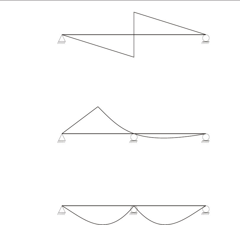
486 Influence Lines and Surfaces
CSI Analysis Reference Manual
(a) Influence Line for Vertical Shear at Center
of a Simple Span
(b) Influence Line for Moment at Center of Left Span
of Two Continuous Spans
(c) Influence Line for Moment at Center Support
of Two Continuous Spans
Figure 86
Examples of Influence Lines for One-Span and Two-Span Beams

Vehicle Live Loads
Any number of Ve hi cle live loads, or sim ply Ve hi cles, may be de fined to act on the
traf fic Lanes. You may use stan dard types of Ve hi cles known to the pro gram, or de -
sign your own us ing the gen eral Ve hi cle speci fi ca tion.
Distribution of Loads
Lon gi tu di nally, each Ve hi cle con sists of one or more axle loads and/or one or more
uni form loads. Axle loads act at a sin gle lon gi tu di nal lo ca tion in the ve hi cle. Uni -
form loads may act be tween pairs of ax les, or ex tend in fi nitely be fore the first axle
or af ter the last axle. The width of each axle load and each uni form load is in de -
pend ently spec i fied. These widths may be fixed or equal to the width of the Lane.
For Mov ing-Load Load Cases us ing the in flu ence sur face, both axle loads and uni -
form loads are used to max i mum ef fect. For step-by-step anal y sis, only the axle
loads are used.
Axle Loads
Lon gi tu di nally, axle loads look like a point load. Trans versely, axle loads may be
rep re sented as one or more point (wheel) loads or as dis trib uted (knife-edge) loads.
Knife-edge loads may be dis trib uted across a fixed width or the full width of the
lane. Axle loads may be zero, which can be used to sep a rate uni form loads of dif fer -
ent mag ni tude.
Uniform Loads
Lon gi tu di nally, the uni form loads are con stant be tween ax les. Lead ing and trail ing
loads may be spec i fied that ex tend to in fin ity. Trans versely, these loads may be dis -
trib uted uni formly across the width of the lane, over a fixed width, or they may be
con cen trated at the cen ter line of the lane.
Min i mum Edge Distances
Cer tain AASHTO ve hi cles re quire that the wheel loads main tain a spec i fied min i -
mum dis tance from the edge of the lane. For any ve hi cle, you may spec ify a min i -
mum dis tance for in te rior edges of lanes, and an other dis tance for ex te rior edges.
By de fault, these dis tances are zero. The spec i fied dis tances ap ply equally to all
axle loads, but do not af fect lon gi tu di nally-uniform loads. The def i ni tion of in te rior
and ex te rior edges is given in Subtopic “Lanes” (page 482).
Vehicle Live Loads 487
Chapter XXVI Moving-Load Analysis

Directions of Loading
All ve hi cle live loads are spec i fied as weight and are as sumed, by de fault, to act
down ward in the –Z global co or di nate di rec tion. How ever, hor i zon tal loads rep re -
sent ing brak ing, ac cel er a tion, and cen trif u gal forces may also be spec i fied as part
of the ve hi cle def i ni tion.
See “Up ward and Hor i zon tal Di rec tions” (page 13) in Chap ter “Co or di nate Sys -
tems.”
All ver ti cal and hor i zon tal loads are gen er ated from the same dis tri bu tion of
weights, i.e., the axle and uni form loads as de scribed above. The var i ous di rec tions
of load are ad di tive, de pend ing upon scale fac tors de fined in the mov ing load cases,
and are com puted si mul ta neously for each ve hi cle po si tion.
In the dis cus sion that fol lows, W is the to tal weight of an axle load or weight per
length of a uni form load at a given lon gi tu di nal po si tion within a ve hi cle. All gen er -
ated ver ti cal or hor i zon tal loads have the same dis tri bu tion across the width of the
ve hi cle, ex cept as de scribed for over turn ing mo ments be low.
Vertical Loads
By de fault the spec i fied axle and uni form loads act in the grav ity di rec tion. You
may op tion ally spec ify that ver ti cal loads are to be ex cluded if you want to de fine a
spe cial ve hi cle that rep re sents hor i zon tal load ing only. Ac cord ingly, the ver ti cal
force FV is either
FW
V= or FV=0
where W is the axle or uni form weight of the ve hi cle at a given lo ca tion.
Note that ver ti cal load is re quired to gen er ate both super-el e va tion and cen trif u gal
over turn ing mo ments, as dis cussed be low.
Braking and Acceleration Loads
Brak ing and ac cel er a tion loads may be con sid ered by spec i fy ing one or two sets of
co ef fi cients mul ti ply ing the axle and uni form loads. For ex am ple, the first set could
spec ify a co ef fi cient of 0.25 on the axle loads and 0.0 on the uni form loads. The sec -
ond set, if re quested, could spec ify a co ef fi cient of 0.05 on both the axle and the
uni form loads. If two sets are re quested, the en ve lope of the two sets will be de ter -
mined and reported.
488 Vehicle Live Loads
CSI Analysis Reference Manual

The spec i fied val ues ef fec tively act as co ef fi cients of fric tion, and the lon gi tu di nal
force FB is com puted as
FbW
B=±
where b is the spec i fied brak ing co ef fi cient for axle or uni form loads, and W is the
axle or uni form weight of the ve hi cle at a given lo ca tion.
Brak ing and ac cel er a tion loads act lon gi tu di nally, par al lel to the cen ter line of the
Lane, and along the grade of the lay out line used to de fine the Lane. These forces
will be as sumed to act both for ward and back ward, so that the max i mum and min i -
mum re sponse re ported will be equal and op po site to each other. They will be based
on ei ther the max i mum or min i mum re sponse com puted, which ever has the larger
ab so lute value.
Op tion ally, skew brak ing and ac cel er a tion loads can be con sid ered by spec i fy ing
skew co ef fi cients for axle and uni form loads. The co ef fi cients mul ti ply the lon gi tu -
di nal brak ing and ac cel er a tion forces, and are ap plied trans versely, per pen dic u lar
to the Lane cen ter line. If the Lane is act ing on a bridge ob ject, the skew forces will
act along the super-el e va tion slope of the bridge. Oth er wise, skew brak ing forces
act in the hor i zon tal plane. Skew forces act ing to the left and right, si mul ta neously
with the lon gi tu di nal forces, will both be con sid ered and the en ve lope re ported. The
skew co ef fi cient is ef fec tively the tan gent of the an gle be tween the di rec tion of
brak ing or ac cel er a tion and the cen ter line of the Lane, and the skew brak ing/ac cel -
er a tion force FK is com puted as
FkF
KB
=±
where k is the skew co ef fi cient.
Centrifugal Loads
Cen trif u gal loads may be con sid ered by spec i fy ing a ve loc ity and a set of co ef fi -
cients mul ti ply ing the axle and uni form loads. The cen trif u gal force FC is
computed as
FcV
g
W
R
CC
=-2
where c is the spec i fied cen trif u gal co ef fi cient for axle or uni form loads,
VC is the
spec i fied ve loc ity, g is the ac cel er a tion due to grav ity, W is the axle or uni form
weight of the ve hi cle at a given lo ca tion, and R is the cen trif u gal ra dius spec i fied as
part of the Lane def i ni tion. When R = 0, the ra dius is taken as in fin ity (straight) and
the force FC=0.
Vehicle Live Loads 489
Chapter XXVI Moving-Load Analysis

For the Eurocode and other pre scrip tive codes, a ref er ence length (typ i cally one
me ter) may be spec i fied in stead of a ve loc ity. In this case the cen trif u gal force is
com puted as
FcLW
R
CC
=-
where LC is the ref er ence length.
Cen trif u gal forces are ap plied trans versely, per pen dic u lar to the cen ter line of the
Lane, and al ways act in the hor i zon tal plane re gard less of any super-el e va tion. Note
that the force acts to the left (neg a tive) when the ra dius curves to the right (pos i -
tive), and vice-versa.
Overturning Moments
Two types of over turn ing mo ments may be con sid ered, cen trif u gal and super-el e -
va tion. Both are pro por tional to the height of the cen troid of ve hi cle weight above
the sur face of the bridge deck. Sep a rate heights are spec i fied for axle and uni form
loads, but the same heights ap ply to both types of over turn ing mo ment.
For cen trif u gal loads, the over turn ing mo ment (torque) TC is given by
TFh
CC
=
where FC is the cen trif u gal force as de fined above, and h is the height to the cen -
troid of the ve hi cle weight caus ing this force. This gen er ates a ver ti cal force cou ple
±FTC act ing over a mo ment arm equal to the wheel spac ing s, com puted as
FT
sFh
s
TCCC
==
For ver ti cal loads, the over turn ing mo ment TV is given by
TFh
VV
=sinq
where FV is the ver ti cal force as de fined above, h is the height to the cen troid of the
ve hi cle weight caus ing the force, q=tan-1e is the an gle of super-el e va tion, and e is
the super-el e va tion de fined as a ra tio. This gen er ates a ver ti cal force cou ple ±FTV
act ing over a mo ment arm equal to the hor i zon tal wheel spac ing scosq, com puted
as
FT
sTeh
s
TVVV
==
cosq
490 Vehicle Live Loads
CSI Analysis Reference Manual

The to tal over turn ing ver ti cal force cou ple ±FT is given by
FFFFFeh
s
TTCTVCV
=+=+()
Note that the over turn ing mo ment due to super-el e va tion tends to coun ter act the
cen trif u gal over turn ing ef fects on a curve, but may it self cause over turn ing when
act ing alone for ve hi cles that are stationary. Both cases must be con sid ered in an
en vel op ing anal y sis or de sign.
For a ve hi cle load of width w, the spac ing s and the ap pli ca tion of the ver ti cal force
FT cou ple de pend on the trans verse dis tri bu tion of the load as fol lows:
•For a sin gle point load, or for a zero-width lane, s = 0 and no over turn ing mo -
ments are con sid ered.
•For two point loads, s = w, and the over turn ing load FT is added to the two ver -
ti cal loads as an equal-but-op po site pair at the two wheel lo ca tions.
•For four equally-spaced point loads, s = 23 w, and over turn ing loads FT/2 are
added to the two ver ti cal loads on one side of the ve hi cle width and sub tracted
from the loads on the other side.
•For a uni form trans verse dis tri bu tion of load, s = 12 w, and a uni form over turn -
ing load FT/(w/2) is added to the ver ti cal load on one half of the ve hi cle width
and sub tracted from the other half.
•Note that the width of the ve hi cle will be re duced, if nec es sary, to fit within the
width of the lane.
Im por tant Note! The over turn ing load is re stricted so as not to cause up lift on the
in ner or up ward side of the ve hi cle. This re stric tion is en forced dur ing anal y sis, and
can be stated as
FF
TV
=2
re gard less of the width dis tri bu tion of loads.
In par tic u lar, no over turn ing mo ments will be con sid ered for a load case where the
ver ti cal load is zero. When de fin ing mov ing load cases, be sure to com bine ver ti cal
load with cen trif u gal load if over turn ing mo ments are im por tant. A cen trif u gal load
case by it self will ex clude over turn ing mo ments, even if later in cluded in a load
com bi na tion with ver ti cal load cases. See Topic “Mov ing-Load Load Cases” (page
509) for more in for ma tion.
Vehicle Live Loads 491
Chapter XXVI Moving-Load Analysis

Elevation of Horizontal Loads
Hor i zon tal loads gen er ated for in flu ence sur faces or in di vid ual ve hi cles are ap plied
at ver ti cal el e va tions in tended to rep re sent the top sur face of the bridge deck.
Specifically:
•For spine and solid mod els of a bridge ob ject, hor i zon tal loads act at the el e va -
tion of the top sur face, af ter tak ing into ac count the grade and super-el e va tion
of the bridge ob ject.
•For area (shell) mod els of a bridge ob ject, the loads act at the joints of the area
ob jects rep re sent ing the top slab. This is typ i cally at the mid-sur face of the top
slab, and hence the loads act at a half slab-thick ness be low the top sur face.
Grade and super-el e va tion are in cluded in the lo ca tion of these joints.
•For mod els not cre ated with the Bridge Mod eler, hor i zon tal loads on frame ob -
jects act at the el e va tion of the lay out line. Hor i zon tal loads on area ob jects act
at their joints (typ i cally at the mid-sur face), and they act at the top-sur face
joints of solid ob jects.
For this rea son, tor sional mo ments cre ated by trans verse loads and ver ti cal mo -
ments (M3) caused by lon gi tu di nal loads may be slightly dif fer ent ac cord ing to the
type of model gen er ated to rep re sent the bridge ob ject. The dif fer ence is gen er ally
small but should be recognized.
Re strict ing a Ve hi cle to the Lane Length
When mov ing a ve hi cle along the length of the lane, the front of the ve hi cle starts at
one end of the lane, and the ve hi cle trav els for ward un til the back of the ve hi cle ex -
its the other end of the lane. This means that all lo ca tions of the ve hi cle are con sid -
ered, whether fully or par tially on the lane
You have the op tion to spec ify that a ve hi cle must re main fully on the lane. This is
use ful for cranes and sim i lar ve hi cles that have stops at the end of their rails that
pre vent them from leav ing the lane. This set ting only af fects in flu ence-sur face
anal y sis, not step-by-step anal y sis where you can ex plic itly con trol where the
vehicle runs.
Ap pli ca tion of Loads to the Influence Surface
The max i mum and min i mum val ues of a re sponse quan tity are com puted us ing the
cor re spond ing in flu ence line or sur face. Con cen trated loads are mul ti plied by the
in flu ence value at the point of ap pli ca tion to ob tain the cor re spond ing re sponse;
492 Vehicle Live Loads
CSI Analysis Reference Manual

dis trib uted loads are mul ti plied by the in flu ence val ues and in te grated over the
length and width of ap pli ca tion.
By de fault, each con cen trated or dis trib uted load is con sid ered to rep re sent a range
of val ues from zero up to a spec i fied max i mum. When com put ing a re sponse quan -
tity (force or dis place ment) the max i mum value of load is used where it in creases
the se ver ity of the re sponse, and zero is used where the load would have a re liev ing
ef fect. Thus the spec i fied load val ues for a given Ve hi cle may not al ways be ap -
plied pro por tion ally. This is a con ser va tive ap proach that ac counts for Ve hi cles
that are not fully loaded. Thus the max i mum re sponse is al ways pos i tive (or zero);
the min i mum re sponse is al ways neg a tive (or zero).
You may over ride this con ser va tive be hav ior as dis cussed in the next Subtopic,
“Op tion to Al low Re duced Re sponse Se ver ity”.
By way of ex am ple, con sider the in flu ence line for the mo ment at the cen ter of the
left span shown in Figure 86(b) (page 486). Any axle load or por tion of a dis trib -
uted load that acts on the left span would con trib ute only to the pos i tive max i mum
value of the mo ment re sponse. Loads act ing on the right span would not de crease
this max i mum, but would con trib ute to the neg a tive min i mum value of this mo ment
re sponse.
Option to Allow Re duced Response Severity
You have the op tion to al low loads to re duce the se ver ity of the re sponse. If you
choose this op tion, all con cen trated and uni form loads will be ap plied at full value
on the en tire in flu ence sur face, re gard less of whether or not that load re duces the
se ver ity of the re sponse. This is less con ser va tive than the de fault method of load
ap pli ca tion. The use of this op tion may be use ful for rout ing spe cial ve hi cles whose
loads are well known. How ever, for no tional loads that rep re sent a dis tri bu tion or
en ve lope of un known ve hi cle load ings, the de fault method may be more ap pro pri -
ate.
Width Effects
Fixed-width loads will be moved trans versely across the width of a Lane for max i -
mum ef fect if the Lane is wider than the load. If the Lane is nar rower than the load,
the load will be cen tered on the Lane and its width re duced to be equal to that of the
Lane, keep ing the to tal mag ni tude of the load un changed.
The load at each lon gi tu di nal lo ca tion in the ve hi cle is in de pend ently moved across
the width of the Lane. This means that the front, back, and mid dle of the ve hi cle
Vehicle Live Loads 493
Chapter XXVI Moving-Load Analysis

may not oc cupy the same trans verse lo ca tion in the lane when placed for max i mum
ef fect.
Length Effects
You may spec ify that the mag ni tude of the load ing de pends on lane length us ing
built-in or user-de fined length func tions. One func tion may be used to af fect the
con cen trated (axle) loads, and an other func tion may be used for the dis trib uted
loads. These func tions act as scale fac tors on the spec i fied load val ues.
Concentrated (Axle) Loads
If you spec ify a length-ef fect func tion for the axle loads, all axle loads will be
scaled equally by the func tion, in clud ing float ing axle loads. Built-in length-ef fect
func tions in clude the AASHTO Stan dard Im pact func tion and the JTG-D60 Lane
load func tion. You may de fine your own func tion.
The in tent of this func tion is to scale the load ac cord ing to span length. In a given
struc ture, there may not be a con stant span length, so the pro gram uses the in flu ence
line to de ter mine what span length to use. This may dif fer for each com puted re -
sponse quan tity, and may not al ways cor re spond to the ob vi ous span length in the
global struc ture.
For a given re sponse quan tity, the max i mum point on the in flu ence line is found,
and the dis tance be tween the zero-cross ings on ei ther side of this max i mum is taken
to be the span length. For the three in flu ence lines of Figure 86 (page 486), this
would re sult in a span length of half the dis tance be tween the sup ports for the shear
in (a), and the full dis tance between the sup ports for the mo ments in (b) and ©). For
shear near the sup port, the span length would be es sen tially the same as the dis tance
be tween the sup port.
This ap proach gen er ally works well for mo ments and for shear near the sup ports. A
shorter span length is com puted for shear near midspan, but here the shear is
smaller any way, so it is not usu ally of con cern.
Distributed Loads
If you spec ify a length-ef fect func tion for the dis trib uted loads, all dis trib uted loads
will be scaled equally by the func tion. Built-in length-ef fect func tions in clude the
AASHTO Stan dard Im pact func tion and the Brit ish HA func tion. You may de fine
your own func tion.
494 Vehicle Live Loads
CSI Analysis Reference Manual

The in tent of this func tion is to scale the load ac cord ing to the loaded length, but not
unconservatively. The in flu ence line is used to de ter mine the loaded length for each
in di vid ual re sponse quan tity. Only loaded lengths that in crease the se ver ity of the
re sponse are con sid ered.
To pre vent long lengths of small in flu ence from unconservatively re duc ing the re -
sponse, an it er a tive ap proach is used where the length con sid ered is pro gres sively
in creased un til the max i mum re sponse is com puted. Any fur ther in creases in length
that re duce the re sponse due to de creas ing func tion value are ig nored.
On the other hand, the loaded length used for scal ing is never re duced be low the
length of a sin gle span, which is de ter mined sep a rately for each in flu ence line as the
dis tance be tween zero cross ings on ei ther side of the point of max i mum in flu ence.
Ap pli ca tion of Loads in Multi-Step Analysis
Ve hi cles can be moved in a multi-step anal y sis. This can use ei ther Multi-Step
Static Load Cases or Time-His tory Load Cases, the lat ter of which can be lin ear or
non lin ear. Cur rently only ver ti cal load ing is con sid ered for multi-step anal y sis.
In flu ence sur faces are not used for this type of anal y sis. Rather, CSiBridge cre ates
many in ter nal Load Pat terns rep re sent ing dif fer ent po si tions of the ve hi cles along
the length of the lanes.
Only axle loads are con sid ered; the uni form loads are not ap plied. In the case of a
vari able axle spac ing, the min i mum dis tance is used. The trans verse dis tri bu tion of
the axle loads is con sid ered. The ve hi cle is moved lon gi tu di nally along the cen ter -
line of the lane; it is not moved trans versely within the lane. To con sider dif fer ent
trans verse po si tions, you can de fine ad di tional lanes.
The full mag ni tude of the loads are ap plied, re gard less of whether they in crease or
de crease the se ver ity of the re sponse. Each step in the anal y sis cor re sponds to a spe -
cific po si tion of each ve hi cle act ing in its lane. All re sponse at that step is fully cor -
re lated.
General Vehicle
The gen eral Ve hi cle may rep re sent an ac tual ve hi cle or a no tional ve hi cle used by a
de sign code. Most trucks and trains can be mod eled by the gen eral Ve hi cle in
CSiBridge.
General Vehicle 495
Chapter XXVI Moving-Load Analysis
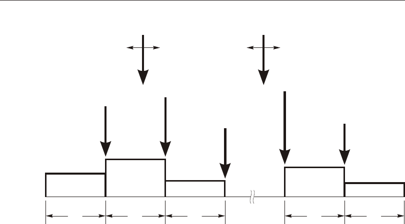
The gen eral Ve hi cle con sists of n ax les with speci fied dis tances be tween them.
Con cen trated loads may ex ist at the ax les. Uni form loads may ex ist be tween pairs
of ax les, in front of the first axle, and be hind the last axle. The dis tance be tween any
one pair of ax les may vary over a speci fied range; the other dis tances are fixed. The
lead ing and trail ing uni form loads are of in fi nite ex tent. Ad di tional “float ing” con -
cen trated loads may be speci fied that are in de pend ent of the po si tion of the ax les.
By de fault for in flu ence sur face anal y sis, ap plied loads never de crease the se ver ity
of the com puted re sponse, so the ef fect of a shorter Ve hi cle is cap tured by a lon ger
496 General Vehicle
CSI Analysis Reference Manual
wn+1
wn
w3
w2
w1
¥d2d3dn¥
p1
pm pxm
p2
p3
pn-1
pn
Leading
Trailing
Notes:
(1) All loads are point loads or uniform line loads acting on the Lane center line
(2) Any of the point loads or uniform line loads may be zero
(3) The number of axles, n, may be zero or more
(4) One of the inter-axle spacings, d through d, may vary over a specified range
2n
(5) The locations of loads pm and pxm are arbitrary
Figure 87
General Vehicle Definition

Ve hi cle that in cludes the same loads and spac ings as the shorter Ve hi cle. Only the
lon ger Ve hi cle need be con sid ered in such cases.
If you choose the option to allow loads to re duce the se ver ity of re sponse, then you
must con sider the shorter and lon ger ve hi cles, if they both ap ply. This is also true
for step-by-step anal y sis.
Specification
To de fine a Ve hi cle, you may spec ify:
•n–1 posi tive dis tances, d, be tween the pairs of ax les; one inter- axle dis tance
may be speci fied as a range from dmin to dmax, where 0 < dmin £ dmax, and
dmax = 0 can be used to rep re sent a maxi mum dis tance of in fin ity
•n con cen trated loads, p, at the ax les, in clud ing the trans verse load dis tri bu tion
for each
•n+1 uni form loads, w: the lead ing load, the inter-axle loads, and the trail ing
load, in clud ing the trans verse load dis tri bu tion for each
•Float ing axle loads:
–Load pm for su per struc ture mo ments, in clud ing its trans verse distribution.
You may spec ify whether or not to dou ble this load for neg a tive su per -
struc ture mo ments over the sup ports, as de scribed be low
–Load pxm for all re sponse quan ti ties ex cept su per struc ture mo ments, in -
clud ing its trans verse dis tri bu tion
•Whether or not this Ve hi cle is to be used for calculating:
–“Nega tive” su per struc ture mo ments over the sup ports
–Re ac tion forces at in te rior sup ports
–Re sponse quan ti ties other than the two types above
•Min i mum dis tances be tween the axle loads and the edges of the lane; by de fault
these dis tances are zero
•Whether or not the ve hi cle must re main fully within the length of lane
•Whether or not to au to mat i cally scale the mag ni tude of the axle loads based on
the loaded length of the lane ac cord ing to the Chi nese JTG or other codes
•Whether or not to au to mat i cally scale the mag ni tude of the uni form loads based
on the loaded length of the lane ac cord ing to the Brit ish or other codes
•Whether or not to con sider ver ti cal load ing, and whether or not to in clude the
cor re spond ing over turn ing mo ments due to super-el e va tion
General Vehicle 497
Chapter XXVI Moving-Load Analysis

•Whether or not to con sider brak ing and ac cel er a tion loading, and the scale fac -
tors de fin ing these loads
•Whether or not to con sider cen trif u gal loading, the scale fac tors de fin ing these
loads, and whether or not to in clude the cor re spond ing over turn ing moments
The num ber of ax les, n, may be zero, in which case only a sin gle uni form load and
the float ing con cen trated loads can be spec i fied.
These pa rame ters are il lus trated in Figure 87 (page 496). Some specific ex am ples
are given in Topic “Stan dard Vehicles” (page 500). Ad di tional de tail is pro vided in
the fol low ing.
Moving the Vehicle
When a Ve hi cle is ap plied to a traf fic Lane, the ax les are moved along the length of
the lane to where the maxi mum and mini mum val ues are pro duced for every re -
sponse quan tity in every ele ment. Usu ally this lo ca tion will be dif fer ent for each re -
sponse quan tity. For asym met ric (front to back) Ve hi cles, both di rec tions of travel
are con sid ered.
Vehicle Response Components
Cer tain fea tures of the AASHTO H, HS, and HL ve hic u lar live loads (AASHTO,
2004) ap ply only to cer tain types of bridge re sponse, such as neg a tive mo ment in
the su per struc ture or the re ac tions at in te rior sup ports. CSiBridge uses the con cept
of ve hi cle re sponse com po nents to iden tify these re sponse quan ti ties. You se lect
the ob jects that need spe cial treat ment, and as sign the ap pro pri ate ve hi cle re sponse
com po nents to them.
The dif fer ent types of avail able ve hi cle re sponse com po nents are de scribed in the
fol low ing subtopics.
Ve hi cle re sponse com po nents do not ap ply to SAP2000.
Su per struc ture (Span) Mo ment
For AASHTO H and HS “Lane” loads, the float ing axle load pm is used for cal cu -
lat ing the su per struc ture mo ment. How this mo ment is rep re sented de pends on the
type of model used. For all other types of re sponse, the float ing axle load pxm is
used.
498 Vehicle Response Components
CSI Analysis Reference Manual

The gen eral pro ce dure is to se lect the el e ments rep re sent ing the su per struc ture and
as sign ve hi cle response components “H and HS Lane Loads – Su per struc ture Mo -
ment” to the de sired re sponse quan ti ties, as de scribed next.
For a spine (spline) model where the su per struc ture is mod eled as a line of frame el -
e ments, su per struc ture mo ment cor re sponds to frame mo ment M3 for el e ments
where the lo cal-2 axis is in the ver ti cal plane (the de fault.) Thus you would se lect
all frame el e ments rep re sent ing the su per struc ture and as sign the ve hi cle re sponse
com po nents to M3, in di cat ing to “Use All Val ues” (i.e., pos i tive and neg a tive.)
Load pm will be used for com put ing M3 of these el e ments.
For a full-shell model of the su per struc ture, su per struc ture mo ment cor re sponds to
lon gi tu di nal stresses or mem brane forces in the shell el e ments. As sum ing the lo -
cal-1 axes of the shell el e ments are ori ented along the lon gi tu di nal di rec tion of the
bridge, you would se lect all shell el e ments rep re sent ing the su per struc ture and as -
sign the ve hi cle re sponse com po nents to S11 and/or F11, in di cat ing to “Use All
Val ues” (i.e., pos i tive and neg a tive.) You could also make this same as sign ment to
shell mo ments M11. Load pm will be used for com put ing any com po nents you
have so as signed.
Negative Su per struc ture (Span) Mo ment
For AASHTO H and HS “Lane” loads, the float ing axle load pm is ap plied in two
ad ja cent spans for cal cu lat ing the neg a tive su per struc ture mo ment over the
supports. Sim i larly, for AASHTO HL loads, a spe cial dou ble-truck ve hi cle is used
for cal cu lat ing neg a tive su per struc ture mo ment over in te rior sup ports. Neg a tive
mo ment here means a mo ment that causes ten sion in the top of the su per struc ture,
even if the sign of the CSiBridge re sponse is pos i tive due to a par tic u lar choice of
lo cal axes.
The pro ce dure for dif fer ent types of struc tures is very sim i lar to that de scribed
above for su per struc ture mo ment: se lect the el e ments rep re sent ing the su per struc -
ture, but now as sign ve hi cle re sponse com po nents “H, HS and HL Lane Loads –
Su per struc ture Neg a tive Mo ment over Supports” to the de sired re sponse quan ti -
ties. How ever, we have to de cide how to han dle the sign.
There are two gen eral ap proaches. Let's con sider the case of the spine model with
frame mo ment M3 rep re sent ing su per struc ture mo ment:
(1) You can se lect the en tire su per struc ture, and as sign the ve hi cle re sponse com -
po nents to M3, in di cat ing to “Use Neg a tive Val ues”. Only neg a tive val ues of
M3 will be com puted us ing the dou ble pm or dou ble-truck load.
Vehicle Response Components 499
Chapter XXVI Moving-Load Analysis

(2) You can se lect only that part of the su per struc ture within a pre-de ter mined neg -
a tive-mo ment re gion, such as be tween the in flec tion points un der dead load.
As sign the ve hi cle re sponse com po nents to M3, in di cat ing to “Use Neg a tive
Val ues” or “Use All Val ues.”
The first ap proach may be slightly more con ser va tive, giv ing neg a tive mo ments
over a larger re gion. However, it does not re quire you to determine a neg a tive-mo -
ment re gion.
The sit u a tion with the shell model is more com pli cated, since neg a tive mo ments
cor re spond to pos i tive mem brane forces and stresses at the top of the su per struc -
ture, neg a tive val ues at the bot tom of the su per struc ture, and chang ing sign in be -
tween. For this rea son, ap proach (2) above may be better: de ter mine a neg a tive-mo -
ment re gion, then as sign the ve hi cle re sponse com po nents to the de sired shell
stresses, mem brane forces, and/or mo ments, in di cat ing to “Use All Val ues.” This
avoids the prob lem of sign where it changes through the depth.
Reactions at Interior Supports
For AASHTO HL loads, a spe cial dou ble-truck ve hi cle is used for cal cu lat ing the
re ac tions at in te rior sup ports. It is up to you to de ter mine what re sponse com po -
nents you want to be com puted for this pur pose. Choices could in clude:
•Ver ti cal up ward re ac tions, or all re ac tions, for springs and re straints at the base
of the col umns
•Com pres sive ax ial force, or all forces and mo ments, in the col umns
•Compressive ax ial force, or all forces and mo ments, in link el e ments rep re sent -
ing bear ings
•Bend ing mo ments in out rig gers at the col umns
The pro ce dure is as above for su per struc ture mo ment. Se lect the el e ments rep re -
sent ing the in te rior sup ports and as sign the ve hi cle re sponse com po nents “HL – Re -
ac tions at Interior Sup ports” to the de sired re sponse quan ti ties. Care fully de cide
whether you want to use all val ues, or only neg a tive or pos i tive val ues. You will
have to re peat this pro cess for each type of el e ment that is part of the in te rior sup -
ports: joints, frames, links, shells, and/or sol ids.
Standard Vehicles
There are many stan dard ve hi cles avail able in CSiBridge to rep re sent ve hicu lar live
loads speci fied in vari ous de sign codes. More are be ing added all the time. A few
500 Standard Vehicles
CSI Analysis Reference Manual

ex am ples are pro vided here for illustrative pur poses. Only the lon gi tu di nal dis tri -
bu tion of load ing is shown in the figures. Please see the graph i cal user in ter face for
all avail able types and fur ther information.
Hn-44 and HSn-44
Ve hi cles speci fied with type = Hn-44 and type = HSn-44 rep re sent the AASHTO
stan dard H and HS Truck Loads, re spec tively. The n in the type is an in te ger scale
fac tor that speci fies the nomi nal weight of the Ve hi cle in tons. Thus H15- 44 is a
nomi nal 15 ton H Truck Load, and HS20- 44 is a nomi nal 20 ton HS Truck Load.
These Ve hi cles are il lus trated in Figure 88 (page 503).
The ef fect of an H Ve hi cle is in cluded in an HS Ve hi cle of the same nomi nal
weight. If you are de sign ing for both H and HS Ve hi cles, only the HS Ve hi cle is
needed.
Hn-44L and HSn-44L
Ve hi cles speci fied with type = Hn-44L and type = HSn-44L rep re sent the
AASHTO stan dard H and HS Lane Loads, re spec tively. The n in the type is an in -
te ger scale fac tor that speci fies the nomi nal weight of the Ve hi cle in tons. Thus
H15- 44 is a nomi nal 15 ton H Lane Load, and HS20- 44 is a nomi nal 20 ton HS
Lane Load. These Ve hi cles are il lus trated in Figure 88 (page 503). The Hn-44L and
HSn-44L Ve hi cles are iden ti cal.
AML
Ve hi cles speci fied with type = AML rep re sent the AASHTO stan dard Al ter nate
Mili tary Load. This Ve hi cle con sists of two 24 kip ax les spaced 4 ft apart.
HL-93K, HL-93M and HL-93S
Ve hi cles speci fied with type = HL- 93K rep re sent the AASHTO stan dard HL- 93
Load con sist ing of the code- specified de sign truck and the de sign lane load.
Ve hi cles speci fied with type = HL- 93M rep re sent the AASHTO stan dard HL- 93
Load con sist ing of the code- specified de sign tan dem and the de sign lane load.
Ve hi cles speci fied with type = HL- 93S rep re sent the AASHTO stan dard HL- 93
Load con sist ing of two code- specified de sign trucks and the de sign lane load, all
scaled by 90%. The axle spac ing for each truck is fixed at 14 ft. The spac ing be -
tween the rear axle of the lead truck and the lead axle of the rear truck var ies from
50 ft to the length of the Lane. This ve hi cle is only used for nega tive su per struc ture
Standard Vehicles 501
Chapter XXVI Moving-Load Analysis

mo ment over sup ports and re ac tions at in te rior sup ports. The re sponse will be zero
for all re sponse quan ti ties that do not have the ap pro pri ately as signed ve hi cle re -
sponse com po nents.
A dy namic load al low ance may be speci fied for each Ve hi cle us ing the pa rame ter
im. This is the ad di tive per cent age by which the con cen trated truck or tan dem axle
loads will be in creased. The uni form lane load is not af fected. Thus if im = 33, all
con cen trated axle loads for the ve hi cle will be mul ti plied by the fac tor 1.33.
These Ve hi cles are il lus trated in Figure 89 (page 504) for im = 0.
P5, P7, P9, P11, and P13
Ve hi cles speci fied with type = P5, type = P7, type = P9, type = P11, and type =
P13 rep re sent the Cal trans stan dard Per mit Loads. These Ve hi cles are il lus trated in
Figure 90 (page 505).
The ef fect of a shorter Cal trans Per mit Load is in cluded in any of the longer Per mit
Loads. If you are de sign ing for all of these per mit loads, only the P13 Ve hi cle is
needed.
Cooper E 80
Ve hi cles speci fied with type = CO OP ERE80 rep re sent the AREA stan dard Coo per
E 80 train load. This Ve hi cle is il lus trated in Figure 91 (page 506).
UICn
Ve hi cles speci fied with type = UICn rep re sent the Euro pean UIC (or Brit ish RU)
train load. The n in the type is an in te ger scale fac tor that speci fies mag ni tude of the
uni form load in KN/m. Thus UIC80 is the full UIC load with an 80 kn/m uni form
load, and UIC60 is the UIC load with an 60 kn/m uni form load. The con cen trated
loads are not af fected by n.
This Ve hi cle is il lus trated in Figure 91 (page 506).
RL
Ve hi cles speci fied with type = RL rep re sent the Brit ish RL train load. This Ve hi cle
is il lus trated in Figure 91 (page 506).
502 Standard Vehicles
CSI Analysis Reference Manual
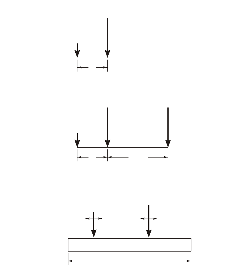
Standard Vehicles 503
Chapter XXVI Moving-Load Analysis
¥
14'
14'
14' to 30'
pm
pxm
8 k
8 k
32 k
32 k
32 k
0.640 k/ft
18 k
26 k
H20-44L and HS20-44L Lane Loads
HS20-44 Truck Load
H20-44 Truck Load
Figure 88
AASHTO Standard H and HS Vehicles
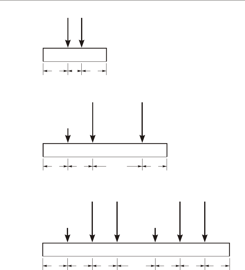
504 Standard Vehicles
CSI Analysis Reference Manual
14'
14'
4'
¥
¥
¥
14'
14' to 30'
50' to ¥14' 14' ¥
¥
¥
7.2 k 7.2 k
8 k
28.8 k 28.8 k 28.8 k 28.8 k
32 k
25 k 25 k
32 k
HL-93S Truck and Lane Load for Negative Moment and Reactions at Interior Piers
HL-93K Truck and Lane Load
HL-93M Tandem and Lane Load
0.576 k/ft
0.640 k/ft
0.640 k/ft
Note: All point loads will be increased
by the dynamic load allowance,
im, expressed as a percentage
Figure 89
AASHTO Standard HL Vehicles
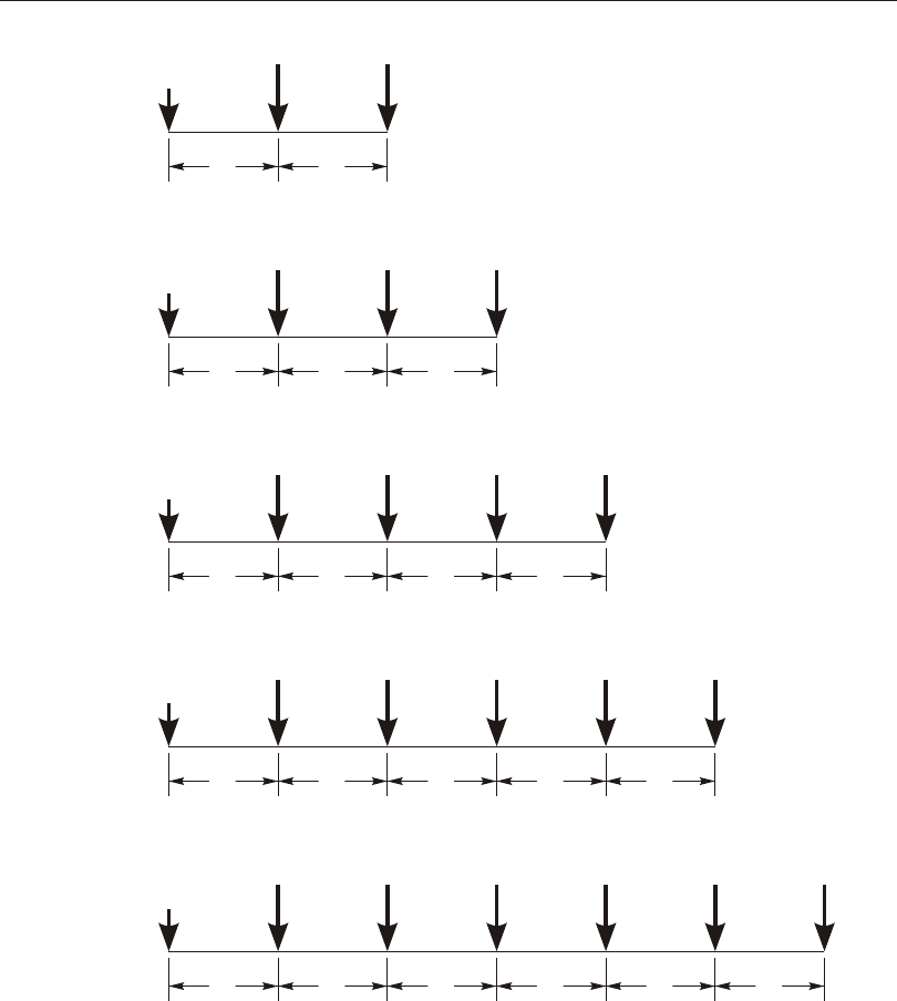
Standard Vehicles 505
Chapter XXVI Moving-Load Analysis
18'
18'
18'
18'
18'
18'
18'
18'
18'
18'
18'
18'
18'
18'
18'
18'
18'
18'
18'
18'
26 k
26 k
26 k
26 k
26 k
48 k
48 k
48 k
48 k
48 k
48 k
48 k
48 k
48 k
48 k
48 k
48 k
48 k
48 k
48 k
48 k
48 k
48 k
48 k
48 k
P11 Permit
Load
P13 Permit
Load
P9 Permit Load
P7 Permit Load
P5 Permit Load
Figure 90
Caltrans Standard Permit Vehicles
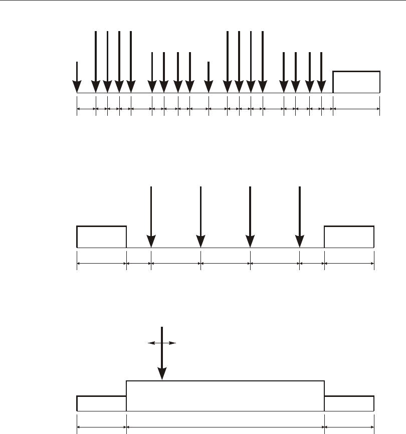
506 Standard Vehicles
CSI Analysis Reference Manual
40 k
250 kN 250 kN
200 kN
250 kN 250 kN
4 @ 80 k
4 @ 52 k 4 @ 52 k
4 @ 80 k
40 k
8 k/ft
80 kN/m80 kN/m
25 kN/m
50 kN/m
25 kN/m
Cooper E 80 Train Load
UIC80 Train Load
RL Train Load
5' 5' 5' 9' 5' 6' 5' 8' 8' 5' 5' 5' 9' 5' 6' 5' 5' ¥
¥
¥
¥
¥
8'
0.8 m 1.6 m 1.6 m
100 m
1.6 m 0.8 m
px
Figure 91
Standard Train Vehicles
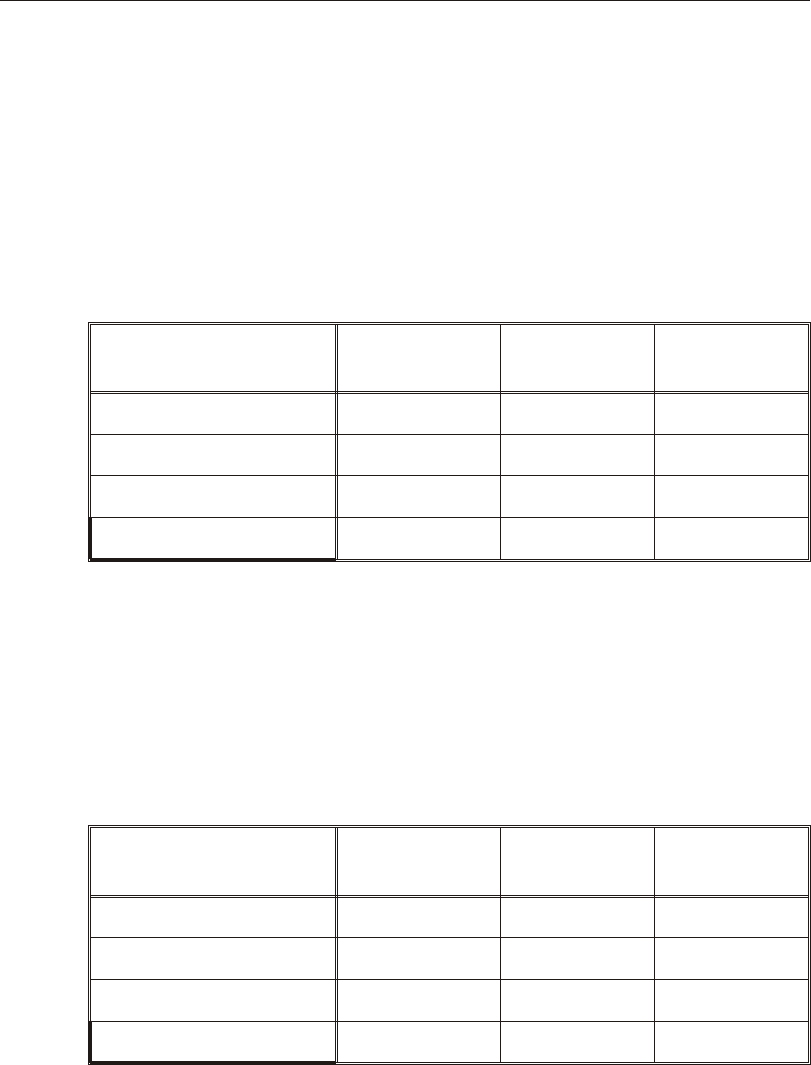
Eurocode Ve hi cles
Ve hi cles are avail able for the four Load Mod els of the Eu ro pean Stan dard EN
1991-2:2003.
There are eight ve hi cles in to tal that rep re sent Load Model 1. Each ve hi cle com -
bines the tan dem sys tem TS (con cen trated load) with the UDL sys tem (uni form
load), but with dif fer ent scale fac tors.
For use as a char ac ter is tic load, there are sep a rate ve hi cles for load ing the first, sec -
ond, third, and sub se quent lanes. These are given in the ta ble be low:
Vehicle Location TS, Axle Load
Qik (KN)
UDL Load
qik (KN/m2)
Euro_LM1_Lane1_Char Lane Number 1 300 9
Euro_LM1_Lane2_Char Lane Number 2 200 2.5
Euro_LM1_Lane3_Char Lane Number 3 100 2.5
Euro_LM1_Other_Char Other lanes 02.5
A mov ing-load case de fined for use as a char ac ter is tic load, and hav ing four or
more lanes, should ap ply a sin gle in stance each of the first three ve hi cles to all the
lanes and ap ply mul ti ple instances of the last ve hi cle to all lanes. The au to matic
per mu ta tions in the mov ing load case will con sider the most severe com bi na tion of
the ve hi cles load ing the var i ous lanes. If there are fewer than four lanes, the lat ter
ve hi cles are not needed, re spec tively.
For use as a fre quent load, there are sep a rate ve hi cles for load ing the first, sec ond,
third, and sub se quent lanes. These are given in the ta ble be low:
Vehicle Location TS, Axle Load
Qik (KN)
UDL Load
qik (KN/m2)
Euro_LM1_Lane1_Freq Lane Number 1 225 3.6
Euro_LM1_Lane2_Freq Lane Number 2 150 1.0
Euro_LM1_Lane3_Freq Lane Number 3 75 1.0
Euro_LM1_Other_Freq Other lanes 01.0
Be cause of the dif fer ent ra tios of TS and UDL load, sep a rate mov ing-load cases
need to be de fined for char ac ter is tic and fre quent load ing.
Standard Vehicles 507
Chapter XXVI Moving-Load Analysis

A mov ing-load case de fined for use as a fre quent load, and hav ing four or more
lanes, should ap ply a sin gle in stance each of the first three ve hi cles to all the lanes
and ap ply mul ti ple in stances of the last ve hi cle to all lanes. The au to matic per mu ta -
tions in the mov ing load case will con sider the most se vere com bi na tion of the ve hi -
cles load ing the var i ous lanes. If there are fewer than four lanes, the lat ter ve hi cles
are not needed, re spec tively.
A sin gle ve hi cle is avail able for Load Model 2, Euro_LM2, that ap plies a sin gle
axle load. This should be ap plied in a mov ing-load case that loads all the lanes, but
only a sin gle lane at a time.
There are mul ti ple ve hi cles avail able to rep re sent the var i ous types de fined for
Load Model 3. For ve hi cles with 100 to 200 kn axle-lines, the axle loads are ap plied
as a knife-edge load dis trib uted over a 2.7 m width. For ve hi cles with 240 kn
axle-lines, the axle loads are ap plied as a knife-edge load dis trib uted over a 4.2 m
width. These can be com bined with the Load Model 1 ve hi cles in a mov ing-load
case, load ing sep a rate lanes. The 240 kn axle-lines are not au to mat i cally ap plied to
two ad ja cent lanes. In stead, you will need to de fine a new lane that is dou ble-wide
and use that lane in the mov ing-load case in place of the two ad ja cent lanes.
A sin gle ve hi cle is avail able for Load Model 4, Euro_LM4, that ap plies a uni form
load. This should be ap plied in a mov ing-load case that loads all lanes si mul ta -
neously. Ad di tional lanes may need to be de fined to rep re sent ar eas that may be
loaded by pe des tri ans but are not oth er wise used for traf fic.
Vehicle Classes
The de signer is of ten in ter ested in the maxi mum and mini mum re sponse of the
bridge to the most ex treme of sev eral types of Ve hi cles rather than the ef fect of the
in di vid ual Ve hi cles. For this pur pose, Ve hi cle Classes are de fined that may in clude
any number of in di vid ual Ve hi cles. The maxi mum and mini mum force and dis -
place ment re sponse quan ti ties for a Ve hi cle Class will be the maxi mum and mini -
mum val ues ob tained for any in di vid ual Ve hi cle in that Class. Only one Ve hi cle
ever acts at a time.
For in flu ence-based anal y ses, all Ve hi cle loads are ap plied to the traf fic Lanes
through the use of Ve hi cle Classes. If it is de sired to ap ply an in di vid ual Ve hi cle
load, you must use a Ve hi cle Class that con tains only that sin gle Ve hi cle. Such sin -
gle-ve hi cle Classes are au to mat i cally cre ated for each Vehicle, and can not be
changed. You need to de fine your own Ve hi cle Classes only if you want to en ve -
lope mul ti ple Vehicles or change the scale fac tor on a sin gle Vehicle.
508 Vehicle Classes
CSI Analysis Reference Manual

For ex am ple, the you may need to con sider the most se vere of a Truck Load and the
cor re spond ing Lane Load, say the HS20- 44 and HS20- 44L loads. A Ve hi cle Class
can be de fined to con tain these two Ve hi cles. Ad di tional Ve hi cles, such as the Al -
ter nate Mili tary Load type AML, could be in cluded in the Class as ap pro pri ate. Dif -
fer ent mem bers of the Class may cause the most se vere re sponse at dif fer ent lo ca -
tions in the struc ture.
For HL- 93 load ing, you would first de fine three Ve hi cles, one each of the stan dard
types HL- 93K, HL- 93M, and HL- 93S. You then could de fine a sin gle Ve hi cle
Class con tain ing all three Ve hi cles.
For step-by-step anal y sis, Ve hi cle loads are ap plied di rectly with out the use of
Classes, since no en vel op ing is per formed.
Moving-Load Load Cases
The fi nal step in the defi ni tion of the in flu ence-based ve hi cle live load ing is the ap -
pli ca tion of the Ve hi cle Classes to the traf fic Lanes. This is done by cre at ing in de -
pend ent Moving-Load Load Cases.
A Mov ing-Load Load Case is a type of Load Case. Un like most other Load Cases,
you can not ap ply Load Pat terns in a Mov ing-Load Load Case. In stead, each Mov -
ing-Load Load Case con sists of a set of as sign ments that spec ify how the Classes
are as signed to the Lanes.
Each as sign ment in a Mov ing-Load Load Case re quires the fol low ing data:
•A Ve hi cle Class, class
•A scale fac tor, sf, mul ti ply ing the ef fect of class (the de fault is unity)
•A list, lanes, of one or more Lanes in which class may act (the de fault is all
Lanes)
•The mini mum number, lmin, of Lanes lanes in which class must act (the de -
fault is zero)
•The maxi mum number, lmax, of Lanes lanes in which class may act (the de -
fault is all of lanes)
The pro gram looks at all of the as sign ments in a Mov ing-Load Load Case, and tries
every pos si ble per mu ta tion of load ing the traf fic Lanes with Ve hi cle Classes that is
per mit ted by the as sign ments. No Lane is ever loaded by more than one Class at a
time.
Moving-Load Load Cases 509
Chapter XXVI Moving-Load Analysis

You may spec ify multiple- lane scale fac tors, rf1, rf2, rf3, ..., for each Mov -
ing-Load Load Case that mul ti ply the ef fect of each per mu ta tion de pend ing upon
the number of loaded Lanes. For ex am ple, the ef fect of a per mu ta tion that loads two
Lanes is mul ti plied by rf2.
The maxi mum and mini mum re sponse quan ti ties for a Mov ing-Load Load Case
will be the maxi mum and mini mum val ues ob tained for any per mu ta tion per mit ted
by the as sign ments. Usu ally the per mu ta tion pro duc ing the most se vere re sponse
will be dif fer ent for dif fer ent re sponse quan ti ties.
The con cepts of as sign ment can be clari fied with the help of the fol low ing ex am -
ples.
Directions of Loading
For each mov ing-load load case, three scale fac tors are spec i fied to mul ti ply and
com bine the ver ti cal load (cfv), brak ing/ac cel er a tion load (cfb), and cen trif u gal
load (cfc) for all ve hi cles act ing in this load case. By de fault, cfv = 1 and cfb = cfc =
0. When two or more fac tors are non-zero, the ef fects of the dif fer ent di rec tions of
load ing for a given ve hi cle are con sid ered si mul ta neously for each po si tion of the
ve hi cle in the lane. This is more ac cu rate and less over-con ser va tive than con sid er -
ing the three di rec tions of load ing sep a rately and then add ing them together later in
a load combination.
Im por tant Note! The over turn ing load due to cen trif u gal load is re stricted so as not
to cause up lift on the in ner or up ward side of the ve hi cle. In par tic u lar, no over turn -
ing mo ments will be con sid ered for a load case where the ver ti cal load is zero. For
this rea son, it is rec om mended to com bine full ver ti cal load with cen trif u gal load if
over turn ing mo ments are im por tant. A cen trif u gal load case by it self will ex clude
over turn ing mo ments, even if later in cluded in a load com bi na tion with ver ti cal
load cases. See topic “Ve hi cle Live Loads” (page 487) for more in for ma tion.
When mul ti ple di rec tions of load ing are con sid ered in a mov ing-load load case, the
fol low ing per mu ta tions are au to mat i cally con sid ered during anal y sis de pend ing
upon the type of com bi na tion re quested by the choice of scale factors:
Combination Vertical (V) Braking (B) Centrif. ©) Double
V only cfv 00
B only 0cfb 0*
C only 00cfc
510 Moving-Load Load Cases
CSI Analysis Reference Manual

Combination Vertical (V) Braking (B) Centrif. ©) Double
V + B
cfv cfb 0*
cfv -cfb 0 *
V + C
cfv 0cfc
cfv 00
B + C
0cfb cfc *
0cfb 0*
0-cfb cfc *
0-cfb 0 *
V + B + C
cfv cfb cfc *
cfv cfb 0*
cfv -cfb cfc *
cfv -cfb 0 *
For ve hi cles with a non-zero skew fac tor spec i fied for brak ing and ac cel er a tion
loads, the per mu ta tions in di cated with (*) in the Dou ble col umn will be dou bled to
con sider both signs of the trans verse load due to skew brak ing/ac cel er a tion.
Note that for the “B only” case, the re sults are au to mat i cally en vel oped in both di -
rec tions with out any ad di tional com pu ta tional ef fort.
Com par ing the com pu ta tional ef fort to con sider all three di rec tions of load ing in a
sin gle load case ver sus run ning them in sep a rate load cases and then add ing them
to gether later in load com bi na tions: A sin gle load case re quires four per mu ta tions,
whereas the three in di vid ual load cases only re quire three per mu ta tions. How ever,
run ning all three in a sin gle load case gen er ally pro vides better re sults and al lows
con sid er ation of over turn ing mo ments. If the three di rec tions of load ing are to be
com bined with var i ous dif fer ent sets of scale fac tors, do ing so with load com bi na -
tions is clearly more ef fi cient than run ning mul ti ple load cases, al though again less
ac cu rate.
In gen eral, it is rec om mended to com bine the var i ous di rec tions of load ing in the
load cases rather than load com bi na tions.
Moving-Load Load Cases 511
Chapter XXVI Moving-Load Analysis

Example 1 — AASHTO HS Loading
Con sider a four- lane bridge de signed to carry AASHTO HS20- 44 Truck and Lane
Loads, and the Al ter nate Mili tary Load (AASHTO, 1996). Sup pose that it is re -
quired that the number of Lanes loaded be that which pro duces the most se vere re -
sponse in every mem ber. Only one of the three Ve hi cle loads is al lowed per lane.
Load in ten si ties may be re duced by 10% and 25% when three or four Lanes are
loaded, re spec tively.
Gen er ally, load ing all of the Lanes will pro duce the most se vere mo ments and
shears along the span and ax ial forces in the piers. How ever, the most se vere tor sion
of the bridge deck and trans verse bend ing of the piers will usu ally be pro duced by
load ing only those Lanes pos sess ing ec cen trici ties of the same sign.
As sume that the bridge struc ture and traf fic Lanes have been de fined. Three Ve hi -
cles are de fined:
•name = HSK, type = HS20- 44
•name = HSL, type = HS20- 44L
•name = AML, type = AML
where name is an ar bi trary la bel as signed to each Ve hi cle. The three Ve hi cles are
as signed to a sin gle Ve hi cle Class, with an ar bi trary la bel of name = HS, so that the
most se vere of these three Ve hi cle loads will be used for every situa tion.
A sin gle Mov ing-Load Load Case is then de fined that seeks the maxi mum and
mini mum re sponses through out the struc ture for the most se vere of load ing all four
Lanes, any three Lanes, any two Lanes or any sin gle Lane. This can be ac com -
plished us ing a sin gle as sign ment. The pa rame ters for the as sign ment are:
•class = HS
•sf = 1
•lanes = 1, 2, 3, 4
•lmin = 1
•lmax = 4
The scale fac tors for the load ing of mul ti ple Lanes in the set of as sign ments are rf1
= 1, rf2 = 1, rf3 = 0.9, and rf4 = 0.75.
There are fif teen pos si ble per mu ta tions as sign ing the sin gle Ve hi cle Class HS to
any one, two, three, or four Lanes. These are pre sented in the fol low ing ta ble:
512 Moving-Load Load Cases
CSI Analysis Reference Manual

Permutation Lane 1 Lane 2 Lane 3 Lane 4 Scale Factor
1HS 1.00
2HS 1.00
3HS 1.00
4HS 1.00
5HS HS 1.00
6HS HS 1.00
7HS HS 1.00
8HS HS 1.00
9HS HS 1.00
10 HS HS 1.00
11 HS HS HS 0.90
12 HS HS HS 0.90
13 HS HS HS 0.90
14 HS HS HS 0.90
15 HS HS HS HS 0.75
An “HS” in a Lane col umn of this ta ble in di cates ap pli ca tion of Class HS; a blank
in di cates that the Lane is un loaded. The scale fac tor for each per mu ta tion is de ter -
mined by the number of Lanes loaded.
Example 2 — AASHTO HL Loading
Con sider a four- lane bridge de signed to carry AASHTO HL- 93 load ing
(AASHTO, 2004). The ap proach is the same as used for AASHTO HS load ing in
the pre vi ous ex am ple. Only the multiple- lane scale fac tors and the Ve hi cles dif fer.
Three Ve hi cles are de fined:
•name = HLK, type = HL- 93K
•name = HLM, type = HL- 93M
•name = HLS, type = HL- 93S
Moving-Load Load Cases 513
Chapter XXVI Moving-Load Analysis

where name is an ar bi trary la bel as signed to each Ve hi cle.
The three Ve hi cles are as signed to a sin gle Ve hi cle Class, with an ar bi trary la bel of
name = HL, so that the most se vere of these three Ve hi cle loads will be used for
every situa tion. By defi ni tion of the stan dard Ve hi cle type HL- 93S, Ve hi cle HLS
will only be used when com put ing nega tive mo ments over sup ports or the re ac tion
at in te rior piers. The other two Ve hi cles will be con sid ered for all re sponse quan ti -
ties.
A sin gle Mov ing-Load Load Case is then de fined that is iden ti cal to that of the pre -
vi ous ex am ple, ex cept that class = HL, and the scale fac tors for mul ti ple Lanes are
rf1 = 1.2, rf2 = 1, rf3 = 0.85, and rf4 = 0.65.
There are again fif teen pos si ble per mu ta tions as sign ing the sin gle Ve hi cle Class
HL to any one, two, three, or four Lanes. These are simi lar to the per mu ta tions of
the pre vi ous ex am ple, with the scale fac tors changed as ap pro pri ate.
Example 3 — Caltrans Permit Loading
Con sider the four- lane bridge of the pre vi ous ex am ples now sub ject to Cal trans
Com bi na tion Group IPW (Cal trans, 1995). Here the per mit load(s) are to be used
alone in a sin gle traf fic Lane, or in com bi na tion with one HS or Al ter nate Mili tary
Load in a sepa rate traf fic lane, de pend ing upon which is more se vere.
Four Ve hi cles are de fined:
•name = HSK, type = HS20- 44
•name = HSL, type = HS20- 44L
•name = AML, type = AML
•name = P13, type = P13
where name is an ar bi trary la bel as signed to each Ve hi cle.
The first three Ve hi cles are as signed to a Ve hi cle Class that is given the la bel name
= HS, as in Ex am ple 1. The last Ve hi cle is as signed as the only mem ber of a Ve hi cle
Class that is given the la bel name = P13. Note that the ef fects of CSiBridge Ve hi cle
types P5, P7, P9, and P11 are cap tured by Ve hi cle type P13.
Com bi na tion Group IPW is then rep re sented as a sin gle Mov ing-Load Load Case
con sist ing of the as sign ment of Class P13 to any sin gle Lane with or with out Class
HS be ing as signed to any other sin gle Lane. This can be ac com plished us ing two
as sign ments. A scale fac tor of unity is used re gard less of the number of loaded
Lanes.
514 Moving-Load Load Cases
CSI Analysis Reference Manual

The first as sign ment as signs Class P13 to any sin gle Lane:
•class = P13
•sf = 1
•lanes = 1, 2, 3, 4
•lmin = 1
•lmax = 1
The sec ond as sign ment as signs Class HS to any sin gle Lane, or to no Lane at all:
•class = HS
•sf = 1
•lanes = 1, 2, 3, 4
•lmin = 0
•lmax = 1
There are six teen pos si ble per mu ta tions for these two as sign ments such that no
Lane is loaded by more than one Class at a time. These are pre sented in the fol low -
ing ta ble:
Permutation Lane 1 Lane 2 Lane 3 Lane 4 Scale Factor
1P1.00
2PHS 1.00
3PHS 1.00
4PHS 1.00
5HS P1.00
6P1.00
7PHS 1.00
8PHS 1.00
9HS P1.00
10 HS P1.00
11 P1.00
Moving-Load Load Cases 515
Chapter XXVI Moving-Load Analysis

Permutation Lane 1 Lane 2 Lane 3 Lane 4 Scale Factor
12 PHS 1.00
13 HS P1.00
14 HS P1.00
15 HS P1.00
16 P1.00
Example 4 — Restricted Caltrans Permit Loading
Con sider the four- Lane bridge and the Cal trans per mit load ing of Ex am ple 3, but
sub ject to the fol low ing re stric tions:
•The per mit Ve hi cle is only al lowed in Lane 1 or Lane 4
•The Lane ad ja cent to the Lane oc cu pied by the per mit Ve hi cle must be empty
Two Mov ing-Load Load Cases are re quired, each con tain ing two as sign ments. A
scale fac tor of unity is used re gard less of the number of loaded Lanes.
The first Mov ing-Load Load Case con sid ers the case where the per mit Ve hi cle oc -
cu pies Lane 1. The first as sign ment as signs Class P13 to Lane 1
•class = P13
•sf = 1
•lanes = 1
•lmin = 1
•lmax = 1
The sec ond as sign ment as signs Class HS to ei ther Lane 3 or 4, or to no Lane at all:
•class = HS
•sf = 1
•lanes = 3, 4
•lmin = 0
•lmax = 1
These as sign ments per mits the fol low ing three per mu ta tions:
516 Moving-Load Load Cases
CSI Analysis Reference Manual
Permutation Lane 1 Lane 2 Lane 3 Lane 4 Scale Factor
1P1.00
2PHS 1.00
3PHS 1.00
Simi larly, the sec ond Mov ing-Load Load Case con sid ers the case where the per mit
Ve hi cle oc cu pies Lane 4. The first as sign ment as signs Class P13 to Lane 4
•class = P13
•sf = 1
•lanes = 4
•lmin = 1
•lmax = 1
The sec ond as sign ment as signs Class HS to ei ther Lane 1 or 2, or to no Lane at all:
•class = HS
•sf = 1
•lanes = 1, 2
•lmin = 0
•lmax = 1
These as sign ments per mits the fol low ing three per mu ta tions:
Permutation Lane 1 Lane 2 Lane 3 Lane 4 Scale Factor
1P1.00
2HS P1.00
3HS P1.00
An envelope- type Combo that in cludes only these two Mov ing-Load Load Cases
would pro duce the most se vere re sponse for the six per mu ta tions above.
See Topic “Load Com bi na tions (Combos)” (page 351) in Chap ter “Load Cases”
for more in for ma tion.
Moving-Load Load Cases 517
Chapter XXVI Moving-Load Analysis

Example 5 — Eurocode Characteristic Load Model 1
Con sider a five-lane bridge Eurocode Load Model 1 for use as a char ac ter is tic load.
There are sep a rate ve hi cles for each of the first three lanes, and a fourth ve hi cle for
the re main ing lanes. All per mu ta tions of ve hi cles load ing the lanes need to be con -
sid ered.
Four Ve hi cles are de fined:
•name = Load1, type = Euro_LM1_Lane1_Char
•name = Load2, type = Euro_LM1_Lane2_Char
•name = Load3, type = Euro_LM1_Lane3_Char
•name = LoadX, type = Euro_LM1_Other_Char
where name is an ar bi trary la bel as signed to each Ve hi cle.
Each ve hi cle is as signed au to mat i cally to a Ve hi cle Class of the same name.
The char ac ter is tic load is then rep re sented as a sin gle Mov ing-Load Load Case
con sist ing of the as sign ment of each of the first three ve hi cles to a sin gle lane, and
the fourth ve hi cle to the re main ing lanes. This can be ac com plished us ing four as -
sign ments. A scale fac tor of unity is used re gard less of the num ber of loaded Lanes.
The first as sign ment as signs Class Load 1 to any sin gle Lane:
•class = Load1
•sf = 1
•lanes = 1, 2, 3, 4, 5
•lmin = 1
•lmax = 1
A sim i lar as sign ment is made for the sec ond and third ve hi cles.
The fourth as sign ment as signs Class LoadX to the re main ing lanes:
•class = LoadX
•sf = 1
•lanes = 1, 2, 3, 4, 5
•lmin = 2
•lmax = 2
518 Moving-Load Load Cases
CSI Analysis Reference Manual

There are 60 pos si ble per mu ta tions for these four as sign ments such that ev ery Lane
is loaded by a sin gle Class at a time. These per mu ta tions will be au to mat i cally cre -
ated. Some of these are pre sented in the fol low ing ta ble:
Permutation Lane 1 Lane 2 Lane 3 Lane 4 Lane 5
1Load1 Load2 Load3 LoadX LoadX
2Load1 Load2 LoadX Load3 LoadX
3Load1 Load2 LoadX LoadX Load3
4Load1 Load3 Load2 LoadX LoadX
5Load1 Load3 LoadX Load2 LoadX
………………
60 LoadX LoadX Load3 Load2 Load1
Con sid er ing the pos si bil ity that the lanes loaded by LoadX are not loaded at all in -
creases the num ber of per mu ta tions from 60 to 240. How ever, this is not nec es sary,
since the load ing will not be ap plied in the case that it de creases the se ver ity of the
re sponse.
A sim i lar mov ing-load case can be de fined for ap ply ing the fre quent Load Model 1
ve hi cles to the Lanes.
Moving Load Response Control
Sev eral pa ram e ters are avail able for con trol ling in flu ence-based Mov ing-Load
Load Cases. These have no ef fect on step-by-step anal y sis.
Bridge Re sponse Groups
By de fault, mov ing-load re sponse is cal cu lated for all joints and el e ments. Be cause
this cal cu la tion is computationally in ten sive, you have the op tion to re strict this cal -
cu la tion to a por tion of the struc ture.
For each of the fol low ing types of re sponse, you may re quest a Group of el e ments
for which the re sponse should be cal cu lated:
•Joint displacements
•Joint re ac tions
Moving Load Response Control 519
Chapter XXVI Moving-Load Analysis

•Frame forces and mo ments
•Shell stresses
•Shell re sul tant forces and mo ments
•Plane stresses
•Solid stresses
•Link/sup port forces and de for ma tions
If the dis place ments, re ac tions, spring forces, or in ter nal forces are not cal cu lated
for a given joint or Frame ele ment, no Mov ing Load re sponse can be printed or
plot ted for that joint or ele ment. Like wise, no re sponse can be printed or plot ted for
any Combo that con tains a Mov ing-Load Load Case.
Ad di tional con trol is avail able as de scribed in the fol low ing subtopics.
Correspondence
For each maxi mum or mini mum Frame- element re sponse quan tity com puted, the
cor re spond ing val ues for the other five in ter nal force and mo ment com po nents may
be de ter mined. For ex am ple, the shear, mo ment, and torque that oc cur at the same
time as the maxi mum ax ial force in a Frame ele ment may be com puted.
Sim i larly, cor re spond ing dis place ments, stresses, forces and mo ments can be com -
puted for any re sponse quan tity of any el e ment type. Only the cor re spond ing val ues
for each joint or el e ment are com puted at each out put location. If you want to see
the full cor re spond ing state of the struc ture, you must use step-by-step anal y sis.
By de fault, no cor re spond ing quan ti ties are com puted since this sig nifi cantly in -
creases the com pu ta tion time for moving- load re sponse.
Influence Line Tolerance
CSiBridge sim pli fies the in flu ence lines used for re sponse cal cu la tion in or der to
in crease ef fi ciency. A rel a tive tol er ance is used to re duce the num ber of load points
by re mov ing those that are ap prox i mately du pli cated or that can be ap prox i mately
lin early-in ter po lated. The de fault value of this tol er ance per mits re sponse er rors on
the or der of 0.01%. Set ting the tol er ance to zero will pro vide ex act re sults to within
the res o lu tion of the anal y sis.
520 Moving Load Response Control
CSI Analysis Reference Manual

Exact and Quick Response Calculation
For the pur pose of mov ing a Ve hi cle along a lane, each axle is placed on ev ery load
point in turn. When an other axle falls be tween two load points, the ef fect of that
axle is de ter mined by lin ear in ter po la tion of the in flu ence val ues. The ef fect of uni -
form loads is com puted by in te grat ing the lin early-in ter po lated seg ments of the in -
flu ence line. This method is ex act to within the res o lu tion of the anal y sis, but is
computationally in ten sive if there are many load points.
A “Quick” method is avail able which may be much faster than the usual “Ex act”
method, but it may also be less ac cu rate. The Quick method ap prox i mates the in flu -
ence line by us ing a lim ited num ber of load points in each “span.” For pur poses of
this dis cus sion, a span is con sid ered to be a re gion where the in flu ence line is all
pos i tive or all neg a tive.
The de gree of ap prox i ma tion to be used is spec i fied by the pa ram e ter quick, which
may be any non-neg a tive in te ger. The de fault value is quick = 0, which in di cates to
use the full in flu ence line, i.e., the Ex act method.
Pos i tive val ues in di cate in creas ing de grees of re fine ment for the Quick method. For
quick = 1, the in flu ence line is sim pli fied by us ing only the max i mum or min i mum
value in each span, plus the zero points at each end of the span. For quick = 2, an
ad di tional load point is used on ei ther side of the max i mum/min i mum. Higher de -
grees of re fine ment use ad di tional load points. The num ber of points used in a span
can be as many as 2quick+1, but not more than the num ber of load points avail able in
the span for the Ex act method.
It is strongly rec om mended that quick = 0 be used for all fi nal anal y ses. For pre lim -
i nary anal y ses, quick = 1, 2, or 3 is usu ally ad e quate, with quick = 2 of ten pro vid -
ing a good bal ance be tween speed and ac cu racy. The ef fect of pa ram e ter quick
upon speed and ac cu racy is prob lem-de pend ent, and you should ex per i ment to de -
ter mine the best value to use for each dif fer ent model.
Step-By-Step Analysis
Step-by-step anal y sis can con sider any com bi na tion of Ve hi cles op er at ing on the
Lanes. Multiple Ve hi cles can op er ate si mul ta neously, even in the same Lane if de -
sired. You de fine a Load Pat tern of type “Vehicle Live,” in which you spec ify one
or more sets of the fol low ing:
•Ve hi cle type
•Lane in which it is trav el ing
Step-By-Step Analysis 521
Chapter XXVI Moving-Load Analysis

•Start ing po si tion in the Lane
•Start ing time
•Ve hi cle speed
•Di rec tion (for ward or back ward, rel a tive to the Lane di rec tion)
You also spec ify a time-step size and the to tal num ber of time steps to be con sid -
ered. The to tal du ra tion of load ing is the prod uct of these two. To get a finer spa tial
discretization of load ing, use smaller time steps, or re duce the speed of the ve hi cles.
Loading
This type of Load Pat tern is multi-stepped. It au to mat i cally cre ates a different pat -
tern of load ing for each time step. At each step, the load ap plied to the struc ture is
de ter mined as fol lows:
•The lon gi tu di nal po si tion of each Vehicle in its Lane at the cur rent time is de -
ter mined from its starting po si tion, speed and di rec tion.
•The Vehicle is cen tered trans versely in the Lane.
•Axle loads are ap plied to the bridge deck. Con cen trated ax les loads are ap plied
as spec i fied. Dis trib uted axle loads are con verted to four equiv a lent con cen -
trated loads.
•For each in di vid ual con cen trated load, con sis tent joint loads are calculated at
the cor ners of any loaded shell or solid el e ment on the deck. In a spine model, a
con cen trated force and ec cen tric mo ment is ap plied to the clos est frame el e -
ment rep re sent ing the su per struc ture.
•Vari able axle spac ing, if pres ent, is fixed at the min i mum dis tance.
•Lon gi tu di nally-uni form loads are not con sid ered.
•Float ing axle loads are not con sid ered.
If you wish to con sider dif fer ent axle spac ing, de fine ad di tional Ve hi cles. If you
wish to con sider dif fer ent trans verse place ment of the Ve hi cles, de fine ad di tional
Lanes.
Static Analysis
When a Load Pat tern of type “Vehicle Live” is ap plied in a Multi-Step Static Load
Case, it re sults in a sep a rate lin ear static so lu tion step for each time step, start ing at
time zero. Each so lu tion is in de pend ent, rep re sent ing the dis place ment and stress
state in the struc ture for the cur rent po si tion of the ve hi cles. You can plot these re -
522 Step-By-Step Analysis
CSI Analysis Reference Manual

sults in se quence, cre ate a video show ing the move ment of the ve hi cles across the
struc ture along with the re sult ing dis place ments and/or stresses, or en ve lope the re -
sults for the Load Case.
Since the anal y sis is static, the speed of the Ve hi cles has no ef fect on the re sults,
other than de ter min ing the change in po si tion from one load step to the next.
If any ad di tional loads are as signed to struc tural ob jects in Load Pattern of type
“Ve hi cle Live”, these loads are ap plied equally to the struc ture in ev ery load step of
a multi-step static load case, and act in ad di tion to the ve hi cle loads.
Time-His tory Analysis
When a Load Pat tern of type “Ve hi cle Live” is ap plied in a Time-His tory Load
Case, a sep a rate time func tion is au to mat i cally cre ated for each load pat tern that
was gen er ated for the ve hi cle. Each time func tion ramps the load up from zero to
one over one time step, and back down to zero in the suc ceed ing time step. This is
done re gard less of what time func tion you may spec ify with the load pat tern in the
load case. Thus at any given time within a time step, the ap plied load due to a Ve hi -
cle is a lin ear in ter po la tion of the load pat tern for the ve hi cle at the be gin ning and
the end of the time step.
If any ad di tional loads are as signed to struc tural ob jects in a Load Pat tern of type
“Ve hi cle Live”, these loads are ap plied us ing the time-func tion spec i fied with the
load pat tern, and act in ad di tion to the ve hi cle loads.
Di rect in te gra tion is rec om mended. Modal su per po si tion would re quire a very
large num ber of modes since the spa tial dis tri bu tion of the load is con stantly chang -
ing.
Dy nam i cal ef fects are im por tant in a time-history anal y sis, and dif fer ent re sults
may be ex pected de pend ing upon the speed of the ve hi cle.
The Time-His tory Load Case may be lin ear or non lin ear. If you wish to con sider
static nonlinearity, you should per form a quasi-static non lin ear time-his tory anal y -
sis, i.e., at very slow speed with long time steps. The speed should be slow enough
so that the time it takes to cross a span is sig nif i cantly lon ger than the first pe riod of
the struc ture.
Step-By-Step Analysis 523
Chapter XXVI Moving-Load Analysis

En vel op ing and Load Com bi na tions
Re sults for each step-by-step Load Case may be dis played or printed for in di vid ual
steps, or as an en ve lope giv ing the max i mum and min i mum re sponse. When in -
cluded in Load Combinations, en ve lope re sults will be used.
You can ap prox i mate an in flu ence-based anal y sis by the fol low ing tech nique:
•De fine one or more Load Pat terns of type Ve hi cle Live, each of which moves a
sin gle Ve hi cle in a sin gle Lane in a sin gle di rec tion
•For each Load Pat tern, cre ate a cor re spond ing Multi-Step Static Load Case that
ap plies only that Load Pat tern
•For each Lane, de fine an en ve lope-type Load Com bi na tion of all Load Cases
de fined for that Lane
•De fine a sin gle range-type Combo that in cludes all of the Lane en ve lope-type
Load Combinations
You can mod ify this pro ce dure as needed for your par tic u lar ap pli ca tion. The im -
por tant thing is to be sure that in the fi nal Load Combination, no Lane is ever
loaded by more than one Ve hi cle at a time, un less that is your in ten tion.
In flu ence-based anal y sis is still more com pre hen sive, since it in cludes dis trib uted
loads, trans verse place ment of the Ve hi cles in the Lanes, vari able axle spac ing, and
more ac cu rate place ment of the Ve hi cles for max i mum ef fect.
See Topic “Load Com bi na tions (Com bos)” (page 351) in Chap ter “Load Cases”
for more in for ma tion.
Computational Considerations
The com pu ta tion of in flu ence lines re quires a mod er ate amount of com puter time
and a large amount of disk stor age com pared with the exe cu tion of other typi cal
CSiBridge analy ses. The amount of com puter time is ap proxi mately pro por tional
to N2L, where N is the number of struc ture degrees- of- freedom, and L is the number
of load points. The amount of disk stor age re quired is ap proxi mately pro por tional
to NL.
The com pu ta tion of Mov ing Load re sponse may re quire a large amount of com -
puter time com pared with the exe cu tion of other typi cal CSiBridge analy ses. The
amount of disk stor age needed (be yond the in flu ence lines) is small.
524 Computational Considerations
CSI Analysis Reference Manual

The com pu ta tion time for Mov ing Load re sponse is pro por tional to the number of
re sponse quan ti ties re quested. The com pu ta tion time for Mov ing Load re sponse is
also di rectly pro por tional to the number of Lanes.
For each Ve hi cle load, the com pu ta tion time is ap proxi mately pro por tional to the
square of the number of ax les. It is also pro por tional to L¢, the ef fec tive number of
load points. Larger val ues of the truck in flu ence tol er ance tend to pro duce smaller
val ues of L¢ com pared to L. The value of L¢ will be dif fer ent for each re sponse quan -
tity; it tends to be smaller for struc tures with sim ple spans than with con tinu ous
spans.
For step-by-step anal y sis, com pu ta tional time is pri mar ily af fected by the num ber
of time steps used. Discretization of the Lanes, and the num ber and type of Ve hi cles
used has a sec ond ary ef fect.
Computational Considerations 525
Chapter XXVI Moving-Load Analysis

526 Computational Considerations
CSI Analysis Reference Manual

Chapter XXVII
References
AASHTO, 2002
Stan dard Spec i fi ca tions for High ways Bridges, 17th Edi tion, The Amer i can
As so ci a tion of State High way and Trans por ta tion Of fi cials, Inc., Wash ing ton,
D.C.
AASHTO, 2008
AASHTO LRFD Bridge De sign Spec i fi ca tions, 4th Edi tion 2007, with 2008 In -
terim Re vi sions, The Amer i can As so ci a tion of State High way and Trans por ta -
tion Of fi cials, Inc., Wash ing ton, D.C.
ACI, 2005
Build ing Code Re quire ments for Struc tural Con crete (ACI 318-05) and Com -
men tary (ACI 318R-05), Amer i can Con crete In sti tute, Farmington Hills, Mich.
AISC, 2005
ANSI/AISC 360-05: An Amer i can Na tional Stan dard ¾ Spec i fi ca tion for
Struc tural Steel Build ings, Amer i can In sti tute of Steel Con struc tion, Chi cago,
Ill.
527

K. J. Bathe, 1982
Fi nite Ele ment Pro ce dures in En gi neer ing Analy sis, Prentice- Hall, Engle wood
Cliffs, N.J.
K. J. Bathe and E. L. Wil son, 1976
Nu meri cal Meth ods in Fi nite Ele ment Analy sis, Prentice- Hall, Engle wood
Cliffs, N.J.
K. J. Bathe, E. L. Wil son, and F. E. Pe ter son, 1974
SAP IV — A Struc tural Analy sis Pro gram for Static and Dy namic Re sponse of
Lin ear Sys tems, Re port No. EERC 73- 11, Earth quake En gi neer ing Re search
Cen ter, Uni ver sity of Cali for nia, Ber keley.
J. L. Ba toz and M. B. Ta har, 1982
“Evalua tion of a New Quad ri lat eral Thin Plate Bend ing Ele ment,” In ter na -
tional Jour nal for Nu meri cal Meth ods in En gi neer ing, Vol. 18, pp.
1655–1677.
Cal trans, 1995
Bridge De sign Speci fi ca tions Man ual, as amended to De cem ber 31, 1995,
State of Cali for nia, De part ment of Trans por ta tion, Sac ra mento, Calif.
Comite Euro-In ter na tional Du Beton, 1993
CEB-FIP Modal Code, Thomas Tel ford, Lon don
P. C. Roussis and M. C. Constantinou, 2005
Ex per i men tal and An a lyt i cal Stud ies of Struc tures Seis mi cally Iso lated with
and Up lift-Re straint Iso la tion Sys tem, Re port No. MCEER-05-0001, MCEER,
State Uni ver sity of New York, Buf falo
R. D. Cook, D. S. Malkus, and M. E. Ple sha, 1989
Con cepts and Ap pli ca tions of Fi nite Ele ment Analy sis, 3rd Edi tion, John Wiley
& Sons, New York, N.Y.
R. D. Cook and W. C. Young, 1985
Ad vanced Me chan ics of Ma te ri als, Macmillan, New York, N.Y.
528
CSI Analysis Reference Manual

R. K. Dowell, F. S. Seible, and E. L. Wilson, 1998
“Pivot Hysteretic Model for Re in forced Con crete Mem bers,” ACI Struc tural
Jour nal, Vol. 95, pp. 607–617.
FEMA, 2000
Prestandard and Com men tary for Seis mic Re ha bil i ta tion of Buildings, Pre -
pared by the American So ci ety of Civil En gi neers for the Fed eral Emer gency
Man age ment Agency (Re port No. FEMA-356), Wash ing ton, D.C.
A. K. Gupta, 1990
Re sponse Spec trum Method in Seis mic Analy sis and De sign of Struc tures,
Black well Sci en tific Pub li ca tions, Cam bridge, Mass.
J. P. Hollings and E. L. Wil son, 1977
3–9 Node Iso para met ric Pla nar or Axi sym met ric Fi nite Ele ment, Re port No.
UC SESM 78-3, Di vi sion of Struc tural En gi neer ing and Struc tural Me chan ics,
Uni ver sity of Cali for nia, Ber keley.
T. J. R. Hughes, 2000
The Fi nite El e ment Method: Lin ear Static and Dy namic Fi nite El e ment Anal y -
sis, Do ver.
A. Ibrahimbegovic and E. L. Wil son, 1989
“Sim ple Nu meri cal Al go rithms for the Mode Su per po si tion Analy sis of Lin ear
Struc tural Sys tems with Non-pro por tional Damp ing,” Com put ers and Struc -
tures, Vol. 33, No. 2, pp. 523–531.
A. Ibra him be go vic and E. L. Wil son, 1991
“A Uni fied For mu la tion for Tri an gu lar and Quad ri lat eral Flat Shell Fi nite El e -
ments with Six Nodal De grees of Free dom,” Com mu ni ca tions in Ap plied Nu -
mer i cal Meth ods, Vol. 7, pp. 1–9.
K. Kasai, O. Takahashi, and Y. Sekiguchi, 2004
“JSSI Man ual for Build ing Pas sive Con trol Tech nol ogy, Part-10 Time-His tory
Anal y sis Model for Nonlinear Oil Damp ers,” Pa per 1283, Pro ceed ings of The
13th World Con fer ence on Earth quake En gi neer ing, Van cou ver, Canada.
529
Chapter XXVII References

M. A. Ketchum, 1986
Re dis tri bu tion of Stresses in Seg men tally Erected Pre stressed Con crete
Bridges, Re port No. UCB/SESM-86/07, De part ment of Civil En gi neer ing,
Uni ver sity of Cal i for nia, Berke ley.
N. Makris and J. Zhang, 2000
“Time-do main Viscoelastic Anal y sis of Earth Struc tures,” Earth quake En gi -
neer ing and Struc tural Dynamics, Vol. 29, pp. 745–768.
L. E. Malvern, 1969
In tro duc tion to the Me chan ics of a Con tinu ous Me dium, Prentice- Hall, Engle -
wood Cliffs, N.J.
C. Menun and A. Der Kiureghian, 1998
“A Re place ment for the 30%, 40%, and SRSS Rules for Multicomponent Seis -
mic Anal y sis,” Earth quake Spec tra, Vol. 14, No. 1, pp. 153-163.
T. A. Mor gan and S. A. Mahin, 2008
“The Op ti mi za tion of Multi-Stage Fric tion Pen du lum Iso la tors for Loss Mit i -
ga tion Con sid er ing a Range of Seis mic Haz ard,” Pro ceed ings of The 14th
World Con fer ence on Earth quake En gi neer ing, Beijing, China
S. Naga ra jaiah, A. M. Re in horn, and M. C. Con stan ti nou, 1991
3D- Basis: Non lin ear Dy namic Analy sis of Three- Dimensional Base Iso lated
Struc tures: Part II, Tech ni cal Re port NCEER- 91- 0005, Na tional Cen ter for
Earth quake En gi neer ing Re search, State Uni ver sity of New York at Buf falo,
Buf falo, N. Y.
NRC, 2006
“Com bin ing Modal Re sponses and Spa tial Com po nents in Seis mic Re sponse
Anal y sis,” Reg u la tory Guide 1.92, Re vi sion 2, U.S. Nu clear Reg u la tory
Com mis sion.
Y. J. Park, Y. K. Wen, and A. H-S. Ang, 1986
“Ran dom Vi bra tion of Hys tere tic Sys tems un der Bi- Directional Ground Mo -
tions,” Earth quake En gi neer ing and Struc tural Dy nam ics, Vol. 14.
R. J. Roark and W. C. Young, 1975
530
CSI Analysis Reference Manual

For mu las for Stress and Strain. 5th Edi tion, McGraw-Hill, New York, N.Y.
T. Takeda, M. A. Sozen, and N. N. Nielsen, 1970
“Re in forced Con crete Re sponse to Sim u lated Earthquakes,” J. Struct. Engrg.
Div., ASCE, Vol. 96, No. 12, pp. 2257–2273.
R. L. Tay lor and J. C. Simo, 1985
“Bend ing and Mem brane Ele ments for Analy sis of Thick and Thin Shells,”
Pro ceed ings of the NU MEETA 1985 Con fer ence, Swan sea, Wales.
K. Ter zaghi and R. B. Peck, 1967
Soil Me chan ics in En gi neer ing Prac tice, 2nd Edi tion, John Wiley & Sons,
New York, N.Y.
S. Ti mosh enko and S. Woinowsky- Krieger, 1959
The ory of Plates and Shells, 2nd Edi tion, McGraw- Hill, New York, N.Y.
Y. K. Wen, 1976
“Method for Ran dom Vi bra tion of Hys tere tic Sys tems,” Jour nal of the En gi -
neer ing Me chan ics Di vi sion, ASCE, Vol. 102, No. EM2.
D. W. White and J. F. Hajjar, 1991
“Ap pli ca tion of Second- Order Elas tic Analy sis in LRFD: Re search to Prac -
tice,” En gi neer ing Jour nal, AISC, Vol. 28, No. 4, pp. 133–148.
E. L. Wil son, 1970
SAP — A Gen eral Struc tural Analy sis Pro gram, Re port No. UC SESM 70- 20,
Struc tural En gi neer ing Labo ra tory, Uni ver sity of Cali for nia, Ber keley.
E. L. Wil son, 1972
SOLID SAP — A Static Analy sis Pro gram for Three Di men sional Solid Struc -
tures, Re port No. UC SESM 71- 19, Struc tural En gi neer ing Labo ra tory, Uni -
ver sity of Cali for nia, Ber keley.
E. L. Wil son, 1985
“A New Method of Dy namic Analy sis for Lin ear and Non- Linear Sys tems,”
Fi nite Ele ments in Analy sis and De sign, Vol. 1, pp. 21–23.
E. L. Wil son, 1993
531
Chapter XXVII References

“An Ef fi cient Com pu ta tional Method for the Base Iso la tion and En ergy Dis si -
pa tion Analy sis of Struc tural Sys tems,” ATC17-1, Pro ceed ings of the Semi nar
on Seis mic Iso la tion, Pas sive En ergy Dis si pa tion, and Ac tive Con trol, Ap plied
Tech nol ogy Coun cil, Red wood City, Calif.
E. L. Wil son, 1997
Three Di men sional Dy namic Analy sis of Struc tures with Em pha sis on Earth -
quake En gi neer ing, Com put ers and Struc tures, Inc., Berkeley, Calif.
E. L. Wil son and M. R. But ton, 1982
“Three Di men sional Dy namic Analy sis for Mul ti com po nent Earth quake Spec -
tra,” Earth quake En gi neer ing and Struc tural Dy nam ics, Vol. 10.
E. L. Wil son, A. Der Kiu re ghian, and E. P. Bayo, 1981
“A Re place ment for the SRSS Method in Seis mic Analy sis,” Earth quake En gi -
neer ing and Struc tural Dy nam ics, Vol. 9.
E. L. Wil son and I. J. Tet suji, 1983
“An Ei gen so lu tion Strat egy for Large Sys tems,” Com put ers and Struc tures,
Vol. 16.
E. L. Wil son, M. W. Yuan, and J. M. Dick ens, 1982
“Dy namic Analy sis by Di rect Su per po si tion of Ritz Vec tors,” Earth quake En -
gi neer ing and Struc tural Dy nam ics, Vol. 10, pp. 813–823.
V. Zayas and S. Low, 1990
“A Sim ple Pen du lum Tech nique for Achiev ing Seis mic Iso la tion,” Earth quake
Spec tra, Vol. 6, No. 2.
O. C. Zi en kiewicz and R. L. Tay lor, 1989
The Fi nite Ele ment Method, 4th Edi tion, Vol. 1, McGraw- Hill, Lon don.
O. C. Zi en kiewicz and R. L. Tay lor, 1991
The Fi nite Ele ment Method, 4th Edi tion, Vol. 2, McGraw- Hill, Lon don.
532
CSI Analysis Reference Manual

Copy right No tice for TAUCS:
TAUCS Ver sion 2.0, No vem ber 29, 2001. Copy right ©) 2001, 2002, 2003 by
Sivan To ledo, Tel-Aviv Univesity, stoledo@tau.ac.il. All Rights Re served.
TAUCS Li cense:
Your use or dis tri bu tion of TAUCS or any de riv a tive code im plies that you
agree to this Li cense.
THIS MA TE RIAL IS PRO VIDED AS IS, WITH AB SO LUTELY NO WAR -
RANTY EX PRESSED OR IM PLIED. ANY USE IS AT YOUR OWN RISK.
Per mis sion is hereby granted to use or copy this pro gram, pro vided that the
Copy right, this Li cense, and the Avail abil ity of the orig i nal ver sion is re tained
on all cop ies. User doc u men ta tion of any code that uses this code or any de riv a -
tive code must cite the Copy right, this Li cense, the Avail abil ity note, and
“Used by per mis sion.” If this code or any de riv a tive code is ac ces si ble from
within MATLAB, then typ ing “help taucs” must cite the Copy right, and “type
taucs” must also cite this Li cense and the Avail abil ity note. Per mis sion to mod -
ify the code and to dis trib ute mod i fied code is granted, pro vided the Copy right,
this Li cense, and the Avail abil ity note are re tained, and a no tice that the code
was mod i fied is in cluded. This soft ware is pro vided to you free of charge.
Avail abil ity:
As of ver sion 2.1, we dis trib ute the code in 4 for mats: zip and tarred-gzipped
(tgz), with or with out bi na ries for ex ter nal li brar ies. The bun dled ex ter nal li -
brar ies should al low you to build the test pro grams on Linux, Win dows, and
MacOS X with out in stall ing ad di tional soft ware. We rec om mend that you
down load the full dis tri bu tions, and then per haps re place the bun dled li brar ies
by higher per for mance ones (e.g., with a BLAS li brary that is spe cif i cally op ti -
mized for your ma chine). If you want to con serve band width and you want to
in stall the re quired li brar ies your self, down load the lean dis tri bu tions. The zip
and tgz files are iden ti cal, ex cept that on Linux, Unix, and MacOS, un pack ing
the tgz file en sures that the con fig ure script is marked as ex e cut able (un pack
with tar zxvpf), oth er wise you will have to change its per mis sions man u ally.
Used by per mis sion.
533
Chapter XXVII References

534
CSI Analysis Reference Manual
