Cadence User Guide
User Manual:
Open the PDF directly: View PDF ![]() .
.
Page Count: 218 [warning: Documents this large are best viewed by clicking the View PDF Link!]
- Contents
- Preface
- Corners Analysis
- Getting Started with Corners Analysis
- Getting to Know the Cadence® Analog Corners Analysis Window
- Running a Corners Analysis
- Evaluating Corners Analysis Results
- Saving Setup Information
- Saving a Script
- Using Process, Design, and Modeling Files
- Working through an Extended Example
- Folded Cascode Schematic
- Setting Up the Cadence® Analog Design Environment Window
- Modeling Style
- Process Customization File (PCF)
- Cadence® Analog Corners Analysis Window for Folded Cascode
- Changing Values in the Cadence® Analog Corners Analysis Window
- Running the Corners Simulation
- Evaluating Corners Results
- Statistical Analysis
- Getting Started with Statistical Analysis
- Getting to Know the Analog Statistical Analysis Window
- Running a Statistical Analysis
- Specifying the Characteristics of a Statistical Analysis
- Selecting Signals and Expressions to Analyze
- Defining Correlations
- Starting and Stopping the Analysis
- Saving Statistical Analysis Results
- Saving and Restoring a Statistical Analysis Session
- How the Statistical Analysis Option Uses the Analysis Variation Setting
- Analyzing Results
- Working through an Extended Example
- Lowpass Filter Schematic
- Model File
- Run Analog Simulation to Check Setup
- Specifying the Analysis in the Analog Statistical Analysis Window
- Running the Statistical Analysis Simulation
- Evaluating Statistical Analysis Results
- Changing Waveform Expressions at Post-simulation Time
- Changing Scalar Expressions at Post-Simulation Time
- Appending More Scalar Iterations to Existing Data
- Appending Waveforms From Different Statistical Analysis Runs.
- Performing a Swept Parameter Statistical Analysis.
- Optimization
- Index

Cadence® Advanced Analysis Tools User
Guide
Product Version 5.0
July 2002

1999-2002 Cadence Design Systems, Inc. All rights reserved.
Printed in the United States of America.
Cadence Design Systems, Inc., 555 River Oaks Parkway, San Jose, CA 95134, USA
Trademarks: Trademarks and service marks of Cadence Design Systems, Inc. (Cadence) contained in
this document are attributed to Cadence with the appropriate symbol. For queries regarding Cadence’s
trademarks, contact the corporate legal department at the address shown above or call 1-800-862-4522.
All other trademarks are the property of their respective holders.
Restricted Print Permission: This publication is protected by copyright and any unauthorized use of this
publication may violate copyright, trademark, and other laws. Except as specified in this permission
statement, this publication may not be copied, reproduced, modified, published, uploaded, posted,
transmitted, or distributed in any way, without prior written permission from Cadence. This statement grants
you permission to print one (1) hard copy of this publication subject to the following conditions:
1. The publication may be used solely for personal, informational, and noncommercial purposes;
2. The publication may not be modified in any way;
3. Any copy of the publication or portion thereof must include all original copyright, trademark, and other
proprietary notices and this permission statement; and
4. Cadence reserves the right to revoke this authorization at any time, and any such use shall be
discontinued immediately upon written notice from Cadence.
Disclaimer: Information in this publication is subject to change without notice and does not represent a
commitment on the part of Cadence. The information contained herein is the proprietary and confidential
information of Cadence or its licensors, and is supplied subject to, and may be used only by Cadence’s
customer in accordance with, a written agreement between Cadence and its customer. Except as may be
explicitly set forth in such agreement, Cadence does not make, and expressly disclaims, any
representations or warranties as to the completeness, accuracy or usefulness of the information contained
in this document. Cadence does not warrant that use of such information will not infringe any third party
rights, nor does Cadence assume any liability for damages or costs of any kind that may result from use of
such information.
Restricted Rights: Use, duplication, or disclosure by the Government is subject to restrictions as set forth
in FAR52.227-14 and DFAR252.227-7013 et seq. or its successor.

Cadence Advanced Analysis Tools User Guide
July 2002 3 Product Version 5.0
Preface. . . . . . . . . . . . . . . . . . . . . . . . . . . . . . . . . . . . . . . . . . . . . . . . . . . . . . . . . . . . . . 7
Related Documents . . . . . . . . . . . . . . . . . . . . . . . . . . . . . . . . . . . . . . . . . . . . . . . . . . . . . . 7
Typographic and Syntax Conventions . . . . . . . . . . . . . . . . . . . . . . . . . . . . . . . . . . . . . . . . 7
1
Corners Analysis. . . . . . . . . . . . . . . . . . . . . . . . . . . . . . . . . . . . . . . . . . . . . . . . . . . 9
Getting Started with Corners Analysis . . . . . . . . . . . . . . . . . . . . . . . . . . . . . . . . . . . . . . . . 9
How Corners Analysis Works . . . . . . . . . . . . . . . . . . . . . . . . . . . . . . . . . . . . . . . . . . . . 9
Opening and Closing the Cadence® Analog Corners Analysis Window . . . . . . . . . . 10
Getting to Know the Cadence® Analog Corners Analysis Window . . . . . . . . . . . . . . . . . 12
Menu . . . . . . . . . . . . . . . . . . . . . . . . . . . . . . . . . . . . . . . . . . . . . . . . . . . . . . . . . . . . . 13
Process and Base Directory Fields . . . . . . . . . . . . . . . . . . . . . . . . . . . . . . . . . . . . . . 15
Corner Definitions Pane . . . . . . . . . . . . . . . . . . . . . . . . . . . . . . . . . . . . . . . . . . . . . . . 15
Performance Measurements Pane . . . . . . . . . . . . . . . . . . . . . . . . . . . . . . . . . . . . . . . 17
Split Pane Adjustment Bar . . . . . . . . . . . . . . . . . . . . . . . . . . . . . . . . . . . . . . . . . . . . . 19
Status Display . . . . . . . . . . . . . . . . . . . . . . . . . . . . . . . . . . . . . . . . . . . . . . . . . . . . . . . 19
Keyboard Navigation and Shortcuts . . . . . . . . . . . . . . . . . . . . . . . . . . . . . . . . . . . . . . 19
Running a Corners Analysis . . . . . . . . . . . . . . . . . . . . . . . . . . . . . . . . . . . . . . . . . . . . . . 20
Defining the Corners for an Analysis . . . . . . . . . . . . . . . . . . . . . . . . . . . . . . . . . . . . . 20
Defining Performance Measurements . . . . . . . . . . . . . . . . . . . . . . . . . . . . . . . . . . . . 26
Controlling the Corners Analysis . . . . . . . . . . . . . . . . . . . . . . . . . . . . . . . . . . . . . . . . 27
Evaluating Corners Analysis Results . . . . . . . . . . . . . . . . . . . . . . . . . . . . . . . . . . . . . . . . 28
Text Outputs . . . . . . . . . . . . . . . . . . . . . . . . . . . . . . . . . . . . . . . . . . . . . . . . . . . . . . . . 29
Graphic Outputs . . . . . . . . . . . . . . . . . . . . . . . . . . . . . . . . . . . . . . . . . . . . . . . . . . . . . 30
Saving Setup Information . . . . . . . . . . . . . . . . . . . . . . . . . . . . . . . . . . . . . . . . . . . . . . . . . 32
Saving Setup Information to the Original Files . . . . . . . . . . . . . . . . . . . . . . . . . . . . . . 33
Saving Setup Information to a Specified File . . . . . . . . . . . . . . . . . . . . . . . . . . . . . . . 33
Saving a Script . . . . . . . . . . . . . . . . . . . . . . . . . . . . . . . . . . . . . . . . . . . . . . . . . . . . . . . . . 35
Using Process, Design, and Modeling Files . . . . . . . . . . . . . . . . . . . . . . . . . . . . . . . . . . 35
Creating Process and Design Customization Files . . . . . . . . . . . . . . . . . . . . . . . . . . 36
Using a .cdsinit File to Load PCFs and DCFs . . . . . . . . . . . . . . . . . . . . . . . . . . . . . . 40
Contents

Cadence Advanced Analysis Tools User Guide
July 2002 4 Product Version 5.0
Implementing Modeling Styles . . . . . . . . . . . . . . . . . . . . . . . . . . . . . . . . . . . . . . . . . . 40
Using the Cadence® Analog Corners Analysis Window to Define and Update Processes
. . . . . . . . . . . . . . . . . . . . . . . . . . . . . . . . . . . . . . . . . . . . . . . . . . . . . . . . . . . . . . . . . . 52
Requirements for Using the Spectre Simulator . . . . . . . . . . . . . . . . . . . . . . . . . . . . . 54
Working through an Extended Example . . . . . . . . . . . . . . . . . . . . . . . . . . . . . . . . . . . . . 55
Folded Cascode Schematic . . . . . . . . . . . . . . . . . . . . . . . . . . . . . . . . . . . . . . . . . . . . 56
Setting Up the Cadence® Analog Design Environment Window . . . . . . . . . . . . . . . . 57
Modeling Style . . . . . . . . . . . . . . . . . . . . . . . . . . . . . . . . . . . . . . . . . . . . . . . . . . . . . . 59
Process Customization File (PCF) . . . . . . . . . . . . . . . . . . . . . . . . . . . . . . . . . . . . . . . 61
Cadence® Analog Corners Analysis Window for Folded Cascode . . . . . . . . . . . . . . 63
Changing Values in the Cadence® Analog Corners Analysis Window . . . . . . . . . . . 65
Running the Corners Simulation . . . . . . . . . . . . . . . . . . . . . . . . . . . . . . . . . . . . . . . . 65
Evaluating Corners Results . . . . . . . . . . . . . . . . . . . . . . . . . . . . . . . . . . . . . . . . . . . . 66
2
Statistical Analysis. . . . . . . . . . . . . . . . . . . . . . . . . . . . . . . . . . . . . . . . . . . . . . . . 69
Getting Started with Statistical Analysis . . . . . . . . . . . . . . . . . . . . . . . . . . . . . . . . . . . . . 69
How Statistical Analysis Works . . . . . . . . . . . . . . . . . . . . . . . . . . . . . . . . . . . . . . . . . 69
Data Types Generated by the Statistical Analysis Tool . . . . . . . . . . . . . . . . . . . . . . . 70
Opening the Analog Statistical Analysis Window . . . . . . . . . . . . . . . . . . . . . . . . . . . . 70
Getting to Know the Analog Statistical Analysis Window . . . . . . . . . . . . . . . . . . . . . . . . . 72
Status Display . . . . . . . . . . . . . . . . . . . . . . . . . . . . . . . . . . . . . . . . . . . . . . . . . . . . . . . 73
Menu . . . . . . . . . . . . . . . . . . . . . . . . . . . . . . . . . . . . . . . . . . . . . . . . . . . . . . . . . . . . . 73
Analysis Setup Pane . . . . . . . . . . . . . . . . . . . . . . . . . . . . . . . . . . . . . . . . . . . . . . . . . 75
Outputs Pane . . . . . . . . . . . . . . . . . . . . . . . . . . . . . . . . . . . . . . . . . . . . . . . . . . . . . . . 77
Edit Fields . . . . . . . . . . . . . . . . . . . . . . . . . . . . . . . . . . . . . . . . . . . . . . . . . . . . . . . . . . 78
Button Bar . . . . . . . . . . . . . . . . . . . . . . . . . . . . . . . . . . . . . . . . . . . . . . . . . . . . . . . . . 79
Running a Statistical Analysis . . . . . . . . . . . . . . . . . . . . . . . . . . . . . . . . . . . . . . . . . . . . . 79
Specifying the Characteristics of a Statistical Analysis . . . . . . . . . . . . . . . . . . . . . . . 80
Selecting Signals and Expressions to Analyze . . . . . . . . . . . . . . . . . . . . . . . . . . . . . . 82
Defining Correlations . . . . . . . . . . . . . . . . . . . . . . . . . . . . . . . . . . . . . . . . . . . . . . . . . 92
Starting and Stopping the Analysis . . . . . . . . . . . . . . . . . . . . . . . . . . . . . . . . . . . . . . 93
Saving Statistical Analysis Results . . . . . . . . . . . . . . . . . . . . . . . . . . . . . . . . . . . . . . . 94
Saving and Restoring a Statistical Analysis Session . . . . . . . . . . . . . . . . . . . . . . . . . 95
How the Statistical Analysis Option Uses the Analysis Variation Setting . . . . . . . . . . 98

Cadence Advanced Analysis Tools User Guide
July 2002 5 Product Version 5.0
Analyzing Results . . . . . . . . . . . . . . . . . . . . . . . . . . . . . . . . . . . . . . . . . . . . . . . . . . . . . 100
Loading Stored Statistical Analysis Results . . . . . . . . . . . . . . . . . . . . . . . . . . . . . . . 100
Creating a New mcdata File from Saved Waveform Data . . . . . . . . . . . . . . . . . . . . 102
Filtering Outlying Data . . . . . . . . . . . . . . . . . . . . . . . . . . . . . . . . . . . . . . . . . . . . . . . 102
Setting Specification Limits . . . . . . . . . . . . . . . . . . . . . . . . . . . . . . . . . . . . . . . . . . . 105
Generating Plots, Tables, and Reports . . . . . . . . . . . . . . . . . . . . . . . . . . . . . . . . . . . 107
Working through an Extended Example . . . . . . . . . . . . . . . . . . . . . . . . . . . . . . . . . . . . 122
Lowpass Filter Schematic . . . . . . . . . . . . . . . . . . . . . . . . . . . . . . . . . . . . . . . . . . . . 122
Model File . . . . . . . . . . . . . . . . . . . . . . . . . . . . . . . . . . . . . . . . . . . . . . . . . . . . . . . . . 126
Run Analog Simulation to Check Setup . . . . . . . . . . . . . . . . . . . . . . . . . . . . . . . . . . 127
Specifying the Analysis in the Analog Statistical Analysis Window . . . . . . . . . . . . . 128
Running the Statistical Analysis Simulation . . . . . . . . . . . . . . . . . . . . . . . . . . . . . . . 130
Evaluating Statistical Analysis Results . . . . . . . . . . . . . . . . . . . . . . . . . . . . . . . . . . . 132
Changing Waveform Expressions at Post-simulation Time . . . . . . . . . . . . . . . . . . . 141
Changing Scalar Expressions at Post-Simulation Time . . . . . . . . . . . . . . . . . . . . . . 142
Appending More Scalar Iterations to Existing Data . . . . . . . . . . . . . . . . . . . . . . . . . 147
Appending Waveforms From Different Statistical Analysis Runs. . . . . . . . . . . . . . . . 149
Performing a Swept Parameter Statistical Analysis. . . . . . . . . . . . . . . . . . . . . . . . . . 150
3
Optimization . . . . . . . . . . . . . . . . . . . . . . . . . . . . . . . . . . . . . . . . . . . . . . . . . . . . . . 153
Getting Started with Optimization . . . . . . . . . . . . . . . . . . . . . . . . . . . . . . . . . . . . . . . . . 154
How Optimization Works . . . . . . . . . . . . . . . . . . . . . . . . . . . . . . . . . . . . . . . . . . . . . 154
Getting Help . . . . . . . . . . . . . . . . . . . . . . . . . . . . . . . . . . . . . . . . . . . . . . . . . . . . . . . 155
Opening and Closing the Cadence® Analog Circuit Optimization Option Window . 156
Getting to Know the Cadence® Analog Circuit Optimization Option Window . . . . . . . . 157
Status Display . . . . . . . . . . . . . . . . . . . . . . . . . . . . . . . . . . . . . . . . . . . . . . . . . . . . . . 157
Menu . . . . . . . . . . . . . . . . . . . . . . . . . . . . . . . . . . . . . . . . . . . . . . . . . . . . . . . . . . . . 158
Goals Pane . . . . . . . . . . . . . . . . . . . . . . . . . . . . . . . . . . . . . . . . . . . . . . . . . . . . . . . . 160
Variables Pane . . . . . . . . . . . . . . . . . . . . . . . . . . . . . . . . . . . . . . . . . . . . . . . . . . . . . 161
Tool Bar . . . . . . . . . . . . . . . . . . . . . . . . . . . . . . . . . . . . . . . . . . . . . . . . . . . . . . . . . . 162
Running an Optimization . . . . . . . . . . . . . . . . . . . . . . . . . . . . . . . . . . . . . . . . . . . . . . . . 162
Defining Goals . . . . . . . . . . . . . . . . . . . . . . . . . . . . . . . . . . . . . . . . . . . . . . . . . . . . . 163
Preparing Design Variables . . . . . . . . . . . . . . . . . . . . . . . . . . . . . . . . . . . . . . . . . . . 178
Controlling the Optimizer . . . . . . . . . . . . . . . . . . . . . . . . . . . . . . . . . . . . . . . . . . . . . 181

Cadence Advanced Analysis Tools User Guide
July 2002 6 Product Version 5.0
Plotting Results . . . . . . . . . . . . . . . . . . . . . . . . . . . . . . . . . . . . . . . . . . . . . . . . . . . . 183
Saving, Changing, and Loading Session Information . . . . . . . . . . . . . . . . . . . . . . . . . . 187
Saving the Session State . . . . . . . . . . . . . . . . . . . . . . . . . . . . . . . . . . . . . . . . . . . . . 187
Loading a Saved Session State . . . . . . . . . . . . . . . . . . . . . . . . . . . . . . . . . . . . . . . . 188
Saving a Script . . . . . . . . . . . . . . . . . . . . . . . . . . . . . . . . . . . . . . . . . . . . . . . . . . . . . 188
Changing Optimization Options . . . . . . . . . . . . . . . . . . . . . . . . . . . . . . . . . . . . . . . . 189
Deleting All Setup Information . . . . . . . . . . . . . . . . . . . . . . . . . . . . . . . . . . . . . . . . . 191
Working through an Extended Example . . . . . . . . . . . . . . . . . . . . . . . . . . . . . . . . . . . . 192
Generating the Targets . . . . . . . . . . . . . . . . . . . . . . . . . . . . . . . . . . . . . . . . . . . . . . . 194
Saving the Targets . . . . . . . . . . . . . . . . . . . . . . . . . . . . . . . . . . . . . . . . . . . . . . . . . . 195
Setting Up and Running the Optimization . . . . . . . . . . . . . . . . . . . . . . . . . . . . . . . . 195
Index. . . . . . . . . . . . . . . . . . . . . . . . . . . . . . . . . . . . . . . . . . . . . . . . . . . . . . . . . . . . . . . 209

Cadence Advanced Analysis Tools User Guide
July 2002 7 Product Version 5.0
Preface
This manual describes how to use the Cadence® advanced analysis tools:
■The Cadence® analog statistical analysis option
■The Cadence® analog corners analysis option
■The Cadence® analog optimization analysis option
The guidance here is designed for users who are already familiar with circuit design and
simulation.
Related Documents
The Cadence® advanced analysis tools are often used within the Cadence® analog design
environment. The following documents give further information.
■All the analysis tools open from the Cadence® Analog Design Environment window. For
information about using that window, see the Cadence® Analog Design Environment
User Guide.
■For information about using the advanced analysis tools in the Open Command
Environment for Analysis (OCEAN) environment, see the OCEAN Reference.
■For information about Cadence SKILL language procedural interface commands for the
Corners customization files, see the Cadence® Analog Design Environment SKILL
Language Reference.
Typographic and Syntax Conventions
The syntax conventions used in this documentation are described below.
literal Words in nonitalic monospaced type indicate text you must type
exactly as it is presented. These words represent command
(function or routine) or option names or system output.

Cadence Advanced Analysis Tools User Guide
Preface
July 2002 8 Product Version 5.0
argument... Words in italic monospaced type indicate text that you must
replace with an appropriate argument or other data, such as a
path. The three dots indicate that you can repeat the argument.
Substitute one or more names or values.
italic Words in italics Indicate names of manuals, commands, and
form buttons, form fields, and other features of the user interface
(UI).

Cadence Advanced Analysis Tools User Guide
July 2002 9 Product Version 5.0
1
Corners Analysis
Corners analysis provides a convenient way to measure circuit performance while simulating
a circuit with sets of parameter values that represent the most extreme variations in a
manufacturing process.
With the Cadence®Analog Corners Analysis option, you can compare the results for each
set of parameter values with the range of acceptable performance values. You can ensure the
largest possible yield of circuits at the end of the manufacturing process by also revising the
circuit, so that all the sets of parameters produce acceptable results.
This chapter explains in detail how you can use the corners analysis option to generate
information about the yields from your circuit designs.
■“Getting Started with Corners Analysis” on page 9
■“Getting to Know the Cadence® Analog Corners Analysis Window” on page 12
■“Running a Corners Analysis” on page 20
■“Evaluating Corners Analysis Results” on page 28
■“Using Process, Design, and Modeling Files” on page 35
■“Working through an Extended Example” on page 55
Getting Started with Corners Analysis
This section briefly explains the theory behind corners analysis, tells you how to get help and
describes how to open the Cadence® Analog Corners Analysis window.
How Corners Analysis Works
In a theoretical manufacturing process, process variables can have exact values and these
exact values can be used to calculate the yield for the process. However, in a real
manufacturing process, process variables are subject to a manufacturing tolerance—they

Cadence Advanced Analysis Tools User Guide
Corners Analysis
July 2002 10 Product Version 5.0
fluctuate randomly around their ideal values. The combined random variation for all the
components results in an uncertain yield for the circuit as a whole.
Corners analysis looks at the performance outcomes generated from the most extreme
variations expected in the process, voltage and temperature values (the corners).
With this information, you can determine whether the circuit performance specifications will
be met, even when the random process variations combine in their most unfavorable
patterns.
Opening and Closing the Cadence® Analog Corners Analysis Window
To prepare for a corners analysis,
1. Set up a simulation in the Cadence®Analog Design Environment window, to run the
analysis you want to use.
2. Ensure that all design variables in the circuit have an initial value.
Cadence Advanced Analysis Tools User Guide
Corners Analysis
July 2002 11 Product Version 5.0
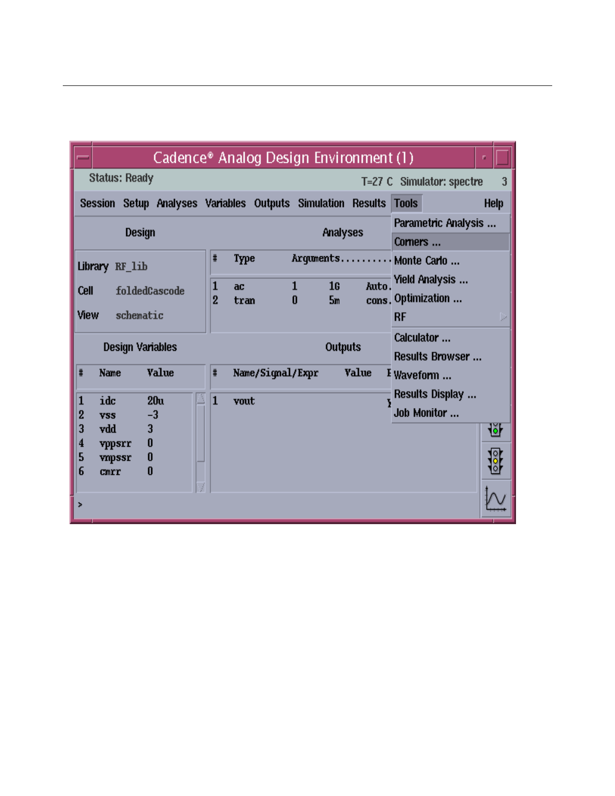
3. In the Cadence® Analog Design Environment window, choose Tools ->Corners.
If you have defined a set of customization files to be loaded automatically, the Cadence®
Analog Corners Analysis window appears.
To close the Cadence® Analog Corners Analysis window,
➤Choose File – Close.
Cadence Advanced Analysis Tools User Guide
Corners Analysis
July 2002 12 Product Version 5.0
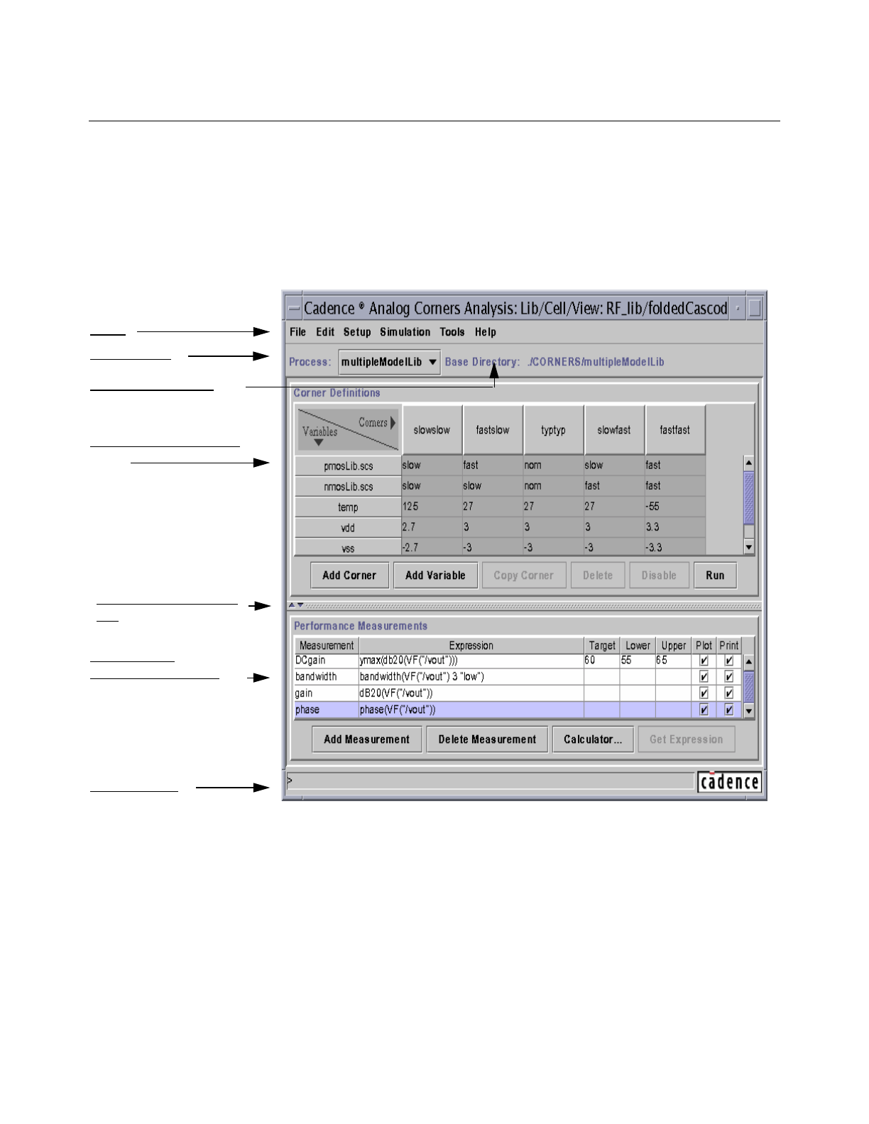
Getting to Know the Cadence® Analog Corners Analysis
Window
The Cadence®Analog Corners Analysis window contains the fields and controls required
to specify the corners and measurements for the analysis you want to run.
Status display
Menu
Process field
Corner Definitions pane
Performance
Measurements pane
Base Directory field
Split Pane Adjustment
Bar

Cadence Advanced Analysis Tools User Guide
Corners Analysis
July 2002 13 Product Version 5.0
Menu
The menu contains the commands needed to prepare for, run and plot the results of a corners
analysis.
For guidance on using the menu selections, see the associated cross-references.
Menu Item For More Information
File
Load “Using the Graphical User Interface to Load PCFs
and DCFs” on page 20
Save Setup “Saving Setup Information to the Original Files” on
page 33
Save Setup As “Saving Setup Information to a Specified File” on
page 33
Save Script “Saving a Script” on page 35
Close “Opening and Closing the Cadence® Analog Corners
Analysis Window” on page 10
Edit
Corner Definitions->
Add Corner “Creating a New Corner” on page 23
Corner Definitions->
Copy Corner “Copying and Modifying an Existing Corner” on
page 23
Corner Definitions->
Enable Corner “Enable Corner” on page 24
Corner Definitions->
Disable Corner “Disable Corner” on page 24
Corner Definitions->
Add Variable “Adding a Row for a New Design Variable” on
page 24
Corner Definitions->
Delete Selected “Deleting Corners or Rows” on page 25

Cadence Advanced Analysis Tools User Guide
Corners Analysis
July 2002 14 Product Version 5.0
Performance
Measurements->
Add Measurement
“Creating a New Performance Measurement by
Entering It Directly” on page 26, and “Creating a New
Performance Measurement by Using the Calculator”
on page 26
Performance
Measurements->
Delete Measurement
“Deleting a Performance Measurement” on page 27
Setup
Add Process “Using the Cadence® Analog Corners Analysis
Window to Define a Process” on page 52
Add/Update Model Info “Using the Cadence® Analog Corners Analysis
Window to Modify Process Model Information” on
page 53
Simulation
Run “Running and Stopping the Analysis” on page 28
Stop “Running and Stopping the Analysis” on page 28
Tools
Calculator “Creating a New Performance Measurement by
Using the Calculator” on page 26
Get Expression “Creating a New Performance Measurement by
Using the Calculator” on page 26
Plot or Print Outputs “Evaluating Corners Analysis Results” on page 28
Help
Contents Displays the documentation ( this user guide)
containing information about the Cadence®Analog
Corners Analysis option.

Cadence Advanced Analysis Tools User Guide
Corners Analysis
July 2002 15 Product Version 5.0
Process and Base Directory Fields
The Process field displays either the name of the current process or None, if no process is
specified. The processes are usually defined in customization files but can also be defined
from the graphical user interface.
If there is no current process, the only active Cadence®Analog Corners Analysis window
menu options are File ->Load,File ->Close, and Setup -> Add Process. These menu
options allow you to either load an existing file that defines a process or to define a new
process.
Note: Process refers to the manufacturing process. Therefore, process parameters are
parameters that pertain to the manufacturing process and are variables that help characterize
the models specific to the manufacturing process.
The Base Directory field displays the path that contains the models used in the analysis for
the process being displayed in the process field.
The base directory is usually defined by the corAddProcess command in a process
customization file (PCF). You can also define the base directory by choosing Setup ->Add
Process or Setup -> Add/Update Model Info.
Corner Definitions Pane
The Corner Definitions pane, located in the upper section of the Cadence® Analog
Corners Analysis window, displays information about the currently defined corners.

Cadence Advanced Analysis Tools User Guide
Corners Analysis
July 2002 16 Product Version 5.0
The information in this pane is usually loaded from process customization files (PCFs) and
design customization files (DCFs) using paths defined in your .cdsinit file. For details
refer to the section, Using a .cdsinit File to Load PCFs and DCFs.
To define or revise corners, you modify the information in this pane. Each column
characterizes a corner. You can select a column by clicking on the corresponding button
along the top of the pane. Each row ( or variable) begins with a group name or design
variable name, followed by the values to be used in each of the corners. You can select a
variable by clicking on the corresponding button along the left side of the pane. You can drag
a selection of variables by clicking and moving the cursor in the variable header. You can
also physically move the corner columns by dragging them around in the column header.
You can alter the width of columns by grabbing the separation bar and dragging it one way or
the other. There are certain limits (upper and lower) to how big or small you can make a
column. This also differs by column type in the case of the measurment table.
Disabled corners are grayed or fuzzed out in the form, while enabled corners are displayed
in normal text. Editable data in the Corners table looks like normal text, while uneditable data
in the Corners table will have a dark gray background. Uneditable group/variant entries will
just appear as a text field with the value of the field in text. Editable group/variant entries will
appear as a drop-down box.
Note: Temperature is a default variable with default value of 27.
The items in the Corner Definitions pane are described in the following table:
Item Description and Usage
Add Corner Click to add a new editable column to the right of the
existing columns.
Add Variable Click to add a new editable variable (row) below the
existing variable (row).
Copy Corner Click to add a new editable column filled with the data from
a highlighted column. This cloumn is added to the right of
the existing columns
Delete Click to delete a highlighted corner or variable (which is
not added by the pcf file).
Note: Variables (rows) and Corners added by the pcf file
cannot be deleted. Variables (rows) and Corners added by
the dcf file or the UI can be deleted.
Cadence Advanced Analysis Tools User Guide
Corners Analysis
July 2002 17 Product Version 5.0
Performance Measurements Pane
The Performance Measurements pane, located in the lower section of the Cadence®
Analog Corners Analysis window, displays information about the currently defined
measurements.
The information in this pane is usually loaded from design customization files (DCFs) using
the loadDcf command in your .cdsinit file. In addition, any outputs defined in the
Cadence®Analog Design Environment window when you first start the corners analysis
option also appear. You can also load measurements from PCF files. You can also use the
Calculator to get an expression.
Note: You can also use the Add Measurment button to add a measurment.
Also mention the
To specify or change the measurements, you modify the information in this pane. You can
select a measurement by clicking in any of the fields in the measurement pane.
Disable Click to disable a highlighted corner column. This
particular corner will not be analysed after simulation and
the column is grayed out. Once the column is disabled, the
Disable button changes to an Enable button. You can re-
enable the disabled corner by selecting it and clicking on
the Enable button.
Run/
Stop Click Run to run all the corners that are not disabled. Click
Stop to end a running corners analysis.
Click Run to run all the corners in the pane which are not
disabled.
Note: Run turns to Stop once you start a run.
Item Description and Usage

Cadence Advanced Analysis Tools User Guide
Corners Analysis
July 2002 18 Product Version 5.0
Note: The Cut,Paste and Copy keys work in the table fields. You can use these keys to
copy a measurement expression into another expression, from within the Corners window.
The items in the Performance Measurements pane are described in the following table:
Item Description and Usage
Measurement column Click to select a field in the Measurement column then
type or edit a name to be used as the label when the
expression is plotted or printed.
Expression column Click to select a field in the Expression column then type
or edit an expression to be evaluated for each corner.
Target column Click to select a field in the Target column and then type
the ideal target value for the measurement. This value is
used when a residual plot is created.
Lower column Left click twice to select a field in the Lower column and
then type the lowest acceptable value for the
measurement. This value is used when a residual plot is
created.
Upper column Left click twice to select a field in the Lower column and
then type the highest acceptable value for the
measurement. This value is used when a residual plot is
created.
Plot checkbox Select a checkbox if you want the output to appear as a
graph.
Print checkbox Select a checkbox if you want the output to appear as text.
Add Measurement button Click to add a new editable row below the existing rows.
Delete Measurement button Click to delete a highlighted row from the Performance
Measurements pane.
Calculator... button Click to open the calculator window.
Note: If the Calculator is not open and if you click on Get
Expression, it will invoke Calculator.
Get Expression button With an Expression field selected, click this button to
retrieve the expression displayed in the calculator buffer.
Note: The existing text in the field is replaced.

Cadence Advanced Analysis Tools User Guide
Corners Analysis
July 2002 19 Product Version 5.0
Split Pane Adjustment Bar
The split pane adjustment bar between the Corner Definitions Pane and the Measurements
Pane can be used to alter the area used by each pane. You can alter the area used by each
pane by dragging the bar upwards or downwards.
Status Display
The status display shows messages in one of three colors, depending on the type of
message.
The corners analysis tool also writes messages to the corners log file, corners0.log. The
corners analysis tool puts the log file in the directory where you start the Cadence®software.
Keyboard Navigation and Shortcuts
Listed below are some shortcut keys that can be used for navigation of the form and tables.
These keys can also be used during the row and column selection mode to change the
selected row or column.
Red Error Messages
Orange Internal Error Messages
Gray Information Messages
Tab Moves through table entries from left to right. Wraps to the next row
and at the end jumps back to the top.
Shift-Tab Reverse of Tab.
Arrow keys Moves as expected, does not wrap around at all.
F2 Opens/Closes a cyclic box.
Page Down Scrolls the table down if there is a vertical scroll bar.
Page Up Scrolls the table up if there is a vertical scroll bar.
Home Moves to the first column in the row.
End Moves to the last column in the row.

Cadence Advanced Analysis Tools User Guide
Corners Analysis
July 2002 20 Product Version 5.0
Running a Corners Analysis
The following sections describe the major steps involved in setting up and running a corners
analysis.
■“Defining the Corners for an Analysis” on page 20
■“Defining Performance Measurements” on page 26
■“Controlling the Corners Analysis” on page 27
Defining the Corners for an Analysis
To specify the corners for an analysis, you begin by loading a set of predefined corners from
one or more process customization files (PCFs). The loading can occur automatically under
the control of a .cdsinit file or you can load PCFs from the graphical user interface. For
information about using the .cdsinit file to load PCFs and DCFs, see “Using a .cdsinit File
to Load PCFs and DCFs” on page 40.
To tailor the predefined corners to the specific circuits you are working on, you can also load
one or more files containing changes and additions to the basic set of corners. These files
are called design customization files (DCFs). For information on preparing PCFs and DCFs,
see “Creating Process and Design Customization Files” on page 36.
If, after loading the PCFs and DCFs, you find that more changes are necessary, you can use
the graphical user interface to specify new corners or change any editable existing corners.
You can load multiple sets of corners information into the corners analysis option.
■If you load a file or files that define more than one process, the processes appear in the
Process cyclic field in the Cadence® Analog Corners Analysis window.
■If you add more than one file (such as a DCF), that modifies a specific process, the
contents of files that are loaded are added to the contents of the existing files.
The next section describes how to load PCFs and DCFs from the graphical user interface.
For information about using the .cdsinit file to load PCFs and DCFs, see “Using a .cdsinit
File to Load PCFs and DCFs” on page 40.
Using the Graphical User Interface to Load PCFs and DCFs
The .cdsinit file typically specifies the PCFs and DCFs, so usually when you open the
Cadence® Analog Corners Analysis window, it already contains some corner, variable,
and measurement definitions.However, if there are no predefined corners or if you need to
Cadence Advanced Analysis Tools User Guide
Corners Analysis
July 2002 21 Product Version 5.0
load a different set, you can use the following steps to load PCFs and DCFs from the
graphical user interface.
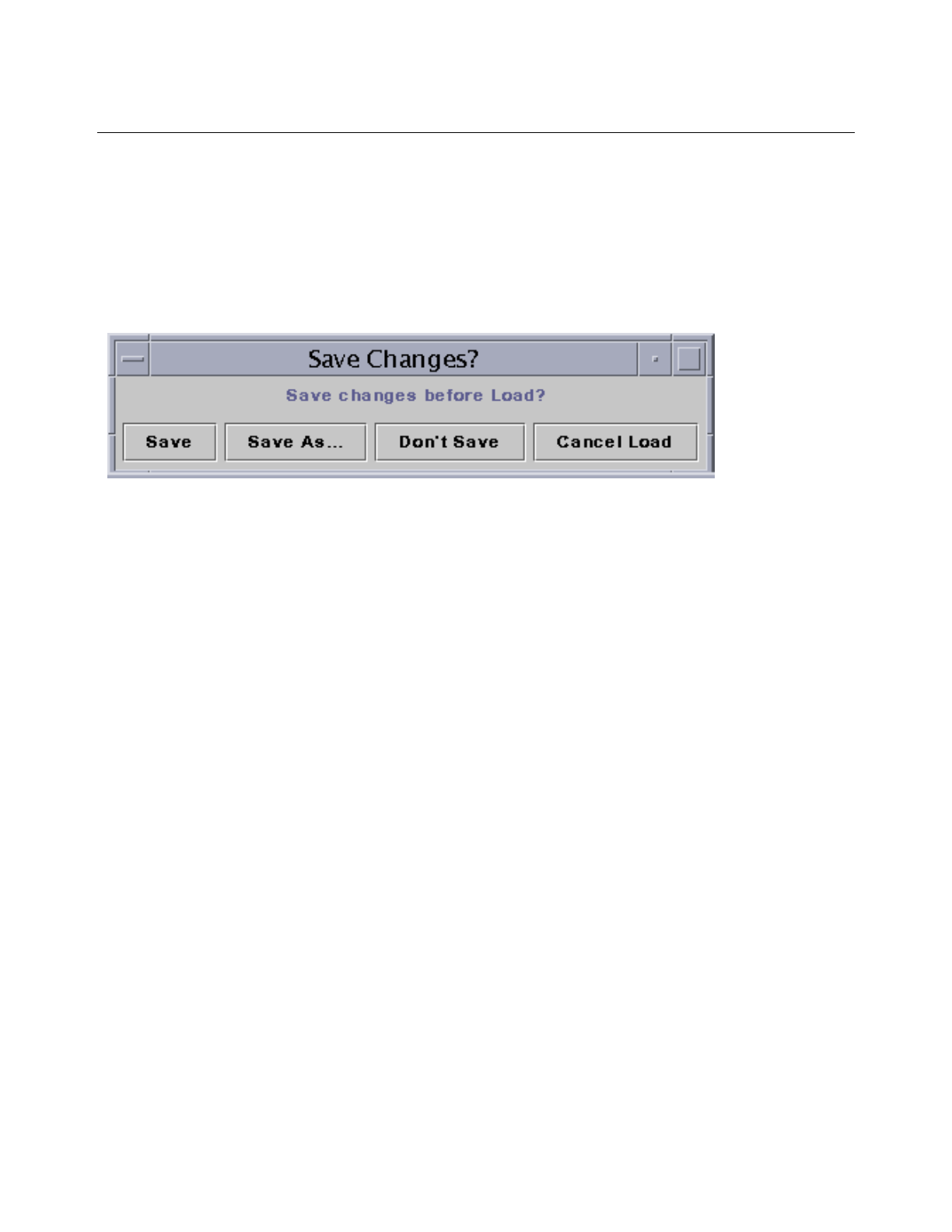
1. Choose File -> Load.
If you have made changes in the Cadence® Analog Corners Analysis window, the
Save Changes? dialog box appears.
2. Click either Save or Save As to save the changes. If you do not want to save the
changes made, but want to load the PCFs and DCFs anyway, click Don’t Save. Click
Cancel Load if you want to retain the existing set of PCFs and DCFs.
Cadence Advanced Analysis Tools User Guide
Corners Analysis
July 2002 22 Product Version 5.0
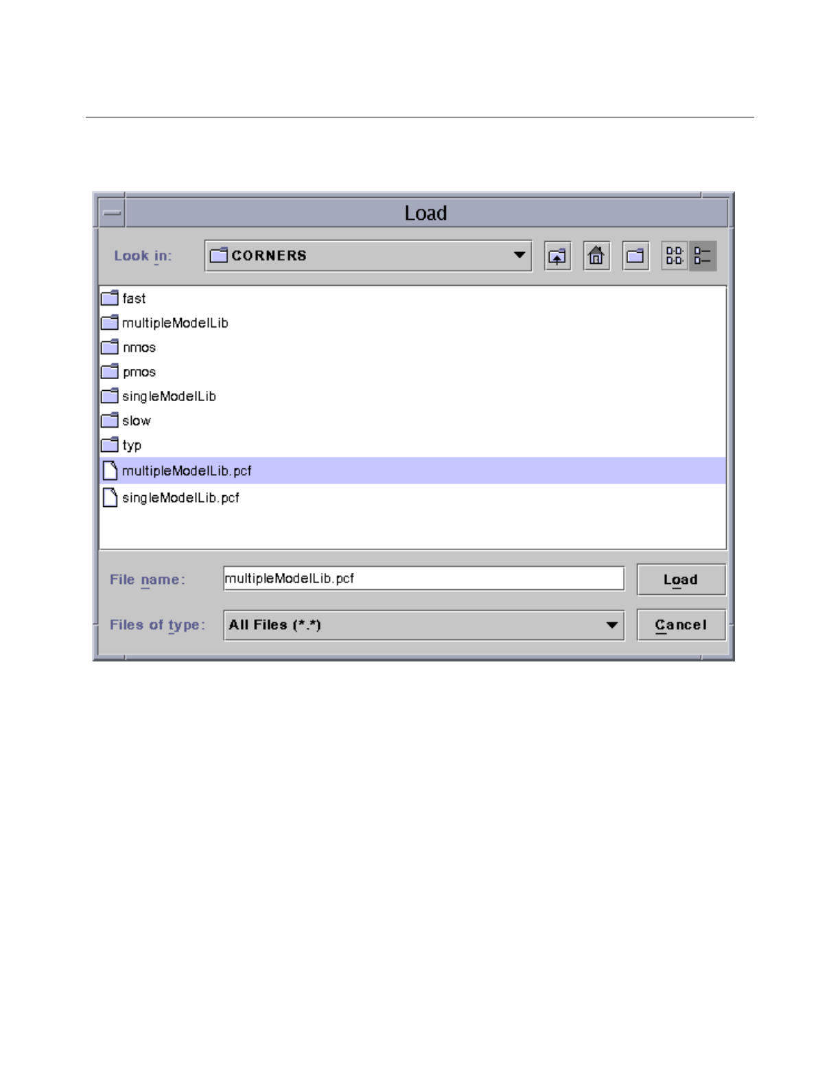
The Load dialog box appears.
3. Click on the Look In drop down field to go to the specific directory. You can also navigate
using the iconified buttons located next to the Look In field. Placing the pointer on each
of the buttons displays a tooltip that describes the function of the button, as follows:
Note: You can double-click a directory folder to descend into that directory.
Button Function
Up One Level Opens the directory one level above the
active directory.
Home Opens the home directory.
Create New Folder Creates a new directory in the active
directory.

Cadence Advanced Analysis Tools User Guide
Corners Analysis
July 2002 23 Product Version 5.0
4. In the Files of Types field, select a type of file from the given list. The list of files is
automatically updated. Default is All Files(*.*).
5. Select the file that you want to load. The name of the file is reflected in the File Name
field. Click on Load button to load the file. Click on Cancel button if you want to cancel
the operation.
Specifying Additional Corners
If you need to specify additional corners from those loaded in the PCFs and DCFs, you can
create new corners in the graphical user interface. You can either create new corners or copy
existing corners and modify them.
Creating a New Corner
To create a new corner,
1. Choose Edit -> Corner Definition -> Add Corner. You also click on the Add Corner
button.
The Enter Corner Name form is displayed.
2. Type a name for the new corner.
3. If you do not want to add the corner, click Cancel Add Corner. Click OK if you want to
add the corner. A new column appears at the right side of the Corner Definitions pane of
the Cadence®Analog Corners Analysis window. The new column is named with the
name from Step 2.
4. Edit the rest of the column as desired.
Copying and Modifying an Existing Corner
If one of the existing corners is similar to the corner you want to use, you can copy the existing
corner and change the copy to meet your needs
1. Highlight the column for the corner you want to copy.
2. Choose Edit -> Corner Definition -> Copy Corner. You can also click on the Copy
Corners button.
The Enter Corner Name form is displayed.
3. Enter a name for the new corner.

Cadence Advanced Analysis Tools User Guide
Corners Analysis
July 2002 24 Product Version 5.0
4. If you do not want to continue, click Cancel Copy Corner. Click OK if you want to
continue. A new column appears at the right side of the Corner Definitions pane of the
Cadence® Analog Corners Analysis window.
5. Fill in the rest of the column as necessary.
Enable Corner
1. Select a disabled corner.
2. Choose Edit -> Corner Definitions -> Enable Corner or click Enable. The selected
corner will be enabled.
Disable Corner
1. Select an enabled corner.
2. Chose Edit -> Corner Definitions -> Disable Corner or click Disable. The selected
corner will be disabled. This particular corner will not be analysed after simulation and
the column is grayed out. Once the column is disabled, the Disable button changes to
an Enable button. You can re-enable the disabled corner by selecting it and clicking on
the Enable button.
Note: You can disable only an editable Variable (row) or column. Variables (rows) and
Corners added by the pcf file are not editable. Variables (rows) and Corners added by
the dcf file or the UI are editable.
Adding New Variables
There are three kinds of variables you can define for a corner: group variables, process
variables and design variables. For information on adding group and process variables, see
“Using the Cadence® Analog Corners Analysis Window to Modify Process Model
Information” on page 53. For guidance on adding design variables, see the next section.
Adding a Row for a New Design Variable
To add a new design variable to the existing variables,
1. Choose Edit -> Corner Definition -> Add Variable. You can also click on the Add
Variable button.
The Enter Variable Name form is displayed.
2. Type a name for the new design variable.

Cadence Advanced Analysis Tools User Guide
Corners Analysis
July 2002 25 Product Version 5.0
The design variable is added not only to the current process but also to all the other
processes listed in the process cyclic field of the Cadence®Analog Corners Analysis
window.
3. Click OK. If you want to continue. Otherwise, click Cancel Add Variable.
4. (Optional) Select the new variable field in each of the corners, and type the values you
want to use.
Deleting Corners or Rows
You cannot delete corners and variables (rows) added by a PCF. However, if the DCFs load
corners you do not plan to use, you can delete them. You can also delete un-needed rows
added by DCFs or from the Cadence®Analog Corners Analysis window. Deleted corners
and rows disappear from the Corners Definition pane of the Cadence®Analog Corners
Analysis window and their underlying data is erased.Corners added from the Corners UI can
also can be deleted.
Deleting Corners
To delete a corner,
1. Highlight the column for the corner you want to delete.
2. Choose Edit – CornerDefinitions-> Delete Selected or click Delete.
The highlighted column disappears from the pane.
Deleting Rows
To delete a row,
1. Highlight the row you want to delete.
Note: You can delete only rows defined by a DCF or added by using the Cadence®
Analog Corners Analysis window. You cannot delete rows defined in a PCF.
2. Choose Edit – Corner Definitions -> Delete Selected or click Delete.
The highlighted row disappears from the pane.

Cadence Advanced Analysis Tools User Guide
Corners Analysis
July 2002 26 Product Version 5.0
Defining Performance Measurements
For convenience, measurements are often specified in design customization files (DCFs).
Measurements defined in this way are displayed in the Performance Measurements pane,
where you can examine them. In addition, any outputs defined in the Cadence®Analog
Design Environment window when you first start the corners analysis option are also
displayed.
If the existing measurements do not meet your needs, you can add new measurements or
make and modify copies of the existing measurements. If you have no plans to use a
measurement, you can delete it. You can add or change performance measurements either
before or after you run the analysis. You can also specify measurements through a PCF file.
Creating a New Performance Measurement by Entering It Directly
To create a new performance measurement by entering it directly,
1. Choose Edit –> Performance Measurements -> Add Measurements or click Add
Measurement.
The Enter Measurement Name form is displayed.
2. Enter a name for the new Measurement.
3. Click Cancel Add Measurement if you do not want to continue. Click OK, if you want
to continue. A new row will appear in the Corner Performance measurement pane.
4. Type the expression in the Expression field.
5. (Optional) Type the Target,Lower and Upper values for the new measurement. You
need to specify these values only if you plan to use this performance measurement in a
residual plot. A residual plot allows you to easily see whether a scalar measurement falls
within the specified boundaries for all of your corners using a histogram like bar plot.
Note: Target is a target value for a scalar measurement.Upper is the acceptible upper
boundary for a scalar measurement. Lower is an acceptable lower boundary for a scalar
measurement. If Target ,Upper and Lower bound are set for a waveform, they will not
be used at all. These options are only used for the residual plots.
Creating a New Performance Measurement by Using the Calculator
To create a new performance measurement using the calculator,
1. Choose Edit -> Performance Measurements -> Add Measurement or click Add
Measurement.

Cadence Advanced Analysis Tools User Guide
Corners Analysis
July 2002 27 Product Version 5.0
The Enter Measurement Name form is displayed.
2. Type a name for the new measurement.
3. Click Cancel Add Measurement if you do not want to continue. Click OK, if you want
to continue. A new row will appear in the Corner Performance measurement pane.
4. Choose Tools ->Calculator or click Calculator to open the calculator window.
5. Build the measurement expression in the calculator.
For information on using the calculator, see the Waveform Calculator User Guide.
6. In the Cadence® Analog Corners Analysis window, select the Expression field for
the new measurement.
Note: If the expression field is selected, then only the Get Expression button will be
highlighted.
7. Choose Tools -> Get Expression, or click Get Expression to retrieve the expression
from the calculator and place it in the selected Expression field.
8. (Optional) Type the Target,Lower and Upper values for the new measurement. You
need to specify these values only if you plan to use this performance measurement in a
residual plot.
Deleting a Performance Measurement
You can delete any measurement displayed in the Cadence® Analog Corners Analysis
window. A deleted measurement disappears from the Performance Measurements pane, and
the data underlying it is erased. If you delete a measurement and then save the setup, the
deleted measurement is not included in the saved setup.
To delete a measurement,
1. Highlight the row for the measurement you want to delete.
2. Choose Edit -> Performance measurement -> Delete Measurement, or click
Delete Measurement.
The highlighted measurement disappears from the pane.
Controlling the Corners Analysis
You are ready to run the analysis after defining the corners and specifying the performance
measurements you need. To do this,
Cadence Advanced Analysis Tools User Guide
Corners Analysis
July 2002 28 Product Version 5.0
❑Disable the corners that you do not want to run.
❑Select the output format for the measurements to determine what type of
measurement output you want, if any. You can use the Plot and Print checkboxes
to specify whether you require a graphic or text output.
To choose the output formats for each measurement, click the Plot and Print
checkboxes on the right side of the Performance Measurements pane.
Then, run the analysis.
Running and Stopping the Analysis
To run the analysis,
➤Choose Simulation -> Run or click Run.
To stop an analysis running on a single machine,
1. Choose Simulation ->Stop or click Stop.
To stop a simulation running distributed, use Job Monitor. For more information about Job
Monitor, refer to the Cadence Analog Distributed Processing Option User Guide.
Note: The Run button automatically changes between Run/Stop depending on whether a
Corners process is currently running or not.
Evaluating Corners Analysis Results
When the analysis finishes, the corners analysis option plots or lists the results according to
whether you chose text or graphic outputs in the Performance Measurements pane.

Cadence Advanced Analysis Tools User Guide
Corners Analysis
July 2002 29 Product Version 5.0
Note: If you run a distributed simulation, the results do not plot or list automatically.
If you want a different set of outputs from those you chose before running the analysis, you
can make new choices in the Performance Measurements pane and then choose Tools –
Plot or Print Outputs from the menu). In response, the corners analysis option evaluates
the selected measurements and displays new lists or plots.
Text Outputs
For a scalar measurement, a text output looks like this.
Each column in this window displays the value of a scalar measurement for each of the
corners. In this example, bandwidth varies from a low of 130.7 K under the slowslow corner
conditions, to a high of 318.7 K under the fastfast corner conditions.
Cadence Advanced Analysis Tools User Guide
Corners Analysis
July 2002 30 Product Version 5.0
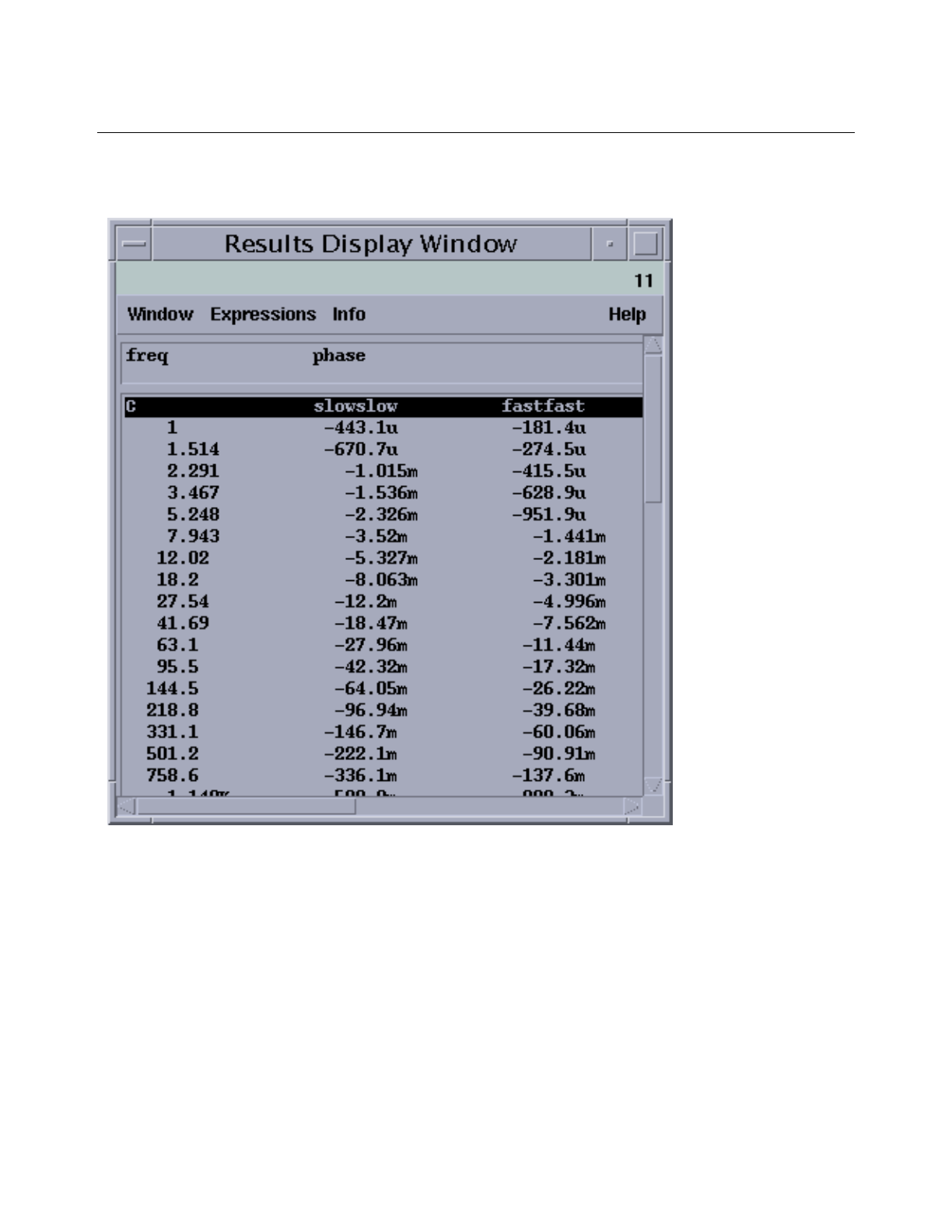
For a waveform measurement, a text output looks like this.
The first column in this window lists the data points for an analysis. Each subsequent column
lists data for a particular corner. In this example, at a frequency of 758.6 Hz, the phase for the
slowslow corner is -336.1 m and for the fastfast corner is -137.6 m.
Graphic Outputs
There are two kinds of graphic output, a residual plot for scalar data and a family-of-curves
plot for waveform data. A residual plot allows you to easily see whether a scalar measurement
Cadence Advanced Analysis Tools User Guide
Corners Analysis
July 2002 31 Product Version 5.0
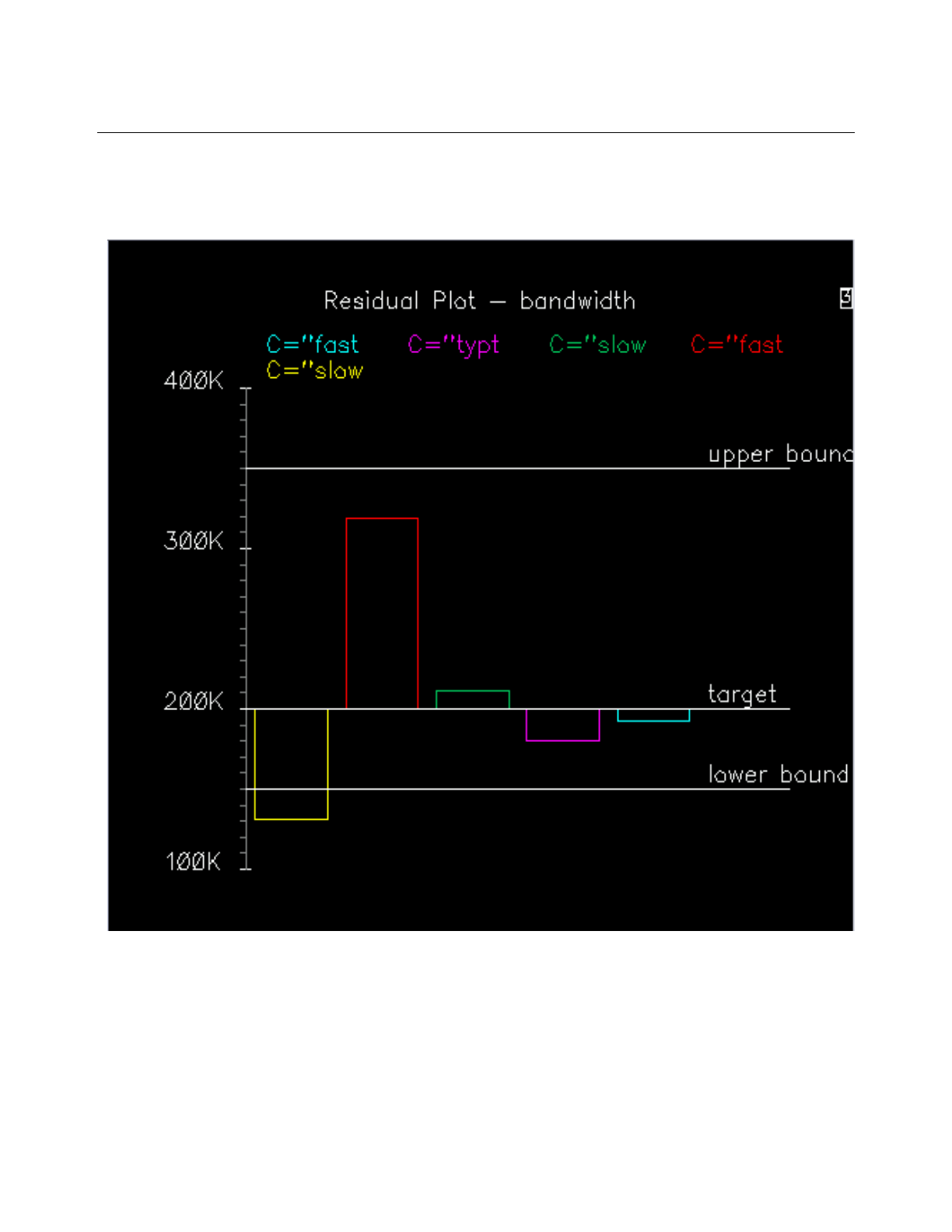
falls within the specified boundaries for all of your corners using a histogram like bar plot. A
residual plot looks like this.
The preceding residual plot, has a specified value of 200 for Target and shows that four of
the corners produce values within specifications. One corner produces a value that does not
lie within the lower boundary of the acceptable range. This result implies that yield for the
manufactured circuit will be less than 100 percent if the circuit is produced in its current form.
For greater yield, the circuit designer might want to redesign the circuit so it performs
acceptably for all the corners.
Cadence Advanced Analysis Tools User Guide
Corners Analysis
July 2002 32 Product Version 5.0
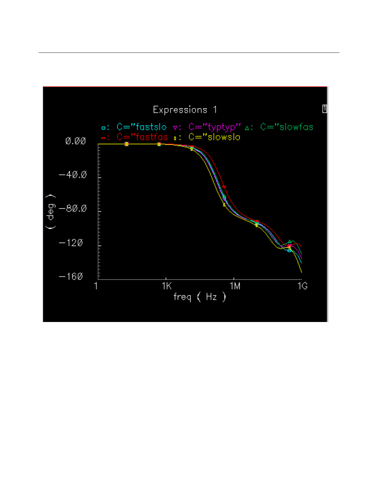
The set of curves for all the corners, looks like this.
The preceding plot shows how the phase varies as a function of frequency for each one of
the corners.
Saving Setup Information
The corners option setup consists of all the information in the Cadence® Analog Corners
Analysis window, including the corner definitions and performance measurements. With
menu selections in the File entry, you can save the setup back to the original files, save the
setup to a specified file, and load a saved setup.

Cadence Advanced Analysis Tools User Guide
Corners Analysis
July 2002 33 Product Version 5.0
Saving Setup Information to the Original Files
To save the current setup back to the files from which it was loaded,
➤Choose File ->Save Setup.
If the PCFs and DCFs are not writable, the corners analysis option reports an error, and
changes and additions made in the Cadence® Analog Corners Analysis window are not
saved.
If the PCFs and DCFs are writable, the corners analysis option saves changes back to those
files, overwriting the original contents of those files. As a result, any comments you might
have in the PCFs or DCFs are overwritten and lost. The corners analysis option saves any
additions to the DCF loaded last, if possible or to a newly created file called
NewEntries.dcf. This implies that if you add any Corners, Variables or Measurements,
they are added to the last loaded DCF. The NewEntries.dcf file is created when no PCF
and no DCF are loaded.
To avoid overwriting comments and to have the changed setup saved in a single easy-to-
understand location, use File -> Save Setup As, described in the following section.
Saving Setup Information to a Specified File
To save the current setup in a file you specify,
1. Choose File -> Save Setup As.

Cadence Advanced Analysis Tools User Guide
Corners Analysis
July 2002 34 Product Version 5.0
The Save Setup As form is displayed.
2. Click on the Look In drop down field to go to the specific directory. You can also navigate
using the iconified buttons located next to the Look In field. Placing the pointer on each
of the buttons displays a tooltip that describes the function of the button, as follows:
Note: You can double-click a directory folder to descend into that directory.
3. In the Files of Types field, select a type of file from the given list. The list of files is
automatically updated. Default is All Files(*.*).
Select the file where the setup information is to be saved. The name of the file is reflected
in the File Name field.
Button Function
Up One Level Opens the folder one level above the active
folder.
Home Opens the home directory.
Create New Folder Creates a new folder in the active folder.

Cadence Advanced Analysis Tools User Guide
Corners Analysis
July 2002 35 Product Version 5.0
4. Click Save. Click on the Cancel button if you want to cancel the operation.
Note: If you double-click on a selected file, the information will be directly saved to the
file.
All of the existing corners option information, whether loaded from PCFs, DCFs or
through the corners option graphical user interface, is saved to the file you specify. If
necessary, you can then cut and paste the lines into other PCFs and DCFs.
Saving a Script
The Open Command Environment for Analysis (OCEAN) lets you set up, simulate, and
analyze circuit data. OCEAN is a text-based process you can run from a UNIX shell or from
the Command Interpreter Window (CIW). You can type OCEAN commands in an interactive
session, or you can create scripts containing your commands and load those scripts into
OCEAN.
You can use the Cadence®Analog Corners Analysis window to set up the analysis you need,
and save the setup procedure in an OCEAN script. You can then edit the script to add
simulation or postprocessing commands as needed.
For more information about OCEAN commands and scripts, see the OCEAN Reference.
To create a script and save it,
➤Choose File ->Save Script.
The Save Ocean Script form appears so you can specify a file for the script.
Using Process, Design, and Modeling Files
There are usually three different kinds of files associated with setting up a corners analysis.
■Process customization files (PCFs) define processes, groups, variants, and corners
shared by an entire organization. PCFs are usually created by a process engineer or
process group.
■Design customization files (DCFs) contain definitions used for a particular design or for
several designs within a design group. DCFs are usually created by designers, who use
the DCFs to add design-specific information to the general information provided in PCFs.
■Modeling files specify the model parameter values to be used for components during a
corners analysis. These files are usually created by a process engineer or process
group.

Cadence Advanced Analysis Tools User Guide
Corners Analysis
July 2002 36 Product Version 5.0
Day-to-day use of the corners analysis option typically does not involve changing a PCF or
DCF. However, if you are involved in writing or changing these kinds of files, read the following
sections for guidance.
Creating Process and Design Customization Files
The process customization files (PCFs) and design customization files (DCFs) contain
Cadence SKILL language commands that define the basic corners and measurements to be
used during analysis. The following sections illustrate how you can use the commands to
develop the set of definitions you need.
You can use any of the corners option SKILL language PI commands in either the PCFs or
DCFs. However, the commands used to define the process, the corners, and the corner
variables are customarily placed in the PCF. The commands used to specify design variables
and measurements, because they are design specific, are usually placed in the DCF.
The corSetModelFile command can be used only with the single model library style.
For more information, including the formal syntax for the commands, see the Cadence®
Analog Design Environment SKILL Language Reference.
To debug PCFs and DCFs, consider using OCEAN. The feedback the corners analysis option
provides is limited, but OCEAN provides more detailed feedback that makes it easier to find
and correct errors. For examples of OCEAN scripts that illustrate using PCFs and DCFs, see
the following directory in your installation hierarchy:
Commands Normally in a PCF Commands Normally in a DCF
corAddProcess
corSetModelFile
corAddCorner
corAddGroupAndVariantChoices
corAddModelFileAndSectionChoices
corSetCornerModelFileSection
corAddProcessVar
corSetProcessVarVal
corSetCornerGroupVariant
corSetCornerNomTempVal
corAddDesignVar
corSetDesignVarVal
corSetCornerRunTempVal
corAddMeas
corSetMeasExpression
corSetMeasLower
corSetMeasUpper
corSetMeasTarget
corSetMeasGraphicalOn
corSetMeasTextualOn
Commands Used in Both
corSetCornerVarVal
corCopyCorner

Cadence Advanced Analysis Tools User Guide
Corners Analysis
July 2002 37 Product Version 5.0
your_install_dir/tools/dfII/samples/artist/corners
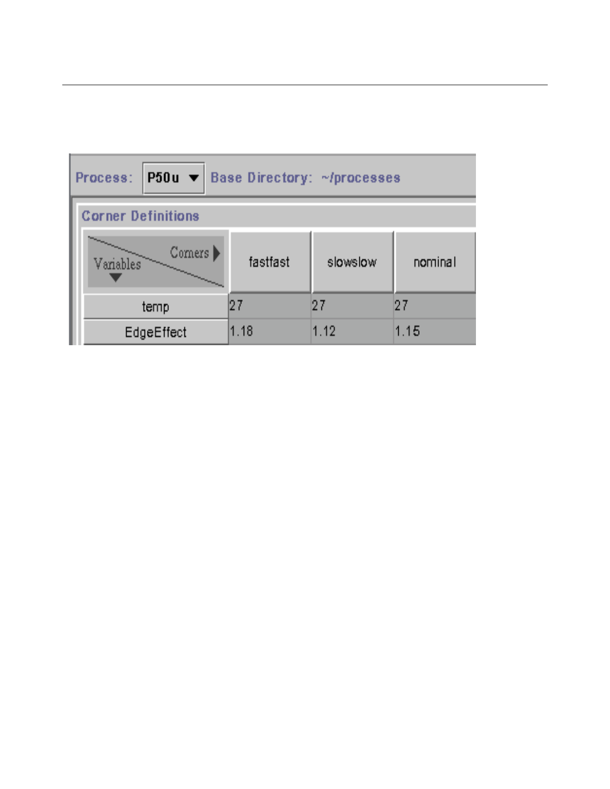
Example: Preparing a Process Customization File
The process customization file (PCF) adds the name of a new process to the corners analysis
option graphical user interface and defines the basic set of corners. For example, the
following PCF adds the process name P50u, specifies the modeling style as
singleModelLib, and defines three corners: slowslow,nominal, and fastfast.
; Example PCF file for the process P50u.
corAddProcess( "P50u" "~/processes" ’singleModelLib )
corSetModelFile("P50u" "P50uModelFile.scs")
; Prepare to add a process variable to each corner.
corAddProcessVar( "P50u" "EdgeEffect" )
; Now add the corners, specifying the values and choices for each.
corAddCorner( "P50u" "fastfast" )
corSetCornerVarVal( "P50u" "fastfast" "EdgeEffect" "1.18" )
corAddCorner( "P50u" "slowslow" )
corSetCornerVarVal( "P50u" "slowslow" "EdgeEffect" "1.12" )
corAddCorner( "P50u" "nominal" )
corSetCornerVarVal( "P50u" "nominal" "EdgeEffect" "1.15" )
The modeling values for the fastest,typical, and slowest variants are not defined in
the PCF. Instead, they are defined in the modeling file. For example, assume the
P50uModelFile.scs referred to by the P50u PCF contains the following statements.
.LIB slowest
.model npn2 npn tf=120n
.model nmosR nmos tox=120n
.ENDL slowest
.LIB typical
.model npn2 npn tf=100n
.model nmosR nmos tox=100n
.ENDL typical
.LIB fastest
.model npn2 npn tf=80n
.model nmosR nmos tox=80n
.ENDL fastest
Cadence Advanced Analysis Tools User Guide
Corners Analysis
July 2002 38 Product Version 5.0
Loading P50u PCF, which refers to the P50uModelFile.scs, produces the following
arrangement in the Cadence® Analog Corners Analysis window.
Note: temp is always added with 27 being the default value for all corners.
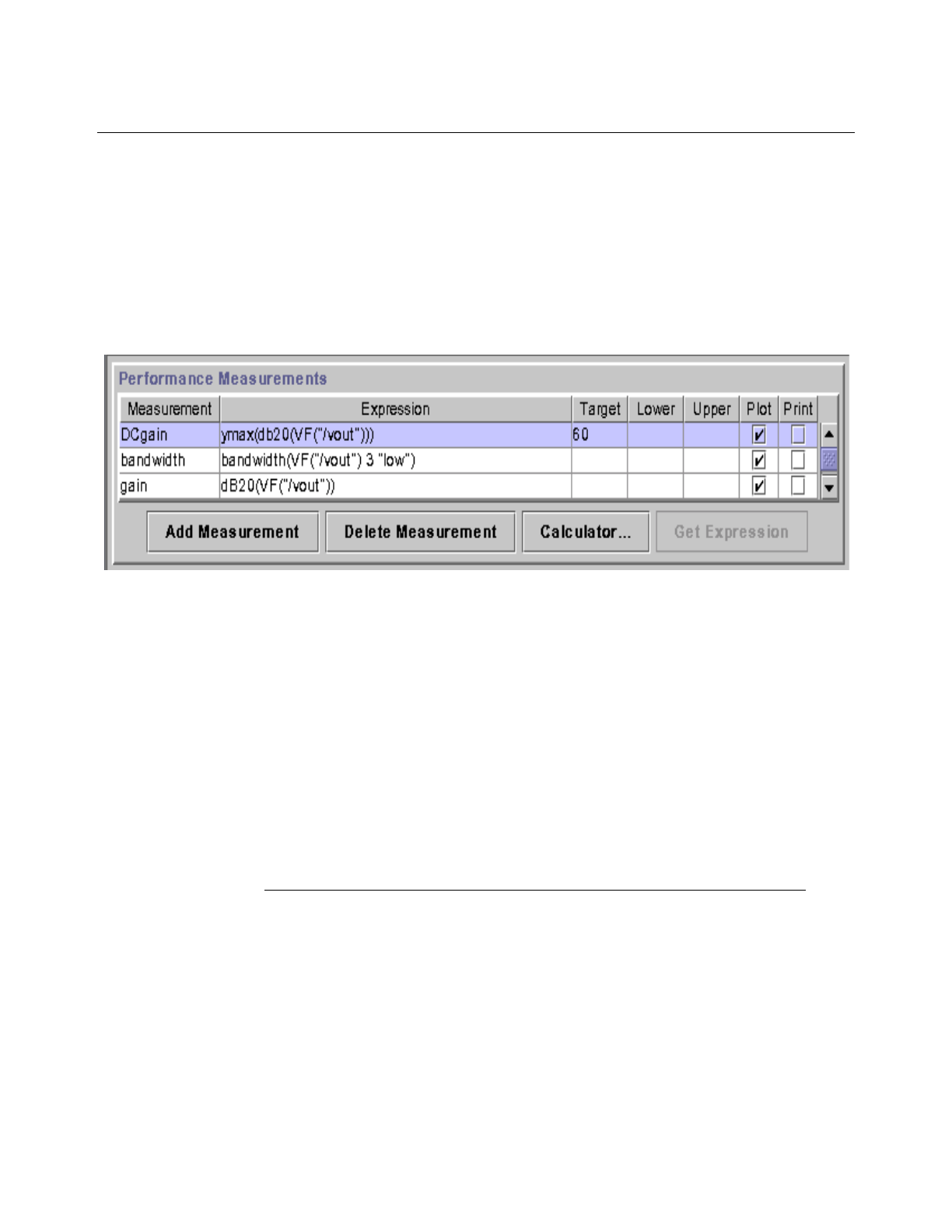
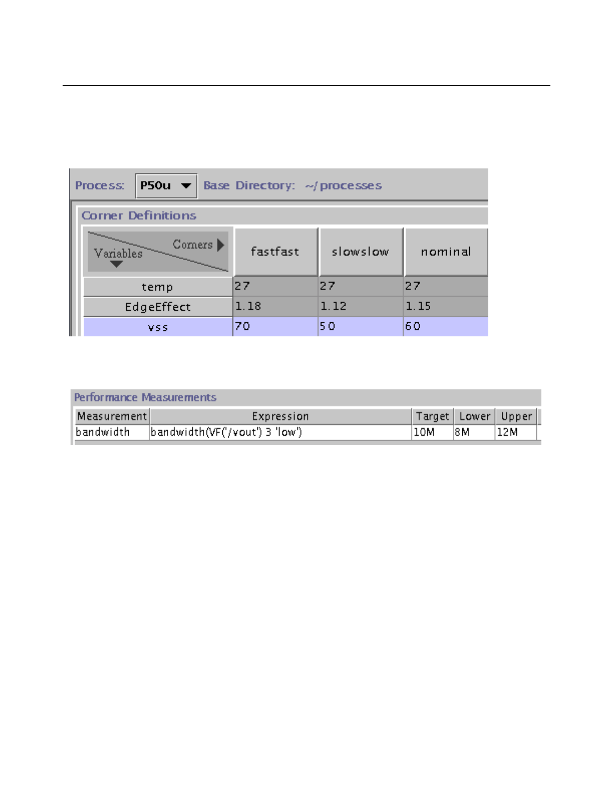
Example: Preparing a Design Customization File
The DCF adds design-specific variables and measurements to the corners analysis option
graphical user interface that is specified in general by information in a PCF. For example, the
following DCF adds a design variable, sets the run temperature, and adds information to the
Performance Measurements pane:
corAddDesignVar( "vss" )
corSetDesignVarVal( "vss" "" )
corSetCornerVarVal( "P50u" "fastfast" "vss" "70" )
corSetCornerVarVal( "P50u" "slowslow" "vss" "50" )
corSetCornerVarVal( "P50u" "nominal" "vss" "60" )
corSetCornerRunTempVal("P50u" "slowslow" -35)
; You must add the measurement before you define it.
corAddMeas( "bandwidth" )
corSetMeasExpression( "bandwidth" "bandwidth(VF('/vout') 3 'low')" )
corSetMeasLower("bandwidth" "8Mhz")
corSetMeasUpper("bandwidth" "12Mhz")
corSetMeasTarget("bandwidth" "10Mhz")
Cadence Advanced Analysis Tools User Guide
Corners Analysis
July 2002 39 Product Version 5.0
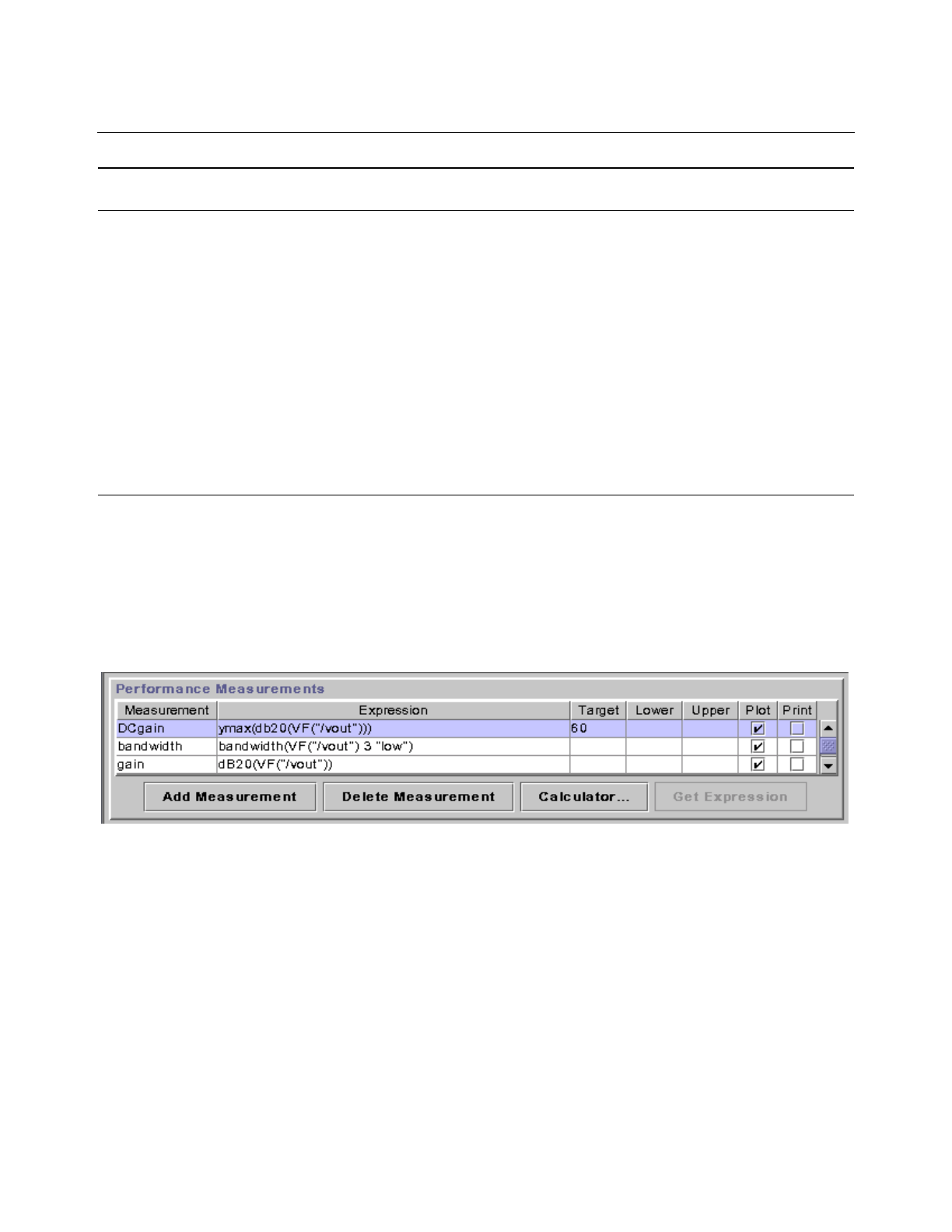
Loading this DCF along with the P50u PCF described in the previous section changes both
panes in the Cadence®Analog Corners Analysis window. The Corner Definitions pane
looks like this.
The Performance Measurements pane looks like this.

Cadence Advanced Analysis Tools User Guide
Corners Analysis
July 2002 40 Product Version 5.0
Using a .cdsinit File to Load PCFs and DCFs
A convenient way to load process and design customization files is to use your .cdsinit
file. You can set up your files in the following ways.
Whichever way you choose to load your files, you must make sure PCFs and DCFs refer only
to definitions that have already been loaded. Usually, that means you must load PCFs before
you can define corners or measurements in a DCF.
Implementing Modeling Styles
The corners analysis option supports five different modeling styles. Cadence recommends
the single model library or multiple model library styles for users running the Cadence®
Spectre® Circuit Simulator. For users running the SpectreS simulator, Cadence
recommends the multiple numeric modeling style.
The remaining two modeling styles, single numeric and multiple parametric, should be
used with caution.
To load both PCFs and DCFs explicitly in
the .cdsinit file To load DCFs explicitly and have them
load the PCFs they need
➤Make sure your .cdsinit file loads all
the necessary PCFs and DCFs.
For example, this .cdsinit file loads
several PCFs and DCFs.
loadPcf "process1.pcf"
loadPcf "process2.pcf"
loadDcf "cellPhone23.dcf
loadDcf "opamp47.dcf
1. Add load statements to each DCF for the
PCF files it uses. That way, when you
load the DCF file, it loads the PCF files
automatically.
For example, this fragment of the
myanalog35u.dcf file loads the
analog35u.pcf file.
; This is the myanalog35u.dcf
loadPcf("mypath/
analog35u.pcf")
2. Set up your .cdsinit file so it loads the
DCF. For example, this .cdsinit file
fragment loads the myanalog35u.dcf
file (which then loads the
analog35u.pcf).
loadDcf("/mnt4/radhikak/
tools/ dfII/src/corners/
myanalog35u.dcf")

Cadence Advanced Analysis Tools User Guide
Corners Analysis
July 2002 41 Product Version 5.0
The following sections illustrate the file structures used by these styles and give examples of
PCFs tailored to each style. For detailed information, see the sections listed below.
■“Single Model Library Style”
■“Multiple Model Library Style” on page 43
■“Single Numeric Style” on page 46
■“Multiple Numeric Style” on page 47
■“Multiple Parametric Modeling” on page 49
Single Model Library Style
Cadence recommends this easy-to-read style for use in corners analysis. With this
approach,
■All models for all corners are located in a single model file
■The model file is located in the base directory
■The model file can have any name
You can type the name in the Cadence®Analog Corners Analysis window or use the
corSetModelFile procedure to specify the name in a PCF or DCF.

Cadence Advanced Analysis Tools User Guide
Corners Analysis
July 2002 42 Product Version 5.0
The following table illustrates the single model library style with an example path, file, and file
contents. If you prefer, you can also use the .LIB syntax for this modeling style.The .LIB
syntax is an hspice modelling syntax that is supported in Spectre.
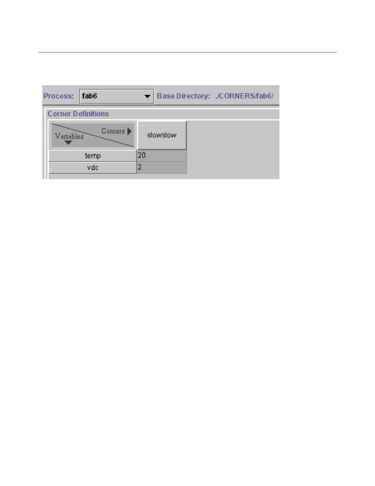
The following code illustrates how you can refer to this modeling structure in a PCF.
corAddProcess("fab6" "./CORNERS/fab6/" ’singleModelLib)
corSetModelFile("fab6" "mylibfile.scs")
corAddProcessVar("fab6" "vdc")
corAddCorner("fab6" "slowslow"
?runTemp 20
?nomTemp 27
?vars ’( ("vdc" 2) )
)
Single Model Library Style (Native Spectre)
Path Filename File Contents
./CORNERS/fab6/ mylibfile.scs library processA
section slowslow
model npn2 npn tf=120n
model npn9 npn tf=320n
model nmosR nmos tox=120n
model nmos8 nmos tox=320n
endsection
section nom
model npn2 npn tf=100n
model npn9 npn tf=300n
model nmosR nmos tox=100n
model nmos8 nmos tox=300n
endsection
section fastfast
model npn2 npn tf=80n
model npn9 npn tf=380n
model nmosR nmos tox=80n
model nmos8 nmos tox=380n
endsection
endlibrary
Cadence Advanced Analysis Tools User Guide
Corners Analysis
July 2002 43 Product Version 5.0
The Cadence® Analog Corners Analysis window produced by this PCF looks like this.
Multiple Model Library Style
This style uses multiple library files, which must be specified by using the
corAddModelFileAndSectionChoices and corAddCorner commands in a PCF or
DCF. In other ways, this style is the same as the single model library style. For example, the
models might be located in the following files:
./CORNERS/fab6/path1/npn.scs
./CORNERS/fab6/path3/nmos.scs

Cadence Advanced Analysis Tools User Guide
Corners Analysis
July 2002 44 Product Version 5.0
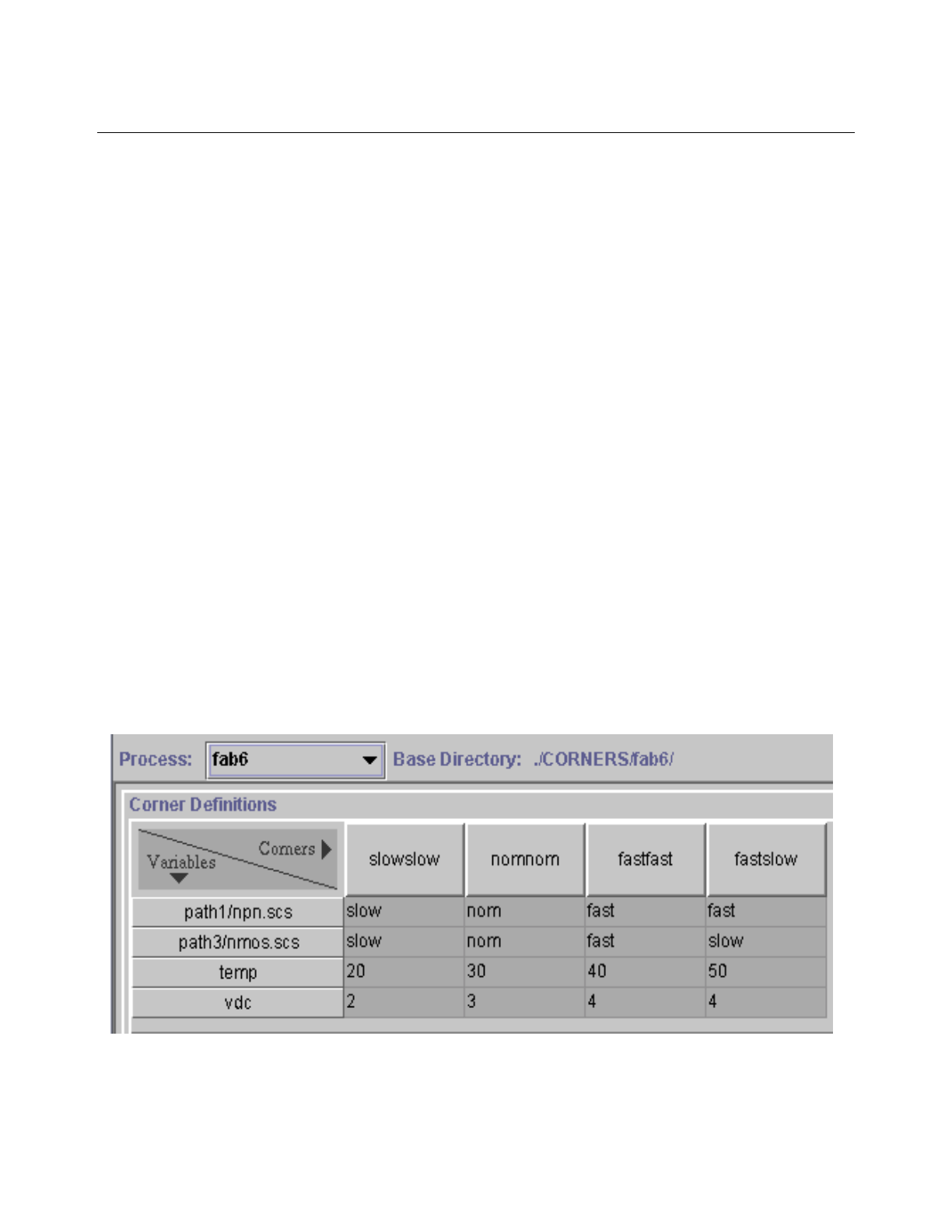
The following table illustrates the multiple model library style. If you prefer, you can also use
the .LIB syntax for this modeling style.
The following code illustrates how you can refer to this multiple model library structure in a
PCF.
corAddProcess("fab6" "./CORNERS/fab6/" 'multipleModelLib)
corAddModelFileAndSectionChoices("fab6" "path1/npn.scs"
Multiple Model Library Style
Path Filename File Contents
./CORNERS/fab6/
path1/
npn.scs library npn
section slow
model npn2 bjt tf=120n
model npn8 bjt tf=80n
endsection
section nom
model npn2 bjt tf=100n
model npn8 bjt tf=60n
endsection
section fast
model npn2 bjt tf=80n
model npn8 bjt tf=50n
endsection
endlibrary
./CORNERS/fab6/
path3/
nmos.scs library nmos
section slow
model nmosR mos3 tox=120n
model nmos2 mos3 tox=140n
endsection
section nom
model nmosR mos3 tox=100n
model nmos2 mos3 tox=115n
endsection
section fast
model nmosR mos3 tox=80n
model nmos2 mos3 tox=90n
endsection
endlibrary
Cadence Advanced Analysis Tools User Guide
Corners Analysis
July 2002 45 Product Version 5.0
'( "slow" "nom" "fast") )
corAddModelFileAndSectionChoices("fab6" "path3/nmos.scs"
'( "slow" "nom" "fast") )
corAddProcessVar("fab6" "vdc")
corAddCorner("fab6" "slowslow"
?sections '( ("path1/npn.scs" "slow")
("path3/nmos.scs" "slow") )
?runTemp 20
?nomTemp -27
?vars '( ("vdc" 2) )
)
corAddCorner("fab6" "nomnom"
?sections '( ("path1/npn.scs" "nom")
("path3/nmos.scs" "nom") )
?runTemp 30
?nomTemp 27
?vars '( ("vdc" 3) )
)
corAddCorner("fab6" "fastfast"
?sections '( ("path1/npn.scs" "fast")
("path3/nmos.scs" "fast") )
?runTemp 40
?nomTemp -27
?vars '( ("vdc" 4) )
)
corAddCorner("fab6" "fastslow"
?sections '( ("path1/npn.scs" "fast")
("path3/nmos.scs" "slow") )
?runTemp 50
?nomTemp -27
?vars '( ("vdc" 4) )
)
The Cadence® Analog Corners Analysis window produced by this PCF looks like this.

Cadence Advanced Analysis Tools User Guide
Corners Analysis
July 2002 46 Product Version 5.0
Single Numeric Style
This modeling style is provided for backward compatibility. If you plan to run your corners
analysis with the Spectre simulator, Cadence recommends that you convert to a preferred
modeling style.
■With this style, each corner is located in a separate file. If there are four corners, there
are four model files. All the model files have the same name.
■Each model file is located in the subdirectory base_directory/corner_name.For
example, if one of the corner names is allfast, then one of the model files is located
in the base_directory/allfast subdirectory.
■The common model filename can be anything.
❑If you use the Spectre direct simulator, specify the name by choosing Setup –
Model Libraries from the menu in the Cadence®Analog Design Environment
window, then type the name into the Model Library Setup form.
❑If you use a socket simulator, choose Setup – Environment to open the
Environment Options form, then type the name into the Include File field.
The following table illustrates the file structure and contents for a model with three corners,
using the single numeric modeling style.
The following code illustrates how you can refer to this modeling structure in a PCF.
corAddProcess("fab6" "./CORNERS/fab6" ’singleNumeric)
corAddCorner("fab6" "allslow"
?runTemp -55
)
Single Numeric Style
Path Filename File Contents
./CORNERS/fab6/
allslow/
models .model npn2 npn tf=120n
.model npn9 npn tf=320n
.model nmosR nmos tox=120n
.model nmos8 nmos tox=320n
./CORNERS/fab6/
allnom/
models .model npn2 npn tf=100n
.model npn9 npn tf=300n
.model nmosR nmos tox=100n
.model nmos8 nmos tox=300n
./CORNERS/fab6/
allfast/
models .model npn2 npn tf=80n
.model npn9 npn tf=380n
.model nmosR nmos tox=80n
.model nmos8 nmos tox=380n

Cadence Advanced Analysis Tools User Guide
Corners Analysis
July 2002 47 Product Version 5.0
corAddCorner("fab6" "allnom"
?runTemp -27
)
corAddCorner("fab6" "allfast"
?runTemp 55
)
The Cadence® Analog Corners Analysis window produced by this PCF looks like this.
Multiple Numeric Style
This modeling style, which has the following characteristics, is provided for backward
compatibility.
■With this style, each model is defined in a separate file. All model parameters are defined
with numeric values.
■Each model file is located in the subdirectory base_directory/group/variant.
For example, if the model includes the group npn and the variant fast, then at least one
of the model files is located in the base_directory/npn/fast subdirectory.
■Each model file can have any name, which the designer enters on the Edit Object
Properties form in the Cadence® Analog Design Environment.
The following table illustrates the file structure and contents for the multiple numeric style.
Multiple Numerics
Path Filename File Contents
./CORNERS/fab6/
npn/slow/
npn2.scs model npn2 bjt tf=120n
npn9.scs model npn9 bjt tf=320n
./CORNERS/fab6/
npn/nom/
npn2.scs model npn2 bjt tf=100n
npn9.scs model npn9 bjt tf=300n

Cadence Advanced Analysis Tools User Guide
Corners Analysis
July 2002 48 Product Version 5.0
The following code illustrates how you can refer to this modeling structure in a PCF.
corAddProcess("fab6" "./CORNERS/fab6" ’multipleNumeric)
corAddGroupAndVariantChoices("fab6" "npn2"
’("slow" "nominal" "fast")
)
corAddGroupAndVariantChoices("fab6" "nmosR"
’("slow" "nominal" "fast")
)
corAddGroupAndVariantChoices("fab6" "npn9"
’("slow" "nominal" "fast")
)
corAddGroupAndVariantChoices("fab6" "nmos8"
’("slow" "nominal" "fast")
)
corAddCorner("fab6" "slowslow"
?variants ’(
("npn2" "slow")
("nmosR" "slow")
("npn9" "slow")
("nmos8" "slow")
)
?nomTemp -55
)
corAddCorner("fab6" "slowfast"
?variants ’(
("npn2" "slow")
("nmosR" "fast")
("npn9" "slow")
("nmos8" "fast")
)
?nomTemp -55
)
./CORNERS/fab6/
npn/fast/
npn2.scs model npn2 bjt tf=80n
npn9.scs model npn9 bjt tf=380n
./CORNERS/fab6/
nmos/slow/
nmosR.scs model nmosR mos3 tox=120
nmos8.scs model nmos8 mos3 tox=320n
./CORNERS/fab6/
nmos/nom/
nmosR.scs model nmosR mos3 tox=100n
nmos8.scs model nmos8 mos3 tox=300n
./CORNERS/fab6/
nmos/fast/
nmosR.scs model nmosR mos3 tox=80n
nmos8.scs model nmos8 mos3 tox=380n
Multiple Numerics, continued
Path Filename File Contents
Cadence Advanced Analysis Tools User Guide
Corners Analysis
July 2002 49 Product Version 5.0
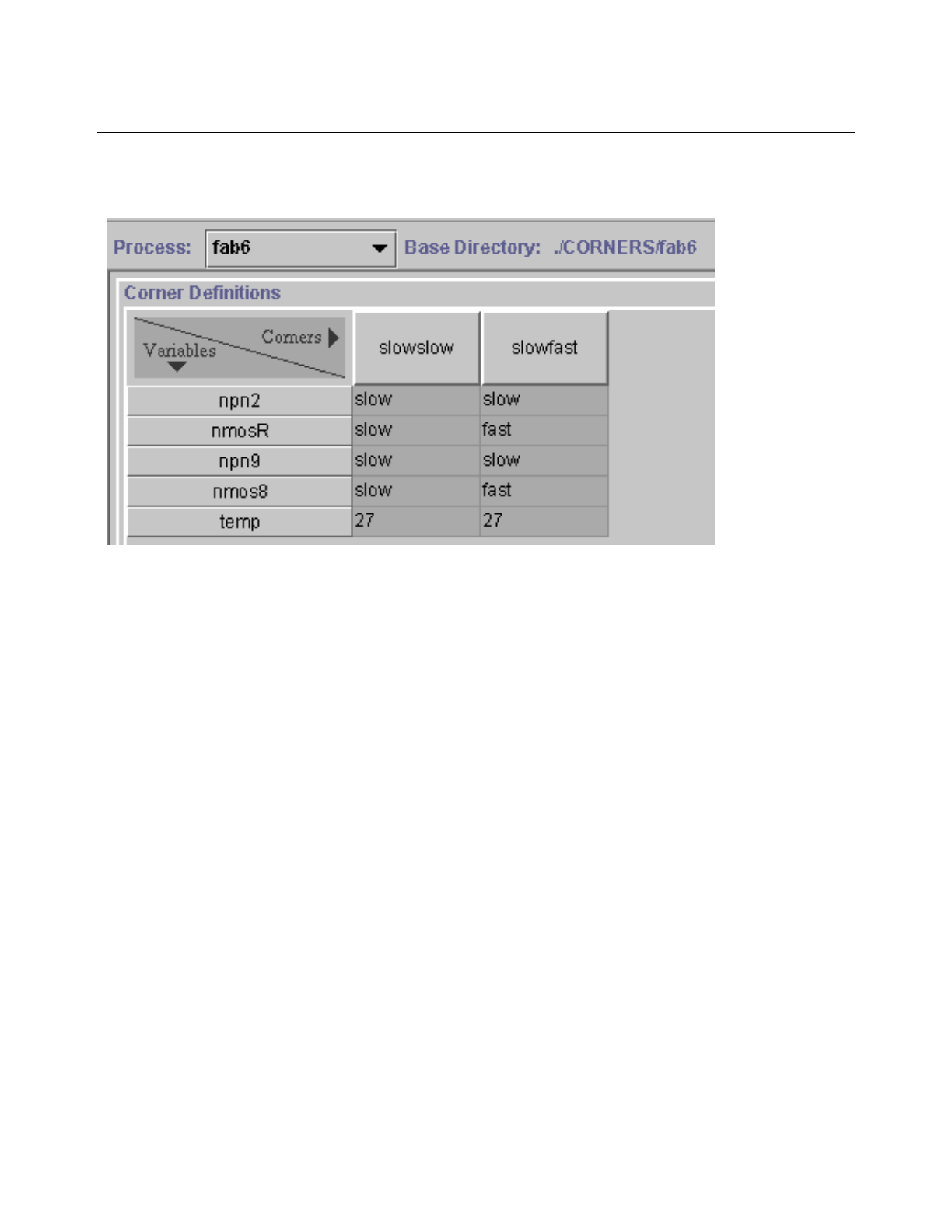
The Cadence® Analog Corners Analysis window produced by this PCF looks like this.
Using the Multiple Numeric Modeling Style with the Spectre Simulator
When you run a multiple numeric modeling style corners analysis with the Spectre simulator,
ensure that the .cdsenv variable includeStyle is set to t.
Multiple Parametric Modeling
This modeling style, which has the following characteristics, is provided for backward
compatibility.
■With this style, each model is defined in a separate file. There is a corresponding
parameter file for every model associated with each corner.
■Model files are located in the subdirectory base_directory/group. For example, if
the model includes the group npn, then the model files associated with that group are
located in the base_directory/npn subdirectory.
■Each parameter file is located in base_directory/group/variant. For example,
if the model includes the group npn and the variant fast, then at least one of the
parameter files is located in the base_directory/npn/fast subdirectory.
■Each model file can have any name, which the designer enters on the Edit Properties
form in the Cadence® Analog Design Environment.

Cadence Advanced Analysis Tools User Guide
Corners Analysis
July 2002 50 Product Version 5.0
The following table illustrates the file structure and contents for the multiple parametric
modeling style.
The following code illustrates how you can refer to this modeling structure in a PCF.
corAddProcess("fab6" "./CORNERS/fab6" 'multipleParametric)
corAddGroupAndVariantChoices("fab6" "npn2"
'("slow" "nominal" "fast")
)
corAddGroupAndVariantChoices("fab6" "nmos8"
'("slow" "nominal" "fast")
)
corAddGroupAndVariantChoices("fab6" "npn9"
'("slow" "nominal" "fast")
)
corAddGroupAndVariantChoices("fab6" "nmosR"
'("slow" "nominal" "fast")
)
Multiple Parametric Style
Path Filename File Contents
./CORNERS/fab6/
npn
npn2.scs include "npn2.param"
model npn2 bjt tf=TF2
npn9.scs include "npn9.param"
model npn9 bjt tf=TF9
./CORNERS/fab6/
npn/slow/
npn2.param parameter TF2=120n
npn9.param parameter TF9=320n
./CORNERS/fab6/
npn/nom/
npn2.param parameter TF2=100n
npn9.param parameter TF9=300n
./CORNERS/fab6/
npn/fast/
npn2.param parameter TF2=80n
npn9.param parameter TF9=380n
./CORNERS/fab6/
nmos
nmosR.scs model npn2 mos3 tf=TOXR
nmos8.scs model npn9 mos3 tf=TOX8
./CORNERS/fab6/
nmos/slow/
nmosR.param parameter TOXR=120
nmos8.param parameter TOX8=320n
./CORNERS/fab6/
nmos/nom/
nmosR.param parameter TOXR=100n
nmos8.param parameter TOX8=300n
./CORNERS/fab6/
nmos/fast/
nmosR.param parameter TOXR=80n
nmos8.param parameter TOX8=380n
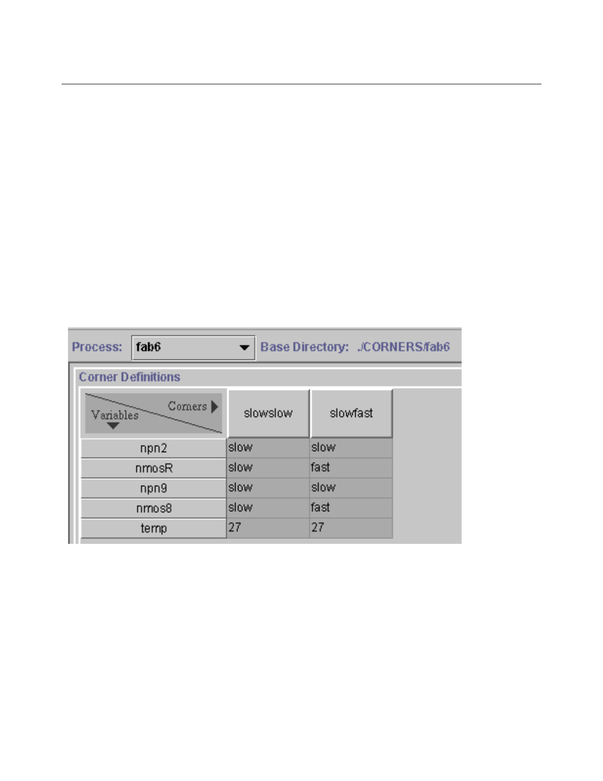
Cadence Advanced Analysis Tools User Guide
Corners Analysis
July 2002 51 Product Version 5.0
corAddCorner("fab6" "slowslow"
?variants '(
("npn2" "slow")
("nmos8" "slow")
("npn9" "slow")
("nmosR" "slow")
)
?nomTemp -55
)
corAddCorner("fab6" "slowfast"
?variants '(
("npn2" "slow")
("nmos8" "fast")
("npn9" "slow")
("nmosR" "fast")
)
?nomTemp -55
)
The Cadence® Analog Corners Analysis window produced by this PCF looks like this.
Using the Multiple Parametric Modeling Style with the Spectre Simulator
When you run a multiple parametric modeling style corners analysis with the Spectre
simulator, ensure that the .cdsenv variable includeStyle is set to t.
Using the Multiple Parametric Modeling Style with a Socket Simulator
To use a multiple parametric modeling style with a socket simulator, specify the parameter
files in an update.s file. For example, update.s might contain
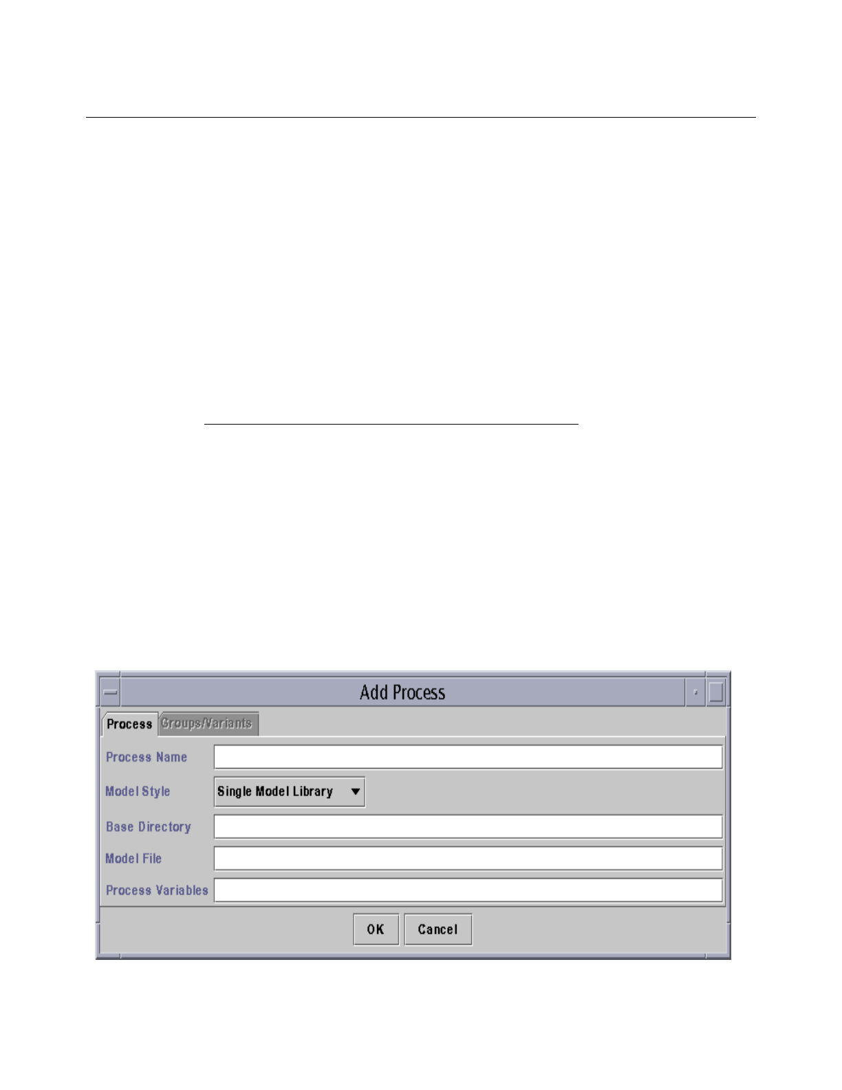
Cadence Advanced Analysis Tools User Guide
Corners Analysis
July 2002 52 Product Version 5.0
use npn2.s
use npn9.s
use nmosR.s
use nmos8.s
If you want to be able to override parameter declarations for specific corners, put these use
statements in an init.s file instead of in an update.s file. Because parameters defined in
the corners analysis option are processed after init.s parameters, you can use the corners
analysis option to override the init.s parameters.
Using the Cadence® Analog Corners Analysis Window to Define and
Update Processes
As described in “Creating Process and Design Customization Files” on page 36, processes
are often defined outside of the Cadence® Analog Corners Analysis window and then
loaded when they are needed. However, you can also use the corners option graphical user
interface to define, update, and save a process.
Using the Cadence® Analog Corners Analysis Window to Define a Process
To define a new process,
1. Choose Setup – Add Process.
The Add Process form appears.
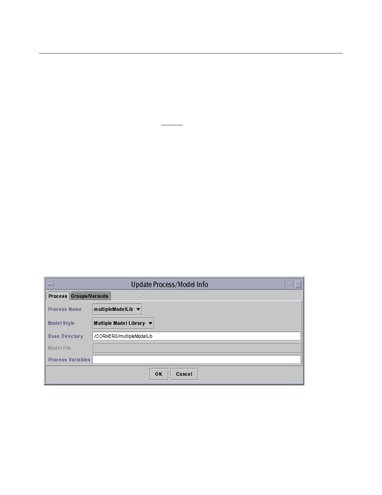
Cadence Advanced Analysis Tools User Guide
Corners Analysis
July 2002 53 Product Version 5.0
2. In the Process Name field, type the name you want to use for the new process.
3. Choose the model style you want to use for the new process.
4. Type the name of the base directory for the model file or files associated with the new
process.
5. If the model style you choose in Step 3 is Single Model Library, type the name of the
associated model file.
6. Type the names of process variables you want to add, separating them with a comma or
white space. (To delete process variables, select the row and click Delete in the
Cadence® Analog Corners Analysis window.)
7. Click OK in the Add Process form to close it.
Using the Cadence® Analog Corners Analysis Window to Modify Process Model
Information
To modify an existing process,
1. Choose Setup – Add/Update Model Info.
The Add/Update Model Info form appears.
This form has two tabs: Process and Group/Variants.Only certain modeling styles allow the
Groups and Variants. You need to make modifications in all tabs before adding or updating
the process. Otherwise, you will have to get back in and update the process again.
1. Choose the Process that you want to change.
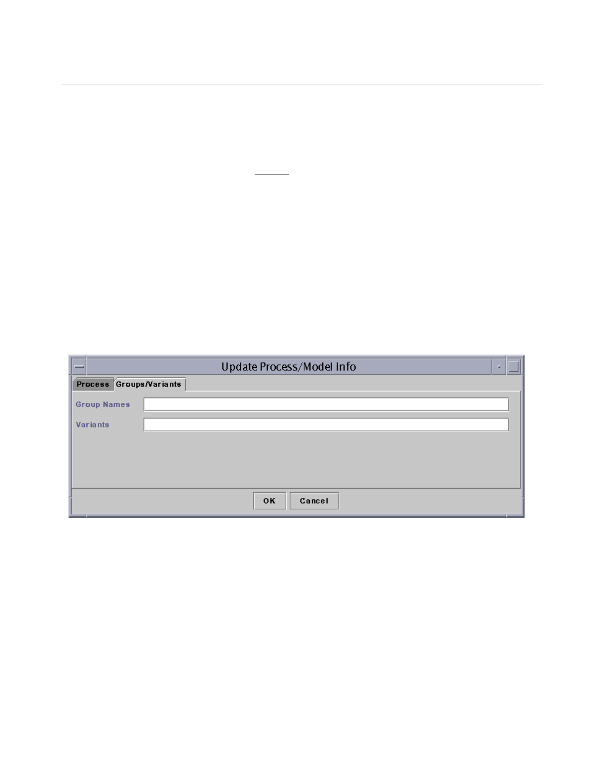
Cadence Advanced Analysis Tools User Guide
Corners Analysis
July 2002 54 Product Version 5.0
2. Choose the Model Style that you want to use for the changed process.
3. Type the name of the Base Directory for the model file or files associated with the
changed process. The form appears with the process base directory.
4. If the model style you choose in Step 3 is Single Model Library, type the name of the
associated model file.
5. Type the names of process variables you want to add, separating them with commas or
spaces. (To delete process variables, select the row and click Delete in theCadence®
Analog Corners Analysis window.)
6. Click OK in the Update Process/Model Info form to close it.
To specify the Groups and Variants, click the Groups/Variants tab.
1. Specify a name in the Group Name field.
2. Specify the variants in the Variants field.
3. Click OK to close the form.
Requirements for Using the Spectre Simulator
When you run a single or multiple model library style corners analysis with the Spectre
simulator, ensure that you comply with the following requirements.
■The value of the .cdsenv variable useAltergroup must be set appropriately. If your
Spectre model supports altergroups, ensure that useAltergroup is set to t. If your
Spectre model does not support altergroups, set useAltergroup to nil.

Cadence Advanced Analysis Tools User Guide
Corners Analysis
July 2002 55 Product Version 5.0
Regardless of the useAltergroup value, the corners analysis option does not use
altergroups when you run a mixed-signal (SpectreVerilog) or distributed simulation.
■Every parameter used in a corner must be in the main circuit.
Working through an Extended Example
This section follows a corners session in detail, demonstrating how you might use the corners
analysis option to examine the characteristics of a real circuit. The example describes a
folded cascode circuit and explains how you might arrange the supporting model files. To
follow along, go to
your_install_dir/tools/dfII/samples/artist/corners/artistExample
and start icms. A .cdsinit file and the other files you need to run this example are all
included at that location.
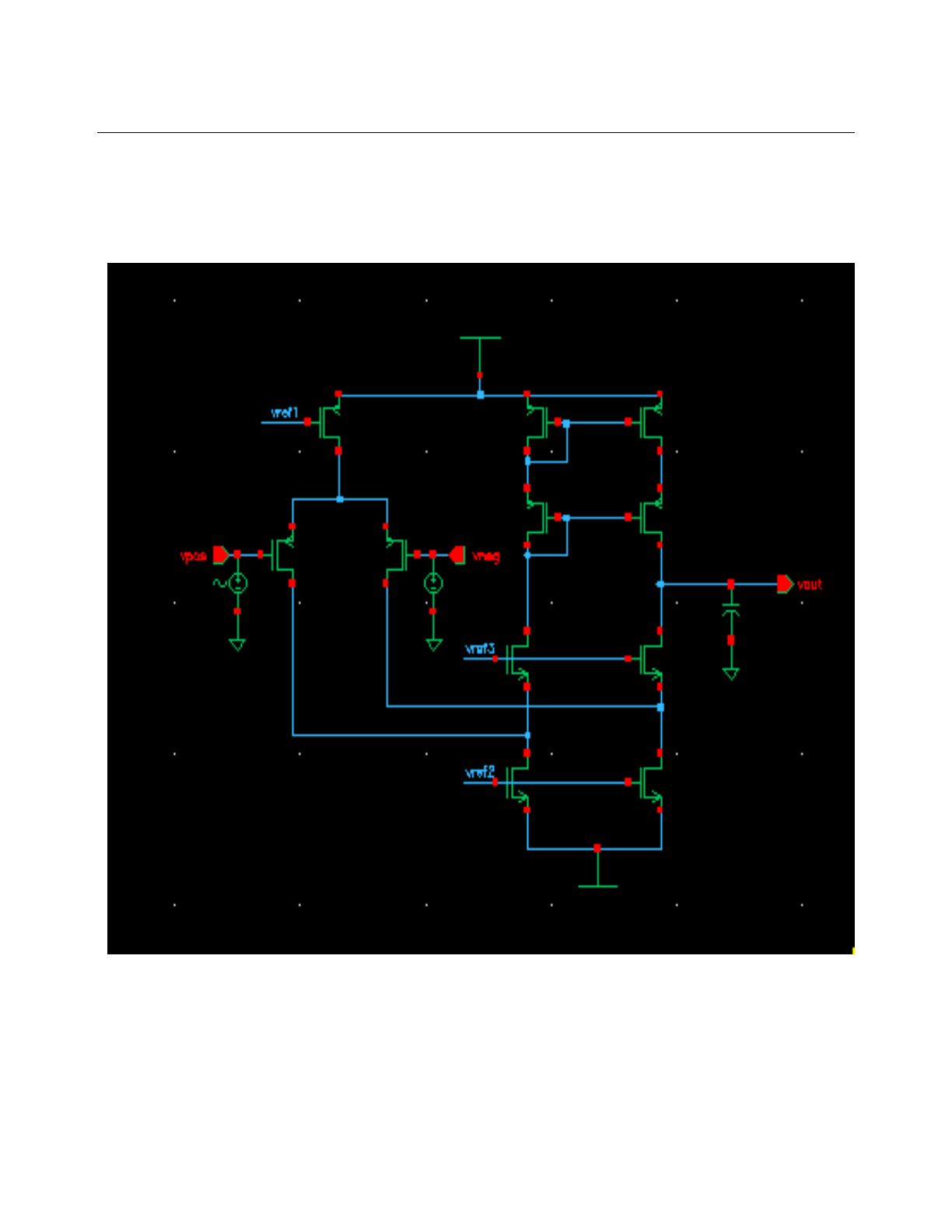
Cadence Advanced Analysis Tools User Guide
Corners Analysis
July 2002 56 Product Version 5.0
Folded Cascode Schematic
The folded cascode used in this example has the following two-part schematic.
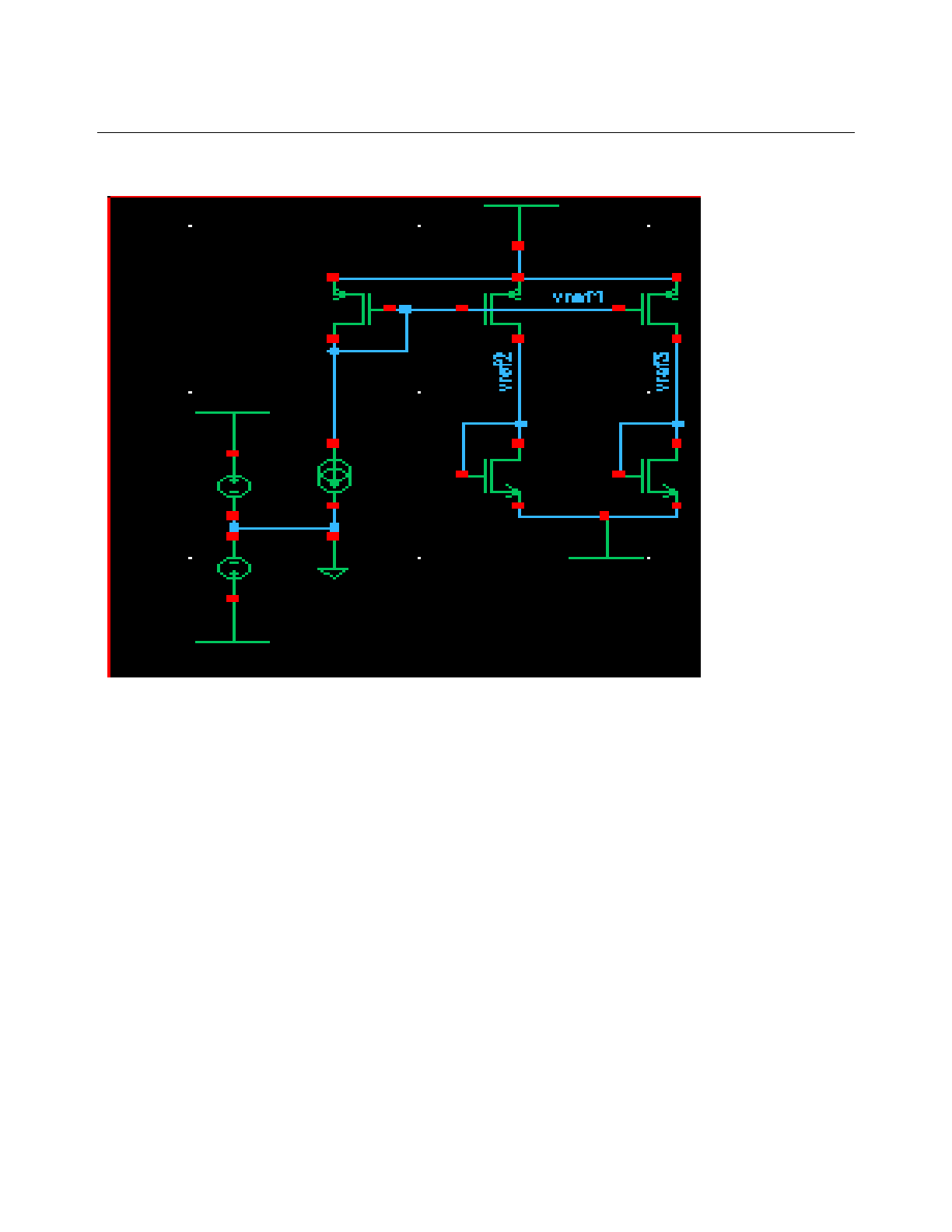
Cadence Advanced Analysis Tools User Guide
Corners Analysis
July 2002 57 Product Version 5.0
This schematic includes several instances of pmos and nmos transistors. Each of the pmos
transistors is nominally identical. Similarly, each of the nmos transistors is nominally identical.
In reality, however, the attributes of each transistor differ slightly from the attributes of each of
the other transistors. In this example, you explore the extent of the variation and the effect the
variation has on the performance of the circuit.
Setting Up the Cadence® Analog Design Environment Window
To run this example, first set up the Cadence® Analog Design Environment window.
1. From the CIW, choose Tools – Analog Environment – Simulation.
The Cadence® Analog Design Environment window appears.
2. Choose Setup – Design.
The Choosing Design form appears.

Cadence Advanced Analysis Tools User Guide
Corners Analysis
July 2002 58 Product Version 5.0
3. Select the RF_lib library and the foldedCascode cell. Click OK.
4. In the Cadence® Analog Design Environment window, choose Session – Load
State.
The Loading State form appears.
5. Choose Corners from the State Name cyclic field. Click OK.
6. In the Cadence® Analog Design Environment window, choose Outputs – To Be
Plotted – Select On Schematic.
The schematic window appears.
7. Click on the net connected to vout in the right side of the plot, then press the Esc key.
There are other outputs defined in the PCF, but this demonstrates how outputs defined
in the Cadence® Analog Design Environment window are incorporated into the
Cadence® Analog Corners Analysis window.
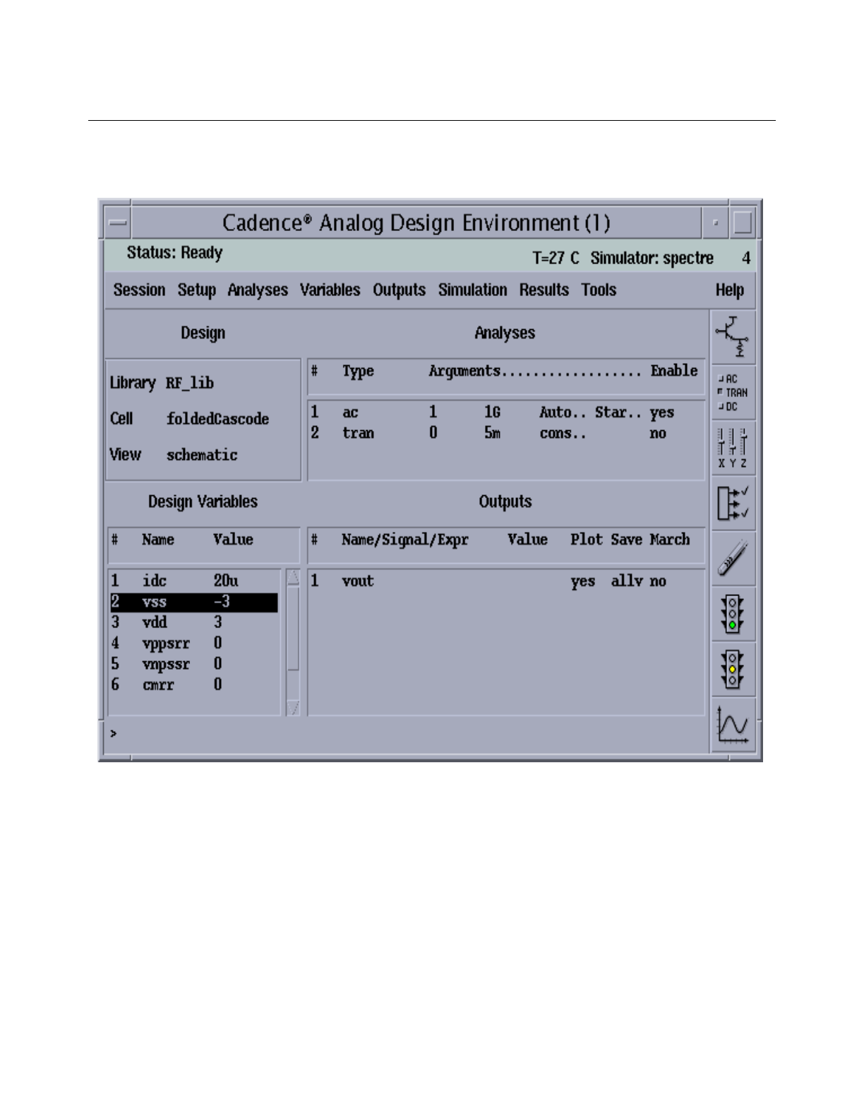
Cadence Advanced Analysis Tools User Guide
Corners Analysis
July 2002 59 Product Version 5.0
The Cadence® Analog Design Environment window looks like this.
Modeling Style
This example uses the multiple model library style with the variants for pmos components
defined in one file of the multipleModelLib directory and the variants for nmos
components defined in another file of that same directory.
For example, the nmos components are defined in the file
CORNERS/multipleModelLib/nmosLib.scs

Cadence Advanced Analysis Tools User Guide
Corners Analysis
July 2002 60 Product Version 5.0
This file contains
library nmosLib
section nom
include "../nmos/typ/nmos.scs"
endsection
section fast
include "../nmos/fast/nmos.scs"
endsection
section slow
include "../nmos/slow/nmos.scs"
endsection
endlibrary
As implemented in this example, the parameters for the variants are not actually included in
this file, although they could be. This example instead uses include statements to include
the files that contain the actual models.
The ../nmos/typ/nmos.scs file referred to in the nom section, for example, contains
simulator lang=spice
* VTI-derived Level=2 nominal model
.model nmos nmos level=2
+ vto = 0.775
+ tox = 400e-10
+ nsub = 8e+15
+ xj = 0.15U
+ ld = 0.20U
+ u0 = 650
+ ucrit = 0.62e+5
+ uexp = 0.125
+ vmax = 5.1e+4
+ neff = 4.0
+ delta = 1.4
+ rsh = 36
+ cgso = 1.95e-10
+ cgdo = 1.95e-10
+ cj = 195U
+ cjsw = 500P
+ mj = 0.76
+ mjsw = 0.30
+ pb = 0.8
These are the values the simulator uses when you run a corner that has the value of the nmos
variant set to nom. When you run a corner that uses the slow variant for the nmos
components, the simulator uses the values defined in
../nmos/slow/nmos.scs
The contents of the ../nmos/slow/nmos.scs file are the following:
simulator lang=spice
* VTI Level=2 slowN/slowP model
.model nmos nmos level=2
+ vto = 0.9

Cadence Advanced Analysis Tools User Guide
Corners Analysis
July 2002 61 Product Version 5.0
+ tox = 430e-10
+ nsub = 1.0e+16
+ xj = 0.15U
*+ ld = 0.20U
+ ld = 0.075U
+ u0 = 620
+ ucrit = 0.62e5
+ uexp = 0.125
+ vmax = 5.1e4
+ neff = 4.0
+ delta = 1.4
+ rsh = 38
+ cgso = 2.10e-10
+ cgdo = 2.10e-10
+ cj = 215U
+ cjsw = 540P
+ mj = 0.76
+ mjsw = 0.30
+ pb = 0.8
The other variants for the nmos and pmos components are defined similarly.
Process Customization File (PCF)
This example does not use a design customization file (DCF) because all the necessary
corners and measurements are defined in a single PCF called multipleModelLib.pcf.
Defining the Cadence® Analog Corners Analysis window in a single file simplifies the
example.
The multipleModelLib.pcf contains the following information.
corAddProcess( "multipleModelLib" "./CORNERS/multipleModelLib"
’multipleModelLib )
corAddProcessVar( "multipleModelLib" "vdd" )
corAddProcessVar( "multipleModelLib" "vss" )
corAddDesignVar( "Cload" )
corAddGroupAndVariantChoices( "multipleModelLib" "pmosLib.scs"
’("slow" "nom" "fast") )
corAddGroupAndVariantChoices( "multipleModelLib" "nmosLib.scs"
’("slow" "nom" "fast") )
corAddCorner( "multipleModelLib" "slowslow" )
corSetCornerGroupVariant( "multipleModelLib" "slowslow"
"nmosLib.scs" "slow" )
corSetCornerGroupVariant( "multipleModelLib" "slowslow"
"pmosLib.scs" "slow" )
corSetCornerNomTempVal( "multipleModelLib" "slowslow" 27 )
corSetCornerRunTempVal( "multipleModelLib" "slowslow" 125 )
corSetCornerVarVal( "multipleModelLib" "slowslow" "Cload" "260f" )
corSetCornerVarVal( "multipleModelLib" "slowslow" "vss" "-2.7" )
corSetCornerVarVal( "multipleModelLib" "slowslow" "vdd" "2.7" )
corAddCorner( "multipleModelLib" "fastslow" )
corSetCornerGroupVariant( "multipleModelLib" "fastslow"
"nmosLib.scs" "slow" )
corSetCornerGroupVariant( "multipleModelLib" "fastslow"

Cadence Advanced Analysis Tools User Guide
Corners Analysis
July 2002 62 Product Version 5.0
"pmosLib.scs" "fast" )
corSetCornerNomTempVal( "multipleModelLib" "fastslow" "27" )
corSetCornerRunTempVal( "multipleModelLib" "fastslow" 27 )
corSetCornerVarVal( "multipleModelLib" "fastslow" "Cload" "200f" )
corSetCornerVarVal( "multipleModelLib" "fastslow" "vss" "-3" )
corSetCornerVarVal( "multipleModelLib" "fastslow" "vdd" "3" )
corAddCorner( "multipleModelLib" "typtyp" )
corSetCornerGroupVariant( "multipleModelLib" "typtyp" "nmosLib.scs"
"nom" )
corSetCornerGroupVariant( "multipleModelLib" "typtyp" "pmosLib.scs"
"nom" )
corSetCornerNomTempVal( "multipleModelLib" "typtyp" 27 )
corSetCornerRunTempVal( "multipleModelLib" "typtyp" 27 )
corSetCornerVarVal( "multipleModelLib" "typtyp" "Cload" "200f" )
corSetCornerVarVal( "multipleModelLib" "typtyp" "vss" "-3" )
corSetCornerVarVal( "multipleModelLib" "typtyp" "vdd" "3" )
corAddCorner( "multipleModelLib" "slowfast" )
corSetCornerGroupVariant( "multipleModelLib" "slowfast"
"nmosLib.scs" "fast" )
corSetCornerGroupVariant( "multipleModelLib" "slowfast"
"pmosLib.scs" "slow" )
corSetCornerNomTempVal( "multipleModelLib" "slowfast" "27" )
corSetCornerRunTempVal( "multipleModelLib" "slowfast" 27 )
corSetCornerVarVal( "multipleModelLib" "slowfast" "Cload" "200f" )
corSetCornerVarVal( "multipleModelLib" "slowfast" "vss" "-3" )
corSetCornerVarVal( "multipleModelLib" "slowfast" "vdd" "3" )
corAddCorner( "multipleModelLib" "fastfast" )
corSetCornerGroupVariant( "multipleModelLib" "fastfast"
"nmosLib.scs" "fast" )
corSetCornerGroupVariant( "multipleModelLib" "fastfast"
"pmosLib.scs" "fast" )
corSetCornerNomTempVal( "multipleModelLib" "fastfast" 27 )
corSetCornerRunTempVal( "multipleModelLib" "fastfast" -55 )
corSetCornerVarVal( "multipleModelLib" "fastfast" "Cload" "160f" )
corSetCornerVarVal( "multipleModelLib" "fastfast" "vss" "-3.3" )
corSetCornerVarVal( "multipleModelLib" "fastfast" "vdd" "3.3" )
corAddMeas( "DCgain" )
corSetMeasExpression( "DCgain" "ymax(db20(VF('/vout')))" )
corSetMeasTarget( "DCgain" 60 )
corSetMeasEnabled( "DCgain" t )
corSetMeasGraphicalOn( "DCgain" t )
corSetMeasTextualOn( "DCgain" nil )
corAddMeas( "bandwidth" )
corSetMeasExpression( "bandwidth" "bandwidth(VF('/vout') 3 'low')" )
corSetMeasEnabled( "bandwidth" t )
corSetMeasGraphicalOn( "bandwidth" t )
corSetMeasTextualOn( "bandwidth" nil )
corAddMeas( "gain" )
corSetMeasExpression( "gain" "dB20(VF('/vout'))" )
corSetMeasEnabled( "gain" t )
corSetMeasGraphicalOn( "gain" t )
corSetMeasTextualOn( "gain" nil )
corAddMeas( "phase" )
corSetMeasExpression( "phase" "phase(VF('/vout'))" )
corSetMeasEnabled( "phase" t )
corSetMeasGraphicalOn( "phase" t )
corSetMeasTextualOn( "phase" nil )

Cadence Advanced Analysis Tools User Guide
Corners Analysis
July 2002 63 Product Version 5.0
You can load a PCF from the Cadence® Analog Corners Analysis window, but it is often
easier to insert a statement in your .cdsinit file that loads the necessary PCFs
automatically. For example, if you look in the included .cdsinit file, you find the following
statement that loads the multipleModelLib.pcf file:
loadPcf( "~/multipleModelLib.pcf" )
Cadence® Analog Corners Analysis Window for Folded Cascode
To open the Cadence® Analog Corners Analysis window,
➤From the Cadence®Analog Design Environment window, choose Tools – Corners.
The Cadence®Analog Corners Analysis window, in this example, is defined primarily by
the multipleModelLib.pcf. In addition, the following items affect the appearance of the
window.
■The run temperature variable temp always appears in the Corner Definitions pane of
the window. By default, it has the value 27. For this example, the
multipleModelLib.pcf sets the value of the run temperature explicitly for each
corner using skill function corSetCornerRunTempVal.
■Any outputs defined in the Cadence®Analog Design Environment window when you
first start the corners analysis option appear in the Performance Measurements pane.
That is why /vout appears as an expression in the Performance Measurements pane
for this example.
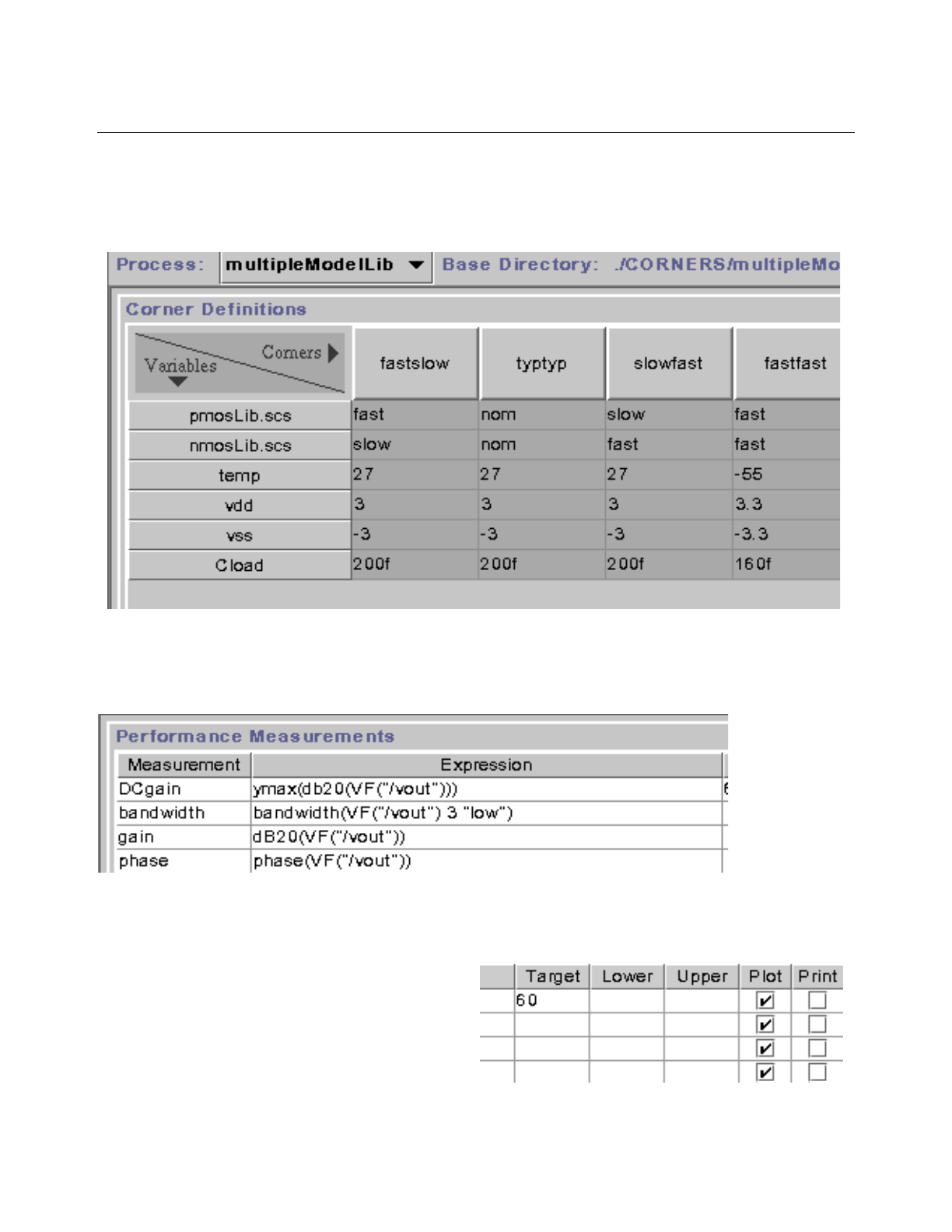
Cadence Advanced Analysis Tools User Guide
Corners Analysis
July 2002 64 Product Version 5.0
When the Cadence® Analog Corners Analysis window opens, the Corner Definitions
pane looks like this. (The slowslow corner, although not visible in this figure, also appears
in the actual Cadence® Analog Corners Analysis window.)
The Performance Measurements pane looks like this.

Cadence Advanced Analysis Tools User Guide
Corners Analysis
July 2002 65 Product Version 5.0
The measurement that appears in the Performance Measurements pane is defined in the
Outputs pane of the Cadence®Analog Design Environment window and is automatically
copied into the Cadence® Analog Corners Analysis window.
Changing Values in the Cadence® Analog Corners Analysis Window
So far, in this example, everything in the Cadence®Analog Corners Analysis window has
been predefined, either by the PCF or because it is defined in the Cadence® Analog
Design Environment window. You can also use the Cadence®Analog Corners Analysis
window to revise and add to the predefined information. For example, this section describes
how you might add a Lower value to a scalar measurement before you run the simulation.
The DCgain measurement produces a scalar value. To facilitate analysis, you want to add a
visual indication of the lowest acceptable value to the graphical output of the corners
simulation. To do that, you need to add the appropriate value to the cells in the Performance
Measurements pane.
To add a Lower value by using the Cadence® Analog Corners Analysis window,
1. Click on the Lower cell for the DCgain measurement.
2. Type the value 55 in the cell.
To add a Upper value by using the Cadence® Analog Corners Analysis window,
1. Click on the Upper cell for the DCgain measurement.
2. Type the Value 65 in the cell.
All of the measurements produce graphical outputs if you make no further changes, but it
might be useful to have the textual output too. To add the textual output,
➤Turn on the Textual button in the Outputs column for each of the measurements.
Running the Corners Simulation
After the corners and measurements are defined, running the corners simulation involves
only a couple of simple steps.
1. Ensure that the corners, measurements, and outputs you want to use are selected.
2. Choose Simulation ->Run or click Run.
The simulation runs and the outputs you requested appear in display windows.
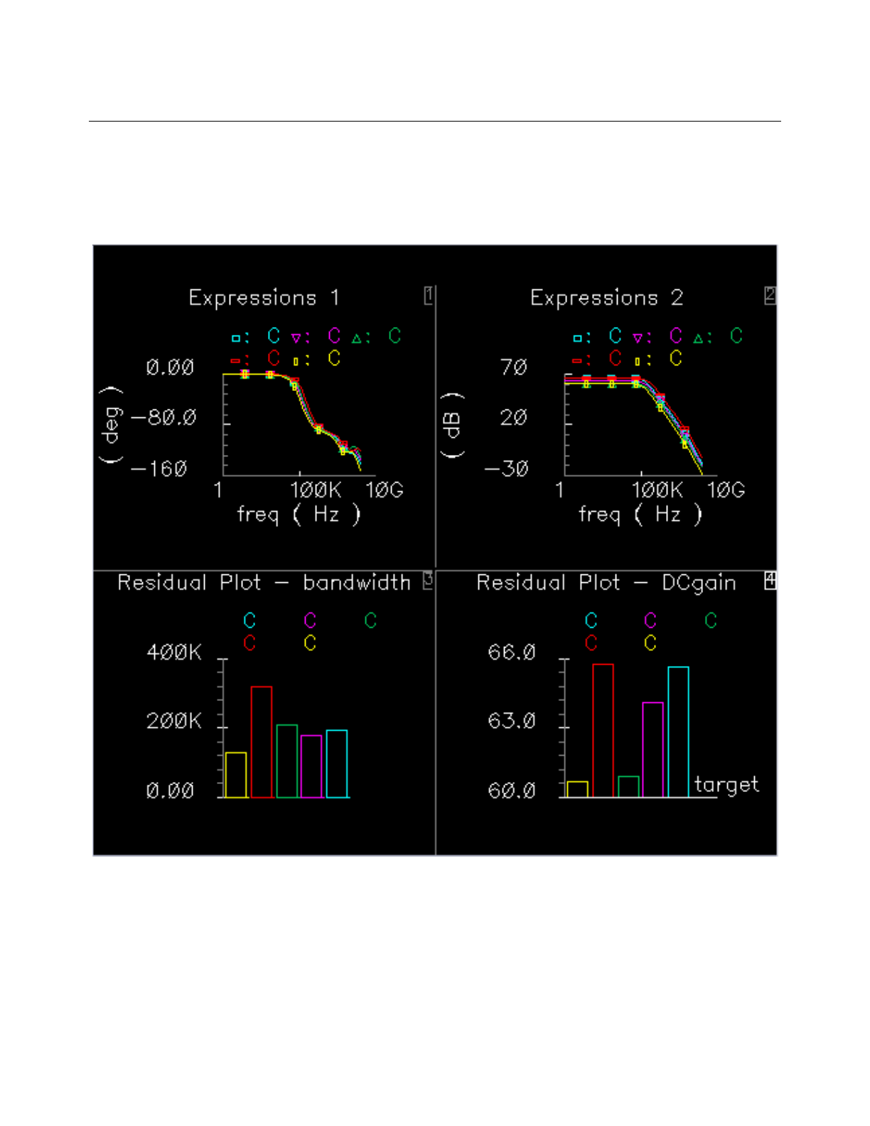
Cadence Advanced Analysis Tools User Guide
Corners Analysis
July 2002 66 Product Version 5.0
Evaluating Corners Results
The graphical outputs appear in a waveform window.
The phase and gain measurements appear as a family of waveforms in the two subwindows
at the top, with each waveform for each corner. The scalar values, DCgain and bandwidth,
appear as bar charts. It is hard to pick out detail in this combined plot, but you can choose
Window – Subwindows in the Waveform Window to open a dialog box that allows you to
choose which plots you want to look at in more detail.
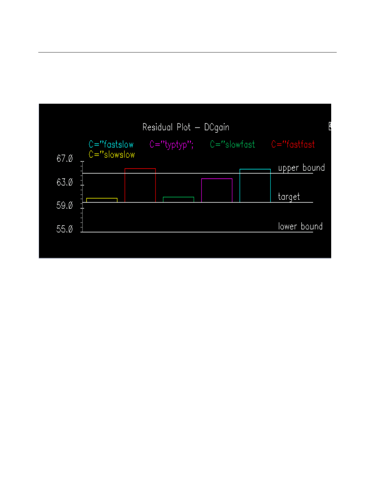
Cadence Advanced Analysis Tools User Guide
Corners Analysis
July 2002 67 Product Version 5.0
Evaluating Residual Plots
Look first at the DCgain bar chart.
In this plot, the horizontal line in the middle represents the Target value, 60. The bottom line
represents the Lower value, which you set in the Cadence® Analog Corners Analysis
window. The top line represents the Upper value. All of the corners reach the target value. (In
the actual window, each corner displays in a different color so you can determine which
corner is which.) If DCgain for one or more corners fails to reach the target, you might decide
to use a slightly different manufacturing process or to change your circuit so DCgain is
greater.
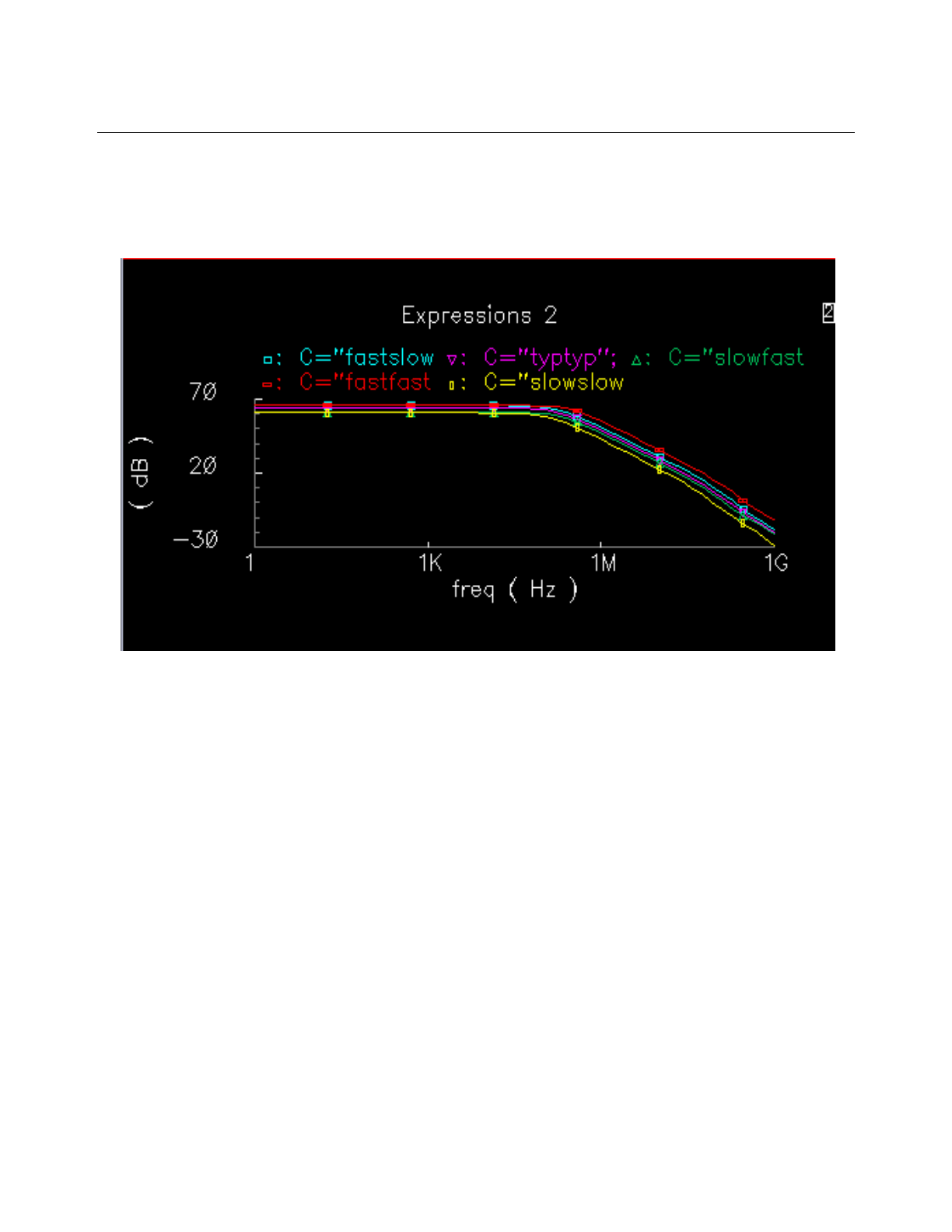
Cadence Advanced Analysis Tools User Guide
Corners Analysis
July 2002 68 Product Version 5.0
Evaluating Family-of-Curve Plots
Now consider the family-of-curves plot for the gain measurement.
The fastfast corner produces the highest gain and the slowslow corner produces the
lowest gain throughout the frequency range. You need to determine whether these possible
outcomes are acceptable in your application.

Cadence Advanced Analysis Tools User Guide
July 2002 69 Product Version 5.0
2
Statistical Analysis
Statistical analysis is a powerful method for estimating parametric yields. The sections in this
chapter explain how you can use the Analog Statistical Analysis option to generate
information about the performance characteristics of the circuits you design.
■“Getting Started with Statistical Analysis” on page 69
■“Getting to Know the Analog Statistical Analysis Window” on page 72
■“Running a Statistical Analysis” on page 79
■“Analyzing Results” on page 100
■“Working through an Extended Example” on page 122
Getting Started with Statistical Analysis
This section briefly explains the theory behind statistical analysis, tells you how to get help
and describes how to open the Analog Statistical Analysis window.
How Statistical Analysis Works
The manufacturing variations in components affect the production yield of any design that
includes them. Statistical analysis allows you to study this relationship in detail.
To prepare for a statistical analysis, you create a design that includes devices or device
models that are assigned statistically varying parameter values. The shape of each statistical
distribution represents the manufacturing tolerances on a device. During the analysis, the
statistical analysis option performs multiple simulations, with each simulation using different
parameter values for the devices based upon the assigned statistical distributions.
When the simulations finish, you can use the data analysis features of the statistical analysis
option to examine how manufacturing tolerances affect the overall production yield of your
design. If necessary, you can then switch to different components or change the design to
improve the yield.

Cadence Advanced Analysis Tools User Guide
Statistical Analysis
July 2002 70 Product Version 5.0
Data Types Generated by the Statistical Analysis Tool
The Statistical Analysis tool creates two types of output data:
Scalar Data
For each iteration during a statistical analysis, the simulator evaluates explicit expressions
that reduce to a single scalar number. These numbers are stored in a file which will ultimately
be used for data analysis by the user at post-simulation.
The simulator evaluates these scalar expressions during runtime so as to reduce the amount
of generated psf data. For each successive iteration analysis, the simulator typically deletes
the psf data from the previous iteration.
However, it is possible to keep all of the psf data from all of the iterations (Spectre only; see
next data type).
The majority of the statistical analysis tool UI is focused on processing and displaying scalar
data.
For the Spectre®simulator, the process parameters declared in a statistics block in the netlist
are also included in the resulting scalar data file.
Psf Data
This is the same kind of psf data that the simulator typically generates. Usually, this data only
includes the last iteration.
However, for the Spectre ®simulator, the user has the additional option to save the psf data
for all of the iterations. From this data the user can either plot waveforms or regenerate new
scalar data files. Since this data is psf, the user will have to evaluate expressions against this
data to created these waveforms and statistical data. Specific waveform expressions are not
processed during a statistical analysis, only scalar expressions are.
Opening the Analog Statistical Analysis Window
To run the statistical analysis option, you must use a simulator that supports statistical
simulation. In addition, the model and device descriptions of the components that you want
to use in the statistical simulations must have statistical values.
To start the statistical analysis option within the Cadence® analog design environment,
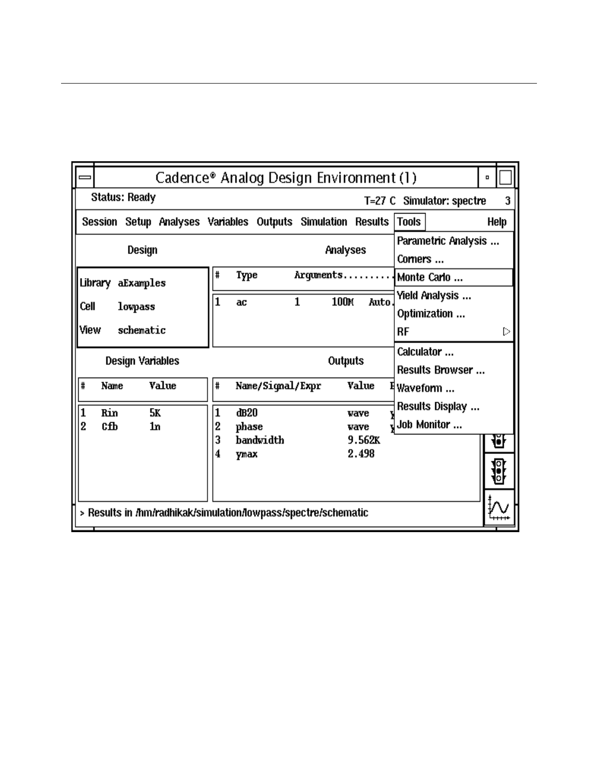
Cadence Advanced Analysis Tools User Guide
Statistical Analysis
July 2002 71 Product Version 5.0
1. Set up your simulation normally, choosing an appropriate simulator.
2. Choose Tools – Monte Carlo.
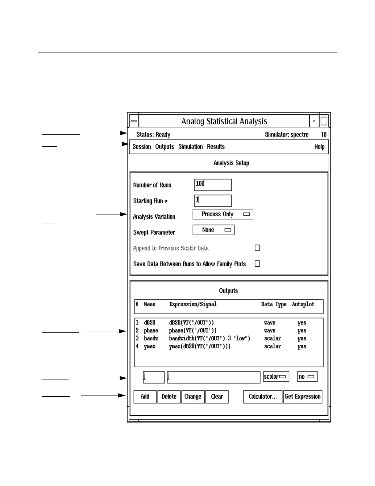
Cadence Advanced Analysis Tools User Guide
Statistical Analysis
July 2002 72 Product Version 5.0
Getting to Know the Analog Statistical Analysis Window
The Analog Statistical Analysis window contains the fields and controls required to specify
the statistical analysis that you want to run.
Status display
Menu
Analysis Setup
pane
Outputs pane
Edit fields
Button bar

Cadence Advanced Analysis Tools User Guide
Statistical Analysis
July 2002 73 Product Version 5.0
Status Display
The status display shows messages that indicate what the statistical analysis option is doing.
The messages include the following:
■Simulate
■Ready
■Plotting Results
■Simulate Distributed
During a simulation, the status display also shows which iteration is running and how many
iterations are left to run.
Note: This feature only works outside of distributed processing mode.
Menu
The menu contains the commands needed to prepare for, run and analyze the results of a
statistical analysis.
For guidance on using the menu choices, see the associated cross references:
Statistical Analysis Menu Choices
Menu Item For More Information
Session
Save State “Saving the Session State” on page 95
Load State “Loading a Saved Session State” on page 96
Save Script “Saving the Script” on page 96
Quit “Closing the Analog Statistical Analysis
Window” on page 98
Outputs
Retrieve Outputs “Selecting Signals and Expressions to Analyze”
on page 82

Cadence Advanced Analysis Tools User Guide
Statistical Analysis
July 2002 74 Product Version 5.0
Save All “Saving All Voltages or Currents” on page 89
Simulation
Check Expressions “Checking the Output Expressions” on page 90
Define Correlations “Defining Correlations” on page 92
Create Input Files “Creating Input Files for a Socket Simulator” on
page 95
Run “Starting and Stopping the Analysis” on page 93
Stop “Starting and Stopping the Analysis” on page 93
Output Log “Viewing the Output Log” on page 97
Results
Filter “Filtering Outlying Data” on page 102
Specification Limits “Setting Specification Limits” on page 105
Print
Iteration vs. Value “Printing Iteration versus Value Tables” on
page 108
Correlation “Printing Correlation Tables” on page 110
Plot
Histogram “Plotting Histograms” on page 111
Curves “Plotting Families of Curves” on page 113
Scatterplot “Plotting Scatter Plots” on page 114
Yield
Simple “Obtaining Reports on Simple Yields” on
page 117
Conditional “Obtaining Reports on Conditional Yields” on
page 120
Multiconditional “Obtaining Reports on Multiconditional Yields”
on page 119
Select “Analyzing Results” on page 100
Statistical Analysis Menu Choices, continued
Menu Item For More Information
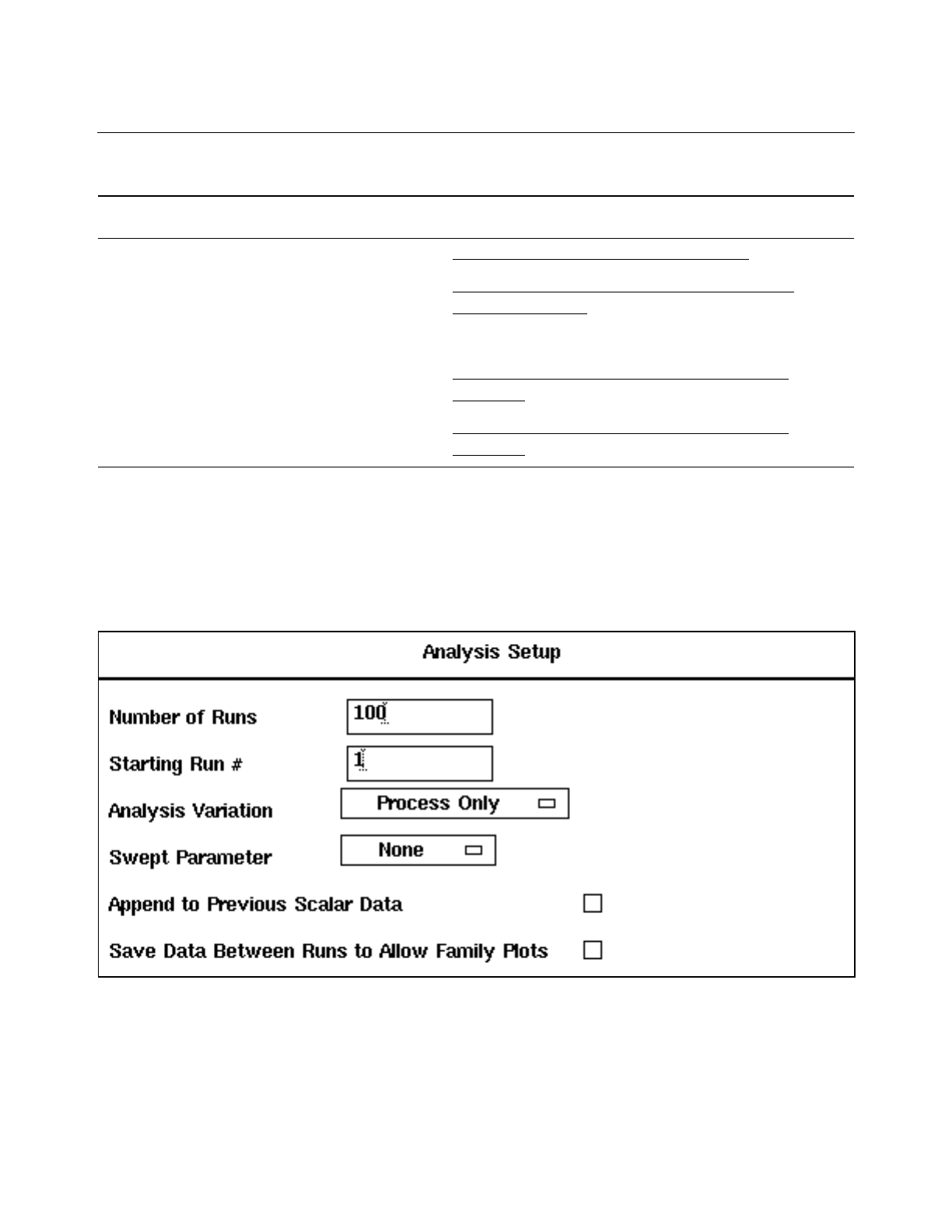
Cadence Advanced Analysis Tools User Guide
Statistical Analysis
July 2002 75 Product Version 5.0
Analysis Setup Pane
The fields and selections in the Analysis Setup pane specify the characteristics of the
statistical analysis to be run by the simulator.
Save “Saving Statistical Analysis Results” on page 94
Evaluate Expressions “Creating a New mcdata File from Saved
Waveform Data” on page 102
Help
Contents “Opening the Analog Statistical Analysis
Window” on page 70
About Analog Statistical
Analysis “Opening the Analog Statistical Analysis
Window” on page 70
Statistical Analysis Menu Choices, continued
Menu Item For More Information

Cadence Advanced Analysis Tools User Guide
Statistical Analysis
July 2002 76 Product Version 5.0
For a brief description of the items in the Analysis Setup pane, see the following table. For
more detailed information, see “Specifying the Characteristics of a Statistical Analysis” on
page 80.
Field or Selection Description and Usage
Number of Runs Specify how many simulations to run for this statistical
analysis.
Starting Run # Specify the starting run number.
Analysis Variation Select the type of statistical variation to be used.
Swept Parameter If desired, select temperature or a design variable to
sweep.
Append to Previous Scalar
Data Enable this button to append scalar output data to
previously saved scalar data. This feature is not supported
in the distributed processing mode. For the Spectre®
simulator, all of the pertinent UI fields are checked for
compatibility with the existing scalar data set prior to
allowing a Monte Carlo run.
Save Data Between Runs to
Allow Family Plots Enable this button to save the raw output data (the
parameter storage format [psf] files) for all the statistical
analysis iterations.
Turn this button off if you want the raw output data to be
deleted before each iteration. In which case, only the psf
data for the last iteration will ultimately be saved. The
ability to append to previous psf data is currently not
supported. This button only appears if you use the
Spectre® simulator.
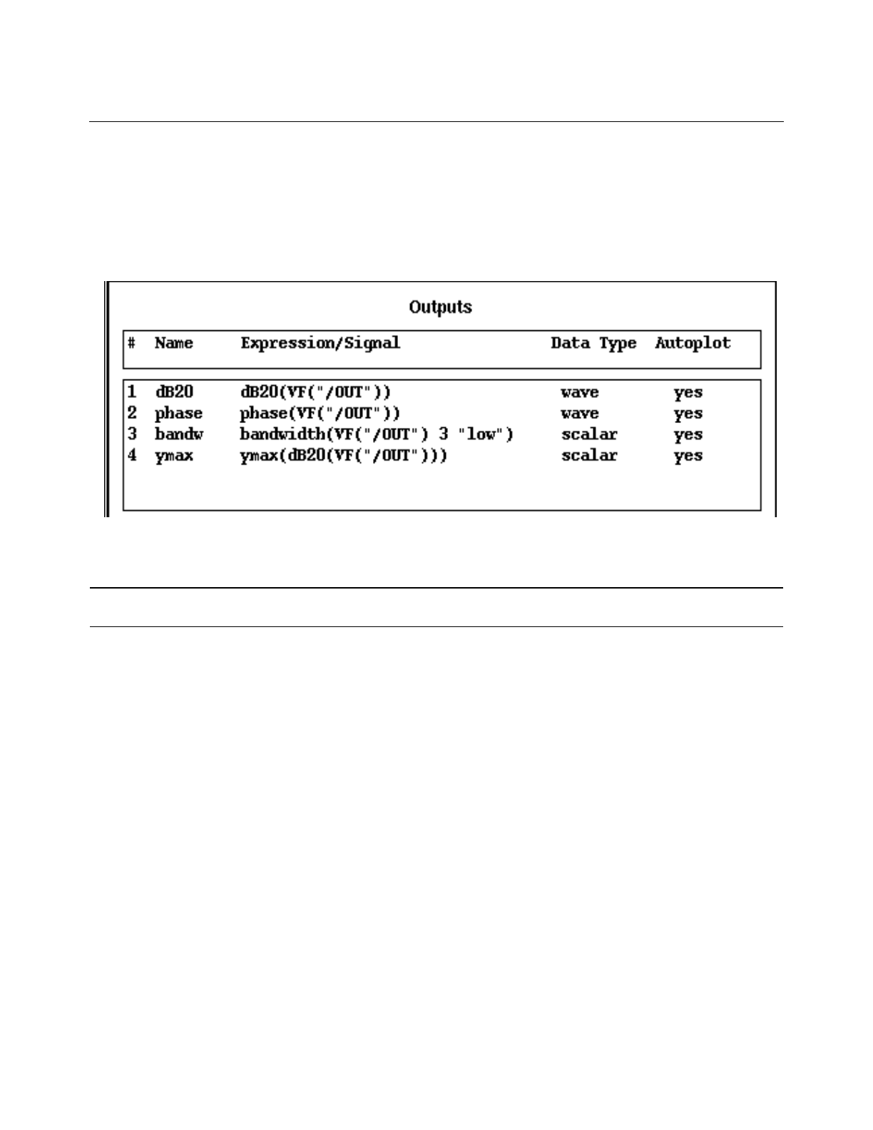
Cadence Advanced Analysis Tools User Guide
Statistical Analysis
July 2002 77 Product Version 5.0
Outputs Pane
The Analog Statistical Analysis window Outputs pane initially lists the expressions and
signals defined in the Outputs pane of the Cadence® Analog Design Environment
window.
The columns in the Outputs pane are described in the following table.
Column Description and Usage
Name A field showing the existing name for the expression or signal.
For expressions that evaluate to a scalar, the final name of the
statistical data set will be of the form name_varval. Where
name is the name on this pane and varval is the particular
swept variable value (if none, defaults to temperature).
Expression/Signal A field showing either an expression or a signal name.

Cadence Advanced Analysis Tools User Guide
Statistical Analysis
July 2002 78 Product Version 5.0
Edit Fields
These fields, located beneath the Outputs pane, are used to add output signals and to add
or modify output expressions.
Data Type A field indicating what type of data will result from an
evaluation of the expression. This field is typically auto set by
the UI, but the user can manually set it as well. The possible
values of this field are:
waveform The expression either evaluates to a waveform or
is a signal. These expressions will not be sent to the simulator
for runtime evaluation, and can only be evaluated against
resulting psf data.
Note: The user scan manually set/override any
expression type to be waveform whenever they do not
want a particular expression sent to the simulator.
scalar The expression evaluates to a scalar value. These
expressions will be sent to the simulator for runtime
evaluation.
unknown There is no currently loaded psf data that can be
used to determine the type of the expression. These
expressions will be sent to the simulator for runtime
evaluation. If there are problems detected with this expression
at runtime, either Spectre will abort or error flag values will be
inserted into the generated data.
Note: The equivalent edit field uses a blank to indicate
unknown.
Autoplot A field that indicates whether to automatically plot the pane
entry after all the statistical analysis simulations finish. If the
element is an expression, it is evaluated against the psf data
and plotted. If the element is a signal, then an individual plot is
created for each primary analysis type found in the psf data.
Column Description and Usage

Cadence Advanced Analysis Tools User Guide
Statistical Analysis
July 2002 79 Product Version 5.0
For more information, see “Working Directly with Expressions and Signals” on page 83.
Button Bar
The buttons at the bottom of the Analog Statistical Analysis window operate on the Outputs
pane and the edit fields.
Running a Statistical Analysis
The major steps involved in setting up and running a statistical analysis are described in the
following sections:
■“Specifying the Characteristics of a Statistical Analysis” on page 80
■“Selecting Signals and Expressions to Analyze” on page 82
■“Defining Correlations” on page 92
■“Starting and Stopping the Analysis” on page 93
Button Description and Usage
Add Click to add a signal or expression defined in the edit fields to
the list of signals and expressions.
Delete Click to delete a signal or expression that is highlighted in the
Outputs pane.
Change Click to replace a signal or expression that is highlighted in
the Outputs pane with whatever is in the edit fields.
Clear Click to clear the edit fields and remove any highlighting in the
Outputs pane.
Calculator Click to open the calculator so that you can build a new signal
or expression in the calculator display buffer.
Get Expression Click to fill the Expression/Signal field with the signal or
expression that is currently in the calculator display buffer.
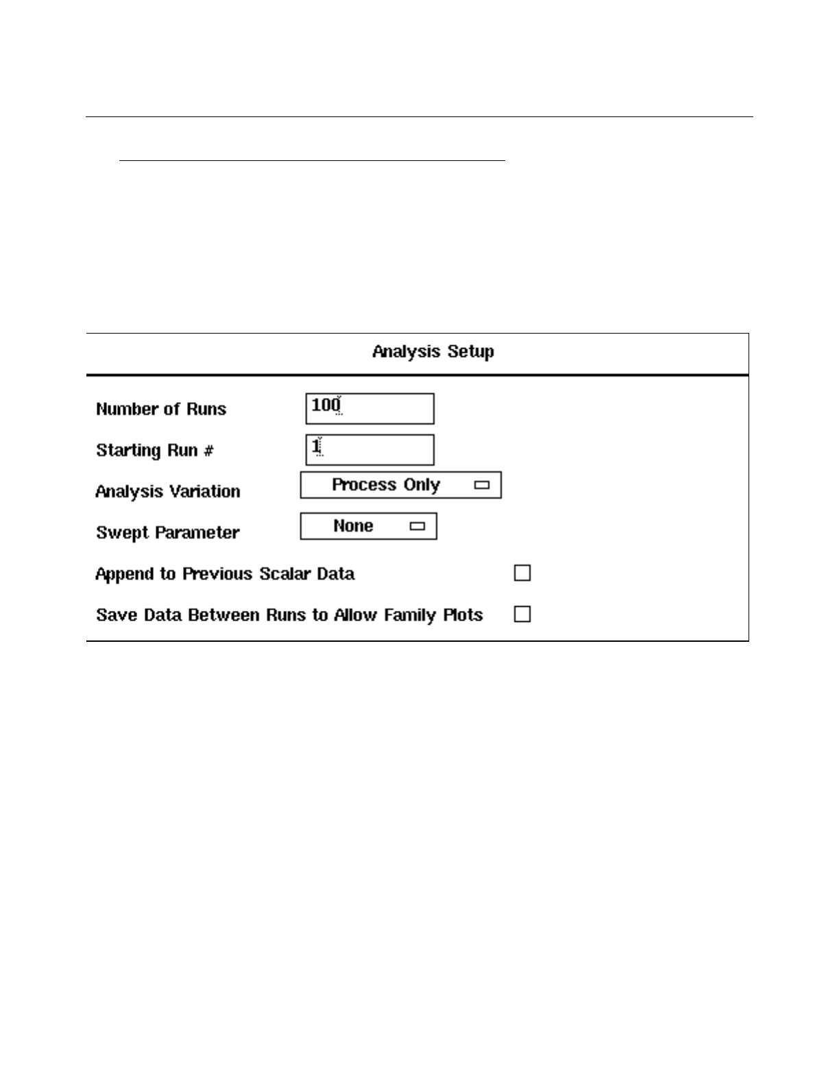
Cadence Advanced Analysis Tools User Guide
Statistical Analysis
July 2002 80 Product Version 5.0
■“Saving and Restoring a Statistical Analysis Session” on page 95
Specifying the Characteristics of a Statistical Analysis
You specify how a statistical analysis proceeds by filling out the fields in the top pane of the
Analog Statistical Analysis window.
1. Specify the Number of Runs for this statistical analysis.
2. Specify the Starting Run #.
By default, this value is 1. However, if you want to collect the results from several sets of
analyses via the Append to Previous Scalar Data boolean, each subsequent set
should not have any run numbers that overlap previous runs numbers. For example, if
your first analysis has a Starting Run # of 1 and the Number of Runs is 100 then the
Starting Run # for the second analysis needs to be at least 101.
3. Choose the type of Analysis Variation.
The available choices depend on the simulator that you are using, but the default choices
include
❑Process Only
❑Mismatch Only

Cadence Advanced Analysis Tools User Guide
Statistical Analysis
July 2002 81 Product Version 5.0
❑Process Variation and Mismatch
Which choice is most appropriate for your analysis depends on whether you want the
statistically valued parameters to vary independently or to track each other. In general,
the parameters of devices on the same die track each other closely and for purposes of
simulation you might want them to track exactly. In a board-level design however, the
parameters of different devices are likely to vary independently. For more information,
see “How the Statistical Analysis Option Uses the Analysis Variation Setting” on
page 98.
4. If desired, choose a parameter to sweep in an inner loop.
The parameter can be either Temperature or one of the design variables. Choose
None, which is the default, if you do not want to sweep a parameter.
5. Select the Append to Previous Scalar Data button if you want to append the scalar
output data from the current analysis to previously saved scalar data.
For example, to add another 100 runs to an existing set of 100 runs, select this button
and, as discussed in Step 2, set the starting Run # to at least 101.
By default, scalar data is saved in the monteCarlo/mcdata file located at the same level
as the psf directory. If you do not select the Append to Previous Scalar Data button,
new scalar data from the current analysis replaces any existing data in that file.
(Spectre simulator only)
This UI field will only be active when valid scalar results are currently selected/loaded.
If the currently loaded scalar results are not from the current copied into the current ADE
run directory when the next monte carlo simulation is run. As a result any previous
existing scalar results in the run directory will be erased.
Before allowing a simulation in this mode, the UI first checks that the current UI
configuration (form field settings) are compatible with the currently loaded results. This
checking includes:
The run numbers do not overlap the run numbers in the existing data.
The Swept Parameter declaration (including values) is the same as in the existing
data.
The scalar expressions in the output pane are the same as in the existing data.
After a simulation in append mode, the UI checks the new data to insure that the
statistical parameters swept are the same as in the pre-appended data. If any
discrepancies are found, the UI blocks reading/loading in the data.

Cadence Advanced Analysis Tools User Guide
Statistical Analysis
July 2002 82 Product Version 5.0
6. (Spectre simulator only) Select the Save Data Between Runs to Allow Family Plots
button if you want to be able to plot graphs showing the variation of entire waveforms or
if you want to evaluate expressions after the analysis finishes.
Be aware that with this option enabled, the amount of data saved during an analysis can
be very large. To reduce disk storage requirements, avoid saving all voltages and
currents. Instead, select only the specific nodes and terminals referenced by your output
expressions.
The statistical analysis option calculates and saves the results of scalar expressions after
every run, whether Save Data Between Runs to Allow Family Plots is selected or
not.
Selecting Signals and Expressions to Analyze
The Analog Statistical Analysis window Outputs pane initially contains any expressions and
signals defined in the Outputs pane of the Cadence® Analog Design Environment window.
You can also retrieve these expressions and signals at any time by choosing Outputs –
Retrieve Outputs. These choices and values from the environment window are often the
most useful ones for a statistical analysis, but, if you want, you can change them. You can
add, modify, or delete expressions and add or delete signals by
■Using the Direct Plot form, Add To Outputs capability
■Typing them in directly
■Using the Calculator
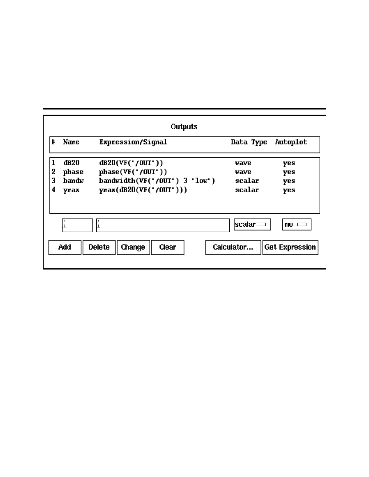
Cadence Advanced Analysis Tools User Guide
Statistical Analysis
July 2002 83 Product Version 5.0
Working Directly with Expressions and Signals
You can use the Outputs pane, edit fields, and button bar to add or delete signals and to add,
delete or change expressions.
Adding a Signal or Expression
To add a signal or expression by typing it in:
1. If the edit fields are not empty, click Clear.
2. In the edit fields, type a name for the new expression and the expression itself.
3. Set the Autoplot cyclic field, which is located at the right side of the edit fields, to yes if
you want the new signal or expression to be plotted after all the simulations finish.
4. Click Add.
The new signal or expression is added to the list of signals and expressions.

Cadence Advanced Analysis Tools User Guide
Statistical Analysis
July 2002 84 Product Version 5.0
Deleting a Signal or Expression
To delete a signal or expression:
1. Highlight the signal or expression in the Outputs pane.
2. Click Delete.
Changing an Expression
To change an expression:
1. Highlight the expression in the Outputs pane.
The expression appears in the edit fields.
2. Working in the edit fields, make any necessary changes to the name, expression, and
autoplot values.
3. Click Change.
Using the Calculator to Build Expressions
To avoid typing in an expression and signal names, you can build an expression in the
calculator and then import the finished expression into the Analog Statistical Analysis
window.
1. Click Calculator to open the calculator window.
2. Use the buttons and commands in the calculator window to build the expression you
need. Leave the completed expression in the display buffer of the calculator.
3. In the Analog Statistical Analysis window, click Get Expression.
The expression appears in the Outputs pane.
Data Access Function Types
In order to create effective monte carlo expressions, knowledge of the two basic types of data
access functions is critical:
Analysis Alias/Type Dependent Functions:
This type searches for a particular analysis alias or type. The alias or type to be sought
after is hardcoded according to the function name, there is no specific type argument on

Cadence Advanced Analysis Tools User Guide
Statistical Analysis
July 2002 85 Product Version 5.0
these functions. For example, the VF() function will look for a voltage (V) signal in the
first found occurrence of ac data (Frequency), whereas the IT() function will look for a
current (I) in transient data (Time).
Here are examples of VF() expressions that can be declared:
mag(VF("/net2") 1e6) => waveform
value(mag(VF("/net2") 1e6)) => scalar
Most of these functions can be found on the calculator tool.
These wildcard functions access data according to the following flow:
a. First look for a specific aliased data name in the current results. For example, the
VF() function would first look for psf data aliased to the name ’ac. If found, then this
data is retrieved.
For more information on alias names, see the section titled Data Name Aliasing.
b. If (1) does not find an alias name match, then the function reverts to a data type
wildcard search operation. Instead of looking for a name match, the function will now
search for the first occurrence of any psf data with a type that matches the one
related to the function name. For example, the VF() function will now look for a
voltage (V) signal in the first found occurrence of ac type data.
Analysis Name Dependent Functions:
This type searches for a particular analysis name (or alias). These functions require
that a psf data name (or its alias) be specified. The benefit to these functions is that
there is no ambiguity as to which data set will be retrieved. Here are examples of ac
data expressions that can be declared:
mag(v("/net2" ?result "ac") 1e6) => waveform
value(mag(getData("/net2" ?result ’ac) 1e6)) => scalar
All of the Ocean data access functions are name dependent. The most commonly
used functions are getData(),v() and i().
Data Name Aliasing
During the course of using the Statistical Analysis tool, the spectre simulator can create up
to nine distinct data names for each analysis type. The name of data being accessed depends
both on the UI configuration for the statistical analysis run and on when the data is being
accessed (by spectre at runtime or by the UI for post processing/plotting).
As a result, a method to declare a single data name that was the equivalent to the nine above
mentioned data name formats was added. Now, when data is selected/loaded, the data

Cadence Advanced Analysis Tools User Guide
Statistical Analysis
July 2002 86 Product Version 5.0
access code automatically aliases any found version of the nine possible data name formats
to the base name equivalent.
For any currently selected/loaded data the user can see what alias names have been
assigned by typing the following command into the ciw:
setof(ana results() symbolp(ana))
An example response is:
(dc ac output dcOp sp_noise model tranOp tran
dcOpInfo instance noise sp variables)
To see the actual psf names generated, enter:
setof(ana foreach(mapcar (na a) results(?noAlias t) results()
list(a na)) symbolp(car(ana)))
An example response is:
(dc "mc1_dc-montecarlo")
(ac "mc1_ac-montecarlo")
(output "mc1_outputParameter-montecarlo")
(dcOp "mc1_dcOp-montecarlo")
(sp_noise "mc1_sp_noise-montecarlo")
(model "mc1_modelParameter-montecarlo")
(tranOp "mc1_finalTimeOP-montecarlo")
(tran "mc1_tran-montecarlo")
(dcOpInfo "mc1_dcOpInfo-montecarlo")
(instance "mc1_element-montecarlo")
(noise "mc1_noise-montecarlo")
(sp "mc1_sp-montecarlo")
(variables "variables")
In this example, we know that the "mc1_ac-montecarlo" psf data will be accessed for
either of the following functions:
VF("/net2")
getData("/net2" ?result ’ac)
So long as all functions which are analysis name dependent use the proper alias name, the
proper data will be retrieved throughout all phases of using the Statistical Analysis tool.
Note that this aliasing is tightly tied to the analysis names that the ADE netlister generates. If
the user tries to run a standalone netlist with different names, the aliasing may not work
properly. The same goes for declaring analyses via an include file. The Statistical Analysis UI
is only intended for use directly within the ADE product.

Cadence Advanced Analysis Tools User Guide
Statistical Analysis
July 2002 87 Product Version 5.0
Results Dir Arguments in Expressions
Many of the data access functions have an optional results directory argument. This
argument must not be set for any expression being used in monte carlo. For more information,
see the Creating Monte Carlo Compatible Expressions section.
Creating Monte Carlo Compatible Expressions
Most of the calculator buttons produce valid expressions for use in the monte carlo flow (this
does not include the results browser button or tool).
Most of the results browser generated data access expressions must be hand edited in order
to conform to the expression syntax requirements of the monte carlo flow.
Most of the ADE->Results->Direct_Plot forms produce the proper expression syntax (via
the Add to Outputs utility). These forms typically produce ocean expressions, but some still
produce old ael style functions.
Before any function/expression will work properly in the Monte Carlo tool, the following Monte
Carlo Expression Syntax Rules should be followed:
1. Whenever an analysis name argument is required, like for Ocean functions, always use
the proper alias name.
2. Never include the current run directory in an expression. When using the results browser
to capture a data access expression in the calculator, always manually delete the run
directory component of the expression.
For example, the results browser may declare something like this in the calculator:
v( "/net4" ?result "ac-ac" ?resultsDir
"/hm/test/simulation/ampTest/spectre/schematic" )
This expression must be manually altered to look like:
v( "/net4" ?result ’ac)
Where ’ac is the standard ac analysis alias name.
For more information on alias names, see the section titled Data Name Aliasing.
The most common symptoms of invalid expressions are:
❑All of the generated scalar data points for an expression is the same nominal value.
❑A waveform plot for a waveform expression only plots a single waveform and there
is no iterations parametric information.

Cadence Advanced Analysis Tools User Guide
Statistical Analysis
July 2002 88 Product Version 5.0
❑All of the scalar data points for an expression is either of the two error flag values (-
1.11111e36 and -2.22222e36).
❑Spectre aborts via the nominal run expression error checker.
Optimizing Monte Carlo Expressions
Some expressions can require significant evaluation times for the Simulation-
>Check_Expressions and Results->Evaluate_Expressions capabilities of the UI. The bigger
the family of psf data created by spectre, the greater the evaluation times of these two utilities.
The analyses that are mostly affected are tran, sp and the rf ones.
The spectre simulator does not experience this slowdown in performance because it only
operates on a single iteration at any one time. It never processes the entire psf family of
iterations data.
Depending on the scope of psf data generated, the user can get better performance out of an
expression if they simply re-arrange it.
For example, the following syntax:
value(exprA num)/value(exprB num)
is faster than using the simpler expression syntax of:
value(exprA/exprB num)
Some functions with complicated internal calculations compound the amount of time required
for evaluation. A prime example is the s-parameter yp() Ocean function. This function
requires performing internal matrix manipulations. As the data sets that yp() operates on grow
linearly, the matrix evaluation time grows exponentially. As a result, it is best to reduce the
data going into the yp() function as opposed to reducing the data coming out of it. For
example, although the following expression is simplistic:
value(yp(sp(1 1 ?result ’sp) sp(1 2 ?result ’sp)
sp(2 1 ?result ’sp) sp(2 2 ?result ’sp)) 1M)
The user will get much better performance if they re-arrange the expression to be:
yp(value(sp(1 1 ?result ’sp) 1M) value(sp(1 2 ?result ’sp) 1M)
value(sp(2 1 ?result ’sp) 1M) value(sp(2 2 ?result ’sp) 1M))
Note: The YP() ael function is doomed to be slow because it does not allow the user to
reduce the dimension of the input s-parameters.
Therefore, it depends on how far the customer wants to go to optimize their expressions. For
transient and s-parameter data, It is highly recommend that they optimize as much as
absolutely possible.
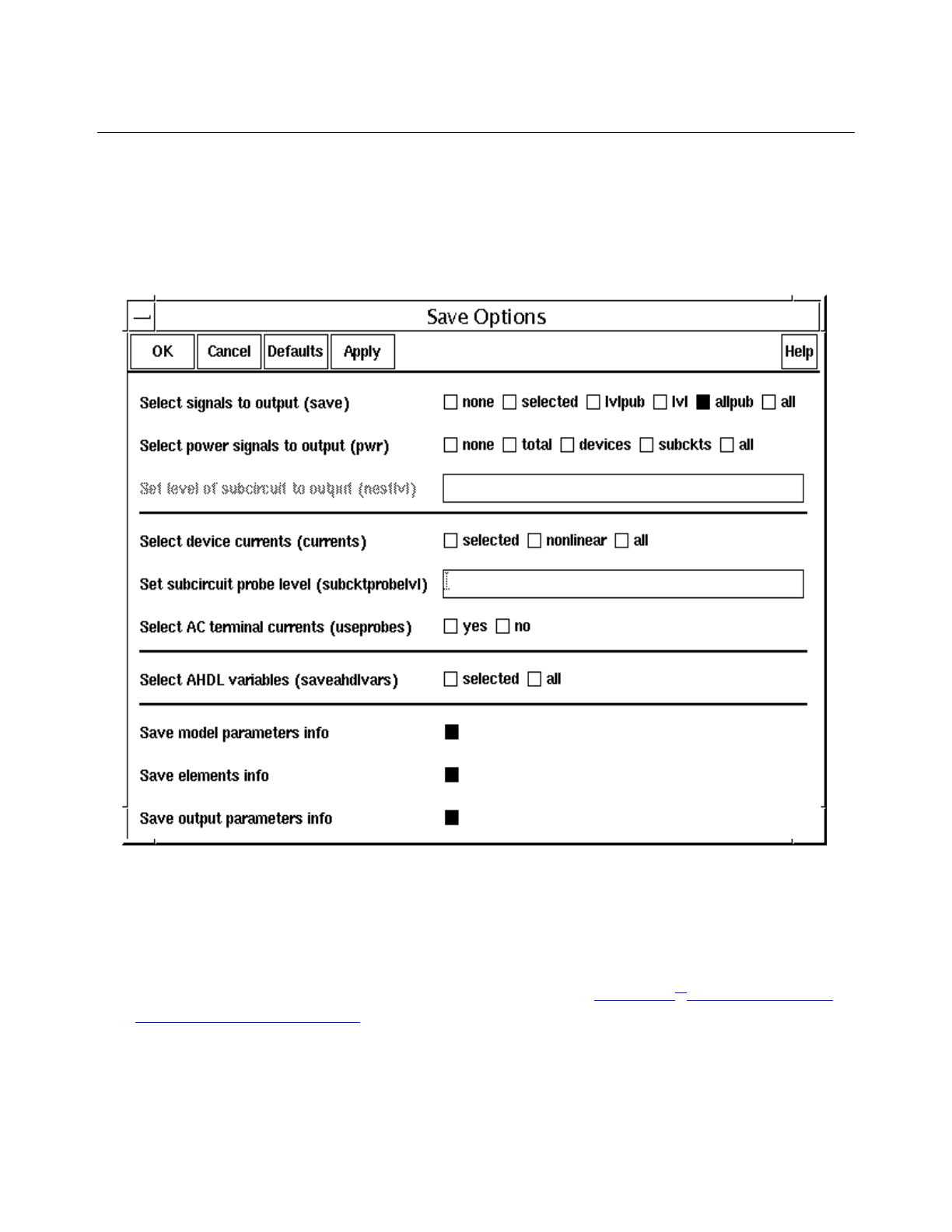
Cadence Advanced Analysis Tools User Guide
Statistical Analysis
July 2002 89 Product Version 5.0
Saving All Voltages or Currents
To save all of the node voltages and terminal currents for later use, perform the following,
1. In the Analog Statistical Analysis window, choose Outputs – Save All.
The options displayed in the form depend on the simulator you use.
2. Select appropriate voltages, currents, or both and click OK.
To reduce the amount of disk space required, select the currents and voltages that
appear in your output expressions and consider selecting individual nets or nodes. For
more information about the Save Options form, see the Cadence® Analog Design
Environment User Guide.
Note: Be aware of the following information about cdsSpice simulations:
❑In cdsSpice simulations, data for terminals in lower-level schematics is not saved
when you use the Save Options form to save all currents. You must explicitly select

Cadence Advanced Analysis Tools User Guide
Statistical Analysis
July 2002 90 Product Version 5.0
each terminal with the Outputs – To Be Saved – Select On Schematic
command from the menu in the Cadence® Analog Design Environment window.
❑In cdsSpice simulations that include a noise analysis, the system turns the Select
all node voltages and Select all terminal currents options off. If you later
deactivate the noise analysis, the system reactivates the options.
3. Select the kinds of information that you want the analog design environment to print.
Turning off the printing improves the performance of a statistical analysis.
Checking the Output Expressions
After all the desired output expressions are declared, the user should execute the following
utility prior to starting the statistical analysis run:
➤Simulation -> Check Expressions
This capability is used to both check and classify each expression element in the Outputs
Pane. Each expression is evaluated against the currently selected/loaded psf data. This data
can either be from a previous statistical analysis or from a straight Cadence®Analog Design
Environment simulation. The result of each evaluation is assigned to the Data Type field on
the Outputs Pane. The three possible outcomes are:
scalar the expression evaluated to a scalar.
waveform the expression evaluated to at least a waveform.
ERROR the expression failed to evaluate.
If no psf data is currently selected/loaded, then a message is produced.
Saving Signals Used in Output Expressions
For any expression entered into the output pane, it is the users responsibility to ensure that
all the pertinent schematic signals contained in all the expressions will be written to the psf
data. The psf data is always used to calculate the scalar values for each iteration run.
In the event that the user will want to produce waveform plots (see the Plotting Families of
Curves and Changing Waveform Expressions at Post-simulation Time sections) or post
generate the scalar data (see the Creating a New mcdata File from Saved Waveform Data
section) then it is a good practice to save any psf schematic signals that will be needed on a
post-simulation basis.
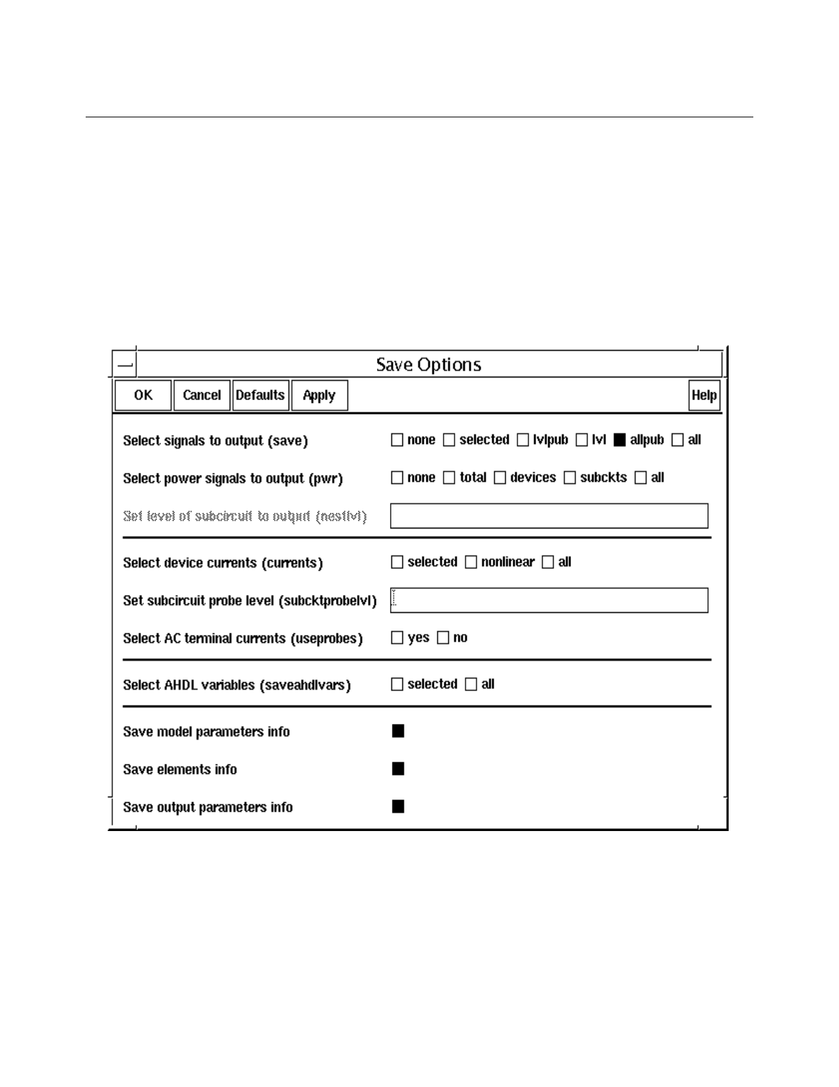
Cadence Advanced Analysis Tools User Guide
Statistical Analysis
July 2002 91 Product Version 5.0
There are two basic ways to declare which schematic signals should be written to psf by the
simulator:
1. Use the ADE->Outputs->To_Be_Saved->Select_On_Schematic menu capability.
This approach allows the user to click directly on the schematic signals they desire.
Note: This approach is best suited when the user wants to limit the amount of disc space
used for psf data.
2. Use the Monte Carlo Outputs->Save_All form. This is the same form as the ADE one.
The options displayed in the form depend on the simulator you use.
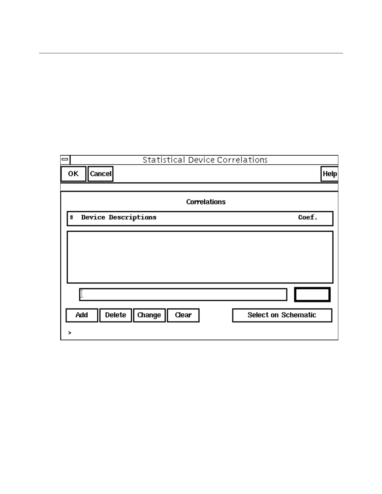
Cadence Advanced Analysis Tools User Guide
Statistical Analysis
July 2002 92 Product Version 5.0
Defining Correlations
Often circuit components are correlated. You can model this behavior by defining correlations
in the model files that you use. As described in this section, you can also use the statistical
analysis option to define correlations.
1. To define correlations, choose Simulation – Define Correlations.
The Statistical Device Correlations form appears.

Cadence Advanced Analysis Tools User Guide
Statistical Analysis
July 2002 93 Product Version 5.0
2. Define the correlations that you need.
3. When you have defined all the correlations, click OK to close the Statistical Device
Correlations form.
The statistical analysis option adds the correlations to the netlist by inserting a new
statistics block after the statistical analysis definition.
Starting and Stopping the Analysis
To start the statistical analysis, choose Simulation – Run.
Normally, the analysis stops when all the iterations are complete. In addition, analyses that
use the Spectre simulator stop if errors are found during the nominal simulation that the
Spectre simulator performs.
If you want to stop the analysis before all the iterations are complete, choose Simulation –
Stop. In response, the statistical analysis option
1. Completes the current iteration
2. Stops the analysis
3. Saves the simulation results
4. Plots the results for each signal or expression that has Autoplot set
To type device names… To select devices in the schematic…
a. Type the full schematic names
into the field near the bottom of
the form.
b. Type the correlation coefficient
for those devices into the field to
the right of the names.
c. Click Add.
a. Click Select on Schematic.
b. In the Composer window, select
the devices that you want to be
correlated.
c. When you finish selecting, press
the Escape key.
d. In the Statistical Device
Correlations form, type the
correlation coefficient for the
devices you selected into the
field to the right of the names.
e. Click Add.
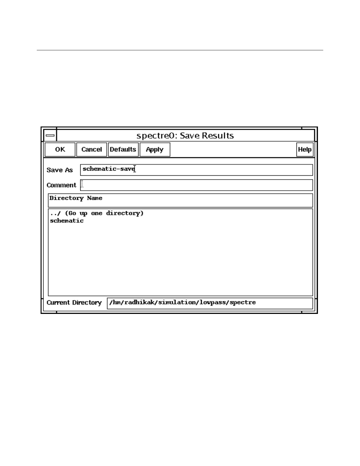
Cadence Advanced Analysis Tools User Guide
Statistical Analysis
July 2002 94 Product Version 5.0
Saving Statistical Analysis Results
After a statistical analysis, the resulting psf and statistical scalar data can be saved.
1. Choose Results – Save.
The Save Results dialog box appears.
2. Type new information, as necessary.
Consider entering a comment to help you identify the data later.
Be aware that this command copies the entire parameter storage format (PSF) directory
structure, which might be very large, to the new location.
3. Click OK.
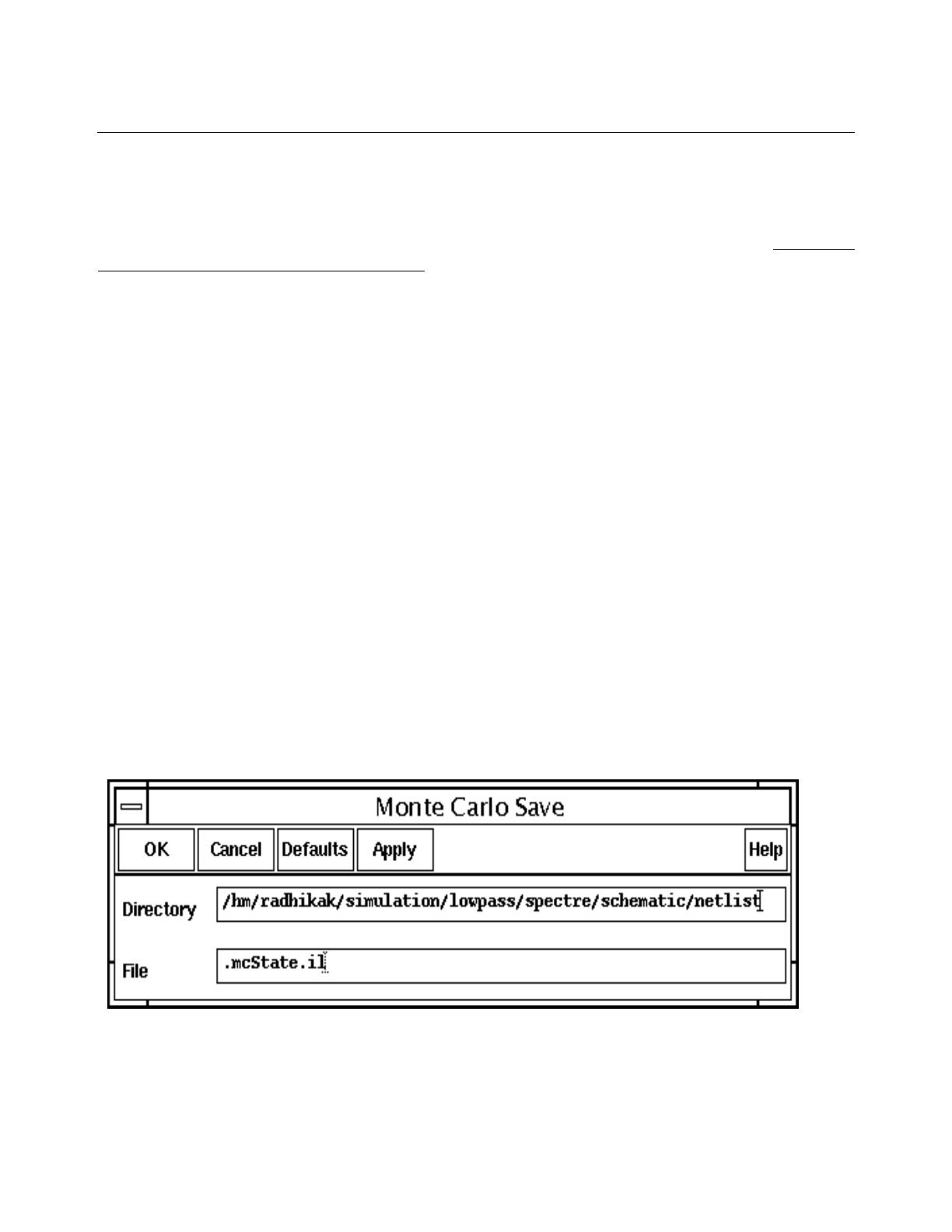
Cadence Advanced Analysis Tools User Guide
Statistical Analysis
July 2002 95 Product Version 5.0
Saving and Restoring a Statistical Analysis Session
This section explains how to create input files, save and reload session states, save scripts,
and quit from the statistical analysis option. For information on starting the tool, see “Opening
the Analog Statistical Analysis Window” on page 70.
Creating Input Files for a Socket Simulator
If you follow the usual procedure of specifying the simulation and then specifying the
statistical analysis that you want to use, the statistical analysis option creates the necessary
input files automatically. However, if you want to hand edit the input files, the statistical
analysis option provides a way for you to do that.
➤From the Analog Statistical Analysis window, choose Simulation – Create Input Files.
The tool creates the mcrun.s and mcparam files.
Saving the Session State
A session state consists of all the information in the Analog Statistical Analysis window,
including the Analysis Setup and Outputs information.
To save the current state,
1. Choose Session – Save State.
The Monte Carlo Save form appears.
2. Type the name of the file where you want to save the session state.
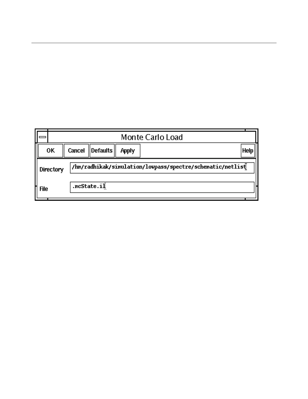
Cadence Advanced Analysis Tools User Guide
Statistical Analysis
July 2002 96 Product Version 5.0
3. Click OK.
Loading a Saved Session State
To load a saved state,
1. Choose Session – Load State.
The Monte Carlo Load form appears.
2. Type the name of the file that contains the saved session state.
3. Click OK.
The values from the saved session state appear in the Analog Statistical Analysis
window.
Saving the Script
To save the script that is automatically generated during each session,
1. Choose Session – Save Script.
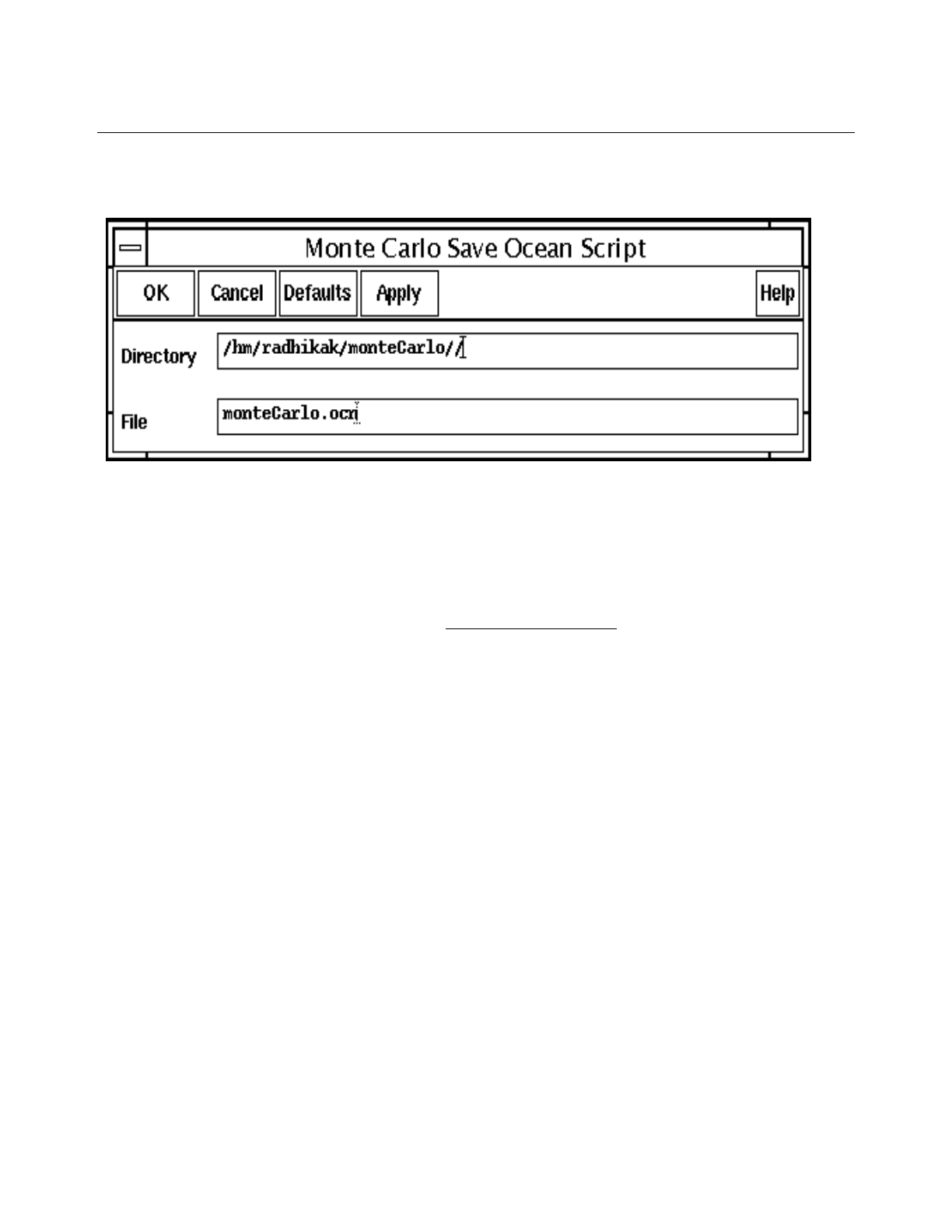
Cadence Advanced Analysis Tools User Guide
Statistical Analysis
July 2002 97 Product Version 5.0
The Monte Carlo Save Ocean Script form appears.
2. Type the name of the directory and file where you want the script to be saved.
3. Click OK.
The script is saved in the file. For additional information about using the statistical
analysis option with OCEAN, see the OCEAN Reference.
Viewing the Output Log
To open a window that contains the history of the statistical analysis simulations,
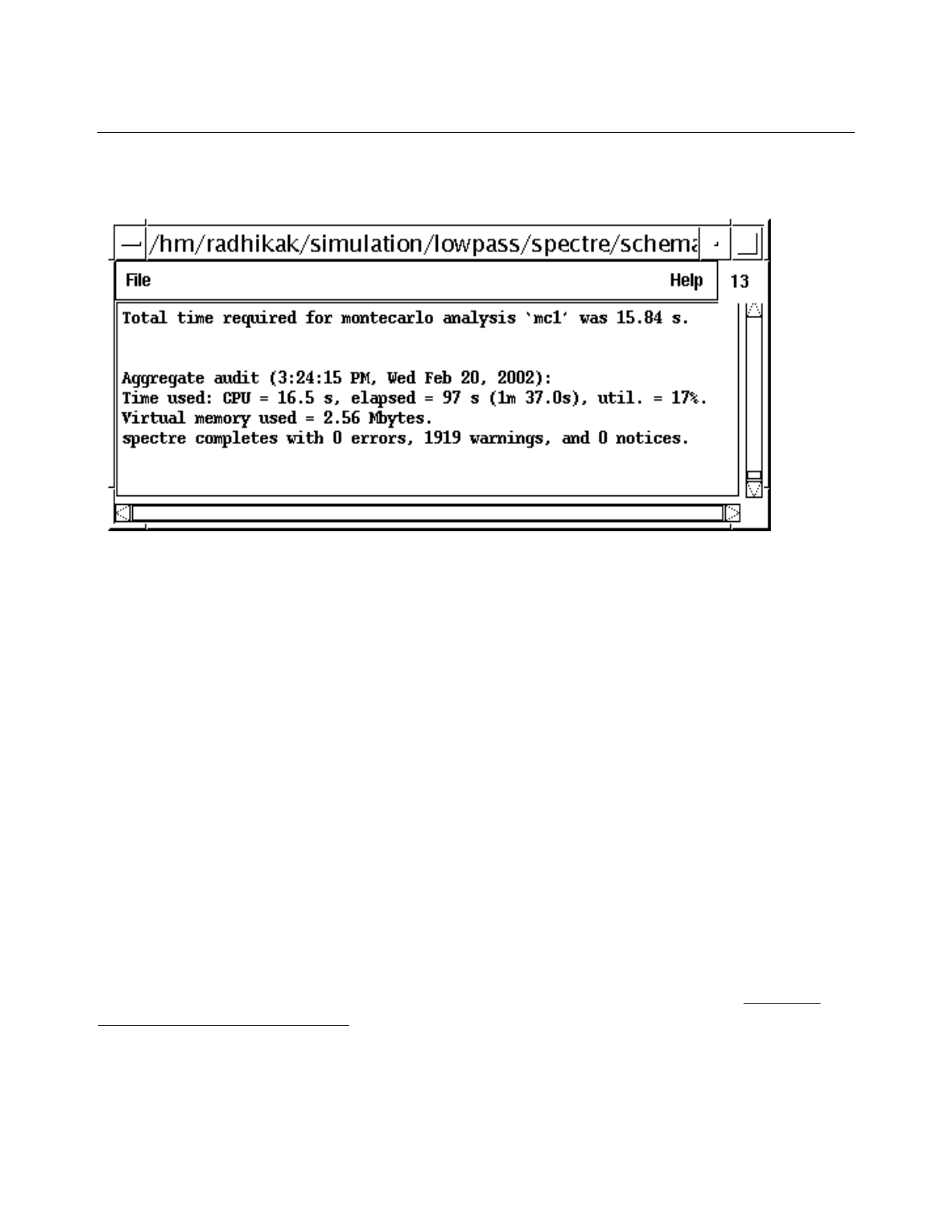
Cadence Advanced Analysis Tools User Guide
Statistical Analysis
July 2002 98 Product Version 5.0
➤Choose Simulation – Output Log.
The simulator updates the Output Log while the simulation runs, so you might find it useful to
have this window open during the simulation.
Closing the Analog Statistical Analysis Window
To end the session and close the Analog Statistical Analysis window,
➤Choose Session – Quit.
How the Statistical Analysis Option Uses the Analysis Variation Setting
When you run the statistical analysis option from the Cadence®Analog Design Environment
window, you use the Analysis Variation cyclic field to select the kinds of variations to be
used during the analysis. However, the connection between the cyclic field choice and how
your models behave is not automatic—you must define your models so that they respond to
the cyclic field choice.
For the Spectre simulator, you use a statistics block to specify model behavior under the
Analysis Variation cyclic field. See the Analysis Statements chapter of the Spectre
Circuit Simulator Reference for more information. The statistics block must be included in
the netlist before the models. For example, you might use a statistics block with the following
contents:
statistics {
process {
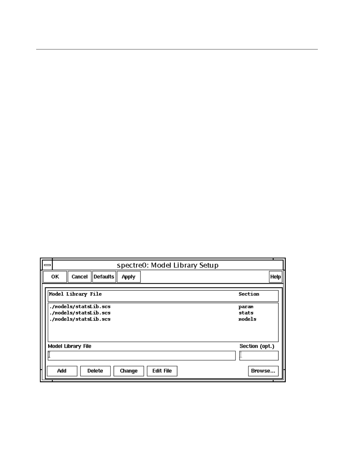
Cadence Advanced Analysis Tools User Guide
Statistical Analysis
July 2002 99 Product Version 5.0
vary PiRho dist=gauss std=250
vary PbRho dist=gauss std=40
vary beta dist=gauss std=20
vary rin1 dist=gauss std=10
vary cin dist=gauss std=20p
vary rin2 dist=gauss std=100
vary cloop dist=gauss std=16p
vary rout1 dist=gauss std=30
vary rout2 dist=gauss std=50
}
mismatch {
vary stat dist=gauss std=.01
}
}
The process and mismatch blocks define the variations for the cyclic field choices.
Before the simulator can use the statistics block, you must include the block in the netlist. For
example, assume that you have a single file called statsLib.scs that has three sections:
parameters,statistics, and models. These sections are arranged so that the
definitions all build without errors.
Then, to include statsLib.scs in the netlist,
1. From the Cadence® Analog Design Environment window, choose Setup – Model
Libraries.
The Model Library Setup form appears.
2. Type the complete path to the statsLib.scs file and click Add.
3. Click OK.

Cadence Advanced Analysis Tools User Guide
Statistical Analysis
July 2002 100 Product Version 5.0
Analyzing Results
You can use the procedures described in the following sections to analyze a set of statistical
analysis results. By default, these procedures operate on the data from a just-concluded
statistical analysis, but you can also analyze saved data from earlier runs. The saved data
can take two forms: either you can use the data in a stored output file or, if the statistical
analysis session that you want to analyze had the Save Data Between Runs to Allow
Family Plots button turned on, you can create a new mcdata output file from the saved
waveform data.
Loading Stored Statistical Analysis Results
To load a stored set of data,
1. Choose Results – Select
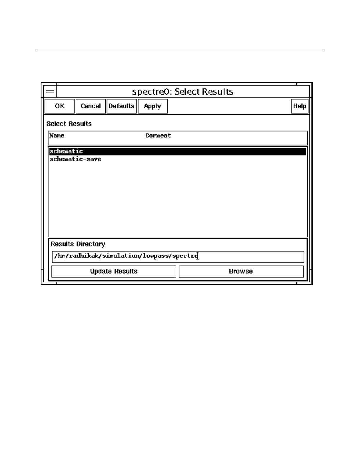
Cadence Advanced Analysis Tools User Guide
Statistical Analysis
July 2002 101 Product Version 5.0
The Select Results form appears.
2. Select the results that you want to load and click OK.
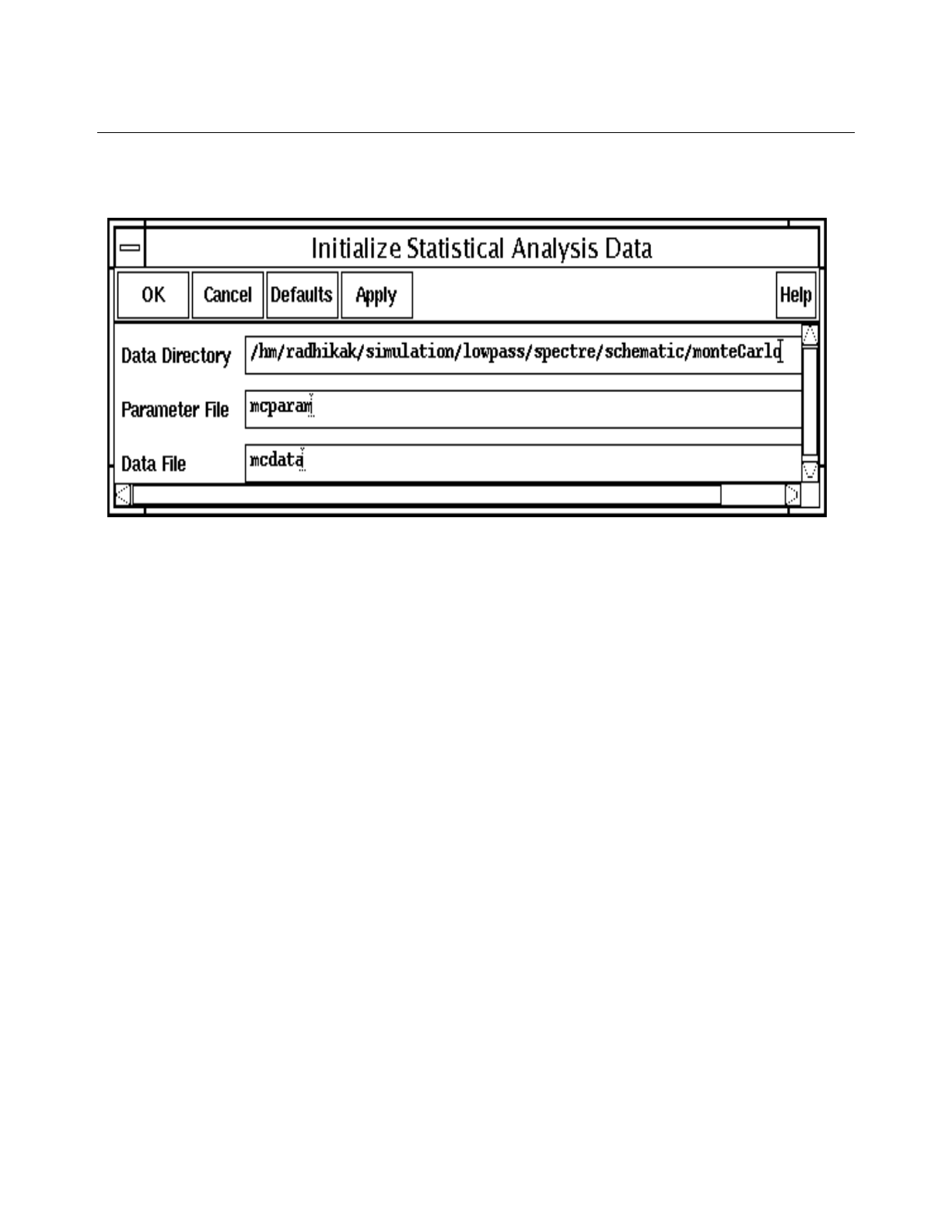
Cadence Advanced Analysis Tools User Guide
Statistical Analysis
July 2002 102 Product Version 5.0
The Initialize Statistical Analysis Data form appears.
3. Verify the names of the files containing the statistical analysis data. At runtime, the UI
automatically assigns the name mcparam for the Parameter File and mcdata for the
Data File. As a result, there are few situations where a user should try to stray from these
names. If the names appear to be proper, then click OK. If either of the file names are
blank, then the data is not present and the user should click Cancel.
Creating a New mcdata File from Saved Waveform Data
If you select Save Data Between Runs to Allow Family Plots before running a simulation,
then after the simulation you can use the data stored by that command to evaluate
expressions and create a new mcdata file.
1. Ensure that the Outputs pane contains the expressions and signals that you want to use.
2. Choose Results – Evaluate Expressions.
Filtering Outlying Data
When it cannot evaluate an expression, a socket simulator returns the value 1e36. The
Spectre simulator returns -1.1111e36 when it cannot evaluate an expression and returns --
2.2222e36 when an expression evaluates to a waveform instead of a scalar. Outlying data
points with values like these can have a large and misleading effect on a statistical analysis.
To avoid distortions, you can follow steps like the ones below to filter outlying data points from
your data set.
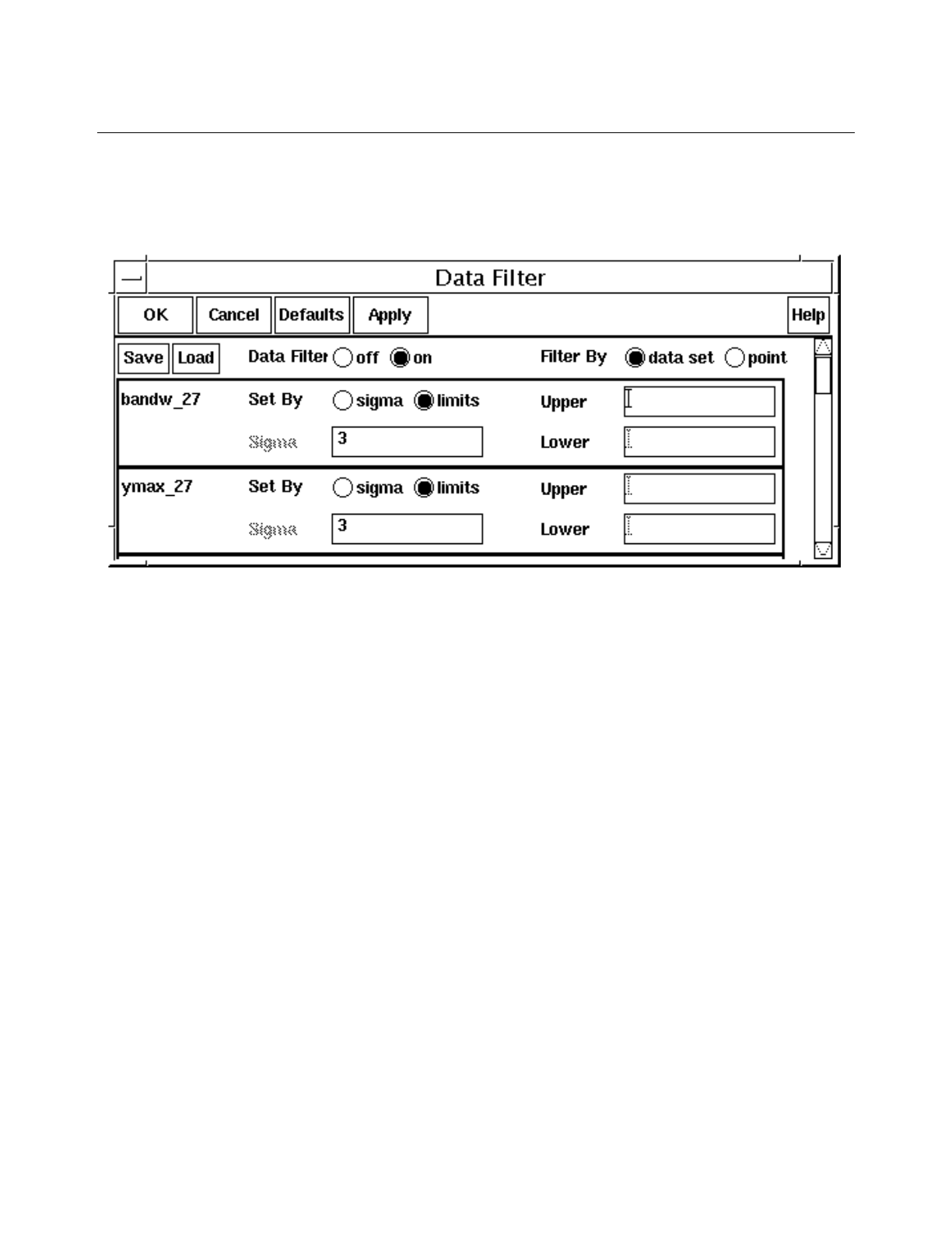
Cadence Advanced Analysis Tools User Guide
Statistical Analysis
July 2002 103 Product Version 5.0
1. Choose Results – Filter.
The Data Filter form appears.
2. Check that Data Filter is set on.
3. Choose how to compute yield statistics.
❑Filter By data set ignores all measurements for a point if the value of any of the
measurements for that point is outside the filter limits.
For example, if a point has a value of 1e36 on the bandw_27 measurement shown
in the previous figure, the value for the ymax_27 measurement for that point is also
ignored even if the value falls between the upper and lower ranges defined by the
filter.
❑Filter By point filters an outlying point only from the specific measurement that
recorded the outlying point.
4. Choose how to set the limits for each parameter.
❑Set By sigma lets you specify how many standard deviations around the mean
value to include.
❑Set By limits lets you set absolute upper and lower values. The Upper and Lower
values are included in the range of acceptable values; so to exclude an error value
of 1e36, you need to specify a smaller value, such as 1e35.
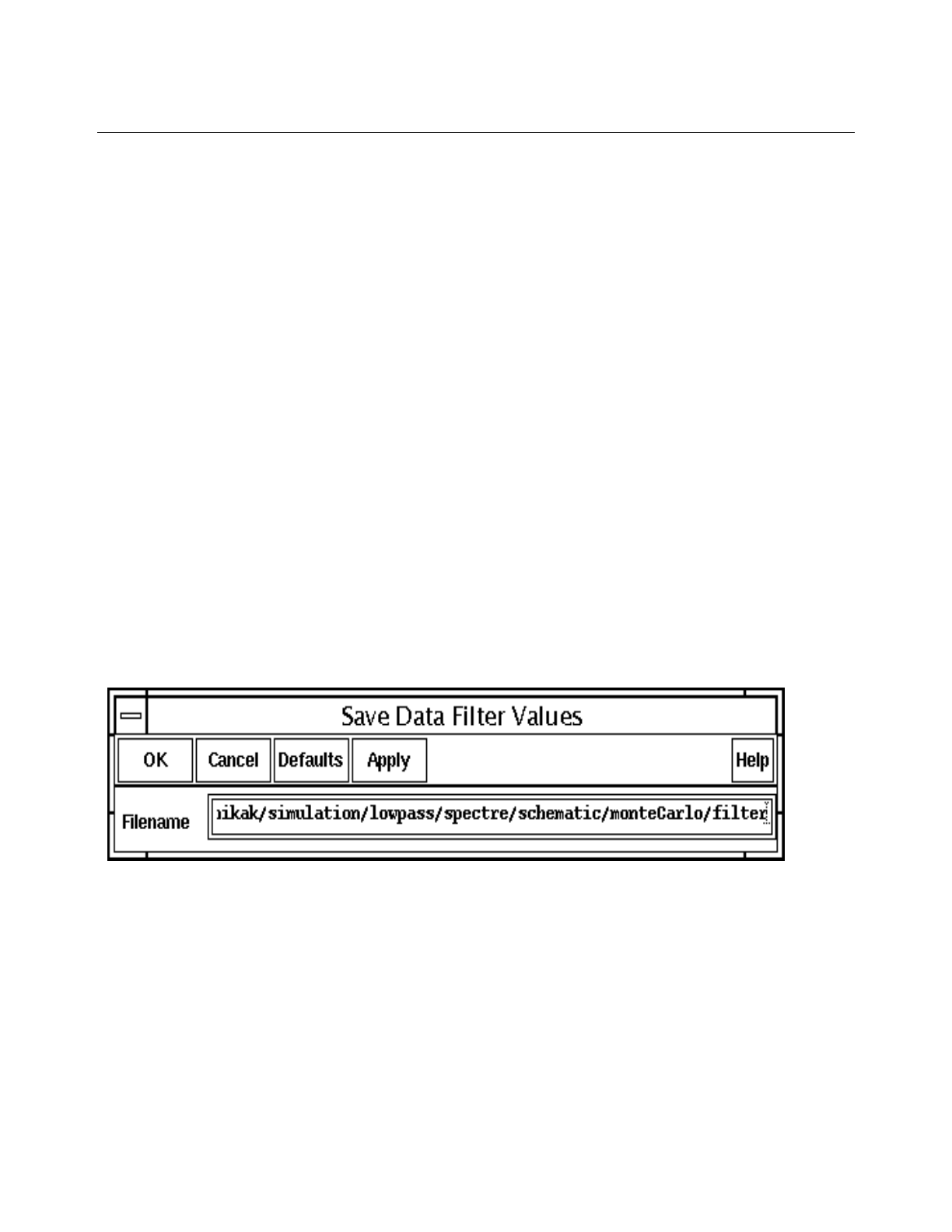
Cadence Advanced Analysis Tools User Guide
Statistical Analysis
July 2002 104 Product Version 5.0
Turning Off Filtering
To turn off data filtering,
1. Choose Results – Filter.
2. In the Data Filter form, set Data Filter to off and click OK.
Saving and Restoring Filter Settings
Whenever new data is selected/loaded into the Monte Carlo UI, the existing Data Filter form
and its settings are destroyed. A new form is recreated based on the new scalar data
information being read in. As a result, any and all settings on the previous Data Filter form
will be lost. Therefore, it is highly recommended that any declarations made on this form be
immediately saved. Especially if one will be running subsequent simulations of selecting or
loading in results.
To save the data filter settings to a file,
1. Choose Results – Filter.
2. In the Data Filter form, click Save.
The Save Data Filter Values form appears.
3. Type a name for the settings file and click OK.
To restore saved data filter settings,
1. Choose Results – Filter.
2. In the Data Filter form, click Load.
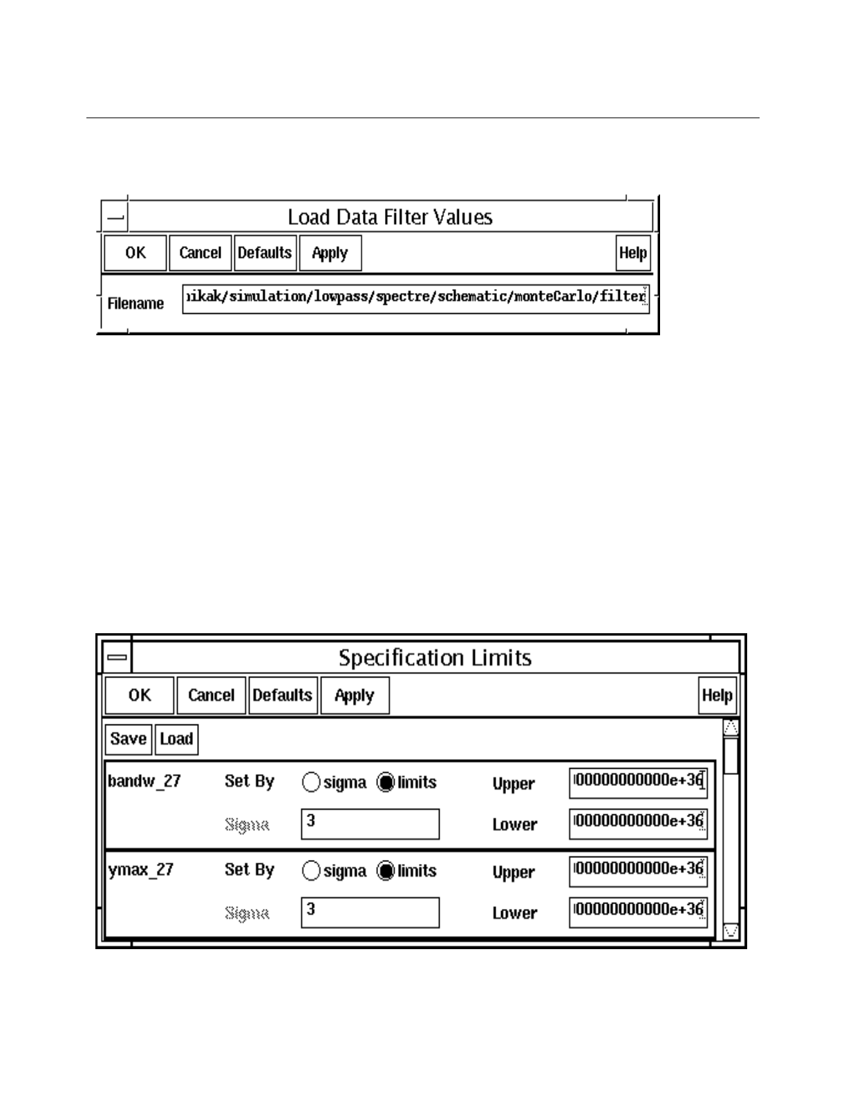
Cadence Advanced Analysis Tools User Guide
Statistical Analysis
July 2002 105 Product Version 5.0
The Load Data Filter Values form appears.
3. Type the name of the settings file and click OK.
Setting Specification Limits
The specification limits define, for each parameter, the range that is considered to be within
tolerance.
To set the specification limits,
1. Choose Results – Specification Limits.
The Specification Limits form appears.
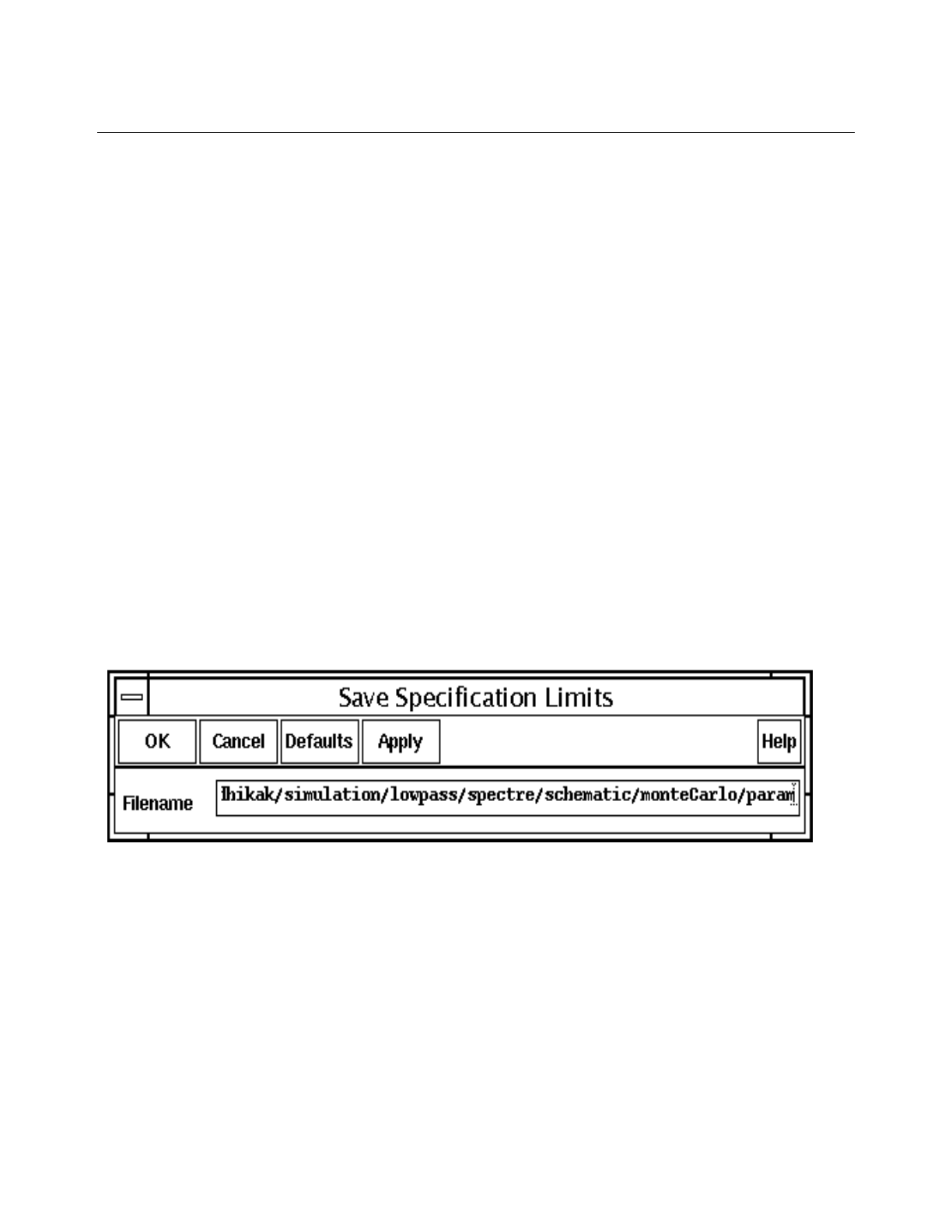
Cadence Advanced Analysis Tools User Guide
Statistical Analysis
July 2002 106 Product Version 5.0
2. Choose how to set the specification limits for each parameter.
❑Set By sigma lets you specify how many standard deviations around the mean
value to allow.
❑Set By limits lets you set absolute upper and lower values.
Saving and Restoring Specification Limits
Whenever new data is selected/loaded into the Monte Carlo UI, the existing Specification
Limits form and its settings are destroyed. A new form is recreated based on the new scalar
data information being read in. As a result, any and all settings on the previous Specification
Limits form will be lost. Therefore, it is highly recommended that any declarations made on
this form be immediately saved. Especially if one will be running subsequent simulations of
selecting/loading in results.
To save and restore the specification limits to a file,
1. Choose Results – Specification Limits.
2. In the Specification Limits form, click Save.
The Save Specification Limits form appears.
3. Type a name for the limits file and click OK.
To restore specification limits,
1. Choose Results – Specification Limits.
2. In the Specification Limits form, click Load.
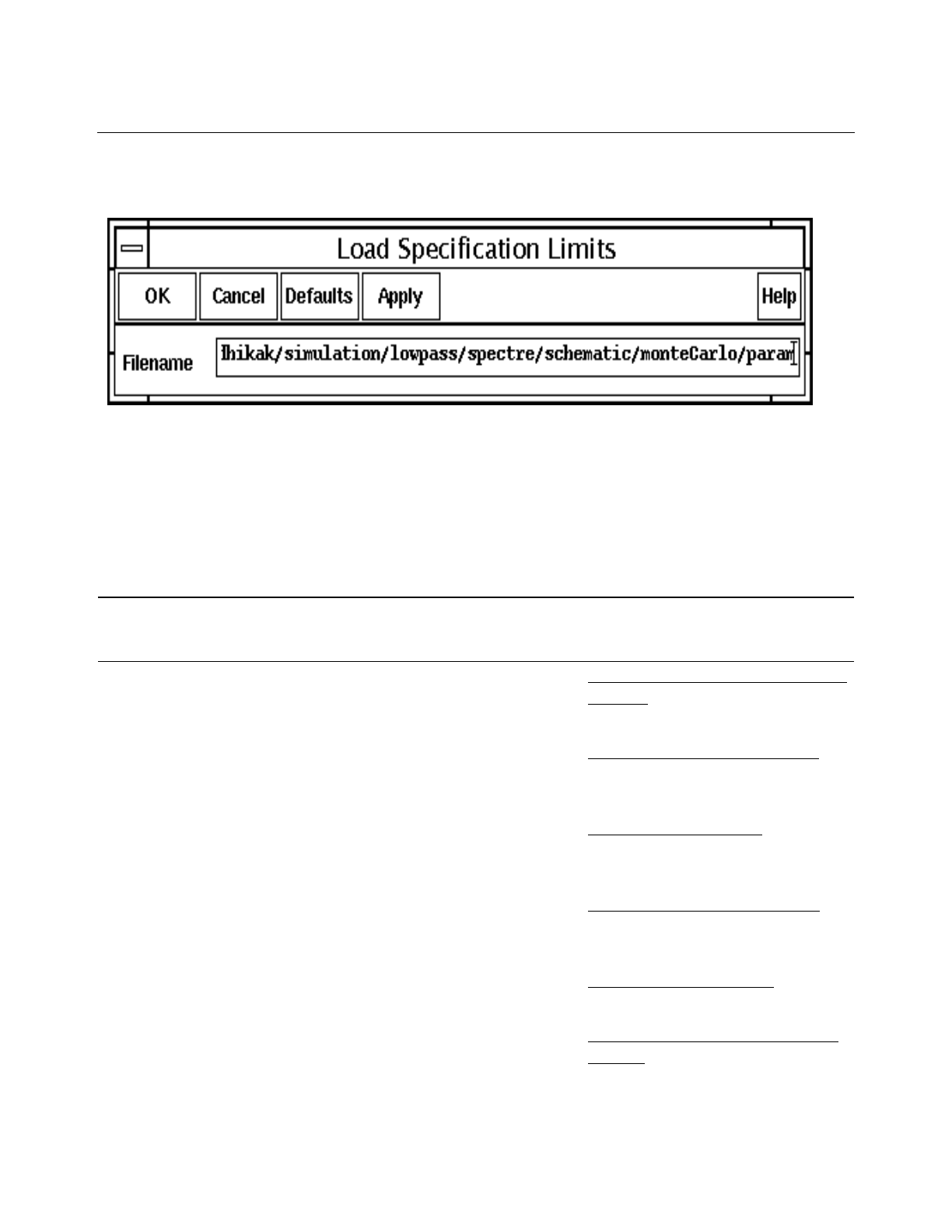
Cadence Advanced Analysis Tools User Guide
Statistical Analysis
July 2002 107 Product Version 5.0
The Load Specification Limits form appears.
3. Type the name of the settings file that you want to load and click OK.
Generating Plots, Tables, and Reports
To help analyze your results, you can generate the following plots, tables, and reports for your
input and output parameters.
Plots, Tables, and Reports
Plot, Table, or
Report Description For More Information
Iteration Versus
Value A table showing the value of a
parameter at the end of each
iteration.
“Printing Iteration versus Value
Tables” on page 108
Correlation A table showing the correlation
coefficients of each parameter with
each of the other parameters.
“Printing Correlation Tables” on
page 110
Histogram A plot showing the number of runs
with scalar parameter values that fall
in each range of values.
“Plotting Histograms” on
page 111
Family-of-Curves A plot showing the superimposed
waveforms for all iterations of a
waveform valued expression.
“Plotting Families of Curves” on
page 113
Scatter Plot A plot depicting the relationship
between pairs of parameters. “Plotting Scatter Plots” on
page 114
Simple Yield A report showing the individual and
total yields for all parameters, given
the specification limits.
“Obtaining Reports on Simple
Yields” on page 117

Cadence Advanced Analysis Tools User Guide
Statistical Analysis
July 2002 108 Product Version 5.0
Understanding Generated Data Names
The output expression names revealed when viewing statistical results will be slightly different
than that shown on the Outputs Pane of the UI.
This is because each scalar expression could be evaluated across several swept parameter
values (a UI capability), there would be several distinct data sets created. In order to cope
with having many data sets for a single output expression, the generated parameter name for
each of these data sets is comprised of the original expression name and the value of the
swept parameter. Each name will be of the form:
Name_ParamValue
Where Name is the name assigned on the Outputs pane of the UI and ParamValue is the
particular value of the swept parameter used while that data was generated.
If the Swept Parameter on the UI is set to None, then the value for ParamValue is set to the
temperature value.
Note: In Spectre, The parameters declared in a statistics block of the spectre netlist will also
be written to the statistical results. The naming convention for these parameters is the same
as for expressions, where Name is the name of the statistically varied parameter.
Printing Iteration versus Value Tables
To print a table showing the value of a parameter at each iteration,
1. Choose Results – Print – Iteration versus Value.
Conditional Yield A report showing the effect on the
rest of the outputs of specification
limits on one parameter.
“Obtaining Reports on
Conditional Yields” on
page 120
Multiconditional
Yield A report showing individual and total
yields, given that the selected
parameters pass the specification
limits test.
“Obtaining Reports on
Multiconditional Yields” on
page 119
Plots, Tables, and Reports, continued
Plot, Table, or
Report Description For More Information
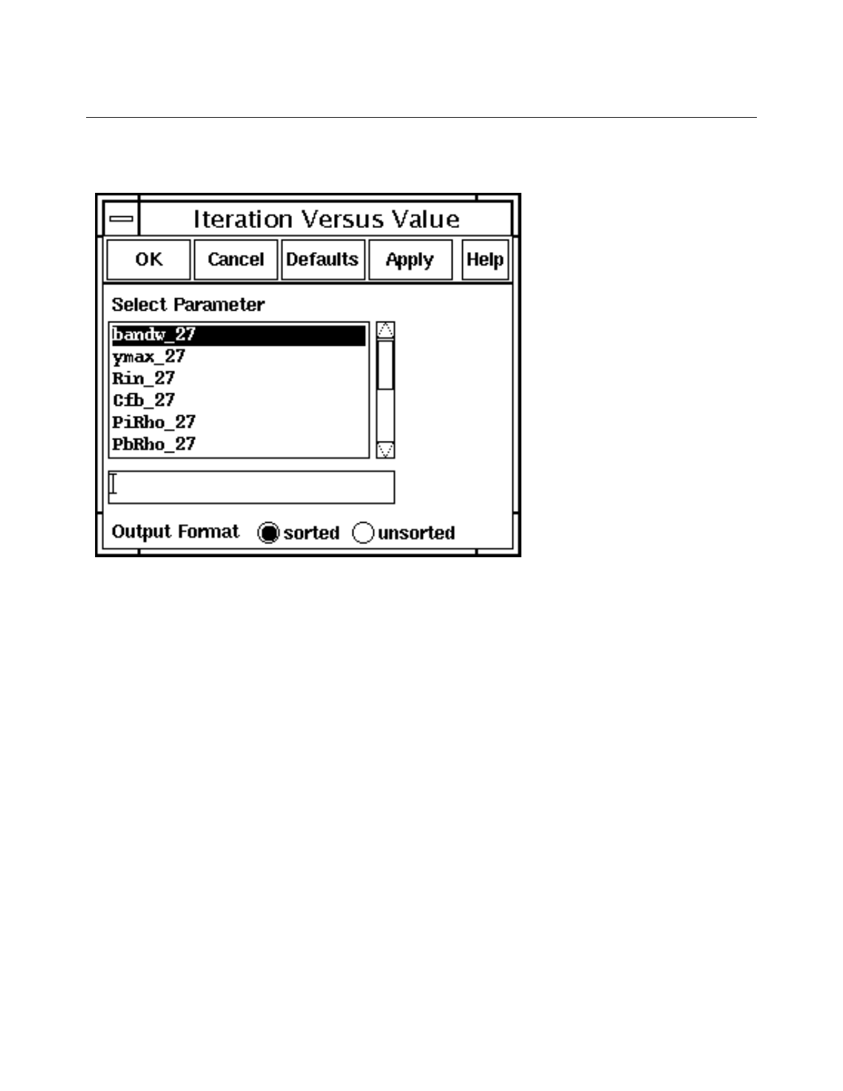
Cadence Advanced Analysis Tools User Guide
Statistical Analysis
July 2002 109 Product Version 5.0
The Iteration Versus Value window appears.
2. Select a parameter, or type a parameter name.
3. Choose the output format:
❑sorted lists the runs by parameter value
❑unsorted lists the runs in chronological order

Cadence Advanced Analysis Tools User Guide
Statistical Analysis
July 2002 110 Product Version 5.0
For example, the following figure illustrates a sorted run, with the value and run number
for each measurement listed horizontally across the window.
Printing Correlation Tables
A correlation table shows the correlation coefficients of each parameter with each of the other
parameters. The parameters are sorted from most correlated to least correlated for each
combination of parameters.
To print a correlation table,
1. Choose Results – Print – Correlation Table.
The Correlation Table window appears.
2. Specify a minimum correlation value. Pairs of parameters with correlations lower than
this value do not appear in the table.
3. Click OK.
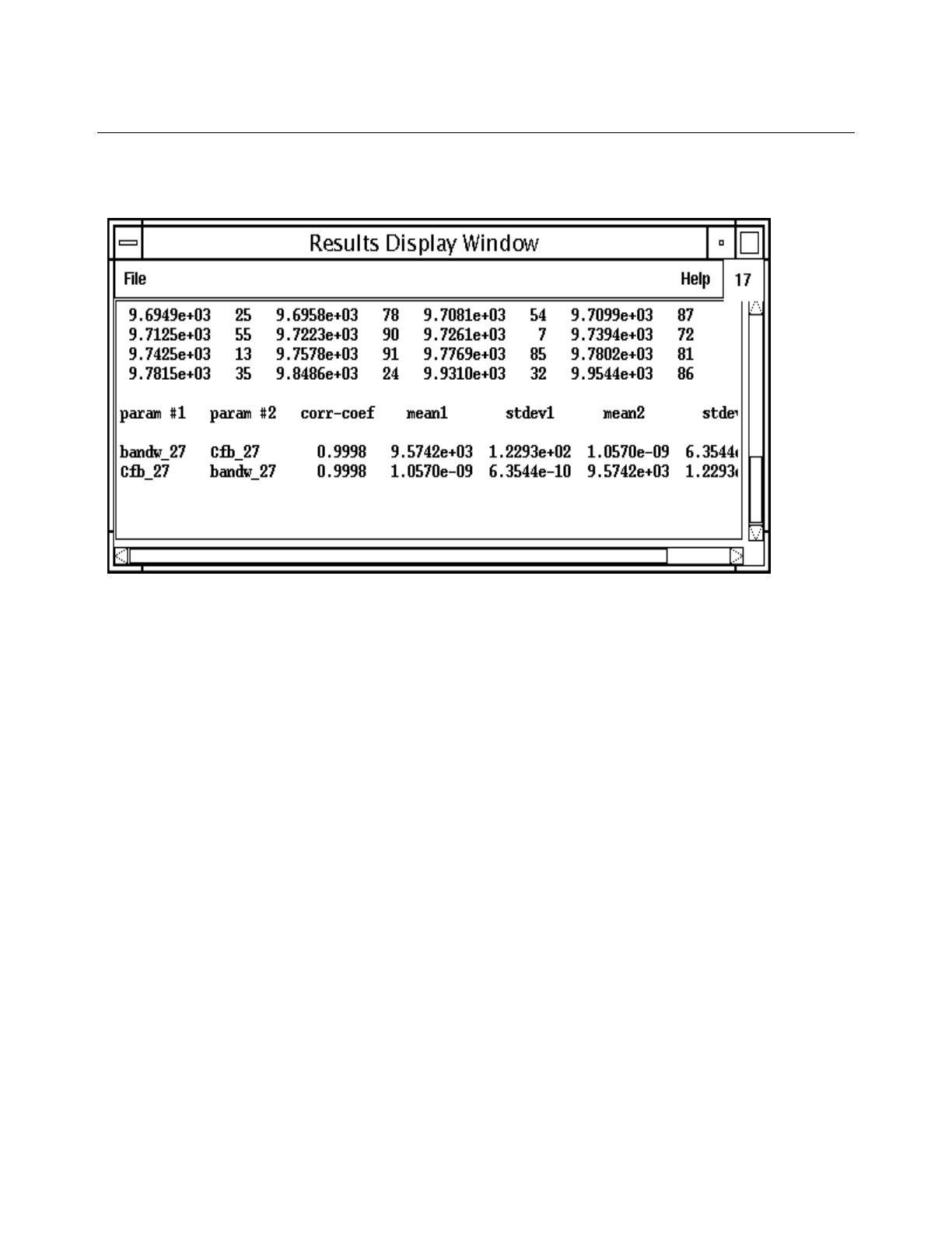
Cadence Advanced Analysis Tools User Guide
Statistical Analysis
July 2002 111 Product Version 5.0
The Results Display Window appears.
Each row lists the pair of measurements being considered, the mean and standard
deviation of the first measurement, the mean and standard deviation of the second
measurement, and the number of data points included in the calculation.
Plotting Histograms
You can plot four types of histograms:
■Standard
■Pass/fail
■Cumulative line
■Cumulative box
To plot a histogram,
1. Choose Results – Plot – Histogram.
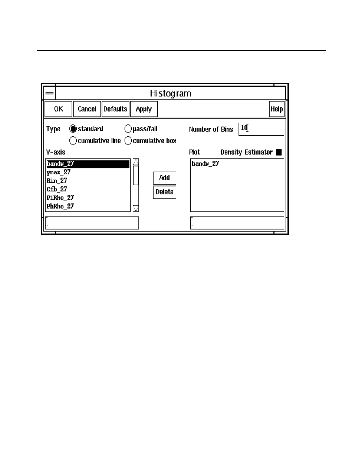
Cadence Advanced Analysis Tools User Guide
Statistical Analysis
July 2002 112 Product Version 5.0
The Histogram form appears.
2. Highlight one or more parameters and click Add.
You can drag or Shift-click to select a group of adjacent parameters or Control-
click to select individual parameters.
3. Type a value from 1 to 50 in the Number of Bins field.
4. (Optional) Click Density Estimator to plot a curve that estimates the distribution
concentration.
5. Click OK.
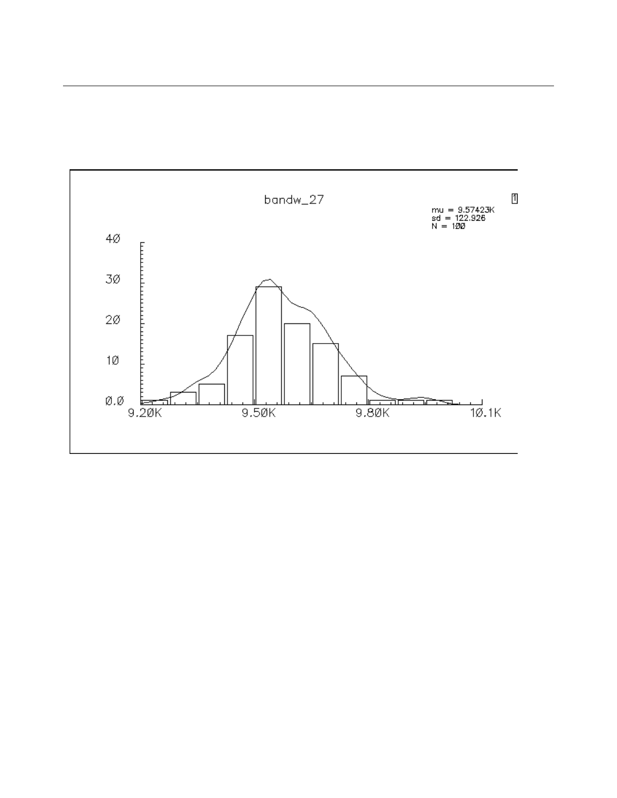
Cadence Advanced Analysis Tools User Guide
Statistical Analysis
July 2002 113 Product Version 5.0
The Waveform window appears, showing the distribution of parameter values found
during the statistical analysis run. In this example, the curved line is the density estimator
line.
Plotting Families of Curves
A family-of-curves shows the superimposed waveforms generated during all of the statistical
analysis iterations. This kind of plot illuminates the variability introduced in waveform
variables by process and mismatch variations.
In order to plot such curves, the Save Data Between Runs to Allow Family Plots button
in the Monte Carlo Analysis Setup Pane must be turned on prior to running the simulation.
To plot a family-of-curves,
➤Choose Results – Plot – Curves.
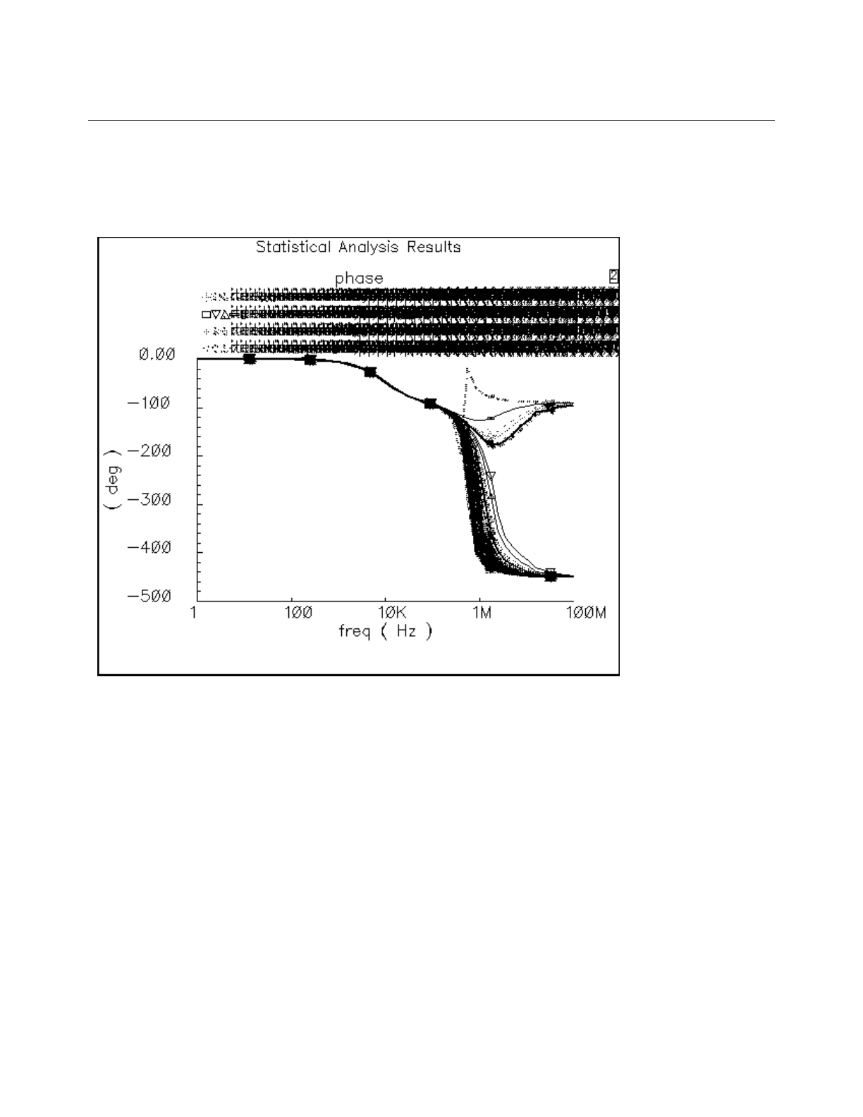
Cadence Advanced Analysis Tools User Guide
Statistical Analysis
July 2002 114 Product Version 5.0
The Waveform window opens with the overlapping waveforms. Depending on the
number of iterations included, you might or might not be able to read the legend that
identifies each individual waveform.
Plotting Scatter Plots
A scatter plot shows the relationship between pairs of parameters.
To plot a scatter plot,
1. Choose Results – Plot – Scatterplot.
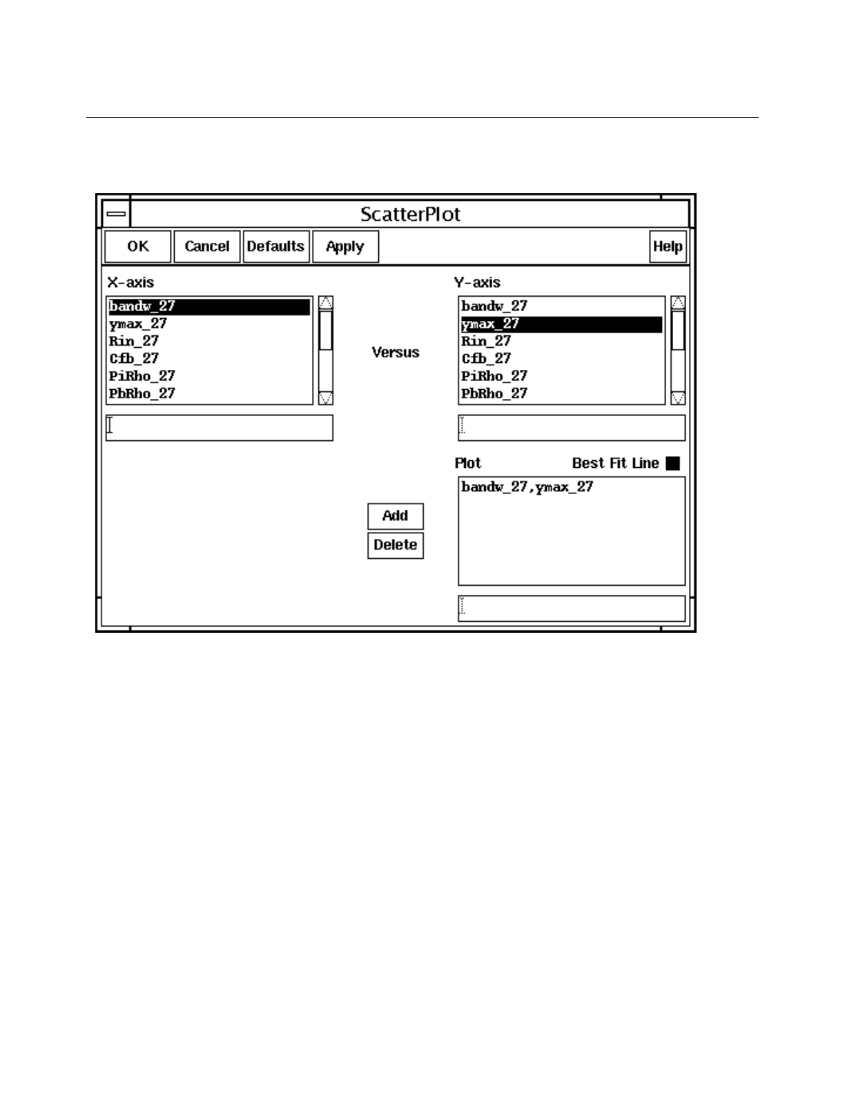
Cadence Advanced Analysis Tools User Guide
Statistical Analysis
July 2002 115 Product Version 5.0
The ScatterPlot form appears.
2. Highlight one parameter in the X-axis list and one in the Y-axis list.
3. Click Add.
4. (Optional) Repeat steps 2 and 3 for other parameter pairs.
5. (Optional) Click Best Fit Line to draw least squares fit lines on each scatter plot.
6. Click OK.
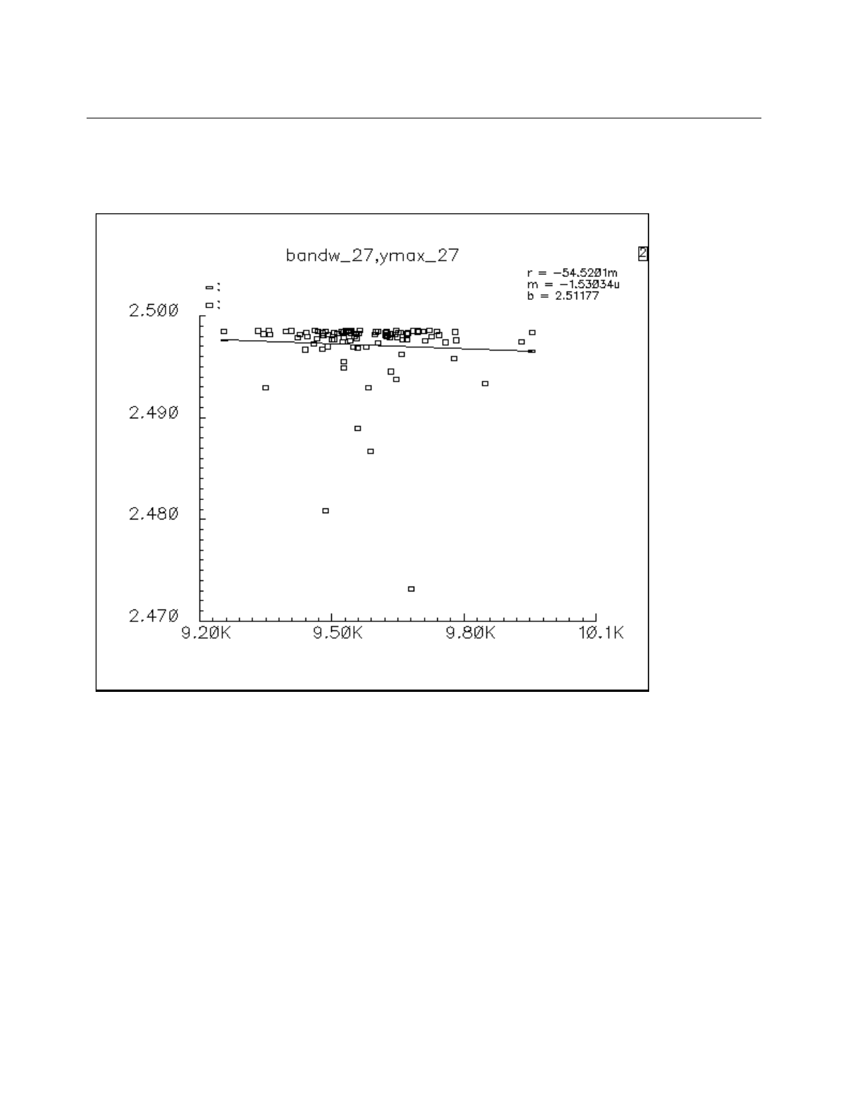
Cadence Advanced Analysis Tools User Guide
Statistical Analysis
July 2002 116 Product Version 5.0
The Waveform window appears with the values for one parameter of each pair on the
vertical axis and the values for the other parameter on the horizontal axis.
Obtaining Reports on Yields
You can compute simple, conditional, and multiconditional yield statistics.
Note: The yield calculations represent parametric yields only and do not include yield
reduction due to defect density or packaging factors.

Cadence Advanced Analysis Tools User Guide
Statistical Analysis
July 2002 117 Product Version 5.0
The table below gives an example of a yield calculation. The next few sections use this table
to illustrate the different kinds of yield statistics. In this table, pass or fail indicates whether
that sample passed or failed the specification limit for that parameter.
Individual yield is the percentage of samples that meet the current specification limits for
each individual parameter. For example, if parameter X has 100 samples of which 80 fall
within the specification limits, the individual yield is 80%. Using the values in Table 2-1 on
page 117, the individual yields are as follows: p1, 66%; p2, 33%; and p3, 100%.
Total yield is the percentage of samples that meet the current specification limits for all
parameters. In Table 2-1 on page 117, of the three samples only sample s1 falls within the
specification limits for all parameters. The total yield, therefore, is 33%.
Multiconditional yield is the individual yield when only the samples for the specified
parameters that are within their respective specification limits are used in the yield
calculation. If the parameter fails the specification limit test, that sample is removed from the
yield calculation. In the example table, the multiconditional yield for p1 with sample s3
removed is as follows: p1, 100%; p2, 50%; and p3, 100%.
Conditional yield is the same as the multiconditional yield except the individual yields are
calculated for each parameter separately.
Obtaining Reports on Simple Yields
The simple yield report shows the individual and total yields for all parameters given the
specification limits. A summary line shows
■Total yield
■Product of the individual yields
■Total sample size
To print a simple yield report,
1. Choose Results – Yield – Simple.
Table 2-1 Yield Calculation Table Example
p1 p2 p3
s1 pass pass pass
s2 pass fail pass
s3 fail fail pass
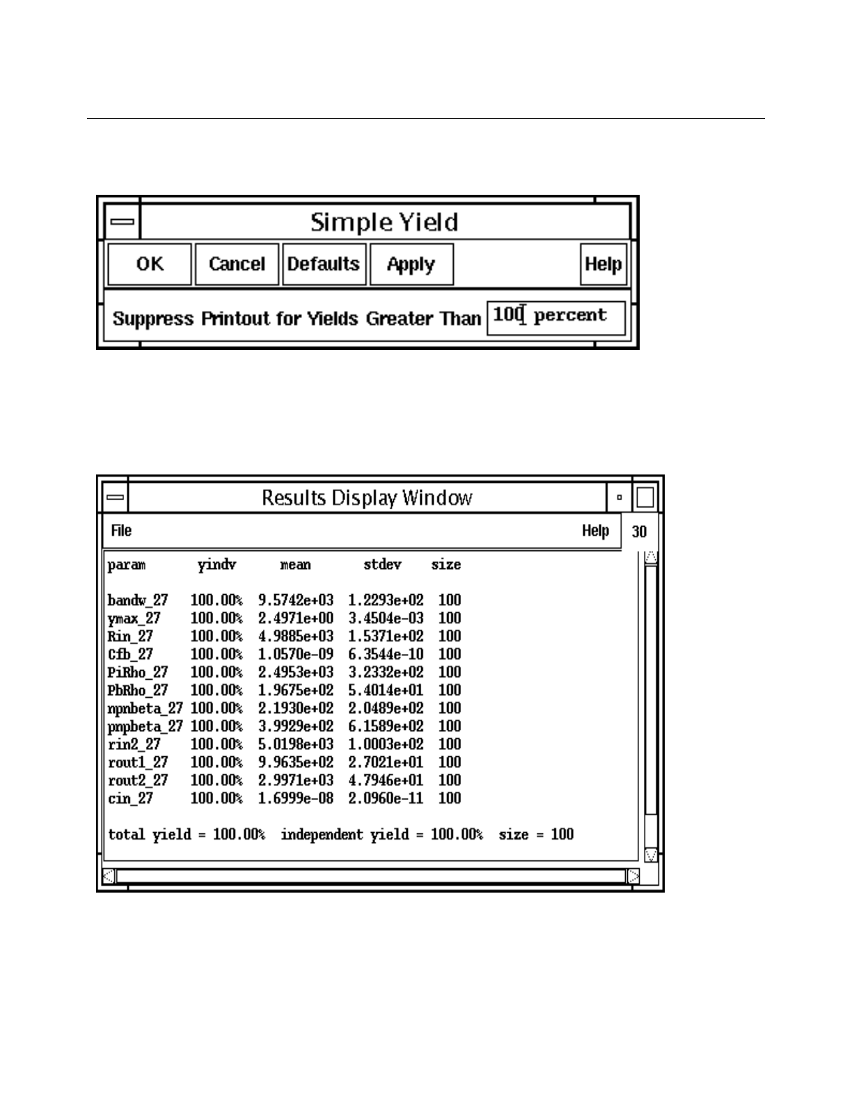
Cadence Advanced Analysis Tools User Guide
Statistical Analysis
July 2002 118 Product Version 5.0
The Simple Yield form appears.
2. (Optional) Type a percentage to filter out statistics for samples with high yields.
3. Click OK.
The Results Display Window appears.
In this report, yindv stands for individual yield.
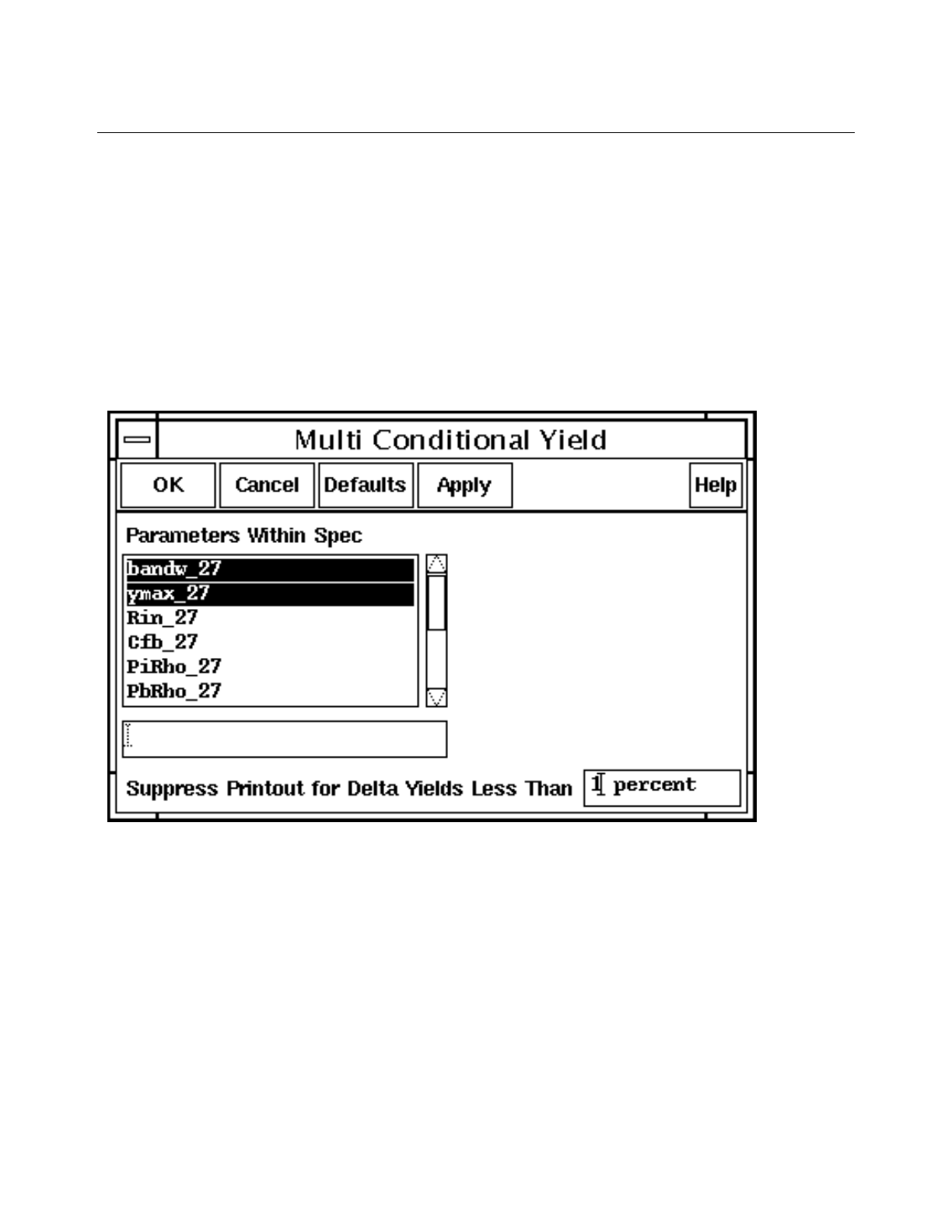
Cadence Advanced Analysis Tools User Guide
Statistical Analysis
July 2002 119 Product Version 5.0
Obtaining Reports on Multiconditional Yields
The multiconditional yield report shows the individual and total yields when the parameters
you select pass the specification limits test. The subset of all data sets that meet these
specifications is determined, and the yield is calculated from only this subset.
To print a multiconditional yield report,
1. Choose Results – Yield – Multiconditional.
The Multi Conditional Yield form appears.
2. Select parameters by double-clicking in the list.
3. (Optional) To omit cases where the individual and simple yields are similar, type a
percentage in the Suppress field.
4. Click OK.
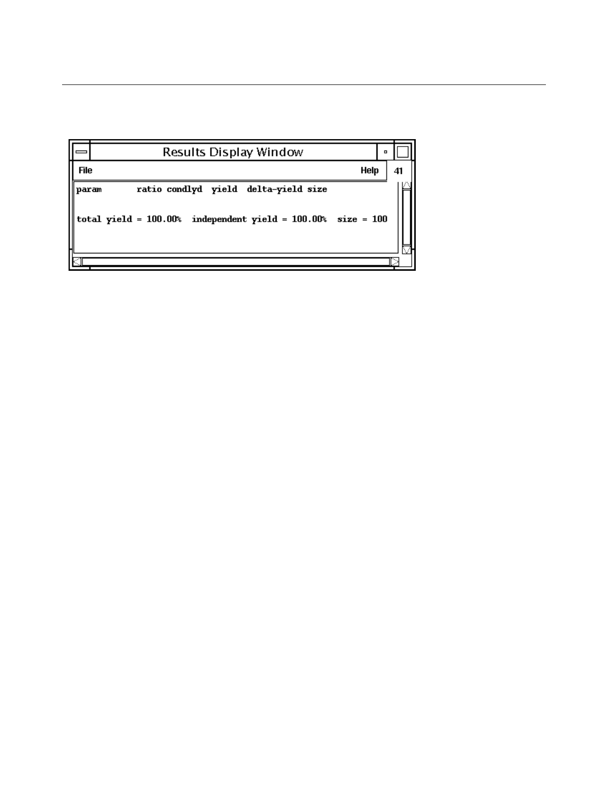
Cadence Advanced Analysis Tools User Guide
Statistical Analysis
July 2002 120 Product Version 5.0
The Results Display Window appears.
In this report, condlyd stands for conditional yield.
Obtaining Reports on Conditional Yields
The conditional yield report is similar to the multiconditional yield report, except that the yield
is calculated for each parameter separately. This allows you to quickly view the effects of
conditional yield for several parameters in a single command.
To print the conditional yield report,
1. Choose Yield – Conditional.
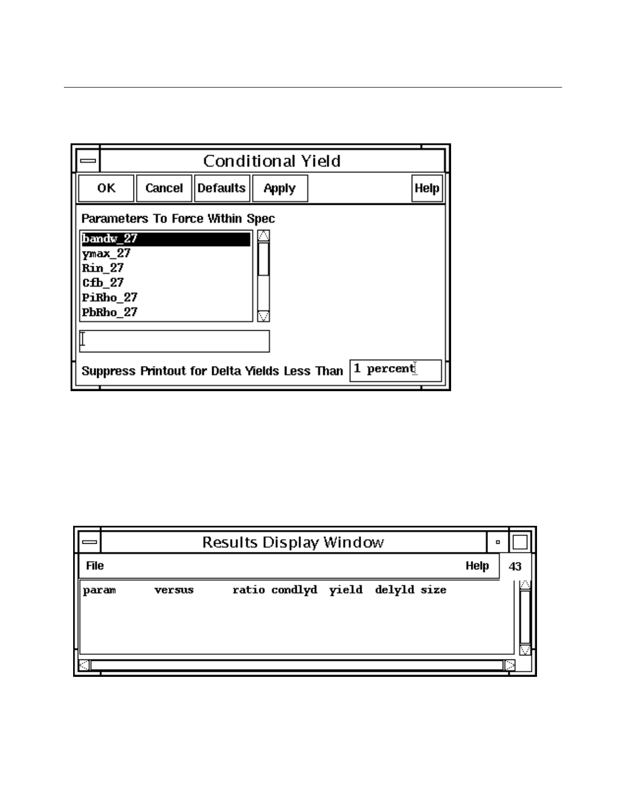
Cadence Advanced Analysis Tools User Guide
Statistical Analysis
July 2002 121 Product Version 5.0
The Conditional Yield form appears.
2. Select parameters by double-clicking in the list.
3. (Optional) To omit cases where the individual and simple yields are similar, type a
percentage in the Suppress Printout for Delta Yields Less Than field.
4. Click OK.
The Results Display Window appears.
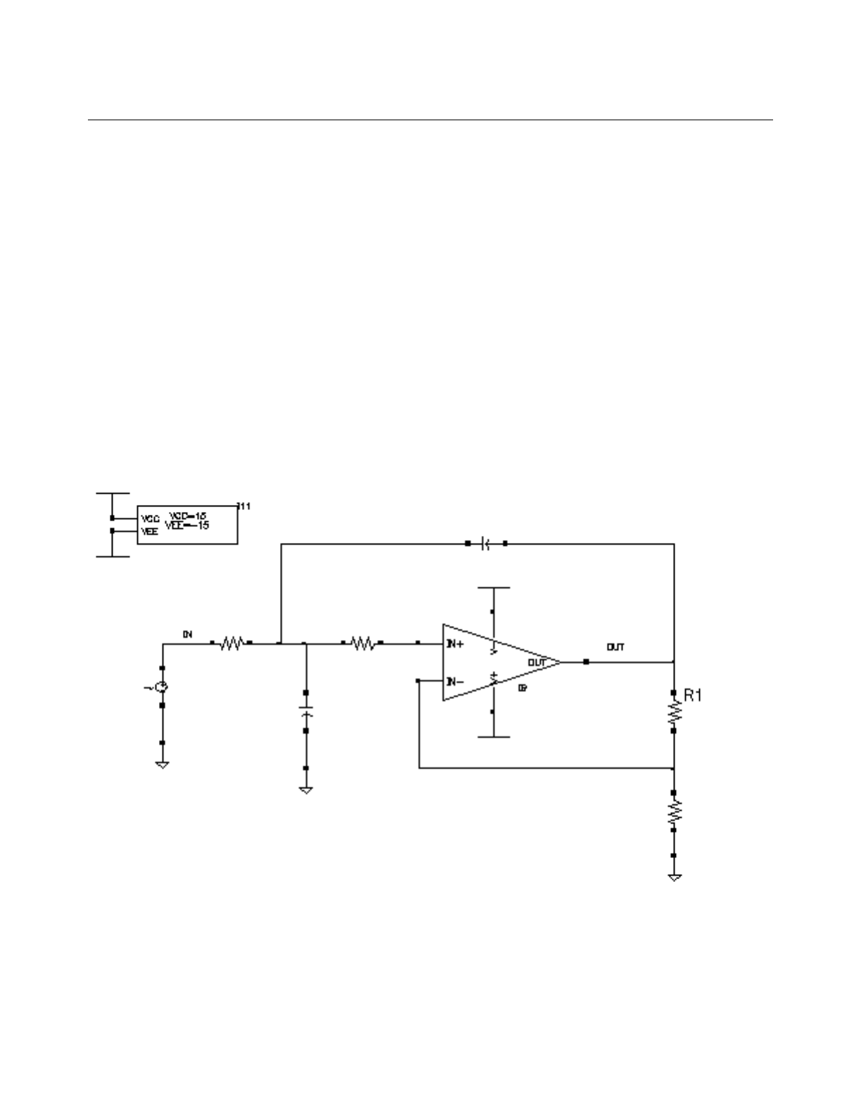
Cadence Advanced Analysis Tools User Guide
Statistical Analysis
July 2002 122 Product Version 5.0
Working through an Extended Example
This section follows a statistical analysis session in detail, demonstrating how you might use
the Analog Statistical Analysis option to examine the characteristics of a lowpass filter. The
sections explain how to arrange supporting files for the Spectre simulator, run the analysis
and analyze the results.
Lowpass Filter Schematic
The circuit used in this example allows low-frequency signals to pass through and attenuates
high-frequency signals. The capacitor values control the attenuation of the circuit, while the
resistor values control the voltage gain of the signals that pass through the circuit.
The lowpass filter has the following top-level schematic.
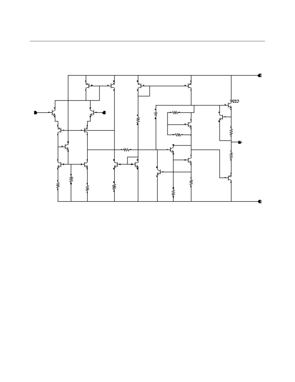
Cadence Advanced Analysis Tools User Guide
Statistical Analysis
July 2002 123 Product Version 5.0
Descending into the amplifier shows that it has the following schematic.
This amplifier schematic includes several instances of npn and pnp transistors. Each of the
npn transistors is nominally identical. Similarly, each of the pnp transistors is nominally
identical. In reality, however, the attributes of each transistor differ randomly from the
attributes of each of the other transistors. In the following sections of this example, you
explore the effect that random variation in transistors has on circuit performance.
To follow along with this example, go to a working directory and use a command like the
following to copy all the contents of the monteCarlo directory into the working directory.
tar -cvhf - -C <install_dir>/tools/dfII/samples/artist monteCarlo |
tar -xvf -
Then go to the working directory you created, start icms, and continue with the following
steps.
1. In the CIW, choose Tools – Analog Environment – Simulation to open the Cadence®
Analog Design Environment window.
2. In the Cadence® Analog Design Environment window, choose Setup – Design.
When the Choosing Design form appears, select the aExamples library and the
lowpass cell. Click OK.

Cadence Advanced Analysis Tools User Guide
Statistical Analysis
July 2002 124 Product Version 5.0
3. In the Cadence® Analog Design Environment window, choose Session – Load
State to open the Loading State form.
4. In the Loading State form, select monte as the State Name that you want to load. Click
OK.
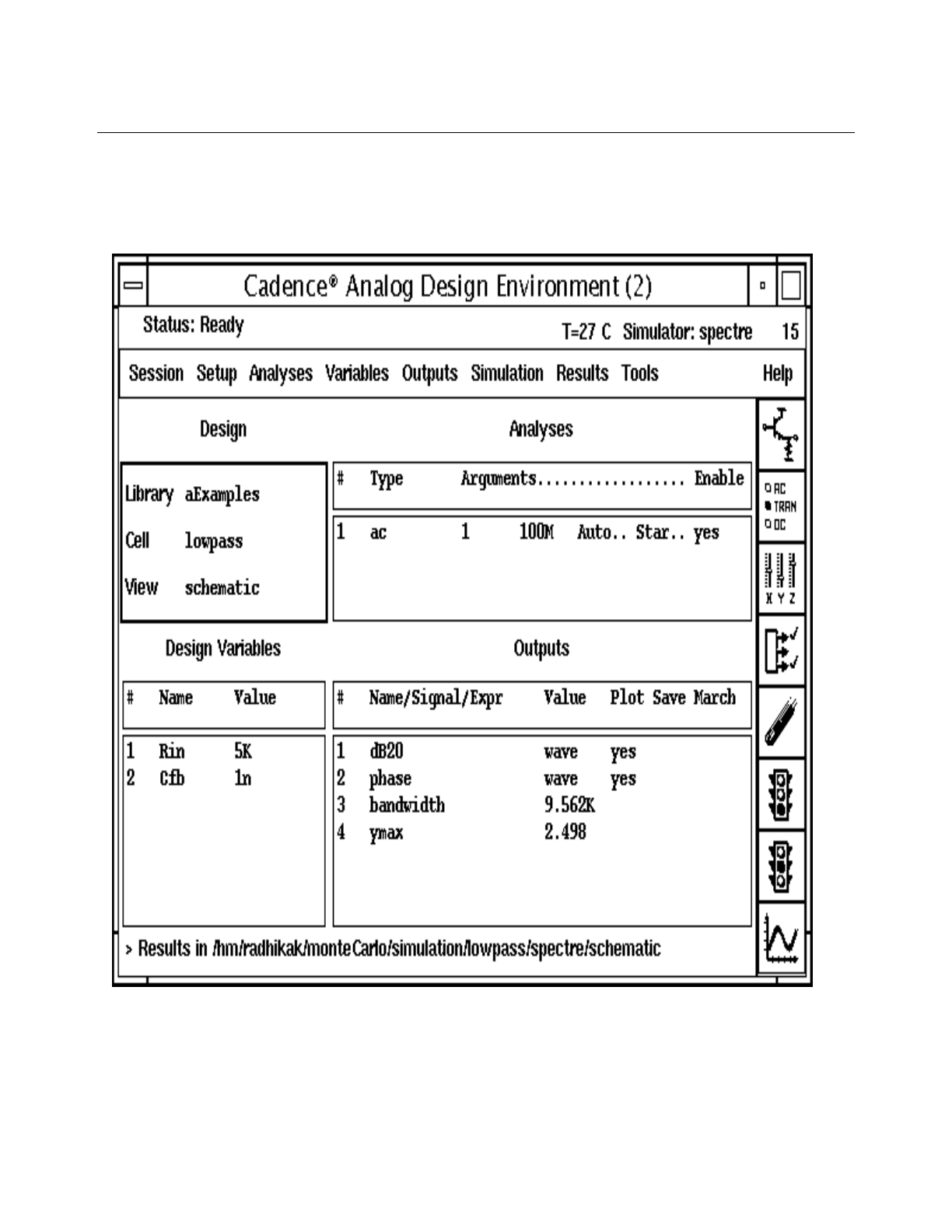
Cadence Advanced Analysis Tools User Guide
Statistical Analysis
July 2002 125 Product Version 5.0
At the end of this series of steps, the Cadence® Analog Design Environment window
looks like this.

Cadence Advanced Analysis Tools User Guide
Statistical Analysis
July 2002 126 Product Version 5.0
Model File
This example uses a model file called spectreLib.scs, which contains all the parameters,
statistics, and modeling information that are required.
library monteLib
section param
simulator lang=spectre
parameters PiRho=2500 PbRho=200 npnbeta=145.5 pnpbeta=200
parameters rin1=1000 rin2=5000 rout1=1000 rout2=3000
parameters cin=1.7e-08 cloop=1e-09
parameters mmstat=1 initstat=1
function Rpb(l,w)=(PbRho*l/w)
function Rpi(l,w)=(PiRho*l/w)
endsection param
section stats
simulator lang=spectre
statistics {
process {
vary PiRho dist=gauss std=350
vary PbRho dist=gauss std=50
vary npnbeta dist=lnorm std=.9
vary pnpbeta dist=lnorm std=1.1
vary Rin dist=gauss std=150
vary cin dist=gauss std=20p
vary rin2 dist=gauss std=100
vary Cfb dist=gauss std=.58n
vary rout1 dist=gauss std=30
vary rout2 dist=gauss std=50
}
mismatch {
vary PiRho dist=gauss std=19
vary PbRho dist=gauss std=3.75
vary npnbeta dist=gauss std=4
vary pnpbeta dist=gauss std=6
}
}
endsection stats
section models
simulator lang=spectre
inline subckt npn (C B E S)
parameters brvbe=.6
model mynpn bjt type=npn is=5.771e-17 bf=npnbeta nf=0.9895 vaf=201.6
+ ikf=0.01573 ise=8.976e-18 ne=1.179 br=3.204 nr=0.9944
+ var=27.03 ikr=0.0003047 isc=1.505e-13 nc=1.912 rb=8.706
+ irb=0.001509 rbm=5.833 re=111.8 rc=54.97 xtb=1.5 eg=1.11
+ xti=3 cje=1.983e-12 vje=0.4818 mje=0.2486 tf=0.33e-9
+ xtf=4.359 itf=0.01753 ptf=176.2 cjc=1.749e-12 vjc=0.5989
+ mjc=0.3349 xcjc=0.5 tr=400e-9 cjs=1e-12 vjs=0.75
+ mjs=0.33 fc=0.5 bvbe=brvbe bvce=1
npn (C B E S) mynpn
ends npn

Cadence Advanced Analysis Tools User Guide
Statistical Analysis
July 2002 127 Product Version 5.0
inline subckt pnp (C B E S)
model mypnp bjt type=pnp
+is=1.2e-16 bf=pnpbeta nf=1.00 vaf=26.00
+ikf=70e-06 ise=1.1e-15 ne=2.00 br=13
+nr=1.00 var=10.00 ikr=100e-06 isc=7.0e-15
+nc=2.50 rb=100
+re=15 rc=150 cje=33e-15 vje=740e-03
+mje=330e-03 tf=2.50e-09 xtf=1.00
+itf=2.00e-03 ptf=5.0 cjc=130e-15 vjc=690e-03
+mjc=440.00e-03 xcjc=500.00e-03 tr=5.00e-09 cjs=200e-15
+vjs=590e-03 mjs=440.00e-03 xtb=780e-03 eg=1.200
+xti=1.80 kf=1.60e-15 af=1.00 fc=850.00e-03
pnp (C B E S) mypnp
ends pnp
endsection models
endlibrary monteLib
Notice the lines in the models section of the model file that define the mynpn model.
parameters brvbe=.6
model mynpn bjt type=npn is=5.771e-17 bf=npnbeta nf=0.9895 vaf=201.6
In particular, notice how the bf parameter is defined as npnbeta. The npnbeta value varies
randomly according to the distributions specified in the statistics block. Consequently,
the value of the bf model parameter also varies. So that mismatch, which is also specified
for this parameter, is effective, the model is defined within an inline subckt block. This allows
each instance of the model to have a slight perturbation.
The statistics block defines how parameters vary during the analysis. In this case, each
parameter has either a Gaussian or a log-normal distribution with a deviation specified by the
std parameter. All the parameters vary when process variation is specified and four of them
vary when mismatch is specified.
Run Analog Simulation to Check Setup
Run a simulation via the ADE->Simulation->Run banner element.
This part of this example is used to verify that the ADE setup is correct. Note that the db20
and phase outputs created plots and that the bandwidth and ymax outputs evaluated to
numbers.
In addition, the psf data created by this run will be used later for expression checking on the
Analog Statistical Analysis UI.
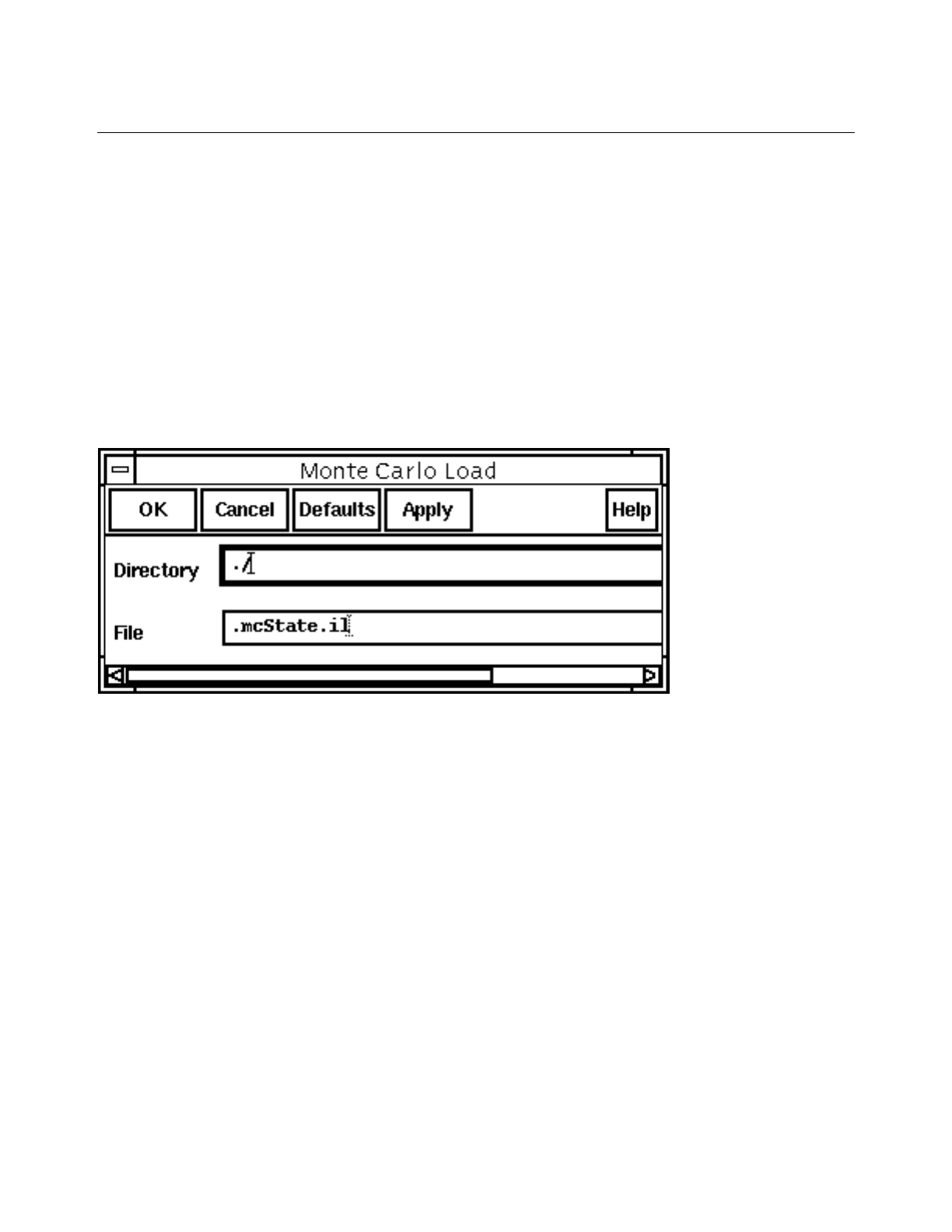
Cadence Advanced Analysis Tools User Guide
Statistical Analysis
July 2002 128 Product Version 5.0
Specifying the Analysis in the Analog Statistical Analysis Window
At this point in the example, you are ready to use the statistical analysis option.
1. To open the Analog Statistical Analysis window, choose Tools – Monte Carlo. The
outputs defined in the Cadence® Analog Design Environment window appear
automatically in the Outputs pane of the Statistical Analysis window.
2. In the Analog Statistical Analysis window, choose Session – Load State. The Monte
Carlo Load dialog appears. Change the Directory entry to ./.
3. Ensure that the File to be loaded is .mcState.il. The Monte Carlo Load dialog should
look like this.
4. Click OK.
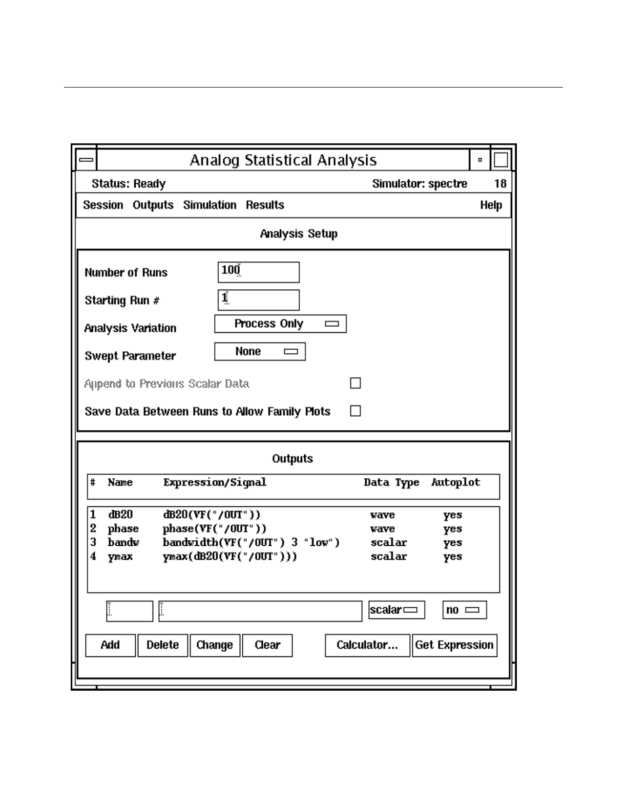
Cadence Advanced Analysis Tools User Guide
Statistical Analysis
July 2002 129 Product Version 5.0
5. Make sure the Analysis Setup pane is set correctly. It should look like this:

Cadence Advanced Analysis Tools User Guide
Statistical Analysis
July 2002 130 Product Version 5.0
The Analysis Setup form is set to perform 100 iterations of the circuit, using both process and
mismatch variations. Turning on Save Data Between Runs to Allow Family Plots makes
it possible to plot families of curves for the two waveform expressions, phase and db20.
Note: The state loaded contained the identical Outputs Pane expressions as was initially
copied over from the ADE Outputs section. Had the state contained different expressions,
then they would have been merged with any existing expressions. The original bandwidth
output name was changed to bandw_27 by the state. However, the actual expression
formulation remained unchanged.
Any unwanted Outputs pane expressions can be deleted.
Checking Expressions Prior to Simulation
Whenever expressions have been added, loaded or changed, it is a good practice to check
them prior to submitting a statistical analysis simulation.
In this example, we will use the ADE simulation data created in a previous step. Invoke
Simulation->Check_Expressions utility of the Analog Statistical Analysis window.
The expression checking utility will automatically verify and assign the proper Data Type field
to each expression. For any expression with an error, the Data Type field will be set to
"ERROR". In this example, there should be no errors.
Running the Statistical Analysis Simulation
To run the statistical analysis,
➤From the Analog Statistical Analysis window, choose Simulation – Run.
The simulation runs and the outputs for which Autoplot is set to yes appear in display
windows.
When the simulation is finished and was completely successful, the ciw will produce the
following information:
simulation completed successfully.
...
Monte Carlo Simulation completed successfully...
Although this example should run clean, additional information concerning simulation
problems is useful to know. When any problems are encountered throughout the course of
running a statistical analysis, both the ciw and simulator output log offer valuable information.
The following three scenarios reflect the most common problems encountered:
1. For situations where a scalar expression could not be evaluated at a particular iteration,
the following error information is produced in the ciw:

Cadence Advanced Analysis Tools User Guide
Statistical Analysis
July 2002 131 Product Version 5.0
Problems encountered during simulation.
Use the Simulation->Output Log menu for more information.
...
Monte Carlo Simulation completed successfully...
When the spectre output log is reviewed, we would see an error similar to:
**** Run Status for Monte Carlo analysis ‘mc1’ ****
Monte Carlo iteration 1 failed.
The two most common reasons for this type of expression evaluation error are:
a. An analysis pertinent to the expression did not simulate. This is typically due to
convergence problems.
b. The data created is not sufficient to satisfy the expression. For example, the phase
at that iteration did not cross the proper threshold needed by the phaseMargin
function.
Note: In this case, monte carlo scalar data was successfully produced. Any iterations
with errors are assigned error flag values (-1.1111e36 or -2.2222e36).
2. For situations where a scalar expression had syntax errors, the following error
information is produced in the ciw:
Problems encountered during simulation.
Use the Simulation->Output Log menu for more information.
...
Monte Carlo Simulation unsuccessful...
When the spectre output log is reviewed, we would see an error similar to:
Error found by spectre during Monte Carlo analysis ‘mc1’.
designParamVals: Error evaluating ocean expression ‘foo=getData("out")’.
Unsuccessfully evaluated export statements (based on return code).
Analysis ‘mc1’ terminated prematurely due to error.
In this case, no monte carlo scalar data was produced.
3. For situations where spectre could not run at all, the following error information is
produced in the ciw:
Problems encountered during simulation.
Use the Simulation->Output Log menu for more information.
Monte Carlo Simulation unsuccessful...
See simulation output log for more information.
When the spectre output log is reviewed, we would see the error.
For example:

Cadence Advanced Analysis Tools User Guide
Statistical Analysis
July 2002 132 Product Version 5.0
Error found by spectre during circuit read-in.
"input.scs" 9: Unable to open input file
‘/example/monteCarlo/models/spectreLib.scs2’.
No such file or directory.
spectre terminated prematurely due to fatal error.
In this case, no monte carlo scalar data was produced.
Evaluating Statistical Analysis Results
These results might contain error flag values that can distort the statistical results (see
problem case 1 in previous section). To check for possible error values, do the following:
1. Choose Results – Print – Iteration vs. Value.
2. In the Iteration Versus Value form, select the bandw_27 parameter, make sure that
sorted is selected for the Output Format, and click Apply.
3. In the Results Display Window, check the values at the beginning and end of the list.
4. In the Iteration Verses Value form, select the ymax_27 parameter and click OK.
5. Repeat step 3 for the ymax_27 parameter values.
Analyzing Scalar Data
There are several ways to look at scalar data. As described in the previous section, you can
simply list the data. You can also plot the data in the form of histograms and calculate yields
for the data.
Printing Correlations Table
To determine which statistically swept parameters had the biggest impact on the output scalar
measurements, perform the following:
1. Choose Results - Print - Correlation...
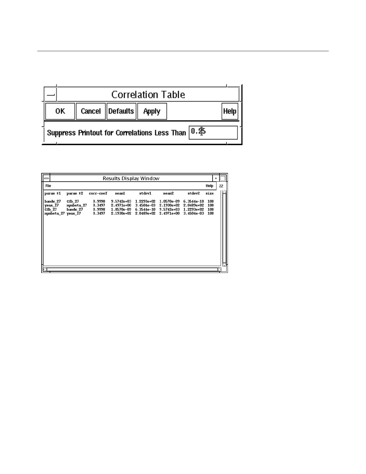
Cadence Advanced Analysis Tools User Guide
Statistical Analysis
July 2002 133 Product Version 5.0
2. Set the Suppress Printout for Correlations Less Than field to 0.25 and click OK.
3. Observe the data printed to the Results Display Window.
From this data we can see that the bandw_27 expression was mostly influenced by the
Cfb_27 parameter, and the ymax_27 expression was mostly influenced by the
npnbeta parameter. We will use this knowledge further along in this example.
Using Histograms
To begin looking at the bandw_27 and ymax_27 data,
1. Choose Results – Plot – Histogram.
The Histogram form appears.
2. Add bandw_27 and ymax_27 to the Plot column.
3. Turn the Density Estimator button on.
4. Click OK.
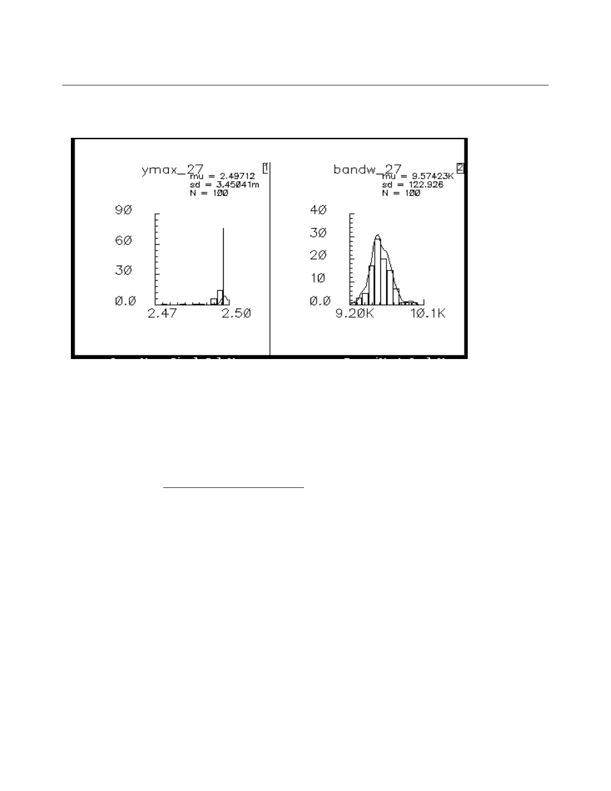
Cadence Advanced Analysis Tools User Guide
Statistical Analysis
July 2002 134 Product Version 5.0
The histograms appear in the Waveform Window.
The ymax_27 distribution shows that the ymax_27 value is almost exactly the same for every
iteration. That value is unaffected by the variations introduced into the circuit by the statistical
analysis.
Plotting Scatter Plots
Scatter plots are very useful for verifying dependencies between different statistical data sets.
Our findings in the Printing Correlation Tables section of this document will help guide this
example.
1. Choose Results - Plot - Scatterplot...
2. Select the bandw_27 entry in the X-axis listbox, and the Cfb_27 entry in the Y-axis
listbox. Click the Add button.
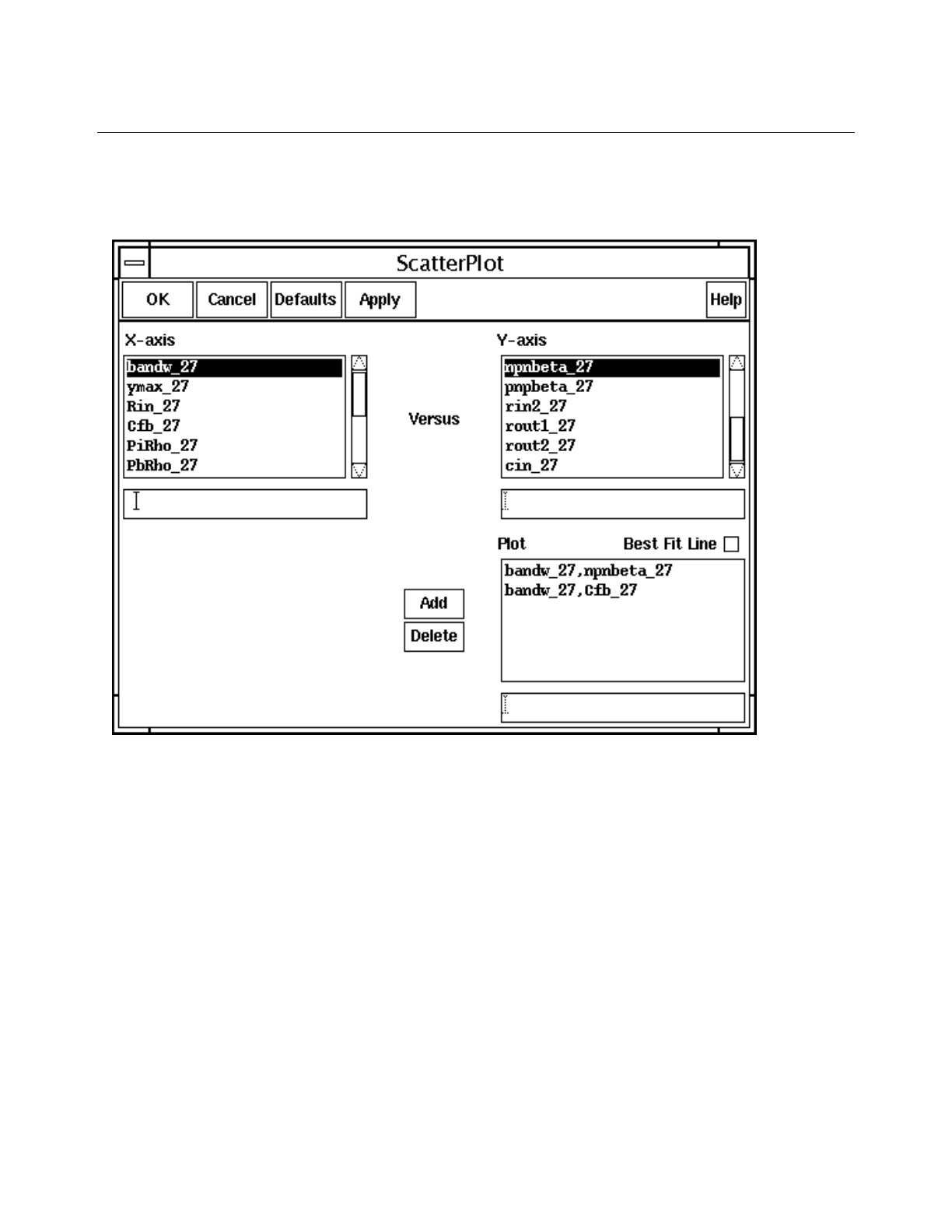
Cadence Advanced Analysis Tools User Guide
Statistical Analysis
July 2002 135 Product Version 5.0
3. Select the npnbeta_27 entry in the Y-axis listbox. Click the Add button. The Scatter
Plot form should look as follows:

Cadence Advanced Analysis Tools User Guide
Statistical Analysis
July 2002 136 Product Version 5.0
4. Click the OK button. The following two scatterplots should be added to the Waveform
Window:
From these two plots we can see that the bandw_27 expression is directly dependent on the
Cfb_27 parameter by observing a straight slanted line of points in the plot. Whereas the
npnbeta parameter has little effect on bandw_27 because there is little order in the plotted
points.
Analyzing Yields
To analyze the yield for this circuit, you first need to define the specification limits for the scalar
parameters. For this example, assume that you can tolerate only 1 sigma of variation.
1. Choose Results – Specification Limits.
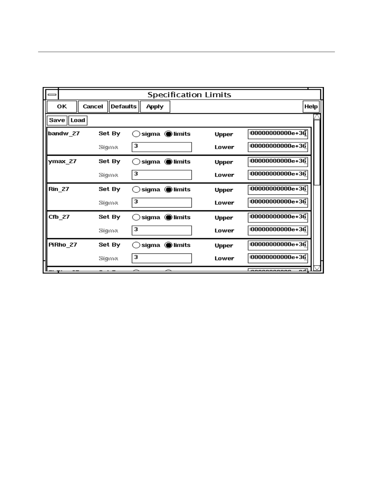
Cadence Advanced Analysis Tools User Guide
Statistical Analysis
July 2002 137 Product Version 5.0
The Specification Limits form appears.
2. Turn Set By sigma on.
3. Type 1 in the Sigma fields for each of the measurements.
4. Click OK.
5. From the Analog Statistical Analysis window, choose Results – Yield – Simple.
The Simple Yield form appears.
6. Set the value of the Suppress Printout for Yields Greater Than field to 98 percent.
7. Click OK.
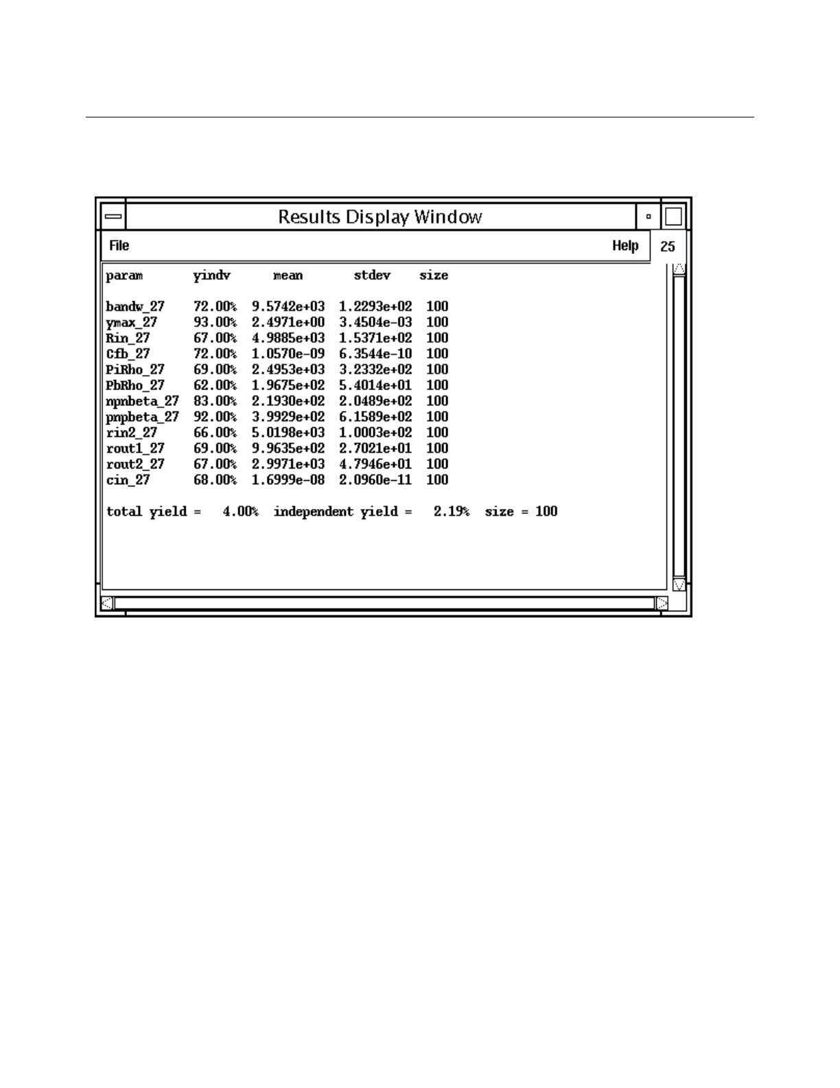
Cadence Advanced Analysis Tools User Guide
Statistical Analysis
July 2002 138 Product Version 5.0
The Results Display Window appears.
These results show that only 64 percent of the iterations produced results where both the
bandw_27and ymax_27 were within specification limits.
Analyzing Waveform Data
Two of the outputs in this example, dB20 and phase, are waveform data. Because this
example was simulated with the Spectre simulator and because Save Data Between Runs
to Allow Family Plots was turned on in the Analog Statistical Analysis window, you can
use family-of-curves plots to examine the data.
1. From the Analog Statistical Analysis window, choose Results – Plot– Curves.
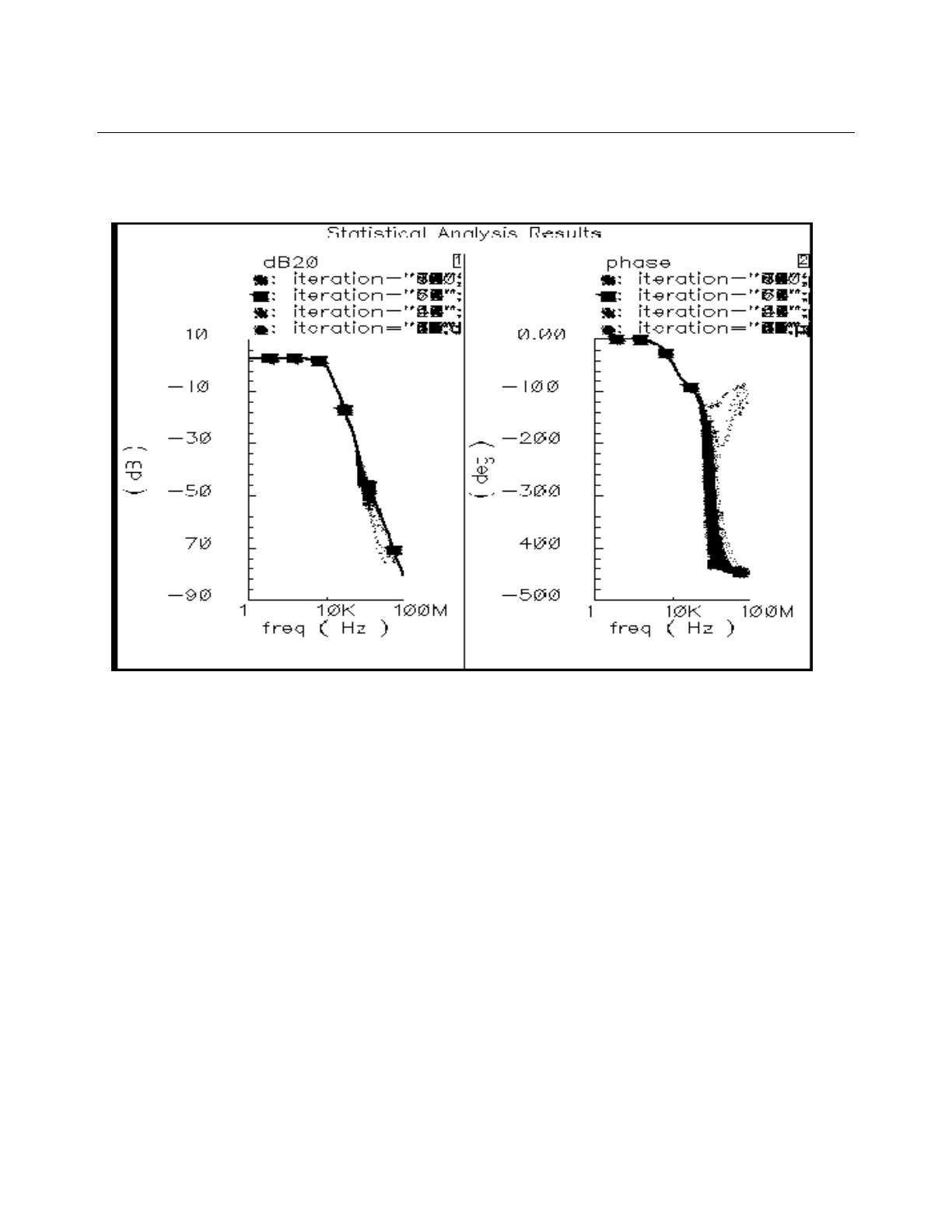
Cadence Advanced Analysis Tools User Guide
Statistical Analysis
July 2002 139 Product Version 5.0
The Waveform Window appears with the statistical analysis results.
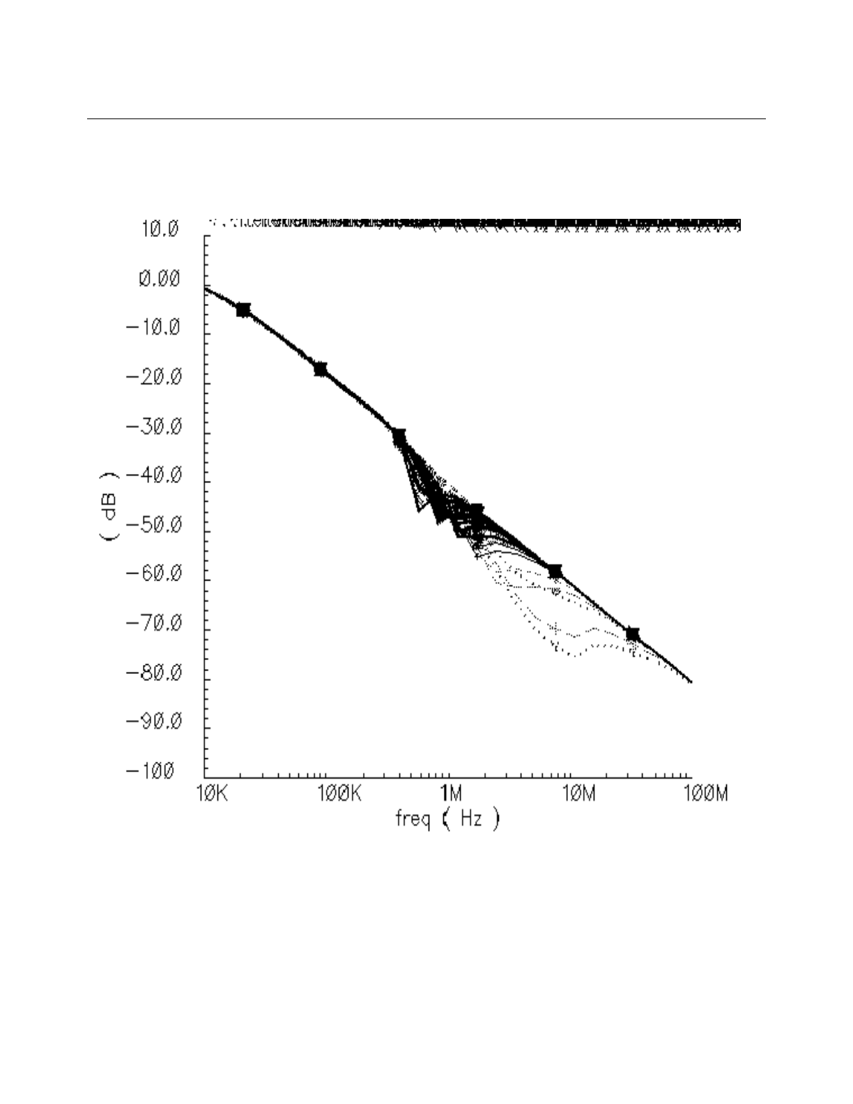
Cadence Advanced Analysis Tools User Guide
Statistical Analysis
July 2002 140 Product Version 5.0
The preceding view is not very useful because the detail is too small to see, but if you
turn off the phase subwindow and zoom in on the dB20 curves, you see a plot like this.
This plot shows that in the frequency range of about 400 K to 100 M, the dB20 value is
affected by the statistical analysis variations introduced in the pnp and npn transistors. If
this frequency range is critical, you might need to redesign your circuit so that the
variation is smaller in this range.

Cadence Advanced Analysis Tools User Guide
Statistical Analysis
July 2002 141 Product Version 5.0
Changing Waveform Expressions at Post-simulation Time
At post-simulation time, waveform expressions can be created, deleted or altered to produce
new plots, so long as the pertinent psf data has been saved.
Note that it is not necessary to declare any waveform expressions in the Outputs Pane prior
to running a statistical analysis simulation. However, doing so facilitates the waveform
autoplot feature.
Remember, whenever attempting to plot a family of waveforms, make sure the Save Data
Between Runs to Allow Family Plots boolean is on prior to running the statistical analysis.
It is also necessary that all the needed circuit outputs are declared.
The previous plotting example involved zooming into the dB20 curves to see a particular
region. Now lets change the dB20 expression to only include the region of concern by
following these steps:
1. In the Outputs Pane window, select the dB20 entry.
2. Go to the editable expression string field and change the expression to:
sample(dB20(VF("/OUT")) 100K 100M "log" 20)
Click the Change button.
3. Invoke the Results->Plot->Curves capability.
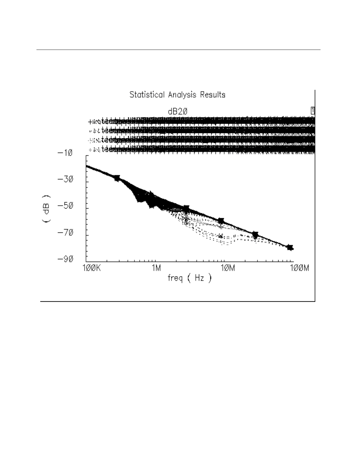
Cadence Advanced Analysis Tools User Guide
Statistical Analysis
July 2002 142 Product Version 5.0
Note that the dB20 plot now shows the desired region without having to manually zoom
in:
Changing Scalar Expressions at Post-Simulation Time
At post-simulation time, scalar expressions can be created, deleted or altered to produce new
statistical data, so long as the pertinent psf data has been properly saved. It is required that
the Save Data Between Runs to Allow Family Plots boolean was on at pre-simulation
time. It is also necessary that all the needed circuit outputs were declared.
Prior to running a statistical analysis, so long as the Save Data Between Runs to Allow
Family Plots boolean is on it is not necessary to declare any scalar expressions in the
Outputs Pane. However, the performance of the Analog Statistical Analysis tool is at its
optimum when all scalar expressions are declared and checked prior to simulation time.

Cadence Advanced Analysis Tools User Guide
Statistical Analysis
July 2002 143 Product Version 5.0
In this example, we are going to add a new scalar to the statistical data by doing the following
steps:
1. In the Outputs Pane window, select the clear button.
2. In the name field, type in gn_mrgn.
3. In the expression field, type in:
"gainMargin(VF("/OUT"))"
4. Set the Data Type to blank (i.e. unknown).
5. Click the Add button. The Outputs pane of the UI should now look like the following:
6. Invoke the Simulation->Check_Expressions capability. The Data Type of this
expression should then get automatically set to scalar. If not, then you will need to
correct/change the expression and try again.
7. Invoke the Results->Evaluate_Expressions capability, and click OK on the Evaluate
Expressions sub-form.
As a result of these actions, the new ph_marg statistical data has been created without the
need to re-simulate. Lets investigate this new data:

Cadence Advanced Analysis Tools User Guide
Statistical Analysis
July 2002 144 Product Version 5.0
a. Invoke the Results->Print->Iteration_Verses_Value... capability.
b. On the Iteration Verses Value form, note that the gn_mrgn_27 entry now appears
in the listbox. Select the gn_mrgn_27 entry.

Cadence Advanced Analysis Tools User Guide
Statistical Analysis
July 2002 145 Product Version 5.0
c. Set the Output Format to sorted. and click OK. The following table will be printed
to the Results Display Window:
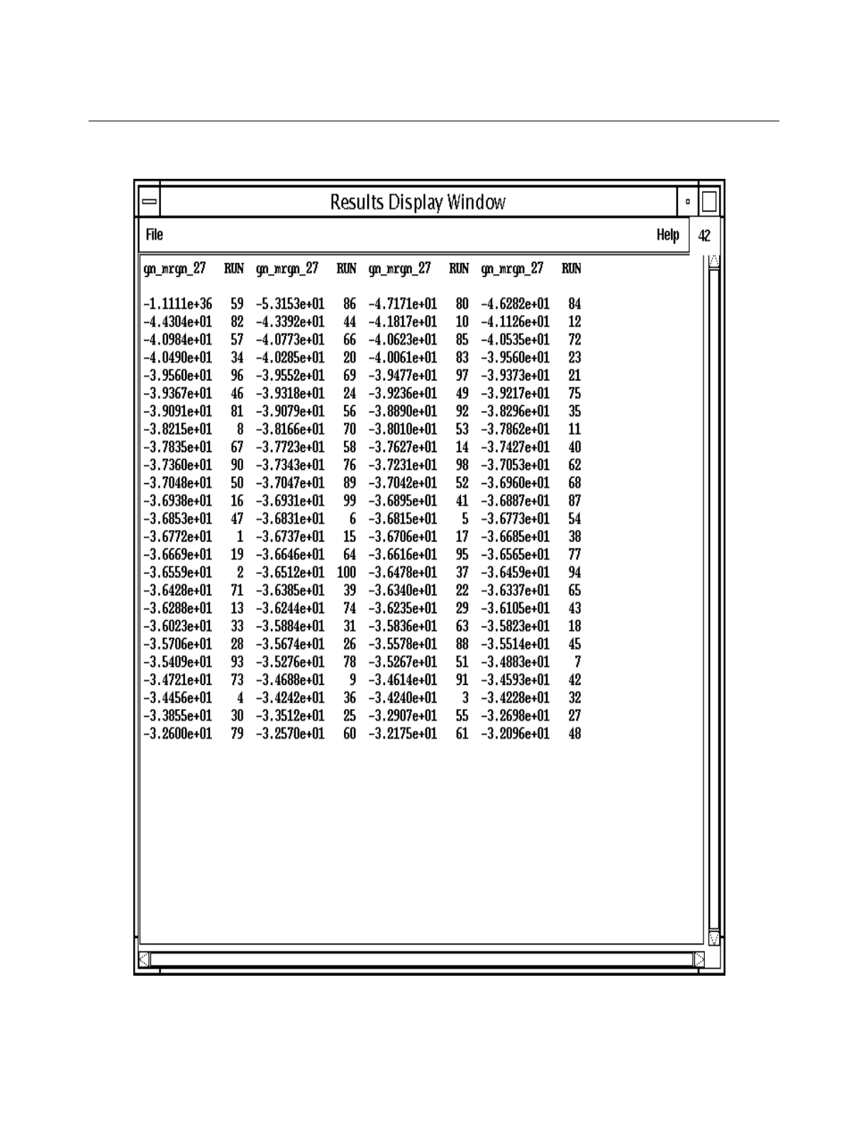
Cadence Advanced Analysis Tools User Guide
Statistical Analysis
July 2002 146 Product Version 5.0

Cadence Advanced Analysis Tools User Guide
Statistical Analysis
July 2002 147 Product Version 5.0
Note that iteration number 59 is an error flag value. If you look at the phase plot created
from a previous section of this example, you will notice that one of the plots does not dip
below -180 degrees. If you put the mouse curser on that single waveform, you can see
the banner of the waveform tool indicating that the waveform is iteration number 59. For
that waveform, the gainMargin() function cannot evaluate properly. The user would have
to use the UI filter capabilities to remove this data point before analyzing this data.
Appending More Scalar Iterations to Existing Data
In this example, we are going to append more statistical iterations onto the existing scalar
data.
Note that this mode will erase the existing psf data for the first 100 iterations. It the user
wishes to save this psf data for later use, then they should use the Results->Save
capability prior to the next simulation. Although the Analog Statistical Analysis UI
does not facilitate appending psf data for waveform plotting, the user can achieve this
operation by using the data access capabilities outside the Analog Statistical Analysis
UI. More on this subject later. For now, lets save the data:
a. Invoke the Results->Save capability.
b. Set the Save As field to first_100_iterations.
c. Click the OK button.
Now lets proceed with appending an additional 100 runs to the existing scalar data. Set
up the UI as follows:
a. Set the Starting Run # to 101.
b. Turn on the Append to Previous Scalar Data boolean.
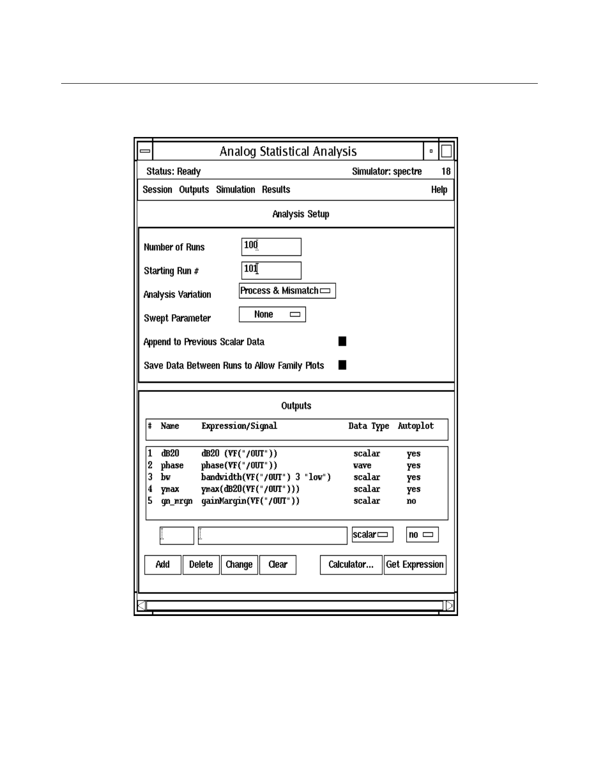
Cadence Advanced Analysis Tools User Guide
Statistical Analysis
July 2002 148 Product Version 5.0
The Analog Statistical Analysis form should appear as follows:
c. Invoke Simulation->Run.
When the simulation completes, you will notice that the autoplotted histograms indicate
a sample set of 200 ("N = 200"). You will also notice that the autoplotted waveforms are

Cadence Advanced Analysis Tools User Guide
Statistical Analysis
July 2002 149 Product Version 5.0
for iterations 101 to 200 when you drag the curser across the waveforms and look at the
banner info.
If you use the Results->Iteration_Verses_Value capability, you will notice that the
iterations are from 1 to 200 (use the unsorted mode).
Note, at this point, attempting to use the Results->Evaluate_Expressions capability
will cause the first 100 iterations to be purged from the scalar data. This is because the
psf data does not contain the first 100 iterations. Whenever scalar iterations data will be
purged, the UI will inform the user prior to purging the data. The user will be able to abort
creating the new scalar data.
Appending Waveforms From Different Statistical Analysis Runs.
The steps in this section outline how the user can overlay waveform plots from two different
analog statistical analysis psf data sets. We are assuming we are continuing from the
previous section. Perform the following steps:
1. Close all open Waveform Windows.
2. On the Analog Statistical Analysis UI Outputs Pane, select the desired expression row.
3. Go to the editable expression field and highlight the entire expression.
4. Bring up the Calculator and paste the expression into the buffer. Push the erplot button.
5. On the Analog Statistical Analysis UI, invoke the Results->Select capability. Set the
result name to first_100_iterations and click OK. Click OK on the Initialize Statistical
Analysis Data form.
6. On the calculator, push the plot button.
Now, all 200 waveforms should be shown in a single plot.

Cadence Advanced Analysis Tools User Guide
Statistical Analysis
July 2002 150 Product Version 5.0
Performing a Swept Parameter Statistical Analysis.
An example UI setup for performing a Swept Parameter statistical analysis is shown in the
following picture.
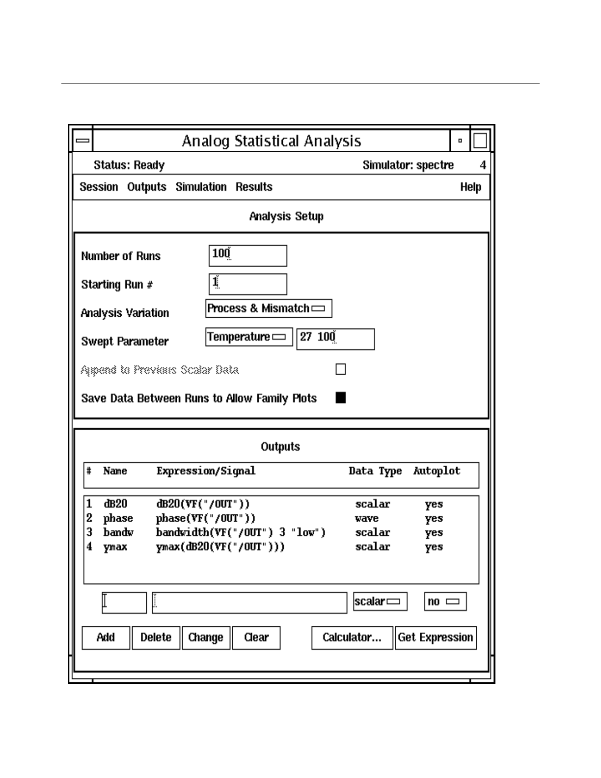
Cadence Advanced Analysis Tools User Guide
Statistical Analysis
July 2002 151 Product Version 5.0

Cadence Advanced Analysis Tools User Guide
Statistical Analysis
July 2002 152 Product Version 5.0
This section will not go into showing all the previously demonstrated UI features. Using the
parametric data sets created by a run with the above UI configuration, please return to the
section titled Evaluating Statistical Analysis Results and repeat the same example
through to the end of this document.

Cadence Advanced Analysis Tools User Guide
July 2002 153 Product Version 5.0
3
Optimization
Optimization is the process of automatically modifying design variables so that
specifications are achieved. The tool that performs optimization is called the optimizer. Often
the optimizer can take a design that is close to meeting performance specifications and
generate new component values that bring the design into the acceptable performance
range.
You can apply optimization profitably in a wide range of activities.
■If you use a top-down design approach, you can optimize a circuit block to match the
performance characteristics of an analog HDL module.
■Using the opposite approach, you can optimize a macro or behavioral module to
describe the behavior of a circuit block. Then, instead of simulating with the circuit block,
you can simulate with the macro or behavioral model, which usually runs much faster.
■You can optimize model parameters to match measured device data under various
conditions.
■You can use optimization to address radio frequency (RF) design problems, such as
impedance matching.
■To increase circuit yield, you can use optimization to achieve better design center values.
■You can use optimization to match the frequency response of a filter to the specifications
for the filter.
■You can use optimization to balance design tradeoffs.
The sections in this chapter explain how you can use the optimizer to help achieve your
design goals.
■“Getting Started with Optimization” on page 154
■“Getting to Know the Cadence® Analog Circuit Optimization Option Window” on
page 157
■“Running an Optimization” on page 162

Cadence Advanced Analysis Tools User Guide
Optimization
July 2002 154 Product Version 5.0
■“Saving, Changing, and Loading Session Information” on page 187
■“Working through an Extended Example” on page 192
Getting Started with Optimization
This section briefly explains the theory behind optimization, tells you how to get help, and
describes how to open the Cadence®™ Analog Optimization Analysis window.
How Optimization Works
A circuit, as originally designed, often fails to meet its specifications. For example, the
bandwidth might be too small or the design might be off center so that the yield is low. You
might be able to improve a marginal design by using components with different values, but
determining the best values to use is often difficult. The optimizer can provide you with
information that can help you choose values that meet your design goals.
To use the optimizer, you specify initial values for a set of design variables. You also specify
the goals you want the circuit to meet. The optimizer first determines how the values of the
goal expressions vary as a function of changes to the design variables. Then the optimizer
changes the design variables in a manner expected to move the values of the expressions in
the direction of the goals. After the change, the optimizer simulates the circuit to check the
outcome. If stopping criteria are not met, the optimizer iterates through the optimization
process.
The following steps describe, in greater detail, the process that the optimizer follows during
an analysis.
1. The optimizer runs a simulation using the initial values you specify for the design
variables.
This step determines the types and initial values of the goal expressions.
2. The optimizer determines which optimization algorithm to use (unless you specify which
to use).
❑The LSQ (least square) algorithm is best suited for optimizing measured, noisy,
unconstrained data. For example, this algorithm is appropriate for designing a filter
with an output waveform that matches measured frequency response data.
❑The CFSQP (C version Feasible Sequential Quadratic Programming) algorithm is
suited for a wide variety of optimization problems, including constrained and
unconstrained, minimizing and maximizing, and sequentially related goals. For
example, this algorithm is appropriate for a low noise amplifier design that has many

Cadence Advanced Analysis Tools User Guide
Optimization
July 2002 155 Product Version 5.0
goals such as maximizing the gain, minimizing the noise, and maintaining a phase
margin greater than 45 degrees.
3. If the CFSQP algorithm is used, the optimizer runs a simulation to determine whether the
initial values are feasible for the given goals. If the initial values are not feasible, the
optimizer computes new values that are feasible.
4. The optimizer determines how sensitive the goal expressions are to each design
variable.
To determine these sensitivities, the optimizer changes each design variable slightly and
then simulates the design again. This technique is called Finite Difference
Perturbation. In this technique, users generally do not need to select which algorithm
to use for their problem. The optimizer decides which algorithm to use based on the type
of optimization to be done. However, this option provides the ability to force the optimizer
to use a particular algorithm.
5. Using the information on sensitivities, the optimizer calculates a new set of values for the
design variables.
6. The optimizer sets the design variables to the new values and simulates the circuit.
If the values of the goal expressions are not better than they were with the previous
design variable values, the optimizer repeats Step 5.
If the values of the goal expressions are better than they were with the previous design
variable values, the new values become the initial values for the next iteration.
7. If the stopping criteria are not yet met, the optimizer begins the next iteration with Step 4.
Optimization stops when either or both of the following stopping criteria are met:
❑The values of the design variables change very little or not at all
❑Further changes to the design variables result in no progress toward the goals
Getting Help
For the most extensive information about using the optimizer, continue reading this
document. To open this document online, choose Help – Contents in the Cadence® Analog
Circuit Optimization Option window menu.
For information about the precise product name and version for this tool, choose Help –
About Analog Circuit Optimization.
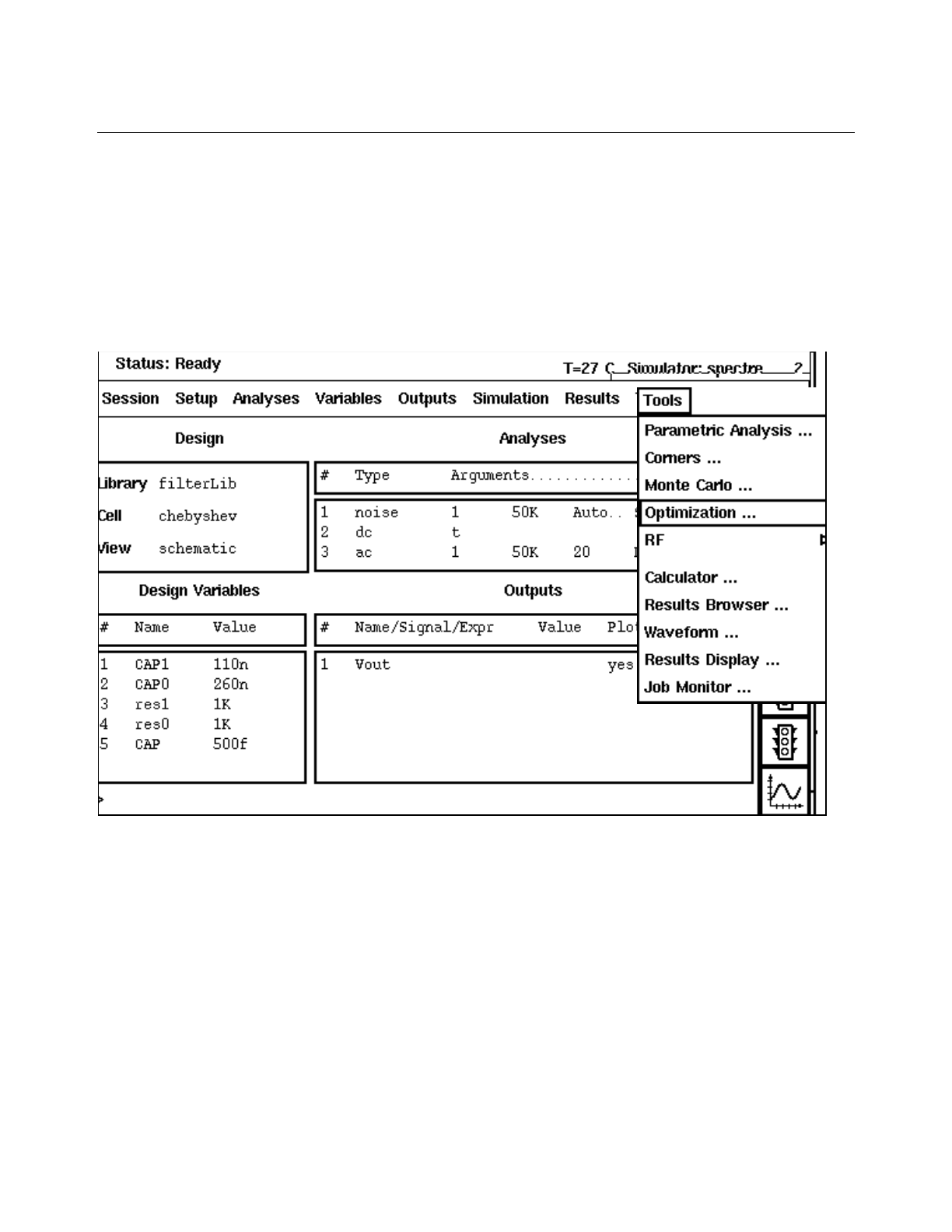
Cadence Advanced Analysis Tools User Guide
Optimization
July 2002 156 Product Version 5.0
Opening and Closing the Cadence® Analog Circuit Optimization Option
Window
When your circuit is ready to optimize,
1. Set up a simulation for it in the usual way.
2. In the Cadence® Analog Design Environment window, choose Tools – Optimization.
To close the Cadence® Analog Circuit Optimization Option window,
➤Choose Session – Quit.
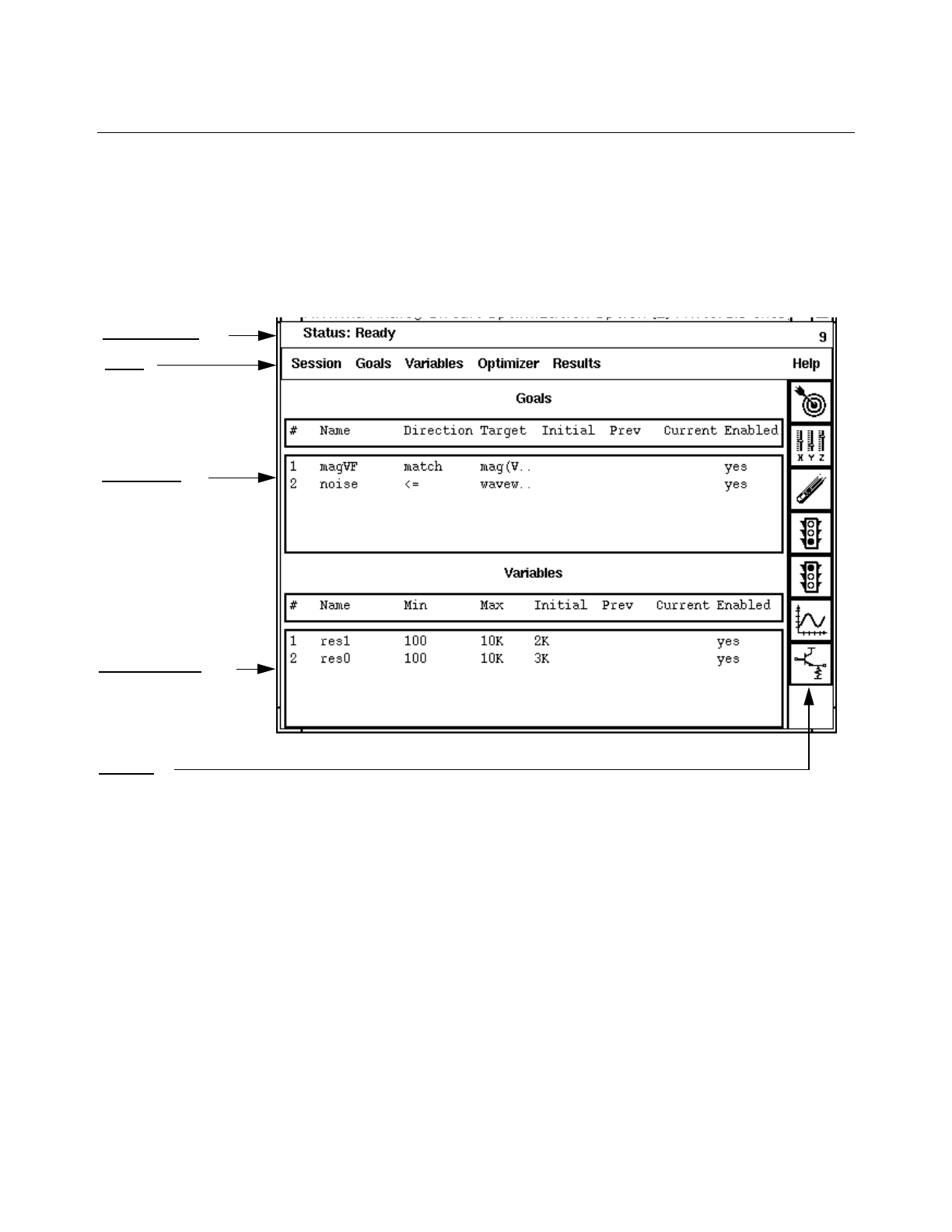
Cadence Advanced Analysis Tools User Guide
Optimization
July 2002 157 Product Version 5.0
Getting to Know the Cadence® Analog Circuit
Optimization Option Window
The Cadence® Analog Circuit Optimization Option window contains the primary controls
and tables you need for an optimization session.
Status Display
The status display shows the current state of the optimizer. For example, the status display
indicates whether the optimizer is simulating, optimizing, or in some other phase of the
analysis.
Status display
Menu
Goals pane
Variables pane
Tool bar
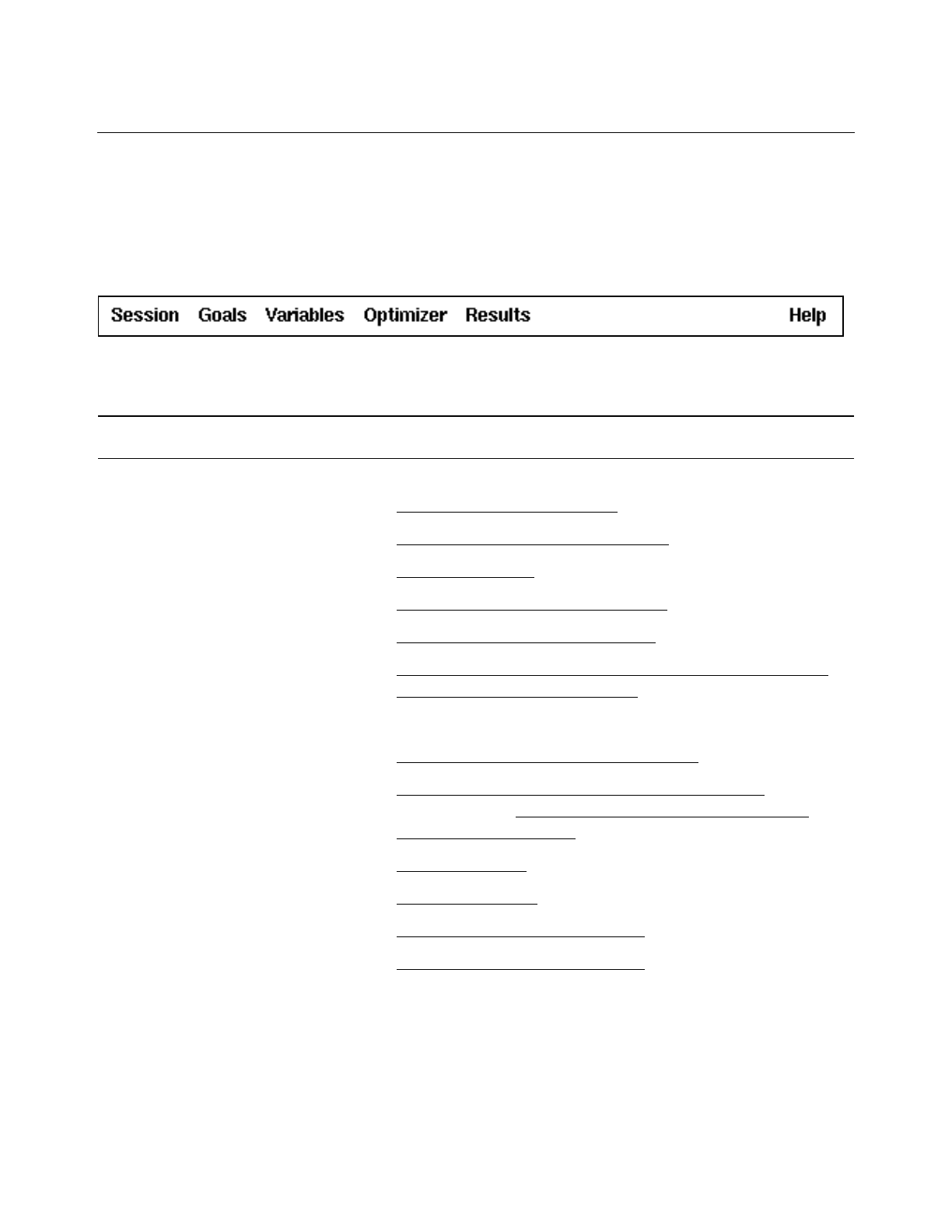
Cadence Advanced Analysis Tools User Guide
Optimization
July 2002 158 Product Version 5.0
Menu
The menu contains the commands needed to prepare for, run, and plot the results of an
optimization.
For guidance on using the menu choices, see the cross-references in the following table.
Optimization Menu Selections
Menu Item For More Information
Session
Save State “Saving the Session State” on page 187
Load State “Loading a Saved Session State” on page 188
Save Script “Saving a Script” on page 188
Options “Changing Optimization Options” on page 189
Reset “Deleting All Setup Information” on page 191
Quit “Opening and Closing the Cadence® Analog Circuit
Optimization Option Window” on page 156
Goals
Retrieve Outputs “Using Simulation Outputs as Goals” on page 163
Add “Creating a New Goal by Entering It Directly” on
page 164 and “Creating a New Goal by Using the
Waveform Calculator” on page 166
Edit “Editing a Goal” on page 169
Delete “Deleting a Goal” on page 170
Enable “Enabling or Disabling a Goal” on page 170
Disable “Enabling or Disabling a Goal” on page 170

Cadence Advanced Analysis Tools User Guide
Optimization
July 2002 159 Product Version 5.0
Variables
Add/Edit “Adding a Design Variable” on page 178 or “Editing a
Design Variable” on page 179
Delete “Deleting a Design Variable” on page 180
Enable “Enabling or Disabling a Design Variable” on page 181
Disable “Enabling or Disabling a Design Variable” on page 181
Optimizer
Run “Running the Optimizer” on page 181
Step “Running the Optimizer” on page 181
Run n “Running the Optimizer” on page 181
Stop “Stopping the Optimizer” on page 182
Stop Now “Stopping the Optimizer” on page 182
Reset “Deleting Simulation Results” on page 183
Results
Plot History “Plotting Output Data” on page 186
Set Plot Options “Setting the Plotting Options” on page 183
Update Design “Updating Your Design” on page 186
Help
Contents “Getting Help” on page 155
About Analog Circuit
Optimization “Getting Help” on page 155
Optimization Menu Selections, continued
Menu Item For More Information
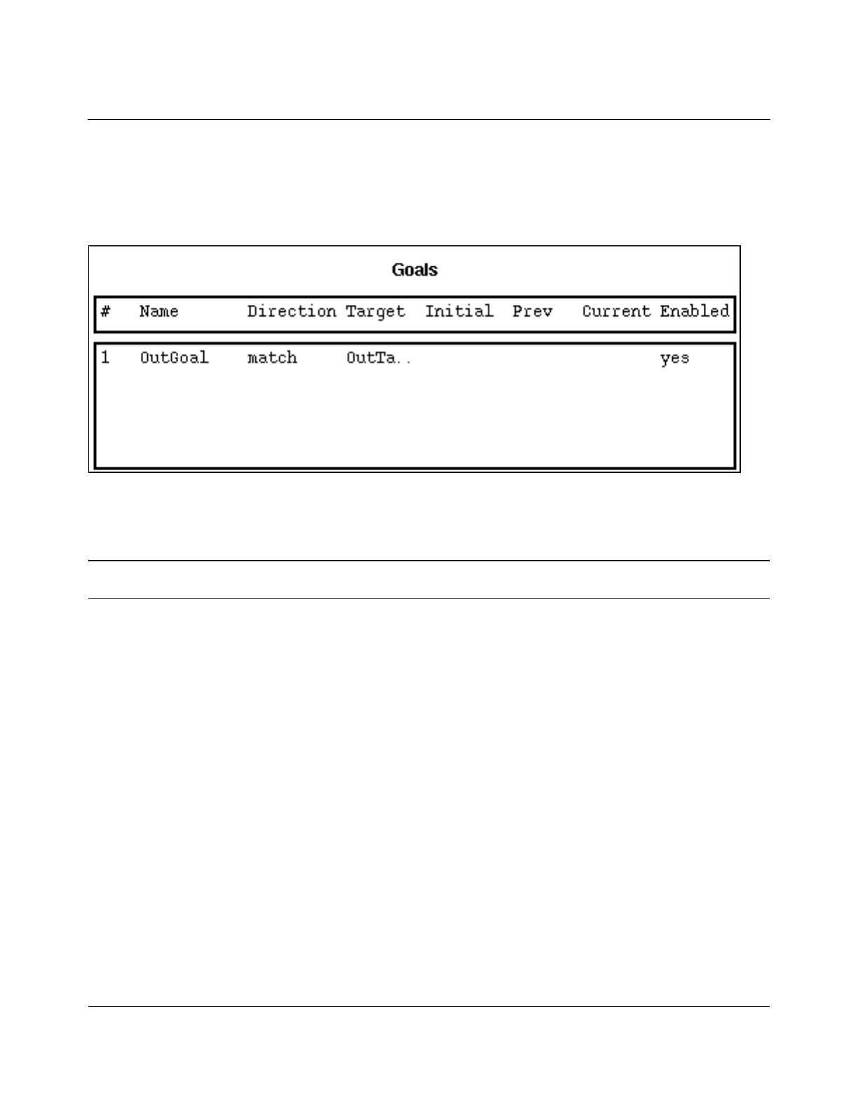
Cadence Advanced Analysis Tools User Guide
Optimization
July 2002 160 Product Version 5.0
Goals Pane
The Goals pane displays information about the currently defined goals.
To define or revise the goals, you use the menu choices and buttons in the Cadence® Analog
Circuit Optimization Option window. For a description of the items in the Goals pane, see the
following table.
Item Description and Usage
Name The name associated with the goal.
Direction One of the following: maximize,minimize,match, >=, or <=.
Target If Direction is match, a value or waveform that the optimizer
attempts to match.
If Direction is maximize or minimize, a value or waveform used to
determine how important the goal is.
If Direction is >=, a value or waveform that is the lower bound.
If Direction is <=, a value or waveform that is the upper bound.
Initial The value of the goal expression as calculated from the initial values
of the design variables.
Prev The value of the goal expression as calculated from the values of the
design variables used in the previous iteration.
Current The value of the goal expression as calculated from the current
values of the design variables.
Enabled Either yes or no.yes indicates that the goal is included in the
current optimization; no, that it is not.
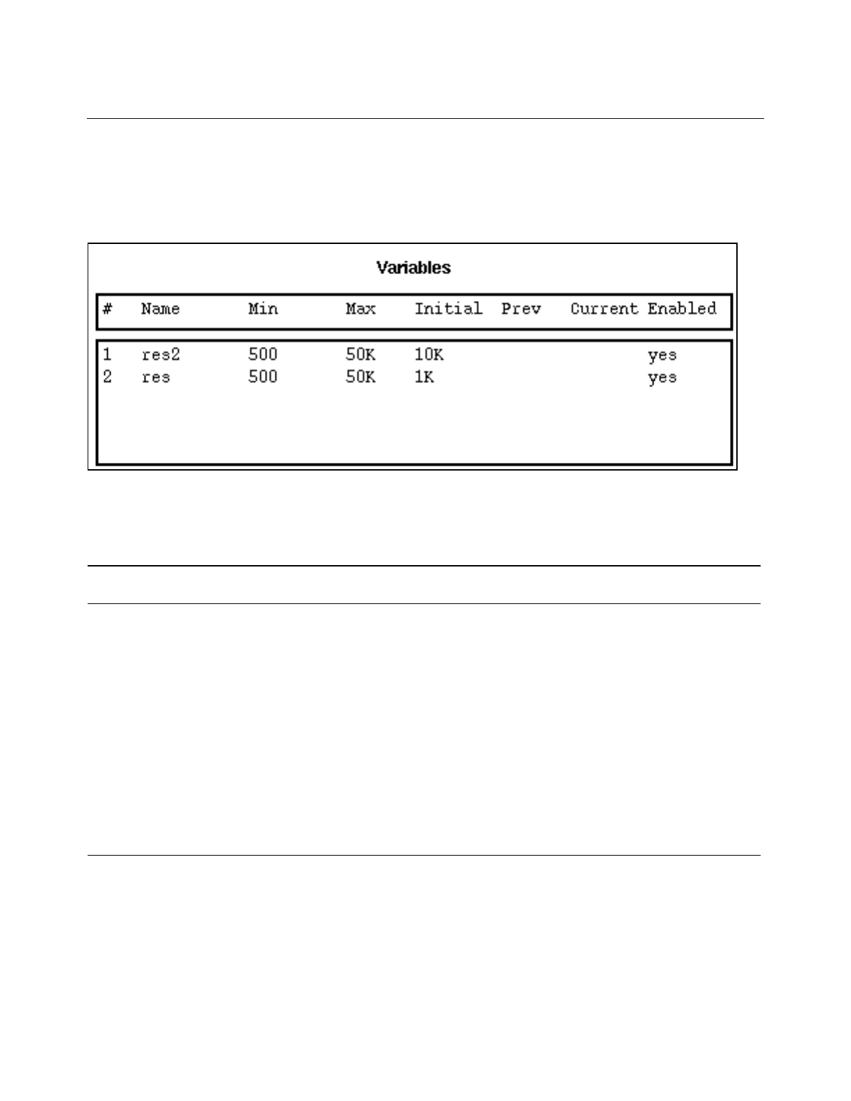
Cadence Advanced Analysis Tools User Guide
Optimization
July 2002 161 Product Version 5.0
Variables Pane
The Variables pane displays information about the current design variables.
To define, revise, or enable the variables, you use the menu choices and buttons in the
Cadence® Analog Circuit Optimization Option window. For a description of the items in the
Variables pane, see the following table.
Item Description and Usage
Name The name of the design variable.
Min The minimum value allowed for the variable.
Max The maximum value allowed for the variable.
Initial The initial value of the design variable.
Prev The value of the design variable used in the previous iteration.
Current The value of the design variable used in the current iteration.
Enabled Either yes or no.
yes indicates that the value of the design variable can be changed
in the current optimization; no, that it cannot be.
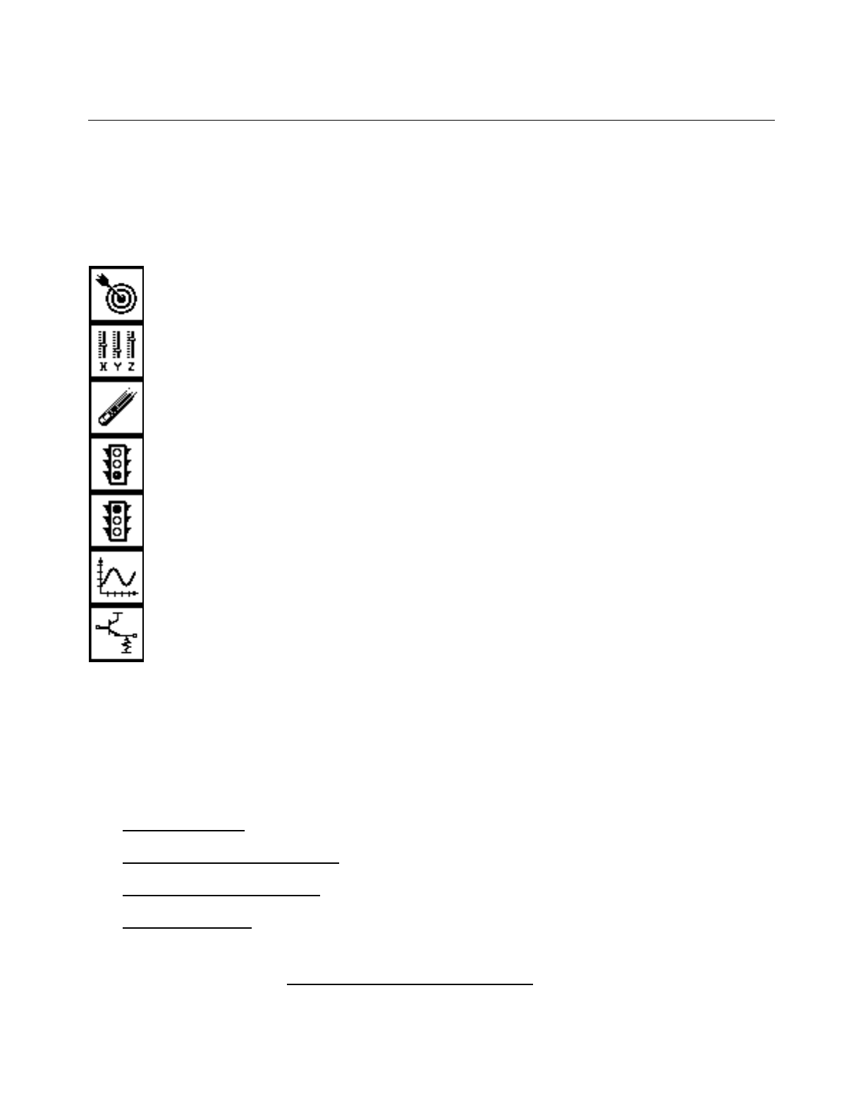
Cadence Advanced Analysis Tools User Guide
Optimization
July 2002 162 Product Version 5.0
Tool Bar
The tool bar contains buttons that perform the most important optimization tasks. The buttons
are arranged from top to bottom in the order they are typically used.
Running an Optimization
The following sections describe the major steps involved in setting up and running an
optimization.
■“Defining Goals” on page 163
■“Preparing Design Variables” on page 178
■“Controlling the Optimizer” on page 181
■“Plotting Results” on page 183
You might be able to skip the first two steps by loading a state you saved in an earlier session.
For more information, see “Loading a Saved Session State” on page 188.
Add/Edit Goals
Add/Edit Variables
Delete
Run Optimizer
Stop Optimizer
Plot History
Update Design

Cadence Advanced Analysis Tools User Guide
Optimization
July 2002 163 Product Version 5.0
Defining Goals
Before you can run the optimizer on a circuit, you must specify the goals for the analysis. A
goal consists of
■An expression whose value can be determined by simulation
■A direction specifying how the value of the expression is to change during optimization
For example, you might define a goal called Bandwidth(3dB) with the expression
bandwidth(VF("/out") 3 "low")
and specify that the value of the expression is to be maximized during optimization.
The following sections describe how to create, edit, delete, enable, and disable goals.
■“Using Simulation Outputs as Goals” on page 163
■“Creating a New Goal by Entering It Directly” on page 164
■“Creating a New Goal by Using the Waveform Calculator” on page 166
■“Editing a Goal” on page 169
■“Deleting a Goal” on page 170
■“Enabling or Disabling a Goal” on page 170
For information about how the optimizer assigns weights to goals or about creating waveform
objects, look also at
■“Creating Waveform Objects from a List of Values” on page 170
■“How the Optimizer Uses Target and Acceptable Values” on page 173
Using Simulation Outputs as Goals
The optimizer allows you to use the simulation outputs defined in the Cadence® Analog
Design Environment window as goals. This approach is particularly useful for RF analyses
where expressions are often developed for Direct Plot. You can easily add these Direct Plot
expressions to the Cadence® Analog Design Environment window Outputs pane, and from
there you can use the following steps to retrieve the expressions for use as optimizer goals.
1. From the Cadence® Analog Circuit Optimization Option window, choose Goals –
Retrieve Outputs.
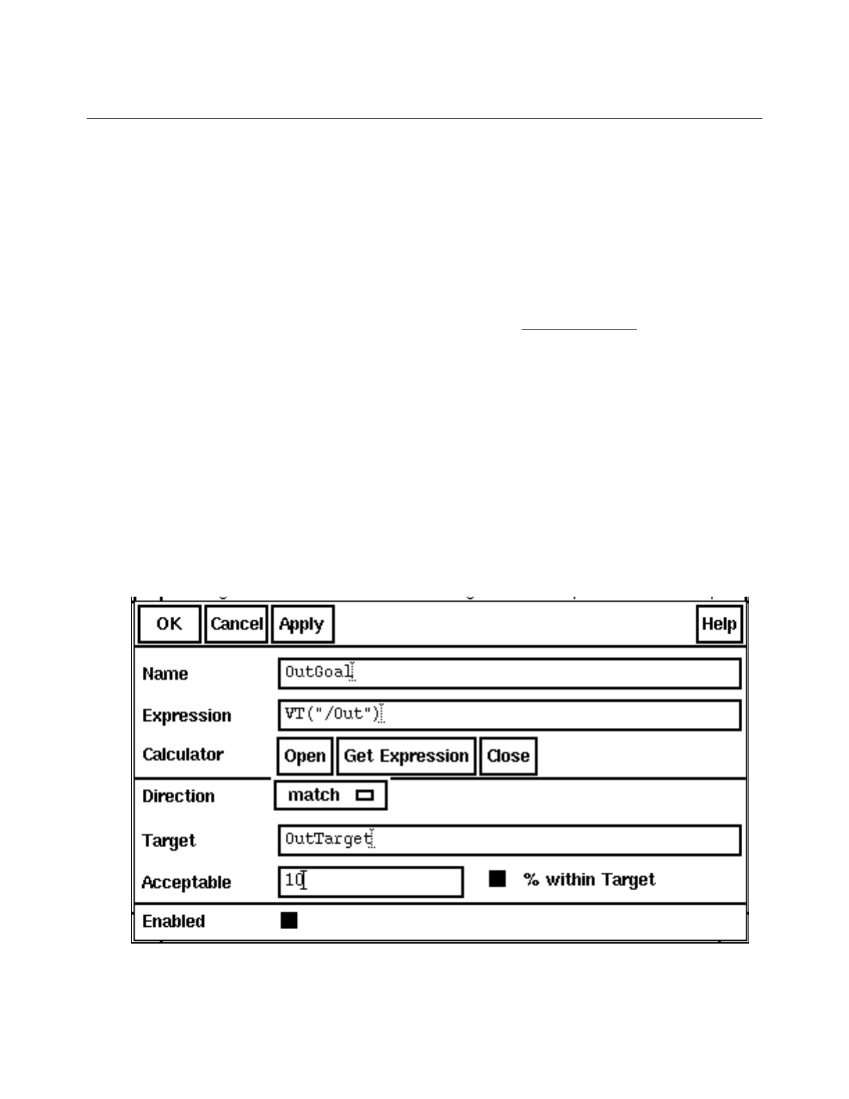
Cadence Advanced Analysis Tools User Guide
Optimization
July 2002 164 Product Version 5.0
The expressions (but not any signals) defined in the Outputs pane of the Design
Environment window appear in the Goals pane of the Optimization Option window.
Initially, the new goals are not enabled.
Unnamed expressions are given names like G1,G2,G3, and so on.
2. Highlight a goal and choose Goals – Edit.
The Editing Goals window appears.
3. Finish defining the goal by following the instructions in “Editing a Goal” on page 169.
Until you edit a retrieved goal in the Editing Goals window, choosing Goals – Retrieve
Outputs updates the goal to match the existing expression in the Outputs pane of the
Design Environment window. After you edit a retrieved goal, choosing Goals – Retrieve
Outputs has no effect on the goal.
Creating a New Goal by Entering It Directly
To create a new goal by entering it directly,
1. Choose Goals – Add or click Add/Edit Goals.
The Adding Goals form appears.
2. Type a name for the goal.

Cadence Advanced Analysis Tools User Guide
Optimization
July 2002 165 Product Version 5.0
3. Type a Cadence® SKILL language expression describing the goal.
The expression can be either a scalar expression or a waveform expression.
4. In the Direction cyclic field, indicate how the value of the expression is to change during
optimization.
5. Type an expression in the Target field.
If the expression you enter in Step 3 is a scalar expression, Target must also be a scalar
expression. If the expression you enter in Step 3 is a waveform, Target can be either a
scalar expression or a waveform expression.
6. Specify a value in the Acceptable field.
As described in “How the Optimizer Uses Target and Acceptable Values” on page 173,
the optimizer uses the Acceptable value to determine how important the goal is.
There are two ways to specify the Acceptable value.
❑You can type an expression in the Acceptable field.
If the expression you enter in Step 3 is a scalar expression, Acceptable must also
be a scalar expression. If the expression you enter in Step 3 is a waveform,
Acceptable can be either a scalar expression or a waveform expression.
A scalar Acceptable expression must meet the following requirements. A waveform
Acceptable expression must meet the following requirements at every point along
the curve.
If you specify
Direction as Then the value of the Acceptable expression
minimize Must be greater than the value of the Target
expression
maximize Must be less than the value of the Target expression
match Can be any value except the Target expression
In addition, a waveform Acceptable expression must
be everywhere greater than or everywhere less than
the Target expression.
<= Must be greater than the value of the Target
expression
>= Must be less than the value of the Target expression

Cadence Advanced Analysis Tools User Guide
Optimization
July 2002 166 Product Version 5.0
❑If % within Target is turned on, you can specify a scalar or waveform percentage
in the Acceptable field. A small percentage indicates that the goal is to be heavily
weighted.
If the expression you enter in Step 3 is a scalar expression, the percentage in the
Acceptable field must also be a scalar expression. If the expression you enter in
Step 3 is a waveform, the percentage in the Acceptable field value can be either a
scalar expression or a waveform expression.
By specifying a scalar percentage, you can ensure that the optimization results are
consistent at both very small and very large values of the Target expression. By
specifying a waveform percentage, you can explicitly specify the importance of each
segment of a waveform goal.
How the optimizer uses the Target and Acceptable expressions depends on the
direction you choose. For details, see “How the Optimizer Uses Target and Acceptable
Values” on page 173.
7. If you want to include the goal in the current optimization, be sure Enabled is on.
8. Click OK.
The new goal is added to the Cadence® Analog Circuit Optimization Option window.
Creating a New Goal by Using the Waveform Calculator
To create a new goal by using the Waveform Calculator,
1. Choose Goals – Add or click Add/Edit Goals.
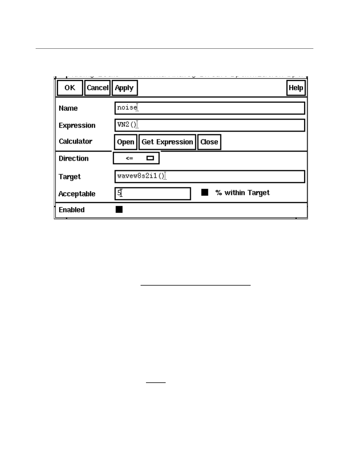
Cadence Advanced Analysis Tools User Guide
Optimization
July 2002 167 Product Version 5.0
The Adding Goals form appears.
2. Type a name for the goal.
3. Click Open.
The calculator window appears.
4. Build the goal expression in the Waveform Calculator. For information on using the
Waveform Calculator, see the Waveform Calculator User Guide.
5. In the Cadence® Analog Circuit Optimization Option window, click in the Expression
field.
6. Click Get Expression, which retrieves the expression from the Waveform Calculator
and places it in the Expression field.
7. In the Direction cyclic field, indicate how the value of the expression is to change during
optimization.
8. Type an expression in the Target field (or click in the Target field, then click Get
Expression to retrieve an expression from the Waveform Calculator).
If the expression you retrieve in Step 5 is a scalar value, Target must also be a scalar
expression. If the expression you retrieve in Step 5 is a waveform, Target can be either
a scalar expression or a waveform expression.

Cadence Advanced Analysis Tools User Guide
Optimization
July 2002 168 Product Version 5.0
9. Specify a value for Acceptable. As described in “How the Optimizer Uses Target and
Acceptable Values” on page 173, the optimizer uses the Acceptable value to determine
how important the goal is.
There are two ways to define this value.
❑First, you can type an expression in the Acceptable field (or click in the Acceptable
field, then click Get Expression to retrieve an expression from the Waveform
Calculator).
If the expression you retrieve in Step 6 is a scalar expression, Acceptable must also
be a scalar expression. If the expression you retrieve is a waveform, Acceptable
can be either a scalar expression or a waveform expression.
A scalar Acceptable expression must meet the following requirements. A waveform
Acceptable expression must meet the following requirements at every point along
the curve.
❑Second, if % within Target is turned on, you can specify a scalar or waveform
percentage in the Acceptable field. A small percentage indicates that the goal is to
be heavily weighted.
If the expression you retrieve in Step 6 is a scalar expression, the percentage you
enter in the Acceptable Field must also be a scalar expression. If the expression
you retrieve is a waveform, the percentage value can be either a scalar expression
or a waveform expression.
By specifying a scalar percentage, you can ensure that the optimization results are
consistent at both very small and very large values of the Target expression. By
If you specify
Direction as Then the value of the Acceptable expression
minimize Must be greater than the value of the Target
expression
maximize Must be less than the value of the Target expression
match Can be any value except the Target expression
In addition, a waveform Acceptable expression must
be everywhere greater than or everywhere less than
the Target expression.
<= Must be greater than the value of the Target
expression
>= Must be less than the value of the Target expression
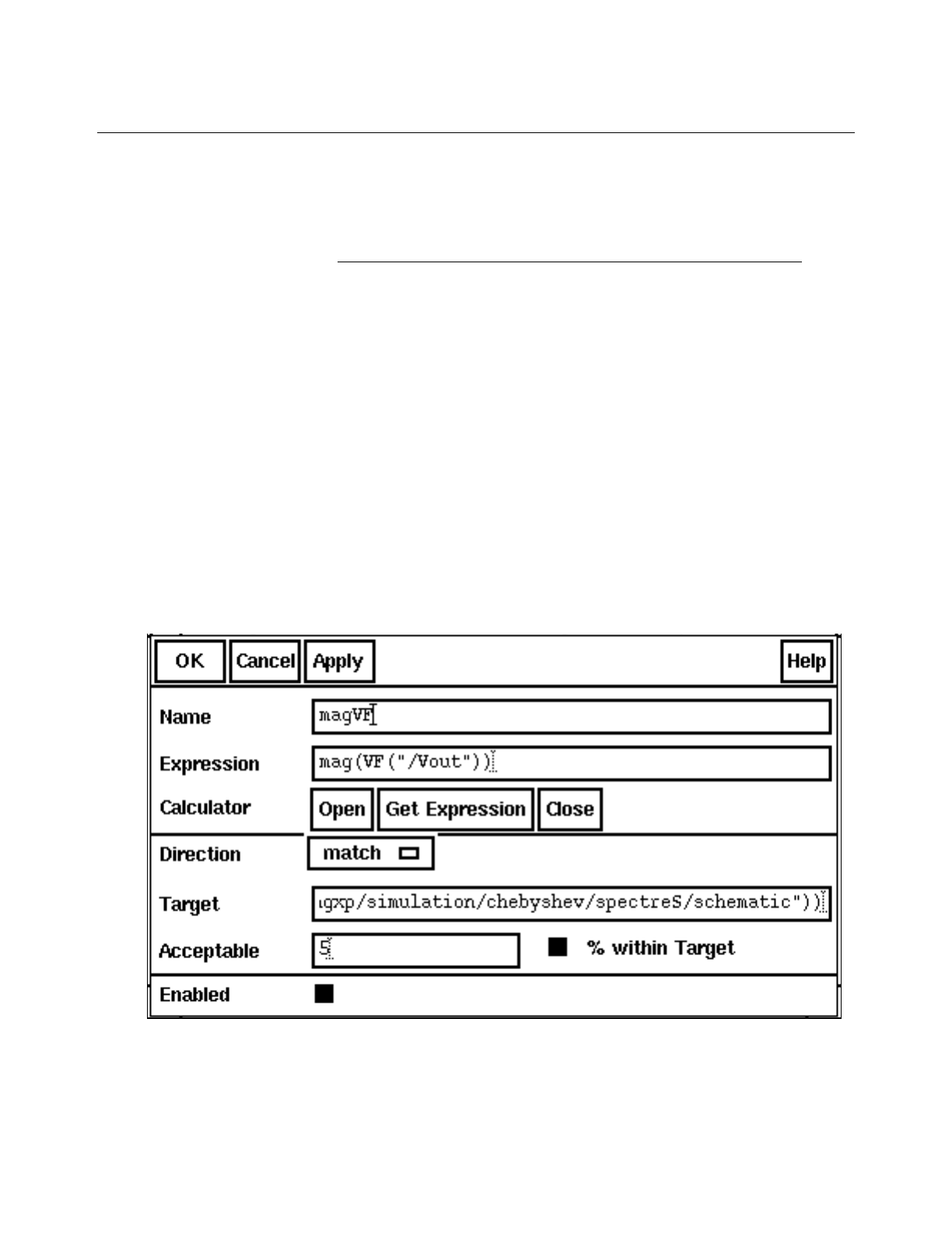
Cadence Advanced Analysis Tools User Guide
Optimization
July 2002 169 Product Version 5.0
specifying a waveform percentage, you can explicitly specify the importance of each
segment of a waveform goal.
How the optimizer uses the Target and Acceptable values depends on the direction you
choose. For details, see “How the Optimizer Uses Target and Acceptable Values” on
page 173.
10. If you want to include the goal in the current analysis, be sure Enabled is on.
11. Click OK to add the new goal to the Cadence® Analog Circuit Optimization Option
window.
Editing a Goal
To edit an existing goal,
1. In the Cadence® Analog Circuit Optimization Option window, highlight the goal you want
to edit.
2. Choose Goals – Edit or click Add/Edit Goals.
The Editing Goals form appears.
Except for the title, this form is identical to the Adding Goals form and you use the two
forms in the same way.

Cadence Advanced Analysis Tools User Guide
Optimization
July 2002 170 Product Version 5.0
3. Make the changes you want to make.
For details, see “Creating a New Goal by Entering It Directly” on page 164 or “Creating
a New Goal by Using the Waveform Calculator” on page 166.
4. Click OK.
The changes are applied to the highlighted goal.
Deleting a Goal
To delete an existing goal,
1. In the Cadence® Analog Circuit Optimization Option window, highlight the goal you want
to delete.
2. Choose Goals – Delete or click Delete.
The highlighted goal disappears from the Cadence® Analog Circuit Optimization Option
window.
Enabling or Disabling a Goal
For a quick way to enable or disable a goal,
1. Highlight the goal in the Cadence® Analog Circuit Optimization Option window.
2. Choose Goals – Enable or Goals – Disable.
The optimization does not include disabled goals.
Creating Waveform Objects from a List of Values
When the expression that defines a goal is a waveform, the Target and Acceptable values
you define can also be waveforms. This section describes how you can create a waveform
object from a list of values stored in a file. For information on some of the other ways you can
create a waveform, see the Waveform Calculator User Guide.
This scenario assumes you have a list of X and Y values stored in a file. The X data values
must be monotonically increasing. For example, you might have a file called mydata
containing the following information:
; The information in column 1 is for the X axis.
; The information in column 2 is for the Y axis.
0.5 5
0.6 5.1
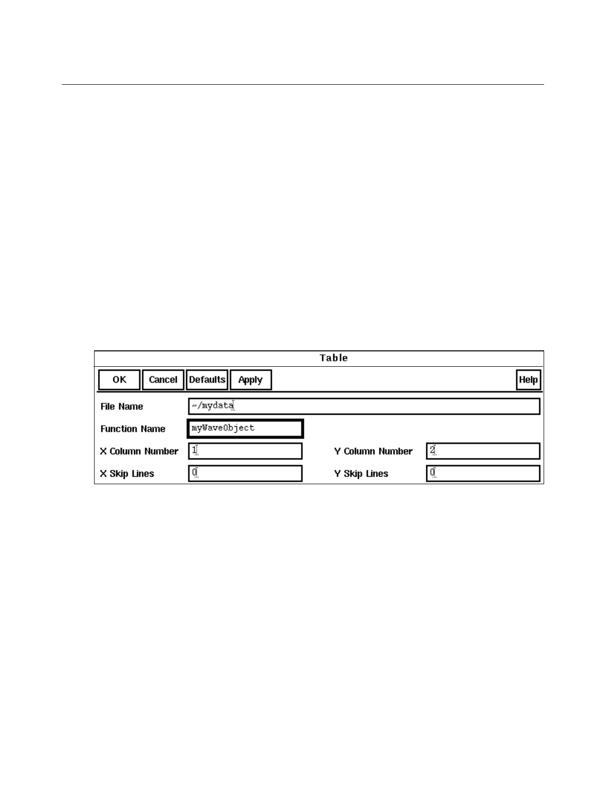
Cadence Advanced Analysis Tools User Guide
Optimization
July 2002 171 Product Version 5.0
1.0 4.8
1.2 4.5
2.0 4.5
2.5 4.7
3.3 4.9
3.9 5.1
4.3 5.2
5.0 5.4
To convert this data into a waveform object,
1. Open the Waveform Calculator.
2. Click Special Functions.
3. Choose table from the list of functions.
The Table form appears.
4. In the File Name field, type the filename of the file that contains your data.
5. In the Function Name field, type the name you want the waveform object to have.
6. (Optional) Specify which columns contain the X and Y data. This step is not required if
the X data is in column 1 and the Y data is in column 2.
7. (Optional) Type the number of lines to skip in each column before reading the data. Do
not count comment lines, which begin with a semicolon, and blank lines in the number of
lines to skip.
8. Click OK.
The Table form closes and the wave object appears in the calculator buffer. For example,
filling in the Table form as shown above and clicking OK causes
myWaveObject()
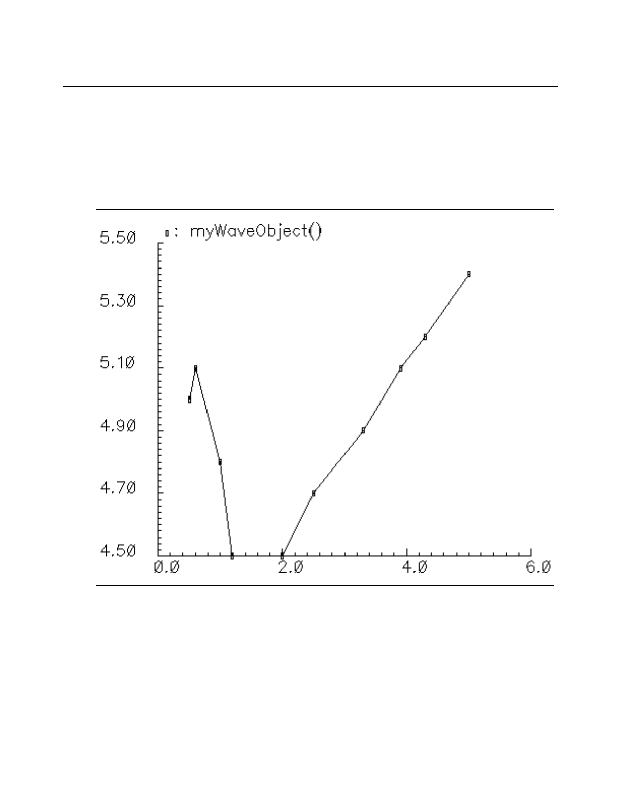
Cadence Advanced Analysis Tools User Guide
Optimization
July 2002 172 Product Version 5.0
to appear in the calculator buffer.
9. (Optional) In the Waveform Calculator, click plot to plot the waveform.
The Waveform Window opens with a plot of the waveform. The myWaveObject()
waveform, for example, looks like this.
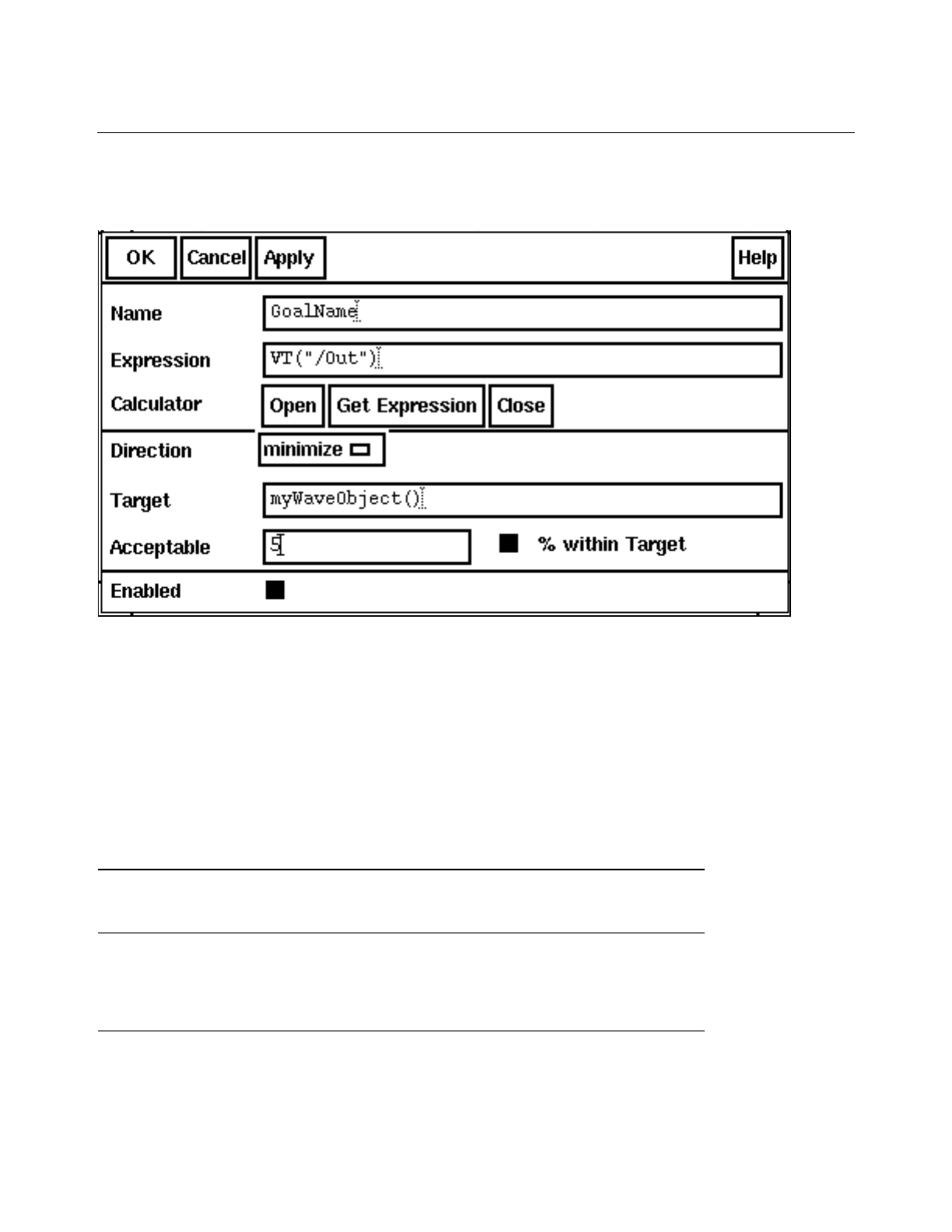
Cadence Advanced Analysis Tools User Guide
Optimization
July 2002 173 Product Version 5.0
You can use the new waveform object in the optimizer wherever waveforms are valid. For
example, to use myWaveObject() as a target, type the name in the Target field.
How the Optimizer Uses Target and Acceptable Values
The optimizer uses a Target value in two ways: as a goal and as an indication of the weight
(importance) of the goal. The following sections describe each use in more detail.
Target Values Used as Goals
The first use, as a goal, is most obvious when you specify a Direction of match,>=,or<=.
In these cases, the target is the value the optimizer attempts to reach.
However, when you specify a Direction of minimize, the optimizer does not stop minimizing
the goal expression when the Target value is reached. In fact, the optimizer makes the goal
When you specify a
Direction of The optimizer attempts to make the
value of the goal expression
match Match the Target value exactly
>=Greater than the Target value
<= Less than the Target value

Cadence Advanced Analysis Tools User Guide
Optimization
July 2002 174 Product Version 5.0
expression as small as the optimization stopping criteria allow, even if that means the final
value is much less than the Target. Similarly, when you specify a Direction of maximize, the
optimizer makes the goal expression as large as possible, even if that means the value is
much greater than the Target value.
Note: The LSQ algorithm makes no distinction among the directions of match,minimize,
and maximize. In each of these cases, the LSQ algorithm works to match the Target value.
For more information, see the information about the LSQ algorithm in “Changing Optimization
Options” on page 189.
Target Values Used to Assign Weights
When you set a Direction of minimize or maximize, the second use of the Target value is
most obvious. In these two cases, the Target value, together with the Acceptable value, is
used only to assign a weight to the goal. By contrast, in the match,>=, and <= cases, the
Target value is used both to set a goal and assign a weight.
The optimizer assigns greater weight to a goal that is defined with an Acceptable value set
very close to the Target value. Similarly, if the Target and Acceptable values are waveforms,
the optimizer assigns more weight to points where the Target and Acceptable values are
close together, and less weight to points where the Target and Acceptable values are farther
apart.
In formal terms, the weight assigned to a goal depends on the current value of the goal
expression( ), the Target value ( ), and the Acceptable value ( ).
For example, assume you have two goals defined as follows.
When you specify
a Direction of The optimizer attempts to make the value of the goal
expression
minimize As small as possible, regardless of the Target value
maximize As large as possible, regardless of the Target value
Name Direction Target Value Acceptable Value
power <= 50 mW 80 mW
delay <= 50 ns 60 ns
fT
A
weight fT–
AT–
--------------=

Cadence Advanced Analysis Tools User Guide
Optimization
July 2002 175 Product Version 5.0
If the current value of the power expression is 90 mW, its weight is
If the current value of the delay expression is 90 ns, its weight is
Because the delay weight is greater than the power weight, the optimizer assigns greater
importance to reducing delay than it does to reducing power. In a tradeoff between the two,
reducing delay comes out ahead.
The next example illustrates how the optimizer determines weights from waveform Target
and Acceptable values. In this example, you match the output of a filter to a particular
waveform. Parts of the range are critical, so you assign a heavy weight to those sections by
defining very similar Target and Acceptable waveforms. The middle section is not critical,
90mW 50mW–
80mW 50mW–
------------------------------------------40mW
30mW
------------------ 1.333==
90ns 50ns–
60ns 50ns–
--------------------------------40ns
10ns
-------------4==
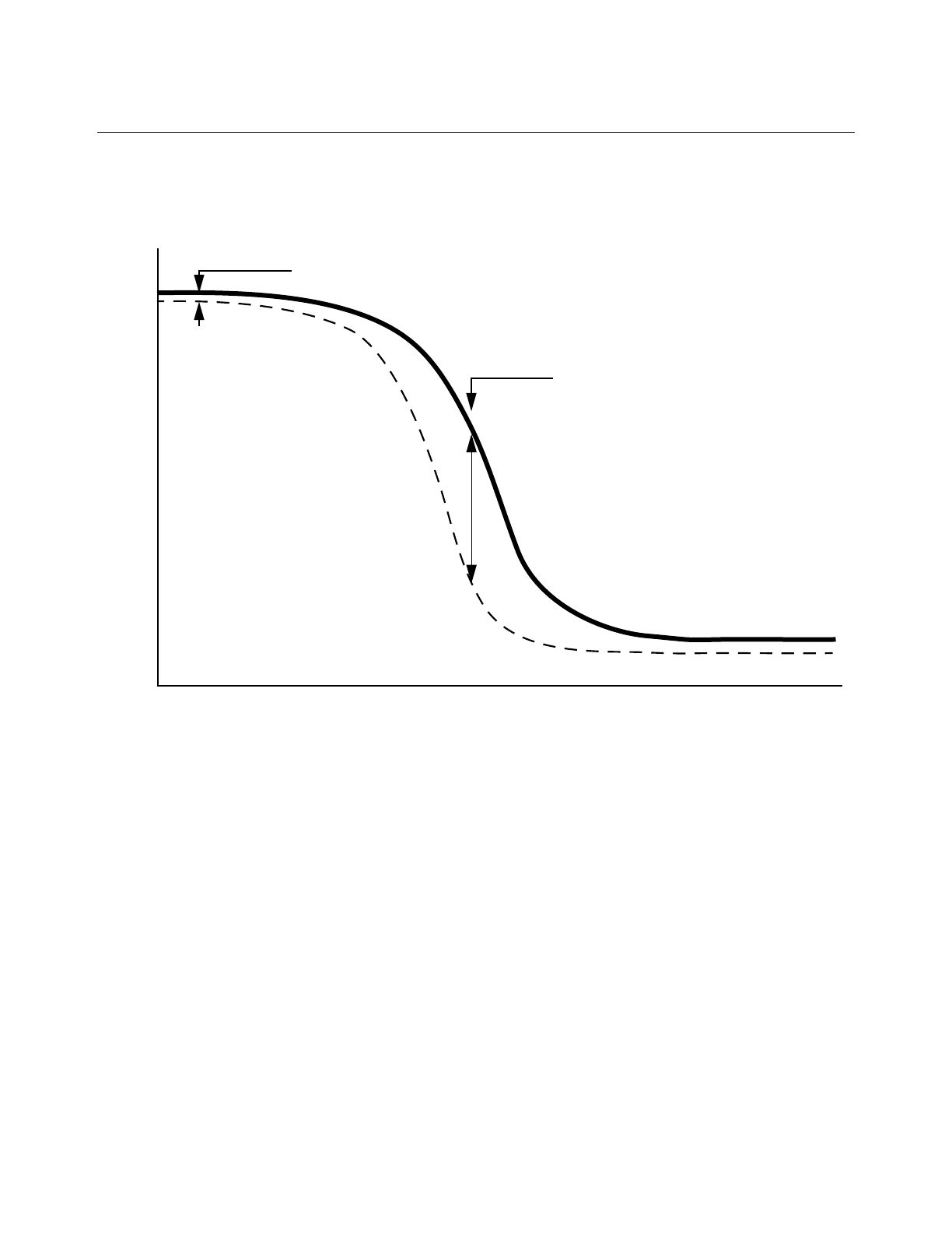
Cadence Advanced Analysis Tools User Guide
Optimization
July 2002 176 Product Version 5.0
so you assign less weight to that area by defining Target and Acceptable waveforms that
are farther apart.
The final example illustrates how the optimizer determines an Acceptable waveform from a
waveform Target and a waveform % within Target value. In this example, Direction is
Gain
Acceptable waveform
Target waveform
Critical area, heavily weighted
Frequency
Not critical, lightly weighted
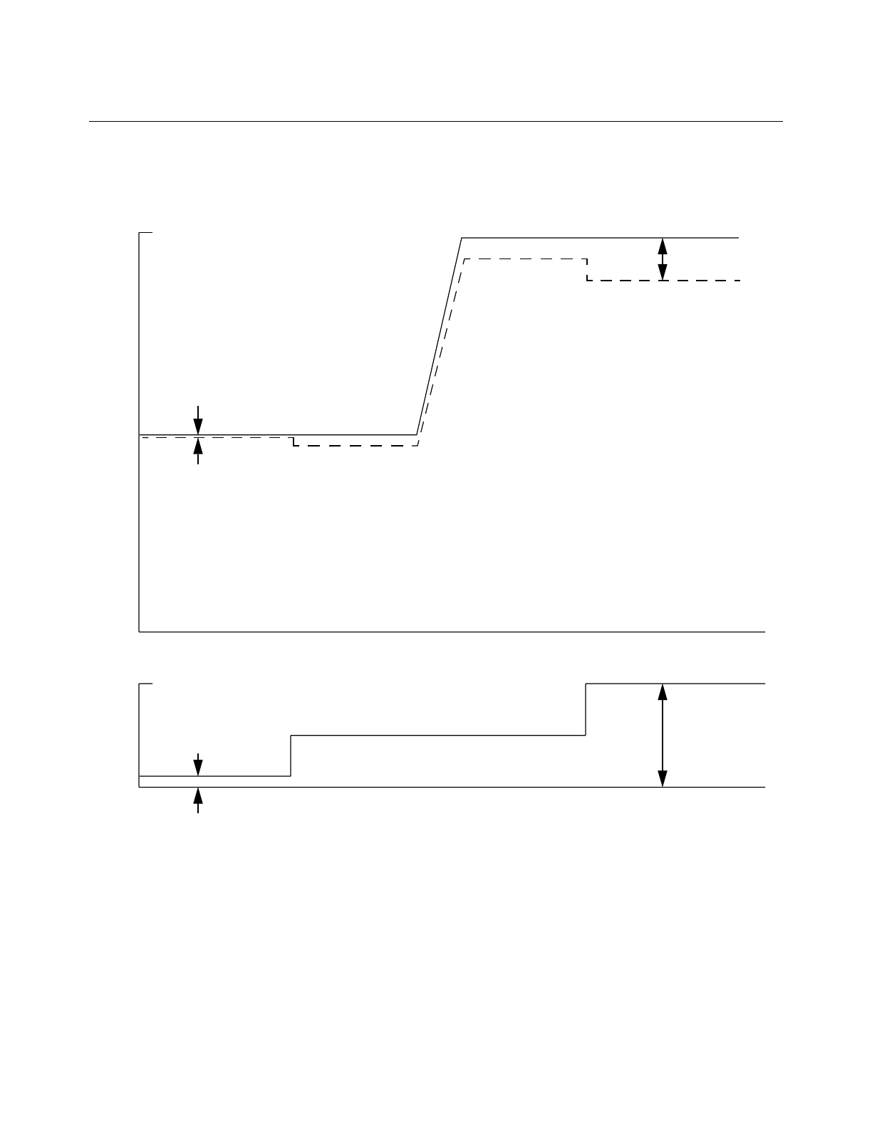
Cadence Advanced Analysis Tools User Guide
Optimization
July 2002 177 Product Version 5.0
specified as >= and the calculated Acceptable waveform is everywhere less than the Target
waveform.
At the left side of the plot, the % within target waveform has the value 1, so the calculated
value of the Acceptable waveform in that region is
100-(0.01 * 100) = 99
At the right side of the plot, the % within target waveform has the value 10, so the calculated
value of the Acceptable waveform in that region is
200-(0.10 * 200) = 180
% within target waveform
10%
5%
0%
0
100
200 Target waveform
Acceptable waveform
Lightly
weighted
Heavily
weighted

Cadence Advanced Analysis Tools User Guide
Optimization
July 2002 178 Product Version 5.0
Preparing Design Variables
Before you can run the optimizer on a circuit, you must specify which design variables the
optimizer is allowed to change. The design variables you specify must be simulation
environment variables such as component parameters and device model parameters. Typical
examples include variables for resistor, capacitor, and inductor values or for device widths,
lengths, and areas.
The following sections describe how to add, edit, delete, enable, and disable design variables.
■“Adding a Design Variable” on page 178
■“Editing a Design Variable” on page 179
■“Deleting a Design Variable” on page 180
■“Enabling or Disabling a Design Variable” on page 181
Adding a Design Variable
To add a design variable to the list of variables in the Cadence® Analog Circuit Optimization
Option window,
1. Choose Variables – Add/Edit or click Add/Edit Variables.
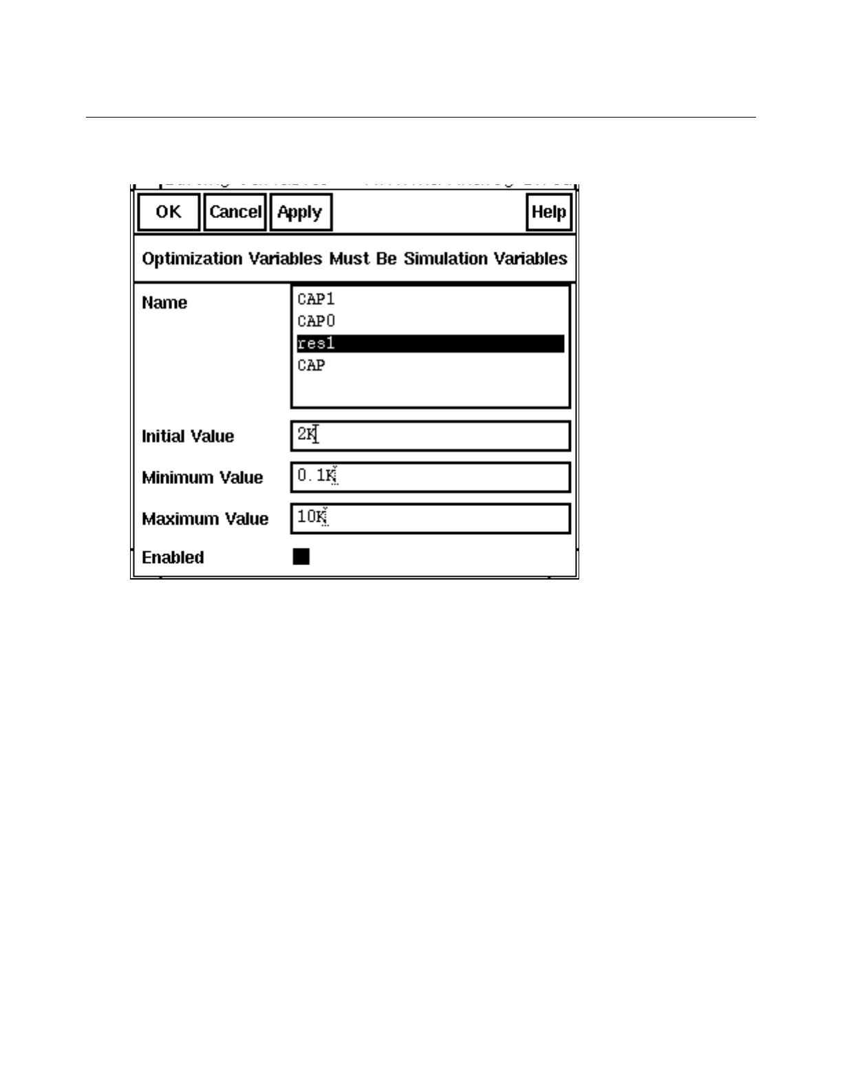
Cadence Advanced Analysis Tools User Guide
Optimization
July 2002 179 Product Version 5.0
The Editing Variables form opens.
2. Highlight the variable you want to add.
3. In the Initial Value field, type a value to be used as the starting point for optimization.
4. In the Minimum Value field, type a minimum value. The optimizer never sets the variable
to a value lower than this.
5. In the Maximum Value field, type a maximum value. The optimizer never sets the
variable to a value greater than this.
6. If you want to include the variable in the current analysis, be sure Enabled is on.
7. Click OK.
The variable is added to the Cadence® Analog Circuit Optimization Option window.
Editing a Design Variable
To edit one of the design variables listed in the Cadence® Analog Circuit Optimization Option
window,
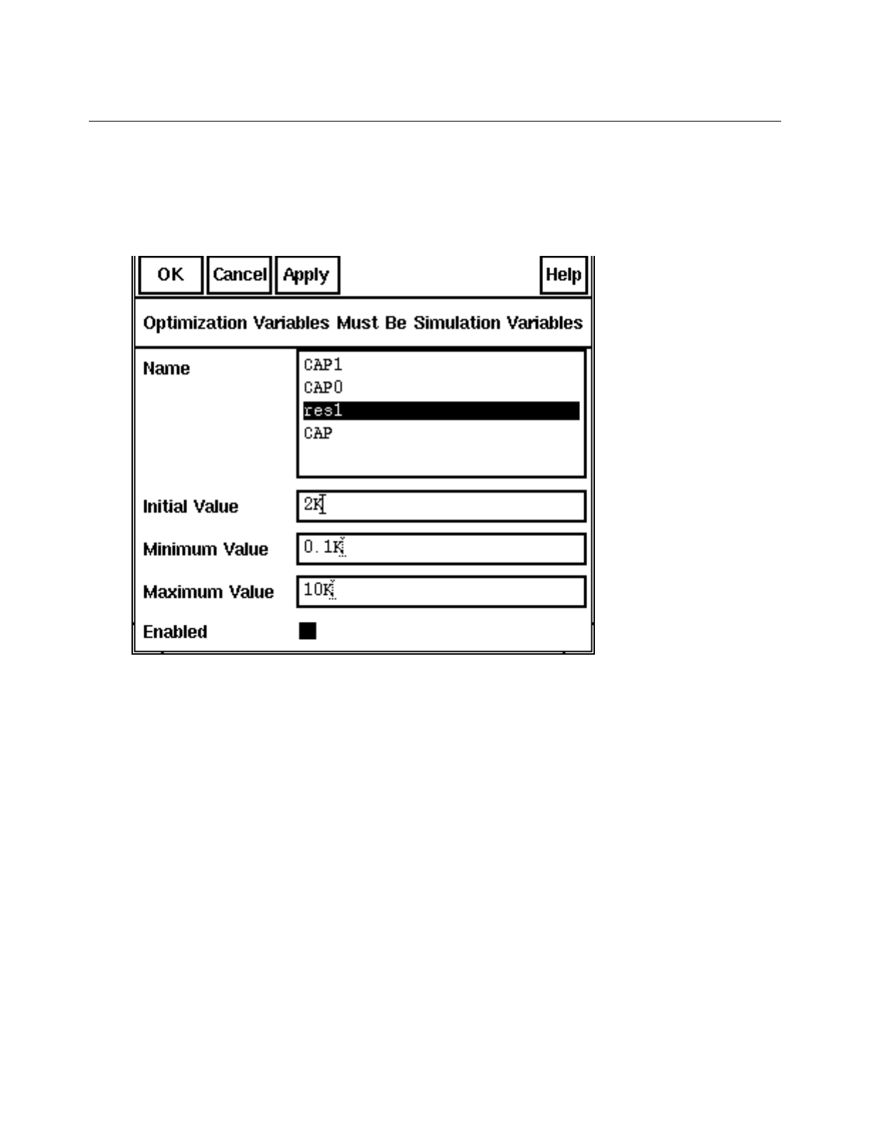
Cadence Advanced Analysis Tools User Guide
Optimization
July 2002 180 Product Version 5.0
1. Highlight the variable you want to edit.
2. Choose Variables – Add/Edit or click Add/Edit Variables.
The Editing Variables form opens.
3. In the Initial Value field, type a value to be used as the starting point for optimization.
4. In the Minimum Value field, type a minimum value. The optimizer never sets the variable
to a value lower than this.
5. In the Maximum Value field, type a maximum value. The optimizer never sets the
variable to a value greater than this.
6. If you want to include the variable in the current analysis, be sure Enabled is on.
7. Click OK.
The changes are applied.
Deleting a Design Variable
To delete one of the design variables listed in the Cadence® Analog Circuit Optimization
Option window,

Cadence Advanced Analysis Tools User Guide
Optimization
July 2002 181 Product Version 5.0
1. Highlight the variable you want to delete.
2. Choose Variables – Delete or click Delete.
Enabling or Disabling a Design Variable
For a quick way to enable or disable a design variable,
1. Highlight the design variable in the Cadence® Analog Circuit Optimization Option
window.
2. Choose Variables – Enable or Variables – Disable.
Controlling the Optimizer
After you define the goals and specify the design variables to use, you are ready to use the
optimizer. The following sections describe how to run and stop the optimizer and how to
delete simulation results you do not want to keep.
Running the Optimizer
To run the optimizer,
1. If the previous run of the optimizer stopped because an error occurred, click Stop
Optimizer to clear the existing state.
2. Choose one of the run commands from the Cadence® Analog Circuit Optimization
Option window.
❑Choose Optimizer –Run or click Run Optimizer to start the optimization from the
beginning and run it until the stopping criteria are met.
❑Choose Optimizer – Step to start the optimization from the most recent stopping
point, iterate once, and then stop.
If you want to start from the beginning of the optimization, choose Optimizer –
Reset before choosing Optimizer – Step.
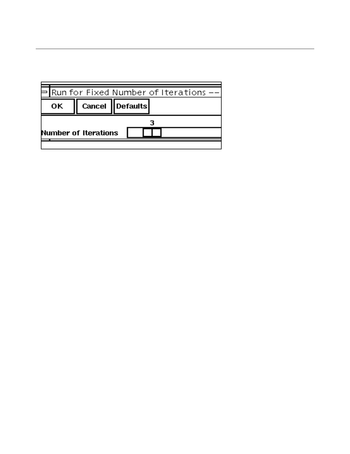
Cadence Advanced Analysis Tools User Guide
Optimization
July 2002 182 Product Version 5.0
❑Choose Optimizer – Run n to open the Run for Fixed Number of Iterations form.
In the form, set the value of n by moving the slider.
Click OK to start the optimization from the most recent stopping point, using the
most recent variable values, and run at most niterations before pausing or stopping.
If you want to start from the beginning of the optimization, choose Optimizer –
Reset before choosing Optimizer – Run n.
As each iteration finishes, the optimizer updates the Prev and Current values displayed in
the Cadence® Analog Circuit Optimization Option window.
Be aware that if you load or reload a state, the next optimizer run starts at the beginning of
the optimization. Be aware also that if you change the characteristics of a goal or the number
of enabled goals and then resume the optimization, the optimizer performs another initial
simulation.
Stopping the Optimizer
To stop the optimizer,
➤Choose one of the stop commands from the Cadence® Analog Circuit Optimization
Option window.
❑Choose Optimizer – Stop or click Stop Optimizer to stop the optimizer after the
current iteration.
❑Choose Optimizer – Stop Now to stop the optimizer immediately without
necessarily completing the current iteration.
You can also click Stop Optimizer to clear the state if an error stops the optimizer before the
normal end of the run.

Cadence Advanced Analysis Tools User Guide
Optimization
July 2002 183 Product Version 5.0
Deleting Simulation Results
To delete all simulation results,
➤Choose Optimizer – Reset.
Any simulation results that exist are deleted. Goals, design variables, and plotting
options remain unchanged.
Plotting Results
The easiest way to track the progress that the optimizer makes toward the goal is to plot the
data as it becomes available at each iteration. When the optimizer achieves acceptable
results, you can update the design to incorporate the optimized variable values.
The following sections explain how to set the plotting options, how to plot the output data, and
how to update your design with the calculated optimal values.
Setting the Plotting Options
To set the plotting options,
1. In the Cadence® Analog Circuit Optimization Option window, choose Results – Set
Plot Options.
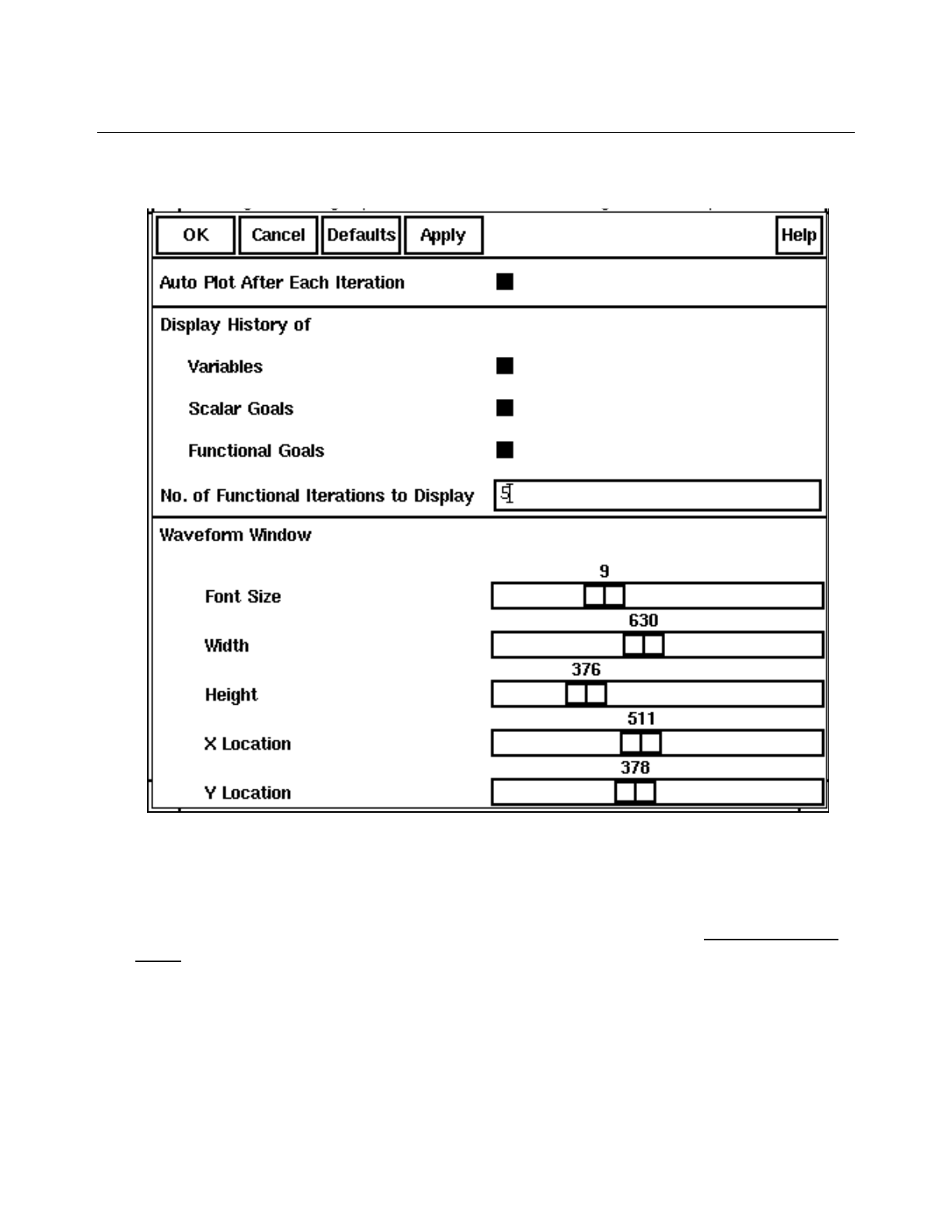
Cadence Advanced Analysis Tools User Guide
Optimization
July 2002 184 Product Version 5.0
The Setting Plotting Options form appears.
2. If you want to be able to follow the progress of the optimization while the optimizer is
running, turn on Auto Plot After Each Iteration.
If you do not want to follow the progress during the run, you can turn off this button and
plot the results when the run has finished. For more information, see “Plotting Output
Data” on page 186.
3. Select at least one kind of information to be included in the output data plot.
❑Turn on Design Variables to produce a plot showing how the design variable
values change during the optimization.
❑Turn on Scalar Goals to produce a plot showing progress toward a scalar goal.
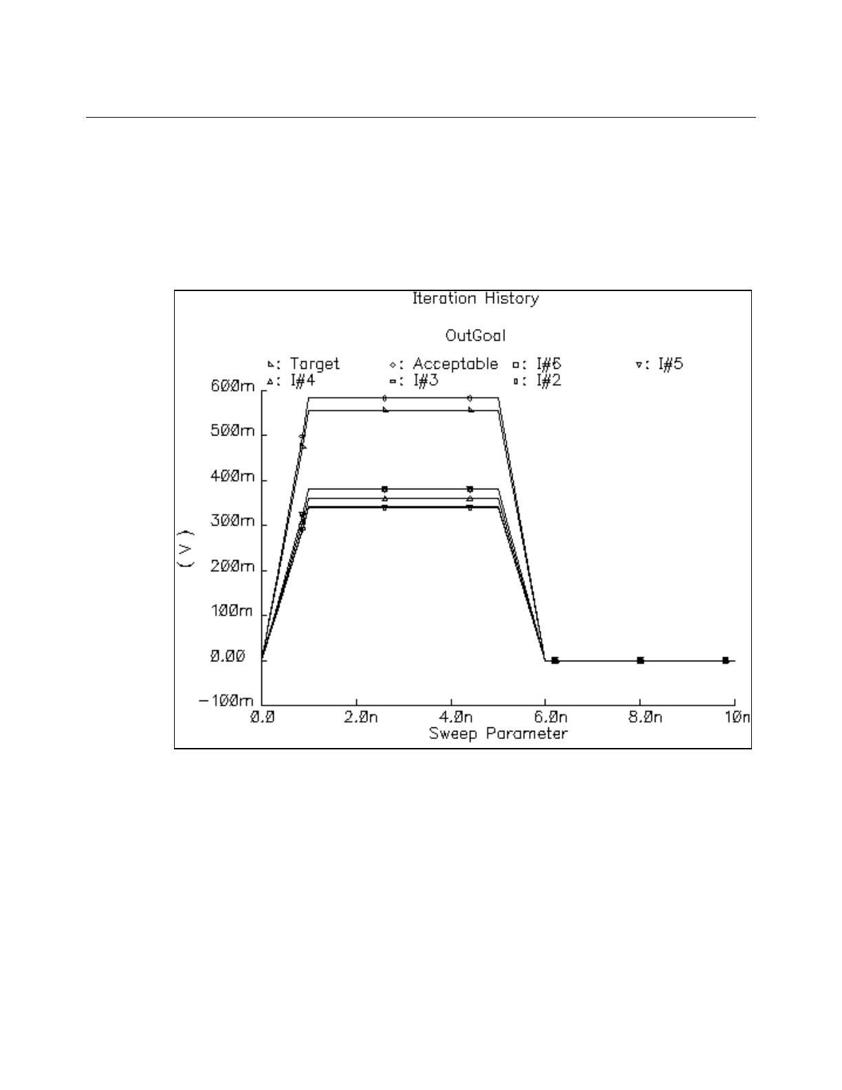
Cadence Advanced Analysis Tools User Guide
Optimization
July 2002 185 Product Version 5.0
You can also see how the scalar numbers change by looking in the Cadence®
Analog Circuit Optimization Option window at the displayed values for Initial,Prev,
and Current.
❑Turn on Functional Goals to produce a plot, like the example below, showing
progress toward a waveform goal.
If there are too many or too few waveforms displayed in this plot, type the number
you want in the No. of Functional Iterations to Display field.
4. Set the Waveform Window characteristics to the values that work best for you. To make
the plot easier to read, for example, you might enlarge the font size and increase the size
of the window.
5. Click OK.
If the Waveform Window is open, the window changes to reflect the new option settings.
If the Waveform Window is closed, it opens with a new plot drawn in accordance with the
changed option settings.
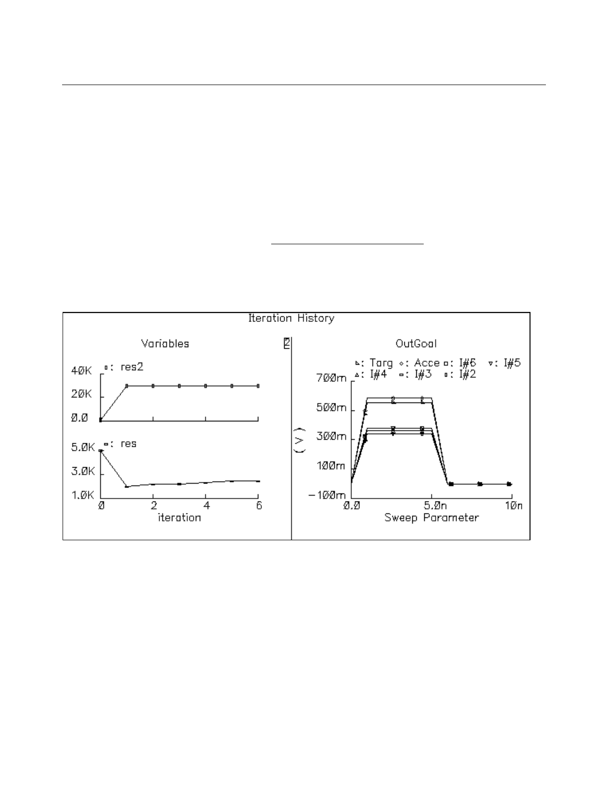
Cadence Advanced Analysis Tools User Guide
Optimization
July 2002 186 Product Version 5.0
Plotting Output Data
If Auto Plot After Each Iteration is turned on in the Setting Plotting Options window, the
Waveform Window automatically opens and displays the results of each optimization. If the
results do not appear automatically, you can use the following procedure to plot them when
the optimization ends.
➤Choose Results – Plot History or click Plot History.
The Waveform Window appears in the format specified by the Setting Plotting Options
window. For more information, see “Setting the Plotting Options” on page 183.
If the plotting options are set so that all the output data is plotted, an output plot might look
like this.
Updating Your Design
To copy the optimized variable values back to your schematic,
1. In the Cadence® Analog Circuit Optimization Option window, choose Results – Update
Design or click Update Design.
2. In the Cadence® Analog Design Environment window, choose Variables – Copy to
Cellview.
3. In the Virtuoso Schematic Editing window, choose Design – Check and Save.
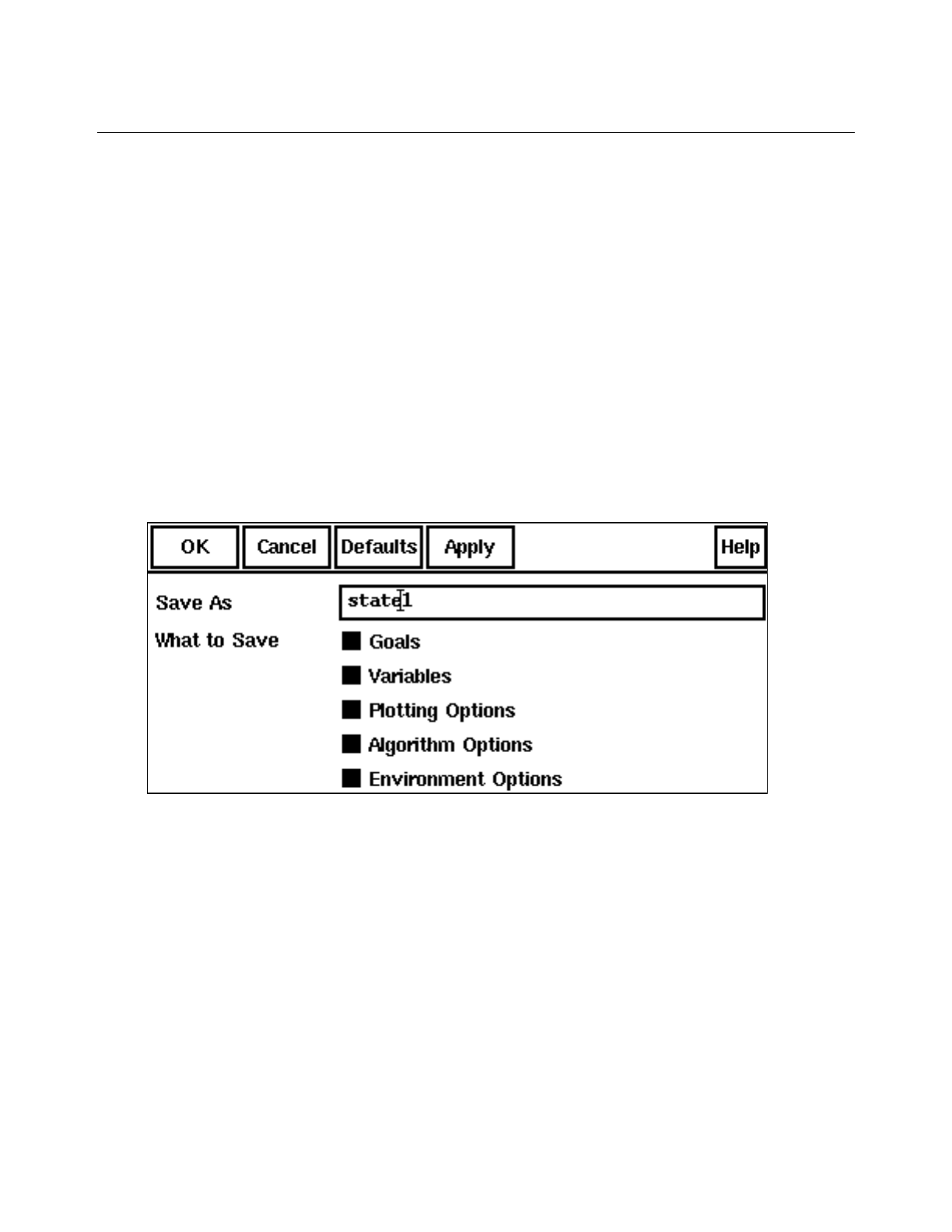
Cadence Advanced Analysis Tools User Guide
Optimization
July 2002 187 Product Version 5.0
Saving, Changing, and Loading Session Information
With the Session menu pulldowns on the Cadence® Analog Circuit Optimization Option
window, you can save the session state, load a saved state, change optimization options, and
clear the window of all information.
Saving the Session State
To save the session state (the goals, variables, and options used in the Cadence® Analog
Circuit Optimization Option window),
1. Choose Session – Save State.
The Saving State form appears.
2. In the Save As field, type a name for the state if you do not want to use the default name.
3. Specify what information is to be saved from the current state.
Only the information you save is available for retrieval when you reload the saved state.
4. Click OK.
The optimizer saves the session state in the directory
~/.artist_states/LibraryName/CellName/.asd_optimization/
StateName
In this directory name, LibraryName and CellName are derived from the circuit you
are optimizing, and StateName is the name you specify in the Saving State form.
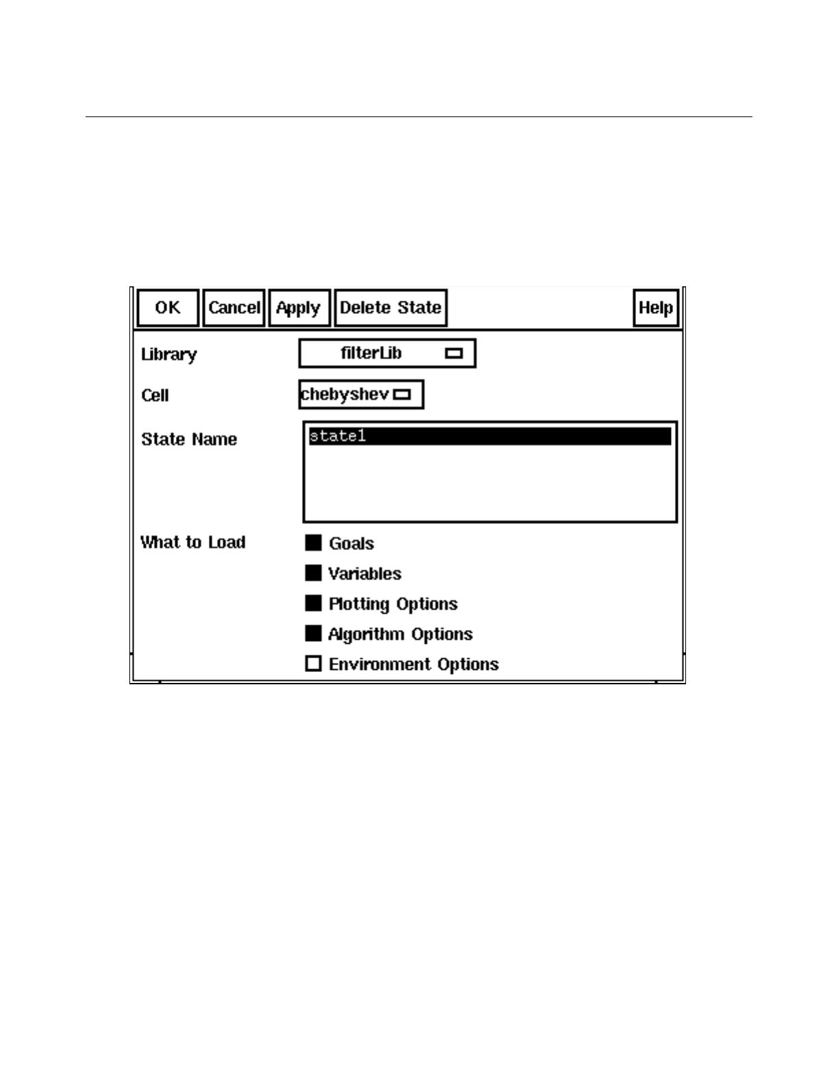
Cadence Advanced Analysis Tools User Guide
Optimization
July 2002 188 Product Version 5.0
Loading a Saved Session State
To load a saved session state,
1. Choose Session – Load State.
The Loading State form appears.
2. From the Library cyclic field, choose the library containing the saved state you want to
load.
3. From the Cell cyclic field, choose the cell containing the saved state you want to load.
4. From the State Name field, choose the state you want to load.
5. Turn on buttons to indicate which information you want to use from the saved state.
6. Click OK.
Saving a Script
The Open Command Environment for Analysis (OCEAN) command language lets you set up,
simulate, and analyze circuit data. OCEAN is a text-based process you can run from a UNIX

Cadence Advanced Analysis Tools User Guide
Optimization
July 2002 189 Product Version 5.0
shell or from the Command Interpreter Window (CIW). You can type OCEAN commands in
an interactive session, or you can create scripts containing your commands and load those
scripts into OCEAN.
You can use the Corners window to set up the analysis you need, and then save the setup
procedure in a script. You can edit the saved script to add simulation or postprocessing
commands as needed.
For more information about OCEAN commands and scripts, see the OCEAN Reference.
To create a script and save it,
1. Choose Session – Save Script.
The Save Ocean Script to File form appears.
2. In the File Name field, specify the name of a file to contain the script.
3. Click OK.
Changing Optimization Options
Most users do not need to change the default optimization options. However, if you want to
use a specific algorithm or if you want to change the values that control the algorithm, follow
these instructions.
1. Choose Session – Options from the Cadence® Analog Circuit Optimization Option
window.
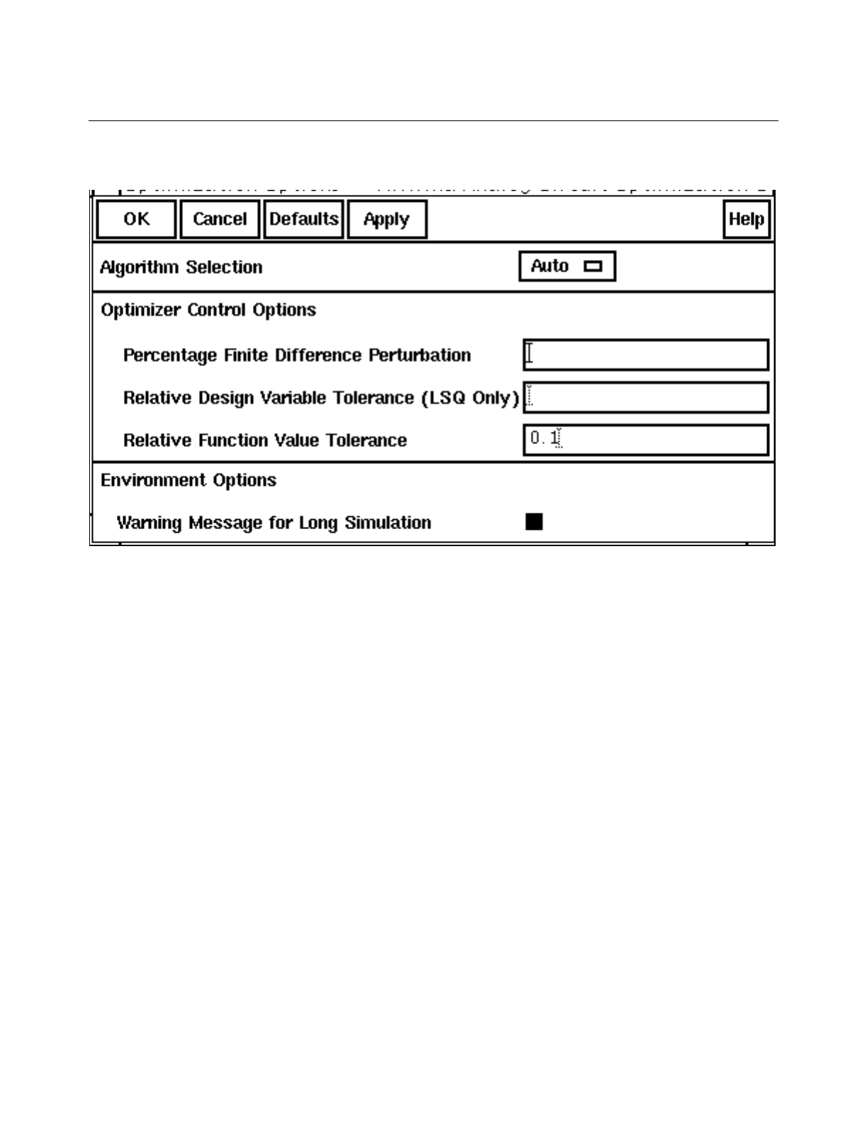
Cadence Advanced Analysis Tools User Guide
Optimization
July 2002 190 Product Version 5.0
The Optimization Options form appears.
2. To force the optimizer to use a particular algorithm, select either LSQ or CFSQP in the
Algorithm Selection field. If you want the optimizer to choose an appropriate algorithm
automatically, select Auto.
The LSQ algorithm is best suited for a pure curve-fitting problem, and Cadence
recommends that you use it only for a problem of that kind.
For the LSQ algorithm, the match,maximize, and minimize directions are all
equivalent. In each of these cases, the LSQ algorithm works to match the specified
Target value. To use the LSQ algorithm for a maximization or minimization problem, you
must specify a Target value that is large enough or small enough that the result reaches
the maximum or minimum before it reaches the Target value.
When the Algorithm Selection cyclic field is set to Auto, the optimizer uses the CFSQP
algorithm in most cases. The optimizer uses the LSQ algorithm only when both of the
following conditions are true.
❑The Direction for all the enabled goals is match.
❑Every enabled goal has a waveform Target.
3. Type values for the Optimizer Control Options you want to change.
❑The Percentage Finite Difference Perturbation value affects how sensitivities
are determined.

Cadence Advanced Analysis Tools User Guide
Optimization
July 2002 191 Product Version 5.0
Be aware that some problems are very sensitive to this value and changing it might
cause the algorithm to perform poorly.
Note: It is recommend that user schoose the default value. For advanced users who
have better knowledge of the effect of the step length, the Finite Difference
Perturbation field provides a way to specify the step length that is appropriate.
Caution should be taken in using this; some problems are very sensitive to the step
length used.
❑The Relative Design Variable Tolerance value affects the LSQ algorithm
stopping criteria. This value has no effect on the CFSQP algorithm.
For example, specifying a value of 0.05 causes the LSQ algorithm to stop when the
relative change in each design variable is smaller than 5 percent.
❑The Relative Function Value Tolerance also affects the algorithm stopping
criteria.
For example, specifying a value of 0.05 causes the algorithm to stop when the
relative change in each function value is smaller than 5 percent.
Note: The Relative Design Variable Tolerance and Relative Function Value
Tolerance fields are designed in a way such that users can stop the algorithm by
specifying stopping criteria to be used rather than using the default settings. These fields
are entered as absolute numbers. For example, if a user specifies 0.01 in the Relative
Design Variable Tolerance field, that means if the relative change in the design
variables is smaller than 1 percent, the algorithm would stop. Likewise, if 0.01 is specified
in the Relative Function Value Tolerance field, the algorithm will stop when the
relative change in each function value is smaller than 1 percent.
4. Set Warning Message for Long Simulation.
The optimization tool and the Cadence® Analog Design Environment are both locked for
the duration of the initial simulation run of the optimization. During that initial run, you
cannot stop the simulation or monitor the progress. If you want to be warned of a
potentially long simulation, leave Warning Message for Long Simulation turned on,
otherwise, turn it off.
5. Click OK.
Deleting All Setup Information
To delete all the setup information about goals, variables, and plotting options,
➤Choose Session – Reset.
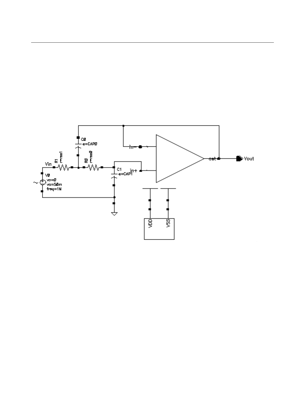
Cadence Advanced Analysis Tools User Guide
Optimization
July 2002 192 Product Version 5.0
Working through an Extended Example
This section follows an optimization session in detail, demonstrating how you might use the
optimizer to improve a real circuit. The example describes how to optimize a Chebyshev filter
so that its frequency response matches a specified waveform and its noise output is
minimized.
The Chebyshev filter has the following schematic:
Notice the two resistors, R0 and R1. These are the components whose values are optimized
during the session.
To follow along with this example, go to a working directory and use a command like the
following to copy all the contents of the optimization directory into the working directory.
tar -cvhf - -C <install_dir>/tools/dfII/samples/artist optimization
| tar -xvf -
Then go to the optimization directory you created, start icms, and continue with the
following steps.
1. In the CIW, choose Tools – Analog Environment – Simulation.
The Cadence® Analog Design Environment window appears.
2. Choose Setup – Design.
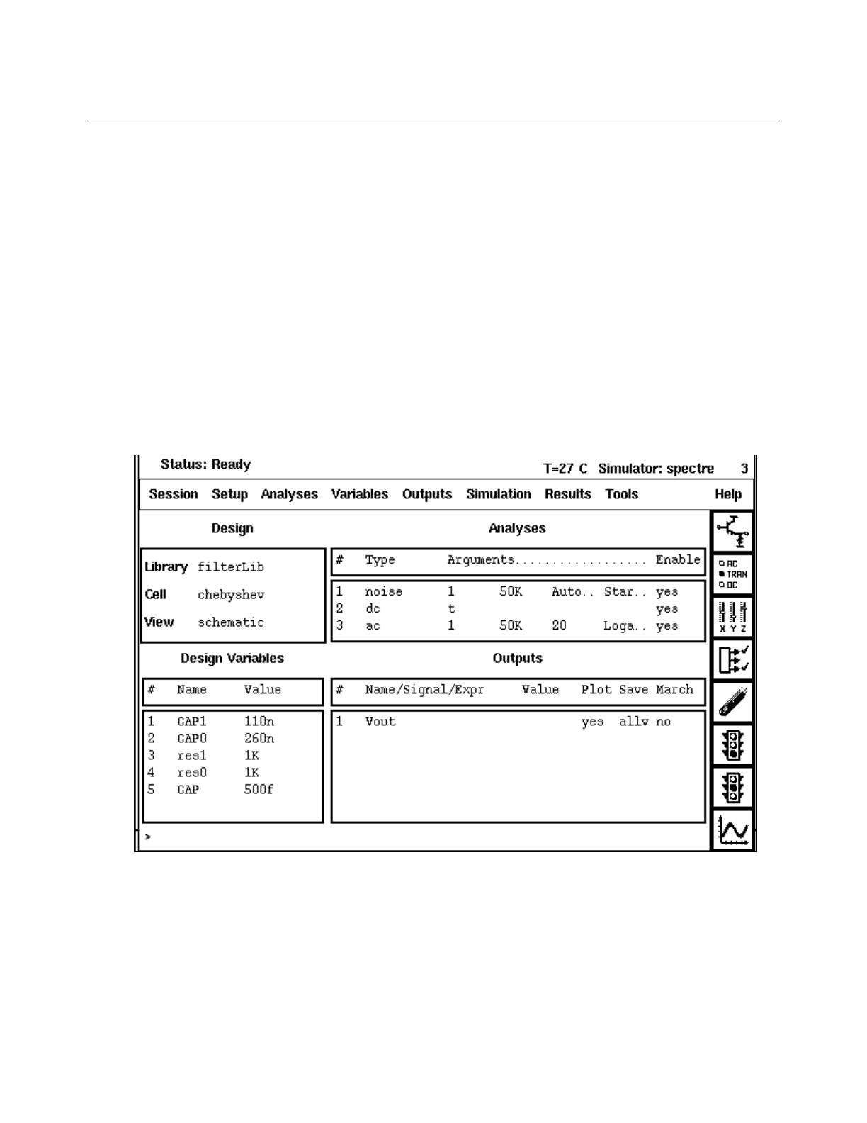
Cadence Advanced Analysis Tools User Guide
Optimization
July 2002 193 Product Version 5.0
The Choosing Design form appears.
3. In the Library Name field, choose the filterlib library.
4. In the Cell Name field, choose the chebyshev cell.
5. Click OK.
6. In the Cadence® Analog Design Environment window, choose Session – Load State.
The Loading State form appears.
7. In the State Name field, choose state1.
8. Click OK.
The Cadence® Analog Design Environment window now looks like this.
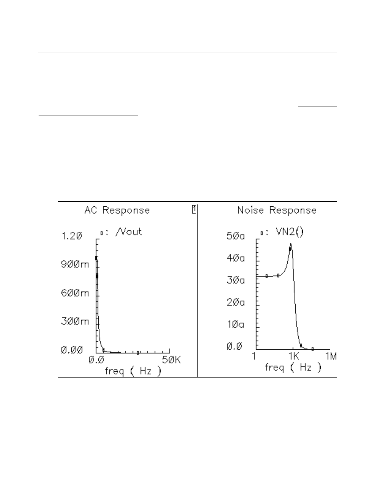
Cadence Advanced Analysis Tools User Guide
Optimization
July 2002 194 Product Version 5.0
Generating the Targets
This section explains how to generate two waveforms, which are used as targets for the
optimization described later. If this were an actual optimization session, you would probably
have existing targets and could skip directly to the optimization step described in “Setting Up
and Running the Optimization” on page 195.
You run this initial simulation, which does not involve using the optimizer at all, just as you run
other ordinary simulations.
➤In the Cadence® Analog Design Environment window, choose Simulation – Run.
If the Welcome to Spectre window appears, click OK to close it.
When the simulation finishes, a waveform window appears.
Close this waveform window.

Cadence Advanced Analysis Tools User Guide
Optimization
July 2002 195 Product Version 5.0
Saving the Targets
1. In the Cadence® Analog Design Environment window, click Results - Save.
2. In the Save Results window, specify schematic-save in the Save As field. Click OK.
3. In the Cadence® Analog Design Environment window, click Results - Select.
4. In the Select Results window, select schematic-save and click OK.
5. In the Cadence® Analog Design Environment window, click the Plot Outputs icon.
A waveform window similar to the one generated earlier appears. These two waveforms
become the targets for the optimization session described in the next section.
Setting Up and Running the Optimization
This section describes how to set up and run the optimization for the Chebyshev filter.
1. In the Cadence® Analog Design Environment window, choose Tools – Optimization.
The Cadence® Analog Circuit Optimization Option window appears.
2. Fill in the Goals and Variables panes with the values that are required for the
optimization.
This step is described in the next section.
Filling in the Goals Pane
In this example, you want to use the optimizer to determine what resistor values will allow you
to match the AC Response waveform while minimizing the noise waveform. The following
sections describe how to specify the goals that correspond to these waveforms.
Specifying the AC Response Goal
To define the goal corresponding to the AC Response, follow these steps.
1. In the Cadence® Analog Circuit Optimization Option window, choose Goals – Add.

Cadence Advanced Analysis Tools User Guide
Optimization
July 2002 196 Product Version 5.0
The Adding Goals window appears.
2. Enter a name for the goal in the Name field.
For this example, type magVF.
3. To create the expression, you can use the Waveform Calculator. To open it, click Open.
4. Open the Virtuoso Schematic window by choosing Session – Schematic Window in
the Cadence® Analog Design Environment window.
5. In the Waveform Calculator, click vf and then go to the Virtuoso Schematic window and
select the net connected to Vout. Press Esc to end the selection.
6. In the Waveform Calculator, click mag.
The calculator display now contains the value mag(VF("/Vout")).
7. In the Adding Goals window, highlight the Expression field, then click Get Expression
to copy the expression from the calculator.
8. For this example, you want to match the AC Response waveform, so choose match in
the Direction cyclic field.
9. The Target value for this goal is to be the AC Response waveform calculated earlier, as
described in “Generating the Targets” on page 194. To specify the waveform, first click
clst in the calculator to clear the calculator display.

Cadence Advanced Analysis Tools User Guide
Optimization
July 2002 197 Product Version 5.0
10. In the calculator, click wave, then go to the Waveform Window and click on the AC
Response waveform.
An expression similar to the following appears in the Calculator display:
mag( VF("/Vout" "/old2/lorenp/simulation/chebyshev/spectre/
schematic-save") )
This expression represents the AC Response waveform.
11. In the Adding Goals window, select the Target field, then click Get Expression to copy
the waveform.
12. Type 5 in the Acceptable field and turn on % within Target.
13. Ensure that Enabled is turned on.
The Adding Goals window now looks like this.
14. Click Apply.
The new goal appears in the Cadence® Analog Circuit Optimization Option window.
Specifying the Noise Goal
The steps required to define the noise goal are similar to those required for the AC Response
goal.

Cadence Advanced Analysis Tools User Guide
Optimization
July 2002 198 Product Version 5.0
1. If the Adding Goals window is not open, choose Goals – Add in the Cadence® Analog
Circuit Optimization Option window.
2. Type a name for the goal in the Name field.
For this example, type noise.
3. Erase any existing information, then type VN2() in the Expression field.
4. Specify the Target, which for this goal is to be the Noise Response waveform calculated
earlier, as described in “Generating the Targets” on page 194. To specify the waveform,
first open the calculator by clicking Open in the Adding Goals window.
5. Click clst in the calculator to clear the calculator display.
6. In the calculator, click wave, then go to the Waveform Window and click on the Noise
Response waveform.
An expression similar to the following appears in the calculator display:
VN2()
Type the following path in the brackets:
"/old2/lorenp/simulation/chebyshev/spectre/schematic-save"
This expression represents the Noise Response waveform.
7. Return to the Adding Goals window, select the Target field, then click Get Expression
to copy the waveform.

Cadence Advanced Analysis Tools User Guide
Optimization
July 2002 199 Product Version 5.0
8. Fill in the other fields of the Adding Goals window, as follows.
9. Click OK.. The new goal appears in the Cadence® Analog Circuit Optimization Option
window.
10. You can return to the calculator window and close it by choosing Window – Close.
Filling in the Variables Pane
In this example, you want to optimize the values of two resistors: res0 and res1. To prepare
for the optimization, you need to set the initial, minimum, and maximum allowed values.
1. In the Cadence® Analog Circuit Optimization Option window, choose Variables – Add/
Edit.
The Editing Variables form appears.

Cadence Advanced Analysis Tools User Guide
Optimization
July 2002 200 Product Version 5.0
2. Click on res1, and then fill in the other fields as shown.
3. Click Apply.
The information about the res1 variable appears in the Cadence® Analog Circuit
Optimization Option window.
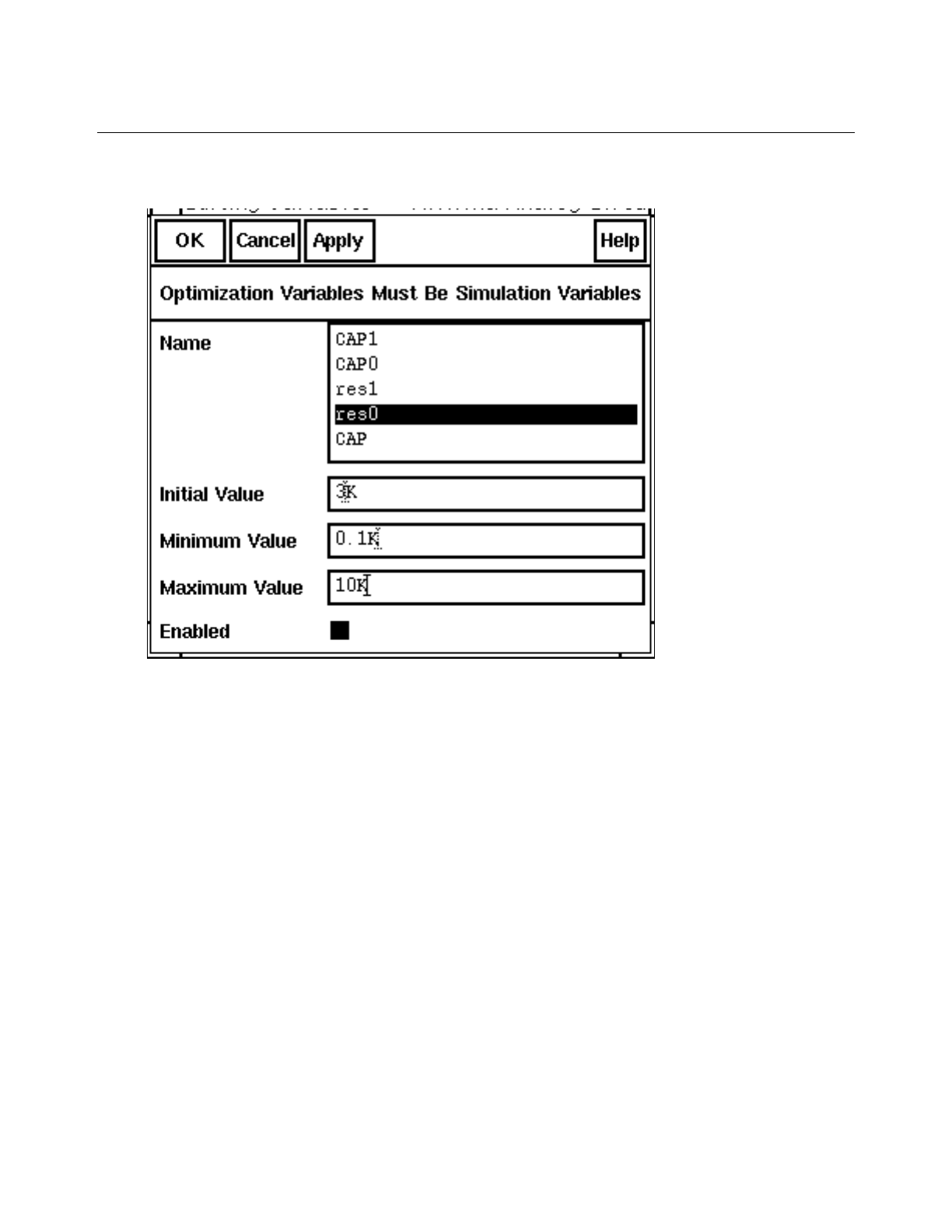
Cadence Advanced Analysis Tools User Guide
Optimization
July 2002 201 Product Version 5.0
4. In the Editing Variables form, click on res0 and then fill in the other fields as shown.
5. Click OK.
The information about the res0 variable appears in the Cadence® Analog Circuit
Optimization Option window.
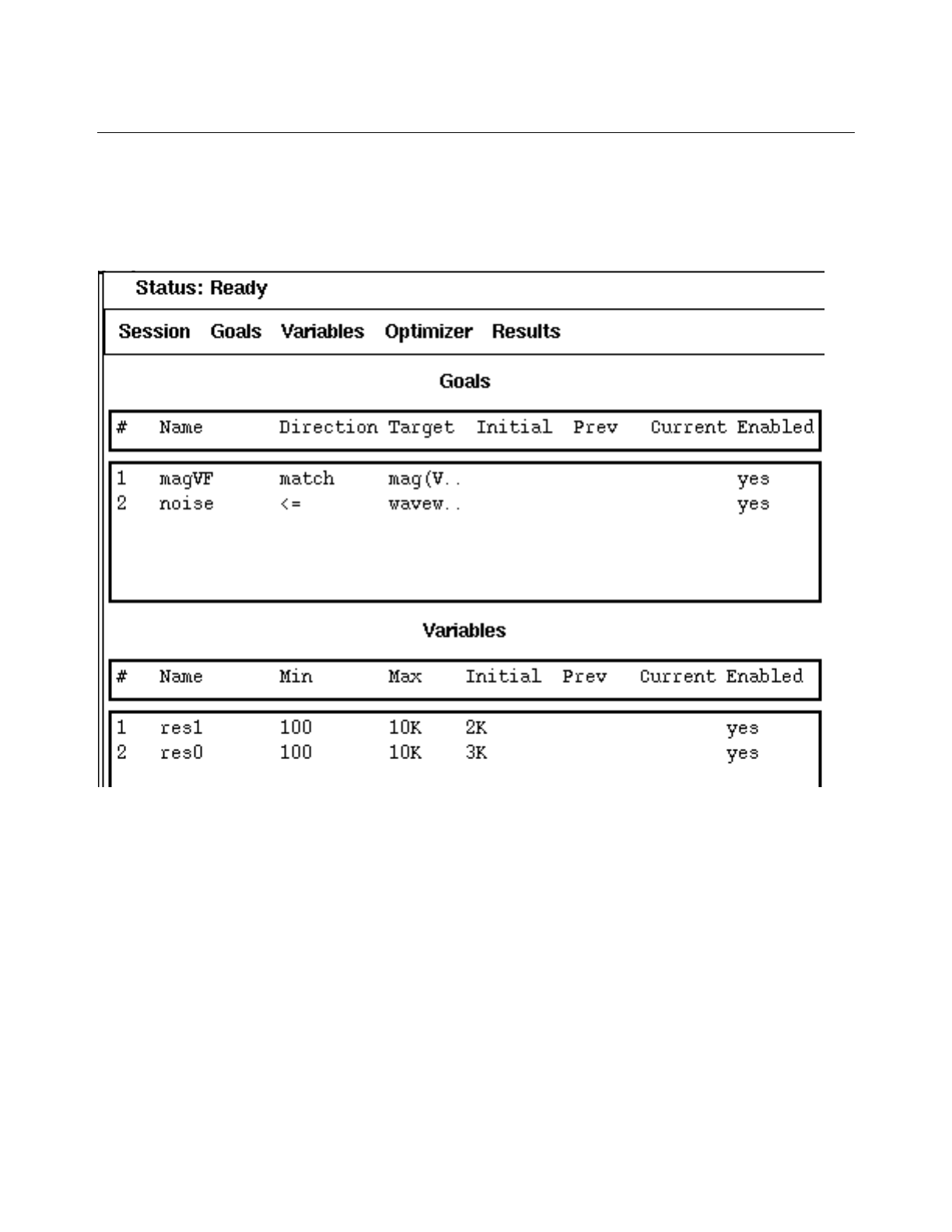
Cadence Advanced Analysis Tools User Guide
Optimization
July 2002 202 Product Version 5.0
Running the Optimization
With the goals and variables defined, the Cadence® Analog Circuit Optimization Option
window looks like this.
At this point in the example, you are ready to run the optimization.
➤In the Cadence® Analog Circuit Optimization Option window, choose Optimizer – Run
or click Run Optimizer.
The optimization starts and the status display updates to reflect the current activity.
Looking at the Output
With the default plotting options, a Waveform Window appears soon after the optimization run
begins and updates after each iteration. When this example optimization ends, the Waveform
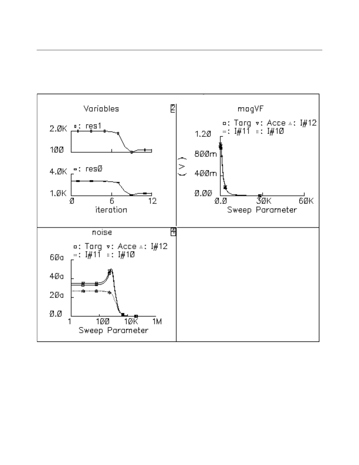
Cadence Advanced Analysis Tools User Guide
Optimization
July 2002 203 Product Version 5.0
Window displays the iteration history of the res0 and res1 variables. It also displays the
changing waveforms for the magVF and noise goals.
You can change the information that displays in the Waveform Window. For example, to look
at the variables in more detail, follow these steps.
1. In the Cadence® Analog Circuit Optimization Option window, choose Results – Set
Plot Options.
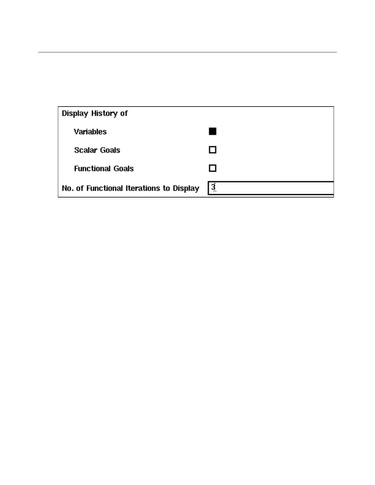
Cadence Advanced Analysis Tools User Guide
Optimization
July 2002 204 Product Version 5.0
2. In the Setting Plotting Options window, turn off Display History of Scalar Goals and
Display History of Functional Goals, leaving only the Display History of Variables
selected.
3. Click OK.
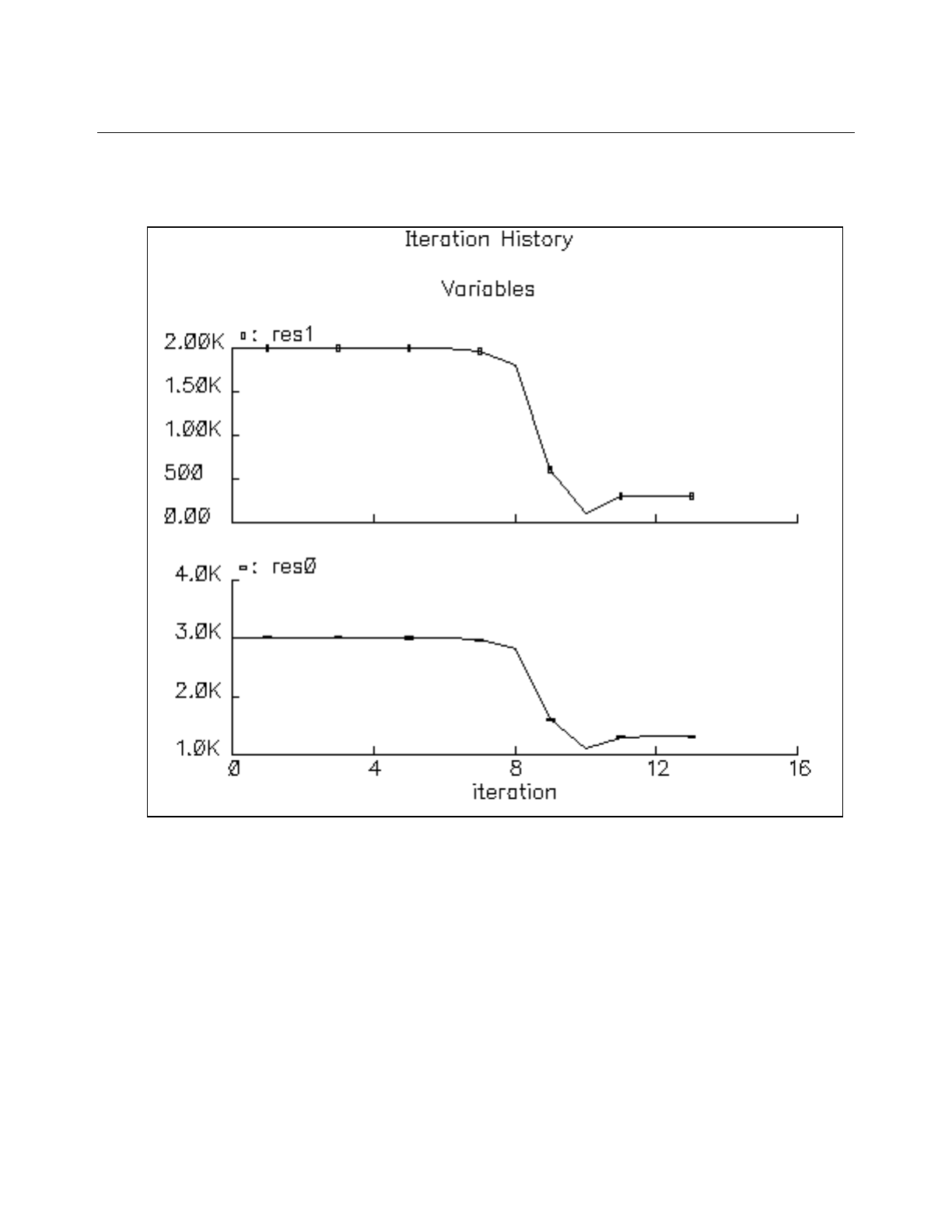
Cadence Advanced Analysis Tools User Guide
Optimization
July 2002 205 Product Version 5.0
The Waveform Window appears, showing only the variables.
During the 13 iterations of this optimization (iteration 0 shows the initial values), the value
of res1 went from the starting value of 2.00 K to the final value of 304.7. This final value
also appears in the Current column of the Variables pane in the Cadence® Analog
Circuit Optimization Option window.
To look at the goals in more detail,
1. In the Setting Plotting Options window, turn on Display History of Functional Goals.
2. Turn off Display History of Variables and Display History of Scalar Goals.
3. Set No. of Functional Iterations to Display to 1.
4. Click OK.
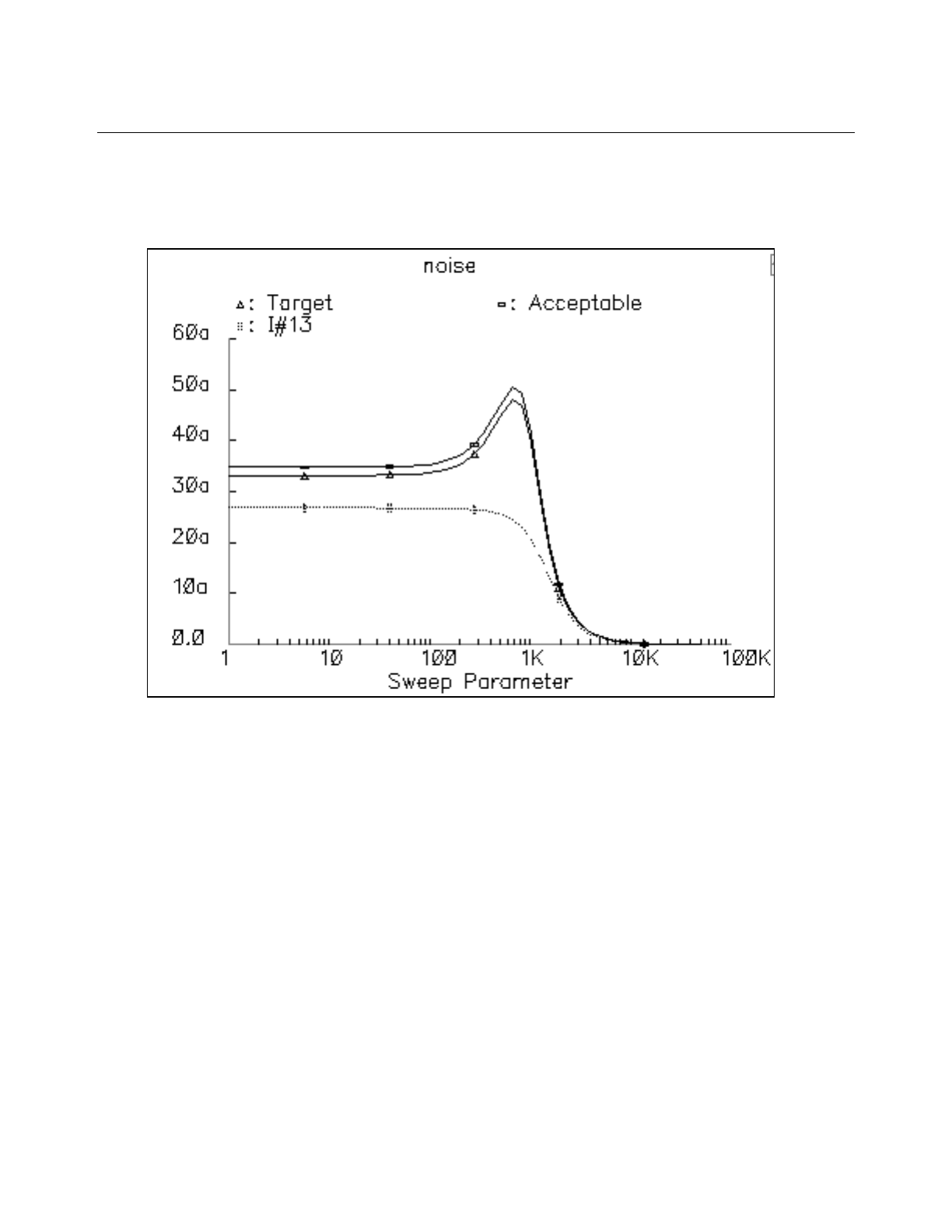
Cadence Advanced Analysis Tools User Guide
Optimization
July 2002 206 Product Version 5.0
The Waveform Window appears or redraws with only the goals showing. For example,
the noise goal looks like this.
The last iteration, I#13, shows that the optimizer was able to lower the noise below the
target throughout the entire frequency range.
The optimized values for the two resistors are displayed in the current column of the
Cadence® Analog Circuit Optimization Option window: res1 has an optimized value of 304.7
and res0 has an optimized value of 1.311 K. To use these values in your design, do the
following:
➤In the Cadence® Analog Circuit Optimization Option window, choose Results – Update
Design.

Cadence Advanced Analysis Tools User Guide
Optimization
July 2002 207 Product Version 5.0
The new values appear in the Design Variables pane of the Cadence® Analog Design
Environment window.

Cadence Advanced Analysis Tools User Guide
Optimization
July 2002 208 Product Version 5.0

Cadence Advanced Analysis Tools User Guide
July 2002 209 Product Version 5.0
Index
Symbols
% within Target 166, 168
.cdsinit file
example 63
loading PCFs and DCFs from 16, 20,
40
A
Acceptable values
creating waveform objects for 170
entering an expression for 165, 168
restrictions on 165, 168
setting as percentage of Target 166,
168
valid 165, 168
weights, using to assign 174
Add button (Monte Carlo) 79, 83
Add Corner button (Corners) 16
Add Measurement button (Corners) 18, 26
Add Process dialog box 52
Add Variable button (Corners) 16
Add/Edit Goals button (optimization) 164,
166, 169
Add/Edit Variables button
(optimization) 178, 180
adding
corners 16
design variables (optimization) 178
variables (Corners) 16, 24
Adding Goals window 196, 197, 199
algorithms
automatic selection of 190
CFSQP 154
choosing manually 190
LSQ 154
amplifier schematic (Monte Carlo) 123
Analysis Setup pane
description 75
Monte Carlo extended example 129
Analysis Variation cyclic field (Monte
Carlo) 98
analysis variation type, specifying 80
appending scalar output data to saved
data 76
Autoplot After Each Iteration button
(optimization) 184, 186
Autoplot button (Monte Carlo) 83
autoplot field 78
B
Best Fit Line 115
button bar (Monte Carlo) 79
buttons
Corners
Add Corner 16
Add Measurement 18, 26
Add Variable 16
Calculator 18, 27
Copy Corner 16
Delete Measurement 18, 27
Delete Row 25
Delete Selected / Delete Corner /
Delete Row 16
Get Expression 18, 27
Plot/Print 29
Run 28
Run / Stop 17
Monte Carlo
Add 79, 83
Autoplot 83
Calculator 79, 84
Change 79, 84
Clear 79
Delete 79, 84
Density Estimator 112
Get Expression 79
Load 104, 106
optimization
Add/Edit Goals 164, 166, 169
Add/Edit Variables 178, 180
Autoplot After Each Iteration 184,
186
Delete (design variables) 181
Delete (goals) 170
Design Variables 184
Enabled (goals) 166, 169, 179, 180
Open 167

Cadence Advanced Analysis Tools User Guide
July 2002 210 Product Version 5.0
Scalar Goals 184
Special Functions 171
Stop Optimizer 182
Update Design 186
Waveform Goals 185
C
Cadence® analog corners analysis window
closing 10
opening 10
Cadence® analog optimization analysis
window, closing 156
window, opening 156
Cadence® analog optimization analysis
window
description 157
opening 195
Cadence® analog statistical analysis
window 72
calculator
building expressions with (Monte
Carlo) 84
building goal expressions with
(optimization) 166
creating waveforms with
(optimization) 171
opening 167
Calculator button
Corners 18, 27
Monte Carlo 79, 84
.cdsinit file 63
.cdsinit file, using to load PCFs and
DCFs 16, 20, 40
cdsSpice simulations
and select all options 90
CFSQP algorithm, data suited for 154
Change button (Monte Carlo)
description 79
example of use 84
Chebychev filter
description 192
Clear button (Monte Carlo) 79
columns, selecting in Corner Definitions
pane 16
conditional yield
definition 117
reports, description 108
reports, printing 120
Conditional Yield form 121
Copy Corner button 16
copying an existing corner 16
Corners
analysis
definition 9
extended example 55
overview 9
starting 28
stopping 28
Corner Definitions pane, description 15
log file 19
menu 13
corners
defining, in Cadence analog corners
analysis window 23
deleting 25
specifying 20
corners0.log 19
Correlation Table window (Monte
Carlo) 110
correlation tables
description 107
printing 110
corSetModelFile procedure
used only with single model library
style 36
using to enter model file name 41
cumulative box histograms 111
cumulative line histograms 111
Current field 160, 161
currents, saving all 89
D
data
filter
reloading settings 104
saving settings 104
specifying settings 103
turning off 104
outlying error values, filtering out 102
saving between runs 82
Data Filter form 103
DCFs. See design customization files
(DCFs)
debugging PCFs and DCFs 36
Delete button (Monte Carlo) 79, 84
Delete button (optimization)
for design variables 181
for goals 170

Cadence Advanced Analysis Tools User Guide
July 2002 211 Product Version 5.0
Delete Measurement button (Corners) 18,
27
Delete Row button (Corners) 25
Delete Selected / Delete Corner / Delete
Row button (Corners) 16
deleting
corners 25
design variables 180
goals 170
simulation results 183
user-defined corners 16
variables or groups 25
Density Estimator button (Monte
Carlo) 112
Design – Check and Save 186
design customization files (DCFs)
.cdsinit, loading with 40
commands normally placed in 36
debugging with OCEAN 36
loaded after PCFs 40
loading from the graphical user
interface 21
tailoring a Corners analysis with 20
use of 35, 38
design variables
adding to DCF 38
deleting all 191
deleting specific 180
determining sensitivities of 155
editing 179
enabling or disabling 181
examples of 178
names, as displayed in Corner
Definitions pane 16
pane showing values of 161
plotting 184
setting maximum value for 179, 180
setting minimum value for 179, 180
stopping criteria for 191
sweeping 81
updating schematic, with optimized 186
Design Variables button 184
design, updating with optimized
values 186
device descriptions, for Monte Carlo 70
direction
specifying for Chebychev filter
example 196
specifying for goals 165, 167
Direction field 160
disabling
design variable 181
goals 170
disk storage requirements, reducing 82
distribution concentration, estimating 112
E
Edit – Add Measurement 26
Edit – Delete Corner 25
Edit – Delete Measurement 27
Edit – Delete Row 25
edit fields
clearing 79
description 78
editing
design variables 179
goals 169
Editing Variables form 199
Enabled button
for goals 166, 169, 179, 180
Enabled field 160, 161
enabling
design variables 181
goals 170
error messages (Corners) 19
example, extended
optimization 192
Expression column, in Corners Performance
Measurements pane 18
expressions
adding 79
adding by typing in 83
changing 79, 84
checking validity 90
creating with the calculator 196
deleting 79, 84
entering in Performance Measurements
pane 18
getting from the calculator 196
listed in the Outputs pane 77
names for 77
retrieving from calculator (Corners) 18
retrieving from calculator (Monte
Carlo) 79
used to specify goals 163
using calculator to build 84
extended examples
Corners analysis 55
Corners, PCF for 61
Monte Carlo 122

Cadence Advanced Analysis Tools User Guide
July 2002 212 Product Version 5.0
F
family of curves
for Monte Carlo extended example 138
plots, description of 107
plotting 113
saving data for 76, 82
feasible initial values, determined by CFSQP
algorithm 155
File – Close 11
File – Load 21
File – Save Ocean Script 35
File – Save Setup 33
File – Save Setup As 33
Filter By data set 103
Filter By point 103
filter, Chebychev 192
filtering, turning off 104
folded cascode, schematic 56
formats, choosing for output 28
forms and windows
Add Process (Corners) 52
Adding Goals 164, 167, 196, 197, 199
Cadence analog corners analysis 12
Cadence analog optimization
analysis 157, 167
Cadence analog statistical analysis 72
Cadence® analog corners analysis 10
Cadence® analog statistical
analysis 72
Conditional Yield 121
Correlation Table 110
Data Filter 103
Editing Goals 169
Editing Variables 179, 180, 199
Histogram 112
Iteration Versus Value 109
Load (Corners) 22
Load Data Filter Values 105
Load Specification Limits 107
Loading State 188
Monte Carlo Load 96
Monte Carlo Save Ocean Script 97
Multiconditional Yield 119
Optimization Options 190
Process/Model Info Setup (Corners) 53
Run for Fixed Number of Iterations 182
Save Changes? (Corners) 21
Save Data Filter Values 104
Save Ocean Script (Corners) 35, 189
Save Results 94
Save Specification Limits 106
Saving State 187
ScatterPlot 115
Select Results 101
Setting Plotting Options 184, 204
Simple Yield 118
Specification Limits 105
Waveform 172, 185, 194
frequency response, matching 192
Functional Goals button 185
G
GAUSS function, used in Monte Carlo 127
Get Expression button (Corners) 18, 27
Get Expression button (Monte Carlo) 79
goals
definition 163
deleting all 191
deleting specific 170
editing 169
enabling or disabling 170
example of specifying 195
saving 187
specifying direction for 165, 167
specifying expression for 165, 167
specifying for Chebychev filter
example 197
specifying name for 167
Goals – Add 164, 166, 195, 198
Goals – Delete 170
Goals – Disable 170
Goals – Edit 169
Goals – Enable 170
Goals pane 160
graphical user interface
Corners 12
Monte Carlo 72
optimization 157
groups
deleting 25
name, as displayed by Corners 16
H
help
for optimization 155
Histogram form 112

Cadence Advanced Analysis Tools User Guide
July 2002 213 Product Version 5.0
histograms
description 107
for Monte Carlo extended example 133
plotting 111
I
individual yield 117
information messages, as displayed by
Corners 19
Initial field 160, 161
initial values, determining feasible values
for 155
input files, creating by hand 95
iteration history 203
iteration versus value tables
description 107
printing 108
Iteration Versus Value window 109
L
least squares fit lines, for scatter plots 115
Load button (Monte Carlo) 104, 106
Load Data Filter Values form 105
Load dialog box 22
Load Specification Limits form 107
loading
session state 96
stored outputs 100
Lower column, in Performance
Measurements pane 18
lowpass filter
description 122
model file 126
schematic 122
LSQ algorithm
conditions of use for 190
data suited for 154
equivalence of match, minimize, and
maximize 174
M
Max field 161
maximize
equivalent to match for LSQ
algorithm 174
Target used only for weighting when
chosen 174
mcdata file, creating from saved waveform
data 102
mcparam file, creating 95
mcrun.s file
creating 95
Measurement column, in Performance
Measurements pane 18
measurements
adding new row for 18
creating by hand 26
creating with calculator 26
deleting 18, 27
setting highest acceptable value for 18
setting lowest acceptable value for 18
setting target value for 18
menu
Corners analysis tool 13
Monte Carlo tool 73
optimizer 158
messages, displayed in Corners status
bar 19
Min field 161
minimize
equivalent to match for LSQ
algorithm 174
Target used only for weighting when
chosen 173
minmax, algorithm for 154
Mismatch Only variation type 80
model files
connecting to Analysis Variation
cyclic 98
for Monte Carlo 70
lowpass filter 126
model files, purpose 35
modeling styles
multiple model library 43
multiple numeric 47
multiple parametric 49
single model library 41
single numeric 46
supported by Corners analysis tool 40
Monte Carlo analysis
Analysis Setup pane 75
analyzing results 132
button bar 79
edit fields 78
extended example 122
graphical user interface for 72

Cadence Advanced Analysis Tools User Guide
July 2002 214 Product Version 5.0
menu 73
number of runs, specifying 80
Outputs pane 77
overview 69
requirements for running 70
results, analyzing 100
specifying analysis variation type for 80
specifying characteristics for 75
specifying initial run number for 80
starting 93
status display 73
stopping 93
Monte Carlo Load form 96
Monte Carlo Save Ocean Script form 97
Monte Carlo tool
closing 98
starting 70
multiconditional yield
definition 117
reports, description 108
reports, printing 119
Multiconditional Yield form 119
multiple model library style
described 43
requirements for using 54
multiple numeric modeling
described 47
example of 59
PCF for 48
multiple parametric modeling
described 49
PCF for 50
N
Name field (goals) 160
Name field (variables) 161
No. of Functional Iterations to Display 205
noisy data, best optimized with LSQ
algorithm 154
number of runs, specifying 76
O
OCEAN script, saving 96
Open button 167
opening the Cadence® analog optimization
analysis window 195
optimization
definition 153
extended example 192
help for 155
output, changing what is displayed
in 204
overview 154
setting options for 189
setting up and running 195
steps followed during 154
using waveform goals for 196
optimized values, where displayed 206
optimizer
control options, setting 190
definition 153
running 181
stopping 182
Optimizer – Reset 183
Optimizer – Run 181, 202
Optimizer – Run n 182
Optimizer – Step 181
Optimizer – Stop 182
Optimizer – Stop Now 182
options
for optimization 189
for plotting 183
outlying data, filtering 102
output data, appending to saved data 76
output formats
choosing (Corners) 28
residual plot example (Corners) 31
text example (Corners) 29
output information for optimization,
changing 203
output log, viewing 98
outputs
choosing after the analysis runs 29
loading 100
of the Chebychev filter example 202
saving all 89
saving to specific file 94
Simulation window outputs appear in
Corners 63
Outputs – Retrieve Outputs 82
Outputs – Save All 89
Outputs – To Be Saved – Select On
Schematic 90
Outputs pane 77

Cadence Advanced Analysis Tools User Guide
July 2002 215 Product Version 5.0
P
parameter storage format (PSF)
directory, copying 94
files, saving between runs 76
parameters
for Spectre, must be in main circuit 55
showing correlations among 110
sweeping 81
pass/fail histograms 111
PCFs. See process customization files
(PCFs)
% within Target 166, 168
percentage finite difference
perturbation 190
performance measurements
adding to DCFs 38
creating by hand 26
creating with calculator 26
deleting 27
pane 17
Plot/Print button 29
plotting
automatic 78
histograms 111
options, resetting all 191
options, saving 187
output data 186
progress toward scalar goals 184
progress toward waveform goals 185
setting options for 183
setting Waveform Window
characteristics 185
specifying number of waveforms to
display 185
waveforms 172
Prev field (for goals) 160
Prev field (for variables) 161
process customization files (PCFs)
.cdsinit, loading with 16, 40
commands normally placed in 36
creators of 35, 36
debugging with OCEAN 36
example 37
for multiple numeric modeling 48
for multiple parametric modeling 50
for single file modeling 42, 44
for single numeric modeling 46
loaded before DCFs 40
loading from DCF 40
loading from the graphical user
interface 21
used for predefined corners 20
process field 15
Process Only variation type 80
process variables
adding in Corners window 53
Process Variation and Mismatch variation
type 81
processes
defining in Corners window 52
modifying in Corners window 53
name of 15
PSF (parameter storage format)
directory, copying 94
files, saving between runs 76
R
red colored messages 19
relative design variable tolerance 191
relative function value tolerance 191
reloading a session state 188
requirements for running Monte Carlo
tool 70
residual plot 31
Results – Evaluate Expressions 102
Results – Filter 103, 104
Results – Plot – Curves 113, 138
Results – Plot – Histogram 111, 133
Results – Plot – Scatter Plot 114
Results – Plot History 186
Results – Plotting Options 183
Results – Print – Correlation Table 110
Results – Print – Iteration versus
Value 108
Results – Print – Iteration vs. Value 132
Results – Save 94
Results – Select 100
Results – Set Plot Options 203
Results – Specification Limits 105, 136
Results – Update Design 186, 206
Results – Yield – Multiconditional 119
Results – Yield – Simple 117, 137
results, plotting 183
Run / Stop button (Corners) 17, 28
Run Optimizer button 202
run temperature, always appears in Corners
window 63
running

Cadence Advanced Analysis Tools User Guide
July 2002 216 Product Version 5.0
Monte Carlo analysis 93
optimization
for a fixed number of iterations 182
for one iteration 181
major steps in 162
until stopping criteria are met 181
S
Save All command 89
Save Changes? dialog box 21
Save Data Between Runs to Allow Family
Plots button 102
Save Data Filter Values form 104
Save Ocean Script form 35, 189
Save Results dialog box 94
Save Specification Limits form 106
saving
all currents 89
all node and terminal values 89
all voltages 89
Monte Carlo session state 95
optimization session state 187
Scalar Goals button 184
scalar output data
analyzing 132
appending to saved data 81
data type 78
scatter plots
description 107
plotting 114
ScatterPlot form 115
schematics
for Chebychev filter example 192
for folded cascode example 56
updating with optimized values 186
Select Results dialog box 101
sensitivities
changing default values for 190
how determined 155
Session – Load State (Monte Carlo) 96
Session – Load State (optimization) 188
Session – Options (optimization) 189
Session – Quit (Monte Carlo) 98
Session – Quit (optimization) 156
Session – Reset (optimization) 191
Session – Save Script (Monte Carlo) 96
Session – Save State (Monte Carlo) 95
Session – Save State (optimization) 187
session state
loading (Monte Carlo) 96
loading (optimization) 188
saving (Monte Carlo) 95
saving (optimization) 187
Set By limits (Data Filter form) 103
Set By limits (Specification Limits
form) 106
Set By sigma (Data Filter form) 103
Set By sigma (Specification Limits
form) 106
Setting Plotting Options window 204
Setup – Add Process 52
Setup – Add/Update Model Info 53
setup information
deleting all 191
saving to default files 33
saving to specified files 33
signals
adding 79, 83
changing 79
deleting 79, 84
Simple Yield form 118
simple yield reports
description 107
printing 117
Simulation – Check Expressions 90
Simulation – Create Input Files 95
Simulation – Output Log 98
Simulation – Run 28, 93, 130, 194
Simulation – Stop 28, 93
simulations
outputs, saving all 89
specifying number to run 76
simulator, choosing 71
single model library style
described 41
PCF for 42, 44
requirements for using 54
single numeric modeling
described 46
PCF for 46
SKILL PI commands, using in PCFs and
DCFs 36
sorting Monte Carlo outputs 109
Special Functions button 171
specification limits
for Monte Carlo extended example 137
saving 106
set by limits 106
Specification Limits form 105
Spectre simulator, using with Corners 54

Cadence Advanced Analysis Tools User Guide
July 2002 217 Product Version 5.0
standard deviations 103
standard histogram 111
starting
Corners analysis 28
Monte Carlo analysis 93
Monte Carlo tool 70
optimization 181
starting run number, specifying 76, 80
statistical values, for Monte Carlo 70
statistical variation, specifying which to
run 76
statistics block
example 98
using with Spectre simulator 98
status display (Corners) 19
status display (Monte Carlo) 73
Stop Optimizer button 182
stopping
Corners analysis 28
criteria for optimization 155, 191
Monte Carlo analysis 93
optimization 182
Suppress field
Conditional Yield form 121
Multiconditional Yield form 119
swept parameter, specifying 76, 81
T
table function, using in optimization 171
Target column, in Performance
Measurements pane 18
Target values
creating waveform objects for 170
field 160
how used by optimizer 173
how used to assign weights 174
relation to Acceptable values 165, 168
setting Acceptable values as percentage
of 166, 168
used as goal 173
valid 165, 167
Temperature, sweeping 81
textoutput example (Corners) 29
tool bar (optimization) 162
Tools – Calculator 27
Tools – Corners 11
Tools – Get Expression 27
Tools – Monte Carlo 128
Tools – Optimization 156, 195
Tools – Plot or Print Outputs 29
total yield 117
U
unknown data 78
Update Design button 186
Upper column, in Performance
Measurements pane 18
useAltergroup variable
value to use with Spectre 54
V
variables
adding (Corners) 24
deleting (Corners) 25
display of, by optimizer 205
setting for Chebychev filter
example 199
Variables – Add/Edit 178, 180, 199
Variables – Copy to Cellview 186
Variables – Delete 181
Variables – Disable 181
Variables – Enable 181
Variables pane 161
variants
defined in modeling file 37
voltages, saving all 89
W
waveform data
creating mcdata file from 102
data type 78
waveform window 194
waveforms
creating 170
generating 194
plotting 172
using as an optimization goal 196
weights
determined by Target and Acceptable
together 174
formula for 174
windows. See forms and windows

Cadence Advanced Analysis Tools User Guide
July 2002 218 Product Version 5.0
X
X and Y values, creating waveforms
from 170
Y
yellow colored messages 19
Yield – Conditional 120
yields
analyzing 136
conditional
description 117
printing report on 120
individual
description 117
printing report of 117
multiconditional
description 117
printing report on 119
simple, printing report on 117
total 117
