Cloud Compare V2.6.1 User Manual(huhongjun)
User Manual:
Open the PDF directly: View PDF ![]() .
.
Page Count: 181 [warning: Documents this large are best viewed by clicking the View PDF Link!]
- 1 Introduction
- 2 General concepts
- 3 Tutorials and guidelines
- 4 Tools and algorithms
- 5 Toolbars and icons
- 6 Plugins
- Standard plugins
- qHPR (Hidden Point Removal)
- qKinect (Point Cloud Acquisition with a Kinect)
- qPCL (Point Cloud Library Wrapper)
- qPCV (ShadeVis / Ambient Occlusion)
- qPoissonRecon (Poisson Surface Reconstruction)
- qRansacSD (RANSAC Shape Detection)
- qSRA (Surface of Revolution Analysis)
- qCANUPO (Point Cloud Classification)
- qM3C2 (Robust C2C Distances Computation)
- qCork (Boolean Operations on Meshes)
- OpenGL 'shaders' plugins
- Standard plugins
- Appendix
CloudCompare
Version 2.6.1
User manual

Index table
Introduction ........................................................................................................................................................................ 7
History ............................................................................................................................................................................. 7
Philosophy ....................................................................................................................................................................... 7
Point cloud Vs Mesh ................................................................................................................................................... 7
Scalar fields ................................................................................................................................................................. 8
Some technical considerations ....................................................................................................................................... 8
Portable ....................................................................................................................................................................... 8
Trade-off between storage and speed ........................................................................................................................ 8
Recent evolution ............................................................................................................................................................. 9
License ............................................................................................................................................................................ 9
Online version ................................................................................................................................................................. 9
General concepts .............................................................................................................................................................. 10
Graphical User Interface ............................................................................................................................................... 10
Entities .......................................................................................................................................................................... 11
Main entities ............................................................................................................................................................. 11
Point cloud associated structures ............................................................................................................................. 12
Other entities ............................................................................................................................................................ 13
DB tree .......................................................................................................................................................................... 15
Drag and drop ........................................................................................................................................................... 15
Selection.................................................................................................................................................................... 15
Context menu ........................................................................................................................................................... 15
Entity properties ........................................................................................................................................................... 16
Scalar field display parameters editor ...................................................................................................................... 17
Supported file formats .................................................................................................................................................. 18
Display modes ............................................................................................................................................................... 20
Main display modes .................................................................................................................................................. 20
Global Shift and Scale ................................................................................................................................................... 23
Introduction .............................................................................................................................................................. 23
But why? ................................................................................................................................................................... 23
Mathematics ............................................................................................................................................................. 23
Properties .................................................................................................................................................................. 24
Edition ....................................................................................................................................................................... 24
Bookmarks ................................................................................................................................................................ 24
Tutorials and guidelines .................................................................................................................................................... 25
Alignment and Registration .......................................................................................................................................... 25
General considerations ............................................................................................................................................. 25
Alignment .................................................................................................................................................................. 26
Automatic registration .............................................................................................................................................. 27
Distances Computation ................................................................................................................................................. 29
Cloud-cloud distances ............................................................................................................................................... 29
Cloud-mesh distances ............................................................................................................................................... 31
How to compare two 3D entities .................................................................................................................................. 32
Load data .................................................................................................................................................................. 32
Data preparation ....................................................................................................................................................... 32
Data comparison ....................................................................................................................................................... 34
Tools and algorithms ......................................................................................................................................................... 36
File menu ...................................................................................................................................................................... 36
Open.......................................................................................................................................................................... 36
Save ........................................................................................................................................................................... 37
Primitive Factory ....................................................................................................................................................... 38
3D mouse > Enable ................................................................................................................................................... 39
Close all ..................................................................................................................................................................... 39
Quit ........................................................................................................................................................................... 39
Edit menu ...................................................................................................................................................................... 40
Clone ......................................................................................................................................................................... 40
Merge ........................................................................................................................................................................ 40
Subsample ................................................................................................................................................................. 41
Apply Transformation ............................................................................................................................................... 43
Multiply / Scale ......................................................................................................................................................... 44
Translate / Rotate (Interactive Transformation Tool) ............................................................................................... 45
Segment (Interactive Segmentation Tool) ................................................................................................................ 46
Crop ........................................................................................................................................................................... 50
Edit global shift and scale ......................................................................................................................................... 51
Toggle (recursive) menu ........................................................................................................................................... 52
Delete ........................................................................................................................................................................ 53
Colors > Set Unique ................................................................................................................................................... 53
Colors > Colorize ....................................................................................................................................................... 53
Colors > Levels .......................................................................................................................................................... 54
Colors > Height Ramp................................................................................................................................................ 55
Colors > Convert to Scalar Field ................................................................................................................................ 56
Colors > Interpolate from another entity ................................................................................................................. 56
Colors > Clear ............................................................................................................................................................ 57
Normals > Compute .................................................................................................................................................. 57
Normals > Invert ....................................................................................................................................................... 59
Normals > Orient Normals > With Minimum Spanning Tree .................................................................................... 59
Normals > Orient Normals > With Fast Marching ..................................................................................................... 59
Normals > Convert to > HSV...................................................................................................................................... 60
Normals > Convert to > Dip and Dip direction SFs .................................................................................................... 60
Normals > Clear ......................................................................................................................................................... 60
Octree > Compute ..................................................................................................................................................... 61
Octree > Resample .................................................................................................................................................... 61
Mesh > Delaunay 2.5D (XY plane) ............................................................................................................................. 62
Mesh > Delaunay 2.5D (best fit plane) ...................................................................................................................... 62
Mesh > Convert texture/material to RGB ................................................................................................................. 63
Mesh > Sample points ............................................................................................................................................... 63
Mesh > Smooth (Laplacian) ....................................................................................................................................... 64
Mesh > Subdivide ...................................................................................................................................................... 64
Mesh > Measure surface ........................................................................................................................................... 65
Mesh > Measure volume .......................................................................................................................................... 65
Mesh > Flag vertices.................................................................................................................................................. 66
Mesh > Scalar field > Smooth .................................................................................................................................... 66
Mesh > Scalar field > Enhance .................................................................................................................................. 67
Sensors > Edit ............................................................................................................................................................ 67
Sensors > Ground Based Lidar > Create .................................................................................................................... 68
Sensors > Ground Based Lidar > Show Depth Buffer ................................................................................................ 69
Sensors > Ground Based Lidar > Export Depth Buffer .............................................................................................. 70
Sensors > Camera Sensor > Create ........................................................................................................................... 71
Sensors > Camera Sensor > Project uncertainty ....................................................................................................... 72
Sensors > Camera Sensor > Compute points visibility (with octree) ........................................................................ 72
Sensors > View from sensor ...................................................................................................................................... 73
Sensors > Compute ranges........................................................................................................................................ 74
Sensors > Compute scattering angles ....................................................................................................................... 74
Scalar fields > Show histogram ................................................................................................................................. 75
Scalar fields > Compute statistical parameters ......................................................................................................... 75
Scalar fields > Gradient ............................................................................................................................................. 76
Scalar fields > Gaussian filter .................................................................................................................................... 77
Scalar fields > Bilateral filter ..................................................................................................................................... 78
Scalar fields > Filter by Value .................................................................................................................................... 78
Scalar fields > Convert to RGB ................................................................................................................................... 78
Scalar fields > Convert to random RGB ..................................................................................................................... 79
Scalar fields > Rename .............................................................................................................................................. 79
Scalar fields > Add constant SF ................................................................................................................................. 80
Scalar fields > Add point indexes as SF ..................................................................................................................... 80
Scalar fields > Export coordinate(s) to SF(s) .............................................................................................................. 81
Scalar fields > Set SF as coordinate(s) ....................................................................................................................... 81
Scalar fields > Arithmetic .......................................................................................................................................... 82
Scalar fields > Color Scales Manager ......................................................................................................................... 83
Scalar fields > Delete ................................................................................................................................................. 85
Scalar fields > Delete all (!) ........................................................................................................................................ 85
Tools menu ................................................................................................................................................................... 86
Level .......................................................................................................................................................................... 86
Point picking .............................................................................................................................................................. 87
Point list picking ........................................................................................................................................................ 89
Clean > Noise filter .................................................................................................................................................... 90
Projection > Unroll .................................................................................................................................................... 92
Projection > Rasterize ............................................................................................................................................... 93
Projection > Contour plot to mesh ........................................................................................................................... 98
Projection > Export coordinate(s) to SF(s) ................................................................................................................ 99
Registration > Match bounding-box centers ............................................................................................................ 99
Registration > Match scales .................................................................................................................................... 100
Registration > Align (point pairs picking) ................................................................................................................ 101
Registration > Fine registration (ICP) ...................................................................................................................... 104
Distances > Cloud/Cloud dist. (cloud-to-cloud distance) ........................................................................................ 106
Distances > Cloud/Mesh dist. (cloud-to-mesh distance) ........................................................................................ 110
Distances > Closest Point Set .................................................................................................................................. 112
Statistics > Local Statistical Test .............................................................................................................................. 113
Statistics > Compute Stat. Params .......................................................................................................................... 116
Segmentation > Label Connected Components ...................................................................................................... 117
Segmentation > Cross Section ................................................................................................................................ 118
Segmentation > Extract Sections ............................................................................................................................ 122
Fit > Plane................................................................................................................................................................ 127
Fit > Sphere ............................................................................................................................................................. 128
Fit > 2D Polygon ...................................................................................................................................................... 129
Fit > Quadric ............................................................................................................................................................ 130
Other > Density ....................................................................................................................................................... 131
Other > Curvature ................................................................................................................................................... 132
Other > Roughness .................................................................................................................................................. 133
Other > Remove duplicate points ........................................................................................................................... 133
Display menu .............................................................................................................................................................. 135
Full screen ............................................................................................................................................................... 135
Refresh .................................................................................................................................................................... 135
Toggle Centered Perspective .................................................................................................................................. 135
Toggle Viewer Based Perspective ........................................................................................................................... 135
Lock rotation about vert. axis ................................................................................................................................. 135
Enter bubble-view mode......................................................................................................................................... 136
Render to File .......................................................................................................................................................... 137
Display settings ....................................................................................................................................................... 138
Camera settings ...................................................................................................................................................... 141
Save viewport as object .......................................................................................................................................... 142
Adjust zoom ............................................................................................................................................................ 142
Test Frame Rate ...................................................................................................................................................... 143
Lights > Toggle Sun Light ......................................................................................................................................... 143
Lights > Toggle Custom Light .................................................................................................................................. 143
Shaders and Filters > Remove filter ........................................................................................................................ 144
Active scalar field > Toggle color scale .................................................................................................................... 144
Active scalar field > Show previous SF .................................................................................................................... 144
Active scalar field > Show next SF ........................................................................................................................... 145
Console ................................................................................................................................................................... 145
Toolbars .................................................................................................................................................................. 145
Reset all GUI elements ............................................................................................................................................ 146
3D Views menu ........................................................................................................................................................... 147
New ......................................................................................................................................................................... 147
Close ........................................................................................................................................................................ 147
Close All ................................................................................................................................................................... 147
Tile ........................................................................................................................................................................... 147
Cascade ................................................................................................................................................................... 147
Next ......................................................................................................................................................................... 147
Previous .................................................................................................................................................................. 147
Help menu ................................................................................................................................................................... 148
Help ......................................................................................................................................................................... 148
About… .................................................................................................................................................................... 148
About Plugins… ....................................................................................................................................................... 148
Toolbars and icons .......................................................................................................................................................... 149
Main toolbar ............................................................................................................................................................... 149
Scalar fields toolbar .................................................................................................................................................... 149
OpenGL filters (shaders) toolbar ................................................................................................................................. 149
Standard plugins toolbar ............................................................................................................................................. 149
3D view toolbar ........................................................................................................................................................... 149
Plugins ............................................................................................................................................................................. 150
Standard plugins ......................................................................................................................................................... 150
qHPR (Hidden Point Removal) ................................................................................................................................ 150
qKinect (Point Cloud Acquisition with a Kinect) ...................................................................................................... 151
qPCL (Point Cloud Library Wrapper) ....................................................................................................................... 151
qPCV (ShadeVis / Ambient Occlusion) .................................................................................................................... 152
qPoissonRecon (Poisson Surface Reconstruction) .................................................................................................. 153
qRansacSD (RANSAC Shape Detection) ................................................................................................................... 156
qSRA (Surface of Revolution Analysis) .................................................................................................................... 158
qCANUPO (Point Cloud Classification) .................................................................................................................... 160
qM3C2 (Robust C2C Distances Computation)......................................................................................................... 165
qCork (Boolean Operations on Meshes) ................................................................................................................. 168
OpenGL 'shaders' plugins ............................................................................................................................................ 169
qEDL (Eye Dome Lighting) ....................................................................................................................................... 169
qSSAO (Screen Space Ambient Occlusion) .............................................................................................................. 170
Appendix ......................................................................................................................................................................... 171
Command line mode ................................................................................................................................................... 171
Example 1 ................................................................................................................................................................ 176
Example 2 ................................................................................................................................................................ 176
Cloud-to-cloud distance .......................................................................................................................................... 177
Cloud-to-mesh distance .......................................................................................................................................... 177
Bundler import ........................................................................................................................................................ 177
(Mesh) format conversion ...................................................................................................................................... 177
Shortcuts ..................................................................................................................................................................... 177
CloudCompare octree ................................................................................................................................................. 178
Structure ................................................................................................................................................................. 179
Computing the octree ............................................................................................................................................. 179
Displaying the octree .............................................................................................................................................. 180
AirPhotoSE .................................................................................................................................................................. 180
Generating orhtophotos ......................................................................................................................................... 180
7
CloudCompare Version 2.6.1 – user manual
Introduction
History
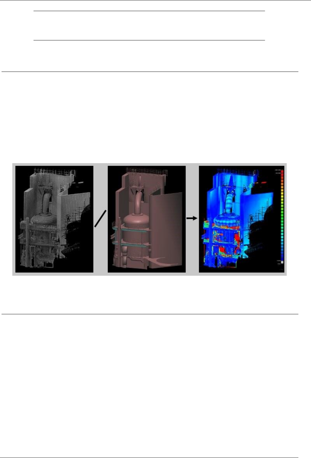
CloudCompare is a 3D point cloud (and triangular mesh) editing and processing software.
Originally, it has been designed to perform direct comparison between dense 3D point clouds. It relies on a specific
octree structure that enables great performances1 when performing this kind of task. Moreover, as most point clouds
were acquired by terrestrial laser scanners, CloudCompare was meant to deal with huge point clouds on a standard
laptop - typically more than 10 million points (in 2005!). Soon after, comparison between a point cloud and a triangular
mesh has been supported (see below). Afterwards, many other point cloud processing algorithms have followed
(registration, resampling, color/normal vectors/scalar fields management, statistics computation, sensor management,
interactive or automatic segmentation, etc.) as well as display enhancement tools (custom color ramps, color & normal
vectors handling, calibrated pictures handling, OpenGL shaders, plugins, etc.).
(1) for instance it took about 10 s. to compute the distances of 3 million points to a 14.000 triangles mesh on a laptop with dual-core processor
Philosophy
Point cloud Vs Mesh
Regarding its particular history, CloudCompare considers almost all 3D entities as point clouds. Typically, a triangular
mesh is only a point cloud (the mesh vertices) with an associated topology (triplets of 'connected' points corresponding
to each triangle). This explains that meshes have always either a point cloud named 'vertices' as sibling or parent
(depending on the way they have been loaded or generated). And while CloudCompare will let the user apply some
tools directly on a mesh structure (i.e. triangles), some tools can only be applied to the mesh vertices. It may be a bit
disturbing at first, but we don't want the user to ignore this: CloudCompare is mainly a point cloud processing
software.
Of course, as CloudCompare is meant to do change detection (e.g. subsidence monitoring) and as a triangular mesh is
a very common way to represent a reference shape (e.g. a building), it is very useful and it couldn't be ignored.
Nevertheless it remains a "secondary" entity, especially as CloudCompare is able to compare two point clouds directly,
without the need to generate an intermediary mesh.
The main reasons for this are:

8
CloudCompare Version 2.6.1 – user manual
• meshes are generally very hard to generate properly on real-life scenes, especially when scanned with a laser
scanner (noise, variable density, etc.)
• and as ALS/TLS point clouds are generally very dense (and accurate), we already have all the information we need
Scalar fields
Among all 'features' that can be associated to a point cloud (colors, normals, etc.) one has a particular place in
CloudCompare: the scalar field.
A scalar field is simply a set of values (one per point - e.g. the distance of each point to another entity). As each value
is associated to a point (or vertex) it is possible to display those values as colors (with custom color ramps) or to apply
filters on them (smooth, gradient, etc.), some basic math operations (exp, log, power of 2 or 3, cos, sin, tan, etc.) and
of course to segment the cloud relatively to those values (thresholding, local statistical filtering, etc.).
CloudCompare can handle multiple scalar fields on the same cloud. It is even possible to apply simple arithmetic
operations (-,+,/,*) between two scalar fields of a same cloud.
Some technical considerations
Portable
CloudCompare is developed in C++. It is currently compiled on Windows, Linux and Mac OS (thanks to CMake) and for
32bits and 64bits architectures.
Trade-off between storage and speed
Here are some details about the technical choices that have been made in CloudCompare (mainly to achieve the goal
of loading as much points as possible without downgrading too much performances - i.e. a good trade-off between
storage and speed):
all stored values and most of computations are done with 32bits floating-point values
to prevent any limitation on the size of arrays (as it's hard to get a big contiguous block of memory on Windows
32 bits), we use a custom container that automatically chunks datasets in small blocks (64 Kb per block).
normal vectors (if any) are compressed on 16 bits (15 bits actually, because of the way quantization
1
works)
the specific octree structure used in CloudCompare requires constant per-point memory (i.e. 8 bytes per point
on a 32 bits OS - with a maximum depth of 10 - and 12 bytes on a 64 bits OS - with a maximum depth of 21!).
It is based on a particular quantization of the 3D point coordinates - a kind of Morton
2
ordering scheme - where
each point position in the octree grid and at any level is represented by a single integer code. We then process
those codes to achieve very efficient nearest-neighbors querying operations. However, while this octree
structure is very efficient for computing distances for instance, it's not suitable for fast display (Level Of Detail,
etc.).
The result of the above choices is that CloudCompare can store about 90 million blank points per gigabyte of memory.
If you add RGB colors, normal vectors, a single scalar field and if you need to compute the octree, you can load up to
32 million points per gigabyte.
On a 64 bits OS you can load as many points as you want (well, up to 4 billion in fact). However, depending on your
graphic card capabilities, display and interactivity may be severely downgraded with this many points ;). With a high-
end graphic card you can keep a reasonable frame rate with up to 150 million points.
1
http://en.wikipedia.org/wiki/Quantization
2
http://en.wikipedia.org/wiki/Z-order_curve

9
CloudCompare Version 2.6.1 – user manual
Recent evolution
While the project has started in 2004 at EDF R&D, it has only been released in the public domain around 2009 (under
GPL license). As CloudCompare is on open-source project, everyone is free (and welcome) to extend its capabilities.
Don't hesitate to ask questions and share your experiences on the forum
3
and to take a look at the Github source
repository
4
.
License
The license of the CCLib library (containing the core algorithms) is LGPL
5
version 2.0.
Therefore CCLib can be integrated in any commercial or non-commercial project. You just have to share any
modification of the code with the authors (us).
The license of the other components is GPL
6
(version 2.0):
• qCC_db (database library)
• qCC_io (file I/O library)
• qCC_gl (OpenGL based 3D display library)
• CloudCompare and ccViewer (standalone applications)
Therefore only GPL-compatible (which means open-source but doesn't necessarily means free) projects can use those
components.
Online version
The latest version of the user documentation can be found at:
http://www.cloudcompare.org/doc/wiki/
3
http://www.cloudcompare.org/forum
4
https://github.com/cloudcompare/trunk
5
http://www.gnu.org/licenses/lgpl-2.0.html
6
http://www.gnu.org/licenses/gpl-2.0.html
10
CloudCompare Version 2.6.1 – user manual
General concepts
Graphical User Interface
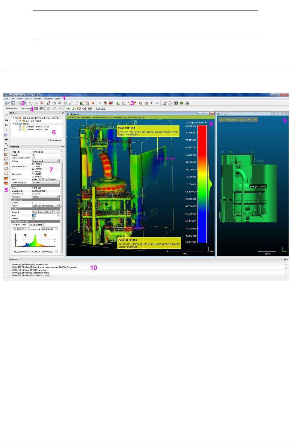
Here is a quick overview of the main user interface:
1. Menus
File (open, save, quit, etc.)
Edit (edit selected entities and their features - colors, normals, scalar fields, etc.)
Tools (segmentation, registration, projection, etc.)
Display (display-related options)
Plugins (loaded plugins)
3D Views (3D views management)
Help (about, help, etc.)
2. Main toolbar (quick access to main editing and processing tools: open/save, point picking, clone, etc.)
3. Scalar fields toolbar (quick access to scalar fields related tools)
4. Plugins toolbar (quick access to currently loaded plugins - standard and OpenGL shaders)
5. View toolbar (quick access to display-related tools)
6. Database tree (for selection and activation of entities and their features)
7. Properties view (information on selected entity)
8. Default 3D view
9. Another 3D view (created with 3D Views > New)
10. Console
11
CloudCompare Version 2.6.1 – user manual
Entities
Main entities
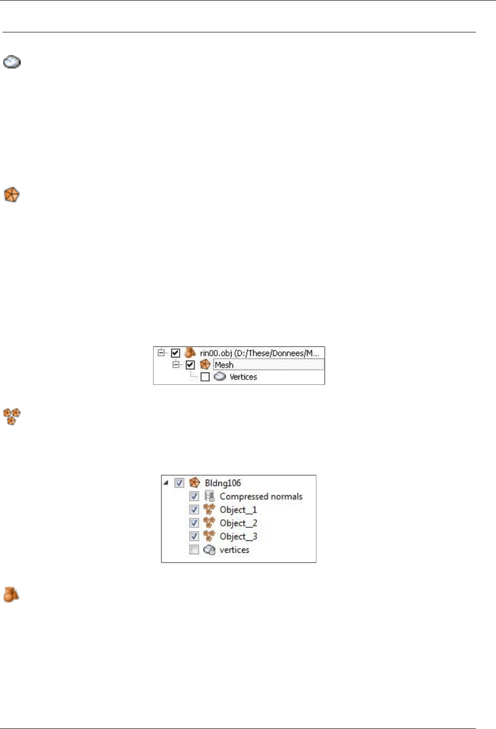
Point cloud
A point cloud is a set of unorganized 3D points (X,Y,Z).
It can be associated to:
a unique color for the whole entity (RGB)
per-point colors (RGB)
per-point normal vectors (Nx,Ny,Nz)
per-point scalar values (a scalar field) - multiple scalar fields can be associated to the same cloud
Mesh
A mesh is a set of triangles. Internally, triangles are represented by triplets of integer indexes. Those indexes are relative
to an associated cloud (the mesh vertices). Therefore a mesh 'inherits' of all the features associated to a point cloud
(see above).
In addition a mesh can be associated to:
per-triangle normal vectors (Nx,Ny,Nz)
per-triangle materials
per-triangle texture coordinates textures
A standard mesh generally corresponds to a single object. Its vertices are stored as a point cloud (which is generally a
child of the mesh object in the DB tree).
Sub-meshes
When importing a mesh with multiple parts (from OBJ or FBX files for instance) or when merging multiple meshes,
CloudCompare can create 'sub-meshes'. They are subsets of a main mesh (and can therefore only be child of this parent
mesh). They all share the same set of vertices and the same features.
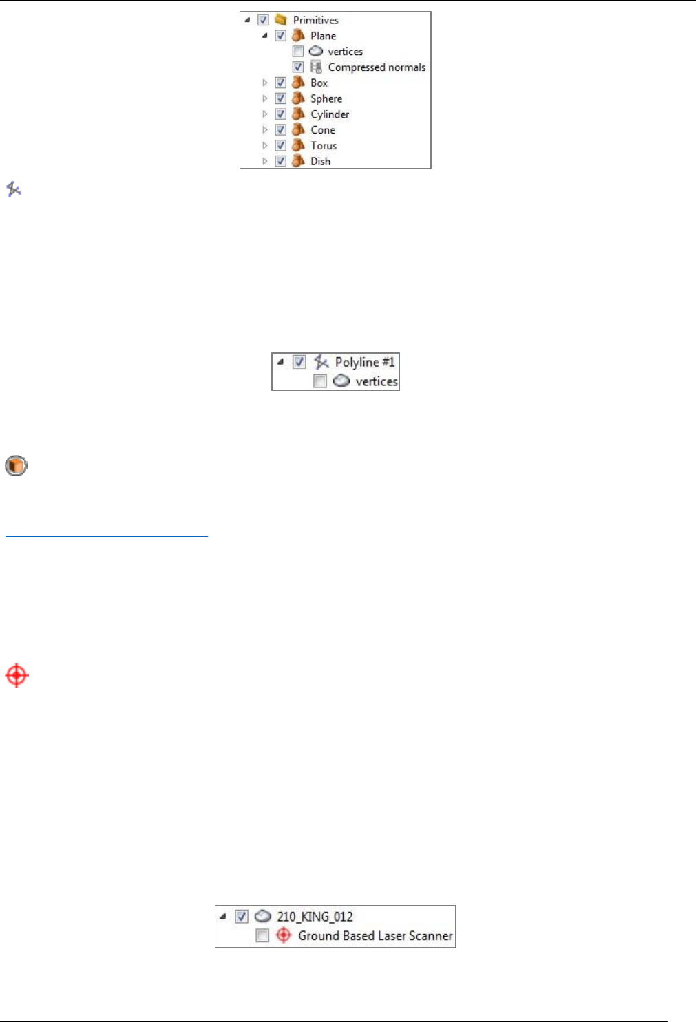
Primitives
Primitives are a special kind of meshes. They can be created with the 'Primitive Factory', or with the 'Tools > Fit' methods
(or also imported from CAD formats - e.g. PDMS macros).
Primitives are described by simple parameters (radius, height, etc.). However they are associated to a tessellated
representation (i.e. a proper triangular mesh). This way they can be used as standard meshes (for distance calculation,
etc.).
Note: for some primitives (spheres, cylinders, etc.) the user can change the 'drawing precision' (i.e. the amount of
tessellated triangles).
12
CloudCompare Version 2.6.1 – user manual
Polyline
A polyline is a set of points connected by contiguous segments. The polyline can be closed (i.e. a loop) or not. By default
a polyline is a 3D object. But they can also be 2D entities (in which case they will be displayed as a 2D overlay object
and their coordinates are always in pixels).
Internally a polyline is a set of indexes. Those indexes are relative to an associated point cloud (the polyline vertices).
Its vertices are stored as a point cloud (which is generally a child of the mesh object in the DB tree).
For now polylines don't inherit the features of their associated cloud (color, normals, etc.). However they can be
associated to a single color (RGB).
Point cloud associated structures
Octree
The octree structure is a very important structure in CloudCompare. It is used by most of the processing algorithms
(distance computation, spatial operators, etc.). For general information about octree structures refer to
http://en.wikipedia.org/wiki/Octree.
For more information about the practical implementation of the octree structure in CloudCompare, see the
‘CloudCompare octree’ section.
Sensors
There are currently two kind of sensors in CloudCompare.
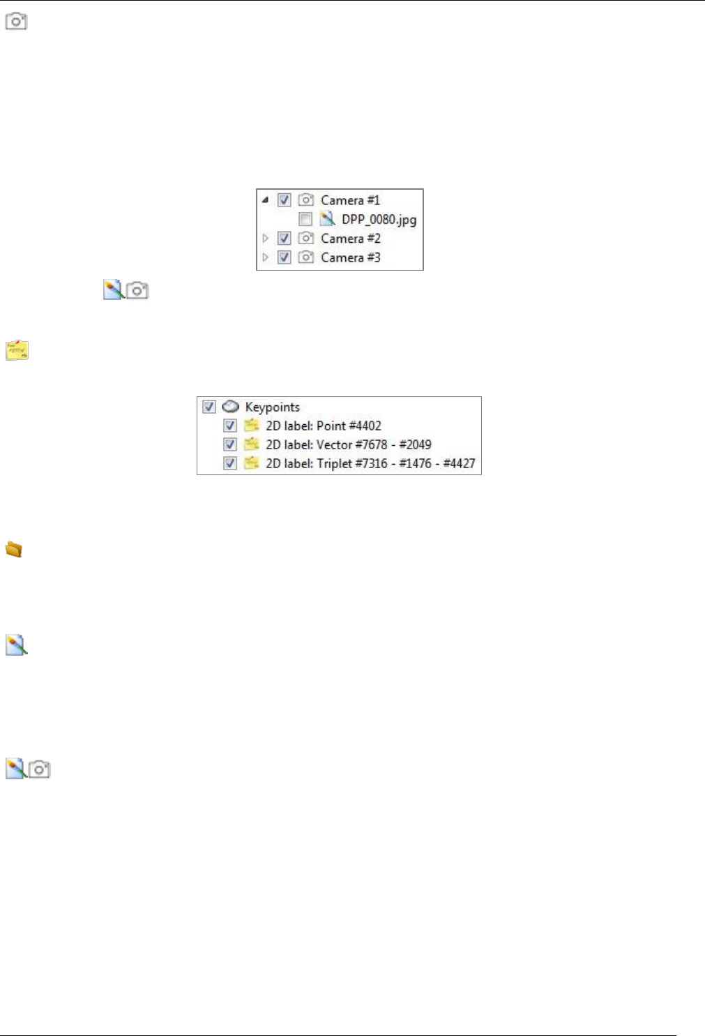
Ground Based Laser Sensor
Point clouds acquired thanks to a Ground Based Laser scanner (also called a Terrestrial Laser Scanner) can be associated
to a sensor entity. This is a structure containing information about the sensor (intrinsic and extrinsic parameters,
position and orientation relatively to the cloud, etc.). It can be used to localize the sensor position in the 3D scene, to
display the cloud in polar coordinates ('Display modes bubble-view' display mode), or to compute scattering angles,
etc.
Proprietary formats typically contain this kind of information (PTX, FARO, DP, etc.). They are automatically created (as
children of the loaded cloud(s)) when loaded from such files.
Otherwise sensors can be 'manually' created:
with the 'Sensors\Ground Based Lidar\Create' method
or via a POV meta-file
13
CloudCompare Version 2.6.1 – user manual
Projective Camera Sensor
Point clouds or pictures acquired thanks to a camera can be associated to a sensor entity. This is a structure containing
information about the sensor (intrinsic and extrinsic parameters, position and orientation relatively to the cloud, etc.).
It can be used to localize the sensor position in the 3D scene, display the cloud as if it was viewed by the camera (see
the 'Apply' button in the sensor properties), filter the points actually viewed by this camera, etc.
Camera sensors are automatically created when loading calibrated pictures from a Bundler .OUT file for instance (or
from some E57 files as well)
They can also be 'manually' created with the ‘Sensors\Camera Sensor\Create’ method.
P.S.: see also the Calibrated picture entity below.
Label
Clouds can be associated to Labels. See the ‘Point picking > Labels’ section for more information.
Other entities
Group
A simple group of other entities (can be used to classify or regroup entities). Groups can be created by right-clicking on
the DB tree – see ‘Context menu’).
Image
Images can be loaded from standard image file formats (jpg, bmp, png, etc.) via the standard 'File > Open' mechanism.
They can only be displayed in the 3D view as a 2D overlay (matching the 3D view extents). The user can change their
transparency so as to visualize the 3D scene behind.
Calibrated picture
Calibrated pictures are standard images that are associated to a 'Camera' sensor. Therefore it is possible to set the
camera parameters and position of the current 3D view to match the sensor parameters. This way the (calibrated)
picture can be displayed above the 3D scene (with a customizable transparency).
Calibrated pictures can be loaded from Bundler .OUT files or from E57 files. They can also be loaded thanks to ICM
meta-files.
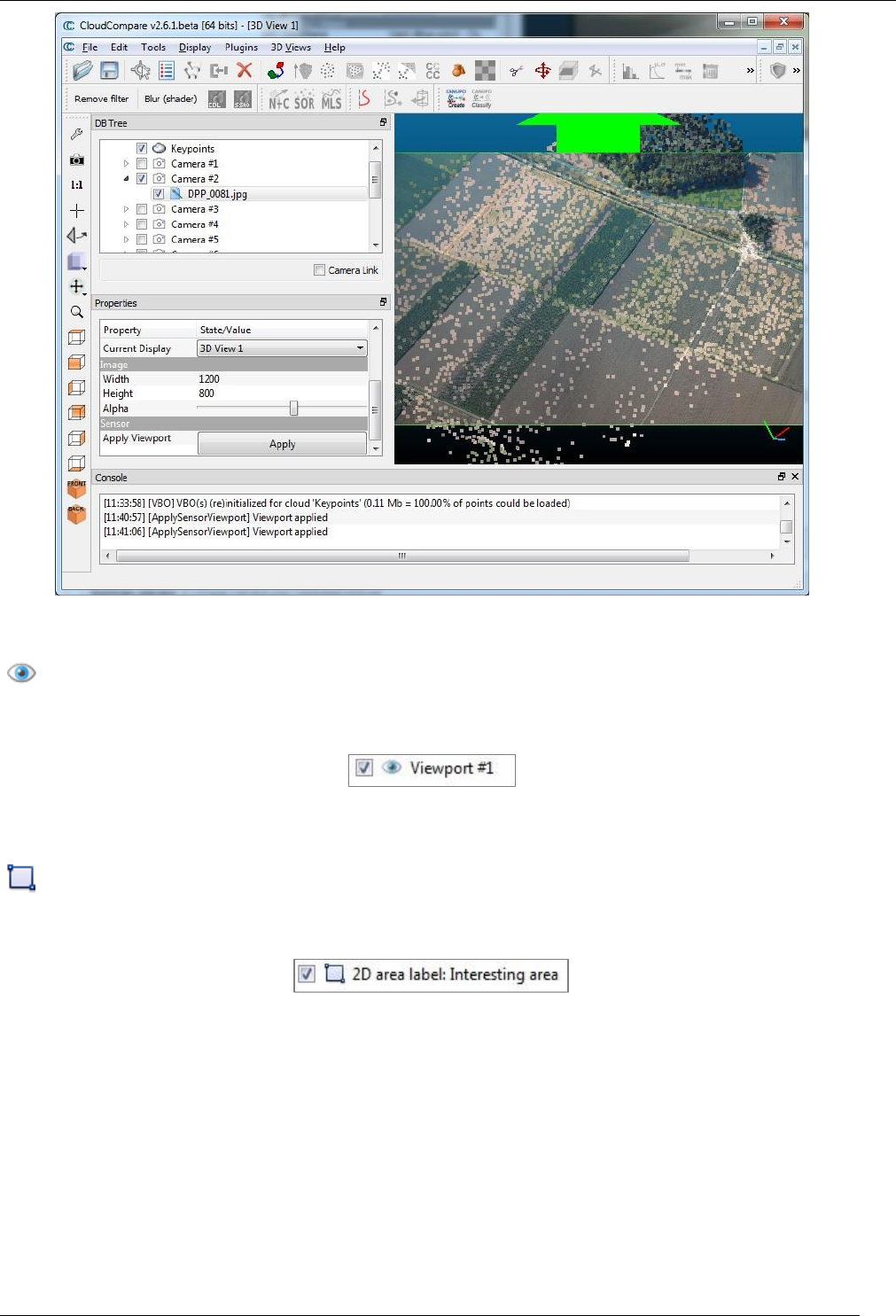
14
CloudCompare Version 2.6.1 – user manual
Calibrated picture overlaid on a cloud
Viewport
The current 3D view 'viewport' can be saved anytime with the 'Display > Save viewport as object' method. The
corresponding viewport can be restored later thanks to this entity.
Note: this entity can only be saved in BIN files.
2D area label
A special kind of label named '2D area label' can be created with the Point Picking tool. It has many common features
with the 'Viewport' entity. And as this entity, it can only be saved in BIN files.
15
CloudCompare Version 2.6.1 – user manual
DB tree
Loaded entities are all stored in the ‘DB tree’ (on the left part by default). Some entities can depend on other ones (such
as a mesh and its vertices) or can also be regrouped (in Group entities ). This is why the database is displayed as a
hierarchical tree.
Drag and drop
Most of the entities can be drag and dropped In the DB tree (so as to regroup them typically). Entities dependent on
others are generally bound to their ‘parent’ however (labels, vertices, etc.).
Selection
Entities can be selected either directly in a 3D view (by left clicking on it) or by clicking on their corresponding entry in
the DB tree (which is generally faster and unambiguous).
Multiple entities can be selected at once by maintaining the CTRL or SHIFT keys pressed and selecting them in the DB
tree.
Equivalently the user can select multiple entities by holding the CTRL key and clicking on entities in the 3D views.
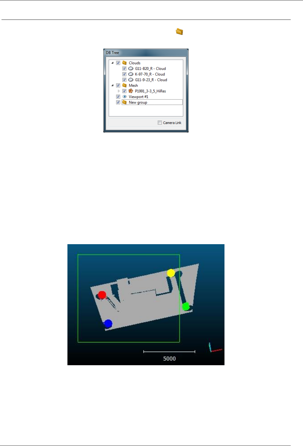
Another option is to hold the ALT key and drawing a rectangle in a 3D view. This way, all the entities falling at least
partly inside the rectangle will be selected:
Selection inside a rectangle (hold the ALT key while drawing the rectangle with the left mouse button pressed)
Context menu
A context menu can be spawned by clicking on an element of the DB tree with the right mouse button. Its content
depends on the type of the element.
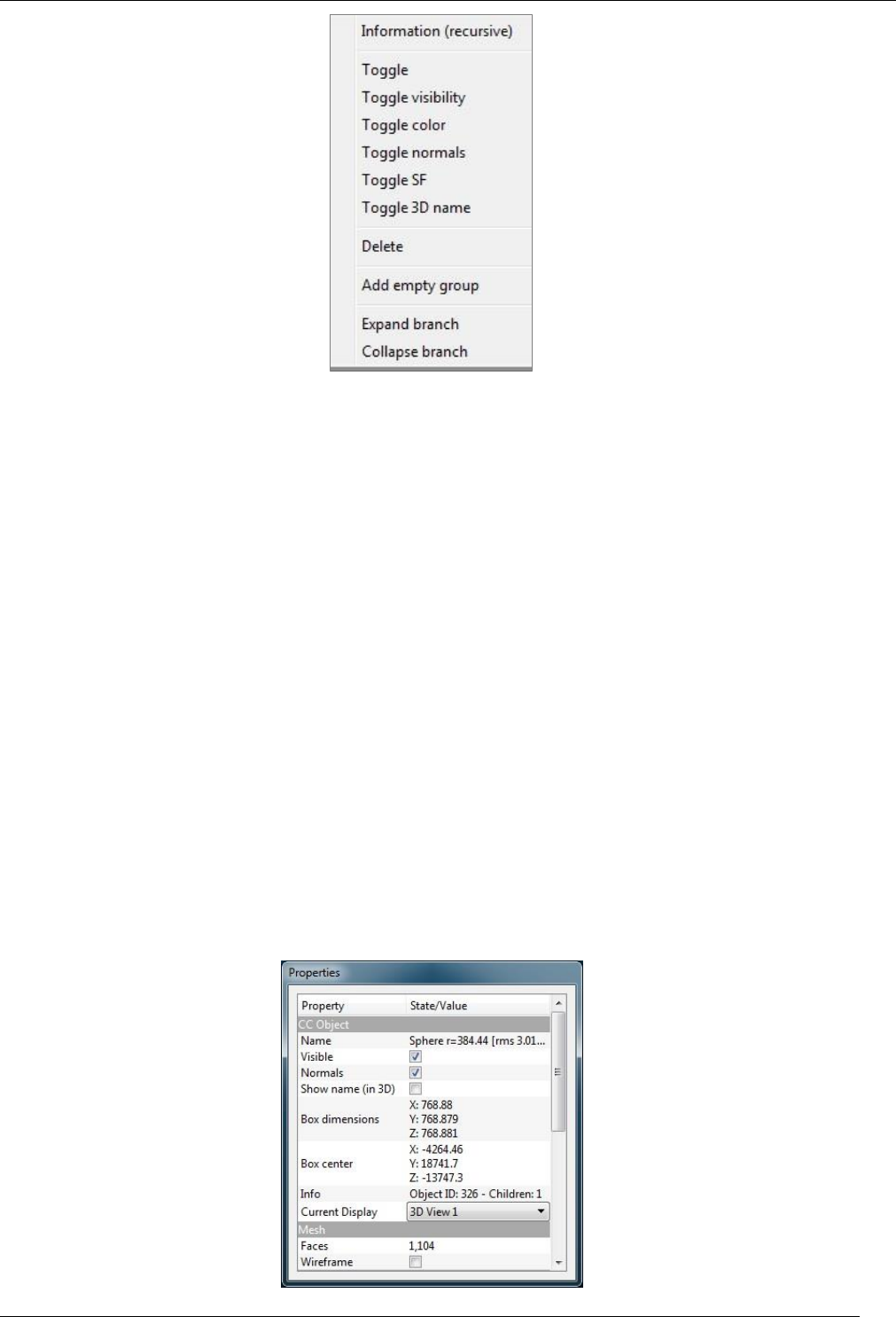
16
CloudCompare Version 2.6.1 – user manual
Context menu (for a cloud)
The most notable elements are:
On all entities:
o Information (recursive): displays information on the the selected entity and all its siblings (in a
recursive manner). Typically the total number of points, triangles, normals, etc.
o Toggle (visibility, color, etc.): to toggle a given property of the selected entities
o Delete: to delete the selected entities
o Add empty group: to add an empty group as a child of the selected entity (can also be called on the
DB tree background area to create a group at the tree root)
o Expand/Collapse branch
o Sort siblings (by names (A-Z) or (Z-A) or by type): to sort the siblings (if the entity has more than one
child)
Only on sensors:
o Bubble-view: to activate ‘Bubble-view (polar)’ mode
Only on planar entities (i.e. ‘3-points’ labels , planes and facets):
o Align camera (inverse or not): to make the camera of the current 3D view face this planar element
(one side or another). The corresponding transformation is also output in the Console.
Entity properties
When a single entity is selected, its properties are accessible in the ‘Properties’ dialog (on the left side below the DB
tree by default).

17
CloudCompare Version 2.6.1 – user manual
Entity properties (a sphere here)
Most of the entities display properties can be set via this dialog:
visibility of the entity
visibility of its features (colors, normals, etc.)
the current 3D view in which the entity is displayed (‘Current Display’ list)
the active scalar field and its display parameters (current color scale, whether it should be displayed in the 3D
view and how, etc.)
etc.
Other parameters can be modified such as
‘wireframe’ or ‘stippling’ – a kind of fake transparency – modes for a mesh for instance
primitives parameters
etc.
And of course various pieces of information:
bounding-box center and extents
the number of points or triangles
the ‘Global shift and scale’
associated meta-data
etc.
There are even some action buttons sometimes (for viewport or sensor entities for instance).
Scalar field display parameters editor
In the Properties dialog, an editor very specific to CloudCompare can be found on clouds and entities with an active
scalar field:
Scalar field parameters editor
This editor lets the user set most of the display parameters of the active scalar field in a very concise way (in addition
to get a quick overview of the scalar field histogram):
use the left and right white circles to set the min and max displayed scalar values. Below and above those
values, the points will either appear in grey or won’t appear at all (depending on the parameter ‘show NaN/out
of range values in grey’ that is accessible in the ‘Parameters’ tab). This way the user can quickly hide points
with values outside a given interval, in order to focus on the other points for instance.
use the red and blue down arrows to set the min and max saturation values (to set the start and end of
‘relative’ color scales – see the ‘Scalar fields > Color Scales Manager’)
set additional parameters with the ‘Parameters’ tab (log or symmetrical scale, etc.)

18
CloudCompare Version 2.6.1 – user manual
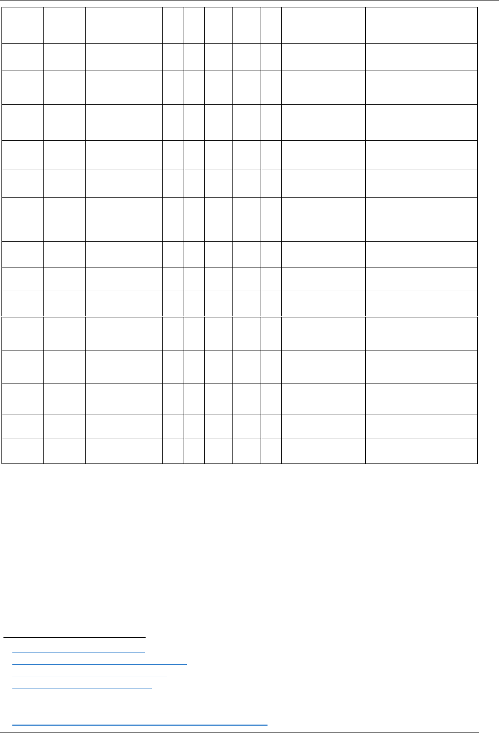
Supported file formats
Type
Extension(s)
Description
Read
Write
Binary/ASCII
Point
Cloud(s)
Mesh(es)
Other
Features
BIN
.bin
CloudCompare own
format
X
X
binary
>1
>1
>1
Normals
Colors (RGB)
Scalar fields (>1)
+ Labels, viewports,
display options, etc.
ASCII
.asc
.txt
.xyz
.neu
.pts
ASCII point cloud file
(X,Y,Z,etc.)
X
X
ASCII
1
Normals
Colors (RGB)
Scalar fields (>1)
LAS
.las
ASPRS7 lidar point
louds
X
X
binary
1
Colors (RGB)
Various scalar fields
(see LAS 1.4 specifications)
E57
.e57
ASTM E578 file format
X
X
mixed
>1
Calibrated picture(s)
Normals
Colors (RGB or I)
Scalar field (intensity)
PTX
.ptx
LEICA point cloud
export format
X
ascii
>1
Sensor(s)
Robust normals can be
computed at loading time
FARO
.fls
.fws
FARO formats
X
binary
>1
Sensor(s)
Scalar field (reflection value)
DP
.dp
DotProduct DPI-7
format
X
binary
>1
Sensor(s)
Colors (RGB)
Robust normals can be
computed at loading time
PCD
.pcd
Point Cloud Library
format
X
X
binary
>1
Colors (RGB)
Normals
Scalar fields (>1)
PLY
.ply
Stanford 3D
geometry format9
(cloud or mesh)
X
X
both
1
1
Normals
Colors (RGB or I)
Scalar fields (all)
Single texture
OBJ
.obj
Wavefront10 mesh
X
X
ASCII
1
>1
Polyline(s)
Normals
Materials and textures
VTK
.vtk
VTK file format
(triangular mesh or
cloud only)
X
X
ASCII
1
1
Normals
Colors (RGB)
Scalar fields (>1)
STL
.stl
STereoLithography11
file format (mesh)
X
X
ASCII
1
Normals
OFF
.off
Object File Format12
(mesh)
X
X
ASCII
1
7
http://www.asprs.org/society/committees/standards/lidar_exchange_format.html
8
http://www.ri.cmu.edu/publication_view.html?pub_id=6767
9
http://www.graphics.stanford.edu/data/3Dscanrep
10
http://en.wikipedia.org/wiki/Wavefront_.obj_file
11
http://en.wikipedia.org/wiki/STL_%28file_format%29
12
http://www.cs.princeton.edu/courses/archive/spr08/cos426/assn2/formats.html
19
CloudCompare Version 2.6.1 – user manual
FBX
.fbx
Autodesk (Filmbox)
File format13
X
X
ASCII
or
binary
>1
>1
Normals
Colors (RGB)
Materials and texture
DXF
.dxf
Autocad DXF
format14
X
X
ASCII
>1
>1
Polyline(s)
Normals
Colors (RGB)
SHP
.shp
ESRI Shape file
format15
X
X
binary
>1
Polyline(s) polygon(s)
Contour plot(s)
etc.
Scalar fields (1 per entity)
PDMS
.pdms
.pdmsmac
.mac
PDMS macros
X
ASCII
>1
Primitive(s)
RASTER
.geotiff,
etc.
Common raster
formats (GDAL)16
X
X17
binary
1
Layers (as scalar fields)
OUT
(Bundler)
.out
Bundler SfM output
file18
X
ASCII
(1)
Calibrated picture(s)
3D keypoints
2D images
.jpg
*.png
*.bmp
etc.
Standard images
binary
PV
.pv
Point cloud + scalar
field
X
X
binary
1
Scalar field (1)
PN
.pn
Point cloud + normals
X
X
binary
1
Normals
SOI
.soi
Mensi/Trimble
Soisic laser scanner
X
ASCII
>1
Colors (I)
POV
.pov
Multiple stations
(meta file)
X
ASCII
+
both
>1
All + sensor poses
ICM
.icm
Cloud + calibrated
pictures
X
ASCII
+
both
1
Picture(s)
All + camera poses
Geo-
Mascaret
.georef
Mascaret profiles19
X
ASCII
Profiles
(polylines)
Sinusx
.sx
Sinusx curves
X
X
ASCII
Polylines
CSV
matrix
.csv
Cloud as 2D1/2
matrix
X
ASCII
1
13
http://en.wikipedia.org/wiki/FBX
14
http://en.wikipedia.org/wiki/AutoCAD_DXF
15
http://en.wikipedia.org/wiki/Shapefile
16
http://en.wikipedia.org/wiki/GDAL
17
Use the ‘Projection > Rasterize’ tool’ to export raster files
18
http://phototour.cs.washington.edu/bundler
19
http://chercheurs.edf.com/logiciels/code-mascaret-41197.html
20
CloudCompare Version 2.6.1 – user manual
Display modes
3D entities can be displayed in one or multiple 3D views. Several display modes can be set in each 3D view.
Main display modes
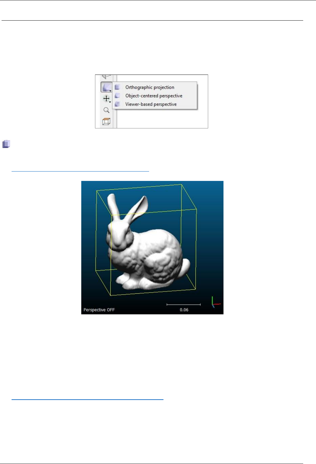
The orthographic and perspective modes can be enabled at any time thanks to the 'Set current view mode' icon in the
left toolbar:
Orthographic view
This is the default viewing mode. It is a parallel projection (i.e. parallel lines never cross).
See http://en.wikipedia.org/wiki/Orthographic_projection for a bit of theory.
Note: in this mode, a white scale is displayed (in the bottom right corner of the 3D view). Its actual dimension in the
current coordinate system is displayed below.
Perspective view
The perspective projection consists in projecting a 3D scene on a 2D plane as if it was seen by the human eye (or a single
camera).
The main parameter for this mode is the field of view (f.o.v.). It can be changed via the ‘Camera settings’.
See http://en.wikipedia.org/wiki/Perspective_%28graphical%29 for a bit of theory.
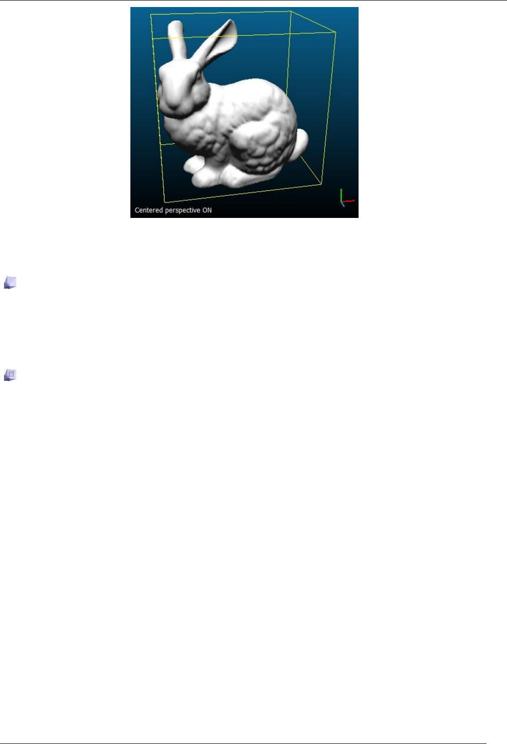
21
CloudCompare Version 2.6.1 – user manual
Notes: in this mode, no scale is displayed as the 'width' depends on the actual depth of each pixel.
There are two types of perspective modes in CloudCompare.
Object-centered
In the 'object-centered perspective' mode, the object rotates when the user moves the mouse while pressing the left
button (the camera orientation is fixed). Using the mouse wheel will make the object farther or nearer from the current
point of view.
Note: this mode can be toggled with the 'F3' shortcut.
Viewer-based
In the 'viewer-based perspective' mode, the camera rotates when the user moves the mouse while pressing the left
button. And using the mouse wheel make the camera move forward or backward in the current viewing direction.
Note: this mode can be toggled with the 'F4' shortcut.
22
CloudCompare Version 2.6.1 – user manual
Bubble-view (polar)
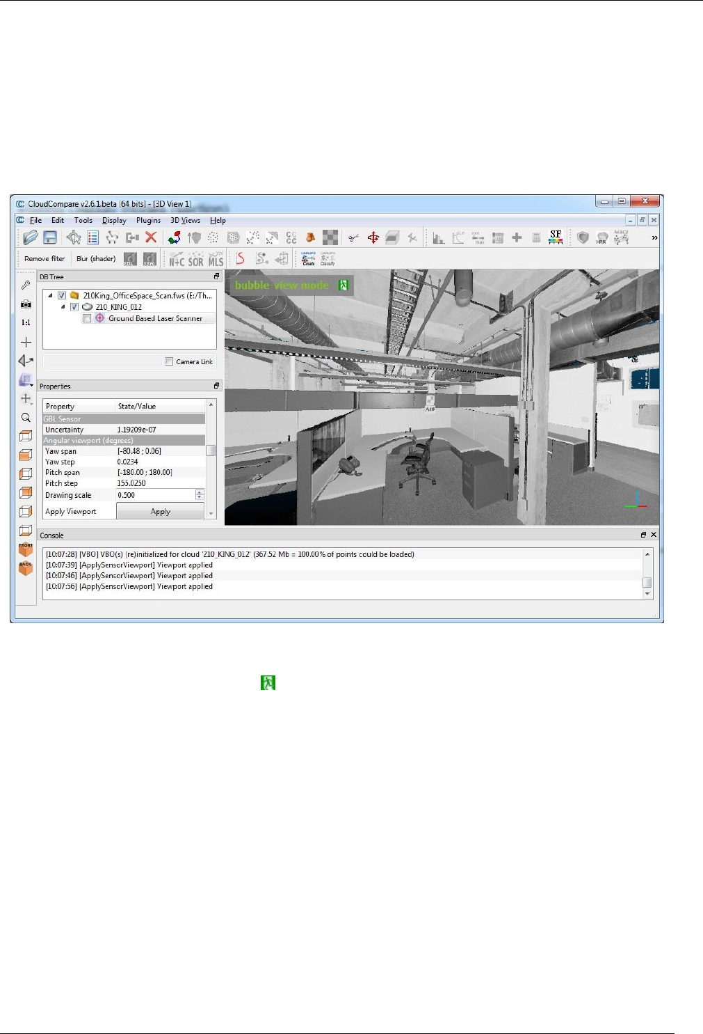
This viewing mode can only be properly enabled via a 'GBL sensor' entity. They are generally associated to point clouds
coming from proprietary files (PTX, FARO, DP, etc.).
To enable it, simply browse the sensor entity properties and click on the 'Apply' button ('Apply viewport' item).
While in this mode, the camera position is fixed (normally at the sensor center) and the user can only rotate it (with the
left mouse button) or change the zoom (with the mouse wheel).
Note: in fact the zoom is simply obtained by modifying the camera field of view (f.o.v.). Therefore high optical distortion
can occur after a certain point.
FARO scan viewed in ‘bubble-view’ mode
To leave this mode the user must click on the
icon in the top left corner of the 3D view.
Note: the B shortcut can be used to enter this method.
23
CloudCompare Version 2.6.1 – user manual
Global Shift and Scale
Introduction
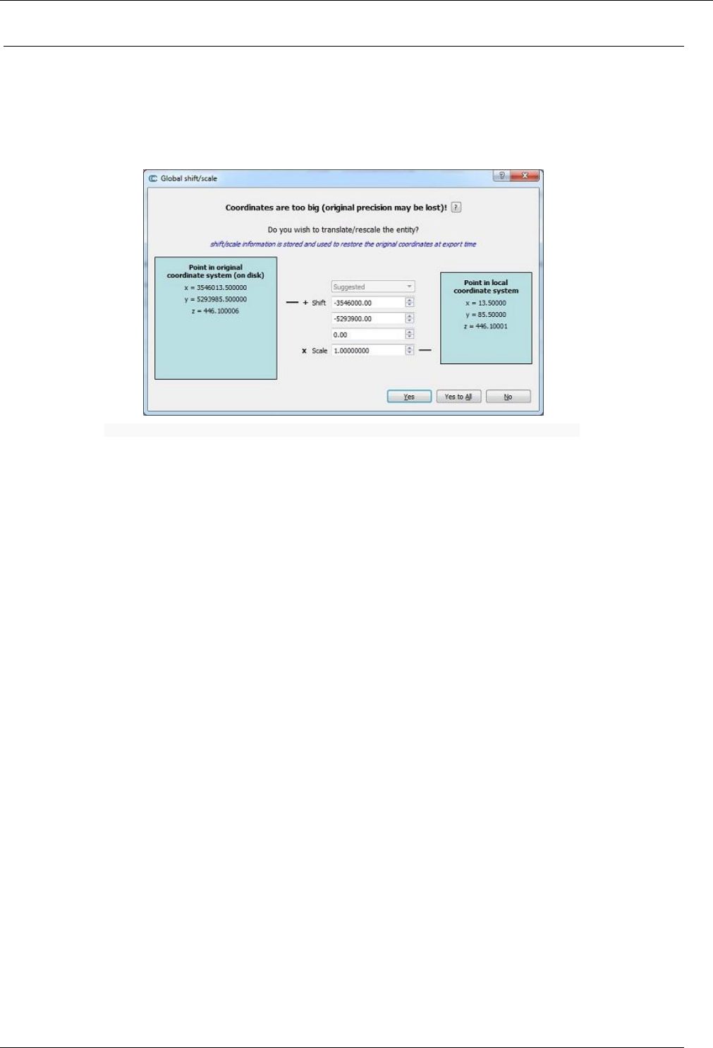
When loading (or generating) an entity with very big coordinates (typically greater than 105), CloudCompare will warn
the user about this and suggest to shift (or rescale) the entity in order to work in a local coordinate system with smaller
coordinates:
CloudCompare will suggest the user to shift the cloud if its original coordinates are too big
It is strongly advised to shift/scale the entities in this case.
But why?
This is due to the fact that both CloudCompare and OpenGL works with 32 bits float values. This allows an increase of
speed and a 50% memory gain compared to 64 bits values.
However the 32 bits representation has a limited resolution (accuracy). Without entering into too much details here,
we can say that the bigger the number is, the less decimals can be stored. As a rule of thumb the 'relative' precision
(i.e. the smallest quantity that can be represented relatively to the maximal value) is roughly between 10-7 and 10-8.
This is generally more than sufficient for real life point clouds expressed in the scanner coordinate system (e.g. for a
100 meters range scan, the data representation precision will be around 10-5 or 10-6 m = 1 to 10 microns).
However if the cloud is expressed in a geo-referenced coordinate system, the point coordinates can be very big
(typically about 106). In this case the data representation precision rises up to 1 or 10 cm!
This is why it is very important to 'shift' the points when loading the file in CloudCompare. Otherwise the original
precision will be lost.
CloudCompare stores the shift and scale values as meta-data and (tries to) keep them all along the entity life.
Eventually, when the user saves the entity CloudCompare will restore the original coordinate system (if the output
file format allows for 64 bits values storage).
Mathematics
The global shift and global scale encode the transformation between the original (global) coordinate system of the
entity and the working local) coordinate system.
Let T(x,y,z) be the global shift (translation), S be the global scale, and P a 3D point, then:
Plocal = (Pglobal + T) * S
or equivalently:
Pglobal = Plocal / S - T
24
CloudCompare Version 2.6.1 – user manual
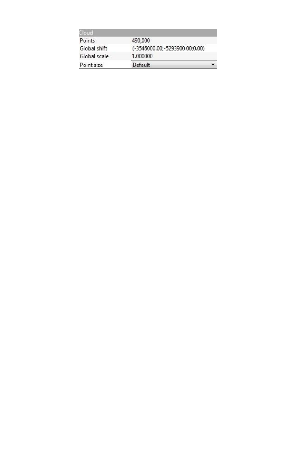
Properties
The shift and scale values are displayed in the entity properties (if the entity support this):
Edition
At any time the user can edit the shift and scale values associated to a given entity. See the 'Edit > Edit global shift and
scale' tool.
Bookmarks
By default CloudCompare tries to guess the best shift vector automatically (typically when loading a file, CloudCompare
will use the very first point coordinates as shift quantity). But the user is free to input the shift and scale values
(especially if one works with several clouds and want to work in a particular local coordinate system).
Once a first shift/scale has been used, CloudCompare will:
use it for the next clouds if it works for them as well
let the user recall it whatever the case thanks to the drop down menu in the middle (just above the 'Shift'
fields see the Last input entry)
However this information will only be stored during the active session of CloudCompare (it will be lost once you close
the program). In order to keep the information persistent, you can edit the global_shift_list_template.txt file next to
CloudCompare's executable and follow the instructions inside. This is a good way to store persistent shift/scale
information sets (kind of "bookmarks").

25
CloudCompare Version 2.6.1 – user manual
Tutorials and guidelines
Alignment and Registration
This section deals with alignment and registration of 3D entities (clouds or meshes).
General considerations
Did you say mesh?
(skip this part if you don't work with triangular meshes)
As often with CloudCompare, meshes will generally be considered as clouds, either by considering only their vertices
or by sampling points on the mesh surface. For instance you can call the ‘Fine registration tool (ICP)’ directly on a mesh.
But behind the scenes CC will automatically sample points on this mesh in order to use it for ICP registration.
There's only one notable exception: the 'Point pair based' alignment tool can now be used directly on meshes (when
the user clicks on a triangle, CloudCompare will determine the actual intersection point on the triangle surface).
So instead of letting CloudCompare chose, you can of course do this conversion yourself:
instead of selecting the mesh entity, you can simply select its 'vertices' (a point cloud named 'vertices' -
generally a child of the mesh entity in the DB tree). In this case you can 'hide' the mesh entity (uncheck the
'visible' checkbox in the mesh properties) and instead display its vertices (check the equivalent 'visible'
checkbox in the 'vertices' cloud properties). As mesh vertices are generally quite sparse, you can also increase
the points size (the -/+ interactors that appear when you hover the mouse in the top-left corner of a 3D view).
you can alternatively sample points on the mesh (this way you'll have more control on this process) and use
the sampled cloud in place of the mesh. In the particular case of registration, if you want to apply the resulting
transformation to the original mesh afterwards, refer to the next section.
Rigid transformation matrices
(skip this part if you really hate maths - otherwise it might give you some interesting hints ;)
Almost all methods presented below are in fact various ways to produce a rigid transformation (matrix) to make an
entity move relatively to another one (see Apply Transformation). Whatever the registration tool you use,
CloudCompare will always issue the resulting transformation matrix in the console. This allows the user to apply it - or
its inverse - to any other entity.
To do so:
first copy the matrix from the Console (typically with the shortcut CTRL+C on Windows)
then select the entity you wish to move call the 'Edit > Apply Transformation' tool
paste the 4x4 matrix in the first tab. You can use the dedicated shortcut (e.g. CTRL+V on Windows) or the
'clipboard' button (CloudCompare should automatically get rid of the block prefix - [time between brackets])
you can even apply the inverse transformation by checking the corresponding checkbox (e.g. to go back to the
previous position of the entity) 'Apply transformation' dialog
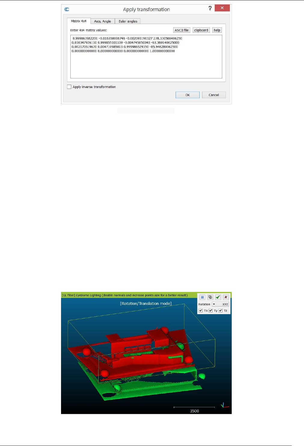
26
CloudCompare Version 2.6.1 – user manual
'Apply transformation' dialog
This trick can be very useful to perform registration on a small portion of a cloud (which you would have segmented
beforehand - typically with the 'Interactive Transformation tool'). Then you can apply the same transformation to the
whole cloud afterwards or to another entity (mesh, etc.). See the 'Alternative method for registering partially
overlapping clouds’ section below.
Alignment
CloudCompare offers various ways to roughly or finely align point clouds or meshes.
Match bounding-box centers
The easiest one is the bounding-box centers matching method. Simply select two (or more) entities, then call ‘Tool >
Registration > Match bounding-box centers’ (immediate effect, no dialog). It will center all the selected entities on their
respective center of gravity.
It's clearly a very simple approach (it can only translate entities, and not rotate them). However it can save you a few
clicks.
Manual transformation
It is possible to interactively displace with the mouse one or several entities (relatively to other entities). See the ‘Edit
> Translate / Rotate (Interactive Transformation Tool)’.
"Rotation/Translation" tool in action
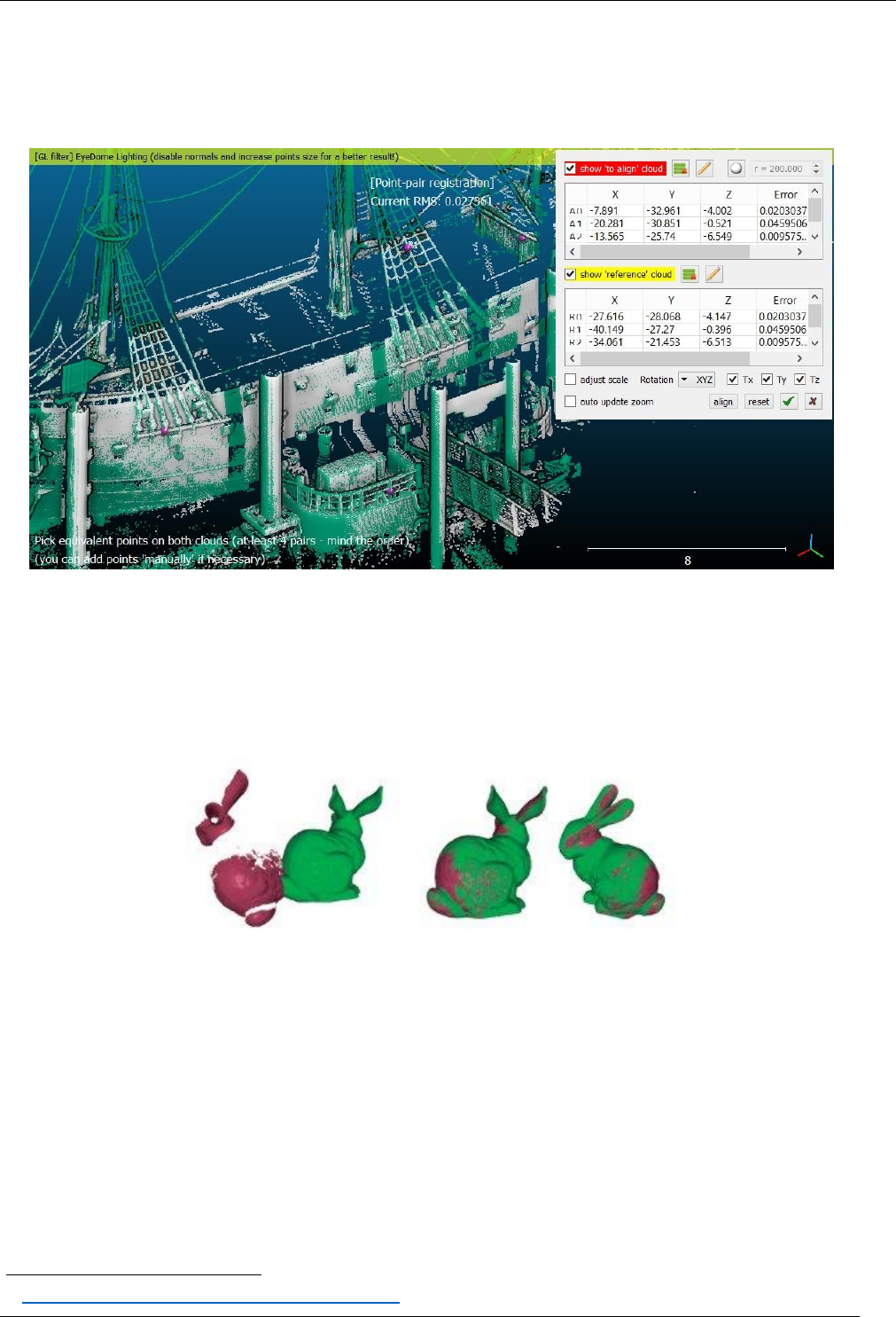
27
CloudCompare Version 2.6.1 – user manual
Picking (equivalent) point pairs
Another powerful yet simple tool to align two entities is the ‘Align (point pairs picking)’ tool. It lets the user pick several
pairs of equivalent points in each cloud in order to register them. While the process is manual it can be relatively fast
and quite accurate (especially if registration spheres are present in both clouds as this tool is now able to detect their
center automatically).
Standard alignment procedure (no spheres)
Automatic registration
Fine registration with ICP
For now, the only automatic method to very finely register two entities is the well-known Iterative Closest Point (ICP)
algorithm
20
. See the ‘Registration > Fine registration (ICP)’ section.
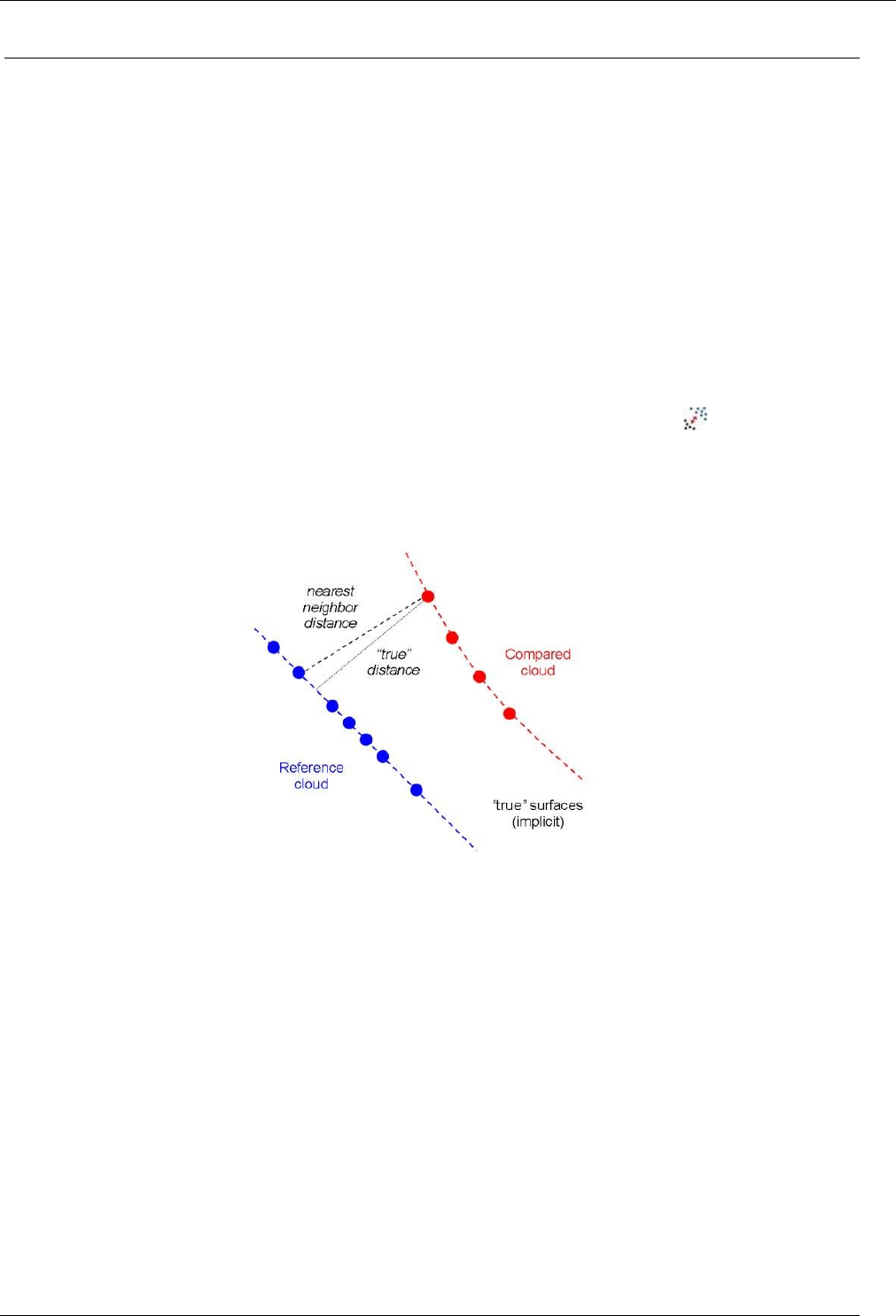
Alternative method for registering partially overlapping clouds
Here is an old way of registering two partially overlapping clouds (i.e. prior to version 2.6.1 and its ‘Final overlap’
parameter).
Preparation
First, roughly register the two clouds (with the ‘Rotate/Translate’ tool for instance).
Note: if you don't already know which cloud will be the ‘data’ cloud (the one that will move) and which one will be the
‘model’ cloud (the one that won't move) then you should select the densest one as model (reference)
Creating a subset of the data cloud
clone the data cloud and hide the original one
20
http://en.wikipedia.org/wiki/Iterative_closest_point

28
CloudCompare Version 2.6.1 – user manual
select the new version of the data cloud and use the Interactive Segmentation tool to keep only the points
clearly overlapping with the model cloud
Register the 'data' cloud (subset) with the model cloud
apply the Fine registration (ICP) algorithm to the data cloud subset and the 'model' cloud
once done, CloudCompare will output the resulting transformation matrix in the Console
copy this transformation (CTRL+C on Windows)
Apply the rigid transformation to the original data cloud
make the original data cloud visible again and select it
launch the ‘Edit > Apply Transformation’ tool
paste the transformation (CTRL+V on Windows) in the first tab
click on the 'OK' button
That's it!
29
CloudCompare Version 2.6.1 – user manual
Distances Computation
This section describes what kind of distances can be computed with CloudCompare and how these distances are
computed.
There's mainly two kinds of distances described below:
either the distances between two point clouds (cloud-cloud distances)
or the distances between a point cloud and a mesh (cloud-mesh distances)
The third kind of distances that would naturally come to mind - the 'mesh-mesh' distance - will be treated by
CloudCompare as a 'cloud-mesh' distance: one can either choose to use only the compared mesh vertices for computing
distances (if they are regularly and densely sampled on the surface) or alternatively to sample points on the compared
mesh surface. More information can be found in the How to compare two 3D models tutorial.
Cloud-cloud distances
Cloud-cloud distances can be computed by selecting two point clouds and then clicking on the icon. See the ‘Cloud-
to-Cloud Distance computation’ tool section for more information.
The default way to compute distances between two point cloud is the 'nearest neighbor distance': for each point of the
compared cloud, CloudCompare searches the nearest point in the reference cloud and computes their (Euclidean)
distance. This corresponds to the (default) case where local model is set to 'NONE'.
Local modeling
If the reference point cloud is dense enough, approximating the distance from the compared cloud to the underlying
surface represented by the reference cloud is acceptable. But if the reference cloud is not dense enough, the nearest
neighbor distance is sometimes not precise enough. Therefore, it can be necessary to get a better model of the surface.
Of course, if one can obtain a global model of the surface easily, it's much simpler and potentially more accurate to
compute directly the distance from the compared cloud to this model (see the ‘Cloud-mesh distances’ section below).
But it's generally not so easy to get a clean and proper global model. Therefore, CloudCompare provides an
intermediate way to get a better approximation of the true distance to the reference surface. Not as precise as a true
global model, but much easier to compute.
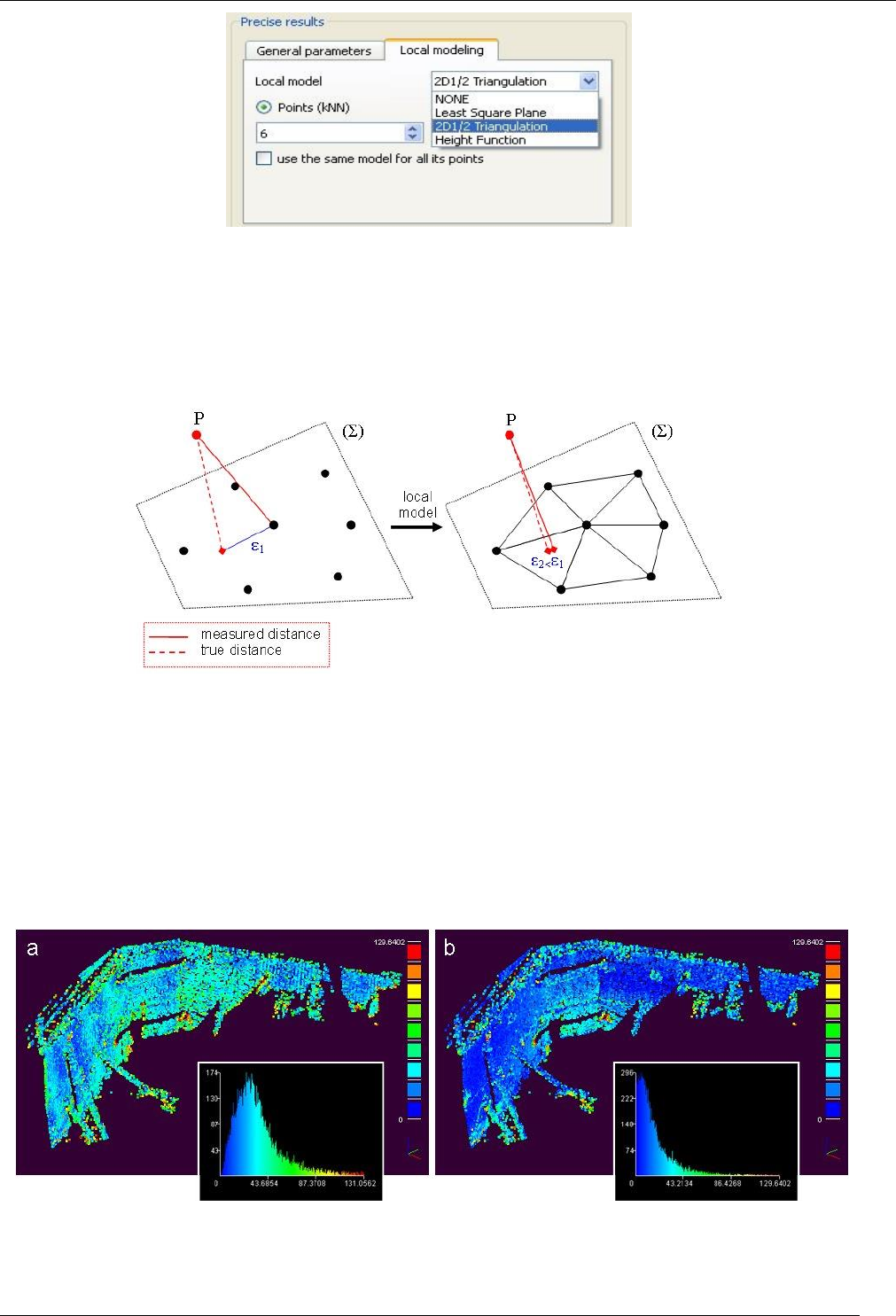
30
CloudCompare Version 2.6.1 – user manual
When CloudCompare has determined the nearest point in the reference cloud, the idea is to locally model the reference
cloud (underlying) surface by fitting a mathematical model on the 'nearest' point and several of its neighbors. The
distance from each point of the compared cloud to its nearest point in the reference cloud is replaced by the distance
to this model. This is statistically more precise and less dependent on the cloud sampling (it can locally produce strange
results - as the modelling phase is very limited - but it gives much better results on a global scale).
With the latest version of CloudCompare, the user can fully setup the way the job is done by choosing:
the mathematical model: either the least square best fitting plane, or a 2D1/2 Delaunay triangulation, or a
quadratic height function (the latter being the more precise but also the longer to compute)
the way the neighbors are extracted around each 'nearest' point in the reference cloud (either by setting a
fixed number of neighbors, or by providing the radius of a spherical neighborhood)
and eventually one can choose to apply an approximation of this scheme by sharing the same local model with
several points of the reference cloud instead of computing a new model for each. The process is much faster
this way (especially for big neighborhoods) but also much noisier.
Result without (left) and with local modeling (right). Note that the maximum distance doesn't change while the lower part of the histogram is clearly
shifted towards zero.
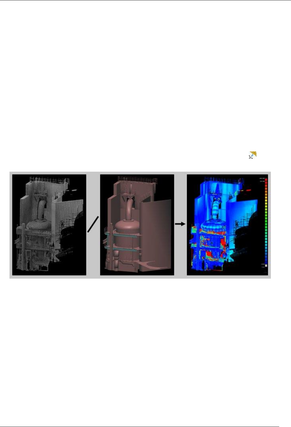
31
CloudCompare Version 2.6.1 – user manual
General considerations
When comparing two points clouds directly (especially without model), here are a few 'guidelines':
make sure that the reference cloud extents are wider than the compared cloud ones (to avoid virtually high
distances on the boundaries). More generally, try to make sure that the reference cloud always overlaps the
compared one (that's also true for cloud-mesh distances).
always try to get the highest possible density for the reference cloud (as it will directly change the results
accuracy)
if the reference cloud is very noisy, consider using the least square best fitting plane model (which is more
robust to noise). On the contrary, if the reference cloud is clean but with high curvature, consider using the
quadratic height function.
Other options
CloudCompare can split the computed distances along the 3 main dimensions (X, Y and Z). If the 'split X, Y and Z
components' checkbox is checked, CloudCompare will generate 3 more scalar fields, on for each axis.
Cloud-mesh distances
Cloud-mesh distances can be computed by selecting one point cloud and one mesh and then clicking on the icon. See
the ‘Cloud-to-Mesh Distance computation’ section for more information.
In this mode, for each point of the compared cloud CloudCompare will simply search the nearest triangle in the
reference mesh. As meshes generally provide (indirectly) a side information (one can determine what is inside and
outside of the mesh by looking at the normal of the triangle), cloud-mesh distances can be signed (this is the default
behavior).
The user can choose to either ignore the normal information (by unchecking the 'signed distances' checkbox) or to
invert it (with the 'flip normals' checkbox).
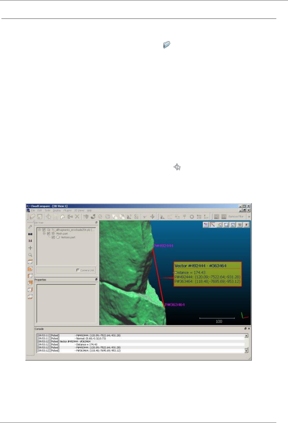
32
CloudCompare Version 2.6.1 – user manual
How to compare two 3D entities
Load data
Open the two 3D entities you want to compare with the ‘File > Open’ menu entry.
These two entities can be:
2 point clouds
2 models (triangular meshes only - see the ‘Supported formats’ section)
or one of each
Data preparation
Scaling the entities
(If the two entities have already the same scale you can skip this step)
first choose an accurate element, visible in the two entities: edge, cornice, line or any other rectilinear element.
If you can't find such an element, then choose two specific points/vertices clearly visible in the two entities:
crossing of two lines or curves, corner, etc.
then measure the length of this element (or the distance between the two specific points) on the entity with
the largest scale. To do this launch use the ‘Tools > Point picking’ tool.
Note: if you work with a model (mesh), you'll have first to make its vertices visible (by enabling the 'vertices' entity in
the database tree) or alternatively to sample points on the mesh - see last remark at the end of this tutorial.
Distance measurement between two points
let's call the measured distance Dmax. Note it down (hint: it will also be displayed in the Console window or you
can also save the corresponding label).
repeat the process on the other entity (i.e. the one with the smaller scale). Let's call the resulting distance Dmin.
compute the scaling factor Sf = Dmax / Dmin
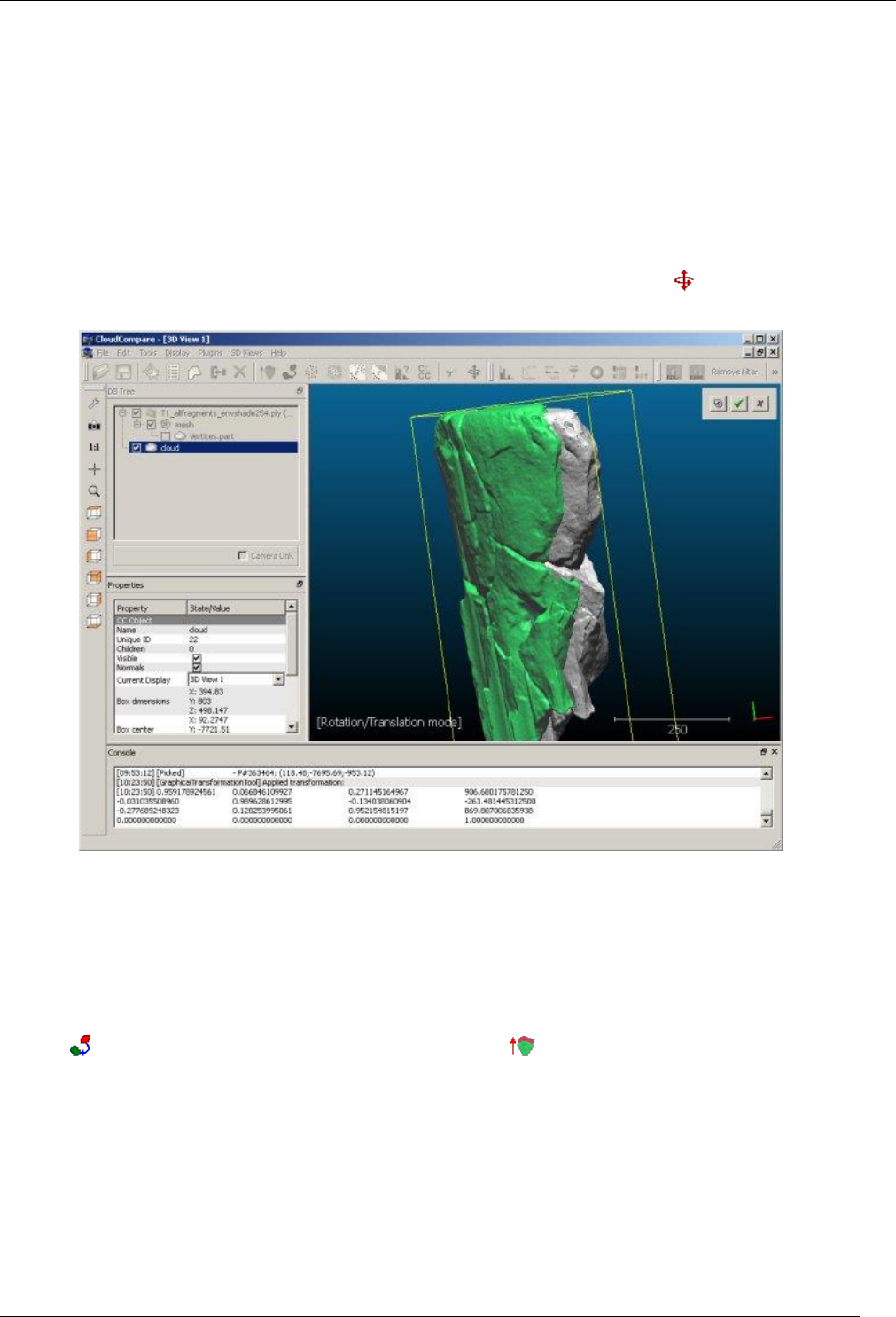
33
CloudCompare Version 2.6.1 – user manual
eventually apply this scaling factor on the smaller entity with the 'Edit > Multiply / Scale' tool (use the Sf factor
for all dimensions).
Note: conversely, you can scale-down the model with the larger scale by applying the inverse factor on it.
Roughly registering the entities
(You can skip this step if the two models are already roughly registered)
first, if the entities are far apart, select both of them and use the 'Tools > Registration > Match bounding-box
centers' method (to make their centers of gravity match).
then select one of the two entities (ideally the one that should move)
eventually with the help of ‘Translate / Rotate (Interactive Transformation Tool)’ , you can interactively
rotate and translate the entity so as to (roughly) superimpose both entities.
Manual registration of two entities with the 'Rotate/Translate' tool
Finely registering the entities
(You can skip this step if the two entities are already finely registered)
refine and finish the registration of the two entities with at least the ‘Registration > Align (point pairs picking)’
tool and ideally the ‘Registration > Fine registration (ICP)’ tool.
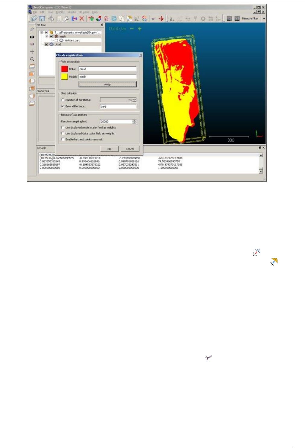
34
CloudCompare Version 2.6.1 – user manual
Automatic registration of two entities with the 'Register' tool (ICP)
Data comparison
You can now compute the distances between the two entities.
Select both of them and choose the appropriate distance computation tool:
for cloud/cloud comparison, use the ‘Distances > Cloud/Cloud dist. (cloud-to-cloud distance)’ tool
for cloud/model comparison, use the ‘Distances > Cloud/Mesh dist. (cloud-to-mesh distance)’ tool.
Warning: in this case the model will always be considered as the 'Reference' by CloudCompare. If you want to
use the model as the 'compared' entity, you'll have either to select its vertices - if they are dense enough - or
sample points on the model as suggested at the end of this tutorial. Eventually you'll have to perform a
cloud/cloud comparison (see above).
for model/model comparison, use the ‘Distances > Cloud/Mesh dist. (cloud-to-mesh distance)’ tool as well.
Warning: in this case CloudCompare will only use the vertices of the 'Compared' mesh. If they are too sparse,
you can also sample points on the model as suggested at the end of this tutorial.
Note: depending on the size of the entities and their spatial extents, this process can take from a few seconds to... a
much longer time. To optimize the process, try to avoid as much as possible large non-overlapping areas (you can
manually segment the entities with the ‘Segment (Interactive Segmentation Tool)’ ).
Once the computation is done, the color scale can be adjusted in the Properties of the compared entity so as to display
the results in a better way.
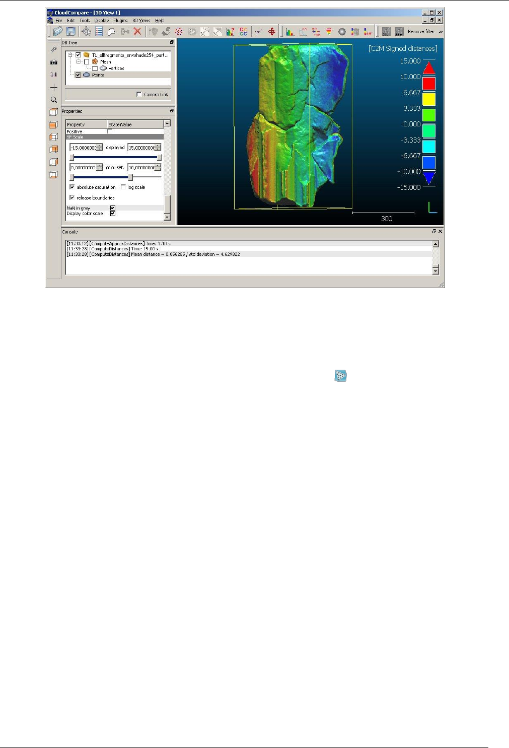
35
CloudCompare Version 2.6.1 – user manual
Typical result of a distance computation process, with color scale display parameters adjusted
Dealing with sparse mesh vertices
If the compared entity is a mesh, CloudCompare will only compute the distances from its vertices to the reference
entity. If those vertices are too sparse (i.e. with a too low density), you may want to sample points on the mesh first
(with a high sampling density). To do this, use the 'Edit > Mesh > Sample points' tool. Then use the resulting cloud
as 'compared' entity instead of the original model.

36
CloudCompare Version 2.6.1 – user manual
Tools and algorithms
Here are described all the methods of CloudCompare in the order they appear in the menu.
File menu
Open
Menu / Icon
This tool is accessible via the 'File > Open' menu or the icon in the upper main toolbar.
Description
Loads entities from one or several files.
‘File > Load’ dialog
Procedure
Select the right file type (with the drop-down list next to the filename field). Alternatively you can let CloudCompare
guess it from the file extension (use the 'All (*.*)' entry).
A file typically contains one or several entities (clouds, meshes, etc.).
Notes:
read-only access to the files. Moreover, once the entities are loaded CloudCompare will close the file and
'forget' about it.
the loaded entities are automatically put in a 'group' which has the input filename as name. However this
group has no link to the file.
alternatively, files can be opened by dragging them from the file explorer and dropping them on a 3D view.
Supported formats
See the supported file formats in the ‘Supported file formats’ section.
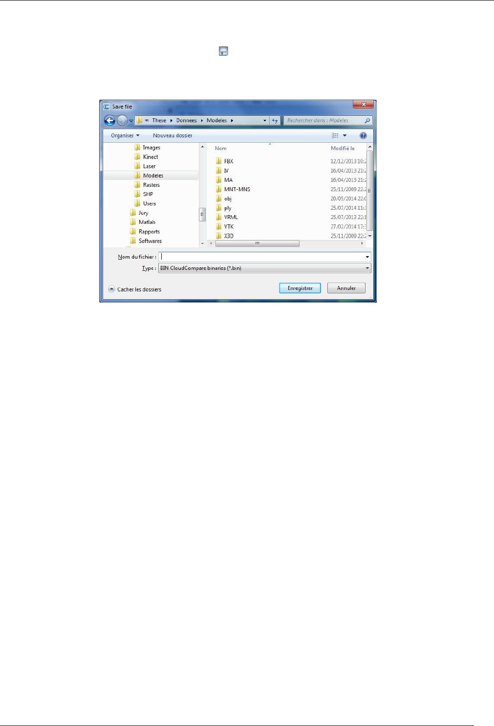
37
CloudCompare Version 2.6.1 – user manual
Save
Menu / Icon
This tool is accessible via the 'File > Save' menu or the icon in the upper main toolbar.
Description
This tool let the user save/export one or several entities to a file.
‘File > Save’ dialog
Procedure
Select one or several entities then call this method.
Warnings:
be sure to select the right file type in the Type drop-down list.
depending on the entities number and types, the available file types may change
some file types don't support non-ASCII characters (accents, non-occidental characters, etc.)
Supported formats
See the supported file formats in the ‘Supported file formats’ section.
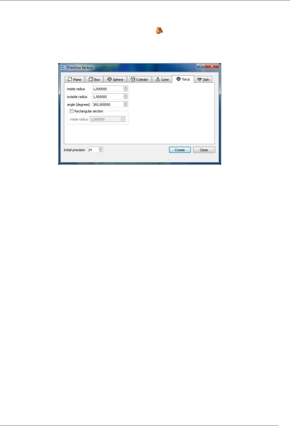
38
CloudCompare Version 2.6.1 – user manual
Primitive Factory
Menu / Icon
This tool is accessible via the 'File > Primitive factory' menu or the icon in the upper main toolbar.
Description
The Primitive Factory lets you create primitive objects (planes, spheres, boxes, etc.).
‘File > Primitive factory’
You can choose the primitive type by selecting the right tab (Plane, Box, Sphere, Cylinder, Cone, Torus and Dish). For
the selected primitive, you can edit its parameters (mainly dimensions) then create it by clicking on the 'Create' button.
The process can be repeated several types (you can change the primitive type as well) until you close the factory with
the 'Close' button.
Notes:
optionally you can also set the initial precision (i.e. the amount of triangles of the tessellated version of the
primitive). However this parameter can be freely changed later in the primitive parameters
primitives are defined along the main axes (X, Y and Z) by default. However you can apply a rigid
transformation to it afterwards with the ‘Edit > Apply Transformation’ method.
39
CloudCompare Version 2.6.1 – user manual
3D mouse > Enable
Menu / Icon
This tool is accessible via the 'File > 3D mouse > Enable' menu.
Description
If a 3Dconnexion device is connected to your PC, you can enable or disable it via this menu entry.
3Dconnexion devices
Success of the operation should be reported in the Console
Close all
Menu
This method is accessible via the 'File > Close
all'http://www.cloudcompare.org/doc/wiki/index.php?title=File:3dconnexion_logo.jpg menu.
Description
Closes all loaded entity.
Note: CloudCompare will ask the user to confirm this action (if entities are loaded).
Quit
Menu
This method is accessible via the 'File >
Quit'http://www.cloudcompare.org/doc/wiki/index.php?title=File:3dconnexion_logo.jpg menu.
Description
Quits the application.
Shortcut: ALT+F4
Note: CloudCompare will ask the user to confirm this action (if entities are loaded).

40
CloudCompare Version 2.6.1 – user manual
Edit menu
Clone
Menu / Icon
This tool is accessible via the 'Edit > Clone' menu, or via the icon in the upper main toolbar.
Description
Clones the selected entities. All data are duplicated.
Merge
Menu / Icon
This tool is accessible via the 'Edit > Merge' menu, or via the icon in the upper main toolbar.
Description
Merges two or more entities. You can currently merge clouds or meshes.
Merging clouds
Warning: when merging clouds, the original clouds will be deleted (you may have to save or clone them first).
Merging meshes
When merging meshes, the original meshes are not modified/deleted. CC will create a new composite mesh structure.
Sub-meshes are also created for each input mesh so that the original structure is preserved (useful when saving the
result as an OBJ file).
Merging meshes (input: 'Knee joint' group - output: 'Merged mesh' entity)
Note: all triangles are copied but not actually merged topologically speaking (i.e. they won't share the same vertices).
Refer to the qCork (Boolean Operations on Meshes) plugin to do this.
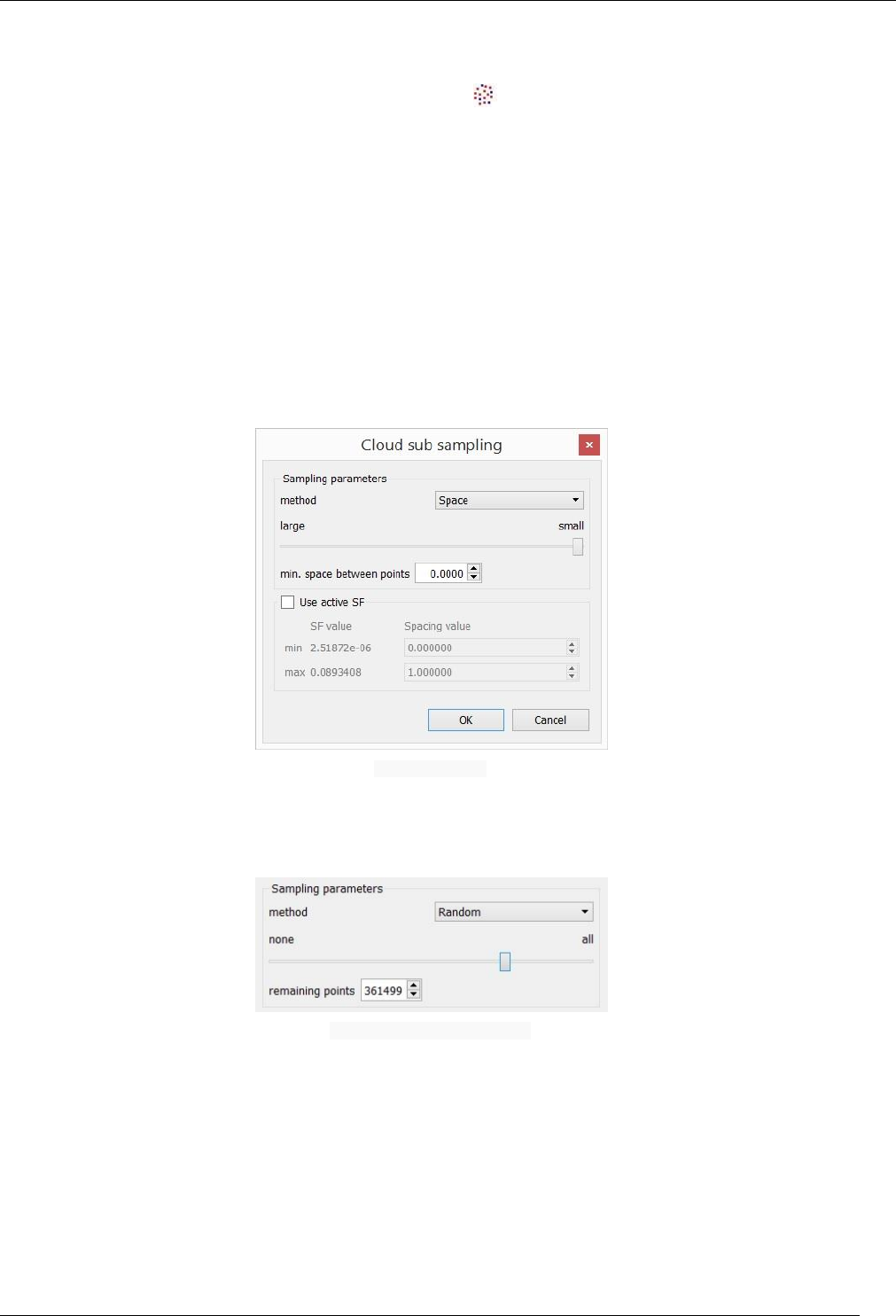
41
CloudCompare Version 2.6.1 – user manual
Subsample
Menu / Icon
This tool is accessible via the 'Edit > Subsample' menu, or via the icon in the upper main toolbar.
Description
Subsamples a point cloud (i.e. decreases the number of points).
Several subsampling methods are available (random, spatial and octree-based).
Notes:
for each input cloud, a new subsampled cloud is created (the original one is simply deactivated)
a subsampled cloud is a subset of the input cloud (the original points are not displaced)
thanks to this, a subsampled cloud keeps the features of its source cloud (scalar fields, colors, normals, etc.)
Procedure
Select one or several clouds then launch the tool.
Subsampling dialog
Random
In 'random' mode, CloudCompare will simply pick the specified number of points in a random manner.
Subsampling 'Random' parameters
Spatial
In 'spatial' mode, the user must set a minimal distance between two points. CloudCompare will then pick points from
the original cloud so that no point in the output cloud is closer to another point than the specified value. The bigger
this value is, the less point will be kept.
Use active SF (option)
Since version 2.6.1., instead of specifying a single value for the spatial subsampling mode, the user can use the currently
active scalar field so as to modulate the sampling distance with the scalar values. The user has to specify the sampling
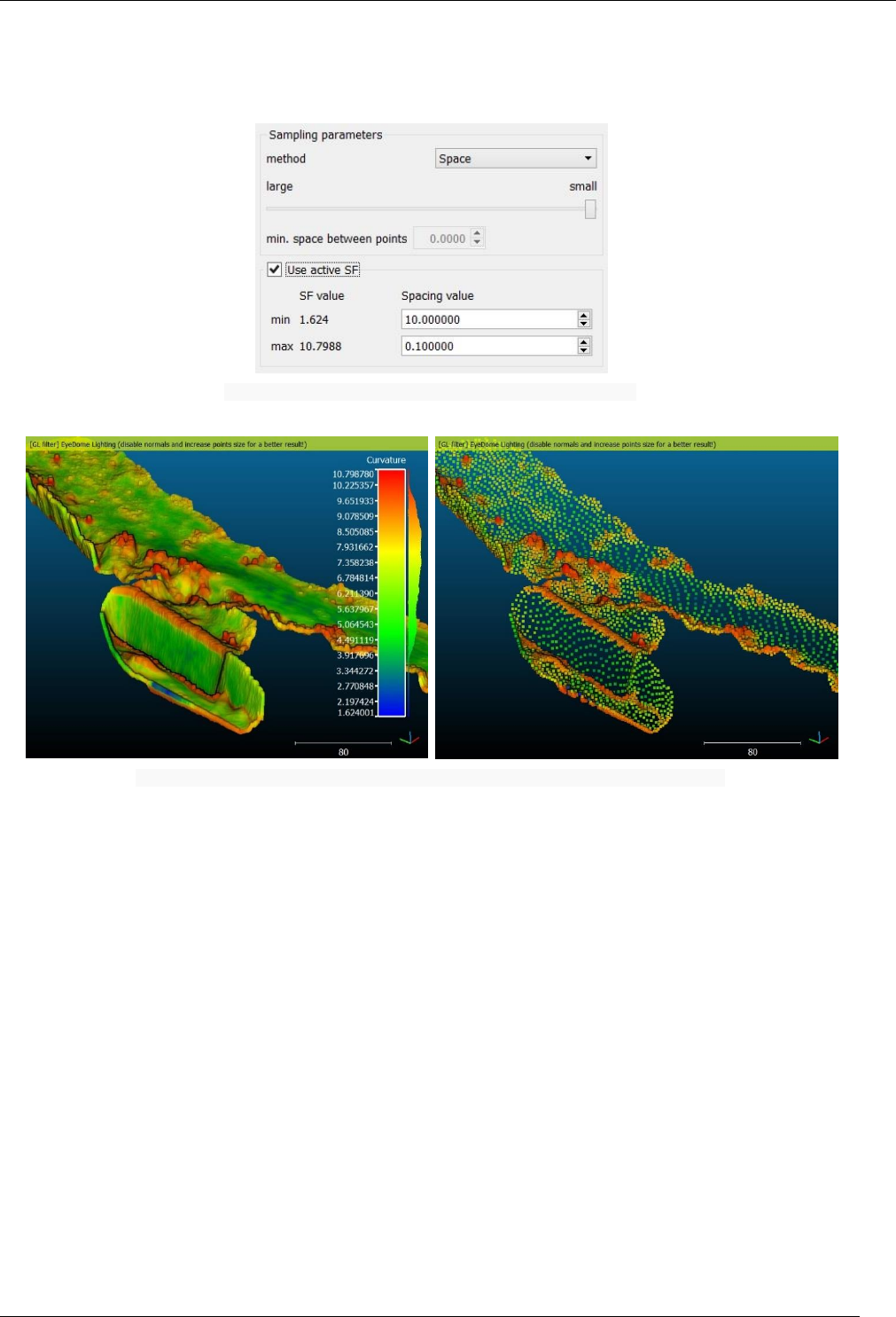
42
CloudCompare Version 2.6.1 – user manual
distance corresponding to the minimum and maximum scalar values and CC will linearly interpolate the spatial
distance.
For instance, if the cloud is associated to a 'curvature' scalar field, you can tell CloudCompare to sample more points in
curvy areas and less points in planar ones:
Subsampling 'Spatial' parameters based on the active scalar field values
Left: original cloud with a scalar field proportional to the local curvature – right: subsampling output
You could do the same with a noise or confidence scalar field, etc.
Octree
The 'octree' mode lets you select a level of subdivision of the octree at which the cloud will be 'simplified'.
In each cell of the octree, the nearest point to the octree cell center is kept.
Notes:
the higher the level is, the smaller the cells are (so the more points you'll keep)
the maximum octree level is 10 in the 32 bits version of CloudCompare, and 21 in the 64 bits version.
the tool differs from the 'Octree > Resample' method. The Resample tool computes the center of gravity of the
points falling in each cell (i.e. the created cloud is not a subset of the original cloud)
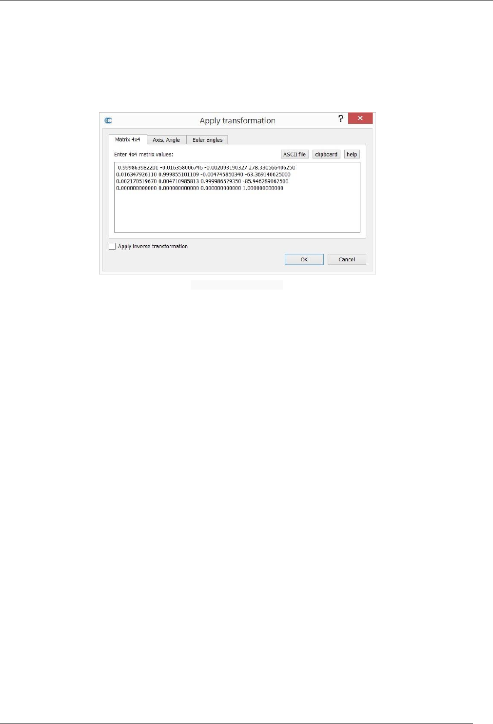
43
CloudCompare Version 2.6.1 – user manual
Apply Transformation
Menu / icon
This tool is accessible via the 'Edit > Apply transformation' menu.
Description
This tool allows the user to transform (i.e. rotate and/or translate) the selected entities. The transformation to apply
can be input in various ways.
'Apply transformation' dialog
Start
The user must select one or several entities before launching this tool. The entities can be about any 3D geometry
(clouds, meshes, polylines, primitives, etc.).
Note: locked entities (sub-meshes, etc.) can't be moved this way.
Procedure
The user has multiple choices to set the transformation to apply (see below for more details):
as a transformation matrix
the combination of a rotation axis, a rotation angle and a translation vector
the combination of Euler angles [1] and a translation vector
A checkbox let the user specify if he wishes to apply the currently defined transformation or it's inverse (Apply inverse
transformation).
Once defined the transformation can be applied by clicking on the OK button (or the process can be canceled by clicking
on the Cancel button).
The transformation is applied to all selected entities and to their children (recursively). The transformation is added
to each entity's Transformation history.
Input a transformation
Transformation matrix
A rigid transformation matrix is a composition of a rotation (a 3x3 matrix) and a translation (a 3D vector). For
convenience, it can be written as a 4x4 matrix (the rotation matrix corresponds to the upper part of the 3 first columns,
the translation vector corresponds to the upper part of the 4th column, and the bottom line is always filled with 3
'zeros' and a 'one').
In he first tab ("Matrix 4x4") the user can input the matrix values directly; or load them from a text file (each row of the
matrix on a single line, i.e. 4 values separated by a space character); or eventually paste it from the clipboard. For
instance, most of the registration tools in CloudCompare will output the final transformation as a 4x4 matrix in the
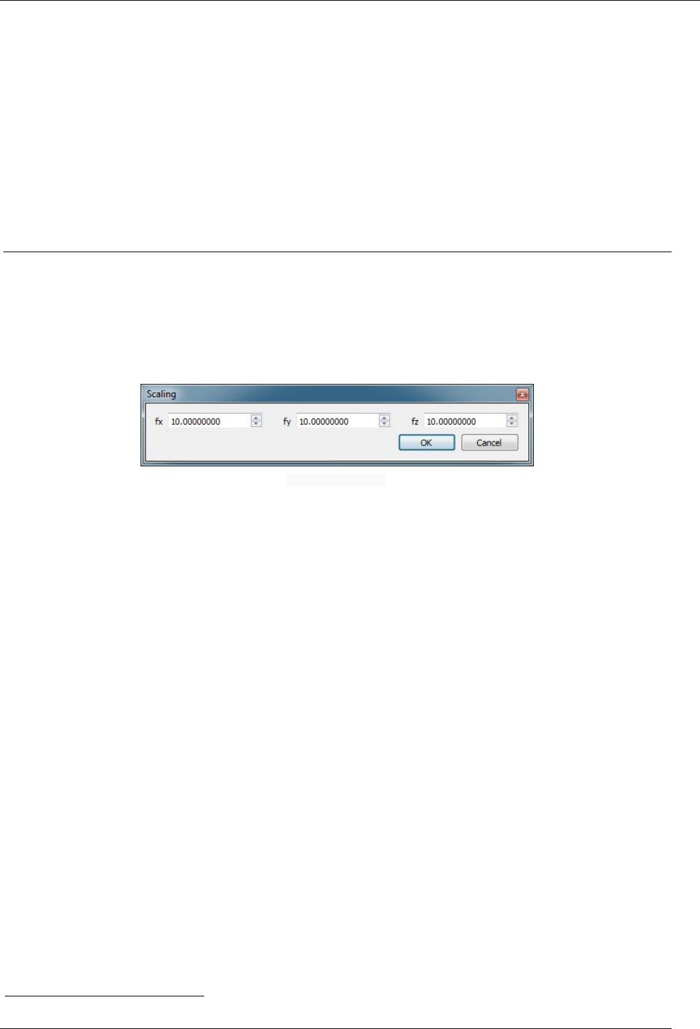
44
CloudCompare Version 2.6.1 – user manual
Console. The user can copy it (with CTRL+C on Windows) and paste it here so as to apply the same transformation to
another entity.
Rotation axis and angle + translation
The rotation part of the transformation can be input as a single rotation angle about a 3D axis. The second tab ("Axis,
Angle") let the user input those values (the angle is in degrees). It's the fastest way to apply simple rotations about X,
Y or Z for instance.
Euler angles + translation
The third tab ("Euler angles") let the user define the rotation as Euler angles
21
(phi, theta and psi).
Multiply / Scale
Menu
This tool is accessible via the 'Edit > Multiply/Scale' menu.
Description
This tool lets the user scale the selected entities (clouds, meshes or polylines).
'Multiply/Scale' dialog
CloudCompare will actually multiply the entities coordinates by user defined factors (one per dimension).
Warnings:
the input entities are changed directly
on completion, the 3D view zoom and camera position won't change. So depending on the scaling values you
might have to update the current zoom (use the magnifier icon for instance)
Procedure
Simply select one or several entities then call this tool.
21
http://en.wikipedia.org/wiki/Euler_angles
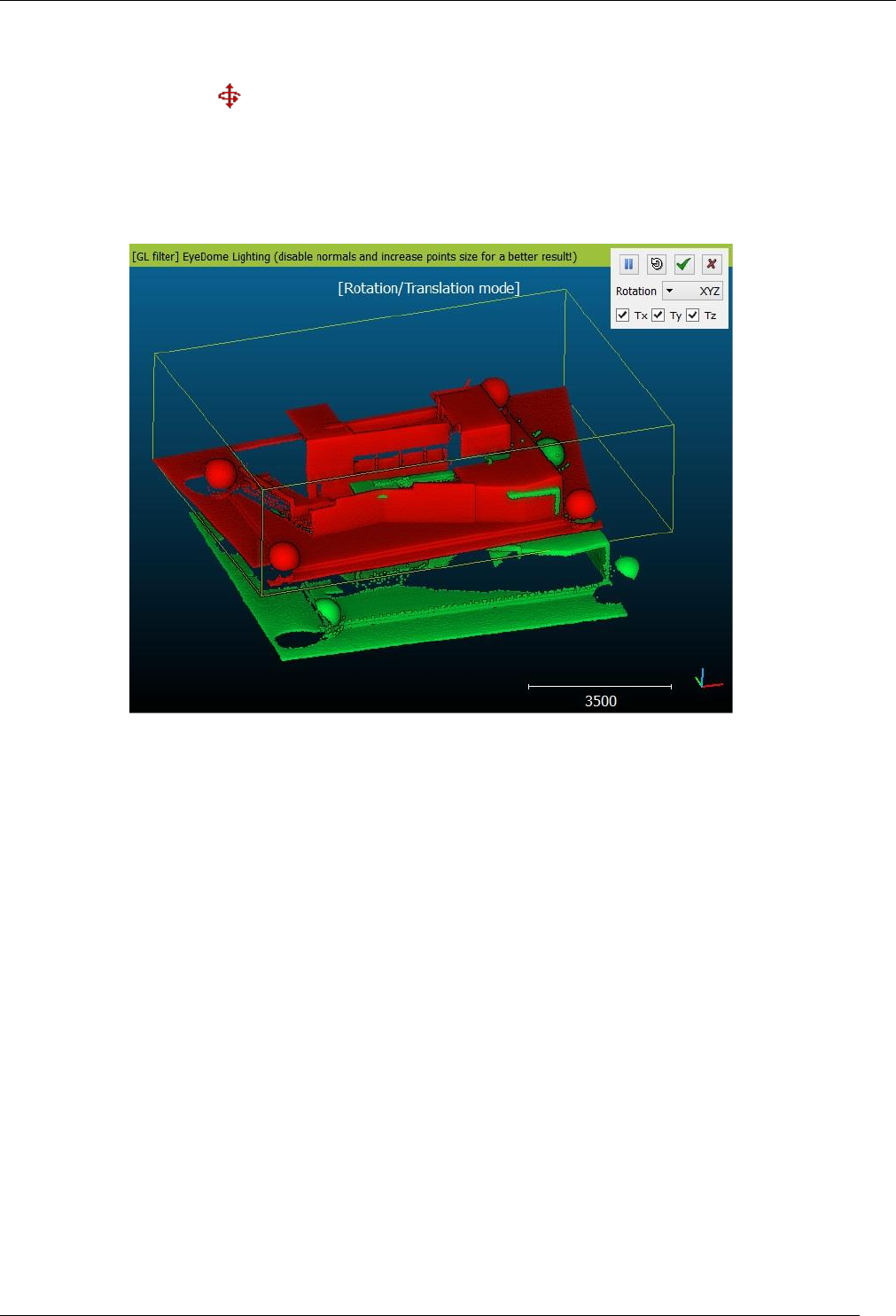
45
CloudCompare Version 2.6.1 – user manual
Translate / Rotate (Interactive Transformation Tool)
Menu / icon
This tool is accessible via the icon in the upper main toolbar or the 'Edit > Rotate/Translate' menu.
Description
This tool allows the user to interactively move the selected entities relatively to the other ones (or equivalently to the
default coordinates system).
‘Rotate/Translate’ tool in action
Start
The user must select one or several entities before launching this tool. The entities can be any 3D geometry entity
(clouds, meshes, polylines, primitives, etc.).
Notes: locked entities (sub-meshes, etc.) can't be moved this way
only the entities displayed in the active 3D view will be considered
Procedure
The standard mouse interactions with the 3D view are used to modify the selected entities position (instead of the
current camera):
left click: rotate
right click: translate
Pause
At any time, the user can 'pause' the transformation mode (click on the 'pause' button or hit the space bar) in order to
modify the camera position/orientation, and then restart the transformation process by 'un-pausing' it (new click on
the 'pause' button or new hit on the space bar).
Constraints
Optionally, constraints can be added to the applied transformation:

46
CloudCompare Version 2.6.1 – user manual
rotation can be constrained to a single axis (X, Y or Z). Use the drop-down menu to select the current
dimension.
translation ca be constrained to zero, one or two dimensions only (among X, Y and Z). Just uncheck the
dimensions that should be ignored.
When done, use the validation icon to apply the transformation, or the cancel button to revert it.
Note: on validation, CC will output the applied transformation to the console.
Shortcuts
Some keyboard shortcuts are available:
Shortcut
Description
Space bar
Toggle 'pause' mode
Escape key
Cancel transformation (close the tool)
Return
key Apply transformation (close the tool)
Segment (Interactive Segmentation Tool)
Menu / icon
This tool is accessible via the icon in the main upper toolbar or the 'Edit > Segment' menu.
Description
This tool allows the user to interactively segment the selected entities by defining a 2D polygon (or a rectangle) on the
screen. This process can be repeated multiple times, changing the orientation of the entities each time, so as to properly
segment the entities in 3D. Each time the user can decide to keep the points (or triangles) falling inside or outside the
polygon border.
‘Interactive Segmentation’ tool in action
Currently this tool can be used to segment clouds or meshes (see below for more information).
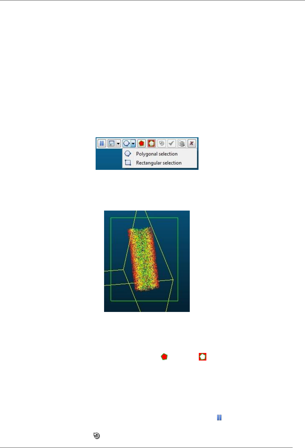
47
CloudCompare Version 2.6.1 – user manual
Procedure
Select one or several entities and start the tool. A new tool bar will appear in the top-right corner of the 3D view.
Polygon edition mode
By default the tool starts in 'polygonal' editing mode. This means that you can start drawing the polygon right away:
left click: create a new polygon vertex
right after the first vertex is created, you'll see that the first polygon edge will start to "follow" the mouse
cursor. You have to define the position of the second vertex (left click) in order to 'fix' it. This process will start
over with the next edge and so on.
right click: stop the polygon edition (warning: the currently 'floating' vertex won't be added to the polygon)
Rectangle edition mode
You can switch the 'Polygon edition' mode to 'Rectangle edition' mode by clicking on the down arrow next to the
'polygon' icon:
In 'Rectangle edition' mode you have to left click a first time to define the first corner of the rectangle then click a
second time to define the opposite corner (alternatively you can keep the left mouse button pressed and the opposite
corner will be created once you release the button).
Segmentation
Once the polygon/rectangle edition is finished, if the user clicks on the left button the edition process will start over
(i.e. the current segmentation polygon will be discarded).
Otherwise the user has to choose whether to keep points inside ( ) or outside ( ) the polygon. Once done the other
points will disappear (as well as the polygon). The tool will fall back in "paused" mode.
Paused mode
In paused mode, the mouse can be used to modify the entities orientation and position in the standard way.
The user has multiple choices:
modify the current entities orientation and segment more points (click on the button to leave the 'paused'
mode and define a new polygon/rectangle)
reset the current selection ( )
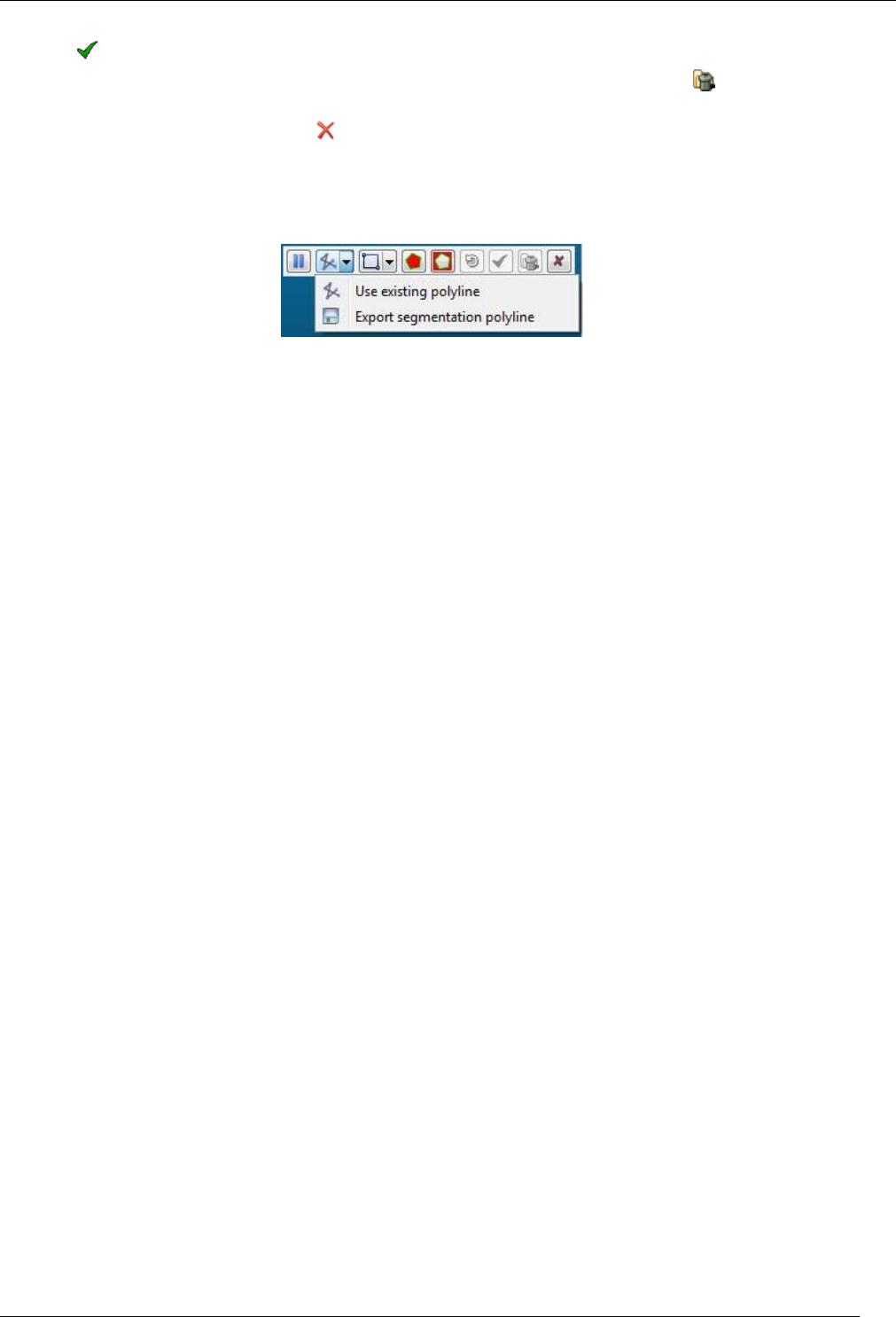
48
CloudCompare Version 2.6.1 – user manual
validate the current segmentation and create two clouds: one with the selected points and one with the others
( )
validate the current segmentation and create only one cloud with the visible points ( ) - the other points
will be deleted
cancel the segmentation process ( ) (no modification will occur)
Polygon Import / Export
The user can import or export the current polygon as a (flat) 3D polyline.
Import
A new segmentation polygon can be imported anytime with the Use existing polyline option. It will be added to the
root of the DB tree with a default name.
CC will display a simple list of all polylines it founds in the DB tree so that the user can select the one he wants to use.
Warning: any previously defined polygon/rectangle will be discarded.
Export
The segmentation polygon can be exported as soon as it has been 'closed' (right-click) and BEFORE segmenting the
points (inside or outside).
Note: the exported polyline will have a ' viewport’ entity as child. This 'viewport' entity stores the current viewport
parameters and allows the user to restore the exact same viewport later (by clicking on the 'Apply' button in its
properties). Viewport can also be saved in BIN files. This way it is possible to apply the exact same segmentation process
to the same entity or to other entities (first apply the viewport, then start the tool and eventually import the polyline -
see above).
About mesh segmentation
In the case of meshes, this tool doesn't cut the triangles crossing the polygon edges. Those triangles are always removed
(i.e. this tool only keeps the triangle having all their vertices inside or outside the polygon). The result can be acceptable
if the mesh has very small triangles. It can be more problematic if big/long triangles cross the segmentation polygon.
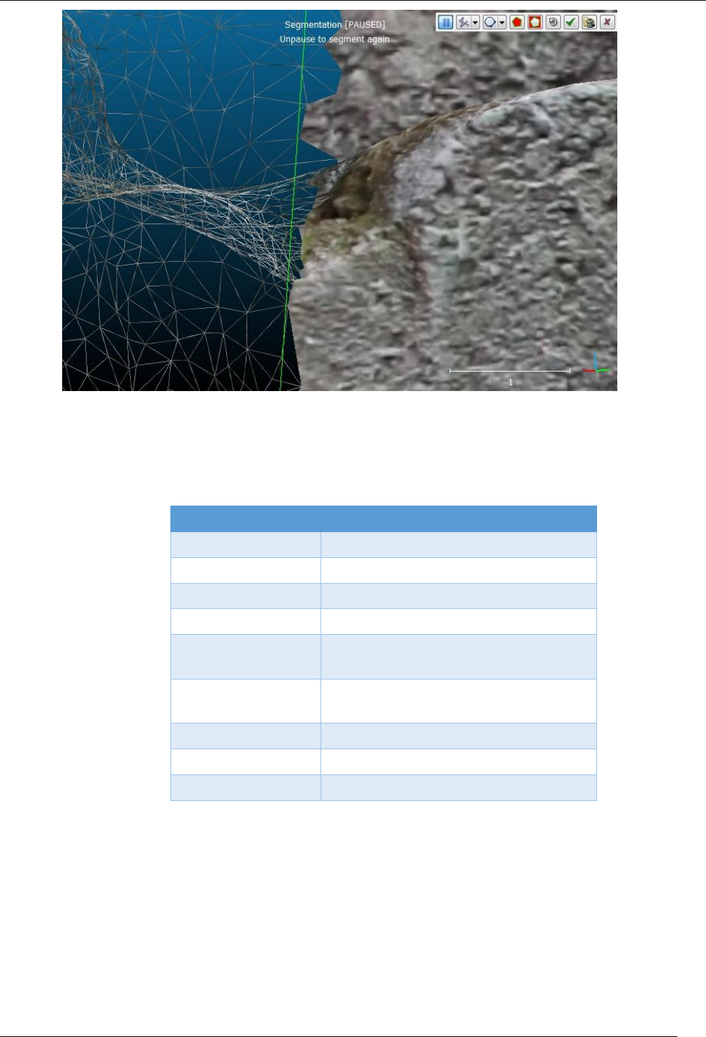
49
CloudCompare Version 2.6.1 – user manual
Close-up of mesh segmentation near the polygon edges (original mesh is shown as wireframe
and the segmented mesh is in plain colors - the polygon edge is in green
Shortcuts
Some keyboard shortcuts are available:
Shortcut
Description
Space bar
Toggle 'pause' mode
Escape key
Cancel
Return key
Apply
Delete key
Apply + delete hidden points
Tab
Switch between polygon and rectangle
edition mode
CTRL key (pressed)
Use a rectangular selection area
(whatever the edition mode)
I
Select points inside
O
Select points outside
Space bar
Toggle 'pause' mode
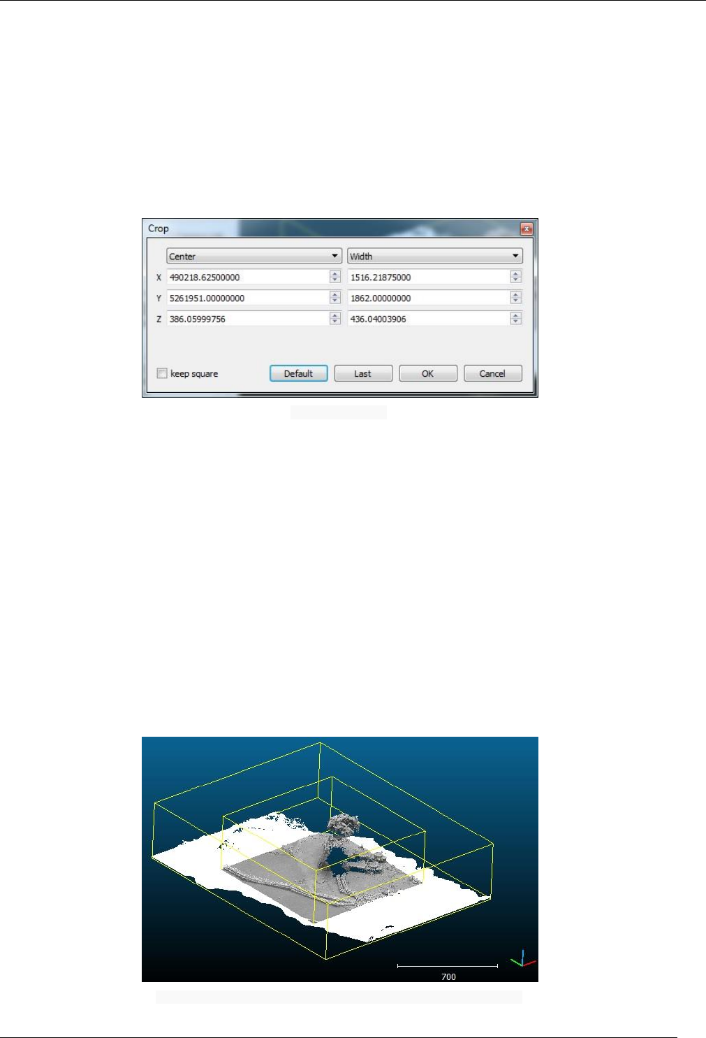
50
CloudCompare Version 2.6.1 – user manual
Crop
Menu
This tool is accessible via the 'Edit > Crop' menu.
Description
This tool is used to crop one or several clouds inside a 3D box.
Note: this tool creates new clouds (one for each input cloud - if the cloud is intersected by the 3D box)
Procedure
Select one or several clouds then start this tool. The standard 3D box editing dialog appears:
3D box editing dialog
By default, the box is initialized to the bounding-box of all selected clouds (this default box can be restored anytime by
clicking on the 'Default' button).
The user can define the cropping box in multiple ways:
by defining the center and dimensions of the box [default]
by defining the min corner and the dimensions of the box • by defining the max corner and the dimensions of
the box
Notes:
for cubical boxes (the same dimension in all directions), you can check the 'keep square' checkbox.
you can recall the previous box (if you call the tool several times) by clicking on the 'Last' button. The 'Last'
button only appears if the tool has been called at least twice.
Eventually click on the 'OK' button to crop the input clouds and create the corresponding subsets (or click on the 'Cancel'
button to cancel the process).
Crop example (the (grey) cloud has been cropped out of the original (white) cloud
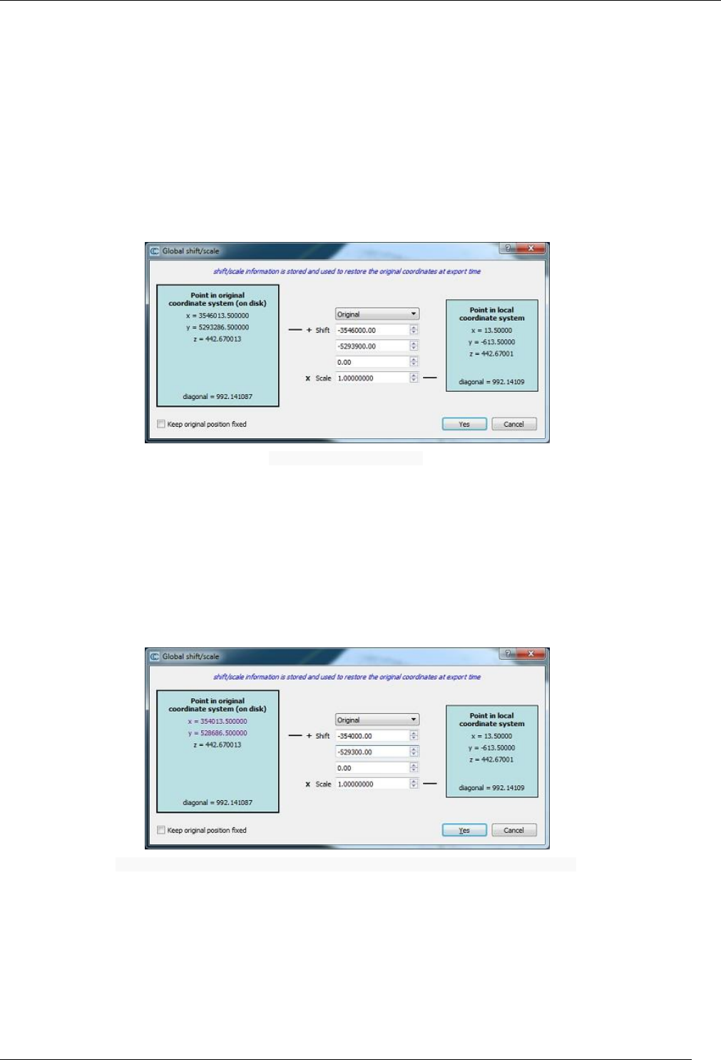
51
CloudCompare Version 2.6.1 – user manual
Edit global shift and scale
Menu
This tool is accessible via the 'Edit > Edit global shift & scale' menu
Description
This tool let the user edit the 'Global Shift & Scale' of the selected entity (cloud, mesh or polyline).
See the ‘Global Shift and Scale’ section for more information.
Procedure
Select an entity (cloud, mesh or polyline) and start this tool. A dialog very similar to the one that CloudCompare displays
when an entity with big coordinates is loaded will appear:
'Edit global shift and scale' dialog
A numerical 'example' of the current shift and scale settings is given in the turquoises frames:
on the left a point is expressed in the global coordinate system (along with the bounding-box diagonal length
in the bottom part)
on the right, the same point is expressed in the local coordinate system (with the equivalent bounding-box
diagonal length as well)
The user can change the shift and scale values. The values in the turquoise frames are automatically updated to reflect
these modifications. The modified values appear in purple or red:
'Edit global shift and scale' dialog with a pending modification (local coordinate system maintained)
When the shift and scale values are modified, then either the local coordinate system or the global coordinate system
will be impacted.
Keep local coordinate system
By default, the tool will modify the global coordinate system. This way one can easily change the geo-localization of
the cloud, or even simply remove them so as to save the cloud in a local coordinate system.
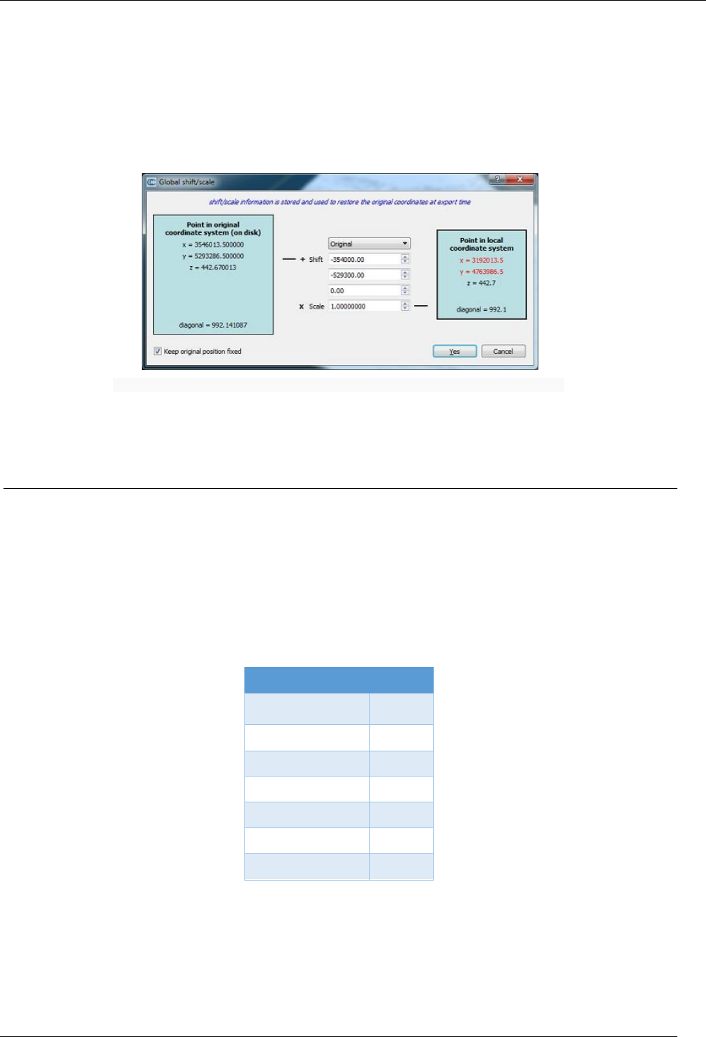
52
CloudCompare Version 2.6.1 – user manual
In this mode, no modification to the cloud currently in memory will occur. However when exported, the entity might
not be in the same place as the original one.
Keep global coordinate system
It is possible to tell CloudCompare to maintain the global coordinate system unchanged. For this the user must check
the 'Keep original position fixed' checkbox.
In this case the local coordinate system will be modified so as to maintain the original (global) one:
'Edit global shift and scale' dialog with a pending modification (local coordinate system maintained)
In this mode the cloud in memory will be translated. However when exported, the cloud will be in the same position as
the original one (apart if other transformations have been applied of course).
Toggle (recursive) menu
Menu
This sub-menu is accessible via 'Edit > Toggle (recursive)'.
Description
This sub-menu is mainly a collection of keyboard shortcuts. Each one toggles a given property of the selected entities
(and their siblings)
Shortcuts
Property
Shortcut
Activation(1)
A
Visibility
V
Colors
C
Normals
N
Scalar field
S
Materials/textures
M
3D name
D
(1)Not recursive (i.e. only the selected entities activation state is toggled, not their siblings)

53
CloudCompare Version 2.6.1 – user manual
Delete
Menu
This tool is accessible via the ‘Edit > Delete’ menu.
Description
Deletes the selected entities.
Shortcut: DEL key
Warning: action is immediate (no confirmation message).
Colors > Set Unique
Menu / Icon
This tool is accessible via the 'Edit > Colors > Set unique' menu.
Description
Set a unique color on the selected entities.
Edit > Colors > Set unique dialog
Warnings:
previous color field (if any) will be overwritten
not all entities can be colored
Colors > Colorize
Menu
This tool is accessible via the 'Edit > Colors > Colorize' menu.
Description
Colorize the selected entities by multiplying their current color(s) by the specified one.
NewColor.r = OldColor.r * (SelectedColor.r / 255)
NewColor.g = OldColor.g * (SelectedColor.g / 255)
NewColor.b = OldColor.b * (SelectedColor.b / 255)
Note: if the entity has no color, this method is equivalent to Set unique.
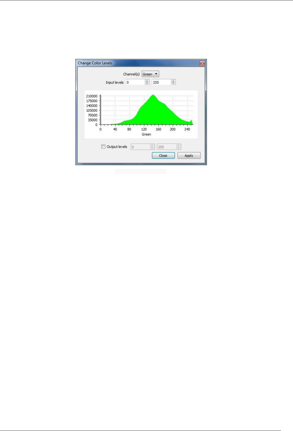
54
CloudCompare Version 2.6.1 – user manual
Colors > Levels
Menu
This tool is accessible via the 'Edit > Colors > Levels' menu.
Description
Edit the color histogram. Similar to Photoshop's Levels method.
Edit > Colors > Levels dialog
You can edit either all channels at once (RGB) or one channel at a time (Red, Green or Blue).
By default, the main usage of this tool is to increase the color dynamics. To do this you'll have to zoom in the global
histogram. The color values falling inside the sub-range in which most of the information is will be extended so as to
use the full [0-255] range.
In practical, once you've identified the smallest interval where most of the information lies (e.g. [40-240] here), set this
new interval as 'Input levels' then click on 'Apply'.
Advanced users can also change the 'Output levels'. In which case the 'Input' interval will be remapped to the 'Output'
one.
Note: the dialog uses a standard histogram display, so you can click on it to get information on the histogram bin
hovered by the mouse

55
CloudCompare Version 2.6.1 – user manual
Colors > Height Ramp
Menu
This tool is accessible via the 'Edit > Colors > Height Ramp' menu.
Description
To apply a color ramp (linear gradient or cycling) to the selected entities.
Edit > Colors > Height ramp
This method let the user apply a linear gradient (either the default one - see below - or any gradient defined by two
colors) or a cycling HSV map ('Banding', see below). For the latter, the user must specify the number of repetitions. And
in all cases, the user must choose the main direction for the height ramp (X, Y or Z).
Left: default height ramp – right: cycling HSV “banding” ramp
Warning: any previous color field (if any) will be overwritten.
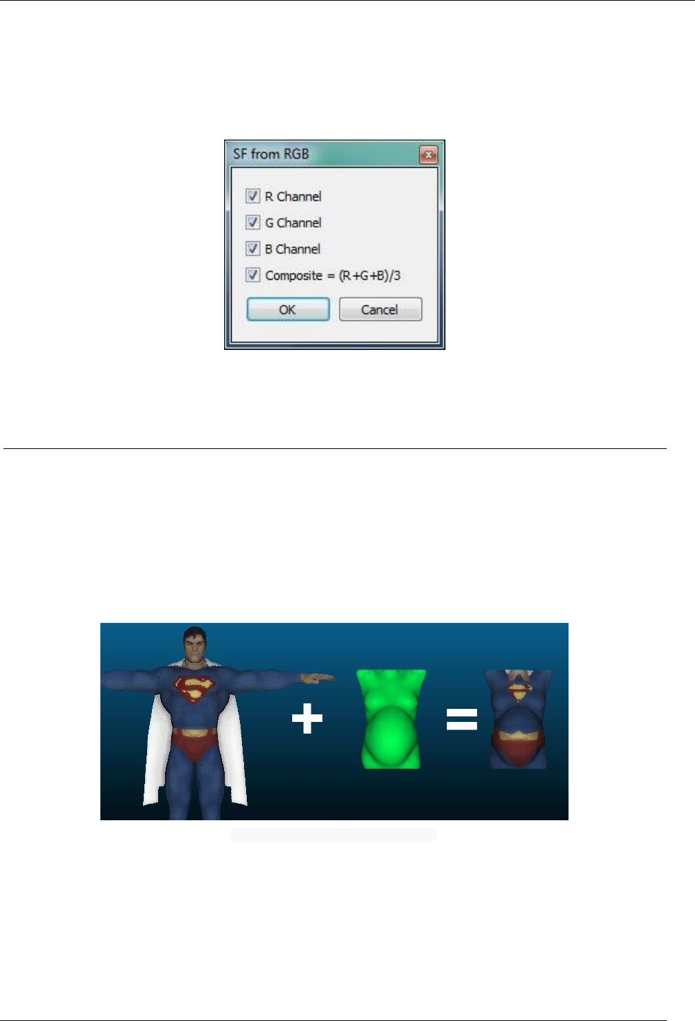
56
CloudCompare Version 2.6.1 – user manual
Colors > Convert to Scalar Field
Menu
This tool is accessible via the 'Edit > Colors > Convert to Scalar field' menu.
Description
Converts the current RGB color field to one or several scalar fields:
Edit > Colors > Convert to SF dialog
The user can choose to export the Red, Green, Blue and Composite (R+G+B/3) color fields as scalar fields (one for each).
Colors > Interpolate from another entity
Menu
This tool is accessible via the 'Edit > Colors > Interpolate from another entity' menu.
Description
Interpolates the color of another entity in order to color the points/vertices of the selected entity.
In the current implementation, for each point of the selected cloud (or the selected mesh vertices) this method will
simply look for the nearest point in the other entity and take its color.
Edit > Colors > Interpolate from another entity
Two entities must be selected (the color 'source' entity and the 'destination' one). In order for CC to differentiate both
entities, the 'destination' entity must have no colors (use the Edit > Colors > Clear entry to remove any existing color
field if necessary). And of course the 'source' entity must have colors...
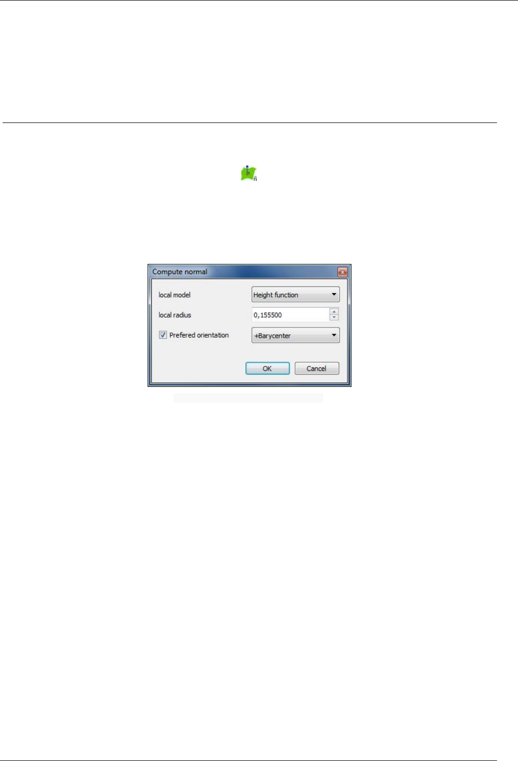
57
CloudCompare Version 2.6.1 – user manual
Colors > Clear
Menu
This tool is accessible via the ‘Edit > Colors > Clear menu.
Description
Remove the color field of the selected entities.
Normals > Compute
Menu / Icon
This tool is accessible via the 'Edit > Normals > Compute' menu.
Description
Computes normals on the selected entities.
Computing normals on a cloud
Edit > Normals > Compute dialog - mesh case
If the entity is a cloud, then the user must specify several parameters:
local model: whether to use a (best fit) plane, 2D triangulation or height function (quadric [1]) to locally
estimate the normal
local radius: radius of the local neighborhood (sphere). If it’s too small (i.e. not enough points to compute the
local model) then the normal will be (0,0,1) by default. If it's too big, the process might be very long and the
result very smooth.
preferred orientation: optional. Let the user specify a simple heuristic to set the normal orientation (outside
of the surface ideally). These heuristics are:
o to be as parallel as possible to an axis, in the positive or negative direction (-X/+X, -Y/+Y, -Z/+Z)
o to be as parallel as possible to a vector coming from the cloud barycenter and passing through the
point or the opposite (+/-Barycenter)
o to be as parallel as possible to a vector coming from the origin (0,0,0) and passing through the point
or the opposite (+/-(0,0,0))
Notes:
if no preferred orientation has been specified, or if the result is still not consistent, it might be necessary to
use a more advanced algorithm to orient the normals. See the ‘Normals > Orient Normals > With Minimum
Spanning Tree’ method
in any case, it might be necessary to globally invert the normals field with the Invert method
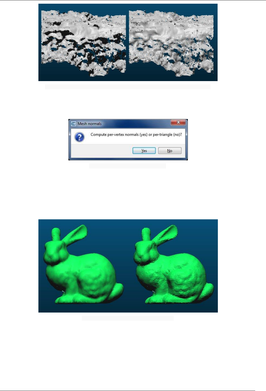
58
CloudCompare Version 2.6.1 – user manual
Normals computed on a cloud (left) then properly oriented with a Minimum Spanning Tree (right)
Computing normals on a mesh
Edit > Normals > Compute dialog - mesh case
If the entity is a mesh, then CC will simply ask the user if the normals should be computed:
per-vertex (i.e. the mean normal of all the triangles connected to a vertex is assigned to this vertex - smooth
look, no preservation of sharp edges)
or per triangle (i.e. the triangle normal is assigned to the triangle - hard/tessellated look, but preserves the
sharp edges)
Per-vertex (left) and per-triangle (right) mesh normals
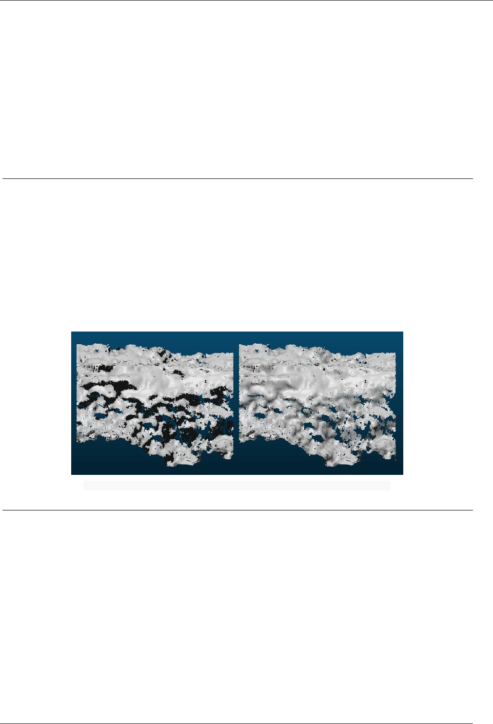
59
CloudCompare Version 2.6.1 – user manual
Normals > Invert
Menu
This tool is accessible via the 'Edit > Normals > Invert' menu.
Description
Inverts the normals of the selected entities.
The appearance of an entity with normals changes depending on the orientation of the light relatively to the normals:
for a cloud, backward lit points will appear black
for a mesh (with default material), backward lit triangles will appear in light blue (while forward lit triangles
will be green)
Normals > Orient Normals > With Minimum Spanning Tree
Menu
This tool is accessible via the 'Edit > Normals > Orient normals > with Minimum Spanning Tree' menu.
Description
This method attempts to re-orient all the normals of a cloud in a consistent way. It starts from a random point then
propagates the normal orientation from one neighbor to the other.
The propagation is done with the help of a Minimum Spanning Tree [1]. Therefore the user must specify the maximum
number of neighbors connected at each node (the more neighbors, the more accurate but also the more memory and
the more time will be necessary).
Normals computed on a cloud (left) then properly oriented with a Minimum Spanning Tree (right)
Normals > Orient Normals > With Fast Marching
Menu
This tool is accessible via the 'Edit > Normals > Orient normals > with Fast Marching' menu..
Description
This method attempts to re-orient all the normals of a cloud in a consistent way. It starts from a random point then
propagates the normal orientation from one neighbor to the other.
The propagation is done with the Fast Marching algorithm applied to a grid. In practical this grid is the cloud octree
considered as a given level of subdivision. Therefore the user must specify this level of subdivision. The problem is to
find the right level: if the cells are too big (i.e. low level of subdivision), the propagation is not very accurate. However
if the cells are too small (i.e. high level of subdivision) empty cells might appear and the propagation in one sweep
won't be possible.
Warning: this method is very fast but very approximate. It is highly advised to use the ‘Normals > Orient Normals > With
Minimum Spanning Tree’ method instead.
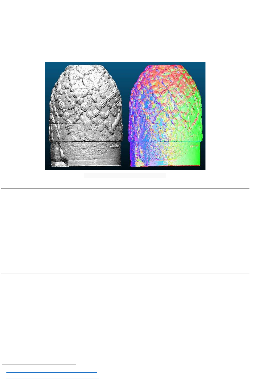
60
CloudCompare Version 2.6.1 – user manual
Normals > Convert to > HSV
Menu
This tool is accessible via the 'Edit > Normals > Convert to > HSV colors' menu.
Description
Converts the normals of a cloud to an HSV
22
color field.
H = dip direction
23
, S = dip and V = 1
Edit > Normals > Convert to HSV colors (example)
Normals > Convert to > Dip and Dip direction SFs
Menu
This tool is accessible via the 'Edit > Normals > Convert to > Dip and dip direction SFs' menu.
Description
Converts the normals of a cloud to two scalar fields:
one with the dip value
and the other with the dip direction value
Note: angles are in degrees.
Normals > Clear
Menu
This tool is accessible via the ‘Edit > Colors > Clear menu.
Description
Remove normals from the selected entities.
22
http://en.wikipedia.org/wiki/HSL_and_HSV
23
http://en.wikipedia.org/wiki/Strike_and_dip
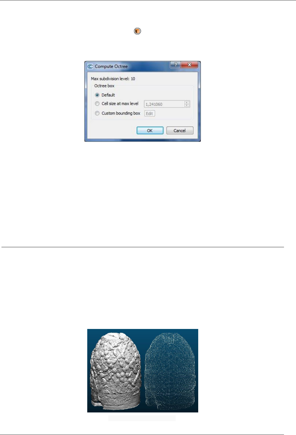
61
CloudCompare Version 2.6.1 – user manual
Octree > Compute
Menu
This tool is accessible via the 'Edit > Octree > Compute' menu.
Description
Forces the computation of the octree on a given entity.
Edit > Octree > Compute dialog (32 bits version)
The octree spatial extents can be set in various ways:
default: the smallest cube that totally includes the entity
bounding-box cell size at max level: the user can define the cell size at the smallest level of subdivision (the
octree box will then be 2N larger, where N is the maximum octree level)
custom: the user can define a custom bounding-box with a dedicated sub-dialog
The maximum octree level (or number of subdivisions) is N=10 in the 32 bits version and N=21 in the 64 bits version.
Note: this operation is generally not necessary (i.e. octree computation is done automatically by CloudCompare when
necessary).
Octree > Resample
Menu
This tool is accessible via the 'Edit > Octree > Resample' menu.
Description
Resamples a cloud by replacing all the points inside each cell of the octree (at a given level of subdivision) by their
gravity center.
The level of subdivision at which the process is applied is chosen to (roughly) match the expected number of output
points specified by the user.
Edit > Octree > Resample (example)
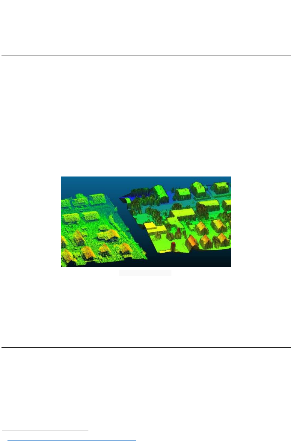
62
CloudCompare Version 2.6.1 – user manual
Warning: this method creates a new cloud with points that are not necessarily at the same position in space as the
input cloud points. Therefore it is not possible to keep the various features attached to the input points (color,
normal, scalar values, etc.). If you want to keep those features (as well as the points original positions) you should
consider using the ‘Subsample’ method instead.
Mesh > Delaunay 2.5D (XY plane)
Menu
This tool is accessible via the 'Edit > Mesh > Delaunay 2.5D (XY plane)' menu.
Description
Computes a Delaunay 2.5D triangulation
24
on a point cloud.
The point cloud is simply projected in 2D on the (XY) plane. Then the corresponding 2D points are triangulated and the
mesh structure is applied to the 3D points.
By default the 2D Delaunay triangulation is done on the cloud convex hull. Therefore CloudCompare will ask the user
to specify a maximum length for the triangle edges. This allows to remove the biggest triangles (generally on the
boundary) that are not necessarily meaningful. If this value is left to zero, then all the triangles output by the Delaunay
triangulation will be kept.
Edit > Mesh > Delaunay 2D
This works very well with rather flat clouds and properly oriented (i.e. with the Z dimension as the vertical one). If the
point cloud is not properly oriented but is still rather flat in a direction, you should consider using the other version of
this method ‘Mesh > Delaunay 2.5D (best fit plane)’.
Note: for 3D triangulation, refer to the qPoissonRecon (Poisson Surface Reconstruction) plugin.
Mesh > Delaunay 2.5D (best fit plane)
Menu
This tool is accessible via the 'Edit > Mesh > Delaunay 2.5D (best fit plane)' menu.
Description
Computes a Delaunay 2.5D triangulation on a point cloud.
24
http://en.wikipedia.org/wiki/Delaunay_triangulation
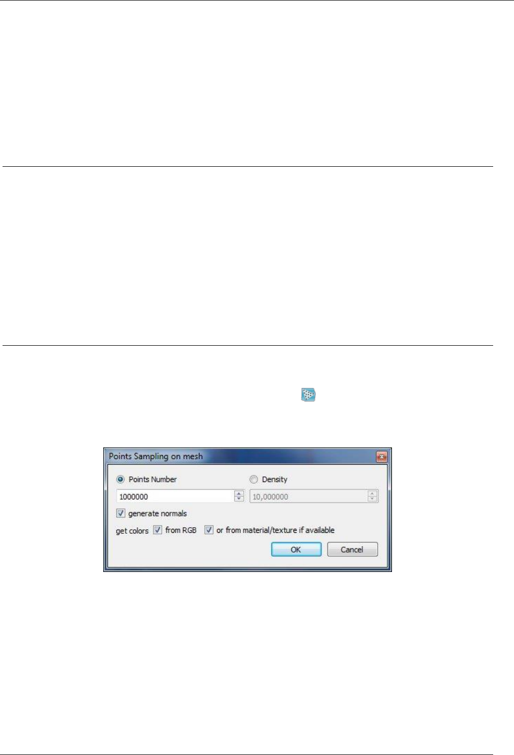
63
CloudCompare Version 2.6.1 – user manual
Same method as ‘Mesh > Delaunay 2.5D (XY plane)’. However the 3D point cloud is first projected on the best fitting
plane (least squares). Then the corresponding 2D points are triangulated and the mesh structure is applied to the 3D
points.
By default the 2D Delaunay triangulation is done on the cloud convex hull. Therefore CloudCompare will ask the user
to specify a maximum length for the triangle edges. This allows to remove the biggest triangles (generally on the
boundary) that are not necessarily meaningful. If this value is left to zero, then all the triangles output by the Delaunay
triangulation will be kept.
Note: for 3D triangulation, refer to the qPoissonRecon (Poisson Surface Reconstruction) plugin.
Mesh > Convert texture/material to RGB
Menu
This tool is accessible via the 'Edit > Mesh > Convert texture/material to RGB' menu.
Description
Converts the mesh material and/or texture information of the selected mesh to a per-vertex RGB field.
For each vertex of the mesh, this method will interpolate the nearest texture color or take the triangle's associated
material color if no texture is available.
Warning: if the vertices are sparse, the visual rendering of the output RGB field might be quite different than the original
one.
Mesh > Sample points
Menu / Icon
This tool is accessible via the 'Edit > Mesh > Sample points' menu or the icon in the upper main toolbar.
Description
Randomly samples points on a mesh.
Edit > Mesh > Sample points dialog
The user can either specify the total (approximate) number of points to be sampled, or the surface density (number of
points per square units). This method is able to export the normals and color information from the original mesh (by
interpolating those pieces of information inside each triangle). Therefore the user can choose whether to actually
export each feature (if available).
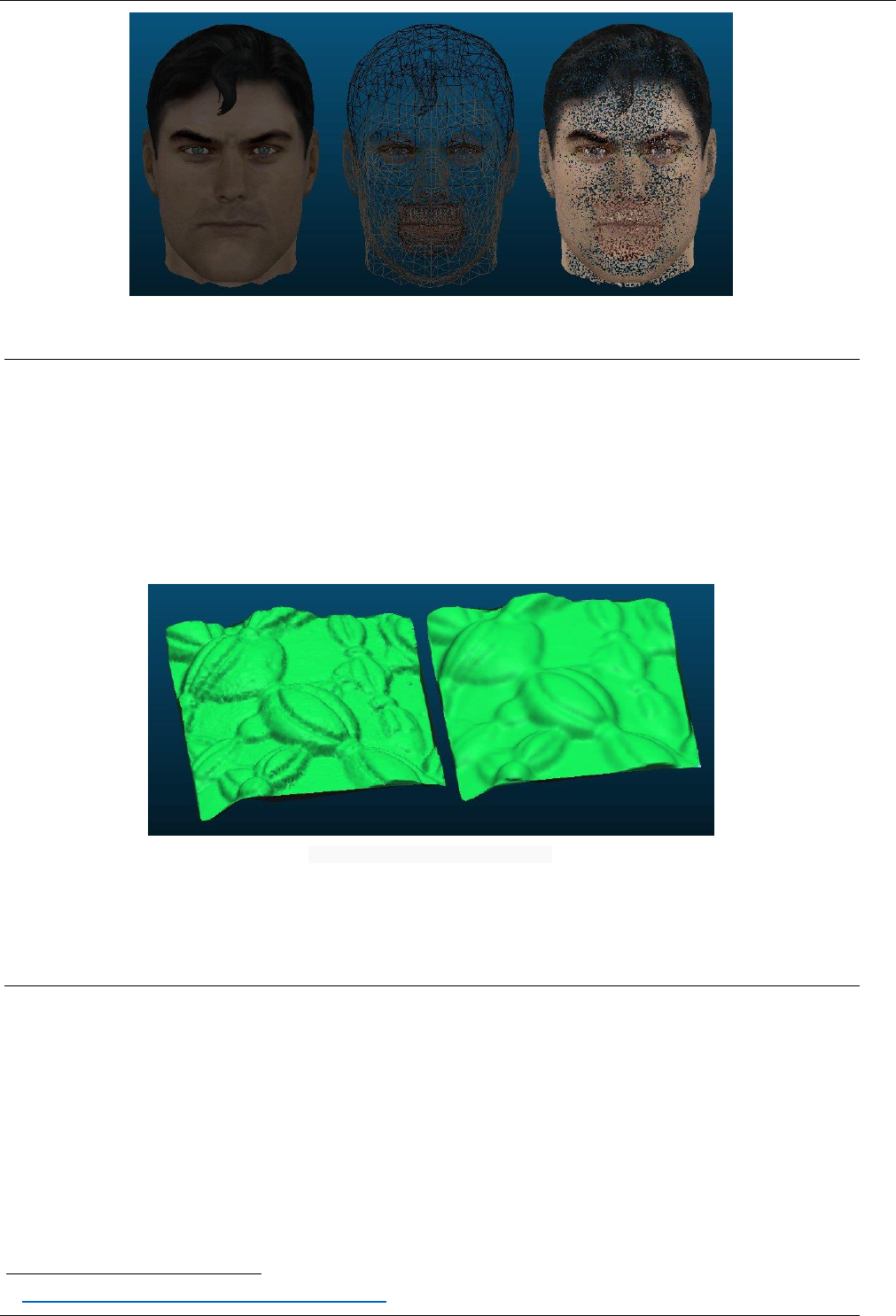
64
CloudCompare Version 2.6.1 – user manual
Plain mesh (left), wireframe display (center) and corresponding sampled points (right)
Mesh > Smooth (Laplacian)
Menu
This tool is accessible via the 'Edit > Mesh > Smooth (Laplacian)' menu.
Description
Smooths a mesh with “Laplacian smoothing”
25
.
The user must specify the number of iterations (20 by default) and the smoothing force ('Smoothing factor' - between
0 and 1 - 0.2 by default) applied at each iteration.
Edit > Mesh > Smooth (Laplacian) example
Warning: the smoothing algorithm does not preserve the volume/surface. Therefore, the mesh might shrink a little if
the number of iterations and/or the smoothing force is too high.
Mesh > Subdivide
Menu
This tool is accessible via the 'Edit > Mesh > Subdivide' menu.
Description
Subdivides a mesh.
The algorithm recursively subdivides the mesh triangles until their surface falls under a limit specified by the user.
25
http://en.wikipedia.org/wiki/Laplacian_smoothing
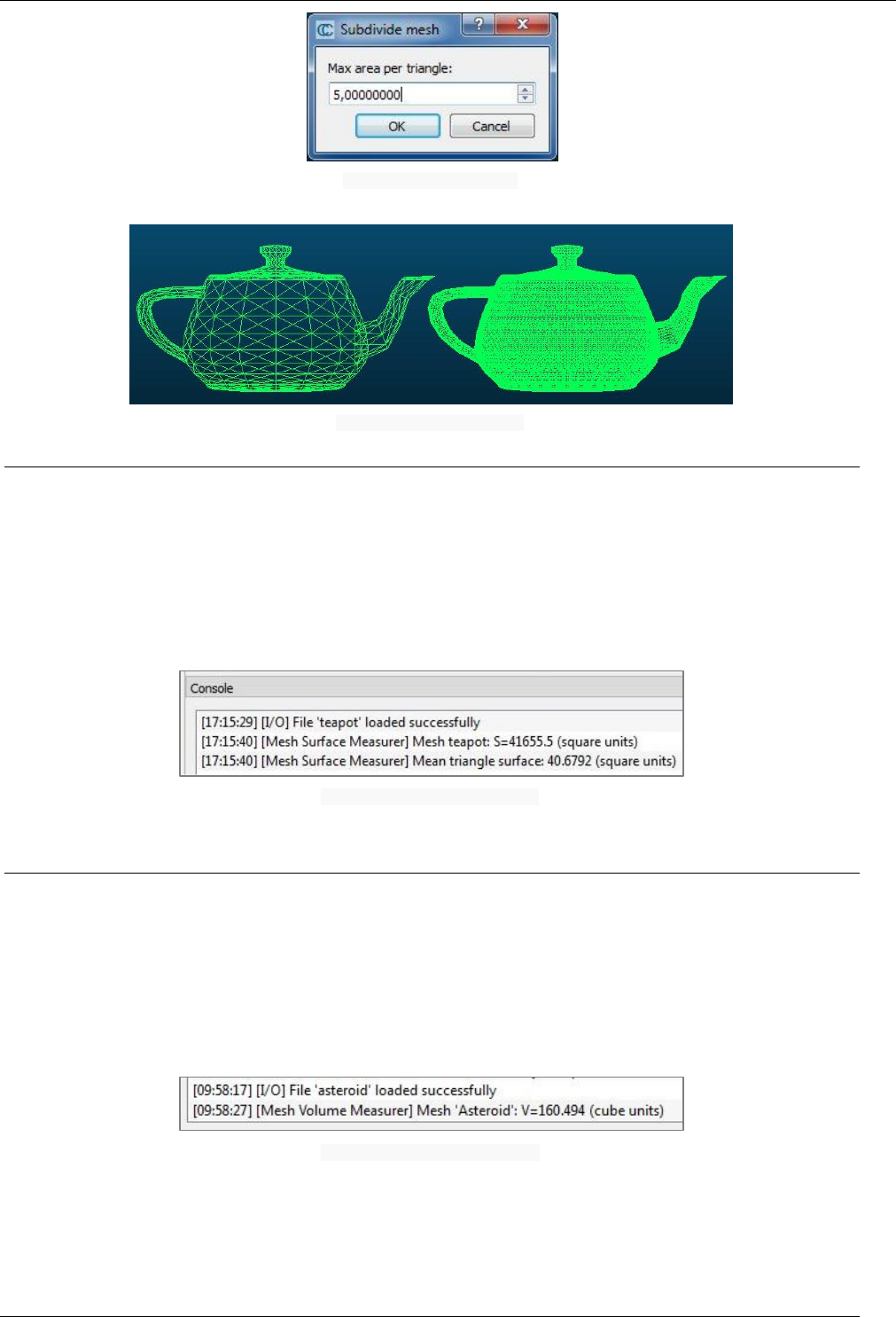
65
CloudCompare Version 2.6.1 – user manual
Edit > Mesh > Subdivide dialog
Edit > Mesh > Subdivide example
Mesh > Measure surface
Menu
This tool is accessible via the 'Edit > Mesh > Measure surface' menu.
Description
Measures the mesh total surface as well as the mean surface per triangle.
Output measurements are displayed in the Console.
Edit > Mesh > Measure surface output
Mesh > Measure volume
Menu
This tool is accessible via the 'Edit > Mesh > Measure volume' menu.
Description
Measures the volume of a closed mesh.
Output measurements are displayed in the Console.
Edit > Mesh > Measure volume output
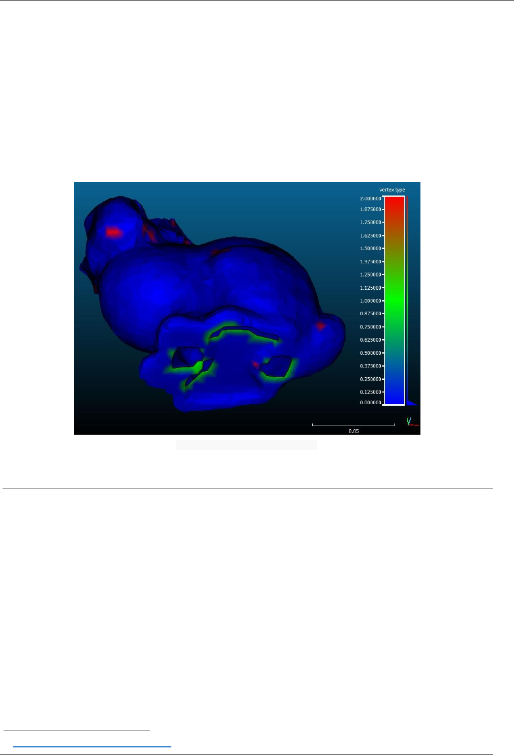
66
CloudCompare Version 2.6.1 – user manual
Mesh > Flag vertices
Menu
This tool is accessible via the 'Edit > Mesh > Flag vertices by type' menu.
Description
Basic mesh quality checking. Flags each mesh vertex by a (scalar value):
0 = normal
1 = border
2 = non-manifold
26
A summary of the number of each type of vertex (as well as a reminder of the meaning of each SF value) is displayed in
the Console.
'Edit > Mesh > Flag vertices by type' output
Mesh > Scalar field > Smooth
Menu
This tool is accessible via the 'Edit > Mesh > Scalar field > Smooth' menu.
Description
Smooths a scalar field associated to mesh vertices.
This method is particularly useful after applying the qPCV plugin.
Contrarily to the ‘Gaussian Filter’ method, the mesh structure is used to determine the nearest neighbors of each
vertex. This is much faster and no parameter is required.
26
http://en.wikipedia.org/wiki/Manifold
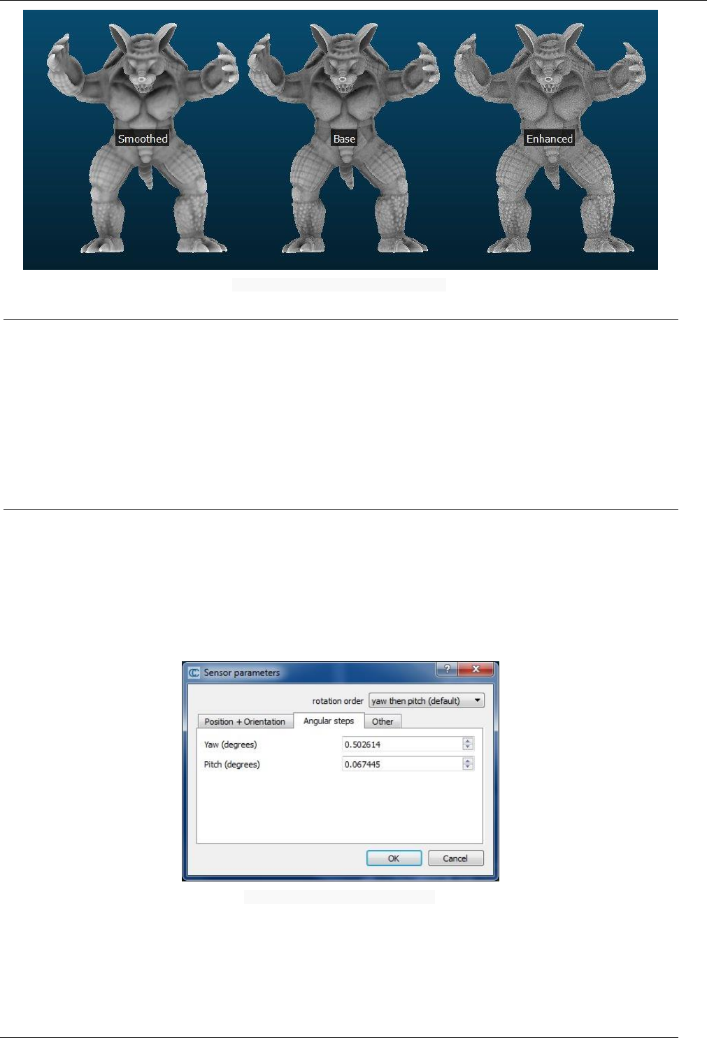
67
CloudCompare Version 2.6.1 – user manual
Edit > Mesh > Scalar Field > Smooth or Enhance
Mesh > Scalar field > Enhance
Menu
This tool is accessible via the 'Edit > Mesh > Scalar field > Enhance' menu.
Description
Enhances a scalar field associated to mesh vertices.
This method is particularly useful after applying the qPCV plugin.
Sensors > Edit
Menu
This tool is accessible via the 'Edit > Sensors > Edit' menu.
Description
This tool lets the user modify the intrinsic and extrinsic parameters of the selected sensor.
GBL/TLS sensor
Edit > Sensor > Modify dialog (GBL sensor)
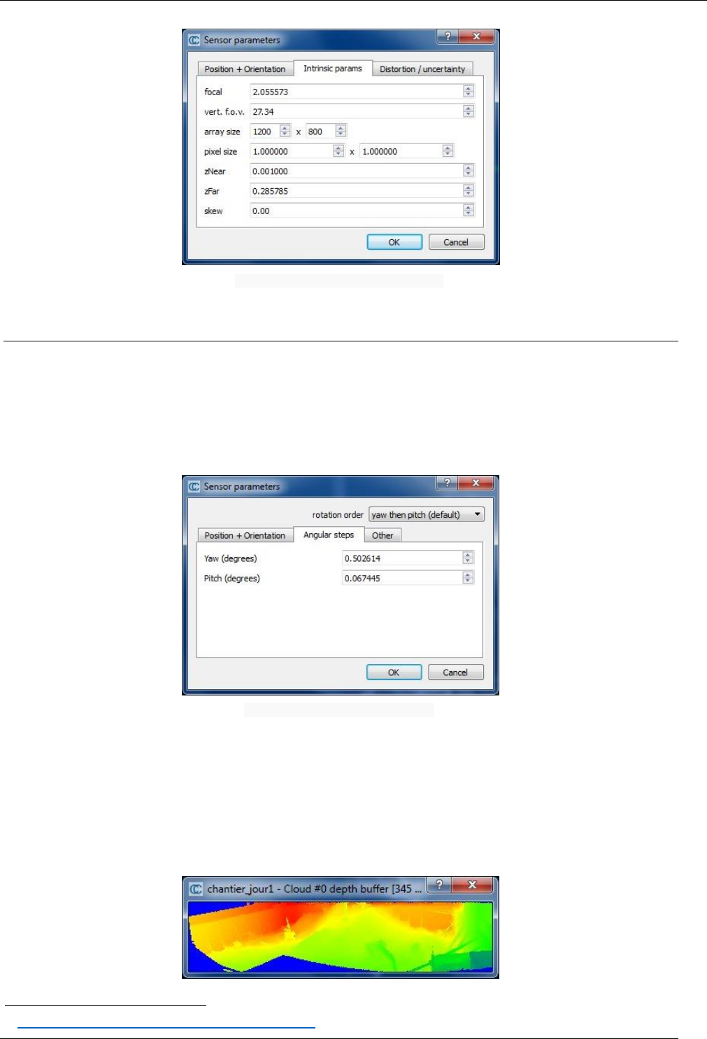
68
CloudCompare Version 2.6.1 – user manual
Camera sensor
Edit > Sensor > Modify dialog (Camera sensor)
Sensors > Ground Based Lidar > Create
Menu
This tool is accessible via the 'Edit > Sensors > Ground Based Laser > Create' menu.
Description
Creates a 'Ground Based Lidar' (= TLS) sensor entity attached to the selected cloud.
Edit > Sensor > Create > GBL sensor dialog
The user must specify the main intrinsic and extrinsic parameters of the sensor (absolute position and orientation,
angular steps, etc.).
Note: since version 2.5.6, angles are now expressed in degrees and aircraft
27
denominations (yaw/pitch) are used so as
to make things clearer.
Clicking on the 'OK' button will create a new sensor object. A depth map is automatically generated and displayed by
CloudCompare so as to let the user visually check the parameters.
27
http://en.wikipedia.org/wiki/Aircraft_principal_axes
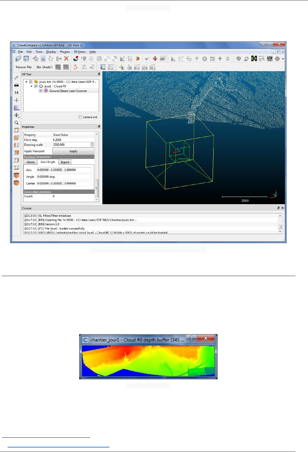
69
CloudCompare Version 2.6.1 – user manual
GBL sensor depth map
By default the sensor object is added as a child of the selected cloud in the DB tree. It is also visible in the 3D view
(warning: you may have to change its 'drawing scale' - see the sensor object properties - to view it correctly).
GBL sensor object (as visible in the DB tree and in a 3D view
Sensors > Ground Based Lidar > Show Depth Buffer
Menu
This tool is accessible via the 'Edit > Sensors > Ground Based Laser > Show Depth Buffer' menu.
Description
Displays the depth map
28
of the selected Ground Based Lidar (GBL) sensor.
GBL sensor depth map
28
http://en.wikipedia.org/wiki/Depth_map

70
CloudCompare Version 2.6.1 – user manual
Sensors > Ground Based Lidar > Export Depth Buffer
Menu
This tool is accessible via the 'Edit > Sensors > Ground Based Laser > Export Depth Buffer' menu.
Description
Exports the depth map [1] of the selected Ground Based Lidar (GBL) sensor as an ASCII file.
CloudCompare will simply ask for a destination filename.
Output file format
The output file is organized as the following:
comment line: title (CLOUDCOMPARE DEPTH MAP)
comment line: cloud name (Associated cloud: XXX)
comment line: first angular step (min and max between brackets)
comment line: second angular step (min and max between brackets)
comment line: max depth (pMax: XXX)
comment line: depth map length (L: XXX)
comment line: depth map height (H: XXX)
comment line (///////////////////////)
then on each line: 3 values per pixel of the depth map (column, row, depth)
Example
// CLOUDCOMPARE DEPTH MAP
// Associated cloud: cloud_name
// dPhi = 0.005000 [ -0.383040 : 0.007195 ]
// dTheta = 0.005000 [ -1.586361 : 0.137948 ]
// pMax = 58841.890625
// L = 345
// H = 79
/////////////////////////
0 0 12.000000000000
1 0 15.000000000000
2 0 16.000000000000...

71
CloudCompare Version 2.6.1 – user manual
Sensors > Camera Sensor > Create
Menu
This tool is accessible via the 'Edit > Sensors > Camera Sensor > Create' menu.
Description
Since version 2.5.6, camera sensors can be created with this function (however it's easier to load them from Bundler
29
files for instance).
For now only the extrinsic and intrinsic parameters can be created / modified (the distortion / uncertainty model can't
be setup this way).
Note: theoretically a camera sensor can be associated to any number of 4x4 transformation matrices (association of a
3D rotation and a translation) stored in a Trans. buffer entity. They would typically represent the camera displacement.
However no file format allows for loading this kind of data yet...
Camera sensor object (as visible in the DB tree and in a 3D view
29
http://www.cs.cornell.edu/~snavely/bundler/
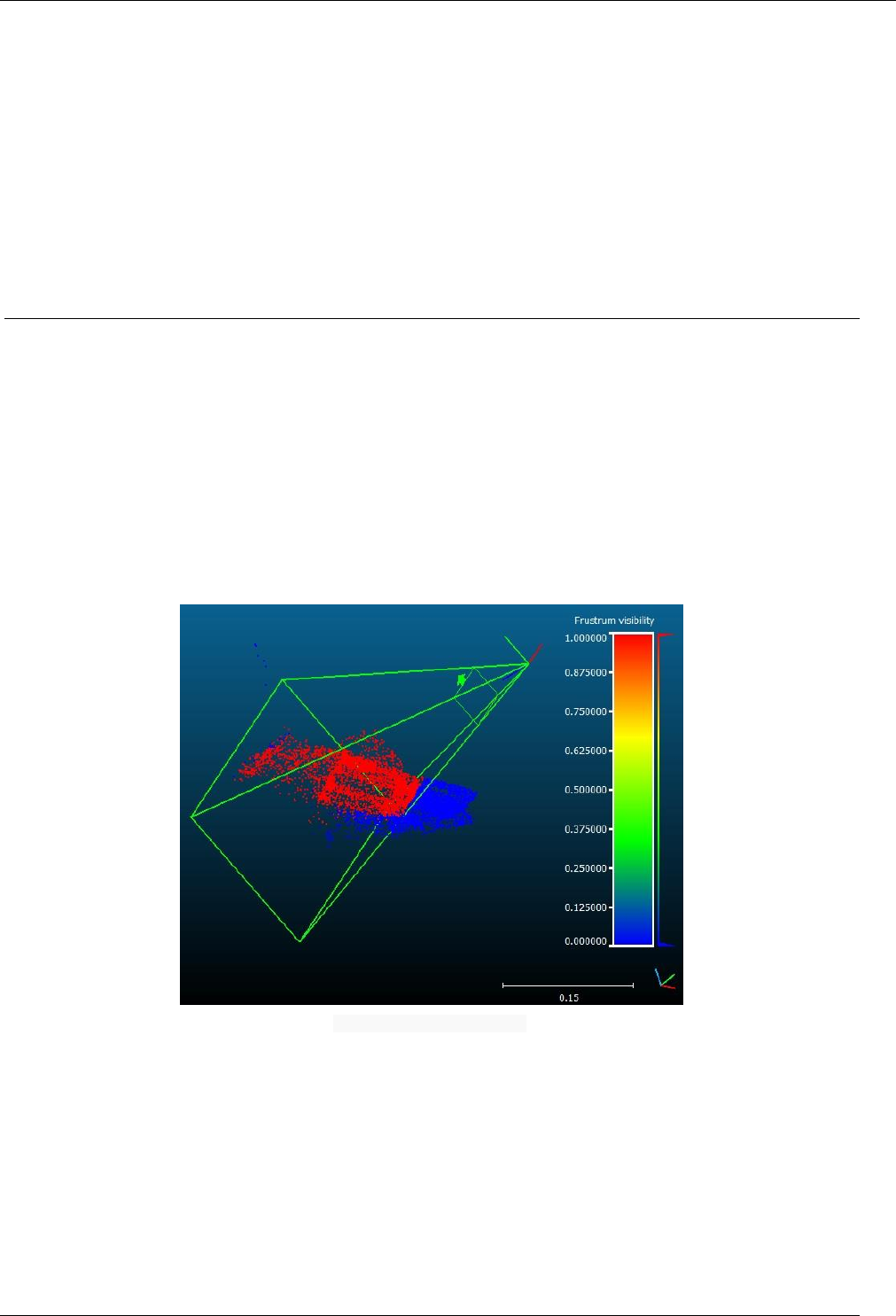
72
CloudCompare Version 2.6.1 – user manual
Sensors > Camera Sensor > Project uncertainty
Menu
This tool is accessible via the 'Edit > Sensors > Camera Sensor > Project uncertainty' menu.
Description
Projects the camera model uncertainty a point cloud. Output consists in several scalar fields:
uncertainty along the X axis
uncertainty along the Y axis
uncertainty along the Z axis
3D uncertainty (norm of the (uX,uY,uZ) vector)
Sensors > Camera Sensor > Compute points visibility (with octree)
Menu
This tool is accessible via the 'Edit > Sensors > Camera Sensor > Compute points visibility (with octree)' menu.
Description
Flags the points of a cloud depending on whether they are viewed by the selected (camera) sensor or not.
The visibility check is done for the 'active' camera position. Per-point visibility information is stored in a scalar field:
0 = NOT VISIBLE
1 = VISIBLE
Result of a 'visibility' computation
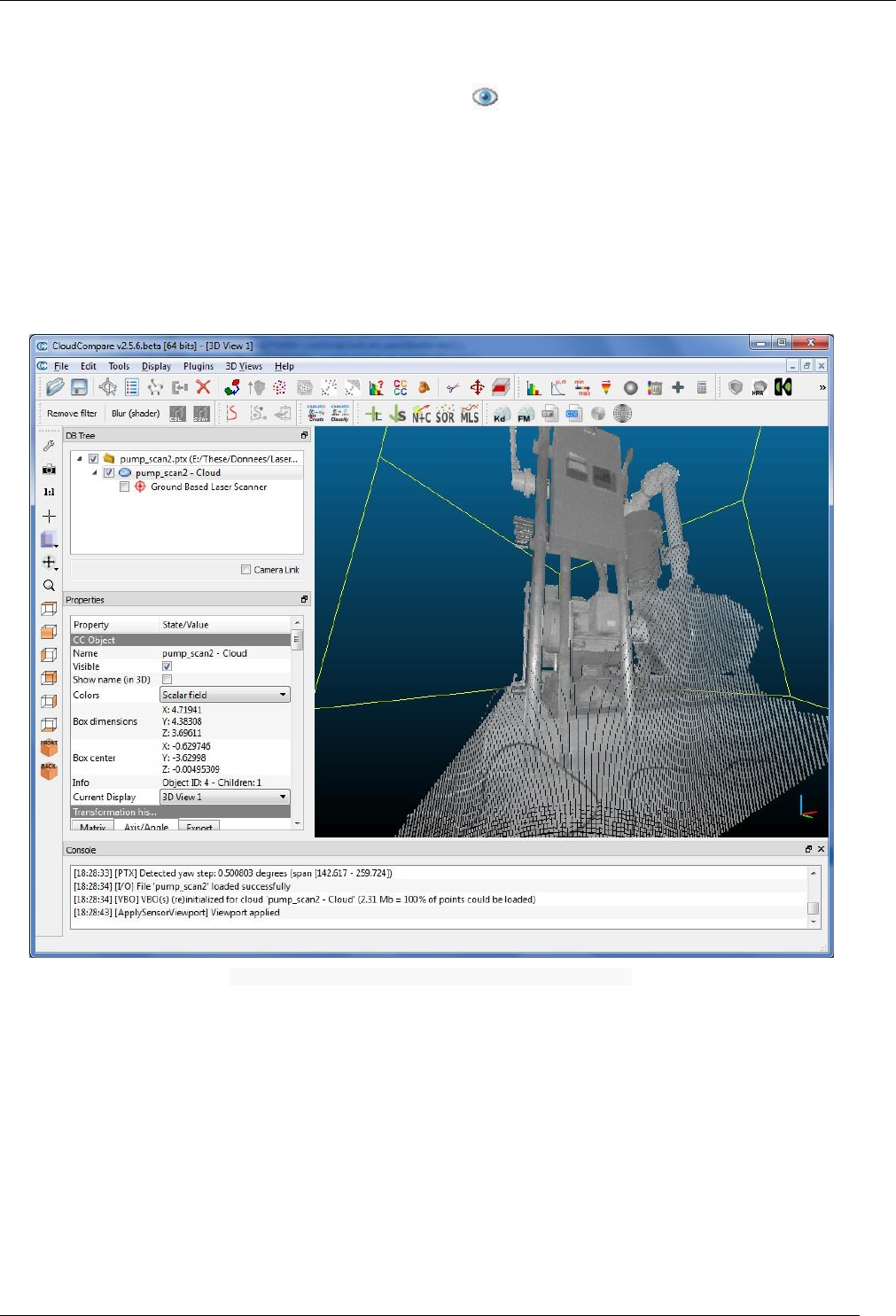
73
CloudCompare Version 2.6.1 – user manual
Sensors > View from sensor
Menu / Icon
This tool is accessible via the 'Edit > Sensors > View from sensor' menu.
Description
Changes the current 3D view camera settings to match the selected sensor settings (bubble view mode).
Notes:
the camera display mode will automatically be changed to 'viewer-based perspective'
for GBL sensors, it may be necessary to manually increase the 3D view camera f.o.v. (see ‘Display > Camera
settings’) so as to get a more realistic display.
Edit > Sensor > View from sensor example (Ground Based Lidar sensor)
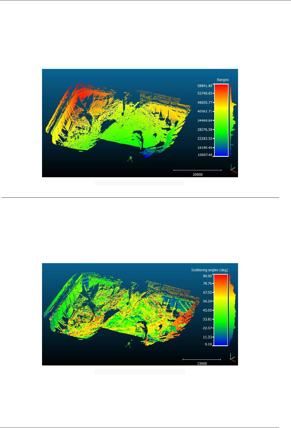
74
CloudCompare Version 2.6.1 – user manual
Sensors > Compute ranges
Menu
This tool is accessible via the 'Edit > Sensors > Compute ranges' menu.
Description
Computes the range of all points (of any cloud) relatively to the selected sensor.
The user can specify whether CloudCompare should output the squared ranges or the non-squared ones.
Edit > Sensor > Compute ranges output example
Sensors > Compute scattering angles
Menu
This tool is accessible via the 'Edit > Senors > Compute scattering angles' menu.
Description
Computes the scattering angle of all points (of any cloud with normals) relatively to the selected sensor.
The user can specify whether CloudCompare should output the angles in radians or degrees.
Edit > Sensor > Scattering angles output example
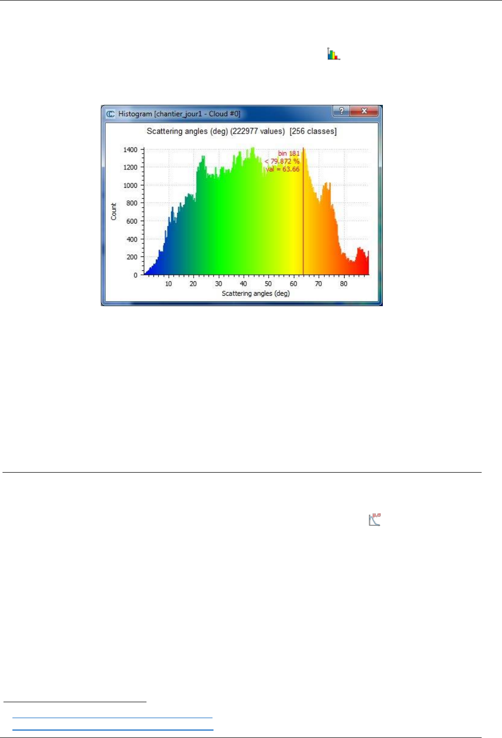
75
CloudCompare Version 2.6.1 – user manual
Scalar fields > Show histogram
Menu /Icon
This tool is accessible via the 'Edit > Scalar fields > Show histogram' menu or the icon in the upper main toolbar.
Description
Shows the histogram of the active scalar field of the currently selected entity:
Edit > Scalar Fields > Show histogram dialog
Interactions
the number of classes (bins) of the histogram can be changed with the mouse wheel
the user can click anywhere on the histogram to make a vertical red line appear. Next to this line will be
indicated the corresponding class (bin), the percentage of points below this class and the corresponding scalar
value.
Colors
The histogram bin colors are the same as the color scale currently associated to the scalar field.
Scalar fields > Compute statistical parameters
Menu / Icon
This tool is accessible via the 'Edit > Scalar fields > Compute stat. params' menu or the icon in the upper main
toolbar.
Description
Fits a statistical distribution on the active scalar field values.
CloudCompare will first ask for the type of distribution to fit:
Gauss (Normal
30
) distribution
Weibull
31
distribution
CloudCompare will then fit the chosen distribution and display the result as a curve overlaid on the SF histogram.
30
http://en.wikipedia.org/wiki/Normal_distribution
31
http://en.wikipedia.org/wiki/Weibull_distribution
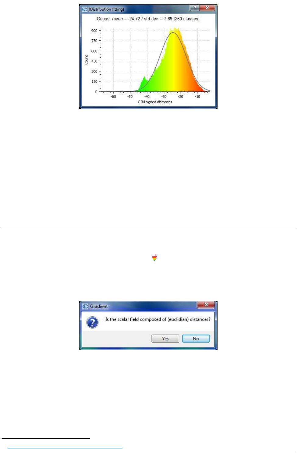
76
CloudCompare Version 2.6.1 – user manual
Edit > Scalar Fields > Compute stat. params output
The numerical parameters of the distribution are also displayed in the Console. The Chi-squared
32
distance is also output
so as to give an evaluation of the fitting process quality.
Folded Normal Distribution
Beware that the Folded Normal distribution is not the same as the Normal distribution.
For instance, the output of the cloud-to-cloud distance computation tool is unsigned (i.e. no negative values are output,
only their absolute values). In such a case there's absolutely no chance that the resulting distance values follow a
Normal Distribution.
Even if the deformations you are measuring do follow a Normal distribution (in real life), then the absolute values will
follow a Folded Normal Distribution. Currently CloudCompare can't fit such a distribution on a scalar field.
Scalar fields > Gradient
Menu / Icon
This tool is accessible via the 'Edit > Scalar fields > Gradient' menu.
Description
Computes the gradient of a scalar field.
CloudCompare will first ask a tricky question: 'is the scalar field composed of (Euclidean) distances?'.
Edit > Scalar Fields > Gradient dialog
You'll generally have to answer 'No' to this question, apart if the active scalar field values are distances or altitudes for
instance. In this case, some basic considerations will allow CC to cap the resulting gradient values below one. This limits
the effect of noise (which tend to be much more visible on the gradient than on the original SF).
32
http://en.wikipedia.org/wiki/Chi-squared_test

77
CloudCompare Version 2.6.1 – user manual
Edit > Scalar Fields > Gradient output example
The gradient is a good way to identify rapid changes in the source SF for instance and other interesting structures.
Note: a new scalar field is generated (i.e. the original scalar field is not overwritten).
Scalar fields > Gaussian filter
Menu / Icon
This tool is accessible via the 'Edit > Scalar fields > Gaussian filter' menu.
Description
Smooths a scalar field by applying a spatial Gaussian filter
33
.
The user must choose a 'kernel' size (in fact the radius of the sphere in which nearest neighbors will be extracted around
each point to compute the mean value). The bigger the stronger the filter will be (and the slower the computation...).
Edit > Scalar Fields > Gaussian and Bilateral filters
Note: a new scalar field is generated (i.e. the original scalar field is not overwritten).
33
http://en.wikipedia.org/wiki/Gaussian_filter
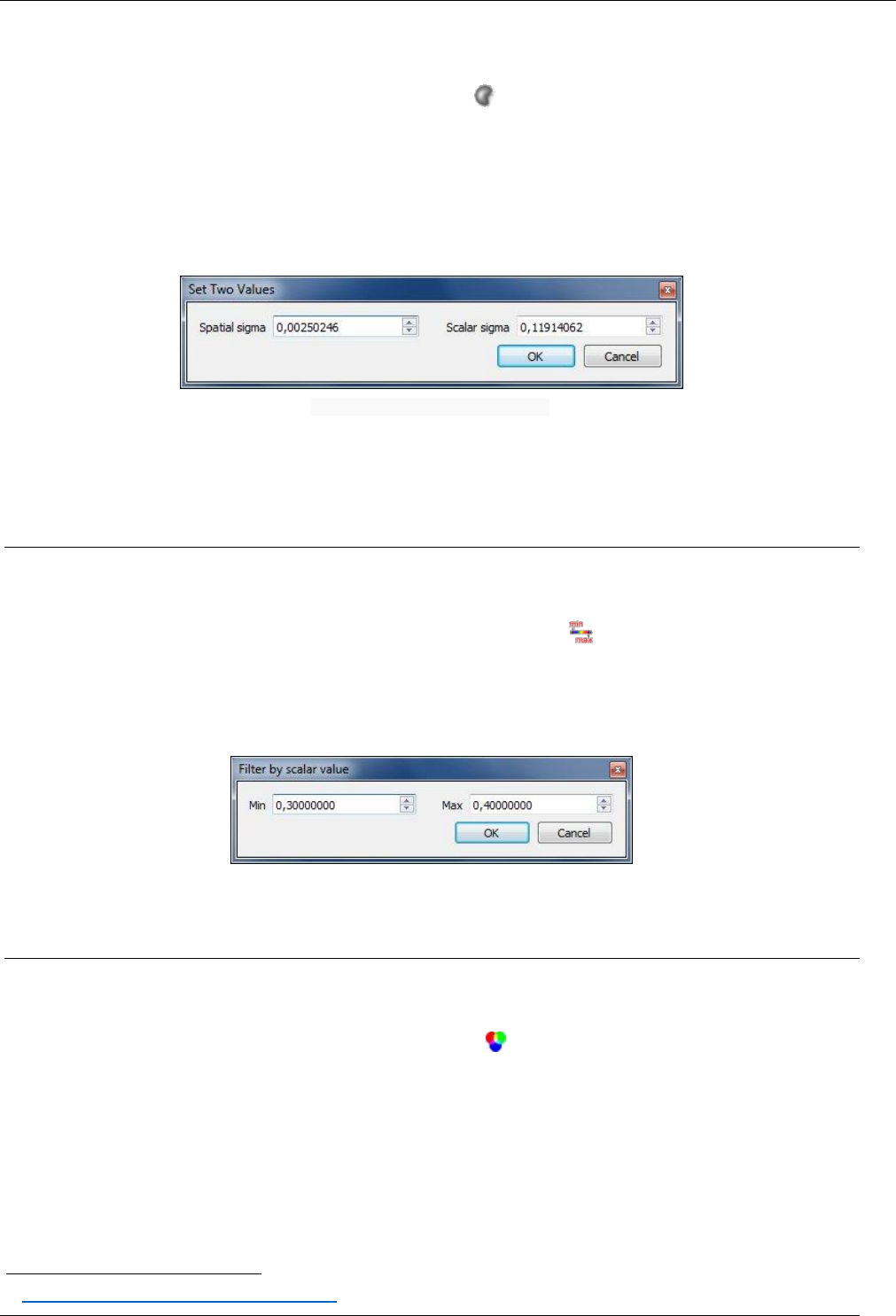
78
CloudCompare Version 2.6.1 – user manual
Scalar fields > Bilateral filter
Menu / Icon
This tool is accessible via the 'Edit > Scalar fields > Bilateral filter' menu.
Description
Smooths a scalar field by applying a bilateral filter
34
.
CloudCompare will first ask for the two parameters of the filter:
spatial sigma: the Normal distribution variance for the spatial part of the filter
scalar sigma: the Normal distribution variance for the scalar part of the filter
Edit > Scalar Fields > Bilateral filter dialog
The bilateral filter tends to preserve the strong edges better.
Note: a new scalar field is generated (i.e. the original scalar field is not overwritten).
Scalar fields > Filter by Value
Menu / Icon
This tool is accessible via the 'Edit > Scalar fields > Filter by value' menu or the icon in the upper main toolbar.
Description
Filters the points of the selected cloud based on their associated scalar value.
A new cloud (or mesh) is created with the points falling inside the specified range.
Edit > Scalar Fields > Filter by value dialog
Scalar fields > Convert to RGB
Menu / Icon
This tool is accessible via the 'Edit > Scalar fields > Convert to RGB' menu.
Description
Simply converts the active scalar field to a RGB color field.
The colors assigned to the points are exactly the ones visible on the screen at the time the method is called. Therefore
the rendering won't change. However, CloudCompare will automatically hide the scalar field and activate the RGB field
instead.
Note: the original scalar field is not modified nor deleted.
34
http://en.wikipedia.org/wiki/Bilateral_filter
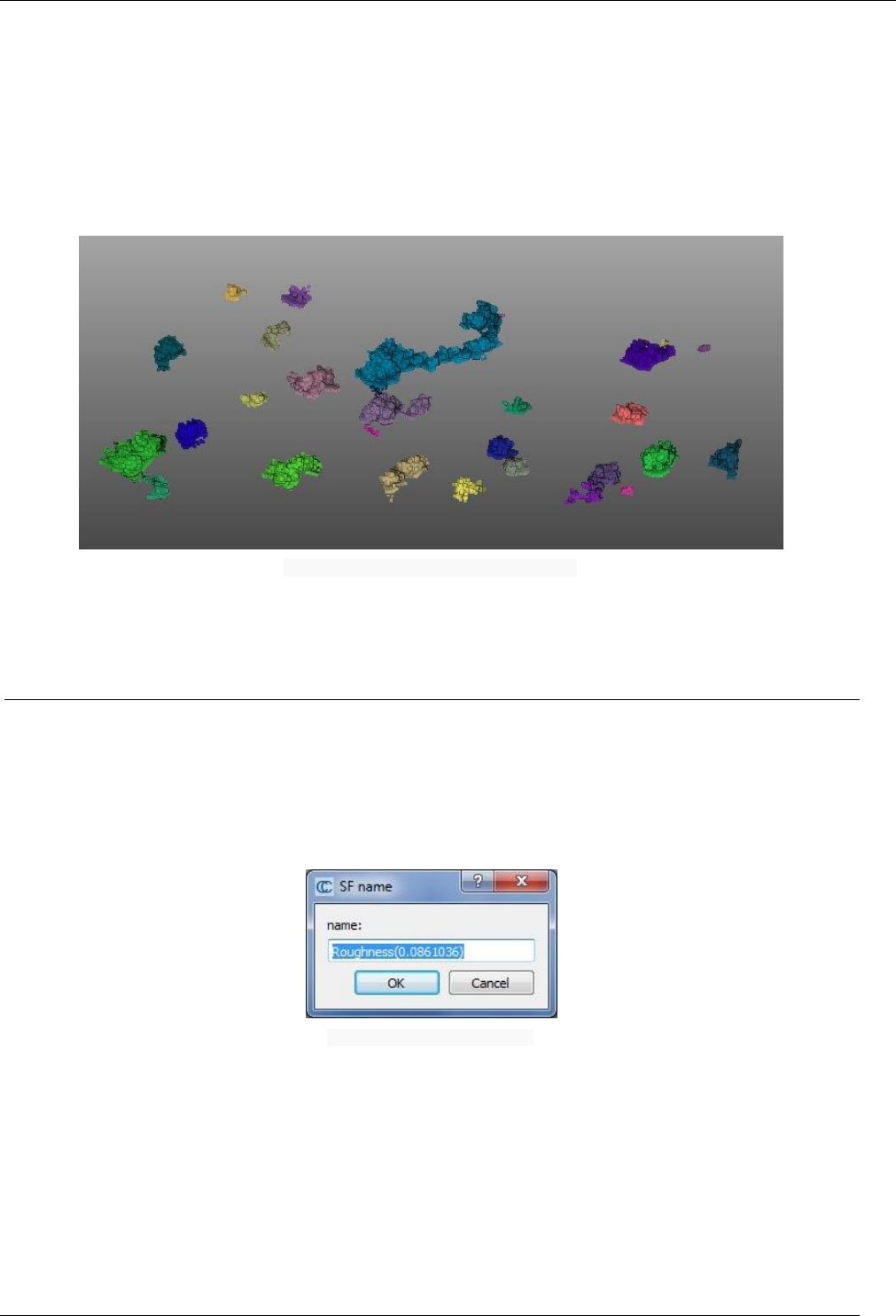
79
CloudCompare Version 2.6.1 – user manual
Scalar fields > Convert to random RGB
Menu / Icon
This tool is accessible via the 'Edit > Scalar fields > Convert to random RGB' menu.
Description
Converts the active scalar field of the selected entity by applying a random color scale.
The user must first define a number of colors that will be randomly generated. CloudCompare will then apply the
corresponding (random) color scale (as a linear scale, regularly sampled over the scalar field range).
Edit > Scalar Fields > Convert to random RGB colors
Note: this is very useful to randomly color a set of points with a classification index as scalar field for instance (just set
the same number of random colors as the number of classes).
Scalar fields > Rename
Menu / Icon
This tool is accessible via the 'Edit > Scalar fields > Rename' menu.
Description
Renames the active scalar field of the selected entity.
Edit > Scalar Fields > Rename dialog
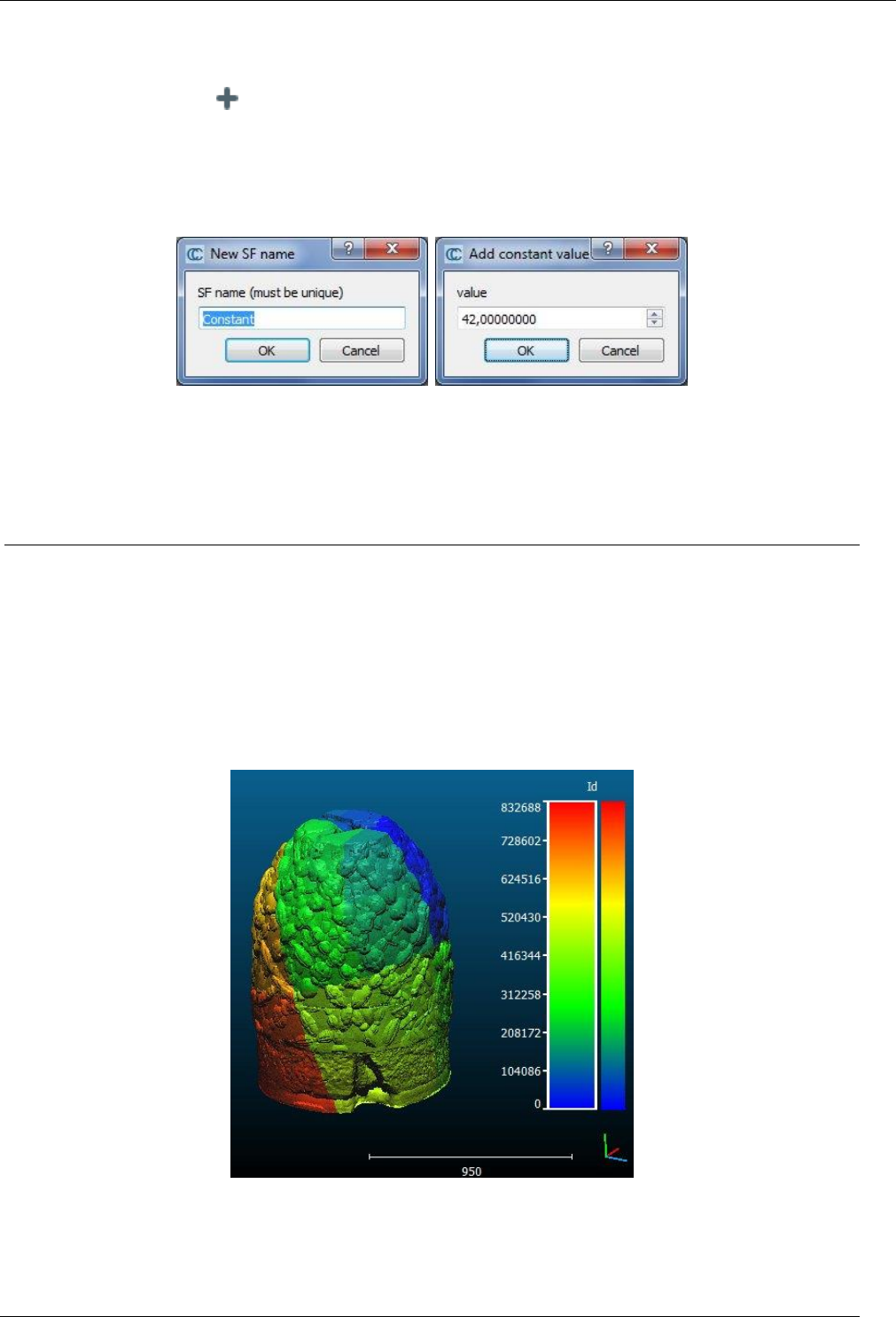
80
CloudCompare Version 2.6.1 – user manual
Scalar fields > Add constant SF
Menu / Icon
This tool is accessible via the icon in the upper main toolbar or the 'Edit > Scalar fields > Add constant SF' menu.
Description
Adds a new scalar field with a constant value (i.e. same value for all points) to the selected cloud.
CloudCompare will first ask for the SF name (must be unique, otherwise if a SF with the same name exists it will be
overwritten). Then CloudCompare will ask for the (constant) SF value.
Edit > Scalar Fields > Add constant SF dialogs (left: SF name – right: SF value)
Note: useful in conjunction with the
Scalar fields > Arithmetic tool.
Scalar fields > Add point indexes as SF
Menu / Icon
This tool is accessible via the 'Edit > Scalar fields > Add point indexes as SF' menu.
Description
Creates a new scalar field on the selected cloud(s) with the point indexes (i.e. their order of creation, or the order in
which they have been read from the originating file) as scalar values.
Edit > Scalar Fields > Add point indexes as SF example
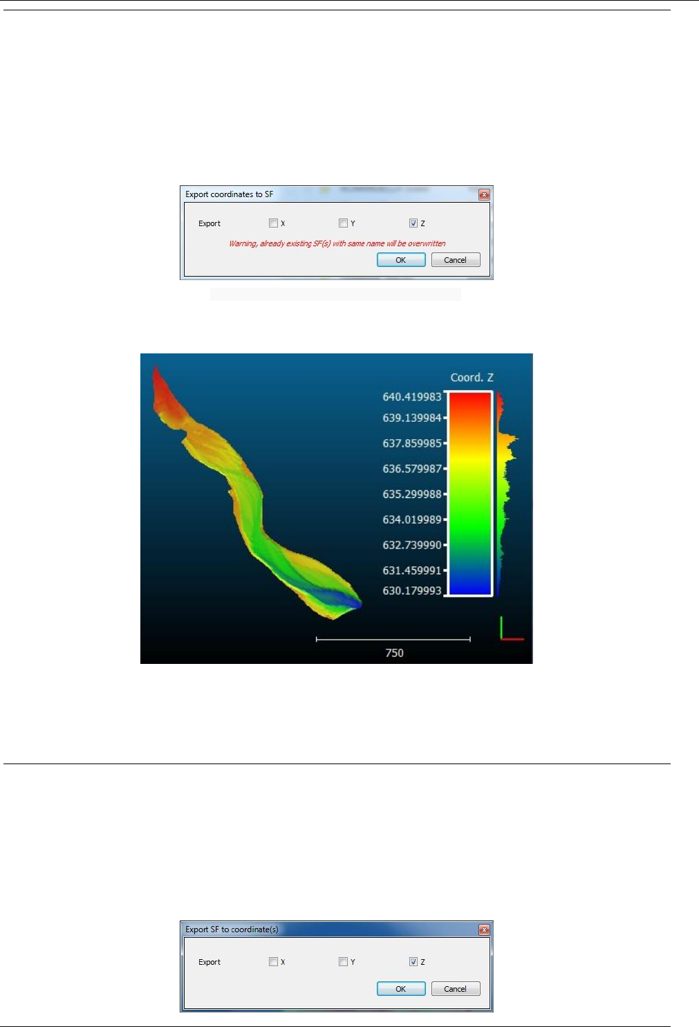
81
CloudCompare Version 2.6.1 – user manual
Scalar fields > Export coordinate(s) to SF(s)
Menu
This tool is accessible via the 'Edit > Scalar fields > Export coordinate(s) to SF(s)' menu or the 'Tools > Projection > Export
coordinate(s) to SF(s)' menu.
Description
This tool lets the user export the points coordinates to one or several scalar fields.
CloudCompare will ask the user to select the source dimension(s):
Edit > Scalar Fields > Export coordinate(s) as SF(s) dialog
Each dimension will be exported to a scalar field with a predefined name ('Coord. X', 'Coord. Y' and 'Coord. Z').
Z coordinates exported to a new scalar field
Warning: if a scalar field with the same name exists, it will be overwritten.
Scalar fields > Set SF as coordinate(s)
Menu
This tool is accessible via the 'Edit > Scalar fields > Set SF as coordinate(s)' menu.
Description
Sets the active scalar field of the selected cloud as one (or several) of its coordinates.
CloudCompare will ask the user to select the destination dimension(s):
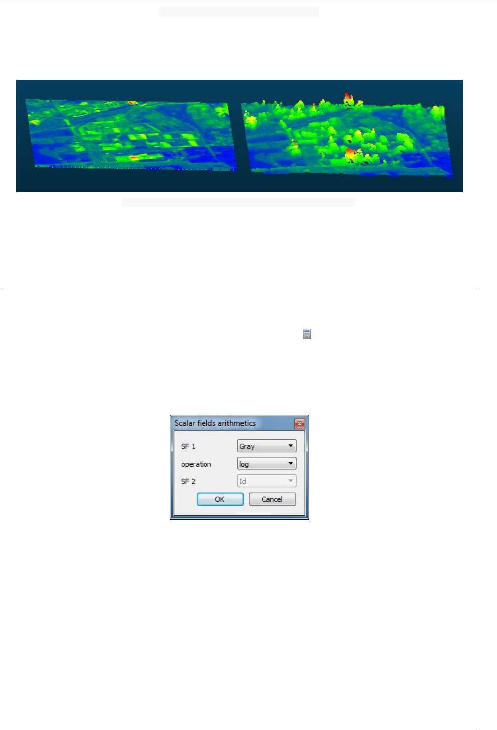
82
CloudCompare Version 2.6.1 – user manual
Edit > Scalar Fields > Set SF as coordinate(s) dialog
For instance one can replace the Z coordinates by any scalar value so as to have a kind of '3D representation' of the
scalar field. More commonly, this method is useful to convert a 2D raster with the altitude coming as scalar field into a
proper 3D cloud/raster.
Left: original raster - right: Z coordinate 'exported' the from associated SF
Note: it is sometimes necessary to rescale the Z coordinate afterwards (with the Multiply / Scale method) as raster
fields are not always in the same units as the XY coordinates (e.g. the altitude is coded as a gray intensity, between 0
and 255).
Scalar fields > Arithmetic
Menu / Icon
This tool is accessible via the 'Edit > Scalar fields > Arithmetic' menu or the icon in the upper main toolbar.
Description
This tool allows to:
perform standard arithmetic operations between two scalar fields of the same cloud (+,-,*,/)
or apply mathematical functions to a single scalar field
Edit > Scalar Fields > Arithmetic dialog
Supported mathematical functions are:
SQRT (square root)
POW2 (power of 2)
POW3 (power of 3)
EXP (exponential)
LOG (natural log)
LOG10 (base 10 log)
COS (radians)
SIN (radians)
TAN(radians)
ACOS
ASIN
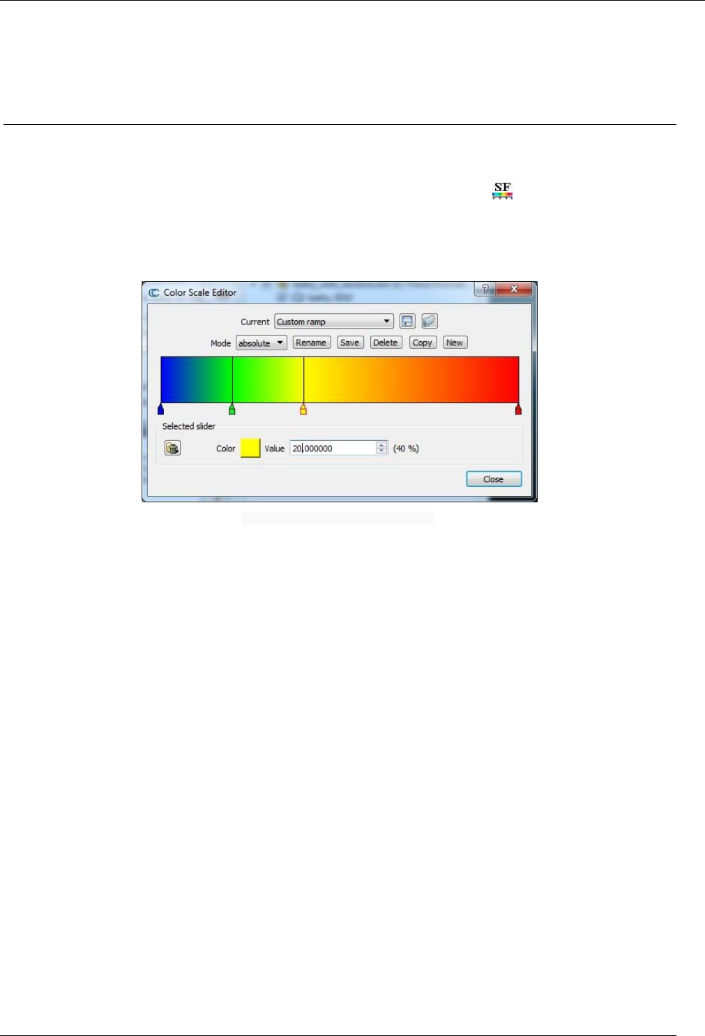
83
CloudCompare Version 2.6.1 – user manual
ATAN
Integer part
Inverse (1/x)
Note: this method will create a new scalar field (the source scalar fields are not modified nor deleted).
Scalar fields > Color Scales Manager
Menu / Icon
This tool is accessible via the 'Edit > Scalar fields > Color Scales Manager' menu or the icon next to the color scales
list in the cloud/mesh properties.
Description
The Color Scales Manager allows the user to manage and create new color scales.
Edit > Scalar Fields > Color Scales Manager
All color scales defined by the user (or imported from a BIN file) are saved in the persistent memory of the operating
system (e.g. the Registry on Windows). They can be created, edited and deleted via the Color Scales Manager.
Note: if an entity is saved with a custom color scale into a BIN file and this file is loaded on another computer, the color
scale will automatically be imported in the other computer registry (and thus will be available in the other instance(s)
of CloudCompare on this computer).
Default color scales
CloudCompare comes with various default color scales:
Blue > Green > Yellow > Red
Grey
Blue > White > Red
Red > Yellow
Red > White
Intensity [0-1]
HSV angle [0-360]
Those color scales can't be edit or deleted.
Custom color scales
The user can create a color scale from scratch ('New' button) or start from an existing one ('Copy' button).
Two modes are available (see the 'Mode' combo-box):
relative: a relative color scale will automatically span over the whole scalar field range (therefore the color
position are expressed as a percentage).

84
CloudCompare Version 2.6.1 – user manual
absolute: an absolute color scale will have color steps defined at particular (absolute) values. This is the
standard way to get a consistent look with multiple clouds having equivalent scalar fields but with different
ranges.
Naming
Color scales can be renamed with the 'Rename' button. The name is not necessarily unique.
Save / delete
each time a color scale is modified, the user must click on the 'Save' button to actually make CC remember the
modifications (CC will automatically ask the user if he wants to save the modifications if the user forgot it).
the 'Delete' button let the user delete the current color scale (if it is not a default one). CC will ask for a
confirmation.
Edition
Existing color 'sliders' can be modified interactively:
by pressing the corresponding 'pencil' symbol and moving it on the left or the right
by double clicking on it to change its color
Equivalently, if the user simply clicks once on the 'pencil' symbol, the 'Selected slider' frame will be updated with the
current slider information:
the 'Color' box can be clicked to change the slider color
the 'Value' spin-box can be edited to change the slider position
the small 'garbage' button is used to deleted the current slider Warnings:
each time a slider value is edited through the 'Value' spin-box, the color scale representation is automatically
updated. This can lead to confusing situations where the sliders are (temporarily) inverted
if two sliders have the same 'Value', the active one (i.e. the one currently edited in the 'Selected slider' frame)
will be randomly picked. Once again this can lead to confusing situations...
Export / Import
Since version 2.6.1 color scales can be exported as XML files.
Use the icon to import such a file and the icon to export the current color scale.

85
CloudCompare Version 2.6.1 – user manual
Scalar fields > Delete
Menu / Icon
This tool is accessible via the 'Edit > Scalar fields > Delete' menu or the icon in the upper main toolbar.
Description
Deletes the active scalar field of the selected entities.
Warning: action is immediate (no confirmation).
Scalar fields > Delete all (!)
Menu / Icon
This tool is accessible via the 'Edit > Scalar fields > Delete all (!)' menu.
Description
Deletes all the scalar fields of the selected entities.
Warning: action is immediate (no confirmation).
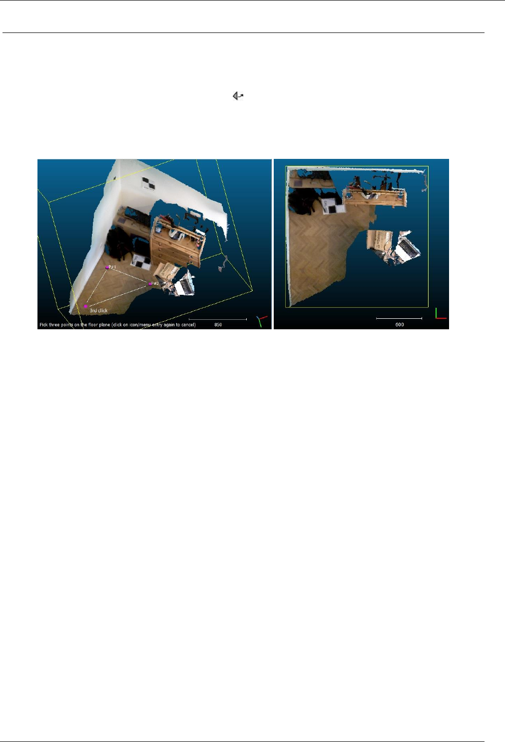
86
CloudCompare Version 2.6.1 – user manual
Tools menu
Level
Menu / Icon
This tool is accessible via the 'Tools > Level' menu or the icon in the left toolbar.
Description
This tool lets the user pick three points on a (horizontal) surface so as to rotate the cloud and make the corresponding
plane parallel to the (XY) plane:
Left: ‘Tools > Level' in action – right: result
Procedure
Select one or several entities (clouds or meshes) or a group of such entities then start the tool.
A message will appear at the bottom left of the 3D view ("Pick three points on the floor plane (etc.)"). Simply click on
the (floor) plane in three different places. Once the third point is picked, CloudCompare will automatically transform
the selected cloud(s) so as to make the plane defined by the 3 points horizontal.
Notes:
try to pick the points as far as possible from each other to optimize the plane orientation 'accuracy'
you can cancel the process any time by clicking on the tool icon again
the first clicked point will be used as origin for the new coordinate system. The vector between the first and
second clicked points will be the new 'X' dimension.
this tool modifies the selected entities directly. You may want to clone or save them prior to call this tool.
Point picking
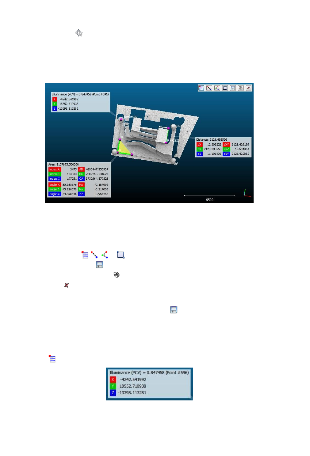
87
CloudCompare Version 2.6.1 – user manual
Point picking
Menu / Icon
This tool is accessible via the icon in the main upper toolbar or the 'Tools > Point picking' menu.
Description
The main purpose of this tool is to let the user pick one, two or three points so as to get various pieces of information
(most notably the distance between two points).
Different kind of labels can be created this way.
Procedure
The tool can be launched directly. No selection needs to be made (any kind of point can be picked).
A toolbar will appear in the top-right corner of the 3D view. One of the following actions can be chosen:
spawn a specific label ( , , or )
save the last spawned label ( )
cancel the current picking process ( )
leave this tool ( )
Notes:
the last picked label stays active as long as it is not saved ( ). If the user picks a new point then the process
starts over and the active label will disappear.
see the equivalent PDF documentation for this tool
Labels
1 point label
With the first icon , the user can pick any point and make a standard label appear.
This label will contain all the information available about the point:
associated scalar value (if a scalar field is active)
point index in the cloud
local coordinates
global coordinates (if any)
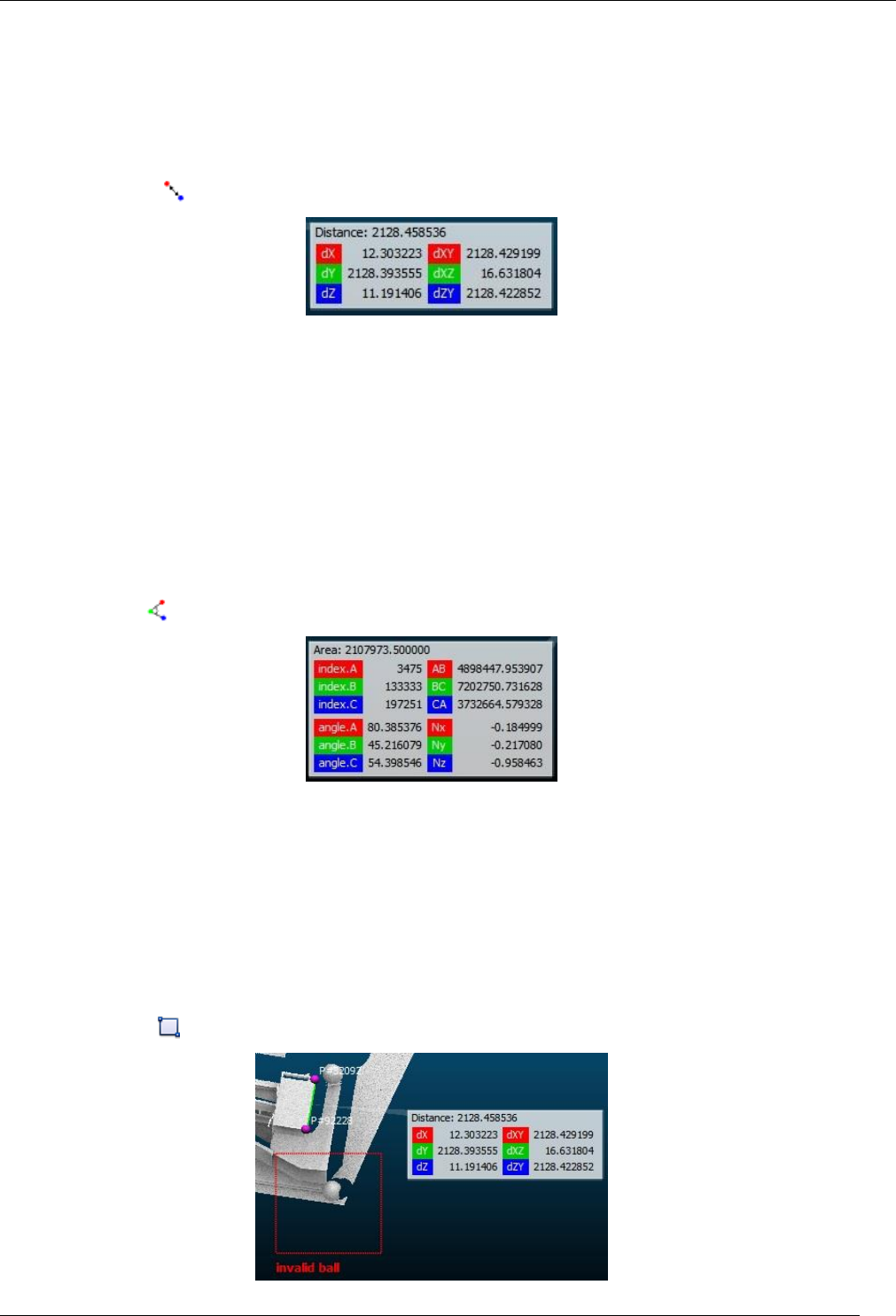
88
CloudCompare Version 2.6.1 – user manual
normals
RGB colors
Notes: an alternative way to create a single point label (outside of this tool) is to pick a point while pressing the SHIFT
key.
2 points label
With the second icon , the user can pick two points and make a 'distance' label appear.
This label will mainly display the distance between the two picked points (as title).
Additionally, the following values are displayed:
dX: algebraic distance along the X dimension
dY: algebraic distance along the Y dimension
dZ: algebraic distance along the Z dimension
dXY: distance in the XY plane
dXZ: distance in the XZ plane
dZY: distance in the ZY plane
3 points label
With the third icon , the user can pick three points and make an 'area' label appear.
This label will display the area of the triangle formed by the three picked points.
Additionally, the following values are displayed:
the indexes of the 3 points
the length of the 3 edges
the 3 angles
the vector normal to this triangle/plane
2D area label
With the fourth icon , the user can draw a rectangle anywhere on the screen so as to create a '2D area' label.
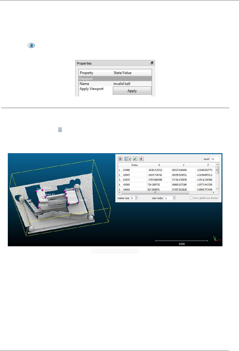
89
CloudCompare Version 2.6.1 – user manual
Simply click and hold the mouse button to define the first corner, then move the mouse cursor and release the button
to define the opposite corner. Once the button is released, CloudCompare will prompt for a title.
Eventually the '2D area' label will appear.
Note: this kind of label is useful to define zones of interest in a 3D view seen in a particular point of view. Therefore
they are only visible in this point of view.
Similarly to a Viewport entity, the associated viewport can be restored anytime by clicking on the 'Apply' button in
the label properties:
Point list picking
Menu / Icon
This tool is accessible via the icon in the main upper toolbar or the 'Tools > Point list picking' menu.
Description
This tool lets the user pick several points on a cloud so as to create a 'list' of points.
'Point list picking' tool in action
This list can then be exported as:
a file
a new cloud
a polyline (picked points are simply connected)
It is very useful to create a 'Ground Control Points' (GCP) list for instance.
Procedure
One and only one point cloud should be selected in order to launch this tool.
A dedicated dialog will then appear in the top-right corner.
At any time the user can pick points on the selected cloud in the 3D view. These points will be automatically added to
the list.
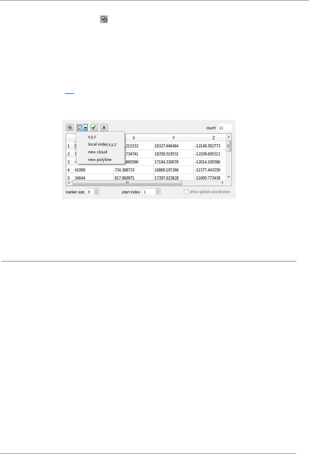
90
CloudCompare Version 2.6.1 – user manual
Here are the actions that can be undertaken while the dialog is visible:
cancel the last picking action (
export the list (see below)
change the marker size in the 3D view (with the marker size spinbox)
change the starting index (with the start index spinbox - default value: 0)
validate the list (in which case all picked points will be 'saved' as a list of labels and the list will be restored
when calling this tool again)
cancel the picking process (the current list won't be saved - see above)
if the cloud has been shifted, the global coordinates can be displayed/exported instead of the local ones
Note: see the equivalent PDF documentation for this tool.
Export options
The list can be exported as:
an ASCII file with 'x,y,z' per line
an ASCII file with 'index,x,y,z' per line (the 'index start' parameter is taken into account)
a new cloud
a polyline (not closed)
Clean > Noise filter
Menu
This tool is accessible via the ‘Tools > Clean > Noise filter’ menu.
Description
The 'Noise filter' tool resembles a lot the S.O.R. filter of the qPCL plugin but with more options. Notably the user can
define a constant radius for the nearest neighbors search (instead of a constant number of neighbors). And the user
also has the choice between a relative error (as S.O.R.) and an absolute error. Eventually isolated points can be removed
in the same run.
This algorithm locally fits a plane (around each point of the cloud) then removes the point if it's too far away from the
fitted plane. This filter can be basically considered as a low pass filter.
Input
One or several clouds (selected in the DB tree).
Parameters
The user has to:
choose either to extract a given number of neighbors around each point (good for clouds with a constant
density) or to specify a ball radius (the ball should be big enough to capture at least 6 points typically)
input a max error (distance of the point to the fitted plane) so as to decide if a point is rejected or not. The
error can be relative (as a factor of the neighbors re-projection error on the fitted plane) or absolute
eventually, isolated points (i.e. with less than 3 neighbors in the sphere) can be removed during the process
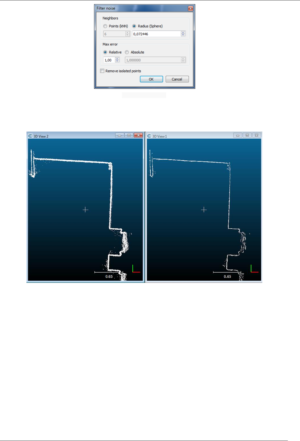
91
CloudCompare Version 2.6.1 – user manual
Noise filter parameters
Output
A new cloud, hopefully cleaner ;)
Typical result of the 'Noise filter'
Note
Due to the way the algorithm works it is very powerful on flat surfaces (walls, etc.). However, especially if you use a too
high kernel radius (or too low error threshold) it will 'eat' the corners. To save the corners or sharp edges one can try
to run the algorithm repeatedly with a small radius and relatively high error threshold.

92
CloudCompare Version 2.6.1 – user manual
Projection > Unroll
Menu
This tool is accessible via the 'Tools > Projection > Unroll' menu.
Description
This method 'unrolls' a point cloud from a cylindrical (or conical) shape onto a plane:
Top: cylindrical shape to unroll – bottom: cylindrical shape unrolled
Procedure
Select a cloud then start this tool.
Cylinder
'Unroll cylinder' dialog
To unroll a cylindrical shape, the parameters are:
axis of revolution (X, Y or Z)
radius
and optionally a point on the axis (otherwise CloudCompare will use the cloud gravity center)
Cone
'Unroll cone' dialog
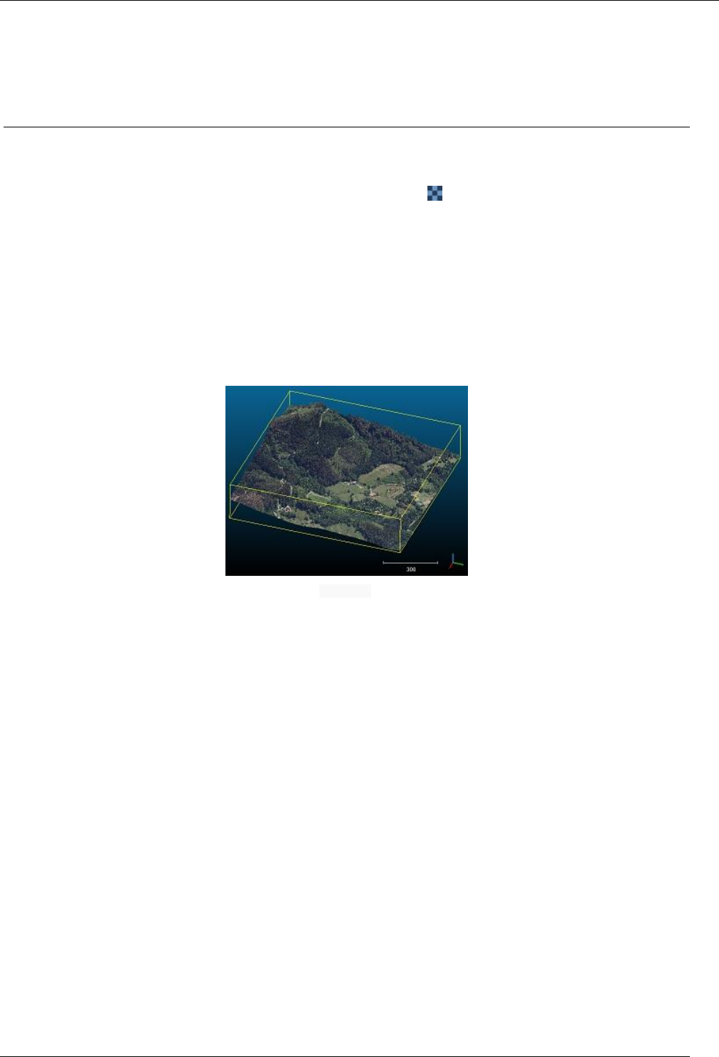
93
CloudCompare Version 2.6.1 – user manual
To unroll a conical shape, the parameters are:
axis of revolution (X, Y or Z)
half angle (this is the aperture angle at the cone apex - in degrees)
the cone apex position
Projection > Rasterize
Menu / Icon
This tool is accessible via the 'Tools > Projection > Rasterize' menu or the icon in the upper main toolbar.
(Prior to version 2.6.1, this tool was named 'Height grid generation')
Description
The main purpose of this tool is to 'rasterize' a point cloud (i.e. convert it to a 2.5D grid) and then export it as a new
cloud or a raster image (geotiff) for instance.
Another application since version 2.6.1 is 'Contour plot' generation.
Procedure
Select one cloud then start this tool.
Input cloud
A dedicated dialog with an embedded 3D view will appear. Some pieces of information about the selected cloud are
displayed in the upper-left corner. The most important is the height range and the minimum and maximum height
values of the cloud (the height being considered along the projection dimension).
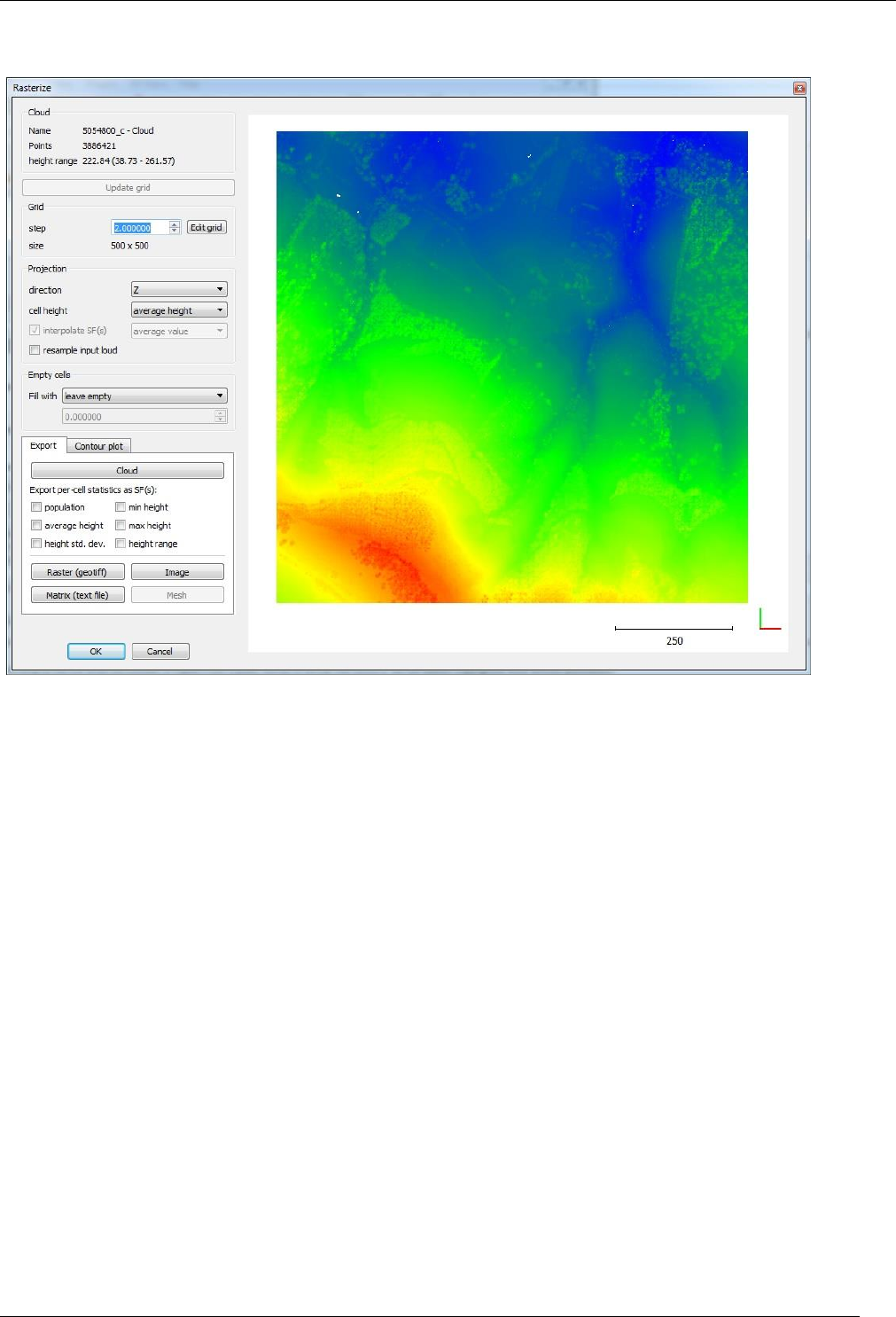
94
CloudCompare Version 2.6.1 – user manual
Generating a raster grid
The first and mandatory step is to generate the raster grid.
The user must define the main (raster) grid generation parameters:
the grid step size (CloudCompare will update the resulting grid size below so that the user can check that the
grid is neither too big nor too small before actually generating the grid)
the projection direction (X, Y or Z - default: Z)
how the 'height' of each cell grid will be computed:
o minimum height of all points falling in this cell
o average height of all points falling in this cell
o maximum height of all points falling in this cell
Once the base parameters are properly set, the user must click on the 'Update grid' button to make CloudCompare
actually computed the grid and display it.
Each time a parameter is modified, the 'Update grid' button will appear in red. The user has to click on it to actually
apply the changes.
Advanced parameters
Empty cells
If no points fall inside a given cell, this cell will be considered as 'empty'. Empty cells are not visible when displayed by
CloudCompare in the 3D view. They generally have a dedicated 'NaN' or 'empty' value when exported to a raster file
(depending on the format).
It is possible to tell CloudCompare to fill those cells in various ways:
use the minimum height of the whole grid
use the average height of the whole grid
use the maximum height of the whole grid
use a user specified value (should be input in the field below the 'Fill with' drop-down list)
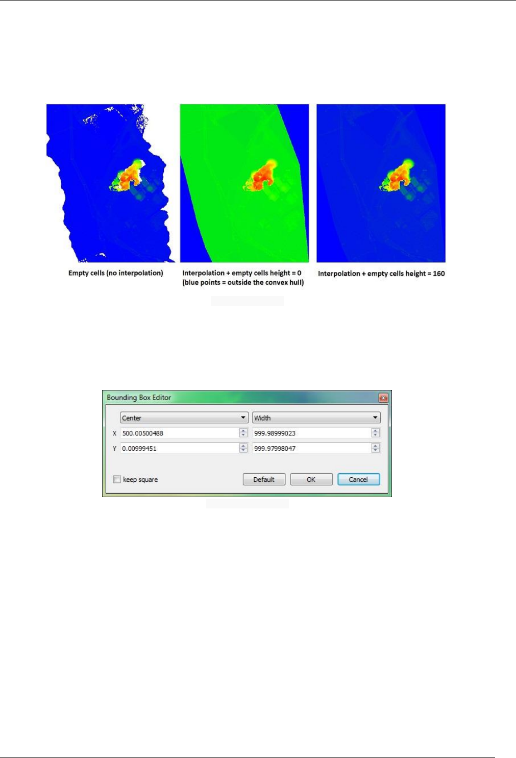
95
CloudCompare Version 2.6.1 – user manual
interpolate (see below)
Interpolating empty cells
The 'interpolate' option consists in a linear interpolation with the nearest non-empty neighboring cells. This can give
very good results in the presence of small holes. However it can be less accurate on big holes. And above all it doesn't
work outside the convex hull of the non-empty cells:
Interpolation principle
This is why a custom value must be specified (in the field below the 'Fill with' drop-down list) to fill these areas (if any).
Grid position
The grid position (in the projection plane) can be finely defined by clicking on the 'Edit grid' button:
Grid extents setup dialog
Interpolate scalar fields
If the input cloud has one or several scalar fields, it is possible to 'interpolate' the scalar field values in each grid cell.
To do this the user has to check the 'interpolate SF(s)' checkbox and define how this interpolation should be conducted:
by keeping the minimum SF value of all the points falling in this cell
by keeping the average SF value of all the points falling in this cell
by keeping the maximum SF value of all the points falling in this cell
Note: interpolated scalar fields can only be used when exporting the raster grid as a new cloud or as a raster file in a
formats that supports real-valued layers.
Resample input cloud
This option tells CloudCompare to keep in each grid cell the point which is the closest to the cell center (in 2D) instead
of generating of using the cell center itself. This way it is possible to subsample the cloud in a semi-gridded pattern. If

96
CloudCompare Version 2.6.1 – user manual
the grid is to be exported as a cloud, all the input cloud features (colors, normals, etc.) can be properly exported as
well.
Export
The (raster) grid can be exported to several destinations.
Cloud
The grid can be exported as a new cloud (see the "Cloud" button in the 'Export' tab in the bottom-left corner).
The grid is always exported as a 3D cloud (with the chosen 'height' as the 'Z' dimension). A 'height' scalar field is also
generated by default.
Several additional scalar fields can be generated:
'population': number of input points falling in each cell
'min height': minimum height of the points falling in each cell
'average height': average height of the points falling in each cell (may be redundant with the default 'height'
scalar field)
'max height': maximum height of the points falling in each cell (may be redundant with the default 'height'
scalar field)
'average height': average height of the points falling in each cell (may be redundant with the default 'height'
scalar field)
'height std. dev.': standard deviation of the height values of the points falling in each cell
'height range': range of the height values of the points falling in each cell
Raster
The grid can be exported as a geotiff raster file (see the "Raster (geotiff)" button in the 'Export' tab in the bottom-left
corner).
Note: CloudCompare relies on GDAL
35
for this operation.
Image
The grid can be exported as a simple image file. Use the 'Image' button (see the "Image" button in the 'Export' tab in
the bottom-left corner).
ASCII matrix
The grid can be exported as an array/matrix of height values saved as an ASCII file (see the "Matrix (text file)" button in
the 'Export' tab in the bottom-left corner).
This file should be easily imported in Excel for Matlab for instance. There's no file header. The number of rows is simply
the number of lines in the file, and the number of columns corresponds to the number of values found on each line
(should always be the same).
Mesh
The grid can be exported as a 2.5D mesh (see the "Mesh" button in the 'Export' tab in the bottom-left corner).
Contour plot generation
Since version 2.6.1, the Rasterize tool can now be used to generate contour plots.
The parameters for this sub-tool are all regrouped in the 'Contour plot' tab in the bottom-left part:
35
http://en.wikipedia.org/wiki/GDAL
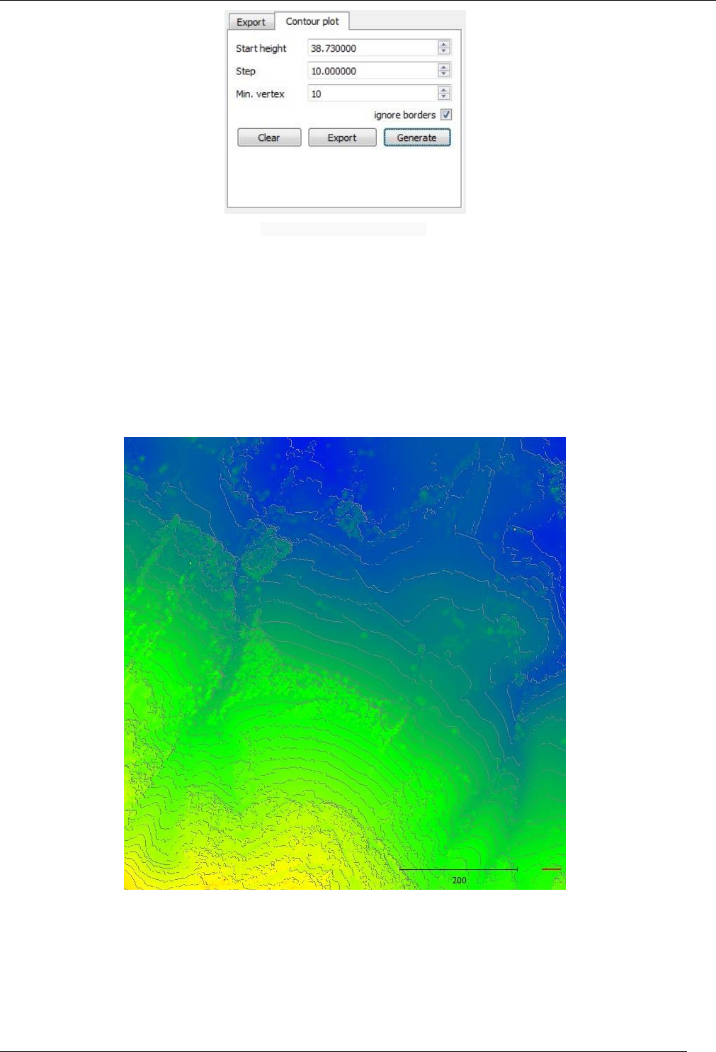
97
CloudCompare Version 2.6.1 – user manual
Contour plot generation parameters
The user must specify:
Start height: height of the first contour line
Step: step between each contour line
Min. vertex: minimum number of vertices per lines (used to remove the very small contours around trees, etc.)
ignore borders: to remove the contour lines created on the grid (square) edges
The first time, and each time the parameters are changed or the grid is updated, the user must click on the 'Generate'
button to generate the contour plot. Then a preview of the generated contour lines will be displayed over the raster
grid:
The user can pan and zoom the 3D view to view it better. The point size can also be modified in the standard way (+/-
interactors appear when the mouse hovers the top-left part of the 3D view).
The resulting contour lines can be removed (with the 'Clear' button) or exported as real polylines in the DB tree (with
the 'Generate' button). All contour lines are exported in a single group (automatically named after the input cloud name
and the 'Step' value).
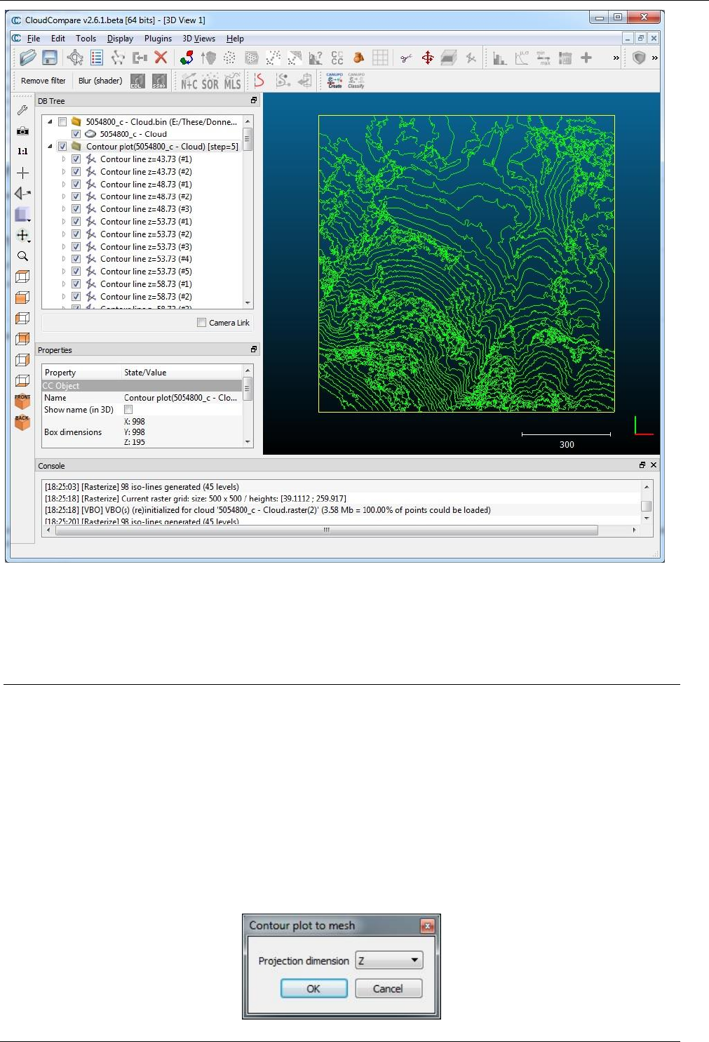
98
CloudCompare Version 2.6.1 – user manual
Notes:
the (group of) contour lines can be exported as a Shape file (to be imported in a GIS software for instance).
if the user has forgotten to export the contour lines when closing the tool, CloudCompare will issue a warning
message and will ask for confirmation.
Projection > Contour plot to mesh
Menu
This tool is accessible via the 'Tools > Projection > Contour plot (polylines) to mesh' menu.
Description
This tool can convert a set of polylines (ideally a set of contour lines) to a mesh. Contrarily to a standard 2.5D Delaunay
triangulation, this method will force the contour lines as edges for the output triangles.
Procedure
Select several polylines or a group of polylines then call this method.
CloudCompare will ask the user the 'projection dimension' (i.e. the dimension orthogonal to the contour lines):
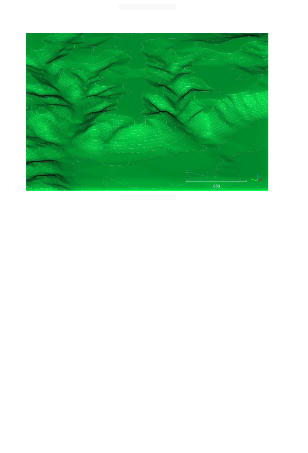
99
CloudCompare Version 2.6.1 – user manual
'Contour plot to mesh' dialog
CloudCompare will eventually generate the mesh.
'Contour plot to mesh' result
Warning: if the contour lines are crossing (in 2D) then holes may appear in the resulting mesh.
Projection > Export coordinate(s) to SF(s)
See ‘Scalar fields > Export coordinate(s) to SF(s)’.
Registration > Match bounding-box centers
Menu
This tool is accessible via the 'Tools > Registration > Match bounding-box centers' menu.
Description
This tool will translate all selected entities so that their bounding-box centers are in the same place.
Procedure
Select at least two entities (clouds or meshes) then start this tool.
The first selected entity will be used as reference. The others will be translated so that their bounding-box center comes
at the same place as the center of the first entity.
Warning: this tool has no dialog (effect is immediate - you may want to save or clone the entities first).
Transformation matrix
For each selected entity (but the first one) the 4x4 transformation matrix corresponding to the applied translation will
be issued in the Console.
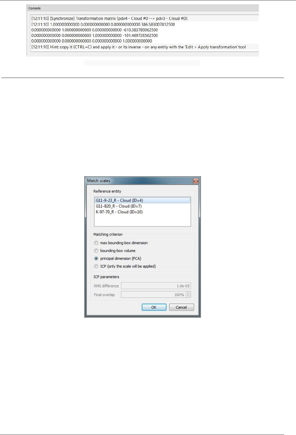
100
CloudCompare Version 2.6.1 – user manual
Console output of the ' Match bounding-box centers' method
Registration > Match scales
Menu
This tool is accessible via the 'Tools > Registration > Match scales' menu.
Description
This tool lets will (try to) make the scales of all selected entities match. The user must choose how the scale is computed.
This tool has been introduced in the 2.6.1 version.
Procedure
Select at least two entities (clouds or meshes) then start this tool.
CloudCompare will display a dedicated dialog:
In the upper part the user can choose which entity will be the 'reference' (i.e. all others will be scale so as to match this
one).
Below the user can choose how the scale is computed:
max bounding-box dimension
bounding-box volume
principal dimension (deduced by Principal Component Analysis)
ICP registration (see below)
Warning: on completion, all entities (but the reference one) will be scaled. Therefore you may want to save or clone the
entities before applying this tool.
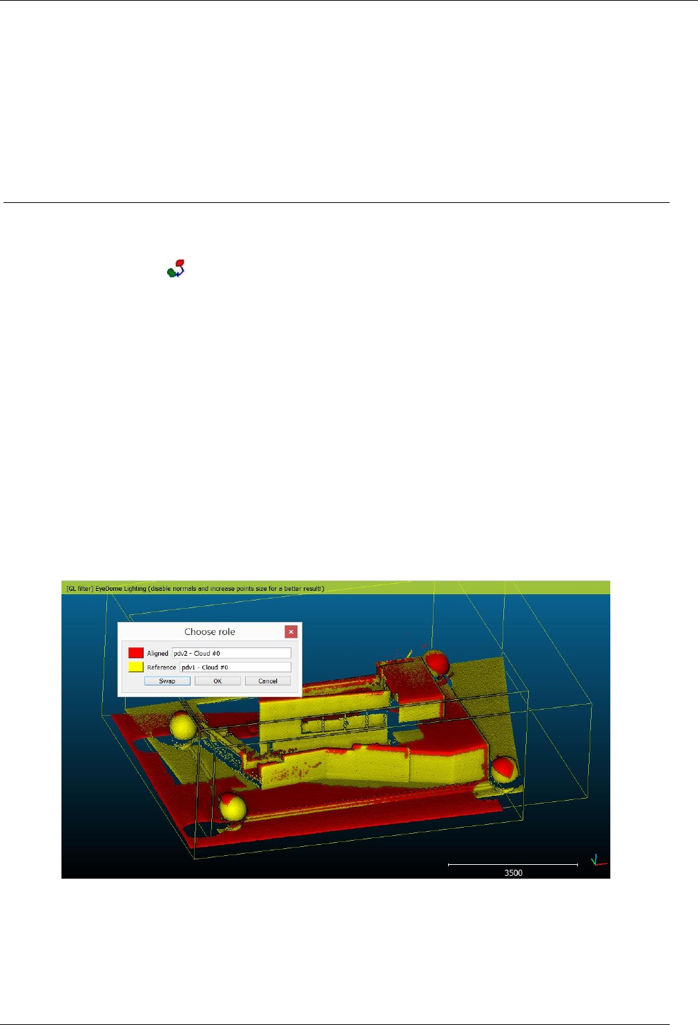
101
CloudCompare Version 2.6.1 – user manual
ICP criterion
If the user selects 'ICP registration' as scale matching criterion, two parameters can be defined (RMS difference and
Final overlap). Refer to the ’
Registration > Fine registration (ICP)’ tool documentation for a description of those parameters.
Note that only the resulting scale will be applied.
Registration > Align (point pairs picking)
Menu / Icon
This tool is accessible via the icon in the main upper toolbar or the 'Tools > Registration > Align (point pairs picking)'
menu.
Description
This tool lets the user align two entities by picking at least three equivalent point pairs in both entities.
This method is very useful to align clouds quite precisely. It's even sometimes the only way to get a fine result (typically
if the two clouds have great differences on large extents, in which case the ICP registration won't work properly).
Note: since version 2.6 you can use this tool directly on meshes - this way you can register two clouds, a cloud ad a
mesh or two meshes.
Procedure
First, select two entities then call this tool.
Role assignment
Then you'll have to designate (with the classical 'role' assignment dialog) which cloud will be the Reference (won't
move) and which one will be the aligned cloud (the one actually moving at the end):
Picking point pairs (or spheres)
Once this is done, the two selected entities will be displayed in a dedicated 3D view, and a new dialog will appear in the
upper-right corner.
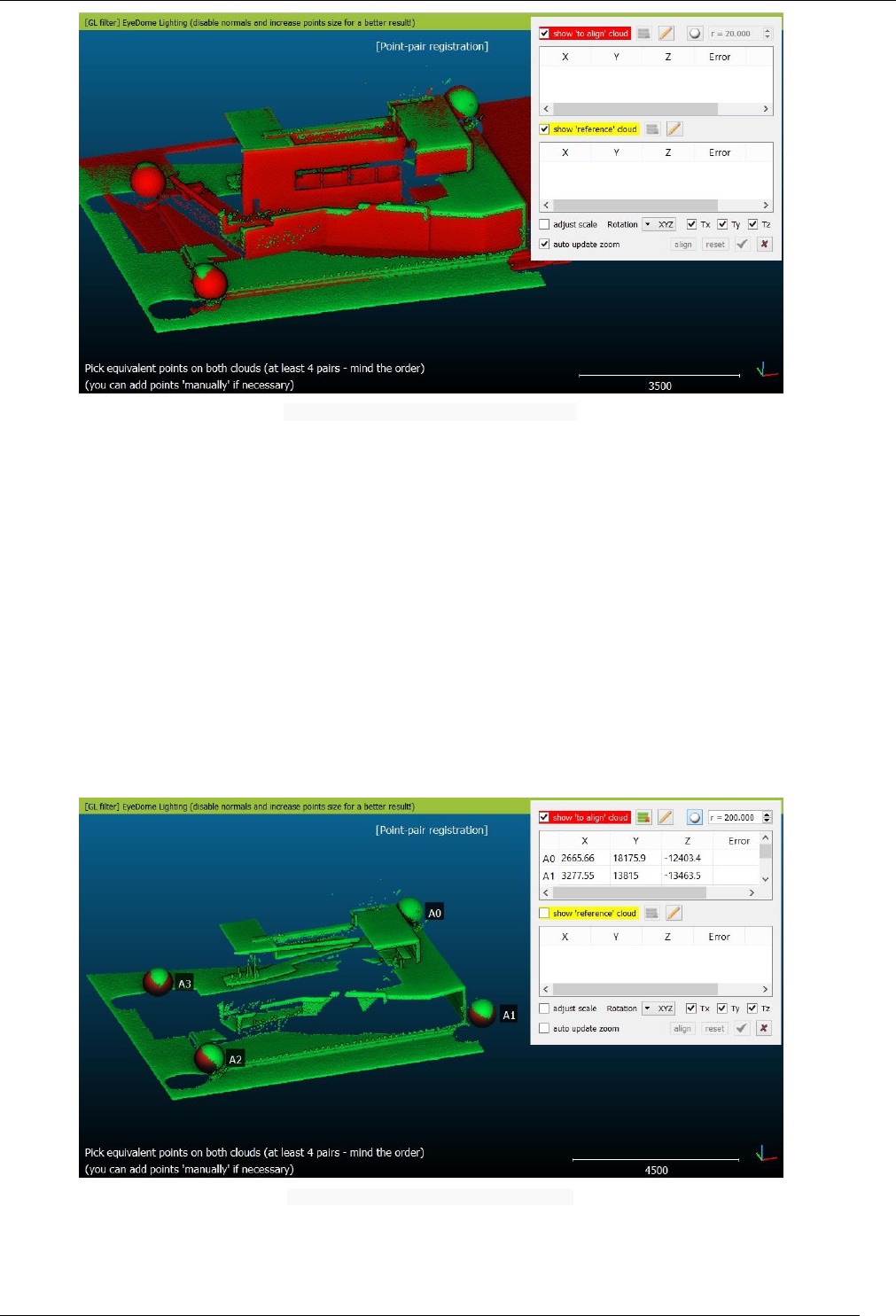
102
CloudCompare Version 2.6.1 – user manual
‘Align (point pairs picking)’ tool - initialization state
You are invited to select on both clouds the same set of remarkable points (mind the order). You can:
input (virtual) points with the 'pencil' icon (e.g. ground control points)
pick points directly on the clouds (3D view)
since version 2.6.1, you can optionally check the 'white sphere' icon (top-right corner) and set a search radius
(roughly the radius of the registration spheres in your scans if you know it). Once activated, CC will try to detect
a sphere in the cloud around each point you pick. If successful, it will use the sphere center as registration
point. Note that the input radius is only indicative (it will be used to search points around the one you pick).
CC will then automatically detect the best fit sphere radius (it is displayed in the Console, along with the best
fit RMS). Spheres and simple 3D points can be mixed without any problem.
During this process, you can hide either the 'reference' or the 'aligned' cloud with the dedicated checkboxes. You can
also freely rotate/translate the view point, enlarge points, zoom in or out, enable or disable OpenGL shaders, etc.
Each time you pick (or manually input) a point, a new entry appears in the corresponding table (either Aligned or
Reference), as well as a marker in the 3D view (aligned markers begin with 'A', and reference markers begin with ... 'R').
Selection of the 'Aligned' cloud points (as spheres)
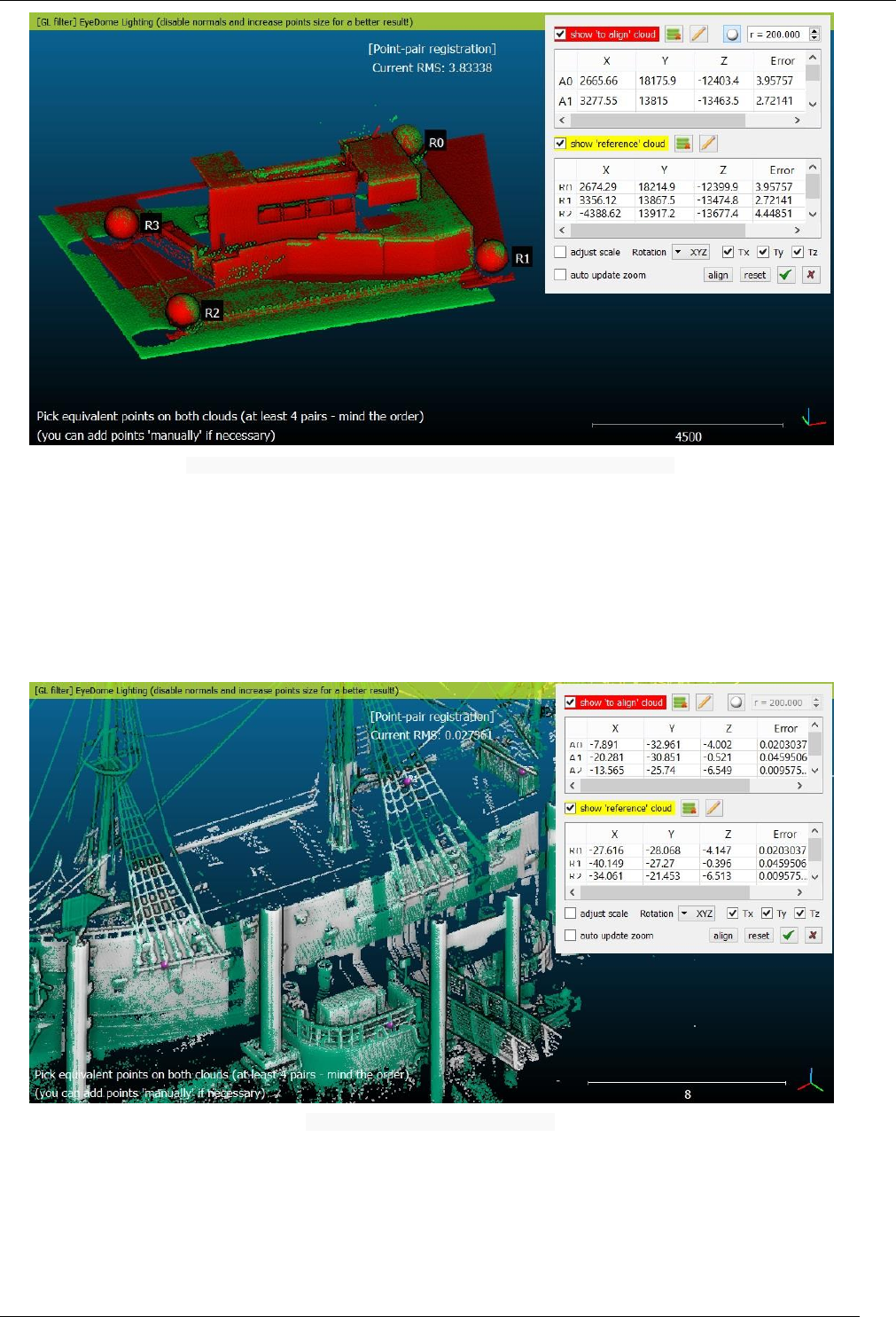
103
CloudCompare Version 2.6.1 – user manual
Selection of the 'Reference' cloud points (as spheres) and resulting alignment preview
Alignment
As soon as you have selected at least 3 or more pairs (you must have picked exactly the same number of points in each
cloud) CC will display the resulting RMS and you can preview the result with the 'align' button. You'll also see the error
contribution for each pair next to each point in the table (so as to remove and pick again the worst pairs for instance).
You can add new points to both sets anytime (even after pressing the 'align' button) in order to add more constraints
and get a more reliable result. And as suggested before, you can also remove points with the dedicated icons above
each tables or with the 'X' icon next to each point.
Standard alignment procedure (no spheres)
Validate / Cancel
You can validate or cancel the current registration process with the green 'V' and red 'X' icons. On validation, CC will
display a report (the same set of information is displayed in the Console (with increased digit accuracy).
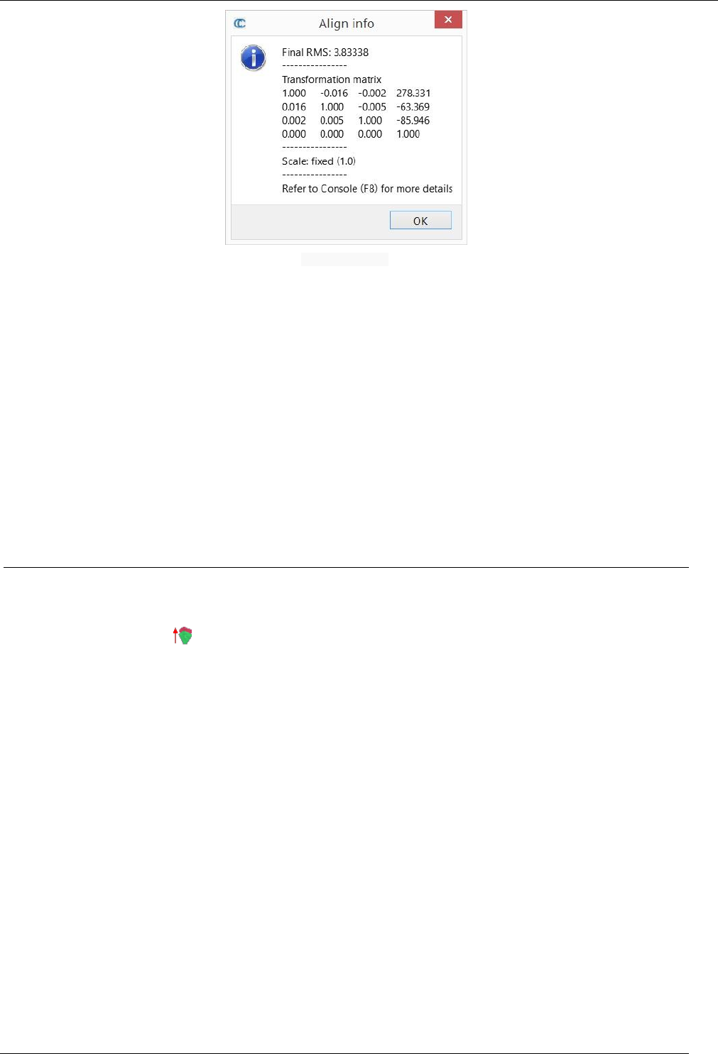
104
CloudCompare Version 2.6.1 – user manual
Registration report
Reset
You can reset the current 'Aligned' cloud pose anytime with the 'reset' button.
Advanced parameters
This tool can also determine the best scale factor between the two point sets. To allow the optimization of the scale
parameter, simply uncheck the fixed scale checkbox.
This can be very useful if the two clouds have different scales and you don't know the scale factor between them
(otherwise you could use either the 'Edit > Multiply/Scale' tool).
Warning: if the scale is not fixed (i.e. different from 1) then the 4x4 transformation matrix issued on completion of
this tool will be affine. Typically, the Edit > Apply transformation tool will fail to invert it...
Registration > Fine registration (ICP)
Menu / Icon
This tool is accessible via the icon in the main upper toolbar or via the 'Tool > Fine Registration (ICP)' menu.
Description
This tool can automatically finely registers two entities.
Main assumptions are:
both clouds are already roughly registered (see the other Alignment and Registration methods)
both clouds should represent the same object or at least have the same shape (at least on their overlapping
parts)
Procedure
Select the two clouds (or meshes) that you want to register and start this tool.
We use the original ICP algorithm denominations here: first you have to choose which entity will be the 'Data' one
(Registered, will eventually move) and which one will be the 'Model' one (Reference, won't move). You can the default
role assignation by clicking on the 'swap' button. You'll see in the 3D view that the two entities colors are forced to
yellow and red so as to correspond to the 'Model' (yellow) and 'Data' (red) colors.
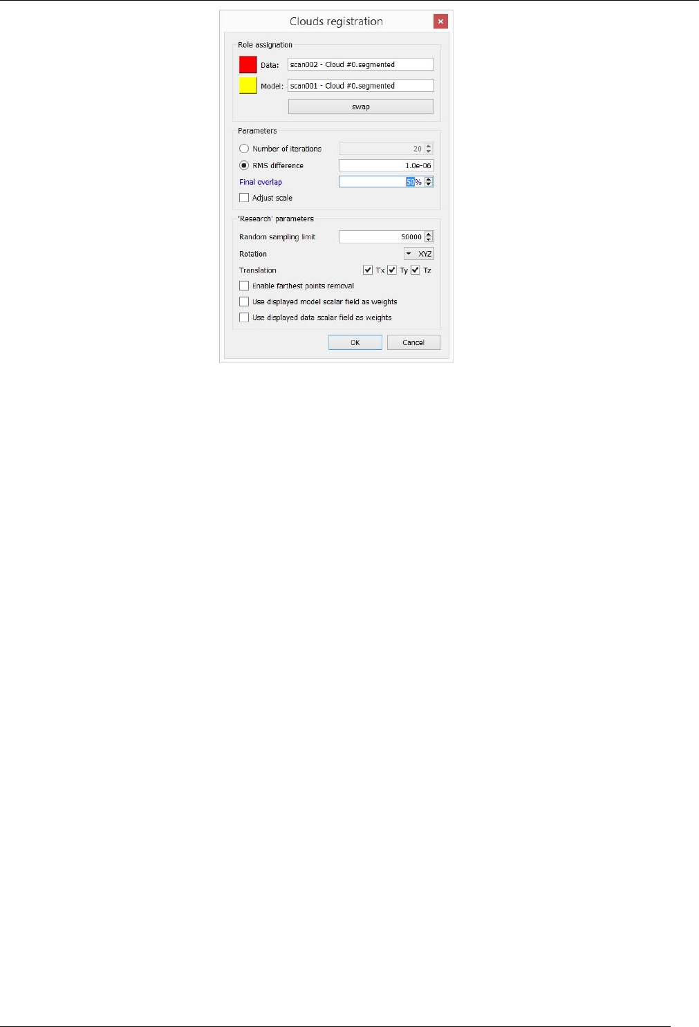
105
CloudCompare Version 2.6.1 – user manual
Fine registration (ICP) dialog
Main parameters
Here are the most important parameters:
Number of iterations/RMS difference: ICP is an iterative process. During this process, the registration error
(slowly) decrease. We can tell CC to stop this process either after a maximum number of iterations, or as soon
as the error (RMS) difference between two iterations becomes lower than a given threshold. The smaller this
threshold is, the longer it will take to converge, but the finer the result should be (note: as CC work with 32
bits floating point values, a 1e-8 threshold is already near the computation accuracy limit and it shouldn't be
necessary to go any lower).
Final overlap: this is a new parameter for the version 2.6.1. It lets the user specify the actual portion of the
data/registered cloud that would actually overlap the model/reference cloud if both clouds were registered.
This let the user register entities with only a partial overlap (down to 10% or even less).
Adjust scale: the modified-ICP algorithm we use is able to determine a potential difference in scaling. If your
clouds have different scales (e.g. photogrammetry clouds) you can check this option so as to resolve the scaling
as well.
Advanced parameters
You can optionally set additional research parameters (some of which are not yet validated, so that if you change them
you might get unexpected results):
Random sampling limit: to drastically increase computation speed on big clouds, we use an optimization
scheme. It consists in randomly sub-sampling the data cloud at each iteration. This parameter is the maximum
number of sub-sampled points. The default value (50000) is generally a good guess and its incidence on the
result is not perceivable. However it may be insufficient for very large clouds. So if you doubt about the results,
or if you want to refine the registration even more and you are not afraid of waiting a long time, don't hesitate
to increase this value (to fully deactivate this optimization scheme, simply input a number greater than the
data cloud size).
Rotation: you can constrain the rotation around a given axis (X, Y or Z)
Translation: you can constrain the translation along none, one or several dimensions (among X, Y and Z)
Enable farthest point removal: this option is very interesting if the shapes of the two entities you are trying to
register are quite different (either because the entities don't represent exactly the same object, or simply

106
CloudCompare Version 2.6.1 – user manual
because the noise on one entity is too high). This tells CC to remove at each iteration the points of the 'data'
cloud that are too far from the 'model' cloud.
Use displayed model/data scalar field as weights: this option should enable the user to use scalar values as
weights (either on the data or the model cloud - it is not advised to use weights on both clouds at the same
time)
Fine registration (ICP) result
Distances > Cloud/Cloud dist. (cloud-to-cloud distance)
Menu / Icon
This tool is accessible via the icon in the main upper toolbar or the 'Tools > Distances > Cloud/Cloud dist.' menu.
Description
This tool computes the distances between two clouds.
Procedure
To launch this tool the user must select two clouds (and only two).
Choosing the cloud roles
Before displaying the tool dialog, CloudCompare will ask you to define the roles of each cloud:
the Compared cloud is the one on which distances will be computed. CloudCompare will compute the distances
of each of its points relatively to the reference cloud (see below). The generated scalar field will be hosted by
this cloud.
the Reference cloud is the cloud that will be used as reference, i.e. the distances will be computed relatively
to its points. If possible, this cloud should have the widest extents and the highest density (otherwise a local
modelling strategy should be used - see below).
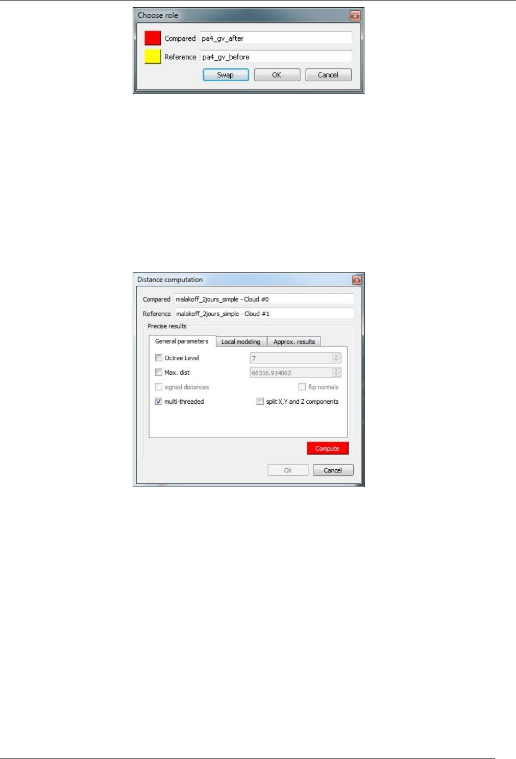
107
CloudCompare Version 2.6.1 – user manual
Approximate distances
When the Cloud/Cloud distance computation dialog appears, CloudCompare will first compute approximate distances
(which are used internally to automatically set the best octree level at which to perform the real distances computation
- see below). The reference cloud is hidden and the compared cloud is colored with those approximate distances.
Some statistics on those approximate distances are displayed in the 'Approx. results' tab (but they shouldn't be
considered as proper measurement values!). Those statistics are only provided for advanced users who would like to
set the octree level at which computation is performed themselves (however this is generally not necessary).
The user must compute the real distances (see the red 'Compute' button) or cancel the process.
Parameters
The main parameters for the computation are:
Octree level: this is the level of subdivision of the octrees at which the distance computation will be performed.
By default it is set automatically by CloudCompare and should be left as is. Changing this parameter only
changes the computation time. The main idea is that the higher the subdivision level is, the smaller the octree
cells are. Therefore the less points will lie in each cell and the less computations will have to be done to find
the nearest one(s). But conversely, the smaller the cells are and the more cells may have to be searched
(iteratively) and this can become very slow if the points are far apart (i.e. the compared point is far from its
nearest reference point). So big clouds will require high octree levels, but if the points of the compared cloud
are rather far from the reference cloud then a lower octree level is better...
Max dist.: if the maximum distance between the two clouds is high, the computation time might be awfully
long (as the farther the points are, the more time it will take to determine their nearest neighbors). Therefore
it can be a good idea to limit the search below a reasonable value to shorten the computation time. All points
farther than this distance won't have their true distance computed - the threshold value will be used instead.
signed distances: not available for cloud-to-cloud distance.
flip normals: not available for cloud-to-cloud distance.
multi-threaded: whether to use all CPU cores available (warning: the computer might not be totally responsive
during the computation)
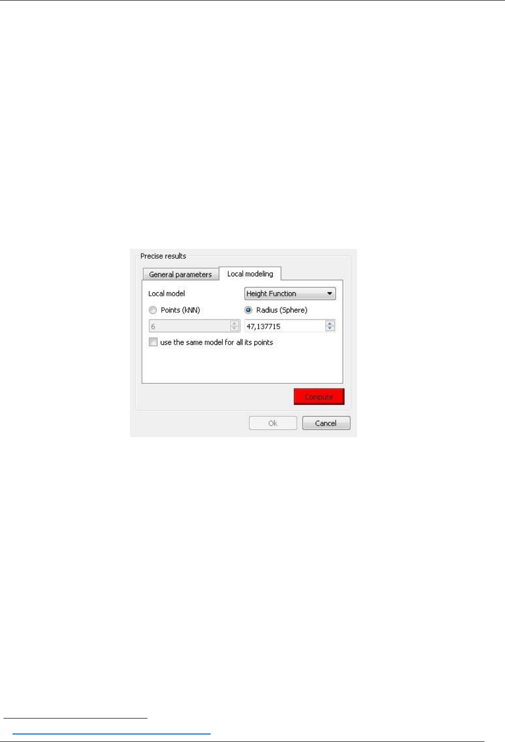
108
CloudCompare Version 2.6.1 – user manual
split X,Y and Z components: generate 3 more scalar fields corresponding to the (absolute) distance between
each compared point and its nearest reference point along each dimensions (i.e. this corresponds to the 3
components of the deviation vector).
Local modelling
(see the ‘Distances Computation' section for additional information)
When no local model is used, the cloud to cloud distance is simply the nearest neighbor distance (using a kind of
Hausdorff
36
distance algorithm). The issue is that the nearest neighbor is not necessarily (rarely in fact) the actual
nearest point on the surface represented by the cloud. This is especially true if the reference cloud has a low density or
has big holes. In this case it can be a good idea to use a 'Local modelling strategy' which consists in computing a local
model around the nearest point so as to approximate the real surface and get a better estimation of the 'real' distance.
The local model can be computed:
either on a given number of neighbors (this is generally faster but it's only valid for clouds with a constant
density)
or by default in a spherical neighborhood (its radius should typically depend on the details you expect to catch
and on the cloud noise).
There are currently three types of local models. All 3 models are based on the least-square best fitting plane that goes
through the nearest point and its neighbors:
Least squares plane: we use this plane directly to compute distances
2D1/2 triangulation: we use the projection of the points on the plane to compute Delaunay's triangulation (but
we use the original 3D points as vertices for the mesh so as to get a 2.5D mesh).
Height function: the name is misleading but it is kept for consistency with the old versions. In fact the
corresponding model is a quadratic function (6 parameters: Z = a.X2 + b.X + c.XY + d.Y + e.Y2 + f). In this case we
only use the plane normal to choose the right dimension for 'Z'.
We could say that the local models are sorted in increasing 'fidelity' to the local geometry (and also by increasing
computation time). One should also take in consideration whether the local geometry is mostly smooth or with sharp
edges. Because the Delaunay triangulation is the only model that can theoretically represent sharp edges (assuming
you have points on the edges) and the quadratic function is the only one that can represent smooth/curvy surfaces. By
default it is recommended to use the quadratic model as it's the more versatile.
Last but not least it's important to understand that due to the local approximation, some modeling aberrations may
occur (even if they are generally rare). The computed distances are statistically much more accurate but locally some
distance values can be potentially worse than the nearest neighbor distance. This means that one should never consider
the distance of a single point in its analysis but preferably a local tendency (this is the same with nearest neighbor
distance anyway). To partially cope with this effect, since version 2.5.2 we now keep for each point the smallest distance
36
http://en.wikipedia.org/wiki/Hausdorff_distance
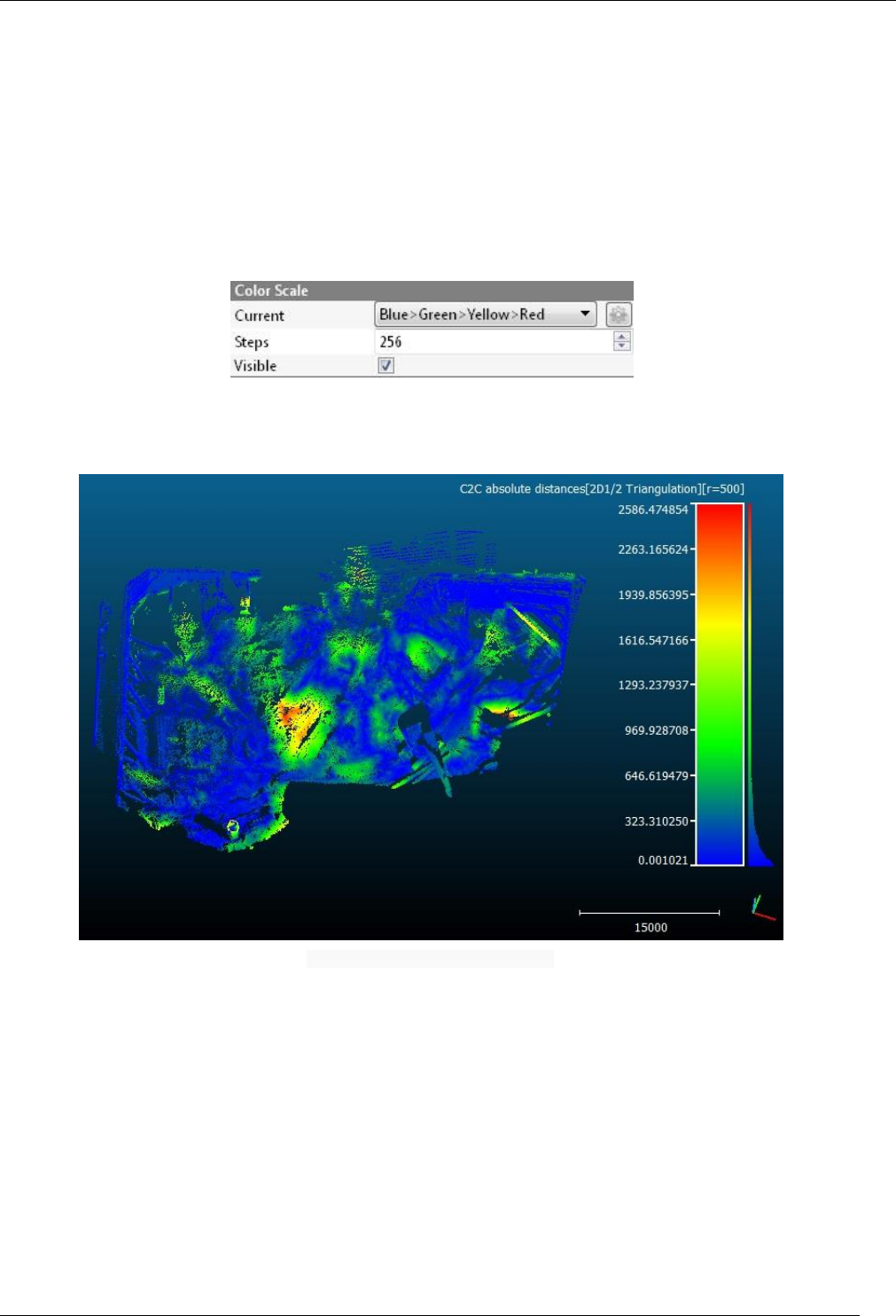
109
CloudCompare Version 2.6.1 – user manual
between the nearest neighbor distance and the distance to the local model. This way, we can't output distances greater
(i.e. worst) than the nearest neighbor's one. However we can still underestimate the 'true' distance in some (hopefully
rare) cases.
The 'local modeling' strategy is meant to cope with sampling-related issues (either a globally too small density or too
high local variations of the density of the reference cloud). It's always a good idea to use the densest cloud as
'reference'.
Displaying the resulting distances color scale
Once the computation is done, the user can close the dialog. To display the resulting scalar field's color scale, just select
the compared cloud and then check the 'Visible' checkbox of the 'Color Scale' section of its properties.
Alternatively use the shortcut 'Shift + C' once the cloud is selected to toggle the color scale visibility.
One can also set the color scale to be used with the 'Current' combo-box (and edit it or create a new one with the 'gear'
icon on the right).
Cloud-to-cloud distances: example of result
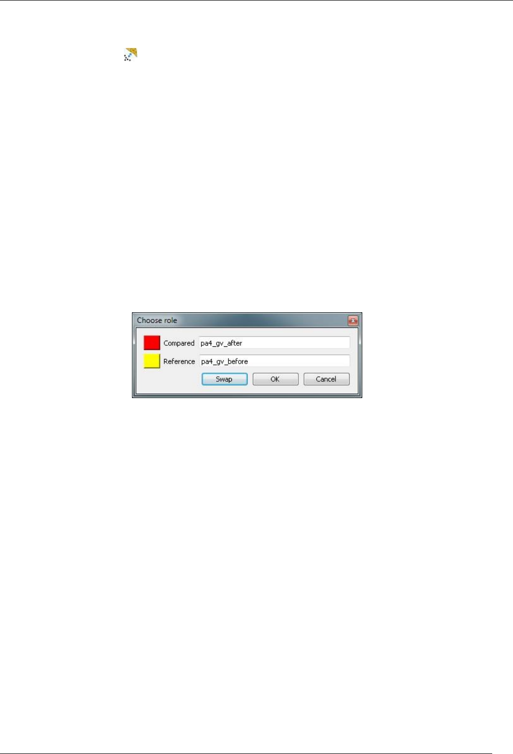
110
CloudCompare Version 2.6.1 – user manual
Distances > Cloud/Mesh dist. (cloud-to-mesh distance)
Menu / Icon
This tool is accessible via the icon in the main upper toolbar or the 'Tools > Distances > Cloud/Mesh dist.' menu.
Description
This tool computes the distances between a cloud and a mesh.
Procedure
To launch this tool you'll have to select either one cloud and one mesh, or two meshes.
Choosing the mesh roles
If you have selected one cloud and one mesh, the mesh will automatically be used as reference.
If you have selected two meshes, CloudCompare will ask you to define the roles of each mesh:
Compared mesh: CloudCompare will in fact only consider its vertices and compute the distances for each of
them relatively to the reference mesh. The generated scalar field will be hosted by this mesh (well, its vertices
in fact).
the Reference mesh will be used as reference, i.e. the distances will be computed relatively to its polygons. If
possible, this mesh should have the widest extents.
Warning: if you want to compare two meshes, and the compared mesh vertices are too sparse, you should consider
using the ‘Mesh > Sample points’ tool first in order to sample (a lot of) points on the compared mesh and then use the
resulting cloud as the compared entity.
Approximate distances
When the Cloud/Cloud distance computation dialog appears, CloudCompare will first compute approximate distances
(which are used internally to automatically set the best octree level at which to perform the real distances computation
- see below). The reference cloud is hidden and the compared cloud is colored with those approximate distances.
Some statistics on those approximate distances are displayed in the 'Approx. results' tab (but they shouldn't be
considered as proper measurement values!). Those statistics are only provided for advanced users who would like to
set the octree level at which computation is performed themselves (however this is generally not necessary).
The user must compute the real distances (see the red 'Compute' button) or cancel the process.
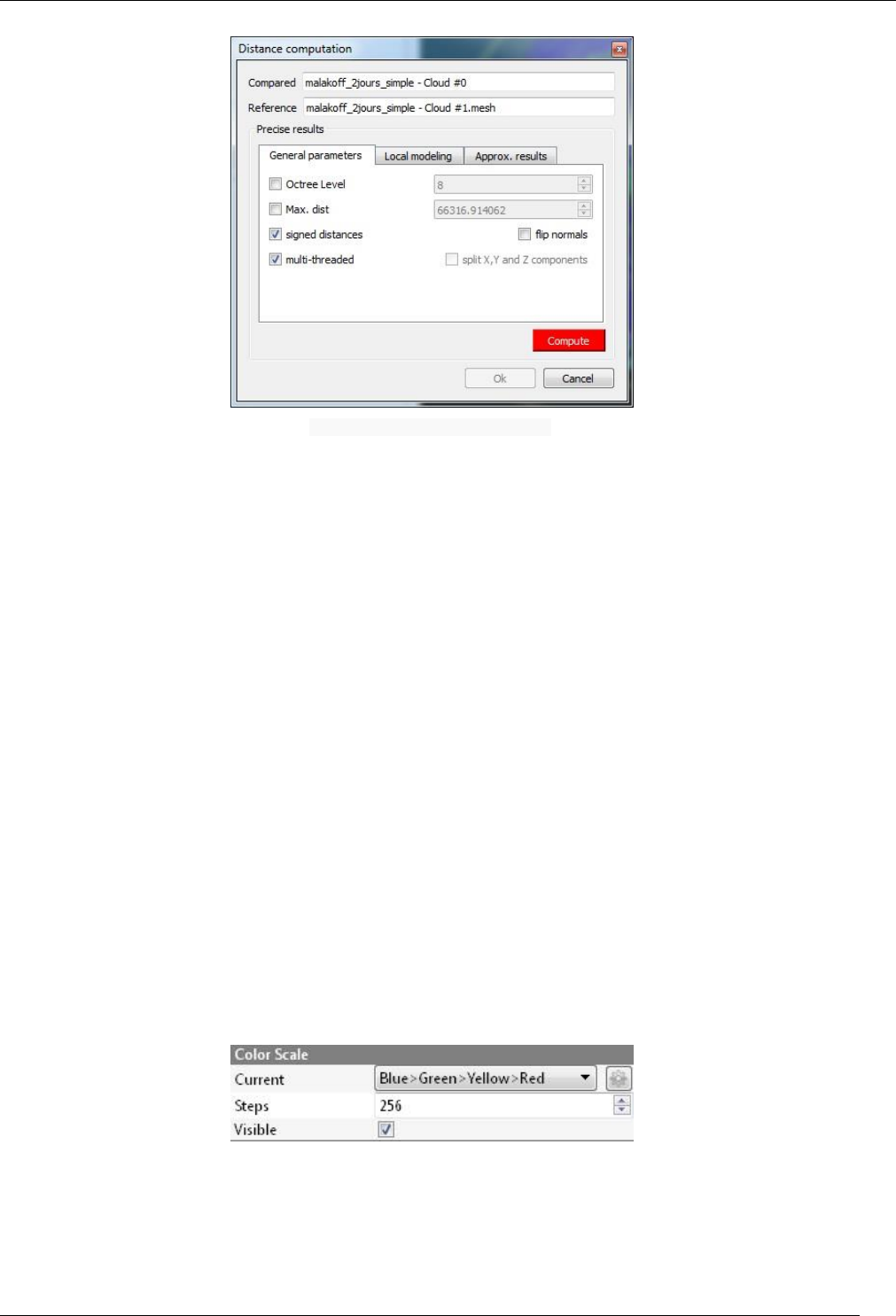
111
CloudCompare Version 2.6.1 – user manual
Parameters
Cloud/Mesh distances computation dialog
The main parameters for the computation are:
Octree level: this is the level of subdivision of the octrees at which the distance computation will be performed.
By default it is set automatically by CloudCompare and should be left as is. Changing this parameter only
changes the computation time. The main idea is that the higher the subdivision level is, the smaller the octree
cells are. Therefore the less points will lie in each cell and the less computations will have to be done to find
the nearest one(s). But conversely, the smaller the cells are and the more cells may have to be searched
(iteratively) and this can become very slow if the points are far apart (i.e. the compared point is far from its
nearest reference point). So big clouds will require high octree levels, but if the points of the compared cloud
are rather far from the reference cloud then a lower octree level is better...
Max dist.: if the maximum distance between the two entities is high, the computation time might be awfully
long (as the farther the points are, the more time it will take to determine their nearest neighbors). Therefore
it can be a good idea to limit the search below a reasonable value to shorten the computation time. All points
farther than this distance won't have their true distance computed - the threshold value will be used instead.
signed distances: whether computed distances should be signed with the triangle normal or not
flip normals: if signed distances is checked, then CloudCompare can automatically invert the sign (may be
necessary if the order of the triangle's vertices is inverted)
multi-threaded: whether to use all CPU cores available (warning: the computer might not be totally responsive
during the computation)
split X,Y and Z components: not available for cloud-to-mesh distance.
Displaying the resulting distances color scale
Once the computation is done, the user can close the dialog. To display the resulting scalar field's color scale, just select
the compared entity and then check the 'Visible' checkbox of the 'Color Scale' section of its properties.
Alternatively use the shortcut 'Shift + C' once the entity is selected to toggle the color scale visibility.
One can also set the color scale to be used with the 'Current' combo-box (and edit it or create a new one with the 'gear'
icon on the right).
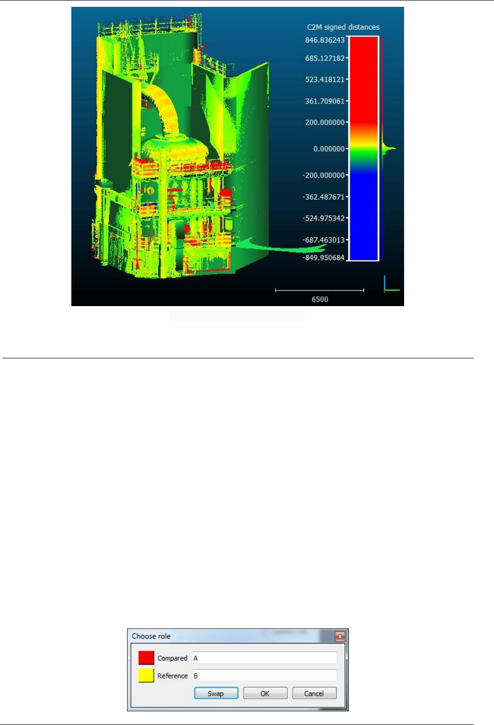
112
CloudCompare Version 2.6.1 – user manual
Cloud-to-mesh distances: example of result
Distances > Closest Point Set
Menu / Icon
This tool is accessible via the 'Tools > Distances > Closest Point Set' menu.
Description
This tool computes 'closest point set' of a cloud relatively to another one. This structure is defined for instance by Besl
et al. in the original ICP article.
Let A and B be two clouds with respectively NA and NB points.
The closest point set of A relatively to B (CPSetB(A)) is the set of points from the B cloud that are closest to each point
of A.
This set has NA points which all come from the B cloud. Moreover, the points of B can be duplicated several times in
the output set as they can be the 'closest' for different points of the A cloud.
Procedure
To launch this tool the user must select two clouds (and only two).
Then the user must choose which cloud will be the A cloud (equivalent to the 'Compared' cloud when computing
distances at each ICP registration iteration - as this is where this concept is used) and which cloud is the B cloud
(equivalent to the 'Reference' cloud).
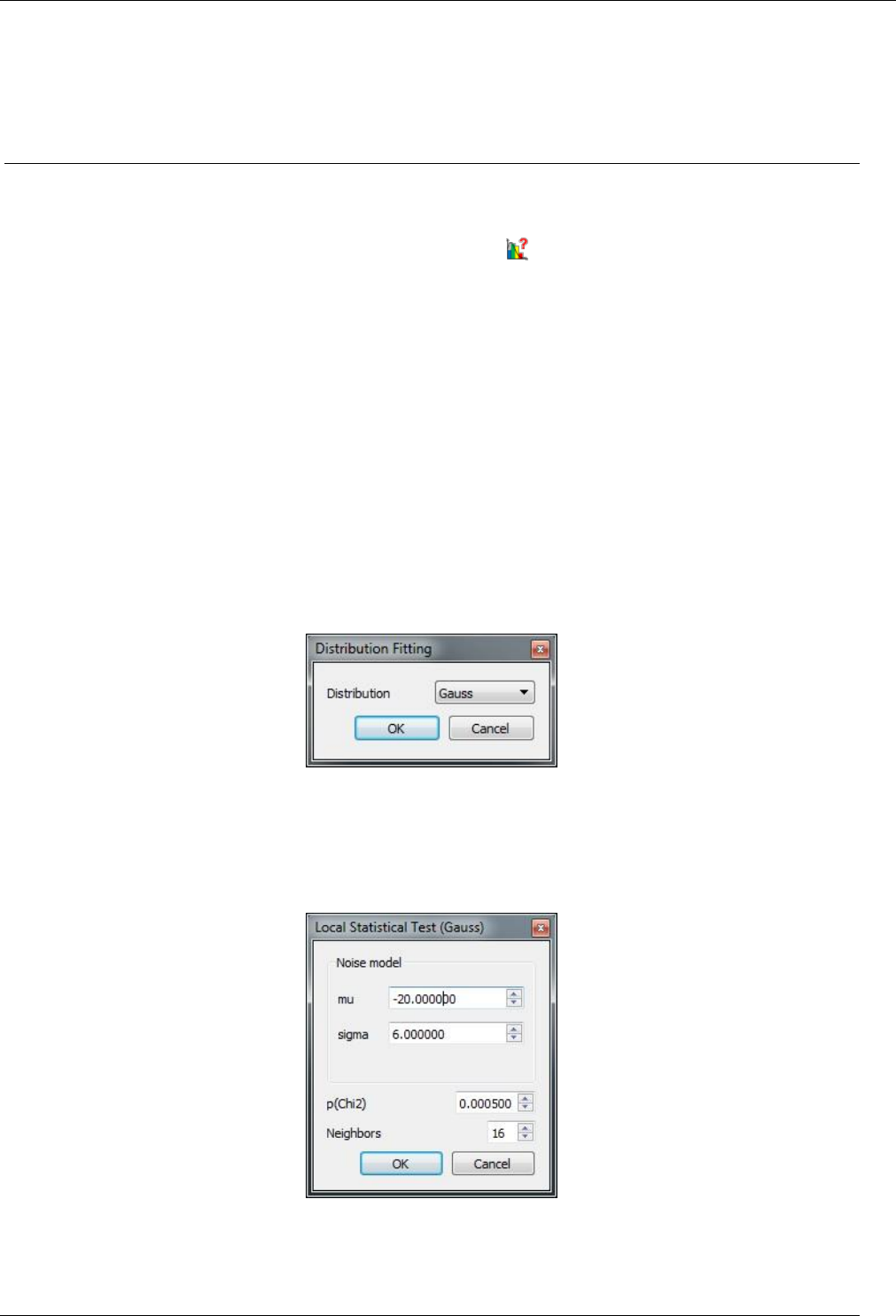
113
CloudCompare Version 2.6.1 – user manual
CloudCompare will then compute the closest point set and add it (as a new cloud) to the DB tree. The Reference/B cloud
will be hidden (as the closest point set will be a subset of it and therefore it wouldn't be visible).
Warning: as stated above, this cloud may have duplicate points.
Statistics > Local Statistical Test
Menu / Icon
This tool is accessible via the 'Tools > Statistics > Local Statistical test' menu.
Description
This tool can be used to segment/filter a point cloud based on the local statistical 'behavior' of the active scalar field.
For instance, if the active scalar field corresponds to distances, and you know the distribution of the measurement
noise, then you can filter the points for which the local scalar values seem to fit the noise distribution.
This way you'll be able to ignore those points and only focus on the points with distances clearly out of the noise
distribution.
Procedure
Select a cloud and start this tool.
As for the 'Statistics > Compute Stat. Params' tool, CloudCompare will first ask the user to choose the distribution
type:
Gauss (aka Normal) distribution
Weibull distribution
Then another dialog will appear so as to let the user input the distribution parameters as well as the two algorithms
parameters:
p(Chi2): the Chi2 test margin of error (see below for more information)
Neighbors: the number of neighbors around each point on which to perform the test (at least 10). This
algorithm works best on clouds with a homogeneous density.
On completion, a new scalar field will be generated on the input cloud: 'Chi2 distances'.
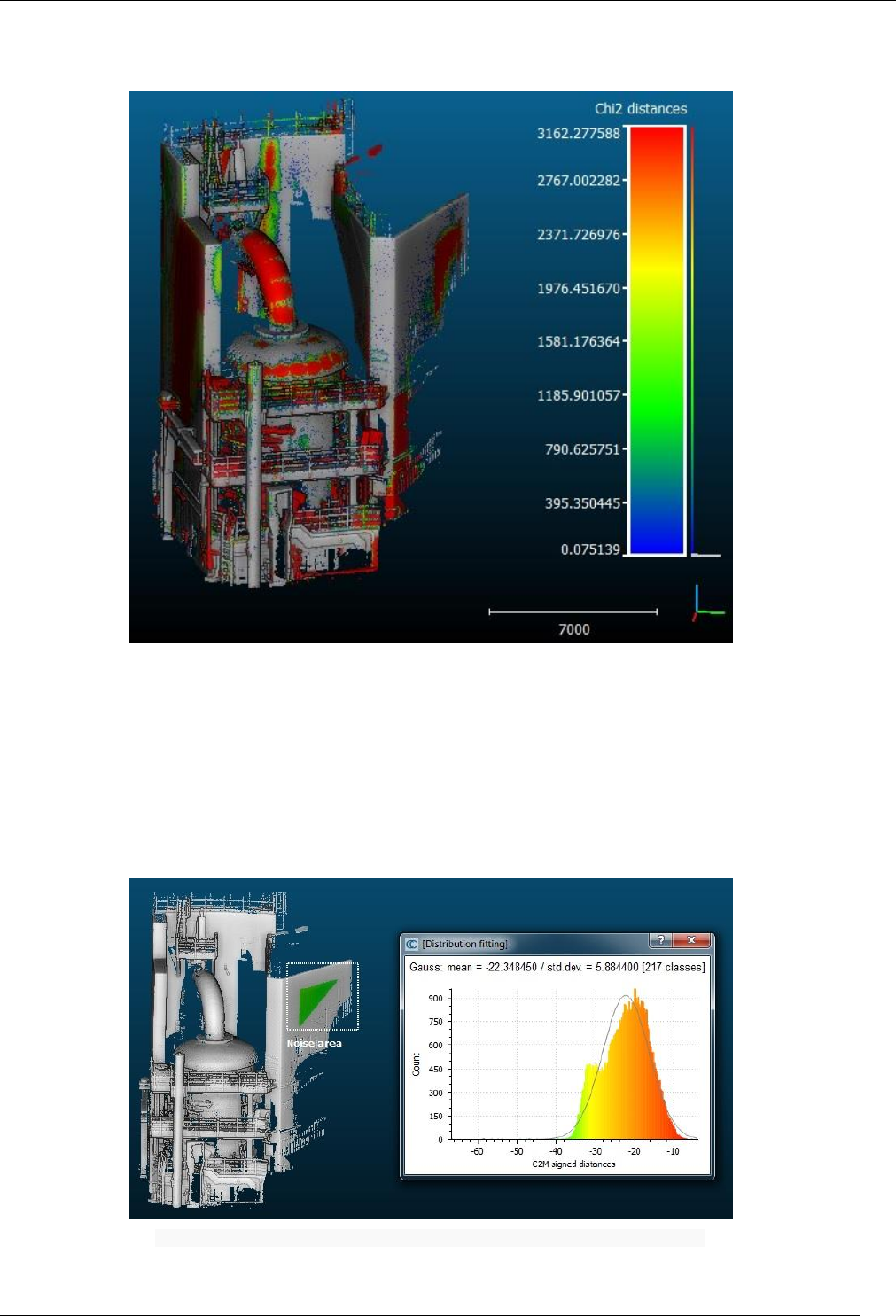
114
CloudCompare Version 2.6.1 – user manual
CloudCompare will automatically set the 'minimum displayed' and 'minimum saturation' values to the theoretical Chi-
squared distance that corresponds to the input parameters. This way all the grey points correspond to the points that
follow the tested (noise) distribution. The others points are not likely to follow the tested distribution.
Local statistical test result
Estimating the noise distribution
Let's assume you already have a scalar field associated to your cloud (e.g. distances) but you don't know the noise
distribution.
If you can isolate a part of this cloud where the scalar-field values should be zero (typically a part that hasn't
moved/changed in the case of distances) then you can segment it with the Interactive Segmentation Tool and fit a
statistical distribution on the resulting subset's scalar fields with the 'Tools > Statistics > Compute Stat. Params' tool:
Evaluation of the measurement noise on a subset of the cloud (where the distances should be 0)
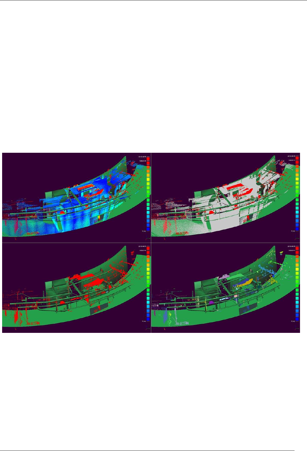
115
CloudCompare Version 2.6.1 – user manual
Warning: if the noise doesn't follow a Gaussian/Normal distribution (for instance if you have computed unsigned
distance), then you should prefer the Weibull distribution that has a third parameter and is more versatile.
About the Chi-squared test
The Chi-squared distance gives an indication on the local concordance between the scalar values (of each point and its
neighbors) and the tested distribution. The greater the less likely is the local distribution likely to follow the tested one.
The margin of error (p) is only used to set the threshold below which points will be considered as being 'in concordance'
with the tested distribution. The smaller this margin, the less discriminating the test will. As this test is used to "reject
the hypothesis that the local scalar values' follow the tested distribution". Therefore if the margin is smaller than this
hypothesis will be less rejected and more points will be considered as being compatible with the tested distribution!
(e.g. noise).
Exploiting the Chi2 distances
The user can directly use the 'Edit > Scalar fields > Filter by Value' method in order to extract and create a new cloud
with the non-grey points (the points which distance is significant for instance). This tool will use the current display
parameters by default.
And from the filtered cloud you can extract connected components for instance (see ‘Segmentation > Label Connected
Components’):
Full workflow involving the Local statistical Test tool
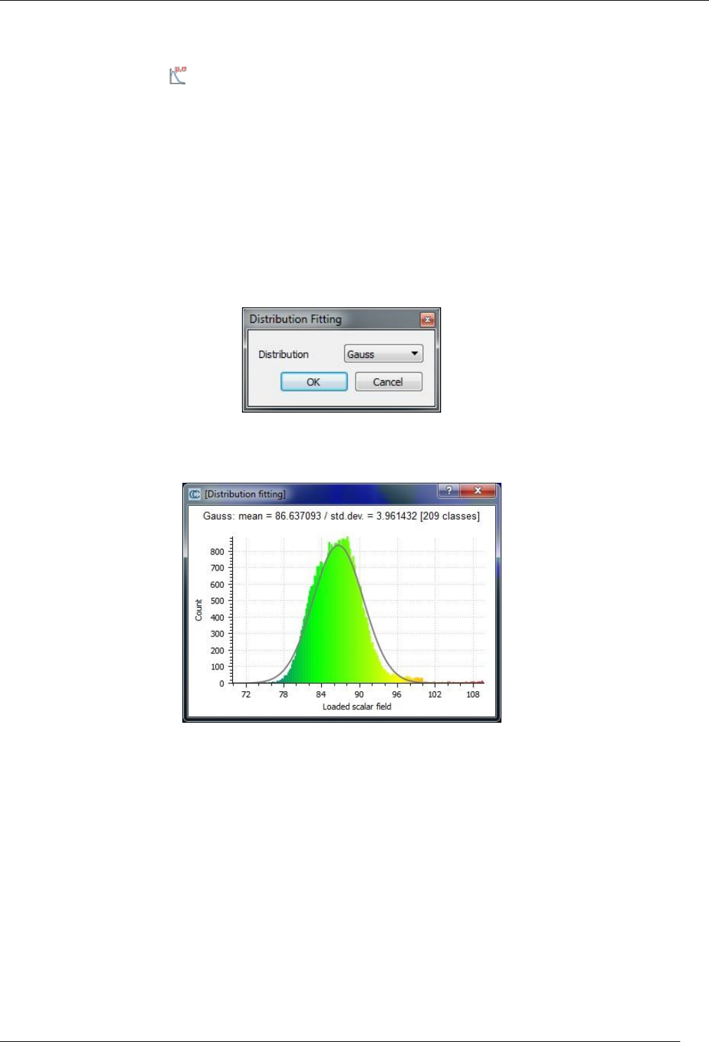
116
CloudCompare Version 2.6.1 – user manual
Statistics > Compute Stat. Params
Menu / Icon
This tool is accessible via the icon in the main upper toolbar or the 'Tools > Statistics > Compute stat. params (active
SF)' menu.
Description
This tool fits a statistical distribution on the active scalar field of the selected entity.
Available distributions are:
Gauss (aka Normal) distribution
Weibull distribution
Procedure
Select an entity (cloud or mesh) then call this tool. A dialog will appear so as to let the user choose the distribution to
fit:
Eventually CloudCompare will compute the corresponding distribution parameters and display the scalar histogram
with a grey curve corresponding to the fitted distribution. The distribution parameters are displayed above the
histogram, and also in the Console (along with the Chi-squared test result so as to get an evaluation of the fit quality).
Compute stat. params. Result
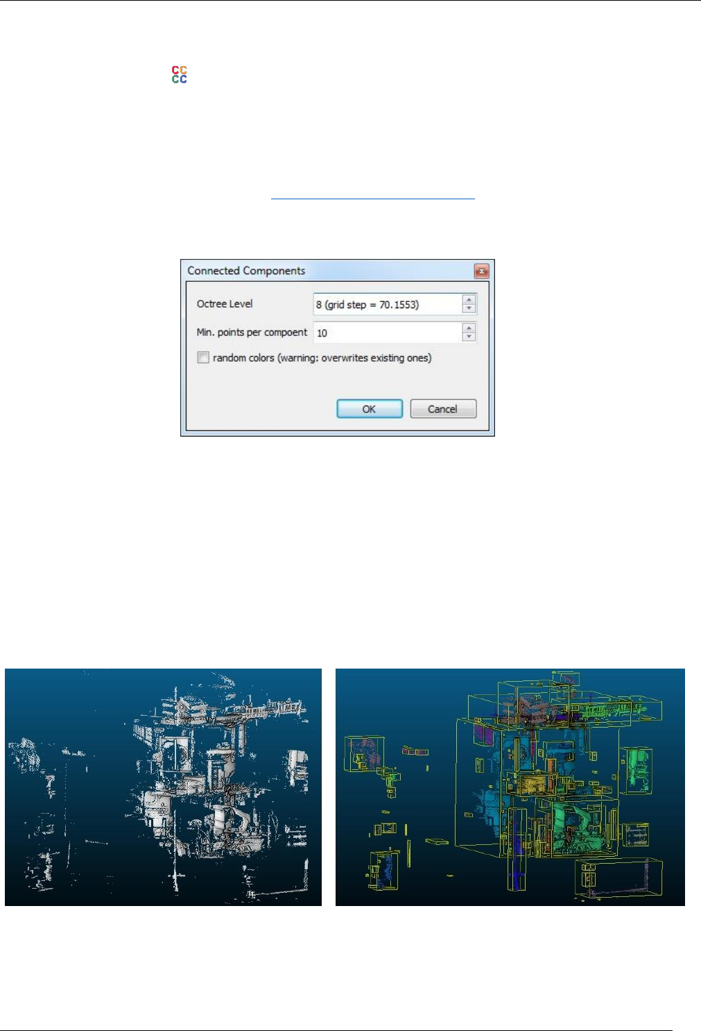
117
CloudCompare Version 2.6.1 – user manual
Segmentation > Label Connected Components
Menu / Icon
This tool is accessible via the icon the upper main toolbar or the 'Tools > Segmentation > Label Connected Comp.'
menu.
Description
This tool segments the selected cloud(s) in smaller parts separated by a minimum distance. Each part is a connected
component (i.e. a set of 'connected' points).
Note: the name of this tool is derived from the classical image processing algorithm with the same name.
Procedure
Select one or several clouds then start this tool.
CloudCompare will ask you to set some parameters:
Octree level: CloudCompare uses a 3D grid to extract the connected components (just as the original
algorithm). This grid is deduced from the octree structure. By selecting on octree level you define how small is
the minimum gap between two components (the corresponding cell size is displayed next to the level). The
higher the level is and the smaller the gap is (so the more components you might get).
Min. points per component: components with less than the specified number of points will be ignored (useful
to remove the smallest components)
random colors: if checked, a random color will be assigned to each component (warning: any existing colors
will be overwritten!)
On completion CloudCompare will create as many clouds as components. Each cloud is a proper subset of the original
cloud with the same features (scalar fields, normals, colors - if random colors are not generated - etc.).
Raw cloud (left) and extracted connected components (right)
Note: all components will be sorted in a new group (name of the input cloud + "[CCs]"). They will be sorted from the
biggest to the smallest (in terms of number of points).

118
CloudCompare Version 2.6.1 – user manual
Segmentation > Cross Section
Menu / Icon
This tool is accessible via the icon the upper main toolbar or the 'Tools > Segmentation > Cross Section' menu.
Description
This tool allows the user to define a clipping box (interactively or not) around a given cloud. The box extents and
orientation can be adjusted in order to segment the cloud for instance. Additionally, this tool can:
repeat the segmentation process in one or several dimensions (to extract multiple 'slices' for instances)
extract polygonal contours in each slice
Procedure
Select a single cloud and start this tool.
A dedicated dialog will appear in the top-right part of the 3D view.
Note: the initial clipping box is the cloud bounding-box.
Editing the clipping box
The clipping box can be edited in various ways.
Interactively
You can drag the 'interactors' (big red, green and blue arrows and tori) so as to move the clipping box boundaries
directly in the 3D view. The arrow tips are used to push and pull the clipping box faces, while the tori can be used to
rotate the box around the arrow axes.
You can also translate the whole box with the lower-left (yellow) interactor.

119
CloudCompare Version 2.6.1 – user manual
Note: you can show or hide the interactors with the 'Show interactors' checkbox in the top left part of the dialog.
Numerically
You can directly edit the box dimensions (width, depth and height) with the 'X', 'Y' and 'Z' fields.
You can also shift the box in all directions with the buttons in the lower part of the dialog ('Shift box' frame). The box
will be shifted of the same quantity as the box width in this dimension.
Eventually, if you need more control, you can click on the 'advanced' button. A 'standard' 3D box edition dialog will
appear. You can setup the box position in space in various ways (and even force the box to be cubical for instance).
Visualization
At any time the 3D view camera can be changed so as to face one of the clipping box faces. Use the standard 'predefined
views' buttons in the lower part. It can be useful to hide the interactors as well in order to properly see the current
cloud section:
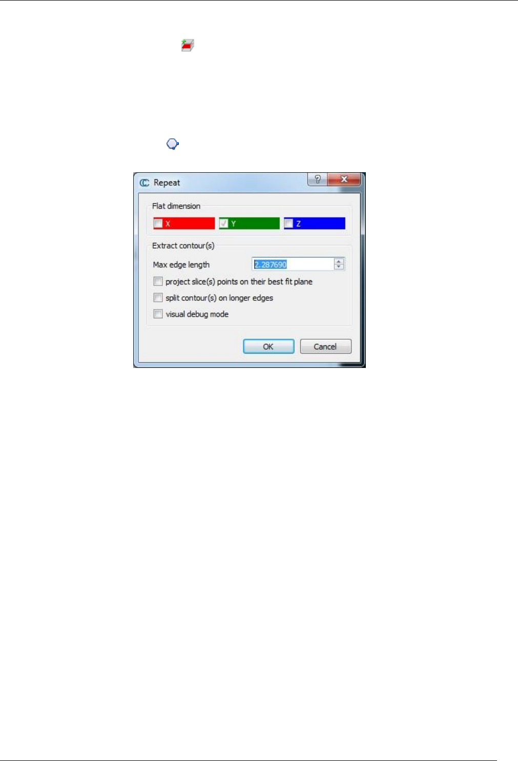
120
CloudCompare Version 2.6.1 – user manual
Extract a single slice
Once the clipping box is defined, you can export the visible cloud subset as a new cloud.
To do this, simply click on the 'Export slice' button (in the right 'Slices' frame). CloudCompare will then create a new
cloud and add it to the database tree.
Extract a single contour
Instead of the subset of points corresponding to the current slice, it is also possible to extract the (closed) contour of
the points.
To do this click on the 'Extract contour' button (in the left 'Contour' frame). A dialog to setup the contour extraction
process will appear:
The user must set:
the 'flat dimension’ (it should be automatically setup based on the current section dimensions).
the ‘maximum edge length’: the contour is extracted thanks to a 'concave hull' algorithm. The only parameter
for this tool is the 'maximum size' of a single edge (if possible). The algorithm starts from the convex hull of
the slice points. As long as an edge is longer than the specified 'max length', the algorithm will try to split it by
using another point in the vicinity. This way the contour will fit the cloud more tightly. So the smaller the
parameter is, the tighter the contour will be. Note that this 'maximum length' can't be guaranteed as only the
input points are used.
Additional options are:
project slice(s) points on their best fit plane: the contour extraction is done in 2D. Instead of using the slice flat
dimension as projection plane, CloudCompare can project the points on their best fit plane (it can be
sometimes better for very thick slices).
split contour(s) on longer edges: CloudCompare can split the contour every time an edge is longer than the
'maximum edge length' parameter. In this case multiple non-closed polylines can be generated instead of a
single closed contour.
visual debug mode: for debug use (can be used to understand why the algorithm doesn't output what one
would expect).
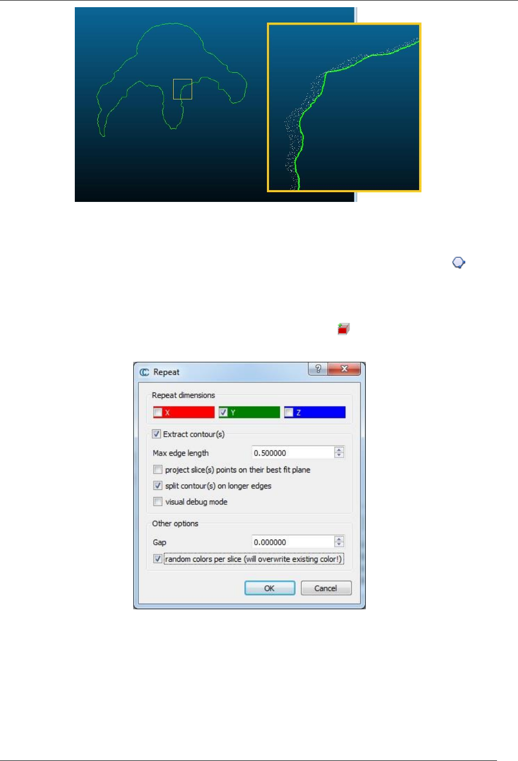
121
CloudCompare Version 2.6.1 – user manual
Extracted contour (close-up with the slice cloud)
Notes:
you can easily 'cancel' (delete) the last generated contour by clicking on the 'revert' icon next to the button
to extract a non-closed contour, see the ‘Segmentation > Extract Sections’ tool.
Extract several slices or contours
To extract several slices or contours at once, click on the 'Extract multiple slices' icon (in the right 'Slices' frame).
CloudCompare will open a dialog:
Most of the parameters are the same as for the 'Single section extraction' dialog (see above).
The user must however explicitly specify if he wishes to generate contours (check the 'Extract contour(s)' checkbox to
enable the associated frame). Otherwise only slices will be generated.
Other parameters are:
Repeat dimension: the extraction process can be repeated in one or multiple dimensions (by default only the
'flat' dimension will be checked)
Gap: a gap can be added between each slice
random colors per slice: if checked, a random color will be assigned to each slice (warning: any existing colors
will be overwritten!)
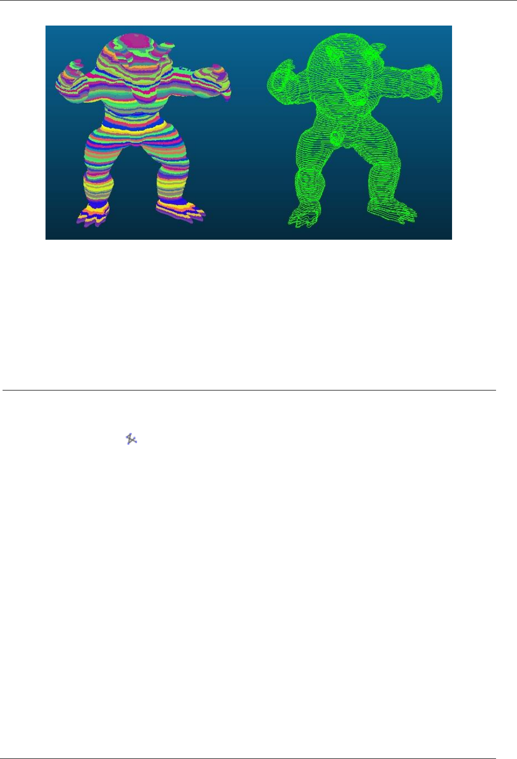
122
CloudCompare Version 2.6.1 – user manual
Multiple slices (left) and contours (right) extraction
Reset the clipping box
You can reset the clipping box to its original state (i.e. the cloud bounding-box) anytime by clicking on the 'reset' button
in the upper right part of the dialog.
Close the tool
You can close the tool by clicking on the 'red cross' button in the upper right part of the dialog.
Segmentation > Extract Sections
Menu / Icon
This tool is accessible via the icon the upper main toolbar or the 'Tools > Segmentation > Extract sections' menu.
Description
This tool allows the user to draw or import poylines on top of a point cloud so as to extract sections and profiles.
Procedure
Select one or more clouds then launch this tool.
A dedicated 3D view will be created and a dialog will appear in the top-right area of this 3D view:
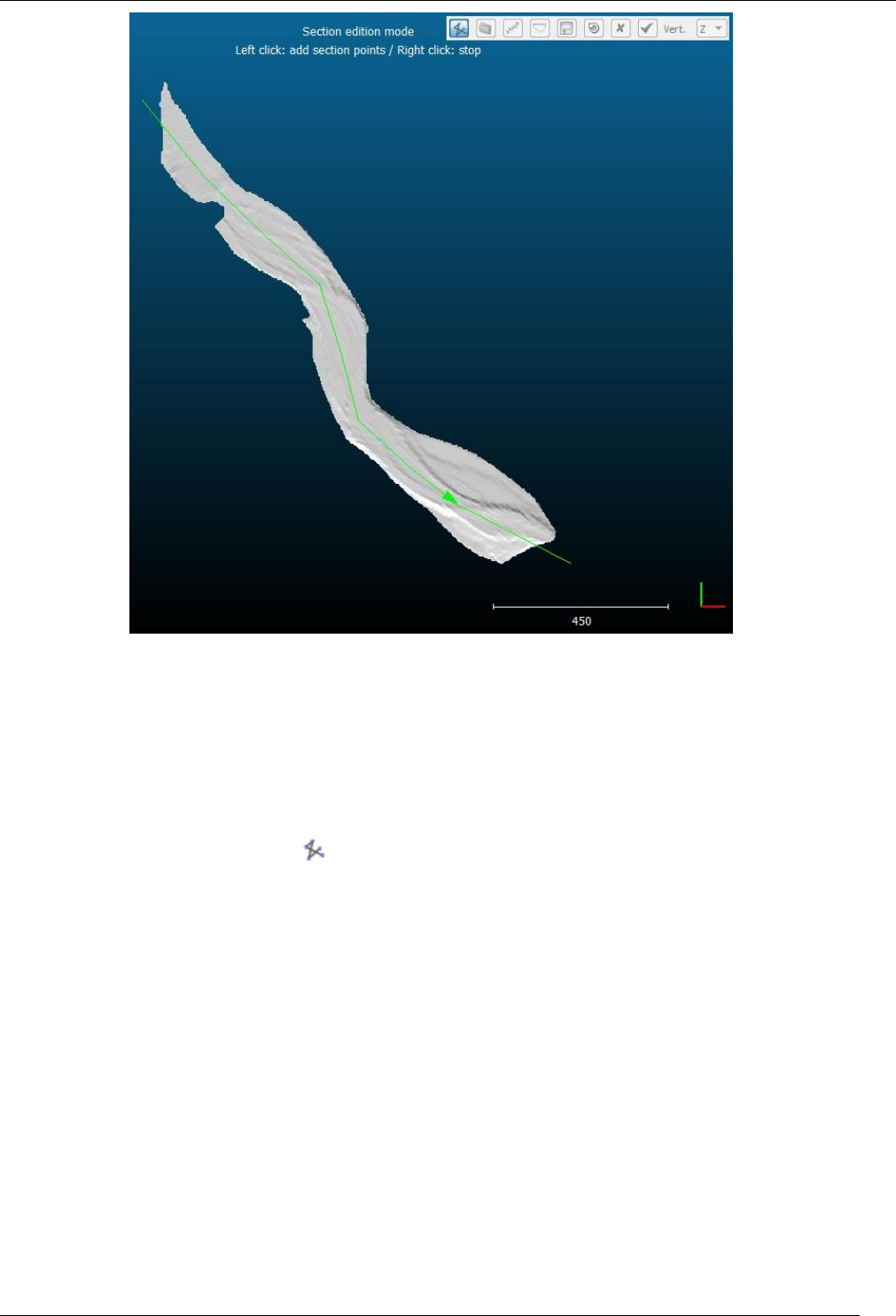
123
CloudCompare Version 2.6.1 – user manual
'Extract sections' tool in action
By default the tool starts in 'polyline edition' mode.
Note: the vertical direction is also set a 'Z' by default. This should be changed right away if the user wants to work with
X or Y as vertical (in which case the 'polyline edition' mode must be deactivated first).
Polyline edition
At startup or when the user clicks on the icon, the 'polyline edition' mode is activated.
In this mode, the other icons are disabled. The user can only click on the 3D view so as to draw polylines:
left click: create a new vertex (or start a new polyline the first time)
right click: stop the current polyline edition
As with the ‘Segment (Interactive Segmentation Tool)’, once a polyline is started, the next edge will 'follow' the mouse
pointer. If the user clicks on the left mouse button the corresponding (end) vertex will be created and the edge will be
'fixed'. A new edge will be created from there. However if the user clicks on the right mouse button, the floating edge
disappears and the current polyline edition is stopped. A new left click will start a new polyline. This way several
polylines can be created in a row:
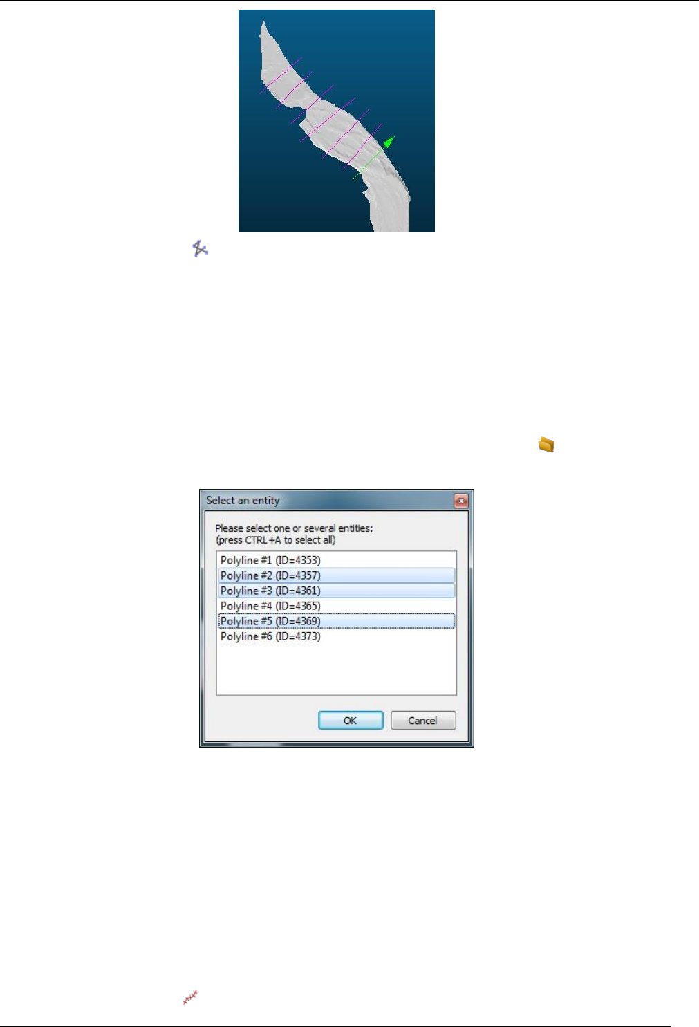
124
CloudCompare Version 2.6.1 – user manual
Once done, a second click on the icon will disable the 'polyline edition' mode. All other tools will then be accessible.
Notes:
during polyline edition, an arrow appears at the (end) tip. This is a way to recall that the vertex order may be
important for some applications (e.g. when generating orthogonal sections along a path and then exporting
the resulting profiles to the Mascaret format for instance).
you can't 'cancel' the last created polyline, but once you quit the 'polyline edition' mode it's possible to select
a polyline and then delete it (with the DEL key)
Polyline import
An alternative to polyline drawing is to import existing polylines. To do this, simply click on the icon.
This will open a dialog with all the polylines already loaded in the DB tree:
You can select one or multiple polylines with the standard selection shortcuts (e.g. on Windows: CTRL or SHIFT key
pressed for multiple selection, and CTRL+A to select all at one).
The selected polylines will then be imported and displayed in the 3D view. Make sure the coordinates systems are
concordant.
Orthogonal sections generation
Instead of defining several orthogonal polylines/sections it may be faster to defined a single 'path' and automatically
generate orthogonal sections with at regular intervals.
First the user needs to draw or import this 'path' and then select it by clicking on it (the 'polyline edition' mode must
be disabled to select a polyline). A selected polyline appears in red. Note that when exiting the 'polyline edition' mode
the latest drawn polyline will be automatically selected.
Once a polyline is selected, the icon can be clicked:
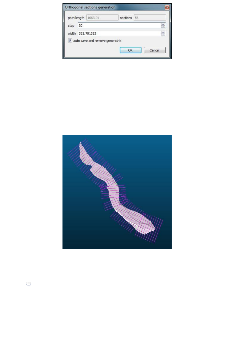
125
CloudCompare Version 2.6.1 – user manual
This dialog displays in the upper part the total length of the selected polyline/path as well as the number of orthogonal
sections that will be created with the current settings.
The current settings are:
the generation step (i.e. the distance along the path between two orthogonal sections)
the orthogonal sections width
A last option named 'auto save and remove generatrix' will tell CloudCompare to remove the selected polyline/path
from the active polylines after having saved it to the main DB tree. This is useful as afterwards the 'profile extraction'
method will use all active sections and it is generally not interesting to generate a profile along the main path. However,
in case the orthogonal sections generation settings were not correct, the user can still undo this, import the path from
the DB tree (see above) and restart the process.
Generating cloud slices and profiles
Once one or several sections have been edited/imported/generated, the user can ask CloudCompare to extract the
corresponding cloud slices and/or to generate polygonal profiles.
Click on the icon in order to make the following dialog appear:
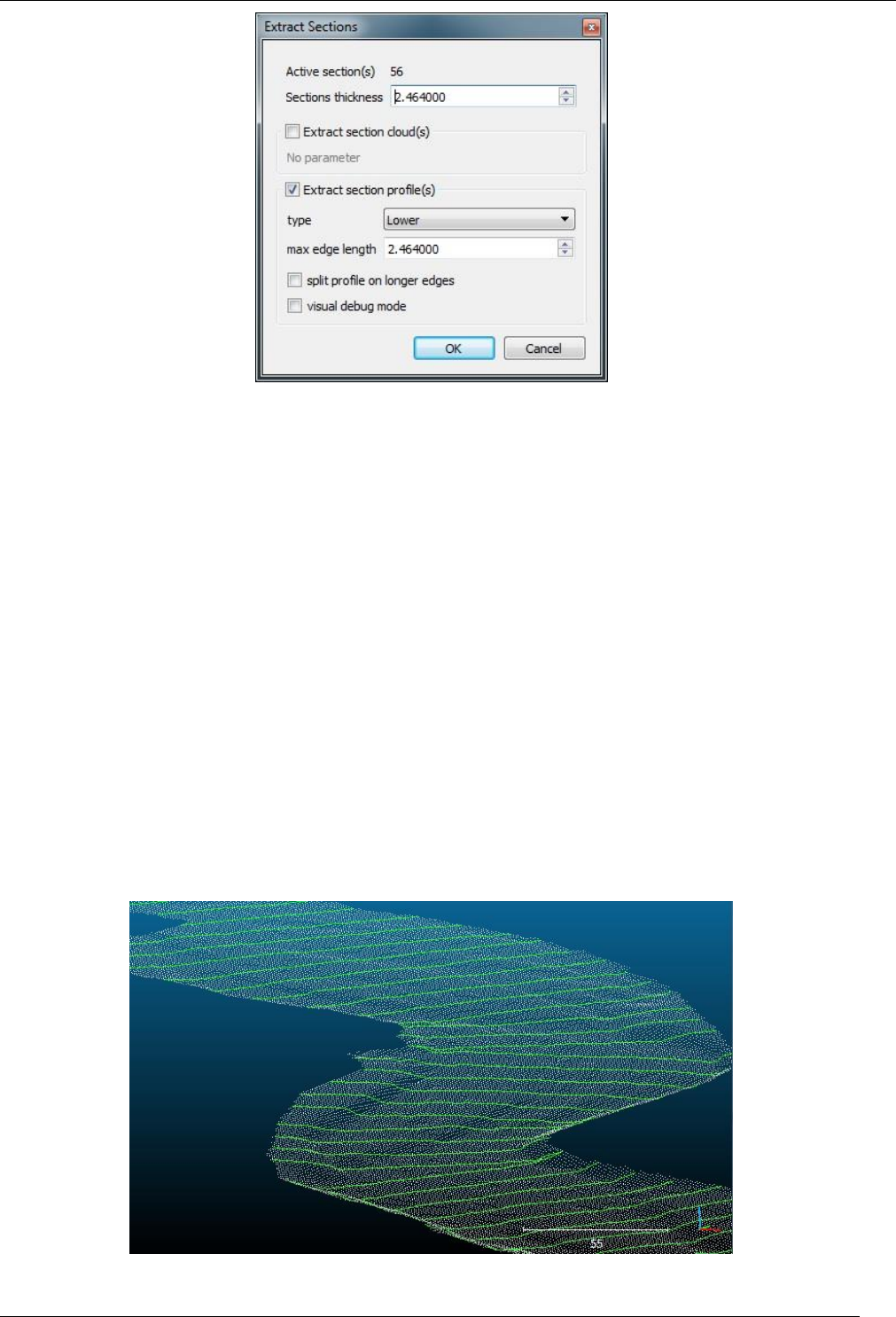
126
CloudCompare Version 2.6.1 – user manual
Warning: all the active polylines will be used.
The main parameter is the section virtual 'thickness'. For each section/polyline, CloudCompare will extract all the points
within this thickness (in 2D). The thickness defined here is the total thickness (i.e. half of it on one side, and the other
half on the other side).
Then the user can choose to generate the clouds corresponding to each section. Simply check the 'Extract section
cloud(s)' option (no parameter).
The user can also choose to generate profiles. In this case check the 'Extract section profile(s)' option then set the
following parameters:
type: profiles can be of three types: Lower, Upper or Both. In effect, from each section cloud a 2D contour can
be extracted (the same 'concave hull' algorithm as in the ‘Segmentation > Cross Section’ tool is used). By
default it's a closed contour. So the user has to choose if the 'profile' should be the lower part of this contour,
or the upper part, or both (in which case the whole contour is extracted).
max edge length: this is the main parameter of the 'concave hull' extraction algorithm. See the ‘Segmentation
> Cross Section’ tool documentation.
Additional options are:
split profile on longer edges: it is possible to split the generated profiles/contours on edges that are longer
than the specified 'max edge length'
visual debug mode: for debug use (can be used to understand why the algorithm doesn't output what one
would expect)
Extracted profiles
127
CloudCompare Version 2.6.1 – user manual
Notes:
all section cloud(s) are stored in a default group named ‘Extracted sections’
all section profiles(s) are stored in a default group named ‘Extracted profiles’
Exporting the active sections/polylines
At any time the user can export all the generated or edited polylines to the main DB tree (so as to export them to a file,
or simply to import them in this tool later). Use the icon to do this.
Notes:
the exporter is smart and will only export the polylines that were not already exported. This way this icon can
be clicked several times without duplicating the polylines.
all polylines are stored in a default group named ‘Exported sections’
Undo
An 'undo' icon can be used to 'undo' the previous operations. All polylines created during the last operation
(polyline edition, import, orthogonal section generation, etc.) will be removed each time.
Notes:
CloudCompare will ask the user to confirm the undo operation each time (specifying the number of polylines
that will be deleted this way)
polylines previously exported to the DB tree will be removed from the 'active' polylines set in the tool, but
they will remain in the DB tree
the undo history will be lost if the user selects a single polyline and deletes it (with the DEL key)
Stopping the tool
To leave the tool, the user has two choices:
click on the icon so as to quit right away (warning: unsaved polylines will be deleted)
click on the icon in which case CloudCompare may warn the user that some polylines have not been
exported to the main DB tree
Fit > Plane
Menu
This tool is accessible via the 'Tools > Fit > Plane' menu.
Description
This tool fits a plane on a point cloud and outputs various pieces of information such as the fitting RMS, the plane
normal and even the geological dip and dip direction values.
Procedure
Select one or several point clouds then launch this tool.
For each cloud CloudCompare will fit a plane primitive (the extents of the plane will be deduced automatically).
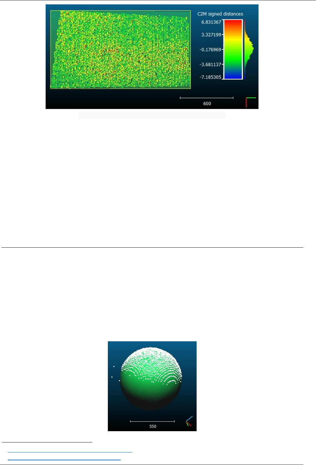
128
CloudCompare Version 2.6.1 – user manual
Fitted plane (+ distances between the original cloud and the fitted plane)
In the console the following pieces of information will be output:
plane fitting RMS
37
plane normal vector (with a positive Z coordinate by default)
dip and dip direction
38
a 4x4x transformation matrix that would make this plane horizontal (see the 'Edit > Apply Transformation'
method to use it for instance)
Notes:
the fitted plane is added to the DB tree as a child of the cloud
the plane primitive is a kind of 'triangular mesh'. Therefore you can select both the cloud and the fitted plane
and compute the distance between them (with 'Tools > Distances > Cloud/Mesh dist. (cloud-to-mesh
distance)’)
Fit > Sphere
Menu
This tool is accessible via the 'Tools > Fit > Sphere' menu.
Description
This tool fits a sphere on a cloud.
Procedure
Select one or several point clouds then launch this tool.
CloudCompare will fit a sphere primitive on each cloud (the radius will be detected automatically).
37
http://en.wikipedia.org/wiki/Root_mean_square
38
http://en.wikipedia.org/wiki/Strike_and_dip
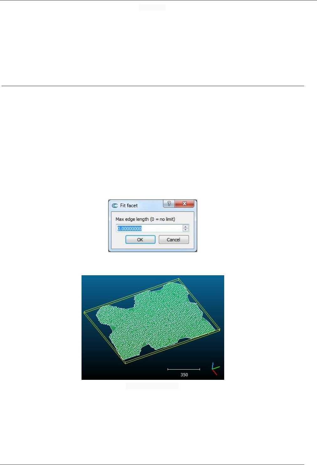
129
CloudCompare Version 2.6.1 – user manual
Fitted sphere
In the console the following pieces of information will be output:
center (can also be found as the center of the sphere bounding-box in the sphere entity properties)
radius (can also be found in the sphere entity properties)
sphere fitting RMS (is recalled in the default sphere entity name)
Note: theoretically the sphere fitting algorithm can handle up to 50% outliers.
Fit > 2D Polygon
Menu
This tool is accessible via the 'Tools > Fit > 2D Polygon (facet)' menu.
Description
This tool fits a 2D polygon on a point cloud. It's very similar to the 'Tools > Fit > Plane' method but the extents of the
fitted plane follows the cloud contour (in 2D).
Procedure
Select one or several point clouds then launch this tool.
For each cloud CloudCompare will first fit a plane and then extract the contour (in 2D).
CloudCompare will therefore ask for the 'max edge length' of the contour:
This is the same parameter used for contour extraction in the Cross Section tool. If zero, the extracted contour will be
the cloud convex hull. Otherwise, the smaller the max edge length is, the tighter the contour will be.
Fitted 'facet' (2D polygon)
In the console the following pieces of information will be output:
plane fitting RMS
plane normal vector (with a positive Z coordinate by default)
dip and dip direction
a 4x4x transformation matrix that would make this plane horizontal (see the 'Edit > Apply Transformation'
method to use it for instance)
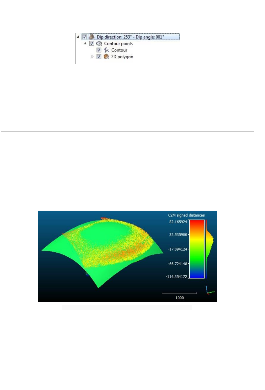
130
CloudCompare Version 2.6.1 – user manual
Note: the fitted facet is added to the DB tree as a child of the cloud
About facets
The facet entity is a composite entity:
the base 'Facet' entity holds some meta-data (the polygon surface, center and normal as well as the fitting
RMS)
it has a point cloud as child (the contour points)
this contour point cloud has itself two children:
o the contour (as a polyline)
o the polygon (as a mesh)
Fit > Quadric
Menu
This tool is accessible via the 'Tools > Fit > 2.5D Quadric' menu.
Description
This tool fits a 2.5D quadric on a point cloud.
Procedure
Select one or several point clouds then launch this tool.
For each cloud CloudCompare will fit a 2.5D Quadric (the cloud is first projected on its best fit plane).
Fitted quadric (+ distances between the original cloud and the fitted quadric)
In the console the following pieces of information will be output:
the 6 quadric equation coefficients (a + b.x + c.y + d.x2 + e.y2 = 0)
the quadric fitting RMS
Notes:
the fitted quadric is added to the DB tree as a child of the cloud
the quadric is represented as a standard triangular mesh. Therefore you can select both the cloud and the
fitted quadric and compute the distance between them (with 'Tools > Distances > Cloud/Mesh dist. (cloud-to-
mesh distance)’)
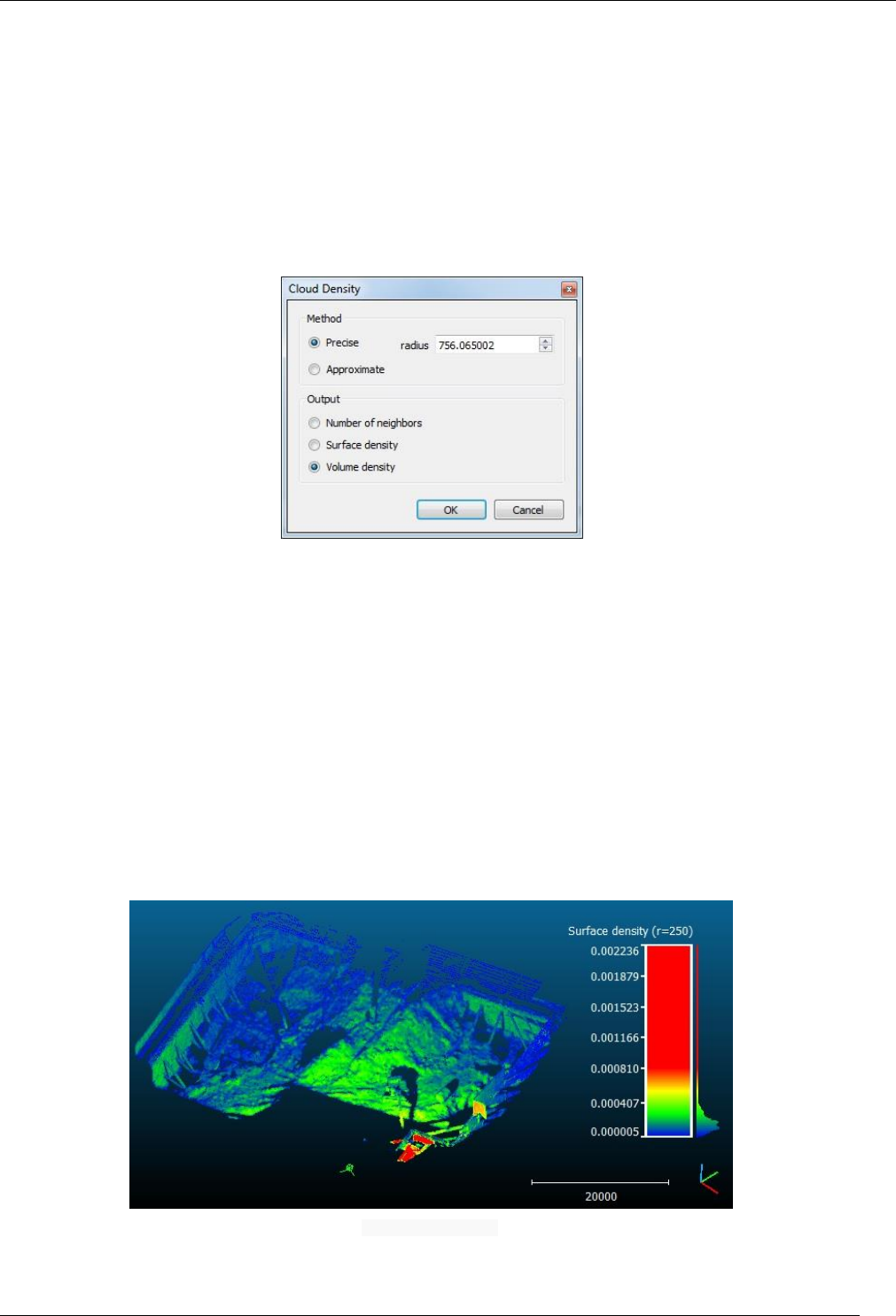
131
CloudCompare Version 2.6.1 – user manual
Other > Density
Menu
This tool is accessible via the 'Tools > Other > Density' menu.
Description
This tool estimates the density of a point cloud.
Procedure
Select one or several point clouds then launch this tool.
A dialog will appear:
Precise or Approximate
Two methods can be used to compute the density:
either 'Precise': the density is estimated by counting for each point the number of neighbors N (inside a sphere
of radius R)
or 'Approximate': the density is simply estimated by determining the distance to the nearest neighbor (which
is generally much faster). This distance is considered as being equivalent to the above spherical neighborhood
radius R (and N = 1).
Output
The density output can be:
the number of neighbors N (only available in 'Precise' mode)
a surface density: number of neighbors divided by the neighborhood surface = N / (π.R2)
a volume density: number of neighbors divided by the neighborhood volume = N / (4/3.π.R3)
Density output example
Note: a point with no neighbor in the spherical neighborhood will have an invalid (NaN) density
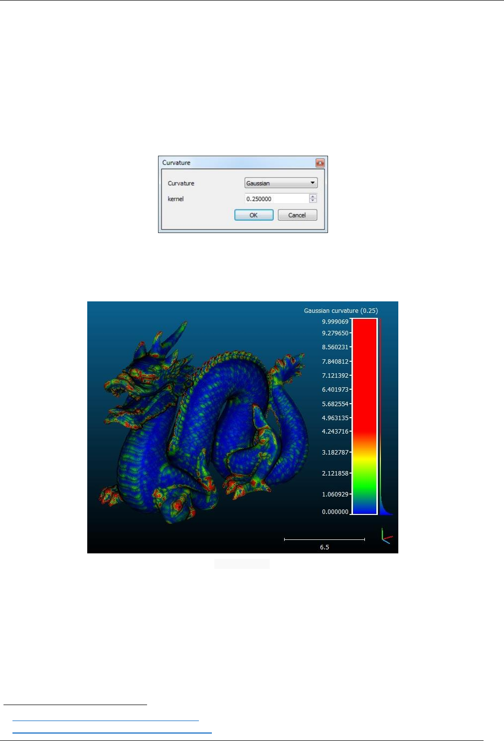
132
CloudCompare Version 2.6.1 – user manual
Other > Curvature
Menu
This tool is accessible via the 'Tools > Other > Curvature' menu.
Description
This tool evaluates the curvature of a point cloud.
Procedure
Select one or several point clouds then start this tool.
A dialog will appear:
Parameters
Curvature: choose the curvature type (Mean
39
, Gaussian
40
or the simpler 'Normal change rate' )
kernel: neighborhood size (for quadric fitting - see Notes below)
Curvature output
Notes:
the curvature at each point is estimated by best fitting a quadric around it
if there's not enough neighbors to compute a quadric (i.e. less than 6) an invalid scalar value (NaN) is set for
this point. This point will appear in grey (or not at all if you uncheck the 'display NaN values in grey' option of
the scalar field parameters).
39
http://en.wikipedia.org/wiki/Mean_curvature
40
http://en.wikipedia.org/wiki/Gaussian_curvature
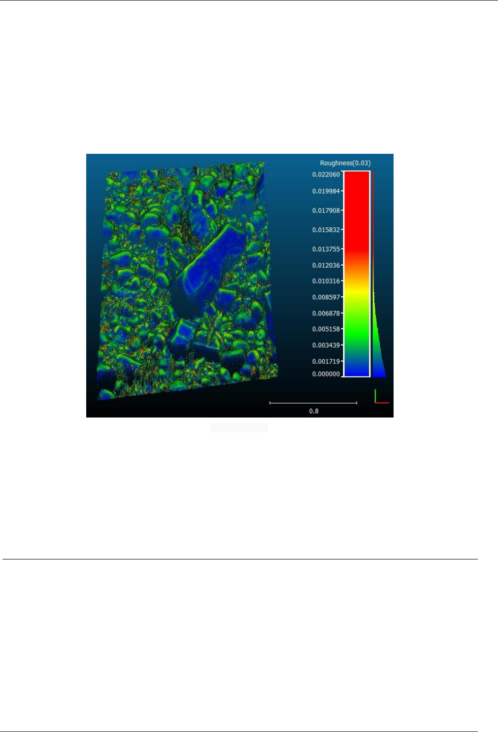
133
CloudCompare Version 2.6.1 – user manual
Other > Roughness
Menu
This tool is accessible via the 'Tools > Other > Roughness' menu.
Description
This tool estimates the 'roughness' of a cloud.
Procedure
Select one or several point clouds then start this tool.
CloudCompare will only ask for the 'kernel size': the radius of a sphere centered on each point (see the Notes below).
Roughness output
Notes:
Roughness estimation is very... simple: for each point, the 'roughness' value is equal to the distance between
this point and the best fitting plane computed on its nearest neighbors.
If there's not enough neighbors to compute a LS plane (i.e. less than 3) an invalid scalar value (NaN) is set for
this point. This point will appear in grey (or not at all if you uncheck the 'display NaN values in grey' option in
the scalar field properties).
Other > Remove duplicate points
Menu
This tool is accessible via the 'Tools > Other > Remove duplicate points' menu.
Description
This tool removes duplicate points (with respect to a minimal distance between points) in a point cloud.
Procedure
Select one or several points clouds then start this tool.
CloudCompare will only ask for the minimum distance between points (with a ridiculously small value by default):
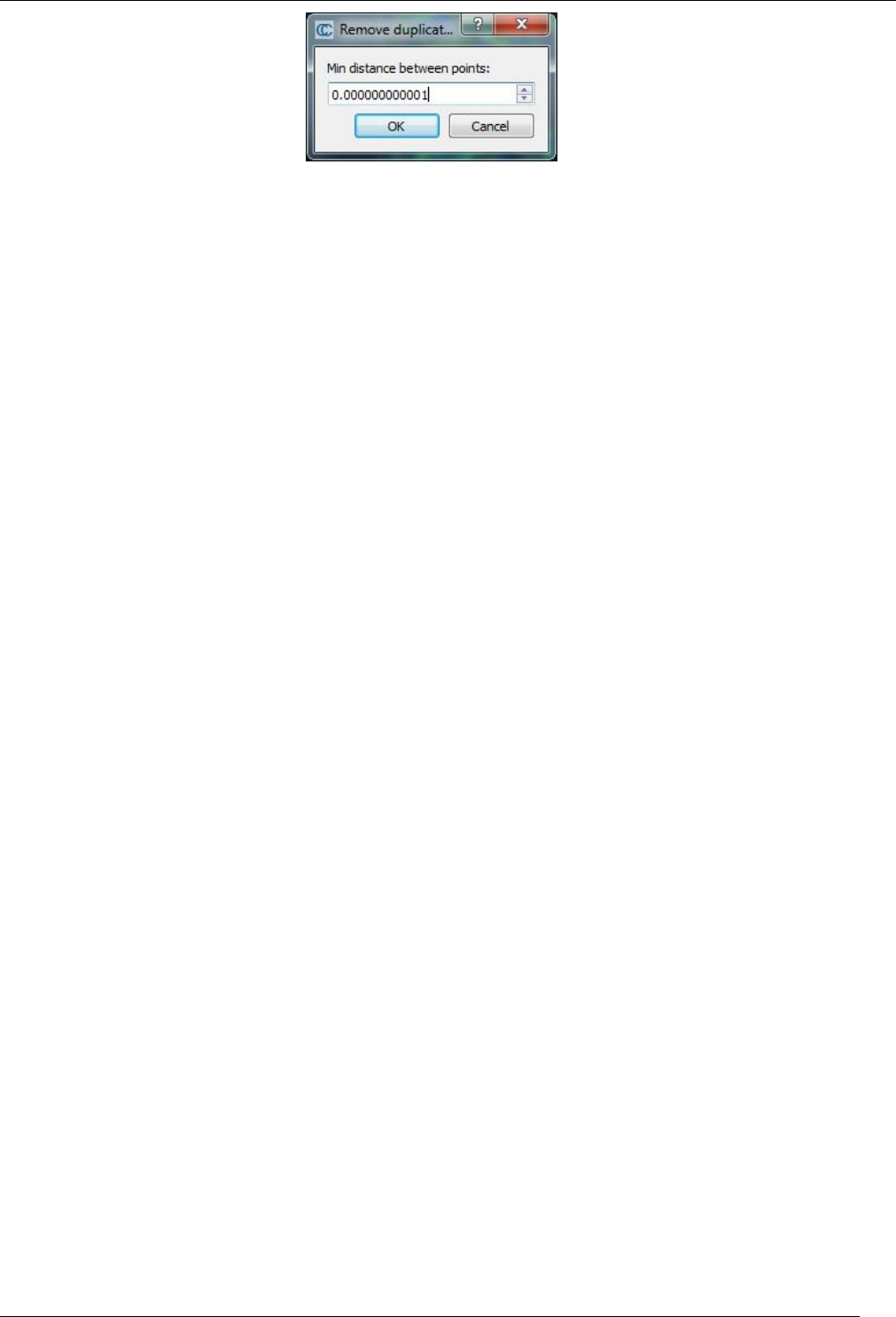
134
CloudCompare Version 2.6.1 – user manual
On completion CloudCompare will output in the console the number of duplicate points removed (or a message stating
that the cloud 'has no duplicate points').
135
CloudCompare Version 2.6.1 – user manual
Display menu
Full screen
Menu
This tool is accessible via the 'Display > Full screen' menu.
Alternatively you can use the F11 shortcut.
Description
This method simply makes the main CloudCompare application window full screen.
Call this method again (via the menu or the F11 shortcut) to restore its original state.
Refresh
Menu
This method is accessible via the 'Display > Refresh' menu. Alternatively you can use the F5 shortcut.
Description
This method simply forces the active 3D view to refresh its content (all OpenGL primitives are redrawn).
Toggle Centered Perspective
Menu
This method is accessible via the icon in the left 'View' toolbar or the 'Display > Toggle Centered Perspective' menu.
Alternatively you can use the F3 shortcut.
Description
This method toggles the current projection of the active 3D view between the 'orthographic' and 'object-centered
perspective' modes (see the ’Display modes’ section).
Toggle Viewer Based Perspective
Menu
This method is accessible via the icon in the left 'View' toolbar or the 'Display > Toggle Viewer-based Perspective'
menu.
Alternatively you can use the F4 shortcut.
Description
This method toggles the current projection of the active 3D view between the 'orthographic' and 'viewer-based
perspective' modes (see the ’Display modes’ section).
Lock rotation about vert. axis
Menu
This method is accessible via the 'Display > Lock rotation about vert. axis' menu.
Alternatively you can use the L shortcut.
Description
This method simply locks the camera rotation around the vertical (Z) axis (in the active 3D view).
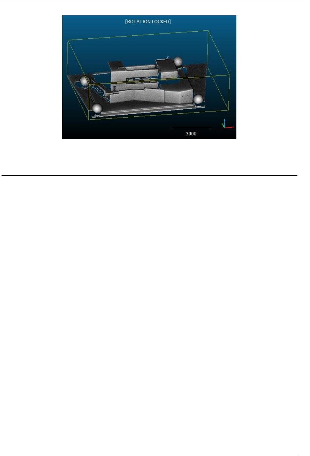
136
CloudCompare Version 2.6.1 – user manual
When activated a '[ROTATION LOCKED]' message will appear in the top part of the 3D view:
Simply call this method again (or use the L shortcut) to disable this mode.
Enter bubble-view mode
Menu
This method is accessible via the 'Display > Enter bubble-view mode' menu.
Alternatively you can use the B shortcut.
Description
This method enables the 'bubble-view' mode.
See the ‘
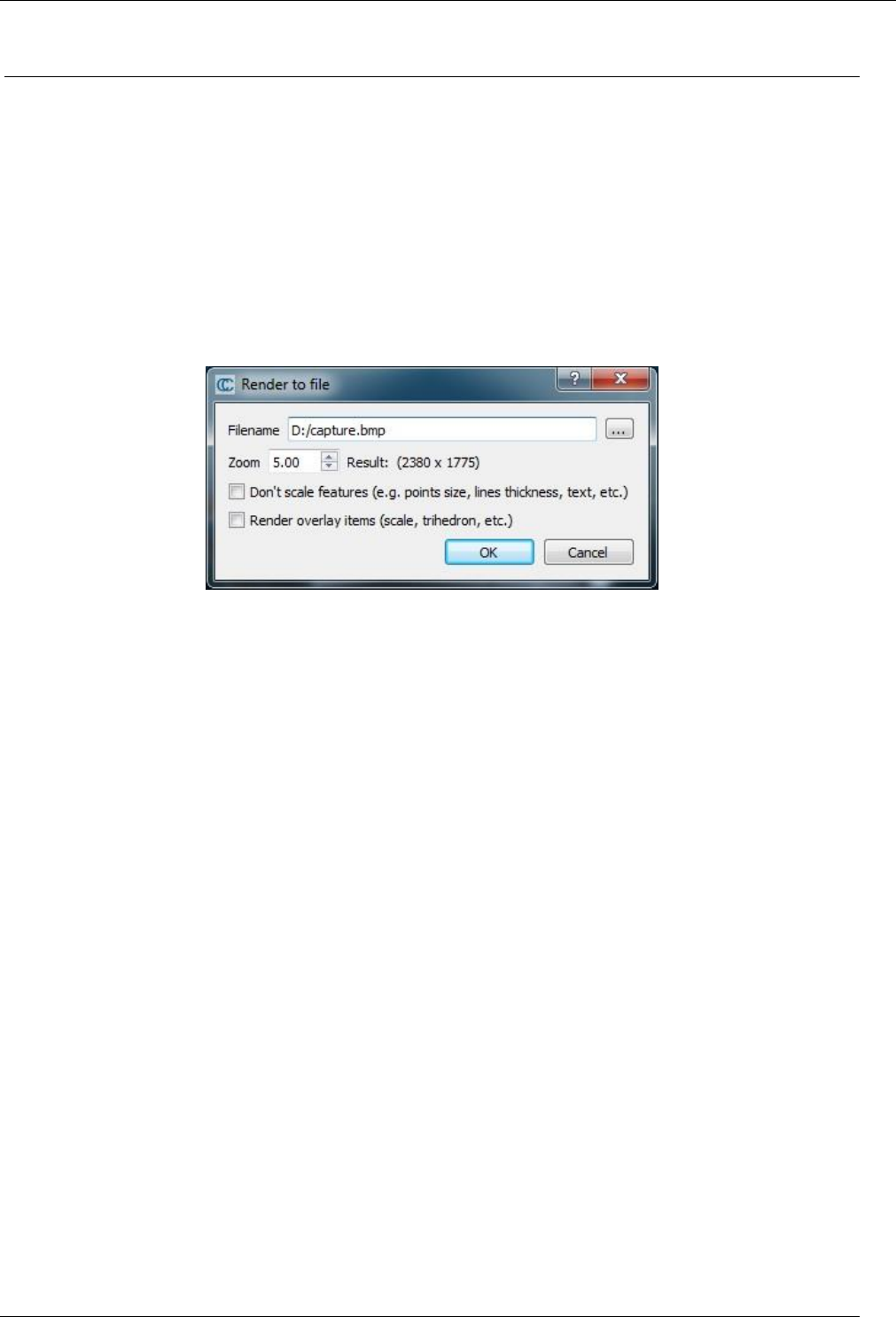
137
CloudCompare Version 2.6.1 – user manual
Bubble-view (polar)’ section.
Render to File
Menu
This tool is accessible via the 'Display > Render to file' menu.
Description
This tool can 'render' the current 3D view as an image file (most of the standard file formats are supported). It can also
apply a zoom so as to render the screen to a much higher resolution than the actual screen resolution.
Procedure
Make the 3D view that you want to render active then call this tool.
A dialog will appear:
You must first set the output image filename (you can use the '...' button to browse a particular file or folder on your
computer). Most common image file formats are supported (bmp, jpg, png, etc.).
By default the output image will have the same resolution as the 3D view (i.e. the same size in pixels). With the 'zoom'
factor, you can increase the rendered image resolution (the resulting size is displayed on the right). CloudCompare will
render the 3D view content off-screen in a potentially much larger buffer than you actual screen.
Warning: depending on your graphic card (and its driver) capabilities, the operation may fail if the output image size is
too big. Most graphic cards / drivers have a limit of 64 M. pixels.
Other options are:
by default, is a zoom factor other than 1 is sued, CloudCompare will 'scale' the displayed features (point size,
lines thickness, etc.) when rendering the 3D view off-screen. The user can deactivate this behavior (this way,
especially if the point cloud is very dense, a much finer rendering can be achieved).
moreover, by default the trihedron, the scale or other 2D overlay items are not rendered. The user can force
CloudCompare to render them.
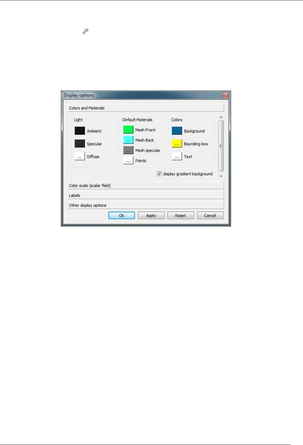
138
CloudCompare Version 2.6.1 – user manual
Display settings
Menu
This method is accessible via the icon in the left 'View' toolbar or the 'Display > Display settings' menu.
Description
This method displays the 'Display settings' dialog.
The options are regrouped in several tabs:
Colors and materials
The first tab regroups options related to the display of 3D entities.
One can set:
the sun light components
the default mesh material components (for triangular meshes without any material definition)
the default point color (for clouds without any RGB color information)
the colors of other display elements:
o the 3D view background (if the display gradient background is checked, CloudCompare will
automatically create a gradient background with the 'Background' color and the inverse of the 'Points'
color)
o the (unselected) bounding-box color
o the text color
Color sale
The second tab regroups options related to the 'Color scale' display.
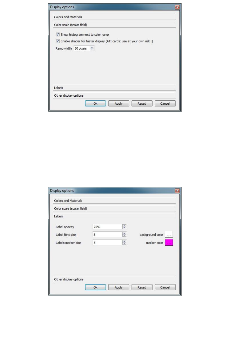
139
CloudCompare Version 2.6.1 – user manual
The user can set:
whether the histogram should be displayed next to the color scale
whether the 'fast color scale display' shader should be enabled or not. This shader accelerates the display of
dynamic colors for points when a scalar field is active. Depending on your graphic card it may not be possible
to enable it. And due to some issues reported with ATI cards, it is deactivated by default on those cards (the
user can still enable it however).
the color ramp width
Labels
The third tab regroups options regarding the display of labels.
The user can set:
the labels opacity
the labels background color
the labels font size (different from the default text size since version 2.6.1)
the labels marker size (in 3D)
the labels marker color (in 3D)
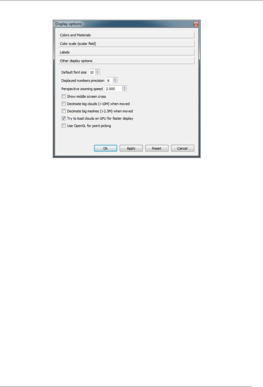
140
CloudCompare Version 2.6.1 – user manual
Other options
The fourth tab regroups all the other parameters.
The user can set:
the default font size
the precision of displayed numbers (i.e. the number of digits)
the zoom speed in perspective mode (since version 2.6.1)
whether a cross should be displayed in the center of the 3D views (middle screen cross)
whether big clouds (over 10 M. points) should be decimated when the view is rotated
whether big meshes (over 2.5 M. triangles) should be decimated when the view is rotated
whether clouds should be loaded on the graphic card memory (thanks to VBOs [1]) - only activated on NVidia
cards by default as crash were reported on ATI cards. The user can still enable this option at his own risks
whether to use OpenGL picking mechanism for point picking (disabled by default as this feature is not
accelerated and is generally slower than CloudCompare's built-in algorithm)

141
CloudCompare Version 2.6.1 – user manual
Camera settings
Menu
This method is accessible via the icon in the left 'View' toolbar or the 'Display > Camera settings' menu.
Description
This method displays the 'Camera settings' dialog:
Main parameters
The user can change most of the parameters of the (OpenGL) camera of the active 3D view:
the camera orientation (with Euler angles: phi, theta and psi)
the scene rotation center (the icon lets the user pick a point in the 3D scene as new rotation center)
the camera/eye center
the field of view (only effective in Display modes perspective mode)
the near clipping plane (only effective in Display modes perspective mode)
Note: when changing a parameter the 3D view is directly updated. And conversely, when modifying the 3D view camera
position or orientation while this dialog is opened the dialog parameters should be directly updated.
Cart system
The cart icon let the user store the current camera orientation.
Once done the stored camera orientation can be restored with the icon.
Moreover the user can set predefined views (from top, bottom, left, right, front, back and 2 isometric views) relatively
to the stored orientation.
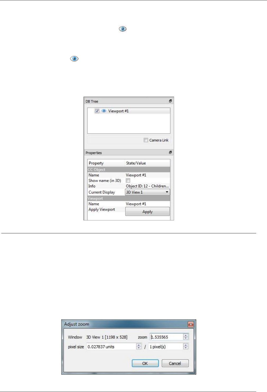
142
CloudCompare Version 2.6.1 – user manual
Save viewport as object
Menu
This tool is accessible via the 'Display > Save viewport' menu. Alternatively the shortcut CTRL+V can be used.
Description
This tool allows the user to save the current viewport parameters (camera position and orientation, perspective state,
etc.) of the active 3D view as a ' Viewport' entity. The entity is automatically added to the root of the DB tree.
Note: viewport entities can be saved in BIN files along with the other entities.
Restoring the viewport
The viewport can be restored at any time by clicking on the 'Apply' button in the viewport entity properties:
Adjust zoom
Menu
This tool is accessible via the 'Display > Adjust zoom' menu.
Description
This tool let the user define the current zoom, potentially in a very accurate way (e.g. in order to get a very specific
dimension per pixel for instance).
Procedure
Make sure the targeted 3D view is active then call this tool.
CloudCompare will display a dedicated dialog:
The zoom can be set in various ways:
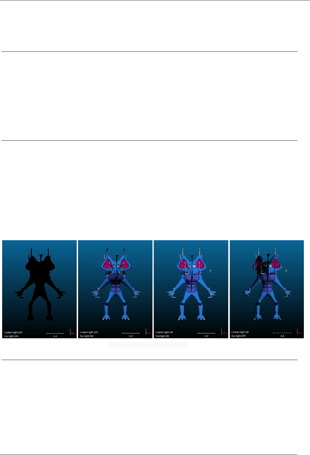
143
CloudCompare Version 2.6.1 – user manual
either directly by setting the 'zoom' value
or by defining the dimension of one (or several) pixels. To do this set the 'pixel size' value to the right
dimension, and optionally set the corresponding number of pixels (one by default). CloudCompare will
automatically update the corresponding 'zoom' value.
Test Frame Rate
Menu
This tool is accessible via the 'Display > Test frame rate' menu.
Description
This tool makes the active 3D view spin for a short time (~10 seconds) in order to estimate the average 'fps' (frame per
second).
The result is displayed in the Console.
Lights > Toggle Sun Light
Menu
This tool is accessible via the 'Display > Lights > Toggle Sun Light' menu.
Alternatively this tool can be called with the F6 shortcut.
Description
This tool toggles the 'sun light'.
By default, a non-directional light is always activated so as to illuminate objects with normals or materials (e.g.
triangular meshes or clouds with normals).
This light can be disabled (or enabled again) with this tool. This is especially interesting when using the ' custom light'.
Sun light and custom light combinations
Lights > Toggle Custom Light
Menu
This tool is accessible via the 'Display > Lights > Toggle Custom Light' menu.
Alternatively this tool can be called with the F7 shortcut.
Description
This tool toggles the 'custom light'.
Procedure
In addition or in replacement of the default ' sun light' a repositionable non directional light can be activated.
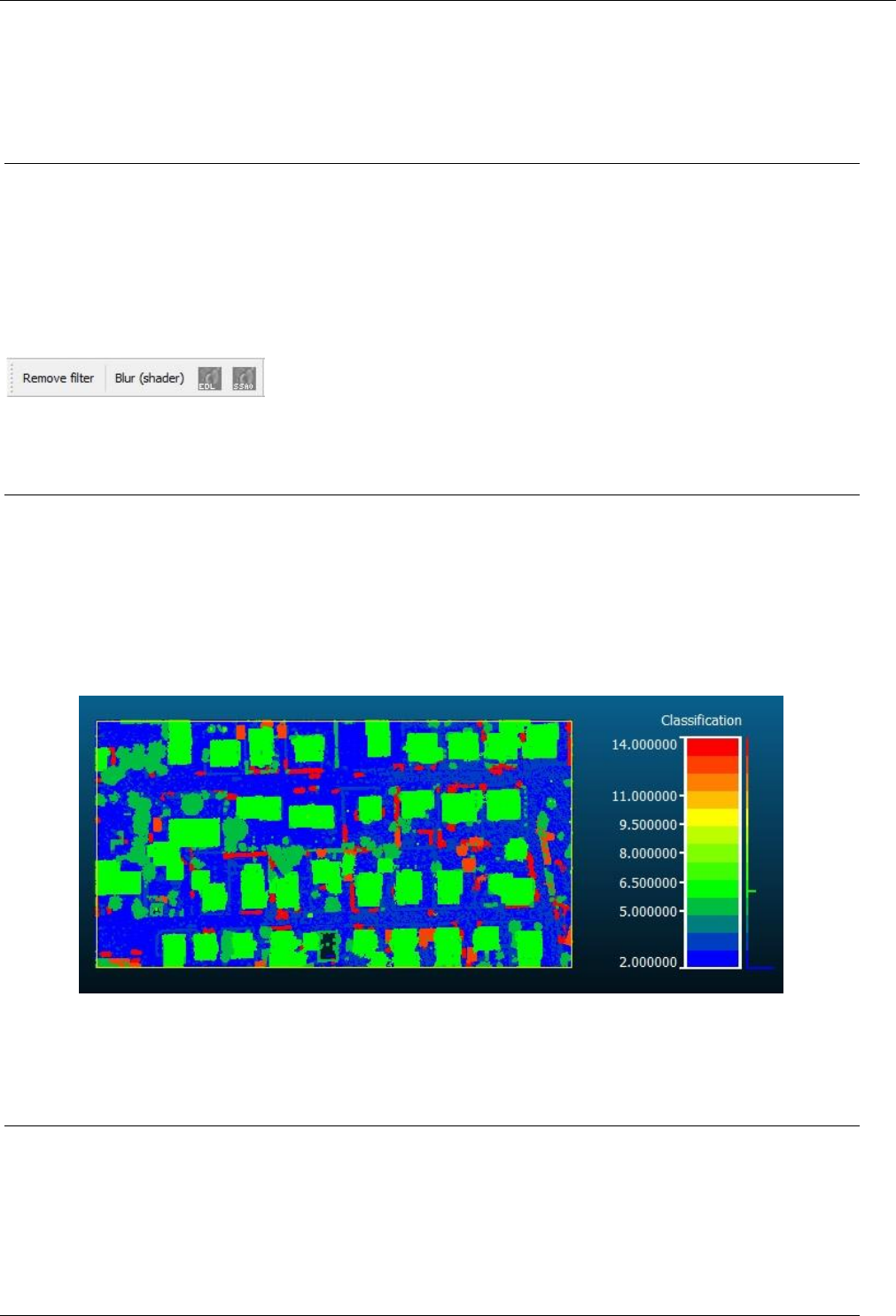
144
CloudCompare Version 2.6.1 – user manual
Once activated, a yellow 'star' will appear in the 3D scene where the custom light is currently positioned.
The user can displace this light source by holding the CTRL key while pressing the right mouse button (and moving the
mouse).
This light can be enabled (or disabled) with this tool.
Shaders and Filters > Remove filter
Menu
This tool is accessible via the 'Display > Shaders & filters > Remove filter' menu or the equivalent Remove filter button
in the upper 'GL filters' toolbar.
Description
This method disables any active shader or OpenGL 'filter'.
OpenGL filters are special plugins that are dynamically loaded at startup. Therefore their number and names can
change. See the qEDL (Eye Dome Lighting) and qSSAO (Screen Space Ambient Occlusion) plugins for instance.
Active scalar field > Toggle color scale
Menu
This method is accessible via the 'Display > Active scalar field > Toggle color scale' menu.
Alternatively this method can be called with the CTRL+C shortcut (an entity with an active scalar field must be selected).
Description
This method toggles the color scale visibility for the active scalar field of the selected entity (cloud or mesh).
Notes:
it is equivalent to check the 'Visible' checkbox of the 'Color Scale' section of the entity's properties
as only one color scale can be visible at a time, make sure no color scale is currently displayed
Active scalar field > Show previous SF
Menu
This method is accessible via the 'Display > Active scalar field > Show previous SF' menu.
Alternatively this method can be called with the SHIFT + Up arrow shortcut (an entity with several scalar fields must be
selected).
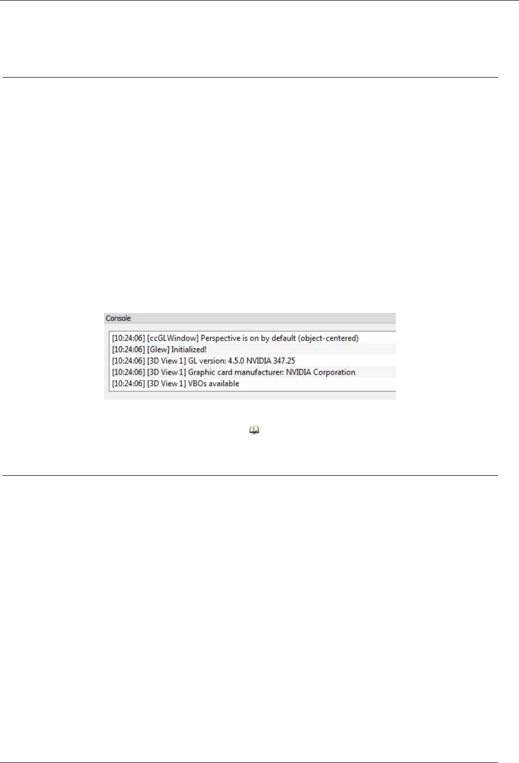
145
CloudCompare Version 2.6.1 – user manual
Description
This method changes the current active scalar field of the selected entity. It activates the previous one (if any). See the
cloud properties for the complete (ordered) list.
Active scalar field > Show next SF
Menu
This method is accessible via the 'Display > Active scalar field > Show next SF' menu.
Alternatively this method can be called with the SHIFT + Down arrow shortcut (an entity with several scalar fields must
be selected).
Description
This method changes the current active scalar field of the selected entity. It activates the next one (if any). See the cloud
properties for the complete (ordered) list.
Console
Description
The console is a dockable widget where all messages (standard information, warnings and errors) are traced. Some
algorithms also output results in it.
Display/Hide
To display or hide the console, use the checkable 'Console' entry in the 'Display' menu. Alternatively the F8 shortcut
can be used.
Toolbars
Menu
This sub-menu is accessible via the 'Display > Toolbars' entry.
Description
The 'Toolbars' sub-menu of the 'Display' menu contains checkable menu entries that can be used to show or hide the
corresponding toolbars:
Main (upper Main tools toolbar with the most useful tools)
Scalar fields (upper Scalar field tools toolbar)
View (left Viewing tools toolbar with all operations related to the current 3D view)
Plugins (upper Plugins toolbar - where all plugins actions with no dedicated toolbar are automatically inserted)
GL filters (upper GL filters toolbar)
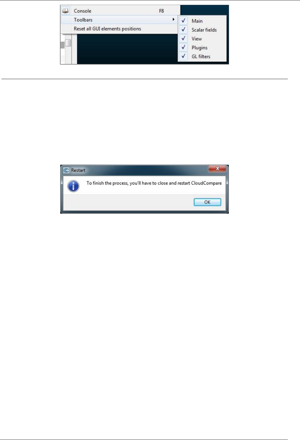
146
CloudCompare Version 2.6.1 – user manual
Reset all GUI elements
Menu
This method is accessible via the 'Display > Reset all GUI elements' menu.
Description
By default CloudCompare saves the current GUI configuration (position and visibility of the toolbars, etc.) when quitting.
This tool can be used to restore the original configuration.
Note: CloudCompare must be closed and restarted to apply the changes.
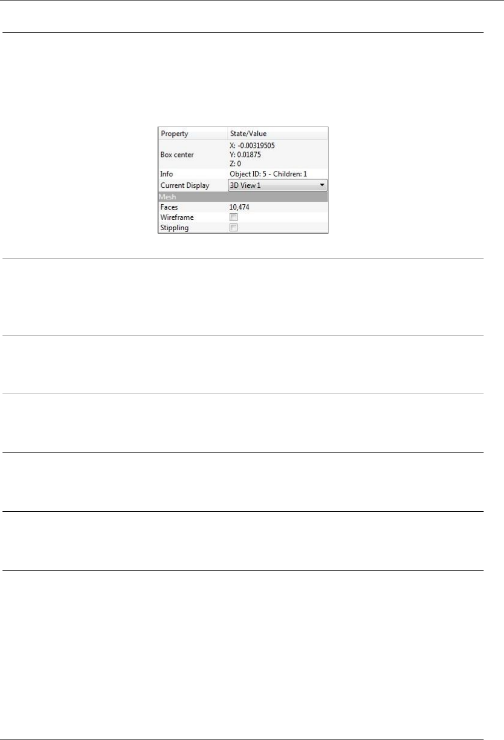
147
CloudCompare Version 2.6.1 – user manual
3D Views menu
New
Create a new 3D view.
Shortcut: CTRL + F3
Note: entities can be moved to 3D views by editing their ‘with the ‘Current Display’ property.
Close
Closes the active 3D view.
Shortcut: CTRL + F4
Close All
Closes all 3D views.
Tile
Share the display space between all the 3D views (as ‘tiles’).
Cascade
Rearrange all the 3D views in a ‘cascade’ way.
Next
Activate the ‘next’ 3D view (order of creation).
Previous
Activate the ‘previous’ 3D view (order of creation).
148
CloudCompare Version 2.6.1 – user manual
Help menu
Help
Menu
This method is accessible via the 'Help > Help' menu.
Alternatively this method can be called with the F1 shortcut.
Description
In a perfect world this method should display the documentation of CloudCompare. However, due to the ever changing
nature of CloudCompare it appeared difficult to ship CloudCompare with a standalone documentation.
Therefore for now a simple dialog invites the user to go the http://www.cloudcompare.org/doc address.
About…
Menu
This method is accessible via the 'Help > About...' menu.
Description
This method displays a dialog with the current version information:
Note: the current version is also displayed in the application title bar (since version 2.6).
About Plugins…
Menu
This method is accessible via the 'Help > About plugins...' menu.
Description
This method displays a list of all the plugins that were (successfully) loaded when CloudCompare started.
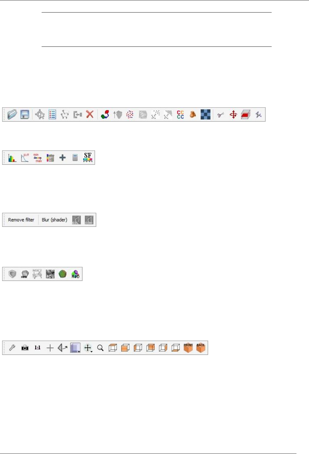
149
CloudCompare Version 2.6.1 – user manual
Toolbars and icons
There are 5 main toolbars in CloudCompare.
All toolbars are dockable elements that can be freely displaced, docked or let floating over the application window.
Main toolbar
Scalar fields toolbar
OpenGL filters (shaders) toolbar
The content of this toolbar depends on the detected/supported ‘shaders’ plugins that have been successfully loaded at
startup.
Standard plugins toolbar
The content of this toolbar depends on the detected/supported plugins that have been successfully loaded at startup.
Notes:
additional toolbars can be added by plugins with multiple methods (e.g. qPCL, qSRA, qCANUPO, etc.)
see the ‘Plugins’ list
3D view toolbar
Note: this toolbar is situated on the left side by default.
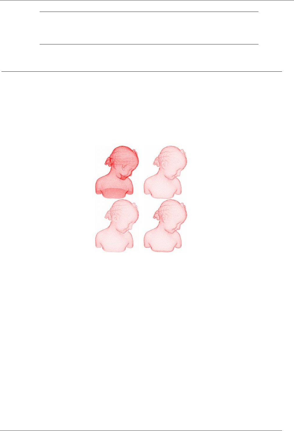
150
CloudCompare Version 2.6.1 – user manual
Plugins
Standard plugins
qHPR (Hidden Point Removal)
Introduction
qHPR stands for "Hidden Point Removal" and is an implementation of the method proposed by S. Katz et al. in their
article titled 'Direct Visibility of Point Sets' [1].
The algorithm filters out the points of a cloud that wouldn't be seen (by the current 3D camera) if the cloud was a closed
surface. Therefore it tries to remove the points that should be hidden in the current viewport configuration.
Therefore, if you use this tool for a scientific publication, please cite the author before citing CloudCompare (which is
also very good but less important in this particular case ;).
Usage
This algorithm only works if the 3D view in which the selected cloud is displayed is in perspective mode.
The user than has to set the octree level at which the cloud will be approximated (the greater the finer the result will
be but also the longer the computation will be).
In the latest versions of CloudCompare the plugin outputs a new cloud with only the visible points.

151
CloudCompare Version 2.6.1 – user manual
qKinect (Point Cloud Acquisition with a Kinect)
Description
This plugin allows for the acquisition of (colored) point clouds with a Kinect
41
device.
Requirements
This plugin requires:
a Kinect device
libfreenect drivers installed (on Windows: be sure to follow the libfreenect driver installation instructions
42
)
See http://openkinect.org/wiki/Main_Page for more information on the OpenKinect / libfreenect project.
qPCL (Point Cloud Library Wrapper)
Introduction
qPCL is a simple interface to some methods of the PCL
43
library.
Therefore, if you use this tool for a scientific publication, please cite the PCL project before citing CloudCompare (which
is also very good but less important in this particular case ;).
CloudCompare simply adds dialogs to set some parameters (see below) and a seamless integration in its own workflow.
This plugin has been developed by Luca Penasa (University of Padova).
Available methods
The following methods are currently accessible though this interface:
Estimate Normals and Curvature (to compute the normals - and optionally the curvature - of a point cloud)
Statistical Outliers Removal
44
http://pointclouds.org/documentation/tutorials/statistical_outlier.php(cleaning filter)
MLS
45
(Moving Least Squares) smoothing / upsampling (to smooth - and optionally to upsample - a point cloud)
41
http://en.wikipedia.org/wiki/Kinect
42
http://openkinect.org/wiki/Getting_Started#Driver_installation
43
http://pointclouds.org/
44
http://pointclouds.org/documentation/tutorials/statistical_outlier.php
45
http://pointclouds.org/documentation/tutorials/resampling.php

152
CloudCompare Version 2.6.1 – user manual
qPCV (ShadeVis / Ambient Occlusion)
Introduction
qPCV stands for "Portion de Ciel Visible" in French which translates into "Portion of Visible Sky" in English.
It calculates the illumination of a point cloud (or vertices of a mesh) as if the light was coming from a theoretical
hemisphere or sphere around the object (the user can also provide its own set of light directions - see below). It uses
only the graphic card to achieve this.
It is a generalization of the algorithm developed by Tarini et al. from the Visual Computing Lab
46
.
Usage
To use this plugin the user must select one cloud or one mesh.
The plugin dialog looks like this:
Most importantly you have to set:
whether the light should come from an hemisphere (the 'sky' hemisphere by default, i.e. to one pointing
towards
+Z) or if it should come from the whole sphere (warning: only works with a closed shape, otherwise the light
will attain points by the front and the back leading to an unrealistic and poorly contrasted result)
you have to set the number of light rays sampled on the (hemi)sphere. The more samples you use, the finer
the result will be, but also the slower the computation will be!
the resolution of the OpenGL context that will internally be used for rendering the different 'views' of the
object. The bigger, the finer the result. But you need enough memory on you graphic card AND if you use a
cloud, you have to get a very dense cloud otherwise holes will appear between the points and let the light
enters...
Secondary options are:
to specify if the mesh is closed (in case the selected entity is mesh). This accelerates the process.
you can input our own 'light directions' by providing a point cloud. Only its normals will be used (considered
as independent vectors sampled over of a unit sphere)
On completion, the selected entity will gain a new scalar field corresponding to the illumination of each point.
46
http://vcg.isti.cnr.it/
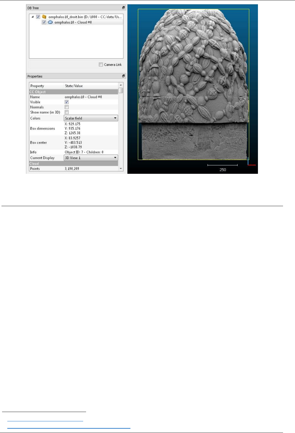
153
CloudCompare Version 2.6.1 – user manual
You can modify the display parameters of this scalar field to increase the contrast for instance. You can also convert
this scalar field to RGB colors, etc.
qPoissonRecon (Poisson Surface Reconstruction)
Introduction
qPoissonRecon stands for "Poisson Surface Reconstruction" and is a simple interface to the triangular mesh generation
algorithm proposed by Misha Kazhdan
47
of Johns Hopkins University.
This is exactly the same implementation as the PoissonRecon
48
library maintained and shared by the author
(currently used version: 6.11).
Therefore, if you use this tool for a scientific publication, please cite the author before citing CloudCompare (which is
also very good but less important in this particular case ;).
CloudCompare simply adds a dialog to set some parameters (see below) and a seamless integration in its own workflow.
Usage
Notes:
to use this plugin, the user must select a point cloud with normals
to obtain good results, the normals of the cloud must be clean (i.e. the orientation of all normals must be
correct/consistent and not too noisy)
by default the algorithm should be applied on closed 3D shapes, but you can use the output 'density'
information to get a valid mesh even on an open mesh (typically such as terrains - see below)
The plugin dialog looks like this:
47
http://www.cs.jhu.edu/~misha/
48
http://www.cs.jhu.edu/~misha/Code/PoissonRecon
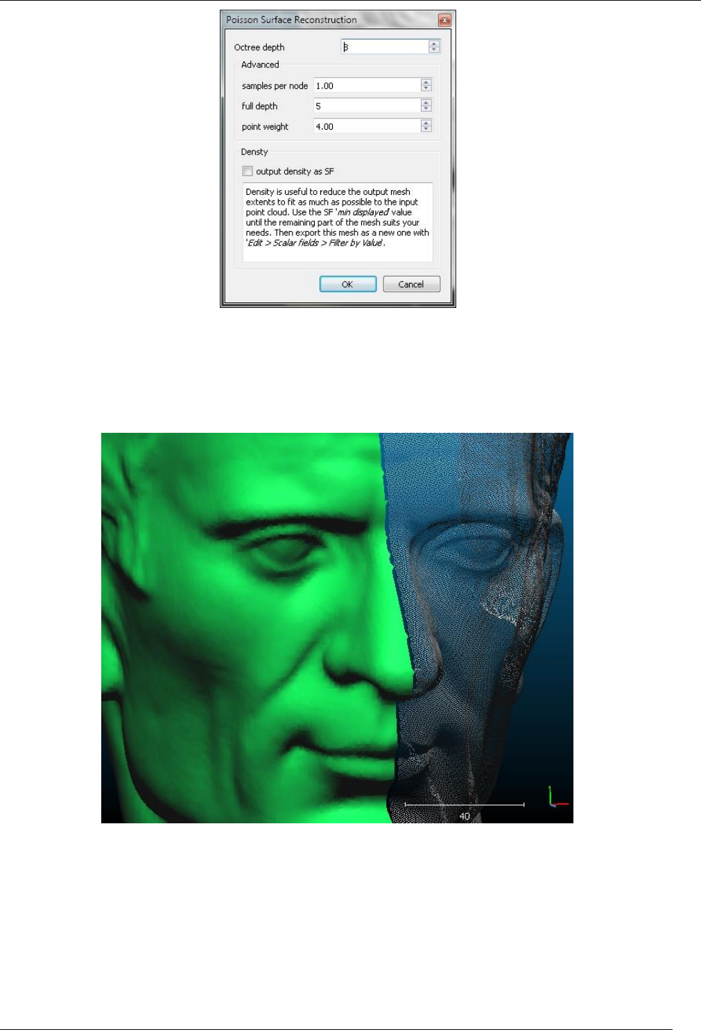
154
CloudCompare Version 2.6.1 – user manual
The parameters are relatively clear and their precise definition can be found on the original library page.
The main parameter is 'octree depth'. The deeper (i.e. greater) the finer the result will be, but also the more time and
memory will be required.
Here is an example of output mesh (the mesh is on the left, and the input cloud - with normals - is on the right):
Using the output density
The most interesting feature when working with open shapes (such as LIDAR clouds, etc.) is the 'density' measure
output by PoissonRecon.
You can use this scalar field to reduce the output mesh extents so as to match as best the input cloud extents:
once the computation is done, close the plugin dialog
select the output mesh
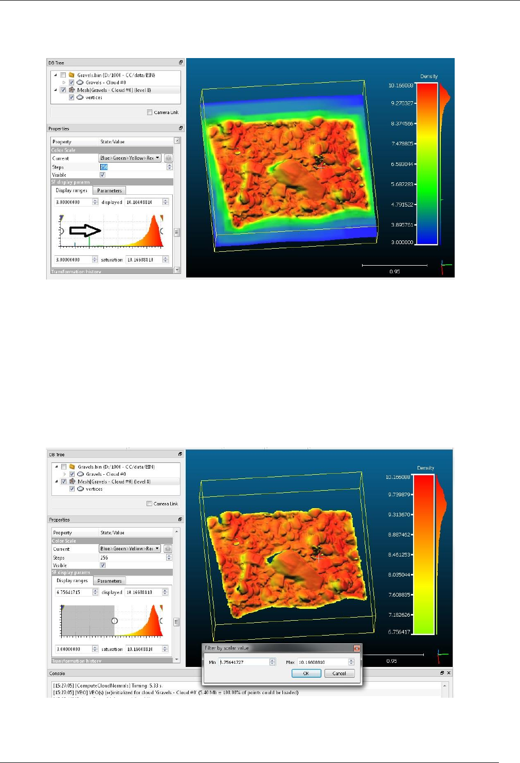
155
CloudCompare Version 2.6.1 – user manual
scroll its properties down (see the 'Properties' dialog - on the left by default) until you see the 'SF display
params' section
You can use the left white circular interactor (which corresponds to the 'minimum displayed value') to interactively hide
the triangles with vertices having the lowest density values. They correspond to the triangles that are the farthest from
the input cloud.
Once you are visually satisfied with the result, you can export the visible triangles as a new mesh:
use the ‘Edit > Scalar fields > Filter by Value’ method
the min and max values should be already set as the one you have interactively set
confirm to create a new mesh
you can drop the 'density' scalar field at least on the output mesh (with Edit > Scalar Fields > Delete)
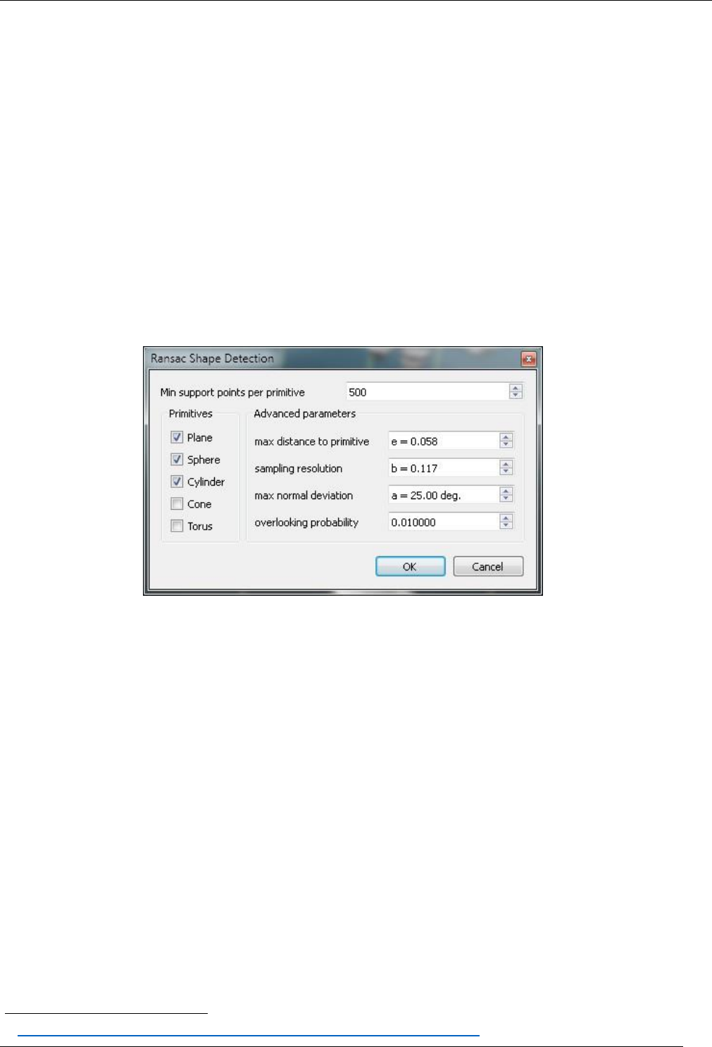
156
CloudCompare Version 2.6.1 – user manual
qRansacSD (RANSAC Shape Detection)
Introduction
qRansacSD stands for "RANSAC Shape Detection" and is a simple interface to the automatic shape detection algorithm
proposed by Ruwen Schnabel
49
et al. of Bonn university.
This is exactly the same implementation as the library shared by the authors on their website (version 1.1).
Therefore, if you use this tool for a scientific publication, please cite the author before citing CloudCompare (which is
also very good but less important in this particular case ;).
CloudCompare simply adds a dialog to set some parameters (see below) and a seamless integration in its own workflow.
Usage
Notes:
to use this plugin, the user must select a point cloud
to obtain better results, you can provide a point cloud with clean normals (otherwise the plugin will compute
them itself)
The plugin dialog looks like this:
The description of each parameter should appear as a tooltip (appears when leaving the mouse over the corresponding
spinbox for a while). The most important one is the number of samples (support points) per primitive. It all depends on
your cloud density and the size of the shapes you are trying to detect. For the other parameters, it may be necessary
to read the original article.
You also have to select only the kind of primitives you actually wish to detect (see the checkboxes on the left) so as to
easily avoid false/unnecessary detections.
On completion, the plugin will create a set of new entities. For each detected shape you get:
a point cloud corresponding to the subset of points that supports the detected primitive. The name of the
cloud incorporates the estimated primitives parameters
the corresponding entity as child of this cloud. Warning: apart for planes, the other primitives are not
displayed by default (as they can be much bigger than the actual cloud, especially for spherical or cylindrical
portions that may only fit on a very small portion of the complete primitive).
each couple (cloud/primitive) is randomly colored
49
http://cg.cs.uni-bonn.de/en/publications/paper-details/schnabel-2007-efficient/

157
CloudCompare Version 2.6.1 – user manual
Example of qRansacSD output
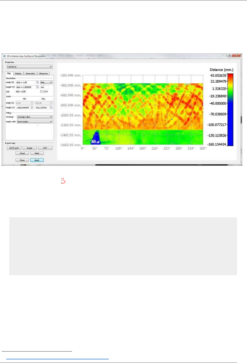
158
CloudCompare Version 2.6.1 – user manual
qSRA (Surface of Revolution Analysis)
Introduction
The qSRA plugin computes distances between a cloud and a theoretical Surface of Revolution
50
. The surface of
revolution is simply defined by a 2D profile.
Once the distances are computed, the plugin lets the user create a 2D map of deviations, either with a cylindrical or a
conical projection.
Loading a 2D profile
2D profiles can be loaded with the ‘Plugins > qSRA > Load profile’ menu entry or the equivalent icon in the plugin's
toolbar.
The corresponding dialog will mainly ask the user to specify a '2D profile' TXT file (the expected format is recalled
directly above the Profile file field):
Xc Yc Zc (profile origin)
4667.000 10057.000 171.000
R H (radius and height of profile vertices)
59.3235190427553 28.685
58.8177164625621 30.142
58.32550519856 31.594
57.8404034801208 33.044
...
Don't change the header lines ('Xc...' and 'R...'), don't add blank lines, etc.
Notes:
The profile origin is a point on the revolution axis corresponding to zero height (H = 0) by default (see below).
The profile is described as a series of (radius, height) couples. The height values must be either constantly
increasing or constantly decreasing.
Eventually the user can specify the revolution axis in 3D (X, Y or Z) and whether the height values are expressed
relatively to the profile origin (i.e. z3D = Zc + H) or if they are absolute (i.e. z3D = H).
50
http://en.wikipedia.org/wiki/Surface_of_revolution
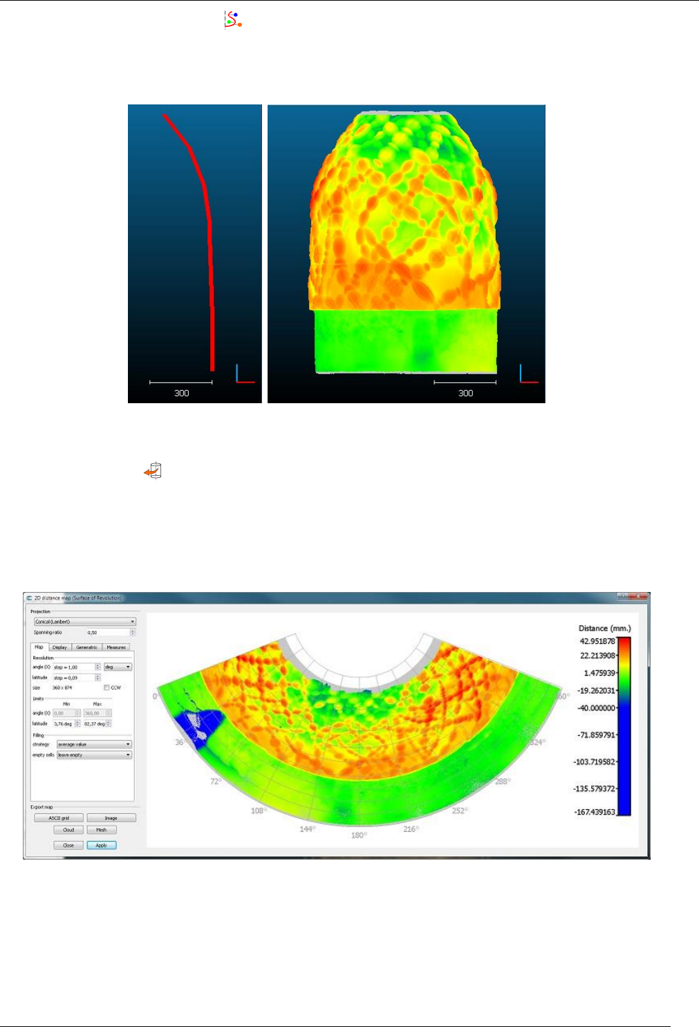
159
CloudCompare Version 2.6.1 – user manual
Computing radial distances
To compute the (radial) distances between a cloud and the profile (i.e. the Surface of Revolution), the user must select
both the cloud and the profile at the same time (keep the CTRL key pressed while selecting both entities in the DB tree).
No dialog is displayed (apart from a progress bar).
On completion, the tool will automatically suggest to launch the Map Generation tool (see below).
Map Generation
To launch the map generation tool, the user must select both the cloud and the profile at the same time (keep the CTRL
key pressed while selecting both entities in the DB tree). The cloud must already have a scalar field with radial distances
(see above).
Most of the parameters are straightforward. You'll have to click on the Apply button to make the map appear (or to
refresh it if you change some parameters).
You can export the map to various formats:
CSV matrix file
image
point cloud (with the cylindrical projection only)
textured mesh of the Surface of Revolution (with the cylindrical projection only)
You can also generate horizontal and/or vertical profiles in Autocad DXF format.
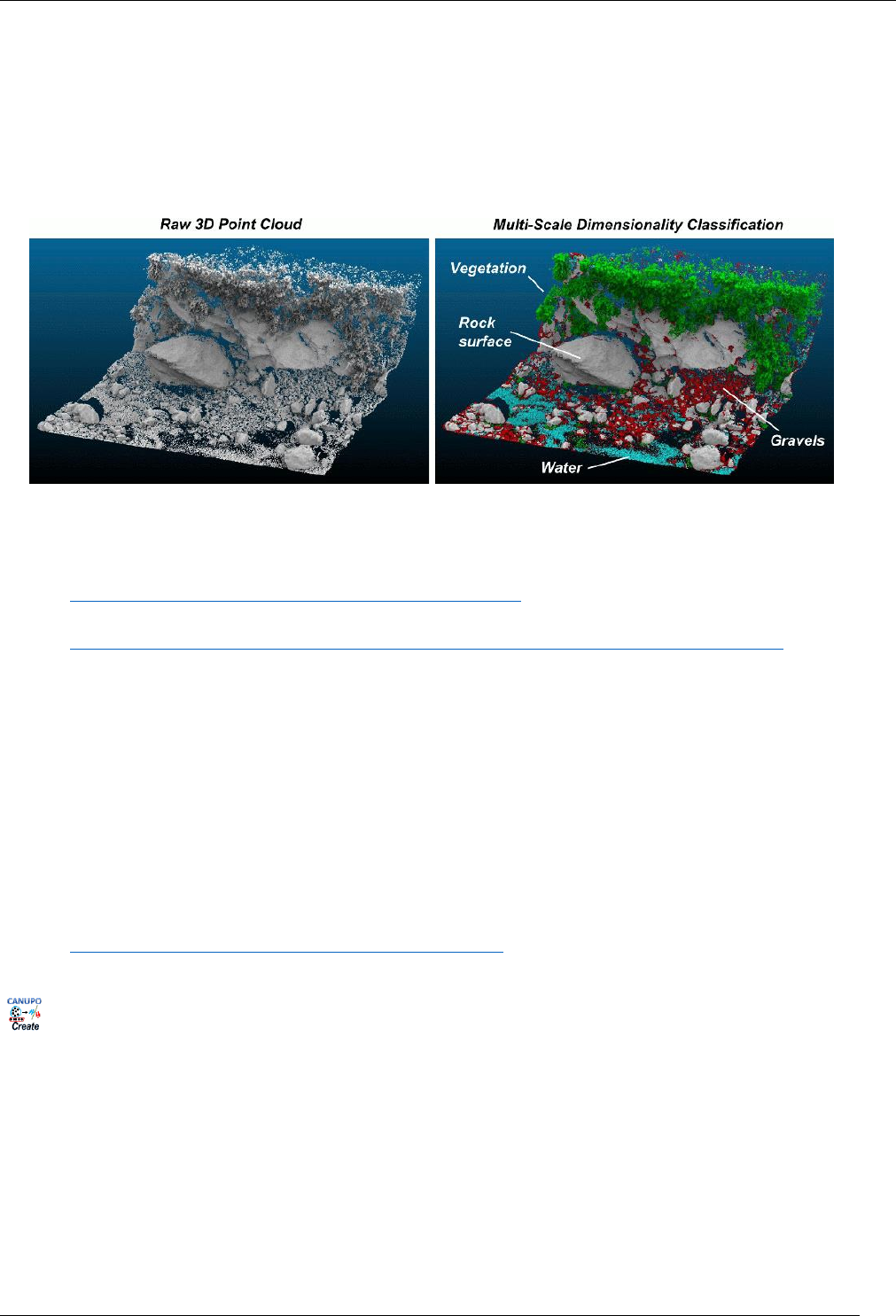
160
CloudCompare Version 2.6.1 – user manual
qCANUPO (Point Cloud Classification)
Introduction
The CANUPO suite is a simple yet efficient way to automatically classify a point cloud. It lets you create your own
classifiers (by training them on small samples) and/or apply one classifier at a time on a point cloud so as to separate it
into two subsets. It also outputs a classification confidence value for each point so that you can quickly identify the
problematic cases (generally on the classes borders).
While the plugin is simple to use, it can be a good idea to read some more information about CANUPO first:
the original article by N. Brodu and D. Lague (Geosciences Rennes):
http://www.geosciences.univ-rennes1.fr/spip.php?article1284
the tutorial for the original command line tool:
http://www.geosciences.univ-rennes1.fr/IMG/pdf/Point_cloud_classification_user_guide_v1-2.pdf
Getting a working classifier
Use an existing ".prm" file
Classifiers are stored in standalone ".prm" files. They can be applied to any point cloud providing its units are concordant
with the classifier. If a classifier has been trained with scales regularly sampled between 0.05 and 0.3 (implicitly in
meters for instance) then your cloud coordinates must be expressed in the same units (i.e. in meters here).
So anyone can share a classifier with others. You can first look at:
the authors webpage for an existing classifier that may suits your needs (link above - see the “Sample data,
classifiers and batch file” section)
or on the dedicated thread on CloudCompare forum:
http://www.cloudcompare.org/forum/viewtopic.php?t=808
Train your own classifier
Prepare the data
Getting a working classifier is really easy (getting an accurate one might be a little longer, but not much).
All you have to do is to manually segment some groups of points representing each class (with the scissors tool of
CloudCompare). For each class you should take several typical subsets of points and regroup them in a single cloud
(with the Edit > Merge method of CloudCompare).
Try to get an exhaustive sampling of the various cases that can be encountered for each class. Make sure also that all
subsets have roughly the same number of points (or at least that the relative quantities are representative of their
occurrence in your data).
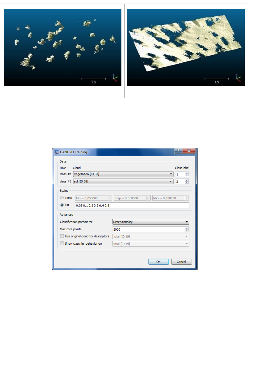
161
CloudCompare Version 2.6.1 – user manual
Class 1: vegetation
Class 2: ground
Tip: make sure that both have unique and clear names so as to differentiate them during the rest of the procedure
(type F2 to rename the selected cloud).
Train a classifier
Once you have the two clouds representing each class, you can call the 'Train classifier' method of the plugin (‘Plugins
> qCANUPO > Train classifier’).
Select the right clouds in the class #1 and class #2 combo-boxes. Then enter the range of scales you wish to use for the
multi-scale descriptors (see the original canupo tutorial and article for more information on how to choose the right
values). You can either input a regular ‘ramp’ (the scale values will be regularly sampled inside an interval) or a custom
list of scales (separated by a space character, e.g. “0.05 0.1 0.2 0.5 1.0”).
Note: the more scales you set, the more discriminative the result might be, but also the longer the computations
(especially if the largest scale is wide relatively to the cloud density).
Optionally you can set more advanced parameters in the lower part of the dialog:
the type of descriptors that will be computed (only “Dimensionality” – as proposed by Brodu and Lague in the
original CANUPO paper – is available for now)
the maximum number of core points that will be randomly extracted from the input cloud (10 or 20 thousands
should be more than enough in most of the cases)
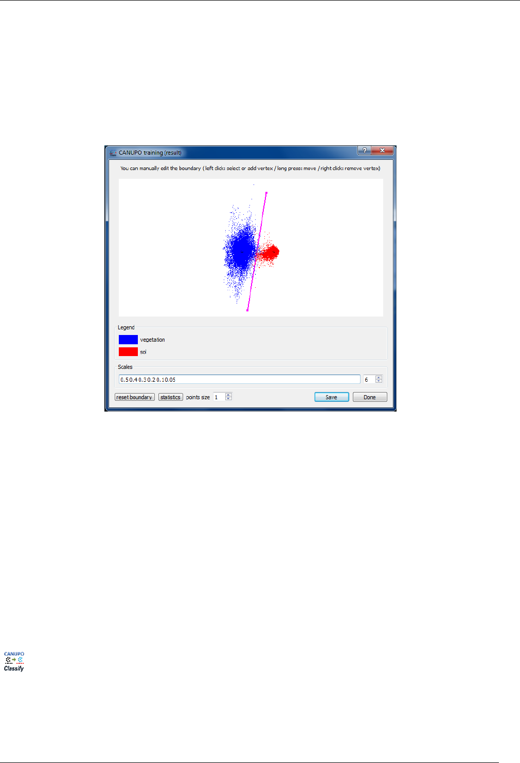
162
CloudCompare Version 2.6.1 – user manual
you can specify to use the original cloud (not the segmented ones) to compute the descriptors (it's a little
longer depending on its size - but it can gives better results on the borders)
eventually you can specify another cloud that will be used to display the classifier behavior (see below)
Once ready, you can click on the “OK” button to start the training. The plugin will start to compute the descriptors on
each cloud and will then try to find the best classification boundary (in a custom 2D space).
The classifier behavior is represented by projecting all the descriptors in the classification space with the classification
boundary in-between (as a magenta line). If a custom cloud has been set for displaying the classifier behavior, all its
descriptors will be represented in grey. Otherwise, the descriptors corresponding to the first class will be displayed in
blue, and the others in red.
From this point, several actions may be realized by the user:
you can decrease the number of scales used to train the classifier (by default, the biggest scales are removed
first). This lets you tune the classifier so as to use the less scales as possible (with the lowest scales radii, so as
to minimize the computation time for descriptors) while keeping a sufficiently discriminating behavior.
you can also edit the boundary position. The vertices of the boundary line can be moved (right click + keep the
button pressed); new vertices can be added (by clicking anywhere – in which case the vertex will be added to
the nearest line’s end – or by click exactly on the line - in which case a new vertex will be created on the line
near the mouse cursor) ; and vertices can be removed (left click – only taken into account if the line has more
than 2 vertices). At any time the boundary can be reset to its original state by clicking on the ‘reset boundary’
button.
Once ready, you can save the classifier in a .prm file. This file will be used as input for the 'Classify' method (see below).
Don't hesitate to share your own classifiers (either with Dimitri Lague himself – he might put up a dedicated webpage
to store the best classifiers – or on the dedicated thread on CloudCompare's forum).
Apply a classifier on a cloud
Once you have a valid classifier file (see above) you can apply it on any cloud (providing its units are concordant with
the classifier - see above).
Select the cloud you wish to classify and call the 'Classify' method of the plugin (‘Plugins > qCANUPO > Classify’).
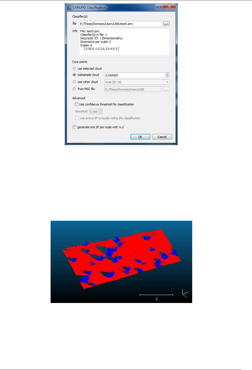
163
CloudCompare Version 2.6.1 – user manual
First load the classifier file (with the '...' button next to the file field).
Then select the 'core points' on which the computation should be done: it's not always necessary useful to use all points
of a cloud for such a process (moreover it can be quite long). Therefore, especially for a first attempt, you can use less
points either by sub-sampling the original cloud or by providing your own core points (a rasterized version of the input
cloud for instance). You can even directly open a “.msc” file generated by the original CANUPO suite developed by
Nicolas Brodu.
Eventually and whatever the choice you've made for core points, all the points will be classified. The classification result
for a given core point is propagated to its nearest neighbors. Therefore using core points instead of the whole cloud
might just be a little less accurate on the borders (and once you are happy with the results, you can launch the same
classification process on every points in the cloud... and go take a coffee ;).
Note that the plugin always generates on the input cloud an additional scalar field with the classification 'confidence':
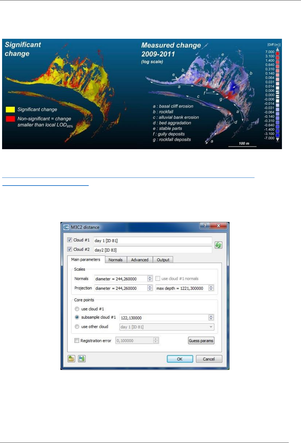
165
CloudCompare Version 2.6.1 – user manual
qM3C2 (Robust C2C Distances Computation)
Introduction
The M3C2 plugin is the unique way to compute signed (and robust) distances directly between two point clouds.
While you can use the 'Guess params' button, it is highly advised to read (even quickly) the original article by D. Lague,
N. Brodu and J. Leroux (Geosciences Rennes):
http://www.geosciences.univ-rennes1.fr/IMG/pdf/Accurate_3D_point_cloud_comparison_Lague_et_al-
_revised_with_figures_feb2013.pdf
Computing M3C2 distances
Select the two clouds you want to compare then call the 'Plugins > M3C2 Distance' method.
Main parameters
As with the CANUPO algorithm, computations can only be done on particular points - called core points - in order to
speed up the computations. The main idea is that while TLS clouds are generally very dense, it is not necessary to
measure the distance at such a high density (and it would very slow in practical). This is why the user has to choose
what 'core points' will be used (lower part of the dialog):
either the whole cloud

166
CloudCompare Version 2.6.1 – user manual
or a sub-sampled version of the input cloud
or eventually a custom set of core points (typically a previously sub-sampled version of the input cloud, or a
rasterized version)
The other important parameters are the normal and projection scales:
the normal scale is the diameter of the spherical neighborhood extracted around each core point to compute
a local normal. This normal is used to orient a cylinder inside which equivalent points in the other cloud will
be searched for. Regarding normals more advanced options can be set in the 'Normals' tab (see below).
the projection scale is the diameter of the above cylinder.
the max depth parameter simply correspond to the cylinder height (in both directions)
Note: the bigger those radii are, the less local surface roughness (and noise) will have an influence. But also the more
points will be 'averaged' and the slower the computation will be.
Eventually, if you now the global registration error (if your cloud has been generated by registering several stations
typically) you can input it in the 'registration error' field. It will be taken into account during the confidence computation
for each point (that let you know if the corresponding displacement is significant or not).
Normals
Using 'clean' normals is very important in M3C2. The second tab let you specify more advanced options regarding their
computation:
Default: the normals are computed thanks to the normal scale parameters defined in the previous tab
Multi-scale: for each core points, normals are computed at several scale and the most 'flat' is used
Vertical: no normal computation is done, only purely vertical normals are used (perfect for 2D problems)
Horizontal: normals are 'constrained' in the (XY) plane
Alternatively you can also use the cloud original normals (if any) by checking the use cloud #1 normal checkbox on the
first tab.
The 'orientation' options let you help the plugin to properly orient the normals:
either by specifying a global orientation (relatively to a given axis or a particular point)
or by specifying a cloud containing all the sensor positions
Advanced
The 'Advanced' tab contains... advanced parameters. Their name should talk for themselves. They can be ignored by
most users.
Output
You can choose to generate additional scalar fields and also on which cloud the measurements should be re-projected
(especially useful if you use core points different from the first input cloud).
Save/load parameters
Note: Parameters can be saved (and re-loaded) via dedicated text files. Use the two icons on the bottom-left part of
the dialog to do this.
Computing distance
When ready, simply click on the "OK" button. Once finished, the dialog will be closed. You will generally have to hide
the input clouds to see the result (generated in a new cloud).
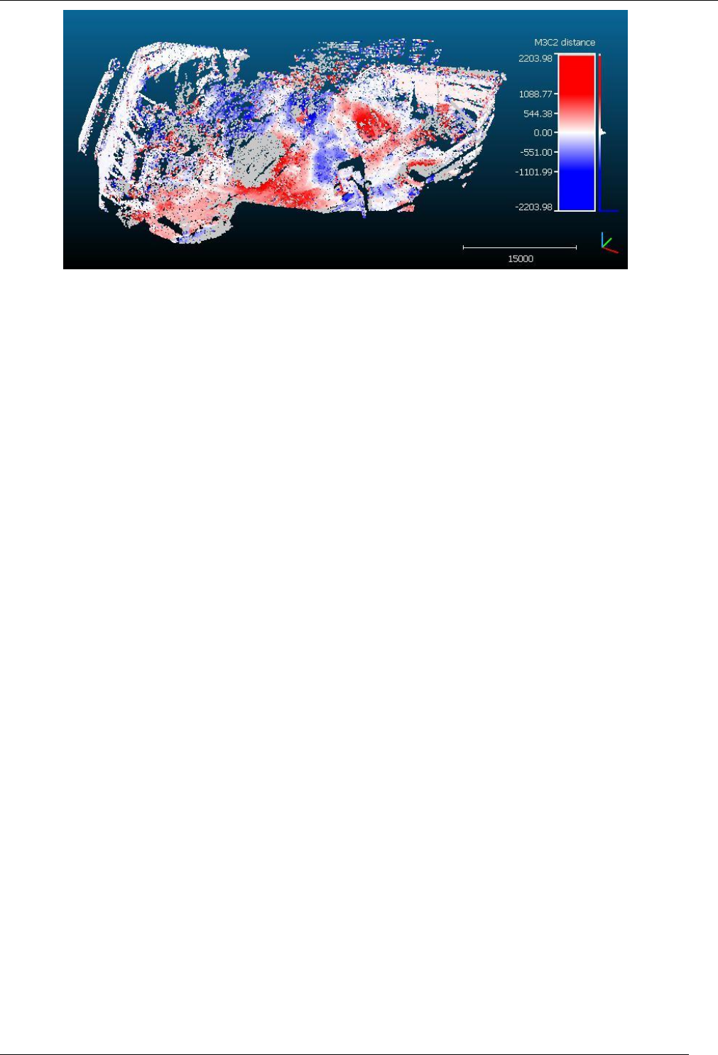
167
CloudCompare Version 2.6.1 – user manual
Note that in addition to the distances, the M3C2 plugin generates several other scalar fields:
distance uncertainty (the closer to zero the better)
change significance (whether the distance probably correspond to a real change or not)
and optionally the standard deviation and number of neighbors at each core point (as specified in the 'output'
tab)
Note also that points without any corresponding points in the other cloud stay in 'gray' (they are associated to NaN –
not a number – distances). This means that no points in the other cloud could be found inside the search cylinder.
Therefore, gray points means that either some parts of the clouds have no equivalent in the other cloud (due to hidden
parts or other holes in the datasets) or simply that the cylinder maximum length is not long enough!
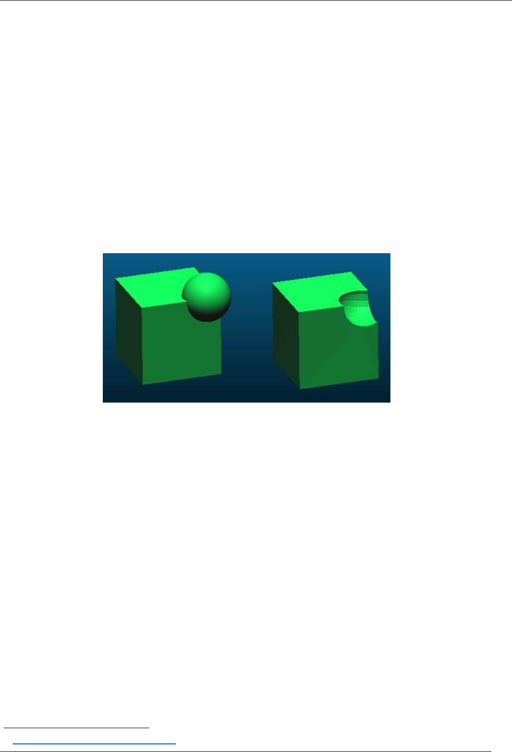
168
CloudCompare Version 2.6.1 – user manual
qCork (Boolean Operations on Meshes)
Presentation
This plugin can be used to perform Boolean operations on meshes (also called CSG = Constructive Solid Geometry).
It is based on the Cork
51
library.
Procedure
Its usage is pretty straightforward:
select two meshes (meshes should be ideally closed, otherwise the output might be wrong)
click on the plugin icon (or the equivalent entry in the 'Plugins' menu: 'Plugins > Mesh Boolean Operations')
When the plugin dialog appears (see above):
o assign each mesh to a role (A or B)
o then select the operation to apply:
union: A + B
difference (symmetric or not): A - B
intersection: A n B
The plugin will create a new mesh corresponding to the operation output:
Warning: due to internal instabilities in the current version of the Cork library, it may be necessary to launch the
process several times in order to get it working ;)
51
https://github.com/cloudcompare/cork

169
CloudCompare Version 2.6.1 – user manual
OpenGL 'shaders' plugins
qEDL (Eye Dome Lighting)
EDL is a real time shading filter that enhances very small features on blank clouds or meshes (i.e. it doesn't rely on any
information apart from the geometry itself). As ‘qSSAO (Screen Space Ambient Occlusion)’ this is a faster alternative to
normal-based shading.
EDL in action on a blank cloud
For more information about how EDL works, refer to this article: http://www.kitware.com/source/home/post/9.
Note: EDL requires a contiguous depth map. Therefore if your cloud is too sparse at the current viewing zoom, you must
increase the point size (so as to fill the holes).

170
CloudCompare Version 2.6.1 – user manual
qSSAO (Screen Space Ambient Occlusion)
S.S.A.O.
52
is a real time shading filter that approximates ambient occlusion. As ’qEDL (Eye Dome Lighting)’ this is a faster
alternative to normal-based shading.
SSAO in action on a blank cloud
Note: SSAO requires a contiguous depth map. Therefore if your cloud is too sparse at the current viewing zoom, you
must increase the point size (so as to fill the holes).
52
http://en.wikipedia.org/wiki/Screen_space_ambient_occlusion
171
CloudCompare Version 2.6.1 – user manual
Appendix
Command line mode
Since version 2.3 (2012/12/11), CloudCompare can be used in "command line" mode.
By default, this mode only opens a small console window, applies the requested actions, and eventually saves the result
in a file in the same directory(ies) as the input file(s). Commands are applied in the order they are written (like a state
machine).
Available options (version 2.6.1 and higher)
Command
Description
-SILENT
enables silent mode (no console will appear)
Warning: must be first if required.
-O {filename}
opens a file
If the file format is ASCII, optional settings are:
• -SKIP {number of lines to skip} If set, CC will automatically skip the specified number of lines
For all formats, optional settings are (version 2.5.6 and above):
• -GLOBAL_SHIFT {AUTO} or {x y z} If set, CC will either handle big coordinates automatically (AUTO) or
apply the specified Global Shift vector (x,y,z)
Note: file type is automatically guessed from its extension.
-COMPUTE_NORMALS
forces CC to compute normals at loading time (which is generally more robust) when importing files
containing structured clouds (i.e. PTX and DP file for now). Normals are not computed by default.
Note: must be placed before the '-O' option.
-MERGE_CLOUDS {filename}
merges all loaded/generated clouds as one unique cloud.
Note: result is automatically saved by default (see the AUTO_SAVE command to change this).
-SS {algorithm} {parameter}
applies a subsampling {algorithm} on the currently opened/generated cloud(s).
{algorithm} can be RANDOM, SPATIAL or OCTREE. Expected parameter is:
• RANDOM: number of randomly selected points
• SPATIAL: minimum distance between two points
• OCTREE: subdivision level (between 1 and 10 in the standard version)
Notes:
• result is automatically saved by default (see the AUTO_SAVE command to change this).
• input clouds are now replaced by their subsampled version (since version 2.6.1)

172
CloudCompare Version 2.6.1 – user manual
-SAMPLE_MESH {method} {parameter}
samples points on the loaded mesh(es). For each mesh, a cloud will be generated (and will be added to the
current loaded cloud set - i.e. further processing can be applied to this cloud).
{method} can be POINTS or DENSITY. Expected parameter is:
• POINTS: the corresponding number of points
• DENSITY: the corresponding surface density
Notes:
• result is automatically saved by default (see the AUTO_SAVE command to change this)
• this cloud can be used as input for cloud-to-cloud or cloud-to-mesh distances computation for instance.
-C2C_DIST
computes cloud-to-cloud distance on the two first loaded/generated clouds (1st = compared / 2nd =
reference).
Optional settings are:
• -SPLIT_XYZ If set, 3 additional scalar fields will be generated (displacement along the 3 dimensions)
• -MAX_DIST {value} to set a max distance above which CC won't have to search for a nearest neighbor
(faster)
• -OCTREE_LEVEL {value} to manually set the octree subdivision level at which the computation will be
performed
• -MODEL {local_model_type} {neighborhood_type}
{neighborhood_size} to specify a local model:
• {local_model_type} = LS / TRI / HF
• {neighborhood_type} = KNN / SPHERE
• {neighborhood_size} = neighbor count (if KNN) or sphere radius (if SPHERE)
Notes:
• result is automatically saved by default (see the AUTO_SAVE command to change
this)
• see below for more details
-C2M_DIST
computes cloud-to-mesh distance between the first loaded/generated cloud (compared) and the first loaded
mesh (reference).
Optional settings are:
• -FLIP_NORMS to consider that normal vectors point inside the matter and not outside
• -MAX_DIST {value} to set a max distance above which CC won't have to search for a nearest neighbor
(faster)
• -OCTREE_LEVEL {value} to manually set the octree subdivision level at which the computation will be
performed
Notes:
• result is automatically saved by default (see the AUTO_SAVE command to change
this)
• see below for more details
-STAT_TEST {distrib} {distrib
parameters} {p-value} {neighbors
count}
applies a local statistical test based on the active scalar field all the of loaded/generated clouds. {distrib}
can be GAUSS or WEIBULL. Expected distribution parameters are:
• GAUSS: the mean value and sigma
• WEIBULL: a, b and the shift value
Note: result is automatically saved by default (see the AUTO_SAVE command to change this).

173
CloudCompare Version 2.6.1 – user manual
-FILTER_SF {minVal} {maxVal}
filters all the loaded/generated clouds based on their active scalar field values.
A new cloud is created each time with only the points falling in the [minVal maxVal] interval.
Notes:
• result is automatically saved by default (see the AUTO_SAVE command to change this).
• input clouds are now replaced by their filteterd version (since version 2.6.1)
You can use special words in place of numbers that CC will replace by the actual SF values:
• 'MIN' = min value
• 'DISP_MIN' = min displayed value
• 'SAT_MIN' = min saturation value
• 'MAX' = max value
• 'DISP_MAX' = max displayed value
• 'SAT_MAX' = max saturation value
-DENSITY {sphere radius}
computes density (inside a sphere around each point) on the currently opened/generated cloud(s).
Optional setting:
• -TYPE {density_type}: to specify the type of density to compute. {density_type} can be KNN (nearest
neighbors count), SURFACE (surface density) or VOLUME (volume density).
Notes:
• a new scalar field is created on each cloud
• result is automatically saved by default (see the AUTO_SAVE command to change this)
-APPROX_DENSITY
computes approximate density on the currently opened/generated cloud(s).
Optional setting:
• -TYPE {density_type}: to specify the type of density to compute. {density_type} can be KNN (nearest
neighbors count), SURFACE (surface density) or VOLUME (volume density).
Notes:
• a new scalar field is created on each cloud.
• result is automatically saved.
-ROUGH {kernel size}
computes roughness with a given kernel size on the currently opened/generated cloud(s).
Notes:
• a new scalar field is created on each cloud
• result is automatically saved by default (see the AUTO_SAVE command to change this)
-CURV {type} {kernel size}
computes local curvature with a given kernel size on the currently opened/generated cloud(s).
{type} can be MEAN or GAUSS.
Notes:
• a new scalar field is created on each cloud
• result is automatically saved by default (see the AUTO_SAVE command to change this)
-SF_GRAD {euclidian}
computes gradient of the active scalar field (or the first one if none is active) on the currently
opened/generated cloud(s).
The {euclidian} option specifies whether the scalar field is 'Euclidian' (TRUE) - typically like a distance field -
or not (FALSE).
Notes:
• a new scalar field is created on each cloud
• result is automatically saved by default (see the AUTO_SAVE command to change this)

174
CloudCompare Version 2.6.1 – user manual
-BEST_FIT_PLANE
computes the best fitting plane on all loaded clouds.
Optional settings are:
• -MAKE_HORIZ: will actually transform the loaded cloud(s) so as to make them 'horizontal'
• -KEEP_LOADED: to keep the resulting plane(s) in memory as mesh(es)
Notes:
• resulting planes are automatically saved
• if MAKE_HORIZ is defined, result is automatically saved by default (see the
AUTO_SAVE command to change this)
-APPLY_TRANS {filename}
applies a 4x4 transformation matrix on the loaded entities (clouds or meshes). The matrix is read from a
simple text file with the matrix rows on each line (4 values per lines, 4 lines).
Notes:
• each entity will be replaced in memory by its transformed version
• resulting entities are automatically saved by default (see the AUTO_SAVE command to change this)
-MATCH_CENTERS
makes all the (bounding-box) centers of the loaded entities match. All the entities will move relatively to
the first one (clouds are always considered first if clouds and meshes are loaded).
Note: result is automatically saved by default (see the AUTO_SAVE command to change this).
-DELAUNAY
Triangulates the loaded clouds with 2.5D Delaunay triangulation. The triangulation is done in the (XY)
plane by default.
Optional settings are:
• -AA: to triangulate the points in the (XY) plane (default behavior).
• -BEST_FIT: to triangulate the points in their best fit plane
• -MAX_EDGE_LENGTH {length}: to remove the triangles with edges longer than a given threshold
Notes:
• the resulting 'mesh' entity is automatically saved (see the AUTO_SAVE command to change this).
• the clouds are automatically removed (from the 'loaded clouds' set).
-ICP
Iterative Closest Point registration procedure.
Optional settings are:
• -REFERENCE_IS_FIRST: by default the ICP registration process will take the first loaded entity as 'data'
and the second as 'model' (clouds are always considered first). If you use this option their respective
role will be inverted.
• -MIN_ERROR_DIFF: to specify the min. error difference between two steps (default = 1e-6)
• -ITER: to specify the number of iterations (in which case the 'MIN_ERROR_DIFF' option will be ignored)
• -OVERLAP: to specify the percentage of (final) overlap (integer number between 10 and 100 - default =
100)
• -ADJUST_SCALE: to enable the ICP registration with adaptive scale
• -RANDOM_SAMPLING_LIMIT: to specify the number of points randomly sampled at each iteration
(default = 20 000)
• -ENABLE_FARTHEST_REMOVAL: to enable the research option that ignores points with the highest
distances at each iteration
Notes:
• the 'data' entity in its final position is automatically saved (see the AUTO_SAVE command to change
this).
• the corresponding transformation matrix is automatically saved in a separate text file (always).

175
CloudCompare Version 2.6.1 – user manual
-CROP
{Xmin:Ymin:Zmin:Xmax:Ymax:Zmax}
Crops all loaded clouds inside or outside a given box.
Optional settings are:
• -OUTSIDE: if defined only the points falling outside the input box will be kept (instead of inside by
default).
Notes:
• result is automatically saved by default (see the AUTO_SAVE command to change this)
• each cloud will be replaced in memory by its cropped version
-CROP2D {ortho_dim} {n:number of
vertices} X1 Y1 X2 Y2 ... Xn Yn
Crops all loaded clouds inside or outisde a given 2D polyline. Cropping is done in a plane defined by its
orthogonal dimension: X, Y or Z (i.e. coordinates along this dimension will be ignored).
Optional settings are:
• -OUTSIDE: if defined only the points falling outside the input polyline will be kept (instead of inside by
default).
Note:
• result is automatically saved by default (see the AUTO_SAVE command to change this)
• each cloud will be replaced in memory by its cropped version
-CBANDING {dim} {freq}
Applies color banding to all loaded entities (clouds and meshes). The user must specify the dimension (dim
= X, Y or Z) and the frequency (in Hz, as an integer).
Note:
• result is automatically saved by default (see the AUTO_SAVE command to change this)
-C_EXPORT_FMT {format}
Specifies the default output format for clouds. Format can be one of the following: ASC, BIN, PLY, LAS, E57,
VTK, PCD, SOI, PN, PV.
Optional settings are:
• -PREC [precision]: to specify the numerical output precision (for ASCII files only). precision is a positive
integer (default = 12).
• -SEP [separator]: to specify the separator character (for ASCII files only). separator can be one of the
following string: SPACE, SEMICOLON, COMMA or TAB (default = SPACE).
• -EXT [extension]: to specify the file extension (typically different from the default one for the chosen
format)
-M_EXPORT_FMT {format}
Specifies the default output format for meshes. Format can be one of the following: BIN, OBJ, PLY, STL, VTK,
MA, FBX.
Optional settings are:
• -EXT [extension]: to specify the file extension (typically different from the default one for the chosen
format)
-FBX_EXPORT_FMT {format}
Specifies the default output format for FBX meshes. Must be specified in addition to M_EXPORT_FMT if FBX
format is chosen. Format can be one of the following: FBX_binary, FBX_ascii, FBX_encrypted,
FBX_6.0_binary, FBX_6.0_ascii, FBX_6.0_encrypted.
Note: if the input format is not supported by the current implementation, a list of available formats will be
output in the console.
-PLY_EXPORT_FMT {format}
Specifies the default output format for PLY files. Format can be one of the following: ASCII, BINARY_BE (big
endian) or BINARY_LE (little endian).
Note: default output format is binary (LE/BE depending on the current OS)
-NO_TIMESTAMP
to prevent CC from generating an automatic suffix (timestamp) for output file name (warning: this make
the name of an output file predictable but if the file already exists it will be overwritten).
176
CloudCompare Version 2.6.1 – user manual
-BUNDLER_IMPORT {filename}
imports a Snavely's Bundler file.
Bundler import through the command line is mainly meant to generate ortho-rectified versions of input
images directly on disk. Optional settings are:
• -ALT_KEYPOINTS [filename]: load alternative keypoints from file filename
• -SCALE_FACTOR [value]: sets image scale factor that has been used during keypoints generation
• -COLOR_DTM [vertices count]: generates colored vertices of a pseudo-DTM with approximately
'vertices count' elements (in command line mode, vertices are automatically saved to
'colored_dtm_vertices.bin' next to ortho-rectified images)
• -UNDISTORT: enables images undistortion Note: see below for more details.
-SET_ACTIVE_SF {index}
Sets the active scalar field index (for all loaded clouds).
Note: scalar field indexes start at 0 ('-1' means 'no SF enabled')
-REMOVE_ALL_SFS
Removes all scalar fields (from all loaded clouds or meshes).
Note: entities are not automatically saved after this command (you can use -SAVE_CLOUDS or -
SAVE_MESHES explicitly)
-AUTO_SAVE {ON/OFF}
Enables (ON) or disables (OFF) automatic backup of clouds and meshes at each step (you'll have to
manually call -SAVE_CLOUDS or -SAVE_MESHES at the right time/position in your command).
-SAVE_CLOUDS
Saves all currently loaded clouds (note that this is not necessary by default as all modified or newly
generated cloud are automatically saved).
Optional settings are:
• ALL_AT_ONCE: saves all clouds in a single file (the current output format must support it!)
-SAVE_MESHES
Saves all currently loaded meshes (note that this is not necessary by default as all modified or newly
generated meshes are automatically saved).
Optional settings are:
• ALL_AT_ONCE: saves all meshes in a single file (the current output format must support it!)
-CLEAR
closes all currently loaded entities.
-CLEAR_CLOUDS
closes all currently loaded clouds.
-CLEAR_MESHES
closes all currently loaded meshes.
Example 1
CloudCompare -O myhugecloud.bin -SS SPATIAL 0.1
This will open file myhugecloud.bin then apply spatial subsampling with a 0.1 step (e.g. in meters) step. The output file
will be ‘myhugecloud_SPATIAL_SUBSAMPLED_YYYY-MM-DD_HHhMM.bin’.
Example 2
CloudCompare -O myhugecloud1.bin -SS SPATIAL 0.1 -O 'myhugecloud2.bin' –SS
RANDOM 1000000 -CLEAR_ALL -O 'myhugecloud3.bin' -SS OCTREE 9
This will open file myhugecloud1.bin then apply spatial subsampling with a 0.1 step (e.g. in meters).
Then it will open file myhugecloud2.bin and apply to both files random subsampling (1 000 000 points each).
Then it will close the two first files.
Eventually it will open file myhugecloud3.bin and apply octree based subsampling (level 9).
The output files will be:
myhugecloud1_SPATIAL_SUBSAMPLED_YYYY-MM-DD_HHhMM.bin
myhugecloud1_RANDOM_SUBSAMPLED_YYYY-MM-DD_HHhMM.bin
myhugecloud2_RANDOM_SUBSAMPLED_YYYY-MM-DD_HHhMM.bin
myhugecloud3_OCTREE_level_9_SUBSAMPLED_YYYY-MM-DD_HHhMM.bin

177
CloudCompare Version 2.6.1 – user manual
Cloud-to-cloud distance
CloudCompare -o cloud1.bin -o cloud2.asc -c2c_dist -split_xyz -model HF
SPHERE 50.0
CC will load cloud1.bin and cloud2.asc, then compute the distance from cloud1 (compared) relatively to cloud2
(reference) with a height function (quadric) computed on all the neighbors falling in a sphere of radius 50.0 around each
point of cloud1. On output a file cloud1_C2C_DIST_YYYY-MM-DD_HHhMM.bin will be generated (with the resulting
distances as first scalar field and the 3 components of the corresponding displacement vector along X, Y and Z as
additional scalar fields).
Note: this cloud stays in memory and can be processed further (with -FILTER_SF for instance).
Cloud-to-mesh distance
CloudCompare -o cloud1.bin -o mesh.obj -c2m_dist
CC will load cloud1.bin and mesh.obj, then compute the distance from cloud1 (compared) relatively to mesh (reference).
On output a file cloud1_C2M_DIST_YYYY-MM-DD_HHhMM.bin will be generated (with the resulting distances as scalar
field).
Note: this cloud stays in memory and can be processed further (with -FILTER_SF for instance).
Bundler import
CloudCompare -BUNDLER_IMPORT bundle.out -COLOR_DTM 1000000
This will generate all ortho-rectified versions of the images declared in 'bundle.out', as well as the colored vertices of a
pseudo-DTM constructed from the keypoints.
(Mesh) format conversion
CloudCompare -M_EXPORT_FMT FBX -FBX_EXPORT_FMT FBX_Binary -O Foot.ply -
NO_TIMESTAMP -SAVE_MESHES
This will open the file named 'Foot.ply' then save it in FBX binary format (same base filename, without any decoration:
i.e. Foot.fbx)
Shortcuts
Here are listed the keyboard shortcuts (version: 2.6 and above)
Shortcut
Description
Ctrl+O
Open file
Ctrl+S
Save selected entities
Ctrl+D
Delete selected entities
Alt+C
Set unique color (selected entities)
Del/Suppr
Delete selected entity
Z
Zoom and center view on selected entities
L
Lock manual rotation around the vertical (screen) axis

178
CloudCompare Version 2.6.1 – user manual
B
Enter bubble-view mode
A
Toggle selected entities activation
V
Toggle selected entities visibility (recursive)
N
Toggle selected entities normals visibility (recursive)
C
Toggle selected entities colors visibility (recursive)
S
Toggle selected entities SF visibility (recursive)
M
Toggle selected entities materials/textures visibility (recursive)
D
Toggle selected entities 3D name visibility (recursive)
Shift + C
Toggle selected entity color ramp visibility (recursive)
Shift + Up arrow
Activate previous scalar field on selected entity
Shift + Down arrow
Activate next scalar field on selected entity
Shift + click on a point/triangle
Spawn a 2D label on the clicked element
F1
Show help
F2
Rename selected entity (in DB tree)
F3
Toggle object-centered perspective (active 3D view)
F4
Toggle viewer-based perspective (active 3D view)
F5
Refresh display (active 3D view)
F6
Toggle sun light (active 3D view)
F7
Toggle custom light (active 3D view)
F8
Toggle Console display
F11
Toggle full-screen mode
Ctrl+F3
New 3D view
Ctrl+F4
Close active 3D view
0
Set default "BACK" view to active 3D display
2
Set default "BOTTOM" view to active 3D display
4
Set default "LEFT SIDE" view to active 3D display
5
Set default "FRONT" view to active 3D display
6
Set default "RIGHT SIDE" view to active 3D display
CloudCompare octree
The octree structure is used throughout CloudCompare: in particular all processing methods involving spatial
considerations use it. Note that the particular structure used in CloudCompare is very efficient for nearest neighbor
extraction but not for display purposes (L.O.D. approaches, etc.).
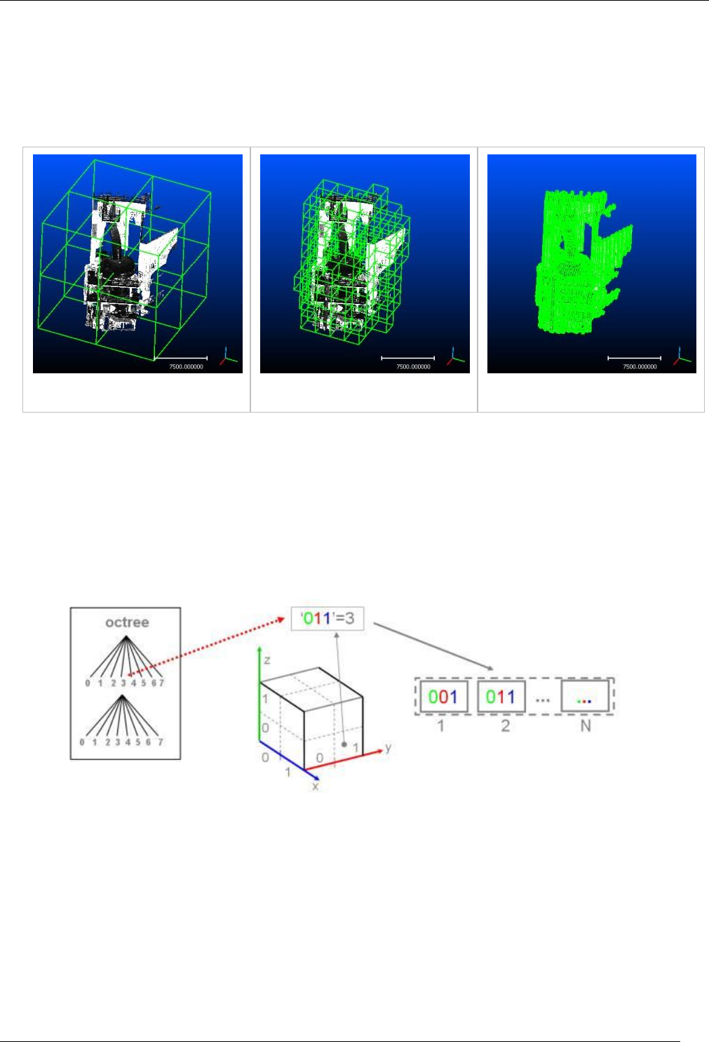
179
CloudCompare Version 2.6.1 – user manual
Structure
An octree corresponds to the recursive partition of a cubical volume of space. From an initial box, octree cells are
formed by dividing cubes into 8 equivalent sub-cubes. By default, the octree subdivision is initiated from the square
bounding box of a cloud, but it can also be computed from an arbitrary cube is space (to optimize comparison
algorithms such as distance computation for example).
Recursive subdivision principle
Depth: 1
Depth: 3
Depth: 6
The octree structure used in CloudCompare (DgmOctree) is not as properly speaking a real 'tree'. It takes the form of a
list of numerical values (one per point) that code the absolute position of a point for all level of subdivision. It is
particularly suited for spatial indexing. Two points lying in the same cell at a given level of subdivision have the same
(partial) associated code. The octree size in memory is also constant.
The code is formed by concatenating sets of 3 bits (0...7) which code the relative position of the cell for each level of
subdivision. The cell at the first level of subdivision corresponds to the most significant bits, and the deepest level
corresponds to the less significant bits. Codes are then sorted to allow fast binary search as well as spatial sweep of the
cloud (adjacent cells are next to each other in the sorted list).
The maximum octree depth in the standard CloudCompare version is 10. In this version codes are coded on 32 bits, and
are associated to a 32 bits index value (i.e. the octree weights 128 bits per point = 8 bytes --> 8 Mb / M. points). One
can compile CloudCompare to use 64 bits codes, which allows to go up to 21 levels of subdivision (but memory
consumption is 50% higher).
Computing the octree
You can force the computation of the octree on any point cloud in CloudCompare (to display it for example - see below):
Edit > Octree > Compute.
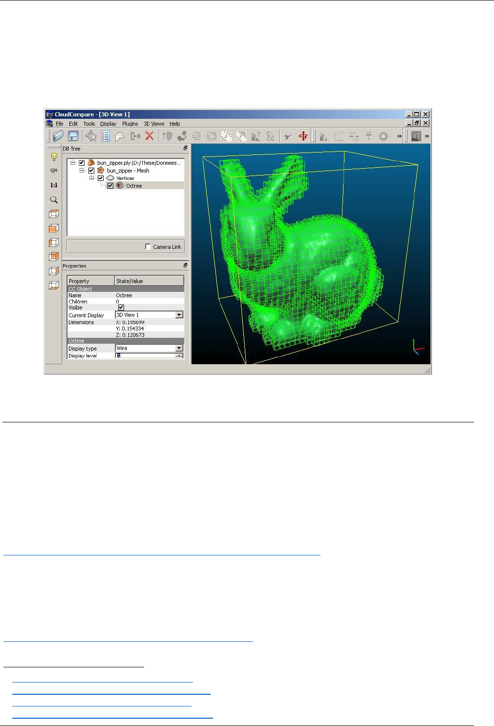
180
CloudCompare Version 2.6.1 – user manual
Displaying the octree
Once computed (either manually - see above - or after a method has requested it), one can display it.
The octree 'object' (in database tree) must be activated and set to 'visible'. Three types of visualization are available:
wire (default)
points (one point per cell)
plain cubes
AirPhotoSE
The Bundler import tool and associated methods (orthophotos generation as images or clouds, colored DTM
generation, etc.) have been developed in association with Pr. Irwin Scollar
53
, creator of the AirPhoto SE software
54
(A
Program for the geometric rectification of aerial images & orthophotos from multiple images).
This (great) software uses internally the Bundler
55
tool to perform automatic intrinsic and extrinsic camera calibration
from multiple aerial images.
This collaboration has led to an article in the bi-annual newsletter of the Aerial Archaeology Research Group (AARG
News
56
). The article can be found: here:
http://www.cloudcompare.org/pdf/AARGnews44-Scollar-GiradeauMontaut.pdf
Generating orhtophotos
In order to generate very easily a set of files compliant with the dedicated importation tool in CloudCompare in order
to generate orthophotos, just follow the AirPhoto SE tutorial about "Orthophotos":
http://www.uni-koeln.de/~al001/airphotose_files/hs1500.htm
53
http://www.uni-koeln.de/~al001/scollar.html
54
http://www.uni-koeln.de/~al001/airphotose.html
55
http://phototour.cs.washington.edu/bundler
56
http://www.univie.ac.at/aarg/php/cms/aarg-news
