Community Detection In Networks A User Guide
User Manual:
Open the PDF directly: View PDF ![]() .
.
Page Count: 43

Community detection in networks: A user guide
Santo Fortunato∗
Center for Complex Networks and Systems Research, School of Informatics and Computing and Indiana University Network
Science Institute (IUNI), Indiana University, Bloomington, USA and
Department of Computer Science, Aalto University School of Science, P.O. Box 15400, FI-00076
Darko Hric
Department of Computer Science, Aalto University School of Science, P.O. Box 15400, FI-00076
(Dated: November 4, 2016)
Community detection in networks is one of the most popular topics of modern network science.
Communities, or clusters, are usually groups of vertices having higher probability of being con-
nected to each other than to members of other groups, though other patterns are possible. Identi-
fying communities is an ill-defined problem. There are no universal protocols on the fundamental
ingredients, like the definition of community itself, nor on other crucial issues, like the validation of
algorithms and the comparison of their performances. This has generated a number of confusions
and misconceptions, which undermine the progress in the field. We offer a guided tour through
the main aspects of the problem. We also point out strengths and weaknesses of popular methods,
and give directions to their use.
PACS numbers: 89.75.Fb, 89.75.Hc
Contents
I. Introduction 1
II. What are communities? 3
A. Variables 3
B. Classic view 5
C. Modern view 7
III. Validation 9
A. Artificial benchmarks 9
B. Partition similarity measures 12
C. Detectability 15
D. Structure versus metadata 17
E. Community structure in real networks 19
IV. Methods 22
A. How many clusters? 22
B. Consensus clustering 24
C. Spectral methods 25
D. Overlapping communities: Vertex or Edge clustering? 25
E. Methods based on statistical inference 27
F. Methods based on optimisation 27
G. Methods based on dynamics 31
H. Dynamic clustering 34
I. Significance 35
J. Which method then? 37
V. Software 38
VI. Outlook 39
Acknowledgments 40
References 40
∗Electronic address: santo@indiana.edu
I. INTRODUCTION
The science of networks is a modern discipline span-
ning the natural, social and computer sciences, as well
as engineering (Barrat et al.,2008;Caldarelli,2007;Co-
hen and Havlin,2010;Dorogovtsev and Mendes,2013;
Estrada,2011;Estrada and Knight,2015;Newman,
2010). Networks, or graphs, consist of vertices and edges.
An edge typically connects a pair of vertices1. Networks
occur in an huge variety of contexts. Facebook, for in-
stance, is a large social network, where more than one bil-
lion people are connected via virtual acquaintanceships.
Another famous example is the Internet, the physical net-
work of computers, routers and modems which are linked
via cables or wireless signals (Fig. 1). Many other exam-
ples come from biology, physics, economics, engineering,
computer science, ecology, marketing, social and political
sciences, etc..
Most networks of interest display community structure,
i. e., their vertices are organised into groups, called com-
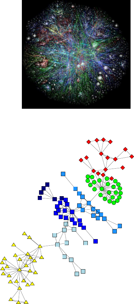
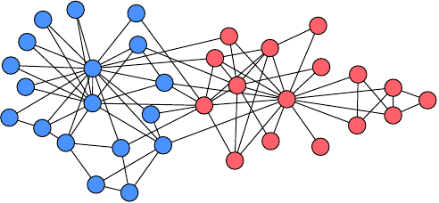
munities,clusters or modules. In Fig. 2we show a col-
laboration network of scientists working at the Santa Fe
Institute (SFI) in Santa Fe, New Mexico. Vertices are
scientists, edges join coauthors. Edges are concentrated
within groups of vertices representing scientists working
on the same research topic, where collaborations are more
natural. Likewise, communities could represent proteins
with similar function in protein-protein interaction net-
works, groups of friends in social networks, websites on
1There may be connections between three vertices or more. In this
case one speaks of hyperedges and the network is a hypergraph.
arXiv:1608.00163v2 [physics.soc-ph] 3 Nov 2016
2
FIG. 1 Internet network. Reprinted figure with permission
from www.opte.org.
Agent-based
Mathematical
Statistical Physics
Ecology
Models
Structure of RNA
FIG. 2 Collaboration network of scientists working at the
Santa Fe Institute (SFI). Edges connect scientists that have
coauthored at least one paper. Symbols indicate the research
areas of the scientists. Naturally, there are more edges be-
tween scholars working on the same area than between schol-
ars working in different areas. Reprinted figure with per-
mission from (Girvan and Newman,2002). c
2002, by the
National Academy of Sciences, USA.
similar topics on the Web graph, and so on.
Identifying communities may offer insight on how the
network is organised. It allows us to focus on regions hav-
ing some degree of autonomy within the graph. It helps
to classify the vertices, based on their role with respect to
the communities they belong to. For instance we can dis-
tinguish vertices totally embedded within their clusters
from vertices at the boundary of the clusters, which may
act as brokers between the modules and, in that case,
could play a major role both in holding the modules to-
gether and in the dynamics of spreading processes across
the network.
Community detection in networks, also called graph
or network clustering, is an ill-defined problem though.
There is no universal definition of the objects that one
should be looking for. Consequently, there are no clear-
cut guidelines on how to assess the performance of dif-
ferent algorithms and how to compare them with each
other. On the one hand, such ambiguity leaves a lot of
freedom to propose diverse approaches to the problem,
which often depend on the specific research question and
(or) the particular system at study. On the other hand, it
has introduced a lot of noise into the field, slowing down
progress. In particular, it has favoured the diffusion of
questionable concepts and convictions, on which a large
number of methods are based.
This work presents a critical analysis of the problem of
community detection, intended to practitioners but ac-
cessible to readers with basic notions of network science.
It is not meant to be an exhaustive survey. The focus
is on the general aspects of the problem, especially in
the light of recent findings. Also, we discuss some popu-
lar classes of algorithms and give advice on their usage.
More info on network clustering can be found in several
review articles (Chakraborty et al.,2016;Coscia et al.,
2011;Fortunato,2010;Malliaros and Vazirgiannis,2013;
Newman,2012;Parthasarathy et al.,2011;Porter et al.,
2009;Schaeffer,2007;Xie et al.,2013).
The contents are organised in three main sections. Sec-
tion II deals with the concept of community, describing
its evolution from the classic subgraph-based notions to
the modern statistical interpretation. Next we discuss
the critical issue of validation (Section III), emphasising
the role of artificial benchmarks, the importance of the
choice of partition similarity scores, the conditions under
which clusters are detectable, the usefulness of metadata
and the structural peculiarities of communities in real
networks. Section IV hosts a critical discussion of some
popular clustering approaches. It also tackles important
general methodological aspects, such as the determina-
tion of the number of clusters, which is a necessary input
for several techniques, the possibility to generate robust
solutions by combining multiple partitions, the main ap-
proaches to discover dynamic communities, as well as the
assessment of the significance of clusterings. In Section V
we indicate where to find useful software. The concluding
remarks of Section VI close the work.
3
II. WHAT ARE COMMUNITIES?
A. Variables
We start with a subgraph Cof a graph G. The number
of vertices and edges are n,mfor Gand nC,mCfor C,
respectively. The adjacency matrix of Gis A, its element
Aij equals 1 if vertices iand jare neighbours, otherwise
it equals 0. We assume that the subgraph is connected
because communities usually are2. Other types of group
structures do not require connectedness (Section II.C).
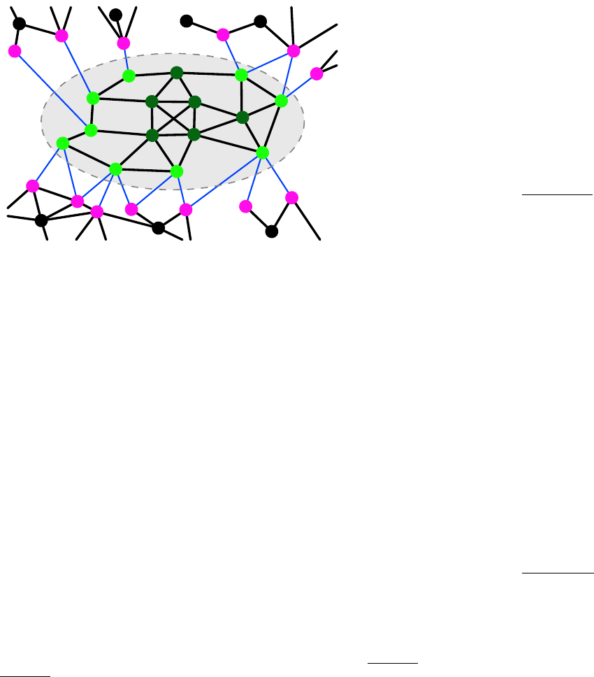
The subgraph is schematically illustrated in Fig. 3. Its
FIG. 3 Schematic picture of a connected subgraph.
vertices are enclosed by the dashed contour. The ma-
genta dots are the external vertices connected to the sub-
graph, while the black ones are the remaining vertices of
the network. The blue lines indicate the edges connecting
the subgraph to the rest of the network.
The internal and external degree kint
iand kext
iof a
vertex iof the network with respect to subgraph Care
the number of edges connecting ito vertices of Cand
to the rest of the graph, respectively. Both definitions
can be expressed in compact form via the adjacency ma-
trix A:kint
i=Pj∈CAij and kext
i=Pj /∈CAij , where
the sums run over all vertices jinside and outside C,
respectively. Naturally, the degree kiof iis the sum of
kint
iand kext
i:ki=PjAij . If kext
i= 0 and kint
i>0i
has neighbours only within Cand is an internal vertex
of C(dark green dots in the figure). If kext
i>0 and
kint
i>0ihas neighbours outside Cand is a boundary
vertex of C(bright green dots in the figure). If kint
i= 0,
instead, the vertex is disjoint from C. The embeddedness
ξiis the ratio between the internal degree and the de-
gree of vertex i:ξi=kint
i/ki. The larger ξi, the stronger
2The variables defined in this section hold for any subgraph, con-
nected or not.
the relationship between the vertex and its community.
The mixing parameter µiis the ratio between the exter-
nal degree and the degree of vertex i:µi=kext
i/ki. By
definition, µi= 1 −ξi.
Now we present a number of variables related to the
subgraph as a whole. We distinguish them in three
classes.
The first class comprises measures based on internal
connectedness, i. e., on how cohesive the subgraph is.
The main variables are:
•Internal degree kint
C. The sum of the internal de-
grees of the vertices of C. It equals twice the
number mCof internal edges, as each edge con-
tributes two units of degree. In matrix form,
kint
C=Pi,j∈CAij .
•Average internal degree kavg-int
C. Average degree
of vertices of C, considering only internal edges:
kavg−int
C=kint
C/nC.
•Internal edge density δint
C. The ratio between the
number of internal edges of Cand the number of
all possible internal edges:
δint
C=kint
C
nC(nC−1).(1)
We remark that nC(nC−1)/2 is the maximum
number of internal edges that a simple graph with
nCvertices may have3.
The second class includes measures based on external
connectedness, i. e., on how embedded the subgraph is in
the network or, equivalently, how separated the subgraph
is from it. The main variables are:
•External degree, or cut,kext
C. The sum of the exter-
nal degrees of the vertices of C. It gives the num-
ber of external edges of the subgraph (blue lines in
Fig. 3). In matrix form, kext
C=Pi∈C,j /∈CAij .
•Average external degree, or expansion,kavg-ext
C. Av-
erage degree of vertices of C, considering only ex-
ternal edges: kavg−ext
C=kext
C/nC.
•External edge density, or cut ratio,δext
C. The ratio
between the number of external edges of Cand the
number of all possible external edges:
δext
C=kext
C
nC(n−nC).(2)
Finally, we have hybrid measures, combining internal
and external connectedness. Notable examples are:
3A simple graph has at most one edge running between any pair
of vertices and no self-loops, i. e., no edges connecting a vertex
to itself.
4
Unweighted networks Weighted networks
Name Symbol Definition Name Symbol Definition
Internal degree kint
iPj∈CAij Internal strength wint
iPj∈CWij
External degree kext
iPj /∈CAij External strength wext
iPj /∈CWij
Degree kiPjAij Strength wiPjWij
Embeddedness ξikint
i
kiWeighted embeddedness ξw
i
wint
i
wi
Mixing parameter µikext
i
kiWeighted mixing parameter µw
i
wext
i
wi
TABLE I Basic vertex community variables, for unweighted and weighted networks. Aand Ware the adjacency and the weight matrix, respectively.
Unweighted networks Weighted networks
Name Symbol Definition Name Symbol Definition
Internal degree kint
CPi,j∈CAij Internal strength wint
CPi,j∈CWij
Average internal degree kavg-int
C
kint
C
nCAverage internal strength wavg-int
C
wint
C
nC
Internal
Internal edge density δint
C
kint
C
nC(nC−1) Internal weight density δint
w,C
wint
C
¯wnC(nC−1)
External degree kext
CPi∈C,j /∈CAij External strength wext
CPi∈C,j /∈CWij
Average external degree kavg-ext
C
kext
C
nCAverage external strength wavg-ext
C
wext
C
nC
External
External edge density δext
C
kext
C
nC(n−nC)External weight density δext
w,C
wext
C
¯wnC(n−nC)
Total degree kCPi∈C,j Aij Total strength wCPi∈C,j Wij
Average degree kavg
C
kC
nCAverage strength wavg
C
wC
nC
Total
Conductance CCkext
C
kCWeighted conductance Cw,C wext
C
wC
TABLE II Basic community variables, for unweighted and weighted networks. Aand Ware the adjacency and the weight matrix, respectively, nCthe number of
vertices of the community, nthe total number of vertices of the graph, ¯wthe average weight of the network edges.
5
•Total degree, or volume,kC. The sum of the degrees
of the vertices of C. Naturally, kC=kint
C+kext
C.
In matrix form, kC=Pi∈C,j Aij .
•Average degree kavg
C. Average degree of vertices of
C:kavg
C=kC/nC.
•Conductance CC. The ratio between the external
degree and the total degree of C:
CC=kext
C
kC
.(3)
All definitions we have given hold for the case of
undirected and unweighted networks. The extension to
weighted graphs is straightforward, as it suffices to re-
place the “number of edges” with the sum of the weights
carried by every edge. For instance, the internal degree
kint
vof a vertex vbecomes the internal strength wint
v,
which is the sum of the weights of the edges joining v
with the vertices of subgraph C. For the internal and ex-
ternal edge densities of Eqs. (1) and (2) one would have
to replace the numerators with their weighted counter-
parts and multiply the denominators by the average edge
weight ¯w=Pij Wij /2m, where Wij is the element of the
weight matrix, indicating the weight of the edge joining
vertices iand j(Wij = 0 if iand jare disconnected) and
mthe total number of graph edges. In Tables Iand II
we list all variables we have presented along with their
extensions to the case of weighted networks. In directed
networks one would have to distinguish between incoming
and outgoing edges. Extensions of the metrics are fairly
simple to implement, though their usefulness is unclear.
B. Classic view
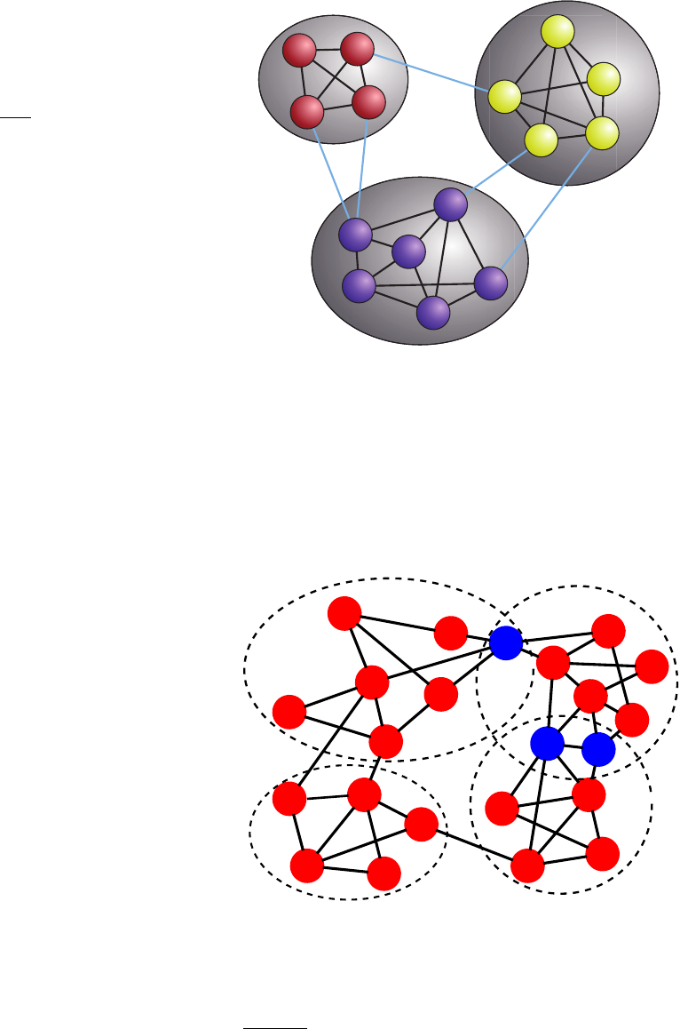
Figure 4shows how scholars usually envision commu-
nity structure. The network has three clusters and in
each cluster the density of edges is comparatively higher
than the density of edges between the clusters. This can
be summarised by saying that communities are dense
subgraphs which are well separated from each other. This
view has been challenged, recently (Jeub et al.,2015;
Leskovec et al.,2009), as we shall see in Section III.E.
Communities may overlap as well, sharing some of the
vertices. For instance, in social networks individuals can
belong to different circles at the same time, like fam-
ily, friends, work colleagues. Figure 5shows an example
of a network with overlapping communities. Commu-
nities are typically supposed to be overlapping at their
boundaries, as in the figure. Recent results reveal a dif-
ferent picture, though (Yang and Leskovec,2014) (Sec-
tion III.E). A subdivision of a network into overlapping
communities is called cover and one speaks of soft clus-
tering, as opposed to hard clustering, which deals with
divisions into non-overlapping groups, called partitions.
The generic term clustering can be used to indicate both
types of subdivisions. Covers can be crisp, when shared
vertices belong to their communities with equal strength,
or fuzzy, when the strength of their membership can be
different in different clusters4.
FIG. 4 Classic view of community structure. Schematic pic-
ture of a network with three communities.
The oldest definitions of community-like objects were
proposed by social network analysts and focused on the
internal cohesion among vertices of a subgraph (Moody
and White,2003;Scott,2000;Wasserman and Faust,
FIG. 5 Overlapping communities. A network is divided in
four communities, enclosed by the dashed contours. Three of
them share boundary vertices, indicated by the blue dots.
4In the literature the word fuzzy is often used to describe both
situations.
6
1994). The most popular concept is that of clique (Luce
and Perry,1949). A clique is a complete graph, that is,
a subgraph such that each of its vertices is connected to
all the others. It is also a maximal subgraph, meaning
that it is not included in a larger complete subgraph. In
modern network science it is common to call clique any
complete graph, not necessarily maximal. Triangles are
the simplest cliques. Finding cliques is an NP-complete
problem (Bomze et al.,1999); a popular technique is the
Bron–Kerbosch method (Bron and Kerbosch,1973).
The notion of cliques, albeit useful, cannot be consid-
ered a good candidate for a community definition. While
a clique has the largest possible internal edge density,
as all internal edges are present, communities are not
complete graphs, in general. Moreover, all vertices have
identical role in a clique, while in real network communi-
ties some vertices are more important than others, due to
their heterogeneous linking patterns. Therefore, in social
network analysis the notion has been relaxed, generat-
ing the related concepts of n-cliques (Alba,1973;Luce,
1950), n-clans and n-clubs (Mokken,1979). Other defi-
nitions are based on the idea that a vertex must be ad-
jacent to some minimum number of other vertices in the
subgraph. A k-plex is a maximal subgraph in which each
vertex is adjacent to all other vertices of the subgraph ex-
cept at most kof them (Seidman and Foster,1978). De-
tails on the above definitions can be found in specialised
books (Scott,2000;Wasserman and Faust,1994).
For a proper community definition, one should take
into account both the internal cohesion of the candidate
subgraph and its separation from the rest of the net-
work. A simple idea that has received a great popularity
is that a community is a subgraph such that “the num-
ber of internal edges is larger than the number of external
edges”5. This idea has inspired the following definitions.
An LS-set (Luccio and Sami,1969), or strong commu-
nity (Radicchi et al.,2004), is a subgraph such that the
internal degree of each vertex is greater than its external
degree. A relaxed condition is that the internal degree
of the subgraph exceeds its external degree [weak com-
munity (Radicchi et al.,2004)]6. A strong community is
also a weak community, while the converse is not gener-
ally true.
A drawback of these definitions is that one separates
the subgraph at study from the rest of the network, which
is taken as a single object. But the latter can be in turn
divided into communities. If a subgraph Cis a proper
community, it makes sense that each of its vertices is
5Here we focus on the case of unweighted graphs, extensions of
all definitions to the weighted case are immediate.
6The definition of weak community is the natural implementation
of the na¨ıve expectation that there must be more edges inside
than outside. However, for a subgraph Cto be a weak commu-
nity it is not necessary that the number of internal edges mC
exceeds that of external edges kext
C. Since the internal degree
kint
C= 2mC(Section II.A) the actual condition is 2mC> kext
C.
more strongly attached to the vertices of Cthan to the
vertices of any other subgraph. This concept, proposed
by Hu et al. (Hu et al.,2008), is more in line (though
not entirely) with the modern idea of community that
we discuss in the following section. It has generated two
alternative definitions of strong and weak community. A
subgraph Cis a strong community if the internal degree
of any vertex within Cexceeds the internal degree of
the vertex within any other subgraph, i. e., the num-
ber of edges joining the vertex to those of the subgraph;
likewise, a community is weak if its internal degree ex-
ceeds the (total) internal degree of its vertices within ev-
ery other community. A strong (weak) community `a la
Radicchi et al. is a strong (weak) community also in the
sense of Hu et al.. The opposite is not true, in general
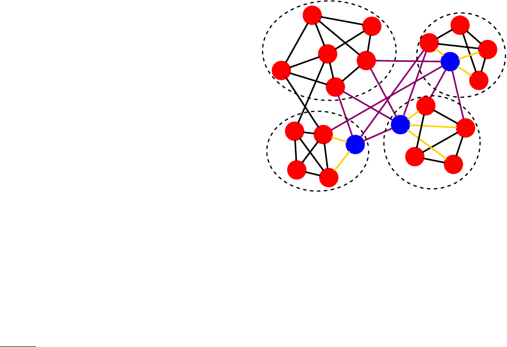
(Fig. 6). In particular, a subgraph can be a strong com-
munity in the sense of Hu et al. even though all of its
vertices have internal degree smaller than their respective
external degree.
FIG. 6 Strong and weak communities. The four subgraphs
enclosed in the contours are weak communities according to
the definitions of Radicchi et al. (Radicchi et al.,2004) and
Hu et al. (Hu et al.,2008). They are also strong communities
according to Hu et al., as the internal degree of each vertex ex-
ceeds the number of edges joining the vertex with the vertices
of every other subgraph. However, three of the subgraphs are
not strong communities according to Radicchi et al., as some
vertices (indicated in blue) have external degree larger than
their internal degree (the internal and external edges of these
vertices are coloured in yellow and magenta, respectively).
The above definitions of communities use extensive
variables: their value tends to be the larger, the bigger
the community (e. g., the internal and external degrees).
But there are also variables discounting community size.
An example is the internal cluster density δint(C) of
Eq. (1). One could assume that a subgraph Cwith k
vertices is a cluster if δint(C) is larger than a threshold
ξ. Setting the size of the subgraph is necessary because
otherwise any clique would be among the best possible
7
communities, including trivial two-cliques (simple edges)
or triangles.
C. Modern view
As we have seen in the previous section, traditional def-
initions of community rely on counting edges (internal,
external), in various ways. But what one should be re-
ally focusing on is the probability that vertices share edges
with a subgraph. The existence of communities implies
that vertices interact more strongly with the other mem-
bers of their community than they do with vertices of
the other communities. Consequently, there is a prefer-
ential linking pattern between vertices of the same group.
This is the reason why edge densities end up being higher
within communities than between them. We can formu-
late that by saying that vertices of the same community
have a higher probability to form edges with their part-
ners than with the other vertices.
Let us suppose that we estimated the edge probabili-
ties between all pairs of vertices, somehow. We can de-
fine the groups by means of those probabilities. It is a
scenario similar to the classic one we have seen in Sec-
tion II.B, where we add and compare probabilities, in-
stead of edges. Natural definitions of strong and weak
community are:
•Astrong community is a subgraph each of whose
vertices has a higher probability to be linked to ev-
ery vertex of the subgraph than to any other vertex
of the graph.
•Aweak community is a subgraph such that the av-
erage edge probability of each vertex with the other
members of the group exceeds the average edge
probability of the vertex with the vertices of any
other group7.
The difference between the two definitions is that, in
the concept of strong community, the inequality between
edge probabilities holds at the level of every pair of ver-
tices, while in the concept of weak community the in-
equality holds only for averages over groups. Therefore,
a strong community is also a weak community, but the
opposite is not true, in general.
Now we can see why the former definitions of strong
and weak community (Hu et al.,2008;Radicchi et al.,
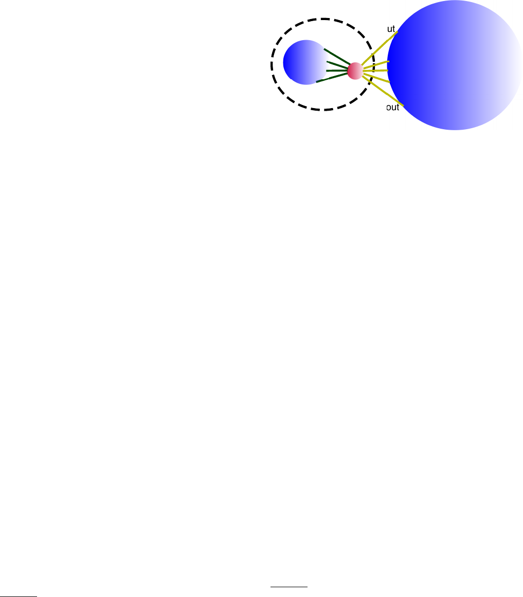
2004) are not satisfactory. Suppose to have a network
with two subgraphs Aand Bof very different sizes, say
with nAand nBnAvertices (Fig. 7). The network
is generated by a model where the edge probability is
7Since we are comparing average probabilities, which come with
a standard error, the definition of weak community should not
rely on the simple numeric inequality between the averages, but
on the statistical significance of their difference. Significance will
be discussed in Section IV.I.
pin
pin
po
po
AB
FIG. 7 Problems of the classic notions of strong and weak
communities. A network is generated by the illustrated
model, with two subgraphs Aand Band edge probabilities
pin between vertices of the subgraphs and pout < pin between
vertices of Aand B. The red circle is a representative vertex
of subgraph A, the smaller blue circle represents the rest of
the vertices of A. The subgraphs are both strong and weak
communities in the probabilistic sense, but they may be nei-
ther strong nor weak communities according to the classic
definitions by Radicchi et al. (Radicchi et al.,2004) and Hu
et al. (Hu et al.,2008), if Bis sufficiently larger than A.
pin between vertices of the same group and pout < pin
for vertices of different groups. The two subgraphs are
communities both in the strong and in the weak sense,
according to the probability-based definitions above. The
expected internal degree of a vertex of Ais kint
A=pinnA:
since there are nApossible internal neighbours8. Like-
wise, the expected external degree of a vertex of Ais
kext
A=poutnB. The expected internal and external de-
grees of Aare Kint
A=pinn2
Aand Kext
A=poutnAnB. For
any two values of pin and pout < pin one can always
choose nBsufficiently larger than nAthat kint
A< kext
A,
which also implies that Kint
A< Kext
A. In this setting
the subgraphs are neither strong nor weak communities,
according to the definitions proposed by Radicchi et al.
and Hu et al..
How can we compute the edge probabilities between
vertices? This is still an ill-defined problem, unless one
has a model stating how edges are formed. One can make
many hypotheses on the process of edge formation. For
instance, if we take social networks, we can assume that
the probability that two individuals know each other is
a decreasing function of their geographical distance, on
average (Liben-Nowell et al.,2005). Each set of assump-
8The number of possible community neighbours should actually
be nA−1, but for simplicity one allows for the formation of self-
edges, from a vertex to itself. Results obtained with and without
self-edges are basically undistinguishable, when community sizes
are much larger than one. We shall stick to this setup throughout
the paper.
8
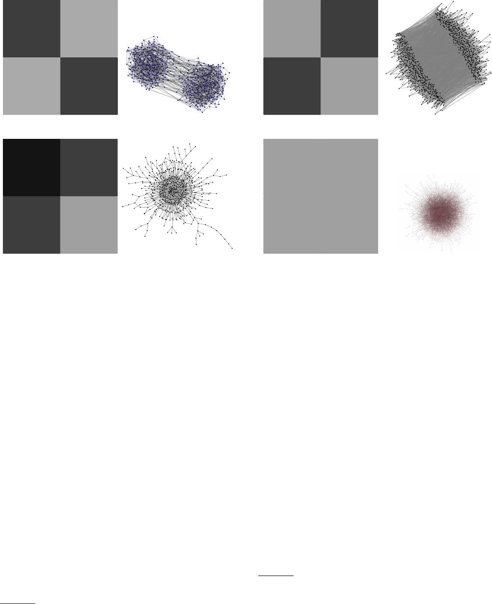
(a) Community structure (b) Disassortative structure
(c) Core-periphery structure (d) Random graph
FIG. 8 Stochastic block model. We show the schematic adjacency matrices of network realisations produced by the model for
special choices of the edge probabilities, along with one representative realisation for each case. For simplicity we show the case
of two blocks of equal size. Darker blocks indicate higher edge probabilities and consequently a larger density of edges inside
the block. Figure 8a illustrates community (or assortative) structure: the probabilities (link densities) are much higher inside
the diagonal blocks than elsewhere. Figure 8b shows the opposite situation (disassortative structure). Figure 8c illustrates a
core-periphery structure. Figure 8d shows a random graph `a la Erd˝os and R´enyi: all edge probabilities are identical, inside
and between the blocks, so there are no actual groups. Adapted figure with permission from (Jeub et al.,2015). c
2015, by
the American Physical Society.
tions defines a model. For our purposes, eligible models
should take into account the possible presence of groups
of vertices, that behave similarly.
The most famous model of networks with group struc-
ture is the stochastic block model (SBM) (Fienberg and
Wasserman,1981;Holland et al.,1983;Snijders and Now-
icki,1997). Suppose we have a network with nvertices,
divided in qgroups. The group of vertex iis indicated
with the integer label gi= 1,2, . . . , q. The idea of the
model is very simple: the probability P(i↔j) that
vertices iand jare connected depends exclusively on
their group memberships: P(i↔j) = pgigj. There-
fore, it is identical for any iand jin the same groups.
The probabilities pgigjform a q×qsymmetric matrix9,
called the stochastic block matrix. The diagonal elements
pkk (k= 1,2, . . . , q) of the stochastic block matrix are
the probabilities that vertices of block kare neighbours,
9For directed graphs, the matrix is in general asymmetric. The
extension of the stochastic block model to directed graphs is
straightforward. Here we focus on undirected graphs.
whereas the off-diagonal elements give the edge probabil-
ities between different blocks10.
For pkk > plm,∀k, l, m = 1,2, . . . , q, with l6=m, we
recover community structure, as the probabilities that
vertices of the same group are connected exceed the
probabilities that vertices of different groups are joined
(Fig. 8a). It is also called assortative structure, as it priv-
ileges bonds between vertices of the same group. The
model is very versatile, though, and can generate vari-
ous types of group structure. For pkk < plm,∀k, l, m =
1,2, . . . , q, with l6=m, we have disassortative struc-
ture, as edges are more likely between the blocks than
inside them (Fig. 8b). In the special case in which
pkk = 0,∀k= 1,2, . . . , q we recover multipartite struc-
10 In another definition of SBM the number of edges ers between
blocks rand sis fixed (r, s = 1,2,...,q), instead of the edge
probabilities. If ers 1,∀r, s = 1,2,...,q the two models are
fully equivalent if the edge probabilities prs are chosen such that
the expected number of edges running between rand scoincides
with ers.

9
ture, as there are edges only between the blocks. If
q= 2, p11 p12 p22, we have core-periphery struc-
ture: the vertices of the first block (core) are relatively
well-connected amongst themselves as well as to a periph-
eral set of vertices that interact very little amongst them-
selves (Fig. 8c). If all probabilities are equal, pij =p,
∀i, j, we recover the classic random graph `a la Erd˝os and
R´enyi (Erd¨os and R´enyi,1959;Erd¨os and R´enyi,1960)
(Fig. 8d). Here any two vertices have identical probabil-
ity of being connected, hence there is no group structure.
This has become a fundamental axiom in community de-
tection, and has inspired some popular techniques like,
e. g., modularity optimisation (Newman,2004b;New-
man and Girvan,2004) (Section IV.F). Random graphs
of this type are also useful in the validation of clustering
algorithms (Section III.A).
Alternative community definitions are based on the in-
terplay between network topology and dynamics. Diffu-
sion is the most used dynamics. Random walks are the
simplest diffusion processes. A simple random walk is a
path such that the vertex reached at step tis a random
neighbour of the vertex reached at step t−1. A ran-
dom walker would be spending a long time within com-
munities, due to the supposedly low number of routes
taking out of them (Delvenne et al.,2010;Rosvall and
Bergstrom,2008;Rosvall et al.,2014). The evolution
of random walks does not depend solely on the number
or density of edges, in general, but also on the structure
and distribution of paths formed by consecutive edges, as
paths are the routes that walkers can follow. This means
that random walk dynamics relies on higher-order struc-
tures than simple edges, in general. Such relationship
is even more pronounced when one considers Markov dy-
namics of second order or higher, in which the probability
of reaching a vertex at step t+ 1 of the walk does not
depend only on where the walker sits at step t, but also
on where it was at step t−1 and possibly earlier (Pers-
son et al.,2016;Rosvall et al.,2014). Indeed, one could
formulate the network clustering problem by focusing on
higher order structures, like motifs (e. g., triangles) (Are-
nas et al.,2008a;Benson et al.,2016;Serrour et al.,2011).
The advantage is that one can preserve more complex fea-
tures of the network and its communities, which typically
get lost when one uses network models solely based on
edge probabilities, like SBMs11. The drawback is that
calculations become more involved and lengthy.
Is a definition of community really necessary? Actu-
ally not, most techniques to detect communities in net-
works do not require a precise definition of community.
The problem can be attacked from many angles. For in-
stance, one can remove the edges separating the clusters
from each other, that can be identified via some partic-
11 Since edges are usually placed independently of each other in
SBMs, higher order structures like triangles are usually under-
represented in the model graphs with respect to the actual graph
at study.
ular feature (Girvan and Newman,2002;Radicchi et al.,
2004). But defining clusters beforehand is a useful start-
ing point, that allows one to check the reliability of the
final results.
III. VALIDATION
In this section we will discuss the crucial issue of
validation of clustering algorithms. Validation usually
means checking how precisely algorithms can recover
the communities in benchmark networks, whose commu-
nity structure is known. Benchmarks can be computer-
generated, according to some model, or actual networks,
whose group structure is supposed to be known via non-
topological features (metadata). The lack of a universal
definition of communities makes the search for bench-
marks rather arbitrary, in principle. Nevertheless, the
best known artificial benchmarks are based on the mod-
ern definition of clusters presented in Section II.C.
We shall present some popular artificial benchmarks
and show that partition similarity measures have to be
handled with care. We will see under which conditions
communities are detectable by methods, and expose the
interplay between topological information and metadata.
We will conclude by presenting some recent results on
signatures of community structure extracted from real
networks.
A. Artificial benchmarks
The principle underneath stochastic block models (Sec-
tion II.C) has inspired many popular benchmark graphs
with group structure. Community structure is recovered
in the case in which the probability for two vertices to
be joined is larger for vertices of the same group than for
vertices of different groups (Fig. 8a). For simplicity, let us
suppose that there are only two values of the edge prob-
ability, pin and pout < pin, for edges within and between
communities, respectively. Furthermore, we assume that
all communities have identical size nc, so qnc=n, where
qis the number of communities. In this version, the
model coincides with the planted l-partition model, in-
troduced in the context of graph partitioning12 (Bui
et al.,1987;Condon and Karp,2001;Dyer and Frieze,
1989). The expected internal and external degrees of
a vertex are hkini=pinncand hkouti=poutnc(q−1),
12 Graph partitioning means dividing a graph in subgraphs, such
to minimise the number of edges joining the subgraphs to each
other. It is related to community detection, as it aims at finding
the minimum separation between the parts. However, it usually
does not consider how cohesive the parts are (number or density
of internal edges), except when special measures are used, like
conductance [Eq. (3)].
10
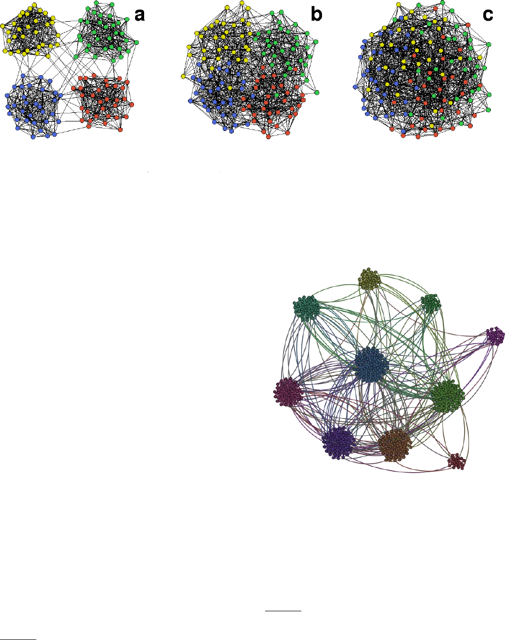
FIG. 9 Benchmark of Girvan and Newman. The three networks correspond to realisations of the model for hkouti= 1 (a),
hkouti= 5 (b) and hkouti= 8 (c). In (c) the four groups are hardly distinguishable by eye and methods fail to assign many
vertices to their groups. Reprinted figure with permission from Ref. (Guimer`a and Amaral,2005). c
2005, by the Nature
Publishing Group.
respectively, yielding an expected (total) vertex degree
hki=hkini+hkouti=pinnc+poutnc(q−1).
Girvan and Newman (Girvan and Newman,2002) set
q= 4, nc= 32 (for a total number of vertices n= 128)
and fixed the average total degree hkito 16. This implies
that pin + 3pout = 1/2 and pin and pout are not indepen-
dent parameters. The benchmark by Girvan and New-
man is still the most popular in the literature (Fig. 9).
Performance plots of clustering algorithms typically
have, on the horizontal axis, the expected external de-
gree hkouti. For low values of hkouticommunities are
well separated13 and most algorithms do a good job at
detecting them. By increasing hkouti, the performance
declines. Still, one expects to do better than by assign-
ing memberships to the vertices at random, as long as
pin > pout, which means for hkouti<12. In Section III.C
we will see that the actual threshold is lower, due to ran-
dom fluctuations.
The benchmark by Girvan and Newman, however,
is not a good proxy of real networks with community
structure. For one thing, all vertices have equal degree,
whereas the degree distribution of real networks is usu-
ally highly heterogeneous (Albert et al.,1999). In ad-
dition, most clustering techniques find skewed distribu-
tions of community sizes (Clauset et al.,2004;Danon
et al.,2007;Lancichinetti et al.,2010;Newman,2004a;
Palla et al.,2005;Radicchi et al.,2004). For this reason,
Lancichinetti, Fortunato and Radicchi proposed the LFR
benchmark, having power-law distributions of degree and
community size (Lancichinetti et al.,2008) (Fig. 10).
The mixing parameters µiof the vertices (Section II.A)
13 They are also more cohesive internally, since hkiniis higher, to
keep the total degree constant.
FIG. 10 LFR benchmark. Vertex degree and community size
are power-law distributed, to account for the heterogeneity
observed in real networks with community structure.
are set equal to a constant µ, which estimates the quality
of the partition14. LFR benchmark networks are built
14 The parameter µis actually only the average of the mixing pa-
rameter over all vertices. In fact, since degrees are integer, it is
impossible to tune them such to have exactly the same value of
µfor each vertex, and keep the constraint on the degree distri-
bution at the same time.

11
by joining stubs at random, once one has established
which stubs are internal and which ones are external
with respect to the community of the vertex attached
to the stubs. In this respect, it is basically a configura-
tion model (Bollob´as,1980;Molloy and Reed,1995) with
built-in communities.
Clearly, when µis low, clusters are better separated
from each other, and easier to detect. When µgrows, per-
formance starts to decline. But for which range of µcan
we expect a performance better than random guessing?
Let us suppose that the group structure is detectable
for µ∈[0, µc]. The upper limit µcshould be such that
the network is random for µ=µc. The network is ran-
dom when stubs are combined at random, without dis-
tinguishing between internal and external stubs, which
yields the standard configuration model. There the ex-
pected number of edges between two vertices with de-
grees kiand kjis kikj/(2m), mbeing the total number
of network edges. Let us focus on a generic vertex i,
belonging to community C. We denote with KCand
˜
KCthe sum of the degrees of the vertices inside and
outside C, respectively. Clearly KC+˜
KC= 2m. In a
random graph built with the configuration model, vertex
iwould have an expected internal degree15 kint-rand
i=
ki(KC−ki)/(2m)≈kiKC/(2m) and an expected exter-
nal degree kext-rand
i=ki˜
KC/(2m). Since, by construc-
tion, kint
i= (1 −µ)kiand kext
i=µki, the community C
is not real when kext
i=kext-rand
iand kint
i=kint-rand
i,
which implies µ=µC=˜
KC/(2m)=1−KC/(2m). We
see that KCdepends on the community C: the larger
the community, the lower the threshold is. Therefore,
not all clusters are detectable at the same time, in gen-
eral. For this to happen, µmust be lower than the mini-
mum of µCover all communities: µ≤µc= minCµC. If
communities are all much smaller than the network as a
whole, KC/(2m)≈0 and µccould get very close to the
upper limit 1 of the variable µ. However, it is possible
that the actual threshold is lower than µc, due to the
perturbations of the group structure induced by random
fluctuations (Section III.C). Anyway, in most cases the
threshold is going to be quite a bit higher than 1/2, the
value which is mistakenly considered as the threshold by
some scholars.
The LFR benchmark turns out to be a special ver-
sion of the recently introduced degree-corrected stochas-
tic block model (Karrer and Newman,2011), with the
degree and the block size distributed according to trun-
cated power laws16.
The LFR benchmark has been extended to directed
15 The approximation is justified when the community is large
enough that KCki.
16 In fact, the correspondence is exact for a slightly different
parametrisation of the benchmark, introduced in (Peixoto,2014).
In this version of the model, instead of the mixing parameter µ,
which is local, a global parameter cis used, estimating how strong
the community structure is.
and weighted networks with overlapping communi-
ties (Lancichinetti and Fortunato,2009). The extensions
to directed and weighted graphs are rather straightfor-
ward. Overlaps are obtained by assigning each vertex to
a number of clusters and distributing its internal edges
equally among them17. Recently, another benchmark
with overlapping communities has been introduced by
Ball, Karrer and Newman (Ball et al.,2011). It consists
of two clusters Aand B, with overlap C. Vertices in the
non-overlapping subsets A−Cand B−Cset edges only
between each other, while vertices in Care connected to
vertices of both Aand B. The expected degree of all
vertices is set equal to hki. The authors considered var-
ious settings, by tuning hki, the size of the overlap and
the sizes of Aand B, which may be uneven. However,
the fact that all vertices have equal degree (on average)
makes the model less realistic and flexible than the LFR
benchmark.
Following the increasing availability of evolving time-
stamped network data sets, the analysis and modelling
of temporal networks have received a lot of attention
lately (Holme and Saram¨aki,2012). In particular, schol-
ars have started to deal with the problem of detecting
evolving communities (Section IV.H). A benchmark de-
signed to model dynamic communities was proposed by
Granell et al. (Granell et al.,2015). It is based on
the planted l-partition model, just like the benchmark
of Girvan and Newman, where pin and pout < pin are
the edge probabilities within communities and between
communities, respectively. Communities may grow and
shrink (Fig. 11a), they may merge with each other or
split into smaller clusters (Fig. 11b), or do all of the
above (Fig. 11c). The dynamics unfold such that at each
time the subgraphs are proper communities in the prob-
abilistic sense discussed in Section II.C. In the merge-
split dynamics, clusters actually merge before the inter-
community edge probability pout reaches the value pin
of the intra-community edge probability, due to random
fluctuations (Section III.C).
In Section II.C we have shown why random graphs can-
not have a meaningful group structure18. That means
that they can be employed as null benchmarks, to test
whether algorithms are capable to recognise the absence
of groups. Many methods find non-trivial communities
in such random networks, so they fail the test. We
strongly encourage doing this type of exam on new al-
gorithms (Lancichinetti and Fortunato,2009).
17 A better way to do it would be taking into account the size of
the communities the vertex is assigned to, and divide the edges
proportionally to the (total) degrees of the communities.
18 Here we refer to random graphs where the edge probabilities do
not depend on their membership in groups. Examples are Erd˝os
and R´enyi random graphs, the configuration model, etc..
12
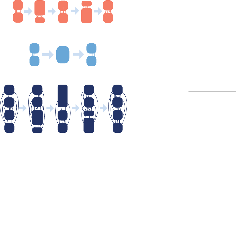
(a) Grow / Shrink
(b) Merge / Split
(c) Mixed
t=0 t=τ/4 t=τ
t=τ/2 t=3τ/4
t=0 t=τ/2 t=τ
t=0 t=τ/4 t=τ/2 t=3τ/4 t=τ
FIG. 11 Dynamic benchmark. (a) Grow-Shrink benchmark.
Starting from two communities of equal size, vertices move
from one cluster to the other and back. (b) Merge-Split bench-
mark. It starts with two communities, edges are added until
there is one community with uniform link density (merge),
then the process is reversed, leading to a fragmentation into
two equal-sized clusters. (c) Mixed benchmark. There are
four communities: the upper pair undergoes the grow-shrink
dynamics of (a), the lower pair the merge-split dynamics of
(b). All processes are periodic with period τ. Reprinted fig-
ure with permission from (Granell et al.,2015). c
2015, by
the American Physical Society.
B. Partition similarity measures
The accuracy of clustering techniques depends on their
ability to detect the clusters of networks, whose com-
munity structure is known. That means that the parti-
tion detected by the method(s) has to match closely the
planted partition of the network. How can the similarity
of partitions be computed? This is an important prob-
lem, with no unique solution. In this section we discuss
some issues about partition similarity measures. More
information can be found in (Meil˘a,2007), (Fortunato,
2010) and (Traud et al.,2011).
Let us consider two partitions X= (X1, X2, ..., XqX)
and Y= (Y1, Y2, ..., YqY) of a network G, with qXand
qYclusters, respectively. Let nbe the total number of
vertices, nX
iand nY
jthe number of vertices in clusters Xi
and Yjand nij the number of vertices shared by clusters
Xiand Yj:nij =|XiTYj|. The qX×qYmatrix NX Y
whose entries are the overlaps nij is called confusion ma-
trix,association matrix or contingency table.
Most similarity measures can be divided in three cate-
gories: measures based on pair counting,cluster matching
and information theory.
Pair counting means computing the number of pairs of
vertices which are classified in the same (different) clus-
ters in the two partitions. Let a11 indicate the number
of pairs of vertices which are in the same community in
both partitions, a01 (a10) the number of pairs of elements
which are in the same community in X(Y) and in differ-
ent communities in Y(X) and a00 the number of pairs of
vertices that are in different communities in both parti-
tions. Several measures can be defined by combining the
above numbers in various ways. A famous example is the
Rand index (Rand,1971)
R(X,Y) = a11 +a00
a11 +a01 +a10 +a00
,(4)
which is the ratio of the number of vertex pairs correctly
classified in both partitions (i. e. either in the same or
in different clusters), by the total number of pairs. An-
other notable option is the Jaccard index (Ben-Hur et al.,
2001),
J(X,Y) = a11
a11 +a01 +a10
,(5)
which is the ratio of the number of vertex pairs classified
in the same cluster in both partitions, by the number
of vertex pairs classified in the same cluster in at least
one partition. The Jaccard index varies over a broader
range than the Rand index, due to the dominance of
a00 in R(X,Y), which typically confines the Rand index
to a small interval slightly below 1. Both measures lie
between 0 and 1.
If we denote with XCand YCthe sets of vertex pairs
with are members of the same community in partitions
Xand Y, respectively, the Jaccard index is just the ra-
tio between the intersection and the union of XCand
YC. Such concept can be used as well to determine the
similarity between two clusters Aand B
JAB =|ATB|
|ASB|.(6)
The score JAB is also called Jaccard index and is the
most general definition of the score, for any two sets A
and B(Jaccard,1901). Measuring the similarity between
communities is very important to determine, given differ-
ent partitions, which cluster of a partition corresponds to
which cluster(s) of the other(s). For instance, the cluster
Yjof Ycorresponding to cluster Xiof Yis the one max-
imising the similarity between Xiand Yj, e. g., JXiYj.
This strategy is also used to track down the evolution
of communities in temporal networks (Lancichinetti and
Fortunato,2012;Palla et al.,2007).
The Rand and the Jaccard indices, as defined in
Eqs. (5) and (6), have the disturbing feature that they do
not take values in the entire range [0,1]. For this reason,
13
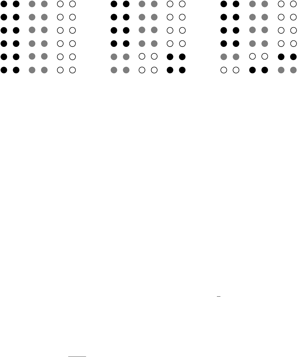
CC' C''
FIG. 12 Partition similarity measures based on cluster matching. There are three partitions in three clusters: C,C0and C00 .
The clusters include all elements of columns 1−2, 3−4 and 5−6, which for Care labelled in black, grey and white, respectively.
Partition C0is obtained from Cby reassigning the same fraction of elements from one cluster to the next, while C00 is derived
from Cby reassigning the same fraction of elements from each cluster equally between the other clusters. From cluster matching
scores one concludes that C0and C00 are equally similar to C, while intuition suggests that C0is closer to Cthan C00. Adapted
figure with permission from (Meil˘a,2007). c
2007, by Elsevier.
adjusted versions of both indices exist, in that a baseline
is introduced, yielding the expected values of the score
for all pairs of partitions ˜
Xand ˜
Yobtained by randomly
assigning vertices to clusters such that ˜
Xand ˜
Yhave the
same number of clusters and the same size for all clus-
ters of Xand Y, respectively (Hubert and Arabie,1985).
The baseline is subtracted from the unadjusted version,
and the result is divided by the range of this difference,
yielding 1 for identical partitions and 0 as expected value
for independent partitions. But there are problems with
these definitions as well. The null model used to compute
the baseline relies on the assumption that the communi-
ties of the independent partitions have the same number
of vertices as in the partitions whose similarity is to be
compared. But such assumption usually does not hold,
in practical instances, as algorithms sometimes need the
number of communities as input, but they never impose
any constraint on the cluster sizes. Adjusted indices have
also the disadvantage of nonlocality (Meil˘a,2005): the
similarity between partitions differing only in one region
of the network depends on how the remainder of the net-
work is subdivided. Moreover, the adjusted scores can
take negative values, when the unadjusted similarity lies
below the baseline.
A better option is to use standardised indices (Brennan
and Light,1974): for a given score Sithe value of the
null model term µiis computed along with its standard
deviation σiover many different randomisations of the
partitions Xand Y. By computing the z-score
zi=Si−µi
σi
,(7)
we can see how non-random the measured similarity score
is, and assess its significance. It can be shown that the z-
scores for the Jaccard, Rand and Adjusted Rand indices
coincide (Traud et al.,2011), so the measures are sta-
tistically equivalent. Since the actual values Siof these
indices differ for the same pair of partitions, in general,
we conclude that the magnitudes of the scores may give
a wrong perception about the effective similarity.
Cluster matching aims at establishing a correspon-
dence between pairs of clusters of different partitions
based on the size of their overlap. A popular measure
is the fraction of correctly detected vertices, introduced
by Girvan and Newman (Girvan and Newman,2002). A
vertex is correctly classified if it is in the same cluster
as at least half of the other vertices in its cluster in the
planted partition. If the detected partition has clusters
given by the merger of two or more groups of the planted
partition, all vertices of those clusters are considered in-
correctly classified. The number of correctly classified
vertices is then divided by the number nof vertices of the
graph, yielding a number between 0 and 1. The recipe
to label vertices as correctly or incorrectly classified is
somewhat arbitrary. The fraction of correctly detected
vertices is similar to
H(X,Y) = 1
nX
k0=match(k)
nkk0,(8)
where k0is the index of the best match Yk0of cluster
Xk(Meil˘a and Heckerman,2001). A common problem
of this type of measures is that partitions whose clusters
have the same overlap would have the same similarity,
regardless of what happens to the parts of the commu-
nities which are unmatched. The situation is illustrated
schematically in Fig. 12. Partitions C0and C00 are ob-
tained from Cby reassigning the same fraction of their
elements to the other clusters. Their overlaps with Care
identical and so are the corresponding similarity scores.
However, in partition C00 the unmatched parts of the clus-
ters are more scrambled than in C0, which should be re-

14
flected in a lower similarity score.
Similarity can be also estimated by computing, given a
partition, the additional amount of information that one
needs to have to infer the other partition. If partitions
are similar, little information is needed to go from one
to the other. Such extra information can be used as a
measure of dissimilarity. To evaluate the Shannon infor-
mation content (Mackay,2003) of a partition, we start
from the community assignments {xi}and {yi}, where
xiand yiindicate the cluster labels of vertex iin par-
tition Xand Y, respectively. The labels xand yare
the values of two random variables Xand Y, with joint
distribution P(x, y) = P(X=x, Y =y) = nxy /n, so
that P(x) = P(X=x) = nX
x/n and P(y) = P(Y=
y) = nY
y/n. The mutual information I(X, Y ) of two
random variables is I(X, Y ) = H(X)−H(X|Y), where
H(X) = −PxP(x) log P(x) is the Shannon entropy of
Xand H(X|Y) = −Px,y P(x, y) log P(x|y) is the condi-
tional entropy of Xgiven Y. The mutual information is
not ideal as a similarity measure: for a given partition X,
all partitions derived from Xby splitting (some of) its
clusters would all have the same mutual information with
X, even though they could be very different from each
other. In this case the mutual information equals the
entropy H(X), because the conditional entropy is zero.
It is then necessary to introduce an explicit dependence
on the other partition, that persists even in those special
cases. This has been achieved by introducing the nor-
malized mutual information (NMI), obtained by dividing
the mutual information by the arithmetic average19 of
the entropies of Xand Y(Fred and Jain,2003)
Inorm(X,Y) = 2I(X, Y )
H(X) + H(Y).(9)
The NMI equals 1 if and only if the partitions are identi-
cal, whereas it has an expected value of 0 if they are inde-
pendent. Since the first thorough comparative analysis of
clustering algorithms (Danon et al.,2005), the NMI has
been regularly used to compute the similarity of parti-
tions in the literature. However, the measure is sensitive
to the number of clusters qYof the detected partition,
and may attain larger values the larger qY, even though
more refined partitions are not necessarily closer to the
planted one. This may give wrong perceptions about the
relative performance of algorithms (Zhang,2015).
A more promising measure, proposed by Meil˘a (Meil˘a,
2007) is the variation of information (VI)
V(X,Y) = H(X|Y) + H(Y|X).(10)
The VI defines a metric in the space of partitions as it
has the properties of distance (non-negativity, symmetry
19 Strehl and Ghosh introduced an earlier definition of NMI, where
the mutual information is divided by the geometric average of
the entropies (Strehl and Ghosh,2002). Alternatively, one could
normalise by the larger of the entropies H(X) and H(Y) (Es-
quivel and Rosvall,2012;McDaid et al.,2011).
and triangle inequality). It is a local measure: the VI
of partitions differing only in a small portion of a graph
depends on the differences of the clusters in that region,
and not on how the rest of the graph is subdivided. The
maximum value of the VI is log n, which implies that the
scores of an algorithm on graphs of different sizes cannot
be compared with each other, in principle. One could di-
vide V(X,Y) by log n(Karrer et al.,2008), to force the
score to be in the range [0,1], but the actual span of val-
ues of the measure depends on the number of clusters of
the partitions. In fact, if the maximum number of com-
munities is q?, with q?≤√n,V(X,Y)≤2 log q?. Con-
sequently, in those cases where it is reasonable to set an
upper bound on the number of clusters of the partitions,
the similarities between planted and detected partitions
on different graphs become comparable, and it is possible
to assess both the performance of an algorithm and to
compare algorithms across different benchmark graphs.
We stress, however, that the measure may not be suitable
when the partitions to be compared are very dissimilar
from each other (Traud et al.,2011) and that it shows un-
intuitive behaviour in particular instances (Delling et al.,
2006).
So far we discussed of comparing partitions. What
about covers? Extensions of the measures we have pre-
sented to the case of overlapping communities are usu-
ally not straightforward. The Omega index (Collins and
Dent,1988) is an extension of the Adjusted Rand in-
dex (Hubert and Arabie,1985). Let Xand Ybe covers of
the same graph to be compared. We denote with ajj the
number of pairs of vertices occurring together in exactly
jcommunities in both covers. It is a natural generali-
sation of the variables a00 and a11 we have seen above,
where jcan also be larger than 1 since a pair of vertices
can now belong simultaneously to multiple communities.
The variable
o(X,Y) = 2
n(n−1) X
j
ajj (11)
is the fraction of pairs of vertices belonging to the same
number of communities in both covers (including the case
j= 0, which refers to the pairs not being in any commu-
nity together). The Omega index is defined as
Ω(X,Y) = o(X,Y)−oe(X,Y)
1−oe(X,Y),(12)
where oe(X,Y) is the expected value of o(X,Y) according
to the null model discussed earlier, in which vertex labels
are randomly reshuffled such to generate covers with the
same number and size of the communities.
The NMI has also been extended to covers by Lan-
cichinetti, Fortunato and Kert´esz (Lancichinetti et al.,
2009). The definition is non-trivial: the community as-
signments of a cover are expressed by a vectorial random
variable, as each vertex may belong to multiple clusters
at the same time. The measure overestimates the sim-
ilarity of two covers, in special situations, where intu-
ition suggests much lower values. The problem can be
15
solved by using an alternative normalisation, as shown
in (McDaid et al.,2011). Unfortunately neither the def-
inition by Lancichinetti, Fortunato and Kert´esz nor the
one by McDaid, Greene and Hurley are proper extensions
of the NMI, as they do not coincide with the classic defi-
nition of Eq. (9) when partitions in non-overlapping clus-
ters are compared. However, the differences are typically
small, and one can rely on them in practice. Esquivel
and Rosvall have proposed an actual extension (Esquivel
and Rosvall,2012). Following the comparative analysis
performed in (Lancichinetti and Fortunato,2009), the
NMI by Lancichinetti, Fortunato and Kert´esz has been
regularly used in the literature, also in the case of regular
partitions, without overlapping communities20.
If covers are fuzzy (Section II.B), the similarity mea-
sures above cannot be used, as they do not take into
account the degree of membership of vertices in the com-
munities they belong to. A suitable option is the Fuzzy
Rand index (H¨ullermeier and Rifqi,2009), which is an
extension of the Adjusted Rand index. Both the Fuzzy
Rand index and the Omega index coincide with the Ad-
justed Rand index when communities do not overlap.
For temporal networks, a na¨ıve approach would be
comparing partitions (or covers) corresponding to con-
figurations of the system in the same time window, and
to see how this score varies across different time windows.
However, this does not tell if the clusters are evolving in
the same way, as there would be no connection between
clusterings at different times. A sensible approach is com-
paring sequences of clusterings, by building a confusion
matrix that takes into account multiple snapshots. This
strategy allows one to define dynamic versions of various
indices, like the NMI and the VI (Granell et al.,2015).
In conclusion, while there is no clear-cut criterion to es-
tablish which similarity measure is best, we recommend
to use measures based on information theory. In par-
ticular, the VI seems to have more potential than oth-
ers, for the reasons we explained, modulo the caveats in
Refs. (Delling et al.,2006;Traud et al.,2011). There are
currently no extensions of the VI to handle the compar-
ison of covers, but it would not be difficult to engineer
one, e. g., by following a similar procedure as in (Lan-
cichinetti et al.,2009;McDaid et al.,2011), though this
might cost the sacrifice of some of its nice features.
One should keep in mind that the choice of one sim-
ilarity index or another is a sensitive one, and warped
conclusions may be drawn when different measures are
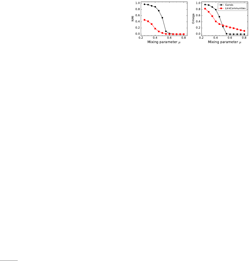
adopted. In Fig. 13 we show the accuracy of two algo-
rithms on the LFR benchmark (Section III.A): Ganxis, a
method based on label propagation (Xie and Szymanski,
2012) and LinkCommunities, a method based on group-
ing edges instead of vertices (Ahn et al.,2010) (Sec-
tion IV.D). The accuracy is estimated with the NMI
20 Recently the NMI has been extended to handle the comparison
of hierarchical partitions as well (Perotti et al.,2015).
by Lancichinetti, Fortunato and Kert´esz (Lancichinetti
et al.,2009) (left diagram) and with the Omega index
[Eq. (12)] (right diagram). From the left plot one would
think that Ganxis clearly outperforms LinkCommunities,
whereas from the right plot Ganxis still prevails for µun-
til about 0.5 (though the curves are closer to each other
than in the NMI plot) and LinkCommunities is better for
larger values of µ.
FIG. 13 Importance of choice of partition similarity measures.
The plots show the comparison between the planted partition
of LFR benchmark graphs and the ones found by two algo-
rithms: Ganxis and LinkCommunities. In the left diagram
similarity was computed with the NMI, in the right one with
the Omega index. The performances of the algorithms appear
much closer when the Omega index is used. The LFR bench-
mark graphs used in the analysis have 1 000 vertices, average
degree 15, maximum degree 50, exponents 2 and 1 for the de-
gree and community size distributions and range [10,50] for
the community size.
C. Detectability
In validation procedures one assumes that, if the net-
work has clusters, there must be a way to identify them.
Therefore, if we do not manage, we have to blame the
specific clustering method(s) adopted. But are we cer-
tain that clusters are always detectable?
Most networks of interest are sparse, i. e., their average
degree is much smaller than the number of vertices. This
means that the number of edges of the graph is much
smaller than the number of possible edges n(n−1)/2.
A more precise way to formulate this is by saying that
a graph is sparse when, in the limit of infinite size, the
average degree of the graph remains finite. A number of
analytical calculations can be carried out by using net-
work sparsity. Many algorithms for community detection
only work on sparse graphs.
On the other hand, sparsity can also give troubles. Due
to the very low density of edges, small amounts of noise
could perturb considerably the structure of the system.
For instance, random fluctuations in sparse graphs could
trick algorithms into finding groups that do not really
exist (Section IV.I). Likewise, they could make actual
groups undetectable. Let us consider the simplest version
of the assortative stochastic block model, which matches
the planted partition model (Section III.A). There are q
communities of the same size n/q, and only two values for
16
the edge probability: pin for pairs of vertices in the same
group and pout for pairs of vertices in different groups.
Since the graphs are sparse, pin and pout vanish in the
limit of infinite graph size. So we shall use the expected
internal and external degrees hkini=npin/q and hkouti=
npout(q−1)/q, which stay constant in that limit. By
construction, the groups are communities so long as pin >
pout or, equivalently, for hkini>hkouti/(q−1). But that
does not mean that they are always detectable.
In principle, dealing with the issue of detectability in-
volves examining all conceivable clustering techniques,
which is clearly impossible. Fortunately, it is not nec-
essary, because we know what model has generated the
communities of the graphs we are considering. The most
effective technique to infer the groups is then fitting the
stochastic block model on the data (a posteriori block
modelling). This can be done via the maximum likelihood
method (Gelman et al.,2014). In recent work (Decelle
et al.,2011), Decelle et al. have shown that, in the limit
of infinite graph size, the partition obtained this way is
correlated with the planted partition whenever
hkini − hkouti
q−1>phkini+hkouti,(13)
which implies
hkini>hkouti
q−1+1
2 1 + s1 + 4qhkouti
q−1!.(14)
So, given a value of hkouti, when hkiniis in the range
hkouti
q−1,hkouti
q−1+1
21 + q1 + 4qhkout i
q−1 the probability
pcof classifying a vertex correctly is not larger than the
probability 1/q of assigning the vertex to a randomly
chosen group, although the groups are communities, ac-
cording to the model. We stress that this result only
holds when the graphs are sparse: if pin and pout remain
non-zero in the large-n limit (dense graph), the classic
detectability threshold pin > pout is correct.
A fortiori, no clustering technique can detect the clus-
ters better than random assignment when the inference
of the model parameters fails to do so. If communities
are searched via the spectral optimisation of Newman-
Girvan’s modularity (Newman,2006), one obtains the
same threshold of Eq. (14) (Nadakuditi and Newman,
2012), provided the network is not too sparse.
For the benchmark of Girvan and Newman (Sec-
tion III.A) (Girvan and Newman,2002) it has long been
unclear where the actual detectability limit sits. Girvan-
Newman benchmark graphs are not infinite, their size
being set to 128, so there is no proper detectability
transition, but rather a smooth crossover from a regime
in which clusters are frequently detectable to a regime
where they are frequently undetectable. For this rea-
son there cannot be a sharp threshold separating the two
regimes. Still it is useful to have an idea of where the
pattern changes. In the following we shall still use the
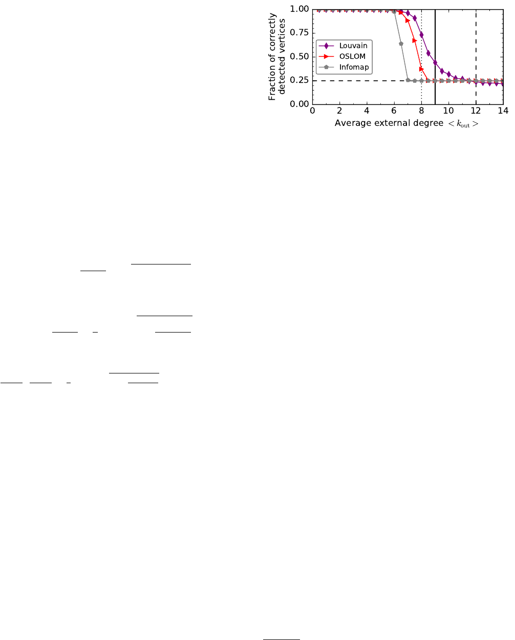
FIG. 14 Detectability of communities. Performances of three
popular algorithms on the benchmark by Girvan and New-
man. The dotted vertical line at hkouti= 8 indicates the
threshold corresponding to the concept of strong community
´a la Radicchi et al., the dashed line at hkouti= 12 the thresh-
old according to the probability-based definition of strong
community we have given in Section II.C. The baseline of
random assignment is 1/4 (horizontal dashed line). All al-
gorithms do not do better than random assignment already
before hkouti= 12. The theoretical detectability limit is at
hkouti= 9, in the limit of groups of infinite size.
term threshold to refer to the crossover point. In the
beginning, scholars thought that clusters are detectable
as long as they satisfy the definition of strong com-
munity by Radicchi et al. (Radicchi et al.,2004) (Sec-
tion II.B), i. e., as long as the expected internal degree
exceeds the expected external degree, yielding a thresh-
old hkini=hkouti(Girvan and Newman,2002). Since
the expected total degree of a vertex is set to 16, com-
munities are detectable as long as hkouti< kstrong
d= 8.
It soon became obvious that the actual threshold should
be the one of the “modern” definition of community we
have presented in Section II.C, according to which the
condition21 is pin > pout, that is hkouti< kstandard
d= 12.
However, numerical calculations reveal that algorithms
tend to fail long before that limit. From Eq. (14) we see
that for the case of four infinite clusters and total ex-
pected degree hktoti= 16, the theoretical detectability
limit is ktheor
d= 9. In Fig. 14 we see the performance
on the benchmark of three well-known algorithms: Lou-
vain (Blondel et al.,2008), a greedy optimisation tech-
nique of Newman–Girvan modularity (Newman and Gir-
van,2004) (Section IV.F); Infomap, which is based on
random walk dynamics (Rosvall and Bergstrom,2008)
(Section IV.G); OSLOM, that searches for clusters via a
local optimisation of a significance score (Lancichinetti
et al.,2011). The accuracy is estimated via the frac-
tion of correctly detected vertices (Section III.B). The
21 In the setting of the Girvan-Newman benchmark, where edge
probabilities are identical for all vertices, the strong and weak
definitions we presented in Section II.C coincide.
17
three thresholds kstrong
d,kstandard
dand ktheor
dare repre-
sented by vertical lines. The performance of all methods
becomes comparable with random assignment well be-
fore kstandard
d. The theoretical limit ktheor
dappears to be
compatible with the performance curves.
Graph sparsity is a necessary condition for clusters to
become undetectable, but it is not sufficient. The sym-
metry of the model we have considered plays a major
role too. Clusters have equal size and vertices have equal
degree. This helps to “confuse” algorithms. If commu-
nities have unequal sizes and the degree of vertices are
correlated with the size of their communities, so that ver-
tices have larger degree, the bigger their clusters, commu-
nity detection becomes easier, as the degrees can be used
as proxy for group membership. In this case, the non-
trivial detectability limit disappears when there are four
clusters or fewer, while it persists up to a given extent
of group size inequality when there are more than four
clusters (Zhang et al.,2016). Other types of block struc-
ture, like core-periphery, do not suffer from detectability
issues (Zhang et al.,2015).
LFR benchmark graphs are more complex models than
the one studied in (Zhang et al.,2016) and it is not clear
whether there is a non-trivial detectability limit, though
it is unlikely, due to the big heterogeneity in the distri-
bution of vertex degree and community size.
D. Structure versus metadata
Another standard way to test clustering techniques is
using real networks with known community structure.
Knowledge about the memberships of the vertices typi-
cally comes from metadata, i. e., non-structural informa-
tion. If vertices are annotated communities are assumed
to be groups of vertices with identical tags. Examples are
user groups in social networks like LiveJournal and prod-
uct categories for co-purchasing networks of products of
online retailers such as Amazon.
In Fig. 15 we show the most popular of such benchmark
graphs, Zachary karate club network (Zachary,1977). It
consists of 34 vertices, the members of a karate club in the
United States, who were observed over a period of three
years. Edges connect individuals interacting outside the
activities of the club. Eventually a conflict between the
club president (vertex 34) and the instructor (vertex 1)
led to the fission of the club in two separate groups, whose
members supported the instructor and the president, re-
spectively (indicated by the colours). Indeed, the groups
make sense topologically: vertices 1 and 34 are hubs, and
most members are directly connected to either of them.
Most algorithms of community detection have been
tested on this network, as well as others, e. g., the Amer-
ican college football network (Evans,2010;Girvan and
Newman,2002) or Lusseau’s network of bottlenose dol-
phins (Lusseau,2003). The idea is that the method doing
the best job at recovering groups with identical annota-
tions would also be the most reliable in applications.
1
2
3
4
5
6
7
8
9
10
11
12
13
14
15
16
17
18
19 20
21
22
23
24
25
26
27
28
29
30
31
32
33
34
FIG. 15 Zachary karate club network. Symbols of different
colours indicate the two groups generated by the fission of
the network, following the disagreement between the club’s
instructor (vertex 1) and its president (34).
Such idea, however, is based on a questionable prin-
ciple, i. e., that the groups corresponding to the meta-
data are also communities in the topological sense we
have discussed in Section II. Communities exist because
their vertices are supposed to be similar to each other,
in some way. The similarity among the vertices is then
revealed topologically through the higher edge probabil-
ity among pairs of members of the same group than be-
tween pairs of members of different groups, whose simi-
larity is lower. Hence, when one is provided with annota-
tions or other sources of information that allows to clas-
sify vertices based on their similarity, one expects that
such similarity-based classes are also the best communi-
ties that structure-based algorithms may detect.
Indeed, for some small networks like Zachary’s karate
club this seems to be the case. But for quite some time
scholars could not test this hypothesis, due to the lim-
ited number of suitable data sets. Over the past few years
this has finally become possible, due to the availability
of several large network data sets with annotated ver-
tices (Hric et al.,2014;Yang and Leskovec,2012a,2013,
2014). It turns out that the alignment between the com-
munities found by standard clustering algorithms and the
annotated groups is not good, in general. In Fig. 16
we show the similarity between the topological parti-
tions found by different methods and the annotated par-
titions, for several social, information and technological
networks (Hric et al.,2014). The heights of the vertical
bars are the values of the normalised mutual information
(NMI) (Lancichinetti et al.,2009). Groups of contiguous
bars represent the scores for a given data set. To the
left of the vertical dashed line we see the results for clas-
sic benchmarks, like LFR graphs (Section III.A) (Lanci-
chinetti et al.,2008), Zachary karate club, etc., and the
scores are generally good. But for the large data sets
to the right of the line the scores are rather low, sig-
nalling a significant mismatch between topological and
annotated communities. For Amazon co-purchasing net-
work (Yang and Leskovec,2012b), in which vertices are
products and edges are set between products often pur-
chased by the same customer(s), the similarity is quite a
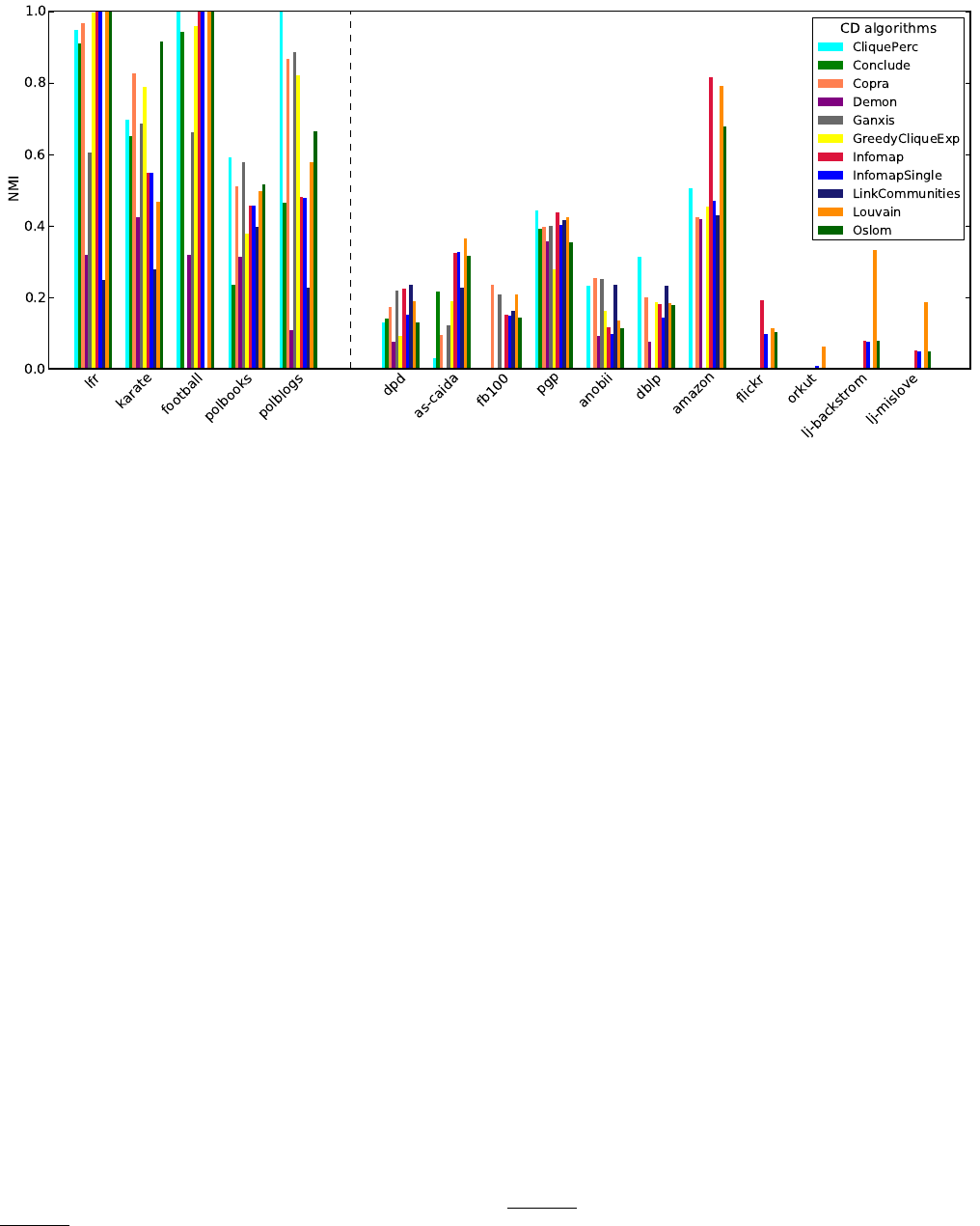
18
FIG. 16 Mismatch between structural communities and metadata groups. The vertical axis reports the similarity between
communities detected via several clustering methods and groups of vertices with identical attributes for several networks,
estimated via the NMI. Scores are grouped by data sets on the horizontal axis. The vertical dashed line separates small classic
data sets from large ones, recently compiled. The low scores obtained for the latter indicate that the correspondence between
structural and annotated communities is poor. Reprinted figure with permission from (Hric et al.,2014). c
2014, by the
American Physical Society.
bit higher than for the other networks. This is because
the classification of Amazon products is hierarchical (e.
g., Books/Fiction/Fantasy), so there are different levels
of annotated communities, and the reported scores refer
to the one which is most similar to the structural ones
detected by the algorithms, while the other levels would
give lower similarity scores. Low similarity at the par-
tition level does not rule out that some communities of
the structural partition significantly overlap with their
annotated counterparts, but precision and recall scores
show that this is not the case. Results depend more on
the network than on the specific method adopted, none
of which appears to be particularly good on any (large)
data set.
So the hypothesis that structural and annotated clus-
ters are aligned is not warranted, in general. There can
be multiple reasons for that. The attributes could be
too general or too specific, yielding communities which
are too large or too small to be interesting. Moreover,
while the best partition of the network delivered by an
algorithm can be poorly correlated with the metadata,
there may be alternative topological divisions that also
belong to a set of valid solutions, according to the al-
gorithm22, but happen to be better correlated with the
22 For instance, for clustering methods based on optimisation, there
are many partitions corresponding to values of the quality func-
annotations (Newman and Clauset,2016).
The fact that structural and annotated communities
may not be strongly correlated has important conse-
quences. Scholars have been regularly testing their algo-
rithms on small annotated graphs, like Zachary’s karate
club, by tuning parameters such to obtain the best possi-
ble performance on them. This is not justified, in general,
as it makes sense only when there is a strong correspon-
dence, which is a priori unknown. Also, forcing an align-
ment with annotations on one data set does not guaran-
tee that there is going to be a good alignment with the
annotations of a different network. Besides, one of the
reasons why people use clustering algorithms is to pro-
vide an improved classification of the vertices, by using
structure. If one obtained the same thing, why bother?
The right thing to do is using structure along with the
annotations, instead of insisting on matching them. This
way the information coming from structure and meta-
data can be combined and we can obtain more accurate
partitions, if there is any correspondence between them.
Recent approaches explicitly assume that the metadata
(or a portion thereof) are either exactly or approximately
correlated with the best topological partition (Bothorel
tion very close to the searched optimum (Good et al.,2010). The
algorithm will return one (or some) of them, but the others are
comparably good solutions.
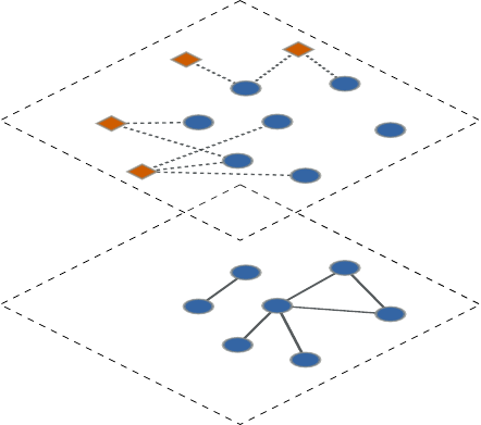
19
Data, A
Metadata, T
FIG. 17 Data-metadata stochastic block model by Hric et
al.. One layer consists of the network itself, with its vertices
and edges. The other layer is composed of the graph vertices
and vertices representing the annotations, the edges indicat-
ing which vertices are associated to which tag. The presence
of network vertices on both layers induces a coupling between
them. Reprinted figure with permission from (Hric et al.,
2016). c
2016, by the American Physical Society.
et al.,2015;Leng et al.,2013;Moore et al.,2011;Peel,
2015;Yang et al.,2013). A better approach is not assum-
ing a priori that the metadata correlate with the struc-
tural communities. The goal is quantifying the relation-
ship between metadata and community and use it to im-
prove the results. If there is no correlation, the metadata
would be ignored, leaving us with the partition derived
from structure alone.
Methods along these lines have been developed, using
stochastic block models. Newman and Clauset (New-
man and Clauset,2016) have proposed a model in which
vertices are initially assigned to clusters based on meta-
data, and then edges are placed between vertices accord-
ing to the degree-corrected stochastic block model (Kar-
rer and Newman,2011). Hric et al. have designed a
similar model (Hric et al.,2016), in which the inter-
play between structure and metadata is represented by
a multilayer network (Fig. 17). The generative model is
an extension of the hierarchical stochastic block model
(SBM) (Peixoto,2014) with degree-correction for the
case with edge layers (Peixoto,2015a). Here the meta-
data is not supposed to correspond simply to a partition
of the vertices. The majority of data sets contain rich
metadata, with vertices being annotated multiple times,
and often few vertices possess the exact same annota-
tions and can be thus associated to the same group. In
addition, while the number of communities is required
as input by the method of Newman and Clauset, here it
is inferred from the data. Finally, it is also possible to
assess the metadata in its power to predict the network
structure, not only their correlation with latent parti-
tions. This way it is possible to predict missing vertices
of the network, i. e., to infer the connections of a vertex
from its annotations only. We stress that neither method
requires that all vertices are annotated.
Applications of the method by Hric et al. (Hric et al.,
2016) reveal that in many data sets there are statisti-
cally significant correlations between the annotations and
the network structure, while in some cases the metadata
seems to be largely uncorrelated with structural clusters.
We conclude that network metadata should not be used
indiscriminately as ground truth for community detec-
tion methods. Even when the metadata is strongly pre-
dictive of the network structure, the agreement between
the annotations and the network division tends to be
complex, and very different from the one-to-one map-
ping that is more commonly assumed. Moreover, data
sets usually contain considerable noise in their annota-
tions, and some metadata tags are essentially random,
with no relationship to structure.
E. Community structure in real networks
Artificial benchmark graphs are certainly very useful
to assess the performance of clustering algorithms. How-
ever, one could always question whether the model of
community structure they propose is reliable. How can
we assess this? In order to characterise “real” commu-
nities we have to find them first. But that can only be
done via some algorithm, and different algorithms search
for different types of objects, in general. Still, one may
hope that general properties of communities can be con-
sistently uncovered across different methods and data
sets, while other features are more closely tied to the
specific method(s) used to detect the clusters and (or)
the specific data set at study (or classes thereof).
A seemingly robust feature of communities in real net-
works is the heterogeneity of their size distribution. Most
clustering techniques find skewed distributions of clus-
ter sizes in many networks. So, there appears to be no
characteristic size for a community: small communities
usually coexist with large ones. This feature is rather
independent of the type of network (Fig. 18). It may sig-
nal a hierarchy among communities, with small clusters
included in large ones. Methods unable to distinguish
between hierarchical levels might find “blended” parti-
tions, consisting of communities of different levels and
hence of very different sizes. The LFR benchmark was
the first graph model to take explicitly into account the
heterogeneity of community sizes (Section III.A).
Another interesting question is how the quality of com-
munities depends on their size. Leskovec et al. (Leskovec
et al.,2009) carried out a systematic analysis of clusters
in many large networks, including traditional and on-line
social networks, technological, information networks and
web graphs. Instead of considering partitions, they fo-
cused on individual communities, which are derived by
optimising conductance (Section II.A) around seed ver-
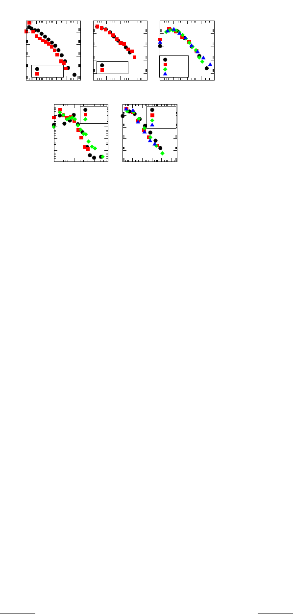
20
100101102103104105
10-10
10-8
10-6
10-4
10-2
P(s)
10-10
10-8
10-6
10-4
10-2
Wiki Talk
Email
100101102103104
10-8
10-6
10-4
10-2
10-8
10-6
10-4
10-2
AS-caida
AS-dimes
100101102103
10-8
10-6
10-4
10-2
10-8
10-6
10-4
10-2
web-G
Arxiv
Amazon
web-BS
100101102
10-5
10-4
10-3
10-2
10-1
P(s)
100101102
10-5
10-4
10-3
10-2
10-1 Dmela
Yeast
Human
100101102103104105
Module Size s
10-10
10-8
10-6
10-4
10-2
10-10
10-8
10-6
10-4
10-2 Live J
Epinions
Last FM
Slashdot
Social
Information
Internet
Biological
Communication
FIG. 18 Distribution of community sizes in real networks.
The clusters were detected with Infomap (Rosvall and
Bergstrom,2008), but other methods yield qualitatively sim-
ilar results. Various classes of networks are considered. All
distributions are broad, spanning several orders of magnitude.
Reprinted figure with permission from (Lancichinetti et al.,
2010).
tices. We remind that the conductance of a cluster is
the ratio between the number of external edges and the
total degree of the cluster. Minimising conductance ef-
fectively combines the two main community demands,
i. e., good separation from the rest of the graph (low
numerator) and large number of internal edges (high de-
nominator). The measure is also relatively insensitive to
the size of the clusters, as both the numerator and the
denominator are typically proportional to the number of
vertices of the community23. Therefore one could use it
to compare the quality of clusters of different sizes. For
any given size kLeskovec et al. identified the subgraph
with kvertices with the lowest conductance. This way,
for each network one can draw the network community
profile (NCP), showing the minimum conductance as a
function of community size. The NCPs of all networks
studied by Leskovec et al. have a characteristic shape:
they go downwards till k∼100 vertices, and then they
rise monotonically for larger subgraphs [Fig. 19 (left)].
Alternative shapes have been recently found for other
data sets (Jeub et al.,2015).
For networks characterised by NCPs like the one in
Fig. 19 (left) the most pronounced communities are fairly
small in size. Such small clusters are weakly connected
to the rest of the network, often by a single edge (in this
case they are called whiskers), and form the periphery
23 This is exactly true when the ratio between the external and the
total degree (mixing parameter) is the same for all community
vertices.
of the graph. Large clusters have comparatively lower
quality and melt into a big core. Large communities can
often be split in parts with lower conductance, so they
can be considered conglomerates of smaller communities.
A schematic picture of the resulting network structure is
shown in Fig. 19 (right). The shape of the NCP is fairly
independent of the specific technique adopted to identify
the subgraphs with minimum conductance. The different
shapes of the NCPs encountered in data suggest that
core-periphery is not the only model of group structure
of real networks (Jeub et al.,2015).
The NCP is a signature that can be used to se-
lect generative mechanisms of community structure. In-
deed, many standard models typically yield NCP sloping
steadily downwards, at odds with the ones encountered in
many social and information networks. Stochastic block
models (Section II.C) are sufficiently versatile that they
can reproduce the NCP shape of Fig. 19 (left), by suitably
tuning the parameters. In the standard LFR benchmark
(Section III.A) the mixing parameters are tightly concen-
trated about a value µby construction, hence all clusters
have approximately conductance µ, yielding a roughly
flat NCP24 (Jeub et al.,2015). However, the model can
be easily modified by making µcommunity-dependent
and a large variety of NCPs are attainable, including the
one of Fig. 19 (left).
The main problem of working with NCPs is that they
are based on extreme statistics, as one systematically re-
ports the minimum conductance for a given cluster size.
How representative is this extremal subgraph of the pop-
ulation of subgraphs with the same size? There may be
just a few clusters of a given size with low conductance.
It may happen that many subgraphs have conductance
near the minimum corresponding to their size(s), which
would then be representative. Alternatively most sub-
graphs might have much larger conductance than the
minimum but low enough that they can be still consid-
ered communities. In this case one should conclude that
communities of that size are not of very high quality,
on average. The above scenarios might lead to different
conclusions about the actual community structure of the
system. In general, even if one could produce a version
of the NCP where the trend refers to representative sam-
ples of communities of equal size (whatever that means),
the actual values of the conductance are as important as
the shape of the curve. If conductance is sufficiently low
for all cluster sizes, it means that there are good com-
munities of any size. The fact that small clusters could
be of higher quality does not undermine the role of large
clusters. The observation that large clusters consist of
smaller clusters of higher quality may just be evidence of
hierarchical structure in the network, which is a trade-
24 If all vertices of a subgraph have mixing parameter equal to µ,
it can be easily shown that the conductance of the subgraph is
exactly equal to µ.
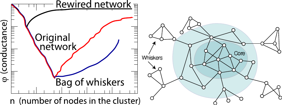
21
FIG. 19 Core-periphery structure of real networks. (Left) Schematic shape of the network community profile (NCP), showing
how the minimum conductance of subgraphs of size kvaries with k. This pattern is very common in large social and information
networks. The “best” communities in terms of conductance have a size of about 100 vertices (minimum of the curve), whereas
communities of larger sizes have lower quality. The curve labeled Rewired network is the NCP of a randomised version of
the network, where edges are randomly rewired by keeping the degree distribution; the one labeled Bag of whiskers gives
the minimum conductance scores of communities composed of disconnected pieces. (Right) Scheme of the core-periphery
structure in large social and information networks associated to the NCP above. Most vertices are in a central core, where
large communities are blended together, whereas the best communities, which are rather small, are weakly connected to the
core. Reprinted figure with permission from Ref. (Leskovec et al.,2009). c
2009, by Taylor and Francis.
mark of many complex systems (Simon,1962). In that
case high levels of the hierarchy are not less important
than low ones, a priori. In fact, the actual relative im-
portance of communities should not only come from the
sheer value of specific metrics, like conductance, but also
from their statistical significance (Section IV.I).
That notwithstanding, we strongly encourage analyses
like the one by Leskovec et al., as they provide a statis-
tical characterisation of community structure, in a way
that is only weakly algorithm-dependent. One has to
define operationally what a cluster is, but in a simple
intuitive way that allows us to draw conclusions about
the structure of the graph. In principle one could do
the same by analysing the clusters delivered by any al-
gorithm, but there would be two important drawbacks.
First, the clusters may not be easy to interpret, as most
clustering algorithms usually do not require a clear-cut
definition of community. Second, one would have to han-
dle a partition of the network in communities, instead
of probing locally the group structure of the network.
Therefore, for a given vertex one would have only one
cluster (or a handful, if communities overlap), while a
local exploration allows to analyse a whole population
of candidate subgraphs, which gives more information.
The local subgraphs recovered this way do not need to
be strongly matching the clusters delivered by any algo-
rithm, but they provide useful signatures that allow to
restrict the set of possible model explanations for the net-
work’s group structure. Such investigation can be repli-
cated on any model graph to check whether the results
match (e. g., whether the NCPs coincide).
Another approach to infer properties of clusters of real
networks is using annotations. While we have shown that
annotated clusters do not necessarily coincide with struc-
tural ones (Section III.D), general features can be still
derived, provided they are consistently found across dif-
ferent data sets and annotations. A recent analysis by
Yang and Leskovec has questioned the common picture
of networks with overlapping communities (Yang and
Leskovec,2014). Scholars usually assume that clusters
overlap at their boundaries, hence edge density should be
larger in the non-overlapping parts (Fig. 5). Instead, by
analysing the overlaps of annotated clusters in large so-
cial and information networks, Yang and Leskovec found
that the probability that two vertices are connected is
larger in the overlaps, and grows with the number of
communities sharing that pair of vertices. In addition,
connector vertices, i. e., vertices with the largest number
of neighbours within a community, are more likely to be
found in the overlaps. These findings suggest that the
overlaps may play an important role in the community
structure of networks. In Fig. 20 we compare the conven-
tional view with the one resulting from the analysis. The
Community-Affiliation Graph Model (AGM) (Yang and
Leskovec,2014) and the Cluster Affiliation Model for Big
Networks (BIGCLAM) (Yang and Leskovec,2013) are
clustering techniques based on generative models of net-
works featuring communities with dense overlaps. The
models are based on the principle that vertices are more
likely to be neighbours the more the communities shar-
ing them, in line with the empirical finding of (Yang and
Leskovec,2014).
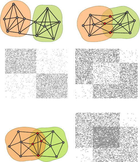
22
(a) No overlaps (b) Sparse overlaps
(c) Dense overlaps (d) Adjacency matrix of (c)
FIG. 20 Stylised views of community structure. In (a) and
(b) we show the conventional pictures of non-overlapping and
overlapping clusters, respectively. Under the network dia-
grams we see the corresponding adjacency matrices. The
overlaps have a lower edge density than the rest of the com-
munities. The analysis by Yang and Leskovec suggests that
a more realistic model could be the one shown in (c, d),
where the overlaps are denser than the non-overlapping parts.
Reprinted figure with permission from (Yang and Leskovec,
2014). c
2014, by the Association for Computing Machinery,
Inc.
Actual overlapping communities exist in many con-
texts. However, it is unclear whether soft clustering is
statistically founded. A recent analysis aiming at identi-
fying suitable stochastic block models to describe real
network data indicate that in many cases hard parti-
tions ought to be preferred, as they give simpler de-
scriptions of the group structure of the data than soft
partitions (Peixoto,2015b). This could be due to the
fact that the underlying models are based on placing
edges independently of each other, neglecting higher or-
der structures between vertices, like motifs. By adopting
approaches that take into account higher-order structures
things may change and community overlaps might be-
come a statistically robust feature. The pervasive over-
laps found by Yang and Leskovec in annotated data can
be found if higher order effects are considered (Persson
et al.,2016;Rosvall et al.,2014), without ad hoc hy-
potheses.
IV. METHODS
There are many algorithms to detect communities in
graphs. They can be grouped in categories, based on dif-
ferent criteria, like the actual operational method (For-
tunato,2010), or the underlying concept of commu-
nity (Coscia et al.,2011). In most applications, how-
ever, just a few popular algorithms are employed. In this
section we present a critical analysis of these methods.
We show the advantages of knowing the number of clus-
ters before-hand and how it is possible to derive robust
solutions from partitions delivered by stochastic cluster-
ing techniques. We discuss approaches to the problem of
detecting communities in evolving networks and how to
assess the significance of the detected clustering. We con-
clude by suggesting the methods that currently appear
to be most promising.
A. How many clusters?
In general, the only preliminary information available
to any algorithm is the structure of the network, i. e.,
which pairs of vertices are connected to each other and
which are not (possibly including weights). Any insight
about community structure is supposed to be given as
output of the procedure. Naturally, it would be valuable
to have some information on the unknown division of the
network beforehand, as one could reduce considerably the
huge space of possible solutions, and increase the chance
of successfully identifying the communities.
Among all the possible pre-detection inputs, the num-
ber qof clusters plays a prominent role. Many popular
classes of algorithms require the specification of qbe-
fore they run, like methods imported from data cluster-
ing or parametric statistical inference approaches (Sec-
tion IV.E). Other methods are capable to infer qas
they can choose among partitions into different num-
bers of communities. But even such methods could ben-
efit from a preliminary knowledge of q(Darst et al.,
2014). In Fig. 21 we report standard accuracy plots
of two algorithms on the planted partition model (Sec-
tion III.A) with two clusters of equal size. The algo-
rithms are modularity optimisation via simulated an-
nealing (Guimer`a and Amaral,2005) and the Absolute
Potts Model (APM) (Ronhovde and Nussinov,2010)
(Section IV.G). There are two performance curves for
each method: one comes from the standard application
of the method, without constraints; the other is obtained
by forcing the method to explore only the subset of par-
titions with the correct number of clusters q= 2.
We see that the accuracy improves considerably when
qis known. This is particularly striking in the case of
modularity optimisation, which is known to have a lim-
ited resolution, preventing the method from identifying
the correct scale of the communities, even when the latter
are very pronounced (Fortunato and Barth´elemy,2007;
Good et al.,2010) (Section IV.F). Knowing qand con-
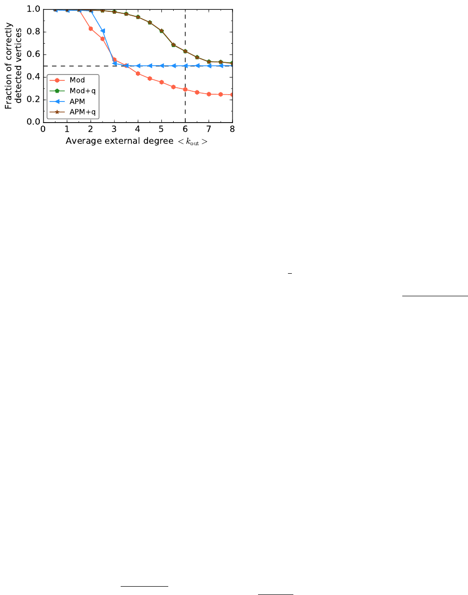
23
FIG. 21 Knowing the number of clusters beforehand improves
community detection. The diagram shows the performance
on the planted partition model of two methods: modular-
ity optimisation via simulated annealing (Guimer`a and Ama-
ral,2005) and the Absolute Potts Model (APM) (Ronhovde
and Nussinov,2010). Networks have 400 vertices, which
are grouped in two equal-sized communities. The accuracy
is measured via the fraction of correctly detected vertices
(Section III.B). The horizontal line indicates the accuracy of
random guessing, the dashed vertical line the theoretical de-
tectability limit (Section III.C). For each algorithm we show
two curves, referring to the results of the method in the ab-
sence of any information on the number of clusters, and when
such information is fed into the model as initial input. In
both cases, knowing the number of clusters beforehand leads
to a much better performance.
straining the optimisation of the measure to partitions
with fixed q, the problem can be alleviated (Nadakuditi
and Newman,2012).
But how do we know how many clusters there are?
Here we briefly discuss some heuristic techniques, for sta-
tistically principled methods we defer the reader to Sec-
tion IV.E. It has been recently shown that in the planted
partition model qcan be correctly inferred all the way
up to the detectability limit from the spectra of two ma-
trices: the non-backtracking matrix B(Krzakala et al.,
2013) and the flow matrix F(Newman,2013). They are
2m×2mmatrices, where mis the number of edges of
the graph. Each edge is considered in both directions,
yielding 2mdirected edges and indicated with the nota-
tion i→j, meaning that the edge goes from vertex ito
vertex j. Their elements read
Bi→j,r→s=δis(1 −δjr) (15)
and
Fi→j,r→s=δis(1 −δjr)
ki−1.(16)
In Eq. (16)kiis the degree of vertex i. So the ele-
ments of Fare basically the elements of B, normalised
by vertex degrees. This is done to account for the hetero-
geneous degree distributions observed in most real net-
works. Both matrices have non-zero elements only for
each pair of edges forming a directed path from the first
vertex of one edge to the second of the other edge. To
do that, edges have to be incident at one vertex. As a
matter of fact, the non-backtracking matrix Bis just the
adjacency matrix of the (directed) edges of the graph.
The name of the matrix Bis due to a connection
with the properties of non-backtracking walks. A non-
backtracking walk (Angel et al.,2015) is a path across
the edges of a graph that is allowed to return to a vertex
visited previously only after at least two other vertices
have been visited; immediate returns like 1 →2→1 are
forbidden. The elements of the k-th power of Byield
the number of non-backtracking walks of length kfrom a
(directed) edge of the graph to another and the trace of
the power matrix the number of closed non-backtracking
walks of length kstarting from any given (directed) edge.
A remarkable property of both matrices is that on net-
works with homogeneous groups (i. e., of similar size and
internal edge density) most eigenvalues, which are gen-
erally complex, are enclosed by a circle centred at the
origin, and that the number of eigenvalues lying outside
of the circle is a good proxy of the number of commu-
nities of the network (Krzakala et al.,2013;Newman,
2013). For Bthe circle’s radius is given by the square
root √cof the leading eigenvalue c, which may diverge
for networks with heterogeneous degree distributions (e.
g., power laws); for Fit equals phk/(k−1)i/hki, which
is never greater than 1.
Unfortunately, computing the eigenvalues of the non-
backtracking or the flow matrix is lengthy. Both are
2m×2mmatrices. The adjacency matrix Ahas n×nele-
ments, so Band Fare larger by a factor of hki2, where hki
is the average degree of the network. An approximate but
reliable computation of the spectra requires a time which
scales superlinearly (approximately quadratic) with the
network size n. So the problem is intractable for graphs
with number of edges of the order of millions or higher.
Also, if communities have diverse sizes and edge densities,
as it happens in most networks encountered in applica-
tions, the bulk of eigenvalues may not have a circular
shape, and it may become problematic to identify eigen-
values falling outside of the bulk.
Besides, non-backtracking walks must contain cycles,
hence trees25 dangling off the graph do not affect the
spectrum of B, which remains unchanged if all dangling
trees are removed. This is a disturbing feature, as tree-
like regions of the graph may play a role in the net-
work’s community structure, and most methods would
find different partitions if trees are kept or removed26.
The spectrum of the flow matrix, instead, changes when
dangling trees are kept or removed (Newman,2013). In
25 We remind that trees are connected acyclic graphs.
26 Singh and Humphries showed that the problem can be solved
via reluctant backtracking walks, in which the walker has a small
but non-zero probability of returning to the vertex immedi-
ately (Singh and Humphries,2015).
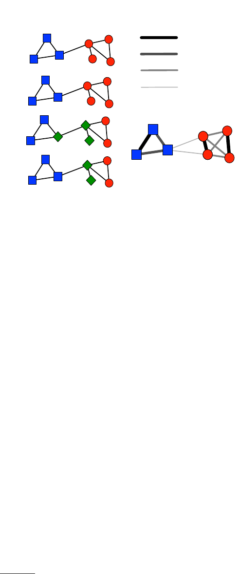
24
the limiting case in which the network itself is a tree, all
eigenvalues of Band Fare zero and even if there were a
community structure one gets no relevant information.
The number of clusters can also be deduced by study-
ing how the eigenvectors of graph matrices rotate when
the adjacency matrix of the graph is subjected to random
perturbations (Sarkar et al.,2016). On stochastic block
models this approach infers the correct value of qup to a
threshold preceding the detectability limit. The method
is also computationally expensive.
In general, if one can identify a set (range) of promis-
ing q-values, from preliminary information or via calcula-
tions like the ones described above or in Section IV.E, it
is better to run constrained versions of clustering meth-
ods, searching for solutions only among partitions with
those numbers of communities, than letting the methods
discover qby themselves, which may lead to solutions of
lower quality.
B. Consensus clustering
Many clustering techniques are stochastic in character
and do not deliver a unique answer. A common scenario
is when the desired solution corresponds to extrema of a
cost function, that can only be found via approximation
techniques, with results depending on random seeds and
on the choice of initial conditions. Techniques not based
on optimisation sometimes have the same feature, when
tie-break rules are adopted in order to choose among mul-
tiple equivalent options encountered along the calcula-
tion.
What to do with all these partitions? Sometimes there
are objective criteria to sort out a specific partition and
discard all others. For instance, in algorithms based on
optimisation, one could pick the solution yielding the
largest (smallest) value of the function to optimise. For
other techniques there is no clear-cut criterion.
A promising approach is combining the information of
the different outputs into a new partition. Consensus
clustering (Goder and Filkov,2008;Strehl and Ghosh,
2002;Topchy et al.,2005) is based on this idea. The
goal is searching for a consensus partition, that is better
fitting than the input partitions. Consensus clustering
is a difficult combinatorial optimisation problem. An al-
ternative greedy strategy (Strehl and Ghosh,2002) re-
lies on the consensus matrix, which is a matrix based on
the co-occurrence of vertices in communities of the input
partitions (Fig. 22). The consensus matrix is used as an
input for the graph clustering technique adopted, leading
to a new set of partitions, which produce a new consensus
matrix, etc., until a unique partition is finally reached,
which is not changed by further iterations. The steps of
the procedure are listed below. The starting point is a
network Gwith nvertices and a clustering algorithm A.
1. Apply Aon G nPtimes, yielding nPpartitions.
2. Compute the consensus matrix D:Dij is the num-
Original Graph Consensus Matrix
Dij = 1
Dij = 3/4
Dij = 2/4
Dij = 1/4
(I)
(II)
(III)
(IV)
FIG. 22 Consensus clustering in networks. A simple graph
has a natural partition in two communities [squares and cir-
cles on diagrams (I) and (II)]. The combination of (I), (II),
(III) and (IV) yields the weighted consensus matrix illustrated
on the right. The thickness of each edge is proportional to
its weight. In the consensus matrix the community struc-
ture of the original network is more visible: the two com-
munities have become cliques, with “heavy” edges, whereas
inter-community edges are rather weak. This improvement is
obtained despite the presence of two inaccurate partitions in
three clusters (III and IV). Reprinted figure with permission
from (Lancichinetti and Fortunato,2012). c
2012, by the
Nature Publishing Group.
ber of partitions in which vertices iand jof Gare
assigned to the same community, divided by nP.
3. All entries of Dbelow a chosen threshold τare set
to zero27.
4. Apply Aon DnPtimes, yielding nPpartitions.
5. If the partitions are all equal, stop28. Otherwise go
back to 2.
Since the consensus matrix is in general weighted, the
algorithm Amust be able to handle weighted net-
works, even if the graph at study is binary. Fortunately
many popular algorithms have natural extensions to the
weighted case.
The integration of consensus clustering with popu-
lar existing techniques leads to more accurate partitions
27 Without thresholding the consensus matrix would quickly turn
into a dense matrix, rendering the application of clustering al-
gorithms computationally expensive. However, the method does
not strictly require thresholding, and if the network is not too
large one can skip step 3 and use the full matrix all along (Bruno
et al.,2015).
28 The consensus matrix is block-diagonal in this case.

25
than those delivered by the methods alone on LFR bench-
mark graphs (Lancichinetti and Fortunato,2012). Inter-
estingly, this holds even for methods whose direct appli-
cation gives poor results on the same graphs, like modu-
larity optimisation (Section IV.F). The variability of the
partitions, rather than being a problem, becomes a factor
of performance enhancement. The outcome of the pro-
cedure depends on the choice of the threshold parameter
τand the number of input partitions nP, which can be
selected by testing the performance on benchmark net-
works (Lancichinetti and Fortunato,2012). Consensus
clustering is also a promising technique to detect com-
munities in evolving networks (Section IV.H).
C. Spectral methods
Spectral graph clustering is an approach to detect clus-
ters using spectral properties of the graph (Fortunato,
2010;von Luxburg,2006). The eigenvalue spectrum of
several graph matrices (e. g., the adjacency matrix, the
Laplacian, etc.) typically consists of a dense bulk of
closely spaced eigenvalues, plus some outlying eigenval-
ues separated from the bulk by a significant gap. The
eigenvectors corresponding to these outliers contain in-
formation about the large-scale structure of the network,
like community structure29. Spectral clustering consists
in generating a projection of the graph vertices in a met-
ric space, by using the entries of those eigenvectors as co-
ordinates. The i-th entries of the eigenvectors are the co-
ordinates of vertex iin a k-dimensional Euclidean space,
where kis the number of eigenvectors used. The resulting
points can be grouped in clusters by using standard parti-
tional clustering techniques like k-means clustering (Mac-
Queen,1967).
Spectral clustering is not always reliable, however.
When the network is very sparse (Section II.C) the sepa-
ration between the eigenvalues of the community-related
eigenvectors and the bulk is not sharp. Eigenvectors cor-
responding to eigenvalues outside of the bulk may be cor-
related to high-degree vertices (hubs), instead of group
structure. Likewise, community-related eigenvectors can
be associated to eigenvalues ending up inside the bulk. In
these situations, selecting eigenvectors based on whether
their associated eigenvalues are inside or outside the bulk
yields a heterogeneous set, containing information both
on communities and on other features (e. g., hubs). Us-
ing those eigenvectors for the spectral clustering proce-
dure renders community detection more difficult, some-
times impossible. Unfortunately, many of the networks
encountered in practical studies are very sparse and can
lead to this type of problems.
29 Typically each such eigenvector is localised, in that its entries are
markedly different from zero in correspondence of the vertices of
a community, while the other entries are close to zero.
Indeed on sparse networks constructed with the
planted partition model spectral methods relying on
standard matrices [adjacency matrix, Laplacian, mod-
ularity matrix (Newman,2006), etc.] fail before the
theoretical detectability limit (Section III.C) (Krzakala
et al.,2013). The non-backtracking matrix Bof Eq. (15)
was introduced to address this problem (Krzakala et al.,
2013). On the planted partition model the associated
eigenvalues of the community-related eigenvectors of B
are separated from the bulk until the theoretical de-
tectability limit, so spectral methods using the top eigen-
vectors of Bare capable to find communities as long as
they are detectable, modulo the caveats we expressed in
Section IV.A.
D. Overlapping communities: Vertex or Edge clustering?
Soft clustering, where communities may overlap, is an
even harder problem than hard clustering, where there
is no community overlap. The possibility of having mul-
tiple memberships for the vertices introduces additional
degrees of freedom in the problem, causing a huge ex-
pansion of the space of possible solutions. It has been
pointed out that overlapping communities, especially in
social networks, reflect different types of associations be-
tween people (Ahn et al.,2010;Evans and Lambiotte,
2009). Two actors could be co-workers, friends, relatives,
sport mates, etc.. Actor Acould be a work colleague of B
and a friend of C, so she would sit in the overlap between
the community of colleagues of Band the community
of friends of C. For this reason, it has been suggested
that an effective way to recover overlapping clusters is to
group edges, rather than vertices. In the example above,
the edges connecting Awith Band Awith Cwould be
placed in different groups, and since they both have A
as endpoint, the latter turns out to be an overlapping
vertex.
Moreover, edge clustering is claimed to have the addi-
tional advantage of reconciling soft clustering with hier-
archical community structure (Ahn et al.,2010). If there
is hierarchy, communities are nested within each other
as many times as there are hierarchical levels. Hierar-
chical structure is often represented via dendrograms30,
with the network being divided in clusters, which are in
turn divided in clusters, and so on until one ends up with
singleton clusters, consisting of one vertex each. But this
can be done only if communities do not share vertices.
30 A dendrogram, or hierarchical tree, is a tree diagram used to rep-
resent hierarchical partitions. At the bottom there are as many
nodes as there are vertices in the graph, representing the single-
ton clusters. At the top there is one node (root), standing for
the partition grouping all vertices in a single cluster. Horizontal
lines indicate mergers of a pair of clusters or, equivalently, splits
of one cluster. Each vertex of the tree identifies one cluster,
whose elements can be read by following all bifurcations starting
from the vertex all the way down to the leaves of the tree.
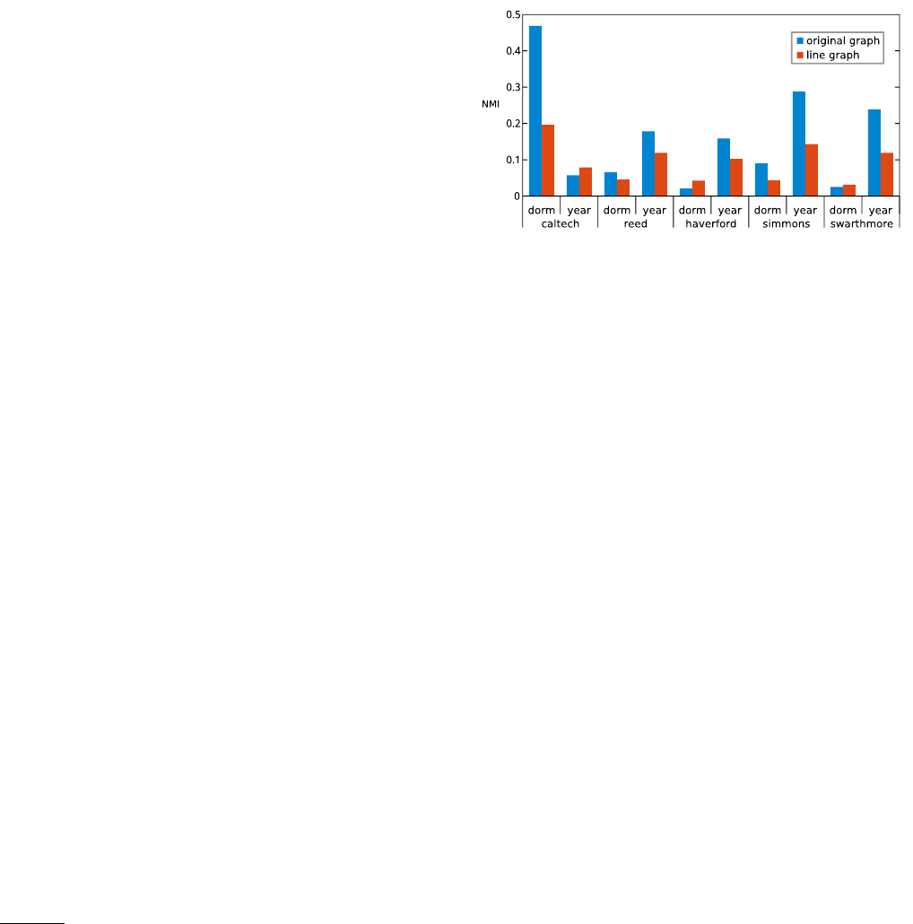
26
Overlapping vertices should be assigned to multiple clus-
ters of lower hierarchical levels, yielding multiple copies
of them in the dendrogram. Instead, one could build
a dendrogram displaying edge communities, where each
edge is assigned to a single cluster, but clusters can still
overlap because edges in different clusters may share one
endpoint (Ahn et al.,2010).
Some remarks are in order. First, there may still be
overlapping communities even if there were a single type
of association between the vertices. For instance, if we
keep only the friendship relationships within a given pop-
ulation of actors, there are many social circles and there
could be active actors with multiple ties within two cir-
cles, or more. Second, in the traditional picture of net-
works with community structure (Fig. 4), the edges con-
necting two different groups may be assigned to one of the
communities they join or they could be put together in
a separate group. Either way, they would signal an over-
lap between the communities, which is artificial. This
happens even in the extreme case of a single edge con-
necting vertices Aand Bof two groups, as that edge
will have to be assigned to a group, which inevitably
forces Aand Binto a common cluster. Third, if we
rely on the picture emerging from the analysis by Yang
and Leskovec (Yang and Leskovec,2014) (Section III.E)
overlaps between clusters could be much denser than we
expect, hence not only vertices but also edges may be
shared among different groups, and edge dendrograms
would have the same problem as classic vertex dendro-
grams31. Fourth, the computational complexity of the
calculation can rise substantially, as in networks of in-
terest there are typically many more edges than vertices.
Finally, there is nothing revealing that there is a concep-
tual or algorithmic advantage in grouping edges versus
vertices, other than works showing that a specific edge
clustering technique outperforms some vertex clustering
techniques on a specific set of networks.
To shed some light on the situation, we performed the
following test. We took some network data sets with
annotated vertices, giving an indication about what the
communities of those networks could be32. For each net-
work Gwe derived the corresponding line graph L(G),
which is the graph whose vertices are the edges of G,
while edges are set between pairs of vertices of L(G)
whose corresponding edges in Gare adjacent at one of
their endpoints. Vertex communities of L(G) are then
edge communities of the original network G. The ques-
tion is whether by working on L(G) the detection im-
proves or not. We searched for overlapping communities
31 In this case, if we used edge clustering, each edge would be placed
in one cluster only. However, when one turns edge communities
into vertex communities, multiple relationships can be still re-
covered (Ahn et al.,2010).
32 We have seen in Section III.D that metadata are not necessarily
correlated with topological clusters. We used data sets for which
there is some correlation.
with OSLOM (Lancichinetti et al.,2011). We applied
OSLOM on the original graphs and on their line graphs.
The covers found on the line graphs were turned into cov-
ers of the vertices of G, by replacing each vertex of L(G)
with the pair of vertices of the corresponding edge of G.
FIG. 23 Comparison between edge communities and vertex
communities. The diagram shows the similarity between the
covers of annotated vertices of five social networks and the
topological covers found by OSLOM on them (left bar of
each pair) and on their line graphs (right bar). The networks
represent FaceBook friendships between students of US uni-
versities (Traud et al.,2012). There are several annotations
for each student, we selected those which are more closely
related to topological groups: year of study and dormitory.
The similarity was computed by using the normalised mutual
information (NMI), in the version for covers proposed by Lan-
cichinetti, Fortunato and Kert´esz (Lancichinetti et al.,2009).
Vertex communities detected in the original graphs are over-
all better correlated with the annotated clusters than edge
communities.
The results can be seen in Fig. 23, showing how similar
the covers found on the original networks and on the line
graphs are with respect to the covers of annotated ver-
tices. Neither approach is very accurate, as expected (see
Section III.D and Fig. 16), but vertex communities show
a greater association to the annotated clusters than edge
communities, except in a few instances where the similar-
ity is very low. Analyses carried out on LFR benchmark
graphs (not shown) lead to the same conclusion. We
stress that traditional line graphs have the problem that
edges adjacent to a hub vertex in the original graph turn
into vertices who are all connected to each other, forming
giant cliques, which might dominate the structure of the
line graph, misleading clustering techniques. The proce-
dure can be refined by introducing weights for the edges
of the line graphs, that can be computed in various ways,
e. g., based on the similarity of the neighbourhoods of
adjacent edges in the original network (Ahn et al.,2010).
Still we believe that our tests provide some evidence
that edge clustering is no better than vertex clustering,
in general. The superiority of algorithms based on either
approach should be assessed a posteriori, case by case,
and the answer may depend on the specific data sets
under investigation.

27
E. Methods based on statistical inference
Statistical inference provides a powerful set of tools to
tackle the problem of community detection. The stan-
dard approach is to fit a generative network model on
the data (Ball et al.,2011;Guimer`a and Sales-Pardo,
2009;Hastings,2006;Karrer and Newman,2011;New-
man and Leicht,2007;Peixoto,2014). The stochas-
tic block model (SBM) is by far the most used genera-
tive model of graphs with communities (see Section II.C
and references therein). We have seen that it can de-
scribe other types of group structure, like disassortative
and core-periphery structure (Fig. 8). The unnormalised
maximum log-likelihood that a given partition gin q
groups of the network Gis reproduced by the standard
SBM reads (Karrer and Newman,2011)
LS(G|g) =
q
X
r,s=1
ers log ers
nrns,(17)
where ers is the number of edges running from group rto
group s,nr(ns) the number of vertices in r(s) and the
sum runs over all pairs of groups (including when r=s).
This version of the model, however, does not account
for the degree heterogeneity of most real networks, so it
does a poor job at describing the group structure of many
of them. Therefore, Karrer and Newman proposed the
degree-corrected stochastic block model (DCSBM) (Kar-
rer and Newman,2011), in which the degrees of the ver-
tices are kept constant, on average, via the introduction
of additional suitable parameters33. The unnormalised
maximum log-likelihood for the DCSBM is
LDC (G|g) =
q
X
r,s=1
ers log ers
eres,(18)
where er(es) is the sum of the degrees of the vertices in
r(s).
The most important drawback of this type of approach
is the need to specify the number qof groups before-
hand, which is usually unknown for real networks. This
is because a straight maximisation of the likelihoods of
Eqs. (17) and (18) over the whole set of possible solu-
tions yields the trivial partition in which each vertex is a
cluster (overfitting). In Section IV.A we have seen ways
to extract qfrom spectral properties of the graph. But it
would be better to have statistically principled methods,
to be consistent with the approach used to perform the
inference.
A possibility is model selection, for instance by choos-
ing the model that best compresses the data (Gr¨unwald
33 The authors were inspired by modularity maximisation, which
gives far better results when the null model consists of rewiring
edges by preserving the degree sequence of the network (on av-
erage), than by preserving only the total number of edges.
et al.,2005;Rissanen,1978). The extent of the compres-
sion can be estimated via the total amount of information
necessary to describe the data, which includes not only
the fitted model, but also the information necessary to
describe the model itself, which is a growing function of
the number of blocks q(Peixoto,2013). This quantity,
that we indicate with Σ, is called the description length.
Minimising the description length naturally avoids over-
fitting. Partitions with large qare associated to “heavy”
models in terms of their information content, and do not
represent the best compression. On the other hand, par-
titions with low qhave high information content, even if
the model itself is not loaded with parameters. Hence the
minimum description length corresponds to a non-trivial
number of groups and it makes sense to minimise Σ to
infer the block structure of the graph.
It turns out that this approach has a limited resolution
on the standard SBM: the maximum number of blocks
that can be resolved scales as √nfor a fixed average de-
gree hki, where nis the number of vertices of the network.
This means that the minimum size of detectable blocks
scales as √n, just as it happens for modularity maximi-
sation (Section IV.F). A more refined method of model
selection, consisting in a nested hierarchy of stochastic
block models, where an upper level of the hierarchy serves
as prior information to a lower level, brings the resolu-
tion limit down to log n, enabling the detection of much
smaller blocks (Peixoto,2014).
Other techniques to extract the number of groups have
been proposed (Cˆome and Latouche,2015;Daudin et al.,
2008;Handcock et al.,2007;Latouche et al.,2012;New-
man and Reinert,2016).
F. Methods based on optimisation
Optimisation techniques have received the greatest at-
tention in the literature. The goal is finding an ex-
tremum, usually the maximum, of a function indicating
the quality of a clustering, over the space of all possible
clusterings. Quality functions can express the goodness
of a partition or of single clusters.
The most popular quality function is the modularity
by Newman and Girvan (Newman and Girvan,2004).
It estimates the quality of a partition of the network in
communities. The general expression of modularity is
Q=1
2mX
ij
(Aij −Pij )δ(Ci, Cj),(19)
where mis the number of edges of the network, the sum
runs over all pairs of vertices iand j,Aij is the element
of the adjacency matrix, Pij is the null model term and
in the Kronecker delta at the end Ciand Cjindicate
the communities of iand j. The term Pij indicates the
average adjacency matrix of an ensemble of networks, de-
rived by randomising the original graph, such to preserve
some of its features. Therefore, modularity measures how
different the original graph is from such randomisations.
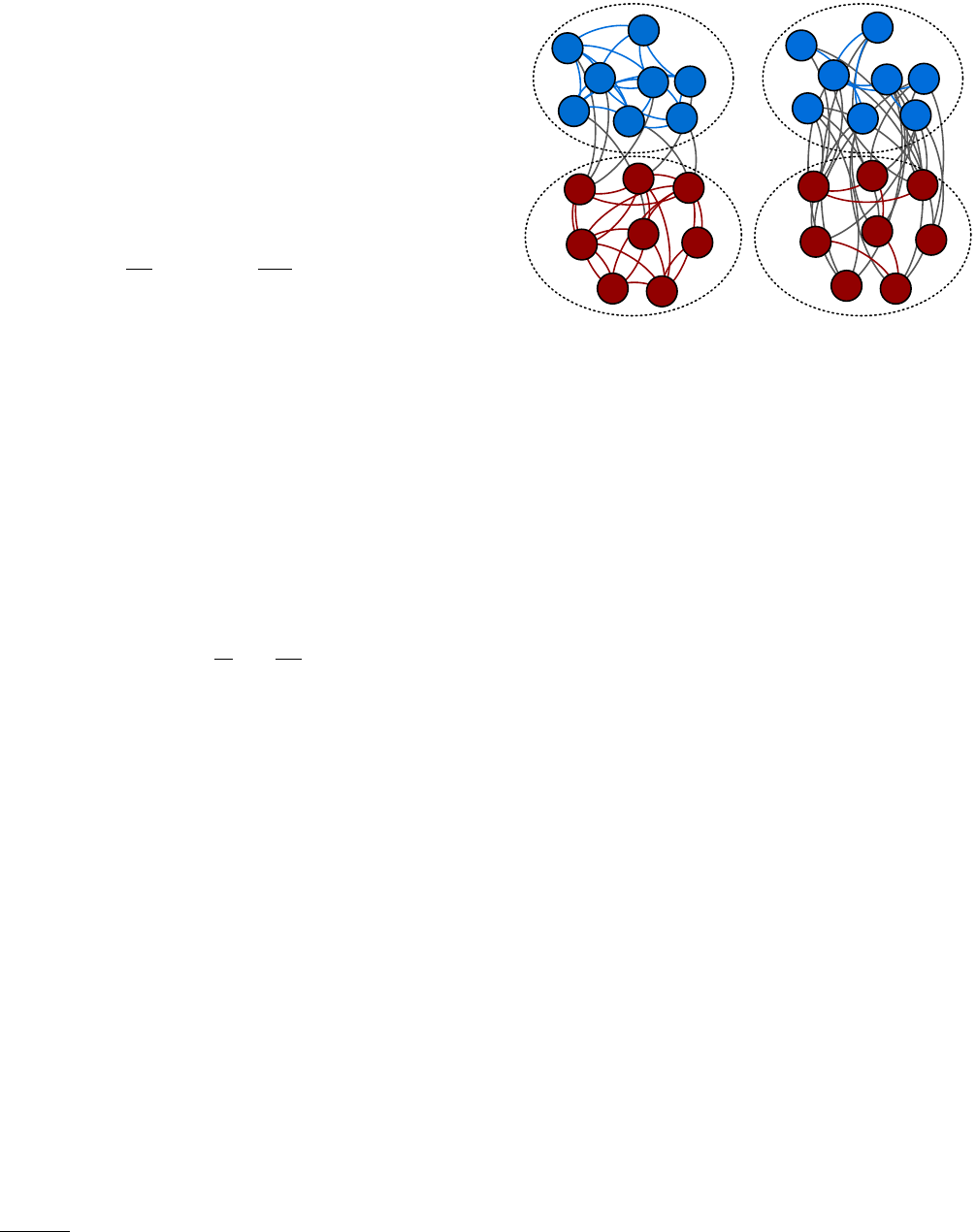
28
The concept was inspired by the idea that by randomis-
ing the network structure communities are destroyed, so
the comparison between the actual structure and its ran-
domisation reveals how non-random the group structure
is. A standard choice is Pij =kikj/2m,kiand kjbeing
the degrees of iand j, and corresponds to the expected
number of edges joining vertices iand jif the edges of
the network were rewired such to preserve the degree of
all vertices, on average. This yields the classic form of
modularity
Q=1
2mX
ij Aij −kikj
2mδ(Ci, Cj).(20)
Other choices of the null model term allow us to in-
corporate specific features of network structure, like bi-
partiteness (Barber,2007), correlations (MacMahon and
Garlaschelli,2015), signed edges (Traag and Bruggeman,
2009), space embeddedness (Expert et al.,2011), etc..
The extension of Eq. (20) and of its variants to the case
of weighted networks is straightforward (Newman,2004).
For simplicity we focus on unweighted graphs here, but
the issues we discuss are general.
Because of the delta, the only contributions to the sum
come from vertex pairs belonging to the same cluster, so
we can group these contributions together and rewrite the
sum over the vertex pairs as a sum over the clusters34
Q=X
ChlC
m−kC
2m2i.(21)
Here lCthe total number of edges joining vertices of com-
munity Cand kCthe sum of the degrees of the vertices
of C(Section II.A). The first term of each summand in
Eq. (21) is the fraction of edges of the graph falling within
community C, whereas the second term is the expected
fraction of edges that would fall inside Cif the graph
were taken from the ensemble of random graphs preserv-
ing the degree of each vertex of the original network, on
average. The difference in the summand would then in-
dicate how “non-random” subgraph Cis. The larger the
difference the more confident we can be that the place-
ment of edges within Cis not random (Fig. 24). Large
values of Qare then supposed to indicate partitions with
high quality.
Modularity maximisation is NP-hard (Brandes et al.,
2008). Therefore one can realistically hope to find only
decent approximations of the modularity maximum and
a wide variety of approaches has been proposed. Due
to its simplicity, the prestige of its inventors and early
results on the benchmark of Girvan and Newman (Sec-
tion III.A) and on small real benchmark networks, like
Zachary karate club network (Fig. 15), modularity has
34 A partition quality function that can be formulated as a sum
over the clusters is called additive.
FIG. 24 Modularity by Newman and Girvan. The network
on the left has a visible community structure, with two clus-
ters, whose vertices are highlighted in blue and red, respec-
tively. Modularity measures how different the clusters of the
partition are from the corresponding clusters of the ensemble
of random graphs obtained by randomly joining the vertices,
such to preserve their degrees, on average. The picture on
the right shows the result of one such randomisation. The
internal edges are coloured in blue and red. They are just a
handful compared to the number of edges joining the same
groups of vertices in the original network (blue and red lines
in the left picture), while there are now many more edges
running between the subgraphs (black lines): the randomisa-
tion has destroyed the community structure of the graph, as
expected. The value of modularity for the bipartition on the
left is expected to be large.
become the best known and most studied object in net-
work clustering. In fact, soon after its introduction, it
seemed to represent the essence of the problem, and the
key to its solution.
However, it became quickly clear that the measure is
not as good as it looks. For one thing, there are high-
modularity partitions even in random graphs without
groups (Guimer`a et al.,2004). This seems counterintu-
itive, given that modularity has been designed to capture
the difference between random and non-random struc-
ture. Modularity is a sort of distance between the actual
network and an average over random networks, ignor-
ing altogether the distribution of the relevant commu-
nity variables, like the fractions of edges within the clus-
ters, over all realisations generated by the configuration
model. If the distribution is not strongly peaked, the val-
ues of the community variables measured on the original
graph may be found in a large number of randomised net-
works, even though the averages look far away from them.
In other words, we should pay more attention to the sig-
nificance of the maximum modularity value Qmax, than
to the value itself. How can we estimate the significance
of Qmax? A natural way is maximising Qover all par-
titions of every randomised graph. One then computes
the average hQrandiand the standard deviation σrand
Qof
the resulting values. The statistical significance of Qmax
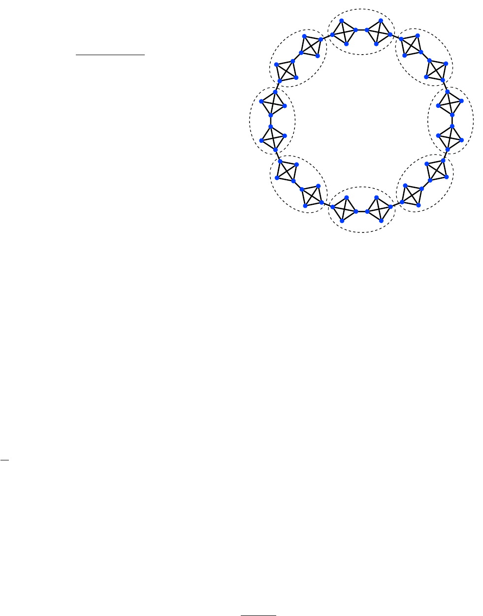
29
is indicated by the distance of Qmax from the null model
average hQrandiin units of the standard deviation σrand
Q,
i. e., by the z-score
z=Qmax − hQrandi
σrand
Q
.(22)
If z1, Qmax indicates strong community structure.
This approach has problems, though. The main draw-
back is that the distribution of Qrand over the ensem-
ble of null model random graphs, though peaked, is not
Gaussian. Therefore, one cannot attribute to the values
of the z-score the significance corresponding to a Gaus-
sian distribution, and one ought to compute the statis-
tical significance for the correct distribution. Also, the
z-score depends on the network size, so the same values
may indicate different levels of significance for networks
differing considerably in size.
Next, it is not true that the modularity maximum al-
ways corresponds to the most pronounced community
structure of a network. In Fig. 25 we show the well-
known example of the ring of cliques (Fortunato and
Barth´elemy,2007). The network consists of 16 cliques
with four vertices each. Every clique has two neigh-
bouring cliques, connected to it via a single edge. In-
tuition suggests that the graph has a natural commu-
nity structure, with 16 communities, each corresponding
to one clique. Indeed, the Q-value of this partition is
Q1= 89/112 ≈0.79464..., pretty close to 1, which is the
upper bound of modularity. However, there are parti-
tions with larger values, like the partition in 8 clusters
indicated by the dashed contours, whose modularity is
Q2= 90/112 ≈0.80357 > Q1.
This is due to the fact that Qhas a preferential scale
for the communities, deriving from the underlying null
model and revealed by its explicit dependence on the
number of edges mof the network [Eq. (21)]. Accord-
ing to the configuration model, the expected number lAB
of edges running between two subgraphs Aand Bwith
total degree kAand kB, respectively, is approximately
kAkB/2m. Consequently, if kAand kBare of the order
of √mor smaller, lAB could become smaller than 1. This
means that in many randomisations of the original graph
G, subgraphs Aand Bare disconnected and even a single
edge joining them in Gsignals a non-random association.
In these cases, modularity is larger when Aand Bare put
together than when they are treated as distinct commu-
nities, as in the example of Fig. 25. The modularity scale
depends only on the number of edges m, and it may have
nothing to do with the size of the actual communities of
the network. The resolution limit questions the useful-
ness of modularity in practical applications (Fortunato
and Barth´elemy,2007).
Many attempts have been made to mitigate the conse-
quences of this disturbing feature. One approach consists
in introducing a resolution parameter γinto modularity’s
formula (Arenas et al.,2008b;Reichardt and Bornholdt,
2006). By tuning γit is possible to arbitrarily vary the
resolution scale of the method, going from very large to
FIG. 25 Resolution limit of modularity optimisation. The
network in the figure is made of cliques of four vertices, ar-
ranged such to form a ring-like structure, with each clique
joined to two other cliques by a single edge. The na¨ıve ex-
pectation is that modularity would reach its maximum for
the partition whose communities are the cliques, which ap-
pears to be the natural partition of the network. However,
it turns out that there are partitions with higher modularity,
whose clusters are combinations of cliques, like the partition
indicated by the dashed contours.
very small communities. We shall discuss such multi-
resolution approaches in Section IV.G. Here we empha-
size that multi-resolution versions of modularity do not
provide a reliable solution to the problem. This is be-
cause modularity maximisation has an additional bias:
large subgraphs are usually split in smaller pieces (Lan-
cichinetti and Fortunato,2011). This problem has the
same source as the resolution limit, namely the choice of
the null model. Since modularity has a preferential scale
for the communities, when a subgraph is too large it is
convenient to break it down, to increase the modularity of
the partition. So, when there is no characteristic scale for
the communities, like when there is a broad cluster size
distribution, large communities are likely to be broken,
and small communities are likely to be merged. Since
multi-resolution versions of modularity can only shift the
resolution scale of the measure back and forth, they are
unable to correct both effects at the same time35 (Lan-
35 More promising results can be obtained with hierarchical multi-
level methods, in which multi-resolution modularity is applied
iteratively on every cluster with independent resolution param-
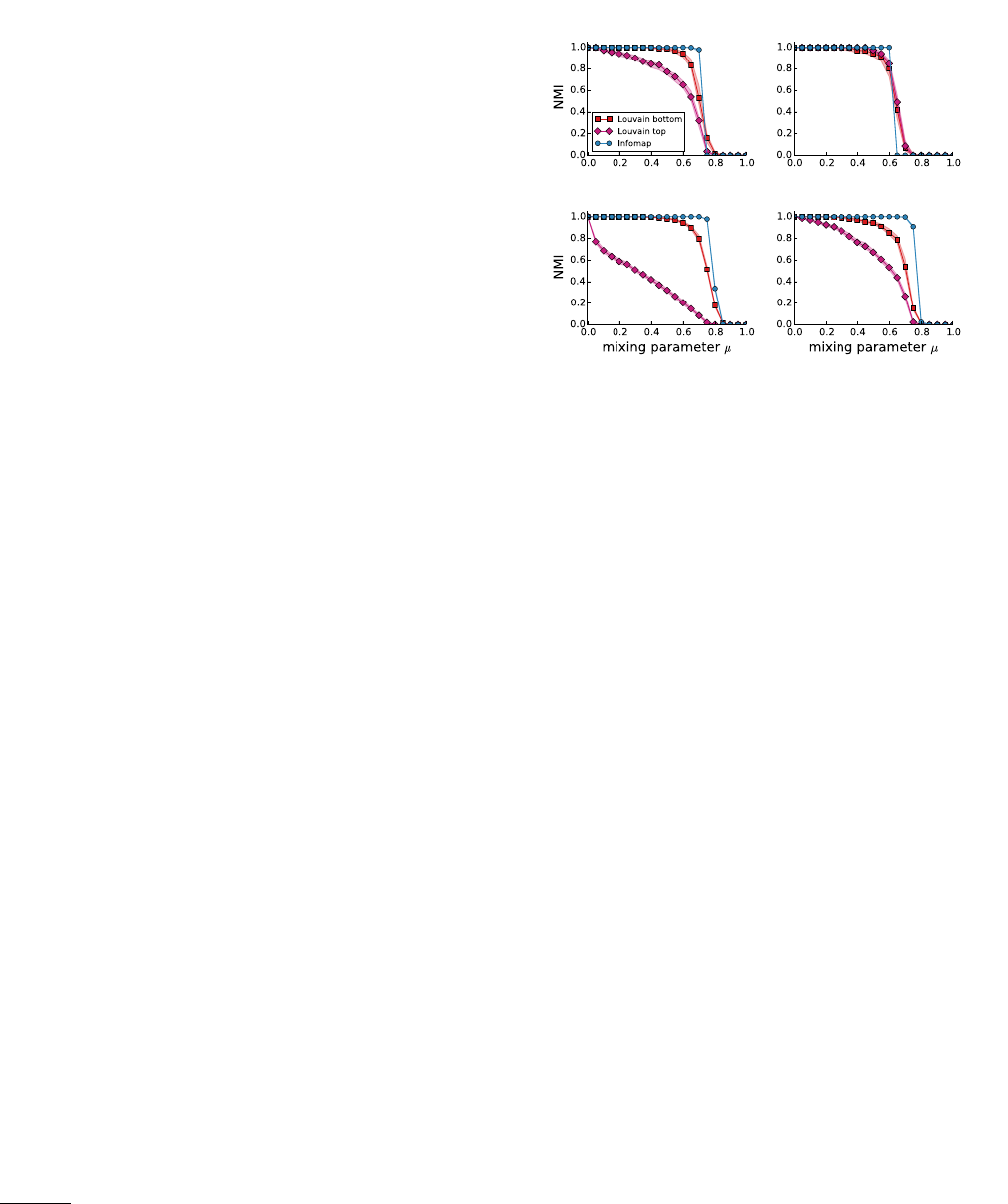
30
cichinetti and Fortunato,2011). In addition, tuning the
resolution parameter in the search for good partitions
is usually computationally very demanding, as in many
cases the optimisation procedure has to be repeated over
and over for all γ-values one desires to investigate.
We stress that the resolution limit is a feature of modu-
larity itself, not of the specific way adopted to maximise
it. Therefore, there is no magic heuristic that can cir-
cumvent this issue. The Louvain method (Blondel et al.,
2008) has been held as one such magic heuristic. The
method performs a greedy optimisation of Qin a hierar-
chical manner, by assigning each vertex to the community
of their neighbours yielding the largest Q, and creating
a smaller weighted super-network whose vertices are the
clusters found previously. Partitions found on this super-
network hence consist of clusters including the ones found
earlier, and represent a higher hierarchical level of clus-
tering. The procedure is repeated until one reaches the
level with largest modularity. In the comparative anal-
ysis of clustering algorithms performed by Lancichinetti
and Fortunato on the LFR benchmark (Lancichinetti and
Fortunato,2009), the Louvain algorithm was the sec-
ond best-performing method, after Infomap (Rosvall and
Bergstrom,2008). This has given the impression that
the peculiar strategy of the method solves the resolution
problems above, which is not true. The reason why the
performance is so good is that Lancichinetti and Fortu-
nato adopted the lowest partition of the hierarchy, the
one with the smallest clusters (Lancichinetti and Fortu-
nato,2014). By using the partition with highest modu-
larity performance degrades considerably (Fig. 26), as ex-
pected. As suggested by the developers of the algorithm
themselves, using the lowest level helps avoiding unnatu-
ral community mergers; as an example, they showed that
the natural partition of the ring of cliques (Fig. 25) can
be recovered this way. However, the bottom level has
lower modularity than the top level, so we face a sort of
contradiction, in that users are encouraged to use subop-
timal partitions, even though one assumes that the best
clustering corresponds to the highest value of the qual-
ity function, which is what the method is supposed to
find. There is no guarantee that the bottom level yields
the most meaningful solution. On the other hand, users
have the option of choosing among a few partitions and
a slightly higher chance to find what they search for.
Moreover, the modularity landscape is characterised
by a larger than exponential36 number of distinct par-
titions, whose modularity values are very close to the
global maximum (Good et al.,2010). This explains why
many heuristic methods of modularity maximisation are
able to come very close to the global maximum of Q,
eters, so that a coexistence of very diverse scales is permit-
ted (Granell et al.,2012). Such approaches, however, deviate
from the original idea of modularity maximisation, which is based
on a global null model valid for the network as a whole.
36 Exponential in the number nof graph vertices.
N=1000, S N=1000, B
N=5000, S N=5000, B
FIG. 26 Performance of the Louvain method. The panels
indicate the accuracy of the algorithm to detect the planted
partition of the LFR benchmark as a function of the mixing
parameter, for different choices of the network size (1000 and
5000 vertices) and of the range of community sizes (label Sin-
dicates that communities have between 10 and 50 vertices, la-
bel Bthat they have between 20 and 100 vertices). Accuracy
is calculated via the normalised mutual information (NMI),
in the version by Lancichinetti, Fortunato and Kert´esz (Lan-
cichinetti et al.,2009). Results are heavily depending on the
hierarchical level one chooses at the end of the procedure.
When one picks the top level (diamonds), which is the one
with largest modularity, the accuracy is poor, as expected,
especially when communities are smaller. When one goes for
the bottom level (squares), which has lower modularity and
smaller clusters than the top level partition, there is a far bet-
ter agreement with the planted partition and the performance
gets closer to that of Infomap (circles). The squares follow the
performance curves used in the comparative analysis by Lan-
cichinetti and Fortunato (Lancichinetti and Fortunato,2009).
Courtesy from Andrea Lancichinetti.
but it also implies that the global maximum is basically
impossible to find. In addition, high-Qpartitions are
not necessarily similar to each other, despite the prox-
imity of their modularity scores. The optimal structural
partition, which may not correspond to the modularity
maximum due to problems exposed above, may however
have a large Q-value. Therefore the optimal partition is
basically indistinguishable from a huge number of high-
modularity partitions, which are in general structurally
dissimilar from it. The large structural diversity of high-
modularity partitions implies that one cannot rely on any
of them, at least in principle. Reliable solutions could
be singled out when the domain user imposes some con-
straints on the clustering of the system, or when she
expects it to have specific features. In the absence of
additional information or expectations, consensus clus-
tering could be used to derive more robust partitions.
Indeed, it has been shown that the consensus of many
high-modularity partitions, combined with a hierarchical

31
approach, could help to solve resolution problems and
to avoid to find communities in random graphs without
groups (Zhang and Moore,2014).
As of today, modularity optimisation is still the most
used clustering technique in applications. This may ap-
pear odd, given the serious issues of the method and the
fact that nowadays more powerful techniques are avail-
able, like a posteriori stochastic block modelling (Sec-
tion IV.J). Indeed Newman has proven that optimising
modularity is equivalent to maximising the likelihood
that the planted partition model reproduces the net-
work (Newman,2016). But the planted partition model
is a very specific case of the general stochastic block
model, in that the intra-group edge probabilities are all
equal to the same value pin and the inter-group edge
probabilities are all equal to the same value pout. There
is no reason to limit the inference to this specific case,
when one could use the full model.
Optimising partition quality functions may lead to res-
olution problems, just like it happens for modularity37.
Instead, one could try to optimise cluster quality func-
tions. One starts with some function q(C) expressing how
“community-like” a subgraph is and with a seed vertex
s. The goal is to build a cluster Csincluding ssuch that
q(Cs) is maximum38. This is usually done by exploring
the neighbours of the temporary subgraph Cs, starting
from the neighbours of swhen Csincludes only s. The
neighbouring vertex whose inclusion yields the largest in-
crease of qis added to the subgraph. When a new vertex
is included, the structure of the subgraph is altered and
the other vertices can be examined again, as it might be
advantageous to knock some of them out. The process
stops when the quality q(Cs) cannot be increased any-
more via the inclusion or the exclusion of vertices.
The optimisation of cluster quality functions offers a
number of advantages over the optimisation of partition
quality functions. First, it is consistent with the idea
that communities are local structures, which are sensi-
tive to what happens in their neighbourhood, but are
fairly unaffected by the rest of the network: the struc-
ture of a social circle in Europe is hardly influenced by
the dynamics of social circles in Australia, though they
are parts of the same global social network of humans.
Consequently, if a network undergoes structural changes
in one region, community structure is altered and is to
37 Traag and Van Dooren have shown that one can design addi-
tive quality functions such that the best partition of the net-
work induces the optimal partition for any subgraph S, i. e.,
the partition found when the detection is performed only on
S(Traag et al.,2011). This is possible when the coefficients
of the summand corresponding to each community does not de-
pend on global properties of the graph. Even those functions
have their own preferential community scale, though.
38 For some functions the optimum corresponds to their minimum,
not the maximum. This occurs when they are related to variables
that are supposed to be small when communities are good, like
the density of edges between clusters.
be recovered only in that region, while the clustering of
the rest of the network remains the same. By optimising
partition quality functions, instead, any little change may
have an effect on every community of the graph. Second,
since cluster quality functions do not embody any global
scale, severe resolution problems are usually avoided39.
Moreover, one can investigate only parts of the network,
which is particularly valuable when the graph is large
and a global analysis would be out of reach, computa-
tionally. The local exploration of the graph allows to
reach vertices already assigned to clusters, so overlaps
can be naturally detected. In the last years several algo-
rithms based on the optimisation of cluster quality func-
tions have been designed (Baumes et al.,2005;Clauset,
2005;Huang et al.,2011;Lancichinetti et al.,2009,2011).
G. Methods based on dynamics
Communities can also be identified by running dynam-
ical processes on the network, like diffusion (Jeub et al.,
2015;Pons and Latapy,2005;Rosvall and Bergstrom,
2008;Van Dongen,2000;Zhou,2003a,b;Zhou and
Lipowsky,2004), spin dynamics (Raghavan et al.,2007;
Reichardt and Bornholdt,2006;Ronhovde and Nussinov,
2010;Traag et al.,2011), synchronisation (Arenas et al.,
2006;Boccaletti et al.,2007), etc.. In this section we
focus on diffusion and spin dynamics, that inform most
approaches.
Random walk dynamics is by far the most exploited in
community detection. If communities have high internal
edge density and are well-separated from each other, ran-
dom walkers would be trapped in each cluster for quite
some time, before finding a way out and migrating to
another cluster. We briefly discuss two broad classes
of algorithms: methods based on vertex similarity and
methods based on the map equation.
The first class of techniques consists in using random
walk dynamics to estimate the similarity between pairs
of vertices. For instance, in the popular method Walk-
trap the similarity between vertices iand jis given by
the probability that a random walker moves from ito j
in a fixed number of steps t(Pons and Latapy,2005).
The parameter thas to be large enough, to allow for the
exploration of a significant portion of the graph, but not
too big, as otherwise one would approach the stationary
limit in which transition probabilities trivially depend on
the degrees of the vertices. If there is a pronounced com-
munity structure, pairs of vertices in the same cluster are
much more easily reachable by a random walk than pairs
of vertices in different clusters, so the vertex similarity
is expected to be considerably higher within groups than
between groups40. In that case, clusters can be readily
39 If one defines the quality of the cluster with respect to the rest
of the network, global scales may still slip into the function.
40 A related method is the Markov Cluster Algorithm
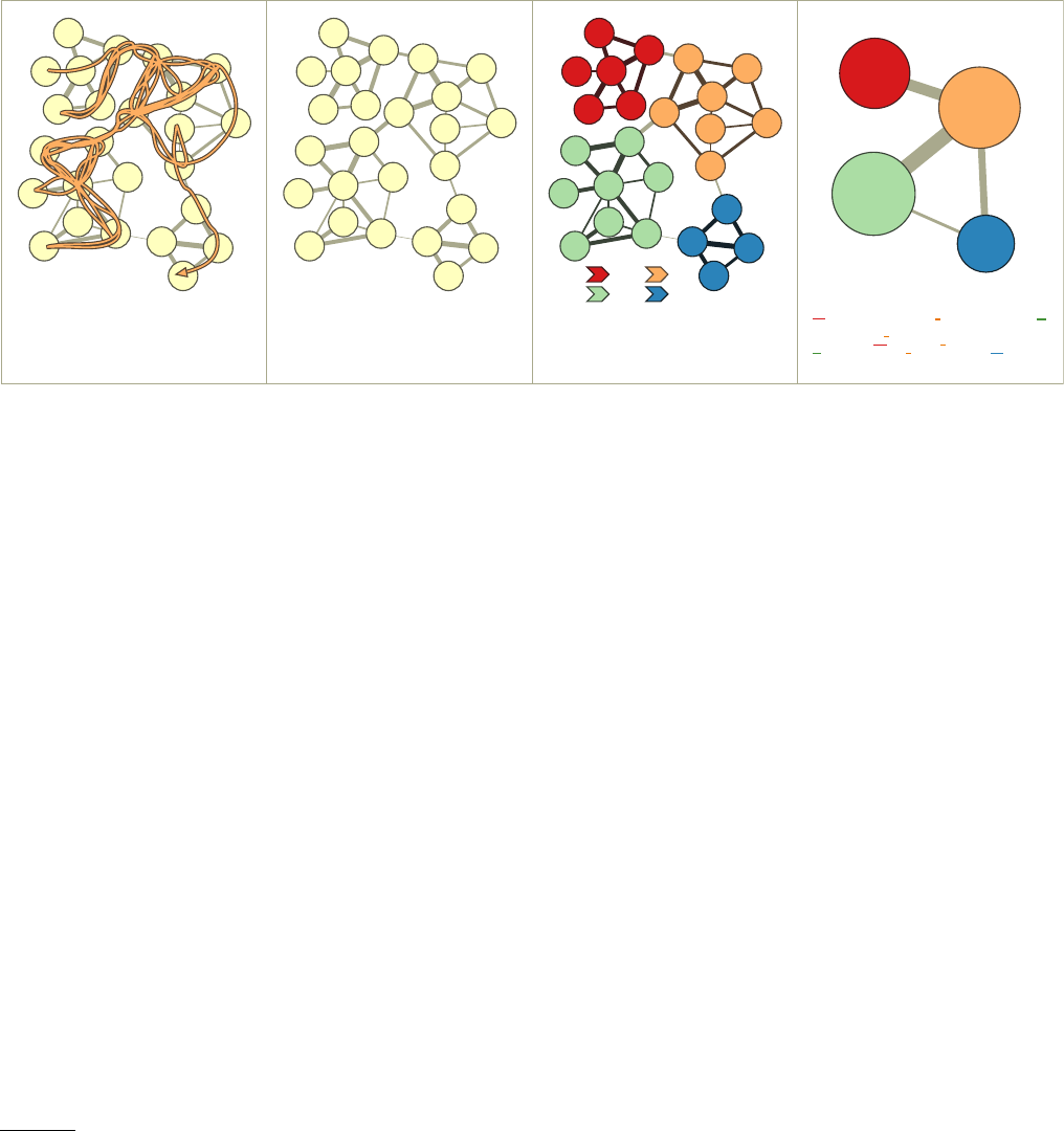
32
A B C D
1111100
01011
1100
10000
0110
11011
0011
10111
1001
0100
111111
11010
10110
10101
11110
00011
0010
0000
1111101
10100
01010
1110
10001
0111
00010
1111100 1100 0110 11011 10000 11011 0110 0011 10111 1001 0011
1001 0100 0111 10001 1110 0111 10001 0111 1110 0000 1110 10001
0111 1110 0111 1110 1111101 1110 0000 10100 0000 1110 10001 0111
0100 10110 11010 10111 1001 0100 1001 10111 1001 0100 1001 0100
0011 0100 0011 0110 11011 0110 0011 0100 1001 10111 0011 0100
0111 10001 1110 10001 0111 0100 10110 111111 10110 10101 11110
00011
0000
001
11
100
01
101
110
011
00
111
1010
100
010
00
10
011
11
011
0010
010
1101
10
000
111
1100
111 0000 11 01 101 100 101 01 0001 0 110 011 00 110 00 111 1011 10
111 000 10 111 000 111 10 011 10 000 111 10 111 10 0010 10 011 010
011 10 000 111 0001 0 111 010 100 011 00 111 00 011 00 111 00 111
110 111 110 1011 111 01 101 01 0001 0 110 111 00 011 110 111 1011
10 111 000 10 000 111 0001 0 111 010 1010 010 1011 110 00 10 011
110 00010 0001
0 1011111 0001
110
10
0
111
111 0000 11 01 101 100 101 01 0001 0110 011 00 110 00 111 1011 10
111 000 10 111 000 111 10 011 10 000 111 10 111 10 0010 10 011 010
011 10 000 111 0001 0111 010 100 011 00 111 00 011 00 111 00 111
110 111 110 1011 111 01 101 01 0001 0110 111 00 011 110 111 1011
10 111 000 10 000 111 0001 0111 010 1010 010 1011 110 00 10 011
FIG. 27 Infomap. The random walk in (A) can be described as a sequence of the vertices, each labeled with unique codewords
(B), or by dividing the graph in regions and using unique codewords only for the vertices of the same region (C). This way the
same codeword can be used for multiple vertices, at the cost of indicating when the random walker leaves a region to enter a
new one, as in that case one has to specify the codeword of the new region, to unambiguously locate the walker. The network
has four communities [indicated by the colours in (C)], and in this case the map-like description of (C) is more parsimonious
than the one in (B). This is shown by looking at the actual code needed in either case (bottom of the figures), which is clearly
shorter for (C). In (D) the transitions between the clusters are highlighted. Reprinted figure with permission from (Rosvall and
Bergstrom,2008). c
2008, by the National Academy of Sciences, USA.
identified via standard hierarchical or partitional cluster-
ing techniques (Jain et al.,1999;Xu and Wunsch,2008).
This class of methods have a high computational com-
plexity, higher than quadratic in the number nof ver-
tices (on sparse graphs), so they cannot be used on large
networks. Besides, they are often parameter-dependent.
The map equation stems from a seminal paper by Ros-
vall and Bergstrom (Rosvall and Bergstrom,2008), who
asked what is the most parsimonious way to describe an
infinitely long random walk taking place on the graph.
The information content of any description is given by
the total number of bits required to indicate the vari-
ous stages of the process. The simplest description is
obtained by listing sequentially all vertices reached by
the random walker, each vertex being described by a
unique codeword. However, if the network has a com-
munity structure, there may be a more compact descrip-
tion, which follows the principle of geographic maps,
(MCL) (Van Dongen,2000), which consists of iterating
two operations: raising to a power the transfer matrix Tof
the graph, whose element Tij equals the probability that a
random walker, sitting at j, moves to i; raising the elements
of the resulting matrix to a power, such that the larger values
are enhanced with respect to the smaller ones, many of which
are set to zero to lighten the calculations, while the remaining
ones are normalised by dividing them by the sum of elements
of their column, yielding a new transfer matrix. The process
eventually reaches a stationary state, corresponding to the
matrix of a disconnected graph, whose connected components
are the sought clusters.
where there are multiple cities and streets with the same
name across regions. Vertex codewords could be recy-
cled among different communities, which play the role of
regions/states, and vertices with identical name are dis-
tinguished by specifying the community they belong to.
If clusters are well separated from each other, transitions
between clusters are infrequent, so it is advantageous to
use the map, with the communities as regions, because
in the description of the random walk the codewords of
the clusters will not be repeated many times, while there
is a considerable saving in the description due to the lim-
ited length of the codewords used to denote the vertices
(Fig. 27). The map equation yields the description length
of an infinite random walk consists of two terms, express-
ing the Shannon entropy of the walk within and between
clusters. The best partition is the one yielding the mini-
mum description length.
This method, called Infomap, can be applied to
weighted networks, both undirected and directed. In the
latter case, random walk dynamics is modified by intro-
ducing a teleportation probability, as in the PageRank
process (Brin and Page,1998), to ensure that a non-
trivial stationary state is reached. It has been succes-
sively extended to the detection of hierarchical commu-
nity structure (Rosvall and Bergstrom,2011) and of over-
lapping clusters (Viamontes Esquivel and Rosvall,2011).
In classic random walks the probability of reaching a ver-
tex only depends on where the walker stands, not on
where it is coming from. The map equation has also
been extended to random walks whose transition proba-
bilities depend on earlier steps too (higher-order Markov
33
dynamics) (Persson et al.,2016;Rosvall et al.,2014), re-
taining memory of the (recent) past. Applications show
that in this way one can recover overlapping communi-
ties more easily than by using standard first-order ran-
dom walk dynamics, especially pervasive overlaps, which
are usually out of reach for most clustering algorithms
(Section III.E).
Infomap and its variants usually return different par-
titions than structure-based methods (e. g., modularity
optimisation). This is because they are based on flows
running across the system, as opposed to structural vari-
ables like number of edges, vertex degrees, etc.. The dif-
ference is particularly striking on directed graphs (Ros-
vall and Bergstrom,2008), where edge directions heavily
constrain the possible flows. Structural features obvi-
ously play a major role on the dynamics of processes
running on graphs, but dynamics cannot be generally re-
duced to an interplay of structural elements, at least not
simple ones like, e. g., vertex degrees. Sometimes struc-
tural and dynamic approaches are equivalent, though.
For instance, Newman-Girvan’s modularity is a special
case of a general quality function, called stability, ex-
pressing the persistence of a random walk within com-
munities (Delvenne et al.,2010;Lambiotte et al.,2008).
The methods we have discussed so far are global, in
that they aim at finding the whole community structure
of the system. However, random walks along with other
dynamical processes can be used as well to explore the
network locally, starting from seed vertices (Jeub et al.,
2015). Good communities correspond to bottlenecks of
the dynamics and depend on the choice of the seed ver-
tices, the time scale of the dynamics, etc.. Such local
perspective enables to identify community overlaps in a
natural way, due to the possibility of reaching vertices
multiple times, even if they are already classified.
Spin dynamics (Baxter,2007) are also regularly used
in network clustering. The first step is to define a spin
model on the network, consisting of a set of spin variables
{si, i = 1,2, . . . , n}, assigned to the vertices and a Hamil-
tonian H({s}), expressing the energy of the spin config-
uration {s}. For community detection, spins are usually
integers: s= 1,2, . . . , q. Contributions to the energy are
usually given by spin-spin interactions. The coupling of a
spin-spin interaction can be ferromagnetic (negative) or
antiferromagnetic (positive), if the energy is lower when
the spins are equal or not, respectively. The goal is to find
those spin configurations that minimise the Hamiltonian
H({s}). If couplings are all ferromagnetic, the minimum
energy would be trivially obtained for the configurations
where all vertices have identical spin values. Instead,
one would like to have identical spins for vertices of the
same cluster, and different spins for vertices in different
clusters, to identify the community structure. There-
fore, Hamiltonians feature both ferromagnetic and anti-
ferromagnetic interactions [spin glass dynamics (Mezard
et al.,1987)]. A popular model consists in rewarding
edges between vertices in the same cluster, as well as
non-edges between vertices in different clusters, and pe-
nalising edges between vertices of different clusters, along
with non-edges between vertices in the same cluster. This
way, if the edge density within communities is apprecia-
bly larger than the edge density between communities,
as it often happens, having equal spin values for ver-
tices in the same cluster would considerably lower the
energy of the configuration. On the other hand, to bring
the energy further down the spins of vertices in different
clusters should be different, as many such vertices would
be disjoint from each other, and such non-edges would
increase the energy of the system if the corresponding
spin variables were equal. A general expression for the
Hamiltonian along these lines is (Reichardt and Born-
holdt,2006)
H({s}) = −X
ij
[aij Aij −bij (1 −Aij )]δ(si, sj),(23)
where Aij is the element of the adjacency matrix,
aij , bij ≥0 are arbitrary coefficients, and the Kronecker
delta selects only the pairs of vertices with the same spin
value.
A popular model is obtained by setting aij = 1 −bij
and bij =γPij , where γis a tunable parameter and Pij
a null model term, expressing the expected number of
edges running between vertices iand junder a suit-
able randomisation of the graph structure. The resulting
Hamiltonian is (Reichardt and Bornholdt,2006)
HRB ({s}) = −X
ij
(Aij −γPij )δ(si, sj).(24)
If γ= 1 and Pij =kikj/2m,ki(kj) being the degree
of i(j) and mthe total number of graph edges, the
Hamiltonian of Eq. (24) coincides with the modularity
by Newman and Girvan [Eq. (20)], up to an irrelevant
multiplicative constant. Consequently, modularity can
be interpreted as the Hamiltonian of a spin glass as well.
By setting aij = 1 and bij =γwe obtain the Abso-
lute Potts Model (APM) (Ronhovde and Nussinov,2010),
whose Hamiltonian reads
HAP M ({s}) = −X
ij
[Aij −γ(1 −Aij )]δ(si, sj).(25)
Here, there is no null model term. The models of
Eqs. (24) and (25) can be trivially extended to weighted
graphs (Traag et al.,2011). They allow to explore the
network at different resolutions, by suitably tuning the
parameter γ. However, there usually is no information
about the community sizes, so it is not possible to de-
cide a priori the proper value(s) of γfor a specific graph.
A common heuristic is to estimate the stability of parti-
tions as a function of γ. It is plausible that partitions
recovered for a given γ-value will not be disrupted if γ
is varied a little. So, the whole range of γcan be split
into intervals, each interval corresponding to the most
frequent partition detected in it. Good candidates for
the unknown community structure of the system could

34
be the partitions found in the widest intervals of γ, as
they are likely to be more stable (or robust) than the
other partitions41. However, the results of the algorithm
do not usually have a linear relationship with γ, hence
the width of the intervals is not necessarily correlated
with stability, as intervals of the same width but centred
at different values of γmay have rather different impor-
tance.
A good operational definition of stability is based on
the stochastic character of optimisation methods, which
typically deliver different results for the same system and
set of parameters, by changing initial conditions and/or
random seeds. If a partition is robust in a given range
of γ-values, most partitions delivered by the algorithm
will be very similar. On the other hand, if one explores
aγ-region in between two strong partitions, the algo-
rithm will deliver the one or the other partition and the
individual replicas will be, on average, not so similar to
each other. So, by calculating the similarity S(γ) of par-
titions found by the method at a given resolution pa-
rameter γ(for different choices of initial conditions and
random seeds), stable communities are revealed by peaks
of S(γ) (Ronhovde and Nussinov,2009). Since cluster-
ing in large graphs can be very noisy, peaks may not be
well resolved. Noise can be reduced by working with con-
sensus partitions of the individual partitions returned by
the method for a given γ(Section IV.B). These manipula-
tions are computationally costly, though. Besides, multi-
resolution techniques may miss relevant cluster sizes, as
it happens for multi-resolution modularity (Lancichinetti
et al.,2011) (Section IV.F).
H. Dynamic clustering
Due to the increasing availability of time-stamped net-
work data, there is currently a lot of activity on the devel-
opment of methods to analyse temporal networks (Holme
and Saram¨aki,2012). In particular, the problem of de-
tecting dynamic communities has received a lot of atten-
tion (Fortunato,2010;Spiliopoulou,2011).
Clustering algorithms used for static graphs can be
(and often are) used for dynamic networks as well. What
needs to be established is how to handle the evolution.
Typically one can describe it as a succession of snapshots
G1, G2, . . . , Gl, where each snapshot Gtcorresponds to
the configuration of the graph in a given time window42.
There are two possible strategies.
41 We stress, however, that the persistence of partitions in intervals
is not necessarily related to clustering robustness (Lewis et al.,
2010;Onnela et al.,2012).
42 A graph configuration consists of the sets of vertices and edges
that are active within the given time frame, along with the in-
tensity of their interactions in that frame (weights) and possibly
other aspects of the dynamics, like burstiness (Barab´asi,2010),
duration of the interactions, etc..
The simplest approach is to detect the community
structure for each individual snapshot, which is a static
graph (Asur et al.,2007;Hopcroft et al.,2004;Palla et al.,
2007). Next, pairs of communities of consecutive win-
dows are associated. A standard procedure is finding
the cluster Ci
tin window tthat is most similar to clus-
ter Cj
t+1 in window t+ 1, for instance by using Jaccard
similarity score [Eq. (6)] (Palla et al.,2007). This way
every community has an image in each phase of the net-
work evolution and one can track its dynamics. Various
scenarios are possible. Communities may disappear at
some point and new communities may appear, following
the exclusion or the introduction of vertices and edges,
respectively. Furthermore, a cluster may fragment into
smaller ones or merge with others. However, since snap-
shots are handled separately, this strategy often produces
significant variations between partitions close in time, es-
pecially when the data sets are noisy, as it usually hap-
pens in applications.
It would be preferable to have a unified framework,
in which communities are inferred both from the current
structure of the graph and from the knowledge of the
community structure at previous times. An interesting
implementation of this strategy is evolutionary cluster-
ing (Chakrabarti et al.,2006). The goal of the approach
is finding a partition that is both faithful to the system
configuration at snapshot tand close to the partition de-
rived for the previous snapshot t−1. A cost function is
introduced, whose optimisation yields a tradeoff between
such two constraints. There is ample flexibility on how
this can be done, in practice. Many known clustering
techniques normally used for static graphs can be refor-
mulated within this evolutionary framework. Some inter-
esting algorithms based on evolutionary clustering have
been proposed (Chi et al.,2007;Lin et al.,2008). Mucha
et al. have also presented a method that couples the
system’s configurations of different snapshots, within a
modularity-based framework (Mucha et al.,2010). In the
resulting quality function (multislice modularity), all con-
figurations are simultaneously taken into account and the
coupling between them is expressed by a tunable param-
eter. The approach can handle general multilayer net-
works (Boccaletti et al.,2014;Kivel¨a et al.,2014), where
layers are either networks whose vertices are connected
by a specific edge type (e. g., friendship, work relation-
ships, etc., in social networks), or networks whose ver-
tices have connections (interactions, dependencies) with
the vertices of other networks/layers. On the other hand,
since the approach is based on modularity optimisation,
it has the drawbacks exposed in Section IV.F.
Consensus clustering (Section IV.B) is a natural ap-
proach to find stable dynamic clusterings by combining
multiple snapshots. Let us suppose we have a time range
going from t0to tm, that we want to divide into wwin-
dows of size ∆t. For the sake of stability, one should con-
sider sliding windows, i. e., overlapping time intervals.
This way consecutive partitions will be based on system
configurations sharing a lot of vertices and edges, and
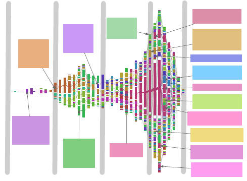
35
change is (typically) smooth. In order to have exactly
wframes, each of them has to be shifted by an interval
δt = (tm−t0)/w with respect to the previous one. So we
obtain the windows [t0, t0+ ∆t], [t0+δt, t0+ ∆t+δt],
[t0+ 2δt, t0+ ∆t+ 2δt], ..., [tm−∆t, tm]. The community
structure of each snapshot can be found via any reliable
static clustering technique. Next, the consensus partition
from the clusterings of rconsecutive snapshots, with r
suitably chosen, is derived (Lancichinetti and Fortunato,
2012). Again, one could consider sliding windows: for in-
stance, the first window could consist of the first rsnap-
shots, the second one by those from 2 to r+ 1, and so
on until the interval spanned by the last rsnapshots. In
Fig. 28 we show an application of this procedure on the
citation network of papers published in journals of the
American Physical Society (APS).
2000 - 2005
Small World
Scale Free
Prisoner's Dilemma
Granular Packing
Materials
Semiflexible
Polymer
Microrheology
Noise Resonance Induced Excitable Network Coherence System Cell Stochastic Oscillatory Spatially Diversity Correlated Neural Med■um , year: 2002.5
Noise
Resonance
Neural Cell
Synchronization
Oscillators
Social Clustering
Community
Modularity
Complex Spreading
Epidemics
Random Boolean
Cellular Automaton
Coloring
Satisfiability Code
Self
Organized
Criticality
Sandpiles
Percolation
Random
Fractal
Elastic
Percolation
Conductivity
Critical
Threshold Fractal
Aggregation
Growth
Diffusion
1980 - 1985
1990 - 1995
1970 - 1975
2007 - 2008
Feedback Noise
Delay Stochastic
FIG. 28 Consensus clustering on dynamic networks. Time
evolution of clusters of the citation network of papers pub-
lished in journals of the American Physical Society (APS).
The clusters with the keyword Network(s) among the top 15
most frequent words appearing in the title of the papers were
selected. Communities were detected with Infomap (Rosvall
and Bergstrom,2008) on snapshots spanning each a window
of 5 years, except at the right end of each diagram: since
there is no data after 2008, the last windows must have 2008
as upper limit, so their size shrinks (2004−2008, 2005−2008,
2006−2008, 2007−2008). Each vertical bar represents a con-
sensus partition combining pairs of consecutive snapshots. A
color uniquely identifies a community, the width of the links
between clusters is proportional to the number of papers they
have in common. The rapid growth of the field Complex Net-
works is clearly visible, as well as its later split into a num-
ber of smaller subtopics, like Community Structure,Epidemic
Spreading,Robustness, etc.. Reprinted figure with permission
from (Lancichinetti and Fortunato,2012). c
2012, by the
Nature Publishing Group.
An alternative way to uncover the evolution of commu-
nities by accounting for the correlation between configu-
rations of neighbouring time intervals is to use probabilis-
tic models (Peixoto,2015a;Peixoto and Rosvall,2015;
Sarkar and Moore,2005;Yang et al.,2009).
If the system is large and its structure is updated in
a stream fashion, instead of working on snapshots one
could detect the clustering online, every time the con-
figuration of the system varies due to new information,
like the addition of a new vertex or edge (Aggarwal and
Philip,2005;Zanghi et al.,2008). An advantage of this
approach is that change is due to the effect that the small
variation in the network structure has on the system, and
it can be tracked by simply adjusting the partition of the
previous configuration, which can be usually done rather
quickly.
I. Significance
Let us suppose that we have identified the communi-
ties, somehow. Are we done? Unfortunately, things are
not that simple.
In Fig. 29 (top left) we show the adjacency matrix
of the random graph ´a la Erd˝os-R´enyi illustrated in
Fig. 8d. The graph has 5 000 vertices, so the matrix
is 5 000 ×5 000. Black dots indicate the existence of an
edge between the corresponding vertices, while missing
edges are represented in white. By construction, there
is no group structure. However, we can rearrange the
elements of the matrix, by reordering the vertex labels.
In Fig. 29 (top right) we see that, by doing that, one
can generate a group structure, of the assortative type,
with two blocks of equal size. If we increase the number
of blocks to three Fig. 29 (bottom left) and ten Fig. 29
(bottom right) we can make the matrix look more and
more modular. This is why many clustering techniques
detect communities in random networks as well, though
they should not. Where do the groups come from? Since
they cannot be real by construction, they must be gener-
ated by random fluctuations in the network construction
process. Random fluctuations are particularly relevant
on sparse graphs (Section III.C).
The lesson we learn from this example is that it is
not sufficient to identify groups in the network, but one
should also ask how significant, or non-random, they are.
Unfortunately, most clustering algorithms are not able
to assess the significance of their results. If the groups
are compatible with random fluctuations, they are not
proper groups and should be disregarded. The lower the
chance that they are generated by randomness, the more
confident we can be that the blocks reflect some actual
group structure. Naturally, this can be done only if one
has a reliable null model, describing how the structure
of the network at study can be randomised and allow-
ing us to estimate how likely it is that the candidate
group structure is generated this way. The configura-
tion model (Bollob´as,1980;Molloy and Reed,1995) is
a popular null model in the literature. It generates all
possible configurations preserving the number of vertices
and edges of the network at study, and the degrees of its
vertices. One may compute some variables of the origi-
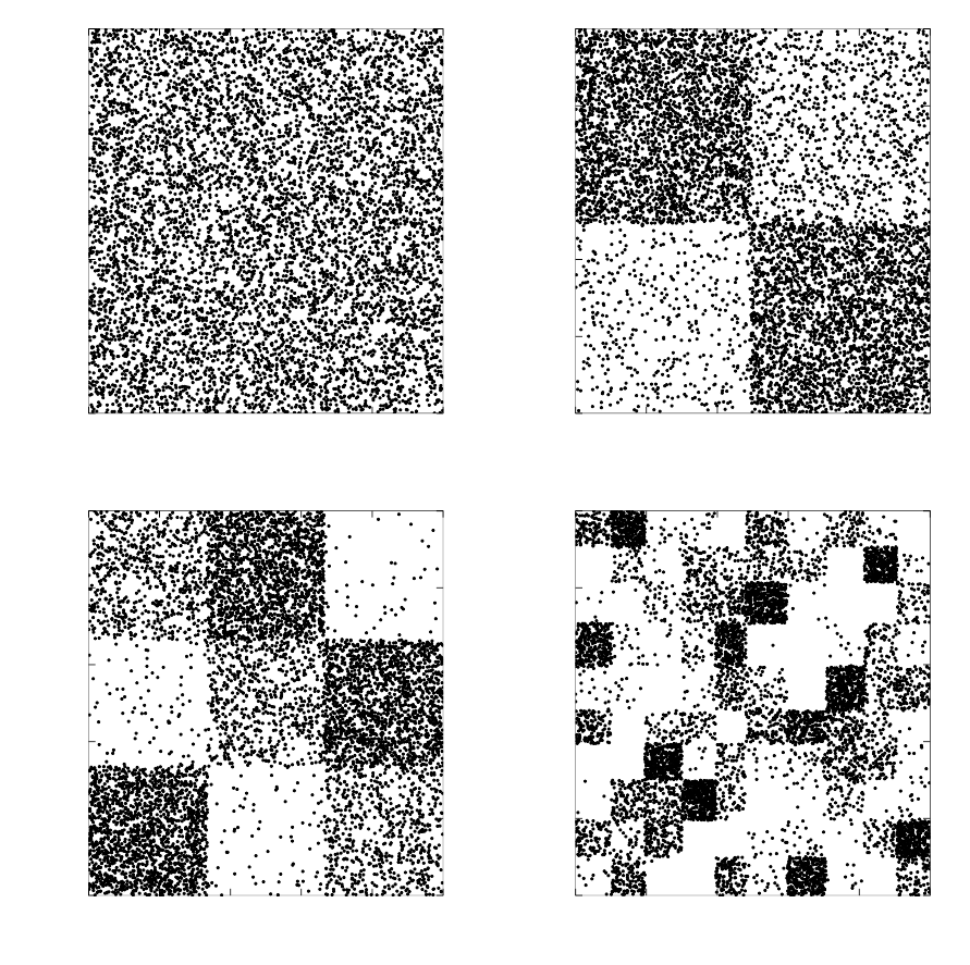
36
0 1000 2000 3000 4000 5000
Vertex
0
1000
2000
3000
4000
5000
Vertex
0 1000 2000 3000 4000 5000
Vertex
0
1000
2000
3000
4000
5000
Vertex
0 1000 2000 3000 4000 5000
Vertex
0
1000
2000
3000
4000
5000
Vertex
0 1000 2000 3000 4000 5000
Vertex
0
1000
2000
3000
4000
5000
Vertex
FIG. 29 Artificial groups in random networks. The elements of the adjacency matrix of an Erd˝os-R´enyi random graph (top left)
can be rearranged, by suitably reshuffling the list of vertices. This procedure may produce a block structure, with the blocks
becoming increasingly more visible the smaller their size. Such groups are not real, though, but they are generated by random
fluctuations in the edge patterns among the vertices. The construction principle of the network does not give any special role
to groups of vertices, since all pairs of vertices have identical probability to be joined. Courtesy by Tiago P. Peixoto.

37
nal network, and estimate the probability that the model
reproduces them, or p-value, i. e., the fraction of model
configurations yielding values of the variables compati-
ble with those measured on the original graph. If the
p-value is sufficiently low (5% is a standard threshold),
one concludes that the property at study cannot be gen-
erated by randomness only. For community structure,
one can compute various properties of the clusters, e. g.,
their internal density, and compare them with the model
values. Some clustering algorithms, like OSLOM (Lanci-
chinetti et al.,2011) are based on this principle. Along
the same lines, z-scores can be used as well [see the ex-
ample of Eq. (22)]. Degree-corrected stochastic block
models (Karrer and Newman,2011) (Section IV.E) also
include the configuration model, which corresponds to
the case without group structure43. In this case signifi-
cance can be estimated by doing model selection between
the versions with and without blocks (Section IV.E).
A concept very related to significance is that of robust-
ness. If clusters are significant it means that they are
resilient if the network structure is perturbed, to some
extent. One way to quantitatively assess this is intro-
ducing into the system a controlled amount of noise, and
checking how much noise it takes to disrupt the group
structure. The greater the required perturbation, the
more robust the communities. For instance, a pertur-
bation could be rewiring a fraction of randomly chosen
edges (Karrer et al.,2008). After the network is per-
turbed, the community structure is derived and com-
pared to the one of the original network44. The trend
of the partition similarity shows how the group structure
responds to perturbations.
A similar approach consists in sampling network con-
figurations from a population which the original network
is supposed to belong to (bootstrapping), and comparing
the clusterings found in those configurations, to check
how frequently subsets of vertices are clustered together
in different samples, which is an index of the robustness
(significance) of their clusters (Rosvall and Bergstrom,
2010).
J. Which method then?
At the end of the day, what most people want to know
is: which method shall I use on my data? Since the clus-
tering problem is ill-defined, there is no clear-cut answer
to it.
Popular techniques are based on similar ideas of com-
43 Actually it would be a variant of the configuration model, as the
degree sequence of the vertices would be preserved only on aver-
age, not exactly. It is the same null model used in the standard
formulation of modularity (Section IV.F).
44 For reliable results multiple configurations have to be generated,
for a given amount of noise, and the similarity scores have to be
averaged.
munities, like the ones we reviewed in Sections II.B and
II.C. What makes the difference is the way clusters are
sought. The specific procedure affects the reliability of
the results (e. g., because of resolution problems) and
the time complexity of the calculation, determining the
scope of the method and constraining its applicability.
Most methods propose a universal recipe, that is sup-
posed to hold on every data set. In so doing, one neglects
the peculiarities of the network at study, which is valu-
able information that could orient the method towards
more reliable solutions. But algorithms are usually not
so flexible to account for specific network features. For
instance, in some cases, there is no straightforward ex-
tension capable to handle high-level features like edge
direction or overlapping communities45.
Validation of algorithms, like the comparative analysis
of (Lancichinetti and Fortunato,2009), have allowed to
identify a set of methods that perform well on artificial
benchmarks. There are two important issues, though.
First, we do not know how well real networks are de-
scribed by currently used benchmark models. There-
fore, there is no guarantee that methods performing well
on benchmarks also give reliable results on real data
sets. Structural analyses like the ones discussed in Sec-
tion III.E might allow to identify more promising bench-
mark models. Second, if we rely so much on current
benchmarks, which are versions of the stochastic block
model (SBM), we already know what the best method
is: a posteriori block modelling, i. e., fitting a SBM on
the data. Indeed, there are several advantages to this
approach. It is more general, it does not only discover
communities but several types of group structures, like
disassortative groups (Fig. 8b) and core-periphery struc-
ture (Fig. 8c). It can also capture the existence of hierar-
chies among the clusters. Moreover, it yields much richer
results than standard clustering algorithms, as it delivers
the entire set of parameters of the most likely SBM, with
which one can construct the whole network, instead of
just grouping vertices. SBMs are very versatile as well.
They can be extended to a variety of contexts, e. g., di-
rected networks (Peixoto,2014), networks with weighted
edges (Aicher et al.,2014), with overlapping communi-
ties (Airoldi et al.,2008), with multiple layers (Peixoto,
2015a), with annotations (Hric et al.,2016;Newman and
Clauset,2016). Besides, the procedure can be applied to
any network model with group structure, not necessar-
ily SBMs. The choice between alternative models can be
done via model selection. A posteriori block modelling
is not among the fastest techniques available. Networks
45 Especially extensions of clustering algorithms to the case of
directed graphs are not straightforward and often impossible.
Spectral methods may not work because spectra of directed
graphs may be rather involved (for instance the eigenvalues of
the adjacency matrix are typically not real). Likewise, some
processes on directed graphs may not reach a stationary state,
like simple random walks.

38
with millions of vertices and edges could be investigated
this way, but very large networks remain out of reach.
Fortunately, many networks of interest can be attacked.
The biggest problem of this class of methods, i. e., the
determination of the number of clusters, seems to be solv-
able (Section IV.E). We recommend to exploit the power
of this approach in applications.
Algorithms based on the optimisation of cluster quality
functions should be considered as well (Section IV.F),
because they may avoid resolution problems and explore
the network locally, which is often the only option when
the system is too large to be studied as a whole.
Algorithms based on the optimisation of partition
quality functions, like modularity maximisation, are
plagued by the problems we discussed in Section IV.F.
Nevertheless, if one knows, or discovers, the correct num-
ber of clusters q, and the optimisation is constrained on
the subset of partitions having qclusters, such algorithms
become competitive (Darst et al.,2014;Nadakuditi and
Newman,2012).
We also encourage to use approaches based on dynam-
ics (Section IV.G). In principle, the resulting clustering
depends on the specific dynamics adopted. In practice,
there often is a substantial overlap between the clusters
found with different dynamics. An important question
is whether dynamics may uncover groups that are not
recoverable from network structure alone. Differences in
the clusterings found via dynamical versus structural ap-
proaches could be due to the fact that dynamical pro-
cesses are sensitive to more complex structural elements
than edges (e. g., paths, motifs) (Arenas et al.,2008a;
Benson et al.,2016;Serrour et al.,2011) (Section II.C).
However, even if that were true, dynamical approaches
could be more natural ways to handle such higher-order
structures, and to make sense of the resulting community
structure.
In general, however, the final word on the reliability
of a clustering algorithm is to be given by the user, and
any output is to be taken with care. Intuition and do-
main knowledge are indispensable elements to support or
disregard solutions.
V. SOFTWARE
In this section we provide a number of links where one
can find the code of clustering algorithms and related
techniques and models.
•Artificial benchmarks. Code to generate
LFR benchmark graphs (Section III.A) can
be found here https://sites.google.com/
site/andrealancichinetti/files. The
code for the dynamic benchmark by Granell
et al. (Granell et al.,2015) is available at
https://github.com/rkdarst/dynbench.
•Partition similarity measures. Many partition sim-
ilarity measures have their own function in R,
Python and MatLab and are easy to find. The
variant of the NMI for covers proposed by Lan-
cichinetti et al. (Lancichinetti et al.,2009) can
be found at https://sites.google.com/site/
andrealancichinetti/mutual, the one by Es-
quivel and Rosvall (Esquivel and Rosvall,2012)
at https://bitbucket.org/dsign/gecmi/wiki/
Home.
•Consensus clustering. The technique pro-
posed by Lancichinetti and Fortunato (Lan-
cichinetti and Fortunato,2012) to derive
consensus partitions from multiple outputs of
stochastic clustering algorithms can be down-
loaded from https://sites.google.com/site/
andrealancichinetti/software.
•Spectral methods. The spectral clustering method
by Krzakala et al. (Krzakala et al.,2013), based
on the non-backtracking matrix (Sections IV.A and
IV.C), can be downloaded here: http://lib.itp.
ac.cn/html/panzhang/dea/dea.tar.gz.
•Edge clustering. The code for the edge cluster-
ing technique by Ahn et al. (Ahn et al.,2010)
can be found here: http://barabasilab.neu.
edu/projects/linkcommunities/. The link to
the stochastic block model based on edge clustering
by Ball et al. (Ball et al.,2011) is provided below.
•Methods based on statistical inference. The
code to perform the inference of the degree-
corrected stochastic block model46 by Karrer and
Newman is available at http://www-personal.
umich.edu/~mejn/dcbm/. The weighted stochas-
tic block model by Aicher et al. (Aicher et al.,
2014) can be found at http://tuvalu.santafe.
edu/~aaronc/wsbm/. The code for the over-
lapping stochastic block model based on edge
clustering by Ball et al. (Ball et al.,2011)
is at http://www-personal.umich.edu/~mejn/
OverlappingLinkCommunities.zip. The model
combining structure and metadata by New-
man and Clauset (Newman and Clauset,2016)
is coded at http://www-personal.umich.edu/
~mejn/Newman_Clauset_code.zip. The program
to infer the bipartite stochastic block model by Lar-
remore et al. (Larremore et al.,2014) can be found
at http://danlarremore.com/bipartiteSBM/.
The algorithms for the inference of community
structure developed by Tiago Peixoto are imple-
mented within the Python module graph-tool and
can be found at https://graph-tool.skewed.
46 We stress that the method is parametric, in that the number of
clusters has to be provided as input. In Section IV.E we have
pointed to techniques to infer the number of clusters beforehand.

39
de/static/doc/dev/community.html. They al-
low us to perform model selection of vari-
ous kinds of stochastic block models: degree-
corrected (Karrer and Newman,2011), with over-
lapping groups (Peixoto,2015b), and for networks
with layers, with valued edges and evolving in
time (Peixoto,2015a). The hierarchical block
model of (Peixoto,2014), that searches for clusters
at high resolution, is also available. All such vari-
ants can be combined at ease by selecting a suitable
set of options.
The algorithms for the inference of overlapping
communities via the Community-Affiliation Graph
Model (AGM) (Yang and Leskovec,2012a) and the
Cluster Affiliation Model for Big Networks (BIG-
CLAM) (Yang and Leskovec,2013) (Section III.E)
can be found in the package http://infolab.
stanford.edu/~crucis/code/agm-package.zip.
•Methods based on optimisation. There is a lot
of free software for modularity optimisation. In
the igraph library (http://igraph.org) there
are several functions, both in the Rand in the
Python package: cluster fast greedy (R) and
community fastgreedy (Python), implement-
ing the fast greedy optimisation by Clauset et
al. (Clauset et al.,2004); cluster leading eigen
(R) and community leading eigenvector
(Python) for the optimisation based on the
leading eigenvector of the modularity ma-
trix (Newman,2006); cluster louvain (R)
and community multilevel (Python) are the
implementations of the Louvain method (Blon-
del et al.,2008); cluster optimal (R) and
community optimal modularity turn the task
into an integer programming problem (Bran-
des et al.,2008); cluster spinglass (R) and
community spinglass (Python) optimise the
multi-resolution modularity proposed by Reichardt
and Bornholdt (Reichardt and Bornholdt,2006).
Some methods based on the optimisation of clus-
ter quality functions are also available. The
code for the optimisation of the local mod-
ularity by Clauset (Clauset,2005) can be
found at http://tuvalu.santafe.edu/~aaronc/
shared/LocalCommunity2005_GPL.zip. The code
for OSLOM is downloadable from the dedicated
website http://www.oslom.org.
•Methods based on dynamics. Infomap (Ros-
vall and Bergstrom,2008) is currently a very
popular algorithm and its code can be found
in various places. It has a dedicated website
http://www.mapequation.org, where several ex-
tensions can be downloaded, including hierarchi-
cal community structure (Rosvall and Bergstrom,
2011), overlapping clusters (Viamontes Esquivel
and Rosvall,2011) and memory (Rosvall et al.,
2014). Infomap has also its own functions on
igraph, both in the R and in the Python pack-
age (cluster infomap and community infomap,
respectively). Walktrap (Pons and Latapy,2005),
another popular method based on random walk dy-
namics, is available on igraph, via the functions
cluster walktrap (R) and community walktrap
(Python). The local community detection algo-
rithms proposed in (Jeub et al.,2015) can be
downloaded from http://people.maths.ox.ac.
uk/jeub/code.html.
•Dynamic clustering. The code to optimise the mul-
tislice modularity by Mucha et al. (Mucha et al.,
2010) is available at http://netwiki.amath.unc.
edu/GenLouvain/GenLouvain. Detection of dy-
namic communities can be performed as well
with consensus clustering (Section IV.B) and via
stochastic block models (Section IV.E). Links to
the related code have been provided above.
VI. OUTLOOK
As long as there will be networks, there will be people
looking for communities in them. So it is of uttermost im-
portance to have a set of reliable concepts and principles
guiding scholars towards promising solutions for network
clustering. We have presented established views of the
main aspects of the problem, and exposed the strengths
as well as the limits of popular notions and approaches.
What’s next? We believe that there will be a trend to-
wards the development of domain-dependent algorithms,
exploiting as much as possible information and peculiar-
ities of network data sets. Generalist methods could still
be used to get first indications about community struc-
ture and orient the investigation in promising directions.
Some existing approaches are sufficiently flexible to ac-
commodate various features of networks and community
structure (Section IV.J).
At the same time, we believe that it is necessary to find
accurate models of networks with community structure,
both for the purpose of designing realistic benchmark
graphs for validation, and for a more precise inference of
the groups and of their features. Investigations of real
networks at the level of subgraphs, along the lines of
those discussed in Section III.E, are instrumental to the
definition of such models.
While benchmark graphs can be improved, there is one
test that one can rely on to assess the performance of clus-
tering algorithms: applying methods on random graphs
without group structure. We know that many popular
techniques find groups in such graphs as well, failing the
test. On a related note, it is critical to determine how
non-random the clusters detected on real networks are,
i. e., to estimate their significance (Section IV.I).
We stress that this exposition is by no means complete.
The emphasis is on the fundamental aspects of network
clustering and on main stream approaches. We discussed
40
works and listed references which are of more immediate
relevance to the topics discussed. A number of topics
have not been dealt with. Still we hope that this work
will help practitioners to design more and more reliable
methods and domain users to extract useful information
from their data.
Acknowledgments
We thank Alex Arenas, Florian Kimm, Tiago Peixoto,
Mason Porter and Martin Rosvall for a careful reading
of the manuscript and many valuable comments. We
gratefully acknowledge MULTIPLEX, grant No. 317532
of the European Commission.
References
Aggarwal, C. C., and S. Y. Philip, 2005, in Proc. of SIAM
Int. Conf. on Data Mining (SDM) (SIAM), pp. 56–67.
Ahn, Y.-Y., J. P. Bagrow, and S. Lehmann, 2010, Nature
466(7307), 761.
Aicher, C., A. Z. Jacobs, and A. Clauset, 2014, J. Complex
Netw. 3(2), 221.
Airoldi, E. M., D. M. Blei, S. E. Fienberg, and E. P. Xing,
2008, J. Mach. Learn. Res. 9, 1981.
Alba, R. D., 1973, J. Math. Sociol. 3, 113.
Albert, R., H. Jeong, and A.-L. Barab´asi, 1999, Nature 401,
130.
Angel, O., J. Friedman, and S. Hoory, 2015, Trans. Am. Math.
Soc. 367(6), 4287.
Arenas, A., A. D´ıaz-Guilera, and C. J. P´erez-Vicente, 2006,
Phys. Rev. Lett. 96(11), 114102.
Arenas, A., A. Fern´andez, S. Fortunato, and S. G´omez, 2008a,
J. Phys. A 41(22), 224001.
Arenas, A., A. Fern´andez, and S. G´omez, 2008b, New J. Phys.
10(5), 053039.
Asur, S., S. Parthasarathy, and D. Ucar, 2007, in KDD ’07:
Proceedings of the 13th ACM SIGKDD International Con-
ference on Knowledge Discovery and Data Mining (ACM,
New York, NY, USA), pp. 913–921.
Ball, B., B. Karrer, and M. E. J. Newman, 2011, Phys. Rev.
E84, 036103.
Barab´asi, A.-L., 2010, Bursts: the hidden patterns behind ev-
erything we do, from your e-mail to bloody crusades (Pen-
guin).
Barber, M. J., 2007, Phys. Rev. E 76(6), 066102.
Barrat, A., M. Barth´elemy, and A. Vespignani, 2008, Dynam-
ical processes on complex networks (Cambridge University
Press, Cambridge, UK).
Baumes, J., M. K. Goldberg, M. S. Krishnamoorthy, M. M.
Ismail, and N. Preston, 2005, in IADIS AC, edited by
N. Guimaraes and P. T. Isaias (IADIS), pp. 97–104.
Baxter, R. J., 2007, Exactly solved models in statistical me-
chanics (Courier Corporation).
Ben-Hur, A., A. Elisseeff, and I. Guyon, 2001, in Pacific Sym-
posium on Biocomputing, volume 7, pp. 6–17.
Benson, A. R., D. F. Gleich, and J. Leskovec, 2016, Science
353(6295), 163.
Blondel, V. D., J.-L. Guillaume, R. Lambiotte, and E. Lefeb-
vre, 2008, J. Stat. Mech. P10008.
Boccaletti, S., G. Bianconi, R. Criado, C. del Genio, J. G.-
G. nes, M. Romance, I. Sendi˜na-Nadal, Z. Wang, and
M. Zanin, 2014, Phys. Rep. 544(1), 1.
Boccaletti, S., M. Ivanchenko, V. Latora, A. Pluchino, and
A. Rapisarda, 2007, Phys. Rev. E 75(4), 045102.
Bollob´as, B., 1980, Eur. J. Combin. 1(4), 311.
Bomze, I. M., M. Budinich, P. M. Pardalos, and M. Pelillo,
1999, in Handbook of Combinatorial Optimization, edited
by D.-Z. Du and P. Pardalos (Kluwer Academic Publishers,
Norwell, USA), pp. 1–74.
Bothorel, C., J. D. Cruz, M. Magnani, and B. Micenkova,
2015, Netw. Sci. 3(03), 408.
Brandes, U., D. Delling, M. Gaertler, R. G¨orke, M. Hoefer,
Z. Nikoloski, and D. Wagner, 2008, IEEE Trans. Knowl.
Data Eng. 20(2), 172.
Brennan, R. L., and R. J. Light, 1974, Br. J. Math. Stat.
Psychol. 27(2), 154.
Brin, S., and L. E. Page, 1998, Comput. Netw. ISDN 30, 107.
Bron, C., and J. Kerbosch, 1973, Commun. ACM 16, 575.
Bruno, A. M., W. N. Frost, and M. D. Humphries, 2015,
Neuron 86(1), 304 .
Bui, T. N., S. Chaudhuri, F. T. Leighton, and M. Sipser, 1987,
Combinatorica 7(2), 171.
Caldarelli, G., 2007, Scale-free networks (Oxford University
Press, Oxford, UK).
Chakrabarti, D., R. Kumar, and A. Tomkins, 2006, in
KDD ’06: Proceedings of the 12th ACM SIGKDD Interna-
tional Conference on Knowledge Discovery and Data Min-
ing (ACM, New York, NY, USA), pp. 554–560.
Chakraborty, T., A. Dalmia, A. Mukherjee, and N. Ganguly,
2016, preprint arXiv:1604.03512 .
Chi, Y., X. Song, D. Zhou, K. Hino, and B. L. Tseng, 2007,
in KDD ’07: Proceedings of the 13th ACM SIGKDD In-
ternational Conference on Knowledge Discovery and Data
Mining (ACM, New York, NY, USA), pp. 153–162.
Clauset, A., 2005, Phys. Rev. E 72(2), 026132.
Clauset, A., M. E. J. Newman, and C. Moore, 2004, Phys.
Rev. E 70(6), 066111.
Cohen, R., and S. Havlin, 2010, Complex Networks: Struc-
ture, Robustness and Function (Cambridge University
Press, Cambridge, UK).
Collins, L. M., and C. W. Dent, 1988, Multivar. Behav. Res.
23(2), 231.
Cˆome, E., and P. Latouche, 2015, Stat. Modelling 15(6), 564.
Condon, A., and R. M. Karp, 2001, Random Struct. Algor.
18, 116.
Coscia, M., F. Giannotti, and D. Pedreschi, 2011, Stat. Anal.
Data Min. 4(5), 512.
Danon, L., A. D´ıaz-Guilera, J. Duch, and A. Arenas, 2005, J.
Stat. Mech. P09008.
Danon, L., J. Duch, A. Arenas, and A. D´ıaz-Guilera, 2007,
in Large Scale Structure and Dynamics of Complex Net-
works: From Information Technology to Finance and Nat-
ural Science, edited by C. G. and V. A. (World Scientific,
Singapore), pp. 93–114.
Darst, R. K., Z. Nussinov, and S. Fortunato, 2014, Phys. Rev.
E89(3), 032809.
Daudin, J.-J., F. Picard, and S. Robin, 2008, Stat. Comput.
18(2), 173.
Decelle, A., F. Krzakala, C. Moore, and L. Zdeborov´a, 2011,
Phys. Rev. Lett. 107, 065701.
Delling, D., M. Gaertler, R. G¨orke, and D. Wagner, 2006,
Experiments on comparing graph clusterings, Technical Re-
port, Universit¨at Karlsruhe, Germany.
41
Delvenne, J.-C., S. N. Yaliraki, and M. Barahona, 2010, Proc.
Natl. Acad. Sci. USA 107(29), 12755.
Dorogovtsev, S. N., and J. F. F. Mendes, 2013, Evolution of
networks: From biological nets to the Internet and WWW
(Oxford University Press).
Dyer, M. E., and A. M. Frieze, 1989, J. Algorithms 10(4),
451.
Erd¨os, P., and A. R´enyi, 1959, Publ. Math. Debrecen 6, 290.
Erd¨os, P., and A. R´enyi, 1960, Publ. Math. Inst. Hungar.
Acad. Sci 5, 17.
Esquivel, A. V., and M. Rosvall, 2012, eprint arXiv:1202.0425.
Estrada, E., 2011, The structure of complex networks: theory
and applications (Oxford University Press, UK).
Estrada, E., and P. A. Knight, 2015, A First Course in Net-
work Theory (Oxford University Press, UK).
Evans, T. S., 2010, J. Stat. Mech. Theor. Exp. 2010(12),
P12037.
Evans, T. S., and R. Lambiotte, 2009, Phys. Rev. E 80(1),
016105.
Expert, P., T. S. Evans, V. D. Blondel, and R. Lambiotte,
2011, Proc. Natl. Acad. Sci. USA 108(19), 7663.
Fienberg, S. E., and S. Wasserman, 1981, Sociol. Methodol.
12, 156.
Fortunato, S., 2010, Phys. Rep. 486, 75.
Fortunato, S., and M. Barth´elemy, 2007, Proc. Natl. Acad.
Sci. USA 104, 36.
Fred, A., and A. K. Jain, 2003, in Computer Vision and Pat-
tern Recognition, 2003. Proceedings. 2003 IEEE Computer
Society Conference on (IEEE), volume 2, pp. II–128.
Gelman, A., J. B. Carlin, H. S. Stern, and D. B. Rubin, 2014,
Bayesian Data Analysis, volume 2 (Taylor & Francis).
Girvan, M., and M. E. Newman, 2002, Proc. Natl. Acad. Sci.
USA 99(12), 7821.
Goder, A., and V. Filkov, 2008, in ALENEX, pp. 109–117.
Good, B. H., Y.-A. de Montjoye, and A. Clauset, 2010, Phys.
Rev. E 81(4), 046106.
Granell, C., R. K. Darst, A. Arenas, S. Fortunato, and
S. G´omez, 2015, Phys. Rev. E 92(1), 012805.
Granell, C., S. G´omez, and A. Arenas, 2012, Int. J. Bifurcat.
Chaos 22(07), 1250171.
Gr¨unwald, P. D., I. J. Myung, and M. A. Pitt, 2005, Advances
in Minimum Description Length: Theory and Applications
(MIT Press, Cambridge, USA).
Guimer`a, R., and L. A. N. Amaral, 2005, Nature 433, 895.
Guimer`a, R., and M. Sales-Pardo, 2009, Proc. Natl. Acad.
Sci. USA 106(52), 22073.
Guimer`a, R., M. Sales-Pardo, and L. A. Amaral, 2004, Phys.
Rev. E 70(2), 025101 (R).
Handcock, M. S., A. E. Raftery, and J. M. Tantrum, 2007, J.
Roy. Stat. Soc. A 170(46), 1.
Hastings, M. B., 2006, Phys. Rev. E 74(3), 035102.
Holland, P., K. B. Laskey, and S. Leinhardt, 1983, Soc. Netw.
5, 109.
Holme, P., and J. Saram¨aki, 2012, Phys. Rep. 519(3), 97.
Hopcroft, J., O. Khan, B. Kulis, and B. Selman, 2004, Proc.
Natl. Acad. Sci. USA 101, 5249.
Hric, D., R. K. Darst, and S. Fortunato, 2014, Phys. Rev. E
90, 062805.
Hric, D., T. P. Peixoto, and S. Fortunato, 2016, Phys. Rev.
X6, 031038.
Hu, Y., H. Chen, P. Zhang, M. Li, Z. Di, and Y. Fan, 2008,
Phys. Rev. E 78(2), 026121.
Huang, J., H. Sun, Y. Liu, Q. Song, and T. Weninger, 2011,
PLoS ONE 6(8), e23829.
Hubert, L., and P. Arabie, 1985, J. Classif. 2(1), 193.
H¨ullermeier, E., and M. Rifqi, 2009, in Joint 2009 Interna-
tional Fuzzy Systems Association World Congress and 2009
European Society of Fuzzy Logic and Technology Confer-
ence, IFSA-EUSFLAT 2009, pp. 1294–1298.
Jaccard, P., 1901, Bull. Soc. Vaud. Sci. Nat. 37, 547.
Jain, A. K., M. N. Murty, and P. J. Flynn, 1999, ACM Com-
put. Surv. 31(3), 264.
Jeub, L. G., P. Balachandran, M. A. Porter, P. J. Mucha, and
M. W. Mahoney, 2015, Phys. Rev. E 91(1), 012821.
Karrer, B., E. Levina, and M. E. J. Newman, 2008, Phys.
Rev. E 77(4), 046119.
Karrer, B., and M. E. J. Newman, 2011, Phys. Rev. E 83,
016107.
Kivel¨a, M., A. Arenas, M. Barthelemy, J. P. Gleeson,
Y. Moreno, and M. A. Porter, 2014, J. Complex Netw.
2(3), 203.
Krzakala, F., C. Moore, E. Mossel, J. Neeman, A. Sly, L. Zde-
borov´a, and P. Zhang, 2013, Proc. Natl. Acad. Sci. USA
110(52), 20935.
Lambiotte, R., J. . Delvenne, and M. Barahona, 2008, eprint
arXiv:0812.1770.
Lancichinetti, A., and S. Fortunato, 2009, Phys. Rev. E 80(1),
016118.
Lancichinetti, A., and S. Fortunato, 2009, Phys. Rev. E 80(5),
056117.
Lancichinetti, A., and S. Fortunato, 2011, Phys. Rev. E 84,
066122.
Lancichinetti, A., and S. Fortunato, 2012, Sci. Rep. 2, 336.
Lancichinetti, A., and S. Fortunato, 2014, Phys. Rev. E 89,
049902.
Lancichinetti, A., S. Fortunato, and J. Kertesz, 2009, New J.
Phys. 11(3), 033015.
Lancichinetti, A., S. Fortunato, and F. Radicchi, 2008, Phys.
Rev. E 78(4), 046110.
Lancichinetti, A., M. Kivel¨a, J. Saram¨aki, and S. Fortunato,
2010, PLoS ONE 5(8), e11976.
Lancichinetti, A., F. Radicchi, J. J. Ramasco, and S. Fortu-
nato, 2011, PLoS ONE 6(4), e18961.
Larremore, D. B., A. Clauset, and A. Z. Jacobs, 2014, Phys.
Rev. E 90(1), 012805.
Latouche, P., E. Birmele, and C. Ambroise, 2012, Stat. Mod-
elling 12(1), 93.
Leng, M., Y. Yao, J. Cheng, W. Lv, and X. Chen, 2013,
in Database Systems for Advanced Applications (Springer),
pp. 324–338.
Leskovec, J., K. J. Lang, A. Dasgupta, and M. W. Mahoney,
2009, Internet Math. 6(1), 29.
Lewis, A., N. Jones, M. Porter, and C. Deane, 2010, BMC
Syst. Biol. 4(1), 100.
Liben-Nowell, D., J. Novak, R. Kumar, P. Raghavan, and
A. Tomkins, 2005, Proc. Natl. Acad. Sci. USA 102(33),
11623.
Lin, Y.-R., Y. Chi, S. Zhu, H. Sundaram, and B. L. Tseng,
2008, in WWW ’08: Proceeding of the 17th International
Conference on World Wide Web (ACM, New York, NY,
USA), pp. 685–694.
Luccio, F., and M. Sami, 1969, IEEE Trans. Circuit Th. CT
16, 184.
Luce, R. D., 1950, Psychometrika 15(2), 169.
Luce, R. D., and A. D. Perry, 1949, Psychometrika 14(2), 95.
Lusseau, D., 2003, Proc. Royal Soc. London B 270, S186.
von Luxburg, U., 2006, A tutorial on spectral clustering, Tech-
nical Report 149, Max Planck Institute for Biological Cy-
42
bernetics.
Mackay, D. J. C., 2003, Information Theory, Inference, and
Learning Algorithms (Cambridge University Press, Cam-
bridge, UK).
MacMahon, M., and D. Garlaschelli, 2015, Phys. Rev. X 5,
021006.
MacQueen, J. B., 1967, in Proc. of the fifth Berkeley Sym-
posium on Mathematical Statistics and Probability, edited
by L. M. L. Cam and J. Neyman (University of California
Press, Berkeley, USA), volume 1, pp. 281–297.
Malliaros, F. D., and M. Vazirgiannis, 2013, Phys. Rep.
533(4), 95.
McDaid, A. F., D. Greene, and N. Hurley, 2011, eprint
arXiv:1110.2515.
Meil˘a, M., 2005, in Proceedings of the 22nd International Con-
ference on Machine Learning (ACM), pp. 577–584.
Meil˘a, M., 2007, J. Multivar. Anal. 98(5), 873.
Meil˘a, M., and D. Heckerman, 2001, Mach. Learn. 42(1), 9.
Mezard, M., G. Parisi, and M. Virasoro, 1987, Spin glass
theory and beyond (World Scientific Publishing Company,
Singapore).
Mokken, R. J., 1979, Qual. Quant. 13(2), 161.
Molloy, M., and B. Reed, 1995, Random Struct. Algor. 6, 161.
Moody, J., and D. R. White, 2003, Am. Sociol. Rev. 68(1),
103.
Moore, C., X. Yan, Y. Zhu, J.-B. Rouquier, and T. Lane,
2011, in Proceedings of the 17th ACM SIGKDD Interna-
tional Conference on Knowledge Discovery and Data Min-
ing (ACM, New York, NY, USA), KDD ’11, pp. 841–849.
Mucha, P. J., T. Richardson, K. Macon, M. A. Porter, and
J. P. Onnela, 2010, Science 328(5980), 876.
Nadakuditi, R. R., and M. E. J. Newman, 2012, Phys. Rev.
Lett. 108, 188701.
Newman, M., 2010, Networks: An Introduction (Oxford Uni-
versity Press, Inc., New York, NY, USA).
Newman, M., 2013, eprint arXiv:1308.6494.
Newman, M., 2016, eprint arXiv:1606.02319.
Newman, M., and A. Clauset, 2016, Nat. Commun. 7, 11863.
Newman, M. E. J., 2004, Phys. Rev. E 70(5), 056131.
Newman, M. E. J., 2004a, Eur. Phys. J. B 38, 321.
Newman, M. E. J., 2004b, Phys. Rev. E 69(6), 066133.
Newman, M. E. J., 2006, Proc. Natl. Acad. Sci. USA 103,
8577.
Newman, M. E. J., 2012, Nat. Phys. 8(1), 25.
Newman, M. E. J., and M. Girvan, 2004, Phys. Rev. E 69(2),
026113.
Newman, M. E. J., and E. A. Leicht, 2007, Proc. Natl. Acad.
Sci. USA 104, 9564.
Newman, M. E. J., and G. Reinert, 2016, Phys. Rev. Lett.
117, 078301.
Onnela, J.-P., D. J. Fenn, S. Reid, M. A. Porter, P. J. Mucha,
M. D. Fricker, and N. S. Jones, 2012, Phys. Rev. E 86,
036104.
Palla, G., A.-L. Barab´asi, and T. Vicsek, 2007, Nature 446,
664.
Palla, G., I. Der´enyi, I. Farkas, and T. Vicsek, 2005, Nature
435, 814.
Parthasarathy, S., Y. Ruan, and V. Satuluri, 2011, in Social
Network Data Analytics (Springer), pp. 79–113.
Peel, L., 2015, J. Complex Netw. 3(3), 431.
Peixoto, T. P., 2013, Phys. Rev. Lett. 110, 148701.
Peixoto, T. P., 2014, Phys. Rev. X 4, 011047.
Peixoto, T. P., 2015a, Phys. Rev. E 92(4), 042807.
Peixoto, T. P., 2015b, Phys. Rev. X 5, 011033.
Peixoto, T. P., and M. Rosvall, 2015, eprint arXiv:1509.04740.
Perotti, J. I., C. J. Tessone, and G. Caldarelli, 2015, Phys.
Rev. E 92, 062825.
Persson, C., L. Bohlin, D. Edler, and M. Rosvall, 2016, eprint
arXiv:1606.08328.
Pons, P., and M. Latapy, 2005, in International Symposium on
Computer and Information Sciences (Springer), pp. 284–
293.
Porter, M. A., J.-P. Onnela, and P. J. Mucha, 2009, Notices
Amer. Math. Soc. 56(9), 1082.
Radicchi, F., C. Castellano, F. Cecconi, V. Loreto, and
D. Parisi, 2004, Proc. Natl. Acad. Sci. USA 101, 2658.
Raghavan, U. N., R. Albert, and S. Kumara, 2007, Phys. Rev.
E76(3), 036106.
Rand, W. M., 1971, J. Am. Stat. Assoc. 66(336), 846.
Reichardt, J., and S. Bornholdt, 2006, Phys. Rev. E 74(1),
016110.
Rissanen, J., 1978, Automatica 14, 465.
Ronhovde, P., and Z. Nussinov, 2009, Phys. Rev. E 80(1),
016109.
Ronhovde, P., and Z. Nussinov, 2010, Phys. Rev. E 81,
046114.
Rosvall, M., and C. T. Bergstrom, 2008, Proc. Natl. Acad.
Sci. USA 105, 1118.
Rosvall, M., and C. T. Bergstrom, 2010, PLoS one 5(1),
e8694.
Rosvall, M., and C. T. Bergstrom, 2011, PLoS ONE 6(4),
e18209.
Rosvall, M., A. V. Esquivel, A. Lancichinetti, J. D. West, and
R. Lambiotte, 2014, Nat. Commun. 5.
Sarkar, P., and A. W. Moore, 2005, ACM SIGKDD Explor.
Newsl. 7(2), 31.
Sarkar, S., S. Chawla, P. A. Robinson, and S. Fortunato, 2016,
Phys. Rev. E 93, 062312.
Schaeffer, S. E., 2007, Comput. Sci. Rev. 1(1), 27.
Scott, J., 2000, Social Network Analysis: A Handbook (SAGE
Publications, London, UK).
Seidman, S. B., and B. L. Foster, 1978, J. Math. Sociol. 6,
139.
Serrour, B., A. Arenas, and S. G´omez, 2011, Comput. Com-
mun. 34(5), 629 .
Simon, H., 1962, Proc. Am. Phil. Soc. 106(6), 467.
Singh, A., and M. D. Humphries, 2015, Scientific reports 5,
8828.
Snijders, T., and K. Nowicki, 1997, J. Classif. 14, 75.
Spiliopoulou, M., 2011, in Social Network Data Analytics,
edited by C. C. Aggarwal (Springer US), pp. 149–175.
Strehl, A., and J. Ghosh, 2002, J. Mach. Learn. Res. 3, 583,
ISSN 1532-4435.
Topchy, A., A. K. Jain, and W. Punch, 2005, IEEE Trans.
Pattern Anal. Mach. Intell. 27, 1866.
Traag, V. A., and J. Bruggeman, 2009, Phys. Rev. E 80(3),
036115.
Traag, V. A., P. Van Dooren, and Y. Nesterov, 2011, Phys.
Rev. E 84, 016114.
Traud, A., E. Kelsic, P. Mucha, and M. Porter, 2011, SIAM
Review 53(3), 526.
Traud, A. L., P. J. Mucha, and M. A. Porter, 2012, Physica
A391(16), 4165.
Van Dongen, S., 2000, Graph Clustering by Flow Simula-
tion, Ph.D. thesis, Dutch National Research Institute for
Mathematics and Computer Science, University of Utrecht,
Netherlands.
Viamontes Esquivel, A., and M. Rosvall, 2011, Phys. Rev. X
43
1, 021025.
Wasserman, S., and K. Faust, 1994, Social network analysis
(Cambridge University Press, Cambridge, UK).
Xie, J., S. Kelley, and B. K. Szymanski, 2013, ACM Comput.
Surv. 45(4), 43:1.
Xie, J., and B. K. Szymanski, 2012, in Proceedings of the
16th Pacific-Asia Conference on Advances in Knowledge
Discovery and Data Mining - Volume Part II (Springer-
Verlag, Berlin, Heidelberg), PAKDD’12, pp. 25–36.
Xu, R., and D. Wunsch, 2008, Clustering (John Wiley & Sons,
Piscataway, NJ, USA).
Yang, J., and J. Leskovec, 2012a, in Data Mining (ICDM),
2012 IEEE 12th International Conference on (IEEE), pp.
1170–1175.
Yang, J., and J. Leskovec, 2012b, in Proceedings of the ACM
SIGKDD Workshop on Mining Data Semantics (ACM,
New York, NY, USA), MDS’12, pp. 3:1–3:8.
Yang, J., and J. Leskovec, 2013, in Proceedings of the Sixth
ACM International Conference on Web Search and Data
Mining (ACM, New York, NY, USA), WSDM’13, pp. 587–
596.
Yang, J., and J. Leskovec, 2014, ACM Trans. Intell. Syst.
Technol. 5(2), 26:1.
Yang, J., J. McAuley, and J. Leskovec, 2013, in 2013 IEEE
13th International Conference on Data mining (ICDM)
(IEEE), pp. 1151–1156.
Yang, T., Y. Chi, S. Zhu, Y. Gong, and R. Jin, 2009, in SIAM
Int. Conf. on Data Mining (SDM) (SIAM), volume 9, pp.
990–1001.
Zachary, W. W., 1977, J. Anthropol. Res. 33, 452.
Zanghi, H., C. Ambroise, and V. Miele, 2008, Pattern Recogn.
41(12), 3592.
Zhang, P., 2015, J. Stat. Mech. Theor. Exp. P11006.
Zhang, P., and C. Moore, 2014, Proc. Natl. Acad. Sci.
111(51), 18144.
Zhang, P., C. Moore, and M. Newman, 2016, Phys. Rev. E
93(1), 012303.
Zhang, X., T. Martin, and M. E. Newman, 2015, Phys. Rev.
E91(3), 032803.
Zhou, H., 2003a, Phys. Rev. E 67(6), 061901.
Zhou, H., 2003b, Phys. Rev. E 67(4), 041908.
Zhou, H., and R. Lipowsky, 2004, Lect. Notes Comp. Sci.
3038, 1062.
