Curves And Surfaces For CAGD: A Practical Guide Curves+and+Surfaces+for+CAGD +A+Practical+Guide,+Fifth+Editi
User Manual:
Open the PDF directly: View PDF ![]() .
.
Page Count: 521 [warning: Documents this large are best viewed by clicking the View PDF Link!]
- 1558607374
- Contents
- Chapter 1. P. Bézier: How a Simple System Was Born
- Chapter 2. Introductory Material
- Chapter 3. Linear Interpolation
- Chapter 4. The de Casteljau Algorithm
- Chapter 5. The Bernstein Form of a Bézier Curve
- Chapter 6. Bézier Curve Topics
- 6.1 Degree Elevation
- 6.2 Repeated Degree Elevation
- 6.3 The Variation Diminishing Property
- 6.4 Degree Reduction
- 6.5 Nonparametric Curves
- 6.6 Cross Plots
- 6.7 Integrals
- 6.8 The Bézier Form of a Bézier Curve
- 6.9 The Weierstrass Approximation Theorem
- 6.10 Formulas for Bernstein Polynomials
- 6.11 Implementation
- 6.12 Problems
- Chapter 7. Polynomial Curve Constructions
- 7.1 Aitken's Algorithm
- 7.2 Lagrange Polynomials
- 7.3 The Vandermonde Approach
- 7.4 Limits of Lagrange Interpolation
- 7.5 Cubic Hermite Interpolation
- 7.6 Quintic Hermite Interpolation
- 7.7 Point-Normal Interpolation
- 7.8 Least Squares Approximation
- 7.9 Smoothing Equations
- 7.10 Designing with Bézier Curves
- 7.11 The Newton Form and Forward Differencing
- 7.12 Implementation
- 7.13 Problems
- Chapter 8. B-Spline Curves
- Chapter 9. Constructing Spline Curves
- Chapter 10. W. Boehm: Differential Geometry I
- Chapter 11. Geometric Continuity
- Chapter 12. Conic Sections
- Chapter 13. Rational Bézier and B-Spline Curves
- 13.1 Rational Bézier Curves
- 13.2 The de Casteljau Algorithm
- 13.3 Derivatives
- 13.4 Osculatory Interpolation
- 13.5 Reparametrization and Degree Elevation
- 13.6 Control Vectors
- 13.7 Rational Cubic B-Spline Curves
- 13.8 Interpolation with Rational Cubics
- 13.9 Rational B-Splines of Arbitrary Degree
- 13.10 Implementation
- 13.11 Problems
- Chapter 14. Tensor Product Patches
- Chapter 15. Constructing Polynomial Patches
- Chapter 16. Composite Surfaces
- 16.1 Smoothness and Subdivision
- 16.2 Tensor Product B-Spline Surfaces
- 16.3 Twist Estimation
- 16.4 Bicubic Spline Interpolation
- 16.5 Finding Knot Sequences
- 16.6 Rational Bézier and B-Spline Surfaces
- 16.7 Surfaces of Revolution
- 16.8 Volume Deformations
- 16.9 CONS and Trimmed Surfaces
- 16.10 Implementation
- 16.11 Problems
- Chapter 17. Bézier Triangles
- Chapter 18. Practical Aspects of Bézier Triangles
- Chapter 19. W. Boehm: Differential Geometry II
- 19.1 Parametric Surfaces and Arc Element
- 19.2 The Local Frame
- 19.3 The Curvature of a Surface Curve
- 19.4 Meusnier's Theorem
- 19.5 Lines of Curvature
- 19.6 Gaussian and Mean Curvature
- 19.7 Euler's Theorem
- 19.8 Dupin's Indicatrix
- 19.9 Asymptotic Lines and Conjugate Directions
- 19.10 Ruled Surfaces and Developables
- 19.11 Nonparametric Surfaces
- 19.12 Composite Surfaces
- Chapter 20. Geometric Continuity for Surfaces
- Chapter 21. Surfaces with Arbitrary Topology
- Chapter 22. Coons Patches
- Chapter 23. Shape
- Chapter 24. Evaluation of Some Methods
- Appendix A. Quick Reference of Curve and Surface Terms
- Appendix B. List of Programs
- Appendix C. Notation
- References
- Index
- Color Plate Section
Curves and Surfaces
for CAGD
A Practical Guide
Fifth Edition
The Morgan Kaufmann Series in
Computer Grapiiics and Geometric Modeling
Series
Editor:
Brian
A.
Barsl^y, University of
California,
Berl^eley
Curves and Surfaces for CAGD: A Practical
Guide, Fifth Edition
Gerald Farin
Subdivision Methods for Geometric Design:
A Constructive Approach
Joe Warren and Henrik Weimer
The Computer Animator's Technical
Handbook
Lynn Pocock and Judson Rosebush
Computer Animation: Algorithms and
Techniques
Rick Parent
Advanced RenderMan: Creating CGI for
Motion Pictures
Anthony A. Apodaca and Larry Gritz
Curves and Surfaces in Geometric Modeling:
Theory and Algorithms
Jean GaUier
Andrew Glassner's Notebook: Recreational
Computer Graphics
Andrew S. Glassner
Warping and Morphing of Graphical Objects
Jonas Gomes, Lucia Darsa, Bruno Costa,
and Luis Velho
Jim Blinn's Corner: Dirty Pixels
Jim BUnn
Rendering with Radiance: The Art and
Science of Lighting Visualization
Greg Ward Larson and Rob Shakespeare
Introduction to Implicit Surfaces
Edited by Jules Bloomenthal
Jim Blinn's Corner: A Trip Down the
Graphics Pipeline
Jim Blinn
Interactive Curves and Surfaces: A
Multimedia Tutorial on CAGD
Alyn Rockwood and Peter Chambers
Wavelets for Computer Graphics: Theory
and Applications
Eric J. Stollnitz, Tony D. DeRose,
and David H. Salesin
Principles of Digital Image Synthesis
Andrew S. Glassner
Radiosity & Global Illumination
Francois X. Sillion and Claude Puech
Knotty: A B-Spline Visualization Program
Jonathan Yen
User Interface Management Systems:
Models and Algorithms
Dan R. Olsen, Jr.
Making Them Move: Mechanics, Control,
and Animation of Articulated Figures
Edited by Norman L Badler,
Brian A. Barsky, and David Zeltzer
Geometric and Solid Modeling:
An Introduction
Christoph M. Hoffmann
An Introduction to Splines for Use in
Computer Graphics and Geometric Modeling
Richard H. Bartels, John C. Beatty,
and Brian A. Barsky
Curves and Surfaces
for CAGD
A Practical Guide
Fifth Edition
Gerald Farin
Arizona State University
U
MORGAN KAUFMANN PUBLISHERS
AN IMPRINT
OF
ACADEMIC PRESS
A Harcourt Science and Technology Company
SAN FRANCISCO
SAN
DIEGO
NEW
YORK BOSTON
LONDON SYDNEY TOKYO
Executive Director Diane D. Cerra
Publishing Services Manager Scott Norton
Senior Production Editor Cheri Palmer
Assistan Editor Belinda Breyer
Editorial Assistant Mona Buehler
Cover Design Yvo Riezbos Design
Cover Image © 1999 Jeff Greenberg / Rainbow / PictureQuest
Glass,
curved rods of steel meet in the center to form a shape similar to the bow
of a boat at the Tampa Aquarium, Tampa, Florida.
Text Design Rebecca Evans & Associates
Composition Windfall Software, using ZzT^X
Technical Illustration LM Graphics
Copyeditor Robert Fiske
Proofreader Erin Milnes
Printer Edwards Brothers
Designations used by companies to distinguish their products are often claimed as
trademarks or registered trademarks. In all instances in which Morgan Kaufmann
Publishers is aware of a claim, the product names appear in initial capital or all capital
letters. Readers, however, should contact the appropriate companies for more complete
information regarding trademarks and registration.
Morgan Kaufmann Publishers
340 Pine Street, Sixth Floor, San Francisco, CA 94104-3205, USA
http://www.mkp.com
ACADEMIC PRESS
A Harcourt Science and Technology Company
525 B Street, Suite 1900, San Diego, CA 92101-4495, USA
http://www.academicpress.com
Academic Press
Harcourt Place, 32 Jamestown Road, London, NWl 7BY, United Kingdom
http://www.academicpress. com
© 2002 by Academic Press
All rights reserved
Printed in the United States of America
06 05 04 03 02 5 4 3 2 1
No part of this publication may be reproduced, stored in a retrieval system, or
transmitted in any form or by any means—electronic, mechanical, photocopying,
recording, or otherwise—without the prior written permission of the publisher.
Library of Congress Control Number: 2001094373
ISBN: 1-55860-737-4
This book is printed on acid-free paper.

To My Parents

This Page Intentionally Left Blank
Contents
Preface
Chapter
1
Chapter
2
Chapter
3
P. Bezier:
How a
Simple System
Ws
Introductory Material
2.1
2.2
2.3
2.4
2.5
Points and Vectors
Affine Maps
Constructing Affine Maps
Function Spaces
Problems
Linear Interpolation
3.1
3.2
3.3
3.4
3.5
3.6
3.7
3.8
Linear Interpolation
Piecewise Linear Interpolation
Menelaos' Theorem
Blossoms
Barycentric Coordinates
in the
Plane
Tessellations
Triangulations
Problems
Chapter 4 The de Casteljau Algorithm
4.1 Parabolas
4.2 The de Casteljau Algorithm
4.3 Some Properties of Bezier Curves
XV
1
13
13
17
20
22
24
25
25
29
30
31
34
37
39
41
43
43
45
47
vii
viii Contents
4.4 The Blossom
4.5 Implementation
4.6 Problems
Chapter 5 The Bernstein Form of a Bezier Curve
5.1 Bernstein Polynomials
5.2 Properties of Bezier Curves
5.5 The Derivatives of a Bezier Curve
5.4 Domain Changes and Subdivision
5.5 Composite Bezier Curves
5.6 Blossom and Polar
5.7 The Matrix Form of a Bezier Curve
5.8 Implementation
5.9 Problems
Chapter 6 Bezier Curve Topics
6.1 Degree Elevation
6.2 Repeated Degree Elevation
6.5 The Variation Diminishing Property
6.4 Degree Reduction
6.5 Nonparametric Curves
6.6 Cross Plots
6.7 Integrals
6.8 The Bezier Form of a Bezier Curve
6.9 The Weierstrass Approximation Theorem
6.10 Formulas for Bernstein Polynomials
6.11 Implementation
6.12 Problems
Chapter 7 Polynomial Curve Constructions
7.1 Aitken's Algorithm
7.2 Lagrange Polynomials
7.5 The Vandermonde Approach
7.4 Limits of Lagrange Interpolation
7.5 Cubic Hermite Interpolation
7.6 Quintic Hermite Interpolation
7.7 Point-Normal Interpolation
50
53
54
57
57
60
62
68
71
73
74
75
78
81
81
83
84
85
86
87
88
89
90
91
92
93
95
95
98
99
101
102
106
107
Chapter 8
Chapter 9
Chapter 10
7.8
7.9
7.10
7.11
7.12
7.13
Least Squares Approximation
Smoothing Equations
Designing with Bezier Curves
The Newton Form and Forward Differencing
Implementation
Problems
B-Spline
Curves
8.1
8.2
8.3
8.4
8.5
8.6
8.7
8.8
8.9
8.10
8.11
Motivation
B-Spline
Segments
B-Spline
Curves
Knot Insertion
Degree Elevation
Greville Abscissae
Smoothness
B-Splines
B-Spline
Basics
Implementation
Problems
Constructing Spline Curves
9.1
9.2
9.3
9.4
9.5
9.6
9.7
9.8
9.9
9.10
Greville Interpolation
Least Squares Approximation
Modifying
B-Spline
Curves
C^ Cubic Spline Interpolation
More End Conditions
Finding a Knot Sequence
The Minimum Property
C^ Piecewise Cubic Interpolation
Implementation
Problems
W. Boeiim: Differential Geometry 1
10.1
10.2
10.3
10.4
Parametric Curves and Arc Length
The Frenet Frame
Moving the Frame
The Osculating Circle
Contents ix
108
110
112
114
116
117
119
120
122
126
130
133
134
135
140
143
144
146
147
147
149
153
154
157
161
167
169
174
176
179
179
181
182
184
Contents
Chapter 11
11
11
11
11
10.5 Nonparametric Curves
10.6 Composite Curves
Geometric Continuity
1 Motivation
2 The Direct Formulation
3 The y,
V,
and p Formulations
4 C^ Cubic Splines
5 Interpolating
C^
Cubic Splines
6 Higher-Order Geometric Continuity
7 Implementation
11.8 Problems
Chapter 12 Conic Sections
12.1 Projective Maps of the Real Line
12.2 Conies as Rational Quadratics
12.5 A de Casteljau Algorithm
12.4 Derivatives
12.5 The Implicit Form
12.6 Two Classic Problems
12.7 Classification
12.8 Control Vectors
12.9 Implementation
12.10 Problems
Chapter 13 Rational Bezier and B-Spline Curves
1
3.1
Rational Bezier Curves
1
3.2 The de Casteljau Algorithm
13.3 Derivatives
1
3.4 Osculatory Interpolation
1
3.5 Reparametrization and Degree Elevation
13.6 Control Vectors
13.7 Rational Cubic B-Spline Curves
13.8 Interpolation with Rational Cubics
13.9 Rational B-Splines of Arbitrary Degree
1
3.10 Implementation
13.11 Problems
187
188
191
191
192
194
195
199
200
203
203
205
205
209
214
215
216
219
220
223
224
225
227
227
230
233
234
235
238
238
240
241
242
243

Contents xi
Chapter 14 Tensor Product Patches
14.1 Bilinear Interpolation
14.2 The Direct de Casteljau Algorithm
1
4.3 The Tensor Product Approach
14.4 Properties
14.5 Degree Elevation
14.6 Derivatives
14.7 Blossoms
14.8 Curves on a Surface
14.9 Normal Vectors
14.10 Twists
14.11 The Matrix Form of a Bezier Patch
14.12 Nonparametric Patches
14.1 3 Problems
245
245
247
250
253
254
255
258
260
261
264
265
266
267
Chapter 15 Constructing Polynomial Patches
15.1 Ruled Surfaces
15.2 Coons Patches
15.3 Translational Surfaces
15.4 Tensor Product Interpolation
15.5 Bicubic Hermite Patches
15.6 Least Squares
1
5.7 Finding Parameter Values
1
5.8 Shape Equations
15.9 A Problem with Unstructured Data
15.10 Implementation
15.11 Problems
269
269
270
272
274
276
278
281
282
282
283
284
Chapter 16 Composite Surfaces
1
6.1 Smoothness and Subdivision
1
6.2 Tensor Product B-Spline Surfaces
1
6.3 Twist Estimation
1
6.4 Bicubic Spline Interpolation
1
6.5 Finding Knot Sequences
16.6 Rational Bezier and B-Spline Surfaces
1
6.7 Surfaces of Revolution
285
285
288
290
293
295
297
299
xii Contents
16.8
16.9
16.10
16.11
Volume Deformations
CONS and Trimmed Surfaces
Implementation
Problems
Chapter 17 Bezier IV-iangles
17.1
17.2
17.3
17.4
17.5
17.6
17.7
17.8
17.9
The de Casteljau Algorithm
Triangular Blossoms
Bernstein Polynomials
Derivatives
Subdivision
Differentiability
Degree Elevation
Nonparametric Patches
The Multivariate Case
17.10 S-Patches
17.11 Implementation
17.12 Problems
Chapter 18 Practical Aspects of Bezier Ik'iangies
18.1 Rational Bezier Triangles
18.2 Quadrics
18.3 Interpolation
18.4 Cubic and Quintic Interpolants
18.5 The Clough-Tocher Interpolant
18.6 The Poweli-Sabin Interpolant
18.7 Least Squares
18.8 Problems
Chapter 19 W. Boelim: Differentiai Geometry 11
19.1 Parametric Surfaces and Arc Element
19.2 The Local Frame
19.3 The Curvature of
a
Surface Curve
19.4 Meusnier's Theorem
19.5 Lines of Curvature
19.6 Gaussian and Mean Curvature
19.7 Euler's Theorem
301
304
306
308
309
309
313
315
316
320
323
326
326
328
330
331
332
335
335
337
341
341
343
345
346
347
349
349
352
352
354
355
357
358
Chapter 20
Chapter 21
Chapter 22
19.8 Dupin's Indicatrix
19.9 Asymptotic Lines and Conjugate Directions
19.10 Ruled Surfaces and Developabies
19.11 Nonparametric Surfaces
19.12 Composite Surfaces
Geometric Continuity for Surfaces
20.1 Introduction
20.2 Triangle-Triangle
20.3 Rectangle-Rectangle
20.4 Rectangle-Triangle
20.5 "Filling in" Rectangular Patches
20.6 "Filling in" Triangular Patches
20.7 Theoretical Aspects
20.8 Problems
Surfaces witii Arbitrary Topology
21.1 Recursive Subdivision Curves
21.2 Doo-Sabin Surfaces
21.5 Catmull-Clark Subdivision
21.4 Midpoint Subdivision
21.5 Loop Subdivision
21.6 \/3 Subdivision
21.7 Interpolating Subdivision Surfaces
21.8 Surface Splines
21.9 Triangular Meshes
21.10 Decimation
21.11 Problems
Coons Patclies
22.1 Coons Patches: Bilinearly Blended
22.2 Coons Patches: Partially Bicubically Blended
22.3 Coons Patches: Bicubically Blended
22.4 Piecewise Coons Surfaces
22.5 Two Properties
22.6 Compatibility
22.7 Gordon Surfaces
Contents xili
359
360
361
363
364
367
367
368
372
373
374
375
375
376
377
377
380
383
386
387
389
389
392
394
395
398
399
400
402
404
406
407
408
410
xiv Contents
Chapter 25
Chapter 24
Appendix A
Appendix B
Appendix C
22.8 Boolean Sums
22.9 Triangular Coons Patches
22.10 Problems
Shape
25.1 Use of Curvature Plots
23.2 Curve and Surface Smoothing
23.3 Surface Interrogation
23.4 Implementation
23.5 Problems
Evaluation of Some Methods
24.1 Bezier Curves or B-Spline Curves?
24.2 Spline Curves or B-Spline Curves?
24.3 The Monomial or the Bezier Form?
24.4 The B-Spline or the Hermite Form?
24.5 Triangular or Rectangular Patches?
Quick Reference of Curve and Surface Terms
List of Programs
Notation
References
Index
412
414
417
419
419
421
425
427
429
431
431
431
432
435
435
437
445
447
449
491
Preface
Computer aided geometric design (CAGD) is a discipline dealing with compu-
tational aspects of geometric objects. It is best explained by a brief historical
sketch.^
Renaissance naval architects in Italy were the first to use drafting techniques
that involved conic sections. Prior to that, ships were built "hands on" without
any mathematics being involved. These design techniques were refined through
the centuries, culminating in the use of splines—wooden beams that were bent
into optimal shapes. In the beginning of the twentieth century, airplanes made
their first appearance. Their design (or rather, the design of the outside fuselage)
was streamlined by the use of conic sections, as pioneered by R. Liming
[390].
He
devised methods that went beyond traditional drafting with conies—for the first
time,
certain conic coefficients could be used to define a shape—thus numbers
could be used to replace blueprints!
The automobile, one of the defining cultural icons of the twentieth century,
also needed new design approaches as mass production started. In the late 1950s,
hardware became available that allowed the machining of 3D shapes out of
blocks of wood or steel.^ These shapes could then be used as stamps and dies for
products such as the hood of a car. The bottleneck in this production method was
soon found to be the lack of adequate software. In order to machine a shape using
a computer, it became necessary to produce a computer-compatible description
of that shape. The most promising description method was soon identified to
be in terms of parametric surfaces. An example of this approach is provided in
1 For more details, see
[204].
2 A process that is now called CAM for computer
aided
manufacturing.
XV
xvi Preface
Color Plates I and III: Color Plate I shows the actual hood of a car; Color Plate
III shows how it is represented internally as a collection of parametric surfaces.
The major breakthroughs in CAGD were the theory of Bezier curves and
surfaces, later combined with B-spline methods. Bezier curves and surfaces were
independently developed by
P.
de Casteljau at Citroen and by
P.
Bezier at Renault.
De Casteljau's development, slightly earlier than Bezier's, was never published,
and so the whole theory of polynomial curves and surfaces in Bernstein form
now bears Bezier's name. CAGD became a discipline in its own right after the
1974 conference at the University of Utah (see Barnhill and Riesenfeld [34]).
Several other disciplines have emerged and interacted with CAGD. Compu-
tational geometry is concerned with the analysis of geometric algorithms. An
example would be finding a bound on the time it takes to triangulate a set of
points. Knowledge of such bounds allows a comparison and evaluation of
dif-
ferent algorithms. The literature includes Prepata and Shamos [497] and de Berg
et al.
[135].
Ironically, another book with the term computational geometry in
it is the one by Faux and Pratt
[228].
It was a very influential text, but today, it
would be classified as a CAGD text.
Another related discipline is solid modeling. It is concerned with the repre-
sentation of objects that are enclosed by an assembly of surfaces, mostly very
elementary ones such as planes, cylinders, or tori. The literature includes
Hoff-
mann [327] and Mantyla
[416].
CAGD has also influenced fields such as medical
imaging, geographic information systems, computer gaming, and scientific visu-
alization. It should go without saying that computer graphics is one of the earliest
and most important applications of CAGD; see [238] or [9].
For this fifth edition, the most notable addition is a chapter on subdivision
surfaces that were of academic interest at best when the first edition appeared in
1988.
A recent special issue of the journal Computer Aided Geometric Design
highlights some of the new developments; see
[393], [432], [470], [579], [598],
and
[631].
Other new topics include triangle meshes, more in-depth treatment
of least squares techniques, and pervasive use of the blossoming principle.
Each chapter is concluded by a set of problems. They come in three categories:
simpler exercises at the beginning of each Problem section, harder problems
marked by asterisks, and programming problems marked by "P." Many of these
programming problems use data on the Web site. Students should thus get a better
feeling for "real" situations. In teaching this material, it is essential that students
have access to computing and graphics facilities; practical experience greatly
helps the understanding and appreciation of what might otherwise remain dry
theory.
The C programs on the Web site are my implementations of some (but not
all) of the most important methods described here. The programs were tested for
many examples, but they are not meant to be "industrial strength." In general.

Preface xvii
no checks are made for consistency or correctness of input data. Also, modularity
was valued higher than efficiency. The programs are in C but with non-C users in
mind—in particular, all modules should be easily translatable into FORTRAN.
The Web page for the book is www.mkp.com/cagd5e. This page includes C
^*'^K^ programs, data sets, and errata.
As for all previous editions, sincere thanks go to Dianne Hansford for help
and advice with all aspects of the book.

This Page Intentionally Left Blank
p. Bezier M
K
How a Simple
System Was
Born
In order to solve CAD/CAM mathematical problems, many solutions have been
offered, each adapted to specific matters. Most of the systems have been invented
by mathematicians, but UNISURF v^as developed by mechanical engineers from
the automotive industry w^ho v^ere familiar v^ith parts mainly described by lines
and circles. Fillets and other blending auxiliary surfaces v^ere scantly defined;
their final shape w^as left to the skill and experience of patternmakers and die-
setters.
Around 1960, designers of stamped parts, that is, car-body panels, used french
curves and sw^eeps, but in fact, the final standard was the "master model," the
shape of w^hich, for many valid reasons, could not coincide w^ith the curves
traced on the drawling board. This resulted in discussions, arguments, haggling,
retouches, expenses, and delay.
Obviously, no significant improvement could be expected so long as a method
w^as not devised that could prove an accurate, complete, and undisputable
definition of freeform shapes.
Computing and numerical control (NC), at that time, had made great progress,
and it w^as certain that only numbers, transmitted from drawing office to tool
drawing office, manufacturing, patternshop, and inspection could provide an
answer; of course, drawings would remain necessary, but they would only be
explanatory, their accuracy having no importance, and numbers being the only
and final definition.
Certainly, no system could be devised without the help of mathematics—yet
designers, who would be in charge of operating it, had a good knowledge of
geometry, especially descriptive geometry, but no basic training in algebra or
analysis.
1
Chapter 1 P. Bezier: How a Simple System Was Born
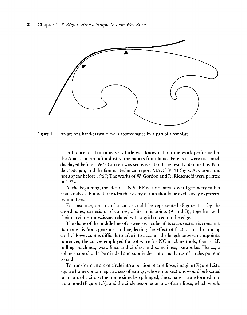
Figure 1.1 An arc of a hand-drawn curve is approximated by a part of a template.
In France, at that time, very httle vv^as know^n about the work performed in
the American aircraft industry; the papers from James Ferguson v^ere not much
displayed before 1964; Citroen was secretive about the results obtained by Paul
de Casteljau, and the famous technical report MAC-TR-41 (by S. A. Coons) did
not appear before 1967; The w^orks of
W.
Gordon and R. Riesenfeld w^ere printed
in 1974.
At the beginning, the idea of UNISURF w^as oriented tow^ard geometry rather
than analysis, but v^ith the idea that every datum should be exclusively expressed
by numbers.
For instance, an arc of a curve could be represented (Figure 1.1) by the
coordinates, cartesian, of course, of its limit points (A and B), together w^ith
their curvilinear abscissae, related w^ith a grid traced on the edge.
The shape of the middle line of a sw^eep is a cube, if its cross section is constant,
its matter is homogeneous, and neglecting the effect of friction on the tracing
cloth. How^ever, it is difficult to take into account the length betw^een endpoints;
moreover, the curves employed for softw^are for NC machine tools, that is, 2D
milling machines, v^ere lines and circles, and sometimes, parabolas. Hence, a
spline shape should be divided and subdivided into small arcs of circles put end
to end.
To transform an arc of circle into a portion of an ellipse, imagine (Figure 1.2) a
square frame containing
tw^o
sets of strings, v^hose intersections w^ould be located
on an arc of a circle; the frame sides being hinged, the square is transformed into
a diamond (Figure 1.3), and the circle becomes an arc of an ellipse, which would
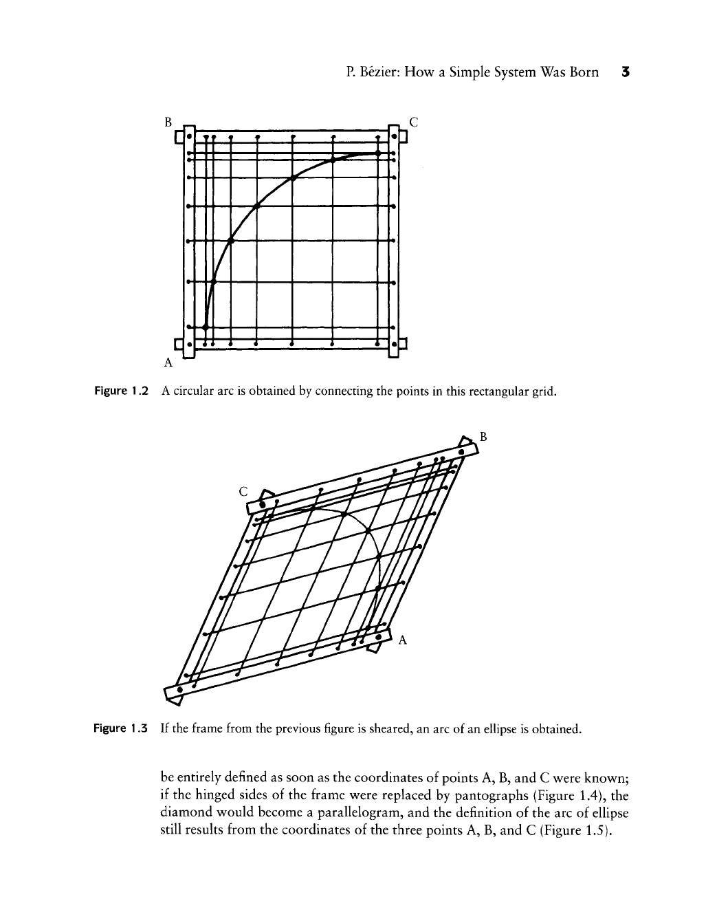
p.
Bezier: How a Simple System Was Born 3
•
[
^f f f f -f -f i^
»[ 1 1
1 1 1 ^^"^^^^^^^^^
^
1 1
1 1 Jkr \ 1 M
•
[II 1 JT 1 1 lit
UK
1 II
1
•
1
4 * * * * * * 1*
c
Figure 1.2 A circular arc is obtained by connecting the points in this rectangular grid.
Figure 1.3 If the frame from the previous figure is sheared, an arc of an ellipse is obtained.
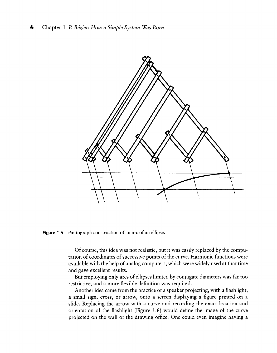
be entirely defined as soon as the coordinates of points A, B, and C were known;
if the hinged sides of the frame were replaced by pantographs (Figure 1.4), the
diamond would become a parallelogram, and the definition of the arc of ellipse
still results from the coordinates of the three points A, B, and C (Figure 1.5).
4 Chapter 1 P. Bezier: How a Simple System Was Born
Figure 1A Pantograph construction of an arc of an ellipse.
Of course, this idea was not realistic, but it was easily replaced by the compu-
tation of coordinates of successive points of the curve. Harmonic functions were
available with the help of analog computers, which were widely used at that time
and gave excellent results.
But employing only arcs of ellipses limited by conjugate diameters was far too
restrictive, and a more flexible definition was required.
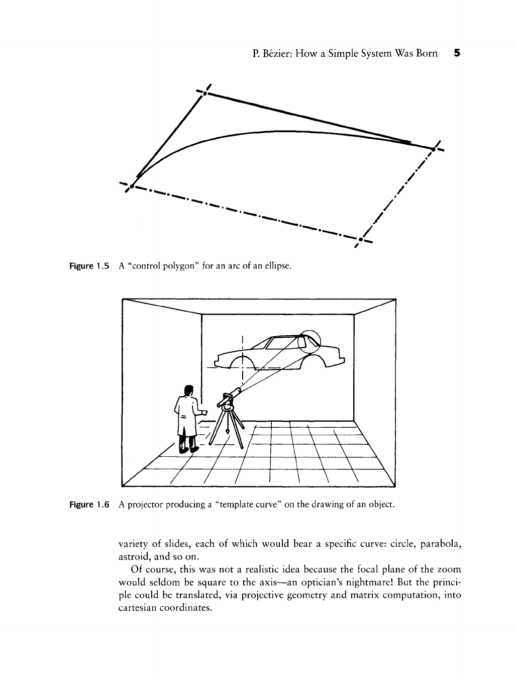
Another idea came from the practice of a speaker projecting, with a flashlight,
a small sign, cross, or arrow, onto a screen displaying a figure printed on a
slide.
Replacing the arrow with a curve and recording the exact location and
orientation of the flashlight (Figure 1.6) would define the image of the curve
projected on the wall of the drawing office. One could even imagine having a
p.
Bezier: How a Simple System Was Born 5
Figure 1.5 A "control polygon" for an arc of an ellipse.
^c2^Z
Figure 1.6 A projector producing a "template curve" on the drawing of an object.
variety of slides, each of which would bear a specific curve: circle, parabola,
astroid, and so on.
Of course, this was not a realistic idea because the focal plane of the zoom
would seldom be square to the axis—an optician's nightmare! But the princi-
ple could be translated, via projective geometry and matrix computation, into
cartesian coordinates.
Chapter 1 P. Bezier: How a Simple System Was Born
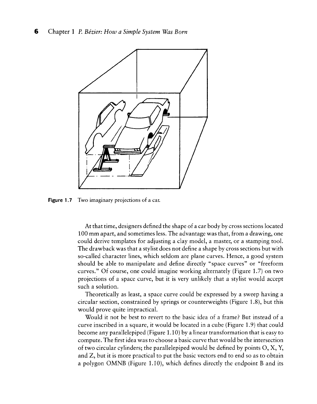
Figure 1.7 Two imaginary projections of a car.
At that time, designers defined the shape of a car body by cross sections located
100 mm apart, and sometimes less. The advantage was that, from a drawing, one
could derive templates for adjusting a clay model, a master, or a stamping tool.
The drawback was that a stylist does not define a shape by cross sections but with
so-called character lines, which seldom are plane curves. Hence, a good system
should be able to manipulate and define directly "space curves" or "freeform
curves." Of course, one could imagine working alternately (Figure 1.7) on two
projections of a space curve, but it is very unlikely that a stylist would accept
such a solution.
Theoretically as least, a space curve could be expressed by a sweep having a
circular section, constrained by springs or counterweights (Figure 1.8), but this
would prove quite impractical.
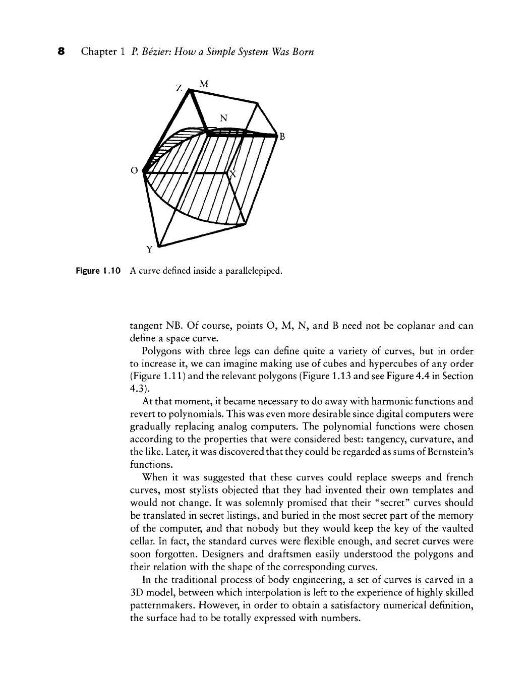
Would it not be best to revert to the basic idea of a frame .^ But instead of a
curve inscribed in a square, it would be located in a cube (Figure 1.9) that could
become any parallelepiped (Figure 1.10) by a linear transformation that is easy to
compute. The first idea was to choose a basic curve that would be the intersection
of two circular cylinders; the parallelepiped would be defined by points O, X, Y,
and Z, but it is more practical to put the basic vectors end to end so as to obtain
a polygon OMNB (Figure
1.10),
which defines directly the endpoint B and its

p.
Bezier: How a Simple System Was Born 7
Figure 1.8 A curve held by springs.
Figure 1.9 A curve defined inside a cube.
8 Chapter 1 P. Bezier: How a Simple System Was Born
Y
Figure 1.10 A curve defined inside a parallelepiped.
tangent NB. Of course, points O, M, N, and B need not be coplanar and can
define a space curve.
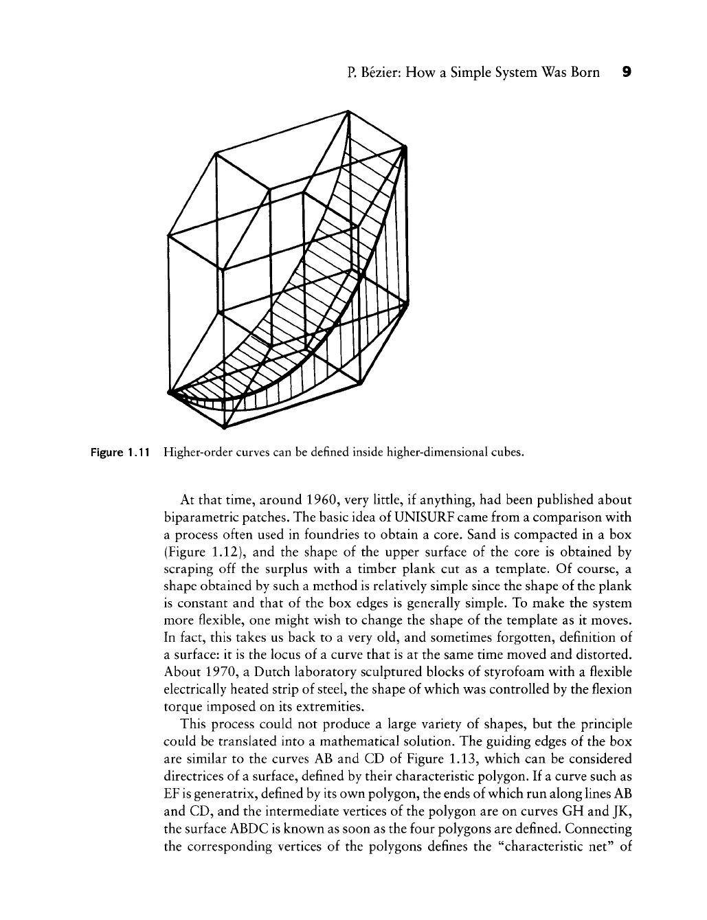
Polygons v^ith three legs can define quite a variety of curves, but in order
to increase it, w^e can imagine making use of cubes and hypercubes of any order
(Figure 1.11) and the relevant polygons (Figure 1.13 and see Figure 4.4 in Section
4.3).
At that moment, it became necessary to do away with harmonic functions and
revert to polynomials. This was even more desirable since digital computers were
gradually replacing analog computers. The polynomial functions were chosen
according to the properties that were considered best: tangency, curvature, and
the like. Later, it was discovered that they could be regarded as sums of Bernstein's
functions.
When it was suggested that these curves could replace sweeps and french
curves, most stylists objected that they had invented their own templates and
would not change. It was solemnly promised that their "secret" curves should
be translated in secret listings, and buried in the most secret part of the memory
of the computer, and that nobody but they would keep the key of the vaulted
cellar. In fact, the standard curves were flexible enough, and secret curves were
soon forgotten. Designers and draftsmen easily understood the polygons and
their relation with the shape of the corresponding curves.
In the traditional process of body engineering, a set of curves is carved in a
3D model, between which interpolation is left to the experience of highly skilled
patternmakers. However, in order to obtain a satisfactory numerical definition,
the surface had to be totally expressed with numbers.
p.
Bezier: How a Simple System Was Born
Figure 1.11 Higher-order curves can be defined inside higher-dimensional cubes.
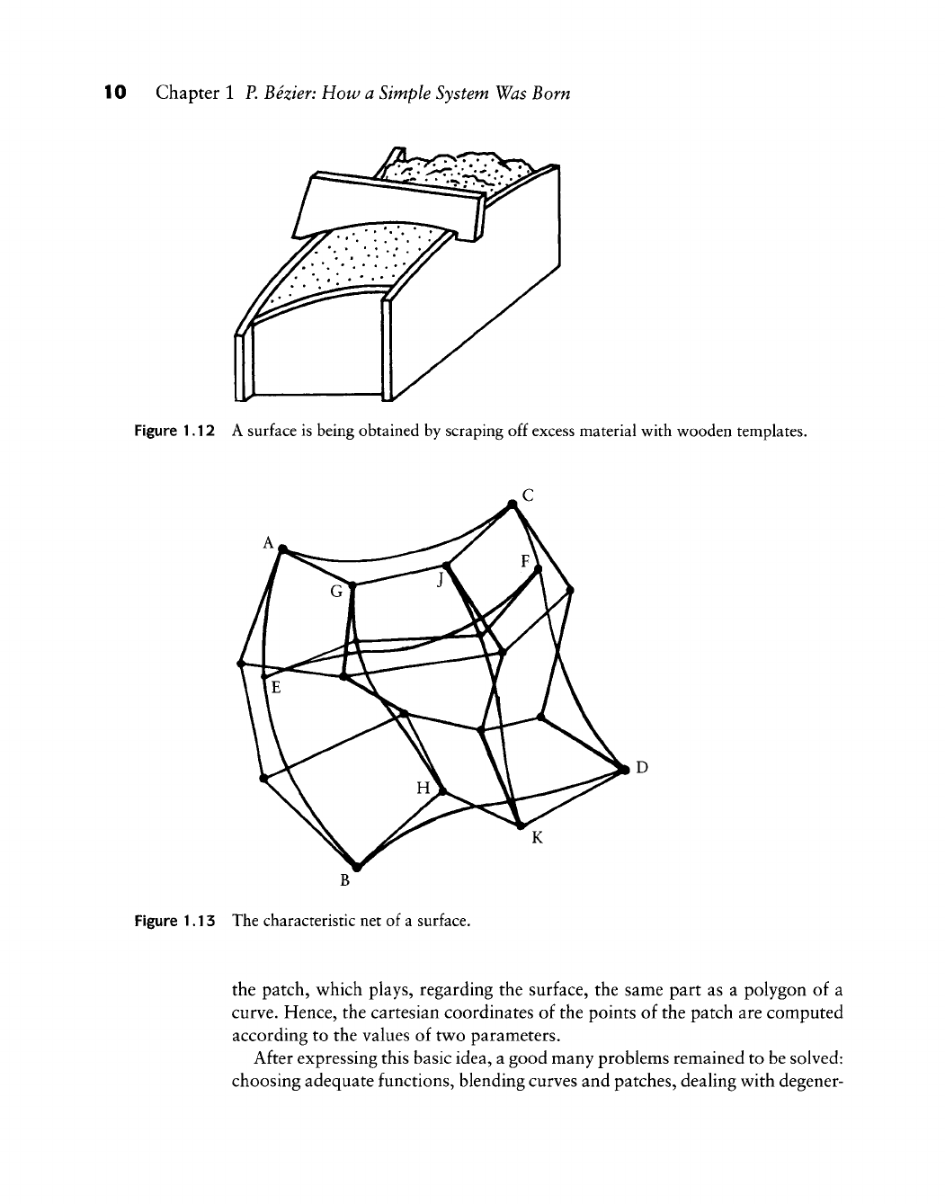
At that time, around 1960, very Uttle, if anything, had been published about
biparametric patches. The basic idea of UNISURF came from a comparison v^ith
a process often used in foundries to obtain a core. Sand is compacted in a box
(Figure
1.12),
and the shape of the upper surface of the core is obtained by
scraping off the surplus w^ith a timber plank cut as a template. Of course, a
shape obtained by such a method is relatively simple since the shape of the plank
is constant and that of the box edges is generally simple. To make the system
more flexible, one might w^ish to change the shape of the template as it moves.
In fact, this takes us back to a very old, and sometimes forgotten, definition of
a surface: it is the locus of a curve that is at the same time moved and distorted.
About 1970, a Dutch laboratory sculptured blocks of styrofoam w^ith a flexible
electrically heated strip of steel, the shape of w^hich w^as controlled by the flexion
torque imposed on its extremities.
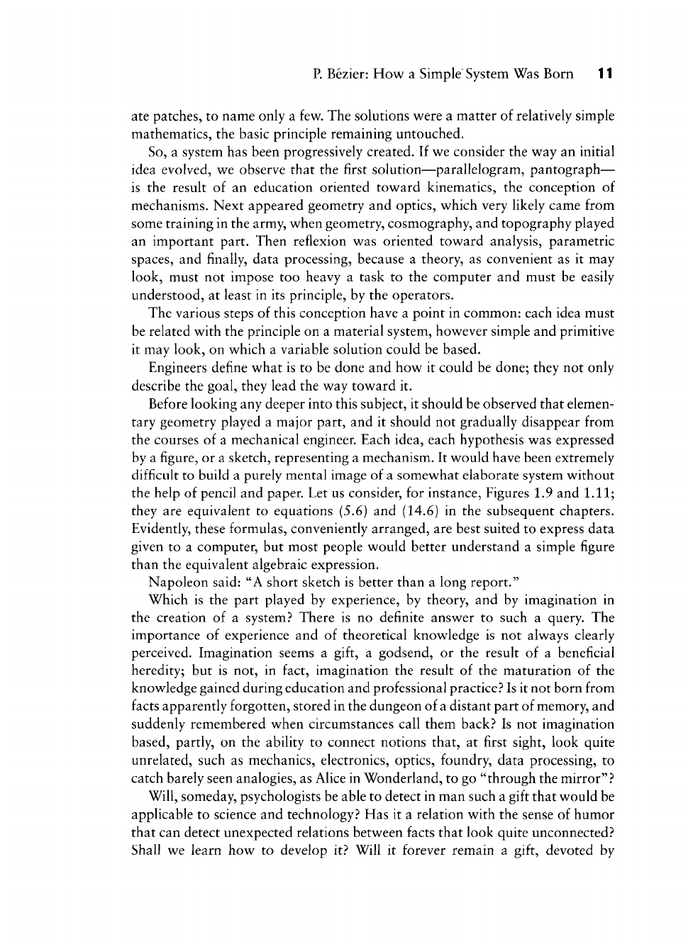
This process could not produce a large variety of shapes, but the principle
could be translated into a mathematical solution. The guiding edges of the box
are similar to the curves AB and CD of Figure 1.13, v^hich can be considered
directrices of a surface, defined by their characteristic polygon. If a curve such as
EF is generatrix, defined by its own polygon, the ends of which run along lines AB
and CD, and the intermediate vertices of the polygon are on curves GH and JK,
the surface ABDC is known as soon as the four polygons are defined. Connecting
the corresponding vertices of the polygons defines the "characteristic net" of
10 Chapter 1 P. Bezier: How a Simple System Was Born
Figure 1.12 A surface is being obtained by scraping off excess material with wooden templates.
Figure 1.13 The characteristic net of a surface.
the patch, which plays, regarding the surface, the same part as a polygon of a
curve. Hence, the cartesian coordinates of the points of the patch are computed
according to the values of two parameters.
After expressing this basic idea, a good many problems remained to be solved:
choosing adequate functions, blending curves and patches, dealing with degener-
p.
Bezier: How a
Simple"
System Was Born 11
ate patches, to name only a few. The solutions were a matter of relatively simple
mathematics, the basic principle remaining untouched.
So,
a system has been progressively created. If we consider the way an initial
idea evolved, we observe that the first solution—parallelogram, pantograph—
is the result of an education oriented toward kinematics, the conception of
mechanisms. Next appeared geometry and optics, which very likely came from
some training in the army, when geometry, cosmography, and topography played
an important part. Then reflexion was oriented toward analysis, parametric
spaces, and finally, data processing, because a theory, as convenient as it may
look, must not impose too heavy a task to the computer and must be easily
understood, at least in its principle, by the operators.
The various steps of this conception have a point in common: each idea must
be related with the principle on a material system, however simple and primitive
it may look, on which a variable solution could be based.
Engineers define what is to be done and how it could be done; they not only
describe the goal, they lead the way toward it.
Before looking any deeper into this subject, it should be observed that elemen-
tary geometry played a major part, and it should not gradually disappear from
the courses of a mechanical engineer. Each idea, each hypothesis was expressed
by a figure, or a sketch, representing a mechanism. It would have been extremely
difficult to build a purely mental image of a somewhat elaborate system without
the help of pencil and paper. Let us consider, for instance, Figures 1.9 and 1.11;
they are equivalent to equations (5.6) and (14.6) in the subsequent chapters.
Evidently, these formulas, conveniently arranged, are best suited to express data
given to a computer, but most people would better understand a simple figure
than the equivalent algebraic expression.
Napoleon said: "A short sketch is better than a long report."
Which is the part played by experience, by theory, and by imagination in
the creation of a system? There is no definite answer to such a query. The
importance of experience and of theoretical knowledge is not always clearly
perceived. Imagination seems a gift, a godsend, or the result of a beneficial
heredity; but is not, in fact, imagination the result of the maturation of the
knowledge gained during education and professional practice? Is it not born from
facts apparently forgotten, stored in the dungeon of a distant part of memory, and
suddenly remembered when circumstances call them back? Is not imagination
based, partly, on the ability to connect notions that, at first sight, look quite
unrelated, such as mechanics, electronics, optics, foundry, data processing, to
catch barely seen analogies, as Alice in Wonderland, to go "through the mirror"?
Will, someday, psychologists be able to detect in man such a gift that would be
applicable to science and technology? Has it a relation with the sense of humor
that can detect unexpected relations between facts that look quite unconnected?
Shall we learn how to develop it? Will it forever remain a gift, devoted by

12 Chapter 1 P. Bezier: How a Simple System Was Born
pure chance to some people, whereas for others carefulness and cold blood
prevail?
It is important that, sometimes, "sensible" men give free rein to imaginative
people. "I succeeded," said Henry Ford, "because I let some fools try what wise
people had advised me not to let them try."
Introductory Material
2.1 Points and Vectors
When a designer or stylist works on an object, he or she does not think of that
object in very mathematical terms. A point on the object would not be thought of
as a triple of coordinates, but rather in functional terms: as a corner, the midpoint
between two other points, and so on. The objective of this book, however, is to
discuss objects that are defined in mathematical terms, the language that lends
itself best to computer implementations. As a first step toward a mathematical
description of an object, one therefore defines a coordinate system in which it
will be described analytically.
The space in which we describe our object does not possess a preferred
coordinate system—we have to define one ourselves. Many such systems could
be picked (and some will certainly be more practical than others). But whichever
one we choose, it should not affect any properties of the object
itself.
Our interest
is in the object and not in its relationship to some arbitrary coordinate system.
Therefore, the methods we develop must be independent of a particular choice
of a coordinate system. We say that those methods must be coordinate-free or
coordinate-independent}
We stress the concept of coordinate-free methods throughout this book. It
motivates the strict distinction between points and vectors as discussed next.
(For more details on this topic, see R. Goldman [262].)
1 More mathematically, the geometry of this book is affine geometry. The objects that we
will consider "live" in affine spaces, not in linear spaces.
13
14 Chapter 2 Introductory Material
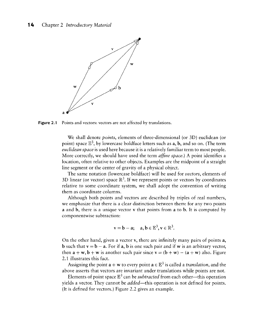
Figure 2.1 Points and vectors: vectors are not affected by translations.
We shall denote points^ elements of three-dimensional (or 3D) euclidean (or
point) space E^, by lowercase boldface letters such as a, b, and so on. (The term
euclidean space is used here because it is a relatively familiar term to most people.
More correctly, v^e should have used the term affine space.) A point identifies a
location, often relative to other objects. Examples are the midpoint of a straight
line segment or the center of gravity of a physical object.
The same notation (low^ercase boldface) w^ill be used for vectors^ elements of
3D linear (or vector) space M^. If we represent points or vectors by coordinates
relative to some coordinate system, we shall adopt the convention of writing
them as coordinate columns.
Although both points and vectors are described by triples of real numbers,
we emphasize that there is a clear distinction between them: for any two points
a and b, there is a unique vector v that points from a to b. It is computed by
componentwise subtraction:
v = b-a; a,bGE^v€Rl
On the other hand, given a vector v, there are infinitely many pairs of points a,
b such that v = b
—
a. For if a, b is one such pair and if w is an arbitrary vector,
then a + w, b + w is another such pair since v = (b + w)
—
(a + w) also. Figure
2.1 illustrates this fact.
Assigning the point a + w to every point a
G
E^ is called a translation^ and the
above asserts that vectors are invariant under translations while points are not.
Elements of point space E^ can be subtracted from each other—this operation
yields a vector. They cannot be added—this operation is not defined for points.
(It is defined for vectors.) Figure 2.2 gives an example.
2.1 Points and Vectors 15
*.'--.-,
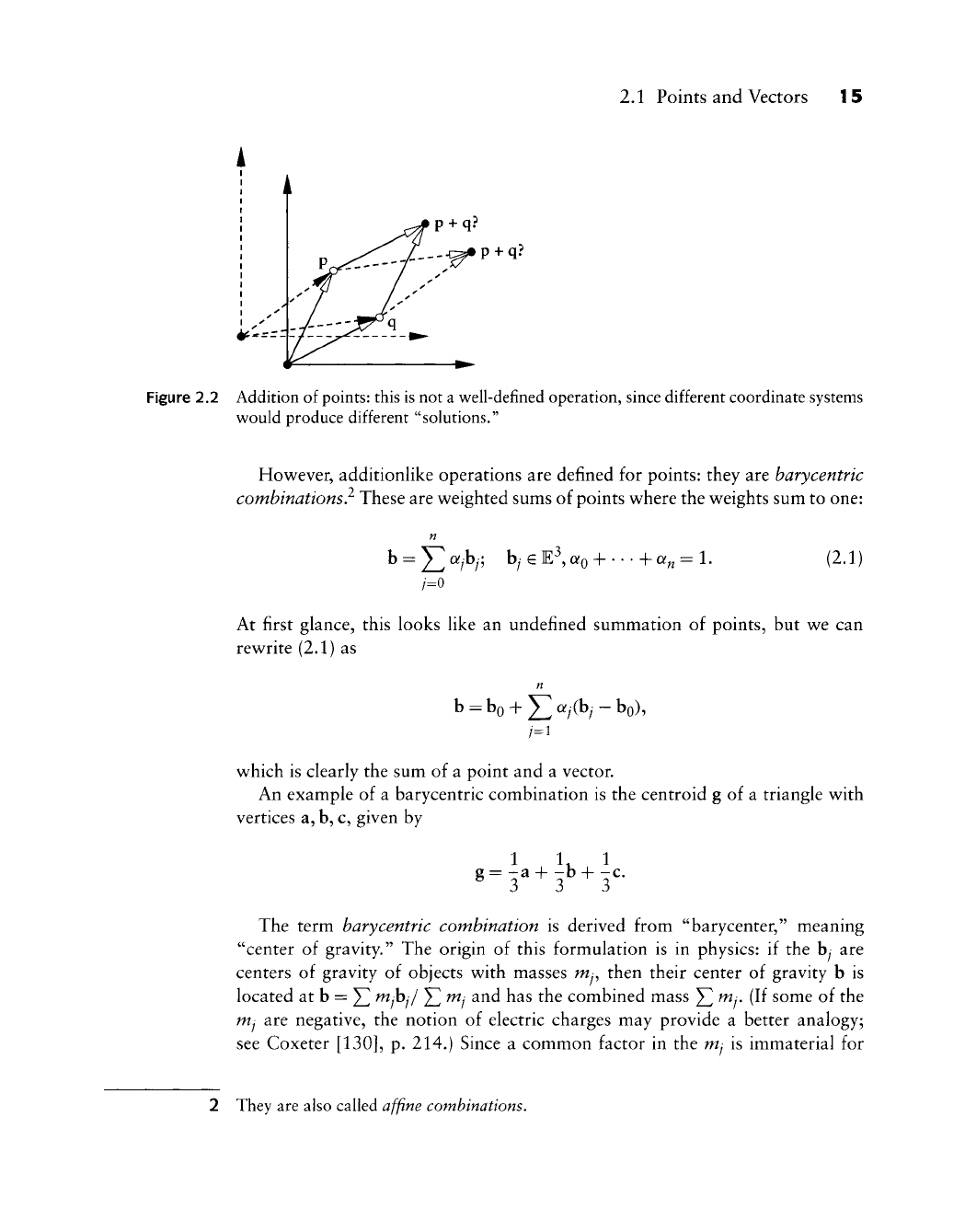
Figure 2.2 Addition of
points:
this is not a well-defined operation, since different coordinate systems
would produce different "solutions."
However, additionlike operations are defined for points: they are barycentric
combinations? These are weighted sums of points where the weights sum to one:
b = ^ Qfyby; by
G
E-^,
QfQ H h
Qf^ = 1.
j=0
(2.1)
At first glance, this looks like an undefined summation of points, but we can
rewrite (2.1) as
n
b = bo + ^Qfy(b^—bo),
which is clearly the sum of a point and a vector.
An example of a barycentric combination is the centroid g of a triangle with
vertices a, b, c, given by
1 1, 1
g= -a + -b + -c.
The term barycentric combination is derived from "barycenter," meaning
"center of gravity." The origin of this formulation is in physics: if the by are
centers of gravity of objects with masses my, then their center of gravity b is
located at b = X! ^/by/ Yl ^j ^^^ has the combined mass ^ my. (If some of the
mj are negative, the notion of electric charges may provide a better analogy;
see Coxeter
[130],
p. 214.) Since a common factor in the mj is immaterial for
2 They are also called
affine
combinations.
16 Chapter 2 Introductory Material
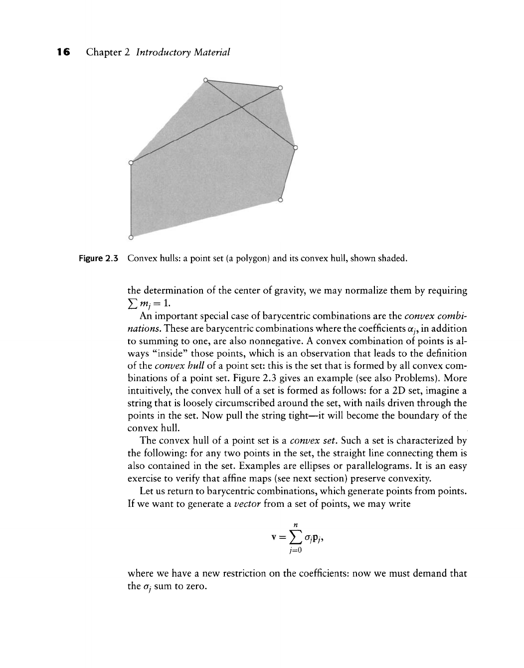
Figure 2.3 Convex hulls: a point set (a polygon) and its convex hull, shown shaded.
the determination of the center of gravity, we may normalize them by requiring
An important special case of barycentric combinations are the convex combi-
nations. These are barycentric combinations v^here the coefficients
ofy,
in addition
to summing to one, are also nonnegative. A convex combination of points is al-
w^ays "inside" those points, w^hich is an observation that leads to the definition
of the convex hull of a point set: this is the set that is formed by all convex com-
binations of a point set. Figure 2.3 gives an example (see also Problems). More
intuitively, the convex hull of a set is formed as follows: for a 2D set, imagine a
string that is loosely circumscribed around the set, with nails driven through the
points in the set. Now pull the string tight—it will become the boundary of the
convex hull.
The convex hull of a point set is a convex set. Such a set is characterized by
the following: for any two points in the set, the straight line connecting them is
also contained in the set. Examples are ellipses or parallelograms. It is an easy
exercise to verify that affine maps (see next section) preserve convexity.
Let us return to barycentric combinations, which generate points from points.
If we want to generate a vector from a set of points, we may write
n
7=0
where we have a new restriction on the coefficients: now we must demand that
the a, sum to zero.
2.2 AffineMaps 17
If we are given an equation of the form
and a is supposed to be a point, then we must be able to split the sum into three
groups:
a= E ^A+ E '^A+ E ^A-
S/6y=l
E^y=0 remaining ^s
Then the by in the first sum are points, and those in the second sum may be
interpreted as either points or vectors. The by in the third sum are vectors.
Whereas the second and third sums may be empty, the first one must contain
at least one term.
The interplay betv^een points and vectors is unusual at first. Later, it w^ill turn
out to be of invaluable theoretical and practical help. For example, w^e can per-
form quick type checking v^hen wt derive formulas. If the point coefficients fail
to add up to one or zero—depending on the context—w^e know^ that something
has gone w^rong. In a more formal w^ay, T. DeRose has developed the concept of
"geometric programming," a graphics language that automatically performs type
checks
[1601,
[161].
R. Goldman's article [262] treats the validity of point/vector
operations in more detail.
2.2 Affine Maps
Most of the transformations that are used to position or scale an object in a
computer graphics or CAD environment are affine maps. (More complicated,
so-called projective maps are discussed in Chapter 12.) The term affine map is
due to L. Euler; affine maps were first studied systematically by R Moebius
[429].
The fundamental operation for points is the barycentric combination. We
will thus base the definition of an affine map on the notion of barycentric
combinations. A map O that maps E^ into itself is called an affine map if it
leaves barycentric combinations invariant. So if
X
= ^ Qfyay; Y^ aj = 1, x,
ay G
E^
and 0 is an affine map, then also
<Dx
= ^ ayOay; Ox, Oay
G
E^ (2.2)
18 Chapter 2 Introductory Material
This definition looks fairly abstract, yet it has a simple interpretation. The
expression x = ^ ofyay specifies how we have to weight the points ay such that
their weighted average is x. This relation is still valid if we apply an affine map
to all points ay and to x. As an example, the midpoint of a straight line segment
will be mapped to the midpoint of the affine image of that straight line segment.
Also,
the centroid of a number of points will be mapped to the centroid of the
image points.
Let us now be more specific. In a given coordinate system, a point x is
represented by a coordinate triple, which we also denote by x. An affine map
now takes on the familiar form
Ox = Ax + v, (2.3)
where A is a 3 x 3 matrix and v is a vector from R^.
A simple computation verifies that (2.3) does in fact describe an affine map,
that is, that barycentric combinations are preserved by maps of that form. For
the following, recall that Yl ^j = 1-
= ^ayAay + 5]ayV
= ^ay(Aay + v)
= ^aycDay,
which concludes our
proof.
It also shows that the inverse of our initial statement
is true as well: every map of the form shown in (2.3) represents an affine map.
Some examples of affine maps are as follows:
The identity. It is given by v = 0, the zero vector, and by A = J, the identity
matrix.
A translation. It is given by A = I, and a translation vector v.
A scaling. It is given by v = 0 and by a diagonal matrix A. The diagonal entries
define by how much each component of the preimage x is to be scaled.
A rotation. If we rotate around the ;^-axis, then v = 0 and
2.2 AffineMaps 19
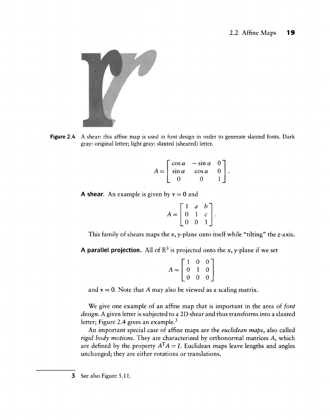
Figure 2.4 A shear: this affine map is used in font design in order to generate slanted fonts. Dark
gray: original letter; light gray: slanted (sheared) letter.
A =
A shear. An example is given by v = 0 and
cos a
—
sin a
sin a cos a
0
V
= 0 and
'1 a
0 1
0 0
0
b'
c
1
0
0
1
This family of shears maps the x, y-plane onto itself while "tilting" the ;^-axis.
A parallel projection. All of
E-^
is projected onto the x, y-plane if we set
A =
1 0 0
0 1 0
0 0 0
and
V
= 0. Note that A may also be viewed as a scaling matrix.
We give one example of an affine map that is important in the area of font
design, A given letter is subjected to a 2D shear and thus transforms into a slanted
letter; Figure 2.4 gives an example.^
An important special case of affine maps are the euclidean maps, also called
rigid body motions. They are characterized by orthonormal matrices A, which
are defined by the property A^A = L Euclidean maps leave lengths and angles
unchanged; they are either rotations or translations.
3 See also Figure 5.11.
20 Chapter 2 Introductory Material
Affine maps can be combined, and a complicated map may be decomposed
into a sequence of simpler maps. Every affine map can be composed of transla-
tions,
rotations, shears, and scalings.
The rank of
A
has an important geometric interpretation: if rank (A) = 3, then
the affine map O maps 3D objects to 3D objects. If the rank is less than three,
O is a parallel projection onto a plane (rank = 2) or even onto a straight line
(rank=l).
An affine map of
E^
to E^ is uniquely determined by a (nondegenerate) triangle
and its image. Thus any two triangles determine an affine map of the plane onto
itself.
In E^, an affine map is uniquely defined by a (nondegenerate) tetrahedron
and its image.
We may also define affine maps of vectors. If w = b
—
a is a vector, and Ax + v
represents an affine map O, then
^(w) = Aw
is the image of w under O. As expected, the translational part v of the affine map
is of no consequence when mapping vectors to vectors.
2.5 Constructing Affine Maps
Suppose we are given a 2D point set pj,. . . ,
PL
whose centroid is located at
the origin. Before discussing affine maps of these points, we first study a unique
ellipse that is associated with this point set; it is called the norm ellipse, see [90],
[155], [449], [448], [510].
Our derivation of this ellipse is as follows: an ellipse with center at the origin
is given by a quadratic from
x^Ax
= 1 (2.4)
where A is a symmetric matrix with two nonnegative eigenvalues.
Our goal is to find a symmetric matrix A that captures some of the character-
istics of the given point set.
Each
p^
is of the form
If it were on an ellipse defined by A, then all points would satisfy
pjAp, = l; /=1,...,L. (2.5)
2.3 Constructing Affine Maps 21
We define
P = [pi ••• PL],
a matrix with two rows and L columns. Equation (2.5) can now be written in
terms of one matrix equation:
P^AP
-1.
We now multiply with P from the left and with P^ from the right to obtain
ppT^ppT ^ ppT
We define
B = PpT,
a 2 X 2 matrix. Assuming it is invertible (which it is for a nondegenerate set of
points Pi), we find that
A = B-^
is the desired matrix for our quadratic form (2.4). It is related to the points
p^
in
an affinely invariant way: subject the data to an affine map and recompute the
norm ellipse. It is the same ellipse as is obtained by mapping the original norm
ellipse by the affine map.
The matrix A is symmetric by construction; the fact that it has nonnegative
eigenvalues (i.e., it represents an ellipse) follows from its definition (2.4).
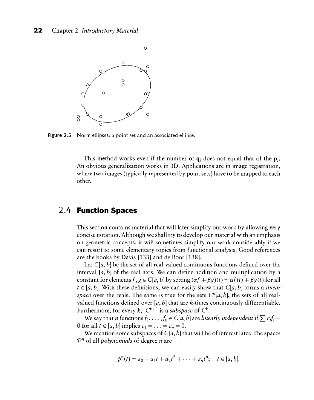
The axes of the ellipse defined by A represent the distribution of the points p^;
Figure 2.5 gives an example. The axes are given by the eigenvectors of A; their
lengths are determined by the corresponding eigenvalues.
Returning to the topic of affine maps, suppose we are given a point set
Pl?
• • • ?
PL
^^d ^ second set q^,. . ., q^^, both with their centroids at the origin. If
there is an affine map, represented by a matrix M with
q, = Mp„
how can we find it.'^
A simple and efficient way is to compute the two norm ellipses Ep and E^ for
the two point sets. Since any two ellipses are related by an affine map 4>p^, we
simply compute it; then O^^ is the desired affine map.
In general, the two point sets are not related by an affine map; this procedure
will still produce an affine map that approximately maps the two point sets.
22 Chapter 2 Introductory Material
Qx o
o
Figure 2.5 Norm ellipses: a point set and an associated ellipse.
This method works even if the number of q/ does not equal that of the p/.
An obvious generalization v^orks in 3D. Applications are in image registration,
where two images (typically represented by point sets) have to be mapped to each
other.
2.4 Function Spaces
This section contains material that will later simplify our work by allowing very
concise notation. Although we shall try to develop our material with an emphasis
on geometric concepts, it will sometimes simplify our work considerably if we
can resort to some elementary topics from functional analysis. Good references
are the books by Davis [133] and de Boor
[138].
Let
C[a^
h\ be the set of all real-valued continuous functions defined over the
interval
\a^
h\ of the real axis. We can define addition and multiplication by a
constant for elements /^,g € C[a, h\ by setting (af + Pg)(t) = af(t) + Pg(t) for all
t 6
[a,
b].
With these definitions, we can easily show that
C[a^
b] forms a linear
space over the reals. The same is true for the sets C^[^,
fe],
the sets of all real-
valued functions defined over
[a,
b]
that are fe-times continuously differentiable.
Furthermore, for every k, C^^^ is a subspace of C^.
We say that n functions
/^i,...,
/^
G
C[a^
b]
are linearly independent if ^
Cifi
=
0 for all t e
[a^
b]
implies ci = .. . = c^ = 0.
We mention some subspaces of C[a,
b]
that will be of interest later. The spaces
V^ of all polynomials of degree n are
p'^it)
= ao-\- ait + ait^ +
• • •
+
aj""-,
t e
[a,
b].
2.4 Function Spaces 23
For fixed
n^
the dimension of V^\sn-\-1: each p^ e V^ is determined uniquely by
the
w
+ 1 coefficients
UQ^,
..., a^. These can be interpreted as a vector in {n + 1)-
dimensional finear space R"+\ which has dimension
w
+ 1. We can also name
a basis for V^: the monomials
\,t,t^^.
.. ,t^ are
w
+ 1 finearly independent
functions and thus form a basis.
Another interesting class of subspaces of C[^,
b]
is given by piecewise linear
functions: let ^ =
^Q
< ^l < '
* *
<
^w
= ^ be a partition of the interval
[a,
b\ A
continuous function that is linear on each subinterval [^/, tij^^ is called a piecewise
linear function. Over a fixed partition of
[a.,
b\ the piecev^ise linear functions form
a linear function space. A basis for this space is given by the hat functions: a hat
function Hi{t) is a piecev^ise linear function v^ith H^(^^) =
1
and H^(^y) = 0 if
/ /=
/•
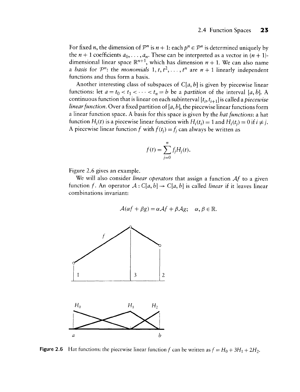
A piecew^ise linear function f v^ith f{tj) = ^ can alw^ays be v^ritten as
n
f{t) =
Y.fi^i^^)'
Figure 2.6 gives an example.
We v^ill also consider linear operators that assign a function Af to a given
function f. An operator ^ : C[a,
b]
-^ C[a,
b]
is called linear if it leaves linear
combinations invariant:
A(af + Pg) = aAf + pAg; a, ^
G
R.
Figure 2.6 Hat functions: the piecewise linear function f can be written as
/"
=
HQ
+ 3Hi + 2H2
24 Chapter 2 Introductory Material
An example is given by the derivative operator that assigns the derivative f^ to a
given function f: Af = f.
2.5 Problems
1 Of all affine maps, shears seem to be the least familiar to most people.^
Construct a matrix that maps the unit square with points (0,0), (1,0), (1,1),
(0,1) to the parallelogram v^ith image points (0,0), (1,0), (2,1), (1,1).
* 2 We have seen that affine maps leave the ratio of three collinear points
constant (i.e., they are ratio preserving). Show that the converse is also
true:
every ratio-preserving map is affine.
* 3 Show that the n-\-l functions fi(t) = f; / =
0,...,«
are linearly indepen-
dent.
P1 Fix two distinct points a, b on the x-axis. Let a third point x trace out all the
X-axis. For each location of x, plot the value of the function ratio(a, x, b),
thus obtaining a graph of the ratio function.
4 Recall that Figure 2.4 illustrates a shear.
Linear Interpolation
M
ost of the computations that we use in CAGD may be broken down into
seemingly trivial steps—sequences of linear interpolations. It is therefore impor-
tant to understand the properties
of
these basic building blocks. This chapter
explores those properties and introduces
a
related concept, called blossoms.
5.1 Linear Interpolation
Let a, b be two distinct points in E^. The set of all points
x e
E^ of the form
x
= x(t) =
(l-t)ei-^th; t eR (3.1)
is called the straight line through a and
b.
Any three (or more) points on a straight
line are said to be collinear.
For
^
=
0, the straight line passes through a and for
^
=
1, it passes through b.
For 0 < ^
<
1, the point x is between
a
and b, whereas for all other values of
t
it
is outside; see Figure 3.1.
Equation (3.1) represents
x
as
a
barycentric combination
of
two points
in
E-^. The same barycentric combination holds for the three points 0, t, 1 in E^:
t =
(l
—
t)-0-\-t'l.Sotis related to 0 and
1
by the same barycentric combination
that relates x to a and b. Hence, by the definition of affine maps, the three points
a,
X,
b are an affine map of the three ID points 0, ^, 1! Thus linear interpolation
is an affine map of the real line onto a straight line in E^.^
1 Strictly speaking, we should therefore use the term affine interpolation instead of
linear
interpolation.
We use linear interpolation because its use is so widespread.
25
26 Chapter 3 Linear Interpolation
0
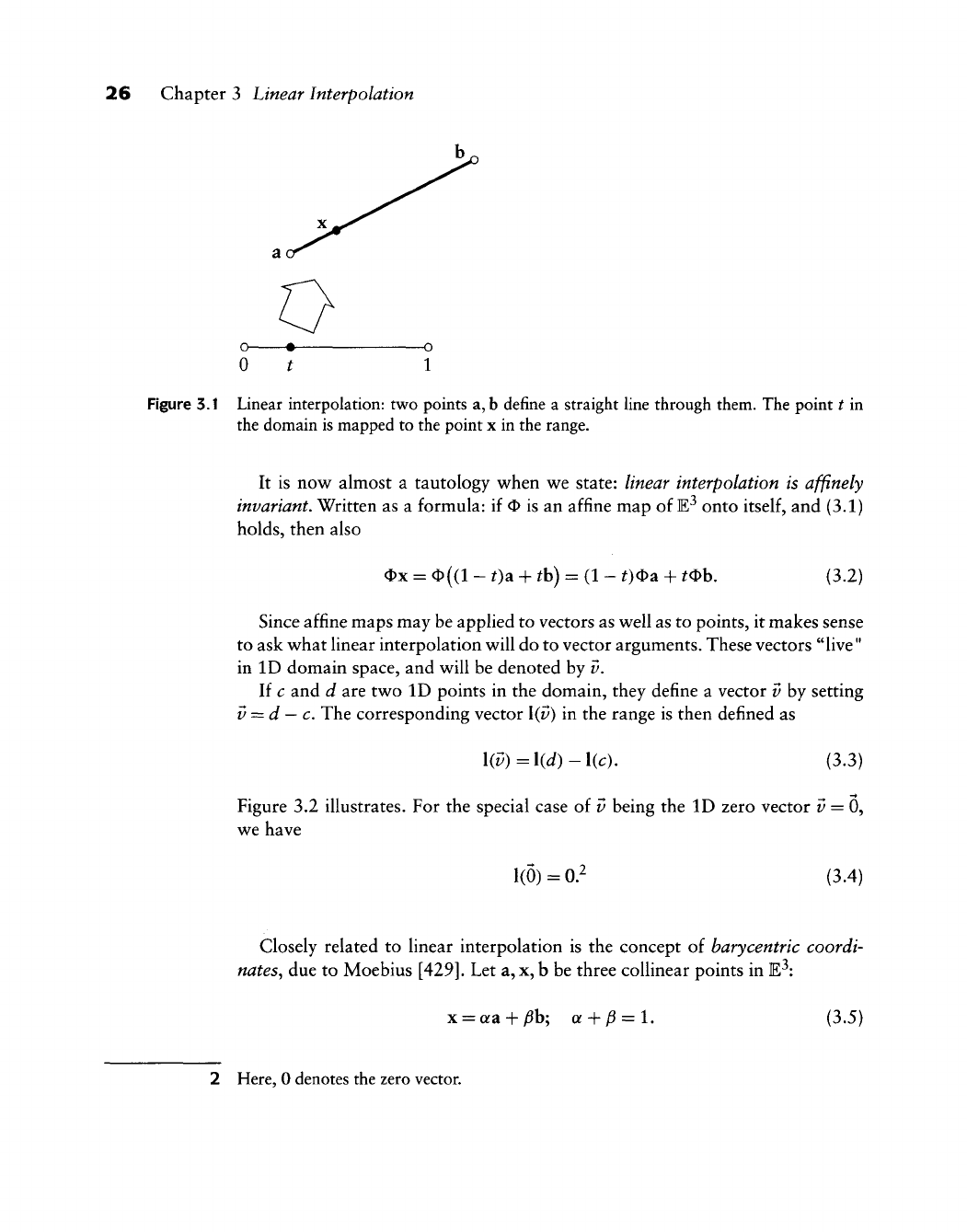
t 1
Figure 3.1 Linear interpolation: two points a,b define a straight hne through them. The point
t
in
the domain is mapped to the point x in the range.
It
is
now almost
a
tautology when we state: linear interpolation is affinely
invariant. Written as
a
formula:
if 0
is an affine map onto
itself,
and (3.1)
holds,
then also
<Dx
=
^{(1
-
t)a
+
^b)
=
(1
-
t)<t>2i
+ t^h. (3.2)
Since affine maps may be applied to vectors as well as to points, it makes sense
to ask what linear interpolation will do to vector arguments. These vectors "live"
in ID domain space, and will be denoted by
v.
If c and
d
are two ID points in the domain, they define
a
vector
v
by setting
y
—
d
—
c. The corresponding vector \(v) in the range is then defined as
\{v)=\{d)-\{c),
(3.3)
Figure 3.2 illustrates. For the special case
of v
being the ID zero vector
? =
0,
we have
1(0)
=
0.^
(3.4)
Closely related
to
linear interpolation
is
the concept
of
barycentric coordi-
nates^ due to Moebius
[429].
Let a, x, b be three coUinear points in E^:
x
=
aa
+
)Sb;
a +
jS
= l. (3.5)
2 Here, 0 denotes the zero vector.
3.1 Linear Interpolation 27
-o«-
0 1 1
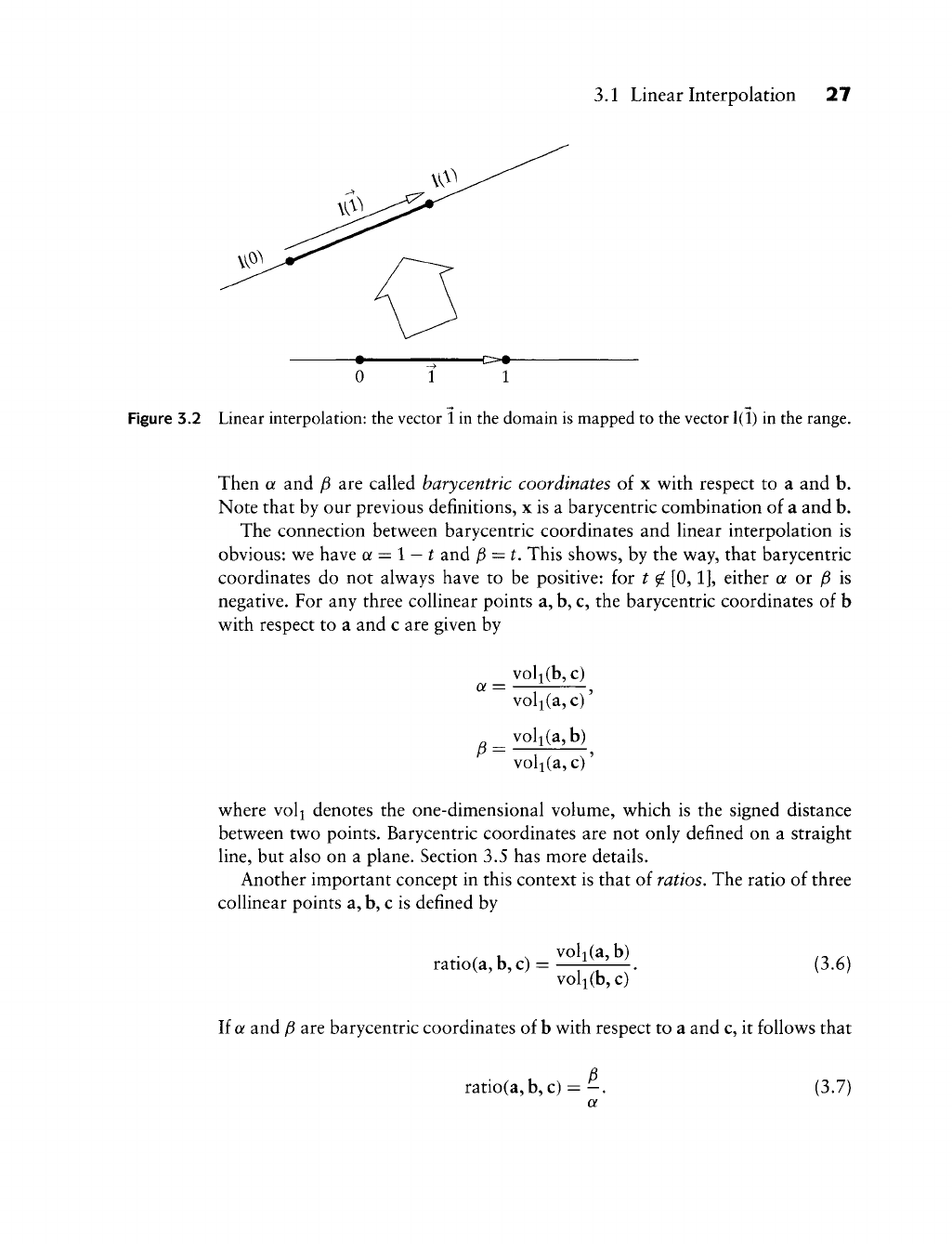
Figure 3.2 Linear interpolation: the vector
1
in the domain is mapped to the vector
1(1)
in the range.
Then a and ^ are called harycentric coordinates of x with respect to a and b.
Note that by our previous definitions, x is a barycentric combination of a and b.
The connection between barycentric coordinates and linear interpolation is
obvious: we have a = \
—
t and ^
—
t. This shows, by the way, that barycentric
coordinates do not always have to be positive: for t ^
[0,1],
either a or ^ is
negative. For any three collinear points a, b, c, the barycentric coordinates of b
with respect to a and c are given by
voli(b,c)
a = —-^ ,
voli(a,c)
voli(a,b)
voli(a, c)'
where vol^ denotes the one-dimensional volume, which is the signed distance
between two points. Barycentric coordinates are not only defined on a straight
line,
but also on a plane. Section 3.5 has more details.
Another important concept in this context is that of ratios. The ratio of three
collinear points a, b, c is defined by
ratio(a, b, c) = voli(a,b) (3.6)
voli(b,c)
If a and ^ are barycentric coordinates of b with respect to a and c, it follows that
ratio(a, b, c) = (3.7)
28 Chapter 3 Linear Interpolation
The barycentric coordinates of a point do not change under affine maps, and
neither does their quotient. Thus the ratio of three cohinear points is not affected
by affine transformations. So if (3.7) holds, then also
ratio(4)a, Ob, Oc) = -, (3.8)
a
where O is an affine map. This property may be used to compute ratios efficiently.
Instead of using square roots to compute the distances between points a, x,
and b, we would project them onto one of the coordinate axes and then use
simple differences of their x- or ^-coordinates.^ This shortcut works since parallel
projection is an affine map!
Equation (3.8) states that affine maps are ratio preserving. This property may
be used to define affine maps. Every map that takes straight lines to straight lines
and is ratio preserving is an affine map.
The concept of ratio preservation may be used to derive another useful prop-
erty of linear interpolation. We have defined the straight line segment [a, b] to be
the affine image of the unit interval
[0,1],
but we can also view that straight line
segment as the affine image of any interval
[a,,
b].
The interval [^,
b]
may itself be
obtained by an affine map from the interval [0,1] or vice versa. With t € [0,1]
and u
G
[a,
b\ that map is given by t = (u
—
a)/(b
—
a). The interpolated point
on the straight line is now given by both
x(t) = (1 - t)a + ^b
and
x(u) = a + b. (3.9)
b
—
a b
—
a
Since
a^
w,
b and 0, ^, 1 are in the same ratio as the triple a, x, b, we have shown
that linear interpolation is invariant under affine domain transformations. By
affine domain transformation, we simply mean an affine map of the real fine
onto
itself.
The parameter t is sometimes called a local parameter of the interval
A more general way to express this is by saying that any barycentric com-
bination of three domain points r, s, t (not necessarily involving any interval
endpoints) carries over to the corresponding range points:
s = {l-ot)r + at=^ x(s) = (1 - Qf)x(r) + ax(0. (3.10)
3 But be sure to avoid projection onto the x-axis if
the
three points are parallel to the y-axis!
3.2 Piecewise Linear Interpolation 29
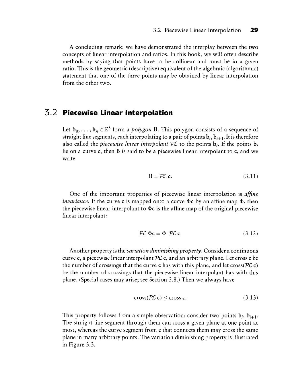
A concluding remark: we have demonstrated the interplay between the two
concepts of linear interpolation and ratios. In this book, we will often describe
methods by saying that points have to be collinear and must be in a given
ratio.
This is the geometric (descriptive) equivalent of the algebraic (algorithmic)
statement that one of the three points may be obtained by linear interpolation
from the other two.
5.2 Piecewise Linear Interpolation
Let bo,... ,b„
G
E^ form a polygon B. This polygon consists of a sequence of
straight line segments, each interpolating to a pair of points
b^,
b^_^i.
It is therefore
also called the piecewise linear interpolant VC to the points b^. If the points b^
lie on a curve c, then B is said to be a piecewise linear interpolant to c, and we
write
B
=
H:C.
(3.11)
One of the important properties of piecewise linear interpolation is affine
invariance. If the curve c is mapped onto a curve Oc by an affine map O, then
the piecewise linear interpolant to Oc is the affine map of the original piecewise
linear interpolant:
P£Oc = ^ VLz, (3.12)
Another property is the variation diminishing property. Consider a continuous
curve c, a piecewise linear interpolant VC c, and an arbitrary plane. Let cross c be
the number of crossings that the curve c has with this plane, and let cross(7X c)
be the number of crossings that the piecewise linear interpolant has with this
plane. (Special cases may arise; see Section 3.8.) Then we always have
cross(P£ c) < cross c. (3.13)
This property follows from a simple observation: consider two points b/, hj^i.
The straight line segment through them can cross a given plane at one point at
most, whereas the curve segment from c that connects them may cross the same
plane in many arbitrary points. The variation diminishing property is illustrated
in Figure 3.3.
30 Chapter
3
Linear Interpolation
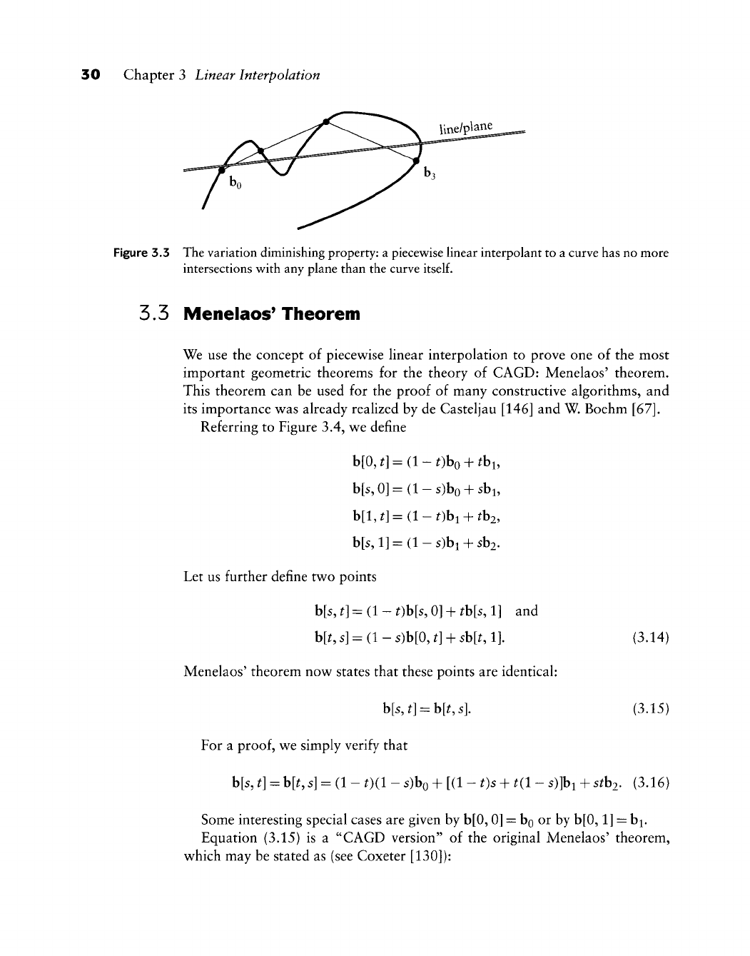
Figure
3.3
The variation diminishing property:
a
piecewise hnear interpolant
to a
curve has
no
more
intersections with
any
plane than
the
curve
itself.
5.5
Menelaos' Theorem
We
use the
concept
of
piecewise linear interpolation
to
prove
one of the
most
important geometric theorems
for the
theory
of
CAGD: Menelaos' theorem.
This theorem
can be
used
for the
proof
of
many constructive algorithms,
and
its importance
v^as
already realized
by de
Casteljau
[146] and
W. Boehm
[67].
Referring
to
Figure
3.4,
w^e define
b[0,
^]
=
(1
-
^)bo
+ thi,
b[s,
0]
=
(1
- s)bo + sbi,
b[l,^]=(l-^)bi
+ fb2,
b[s,l]
=
(l-s)bi
+ sb2.
Let
us
further define
tv^o
points
b[s,
^]
=
(1
-
Ob[s, 0]
+ th[s,
1]
and
b[^
s]
= (1 -
s)b[0, t]
+ sh[t,
1]. (3.14)
Menelaos' theorem
now
states that these points
are
identical:
b[5,^]
= b[^4
(3.15)
For
a proof, we
simply verify that
b[s,
t]
= h[t, s\ = {l- t){l - s)bo + [(1 - t)s + t{l - s)]bi +
sth2. (3.16)
Some interesting special cases
are
given
by b[0, 0] = bo or by
b[0,1]
= b^.
Equation (3.15)
is a
"CAGD version"
of the
original Menelaos' theorem,
which
may be
stated
as (see
Coxeter [130]):
3.4 Blossoms 31
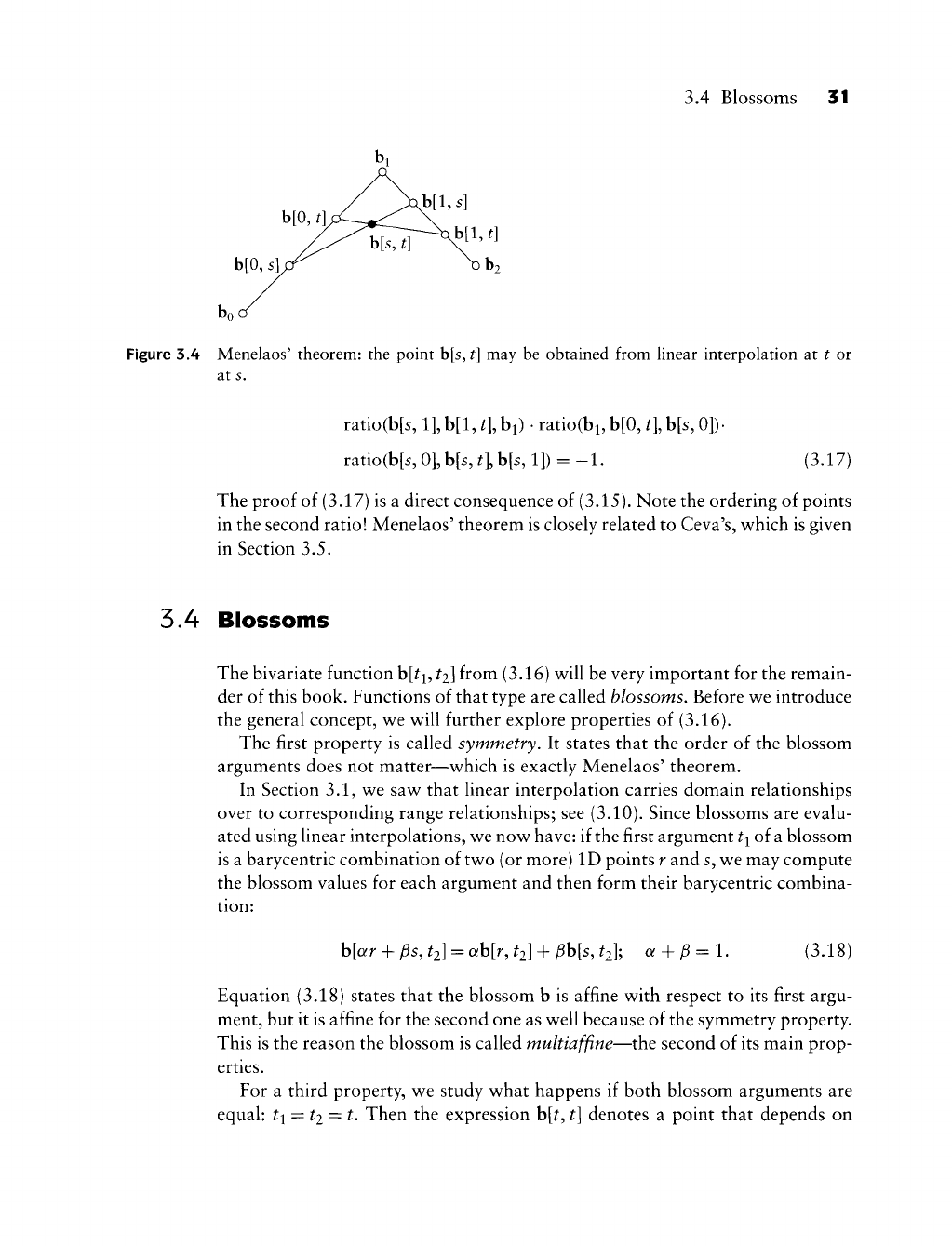
Figure 3.4 Menelaos' theorem: the point b[s,
t]
may be obtained from Hnear interpolation at t or
at s.
ratio(b[s, l],b[l,4bi)
•
ratio(bi,b[0,4b[s, 0])-
ratio(b[s, 0],b[s, 4b[s, 1]) =
-1.
(3.17)
The proof of (3.17) is a direct consequence of (3.15). Note the ordering of points
in the second ratio! Menelaos' theorem is closely related to Ceva's, which is given
in Section 3.5.
5.4 Blossoms
The bivariate function b[^i, ti] from (3.16) will be very important for the remain-
der of this book. Functions of that type are called blossoms. Before we introduce
the general concept, we will further explore properties of (3.16).
The first property is called symmetry. It states that the order of the blossom
arguments does not matter—which is exactly Menelaos' theorem.
In Section 3.1, we saw that linear interpolation carries domain relationships
over to corresponding range relationships; see (3.10). Since blossoms are evalu-
ated using linear interpolations, we now have: if the first argument ti of a blossom
is a barycentric combination of two (or more) ID points r and s, we may compute
the blossom values for each argument and then form their barycentric combina-
tion:
h[ar + ^s,
t2]
= ah[r, ti] + ^h{s, til a +
^6
= 1. (3.18)
Equation (3.18) states that the blossom b is affine with respect to its first argu-
ment, but it is affine for the second one as well because of the symmetry property.
This is the reason the blossom is called multiaffine—the second of its main prop-
erties.
For a third property, we study what happens if both blossom arguments are
equal: ti = t2 = t. Then the expression b[^, t\ denotes a point that depends on
32 Chapter 3 Linear Interpolation
one variable
t—^thus
it traces out a polynomial curve.^ This property is called the
diagonal property.
Our special blossom b[^i,
^2]
has two arguments. Blossoms with an arbitrary
number n of arguments are easily defined by the preceding three properties. A
blossom is an w-variate function b[^i,
• •
•,
^w]
from W into E^ or E^. It is defined
by three properties:
Symmetry:
b[^i,...,y = b[7rai,...,y] (3.19)
where 7t{ti^...,
^«)
denotes a permutation of the arguments
^1,...,
t^. Thus, for
example b[^i, ti,
t^]
= h[t2, t^, t^],
Multiafftnity:
h[{ar + Ps), *] = ah[r, *] + ph[s,
*];
a +
)6
= 1. (3.20)
Here, the symbol * indicates that there are the same arguments on both sides of
the equation, but their exact meaning is not of interest. Because of symmetry,
this property holds for all arguments, not just the first one.
Diagonality:
If all arguments of the blossom are the same:
^
=
^j,...,
^„, then we obtain a
polynomial curve (to be discussed later). We will use the notation
h[t,...,t]=h[t<">]
if the argument t is repeated n times.
We defined vector arguments for linear interpolation in Section 3.1. Blossoms
may also have vector arguments, resulting in expressions such as
b[/7,
r,
s].
If we
assume (without loss of generality) that the first argument of a blossom is a vector
h = b
—
a, then the multiaffine property becomes
h[b - ^, *] = b[fo, *] - h[a,
*].
(3.21)
Thus if (at least) one of the blossom arguments is a vector, then the blossom
value is a vector. For example, if we denote by 1 the ID unit vector, then
b[l,
r,
s]
= b[l, r,
s]
- b[0, r,
s]
or b[l, r,
s]
=
b[3,
r,
s] —
b[2, r, s\
4 This kind of curve will later be called a Bezier curve.
3.4 Blossoms 33
As an application of the blossom properties, let us derive a formula that will
be used later. We consider the special case when a blossom argument is of the
form {ar +
^s)^^^.
For this, we get
b[(ar + )Ss)<"^] = Y.
(''\'P''~Hr^'^.
s^^"^^].
(3.22)
.=0 -'
We refer to this equation as the Leibniz formula,^
The proof is by induction. The case « = 1 is a trivial start. The inductive step
proceeds as follows (keeping in mind that
(^^-^)
= (^J = 0):
r=0 ^'^
Now we transform the index of the first sum and let the second sum run to
w
+ 1:
n+l . .
i=0
The first sum may start with / = 0. Keeping in mind the recursion
n-\-t\
( ^ \ f^\
i
)~\i-l)^\i)
we can combine the last two sums and get
h[(ar + ^s)<^+l^] - Y] f"" ^ -^V^'^^+^-^bfr^^'^, s^^+l-^"^],
which concludes our
proof.
This result will be used several times later on.
5 It has the structure of Leibniz's rule for higher-order derivatives of
a
product of functions.
54 Chapter 3 Linear Interpolation
A different form of (3.22) is sometimes useful:
b[(ar + )Ss)<">]= Y. (.''.)«'>b[r<^=^,s<^=^] (3.23)
where
/
w
\ _ w!
V,/7 ^'
5.5 Barycentric Coordinates in tiie Plane
Barycentric coordinates were discussed in Section 3.1, where they were used in
connection with straight lines. Now we will use them as coordinate systems when
dealing with the plane. Planar barycentric coordinates are at the origin of affine
geometry—they were introduced by
F.
Moebius in 1827; see his collected works
[429].
Consider a triangle with vertices a, b, c and a fourth point p, all in E^. It
IS
always possible to write p as a barycentric combination of a, b, c:
p =
u2i
+ vh + wc. (3.24)
A reminder: if (3.24) is to be a barycentric combination (and hence geometrically
meaningful), we require that
u-\-v-]-w=l, (3.25)
The coefficients u := (u,
v^
w) are called barycentric coordinates of p with respect
to a, b, c. We will often drop the distinction between the barycentric coordinates
of a point and the point
itself;
we then speak of "the point u."
If the four points a, b, c, and p are given, we can always determine p's
barycentric coordinates u,v^w: Equations (3.24) and (3.25) can be viewed as
a linear system of three equations^ in three unknowns u, v, w. The solution is
obtained by an application of Cramer's rule:
area(p, b, c) area(a, p, c) area(a, b, p)
^=
7—r—:'
^^ TTT' ^"^ TTT^' ^^'^^^
area(a, b, c) area(a, b, c) area(a, b, c)
6 Recall that (3.24) is shorthand for two scalar equations.
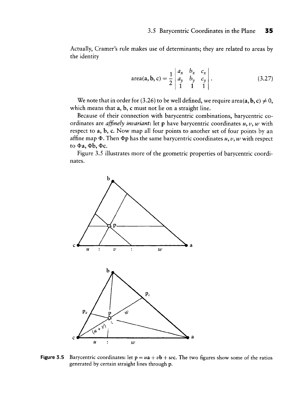
3.5 Barycentric Coordinates in the Plane 35
Actually, Cramer's rule makes use of determinants; they are related to areas by
the identity
area(a, b, c) = -
b.
1 1 1
(3.27)
We note that in order for (3.26) to be well defined, we require area(a, b, c) ^ 0,
which means that a, b, c must not lie on a straight line.
Because of their connection with barycentric combinations, barycentric co-
ordinates are affinely invariant: let p have barycentric coordinates w, z/, w with
respect to a, b, c. Now map all four points to another set of four points by an
affine map O. Then Op has the same barycentric coordinates
w,
v^
w with respect
to Oa, Ob, Oc.
Figure 3.5 illustrates more of the geometric properties of barycentric coordi-
nates.
Figure 3.5 Barycentric coordinates: let p =
wa
-h i/b + wc. The two figures show some of the ratios
generated by certain straight lines through p.
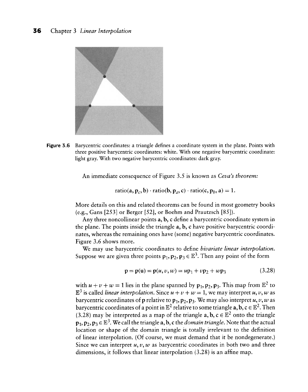
36 Chapter 3 Linear Interpolation
f ^
Figure 3.6 Barycentric coordinates: a triangle defines a coordinate system in the plane. Points with
three positive barycentric coordinates: white. With one negative barycentric coordinate:
light gray. With two negative barycentric coordinates: dark gray.
An immediate consequence of Figure 3.5 is known as Ceva's theorem:
ratio(a,
p^,
b)
•
ratio(b,
p^,
c)
•
ratio(c,
p^,
a) = 1.
More details on this and related theorems can be found in most geometry books
(e.g., Cans [253] or Berger [52], or Boehm and Prautzsch [85]).
Any three noncoUinear points a, b, c define a barycentric coordinate system in
the plane. The points inside the triangle a, b, c have positive barycentric coordi-
nates,
w^hereas the remaining ones have (some) negative barycentric coordinates.
Figure 3.6 shoves more.
We may use barycentric coordinates to define bivariate linear interpolation.
Suppose v^e are given three points pj, p2,
P3 G
E^. Then any point of the form
p = p(u) = p(w,
V,
w) = upi -f z;p2 +
wp2>
(3.28)
with u-{-v-\-w=l lies in the plane spanned by pi, p2,
P3.
This map from E^ to
E^ is called linear interpolation. Since u-\-v-\-w=l,wt may interpret
w,
v, w as
barycentric coordinates of p relative to pi,
p2,
P3.
We may also interpret
w,
v, w as
barycentric coordinates of a point in E^ relative to some triangle a, b, c
G
E-^.
Then
(3.28) may be interpreted as a map of the triangle a, b, c
G
E^ onto the triangle
Pl5 P25 P3
^ ^^- We call the triangle a,
b,
c the domain triangle. Note that the actual
location or shape of the domain triangle is totally irrelevant to the definition
of linear interpolation. (Of course, we must demand that it be nondegenerate.)
Since we can interpret
w,
v, w as barycentric coordinates in both two and three
dimensions, it follows that linear interpolation (3.28) is an affine map.
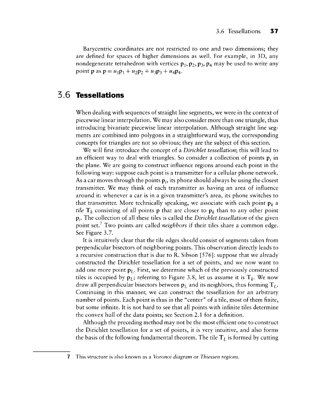
3.6 Tessellations 37
Barycentric coordinates are not restricted to one and two dimensions; they
are defined for spaces of higher dimensions as well. For example, in 3D, any
nondegenerate tetrahedron with vertices
p^,
p2,
P3,
P4 may be used to write any
point p as p = u^pi
-\- U2P2
+ ^3P3 + ^4p4-
5.6 Tessellations
When dealing with sequences of straight line segments, we were in the context of
piecewise linear interpolation. We may also consider more than one triangle, thus
introducing bivariate piecewise linear interpolation. Although straight line seg-
ments are combined into polygons in a straightforward way, the corresponding
concepts for triangles are not so obvious; they are the subject of this section.
We will first introduce the concept of a Dirichlet tessellation; this will lead to
an efficient way to deal with triangles. So consider a collection of points p^ in
the plane. We are going to construct influence regions around each point in the
following way: suppose each point is a transmitter for a cellular phone network.
As a car moves through the points
p^,
its phone should always be using the closest
transmitter. We may think of each transmitter as having an area of influence
around it: whenever a car is in a given transmitter's area, its phone switches to
that transmitter. More technically speaking, we associate with each point p^ a
tile T^ consisting of all points p that are closer to p^ than to any other point
p^.
The collection of all these tiles is called the Dirichlet tessellation of the given
point set.^ Two points are called neighbors if their tiles share a common edge.
See Figure 3.7.
It is intuitively clear that the tile edges should consist of segments taken from
perpendicular bisectors of neighboring points. This observation directly leads to
a recursive construction that is due to R. Sibson
[576]:
suppose that we already
constructed the Dirichlet tessellation for a set of points, and we now want to
add one more point p^. First, we determine which of the previously constructed
tiles is occupied by pi; referring to Figure 3.8, let us assume it is T^. We now
draw all perpendicular bisectors between p^ and its neighbors, thus forming T^.
Continuing in this manner, we can construct the tessellation for an arbitrary
number of points. Each point is thus in the "center" of a tile, most of them finite,
but some infinite. It is not hard to see that all points with infinite tiles determine
the convex hull of the data points; see Section 2.1 for a definition.
Although the preceding method may not be the most efficient one to construct
the Dirichlet tessellation for a set of points, it is very intuitive, and also forms
the basis of the following fundamental theorem. The tile T^^ is formed by cutting
7 This structure is also known as a
Voronoi diagram
or
Thiessen
regions.
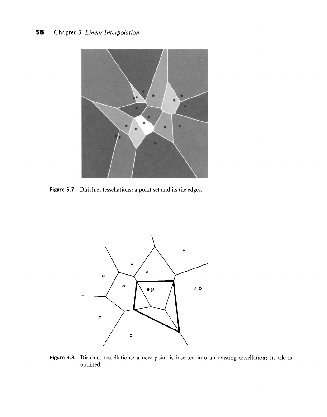
38 Chapter 3 Linear Interpolation
Figure
3.7
Dirichlet tessellations:
a
point
set and its
tile edges.
Figure
3.8
Dirichlet tessellations:
a new
point
is
inserted into
an
existing tessellation;
its
tile
is
outlined.
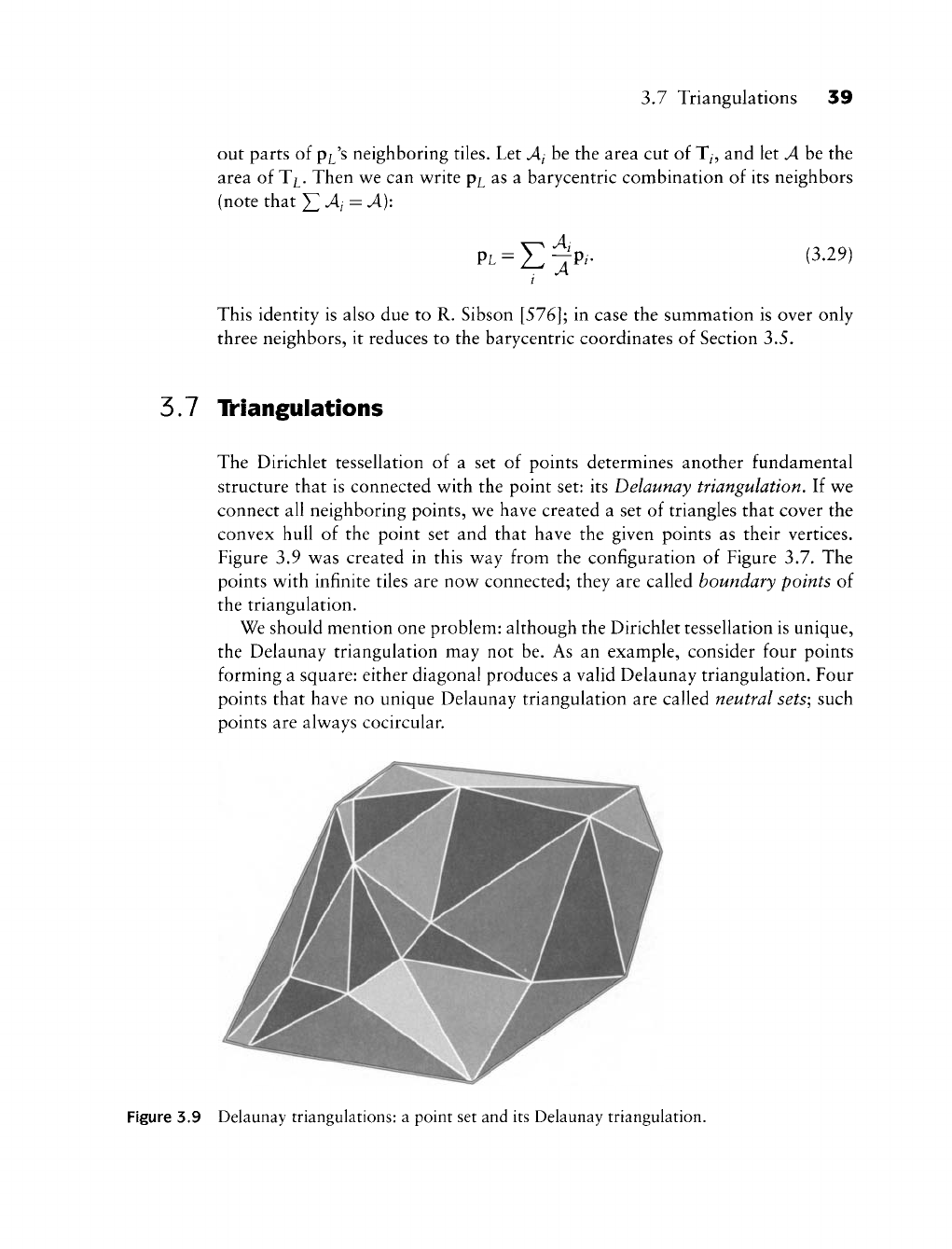
3.7 Triangulations 39
out parts of p^^'s neighboring tiles. Let Aj be the area cut of T^, and let A be the
area of T^. Then we can write pi as a barycentric combination of its neighbors
(note that ^^• = ^):
p^^E-jp-
(3.29)
This identity is also due to R. Sibson
[576];
in case the summation is over only
three neighbors, it reduces to the barycentric coordinates of Section 3.5.
5.7 Triangulations
The Dirichlet tessellation of a set of points determines another fundamental
structure that is connected with the point set: its Delaunay triangulation. If we
connect all neighboring points, we have created a set of triangles that cover the
convex hull of the point set and that have the given points as their vertices.
Figure 3.9 was created in this way from the configuration of Figure 3.7. The
points with infinite tiles are now connected; they are called boundary points of
the triangulation.
We should mention one problem: although the Dirichlet tessellation is unique,
the Delaunay triangulation may not be. As an example, consider four points
forming a square: either diagonal produces a valid Delaunay triangulation. Four
points that have no unique Delaunay triangulation are called neutral sets; such
points are always cocircular.
Figure 3.9 Delaunay triangulations: a point set and its Delaunay triangulation.
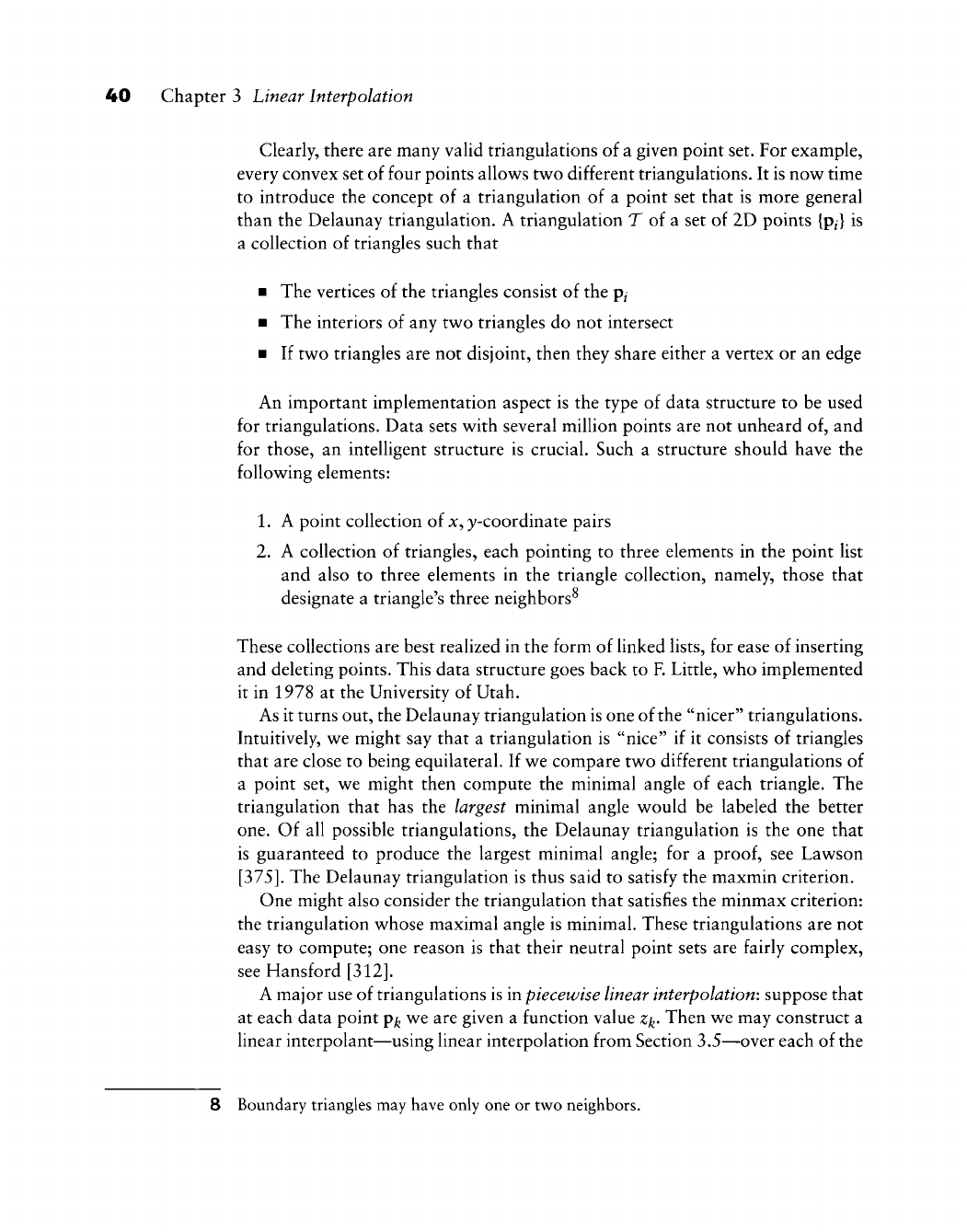
40 Chapter 3 Linear Interpolation
Clearly, there are many valid triangulations of a given point set. For example,
every convex set of four points allov^s tv^o different triangulations. It is
now^
time
to introduce the concept of a triangulation of a point set that is more general
than the Delaunay triangulation. A triangulation T of a set of 2D points {pj is
a collection of triangles such that
• The vertices of the triangles consist of the p^
• The interiors of any tv^o triangles do not intersect
• If two triangles are not disjoint, then they share either a vertex or an edge
An important implementation aspect is the type of data structure to be used
for triangulations. Data sets v^ith several million points are not unheard of, and
for those, an intelligent structure is crucial. Such a structure should have the
foUov^ing elements:
1.
A point collection of x, y-coordinate pairs
2.
A collection of triangles, each pointing to three elements in the point list
and also to three elements in the triangle collection, namely, those that
designate a triangle's three neighbors^
These collections are best realized in the form of linked lists, for ease of inserting
and deleting points. This data structure goes back to F. Little, v^ho implemented
it in 1978 at the University of Utah.
As it turns out, the Delaunay triangulation is one of the "nicer" triangulations.
Intuitively, we might say that a triangulation is "nice" if it consists of triangles
that are close to being equilateral. If
w^e
compare two different triangulations of
a point set, w^e might then compute the minimal angle of each triangle. The
triangulation that has the largest minimal angle w^ould be labeled the better
one.
Of all possible triangulations, the Delaunay triangulation is the one that
is guaranteed to produce the largest minimal angle; for a
proof,
see Lawson
[375].
The Delaunay triangulation is thus said to satisfy the maxmin criterion.
One might also consider the triangulation that satisfies the minmax criterion:
the triangulation w^hose maximal angle is minimal. These triangulations are not
easy to compute; one reason is that their neutral point sets are fairly complex,
see Hansford
[312].
A major use of triangulations is in piecewise linear interpolation: suppose that
at each data point p^ v^e are given a function value
Zk-
Then v^e may construct a
linear interpolant—using linear interpolation from Section 3.5—over each of the
8 Boundary triangles may have only one or two neighbors.
3.8 Problems 41
triangles. We obtain a faceted, continuous surface that interpolates to all given
data. This surface is not smooth, but it will give a decent idea of the shape of
the given data. One application is in cartography: here, the given data points
might be coordinates obtained from satellite readings and the function values
might be their elevations. Our piecewise linear surface is an approximation to
the landscape being surveyed.
Once function values are involved, it may be advantageous to construct a
triangulation that reflects this information. Such triangulations are called data
dependent^ see Dyn, Levin, and Rippa [180] or Brow^n [92]. Here, one does not
just consider triangles in the plane, but rather the 3D triangles generated by the
data points (x^,
y^^,
Zk).
5.8 Problems
1 In the definition of the variation diminishing property, we counted the
crossings of a polygon with a plane. Discuss the case when the plane
contains a whole polygon leg.
* 2 We defined the convex hull of a point set to be the set of all convex
combinations formed by the elements of that set. Another definition is the
following: the convex hull of a point set is the intersection of all convex
sets that contain the given set. Show that both definitions are equivalent.
* 3 Our definition of barycentric combinations gives the impression that it
needs the involved points expressed in terms of some coordinate system.
Show that this is not necessary: draw five points on a piece of paper, assign
a weight to each one, and construct the barycenter of your points using a
ruler (or compass and straightedge if you are more classically inclined).
Remark: For this construction, it is not necessary for the weights to
sum to one. This is so because the geometric construction remains the
same if we multiplied all weights by a common factor. In fact, one may
replace the concept of points (having mass one and requiring barycentric
combinations as the basic point operation) by that of mass points^ having
arbitrary weights and yielding their barycenter (with the combined mass of
all points) as the basic operation. In such a setting, vectors would also be
mass points, but with mass zero.^
* 4 Let a triangulation consist of b boundary points and of / interior points.
Show that the number of triangles is 2i
-\-
b
—
2.
9 I was introduced to this concept by A. Swimmer. It was developed by H. Grassmann in
1844.
42 Chapter 3 Linear Interpolation
PI Let three points be given by
bn
For s = 0,0.05,0.1,..., 1 and
^
= 0,0.05,0.1,..., 1, plot the points b[s, t]
as defined by (3.16). Mark each point by a circle with radius 0.4.
P2 There is a 2D triangulation data set on this book's web site. Plot that
triangulation using gray shades or colors such that no two neighboring
triangles have the same color.
P3 Use the recursive algorithm from Section 3.6 to implement Dirichlet tessel-
lations.
The de Casteljau
Algorithm
I he algorithm described in this chapter is probably the most fundamental
one in the field of curve and surface design, yet it is surprisingly simple. Its
main attraction is the beautiful interplay between geometry and algebra: a very
intuitive geometric construction leads to a pow^erful theory.
Historically, it is v^ith this algorithm that the w^ork of de Casteljau started
in 1959. The only w^ritten evidence is in [145] and
[146],
both technical reports
that are not easily accessible. De Casteljau's v^ork w^ent unnoticed until
W.
Boehm
obtained copies of the reports in 1975. Since then, de Casteljau's w^ork has gained
more popularity.
4.1
Parabolas
We give a simple construction for the generation of a parabola; the straightfor-
v^ard generalization w^ill then lead to Bezier curves. Let bo,
b^,
hi be any three
points in E^, and let t eR. Construct
bj(0 = (1 - t)ho + ^bi,
h\it) = (1 - Obi + th2,
hl(t) = (l-t)hl(t)
+
th\(t).
Inserting the first tv^o equations into the third one, v^e obtain
hlit) = (1 - t)% + 2t(l - Obi + t%. (4.1)
43
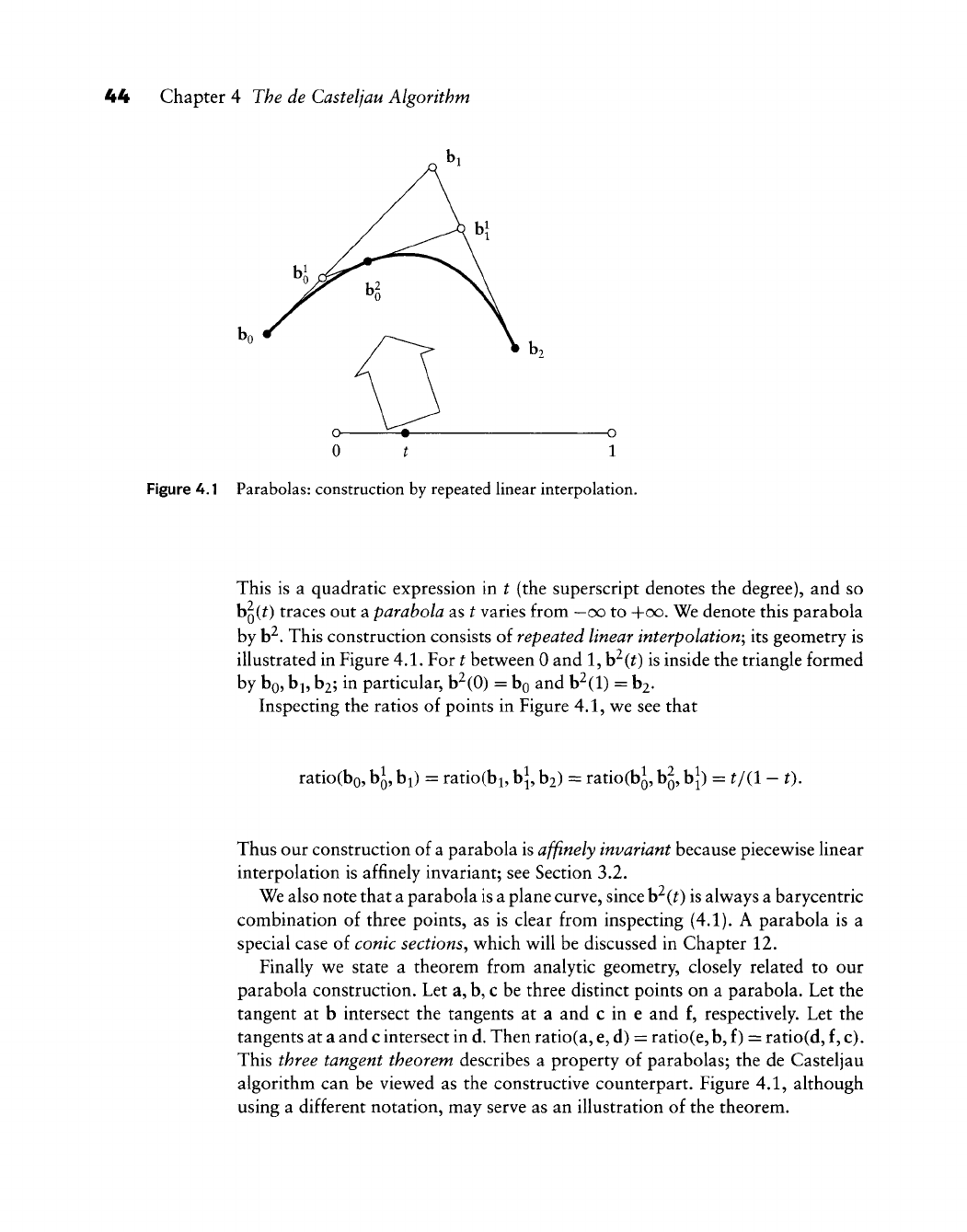
44 Chapter 4 The de Casteljau Algorithm
0 t
Figure 4.1 Parabolas: construction by repeated linear interpolation.
This is a quadratic expression in t (the superscript denotes the degree), and so
hi^it) traces out a parabola as t varies from —oo to +oo. We denote this parabola
by
b^.
This construction consists of repeated linear interpolation^ its geometry is
illustrated in Figure
4.1.
For t between 0 and 1, b^(^) is inside the triangle formed
by bo, bi,
b2;
in particular, b^(0) = bo and b^(l) = b2.
Inspecting the ratios of points in Figure 4.1, we see that
ratio(bo, bj, bi) = ratio(bi, bj, hi) = ratio(bJ,
b^,
b^) = t/(l
—
t).
Thus our construction of a parabola is affinely invariant because piecewise linear
interpolation is affinely invariant; see Section 3.2.
We also note that a parabola is a plane curve, since h^{t) is always a barycentric
combination of three points, as is clear from inspecting (4.1). A parabola is a
special case of conic sections^ which will be discussed in Chapter 12.
Finally we state a theorem from analytic geometry, closely related to our
parabola construction. Let a, b, c be three distinct points on a parabola. Let the
tangent at b intersect the tangents at a and c in e and f, respectively. Let the
tangents at a and c intersect in d. Then ratio(a, e, d) = ratio(e, b, f) = ratio(d, f, c).
This three tangent theorem describes a property of parabolas; the de Casteljau
algorithm can be viewed as the constructive counterpart. Figure 4.1, although
using a different notation, may serve as an illustration of the theorem.
4.2
The de
Casteljau Algorithm
45
4.2 The
de
Casteljau Algorithm
Parabolas
are
plane curves. However, many applications require true space
curves.^
For
those purposes,
the
previous construction
for a
parabola
can be
generalized
to
generate
a
polynomial curve
of
arbitrary degree
n\
de Casteljau algorithm:
Given:
bo,
bj,...,
b„
G
E^
and
t e
M,
set
mt)
^
(1
-
t)hi\t)+th^-iit)
{'lo;•••;;_, (4.2)
and
h^(t) =
b/. Then
h^it) is the
point with parameter value
t on the
Bezier
curve b", hence \y^{t)
= ^(t).
The polygon
P
formed
by
bo,..., b„
is
called
the
Bezier polygon
or
control
polygon
of the
curve
h^?
Similarly,
the
polygon vertices
b^ are
called control
points
or
Bezier points. Figure
4.2
illustrates
the
cubic case.
Sometimes
we
also write b^(^)
=
B[bo,..., b„; ^]
=
B[P;
t] or,
shorter,
b^ =
B[bo,...,
b„]
=
BP. This notation-^ defines
B to be the
(linear) operator that
associates
the
Bezier curve with
its
control polygon.
We say
that
the
curve
B[bo,...,
b„]
is the
Bernstein-Bezier approximation
to the
control polygon,
a
terminology borrowed from approximation theory;
see
also Section
6.9.
The intermediate coefficients b[(^)
are
conveniently written into
a
triangular
array
of
points,
the de
Casteljau scheme.
We
give
the
example
of
the cubic case:
bl
K
hi
b\ hi
b3
bl b2 hi.
(4.3)
This triangular array
of
points seems
to
suggest
the use of a
two-dimensional
array
in
writing code
for the de
Casteljau algorithm. That would
be a
waste
of
1 Compare the comments by
P.
Bezier
in
Chapter
1!
2 In the cubic
case,
there are four control
points;
they form
a
tetrahedron in the 3D
case.
This
tetrahedron was already mentioned by
W.
Blaschke
[65]
in
1923; he called
it
"osculating
tetrahedron."
3 This notation should
not
be confused with the blossoming notation used later.
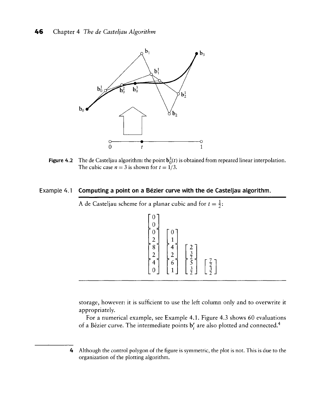
46 Chapter 4 The de Casteljau Algorithm
Figure 4.2 The de Casteljau algorithm: the point h^it) is obtained from repeated linear interpolation.
The cubic case
w
= 3 is shown for t = 1/3.
Example 4.1 Computing a point on a Bezier curve with the de Casteljau algorithm.
A de Casteljau scheme for a planar cubic and for t = j:
ro]
0
[2
8
[2
[4'
0
"0"
1
4
2
''6''
1
2
3
- 2 -
[5]
3
r 7 1
2
3
- 7 J
Storage, however: it is sufficient to use the left column only and to overwrite it
appropriately.
For a numerical example, see Example 4.1. Figure 4.3 shows 60 evaluations
of a Bezier curve. The intermediate points
W-
are also plotted and connected."^
4 Although the control polygon of the
figure
is symmetric, the plot is not. This is due to the
organization of the plotting algorithm.
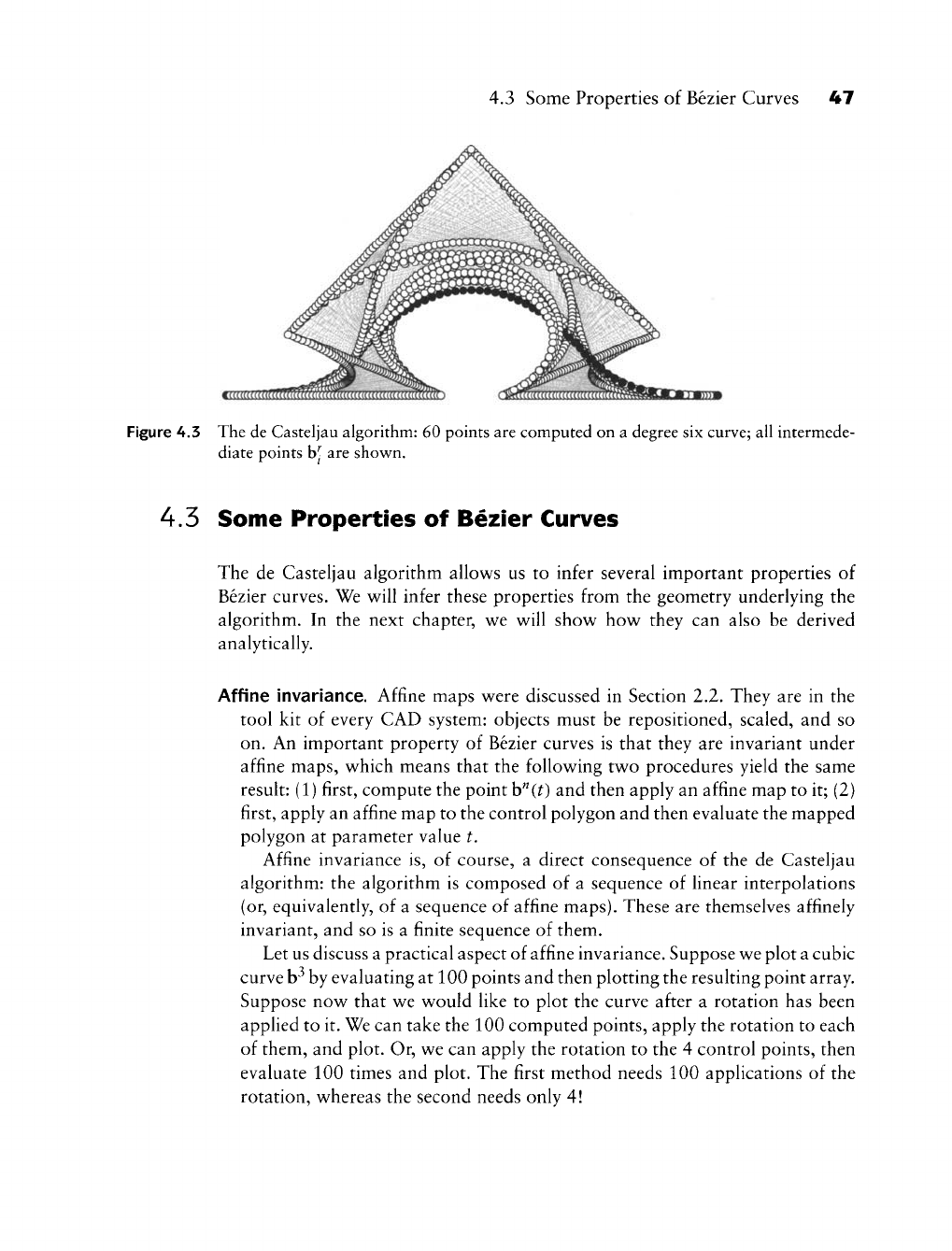
4.3 Some Properties of Bezier Curves 47
Figure 4.3 The de Casteljau algorithm: 60 points are computed on a degree six curve; all intermede-
diate points
b^
are shown.
4.5 Some Properties of Bezier Curves
The de Casteljau algorithm allows us to infer several important properties of
Bezier curves. We will infer these properties from the geometry underlying the
algorithm. In the next chapter, we will show how they can also be derived
analytically.
Afflne invariance. Affine maps were discussed in Section 2.2. They are in the
tool kit of every CAD system: objects must be repositioned, scaled, and so
on. An important property of Bezier curves is that they are invariant under
affine maps, which means that the following two procedures yield the same
result: (1) first, compute the point h^(t) and then apply an affine map to it; (2)
first, apply an affine map to the control polygon and then evaluate the mapped
polygon at parameter value t.
Affine invariance is, of course, a direct consequence of the de Casteljau
algorithm: the algorithm is composed of a sequence of linear interpolations
(or, equivalently, of a sequence of affine maps). These are themselves affinely
invariant, and so is a finite sequence of them.
Let us discuss a practical aspect of affine invariance. Suppose we plot a cubic
curve
b^
by evaluating at 100 points and then plotting the resulting point array.
Suppose now that we would like to plot the curve after a rotation has been
applied to it. We can take the 100 computed points, apply the rotation to each
of them, and plot. Or, we can apply the rotation to the 4 control points, then
evaluate 100 times and plot. The first method needs 100 applications of the
rotation, whereas the second needs only 4!
48 Chapter 4 The de Casteljau Algorithm
Affine invariance may not seem to be a very exceptional property for a
useful curve scheme; in fact, it is not straightforward to think of a curve
scheme that does not have it (exercise!). It is perhaps v^orth noting that Bezier
curves do not enjoy another, also very important, property: they are not
projectively invariant. Projective maps are used in computer graphics when
an object is to be rendered realistically. So if we try to make life easy and
simplify a perspective map of a Bezier curve by mapping the control polygon
and then computing the curve, we have actually cheated: that curve is not the
perspective image of the original curve! More details on perspective maps can
be found in Chapter 12.
Invariance under affine parameter transformations. Very often, one thinks
of a Bezier curve as being defined over the interval
[0,1].
This is done because it
is convenient, not because it is necessary: the de Casteljau algorithm is "blind"
to the actual interval that the curve is defined over because it uses ratios only.
One may therefore think of the curve as being defined over any arbitrary
interval a<u<boi the real line—after the introduction of local coordinates
t = (u
—
a)/(b
—
a), the algorithm proceeds as usual. This property is inherited
from the linear interpolation process (3.9). The corresponding generalized
de Casteljau algorithm is of the form:
^ b-a ^ b-a ^^^
The transition from the interval [0,1] to the interval
[a,
b] is an affine
map.
Therefore, we can say that Bezier curves are invariant under affine
parameter transformations. Sometimes, one sees the term linear parameter
transformation in this context, but this terminology is not quite correct: the
transformation of the interval [0,1] to
[a^
b]
typically includes a translation,
which is not a linear map.
Convex hull property. For t e
[0,1],
h^{t) lies in the convex hull (see Figure 2.3)
of the control polygon. This follows since every intermediate
W-
is obtained
as a convex barycentric combination of previous bp —at no step of the
de Casteljau algorithm do we produce points outside the convex hull of
the b^.
A simple consequence of the convex hull property is that a planar control
polygon always generates a planar curve.
4.3 Some Properties of Bezier Curves 49
The importance of the convex hull property lies in what is known as
interference checking. Suppose we want to know if two Bezier curves intersect
each other—for example, each might represent the path of a robot arm, and
our aim is to make sure that the two paths do not intersect, thus avoiding
expensive collisions of the robots. Instead of actually computing a possible
intersection, we can perform a much cheaper test: circumscribe the smallest
possible box around the control polygon of each curve such that it has its edges
parallel to some coordinate system. Such boxes are called minmax boxes., since
their faces are created by the minimal and maximal coordinates of the control
polygons. Clearly each box contains its control polygon, and, by the convex
hull property, also the corresponding Bezier curve. If we can verify that the
two boxes do not overlap (a trivial test), we are assured that the two curves
do not intersect. If the boxes do overlap, we would have to perform more
checks on the curves. The possibility for a quick decision of no interference
is extremely important, since in practice one often has to check one object
against thousands of others, most of which can be labeled "no interference"
by the minmax box test.^
Endpoint interpolation. The Bezier curve passes through
BQ
and b„: we have
b"(0) =
bo,
b"(l) =
b^.
This is easily verified by writing down the scheme (4.3)
for the cases
^
= 0 and
^
= 1. In a design situation, the endpoints of a curve
are certainly two very important points. It is therefore essential to have direct
control over them, which is assured by endpoint interpolation.
Designing with Bezier curves. Figure 4.4 shows two Bezier curves. From the
inspection of these examples, one gets the impression that in some sense the
Bezier curve "mimics" the Bezier polygon—this statement will be made more
precise later. It is the reason Bezier curves provide such a handy tool for the
design of
curves:
to reproduce the shape of a hand-drawn curve, it is sufficient
to specify a control polygon that somehow "exaggerates" the shape of the
curve. One lets the computer draw the Bezier curve defined by the polygon,
and, if necessary, adjusts the location (possibly also the number) of the polygon
vertices. Typically, an experienced person will reproduce a given curve after
two to three iterations of this interactive procedure.
5 It is possible to create volumes (or areas, in the 2D case) that hug the given curve closer
than the minmax box does. See Sederberg et al.
[560].

50 Chapter 4 The de Casteljau Algorithm
Figure 4.4 Bezier curves: some examples.
4.4 The Blossom
In recent years, a new way to look at Bezier curves has been developed; it is
called the principle of blossoming. This principle was independently developed
by de Casteljau [147] and Ramshaw
[498], [499].
Other literature includes Seidel
[562], [565], [566];
DeRose and Goldman
[165];
Boehm [75]; Lee
[379];
and
Gallier
[252].
Blossoms were introduced in Section 3.4. They are closely related to the
de Casteljau algorithm: in column r, do not again perform a de Casteljau step
for parameter value ^, but use a new value
t^..
Restricting ourselves to the cubic
case,
we obtain:
bo
bi
bi
b3
H[h]
h\[h]
Hih]
hl[h, t2]
bjl^i,
t2]
4.4 The Blossom
51
(4.5)
The resulting point h^lti,
ti-, ^3]
is now a function of three independent variables;
thus it no longer traces out a curve, but a region of E^. This trivariate function
b[-,
•, •] is called the blossom from Section 3.4. The original curve is recovered if
v^e set all three arguments equal:
t
= ti = t2 = ty
To understand the blossom better, v^e now evaluate
it
for several special
arguments. We already know, of course, that b[0, 0, 0] = bo and b[l, 1,1] = b3.
Let us start with
[^1, ^2? ^3]
= [0? 0,1]. The scheme (4.5) reduces to:
bo
(4.6)
bi
bo
b2
bj
bo
b3
b2 bi
bi
=
b[0,0,l].
Similarly, we can show that b[0,1,1] =
b2.
Thus the original Bezier points can
be found by evaluating the curve's blossom at arguments consisting only of O's
and I's.
But the remaining entries in (4.3) may also be written as values of the blossom
for special arguments. For instance, setting [^j,
ti-, ^3]
= [0, 0,
t\
we have the
scheme
bo
(4.7)
bi
bo
bi
bi bo
b3
b2 bi
bj
=
b[0,0,^].
Continuing in the same manner, we may write the complete scheme (4.3) as:
bo = b[0,0,0]
bi = b[0,0,l] h[0,0,t]
b2-b[0,l,l]
b[0,f,l] h[<d,t,t]
^ '
b3 = b[l,l,l] h[t,l,l] h[t,t,l] h[t,t,t].
This is easily generalized to arbitrary degrees, where we can also express the
Bezier points as blossom values:
b,=b[0<"-^^,r^'^],
(4.9)
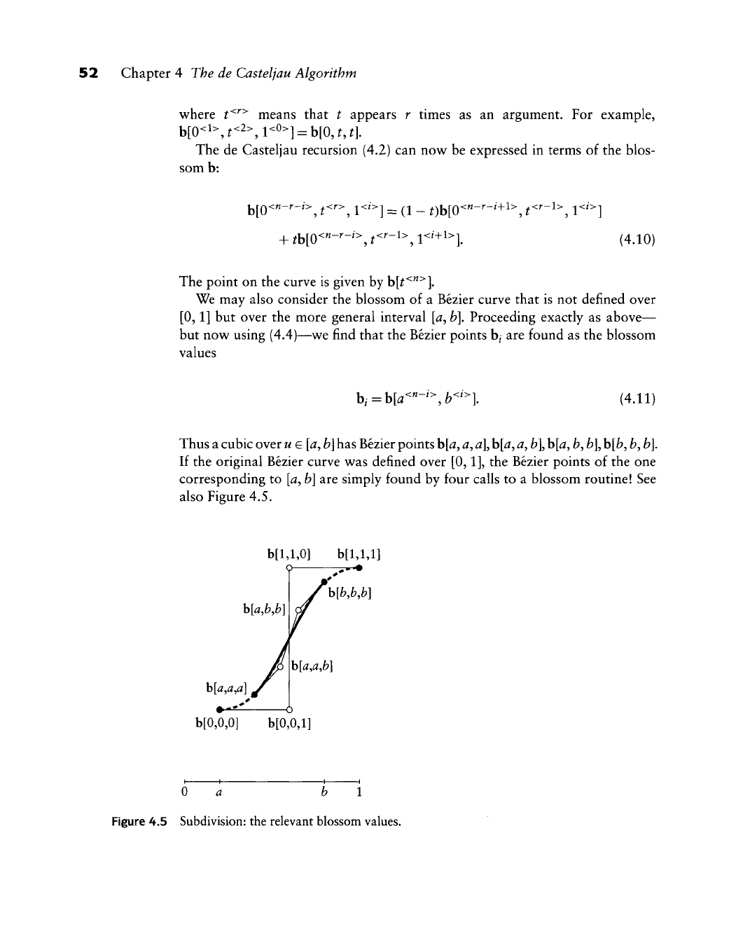
52 Chapter
4
The de Casteljau Algorithm
where
t^''^
means that
t
appears
r
times
as an
argument.
For
example,
The de Casteljau recursion (4.2) can now be expressed
in
terms
of
the blos-
som b:
b[0<"-'-'>,
t^'^,
r'>]
=
(1
-
^)b[0<"-^-'+i>,
t^'-^^,
r'>]
+ fb[o<«-'-'>,
t-"-^^,
i<'+i=^]. (4.10)
The point on the curve is given by
b[f^^^].
We may also consider the blossom
of a
Bezier curve that is not defined over
[0,1] but over the more general interval
[a,
b].
Proceeding exactly
as
above—
but nov^ using (4.4)—v^e find that the Bezier points b/ are found as the blossom
values
b,=b[^<^-^>,6^^>].
(4.11)
Thus a cubic over u
e
[a,
b]
has Bezier points
h[a^
a,
a\
h[a^
a,
fo],
h[a,
fc,
fc],
b[fc,
fo,
b].
If the original Bezier curve was defined over
[0,1],
the Bezier points
of
the one
corresponding to
[a,
b]
are simply found by four calls to
a
blossom routine! See
also Figure 4.5.
b[l,l,0] b[l,l,l]
0
^w-#
h[a,b,b]
h[b,bM
h[a,a,a
h[a,a,b]
b[0,0,0] b[0,0,l]
0
a hi
Figure 4.5 Subdivision: the relevant blossom values.
4.5 Implementation 53
We may also find explicit formulas for blossoms; here is the case of a cubic:
= (1 -
t{)[(\
- ^2)b[0,0,
^3]
+
^2b[0,1,
^3]]
+ h[(X -
^2)b[0,1,
^3]
= b[0,0,0](l-^i)(l-?2)a-^3)
+ b[0,0, !][(! - ^i)(l - ^2)^3 + (1 - ^1)^2(1 - ^3) + ^i(l - t2){l - ^3)]
+
b[0,1,
l][^i^2(l - ^3) + ^i(l - ^2)^3 + (1 - ^1)^2^3]
+ b[l,l,l]^1^2^3.
For each step, we have exploited the fact that blossoms are multiaffine, following
the inductive proof of the Leibniz equation (3.22).
We should add that every multivariate polynomial function may be interpreted
as the blossom of a Bezier curve—as long as it is both symmetric and multiaffine.
4.5 Implementation
The header of the de Casteljau algorithm program is:
float decas(degree,coeff,t)
/*
uses
de
Casteljau
to
compute
one
coordinate
value
of a
Bezier curve.
Has to be
called
for each coordinate (x,y, and/or z)
of a
control polygon.
Input: degree: degree
of
curve.
coeff: array with coefficients
of
curve,
t: parameter value.
Output: coordinate value.
V
This procedure invites several comments. First, we see that it requires the use of
an auxiliary array coeff a. Moreover, this auxiliary array has to be filled for each
function
call!
So on top of the already high computational cost of the de Casteljau
algorithm, we add another burden to the routine, keeping it from being very
efficient. A faster evaluation method is given at the end of the next chapter.
54 Chapter 4 The de Casteljau Algorithm
To plot a Bezier curve, we would then call the routine several times:
void bez_to_points(degree,npoints,coeff,points)
/* Converts Bezier curve into point sequence. Works on
one coordinate only.
Input: degree: degree of curve.
npoints: # of coordinates to be generated, (counting
from 0!)
coeff:
coordinates of control polygon.
Output: points: coordinates of points on curve.
Remark: For a 2D curve, this routine needs to be called twice,
once for the x-coordinates and once for y.
*/
The last subroutine has to be called once for each coordinate, that is, two or
three times. The main program decasmai
n.
c
on the enclosed disk gives an example
of how to use it and how to generate postscript output.
4.6 Problems
1 Suppose a planar Bezier curve has a control polygon that is symmetric
with respect to the y-axis. Is the curve also symmetric with respect to
the y-axis? Be sure to consider the control polygon
(—1,
0), (0,1), (1,1),
(0,
2), (0,1), (-1, 1), (0, 2), (0, 1), (1, 0). Generalize to other symmetry
properties.
2 Use the de Casteljau algorithm to design a curve of degree four that has its
middle control point on the curve. More specifically, try to achieve
Five collinear control points are a solution; try to be more ambitious!
''
3 The de Casteljau algorithm may be formulated as
B[bo,
...,K;t] = a- OB[bo,..., K-i; t] + ^[bi,...,
b^;
t].
Show that the computation count is exponential (in terms of the degree) if
you implement such a recursive algorithm in a language like C.

4.6 Problems 55
•
4 Show that every nonplanar cubic in
E"^
can be obtained as an affine map of
the standard cubic (see Boehm [70])
xW =
PI Write an experimental program that replaces {1
—
t) and t in the recursion
(4.2) by [1
—
f{t)] and f{t)^ where f is some "interesting" function. Change
the routine decas accordingly and comment on your results.
P2 Rewrite the routine decas to handle blossoms. Evaluate and plot for some
"interesting" arguments.
P3 Experiment with the data set outl
i
ne_2D.
dat on the floppy: try to recapture
its shape using one, two, and four Bezier curves. These curves should have
decreasing degrees as you use more of them.
P4 Then repeat the previous problem with outline_3D.dat. This data set is
three dimensional, and you will have to use (at least) two views as you
approximate the data points. The points, by the way, are taken from the
outline of a high heel shoe sole.

This Page Intentionally Left Blank
The Bernstein Form
of a Bezier Curve
Dezier curves can be defined by a recursive algorithm, which is how de Casteljau
first developed them. It is also necessary, however, to have an explicit represen-
tation for them; this will facilitate further theoretical development considerably.
5.1 Bernstein Polynomials
We will express Bezier curves in terms of Bernstein polynomials^ defined explicitly
by
B"^it)^{^^t\l-t)"-\
(5.1)
where the binomial coefficients are given by
V/7
1 0
else.
There is a fair amount of literature on these polynomials. We cite just a few:
Bernstein [53], Lorentz
[399],
Davis
[133],
and Korovkin
[364].
An extensive
bibliography is given in Gonska and Meier
[269].
Before we explore the importance of Bernstein polynomials to Bezier curves,
let us first examine them more closely. One of their important properties is that
they satisfy the following recursion:
B'lit) = (1 - t)B'l-\t) + tB'lzlit) (5.2)
57
58 Chapter 5 The Bernstein Form of a Bezier Curve
with
^Om _
and
Blit) ^ 1 (5.3)
BJ(O = 0 for
;^{0,...,n}.
(5.4)
The proof is simple:
n—t
=C7>'<'-'»-'-(::0''<'-'>
Another important property is that Bernstein polynomials form a partition of
unity:
1]B«(0
= 1. (5.5)
This fact is proved with the help of the binomial theorem:
1=[^+(1
-
t)r=J2
C'^^i^
-
tr-^=E
^^^)-
Figure 5.1 shows the family of the four cubic Bernstein polynomials. Note that
the B" are nonnegative over the interval
[0,1].
We are now ready to see why Bernstein polynomials are important for the
development of Bezier curves. Recall that a Bezier curve may be written as b[^'^"^]
in blossom form. Since t = (I
—
t)
-
0
-{-1
•
1^
the blossom may be expressed as
b[(l -t)'0 + t'
l)^"""^],
and now the Leibniz formula (3.22) directly yields
n
hit) =
h[t<">]
= J2^iBlit) (5.6)
«=o
since b, = h[0<"-'>,
!<'>]
according to (4.9).
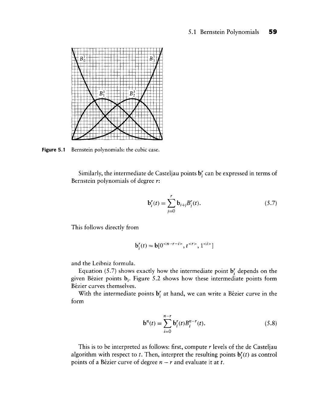
5.1 Bernstein Polynomials 59
Ik
1 1 1 1 1 1 1 1 1 1 1 1 1 1 1 1 1 1 1 1 1 1 1
i
y M/
1 T^^ T-l^ /
U
?^n
^"^ /
\ P^ P^ /
Nl M ^ M
Figure 5.1 Bernstein polynomials: the cubic case.
Similarly, the intermediate de Casteljau points
W-
can be expressed in terms of
Bernstein polynomials of degree r:
(5.7)
This follows directly from
and the Leibniz formula.
Equation (5.7) shows exactly how the intermediate point
W-
depends on the
given Bezier points hj. Figure 5.2 shows how these intermediate points form
Bezier curves themselves.
With the intermediate points
W-
at hand, we can write a Bezier curve in the
form
b^(0 = ^b;(OBpw. (5.8)
/=0
This is to be interpreted as follows: first, compute r levels of the de Casteljau
algorithm with respect to t. Then, interpret the resulting points b[(t) as control
points of a Bezier curve of degree n
—
r and evaluate it at t.
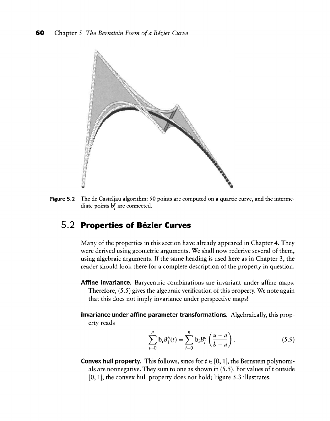
60 Chapter 5 The Bernstein Form of a Bezier Curve
Figure 5.2 The de Casteljau algorithm: 50 points are computed on a quartic curve, and the interme-
diate points
b^
are connected.
5.2 Properties of Bezier Curves
Many of the properties in this section have aheady appeared in Chapter 4. They
were derived using geometric arguments. We shall now^ rederive several of them,
using algebraic arguments. If the same heading is used here as in Chapter 3, the
reader should look there for a complete description of the property in question.
Affine invariance. Barycentric combinations are invariant under affine maps.
Therefore, (5.5) gives the algebraic verification of this property. We note again
that this does not imply invariance under perspective maps!
Invariance under affine parameter transformations. Algebraically, this prop-
erty reads
f:hfiiit)=j2hfi"A'^).
{5.9)
i=0 /=0
Convex hull property. This follows, since for t e
[0,1],
the Bernstein polynomi-
als are nonnegative. They sum to one as show^n in (5.5). For values of t outside
[0,1],
the convex hull property does not hold; Figure 5.3 illustrates.
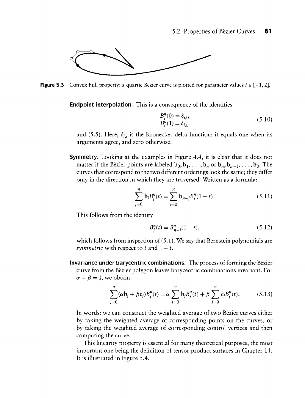
5.2 Properties of Bezier Curves 61
Figure 5.3 Convex hull property: a quartic Bezier curve is plotted for parameter values t e [—1,2].
Endpoint interpolation. This is a consequence of the identities
and
{S.5),
Here, 5^y is the Kronecker delta function: it equals one when its
arguments agree, and zero otherwise.
Symmetry. Looking at the examples in Figure 4.4, it is clear that it does not
matter if the Bezier points are labeled bo,
b^,...,
b„ or b„, b„_i, ..., bg. The
curves that correspond to the two different orderings look the same; they differ
only in the direction in which they are traversed. Written as a formula:
n n
^b,B;a) = ^b,_^B;(i-o. (5.11)
This follows from the identity
B1(t) =
Bl_.(l-t\
(5.12)
which follows from inspection of (5.1). We say that Bernstein polynomials are
symmetric with respect to t and 1
—
t,
Invariance under barycentric combinations. The process of forming the Bezier
curve from the Bezier polygon leaves barycentric combinations invariant. For
Of
+
jS
= 1, we obtain
n n n
j=0 j=0 j=0
In words: we can construct the weighted average of two Bezier curves either
by taking the weighted average of corresponding points on the curves, or
by taking the weighted average of corresponding control vertices and then
computing the curve.
This linearity property is essential for many theoretical purposes, the most
important one being the definition of tensor product surfaces in Chapter 14.
It is illustrated in Figure 5.4.
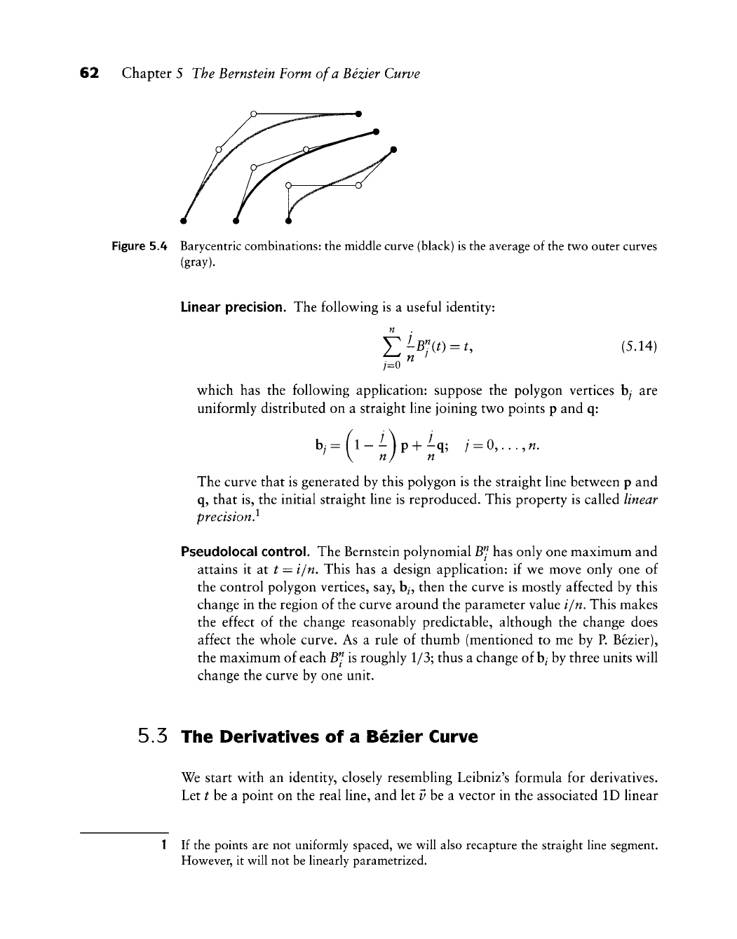
62 Chapters The Bernstein Form of a Bezier Curve
Figure 5.4 Barycentric combinations: the middle curve (black) is the average of the two outer curves
(gray).
Linear precision. The following is a useful identity:
J2-B';(t)
=
t,
(5.14)
which has the following application: suppose the polygon vertices by are
uniformly distributed on a straight line joining two points p and q:
^i=\^--)p+-^'^
7
= 0,...,^.
\ nj n
The curve that is generated by this polygon is the straight line between p and
q, that is, the initial straight line is reproduced. This property is called linear
precision}
Pseudolocal control. The Bernstein polynomial B^ has only one maximum and
attains it at
^
= i/n. This has a design application: if we move only one of
the control polygon vertices, say, b^, then the curve is mostly affected by this
change in the region of the curve around the parameter value i/n. This makes
the effect of the change reasonably predictable, although the change does
affect the whole curve. As a rule of thumb (mentioned to me by P. Bezier),
the maximum of each
JB^
is roughly 1/3; thus a change of b/ by three units will
change the curve by one unit.
5.5 The Derivatives of a Bezier Curve
We start with an identity, closely resembling Leibniz's formula for derivatives.
Let ^ be a point on the real line, and let ? be a vector in the associated ID linear
1 If the points are not uniformly spaced, v^e will also recapture the straight line segment.
However, it will not be linearly parametrized.

5.3 The Derivatives of a Bezier Curve 63
space. Then
h[(t
+
?)<"^]
= J2 ('')b[^<^-^^,
v^^n
i=0
(5.15)
This is an immediate consequence of the Leibniz formula (3.22).
The derivative of a curve x(^) is typically defined as
dt h-^0 h
We will be a little more precise and observe that f is a ID point, whereas /? is a
ID vector. We thus denote it by h and obtain
^ = lim4[xa +
^)-x(0].
dt h^o \h\
Invoking (5.15), we have
dx(t) ,. 1
—-— = lim -^
dt h-^o \h\ J2 ('')b[^"''"'^,
i^^'n
-
Ht^'^n
.1=0 ^^^
(5.16)
For / = 0, two terms b[^^"^] cancel. We expand the rest and factor in the term
\h\:
—
lim I nb
dt h^o \
f<n-l> _^
L
1^1
J
+(:>
V2/
t<"-^>,i,h
I
1^1 J +
.
We observe that -§-
==
1. Taking the limit annihilates all other terms containing
\h\
h,
and we thus have
dx(t)
"dT = nh[t^''-'^,l]. (5.17)
Figure 5.5 illustrates the cubic case.
From now on, we use the expression x(^) for the first derivative.
This has two possible interpretations. For the first one, we perform a de
Casteljau step with respect to 1, and then n
—
1 steps with respect to t; as an
equation:
n—l
Kit)
= n l](b;+i - hi)Bl-\t).
;=0
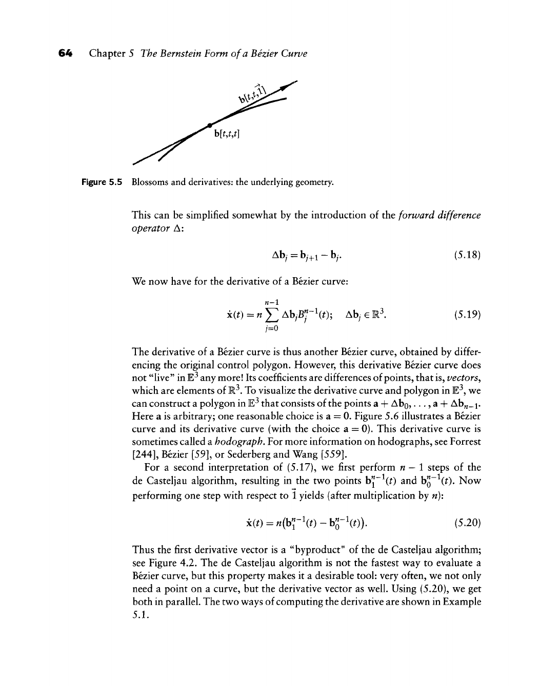
64 Chapter
5
The Bernstein Form of a Bezier Curve
Figure 5.5 Blossoms and derivatives: the underlying geometry.
This can
be
simplified somewhat
by
the introduction
of
the forward difference
operator
A:
Aby
=
by+i-by. (5.18)
We now have
for
the derivative
of a
Bezier curve:
n-l
x(t)
= nY^
AbyBp^O; Aby
€
R\ (5.19)
The derivative
of a
Bezier curve is thus another Bezier curve, obtained by differ-
encing the original control polygon. However, this derivative Bezier curve does
not "live" in E^ any
more!
Its coefficients are differences of points, that
is,
vectors,
which are elements of R^. To visualize the derivative curve and polygon in E^, we
can construct
a
polygon in E^ that consists of the points
a +
Abo,
• • • 5
a +
Ab„_i.
Here
a
is arbitrary; one reasonable choice is
a =
0. Figure 5,6 illustrates
a
Bezier
curve
and its
derivative curve (with
the
choice
a =
0). This derivative curve
is
sometimes called a hodograph. For more information on hodographs, see Forrest
[244],
Bezier [59],
or
Sederberg and Wang
[559].
For
a
second interpretation
of
(5.17),
we
first perform
n
—
1
steps
of the
de Casteljau algorithm, resulting
in the two
points h^'^it)
and
h^~^(t).
Now
performing one step with respect
to
1 yields (after multiplication by n):
x(t)
=
n{h"f\t)-h"f\t)).
(5.20)
Thus the first derivative vector
is a
"byproduct"
of
the
de
Casteljau algorithm;
see Figure 4.2. The
de
Casteljau algorithm
is not
the fastest way
to
evaluate
a
Bezier curve, but this property makes
it a
desirable tool: very often, we not only
need
a
point
on a
curve, but the derivative vector
as
well. Using (5.20), we get
both in parallel. The two ways of computing the derivative are shown in Example
5.1.
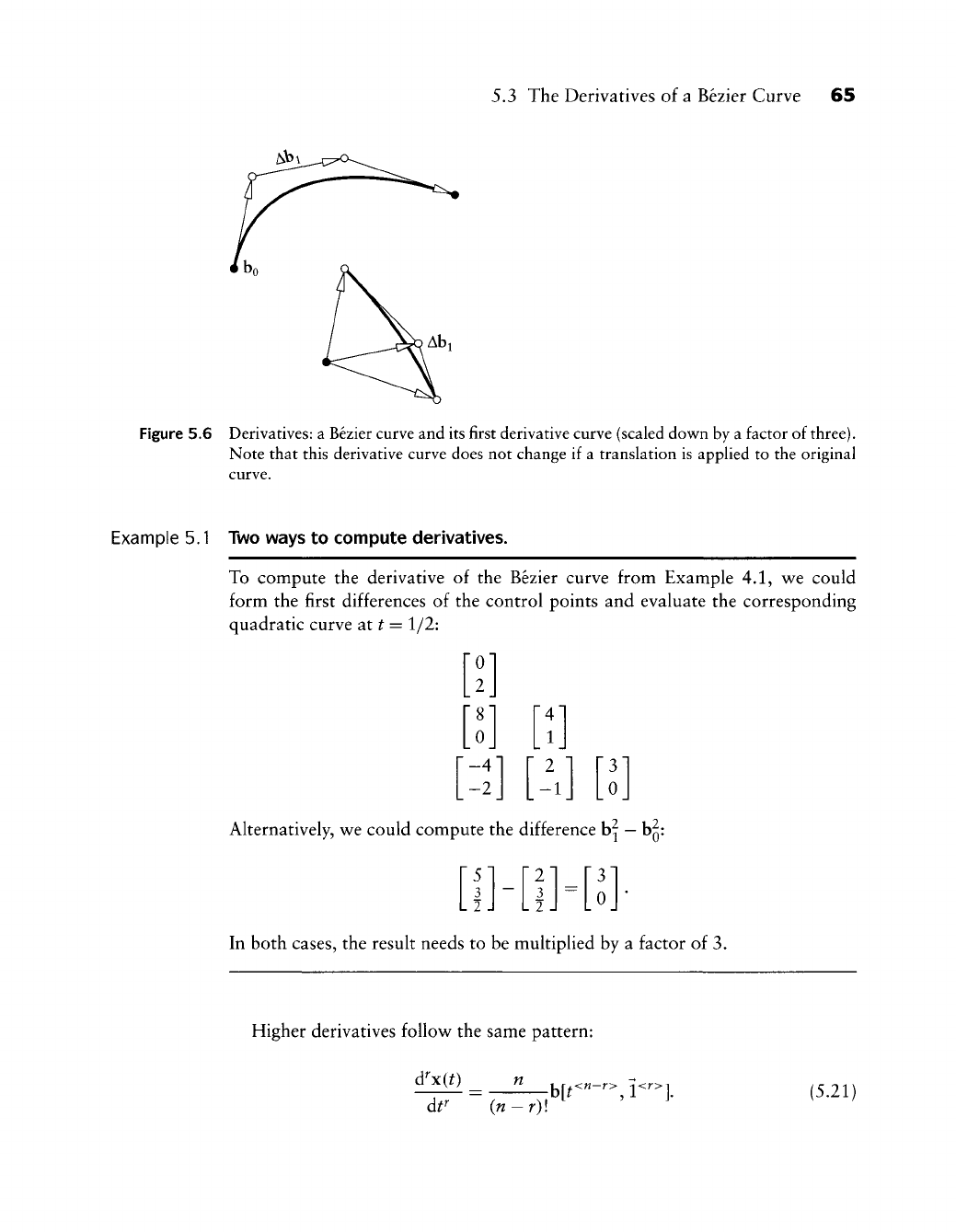
5.3 The Derivatives of a Bezier Curve 65
Figure 5.6 Derivatives: a Bezier curve and its first derivative curve (scaled down by a factor of three).
Note that this derivative curve does not change if a translation is applied to the original
Example 5.1 Two ways to compute derivatives.
To compute the derivative of the Bezier curve from Example 4.1, we could
form the first differences of the control points and evaluate the corresponding
quadratic curve at
^
= 1/2:
ro]
[ij
[8]
[oj
-4
-2
r4]
[ij
• 2 •
-1
'3'
0
Alternatively, v^e could compute the difference b^
—
bg:
'5"
3
- ? .
-
"2"
3
- ? -
=
"3"
0
In both cases, the resuh needs to be multiphed by a factor of 3.
Higher derivatives follow the same pattern:
dr (n
—
r)\
hit""-'^,
!<'•>].
(5.21)
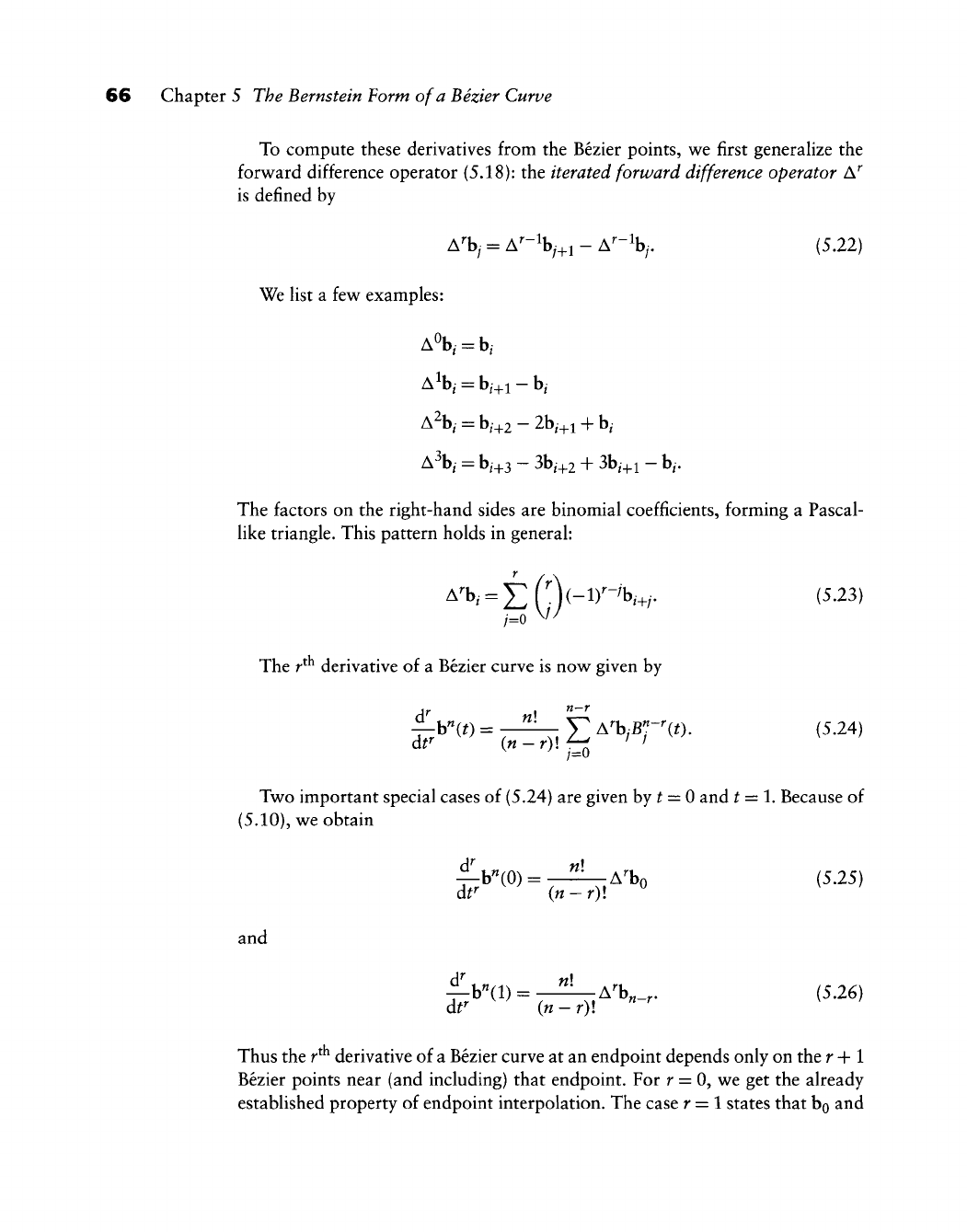
66 Chapter 5 The Bernstein Form of a Bezier Curve
To compute these derivatives from the Bezier points, wt first generalize the
forward difference operator (5.18): the iterated forward difference operator A^
is defined by
A^by = A^-^by+i - A^-^by. (5.22)
We Ust a fev^ examples:
A\ =
b,-
A b, = b,+i - b,
A^by = b,-+2-2b,-+i +
b,-
^\ = b,+3 - 3b,+2 + 3b^+i - b,-.
The factors on the right-hand sides are binomial coefficients, forming a Pascal-
like triangle. This pattern holds in general:
;=0 ^^^
The r^ derivative of a Bezier curve is now^ given by
^h"(t) = -^ £ A^b^Bj-W. (5.24)
dt^ (n
—
r)\ ^ ' '
Two important special cases of (5.24) are given by
^
= 0 and f = 1. Because of
(5.10),
we obtain
^b«(0) = —^A% (5.25)
at^ {n
—
r)\
and
ilb^(l) = _!!!_A%_^. (5.26)
dt'
{n-r)\
"" '
Thus the
r^^
derivative of a Bezier curve at an endpoint depends only on the r -\-l
Bezier points near (and including) that endpoint. For r = 0, we get the already
established property of endpoint interpolation. The case r = 1 states that bg and
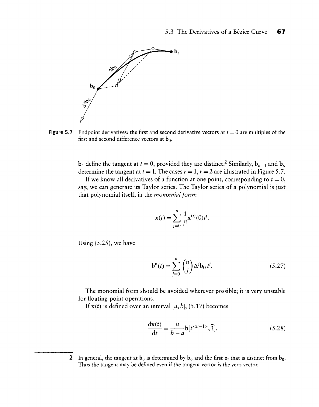
5.3 The Derivatives of a Bezier Curve 67
Figure 5.7 Endpoint derivatives: the first and second derivative vectors at
^
= 0 are mukiples of the
first and second difference vectors at bo-
bi define the tangent at
^
= 0, provided they are distinct.^ Similarly, b„_i and b„
determine the tangent at
^
= 1. The cases r = 1, r = 2 are illustrated in Figure 5.7.
If we knov^ all derivatives of a function at one point, corresponding to
^
= 0,
say, we can generate its Taylor series. The Taylor series of a polynomial is just
that polynomial
itself,
in the monomial form:
xit) = J2
-.x^'how.
,"''•
Using (5.25), we have
7=0 ^'^
(5.27)
The monomial form should be avoided wherever possible; it is very unstable
for floating-point operations.
If x(^) is defined over an interval
[a^
fc],
(5.17) becomes
dx(t)
b - a
b[^<"-^>, 1]. (5.28)
2 In general, the tangent at bo is determined by bo and the first
b^
that is distinct from bo-
Thus the tangent may be defined even if the tangent vector is the zero vector.
68 Chapter 5 The Bernstein Form of a Bezier Curve
5.4 Domain Changes and Subdivision
A Bezier curve b" is usually defined over the interval (the domain)
[0,1],
but it can
also be defined over any interval [0,
c].
The part of the curve that corresponds to
[0,
c]
can also be defined by a Bezier polygon, as illustrated in Figure 5.8. Finding
this Bezier polygon is referred to as subdivision of the Bezier curve.
The unknown Bezier points
Cj
are found v^ithout much w^ork if we use the
blossoming principle from Section 4.4. There, (4.11) gave us the Bezier points
of a polynomial curve that is defined over an arbitrary interval
[a,
b].
We are
currently interested in the interval [0,
c],
and so our Bezier points are:
q = b[0<^-^'>,c<^^].
Thus each q is obtained by carrying out / de Casteljau steps with respect to c, in
nonblossom notation:
Cy-b^W. (5.29)
This formula is called the subdivision formula for Bezier curves.
Thus it turns out that the de Casteljau algorithm not only computes the point
b"(c),
but also provides the control vertices of the Bezier curve corresponding to
the interval [0,
c].
Because of the symmetry property (5.11), it follows that the
control vertices of the part corresponding to [c, 1] are given by the \y~\ Thus,
in Figures 4.1 and 4.2, we see the two subpolygons defining the arcs from b"(0)
to b"(0 and from b"(0 to b"(l).
Instead of subdividing a Bezier curve, we may also extrapolate it: in that case,
we might be interested in the Bezier points dj corresponding to an interval [l,d].
They are given by
It should be mentioned that extrapolation is not a numerically stable process,
and should be avoided for large values of d.
Subdivision for Bezier curves, although mentioned by de Casteljau
[146],
was rigorously proved by E. Staerk
[578].
Our blossom development is due to
Ramshaw [498] and de Casteljau
[147].
Subdivision may be repeated: we may subdivide a curve at
^
= 1/2, then split
the two resulting curves at
^
= 1/2 of their respective parameters, and so on. After
k levels of subdivisions, we end up with 2^ Bezier polygons, each describing a
small arc of the original curve. These polygons converge to the curve if we keep
increasing k, as was shown by Lane and Riesenfeld
[369].
Convergence of this repeated subdivision process is very fast (see Cohen and
Schumaker [123] and Dahmen [131]), and thus it has many practical applica-
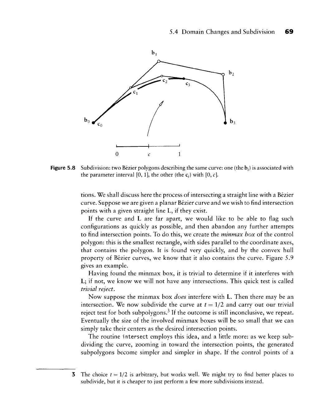
5.4 Domain Changes and Subdivision 69
bi
0 1
Figure 5.8 Subdivision: two Bezier polygons describing the same
curve:
one (the
b^)
is associated v^ith
the parameter interval
[0,1],
the other (the
Cj)
with
[0,
c].
tions.
We shall discuss here the process of intersecting a straight line with a Bezier
curve. Suppose we are given a planar Bezier curve and we wish to find intersection
points with a given straight line L, if they exist.
If the curve and L are far apart, we would like to be able to flag such
configurations as quickly as possible, and then abandon any further attempts
to find intersection points. To do this, we create the minmax box of the control
polygon: this is the smallest rectangle, with sides parallel to the coordinate axes,
that contains the polygon. It is found very quickly, and by the convex hull
property of Bezier curves, we know that it also contains the curve. Figure 5.9
gives an example.
Having found the minmax box, it is trivial to determine if it interferes with
L; if not, we know we will not have any intersections. This quick test is called
trivial reject.
Now suppose the minmax box does interfere with L. Then there may be an
intersection. We now subdivide the curve at
^
= 1/2 and carry out our trivial
reject test for both subpolygons.^ If the outcome is still inconclusive, we repeat.
Eventually the size of the involved minmax boxes will be so small that we can
simply take their centers as the desired intersection points.
The routine intersect employs this idea, and a little more: as we keep sub-
dividing the curve, zooming in toward the intersection points, the generated
subpolygons become simpler and simpler in shape. If the control points of a
3 The choice t = 1/2 is arbitrary, but works well. We might try to find better places to
subdivide, but it is cheaper to just perform a few more subdivisions instead.
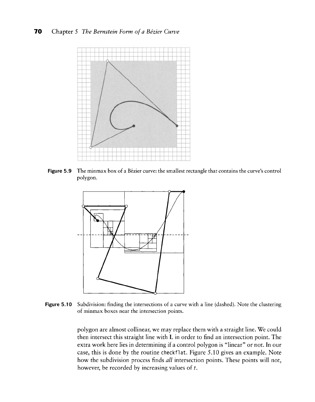
70 Chapter 5 The Bernstein Form of a Bezier Curve
Figure 5.9 The minmax box of
a
Bezier
curve:
the smallest rectangle that contains the curve's control
polygon.
Figure 5.10 Subdivision: finding the intersections of a curve with a line (dashed). Note the clustering
of minmax boxes near the intersection points.
polygon are almost collinear, we may replace them with a straight line. We could
then intersect this straight line with L in order to find an intersection point. The
extra work here lies in determining if a control polygon is "linear" or not. In our
case,
this is done by the routine checkflat. Figure 5.10 gives an example. Note
how the subdivision process finds all intersection points. These points will not,
however, be recorded by increasing values of t.
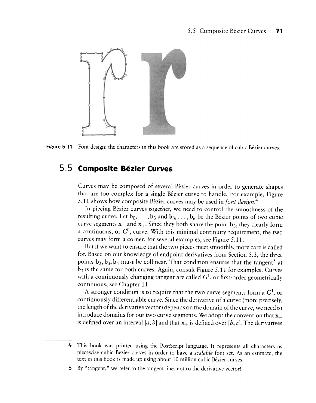
5.5 Composite Bezier Curves 71
Figure 5.11 Font design: the characters in this book are stored as a sequence of cubic Bezier curves.
5.5 Composite Bezier Curves
Curves may be composed of several Bezier curves in order to generate shapes
that are too complex for a single Bezier curve to handle. For example, Figure
5.11 shows how composite Bezier curves may be used in font design^
In piecing Bezier curves together, we need to control the smoothness of the
resulting curve. Let bo,. . ., b3 and b3,. . ., b^ be the Bezier points of two cubic
curve segments x_ and x^. Since they both share the point b3, they clearly form
a continuous, or C^, curve. With this minimal continuity requirement, the two
curves may form a corner; for several examples, see Figure 5.11.
But if we want to ensure that the two pieces meet smoothly, more care is called
for. Based on our knowledge of endpoint derivatives from Section 5.3, the three
points b2,
b3,
h^ must be coUinear. That condition ensures that the tangent^ at
b3 is the same for both curves. Again, consult Figure 5.11 for examples. Curves
with a continuously changing tangent are called G^ or first-order geometrically
continuous; see Chapter 11.
A stronger condition is to require that the two curve segments form a C^, or
continuously differentiable curve. Since the derivative of a curve (more precisely,
the length of the derivative vector) depends on the domain of the curve, we need to
introduce domains for our two curve segments. We adopt the convention that x_
is defined over an interval
[a,
b]
and that x+ is defined over
[b,
c].
The derivatives
4 This book was printed using the PostScript language. It represents all characters as
piecewise cubic Bezier curves in order to have a
scalable
font set. As an estimate, the
text in this book is made up using about 10 million cubic Bezier curves.
5 By "tangent," we refer to the tangent line, not to the derivative vector!
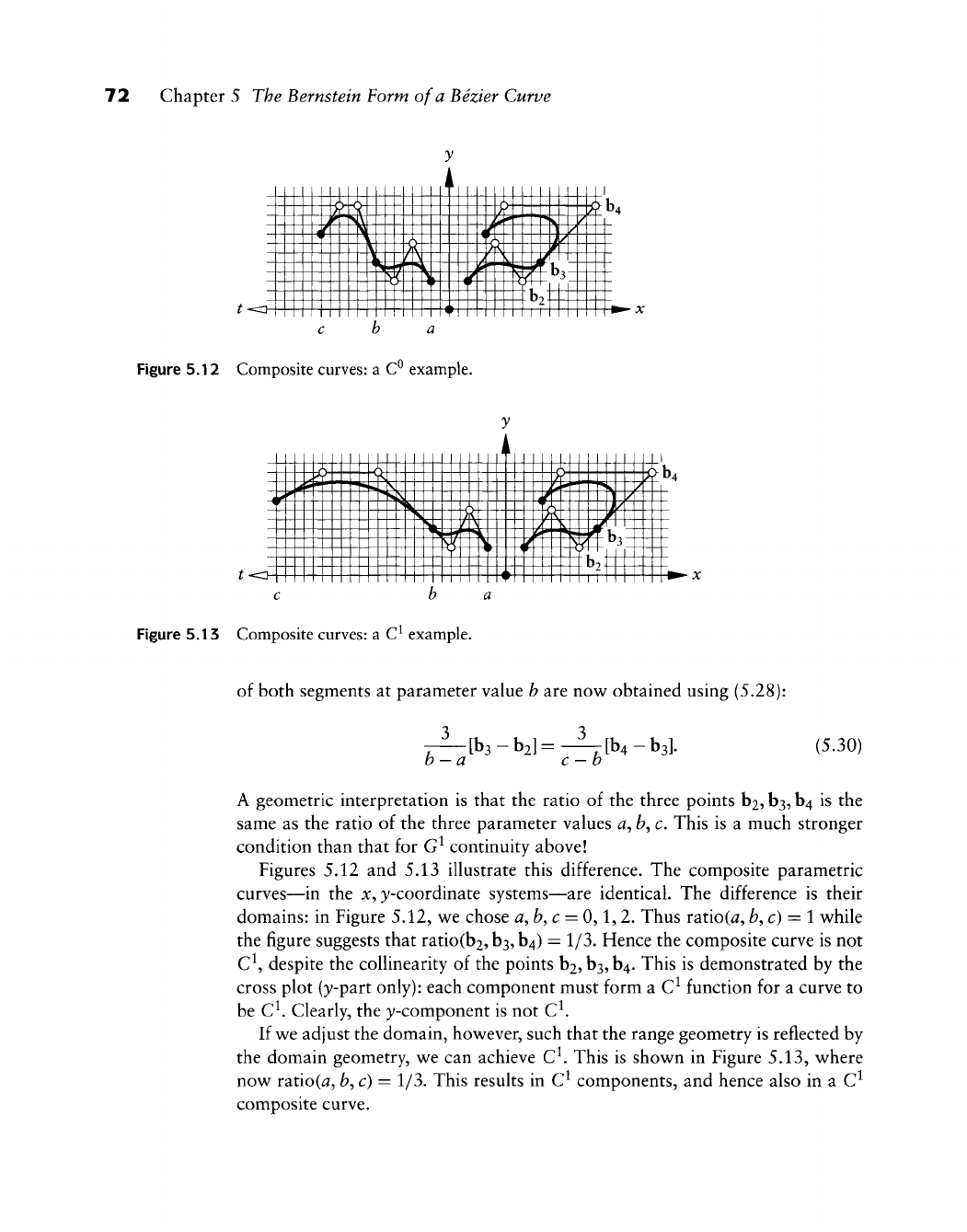
72 Chapter 5 The Bernstein Form of a Bezier Curve
?o
c b a
Figure 5.12 Composite curves: a C^ example.
1^
3 1
1
y
\\\M^
1 |TK||
1 i ttlM W^
Figure 5.13 Composite curves: a C^ example.
of both segments at parameter value b are nov^ obtained using (5.28):
^ [b3-b2]=^[b4-b3].
b-a -y (5.30)
A geometric interpretation is that the ratio of the three points b2,
b3,
b4 is the
same as the ratio of the three parameter values a^
fc,
c. This is a much stronger
condition than that for G^ continuity above!
Figures 5.12 and 5.13 illustrate this difference. The composite parametric
curves—in the x, y-coordinate systems—are identical. The difference is their
domains: in Figure 5.12, w^e chose a^b,c = 0,1,2. Thus ratio(^, b^c) = 1 v^hile
the figure suggests that ratio(b2,
b3,
b4) = 1/3. Hence the composite curve is not
C\ despite the collinearity of the points b2, b3,b4. This is demonstrated by the
cross plot (y-part only): each component must form a C^ function for a curve to
be C^. Clearly, the }'-component is not C\
If
v^e
adjust the domain, hovs^ever, such that the range geometry is reflected by
the domain geometry, wt can achieve C^. This is show^n in Figure 5.13, v^here
now^ ratio(<3t,
fc,
c) = 1/3. This results in C^ components, and hence also in a C^
composite curve.
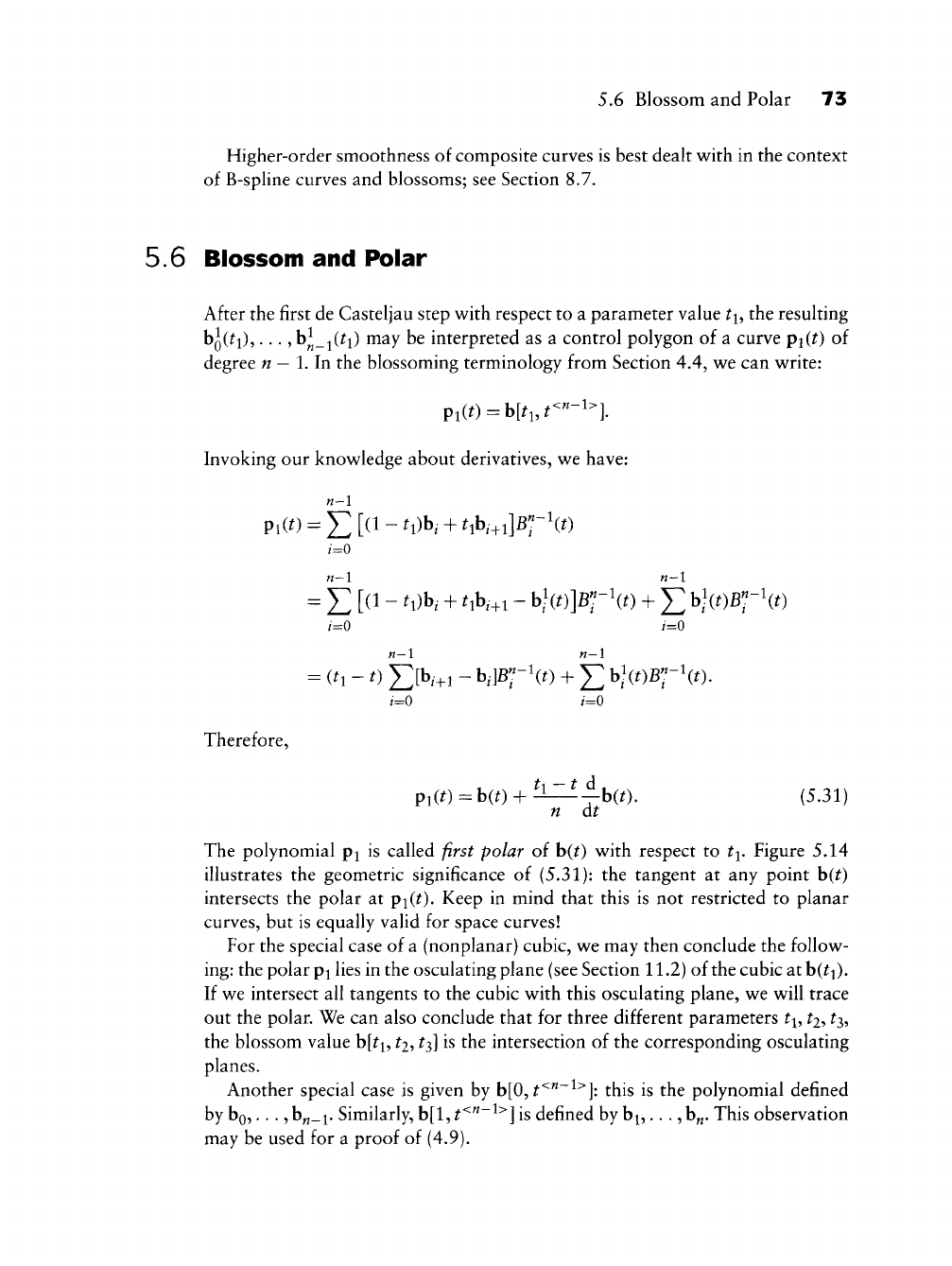
5.6 Blossom and Polar
73
Higher-order smoothness of composite curves is best dealt with in the context
of B-spline curves and blossoms; see Section 8.7.
5.6 Blossom and Polar
After the first de Casteljau step with respect to a parameter value
ti,
the resulting
bjc^l),...,
h^_^(ti) may be interpreted as
a
control polygon of a curve pi(t) of
degree
n
—
lAn
the blossoming terminology from Section 4.4, we can write:
Pt{t)=b[ti,t<"-'>].
Invoking our knowledge about derivatives, we have:
n-l
i=0
n-l
n-l
=^
[(1
-
t,)h,+^A>i
-
h](t)]B'i-\t)+j2 W(^)^r'(^)
i=0
i=0
n-l
n-l
= {t, -1) ^[b,+i
-
h,w-\t)+Y.
b-w^r'(^)-
i=0
i=0
Therefore,
p^(t)=h(t)+^-^-^^h(t),
(5.31)
n
at
The polynomial p^
is
called first polar
of
h(t) with respect
to
t^. Figure 5.14
illustrates the geometric significance
of
(5.31): the tangent
at
any point
h(t)
intersects the polar
at
pi(^). Keep
in
mind that this
is
not restricted
to
planar
curves, but is equally valid for space curves!
For the special case of a (nonplanar) cubic, we may then conclude the follow-
ing: the polar pi lies in the osculating plane (see Section 11.2) of the cubic at b(^i).
If we intersect all tangents to the cubic with this osculating plane, we will trace
out the polar. We can also conclude that for three different parameters
t^^
ti^
^3,
the blossom value b[^i,
^2? ^3]
is the intersection of the corresponding osculating
planes.
Another special case
is
given by b[0,
f^"~^^]:
this
is
the polynomial defined
by bo,..., ^n-l' Similarly, b[l,
t^^"^^]
is defined by
b^,..., b^.
This observation
may be used for
a
proof of (4.9).
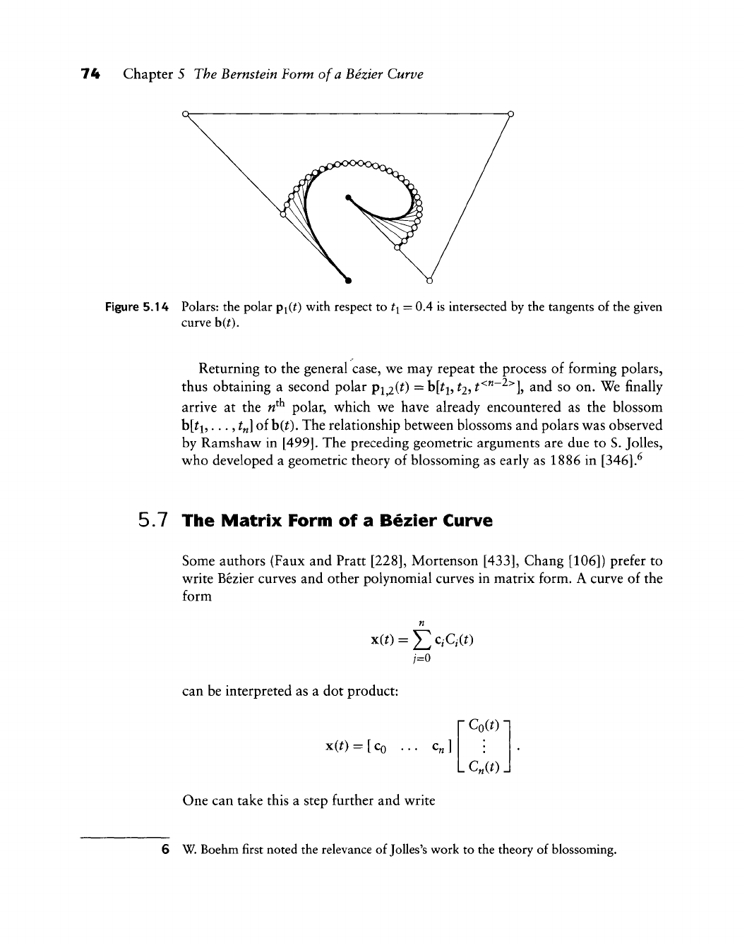
74 Chapter 5 The Bernstein Form of a Bezier Curve
Figure 5.14 Polars: the polar pi(^) with respect to ti = 0.4 is intersected by the tangents of the given
curve h(t).
Returning to the general case, we may repeat the process of forming polars,
thus obtaining a second polar pi^2(0 = b[^i,
^25
^^""^^L ^^^ so on. We finally
arrive at the « polar, which we have already encountered as the blossom
b[^i,..
• 5 ^«]
oih(t). The relationship between blossoms and polars was observed
by Ramshaw in
[499].
The preceding geometric arguments are due to S. JoUes,
who developed a geometric theory of blossoming as early as 1886 in
[346].^
5.7 The Matrix Form of a Bezier Curve
Some authors (Faux and Pratt
[228],
Mortenson
[433],
Chang [106]) prefer to
write Bezier curves and other polynomial curves in matrix form. A curve of the
form
n
x(o-;^c,Q(f)
/=o
can be interpreted as a dot product:
xit) =
[ Co
... c„]
One can take this a step further and write
Coit)
L C„{t)
J
6 W. Boehm first noted the relevance of
JoUes's
w^ork to the theory of blossoming.
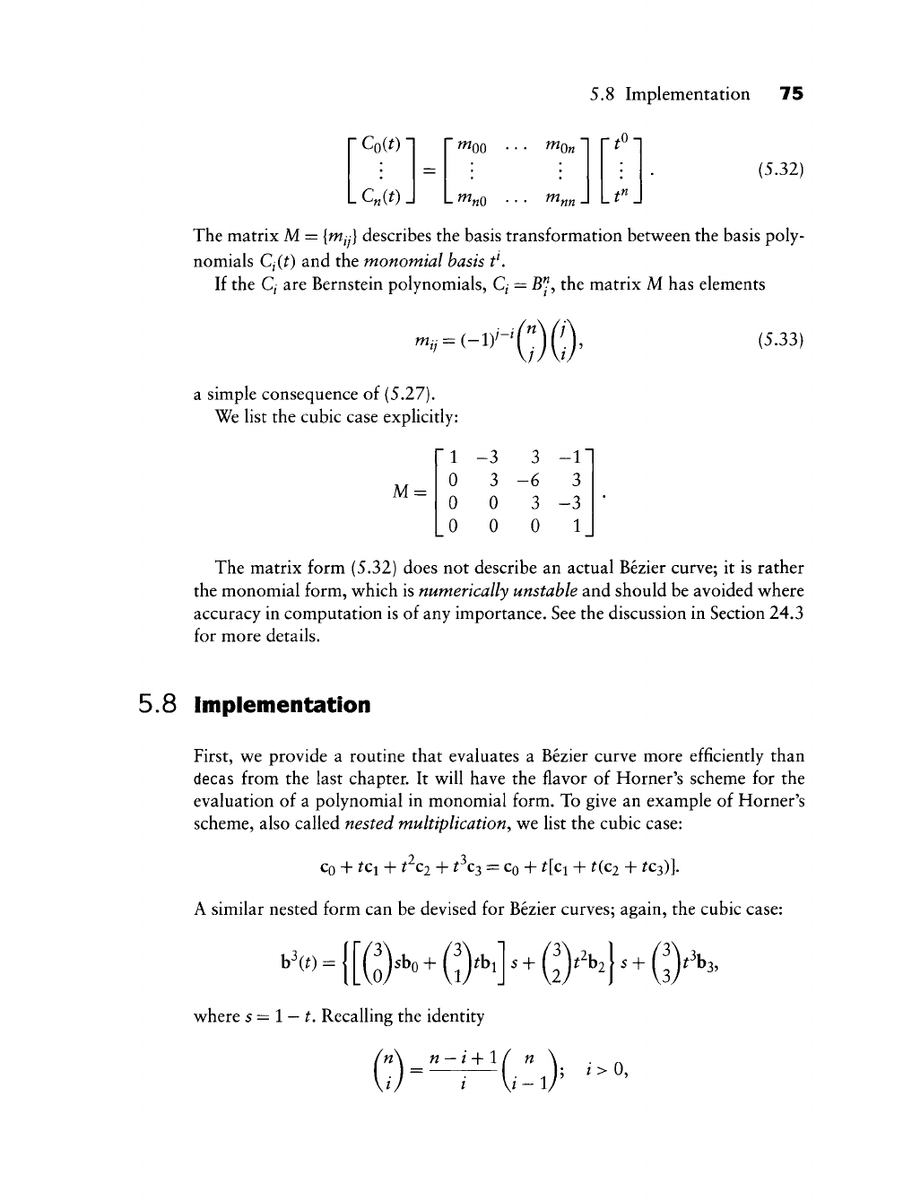
5.8 Implementation 75
Coit)
C„{t) J
mm
f"nO
mo„
m„
n^On
t".
(5.32)
The matrix M =
{m^y}
describes the basis transformation between the basis poly-
nomials Q(0 and the monomial basis f.
If the Q are Bernstein polynomials, Q = B^ the matrix M has elements
m/;-(-iy-^ (5.33)
a simple consequence of (5.27).
We list the cubic case explicitly:
M =
1
0
0
0
-3
3
0
0
3
-6
3
0
-1
3
-3
1
The matrix form (5.32) does not describe an actual Bezier curve; it is rather
the monomial form, which is numerically unstable and should be avoided where
accuracy in computation is of any importance. See the discussion in Section 24.3
for more details.
5.8 Implementation
First, we provide a routine that evaluates a Bezier curve more efficiently than
decas from the last chapter. It will have the flavor of Horner's scheme for the
evaluation of a polynomial in monomial form. To give an example of Horner's
scheme, also called nested multiplication^ we list the cubic case:
Co
+ tCi +
t^C2
+
t^C^
=
Co
+ ^[Ci +
t{C2
+
^€3)].
A similar nested form can be devised for Bezier curves; again, the cubic case:
h\t)
where s = 1
—
^. Recalling the identity
Q)A,)».QA3,

76 Chapter 5 The Bernstein Form of a Bezier Curve
we arrive at the following program (for the general case):
float hornbez(clegree,coeff,t)
/* uses a Horner-like scheme to compute one coordinate
value of a Bezier curve. Has to be called
for each coordinate (x,y, and/or z) of a control polygon.
Input: degree: degree of curve.
coeff: array with coefficients of curve,
t: parameter value.
Output: coordinate value.
V
To use this routine for plotting a Bezier curve, we would replace the call to decas
in bez_to_points by an identical call to hornbez. Replacing decas with hornbez
results in a significant savings of
time:
we do not have to save the control polygon
in an auxiliary array; also, hornbez is of order «, whereas decas is of order n^.
This is not to say, however, that we have produced superefficient code for
plotting points on a Bezier curve. For instance, we have to call hornbez once for
each coordinate, and thus have to generate the binomial coefficients n_choose_i
twice. This could be improved by writing a routine that combines the two calls. A
further improvement could be to compute the sequence of binomial coefficients
only once, and not over and over for each new value of t. All these (and possibly
more) improvements would speed up the program, but would be less modular
and thus less understandable. For the code in this book, modularity is placed
above efficiency (in most cases).
We also include the programs to convert from the Bezier form to the monomial
form:
voi
d
bezi er_to_power(degree,bez,coeff)
/*Converts Bezier form to power (monomial) form. Works on
one coordinate only.
Input: degree: degree of curve.
bez: coefficients of Bezier form
Output: coeff: coefficients of power form.
Remark: For a 2D curve, this routine needs to be called twice,
once for the x-coordinates and once for y.
V
The conversion program internally calls iterated forward differences:
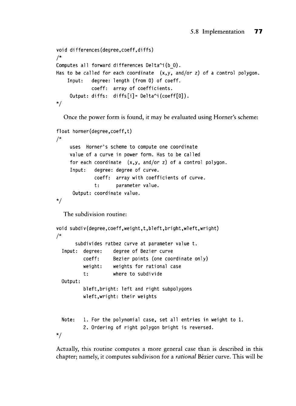
5.8 Implementation
77
void differences(degree,coeffjdiffs)
/*
Computes
all
forward differences
Delta^i(b_0).
Has
to be
called
for
each coordinate (x,y, and/or z)
of a
control polygon.
Input: degree: length (from 0)
of
coeff.
coeff: array
of
coefficients.
Output: diffs: diffs[i]= Delta'^i (coeff
[0]).
V
Once the power form is found, it may be evaluated using Horner's scheme:
float horner(degree,coeff,t)
/*
uses Horner's scheme
to
compute
one
coordinate
value
of a
curve
in
power form.
Has
to be
called
for each coordinate (x,y, and/or z)
of a
control polygon.
Input: degree: degree
of
curve.
coeff: array with coefficients
of
curve.
t: parameter value.
Output: coordinate value.
V
The subdivision routine:
void subdiV(degree,coeff,weight,t,bleft,bright,wleft,Wright)
/*
subdivides ratbez curve
at
parameter value
t.
Input: degree: degree
of
Bezier curve
coeff: Bezier points (one coordinate only)
weight: weights
for
rational case
t: where
to
subdivide
Output:
bleft,bright: left
and
right subpolygons
wleft,wright: their weights
Note:
1. For the
polynomial case,
set all
entries
in
weight
to 1.
2.
Ordering
of
right polygon bright
is
reversed.
*/
Actually, this routine computes a more general case than is described in this
chapter; namely, it computes subdivison for a rational Bezier curve. This will be

78 Chapter 5 The Bernstein Form of
a
Bezier Curve
discussed later; if the entries in weight are all unity, then wleft and wright will
also be unity and can be safely ignored in the context of this chapter.
Now we present the routine to intersect a Bezier curve with a straight line (the
straight line is assumed to be the x-axis):
void intersect(bx,by,w,degree,tol)
/* Intersects Bezier curve with x-axis by adaptive subdivision.
Subdivision is controlled by tolerance tol. There is
no check for stack depth! Intersection points are not found in
'natural'
order. Results are written into file outfile.
Input: bx,by,w: rational Bezier curve
degree: its degree
tol:
accuracy for results
Output: intersection points, written into a file
*/
This routine (again covering the rational case as well) uses a routine to check
if a control polygon is flat:
int check_flat(bx,by,degree,tol)
/* Checks if a polygon is flat. If all points
are closer than tol to the connection of the
two endpoints, then it is flat. Crashes if the endpoints
are identical.
Input: bx,by, degree: the Bezier curve
tol:
tolerance
Output: 1 if flat, 0 else.
V
5.9 Problems
1 Consider the cubic Bezier curve given by the planar control points
11
0
1
[-1]
L
1 J
1
^
1
111
1
"-^
1
0
At
^
= 1/2, this curve has a cusp\ its first derivative vanishes and it shows
a sharp corner. You should verify this by a sketch. Now perturb the
x-coordinates of b^ and hi by opposite amounts, thus maintaining a sym-
metric control polygon. Discuss what happens to the curve.
5.9 Problems 79
2 Show that a nonplanar cubic Bezier curve cannot have a cusp. Hint: use
the fact that b^" , b^~ ,
bQ
are identical v^hen we evaluate at the cusp.
3 Show that the Bernstein polynomial B^ attains its maximum at
^
= i/n. Find
the maximum value. What happens for large n}
* 4 Show that the Bernstein polynomials B^ form a basis for the linear space
of all polynomials of degree n,
PI Compare the run times of decas and hornbez for curves of various degrees.
P2 Use subdivision to create smooth fractals. Start with a degree four Bezier
curve. Subdivide it into two curves and then perturb the middle control
point b2 for each of the two subpolygons. Continue for several levels. Try
to perturb the middle control point by a random displacement and then by
a controlled displacement. Literature on fractals: [35],
[411].
P3 Use subdivision to approximate a high-order (n > 2) Bezier curve by a
collection of quadratic Bezier curves. You will have to write a routine
that determines if a given Bezier curve may be replaced by a quadratic one
within a given tolerance. Literature on approximating higher-order curves
by lower-order ones:
[336], [341].

This Page Intentionally Left Blank

Bezier Curve Topics
6.1 Degree Elevation
i^uppose we were designing with Bezier curves as described in Section
4.3,
trying
to use a Bezier curve of degree n. After modifying the polygon a few times, it may
turn out that a degree n curve does not possess sufficient flexibiUty to model the
desired shape. One way to proceed in such a situation is to increase the flexibility
of the polygon by adding another vertex to it. As a first step, we might want to
add another vertex yet leave the shape of the curve unchanged—this corresponds
to raising the degree of the Bezier curve by one. We are thus looking for a curve
with control vertices b^ ,. . ., b^^ that describes the same curve as the original
polygon bo,..., b„.
Using the identities (6.24) to (6.26)—each easy to prove—we rewrite our given
curve as x(0 = (1
—
t)iL{t) + ^x(0, or
The upper limit of the first sum may be extended to « +
1
since the corresponding
term is zero. The summation of the second sum may be shifted to the limits
1
and
w
+ 1, and then changed to the lower limit 0 since only a zero term is added. We
thus have
81
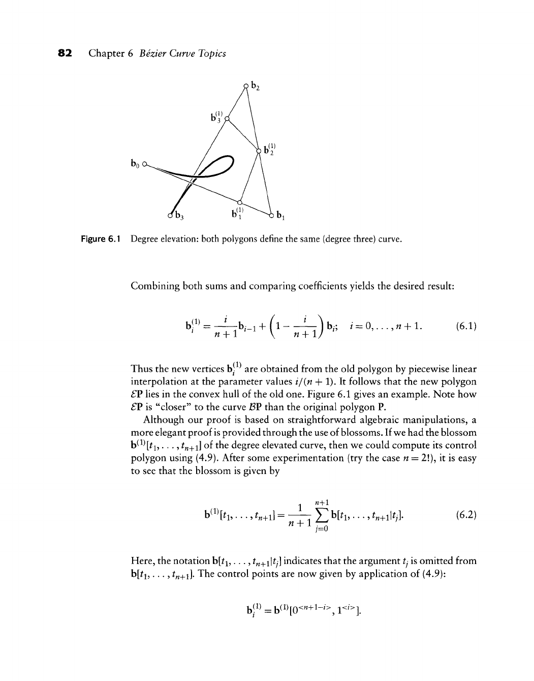
82 Chapter 6 Bezier Curve Topics
rb3 b
I
^^ hi
Figure 6.1 Degree elevation: both polygons define the same (degree three) curve.
Combining both sums and comparing coefficients yields the desired result:
M
+ 1 V
M
+ 1/ (6.1)
Thus the new vertices h- are obtained from the old polygon by piecewise linear
interpolation at the parameter values i/{n + 1). It follov^s that the nev^ polygon
£V lies in the convex hull of the old one. Figure 6.1 gives an example. Note how
SV is "closer" to the curve BV than the original polygon P.
Although our proof is based on straightforward algebraic manipulations, a
more elegant proof
is
provided through the use of
blossoms.
If we had the blossom
b(l)[
^1,...,
^„+i] of the degree elevated curve, then we could compute its control
polygon using (4.9). After some experimentation (try the case n = 2!), it is easy
to see that the blossom is given by
h^\h,..., ^„+i] = —- Y b[^i,...,
t^^^\t^\
(6.2)
Here, the notation b[^i,...,
t^^i\tj\
indicates that the argument tj is omitted from
b[^i,...,
^«+i]-
The control points are now given by application of (4.9):
b|^^
=
b^^^[o<"+^-^'^,r^"^].
6.2 Repeated Degree Elevation
83
Inspection of all terms that now arise in (6.2) reveals that the point b^_i appears
/ times and that the point b/ appears n-j-1
—
i times, thus reproving our previous
result.^
Degree elevation has important applications in surface design: for several
algorithms that produce surfaces from curve input,
it
is necessary that these
curves be of the same degree. Using degree elevation, v^e may achieve this by
raising the degree of all input curves to the one of the highest degree. Another
application lies in the area of data transfer between different CAD/CAM or
graphics systems: suppose you have generated a parabola (i.e., a degree two Bezier
curve),
and you want to feed it into a system that knows only about cubics. All
you have to do is degree elevate your parabola.
6.2 Repeated Degree Elevation
The process of degree elevation assigns a polygon £V to an original polygon P.
We may repeat this process and obtain a sequence of polygons P, f
P,
f
^P,
and
so on. After r degree elevations, the polygon E^V has the vertices b^j ,.. .,
b|^^^^,
and each b
•
is explicitly given by
This formula is easily proved by induction.
Let us now investigate what happens
if
we repeat the process
of
degree
elevation again and again. As we shall see, the polygons E^V converge to the
curve that all of them define:
lim E'V = BV.
(6.4)
To prove this result,
fix
some parameter value
t.
For each r, find the index
/
such that i/{n + r) is closest to
t.
We can think of i/{n + r) as
a
parameter on
the polygon f
^P,
and as
r
-> oo, this ratio tends to t. We can now show (using
Stirling's formula) that
lim :±j;-^t\\-tr-i, (6.5)
1 Again, work out the example n = 2to build your confidence in this technique!
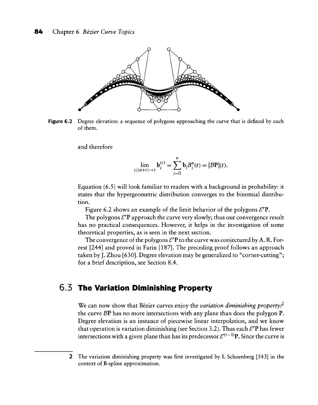
84 Chapter 6 Bezier Curve Topics
Figure 6.2 Degree elevation: a sequence of polygons approaching the curve that is defined by each
of them.
and therefore
i/{n+r)^t ^ c '
Equation {6.S) will look familiar to readers with a background in probability: it
states that the hypergeometric distribution converges to the binomial distribu-
tion.
Figure 6.2 shows an example of the limit behavior of the polygons £^V,
The polygons £^V approach the curve very slowly; thus our convergence result
has no practical consequences. However, it helps in the investigation of some
theoretical properties, as is seen in the next section.
The convergence of the polygons
£^V
to the curve was conjectured by
A.
R. For-
rest [244] and proved in Farin
[187].
The preceding proof follows an approach
taken by
J.
Zhou
[630].
Degree elevation may be generalized to "corner-cutting";
for a brief description, see Section 8.4.
6.5 The Variation Diminisiiing Property
We can now show that Bezier curves enjoy the variation diminishing property?
the curve BV has no more intersections with any plane than does the polygon P.
Degree elevation is an instance of piecewise linear interpolation, and we know
that operation is variation diminishing (see Section 3.2). Thus each £^V has fewer
intersections with a given plane than has its predecessor
£^^~^^V.
Since the curve is
The variation diminishing property was first investigated by I. Schoenberg [543] in the
context of B-spline approximation.
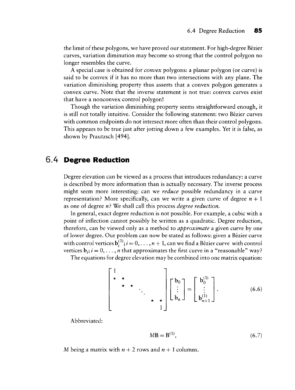
6.4 Degree Reduction 85
the limit of these polygons, we have proved our statement. For high-degree Bezier
curves, variation diminution may become so strong that the control polygon no
longer resembles the curve.
A special case is obtained for convex polygons: a planar polygon (or curve) is
said to be convex if it has no more than tw^o intersections with any plane. The
variation diminishing property thus asserts that a convex polygon generates a
convex curve. Note that the inverse statement is not true: convex curves exist
that have a nonconvex control polygon!
Though the variation diminishing property seems straightforward enough, it
is still not totally intuitive. Consider the following statement: two Bezier curves
with common endpoints do not intersect more often than their control polygons.
This appears to be true just after jotting down a few examples. Yet it is false, as
shown by Prautzsch
[494].
6.4 Degree Reduction
Degree elevation can be viewed as a process that introduces redundancy: a curve
is described by more information than is actually necessary. The inverse process
might seem more interesting: can we reduce possible redundancy in a curve
representation? More specifically, can we write a given curve of degree n-\-1
as one of degree n} We shall call this process degree reduction.
In general, exact degree reduction is not possible. For example, a cubic with a
point of inflection cannot possibly be written as a quadratic. Degree reduction,
therefore, can be viewed only as a method to approximate a given curve by one
of lower degree. Our problem can now be stated as follows: given a Bezier curve
with control vertices b|
;
/ = 0,.. .,
w
-h 1, can we find a Bezier curve with control
vertices
b^;
/ = 0,. . .,
w
that approximates the first curve in a "reasonable" way?
The equations for degree elevation may be combined into one matrix equation:
1
• •
• *
• *
1
bo'
b„.
r K(1) n
L "n+1
{6.6)
Abbreviated:
MB = B^i\
M being a matrix with n-\-l rows and n-\-l columns.
(6.7)
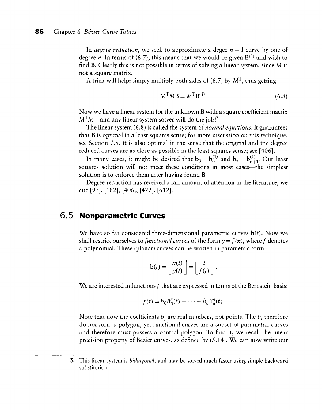
86 Chapter 6 Bezier Curve Topics
In degree reduction, we seek to approximate a degee n + 1 curve by one of
degree n. In terms of (6.7), this means that we would be given
B^^^
and wish to
find
B.
Clearly this is not possible in terms of solving a linear system, since M is
not a square matrix.
A trick will help: simply multiply both sides of (6.7) by M^, thus getting
M^MB = AfB^^\ (6.8)
Now we have a linear system for the unknown B with a square coefficient matrix
M^M—and any linear system solver will do the job!^
The linear system (6.8) is called the system of normal equations. It guarantees
that B is optimal in a least squares sense; for more discussion on this technique,
see Section 7.8. It is also optimal in the sense that the original and the degree
reduced curves are as close as possible in the least squares sense; see
[406].
In many cases, it might be desired that bg =
bQ
and b„ = b^^. Our least
squares solution will not meet these conditions in most cases—the simplest
solution is to enforce them after having found B.
Degree reduction has received a fair amount of attention in the literature; we
cite [97],
[182], [406], [472], [612].
6.5 Nonparametric Curves
We have so far considered three-dimensional parametric curves b(^). Now we
shall restrict ourselves to functional curves of the form y = f(x), where f denotes
a polynomial. These (planar) curves can be written in parametric form:
x(t)
yit)
t
fit)
Ht) =
We are interested in functions f that are expressed in terms of the Bernstein basis:
Note that now the coefficients bj are real numbers, not points. The bj therefore
do not form a polygon, yet functional curves are a subset of parametric curves
and therefore must possess a control polygon. To find it, we recall the linear
precision property of Bezier curves, as defined by (5.14). We can now write our
3 This linear system is
bidiagonal,
and may be solved much faster using simple backward
substitution.
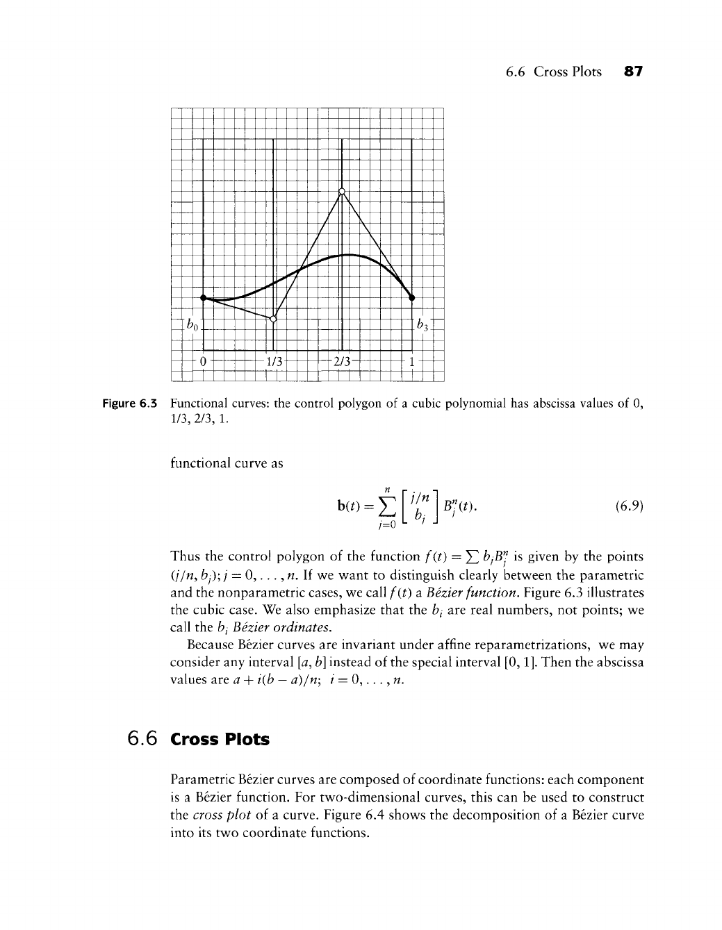
6.6 Cross Plots 87
b
0
-0
1
i
1
/3-
1
1
/
/
/
/T\
\
1 /I
Z/J
1 1
1
r
1-
1
s
Figure 6.3 Functional curves: the control polygon of a cubic polynomial has abscissa values of 0,
1/3,2/3,1.
functional curve as
hit)
= J2
7=0
j/n
b,
Blit).
(6.9)
Thus the control polygon of the function f(t) = ^ bjB^ is given by the points
(j/n,
bj);j
—
0,. . .,
w.
If we want to distinguish clearly between the parametric
and the nonparametric cases, we call f(t) a Bezier function. Figure 6.3 illustrates
the cubic case. We also emphasize that the bi art real numbers, not points; we
call the bj Bezier ordinates.
Because Bezier curves are invariant under affine reparametrizations, we may
consider any interval
[a.,
b]
instead of the special interval
[0,1].
Then the abscissa
values are a + i{b
—
a)/n; / = 0,..., ^.
6.6 Cross Plots
Parametric Bezier curves are composed of coordinate functions: each component
is a Bezier function. For two-dimensional curves, this can be used to construct
the cross plot of a curve. Figure 6.4 shows the decomposition of a Bezier curve
into its two coordinate functions.
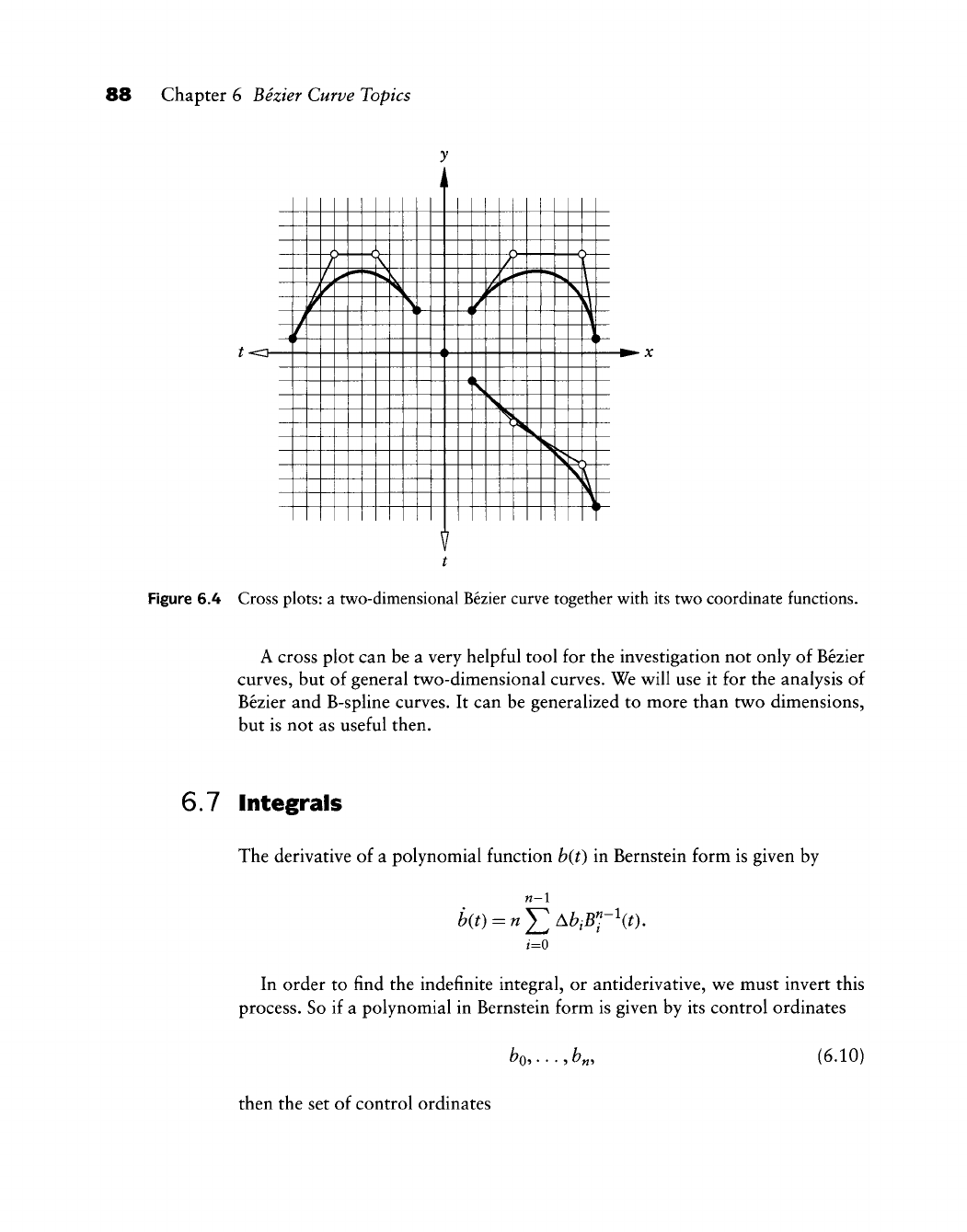
88 Chapter 6 Bezier Curve Topics
?<H
Figure 6.4 Cross plots: a two-dimensional Bezier curve together with its two coordinate functions.
A cross plot can be a very helpful tool for the investigation not only of Bezier
curves, but of general tw^o-dimensional curves. We will use it for the analysis of
Bezier and B-spline curves. It can be generalized to more than tvvro dimensions,
but is not as useful then.
6.7 Integrals
The derivative of a polynomial function b{t) in Bernstein form is given by
n-l
i=0
In order to find the indefinite integral, or antiderivative, we must invert this
process. So if a polynomial in Bernstein form is given by its control ordinates
^05 • • •
9
^«9 (6.10)
then the set of control ordinates
6.8 The Bezier Form of a Bezier Curve 89
1 "
defines a polynomial B(t) whose derivative is exactly the one defined by the con-
trol ordinates (6.10). The scalar c is the usual constant encountered in indefinite
integration.
Since
[ b(t)dt = B(l)-B(0), (6.11)
Jo
we have immediately
/ bmt
=
-Tb,
(6.12)
Jo
^ +
1
^
The special case
b^
=
5^
y
gives
f Bnx)dx=-^; (6.13)
Jo ^ n + 1
that is, all basis functions B" (for a fixed n) have the same definite integral.
6.8 The Bezier Form of a Bezier Curve
In his work ([56], [57], [58], [59], [60], [61], [63], see also Vernet [599]), Bezier
did not use the Bernstein polynomials as basis functions. He wrote the curve b"
as a linear combination of functions Ff:
n
h"(t)^Y^c^F^(t),
(6.14)
,=0
where the F" are polynomials that obey the following recursion:
Ffit) ^{1- t)Ff-\t) + tFfzlit) (6.15)
with
foW = l, f;+iW = 0, FiW = l. (6.16)
90 Chapter 6 Bezier Curve Topics
Note that the third condition in the last equation is the only instance where the
definition of the F^ differs from that of the
B"!
An explicit expression for the F^
is given by
n
A consequence of (6.17) is that F^ = l for all n. Since F^it) >Oiorte
[0,1],
it
follows that (6.14) is not a barycentric combination of the
Cy.
In fact,
CQ
is a point
whereas the other
Cy
are vectors. The following relations hold:
co = bo, (6.18)
Cy
= Aby_i; ;>0. (6.19)
This undesirable distinction between points and vectors was abandoned soon
after Forrest's discovery that the Bezier form (6.14) of a Bezier curve could be
written in terms of Bernstein polynomials (see the appendix in [59]).
Comparing both forms, we notice that the Bernstein form is symmetric with
respect to t and 1
—
t, whereas the Bezier form is not. Let us assume the defining
coefficients b^ or C/ are affected by some numerical error and then let us check
the effect on the point x(l). In the Bernstein form, x(l) changes its value only if
b„ is in error. In the Bezier form, the value of x(l) is the sum of all errors in the
c^. If those cancel out, no harm is done—but if they do not, we may see serious
error accumulation!
6.9 The Weierstrass Approximation Tiieorem
One of the most important results in approximation theory is the Weierstrass
approximation theorem. S. Bernstein invented the polynomials that now bear
his name in order to formulate a constructive proof of this theorem (see Davis
[133]orKorovkin[364]).
We will give a "customized" version of the theorem, namely, we state it in the
context of parametric curves. So let c be a continuous curve that is defined over
[0,1].
For some fixed n, we can sample c at parameter values i/n. The points
c{i/n) can now be interpreted as the Bezier polygon of a polynomial curve x„:
X„W-^C(-)B^(0.
We say that x„ is the
n^"^
degree Bernstein-Bezier approximation to c.
6.10 Formulas
for
Bernstein Polynomials
91
We
are
next going
to
increase
the
density
of our
samples, that
is, we
increase
n.
This generates
a
sequence
of
approximations x„, x^^^,....
The
Weierstrass
approximation theorem states that this sequence
of
polynomials converges
to
the curve
c:
lim
x„(0 = c(0.
n-^OQ
At first sight, this looks like
a
handy
way to
approximate
a
given curve
by
polynomials:
we
just have
to
pick
a
degree
n
that
is
sufficiently large,
and we
are
as
close
to the
curve
as we
like. This
is
only theoretically true, however.
In
practice,
we
would have
to
choose values
of n in the
thousands
or
even millions
in order
to
obtain
a
reasonable closeness
of fit (see
Korovkin
[364] for
more
details).
The value
of the
theorem
is
therefore more
of a
theoretical nature.
It
shows
that every curve
may be
approximated arbitrarily closely
by a
polynomial curve.
6.10 Formulas
for
Bernstein Polynomials
This section
is a
collection
of
formulas; some appeared
in the
text, some
did not.
Credit
for
some
of
these goes
to R.
Farouki
and
V. Rajan
[225].
A Bernstein polynomial
is
defined
by
^
I 0
else.
The power basis
[f] and the
Bernstein basis {B^}
are
related
by
and
n
B"(t)
=
Y{-\i-'{ \{'\tL
(6.21)
Recursion:
B'i{t)
= (i-t)B';-\t)^tB';:i(t),
92 Chapter 6 Bezier Curve Topics
Subdivision:
Derivative:
Integral:
B^(CO = ^B^WB;(0. (6.22)
±B^(t) = n[B^:l(t)-B^-\t)l
/ B^(x)dx=: V B"+i(0, (6.23)
Jo n +
1
^^^ ^
Jo (x)dx
••
1
n-\-l
Three degree elevation formulas:
n + 1
Product:
(6.24)
tBIit) = l±lBl+lit), (6.25)
n +
1
^
Blit) = !l±l^B';+\t) + i±lBl+l(t). (6.26)
n +
1
n +
1
^
B-(«)B;(«) = )^B-)"(«). (6.27)
6.11 Implementation
A C routine for degree elevation follows. Note that we have to treat the cases
/ = 0 and / = « + 1 separately; the program would not like the correspond-
ing nonexisting array elements. The program actually handles the rational
case,
which will be covered later. For the polynomial case, fill
wb
with I's and
ignore wc.
6.12 Problems 93
void degree_elevdte(bx,by,wb,degree,ex,cy,wc)
/* input: two-d Bezier polygon in bx, by and with weights
in wb. Degree is degree.
Output:degree elevated curve in cx,cy and with weights in wc.
Note: for nonrational (polynomial) case, fill wc with I's.
V
6.12 Problems
*1 Prove (6.17).
* 2 Prove the relationship betv^een the "Bezier" and the Bernstein form for a
Bezier curve (6.14).
3 Prove that
/.
* 4 With the result from the previous problem, prove
f;^(0 = n ( Bpi(x)dx.
PI The recursion formula for Bernstein polynomials is equivalent to the
de Casteljau algorithm. Devise a recursive curve evaluation algorithm for
curves in Chebychev form based on the recursion for Chebychev polyno-
mials.
Program it up and experiment!
P2 Program up degree reduction with some of the methods outlined in Section
6.4. Work with the Bezier polygon supplied in the file degred.dat.

This Page Intentionally Left Blank
Polynomial Curve
Constructions
1 olynomial interpolation is a fundamental concept for all of CAGD. Although
its uses are limited to low degrees, the basic concept still needs to be understood
in order to develop new algorithms. If the amount of data is too large for
interpolation to be successful, one uses approximation methods instead.
7.1 Aitken's Aigoritiim
A common problem in curve design is point data interpolation: from data points
p^
with corresponding parameter values f^, find a curve that passes through the
p^.^
One of the oldest techniques to solve this problem is to find an interpo-
lating polynomial through the given points. That polynomial must satisfy the
interpolatory constraints
ip{ti)
= p-
/•
= 0,..., ^.
Several algorithms exist for this problem—any textbook on numerical analysis
will discuss several of them. In this section, we shall present a recursive technique
that is due to A. Aitken.
We have already solved the linear case, n=\ in Section 3.1. The Aitken
recursion computes a point on the interpolating polynomial through a sequence
The shape of the curve depends heavily on the parameter values
t^.
Methods for their
determination will be discussed later in the context of spline interpolation; see Section
9.6.
95
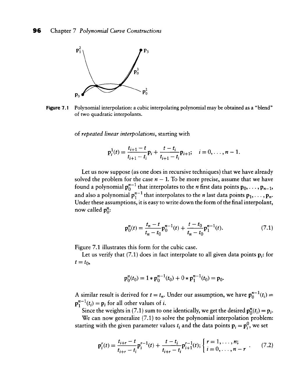
96 Chapter 7 Polynomial Curve Constructions
Figure 7.1 Polynomial interpolation: a cubic interpolating polynomial may be obtained as a "blend"
of two quadratic interpolants.
of repeated linear interpolations^ starting with
Let us now suppose (as one does in recursive techniques) that we have already
solved the problem for the case «
—
1. To be more precise, assume that we have
found a polynomial pQ~ that interpolates to the n first data points po,..., pn-h
and also a polynomial Pj~ that interpolates to the n last data points
pj,...,
p„.
Under these assumptions, it is easy to write down the form of the final interpolant,
now called p^:
PoW = T^Pr'W + —TPT'it)- (7.1)
Figure 7.1 illustrates this form for the cubic case.
Let us verify that (7.1) does in fact interpolate to all given data points
p^:
for
^ = ^05
Po(^o) =
1
* Po"^(^o) + 0 *
p'l-\to)
= Po.
A similar result is derived for t = tn. Under our assumption, we have pQ~ {fi) =
p\~^{ti)
=
Pi
for all other values of /.
Since the weights in (7.1) sum to one identically, we get the desired
p^{ti)
= p/.
We can now generalize (7.1) to solve the polynomial interpolation problem:
starting with the given parameter values tj and the data points p/ = p^ we set
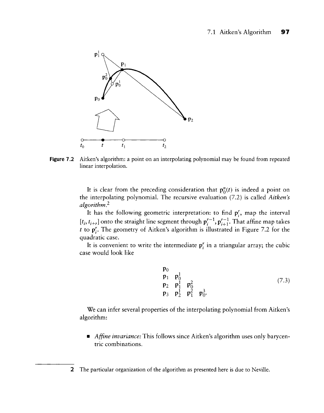
7.1 Aitken's Algorithm 97
o • o o
Figure 7.2 Aitken's algorithm: a point on an interpolating polynomial may be found from repeated
linear interpolation.
It is clear from the preceding consideration that p^(t) is indeed a point on
the interpolating polynomial. The recursive evaluation (7.2) is called Aitken's
algorithm?
It has the follow^ing geometric interpretation: to find p[, map the interval
[tj,
tj^j.]
onto the straight line segment through pp ,
p^~^.
That affine map takes
t to p^. The geometry of Aitken's algorithm is illustrated in Figure 7.2 for the
quadratic case.
It is convenient to write the intermediate p^ in a triangular array; the cubic
case would look like
Po
^' 1 2 (7.3)
P2 Pi Po
P3 pi Pi Po-
We can infer several properties of the interpolating polynomial from Aitken's
algorithm:
Affine invariance: This follows since Aitken's algorithm uses only barycen-
tric combinations.
2 The particular organization of the algorithm as presented here is due to Neville.
98 Chapter 7 Polynomial Curve Constructions
Linear precision: If all p^ are uniformly distributed^ on a straight line
segment, all intermediate p[(^) are identical for r > 0. Thus the straight
line segment is reproduced.
No convex hull property: The parameter t in (7.2) does not have to lie
between ti and tij^y. Therefore, Aitken's algorithm does not use convex
combinations only:
PQ(^)
is not guaranteed to lie within the convex hull
of the p/. We should note, however, that no smooth curve interpolation
scheme exists that has the convex hull property.
No variation diminishing property: By the same reasoning, we do not
get the variation diminishing property. Again, no "decent" interpolation
scheme has this property. However, interpolating polynomials can augment
variation to an extent that renders them useless for practical problems.
7.2 Lagrange Polynomials
Aitken's algorithm allows us to compute a point p^(^) on the interpolating
polynomial through
w
+ 1 data points. It does not provide an answer to the
following questions: (1) Is the interpolating polynomial unique? (2) What is
a closed form for it? Both questions are resolved by the use of the Lagrange
polynomials L".
The explicit form of the interpolating polynomial p is given by
n
p(0 = ^P.Lf(0, (7.4)
where the L^ are Lagrange polynomials
Before we proceed further, we should note that the L" must sum to one in order
for (7.4) to be a barycentric combination and thus be geometrically meaningful;
we will return to this topic later.
3 If the points are on a straight line, but distributed unevenly, we will still recapture the
graph of the straight line, but it will not be parametrized linearly.
7.3 The Vandermonde Approach 99
We verify (7.4) by observing that the Lagrange polynomials are cardinal: they
satisfy
L-(?;) = 5,„, (7.6)
vv^ith
5^
y
being the Kronecker delta. In other words, the /th Lagrange polynomial
vanishes at all knots except at the /th one, w^here it assumes the value 1. Because
of this property of Lagrange polynomials, (7.4) is called the cardinal form of the
interpolating polynomial p. The polynomial p has many other representations,
of course (v^e can rewrite it in monomial form, for example), but (7.4) is the only
form in which the data points appear explicitly.
We have thus justified our use of the term the interpolating polynomial. In
fact, the polynomial interpolation problem always has a solution, and it always
has a unique solution. The reason is that, because of (7.6), the L^ form a basis
of all polynomials of degree n. Thus, (7.4) is the unique representation of the
polynomial p in this basis. This is why one sometimes refers to all polynomial
interpolation schemes as Lagrange interpolation.^
We can now be sure that Aitken's algorithm yields the same point as does (7.4).
Based on that knowlege, we can conclude a property of Lagrange polynomials
that was already mentioned right after
{7.5)^
namely, that they sum to 1:
This is a simple consequence of the affine invariance of polynomial interpolation,
as shown for Aitken's algorithm.
7.5 The Vandermonde Approach
Suppose we want the interpolating polynomial p^ in the monomial basis:
n
/=0
4 More precisely, we refer to all those schemes that interpolate to a given set of data points.
Other forms of polynomial interpolation exist and are discussed later.
100 Chapter 7 Polynomial Curve Constructions
The standard approach to finding the unknown coefficients from the known data
is simply to write down everything one knows about the problem:
P^'C^o) = Po = ^0 + ^1^0 +
• • •
+ a„^Q,
P'^ih) = Pi = ao + ai^i + ... + a^t^,
P"(^«) = P« = ao + ^itn + . . . + ^n^n'
matrix form:
e
can shorten this
"Po"
Pi
-P«-
to
~1
1
_1
^0
h
tn
A
•
tl
•
t^
. t""
n
-J
ai
-a„_
(7.8)
p = Ta. (7.9)
We already know that a solution a to this linear system exists, but one can
show independently that the determinant det T is nonzero (for distinct parameter
values ti). This determinant is known as the Vandermonde of the interpolation
problem. The solution, that is, the vector a containing the coefficients a^, can be
found from
a
= T-V (7.10)
This should be taken only as a shorthand notation for the solution—not as an
algorithm! Note that the linear system (7.9) really consists of three linear systems
with the same coefficient matrix, one system for each coordinate. It is known
from numerical analysis that in such cases the LJJ decomposition of T is a more
economical way to obtain the solution a. This will be even more important when
we discuss tensor product surface interpolation in Section 15.4.
The interpolation problem can also be solved if we use basis functions other
than the monomials. Let {ff }^^o ^^ ^^^'^ ^ basis. We then seek an interpolating
polynomial of the form
p«(o-^cyp;w. (7.11)
7=0
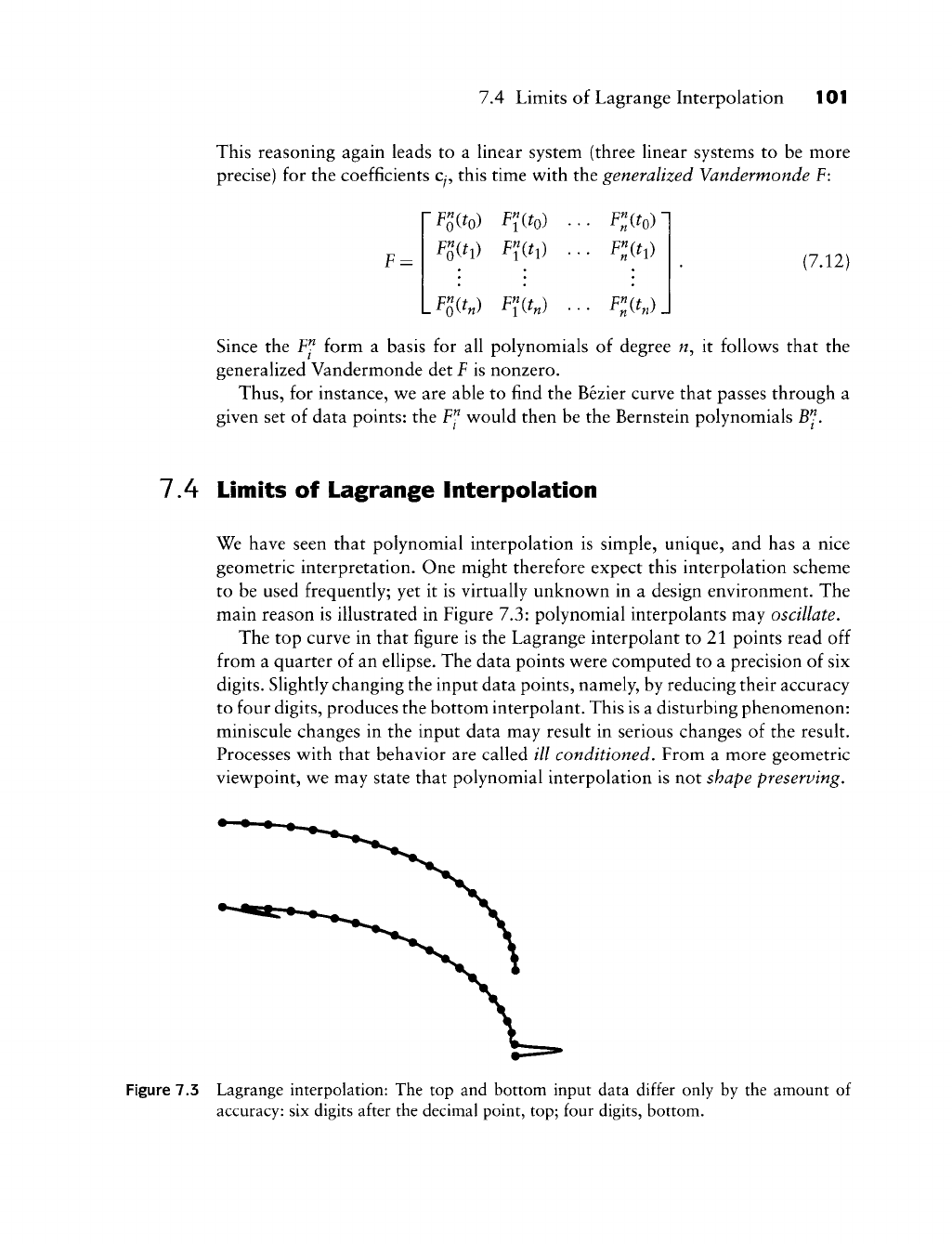
7.4 Limits of Lagrange Interpolation 101
This reasoning again leads to a linear system (three linear systems to be more
precise) for the coefficients c., this time with the generalized Vandermonde F:
F =
F"oit„)
F1(t„)
••
F"„(h)
••
F"„'it„)j
(7.12)
Since the F^ form a basis for all polynomials of degree n, it follows that the
generalized Vandermonde det F is nonzero.
Thus,
for instance, we are able to find the Bezier curve that passes through a
given set of data points: the F^ would then be the Bernstein polynomials B^.
1A Limits of Lagrange Interpolation
We have seen that polynomial interpolation is simple, unique, and has a nice
geometric interpretation. One might therefore expect this interpolation scheme
to be used frequently; yet it is virtually unknown in a design environment. The
main reason is illustrated in Figure 7.3: polynomial interpolants may oscillate.
The top curve in that figure is the Lagrange interpolant to 21 points read off
from a quarter of an ellipse. The data points were computed to a precision of six
digits.
Slightly changing the input data points, namely, by reducing their accuracy
to four digits, produces the bottom interpolant. This is a disturbing phenomenon:
miniscule changes in the input data may result in serious changes of the result.
Processes with that behavior are called ill conditioned. From a more geometric
viewpoint, we may state that polynomial interpolation is not shape preserving.
Figure 7.3 Lagrange interpolation: The top and bottom input data differ only by the amount of
accuracy: six digits after the decimal point, top; four digits, bottom.
102 Chapter 7 Polynomial Curve Constructions
This phenomenon is not due to numerical effects; it is actually inherent in
the polynomial interpolation process. Suppose we are given a finite arc of a
smooth curve c. We can then sample the curve at parameter values t^ and pass
the interpolating polynomial through those points. If we increase the number of
points on the curve, thus producing interpolants of higher and higher degree, we
would expect the corresponding interpolants to converge to the sampled curve
c. But this is not generally true: smooth curves exist for which this sequence of
interpolants diverges. This fact is dealt with in numerical analysis, where it is
known by the name of its discoverer: it is called the Runge phenomenon
[513].
Note, however, that the Runge phenomenon does not contradict the Weierstrass
approximation theorem!
As a second consideration, let us examine the cost of polynomial interpola-
tion, that is, the number of operations necessary to construct and then evaluate
the interpolant. Solving the Vandermonde system (7.8) requires roughly n^ op-
erations; subsequent computation of a point on the curve requires n operations.
The operation count for the construction of the interpolant is much smaller for
other schemes, as is the cost of evaluations (here piecewise schemes are far supe-
rior).
This latter cost is the more important one, of course: construction of the
interpolant happens once, but it may have to be evaluated thousands of times!
7.5 Cubic Hermite Interpolation
Polynomial interpolation is not restricted to interpolation to point data; we can
also interpolate to other information, such as derivative data. This leads to an
interpolation scheme that is more useful than Lagrange interpolation: it is called
Hermite interpolation. We treat the cubic case first, in which one is given a
set of points p/, associated parameter values ^/, and associated tangent vectors
(i.e.,
derivatives) m^. We just consider the case of two points po, pi and two
tangent vectors mo, m^, setting
tQ
= 0 and t^ = 1. The objective is to find a cubic
polynomial curve p that interpolates to these data:
P(0) = Po,
p(0) = mo,
p(l) = mi,
P(l)=Pi.
where the dot denotes differentiation.
We will write p in cubic Bezier form, and therefore must determine four Bezier
points bo,...,
b3.
Two of them are quickly determined:
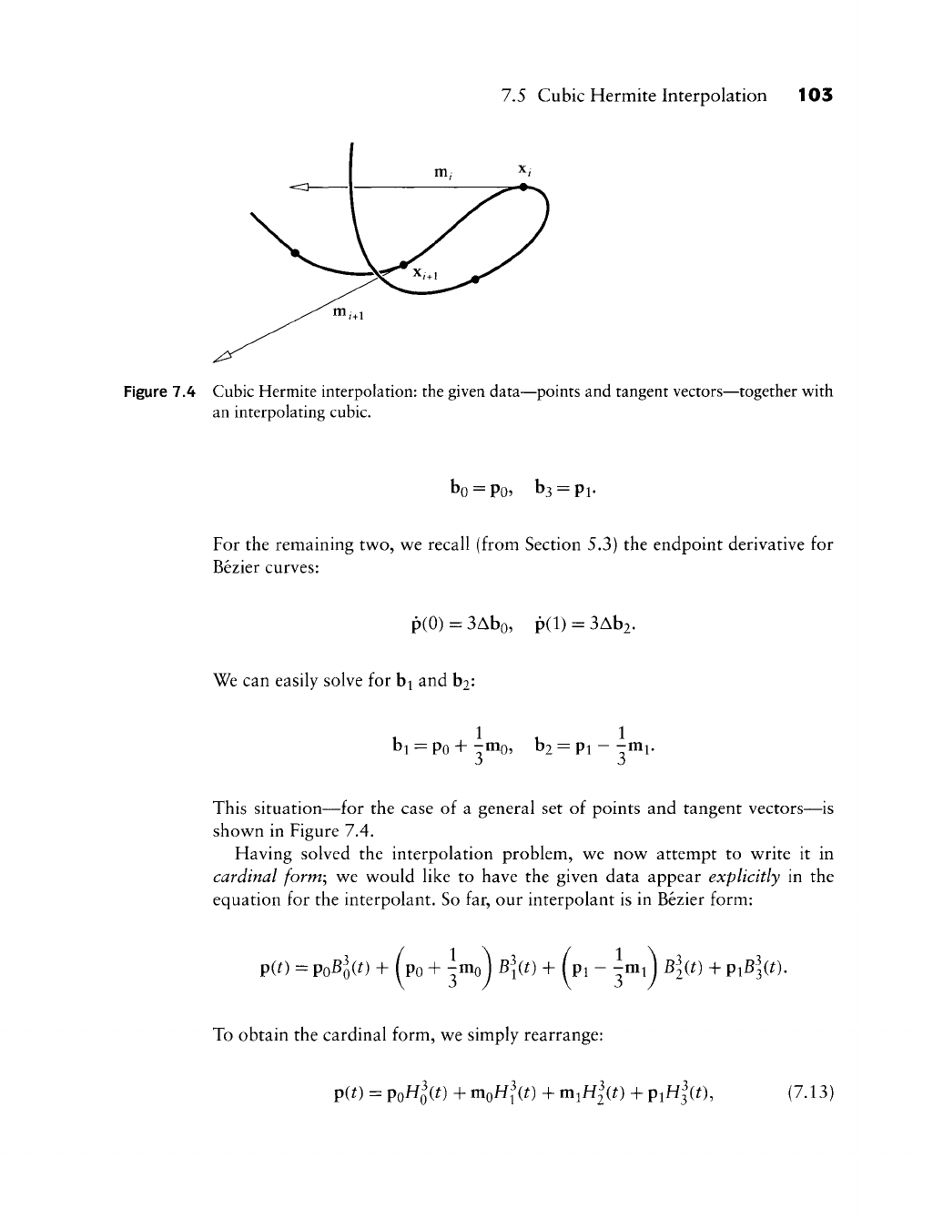
7.5 Cubic Hermite Interpolation 103
Figure 7.4 Cubic Hermite interpolation: the given data—points and tangent vectors—together v^ith
an interpolating cubic.
bo =
Po?
b3 = pi.
For the remaining two, we recall (from Section 5.3) the endpoint derivative for
Bezier curves:
p(0) = 3Abo, p(l) = 3Ab2.
We can easily solve for b^ and hi'-
u 1 1. 1
oi = Po + THIO, b2 = pi - -mi.
This situation—for the case of a general set of points and tangent vectors—is
shown in Figure 7.4.
Having solved the interpolation problem, we now attempt to write it in
cardinal form; we would like to have the given data appear explicitly in the
equation for the interpolant. So far, our interpolant is in Bezier form:
Pit) = poBlit) + Lo + ^mo j B\it) + Li - ^mi j Bl(t) + p^B^W-
To obtain the cardinal form, we simply rearrange:
Pit) = PoH^it) + moHlit) + m^Hlit) + PiH^it), (7.13)
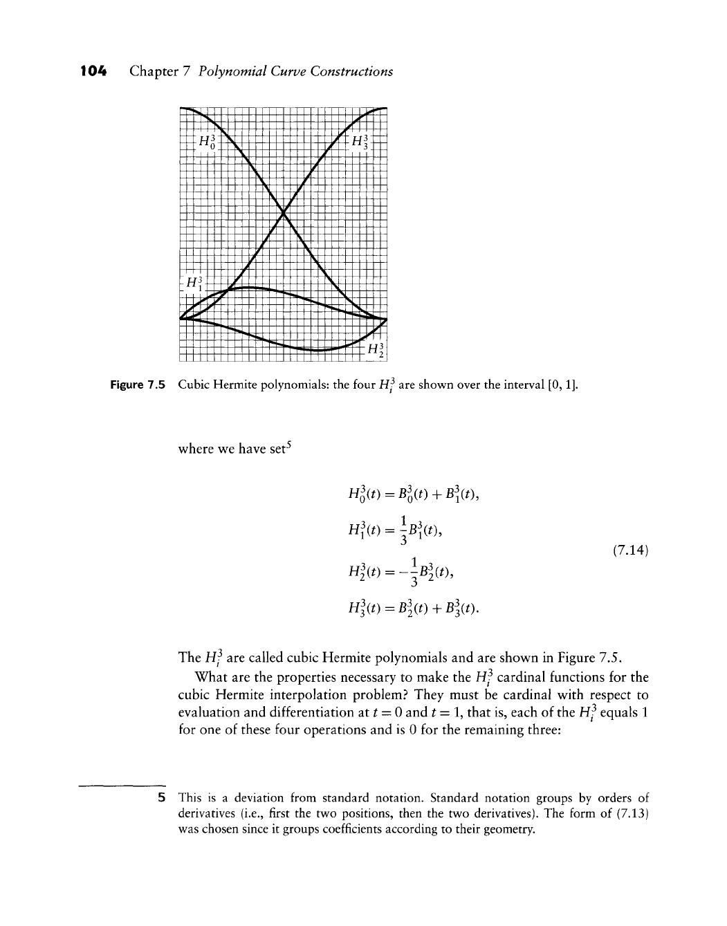
104 Chapter 7 Polynomial Curve Constructions
\\H^\%i\\\\\\\\\\\\\]/^H^\\\
0 \J MX 3
III X. \Jr ill
R3 K PV
^1 MJ4 MM n\J
4
1
l^il
1
nin4^44-U44fTr Hj
M M
M
M M M ITM M M
^i
Figure 7.5 Cubic Hermite polynomials: the four Hf are shown over the interval
[0,1].
where we have set^
WQ(t) = Bl(t)+B\(t),
Hl(t) =
h\(t),
Hl(t) =
-lBl(t\
(7.14)
Hl(t)
=
Bl(t)-]-Bl{t).
The Hf are called cubic Hermite polynomials and are shown in Figure 7.5.
What are the properties necessary to make the Hf cardinal functions for the
cubic Hermite interpolation problem? They must be cardinal with respect to
evaluation and differentiation at t = 0 and
^
= 1, that is, each of the Hf equals 1
for one of these four operations and is 0 for the remaining three:
5 This is a deviation from standard notation. Standard notation groups by orders of
derivatives (i.e., first the two positions, then the two derivatives). The form of (7.13)
was chosen since it groups coefficients according to their geometry.
7.5 Cubic Hermite Interpolation 105
H3(0)
= 1, ^H3(0) = 0,
^H3(1)
= 0, H3(1) = 0,
d^ d^
H|(0)
= 0,
^H|(0)
= 0,
^^2^1)
= !,
H|(1)
= 0,
H|(0) = 0, AH|(0) = 0,
AH3(1)
= 0, H|(1) = 1.
Another important property of the Hf follows from the geometry of the
interpolation problem; (7.13) contains combinations of points and vectors. We
know that the point coefficients must sum to 1 if (7.13) is to be geometrically
meaningful:
This is, of course, also verified by inspection of (7.14).
Cubic Hermite interpolation has one annoying pecufiarity: it is not invariant
under affine domain transformations. Let a cubic Hermite interpolant be given
as in (7.13), that is, having the interval [0,1] as its domain. Now apply an affine
domain transformation to it by changing t to i = (1
—
t)a + tb, thereby changing
[0,1] to some
[a,
b].
The interpolant (7.13) becomes
Pit) = poH^(?) + moHld) + m^Hld) + PiH|(?), (7.15)
where the Hf(i) are defined through their cardinal properties:
H|(^)-0, jMl{a)^0,
j.Hlib)
= l, Hlib) = 0,
To satisfy these requirements, the new Hf must differ from the original Hf. We
obtain
106 Chapter 7 Polynomial Curve Constructions
j5ti\ _ u3/
Hl{t) = {b-a)Hl{t),
(7.16)
Hl{i) = {b-a)Hl(t\
where t e [0,1] is the local parameter of the interval
[a^
b\
Evaluation of (7.15) at
?
= ^ and i = b yields ^{d) = po, p(b) =
p^.
The deriva-
tives have changed, hov^ever. Invoking the chain rule, we find that dp(^)/d^ =
(b
— a)mQ
and, similarly, dp(fc)/d^ = (b
—
a)mi.
Thus an affine domain transformation changes the curve unless the defining
tangent vectors are changed accordingly—a drawback that is not encountered
with the Bernstein-Bezier form.
To maintain the same curve after a domain transformation, we must change
the length of the tangent vectors: if the length of the domain interval is changed by
a factor a, we must replace mg and
m^
by mo/a and m^/a, respectively. There is an
intuitive argument for this: interpreting the parameter as time, we assume we had
one time unit to traverse the curve. After changing the interval length by a factor
of 10, for example, we have 10 time units to traverse the same curve, resulting in
a much smaller speed of traversal. Since the magnitude of the derivative equals
that speed, it must also shrink by a factor of 10.
We also note that the Hermite form is not symmetric: if we replace ^ by 1
—
^
(assuming again the interval [0,1] as the domain), the curve coefficients cannot
simply be renumbered (as in the case of Bezier curves). Rather, the tangent vectors
must be reversed. This follows from the above by applying the affine map to the
[0,1] that maps that interval to
[1,
0], thus reversing its direction.
The dependence of the cubic Hermite form on the domain interval is rather
unpleasant—it is often overlooked and can be blamed for countless programming
errors by both students and professionals. We will use the Bezier form whenever
possible.
7.6 Quintic Hermite Interpolation
Instead of prescribing only position and first derivative information at two points,
one might add information for second-order derivatives. Then our data are
Po,
mo,
SQ
and
p^,
m^, s^, where So and s^ denote second derivatives. The lowest-
order polynomial to interpolate to these data is of degree five. Its Bezier points
are easily obtained following the preceding approach. If we rearrange the Bezier
form to obtain a cardinal form of the interpolant p, we find
1.1 Point-Normal Interpolation 107
p(0 = PoH^W + moH^^W + soH|(0 + ^x^\if) + v^x^\(t) + PiH|(0, (7.17)
where
^ 20 ^
^5 1 R5
3 20 3
It is easy to verify the cardinal properties of the
H^^:
they are the straightforward
generalization of the cardinal properties for cubic Hermite polynomials. If used
in the context of piecewise curves, the quintic Hermite polynomials guarantee
C^ continuity since adjoining curve pieces interpolate to the same second-order
data. For most applications, one will have to estimate the second derivatives that
are needed as input. This estimation is a very sensitive procedure—so unless the
quintic form is mandated by a particular problem, the simpler C^ cubic splines
presented in Chapter 9 are recommended.
7.7 Point-Normal Interpolation
In a surface generation environment, one is often given a set of points p^
G
E^
and a surface normal vector n^ at each data point, as illustrated in Figure 7.6.
Thus we know only the tangent plane of the desired surface at each data point,
not the actual endpoint derivatives of the patch boundary curves.
If we know that two points p/ and py have to be connected, then we must
construct a curve leading from p^ to py that is normal to n^ at p^ and to n. at p..
A cubic will suffice to solve this generalized Hermite interpolation problem. In
Bezier form, we already have bo = p/ and b3 =
py.
We still need to find b^ and h^.
There are infinitely many solutions, so we may try to pick one that is both
convenient to compute and of reasonable shape in most cases. Two approaches to
this problem appear in Piper [483] and Nielson
[447].
Both approaches, although
formulated differently, yield the same result.
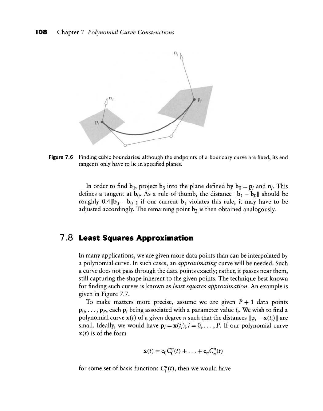
108 Chapter 7 Polynomial Curve Constructions
Figure 7.6 Finding cubic boundaries: although the endpoints of a boundary curve are fixed, its end
tangents only have to lie in specified planes.
In order to find b^, project b3 into the plane defined by bo = p/ and n^. This
defines a tangent at bg. As a rule of thumb, the distance ||bi
—
boll should be
roughly 0.4||b3
—
boll; if our current b^ violates this rule, it may have to be
adjusted accordingly. The remaining point hi is then obtained analogously.
7.8 Least Squares Approximation
In many applications, v^e are given more data points than can be interpolated by
a polynomial curve. In such cases, an approximating curve w^ill be needed. Such
a curve does not pass through the data points exactly; rather, it passes near them,
still capturing the shape inherent to the given points. The technique best known
for finding such curves is knov^n as least squares approximation. An example is
given in Figure 7.7.
To make matters more precise, assume wt are given P + 1 data points
po,...,
pp, each pi being associated with a parameter value tj. We wish to find a
polynomial curve x(^) of a given degree n such that the distances ||p^
—
x(^/)
||
are
small. Ideally, we would have p^ =
x(^/);
/ = 0,..., P. If our polynomial curve
x(t) is of the form
xw = coqw + ... + c^c^w
for some set of basis functions
Cf(t),
then we would have

7.8 Least Squares Approximation 109
Figure 7.7 Least squares approximation: data points are sampled from the cross section of an airplane
wing and a quinitic Bezier curve is fitted to them.
oqc^o)
+ •.
•
+ c„qao) =Po
This may be condensed into matrix form:
Pp.
Clitp)
Or, even shorter:
qcfp)
J
MC = P.
Co
Po
LPPJ
(7.18)
Since we assume the number P of data points is larger than the degree n of
the curve, this hnear system is clearly overdetermined. We attack it by simply
multiplying both sides by M^:
M^MC = M^V. (7.19)
This is a linear system with
w
+ 1 equations in n-\-1 unknow^ns, with a square
and symmetric coefficient matrix M^M, Its solution is straightforward, provided
that M^M is always invertible. This is in fact the case: since the C" are assumed
to be linearly independent, the « +
1
columns of M are linearly independent, thus
ensuring full rank of M^M,
110 Chapter 7 Polynomial Curve Constructions
But is the solution meaningful? After all, we employed a rather crude trick in
going from (7.18) to (7.19). It turns out that our solution is not only meaningful—
in fact it is optimal.
In order to justify this claim (and also making it more precise), we give a
second derivation of (7.19).
Consider the following expression:
/"(Co,...,
c„) = ^ lip,- - x(^,) (7.20)
/=0
If the curve x(t) does not deviate from the data points p/ by much, then f will
attain a small value. Ideally, if x were to pass through all pj exactly, we would
have
/"
= 0.
If we substitute the full definition of x(^) into (7.20), we obtain
/•(Co,...,
c^) = ^
/=0 j=0
(7.21)
We wish to find a set of
C/
such that the value of f becomes minimal. Since f is
a multivariate function of all components of the C/, that minimum is achieved if
f's
partials with respect to all these components vanish:
= 0; ^ = 0, ...,w; d = 1,2 or J = 1,2, 3,
where the superscript d labels the individual components of the c^^. Computing
the required derivatives yields
p
E
/=0
n
pf-J^cfCfit,)
'=0
Cl(t,) = 0; k =
0,,..,n;
J = 1,2 or J = 1,2, 3.
Upon rearranging, we see that this is identical to (7.19)!
7.9 Smoothing Equations
The solution to the least squares problem aims only at minimizing the error
function f in (7.20). It does not "care" about the shape of the resulting curve.
It may wiggle more than we would like, yet it is as close to the data points as
possible. Sometimes wiggles are undesired, even if closeness of approximation is
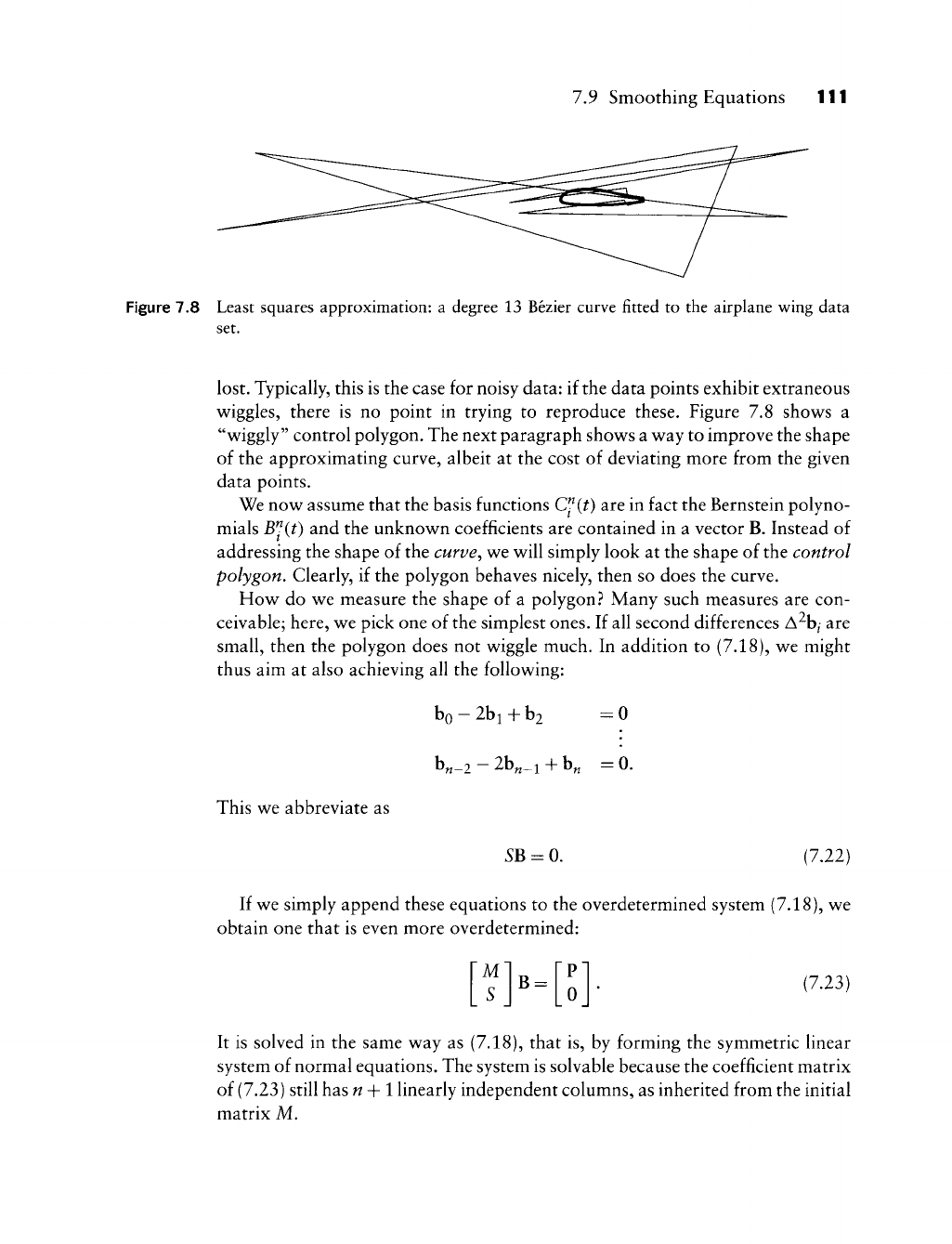
13 Smoothing Equations 111
Figure 7.8 Least squares approximation: a degree 13 Bezier curve fitted to the airplane wing data
set.
lost. Typically, this is the case for noisy data: if the data points exhibit extraneous
wiggles, there is no point in trying to reproduce these. Figure 1.% shows a
"wiggly" control polygon. The next paragraph shows a way to improve the shape
of the approximating curve, albeit at the cost of deviating more from the given
data points.
We now assume that the basis functions
C^^{t)
are in fact the Bernstein polyno-
mials W^(t) and the unknown coefficients are contained in a vector B. Instead of
addressing the shape of the curve^ we will simply look at the shape of the control
polygon. Clearly, if the polygon behaves nicely, then so does the curve.
How do we measure the shape of a polygon.^ Many such measures are con-
ceivable; here, we pick one of the simplest ones. If all second differences A^hj are
small, then the polygon does not wiggle much. In addition to (7.18), we might
thus aim at also achieving all the following:
bo
—
2bi + b2 :0
b„_2 - 2b„
b.
=0.
This we abbreviate as
5B = 0. (7.22)
If we simply append these equations to the overdetermined system (7.18), we
obtain one that is even more overdetermined:
M
S B = (7.23)
It is solved in the same way as (7.18), that is, by forming the symmetric linear
system of normal equations. The system is solvable because the coefficient matrix
of (7.23) still has n-\-l linearly independent columns, as inherited from the initial
matrix M.
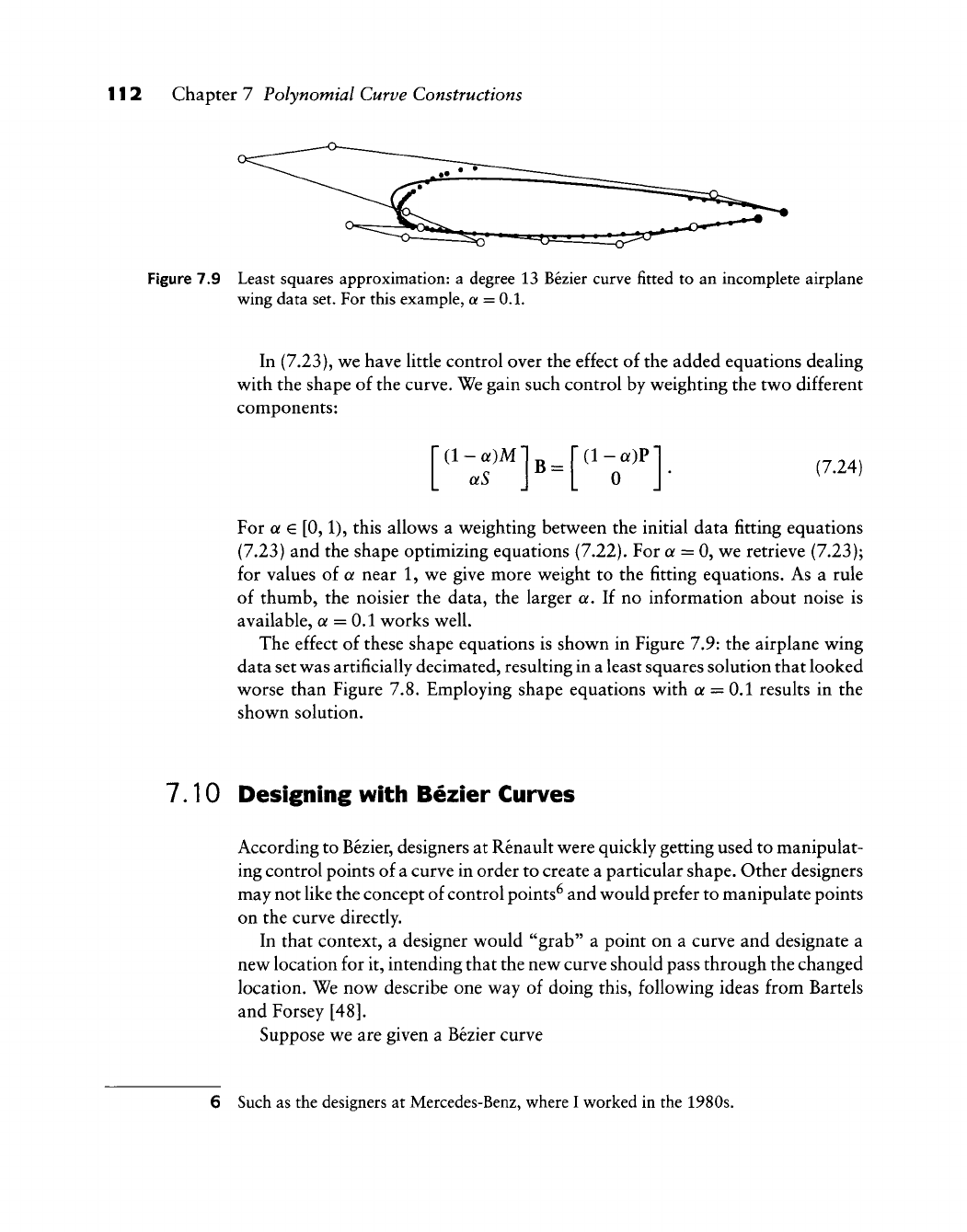
112 Chapter 7 Polynomial Curve Constructions
Figure 7.9 Least squares approximation: a degree 13 Bezier curve fitted to an incomplete airplane
wing data set. For this example, a = 0.1.
In (7.23), we have little control over the effect of the added equations deahng
with the shape of the curve. We gain such control by weighting the two different
components:
[";r]-["Tl-
(7.24)
For a e [0,1), this allows a weighting between the initial data fitting equations
(7.23) and the shape optimizing equations (7.22). For a = 0, we retrieve (7.23);
for values of a near 1, we give more weight to the fitting equations. As a rule
of thumb, the noisier the data, the larger a. If no information about noise is
available, a = 0.1 works well.
The effect of these shape equations is shown in Figure 7.9: the airplane wing
data set was artificially decimated, resulting in a least squares solution that looked
worse than Figure 7.8. Employing shape equations with a = 0.1 results in the
shown solution.
7.10 Designing witii Bezier Curves
According to Bezier, designers at Renault were quickly getting used to manipulat-
ing control points of a curve in order to create a particular shape. Other designers
may not like the concept of control points^ and would prefer to manipulate points
on the curve directly.
In that context, a designer would "grab" a point on a curve and designate a
new location for it, intending that the new curve should pass through the changed
location. We now describe one way of doing this, following ideas from Barrels
and Forsey [48].
Suppose we are given a Bezier curve
6 Such as the designers at Mercedes-Benz, where I worked in the 1980s.
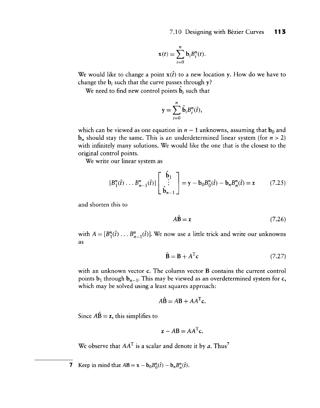
7.10 Designing with Bezier Curves 113
n
i=0
We would like to change a point x{i) to a new location y. How do we have to
change the b/ such that the curve passes through y?
We need to find new control points b/ such that
y
=
X]W^^
i=0
which can be viewed as one equation inn— 1 unknowns, assuming that bo and
b„ should stay the same. This is an underdetermined linear system (for n > 2)
with infinitely many solutions. We would like the one that is the closest to the
original control points.
We write our linear system as
[B",ii)...B"„_,ii)]
and shorten this to
Lb«-i J
= y-boB^(?)-b,B^(?) = z (7.25)
AB = z (7.26)
with A = [B^(i)...
B^_-^(i)],
We now use a little trick and write our unknowns
as
B = B + A^c (7.27)
with an unknown vector c. The column vector B contains the current control
points bi through b„_i. This may be viewed as an overdetermined system for c,
which may be solved using a least squares approach:
AB = AB + AA'^C.
Since AB = z, this simplifies to
z - AB = AA'^C.
We observe that AA^ is a scalar and denote it by a. Thus'^
7 Keep in mind that
AB
= x - hoB^ii) - b„B^(?).
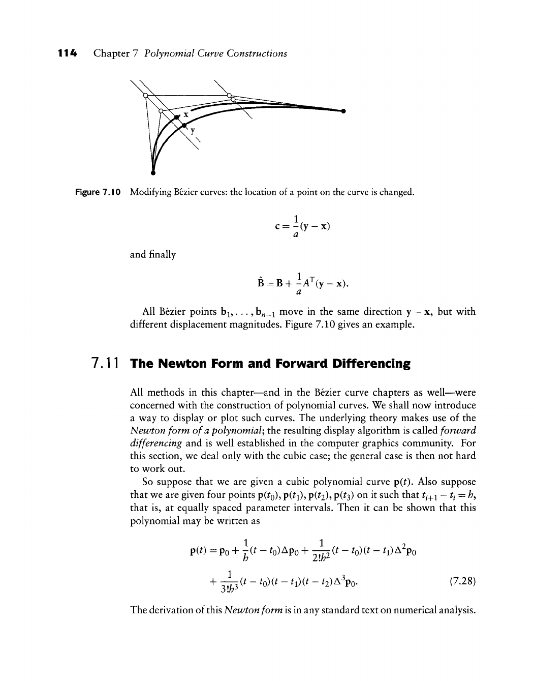
114 Chapter 7 Polynomial Curve Constructions
Figure 7.10 Modifying Bezier curves: the location of a point on the curve is changed.
and finally
c=-(y-x)
a
B = B+-A'^(y-x).
All Bezier points b^,. .., b„_i move in the same direction y
—
x, but v^ith
different displacement magnitudes. Figure 7.10 gives an example.
7.11 The Newton Form and Forward Differencing
AH methods in this chapter—and in the Bezier curve chapters as well—^were
concerned with the construction of polynomial curves. We shall now introduce
a way to display or plot such curves. The underlying theory makes use of the
Newton form of a polynomial; the resulting display algorithm is called forward
differencing and is well established in the computer graphics community. For
this section, we deal only with the cubic case; the general case is then not hard
to work out.
So suppose that we are given a cubic polynomial curve p(^). Also suppose
that we are given four points
pC^o)?
P(^i)?
p(h)'>
p(h) ^^ i^ such that tj^i
—
tj = h,
that is, at equally spaced parameter intervals. Then it can be shown that this
polynomial may be written as
1 1
P(^) =
Po
+ ^(* - ^o)Apo + ^it - to)it - ti)A^Po
1
(7.28)
The derivation of this Newton form is in any standard text on numerical analysis.
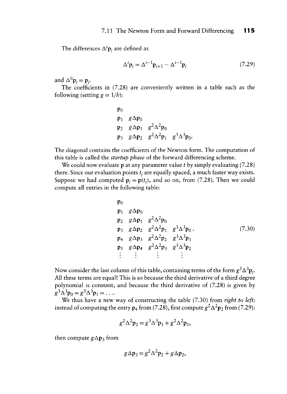
7.11 The Newton Form and Forward Differencing 115
The differences A^py are defined as
A'p,.
= A'-V/+i-A'-ipy (7.29)
and A^py = py.
The coefficients in (7.28) are conveniently written in a table such as the
following (setting g = 1/h):
Po
Pi gApo
P2 g^Pl g^^^Po
P3 g^Pl g^^^Pl g^^W
The diagonal contains the coefficients of the Newton form. The computation of
this table is called the startup phase of the forward differencing scheme.
We could now evaluate p at any parameter value t by simply evaluating (7.28)
there. Since our evaluation points tj are equally spaced, a much faster way exists.
Suppose we had computed py = p(^y), and so on, from (7.28). Then we could
compute all entries in the following table:
Po
Pi gApo
P2 g^Pi g^A^po
P3 g^Pi g^^^Pi g^^^PO' (7-30)
P4 gAp3 g^A2p2 g^A^pi
P5 ^Ap4 g^A2p3 g^A^p2
Now consider the last column of this table, containing terms of the form g^A^py.
All these terms are equal! This is so because the third derivative of a third degree
polynomial is constant, and because the third derivative of (7.28) is given by
g^A^P0 = g^A^Pl = ....
We thus have a new way of constructing the table (7.30) from right to left:
instead of computing the entry p4 from (7.28), first compute g'^ A^p2 from (7.29):
g^A^P2=g^A^Pl+g^A^Pl,
then compute gAp3 from
gAp3 = g^A^P2+gAp2,
116 Chapter 7 Polynomial Curve Constructions
and finally
P4=gAp3 + P3.
Then compute P5 in the same manner, and so on. The general formula is, with
qj = g^A^Py:
q; = q;:^l + q;_i; / = 2,1,0. (7.31)
It yields the points py = q^^.^
This way of computing the py does not involve a single multiplication after
the startup phase! It is therefore extremely fast and has been implemented in
many graphics systems. Given four initial points po, pi, p2,
P3
and a stepsize
/?,
it
generates a sequence of points on the cubic polynomial through the initial four
points. Typically, the polynomial will be given in Bezier form, so those four points
have to be computed as a startup operation.
In a graphics environment, it is desirable to adjust the stepsize h such that
each pixel along the curve is hit. One way of doing this is to adjust the stepsize
while marching along the curve. This is called adaptive forward differencing and
is described by Lien, Shantz, and Pratt [389] and by Chang, Shantz, and Rochetti
[109].
Although fast, forward differencing is not
foolproof.
As we compute more
and more points on the curve, they begin to be affected by
roundoff.
So while we
intend to march along our curve, we may instead leave its path, deviating from it
more and more as we continue. For more literature on this method, see Abi-Ezzi
[1],
Bartels, Beatty, and Barsky [47], or Shantz and Chang
[571].
7.12 Implementation
The code for Aitken's algorithm is very similar to that for the de Casteljau
algorithm. Here is its header:
float aitken(degree,coeff,t)
/* uses Aitken to compute one coordinate
value of a Lagrange interpolating polynomial. Has to be called
for each coordinate (x,y, and/or z) of data points.
Input: degree: degree of curve.
8 It holds for any degree n if we replace / = 2,1,0 by / = «
—
1,
w —
2,...,
0.
7.13 Problems 117
coeff: array with coordinates
to be
interpolated,
t: parameter value.
Output: coordinate value.
Note:
we
assume
a
uniform knot sequence!
V
7.15 Problems
1 Show that the cubic and quintic Hermite polynomials are linearly indepen-
dent.
2 Generahze Hermite interpolation to degrees 7, 9, and so on.
* 3 The de Casteljau algorithm for Bezier curves has as its "counterpart" the
recursion formula (5.2) for Bernstein polynomials. Deduce a recursion
formula for Lagrange polynomials from Aitken's algorithm.
* 4 The de Casteljau algorithm may be generalized to yield the concept of
blossoms. This is not possible for Aitken's algorithm. Why?
* 5 The Hermite form is not invariant under affine domain transformations,
v^hereas the Bezier form
is.
What about the Lagrange and monomial forms?
What are the general conditions for a curve scheme to be invariant under
affine domain transformations?
* 6 When P = n in least squares approximation, we should be back in an
interpolation context. Shov^ that this is indeed the case.
PI Aitken's algorithm looks very similar to the de Casteljau algorithm. Use
both to define a whole class of algorithms, of which each would be a special
case (see [205]). Write a program that uses as input a parameter specifying
if the output curve should be "more Bezier" or "more Lagrange."
P2 The function that was used by Runge to demonstrate the effect that now
bears his name is given by
fW = 7^; xG[-l,l].
Use the routine ait ken to interpolate at equidistant parameter intervals.
Keep increasing the degree of the interpolating polynomial until you notice
"bad" behavior on the part of the interpolant.
P3 In Lagrange interpolation, each p^ is assigned a corresponding parameter
value tj. Experiment (graphically) by interchanging two parameter values
ti and tj without interchanging
p^
and py. Explain your results.

This Page Intentionally Left Blank

B-Spline Curves
D-splines were investigated as early as the nineteenth century by N. Lobachevsky
(see Renyi
[506],
p. 165); they were constructed as convolutions of certain prob-
ability distributions.^ In
1946,1.
J. Schoenberg [542] used B-splines for statistical
data smoothing, and his paper started the modern theory of spline approxima-
tion. For the purposes of this book, the discovery of the recurrence relations
for B-splines by C. de Boor
[137],
M. Cox
[129],
and L. Mansfield was one of
the most important developments in this theory. The recurrence relations were
first used by Gordon and Riesenfeld [284] in the context of parametric B-spline
curves.
This chapter presents a theory for arbitrary degree B-spline curves. The orig-
inal development of these curves makes use of divided differences and is math-
ematically involved and numerically unstable; see de Boor [138] or Schumaker
[546].
A different approach to B-splines was taken by de Boor and Hollig
[143];
they used the recurrence relations for B-splines as the starting point for the the-
ory. In this chapter, the theory of B-splines is based on an even more fundamental
concept: the blossoming method proposed by L. Ramshaw [498] and, in a
dif-
ferent form, by R de Casteljau
[147].
More literature on blossoms: Gallier
[252],
Boehm and Prautzsch [87].
1 However, those were only defined over a very special knot sequence.
119
120 Chapter 8 B-Spline Curves
8.1 Motivation
B-spline curves consist of many polynomial pieces, offering much more versatility
than do Bezier curves. Many B-spline curve properties can be understood by
considering just one polynomial piece—that is how
w^e
start this chapter.
The Bezier points of a quadratic Bezier curve may be written as blossom values
b[0,0],b[0,l],b[l,l].
Based on this, we could get the de Casteljau algorithm by repeated use of the
identity t = (l
—
t)'0-\-t'l. The pairs
[0,0], [0,1],
[1,1] may be viewed as being
obtained from the sequence 0,0,1,1 by taking successive pairs.
Let us now generalize the sequence 0,0,1,1 to a sequence
WQ,
U^,
ui-,
Uy The
quadratic blossom b[w, u\ may be written as
1 r n ^2 — ^
1
r i U — UA ^ ^ ^
b[w, u\ = -^ b[^/i, u\
H
b[w,
U2\
U2-U1 \U2-U0 U2-UQ /
U
—
U^{u^
—
U.^ -, U
—
U^^^ \
+ — b[wi, U2] +
^b[^2,
^3] •
U2
—
Ui \W3
—
Ui U^
—
Ui )
This uses the identity
uy
—
u u
—
u^
u = ui
H
-U2
U2
—
U\ ^2 ~ ^1
for the first step and the two identities
U2
—
U U
— Ur)
u
—
^0
"^
^2
^2 ~ ^0 ^2 ~ ^0
and
U-i
—
U U
—
U\
u =
—^ Ux H
-u^
^3
—
^1 ^3
—
^1
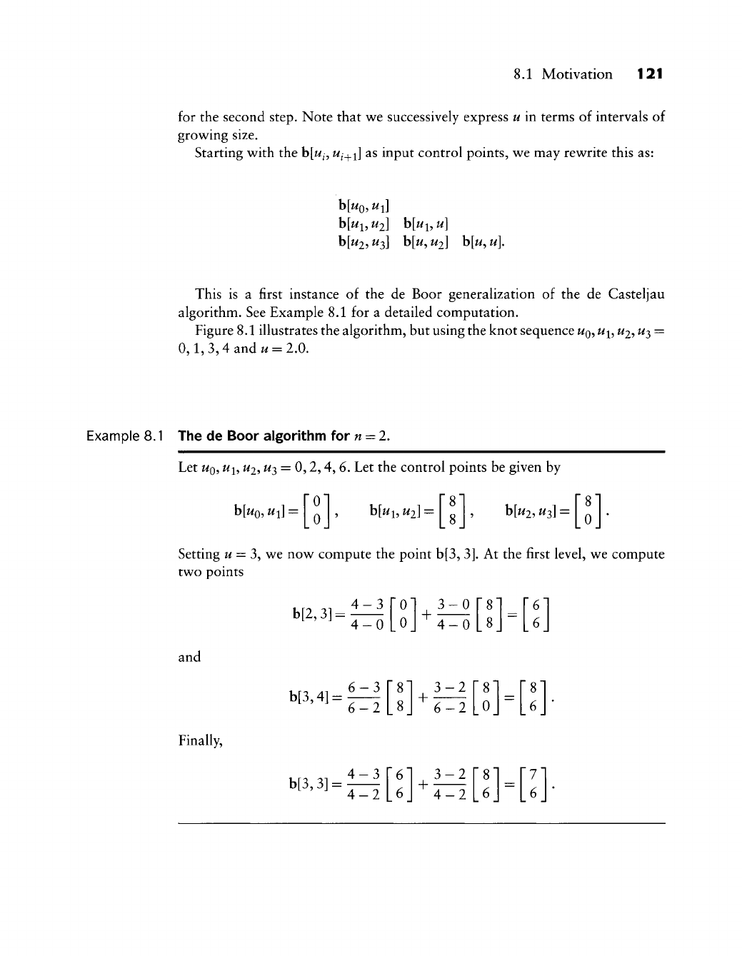
8.1 Motivation 121
for the second step. Note that we successively express u in terms of intervals of
growing size.
Starting with the b[w^,
w^.^^]
as input control points, we may rewrite this as:
b[w2? ^3] b[w, t/2] b[w, u\.
This is a first instance of the de Boor generalization of the de Casteljau
algorithm. See Example 8.1 for a detailed computation.
Figure 8.1 illustrates the algorithm, but using the knot sequence
WQ?
^l?
^2?
^3 =
0,1,
3,4 and ^ = 2.0.
Example 8.1 The de Boor algorithm for
n
= l.
Let
t/Q,
^1,
^2? ^3 = 0,2,4, 6. Let the control points be given by
h[uQ,
ui] = b[wi,
U2]
=
b[w2,
u^]
= 0
Setting
w
= 3, we now compute the point b[3,
3].
At the first level, we compute
two points
and
Finally,
b[2,3]
=
b[3,4] =
4-3
4-0
6-3
6-2
+ 3-0
4-0
[t\
[8]
_8_
3-2
+ 631 [8]
_0_
—
[8]
_6_
b[3,3]:
4-3
4-2 + 3-2
4-2
7
6
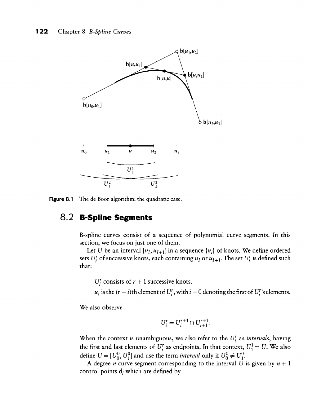
122 Chapter 8 B-Spline Curves
h[u2,u^]
Figure 8.1
1 1
UQ Ui
____^___
•
u
ul
The de Boor algorithm:
1 1
«2 ^3
the quadratic case.
8.2 B-Spline Segments
B-spUne curves consist of a sequence of polynomial curve segments. In this
section, w^e focus on just one of them.
Let U be an interval [t/j, t^/+i] in a sequence {wj of knots. We define ordered
sets W- of successive knots, each containing ui or Ui^i. The set W- is defined such
that:
W- consists of r + 1 successive knots.
ui is the (r
—
/)th element of U[, with
/
= 0 denoting the first of I7['s elements.
We also observe
u;
=
u[+inu[+/.
When the context is unambiguous, we also refer to the U[ as intervals^ having
the first and last elements of W- as endpoints. In that context, l]\ = 17. We also
define U = [Ug, Uj] and use the term interval only if
U^^U^,
A degree n curve segment corresponding to the interval U is given by « + 1
control points d^ which are defined by
8.2 B-Spline Segments 123
d,=b[Uf-l]; / = 0,...,«. (8.1)
The point x(u) = h[u^^^] on the curve is recursively computed as
d'.(u) = b[^<'^, Uf
"^"1;
r=l,,..,n;i =
0,...,n-r
(8.2)
with x(u) =
d-Qiu)?
This is knov^n as the de Boor algorithm after Carl de Boor
see
[137].
See Example 8.2 for the case n = 3 and Figure 8.2 for an illustration.
Equation (8.2) may alternatively be written as
d;(«) = (1 - Cr^dpl ^ CrM;;l; r=l,...,n;i =
0,...,n-r,
(8.3)
where
t^7('^
is the local parameter in the interval
Uf~-[~^
.
A geometric interpretation is as follows. Each intermediate control polygon
leg dp
d^-^-^
may be viewed as an affine image of
Uf_^/^
. The point d^^ is then
the image of u under that affine map.
For the special knot sequence 0^"^, 1^^^ and U =
[0,1],
the de Boor algorithm
becomes
d^(«)=b[«->,0<«—'>,l<-]; r =!,...,«;
i^O,...,n-r,
(8.4)
which is simply the de Casteljau algorithm.
If the parameter u happens to be one of the knots, the algorithm proceeds as
before, except that we do not need as many levels of the algorithm. For example,
if a quadratic curve segment is defined by
h[uQ,
u^],
b[wi, ^2]? ^Wi^ ^3] ^^^ we
want to evaluate at u = ^2? then two of the intermediate points in the de Boor
algorithm are already known, namely, h[ui,
U2]
and b[t/2,
^3].
From these two,
we immediately calculate the desired point h[u2, ^2]? thus the de Boor algorithm
now needs only one level instead of two.
Derivatives of a B-spline curve segment are computed in analogy to the Bezier
curve case (5.17)
x(u) = nh[u^''-^^,ll (8.5)
Expanding this expression and using the control point notation, this becomes
x(«) = ^(dri-d^-i), (8.6)
2 This notation is different from the one used in previous editions of this book.
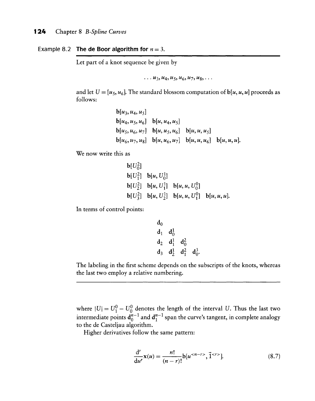
124 Chapter 8 B-Spline Curves
Example 8.2 The de Boor algorithm for « = 3.
Let part of a knot sequence be given by
. . . ^3, ^4, ^5, ^5, Wy,
Wg?
•
• •
and let U = [^5,
w^].
The standard blossom computation of
b[w,
w,
u\ proceeds as
follows:
b[W4,
^5,
U^]
h[u,
U4,
Us]
h[us,
u^,
uj] h[u.
Us,
u^]
h[u, u, us\
h[u^,uj^ug] h[u^u^^uj\ h[u,u,u^] h[u,u,u].
We now write this as
h[Uf] h[u,Ul]
b[Uf] h[u,Ul] h[u,u,U^^]
HUJ] h[u,Ul] h[u,u,U^] h[u,u,u].
In terms of control points:
dl 4
di d\
d3 dl
dl
dl dl
The labeling in the first scheme depends on the subscripts of the knots, whereas
the last two employ a relative numbering.
where \U\ = U^
—
UQ
denotes the length of the interval 17. Thus the last two
intermediate points dQ~^ and d^~ span the curve's tangent, in complete analogy
to the de Casteljau algorithm.
Higher derivatives follow the same pattern:
/-X(«) = -Jll—h[u<"-r>, l<r>l (8.7)
du^
{n
—
r)i
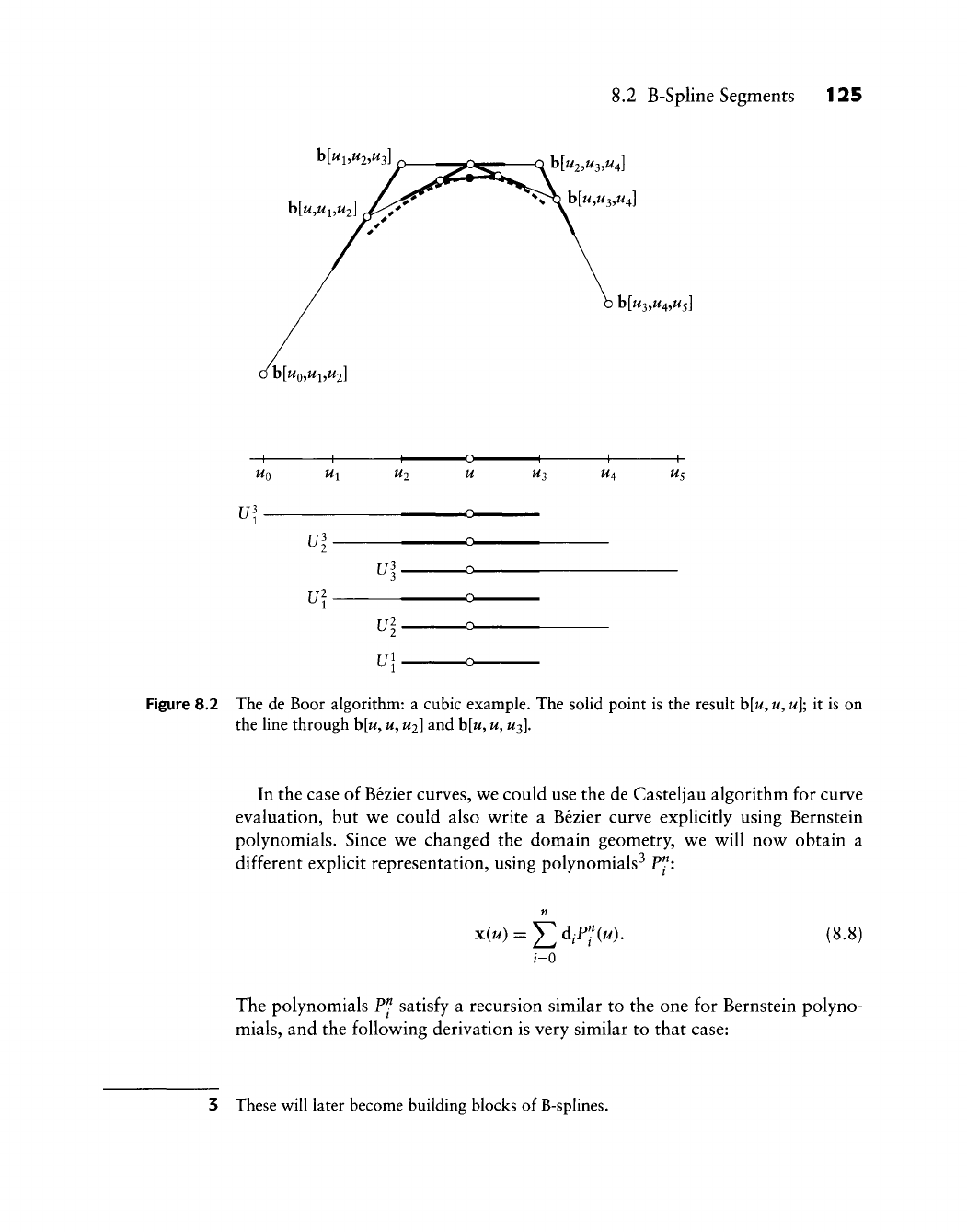
i.2 B-Spline Segments 125
b[W2,W3,W4]
h[u^,U4,Us]
I h[UQ,Ui,U2\
UQ U^ U2 U W3 M4 W5
m-
m
ul
ui.
Figure 8.2 The de Boor algorithm: a cubic example. The solid point is the result
h[u,
u,
u];
it is on
the line through
b[w,
w,
U2]
and
b[w,
w,
W3].
In the case of Bezier curves, we could use the de Casteljau algorithm for curve
evaluation, but we could also write a Bezier curve explicitly using Bernstein
polynomials. Since we changed the domain geometry, we will now obtain a
different explicit representation, using polynomials^ P":
x(^) = ^d,Pf(^). (8.8)
/=o
The polynomials P" satisfy a recursion similar to the one for Bernstein polyno-
mials,
and the following derivation is very similar to that case:
3 These will later become building blocks of B-splines.

126 Chapter 8 B-Spline Curves
xiu) = J2djP^-\u)
=Ed - ti^)d,pr\^)+E
tfd^pth")
n-\
i=0
n—\
n—\
i=0 i=l
For the first step, we used the de Boor algorithm, letting tf be the local parameter
in the interval U^^^ For the second step, we used the convention P^~^ = 0 to
modify the first term. Using a similar argument: P^ = 0, we may extend the
second term to start with / = 0. We conclude
P^(u) = (1 - tl^)P'^-\u) + tfP'Izliu). (8.10)
This recursion has to be anchored in order to be useful. This is straightforward
for the case n = l:
phu) = ^,
P](u)
= ^,
ov
1^1 IV 1^1
where |U| = Uj - Ug. For the special knot sequence 0<"^, 1<"> and U =
[0,1],
this is the Bernstein recursion.
8.5 B-Spline Curves
A B-spline curve consists of several polynomial curve segments, each of which
may be evaluated using a de Boor algorithm. A B-spline curve is defined by
the degree n of each curve segment,
the knot sequence
UQ,
...
^
Uf^^
consisting of
iC
+ 1 knots
Uj
< /^/+i,
the control polygon dg,..., d^ with L = K ~ n + 1.
Some comments: the numbering of the control points d^ in this definition is
global, whereas in Section 8.2 it was local relative to an interval U. Each dj
may be written as a blossom value with n subsequent knots as arguments. Hence
the number L + 1 of control points equals the number of w-tuples in the knot
sequence.

8.3 B-Spline Curves 127
Example 8.3 Some examples of B-spline curve definitions.
Let n=
1^
and let the knot sequence be 0,1,2, hence K = 2. There will be control
points do, d^,
d3.
The curve's domain is
[UQ^
U^\ and there are two linear curve
segments.
Let n = l with the knot sequence 0, 0.2, 0.4, 0.5,
0.7,1,
hence K = S. There will
be control points do, d^, d2,
d3,
A^
and three quadratic curve segments. If we now
change the knot sequence to 0, 0.2, 0.45, 0.45,
0.7,1,
then the number of curve
segments will drop to two.
Each knot may be repeated in the knot sequence up to n times. In some cases it
is approriate to simply list those knots multiple times. For other applications, it is
better to list the knot only once and record its multiplicity in an integer array. For
example, the knot sequence 0.0,0.0,1.0,2.0,3.0,3.0,4.0,4.0 could be stored as
0.0,1.0,2.0, 3.0,4.0 and a multiplicity array 2,1,1,2,2.
There is a different de Boor algorithm for each curve segment. Each is "started"
with a set of
U^",
that is, by sequences o{n-\-l knots. In order for local coordinates
to be defined in (8.3), no successive
w
+ 1 knots may coincide.
In Section 8.2, we assumed that we could find the requisite V^ for each interval
U. This is possible only if U is "in the middle" of the knot sequence; more
precisely, the first possible de Boor algorithm is defined for U = [u^-i-, u^ and
the last one is defined for U =
WK-n->
^X-w+il = Wx-m
^LI-
^^ ^^^^
^^11
Wn-h
^LI
the domain of the B-spline curve. A B-spline curve has as many curve segments
as there are nonzero intervals U in the domain. Example 8.3 illustrates these
comments.
For more examples of B-spline curves, see Figure 8.3.
Since a B-spline curve consists of a number of polynomial segments, one might
ask for the Bezier form of these segments. For a segment U = [uj, uj^i] of the
curve, we simply evaluate its blossom b^ and obtain the Bezier points h^,. . ., b^
as
j^
=b [Uj , Uj^^ J.
An example is shown in Figure 8.4. Several constituent curve pieces of the same
curve are shown in Figure 8.5.
When dealing with B-spline curves, it is convenient to treat it as one curve, not
just as a collection of polynomial segments. A point on such a curve is denoted
by d(w), with u e [u^-i-,
uj^_^_^i].
In order to evaluate, we perform the following
steps:
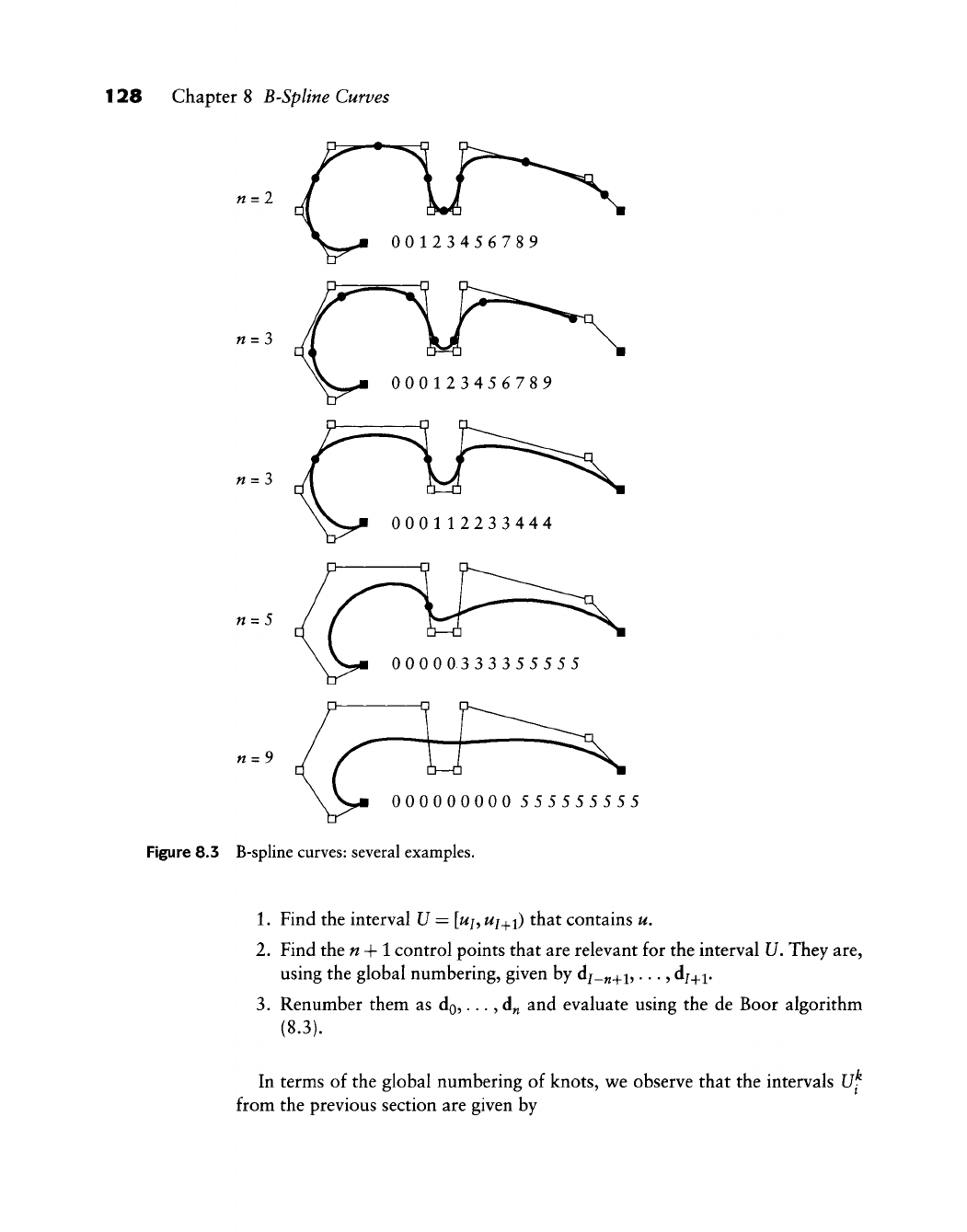
128 Chapter 8 B-Spline Curves
\^ 00123456789
n
=
3
n
=
3
n
=
5
n
=
9
000000000 555555555
Figure 8.3 B-spline curves: several examples.
1.
Find the interval U = [uj,
ui_^i)
that contains u,
2.
Find the n-\-l control points that are relevant for the interval U, They are,
using the global numbering, given by dj_„_^i,...,
d/.^!.
3.
Renumber them as do,..., d„ and evaluate using the de Boor algorithm
(8.3).
In terms of the global numbering of knots, w^e observe that the intervals U^
from the previous section are given by
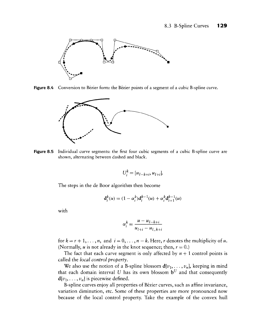
8.3 B-Spline Curves 129
Figure 8.4 Conversion to Bezier form: the Bezier points of a segment of a cubic B-spline curve.
Figure 8.5 Individual curve segments: the first four cubic segments of a cubic B-sphne curve are
shown, ahernating between dashed and black.
The steps in the de Boor algorithm then become
d^iu) = (1 - af)d^-\u) + afd^-/(«)
with
k^ ^ - ^l-k+i
^IM ~ ^l_k+i
for ^ = r + 1,.. .,
w,
and / = 0,.. .,
w —
^. Here, r denotes the multiplicity of u,
(Normally, u is not already in the knot sequence; then, r = 0.)
The fact that each curve segment is only affected by
w
+ 1 control points is
called the local control property.
We also use the notion of a B-spline blossom d[t'i,..., f
„],
keeping in mind
that each domain interval U has its ov^n blossom b^ and that consequently
d[^'i,...,
f „] is piecewise defined.
B-spline curves enjoy all properties of Bezier curves, such as affine invariance,
variation diminution, etc. Some of these properties are more pronounced now
because of the local control property. Take the example of the convex hull
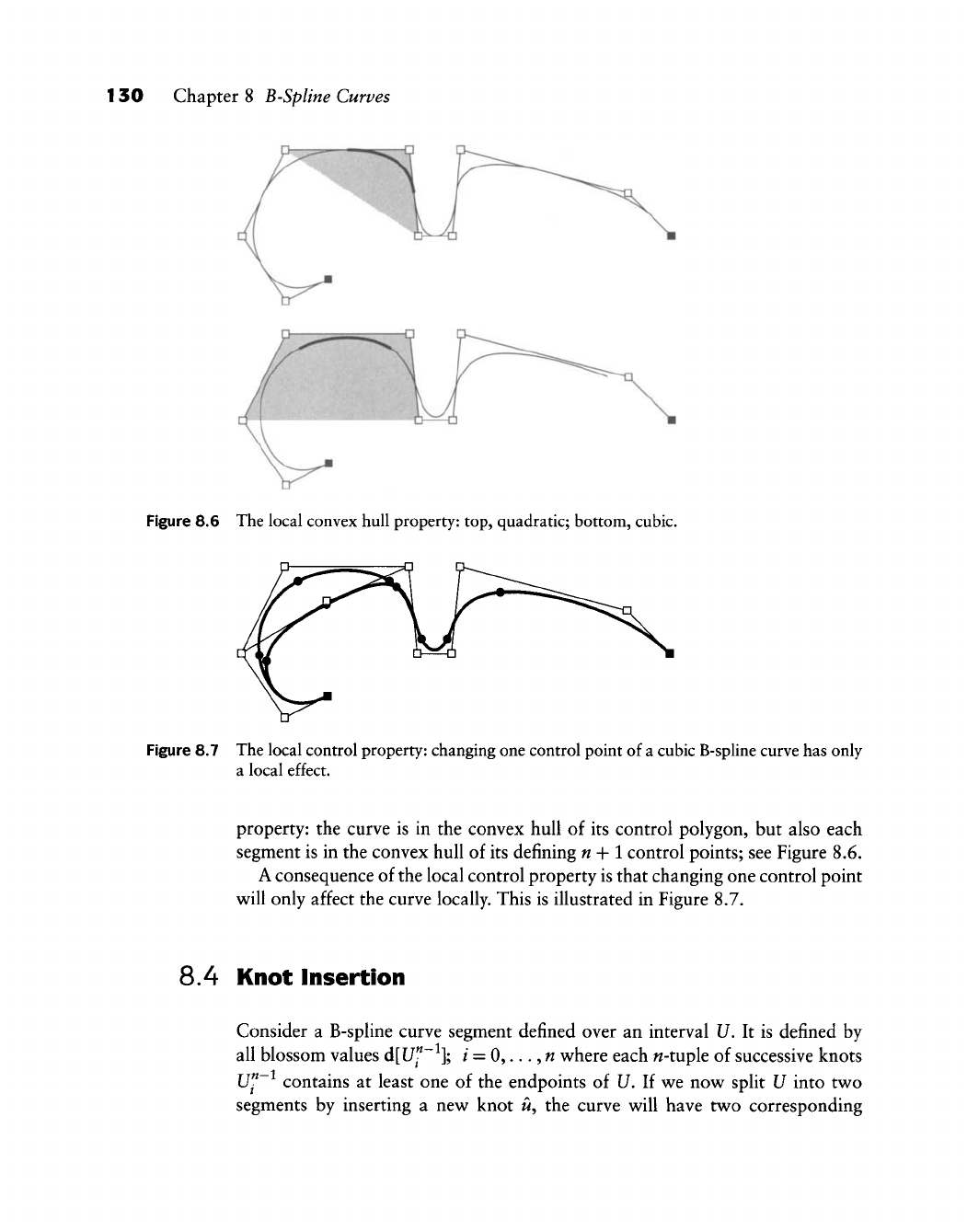
1 30 Chapter 8 B-Spline Curves
Figure 8.6 The local convex hull property: top, quadratic; bottom, cubic.
Figure 8.7 The local control property: changing one control point of a cubic B-spline curve has only
a local effect.
property: the curve is in the convex hull of its control polygon, but also each
segment is in the convex hull of its defining n-\-l control points; see Figure 8.6.
A consequence of the local control property is that changing one control point
w^ill only affect the curve locally. This is illustrated in Figure 8.7.
8.4 Knot Insertion
Consider a B-spline curve segment defined over an interval U. It is defined by
all blossom values d[[7"~ ]; / =
0,...,«
w^here each «-tuple of successive knots
U^ contains at least one of the endpoints of U. If we now split U into two
segments by inserting a new knot ii, the curve will have two corresponding

8.4 Knot Insertion 131
Example 8.4 Knot insertion.
In Figure 8.8, just one de Boor step is carried out for the parameter value u. The
two new resulting points, in blossom notation, are b[wi, u] and b[ii,
U2\.
Let us
now consider the points
These are the B-spline control points of our curve b[w,
u]
for the interval [wj, u\\
Similarly, the B-spline control points for the interval [ii,
Uj}
are given by
h[u,U2]
bK,Wi
h[U2,U^]
H
UQ Ui U U2 ^3
Figure 8.8 Knot insertion: a quadratic example.
segments. What are the control points for these two segments.^ The answer is
surprisingly simple: all blossom values
d[l7^"~^];
/ = 0,...,
w
+ 1 where each n-
tuple of successive knots U^~^ contains at least one of the endpoints of U. This
result is due to W. Boehm [68], although it was not originally derived using
blossoms. See Example 8.4.
Knot insertion works since B-spline control points are nothing but blossom
values of successive knots—now they involve the new knot u. We may also view
the process of knot insertion as one level of the de Boor algorithm, as illustrated
in Example 8.4.
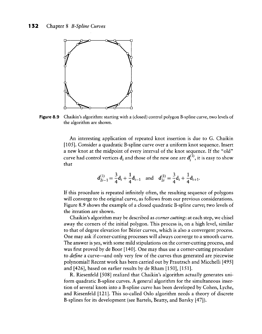
132 Chapter 8 B-Spline Curves
Figure 8.9 Chaikin's algorithm: starting with a (closed) control polygon B-spline curve, two levels of
the algorithm are shown.
An interesting application of repeated knot insertion is due to G. Chaikin
[105].
Consider a quadratic B-spline curve over a uniform knot sequence. Insert
a new^ knot at the midpoint of every interval of the knot sequence. If the "old"
curve had control vertices d/ and those of the nev^ one are
d^-
, it is easy to show^
that
4L = ^d, + ld,_i and
d(j>
= ^d, + ld.+i.
If this procedure is repeated infinitely often, the resulting sequence of polygons
w^ill converge to the original curve, as follov^s from our previous considerations.
Figure 8.9 show^s the example of a closed quadratic B-spline curve; two levels of
the iteration are shov^n.
Chaikin's algorithm may be described as corner cutting: at each step,
vs^e
chisel
away the corners of the initial polygon. This process is, on a high level, similar
to that of degree elevation for Bezier curves, w^hich is also a convergent process.
One may ask if corner-cutting processes v^ill alw^ays converge to a smooth curve.
The answer is
yes^
with some mild stipulations on the corner-cutting process, and
was first proved by de Boor
[140].
One may thus use a corner-cutting procedure
to define a curve—and only very few of the curves thus generated are piecewise
polynomial! Recent work has been carried out by Prautzsch and Micchelli [495]
and
[426],
based on earlier results by de Rham
[150], [151].
R. Riesenfeld [508] realized that Chaikin's algorithm actually generates uni-
form quadratic B-spline curves. A general algorithm for the simultaneous inser-
tion of several knots into a B-spline curve has been developed by Cohen, Lyche,
and Riesenfeld
[121].
This so-called Oslo algorithm needs a theory of discrete
B-splines for its development (see Barrels, Beatty, and Barsky [47]).
8.5 Degree Elevation 133
8.5 Degree Elevation
We may degree elevate in (almost) the same way we could degree elevate Bezier
curves using (6.2). The difference: a given B-spline is a piecewise degree n
curve over a given knot sequence. Its differentiability is determined by the knot
multiplicities. If we write it as a piecewise degree
w
+ 1 curve, we need to
increase the multiplicity of every knot by one, thus maintaining the original
differentiability properties. For example, if we degree elevate a C^ piecewise
linear curve to piecewise quadratic, it is still C^. But for a piecewise quadratic
to be C^, it has to have double knots. Let us denote the knots in this augmented
knot sequence by ii^.
Let V" be a sequence of « +
1
real numbers i/^,..., t'^+i- Let y^\vi denote the
sequence V" with the value
Vi
removed. Then the degree n-\-l blossom b may be
expressed in terms of the degree n blossom b via
b[y(-+i)]= -^ (b[V("+^Vi] + ... +b[y^^+iV.+i]) . (8.11)
W
+ 1 V /
The proof is identical to that for degree elevation of Bezier curves. The control
points are then recovered from the blossom as before (see Example 8.5).
The inverse process—degree reduction is more important for practical ap-
plications. Following the example of the analogous Bezier case, we write the
elevation process as a matrix product and invert it by a least squares technique
for the reduction process; see Section 6.4. This method is described in detail in
[617].
Other methods exist, see [481] and
[624].
Example 8.5 B-spline degree elevation and blossoms.
Let a cubic B-spline curve be defined over
{^Q
= ui = u^^
^3,..
.}.
Then the
interval
\u^^
u^] corresponds to [iiy,
u^].
We denote the corresponding blossoms
by d^la^
fe,
c]
and d-jla,
fe,
c, d]. The new control point d^ is computed as follows:
d4 = dy[u4,us,u^,uy]
\
= - (d4[^4.
Us,
u^] + d4[^4.
Us,
uj] + d4[^4, u^, uj] + d^ius, u^, uj^
\
= -
(d4[^3.
^3.
^4] +
d4[w3,
^4,
U4])
.
For the last step, we have used
U4
= us =
W3
and u^ = uj = u^.
1 34 Chapter 8 B-Spline Curves
8.6 Greville Abscissae
Let
l[u]
= uht the blossom of the (nonparametric) hnear function u. If we want
to write this linear blossom as a quadratic one: /^[w, v] = l[u], we easily see that
i(2^[u,v]=h[u] + h[v]
gives the desired quadratic form of our linear blossom. If we asked for a cubic
form
/^^^[w,
V,
w] of l[u\ we find that
111
P\u,
V,
w] = -f[v, w] + -f[u, w] + -fi[u, v\
If we denote a degree n version of the linear blossom by /(")[V"] with V" =
1^1,...,
!/„,
it follows that
/(")[V«]=-(t;i+ ... + £/„).
n
The proof is by induction and was anchored by the earlier examples. The
inductive step starts with the degree elevation formula (8.11):"^
n-\-\
^ n
This is easily transformed to
n-\-l
thus finishing the
proof.
If we are given a knot sequence
UQ^.
.. ,Uj^ and a degree w, then we know that
any B-spline function d(u) has control vertices d[uQ,...,
w„_i],...,
<i[^x_„+i,...,
Uf^],
In the case of a linear function /, we thus have control vertices
1 1
-(UQ
+ . . . + W„_i), . . . , -(W]C-«+l + • V + W«).
4 We do not have to work with augmented knot sequences here since we always deal with
one linear function.
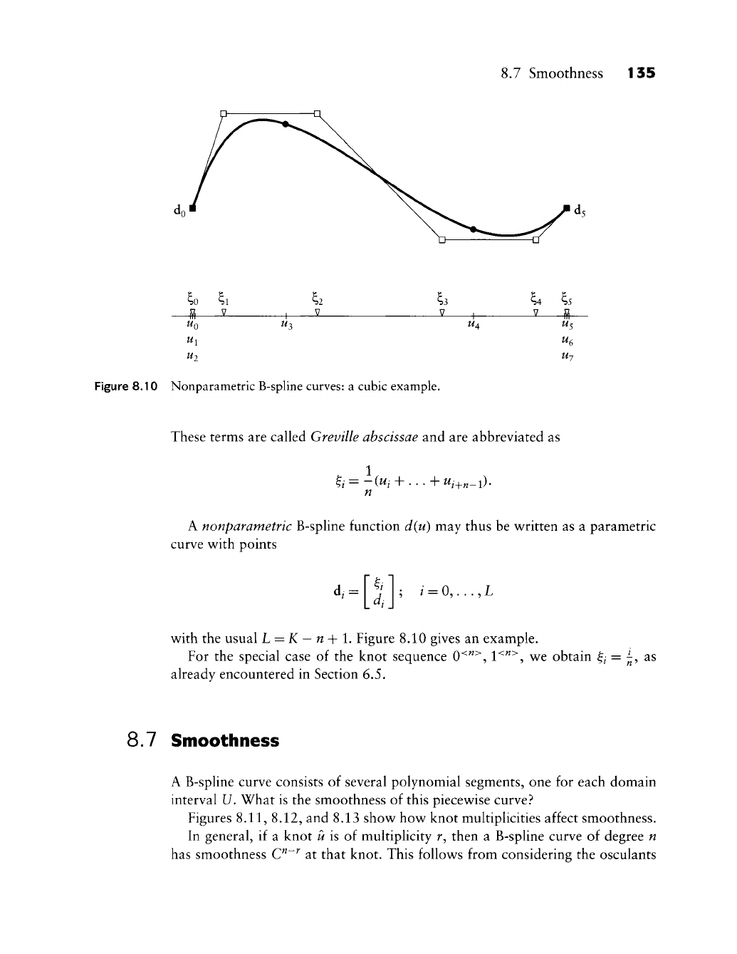
8.7 Smoothness 135
^0 ^1
V
^3
W4
^4 ^5
-2
S5-
^2
Figure 8.10 Nonparametric B-spline curves: a cubic example.
These terms are called Greville abscissae and are abbreviated as
n
A nonparametric B-spline function d{u) may thus be w^ritten as a parametric
curve w^ith points
d. 4-
/•
= 0,..., L
w^ith the usual L = K
—
n-^1. Figure 8.10 gives an example.
For the special case of the knot sequence 0^"^, 1"^"^, wt obtain
^1
= ^, as
already encountered in Section 6.S.
8.7 Smoothness
A B-spline curve consists of several polynomial segments, one for each domain
interval U. What is the smoothness of this piecew^ise curve?
Figures 8.11, 8.12, and 8.13 show^ how^ knot multiplicities affect smoothness.
In general, if a knot u is of multiplicity r, then a B-spline curve of degree n
has smoothness C^~^ at that knot. This follow^s from considering the osculants
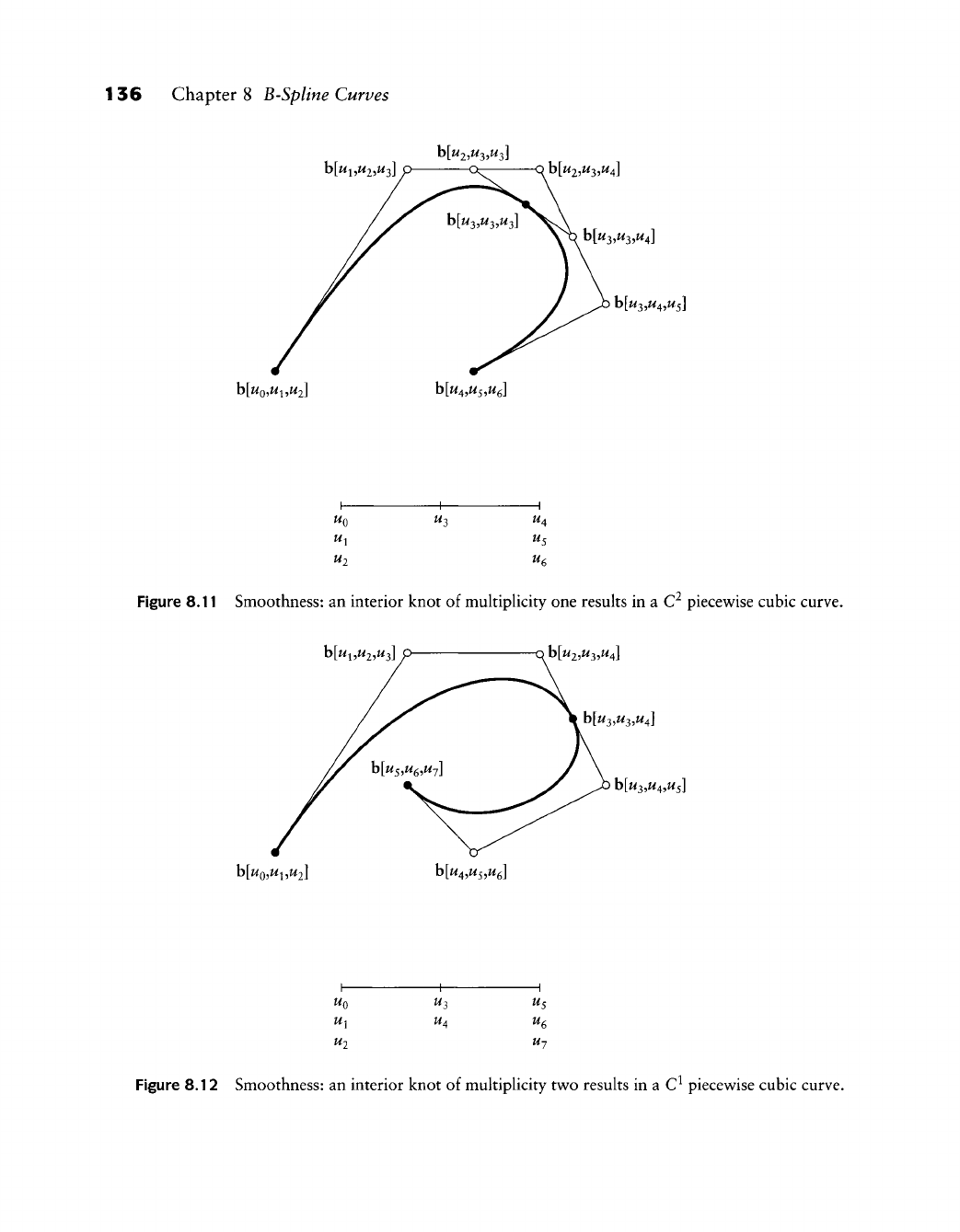
1 36 Chapter 8 B-Spline Curves
h[u^,U2,U^]p O:- q b[W2,W3,W4]
b[Wo,«i,W2] bK,%,w6;
UQ
U2
^5
Figure 8.11 Smoothness: an interior knot of mukiphcity one results in a C^ piecewise cubic curve.
b[Wi,«2,W3 b[W2,W3,W4]
h[UQ,U^,U2] h[u^,Us,u^]
h[u^,u^,u^]
b[W3,W4,W5
UQ
U2
^3
W4
Figure 8.12 Smoothness: an interior knot of mukiphcity two resuks in a C^ piecewise cubic curve.
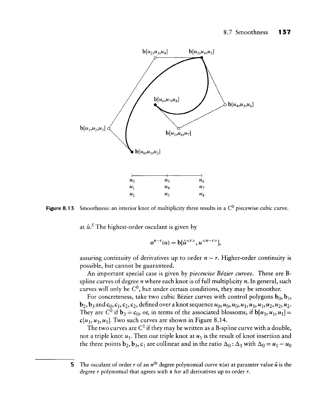
8.7 Smoothness 137
h[u^,U2,u
b[W4,W5,W6]
UQ
W3 U^
H^
U^ tij
^2 ^5 ^8
Figure 8.13 Smoothness: an interior knot of muhipUcity three resuhs in a C^ piecewise cubic curve,
at u.^ The highest-order osculant is given by
assuring continuity of derivatives up to order n
—
r. Higher-order continuity is
possible, but cannot be guaranteed.
An important special case is given by piecewise Bezier curves. These are B-
spline curves of degree n where each knot is of full multiplicity n. In general, such
curves w^ill only be C^, but under certain conditions, they may be smoother.
For concreteness, take tv^o cubic Bezier curves with control polygons bo, b^,
b2, b3
and
CQ,
C^,
C2, C2,
defined over a knot sequence
WQ?
^O?
^0?
^\->
^h ^l?
^2? ^2? ^2-
They are =
Co,
or, in terms of the associated blossoms, if b[^i,
w^, Ui]
=
c[ui^ Ui, ui]. Two such curves are shown in Figure 8.14.
The two curves are C^ if they may be written as a B-spline curve with a double,
not a triple knot u^. Then our triple knot at u^ is the result of knot insertion and
the three points
b2, b3,
c^ are collinear and in the ratio Ao : A| with
AQ
=
UI —
UQ
5 The osculant of order r of an
n^^
degree polynomial curve x(u) at paramter value
w
is the
degree r polynomial that agrees w^ith x for all derivatives up to order r.
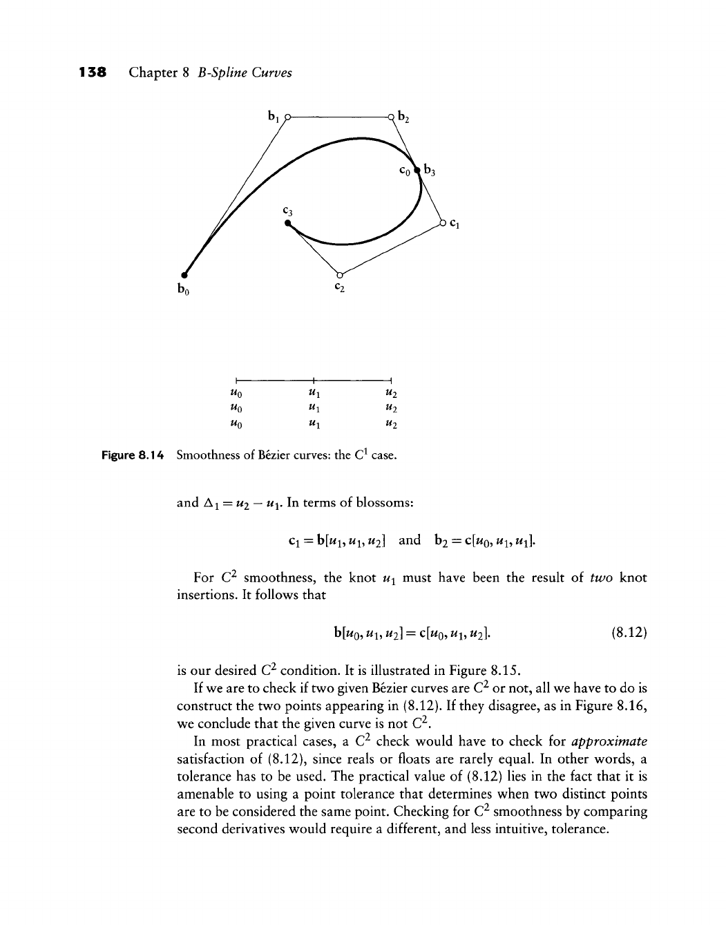
1 38 Chapter 8 B-Spline Curves
UQ
UQ U2
Figure 8.14 Smoothness of Bezier curves: the C^ case.
and Ai =
U2 —
u^. In terms of blossoms:
Ci = h[ui,
wj,
ui] and hi =
C[UQ,
W^, ui\.
For C^ smoothness, the knot ui must have been the resuh of two knot
insertions. It follows that
b[wo,
^1,
U2]
=
c[uo,
ux,
U2].
(8.12)
is our desired C^ condition. It is illustrated in Figure 8.15.
If we are to check if two given Bezier curves are C^ or not, all we have to do is
construct the two points appearing in (8.12). If they disagree, as in Figure 8.16,
we conclude that the given curve is not C^.
In most practical cases, a C^ check would have to check for approximate
satisfaction of (8.12), since reals or floats are rarely equal. In other words, a
tolerance has to be used. The practical value of (8.12) lies in the fact that it is
amenable to using a point tolerance that determines when two distinct points
are to be considered the same point. Checking for C^ smoothness by comparing
second derivatives would require a different, and less intuitive, tolerance.
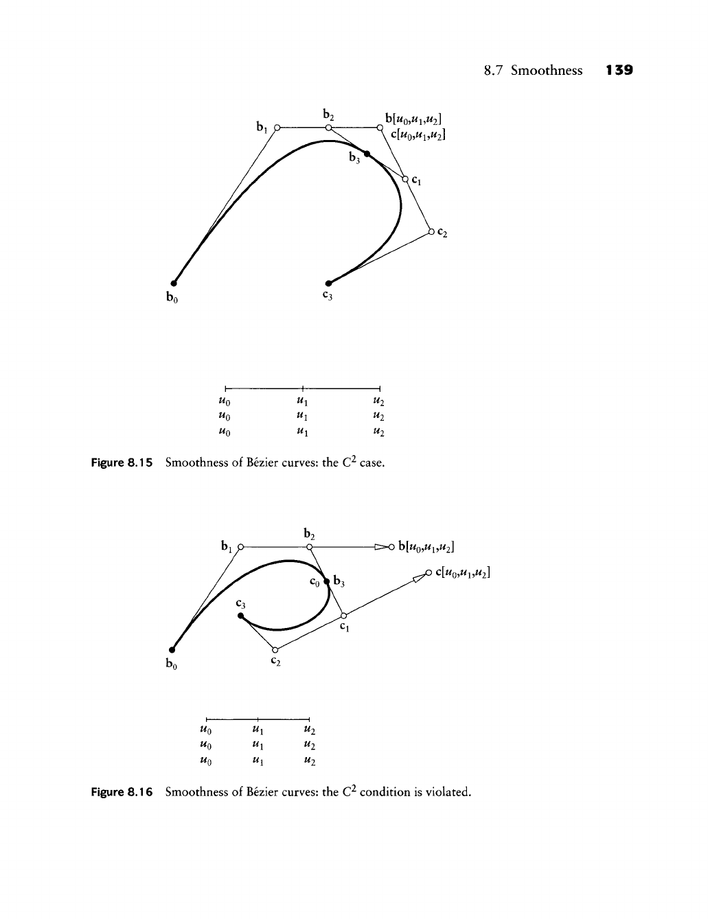
8.7 Smoothness
1
39
b[Mo,Wi,W2]
1
UQ
UQ
1
Wi
Ux
1
U2
U2
Figure 8.15 Smoothness of Bezier curves: the C^ case.
€>0 h[Uo,Ux,U2]
C[UQ,UX,U2]
UQ
UQ
U2
U2
U2
Figure 8.16 Smoothness of Bezier curves: the C^ condition is violated.
140 Chapter 8 B-Spline Curves
8.8 B-Splines
Consider a knot sequence
^Q?
• • • ?
^M ^^^ ^^e set of piecewise polynomials
of degree n defined over it, where each function in that set is n
—
TJ
times
continuously differentiable at knot
Uj.
All these piecewise polynomials form a
linear space, with dimension
M-l
dim=(w + l)+ Y^Vi, (8.13)
i=l
For a
proof,
suppose we want to construct an element of our piecewise polyno-
mial linear space. The number of independent constraints that we can impose
on an arbitrary element, or its number of degrees of freedom, is equal to the
dimension of the considered linear space. We may start by completely specifying
the first polynomial segment, defined over
[UQ,
U^];
we can do this in
w
+
1
ways,
which is the number of coefficients that we can specify for a polynomial of degree
n.
The next polynomial segment, defined over [wj, ui], must agree with the first
segment in position and n
—
r^ derivatives at u^, thus leaving only r^ coefficients
to be chosen for the second segment. Continuing further, we obtain (8.13).
We are interested in B-spline curves that are piecewise polynomials over the
special knot sequence [w„_i, ui]. The dimension of the linear space that they form
is L + 1, which also happens to be the number of B-spfine vertices for a curve in
this space. If we can define L + 1 linearly independent piecewise polynomials in
our linear function space, we have found a basis for this space. We proceed as
follows.
Define functions
N^{u),
called B-splines by defining their de Boor ordinates
to satisfy dj = 1 and dj = 0 for all / ^ i. The N^(u) are clearly elements of the
linear space formed by all piecewise polynomials over [w„_i,
w^].
They have local
support:
Nf(u) 7^ 0 only Hue [w,_i,
w,+„].
This follows because knot insertion, and hence the de Boor algorithm, is a local
operation; if a new knot is inserted, only those Greville abscissae that are "close"
will be affected.
B-splines also have minimal support: if a piecewise polynomial with the same
smoothness properties over the same knot vector has less support than N^", it
must be the zero function. All piecewise polynomials defined over [w^_i,
w^_^„],
the support region of N^, are elements of a function space of dimension In + 1,
according to (8.13). A support region that is one interval "shorter" defines a
function space of dimension In, The requirement of vanishing n
—
rj_i derivatives
at Ui_i and of vanishing n
—
r/_^„ derivatives at
Uj_^^
imposes 2n conditions on
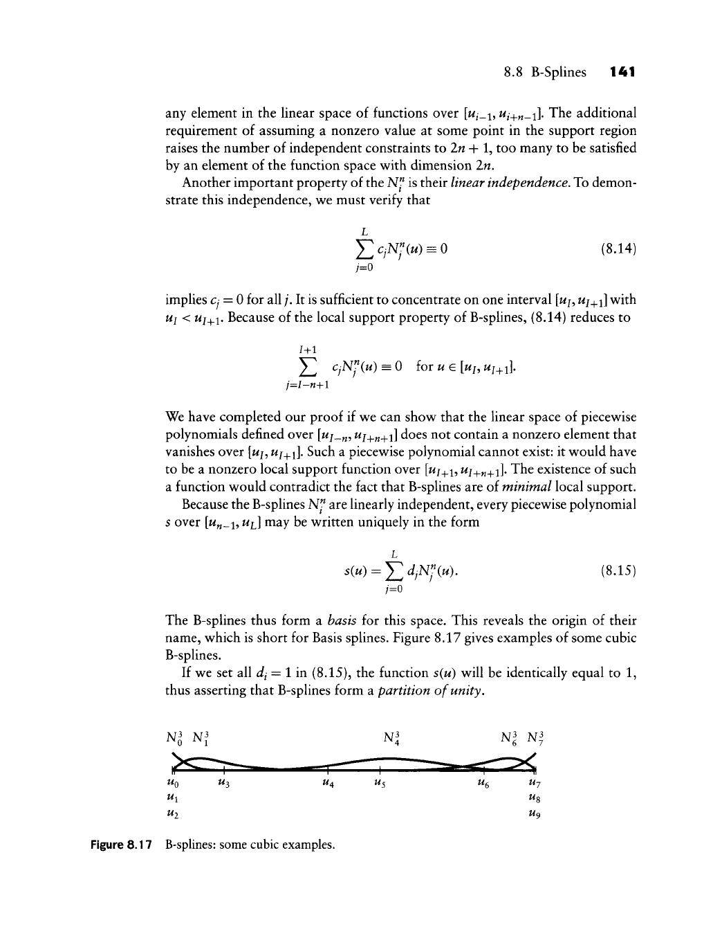
8.8 B-Spiines 141
any element in the linear space of functions over [w/_i,
Uj_^^_i\.
The additional
requirement of assuming a nonzero value at some point in the support region
raises the number of independent constraints to 2n + 1, too many to be satisfied
by an element of the function space with dimension 2n,
Another important property of the N" is their linear independence. To demon-
strate this independence, we must verify that
L
^CjN1{u) = 0 (8.14)
implies
Cj
= 0 for all;. It is sufficient to concentrate on one interval
[wj,
ui_^i]
with
Ui < ui^i. Because of the local support property of B-splines, (8.14) reduces to
/+1
J2 ^j^^i^) = 0 for
w G
K,
wj+i].
j=I-n-\-l
We have completed our proof if we can show that the linear space of piecewise
polynomials defined over [w/_„, Uj^^^i] does not contain a nonzero element that
vanishes over [w/,
w/_^i].
Such a piecewise polynomial cannot exist: it would have
to be a nonzero local support function over
[w/_|_i,
wj_^„+i].
The existence of such
a function would contradict the fact that B-splines are of minimal local support.
Because the B-splines N^ are linearly independent, every piecewise polynomial
s over [«„_!, ui] may be written uniquely in the form
L
s(u)
= J2diNJ{u), (8.15)
j=o
The B-splines thus form a basis for this space. This reveals the origin of their
name, which is short for Basis splines. Figure 8.17 gives examples of some cubic
B-splines.
If we set all 4 = 1 ii^ (8.15), the function s(u) will be identically equal to 1,
thus asserting that B-splines form a partition of unity.
Nl Nl Nl Nl N^
Figure 8.17 B-splines: some cubic examples.
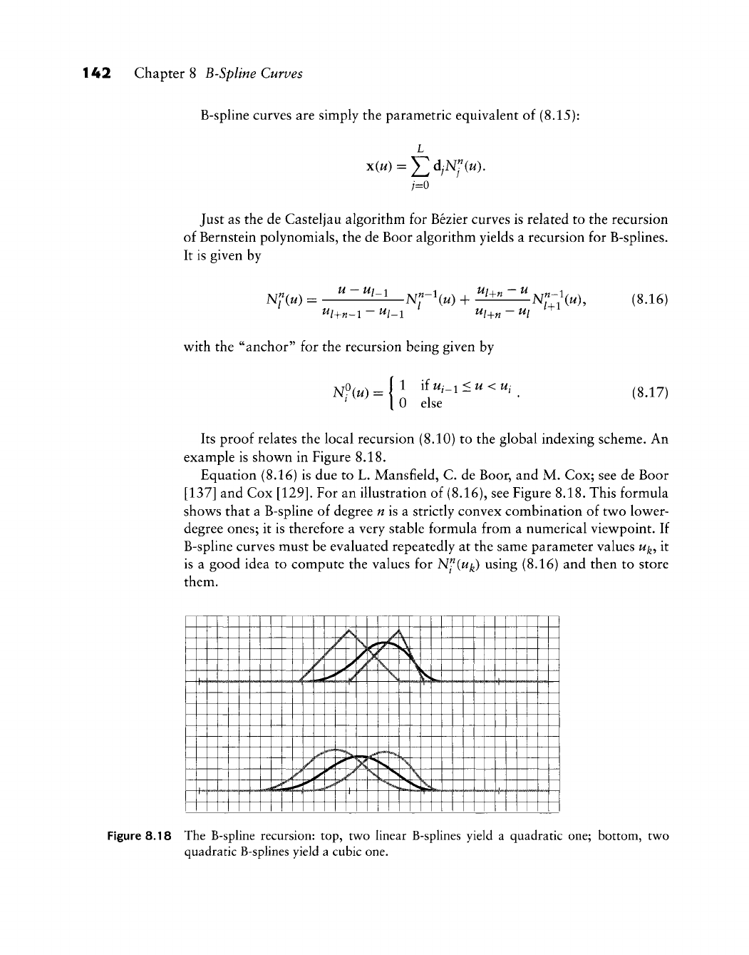
142 Chapter 8 B-Spline Curves
B-spline curves are simply the parametric equivalent of (8.15):
L
x(u) =
J2djNf{u),
;=0
Just as the de Casteljau algorithm for Bezier curves is related to the recursion
of Bernstein polynomials, the de Boor algorithm yields a recursion for B-splines.
It is given by
Nf(u) = ^"^^-^ N^Hu) + ^l^±^ZiiN-i(^), (8.16)
w^ith the "anchor" for the recursion being given by
"?<«' iO else
1 if Ui_i <u <Uj (8.17)
Its proof relates the local recursion (8.10) to the global indexing scheme. An
example is shov^^n in Figure 8.18.
Equation (8.16) is due to L. Mansfield, C. de Boor, and M. Cox; see de Boor
[137] and Cox
[129].
For an illustration of (8.16), see Figure 8.18. This formula
shows that a B-spline of degree
w
is a strictly convex combination of tw^o lower-
degree ones; it is therefore a very stable formula from a numerical viewpoint. If
B-spline curves must be evaluated repeatedly at the same parameter values w^, it
is a good idea to compute the values for N^{uf^) using (8.16) and then to store
them.
T" -
... ...
«...
A
/_
/
A
V
J\
..„
4
f
ri
««»''<
V
'"
k
>^
+-
\
X
V
*•,
y^.^
\
("•^
k
-• .
ffM
-
-
-^.
-'
4.
4-
-
-
...
Figure 8.18 The B-spline recursion: top, two linear B-splines yield a quadratic one; bottom, two
quadratic B-splines yield a cubic one.
8.9 B-Spline Basics 143
A comment on end knot multiplicities: the widespread data format IGES uses
two additional knots at the ends of the knot sequence; in our terms, it adds knots
u_i and ^L+2n-l- The reason is that formulas like (8.16) seemingly require the
presence of these knots. Since they are multiplied only by zero factors, their values
have no influence on any computation. There is no reason to store completely
inconsequential data, and hence the "leaner" notation of this chapter.
8.9 B-Spline Basics
Here, we present a collection of the most important formulas and definitions of
this chapter. As before, n is the (maximal) degree of each polynomial segment,
L + 1 is the number of control points, and K is the number of intervals.
Knot sequence:
{WQ,
...,
Uf^},
Control points: do,..., d^, with L = K -n + 1.
Domain: Curve is only defined over [u^-\^..., u^],
Greville abscissae:
^i
=
^(Uj-\
h
^/-f^-i).
Support: N^ is nonnegative over [w/_i,
^/+„].
Knot insertion: To insert uj <u < w/+i, first find new Greville abscissae |/, then
set new dj = P(|/).
de Boor algorithm: Given uj <u < uj^i^ renumber the relevant control points
d/_^^i,..., Aj^i as do,..., d„ and then set
df
(M)
- (1 - af )df-l(«) + «f df^i^M)
with
for ^ = r + 1,...,
w,
and i = 0,... ,n
—
k. Here, r denotes the multiplicity of
u, (Normally, u is not already in the knot sequence; then, r = 0.)
Mansfield, de Boor, Cox recursion:
Ul+„-l~Ui_^ Ui+„-Ul
144 Chapter 8 B-Spline Curves
Derivative:
-^Nfiu) = N^-\u)
N^-\u),
Derivative of B-spline curve
_d_
Degree elevation:
^»
=
;;^E^rV;^;),
where Nf'^ (u;
Uj)
is defined over the original knot sequence except that the
knot
Uj
has its muhiphcity increased by one. This identity was discovered by
H. Prautzsch in 1984
[493].
Another reference is Barry and Goldman [39].
8.10 Implementation
Here is the header for the de Boor algorithm code:
float deboor(degree,coeff,knot,u,i)
/*
uses
de
Boor algorithm
to
compute
one
coordinate
on
B-spline curve
for
param. value
u in
interval
i.
Input: degree: polynomial degree
of
each piece
of
curve
coeff: B-spline control points
knot: knot sequence
u: evaluation abscissa
i:
u's
interval: u[i]<=
u <
u[i+l]
Output: coordinate value.
V
This program does not need to know about L. The next program generates a
set of points on a whole B-spline curve—for one coordinate, to be honest—so it
has to be called twice for a 2D curve and three times for a 3D curve.
bspl_to_points(degree,1,coeff,knot,dense,points,point_num)
/* generates points on B-spline curve, (one coordinate)
Input: degree: polynomial degree of each piece of curve
1:
number of active intervals
8.10 Implementation 145
coeff:
B-spline control points
knot: knot sequence: knot[0].. .knot[l+2*clegree-2]
dense:
how
many points
per
segment
Output:points: output array with function values.
point_num:
how
many points
are
generated. That number
is
easier computed here than
in the
calling program:
no points
are
generated between multiple knots.
V
The main program deboormai
n. c
generates a postscript plot of a B-spline curve.
A sample input file is in bspl .dat; it creates the outline of the letter r from Figure
5.11.
As a second example, the input data for the y-values of the curve in Figure
8.10 are
degree = 3; 1 = 3; coeff = 1,4,4,0,0,1;
knot = 0,0,0,3,9,12,12,12; dense = 10.
Next, w^e include a B-spline blossom routine:
deboor_blossom(control,degree,deboor,deboor_wts,
knot,uvec,i nterval,poi nt,poi nt_wt)
/*
FUNCTION: deBoor algorithm
to
evaluate
a
B-spline curve blossom.
For polynomial
or
rational curves.
INPUT: control[] [0]: indicates type
of
input curve
0
=
polynomial
1
=
rational
[1]:
indicates
if
input/output
is
in
R3 or
R4;
3
= R3
4
= R4
degree polynomial degree
of
each piece
of
the
input curve, must
be
<=20
deboor[][3] deboor control points
deboor_wts[] rational weights associated with
the control points
if
control[0]=1;
otherwise weights
not
used
146 Chapter 8 B-Spline Curves
knot[] knot sequence with multiplicities
entered explicitly
uvec[] blossom (parameter) values
to evaluate
i
nterval
i
nterval
wi thi n
knot sequence
with which
to
evaluate wrt
u
(typically: i=interval then
knot[i]<=
u <
knot[i+l])
OUTPUT: point [3]
point_wt
evaluation point;
depending on control[] values,
this point will be in R3 or R4
if control[0]=1 then this is the
rational weight associated with
the point
8.11 Problems
1 For the case of a planar parametric B-spHne curve, does symmetry of the
polygon with respect to the y-axis imply that same symmetry for the curve?
Derive (8.16) from (8.10).
Find the Bezier points of the closed B-spline curves of degree four whose
control polygons consist of the edges of a square and have (a) uniform knot
spacing and simple knots and (b) uniform knot spacing and knots all with
multiplicity two.
PI Use de_boor_blossom to program degree elevation for B-spline curves.
*2
*3
Constructing Spline
Curves
/V spline is a flexible rod of wood or plastic. It has its origins in shipbuilding,
where splines were used to draft the curves (ribs) that define a ship body. Early
uses go back to the 1600s, and are documented in
[450].
Although mechanical
splines are used less frequently now, the underlying principle still gives rise to
new algorithms.
9.1 Greville Interpolation
In Chapter 7, we saw how to pass a polynomial curve of degree n through
n
-\-
1 data points Po?
• • • ? Pw
with parameter values
^Q?
• • • ?
^w The key to the
solvability of the problem was simple: the number of knowns (the data points
with parameter values) had to equal the number of unknowns (the polynomial
coefficients).
Something quite analogous happens in a spline context. A spline curve of
degree n is defined over a knot sequence
UQ,
.. .
^
u^^.
Such a knot sequence has
K
—
n-\-2 Greville abscissae ^/ and hence the spline curve has L-^1 = K
—
n-\-2
B-spline control points do,..., d^^.
In view of these numbers, the following is a meaningful interpolation problem:
Given: A knot sequence
WQ,
...,
w^^
and a degree n, also a set of data points
po ...
PL
with L = K
—
n-\-l.
Find: A set of B-spline control points dg,..., d^ such that the resulting curve
x(u) satisfies
x(?/) =
P,-;
i =
0,...,L.
(9.1)
147
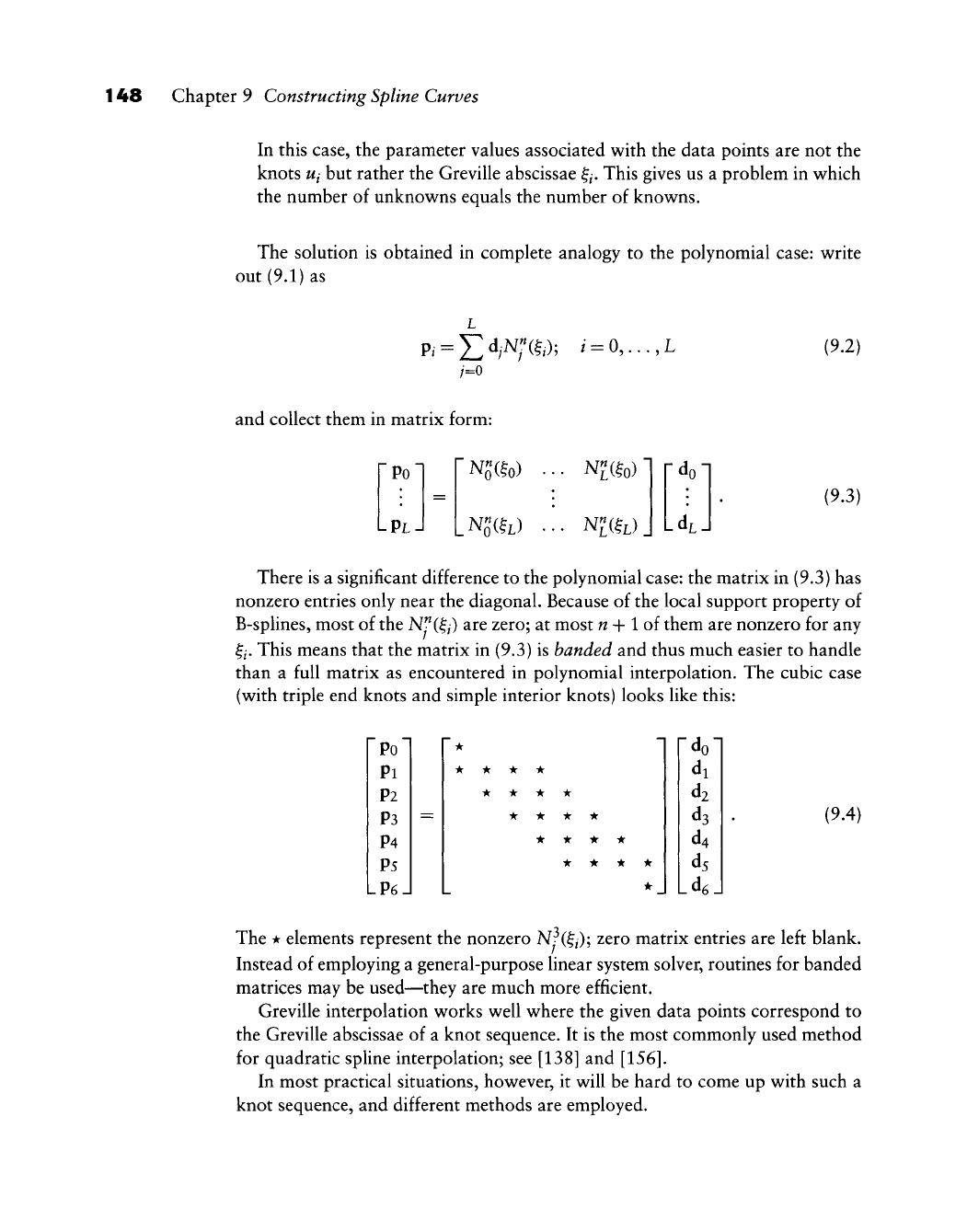
148 Chapter 9 Constructing Spline Curves
In this case, the parameter values associated with the data points are not the
knots
Ui
but rather the Greville abscissae
§^.
This gives us a problem in which
the number of unknowns equals the number of knowns.
The solution is obtained in complete analogy to the polynomial case: write
out (9.1) as
p,=:^dyN;(?,); / =
0,...,L
/=0
(9.2)
and collect them in matrix form:
Po
LPLJ
NS(to)
l^Hh)
N?(^o)
N£(IL)J LdJ
(9.3)
There is a significant difference to the polynomial case: the matrix in (9.3) has
nonzero entries only near the diagonal. Because of the local support property of
B-splines, most of the N^i^j) are zero; at most
w
+ 1 of them are nonzero for any
§^. This means that the matrix in (9.3) is banded and thus much easier to handle
than a full matrix as encountered in polynomial interpolation. The cubic case
(with triple end knots and simple interior knots) looks like this:
Po"
Pi
P2
P3
P4
P5
P6-
"•
* * * *
• * * •
• * * •
• * * *
* • * •
•
_
fdo
di
d2
ds
d4
ds
Ld6
(9.4)
The * elements represent the nonzero N^(§/); zero matrix entries are left blank.
Instead of employing a general-purpose linear system solver, routines for banded
matrices may be used—they are much more efficient.
Greville interpolation works well where the given data points correspond to
the Greville abscissae of a knot sequence. It is the most commonly used method
for quadratic spline interpolation; see [138] and
[156].
In most practical situations, however, it will be hard to come up with such a
knot sequence, and different methods are employed.
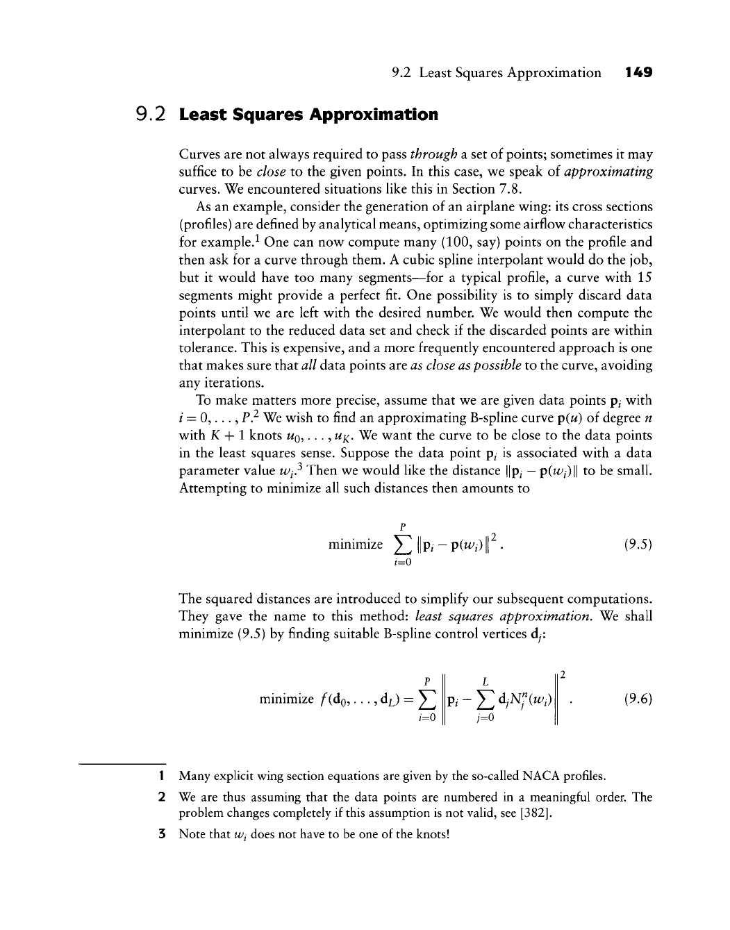
9.2 Least Squares Approximation 149
9.2 Least Squares Approximation
Curves are not always required to pass through a set of points; sometimes it may
suffice to be close to the given points. In this case, we speak of approximating
curves. We encountered situations Hke this in Section 7.8.
As an example, consider the generation of an airplane wing: its cross sections
(profiles) are defined by analytical means, optimizing some airflow characteristics
for example.^ One can now compute many (100, say) points on the profile and
then ask for a curve through them. A cubic spline interpolant would do the job,
but it would have too many segments—for a typical profile, a curve with 15
segments might provide a perfect fit. One possibility is to simply discard data
points until we are left with the desired number. We would then compute the
interpolant to the reduced data set and check if the discarded points are within
tolerance. This is expensive, and a more frequently encountered approach is one
that makes sure that all data points are as close as possible to the curve, avoiding
any iterations.
To make matters more precise, assume that we are given data points p^ with
/ = 0,. .., F? We wish to find an approximating B-spline curve p(w) of degree n
with K-\-\ knots
WQ?
• • • 5
^x- ^^ want the curve to be close to the data points
in the least squares sense. Suppose the data point p^ is associated with a data
parameter value Wi? Then we would like the distance ||p^
—
pCu^/)!!
to be small.
Attempting to minimize all such distances then amounts to
minimize Y^ ||p^
—
p(w//) | (9.5)
The squared distances are introduced to simplify our subsequent computations.
They gave the name to this method: least squares approximation. We shall
minimize (9.5) by finding suitable B-spline control vertices dy:
minimize /^(do,..., d^^) = 2_. p,-^d,N;(u/,) (9.6)
1 Many explicit wing section equations are given by the so-called NACA profiles.
2 We are thus assuming that the data points are numbered in a meaningful order. The
problem changes completely if this assumption is not valid, see
[382].
3 Note that
Wi
does not have to be one of the knots!
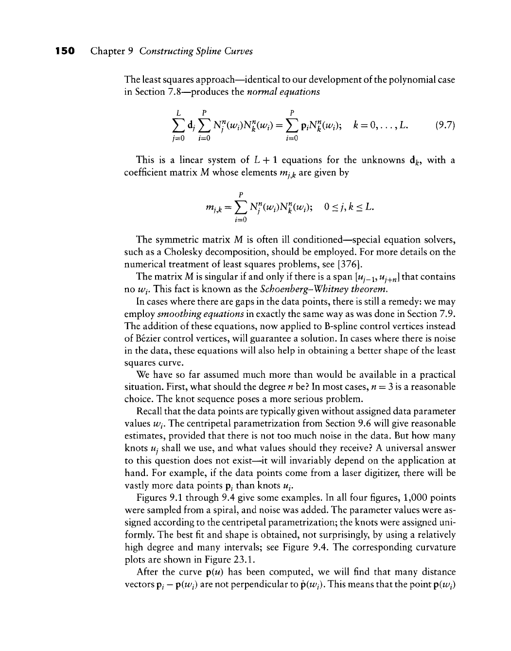
150 Chapter 9 Constructing Spline Curves
The least squares approach—identical to our development of the polynomial case
in Section 7.8—produces the normal equations
LP P
Y,
d;
J2
Nf(Wi)NliWi) =
J2 PtK(^i); fe = 0,...,
L.
(9.7)
This is a linear system of L + 1 equations for the unknowns d^, with a
coefficient matrix M whose elements my^^ are given by
p
The symmetric matrix M is often ill conditioned—special equation solvers,
such as a Cholesky decomposition, should be employed. For more details on the
numerical treatment of least squares problems, see
[376].
The matrix M is singular if and only if there is a span
[^y_i,
Uj_^^]
that contains
no Wj. This fact is known as the Schoenberg-Whitney theorem.
In cases where there are gaps in the data points, there is still a remedy: we may
employ smoothing equations in exactly the same way as was done in Section 7.9.
The addition of these equations, now applied to B-spline control vertices instead
of Bezier control vertices, will guarantee a solution. In cases where there is noise
in the data, these equations will also help in obtaining a better shape of the least
squares curve.
We have so far assumed much more than would be available in a practical
situation. First, what should the degree n ht} In most cases,
w
= 3 is a reasonable
choice. The knot sequence poses a more serious problem.
Recall that the data points are typically given without assigned data parameter
values Wi. The centripetal parametrization from Section 9.6 will give reasonable
estimates, provided that there is not too much noise in the data. But how many
knots
Uj
shall we use, and what values should they receive? A universal answer
to this question does not exist—it will invariably depend on the application at
hand. For example, if the data points come from a laser digitizer, there will be
vastly more data points p^ than knots w/.
Figures 9.1 through 9.4 give some examples. In all four figures, 1,000 points
were sampled from a spiral, and noise was added. The parameter values were as-
signed according to the centripetal parametrization; the knots were assigned uni-
formly. The best fit and shape is obtained, not surprisingly, by using a relatively
high degree and many intervals; see Figure 9.4. The corresponding curvature
plots are shown in Figure 23.1.
After the curve p(w) has been computed, we will find that many distance
vectors
p^
—
p(w//) are not perpendicular to
p(w^/).
This means that the point p(w//)
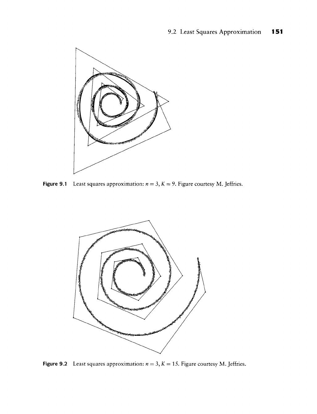
9.2 Least Squares Approximation 151
Figure 9.1 Least squares approximation: n = 3,K = 9. Figure courtesy M. Jeffries.
Figure 9.2 Least squares approximation: n = 3,K = 15. Figure courtesy M. Jeffries.
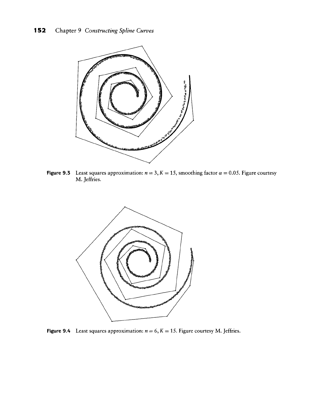
152 Chapter 9 Constructing Spline Curves
Figure 9.3 Least squares approximation:
w
= 3, K = 15, smoothing factor a = 0.05. Figure courtesy
M. Jeffries.
Figure 9.4 Least squares approximation: n = 6,K = 15. Figure courtesy M. Jeffries.
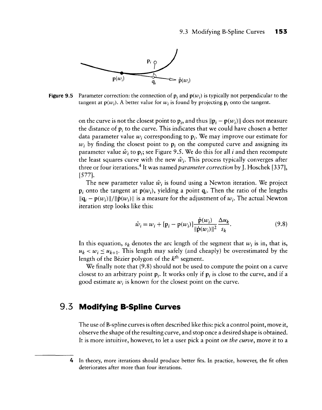
9.3 Modifying B-Spline Curves 153
Figure 9.5 Parameter correction: the connection of
p^
and piwj) is typically not perpendicular to the
tangent at
p(Wi).
A better value for
Wj
is found by projecting pi onto the tangent.
on the curve is not the closest point to
p^,
and thus ||p^
—
piWj)
\\
does not measure
the distance of p/ to the curve. This indicates that we could have chosen a better
data parameter value Wj corresponding to p/. We may improve our estimate for
Wj by finding the closest point to p^ on the computed curve and assigning its
parameter value Wj to
p^;
see Figure 9.5. We do this for all / and then recompute
the least squares curve with the new Wj, This process typically converges after
three or four iterations."* It was named parameter correction by
J.
Hoschek
[337],
[577].
The new parameter value Wi is found using a Newton iteration. We project
p^
onto the tangent at p(u^^), yielding a point q^. Then the ratio of the lengths
llq^
—
p(t6'/)||/||p(t^^/)|| is a measure for the adjustment of
Wi,
The actual Newton
iteration step looks like this:
^. = "^. + [p.-pK)]^^^. (9.8)
llpKOIr sk
In this equation, s^ denotes the arc length of the segment that Wi is in, that is,
Uj^
< Wi <
Uj^^i.
This length may safely (and cheaply) be overestimated by the
length of the Bezier polygon of the k}^ segment.
We finally note that (9.8) should not be used to compute the point on a curve
closest to an arbitrary point p/. It works only if
p^
is close to the curve, and if a
good estimate Wi is known for the closest point on the curve.
9.5 Modifying B-Spline Curves
The use of B-spline curves is often described like
this:
pick a control point, move it,
observe the shape of the resulting curve, and stop once a desired shape is obtained.
It is more intuitive, however, to let a user pick a point on the curve^ move it to a
4 In theory, more iterations should produce better fits. In practice, however, the fit often
deteriorates after more than four iterations.
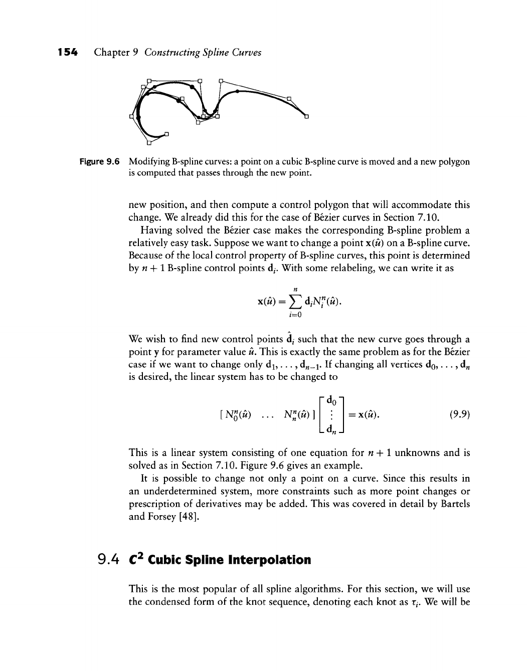
154 Chapter 9 Constructing Spline Curves
Figure 9.6 Modifying B-spline
curves:
a point on a cubic B-spline curve is moved and a new polygon
is computed that passes through the new point.
new position, and then compute a control polygon that will accommodate this
change. We already did this for the case of Bezier curves in Section 7.10.
Having solved the Bezier case makes the corresponding B-spline problem a
relatively easy task. Suppose we want to change a point x(u) on a B-spline curve.
Because of the local control property of B-spline curves, this point is determined
by n + 1 B-spline control points d^. With some relabeling, we can write it as
n
We wish to find new control points d^ such that the new curve goes through a
point y for parameter value u. This is exactly the same problem as for the Bezier
case if we want to change only
dj,...,
d„_i. If changing all vertices do,..., d„
is desired, the linear system has to be changed to
[N^(u)
N"„(u)
]
Ld„
= X(M). (9.9)
This is a linear system consisting of one equation for
w
+ 1 unknowns and is
solved as in Section 7.10. Figure 9.6 gives an example.
It is possible to change not only a point on a curve. Since this results in
an underdetermined system, more constraints such as more point changes or
prescription of derivatives may be added. This was covered in detail by Bartels
and Forsey [48].
9.4 C^ Cubic Spline Interpolation
This is the most popular of all spline algorithms. For this section, we will use
the condensed form of the knot sequence, denoting each knot as
Xj,
We will be
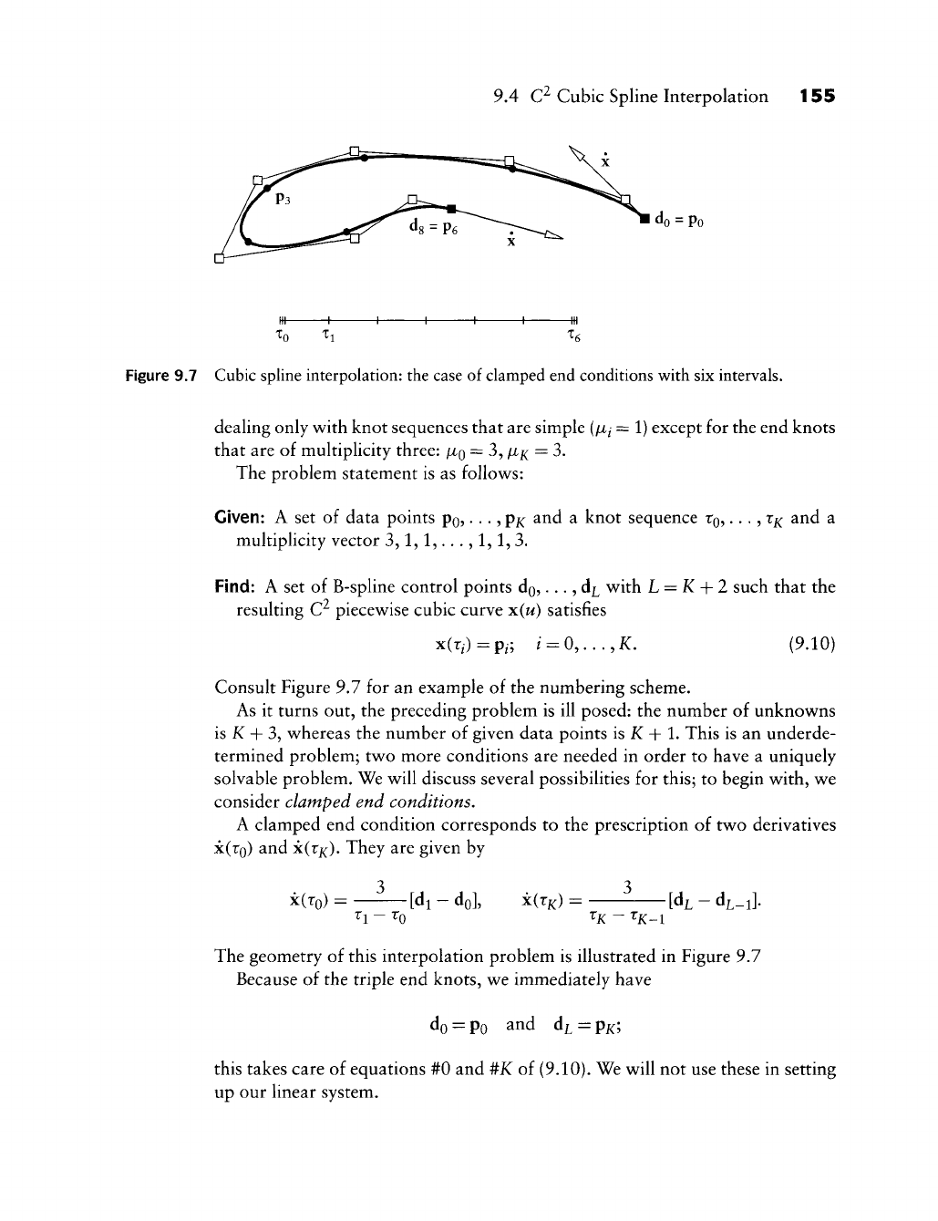
9.4 C^ Cubic Spline Interpolation 155
do
=
Po
XQ X^ Xg
Figure 9.7 Cubic spline interpolation: the case of clamped end conditions with six intervals.
dealing only with knot sequences that are simple (/x^ = 1) except for the end knots
that are of multiplicity three:
/XQ
= 3,
/Xj^;
= 3.
The problem statement is as follows:
Given: A set of data points Po?
• • • ?
Px ^nd a knot sequence
TQ,
...,
T]^
and a
multiplicity vector 3,1,1,...,1,1,3.
Find: A set of B-spline control points do,..., d^^ with L = K -\-2 such that the
resulting C^ piecewise cubic curve x(u) satisfies
x(r,) =
p,-;
/ =
0,...,K.
(9.10)
Consult Figure 9.7 for an example of the numbering scheme.
As it turns out, the preceding problem is ill posed: the number of unknowns
is K + 3, whereas the number of given data points is K + 1. This is an underde-
termined problem; two more conditions are needed in order to have a uniquely
solvable problem. We will discuss several possibilities for this; to begin with, we
consider clamped end conditions,
A clamped end condition corresponds to the prescription of two derivatives
x(ro) and x(rx). They are given by
3 3
x(ro) = [di - do], xCr^) =
[d^^
-
d^-i].
Ti - to tx - Tj^-\
The geometry of this interpolation problem is illustrated in Figure 9.7
Because of the triple end knots, we immediately have
do = Po and di^ = px;
this takes care of equations #0 and #X of (9.10). We will not use these in setting
up our linear system.
156 Chapter 9 Constructing Spline Curves
The clamped end conditions yield
di = do + ^^^x(ro) and d,^_i = d^, - ^^^^^xCr^).
Thus,
the first and last equations of our linear system become
d2N|(ri) + daN^Cri) = r, and ^L-?>^1-2>^-^K-\) + ^L-l^l-ii^K-i) =
^e
with
rs = Pi-diN^(ri) and r^ =
PK-1
- dL-iN^_i(rK-i).
Each of the remaining unknowns
d25...,
dj^_2 is related to the data points by
one equation. Because of the local support property of cubic B-splines, it is of
the form
p,
= d,N3(r,) + d,+iN^i(r,) +
Ai^rn]^-^{x>);
i = 2,...,K-2. (9.11)
Together, these are iC
—
1 equations for the K
—
1 unknown control points. In
matrix form, we have
N|(T2)
Ni_3(rK_2) Ni_2(TK_2) H-l(-'K-2)
L^L-2
P2
PK-2
L r^
(9.12)
Schematically, the case K = 5 looks like this:
* •
• • •
• • •
• •
d2
ds
d4
Ids]
ts
P2
P3
.^e]
The entries in this tridiagonal matrix are easily computed from the definitions
of the cubic B-splines Nf,
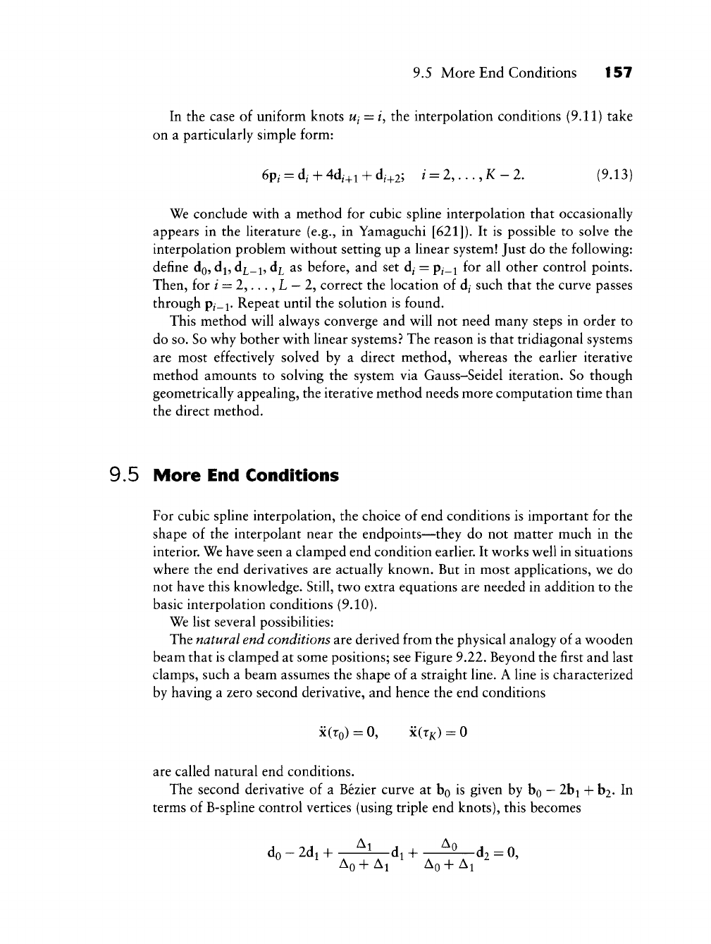
9.5 More End Conditions 157
In the case of uniform knots
Ui
= /, the interpolation conditions (9.11) take
on a particularly simple form:
6p,-
= d, + 4d,+i + d,+2; / =
2,...,
X - 2. (9.13)
We conclude with a method for cubic spline interpolation that occasionally
appears in the literature (e.g., in Yamaguchi [621]). It is possible to solve the
interpolation problem without setting up a linear system! Just do the following:
define do, d^, dj^_i, d^^ as before, and set d/ = p/_i for all other control points.
Then, for / =
2,...,
L
—
2, correct the location of d^ such that the curve passes
through p^_i. Repeat until the solution is found.
This method will always converge and will not need many steps in order to
do so. So why bother with linear systems? The reason is that tridiagonal systems
are most effectively solved by a direct method, whereas the earlier iterative
method amounts to solving the system via Gauss-Seidel iteration. So though
geometrically appealing, the iterative method needs more computation time than
the direct method.
9.5 More End Conditions
For cubic spline interpolation, the choice of end conditions is important for the
shape of the interpolant near the endpoints—they do not matter much in the
interior. We have seen a clamped end condition earlier. It works well in situations
where the end derivatives are actually known. But in most applications, we do
not have this knowledge. Still, two extra equations are needed in addition to the
basic interpolation conditions (9.10).
We list several possibilities:
The natural end conditions are derived from the physical analogy of a wooden
beam that is clamped at some positions; see Figure 9.22. Beyond the first and last
clamps, such a beam assumes the shape of a straight line. A line is characterized
by having a zero second derivative, and hence the end conditions
x(ro) = 0, x(rx) = 0
are called natural end conditions.
The second derivative of a Bezier curve at bo is given by bo
—
2bi + b2. In
terms of B-spline control vertices (using triple end knots), this becomes
do
- 2di + -4^di + -4^d2 = 0,
AA+AI An + A,

158 Chapter 9 Constructing Spline Curves
where we set A^ = r^+i
—
r^ We rearrange and obtain
(Ao + Ai)do - (2Ao + Ai)di + Aod2 = 0. (9.14)
A similar condition holds at the other endpoint. Unless required by a specific
application, this end condition should be avoided since it forces the curve to
behave linearly near the endpoints.
Typically another end condition, called Bessel end condition, yields better
results. It works as follows: the first three data points and their parameter values
determine an interpolating quadratic curve. Its first derivative at po is taken to
be the one for the spline curve. If we set
a = — and
j6
=
1
—
of
^2 -
"^0
and
1
lap
then
2 1
di=-(apo + ^a) + -po.
This value for dj is then used in the earlier clamped end condition. The control
point d£^_i is obtained in complete analogy; it is then also used for a clamped
end condition.
Other end conditions exist: requiring x(ro) = x(ri) is called a quadratic end
condition. If all data points and parameter values were read off from a quadratic
curve, then this condition would ensure that the spline interpolant reproduces
that quadratic. The same is true, of course, for the Bessel end conditions. If
the first and second cubic segment are parts of one cubic, then their third
derivatives at X\ would agree. The corresponding end condition is called not-
a-knot condition since the knot r^ does not act as a breakpoint between two
distinct cubic segments.
We finish this section with a few examples, courtesy T. Foley, using uni-
form parameter values in all examples.^ Figure 9.8 shows equally spaced data
5 Owing to the symmetry inherent in the data points, all parametrizations discussed later
yield the same knot spacing. All circle plots are scaled down in the }/-direction.
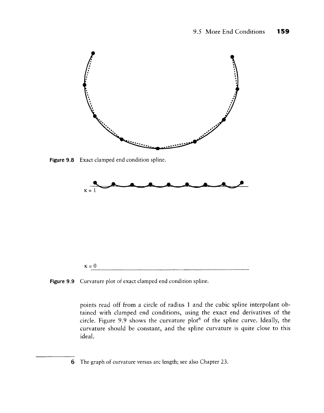
9.5 More End Conditions 159
Figure 9.8 Exact clamped end condition spline.
K=l
K=0
Figure 9.9 Curvature plot of exact clamped end condition spline.
points read off from a circle of radius 1 and the cubic spline interpolant ob-
tained with clamped end conditions, using the exact end derivatives of the
circle. Figure 9.9 show^s the curvature plot^ of the spline curve. Ideally, the
curvature should be constant, and the spline curvature is quite close to this
ideal.
6 The graph of curvature versus arc length; see also Chapter 23.
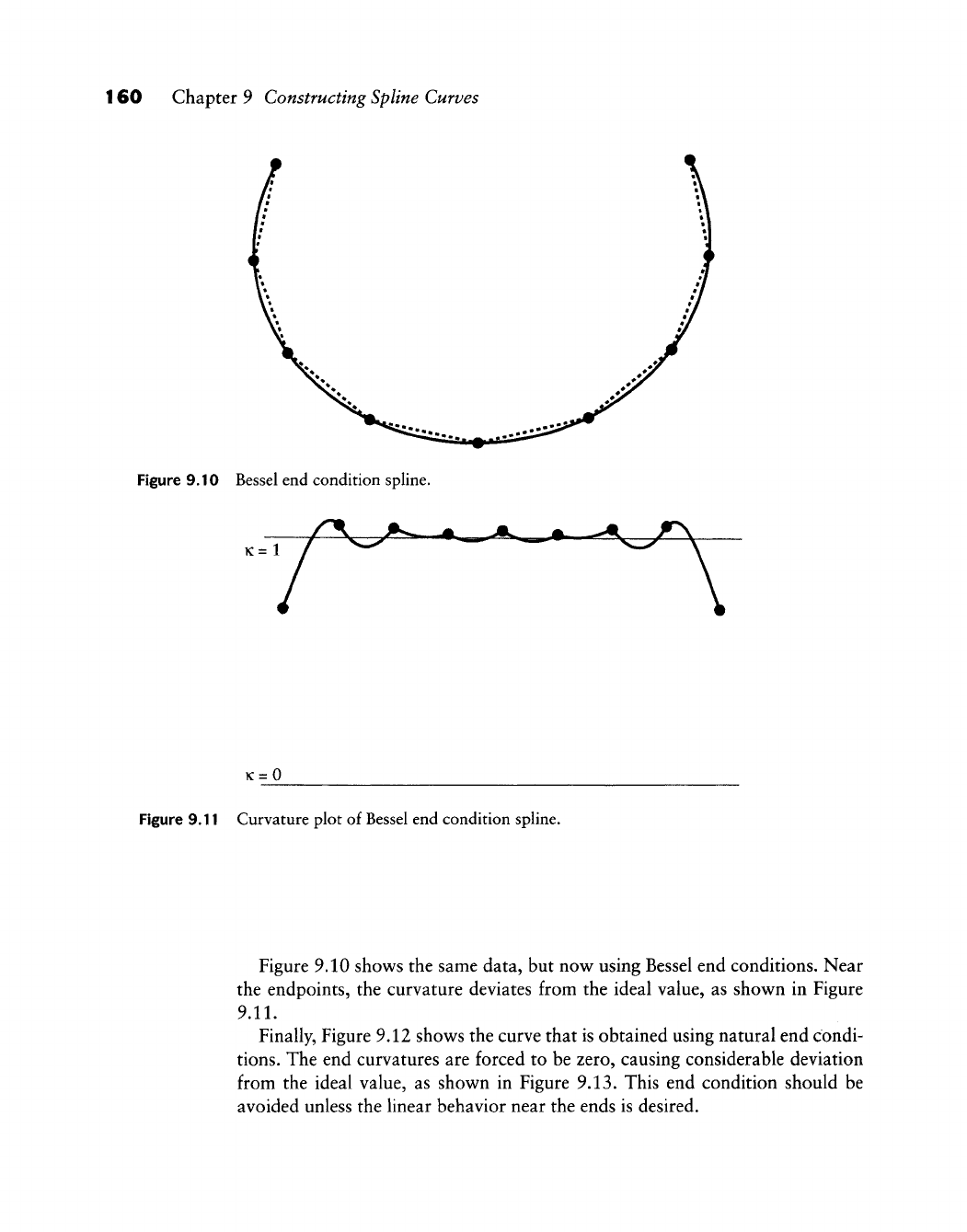
160 Chapter 9 Constructing Spline Curves
Figure 9.10 Bessel end condition spline.
K=l
K=0
Figure 9.11 Curvature plot of Bessel end condition spline.
Figure 9.10 shows the same data, but now using Bessel end conditions. Near
the endpoints, the curvature deviates from the ideal value, as shown in Figure
9.11.
Finally, Figure 9.12 shows the curve that is obtained using natural end condi-
tions.
The end curvatures are forced to be zero, causing considerable deviation
from the ideal value, as shown in Figure 9.13. This end condition should be
avoided unless the linear behavior near the ends is desired.
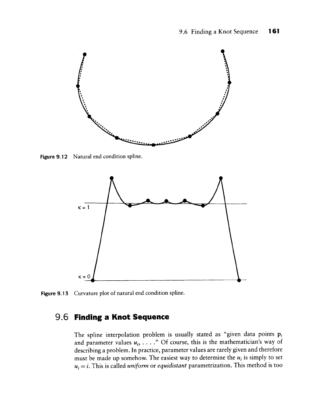
9.6 Finding a Knot Sequence 161
Figure 9.12 Natural end condition spline.
K=l
K=0
Figure 9.13 Curvature plot of natural end condition spline.
9.6 Finding a Knot Sequence
The spline interpolation problem is usually stated as "given data points p^
and parameter values w^, . ..." Of course, this is the mathematician's way of
describing a problem. In practice, parameter values are rarely given and therefore
must be made up somehow. The easiest way to determine the ui is simply to set
Ui
= i. This is called uniform or equidistant parametrization. This method is too
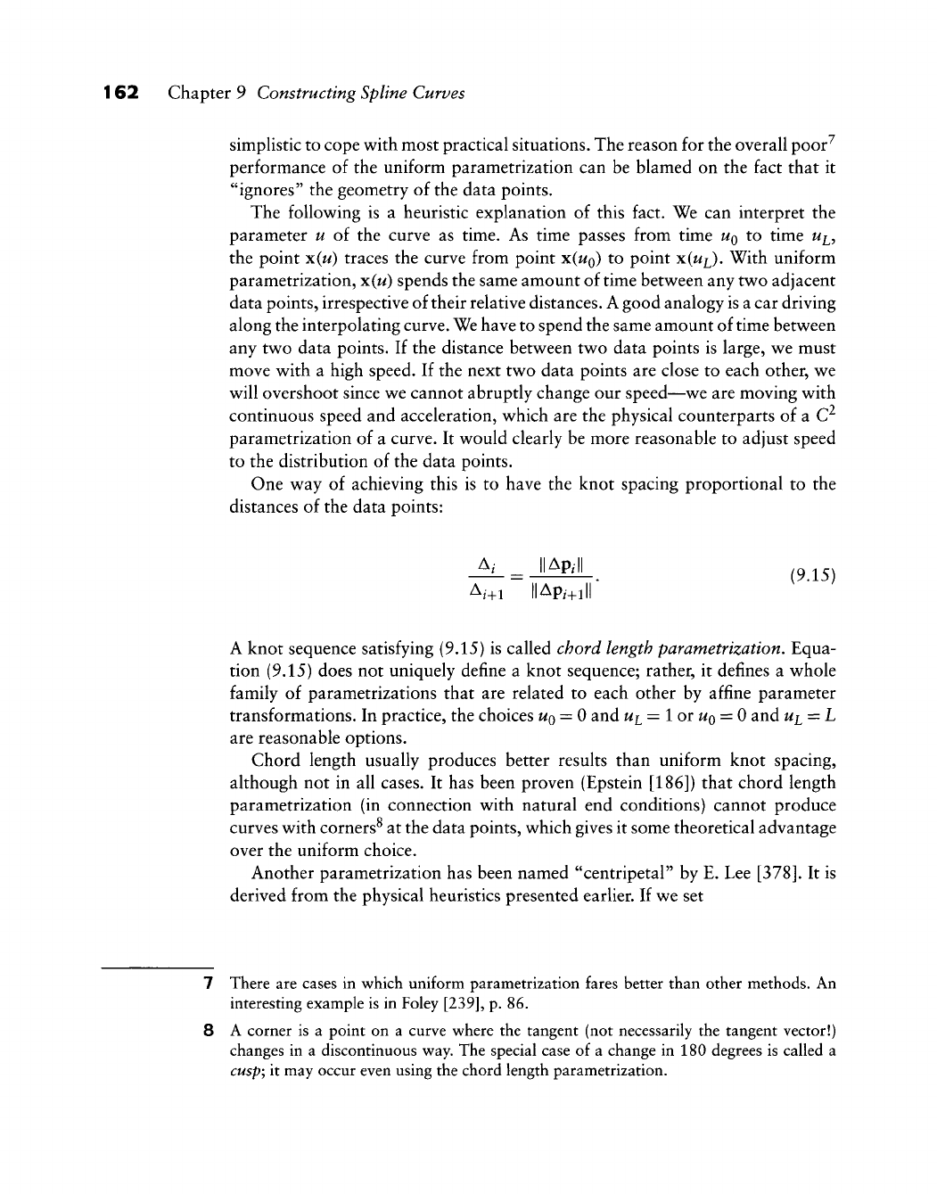
162 Chapter 9 Constructing Spline Curves
simplistic to cope with most practical situations. The reason for the overall poor^
performance of the uniform parametrization can be blamed on the fact that it
"ignores" the geometry of the data points.
The following is a heuristic explanation of this fact. We can interpret the
parameter u of the curve as time. As time passes from time
UQ
to time u^^
the point x(w) traces the curve from point x(wo) ^^ point x(wj^). With uniform
parametrization, x(w) spends the same amount of time between any two adjacent
data points, irrespective of their relative distances. A good analogy is a car driving
along the interpolating curve. We have to spend the same amount of time between
any two data points. If the distance between two data points is large, we must
move with a high speed. If the next two data points are close to each other, we
will overshoot since we cannot abruptly change our speed—we are moving with
continuous speed and acceleration, which are the physical counterparts of a C^
parametrization of a curve. It would clearly be more reasonable to adjust speed
to the distribution of the data points.
One way of achieving this is to have the knot spacing proportional to the
distances of the data points:
A. _ IIAp.ll (9^^^)
A,+i ||Ap,-+i||
A knot sequence satisfying (9.15) is called chord length parametrization. Equa-
tion (9.15) does not uniquely define a knot sequence; rather, it defines a whole
family of parametrizations that are related to each other by affine parameter
transformations. In practice, the choices
UQ
= 0 and
ui^
=
lor:uQ^
= 0 and ui = L
are reasonable options.
Chord length usually produces better results than uniform knot spacing,
although not in all cases. It has been proven (Epstein [186]) that chord length
parametrization (in connection with natural end conditions) cannot produce
curves with corners^ at the data points, which gives it some theoretical advantage
over the uniform choice.
Another parametrization has been named "centripetal" by E. Lee
[378].
It is
derived from the physical heuristics presented earlier. If we set
There are cases in which uniform parametrization fares better than other methods. An
interesting example is in Foley
[239],
p. 86.
A corner is a point on a curve where the tangent (not necessarily the tangent vector!)
changes in a discontinuous way. The special case of a change in 180 degrees is called a
cusp;
it may occur even using the chord length parametrization.
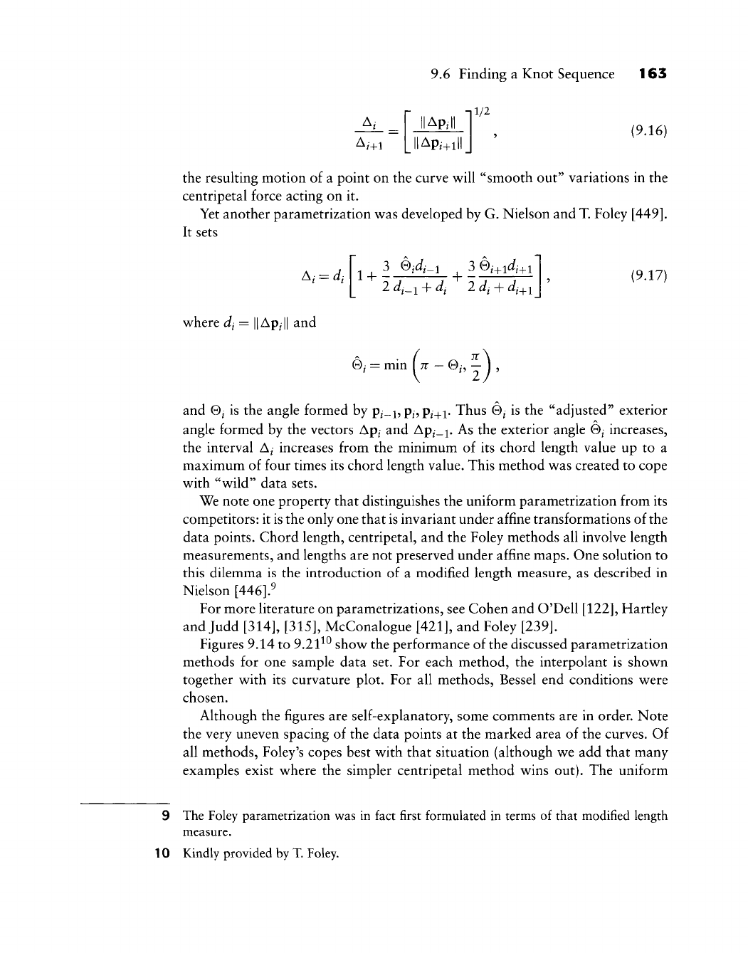
A,+i
9.6 Finding a Knot Sequence 163
,1/2
lApil'
|Api+ill (9.16)
the resulting motion of a point on the curve will "smooth out" variations in the
centripetal force acting on it.
Yet another parametrization v^as developed by G. Nielson and T. Foley
[449].
It sets
A,-
= di
where dj =
||
Ap^||
and
^ 3 Q/4-1 3 0^+i4fl
2 di_i + dj 2 dj -h
di_^i
(9.17)
0; = min
(.-e,.|).
and 0/ is the angle formed by p/-i, P/, p^+i- Thus 0^ is the "adjusted" exterior
angle formed by the vectors Ap/ and
Ap^.j.
As the exterior angle 0^ increases,
the interval A^ increases from the minimum of its chord length value up to a
maximum of four times its chord length value. This method was created to cope
with "wild" data sets.
We note one property that distinguishes the uniform parametrization from its
competitors: it is the only one that is invariant under affine transformations of the
data points. Chord length, centripetal, and the Foley methods all involve length
measurements, and lengths are not preserved under affine maps. One solution to
this dilemma is the introduction of a modified length measure, as described in
Nielson
[446].^
For more literature on parametrizations, see Cohen and O'Dell
[122],
Hartley
and Judd
[314], [315],
McConalogue
[421],
and Foley
[239].
Figures 9.14 to
9.21^^
show the performance of the discussed parametrization
methods for one sample data set. For each method, the interpolant is shown
together with its curvature plot. For all methods, Bessel end conditions were
chosen.
Although the figures are self-explanatory, some comments are in order. Note
the very uneven spacing of the data points at the marked area of the curves. Of
all methods, Foley's copes best with that situation (although we add that many
examples exist where the simpler centripetal method wins out). The uniform
9 The Foley parametrization was in fact first formulated in terms of that modified length
measure.
10 Kindly provided by
T.
Foley.
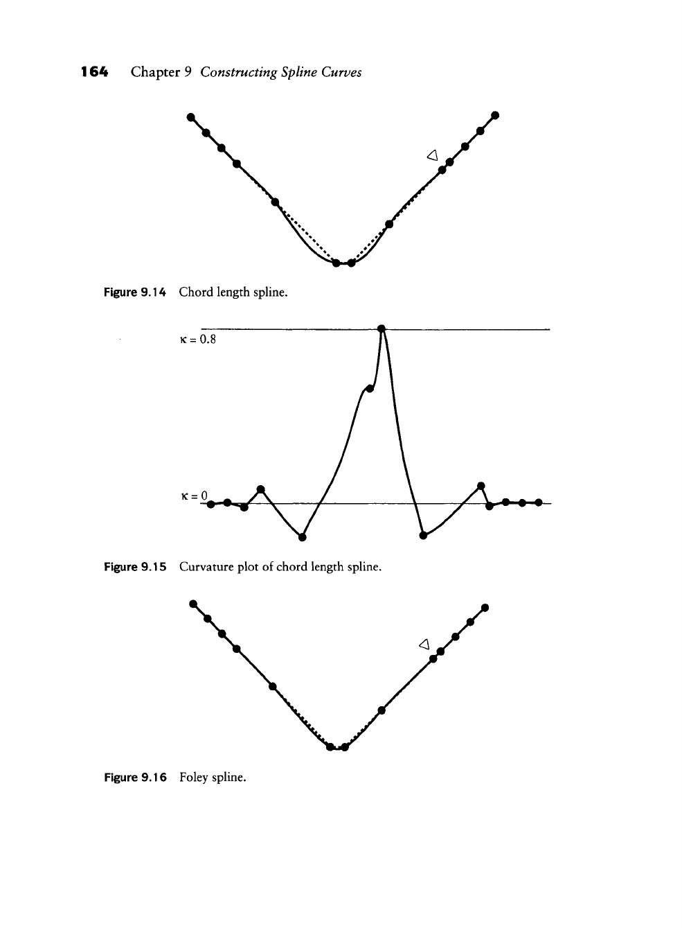
164 Chapter 9 Constructing Spline Curves
Figure 9.14 Chord length sphne.
K =
0.8
Figure 9.15 Curvature plot of chord length spUne.
Figure 9.16 Foley spline.
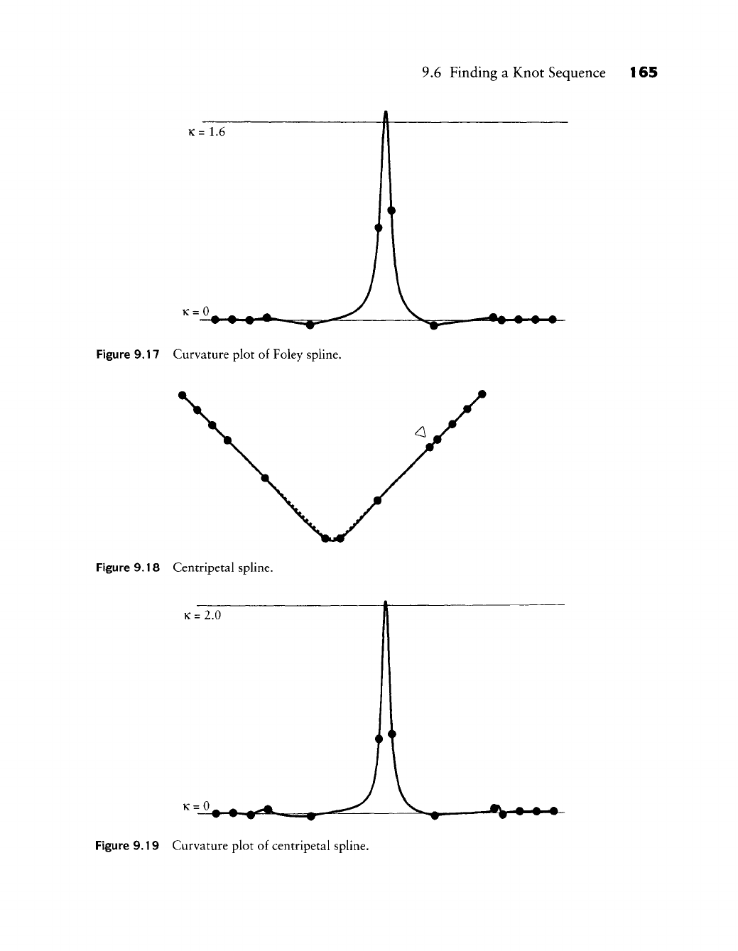
9.6 Finding a Knot Sequence 165
K= 1.6
K=0
Figure 9.17 Curvature plot of Foley spline.
Figure 9.18 Centripetal spline.
K =
2.0
K=0
Figure 9.19 Curvature plot of centripetal spline.
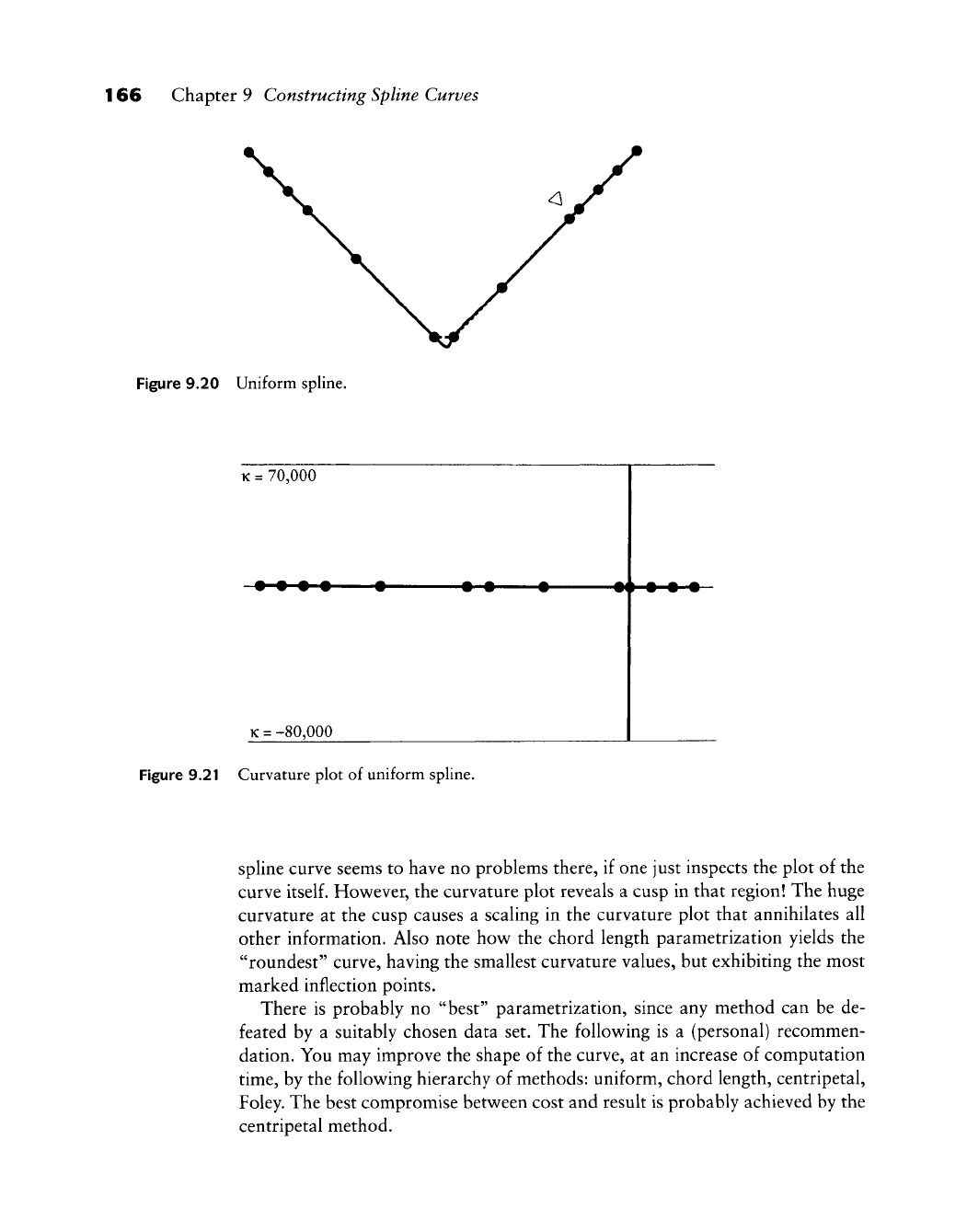
166 Chapter 9 Constructing Spline Curves
Figure 9.20 Uniform spline.
K =
70,000
• • • • • • • • •• • • •
K =
-80,000
Figure 9.21 Curvature plot of uniform spline.
Spline curve seems to have no problems there, if one just inspects the plot of the
curve
itself.
However, the curvature plot reveals a cusp in that region! The huge
curvature at the cusp causes a scaling in the curvature plot that annihilates all
other information. Also note hov^ the chord length parametrization yields the
"roundest" curve, having the smallest curvature values, but exhibiting the most
marked inflection points.
There is probably no "best" parametrization, since any method can be de-
feated by a suitably chosen data set. The foUov^ing is a (personal) recommen-
dation. You may improve the shape of the curve, at an increase of computation
time,
by the follov^ing hierarchy of methods: uniform, chord length, centripetal,
Foley. The best compromise betv^een cost and result is probably achieved by the
centripetal method.
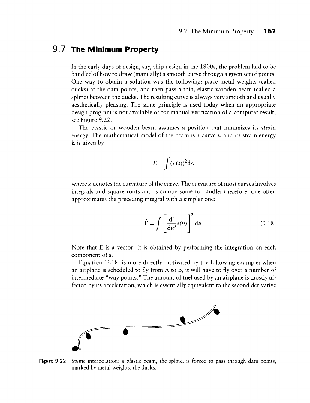
9.7 The Minimum Property 167
9.7 The Minimum Property
In the early days of design, say, ship design in the 1800s, the problem had to be
handled of how to draw (manually) a smooth curve through a given set of points.
One way to obtain a solution was the following: place metal weights (called
ducks) at the data points, and then pass a thin, elastic wooden beam (called a
spline) between the ducks. The resulting curve is always very smooth and usually
aesthetically pleasing. The same principle is used today when an appropriate
design program is not available or for manual verification of a computer result;
see Figure 9.22.
The plastic or wooden beam assumes a position that minimizes its strain
energy. The mathematical model of the beam is a curve s, and its strain energy
£ is given by
h
(s)fds,
where
/c
denotes the curvature of the curve. The curvature of most curves involves
integrals and square roots and is cumbersome to handle; therefore, one often
approximates the preceding integral with a simpler one:
-/ s{u)
du.
(9.18)
Note that E is a vector; it is obtained by performing the integration on each
component of s.
Equation (9.18) is more directly motivated by the following example: when
an airplane is scheduled to fly from A to B, it will have to fly over a number of
intermediate "way points." The amount of fuel used by an airplane is mostly af-
fected by its acceleration, which is essentially equivalent to the second derivative
j^
Figure 9.22 Spline interpolation: a plastic beam, the spline, is forced to pass through data points,
marked by metal weights, the ducks.
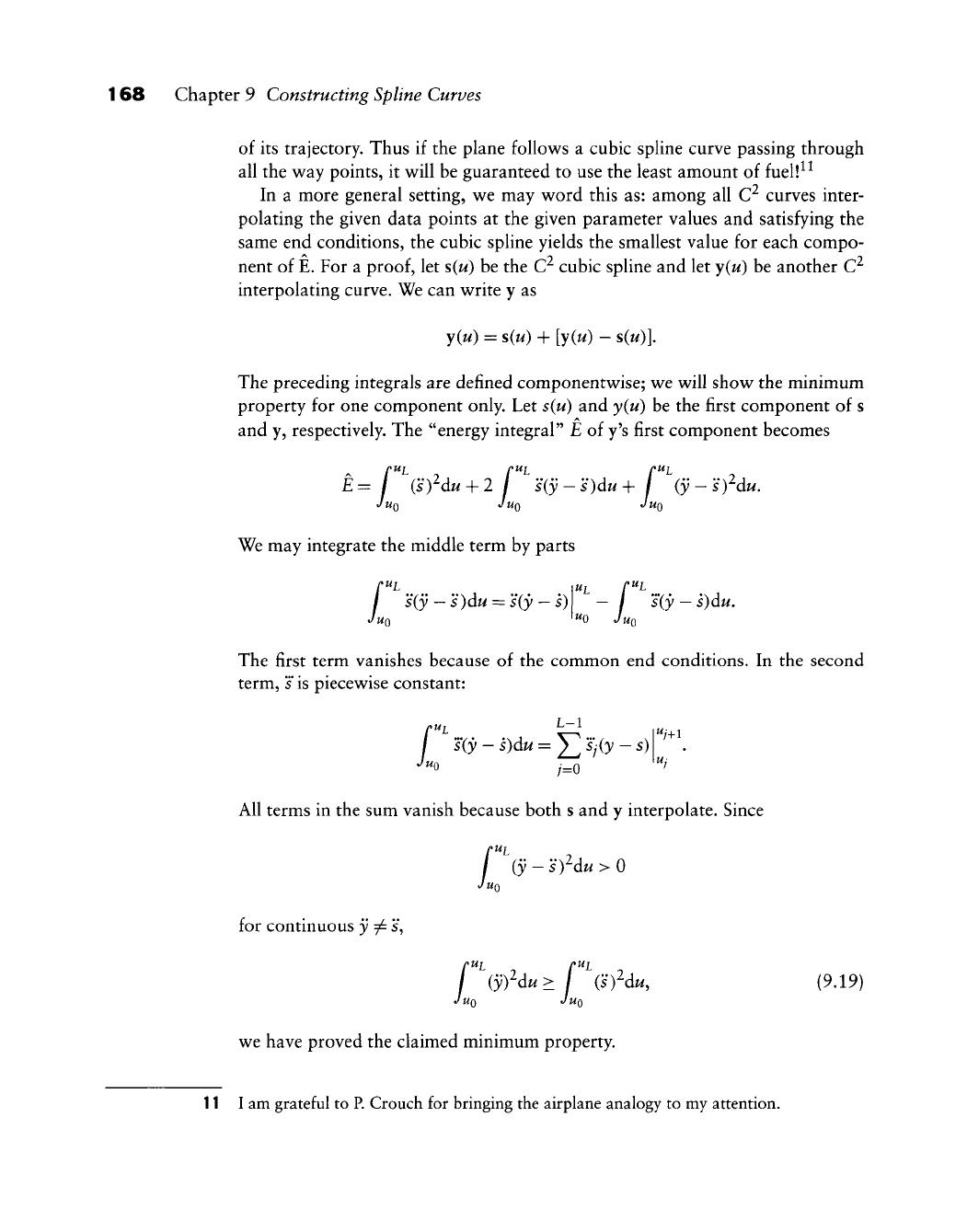
168 Chapter 9 Constructing Spline Curves
of its trajectory. Thus if the plane follows a cubic spline curve passing through
all the way points, it will be guaranteed to use the least amount offuell^i
In a more general setting, we may word this as: among all C^ curves inter-
polating the given data points at the given parameter values and satisfying the
same end conditions, the cubic spline yields the smallest value for each compo-
nent of E. For a
proof,
let s{u) be the C^ cubic spline and let y{u) be another C^
interpolating curve. We can write y as
y{u) = s(u) + [y(u) - s(u)l
The preceding integrals are defined componentwise; we will show the minimum
property for one component only. Let s(u) and y(u) be the first component of s
and y, respectively. The "energy integral" E of y's first component becomes
pUi pUi pUi
E= (sfdu + 2 / s(y - s)du + / (y - sfdu.
JUQ JUQ JUQ
We may integrate the middle term by parts
I s(y
—
s)du = s(y
—
s) — / s\y
—
s)du,
Jua '"0 Juo
The first term vanishes because of the common end conditions. In the second
term, s is piecewise constant:
/
UT ^-1
"s{y
- s)du = ^ Sj(y - s)
"0 /=o
*/
All terms in the sum vanish because both s and y interpolate. Since
/ {y - 'iydu > 0
JUQ
for continuous y ^ s,
f ^(yfdu
>
f ^(sfdu, (9.19)
JUQ JUQ
we have proved the claimed minimum property.
11 I am grateful to
P.
Crouch for bringing the airplane analogy to my attention.
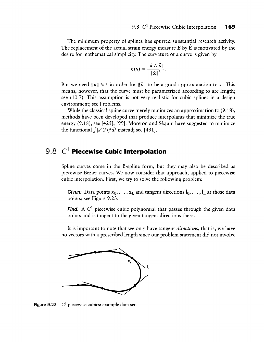
9.8 C^ Piecewise Cubic Interpolation 169
The minimum property of splines has spurred substantial research activity.
The replacement of the actual strain energy measure £ by E is motivated by the
desire for mathematical simplicity. The curvature of a curve is given by
, , IIXAXII
llxlP
But we need ||x|| ^ 1 in order for ||x|| to be a good approximation to /c. This
means, how^ever, that the curve must be parametrized according to arc length;
see (10.7). This assumption is not very realistic for cubic splines in a design
environment; see Problems.
While the classical spline curve merely minimizes an approximation to (9.18),
methods have been developed that produce interpolants that minimize the true
energy (9.18), see
[425],
[99]. Moreton and Sequin have suggested to minimize
the functional f[K\t)f-dt instead; see
[431].
9.8 C^ Piecewise Cubic Interpolation
Spline curves come in the B-spline form, but they may also be described as
piecew^ise Bezier curves. We now^ consider that approach, applied to piecewise
cubic interpolation. First, v^e try to solve the foUow^ing problem:
Given: Data points
XQ,
...,
x^^
and tangent directions
IQ,
...,
1^
at those data
points; see Figure 9.23.
Find:
A C^ piecewise cubic polynomial that passes through the given data
points and is tangent to the given tangent directions there.
It is important to note that we only have tangent directions^ that is, we have
no vectors with a prescribed length since our problem statement did not involve
Figure 9.23 C^ piecewise cubics: example data set.
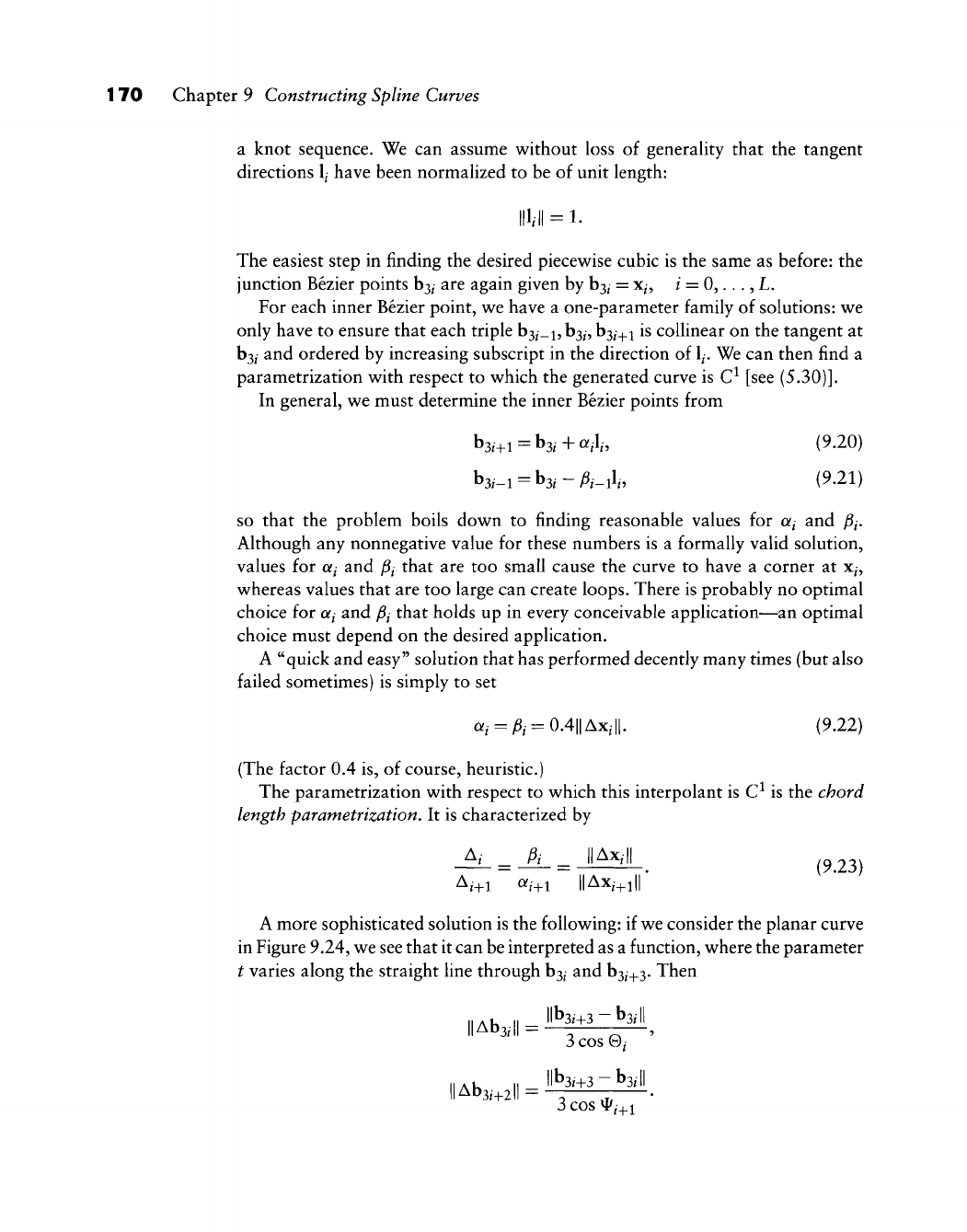
170 Chapter 9 Constructing Spline Curves
a knot sequence. We can assume without loss of generahty that the tangent
directions
1^
have been normahzed to be of unit length;
111;
II
=
1.
The easiest step in finding the desired piecewise cubic is the same as before: the
junction Bezier points
hi^i
are again given by b3/ = X/, / = 0,..., L.
For each inner Bezier point, we have a one-parameter family of solutions: we
only have to ensure that each triple h^i-i-,
h^^i^
^^i^^i
is coUinear on the tangent at
hi^i
and ordered by increasing subscript in the direction of
1^.
We can then find a
parametrization with respect to which the generated curve is C^ [see (5.30)].
In general, we must determine the inner Bezier points from
b3/+i = b3,+a,l„ (9.20)
b3.-i = b3,-^,_il„ (9.21)
so that the problem boils down to finding reasonable values for oti and )6^.
Although any nonnegative value for these numbers is a formally valid solution,
values for a^ and Pi that are too small cause the curve to have a corner at x^,
whereas values that are too large can create loops. There is probably no optimal
choice for of/ and Pi that holds up in every conceivable application—an optimal
choice must depend on the desired application.
A "quick and easy" solution that has performed decently many times (but also
failed sometimes) is simply to set
a, = ft = 0.4||Ax,||. (9.22)
(The factor 0.4 is, of course, heuristic.)
The parametrization with respect to which this interpolant is C^ is the chord
length parametrization. It is characterized by
A, _ ft _ ||Ax,|| ^^^^^^
A,+i a,+i ||Ax,+i||
A more sophisticated solution is the following: if we consider the planar curve
in Figure 9.24, we see that it can be interpreted as a function, where the parameter
t varies along the straight line through
b3^
and
b3^_^3.
Then
l|Ab3,||-'l''^'>^-^^'l'
3 cos 0/
3
COS
^ij^i
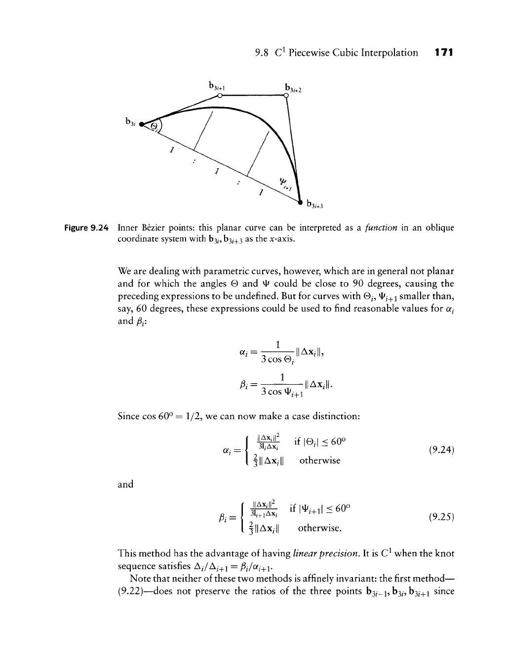
9.8 C^ Piecewise Cubic Interpolation 171
Figure 9.24 Inner Bezier points: this planar curve can be interpreted as a function in an oblique
coordinate system with
b3/,
b3/+3
as the x-axis.
We are dealing with parametric curves, however, which are in general not planar
and for which the angles 0 and ^ could be close to 90 degrees, causing the
preceding expressions to be undefined. But for curves with 0^, ^^_^i smaller than,
say, 60 degrees, these expressions could be used to find reasonable values for of/
and ^i'.
1
P^
3 cos 0/
1
lAX;
I
Ax,
I
3 cos ^ij^\
Since cos 60^ = 1/2, we can now make a case distinction:
iiAx,r
31/Ax, if |0,| < 60^
|||Ax;|| Otherwise
(9.24)
and
II
Ax,
I
^,=
131;;^
if|*ml<60°
lAX; Otherwise.
(9.25)
This method has the advantage of having linear precision. It is C^ when the knot
sequence satisfies Aj/Aj^i = ^i/oti^\.
Note that neither of these two methods is affinely invariant: the first method—
(9.22)—does not preserve the ratios of the three points b3,_i, b3p b3/_^i since
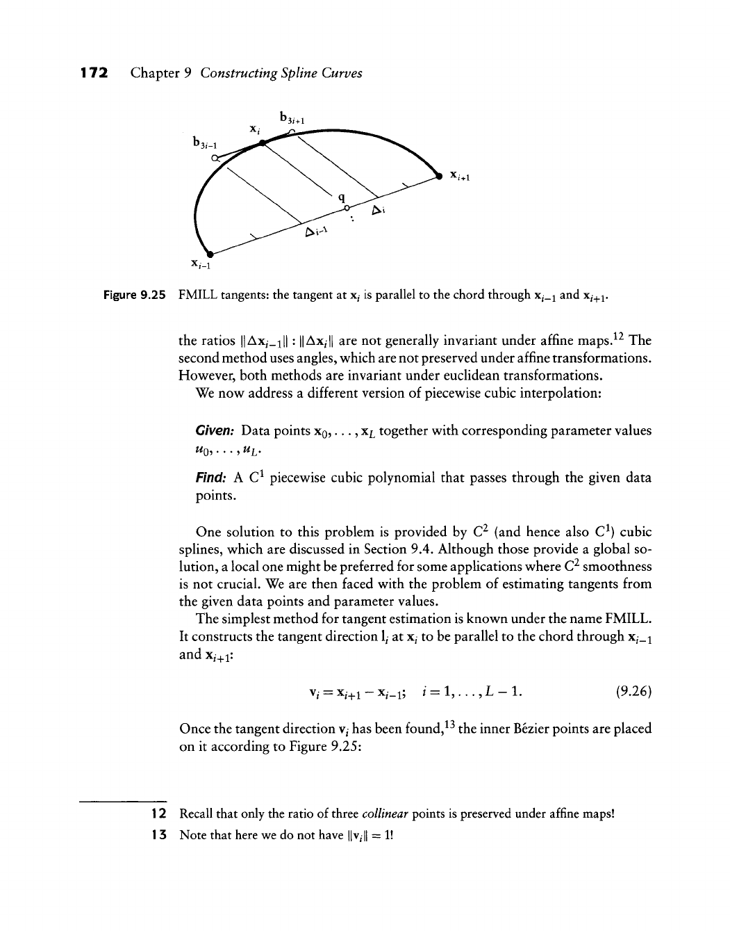
172 Chapter 9 Constructing Spline Curves
Figure 9.25 FMILL tangents: the tangent at
x^
is parallel to the chord through x^_i and Xj^i,
the ratios ||Ax^_i|| : ||Ax^|| are not generally invariant under affine maps.^^ The
second method uses angles, which are not preserved under affine transformations.
However, both methods are invariant under euclidean transformations.
We now address a different version of piecewise cubic interpolation:
Given: Data points
XQ,
...,
xj^
together with corresponding parameter values
WQ,
. . . , Ui.
Find:
A C^ piecewise cubic polynomial that passes through the given data
points.
One solution to this problem is provided by C^ (and hence also C^) cubic
splines, which are discussed in Section 9.4. Although those provide a global so-
lution, a local one might be preferred for some applications where C^ smoothness
is not crucial. We are then faced with the problem of estimating tangents from
the given data points and parameter values.
The simplest method for tangent estimation is known under the name FMILL.
It constructs the tangent direction
1/
at
x^
to be parallel to the chord through x^_i
and Xi^i:
Vi
= Xi^i - Xi_i;
/•
= 1,..., L - 1. (9.26)
Once the tangent direction
V/
has been found,^^ the inner Bezier points are placed
on it according to Figure 9.25:
12 Recall that only the ratio of three
collinear
points is preserved under affine maps!
1
3 Note that here we do not have ||v^|| = 1!
9.8 C^ Piecewise Cubic Interpolation 173
b3.-i-b3,-^^/^-;^
V,, (9.27)
3(A,_i + A,)
b3m = b3,+ .^^ \^yr (9.28)
3(A,_i + A,)
This interpolant is also known as a Catmull-Rom spline.
This construction of the inner Bezier points does not work at
XQ
and x^. The
next method, Bessel tangents, does not have that problem.
The idea behind Bessel tangents^^ is as follows: to find the tangent vector
m^
at
x^, pass the interpolating parabola q/(w) through x^_i,
x^,
x^_^i
with corresponding
parameter values w^_i,
w^,
u^j^i
and let
m^
be the derivative of q^. We differentiate
q, at
Ui',
d , ,
au
Written in terms of the given data, this gives
m,
= ^^^^^x,_, + ^AXi; i=l,...,L-l, (9.29)
A,_i A,-
where
«,=
The endpoints are treated in the same way: mo = d/duqi(uQ)^mi = d/duqi_i(ui),
which gives
mo = 2— mi,
^ Ax^_l
m^ = 2— m^_i.
AL-1
Another interpolant that makes use of the parabolas q^ is known as an
Overhauser spline, after work by A. Overhauser [452] (see also [91] and [154]).
The
i^^
segment s^ of such a spline (defined over
[uj,
W/+i]) is defined by
Si(u) = -^±i q,(M) + —_^q,.+i(M); t = l,...,L-2.
A,- A,-
14 They are also attributed to Ackland [2].
174 Chapter 9 Constructing Spline Curves
In other words, each S/ is a Hnear blend between q/ and q/+i. At the ends, one
sets So(w) = qo(w) and S£^_i(w) = qi-iW.
On closer inspection, it turns out that the last two interpolants are not different
at all: they both yield the same C^ piecewise cubic interpolant (see Problems).
A similar way of determining tangent vectors was developed by McConalogue
[421], [422].
Finally, we mention a method created by H. Akima [3]. It sets
m,- = (1 - Ci)2ii_i + Ci2ii,
where
AX;
A;
and
lAa;
|Aa,_2ll + ||Aa,-||
This interpolant appears fairly involved. It generates very good results, however,
in situations where curves are needed that oscillate only minimally.
9.9 Implementation
The following routines produce the cubic B-spline polygon of an interpolating
C^ cubic spline curve. First, we set up the tridiagonal linear system:
void set_up_system(knot,l,alpha,beta,gamma)
/* given the knot sequence, the linear system for clamped end
condition B-spline interpolation is set up.
Input: knot: knot sequence (all knots are simple; but,
in the terminology of Chapter 10, knot[0]
and knot[l] are of multiplicity three.)
points: points to be interpolated
1:
number of intervals
Output:alpha, beta,gamma: 1-D arrays that constitute
the elements of the interpolation matrix.
Note: no data points needed so far!
V
9.9 Implementation 175
The next routine performs the LU decomposition of the matrix from the
previous routine. (Note that we do not generate a full matrix but rather three
linear arrays!)
void l_u_system(alpha,beta,gamma,],up,low)
/* perform
LU
decomposition
of
tridiagonal system with
lower diagonal alpha, diagonal beta, upper diagonal gamma.
Input: alpha,beta,gamma:
the
coefficient matrix entries
1:
matrix size [0,l]x[0,l]
Output:low: L-matrix entries
up:
U-matrix entries
V
Finally, the routine that solves the system for the B-spline coefficients d^:
solve_system(up,1ow,gamma,1,rhs,d)
/*
solve tridiagonal linear system
of size (1+1)(1+1) whose
LU
decomposition
has
entries
up
and low,
and whose right hand side
is
rhs,
and
whose original matrix
had gamma
as
its
upper diagonal. Solution
is
d[0]
d[l+2].
Input: up,low,gamma:
as
above.
1: size
of
system:
1+1 eqs
in
1+1
unknowns,
rhs:
right hand side, i.e, data points with
end
'tangent Bezier points'
in
rhs[l]
and
rhs[l+l].
Output:d: solution vector.
Note shift
in
indexing from text! Both
rhs and
d
are
from
0 to
1+2.
V
In case Bessel ends are desired instead of clamped ends, this is the code:
void bessel_ends(data,knot,l)
/*
Computes B-spline points data[l]
and
data[l+l]
according
to
bessel
end
condition.
Input: data: sequence
of
data coordinates data[0]
to
data[l+2].
Note that data[l]
and
data[l+l]
are
expected
to
be empty,
as
they will
be
filled
by
this routine.
They correspond
to
the
Bezier points bez[l]
and
bez[31-l].
knot: knot sequence
1: number
of
intervals
Output: data:
now
including ''tangent Bezier points''
data[l],
data[l+l].
*/
176 Chapter 9 Constructing Spline Curves
The centripetal parametrization is achieved by the following routine:
void parameters(data_x,data_y,l,knot)
/*
Finds
a
centripetal parametrization for
a
given set
of 2D data points.
Input: data_x, data_y: input points, numbered from
0 to
1+2.
1: number
of
intervals.
Output: knot: knot sequence. Note:
not
(knot[l]=1.0)!
Note: data_x[l], data_x[l+l] are not used! Same for data_y.
*/
A calling sequence that uses the preceding programs might look like this:
parameters(data_x,data_y,l,knot);
set_up_system(knot,l,alpha,beta,gamma);
1
_u__system
(al
pha,
beta,
gamma,
1,
up,
1
ow);
bessel_ends(data_x,knot,l);
bessel_ends(data_y,knot,l);
sol ve_system(up,low,gamma,!,data_x,bspl_x);
solve_system(up,low,gamma,1,data_y,bspl_y);
Here, we solved the 2D interpolation problem with given data points in data_
X, data_y, a knot sequence knot, and the resulting B-spline polygon in bspl_x,
bspl__y. This calling sequence is realized in the routine c2_spl ine.c.
9.10 Problems
1 For the case of closed curves, C^ quadratic spline interpolation with uni-
form knots does not always have a solution. Why?^^
* 2 Show that interpolating splines reproduce cubic polynomial curves—that
they have cubic precision. This means that if all data points p/ are read off
from a cubic, p^ = c(w^), and the end tangent vectors are read off from the
cubic, then the interpolating spline equals the original cubic.
15 T. DeRose pointed this out to me.
9.10 Problems 177
3 Show that Akima's interpolant always passes a straight line segment
through three subsequent points if they happen to lie on a straight line.
* 4 Show that Overhauser splines are piecewise cubics with Bessel tangents at
the junction points.
* 5 One can generalize the quintic Hermite interpolants from Section 7.6 to
piecewise quintic Hermite interpolants. These curves need first and second
derivatives as input positions. Devise ways to generate second derivative
information from data points and parameter values.
PI Using piecewise cubic C^ interpolation, approximate the semicircle with
radius 1 to within a tolerance of 6 =
0.001.
Use as few cubic segments as
possible. Literature:
[172], [260].
P2 Program the following: instead of prescribing end conditions for interpolat-
ing C^ splines at both ends, prescribe first and second derivatives at
TQ.
The
interpolant can then be built segment by segment. Discuss the numerical
aspects of this method (they will not be wonderful).

This Page Intentionally Left Blank
W. Boehm
Differential
Geometry
I
Uifferential geometry is based largely on the pioneering work of L. Euler
(1707-1783), C. Monge (1746-1818), and C F. Gauss (1777-1855). One of
their concerns was the description of local curve and surface properties such
as curvature. These concepts are also of interest in modern computer-aided
geometric design. The main tool for the development of general results is the use
of local coordinate systems, in terms of which geometric properties are easily
described and studied. This introduction discusses local properties of curves
independent of a possible embedding into a surface.
10.1 Parametric Curves and Arc Length
A curve in E^ is given by the parametric representation
t e[a,b]c]
X
= x(t) =
x(t)
y(t)
z(t)
(10.1)
where its cartesian coordinates x, y, z are differentiable functions of t. (We have
encountered a variety of such curves already, among them Bezier and B-spline
curves.) To avoid potential problems concerning the parametrization of the curve,
we shall assume that
x(t) =
x{t)
m
m
^0,
te
[a,
bl (10.2)
179
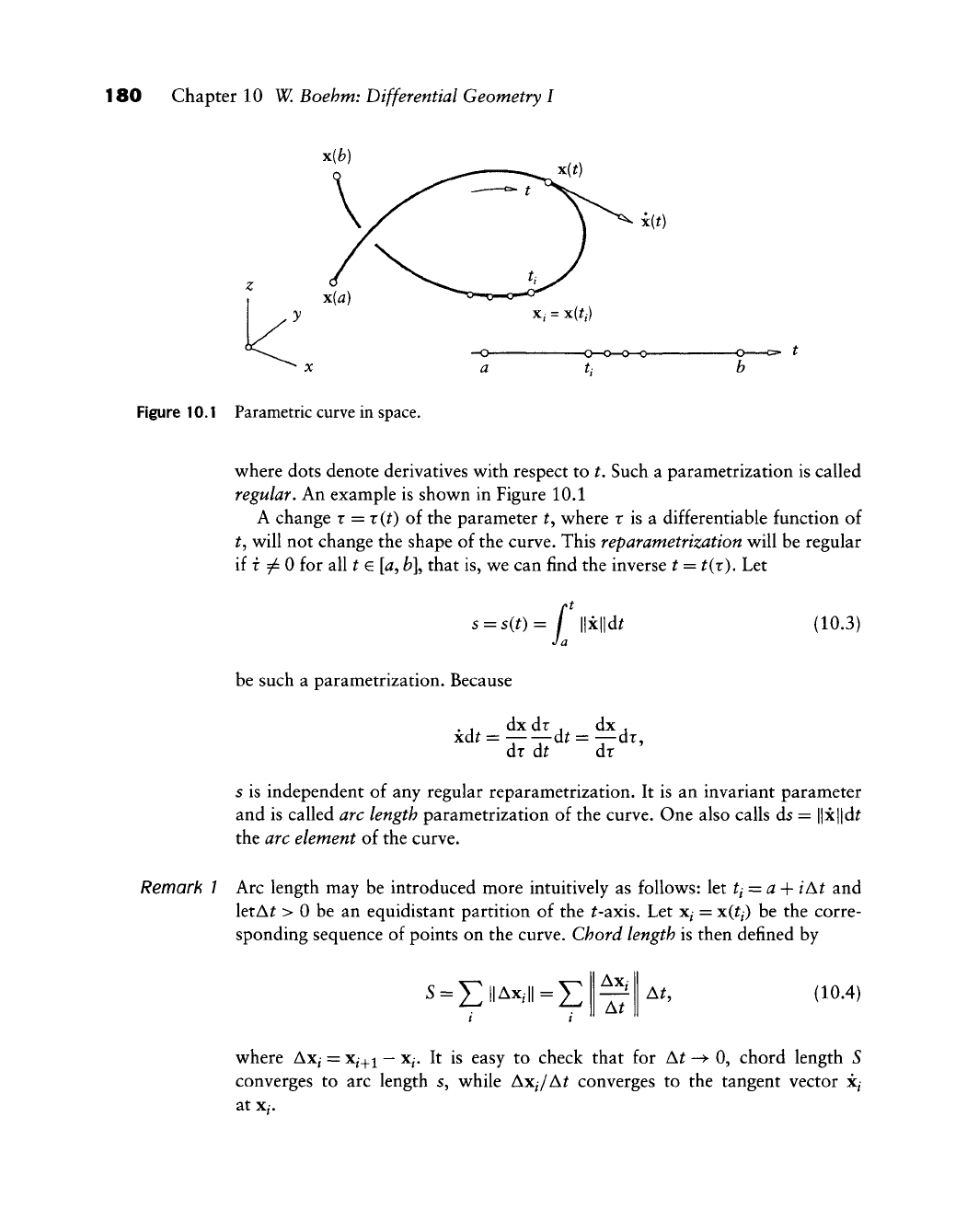
180 Chapter 10 W. Boehm: Differential Geometry I
Xi = X(ti)
a
-o—o—a—o-
Figure 10.1 Parametric curve in space.
where dots denote derivatives vs^ith respect to t. Such a parametrization is called
regular. An example is shown in Figure 10.1
A change x = x{t) of the parameter t^ where r is a differentiable function of
t^ will not change the shape of the curve. This reparametrization will be regular
if f
7«^
0 for all t e [a, fc], that is, we can find the inverse t = ^(r). Let
' =
s(t)=
f ||x
Ja
\\dt (10.3)
be such a parametrization. Because
. . dxdr , dx .
xd^ = -——d^ = -—dr,
dr at dr
s is independent of any regular reparametrization. It is an invariant parameter
and is called arc length parametrization of the curve. One also calls ds = \\x\\dt
the arc element of the curve.
Remark 7 Arc length may be introduced more intuitively as follows: let ti = a-\- iAt and
letA^ > 0 be an equidistant partition of the ^-axis. Let x^ = x{tj) be the corre-
sponding sequence of points on the curve. Chord length is then defined by
(10.4)
where Ax^ = x^.^^
—
x^. It is easy to check that for A^ -^ 0, chord length S
converges to arc length s, while Axj/At converges to the tangent vector x^
at Xj,
10.2 The Frenet Frame 181
Remark 2 Although arc length is an important concept, it is primarily used for theoretical
considerations and for the development of curve algorithms. If, for some appli-
cation, computation of the arc length is unavoidable, it may be approximated by
the chord length (10.4).
10.2 The Frenet Frame
We
w^ill
nov^ introduce a special local coordinate system, linked to a point x(0 on
the curve, that
w^ill
significantly facilitate the description of local curve properties
at that point. Let us assume that all derivatives needed below do exist. The first
terms of the Taylor expansion of x(^ + A^) at t are given by
1 1
x(f + AO =
X
+ xA^ + X-A^^ + X-A^^ + ^
2 6
Let us assume that the first three derivatives are linearly independent. Then
X, X,
X
form a local affine coordinate system w^ith origin x. In this system, x(t) is
represented by its canonical coordinates
A^H-...
lAf^ + ...
v^here . . . denotes terms of degree four and higher in A^.
From this local affine coordinate system, one easily obtains a local cartesian
(orthonormal) system w^ith origin x and axes t, m, b by the Gram-Schmidt process
of orthonormalization, as shov^n in Figure 10.2:
t=^^,
m = bAt, b=^^—^, (10.5)
llxll llxAxll
w^here A denotes the cross product.
The vector t is called tangent vector (see Remark 1), m is called main normal
vector^'^
and b is called binormal vector. The frame (or trihedron) t, m, b is called
the Frenet frame\ it varies its orientation as t traces out the curve.
1 We use the abbreviation
A?-^
= (A?)^.
2 One often sees the notation n for this vector. We use m to avoid confusion with surface
normals, which are discussed later.

182 Chapter 10 W. Boehm: Differential Geometry I
Figure 10.2 Local affine system (left) and Frenet frame (right).
The plane spanned by the point x and the two vectors t, m is called the
osculating plane O. Its equation is
det y X X x"j _
1 1 0 0j~
det[y
—
X,
x,x] = 0,
where y denotes any point on O. Its parametric form is
0(w, v) =x-\-ux-\- vx.
Remark 5 The process of orthonormalization yields
m =
XX
•
X — XX
•
X
XX
•
X — XX
•
X
This equation may also be used for planar curves, where the binormal vector
b = t
A
m agrees with the normal vector of the plane.
10.5 Moving the Frame
Letting the Frenet frame vary with t provides a good idea of the curve's behavior in
space. It is a fundamental idea in differential geometry to express the local change
of the frame in terms of the frame
itself.
The resulting formulas are particularly
simple if one uses arc length parametrization. We denote differentiation with
respect to arc length by a prime. Since x' = t is a unit vector, we find the following
two identities:
x^x' = l and x^x''=:0.
The first identity states that the curve is traversed with unit speedy the second
one states that the tangent vector is perpendicular to the second derivative vector,
provided the curve is parametrized with respect to arc length.
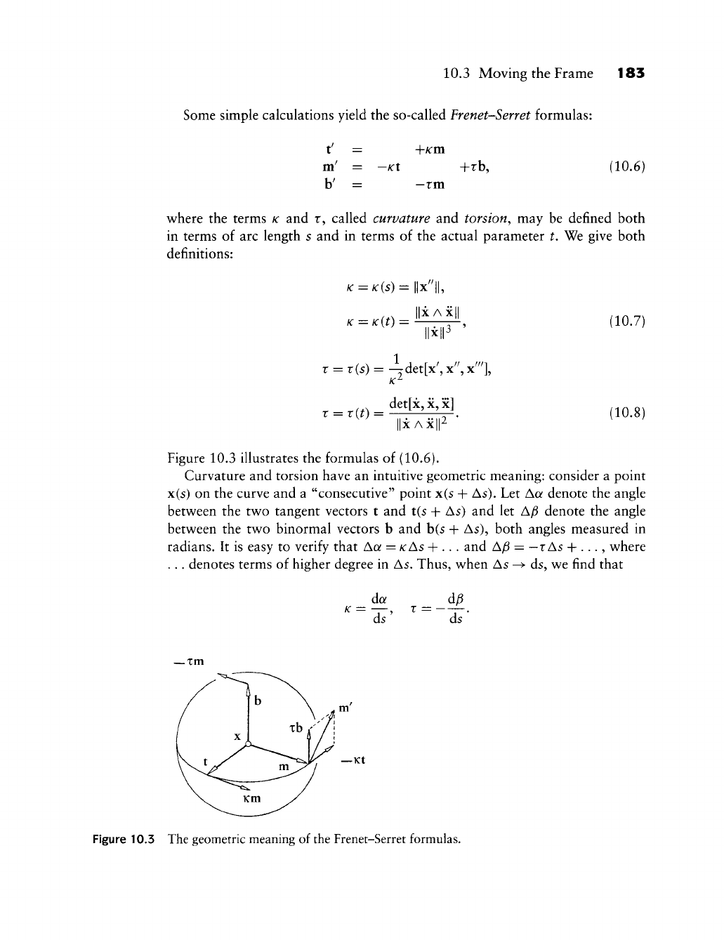
10.3 Moving the Frame 183
Some simple calculations yield the so-called Frenet-Serret formulas:
t' = +/cm
m' = —Kt +rb,
b'
= —rm
(10.6)
where the terms K and r, called curvature and torsion^ may be defined both
in terms of arc length s and in terms of the actual parameter t. We give both
definitions:
K=K{S)=\W'\1
IIXAXII
K=K(t) = (10.7)
r = r(s) = ^det[x>^xn,
T = r(t) =
det[x,
X,
x]
X AX |2 * (10.8)
Figure 10.3 illustrates the formulas of (10.6).
Curvature and torsion have an intuitive geometric meaning: consider a point
x(s) on the curve and a "consecutive" point x(s + As). Let Aa denote the angle
between the two tangent vectors t and t(s + As) and let A^ denote the angle
between the two binormal vectors b and b(s + As), both angles measured in
radians. It is easy to verify that Aa = KAS -\-.. . and A^ = — r
As
+ ..., where
. . . denotes terms of higher degree in As. Thus, when As -> ds, we find that
K =
da
d7'
r =
ds'
— xm
—Kt
Figure 10.3 The geometric meaning of the Frenet-Serret formulas.
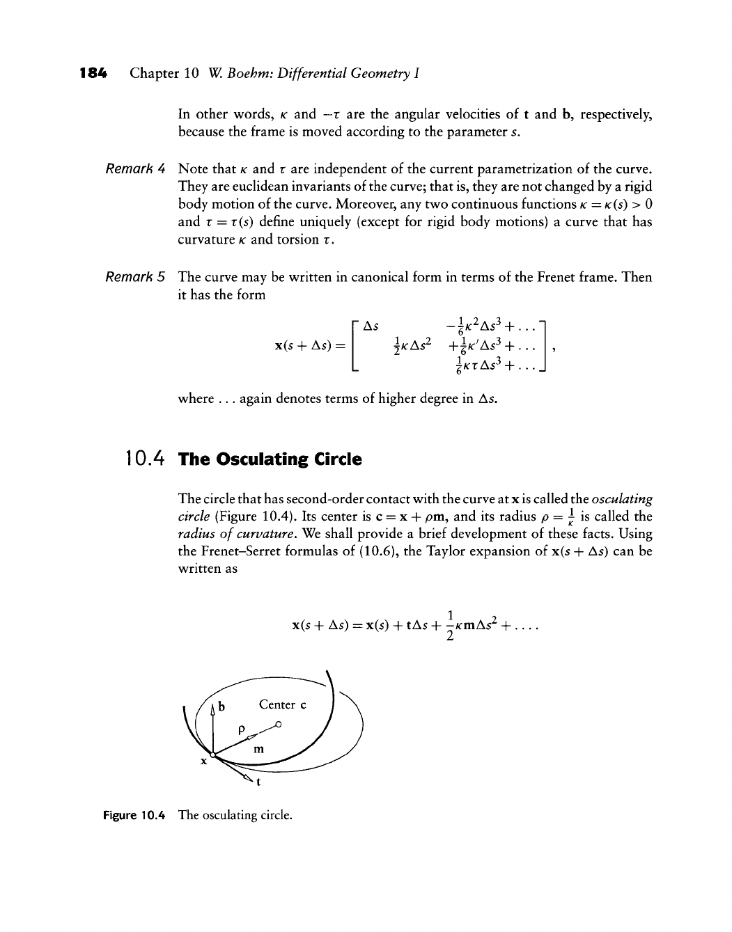
184 Chapter 10 W, Boehm: Differential Geometry I
In other words, K and — r are the angular velocities of t and b, respectively,
because the frame is moved according to the parameter 5.
Remark 4 Note that
K
and r are independent of the current parametrization of the curve.
They are euclidean invariants of the curve; that is, they are not changed by a rigid
body motion of the curve. Moreover, any two continuous functions
K
=K(S) > 0
and r = r(s) define uniquely (except for rigid body motions) a curve that has
curvature
K
and torsion r.
Remark 5 The curve may be written in canonical form in terms of the Frenet frame. Then
it has the form
x(s + As) =
As
|/crAs^
+ ...
where ... again denotes terms of higher degree in As.
10.4 The Osculating Circle
The circle that has second-order contact with the curve at x is called the osculating
circle (Figure 10.4). Its center is c = x + pm, and its radius p = ^ is called the
radius of curvature. We shall provide a brief development of these facts. Using
the Frenet-Serret formulas of (10.6), the Taylor expansion of x(s -f As) can be
written as
1 2
x(s + As) = x(s) +1As + -/cmAs + ...,
Figure 10.4 The osculating circle.
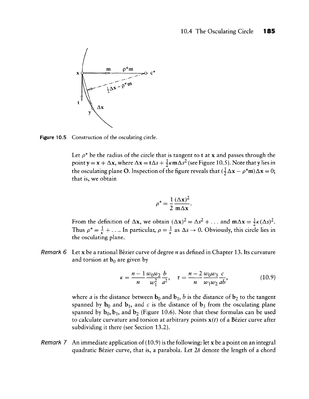
10.4 The Osculating Circle 185
m p'^m
Figure 10.5 Construction of the osculating circle.
Let p* be the radius of the circle that is tangent to t at x and passes through the
point y =
X
+ Ax, where Ax = tAs + ^/cmAs^ (see Figure 10.5). Note that y lies in
the osculating plane O. Inspection of the figure reveals that (^ Ax
—
p*m)
Ax = 0;
that is, we obtain
. ^ 1 (Ax)^
2 mAx
From the definition of Ax, we obtain (Ax)^ = As^ + ... and mAx = ^'^(As)^.
Thus p* = ^ + .... In particular, p = ^ as As ^- 0. Obviously, this circle lies in
the osculating plane.
Remark 6 Let x be a rational Bezier curve of degree n as defined in Chapter 13. Its curvature
and torsion at bo are given by
K =
_n ~ 1
WQWI
b
n 1 1'
n
—
1 WQW^ C
n WiWi ah (10.9)
where a is the distance between bo and b^, h is the distance of h^ to the tangent
spanned by bo and b^, and c is the distance of b3 from the osculating plane
spanned by bo, bj, and b2 (Figure 10.6). Note that these formulas can be used
to calculate curvature and torsion at arbitrary points x(0 of a Bezier curve after
subdividing it there (see Section 13.2).
Remark 7 An immediate application of (10.9) is the following: let x be a point on an integral
quadratic Bezier curve, that is, a parabola. Let 28 denote the length of a chord
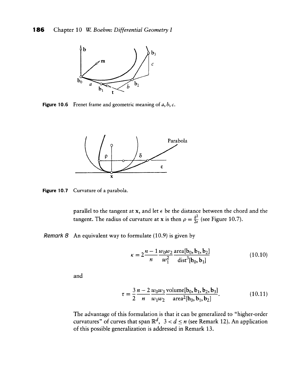
186 Chapter 10 W. Boehm: Differential Geometry I
Figure 10.6 Frenet frame and geometric meaning of
a,
b, c.
Parabola
Figure 10.7 Curvature of a parabola.
parallel to the tangent at x, and let € be the distance between the chord and the
tangent. The radius of curvature at x is then P = j^ (see Figure 10.7).
Remark 8 An equivalent way to formulate (10.9) is given by
n
—
1
WQWI
area[bo,
bj, b2]
K=l- n w\ dist^[bo,bi]
and
_ 3 «
—
2
WQW2,
volume
[bo,
bj,
hi^
h^]
2 n wiWi area^[bo5bi,b2]
(10.10)
(10.11)
The advantage of this formulation is that it can be generalized to "higher-order
curvatures" of curves that span M^, 3 < d <n (see Remark 12). An application
of this possible generalization is addressed in Remark 13.

10.5 Nonparametric Curves 187
10.5 Nonparametric Curves
Let y = y(t); t e[a,
b]
be a function. The planar curve .
x
is called the graph
L
y{t) J
of y(t) or a nonparametric curve. From this, we derive the following:
the arc element:
the tangent vector:
the curvature:
ds
= y
1
+ y^dt,
K = —^
[l + y^J
and the center of curvature:
--¥[7]
Remark 9 Note that
K
has a sign here. Any planar parametric curve can be given a signed
curvature, for instance, by using the sign of det(x, x); see also (23.1).
Remark 10 For a nonparametric Bezier curve (see Section 6.5),
Where
U
=
UQ
+ tAu is a global parameter, we obtain
n^
n a
as illustrated in Figure 10.8.
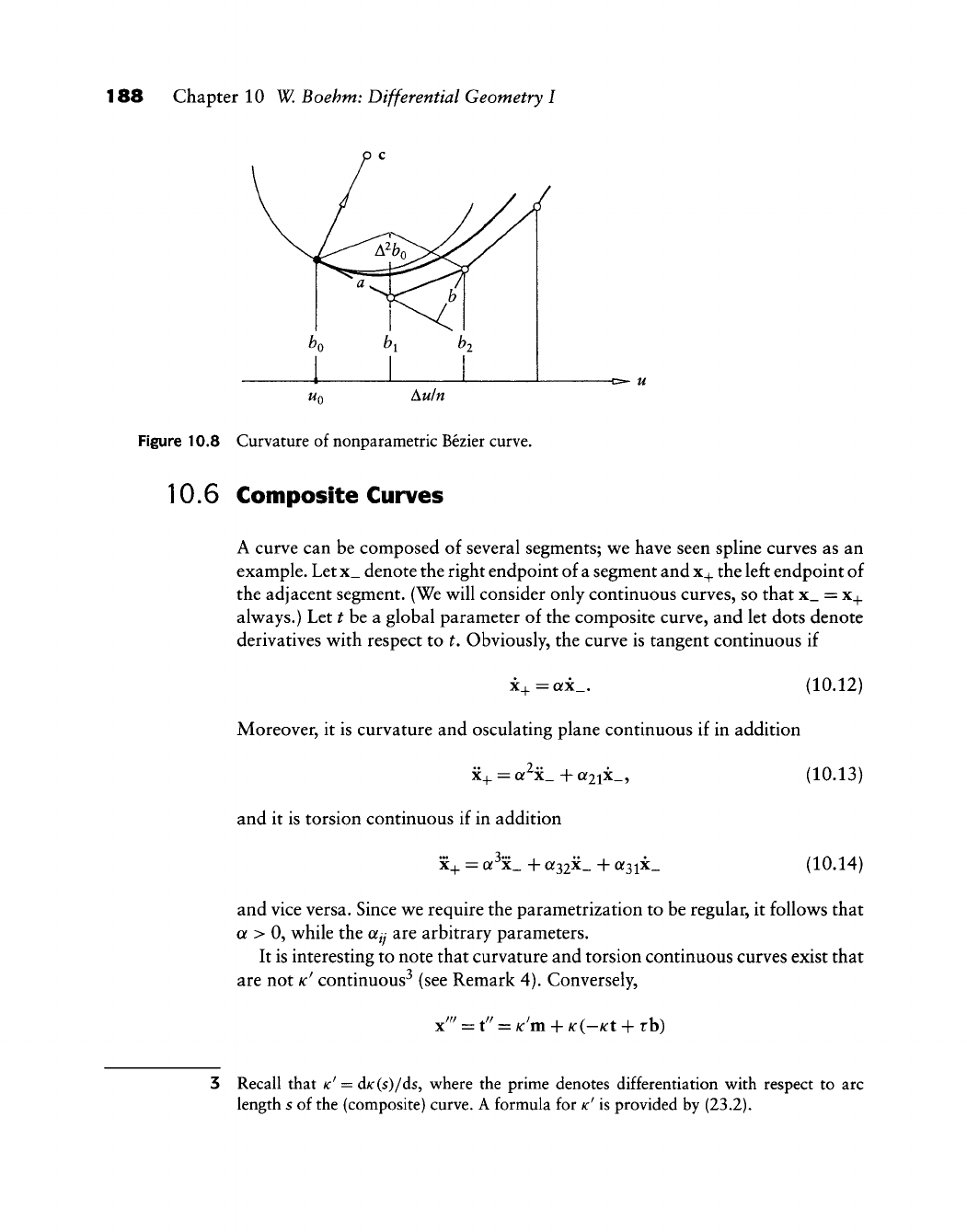
188 Chapter 10 W, Boehm: Differential Geometry I
UQ Au/n
Figure 10.8 Curvature of nonparametric Bezier curve.
10.6 Composite Curves
A curve can be composed of several segments; we have seen sphne curves as an
example. Let x_ denote the right endpoint of
a
segment and
x_^
the left endpoint of
the adjacent segment. (We w^ill consider only continuous curves, so that x_ =
x_^
always.) Let
^
be a global parameter of the composite curve, and let dots denote
derivatives with respect to t. Obviously, the curve is tangent continuous if
x+=Qfx_. (10.12)
Moreover, it is curvature and osculating plane continuous if in addition
x_|. = Qf^x_ + a2ix_,
and it is torsion continuous if in addition
x^ = a x_ + a32X_ + 0f3ix_
(10.13)
(10.14)
and vice versa. Since we require the parametrization to be regular, it follows that
Q;
> 0, while the ajj are arbitrary parameters.
It is interesting to note that curvature and torsion continuous curves exist that
are not
K^
continuous^ (see Remark 4). Conversely,
x'^' = t'' =
K^m
+ K(-Kt + rb)
3 Recall that
K^
= d/c(s)/ds, v^here the prime denotes differentiation with respect to arc
length s of the (composite) curve. A formula for
K'
is provided by (23.2).
10.6 Composite Curves 189
implies that
x.'^'
is continuous if K' is and vice versa. To ensure
x.'^
= x^', the
coefficients a and of^y must be the result of the application of the chain rule; that
is,
with Qf2i =
)6
and a^^x^y^ one finds that
0^32
= 30?^. Now, as before, the curve
is tangent continuous if
x_^ = ax_, a > 0,
it is curvature and osculating plane continuous if in addition
..
9
.. .
X_^
=
Of
X_ + j6x_,
but it is /c' continuous if in addition
x^ = a\_ + 3a^x_ + yx_
and vice versa.
Remark / / For planar curves, torsion continuity is a vacuous condition, but
K'
continuity is
meaningful.
Remark
/
2 The preceding results may be used for the definition of higher-order geometric
continuity, A curve is said to be G^, or rth order geometrically continuous if a
regular reparametrization exists after which it is U. This definition is obviously
equivalent to the requirement of C^~^ continuity of
K
and C~^ continuity of r.
As a consequence, geometric continuity may be defined by using the chain rule,
as in the example for r = 3.
Remark 13 The geometric invariants curvature and torsion may be generalized for higher-
dimensional curves. Continuing the process mentioned in Remark 8, we find
that a J-dimensional curve has d
—
1 geometric invariants. Continuity of these
invariants makes sense only in E^, as was demonstrated for d = 2'm Remark 11.
Remark / 4 Note that although curvature and torsion are euclidean invariants, curvature and
torsion continuity (as well as the generalizations discussed in Remarks 12 and 13)
are affinely invariant properties of a curve. Both are also projectively invariant
properties; see Boehm [76] and Goldman and Micchelli
[267].
Remark 15 If two curve segments meet with a continuous tangent and have (possibly differ-
ent) curvatures K_ and
K_^
at the common point, then the ratio K_/K^ is also a
projectively invariant quantity. This is known as Memke's theorem; see Bol [88].

This Page Intentionally Left Blank
Geometric
Continuity i4 Ns
u u
11.1 Motivation
Before we explain in detail the concept of geometric continuity, we will give
an example of a curve that is curvature continuous yet not twice differentiate.
Such curves (and, later, surfaces) are the objects that we will label geometrically
continuous.
Figure 11.1 shows three parabolas with junction points at the midpoints of
an equilateral triangle. According to (10.10), where we have to set all Wi equal
to 1, all three parabolas have the same curvature at the junction points. We thus
have a closed, curvature continuous curve. It is C^ over a uniform knot sequence.
But it is not C^ as is easily seen by sketching the second derivative vectors at the
junction points.
Differential geometry teaches us that our closed curve can be reparametrized
such that the new parameter is arc length. With that new parametrization, the
curve will actually be C^. Details are explained in Chapter 10. We shall adopt the
term G^ curves (second-order geometrically continuous) for curves that are twice
differentiable with respect to arc length but not necessarily twice differentiate
with respect to their current parametrization. Note that curves with a zero tangent
vector cannot be G^ under this definition. Planar G^ curves have continuously
varying signed curvature; G^ space curves have continuously varying binormal
vectors and continuously varying curvature.
191
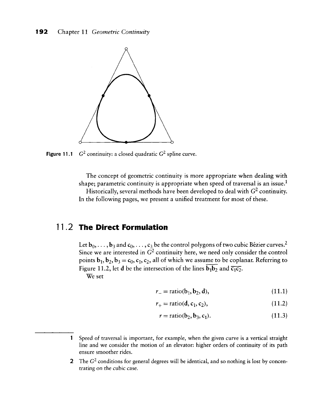
192 Chapter 11 Geometric Continuity
Figure 11.1 G^ continuity: a closed quadratic G^ spline curve.
The concept of geometric continuity is more appropriate when dealing with
shape; parametric continuity is appropriate when speed of traversal is an issue.^
Historically, several methods have been developed to deal with G^ continuity.
In the following pages, we present a unified treatment for most of these.
11.2 The Direct Formulation
Let bo,...,
b3
and
CQ,
...,
C3
be the control polygons of two cubic Bezier curves.-^
Since we are interested in G^ continuity here, we need only consider the control
points bi, b2, b3 =
CQ,
CJ,
C2,
all of which we assume to be coplanar. Referring to
Figure 11.2, let d be the intersection of the lines bib2 and c^.
We set
r_ = ratio(bi,b2,d), (11.1)
r+= ratio(d, Ci,
C2),
(11.2)
r = ratio(b2,b3,Ci). (11.3)
Speed of traversal is important, for example, when the given curve is a vertical straight
line and we consider the motion of an elevator: higher orders of continuity of its path
ensure smoother rides.
The G^ conditions for general degrees will be identical, and so nothing is lost by concen-
trating on the cubic case.
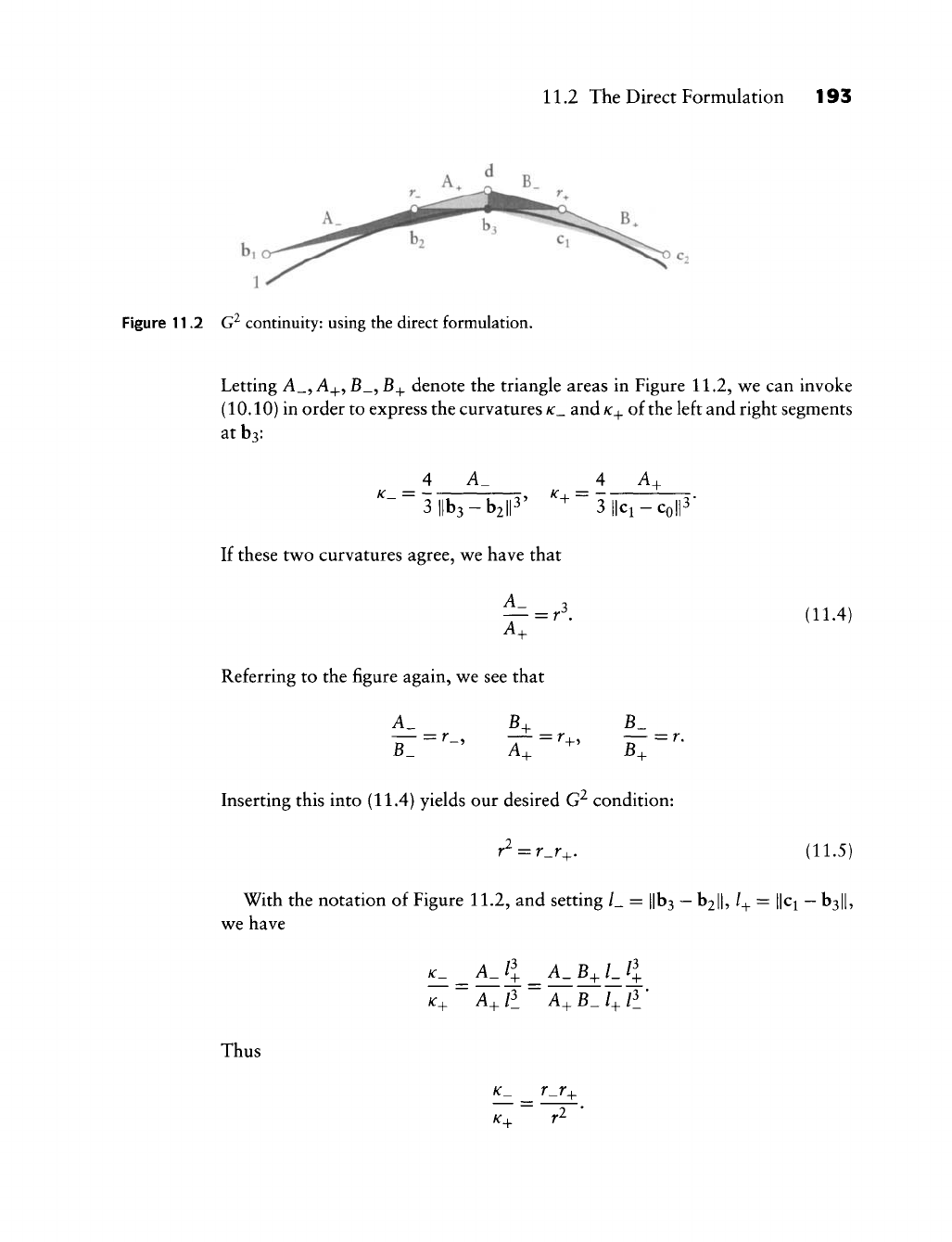
11.2 The Direct Formulation 193
Figure 11.2 G^ continuity: using the direct formulation.
Letting A_,A^,B_,B^ denote the triangle areas in Figure 11.2, we can invoke
(10.10) in order to express the curvatures
K_
and
/c+
of the left and right segments
atbj:
4 A. 4 A,
K,=
3||b3-b2lP' + 3||ci-coll3"
If these two curvatures agree, we have that
A.
A;
Referring to the figure again, we see that
A_
B4-
= r\ (11.4)
T_='- = r.
+5
A+ -' B^
= r.
Inserting this into (11.4) yields our desired G^ condition:
'-'+' (11.5)
With the notation of Figure 11.2, and setting /_ = ||b3
—
b2l|, /+ = ||ci
—
b3||,
we have
Thus
r_r.
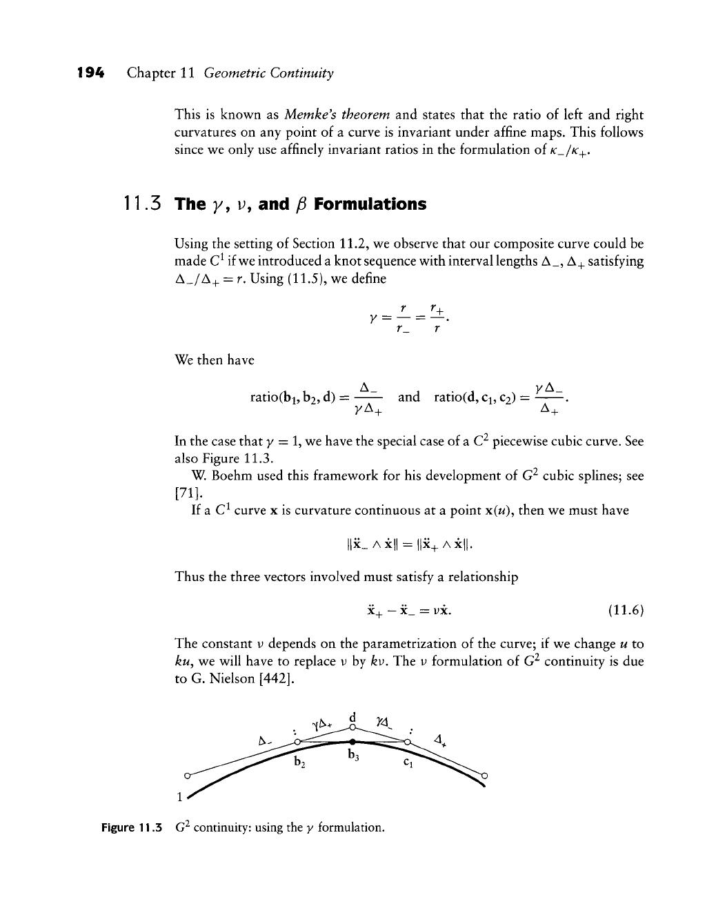
194 Chapter 11 Geometric Continuity
This is known as Memke's theorem and states that the ratio of left and right
curvatures on any point of a curve is invariant under affine maps. This follows
since we only use affinely invariant ratios in the formulation of K_/K_^.
11.3 The y, Vj and fi Formulations
Using the setting of Section 11.2, we observe that our composite curve could be
made C^ if we introduced a knot sequence with interval lengths A_,
A_^
satisfying
A_/A_^ = r. Using (11.5), we define
We then have
ratio(bi, hi, d) = and ratio(d,
Cj,
C2)
=
yA+
In the case that y = 1, we have the special case of a C^ piecewise cubic curve. See
also Figure 11.3.
W. Boehm used this framework for his development of G^ cubic splines; see
[71].
If a C^ curve x is curvature continuous at a point x(w), then we must have
Thus the three vectors involved must satisfy a relationship
(11.6)
The constant v depends on the parametrization of the curve; if we change u to
ku,
we will have to replace v by ^y. The v formulation of
G'^
continuity is due
to G. Nielson
[442].
Figure 11.3 G^ continuity: using the y formulation.

11.4 G^ Cubic Splines 195
There is a one-to-one relationship between the constants y and v.
„ =
2(^^)1^.
,11.7)
first found by W. Boehm [71].
A similar approach was taken by B. Barsky [40], [47];he uses
Pi = —^ and ^2 =
1^
(11-8)
^+
as the descriptors of G^ continuity and calls them bias and tension, respectively.
Why three or four different formulations for G^ continuity of piecewise cubic
curves? The reason is partly historical, and partly depends on applications. In
fact, the preceding formulations are by no means the only ones—the discussion
of G^ continuity goes back as far as Baer [12], Bezier [59], Geise
[256],
and
Manning
[414].
Applications that aim at constructing surfaces will be better served by ^, y, or
y
splines. These involve a knot sequence and thus lend themselves to the framework
of tensor product surfaces; see Chapter 16.
Freeform curve design, on the other hand, will benefit more from the direct
formulation since it is linked the closest to the curve geometry. The direct
approach is the most geometric, followed by the y formulation, which needs
a knot sequence. The least geometric are the v and fi formulations; their defining
quantities are not invariant under scaling of the knot sequence.
11.4 C^ Cubic Splines
We start with a control polygon do,..., d^^. In the context of C^ cubic B-splines,
we now needed a knot sequence in order to place the inner Bezier points on the
control polygon legs; the junction points then were fixed by the C^ conditions.
In our case, we have more freedom: we may place the inner Bezier points
anywhere on the control polygon legs; the junction points are then fixed by the
conditions.
To be more precise, consider Figure 11.4. Placing h^j-i ^^ ^^e polygon leg
dp
dj_^i
amounts to picking a number aj (between 0 and 1) and then setting
b3,_2 = (l-aM+M.+l. (11.9)
Similarly, we place h^i_i by picking a number
coj
and setting
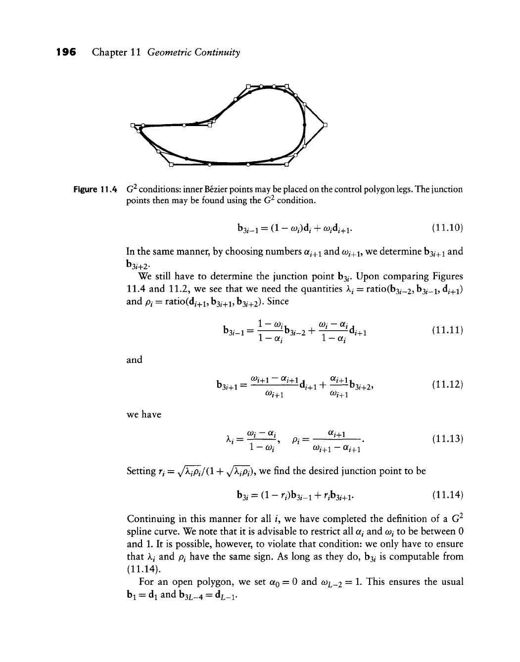
196 Chapter 11 Geometric Continuity
Figure 11.4
G^
conditions; inner Bezier points may
be
placed on the control polygon
legs.
The junction
points then may be found using the G^ condition.
b3/-i = (1 -
C0i)di
+
coidi^^,
(11.10)
In the same manner, by choosing numbers aj^i and o^^+i, we determine
h^i-^^
and
We still have to determine the junction point b3/. Upon comparing Figures
11.4 and 11.2, we see that we need the quantities A/ = ratio(b3/_2, b3/_i,
d^_^i)
and
Pi
= ratio(d,+i,
^3i-\-h
ba^+i)- Since
b3,-l = i^b3,_2 + ^d,.i (11.11)
1
—
aj 1
—
aj
and
we have
b3/+l = ^/+1 + b3/+2? (11.12)
A,
= ^, p, = -^i±^. (11.13)
Setting
Yi —
^kiPilil +
y/T~pi)^
we find the desired junction point to be
b3,
= (l-r,)b3,_i + r,b3,+i. (11.14)
Continuing in this manner for all /, we have completed the definition of a G^
spline curve. We note that it is advisable to restrict all a^ and
coi
to be between 0
and 1. It is possible, however, to violate that condition: we only have to ensure
that Xi and pi have the same sign. As long as they do, b3^ is computable from
(11.14).
For an open polygon, we set
Q^Q
= 0 and
(Oi_2
= 1. This ensures the usual
bi = di and h^L-4 = ^L-i-
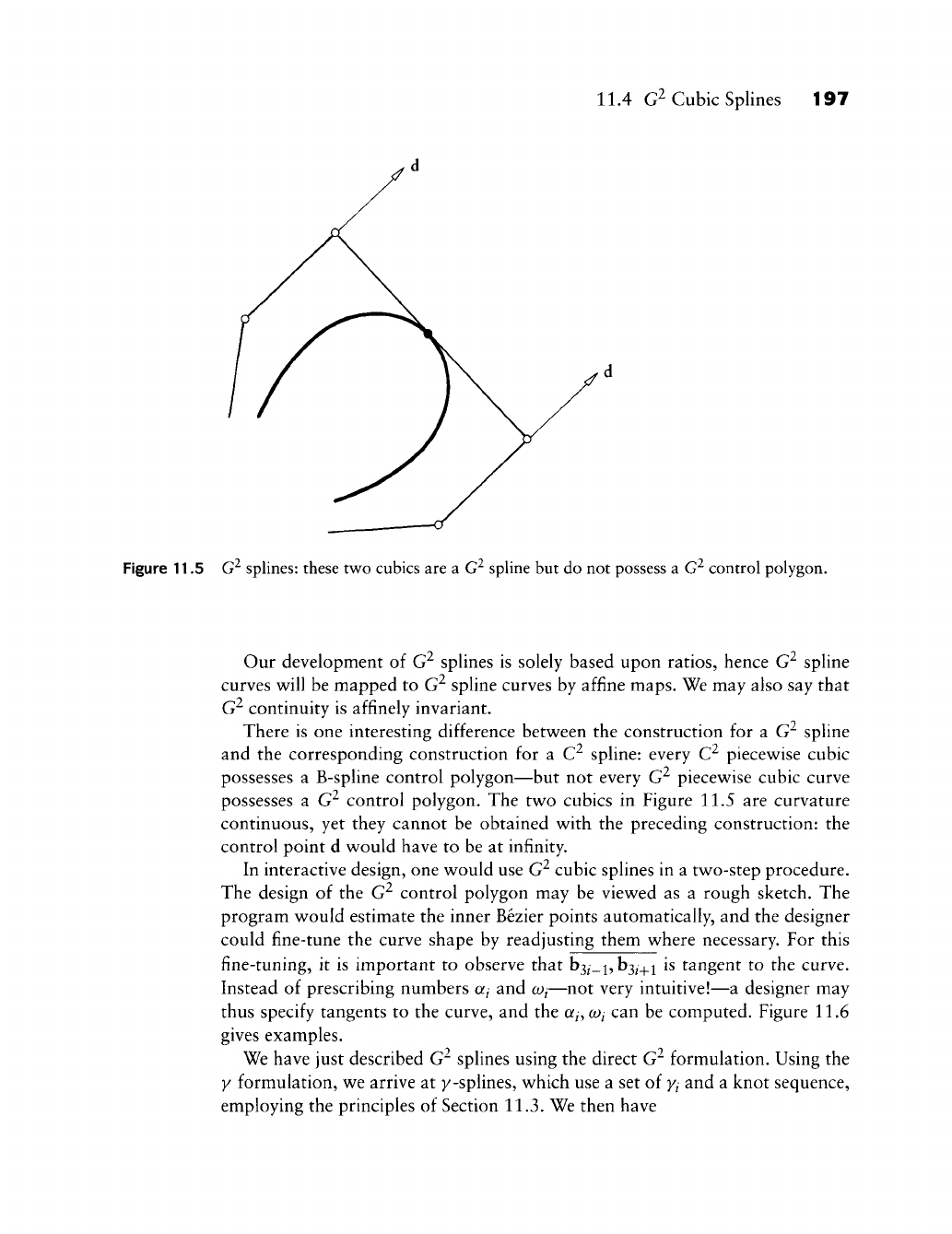
11.4 G^ Cubic Splines 197
Figure 11.5 G^ splines: these two cubics are a G^ spline but do not possess a G^ control polygon.
Our development of G^ splines is solely based upon ratios, hence G^ spline
curves will be mapped to G^ spline curves by affine maps. We may also say that
continuity is affinely invariant.
There is one interesting difference between the construction for a G spline
and the corresponding construction for a C^ spline: every C^ piecewise cubic
possesses a B-spline control polygon—but not every G^ piecewise cubic curve
possesses a G^ control polygon. The two cubics in Figure 11.5 are curvature
continuous, yet they cannot be obtained with the preceding construction: the
control point d would have to be at infinity.
In interactive design, one would use G^ cubic splines in a two-step procedure.
The design of the G^ control polygon may be viewed as a rough sketch. The
program would estimate the inner Bezier points automatically, and the designer
could fine-tune the curve shape by readjusting them where necessary. For this
fine-tuning, it is important to observe that h^j_i,h^i^i is tangent to the curve.
Instead of prescribing numbers aj and coj—not very intuitive!—a designer may
thus specify tangents to the curve, and the a^,
coj
can be computed. Figure 11.6
gives examples.
We have just described G^ splines using the direct G^ formulation. Using the
y formulation, we arrive at y-splines, which use a set of
y^
and a knot sequence,
employing the principles of Section 11.3. We then have
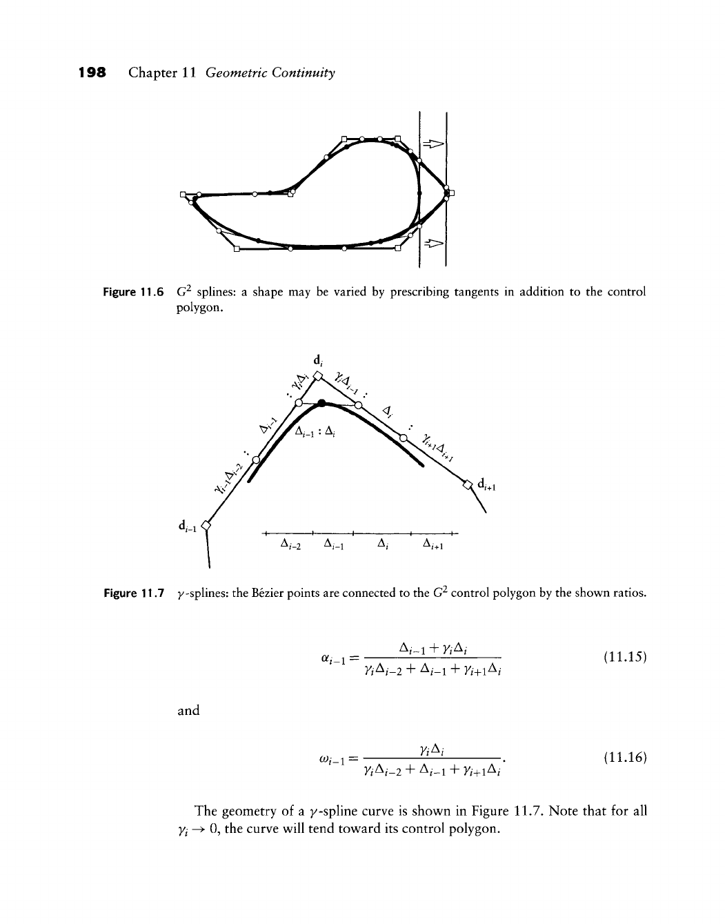
198 Chapter 11 Geometric Continuity
Figure 11.6 G^ splines: a shape may be varied by prescribing tangents in addition to the control
polygon.
A/_2 A,_i A,- A,„i
Figure 11.7 y-splines: the Bezier points are connected to the G^ control polygon by the shown ratios.
a,_l: A,-i + vAi
VAi-l + A,_i + Yi^i^i
(11.15)
ind
^/-i
=
vAi
vAi-l + A,_i + Yi^i^i
(11.16)
The geometry of a y-spline curve is shov^n in Figure 11.7. Note that for all
Yl -^ 0, the curve v^ill tend tov^ard its control polygon.
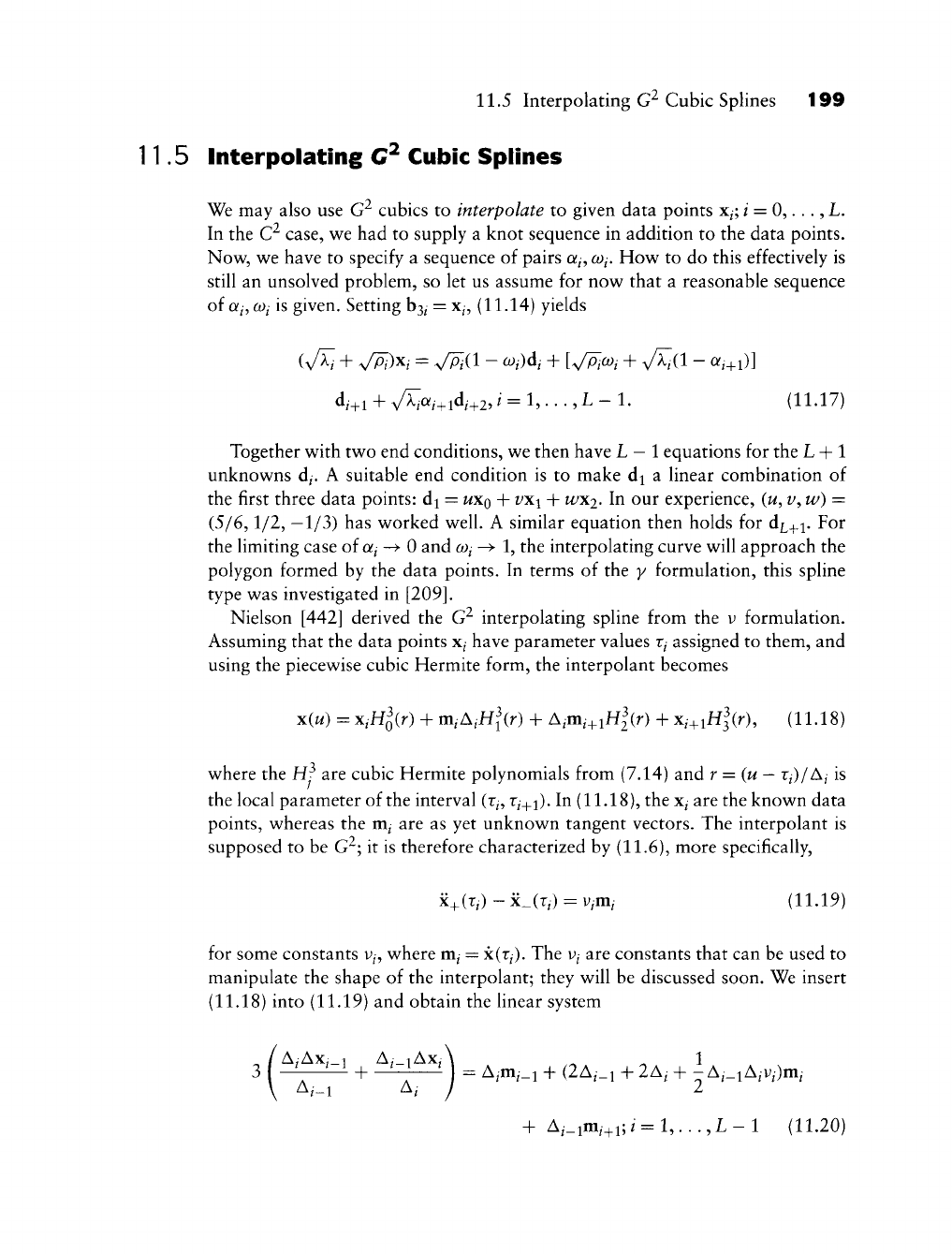
11.5 Interpolating G^ Cubic Splines 199
11.5 Interpolating C^ Cubic Splines
We may also use G^ cubics to interpolate to given data points x^; / = 0,. . ., L.
In the C^ case, we had to supply a knot sequence in addition to the data points.
Now, we have to specify a sequence of pairs a^,
coi.
How to do this effectively is
still an unsolved problem, so let us assume for now that a reasonable sequence
of
Qfp coi
is given. Setting b3/ = x^, (11.14) yields
d,+i + y/^iOti+A+2,
/•
= 1,..., L - 1. (11.17)
Together with two end conditions, we then have L
— 1
equations for the L + 1
unknowns d^. A suitable end condition is to make d^ a linear combination of
the first three data points: d^ =
WXQ
+ v^\ + wi^i. In our experience, (w,
v^
w) =
(5/6,1/2,
—1/3) has worked well. A similar equation then holds for
dj^^^.
For
the limiting case of aj -> 0 and
coi
-^ 1, the interpolating curve will approach the
polygon formed by the data points. In terms of the y formulation, this spline
type was investigated in
[209].
Nielson [442] derived the G^ interpolating spline from the v formulation.
Assuming that the data points x^ have parameter values
TJ
assigned to them, and
using the piecewise cubic Hermite form, the interpolant becomes
xiu) = x^H^ir) + m,A,Hl{r) + A,m,+iH|(r) +
x,_,^Hl(r),
(11.18)
where the
Hj*
are cubic Hermite polynomials from (7.14) and r = (u
—
r^)/A^ is
the local parameter of the interval (r/, r/+i). In (11.18), the
x^
are the known data
points, whereas the m^ are as yet unknown tangent vectors. The interpolant is
supposed to be G^; it is therefore characterized by (11.6), more specifically,
x+(T,)-x_(T,) = y,m, (11.19)
for some constants v^, where m^ = x(r^). The
Vj
are constants that can be used to
manipulate the shape of the interpolant; they will be discussed soon. We insert
(11.18) into (11.19) and obtain the linear system
(
A;AX; 1 A;_iAX;\ ^ ^1
^-^i + 'I = A,m,_i + (2A,_i + 2 A, + - A,_iA,y,)m,
A,_i A, / 2
+ A,_im,+i;/=l,...,L-l (11.20)
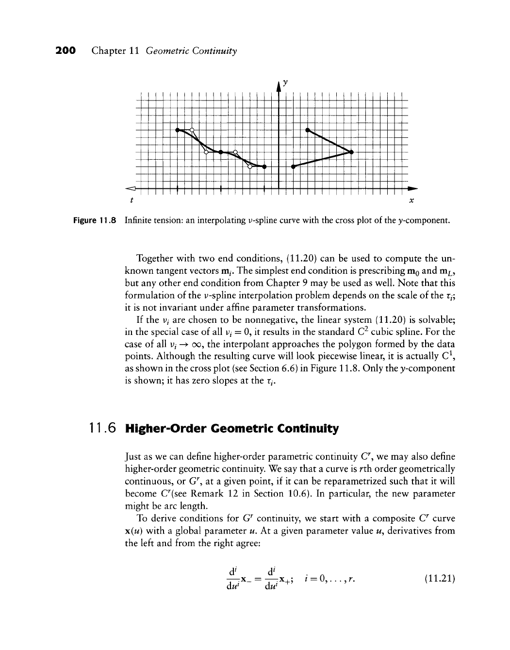
200 Chapter 11 Geometric Continuity
Figure 11.8 Infinite tension: an interpolating y-spline curve with the cross plot of the y-component.
Together with two end conditions, (11.20) can be used to compute the un-
known tangent vectors m^. The simplest end condition is prescribing mo and m^,
but any other end condition from Chapter 9 may be used as well. Note that this
formulation of the y-spline interpolation problem depends on the scale of the r^;
it is not invariant under affine parameter transformations.
If the
Vi
are chosen to be nonnegative, the linear system (11.20) is solvable;
in the special case of all
V/
= 0, it results in the standard C^ cubic spline. For the
case of all
V/
-^ oo, the interpolant approaches the polygon formed by the data
points. Although the resulting curve will look piecewise linear, it is actually C^,
as shown in the cross plot (see Section 6,6) in Figure 11.8. Only the y-component
is shown; it has zero slopes at the r^.
11.6 Higher-Order Geometric Continuity
Just as we can define higher-order parametric continuity C^, we may also define
higher-order geometric continuity. We say that a curve is rth order geometrically
continuous, or G^, at a given point, if it can be reparametrized such that it will
become C^(see Remark 12 in Section 10.6). In particular, the new parameter
might be arc length.
To derive conditions for G^ continuity, we start with a composite O curve
x(w) with a global parameter u. At a given parameter value w, derivatives from
the left and from the right agree:
—-x_
= —-x.
au^
aw
+' :0,...,r. (11.21)
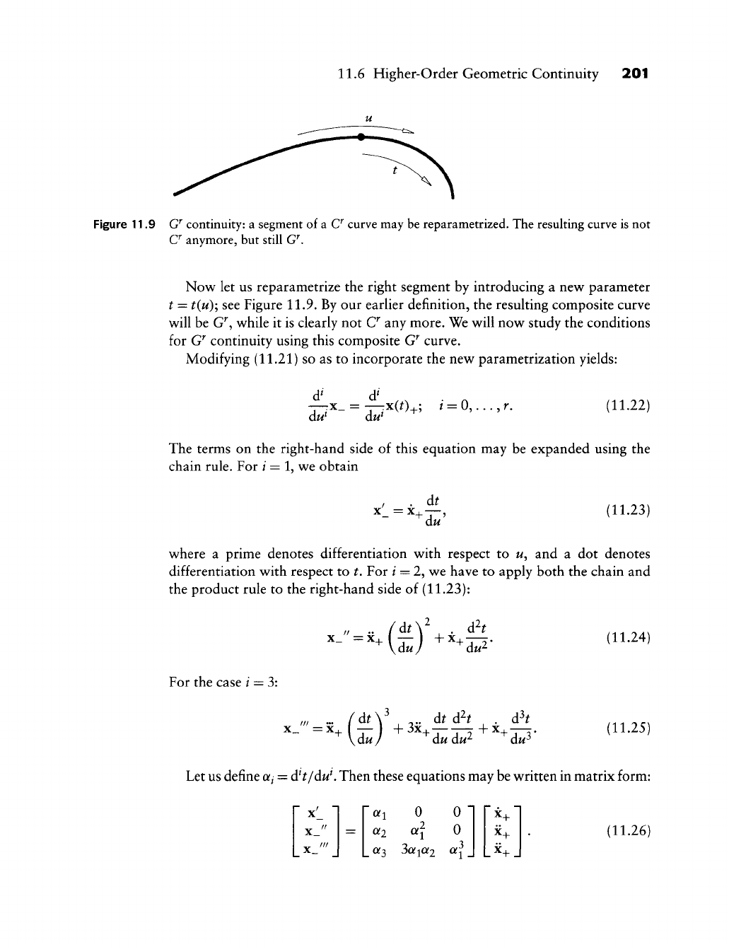
11.6 Higher-Order Geometric Continuity 201
Figure 11.9 G^ continuity: a segment of a
C^
curve may be reparametrized. The resuhing curve is not
C^ anymore, but still G^.
Now let us reparametrize the right segment by introducing a new parameter
t = t{u); see Figure 11.9. By our earlier definition, the resulting composite curve
will be G^, while it is clearly not C any more. We will now study the conditions
for G^ continuity using this composite G^ curve.
Modifying (11.21) so as to incorporate the new parametrization yields:
d' d'
dw
du'
(11.22)
The terms on the right-hand side of this equation may be expanded using the
chain rule. For / = 1, we obtain
X =X
d^
dw' (11.23)
where a prime denotes differentiation with respect to w, and a dot denotes
differentiation with respect to t. For / = 2, we have to apply both the chain and
the product rule to the right-hand side of (11.23):
„ .. /dty . d^t (11.24)
For the case / = 3:
X ^'/-x (^\^ 3x —— X
\duj dudu^
dtdh . . dft
+
dt/3-
(11.25)
Let us define a/ = dH/duK Then these equations may be written in matrix form:
x'_ •
x_"
x_'"
_. «2
_«3
0
3o;ia2
0 •
0
4\
_x+_
(11.26)
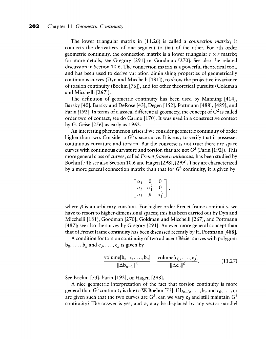
202 Chapter 11 Geometric Continuity
The lower triangular matrix in (11.26) is called a connection matrix^ it
connects the derivatives of one segment to that of the other. For rth order
geometric continuity, the connection matrix is a lov^er triangular r y. r matrix;
for more details, see Gregory [291] or Goodman
[270].
See also the related
discussion in Section 10.6. The connection matrix is a powerful theoretical tool,
and has been used to derive variation diminishing properties of geometrically
continuous curves (Dyn and Micchelli [181]), to show the projective in variance
of torsion continuity (Boehm [76]), and for other theoretical pursuits (Goldman
andMiccheni[267]).
The definition of geometric continuity has been used by Manning
[414],
Barsky [40], Barsky and DeRose [43], Degen
[152],
Pottmann
[488], [489],
and
Farin
[192].
In terms of classical differential geometry, the concept of G^ is called
order two of contact; see do Carmo
[170].
It was used in a constructive context
by G. Geise [256] as early as 1962.
An interesting phenomenon arises if we consider geometric continuity of order
higher than two. Consider a G^ space curve. It is easy to verify that it possesses
continuous curvature and torsion. But the converse is not true: there are space
curves with continuous curvature and torsion that are not G^ (Farin [192]). This
more general class of curves, called Frenet frame continuous^ has been studied by
Boehm [74]; see also Section 10.6 and Hagen
[298],
[299], They are characterized
by a more general connection matrix than that for G^ continuity; it is given by
«! 0 0 •
0^2 oi^ 0
L «3
^ «i .
where fi is an arbitrary constant. For higher-order Frenet frame continuity, we
have to resort to higher-dimensional spaces; this has been carried out by Dyn and
MiccheUi
[181],
Goodman
[270],
Goldman and MiccheUi
[267],
and Pottmann
[487];
see also the survey by Gregory
[291].
An even more general concept than
that of Frenet frame continuity has been discussed recently by H. Pottmann
[488].
A condition for torsion continuity of two adjacent Bezier curves with polygons
bo,...,
b^ and
CQ,
..., c„ is given by
volume[b„_3,...
,b^] _ volume[co,... ,03] (H 27)
|Ab^_ll|6 IIAq
•Oil
116
See Boehm [73], Farin
[192],
or Hagen
[298].
A nice geometric interpretation of the fact that torsion continuity is more
general than G^ continuity is due to
W.
Boehm [73]. If
b„_3,...,
b„ and
CQ,
...,
C3
are given such that the two curves are G^, can we vary
C3
and still maintain G^
continuity? The answer is yes, and
C3
may be displaced by any vector parallel
11.8 Problems 203
to the tangent spanned by b„_i and c^. But we may displace C3 by any vector
parallel to the osculating plane spanned by b„_2,
b^,
Ci
and still maintain torsion
continuity!
11.7 Implementation
We include a direct G^ spline program. It assumes that the piecewise Bezier
polygon has been determined except for the junction points h^i^ which will be
computed:
void direct_gspline(l,bez_x,bez_y)
/* From given interior Bezier points,
the junction Bezier points b3i are found from the G2 conditions.
Input: 1: no of cubic pieces.
bez_x,bez_y: interior Bezier points b_{3i+l}, b_{3i-l}.
Output:bez_x,bez_y: completed piecewise Bezier polygon.
Note:
b_0 and b_{31+3} should be provided, too!
V
11.8 Problems
1 Figure 11.1 shows a triangle and an inscribed piecewise quadratic curve.
Find the ratio of the areas enclosed by the curve and the triangle.
2 Show that the average of two G^ piecewise cubics is in general not G^.
3 Find an example of a G^ torsion continuous curve that is not
* 4 Let a G^ curve consist of two cubic Bezier curves. The derivatives of the
two curves at the junction point are related by a connection matrix. Work
out the corresponding connection matrix for the Bezier points.
* 5 Show that a nonplanar cubic cannot have zero curvature or torsion any-
where.
* 6 The G^ piecewise cubic from Figure 11.5 cannot be represented as a direct
G^ spline. Can it be obtained from a v-spline interpolation problem.^
PI Change the programs for interpolating C^ cubics so that they compute
interpolating G^ splines.

This Page Intentionally Left Blank
Conic Sections
V^onic sections (or, simply, conies) have received the most attention throughout
the centuries of any knov^n curve type. Today, they are an important design tool in
the aircraft industry; they are also used in areas such as font design. A great many
algorithms for the use of conies in design were developed in the 1940s; Liming
[390] and [391] are two books with detailed descriptions of those methods. A
thorough development of conies can also be found in [85] and
[202].
The first person to consider conies in a CAD environment was S. Coons
[124].
Later, Forrest [240] further investigated conies and also rational cubics. We shall
treat conies in the rational Bezier form; a good reference for this approach is Lee
[377].
We present conies partly as a subject in its own right, but also as a first
instance of rational Bezier and B-spline curves (NURBS), to be discussed later.
12.1 Projective Maps of tiie Real Line
Polynomial curves, as studied before, bear a close relationship to affine geometry.
Consequently, the de Casteljau algorithm makes use of ratios, which are the
fundamental invariant of affine maps. Thus the class of polynomial curves is
invariant under affine transformations: an affine map maps a polynomial curve
onto another polynomial curve.
Conic sections, and later rational polynomials, are invariant under a more
general type of map: the so-called projective maps. These maps are studied in
projective geometry. This is not the place to outline the ideas of that kind of
geometry; the interested reader is referred to the text by Penna and Patterson
[461] or to [85] and
[202].
All we need here is the concept of a projective map.
205
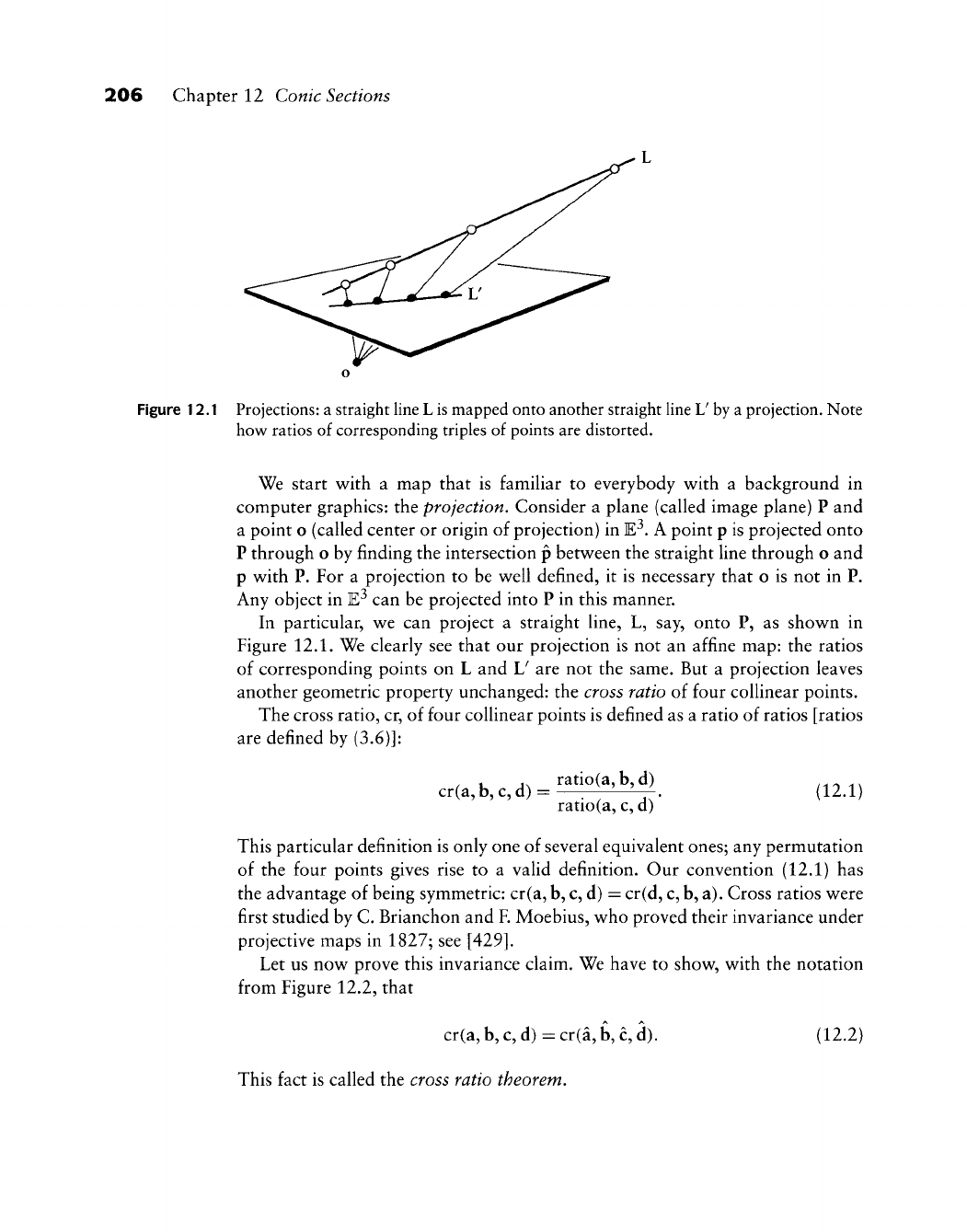
206 Chapter 12 Conic Sections
Figure 12.1 Projections: a straight
Hne L
is mapped onto another straight
Hne
\J by a projection. Note
how ratios of corresponding triples of points are distorted.
We start with a map that is famihar to everybody with a background in
computer graphics: the projection. Consider a plane (called image plane) P and
a point o (called center or origin of projection) in
E-^.
A point p is projected onto
P through o by finding the intersection p between the straight line through o and
p with P. For a projection to be well defined, it is necessary that o is not in P.
Any object in E-^ can be projected into P in this manner.
In particular, we can project a straight line, L, say, onto P, as shown in
Figure 12.1. We clearly see that our projection is not an affine map: the ratios
of corresponding points on L and V are not the same. But a projection leaves
another geometric property unchanged: the cross ratio of four collinear points.
The cross ratio, cr, of four collinear points is defined as a ratio of ratios [ratios
are defined by
(3.6)]:
cr(a, b, c, d) = ratio(a,b, d)
ratio(a, c, d) (12.1)
This particular definition is only one of several equivalent ones; any permutation
of the four points gives rise to a vahd definition. Our convention (12.1) has
the advantage of being symmetric: cr(a, b, c, d) = cr(d, c, b, a). Cross ratios were
first studied by C. Brianchon and
F.
Moebius, who proved their invariance under
projective maps in 1827; see
[429].
Let us now prove this invariance claim. We have to show, with the notation
from Figure 12.2, that
cr(a, b, c, d) = cr(a, b, c, d).
This fact is called the cross ratio theorem.
(12.2)
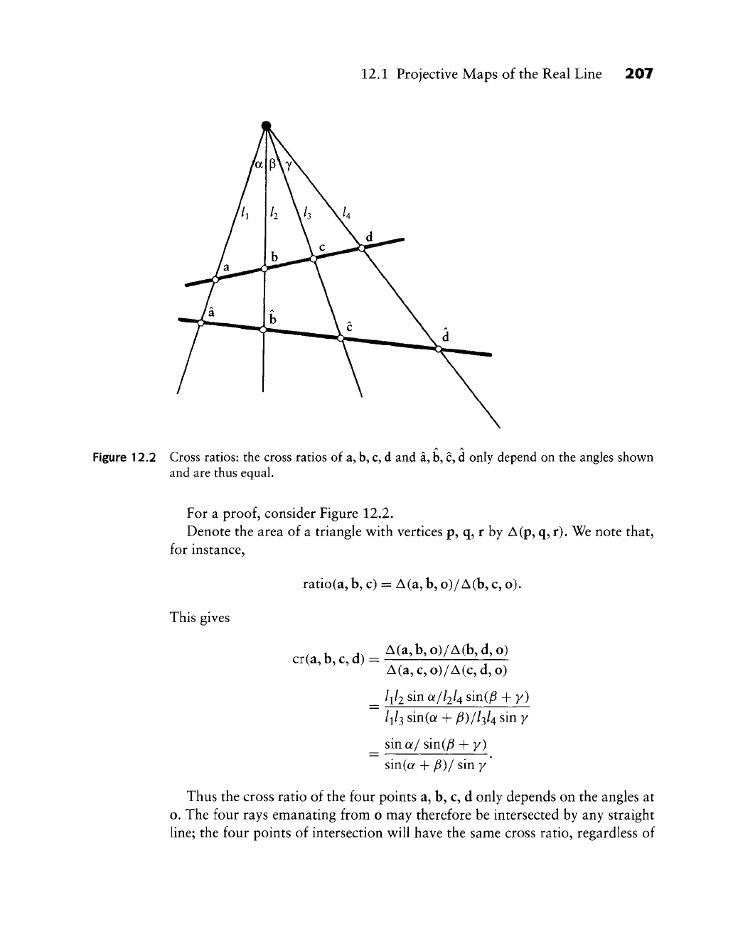
12.1 Projective Maps of the Real Line 207
Figure 12.2 Cross ratios: the cross ratios of a,
b,
c, d and a,
b,
c, d only depend on the angles shown
and are thus equal.
For a
proof,
consider Figure 12.2.
Denote the area of a triangle with vertices p, q, r by A(p, q, r). We note that,
for instance,
ratio(a, b, c) = A(a, b, o)/A(b, c, o).
cr(a,b,
c, d) =
This gives
A(a, b, o)/A(b, d, o)
A(a,c,o)/A(c,d,o)
_ lili sin a/l2l4 sin(j6 + y)
lil^ sin((y + P)/l^U sin y
_ sin Of/ sin(^ + y)
sin(a + y6)/ sin y
Thus the cross ratio of the four points a, b, c, d only depends on the angles at
o. The four rays emanating from o may therefore be intersected by any straight
line;
the four points of intersection will have the same cross ratio, regardless of
208 Chapter
12
Conic Sections
the choice
of the
straight Hne.
All
such straight lines
are
related
by
projections,
and
we can
therefore
say
that projections leave
the
cross ratio
of
four collinear
points invariant. Since
the
cross ratio
is the
same
for any
straight line intersecting
the given four straight lines,
one
also calls
it the
cross ratio
of
the four given lines.
A concept that
is
slightly more abstract than that
of
projections
is
that
of
projective maps. Going back
to
Figure 12.1,
we can
interpret both
L and \J as
copies
of
the real line. Then
the
projection
of
L onto
\J can be
viewed
as a map of
the real line onto
itself.
With this interpretation,
a
projection defines
a
projective
map
of
the real line onto
itself. On the
real line,
a
point
is
given
by a
real number,
so
we can
assume
a
correspondence between
the
point
a and a
real number
a.
An important observation about projective maps
of
the real line
to
itself
is
that
they
are
defined
by
three preimage
and
three image points.
To
observe this,
we
inspect Figure
12.2. The
claim
is
that
a, b, d and
their images
a, b, d
determine
a projective
map. It is
true since
if we
pick
an
arbitrary fourth point
c on L, its
image
c on V is
determined
by the
cross ratio theorem.
A projective
map of the
real line onto itself
is
thus determined
by
three
preimage numbers
a^
fo,
c and
three image numbers
5,
fc,
2. The
projective image
?
of a
point
t can
then
be
computed from
cr(^,
fo,
^,
c)
=
cr(5,
&,
?,
c).
Setting
p = (b
—
a)/(c
—
b) and p = (b
—
a)/{c
—
b)^ this
is
equivalent
to
(t-a)/(c-t) (i-a)/(c-iy
Solving
for i:
^^{t-
a)pc
+ (c- t)ap
pic-t)
+
p(t-a)
*
A convenient choice
for the
image
and
preimage points
is a = a =
0^
c = c = 1.
Equation (12.3) then takes
on the
simpler form
^^-
'^
(12.4)
pil-t)-\-pt
Thus
a
projective
map of the
real line onto itself corresponds
to a
rational
linear transformation.
It is
left
for the
reader
to
verify that
the
projective
map
becomes
an
affine
map in the
special case that
p
—
p.
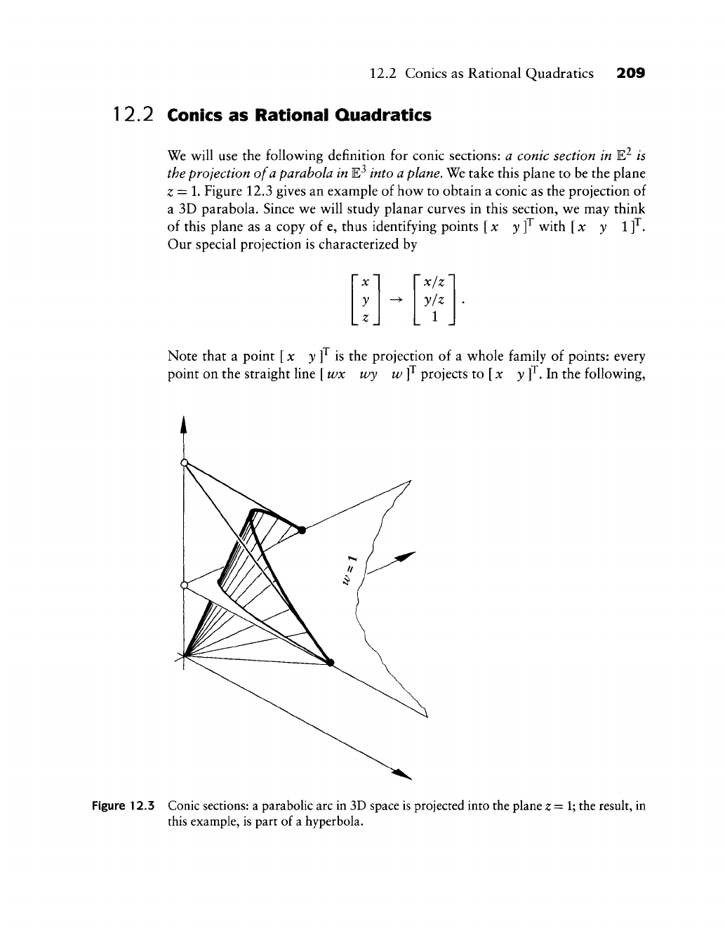
12.2 Conies as Rational Quadratics 209
12.2 Conies as Rational Quadratics
We will use the following definition for conic sections: a conic section in E^ is
the projection of a parabola in ¥? into a plane. We take this plane to be the plane
z=l. Figure 12.3 gives an example of how to obtain a conic as the projection of
a 3D parabola. Since we will study planar curves in this section, we may think
of this plane as a copy of e, thus identifying points [x y]^ with [x y
1
]^.
Our special projection is characterized by
X
y
_z
_
->
x/z
y/z
1
Note that a point [x y ]^ is the projection of a whole family of points: every
point on the straight line
[
wx wy w ]^ projects to
[
x y
]^.
In the following,
Figure 12.3 Conic sections: a parabolic arc in 3D space is projected into the plane z =
V^
the result, in
this example, is part of a hyperbola.

210 Chapter 12 Conic Sections
Figure 12.A Projections: the special projection that is used to write objects in the plane
;2
= 1 as
projections of objects in E^.
we will use the shorthand notation
[
wx w ]^ with x
E
E^ for
[
wx wy w ]^}
An illustration of this special projection is given in Figure 12.4.
Let c{t)
G
E^ be a point on a conic. Then there exist real numbers
WQ^
Wi, wi
and points bo,
b^,
hi
G
E^ such that
c{t) =
wohoBlit) + wihiBlit) + wihiBlit)
woBlit) + wiB\it) + wiBlit) (12.5)
Let us prove (12.5). We may identify c(t) e E^ with
[
c(0 1F ^ E^. This point
is the projection of a point
[
w(t)c(t) w(t)
]^,
which lies on a 3D parabola. The
third component w(t) of this 3D point must be a quadratic function in t, and
1 The set of all points
[
wx wy w
]^
is called the homogeneous form or homogeneous
coordinates
oi{x y
]^.
12.2 Conies as Rational Quadratics 211
may be expressed in Bernstein form:
wit) = woBlit) + w^Blit) + W2B\{t),
Having determined w{t)^ we may now write
wit) \c{t)-\\^it)Y.w,B]{t)l
L
1 J L
E^.^fW
J
Since the left-hand side of this equation denotes a parabola, we may write
/=0
with some points p^ e E^. Thus
2 2
J2PtBJit) = c{t)J2wiBJit),
i=0
(12.6)
/=0
and hence
c{t) = PoBl(t)^p^B](t)+p2Bl(t)
woBl(t) + wiB^it) + W2Bl(t)'
Setting
p^
= Wihi now proves (12.5).
We call the points b/ the control polygon of the conic c; the numbers Wi are
called weights of the corresponding control polygon vertices. Thus the conic con-
trol polygon is the projection of the control polygon with vertices
[
w^^ w^ ]^,
which is the control polygon of the 3D parabola that we projected onto c.
The form (12.5) is called the rational quadratic form of a conic section. If
all weights are equal, we recover nonrational quadratics, that is, parabolas. The
influence of the weights on the shape of the conic is illustrated in Figure 12.5. In
that figure, we have chosen
bo =
Note that a common nonzero factor in the w^ does not affect the conic at all.
If
WQ
7^ 0, we may therefore always achieve
WQ
—
lhydi simple scaling of all Wi,
0
1 ,bi = 0
0 ,b2 = 1
0
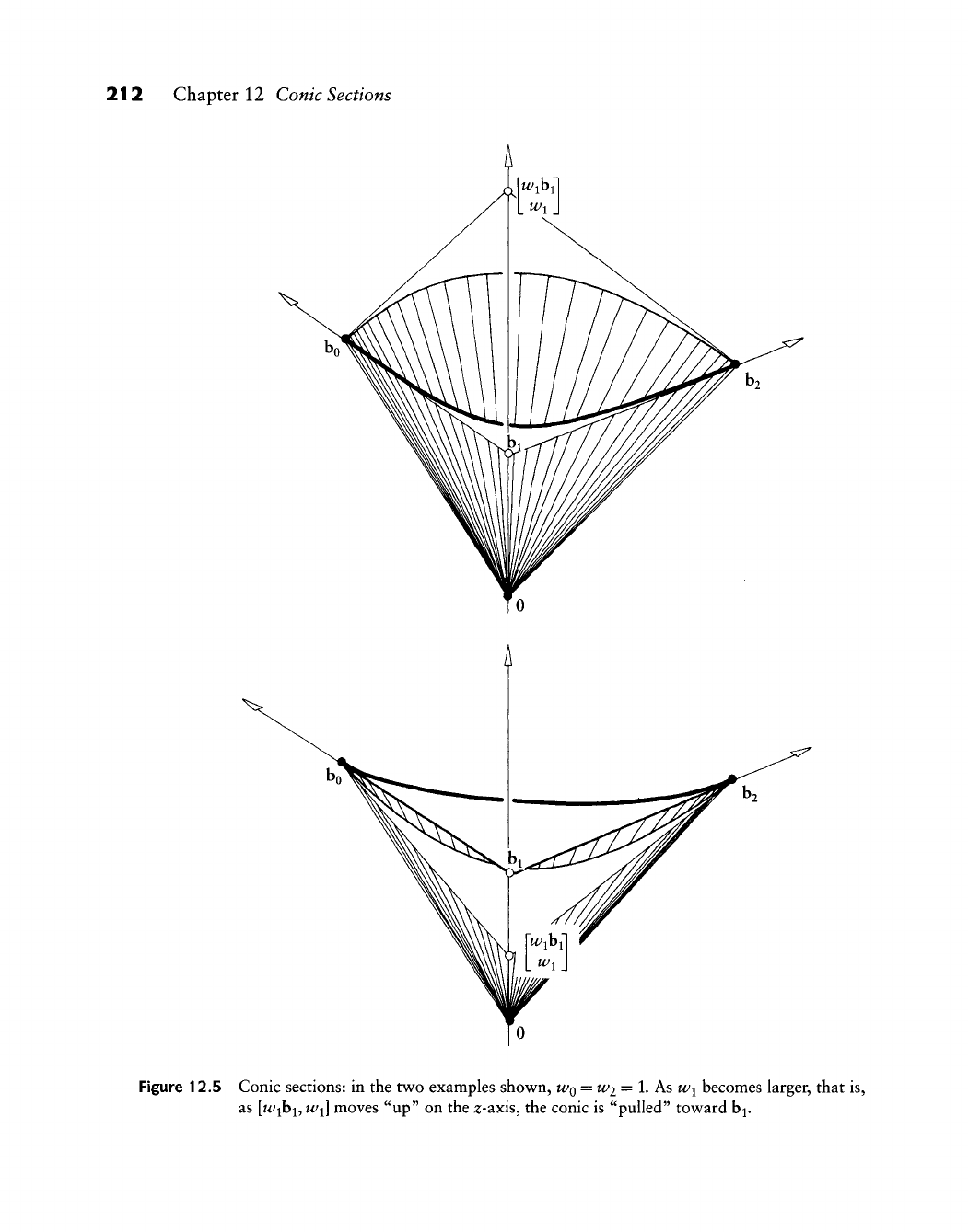
212 Chapter 12 Conic Sections
Figure 12.5 Conic sections: in the two examples shown,
WQ
=
W2
= 1. As wi becomes larger, that is,
as [t^ibi,
Wi]
moves "up" on the z-^xis, the conic is "pulled" toward b^.
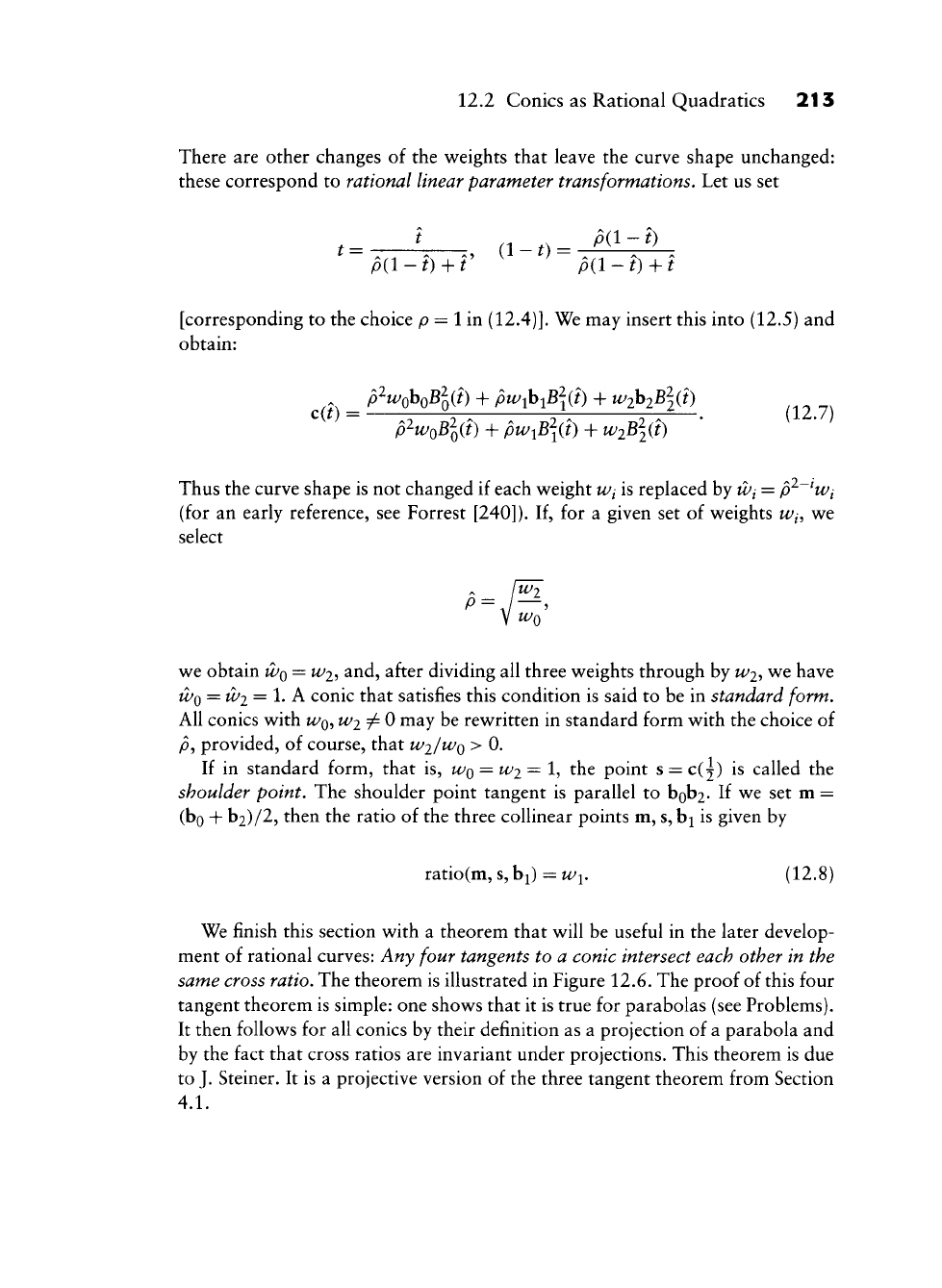
12.2 Conies as Rational Quadratics 213
There are other changes of the weights that leave the curve shape unchanged:
these correspond to rational linear parameter transformations. Let us set
„ (1-0- ''"'-'^
p{l-t)-\-t p{l-t) + t
[corresponding to the choice p = 1 in (12.4)]. We may insert this into (12.5) and
obtain:
c(?) ^ ^^^0^0-^0^^^) + P^ibiB^(f) + W2h2B\{t)
p^woBlii)
+ pwiB\{i) + W2B\{i)
Thus the curve shape is not changed if each weight
Wi
is replaced by
Wi —
p^~^Wi
(for an early reference, see Forrest [240]). If, for a given set of weights
iv^^
we
select
we obtain
WQ
= wi-, and, after dividing all three weights through by wi-, we have
t2/o =
t2^2
= 1- A conic that satisfies this condition is said to be in standard form.
All conies with
U/Q,
wii^O may be rewritten in standard form with the choice of
yo,
provided, of course, that
WI/WQ
> 0.
If in standard form, that is,
WQ
=
W2
= 1, the point s = c(|) is called the
shoulder point. The shoulder point tangent is parallel to bob2. If we set m =
(bo + b2)/2, then the ratio of the three collinear points m, s, b^ is given by
ratio(m, s, b^) = Wi. (12.8)
We finish this section with a theorem that will be useful in the later develop-
ment of rational curves: Any four tangents to a conic intersect each other in the
same cross ratio. The theorem is illustrated in Figure 12.6. The proof of this four
tangent theorem is simple: one shows that it is true for parabolas (see Problems).
It then follows for all conies by their definition as a projection of a parabola and
by the fact that cross ratios are invariant under projections. This theorem is due
to J. Steiner. It is a projective version of the three tangent theorem from Section
4.1.
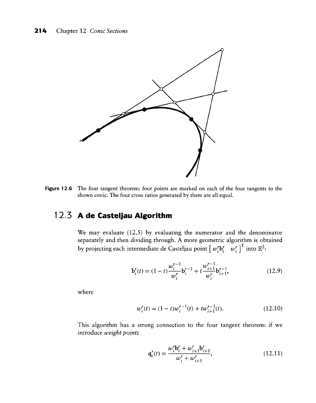
214 Chapter 12 Conic Sections
Figure 12.6 The four tangent theorem: four points are marked on each of the four tangents to the
shown conic. The four cross ratios generated by them are all equal.
12.5 A de Casteljau Algorithm
We may evaluate (12.5) by evaluating the numerator and the denominator
separately and then dividing through. A more geometric algorithm is obtained
by projecting each intermediate de Casteljau point [
w^W-
w^-
] into E^:
W': W,
(12.9)
w^here
,.r-l/
w\(t) = (\-t)w'r\t)
+
tw'^[{t) (12.10)
This algorithm has a strong connection to the four tangent theorem: if wt
introduce weight points
OL'iit)
• (12.11)
12.4 Derivatives 215
then
cr(b;:,q;,b^+\b^^i) = i^ (12.12)
assumes the same value for all r, /. Though computationally more involved than
the straightforward algebraic approach, this generalized de Casteljau algorithm
has the advantage of being numerically stable: it uses only convex combinations,
provided the weights are positive and t
G
[0,1].
12.4 Derivatives
To find the derivative of a conic section, that is, the vector c{t) = dc/d^, we may
employ the quotient rule. For a simpler derivation, let us rewrite (12.6) as
p(t) = w(t)c(t).
We apply the product rule:
p(^) = w{t)c(t) + w(t)c(t)
and solve for c(t):
c(t) = -^\p(t) - w{t)cm (12.13)
w(t)
We may evaluate (12.13) at the endpoint
^
= 0:
2
c(0) = —[wihi - woho - (wi -
WQ)ho].
After some simplifications, we obtain
c(0) = ^^Abo. (12.14)
WQ
Similarly, we obtain
c(l) = ^Abi. (12.15)
W2
Let us now consider two conies, one defined over the interval
[UQ,
U^ with
control polygon bo,
b^,
hi and weights
W/Q,
^i, wi and the other defined over
216 Chapter 12 Conic Sections
the interval [wj, ui] with control polygon
b2,
b3,
b4 and weights
W2,
w^,
W4,
Both
segments form a C^ curve if
^Ab,= ^Ab2, (12.16)
Ao Ai
where the appearance of the interval lengths A^ is due to the application of the
chain rule, which is necessary since we now consider a composite curve with a
global parameter u.
12.5 The Implicit Form
Every conic c(^) has an implicit representation of the form
f{x,y) = 0,
where /^ is a quadratic polynomial in x and y. To find this representation, recall
that c{t) may be written in terms of barycentric coordinates of the polygon
vertices bo, bj, hi:
c(t) = robo + ribi + tihi; (12.17)
see Section 3.5. Since c(t) may also be written as a rational Bezier curve (12.5),
and since both representations are unique, we may compare the coefficients of
the hi'.
To
= [woa-tf]/D, (12.18)
r^ = [2wit(l-t)]/D, (12.19)
T2
= [W2t^]/D, (12.20)
where D = ^
WjBJ,
We may solve (12.18) and (12.20) for (1 - t) and if, respec-
tively. Inserting both expressions into (12.19) yields
Tj — t
WQW2
This may be written more symmetrically as
ror2 W0W2
(12.21)
12.5 The Implicit Form 217
This is the desired impHcit form, since the barycentric coordinates
TQ,
r^,
X2
of
c(^) are given by
^0 =
1
c^
b\ ^2
\cy bl bl
111
1
b^ fcJ ^2
111
^1=-
b^
1
LX
1
cy
1
1
bl
bl
1
1
X2=-
bl b\ (f\
bl b\ cy\
111
^Q b\
b^
1
K
b\ fed
111
The implicit form has an important application: suppose we are given a conic
section c and an arbitrary point x
G
E^. Does x lie on c? This question is hard to
ansv^er if c is given in the parametric form (12.5). Using the implicit form, this
question is ansv^ered easily. First, compute the barycentric coordinates
TQ,
r^, Xi
of X v^ith respect to bg,
b^,
b2. Then insert
TQ,
r^, Xi into (12.21). If (12.21) is
satisfied, x lies on the conic (but see Problems).
The implicit form is also important when dealing with the IGES data specifi-
cation. In that data format, a conic is given by its implicit form f(x^ y) = 0 and
two points on it, implying a start point and endpoint bo and hi of a conic arc.
Many applications, however, need the rational quadratic form. To convert to
this form, we have to determine b^ and its weight w/^, assuming standard form.
First, we find tangents at bo and hi', we know that the gradient of /^ is a vec-
tor that is perpendicular to the conic. The gradient at bo is given by /"'s partials:
V/*(bo) = [/x(bo)9/y(bo)F- The tangent is perpendicular to the gradient and thus
has direction V-^/"(bo) =
{—fy(ho)',fx0^o)V'
Thus our tangents are given by
to(0=bo + ^V-^/"(bo) and
t2(s)=b2 + sVV(b2).
Their intersection determines
b^.
Next, we compute the midpoint m of
bo
and b2.
Then the line mb^ will intersect our conic in the shoulder point s. This requires
the solution of a quadratic equation,^ but then, using (12.8), we have found our
desired weight Wi\
If the input is not well defined—imagine bo and b2 being on two different
branches of a hyperbola!—then the preceding quadratic equation may have
complex solutions. An error flag would be appropriate here. If the arc between bo
2 The quadratic equation will in general have two solutions. We take the one inside the
triangle
bo,
bi,b2.
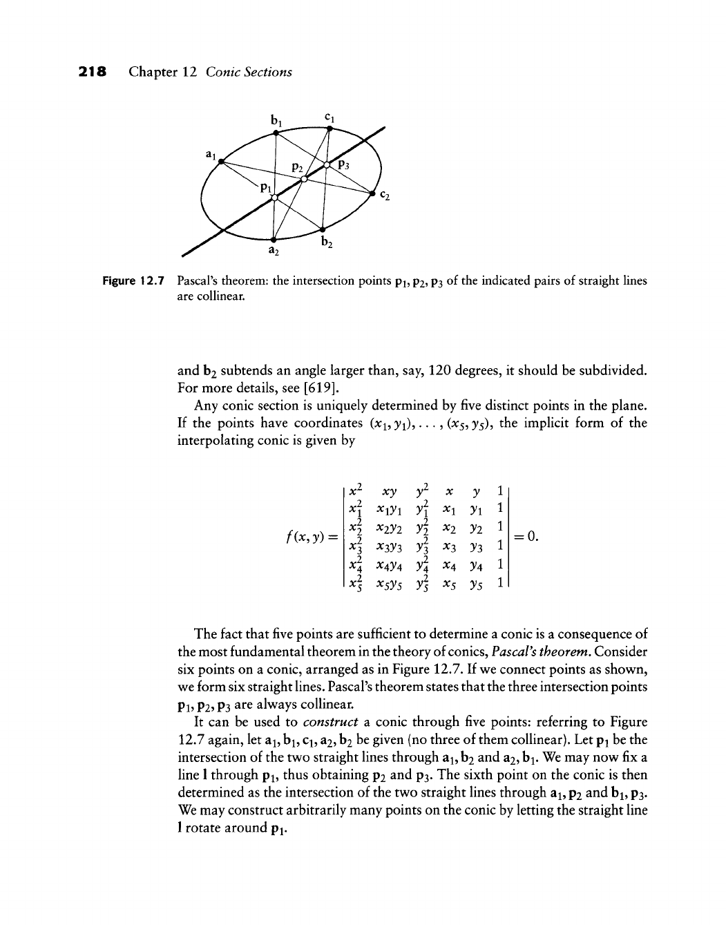
218 Chapter 12 Conic Sections
bi i
Figure 12.7 Pascal's theorem: the intersection points pi,
p2,
P3
of the indicated pairs of straight Hnes
are colUnear.
and b2 subtends an angle larger than, say, 120 degrees, it should be subdivided.
For more details, see
[619].
Any conic section is uniquely determined by five distinct points in the plane.
If the points have coordinates (x^,
yi),...,
(^5,3/5), the implicit form of the
interpolating conic is given by
f(x, y):
xy y 1
x\
xiyi y\ X]^ yi 1
^2
4
-\
^]
XlJl
^33'3
x^y^
XsJs
A
y\
y\
yl
Xi
^3
Xj^
xs
yi
y3
y4
ys
1
1
1
1
The fact that five points are sufficient to determine a conic is a consequence of
the most fundamental theorem in the theory of conies, Pascal's theorem. Consider
six points on a conic, arranged as in Figure 12.7. If
w^e
connect points as shown,
we form six straight
lines.
Pascal's theorem states that the three intersection points
pl,
p2, p3 are always coUinear.
It can be used to construct a conic through five points: referring to Figure
12.7 again, let a^, bj,
Cj,
a2,
b2 be given (no three of them collinear). Let pj be the
intersection of the two straight lines through a^, b2 and
a25
bj.
We may now fix a
line
1
through pi, thus obtaining p2 and P3. The sixth point on the conic is then
determined as the intersection of the two straight lines through a^, p2 and
b^,
P3.
We may construct arbitrarily many points on the conic by letting the straight line
1 rotate around pj.
12.6 Two Classic Problems 219
1
2.6 IWo Classic Problems
A large number of methods exist to construct conic sections from given pieces
of information, most based on Pascal's theorem. A nice collection is given in the
book by R. Liming
[391].
An in-depth discussion of those methods is beyond the
scope of this book; we restrict ourselves to the solution of two problems.
1.
Conic from two points and tangents plus another point. The given data
amount to prescribing bo^bi, b2. The missing weight Wi must be determined
from the point p, which is assumed to be on the conic. We assume, without loss
of generality, that the conic is in standard form
(WQ
= tv2 = Vj.
For the solution, we make use of the implicit form (12.21). We can easily
determine the barycentric coordinates
TQ,
tj, Xi of p with respect to the triangle
formed by the three b/. We can then solve (12.21) for the unknown weight Wi:
wi= ^^ . (12.22)
If p is inside the triangle formed by
bo,
b^,
b2,
then (12.22) always has a solution.
Otherwise, problems might occur (see Problems). If we do not insist on the conic
in standard form, the given point may be given the parameter value t
—
1/2, in
which case it is referred to as a shoulder point,
2.
Conic from two points and tangents plus a third tangent. Again, we are
given the Bezier polygon of the conic plus a tangent, which passes through two
points that we call bj and bj. We have to find the interior weight u/j, assuming
the conic will be in standard form. The unknown weight
Wx
determines the two
weight points qo and q^, with q^qi parallel to bob2; see Figure 12.8.
We compute the ratios ro = ratio(bo, bj, b^) and r^ = ratio(bi, bj, b2). From
the definition of the q^ in (12.11), it follows that ratio(bo, qo? b^) = Wi and
ratio(bi, qi, b2) = l/w^. The cross ratio property (12.12) now yields
^=rxwi, (12.23)
from which we easily determine w^ = y/ro/rl. The number under the square root
must be nonnegative for this to be meaningful (see Problems). Again, if we do
not insist on standard form, we may associate the parameter value t = 1/2 with
the given tangent—it is then called a shoulder tangent.
Figure 12.8 also gives a strictly geometric construction: intersect lines bobj
and b2bo. Connect the intersection with bj and intersect with the given tangent:
the intersection is the desired point p.
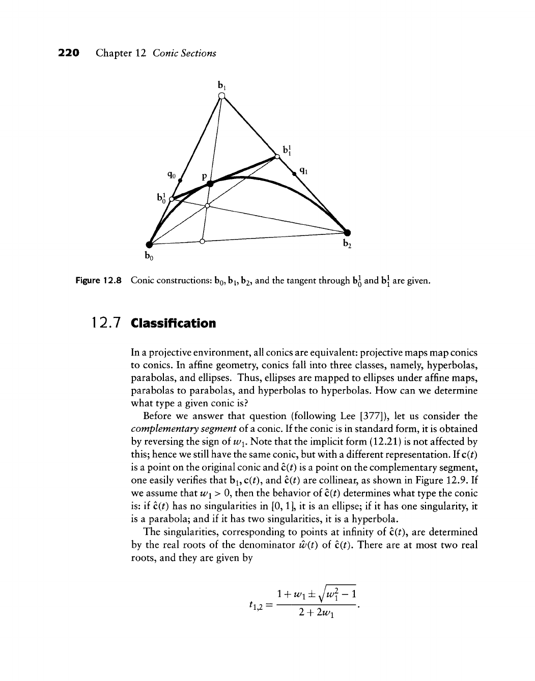
220 Chapter 12 Conic Sections
bo
Figure 12.8 Conic constructions:
bo,
b^,
hi-,
and the tangent through bj and h\ are given.
1
2.7 Classification
In a projective environment, all conies are equivalent: projective maps map conies
to conies. In affine geometry, conies fall into three classes, namely, hyperbolas,
parabolas, and ellipses. Thus, ellipses are mapped to ellipses under affine maps,
parabolas to parabolas, and hyperbolas to hyperbolas. Hov^ can we determine
vv^hat type a given conic is?
Before we answer that question (following Lee [377]), let us consider the
complementary segment of a conic. If the conic is in standard form, it is obtained
by reversing the sign of wx. Note that the implicit form (12.21) is not affected by
this;
hence we still have the same conic, but with a different representation. If c{t)
is a point on the original conic and c{t) is a point on the complementary segment,
one easily verifies that b^, c{t)^ and c{t) are coUinear, as shown in Figure 12.9. If
we assume that W\ > 0, then the behavior of c(^) determines what type the conic
is:
if c(^) has no singularities in
[0,1],
it is an ellipse; if it has one singularity, it
is a parabola; and if it has two singularities, it is a hyperbola.
The singularities, corresponding to points at infinity of c(^), are determined
by the real roots of the denominator w{t) of c{t). There are at most two real
roots,
and they are given by
l-\-Wi± Jw\
—
1
^ 2 = •
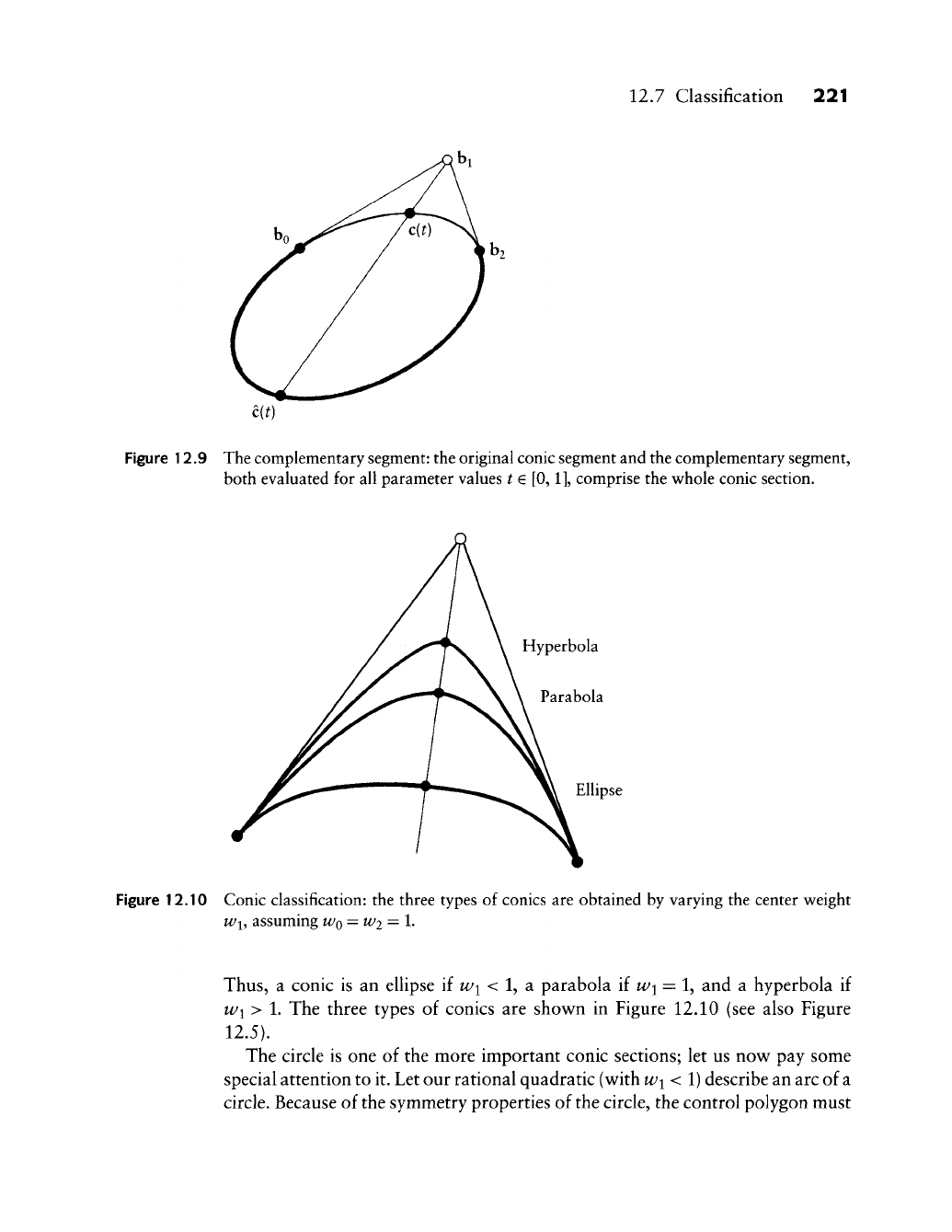
12.7 Classification 221
Figure 12.9 The complementary segment: the original conic segment and the complementary segment,
both evaluated for all parameter values t e
[0,1],
comprise the w^hole conic section.
Ellipse
Figure 12.10 Conic classification: the three types of conies are obtained by varying the center v^eight
Wi, assuming
WQ
=
W2
= 1.
Thus,
a conic is an ellipse if w/^ < 1, a parabola if wi = 1, and a hyperbola if
Wi > 1. The three types of conies are shown in Figure 12.10 (see also Figure
12.5).
The circle is one of the more important conic sections; let us now pay some
special attention to it. Let our rational quadratic (with Wi<l) describe an arc of a
circle. Because of the symmetry properties of the circle, the control polygon must
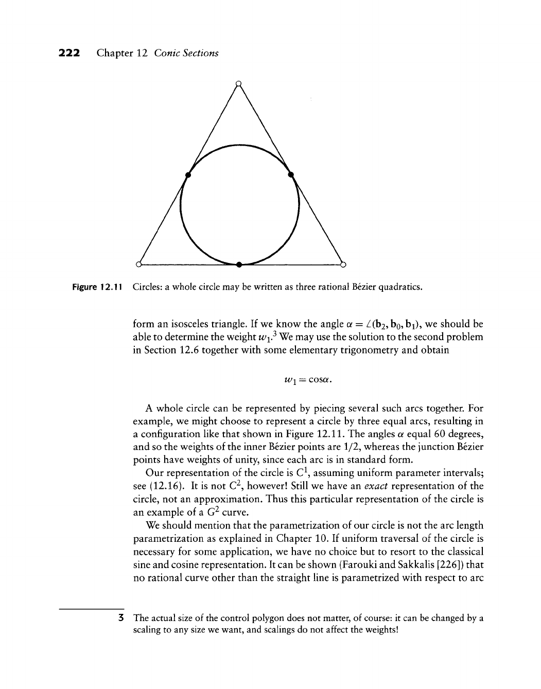
222 Chapter 12 Conic Sections
Figure 12.11 Circles: a whole circle may be written as three rational Bezier quadratics.
form an isosceles triangle. If we know the angle a = Z(b2, bo,
b^),
we should be
able to determine the weight w^? We may use the solution to the second problem
in Section 12.6 together with some elementary trigonometry and obtain
W^ =
COSQf.
A whole circle can be represented by piecing several such arcs together. For
example, we might choose to represent a circle by three equal arcs, resulting in
a configuration like that shown in Figure
12.11.
The angles a equal 60 degrees,
and so the weights of the inner Bezier points are 1/2, whereas the junction Bezier
points have weights of unity, since each arc is in standard form.
Our representation of the circle is C^, assuming uniform parameter intervals;
see (12.16). It is not C^, however! Still we have an exact representation of the
circle, not an approximation. Thus this particular representation of the circle is
an example of a G^ curve.
We should mention that the parametrization of our circle is not the arc length
parametrization as explained in Chapter 10. If uniform traversal of the circle is
necessary for some application, we have no choice but to resort to the classical
sine and cosine representation. It can be shown (Farouki and Sakkalis [226]) that
no rational curve other than the straight line is parametrized with respect to arc
3 The actual size of the control polygon does not matter, of
course:
it can be changed by a
scaling to any size we want, and scalings do not affect the weights!
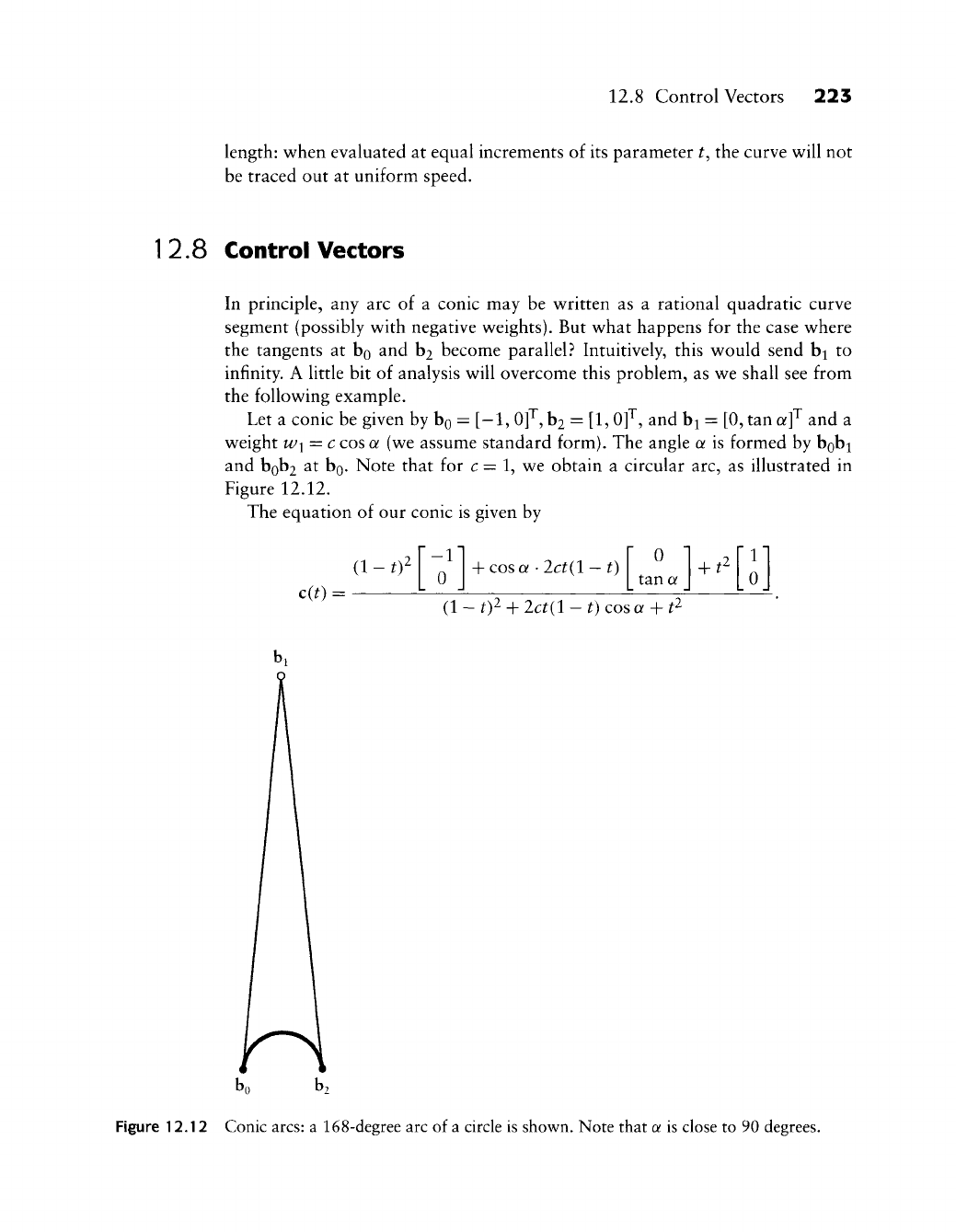
12.8 Control Vectors 223
length: when evaluated at equal increments of its parameter t^ the curve v^ill not
be traced out at uniform speed.
12.8 Control Vectors
In principle, any arc of a conic may be v^ritten as a rational quadratic curve
segment (possibly v^ith negative w^eights). But w^hat happens for the case w^here
the tangents at bg and hi become parallel? Intuitively, this v^ould send b^ to
infinity. A little bit of analysis w^ill overcome this problem, as wt shall see from
the foUov^ing example.
Let a conic be given by bo =
[—1,
0]^,b2 =
[1,
0]^,
and b^ = [0,tancy]^ and a
v^eight Wi = c cos a (v^e assume standard form). The angle a is formed by bob^
and bob2 at bg. Note that for c = 1, w^e obtain a circular arc, as illustrated in
Figure 12.12.
The equation of our conic is given by
(1
- ty
c(t) = 0 + cos a
•
2ct{l
—
t) 0
tan
Of
+
^"
(1 - t)^ + 2ct(l - t) cos a + fi
bo b2
Figure 12.12 Conic arcs: a 168-degree arc of a circle is shown. Note that a is close to 90 degrees.
224 Chapter 12 Conic Sections
What happens as a tends to 7r/2? For the Hmiting conic, we obtain the equation
(1 -1)^
c(t) =
-1
0 + 2t{l -1) +
t^ [J]
(1
-
0^
+
t^
(12.24)
The problem of a weight tending to zero and a control point tending to infinity
has thus been resolved. For c = 1, we obtain a semicircle; other values of c give
rise to different conies. For c =
—
1,
we obtain the "lower" half of the unit circle.
We have been able to overcome possible problems with parallel end tangents.
But there is a price to be paid: if we look at (12.24) closely, we see that it does
not constitute a barycentric combination any more! The factors of
bo
and b2 sum
to one identically, hence [0, c]^ must be interpreted as a vector. Thus (12.24)
contains both control points and control vectors."^ An important property of
Bezier curves is thus lost, namely, the convex hull property: it is defined only for
point sets, not for a potpourri of points and vectors.
The use of control vectors allows a very compact form of writing a semi-
circle. But two disadvantages argue against its use: first, the loss of the convex
hull property. Second: to write the control vector form in the context of "normal"
rational quadratics, one will have to resort to a special case treatment. We shall
see later (Section 13.6) how to avoid the use of the control vector form.
1
2.9 Implementation
The following routine solves the first problem in Section 12.6:
float conic_weight(b0,bl,b2,p)
/*
Input:b0,bl,b2: conic control polygon vertices
p:
point
on
conic
Output: weight of bl (assuming standard
form).
Note:
will crash
in
"forbidden" situations.
V
4 In projective geometry, vectors are sometimes called points at infinity. This has given rise
to the name
infinite control
points by Versprille
[601];
see also L. Piegl
[477].
We prefer
the term control
vector
since this allows us to distinguish between
[0,
c^ and [0, —c^.
12.10 Problems 225
12.10 Problems
1 Equation (12.22) does not always have a solution. Identify the "forbidden"
regions for the third point p on the conic.
2 In the same manner, investigate (12.23).
3 Prove that the four tangent theorem holds for parabolas.
* 4 Establish the connection betw^een (12.12) and the four tangent theorem.
*5 Our discussion of the implicit form (12.21) w^as somev^hat academic: in
a "real-life" situation, (12.21) will never be satisfied exactly. Discuss the
tolerance problem that arises here; that is, how closely does (12.21) have
to be satisfied for a point to be within a given tolerance to the conic?
PI Write a routine to iteratively subdivide a conic, putting each piece into
standard form. The middle weights will converge to unity. How do the
convergence rates depend on the type of the initial conic.^ (See also [403].)
P2 Write a routine to approximate a given Bezier curve by a sequence of elliptic
arcs within a given tolerance.

This Page Intentionally Left Blank
Rational Bezier
and B-Spline Curves
tvational B-spline curves^ have become the standard curve and surface descrip-
tion in the field of CAD and graphics. The use of rational curves in CAGD may
be traced to Coons
[124], [126],
and Forrest
[240].
By now, there are books on
NURBS:
Fiorot and Jeannin
[233],
Farin
[202],
Piegl and Tiller
[482].
15.1 Rational Bezier Curves
In Chapter 12, we obtained a conic section in E^ as the projection of a parabola
(a quadratic) in E^. Conic sections may be expressed as rational quadratic
(Bezier) curves, and their generalization to higher-degree rational curves is quite
straightforward: a rational Bezier curve of degree n in E^ is the projection of
an wth degree Bezier curve in E^ into the hyperplane iv =\. We may view this
4D hyperplane as a copy of E^; we assume that a point in E"* is given by its
coordinates [ x y z tf ] . Proceeding in exactly the same way as we did for
conies, we can show that an «th degree rational Bezier curve is given by
Mt) = woB"{t) + --- + w„B"(t) '•
x(0,b,eE^
(13.1)
The Wj art again called weights; the
b^
form the control polygon. It is the projec-
tion of the 4D control polygon [ Wjhi
Wj
] of the nonrational 4D preimage of
x(t).
1 Often called NURBS for nonuniform
rational
B-spUnes.
227
228 Chapter 13 Rational Bezier and B-Spline Curves
If all weights equal one, we obtain the standard nonrational Bezier curve, since
the denominator is identically equal to one.^ If some
Wj
are negative, singularities
may occur; we will therefore deal only with nonnegative Wj, Rational Bezier
curves enjoy all the properties that their nonrational counterparts possess; for
example, they are affinely invariant. We can see this by rewriting (13.1) as
x(t) = 2_^bi-
i=0 Tto"'.^r«
We see that the basis functions
sum to one identically, thus asserting affine invariance. If all
Wi
are nonnegative,
we have the convex hull property. We also have symmetry, invariance under
affine parameter transformations, endpoint interpolation, and the variation di-
minishing property. Obviously, the conic sections from the preceding chapter are
included in the set of all rational Bezier curves, further justifying their increasing
popularity.
The
Wi
are typically used as shape parameters. If we increase one w//, the curve
is pulled toward the corresponding
b/,
as illustrated in Figure
13.1.
Note that the
effect of changing a weight is different from that of moving a control vertex. If we
let all weights tend to infinity at the same rate, we do not approach the control
polygon since a common (if large) factor in the weights does not matter—the
rational Bezier curve shape parameters behave differently from y- or y-spline
shape parameters.
Two properties differ from the nonrational case. First, we have projective
invariance; that is, if a rational Bezier curve is transformed by a projective
transformation, we could just as well apply that transformation to the control
polygon (using its weights to write it in homogeneous form) and would end up
with the same curve. Note that nonrational curves have this property only for
a subset of all projective maps, that is, the affine maps. The second difference
is the linear precision property. Rational curves may have all Bezier points b/
distributed on a straight line in a totally arbitrary fashion:
hi = (1 - a/)bo + a,b„; / = 0,...,
w
This is also true if
the
weights are not unity, but are equal to each other—a common factor
does not matter.
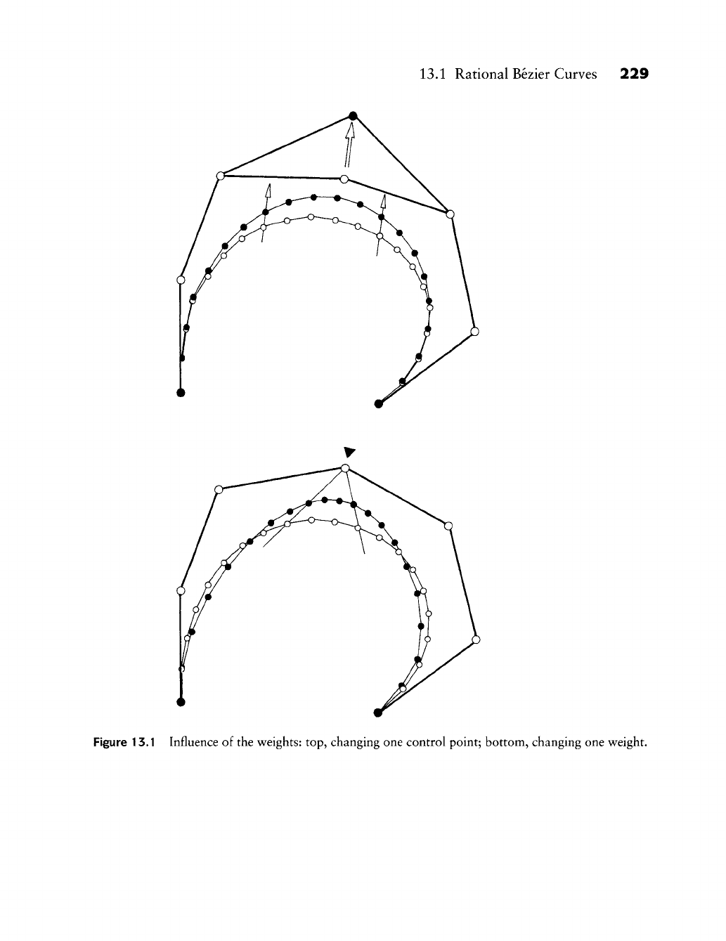
13.1 Rational Bezier Curves 229
Figure 13.1 Influence of the weights: top, changing one control point; bottom, changing one weight.
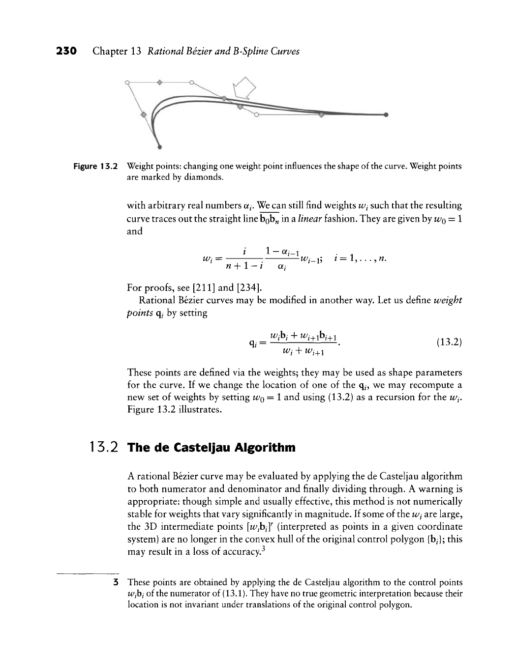
230 Chapter 13 Rational Bezier and B-Spline Curves
Figure 13.2 Weight
points:
changing one weight point influences the shape of
the
curve. Weight points
are marked by diamonds.
with arbitrary real numbers aj. We can still find weights
Wj
such that the resulting
curve traces out the straight line bob^ in
2i
linear fashion. They are given by
W^Q
= ^
and
i
!-«/-!
. 1
Wj = ^/-i; / =
1,...,
w.
n-\-l
—
i aj
For proofs, see [211] and
[234].
Rational Bezier curves may be modified in another way. Let us define weight
points qi by setting
q, = • . (13.2)
Wi + Wi^i
These points are defined via the weights; they may be used as shape parameters
for the curve. If we change the location of one of the q^, we may recompute a
new set of weights by setting
WQ
= 1 and using (13.2) as a recursion for the Wj,
Figure 13.2 illustrates.
15.2 The de Casteljau Algorithm
A rational Bezier curve may be evaluated by applying the de Casteljau algorithm
to both numerator and denominator and finally dividing through. A warning is
appropriate: though simple and usually effective, this method is not numerically
stable for weights that vary significantly in magnitude. If some of the
Wj
are large,
the 3D intermediate points [wjhjj (interpreted as points in a given coordinate
system) are no longer in the convex hull of the original control polygon {bj; this
may result in a loss of accuracy.-^
3 These points are obtained by applying the de Casteljau algorithm to the control points
Wjhj
of the numerator of
(13.1).
They have no true geometric interpretation because their
location is not invariant under translations of the original control polygon.
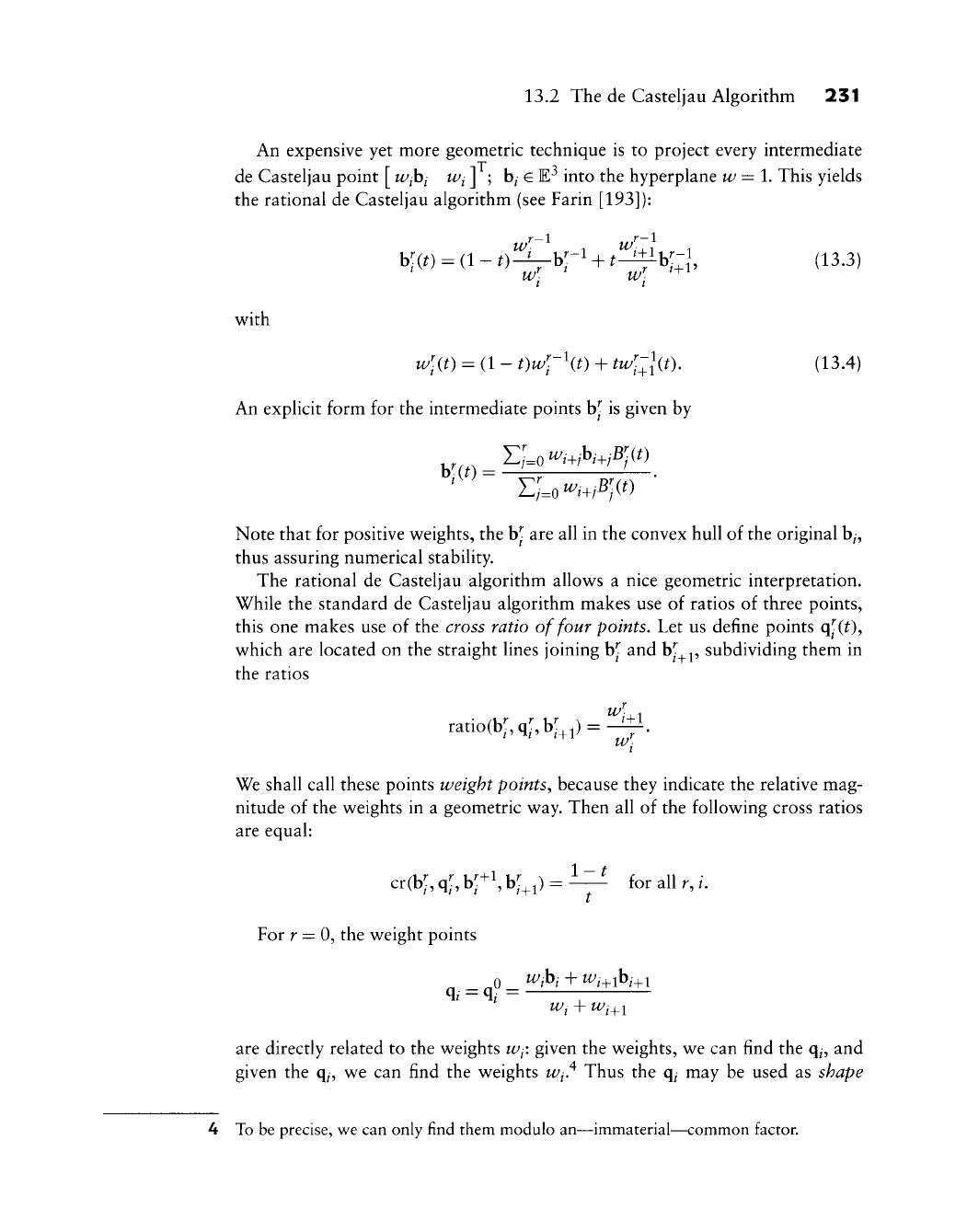
13.2 The de Casteljau Algorithm 231
An expensive yet more geometric technique is to project every intermediate
de Casteljau point [ Wjhj
Wj
] ; b/ e E^ into the hyperplane w = l. This yields
the rational de Casteljau algorithm (see Farin [193]):
mt)
=
a- 0-VK + i^^^v
(13.3)
^ WW ^
v^ith
w'^it) = (1- t)w'r\t) + tw'-_l{t). (13.4)
An explicit form for the intermediate points b[ is given by
h\{t) = TU^t+i^it)
Note that for positive weights, the b^ are all in the convex hull of the original b/,
thus assuring numerical stability.
The rational de Casteljau algorithm allows a nice geometric interpretation.
While the standard de Casteljau algorithm makes use of ratios of three points,
this one makes use of the cross ratio of four points. Let us define points q^CO?
which are located on the straight lines joining b[ and b[^, subdividing them in
the ratios
ratio(b^,q^,b;:^l) = ^.
^ w
We shall call these points weight points^ because they indicate the relative mag-
nitude of the weights in a geometric way. Then all of the following cross ratios
are equal:
cr(b^,q^,b^+l,b^^l) = i^ for all r,/.
For r = 0, the weight points
q/
= q, =
Wi + Wi^i
are directly related to the weights Wf. given the weights, we can find the q^, and
given the q^, we can find the weights Wi,^ Thus the q^ may be used as shape
4 To be precise, we can only find them modulo an—immaterial—common factor.
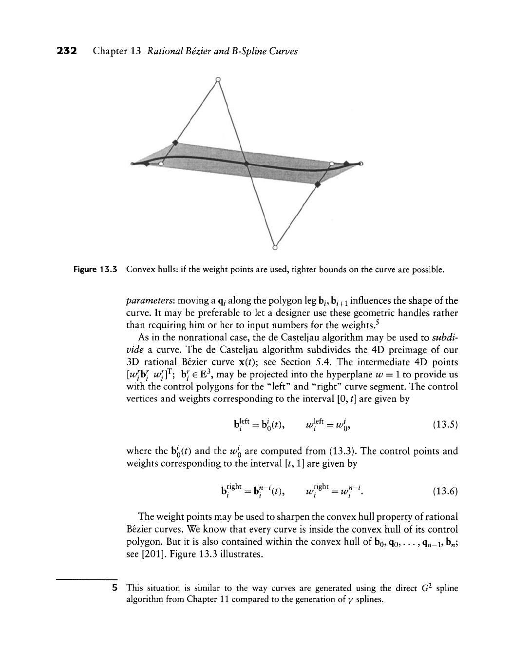
232 Chapter 13 Rational Bezier and B-Spline Curves
Figure 13.3 Convex hulls: if the weight points are used, tighter bounds on the curve are possible.
parameters: moving a q^ along the polygon leg
b/,
b^_^i
influences the shape of the
curve. It may be preferable to let a designer use these geometric handles rather
than requiring him or her to input numbers for the v^eights.^
As in the nonrational case, the de Casteljau algorithm may be used to subdi-
vide a curve. The de Casteljau algorithm subdivides the 4D preimage of our
3D rational Bezier curve x(^); see Section 5.4. The intermediate 4D points
[w/[b[ w^-Yy b^ e E^, may be projected into the hyperplane w=lto provide us
v^ith the control polygons for the "left" and "right" curve segment. The control
vertices and w^eights corresponding to the interval [0, t] are given by
hf' =
h',(t),
wf'^w'^,
(13.5)
w^here the bQ(^) and the
WQ
art computed from (13.3). The control points and
w^eights corresponding to the interval [t, 1] are given by
hf^^' =
h';-'it),
u/^ =
u/l-'.
(13.6)
The w^eight points may be used to sharpen the convex hull property of rational
Bezier curves. We know^ that every curve is inside the convex hull of its control
polygon. But it is also contained w^ithin the convex hull of bo, qo,. .., q^-i? b„;
see
[201].
Figure 13.3 illustrates.
5 This situation is similar to the way curves are generated using the direct G^ spline
algorithm from Chapter 11 compared to the generation of y splines.
13.3 Derivatives 233
15.3 Derivatives
For the first derivative of a rational Bezier curve, we obtain
1
x{t) = ^[p(t) - wit)x(t)l
wit) (13.7)
where we have set
p(0 = w(t)xit); pit), xit) e E^ (13.8)
in complete analogy to the development in Section 12.4. For higher derivatives,
we differentiate (13.8) r times:
p^'\t)
= J2(j]w^\t)x^'-^\t),
We can solve for
x^^\t):
x^'\t)
wit)
^(r) -go
w^\t)x^''-'\t) (13.9)
This is a recursive formula for the rth derivative of a rational Bezier curve. It only
involves taking derivatives of polynomial curves.
The first derivative may also be obtained as a byproduct of the de Casteljau
algorithm, as described by Floater
[235]:
w^'-^w'!-^ 1 1
^it) = n—p-^;^;—[bj -bQ J.
[<
ml (13.10)
At the endpoint
^
= 0, we find
WQ
Let us now consider two rational Bezier curves, one defined over the interval
[WQ?
^i] with control polygon bo,..., b„ and weights
W/Q?
•.., t^„ and the other
defined over the interval [t/j, uj] with control polygon b„,... ,b2„ and weights
w/„,...,
Win. ^oxh segments form a C^ curve if
!f:^Ab„_i=^^^Ab„ (13.11)
234 Chapter 13 Rational Bezier and B-Spline Curves
where the appearance of the interval lengths A^ is due to the application of the
chain rule. This is necessary since we now consider a composite curve with a
global parameter u. Note that the weight w^ has no influence on differentiability
at all!
Of course, two rational Bezier curves form a C^ curve if all of their components
are C^ in homogeneous form:
A'[w^.rK-r]
A'lWnK]
(Ao)^
(Air
But keep in mind that there are composite C^ curves that do not satisfy this
condition!
Although the computation of higher-order derivatives is quite involved in the
case of rational Bezier curves, we note that the computation of curvature or
torsion may be simplified by the application of (10.9) or (10.10) and (10.11).
15.4 Oscuiatory Interpolation
With rational cubics, it is easy to solve an interesting kind of interpolation
problem: given a Bezier polygon bo, b^, b2, b3 and a curvature value at each
endpoint, find a set of weights
U/Q,
^i, wi, w^ such that the corresponding rational
cubic assumes the given curvatures at bg and b3. The following method is very
similar to one developed by T. Goodman in 1988; see
[271].
We assume without
loss of generality that
WQ
= W^ = 1.^ The given curvatures
KQ
and K^ are then
related to the unknown weights by (10.10):
KQ: 4W2
^3-
4wi
3
w?;
--j"^' (13.12)
where
CQ: area[bQ,bi,b2]
dist^[bo,bi]
Ci = area[bi,b2,b3]
dist^[b2,b3]
Equations (13.12) decouple nicely so that we can determine our unknowns ivi
and Wi:
tv,-- fo£i U.2=-fofi (13.13)
6 Goodman [271] assumes that
Wj
=
M'2
= 1.
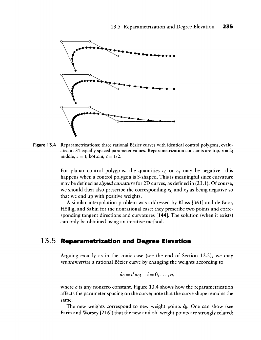
13.5 Reparametrization and Degree Elevation 235
Figure 13.4 Reparametrizations: three rational Bezier curves with identical control polygons, evalu-
ated at 31 equally spaced parameter values. Reparametrization constants are top, c = 2;
middle, c = l; bottom, c = 1/2.
For planar control polygons, the quantities
CQ
or Ci may be negative—this
happens when a control polygon is S-shaped. This is meaningful since curvature
may be defined as signed curvature for 2D curves, as defined in (23.1). Of course,
we should then also prescribe the corresponding
KQ
and
/C3
as being negative so
that we end up with positive weights.
A similar interpolation problem was addressed by Klass [361] and de Boor,
HoUig, and Sabin for the nonrational case: they prescribe two points and corre-
sponding tangent directions and curvatures
[144].
The solution (when it exists)
can only be obtained using an iterative method.
15.5 Reparametrization and Degree Elevation
Arguing exactly as in the conic case (see the end of Section 12.2), we may
reparametrize a rational Bezier curve by changing the weights according to
Wi = c^Wj; / = 0,..., w.
where c is any nonzero constant. Figure 13.4 shows how the reparametrization
affects the parameter spacing on the curve; note that the curve shape remains the
same.
The new weights correspond to new weight points q^. One can show (see
Farin and Worsey [216]) that the new and old weight points are strongly related:
236 Chapter 13 Rational Bezier and B-Spline Curves
the cross ratios of any four points
[b^,
q^, q^, b/+i] are the same for all polygon
legs.
We may always transform a rational Bezier curve to standard form by using
the rational linear parameter transformation resulting from the choice
c =
This results in w^ =
WQ;
after dividing all weights through by
WQ^
we have the
standard form
WQ
= W^ = 1. Of course, we have to require that the root exists.
A different derivation of this result is in Patterson
[457].
How can rational Bezier curves in nonstandard form arise? A common case
occurs in connection with rational Bezier surfaces, as discussed in Section 16.6:
the end weights of an isoparametric curve will in general not be unity. Such
curves are often "extracted" from a surface and then treated as entities in their
own right.
We may perform degree elevation (in analogy to Section 6.1) by degree el-
evating the 4D polygon with control vertices
[
w^i w^ ]^ and projecting the
resulting control vertices into the hyperplane w=\. Let us denote the control
vertices of the degree elevated curve
by
hf; they are given by
b-'
= • —; / =
0,...,«
+ l (13.14)
and a I = i/{n + 1). The weights w- of the new control vertices are given by
w^ = Wi_iai -f- Wi{l
—
Qf^); / =
0,...,«
+ 1.
Degree elevation is illustrated in Example 13.1.
The connection of reparametrization and degree elevation may lead to surpris-
ing situations. Consider the following procedure: take any rational Bezier curve in
standard form and degree elevate it. Next, take the original curve, reparametrize
it, then degree elevate it and bring it to standard form. We end up with two differ-
ent polygons (and two different sets of standardized weights) that both describe
the same rational curve. This situation is very different from the nonrational case!
It is illustrated in Figure 13.5.
For the sake of completeness, we should mention that ways other than just
by rational linear reparametrizations exist to reparametrize rational curves. For
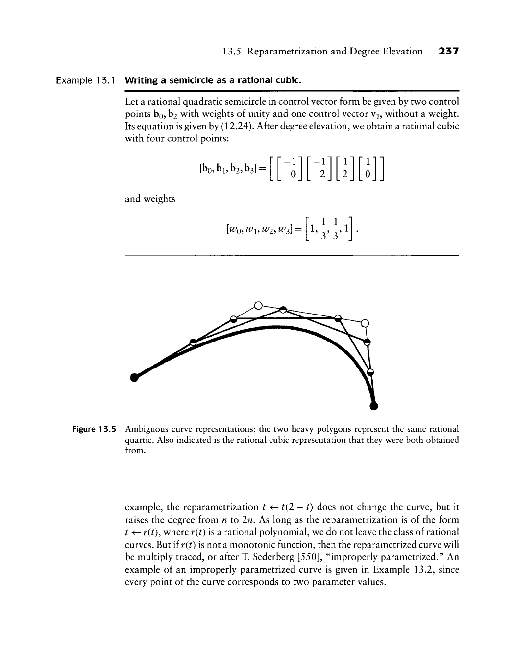
13.5 Reparametrization and Degree Elevation 237
Example 13.1 Writing a semicircle as a rational cubic.
Let a rational quadratic semicircle in control vector form be given by two control
points bo, hi with weights of unity and one control vector v^, without a weight.
Its equation is given by (12.24). After degree elevation, we obtain a rational cubic
with four control points:
[bo,
bi,
b2,
b3]:
-11
0
1
r-1]
L
2J
1
^
1
121
1
1
10
and weights
[WQ, tVi, W2, W^] = "
1,
1
3
1
3
~
1
Figure 13.5 Ambiguous curve representations: the two heavy polygons represent the same rational
quartic. Also indicated is the rational cubic representation that they were both obtained
from.
example, the reparametrization t <-t(2
—
t) does not change the curve, but it
raises the degree from n to In, As long as the reparametrization is of the form
t <- r{t), where r(t) is a rational polynomial, we do not leave the class of rational
curves. But if r(t) is not a monotonic function, then the reparametrized curve will
be multiply traced, or after T. Sederberg
[550],
"improperly parametrized." An
example of an improperly parametrized curve is given in Example 13.2, since
every point of the curve corresponds to two parameter values.
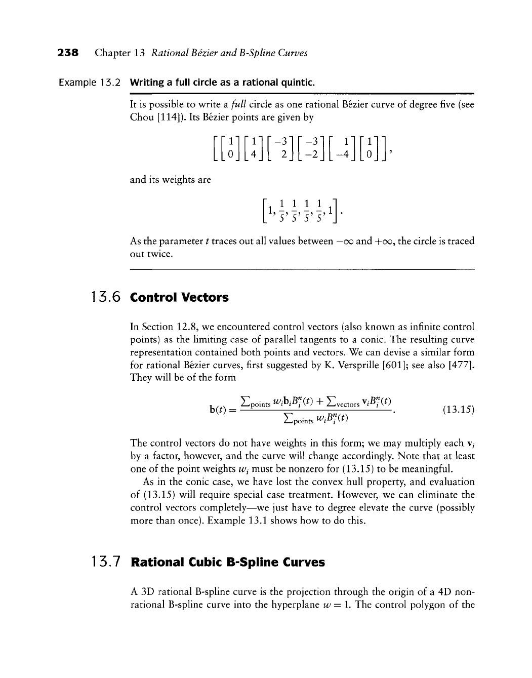
238 Chapter 13 Rational Bezier and B-Spline Curves
Example 13.2 Writing a full circle as a rational quintic.
It is possible to write a full circle as one rational Bezier curve of degree five (see
Chou [114]). Its Bezier points are given by
"1]
0
1
ri]
1
"^
1
[-3]
L
2J
[-3]
[-2
J
r ii
[-4
J
rr
10
and its weights are
'1111;
'5'5'5'5'
As the parameter t traces out all values betv^een —00 and +00, the circle is traced
out tv^ice.
15.6 Control Vectors
In Section 12.8, v^e encountered control vectors (also known as infinite control
points) as the limiting case of parallel tangents to a conic. The resulting curve
representation contained both points and vectors. We can devise a similar form
for rational Bezier curves, first suggested by K. Versprille
[601];
see also
[477].
They will be of the form
Ht) ^points ^.M^O + EvectorsV.^?W
Epomts^.^?(0
(13.15)
The control vectors do not have weights in this form; we may multiply each v^
by a factor, however, and the curve will change accordingly. Note that at least
one of the point weights Wj must be nonzero for (13.15) to be meaningful.
As in the conic case, we have lost the convex hull property, and evaluation
of (13.15) will require special case treatment. However, we can eliminate the
control vectors completely—we just have to degree elevate the curve (possibly
more than once). Example 13.1 shows how to do this.
15.7 Rational Cubic B-Spline Curves
A 3D rational B-spline curve is the projection through the origin of a 4D non-
rational B-spline curve into the hyperplane w = 1. The control polygon of the
13.7 Rational Cubic B-Spline Curves 239
Figure 13.6 Rational B-splines: the weight of the indicated control point is changed. Dashed curve,
weight
=
3.0; black curve, weight
=
0.33.
rational B-spline curve is given by vertices do,..., d^^; each vertex d/ € E^ has a
corresponding weight Wi, A point x(w) on a rational B-spline curve is thus given
by
x(w) = (13.16)
It may be evaluated by applying the de Boor algorithm (see Section 8.2), to
the homogeneous coordinates, in the same way as we evaluated rational Bezier
curves. We have affine and projective invariance, and also the local control
property. For nonnegative weights, we have the variation diminishing property
as well as the convex hull property.
Designing with rational B-spline curves is not very different from designing
with their nonrational counterparts. We now have the added freedom of being
able to change weights. A change of only one weight affects a rational B-spline
curve only locally, as shown in Figure 13.6.
Let us close this section with a somewhat negative result: there is no symmetric
periodic representation of
a
circle as a C^ rational cubic B-spline curve. If such
a representation existed, it would be of the form
x(^) = Y, w,d,Nf(u)/ J2
^tN^u),
where all
Wj
art equal by symmetry. Then the
Wj
cancel, leaving us with an integral
B-spline curve, which is not capable of representing a circle. Note, however, that
we can represent any open circular arc by C^ rational cubics.
240 Chapter 13 Rational Bezier and B-Spline Curves
1
5.8 Interpolation with Rational Cubics
The interpolation problem in the context of rational B-splines is the following:
Given: 3D data points
XQ,
...,
x^^,
parameter values
UQ,
...,
uj^^
and weights
Find:
A C^ rational cubic B-spline curve with control vertices do,..., d^+i
and weights f
Q^
• • • ?
^K+l ^hat interpolates to the given data and weights.
For the solution of this problem, we follow the philosophy outlined at the
end of the last section: solve a 4D interpolation problem to the data points
[
w-Ki
Wi
]^ and parameter values W/. All we have to do is to solve the linear
system (9.10), where input and output is now 4D instead of the usual 3D. We
nr
will obtain a 4D control polygon [
e^
Vi
] , from which we now obtain the
desired d^ as d^ = ^i/Vv The
Vi
are the weights of the control vertices d^.
We have not yet addressed the problem of how to choose the weights Wi
for the data points x^. No known algorithms exist for this problem. It seems
reasonable to assign high weights in regions where the interpolant is expected
to curve sharply. Yet there is a limit to the assignment of weights: if all of them
are very high, this will not have a significant effect on the curve since a common
factor in all weights will simply cancel. Moreover, care must be taken to prevent
the denominator of the interpolant from being zero. This is not a trivial task—
for instance, we might assign a very large weight to one data point while keeping
all the others at unity. The resulting weight function w{t) will not be positive
everywhere, giving rise to singularities at its zeros.
Integral cubic spline interpolation has cubic precision: if the data points and
the parameter values come from one global cubic, the interpolant reproduces
that cubic. In the context of rational spline interpolation, an analogous question
is that of conic precision: if the data points and the parameter values come from
one global conic, can we reproduce it? We must also require that the data points
have weights assigned to them. With them, we may view the rational spline
interpolation problem as an integral spline interpolation problem in E"^. There,
cubic splines have quadratic precision; that is, we may recapture any parabola.
The projection of the parabola yields a conic section; thus if our data—points,
parameter values, and weights—were taken from a conic, rational cubic spline
interpolation will reproduce the conic.
We should note, however, that this argument is limited to open curves; for
closed curves, we have already seen that we cannot represent a circle as a C^
symmetric periodic B-spline curve.
More approaches to rational sphne interpolation have recently appeared; we
hst Schneider [541] and Ma and Kruth
[408].
13.9 Rational B-Splines of Arbitrary Degree 241
13.9 Rational B-Splines of Arbitrary Degree
The process of generalizing the concept of general B-spline curves to the rational
case is now straightforward. A 3D rational B-spline curve is the projection
through the origin of a 4D nonrational B-spline curve into the hyperplane w=l.
It is thus given by
^M^^ • (13-17)
We have chosen the notation from Chapter 8. Thus (13.17) is the generalization
of (8.15) to the rational parametric case.
A rational B-spline curve is given by its knot sequence, its 3D control polygon,
and its weight sequence. The control vertices dj art the projections of the 4D
control vertices
[
Wjdi
Wj
]^.
To evaluate a rational B-spline curve at a parameter value w, we may apply
the de Boor algorithm to both numerator and denominator of (13.17) and finally
divide through. This corresponds to the evaluation of the 4D nonrational curve
with control vertices
[
Wjdj
Wi
]^ and to projecting the result into
E-^.
Just as in
the case of Bezier curves, this may lead to instabilities, and so we give a rational
version of the de Boor algorithm that is more stable but also computationally
more involved.
de Boor algorithm, rational: Let u e [uj, uj^i) c [w„_i, uj}. Define
d^{u) = [a - af)wf:ldf:l(u) + afwf-^df-\u)]/wf (13.18)
for ^ = 1,. ..,
w —
r, and / = I
— w
+ ^ + 1,.. ., / + 1, where
k ^ - ^i-i
"-i-^-n-k ^i-1
and
Then
wf = il-af)wf:l +
afwf-
siu) = d'^-[(u) (13.19)
is the point on the B-spline curve at parameter value u. Here, r denotes the
multiplicity of u in case it was already one of the knots. If it was not, set r = 0.
As usual, we set d^ = dj and w^ = Wj.
Refer to Section 8.3 for the notation.
242 Chapter 13 Rational Bezier and B-Spline Curves
Knot insertion is, as in the nonrational case, performed by executing just one
step of the de Boor algorithm, that is, by fixing ^ = 1 in the preceding algorithm.
The original polygon vertices d/_„_^25
•
• •
J
d/ are replaced by the
dj_^, 2?
•
• •
5
^ilv
their weights are the numbers Wj_^^2^..., Wj^^
A rational B-spline curve, being a piecewise rational polynomial, has a piece-
wise rational Bezier representation. We can find the Bezier points and their
weights for each segment by inserting every knot until it has multiplicity «, that
is,
by applying the de Boor algorithm to each knot. The routine bsptobez_bl ossom
uses blossoms to perform this task.
It is also possible to reparametrize a rational B-spline curve, just as we could
do for Bezier curves. For a description, see Lee and Lucian
[381].
The derivative of a rational B-spline curve is conveniently found using a result
by Floater:
s{u)
= —^ !^L^[d«;i -
d«-i],
(13.20)
which is quite analogous to (13.10).
15.10 Implementation
The following computes a point on a rational Bezier curve:
float ratbez(degree,coeff.weight.t)
/*
uses rational
de
caste!jau
to
compute
point
on
ratbez curve for param. value
t.
Input: degree: degree
of
curve
coeff: control point coordinates
weight: weights
t: evaluation parameter
V
Reparametrizing a rational Bezier curve:
void reparam(wold,degree,s,wnew)
/*
reparametrizes ratbez curve: only the weights, stored
in
wold,
are changed. New weights are in wnew. Parametrization
is
determined
by
shoulder point s. For s=0.5, nothing changes.
Also,
s
should
be in
(0,1).
V
13.11 Problems 243
The routine to subdivide a rational Bezier curve at a parameter value t was
already given in Section 5.8.
A program that generates the piecew^ise rational Bezier form from a rational
cubic B-spline curve is:
void ratbspline_to_bezier(bsp1_x,bspl_y,bspl_w,knot,l,bez_x,bez_y,bez_w)
/* converts rational cubic B-spline polygon into piecewise
rational Bezier polygon
Input: bspl_x, bspl_y: planar B-spline control polygon
bspl_w: B-spline weights
knot: knot sequence
1: no.
of
intervals
Output: bez_x, bez_y: planar piecewise Bezier polygon
bez_w: Bezier weights (not
in
piecewise standard form!)
V
1
5.11 Problems
1 Suppose you are given two coplanar rational quadratic segments that form
a C^ curve, but not a G^ curve. Can you adjust the weights (not the control
polygons!) such that the resulting new segments form a G^ curve? Hint: use
(10.9).
* 2 A rational Bezier curve may be
closed^
as in the example of a degree elevated
ellipse. Show that a nonplanar 3D rational cubic cannot be closed.
* 3 In Section 13.4, we said that signed curvature makes sense only in e. Why
not in ¥?}
*4 In Section 13.5, we remarked that the cross ratios of any four points
(b/,
q^, q^, b/_^i) are the same for all polygon legs. How is this cross ratio
related to the reparametrization constant c?
PI Define and program a rational Aitken algorithm, that is, one where the
data points are assigned weights. Try to adjust those weights in an attempt
to reduce the oscillatory behavior of the interpolant.
P2 Use deboor_blossom to write a degree elevation program for rational B-
splines. Apply it repeatedly and study the behavior of the weights.

This Page Intentionally Left Blank
Tensor Product
Patches
I he first person to consider this class of surfaces for design purposes was
probably de Casteljau, who investigated them between 1959 and 1963. The
popularity of this type of surface is, however, due to the work of Bezier only
slightly later, as documented in Chapter 1. Initially, Bezier patches were only
used to approximate a given surface. It took some time for people to realize that
any B-spline surface can also be written in piecewise Bezier form.
We will use the example of Bezier patches to demonstrate the tensor product
approach to surface patches. Once that principle is developed, it will be trivial
to generalize other curve schemes to tensor product surfaces.
14.1 Bilinear Interpolation
In Section
3.1,
we studied linear interpolation in E^ and derived properties of this
elementary method that we then used for the development of Bezier curves. In
an analogous fashion, we can base the theory of tensor product Bezier surfaces
on the concept of bilinear interpolation. Whereas linear interpolation fits the
"simplest" curve between two points, bilinear interpolation fits the "simplest"
surface between four points.
To be more precise: let
bo^o? ^0,1?
b^
Q?
b^
1
be four distinct points in E^. The set
of all points x
G
E^ of the form
1 1
/=0 /=0
(14.1)
245
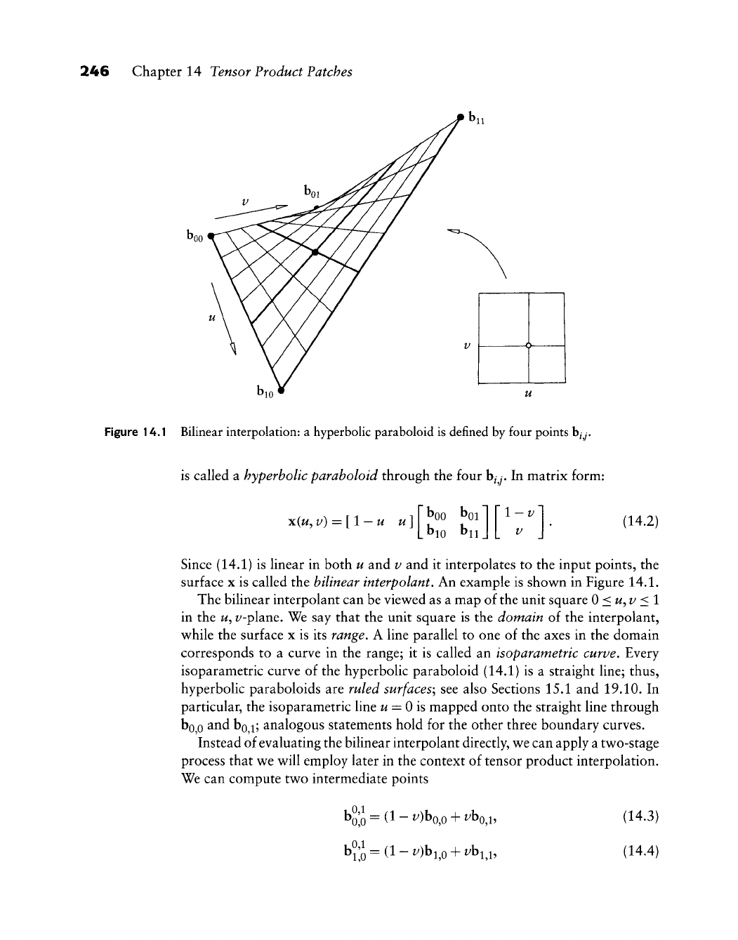
246 Chapter 14 Tensor Product Patches
-0
Figure 14.1 Bilinear interpolation: a hyperbolic paraboloid is defined by four points b^y.
is called a hyperbolic paraboloid through the four hjj. In matrix form:
x(w, v) = [l
—
u u]
boo boi
bio bii
1-v
V (14.2)
Since (14.1) is linear in both u and v and it interpolates to the input points, the
surface x is called the bilinear interpolant. An example is shown in Figure 14.1.
The bilinear interpolant can be viewed as a map of the unit square 0<u^v <l
in the u, i^-plane. We say that the unit square is the domain of the interpolant,
while the surface x is its range. A line parallel to one of the axes in the domain
corresponds to a curve in the range; it is called an isoparametric curve. Every
isoparametric curve of the hyperbolic paraboloid (14.1) is a straight line; thus,
hyperbolic paraboloids are ruled
surfaces-^
see also Sections 15.1 and 19.10. In
particular, the isoparametric line
w
= 0 is mapped onto the straight line through
bo
0
^nd bo i; analogous statements hold for the other three boundary curves.
Instead of evaluating the bilinear interpolant directly, we can apply a two-stage
process that we will employ later in the context of tensor product interpolation.
We can compute two intermediate points
0,1
\o = (1 - ^)bo,o + ^bo,i.
0.1
bi;o = (1 - ^)bi,o + ^bi4.
(14.3)
(14.4)
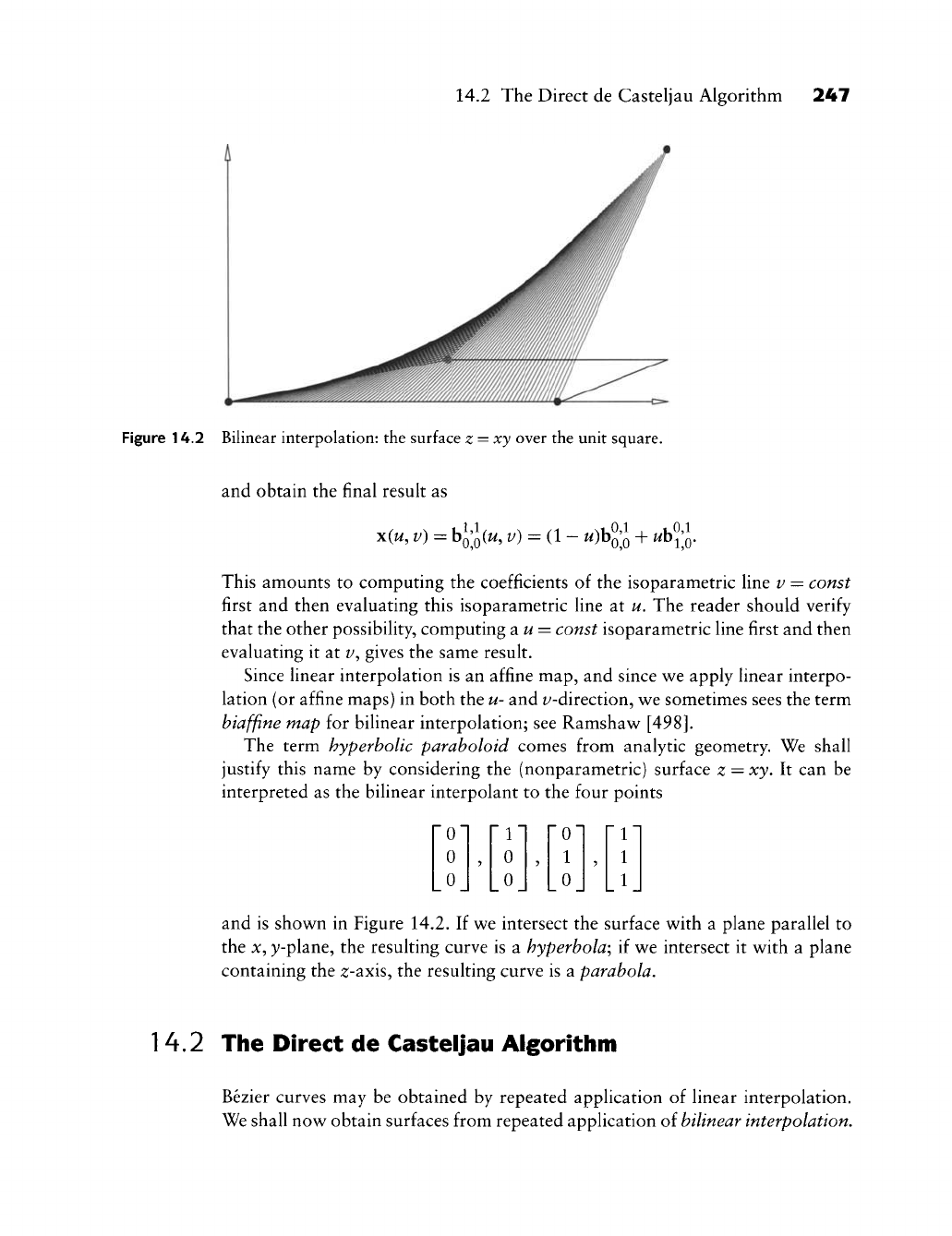
14.2 The Direct de Casteljau Algorithm 247
Figure 14.2 Bilinear interpolation: the surface z = xy over the unit square.
and obtain the final result as
x(w, v) = h^^^iu, v) = {l- u)h^^Q + wb^^Q.
This amounts to computing the coefficients of the isoparametric line v = const
first and then evaluating this isoparametric line at u. The reader should verify
that the other possibility, computing au = const isoparametric line first and then
evaluating it at v, gives the same result.
Since linear interpolation is an affine map, and since v^e apply linear interpo-
lation (or affine maps) in both the u- and ^/-direction, v^e sometimes sees the term
biaffine map for bilinear interpolation; see Ramshaw^
[498].
The term hyperbolic paraboloid comes from analytic geometry. We shall
justify this name by considering the (nonparametric) surface z = xy. It can be
interpreted as the bilinear interpolant to the four points
0
0
0
9
1
0
0
?
0
1
0
9
1
1
1
and is show^n in Figure 14.2. If wt intersect the surface v^ith a plane parallel to
the
X,
}/-plane, the resulting curve is a hyperbola; if we intersect it w^ith a plane
containing the ^-axis, the resulting curve is a parabola.
1
4.2 The Direct de Casteljau Algorithm
Bezier curves may be obtained by repeated application of linear interpolation.
We shall now^ obtain surfaces from repeated application of bilinear interpolation.
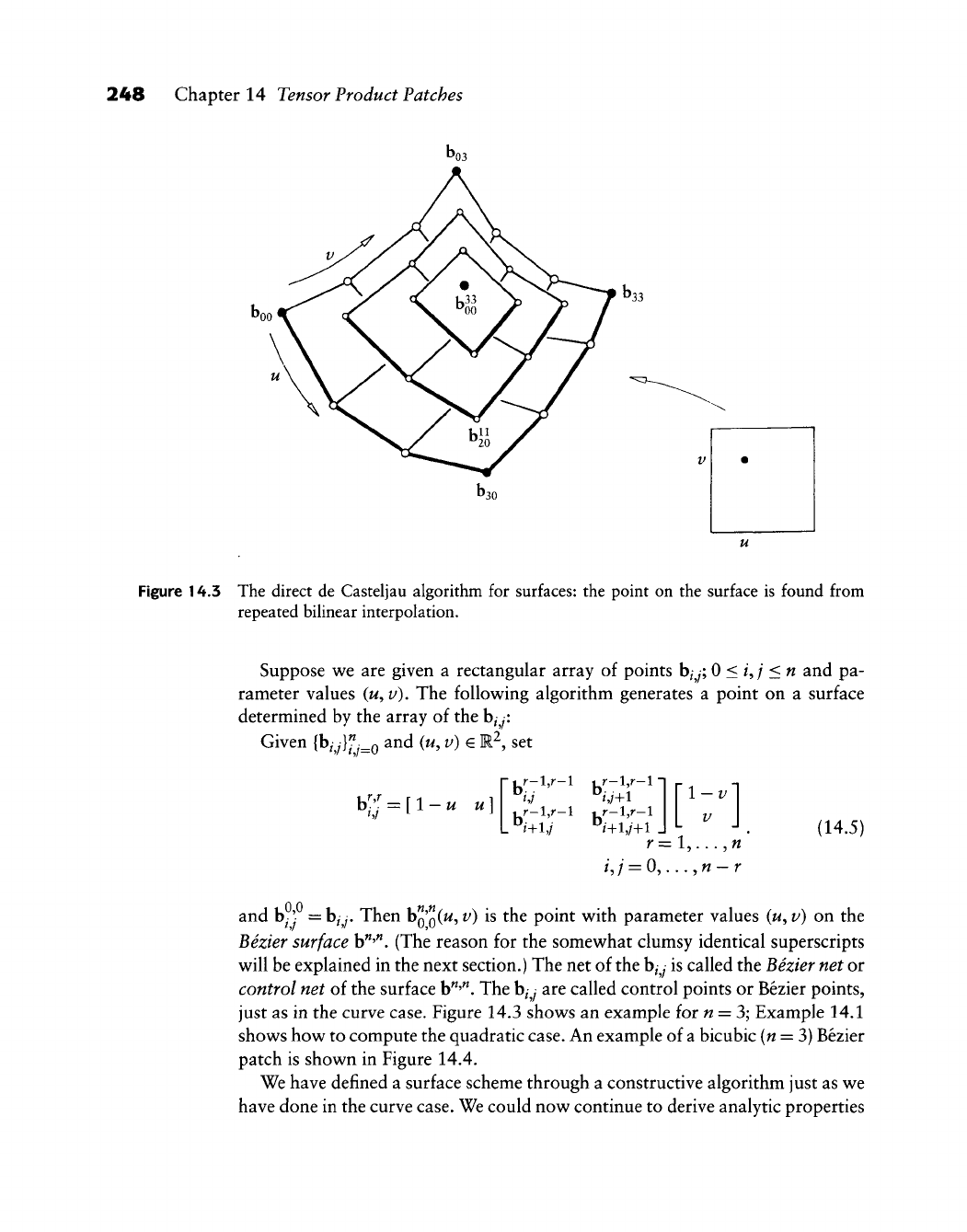
248 Chapter 14 Tensor Product Patches
Figure 14.3 The direct de Casteljau algorithm for surfaces: the point on the surface is found from
repeated biUnear interpolation.
Suppose we are given a rectangular array of points
b^
y;
0 <ij <n and pa-
rameter values
(M,
V). The following algorithm generates a point on a surface
determined by the array of the hjji
Given
{b^^}"-
Q
and (w, v) e M^, set
h'j=[l-u u]
1 r-l,r-l
hi
,r-l,r-l
1-V
V
r=l,...,«
ij =
0,...,n-r
(14.5)
and b-' =
b^y.
Then h^'^iu^ v) is the point with parameter values (w, v) on the
Bezier surface h^'^, (The reason for the somewhat clumsy identical superscripts
will be explained in the next section.) The net of the hjj is called the Bezier net or
control net of the surface
b"'".
The
b^
y
are called control points or Bezier points,
just as in the curve case. Figure 14.3 shows an example for n = 3; Example 14.1
shows how to compute the quadratic case. An example of a bicubic (n = 3) Bezier
patch is shown in Figure 14.4.
We have defined a surface scheme through a constructive algorithm just as we
have done in the curve case. We could now continue to derive analytic properties
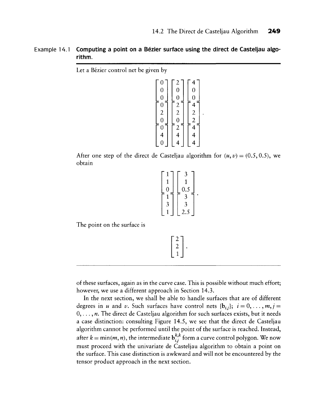
14.2 The Direct de Casteljau Algorithm 249
Example 14.1 Computing a point on a Bezier surface using the direct de Casteljau algo-
rithm.
Let a Bezier control net be given by
0
0
0
0
2
0
0
4
0
2
0
0
2
2
0
2
4
4
4
0
0
4
2
2
4
4
4
After one step of the direct de Casteljau algorithm for (w, v) = (0.5, 0.5), we
obtain
["11
1
0
ri'
3
LI
[31
1
0.5
" 3 "
3
2.5
The point on the surface is
of these surfaces, again as in the curve case. This is possible w^ithout much effort;
how^ever, we use a different approach in Section 14.3.
In the next section, v^e shall be able to handle surfaces that are of different
degrees in u and v. Such surfaces have control nets
{hjj};
/ = 0,..., m,/ =
0,...,
w.
The direct de Casteljau algorithm for such surfaces exists, but it needs
a case distinction: consulting Figure 14.5, v^e see that the direct de Casteljau
algorithm cannot be performed until the point of the surface is reached. Instead,
after k = min(m,«), the intermediate b-' form a curve control polygon. We now^
must proceed with the univariate de Casteljau algorithm to obtain a point on
the surface. This case distinction is awkward and will not be encountered by the
tensor product approach in the next section.
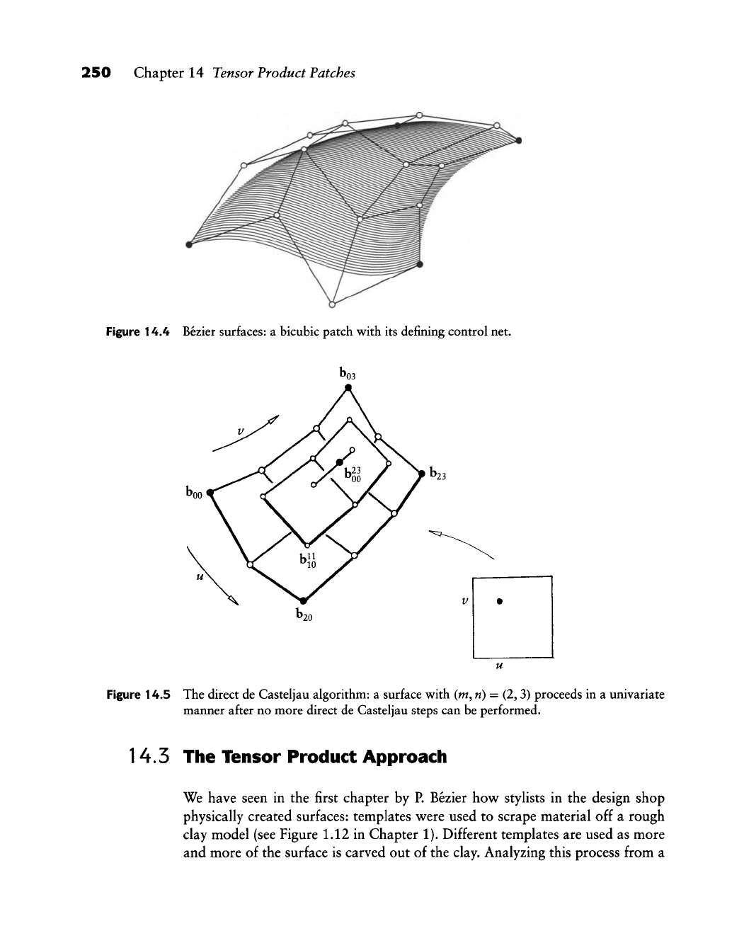
250 Chapter 14 Tensor Product Patches
Figure 14.4 Bezier surfaces: a bicubic patch with its defining control net.
Figure 14.5 The direct de Casteljau algorithm: a surface with
(m,
n)
= (2,3) proceeds in a univariate
manner after no more direct de Casteljau steps can be performed.
14.5 The Tensor Product Approach
We have seen in the first chapter by P. Bezier how stylists in the design shop
physically created surfaces: templates were used to scrape material off a rough
clay model (see Figure 1.12 in Chapter 1). Different templates are used as more
and more of the surface is carved out of the clay. Analyzing this process from a

14.3 The Tensor Product Approach
251
Figure 14.6 Tensor product surfaces: a surface can be thought of as being swept out by a moving and
deforming curve.
theoretical viewpoint, we arrive at the following intuitive definition of a surface: a
surface is the locus of a curve that is moving through space and thereby changing
its shape. See Figure 14.6 for an illustration.
We will now formalize this intuitive concept in order to arrive at a mathemat-
ical description of a surface. First, we assume that the moving curve is
a
Bezier
curve of constant degree m. (This assumption is made so that the following for-
mulas will work out; it is actually a serious restriction on the class of surfaces that
we can represent using the tensor product approach.) At any time, the moving
curve is then determined by a set of control points. Each original control point
moves through space on a curve. Our next assumption is that this curve is also
a Bezier curve, and that the curves on which the control points move are all of
the same degree. An example is given in Figure 14.7.
This can be formalized as follows: let the initial curve be
a
Bezier curve of
degree m:
b-(^)
=
^b,Br(^).
^=0
Let each
b^
traverse a Bezier curve of degree n:
n
j=0
We can now combine these two equations and obtain the point h^'^{u, v) on
the surface b^'^ as
m
n
{T'^iu,
v) =
Y,Y. Mr(«)^"(^)-
(14-6)
!=0 /=0
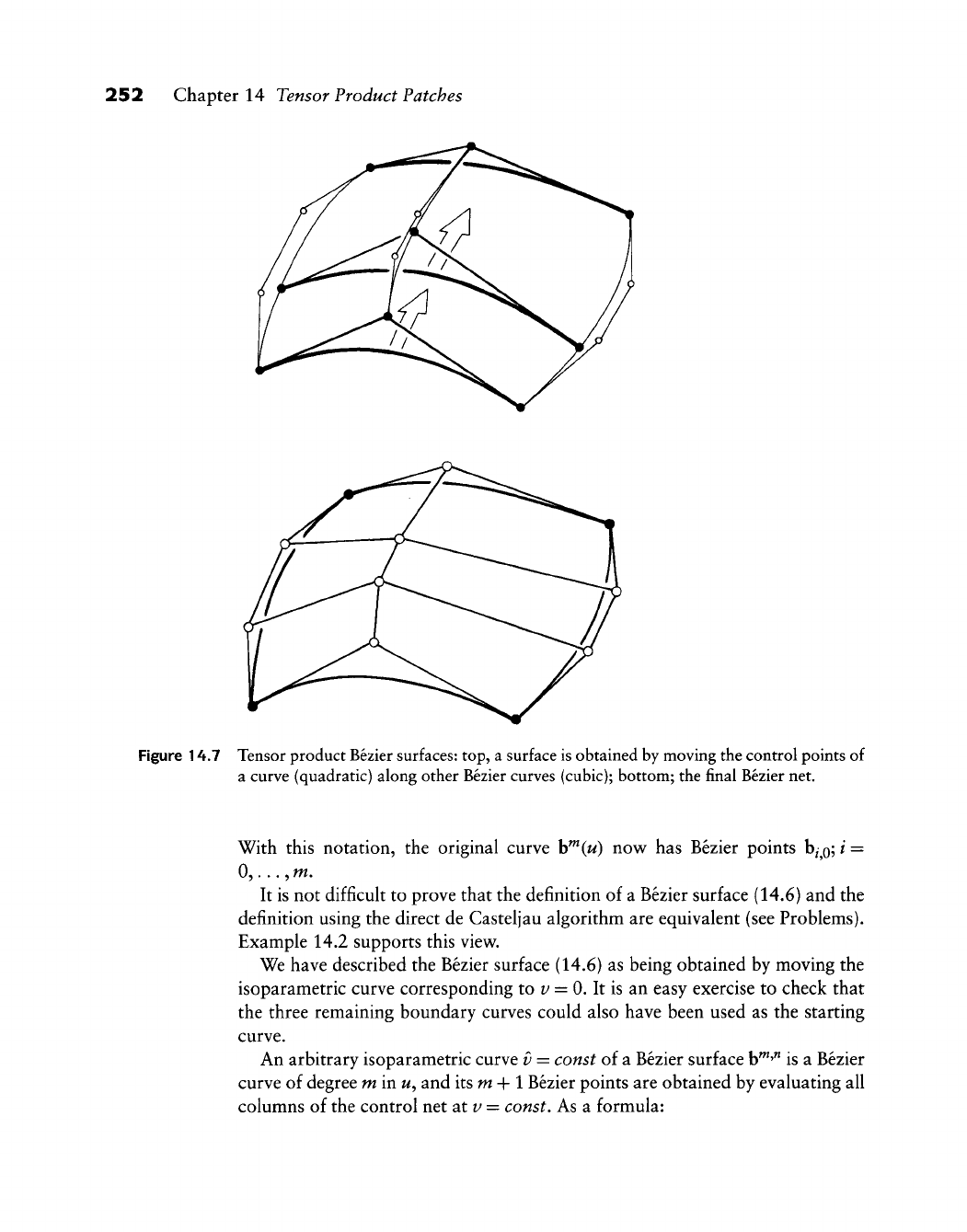
252 Chapter 14 Tensor Product Patches
Figure 14.7 Tensor product Bezier surfaces: top, a surface is obtained by moving the control points of
a curve (quadratic) along other Bezier curves (cubic); bottom; the final Bezier net.
With this notation, the original curve h^(u) now has Bezier points
b/Q;
i =
0,... ,m.
It is not difficult to prove that the definition of a Bezier surface (14.6) and the
definition using the direct de Casteljau algorithm are equivalent (see Problems).
Example 14.2 supports this view^.
We have described the Bezier surface (14.6) as being obtained by moving the
isoparametric curve corresponding to
i^
= 0. It is an easy exercise to check that
the three remaining boundary curves could also have been used as the starting
curve.
An arbitrary isoparametric curve v = const of a Bezier surface h^'^ is a Bezier
curve of degree m in w, and its m + 1 Bezier points are obtained by evaluating all
columns of the control net at i/ = const. As a formula:
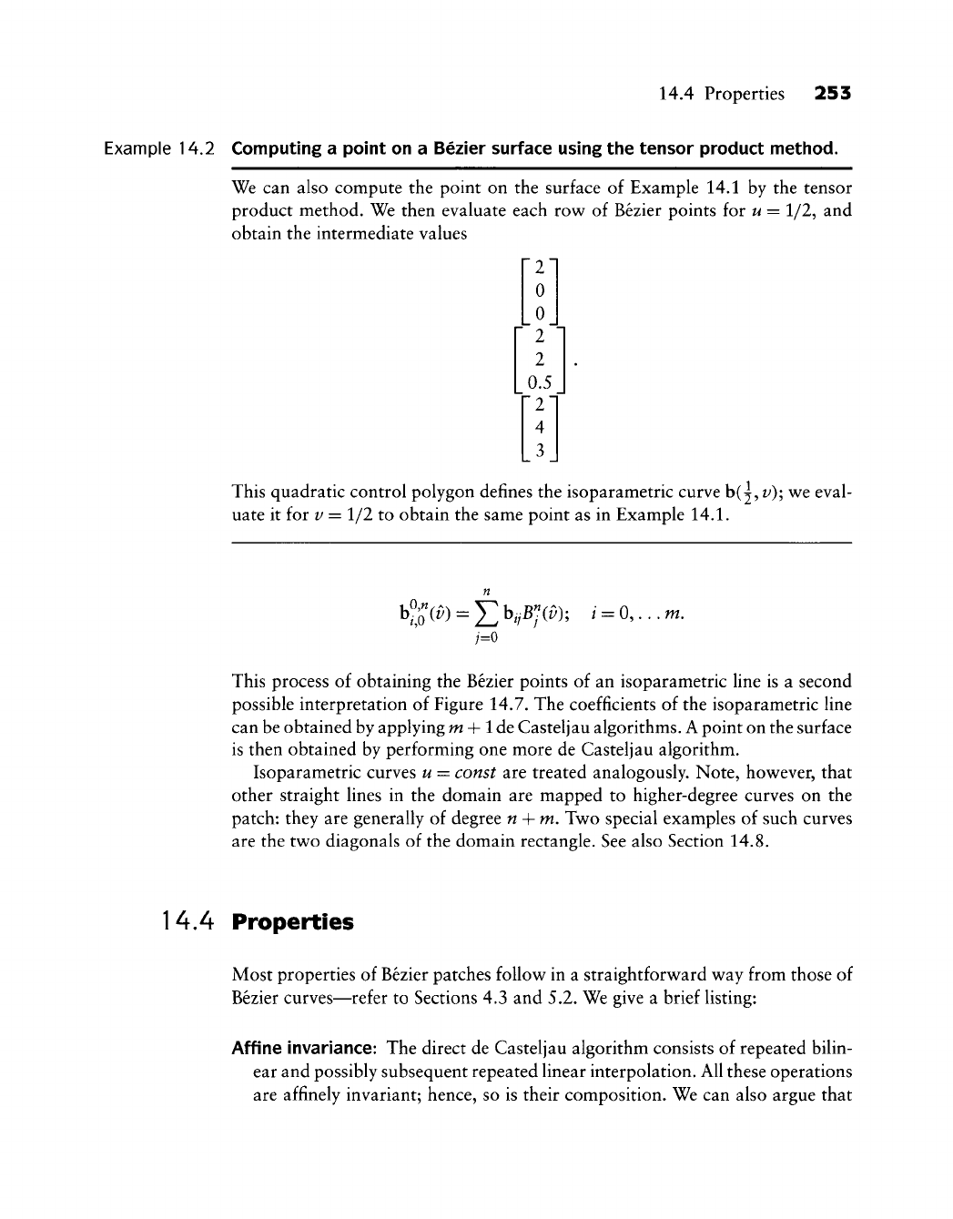
14.4 Properties 253
Example 14.2 Computing a point on a Bezier surface using the tensor product method.
We can also compute the point on the surface of Example 14.1 by the tensor
product method. We then evaluate each row of Bezier points for u = 1/2, and
obtain the intermediate values
"2"
0
0
'l'
2
0.5
"2"
4
_3_
This quadratic control polygon defines the isoparametric curve h{j,v); we eval-
uate it for
V —
1/2 to obtain the same point as in Example 14.1.
j=0
. m.
This process of obtaining the Bezier points of an isoparametric Hne is a second
possible interpretation of Figure 14.7. The coefficients of the isoparametric Hne
can be obtained by applying m +
1
de Casteljau algorithms. A point on the surface
is then obtained by performing one more de Casteljau algorithm.
Isoparametric curves u = const are treated analogously. Note, however, that
other straight lines in the domain are mapped to higher-degree curves on the
patch: they are generally of degree n + m. Two special examples of such curves
are the two diagonals of the domain rectangle. See also Section 14.8.
14.4 Properties
Most properties of Bezier patches follow in a straightforward way from those of
Bezier curves—refer to Sections 4.3 and 5.2. We give a brief listing:
Affine invariance: The direct de Casteljau algorithm consists of repeated bilin-
ear and possibly subsequent repeated linear interpolation. All these operations
are affinely invariant; hence, so is their composition. We can also argue that
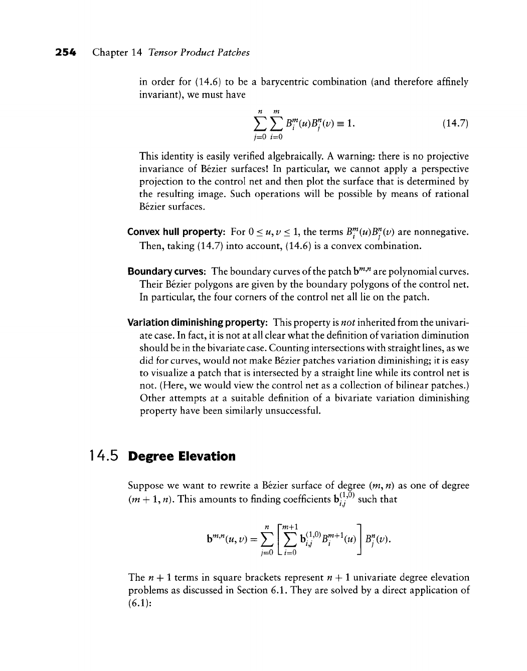
254 Chapter 14 Tensor Product Patches
in order for (14.6) to be a barycentric combination (and therefore affinely
invariant), we must have
n m
Y^J^B'I'MBjiv)^!. (14 J)
This identity is easily verified algebraically. A warning: there is no projective
invariance of Bezier surfaces! In particular, we cannot apply a perspective
projection to the control net and then plot the surface that is determined by
the resulting image. Such operations will be possible by means of rational
Bezier surfaces.
Convex hull property: For 0<u,v <l, the terms B^(u)B^(v) are nonnegative.
Then, taking (14.7) into account, (14.6) is a convex combination.
Boundary
curves:
The boundary curves of the patch
b^'"
are polynomial curves.
Their Bezier polygons are given by the boundary polygons of the control net.
In particular, the four corners of the control net all lie on the patch.
Variation diminishing property: This property is not inherited from the univari-
ate case. In fact, it is not at all clear what the definition of variation diminution
should be in the bivariate case. Counting intersections with straight lines, as we
did for curves, would not make Bezier patches variation diminishing; it is easy
to visualize a patch that is intersected by a straight line while its control net is
not. (Here, we would view the control net as a collection of bilinear patches.)
Other attempts at a suitable definition of a bivariate variation diminishing
property have been similarly unsuccessful.
14.5 Degree Elevation
Suppose we want to rewrite a Bezier surface of degree (m, n) as one of degree
(m + 1,
w).
This amounts to finding coefficients b| ' such that
1=0
"w+l
0
B'Hv).
The n-\-l terms in square brackets represent n + 1 univariate degree elevation
problems as discussed in Section 6.1. They are solved by a direct application of
(6.1):
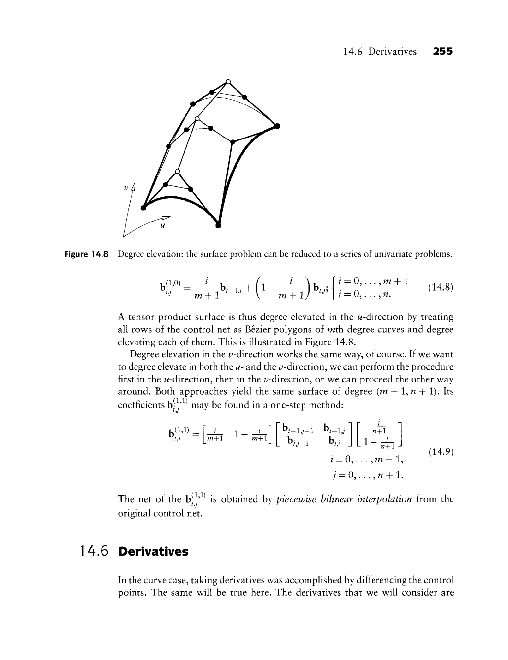
14.6 Derivatives
255
Figure 14.8 Degree elevation: the surface problem can be reduced to
a
series of univariate problems.
m-\-\
b,-i,/
+
I 1
-
,
I
/
=
0,...,
m
+
1 (14.8)
A tensor product surface
is
thus degree elevated
in the
w-direction
by
treating
all rov^s
of
the control
net as
Bezier polygons
of
mth degree curves
and
degree
elevating each
of
them. This
is
illustrated
in
Figure 14.8.
Degree elevation in the i^-direction works the same way,
of
course.
If
we want
to degree elevate in both the u- and the z/-direction, we can perform the procedure
first
in
the w-direction, then
in
the i^-direction,
or
we can proceed the other way
around. Both approaches yield
the
same surface
of
degree (m
+
1,
w
+
1).
Its
coefficients b
•
'
may be found
in a
one-step method:
^/,/
[m+l
m+lj
/
n+1
1 /
w+1
-J
/•
=
0,.
.
.
,m + 1,
/=:0,...,^+l.
(14.9)
The
net of the b- ' is
obtained
by
piecewise bilinear interpolation from
the
original control net.
14.6 Derivatives
In the curve case, taking derivatives was accomplished by differencing the control
points.
The
same will
be
true here.
The
derivatives that
we
will consider
are
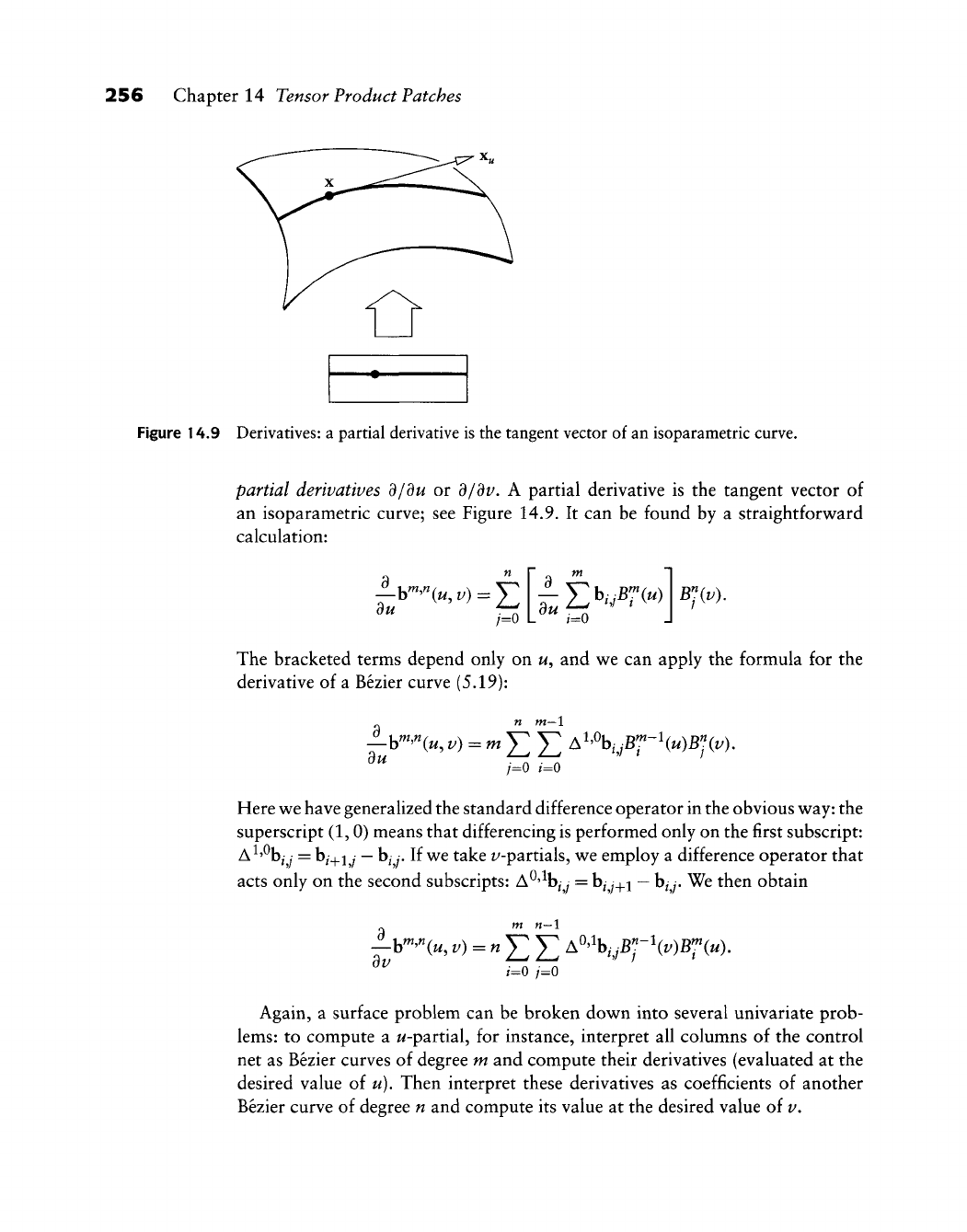
256 Chapter 14 Tensor Product Patches
Figure 14.9 Derivatives: a partial derivative is the tangent vector of an isoparametric curve.
partial derivatives d/du or d/dv. A partial derivative is the tangent vector of
an isoparametric curve; see Figure 14.9. It can be found by a straightforw^ard
calculation:
du b^'"(^,z/) = ^
/=0 du ^
EMr(«)
(=0
Bliv).
The bracketed terms depend only on u, and w^e can apply the formula for the
derivative of a Bezier curve (5.19):
du
n m—1
/=0 /=0
Here
v^e
have generalized the standard difference operator in the obvious
w^ay:
the
superscript (1,0) means that differencing is performed only on the first subscript:
A^'%^
y
= hj^ij
—
hjj. If
w^e
take i^-partials,
w^e
employ a difference operator that
acts only on the second subscripts: A^'^b/y =
b^
y_^i
—
b^
y.
We then obtain
d_
Vv
m n—\
b^'^^C^,
v) = nY,Y. ^^\iB]~\v)B';'iuy
i=0 j=0
Again, a surface problem can be broken dov^n into several univariate prob-
lems:
to compute a ^-partial, for instance, interpret all columns of the control
net as Bezier curves of degree m and compute their derivatives (evaluated at the
desired value ol u). Then interpret these derivatives as coefficients of another
Bezier curve of degree n and compute its value at the desired value of v.
14.6 Derivatives 257
We can write down formulas for higher-order partials:
f-b-'^Cw,
V)
= -^ T V A'-%,iBf-''{u)B"{v) (14.10)
j=0 t=0
and
OS I ^ ^"-^
Here, the difference operators are defined by
and
It is not hard now to write down the most general case, namely, mixed partials
of arbitrary order:
-b^'"(t/,i;)
mini ^ J2 A'^%,iBf-\u)Bl-\v). (14.12)
(m-r)\(n-s)\
.^^ .^^
Before we proceed to consider some special cases, recall that the coefficients
A^'^b^y are vectors and therefore do not "live" in E^. See Section 5.3 for more
details.
For r = s = 1, we obtain a mixed partial which is known as the "twist." It is
discussed in more detail in Section 14.10.
A partial derivative of a point-valued surface is itself a vector-valued surface.
We can evaluate it along isoparametric lines, of which the four boundary curves
are the ones of most interest. Such a derivative, for example, d/du |^^o?
^^
called
a cross boundary derivative. We can thus restrict (14.10) to
w
= 0 and get, with
a slight abuse of notation,
^b'«'"(0,
V)
= -^ J2 ^''\,iB"{v). (14.13)
du^
(m
—
r)! ^ ^
/=0
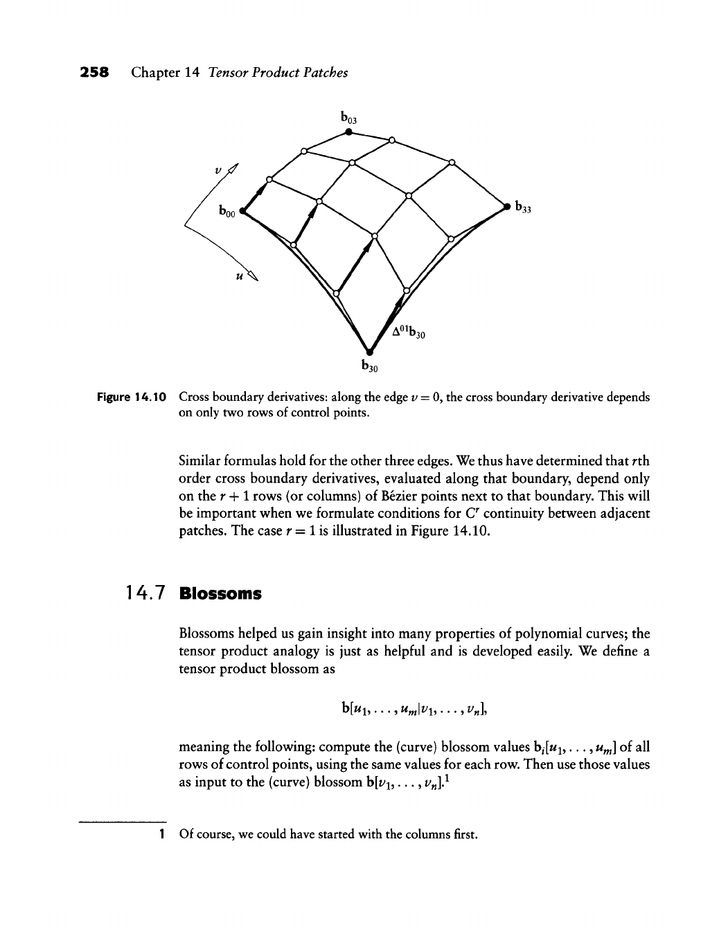
258 Chapter 14 Tensor Product Patches
Figure 14.10 Cross boundary derivatives: along the edge v = 0, the cross boundary derivative depends
on only two rows of control points.
Similar formulas hold for the other three edges. We thus have determined that rth
order cross boundary derivatives, evaluated along that boundary, depend only
on the r 4-1 rows (or columns) of Bezier points next to that boundary. This will
be important when we formulate conditions for C continuity between adjacent
patches. The case r = 1 is illustrated in Figure 14.10.
14.7 Blossoms
Blossoms helped us gain insight into many properties of polynomial curves; the
tensor product analogy is just as helpful and is developed easily. We define a
tensor product blossom as
b[wi,...,w^|t;i,...,z/„],
meaning the following: compute the (curve) blossom values b/[Mi,..., u^] of all
rows of control points, using the same values for each row. Then use those values
as input to the (curve) blossom b[t^i,..., v^]}
1 Of course, we could have started with the columns first.

14.7 Blossoms 259
Tensor product blossoms inherit their properties from their curve building
blocks. Thus, the blossom h[u^^^\v^^^] is the point on the surface, the order of
evaluations does not matter, and we have multiaffinity in both u and v.
Two examples of blossoms: the osculating bilinear surface t(s, t) at a point
x(w, v) may be written as
t(s,
t) = b[w<^-i^, s|i/<"-i^, tl (14.14)
This surface is linear in both s and t and agrees with x(w, v) in both partials and
twist (modulo some constant factors). The surface 0(5, t) given by
0(5,0 =bKs<'^-^^|i/,?<"-i^]
is the osculant or first polar of the given surface at x(w, v). It is the analog of the
univariate polar from Section 5.6.
Just as in the curve case, we may use blossoms for subdivision or domain
transformation. If the new patch is to be defined over the domain rectangle
[a^
b\ X [c, d\ then its Bezier points
CQ
are given by
qy = b[^<^-^'^,
b^'^\c^''-i^,
J<>]. (14.15)
For the special case
[a^
b]
= [c, d] =
[0,1],
we recover the original Bezier points.
Though (14.15) may look complicated, it really is not: all we have to do is to
write a tensor product blossom routine—a matter of about ten lines of code!
Blossoms may also be used to find derivatives, in complete analogy to Section
5.3.
Mixed partials take the form
dWdv^ {ni
—
r)\{n
—
s)\
Evaluations with respect to the vector 1 in the w-domain are equivalent to
taking differences in the /-direction, those with respect to the z/-vector 1 corre-
spond to differences in the /-direction. Again, it does not matter in which order
we perform the evaluations.
We may use the blossom formulation of derivatives to approach a practical
problem. It is often the case^ that not only a point on a surface is needed, but
also its u- and ^'-partials. Standard tensor product evaluation will give us only
either a w-partial or a i/-partial as a byproduct. However, (14.14) may always be
used to compute both partials. Algorithmically, here is what to do: for a given
2 For applications such as rendering or numerical methods.
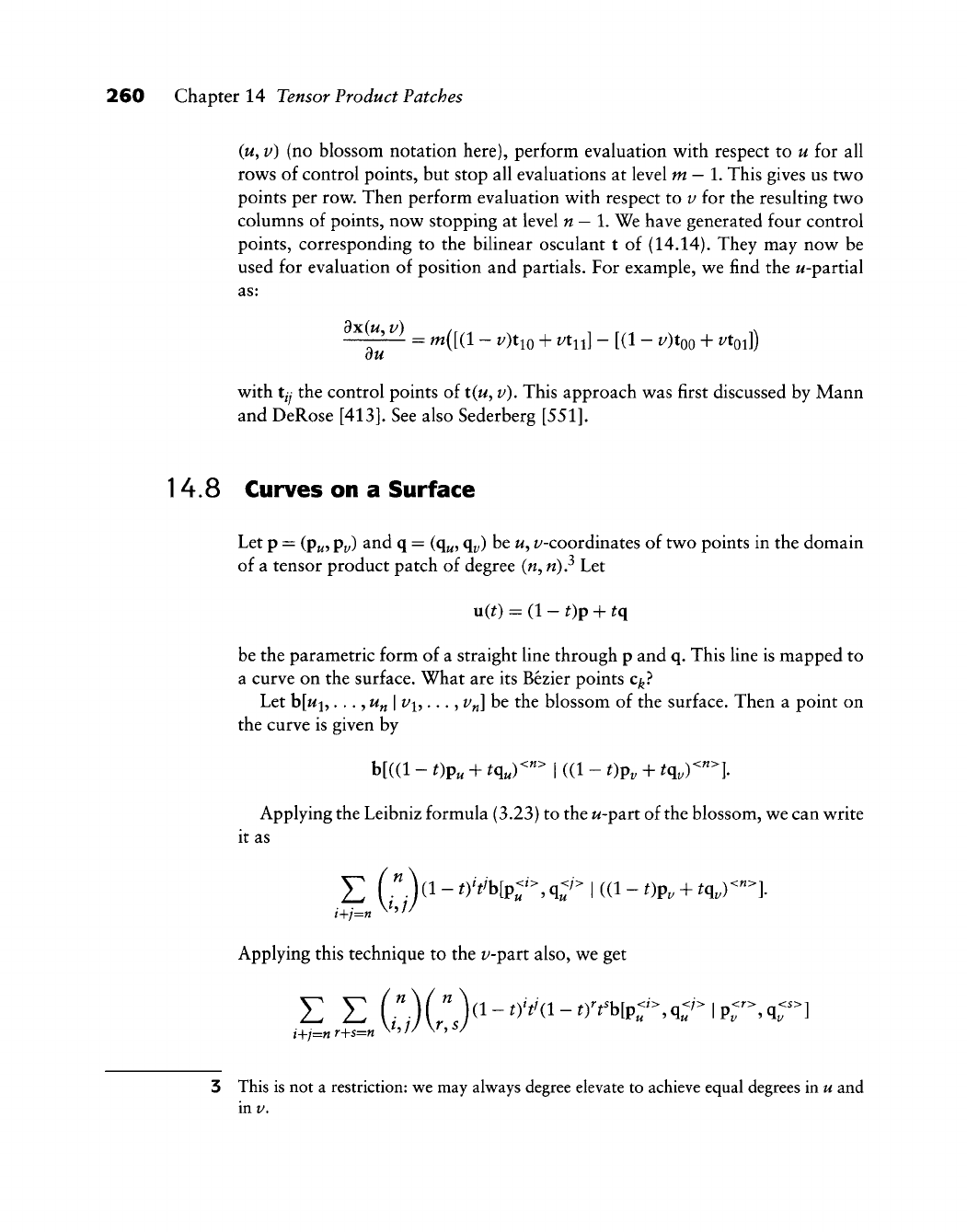
260 Chapter
14
Tensor Product Patches
(u^
v) (no
blossom notation here), perform evaluation with respect
to u for all
rows
of
control points,
but
stop
all
evaluations
at
level
m
—
1.
This gives
us two
points
per
row. Then perform evaluation with respect
to v for the
resulting
two
columns
of
points,
now
stopping
at
level
n
—
\. We
have generated four control
points, corresponding
to the
bilinear osculant
t of
(14.14). They
may now be
used
for
evaluation
of
position
and
partials.
For
example,
we
find
the
w-partial
as:
^^^^
= m{[(l - v)^Q + vtn] -
[(1
-
i^)too
+
t^toi])
ou
with
tjj the
control points
of
t(w,
v).
This approach
was
first discussed
by
Mann
and DeRose
[413].
See
also Sederberg
[551].
14.8 Curves on a Surface
Let
p =
(pj^,
pjj)
and q =
(q^,
q^^)
be
w,
z^-coordinates
of
two points
in the
domain
of
a
tensor product patch
of
degree («,
n)? Let
u(t)
=
(1
- t)p + tq
be
the
parametric form
of a
straight line through
p and q.
This line
is
mapped
to
a curve
on the
surface. What
are its
Bezier points c^.'*
Let b[wi,...,
w„ I
i/i,...,
f„] be the
blossom
of the
surface. Then
a
point
on
the curve
is
given
by
b[((l
- t)p, +
^,)<">
I
((1
- t)p, +
^q,)<""].
Applying the Leibniz formula (3.23)
to
the w-part
of
the blossom, we can write
it
as
Y^
(.^)(l-OVb[p->,q</>
I
((l-Op,
+
^q,)<-].
Applying this technique
to the
v-part also,
we get
3 This
is not a
restriction:
we
may always degree elevate
to
achieve equal degrees
in u and
in
V.
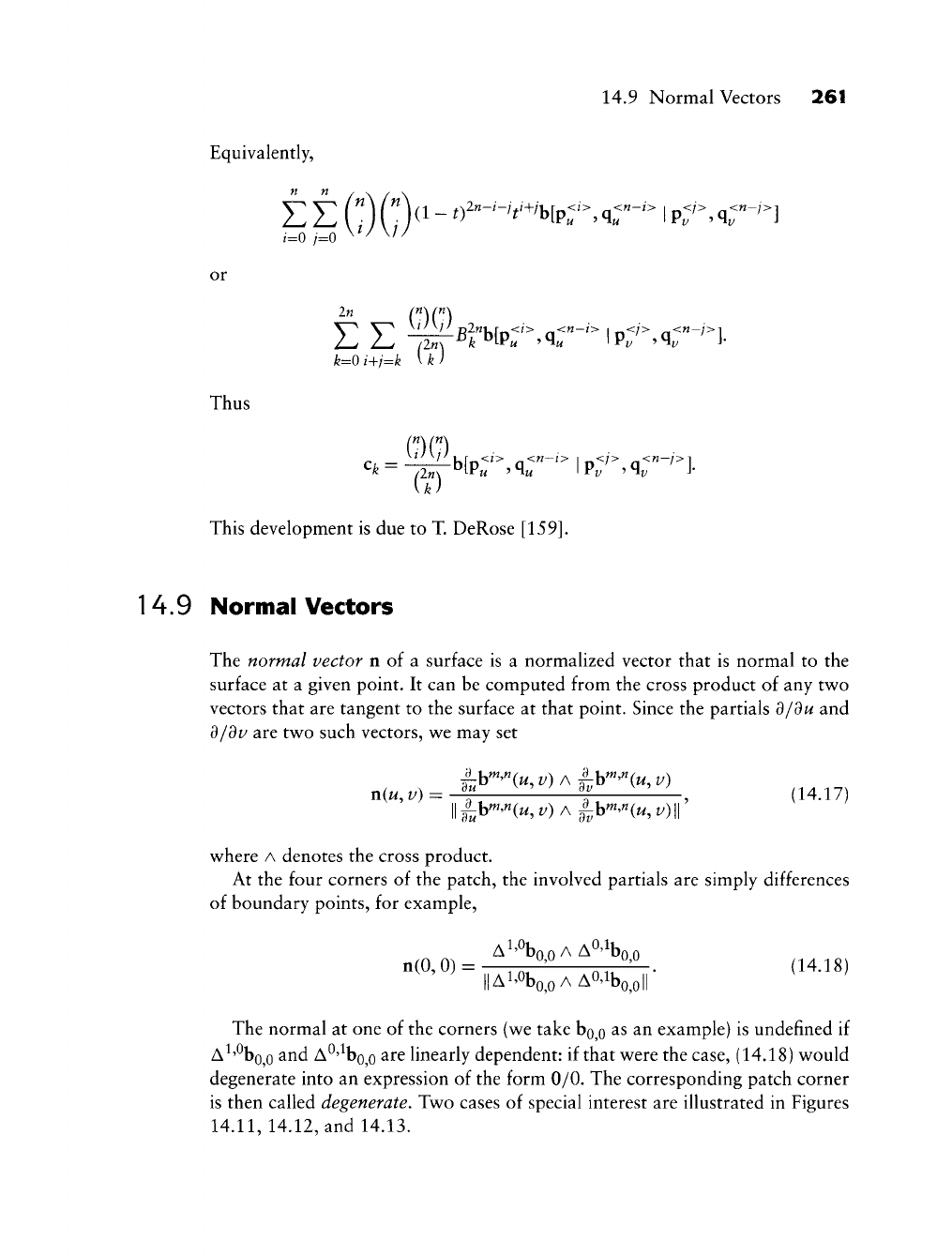
14.9 Normal Vectors 261
Equivalently,
n n
^=0 /=0
or
Thus
In
(n\(n\
fe=0
/+7=f^
V
fe
/
This development is due to T DeRose
[159].
14.9 Normal Vectors
The normal vector n of a surface is a normalized vector that is normal to the
surface at a given point. It can be computed from the cross product of any two
vectors that are tangent to the surface at that point. Since the partials d/du and
d/dv
2iTt
two such vectors, we may set
n(u,
V)
= -^^ '\ ^^—, (14.17)
where A denotes the cross product.
At the four corners of the patch, the involved partials are simply differences
of boundary points, for example,
A^'^ooAA^'lboo
||Ai'%,oAA04bo^oll
The normal at one of the corners (we take bg^o ^^ ^^ example) is undefined if
A^'%0,0 ^^^ ^^'^bo^O ^^^ linearly dependent: if that were the case, (14.18) would
degenerate into an expression of the form 0/0. The corresponding patch corner
is then called degenerate. Two cases of special interest are illustrated in Figures
14.11,
14.12, and
14.13.
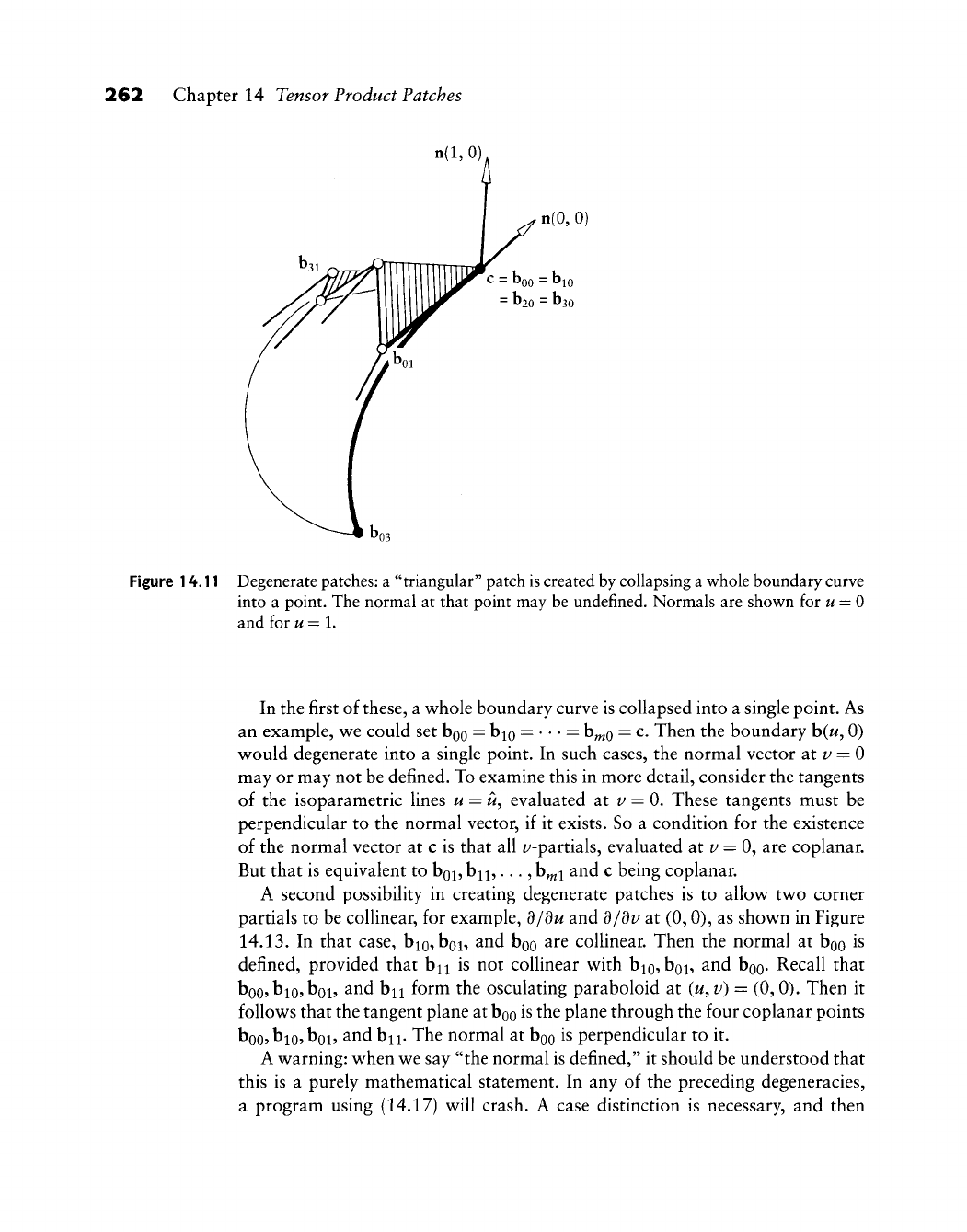
262 Chapter 14 Tensor Product Patches
n(l,0),
n(0,
0)
c - boo - "10
= "20 = D30
Figure 14.11 Degenerate
patches:
a "triangular" patch is created by collapsing a whole boundary curve
into a point. The normal at that point may be undefined. Normals are shown for
M
= 0
and for u=l.
In the first of these, a whole boundary curve is collapsed into a single point. As
an example, we could set boo = b^o =
• • •
= b^o = c- Then the boundary b(w, 0)
v^ould degenerate into a single point. In such cases, the normal vector at i/ = 0
may or may not be defined. To examine this in more detail, consider the tangents
of the isoparametric lines u = u^ evaluated at v = 0, These tangents must be
perpendicular to the normal vector, if it exists. So a condition for the existence
of the normal vector at c is that all z/-partials, evaluated at f = 0, are coplanar.
But that is equivalent to boi,
b^,...,
b^i and c being coplanar.
A second possibility in creating degenerate patches is to allov^ tw^o corner
partials to be coUinear, for example, d/du and d/dv at (0,0), as shov^n in Figure
14.13.
In that case, b^o^boi, and boo ^^^ coUinear. Then the normal at boo is
defined, provided that b^^ is not coUinear v^^ith bio?boi, and boo- Recall that
boo?bio?boi, and b^ form the osculating paraboloid at {u, v) = (0, 0). Then it
follow^s that the tangent plane at
boo
is the plane through the four coplanar points
boo?
bio? boi? and b^. The normal at boo is perpendicular to it.
A warning: when we say "the normal is defined," it should be understood that
this is a purely mathematical statement. In any of the preceding degeneracies,
a program using (14.17) will crash. A case distinction is necessary, and then
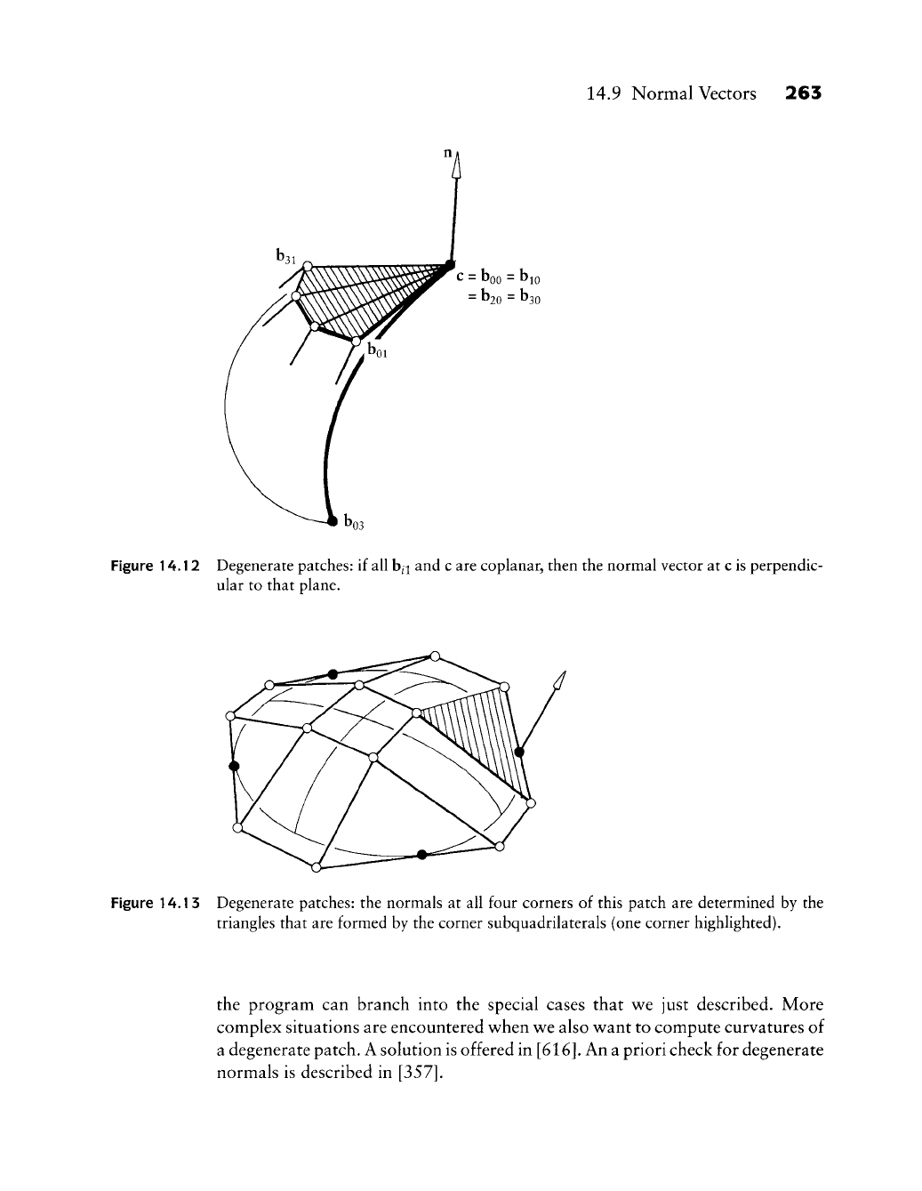
14.9 Normal Vectors 263
•
boo - bio
•
^20 = "30
Figure 14.12 Degenerate patches: if all h^ and c are coplanar, then the normal vector at c is perpendic-
ular to that plane.
Figure 14.13 Degenerate patches: the normals at all four corners of this patch are determined by the
triangles that are formed by the corner subquadrilaterals (one corner highlighted).
the program can branch into the special cases that we just described. More
complex situations are encountered when we also want to compute curvatures of
a degenerate patch. A solution is offered in
[616].
An a priori check for degenerate
normals is described in
[357].
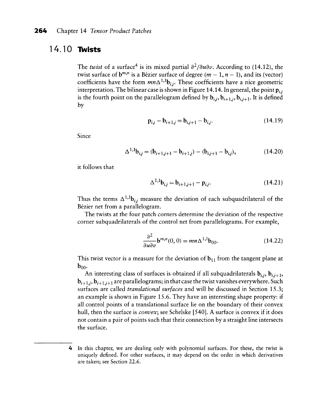
264 Chapter 14 Tensor Product Patches
14.10 IWists
The twist of a surface^ is its mixed partial d^/dudv. According to (14.12), the
twist surface of
b'^'^
is a Bezier surface of degree (m
—
1,
w —
1), and its (vector)
coefficients have the form mwA^'^b/y. These coefficients have a nice geometric
interpretation. The bihnear case is shown in Figure 14.14. In general, the point p/y
is the fourth point on the parallelogram defined by
b^
y,
b/+i
y,
b^
y_^i.
It is defined
by
Pw-bm,/=k;+l-kr (14.19)
Since
A^'^b,-,-
= (b,+i,,+i - b,+i,) - (b,-,,+i - b,,), (14.20)
it follows that
A''\, = b,+i,+i-p,-,. (14.21)
Thus the terms A^'^b^y measure the deviation of each subquadrilateral of the
Bezier net from a parallelogram.
The twists at the four patch corners determine the deviation of the respective
corner subquadrilaterals of the control net from parallelograms. For example,
dudv
b^'"(0,
0) = mwA^Xo- (14.22)
This twist vector is a measure for the deviation of b^ from the tangent plane at
boo-
An interesting class of surfaces is obtained if all subquadrilaterals
b^
y,
b^,y_^i,
b/+i,/9
b^_^i
y^i are parallelograms; in that case the twist vanishes everywhere. Such
surfaces are called translational surfaces and will be discussed in Section 15.3;
an example is shown in Figure 15.6. They have an interesting shape property: if
all control points of a translational surface lie on the boundary of their convex
hull, then the surface is convex; see Schelske
[540].
A surface is convex if it does
not contain a pair of points such that their connection by a straight line intersects
the surface.
4 In this chapter, we are dealing only with polynomial surfaces. For these, the twist is
uniquely defined. For other surfaces, it may depend on the order in which derivatives
are taken; see Section 22.6.
14.11 The Matrix Form of a Bezier Patch 265
Figure 14.14 Twists: the twist is proportional to the deviation of a control net quadrilateral from a
parallelogram.
14.11 The Matrix Form of a Bezier Patcii
In Section S.7^ we formulated a matrix expression for Bezier curves. This ap-
proach carries over v^ell to tensor product patches. We can write:
[B^{u) ... BZiu)]
boo
• • •
\n
L D^Q . . . ^mn -I
(14.23)
The matrix
{b^;},
defining the control net, is sometimes called the geometry
matrix of the patch. If we perform a basis transformation and write the Bernstein
polynomials in monomial form, we obtain
rb,
b'^'^CM,
v)^[u^ ...
u'"]M^
00 bn„1 W^^
L
b^o
••
•
b„„J
L
f"J
N (14.24)
The square matrices M and N are given by
'-<-"'-'(:)(:
(14.25)
and
«,/ = (-1>
,Mru'
//Vy
(14.26)
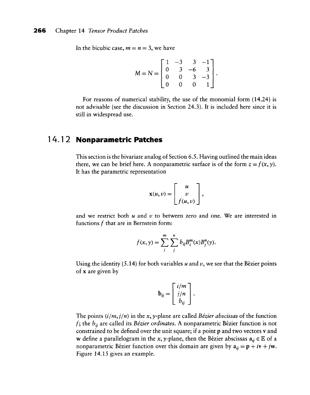
266 Chapter 14 Tensor Product Patches
In the bicubic case, m = n = 3^we have
M = N =
1
0
0
0
-3
3
0
0
3
-6
3
0
-1
3
-3
1
For reasons of numerical stabiUty, the use of the monomial form (14.24) is
not advisable (see the discussion in Section 24.3). It is included here since it is
still in widespread use.
14.12 Nonparametric Patches
This section is the bivariate analog of Section 6.5. Having outlined the main ideas
there, we can be brief here. A nonparametric surface is of the form z = f(x^ y).
It has the parametric representation
X(M, V) =
u
V
L
f{u, v) J
and we restrict both u and v to between zero and one. We are interested in
functions f that are in Bernstein form:
A^'3^)=EEMrw^F(y)-
I /
Using the identity (5.14) for both variables u and z/, we see that the Bezier points
of
X
are given by
i/m
jIn
The points (//m, j/n) in the x, y-plane are called Bezier abscissas of the function
f\ the bij are called its Bezier ordinates, A nonparametric Bezier function is not
constrained to be defined over the unit square; if a point p and two vectors v and
w define a parallelogram in the x, y-plane, then the Bezier abscissas a^y
G
E of a
nonparametric Bezier function over this domain are given by a/y = p + /v + /w.
Figure 14.15 gives an example.
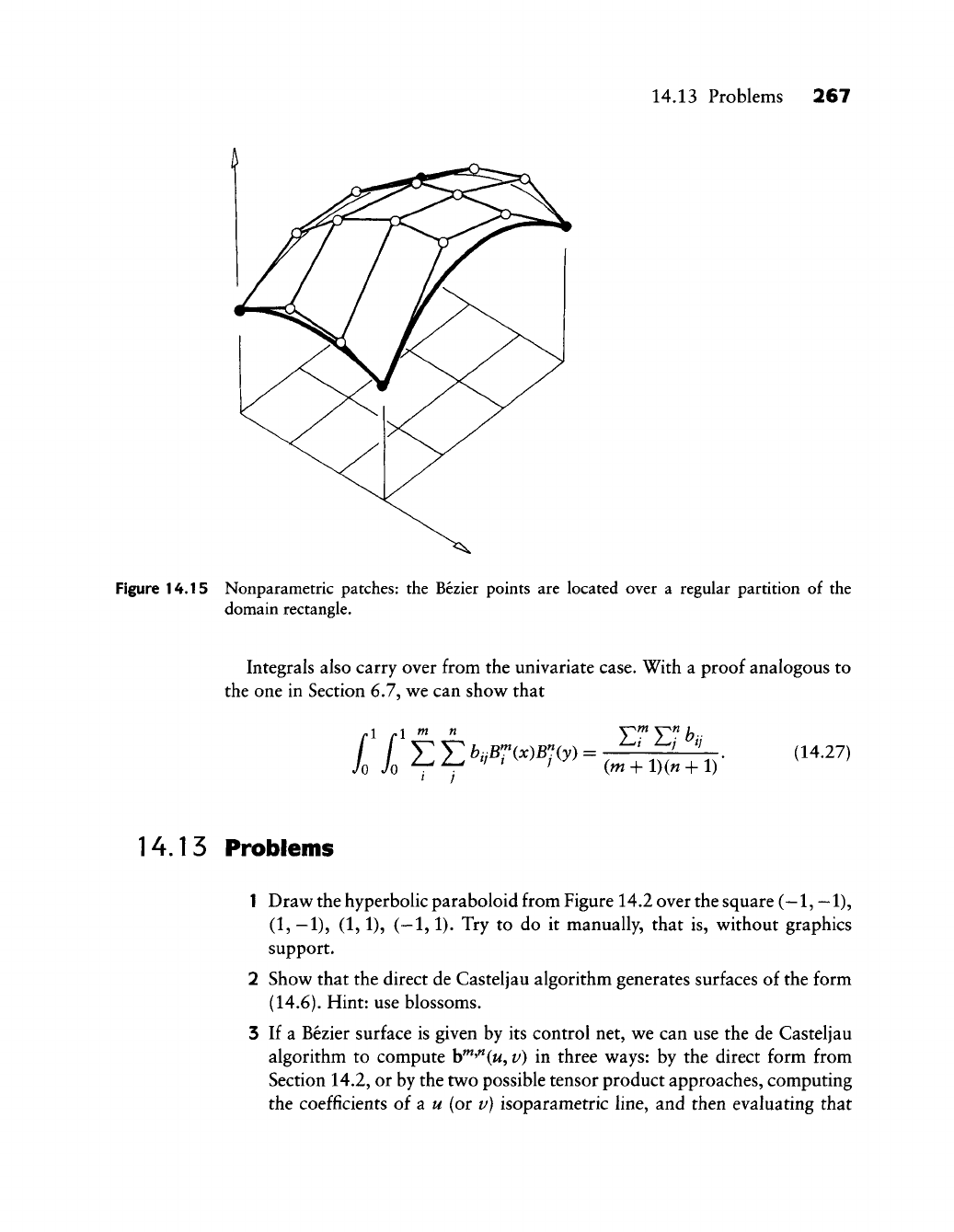
14.13 Problems 267
Figure 14.15 Nonparametric patches: the Bezier points are located over a regular partition of the
domain rectangle.
Integrals also carry over from the univariate case. With a proof analogous to
the one in Section 6.7, we can show that
-1 »i m n
y'"y"bii
I I TThB'"(x)B"(y)= ^' ^' " .
yo Jo Y /
(m
+ l)(« + l) (14.27)
14.15 Problems
1 Draw the hyperbolic paraboloid from Figure 14.2 over the square
(—1,
—1),
(1,
—1), (1,1), (—1,1). Try to do it manually, that is, without graphics
support.
2 Show that the direct de Casteljau algorithm generates surfaces of the form
(14.6).
Hint: use blossoms.
3 If a Bezier surface is given by its control net, we can use the de Casteljau
algorithm to compute b'^'^^Cw, v) in three ways: by the direct form from
Section 14.2, or by the two possible tensor product approaches, computing
the coefficients of a w (or v) isoparametric line, and then evaluating that
268 Chapter 14 Tensor Product Patches
curve at
1/
(or
w).
Though theoretically equivalent, the computation counts
for these methods differ. Work out the details.
* 4 Show that Bezier surfaces have bilinear precision: if hjj = x(^, ^) and x is
bilinear, then b^'"(w, v) = x(w, v) for all
w,
v and for arbitrary m, n,
* 5 Generalize (5.31) to the tensor product case.
PI Generalize the routine degree_e1 evate to the tensor product case.
P2 Generalize the routine ait ken to the tensor product case, that is, program
tensor product Lagrange interpolation.
P3 The data file car .dat contains data points (slightly modified) of four bound-
ary curves of one of the surfaces shov^n in Color Plate III. Try to fit a Bezier
patch (your pick of the degrees!) so that you get close to the corresponding
surface in the color plates.
Constructing
Polynomial Patches
We '
e
have discussed the underlying principles of polynomial patches; now it is
time to study how they can be used. First applications of tensor product patches
go back to General Motors, and Boeing in the United States, and to Renault and
Citroen in France.
15.1 Ruled Surfaces
One of the most elementary surface-building schemes is this: let two Bezier curves
h(u) and c(u) be given by their control polygons bo,
•
. ., b„ and
CQ,
.. ., c„, and
find a surface r(^, v) that connects them. The simplest such surface will use a
linear type of connection; it is called a ruled surface or lofted surface^ It is given
by
r(w, v) = (1
—
v)h(u)
-\-
vc{u). (15.1)
For z/ = 0, it interpolates to b(w); for v—l^'\t interpolates to c{u).
The ruled surface r is linear in v and of degree n in u. In Bezier form, it becomes
r(w, v) = [1
— V
v]
bo
Co
B"{u)
lB"„{u)A
1 The word lofted has an interesting history. In the days of completely manual ship design,
full-scale drawings were difficult to handle in the design office. These drawings were stored
and dealt with in large attics, called lofts.
269
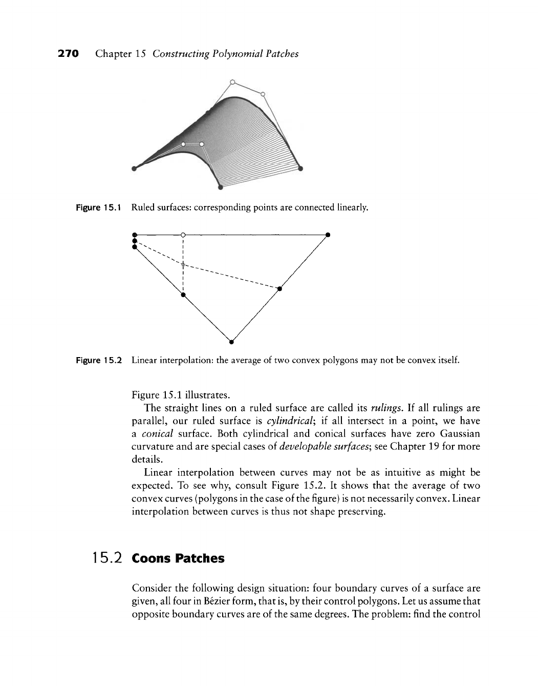
270 Chapter 15 Constructing Polynomial Patches
Figure 15.1 Ruled surfaces: corresponding points are connected linearly.
Figure 15.2 Linear interpolation: the average of two convex polygons may not be convex
itself.
Figure 15.1 illustrates.
The straight lines on a ruled surface are called its rulings. If all rulings are
parallel, our ruled surface is cylindrical; if all intersect in a point, we have
a conical surface. Both cylindrical and conical surfaces have zero Gaussian
curvature and are special cases of developable surfaces; see Chapter 19 for more
details.
Linear interpolation betw^een curves may not be as intuitive as might be
expected. To see v^hy, consult Figure 15.2. It show^s that the average of tw^o
convex curves (polygons in the case of the figure) is not necessarily convex. Linear
interpolation betv^een curves is thus not shape preserving.
15.2 Coons Patches
Consider the follov^ing design situation: four boundary curves of a surface are
given, all four in Bezier form, that
is,
by their control polygons. Let us assume that
opposite boundary curves are of the same degrees. The problem: find the control
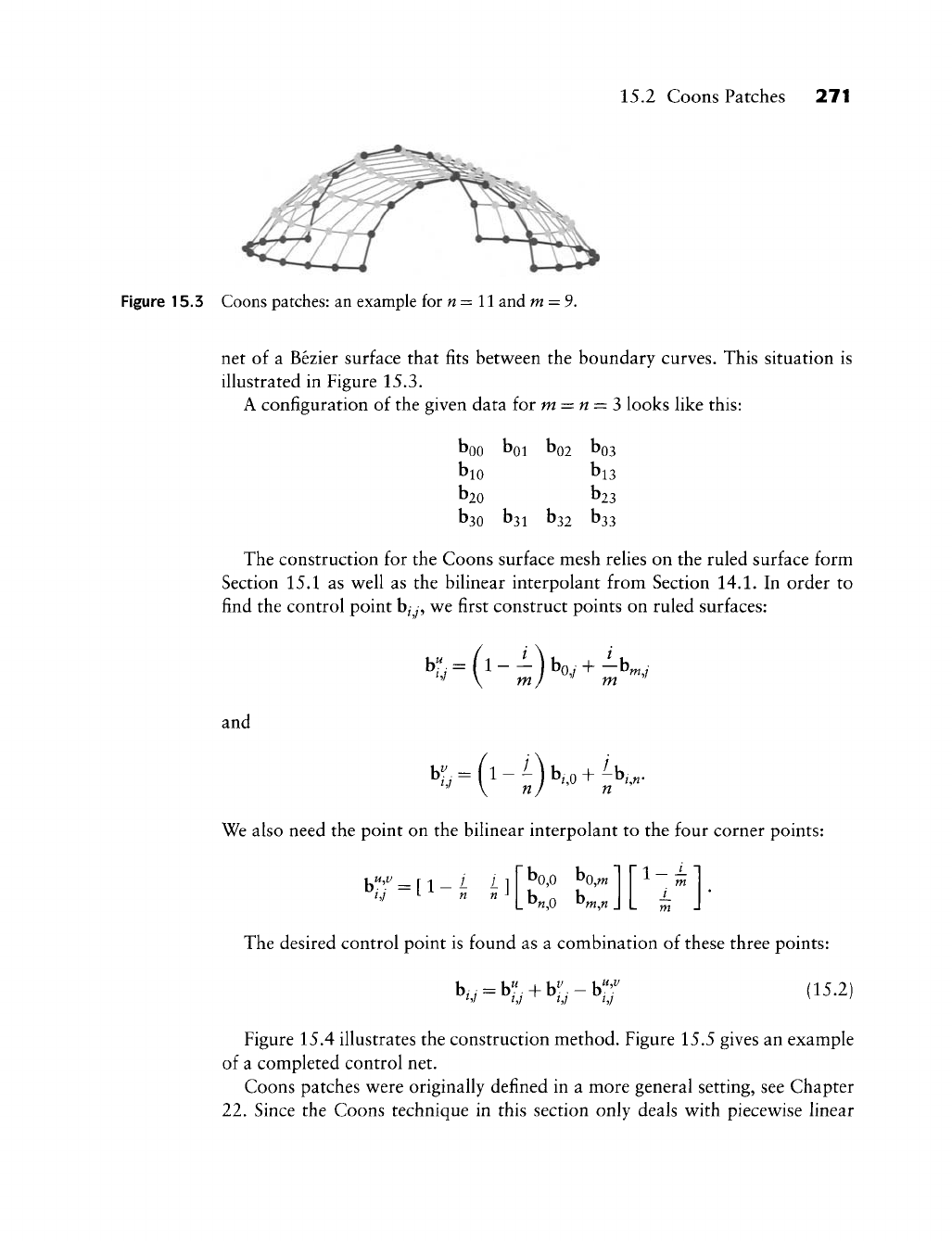
15.2 Coons Patches 271
Figure 15.3 Coons patches: an example for
w
= 11 and m = 9.
net of a Bezier surface that fits between the boundary curves. This situation is
illustrated in Figure 15.3.
A configuration of the given data for m = n = 3 looks like this:
boo ^01 bo2 bo3
bio bi3
b20 b23
bso b3i b32 b33
The construction for the Coons surface mesh relies on the ruled surface form
Section 15.1 as well as the bilinear interpolant from Section 14.1. In order to
find the control point b/y, we first construct points on ruled surfaces:
and
bL =
(l-Mb,o
+
^,,«
We also need the point on the bilinear interpolant to the four corner points:
hi
-•
•- n n
bo,o bo,^
bw,0 ^m,n
1-zr.
L.
m -J
The desired control point is found as a combination of these three points:
hi=h,,+h,rhf
(15-2)
Figure 15.4 illustrates the construction method. Figure 15.5 gives an example
of a completed control net.
Coons patches were originally defined in a more general setting, see Chapter
22.
Since the Coons technique in this section only deals with piecewise linear

272 Chapter 15 Constructing Polynomial Patches
Figure 15.4 Coons patches: the construction. Gray points, from bottom:
b"'2,
b"
2?
h^
2*
Above them,
solid black:
b^
2-
Figure 15.5 Coons patches: an example.
boundary polygons and control meshes, these are often referred to as discrete
Coons patches.
15.5 Tkranslational Surfaces
A translational surface has the simple structure of being generated by two
curves: let Ci(u) and C2(^') be tw^o such curves, intersecting at a common point
a = ci(0) = C2(0). A translational surface t(w, v) is then defined by
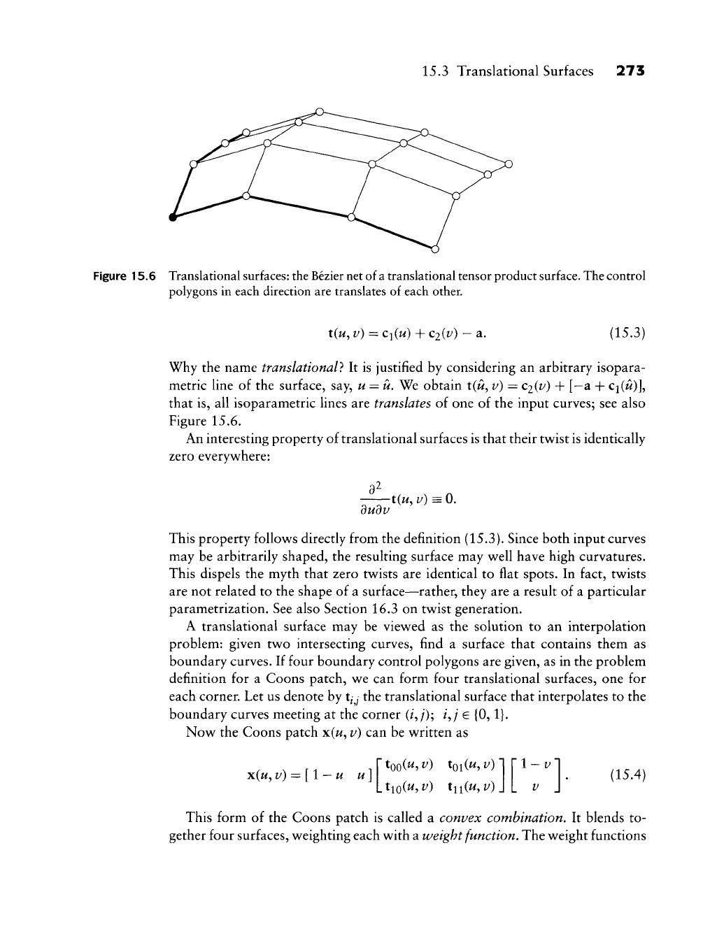
15.3 Translational Surfaces 273
Figure 15.6 Translational surfaces: the Bezier net of
a
translational tensor product surface. The control
polygons in each direction are translates of each other.
t(u,
v) = Ciiu) + C2(i^) - a. (15.3)
Why the name translational} It is justified by considering an arbitrary isopara-
metric line of the surface, say, u = u. We obtain t(w, v) = C2(i^) + [—a + Ci(ii)],
that is, all isoparametric lines are translates of one of the input curves; see also
Figure 15.6.
An interesting property of translational surfaces is that their twist is identically
zero everywhere:
dudv
t(u,
v) = 0.
This property follows directly from the definition (15.3). Since both input curves
may be arbitrarily shaped, the resulting surface may well have high curvatures.
This dispels the myth that zero twists are identical to flat spots. In fact, twists
are not related to the shape of a surface—rather, they are a result of a particular
parametrization. See also Section 16.3 on twist generation.
A translational surface may be viewed as the solution to an interpolation
problem: given two intersecting curves, find a surface that contains them as
boundary curves. If four boundary control polygons are given, as in the problem
definition for a Coons patch, we can form four translational surfaces, one for
each corner. Let us denote by tjj the translational surface that interpolates to the
boundary curves meeting at the corner (/,/); /,; €
{0,1}.
Now the Coons patch x(w, v) can be written as
x(^,
v) = [1
—
u u]
too(^, v) toi(w, v) 1-v
V
(15.4)
This form of the Coons patch is called a convex combination. It blends to-
gether four surfaces, weighting each with a weight function. The weight functions
274 Chapter 15 Constructing Polynomial Patches
sum to one (a necessity: nonbarycentric combinations are disallowed) and are
nonnegative for u,v e
{0,1}.
Note that the weight functions are zero where the
corresponding t^y is "wrong."
Translational and Coons surfaces are related in yet another way. If four
boundary control polygons are related such that opposite polygons are translates
of each other, then the resulting Coons control net will be a translational surface;
an example is provided by Figure 15.6.
1
5.4 Tensor Product Interpolation
We could use curves for both free-form design and for interpolation; the same is
true for tensor product patches. As a preparatory step, let us rewrite (14.6) in an
equivalent matrix form:
x{u,v) = [B^(u) BZiuy
^00
LD^O
^On Bl{v)
.B>),
(15.5)
Suppose now that we are given an (m + 1) x (w + 1) array of data points
X/y; 0 <i <m,0<j <n. We want the surface (15.5) to interpolate to them, that
is,
(15.5) must be true for each pair
(w^,
Vj).
We thus obtain (n-\-1) x (m-\- 1)
equations, which we may write concisely as
X = UBV, (15.6)
where
XOO
.
^mO •
U =
boo
B =
•'mO
XOn
BZi^o)
K
I
and
v =
15.4 Tensor Product Interpolation 275
B«(t/o) ••• B"Qiv„)l
lB"Jvo)
•••
B"„{v„)}
Matrices U and V already appeared in Section 7.3; they are Vandermonde
matrices.
In an interpolation context, the x^y are known and the coefficients b/y are
unknown. They are found from (15.6) by setting
B=U-iXV-l (15.7)
The inverse matrices in (15.7) exist since the functions B^ and B^ art linearly
independent.
Equation (15.7) shows how a solution to the interpolation problem could
be found, but one should not try to invert the matrices U and V explicitly! To
solve and understand better the tensor product interpolation problem, we rewrite
(15.6) as
X = DV, (15.8)
where we have set
D=:L7B.
(15.9)
Note that D consists of (m + 1) rows and (n + 1) columns. Equation (15.8) can
be interpreted as a family of (m+1) univariate interpolation problems—one for
each row of X and D, where D contains the unknowns. Having solved all {m + 1)
problems (all having the same coefficient matrix V!), we can attack (15.9),
since we have just computed D. Equation (15.9) may be interpreted as a family
of (n + 1) univariate interpolation problems, all having the same coefficient
matrix U.
We thus see how the tensor product form allows a significant "compactifi-
cation" of the interpolation process. Without the tensor product structure, we
would have to solve a linear system of order (m
-\-
l)(n -\-1) x (m
-\-
l){n + 1).
That is an order of magnitude more complex than solving m + 1 problems with
the same (n-\-1) x (n-\-1) matrix and then solving
w
+
1
problems with the same
(m + 1) X (m + 1) matrix. If m = w, the naive approach would thus need O(m^)
computations, whereas the tensor product approach just needs O(m^). This will
be even more dramatic for interpolating spline surfaces.
There is a less algebraic way to describe the tensor product interpolation
process as well. Considering (15.8), we see that it may be interpreted as a family
of univariate interpolation problems with the same coefficient matrix V. That is
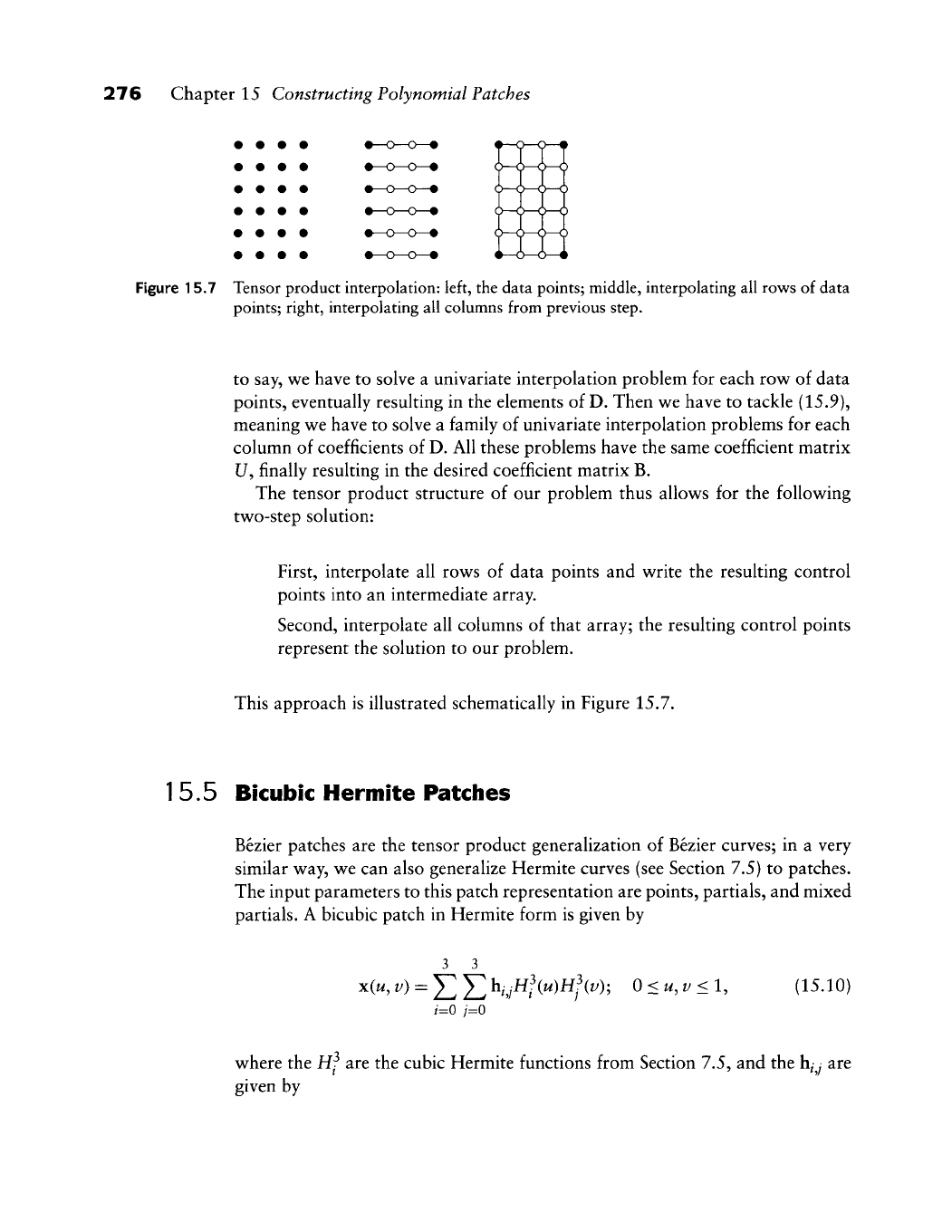
276 Chapter 15 Constructing Polynomial Patches
Figure 15.7 Tensor product interpolation: left, the data points; middle, interpolating all rows of data
points; right, interpolating all columns from previous step.
to say, we have to solve
a
univariate interpolation problem for each row of data
points, eventually resulting in the elements of D. Then we have to tackle (15.9),
meaning we have to solve
a
family of univariate interpolation problems for each
column of coefficients of D. All these problems have the same coefficient matrix
U, finally resulting in the desired coefficient matrix B.
The tensor product structure
of
our problem thus allows
for
the following
two-step solution:
First, interpolate all rows
of
data points and write the resulting control
points into an intermediate array.
Second, interpolate all columns of that array; the resulting control points
represent the solution to our problem.
This approach is illustrated schematically in Figure 15.7.
15.5 Bicubic Hermite Patciies
Bezier patches are the tensor product generalization
of
Bezier curves;
in a
very
similar way, we can also generalize Hermite curves (see Section 7.5) to patches.
The input parameters to this patch representation are points, partials, and mixed
partials. A bicubic patch in Hermite form is given by
3
3
xiu, v) =
J^Yl Kj^fMHfiv); 0<u,v<l,
(15.10)
/=0 /=0
where the
Hf
are the cubic Hermite functions from Section 7.5, and the
h^
y
are
given by
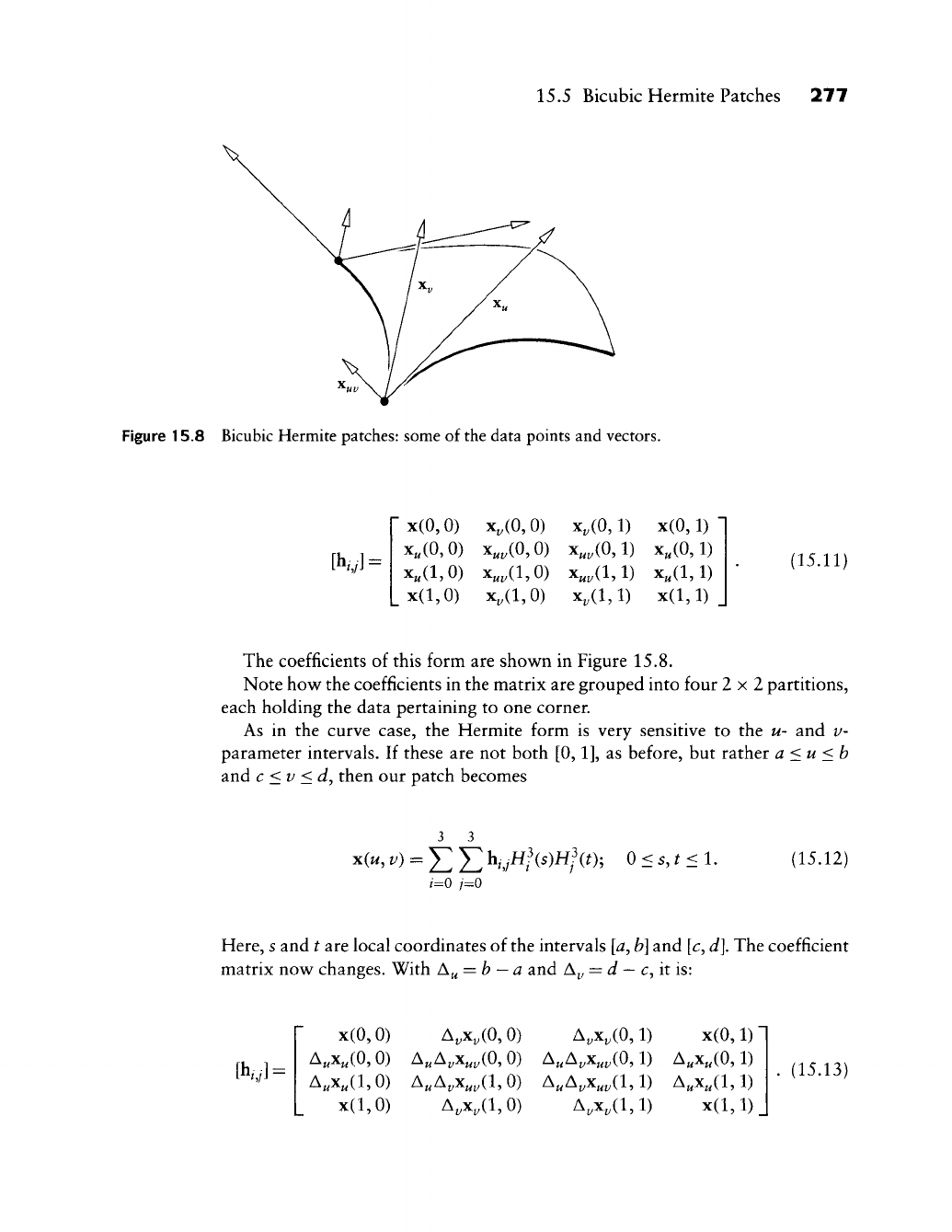
15.5 Bicubic Hermite Patches 277
Figure 15.8 Bicubic Hermite patches: some of the data points and vectors.
[k/]=
x(0,0)
x„(0,0)
x„(l,0)
x(l,0)
x,(0,0)
x„^(0,0)
x„,(l,0)
x^(l,0)
x,(0,1)
x„,(0,1)
X„;,(l, 1)
x,(l, 1)
x(0,1)
x„(0,1)
x„(l, 1)
x(l,l)
(15.11)
The coefficients of this form are shown in Figure 15.8.
Note how the coefficients in the matrix are grouped into four 2x2 partitions,
each holding the data pertaining to one corner.
As in the curve case, the Hermite form is very sensitive to the u- and v-
parameter intervals. If these are not both
[0,1],
as before, but rather a<u<b
and c <v <d, then our patch becomes
/=0 /=0
0<s,^< 1. (15.12)
Here, s and t art local coordinates of the intervals
[a,
b]
and [c,
d].
The coefficient
matrix now changes. With ^^ = b
—
a and A^ = J
—
c, it is:
[k;] =
x(0,0)
A„x„(0,0)
A„x„(l,0)
x(l,0)
A,x,(0,0)
A„A^x„^(0,0)
KK^uvO-, 0)
A,x„(l,0)
A,x,(0,1)
A„A^x„j,(0,1)
x(0,1)
A„x„(0,1)
A„A„x„,/l,l) A„x„(l,l)
^u'-^v^uv\
Aj,Xj,(l, 1)
x(l,
1) J
. (15.13)
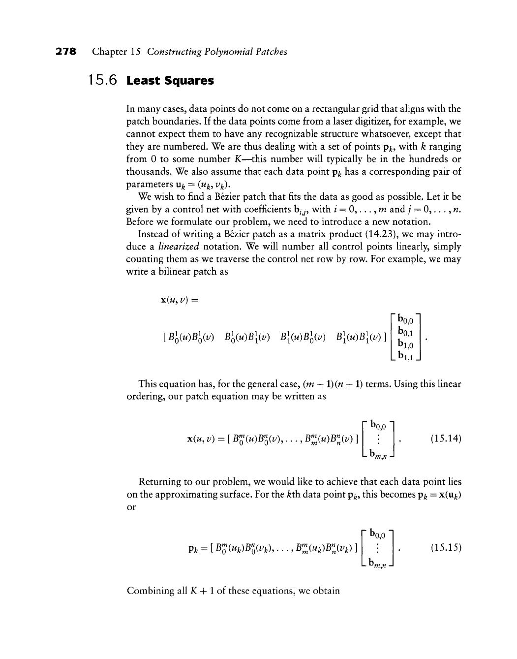
278 Chapter 15 Constructing Polynomial Patches
1
5.6 Least Squares
In many cases, data points do not come on a rectangular grid that ahgns with the
patch boundaries. If the data points come from a laser digitizer, for example, we
cannot expect them to have any recognizable structure whatsoever, except that
they are numbered. We are thus dealing with a set of points p^, with k ranging
from 0 to some number K—this number will typically be in the hundreds or
thousands. We also assume that each data point p^ has a corresponding pair of
parameters u^ = (w^,
Vf^).
We wish to find a Bezier patch that fits the data as good as possible. Let it be
given by a control net with coefficients b/y, with / = 0,..., m and; = 0,...,«.
Before we formulate our problem, we need to introduce a new notation.
Instead of writing a Bezier patch as a matrix product (14.23), we may intro-
duce a linearized notation. We will number all control points linearly, simply
counting them as we traverse the control net row by row. For example, we may
write a bilinear patch as
x(w, v) =
[Bl(u)Bl(v) Bliu)B\{v) B\(u)Bl(v) B\iu)B\iv)]
r
bo,o
1
bo,i
^1,0
Lbi,i_
This equation has, for the general case, (m + l)(w + 1) terms. Using this linear
ordering, our patch equation may be written as
xiu,
V)
=
[
B^(u)Bl(v),..., Bl{u)Bl{v) ]
r Vo
(15.14)
Returning to our problem, we would like to achieve that each data point lies
on the approximating surface. For the kxh data point
p^,
this becomes p^ = x(u^)
or
^k = [B'S{Uk)Bl(vk),...,Bl{u0Bl{Vk)
•»o,o
(15.15)
Combining all K + 1 of these equations, we obtain
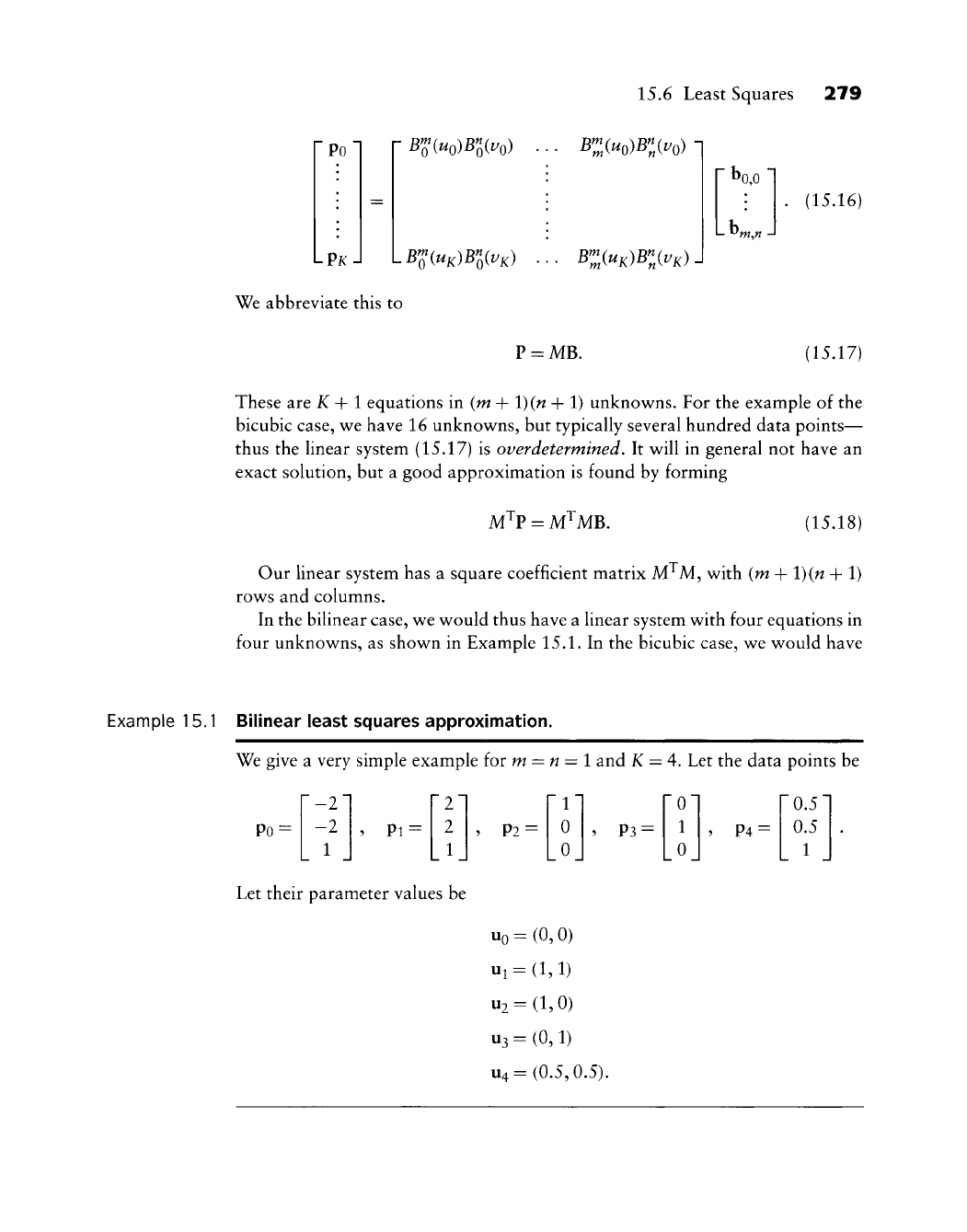
15.6 Least Squares
279
Po B^(uo)B^Jvo)
PK-i
IB^(UK)B-^(VK)
BZ(uo)B':,(vo)
BZ(UK)BI(VK)J
^0,0
^m.n
-«
We abbreviate this
to
(15.16)
P
=
MB. (15.17)
These
are X + 1
equations
in (m + l)(/7 + 1)
unknowns.
For the
example
of the
bicubic case,
we
have
16
unknowns,
but
typically several hundred data points—
thus
the
linear system (15.17)
is
overdetermined.
It
will
in
general
not
have
an
exact solution,
but a
good approximation
is
found
by
forming
M^V
=
M^MB. (15.18)
Our linear system
has a
square coefficient matrix
M^M^
with
(m + l)(w + 1)
rows
and
columns.
In
the
bilinear case,
we
would thus have
a
linear system with four equations
in
four unknowns,
as
shown
in
Example 15.1.
In the
bicubic case,
we
would have
Example
15.1
Bilinear least squares approximation.
We give
a
very simple example
for m = n = l and K = 4. Let the
data points
be
~-2~
-2
1
,
Pi =
[21
2
1
,
P2 =
T
0
0
»
P3 =
[01
1
0
5
P4 =
[0.51
0.5
1
Po
=
Let their parameter values
be
uo-(0,0)
ui
= (l,l)
U2
= (l,0)
U3
= (0, 1)
U4
=
(0.5,0.5).
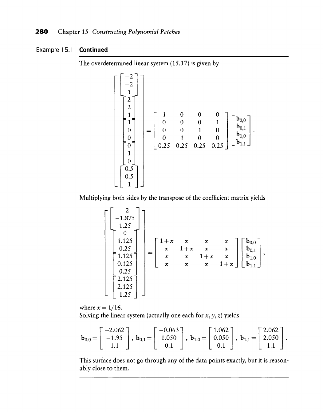
280 Chapter
15
Constructing Polynomial Patches
Example 15.1 Continued
The overdetermined linear system (15.17)
is
given
by
r
r
L L
•-2"
-2
1
[21
2
ril
0
rol
1
[oj
'0.5'
0.5
1
=
"
1
0
0
0
0.25
0
0
0
1
0.25
0
0
1
0
0.25
0
1
0
0
0.25
" bo,o
'
bo,i
bi,o
Lbi,iJ
Multiplying both sides
by the
transpose
of
the coefficient matrix yields
n
1
L
•
-2 •
-1.875
1.25
rol
1.125
L
0.25
J
[1.1251
0.125
I
0.25
J
[2.1251
2.125
L
1-25
J
1
~]
J
+ x
X
X
X
X
1
+ x
X
X
X
X
14-x
X
X
X
X
l + x_
bo,o
bo,i
bi,o
-^1,1
where
x = 1/16.
Solving
the
linear system (actually
one
each
for x,
y,
z)
yields
Vo
=
[-2.0621
-1.95
L
1-1
5 Vi =
[-0.0631
1.050
0.1
>
\o^
[1.0621
0.050
0.1
. bi^i
=
[ 2.0621
2.050
1.1
This surface does
not go
through
any of
the data points exactly,
but it is
reason-
ably close
to
them.
15.7 Finding Parameter Values 281
to solve a linear system with 16 equations in 16 unknowns. A note of caution: if
the number of data points is very large (10^ or more), then the normal equations
become ill-conditioned and the least squares problem may not be solvable.
15.7 Finding Parameter Values
In a practical setting, we would not typically be given the parameter values
u^ = i'^h ^k)- Finding good values for the u^ is not an easy problem.
But often, the data points can be projected into a plane; let us assume they
can be projected into the x,
}/-plane
for simplicity. Each p^ is projected by simply
dropping its ;^-coordinate, leaving a pair (x^, y^). We scale the (x^, y^) so that
they fit into the unit square. Then we can simply set
uj^
=
xj^
and Vk^Jk-
Another solution may be obtained by using a triangulation of the data points.
This scenario is realistic for data obtained using a laser digitizer. Assuming
that the triangulation is isomorphic to the unit square, we can construct a
triangulation in the unit square with the same connectivity as the given one
in 3D.
The following method is due to Floater
[236].
First, a convex polygon is built
in the (^, v) unit square with as many vertices as the 3D mesh has boundary
vertices. This polygon is somewhat arbitray; a circle or the boundary of the unit
square is a good candidate for forming it. In this way, we assign 2D parameters
to the 3D mesh boundary points.
Next, consider any interior point u^ of the 2D mesh with
Uj.
neighbors. We call
these neighbors u^ i,. . .,
u^ „
. For a "nice" triangulation, the following condition
should be satisfied: all interior
u^.
may be expressed as^
1 "^
We now observe that there are as many equations (15.19) as there are interior
points in the mesh. Some of these equations involve boundary points, others will
not. Thus we have a linear system for the interior u^, with as many equations as
there are interior points. It is always solvable.
2 Triangulations with this property are the result of
Laplacian
smoothing of a mesh.
282 Chapter
15
Constructing Polynomial Patches
1
5.8
Shape Equations
The solution
to a
least squares problem
may be
close
to the
data points,
yet the
control
net
might "behave badly," similar
to the
curve case.
A way to
combat
such behavior
is to
invoke shape equations. These
are
conditions that
a
"good"
control
net
v^ould satisfy.
Out of
many possibilities,
we
choose
the
following:
a
translational surface
(see 15.3) is
characterized
by the
fact that
its
twist vanishes
everywhere.
For the
control
net,
this means
.
1,1]
K;
=
0;
/ =
0,..., m
- 1, / =
0,...,
w
- 1.
When
we add
these equations
to our
overdetermined linear system (15.17),
we
will
be
less faithful
to the
data points,
but
achieve
a
better shape
of the
control
net.
In
practice,
we
would weight
the
shape equations, maybe
by a
factor
of
0.1,
just
as we did for the
curve case.
1
5.9 A
Problem with Unstructured Data
The least squares approximation problem
for
Bezier patches leads
to an
interest-
ing question: what happens
if the
number
of
data points equals
the
number
of
unknowns.^
In
this case,
we do not
have
to
use
the
normal equations;
the
problem
directly yields
a
linear system with
a
square coefficient matrix.
Although this interpolation scenario appears simpler than
the
least squares
problem,
it has a
potential
for a
serious pitfall.
Our linear system
is
given
by
Po
LPKJ
B^{UQ)BI{VO)
.B^(UK)B-^{VK)
K(^O)B:(VO)
BZ(UK)B-{VK)^
rb,
'0,0
L
'^rn,n
-•
, (15.20)
but
now we
have
K = {m
-\-
l)(n
-\-1).
The assignment
of
parameter values
(^^,
Vj)
to the
data points
p/ is
(theoreti-
cally) arbitrary. We
now
perform
a
"thought experiment."^ Take
two
data points
PI
and
py.
They have parameters
(w^,
Vj)
and
(wy,
Vj),
Now,
leaving
the
data points
untouched, start changing their parameter values.
Do
this
as
follows: find
the
circle having (w/,
Vj)
and
(wy,
Vj)
as
diameter
and
move both (w/,
Vi)
and
(wy,
Vj)
3
Or
"Gedankenexperiment"
as
coined
by
A. Einstein.
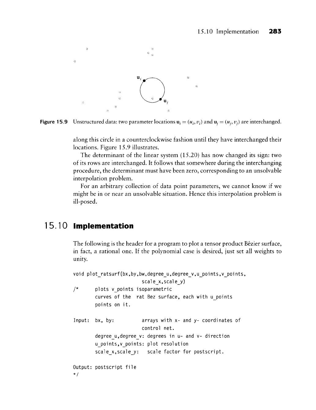
15.10 Implementation 283
Figure 15.9 Unstructured data: two parameter locations
u^
=
(w^, Vj)
and
Uy
=
(wy, Vj)
are interchanged.
along this circle in a counterclockwise fashion until they have interchanged their
locations. Figure 15.9 illustrates.
The determinant of the linear system (15.20) has now changed its sign: two
of its rows are interchanged. It follows that somewhere during the interchanging
procedure, the determinant must have been zero, corresponding to an unsolvable
interpolation problem.
For an arbitrary collection of data point parameters, we cannot know if we
might be in or near an unsolvable situation. Hence this interpolation problem is
ill-posed.
15.10 Implementation
The following is the header for a program to plot a tensor product Bezier surface,
in fact, a rational one. If the polynomial case is desired, just set all weights to
unity.
void plot_ratsurf(bx,by,bw,degree_u,degree_v,u_points,v_points,
seale_x,seale_y)
/*
plots v_points isoparametric
curves
of the rat Bez
surface, each with u_points
points
on it.
Input:
bx, by:
arrays with
x- and y-
coordinates
of
control
net.
degree_u,degree_v: degrees
in u- and v-
direction
u_points,v_points: plot resolution
seale_x,seale_y: scale factor
for
postscript.
Output: postscript file
284 Chapter 15 Constructing Polynomial Patches
Next is a routine that fits a biHnearly blended Coons patch in between four
boundary control polygons, as described in Section 15.2. The routine works on
one coordinate only, and will have to be called separately for the x-, y-, and
^-components of a control net.
void netcoons(net,rows,columns)
/* Uses bilinear Coons blending to complete a control
net of which only the four boundary polygons are used as input.
Works for one coordinate only.
Input: net: control net.
rows,
columns: dimensions of net.
Output: net: the completed net, with the old boundaries.
*
/
15.11 Problems
1 Justify that in tensor product interpolation (Section 15.4), it does not
matter if we start with the row interpolation process or with the column
interpolation process. Give computation counts for both strategies. (In
general, they are not equal!)
2 Generalize Lagrange interpolation to the tensor product case.
* 3 Generalize quintic Hermite interpolation to the tensor product case.
* 4 Suppose we want to find a parametrization {ui) for a tensor product in-
terpolant. We may parametrize all rows of data points and then form the
averages of the parametrizations thus obtained. Or we could average all
rows of data points, for example, by setting p^ = ^-
^x^
y
and we could
then parametrize the
p^.
Do we get the same result? Discuss both methods.
PI Figure 7.3 shows how Lagrange interpolation behaves badly for curves.
Write a program to exhibit this effect for tensor product patches.
Composite
Surfaces
1 ensor product Bezier patches were under development in the early 1960s; at
about the same time, people started to think about piecewise surfaces. One of the
first publications was de Boor's work on bicubic splines [136] in 1962. Almost
simultaneously, and apparently unaware of de Boor's work, J. Ferguson [231]
implemented piecewise bicubics at Boeing. His method was used extensively,
although it had the serious flaw of using only zero corner twist vectors. An
excellent account of the early industrial use of piecewise bicubics is the article by
G. Peters
[462].
16.1 Smoothness and Subdivision
Let x(w, v) and y(w, v) be two patches, defined over [w/_i, uj] x [vj, Vj^i] and
[w/, w/+i] X [vj,
^'/+i],
respectively. They are r times continuously differentiable
across their common boundary curve x(wj, v) = y(w/, v) if all w-partials up to
order r agree there:
Z
dw
•x(u, v) (16.1)
u—ui
Now suppose both patches are given in Bezier form; let the control net of
the "left" patch be
{b^y};
0<i<m,0<j<n and those of the "right" patch be
{b^y};
m<i< Im^ 0 <j <n. We can then invoke (14.13) for the cross boundary
derivative of a Bezier patch. That formula is in local coordinates. To make the
transition to global coordinates (w, v), we must invoke the chain rule:
285
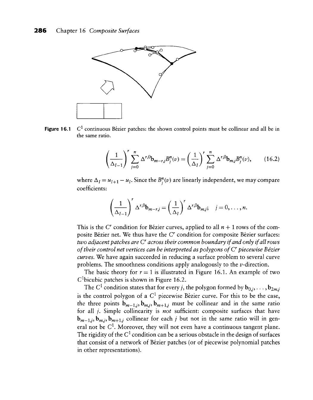
286 Chapter 16 Composite Surfaces
Figure 16.1 C^ continuous Bezier patches: the shown control points must be colHnear and all be in
the same ratio.
(xf^) E
A^'X-.^BJCt')
=
{£j i: ^'''K,iBy\ (16.2)
where Aj = wj^j
—
Wj.
Since the
B^Av)
are linearly independent, we may compare
coefficients:
This is the C^ condition for Bezier curves, applied to all « + 1 rows of the com-
posite Bezier net. We thus have the C^ condition for composite Bezier surfaces:
two adjacent patches are (J across their common boundary if and only if all rows
of their control net vertices can he interpreted as polygons ofC^ piecewise Bezier
curves. We have again succeeded in reducing a surface problem to several curve
problems. The smoothness conditions apply analogously to the t^-direction.
The basic theory for r = 1 is illustrated in Figure 16.1. An example of two
C^bicubic patches is shown in Figure 16.2.
The C^ condition states that for every;, the polygon formed by bo^y,...,
him^j
is the control polygon of a C^ piecewise Bezier curve. For this to be the case,
the three points b^_i
y,
b^y, b^_^i
y
must be collinear and in the same ratio
for all ;. Simple collinearity is not sufficient: composite surfaces that have
bm-l,/?^^,/,
bm+i,y collinear for each / but not in the same ratio will in gen-
eral not be C^. Moreover, they will not even have a continuous tangent plane.
The rigidity of the C^ condition can be a serious obstacle in the design of surfaces
that consist of a network of Bezier patches (or of piecewise polynomial patches
in other representations).
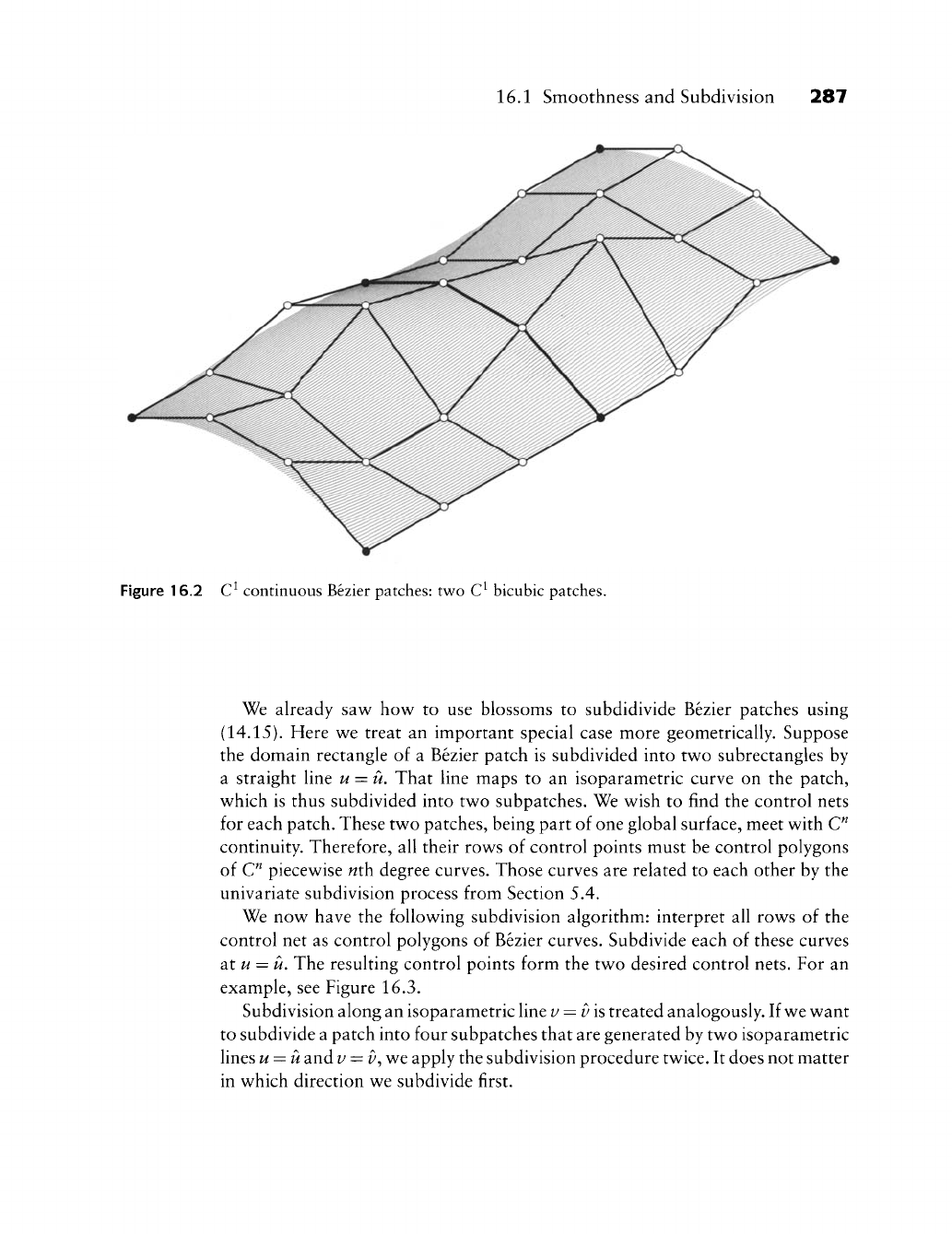
16.1 Smoothness and Subdivision 287
Figure 16.2 C^ continuous Bezier patches: two C^ bicubic patches.
We already saw how to use blossoms to subdidivide Bezier patches using
(14.15).
Here we treat an important special case more geometrically. Suppose
the domain rectangle of a Bezier patch is subdivided into two subrectangles by
a straight line u = u. That line maps to an isoparametric curve on the patch,
which is thus subdivided into two subpatches. We wish to find the control nets
for each patch. These two patches, being part of one global surface, meet with C"
continuity. Therefore, all their rows of control points must be control polygons
of C" piecewise ^th degree curves. Those curves are related to each other by the
univariate subdivision process from Section 5.4.
We now have the following subdivision algorithm: interpret all rows of the
control net as control polygons of Bezier curves. Subdivide each of these curves
2itu = u. The resulting control points form the two desired control nets. For an
example, see Figure 16.3.
Subdivision along an isoparametric line v = v\s treated analogously. If we want
to subdivide a patch into four subpatches that are generated by two isoparametric
lines u = u and
i^
=
z),
we apply the subdivision procedure twice. It does not matter
in which direction we subdivide first.
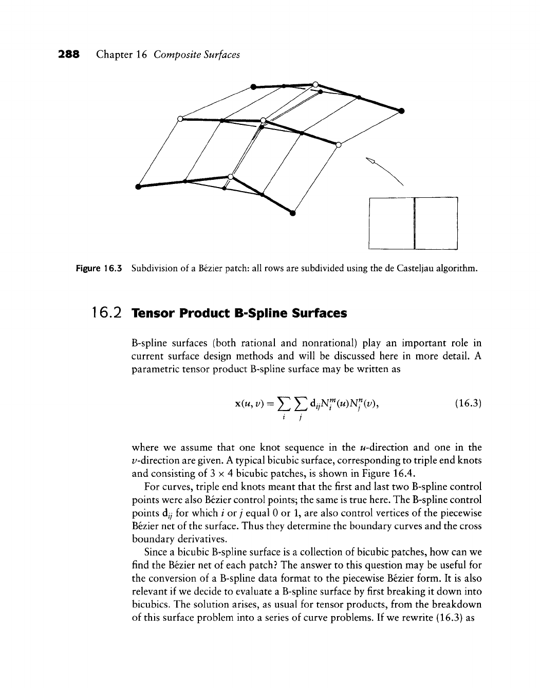
288 Chapter 16 Composite Surfaces
Figure 16.3 Subdivision of a Bezier patch: all rows are subdivided using the de Casteljau algorithm.
1
6.2 Tensor Product B-Spline Surfaces
B-spline surfaces (both rational and nonrational) play an important role in
current surface design methods and will be discussed here in more detail. A
parametric tensor product B-spline surface may be written as
x(i«,
v)
= Y,Y. di,Nf (M)N«(i;), (16.3)
where we assume that one knot sequence in the w-direction and one in the
^/'direction are given. A typical bicubic surface, corresponding to triple end knots
and consisting of 3 x 4 bicubic patches, is shown in Figure 16.4.
For curves, triple end knots meant that the first and last two B-spline control
points were also Bezier control points; the same is true here. The B-spline control
points dij for which / or / equal 0 or 1, are also control vertices of the piecewise
Bezier net of the surface. Thus they determine the boundary curves and the cross
boundary derivatives.
Since a bicubic B-spline surface is a collection of bicubic patches, how can we
find the Bezier net of each patch? The answer to this question may be useful for
the conversion of a B-spline data format to the piecewise Bezier form. It is also
relevant if we decide to evaluate a B-spline surface by first breaking it down into
bicubics. The solution arises, as usual for tensor products, from the breakdown
of this surface problem into a series of curve problems. If we rewrite (16.3) as
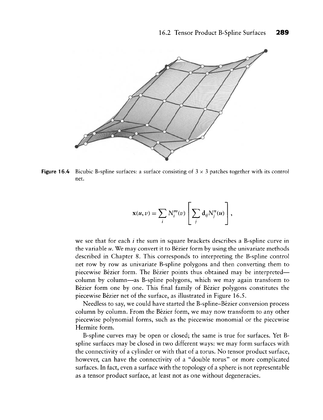
16.2 Tensor Product B-Spline Surfaces 289
Figure 16.4 Bicubic B-spline surfaces: a surface consisting of 3 x 3 patches together with its control
net.
x(u,v) =
Y,NT(^^
EW(")
we see that for each i the sum in square brackets describes a B-spHne curve in
the variable u. We may convert it to Bezier form by using the univariate methods
described in Chapter 8. This corresponds to interpreting the B-spline control
net rov^ by rov^ as univariate B-spline polygons and then converting them to
piecev^ise Bezier form. The Bezier points thus obtained may be interpreted—
column by column—as B-spline polygons, v^hich we may again transform to
Bezier form one by one. This final family of Bezier polygons constitutes the
piecewise Bezier net of the surface, as illustrated in Figure 16.5.
Needless to say, we could have started the B-spline-Bezier conversion process
column by column. From the Bezier form, we may now transform to any other
piecewise polynomial forms, such as the piecewise monomial or the piecewise
Hermite form.
B-spline curves may be open or closed; the same is true for surfaces. Yet B-
spline surfaces may be closed in two different ways: we may form surfaces with
the connectivity of a cylinder or with that of a torus. No tensor product surface,
however, can have the connectivity of a "double torus" or more complicated
surfaces. In fact, even a surface with the topology of a sphere is not representable
as a tensor product surface, at least not as one without degeneracies.
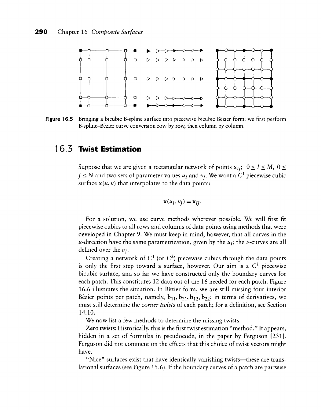
290 Chapter 16 Composite Surfaces
0—g
n—rt
0 0—0
Figure 16.5 Bringing a bicubic B-spline surface into piecewise bicubic Bezier form: we first perform
B-spline-Bezier curve conversion row by row, then column by column.
1
6.5 IWist Estimation
Suppose that we are given a rectangular network of points x/y; 0 < I < M, 0 <
J <N and two sets of parameter values uj and Vj, We want a C^ piecewise cubic
surface x(w, v) that interpolates to the data points:
x(Ui, Vj) = Xjj.
For a solution, we use curve methods wherever possible. We will first fit
piecewise cubics to all rows and columns of data points using methods that were
developed in Chapter 9. We must keep in mind, however, that all curves in the
^/-direction have the same parametrization, given by the
Uj;
the i/-curves are all
defined over the Vj.
Creating a network of C^ (or C^) piecewise cubics through the data points
is only the first step toward a surface, however. Our aim is a C^ piecewise
bicubic surface, and so far we have constructed only the boundary curves for
each patch. This constitutes 12 data out of the 16 needed for each patch. Figure
16.6 illustrates the situation. In Bezier form, we are still missing four interior
Bezier points per patch, namely, b^, b2i, bi25b22; in terms of derivatives, we
must still determine the corner twists of each patch; for a definition, see Section
14.10.
We now list a few methods to determine the missing twists.
Zero twists: Historically, this is the first twist estimation "method." It appears,
hidden in a set of formulas in pseudocode, in the paper by Ferguson
[231].
Ferguson did not comment on the effects that this choice of twist vectors might
have.
"Nice"
surfaces exist that have identically vanishing twists—these are trans-
lational surfaces (see Figure 15.6). If the boundary curves of a patch are pairwise
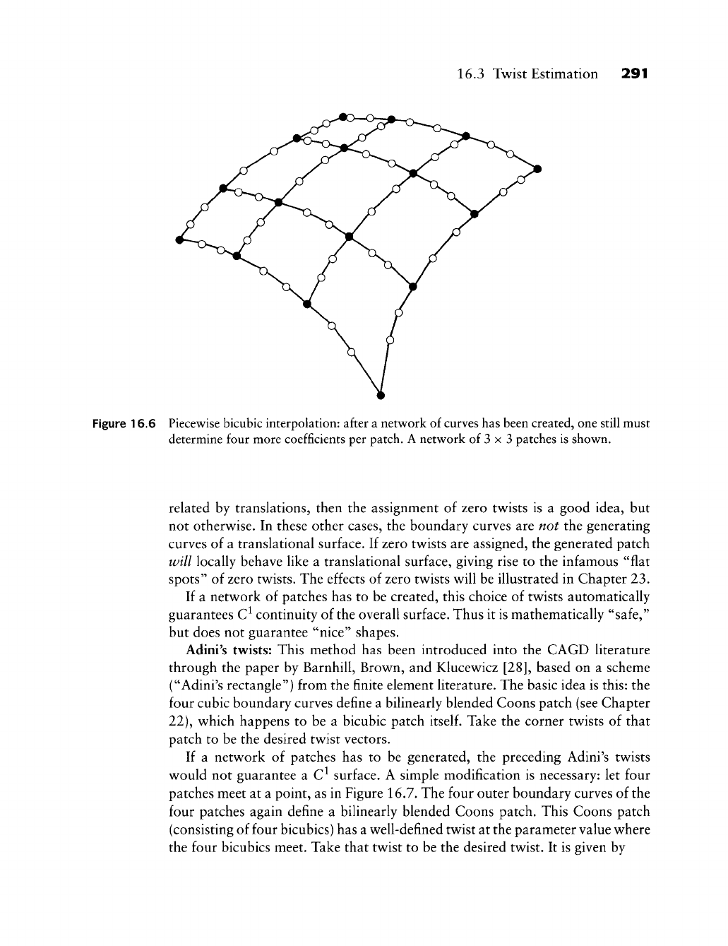
16.3 Twist Estimation 291
Figure 16.6 Piecewise bicubic interpolation: after a network of curves has been created, one still must
determine four more coefficients per patch. A network of 3 x 3 patches is shown.
related by translations, then the assignment of zero twists is a good idea, but
not otherwise. In these other cases, the boundary curves are not the generating
curves of a translational surface. If zero twists are assigned, the generated patch
will locally behave like a translational surface, giving rise to the infamous "flat
spots"
of zero twists. The effects of zero twists will be illustrated in Chapter 23.
If a network of patches has to be created, this choice of twists automatically
guarantees C^ continuity of the overall surface. Thus it is mathematically "safe,"
but does not guarantee "nice" shapes.
Adini's twists: This method has been introduced into the CAGD literature
through the paper by Barnhill, Brown, and Klucewicz [28], based on a scheme
("Adini's rectangle") from the finite element literature. The basic idea is this: the
four cubic boundary curves define a bilinearly blended Coons patch (see Chapter
22),
which happens to be a bicubic patch
itself.
Take the corner twists of that
patch to be the desired twist vectors.
If a network of patches has to be generated, the preceding Adini's twists
would not guarantee a C^ surface. A simple modification is necessary: let four
patches meet at a point, as in Figure 16.7. The four outer boundary curves of the
four patches again define a bilinearly blended Coons patch. This Coons patch
(consisting of four bicubics) has a well-defined twist at the parameter value where
the four bicubics meet. Take that twist to be the desired twist. It is given by
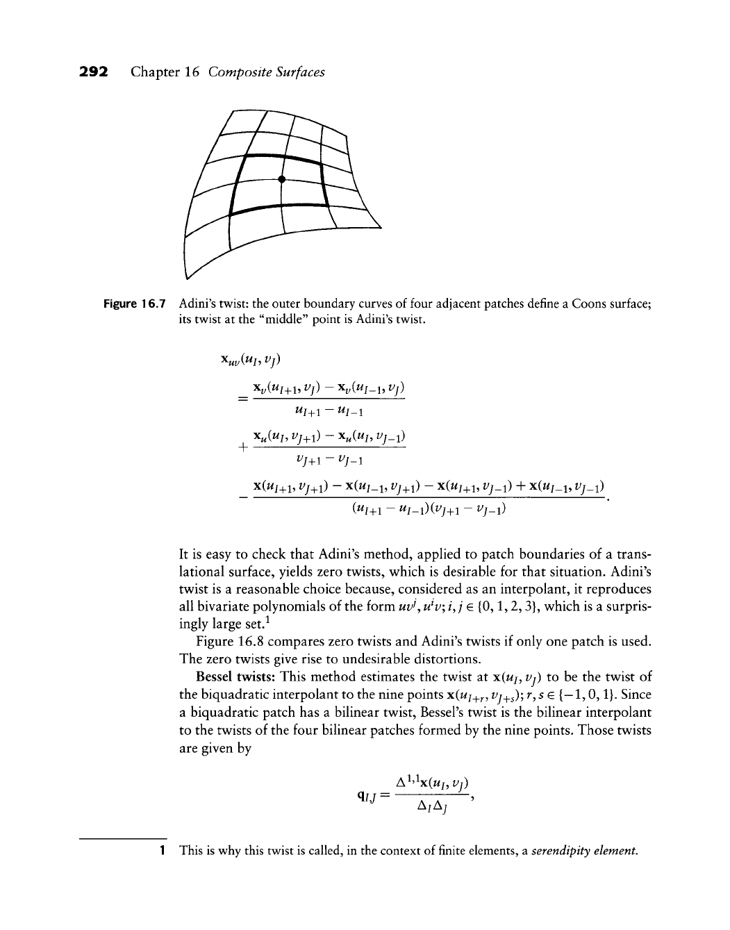
292 Chapter 16 Composite Surfaces
Figure 16.7 Adini's twist: the outer boundary curves of four adjacent patches define a Coons surface;
its twist at the "middle" point is Adini's twist.
+
Uj_^l
- Uj_i
X(^j^l, Vj^l) - x{Uj_i, Vj^i) - XJUj^i, Vj_i) + X(Uj_i, Vj_i)
It is easy to check that Adini's method, apphed to patch boundaries of a trans-
lational surface, yields zero twists, which is desirable for that situation. Adini's
twist is a reasonable choice because, considered as an interpolant, it reproduces
all bivariate polynomials of the form uv^,
u^v;
ij e
{0,1,2,3},
which is a surpris-
ingly large set.^
Figure 16.8 compares zero twists and Adini's twists if only one patch is used.
The zero twists give rise to undesirable distortions.
Bessel twists: This method estimates the twist at x(wj, Vj) to be the twist of
the biquadratic interpolant to the nine points
x(wj_^^,
^'^+5);
r, s € {—1,0,1}. Since
a biquadratic patch has a bilinear twist, Bessel's twist is the bilinear interpolant
to the twists of the four bilinear patches formed by the nine points. Those twists
are given by
q/j =
A^'^x(ui,Vj)
A/A;
1 This is why this twist is called, in the context of finite elements, a
serendipity
element.
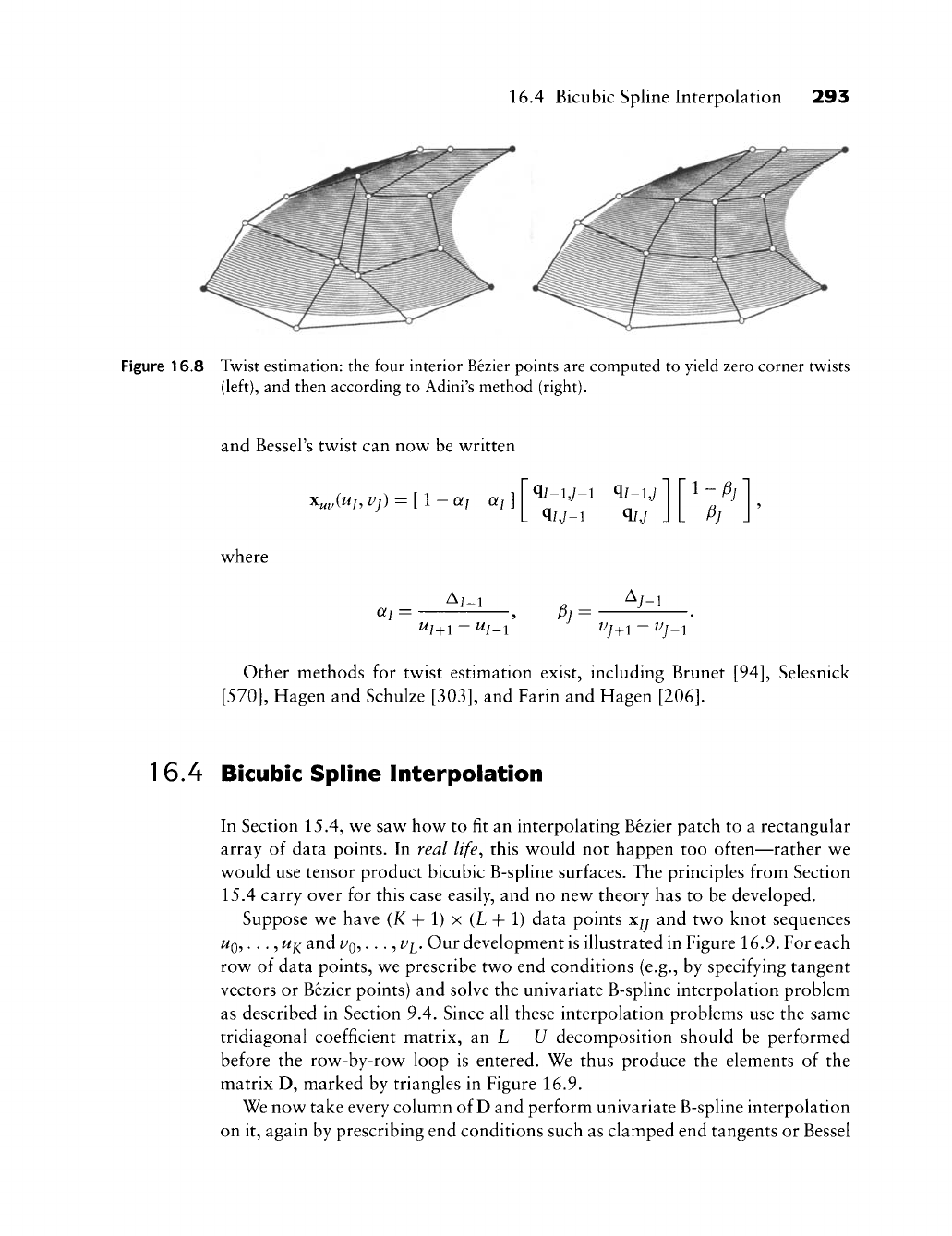
16.4 Bicubic Spline Interpolation 293
Figure 16.8 Twist estimation: the four interior Bezier points are computed to yield zero corner twists
(left),
and then according to Adini's method (right).
and Bessel's twist can now be written
^uvi^h vj) = [l-ai aj]
where
Q/-i,/-i
Q/-1,/
q/,/-i
q/j
ai = ^i-i
Uj_^l - Ui_i Pj = V-i
^/+i ~ ^/-l
Other methods for twist estimation exist, including Brunet [94], Selesnick
[570],
Hagen and Schulze
[303],
and Farin and Hagen
[206].
1
6.4 Bicubic Spline Interpolation
In Section 15.4, we saw how to fit an interpolating Bezier patch to a rectangular
array of data points. In real life^ this would not happen too often—rather we
would use tensor product bicubic B-spline surfaces. The principles from Section
15.4 carry over for this case easily, and no new theory has to be developed.
Suppose we have (K + 1) x (L + 1) data points X/y and two knot sequences
WQ,
.
. .,
/^l^
and
i/Q,.
. ., Vi. Our development is illustrated in Figure 16.9. For each
row of data points, we prescribe two end conditions (e.g., by specifying tangent
vectors or Bezier points) and solve the univariate B-spline interpolation problem
as described in Section 9.4. Since all these interpolation problems use the same
tridiagonal coefficient matrix, an L
—
17 decomposition should be performed
before the row-by-row loop is entered. We thus produce the elements of the
matrix D, marked by triangles in Figure 16.9.
We now take every column of D and perform univariate B-spline interpolation
on it, again by prescribing end conditions such as clamped end tangents or Bessel
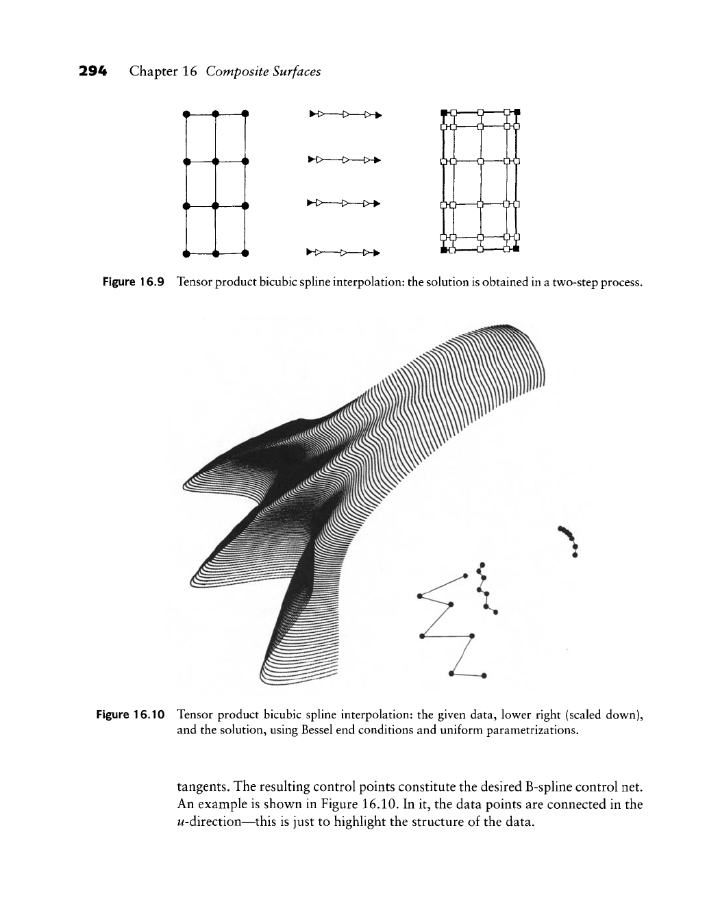
294 Chapter 16 Composite Surfaces
T—T—T
T—T—7
T—T—T
i—4—i
Q
D
Figure 16.9 Tensor product bicubic spline interpolation: the solution
is
obtained in a two-step process.
^
Figure 16.10 Tensor product bicubic spline interpolation: the given data, lower right (scaled down),
and the solution, using Bessel end conditions and uniform parametrizations.
tangents. The resulting control points constitute the desired B-spline control net.
An example is shown in Figure 16.10. In it, the data points are connected in the
w-direction—this is just to highlight the structure of the data.

16.5 Finding Knot Sequences 295
The final B-spline control net has two more rows and columns than X.^ This is
due to the end conditions; to resolve the apparent discrepancy, we may think of
X as having two additional rows and columns that constitute the end condition
data. This concept is implemented in the attached code.
Although mathematically equivalent, the two processes—first row by row,
then column by column; or first column by column, then row by row—do not
yield the same computation count if K
7^
L.
1
6.5 Finding Knot Sequences
Although tensor product spline interpolation is very elegant, its use is limited to
cases where the data points possess a rectangular structure. When the data points
deviate from a nice grid, the problem of finding an appropriate parametrization
is not easy; it may not have a solution at all. In the curve case (Section 9.6),
we were able to devise several methods that assigned parameter values to the
given data points. So why not take those methods and apply them to the tensor
product case in much the same way in which we generalized curve methods to
their tensor product counterparts.^ The problem is that we have to produce one
set of parameter values for all isoparametric curves in the ^-direction; the same
holds for the z/-direction.
We may endow each isoparametric curve (in the ^-direction, say) with a
parametrization from Section 9.6. To arrive at one parametrization for all of
them, we may then carry out some averaging process. Such an approach will
produce acceptable results only if all of our isoparametric curves have the same
shape characteristics, that is, if they essentially yield the same parametrization.
This is, however, not always the case, as Figures
16.11,
16.12, and 16.13
illustrate.^
Are there ways out of the dilemma.^ Not if we have unevenly distributed data
and insist on bicubic spline interpolation. If we are willing to go to higher degrees
and to replace C^ or C^ continuity by G^ continuity (see Chapter 20), then several
methods exist; see the literature cited in that chapter.
2 This is inherited from the curve
case:
there one gets L + 2 control points for
L
data points.
3 Another interesting phenomenon may be observed here: note how the first and the third
of this set of surfaces have varying densities in their plots. The reason is that each cubic
isoparametric curve was plotted in 90 increments on a pen plotter. With very unequal
parameter spacing, this generates abruptly varying spacing on the curves.
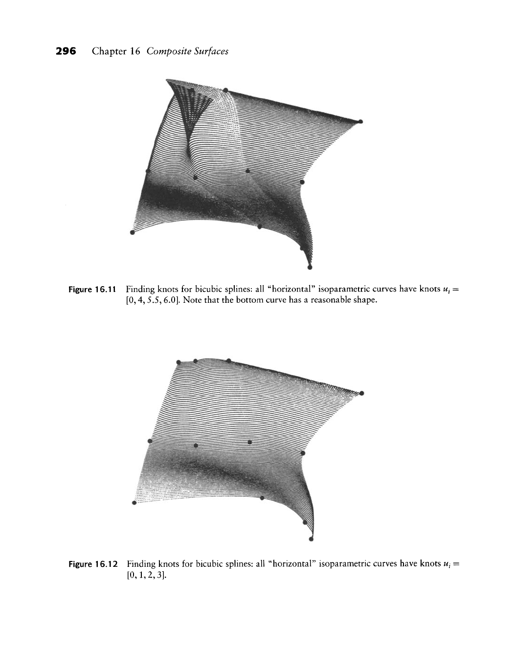
296 Chapter 16 Composite Surfaces
Figure 16.11 Finding knots for bicubic splines: all "horizontal" isoparametric curves have knots
Ui •
[0,4,
S.S^ 6.0]. Note that the bottom curve has a reasonable shape.
Figure 16.12 Finding knots for bicubic sphnes: all "horizontal" isoparametric curves have knots
Ui ••
[0,1,2,3].
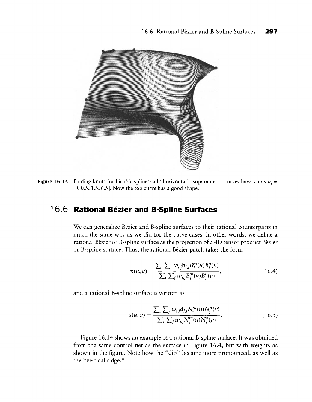
16.6 Rational Bezier and B-Spline Surfaces 297
Figure
16.1
3 Finding knots for bicubic splines: all "horizontal" isoparametric curves have knots ui =
[0,
0.5,1.5,
6.5].
Novv^
the top curve has a good shape.
16.6 Rational Bezier and B-Spiine Surfaces
We can generalize Bezier and B-spline surfaces to their rational counterparts in
much the same way as we did for the curve cases. In other words, we define a
rational Bezier or B-spline surface as the projection of a 4D tensor product Bezier
or B-spline surface. Thus, the rational Bezier patch takes the form
x(w, v) = (16.4)
and a rational B-spline surface is written as
E,E;^,,A,N,"'(^)N;(t/)
E,E;^,vNr(«)N;(i^) •
s(w, v) = (16.5)
Figure 16.14 shows an example of a rational B-spline surface. It was obtained
from the same control net as the surface in Figure 16.4, but with weights as
shown in the figure. Note how the "dip" became more pronounced, as well as
the "vertical ridge."
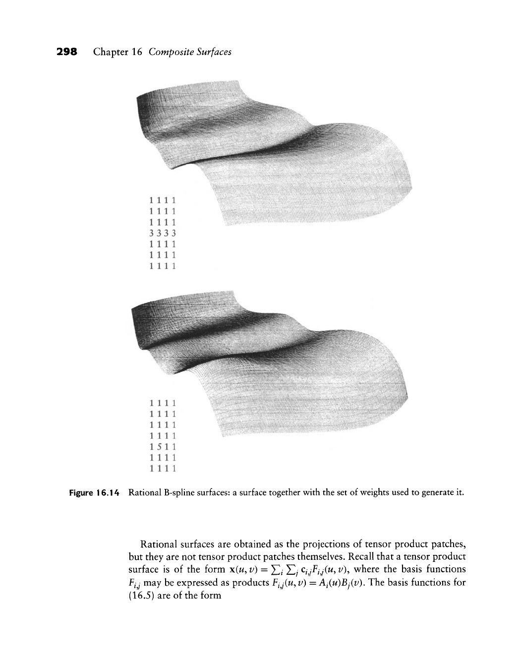
298 Chapter 16 Composite Surfaces
^^Mi'
'^^^^^^
1111
1111
1111
3333
1111
1111
1111
x\\\\\\\
V
1111
1111
1111
1111
15 11
1111
1111
Figure 16.14 Rational B-spline surfaces: a surface together with the set of weights used to generate it.
Rational surfaces are obtained as the projections of tensor product patches,
but they are not tensor product patches themselves. Recall that a tensor product
surface is of the form x(w, v) = ^- ^- c^yF^y(w, v), where the basis functions
Fjj may be expressed as products Fij(u, v) = Aj(u)Bj(v), The basis functions for
(16.5) are of the form
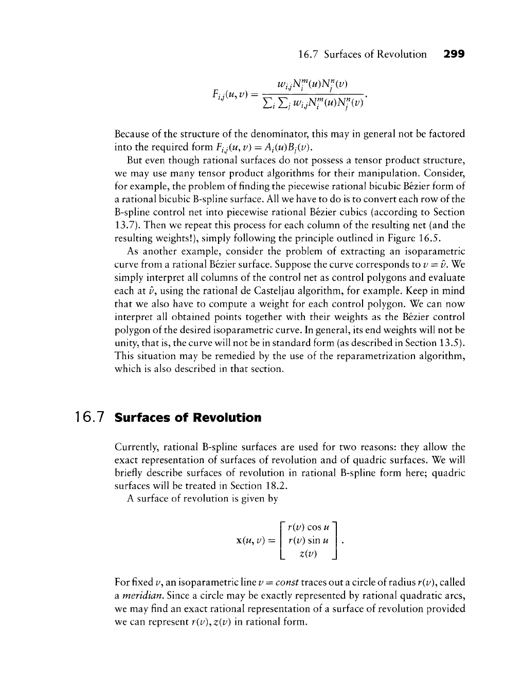
F,^j(u,v) =
16.7 Surfaces of Revolution 299
E.J:iW,,iN^(u)NJiv)
Because of the structure of the denominator, this may in general not be factored
into the required form Fjj(u^ v) = Ai(u)Bj(v).
But even though rational surfaces do not possess a tensor product structure,
we may use many tensor product algorithms for their manipulation. Consider,
for example, the problem of finding the piecewise rational bicubic Bezier form of
a rational bicubic B-spline surface. All we have to do is to convert each row of the
B-spline control net into piecewise rational Bezier cubics (according to Section
13.7).
Then we repeat this process for each column of the resulting net (and the
resulting weights!), simply following the principle outlined in Figure 16.5.
As another example, consider the problem of extracting an isoparametric
curve from a rational Bezier surface. Suppose the curve corresponds to
z/
= f). We
simply interpret all columns of the control net as control polygons and evaluate
each at v, using the rational de Casteljau algorithm, for example. Keep in mind
that we also have to compute a weight for each control polygon. We can now
interpret all obtained points together with their weights as the Bezier control
polygon of the desired isoparametric curve. In general, its end weights will not be
unity, that is, the curve will not be in standard form (as described in Section 13.5).
This situation may be remedied by the use of the reparametrization algorithm,
which is also described in that section.
1
6.7 Surfaces of Revolution
Currently, rational B-spline surfaces are used for two reasons: they allow the
exact representation of surfaces of revolution and of quadric surfaces. We will
briefly describe surfaces of revolution in rational B-spline form here; quadric
surfaces will be treated in Section 18.2.
A surface of revolution is given by
x(^,
v) =
r(v) cos u
r(v) sin u
z(v)
For fixed v, an isoparametric fine v = const traces out a circle of radius r(v), called
a meridian. Since a circle may be exactly represented by rational quadratic arcs,
we may find an exact rational representation of a surface of revolution provided
we can represent r{v)^ z{v) in rational form.
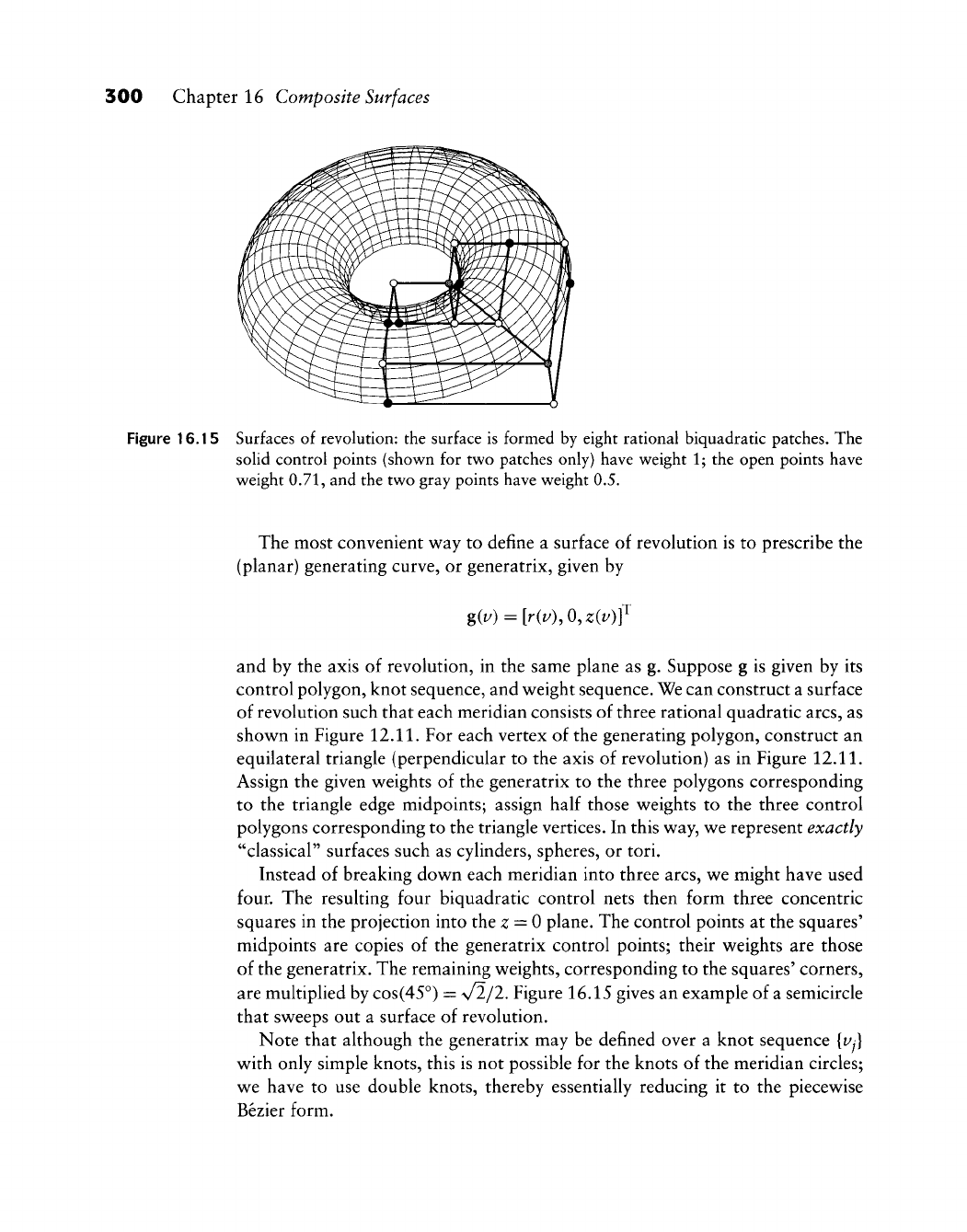
300 Chapter 16 Composite Surfaces
Figure 16.15 Surfaces of revolution: the surface is formed by eight rational biquadratic patches. The
solid control points (shown for two patches only) have weight 1; the open points have
weight 0.71, and the two gray points have weight 0.5.
The most convenient way to define a surface of revolution is to prescribe the
(planar) generating curve, or generatrix, given by
giv) = [riv\0,ziv)f
and by the axis of revolution, in the same plane as g. Suppose g is given by its
control polygon, knot sequence, and weight sequence. We can construct a surface
of revolution such that each meridian consists of three rational quadratic arcs, as
shown in Figure
12.11.
For each vertex of the generating polygon, construct an
equilateral triangle (perpendicular to the axis of revolution) as in Figure
12.11.
Assign the given weights of the generatrix to the three polygons corresponding
to the triangle edge midpoints; assign half those weights to the three control
polygons corresponding to the triangle vertices. In this way, we represent exactly
"classical" surfaces such as cylinders, spheres, or tori.
Instead of breaking down each meridian into three arcs, we might have used
four. The resulting four biquadratic control nets then form three concentric
squares in the projection into the z = 0 plane. The control points at the squares'
midpoints are copies of the generatrix control points; their weights are those
of the generatrix. The remaining weights, corresponding to the squares' corners,
are multiplied by cos(45°) =
%/2/2.
Fi gure 16.15 gives an example of a semicircle
that sweeps out a surface of revolution.
Note that although the generatrix may be defined over a knot sequence {Vj}
with only simple knots, this is not possible for the knots of the meridian circles;
we have to use double knots, thereby essentially reducing it to the piecewise
Bezier form.
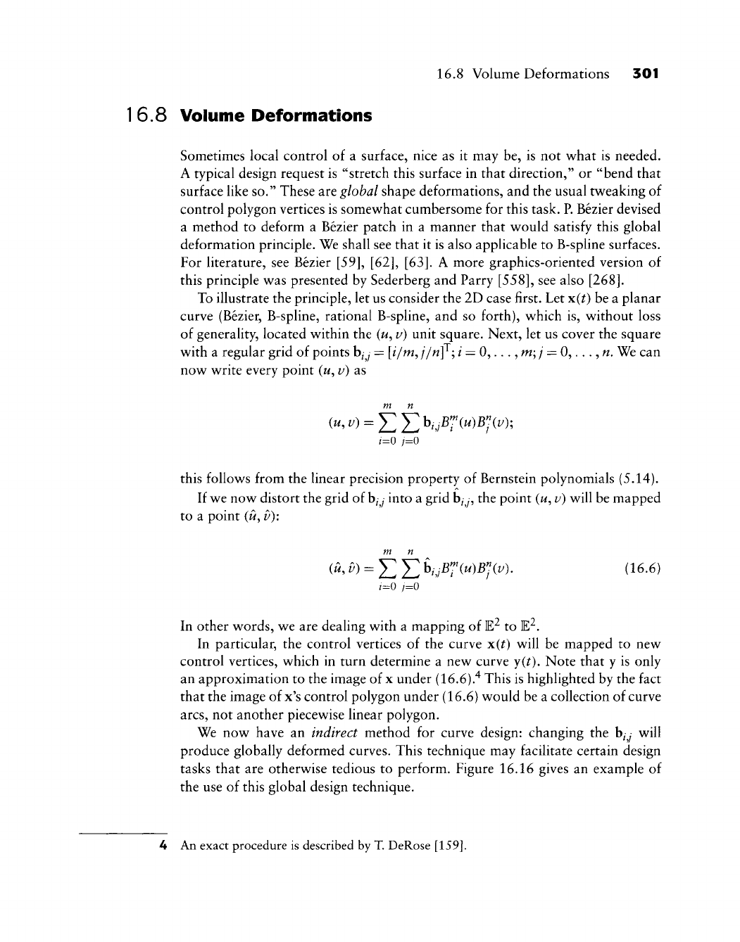
16.8 Volume Deformations 301
1
6.8 Volume Deformations
Sometimes local control of a surface, nice as it may be, is not what is needed.
A typical design request is "stretch this surface in that direction," or "bend that
surface like so." These are global shape deformations, and the usual tweaking of
control polygon vertices is somewhat cumbersome for this task. P. Bezier devised
a method to deform a Bezier patch in a manner that would satisfy this global
deformation principle. We shall see that it is also applicable to B-spline surfaces.
For literature, see Bezier [59], [62], [63]. A more graphics-oriented version of
this principle was presented by Sederberg and Parry
[558],
see also
[268].
To illustrate the principle, let us consider the 2D case first. Let x(t) be a planar
curve (Bezier, B-spline, rational B-spline, and so forth), which is, without loss
of generality, located within the (w, v) unit square. Next, let us cover the square
with a regular grid of points hjj = [i/m^
j/^V'-,
/ = 0,.. ., m; / = 0,...,
w.
We can
now write every point (w, v) as
m n
/=0 j=0
this follows from the linear precision property of Bernstein polynomials (5.14).
If we now distort the grid of b/y into a grid
b^
y,
the point
(w,
v) will be mapped
to a point
(u^v):
m n
In other words, we are dealing with a mapping of E^ to E^.
In particular, the control vertices of the curve x(^) will be mapped to new
control vertices, which in turn determine a new curve y(^). Note that y is only
an approximation to the image of x under (16.6).^ This is highlighted by the fact
that the image of x's control polygon under (16.6) would be a collection of curve
arcs,
not another piecewise linear polygon.
We now have an indirect method for curve design: changing the b/y will
produce globally deformed curves. This technique may facilitate certain design
tasks that are otherwise tedious to perform. Figure 16.16 gives an example of
the use of this global design technique.
4 An exact procedure is described by T. DeRose
[159],
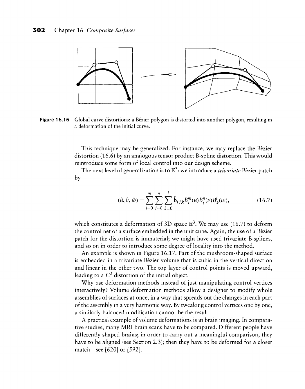
302 Chapter 16 Composite Surfaces
Figure 16.16 Global curve distortions: a Bezier polygon is distorted into another polygon, resulting in
a deformation of the initial curve.
This technique may be generalized. For instance, we may replace the Bezier
distortion (16.6) by an analogous tensor product B-spline distortion. This would
reintroduce some form of local control into our design scheme.
The next level of generalization is to E^: we introduce a trivariate Bezier patch
by
,=0 7=0 k=0
(16.7)
which constitutes a deformation of 3D space E-^. We may use (16.7) to deform
the control net of a surface embedded in the unit cube. Again, the use of a Bezier
patch for the distortion is immaterial; we might have used trivariate B-splines,
and so on in order to introduce some degree of locality into the method.
An example is shown in Figure 16.17. Part of the mushroom-shaped surface
is embedded in a trivariate Bezier volume that is cubic in the vertical direction
and linear in the other two. The top layer of control points is moved upward,
leading to a C^ distortion of the initial object.
Why use deformation methods instead of just manipulating control vertices
interactively? Volume deformation methods allow a designer to modify whole
assemblies of surfaces at once, in a way that spreads out the changes in each part
of the assembly in a very harmonic way. By tweaking control vertices one by one,
a similarly balanced modification cannot be the result.
A practical example of volume deformations is in brain imaging. In compara-
tive studies, many MRI brain scans have to be compared. Different people have
differently shaped brains; in order to carry out a meaningful comparison, they
have to be aligned (see Section 2.3); then they have to be deformed for a closer
match—see [620] or
[592].
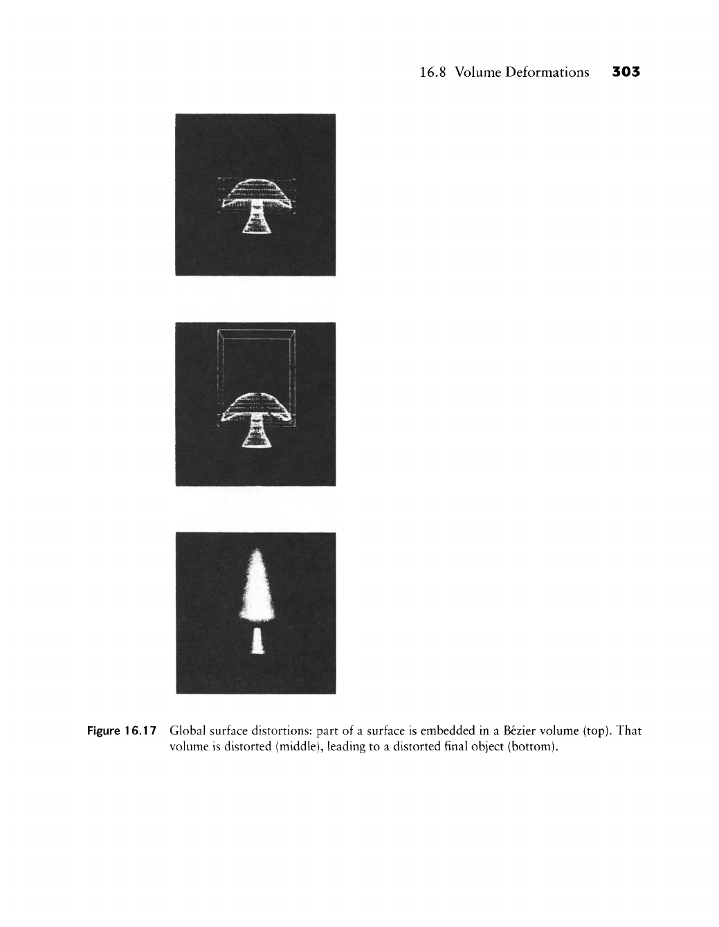
16.8 Volume Deformations 303
Figure 16.17 Global surface distortions: part of a surface is embedded in a Bezier volume (top). That
volume is distorted (middle), leading to a distorted final object (bottom).
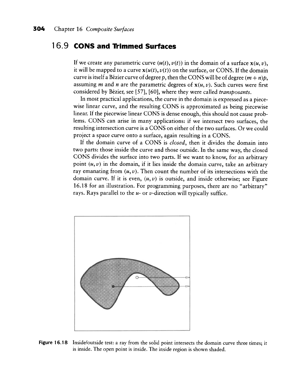
304 Chapter 16 Composite Surfaces
16.9 CONS and Trimmed Surfaces
If we create any parametric curve
{u{t)^
v{t)) in the domain of a surface x(w, i/),
it will be mapped to a curve x(u(t), v(t)) on the surface, or CONS. If the domain
curve is itself
a
Bezier curve of degree p, then the CONS will be of degree (m + n)p,
assuming m and n are the parametric degrees of x(w, v). Such curves were first
considered by Bezier, see [57], [60], where they were called transposants.
In most practical applications, the curve in the domain is expressed as a piece-
wise linear curve, and the resulting CONS is approximated as being piecewise
linear. If the piecewise linear CONS is dense enough, this should not cause prob-
lems.
CONS can arise in many applications: if we intersect two surfaces, the
resulting intersection curve is a CONS on either of the two surfaces. Or we could
project a space curve onto a surface, again resulting in a CONS.
If the domain curve of a CONS is
closed,
then it divides the domain into
two parts: those inside the curve and those outside. In the same way, the closed
CONS divides the surface into two parts. If we want to know, for an arbitrary
point (u, v) in the domain, if it lies inside the domain curve, take an arbitrary
ray emanating from (w, v). Then count the number of its intersections with the
domain curve. If it is even, («, v) is outside, and inside otherwise; see Figure
16.18 for an illustration. For programming purposes, there are no "arbitrary"
rays.
Rays parallel to the u- or i/-direction will typically suffice.
Figure 16.18 Inside/outside test: a ray from the solid point intersects the domain curve three times; it
is inside. The open point is inside. The inside region is shown shaded.
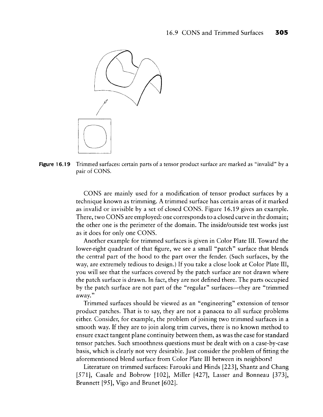
16.9 CONS and Trimmed Surfaces 305
Figure 16.19 Trimmed surfaces: certain parts of a tensor product surface are marked as "invalid" by a
pair of CONS.
CONS are mainly used for a modification of tensor product surfaces by a
technique known as trimming. A trimmed surface has certain areas of it marked
as invalid or invisible by a set of closed CONS. Figure 16.19 gives an example.
There, two CONS are employed: one corresponds to a closed curve in the domain;
the other one is the perimeter of the domain. The inside/outside test works just
as it does for only one CONS.
Another example for trimmed surfaces is given in Color Plate III. Toward the
lower-right quadrant of that figure, we see a small "patch" surface that blends
the central part of the hood to the part over the fender. (Such surfaces, by the
way, are extremely tedious to design.) If you take a close look at Color Plate III,
you will see that the surfaces covered by the patch surface are not drawn where
the patch surface is drawn. In fact, they are not defined there. The parts occupied
by the patch surface are not part of the "regular" surfaces—they are "trimmed
away."
Trimmed surfaces should be viewed as an "engineering" extension of tensor
product patches. That is to say, they are not a panacea to all surface problems
either. Consider, for example, the problem of joining two trimmed surfaces in a
smooth way. If they are to join along trim curves, there is no known method to
ensure exact tangent plane continuity between them, as was the case for standard
tensor patches. Such smoothness questions must be dealt with on a case-by-case
basis,
which is clearly not very desirable. Just consider the problem of fitting the
aforementioned blend surface from Color Plate III between its neighbors!
Literature on trimmed surfaces: Farouki and Hinds
[223],
Shantz and Chang
[571],
Casale and Bobrow
[102],
Miller
[427],
Lasser and Bonneau
[373],
Brunnett [95], Vigo and Brunet
[602].

306 Chapter 16 Composite Surfaces
16.10 Implementation
The routines in this section are written for rational surfaces. By setting all weights
equal to one, the standard piecewise polynomial case is recovered.
The routine that converts a rational bicubic B-spline control net into the
piecewise bicubic Bezier form:
void ratbspl_to_bez_surf(bspl_x,bspl_y,bspl_w,lu,lv,knot_u,
knot_v,bez_x,bez_y,bez_w,dux_x,aux_y,aux_w)
/*
Converts B-spline control
net
into piecewise
Bezier control
net
(bicubic).
Input: bspl_x,bspl_y: B-spline control
net
(one coordinate only)
bspl_w: B-spline weights
lu,lv: no.
of
intervals
in u-
and
v-directi on
knot_u, knot_v: knot vectors
in u-
and
v-directi on
Output: bez_x,bez_y: piecewise bicubic Bezier net.
bez_w: Bezier weights.
Work space:aux_x,aux_y,aux_w: needed
to
store intermediate results.
Remark:
The
piecewise Bezier
net
only stores each control point once,
i.e., neighboring patches share
the
same boundary.
Knots
are
simple (but,
in
the
language
of
Chapter 10,
the
boundary knots have multiplicity
three).
V
Once the piecewise rational Bezier representation of a bicubic spline surface
is achieved, the following routine plots the whole surface:
void piot_ratbez_surfaces(bez_x,bez_y,bez_w,1u,1v,u_points,v_points,
seale_x,scale_y,val ue)
/* Plots piecewise cubic surface,
i.e.,
generates postscript output
Input: bez_x, bez_y: control nets
lu,lv:
no. of
segments
in u- and v-
direction
u_points,v_points:
per
patch: v_points many
isoparametric curves with
u_points
points
on
each
value:
minmax
box of all
control nets,
seale_x,seale_y: scale factors
for
postscript
V
Tensor product spline interpolation (bicubic) is carried out by the following
routine. It uses Bessel end conditions.
16.10 Implementation 307
void spline_surf_int(data_x,data_y,bspl__x,bspl_y,lu,lv,knot_u,
knot_v,aux_x,aux_y)
/*
Interpolates
to an
array
of
size [0,lu+2]x[0,lv+2]
Input: data_x, data_y: data array (one coordinate only)
lu,lv: no.
of
intervals
in u- and
v-directi on
knot_u, knot_v: knot vectors
in u- and
v-directi on
Output: bspl_x,bspl_y: B-spline control
net.
Work space: aux_x, aux_y.
Remark:
On
input,
it is
assumed that data_x
and
data_y have rows
1
and
lu+1
and
columns
1 and
lv+1 empty, i.e., they
are
not filled with data points. Example
for
lu=4,
lv=7:
xOxxxxxxOx
0000000000
xOxxxxxxOx x=data coordinate,
xOxxxxxxOx 0=unused input array
xOxxxxxxOx element.
0000000000
The O's
will
be
filled with
xOxxxxxxOx 'tangent Bezier points'.
This approach makes
it
easy
to
feed
in
clamped
end
conditions
if
so
desired:
put in
values
in the O's and
delete
the
calls
to bessel_ends below.
V
Next is the header of a program that plots the control net of a Bezier surface
or of a composite surface.
void psplot_net(lu,lv,bx,by,step_u,step_v,seale_x,seale_y,value)
/* plots control net into postscript-file.
Input: lu,lv: dimensions of net
bXjby: net vertices
step_u,step_v: subnet sizes (e.g. both=3 for pw bicubic net)
scale_x,scale_y:scale factors for ps
value:
window size in world coords
Output: written into postscript file
V
308 Chapter 16 Composite Surfaces
16.11 Problems
1 Generalize the B-spHne knot insertion algorithm to the tensor product case.
* 2 Show that if two polynomial surfaces are across a common boundary,
then they are also twist continuous across that boundary.
* 3 Suppose we want to find a parametrization [uj] for a tensor product in-
terpolant. We may parametrize all rows of data points and then form the
averages of the parametrizations thus obtained. Or we could average all
rows of data points, for example, by setting p^ = J^j n^ij ^^^ ^^ could
then parametrize the
p^.
Do we get the same result? Discuss both methods.
P1 Embed your Bezier surface from Problem
P3
of Chapter 14 in a tricubic grid,
similar to Figure 16.17. Then "stretch" your surface, leaving the front part
unchanged.
P2 Model a Klein bottle as a closed bicubic B-spline surface. Literature:
[323],
[170].
If you have the graphics capabilities, display your result as a translu-
cent surface.
P3 Generate an array of points on a sphere. For latitudes, take 0/ = 0,10,20,
..., 90 degrees. For longitudes, take
i/zj
= 45,50,55,..., 75 degrees. Pass
several tensor product interpolants through the data and compare their
deviations from the true sphere. For the bicubic C^ spline interpolant, also
compare uniform and chord length parametrizations.
Bezier Triangles
When de Casteljau invented Bezier curves in 1959, he realized the need for the
extension of the curve ideas to surfaces. Interestingly enough, the first surface
type that he considered was what we now call Bezier triangles. This historical
"first" of triangular patches is reflected by the mathematical statement that they
are a more "natural" generalization of Bezier curves than are tensor product
patches. We should note that although de Casteljau's work was never published,
Bezier's was; therefore, the corresponding field now bears Bezier's name. For
the placement of triangular Bernstein-Bezier surfaces in the field of CAGD, see
Barnhill [24].
Though de Casteljau's work (established in two internal Citroen technical
reports [145] and [146]) remained unknown until its discovery by W. Boehm
around 1975, other researchers realized the need for triangular patches. M. Sabin
[516] worked on triangular patches in terms of Bernstein polynomials, unaware
of de Casteljau's work. Among the people concerned with the development of
triangular patches we name L. Frederickson
[249],
P. Sablonniere
[522],
and D.
Stancu
[580].
All of their Bezier-type approaches relied on the fact that piecewise
surfaces were defined over regular triangulations; arbitrary triangulations were
considered by Farin
[189].
Two surveys on the field of triangular Bezier patches
are Farin [197] and de Boor
[139].
17.1 The de Casteljau Algorithm
The de Casteljau algorithm for triangular patches is a direct generalization of
the corresponding algorithm for curves. The curve algorithm uses repeated linear
interpolation, and that process is also the key ingredient in the triangle case. The
309
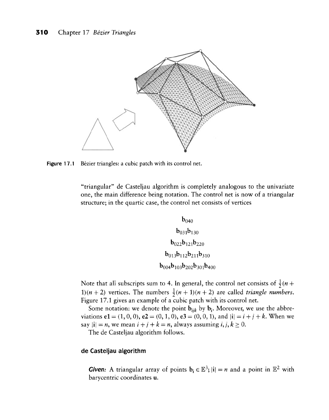
310 Chapter 17 Bezier Triangles
Figure 17.1 Bezier triangles: a cubic patch with its control net.
"triangular" de Casteljau algorithm is completely analogous to the univariate
one,
the main difference being notation. The control net is now of a triangular
structure; in the quartic case, the control net consists of vertices
bo40
^031^130
^022^121^220
boi3bll2b21lb3io
^0041^103^202^301^400
Note that all subscripts sum to 4. In general, the control net consists of j(n +
l)(n + 2) vertices. The numbers j(n + l)(w + 2) are called triangle numbers.
Figure 17.1 gives an example of a cubic patch with its control net.
Some notation: we denote the point b/y^ by bj. Moreover, we use the abbre-
viations el =
(1,
0,0), e2 = (0,1, 0), e3 = (0,0,1), and |i| =i + j + k. When we
say |i| = w, we mean / + / + fe = w, always assuming /, /, k>0.
The de Casteljau algorithm follows.
de Casteljau algorithm
Given: A triangular array of points h[ € E^; |
barycentric coordinates u.
: n and a point in E^ with
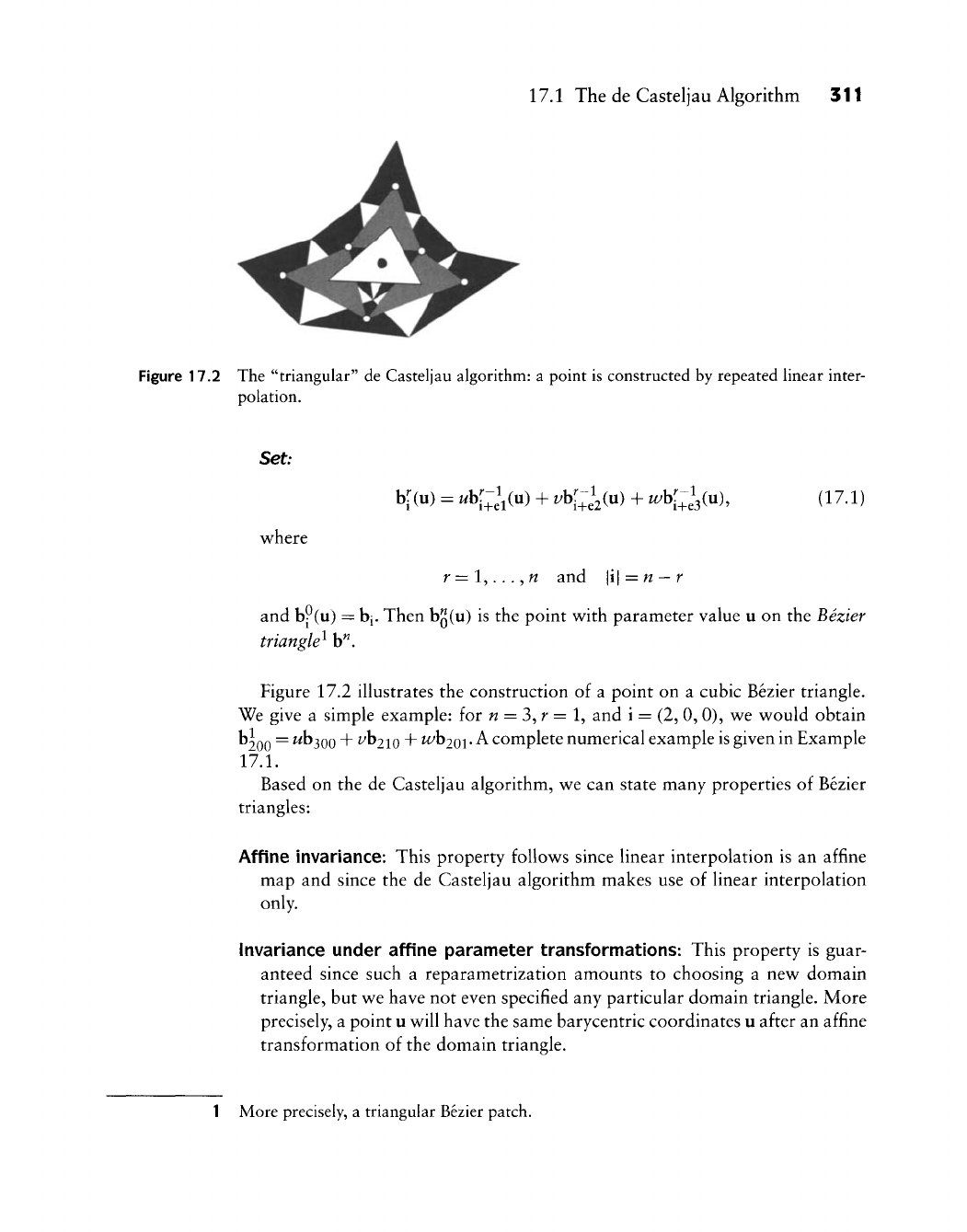
17.1 The de Casteljau Algorithm 311
Figure 17.2 The "triangular" de Casteljau algorithm: a point is constructed by repeated linear inter-
polation.
Set;
where
br(u) = «b[;^V") + ^K;e2(") + ^K;e3(")' d^'D
r =
l,...,w
and \i\=n
—
r
and bP(u) =
h[.
Then bgCu) is the point with parameter value u on the Bezier
triangle^ b".
Figure 17.2 illustrates the construction of a point on a cubic Bezier triangle.
We give a simple example: ior n = 3^r = 1, and i = (2, 0, 0), we would obtain
b^QQ
=
uh^QQ
H-
i^b2io + ^b2oi- A complete numerical example is given in Example
17.1.
Based on the de Casteljau algorithm, we can state many properties of Bezier
triangles:
Affine invariance: This property follows since linear interpolation is an affine
map and since the de Casteljau algorithm makes use of linear interpolation
only.
Invariance under affine parameter transformations: This property is guar-
anteed since such a reparametrization amounts to choosing a new domain
triangle, but we have not even specified any particular domain triangle. More
precisely, a point u will have the same barycentric coordinates u after an affine
transformation of the domain triangle.
1 More precisely, a triangular Bezier patch.
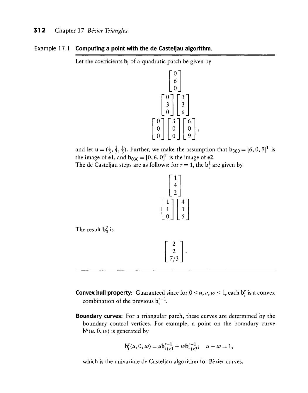
312 Chapter 17 Bezier Triangles
Example 17.1 Computing a point with the de Casteljau algorithm.
Let the coefficients bj of a quadratic patch be given by
0
0
0
3
0
0
6
0
9
and let u = (^, ^, ^). Further, we make the assumption that b3oo = [6, 0, 9]^ is
the image of el, and boao = [0, 6,0]^ is the image of e2.
The de Casteljau steps are as follows: for r = 1, the
b^^
are given by
The result bg is
2
2
7/3
Convex hull property: Guaranteed since for 0 <u^v,w <l, each b[ is a convex
combination of the previous b[~ .
Boundary curves: For a triangular patch, these curves are determined by the
boundary control vertices. For example, a point on the boundary curve
b"(w, 0, w) is generated by
b[(w, 0, w) = uhl~l^ +
^K+e3'
u + w=l,
which is the univariate de Casteljau algorithm for Bezier curves.
17.2 Triangular Blossoms 313
17.2 Triangular Blossoms
The blossoming principle was introduced in Section 4.4 and also proves useful
here.
Our development follows a familiar flavor: we feed different arguments
into the de Casteljau algorithm. At level r of the algorithm, we will use u^ as its
argument, arriving finally at level n, with the blossom value b[ui,...,
u„].
Note
that all arguments are triples of numbers, because they represent points in the
domain plane. The multivariate polynomial b[ui,..., u„] is called the blossom of
the triangular patch b(u). This blossom has all the properties that we encountered
earlier: it agrees with the patch if all arguments are equal: b(u) = b[u^"^] (recall
that u^^^ is short for w-fold repetition of u), it is multiaffine, and it is symmetric.
The last property is perhaps the least obvious one. We derived the symmetry
property of curve blossoms as a consequence of Menelaos' theorem; see Section
3.3.
A similar theorem holds when dealing with triangular blossoms: let bi; |i| =
n = 2 be an array of six control points, and let u and v be (the barycentric
coordinates of) two points. Then b[u, v] = b[v, uj.
This is seen by verifying that both expressions equal
boo2^3^3 + bo2o^2^2 +
^im^\^\
+ boi
1(^31^2
+ ^2^3)
+ bioi(Wil^3 +
Ui^Vi)
+ hxiQ{UiV2 + U2V{).
Let us consider a special case, namely, that of fixing one argument and letting
the remaining ones be equal, similar to the developments of polars in Section
5.6. So consider b[el,
u^"~^^].
We have to carry out one de Casteljau step with
respect to el, and then continue as in the standard algorithm. Since a step with
respect to el yields
biV)=b,+i,;^; |i|=^-l,
we end up with a triangular patch of degree n
— 1
whose vertices are the original
vertices with the exception of the bgy^—that row of control points is "peeled
off."
We may continue this experiment: if we next use e2, we peel off another layer
of coefficients, and so on. Let us use el / times, e2 / times, and e3 k times. We are
then left with a single control point:
bi = b[el<^'^, e2<^'^, e3<^^] |i| = n. (17.2)
So again the Bezier control points are obtainable as special blossom values!
We may also write the intermediate points of the de Casteljau algorithm as
special blossom values:
br(u) = b[u<^^, er^"^, e2<^'^,
e3<^^];
i^j + k^r = n, (17.3)

314 Chapter 17 Bezier Triangles
Figure 17.3 A curve on a surface: a line segment in the domain is mapped to a curve on a triangular
patch.
If we are interested in the control vertices Cj w^ith respect to a triangle with
vertices f
1,
f2, f3, all we have to do is to evaluate the blossom:
q = b[fr^'^, f2<^'^,
£3^^^].
(17.4)
This relationship, without use of the blossoming principle, is discussed by Gold-
man [261] and by Boehm and Farin [81]. See also Seidel
[564].
The triangular analogue to the Leibniz formula (3.22) is as follows:
h[(at + Psr^'n = Yl ('')«')^""'b[r<^>,
s<"-^^].
(17.5)
i=o ^^^
There is an immediate practical ramification of this formula: suppose we are
given two points r and s in the domain. The straight line through them is mapped
to a curve of degree n on the triangular patch. This curve may be written as a
Bezier curve, and its Bezier points are given by
b[r^"^],
b[r^^~^^,
s],...,
b[s^"^].
See Figure 17.3.
If we use three points r, s, t in the domain, we obtain
b[(ar + ps + yt)<^>] = ^ ('''V^>y^b[r<^>,
s<^'>,
t<^>].
(17.6)
liM ^^^
Here, (^) is the generalized binomial coefficient and is defined as
n\
n\
iljlkl
and the summation Xliii=« i^ meant to sum over all triples (/,/, k) with /,/, ^ > 0
and
\i\
=
i~\-
j + k = n.
17.3 Bernstein Polynomials 315
17.5 Bernstein Polynomials
Univariate Bernstein polynomials are the terms of the binomial expansion of
[^ + (1
—
t)f. In the bivariate case, Bernstein polynomials B^ are defined by^
B'liu)
= r UV^^; |i| = n. (17.7)
We define B^{u) = 0 if /,/, ^ < 0 or /,/', k> n. This follows standard convention
for the trinomial coefficients (^). Some of the cubic Bernstein polynomials are
show^n in Figure 17.4.
As a further example, the quartic Bernstein polynomials may be arranged in
the following triangular scheme (corresponding to the control point arrangement
in the de Casteljau algorithm):
Gv^uP' lluv^w 6u^v^
4vw^ lluvw^ llu^vw 4u^v
w^ 4uw^ Gu^u?' 4u^w u^
Bernstein polynomials satisfy the following recursion:
B'liu) = uB\zl^{n) + vBlzl^{xx) +
wB^lzl^ixx)-,
|i| = n. (17.8)
This follows from their definition, as given in (17.7), and the use of the identity
Just as in the curve case, Bernstein polynomials may be used to define a Bezier
triangular patch:
b(u) - Y. MfCu). (17.9)
The proof is a straightforward application of (17.6) and the observation that
u = ut\ + vol +
wt?>.
2 Keep in mind that although
B^(u,
f, w) looks trivariate, it is not, since u-\-v-\-w = l.
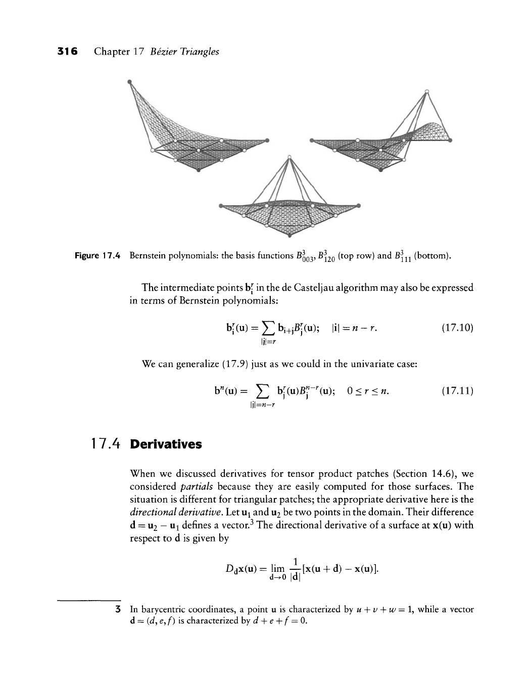
316 Chapter 17 Bezier Triangles
Figure 17.4 Bernstein polynomials: the basis functions
^003'
^120 (^^P ^^^) ^^^ ^lll (hottom).
The intermediate points b[ in the de Casteljau algorithm may also be expressed
in terms of Bernstein polynomials:
br(u) = ^bi+jBr(u); \i\=n-r. (17.10)
We can generalize (17.9) just as we could in the univariate case:
b«(u)= Y^ br(u)Bp''(u); 0<r<n, (17.11)
17.4 Derivatives
When we discussed derivatives for tensor product patches (Section 14.6), we
considered partials because they are easily computed for those surfaces. The
situation is different for triangular patches; the appropriate derivative here is the
directional derivative. Let u^ and
xxi
be two points in the domain. Their difference
d =
U2 —
Ui defines a vector.^ The directional derivative of a surface at x(u) with
respect to d is given by
Ddx(u) = lim — [x(u + d) -
x(u)].
d^o \a\
3 In barycentric coordinates, a point u is characterized hy u-\- v -\-w =
1^
while a vector
d = (J,
e^
f) is characterized hy d-\- e-\-f = 0.
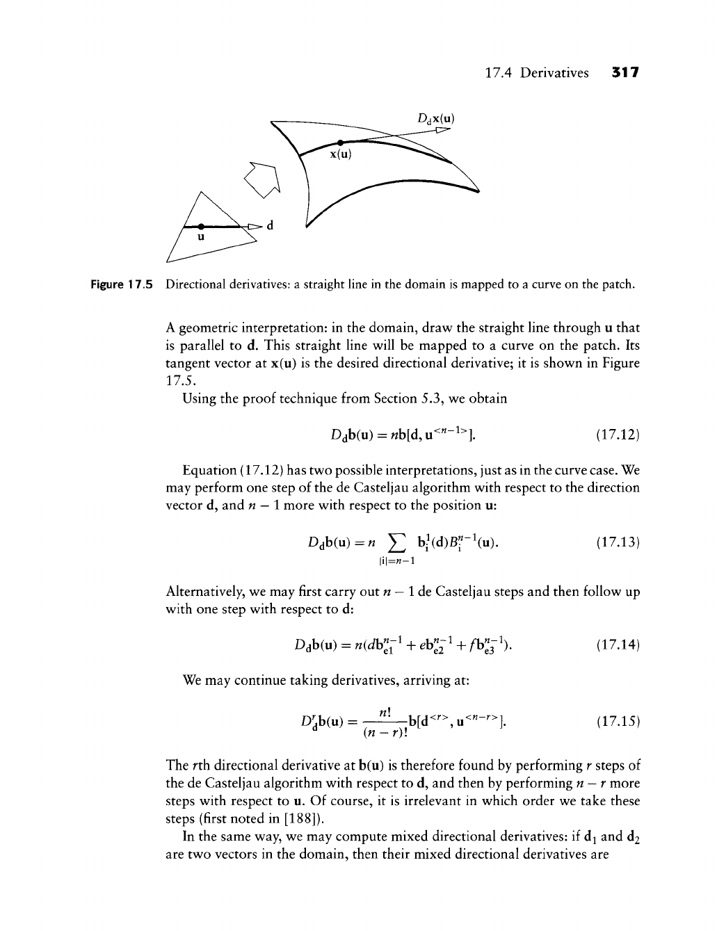
17.4 Derivatives 517
Dax(u)
Figure 17.5 Directional derivatives: a straight line in the domain is mapped to a curve on the patch.
A geometric interpretation: in the domain, draw the straight line through u that
is parallel to d. This straight line will be mapped to a curve on the patch. Its
tangent vector at x(u) is the desired directional derivative; it is shown in Figure
17.5.
Using the proof technique from Section 5.3, we obtain
Ddb(u) = nh[d,
u^"-^^].
(17.12)
Equation (17.12) has two possible interpretations, just as in the curve case. We
may perform one step of the de Casteljau algorithm with respect to the direction
vector d, and n
—
1 more with respect to the position u:
DM^)
= n
J2 W(d)Br^(u). (17.13)
\i\=n-l
Alternatively, we may first carry out «
—
1 de Casteljau steps and then follow up
with one step with respect to d:
Ddb(u) = n(db"^-^ +
eh"^-^
+
/1>^3-l).
(17.14)
We may continue taking derivatives, arriving at:
D^jb(u) = -^h[d<^>,
„<"—].
(17.15)
(n
—
r):
The rth directional derivative at b(u) is therefore found by performing r steps of
the de Casteljau algorithm with respect to d, and then by performing n
—
r more
steps with respect to u. Of course, it is irrelevant in which order we take these
steps (first noted in [188]).
In the same way, we may compute mixed directional derivatives: if dj and 62
art two vectors in the domain, then their mixed directional derivatives are
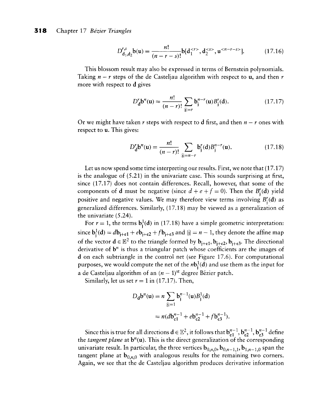
318 Chapter 17 Bezier Triangles
D'f. b(u) = b[d<^^,d<^>,u<"-^-^>]. (17.16)
This blossom resuh may also be expressed in terms of Bernstein polynomials.
Taking n
—
r steps of the de Casteljau algorithm with respect to u, and then r
more with respect to d gives
D^jb«(u) = -^ T h"-\u)BUd). (17.17)
(n
—
r)l ,T-^ ^ ^
\]\=r
Or we might have taken r steps with respect to d first, and then n
—
r ones with
respect to u. This gives:
D'h"(u)^-^
T hUd)B"-''(u). (17.18)
\\=n-r
Let us now spend some time interpreting our results. First, we note that (17.17)
is the analogue of (5.21) in the univariate case. This sounds surprising at first,
since (17.17) does not contain differences. Recall, however, that some of the
components of d must be negative (since J + ^ +
/^
= 0). Then the B|'(d) yield
positive and negative values. We may therefore view terms involving B-'(d) as
generalized differences. Similarly, (17.18) may be viewed as a generalization of
the univariate (5.24).
For r = 1, the terms b^d) in (17.18) have a simple geometric interpretation:
since bKd) = ^bj_^ei + ^\-\-^i + /bj+e3 ^^d
|j|
=
w —
1, they denote the affine map
of the vector d e E^ to the triangle formed by bj_^ei, bj+e2?
bj+e3-
The directional
derivative of b" is thus a triangular patch whose coefficients are the images of
d on each subtriangle in the control net (see Figure 17.6). For computational
purposes, we would compute the net of the wb^d) and use them as the input for
a de Casteljau algorithm of an (n
—
1)^^ degree Bezier patch.
Similarly, let us set r = 1 in (17.17). Then,
Ddb"(u) = «^bj'-i(u)B;(d)
1)1=1
= «(Jb«,-i + eb^2"' + ^b«3-i).
Since this is true for all directions d
G
E^, it follows that b^^\ ^^a^^
^^3"^
define
the tangent plane at b'^(u). This is the direct generalization of the corresponding
univariate result. In particular, the three vertices bo^„^o?bo,w-i,i?bi^^_i
Q
span the
tangent plane at bo^^^o with analogous results for the remaining two corners.
Again, we see that the de Casteljau algorithm produces derivative information
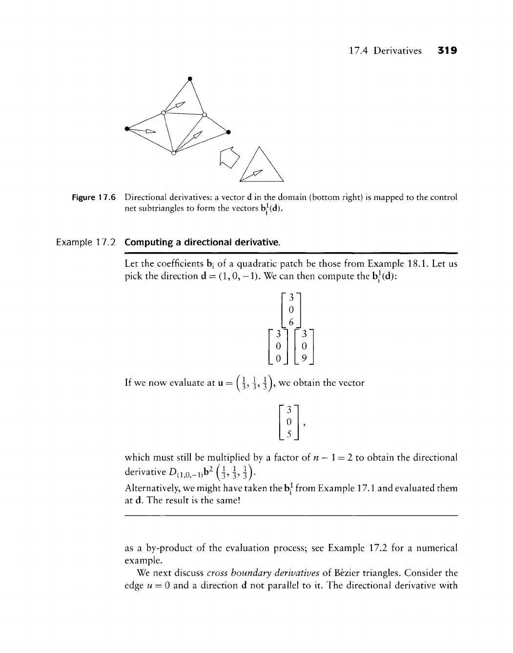
17.4 Derivatives 319
Figure 17.6 Directional derivatives: a vector d in the domain (bottom right) is mapped to the control
net subtriangles to form the vectors bj^(d).
Example 17.2 Computing a directional derivative.
Let the coefficients bj of a quadratic patch be those from Example 18.1. Let us
pick the direction d =
(1,
0,
—
1).
We can then compute the bj^(d):
[3'
0
0
'3'
0
6
•31
0
9
If we now evaluate at u = ( 3, 3, ^ 1, we obtain the vector
which must still be multiplied by a factor oin
—
l = 2to obtain the directional
derivative D(i^o,-i)b^ (i h l)'
Alternatively, we might have taken the hj from Example 17.1 and evaluated them
at d. The result is the same!
as a by-product of the evaluation process; see Example 17.2 for a numerical
example.
We next discuss cross boundary derivatives of Bezier triangles. Consider the
edge
w
= 0 and a direction d not parallel to it. The directional derivative with

320 Chapter 17 Bezier Triangles
Figure 17.7 Cross boundary derivatives: any first-order cross boundary directional derivative of a
quartic, evaluated along the indicated edge, depends only on the two indicated rows of
Bezier points.
respect to d, evaluated along
w
= 0, is the desired cross boundary derivative. It
is given by
D',h\u)
n\
u=o
{n-r)\
E (u)
\\Q\=n-r M=0 (17.19)
where
\Q
= (0,/, k). Since u = (0, v, w) = (0, v,l
—
v), this is a univariate expres-
sion, that is, a Bezier curve in terms of barycentric coordinates. Note that it
depends only on the r + 1 rows of Bezier points closest to the boundary under
consideration. Analogous results hold for the other two boundaries; see Figure
17.7.
This result is the straightforward generalization of the corresponding uni-
variate result. We will use it for the construction of composite surfaces, just as
we did for curves.
17.5 Subdivision
We will later study surfaces that consist of several triangular patches forming
a composite C surface. Now, we start with a surface consisting of just two
triangular patches. Let their domain triangles be defined by points a, b, c, d, as
shown in Figure 17.8. If the common boundary is through b and c, then the
(domain!) point d can be expressed in terms of barycentric coordinates of a, b, c:
d = v^a + Vih + f
3C.
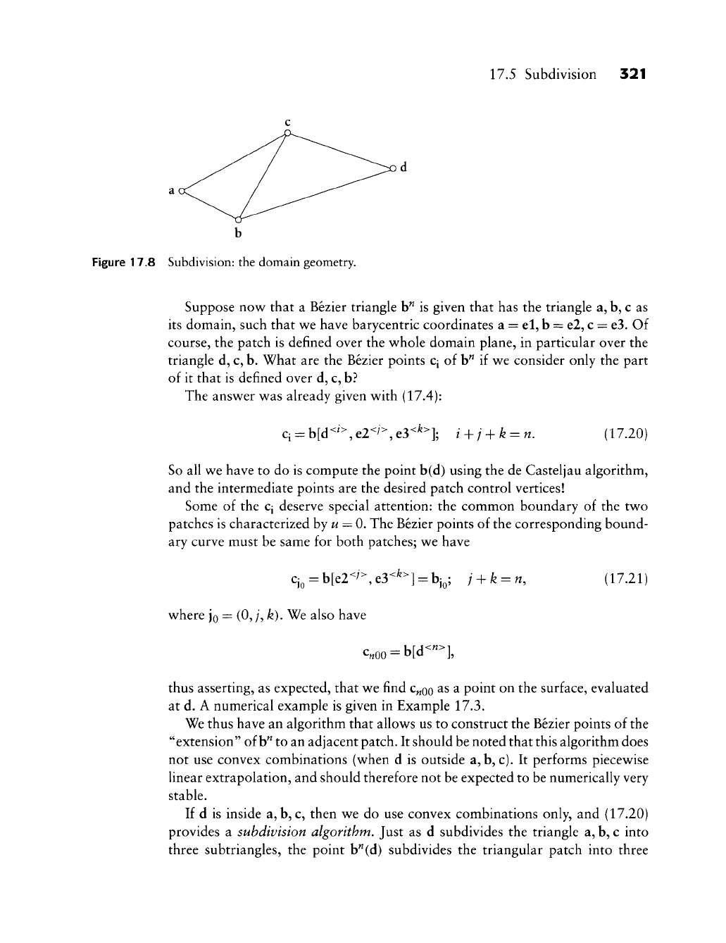
17.5 Subdivision 321
b
Figure 17.8 Subdivision: the domain geometry.
Suppose now that a Bezier triangle b" is given that has the triangle a, b, c as
its domain, such that we have barycentric coordinates a = el, b = e2, c = e3. Of
course, the patch is defined over the whole domain plane, in particular over the
triangle d, c, b. What are the Bezier points Cj of b" if we consider only the part
of it that is defined over d, c, b?
The answer was already given with (17.4):
q = b[d<^^,
e2<^=^,
e3^^^];
i + j + k = n. (17.20)
So all we have to do is compute the point b(d) using the de Casteljau algorithm,
and the intermediate points are the desired patch control vertices!
Some of the Cj deserve special attention: the common boundary of the two
patches is characterized hyu = 0. The Bezier points of the corresponding bound-
ary curve must be same for both patches; we have
Cj„ = b[e2<'>,e3<*>] = bj,; i + k = n, (17.21)
where Jo = (0,/, k). We also have
c„oo =
b[d<">],
thus asserting, as expected, that we find c„oo ^s a point on the surface, evaluated
at d. A numerical example is given in Example 17.3.
We thus have an algorithm that allows us to construct the Bezier points of the
"extension" of
b^
to an adjacent patch. It should be noted that this algorithm does
not use convex combinations (when d is outside a, b, c). It performs piecewise
linear extrapolation, and should therefore not be expected to be numerically very
stable.
If d is inside a, b, c, then we do use convex combinations only, and (17.20)
provides a subdivision algorithm. Just as d subdivides the triangle a, b, c into
three subtriangles, the point b"(d) subdivides the triangular patch into three
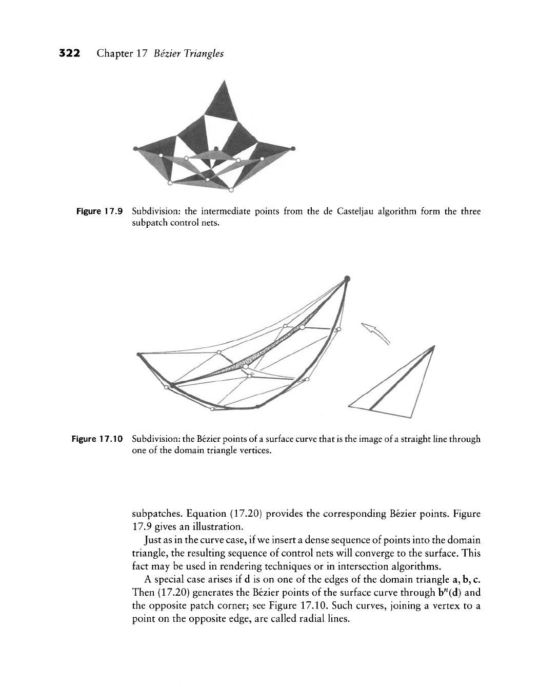
322 Chapter 17 Bezier Triangles
Figure 17.9 Subdivision: the intermediate points from the de Casteljau algorithm form the three
subpatch control nets.
Figure 17.10 Subdivision: the Bezier points of
a
surface curve that
is
the image of
a
straight line through
one of the domain triangle vertices.
subpatches. Equation (17.20) provides the corresponding Bezier points. Figure
17.9 gives an illustration.
Just as in the curve case, if
v^e
insert a dense sequence of points into the domain
triangle, the resulting sequence of control nets w^ill converge to the surface. This
fact may be used in rendering techniques or in intersection algorithms.
A special case arises if d is on one of the edges of the domain triangle a, b, c.
Then (17.20) generates the Bezier points of the surface curve through b^(d) and
the opposite patch corner; see Figure 17.10. Such curves, joining a vertex to a
point on the opposite edge, are called radial lines.
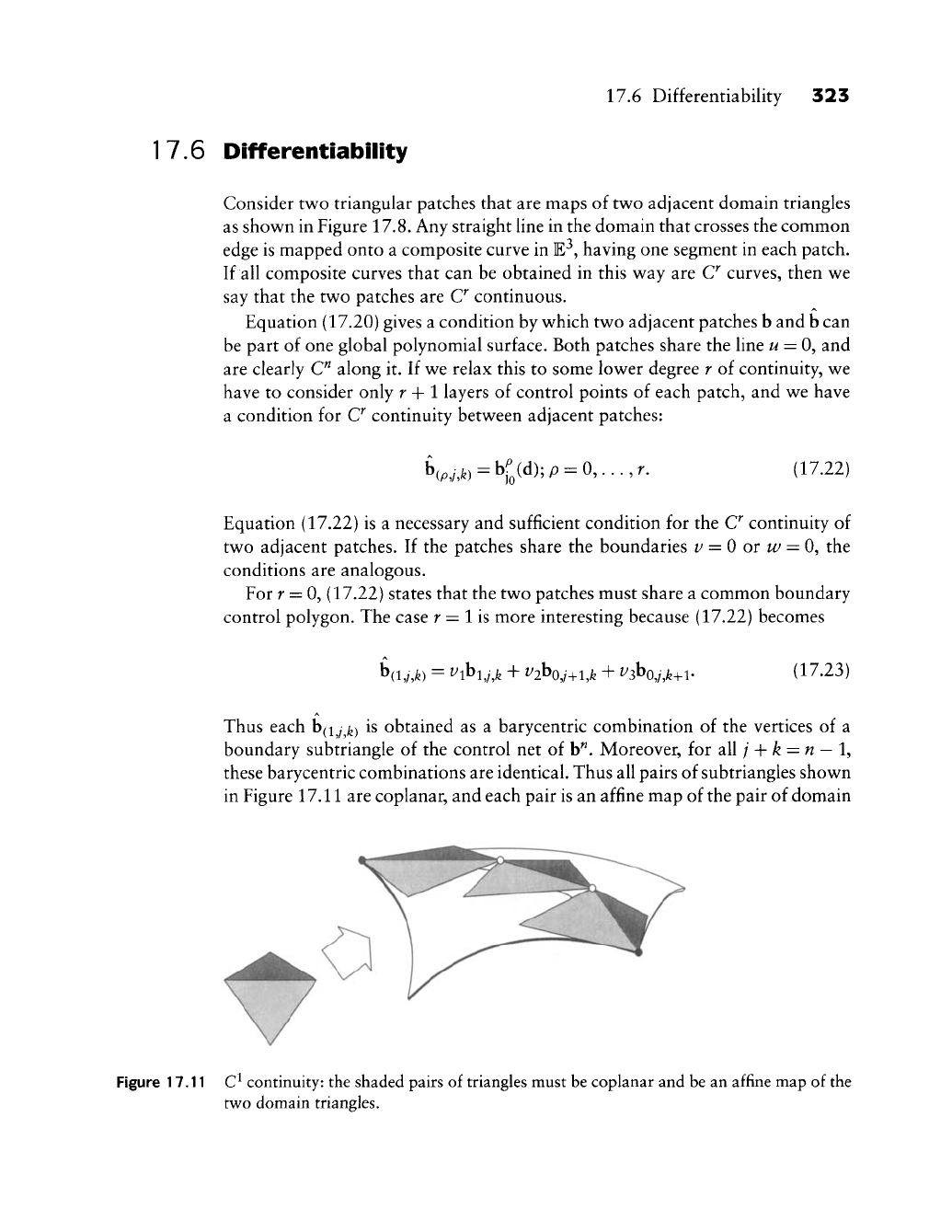
17.6 Differentiability
323
17.6 Differentiability
Consider
two
triangular patches that
are
maps
of two
adjacent domain triangles
as shown
in
Figure 17.8.
Any
straight Hne
in the
domain that crosses
the
common
edge
is
mapped onto
a
composite curve
in E^,
having
one
segment
in
each patch.
If
all
composite curves that
can be
obtained
in
this
way are C^
curves, then
we
say that
the two
patches
are C^
continuous.
Equation (17.20) gives
a
condition
by
which
two
adjacent patches
b and b can
be part
of one
global polynomial surface. Both patches share
the
line
w
= 0, and
are clearly
C^
along
it. If we
relax this
to
some lower degree
r of
continuity,
we
have
to
consider only
r + 1
layers
of
control points
of
each patch,
and we
have
a condition
for C^
continuity between adjacent patches:
^{p.iM)
= bf(d);p
= 0,...,r.
(17.22)
)o
Equation (17.22)
is a
necessary
and
sufficient condition
for the C^
continuity
of
two adjacent patches.
If the
patches share
the
boundaries
i/ = 0 or
w/
= 0, the
conditions
are
analogous.
For
r = 0,
(17.22) states that
the two
patches must share
a
common boundary
control polygon.
The
case
r = 1 is
more interesting because (17.22) becomes
b(i,/,)^)
=
^ibi,/,)^
+
^^iV/'+i,)^
+ ^SVM+I-
(17.23)
Thus each
b(i
;^^)
is
obtained
as a
barycentric combination
of the
vertices
of a
boundary subtriangle
of the
control
net of
b". Moreover,
for all /-f fe = n
—
1,
these barycentric combinations
are
identical. Thus
all
pairs
of
subtriangles shown
in Figure 17.11
are
coplanar,
and
each pair
is an
affine
map of
the pair
of
domain
Figure 17.11 C^ continuity:
the
shaded pairs
of
triangles must be coplanar
and be an
affine map
of
the
two domain triangles.
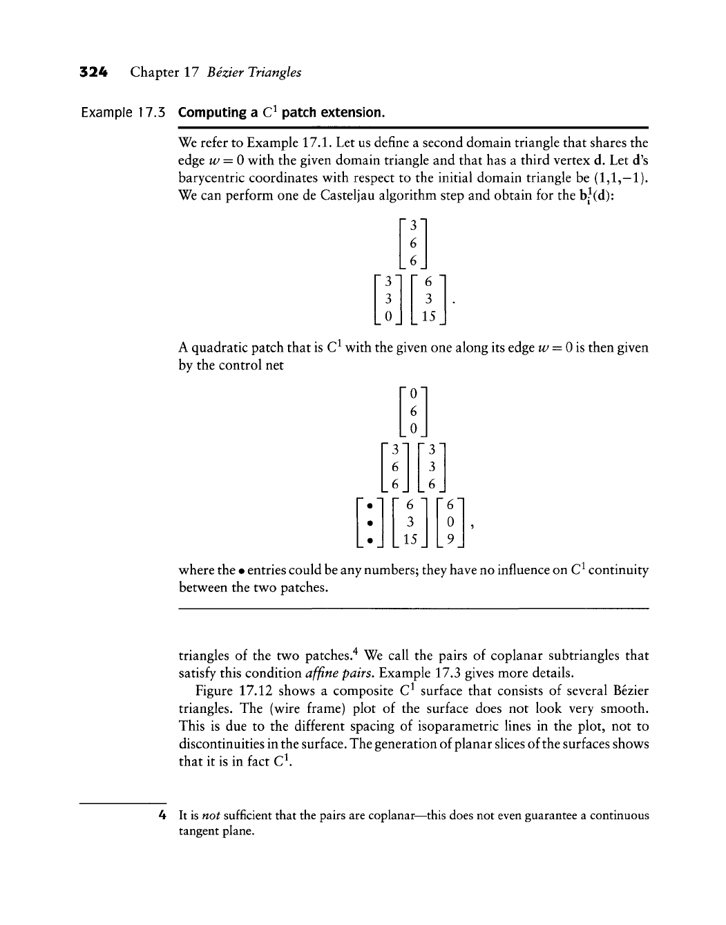
324 Chapter 17 Bezier Triangles
Example 17.3 Computing a C^ patch extension.
We refer to Example 17.1. Let us define a second domain triangle that shares the
edge w = 0 with the given domain triangle and that has a third vertex d. Let d's
barycentric coordinates with respect to the initial domain triangle be (1,1,—!)•
We can perform one de Casteljau algorithm step and obtain for the
hjid):
[3"
3
0
• 31
6
6_
6
1
3
_15_
A quadratic patch that is C^ with the given one along its edge w = Ois then given
by the control net
0
•
•
6
3
15
6
0
9
where the • entries could be any numbers; they have no influence on C^ continuity
between the two patches.
triangles of the two patches."^ We call the pairs of coplanar subtriangles that
satisfy this condition affine pairs. Example 17.3 gives more details.
Figure 17.12 shows a composite C^ surface that consists of several Bezier
triangles. The (wire frame) plot of the surface does not look very smooth.
This is due to the different spacing of isoparametric lines in the plot, not to
discontinuities in the surface. The generation of planar slices of the surfaces shows
that it is in fact C^.
4 It is not sufficient that the pairs are coplanar—this does not even guarantee a continuous
tangent plane.
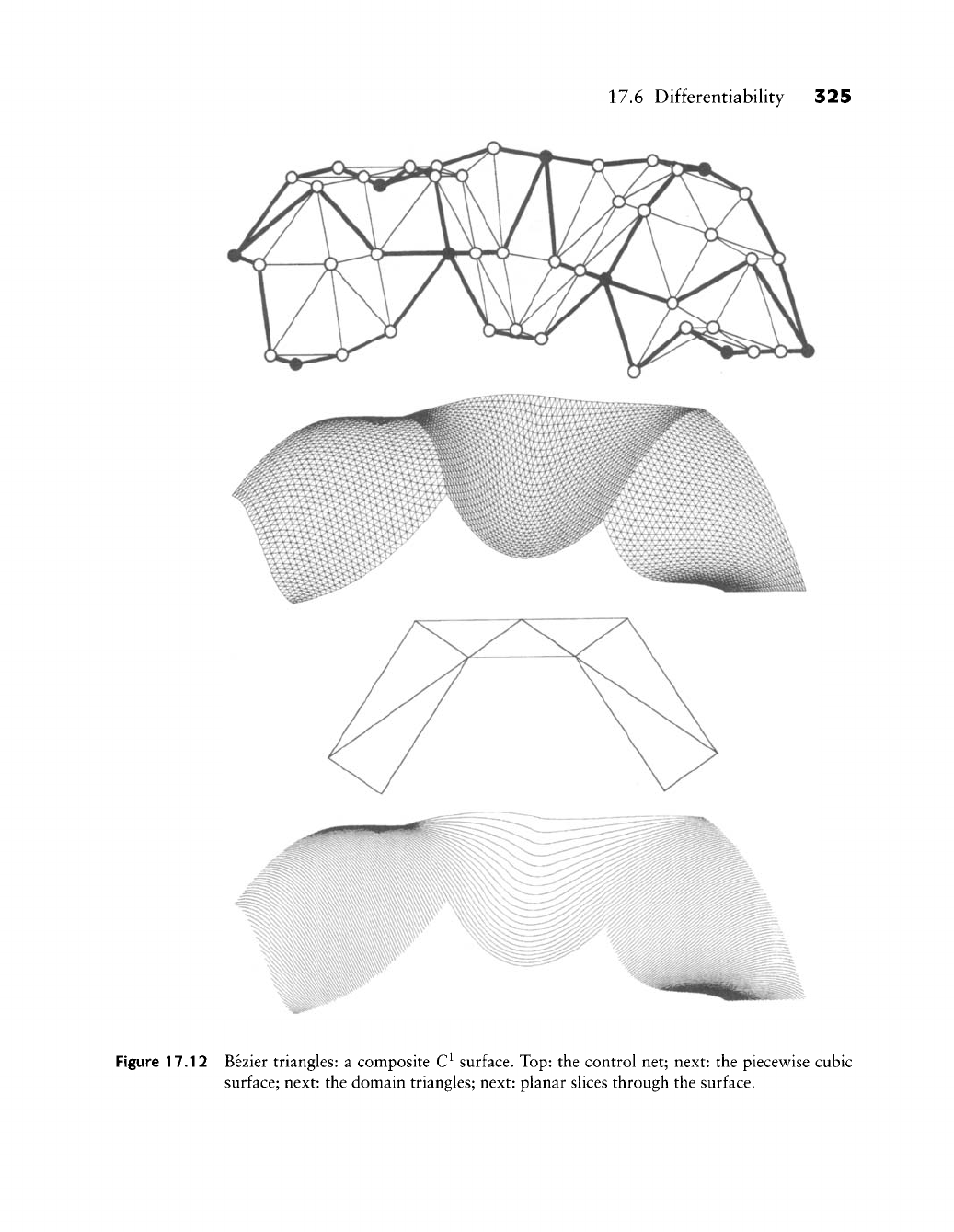
17.6 Differentiability 325
Figure 17.12 Bezier triangles: a composite C^ surface. Top: the control net; next: the piecewise cubic
surface; next: the domain triangles; next: planar slices through the surface.
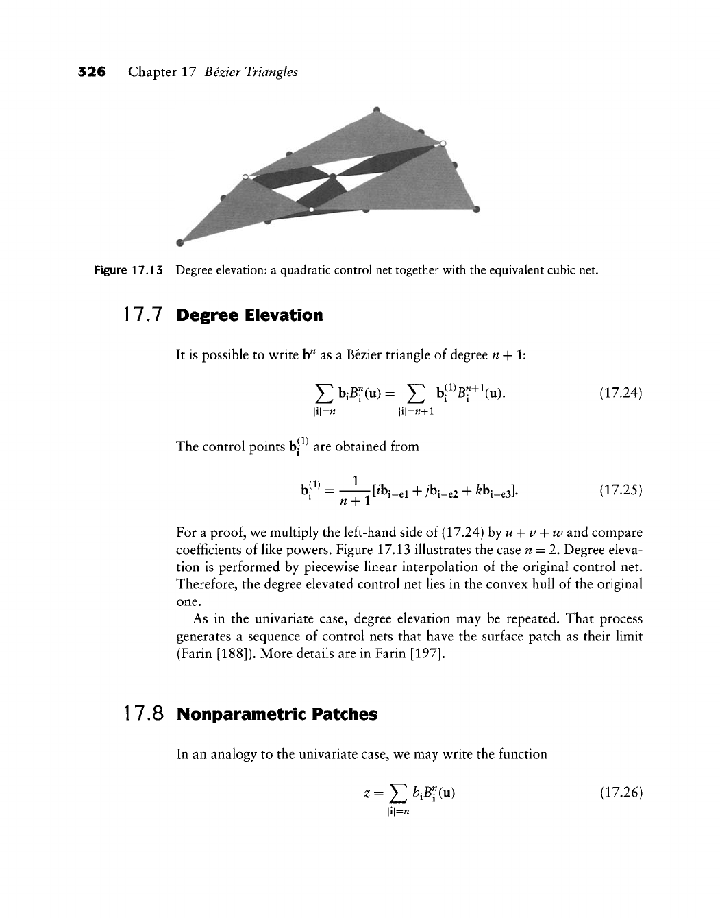
326 Chapter 17 Bezier Triangles
Figure 17.13 Degree elevation: a quadratic control net together with the equivalent cubic net.
17.7 Degree Elevation
It is possible to write b" as a Bezier triangle of degree n + 1:
^biB«(u)^ ^ h^^Bl+\u). (17.24)
|i|=„ |i|=«+i
The control points b[ are obtained from
b|« = -^ [fbi_ei + /bi_e2 + febi_e3]. (17.25)
n-\-
1
For a
proof,
we multiply the left-hand side of (17.24) hyu + v i-w and compare
coefficients of like powers. Figure 17.13 illustrates the case n = 2. Degree eleva-
tion is performed by piecewise linear interpolation of the original control net.
Therefore, the degree elevated control net lies in the convex hull of the original
one.
As in the univariate case, degree elevation may be repeated. That process
generates a sequence of control nets that have the surface patch as their limit
(Farin [188]). More details are in Farin
[197].
1
7.8 Nonparametric Patches
In an analogy to the univariate case, we may write the function
z=J2biB"{vO (17.26)
|i|=«
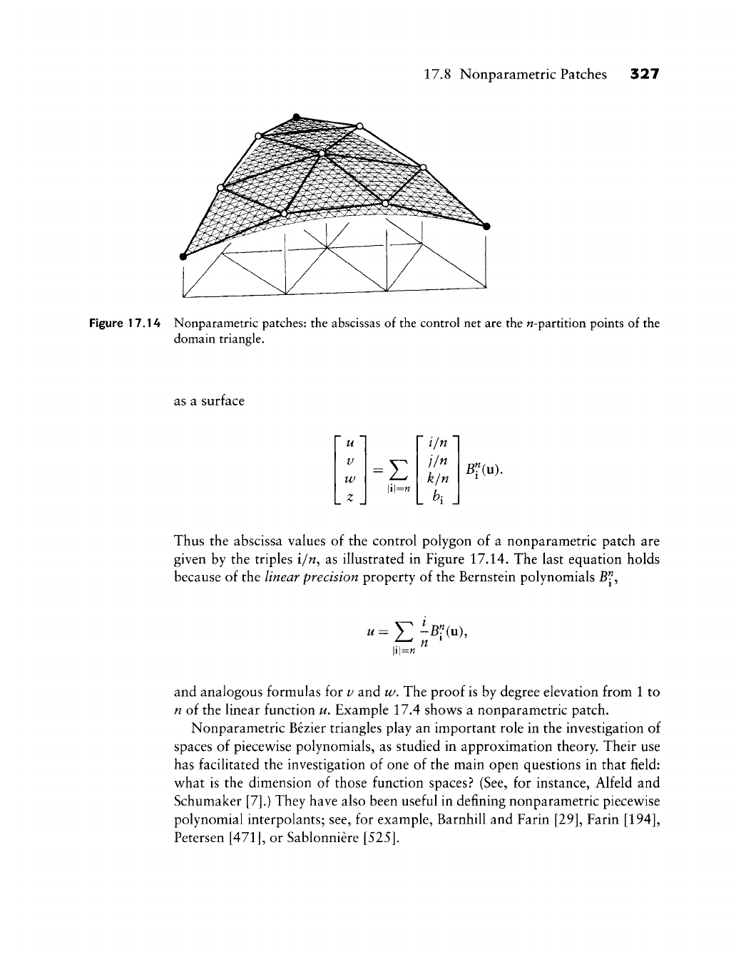
17.8 Nonparametric Patches 327
Figure 17.14 Nonparametric patches: the abscissas of the control net are the w-partition points of the
domain triangle.
as a s
urface
u
V
w
z
E
\i\=n
i/n
j/n
k/n
B'liu).
Thus the abscissa values of the control polygon of a nonparametric patch are
given by the triples i/w, as illustrated in Figure 17.14. The last equation holds
because of the linear precision property of the Bernstein polynomials
JB^
«=v-Br(u),
and analogous formulas for v and w. The proof is by degree elevation from 1 to
n of the linear function u. Example 17.4 shows a nonparametric patch.
Nonparametric Bezier triangles play an important role in the investigation of
spaces of piecewise polynomials, as studied in approximation theory. Their use
has facilitated the investigation of one of the main open questions in that field:
what is the dimension of those function spaces.'^ (See, for instance, Alfeld and
Schumaker [7].) They have also been useful in defining nonparametric piecewise
polynomial interpolants; see, for example, Barnhill and Farin [29], Farin
[194],
Petersen
[471],
or Sablonniere
[525].
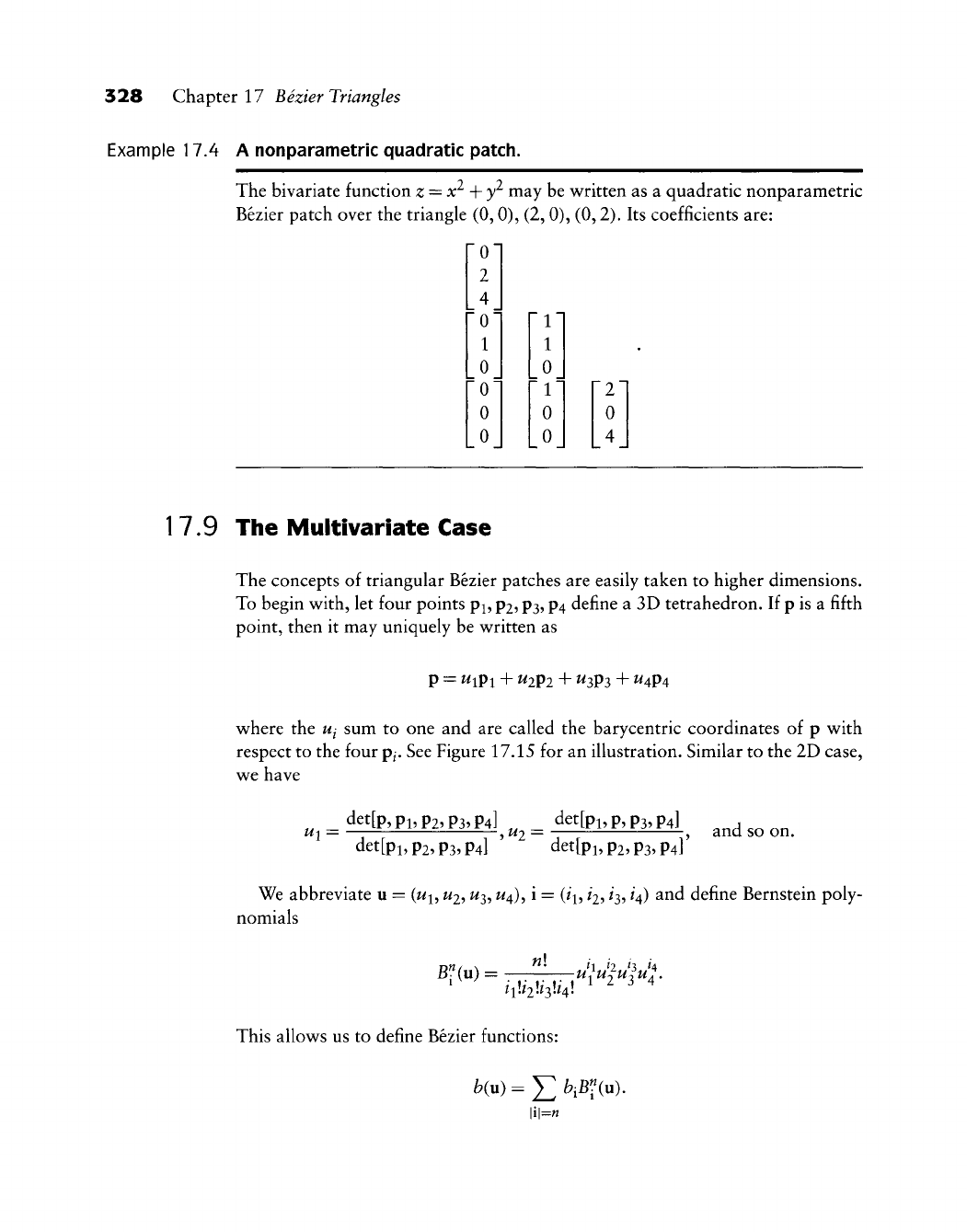
328 Chapter 17 Bezier Triangles
Example 17.4 A nonparametric quadratic patch.
The bivariate function z = x^ + y^ may be written as a quadratic nonparametric
Bezier patch over the triangle (0,0), (2,0), (0,2). Its coefficients are:
roi
2
4
1
0
0
0
0
"1"
1
0
1
0
0
2
0
4
1
7.9 The Multivariate Case
The concepts of triangular Bezier patches are easily taken to higher dimensions.
To begin with, let four points pi, p2,
P3,
p4 define a 3D tetrahedron. If p is a fifth
point, then it may uniquely be written as
P = ^iPl + ^2P2 + ^3P3 + ^4P4
where the Uj sum to one and are called the barycentric coordinates of p with
respect to the four
p^.
See Figure 17.15 for an illustration. Similar to the 2D case,
we have
det[p,
pi, p2,
P3,
P4]
det[pi,p,p3,p4]
Ui = — ,
U2
= , and so on.
det[pi, P2,
p3,
P4]
det[pi, p2,
P3,
P4]
We abbreviate u =
(w^,
^2? ^3? ^4)5 i =
(^1?
h->
h^ H) ^^d define Bernstein poly-
nomials
B«(u) = "": _ii}xiUlul
This allows us to define Bezier functions:
l-j Ul^ l/l^ l/l* .
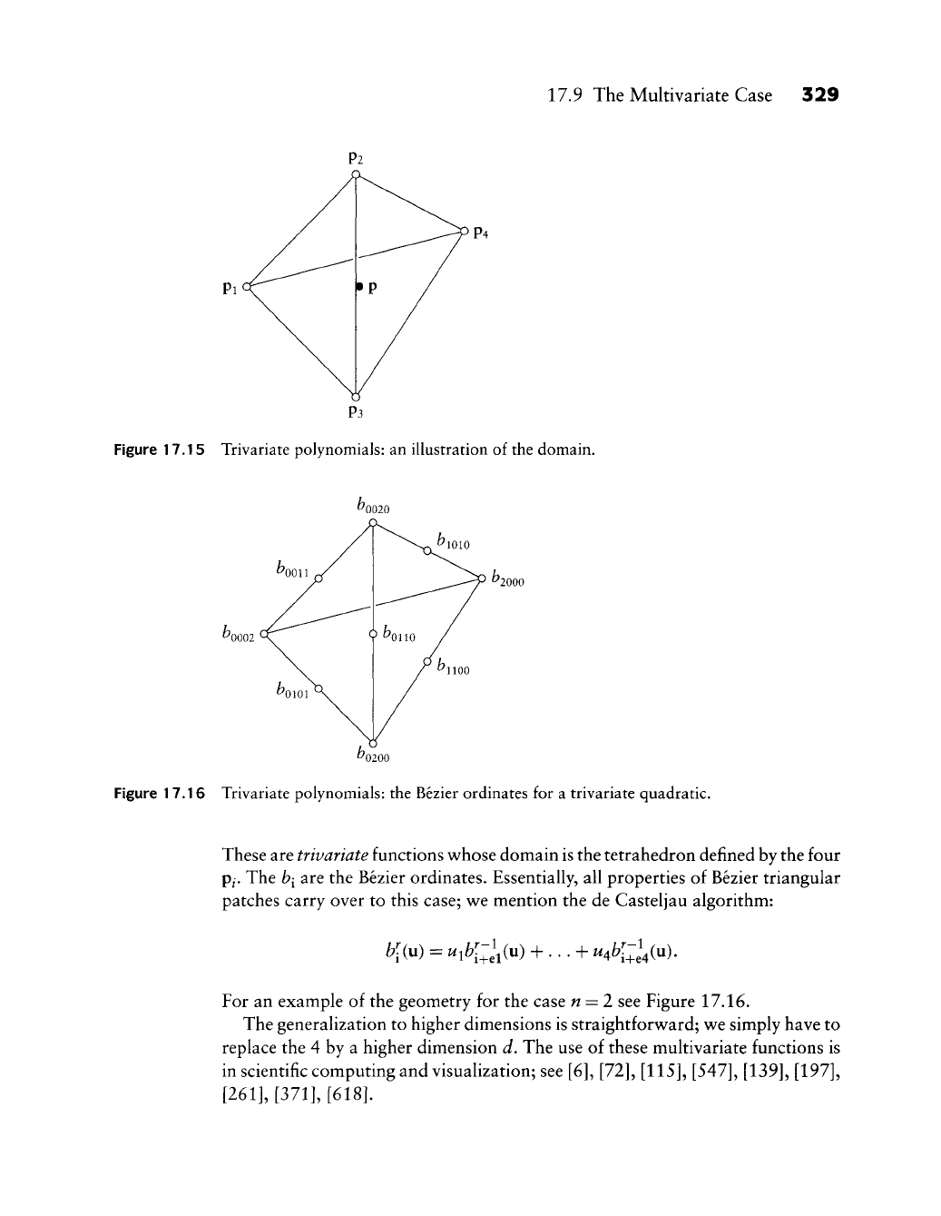
17.9 The Multivariate Case 329
Figure 17.15 Trivariate polynomials: an illustration of the domain.
^0002
2000
Figure 17.16 Trivariate polynomials: the Bezier ordinates for a trivariate quadratic.
These are trivariate functions whose domain is the tetrahedron defined by the four
P/.
The
b{
are the Bezier ordinates. Essentially, all properties of Bezier triangular
patches carry over to this case; we mention the de Casteljau algorithm:
^[(u) = u^b[-l^{vi) + ... + u^b[-l^{n).
b\{
For an example of the geometry for the case « = 2 see Figure 17.16.
The generalization to higher dimensions is straightforward; we simply have to
replace the 4 by a higher dimension d. The use of these multivariate functions is
in scientific computing and visualization; see [6], [72],
[115], [547], [139], [197],
[261], [371], [618].

330 Chapter 17 Bezier Triangles
17.10 S-Patches
Bezier patches in higher dimensions have a fairly abstract flair; yet, they may
be used to design "normal" surfaces in 3D. One method to do this is due to T.
DeRose and C. Loop; see
[167], [168], [398],
They devised a method to contruct
patches with an arbitrary number s of edges.
In order to build an s-sided patch, we take as its domain a convex 2D polygon
Vs with vertices
pj,...,
p^,
ordered counterclockwise. For every point p inside
this polygon, we construct "generalized barycentric coordinates" w^,...,
w^,
by
considering all triangles formed by p and the polygon vertices p^—this approach
is due to Gregory and Charrot
[110].
If the area^ of triangle p,
p^,
pj^i is denoted
by A/, then we define
;r,- = Ai..... A,_2
•
A,+i •...
•
A,.
Since these
TTJ
do not sum to one, we normalize and obtain
Ui= "^ . (17.27)
TTi + . . . +
TT,
For s = 3, we obtain standard barycentric coordinates in a triangle. If p is on the
edge
p^,
pi^i of
7^5,
then only
Uj
and Uj^i are nonzero.
The key idea now is this: since the u^ sum to one, they may be interpreted
as barycentric coordinates of an (s
—
l)-dimensional simplex S^; see Section 3.5.
We call the vertices of the simplex
Sj;
|i| = 1. In particular, if s = 3, the simplex is
a triangle; if s = 4, it is a tetrahedron. We associate the point p/ of Vs with the
point
[0^^~^^,
1,0^^~^^]
of
tS^.
All points u = (w^,...,
w^)
inside this simplex that
have barycentric coordinates (17.27) trace out a two-dimensional subset of the
simplex. It has the property that if p is on one of the edges of
Vg^
then u is on the
corresponding edge of 5^.
Next, we may define a Bezier patch over S^. Recall that S^ is just the domain
of that patch; the corresponding Bezier points may "live" in any dimension. We
restrict them to be 3D points bj, with |i| =
w,
the degree of the Bezier patch. This
number n is referred to as the depth of the S-patch. The equation of the S-patch
becomes
x(u) = J]) bjBf
(u).
(17.28)
\i\=n
5 If p is outside the polygon, we use signed areas.
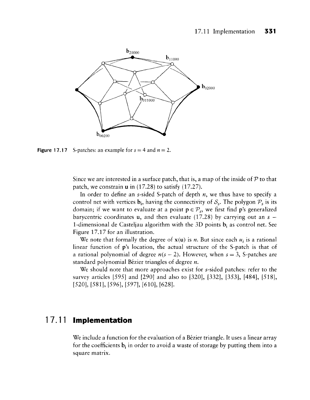
17.11 Implementation 331
1^02000
^00200
Figure 17.17 S-patches: an example for s = 4 and n = l.
Since we are interested in a surface patch, that is, a map of the inside of V to that
patch, we constrain u in (17.28) to satisfy (17.27).
In order to define an s-sided S-patch of depth n^ we thus have to specify a
control net with vertices bj, having the connectivity of
^S^.
The polygon Vs is its
domain; if we want to evaluate at a point p
G
Vs-,
we first find p's generalized
barycentric coordinates u, and then evaluate (17.28) by carrying out an s
—
1-dimensional de Casteljau algorithm with the 3D points bj as control net. See
Figure 17.17 for an illustration.
We note that formally the degree of x(u) is n. But since each
Ui
is a rational
linear function of p's location, the actual structure of the S-patch is that of
a rational polynomial of degree n{s
—
2). However, when s = 3, S-patches are
standard polynomial Bezier triangles of degree n.
We should note that more approaches exist for s-sided patches: refer to the
survey articles [595] and [290] and also to
[320], [332], [353], [484], [518],
[520], [581], [596],
[S97],
[610], [628].
17.11 Implementation
We include a function for the evaluation of a Bezier triangle. It uses a linear array
for the coefficients bj in order to avoid a waste of storage by putting them into a
square matrix.
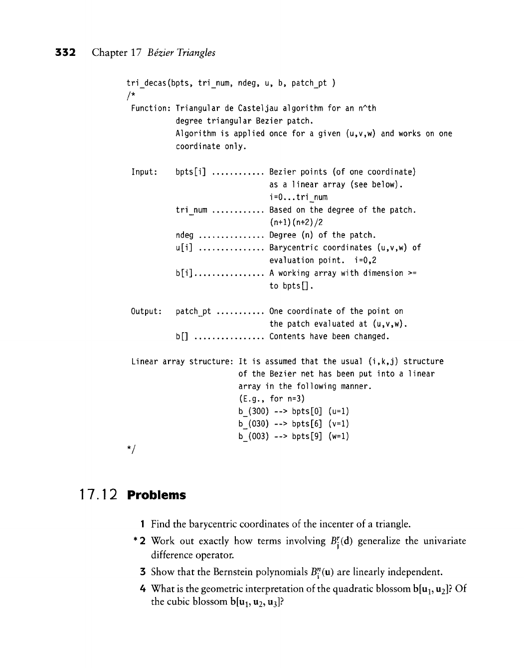
332 Chapter 17 Bezier Triangles
tri_decas(bpts, tri_num, ndeg, u, b, patch_pt )
/*
Function: Triangular
de
Casteljau algorithm for
an
n^th
degree triangular Bezier patch.
Algorithm
is
applied once for
a
given (u,v,w) and works
on
one
coordinate only.
Input: bpts[i] Bezier points (of one coordinate)
as
a
linear array (see
below).
i=0...tri_num
tri_num Based
on
the degree
of
the patch.
(n+l)(n+2)/2
ndeg Degree (n)
of
the patch.
u[i] Barycentric coordinates (u,v,w)
of
evaluation point. i=0,2
b[i]
A
working array with dimension
>=
to
bpts[].
Output: patch_pt One coordinate
of
the point
on
the patch evaluated
at
(u,v,w).
b []
Contents have been changed.
Linear array structure: It
is
assumed that the usual (i,k,j) structure
of the Bezier net has been put into
a
linear
array
in
the following manner.
(E.g., for n=3)
b_(300)
">
bpts[0] (u=l)
b_(030) --> bpts[6] (v=l)
b_(003)
->
bpts[9] (w=l)
17.12
Problems
1 Find the barycentric coordinates of the incenter of a triangle.
'
2 Work out exactly how terms involving B|^(d) generalize the univariate
difference operator.
3 Show^ that the Bernstein polynomials B^(u) are linearly independent.
4 What is the geometric interpretation of the quadratic blossom b[ui,
U2]?
Of
the cubic blossom b[ui,
U2,
U3]?

17.12 Problems 333
PI In Section 16.8, we saw how to modify surfaces by embedding them in the
unit cube and then distorting it using trivariate tensor product schemes.
Experiment with the following: instead of embedding a surface in a cube,
embed it in a tetrahedron and distort it using a Bezier tetrahedron,
P2 Program up S-patches with n = 3 and varying values of s.
P3 Work out a degree reduction procedure for Bezier triangles. Literature:
Petersen
[471].
P4 Problem PI of Chapter 7 addressed the similarity between Aitken and de
Casteljau algorithms. Generalize to the triangular patch case and write a
program that modifies tri_decas accordingly.

This Page Intentionally Left Blank
Practical Aspects
of Bezier Triangles
Dezier triangular patches are not only the most natural generalization of Bezier
curves, they also offer a variety of applications. They lend themselves easily to
patches on spheres or quadrics, and they may be used for scattered data interpo-
lation. Although rectangular patches are traditionally dominating CAD/CAM,
some recent applications of triangular patches are in gaming and animation.
18.1 Rational Bezier TV'iangles
Following the familiar theme of generating rational curve and surface schemes,
we define a rational Bezier triangle to be the projection of a polynomial 4D Bezier
triangle. We thus have:
^t^ibi^fCu)
b»=b»: \x\=n (18.1)
where, as usual, the
W[
are the weights associated with the control vertices h[.
For positive weights, we have the convex hull property. We also have affine and
projective invariance.
Rational Bezier triangles may be evaluated by a de Casteljau algorithm in a
not too surprising way.
Rational de Casteljau algorithm
Given: A triangular array of points
b^
G
E^;
|i| =
W,
corresponding weights
^j,
and a point in a domain triangle with barycentric coordinates u.
335
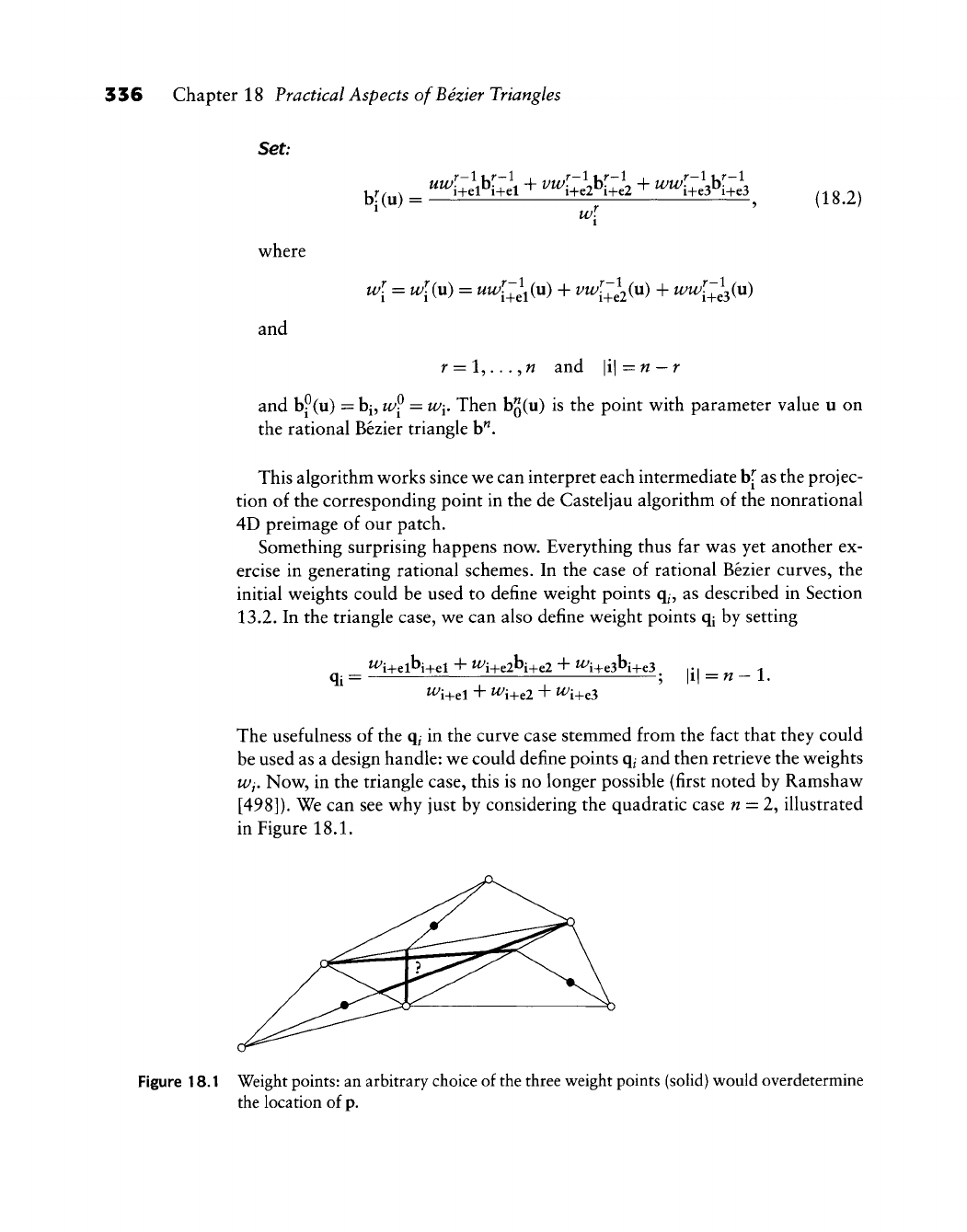
336 Chapter 18 Practical Aspects ofBezier Triangles
Set:
br(u):
(18.2)
where
and
r-l
./-I,
wl = wl(u) = uwl^^^iu) +
vw[_^^2^\x)
+ ww\^^^{\x)
r = !,...,« and \\\ = n
—
r
and b?(u) = bj, w^ =
W[,
Then bgCu) is the point with parameter value u on
the rational Bezier triangle b".
This algorithm works since we can interpret each intermediate b[ as the projec-
tion of the corresponding point in the de Casteljau algorithm of the nonrational
4D preimage of our patch.
Something surprising happens now. Everything thus far was yet another ex-
ercise in generating rational schemes. In the case of rational Bezier curves, the
initial weights could be used to define weight points q^ as described in Section
13.2.
In the triangle case, we can also define weight points qi by setting
qi = ^i+el + ^i+e2 + ^i+e3
\i\
= n-l.
The usefulness of the q^ in the curve case stemmed from the fact that they could
be used as a design handle: we could define points
q^
and then retrieve the weights
Wj. Now, in the triangle case, this is no longer possible (first noted by Ramshaw
[498]).
We can see why just by considering the quadratic case
w
= 2, illustrated
in Figure 18.1.
Figure 18.1 Weight
points:
an arbitrary choice of the three weight points (solid) would overdetermine
the location of p.
18.2 Quadrics 357
If we were given a set of weights
w^;
|i| = 2, we would not only generate the
weight points qj, but also the point
^011^011 + ^loibioi + ^iipbiio
^011+ ^101+ "^110
The point p is then at the intersection of the three straight lines qooi, b^o?
and so on. If we prescribed the three q^ arbitrarily (as shown in Figure 18.1),
those straight lines would not intersect in one point any more, thus leaving p
over determined. Since the existence of a set of weights implies the existence of p,
the nonexistence of p implies that we cannot find a set of weights if we prescribe
the qi arbitrarily.
For higher degrees, the situation is analogous. So far, no geometric means is
known that could define weights similar to the weight point approach for curves.
A first step could be the paper by G. Albrecht [4] or H. Theisel
[586].
We now give a formula for the directional derivative of a rational Bezier
triangle. Just as in Section 17.4, let d denote a direction in the domain triangle,
expressed derivative D^ of a rational triangular Bezier patch b"(u). Proceeding
exactly as in the curve case (see Section 12.4), we obtain:
Dab^u) = -^[p(u) - Dd(u)b"(u)],
wyxx)
where we have set
p(u) = w{\xW{\x) = J2 ^ibiBf
(u).
\i\=n
Higher derivatives follow the pattern outlined in Section 12.4, that is.
D:.b"(u)= ^
w(u)
18.2 Quadrics
There were (at least) two motivations for the use of rational Bezier curves: they
are protectively invariant, and they allow us to represent conies in the form of
rational quadratics. While the first argument holds trivially for rational Bezier
triangles, the second one does not carry over immediately.
The proper generalization of a conic to the case of surfaces is a quadric
surface^
quadric for short. A conic (curve) has the implicit equation q{x^ y) = 0, where q
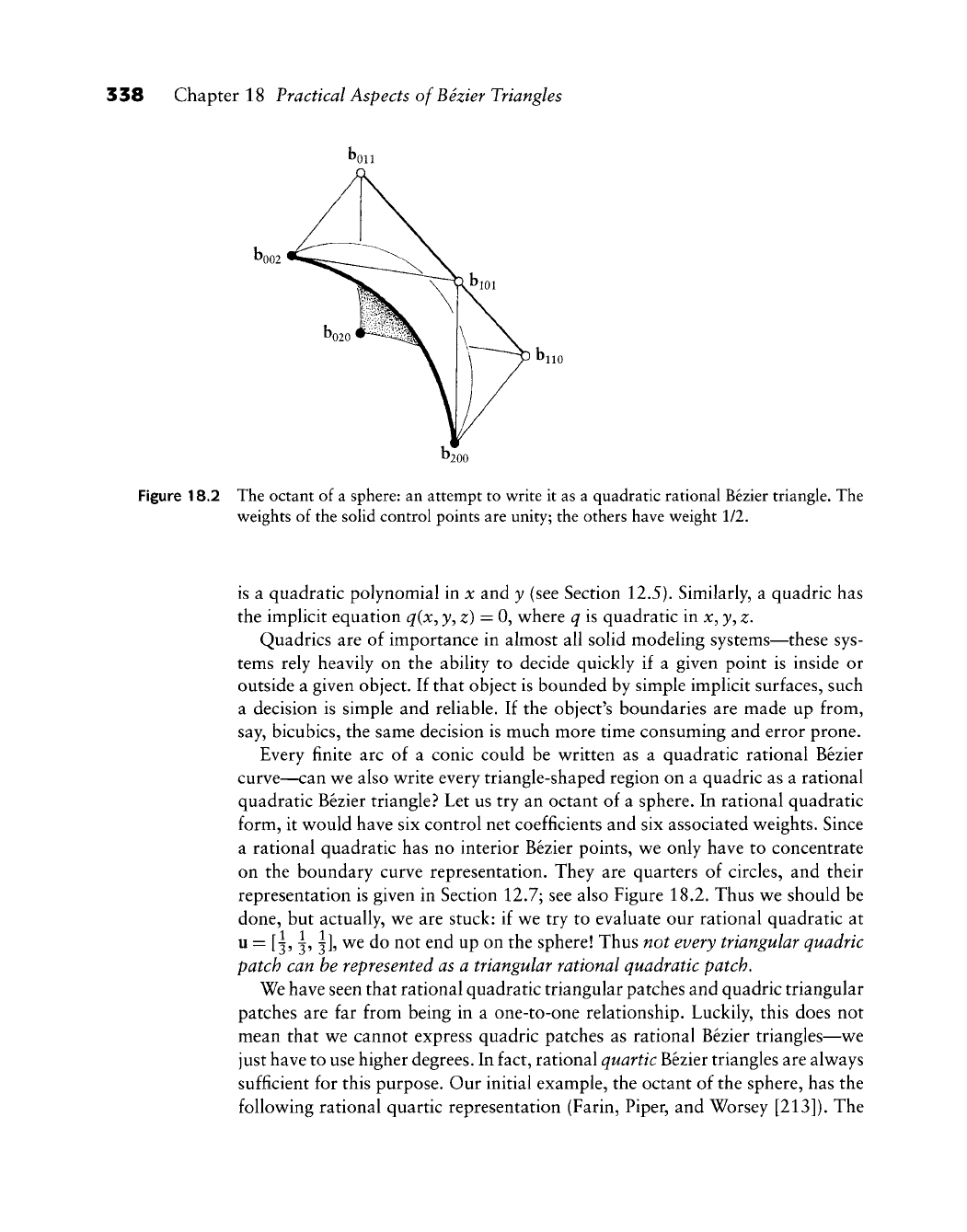
338 Chapter 18 Practical Aspects ofBezier Triangles
Figure 18.2 The octant of a sphere: an attempt to write it as a quadratic rational Bezier triangle. The
weights of the solid control points are unity; the others have weight 1/2.
is a quadratic polynomial in x and y (see Section 12.5). Similarly, a quadric has
the implicit equation q{x^ y, z) = 0, where q is quadratic in x^ y, z.
Quadrics are of importance in almost all solid modeling systems—these sys-
tems rely heavily on the ability to decide quickly if a given point is inside or
outside a given object. If that object is bounded by simple implicit surfaces, such
a decision is simple and reliable. If the object's boundaries are made up from,
say, bicubics, the same decision is much more time consuming and error prone.
Every finite arc of a conic could be w^ritten as a quadratic rational Bezier
curve—can v^e also write every triangle-shaped region on a quadric as a rational
quadratic Bezier triangle.'^ Let us try an octant of a sphere. In rational quadratic
form, it would have six control net coefficients and six associated weights. Since
a rational quadratic has no interior Bezier points, we only have to concentrate
on the boundary curve representation. They are quarters of circles, and their
representation is given in Section 12.7; see also Figure 18.2. Thus we should be
done, but actually, we are stuck: if we try to evaluate our rational quadratic at
u = [^, ^,
^],
we do not end up on the sphere! Thus not every triangular quadric
patch can be represented as a triangular rational quadratic patch.
We have seen that rational quadratic triangular patches and quadric triangular
patches are far from being in a one-to-one relationship. Luckily, this does not
mean that we cannot express quadric patches as rational Bezier triangles—we
just have to use higher degrees. In fact, rational quartic Bezier triangles are always
sufficient for this purpose. Our initial example, the octant of the sphere, has the
following rational quartic representation (Farin, Piper, and Worsey [213]). The
18.2 Quadrics 339
control net (for the octant of the unit sphere) is given by
[0,0,1]
[a, 0,1] [0,a,l]
[;6,0,y6]
[K,y,l] [0,/J,^]
[l,0,a] [l,K,y] [y,Uy] [0,l,«]
[1,0,0] [l,a,0] [p,p,0] [a, 1,0] [0,1,0]
where
ot
= {V3-
1)/V3,
^ = (V3 + 1)/2V3, y = 1 - (5 -
A/2)(7
- ^/3)/46.
The weights are:
u/040 = 4V3(V3 - 1), ^031 = 3^2, w/202 = 4, ^121 = -^(3 + 2V2 - VS),
the other ones following by symmetry.
To represent the whole sphere, we would assemble eight copies of this octant
patch. Other representations are also possible: each octant may be written as
a rational biquadratic patch (introducing singularities at the north and south
poles);
see
[480].
A representation of the whole sphere as two rational bicubics
(Piegl [475]) turned out to be incorrect (see Cobb [119]). Quite a different way
of representing the sphere is also due to J. Cobb: he covers it with six rational
bicubics having a cubelike connectivity
[118].
Let us now discuss the following question: given a rational quadratic Bezier
triangle, what are the conditions under which it represents a quadric patch.^ The
following will be useful for that purpose.
We defined a conic section as the projective map of a parabola, the only conic
allowing a polynomial parametrization. For surfaces, we again consider those
quadrics that permit polynomial parametrizations: these are the paraboloids,
consisting of elliptic and hyperbolic paraboloids and of the parabolic cylinders.
Every quadric surface may be defined as a projective image of one of these
paraboloids.^
A paraboloid may be represented by a parametric polynomial surface of degree
two.
However, as we have seen, not every parametric quadratic is a paraboloid.
We need an extra condition, which is easily formulated if we write the quadratic
1 W. Boehm (1990), private communication.
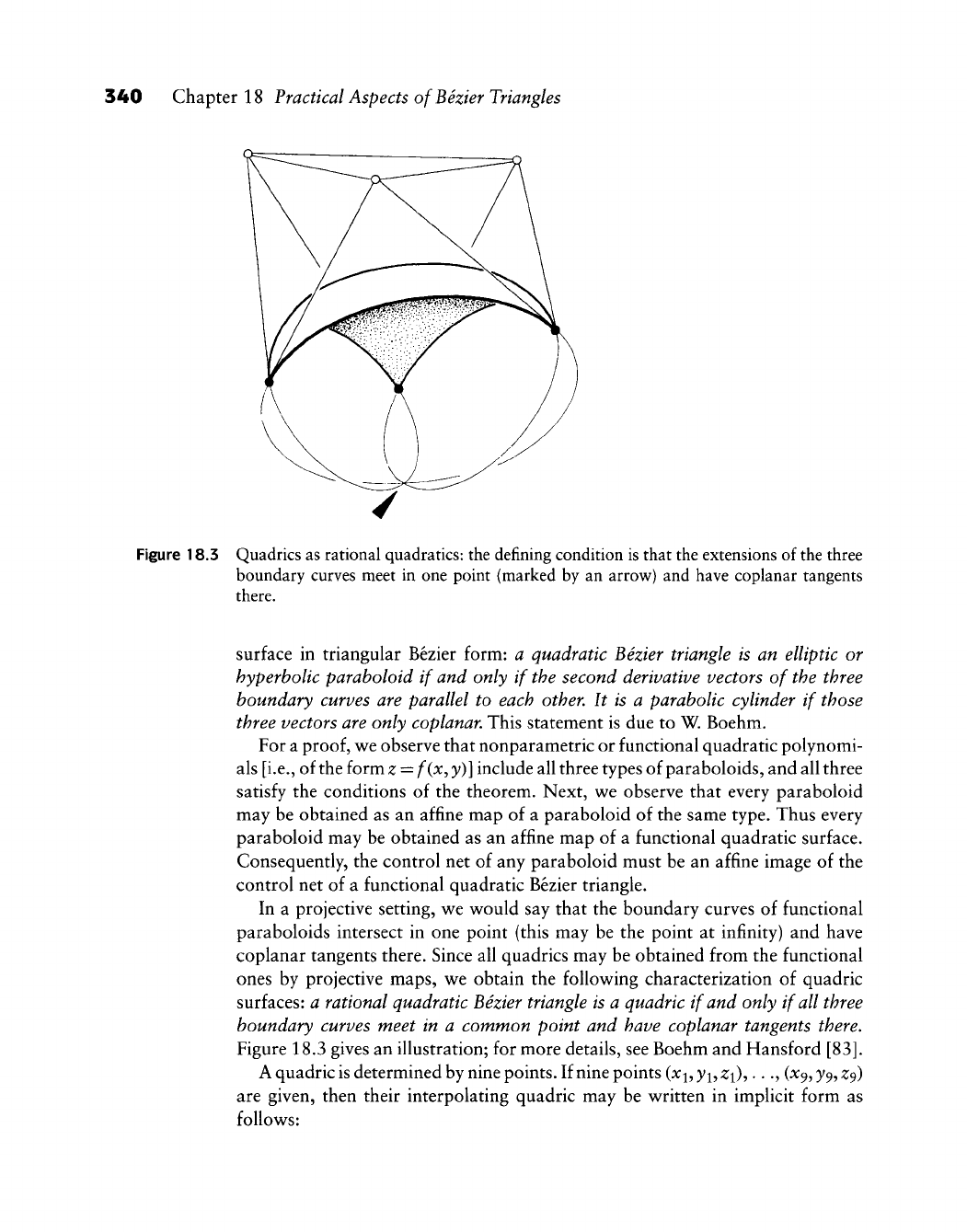
540 Chapter 18 Practical Aspects ofBezier Triangles
Figure 18.3 Quadrics as rational quadratics: the defining condition is that the extensions of the three
boundary curves meet in one point (marked by an arrow) and have coplanar tangents
there.
surface in triangular Bezier form: a quadratic Bezier triangle is an elliptic or
hyperbolic paraboloid if and only if the second derivative vectors of the three
boundary curves are parallel to each other. It is a parabolic cylinder if those
three vectors are only coplanar. This statement is due to W. Boehm.
For a
proof,
v^e observe that nonparametric or functional quadratic polynomi-
als [i.e., of the form z = f(x^ y)] include all three types of paraboloids, and all three
satisfy the conditions of the theorem. Next, we observe that every paraboloid
may be obtained as an affine map of a paraboloid of the same type. Thus every
paraboloid may be obtained as an affine map of a functional quadratic surface.
Consequently, the control net of any paraboloid must be an affine image of the
control net of a functional quadratic Bezier triangle.
In a projective setting, v^e w^ould say that the boundary curves of functional
paraboloids intersect in one point (this may be the point at infinity) and have
coplanar tangents there. Since all quadrics may be obtained from the functional
ones by projective maps, wt obtain the following characterization of quadric
surfaces: a rational quadratic Bezier triangle is a quadric if and only if all three
boundary curves meet in a common point and have coplanar tangents there.
Figure 18.3 gives an illustration; for more details, see Boehm and Hansford [83].
A quadric is determined by nine points. If nine points
(x^,
y^,
;^i),...,
(X9,
^9,
z^
are given, then their interpolating quadric may be w^ritten in implicit form as
foUovvrs:
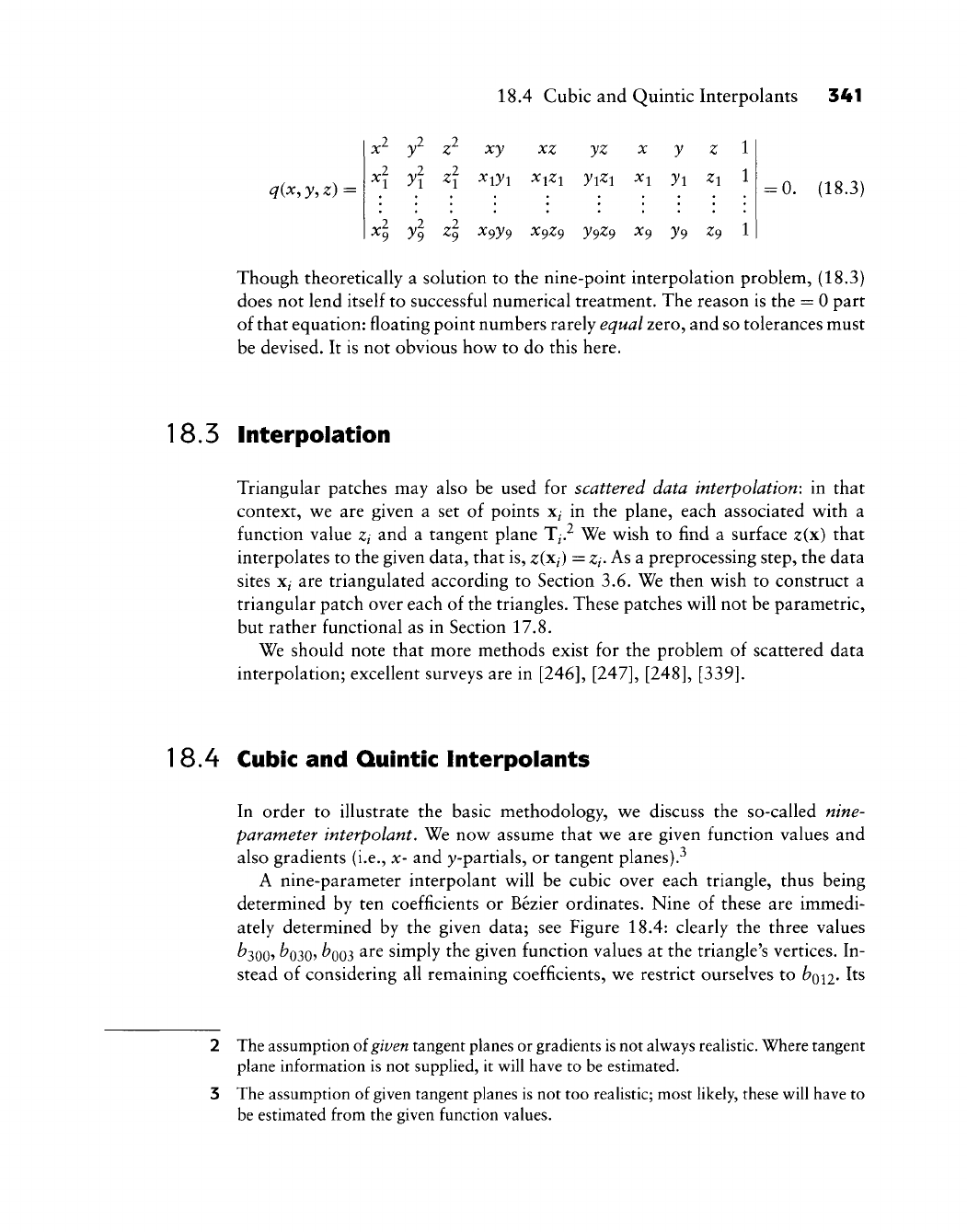
18.4 Cubic and Quintic Interpolants 341
q(x, y, z) =
111
x^
y^ z xy xz yz
q yj H ^i>'i ^1^1 >'i^i ^1 >'i ^1
<\ y\ zj x^y^ x^Z9 y^z^ x^ y^ z^ 1
:0.
(18.3)
Though theoretically a solution to the nine-point interpolation problem, (18.3)
does not lend itself to successful numerical treatment. The reason is the = 0 part
of that equation: floating point numbers rarely equal zero, and so tolerances must
be devised. It is not obvious how to do this here.
18.5 Interpolation
Triangular patches may also be used for scattered data interpolation: in that
context, we are given a set of points x^ in the plane, each associated with a
function value Zj and a tangent plane Tj? We wish to find a surface ^(x) that
interpolates to the given data, that is, zixj) =
Zj.
As a preprocessing step, the data
sites Xj are triangulated according to Section 3.6. We then wish to construct a
triangular patch over each of the triangles. These patches will not be parametric,
but rather functional as in Section 17.8.
We should note that more methods exist for the problem of scattered data
interpolation; excellent surveys are in
[246], [247], [248], [339].
1
8.4 Cubic and Quintic Interpolants
In order to illustrate the basic methodology, we discuss the so-called nine-
parameter interpolant. We now assume that we are given function values and
also gradients (i.e., x- and y-partials, or tangent planes).^
A nine-parameter interpolant will be cubic over each triangle, thus being
determined by ten coefficients or Bezier ordinates. Nine of these are immedi-
ately determined by the given data; see Figure 18.4: clearly the three values
^300? ^030? ^003 ^^^ simply the given function values at the triangle's vertices. In-
stead of considering all remaining coefficients, we restrict ourselves to fcoil- ^^
The assumption oi
given
tangent planes or gradients
is
not always
realistic.
Where tangent
plane information is not supplied, it will have to be estimated.
The assumption of given tangent planes is not too realistic; most likely, these will have to
be estimated from the given function values.
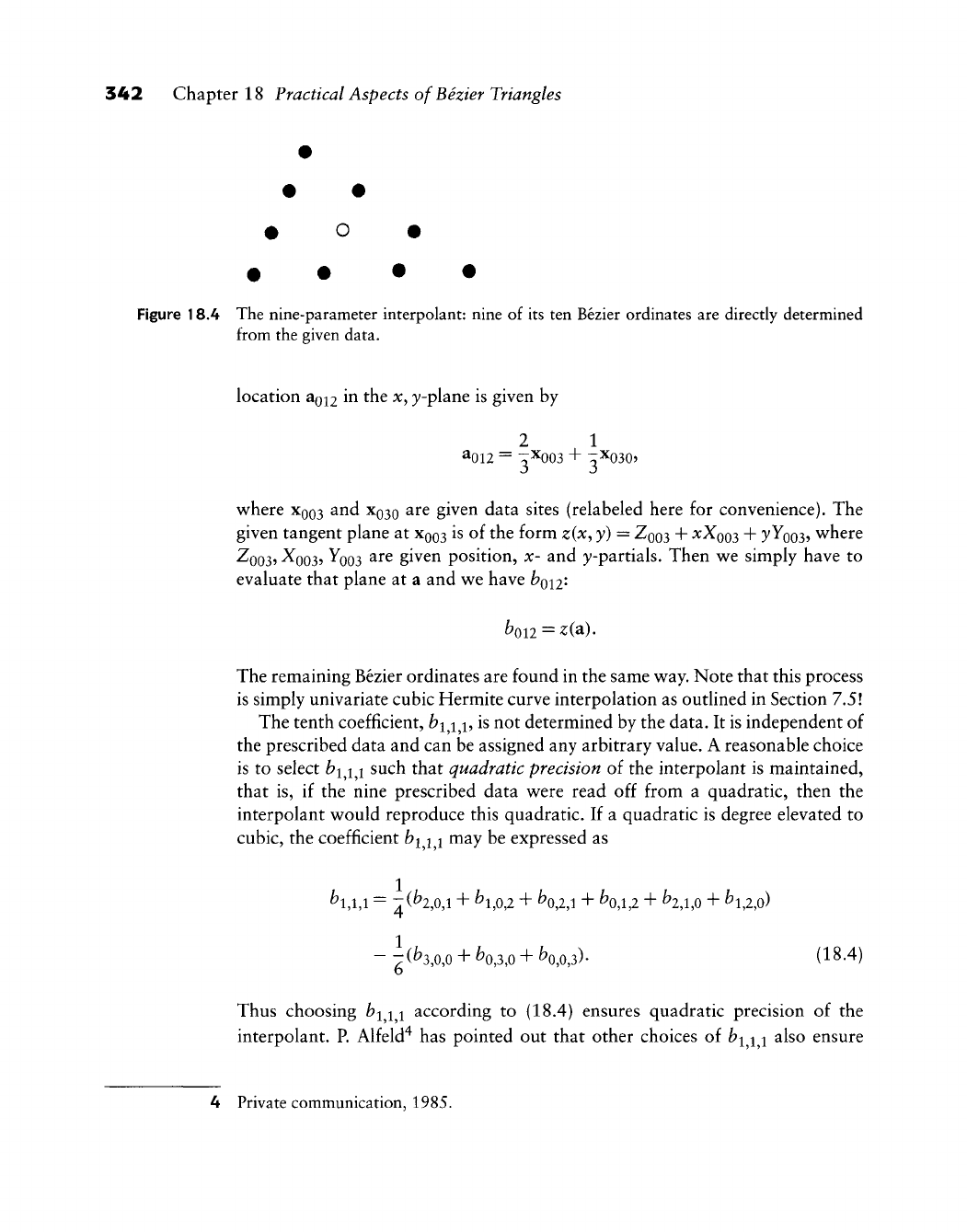
342 Chapter 18 Practical Aspects of Bezier Triangles
• O •
• • • •
Figure 18.4 The nine-parameter interpolant: nine of its ten Bezier ordinates are directly determined
from the given data.
location aon in the x,
}/-plane
is given by
2 1
^012 =
:TX003
+
:;Xo305
v^here XQOS and X030 are given data sites (relabeled here for convenience). The
given tangent plane at
XQOS
is of the form z{x^ y) =
Z003
+ ^^003 +
!V^003?
where
Zoo3,
^003? "^003 ^^^ given position, x- and y-partials. Then wt simply have to
evaluate that plane at a and we have fcoi2-
boi2 = z(a).
The remaining Bezier ordinates are found in the same
w^ay.
Note that this process
is simply univariate cubic Hermite curve interpolation as outlined in Section 7,51
The tenth coefficient, bm/is not determined by the data. It is independent of
the prescribed data and can be assigned any arbitrary value. A reasonable choice
is to select ^i 11 such that quadratic precision of the interpolant is maintained,
that is, if the nine prescribed data w^ere read off from a quadratic, then the
interpolant would reproduce this quadratic. If a quadratic is degree elevated to
cubic, the coefficient bm may be expressed as
1
^1,1,1
==
7(^2,0,1 + ^1,0,2 + ^2,1 + Vl,2 + ^2,1,0 + ^1,2,0)
-^(Ko,0 + V3,0 + Vo,3)- (18.4)
Thus choosing biii according to (18.4) ensures quadratic precision of the
interpolant. P. Alfeld"^ has pointed out that other choices of b^ii also ensure
4 Private communication, 1985.
18.5 The Clough-Tocher Interpolant 343
• • •
• O o •
• • o • «
• •••••
Figure 18.5 Quintic C^ interpolants: the solid points are derived from the C^ data at the vertices; the
open ones have to be chosen in order to ensure C^ continuity across patch boundaries.
quadratic precision; it is an open question if any of these choices can be sensibly
labeled "best."
In a situation where data are prescribed at several triangles in a triangulation,
the preceding interpolant has a serious drawback: it requires C^ data, but the
produced overall surface is only C^. You are invited to construct an example!
If we insist on C^ continuity, we could raise the degree from three to five.
We then have to prescribe position, two first and three second derivatives at
the vertices of each triangle. This fixes 18 of the quintic's 21 coefficients. The
remaining three are used to ensure C^ continuity between neighboring patches,
in the same way as described later for the Clough-Tocher interpolant. This
method for C^ interpolation is described in detail in [29]; see Figure 18.5 for
an illustration. Again, we have the drawback that second-order information has
to be supplied, yet only first-order smoothness is obtained.
18.5 The Clough-Tocher Interpolant
This interpolant is conceptually the simplest of all so-called split-triangle inter-
polants^ and it has been known in the finite element literature for some time; see
Strang and Fix
[582].
It is characterized by the "simplest" symmetric split of a
triangle: each vertex is joined to the triangle's centroid; thus a macro-triangle^ is
split into three mini-triangles. Any other interior point other than the centroid
would do; the centroid is chosen for symmetry reasons.
5 The given triangles in a triangulation are referred to as macro-triangles in order to
differentiate between them and the triangles resulting from the splitting process, the mini-
triangles.

344 Chapter 18 Practical Aspects ofBezier Triangles
The first-order data that this interpolant requires are position and gradient
value at the vertices of the macro-triangle plus some cross-boundary derivative
at the midpoint of each edge. The prescribed cross-boundary derivative could
be in any direction not parallel to its edge; but since adjacent macro-triangles
should share the same data along the common edge, it is most natural to choose
the direction perpendicular to that edge. We then speak of a cross-boundary
normal derivative.
In summary, we have 12 data per macro-triangle. It is easily seen that inter-
polation to this data produces a globally C^ surface if cubic polynomials are
employed over each mini-triangle.
We shall nov^ turn to the description of the actual interpolant; w^e refer to
Figure 18.6. The Bezier ordinates of the three boundary curves (marked by full
circles) are found exactly as for the nine-parameter interpolant. The next "layer"
of ordinates, marked by full circles and diamonds, is determined if v^e enforce
interpolation to the cross-boundary derivatives: the cross-boundary derivative,
evaluated along an edge, is a univariate quadratic polynomial. It can be v^ritten
as a univariate Bezier polynomial with three coefficients according to (17.19).
The first and last of the three coefficients is determined by the gradients at the
vertices, the center one as well by the cross-boundary derivative at the midpoints
of that edge.
We are still left with the task of specifying the ordinates marked by open cirlces
in Figure 18.6. Since the interpolant must be C^ over each macro-triangle, those
ordinates must satisfy the C^ conditions. Thus each of the three outer ordinates
of the four ones under consideration must be the average of the adjacent three
ordinates that have already been determined. Finally, the center ordinate must
be the average of the three just found.
In many applications, we will not be given the required cross-boundary deriva-
tives at the edge midpoints. The most obvious method to estimate this derivative
Figure 18.6 The Clough-Tocher interpolant: each macro-triangle is split into three mini-triangles.
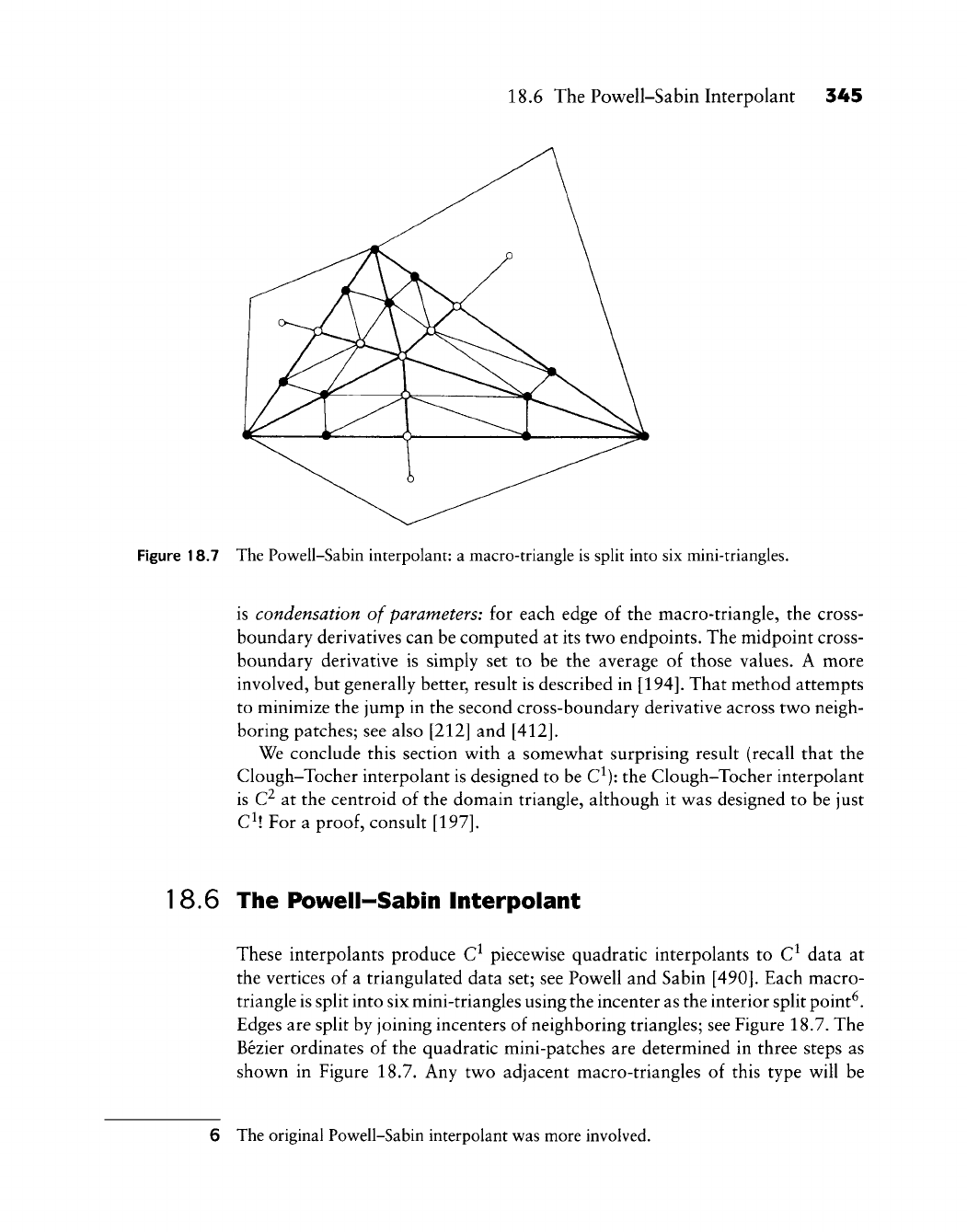
18.6 The Powell-Sabin Interpolant 345
Figure 18.7 The Powell-Sabin interpolant: a macro-triangle is split into six mini-triangles.
is condensation of parameters: for each edge of the macro-triangle, the cross-
boundary derivatives can be computed at its two endpoints. The midpoint cross-
boundary derivative is simply set to be the average of those values. A more
involved, but generally better, result is described in
[194].
That method attempts
to minimize the jump in the second cross-boundary derivative across tv^o neigh-
boring patches; see also [212] and
[412].
We conclude this section w^ith a somewhat surprising result (recall that the
Clough-Tocher interpolant is designed to be C^): the Clough-Tocher interpolant
is C^ at the centroid of the domain triangle, although it was designed to be just
C^! For a
proof,
consult
[197].
18.6 The Powell-Sabin Interpolant
These interpolants produce C^ piecewise quadratic interpolants to C^ data at
the vertices of a triangulated data set; see Powell and Sabin
[490].
Each macro-
triangle is split into six mini-triangles using the incenter as the interior split point^.
Edges are split by joining incenters of neighboring triangles; see Figure 18.7. The
Bezier ordinates of the quadratic mini-patches are determined in three steps as
shown in Figure 18.7. Any two adjacent macro-triangles of this type will be
6 The original Powell-Sabin interpolant was more involved.
346 Chapter
18
Practical Aspects ofBezier Triangles
differentiable across their common edge:
by
construction, each cross-boundary
derivative
is
just
one
hnear function instead
of
being piecev^ise hnear.
The Pov^ell-Sabin interpolant uses more triangles than does
the
Clough-
Tocher method—but
it is
easier
to
contour. Each Pow^ell-Sabin patch
is a
qua-
dratic
of the
form
z = f(x, y), and a
contour
is of the
form
c =
/"(x, y), that
is, a
conic. This conic
may be
v^ritten
as a
rational quadratic Bezier curve according
to Chapter
12. Its
Bezier points
and
w^eights
may be
determined
by
solving
a
number
of
quadratic equations;
see
[619].
18.7 Least Squares
Although
w^e
covered interpolation methods
so far,
approximation is
a
possibility
as v^ell.
In
that context,
we
v^ould
be
given
a
triangle
in
the
x,
3;-plane
and a set of
points ui,...,
Up
in the x,
y-plane, expressed
in
terms
of
barycentric coordinates
of the given triangle. Each
of
these points
has a
function value
Zj
associated v^ith
it.
We now^
seek
a
triangular functional Bezier patch
of a
given degree
n
that
approximates
the
given data:
^fe^EMfCu*). (18.5)
\i\=n
In order
to
tackle this problem,
wt
linearize this equation, similar
to
the approach
of Section 15.6. With
L =
{n-\-l)(n-\-2)
/2,
a
linearized version
of
(18.5) becomes
Zk^[B",,„(uk)
...
B«„oo("*)]
boOn
L
bnOO
(18.6)
There
are
several v^ays
to
construct
the
linearization;
a
simple
one
v^ould
be the
foUow^ing:
For
the
case
w
= 2, it
v^ould produce this ordering
of
indices:
(0,0,2),
(1,0,1), (2,0,0), (0,1,1), (1,1,0), (0,2,0).
Combining
all P
equations (18.6),
we
obtain
a
linear system
18.8 Problems 347
•^"oo«("i)
We abbreviate it as
B«oo("i)
^"„nn("L)J
Mb:
boOn
L b„QQ,
Zl
L^LJ
(18.7)
noting that M has many more rows than columns. The optimal solution to our
problem is obtained by solving the system of normal equations
M^Mb = M^z. (18.8)
It is also possible to formulate this type of least squares approximation for
the parametric case. Then, the function values
Zk
are replaced by data points p^
with associated parameter values u^.
18.8 Problems
1 Suppose that in Figure 18.1 we prescribed p instead of the three qj. We
could then find several sets of weights. Can that idea be generalized to
higher degrees?
2 Discuss how we could add shape equations to the least squares problem of
Section 18.7, in analogy to the approach taken in Section 15.6.
* 3 The Clough-Tocher interpolant turns out to be C^ at the centroid "for
free."
What can you say about the Powell-Sabin interpolant?
PI Non-split interpolants of degrees higher than three or five may be de-
fined for triangular patches. Experiment. Try to reproduce the Runge phe-
nomenon.
P2 Program up a triangulation algorithm for a 2D point set.
P3 Write a routine for constructing the Powell-Sabin interpolant over a 2D
triangulation.

This Page Intentionally Left Blank
W. Boehm
Differential
Geometry
II
19.1 Parametric Surfaces and Arc Element
A surface may be given by an implicit form f{x^ y^z) = 0 or, more useful for
CAGD, by its parametric form
X = X(W, V) —
x(u^ v)
y(u, v)
z(u, v)
"-[:]
G[a,b]c: (19.1)
where the cartesian coordinates x, y, z of a surface point are differentiable func-
tions of the parameters u and v and [a, b] denotes a rectangle in the w, i^-plane;
see Figure 19.1 (sometimes other domains are used, for example, triangles). To
avoid potential problems w^ith undefined normal vectors, we will assume
x^
A
x^
7^
0 for u
G
[a,
b],
that is, that both families of isoparametric lines are regular (see Section 10.1) and
are nowhere tangent to each other. Such a parametrization is called regular}
Any change r = r(u) of the parameters will not change the shape of the surface;
the new parametrization is regular if det[r^,
r^,]
/ 0 for u
G
[a,
b],
that is, if one
can find the inverse u = u(r) of r.
A regular curve u = u(^) in the
w,
i/-plane defines a regular curve x[u(^)] on the
surface. One can easily compute the (squared) arc element (see Section 10.1) of
1 Examples of irregular parametrizations are shown in Figures
14.11,
14.12, and
14.13.
349
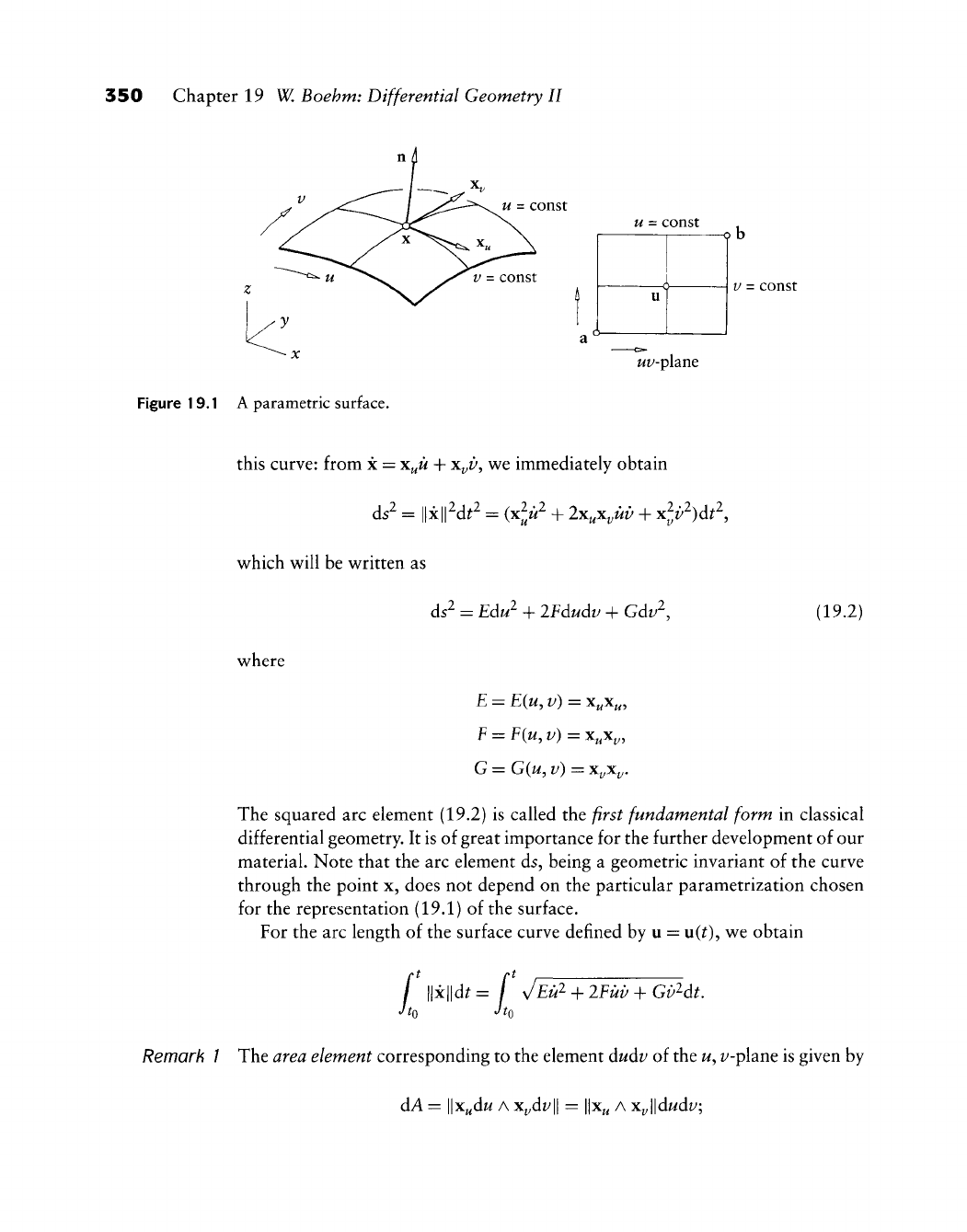
350 Chapter 19 W. Boehm: Differential Geometry II
u
=
const
V
=
const
Figure 19.1 A parametric surface.
u
=
const 0
uT
1
S
1
uv-plsine
V
=
const
this curve: from x = x^u + x^z), we immediately obtain
ds^
= ||x||^d^^ = (xlii^ + Ix^Xytiv + xlv^)dt^,
which will be written as
ds^
= Edu^ + IFdudv + Gdv^, (19.2)
where
E = E{u, v) = x^x^,
E = F(u, v) = x^Xy,
G = G(u, v) = x^x^.
The squared arc element (19.2) is called the first fundamental form in classical
differential geometry. It is of great importance for the further development of our
material. Note that the arc element ds, being a geometric invariant of the curve
through the point x, does not depend on the particular parametrization chosen
for the representation (19.1) of the surface.
For the arc length of the surface curve defined by u =
\x{t)^
we obtain
/
||x||d^=
f
JtQ Jto
^Eu^
+ lEuv + GiP^dt,
Remark / The area element corresponding to the element dudv of the
w,
i/-plane is given by
dA = llx^dw
A
x^dz/|| = ||x^
A
xjdudv;
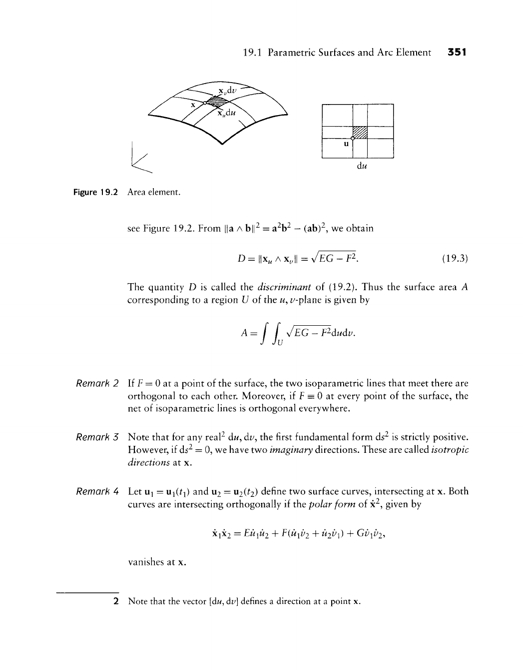
19.1 Parametric Surfaces and Arc Element 351
u
m
du
Figure 19.2 Area element.
see Figure 19.2. From ||a
A
hf = aV - (ab)^, we obtain
D=||x„Ax,||=y£G-f2. (19.3)
The quantity D is called the discriminant of (19.2). Thus the surface area A
corresponding to a region U of the
w,
i^-plane is given by
A
-IL^-
F^dudv.
Remark 2 If P = 0 at a point of the surface, the two isoparametric lines that meet there are
orthogonal to each other. Moreover, if f = 0 at every point of the surface, the
net of isoparametric lines is orthogonal everywhere.
Remark 5 Note that for any real^ du, dv, the first fundamental form ds^ is strictly positive.
However, if ds^ = 0, we have two imaginary directions. These are called isotropic
directions at x.
Remark 4 Let u^ = Vi\{ti) and
U2
= ^^liti) define two surface curves, intersecting at x. Both
curves are intersecting orthogonally if the polar form of x^, given by
X2X2 = EuiU2 + F{uiV2 + U2V\) -\- GviVi,
vanishes at x.
2 Note that the vector
[dw,
dv]
defines a direction at a point x.
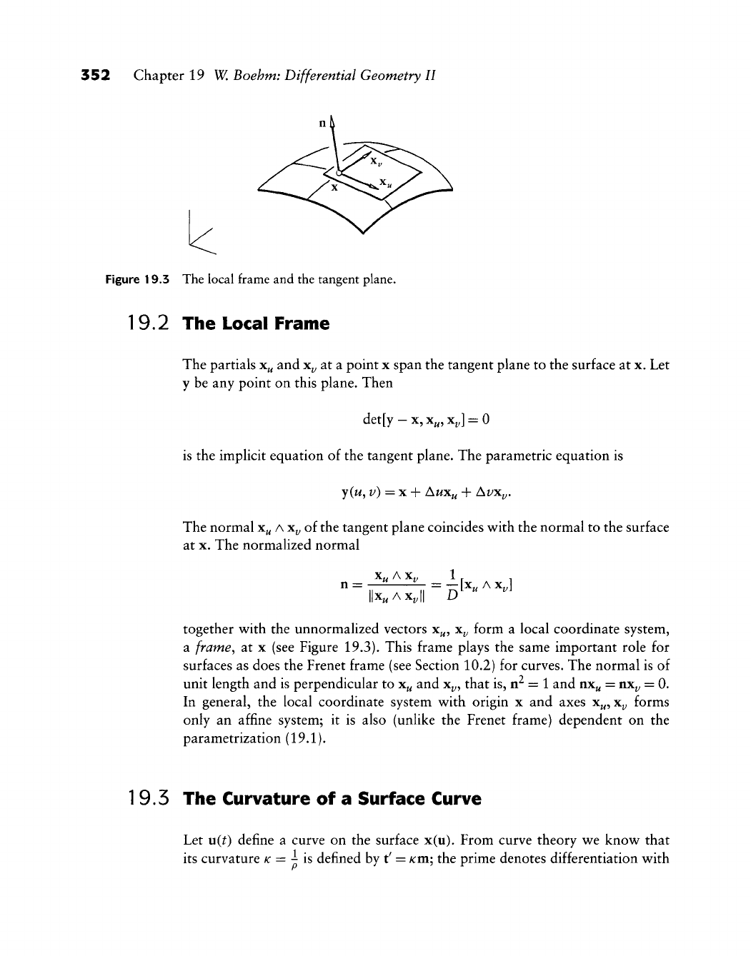
352 Chapter 19 W, Boehm: Differential Geometry II
Figure 19.3 The local frame and the tangent plane.
1
9.2 The Local Frame
The partials x^ and x^ at a point x span the tangent plane to the surface at x. Let
y be any point on this plane. Then
det[y -
X,
x^, x^] = 0
is the implicit equation of the tangent plane. The parametric equation is
y(w, v) =x-\-
AuXj^
+ At/x^.
The normal x^
A
x^ of the tangent plane coincides with the normal to the surface
at X. The normalized normal
n=„''^'^''"„=7-KAxJ
llx^Ax^ll D
together with the unnormalized vectors x^, x^ form a local coordinate system,
a frame, at x (see Figure 19.3). This frame plays the same important role for
surfaces as does the Frenet frame (see Section 10.2) for curves. The normal is of
unit length and is perpendicular to x^ and Xj,, that is, n^ = 1 and nx^ =
nx^^
= 0.
In general, the local coordinate system with origin x and axes x^,
Xp
forms
only an affine system; it is also (unlike the Frenet frame) dependent on the
parametrization (19.1).
1
9.5 The Curvature of a Surface Curve
Let u(t) define a curve on the surface x(u). From curve theory we know that
its curvature
K
= ^ is defined by t^ = /cm; the prime denotes differentiation with
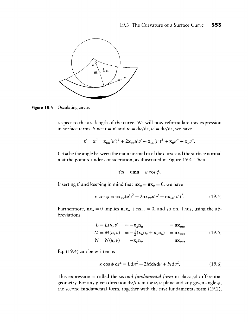
19.3 The Curvature of a Surface Curve 353
Figure 19.4 Osculating circle.
respect to the arc length of the curve. We will now reformulate this expression
in surface terms. Since t = x^ and u' = dw/ds, v' = dt'/ds, we have
t' = x'' = x^^iu'f + Ix^^u'v' + x^^iv'f + x^ + xy.
Let 0 be the angle between the main normal m of the curve and the surface normal
n at the point x under consideration, as illustrated in Figure 19.4. Then
t n = /cmn = K
COS
0.
Inserting t^ and keeping in mind that nx^ = nx^ = 0, we have
K
cos 0 =
nxj^j^{u')
+
2nXj^jjU^v^
+
nx^^{v^)'^.
(19.4)
Furthermore, nx^ = 0 implies n^^x^^ + nx^^ = 0, and so on. Thus, using the ab-
breviations
L = L(u, v) = -x^n^ = nx^^,
M = M(u,v) =-^(x^n^ + x^nJ = nx^^, (19.5)
N = N{u, v) = -XyXiy = nx^^,
Eq. (19.4) can be written as
K
cos 0 ds^ = Ldu^ + IMdudv + Ndv^, (19.6)
This expression is called the second fundamental form in classical differential
geometry. For any given direction du/dv in the
w,
^'-plane and any given angle 0,
the second fundamental form, together with the first fundamental form (19.2),
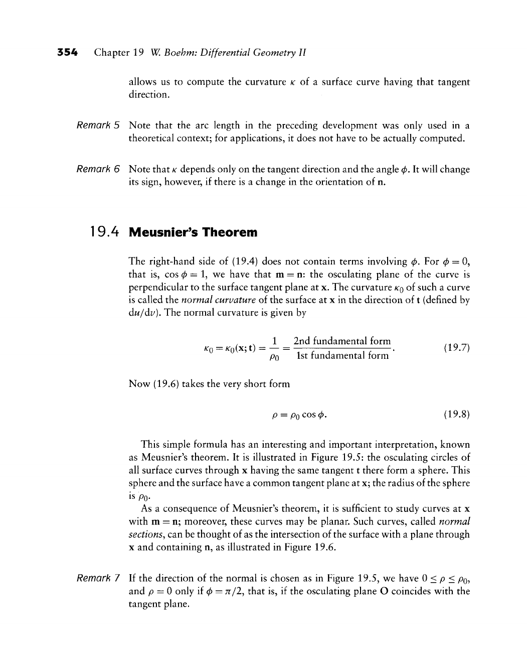
354 Chapter 19 W. Boehm: Differential Geometry II
allows us to compute the curvature /c of a surface curve having that tangent
direction.
Remark 5 Note that the arc length in the preceding development was only used in a
theoretical context; for applications, it does not have to be actually computed.
Remark 6 Note that
K
depends only on the tangent direction and the angle 0. It will change
its sign, however, if there is a change in the orientation of n.
19.4 Meusnier's Theorem
The right-hand side of (19.4) does not contain terms involving 0. For 0 = 0,
that is, cos 0 = 1, we have that m = n: the osculating plane of the curve is
perpendicular to the surface tangent plane at x. The curvature
KQ
of such a curve
is called the normal curvature of the surface at x in the direction of t (defined by
du/dv).
The normal curvature is given by
_
N
_ 1 _ ^^d fundamental form
Po 1st fundamental form (19.7)
Now (19.6) takes the very short form
p =
Po
cos 0. (19.8)
This simple formula has an interesting and important interpretation, known
as Meusnier's theorem. It is illustrated in Figure 19.5: the osculating circles of
all surface curves through x having the same tangent t there form a sphere. This
sphere and the surface have a common tangent plane at x; the radius of the sphere
is Po-
As a consequence of Meusnier's theorem, it is sufficient to study curves at x
with m = n; moreover, these curves may be planar. Such curves, called normal
sections^ can be thought of as the intersection of the surface with a plane through
X and containing n, as illustrated in Figure 19.6.
Remark 7 If the direction of the normal is chosen as in Figure 19.5, we have 0 < p < po,
and p = 0 only if 0 = 7r/2, that is, if the osculating plane O coincides with the
tangent plane.
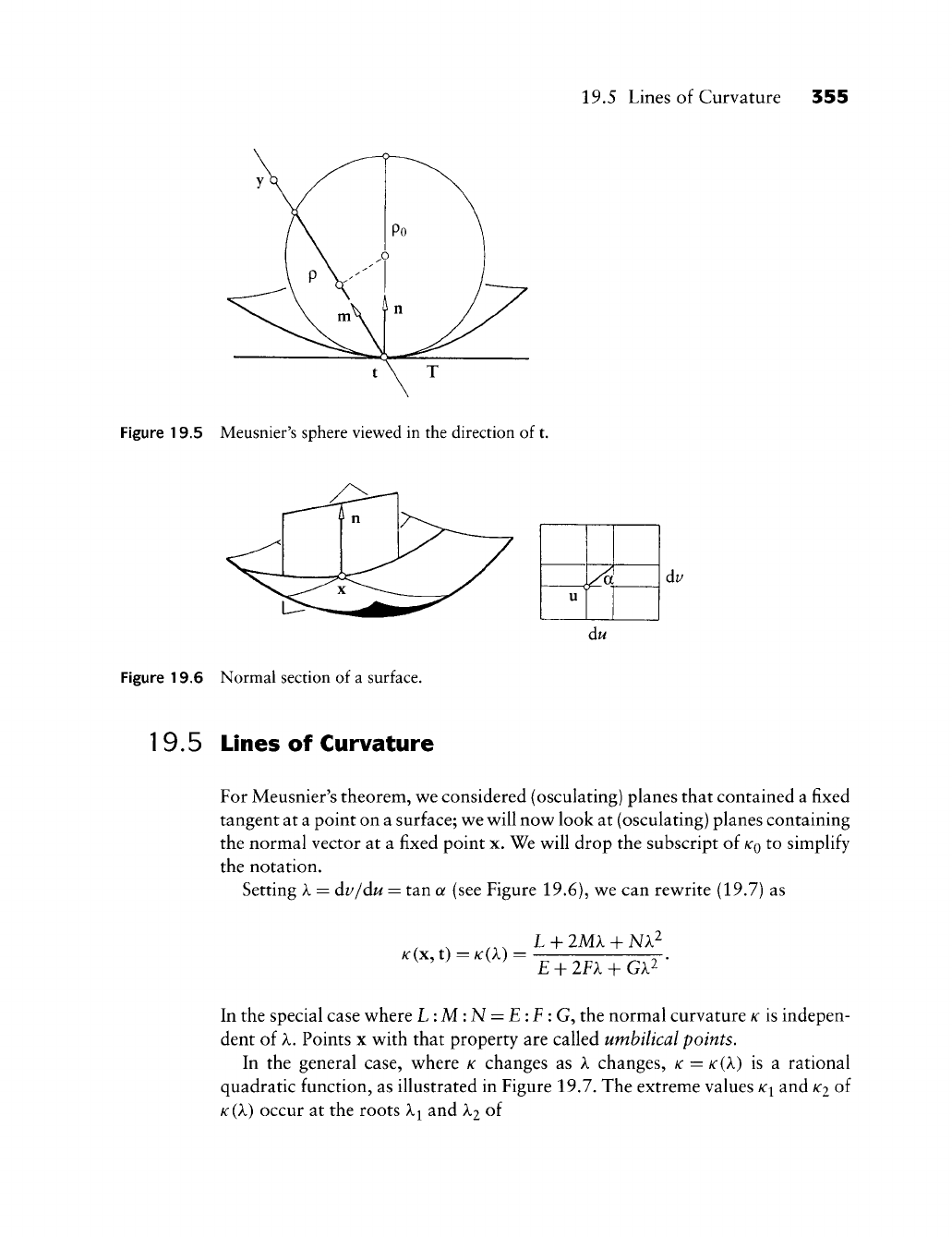
19.5 Lines of Curvature 355
Figure 19.5 Meusnier's sphere viewed in the direction of t.
u A dv
du
Figure 19.6 Normal section of a surface.
19.5 Lines of Curvature
For Meusnier's theorem, we considered (osculating) planes that contained a fixed
tangent at a point on a surface; we will now look at (osculating) planes containing
the normal vector at a fixed point x. We will drop the subscript of
KQ
to simplify
the notation.
Setting X = dv/du = tan a (see Figure 19.6), we can rewrite (19.7) as
In the special case where L:M:N = E:F :G^ the normal curvature
K
is indepen-
dent of
A.
Points x with that property are called umbilical points.
In the general case, where K changes as X changes, K =
K{X)
is a rational
quadratic function, as illustrated in Figure 19.7. The extreme values
/c^
and
KI
of
KQC)
occur at the roots Xi and
X2
of
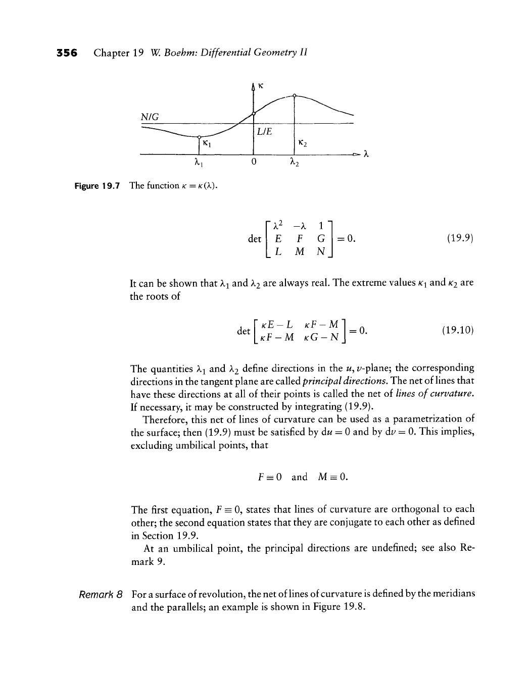
356 Chapter 19 W, Boehm: Differential Geometry II
Figure 19.7 The function
K
=K(X).
ri2
det
-X 1
E F G
L M N
= 0. (19.9)
It can be shown that
X^
and
X2
are always real. The extreme values
K^
and
K2
are
the roots of
det KE
KF-
-L KF-M1_
M KG-N\~ (19.10)
The quantities X^ and X2 define directions in the u, i^-plane; the corresponding
directions in the tangent plane are called principal directions. The net of lines that
have these directions at all of their points is called the net of lines of curvature.
If necessary, it may be constructed by integrating (19.9).
Therefore, this net of lines of curvature can be used as a parametrization of
the surface; then (19.9) must be satisfied by dw = 0 and by Av = 0. This implies,
excluding umbilical points, that
F = 0 and M = 0.
The first equation, f = 0, states that lines of curvature are orthogonal to each
other; the second equation states that they are conjugate to each other as defined
in Section 19.9.
At an umbilical point, the principal directions are undefined; see also Re-
mark 9.
Remark 8 For a surface of revolution, the net of
lines
of curvature is defined by the meridians
and the parallels; an example is shown in Figure 19.8.
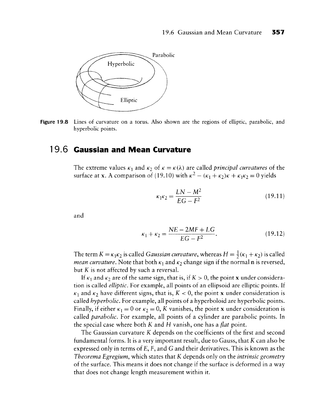
19.6 Gaussian and Mean Curvature 357
^ Parabolic
Hyperbolic
Figure 19.8 Lines of curvature on a torus. Also shown are the regions of eUiptic, parabolic, and
hyperbolic points.
19.6 Gaussian and Mean Curvature
The extreme values /c^ and
K2
oi
K
= /c(A) are called principal curvatures of the
surface at x. A comparison of (19.10) with /c^
—
(/c^ + K2)K +
KIKI
= 0 yields
LN-M^ ,._...
/Ci/C2= ^ 19.11
EG-F^
and
NE-2MP + LG
,.„..,
/C1+/C2 — . 19.12
The term K =
KIKI
is called Gaussian curvature^ whereas H =
^
(^l + ^l)
i^
called
mean curvature. Note that both
K\
and
/C2
change sign if the normal n is reversed,
but K is not affected by such a reversal.
If
K\
and
K2
are of the same sign, that is, if K > 0, the point x under considera-
tion is called elliptic. For example, all points of an ellipsoid are elliptic points. If
Ki and
/C2
have different signs, that is, K < 0, the point x under consideration is
called hyperbolic. For example, all points of a hyperboloid are hyperbolic points.
Finally, if either
/c^
= 0 or
A:2
= 0, iC vanishes, the point x under consideration is
called parabolic. For example, all points of a cylinder are parabolic points. In
the special case where both K and H vanish, one has a ^at point.
The Gaussian curvature K depends on the coefficients of the first and second
fundamental forms. It is a very important result, due to Gauss, that K can also be
expressed only in terms of £, F, and G and their derivatives. This is known as the
Theorema Egregium., which states that K depends only on the intrinsic geometry
of the surface. This means it does not change if the surface is deformed in a way
that does not change length measurement within it.
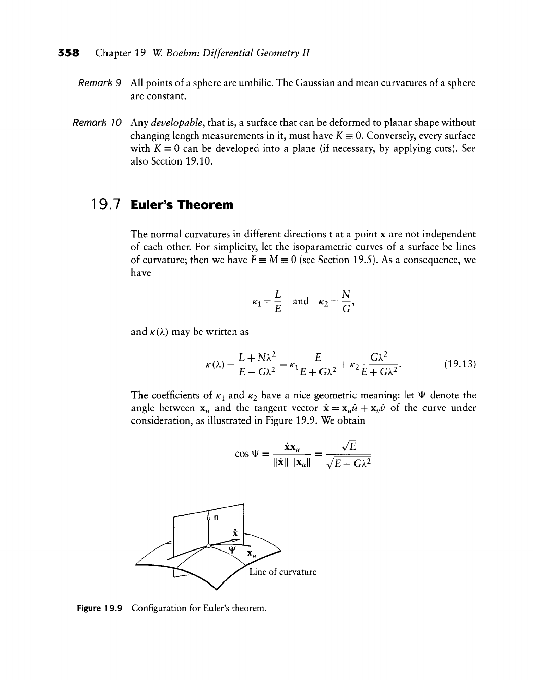
358 Chapter 19 W, Boehm: Differential Geometry II
Remark 9 All points of a sphere are umbilic. The Gaussian and mean curvatures of a sphere
are constant.
Remark W Any developable^ that is, a surface that can be deformed to planar shape without
changing length measurements in it, must have X = 0. Conversely, every surface
with K = 0 can be developed into a plane (if necessary, by applying cuts). See
also Section 19.10.
19.7 Euler's Theorem
The normal curvatures in different directions t at a point x are not independent
of each other. For simplicity, let the isoparametric curves of a surface be lines
of curvature; then we have P = M = 0 (see Section 19.5). As a consequence, we
have
L , N
/ci=-
and '<^2=-^^
and
K(X)
may be written as
^^^ L + NX^ E
K(X) = ^ ^ ., = Ki + ^21 Gk^
E + GX^ 'E + GX^ ^E + GA.2 (19.13)
The coefficients of
K-[
and KI have a nice geometric meaning: let ^ denote the
angle between x„ and the tangent vector x =
X„M
+ x^v of the curve under
consideration, as illustrated in Figure 19.9. We obtain
cos ^
—
xx„ VI
\n llxjl ^E
+
GX^
Line of curvature
Figure 19.9 Configuration for Euler's theorem.
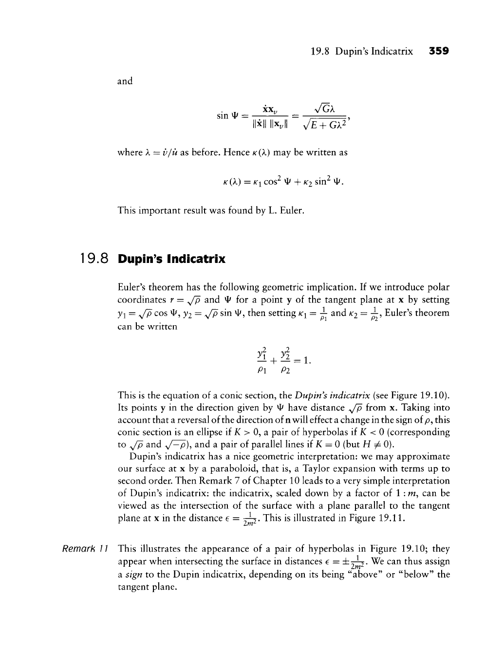
and
sin vl/ = ^
19.8 Dupin's Indicatrix 359
^/GA.
llxll ||x,|| ^E + GA^'
where
A
= vju as before. Hence K(X) may be written as
K(X) = /ci cos^ ^ +
/C2
sin^ ^.
This important resuh was found by L. Euler.
19.8 Dupin's Indicatrix
Euler's theorem has the following geometric implication. If we introduce polar
coordinates r = ^p and ^ for a point y of the tangent plane at x by setting
y^
= ^
COS
^, ^2 = ^ sin ^, then setting ^\ = -^ and K2=
j--,
Euler's theorem
can be written
2 2
Pi Pi
This is the equation of a conic section, the Dupin's indicatrix (see Figure 19.10).
Its points y in the direction given by ^ have distance ,y/p from x. Taking into
account that a reversal of the direction of n will effect a change in the sign of
p,
this
conic section is an ellipse if
i<C
> 0, a pair of hyperbolas if K < 0 (corresponding
to yp and ^—p), and a pair of parallel lines if X = 0 (but H ^ 0).
Dupin's indicatrix has a nice geometric interpretation: we may approximate
our surface at x by a paraboloid, that is, a Taylor expansion with terms up to
second order. Then Remark 7 of Chapter 10 leads to a very simple interpretation
of Dupin's indicatrix: the indicatrix, scaled down by a factor of 1
:
m, can be
viewed as the intersection of the surface with a plane parallel to the tangent
plane at x in the distance 6 = y^. This is illustrated in Figure
19.11.
Remark 11 This illustrates the appearance of a pair of hyperbolas in Figure 19.10; they
appear when intersecting the surface in distances 6 = ±y^. We can thus assign
a sign to the Dupin indicatrix, depending on its being "above" or "below" the
tangent plane.
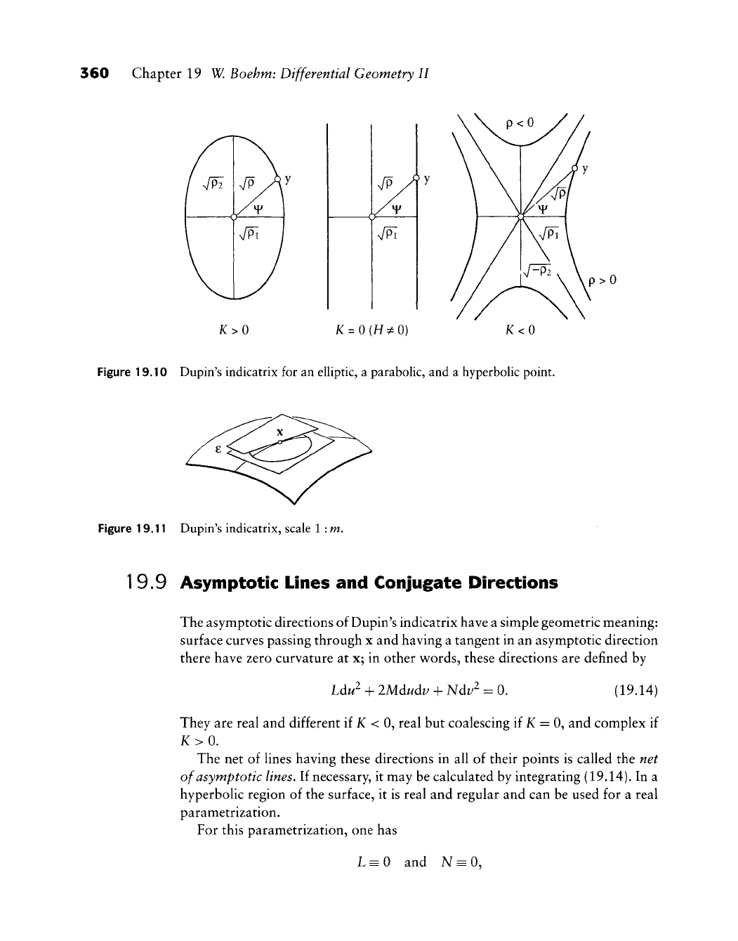
360 Chapter 19 W. Boehm: Differential Geometry II
p>0
K>0 K
=
0(H^O) K<0
Figure 19.10 Dupin's indicatrix for an elliptic, a parabolic, and a hyperbolic point.
Figure 19.11 Dupin's indicatrix, scale 1
:
m.
1
9.9 Asymptotic Lines and Conjugate Directions
The asymptotic directions of Dupin's indicatrix have a simple geometric meaning:
surface curves passing through x and having a tangent in an asymptotic direction
there have zero curvature at x; in other v^ords, these directions are defined by
Ldu^ + IMdudv + Ndv^ = 0. (19.14)
They are real and different if K < 0, real but coalescing if K = 0, and complex if
K>0.
The net of lines having these directions in all of their points is called the net
of asymptotic lines. If necessary, it may be calculated by integrating (19.14). In a
hyperbolic region of the surface, it is real and regular and can be used for a real
parametrization.
For this parametrization, one has
L = 0 and N = 0,
19.10 Ruled Surfaces and Developables 361
and vice versa.
As earlier, let y be a point on Dupin's indicatrix at a point x. Let y denote its
tangent direction at y. The direction y is called conjugate to the direction x from
X
to y. Consider two surface curves
\Xi{ti)
and 02(^2) ^hat have tangent directions
xi and
X2
at x. Some elementary calculations yield that x^ is conjugate to
X2
if
Liiiiii + M(^iz>2 + ^2^1) +
Nz>iZ>2
= 0.
Note that this expression is symmetric in u^,
U2.
By definition asymptotic direc-
tions are self-conjugate.
Remark 12 Isoparametric curves of a surface are conjugate if M = 0 and vice versa.
Remark 15 The principal directions, defined by (19.9), are orthogonal and conjugate; they
bisect the angles between the asymptotic directions; that is, they are the axis
directions of Dupin's indicatrix (see Figure 19.10).
Remark 14 The tangent planes of two "consecutive" points on a surface curve intersect in a
straight line s. Let the curve have direction t at a point x on the surface. Then s
and t are conjugate to each other. In particular, if t is an asymptotic direction, s
coincides with t. If t is one of the principal directions at x, then s is orthogonal to
t and vice versa. These properties characterize lines of curvature and asymptotic
lines and may be used to define them geometrically.
19.10 Ruled Surfaces and Developables
If a surface contains a family of straight lines, it is called a ruled surface. It is
convenient to use these straight lines as one family of isoparametric lines. Then
the ruled surface may be written
x = x(t,v)=p(t)-\-vq(t), (19.15)
where p is a point and q is a vector, both depending on t. The isoparametric lines
t = const are called the generatrices of the surface; see Figure 19.12.
The partials of a ruled surface are given by
x^
= p + i^q and
x^^
= q. The normal
n at
X
is given by
n =
(p + t^q)
A
q
||(p + i/q)Aq||
A point y on the tangent plane at x satisfies
det[y - p, p, q] + zydet[y - p, q, q] = 0;
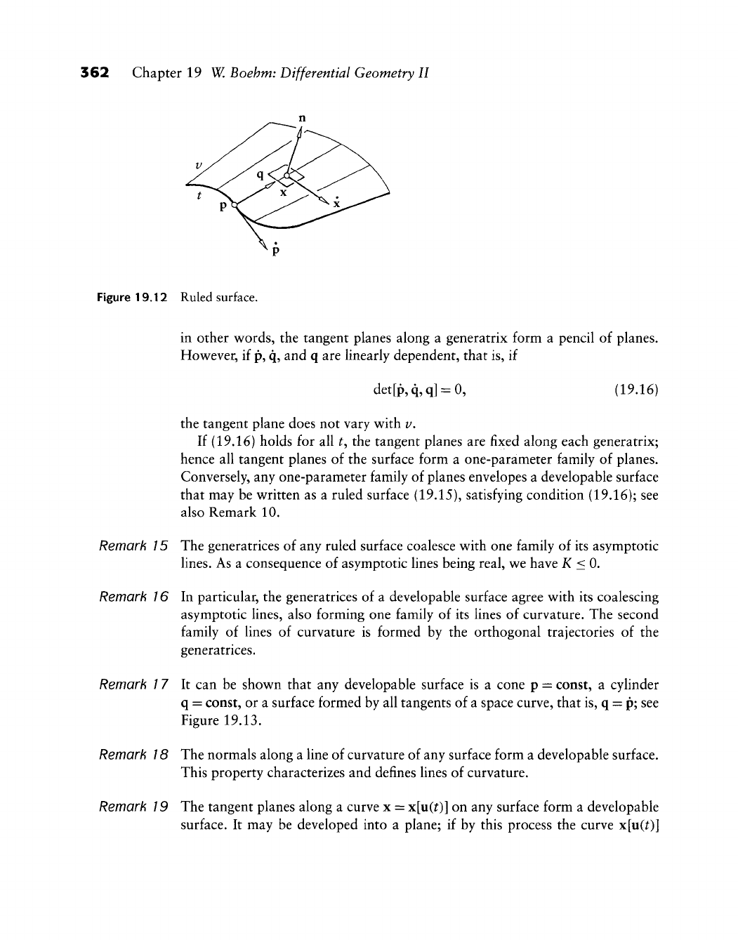
362 Chapter 19 W. Boehm: Differential Geometry II
Figure 19.12 Ruled surface.
in other words, the tangent planes along a generatrix form a pencil of planes.
However, if p, q, and q are linearly dependent, that is, if
det[p,q,q] = 0, (19.16)
the tangent plane does not vary with v.
If (19.16) holds for all f, the tangent planes are fixed along each generatrix;
hence all tangent planes of the surface form a one-parameter family of planes.
Conversely, any one-parameter family of planes envelopes a developable surface
that may be written as a ruled surface (19.15), satisfying condition (19.16); see
also Remark 10.
Remark / 5 The generatrices of any ruled surface coalesce with one family of its asymptotic
lines.
As a consequence of asymptotic lines being real, we have K <0,
Remark 16 In particular, the generatrices of a developable surface agree with its coalescing
asymptotic lines, also forming one family of its lines of curvature. The second
family of lines of curvature is formed by the orthogonal trajectories of the
generatrices.
Remark
1
7 It can be shown that any developable surface is a cone p = const, a cylinder
q = const, or a surface formed by all tangents of a space curve, that is, q = p; see
Figure
19.13.
Remark 18 The normals along a line of curvature of any surface form a developable surface.
This property characterizes and defines lines of curvature.
Remark 19 The tangent planes along a curve x = x[u(0] on any surface form a developable
surface. It may be developed into a plane; if by this process the curve x[u(0]
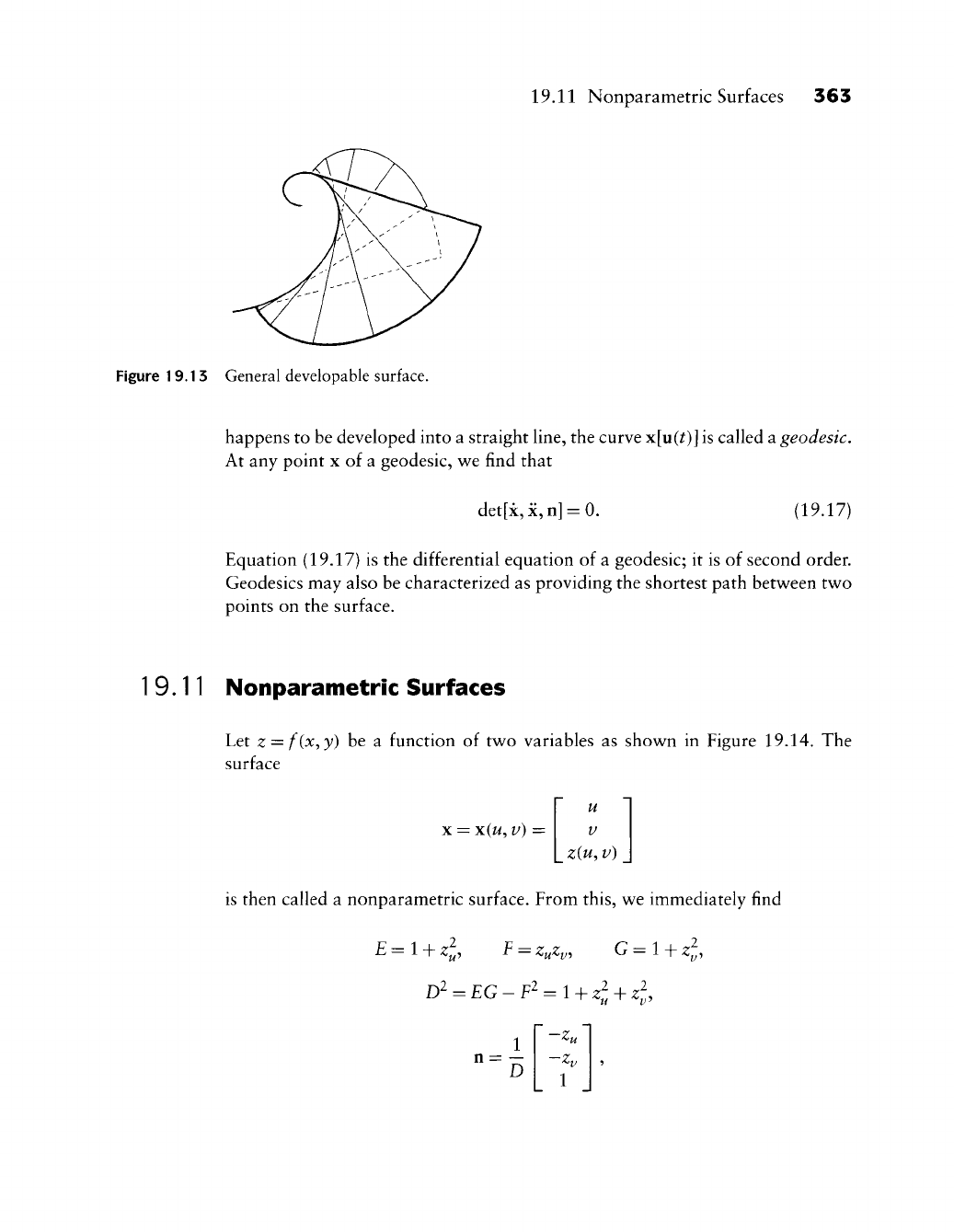
19.11 Nonparametric Surfaces 365
Figure 19.13 General developable surface.
happens to be developed into a straight line, the curve x[u(0] is called a geodesic.
At any point x of a geodesic, we find that
det[x,
X,
n] = 0. (19.17)
Equation (19.17) is the differential equation of a geodesic; it is of second order.
Geodesies may also be characterized as providing the shortest path betw^een two
points on the surface.
19.11 Nonparametric Surfaces
Let z = f(x,y) be a function of two variables as shown in Figure 19.14. The
surface
X
= x(w, v)
u
V
z(u, v)
is then called a nonparametric surface. From this, we immediately find
D^
= EG-F^ = l + zl + zl,
n = D Zy
1
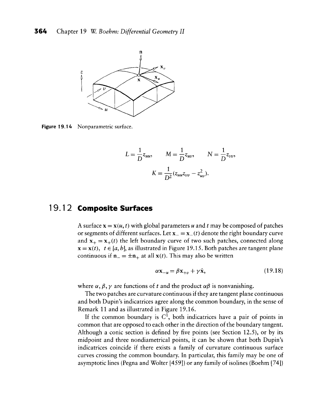
364 Chapter 19 W. Boehm: Differential Geometry II
Figure 19.14 Nonparametric surface.
Ill
D2'
^ T^o y^uu^vv ^uv^'
19.12 Composite Surfaces
A surface x = x(w, t) with global parameters u and t may be composed of patches
or segments of different surfaces. Let x_ = x_(0 denote the right boundary curve
and x_^ = x_^(0 the left boundary curve of two such patches, connected along
X
=
xCO,
t
G
[a^
b\ as illustrated in Figure 19.15. Both patches are tangent plane
continuous if n_ = ibn_^ at all x(^). This may also be written
QfX.
-u
=
P^-hv
+ yx, (19.18)
where a,
)6,
y are functions of t and the product afi is nonvanishing.
The two patches are curvature continuous if they are tangent plane continuous
and both Dupin's indicatrices agree along the common boundary, in the sense of
Remark 11 and as illustrated in Figure 19.16.
If the common boundary is C\ both indicatrices have a pair of points in
common that are opposed to each other in the direction of the boundary tangent.
Although a conic section is defined by five points (see Section 12.5), or by its
midpoint and three nondiametrical points, it can be shown that both Dupin's
indicatrices coincide if there exists a family of curvature continuous surface
curves crossing the common boundary. In particular, this family may be one of
asymptotic lines (Pegna and Wolter [459]) or any family of isolines (Boehm [74])
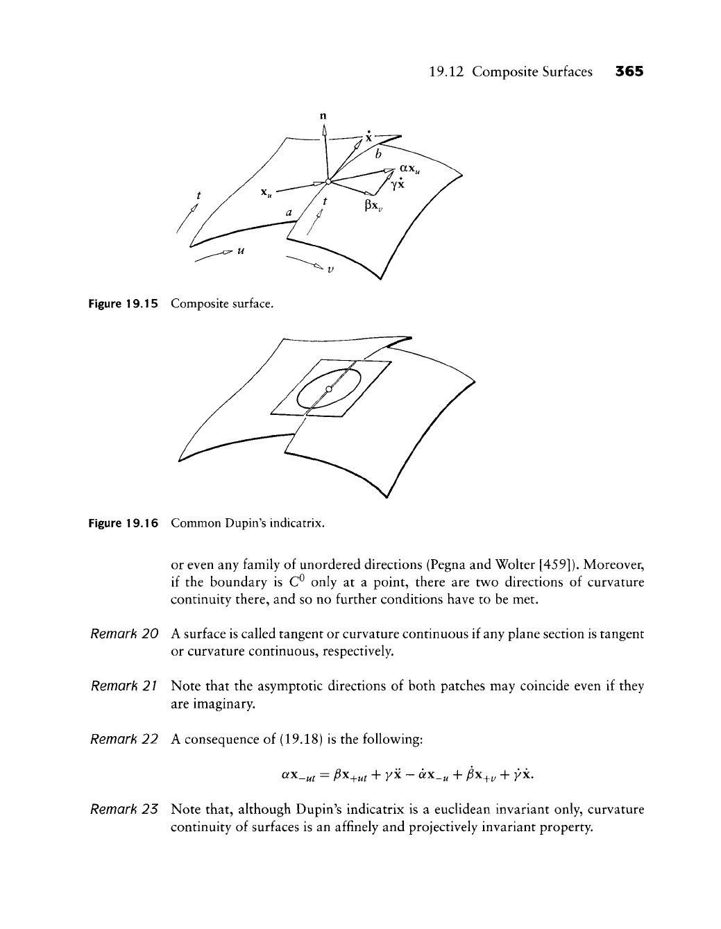
19.12 Composite Surfaces 365
Figure 19.15 Composite surface.
Figure 19.16 Common Dupin's indicatrix.
or even any family of unordered directions (Pegna and Wolter [459]). Moreover,
if the boundary is C^ only at a point, there are two directions of curvature
continuity there, and so no further conditions have to be met.
Remark 20 A surface is called tangent or curvature continuous if any plane section is tangent
or curvature continuous, respectively.
Remark 2 / Note that the asymptotic directions of both patches may coincide even if they
are imaginary.
Remark 22 A consequence of (19.18) is the following:
ax_^t = fix^^t + yx- ax_^ + $x^^ + yx.
Remark 25 Note that, although Dupin's indicatrix is a euclidean invariant only, curvature
continuity of surfaces is an affinely and projectively invariant property.

This Page Intentionally Left Blank
Geometric
Continuity for
Surfaces
I he concept of geometric continuity is not restricted to curves. Surfaces in this
regard are much more complex to deal with, so we will restrict ourselves to the
case of first-order geometric continuity. Here are some pointers to the literature:
Boehm [77], Charrot and Gregory
[110],
DeRose
[161],
Farin
[190],
Gregory
[291],
Hahn
[306],
Herron
[322],
Liu and Hoschek
[395],
Kahmann
[350],
Kiciak
[356],
Jensen
[343],
Jones
[349],
Nielson
[447],
Piper
[483],
Sarraga
[536], [537],
Shirman and Sequin
[573],
van Wijk
[594],
Vinacua and Brunet
[603],
and Veron et al.
[600].
20.1 Introduction
Let us take a look at Figure
20.1.
It shows the (potential) boundary curves of two
cubic triangular Bezier patches. In each, the interior control point bx^ is missing.
Can we determine these two missing points such that the resulting two patches
form a C^ surface.^ We must thus produce two control nets that satisfy the C^
condition as illustrated in Figure
17.11.
But this is not possible in our example:
the two shaded pairs of triangles in Figure 20.1 are not affine pairs in the sense
of Section 17.6, that is, they cannot be obtained as an affine map of one pair of
domain triangles.
We have a better chance of solving the problem if we relax the requirement
of C^ continuity to that of G^ continuity: two patches with a common boundary
curve are called G^ if they have a continuously varying tangent plane along that
boundary curve. The concept of G^ continuity is a genuine generalization of C^
continuity: all (nondegenerate) C^ surfaces are G\ but not the other way around.
367
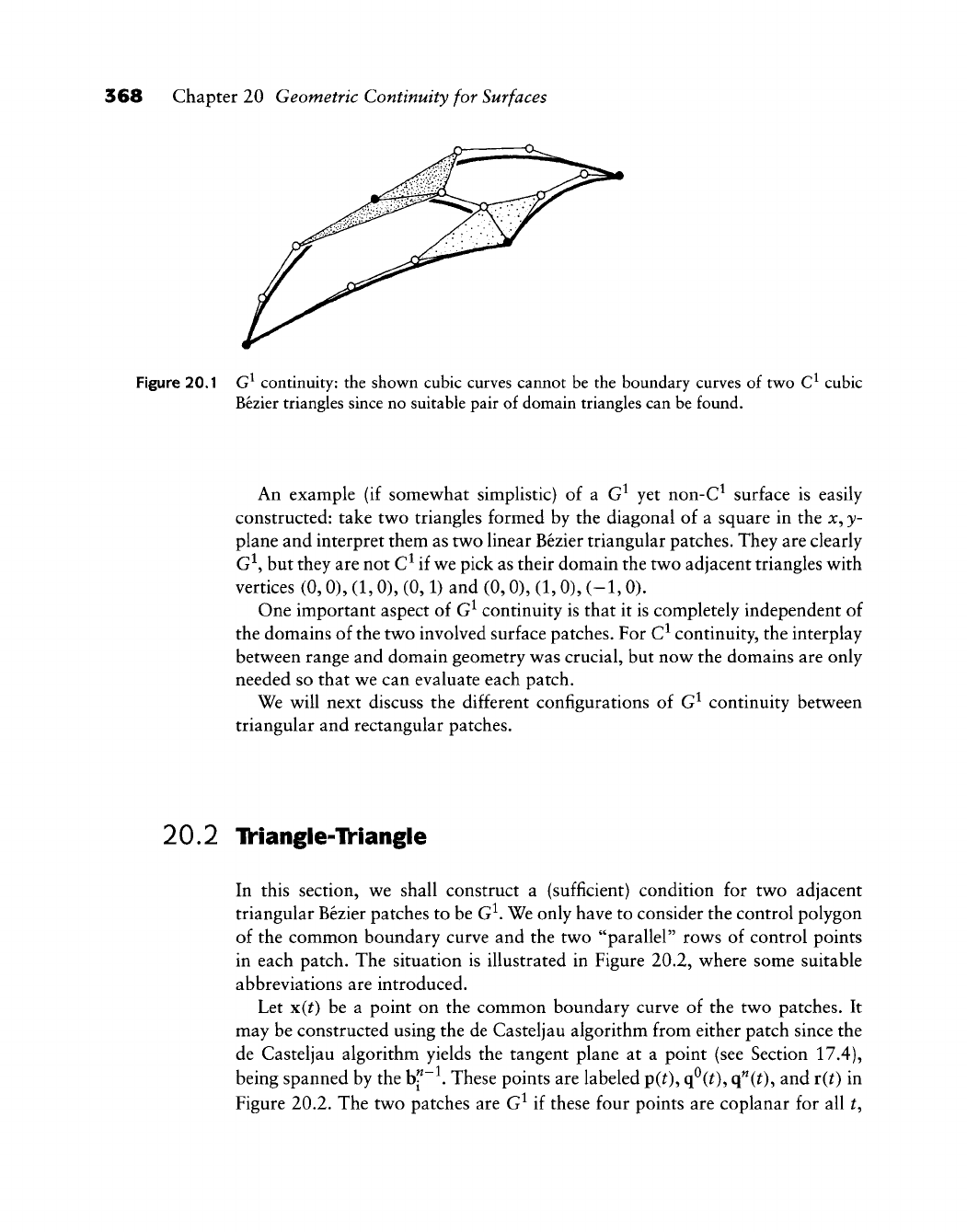
368 Chapter 20 Geometric Continuity for Surfaces
Figure 20.1 G^ continuity: the shown cubic curves cannot be the boundary curves of two C^ cubic
Bezier triangles since no suitable pair of domain triangles can be found.
An example (if somewhat simplistic) of a G^ yet non-C^ surface is easily
constructed: take two triangles formed by the diagonal of a square in the x, y-
plane and interpret them as two linear Bezier triangular patches. They are clearly
G^, but they are not C^ if we pick as their domain the two adjacent triangles with
vertices (0,0), (1,0), (0,1) and (0,0), (1,0), (-1,0).
One important aspect of G^ continuity is that it is completely independent of
the domains of the two involved surface patches. For C^ continuity, the interplay
between range and domain geometry was crucial, but now the domains are only
needed so that we can evaluate each patch.
We will next discuss the different configurations of G^ continuity between
triangular and rectangular patches.
20.2 IV'iangle-TV'iangle
In this section, we shall construct a (sufficient) condition for two adjacent
triangular Bezier patches to be G^. We only have to consider the control polygon
of the common boundary curve and the two "parallel" rows of control points
in each patch. The situation is illustrated in Figure 20.2, where some suitable
abbreviations are introduced.
Let x(t) be a point on the common boundary curve of the two patches. It
may be constructed using the de Casteljau algorithm from either patch since the
de Casteljau algorithm yields the tangent plane at a point (see Section 17.4),
being spanned by the bp^ These points are labeled p(0, q^CO^ q^CO? and T(t) in
Figure 20.2. The two patches are G^ if these four points are coplanar for all t.
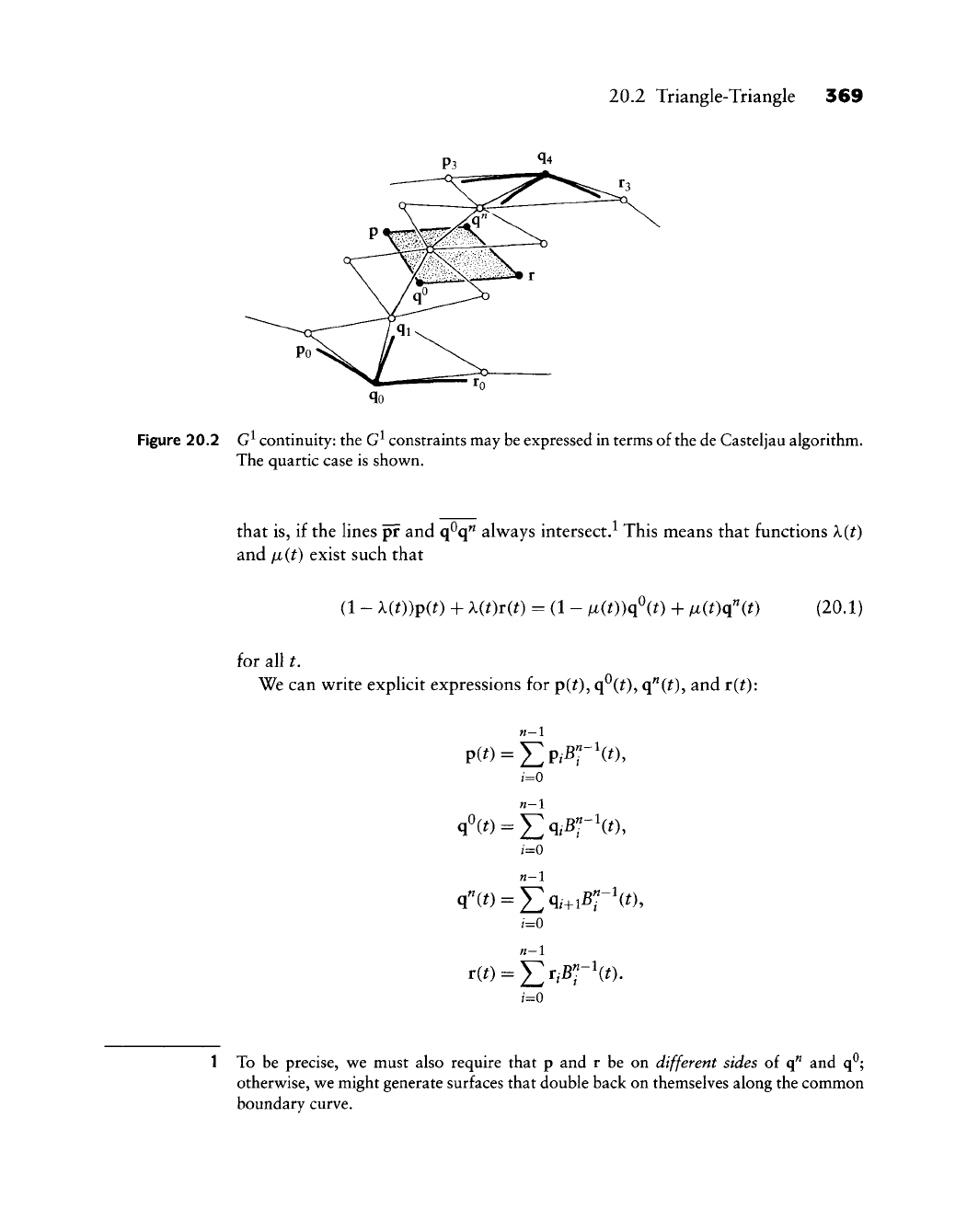
20.2 Triangle-Triangle 369
Figure 20.2
G^
continuity: the
G^
constraints may be expressed in terms of
the
de Casteljau algorithm.
The quartic case is shown.
that is, if the lines pr and q^q" always intersect.^ This means that functions X(t)
and /ji(t) exist such that
(1 - X(t))p(t) + X(t)T(t) = (1 - /x(t))q\t) + /x(Oq"(0 (20.1)
for all t.
We can write explicit expressions for p(0, q^(0? q"(^)) and r{t):
n-l
i=0
i=0
n-l
n-l
=0
1 To be precise, we must also require that p and r be on different sides of q" and q^;
otherwise, we might generate surfaces that double back on themselves along the common
boundary curve.
370 Chapter 20 Geometric Continuity for Surfaces
We know that the first and last pair of triangles must be coplanar. This means
that numbers
XQ,
A.^,
/XQ,
MI
exist such that (with the definition x=l
—
x)
^oPo + ^0^0 = Aoqo + /^oqi- (20.2)
and
hPn-i + h^n-i = Aiq«-i + Miq«- (20.3)
The numbers
XQ
and
/XQ
describe the geometry of the first pair of triangles,
whereas k^ and
/JL^
describe that of the last pair.
We now attempt to simplify our task of formulating G^ conditions: we make
the assumption that X(t) and fi(t) are both linear^ that is,
X{t) = (1 - t)ko + ai, fi(t) = (1 - OMO + ^Mi-
We also observe that
1 - X{t) = (1 - 0^0 + t^h
1
- M(0 = (1 - OMO + ^Ai-
The G^ condition (20.1) then becomes
n-l n-l
((1
- 0^0 + tl{) Y, ViK^it) +
((1
- 0^0 + ^^i) E ^i^T^^t)
n-l n-l
= ((1
-
oAo + ti^i) J2
q/-^r^(^)
+ ((1
-
^)^o+^Mi)
E
q^+i^r^w-
Using (5.32) and (5.33) and regrouping, we obtain
,=0 " ,=0 "
= E ^^-^(Aoq,- + Moq,+i)B"(0 + ^ -—(Aiq, + /^iq,+i)B"+i(0.
After an index transformation involving the B"^ terms, we may compare
coefficients for / = 0,..., w:
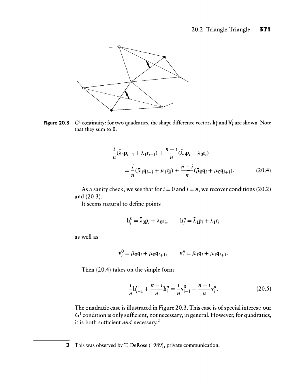
20.2 Triangle-Triangle 371
Figure 20.3 G^ continuity: for two quadratics, the shape difference vectors h^ and hj are shown. Note
that they sum to 0.
-(Aip,_l + Air,_i) + (Aop/ +
koTi)
n n
/ _ n
—
i _
= -(/xiq,_i + Miq,) +
(/xoq,-
+ /xoq/+i).
n n (20.4)
As a sanity check, we see that for / = 0 and / =
w,
we recover conditions (20.2)
and (20.3).
It seems natural to define points
hf =
AoP,-
+ Aor„ hf = Aip,- + k^ti
as well as
Then (20.4) takes on the simple form
« n n n (20.5)
The quadratic case is illustrated in Figure
20.3.
This case is of special interest: our
G^ condition is only sufficient, not necessary, in general. However, for quadratics,
it is both sufficient and necessary.^
2 This was observed by
T.
DeRose (1989), private communication.
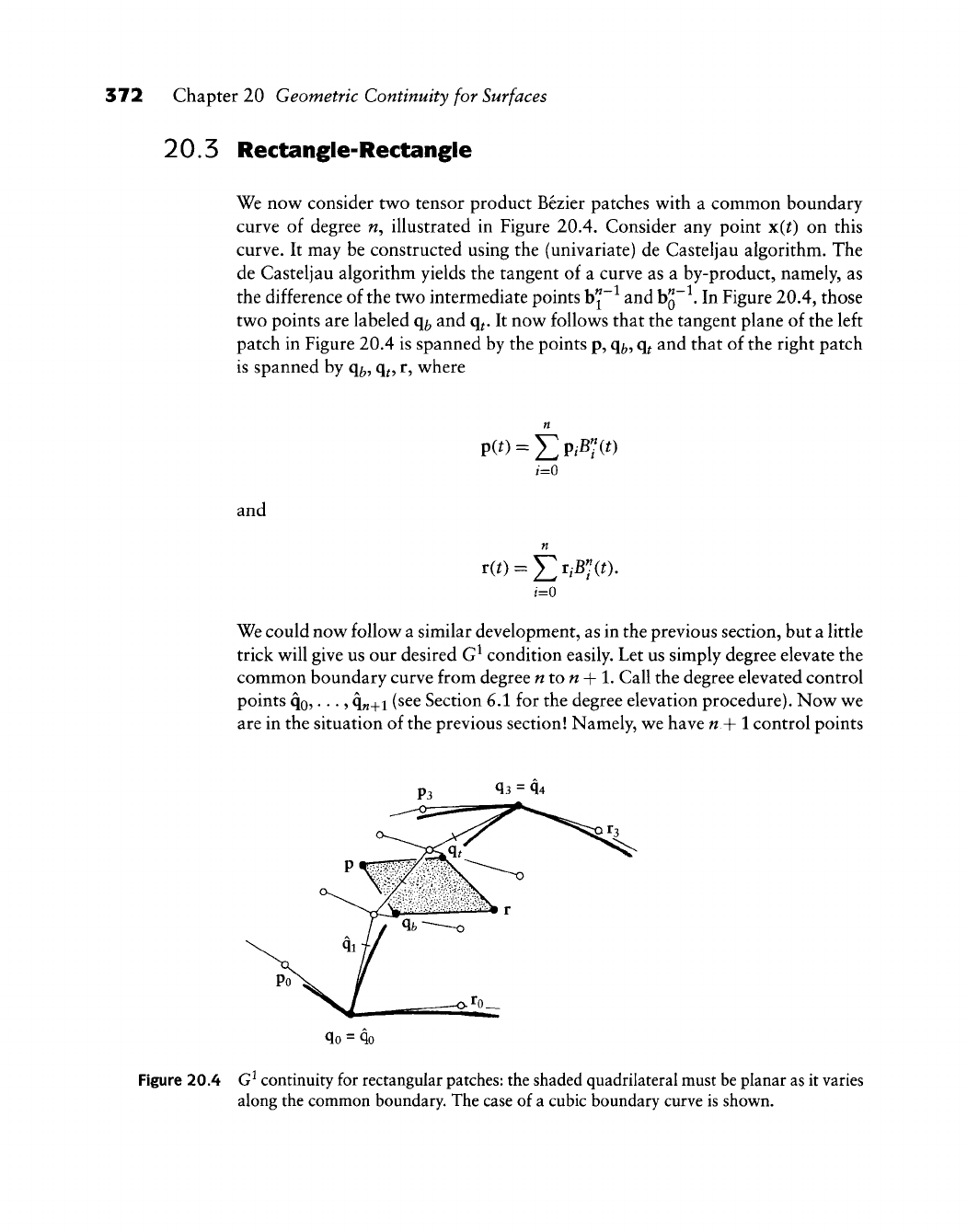
372 Chapter 20 Geometric Continuity for Surfaces
20.5 Rectangle-Rectangle
We now consider two tensor product Bezier patches with a common boundary
curve of degree n, illustrated in Figure 20.4. Consider any point x(^) on this
curve. It may be constructed using the (univariate) de Casteljau algorithm. The
de Casteljau algorithm yields the tangent of a curve as a by-product, namely, as
the difference of the two intermediate points
b^~^
and h^~^. In Figure 20.4, those
two points are labeled q/^ and q^. It now follows that the tangent plane of the left
patch in Figure 20.4 is spanned by the points p, q^, q^ and that of the right patch
is spanned by q^, q^, r, where
p(t) = j2PiB';(t)
i=0
and
r(0 = X^r,B^(0.
i=0
We could now follow a similar development, as in the previous section, but a little
trick will give us our desired G^ condition easily. Let us simply degree elevate the
common boundary curve from degree nton-\-l. Call the degree elevated control
points qo,..., q„+i (see Section 6.1 for the degree elevation procedure). Now we
are in the situation of the previous section! Namely, we have n-\-l control points
q3 = q4
qo
=
qo
Figure 20.4 G^ continuity for rectangular
patches:
the shaded quadrilateral must be planar as it varies
along the common boundary. The case of a cubic boundary curve is shown.
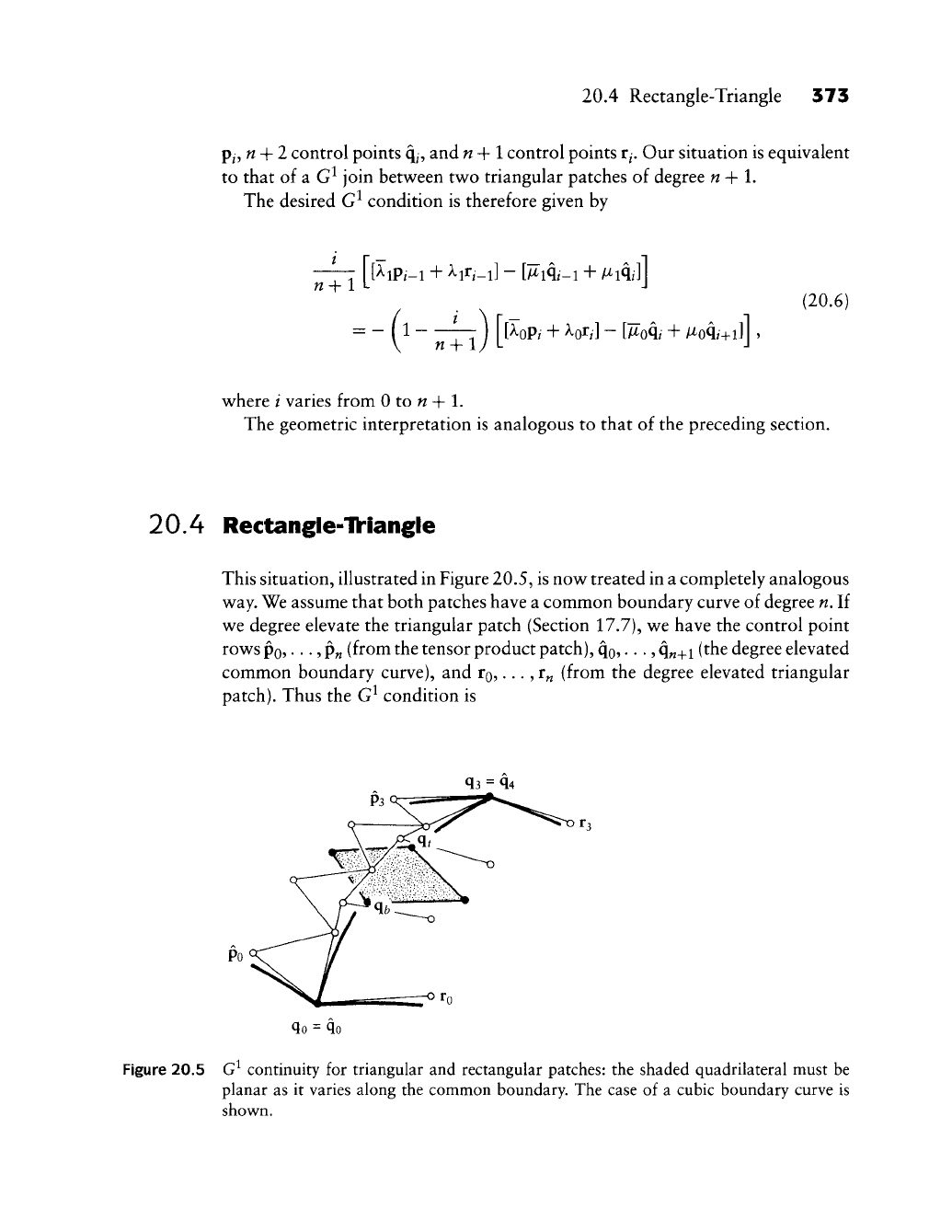
20.4 Rectangle-Triangle 373
p^,
n + 2 control points 4, and n +
1
control points r^. Our situation is equivalent
to that of a G^ join between two triangular patches of degree
n-\-l.
The desired G^ condition is therefore given by
—TT |"[^iP/-i + ^i^i-i\ -
[M
A-i + M All
n-\-
1 t- J
(20.6)
where / varies from 0 to « + 1.
The geometric interpretation is analogous to that of the preceding section.
20.4 Rectangle-Tk*iangle
This situation, illustrated in Figure 20.5, is now treated in a completely analogous
way. We assume that both patches have a common boundary curve of degree n. If
we degree elevate the triangular patch (Section 17.7), we have the control point
rows
Po? • • • ? P«
(from the tensor product patch), qo,..., q„+i (the degree elevated
common boundary curve), and
IQ,
..., r„ (from the degree elevated triangular
patch).
Thus the G^ condition is
q3 = q4
Figure 20.5 G^ continuity for triangular and rectangular patches: the shaded quadrilateral must be
planar as it varies along the common boundary. The case of a cubic boundary curve is
shown.
374 Chapter 20 Geometric Continuity for Surfaces
n +
= - (1 - ~^) [[^oPi + ^or/] - [Moq/ + Moq^+il] .
again with / ranging from 0 to « + 1.
(20.7)
20.5 ^^Filling
in"
Rectangular Patches
Suppose that we were given the boundary curves of two bicubic patches, as shown
in Figure 20.4. At the endpoints of the common boundary curve, we assume that
the three curves meeting there have coplanar tangents. Can we find interior Bezier
points pi, p2 and r^,
T2
such that the two patches will have a continuously varying
tangent plane along the common boundary? We shall employ the G^ condition
(20.6) for this purpose. As a first step, we determine a^ and
PQ
from po,
qo?
TQ,
qi
and ofi, Pi from
P3,
q3,13,
^4.
There are three equations in (20.6) that involve our four unknowns
p^,
p2 and
r^,
12-
After some suitable modification, they are of the form
«oPi + (1 - «o)ri = rhsl,
«lPl + (1 - «i)ri + aoP2 + (1 - ^0)^2 = rhs2,
^iP2 + (1
—
oid^i =
rhs3.
We have abbreviated the right-hand sides of the equations somewhat.
These may be written in matrix form:
with
A =
Ax = b,
Qfl
1 — Qfi
aQ
1 — OfQ
Oil (1 - Q^l)
(20.8)
X
= [pi, p2, r^,
12]^,
and b = [rhsl, rhs2,
rhs3]^.
Since the rows of A are linearly
independent, the underdetermined system (20.8) always has solutions. One way
of finding one is as follows: suppose we already have an estimate x = [pi,
p2,
f
1,
f 2]
for the unknowns. Then one solves the system
AA^Y = h-Ax
20.7 Theoretical Aspects 375
for y, and the solution is given by
X
=
X
+ A^y.
This solution stays as close as possible to the initial guess x; see [86].
The
Tj
and pj could, for instance, be generated by Adini's twists (see Section
16.3).
This idea was carried out by Sarraga
[536],
[537] in a slightly different
context.
20.6 ^Tilling in'' Tk-iangular Patches
Let us reconsider Figure 20.1. Do our G^ conditions allow us to complete the
cubic curve network such that the resulting surface will be G^? In our notation,
the undetermined points are p^ and r^. There are two G^ equations that involve
these points. They are of the form
Qfipi + (1 - Qfi)ri = rhsl,
Qfopi + (1 -
oiQ)ri
= rhs2.
The coefficient matrix of this system:
A = ai 1
—
Q?!
«0 1-^0
is singular if
aQ
= a^. Therefore, in this case, we are not guaranteed to have a
solution (see Piper [483] for an explicit counterexample).
We can, however, solve the problem if we resort to quartics. After we degree
elevate all boundary curves, we now have to determine unknown control points
Pl,
p2 and r^, ti- This is exactly the situation from the preceding section and is
solved in exactly the same way. B. Piper [483] first used quartics to solve this
kind of Hermite interpolation problem.
20.7 Theoretical Aspects
We have developed an approach to geometric continuity that is powerful enough
to solve several applications-oriented problems. It is practical, but it is not
general: there are G^ surfaces that do not satisfy the condition (20.4); see
Problems. T. DeRose has developed conditions that are both necessary and
sufficient for G^ continuity of adjacent Bezier patches.
376 Chapter 20 Geometric Continuity for Surfaces
Several authors (consuh the surveys by Boehm [77], Herron
[322],
and Gre-
gory [291]) define geometric continuity of surfaces in the following way: two
surfaces that share a common boundary curve are called C if, for every point
of the boundary curve, a reparametrization exists such that both surfaces are C^
in a neighborhood of that point. For the case r = 1, this definition yields tangent
plane continuity. Its advantage is that it also works for higher orders; the price to
be paid is that it is rather abstract. For the case of G^ continuity, another popular
definition is to require a common Dupin's indicatrix along the boundary curve
(see Section 19.12, Kahmann
[350],
and Pegna and Wolter [459]).
20.8 Problems
1 In Section 20.1 we saw an example of triangular patch boundaries that
could not be completed to construct an overall C^ surface. Find similar
examples for tensor product patches.
2 Show that the G^ conditions (20.4) include the case of strict contmuity
(17.23) between triangular patches.
3 Construct surfaces that are G^ yet do not satisfy (20.4).
A Consider eight triangular patches, assembled so as to form eight octants
of a spherelike surface. Show that this closed surface cannot be C^, that
is,
one cannot find a region in the plane that comprises eight triangles that
have a C^ map that maps them to the surface.
PI Construct a spherelike G^ surface that is made up of six biquartic patches
having a cubelike connectivity.
Surfaces with
Arbitrary Topology
I he surfaces that we have met so far are best suited for shapes that are the
image of some part of the plane—of a rectangle in the case of B-spline or Bezier
surfaces, of a triangulated region in the case of composite Bezier triangles. This
limits the topology of these surfaces; for example, it is not possible to construct
even a sphere without introducing degenerate patches while using a C^ map of a
part of the plane. Even shapes that have the topology of a planar region may be
too complex to model with one tensor product surface; just imagine modeling
a glove that way. The complexity issue may be tackled using the approach of
hierarchical B-spline surfaces as proposed by Forsey and Bartels
[245].
But even
with this method, arbitrary topology is not achievable.
In this chapter, we will investigate methods that are suited for the construction
of shapes of arbitrary complexity and/or topology. We can present only a brief
selection of methods; more literature on the topic:
[177],
[596], [595],
[594],
[289], [290], [293], [321], [431], [627], [398], [561].
The first in-depth study of
recursive subdivision processes goes back to U. Reif
[503].
The basic concepts of
surface topology are nicely explained in
[323].
21.1 Recursive Subdivision Curves
We already encountered Chaikin's algorithm in Section 8.4. Starting with a
polygon, it produces a sequence of refined polygons that ultimately converge
to the uniform quadratic B-spline curve defined by the initial polygon.
This principle may be applied to higher-degree uniform splines; we discuss the
cubic case here. If we double a uniform knot sequence by inserting the midpoint
577
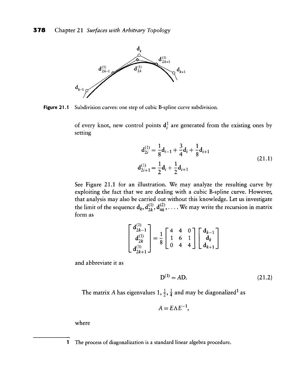
378 Chapter 21 Surfaces with Arbitrary Topology
Figure 21.1 Subdivision curves: one step of cubic B-spline curve subdivision.
of every knot, new control points d] are generated from the existing ones by
setting
d«:
1(1)
1,
3, 1.
1 1
(21.1)
4Vi-^d«
+
H
+ 1
4 4 0"
1 6 1
0 4 4
^k-i~
dfe
_
dfe+i_
See Figure 21.1 for an illustration. We may analyze the resulting curve by
exploiting the fact that we are dealing with a cubic B-spline curve. However,
that analysis may also be carried out without this knowledge. Let us investigate
the limit of the sequence d^, d^^^
d^^,....
We may write the recursion in matrix
form as
^ik
L ^lk+1 -I
and abbreviate it as
D^i^=AD. (21.2)
The matrix A has eigenvalues 1, 2? ^ ^^^ ^^y ^^ diagonalized^ as
A = EAE-\
where
1 The process of diagonalization is a standard linear algebra procedure.
21.1 Recursive Subdivision Curves 379
E =
1 1 2
1 0 -1
1 -1 2
1
3
1
4
0
-2
1 "
-3
1
A =
"1 0
0 i
_0 0
0
0
1
4
The matrix E contains A's eigenvectors, and the diagonal matrix A contains A's
eigenvalues.
For the next iteration, v^e have
Using our diagonalization for A, w^e get
A^
= EAE-^E-^AE = EA^E'^
(21.3)
and further
Taking the limit r ^^ oo yields
A'
= EA'E-\
A~ = £A~£-i.
Since
this becomes
A^
A^ = -
1 0 0"
0 0 0
0 0 0
1 4 1
1 4 1
1 4 1
implying that all three points d^_i, d^, d^+j converge to the same point (d^_i +
4d^ + d^+l)/6. This result is no surprise since we know^ v^e are dealing v^ith
B-spline curves. It does illustrate, how^ever, a general principle that is ubiquitous
in all subdivision theory, namely, that convergence analysis is normally carried
out via an eigenvalue analysis.
Subdivision may also be used to generate interpolating curves. The basic four-
point principle w^as developed by Dyn, Levin, and Gregory
[178], [176].
Let a
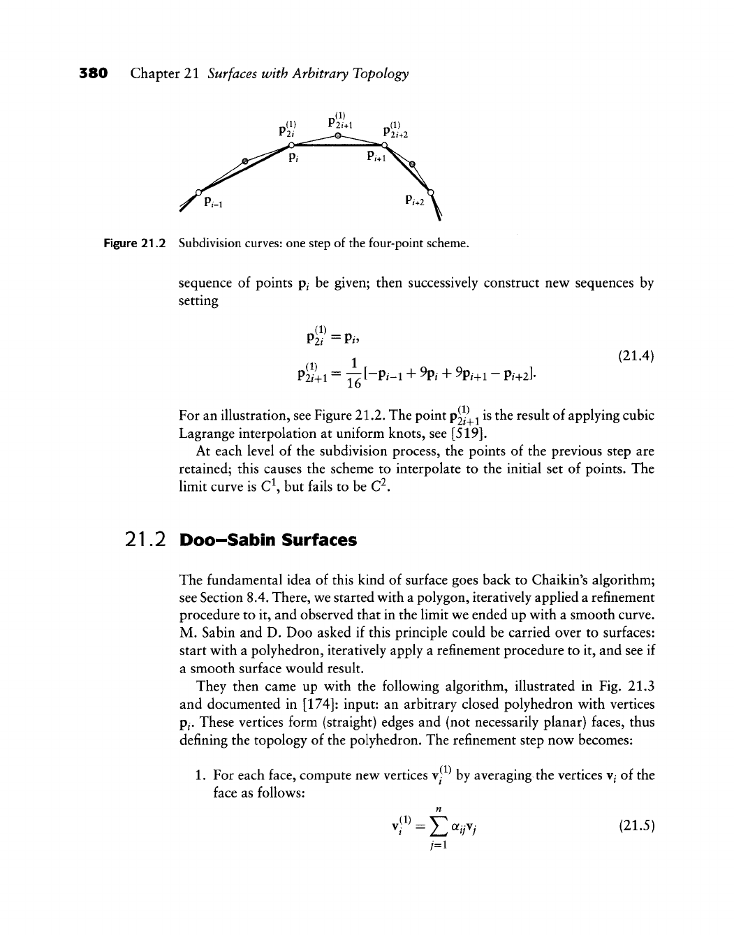
380 Chapter 21 Surfaces with Arbitrary Topology
Figure 21.2 Subdivision curves: one step of the four-point scheme.
sequence of points p^ be given; then successively construct new sequences by
setting
P^NP.
(21.4)
^—O.-
1
+ 9o.- + 90;
,1
—
O;
.
T1.
P2/+1 = T2t"P^-i +
^P^'
"^ ^P^+i ~ P^+2]'
For an illustration, see Figure 21.2. The point
P2/+1
is the result of applying cubic
Lagrange interpolation at uniform knots, see
[519].
At each level of the subdivision process, the points of the previous step are
retained; this causes the scheme to interpolate to the initial set of points. The
limit curve is C\ but fails to be C^.
21.2 Doo-Sabin Surfaces
The fundamental idea of this kind of surface goes back to Chaikin's algorithm;
see Section 8.4. There, v^e started w^ith a polygon, iteratively applied a refinement
procedure to it, and observed that in the limit vjt ended up vv^ith a smooth curve.
M. Sabin and D. Doo asked if this principle could be carried over to surfaces:
start with a polyhedron, iteratively apply a refinement procedure to it, and see if
a smooth surface would result.
They then came up with the following algorithm, illustrated in Fig. 21.3
and documented in
[174]:
input: an arbitrary closed polyhedron with vertices
p^.
These vertices form (straight) edges and (not necessarily planar) faces, thus
defining the topology of the polyhedron. The refinement step now becomes:
1.
For each face, compute new vertices
v^-
by averaging the vertices v^ of the
face as follows:
n
(1)
E«';^/
(21.5)
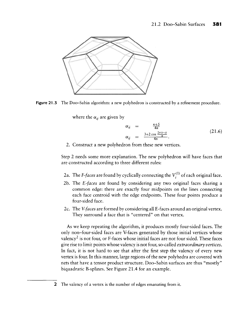
21.2 Doo-Sabin Surfaces 381
Figure 21.3 The Doo-Sabin algorithm: a new polyhedron is constructed by a refinement procedure,
where the aij are given by
3+2 cos
n±5_
4n
2n(i-j)
(21.6)
2.
Construct a new polyhedron from these new vertices.
Step 2 needs some more explanation. The new polyhedron will have faces that
are constructed according to three different rules:
2a. The F-faces are found by cyclically connecting the
V^-
of each original face.
2b.
The E-faces are found by considering any two original faces sharing a
common edge: there are exactly four midpoints on the lines connecting
each face centroid with the edge endpoints. These four points produce a
four-sided face.
2c.
The
V-faces
are formed by considering all E-faces around an original vertex.
They surround a face that is "centered" on that vertex.
As we keep repeating the algorithm, it produces mostly four-sided faces. The
only non-four-sided faces are V-faces generated by those initial vertices whose
valency^ is not four, or F-faces whose initial faces are not four sided. These faces
give rise to limit points whose valency is not four, so-called extraordinary vertices.
In fact, it is not hard to see that after the first step the valency of every new
vertex is four. In this manner, large regions of the new polyhedra are covered with
nets that have a tensor product structure. Doo-Sabin surfaces are thus "mostly"
biquadratic B-splines. See Figure 21.4 for an example.
2 The valency of a vertex is the number of edges emanating from it.
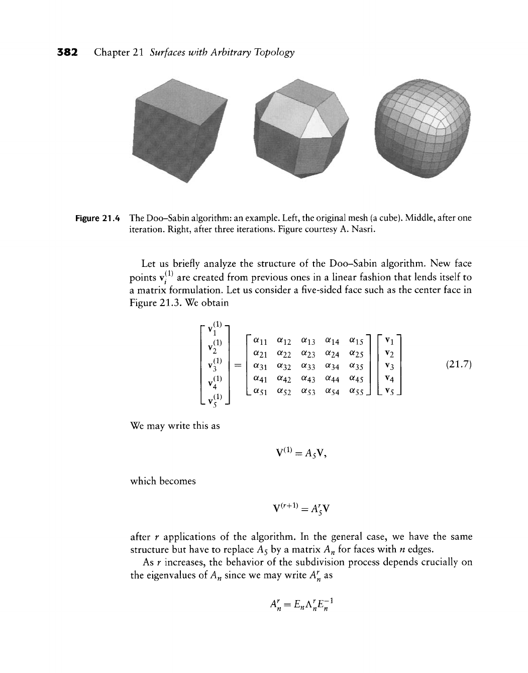
382 Chapter 21 Surfaces with Arbitrary Topology
Figure 21.4 The Doo-Sabin algorithm: an example. Left, the original mesh (a
cube).
Middle, after one
iteration. Right, after three iterations. Figure courtesy A. Nasri.
Let us briefly analyze the structure of the Doo-Sabin algorithm. New face
points
V-
are created from previous ones in a linear fashion that lends itself to
a matrix formulation. Let us consider a five-sided face such as the center face in
Figure 21.3. We obtain
rvf^i
vf
r^'
U?
V.f\
=
0^11 «12 ^13 (^U ^\S
«21 «22 «23 0^24 «25
«31 «32 «33 «34 «35
«41 «42 «43 «44 «45
.0^51 «52 «53 <^54 «55 J
V2
V3
V4
LV5.
(21.7)
We may write this as
which becomes
N^^^=As\,
V(^+1)^A;V
after r applications of the algorithm. In the general case, we have the same
structure but have to replace A5 by a matrix A„ for faces with n edges.
As r increases, the behavior of the subdivision process depends crucially on
the eigenvalues of A„ since we may write A^ as
^^ -
^n^'^n^n
-1
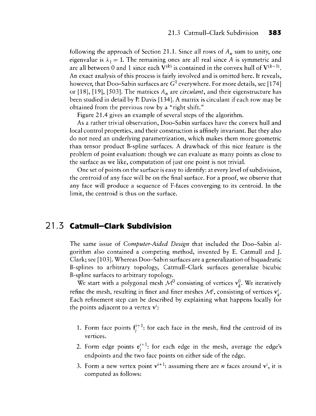
21.3 CatmuU-Clark Subdivision 383
following the approach of Section 21.1. Since all rows of A„ sum to unity, one
eigenvalue is Xi = 1. The remaining ones are all real since A is symmetric and
are all between 0 and 1 since each V^^ is contained in the convex hull of V^^~^\
An exact analysis of this process is fairly involved and is omitted here. It reveals,
however, that Doo-Sabin surfaces are G^ everywhere. For more details, see [174]
or [18], [19],
[503].
The matrices A„ are circularity and their eigenstructure has
been studied in detail by
P.
Davis
[134].
A matrix is circulant if each row may be
obtained from the previous row by a "right shift."
Figure 21.4 gives an example of several steps of the algorithm.
As a rather trivial observation, Doo-Sabin surfaces have the convex hull and
local control properties, and their construction is affinely invariant. But they also
do not need an underlying parametrization, which makes them more geometric
than tensor product B-spline surfaces. A drawback of this nice feature is the
problem of point evaluation: though we can evaluate as many points as close to
the surface as we like, computation of just one point is not trivial.
One set of points on the surface is easy to identify: at every level of subdivision,
the centroid of any face will be on the final surface. For a
proof,
we observe that
any face will produce a sequence of F-faces converging to its centroid. In the
limit, the centroid is thus on the surface.
21.5 Catmull-Clark Subdivision
The same issue of Computer-Aided Design that included the Doo-Sabin al-
gorithm also contained a competing method, invented by E. CatmuU and J.
Clark; see
[103].
Whereas Doo-Sabin surfaces are a generalization of biquadratic
B-splines to arbitrary topology, Catmull-Clark surfaces generalize bicubic
B-spline surfaces to arbitrary topology.
We start with a polygonal mesh MP consisting of vertices v9. We iteratively
refine the mesh, resulting in finer and finer meshes M\ consisting of vertices v^.
Each refinement step can be described by explaining what happens locally for
the points adjacent to a vertex v^:
1.
Form face points f ^^: for each face in the mesh, find the centroid of its
vertices.
2.
Form edge points e-^ : for each edge in the mesh, average the edge's
endpoints and the two face points on either side of the edge.
3.
Form a new vertex point v^"^^: assuming there are n faces around v^, it is
computed as follows:
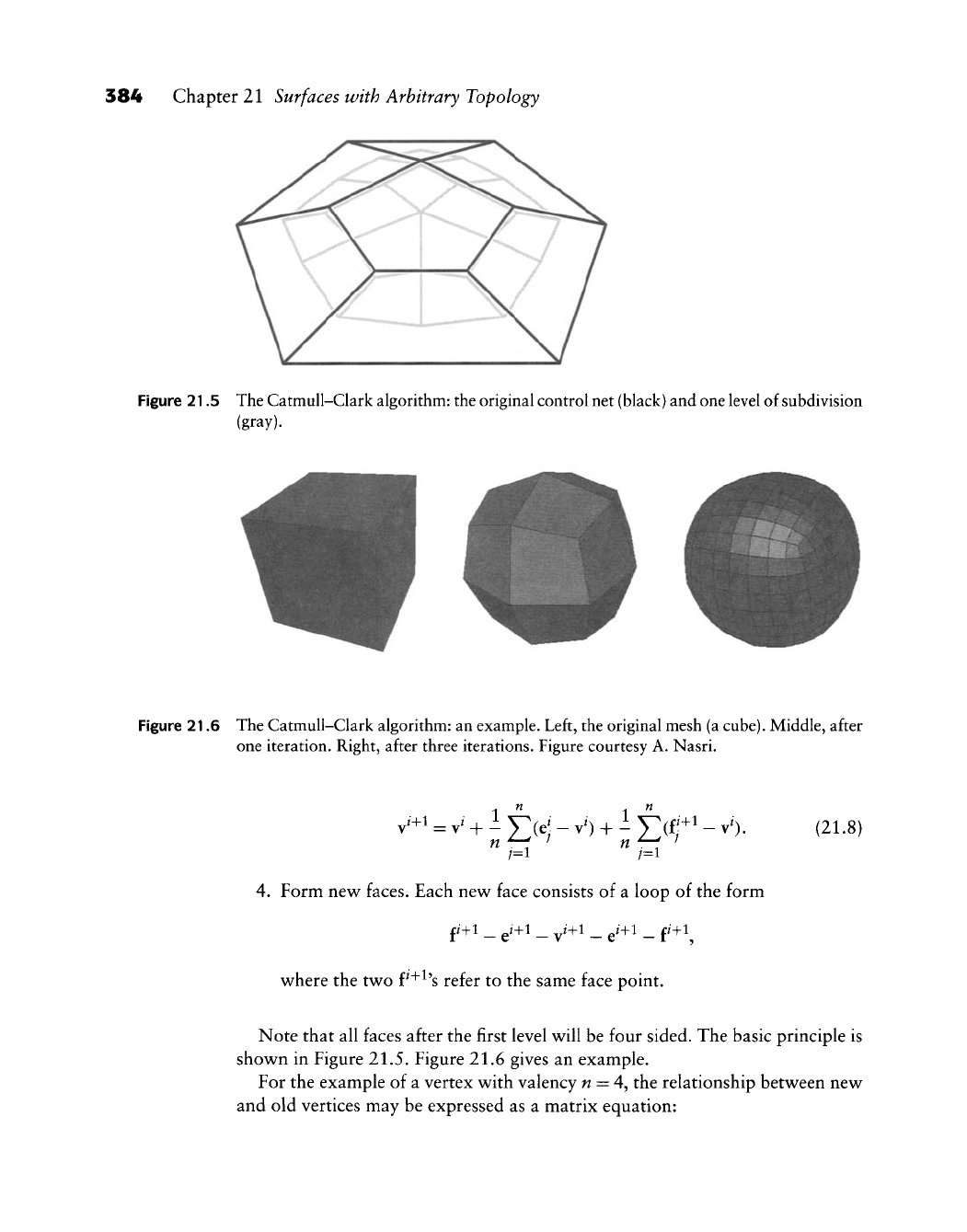
384 Chapter 21 Surfaces with Arbitrary Topology
Figure 21.5 The Catmull-Clark algorithm: the original control net (black) and one level of subdivision
(gray).
Figure 21.6 The Catmull-Clark algorithm: an example. Left, the original mesh (a
cube).
Middle, after
one iteration. Right, after three iterations. Figure courtesy A. Nasri.
J+^
- J
;=i "7=1
(21.8)
4.
Form new faces. Each nev^ face consists of a loop of the form
where the two P"^^'s refer to the same face point.
Note that all faces after the first level will be four sided. The basic principle is
shown in Figure 21.5. Figure 21.6 gives an example.
For the example of a vertex with valency
w
= 4, the relationship between new
and old vertices may be expressed as a matrix equation:
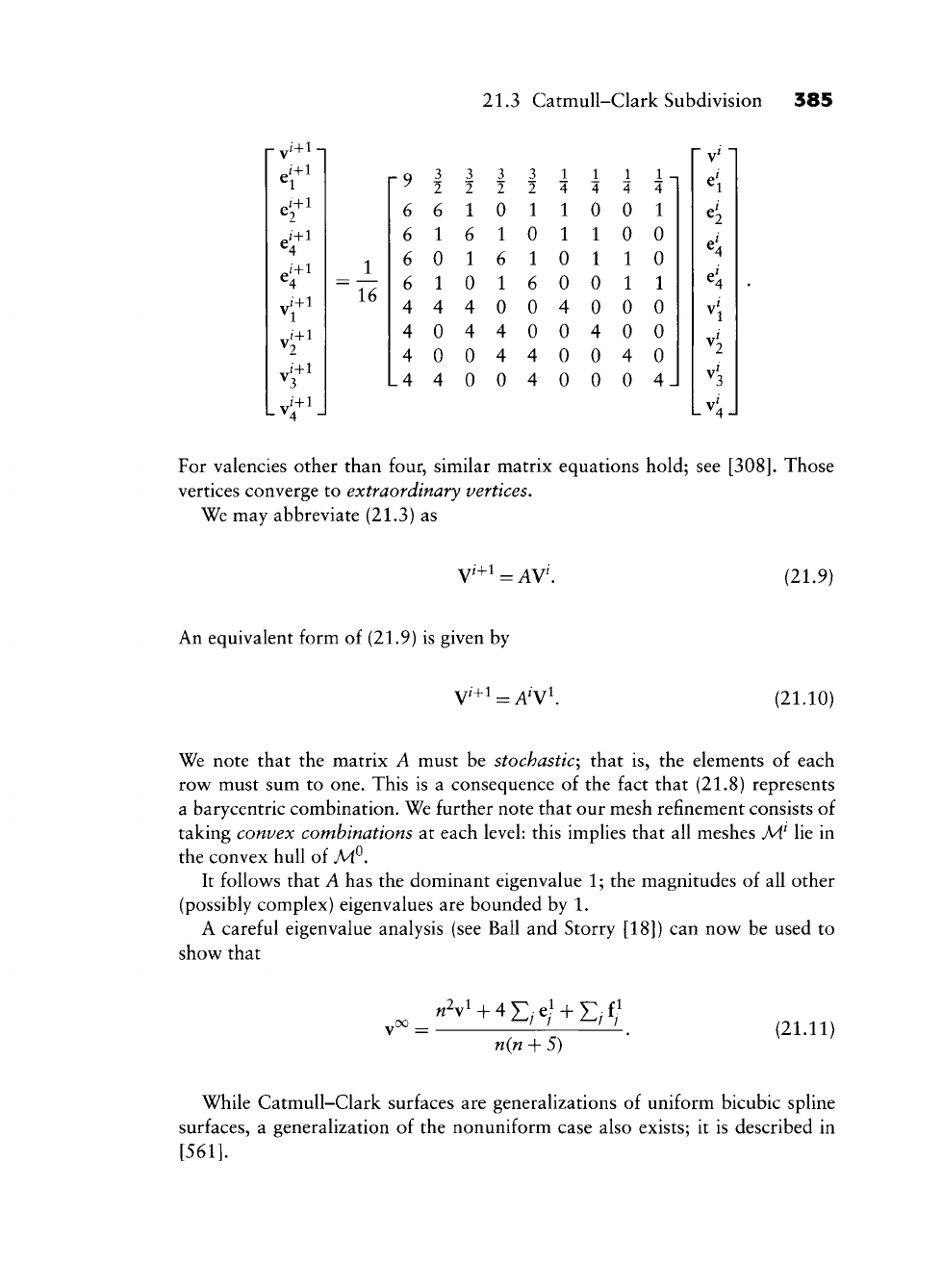
21.3 CatmuU-Clark Subdivision 385
J_
16
9
6
6
6
6
4
4
4
4
3
6
1
0
1
4
0
0
4
3
2
1
6
1
0
4
4
0
0
3
2
0
1
6
1
0
4
4
0
3
2
1
0
1
6
0
0
4
4
1
4
1
1
0
0
4
0
0
0
1
4
0
1
1
0
0
4
0
0
1
4
0
0
1
1
0
0
4
0
1
4
1
0
0
1
0
0
0
4
V
For valencies other than four, similar matrix equations hold; see
[308].
Those
vertices converge to extraordinary vertices.
We may abbreviate (21.3) as
7'+l . :AV'. (21.9)
An equivalent form of (21.9) is given by
V+i = A^Vi. (21.10)
We note that the matrix A must be stochastic^ that is, the elements of each
row must sum to one. This is a consequence of the fact that (21.8) represents
a barycentric combination. We further note that our mesh refinement consists of
taking convex combinations at each level: this implies that all meshes M^ lie in
the convex hull of M^.
It follows that A has the dominant eigenvalue 1; the magnitudes of all other
(possibly complex) eigenvalues are bounded by 1.
A careful eigenvalue analysis (see Ball and Storry [18]) can now be used to
show that
«V + 4X:;e/ + E;f/
n{n + 5) (21.11)
While Catmull-Clark surfaces are generalizations of uniform bicubic spline
surfaces, a generalization of the nonuniform case also exists; it is described in
[561].
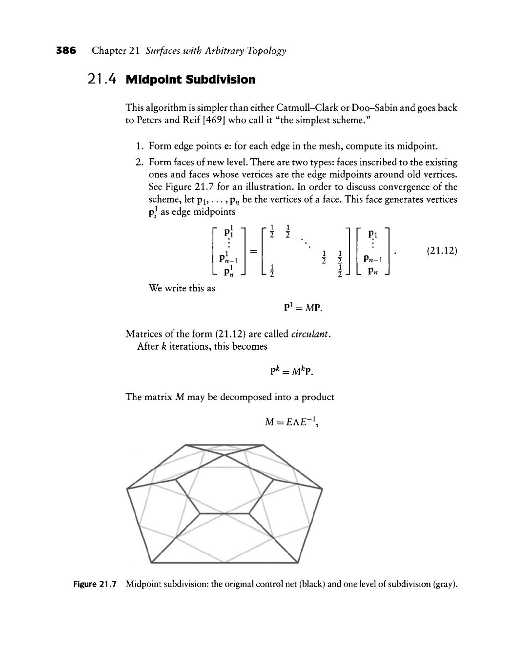
386 Chapter 21 Surfaces with Arbitrary Topology
21.4 Midpoint Subdivision
This algorithm is simpler than either Catmull-Clark or Doo-Sabin and goes back
to Peters and Reif [469] who call it "the simplest scheme."
1.
Form edge points e: for each edge in the mesh, compute its midpoint.
2.
Form faces of new level. There are two types: faces inscribed to the existing
ones and faces whose vertices are the edge midpoints around old vertices.
See Figure 21.7 for an illustration. In order to discuss convergence of the
scheme, let Pi,. •., p« be the vertices of a face. This face generates vertices
p^^
as edge midpoints
["^ 1
r 1
2
1
write this as
1
2
Pl
,
1
2
= MP.
~
1
2
1
2 -J
p.l
p«-l
L P« ,
(21.12)
Matrices of the form (21.12) are called circulant.
After k iterations, this becomes
P*
= M^P.
The matrix M may be decomposed into a product
M = £A£-^
Figure 21.7 Midpoint subdivision: the original control net (black) and one level of subdivision (gray).
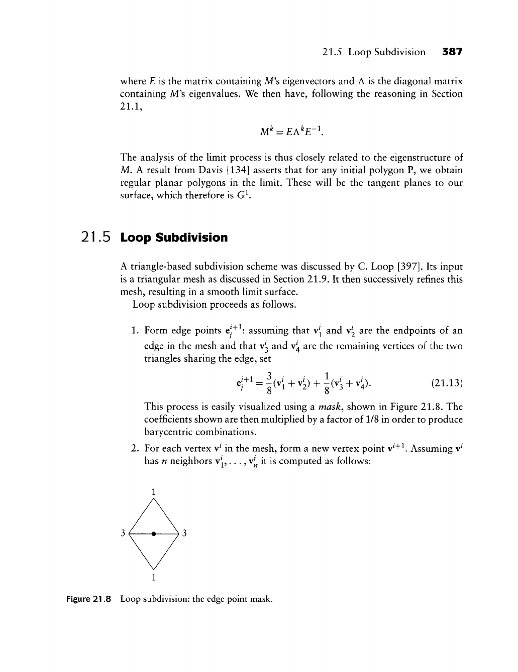
21.5 Loop Subdivision 387
where E is the matrix containing M's eigenvectors and A is the diagonal matrix
containing M's eigenvalues. We then have, foUov^ing the reasoning in Section
21.1,
M^ = £A^£-K
The analysis of the limit process is thus closely related to the eigenstructure of
M. A result from Davis [134] asserts that for any initial polygon P, we obtain
regular planar polygons in the limit. These will be the tangent planes to our
surface, which therefore is G^
21.5 Loop Subdivision
A triangle-based subdivision scheme was discussed by C. Loop
[397].
Its input
is a triangular mesh as discussed in Section 21.9. It then successively refines this
mesh, resulting in a smooth limit surface.
Loop subdivision proceeds as follows.
1.
Form edge points ej"^ : assuming that v^^ and Vj are the endpoints of an
edge in the mesh and that v^ and v^ are the remaining vertices of the two
triangles sharing the edge, set
^r'=^K+^1)+^(^3+<)• (21-13)
This process is easily visualized using a masky shown in Figure 21.8. The
coefficients shown are then multiplied by a factor of 1/8 in order to produce
barycentric combinations.
2.
For each vertex
v^
in the mesh, form a new vertex point v^"^^ Assuming v^
has n neighbors v^ . . ., v^ it is computed as follows:
1
Figure 21.8 Loop subdivision: the edge point mask.
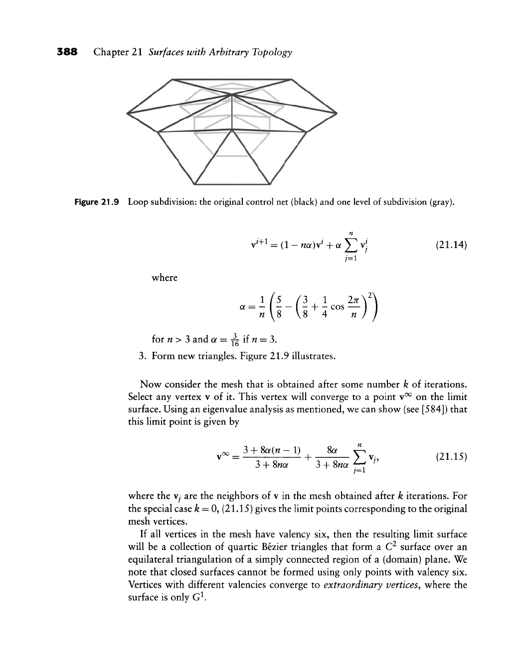
388 Chapter 21 Surfaces with Arbitrary Topology
Figure 21.9 Loop subdivision: the original control net (black) and one level of subdivision (gray).
v^+1
=
(1
- naW + « 1] ^/ (21.14)
where
1/5 /3 1 27r\^\
a = - \ - + - cos —
« \8 V8 4 n ) I
for n> 3 and a =
j^iin
=
?>.
3.
Form new triangles. Figure 21.9 illustrates.
Now consider the mesh that is obtained after some number k of iterations.
Select any vertex v of it. This vertex will converge to a point v^ on the limit
surface. Using an eigenvalue analysis as mentioned, we can show (see [584]) that
this limit point is given by
3 + 8(y(fz-l)
3 + 8wa + 8a
3
+ 8«a /=1
(21.15)
where the
Vy
are the neighbors of v in the mesh obtained after k iterations. For
the special case ^ = 0, (21.15) gives the limit points corresponding to the original
mesh vertices.
If all vertices in the mesh have valency six, then the resulting limit surface
will be a collection of quartic Bezier triangles that form a C^ surface over an
equilateral triangulation of a simply connected region of a (domain) plane. We
note that closed surfaces cannot be formed using only points with valency six.
Vertices with different valencies converge to extraordinary vertices^ where the
surface is only G^.
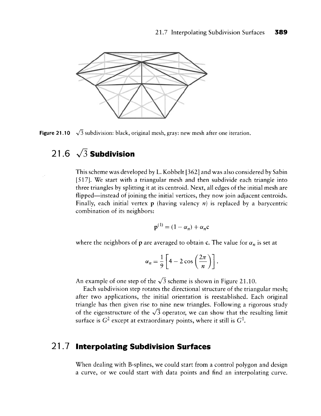
21.7 Interpolating Subdivision Surfaces 389
Figure 21.10 \/3 subdivision: black, original mesh, gray: new mesh after one iteration.
21.6 V3 Subdivision
This scheme was developed by L. Kobbelt [362] and was also considered by Sabin
[517].
We start with a triangular mesh and then subdivide each triangle into
three triangles by splitting it at its centroid. Next, all edges of the initial mesh are
flipped—instead of joining the initial vertices, they now join adjacent centroids.
Finally, each initial vertex p (having valency n) is replaced by a barycentric
combination of its neighbors:
.(1)
p^'^
= (1 - a J +
a„c
where the neighbors of p are averaged to obtain c. The value for a^ is set at
1
^ 9
4_2cos(—")
An example of one step of the \/3 scheme is shown in Figure 21.10.
Each subdivision step rotates the directional structure of the triangular mesh;
after two applications, the initial orientation is reestabUshed. Each original
triangle has then given rise to nine new triangles. Following a rigorous study
of the eigenstructure of the \/3 operator, we can show that the resulting limit
surface is G^ except at extraordinary points, where it still is G^.
21.7 interpolating Subdivision Surfaces
When dealing with B-splines, we could start from a control polygon and design
a curve, or we could start with data points and find an interpolating curve.
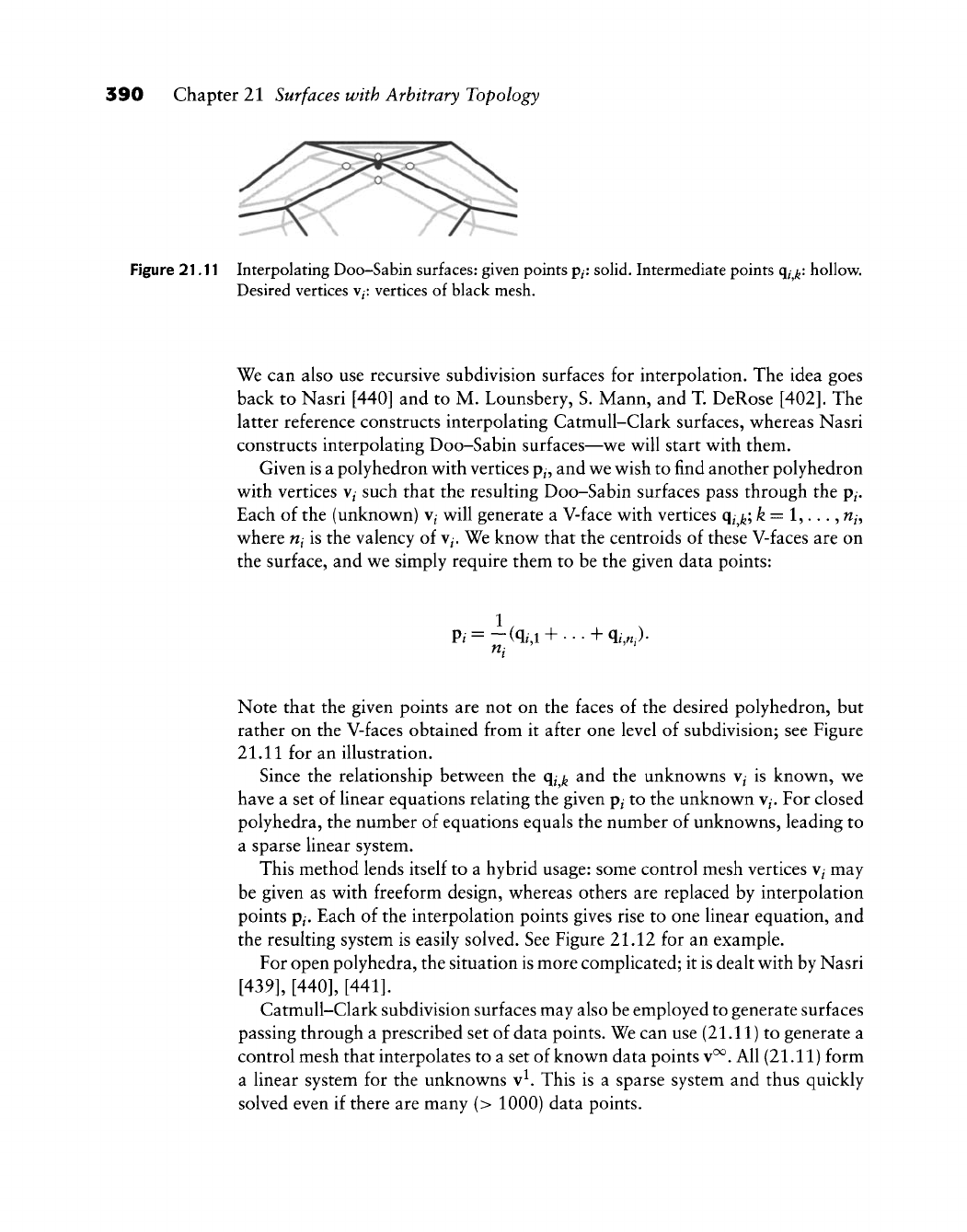
390 Chapter 21 Surfaces with Arbitrary Topology
Figure 21.11 Interpolating Doo-Sabin surfaces: given points
p^:
solid. Intermediate points
q^^^:
hollow.
Desired vertices
v^:
vertices of black mesh.
We can also use recursive subdivision surfaces for interpolation. The idea goes
back to Nasri [440] and to M. Lounsbery, S. Mann, and T. DeRose
[402].
The
latter reference constructs interpolating Catmull-Clark surfaces, w^hereas Nasri
constructs interpolating Doo-Sabin surfaces—v^e will start w^ith them.
Given is a polyhedron with vertices
p^,
and we wish to find another polyhedron
with vertices V/ such that the resulting Doo-Sabin surfaces pass through the p^.
Each of the (unknown) v^ will generate a V-face with vertices q^^; ^ = 1,. ..,
w^,
where fii is the valency of
v^.
We know that the centroids of these V-faces are on
the surface, and we simply require them to be the given data points:
1
fl:
'
Note that the given points are not on the faces of the desired polyhedron, but
rather on the V-faces obtained from it after one level of subdivision; see Figure
21.11 for an illustration.
Since the relationship between the
q^
^^
and the unknowns v^ is known, we
have a set of linear equations relating the given
p^
to the unknown v^. For closed
polyhedra, the number of equations equals the number of unknowns, leading to
a sparse linear system.
This method lends itself to a hybrid usage: some control mesh vertices v/ may
be given as with freeform design, whereas others are replaced by interpolation
points p/. Each of the interpolation points gives rise to one linear equation, and
the resulting system is easily solved. See Figure 21.12 for an example.
For open polyhedra, the situation is more complicated; it is dealt with by Nasri
[439], [440], [441].
CatmuU-Clark subdivision surfaces may also be employed to generate surfaces
passing through a prescribed set of data points. We can use (21.11) to generate a
control mesh that interpolates to a set of known data points v^. All (21.11) form
a linear system for the unknowns v^. This is a sparse system and thus quickly
solved even if there are many (> 1000) data points.
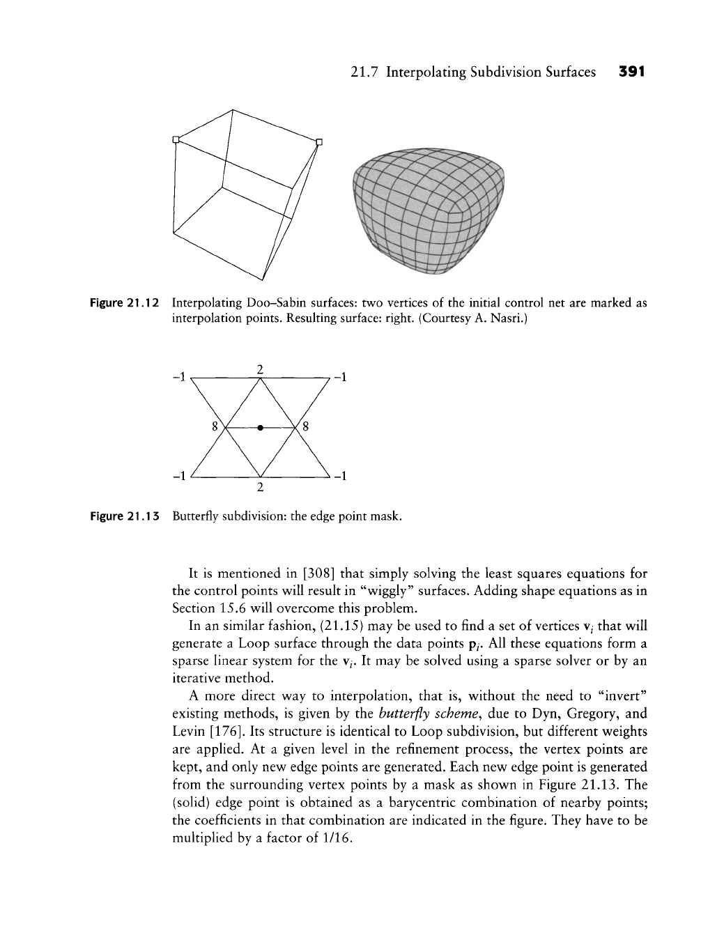
21.7 Interpolating Subdivision Surfaces 391
Figure 21.12 Interpolating Doo-Sabin surfaces: two vertices of the initial control net are marked as
interpolation points. Resulting surface: right. (Courtesy A. Nasri.)
Figure 21.13 Butterfly subdivision: the edge point mask.
It is mentioned in [308] that simply solving the least squares equations for
the control points will result in "wiggly" surfaces. Adding shape equations as in
Section 15.6 will overcome this problem.
In an similar fashion, (21.15) may be used to find a set of vertices v^ that will
generate a Loop surface through the data points p^. All these equations form a
sparse linear system for the V/. It may be solved using a sparse solver or by an
iterative method.
A more direct way to interpolation, that is, without the need to "invert"
existing methods, is given by the butterfly scheme^ due to Dyn, Gregory, and
Levin
[176].
Its structure is identical to Loop subdivision, but different weights
are applied. At a given level in the refinement process, the vertex points are
kept, and only new edge points are generated. Each new edge point is generated
from the surrounding vertex points by a mask as shown in Figure
21.13.
The
(solid) edge point is obtained as a barycentric combination of nearby points;
the coefficients in that combination are indicated in the figure. They have to be
multiplied by a factor of 1/16.
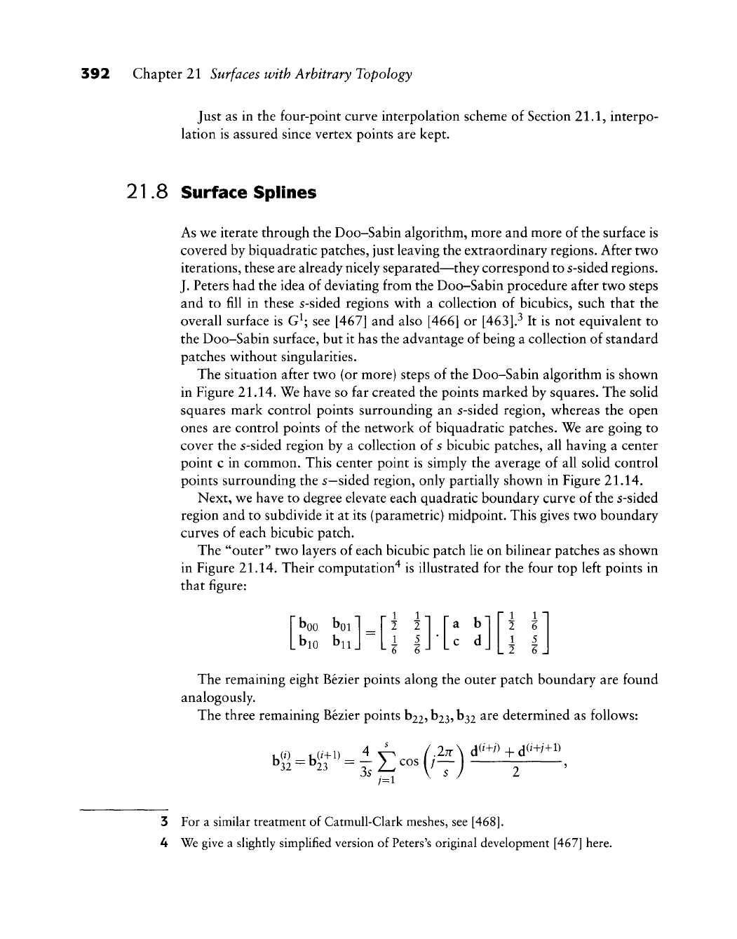
392 Chapter 21 Surfaces with Arbitrary Topology
Just as in the four-point curve interpolation scheme of Section 21.1, interpo-
lation is assured since vertex points are kept.
21.8 Surface Splines
As
w^e
iterate through the Doo-Sabin algorithm, more and more of the surface is
covered by biquadratic patches, just leaving the extraordinary regions. After tw^o
iterations, these are already nicely separated—they correspond to s-sided regions.
J. Peters had the idea of deviating from the Doo-Sabin procedure after two steps
and to fill in these s-sided regions w^ith a collection of bicubics, such that the
overall surface is G^; see [467] and also [466] or
[463].^
It is not equivalent to
the Doo-Sabin surface, but it has the advantage of being a collection of standard
patches without singularities.
The situation after two (or more) steps of the Doo-Sabin algorithm is shown
in Figure 21.14. We have so far created the points marked by squares. The solid
squares mark control points surrounding an s-sided region, whereas the open
ones are control points of the network of biquadratic patches. We are going to
cover the s-sided region by a collection of s bicubic patches, all having a center
point c in common. This center point is simply the average of all solid control
points surrounding the s—sided region, only partially shown in Figure 21.14.
Next, we have to degree elevate each quadratic boundary curve of the s-sided
region and to subdivide it at its (parametric) midpoint. This gives two boundary
curves of each bicubic patch.
The "outer" two layers of each bicubic patch lie on bilinear patches as shown
in Figure 21.14. Their computation"^ is illustrated for the four top left points in
that figure:
'nj [\ \[l
boo boi
1
^ r 2 2 1 fa b
bio
bii
I
u I rl c d
1 1
2 6
1 i
2 6
The remaining eight Bezier points along the outer patch boundary are found
analogously.
The three remaining Bezier points hii^
b23,
hi^i
are determined as follows:
.27r\ d(^+/)+d(^+/+i)
,«.br=iE-(,f)
3 For a similar treatment of Catmull-Clark meshes, see
[468].
4 We give a slightly simplified version of Peters's original development [467] here.
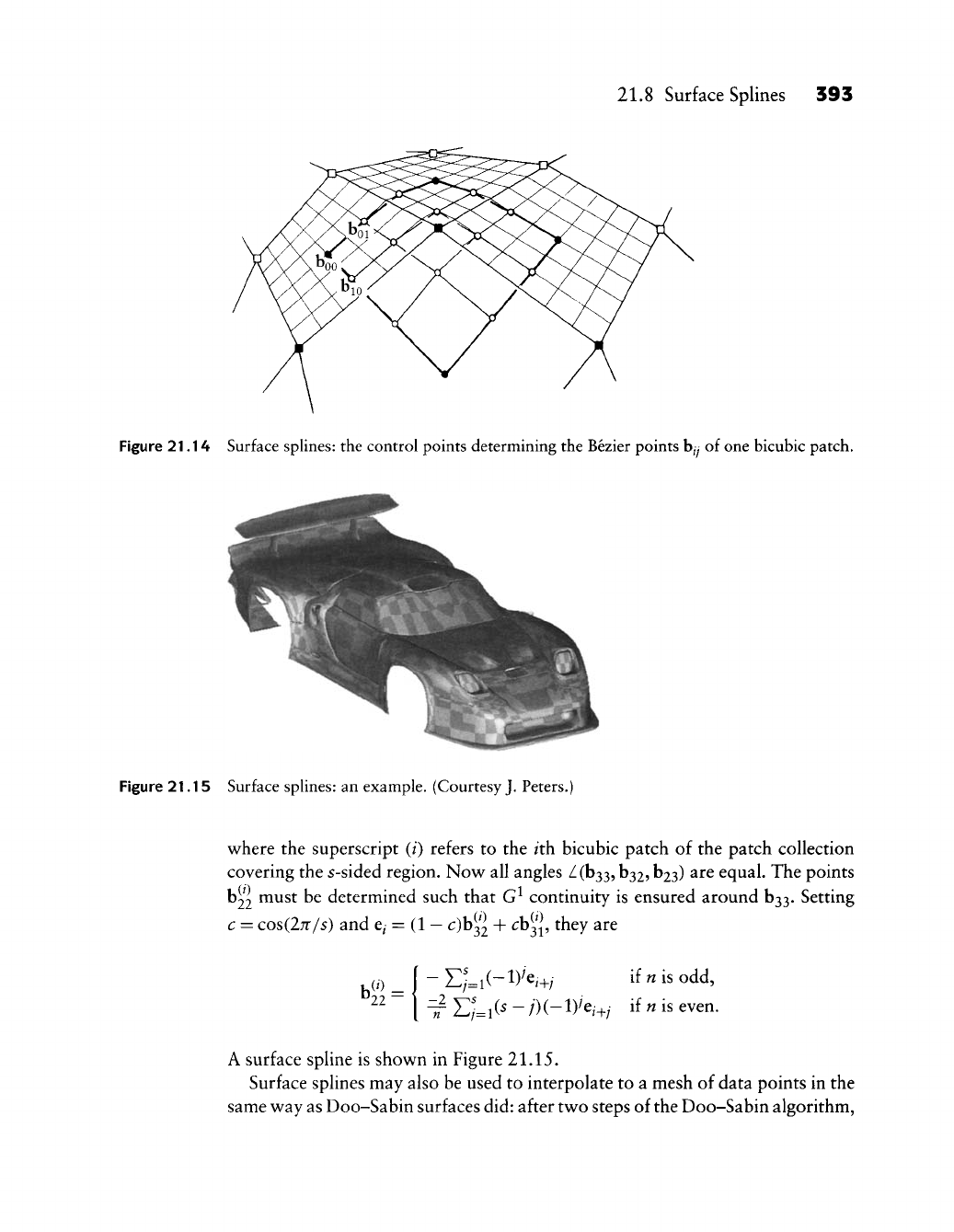
21.8 Surface Splines 395
Figure 21.14 Surface splines: the control points determining the Bezier points
b/y
of one bicubic patch.
Figure 21.15 Surface splines: an example. (Courtesy J. Peters.)
where the superscript (/) refers to the /th bicubic patch of the patch collection
covering the s-sided region. Now all angles
Z(b33,
^32?
^23) are equal. The points
b22 must be determined such that G^ continuity is ensured around 633. Setting
c = Qos{ln/s) and e^ = (1
— c)\y^2
+ ^^-^v ^^^Y ^^^
D22-
E;=i(-iye,^; if n is odd,
[ -T
T!j=ii^
- i)i-^y^i+j if n is even.
A surface spline is shown in Figure 21.15.
Surface splines may also be used to interpolate to a mesh of data points in the
same way as Doo-Sabin surfaces did: after two steps of the Doo-Sabin algorithm,
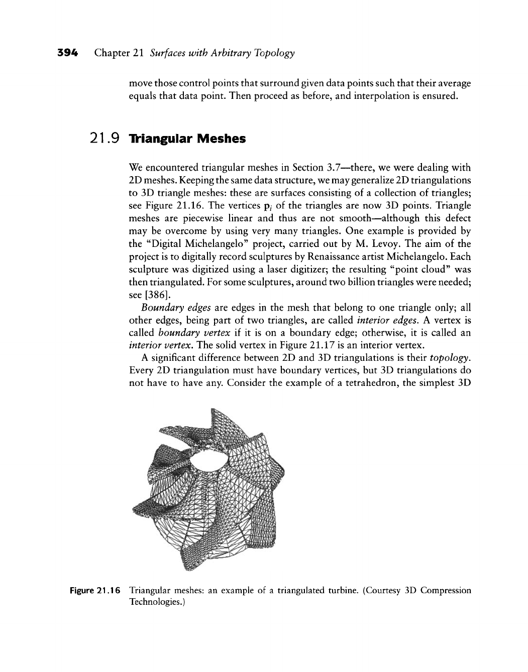
394 Chapter 21 Surfaces with Arbitrary Topology
move those control points that surround given data points such that their average
equals that data point. Then proceed as before, and interpolation is ensured.
21.9 IV'iangular Meshes
We encountered triangular meshes in Section 3.7—there, we v^ere deahng with
2D meshes. Keeping the same data structure, we may generalize 2D triangulations
to 3D triangle meshes: these are surfaces consisting of a collection of triangles;
see Figure 21.16. The vertices p^ of the triangles are now 3D points. Triangle
meshes are piecewise linear and thus are not smooth—although this defect
may be overcome by using very many triangles. One example is provided by
the "Digital Michelangelo" project, carried out by M. Levoy. The aim of the
project is to digitally record sculptures by Renaissance artist Michelangelo. Each
sculpture was digitized using a laser digitizer; the resulting "point cloud" was
then triangulated. For some sculptures, around two billion triangles were needed;
see
[386].
Boundary edges are edges in the mesh that belong to one triangle only; all
other edges, being part of two triangles, are called interior edges. A vertex is
called boundary vertex if it is on a boundary edge; otherwise, it is called an
interior vertex. The solid vertex in Figure 21.17 is an interior vertex.
A significant difference between 2D and 3D triangulations is their topology.
Every 2D triangulation must have boundary vertices, but 3D triangulations do
not have to have any. Consider the example of a tetrahedron, the simplest 3D
Figure 21.16 Triangular meshes: an example of a triangulated turbine. (Courtesy 3D Compression
Technologies.)
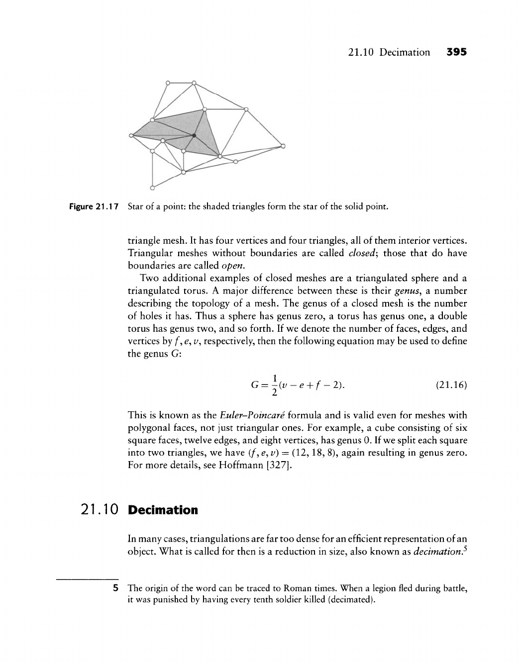
21.10 Decimation 395
Figure 21.17 Star of a point: the shaded triangles form the star of the soHd point.
triangle mesh. It has four vertices and four triangles, all of them interior vertices.
Triangular meshes without boundaries are called
closed;
those that do have
boundaries are called open.
Two additional examples of closed meshes are a triangulated sphere and a
triangulated torus. A major difference between these is their genus^ a number
describing the topology of a mesh. The genus of a closed mesh is the number
of holes it has. Thus a sphere has genus zero, a torus has genus one, a double
torus has genus two, and so forth. If we denote the number of faces, edges, and
vertices by f^
e^
v^
respectively, then the following equation may be used to define
the genus G:
G=hv-e^f
-1). (21.16)
This is known as the Euler-Foincare formula and is valid even for meshes with
polygonal faces, not just triangular ones. For example, a cube consisting of six
square faces, twelve edges, and eight vertices, has genus 0. If we split each square
into two triangles, we have (/^, ^, v) = (12,18, 8), again resulting in genus zero.
For more details, see Hoffmann
[327].
21.10 Decimation
In many cases, triangulations are far too dense for an efficient representation of an
object. What is called for then is a reduction in size, also known as decimation,^
5 The origin of the word can be traced to Roman times. When a legion fled during battle,
it was punished by having every tenth soldier killed (decimated).
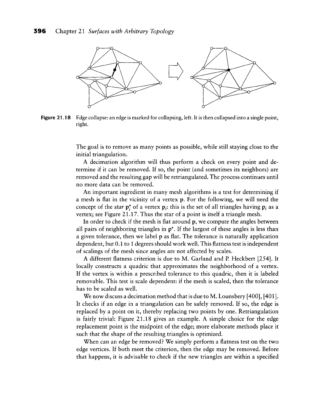
396 Chapter 21 Surfaces with Arbitrary Topology
Figure 21.18 Edge
collapse:
an edge
is
marked for collapsing, left. It
is
then collapsed into a single point,
right.
The goal is to remove as many points as possible, while still staying close to the
initial triangulation.
A decimation algorithm will thus perform a check on every point and de-
termine if it can be removed. If so, the point (and sometimes its neighbors) are
removed and the resulting gap will be retriangulated. The process continues until
no more data can be removed.
An important ingredient in many mesh algorithms is a test for determining if
a mesh is flat in the vicinity of a vertex p. For the following, we will need the
concept of the star p* of a vertex
p^:
this is the set of all triangles having p^ as a
vertex; see Figure 21.17. Thus the star of a point is itself a triangle mesh.
In order to check if the mesh is flat around p, we compute the angles between
all pairs of neighboring triangles in p*. If the largest of these angles is less than
a given tolerance, then we label p as flat. The tolerance is naturally application
dependent, but 0.1 to
1
degrees should work well. This flatness test is independent
of scalings of the mesh since angles are not affected by scales.
A different flatness criterion is due to M. Garland and P. Heckbert
[254].
It
locally constructs a quadric that approximates the neighborhood of a vertex.
If the vertex is within a prescribed tolerance to this quadric, then it is labeled
removable. This test is scale dependent: if the mesh is scaled, then the tolerance
has to be scaled as well.
We now discuss a decimation method that is due to M. Lounsbery
[400], [401].
It checks if an edge in a triangulation can be safely removed. If so, the edge is
replaced by a point on it, thereby replacing two points by one. Retriangulation
is fairly trivial: Figure 21.18 gives an example. A simple choice for the edge
replacement point is the midpoint of the edge; more elaborate methods place it
such that the shape of the resulting triangles is optimized.
When can an edge be removed? We simply perform a flatness test on the two
edge vertices. If both meet the criterion, then the edge may be removed. Before
that happens, it is advisable to check if the new triangles are within a specified
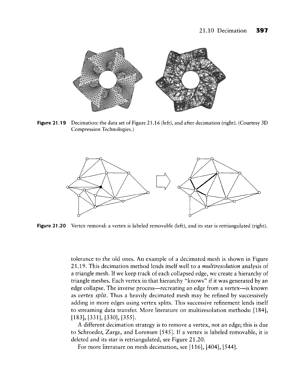
21.10 Decimation 397
Figure 21.19 Decimation: the data set of Figure 21.16 (left), and after decimation (right). (Courtesy 3D
Compression Technologies.)
Figure 21.20 Vertex removal: a vertex is labeled removable (left), and its star is retriangulated (right).
tolerance to the old ones. An example of a decimated mesh is shown in Figure
21.19.
This decimation method lends itself well to a multiresolution analysis of
a triangle mesh. If we keep track of each collapsed edge, we create a hierarchy of
triangle meshes. Each vertex in that hierarchy "knows" if it was generated by an
edge collapse. The inverse process—recreating an edge from a vertex—is known
as vertex split. Thus a heavily decimated mesh may be refined by successively
adding in more edges using vertex splits. This successive refinement lends itself
to streaming data transfer. More literature on multiresolution methods:
[184],
[183], [331], [330], [355].
A different decimation strategy is to remove a vertex, not an edge; this is due
to Schroeder, Zarge, and Lorensen
[545].
If a vertex is labeled removable, it is
deleted and its star is retriangulated, see Figure 21.20.
For more literature on mesh decimation, see
[116], [404], [544].
398 Chapter 21 Surfaces with Arbitrary Topology
21.11 Problems
1 Consider the following subdivision method: starting with a closed polygo-
nal mesh, recursively subdivide by alternating between the Doo-Sabin and
CatmuU-Clark schemes. What can you say about the number of extraor-
dinary vertices?
2 The Euler-Poincare formula (21.16) always produces a genus that is an
integer. Why.^
3 Take a cube with square faces and place three square holes through it, each
hole connecting opposite faces. What is the genus of the resulting object.^
4 Sketch the effect of two levels of the >/3 scheme.
* 5 The Doo-Sabin recursion generates a sequence of F-faces for every face, in
the limit converging to the centroid of the considered face. Show that the
limiting F-faces are planar.
* 6 Each of the triangles in p* forms an angle at p. Call the sum of all these
angles Ep. If Ep = 360, then all triangles are in one plane. Thus the quantity
360
— I Dpi
measures the nonplanarity of p*—yet it is not a good flatness
indicator. Why?
PI Write a program to find an interpolating Doo-Sabin surface to the eight
vertices of a cube.
Coons Patches
w e have already encountered design tools that originated in car companies;
Bezier curves and surfaces were developed by Citroen and Renault in Paris. Two
other major concepts also emerged from the automotive field: Coons patches (S.
Coons consulted for Ford, Detroit) and Gordon surfaces (W. Gordon worked for
General Motors, Detroit).^ These methods have a different flavor than Bezier or
B-spline methods: instead of being described by control nets, they "fill in" curve
networks in order to generate surfaces.
A designer does not think in terms of surfaces but rather in terms of "feature
curves"; these are lines on a car between which the actual surfaces fit "naturally."
In Color Plate III, we can see some of these lines as boundary curves of B-spline
surfaces. Once a designer has produced the feature lines, a filling-in process
follows that generates a surface from a network of curves. The techniques used
in this process are known by the names of their inventors. Coons and Gordon.
Additional literature on Coons patches includes Coons's "little red book"
[125] (also available in a French translation [128]) and Barnhill [21], [22].
In the area of numerical grid generation for computational fluid dynamics.
Coons patches are also frequently employed; here, they are known as transfinite
interpolants; see
[588].
1 Just for the record, in the late 1960s, Chrysler began to develop a curve and surface scheme
that was based on Chebychev polynomials.
399
400 Chapter 22 Coons Patches
22.1 Coons Patches: Bilinearly Blended
We encountered Coons patches in the context of "fiUing in" control nets in Sec-
tion 15.2. The underlying principle is applicable to more general surfaces. Here,
the boundary curves are not piecewise linear control polygons, but arbitrary
parametric curves. This simplest instance of Coons patches was also developed
first by Coons
[124].
To be more precise: given are four arbitrary curves Ci(u), Ciiu) and di(t'),
diiv),
defined over
w
G
[0,1] and v e
[0,1],
respectively, find a surface x that has these
four curves as boundary curves:
x(w, 0) = Ci(w), x(w, 1) = C2(w), (22.1)
x(0,
v) = di(i/), x(l, v) = d2iv), (22.2)
The four boundary curves define two ruled surfaces:
r^(w, v) = (1
—
v)x(u^ 0) + vx(u, 1)
and
r^(w, i;) = (1 - w)x(0, v) + wx(l, v).
Both interpolants are shown in Figure
22.1,
and we see that r^ interpolates to the
c-curves, yet fails to reproduce the d-curves. The situation for r^ is similar, and
therefore equally unsatisfactory. Both r^ and r^ do well on two sides, yet fail on
the other two, where they are linear. Our strategy is therefore as follows: let us
try to retain what each ruled surface interpolates to, and let us try to eliminate
what each fails to interpolate to. A little thought reveals that the "interpolation
failures" are captured by one surface: the bilinear interpolant v^d ^^ ^he four
corners (see also Section 14.1):
. X r. if x(0,0) x(0,1) 1 r 1 - 1/1
We are now ready to create a Coons patch x. It is given by
x = r^ + rj-r^^, (22.3)
or, in the form of a recipe: "loft^ + loft^
—
bilinear." The involved surfaces and
the solution are illustrated in Figure 22.1. Writing (22.3) in full detail gives
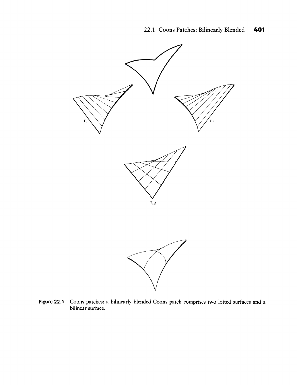
22.1 Coons Patches: Bilineariy Blended 401
Figure 22.1 Coons patches: a biUnearly blended Coons patch comprises two lofted surfaces and a
bilinear surface.
402 Chapter
22
Coons Patches
+ [x(^,0) x(«,l)]P^''l (22.4)
^ ^Lx(l,0) x(l,l)J[
V J
It
is
left
as an
exercise
to
verify that (22.4) does indeed interpolate
to all
four
boundary curves.
We can now justify the name bilinearly blended
for
the preceding Coons patch:
a ruled surface "blends" together the two defining boundary curves; this blending
takes place
in
both directions. However,
the
Coons patch
is not
generally itself
a bilinear surface—the name refers purely
to the
method
of
construction.
The functions
1—w, u and 1—f, v are
called blending functions,
A
close
inspection
of
(22.4) reveals that many other pairs
of
blending functions,
say,
/i(w),
fiiu)
and
g\{v)^
giip)^
could also
be
used
to
construct
a
generalized Coons
patch.
It
would then
be of the
general form
x{u,v)=[h{u) /2(«)][^J5;^J]
+ [x(«,0) x(«,l)]|^jij|;jl (22.5)
Ihiu) f2(«)][^(i^o) x(l,l)JLg2(t^)J-
There
are
only
two
restrictions
on the d and gi:
each pair must
sum to
one identically: otherwise,
we
would generate nonbarycentric combinations
of
points (see Section 2.1). Further, we must have /^(O)
=
^^(O)
=
1,
fi(l) =
gi(l)
= 0
in order
to
actually interpolate.
The
shape
of the
blending functions
has a
predictable effect
on
the shape
of
the resulting Coons patch. Typically,
we
require
fi
and gi to be
monotonically decreasing; this produces surfaces
of
predictable
shape,
but is not
necessary
for
theoretical reasons.
22.2 Coons Patches: Partially Bicubically Blended
The bilinearly blended Coons patch solves
a
problem
of
considerable importance
with very little effort,
but we pay for
that
by an
annoying drawback. Consider
Figure
22.2: it
shows
two
bilinearly blended Coons patches, defined over
u e
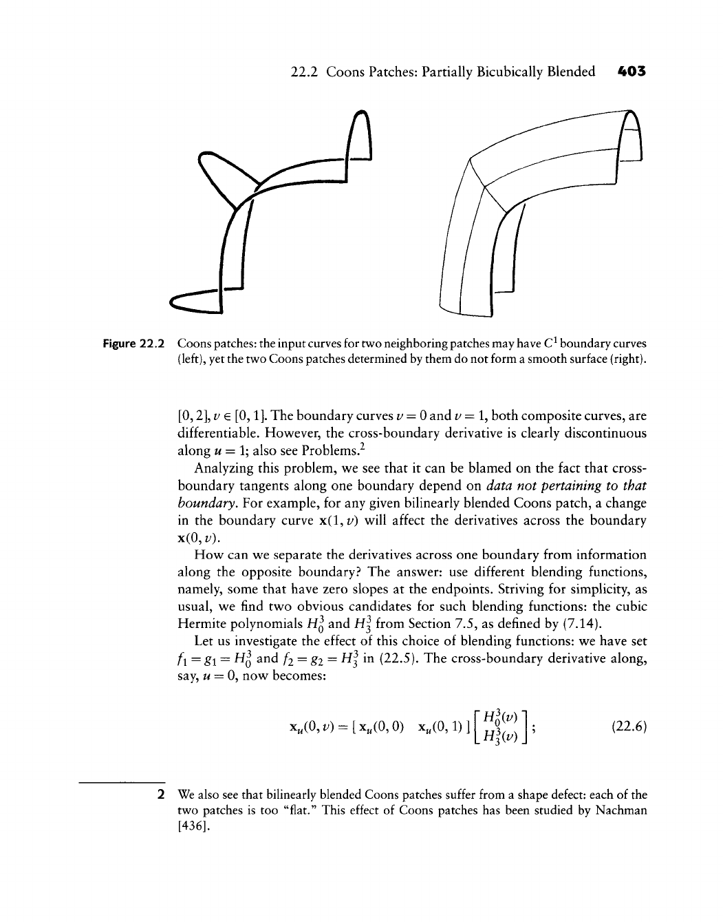
22.2 Coons Patches: Partially Bicubically Blended 403
Figure 22.2 Coons
patches:
the input
curves
for two neighboring patches may
have
C^
boundary curves
(left),
yet the
tw^o
Coons patches determined
by
them do not form
a
smooth surface (right).
[0,2],
V G
[0,1].
The boundary curves v = 0 and v=\^ both composite curves, are
differentiable. How^ever, the cross-boundary derivative is clearly discontinuous
along
w
= 1; also see Problems."^
Analyzing this problem, w^e see that it can be blamed on the fact that cross-
boundary tangents along one boundary depend on data not pertaining to that
boundary. For example, for any given bilinearly blended Coons patch, a change
in the boundary curve x(l,i/) w^ill affect the derivatives across the boundary
x(0,i/).
How^ can w^e separate the derivatives across one boundary from information
along the opposite boundary.^ The answer: use different blending functions,
namely, some that have zero slopes at the endpoints. Striving for simplicity, as
usual, v^e find tv^o obvious candidates for such blending functions: the cubic
Hermite polynomials H^ and H| from Section 7,5^ as defined by (7.14).
Let us investigate the effect of this choice of blending functions: w^e have set
f\=g\
= ^0 ^^^ /2 = g2
=
say,
w
= 0, now^ becomes:
H|
in (22.5). The cross-boundary derivative along.
x„(0,t^) = [x„(0,0) x„(0,l)] (22.6)
2 We also see that bilinearly blended Coons patches suffer from a shape defect: each of the
two patches is too "flat." This effect of Coons patches has been studied by Nachman
[436].
404 Chapter 22 Coons Patches
all other terms vanish since d/dwH|.(0) = d/dwH|.(l) = 0 for / = 0 and / = 1.
Thus,
the only data that influence x^ along
w
= 0 are the two tangents x^(0, 0)
and x^(0,1)—^we have achieved our goal of making the cross-boundary derivative
along one boundary depend only on information pertaining to that boundary.
With our new blending functions, the two patches from Figure 22.2 would now
beCi.
Unfortunately, we have also created a new problem. At the patch corners,
these patches often have "flat spots." The reason; partially bicubically blended
Coons patches,^ constructed as before, suffer from zero corner twists:
x^^(ij)
= 0;
/,/€{0,l}.
This is easily verified by simply taking the wi/-partial of (22.5) and evaluating at
the patch corners.
The reason for this poor performance lies in the fact that we use only two
functions,
HQ
and H3 from the full set of four Hermite polynomials. Both have
zero derivatives at the interval endpoints, and pass that property on to the surface
interpolant.
We will now modify the partially bicubically blended Coons patch in order to
avoid the flat spots at the corners.
22.5 Coons Patches: Bicubically Blended
Cubic Hermite interpolation needs more input than positional data—first deriva-
tive information is needed. Since our positional input consists of whole curves,
not just points, the obvious data to supply are derivatives along those input
curves. Our given data now consist of
x(w,0),
x(w, 1), x(0,i/), x(l,i/)
and
x^(w,0), x^(w, 1), x^(0,i/), x^(l,i/).
We can think of the now prescribed cross-boundary derivatives as "tangent
ribbons," illustrated in Figure 22.3 (only two of the four "ribbons" are shown
there).
3 We use the term
partially
bicubically blended since only a part of all cubic Hermite basis
functions is used.
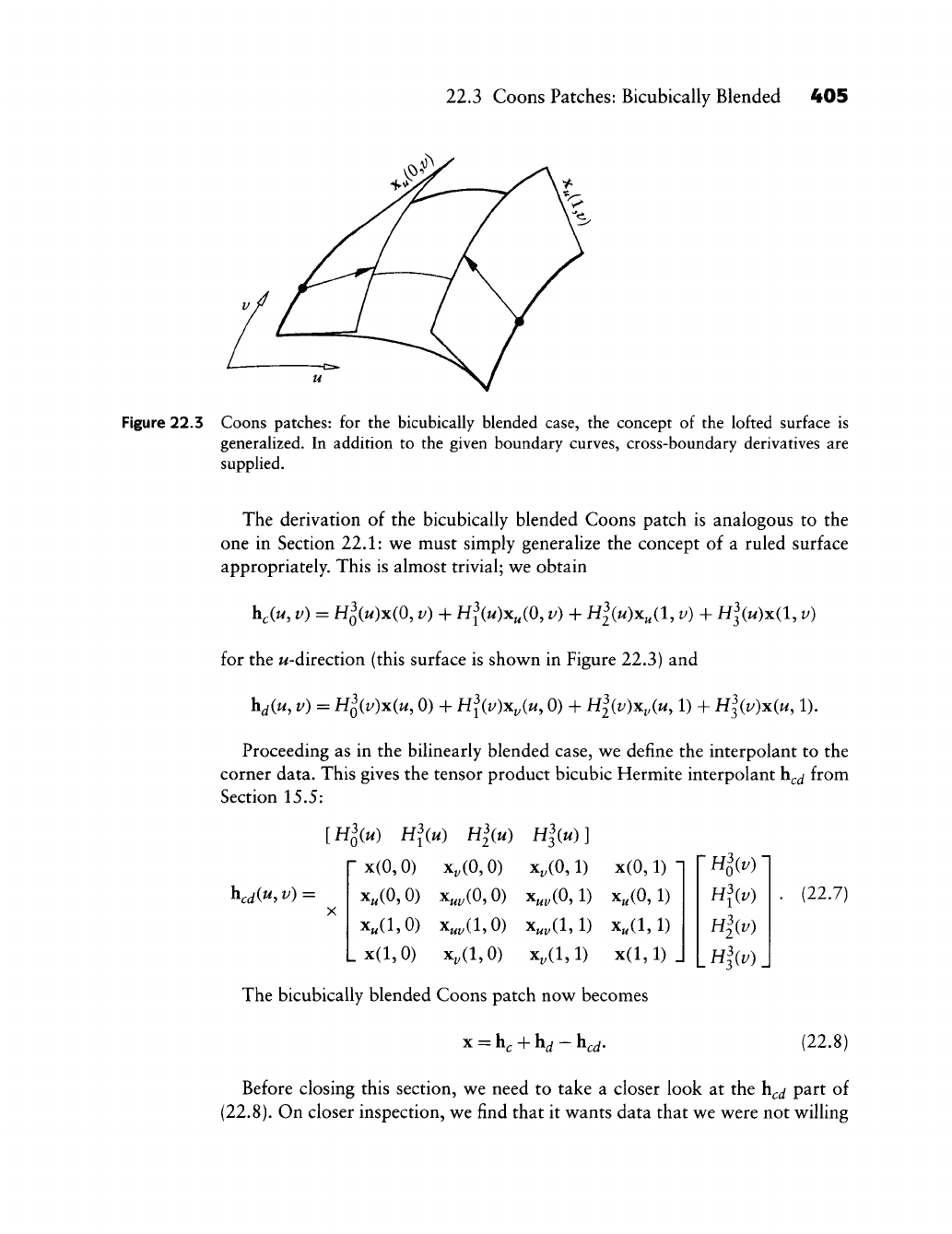
22.3 Coons Patches: Bicubically Blended 405
Figure 22.3 Coons patches: for the bicubically blended case, the concept of the lofted surface is
generalized. In addition to the given boundary curves, cross-boundary derivatives are
supplied.
The derivation of the bicubically blended Coons patch is analogous to the
one in Section 22.1: we must simply generalize the concept of a ruled surface
appropriately. This is almost trivial; we obtain
h,(u,
V)
= H^Wx(0,
V)
+ Hi^(w)x^(0,
V)
+ H|(w)x^(l, v) + H|(W)X(1, V)
for the w-direction (this surface is shown in Figure 22.3) and
h^(t/,
V)
= H^(i/)x(w, 0) + Hl{v)^y{u, 0) + Hl(v)x^(u, 1) + HI(V)X(U, 1).
Proceeding as in the bilinearly blended case, we define the interpolant to the
corner data. This gives the tensor product bicubic Hermite interpolant h^j from
Section 15.5:
hcj(«, v) =
[H^iu) Hl(u) Hliu) Hliu)]
•x(0,0) x,(0,0) x^(0,l) x(0,l)
x^(0,0) x^^(0,0) x^,(0,l) x^(0,l)
x^(l,0) x^,(l,0) x^^(l,l) x^(l,l)
L x(l, 0) x,(l, 0) x,(l, 1) x(l, 1) J
L
Hliv) J
The bicubically blended Coons patch now becomes
H^v)
(22.7)
X
= h^ + hj - h
^cd- (22.8)
Before closing this section, we need to take a closer look at the h^j part of
(22.8).
On closer inspection, we find that it wants data that we were not willing
406 Chapter 22 Coons Patches
(or able) to provide in our initial problem description, namely, the central "twist
partition" of the 4x4 matrix in (22.7). The bicubically blended Coons patch
needs these quantities as input, and this has caused CAD software developers
many headaches since Coons proposed his surface scheme in 1964. The most
popular "solution" seems to be simply to define each of the four corner twists
to be the zero vector. The drawbacks of that choice were already discussed in
Section 14.10, but alternatives are pointed out in that section, too.
22.4 Piecewise Coons Surfaces
We will now apply the bicubically blended patch to the situation for which it was
intended: we assume that we are given a network of curves as shown in Figure
22.6 and that we want to fill in this curve network with bicubically blended
Coons patches. The resulting surface will be C^.
To apply (22.8), we must create twist vectors and cross-boundary derivatives
(tangent ribbons) from the given curve network. As a preprocessing step, we
estimate a twist vector ^^y{ui^
Vj)
at each patch corner. This can be done by using
any of the twist vector estimators discussed in Section 16.3. In that section, we
assumed that the boundary curves of each patch were cubics; that assumption
does not affect the computation of the twist vectors at all, however.
Having found a twist vector for each data point, we now need to create cross-
boundary derivatives for each boundary curve. Let us focus our attention on
one patch of our network, and let us assume for simplicity (but without loss of
generality!) that the parameters u and v vary between 0 and 1. We shall now
construct the tangent ribbon x^(w, 0). We have four pieces of information about
x^(w, 0): the values of ^y{u^ 0) at u = 0 and at
w
= 1, and the derivatives with
respect to u there—these are the twists that we made up earlier, namely, x^j;(0,0)
andx^^(l,0).
We therefore have the input data for a univariate cubic Hermite interpolant,
and the desired tangent ribbon assumes the form
x,(u,
0) = x,(0, O)Ho^(^) + x^,(0,0)Hliu)
+ x^,(l, 0)Hl(u) + x,(l, 0)Hl(u), (22.9)
The remaining three tangent ribbons are computed analogously.
We have thus found a way to pass a C^ surface through a C^ network of curves.
All we needed was the ability to estimate the twists at the data points.

22.5 Two Properties 407
22.5 IWo Properties
Coons patches are twist minimizing in the sense that
xLdS (22.10)
Js"""'
is minimal exactly for the Coons patch (S being the domain).
If we apply the minimum principle to the discrete Coons patch, we have that
m—ln—1
i=0 j=0
is minimal if the hjj form a discrete Coons patch.
Coons patches satisfy a permanence principle: let two points
(WQ?
^O)
^^^
(^1,
vi) define a rectangle R in the domain of a Coons patch. The four boundaries
of this subpatch will map to four curves on the Coons patch. You may ask what
the Coons patch to those four boundary curves is. The answer: the original Coons
patch, restricted to the rectangle R^ In this sense. Coons patches are self-similar!
We can apply this principle to a 3 x 3 grid of a discrete Coons patch. Such a
grid is given by
b/-l,/+l b^-,;+l b/^l,;+l
b/-i,;-i b^-,/-i b^+i,;-i
As a consequence of the permanence principle,
1
^(b.,;+i +
b,_i,^-
+
b,,.!,^-
+
b,,_i).
(22.11)
We could thus obtain the discrete Coons patch as the solution to a Unear
system of equations. This is not practical for the construction of a rectangular
control net, but offers a basic construction principle for more complex surfaces.
For more details, see
[207].
4 The term
permanence principle
for Coons patches was coined by R. Barnhill in a slightly
different context around 1980.
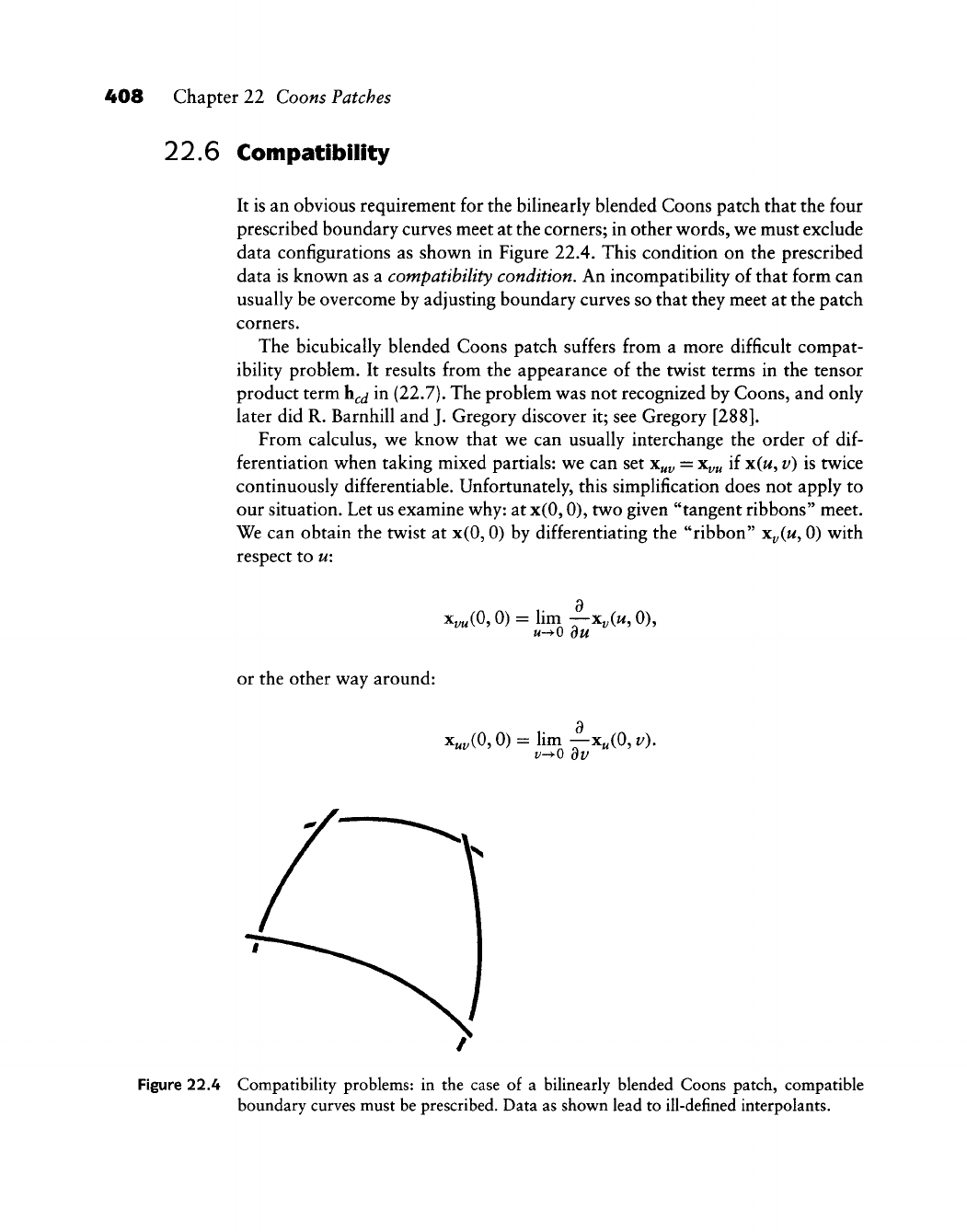
408 Chapter 22 Coons Patches
22.6 Compatibility
It is an obvious requirement for the bilinearly blended Coons patch that the four
prescribed boundary curves meet at the corners; in other words, we must exclude
data configurations as shown in Figure 22.4. This condition on the prescribed
data is known as a compatibility condition. An incompatibility of that form can
usually be overcome by adjusting boundary curves so that they meet at the patch
corners.
The bicubically blended Coons patch suffers from a more difficult compat-
ibility problem. It results from the appearance of the twist terms in the tensor
product term h^j in (22.7). The problem was not recognized by Coons, and only
later did R. Barnhill and J. Gregory discover it; see Gregory
[288].
From calculus, we know that we can usually interchange the order of
dif-
ferentiation when taking mixed partials: we can set
x^^^
= x^;^ if x(«, v) is twice
continuously differentiable. Unfortunately, this simplification does not apply to
our situation. Let us examine why: at x(0,0), two given "tangent ribbons" meet.
We can obtain the twist at x(0,0) by differentiating the "ribbon"
yiy{u^
0) with
respect to u:
Xi;„(0,0) = lim —x^(w, 0),
M-^0 du
or the other way around:
x«t;(0,0) = lini —x„(0, v).
v-^0 dv
Figure 22.4 Compatibility problems: in the case of a bilinearly blended Coons patch, compatible
boundary curves must be prescribed. Data as shown lead to ill-defined interpolants.
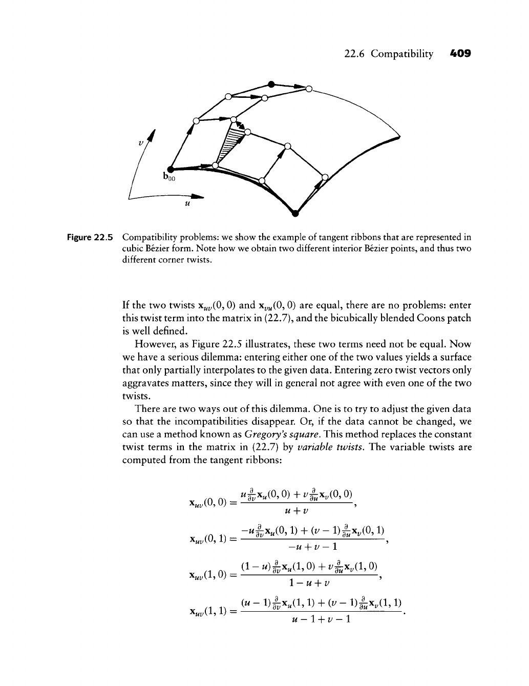
22.6 Compatibility 409
Figure 22.5 Compatibility problems: we show the example of tangent ribbons that are represented in
cubic Bezier form. Note how we obtain two different interior Bezier points, and thus two
different corner twists.
If the two twists x^^(0, 0) and x^^(0, 0) are equal, there are no problems: enter
this twist term into the matrix in (22.7), and the bicubically blended Coons patch
is well defined.
However, as Figure 22.5 illustrates, these two terms need not be equal. Now
we have a serious dilemma: entering either one of the two values yields a surface
that only partially interpolates to the given data. Entering zero twist vectors only
aggravates matters, since they will in general not agree with even one of the two
twists.
There are two ways out of this dilemma. One is to try to adjust the given data
so that the incompatibilities disappear. Or, if the data cannot be changed, we
can use a method known as Gregory's square. This method replaces the constant
twist terms in the matrix in (22.7) by variable twists. The variable twists are
computed from the tangent ribbons:
x^,(0,0) =
x^,(0,1) -
x^^(l, 1) =
^|;X^(Q,0)+l/|^X,(0,0)
u-\-v
-^|;x,(0,l) + (i;-l)|^x,(0,l)
—u
+ v
—
1
a-u)ix^a,o)
+ vix,a,o)
l
—
U
+ P
(M-1)|;X„(1,1) + (Z;-1)|-X^(1,1)
u-l+v-1
410 Chapter 22 Coons Patches
The resulting surface does not have a continuous twist at the corners. In fact,
it is designed to be discontinuous: it assumes two different values, depending
on from where the corner is approached. If we approach x(0,0), say, along the
isoparametric line
w
= 0, we should get the w-partial of the given tangent ribbon
x^(w, 0) as the twist x^^(0, 0). If we approach the same corner along z/ = 0, we
should get the i/-partial of the given ribbon x^(0, v) to be x^^(0,0).
An interesting application of Gregory's square was developed by Chiyokura
and Kimura
[112]:
suppose we are given four boundary curves of a patch in cubic
Bezier form, and suppose that the cross-boundary derivatives also vary cubically.
Let us consider the corner x(0,0) and the two boundary curves that meet there.
These curves define the Bezier points boy and
b^o-
The cross-boundary derivatives
determine by and
b^j.
Note that bn is defined twice! This situation is illustrated
in Figure 22.5. Chiyokura and Kimura made b^ a function of u and v:
bii = bii(w, V) = • ,
where hii(u) denotes the point b^ that would be obtained from the cross-
boundary derivative x^(0, v), and so on. Similar expressions hold for the remain-
ing three interior Bezier points, all following the pattern of Gregory's square.
Although a solution to the posed problem, we should note that Gregory's
square (or the Chiyokura and Kimura application) is not free of problems. Even
with polynomial input data, it will produce a rational patch. Written in rational
Bezier form, its degree is seven in both u and v and the corner weights are
zero (see [202]). The resulting singularities are removable, but require special
attention. In situations where we are not forced to use incompatible cross-
boundary derivatives, it is therefore advisable first to estimate corner twists and
then to use (22.9) as a cross-boundary derivative generator.
22.7 Gordon Surfaces
Gordon surfaces are a generalization of Coons patches. They were developed
in the late 1960s by W. Gordon
[281], [283], [280], [282],
who was then
working for the General Motors Research labs. He coined the term transfinite
interpolation for this kind of surface.
It is often not sufficient to model a surface from only four boundary curves. A
more complicated (and realistic) situation arises when a network of curves is pre-
scribed, as shown in Figure 22.6. We will construct a surface g that interpolates
to all these curves—they will then be isoparametric curves g(w/, t/); / = 0,..., m
and g(M, Vj)\j = 0,...,
w.
We shall therefore refer to these input curves in terms
of the final surface g. The idea behind the construction of this Gordon surface
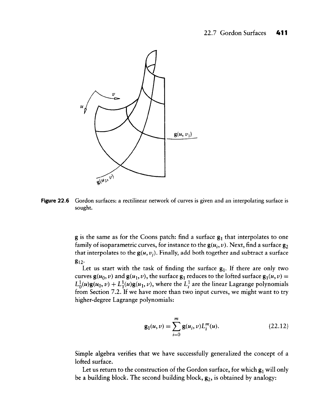
22.7 Gordon Surfaces 411
Figure 22.6 Gordon surfaces: a rectilinear network of curves is given and an interpolating surface is
sought.
g is the same as for the Coons patch: find a surface gj that interpolates to one
family of isoparametric curves, for instance to the g(w/, v). Next, find a surface g2
that interpolates to the
g(M,
Vj),
Finally, add both together and subtract a surface
gl2-
Let us start vv^ith the task of finding the surface gj. If there are only two
curves
gC^o?
^) ^^^ g(^i5
^)y
the surface gi reduces to the lofted surface gi(w, v) =
Lliu)g{uQ^ v)
-\-
Lj(w)g(wi, f), v^here the L\ are the linear Lagrange polynomials
from Section 7.2. If we have more than two input curves, we might want to try
higher-degree Lagrange polynomials:
%Mv) =
Y,%{Ui,v)Vl^{u).
{IIAI)
i=0
Simple algebra verifies that we have successfully generalized the concept of a
lofted surface.
Let us return to the construction of the Gordon surface, for which gj will only
be a building block. The second building block, g2, is obtained by analogy:
4>12 Chapter 22 Coons Patches
n
The third building block, gi25 is simply the interpolating tensor product
surface
m n
The Gordon surface g now becomes
g = gi + g2-gi2- (22.13)
It is left as an exercise to verify that (22.13) in fact interpolates to all given
curves. Note that for the actual computation of g, we do not have to use the
Lagrange polynomials. We only have to be able to solve the univariate polynomial
interpolation problem, for example, by using the Vandermonde approach.
We have derived Gordon surfaces as based on polynomial interpolation. Much
more generality is available. Equation (22.13) is also true if we use interpolation
methods other than polynomial interpolation. The essence of (22.13) may be
stated as follows: take a univariate interpolation scheme, apply it to all curves
g(w, vj) and to all curves
g(M^,
t/), add the resulting two surfaces, and subtract
the tensor product interpolant that is defined by the univariate scheme. We
may replace polynomial interpolation by spline interpolation, in which case we
speak of spline-blended Gordon surfaces. The basis functions of the univariate
interpolation scheme are called blending functions,
22.8 Boolean Sums
Our development of Coons patches was quite straightforward, yet it is slightly
flawed from a geometric viewpoint. When we derived (22.3), we added the two
surfaces r^ and r^ as an intermediate step. This is illegal—the sum of two surfaces
would depend on the choice of a coordinate system (see the discussion in Section
2.1).
Although the situation is straightened out by subtracting the bilinear surface
r^^, one might ask for a cleaner development. It is provided by the use of Boolean
sums.
Let us define an operator V\ that, when applied to a rectangular surface x,
returns the ruled surface through
X(M,
0) and x(«, 1):
[Vxx\{u, v) = {\- v)x(u, 0) + vx(u, 1).
22.8 Boolean Sums 413
Similarly, we define Vi to return the ruled surface through x(0, v) and x(l, v):
[ViAiu, v) = {l- u)x(0, v) + wx(l, v).
In terms of Section 22.1, Pj and Vi yield the surfaces r^ and rj.
We would like to formulate the bilinearly blended Coons patch—which we
now call Px—in terms of Vi and Vi,
Let us take P^x as a first building block for the Coons patch. Since V\S.
interpolates only on two boundaries, we will try to add another surface to it,
such that the final result will interpolate to all four boundaries. Such a correction
surface must interpolate to all four boundaries of the error surface x
—
V\x.^ It
may be obtained by applying Vi to the error surface. We then obtain
Px = 7^ix + p2(x-7^ix).
This expression for the bilinearly blended Coons patch may be shortened by
showing only the involved operators:
V = Vi +
V2{l-Vi),
(22.14)
where X is the identity operator. This means of obtaining one operator 'P as a
combination of two operators V\^ Vi is called a Boolean sum and is often written
^ = ^10^2. (22.15)
Of course, we may also multiply out the terms in (22.14). We then obtain
J>
= p^^V2 = Vi + V2- V{P2'
We now see that, even with the use of an operator calculus, we still have the
same old Coons patch as defined by (22.3): the term V{P2 is simply the bilinear
interpolant to the patch corners.
Let us summarize the essence of the Boolean sum approach: an interpolant
to the given data is built by applying Pj. A second operator V2 is then applied
to the "failures" of P^, and the result is added back to the output from Vi. The
interpolant V2 may actually be of a simpler nature than V^, since it has to act on
only zero data where Vi was "successful." We can illustrate this for the example
of univariate cubic Hermite interpolation: we define Vi to be the (point-valued)
linear interpolant between two points
XQ
and x^ and V2 to be the (vector-valued)
5 Note that this error surface is vector valued, since both x and Vix are point valued.
414 Chapter 22 Coons Patches
cubic Hermite interpolant to a data set 0,
HIQ,
mi, 0. Then Vi
0
P2 is the standard
cubic Hermite interpolant.
A note on the notation used in this section: the letter
V
that we used to denote
our building-block interpolants is due to the term projector, A projector is an
operator, which,
if
applied to its own output, will not change the result.^ For
example,
Vix
is
a
ruled surface, and V{PiX is the same ruled surface. Operators
with the property of being projectors are also called idempotent.
It was W. Gordon who realized the underlying algebraic structure
of
Coons
patches. That discovery then led him to the generalization that now bears his
name (Section 22.7). Boolean sums may be used
in
the development
of
many
surface interpolation schemes, for an excellent survey, see Barnhill [21].
22.9 IV'iangular Coons Patches
Just as triangular Bezier patches provide an alternative to the rectangular variety,
we may devise a triangular version of Coons patches. Several solutions have been
proposed through the years; we will briefly explain the ones by Barnhill,
Birkhoff,
and Gordon [26] and by Nielson
[443].
The C^ Barnhill,
Birkhoff,
and Gordon (BBG) approach can be explained as
follows. Suppose we are given three boundary curves, as shown in Figure 22.7.
We seek
a
surface that interpolates
to
all three
of
them, that is,
a
transfinite
triangular interpolant. The construction follows the standard Coons patch de-
velopment in that it consists of several building blocks, which are then combined
in
a
clever way.
Let us denote^ the three boundary curves by x(0, z/, w)^ x(w, 0, w/), x(w, z/, 0).
We define three building blocks, each being
a
ruled surface that interpolates
to
two boundary curves:
Pix(u)
=
(1
-
r)x(^, 0, w)
+
rx(^, v, 0); r =
^,
V2x(u)
=
a-s)x(u,v,0)+sx(0,v,w); 5=^,
(22.16)
P3x(u)
=
(1
-
t)x(u, 0, w)
+
^x(0, v,w);
t
=
^.
Several combinations
of
these surfaces yield
an
interpolant
Vx to
all three
boundaries: the Boolean sum of any two—for example,
V
= V\®
V^—will
have
that property.
6 The term comes from geometry:
if
a 3D object is projected into
a
plane, we may then
repeat that projection, yet it will not change the image.
7 We use the concept of barycentric coordinates as outlined in Section 3.5.
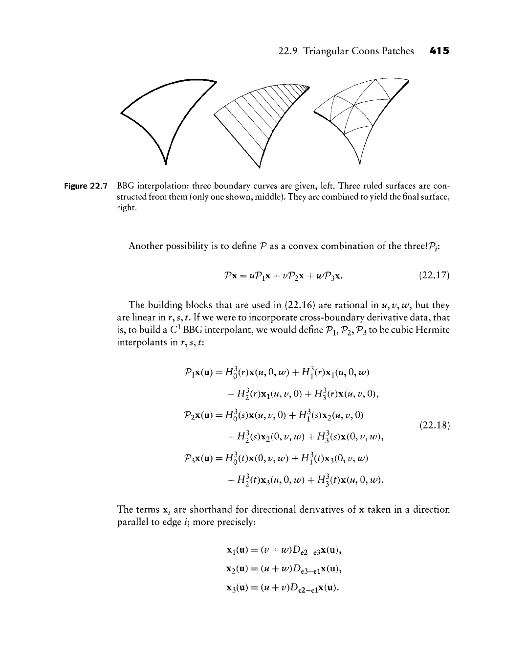
22.9 Triangular Coons Patches
415
Figure
22.7
BBG interpolation: three boundary curves
are
given, left. Three ruled surfaces
are
con-
structed from them (only one shown,
middle).
They are combined to yield the
final
surface,
right.
Another possibility
is to
define
P as a
convex combination
of the
threelP^:
Vx
= uV\x
-h
VV2X
H-
WVT,X,
(22.17)
The building blocks that
are
used
in
(22.16)
are
rational
in
w,
^',
w, but
they
are linear
in r, s, t,
liwt w^ere
to
incorporate cross-boundary derivative data, that
is,
to
build
a C^
BBG interpolant, v^e w^ould define P^,
7^2?
^3
^^
be
cubic Hermite
interpolants
in r, s, t:
Pix(u)
=
H^(r)x(w,
0, w) +
Hl(r)xi(u,
0, w)
+ Hl(r)x^(u,
V,
0) +
H|(r)x(w,
v, 0),
P2x(u)
=
Hl{s)x(u,
V,
0) +
H^^(s)x2(^,
V,
0)
+
H|(S)X2(0,
V,
w) + H^(s)x(0,1/, w),
V^xiu) =
H^(Ox(0,
zy,
w) +
H^\0x3(0,
^, u/)
+ Hlit)x2(u,
0, u/) +
Hl{t)x(u,
0, ^).
(22.18)
The terms
x^ are
shorthand
for
directional derivatives
of x
taken
in a
direction
parallel
to
edge
/;
more precisely:
Xi(u)
= (1/ +
W/)De2_e3X(u),
X2(U)
= (W +
W/)De3_elX(u),
X3(u)
= (w +
Z/)De2-elX(u).
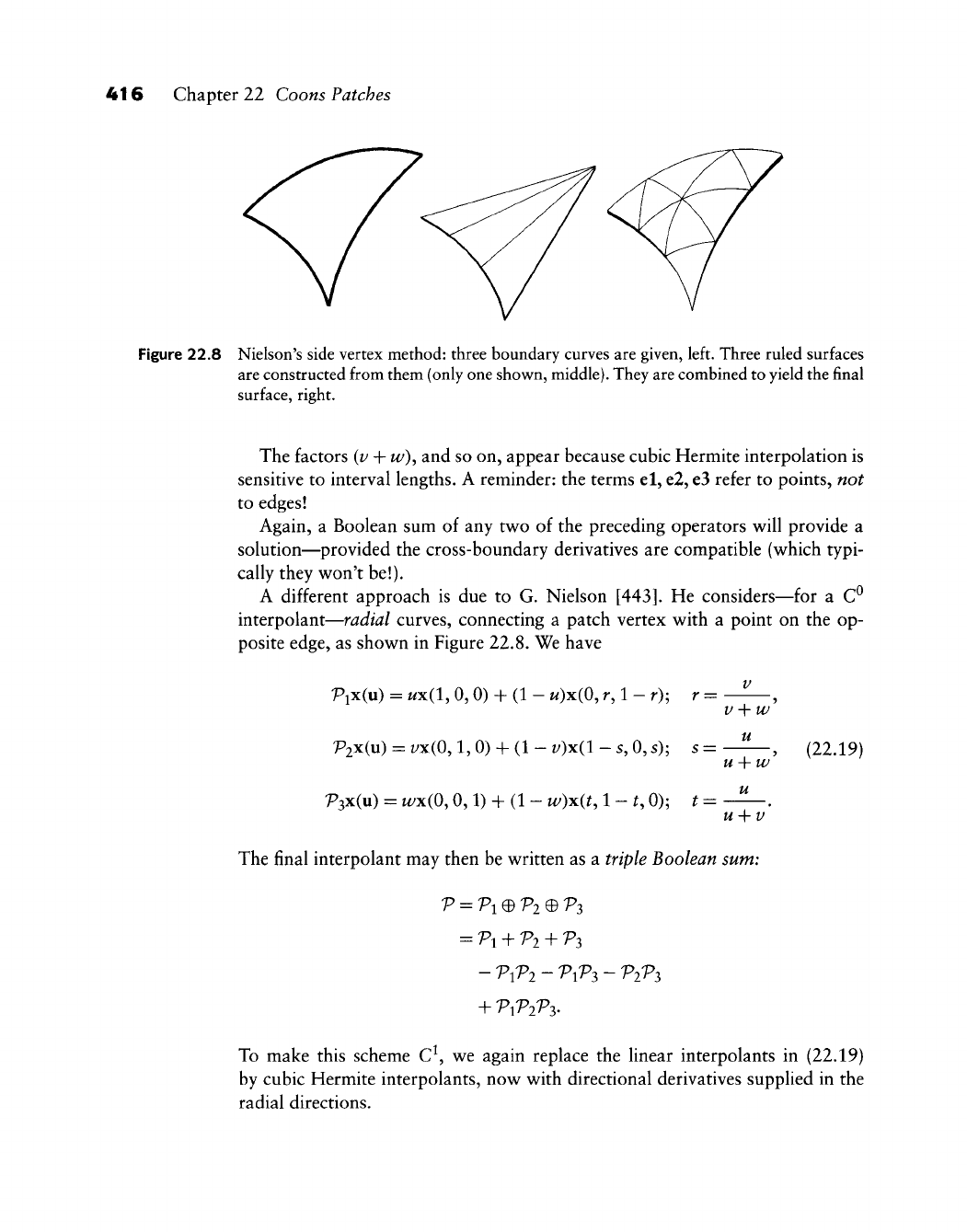
416 Chapter 22 Coons Patches
Figure 22.8 Nielsen's side vertex method: three boundary curves are given, left. Three ruled surfaces
are constructed from them (only one shown, middle). They are combined to yield the final
surface, right.
The factors {v
-\-w)^
and so on, appear because cubic Hermite interpolation is
sensitive to interval lengths. A reminder: the terms el, e2, e3 refer to points, not
to edges!
Again, a Boolean sum of any tw^o of the preceding operators will provide a
solution—provided the cross-boundary derivatives are compatible (v^hich typi-
cally they won't be!).
A different approach is due to G. Nielson
[443].
He considers—for a C^
interpolant—radial curves, connecting a patch vertex with a point on the op-
posite edge, as shown in Figure 22.8. We have
Pix(u) = wx(l, 0, 0) + (1 - w)x(0, r, 1 - r); r = ^
V -\-w
'P2x(u) = i/x(0,1,0) + (1 - zy)x(l - s, 0, s); s = ^^, (22.19)
u-\-w
p3x(u) = w/x(0,0,1) + (1 - M/)x(^
1-^0);
t= —^.
u-{-v
The final interpolant may then be written as a triple Boolean sum:
=
7^1
+ ^2 + ^3
- V{P2 - V{P^ - V2V3
+ V{P2Vy
To make this scheme C\ we again replace the linear interpolants in (22.19)
by cubic Hermite interpolants, now with directional derivatives supplied in the
radial directions.
22.10 Problems 417
For more literature on triangular Coons-type interpolants, consult the follow-
ing: Barnhill [20], Barnhill and Gregory [33], [32], Gregory and Charrot
[292],
Marshall and Mitchell
[420],
Lacombe and Bedard
[367],
and Nielson
[444].
22.10 Problems
1 Show that the bilinearly blended Coons patch is not in the convex hull of
its boundary curves. Is this a good or a bad property.'*
2 Verify the caption to Figure 22.2 algebraically.
3 Equation (22.9) generates tangent ribbons from the given boundary curve
network. Verify that the resulting surface does not suffer from twist incom-
patibilities.
* 4 Translational surfaces have zero twists. Show that the inverse statement is
also true: every surface with identically vanishing twists is a translational
surface.
* 5 Show that the bilinearly blended Coons patch, when applied to cubic
boundary curves, yields a bicubic patch.
*6 Show that Adini's twist from Section 16.3 is the twist of the bilinearly
blended Coons patch for the four boundary cubics.
* 7 As we have seen, two adjacent bihnearly blended Coons patches are not
C^ in general. What are the conditions for the boundary curves of the two
patches such that the Coons patches are C^?
PI Use the data set car.dat. Interpolate all four boundaries using uniform
B-spline interpolation. Then compute the bilinearly blended Coons patch.
Next, experiment with different blending functions and discuss how they
change the shape of the surface.

This Page Intentionally Left Blank
Shape
w e discussed many methods for curve and surface generation. In this chapter,
we shall discuss some ways to inspect the geometric quality of those curves and
surfaces, and develop a few ideas on how to remove shape imperfections. There
is a growing interest in this area; see for example, the collection of Sapidis
[532].
25.1 Use of Curvature Plots
A spline curve is typically obtained in one of two
ways:
as a curve that interpolates
to given data points, or as the result of interactive manipulation of a B-spline
polygon. In both cases, it is hard to tell from the display on the screen if the
shape of the curve is acceptable or not: two curves may look identical on the
screen, yet reveal significant shape differences when plotted to full scale. Such
plots are both expensive and time consuming—one needs a tool to analyze curve
shape at the CAD terminal.
The most commonly used tool for this task is provided by the curvature plot
of the curve. For a given curve, we can plot curvature versus arc length or versus
the parameter. The resulting graph is the curvature plot. We have already used
curvature plots in Chapter 9. All three curves from Figures 9.8, 9.10, and 9.12
look very similar, yet their curvature plots reveal substantial differences. The
same is true for Figures 9.16 and 9.18. What actually constitutes a "substantial"
difference depends on the application at hand, of course.
419
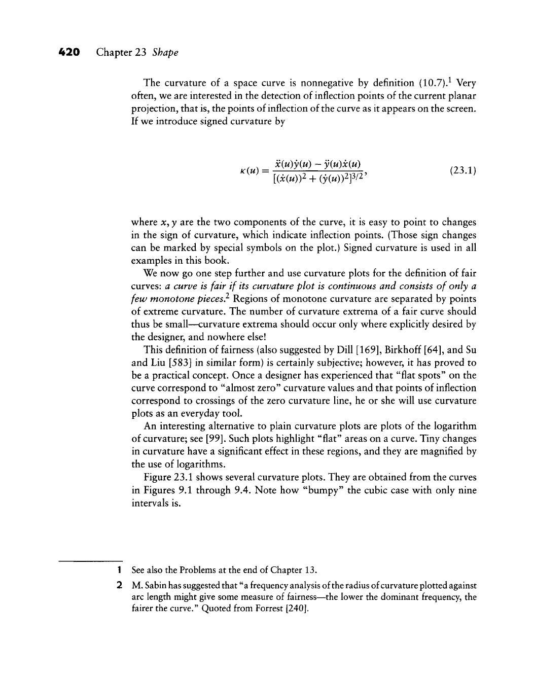
420 Chapter 23 Shape
The curvature of a space curve is nonnegative by definition (10.7).^ Very
often, we are interested in the detection of inflection points of the current planar
projection, that is, the points of inflection of the curve as it appears on the screen.
If we introduce signed curvature by
x{u)y{u) ~ y{u)x{u)
'^(^)
= 7 ^i
^TTTT?
23.1
[(x(«))2 + (y(^))2]3/2'
where
;c,
y are the two components of the curve, it is easy to point to changes
in the sign of curvature, which indicate inflection points. (Those sign changes
can be marked by special symbols on the plot.) Signed curvature is used in all
examples in this book.
We now go one step further and use curvature plots for the definition of fair
curves: a curve is fair if its curvature plot is continuous and consists of only a
few monotone pieces? Regions of monotone curvature are separated by points
of extreme curvature. The number of curvature extrema of a fair curve should
thus be small—curvature extrema should occur only where explicitly desired by
the designer, and nowhere else!
This definition of fairness (also suggested by Dill
[169],
Birkhoff [64], and Su
and Liu [583] in similar form) is certainly subjective; however, it has proved to
be a practical concept. Once a designer has experienced that "flat spots" on the
curve correspond to "almost zero" curvature values and that points of inflection
correspond to crossings of the zero curvature line, he or she will use curvature
plots as an everyday tool.
An interesting alternative to plain curvature plots are plots of the logarithm
of curvature; see [99]. Such plots highlight "flat" areas on a curve. Tiny changes
in curvature have a significant effect in these regions, and they are magnified by
the use of logarithms.
Figure 23.1 shows several curvature plots. They are obtained from the curves
in Figures 9.1 through 9.4. Note how "bumpy" the cubic case with only nine
intervals is.
1 See also the Problems at the end of Chapter 13.
2 M. Sabin
has
suggested that "a frequency analysis of the radius of curvature plotted against
arc length might give some measure of fairness—the lower the dominant frequency, the
fairer the curve." Quoted from Forrest
[240].
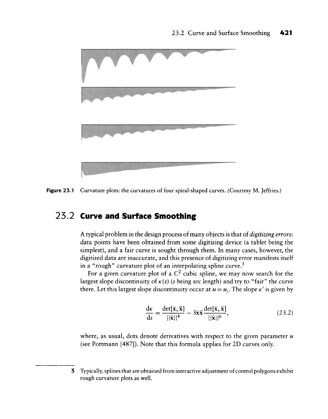
23.2 Curve and Surface Smoothing 421
4?^^^t-
:
>-^
7:--^x
^^is^^
;Cpj3:i;^^S;^ '^'.
Figure 23.1 Curvature plots: the curvatures of four spiral-shaped curves. (Courtesy M. Jeffries.^
25.2 Curve and Surface Smoothing
A typical problem in the design process of many objects is that of digitizing errors:
data points have been obtained from some digitizing device (a tablet being the
simplest), and a fair curve is sought through them. In many cases, however, the
digitized data are inaccurate, and this presence of digitizing error manifests itself
in a "rough" curvature plot of an interpolating spline curve.^
For a given curvature plot of a C^ cubic spline, we may now search for the
largest slope discontinuity of
K(S)
(S
being arc length) and try to "fair" the curve
there. Let this largest slope discontinuity occur atu =
Uj.
The slope
K'
is given by
d^
ds
det[x, x] 3xx
. det[x, x] (23.2)
where, as usual, dots denote derivatives with respect to the given parameter u
(see Pottmann [487]). Note that this formula applies for 2D curves only.
3 Typically, splines that
are
obtained from interactive adjustment of control polygons exhibit
rough curvature plots as well.
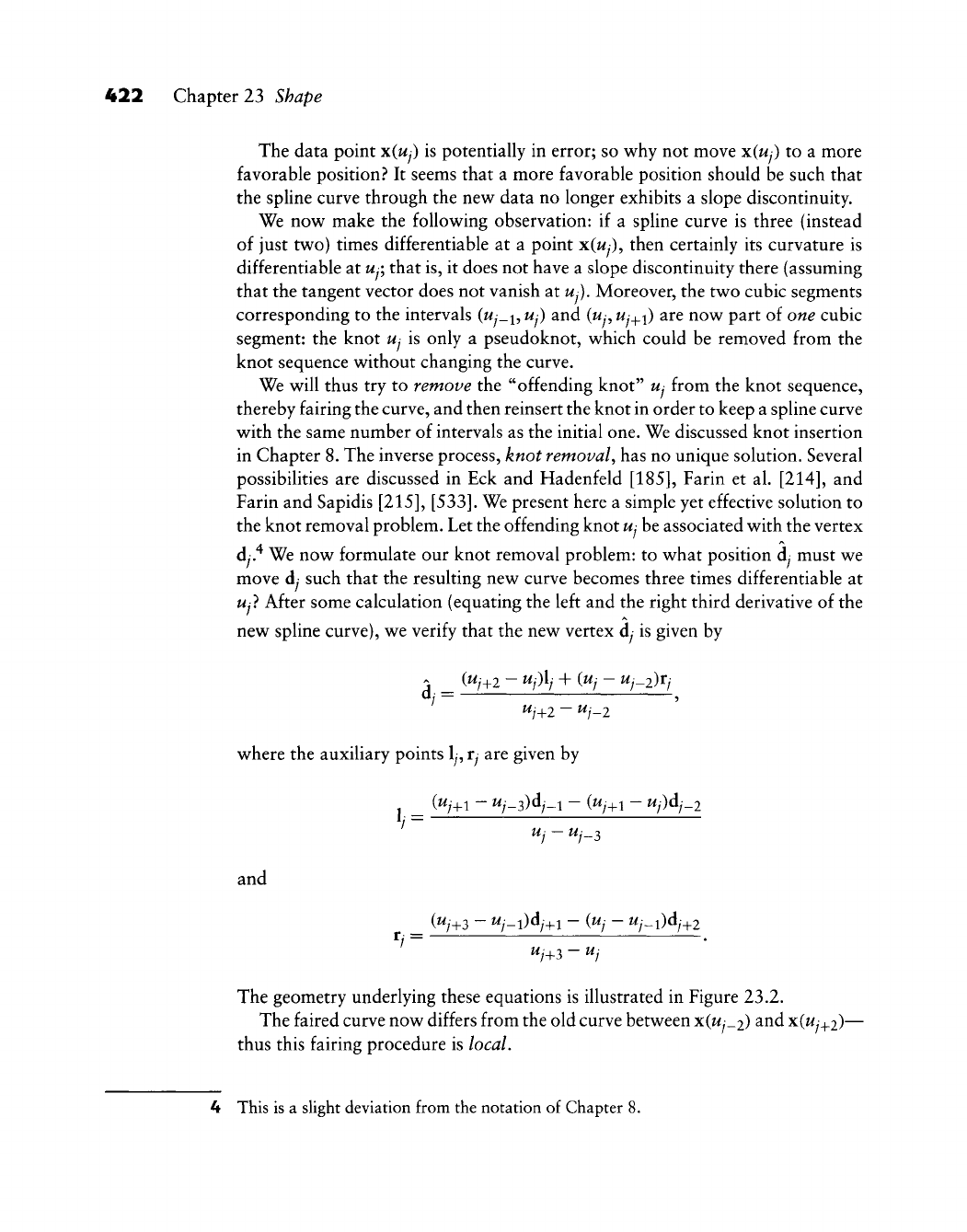
422 Chapter 23 Shape
The data point x(Uj) is potentially in error; so why not move x{Uj) to a more
favorable position? It seems that a more favorable position should be such that
the spline curve through the new data no longer exhibits a slope discontinuity.
We now make the following observation: if a spline curve is three (instead
of just two) times differentiable at a point x(^y), then certainly its curvature is
differentiable at
UJ;
that is, it does not have a slope discontinuity there (assuming
that the tangent vector does not vanish at
Uj),
Moreover, the two cubic segments
corresponding to the intervals (t/y_i,
Uj)
and
(wy,
Uj_^i)
are now part of one cubic
segment: the knot
Uj
is only a pseudoknot, which could be removed from the
knot sequence without changing the curve.
We will thus try to remove the "offending knot"
Uj
from the knot sequence,
thereby fairing the curve, and then reinsert the knot in order to keep a spline curve
with the same number of intervals as the initial one. We discussed knot insertion
in Chapter 8. The inverse process, knot removal^ has no unique solution. Several
possibilities are discussed in Eck and Hadenfeld
[185],
Farin et al.
[214],
and
Farin and Sapidis
[215], [533].
We present here a simple yet effective solution to
the knot removal problem. Let the offending knot
Uj
be associated with the vertex
Aj,^ We now formulate our knot removal problem: to what position dy must we
move dy such that the resulting new curve becomes three times differentiable at
Uj}
After some calculation (equating the left and the right third derivative of the
new spline curve), we verify that the new vertex dy is given by
^ (Wy+2 -
^;)1/
+ {Uj - Uj_2)Tj
where the auxiliary points
ly,
ry
are given by
J _ (^y+i - ^y-3)dy-i - (^;+i - ^;)dy_2
and
^i
=
(Wy+3 - ^;-l)dy+i - {Uj - Wy_i)dy+2
^/+3 - ^j
The geometry underlying these equations is illustrated in Figure 23.2.
The faired curve now differs from the old curve between x(Uj_2) and
x(wy_^2)—
thus this fairing procedure is local.
4 This is a slight deviation from the notation of Chapter 8.
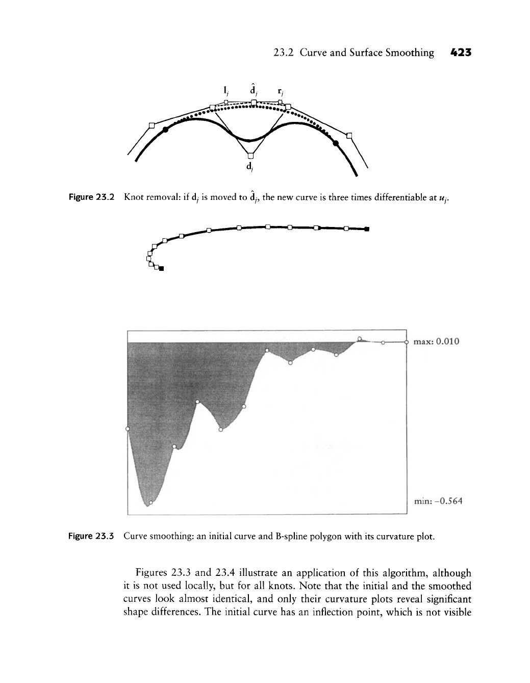
23.2 Curve and Surface Smoothing 423
Figure 23.2 Knot removal: if
dy
is moved to dy, the
nevv^
curve is three times differentiable at
Uj.
h max: 0.010
min: -0.564
Figure 23.3 Curve smoothing: an initial curve and B-spline polygon with its curvature plot.
Figures 23.3 and 23.4 illustrate an application of this algorithm, although
it is not used locally, but for all knots. Note that the initial and the smoothed
curves look almost identical, and only their curvature plots reveal significant
shape differences. The initial curve has an inflection point, which is not visible
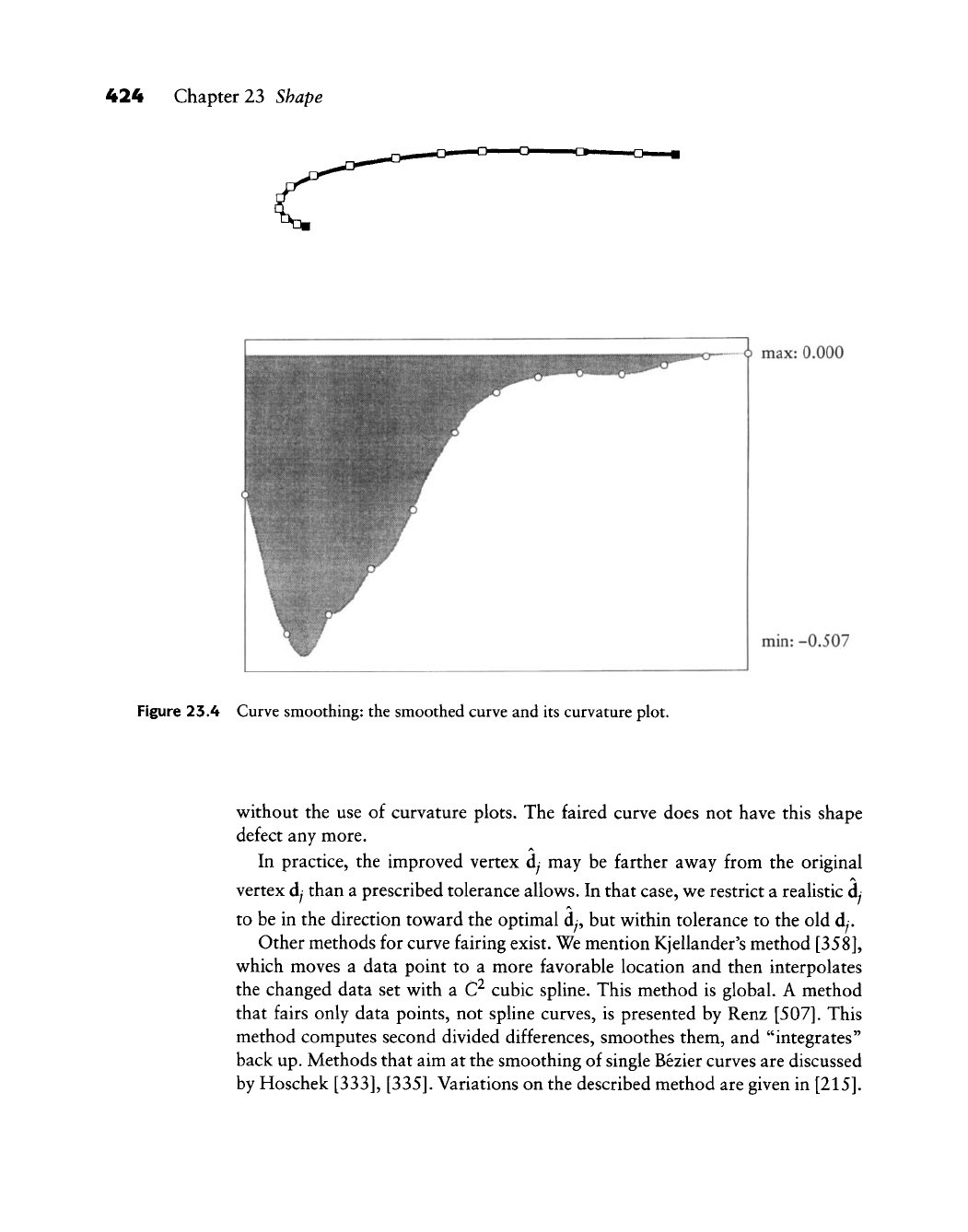
424 Chapter 23 Shape
}>
max: 0.000
min: -0.507
Figure 23.4 Curve smoothing: the smoothed curve and its curvature plot.
without the use of curvature plots. The faired curve does not have this shape
defect any more.
In practice, the improved vertex dy may be farther aw^ay from the original
vertex
dy
than a prescribed tolerance allows. In that case, we restrict a realistic d;
to be in the direction toward the optimal dy, but within tolerance to the old dy.
Other methods for curve fairing exist. We mention Kjellander's method
[358],
which moves a data point to a more favorable location and then interpolates
the changed data set with a C^ cubic spline. This method is global. A method
that fairs only data points, not spline curves, is presented by Renz
[507].
This
method computes second divided differences, smoothes them, and "integrates"
back up. Methods that aim at the smoothing of single Bezier curves are discussed
by Hoschek
[333], [335].
Variations on the described method are given in
[215].
23.3 Surface Interrogation 425
A method that tries to reduce the degrees of each cubic segment to quadratic is
given in
[200].
25.5 Surface Interrogation
Curvature plots are useful for curves; it is reasonable, therefore, to investigate the
analogous concepts for surfaces. Several authors have done this, including Beck et
al.
[49], Farouki
[219],
Dill
[169],
Munchmeyer
[435], [434],
and Forrest
[242].
An interesting early example is on page 197 of Hilbert and Cohn-Vossen
[323].
Surfaces have tv^o major kinds of curvature: Gaussian and mean; see Section
19.6.
Both kinds can be used for the detection of surface imperfections. Another
type of curvature can be useful, too: absolute curvature
K^\^^.
It is defined by
'^abs=kll + k2l5
where KI and KI are the maximal and minimal normal curvatures at the point
under consideration.
Gaussian curvature does not offer much information about generalized cylin-
ders of the form
c(w, v) = {l
—
u)x(v) + u[x(v) + v].
Even if the generating curve x(v) is highly curved, we still have K = 0 for these
surfaces. A similar statement can be made about the mean curvature H, which
is always zero for minimal surfaces, no matter how complicated.
Color Plates IV and V illustrate the use of curvatures in nonengineering
applications. Plate IV shows the digitized model of
a
bone (digitized as a mesh and
locally fitted with Bezier patches) and a color coding of the absolute curvature:
where the curvature is high, the surface is "painted" red, and where it is low,
it is "painted" blue. This process is referred to as texture mapping in computer
graphics.
Color Plate V shows an application in archeology: a digitized vessel (Native
American) is represented as a triangle mesh (left, with original texture). A cross
section is computed, fitted with a B-spline curve, and its curvature is displayed
(middle). Finally, Gaussian curvature is used as a texture map (right).
Another method for surface interrogation is the use of reflection
lines^
first de-
scribed in Klass
[360].
Poeschl [486] introduced a simplified method, isophotes.
Reflection lines are a standard surface interrogation tool in the styling shop of
a car manufacturer. They are the pattern that is formed on the polished car sur-
face by the mirror images of a number of parallel fluorescent strip lights. If the

426 Chapter 23 Shape
Figure 23.5 Isophotes: a line light source (top) is reflected by a surface.
Figure 23.6 Isophotes: left, a surface with "perfect" isophotes; right, after a perturbation was applied
to the surface.
mirror images are "nice," then the corresponding surface is deemed acceptable.
Whereas reflection lines depend on the position of an observer, isophotes consider
only the angle formed between surface normals and light source. The principle
is illustrated in Figure 23.5.
Reflection lines and isophotes can easily be simulated on a raster graphics
device (mark points whose normal points to one of the light sources). With some
more effort, they can also be computed on a hne drawing device (see Klass [360]).
Figure 23.6 shows a surface with several isophotes and the effect that a small
perturbation can have on them.
Reflection lines and curvature "paintings" have different usages: reflection
lines are not as fine-tuned as curvatures; they are prone to miss local shape defects
of a surface.^ On the other hand, curvatures of a surface may look perfect, yet it
might not have a "pleasant" overall shape—reflection lines have a better chance
of flagging global imperfections.
This is because reflection lines may be viewed as a first-order interrogation tool (involving
only first derivatives), whereas curvature plots are second-order interrogation tools.
23.4 Implementation 427
Once imperfections are detected in a tensor product B-spline surface, we would
want methods to remove them without time-consuming interactive adjustment
of control polygons. One such method is to apply the curve-smoothing method
from Section 23.2 in a tensor product way: smooth all control net rows, then all
control net columns. The resulting surface is usually smoother than the original
surface. Figure 23.6 is an example of this method: the right figure is a B-spline
surface; four iterations of the program f ai r_surf produced the figure on the left.
More involved methods for surface fairing exist; they aim for the enforcement
of convexity constraints in tensor product spline surfaces. We mention Andersson
et al. [8], Jones
[348],
and Kaufmann and Klass
[354].
25.4 Implementation
The routine curvatures may be used to generate curvature values of a rational
Bezier curve. It writes the values into a file that might be read by another program
that generates a curvature plot.
To compute the curvature at the parameter value ^, the curve is subdivided
using the (rational) de Casteljau algorithm. Of the two subpolygons that are
generated, the larger one is selected, and its beginning curvature is computed.
Since the subdivision routine rat__subdiv orders both subpolygons beginning at
the subdivision point, only one curvature routine curvature_0 is needed.
void curvatures(coeffx,coeffy,weight,degree,dense)
/* writes signed curvatures of a rational Bezier curve into
a file,
input:
coeffx, coeffy:
2D
Bezier polygon
weight: the weights
degree: the degree
dense: how many curvature values
to
compute
output:
written into file outfile
V
The routine curvature^O is a simple application of (10.10):
float curvature_0(bez_x,bez_y,weight,degree)
/*
computes curvature
of
rational Bezier curve
at
t=0
Input: bez_x, bez_y, weight: control polygon and weights
degree: degree
of
curve
V
428 Chapter 23 Shape
The following area routine is included for completeness:
float area(pl,p2,p3)
/* find area
of
triangle pl,p2,p3
*/
Note,
however, that area returns a negative value if the input points are
ordered clockwise!
The following routine generates the "raw data" that are needed to create the
curvature plot of a rational B-spline curve. Of course, we may simply set all
weights to unity for the polynomial case.
void bspl_kappas(bspl_x,bspl_y,bspl_w,knot,l,dense)
/* writes curvatures
of
cubic rational B-spline curve into
a file,
input:
bspl_x,bspl_y:
2D rat.
B-spline polygon
bspl_w:
the
B-spline weights
knot:
the
knot sequence
dense:
how
many curvature values
to
compute
per
interval
1:
no. of
intervals
output:
written into file outfile
V
The preceding programs are used by the main program pi ot_b_kappa.
c
in order
to produce Postscript output for a curvature plot.
Now the programs to fair curves and surfaces. First, the curve case:
void fair_bspline(bspl,knot,l,from,to)
/* Fairs
a
cubic rational B-spline curve
by
knot removal/reinsertion.
Input:
bspl:
cubic B-spline control polygon
(one
coord.)
knot: knot sequence
1:
no. of
intervals
from,
to:
from where
to
where
to
fair
Output: same
as
input,
but
hopefully fairer.
V
Second, the surface case:
void fair_surf(bspl,lu,lv,knot_u, knot_v)
/* Fairs B-spline control
net.
23.5 Problems 429
Input: bspl: B-spline control
net
(one coordinate only)
lu,lv: no.
of
intervals
in u- and
v-directi on
knots_u, knots_v: knot vectors
in u- and
v-directi on
Output:
as
input
Note:
Has to be
called once
for
each x-,y-,z- coordinate.
25.5 Problems
1 Show that a planar cubic curve may have tv^o points of inflection, that is,
points v^here curvature changes sign.
2 Show^ that a true space cubic cannot have any points v^ith zero curvature.
PI The routine curvatures produces a file that contains pairs
^/,/c^;
that is, it
can be used to plot curvature versus parameter. Modify the program so it
can be used to produce plots of curvature versus arc length.
P2 Write a program to compute the torsion of a Bezier or a spline curve. Then
produce torsion plots as an additional interrogation tool for space curves.
P3 Compute the curvatures of isoparametric curves of a spline surface, color
code them, and use them as an interrogation tool.
P4 Produce a uniform B-spline surface that interpolates the four boundary data
sets from car.dat. Test if that surface is fair (using P3 if you v^ant); if not,
improve its shape by using fai
r_surf.

This Page Intentionally Left Blank
Evaluation of
Some Methods
In this chapter, we will examine some of the many methods that have been
presented. We will try to point out the relative strengths and weaknesses of each,
a task that is necessarily influenced by personal experience and opinion.
24.1 Bezier Curves or B-Spline Curves?
Taken at face value, this is a meaningless question: Bezier curves are a special
case of B-spline curves. Any system that contains B-splines in their full generality,
allowing for multiple knots, is capable of representing a Bezier curve or, for that
matter, a piecewise Bezier curve.
In fact, several systems use both concepts simultaneously. A curve may be
stored as an array holding B-spline control vertices, knots, and knot multiplici-
ties.
For evaluation purposes, the curve may then be converted to the piecewise
Bezier form.
24.2 Spline Curves or B-Spline Curves?
This question is often asked, yet it does not make much sense. B-splines form a
basis for all splines, so any spline curve can be written as a B-spline curve. What
is often meant is the following: if we want to design a curve, should we pass an
interpolating spline curve through data points, or should we design a curve by
interactively manipulating a B-spline polygon.'' Now the question has become one
concerning curve generation methods rather than curve representation methods.
431
432 Chapter 24 Evaluation of Some Methods
A flexible system should have both: interpolation and interactive manipula-
tion. The interpolation process may of course be formulated in terms of B-splines.
Since many designers do not favor interactive manipulation of control polygons,
w^e should allow them to generate curves using interpolation. Subsequent curve
modification may also take place without display of a control polygon: for in-
stance, the designer might move one (interpolation) point to a new position. The
system could then compute the B-spline polygon modification that would pro-
duce exactly that effect. So a user might actually work with a B-spline package,
but a system that is adapted to his or her needs might hide that fact. See Section
9.3 for details.
We finally note that every C^ B-spline curve may be generated as an interpolat-
ing spline curve: read off junction points, end tangent vectors, and knot sequence
from the B-spline curve. Feed these data into a C^ cubic spline interpolator, and
the original curve will be regenerated.
24.5 The Monomial or the Bezier Form?
We have made the point in this book that the monomial form^ is less geometric
than the Bezier form for a polynomial curve. A software developer, however,
might not care much about the beauty of geometric ideas—in the workplace,
the main priority is performance. Since the fundamental work by Farouki and
Rajan
[224], [225], [220],
one important performance issue has been resolved:
the Bezier form is numerically more stable than the monomial form. Farouki
and Rajan observed that numerical inaccuracies, unavoidable with the use of
finite precision computers, affect curves in the monomial form significantly more
than those in Bezier form. More precisely, they show that the condition number
of simple roots of a polynomial^ is smaller in the Bernstein basis than in the
monomial basis. If one decides to use the Bezier form for stability reasons, then
it is essential that no conversions be made to other representations; these will
destroy the accuracy gained by the use of the Bezier form. For example, it is not
advisable from a stability viewpoint to store data in the monomial form and to
convert to Bezier form to perform certain operations. More details are given in
Daniel and Daubisse
[132].
Figure 24.1 shows a numerical example, carried out using the routine bez__to_
pow
with single precision arithmetic. A degree 18 Bezier curve (top) was converted
1 This form is also called the power
basis
form.
2 This number indicates by how much the location of a root is perturbed as a result of a
perturbation of the coefficients of the given polynomial.
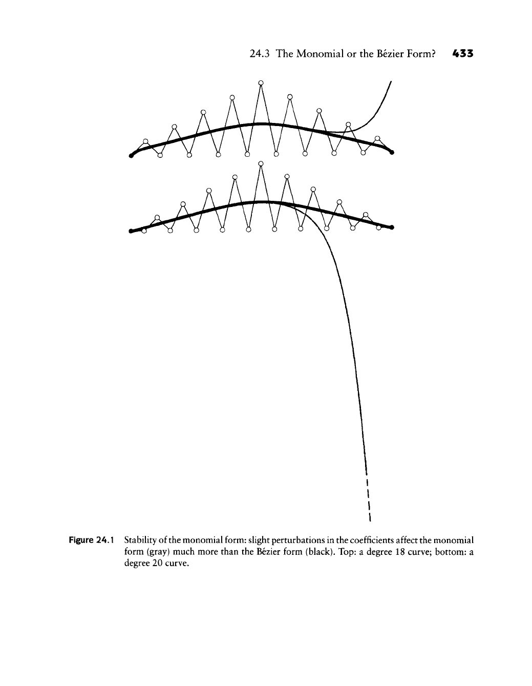
24.3 The Monomial or the Bezier Form? 433
Figure 24.1 Stability of the monomial form: slight perturbations in the coefficients affect the monomial
form (gray) much more than the Bezier form (black). Top: a degree 18 curve; bottom: a
degree 20 curve.
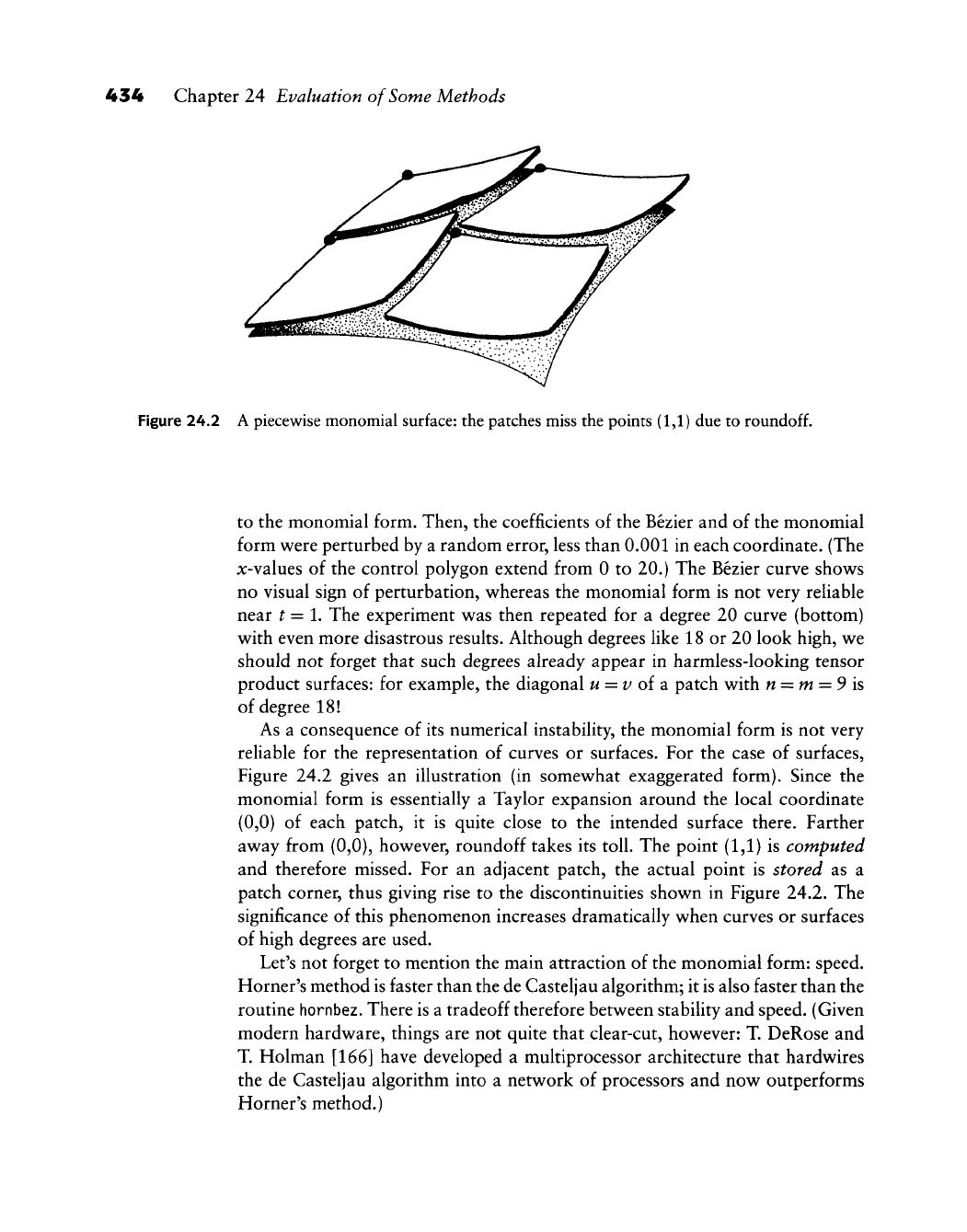
434 Chapter 24 Evaluation of Some Methods
Figure 24.2 A piecewise monomial surface: the patches miss the points (1,1) due to
roundoff.
to the monomial form. Then, the coefficients of the Bezier and of the monomial
form were perturbed by a random error, less than 0.001 in each coordinate. (The
x-values of the control polygon extend from 0 to 20.) The Bezier curve shows
no visual sign of perturbation, whereas the monomial form is not very reliable
near t = 1, The experiment was then repeated for a degree 20 curve (bottom)
with even more disastrous results. Although degrees like 18 or 20 look high, we
should not forget that such degrees already appear in harmless-looking tensor
product surfaces: for example, the diagonal u = v oi a patch with n = m = 9 is
of degree 18!
As a consequence of its numerical instability, the monomial form is not very
reliable for the representation of curves or surfaces. For the case of surfaces.
Figure 24.2 gives an illustration (in somewhat exaggerated form). Since the
monomial form is essentially a Taylor expansion around the local coordinate
(0,0) of each patch, it is quite close to the intended surface there. Farther
away from (0,0), however, roundoff takes its toll. The point (1,1) is computed
and therefore missed. For an adjacent patch, the actual point is stored as a
patch corner, thus giving rise to the discontinuities shown in Figure 24.2. The
significance of this phenomenon increases dramatically when curves or surfaces
of high degrees are used.
Let's not forget to mention the main attraction of the monomial form: speed.
Horner's method is faster than the de Casteljau algorithm; it is also faster than the
routine hornbez. There is a tradeoff therefore between stability and speed. (Given
modern hardware, things are not quite that clear-cut, however: T. DeRose and
T. Flolman [166] have developed a multiprocessor architecture that hardwires
the de Casteljau algorithm into a network of processors and now outperforms
Horner's method.)
24.5 Triangular or Rectangular Patches? 435
24.4 The B-Spline or the Hermite Form?
Cubic B-spline curves are numerically more stable than curves in the piecewise
cubic Hermite form. This comes as no surprise, since some of the Hermite
basis functions are negative, giving rise to numerically unstable nonconvex
combinations. However, there is an argument in favor of the piecev^ise Hermite
form: it stores interpolation points explicitly. In the B-spline form, they must be
computed. Even if this computation is stable, it may produce
roundoff.
A significant argument against the use of the Hermite form points to its
lack of invariance under affine parameter transformations. Everyone who has
programmed the Hermite form has probably experienced the trauma resulting
from miscalculated tangent lengths. A programmer should not be burdened with
the subtleties of the interplay between tangent lengths and parameter interval
lengths.
An important advantage of the B-spline form is storage. For B-spline curves,
one needs a control point array of length L + 2 plus a knot vector array of length
L + 1 for a curve with L data points, resulting in an overall storage requirement
of 4L -h 7 reals.^ For the piecewise Hermite form, one needs a data array of
length IL (position and tangent at each data point) plus a knot vector of length
L -h 1, resulting in a storage requirement of 7L + 1 reals. For surfaces (with
same degrees in u and v for simplicity), the discrepancy becomes even larger:
3(L + 2)^ + 2(L + 1) versus 12L^ + 2(L + 1) reals. (For the Hermite form, we
have to store position, u- and i/-tangents, and twist for each data point.)
When both forms are used for tensor product interpolation, the Hermite form
must solve three sets of linear equations (see Section 15.5) while the B-spline form
must solve only two sets (see Section 15.4).
24.5 Triangular or Rectangular Patches?
Most of the early CAD efforts were developed in the car industry, and this is per-
haps the main reason for the predominance of rectangular patches in most CAD
systems; the first applications of CAD methods to car body design were to the
outer panels such as
roof,
doors, and hood. These parts basically have a rectan-
gular geometry, hence it is natural to break them down into smaller rectangles.
These smaller rectangles were then represented by rectangular patches.
Once a CAD system had been successfully applied to a design problem, it
seemed natural to extend its use to other tasks: the design of the interior car
3 We are not storing knot multiplicities. We would then be able to represent curves that are
only C^, which the cubic Hermite form is not capable of.
436 Chapter 24 Evaluation of Some Methods
body panels, for instance. Such structures do not possess a notably rectangular
structure, and rectangular patches are therefore not a natural choice for modeling
these complicated geometries. However, rectangle-based schemes already existed,
and the obvious approach
w^as
to make them v^ork in "unnatural" situations also.
They do the job, although w^ith some difficulties, w^hich arise mainly in the case
of degenerate rectangular patches.
Triangular patches do not suffer from such degeneracies and are thus better
suited to describe complex geometries than are rectangular patches. It seems
obvious, therefore, to advise any CAD system developer to add triangular patches
to the system.
The French car company Citroen used triangular patches in the early 1960s,
but later abandoned their use. In the middle 1980s, Evans and Sutherland used
triangular patches as the backbone of their CDDRS system—they were subse-
quently replaced by B-spline surfaces. More recently, NVIDIA uses triangular
patches to fill in holes in rectangular topologies.
Quick Reference
of Curve and
Surface Terms
ab initio design Latin: from the beginning. Used to describe design processes
in which the designer inputs his or her ideas directly into the computer, without
constraints such as interpolatory constraints.
Affine combination Same as a barycentric combination.
Affine invariance A property of a curve or surface generation scheme: the same
resuh is obtained if computation of a point on a curve or surface occurs before
or after an affine map is apphed to the input data.
Affine map Any map comprising translations, rotations, scalings, and shears.
Maps parallels to parallels. Leaves ratios of collinear points unchanged.
Approximation Fitting a curve or surface to given data. As opposed to interpo-
lation, the curve or surface approximation only has to be close to the data.
Barycentric combination A weighted average where the sum of the weights
equals one.
Barycentric coordinates A point in E^ may be written as a unique barycentric
combination of three points. The coefficients in this combination are its barycen-
tric coordinates.
Basis function Functions form linear spaces, which have bases. The elements
of these bases are the basis functions.
Bernstein polynomial The basis functions for Bezier curves.
Beta-spline curve A G^ piecewise cubic curve that is defined over a uniform
knot sequence.
Bezier curve A polynomial curve that is expressed in terms of Bernstein poly-
nomials.
437
438 Appendix A Quick Reference of Curve and Surface Terms
Bezier polygon The coefficients in the expansion of a Bezier curve in terms of
Bernstein polynomials are points. Connected according to their natural number-
ing, they form the Bezier polygon.
Bilinear patch A patch that is ruled in two directions. Or: a hyperbolic para-
boloid.
Blossom A multivariate polynomial that is associated v^ith a given polynomial
through the process of blossoming.
Blossoming The procedure of applying n (the polynomial degree) de Casteljau
algorithm steps or n de Boor steps to a polynomial (or to a segment of a spline
curve),
but each one for a different parameter value.
B-spline A piecev^ise polynomial function. It is defined over a knot partition,
has local support, and is nonnegative. If a spline curve is expressed in terms of
B-splines, it is called a B-spline curve.
B-spline polygon The coefficients in the expansion of a B-spline curve in terms
of B-splines are points. Connected according to their natural numbering, they
form the B-spline polygon. Also called de Boor polygon.
Breakpoint Same as a knot.
Butterfly scheme An interpolatory recursive subdivision scheme that creates
smooth surfaces from a given set of triangulated points.
CAGD Computer aided geometric design.
Catmull-Clark Surfaces Subdivision surfaces that are bicubic spline surfaces
v^hen the input mesh is rectangular.
C^ A smoothness property of curves or surfaces: being r times differentiable w^ith
respect to the given parametrization.
Chord length parameters In many curve interpolation problems, data points
need to be assigned parameter values. If these are spaced relative to the spacing
of the data points, we have chord length parameters.
Collinear Being on a straight line.
Compatibility For some interpolation problems, the input data may not be
arbitrary but must satisfy some consistency constraints, called compatibility
conditions.
Conic section The intersection curve between a cone and a plane. Or: the
projective image of a parabola. A nondegenerate conic is an ellipse, a parabola,
or a hyperbola.
CONS Curve on surface.
Control polygon See Bezier polygon or B-spline polygon.
Quick Reference of Curve and Surface Terms 439
Control vector For rational curves, a Bezier or B-spline control point that has
degenerated to a vector, implying a zero weight.
Convex curve A planar curve that is a subset of the boundary of its convex hull.
Convex hull The smallest convex set that contains a given set.
Convex set A set such that the straight line segment connecting any tv^o points
of the set is completely contained within the set.
Coons patch A patch that is fitted between four arbitrary boundary curves.
Coplanar Being on the same plane.
Cross plot Breaking down the plot of a parametric curve into the plots of each
coordinate function.
Cross ratio A quantity computed from four coUinear points, invariant under
projective maps. A generalization of affine ratios.
Curvature At a point on a curve, curvature is the inverse of the radius of the
osculating circle. Also: curvature measures by how much a curve deviates from
a straight line at a given point.
Curve The path of a point moving through space. Or: the image of the real line
under a continuous map.
de Boor algorithm The algorithm that recursively computes a point on a
B-spline curve.
de Casteljau algorithm The algorithm that recursively computes a point on a
Bezier curve.
Decimation Reducing the number of triangles in a triangulation while staying
close to the initial geometry.
Delaunay triangulation A triangulation that maximizes the minimal angle of
all triangles. Or: the dual of the Dirichlet tessellation.
Developable surface A ruled surface whose Gaussian curvature vanishes ev-
erywhere.
Direct
G^
splines G^ piecewise cubics that are generated by specifying a control
polygon and some Bezier points.
Dirichlet tessellation A partition of E^ or E^ into convex tiles. Each tile is
associated with a given data point such that all of its points are closer to "its"
data point than to any other data point.
Domain The preimage of a curve or surface.
Doo-Sabin surfaces Subdivision surfaces that are biquadratic spline surfaces
when the input mesh is rectangular.
440 Appendix A Quick Reference of Curve and Surface Terms
End condition In cubic spline curve interpolation, one has to supply an extra
condition at each of the two endpoints. Examples of such end conditions: pre-
scribed tangents or zero curvature.
Four-point sciieme An interpolatory curve subdivision scheme.
Frenet frame At each point of a (nondegenerate) curve, the first, second, and
third derivative vectors are linearly independent. Applying Gram-Schmidt or-
thonormalization to them yields the Frenet frame of the curve at the given point.
Functional curve or surface A curve of the form y = f{x) or a surface of the
form z =
f{x^y),
C^ spline curve A C^ piecewise cubic curve that is twice differentiable with
respect to arc length.
y-spline A G^ spline that is C^ over a given knot sequence.
Geometric continuity Smoothness properties of a curve or a surface that are
more general than its order of differentiability.
Gordon surface A generalization of Coons patches. Interpolates to a rectilinear
network of curves.
Hermite interpolation Generating a curve or surface from data that consist of
points and first and/or higher derivatives.
Hodograph The first derivative curve of a parametric curve.
Homogeneous coordinates A coordinate system that is used to describe ra-
tional curves and surfaces in terms of projective geometry, where they are just
polynomial.
Horner's scheme An efficient method to evaluate a polynomial in monomial
form by nested multiplication.
IGES Initial Graphics Exchange Specification. A popular data specification for-
mat, aiming at unifying geometry descriptions.
Infinite control point Same as control vector.
Inflection point A point on a curve where the tangent intersects the curve. Often
corresponds to points with zero curvature.
Interior Bezier points For curves, those Bezier points that are not junction
points. For surfaces, those Bezier points that are not boundary points.
Interpolation Finding a curve or surface that satisfies some imposed constraints
exactly. The most common constraint is the requirement of passing through a set
of given points.
Junction point A spline curve comprises segments. The common point shared
by two segments is called the junction point. See also knot.
Quick Reference of Curve and Surface Terms 441
Knot A spline curve is defined over a partition of an interval of the real line. The
points that define the partition are called knots. If evaluated at a knot, the spline
curve passes through a junction point.
Knot insertion Adding a new knot to the knot sequence of a B-spline curve
without changing the graph of the curve.
Lagrange interpolation Finding a polynomial curve through a given set of data
points.
Least squares An approximation process that aims at minimizing the devia-
tions of given data points from a desired curve or surface.
Linear precision A property of many curve schemes: if the curve generation
scheme is applied to data read off from a straight line, that straight line is
reproduced.
Local control A curve or surface scheme has the local control property if a
change in the input data only changes the curve or surface in a region near the
changed data.
Lofting Creating a ruled surface between two given curves.
Minmax box Smallest 2D or 3D box with edges parallel to the coordinate axes
that completely contains a given object.
Monomial form A polynomial is in monomial form if it is expressed in terms
of the monomials 1, ^, ^^,.. ..
Multiresolution Breaking down an object into a sequence of approximations
with increasing accuracy.
Node A term that is used inconsistently in the literature: it sometimes refers to
a knot, sometimes to a control point.
NURB Nonuniform rational B-spline curve or surface.
y-spline An interpolating G spline curve that is C^ over a given knot sequence.
Osculating circle At a given point, the osculating circle approximates the curve
"better" than any other circle.
Osculating plane The plane that contains the osculating circle of a curve at a
given point. This plane is spanned by the given point and the curve's first and
second derivative vectors.
Oslo algorithm The process of simultaneously inserting several knots into a
B-spline curve.
Parametrization Assigning parameter values to junction points in spline curves.
Also used with a different meaning: the function that describes the speed of a
point traversing a curve.
442 Appendix A Quick Reference of Curve and Surface Terms
Patch Complicated surfaces are usually broken down into smaller units, called
patches. For example, a bicubic spline surface consists of a collection of bicubic
patches.
Point A location in space. If one uses coordinate systems to describe space, a
point is represented as an w-tuple of real numbers.
Point cloud A (typically large) set of 3D points without any ordering or struc-
ture.
Precision A curve or surface generation scheme has nth order precision if it
reproduces polynomials of degree n.
Projective map A map comprising affine maps and central projections. Leaves
cross ratios of coUinear points unchanged. Does (in general) not map parallels
to parallels.
Quad Short for quadrilateral.
Quadric A surface with the implicit representation f{x, y, z) = 0, where f is
a quadratic polynomial. Or: the projective image of an elliptic paraboloid, a
hyperbolic paraboloid, or a parabolic cyHnder.
Ratio A quantity computed from three coUinear points. Invariant under affine
maps,
but not under projective maps.
Rational curves and surfaces Projections of nonrational (integral) curves or
surfaces from four-space into three-space.
Recursive subdivision Curves or surfaces that are defined as the limit of a
polygon or polyhedron refinement process.
Ruled surface A surface containing a family of straight lines. Obtained as linear
interpolation between two given curves.
S-patch A surface patch with an arbitrary number of boundary curves, con-
structed by mapping a multidimensional simplex onto a 2D polygon, the domain
of the patch.
Segment An individual polynomial (or rational polynomial) curve in an assem-
bly of such curves to form a spline curve. The bivariate analog of a segment is a
patch.
Shape parameter A degree of freedom (usually a real number) in a curve or
surface representation that can be used to fine-tune the shape of that curve or
surface.
Solid modeling The description of closed objects that are bounded by a collec-
tion of surfaces.
Space The collection of all points.
Quick Reference of Curve and Surface Terms 443
Spline curve A continuous curve that comprises several polynomial segments.
Spline curves are often represented in terms of B-splines. They may be the result
of an interpolation process or of an ab initio design process. If the segments are
rational polynomials, we have a rational spline curve.
Standard form The property of a rational curve of having its end weights equal
to unity.
Star In a triangular mesh: the set of all triangles having a given point as a vertex.
Stereo lithography The process of producing a physical (usually plastic) model
of a part, involving building layers of material hardened by laser rays aimed
inside a tank of liquid resin.
Subdivision Breaking a curve or surface down into smaller pieces of the same
type as the original curve or surface.
Subdivision surface A surface that is the result of iteratively refining a given
control mesh.
Support The region over which a nonnegative function is actually positive.
Surface The locus of all points of a moving and deforming curve. Or: the 3D
image of a region in two-space under a continuous map. A surface is often broken
down into patches.
Surface spline A piecewise bicubic approximation to a Doo-Sabin surface.
Surface triangulation A collection of triangular facets that covers a smooth
surface, obeying the structure of a triangulation.
Tangent The straight line that best approximates a smooth curve at a point on
it. This straight line is parallel to the tangent vector.
Tangent vector The first derivative of a differentiable curve at a point on it. The
length of the tangent vector depends on the parametrization of the curve.
Tensor product A method to generate rectangular surfaces using curve methods.
Tile The interior of a convex closed 2D polygon.
Torsion A measure of how much a curve "curves away" from the osculating
plane at a given point.
Transfinite interpolation Interpolating to curves, with infinitely, that is, trans-
finitely many points on it, as opposed to discrete interpolation, which interpolates
only to finitely many points.
Translational surface A surface that is obtained by translating one curve along
another one.
Triangular patch A patch whose domain is a triangle.
444 Appendix A Quick Reference of Curve and Surface Terms
Triangulation A collection of triangles, covering a region in E^, such that the
triangles do not overlap, and that any two triangles either have no points in
common, or they have one edge in common, or they have one vertex in common.
See also surface triangulation.
Trimmed surface If the domain of a parametric surface is divided into "valid"
and "invalid" regions, the image of the valid regions is called a trimmed surface.
Twist vector The mixed second partial of a surface at a point. Note: not a
geometric property of the surface, but parametrization dependent.
Valency A vertex in a polygonal mesh has valency niin edges emanate from the
vertex. Also: valence.
Variation diminution Intuitively: a curve or surface scheme has this property if
its output "wiggles less" than the data from which it is constructed.
Vector A direction. Usually the difference of two points.
Volume deformation A surface or a collection of surfaces may be embedded
in a cube. That cube may then be deformed using some trivariate Bezier or
B-spline method—this is the volume distortion—in order to change the shape
of the initial surface(s).
Voronoi diagram Same as Dirichlet tessellation.
Weight Rational curves and surfaces are often defined in terms of homogeneous
coordinates. The last component of the homogeneous coordinate is called weight.
Weight point The point formed by a weighted average of two control points of
a rational curve; the weights in the average are the weights of the control points.

List of Programs
The following list contains all programs that are contained in the text.
aitken: Section 7.12
area: Section 23.4
bessel_ends: Section 9.9
bez_to_points: Section 4.5
bspl_to_points: Section 8.10
curvature_0: Section 23.4
curvatures: Section 23.4
deboor: Section 8.10
deboor_blossom: Section 8.10
decas:
Section 4.5
degree_elevate: Section 6.11
direct_gspline: Section 11.7
hornbez: Section 5.8
l_u_system: Section 9.9
netcoons: Section 15.10
parameters: Section 9.9
plot_bez_surfaces: Section 16.10
plot_surf:
Section 15.10
ratbez: Section 13.10
ratbspline_to_bezier: Section 13.10
ratbspl_to_bez_surf: Section 16.10
445

446
Appendix
B
List
of
Programs
rat_subdiv:
set_up_system:
solve_system:
spline_surf_int:
subdiv_rat:
Section
13.10
Section
9.9
Section
9.9
Section
16.10
Section
13.2
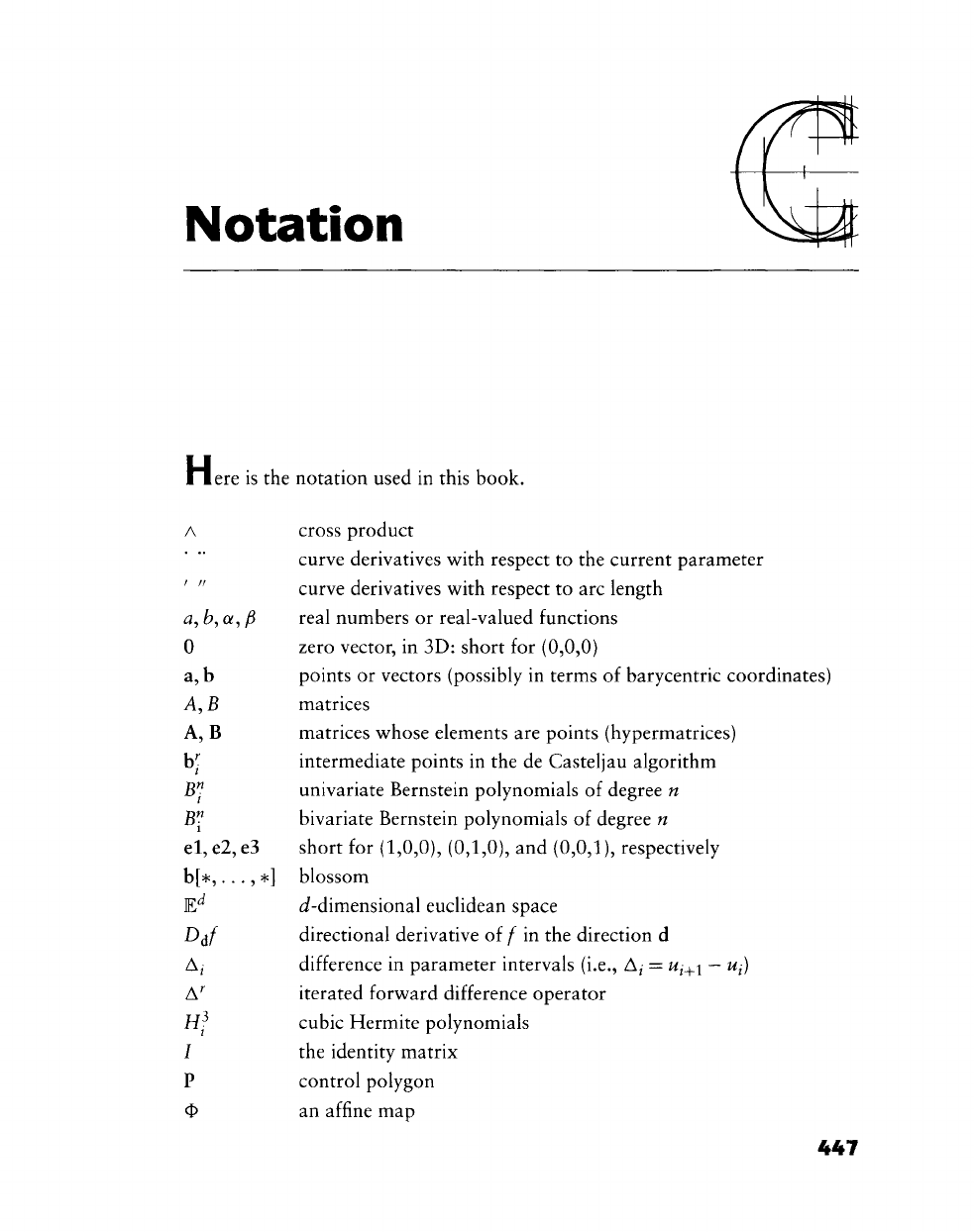
Notation
H
ere is the notation used in this book.
A cross product
curve derivatives v^ith respect to the current parameter
' " curve derivatives with respect to arc length
a,
fc,
a,
j6
real numbers or real-valued functions
0 zero vector, in 3D: short for (0,0,0)
a, b points or vectors (possibly in terms of barycentric coordinates)
A, B matrices
A, B matrices v^hose elements are points (hypermatrices)
b[ intermediate points in the de Casteljau algorithm
B^
univariate Bernstein polynomials of degree n
B^
bivariate Bernstein polynomials of degree n
el,
e2, e3 short for (1,0,0), (0,1,0), and (0,0,1), respectively
b[*,
...,*] blossom
E^ J-dimensional euclidean space
D^f
directional derivative of f in the direction d
Aj difference in parameter intervals (i.e., A^ =
Ui_^i — Uj)
A^ iterated forward difference operator
Hr' cubic Hermite polynomials
/ the identity matrix
P control polygon
O an affine map
447

448 Appendix C Notation
Vi operators
t^^^ n-io\d repetition of an argument t
I
|v|
I (euclidean) length of the vector v
x^ w-partial of x(w, v)
References
[1] S. Abi-Ezzi. The graphical processing of B-splines in a highly dynamic
environment. PhD thesis, RPI, 1989. Rensselaer Design Research Center.
[2] T. Ackland. On osculatory interpolation, where the given values of the
function are at unequal intervals. / Inst. Actuar., 49:369-375, 1915.
[3] H. Akima. A nev^ method of interpolation and smooth curve fitting based
on local procedures./ACM, 17(4):589-602, 1970.
[4] G. Albrecht. A remark on Farin points for Bezier triangles. Computer
Aided Geometric Design, 12(5):507-512, 1995.
[5] P. Alfeld. A bivariate C^ Clough-Tocher scheme. Computer Aided Geo-
metric Design, l(3):257-267, 1984.
[6] P. Alfeld. A case study of multivariate piecewise polynomials. In G. Farin,
editor. Geometric Modeling: Algorithms and New Trends, pages 149-
160.
SIAM, Philadelphia, 1987.
[7] P. Alfeld and L. Schumaker. The dimension of bivariate spline spaces of
smoothness r and degree d>4r+l. Constructive Approximation, 3:189-
197,
1987.
[8] R. Andersson, E. Andersson, M. Boman, B. Dahlberg, T. Elmroth, and
B.
Johansson. The automatic generation of convex surfaces. In R. Martin,
editor. The Mathematics of Surfaces II, pages 427-446. Oxford University
Press,
1987.
[9] E. Angel. Interactive Computer Graphics. Addison-Wesley, 2000. Second
edition.
449
450 References
[10
[11
[12:
[13
[14:
[15
[16
[17:
[18
[19
[20
[21
[22
[23
[24
[25
[26
M. Vigo Anglada, N. Pla Garcia, and P. Brunet Crosa. Directional
adaptive surface triangulation. Computer Aided Geometric Design^
16(2):107-126, 1999.
G. Aumann. Interpolation with developable Bezier patches. Computer
Aided Geometric Design, 8(5):409-420, 1991.
G. Baer. Parametrische Interpolation empirischer Raumkurven.
ZAMM,
57:305-314, 1977.
A. Ball. Consurf I: introduction of the conic lofting tile. Computer Aided
Design, 6(4):243-249, 1974.
A. Ball. Consurf
II:
description of the algorithms. Computer Aided Design,
7(4):237-242, 1975.
A. Ball. Consurf III: how the program is used. Computer Aided Design,
9(1):9-12, 1977.
A. Ball. Reparametrization and its application in computer-aided geomet-
ric design. Int, J for Numen Methods in Eng., 20:197-216, 1984.
A. Ball. The parametric representation of curves and surfaces using ra-
tional polynomial functions. In R. Martin, editor. The Mathematics of
Surfaces II, pages 39-62. Oxford University Press, 1987.
A. Ball and D. Storry. A matrix approach to the analysis of recursively
generated B-spline surfaces. Computer Aided Design, 18(8):437-442,
1986.
A. Ball and D. Storry. Conditions for tangent plane continuity of re-
cursively generated B-spline surfaces. ACM Transactions on Graphics,
7(2):83-102, 1988.
R. Barnhill. Smooth interpolation over triangles. In R. Barnhill and
R. Riesenfeld, editors, Computer Aided Geometric Design, pages 45-70.
Academic Press, 1974.
R. Barnhill. Representation and approximation of surfaces. In J. R. Rice,
editor. Mathematical Software III, pages 69-120. Academic Press, 1977.
R. Barnhill. Coons' patches. Computers in Industry, 3:37-43, 1982.
R. Barnhill. A survey of the representation and design of surfaces. IEEE
Computer Graphics and Applications, 3:9-16, 1983.
R. Barnhill. Surfaces in computer aided geometric design: a survey with
new results. Computer Aided Geometric Design, 2(1-3):1-17, 1985.
R. Barnhill, editor. Geometry Processing, SIAM, Philadelphia, 1992.
R. Barnhill, G.
Birkhoff,
and W. Gordon. Smooth interpolation in trian-
gles.
/ Approx. Theory, 8(2):114-128, 1973.

References 451
[27] R. Barnhill, W. Boehm, and J. Hoschek, editors. Surfaces in CAGD '89,
North Holland, Amsterdam, 1990.
[28] R. Barnhill, J. Brown, and I. Klucewicz. A new twist in CAGD. Computer
Graphics and Image Processings 8(1):78-91, 1978.
[29] R. Barnhill and G. Farin. C^ quintic interpolation over triangles: two
explicit representations. Int. J Numer. Methods in Eng,, 17:1763-1778,
1981.
[30] R. Barnhill, G. Farin, L. Fayard, and H. Hagen. Twists, curvatures, and
surface interrogation. Computer Aided Design^ 20(6):341-346, 1988.
[31] R. Barnhill, G. Farin, M. Jordan, and B. Piper. Surface/surface intersec-
tion. Computer Aided Geometric Design, 4(l-2):3-16, 1987.
[32] R. Barnhill and J. Gregory. Compatible smooth interpolation in triangles.
JofApprox. Theory, 15(3):214-225, 1975.
[33] R. Barnhill and J. Gregory. Polynomial interpolation to boundary data on
triangles. Math, of Computation, 29(131):726-735, 1975.
[34] R. Barnhill and R. F. Riesenfeld, editors. Computer Aided Geometric
Design, Academic Press, 1974.
[35] M. Barnsley. Fractals everywhere. Academic Press, 1988.
[36]
P.
Barron. The general formula of the quadratically precise nine-parameter
interpolant. Technical report. University of Utah, 1988. Manuscript.
[37] P. Barry, de Boor-Fix functional and polar forms. Computer Aided Geo-
metric Design, 7(5):425-430, 1990.
[38] P. Barry and R. Goldman. De Casteljau-type subdivision is peculiar to
Bezier curves. Computer Aided Design, 20(3):114-116, 1988.
[39] P. Barry and R. Goldman. A recursive proof of a B-spline identity for de-
gree elevation. Computer Aided Geometric Design, 5(2):173-175, 1988.
[40] B. Barsky. The Beta-spline: a local representation based on shape parame-
ters and fundamental geometric measures, PhD thesis, Dept. of Computer
Science, U. of Utah, 1981.
[41] B. Barsky. Exponential and polynomial methods for applying tension
to an interpolating spline curve. Computer Vision, Graphics and Image
Processing, 27:1-18, 1984.
[42] B. Barsky and J. Beatty. Varying the Betas in Beta-splines. Technical
Report CS-82-49, U. of Waterloo, Waterloo, Ontario, Canada N31 3G1,
December 1982.
452 References
[43] B. Barsky and T. DeRose. Geometric continuity of parametric curves.
Technical Report UCB/CSB 84/205, Computer Science Division, U. of
California, Berkley, 1984.
[44] B. Barsky and T. DeRose. The beta2-spHne: a special case of the beta-
spline curve and surface representation. IEEE Computer Graphics and
Applications, 5(9):46-58, 1985.
[45] B. Barsky and D. Greenberg. Determining a set of B-spline control ver-
tices to generate an interpolating surface. Computer Graphics and Image
Processing, 14(3):203-222, 1980.
[46] R. Bartels and J. Beatty. Beta-splines with a difference. Technical Re-
port CS-83-40, Computer Science Department, U. of Waterloo, Ontario,
Canada, 1984.
[47] R. Bartels, J. Beatty, and B. Barsky. An Introduction to Splines for Use in
Computer Graphics and Geometric Modeling, Morgan Kaufmann, 1987.
[48] R. Bartels and D. Forsey. Modifying B-spline curves. IEEE Computer
Graphics and Applications, 12(3):179-208, 1995.
[49] J. Beck, R. Farouki, and J. Hinds. Surface analysis methods. IEEE Com-
puter Graphics and Applications, 6(12):18-36, 1986.
[50] E. Beeker. Smoothing of shapes designed v^ith free-form surfaces. Com-
puter Aided Design, 18(4):224-232, 1986.
[51] G. Behforooz and N. Papamichael. End conditions for interpolatory cubic
splines with unequally spaced knots. / of Comp. Applied Math,, 6(1),
1980.
[52] M. Berger. Geometry I, Springer-Verlag, 1987.
[53] S. Bernstein. Demonstration du theoreme de Weierstrass fondee sur le
calcul des probabilites. Harkov Soobs, Matem ob-va, 13:1-2, 1912.
[54] H. Bez. On invariant curve forms. Computer Aided Geometric Design,
3(3):193-204, 1986.
[55] H. Bez and J. Edwards. Distributed algorithm for the planar convex hull
algorithm. Computer Aided Design, 22(2):81-86, 1990.
[56] P. Bezier. Definition numerique des courbes et surfaces I. Automatisme,
XI:625-632, 1966.
[57] P. Bezier. Definition numerique des courbes et surfaces II. Automatisme,
XII:17-21,
1967.
[58] P. Bezier. Procede de definition numerique des courbes et surfaces non
mathematiques. Automatisme, XIII(5):189-196, 1968.
References 453
[59]
P.
Bezier. Numerical Control: Mathematics and Applications. Wiley, 1972.
translated from the French by A. R. Forrest.
[60] P. Bezier. Mathematical and practical possibilities of UNISURF. In
R. Barnhill and R. Riesenfeld, editors, Computer Aided Geometric De-
sign.,
pages 127-152. Academic Press, 1974.
[61] P. Bezier. Essay de definition numerique des courbes et des surfaces
experimentales. PhD thesis. University of Paris VI, 1977.
[62] P. Bezier. General distortion of an ensemble of biparametric patches.
Computer Aided Design, 10(2):116-120, 1978.
[63] R Bezier. The Mathematical Basis of the UNISURF CAD System. Butter-
worths, London, 1986.
[64] G.
Birkhoff.
Aesthetic Measure. Harvard University Press, 1933.
[65] W. Blaschke. Differentialgeometrie. Chelsea, 1953. Reprint of the original
1923 edition.
[66] W. Boehm. Parameterdarstellung kubischer und bikubischer Splines.
Computing, 17:87-92, 1976.
[67] W. Boehm. Cubic B-spline curves and surfaces in computer aided geomet-
ric design. Computing, 19(l):29-34, 1977.
[68] W. Boehm. Inserting nev^ knots into B-spline curves. Computer Aided
Design, 12(4):199-201, 1980.
[69] W. Boehm. Generating the Bezier points of B-spline curves and surfaces.
Computer Aided Design, 13(6):365-366, 1981.
[70] W. Boehm. On cubics: a survey. Computer Graphics and Image Process-
ing, 19:201-226, 1982.
[71] W. Boehm. Curvature continuous curves and surfaces. Computer Aided
Geometric Design, 2(4):313-323, 1985.
[72] W. Boehm. Multivariate spline methods in CAGD. Computer Aided De-
sign,
18(2):102-104, 1986.
[73] W. Boehm. Rational geometric splines. Computer Aided Geometric De-
sign,
4(l-2):67-77, 1987.
[74] W. Boehm. Smooth curves and surfaces. In G. Farin, editor. Geometric
Modeling: Algorithms and New Trends, pages 175-184. SIAM, Philadel-
phia, 1987.
[75] W. Boehm. On de Boor-like algorithms and blossoming. Computer Aided
Geometric Design, 5(l):71-80, 1988.
[76] W. Boehm. On the definition of geometric continuity. Computer Aided
Design, 20(7):370-372, 1988. Letter to the editor.
454 References
[7?:
[78
[79
[80:
[81
[82
[83
[84
[85
[86
[87
[88
[89
[90
[91
[92
[93
[94
W. Boehm. Visual continuity. Computer Aided Design^ 20(6):307-311,
1988.
W. Boehm. On cyclides in geometric modeling. Computer Aided Geomet-
ric Design, 7(l-4):243-256, 1990.
W. Boehm. Smooth rational curves. Computer Aided Design,
22(1
):70,
1990.
Letter to the editor.
W. Boehm. Circles of curvature for curves in space. Computer Aided
Geometric Design, 16(7):633-638, 2000.
W. Boehm and G. Farin. Letter to the editor. Computer Aided Design,
15(5):260-261,
1983. Concerning subdivison of Bezier triangles.
W. Boehm, G. Farin, and J. Kahmann. A survey of curve and surface
methods in CAGD. Computer Aided Geometric Design,
1(1):
1-60,1984.
W. Boehm and D. Hansford. Bezier patches on quadrics. In G. Farin,
editor, NURBS for Curve and Surface Design, pages 1-14. SIAM, 1991.
W. Boehm and A. Miiller. On de Casteljau's algorithm. Computer Aided
Geometric Design, 16(7):583-586, 2000.
W. Boehm and H. Prautzsch. Geometric Foundations of Geometric De-
sign,
AK Peters, Boston, 1992.
W. Boehm and H. Prautzsch. Numerical Methods. Vieweg, 1992.
W. Boehm and H. Prautzsch. B-Methods, Springer-Verlag, Heidelberg,
2002.
G. Bol. Projective Differential Geometry, Vol. 1, Vandenhoeck and
Ruprecht, Gottingen, 1950. Vol. 2 in 1954, Vol. 3 in 1967. In German.
G. Bonneau. Weight estimation of rational Bezier curves and surfaces. In
H. Hagen, G. Farin, and H. Noltemeier, editors. Geometric Modeling,
pages 79-86. Springer, Vienna, 1995.
F.
Bookstein. Fitting conic sections to scattered data. CGIP, 9:56-71,
1979.
J. Brewer and D. Anderson. Visual interaction with Overhauser curves
and surfaces. Computer Graphics, 11(2):132-137, 1977.
J. Brown. Vertex based data dependent triangulations. Computer Aided
Geometric Design, 8(3):239-251, 1991.
I. Brueckner. Construction of Bezier points of quadrilaterals from those
of triangles. Computer Aided Design, 12(l):21-24, 1980.
P.
Brunet. Increasing the smoothness of bicubic spline surfaces. Computer
Aided Geometric Design, 2(1-3):157-164, 1985.
References 455
[95] G. Brunnett. Geometric design with trimmed surfaces. In H. Hagen,
G. Farin, and H. Noltemeier, editors, Geometric Modeling, pages 101-
116.
Springer, Vienna, 1995.
[96] G. Brunnett, H. Bieri, and G. Farin, editors. Geometric Modeling '99,
Springer, 2001.
[97] G. Brunnett, T. Schreiber, and J. Braun. The geometry of optimal degree re-
duction of Bezier curves. Computer Aided Geometric Design, 13(8):773-
788,
1996.
[98] B. Buchberger. Apphcations of Groebner bases in non-hnear computa-
tional geometry. In J. Rice, editor. Mathematical Aspects of Scientific
Software. Springer-Verlag, 1988.
[99] H. Burchardt, J. Ayers, W. Frey, and N. Sapidis. Approximation with
aesthetic constraints. In N. Sapidis, editor. Designing Fair Curves and
Surfaces, pages 3-28. SIAM, Philadelphia, 1994.
[100] C. Calladine. Gaussian curvature and shell structures. In J. Gregory,
editor. The Mathematics of Surfaces, pages 179-196. Clarendon Press,
1986.
[101] Y. Cao and X. Hua. The convexity of quadratic parametric triangular
Bernstein-Bezier surfaces. Computer Aided Geometric Design, 8(l):l-6,
1991.
[102] M. Casale and J. Bobrow. A set operation algorithm for sculptured solids
modeled with trimmed patches. Computer Aided Geometric Design,
6(3):235-248, 1989.
[103] E. Catmull and J. Clark. Recursively generated B-spline surfaces on arbi-
trary topological meshes. Computer Aided Design, 10(6):350-355,1978.
[104] E. Catmull and R. Rom. A class of local interpolating splines. In R. Barn-
hill and R. Riesenfeld, editors. Computer Aided Geometric Design, pages
317-326. Academic Press, 1974.
[105] G. Chaikin. An algorithm for high speed curve generation. Computer
Graphics and Image Processing, 3:346-349, 1974.
[106] G. Chang. Matrix formulation of Bezier technique. Computer Aided
Design, 14(6):345-350, 1982.
[107] G. Chang and P. Davis. The convexity of Bernstein polynomials over
triangles. / A/?/?rox Theory, 40:11-28, 1984.
[108] G. Chang and Y. Feng. An improved condition for the convexity of
Bernstein-Bezier surfaces over triangles. Computer Aided Geometric De-
sign,
l(3):279-283, 1985.
456 References
109] S. Chang, M. Shantz, and R. Rochetti. Rendering cubic curves and sur-
faces with integer adaptive forward differencing. Computer Graphics^
23(3):157-166, 1989. SIGGRAPH '89 Proceedings.
110] P. Charrot and J. Gregory. A pentagonal surface patch for computer aided
geometric design. Computer Aided Geometric Design^ l(l):87-94,1984.
Ill] F. Cheng and B. Barsky. Interproximation: interpolation and approxima-
tion using cubic spline curves. Computer Aided Design^ 23(10):700--706,
1991.
112] H. Chiyokura and F. Kimura. Design of solids with free-form surfaces.
Computer Graphics, 17(3):289-298, 1983.
113] H. Chiyokura, T. Takamura, K. Konno, and T. Harada. G^ surface inter-
polation over irregular meshes with rational curves. In G. Farin, editor,
NURBS for Curve and Surface Design, pages 15-34. SIAM, 1991.
114] J. Chou. Higher order Bezier circles. Computer Aided Design, 27(4):303-
309,
1995.
115] C. Chui. Multivariate Splines, SIAM, Philadelphia, 1988.
116] P. Cignoni, C. Montani, and R. Scopigno. A comparison of mesh simpli-
fication algorithms. Computers & Graphics, 22(l):37-54, 1998.
117] R. Clough and J. Tocher. Finite element stiffness matrices for analysis of
plates in blending. In Proceedings of Conference on Matrix Methods in
Structural Analysis, 1965.
118] J. Cobb. A rational bicubic representation of the sphere. Technical report.
Computer science, U. of Utah, 1988.
119] J. Cobb. Letter to the editor. Computer Aided Geometric Design,
6( 1
):85,
1989.
Concerning Piegl's sphere approximation.
120] E. Cohen. A new local basis for designing with tensioned splines. ACM
Transactions on Graphics, 6(2):81-122, 1987.
121] E. Cohen, T. Lyche, and R. Riesenfeld. Discrete B-splines and subdivision
techniques in computer aided geometric design and computer graphics.
Comp. Graphics and Image Process,, 14(2):87-111, 1980.
122] E. Cohen and C. O'Dell. A data dependent parametrization for spline
approximation. In T. Lyche and L. Schumaker, editors. Mathematical
Methods in Computer Aided Geometric Design, pages 155-166. Aca-
demic Press, 1989.
123] E. Cohen and L. Schumaker. Rates of convergence of control polygons.
Computer Aided Geometric Design, 2(l-3):229-235, 1985.
References 457
[124] S. Coons. Surfaces for computer aided design. Technical report, MIT,
1964.
Available as AD 663 504 from the National Technical Information
service, Springfield, VA
22161.
[125] S. Coons. Surfaces for computer aided design of space forms. Technical
report, MIT, 1967. Project MAC-TR 41.
[126] S. Coons. Rational bicubic surface patches. Technical report, MIT, 1968.
Project MAC.
[127] S. Coons. Surface patches and B-spline curves. In R. Barnhill and
R. Riesenfeld, editors. Computer Aided Geometric Design^ pages 1-16.
Academic Press, 1974.
[128] S. Coons. Methode Matricielle, Hermes, Paris, 1987. Translation from
English by P. Bezier and M. Moronval.
[129] M. Cox. The numerical evaluation of B-splines. / Inst. Maths, Applies,,
10:134-149, 1972.
[130] H. Coxeter. Introduction to Geometry, Wiley, 1961.
[131] W. Dahmen. Subdivision algorithms converge quadratically. /. of Com-
putational and Applied Mathematics, 16:145-158, 1986.
[132] M. Daniel and J. Daubisse. The numerical problem of using Bezier curves
and surfaces in the powder basis. Computer Aided Geometric Design,
6(2):121-128, 1989.
[133] P. Davis. Interpolation and Approximation. Dover, New York, 1975. first
edition 1963.
[134] P Davis. Circulant Matrices, Wiley, Nev^ York, 1979.
[135] M. de Berg, M. van Kreveld, M. Overmars, and O. Schwarzkopf. Compu-
tational Geometry: Algorithms and Applications, Springer-Verlag, 2000.
Second edition.
[136] C. de Boor. Bicubic spfine interpolation. /. Math, Phys,, 41:212-218,
1962.
[137] C. de Boor. On calculating with B-splines. / Approx, Theory, 6(l):50-62,
1972.
[138] C. de Boor. A Practical Guide to Splines, Springer, 1978.
[139] C. de Boor. B-form basics. In G. Farin, editor. Geometric Modeling:
Algorithms and New Trends, pages 131-148. SIAM, Philadelphia, 1987.
[140] C. de Boor. Cutting corners always works. Computer Aided Geometric
Design, 4(1-2):125-131, 1987.
[141] C. de Boor. Local corner cutting and the smoothness of the limiting curve.
Computer Aided Geometric Design, 7(5):389-398, 1990.
458 References
142
143
144
145
146
147
148
149
150
151
152
153
154
155
156
157
158
C. de Boor and R. de Vore. A geometric proof of total positivity for spline
interpolation. Math, of Computation, 45(172):497-504, 1985.
C. de Boor and K. HoUig. B-splines without divided differences. In
G. Farin, editor, Geometric Modeling - Algorithms and New Trends,
pages 21-27. SIAM, Philadelphia, 1987.
C. de Boor, K. HoUig, and M. Sabin. High accuracy geometric Hermite
interpolation. Computer Aided Geometric Design, A{A):169-T7^, 1987.
R de Casteljau. Outillages methodes calcul. Technical report, A. Citroen,
Paris,
1959.
P.
de Casteljau. Courbes et surfaces a poles. Technical report, A. Citroen,
Paris,
1963.
P.
de Casteljau. Shape Mathematics and CAD. Kogan Page, London,
1986.
P.
de Casteljau. Le Lissage. Hermes, Paris, 1990.
P.
de Casteljau. de Casteljau's autobiography: My time at Citroen. Com-
puter Aided Geometric Design, 16(7):583-586, 2000.
G. de Rham. Un peu de mathematique a propos d'une courbe plane. Elem.
Math.,
liJ-i-lG', 89-97,1947. Also in Collected Works, 678-689.
G. de Rham. Sur une courbe plane. / Math. Pures Appl., 35:25-42,1956.
Also in Collected Works, 696-713.
W. Degen. Some remarks on Bezier curves. Computer Aided Geometric
Design, 5(3):259-268, 1988.
W. Degen. Explicit continuity conditions for adjacent Bezier surface
patches. Computer Aided Geometric Design, 7(1-4):181-190, 1990.
W. Degen. The shape of the Overhauser spline. In H. Hagen, G. Farin, and
H. Noltemeier, editors. Geometric Modeling, pages 117-128. Springer,
Vienna, 1995.
W. Degen and V. Milbrandt. The geometric meaning of Nielson's affine
invariant norm. Computer Aided Geometric Design, 15(l):19-25, 1997.
S. Demko. Interpolation by quadratic splines./. Approx. Theory, 23:392-
400,
1978.
Y. DeMontaudouin. Resolution of p(x, y) = 0. Computer Aided Design,
23(9):653-654, 1991.
T. DeRose. Geometric continuity: a parametrization independent measure
of continuity for computer aided geometric design. PhD thesis, Dept. of
Computer Science, U.
Calif,
at Berkeley, 1985. Also tech report UCB/CSD
86/255.
References 459
159] T. DeRose. Composing Bezier simplices. ACM Transactions on Graphics^
7(3):198-221,
1988.
160] T. DeRose. Geometric programming. In SIGGRAPH '88 course notes,
1988.
161] T. DeRose. A coordinate-free approach to geometric programming. In
W. Strasser and H.-R Seidel, editors, Theory and Practice of Geometric
Modeling, pages 291-306. Springer-Verlag, Berlin, 1989.
162] T. DeRose. Necessary and sufficient conditions for tangent plane conti-
nuity of Bezier surfaces. Computer Aided Geometric Design,
7(
1-4): 165-
180,
1990.
163] T. DeRose. Rational Bezier curves and surfaces on projective domains.
In G. Farin, editor, NURBS for Curve and Surface Design, pages 35-46.
SIAM, 1991.
164] T. DeRose and B. Barsky. Geometric continuity, shape parameters, and
geometric constructions for CatmuU-Rom splines. ACM Transactions on
Graphics,7{l):\-41,\9U,
165] T. DeRose and R. Goldman. A tutorial introduction to blossoming. In
H. Hagen and D. Roller, editors. Geometric Modeling, Springer, 1991.
166] T. DeRose and T. Holman. The triangle: a multiprocessor architecture for
fast curve and surface generation. Technical Report 87-08-07, Computer
Science Department, Univ. of Washington, 1987.
167] T. DeRose and C. Loop. S-patches: a class of representations for multi-
sided surface patches. Technical Report 88-05-02, Computer Science De-
partment, Univ. of Washington, 1988.
168] T. DeRose and C. Loop. The
S-patch:
a new multisided patch scheme.
ACM Transactions on Graphics, 8(3):204-234, 1989.
169] J. Dill. An application of color graphics to the display of surface curvature.
Computer Graphics, 15:153-161, 1981.
170] M. do Carmo. Differential Geometry of Curves and Surfaces. Prentice
Hall, Englewood Cliffs, 1976.
171] T. Dokken. Finding intersections of B-spline represented geometries using
recursive subdivision techniques. Computer Aided Geometric Design,
2(1-3):189-195, 1985.
172] T. Dokken, M. Daehlen, T. Lyche, and K. Morken. Good approxima-
tion of circles by curvature-continuous Bezier curves. Computer Aided
Geometric Design, 7(l-4):33-42, 1990.
460 References
[173] T. Dokken and
A.
Ytrehus. Recursive subdivision and iteration in intersec-
tions and related problems. In T. Lyche and L. Schumaker, editors, Math-
ematical Methods in Computer Aided Geometric Design^ pages 207-214.
Academic Press, 1989.
174] D. Doo and M. Sabin. Behaviour of recursive division surfaces near
extraordinary points. Computer Aided Design^ 10(6):356-360, 1978.
175] W-H. Du and
F.
Schmitt. On the G^ continuity of piecewise Bezier surfaces:
a review with new results. Computer Aided Design^ 22(9):556-573,1990.
176] N. Dyn, J. Gregory, and D. Levin. A butterfly subdivision scheme for sur-
face interpolation with tension control. ACM Transactions on Graphics^
9:160-169, 1990.
177] N. Dyn, J. Gregory, and D. Levin. Piecewise uniform subdivision schemes.
In M. Daehlen, T. Lyche, and L. Schumaker, editors. Mathematical Meth-
ods for Curve and Surface Design^ pages 111-120. Vanderbilt University
Press,
1995.
178] N. Dyn, D. Levin, and J. Gregory. A 4-point interpolatory subdivision
scheme for curve design. Computer Aided Geometric Design^ 4(4):257-
268,
1987.
179] N. Dyn, D. Levin, and C. Micchelli. Using parameters to increase smooth-
ness of curves and surfaces generated by subdivision. Computer Aided
Geometric Design, 7(1-4):129-140, 1990.
180] N. Dyn, D. Levin, and S. Rippa. Data dependent triangulations for piece-
wise linear interpolation. IMA J Numer, Analysis, 10:137-154, 1990.
181] N. Dyn and C. Micchelli. Piecewise polynomial spaces and geometric
continuity of
curves.
Technical report, IBM report RCC11390, Yorktown
Heights, 1985.
182] M. Eck. Degree reduction of Bezier curves. Computer Aided Geometric
Design, 10(3-4):237-252, 1993.
183] M. Eck. Multiresolution analysis of arbitrary meshes. Computer Graph-
ics,
29:173-182, 1995. Proceedings SIGGRAPH 1995.
184] M. Eck, T. DeRose, T. Duchamp, H. Hoppe, M. Lounsbery, and W.
Stuetzle. Multiresolution analysis of arbitrary meshes. In SIGGRAPH '95
Proc, pages 173-182. ACM, August 1995.
185] M. Eck and J. Hadenfeld. A stepwise algorithm for converting B-splines.
In P.-J. Laurent, A. Le Mehaute, and L. Schumaker, editors. Curves and
Surfaces in Geometric Design, pages 131-138. AK Peters, Ltd., 1994.
186] M. Epstein. On the influence of parametrization in parametric interpola-
tion. SIAMJNumer. Analysis, 13(2):261-268, 1976.
References 461
[187] G. Farin. Konstruktion und Eigenschaften von Bezier-Kurven und-
Fldchen. Master's thesis, Technical University Braunschweig, Germany,
1977.
[188] G. Farin. Subsplines ueber Dreiecken, PhD thesis. Technical University
Braunschweig, Germany, 1979.
[189] G. Farin. Bezier polynomials over triangles and the construction of
piecewise C^ polynomials. Technical Report
TR/91,
Brunei University,
Uxbridge, England, 1980.
[190] G. Farin. A construction for the visual C^ continuity of polynomial surface
patches. Computer Graphics and Image Processings lOiUl-l^tl^ 1982.
[191] G. Farin. Designing C^ surfaces consisting of triangular cubic patches.
Computer Aided Design, 14(5):253-256, 1982.
[192] G. Farin. Visually C^ cubic sphnes. Computer Aided Design, 14(3):137-
139,
1982.
[193] G. Farin. Algorithms for rational Bezier curves. Computer Aided Design,
15(2):73-77, 1983.
[194] G. Farin. A modified Clough-Tocher interpolant. Computer Aided Geo-
metric Design, 2(l-3):19-27, 1985.
[195] G. Farin. Some remarks on V^-splines. Computer Aided Geometric De-
sign,
2(2):325-328, 1985.
[196] G. Farin. Piecewise triangular C^ surface strips. Computer Aided Design,
18(l):45-47, 1986.
[197] G. Farin. Triangular Bernstein-Bezier ^ztdats. Computer Aided Geomet-
ric Design, 3(2):83-128, 1986.
[198] G. Farin. Curvature continuity and offsets for piecewise conies. ACM
Transactions on Graphics, 8(2):89-99, 1989.
[199] G. Farin, editor. NURBS for Curve and Surface Design, SIAM, Philadel-
phia, 1991.
[200] G. Farin. Degree reduction fairing of cubic B-spline curves. In R. Barnhill,
editor. Geometry Processing for Design and Manufacturing, pages 87-99.
SIAM, Philadelphia, 1992.
[201] G. Farin. Tighter convex hulls for rational Bezier curves. Computer Aided
Geometric Design, 10(2):123-126, 1993.
[202] G. Farin. NURB Curves and Surfaces. AK Peters, Boston, 1995. Second
edition 1999.
[203] G. Farin. Shape. In B. Engquist and W. Schmid, editors. Mathematics
Unlimited—2001 and
Beyond,
pages 463-467. Springer, 2001.
462 References
[204] G. Farin. A history of curves and surfaces in CAGD. In G. Farin,
J. Hoschek, and M.-S. Kim, editors, Handbook of 3D Modeling and
Graphics, pages 1-22. Elsevier, 2002. In preparation.
[205] G. Farin and P. Barry. A link betw^een Lagrange and Bezier curve and
surface schemes. Computer Aided Design, 18:525-528, 1986.
[206] G. Farin and H. Hagen. Optimal tv^ist estimation. In H. Hagen, editor.
Surface Design, SIAM, Philadelphia, 1992.
[207] G. Farin and D. Hansford. Discrete Coons patches. Computer Aided
Geometric Design, 16(7):691-700, 1999.
[208] G. Farin and D. Hansford. The Essentials of CAGD. AK Peters, 2000.
[209] G. Farin, D. Hansford, and A. Worsey. The singular cases for y-spline
interpolation. Computer Aided Geometric Design, 7(6):533-546, 1990.
[210] G. Farin, J. Hoschek, and M.-S. Kim, editors. Handbook of 3D Modeling
and Graphics. Elsevier, 2002. In preparation.
[211] G. Farin and D. Jung. Linear precision of rational Bezier curves. Computer
Aided Geometric Design, 12(4):431-433, 1995.
[212] G. Farin and P. Kashyap. An iterative Clough-Tocher interpolant. Math-
ematical Modelling and Numerical Analysis, 26(l):201-209, 1992.
[213] G. Farin, B. Piper, and A. Worsey. The octant of a sphere as a non-
degenerate triangular Bezier patch. Computer Aided Geometric Design,
4(4):329-332, 1988.
[214] G. Farin, G. Rein, N. Sapidis, and A. Worsey. Fairing cubic B-spline
curves. Computer Aided Geometric Design, 4(1-2):91-104, 1987.
[215] G. Farin and N. Sapidis. Curvature and the fairness of curves and surfaces.
IEEE Computer Graphics and Applications, 9(2):52-57, 1989.
[216] G. Farin and A. Worsey. Reparametrization and degree elevation of ra-
tional Bezier curves. In G. Farin, editor, NURBS for Curve and Surface
Design, pages 47-58. SIAM, 1991.
[217] R. Farouki. Exact offset procedures for simple solids. Computer Aided
Geometric Design, 2(4):257-279, 1985.
[218] R. Farouki. The approximation of non-degenerate offset surfaces. Com-
puter Aided Geometric Design, 3(l):15-43, 1986.
[219] R. Farouki. Direct surface section evaluation. In G. Farin, editor. Geo-
metric Modeling: Algorithms and New Trends, pages 319-334. SIAM,
Philadelphia, 1987.
References 463
[220] R. Farouki. On the stability of transformations between power and Bern-
stein polynomial forms. Computer Aided Geometric Design^ 8(l):29-36,
1991.
[221] R. Farouki. Pythagorean-hodograph curves in practical use. In R. E.
Barnhill, editor, Geometry Processing for Design and Manufacturings
pages 3-33. SIAM, Philadelphia, 1992.
[222] R. Farouki and T. Goodman. On the optimal stability of the Bernstein
basis.
Mathematics of Computation^ 65:1553-1566, 1996.
[223] R. Farouki and J. Hinds. A hierarchy of geometric forms. IEEE Computer
Graphics and Applications^ 5{S):Sl-7^, 1985.
[224] R. Farouki and V. Rajan. On the numerical condition of polynomials
in Bernstein form. Computer Aided Geometric Design^ 4(3):191-216,
1987.
[225] R. Farouki and V. Rajan. Algorithms for polynomials in Bernstein form.
Computer Aided Geometric Design^ 5(l):l-26, 1988.
[226] R. Farouki and T. Sakkalis. Real rational curves are not 'unit speed.'
Computer Aided Geometric Design^ 8(2):151-158, 1991.
[227] R. T. Farouki and H. Pottmann. Polynomial and rational pythagorian-
hodograph curves reconciled. In Glen MuUineux, editor. The Mathematics
of Surfaces V7, pages 355-378. Oxford University Press, 1996.
[228] I. Faux and M. Pratt. Computational Geometry for Design and Manu-
facture. Ellis Horwood, 1979.
[229] L. Fayard. Surface interrogation using curvature plots. Master's thesis,
Dept. of Computer Science, Arizona State Univ., 1988.
[230] D. Ferguson. Construction of curves and surfaces using numerical opti-
mization techniques. Computer Aided Design^ 18(1):15-21, 1986.
[231] J. Ferguson. Multivariable curve interpolation. / ACM, ll(2):221-228,
1964.
[232] D. Filip. Adaptive subdivision algorithms for a set of Bezier triangles.
Computer Aided Design, 18(2):74-78, 1986.
[233] J. Fiorot and P. Jeannin. Rational Curves and Surfaces. Wiley, Chicester,
1992.
Translated from the French by M. Harrison.
[234] J. Fiorot and P. Jeannin. Linear precision of BR-curves. Computer Aided
Geometric Design, 12(4):435-438, 1995.
[235] M. Floater. Derivatives of rational Bezier curves. Computer Aided Geo-
metric Design, 10, 1993.
464 References
[236
[237
[238
[239
[240
[241
[242
[243
[244
[245
[246
[24?:
[248
[249
[250
[251
M. Floater. Parametrization and smooth approximation of surface trian-
gulations. Computer Aided Geometric Design, 14(3):231-271, 1997.
N.
Fog. Creative definition and fairing of ship hulls using a B-spline
surface. Computer Aided Design, 16(4):225-230, 1984.
J. Foley and A. Van Dam. Fundamentals of Interactive Computer Graph-
ics,
Addison-Wesley, 1982.
T. Foley. Interpolation with interval and point tension controls using cubic
w^eighted v-splines. ACM Trans, on Math. Software, 13(l):68-96, 1987.
A. R. Forrest. Curves and surfaces for computer-aided design. PhD thesis,
Cambridge, 1968.
A. R. Forrest. On Coons' and other methods for the representation of
curved surfaces. Computer Graphics and Image Processing,
1(4):341-
359,
1972.
A. R. Forrest. On the rendering of surfaces. Computer Graphics, 13(2):
253-259, 1979.
A. R. Forrest. The tv^isted cubic curve: a computer-aided geometric design
approach. Computer Aided Design, 12(4):165-172, 1980.
A. R. Forrest. Interactive interpolation and approximation by Bezier
polynomials. The Computer J, 15(l):71-79, 1972. reprinted in CAD
22(9):527-537, 1990.
D.
Forsey and R. Barrels. Hierarchical B-spline refinement. Computer
Graphics, 22(4):205-212, 1988. SIGGRAPH Proceedings.
R. Franke. Scattered data interpolation: tests of some methods. Math.
Computation, 38(157):181-200, 1982.
R. Franke. Recent advances in the approximation of surfaces from scat-
tered data. Topics in Multivariate Approx., pages 79-98, 1987.
R. Franke and L. Schumaker. A bibliography of multivariate approxi-
mation. In C. Chui and L. Schumaker, editors. Topics in Multivariate
Approximation. Academic Press, 1986.
L. Frederickson. Triangular spline interpolation/generalized triangular
splines. Technical Report no. 6/70 and 7/71, Dept. of Math., Lakehead
University, Canada, 1971.
F.
Fritsch. Energy comparison of Wilson-Fowler splines with other
interpolating splines. In G. Farin, editor. Geometric Modeling: Algorithms
and New Trends, pages
185-201.
SIAM, Philadelphia, 1987.
Q. Fu. The intersection of a bicubic patch and a plane. Computer Aided
Geometric Design, 7(6):475-488, 1990.
References 465
[252] J. Gallier. Curves and Surfaces in Geometric Modeling: Theory and Algo-
rithms, Morgan Kaufmann, 1998.
[253] D. Gans. Transformations and Geometries, Appleton-Century-Crofts,
1969.
[254] M. Garland and P. Heckbert. Simplifying surfaces with color and texture
using quadric error bounds. In Proceedings of IEEE Visualization '98.
ACM Press, 1998.
[255] T. Garrity and J. Warren. Geometric continuity. Computer Aided Geo-
metric Design, 8(l):51-66, 1991.
[256] G. Geise. Uber beriihrende Kegelschnitte ebener Kurven.
ZAMM,
42:297-
304,1962.
[257] G. Geise and U. Langbecker. Finite quadratic segments with four conic
boundary curves. Computer Aided Geometric Design,, 7(1-4):141-150,
1990.
[258] A. Geisow. Surface interrogations, PhD thesis, Univ. of East Anglia, 1983.
[259] A. Glassner, editor. An Introduction to Ray Tracing, Academic Press,
1989.
[260] M. Goldapp. Approximation of circular arcs by cubic polynomials. Com-
puter Aided Geometric Design, 8(3):227-238, 1991.
[261] R. Goldman. Using degenerate Bezier triangles and tetrahedra to subdi-
vide Bezier curves. Computer Aided Design, 14(6):307-311, 1982.
[262] R. Goldman. Illicit expressions in vector algebra. ACM Transactions on
Graphics, 4(3):223-243, 1985.
[263] R. Goldman. The method of resolvents: a technique for the implicitiza-
tion, inversion, and intersection of non-planar, parametric, rational cubic
curves. Computer Aided Geometric Design, 2(4):237-255, 1985.
[264] R. Goldman. Blossoming and knot insertion algorithms for B-spline
curves. Computer Aided Geometric Design, 7(l-4):69-82, 1990.
[265] R. Goldman. Blossoming with cancellation. Computer Aided Geometric
Design, 16(7):671-689, 2000.
[266] R. Goldman and T. DeRose. Recursive subdivision without the convex
hull property. Computer Aided Geometric Design, 3(4):247-265, 1986.
[267] R. Goldman and C. MiccheUi. Algebraic aspects of geometric continuity.
In T. Lyche and L. Schumaker, editors. Mathematical Methods in Com-
puter Aided Geometric Design, pages 313-332. Academic Press, 1989.
[268] J. Gomes, L. Darsa, B. Costa, and L. Velho, editors. Warping and Mor-
phing of Graphical Objects, Morgan Kaufmann, 1999.
466 References
[269] H. Gonska and J. Meier. A bibliography on approximation of functions
by Bernstein type operators. In L. Schumaker and K. Chui, editors, Ap-
proximation Theory IV. Academic Press, 1983.
[270] T. Goodman. Properties of Beta-splines. / Approx. Theory., 44(2):132-
153,
1985.
[271] T. Goodman. Shape preserving interpolation by parametric rational cubic
splines. Technical report. University of Dundee, 1988. Department of
Mathematics and Computer Science.
[272] T. Goodman. Constructing piecewise rational curves with Frenet frame
continuity. Computer Aided Geometric Design., 7(l-4):15-32, 1990.
[273] T. Goodman. Closed surfaces defined from biquadratic splines. Construc-
tive Approximation, 7(2):149-160, 1991.
[274] T. Goodman. Convexity of Bezier nets on triangulations. Computer Aided
Geometric Design, 8(2):175-180, 1991.
[275] T. Goodman. Inflections on curves in two and three dimensions. Computer
Aided Geometric Design, 8(1):37-51, 1991.
[276] T. Goodman, B. Ong, and K. Unsworth. Constrained interpolation using
rational cubic splines. In G. Farin, editor, NURBS for Curve and Surface
Design. SIAM, 1991.
[277] T. Goodman and H. Said. Properties of generalized Ball curves and sur-
faces.
Computer Aided Design,13{^y.S54-SG(), 1991.
[278] T. Goodman and H. Said. Shape preserving properties of the generahsed
Ball basis. Computer Aided Geometric Design, 8(2):115-122, 1991.
[279] T. Goodman and K. Unsworth. Manipulating shape and producing geo-
metric continuity in beta-spline surfaces. IEEE Computer Graphics and
Applications, 6(2):50-56, 1986.
[280] W. Gordon. Blending-function methods of bivariate and multivariate
interpolation and approximation. SIAM J Numer. Analysis, 8(1):158-
177,
1969.
[281] W. Gordon. Distributive lattices and the approximation of multivariate
functions. In I. Schoenberg, editor, Approximation with Special Emphasis
on Splines. University of Wisconsin Press, Madison, 1969.
[282] W. Gordon. Free-form surface interpolation through curve networks.
Technical Report GMR-921, General Motors Research Laboratories,
1969.
[283] W. Gordon. Spline-blended surface interpolation through curve networks.
] of Math, and Mechanics, 18(10):931-952, 1969.
References 467
[284] W. Gordon and R. Riesenfeld. B-spline curves and surfaces. In R. E.
Barnhill and R.
F.
Riesenfeld, editors, Computer Aided Geometric Design^
pages 95-126. Academic Press, 1974.
[285] T. Gossing. Bulge, shear and squash: a representation for the general conic
arc.
Computer Aided Design, 13(2):81-84, 1981.
[286] J. Gourret, N. Magnenat-Thalmann, and D. Thalmann. Modeling of
contact deformations between a synthetic human and its environment.
Computer Aided Design, 23(7):514-520, 1991.
[287] T. Grandine. Computing zeros of spline functions. Computer Aided Ge-
ometric Design, 6(2):129-136, 1989.
[288] J. Gregory. Smooth interpolation without twist constraints. In R. E. Barn-
hill and R. F. Riesenfeld, editors. Computer Aided Geometric Design,
pages 71-88. Academic Press, 1974.
[289] J. Gregory. C^ rectangular and non-rectangular surface patches. In
R. Barnhill and W. Boehm, editors. Surfaces in Computer Aided Geo-
metric Design, pages 25-34. North-Holland, 1983.
[290] J. Gregory. N-sided surface patches. In J. Gregory, editor. The Mathemat-
ics of Surfaces, pages 217-232. Clarendon Press, 1986.
[291] J. Gregory. Geometric continuity. In T. Lyche and L. Schumaker, editors.
Mathematical Methods in Computer Aided Geometric Design, pages
353-372. Academic Press, 1989.
[292] J. Gregory and P. Charrot. A C^ triangular interpolation patch for
computer-aided geometric design. Computer Graphics and Image Pro-
cessing, 13(l):80-87, 1980.
[293] J. Gregory and J. Hahn. Geometric continuity and convex combination
patches. Computer Aided Geometric Design, 4(l-2):79-90, 1987.
[294] J. Gregory and M. Safraz. A rational cubic spline with tension. Computer
Aided Geometric Design, 7(1-4):1-14, 1990.
[295] J. Gregory and J. Zhou. Convexity of Bezier on sub-triangles. Computer
Aided Geometric Design, 8(3):207-213, 1991.
[296] E. Grosse. Tensor spline approximation. Linear Algebra and Its Applica-
tions,
34:29-41,
1980.
[297] H. Gursoy. Shape interrogation by medial axis transform for automated
analysis. PhD thesis, MIT, Dept. of Ocean Engineering, 1989.
[298] H. Hagen. Geometric spline curves. Computer Aided Geometric Design,
2(l-3):223-228, 1985.

468 References
[299] H. Hagen. Bezier-curves with curvature and torsion continuity. Rocky
MtnJofMath., 16(3):629-638, 1986.
[300] H. Hagen. Geometric surface patches without twist constraints. Com-
puter Aided Geometric Design, 3(3):179-184, 1986.
[301] H. Hagen and G. Bonneau. Variational design of smooth rational Bezier
curves. Computer Aided Geometric Design, 8(5):393-400, 1991.
[302] H. Hagen and H. Pottmann. Curvature continuous triangular inter-
polants. In T. Lyche and L. Schumaker, editors, Mathematical Methods
in Computer Aided Geometric Design, pages 373-384. Academic Press,
1989.
[303] H. Hagen and G. Schulze. Automatic smoothing with geometric surface
patches. Computer Aided Geometric Design, 4(3):231-236, 1987.
[304] S. Hahmann. Shape improvement of surfaces. In G. Farin, H. Bieri,
G. Brunnett, and T. DeRose, editors. Geometric Modeling, pages 135-
152.
Springer-Verlag, Vienna, 1998.
[305] S. Hahmann and S. Kontz. Knot-removal surface fairing using search
strategies. Computer Aided Design, 30(2):131-138, 1998.
[306] J. Hahn. Geometric continuous patch complexes. Computer Aided Geo-
metric Design, G{l):5S-67, 1989.
[307] R. Hall and G. MuUineux. The Zheng-Ball construction without twist
constraints. Computer Aided Geometric Design, 16(3):165-175, 1999.
[308] M. Halstead, M. Kass, and T. DeRose. Efficient, fair interpolation using
CatmuU-Clark surfaces. Computer Graphics, pages 35-44, 1993. SIG-
GRAPH 1993 Proceedings.
[309] B. Hamann, G. Farin, and G. Nielson. G^ surface interpolation based on
degree elevated conies. In G. Farin, editor, NURBS for Curve and Surface
Design, pages 75-86. SIAM, 1991.
[310] J. Hands. Reparametrisation of rational surfaces. In R. Martin, editor.
The Mathematics of Surf aces II, pages 87-100. Oxford University Press,
1987.
[311] S. Hanna, J. Abel, and D. Greenberg. Intersection of parametric surfaces
by means of lookup tables. IEEE Computer Graphics and Applications,
3(7):39-48,
1983.
[312] D. Hansford. The neutral case for the min-max triangulation. Computer
Aided Geometric Design, 7(5):431-438, 1990.
References 469
[313] D. Hansford. Bezier techniques. In G. Farin, J. Hoschek, and M.-S. Kim,
editors, Handbook of 3D Modeling and Graphics. Elsevier, 2002. In
preparation.
[314] P. Hartley and C. Judd. Parametrization of Bezier-type B-spline curves.
Computer Aided Design, 10(2):130-134, 1978.
[315] P. Hartley and C. Judd. Parametrization and shape of B-spline curves.
Computer Aided Design, 12(5):235-238, 1980.
[316] J. Hayes. Nevv^ shapes from bicubic splines. Technical report, National
Physics Laboratory, 1974.
[317] L. Hering. Closed C^ and C^ continuous Bezier and B-spline curves w^ith
given tangents. Computer Aided Design, 15(l):3-6, 1983.
[318] T. Hermann. On the smoothness of offset surfaces. Computer Aided
Geometric Design, 15(5):529-533, 1998.
[319] T. Hermann. On the derivatives of second and third degree rational Bezier
curves. Computer Aided Geometric Design, 16(3):157-163, 1999.
[320] T. Hermann and G. Renner. Subdivision of w-sided regions into four-sided
patched. In D. C. Handscomb, editor. The Mathematics of Surfaces III,
pages 347-358. Clarendon Press, 1989.
[321] G. Herron. Smooth closed surfaces w^ith discrete triangular interpolants.
Computer Aided Geometric Design, 2(4):297-306, 1985.
[322] G. Herron. Techniques for visual continuity. In G. Farin, editor. Geometric
Modeling, pages 163-174. SIAM, Philadelphia, 1987.
[323] D. Hilbert and S. Cohn-Vossen. Geometry and the Imagination, Chelsea,
New York, 1952.
[324] B. Hinds, J. McCartney, and G. Woods. Pattern development for 3d
surfaces. Computer Aided Design, 23(^):5S3-592, 1991.
[325] H. Hochfeld and M. Ahlers. Role of Bezier curves and surfaces in the
Volksw^agen CAD approach from 1967 to today. Computer Aided Design,
22(9):598-608, 1990.
[326] G. Hoelzle. Knot placement for piecev^ise polynomial approximation of
curves. Computer Aided Design, 15(5):295-296, 1983.
[327] C. Hoffmann. Geometric & Solid Modeling. Morgan Kaufmann, 1989.
[328] D. Hoitsma and M. Lee. Generalized rational B-spline surfaces. In
G. Farin, editor, NURBS for Curve and Surface Design, pages 87-102.
SIAM, 1991.
[329] K. Hollig and H. Mogerle. G-splines. Computer Aided Geometric Design,
7(l-4):197-208, 1990.
470 References
[330] H. Hoppe. Progressive meshes. In SIGGRAPH '96 Proc, pages 99-108,
August 1996. http://research.microsoft.com/hoppe/,
[331] H. Hoppe, T. DeRose, T. Duchamp, J. McDonald, and W. Stuetzle.
Mesh optimization. In SIGGRAPH '93 Proc, pages 19-26, August 1993.
http://research.microsoft.com/hoppe/.
[332] M. Hosaka and E Kimura. Non-four-sided patch expressions with control
points. Computer Aided Geometric Design., l(l):75-86, 1984.
[333] J. Hoschek. Detecting regions with undesirable curvature. Computer
Aided Geometric Design, 1(2):183-192, 1984.
[334] J. Hoschek. Offset curves in the plane. Computer Aided
Design.,
17(2):77-
82,
1985.
[335] J. Hoschek. Smoothing of curves and surfaces. Computer Aided Geomet-
ric Design, 2(l-3):97-105, 1985.
[336] J. Hoschek. Approximate conversion of spline curves. Computer Aided
Geometric Design, 4(l-2):59-66, 1987.
[337] J. Hoschek. Intrinsic parametrization for approximation. Computer
Aided Geometric Design, 5(1):27-31, 1988.
[338] J. Hoschek. Spline approximation of offset curves. Computer Aided Ge-
ometric Design, 5(l):33-40, 1988.
[339] J. Hoschek and D. Lasser. Grundlagen der Geometrischen Datenverar-
heitung. B.G. Teubner, Stuttgart, 1989. English translation: Eundamentals
of Computer Aided Geometric Design, AK Peters, 1993.
[340] J. Hoschek and E Schneider. Spline conversion for trimmed rational
Bezier- and B-spline surfaces. Computer Aided Design, 22(9):580-590,
1990.
[341] J. Hoschek and N. Wissel. Optimal approximate conversion of spline
curves and spline approximation of offset curves. Computer Aided De-
sign,
20(8) A7 5-483,1988.
[342] E. Houghton, E. Emnett, R. Eactor, and L. Sabharwal. Implementation of
a divide-and-conquer-method for the intersection of parametric surfaces.
Computer Aided Geometric Design, 2(1-3):173-184, 1985.
[343]
T.
Jensen. Assembhng triangular and rectangular patches and multivariate
splines. In G. Farin, editor. Geometric Modeling: Algorithms and New
Trends, pages 203-220. SIAM, Philadelphia, 1987.
[344] T. Jensen, C. Petersen, and M. Watkins. Practical curves and surfaces for
a geometric modeler. Computer Aided Geometric Design, 8(5):357-370,
1991.
References 471
[345] B. Joe. Knot insertion for beta-spline curves and surfaces. ACM Transac-
tions on Graphics, 9(l):41-66, 1990.
[346] S. Jolles. Die Theorie der Oskulanten und das Sehnensystem der Raum-
kurve 4. Ordnung, 2. Spezies, PhD thesis, Technical Univ. Aachen, 1886.
[347] A. Jones. An algorithm for convex parametric splines. Technical Report
ETA-TR-29, Boeing Computer Services, 1985.
[348] A. Jones. Shape control of curves and surfaces through constrained opti-
mization. In G. Farin, editor, Geometric Modeling: Algorithms and New
Trends, pages 265-279. SIAM, Philadelphia, 1987.
[349]
A.
Jones. Nonrectangular surface patches w^ith curvature continuity. Com-
puter Aided Design, 20(6):325-335, 1988.
[350] J. Kahmann. Continuity of curvature betv^een adjacent Bezier patches. In
R. Barnhill and W. Boehm, editors. Surfaces in Computer Aided Geomet-
ric Design, pages 65-76. North-Holland, 1983.
[351] M. Kallay and
B.
Ravani. Optimal tw^ist vectors as a tools for interpolating
a netw^ork of curves with a minimum surface energy. Computer Aided
Geometric Design, 7(6):465-474, 1990.
[352] P. Kashyap. Geometric interpretation of continuity over triangular do-
mains. Computer Aided Geometric Design, 15(9):773-786, 1998.
[353] K. Kato. Generation of w-sided surface patches with holes. Computer
Aided Design, 23(10):676-683, 1991.
[354] E. Kaufmann and R. Klass. Smoothing surfaces using reflection lines for
families of splines. Computer Aided Design, 20(6):312-316, 1988.
[355] A. Khodakovosky, P. Schroeder, and W. Sweldens. Progressive geometry
compression. Computer Graphics, 34:271-278, 2000. Proceedings SIG-
GRAPH 2000.
[356] P. Kiciak. Constructions of G^ continuous joins of rational Bezier patches.
Computer Aided Geometric Design, 12(3):283-303, 1995.
[357] D. Kim. Cones on Bezier curves and surfaces. PhD thesis. Industrial and
Operations Engineering Dept, U. of Michigan at Ann Arbor, 1990.
[358] J. Kjellander. Smoothing of bicubic parametric surfaces. Computer Aided
Design, 15(5):288-293, 1983.
[359] J. Kjellander. Smoothing of cubic parametric splines. Computer Aided
Design, 15(3):175-179, 1983.
[360] R. Klass. Correction of local surface irregularities using reflection lines.
Computer Aided Design, 12(2):73-77, 1980.
472 References
[361] R. Klass. An offset spline approximation for plane cubics. Computer
Aided Design, 15(5):296-299, 1983.
[362] L. Kobbelt. V3 subdivision. Computer Graphics, pages 103-112, 2000.
SIGGRAPH 2000.
[363] L. Kocic. Modification of Bezier curves and surfaces by degree elevation
technique. Computer Aided Design, 23(10):692-699, 1991.
[364] R Korovkin. Linear Operators and Approximation Theory, Hindustan
Publishing Co., Delhi, 1960.
[365] M. Kosters. Curvature-dependent parametrization of curves and surfaces.
Computer Aided Design, 23(8):569-578, 1991.
[366] M. Lachance and A. Schv^artz. Four point parabolic interpolation. Com-
puter Aided Geometric Design, 8(2):143-150, 1991.
[367] C. Lacombe and C. Bedard. Interpolation function over a general triangu-
lar mid-edge finite element. Comp, Math. AppL, 12A(3):362-373, 1986.
[368] P. Lancaster and K. Salkauskas. Curve and Surface Fitting. Academic
Press,
1986.
[369] J. Lane and R. Riesenfeld. A theoretical development for the computer
generation and display of piecewise polynomial surfaces. IEEE Trans.
Pattern Analysis Machine IntelL, 2(l):35-46, 1980.
[370] J. Lane and R. Riesenfeld. A geometric proof for the variation diminishing
property of B-spline approximation./ of Approx. Theory, 37:1-4, 1983.
[371] D. Lasser. Bernstein-Bezier representation of volumes. Computer Aided
Geometric Design, 2(1-3):145-150, 1985.
[372] D. Lasser. Intersection of parametric surfaces in the Bernstein-Bezier rep-
resentation. Computer Aided Design, 18(4):186-192, 1986.
[373] D. Lasser and G. Bonneau. Bezier representation of trim curves. In H. Ha-
gen, G. Farin, and H. Noltemeier, editors. Geometric Modeling, pages
227-242. Springer, Vienna, 1995.
[374] D. Lasser and A. Purucker. B-spline-Bezier representations of rational
geometric spline curves: quartics and quintics. In G. Farin, editor, NURBS
for Curve and Surface Design, pages 115-130. SIAM, 1991.
[375] C. Lawson. Transforming triangulations. Discrete Mathematics, 3:365-
372,
1971.
[376] C. Lawson and R. Hanson. Solving Least Squares Problems. SIAM, 1995.
Republication of same title by Prentice Hall 1974.
References 473
[377] E. Lee. The rational Bezier representation for conies. In G. Farin, editor,
Geometric Modeling: Algorithms and New Trends^ pages 3-19. SIAM,
Philadelphia, 1987.
[378] E. Lee. Choosing nodes in parametric curve interpolation. Computer
Aided Design, 21(6), 1989. Presented at the SIAM Applied Geometry
meeting, Albany, N.Y., 1987.
[379] E. Lee. A note on blossoming. Computer Aided Geometric Design,
6(4):359-362, 1989.
[380] E. Lee. Energy, fairness, and a counterexample. Computer Aided Design,
22(l):37-40, 1990.
[381] E. Lee and M. Lucian. Moebius reparametrizations of rational B-splines.
Computer Aided Geometric Design, 8(3):213-216, 1991.
[382] I.-K. Lee. Curve reconstruction from unorganized points. Computer
Aided Geometric Design, 17(2):161-177, 2000.
[383] S. Leopoldseder and H. Pottmann. Approximation of developable sur-
faces w^ith cone spline surfaces. Computer Aided Design, 30(7):571-582,
1998.
[384] J. Levin. Mathematical models for determining the intersection of quadric
surfaces. Computer Graphics and Image Processing, 11:73-87, 1979.
[385] G. Levner, P. Tassinari, and D. Marini. A simple method for raytracing
bicubic surfaces. In R. Earnshav^, editor. Theoretical Foundations of
Com-
puter Graphics and CAD, pages 805-820. Springer Verlag, 1988.
[386] M. Levoy et al. The Digital Michelangelo Project: 3D scanning of large
statues. SIGGRAPH 2000, pages 131-144, 2000.
[387] J. Li, J. Hoschek, and E. Hartmann. G^~^ functional splines for interpo-
lation and approximation of curves, surfaces and solids. Computer Aided
Geometric Design, 7(l-4):209-220, 1990.
[388] Y.-M. Li and X.-Y. Zhang. Basis conversion among Bezier, Tchebyshev
andLegendre. Computer Aided Geometric Design, 15(6):637-642,1998.
[389] S. Lien, M. Shantz, and V. Pratt. Adaptive forw^ard differencing for ren-
dering curves and surfaces. Computer Graphics, 21, 1987. SIGGRAPH
'87 proceedings.
[390] R. Liming. Practical analytical geometry with applications to aircraft,
Macmillan, 1944.
[391] R. Liming. Mathematics for Computer Graphics, Aero publishers, 1979.
[392] Q. Lin and J. Rokne. Disk Bezier curves. Computer Aided Geometric
Design, 15(7):721-737, 1998.
474 References
[393] N. Litke, A. Levin, and P. Schroeder. Trimming for subdivision surfaces.
Computer Aided Geometric Design, 18(5):463-482, 2001.
[394] D. Liu. GC^ continuity conditions between two adjacent rational Bezier
surface patches. Computer Aided Geometric Design,
7(1-4):
151-164,
1990.
[395] D. Liu and J. Hoschek. GC^ continuity conditions between adjacent rec-
tangular and triangular Bezier surface patches. Computer Aided Design,
21(4):194-200, 1989.
[396] S. Lodha and J. Warren. Bezier representation for quadric surface patches.
Computer Aided Design, 22(9):574-579, 1990.
[397] C. Loop. A G^ triangular spline surface of arbitrary topological type.
Computer Aided Geometric Design, ll(3):303-330, 1994.
[398] C. Loop and T. DeRose. Generalized B-sphne surfaces of arbitrary topol-
ogy. Computer Graphics, 24(4):347-356, 1990.
[399] G. Lorentz. Bernstein Polynomials. Toronto press, 1953. Second edition,
Chelsea 1986.
[400] M. Lounsbery. Multiresolution Analysis for Surfaces of Arbitrary Topo-
logical Type. PhD thesis, Dept. of Computer Science and Engineering, U.
of Washington, 1994.
[401] M. Lounsbery, T. D. DeRose, and J. Warren. Multiresolution analysis
for surfaces of arbitrary topological type. ACM Trans, on Graphics,
16(l):34-73,
1997.
[402] M. Lounsbery, S. Mann, and
T.
DeRose. Parametric surface interpolation.
IEEE Computer Graphics and Applications, 12(5):45-52, 1992.
[403] M. Lucian. Linear fractional transformations of rational Bezier curves. In
G. Farin, editor, NURBS for Curve and Surface Design, pages 131-139.
SIAM, Philadelphia, 1991.
[404] D. Luebke. A developer's survey of polygonal simplification algorithms.
IEEE Computer Graphics and Applications, 20:24-35, 2001.
[405] G. Lukacs. Differential geometry of Gl variable radius rolling ball blend
surfaces. Computer Aided Geometric Design, 15(6):585-613, 1998.
[406] D. Lutterkort, J. Peters, and U.
Reif.
Polynomial degree reduction in
the L2-norm equals best Euclidean approximation of Bezier coefficients.
Computer Aided Geometric Design, 16(7):607-612, 2000.
[407] T. Lyche and V. Morken. Knot removal for parametric B-spline curves
and surfaces. Computer Aided Geometric Design, 4(3):217-230, 1987.
References 475
[408] W. Ma and J.-P. Kruth. Mathematical modelling of free-form curves
and surfaces from discrete points with NURBS. In R-J. Laurent, A. Le
Mehaute, and L. Schumaker, editors, Curves and Surfaces in Geometric
Design, pages 319-326. A K Peters, Ltd., 1994.
[409] T. Maekawa and N. Patrikalakis. Computation of singularities and inter-
sections of offsets and planar curves. Computer Aided Geometric Design,
10(5):407-429, 1993.
[410] T. Maekav^a, R-E. Wolter, and N. Patrikalakis. Umbilics and hues of
curvature for shape interrogation. Computer Aided Geometric Design,
13(2):133-163,
1996.
[411]
B.
Mandelbrot. The Fractal Geometry of Nature, Freeman, San Francisco,
1983.
[412] S. Mann. Cubic precision Clough-Tocher interpolation. Computer Aided
Geometric Design, 16(2):85-88, 1999.
[413] S. Mann and T. DeRose. Computing values and derivatives of Bezier and
B-spline tensor products. Computer Aided Geometric Design, 12(1):107-
109,
1995.
[414] J. Manning. Continuity conditions for spline curves. The Computer J,
17(2):181-186, 1974.
[415] D. Manocha and J. Canny. Rational curves with polynomial parametriza-
tion. Computer Aided Design, 23{9):645-652, 1991.
[416] M. Mantyla. An Introduction to Solid Modeling. Computer Science Press,
Rockville, Md, 1988.
[417] R. Markot and R. Magedson. Solutions of tangential surface and curve
intersections. Computer Aided Design, 21(7):421-429, 1989.
[418] R. Markot and R. Magedson. Procedural method for evaluating the
intersection curves of two parametric surfaces. Computer Aided Design,
23(6):395-404, 1991.
[419] D. Marsh. Applied Geometry for Computer Graphics and CAD. Springer-
Verlag, 1999.
[420] J. Marshall and A. Mitchell. Blending interpolants in the finite element
method. Int. J Numer. Meth. Eng., 12:77-83, 1978.
[421] D. McConalogue. A quasi-intrinsic scheme for passing a smooth curve
through a discrete set of points. The Computer J, 13:392-396, 1970.
[422] D. McConalogue. Algorithm 66—an automatic French-curve procedure
for use with an incremental plotter. The Computer J, 14:207-209, 1971.

476 References
[423] H. McLaughlin. Shape preserving planar interpolation: an algorithm.
IEEE Computer Graphics and Applications^ 3(3):58-67, 1985.
[424] A. Meek and R. Thomas. A guided clothoid spline. Computer Aided
Geometric Design, 8(2):163-174, 1991.
[425] E. Mehlum. Nonlinear splines. In R. Barnhill and R. Riesenfeld, editors,
Computer Aided Geometric Design, pages 173-208. North-Holland,
1974.
[426] C. Micchelli and H. Prautzsch. Computing surfaces invariant under sub-
division. Computer Aided Geometric Design, 4(4):321-328, 1987.
[427] J. Miller. Sculptured surfaces in solid models: issues and alternative
approaches. IEEE Computer Graphics and Applications, 6(12):37-48,
1986.
[428] C. Millham and A. Meyer. Modified Hermite quintic curves and applica-
tions.
Computer Aided Design, 1?>{10):707-711, 1991.
[429] F. Moebius. August Ferdinand Moebius, Gesammelte Werke. Verlag von
S. Hirzel, 1885. also pubUshed by Dr. M. Saendig oHG, Wiesbaden, FRG,
1967.
[430] R Montes. Kriging interpolation of a Bezier curve. Computer Aided De-
sign,
23 (10):713-716, 1991.
[431] H. Moreton and C. Sequin. Minimum variation curves and surfaces for
CAGD. In N. Sapidis, editor, Designing Fair Curves and Surfaces, pages
123-160. SIAM, Philadelphia, 1994.
[432] G. Morin, J. Warren, and H. Weimer. A subdivision scheme for surfaces
of revolution. Computer Aided Geometric Design, 18(5):483-502, 2001.
[433] M. Mortenson. Geometric Modeling, Wiley, 1985.
[434] F. Munchmeyer. On surface imperfections. In R. Martin, editor. The
Mathematics of Surfaces II, pages 459-474. Oxford University Press,
1987.
[435]
F.
Munchmeyer. Shape interrogation: A case study. In G. Farin, editor. Ge-
ometric Modeling: Algorithms and New Trends, pages
291-301.
SIAM,
Philadelphia, 1987.
[436] L. Nachman. Blended tensor product B-spline surface. Computer Aided
Design, 20(6):336-340, 1988.
[437] L. Nachman. A note on control polygons and derivatives. Computer
Aided Geometric Design, 8(3):223-226, 1991.
References 477
[438] D. Nairn, J. Peters, and D. Lutterkort. Sharp, quantitative bounds on
the distance between a polynomial piece and its Bezier control polygon.
Computer Aided Geometric Design^ 16(7):613-631, 2000.
[439] A. Nasri. Boundary-corner control in recursive-subdivision surfaces.
Computer Aided Design, 23(6):405-411, 1991.
[440] A. Nasri. Surface interpolation on irregular networks with normal condi-
tions.
Computer Aided Geometric Design, 8(l):89-96, 1991.
[441] A. Nasri. Recursive subdivision of polygonal complexes and its applica-
tions in CAGD. Computer Aided Geometric Design, 17:595-619, 2000.
[442] G. Nielson. Some piecewise polynomial alternatives to splines under ten-
sion. In R. E. Barnhill and R. F. Riesenfeld, editors. Computer Aided
Geometric Design, pages 209-235. Academic Press, 1974.
[443] G. Nielson. The side-vertex method for interpolation in triangles. / of
Approx. Theory, 25:318-336, 1979.
[444] G. Nielson. Minimum norm interpolation in triangles. SIAM J Numen
Analysis, 17(l):46-62, 1980.
[445] G. Nielson. A rectangular nu-spline for interactive surface design. IEEE
Computer Graphics and Applications, 6(2):35-41, 1986.
[446] G. Nielson. Coordinate free scattered data interpolation. In L. Schumaker,
editor, Topics in Multivariate Approximation. Academic Press, 1987.
[447] G. Nielson. A transfinite, visually continuous, triangular interpolant. In
G. Farin, editor. Geometric Modeling: Algorithms and New Trends, pages
235-246. SIAM, Philadelphia, 1987.
[448] G. Nielson. A characterization of an affine invariant triangulation. In
G. Farin, H. Hagen, and H. Noltemeier, editors. Geometric Modelling,
pages 191-210. Springer, Vienna, 1993.
[449] G. Nielson and T. Foley. A survey of applications of an affine invariant
norm. In T. Lyche and L. Schumaker, editors. Mathematical Methods in
CAGD, pages 445-467. Academic Press, 1989.
[450] H. Nowacki. Splines in shipbuilding. Proc. 21st Duisburg colloquium on
marine technology. May 2000.
[451] H. Nowacki, D. Liu, and X. Lu. Fairing Bezier curves with constraints.
Computer Aided Geometric Design, 7(l-4):43-56, 1990.
[452] A. Overhauser. Analytic definition of curves and surfaces by parabolic
blending. Technical report. Ford Motor Company, 1968.
[453] D. Paglieroni. The directional parameter plane transform of a height field.
ACM Transactions on Graphics, 17(l):50-70, 1998.
478 References
[454] M. Paluszny and
W.
Boehm. General cyclides. Computer Aided Geometric
Design, 15(7):699-710, 1998.
[455] D. Parkinson and D. Moreton. Optimal biarc-curve fitting. Computer
Aided Design, 23(6):411-419, 1991.
[456] N. Patrikalakis. Shape interrogation. In C. Chrystossomidis, editor, Au-
tomation in the Design and Manufacture of Large Marine Systems, pages
83-104. Hemisphere, New York, 1990.
[457] R. Patterson. Projective transformations of the parameter of a rational
Bernstein-Bezier curve. ACM Transactions on Graphics, 4:276-290,
1986.
[458] T. Pavlidis. Curve fitting v^ith conic splines. ACM Transactions on Graph-
ics,
2{1):1-31,19S3,
[459] J. Pegna and F. Wolter. Geometric criteria to guarantee curvature con-
tinuity of blend surfaces. ASME Transactons, J, of Mech, Design, 114,
1992.
[460] Q. Peng. An algorithm for finding the intersection lines between two
B-spline surfaces. Computer Aided Design, 16(4):191-196, 1984.
[461] M. Penna and R. Patterson. Projective Geometry and Its Applications to
Computer Graphics. Prentice Hall, 1986.
[462] G. Peters. Interactive computer graphics application of the paramet-
ric bicubic surface to engineering design problems. In R. Barnhill and
R. Riesenfeld, editors. Computer Aided Geometric Design, pages 259-
302.
Academic Press, 1974.
[463] J. Peters. Local cubic and bicubic C^ surface interpolation with linearly
varying boundary normal. Computer Aided Geometric Design, 7(6):499-
516,
1990.
[464] J. Peters. Local smooth surface interpolation: a classification. Computer
Aided Geometric Design, 7(1-4):191-196, 1990.
[465] J. Peters. Smooth mesh interpolation with cubic patches. Computer Aided
Design, 22(2):109-120, 1990.
[466] J. Peters. Smooth interpolation of a mesh of
curves.
Constructive Approx-
imation, 7{l)ai\-lA7, 1991.
[467] J. Peters. Constructiong C^ surfaces of arbitrary topology using bi-
quadratic and bicubic splines. In N. Sapidis, editor. Designing
Fair
Curves
and Surfaces, pages 277-294. SIAM, Philadelphia, 1994.
[468] J. Peters. Patching CatmuU-Clark meshes. Computer Graphics, pages
255-258,
2000. Proceedings SIGGRAPH 2000.
References 479
[469] J. Peters and U.
Reif.
The 42 equivalence classes of quadratic surfaces in
affine/^-space. Computer Aided Geometric Design^ 15(5):459-474,1998.
[470] J. Peters and G.
Umlauf.
Computing curvature bounds for bounded cur-
vature subdivision. Computer Aided Geometric Design^ 18(5):455-462,
2001.
[471] C. Petersen. Adaptive contouring of three-dimensional surfaces. Com-
puter Aided Geometric Design^ l(l):61-74, 1984.
[472] J. Peterson. Degree reduction of Bezier curves. Computer Aided Design,
23(6):460-461,
1991. Letter to the editor.
[473] H. N. Phien and N. Dejdumrong. Efficient algorithms for Bezier curves.
Computer Aided Geometric Design, 17(3):247-250, 2000.
[474] L. Piegl. A geometric investigation of the rational Bezier scheme in com-
puter aided geometric design. Computers in Industry, 7(5):401-410,
1986.
[475] L. Piegl. The sphere as a rational Bezier surface. Computer Aided
Geometric Design, 3(l):45-52, 1986.
[476] L. Piegl. Interactive data interpolation by rational Bezier curves. IEEE
Computer Graphics and Applications, 7(4):45-58, 1987.
[477] L. Piegl. On the use of infinite control points in CAGD. Computer Aided
Geometric Design, 4(1-2):155-166, 1987.
[478] L. Piegl. Hermite- and Coons-like interpolants using rational Bezier ap-
proximation form with infinite control points. Computer Aided Design,
20(1):2-10, 1988.
[479] L. Piegl. On NURBS: a survey. Computer Graphics and Applications,
11(1):55-71,1990.
[480] L. Piegl and W. Tiller. Curve and surface constructions using rational
B-splines. Computer Aided Design, 19(9):485-498, 1987.
[481] L. Piegl and W. Tiller. Algorithm for degree reduction of B-spline curves.
Computer Aided Design, 27(2):101-110, 1995.
[482] L. Piegl and W. Tiller. The NURBS Book. Springer Verlag, 1997. Second
edition.
[483] B. Piper. Visually smooth interpolation with triangular Bezier patches.
In G. Farin, editor, Geometric Modeling: Algorithms and New Trends,
pages 221-233. SIAM, Philadelphia, 1987.
[484] D. Plowman and P. Charrot. A practical implementation of vertex blend
surfaces using an w-sided patch. In Glen Mullineux, editor. The Mathe-
matics of Surfaces VI, pages 67-78. Oxford University Press, 1996.
480 References
[485] A. Pobegailo. Local interpolation with weight functions for variable-
smoothness curve design. Computer Aided Design^ 23(8):579-582,1991.
[486] T. Poeschl. Detecting surface irregularities using isophotes. Computer
Aided Geometric Design, 1(2):163-168, 1984.
[487] H. Pottmann. Curves and tensor product surfaces with third order geo-
metric continuity. In S. Slaby and H. Stachel, editors, Proceedings of the
Third International Conference on Engineering Graphics and Descriptive
Geometry, pages 107-116, 1988.
[488] H. Pottmann. Projectively invariant classes of geometric continuity for
CAGD. Computer Aided Geometric Design, 6(4):307-322, 1989.
[489] H. Pottmann. A projectively invariant characterization of G^ continuity
for rational curves. In G. Farin, editor, NURBS for Curve and Surface
Design, pages 141-148. SIAM, Philadelphia, 1991.
[490] M. Powell and M. Sabin. Piecewise quadratic approximation on triangles.
ACM Trans, Math, Software, 3(4):316-325, 1977.
[491] M. Pratt. Cyclides in computer aided geometric design. Computer Aided
Geometric Design, 7(l-4):221-242, 1990.
[492] M. Pratt and A. Geisow. Surface/surface intersection problems. In J. Gre-
gory, editor, The Mathematics of Surfaces, Clarendon Press, 1986.
[493] H. Prautzsch. Degree elevation of B-spline curves. Computer Aided Geo-
metric Design, 1(12):193-198, 1984.
[494] H. Prautzsch. On Degen's conjecture. Computer Aided Geometric Design,
ll(5):593-596, 1994.
[495] H. Prautzsch and C. Micchelli. Computing curves invariant under halving.
Computer Aided Geometric Design, 4(1-2):133-140, 1987.
[496] H. Prautzsch and B. Piper. A fast algorithm to raise the degree of B-spline
curves. Computer Aided Geometric Design, 8(4):253-266, 1991.
[497]
F.
Preparata and M. Shamos. Computational Geometry: An Introduction.
Springer Verlag, 1985.
[498] L. Ramshaw. Blossoming: a connect-the-dots approach to splines. Tech-
nical report. Digital Systems Research Center, Palo Alto, Ca, 1987.
[499] L. Ramshaw. Blossoms are polar forms. Computer Aided Geometric
Design, 6(4):323-359, 1989.
[500] T. Rando and J. Roulier. Designing faired parametric surfaces. Computer
Aided Design, 23(7):492-497, 1991.
References 481
[501] A. Razdan and G. Farin. Determination of end conditions for NURB
surface interpolation. Computer Aided Geometric Design^ 15(7):757-
768,
1998.
[502] D. Reese, M. Reidger, and R. Lang. Flaechenhaftes Glaetten und Veraen-
dern von Schiffsoberflaechen. Technical Report MTK
0243,
T. U. Berlin,
1983.
[503] U.
Reif.
A unified approach to subdivision algorithms near extraordinary
vartices. Computer Aided Geometric Design^ 12(2):153-174, 1995.
[504] U.
Reif.
On the local existence of the quadratic geometric Hermite inter-
polant. Computer Aided Geometric Design^ 16(3):217-221, 1999.
[505] G. Renner. Inter-patch continuity of surfaces. In R. Martin, editor. The
Mathematics of Surfaces II, pages 237-254. Oxford University Press,
1987.
[506] A. Renyi. Wahrscheinlichkeitsrechnung. VEB Deutscher Verlag der Wis-
senschaften, 1962.
[507] W. Renz. Interactive smoothing of digitized point data. Computer Aided
Design, 14(5):267-269, 1982.
[508] R. Riesenfeld. On Chaikin's algorithm. Computer Graphics and Image
Processing, 4(3):304-310, 1975.
[509] D. Rogers and L. Adlum. Dynamic rational B-spline surfaces. Computer
Aided Design, 22(9):609-616, 1990.
[510] R Rosin. A note on the least squares fitting of
ellipses.
Pattern Recognition
Letters, 14:799-808, 1995.
[511] J. Rossignac and A. Requicha. Offsetting operations in solid modelling.
Computer Aided Geometric Design, 3(2):129-148, 1986.
[512] J. Roulier and E. Passow. Monotone and convex spline interpolation.
SIAMJNumer, Analysis, 14(5):904-909, 1977.
[513] C. Runge. Ueber empirische Funktionen und die Interpolation zv^ischen
aequidistanten Ordinaten.
ZAMM,
46:224-243, 1901.
[514] M. Sabin. General interrogations of parametric surfaces. Technical Report
VTO/MS/150, British Aircraft Corporation, 1968.
[515] M. Sabin. A method for displaying the intersection curve of two quadric
surfaces. The Computer J, 19:336-338, 1976.
[516] M. Sabin. The use of piecewise forms for the numerical representation of
shape. PhD thesis, Hungarian Academy of Sciences, Budapest, Hungary,
1976.
482 References
[51?:
[518
[519
[520
[521
[522
[523
[524
[525
[526
[52?:
[528
[529
[530
[531
[532
[533
M. Sabin. Recursive subdivision. In J. Gregory, editor, The Mathematics
of Surfaces^ pages
269-281.
Clarendon Press, 1986.
M. Sabin. Some negative results in w-sided patches. Computer Aided
Design, 18(l):38-44, 1986.
M. Sabin. Recursive subdivision surfaces. In Handbook of CAGD. Else-
vier, 2001.
M. Sabin and
F.
Kimura. Letters to the editor. Computer Aided Geometric
Design, l(3):289-290, 1984. Concerning w-sided patches.
R Sablonniere. Spline and Bezier polygons associated with a polynomial
spline curve. Computer Aided Design, 10(4):257-261, 1978.
R Sablonniere. Bases de Bernstein et approximants splines, PhD thesis,
Univ. of Lille, 1982.
P.
Sablonniere. Interpolation by quadratic splines on triangles and squares.
Computers in Industry, 3:45-52, 1982.
P.
Sablonniere. Bernstein-Bezier methods for the construction of bivariate
spline approximants. Computer Aided Geometric Design, 2(l-3):29-36,
1985.
P.
Sablonniere. Composite finite elements of class C^, J of Computational
andAppL Math., 12,13:542-550, 1985.
M. Sakai. Inflection points and singularities on planar rational cubic curve
segments. Computer Aided Geometric Design, 16(3):149-156, 1999.
K. Salkauskas. C^ splines for interpolation of rapidly varying data. Rocky
Mtn.JofMath., 14(l):239-250, 1984.
J. Sanchez-Reyes. Single-valued curves in polar coordinates. Computer
Aided Design, 22(l):19-26, 1990.
J. Sanchez-Reyes. Single-valued surfaces in cylindrical coordinates. Com-
puter Aided Design, 23(8):561-568, 1991.
J. Sanchez-Reyes. The symmetric analogue of the polynomial pov^er basis.
ACM Transactions on Graphics, 16(3):319-357, 1997.
J. Sanchez-Reyes. Harmonic rational Bezier curves, p-Bezier curves and
trigonometric polynomials. Computer Aided Geometric Design, 15(9):
909-923,
1998.
N.
Sapidis, editor. Designing Fair Curves and Surfaces, SIAM, Philadel-
phia, 1994.
N.
Sapidis and G. Farin. Automatic fairing algorithm for B-spline curves.
Computer Aided Design, 22(2):121-129, 1990.
References 483
[534] B. Sarkar and C. Meng. Parameter optimization in approximating curves
and surfaces to measurement data. Computer Aided Geometric Design^
8(4):267-290, 1991.
[535] B. Sarkar and C-H. Meng. Smooth-surface approximation and reverse
engineering. Computer Aided Design^ 23(9):623-628^ 1991.
[536] R. Sarraga. G^ interpolation of generally unrestricted cubic Bezier curves.
Computer Aided Geometric Design, 4(l-2):23-40, 1987.
[537] R. Sarraga. Errata: G^ interpolation of generally unrestricted cubic Bezier
curves. Computer Aided Geometric Design, 6(2):167-172, 1989.
[538] R. Sarraga. Recent methods for surface shape optimization. Computer
Aided Geometric Design, 15(5):417-436, 1998.
[539] J. Schaaf and
B.
Ravani. Geometric continuity of ruled surfaces. Computer
Aided Geometric Design, 15(3):289-310, 1998.
[540] J. Schelske. Lokale Glaettung segmentierter Bezierkurven und Bezier-
flaechen. PhD thesis, TH Darmstadt, Germany, 1984.
[541] F. Schneider. Interpolation and approximation using rational B-splines.
Technical report, TH Darmstadt, 1993.
[542] I. Schoenberg. Contributions to the problem of approximation of equidis-
tant data by analytic functions. Quart. AppL Math., 4:45-99, 1946.
[543] I. Schoenberg. On variation diminishing approximation methods. In R. E.
Langer, editor. On Numerical Approximation, pages 249-274. Univ. of
Wisconsin Press, 1953.
[544] W. Schroeder, K. Martin, and B. Lorensen. The Visualization Toolkit, An
Object-Oriented Approach to 3D Graphics. Prentice Hall, 1996. Code at
h ttp ill www.
cs.
rp i. edu: 8
01
martin kl.
[545] W. J. Schroeder, J. A. Zarge, and W. E. Lorensen. Decimation of triangle
meshes. Computer Graphics (SIGGRAPH '92 Proc), 26(2):65-70, July
1992.
[546] L. Schumaker. Spline Functions: Basic Theory. Wiley, 1981.
[547] L. Schumaker. Bounds on the dimension of spaces of multivariate piece-
v^ise polynomials. Rocky Mtn. J of Math., 14(l):251-264, 1984.
[548] L. Schumaker and W. Volk. Efficient evaluation of multivariate polyno-
mials.
Computer Aided Geometric Design, 3(2):149-154, 1986.
[549] A. Schwartz. Subdividing Bezier curves and surfaces. In G. Farin, editor.
Geometric Modeling: Algorithms and New Trends, pages 55-66. SI AM,
Philadelphia, 1987.
484 References
[550] T. Sederberg. Improperly parametrized rational curves. Computer Aided
Geometric Design^ 3(l):67-75, 1986.
[551] T. Sederberg. Point and tangent computation of tensor product rational
Bezier surfaces. Computer Aided Geometric Design^ 12(1):103-106,
1995.
[552] T. Sederberg and D. Anderson. Steiner surface patches. IEEE Computer
Graphics and Applications^ 5(5):23-36, 1985.
[553] T. Sederberg, H. Christiansen, and S. Katz. Improved test for closed loops
in surface intersections. Computer Aided Design^ 21(8):505-508, 1989.
[554] T. Sederberg and M. Kakimoto. Approximating rational curves using
polymial curves. In G. Farin, editor, NURBS for Curve and Surface
Design, pages 149-158. SIAM, 1991.
[555] T. Sederberg and R. Meyers. Loop detection in surface patch intersections.
Computer Aided Geometric Design, 5(2):161-171, 1988.
[556] T. Sederberg and
T.
Nishita. Geometric Hermite approximation of surface
patch intersection curves. Computer Aided Geometric Design, 8(2):97-
114,1991.
[SS7] T. Sederberg and S. Parry. A comparison of three curve intersection algo-
rithms. Computer Aided Design, 18(l):58-63, 1986.
[558] T. Sederberg and S. Parry. Free-form deformation of solid geometric mod-
els.
Computer Graphics, 20(4):151-160,1986. SIGGRAPH proceedings.
[S59] T. Sederberg and X. Wang. Rational hodographs. Computer Aided Geo-
metric Design, 4(4):333-335, 1987.
[560] T. Sederberg, S. White, and A. Zundel. Fat arcs: a bounding region with
cubic convergence. Computer Aided Geometric Design, 6(3):205-218,
1989.
[561] T. Sederberg, J. Zheng, D. Sewell, and M. Sabin. Non-uniform subdivision
surfaces. Computer Graphics, 32:387-394, 1998. SIGGRAPH 1998.
[562] FI.-P. Seidel. Knot insertion from a blossoming point of view. Computer
Aided Geometric Design, 5(l):81-86, 1988.
[563] H.-P. Seidel. Computing B-spline control points. In W. Strasser and H.-P.
Seidel, editors, Theory and Practice of Geometric Modeling, pages 17-32.
Springer-Verlag, Berlin, 1989.
[564] H.-P. Seidel. A general subdivision theorem for Bezier triangles. In
T.
Lyche
and L. Schumaker, editors. Mathematical Methods in Computer Aided
Geometric Design, pages 573-582. Academic Press, 1989.
References 485
[565] H.-P. Seidel. A new multiaffine approach to B-splines. Computer Aided
Geometric Design, 6(l):23-32, 1989.
[S66] H.-P. Seidel. Symmetric triangular algorithms for curves. Computer Aided
Geometric Design, 7(l-4):57-68, 1990.
[567] H.-P. Seidel. Computing B-spline control points using polar forms. Com-
puter Aided Design, 23(9):634-640, 1991.
[568] H.-P. Seidel. Symmetric recursive algorithms for surfaces: B-patches and
the de Boor algorithm for polynomials over triangles. Constructive Ap-
proximation, 7(2):257-279, 1991.
[569] H.-P. Seidel. Polar forms for geometrically continuous spline curves of
arbitrary degree. ACM Transactions on Graphics,
12(1):
1-34, 1993.
[570] S. Selesnick. Local invariants and twist vectors in CAGD. Computer
Graphics and Image Processing,
17(2):
145-160, 1981.
[571] M. Shantz and S. Chang. Rendering trimmed NURBS with adaptive
forward differencing. Computer Graphics, 22(4):189-198, 1988.
[572] S. Shetty and P. White. Curvature-continuous extensions for rational
B-spline curves and surfaces. Computer Aided Design, 23(7):484-491,
1991.
[573] L. Shirman and C. Sequin. Local surface interpolation with Bezier patches.
Computer Aided Geometric Design, 4(4):279-295, 1987.
[574] L. Shirman and C. Sequin. Local surface interpolation with shape pa-
rameters between adjoining Gregory patches. Computer Aided Geometric
Design, 7(5):375-388, 1990.
[575] L. Shirman and C. Sequin. Local surface interpolation with Bezier patches:
errata and improvements. Computer Aided Geometric Design, 8(3):217-
222,
1991.
[576] R. Sibson. A brief description of the natural neighbour interpolant. In
V. Barnett, editor. Interpreting Multivariate Data. John Wiley & Sons,
1981.
[577] T. Speer, M. Kuppe, and J. Hoschek. Global reparametrization for curve
approximation. Computer Aided Geometric Design, 15(9):869-877,
1998.
[578] E. Staerk. Mehrfach differenzierbare Bezierkurven und Bezierfldchen.
PhD thesis, T. U. Braunschweig, 1976.
[579] J. Stam. On subdivision schemes generalizing uniform B-spline surfaces
of arbitrary degree. Computer Aided Geometric Design, 18(5):383-396,
2001.
486 References
[580
[581
[582
[583
[584
[585
[586
[58?:
[588
[589
[590
[591
[592
[593
[594
[595
[S96
[597
D.
Stancu. Some Bernstein polynomials in two variables and their appli-
cations. Soviet Mathematics^ 1:1025-1028, 1960.
D.
Storry and A. Ball. Design of an n-sidtd surface patch from Hermite
boundary data. Computer Aided Geometric Design^ 6(2):111-120,1989.
G. Strang and G. Fix. An Analysis of the Finite Element Method. Prentice-
Hall, 1973.
B.-Q.
Su and D.-Y. Liu. Computational Geometry. Academic Press, 1989.
H. Suzuici, S. Takeuchi, T. Kanai, and F. Kimura. Subdivision surface
fitting to a range of points. IEEE Computer Graphics and Applications.,
pages 158-167, 1999.
M. Szilvasi-Nagy. Flexible rounding operation for polyhedra. Computer
Aided Design, 23(9):629-633, 1991.
H. Theisel. Using Farin points for rational Bezier surfaces. Computer
Aided Geometric Design, 16(8):817-835, 1999.
H. Theisel and G. Farin. The curvature of characteristic curves on surfaces.
IEEE Computer Graphics and Applications, pages 88-96, 1997.
J. Thompson, Z. Warsi, and C. Mastin. Numerical Grid Generation:
Foundations and Applications. North-Holland, 1985.
W. Tiller. Rational B-splines for curve and surface representation. IEEE
Computer Graphics and Applications, 3(6):61-69, 1983.
W. Tiller and E. Hanson. Offsets of tv^o-dimensional profiles. IEEE Com-
puter Graphics and Applications, 4:36-46, 1984.
P.
Todd and R. McLeod. Numerical estimation of the curvature of sur-
faces.
Computer Aided Design, 18(l):33-37, 1986.
A. Toga, editor. Brain Warping. Academic Press, 1999.
C. van Overveld. Family of recursively defined curves, related to the cubic
Bezier curve. Computer Aided Design, 22(9):59l-597, 1990.
J. van Wijk. Bicubic patches for approximating non-rectangular control-
point meshes. Computer Aided Geometric Design, 3(1):1-13, 1986.
T. Varady. Survey and nev^ results in w-sided patch generation. In R. Mar-
tin, editor. The Mathematics of Surfaces II, pages 203-236. Oxford Uni-
versity Press, 1987.
T. Varady. Overlap patches: a new scheme for interpolating curve net-
works with w-sided regions. Computer Aided Geometric Design, 8(1):7-
26,
1991.
T. Varady and A. Rockwood. Vertex blending based on the setback split.
In M. Daehlen, T. Lyche, and L. Schumaker, editors. Mathematical Meth-
References 487
ods for Curve and Surface Design^ pages ST7-S42. Vanderbilt University
Press,
1995.
[598] L. Velho and D. Zorin. 4-8 subdivision. Computer Aided Geometric
Design, 18(5):397-428, 2001.
[599] D. Vernet. Expression mathematique des formes. Ingenieurs de VAutomo-
bile, 10:509-520, 1971.
[600] M. Veron, G. Ris, and J. Musse. Continuity of biparametric surface
patches. Computer Aided Design, 8(4):267-273, 1976.
[601] K. Verspriiie. Computer aided design applications of the rational B-spline
approximation form. PhD thesis, Syracuse U., 1975.
[602] M. Vigo and P. Brunet. Piecew^ise linear approximation of trimmed sur-
faces.
In H. Hagen, G. Farin, and H. Nohemeier, editors. Geometric
Modeling, page 341. Springer, Vienna, 1995.
[603] A. Vinacua and P. Brunet. A construction for VC^ continuity for rational
Bezier patches. In T. Lyche and L. Schumaker, editors, Mathematical
Methods in Computer Aided Geometric Design, pages
601-611.
Aca-
demic Press, 1989.
[604] M. Wagner and B. Ravani. Curves with rational Frenet-Serret motion.
Computer Aided Geometric Design, 15(1):79-101, 1997.
[605] M. Walker. Current experience w^ith transfinite interpolation. Computer
Aided Geometric Design, 16(2):77-83, 1999.
[606] R. Walter. Visibility of surfaces via differential geometry. Computer Aided
Geometric Design, 7(l-4):353, 1990.
[607] C. Wang. Shape classification of the parametric cubic curve and paramet-
ric B-spline cubic curve. Computer Aided Design, 13(4):199-206, 1981.
[608] L. Wang. Coons type blended B-spline surface and its conversion to
NURBS surface. Computer and Graphics, 21(3):387-401, 1997.
[609] W. Wang and B. Joe. Interpolation on quadric surfaces v^ith rational
quadratic spline curves. Computer Aided Geometric Design, 14(3):207-
230,
1997.
[610] J. Warren. Creating multisided rational Bezier surfaces using base points.
ACM Transactions on Graphics, 11(2):127-139, 1992.
[611] J. Warren. Sparse filter banks for binary subdivision schemes. In T. Good-
man and R. Martin, editors. The Mathematics of Surfaces VII, pages
427-438.
Information Geometers, Winchester, UK, 1997.
[612] M. Watkins and A. Worsey. Degree reduction for Bezier curves. Computer
Aided Design, 20(7):398-405, 1988.
488 References
[613
[614
[615
[616
[617
[618
[619
[620
[621
[622
[623
[624
[625
[626
[627:
U. Wever. Optimal parametrization for cubic splines. Computer Aided
Design, 23(9):641-644, 1991.
R. Wielinga. Constrained interpolation using Bezier curves as a new tool
in computer aided geometric design. In R. Barnhill and R. Riesenfeld,
editors, Computer Aided Geometric Design, pages 153-172. Academic
Press,
1974.
G. Wolberg, S. Lee, and S. Shin. Scattered data interpolation with multi-
level B-splines. IEEE Visualization and Computer Graphics, 17(3):228-
244,
1997.
F.
Wolter and S. Tuohy. Curvature computations for degenerate surface
patches. Computer Aided Geometric Design, 7, 1992.
H. Wolters, G. Wu, and G. Farin. Degree reduction of B-spline curves.
In G. Farin, H. Bieri, G. Brunnett, and T. DeRose, editors. Geometric
Modelling. Springer-Verlag, 1998.
A. Worsey and G. Farin. An w-dimensional Clough-Tocher element. Con-
structive Approximation, 3:99-110, 1987.
A. Worsey and G. Farin. Contouring a bivariate quadratic polynomial
over a triangle. Computer Aided Geometric Design, 7(l-4):337-352,
1990.
Z.
Xie and G. Farin. Hierarchical B-spline deformation with an applica-
tion to brain imaging. In L. Schumaker and T. Lyche, editors. Mathemat-
ical Methods in CAGD. Vanderbilt University Press, 2001.
F.
Yamaguchi. Curves and Surfaces in Computer Aided Geometric Design.
Springer, 1988.
C. Yao and J. Rokne. An efficient algorithm for subdividing linear Coons
surfaces. Computer Aided Geometric Design, 8(4):291-304, 1991.
X. Ye. Curvature continuous interpolation of curve meshes. Computer
Aided Geometric Design, 14(2):169-190, 1997.
J. Yong, S. Hu, J. Sun, and X. Tan. Degree reduction of B-spline curves.
Computer Aided Geometric Design, 18(2):117-128, 2001.
A. Zenisek. Interpolation polynomials on the triangle. Numerische Math.,
15:283-296, 1970.
A. Zenisek. Polynomial approximation on tetrahedrons in the finite ele-
ment method. / A/?/?rox. Theory, 7:334-351, 1973.
Y. Zhao and A. Rockwood. A convolution approach to ^-sided patches
and vertex blending. In N. Sapidis, editor. Designing Fair Curves and
Surfaces, pages 295-314. SIAM, Philadelphia, 1994.

References 489
[628] J. Zheng and A. Ball. Control point surfaces over non-four-sided areas.
Computer Aided Geometric Design, 14(9):807-821, 1997.
[629] C.-Z. Zhou. On the convexity of parametric Bezier triangular surfaces.
Computer Aided Geometric Design, 7(6):459-464, 1990.
[630] J. Zhou. The positivity and convexity of Bezier polynomials over triangles.
PhD thesis, Beijing Univ., 1985.
[631] D. Zorin and
P.
Schroeder. A unified framew^ork for primal/dual quadrilat-
eral subdivision schemes. Computer Aided Geometric Design, 18(5):429-
454,2001.

This Page Intentionally Left Blank
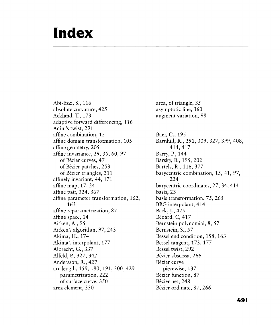
Index
Abi-Ezzi, S., 116
absolute curvature, 425
Ackland, X, 173
adaptive forward differencing, 116
Adini's twist, 291
affine combination, 15
affine domain transformation, 105
affine geometry, 205
affine invariance, 29, 35, 60, 97
of Bezier curves, 47
of Bezier patches, 253
of Bezier triangles, 311
affinely invariant, 44, 171
affine map, 17, 24
affine pair, 324, 367
affine parameter transformation, 162,
163
affine reparametrization, 87
affine space, 14
Aitken, A., 95
Aitken's algorithm, 97, 243
Akima, H., 174
Akima's interpolant, 177
Albrecht, G., 337
Alfeld, P., 327, 342
Andersson, R., 427
arc length, 159, 180, 191, 200, 429
parametrization, 222
of surface curve, 350
area element, 350
area, of triangle, 35
asymptotic line, 360
augment variation, 98
Baer, G., 195
BarnhiU, R., 291, 309, 327, 399, 408,
414,417
Barry, R, 144
Barsky, B., 195, 202
Bartels, R., 116,377
barycentric combination, 15, 41, 97,
224
barycentric coordinates, 27, 34, 414
basis,
23
basis transformation, 75, 265
BBG interpolant, 414
Beck, J., 425
Bedard, C, 417
Bernstein polynomial, 8, 57
Bernstein, S., 57
Bessel end condition, 158, 163
Bessel tangent, 173, 177
Bessel twist, 292
Bezier abscissa, 266
Bezier curve
piecewise, 137
Bezier function, 87
Bezier net, 248
Bezier ordinate, 87, 266
491

492 Index
Bezier, P., 64, 89, 195, 301, 304
Bezier patch, trivariate, 302
Bezier points, 45
Bezier polygon, 45
Bezier surface, 248
Bezier tetrahedron, 333
biaffine, 247
bias,
195
bicubic Hermite interpolant, 405
bicubic Hermite patch, 276
bihnear interpolant, 245, 271, 292,
400
bilinearly blended Coons patch, 291,
402,408
binomial coefficient, 57
binormal, 181
Birkhoff,
G., 414, 420
Blaschke, W., 45
blending function, 402, 412
blossom, 31, 51, 74, 313
of tensor product surface, 258
for triangular patches, 313
Bobrow, J., 305
Boehm, W., 30, 43, 50, 119, 189, 194,
195,
202, 314, 340, 364, 367,
376
Bol,G.,l 89
Bonneau, G., 305
Boolean sum, 412, 414
boundary edge, 394
boundary point, 39
boundary vertex, 394
brain imaging, 302
Brianchon, C., 206
Brown, J., 41, 291
Brunet, P., 293, 305, 367
Brunnett, G., 305
B-spline
polygon, 289, 419, 431
B-splines, 399,431
butterfly scheme, 391
canonical coordinates, 181
canonical form, 184
cardinal, 99, 103, 106
Casale, M., 305
Catmull-Clark surfaces, 383, 392
Catmull, E., 383
Catmull-Rom spline, 173
centroid, 15, 18
Ceva's theorem, 36
Chaikin, G., 132
Chang, G., 74
Chang, S., 116, 305
Charrot, P, 330, 367, 417
Chebychev polynomials, 399
Chiyokura, H., 410
chord length, 180
parametrization, 170
Chou,J.,238
Chrysler, 399
circle, 2, 5, 159, 221, 239, 299
osculating, 184
circulant matrix, 383, 386
clamped end condition, 155
Clark,].,
383
clay model, 6
closed mesh, 395
Clough-Tocher interpolant, 343
Cobb,
J., 339
Cohen, E., 68, 132, 163
Cohn-Vossen, S., 425
collinear, 25
compatibility, 408
complementary segment of a conic,
220
computational fluid dynamics, 399
computation count, 268
conic precision, 240
conic section, 44, 205, 209, 337, 359,
364
conjugate direction, 361
connection matrix, 202
CONS,
304
control net, 248
control points, 45
infinite, 224
control polygon, 45
of a conic, 211
control vectors, 238
conversion of
B-spline
surfaces, 288
convex, 41, 85
convex combination, 16, 273
convex hull, 16,37,41,48

Index 493
convex hull property, 48, 60, 98, 224,
335
of rational Bezier curves, 228
of Bezier patches, 254
of Bezier triangles, 312
convexity, 270
convexity of surfaces, 264
convex set, 16
Coons patch
discrete, 272
Coons patch, bilinearly blended, 291,
402
Coons, S., 2, 205, 227, 399
coordinate-free, 13
coordinate system, 13
corner, 170
corner-cutting, 132
corner of a curve, 162
corner tv^ist, 290
correction surface, 413
Coxeter, H., 15
Cox,M., 119, 142
Cramer's rule, 34
cross-boundary derivative, 257, 319,
403
cross-boundary normal derivative, 344
cross plot, 87
cross ratio, 206, 213, 219, 231
cross ratio theorem, 206
Crouch, P., 168
cubic Hermite interpolant, 416
cubic Hermite interpolation, 404, 413,
415
cubic Hermite polynomial, 104, 199,
403
cubic precision, 176, 240
curvature, 167, 183,419
Gaussian, 270
curvature,
derivative of, 188,421
of nonparametric curve, 187
of rational Bezier curve, 185
signed, 235, 243
curvature plot, 159, 163, 419
curve on surface, 304
cusp,
166
cylinder, 300
Dahmen. W., 68
Daniel, M, 432
data transfer, 83
Daubisse, J., 432
Davis,
P., 22, 57, 90
de Boor algorithm, 123
rational, 242
for rational B-splines, 241
de Boor, C, 22, 119, 123, 132, 142,
235,285,309
de Casteljau, P., 2, 30, 43, 50, 68, 119,
245,
309
de Casteljau algorithm, 45, 68, 247
degenerate patch, 261
Degen, W., 202
degree elevation, 238, 326
for B-splines, 144
for Bernstein polynomials, 92
for Bezier curves, 81, 132
for Bezier patches, 254
for rational Bezier curves, 236
degree reduction, 85
for B-spline curves, 133
for Bezier triangles, 333
Delaunay triangulation, 39
depth
of an
S-patch,
330
de Rham G., 132
derivative
of a B-spline, 144
of a conic, 215
of a rational Bezier curve, 233
DeRose, T, 17, 50, 202, 260, 301, 330,
367,
390, 434
design, 49
developable surface, 270, 358
diagonalization, 378
difference operator, G6, 256
Dill, J., 420, 425
dimension
of B-spline spaces, 140
directional derivative, 316
directrix, 9
Dirichlet tessellation, 37
discrete Coons patch, 272
discriminant, 351
divided differences, 119

494 Index
do Carmo, M., 202
domain, 68, 246
Doo,
D., 380
Doo-Sabin surfaces, 380, 392
duck, 167
Dupin's indicatrix, 359, 364, 376
Dyn, N., 41, 202, 379, 391
ellipse, 220, 359
elliptic point, 357
end condition
Bessel, 158, 306
clamped, 155
natural, 157
not-a-knot, 158
endpoint interpolation, 61
of Bezier curves, 49
Epstein, M., 162
euclidean map, 19
euclidean space, 14
Euler, L., 17, 179, 359
Euler-Poincare formula, 395
extraordinary vertex, 381, 385, 388
extrapolation, 68
fairness of a curve, 420
Farin, G., 84, 202, 309, 326, 327, 422
Farouki, R., 222, 305, 425, 432
Faux, I., 74
Ferguson, J., 2, 285, 290
fine
tune,
197
Fiorot, J., 227
first fundamental form, 350
flat point, 357
flat spot, 404
Floater, M., 233, 242
FMILL, 172
Foley, T, 162, 163
font design, 19, 71
Ford, 399
Ford, H., 12
Forrest, A. R., 64, 84, 205, 213, 227,
420,
425
Forsey, D., 377
forward difference, 64
forward differencing, 114
four-point scheme, 379
four tangent theorem, 213
fractals, 79
Frederickson, L., 309
Frenet frame, 181
Frenet frame continuity, 202
Frenet-Serret formulas, 183
functional curve, 86
Gallier,].,
119
Garland, M, 396
Gauss, C., 179, 357
Gaussian curvature, 270, 357, 425
Gauss-Seidel iteration, 157
Geise, G., 195, 202
generalized Vandermonde matrix, 101
General Motors, 399
generatrix, 300, 361
genus,
395
geodesic, 363
geometric continuity, 189, 191, 222
geometric programming, 17
geometry matrix, 265
Goldman, R., 13, 17, 50, 144, 189, 202,
314
Gonska, H., 57
Goodman, T., 202, 234
Gordon surface, 410
spline-blended, 412
Gordon, W., 2, 399,410,414
gradient, of implicit conic, 217
Grassmann, H., 41
Gregory, J., 202, 330, 367, 379, 391,
408,417
Gregory's square, 409
Greville abscissa, 135, 148
Hagen, H., 202, 293
Hahn, J., 367
Hansford, D., 40, 340
harmonic function, 8
Hartley, R, 163
hat function, 23
Heckbert, R, 396

Index 495
Hermite form, 435
Hermite interpolation, 102, 375, 413
Hermite patch, 276
Herron, G., 367, 376
hierarchical
B-spline
surface, 377
Hilbert, D., 425
Hinds, J., 305, 425
hodograph, 64
Hollig,K., 119,235
Holman, T., 434
homogeneous coordinates, 210
Horner's scheme, 75
Hoschek,].,
153, 367,424
hyperbola, 220, 247, 359
hyperbolic paraboloid, 246
hyperbolic point, 357
idempotent operator, 414
identity map, 18
IGES,
143, 217
image plane, 206
image registration, 22
implicit form
of conic, 216
of quadric, 340
of surface, 349
tolerances, 225
improper parametrization, 237
incenter, 345
infinite control point, 224, 238
inflection point, 429
integrals, 88
integrals of tensor product patches, 267
interference checking, 49
interior vertex, 394
interpolating
conic, 218
polynomial, 95
quadric, 340
intrinsic geometry, 357
invariance under affine parameter
transformations, 435
of Bezier curves, 48
isoparametric curve, 246, 252, 410
isophotes, 425
isotropic directions, 351
Jeannin, P., 227
Jensen, T., 367
JoUes, S., 74
Jones,
A., 367, 427
Judd, C, 163
junction points, 170
Kahmann, J., 367, 376
Kaufmann, E., 427
Kiciak, P., 367
Kimura, E, 410
Kjellander, J., 424
Klass,
R., 235, 425, 427
Klein bottle, 308
Klucewicz, I., 291
knot insertion for rational B-splines,
242
knot multiplicities, in IGES, 143
Kobbelt, L., 389
Korovkin, R, 57, 90, 91
Kronecker Delta, 61
Kruth, J., 240
Lacombe, C., 417
Lagrange interpolation, 99
Lagrange polynomial, 98, 411
Lane, J., 68
Laplacian smoothing, 281
Lasser, D., 305
least squares, 108, 149, 278, 346
tensor product, 278
Lee,
E., 50, 162, 220, 242
Leibniz formula, 33
Levin, D., 41, 391
Levin, S., 379
Levoy, M., 394
Lien, S., 116
Liming, R., 205, 219
linear independence of B-splines, 141
linear interpolation, 25
bivariate, 36
linear interpolation, repeated, 44
linearly independent, 22
linear operator, 23, 45
linear parameter transformation, 48

496 Index
linear precision, 62, 98, 171
of Bezier triangles, 327
of rational curves, 228
linear space, 14, 22
line of curvature, 356
of a surface of revolution, 356
Little, R, 40
Liu, D., 367, 420
Lobachevsky, N., 119
local control, 129
local coordinates, 48
local parameter, 28
local support, 140
lofted surface, 269, 411
loop,
170
Loop,
C, 330, 387
Lorentz, L., 57
Lounsbery, M., 390
Lucian, M., 242
Lyche, T, 132
main normal vector, 181
Manning,].,
195, 202
Mann, S., 260, 390
Mansfield, L., 119, 142
Marhsall,J.,417
mass point, 41
matrix circulant, 383, 386
matrix form of curves, 74
Ma, W., 240
maxmin criterion, 40
McConalogue, D., 163, 174
mean curvature, 357, 425
Meier, J., 57
Memke's theorem, 189, 194
Menelaos' theorem, 30
meridian, 299
Meusnier's theorem, 354
Micchelli,C., 132, 189,202
Michelangelo, 394
digital, 394
Miller, J., 305
minimal support of B-splines, 140
minmax box, 49, 69
minmax criterion, 40
Mitchell, A., 417
mixed partials, 257
Moebius, R, 17, 26, 34, 206
Monge, C, 179
monomial basis, 75, 432
monomial form, Gl
of Bezier patches, 265
monomials, 23, 99
Mortenson, M., 74
multiaffine, 31, 53
multiaffine function, 313
multiplicities, of end knots, 143
multiplicity
of a knot, 127
multiresolution, 397
Munchmeyer, R, 425
Musse, J., 367
Nachman, L., 403
NAPOLEON, 11
Nasri, A., 390
natural end condition, 157, 162
nested multiplication, IS
neutral set, 39
Neville, ^l
New^ton form, 114
New^ton iteration, 153
Nielson, G., 107, 163, 194, 199, 367,
414,416,417
nine parameter interpolant, 341
nonparametric curve, 187
nonparametric patch, 266
normal curvature, 354
normal equations, 86, 150, 347
normal section, 354
normal vector, 261
numerical control, 1
NURBS,
227
O'Dell,
C, 163
open mesh, 395
order of contact, 202
orthonormal matrix, 19
osculant, of tensor product surface, 259
osculating circle, 184
osculating plane, 73, 182, 203
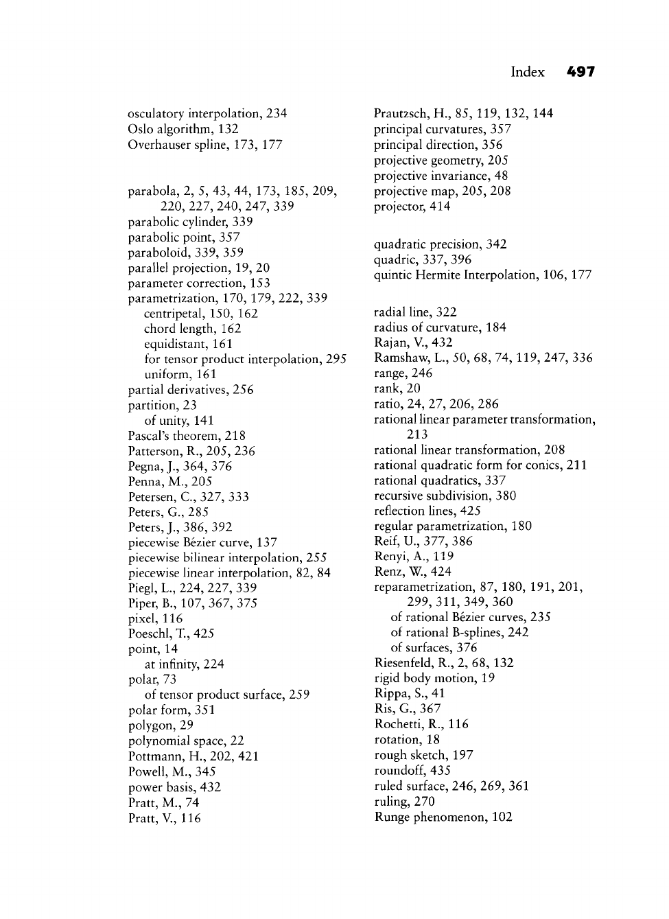
Index 497
osculatory interpolation, 234
Oslo algorithm, 132
Overhauser spline, 173, 177
parabola, 2, 5, 43, 44, 173, 185, 209,
220,
227, 240, 247, 339
parabolic cylinder, 339
parabolic point, 357
paraboloid, 339, 359
parallel projection, 19, 20
parameter correction, 153
parametrization, 170, 179, 222, 339
centripetal, 150, 162
chord length, 162
equidistant, 161
for tensor product interpolation, 295
uniform, 161
partial derivatives, 256
partition, 23
of unity, 141
Pascal's theorem, 218
Patterson, R., 205, 236
Pegna, J., 364, 376
Penna, M., 205
Petersen, C, 327, 333
Peters, G., 285
Peters,].,
386, 392
piecev^ise Bezier curve, 137
piecewise bilinear interpolation, 255
piecewise linear interpolation, 82, 84
Piegl, L., 224, 227, 339
Piper, B., 107, 367, 375
pixel, 116
Poeschl, T, 425
point, 14
at infinity, 224
polar, 73
of tensor product surface, 259
polar form, 351
polygon, 29
polynomial space, 22
Pottmann, H., 202, 421
Powell, M., 345
pov^er basis, 432
Pratt, M., 74
Pratt, v., 116
Prautzsch, H., 85, 119, 132, 144
principal curvatures, 357
principal direction, 356
projective geometry, 205
projective invariance, 48
projective map, 205, 208
projector, 414
quadratic precision, 342
quadric, 337, 396
quintic Hermite Interpolation, 106, 177
radial line, 322
radius of curvature, 184
Rajan, V., 432
Ramshaw, L., 50, 68, 74, 119, 247, 336
range, 246
rank, 20
ratio,
24, 27, 206, 286
rational linear parameter transformation,
213
rational linear transformation, 208
rational quadratic form for conies, 211
rational quadratics, 337
recursive subdivision, 380
reflection lines, 425
regular parametrization, 180
Reif,
U., 377, 386
Renyi, A., 119
Renz, W., 424
reparametrization, 87, 180, 191, 201,
299,311,349,360
of rational Bezier curves, 235
of rational B-splines, 242
of surfaces, 376
Riesenfeld, R., 2, 68, 132
rigid body motion, 19
Rippa, S., 41
Ris,
G., 367
Rochetti, R., 116
rotation, 18
rough sketch, 197
roundoff,
435
ruled surface, 246, 269, 361
ruling, 270
Runge phenomenon, 102

498 Index
S. Parry, 301
Sabin, M., 235, 309, 345, 380, 389, 420
Sablonniere, P., 309, 327
Sakkalis, T, 222
Sapidis, N., 419
Sarraga, R., 367, 375
scaling, 18
scattered data interpolation, 341
Schelske, J., 264
Schneider, R, 240
Schoenberg, L, 84, 119
Schoenberg-Whitney theorem, 150
Schulze, G., 293
Schumaker, L., 68, 327
second fundamental form, 353
Sederberg, X, 49, 64, 237, 260, 301
Seidel,H.,50, 314
Selesnick, S., 293
self-conjugate, 361
semicircle, 224
Sequin, C, 367
Shantz,M., 116, 305
shape preservation, 101, 270
shear, 19, 24
Shirman, L., 367
shoulder point, 213, 219
shoulder tangent, 219
signed curvature, 187
simplest scheme, 386
slanted font, 19
smoothness
of piecewise Bezier curves, 137
soHd modeling, 338
sphere, 300
spline, 2, 167, 173, 240, 421, 424
spline interpolation, 412
iterative, 157
stability of the monomial form, 432
Staerk, E., 68
Stancu, D., 309
standard cubic, 55
standard form
for conies, 213
of rational Bezier curve, 236, 299
star, 396
Steiner, J., 213
stochastic matrix, 385
storage for
B-spline
curves, 435
straight line, 25
strain energy, 167
Su, B., 420
subdivision, 6S
formula, 68
of Bezier curves, 68
of Bezier patches, 259
of Bezier triangles, 321
of rational Bezier curves, 232
in terms of Bernstein polynomials, 92
subspace, 22
surface, 9
butterfly, 391
conical, 270
cylindrical, 270
developable, 270
lofted, 269
ruled, 269
translational, 272
surface of revolution, 299
Sw^immer, A., 41
symmetric function, 313
symmetry, 61
tangent length, 435
tangent plane of Bezier triangle, 318
tangent ribbon, 404
tangent vector, 181
Taylor series, 67
tension, 195
tensor product, 246, 412
interpolant, 405, 435
surfaces, 245
tetrahedron, 333
texture mapping, 425
theorema egregium, 357
Thiessen region, 37
three tangent theorem, 44
Tiller, W., 227, 339
topology of triangulations, 394
torsion, 183
continuity, 202
of nonparametric curve, 187
of rational Bezier curve, 185, 186,
234

Index 499
torus,
300
transfinite interpolation, 399, 410
translation, 14, 18
translational surface, 264, 272, 282, 290
transposant, 304
triangle
area of, 35
numbers, 310
triangulation, 39
data dependent, 41
trimmed surfaces, 304
trinomial coefficient, 315
trivariate B-splines, 302
trivial reject, 69
twist estimation, 406
twist incompatibility, 417
twist, variable, 409
twist vector, 257, 264
type check, 17
umbilical point, 355
uniform parametrization, 222
UNISURF, 1
unit interval, 28
unit sphere, 339
unit square, 246
variable twists, 409
variation diminishing property, 29, 41,
84,
98, 202
for Bezier patches, 254
of rational Bezier curves, 228
vectors, 14
Vernet, P., 89
Veron, M., 367
Versprille, K., 224, 238
vertex split, 397
Vigo,
M., 305
Vinacua, A., 367
volume distortion, 301
Voronoi diagram, 37
Wang, X., 64
Weierstrass approximation theorem, 90
weight point, 214, 219, 230, 231, 235,
336
weights, 211
of rational Bezier curves, 227
Wolter, R, 364, 376
Worsey, A., 235
Yamaguchi, R, 157
valency, 381
Vandermonde, 100, 275
vanWijk,].,
367
zero twist, 273, 290, 404
Zhou, J., 84

This Page Intentionally Left Blank
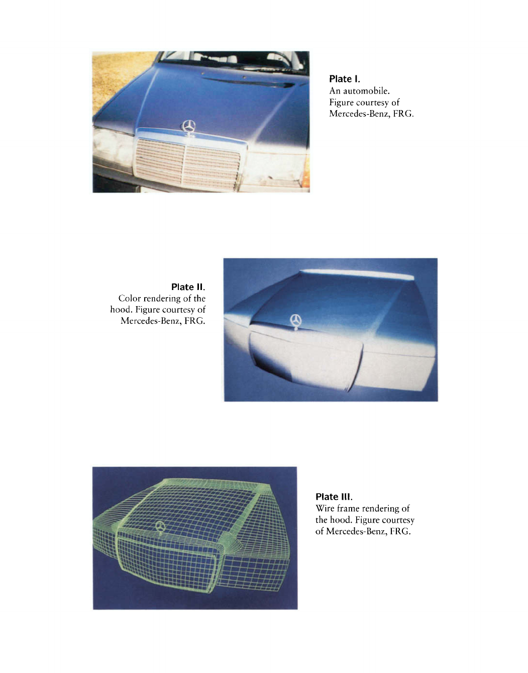
Plate I.
An automobile.
Figure courtesy of
Mercedes-Benz, FRG.
Plate II.
Color rendering of the
hood. Figure courtesy of
Mercedes-Benz, FRG.
Plate
111.
Wire frame rendering of
the hood. Figure courtesy
of Mercedes-Benz, FRG.
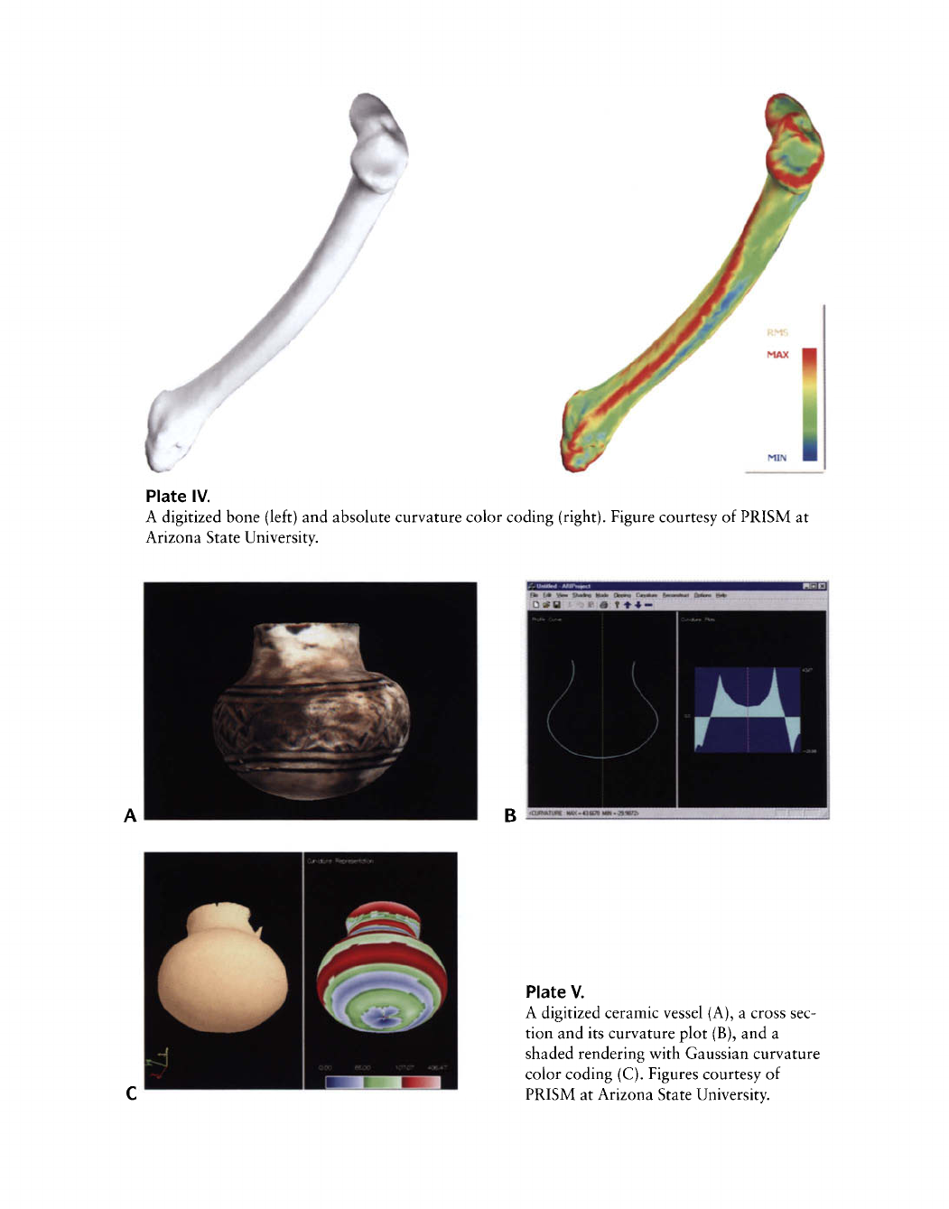
Plate IV.
A digitized bone (left) and absolute curvature color coding (right). Figure courtesy of PRISM at
Arizona State University.
Plate V.
A digitized ceramic vessel (A), a cross sec-
tion and its curvature plot (B), and a
shaded rendering with Gaussian curvature
color coding (C). Figures courtesy of
PRISM at Arizona State University.
