Beginner's Guide To Using The DESeq2 Package DEGSeq2
User Manual:
Open the PDF directly: View PDF ![]() .
.
Page Count: 32

Beginner’s guide to using the DESeq2 package
Michael Love1∗, Simon Anders2, Wolfgang Huber2
1Department of Biostatistics, Dana Farber Cancer Institute and
Harvard School of Public Health, Boston, US;
2European Molecular Biology Laboratory (EMBL), Heidelberg, Germany
∗michaelisaiahlove (at) gmail.com
May 13, 2014
Abstract
This vignette describes the statistical analysis of count matrices for systematic changes be-
tween conditions using the DESeq2 package, and includes recommendations for producing count
matrices from raw sequencing data. This vignette is designed for users who are perhaps new
to analyzing RNA-Seq or high-throughput sequencing data in R, and so goes at a slower pace,
explaining each step in detail. Another vignette, “Differential analysis of count data – the DESeq2
package” covers more of the advanced details at a faster pace.
DESeq2 version: 1.4.5
If you use DESeq2 in published research, please cite:
M. I. Love, W. Huber, S. Anders: Moderated estimation of
fold change and dispersion for RNA-Seq data with DESeq2.
bioRxiv (2014). doi:10.1101/002832 [1]
1

Beginner’s guide to using the DESeq2 package 2
Contents
1 Introduction 2
2 Input data 2
2.1 Preparing count matrices ................................. 3
2.2 Aligning reads to a reference ................................ 3
2.3 Counting reads in genes .................................. 4
2.4 Experiment data ...................................... 7
2.4.1 The DESeqDataSet, column metadata, and the design formula ......... 7
2.4.2 Starting from SummarizedExperiment ....................... 8
2.4.3 Starting from count tables ............................. 10
2.5 Collapsing technical replicates ............................... 12
3 Running the DESeq2 pipeline 13
3.1 Preparing the data object for the analysis of interest ................... 13
3.2 Running the pipeline .................................... 14
3.3 Inspecting the results table ................................ 15
3.4 Other comparisons ..................................... 16
3.5 Multiple testing ...................................... 17
3.6 Diagnostic plots ...................................... 19
4 Independent filtering 22
4.1 Adding gene names .................................... 24
4.2 Exporting results ...................................... 25
5 Working with rlog-transformed data 25
5.1 The rlog transform ..................................... 25
5.2 Sample distances ...................................... 27
5.3 Gene clustering ....................................... 30
6 Session Info 31
1 Introduction
In this vignette, you will learn how to produce a read count table – such as arising from a summarized
RNA-Seq experiment – analyze count tables for differentially expressed genes, visualize the results, add
extra gene annotations, and cluster samples and genes using transformed counts.
2 Input data

Beginner’s guide to using the DESeq2 package 3
2.1 Preparing count matrices
As input, the DESeq2 package expects count data as obtained, e. g., from RNA-Seq or another high-
throughput sequencing experiment, in the form of a matrix of integer values. The value in the i-th
row and the j-th column of the matrix tells how many reads have been mapped to gene iin sample j.
Analogously, for other types of assays, the rows of the matrix might correspond e. g. to binding regions
(with ChIP-Seq) or peptide sequences (with quantitative mass spectrometry).
The count values must be raw counts of sequencing reads. This is important for DESeq2 ’s statistical
model to hold, as only the actual counts allow assessing the measurement precision correctly. Hence,
please do not supply other quantities, such as (rounded) normalized counts, or counts of covered base
pairs – this will only lead to nonsensical results.
2.2 Aligning reads to a reference
The computational analysis of an RNA-Seq experiment begins earlier however, with a set of FASTQ
files, which contain the bases for each read and their quality scores. These reads must first be aligned
to a reference genome or transcriptome. It is important to know if the sequencing experiment was
single-end or paired-end, as the alignment software will require the user specify both FASTQ files for a
paired-end experiment.
A number of software programs exist to align reads to the reference genome, and the development is
too rapid for this document to provide a current list. We recommend reading benchmarking papers
which discuss the advantages and disadvantages of each software, which include accuracy, ability to
align reads over splice junctions, speed, memory footprint, and many other features.
We have experience using the TopHat2 spliced alignment software1[2] in combination with the Bowtie
index available at the Illumina iGenomes page2. For full details on this software and on the iGenomes,
users should follow the links to the manual and information provided in the links in the footnotes. For
example, the paired-end RNA-Seq reads for the parathyroidSE package were aligned using TopHat2
with 8 threads, with the call:
tophat2 -o file_tophat_out -p 8 genome file_1.fastq file_2.fastq
samtools sort -n file_tophat_out/accepted_hits.bam _sorted
The second line sorts the reads by name rather than by genomic position, which is necessary for counting
paired-end reads within Bioconductor. This command uses the SAMtools software3[3]. The BAM files
for a number of sequencing runs can then be used to generate coun matrices, as described in the
following section.
1http://tophat.cbcb.umd.edu/
2http://tophat.cbcb.umd.edu/igenomes.html
3http://samtools.sourceforge.net

Beginner’s guide to using the DESeq2 package 4
2.3 Counting reads in genes
Once the reads have been aligned, there are a number of tools which can be used to count the number
of reads which can be unambiguously assigned to genomic features for each sample. These often take
as input BAM or SAM alignment files and a file specifiying the genomic features, e.g. GFF3 or GTF
files specifying a gene model.
The following tools can be used generate count tables:
function package output DESeq2 input function
summarizeOverlaps GenomicAlignments (Bioc) SummarizedExperiment DESeqDataSet
htseq-count[4]HTSeq (Python) count files DESeqDataSetFromHTSeq
featureCounts[5]Rsubread (Bioc) count matrix DESeqDataSetFromMatrix
simpleRNASeq[6]easyRNASeq (Bioc) SummarizedExperiment DESeqDataSet
In order to produce correct counts, it is important to know if the experiment was strand-specific or not.
For example, summarizeOverlaps has the argument ignore.strand, which should be set to TRUE
if the experiment was not strand-specific and FALSE if the experiment was strand-specific. Similarly,
htseq-count has the argument --stranded yes/no/reverse, where strand-specific experiments
should use --stranded yes and where reverse indicates that the positive strand reads should be
counted to negative strand features.
The following example uses summarizeOverlaps for read counting, while produces a SummarizedEx-
periment object. This class of object contains a variety of information about an experiment, and will be
described in more detail below. We will demonstrate using example BAM files from the parathyroidSE
data package. First, we read in the gene model from a GTF file, using makeTranscriptDbFromGFF.
Alternatively the makeTranscriptDbFromBiomart function can be used to automatically pull a gene
model from Biomart. However, keeping the GTF file on hand has the advantage of bioinformatic re-
producibility: the same gene model can be made again, while past versions of gene models might not
always be available on Biomart. These GTF files can be downloaded from Ensembl’s FTP site or other
gene model repositories. The third line here produces a GRangesList of all the exons grouped by gene.
library("GenomicFeatures" )
hse <- makeTranscriptDbFromGFF("/path/to/your/genemodel.GTF",format="gtf" )
exonsByGene <- exonsBy( hse, by="gene" )
We specify the BAM files which will be used for counting.
fls <- list.files("/path/to/bam/files",pattern="bam$",full=TRUE )
We indicate in Bioconductor that these fls are BAM files using the BamFileList function. Here we
also specify details about how the BAM files should be treated, e.g., only process 100000 reads at a
time.
library("Rsamtools" )
bamLst <- BamFileList( fls, yieldSize=100000 )
We call summarizeOverlaps to count the reads. We use the counting mode "Union" which indi-
cates that reads which overlap any portion of exactly one feature are counted. For more ihnforma-
Beginner’s guide to using the DESeq2 package 5
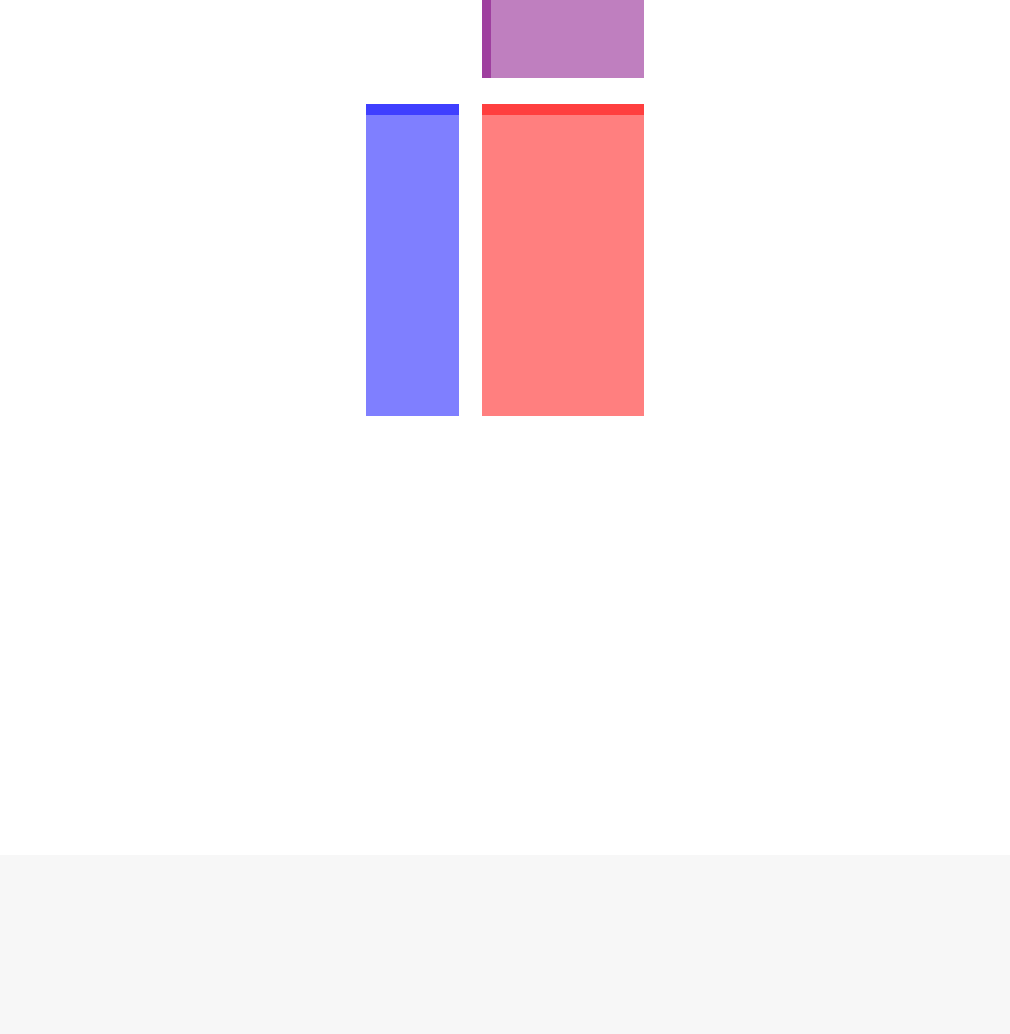
assay(s)
e.g. 'counts'
rowData
colData
Figure 1: Diagram of SummarizedExperiment Here we show the component parts of a Summa-
rizedExperiment object, and also its subclasses, such as the DESeqDataSet which is explained in the
next section. The assay(s) (red block) contains the matrix (or matrices) of summarized values, the
rowData (blue block) contains information about the genomic ranges, and the colData (purple block)
contains information about the samples or experiments. The highlighted line in each block represents
the first row (note that the first row of colData lines up with the first column of the assay.
tion on the various counting modes, see the help page for summarizeOverlaps. As this experiment
was a paired-end, we specify singleEnd=FALSE. As it was not a strand-specific protocol, we specify
ignore.strand=TRUE.fragments=TRUE indicates that we also want to count reads with unmapped
pairs. This last argument is only for use with paired-end experiments.
library("GenomicAlignments" )
se <- summarizeOverlaps( exonsByGene, bamLst,
mode="Union",
singleEnd=FALSE,
ignore.strand=TRUE,
fragments=TRUE )
This example code above actually only counts a small subset of reads from the original experiment: for
3 samples and for 100 genes. Nevertheless, we can still investigate the resulting SummarizedExperiment
by looking at the counts in the assay slot, the phenotypic data about the samples in colData slot (in
this case an empty DataFrame), and the data about the genes in the rowData slot.

Beginner’s guide to using the DESeq2 package 6
se
## class: SummarizedExperiment
## dim: 100 3
## exptData(0):
## assays(1): counts
## rownames(100): ENSG00000000003 ENSG00000000005 ... ENSG00000005469
## ENSG00000005471
## rowData metadata column names(0):
## colnames(3): SRR479052.bam SRR479053.bam SRR479054.bam
## colData names(0):
head(assay(se) )
## SRR479052.bam SRR479053.bam SRR479054.bam
## ENSG00000000003 0 0 1
## ENSG00000000005 0 0 0
## ENSG00000000419 0 0 0
## ENSG00000000457 0 1 0
## ENSG00000000460 0 0 0
## ENSG00000000938 0 0 0
colSums(assay(se) )
## SRR479052.bam SRR479053.bam SRR479054.bam
## 31 21 27
colData(se)
## DataFrame with 3 rows and 0 columns
rowData(se)
## GRangesList of length 100:
## $ENSG00000000003
## GRanges with 17 ranges and 2 metadata columns:
## seqnames ranges strand | exon_id exon_name
## <Rle> <IRanges> <Rle> | <integer> <character>
## [1] X [99883667, 99884983] - | 664095 ENSE00001459322
## [2] X [99885756, 99885863] - | 664096 ENSE00000868868
## [3] X [99887482, 99887565] - | 664097 ENSE00000401072
## [4] X [99887538, 99887565] - | 664098 ENSE00001849132
## [5] X [99888402, 99888536] - | 664099 ENSE00003554016
## ... ... ... ... ... ... ...
## [13] X [99890555, 99890743] - | 664106 ENSE00003512331
## [14] X [99891188, 99891686] - | 664108 ENSE00001886883
## [15] X [99891605, 99891803] - | 664109 ENSE00001855382
## [16] X [99891790, 99892101] - | 664110 ENSE00001863395
## [17] X [99894942, 99894988] - | 664111 ENSE00001828996

Beginner’s guide to using the DESeq2 package 7
##
## ...
## <99 more elements>
## ---
## seqlengths:
## 1 2 ... LRG_98 LRG_99
## 249250621 243199373 ... 18750 13294
Note that the rowData slot is a GRangesList, which contains all the information about the exons for
each gene, i.e., for each row of the count table.
This SummarizedExperiment object se is then all we need to start our analysis. In the following section
we will show how to create the data object which is used in DESeq2, either using the SummarizedEx-
periment, or in general, a count table which has been loaded into R.
2.4 Experiment data
2.4.1 The DESeqDataSet, column metadata, and the design formula
Each Bioconductor software package often has a special class of data object, which contains special
slots and requirements. The data object class in DESeq2 is the DESeqDataSet, which is built on top
of the SummarizedExperiment. One main differences is that the assay slot is instead accessed using
the count accessor, and the values in this matrix must non-negative integers.
A second difference is that the DESeqDataSet has an associated “design formula”. The design is
specified at the beginning of the analysis, as this will inform many of the DESeq2 functions how to
treat the samples in the analysis (one exception is the size factor estimation – adjustment for differing
library sizes – which does not depend on the design formula). The design formula tells which variables
in the column metadata table (colData) specify the experimental design and how these factors should
be used in the analysis.
The simplest design formula for differential expression would be ∼condition, where condition is a
column in colData(dds) which specifies which of two (or more groups) the samples belong to. For
the parathyroid experiment, we will specify ∼patient + treatment, which means that we want to
test for the effect of treatment (the last factor), controlling for the effect of patient (the first factor).
You can use R’s formula notation to express any experimental design that can be described within an
ANOVA-like framework. Note that DESeq2 uses the same kind of formula as in base R, e.g., for use
by the lm function. If the question of interest is whether a fold change due to treatment is different
across groups, for example across patients, “interaction terms” can be included using models such as
∼patient + treatment + patient:treatment. More complex designs such as these are covered
in the other DESeq2 vignette.
In the following section, we will demonstrate the construction of the DESeqDataSet from two starting
points:
1. from a SummarizedExperiment object created by, e.g., summarizeOverlaps in the above example
Beginner’s guide to using the DESeq2 package 8
2. more generally, from a count table (i.e. matrix) and a column metadata table which have been
loaded into R
For a full example of using the HTSeq Python package4for read counting, please see the pasilla or
parathyroid data package. For an example of generating the DESeqDataSet from files produced by
htseq-count, please see the other DESeq2 vignette.
2.4.2 Starting from SummarizedExperiment
We load a prepared SummarizedExperiment, which was generated using summarizeOverlaps from
publicly available data from the article by Felix Haglund et al., “Evidence of a Functional Estrogen
Receptor in Parathyroid Adenomas”, J Clin Endocrin Metab, Sep 20125. Details on the generation of
this object can be found in the vignette for the parathyroidSE package.
The purpose of the experiment was to investigate the role of the estrogen receptor in parathyroid
tumors. The investigators derived primary cultures of parathyroid adenoma cells from 4 patients. These
primary cultures were treated with diarylpropionitrile (DPN), an estrogen receptor βagonist, or with
4-hydroxytamoxifen (OHT). RNA was extracted at 24 hours and 48 hours from cultures under treatment
and control. The blocked design of the experiment allows for statistical analysis of the treatment effects
while controlling for patient-to-patient variation.
We first load the DESeq2 package and the data package parathyroidSE , which contains the example
data set.
library("DESeq2" )
library("parathyroidSE" )
The data command loads a preconstructed data object:
data("parathyroidGenesSE" )
se <- parathyroidGenesSE
colnames(se) <- se$run
Supposing we have constructed a SummarizedExperiment using one of the methods described in the
previous section, we now ensure that the object contains the necessary information about the samples,
i.e., a table with metadata on the count table’s columns stored in the colData slot:
colData(se)[1:5,1:4]
## DataFrame with 5 rows and 4 columns
## run experiment patient treatment
## <character> <factor> <factor> <factor>
## SRR479052 SRR479052 SRX140503 1 Control
## SRR479053 SRR479053 SRX140504 1 Control
## SRR479054 SRR479054 SRX140505 1 DPN
## SRR479055 SRR479055 SRX140506 1 DPN
4described in [4]
5http://www.ncbi.nlm.nih.gov/pubmed/23024189
Beginner’s guide to using the DESeq2 package 9
## SRR479056 SRR479056 SRX140507 1 OHT
This object does, because it was prepared so, as can be seen in the parathyroidSE vignette. However,
users will most likely have to add pertinent sample/phenotypic information for the experiment at this
stage. We highly recommend keeping this information in a comma-separated value (CSV) or tab-
separated value (TSV) file, which can be exported from an Excel spreadsheet. The advantage of this
over typing out the characters into an R script, is that while scrolling through a script, accidentally typed
spaces or characters could lead to changes to the sample phenotypic information, leading to spurious
results.
Suppose we have a CSV file which contains such data, we could read this file in using the base R
read.csv function:
sampleInfo <- read.csv("/path/to/file.CSV" )
Here we show a toy example of such a table. Note that the order is not the same as in the Summarized-
Experiment. Here instead of run, most users will have the filename of the BAM files used for counting.
We convert the sampleInfo object into a DataFrame which is the format of the colData.
head( sampleInfo )
## run pheno
## 1 SRR479078 pheno1
## 2 SRR479077 pheno2
## 3 SRR479076 pheno1
## 4 SRR479075 pheno2
## 5 SRR479074 pheno1
## 6 SRR479073 pheno2
head(colnames(se) )
## [1] "SRR479052" "SRR479053" "SRR479054" "SRR479055" "SRR479056" "SRR479057"
sampleInfo <- DataFrame( sampleInfo )
We create an index which will put them in the same order: the SummarizedExperiment comes first
because this is the sample order we want to achieve. We then check to see that we have lined them up
correctly, and then we can add the new data to the existing colData.
seIdx <- match(colnames(se), sampleInfo$run)
head(cbind(colData(se)[ , 1:3], sampleInfo[ seIdx, ] ) )
## DataFrame with 6 rows and 5 columns
## run experiment patient run.1 pheno
## <character> <factor> <factor> <factor> <factor>
## SRR479052 SRR479052 SRX140503 1 SRR479052 pheno1
## SRR479053 SRR479053 SRX140504 1 SRR479053 pheno2
## SRR479054 SRR479054 SRX140505 1 SRR479054 pheno1
## SRR479055 SRR479055 SRX140506 1 SRR479055 pheno2
## SRR479056 SRR479056 SRX140507 1 SRR479056 pheno1

Beginner’s guide to using the DESeq2 package 10
## SRR479057 SRR479057 SRX140508 1 SRR479057 pheno2
colData(se) <- cbind(colData(se), sampleInfo[ seIdx, ] )
The following line builds the DESeqDataSet from a SummarizedExperiment se and specifying a design
formula, as described in the previous section. The names of variables used in the design formula must
be the names of columns in the colData of se.
ddsFull <- DESeqDataSet( se, design =~patient +treatment )
2.4.3 Starting from count tables
In the following section, we will show how to build an DESeqDataSet from a count table and a table
of sample information. While the previous section would be used to contruct a DESeqDataSet from
aDESeqDataSet, here we first extract the individual object (count table and sample info) from a
SummarizedExperiment in order to build it back up into a new object for demonstration purposes. In
practice, the count table would either be read in from a file or perhaps generated by an R function like
featureCounts from the Rsubread package.
The information in a SummarizedExperiment object can be accessed with accessor functions. For
example, to see the actual data, i.e., here, the read counts, we use the assay function. (The head
function restricts the output to the first few lines.)
countdata <- assay( parathyroidGenesSE )
head( countdata )
## [,1] [,2] [,3] [,4] [,5] [,6] [,7] [,8] [,9] [,10] [,11] [,12]
## ENSG00000000003 792 1064 444 953 519 855 413 365 278 1173 463 316
## ENSG00000000005 4 1 2 3 3 1 0 1 0 0 0 0
## ENSG00000000419 294 282 164 263 179 217 277 204 189 601 257 183
## ENSG00000000457 156 184 93 145 75 122 228 171 116 422 182 122
## ENSG00000000460 396 207 210 212 221 173 611 199 426 1391 286 417
## ENSG00000000938 3 8 2 5 0 4 13 22 3 38 13 10
## [,13] [,14] [,15] [,16] [,17] [,18] [,19] [,20] [,21] [,22]
## ENSG00000000003 987 424 305 391 586 714 957 346 433 402
## ENSG00000000005 0 0 0 0 0 0 1 0 0 0
## ENSG00000000419 588 275 263 281 406 568 764 288 259 250
## ENSG00000000457 441 211 131 115 196 266 347 133 168 148
## ENSG00000000460 1452 238 188 102 389 294 778 162 85 339
## ENSG00000000938 26 13 7 3 10 18 15 7 8 7
## [,23] [,24] [,25] [,26] [,27]
## ENSG00000000003 277 511 366 271 492
## ENSG00000000005 0 0 0 0 0
## ENSG00000000419 147 271 227 197 363
## ENSG00000000457 83 184 136 118 195
## ENSG00000000460 75 154 314 117 233
Beginner’s guide to using the DESeq2 package 11
## ENSG00000000938 5 13 8 7 8
In this count table, each row represents an Ensembl gene, each column a sequenced RNA library, and
the values give the raw numbers of sequencing reads that were mapped to the respective gene in each
library.
We also have metadata on each of the samples (the “columns” of the count table):
coldata <- colData( parathyroidGenesSE )
rownames( coldata ) <- coldata$run
colnames( countdata ) <- coldata$run
head( coldata[ , c("patient","treatment","time" ) ] )
## DataFrame with 6 rows and 3 columns
## patient treatment time
## <factor> <factor> <factor>
## SRR479052 1 Control 24h
## SRR479053 1 Control 48h
## SRR479054 1 DPN 24h
## SRR479055 1 DPN 48h
## SRR479056 1 OHT 24h
## SRR479057 1 OHT 48h
We now have all the ingredients to prepare our data object in a form that is suitable for analysis, namely:
countdata: a table with the read counts
coldata: a table with metadata on the count table’s columns
To now construct the data object from the matrix of counts and the metadata table, we use:
ddsFullCountTable <- DESeqDataSetFromMatrix(
countData = countdata,
colData = coldata,
design =~patient +treatment)
ddsFullCountTable
## class: DESeqDataSet
## dim: 63193 27
## exptData(0):
## assays(1): counts
## rownames(63193): ENSG00000000003 ENSG00000000005 ... LRG_98 LRG_99
## rowData metadata column names(0):
## colnames(27): SRR479052 SRR479053 ... SRR479077 SRR479078
## colData names(8): run experiment ... study sample
We will continue with the object generated from the SummarizedExperiment section.

Beginner’s guide to using the DESeq2 package 12
2.5 Collapsing technical replicates
There are a number of samples which were sequenced in multiple runs. For example, sample SRS308873
was sequenced twice. To see, we list the respective columns of the colData. (The use of as.data.frame
forces R to show us the full list, not just the beginning and the end as before.)
as.data.frame(colData( ddsFull )[ ,c("sample","patient","treatment","time") ] )
## sample patient treatment time
## SRR479052 SRS308865 1 Control 24h
## SRR479053 SRS308866 1 Control 48h
## SRR479054 SRS308867 1 DPN 24h
## SRR479055 SRS308868 1 DPN 48h
## SRR479056 SRS308869 1 OHT 24h
## SRR479057 SRS308870 1 OHT 48h
## SRR479058 SRS308871 2 Control 24h
## SRR479059 SRS308872 2 Control 48h
## SRR479060 SRS308873 2 DPN 24h
## SRR479061 SRS308873 2 DPN 24h
## SRR479062 SRS308874 2 DPN 48h
## SRR479063 SRS308875 2 OHT 24h
## SRR479064 SRS308875 2 OHT 24h
## SRR479065 SRS308876 2 OHT 48h
## SRR479066 SRS308877 3 Control 24h
## SRR479067 SRS308878 3 Control 48h
## SRR479068 SRS308879 3 DPN 24h
## SRR479069 SRS308880 3 DPN 48h
## SRR479070 SRS308881 3 OHT 24h
## SRR479071 SRS308882 3 OHT 48h
## SRR479072 SRS308883 4 Control 48h
## SRR479073 SRS308884 4 DPN 24h
## SRR479074 SRS308885 4 DPN 48h
## SRR479075 SRS308885 4 DPN 48h
## SRR479076 SRS308886 4 OHT 24h
## SRR479077 SRS308887 4 OHT 48h
## SRR479078 SRS308887 4 OHT 48h
We recommend to first add together technical replicates (i.e., libraries derived from the same samples),
such that we have one column per sample. We have implemented a convenience function for this,
which can take am object, either SummarizedExperiment or DESeqDataSet, and a grouping factor, in
this case the sample name, and return the object with the counts summed up for each unique sample.
This will also rename the columns of the object, such that they match the unique names which were
used in the grouping factor. Optionally, we can provide a third argument, run, which can be used
to paste together the names of the runs which were collapsed to create the new object. Note that
dds variable is equivalent to colData(dds) variable.
Beginner’s guide to using the DESeq2 package 13
ddsCollapsed <- collapseReplicates( ddsFull,
groupby = ddsFull$sample,
run = ddsFull$run )
head(as.data.frame(colData(ddsCollapsed)[ ,c("sample","runsCollapsed") ] ), 12 )
## sample runsCollapsed
## SRS308865 SRS308865 SRR479052
## SRS308866 SRS308866 SRR479053
## SRS308867 SRS308867 SRR479054
## SRS308868 SRS308868 SRR479055
## SRS308869 SRS308869 SRR479056
## SRS308870 SRS308870 SRR479057
## SRS308871 SRS308871 SRR479058
## SRS308872 SRS308872 SRR479059
## SRS308873 SRS308873 SRR479060,SRR479061
## SRS308874 SRS308874 SRR479062
## SRS308875 SRS308875 SRR479063,SRR479064
## SRS308876 SRS308876 SRR479065
We can confirm that the counts for the new object are equal to the summed up counts of the columns
that had the same value for the grouping factor:
original <- rowSums(counts(ddsFull)[ , ddsFull$sample == "SRS308873" ] )
all( original == counts(ddsCollapsed)[ ,"SRS308873" ] )
## [1] TRUE
3 Running the DESeq2 pipeline
Here we will analyze a subset of the samples, namely those taken after 48 hours, with either control,
DPN or OHT treatment, taking into account the multifactor design.
3.1 Preparing the data object for the analysis of interest
First we subset the relevant columns from the full dataset:
dds <- ddsCollapsed[ , ddsCollapsed$time == "48h" ]
Sometimes it is necessary to drop levels of the factors, in case that all the samples for one or more
levels of a factor in the design have been removed. If time were included in the design formula, the
following code could be used to take care of dropped levels in this column.
dds$time <- droplevels( dds$time )

Beginner’s guide to using the DESeq2 package 14
It will be convenient to make sure that Control is the first level in the treatment factor, so that the
default log2 fold changes are calculated as treatment over control and not the other way around. The
function relevel achieves this:
dds$treatment <- relevel( dds$treatment, "Control" )
A quick check whether we now have the right samples:
as.data.frame(colData(dds) )
## run experiment patient treatment time submission study
## SRS308866 SRR479053 SRX140504 1 Control 48h SRA051611 SRP012167
## SRS308868 SRR479055 SRX140506 1 DPN 48h SRA051611 SRP012167
## SRS308870 SRR479057 SRX140508 1 OHT 48h SRA051611 SRP012167
## SRS308872 SRR479059 SRX140510 2 Control 48h SRA051611 SRP012167
## SRS308874 SRR479062 SRX140512 2 DPN 48h SRA051611 SRP012167
## SRS308876 SRR479065 SRX140514 2 OHT 48h SRA051611 SRP012167
## SRS308878 SRR479067 SRX140516 3 Control 48h SRA051611 SRP012167
## SRS308880 SRR479069 SRX140518 3 DPN 48h SRA051611 SRP012167
## SRS308882 SRR479071 SRX140520 3 OHT 48h SRA051611 SRP012167
## SRS308883 SRR479072 SRX140521 4 Control 48h SRA051611 SRP012167
## SRS308885 SRR479074 SRX140523 4 DPN 48h SRA051611 SRP012167
## SRS308887 SRR479077 SRX140525 4 OHT 48h SRA051611 SRP012167
## sample run.1 runsCollapsed
## SRS308866 SRS308866 SRR479053 SRR479053
## SRS308868 SRS308868 SRR479055 SRR479055
## SRS308870 SRS308870 SRR479057 SRR479057
## SRS308872 SRS308872 SRR479059 SRR479059
## SRS308874 SRS308874 SRR479062 SRR479062
## SRS308876 SRS308876 SRR479065 SRR479065
## SRS308878 SRS308878 SRR479067 SRR479067
## SRS308880 SRS308880 SRR479069 SRR479069
## SRS308882 SRS308882 SRR479071 SRR479071
## SRS308883 SRS308883 SRR479072 SRR479072
## SRS308885 SRS308885 SRR479074 SRR479074,SRR479075
## SRS308887 SRS308887 SRR479077 SRR479077,SRR479078
3.2 Running the pipeline
Finally, we are ready to run the differential expression pipeline. With the data object prepared, the
DESeq2 analysis can now be run with a single call to the function DESeq:
dds <- DESeq(dds)
This function will print out a message for the various steps it performs. These are described in more
detail in the manual page for DESeq, which can be accessed by typing ?DESeq. Briefly these are: the

Beginner’s guide to using the DESeq2 package 15
estimation of size factors (which control for differences in the library size of the sequencing experiments),
the estimation of dispersion for each gene, and fitting a generalized linear model.
ADESeqDataSet is returned which contains all the fitted information within it, and the following section
describes how to extract out results tables of interest from this object.
3.3 Inspecting the results table
Calling results without any arguments will extract the estimated log2 fold changes and pvalues for
the last variable in the design formula. If there are more than 2 levels for this variable – as is the case
in this analysis – results will extract the results table for a comparison of the last level over the first
level. The following section describes how to extract other comparisons.
res <- results( dds )
res
## log2 fold change (MAP): treatment OHT vs Control
## Wald test p-value: treatment OHT vs Control
## DataFrame with 4000 rows and 6 columns
## baseMean log2FoldChange lfcSE stat pvalue
## <numeric> <numeric> <numeric> <numeric> <numeric>
## ENSG00000000003 616.390 -0.04917 0.0868 -0.5667 0.57094
## ENSG00000000005 0.553 -0.08167 0.1658 -0.4927 0.62225
## ENSG00000000419 305.400 0.10779 0.0945 1.1405 0.25410
## ENSG00000000457 184.341 0.00189 0.1196 0.0158 0.98742
## ENSG00000000460 208.305 0.44504 0.1371 3.2456 0.00117
## ... ... ... ... ... ...
## ENSG00000112851 1071.1 -0.04915 0.0628 -0.7827 0.434
## ENSG00000112852 11.8 0.24846 0.3184 0.7803 0.435
## ENSG00000112855 257.8 0.03485 0.1019 0.3421 0.732
## ENSG00000112874 311.4 0.00817 0.1058 0.0772 0.938
## ENSG00000112877 44.4 -0.01252 0.2085 -0.0600 0.952
## padj
## <numeric>
## ENSG00000000003 0.9984
## ENSG00000000005 NA
## ENSG00000000419 0.9894
## ENSG00000000457 0.9984
## ENSG00000000460 0.0995
## ... ...
## ENSG00000112851 0.998
## ENSG00000112852 NA
## ENSG00000112855 0.998
## ENSG00000112874 0.998
## ENSG00000112877 NA

Beginner’s guide to using the DESeq2 package 16
As res is a DataFrame object, it carries metadata with information on the meaning of the columns:
mcols(res, use.names=TRUE)
## DataFrame with 6 rows and 2 columns
## type description
## <character> <character>
## baseMean intermediate the base mean over all rows
## log2FoldChange results log2 fold change (MAP): treatment OHT vs Control
## lfcSE results standard error: treatment OHT vs Control
## stat results Wald statistic: treatment OHT vs Control
## pvalue results Wald test p-value: treatment OHT vs Control
## padj results BH adjusted p-values
The first column, baseMean, is a just the average of the normalized count values, dividing by size
factors, taken over all samples. The remaining four columns refer to a specific contrast, namely the
comparison of the levels DPN versus Control of the factor variable treatment. See the help page for
results (by typing ?results) for information on how to obtain other contrasts.
The column log2FoldChange is the effect size estimate. It tells us how much the gene’s expression
seems to have changed due to treatment with DPN in comparison to control. This value is reported on
a logarithmic scale to base 2: for example, a log2 fold change of 1.5 means that the gene’s expression
is increased by a multiplicative factor of 21.5≈2.82.
Of course, this estimate has an uncertainty associated with it, which is available in the column lfcSE,
the standard error estimate for the log2 fold change estimate. We can also express the uncertainty of
a particular effect size estimate as the result of a statistical test. The purpose of a test for differential
expression is to test whether the data provides sufficient evidence to conclude that this value is really
different from zero. DESeq2 performs for each gene a hypothesis test to see whether evidence is
sufficient to decide against the null hypothesis that there is no effect of the treatment on the gene
and that the observed difference between treatment and control was merely caused by experimental
variability (i. e., the type of variability that you can just as well expect between different samples in the
same treatment group). As usual in statistics, the result of this test is reported as a pvalue, and it is
found in the column pvalue. (Remember that a pvalue indicates the probability that a fold change as
strong as the observed one, or even stronger, would be seen under the situation described by the null
hypothesis.)
We note that a subset of the pvalues in res are NA (“not available”). This is DESeq’s way of reporting
that all counts for this gene were zero, and hence not test was applied. In addition, pvalues can be
assigned NA if the gene was excluded from analysis because it contained an extreme count outlier. For
more information, see the outlier detection section of the advanced vignette.
3.4 Other comparisons
In general, the results for a comparison of any two levels of a variable can be extracted using the
contrast argument to results. The user should specify three values: the name of the variable, the

Beginner’s guide to using the DESeq2 package 17
name of the level in the numerator, and the name of the level in the denominator. Here we extract
results for the log2 of the fold change of DPN /Control.
res <- results( dds, contrast =c("treatment","DPN","Control") )
res
## log2 fold change (MAP): treatment DPN vs Control
## Wald test p-value: treatment DPN vs Control
## DataFrame with 4000 rows and 6 columns
## baseMean log2FoldChange lfcSE stat pvalue
## <numeric> <numeric> <numeric> <numeric> <numeric>
## ENSG00000000003 616.390 -0.01579 0.0856 -0.1844 0.8537
## ENSG00000000005 0.553 -0.00836 0.1703 -0.0491 0.9609
## ENSG00000000419 305.400 -0.01647 0.0935 -0.1762 0.8601
## ENSG00000000457 184.341 -0.09290 0.1180 -0.7874 0.4310
## ENSG00000000460 208.305 0.33561 0.1360 2.4669 0.0136
## ... ... ... ... ... ...
## ENSG00000112851 1071.1 -0.0420 0.062 -0.677 0.498
## ENSG00000112852 11.8 0.2125 0.317 0.671 0.502
## ENSG00000112855 257.8 -0.0832 0.101 -0.826 0.409
## ENSG00000112874 311.4 0.1196 0.104 1.153 0.249
## ENSG00000112877 44.4 0.0542 0.204 0.266 0.790
## padj
## <numeric>
## ENSG00000000003 0.971
## ENSG00000000005 NA
## ENSG00000000419 0.973
## ENSG00000000457 0.879
## ENSG00000000460 0.250
## ... ...
## ENSG00000112851 0.892
## ENSG00000112852 NA
## ENSG00000112855 0.872
## ENSG00000112874 0.777
## ENSG00000112877 NA
If results for an interaction term are desired, the name argument of results should be used. Please
see the more advanced vignette for more details.
3.5 Multiple testing
Novices in high-throughput biology often assume that thresholding these pvalues at a low value, say
0.01, as is often done in other settings, would be appropriate – but it is not. We briefly explain why:
There are 121 genes with a pvalue below 0.01 among the 4000 genes, for which the test succeeded in
reporting a pvalue:

Beginner’s guide to using the DESeq2 package 18
sum( res$pvalue <0.01,na.rm=TRUE )
## [1] 121
table(is.na(res$pvalue) )
##
## FALSE
## 4000
Now, assume for a moment that the null hypothesis is true for all genes, i.e., no gene is affected by the
treatment with DPN. Then, by the definition of pvalue, we expect up to 1% of the genes to have a p
value below 0.01. This amounts to 40 genes. If we just considered the list of genes with a pvalue below
0.01 as differentially expressed, this list should therefore be expected to contain up to 40/121 = 33%
false positives!
DESeq2 uses the so-called Benjamini-Hochberg (BH) adjustment; in brief, this method calculates for
each gene an adjusted pvalue which answers the following question: if one called significant all genes
with a pvalue less than or equal to this gene’s pvalue threshold, what would be the fraction of false
positives (the false discovery rate, FDR) among them (in the sense of the calculation outlined above)?
These values, called the BH-adjusted pvalues, are given in the column padj of the results object.
Hence, if we consider a fraction of 10% false positives acceptable, we can consider all genes with an
adjusted pvalue below 10%=0.1 as significant. How many such genes are there?
sum( res$padj <0.1,na.rm=TRUE )
## [1] 73
We subset the results table to these genes and then sort it by the log2 fold change estimate to get the
significant genes with the strongest down-regulation
resSig <- res[ which(res$padj <0.1 ), ]
head( resSig[ order( resSig$log2FoldChange ), ] )
## log2 fold change (MAP): treatment DPN vs Control
## Wald test p-value: treatment DPN vs Control
## DataFrame with 6 rows and 6 columns
## baseMean log2FoldChange lfcSE stat pvalue
## <numeric> <numeric> <numeric> <numeric> <numeric>
## ENSG00000091137 1150 -0.642 0.100 -6.39 1.65e-10
## ENSG00000041982 1384 -0.639 0.173 -3.69 2.24e-04
## ENSG00000105655 5217 -0.546 0.182 -3.00 2.70e-03
## ENSG00000035928 2180 -0.543 0.153 -3.55 3.87e-04
## ENSG00000111799 822 -0.527 0.108 -4.89 1.03e-06
## ENSG00000107518 198 -0.481 0.143 -3.37 7.56e-04
## padj
## <numeric>
## ENSG00000091137 1.32e-07

Beginner’s guide to using the DESeq2 package 19
## ENSG00000041982 1.99e-02
## ENSG00000105655 9.25e-02
## ENSG00000035928 3.09e-02
## ENSG00000111799 2.76e-04
## ENSG00000107518 4.32e-02
and with the strongest upregulation
tail( resSig[ order( resSig$log2FoldChange ), ] )
## log2 fold change (MAP): treatment DPN vs Control
## Wald test p-value: treatment DPN vs Control
## DataFrame with 6 rows and 6 columns
## baseMean log2FoldChange lfcSE stat pvalue
## <numeric> <numeric> <numeric> <numeric> <numeric>
## ENSG00000044574 4691 0.482 0.0642 7.51 5.87e-14
## ENSG00000103942 238 0.486 0.1404 3.46 5.36e-04
## ENSG00000070669 284 0.520 0.1521 3.42 6.31e-04
## ENSG00000103257 169 0.781 0.1544 5.06 4.22e-07
## ENSG00000101255 256 0.837 0.1590 5.27 1.40e-07
## ENSG00000092621 561 0.873 0.1203 7.26 3.99e-13
## padj
## <numeric>
## ENSG00000044574 1.41e-10
## ENSG00000103942 4.02e-02
## ENSG00000070669 4.21e-02
## ENSG00000103257 1.26e-04
## ENSG00000101255 4.79e-05
## ENSG00000092621 4.79e-10
3.6 Diagnostic plots
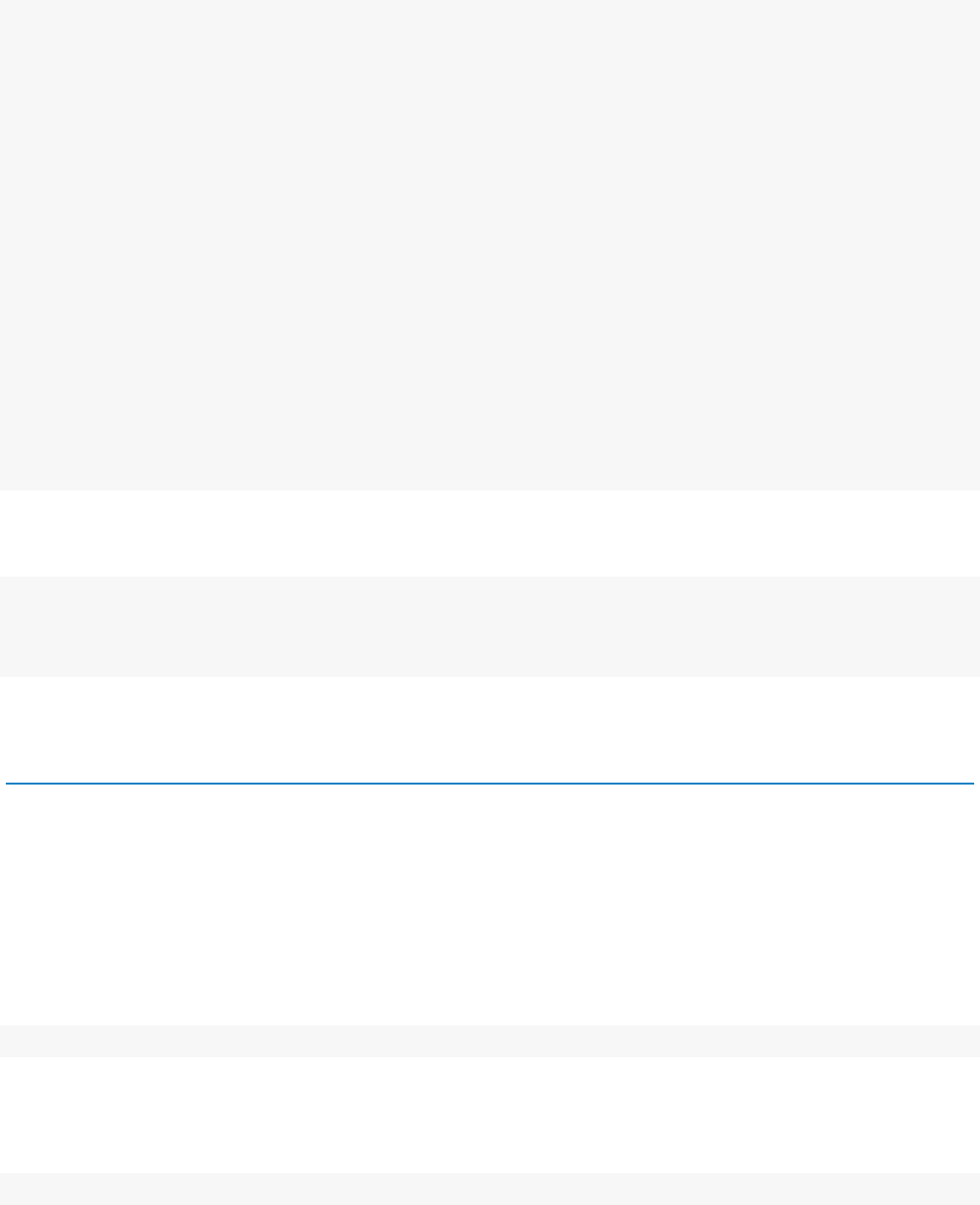
A so-called MA plot provides a useful overview for an experiment with a two-group comparison:
plotMA( res, ylim =c(-1,1) )
The plot (Fig. 2) represents each gene with a dot. The xaxis is the average expression over all samples,
the yaxis the log2 fold change between treatment and control. Genes with an adjusted pvalue below
a threshold (here 0.1, the default) are shown in red.
This plot demonstrates that only genes with a large average normalized count contain sufficient infor-
mation to yield a significant call.
Also note DESeq2’s shrinkage estimation of log fold changes (LFCs): When count values are too low to
allow an accurate estimate of the LFC, the value is “shrunken” towards zero to avoid that these values,
which otherwise would frequently be unrealistically large, dominate the top-ranked log fold changes.
Beginner’s guide to using the DESeq2 package 20
Figure 2: MA-plot The MA-plot shows the log2 fold changes from the treatment over the mean
of normalized counts, i.e. the average of counts normalized by size factor. The DESeq2 package
incorporates a prior on log2 fold changes, resulting in moderated estimates from genes with low counts
and highly variable counts, as can be seen by the narrowing of spread of points on the left side of the
plot.
Whether a gene is called significant depends not only on its LFC but also on its within-group variability,
which DESeq2 quantifies as the dispersion. For strongly expressed genes, the dispersion can be under-
stood as a squared coefficient of variation: a dispersion value of 0.01 means that the gene’s expression
tends to differ by typically √0.01 = 10% between samples of the same treatment group. For weak
genes, the Poisson noise is an additional source of noise, which is added to the dispersion.
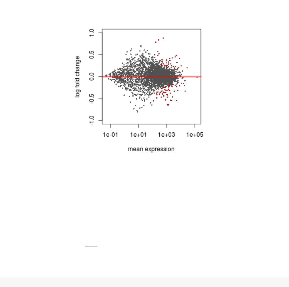
The function plotDispEsts visualizes DESeq2’s dispersion estimates:
plotDispEsts( dds, ylim =c(1e-6,1e1) )
The black points are the dispersion estimates for each gene as obtained by considering the information
from each gene separately. Unless one has many samples, these values fluctuate strongly around their
true values. Therefore, we fit the red trend line, which shows the dispersions’ dependence on the mean,
and then shrink each gene’s estimate towards the red line to obtain the final estimates (blue points) that
are then used in the hypothesis test. The blue circles above the main “cloud” of points are genes which
have high gene-wise dispersion estimates which are labelled as dispersion outliers. These estimates are
therefore not shrunk toward the fitted trend line.
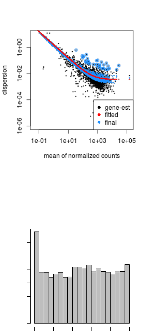
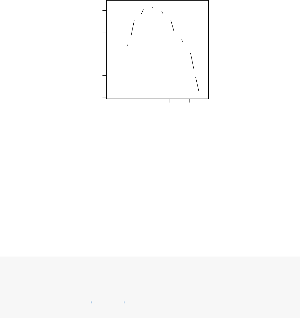
Another useful diagnostic plot is the histogram of the pvalues (Fig. 4).
Beginner’s guide to using the DESeq2 package 21
Figure 3: Plot of dispersion estimates See text for details
Histogram of res$pvalue
res$pvalue
Frequency
0.0 0.2 0.4 0.6 0.8 1.0
0 50 150 250 350
Figure 4: Histogram of the pvalues returned by the test for differential expression
Beginner’s guide to using the DESeq2 package 22
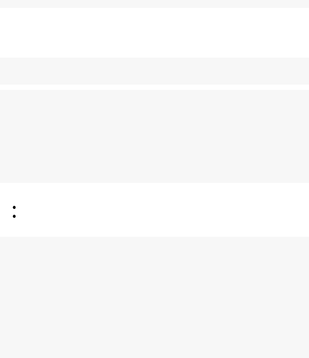
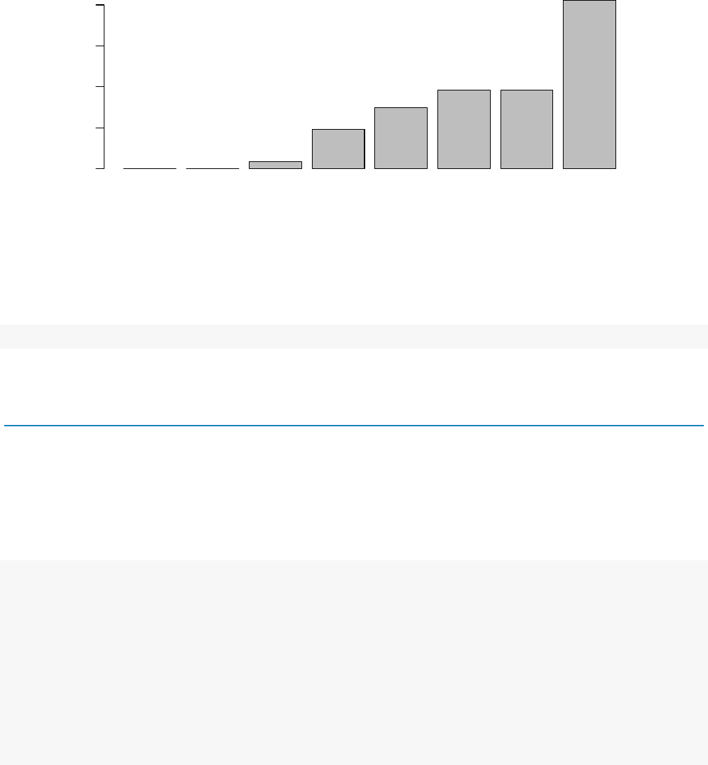
~0 ~3 ~38 ~131 ~282 ~493 ~860 ~74699
mean normalized count
ratio of small $p$ values
0.00 0.02 0.04 0.06 0.08
Figure 5: Ratio of small p values for groups of genes binned by mean normalized count
hist( res$pvalue, breaks=20,col="grey" )
4 Independent filtering
The MA plot (Figure 2) highlights an important property of RNA-Seq data. For weakly expressed genes,
we have no chance of seeing differential expression, because the low read counts suffer from so high
Poisson noise that any biological effect is drowned in the uncertainties from the read counting. We can
also show this by examining the ratio of small pvalues (say, less than, 0.01) for genes binned by mean
normalized count:
# create bins using the quantile function
qs <- c(0,quantile( res$baseMean[res$baseMean >0], 0:7/7) )
# "cut" the genes into the bins
bins <- cut( res$baseMean, qs )
# rename the levels of the bins using the middle point
levels(bins) <- paste0("~",round(.5*qs[-1]+.5*qs[-length(qs)]))
# calculate the ratio of £p£ values less than .01 for each bin
ratios <- tapply( res$pvalue, bins, function(p)mean( p <.01,na.rm=TRUE ) )
# plot these ratios
barplot(ratios, xlab="mean normalized count",ylab="ratio of small $p$ values")
At first sight, there may seem to be little benefit in filtering out these genes. After all, the test found
them to be non-significant anyway. However, these genes have an influence on the multiple testing
adjustment, whose performance improves if such genes are removed. By removing the weakly-expressed
Beginner’s guide to using the DESeq2 package 23
●●●●
●
● ●
●●
●●
● ●
●●
●
●
●
● ●
0.0 0.2 0.4 0.6 0.8
30 40 50 60 70
quantiles of 'baseMean'
number of rejections
Figure 6: Independent filtering. DESeq2 automatically determines a threshold, filtering on mean
normalized count, which maximizes the number of genes which will have an adjusted pvalue less than
a critical value.
genes from the input to the FDR procedure, we can find more genes to be significant among those
which we keep, and so improved the power of our test. This approach is known as independent filtering.
The DESeq2 software automatically performs independent filtering which maximizes the number of
genes which will have adjusted pvalue less than a critical value (by default, alpha is set to 0.1). This
automatic independent filtering is performed by, and can be controlled by, the results function. We
can observe how the number of rejections changes for various cutoffs based on mean normalized count.
The following optimal threshold and table of possible values is stored as an attribute of the results
object.
attr(res,"filterThreshold")
## 40%
## 165
plot(attr(res,"filterNumRej"),type="b",
xlab="quantiles of baseMean ",
ylab="number of rejections")
The term independent highlights an important caveat. Such filtering is permissible only if the filter
criterion is independent of the actual test statistic [7]. Otherwise, the filtering would invalidate the test
and consequently the assumptions of the BH procedure. This is why we filtered on the average over all
Beginner’s guide to using the DESeq2 package 24
samples: this filter is blind to the assignment of samples to the treatment and control group and hence
independent.
4.1 Adding gene names
Our result table only uses Ensembl gene IDs, but gene names may be more informative. Bioconductor’s
biomaRt package can help with mapping various ID schemes to each other.
First, we split up the rownames of the results object, which contain ENSEMBL gene ids, separated by
the plus sign, +. The following code then takes the first id for each gene by invoking the open square
bracket function "[" and the argument, 1.
res$ensembl <- sapply(strsplit(rownames(res), split="\\+" ), "[",1)
The following chunk of code uses the ENSEMBL mart, querying with the ENSEMBL gene id and
requesting the Entrez gene id and HGNC gene symbol.
library("biomaRt" )
ensembl =useMart("ensembl",dataset ="hsapiens_gene_ensembl" )
genemap <- getBM(attributes =c("ensembl_gene_id","entrezgene","hgnc_symbol"),
filters ="ensembl_gene_id",
values = res$ensembl,
mart = ensembl )
idx <- match( res$ensembl, genemap$ensembl_gene_id )
res$entrez <- genemap$entrezgene[ idx ]
res$hgnc_symbol <- genemap$hgnc_symbol[ idx ]
Now the results have the desired external gene ids:
head(res,4)
## log2 fold change (MAP): treatment DPN vs Control
## Wald test p-value: treatment DPN vs Control
## DataFrame with 4 rows and 9 columns
## baseMean log2FoldChange lfcSE stat pvalue
## <numeric> <numeric> <numeric> <numeric> <numeric>
## ENSG00000000003 616.390 -0.01579 0.0856 -0.1844 0.854
## ENSG00000000005 0.553 -0.00836 0.1703 -0.0491 0.961
## ENSG00000000419 305.400 -0.01647 0.0935 -0.1762 0.860
## ENSG00000000457 184.341 -0.09290 0.1180 -0.7874 0.431
## padj ensembl entrez hgnc_symbol
## <numeric> <character> <integer> <character>
## ENSG00000000003 0.971 ENSG00000000003 7105 TSPAN6
## ENSG00000000005 NA ENSG00000000005 64102 TNMD
## ENSG00000000419 0.973 ENSG00000000419 8813 DPM1
## ENSG00000000457 0.879 ENSG00000000457 57147 SCYL3

Beginner’s guide to using the DESeq2 package 25
4.2 Exporting results
Finally, we note that you can easily save the results table in a CSV file, which you can then load with
a spreadsheet program such as Excel:
res[1:2,]
## log2 fold change (MAP): treatment DPN vs Control
## Wald test p-value: treatment DPN vs Control
## DataFrame with 2 rows and 9 columns
## baseMean log2FoldChange lfcSE stat pvalue
## <numeric> <numeric> <numeric> <numeric> <numeric>
## ENSG00000000003 616.390 -0.01579 0.0856 -0.1844 0.854
## ENSG00000000005 0.553 -0.00836 0.1703 -0.0491 0.961
## padj ensembl entrez hgnc_symbol
## <numeric> <character> <integer> <character>
## ENSG00000000003 0.971 ENSG00000000003 7105 TSPAN6
## ENSG00000000005 NA ENSG00000000005 64102 TNMD
write.csv(as.data.frame(res), file="results.csv" )
5 Working with rlog-transformed data
5.1 The rlog transform
Many common statistical methods for exploratory analysis of multidimensional data, especially methods
for clustering and ordination (e. g., principal-component analysis and the like), work best for (at least
approximately) homoskedastic data; this means that the variance of an observable quantity (i.e., here,
the expression strength of a gene) does not depend on the mean. In RNA-Seq data, however, variance
grows with the mean. For example, if one performs PCA directly on a matrix of normalized read counts,
the result typically depends only on the few most strongly expressed genes because they show the largest
absolute differences between samples. A simple and often used strategy to avoid this is to take the
logarithm of the normalized count values plus a small pseudocount; however, now the genes with low
counts tend to dominate the results because, due to the strong Poisson noise inherent to small count
values, they show the strongest relative differences between samples.
As a solution, DESeq2 offers the regularized-logarithm transformation, or rlog for short. For genes
with high counts, the rlog transformation differs not much from an ordinary log2 transformation. For
genes with lower counts, however, the values are shrunken towards the genes’ averages across all
samples. Using an empirical Bayesian prior in the form of a ridge penality, this is done such that the
rlog-transformed data are approximately homoskedastic.
Note that the rlog transformation is provided for applications other than differential testing. For dif-
ferential testing we recommend the DESeq function applied to raw counts, as described earlier in this
Beginner’s guide to using the DESeq2 package 26
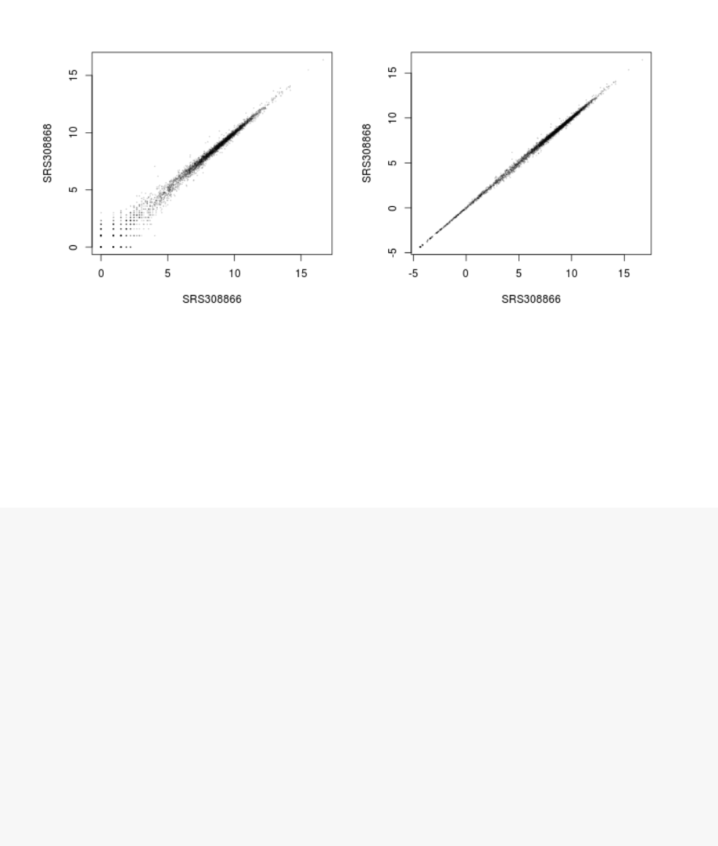
Figure 7: Scatter plot of sample 2 vs sample 1. Left: using an ordinary log2transformation.
Right: Using the rlog transformation.
vignette, which also takes into account the dependence of the variance of counts on the mean value
during the dispersion estimation step.
The function rlogTransform returns a SummarizedExperiment object which contains the rlog-transformed
values in its assay slot:
rld <- rlog( dds )
head(assay(rld) )
## SRS308866 SRS308868 SRS308870 SRS308872 SRS308874 SRS308876
## ENSG00000000003 9.800 9.778 9.918 9.095 9.163 9.062
## ENSG00000000005 -0.922 -0.812 -0.904 -0.893 -0.975 -0.975
## ENSG00000000419 8.055 8.080 8.117 8.238 8.297 8.379
## ENSG00000000457 7.414 7.255 7.312 7.869 7.739 7.907
## ENSG00000000460 7.573 7.704 7.727 8.076 8.287 8.079
## ENSG00000000938 3.225 3.108 3.114 3.995 3.571 3.573
## SRS308878 SRS308880 SRS308882 SRS308883 SRS308885 SRS308887
## ENSG00000000003 8.883 8.752 8.809 9.049 9.073 8.857
## ENSG00000000005 -0.975 -0.977 -0.975 -0.975 -0.977 -0.977
## ENSG00000000419 8.323 8.313 8.420 8.272 8.157 8.323
## ENSG00000000457 7.163 7.296 7.383 7.617 7.490 7.501
## ENSG00000000460 7.057 7.433 7.630 6.904 7.347 7.654
## ENSG00000000938 3.025 3.356 3.287 3.331 3.435 3.288
To show the effect of the transformation, we plot the first sample against the second, first simply using
the log2 function (after adding 1, to avoid taking the log of zero), and then using the rlog-transformed
values.
Beginner’s guide to using the DESeq2 package 27
12
11
10
7
8
9
5
6
4
2
1
3
OHT−4
DPN−4
Control−4
Control−3
DPN−3
OHT−3
DPN−2
OHT−2
Control−2
DPN−1
Control−1
OHT−1
0 40
Value
0
Color Key
and Histogram
Count
Figure 8: Heatmap of Euclidean sample distances after rlog transformation.
par(mfrow =c(1,2) )
plot(log2(1+counts(dds, normalized=TRUE)[, 1:2] ), col="#00000020",pch=20,cex=0.3 )
plot(assay(rld)[, 1:2], col="#00000020",pch=20,cex=0.3 )
Note that, in order to make it easier to see where several points are plotted on top of each other, we
set the plotting color to a semi-transparent black (encoded as #00000020) and changed the points to
solid disks (pch=20) with reduced size (cex=0.3)6.
In Figure 7, we can see how genes with low counts seem to be excessively variable on the ordinary
logarithmic scale, while the rlog transform compresses differences for genes for which the data cannot
provide good information anyway.
5.2 Sample distances
A useful first step in an RNA-Seq analysis is often to assess overall similarity between samples: Which
samples are similar to each other, which are different? Does this fit to the expectation from the
experiment’s design?
We use the R function dist to calculate the Euclidean distance between samples. To avoid that the
distance measure is dominated by a few highly variable genes, and have a roughly equal contribution
6The function heatscatter from the package LSD offers a colorful alternative.

Beginner’s guide to using the DESeq2 package 28
from all genes, we use it on the rlog-transformed data:
sampleDists <- dist(t(assay(rld) ) )
sampleDists
## SRS308866 SRS308868 SRS308870 SRS308872 SRS308874 SRS308876 SRS308878
## SRS308868 10.55
## SRS308870 8.97 10.98
## SRS308872 34.38 35.82 35.34
## SRS308874 34.64 35.29 35.21 10.02
## SRS308876 33.99 35.48 34.90 9.04 9.96
## SRS308878 47.60 49.41 48.57 48.35 49.78 48.53
## SRS308880 47.84 49.23 48.64 49.04 50.14 49.32 9.69
## SRS308882 47.71 49.12 48.48 49.25 50.32 49.36 11.15
## SRS308883 40.27 42.28 41.69 39.70 41.14 39.63 33.32
## SRS308885 38.97 40.28 40.10 38.63 39.50 38.75 33.71
## SRS308887 40.02 41.56 41.06 40.14 41.27 39.97 33.51
## SRS308880 SRS308882 SRS308883 SRS308885
## SRS308868
## SRS308870
## SRS308872
## SRS308874
## SRS308876
## SRS308878
## SRS308880
## SRS308882 8.21
## SRS308883 33.56 33.80
## SRS308885 32.98 33.42 10.35
## SRS308887 32.79 32.58 11.91 10.44
Note the use of the function tto transpose the data matrix. We need this because dist calculates
distances between data rows and our samples constitute the columns.
We visualize the distances in a heatmap, using the function heatmap.2 from the gplots package.
sampleDistMatrix <- as.matrix( sampleDists )
rownames(sampleDistMatrix) <- paste( rld$treatment,
rld$patient, sep="-" )
colnames(sampleDistMatrix) <- NULL
library("gplots" )
library("RColorBrewer" )
colours =colorRampPalette(rev(brewer.pal(9,"Blues")) )(255)
heatmap.2( sampleDistMatrix, trace="none",col=colours)
Note that we have changed the row names of the distance matrix to contain treatment type and patient
number instead of sample ID, so that we have all this information in view when looking at the heatmap
(Fig. 8).
Beginner’s guide to using the DESeq2 package 29
1 : Control
1 : DPN
1 : OHT
2 : Control
2 : DPN
2 : OHT
3 : Control
3 : DPN
3 : OHT
4 : Control
4 : DPN
4 : OHT
PC1
PC2
−15
−10
−5
0
5
10
−10 0 10 20
●
●
●
●
●
●
●
●
●
●
●
●
Figure 9: Principal components analysis (PCA) of samples after rlog transformation.
Another way to visualize sample-to-sample distances is a principal-components analysis (PCA). In this
ordination method, the data points (i.e., here, the samples) are projected onto the 2D plane such that
they spread out optimally (Fig. 9). If we only had two treatments, the plotPCA will automatically use
a paired color palette for each combination of the levels of patient and treatment. As we have three
treatments, we supply a vector which specifies three shades of red, green, blue and purple for each
patient.
ramp <- 1:3/3
cols <- c(rgb(ramp, 0,0),
rgb(0, ramp, 0),
rgb(0,0, ramp),
rgb(ramp, 0, ramp))
print(plotPCA( rld, intgroup =c("patient","treatment"), col=cols ) )
Here, we have used the function plotPCA which comes with DESeq2. The two terms specified as
intgroup are column names from our sample data; they tell the function to use them to choose
colours.
From both visualizations, we see that the differences between patients is much larger than the difference
between treatment and control samples of the same patient. This shows why it was important to account
for this paired design (“paired”, because each treated sample is paired with one control sample from the
same patient). We did so by using the design formula ∼patient + treatment when setting up the
data object in the beginning. Had we used an un-paired analysis, by specifying only ∼treatment, we
Beginner’s guide to using the DESeq2 package 30
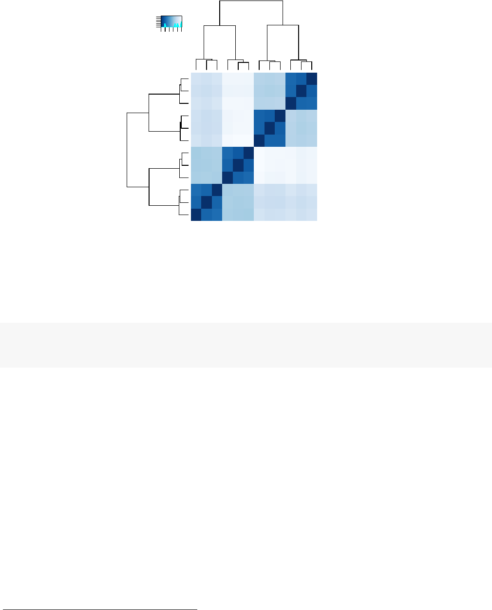
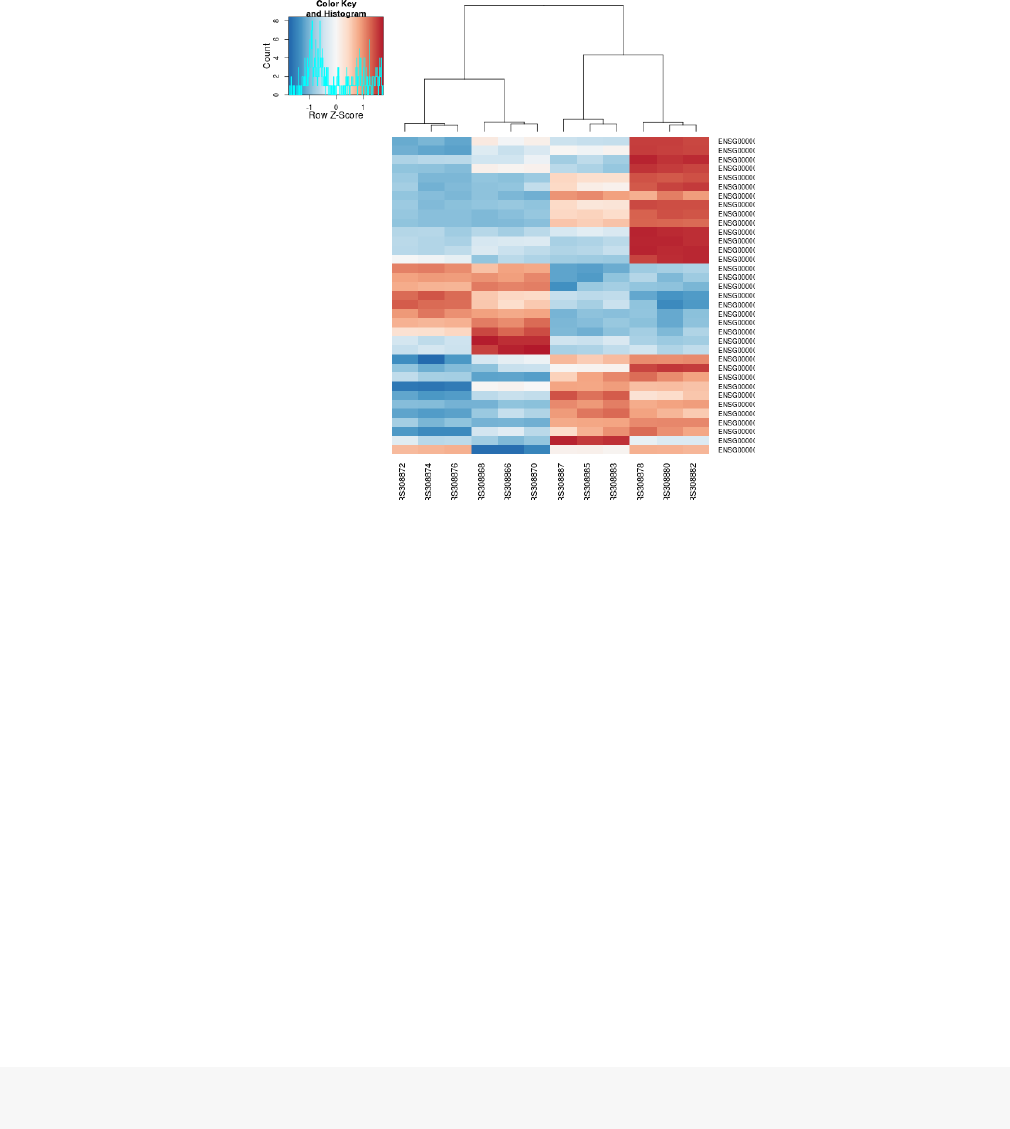
Figure 10: Heatmap with gene clustering.
would not have found many hits, because then, the patient-to-patient differences would have drowned
out any treatment effects.
Here, we have performed this sample distance analysis towards the end of our analysis. In practice,
however, this is a step suitable to give a first overview on the data. Hence, one will typically carry
out this analysis as one of the first steps in an analysis. To this end, you may also find the function
arrayQualityMetrics, from the package of the same name, useful.
5.3 Gene clustering
In the heatmap of Fig. 8, the dendrogram at the side shows us a hierarchical clustering of the samples.
Such a clustering can also be performed for the genes.
Since the clustering is only relevant for genes that actually carry signal, one usually carries it out only
for a subset of most highly variable genes. Here, for demonstration, let us select the 35 genes with the
highest variance across samples:
library("genefilter" )
topVarGenes <- head(order(rowVars(assay(rld) ), decreasing=TRUE ), 35 )
The heatmap becomes more interesting if we do not look at absolute expression strength but rather at
the amount by which each gene deviates in a specific sample from the gene’s average across all samples.
Hence, we center and scale each genes’ values across samples, and plot a heatmap.

Beginner’s guide to using the DESeq2 package 31
heatmap.2(assay(rld)[ topVarGenes, ], scale="row",
trace="none",dendrogram="column",
col =colorRampPalette(rev(brewer.pal(9,"RdBu")) )(255))
We can now see (Fig. 10) blocks of genes which covary across patients. Often, such a heatmap is
insightful, even though here, seeing these variations across patients is of limited value because we are
rather interested in the effects between the treatments from each patient.
References
[1] Wolfgang Huber Michael I Love and Simon Anders. Moderated estimation of fold change and
dispersion for RNA-Seq data with DESeq2. bioRxiv preprint, 2014. URL: http://dx.doi.org/
10.1101/002832.
[2] Daehwan Kim, Geo Pertea, Cole Trapnell, Harold Pimentel, Ryan Kelley, and Steven Salzberg.
TopHat2: accurate alignment of transcriptomes in the presence of insertions, deletions and
gene fusions. Genome Biology, 14(4):R36+, 2013. URL: http://dx.doi.org/10.1186/
gb-2013-14-4-r36,doi:10.1186/gb-2013-14-4-r36.
[3] Heng Li, Bob Handsaker, Alec Wysoker, Tim Fennell, Jue Ruan, Nils Homer, Ga-
bor Marth, Goncalo Abecasis, Richard Durbin, and 1000 Genome Project Data Process-
ing Subgroup. The Sequence Alignment/Map format and SAMtools. Bioinformatics,
25(16):2078–2079, 2009. URL: http://bioinformatics.oxfordjournals.org/content/25/
16/2078.abstract,arXiv:http://bioinformatics.oxfordjournals.org/content/25/16/
2078.full.pdf+html,doi:10.1093/bioinformatics/btp352.
[4] Paul Theodor Pyl Simon Anders and Wolfgang Huber. HTSeq - A Python framework to work with
high-throughput sequencing data. bioRxiv preprint, 2014. URL: http://dx.doi.org/10.1101/
002824.
[5] Y. Liao, G. K. Smyth, and W. Shi. featureCounts: an efficient general purpose program for assigning
sequence reads to genomic features. Bioinformatics, Nov 2013.
[6] N. Delhomme, I. Padioleau, E. E. Furlong, and L. M. Steinmetz. easyRNASeq: a bioconductor
package for processing RNA-Seq data. Bioinformatics, 28(19):2532–2533, Oct 2012.
[7] Richard Bourgon, Robert Gentleman, and Wolfgang Huber. Independent filtering increases detection
power for high-throughput experiments. PNAS, 107(21):9546–9551, 2010. URL: http://www.
pnas.org/content/107/21/9546.long.
6 Session Info
As last part of this document, we call the function sessionInfo, which reports the version numbers
of R and all the packages used in this session. It is good practice to always keep such a record as it will

Beginner’s guide to using the DESeq2 package 32
help to trace down what has happened in case that an R script ceases to work because a package has
been changed in a newer version. The session information should also always be included in any emails
to the Bioconductor mailing list.
R version 3.1.0 (2014-04-10), x86_64-unknown-linux-gnu
Locale: LC_CTYPE=en_US.UTF-8,LC_NUMERIC=C,LC_TIME=en_US.UTF-8,LC_COLLATE=C,
LC_MONETARY=en_US.UTF-8,LC_MESSAGES=en_US.UTF-8,LC_PAPER=en_US.UTF-8,
LC_NAME=C,LC_ADDRESS=C,LC_TELEPHONE=C,LC_MEASUREMENT=en_US.UTF-8,
LC_IDENTIFICATION=C
Base packages: base, datasets, grDevices, graphics, methods, parallel, stats, utils
Other packages: AnnotationDbi 1.26.0, BSgenome 1.32.0, Biobase 2.24.0, BiocGenerics 0.10.0,
Biostrings 2.32.0, DESeq2 1.4.5, GenomeInfoDb 1.0.2, GenomicAlignments 1.0.1,
GenomicFeatures 1.16.0, GenomicRanges 1.16.3, IRanges 1.22.6, RColorBrewer 1.0-5,
Rcpp 0.11.1, RcppArmadillo 0.4.300.0, Rsamtools 1.16.0, XVector 0.4.0, biomaRt 2.20.0,
genefilter 1.46.1, gplots 2.13.0, knitr 1.5, parathyroidSE 1.2.0, pasilla 0.4.0, vsn 3.32.0
Loaded via a namespace (and not attached): BBmisc 1.6, BatchJobs 1.2, BiocInstaller 1.14.2,
BiocParallel 0.6.0, BiocStyle 1.2.0, DBI 0.2-7, DESeq 1.16.0, KernSmooth 2.23-12,
RCurl 1.95-4.1, RSQLite 0.11.4, XML 3.98-1.1, affy 1.42.2, affyio 1.32.0, annotate 1.42.0,
bitops 1.0-6, brew 1.0-6, caTools 1.17, codetools 0.2-8, digest 0.6.4, evaluate 0.5.5, fail 1.2,
foreach 1.4.2, formatR 0.10, gdata 2.13.3, geneplotter 1.42.0, grid 3.1.0, gtools 3.4.0, highr 0.3,
iterators 1.0.7, lattice 0.20-29, limma 3.20.1, locfit 1.5-9.1, plyr 1.8.1, preprocessCore 1.26.1,
rtracklayer 1.24.0, sendmailR 1.1-2, splines 3.1.0, stats4 3.1.0, stringr 0.6.2, survival 2.37-7,
tools 3.1.0, xtable 1.7-3, zlibbioc 1.10.0
