Using DeepLabCut For 3D Markerless Pose Estimation Across Species And Behaviors DLC User Guide

User Manual:

Open the PDF directly: View PDF .
Page Count: 23

Using DeepLabCut for 3D markerless pose estimation across species and behaviors

Tanmay Nath1,†, Alexander Mathis2,3,†, An Chi Chen4, Amir

Patel4, Matthias Bethge2,5, & Mackenzie Weygandt Mathis1,∗

1: The Rowland Institute at Harvard, Harvard University, Cambridge, MA USA

2: Institute for Theoretical Physics, Werner Reichardt Center for Integrative Neuroscience,

Eberhard Karls Universität Tübingen, Tübingen, Germany

3: Center for Brain Science & Department of Molecular & Cellular Biology

Harvard University, Cambridge, MA USA

4: Department of Electrical Engineering, University of Cape Town, South Africa

5: Max Planck Institute for Biological Cybernetics

& Bernstein Center for Computational Neuroscience, Tübingen, Germany

†co-first authors and

*corresponding author: mackenzie@post.harvard.edu

(Dated: November 21, 2018)

Noninvasive behavioral tracking of animals during experiments is crucial to many

scientific pursuits. Extracting the poses of animals without using markers is often

essential for measuring behavioral effects in biomechanics, genetics, ethology & neu-

roscience. Yet, extracting detailed poses without markers in dynamically changing

backgrounds has been challenging. We recently introduced an open source toolbox

called DeepLabCut that builds on a state-of-the-art human pose estimation algorithm

to allow a user to train a deep neural network using limited training data to precisely

track user-defined features that matches human labeling accuracy. Here, with this

paper we provide an updated toolbox that is self contained within a Python package

that includes new features such as graphical user interfaces and active-learning based

network refinement. Lastly, we provide a step-by-step guide for using DeepLabCut.

INTRODUCTION

Advances in computer vision and deep learning are transforming research. Applications like autonomous car driving,

estimating the poses of humans, controlling robotic arms, or predicting the sequence specificity of DNA- and RNA-

binding proteins are rapidly developing [1–4]. However, many of the underlying algorithms are “data hungry” as

they require thousands of labeled examples, which potentially prohibits these approaches to be useful for small scale

operations, such as in single laboratory experiments [5]. Yet transfer learning, the ability to take a network, which

was trained on a task with a large supervised data set, and utilize it for another task with a small supervised data

set, is beginning to allow users to broadly apply deep learning methods [6–10]. We recently demonstrated that due to

transfer learning, a state-of-the-art human pose estimation algorithm called DeeperCut [10,11] could be tailored to

use in the laboratory with relatively small amounts of annotated data [12]. Our toolbox, DeepLabCut [12], provides

tools to create annotated training sets, train robust feature detectors, and utilize them to analyze novel behavioral

videos. Current applications range across the common model systems like mice, zebrafish and flies as well as rarer

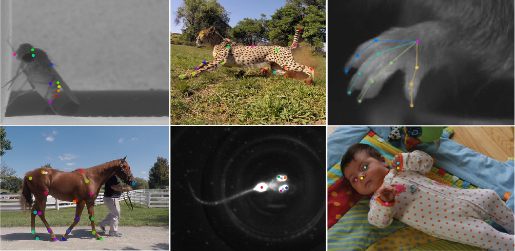
ones like babies and cheetahs (Figure 1)

Here, we provide a comprehensive protocol and expansion of DeepLabCut that allows researchers to estimate the

pose of the subject, efficiently enabling them to quantify the behavior. The major motivation for developing the

DeepLabCut toolbox was to provide a reliable and efficient tool for high-throughput video analysis, where powerful

feature detectors of user-defined body parts need to be learned for a specific situation. The toolbox is aimed to

solve the problem of detecting body parts in dynamic visual environments where varying background, reflective walls

or motion blur hinder the performance of common techniques, such as thresholding or regression based on visual

features [13–21]. The uses of the toolbox are broad, however certain paradigms will most benefit from this approach.

Specifically, DeepLabCut is best suited for behaviors that can be consistently captured by one or multiple cameras

with minimal occlusions.

The DeepLabCut Python toolbox is versatile, and easy to use without extensive programming skills. With only a

small set of training images a user can train a network to within human level labeling accuracy, thus expanding its

application to not only behavior analysis in the laboratory, but to potentially also in sports, gait analysis, medicine

and rehabilitation studies [13,22–26].

.CC-BY-NC-ND 4.0 International licenseIt is made available under a

(which was not peer-reviewed) is the author/funder, who has granted bioRxiv a license to display the preprint in perpetuity.

The copyright holder for this preprint. http://dx.doi.org/10.1101/476531doi: bioRxiv preprint first posted online Nov. 24, 2018;

2

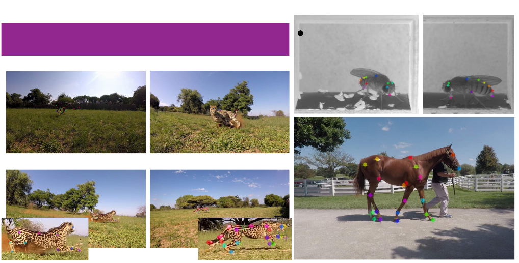
FIG. 1. Pose estimation with DeepLabCut Six examples with automatically applied labels from DeepLabCut. The colored

points represent features the user wished to measure. Clockwise from the top left: a fruit fly, a cheetah, a mouse hand, a baby,

a zebrafish, and a horse. The mouse hand image is adapted from [12], and the baby image is adapted from [26].

Overview of using DeepLabCut

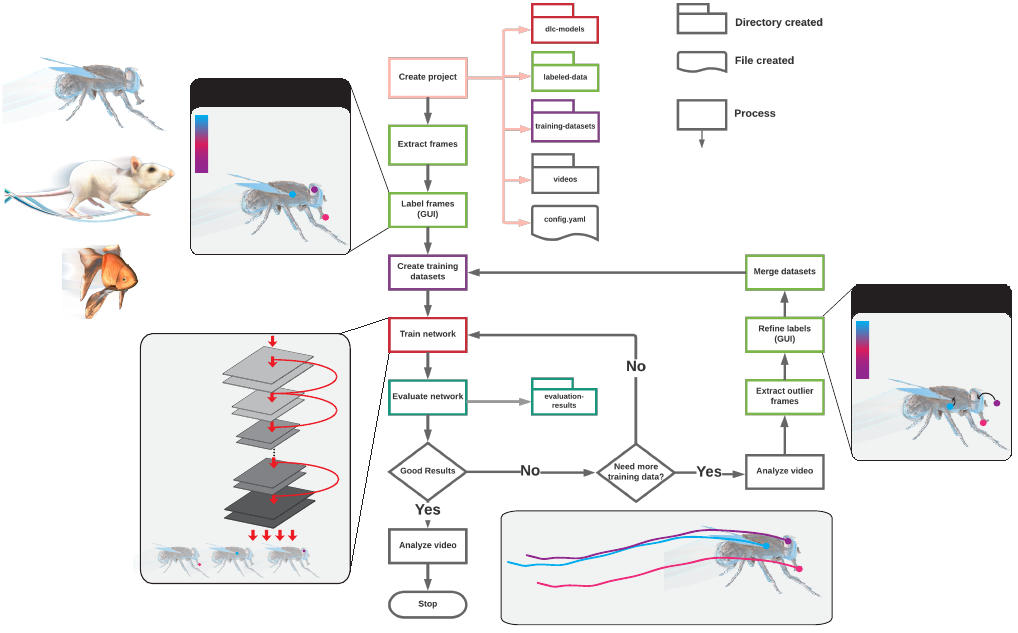
DeepLabCut is organized according to the following workflow (Fig 2). The user starts by creating a new project

based on a project and username as well as some (initial) videos, which are required to create the training dataset

(Step A-B). Additional videos can also be added after the creation of the project, which will be explained in greater

detail below. Next, DeepLabCut extracts frames, which reflect the diversity of the behavior with respect to postures,

animal identities, etc. (Step C). Then the user can label the points of interest in the extracted frames (Step D). These

annotated frames can be visually checked for accuracy, and corrected if necessary (Step E). Eventually, a training

dataset is created by merging all the extracted labeled frames and splitting them into subsets of test and train frames

(Step F). Then, a pre-trained network (ResNet) is trained end-to-end to adapt its weights in order to predict the

desired features (i.e. labels supplied by the user; Step G). The performance of the trained network can then be

evaluated on the training and test frames (Step H). The trained network can be used to analyze videos yielding

extracted pose files (Step I). In case the trained network does not generalize well to unseen data in the evaluation

and analysis step (Step H), then additional frames with poor results can be extracted (Step J) and the predicted

labels can be manually shifted to their ideal location (Step K). This refinement step, if needed, creates an additional

set of annotated images that can then be merged with the original training dataset to create a new training dataset

(Step F). This larger training set can then be used to re-train the feature detectors for better results (Step G). This

active learning loop can be done iteratively to robustly and accurately analyze videos with potentially large variability

- i.e. experiments that include many individuals, and run over long time periods. Furthermore, the user can add

additional body parts/labels at later stages during a project (Step D) as well as correct user-defined labels (Step K).

Lastly, we provide Jupyter Notebooks (Section M), a summary of the commands (Section N), and a troubleshooting

section (Section O).

Applications

DeepLabCut has been used to extract user-defined, key body part locations from animals (including humans)

in various experimental settings. Current applications range from tracking mice in open-field behaviors, to more

complicated hand articulations in mice, whole-body movements in flies in a 3D environment (all shown in [12]), as

well as pose-estimation in human babies [26], 3D-locomotion studies in rodents [27], multi-bodypart including eye

.CC-BY-NC-ND 4.0 International licenseIt is made available under a

(which was not peer-reviewed) is the author/funder, who has granted bioRxiv a license to display the preprint in perpetuity.

The copyright holder for this preprint. http://dx.doi.org/10.1101/476531doi: bioRxiv preprint first posted online Nov. 24, 2018;

3

GUI: LABEL

unique label 1

unique label 2

unique label 3

Frames extracted from video

(any species can be used)

ResNet

(pre-trained

on ImageNet)

deconvolutional

layer

GUI: REFINE

unique label 1

unique label 2

unique label 3

Analyze Novel Videos

Train Network

FIG. 2. DeepLabCut work-flow. The diagram delineates the work-flow as well as the directory and file structures. The

process of the work-flow is color-coded to represent the location of their output. The main steps are opening a python session,

importing deeplabcut, creating a project, selecting frames, labeling frames, then training a network. Once trained, this network

can be used to apply labels on new videos, or the network can be refined if needed. The process is enabled by interactive GUIs

at several key steps, and all lines can be run from a simple terminal interface.

tracking during perceptual decision making [28], horses and cheetahs (Figure 1). Other (currently unpublished) use

cases can be found at www.mousemotorlab.org/deeplabcut. Lastly, 3D pose estimation for a challenging cheetah

hunting data set will be presented within this manuscript.

Comparison with other methods

Pose-estimation is a challenging, yet classical computer vision problem [29], whose human pose estimation bench-

marks have recently been shattered by deep learning algorithms [2,10,11,30–33]. There are several main considera-

tions when deciding on what deep learning algorithms to use, namely, the amount of labeled input data required, the

speed, and the accuracy. DeepLabCut was developed to require little labeled data, to allow for real-time processing

(i.e. as fast or faster than camera acquisition), and be as accurate as human annotators.

DeepLabCut utilizes parts of an algorithm called DeeperCut, which is one of the best algorithms for several human

pose estimation benchmarks in recent years [10]. Specifically, DeepLabCut uses deep, residual networks with either 50

or 101 layers (ResNets) [34] and deconvolutional layers as developed in DeeperCut [10]. As pose-estimation in the lab

is typically simpler than most benchmarks in computer vision, we were able to remove aspects of DeeperCut that were

not required to achieve human-level accuracy on several laboratory tasks [12]. This removal of the pairwise refinement,

as well as our addition of integer linear programming on top of the part detectors significantly increased the inference

speed (full multi-human DeeperCut: 578-1171 seconds per frame vs. 10-90 frames per second). Furthermore, we

recently implemented faster inference for the feature detectors [27] (see below).

However, if a user aims to track (adult) human poses, many excellent options exist, including DeeperCut, ArtTrack,

DeepPose, OpenPose, and OpenPose-Plus [2,10,11,30–33,35]. Some of these methods also allow real-time inference.

To our knowledge, the performance of those methods has not been investigated on non-human animals. Conversely,

.CC-BY-NC-ND 4.0 International licenseIt is made available under a

(which was not peer-reviewed) is the author/funder, who has granted bioRxiv a license to display the preprint in perpetuity.

The copyright holder for this preprint. http://dx.doi.org/10.1101/476531doi: bioRxiv preprint first posted online Nov. 24, 2018;

4

since the trained networks can be used they provide excellent tools for pose-estimation of humans. There are also

specific networks for faces [32] and hands [33]. However, if (additional) body parts beyond the body parts contained

in the pre-trained networks need to be labeled, then DeepLabCut could also be useful.

While DeepLabCut, to the best of our knowledge, is the first example of using deep learning in the laboratory for

pose-estimation, recently another deep learning package called LEAP was described [21]. LEAP requires the user to

align the subject in the center of the frame, and there is some cost to rotations of the animal in terms of accuracy [21].

In contrast, DeepLabCut is robust for estimating the pose of animals that were not aligned. DeepLabCut was also

shown to generalize to novel individuals (both flies and mice), as well as multiple mice, and conditions [12]. Certain

behaviors are also not particularly amendable to alignment, like a Drosophila moving in 3D space [12].

DeepLabCut was shown to need less than 150 frames of human-labeled data for even challenging 3D hand movements

of a mouse [12]. LEAP requires more training data to match similar performance, i.e. human-level accuracy. While

the authors highlight an interactive training framework (which can be done with DeepLabCut if desired), and suggest

starting with tens of frames, it needs approximately 500 images to achieve less than 3 pixel error on 192x192 pixel

frames [21]. For example, DeepLabCut achieves < 5 pixel error with 100 labeled frames on a 800x800 pixel sized data

set and reaches human level accuracy of 2.7 pixel with 500 labeled frames. Note this means the relative error (in

relation to the frame size) is more than 4 times lower for DeepLabCut than for LEAP. These advantages seem to be

due to transfer learning [12], while LEAP is trained from scratch.

Inference speed (i.e. the run time of the trained network on novel videos) may also be a consideration for users.

While DeepLabCut takes 30-100 FPS (depending on the frame size) to process the data (if the batch size is 1). This

means that it achieves real-time processing if the camera speed is less than 30-100 FPS. In contrast, LEAP may be

faster, due to its 15 layer convolutional network, as the authors report 185 FPS with a batch size of 32 images for 192

x 192 sized images [21]. For similarly sized videos DeepLabCut runs at 90 FPS with batch size of 1 and accelerates

substantially (up to 1000 FPS) for larger batch sizes [27].

Advantages

DeepLabCut has been applied to a range of organisms with diverse visual background challenges. The main

advantages are (i) our code guides the experimenter with a step-by-step procedure from labeling data to automated

pose-extraction in a fast and efficient way; (ii) minimizes the cost of manual behavior analysis and with only a small

number of training images can achieve human level accuracy; (iii) eliminates the need to put visible markers on the

locations of interest to track the positions; (iv) can be easily adapted to analyze behaviors across species; (v) is open-

source and free. Due to the use of deep features, DeepLabCut can learn to robustly extract body parts even with

cluttered and varying background, inhomogeneous illumination, camera distortions, etc [12]. Thus, experimenter’s

can perhaps design studies more around their scientific question, rather than constraints imposed by previous tracking

algorithms. For example, it is common to image mice in a plain white, grey or black background to contrast heavily

with their coat color. Now, even natural backgrounds, such as home cage bedding, natural grass, or dynamically

changing backgrounds, as in trail-tracking [12], can be used. This is perhaps best illustrated by the cheetah example

provided in this paper (Figures 1and 7).

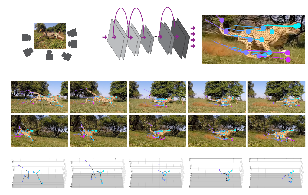
DeepLabCut also allows for 3D pose estimation via multi-camera use. A user can easily a train network for each

camera view and use standard camera calibration techniques [36] to resolve 3D locations. Alternatively, a user can

combine multiple camera views into one network (i.e. see Figure 7below and [27]), if the total pixel size is not too

large given the available hardware, and then train this single network on the combined view. DeepLabCut does not

require images to have a fixed frame size, as the feature detectors are not insensitive (within bounds) to the size due

to automatic re-scaling during training [12]. There are also no camera requirements. Color and greyscale images

captured from scientific cameras or consumer-grade cameras such as a GoPro can be used (and the package supports

multiple video types such as .mp4 and .avi). Also we recently showed that DeepLabCut is robust to video-compression,

potentially saving users >100 fold on data storage [27].

In addition to providing step-by-step procedures, our protocol allows the researcher to work on various projects

simultaneously while keeping each of the projects isolated (on the computer). Moreover, the toolbox provides different

frame-extraction methods to accommodate the analysis of videos from varying recording sessions. The toolbox is

modular and by changing desired parameters at execution, the user can, for instance, utilize different frame extraction

methods or identify frames which require further inspection. Reliably defining the user-defined labels across different

frames is of paramount importance for supervised learning approaches like DeepLabCut. The labels can be body

parts, or any other readily visible (part of an) object. The toolbox also provides interactive tools (graphical user

interfaces, GUIs) to create, edit, and even add additional, new labels at a later stage of the project. The labels are

stored in human readable and efficient data structures. The code also generates output files/directories for essential

intermediate and final results in an automatic fashion. We believe that the error messages are intuitive, and enable

.CC-BY-NC-ND 4.0 International licenseIt is made available under a

(which was not peer-reviewed) is the author/funder, who has granted bioRxiv a license to display the preprint in perpetuity.

The copyright holder for this preprint. http://dx.doi.org/10.1101/476531doi: bioRxiv preprint first posted online Nov. 24, 2018;

5

researchers to efficiently utilize the toolbox. Furthermore, the toolbox facilitates visualization of the labeled data

and creates videos with the extracted labels overlaid, making the entire toolbox a complete package for behavioral

tracking. The extracted poses per video can also further analyzed with Python or imported to many other programs

for further analysis.

Limitations

One main limitation is that the toolbox requires modern computational hardware to produce fast and efficient results

(namely, Graphical Processing Units - GPUs [5]). However, it is possible to run this toolbox on a standard computer

with a compromise on the speed of analysis. It is about 10-100x slower [27]. However, the availability of inexpensive

consumer-grade GPUs has opened the door for labs to perform advanced image processing in an autonomous way

(i.e. in the lab, without lengthy transferring of data to centralized clusters).

Another consideration is that deep learning networks scale with the size of pixels, therefore larger images will

be processed slower. Thus, for applications that would benefit from rapid tracking of the input images should be

downsampled to achieve high rates (i.e. ∼90 frames per second (FPS) for a frame size of 138 ×138 with a batch size

of 1). However, with new code updates and batch processing options, one can rapidly increase analysis speed. We

recently demonstrated that with a batch size of 64, for a frame size of approx. 138×138 one can achieve 600 FPS [27].

Another limitation is that DeepLabCut, because it is designed to be general purpose, does not rely on heuristics

such as a body model, and therefore occluded points cannot be tracked. However, DeepLabCut outputs a confidence

score, which reports if a body part is actually visible. As we showed, one can (for instance) tell which legs are visible

in a fly moving through a 3D space, or whether the finger tips of a reaching mouse are grasping the joystick and are

thus occluded [12]. Furthermore, since DeepLabCut performs frame-by-frame prediction, even if due to occlusions,

motion blur, etc, features cannot be detected in a few frames, they will be detected as soon as they are visible (unlike

in many (actual) tracking methods, which required consistency across frames, such as the widely used Lucas —Kanade

method [37]).

Equipment

Software

•Operating System: Linux (Ubuntu) or Windows (10). However, the authors recommend Ubuntu 16.04 LTS.

•DeepLabCut: The actively maintained toolbox is freely available at https://github.com/AlexEMG/

DeepLabCut. The code is written in Python 3 [38] and TensorFlow [39] for the feature detectors [10]. It

can be simply installed with “pip install deeplabcut”, see the installation guide below.

•Anaconda: a free and open source distribution of the Python programming language (download from: https:

//www.anaconda.com/). DeepLabCut is written in Python 3 (https://www.python.org/) and not compatible

with Python 2.

•TensorFlow [39]: an open-source software library for Deep Learning. The toolbox is tested with TensorFlow

versions 1.0 to 1.4, 1.8, 1.10 and 1.11. Any one of these versions can be installed from https://www.tensorflow.

org/install/

•OPTIONAL - Docker [40]: It is recommended to use the supplied docker container which includes a pre-installed

TensorFlow with GPU support. This container builds on the nvidia-docker, which is only supported in Ubuntu.

Hardware

•Computer: Any modern desktop workstation will be sufficient, as long as it has a PCI slot space as well as

sufficient power supply for a GPU (see next item). The toolbox can also be used on laptops (e.g. for labeling

data), then training can occur either on a CPU or elsewhere with a GPU. To note, training and evaluating

the feature detectors will be slow without a GPU, but it is possible [27]. We recommend 32 GB of RAM on

the system for CPU for analysis, but this is not a hard minimum. More information on optimally running

TensorFlow can be found here: https://www.tensorflow.org/guide/performance/overview.

•GPU: It is recommended to have a GPU with at least 8 GB memory such as the NVIDIA GeForce 1080. However,

is it not required to use a GPU, a CPU is sufficient but training and evaluating the network steps are considerably

slower [27]. This toolbox can also be used on cloud computing services (such as Google Cloud/Amazon Web

Services).

.CC-BY-NC-ND 4.0 International licenseIt is made available under a

(which was not peer-reviewed) is the author/funder, who has granted bioRxiv a license to display the preprint in perpetuity.

The copyright holder for this preprint. http://dx.doi.org/10.1101/476531doi: bioRxiv preprint first posted online Nov. 24, 2018;

6

•Camera(s): The toolbox is robust to extraction of poses from data collected by many cameras. There are no a

priori limitations in terms of lighting; color or greyscale images are acceptable, videos captured under infrared

light, and inhomogeneous or natural lighting can be used. Cameras should be placed such that the features the

user wishes to track are visible. For reference, as reported in [12], the following cameras have been used for

video capture: Point Grey Firefly (FMVU-03MTM-CS), Grasshopper 3 4.1MP Mono USB3 Vision (CMOSIS

CMV4000-3E12), infrared-sensitive CMOS camera from Basler. Here, the Cheetahs were filmed with GoPro

Hero 5 Session cameras, and DFK-37BUX287 cameras from The Imaging Source, Inc. were used to film mice.

Installation

CRITICAL POINT: We recommend that the user first simply installs DeepLabCut in an Anaconda environ-

ment, as they can access all steps on a CPU. We also provide Jupyter Notebooks for quick demonstrations of the

workflow.

Then for GPU support, the user can either set up TensforFlow, CUDA and the NVIDIA card driver on their own

computer (following NVIDIA and TensorFlow’s operation system and graphic card specific instructions provided,

see below for links), or alternatively, they can use our supplied Docker container that has TensorFlow and CUDA

pre-installed.

Timing: It takes around 10-60 minutes to install the toolbox, depending on the installation method chosen.

All the following commands will be run in the app “terminal” (in Ubuntu, and called “cmd” in Windows). Please first

open the terminal (search “terminal” or “cmd”).

Warning: By running “pip install deeplabcut”, all required distributions are installed (except wxPython and

TensorFlow). If you perform a system wide installation, and the computer has other Python packages or TensorFlow

versions installed that conflict, this will overwrite them. If you have a dedicated machine for DeepLabCut, this is

fine. If there are other applications that require different versions of libraries, then one would potentially break those

applications. One solution to this problem is to create a virtual environment, a self-contained directory that

contains a Python installation for a particular version of Python, plus additional packages. One way to manage

virtual environments is to use conda environments (for which you need Anaconda installed).

An Anaconda environment can be created in the following way:

conda create -n <name of the environment> python=3.6

This environment can be accessed by typing:

in Windows: activate <name of the environment>

in Linux: source activate <name of the environment>

Once the environment was activated, the user can install DeepLabCut, as described below.

A user can exit the conda environment at any time by typing the following command in the terminal:

in Windows: deactivate <name of the environment>

in Linux: source deactivate <name of the environment>

The user can re-activate the environment as shown above. The toolbox is installed within the environment and once

the user deactivates it, they must re-enter the environment use the DeepLabCut toolbox.

To install DeepLabCut, in the terminal type:

pip install deeplabcut

For GUI support in the terminal type:

Windows: pip install -U wxPython

Linux (Ubuntu 16.04): pip install https://extras.wxpython.org/wxPython4/extras/

linux/gtk3/ubuntu-16.04/wxPython-4.0.3-cp36-cp36m-linux_x86_64.whl

As users may vary in their use of a GPU or CPU, TensorFlow is not installed with the command “pip install deeplabcut”.

For CPU only support, in the terminal please type:

pip install tensorflow==1.10

.CC-BY-NC-ND 4.0 International licenseIt is made available under a

(which was not peer-reviewed) is the author/funder, who has granted bioRxiv a license to display the preprint in perpetuity.

The copyright holder for this preprint. http://dx.doi.org/10.1101/476531doi: bioRxiv preprint first posted online Nov. 24, 2018;

7

If you have a GPU, you should then install the NVIDIA CUDA package and an appropriate driver for your specific

GPU. Please follow the instructions found here, https://www.tensorflow.org/install/gpu, as we cannot cover

all the possible combinations that exist (and these are continually updated packages).

DeepLabCut Docker: When using a GPU, it is recommended to use the supplied Docker container if you use

Ubuntu, as TensorFlow and DeepLabCut are already installed. Unfortunately, a dependency (nvidia-docker) is

currently not compatible with Windows. Additionally, the GUIs cannot be used inside the Docker container. We

envision a user installing DeepLabCut into an Anaconda environment, but then executing the GPU steps inside the

container. This way, installation is extremely simple. Full details on installing Docker4DeepLabCut2.0 can be found

at: https://github.com/MMathisLab/Docker4DeepLabCut2.0.

Lastly, it is also possible to run the network training steps of DeepLabCut in the supplied Docker, or on cloud

computing resources (such as AWS, Google, or on a University cluster). For running DeepLabCut on certain platforms

you will need to suppress the GUI support. This can be done by setting an environment variable before loading the

toolbox:

Linux: export DLClight=True

Windows: set DLClight=True

If you want to re-engage the GUIs (and have installed wxPython as described above):

Linux: unset DLClight

Windows: set DLClight=

STEP-BY-STEP PROCEDURE:

The following commands will guide the user on how to use the toolbox in python/ipython. We also provide an

overview guide for all the commands in Step N, and provide Jupyter Notebooks, described in Section M.

For any DeepLabCut function, there is a ‘help’ document that defines all the required and optional functions. In

ipython, simply place a ?after the function, i.e. deeplabcut.create_new_project?. See more options in Sec-

tion O. To begin, open an ipython session and import the package by typing in the terminal:

ipython

import deeplabcut

A. Create a New Project

Timing: The time required to create a new project 2 minutes.

The function create_new_project creates a new project directory, required subdirectories, and a basic project

configuration file. Each project is identified by the name of the project (e.g. Reaching), name of the experimenter

(e.g. YourName), as well as the date at creation. Thus, this function requires the user to input the enter the name

of the project, the name of the experimenter, and the full path of the videos that are (initially) used to create the

training dataset (without spaces in each, i.e. Test1 vs. Test 1).

Optional arguments specify the working directory, where the project directory will be created, and if the user wants

to copy the videos (to the project directory). If the optional argument working_directory is unspecified, the project

directory is created in the current working directory, and if copy_videos is unspecified symbolic links for the videos

are created in the videos directory. Each symbolic link creates a reference to a video and thus eliminates the need to

copy the entire video to the video directory (if the videos remain at that original location).

>> deeplabcut.create_new_project(‘Name of the project’,‘Name of the experimenter’,

[‘Full path of video 1’,‘Full path of video2’,‘Full path of video3’],

working_directory=‘Full path of the working directory’,copy_videos=True/False)

To automatically create a variable that points to the ‘config_path’ variable, which will be used below, add:

>> config_path = deeplabcut.create_new_project(...

.CC-BY-NC-ND 4.0 International licenseIt is made available under a

(which was not peer-reviewed) is the author/funder, who has granted bioRxiv a license to display the preprint in perpetuity.

The copyright holder for this preprint. http://dx.doi.org/10.1101/476531doi: bioRxiv preprint first posted online Nov. 24, 2018;

8

This set of arguments will create a project directory with the name “Name of the project+name of the

experimenter+date of creation of the project” in the “Working directory” and creates the symbolic links

to videos in the “videos” directory. The project directory will have subdirectories: “dlc-models”,“labeled-data”,

“training-datasets”, and “videos”. All the outputs generated during the course of a project will be stored in one

of these subdirectories, thus allowing each project to be curated in separation from other projects. The purpose of

the subdirectories is as follows:

•dlc-models: This directory contains the subdirectories “test” and “train”, each of which holds the meta

information with regard to the parameters of the feature detectors in configuration file. The configuration files

are YAML files, a common human-readable data serialization language. These files can be opened and edited

with standard text editors. The subdirectory “train” will store checkpoints (called snapshots in TensorFlow)

during training of the model. These snapshots allow the user to reload the trained model without re-training

it, or to pick-up training from a particular saved checkpoint, in case the training was interrupted.

•labeled-data: This directory will store the frames used to create the training dataset. Frames from different

videos are stored in separate subdirectories. Each frame has a filename related to the temporal index within

the corresponding video, which allows the user to trace every frame back to its origin.

•training-datasets: This directory will contain the training dataset used to train the network and metadata,

which contains information about how the training dataset was created.

•videos: Directory of video links or videos. When copy_videos is set to “False”, this directory contains symbolic

links to the videos. If it is set to “True” then the videos will be copied to this directory. The default is “False”.

Additionally, if the user wants to add new videos to the project at any stage, the function add_new_videos

can be used. This will update the list of videos in the project’s configuration file.

>> deeplabcut.add_new_videos(‘Full path of the project configuration file*’,[‘full path of

video 4’, ‘full path of video 5’],copy_videos=True/False)

*Please note, ‘Full path of the project configuration file’ will be referenced as a variable called config_path

throughout this protocol.

The project directory also contains the main configuration file called config.yaml. The config.yaml file contains

many important parameters of the project. A complete list of parameters including their description can be found in

Box 1.

The ‘create a new project’ step writes the following parameters to the configuration file: Task,scorer,date,

project_path as well as a list of videos video_sets. The first three parameters should not be changed. The list of

videos can be changed by adding new videos or manually removing videos.

Box 1: Glossary of parameters in the project configuration file (config.yaml)

The config.yaml file sets the various parameters for generation of the training set file and evaluation of results.

The meaning of these parameters is defined here, as well as the step, when they are relevant, referenced.

•task: Name of the project (e.g. mouse-reaching). (Set in step A; do not edit)

•scorer : Name of the experimenter (set in step A; do not edit)

•date: Date of creation of the project. (Set in step A; do not edit)

•project_path: Full path of the project (set in Step A; edit if you need to move the project to a clus-

ter/server/another computer or a different directory on your computer)

•video_sets: It is a dictionary with the keys as the full path of the video file and the values, crop as their

cropping parameters. (Step A;add_new_videos; if necessary they can be edited manually)

•bodyparts: List containing names of the points to be tracked. The default is set to hand, Finger1, Finger2,

Joystick. (Step B; do not change after labeling frames for the first time (Step D))

•numframes2pick : This is an integer that specifies the number of frames to be extracted from a video or a

segment of video. The default is set to 20. (Step Cand J)

.CC-BY-NC-ND 4.0 International licenseIt is made available under a

(which was not peer-reviewed) is the author/funder, who has granted bioRxiv a license to display the preprint in perpetuity.

The copyright holder for this preprint. http://dx.doi.org/10.1101/476531doi: bioRxiv preprint first posted online Nov. 24, 2018;

9

•start : Start point of interval to sample frames from when extracting frames. Value in relative terms of video

length, i.e. [start=0,stop=1] is the full video. The default is set to 0. (Step Cand J)

•stop: Same as start, but the end of the interval. Default is 1. (Step Cand J)

•cropping: Specifies if the testing video needs to be cropped. The default is set to False. (Step C,Jand I)

•x1,x2,y1,y2 : These are the cropping parameters used for cropping a test video. The default is set to the

frame size of the video. (Step C,Jand I)

•colormap: It specifies the colormap used for plotting the labels in images or videos. The default is set

to ‘hsv’. All matplotlib colormaps are possible ( https://matplotlib.org/examples/color/colormaps_

reference.html). (Steps E,Hand I)

•dotsize: Specifies the marker size when plotting the labels in images or videos. The default is set to 12.

(Steps E,Hand I)

•alphavalue: Specifies the transparency of the plotted labels. The default is set to 0.5. (Step E,Hand I)

•iteration: This keeps the count of the number of iterations used to create the training dataset. The first

iteration starts with 0 and thus the default value is set to 0. (Step A)

•TrainingFraction: This is a two digit floating point number in the range [0-1] to split the dataset into training

and testing dataset. The default is set to 0.95. (Set in Step F)

•resnet: This specifies which pre-trained model to use. The default is set to 50 (user can chose 50 or 101, see

also ref. [12]). (Set in Step F)

•snapshotindex : This specifies which checkpoint to use to evaluate the network. The default is set to -1. Use

‘all’ to evaluate all the checkpoints. Snapshots refer to the stored TensorFlow configuration, which holds the

weights of the feature detectors (Steps G,H,I)

•batch_size: This specifies how many frames to process at once during inference (Step I; for tuning of this

parameter see [27]).

•p-cutoff : This specifies the threshold of the likelihood and helps distinguishing likely body parts from uncer-

tain ones. The default is set to 0.1. (Step H,Iand J)

•move2corner: In some (rare) cases the predictions from DeepLabCut will be outside of the image (due to

the location refinement shifts). This binary parameter makes sure that those points are mapped to a user

defined point within the image so that the label can be manually moved to the correct location. The default

is set to False. (Step K).

•corner2move2 : This is the target location, if move2corner is True. The default is set to (50,50). (Step K)

B. Configure the Project

Timing: The time required to edit the config.yaml file is ≈5 minutes.

Next, open the config.yaml file, which was created during create_new_project. You can edit this file in any

text editor. Familiarize yourself with the meaning of the parameters (Box 1). You can edit various parameters, in

particular add the list of bodyparts (or points of interest) that you want to track. For the next data selection step

numframes2pick,start,stop,x1, x2, y1, y2 and cropping are of major importance.

C. Data Selection

Timing: The time required to select the data is mainly related to the mode of selection, number of videos, and

the algorithm used to extract the frames (Figure 3). It takes ≈30 sec/video in an automated mode with default

parameter settings (processing time strongly depends on length and size (seconds) of video). However, it may take

.CC-BY-NC-ND 4.0 International licenseIt is made available under a

(which was not peer-reviewed) is the author/funder, who has granted bioRxiv a license to display the preprint in perpetuity.

The copyright holder for this preprint. http://dx.doi.org/10.1101/476531doi: bioRxiv preprint first posted online Nov. 24, 2018;

10

longer in the manual mode and mainly depends on the time it takes to find frames with diverse behavior.

CRITICAL POINT: A good training dataset should consist of a sufficient number of frames that capture the

full breadth of the behavior. This implies to select the frames from different (behavioral) sessions and different animals,

if those vary substantially (to train an invariant, robust feature detector). Thus, a good training dataset should reflect

the diversity of the behavior with respect to postures, luminance conditions, background conditions, animal identities,

etc. of the data that will be analyzed. For the behaviors we have tested so far, a data set of 100−200 frames gave good

results [12]. However, depending on the required accuracy and the nature of the scene statistics, more or less frames

might be necessary to create the training data set. Ultimately, in order to scale up the analysis to large collections

of videos with perhaps unexpected conditions, one can also refine the data set in an adaptive way (Step Jand Step K).

The function extract_frames extracts the random frames from all the videos in the project configuration file in

order to create a training dataset. The extracted frames from all the videos are stored in a separate subdirectory

named after the video file’s name under the ‘labeled-data’. This function also has various parameters that might be

useful based on the user’s need. The default values are ‘automatic’ and ‘kmeans’.

>> deeplabcut.extract_frames(config_path,‘automatic/manual’,‘uniform/kmeans’)

CRITICAL POINT: It is advisable to keep the frame size small, as large frames increase the training and

inference time. The cropping parameters for each video can be provided in the config.yaml file (and see below).

When running the function extract_frames, if the parameter crop=True and checkcropping=True, then it will crop

the frames to the size provided in the config.yaml file, and the user can first check the bounding box of the cropping.

Upon calling extract_frames a image will pop up with a red bounding box based on the crop parameters so that

the user can check those parameters. Once the user closes the pop-up window, they will be asked if the cropping is

correct. If yes, then the frames are extracted accordingly. If not, the cropping parameters can be iteratively adjusted

based on this graphical feedback before proceeding. As as reminder, for each function, place a ‘?’ after the function

(i.e. deeplabcut.extract_frames?) to see all the available options.

The provided function either selects frames from the videos in a randomly and temporally uniformly distributed

way (uniform), by clustering based on visual appearance (k-means), or by manual selection (Figure 3). Random

selection of frames works best for behaviors where the postures vary across the whole video. However, some behaviors

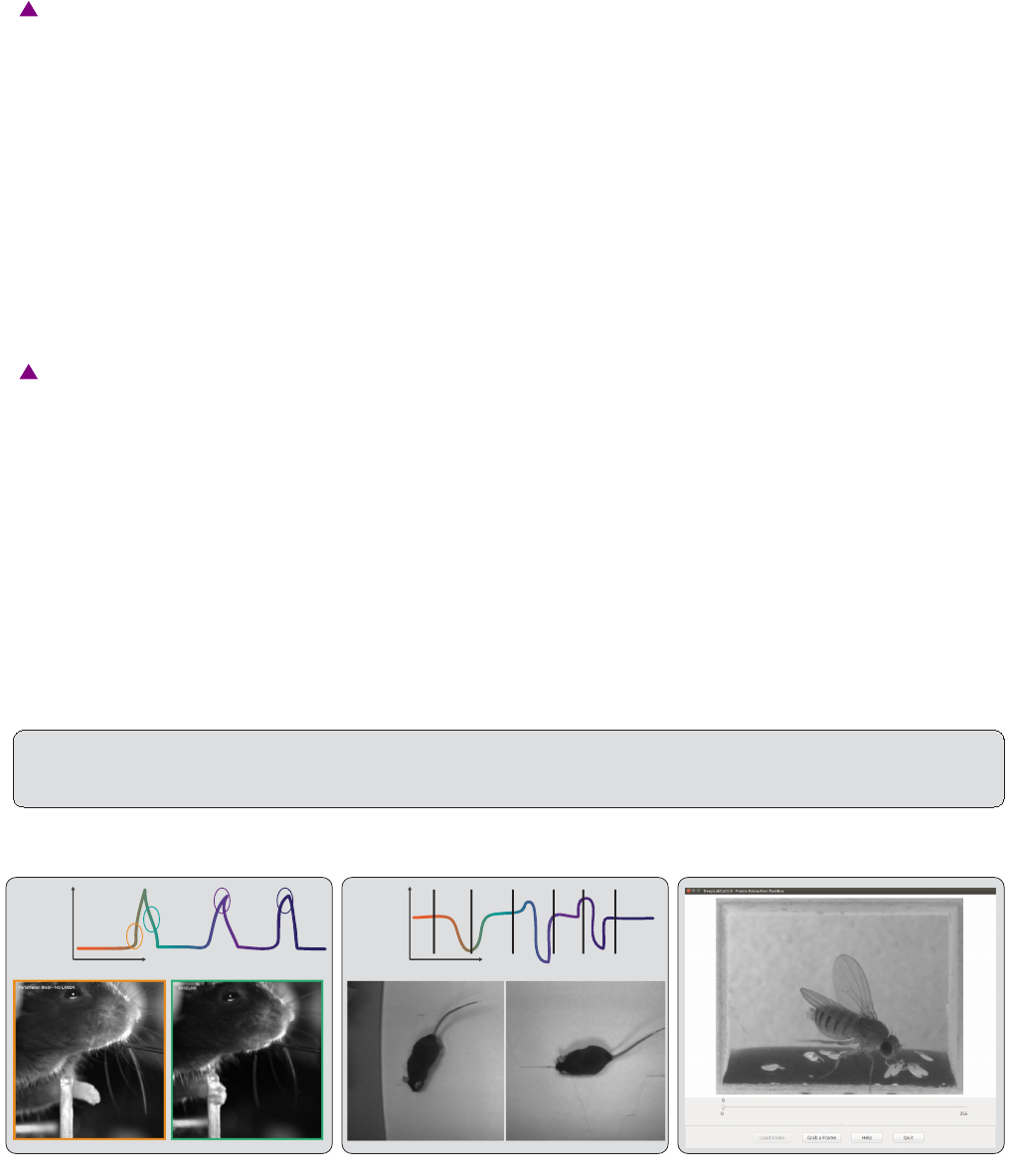
3 methods for frame extraction to create a labeled train/test set

Image based clustering (k-means) Random temporal sampling (uniform) GUI for manual frame grabbing

behavioral

state

time

behavioral

state

time

Select videos to grab frames:

Use videos with image from:

- different sessions reflecting (if the case) varying light conditions, backgrounds, setups, and camera angles (etc).

- different individuals, especially if they look different (i.e. brown + black mice)

FIG. 3. Three methods for frame selection. The toolbox contains three methods to extracting frames, namely, by clustering

based on visual content, by randomly sampling in uniform way across time, or by manually grabbing frames of interest using

a custom GUI. Depending on the studied behavior, the appropriate method can be used. Additional methods will be added in

the future.

.CC-BY-NC-ND 4.0 International licenseIt is made available under a

(which was not peer-reviewed) is the author/funder, who has granted bioRxiv a license to display the preprint in perpetuity.

The copyright holder for this preprint. http://dx.doi.org/10.1101/476531doi: bioRxiv preprint first posted online Nov. 24, 2018;

11

might be sparse, as in the case of reaching where the reach and pull are very fast and the mouse is not moving much

between trials. In such a case, the function that allows selecting frames based on k-means derived quantization would

be useful. If the user chooses to use k-means as a method to cluster the frames, then this function downsamples the

video and clusters the frames using k-means, where each frame is treated as a vector. Frames from different clusters

are then selected. This procedure makes sure that the frames look different. However, on large and long videos, this

code is slow due to computational complexity.

CRITICAL POINT: It is advisable to extract frames from a period of the video that contains interesting

behaviors, and not extract the frames across the whole video. This can be achieved by using the start and stop

parameters in the config.yaml file. Also, the user can change the number of frames to extract from each video using

the numframes2extract in the config.yaml file.

However, picking frames is highly dependent on the data and the behavior being studied. Therefore, it is hard to

provide all purpose code that extracts frames to create a good training dataset for every behavior and animal. If

the user feels specific frames are lacking, they can extract hand selected frames of interest using the interactive GUI

provided along with the toolbox. This can be launched by using:

>> deeplabcut.extract_frames(config_path,‘manual’)

The user can use the ‘Load Video’ button to load one of the videos in the project configuration file, use the scroll

bar to navigate across the video and ‘Grab a Frame’ to extract the frame. The user can also look at the extracted

frames and e.g. delete frames (from the directory) that are too similar before re-loading the set and then manually

annotating them.

D. Label Frames

Timing: The time required to label the frames depends on the speed of the experimenter to identify the correct

label and is mainly related to the number of body parts and the total number of extracted frames.

The toolbox provides a function ‘label_frames’ which helps the user to easily label all the extracted frames using

an interactive graphical user interface (GUI). The user should have already named the body parts to label (points of

interest) in the project’s configuration file by providing a list. The following command invokes the labeling toolbox.

>> deeplabcut.label_frames(config_path)

The GUI is launched taking the size of the user’s screen into account, so if two monitors are used (in landscape mode)

place ‘Screens=2’ after config_path (The default is 1). For other configurations, please see the linked troubleshooting

guide, Section ( O).

Next, the user needs to use the ‘Load Frames’ button to select the directory which stores the extracted frames from

one of the videos. A right click places the first body part, and subsequently, the user can either select one of the radio

buttons (top right) to select a body part to label, or there is a built in auto-advance to the next body part. If a body

part is not visible, simply do not label the part and click on the next body part you can label. Clicking the right arrow

key will advance to the next frame. Each label will be plotted as a dot in a unique color (see Figure 4for more details).

CRITICAL POINT: Finalize the position of the selected label before changing the dot size for the next

labels. it is recommended to do this once after the first frame is labeled. Then, proceed to the next frame.

The user is free to move around the body part with a left click and drag once they satisfied with its position, can

select another radio button (in the top right) to switch to the respective body part. Once the user starts labeling a

subsequent body part, preceding labels of the body parts can no longer be moved. The user can skip a body part if

it is not visible. Once all the visible body parts are labeled, then the user can use ‘Next Frame’ to load the following

frame. The user needs to save the labels after all the frames from one of the videos are labeled by clicking the save

button at the bottom right. Saving the labels will create a labeled dataset for each video in a hierarchical data file

format (HDF) in the subdirectory corresponding to the particular video in ‘labeled-data’.

CRITICAL POINT: It is advisable to consistently label similar spots (e.g. on a wrist that is very large, try

to label the same location). In general, invisible or occluded points should not be labeled by the user. They can

simply be skipped by not applying the label anywhere on the frame.

.CC-BY-NC-ND 4.0 International licenseIt is made available under a

(which was not peer-reviewed) is the author/funder, who has granted bioRxiv a license to display the preprint in perpetuity.

The copyright holder for this preprint. http://dx.doi.org/10.1101/476531doi: bioRxiv preprint first posted online Nov. 24, 2018;

12

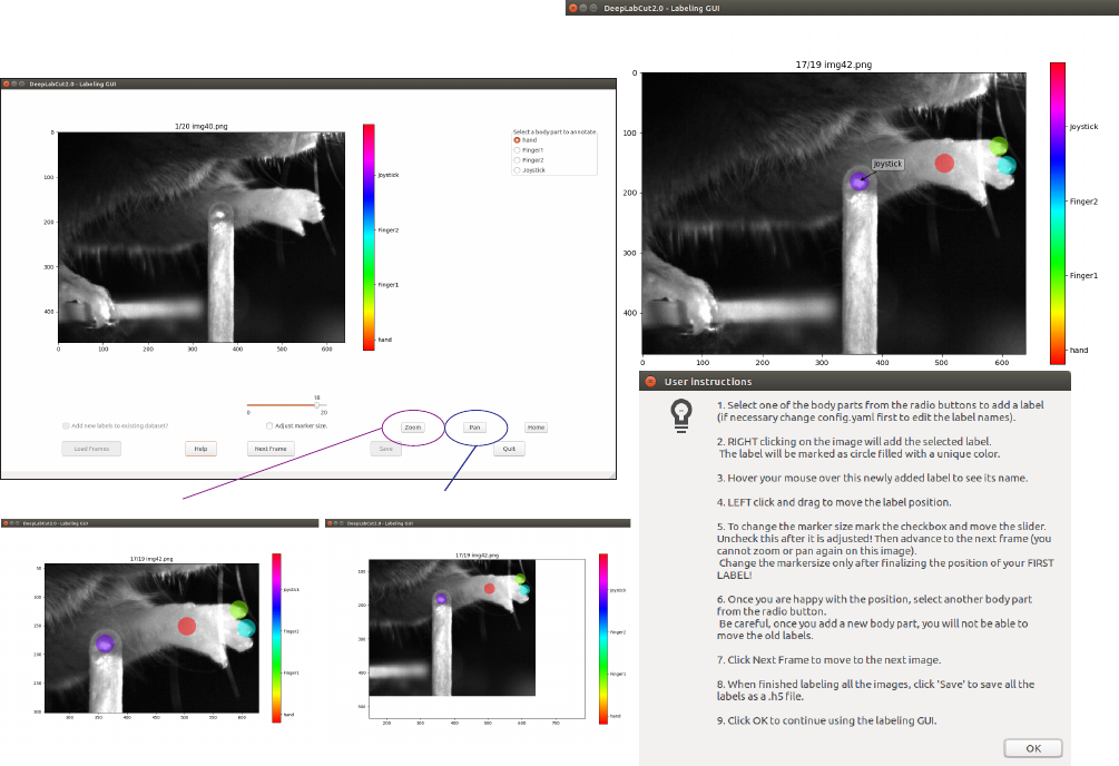
Label Frames using interactive GUI:

ZOOM PAN

deeplabcut.label_frames(config_path)

FIG. 4. Labeling GUI: The toolbox contains a labeling GUI that allows for frame loading, labeling, re-adjustments, and

saving the dataset into the correct format for future steps. An example label is shown, and the help functions are described.

Additionally, a user can decide to add more points to an existing labeled dataset by adding the new labels to the config.yaml

file and re-opening the labeling GUI and then the user can click the tick box in the bottom left corner to add new points.

OPTIONAL: In an event of adding more labels to the existing labeled dataset, the user need to append the new

labels to the bodyparts in the config.yaml file. Thereafter, the user can call the function ‘label_frames’ and check

the left lower tick box, ‘Add new labels to existing dataset?’ before loading the frames. Saving the labels after all the

images are labelled will append the new labels to the existing labeled dataset.

E. Check Annotated Frames

OPTIONAL: Checking if the labels were created and stored correctly is beneficial for training, since labeling

is one of the most critical parts for creating the training dataset. The DeepLabCut toolbox provides a function

‘check_labels’ to do so. It is used as follows:

>> deeplabcut.check_labels(config_path)

For each video directory in labeled-data this function creates a subdirectory with ‘labeled’ as a suffix. Those directories

contain the frames plotted with the annotated body parts. The user can double check if the body parts are labeled

correctly. If they are not correct, the user can call the refinement GUI (Step Kand check the tick box for “adjust

original labels" to adjust the location of the labels).

.CC-BY-NC-ND 4.0 International licenseIt is made available under a

(which was not peer-reviewed) is the author/funder, who has granted bioRxiv a license to display the preprint in perpetuity.

The copyright holder for this preprint. http://dx.doi.org/10.1101/476531doi: bioRxiv preprint first posted online Nov. 24, 2018;

13

F. Create Training Dataset

Timing: The time required to create a training dataset is <1 minute.

Combining the labeled datasets from all the videos and splitting them will create train and test datasets. The

training data will be used to train the network, while the test data set will be used for evaluating the network. The

function ‘create_training_dataset’ performs those steps.

>> deeplabcut.create_training_dataset(config_path,num_shuffles=1)

The set of arguments in the function will shuffle the combined labeled dataset and split it to create train and test

sets. The subdirectory with suffix ‘iteration#’ under the directory ‘training-datasets’ stores the dataset and meta

information, where the ‘#’ is the value of ‘iteration’ variable stored in the project’s configuration file (this number

keeps track of how often the dataset was refined).

OPTIONAL: If the user wishes to benchmark the performance of the DeepLabCut, they can create multiple

training datasets by specifying an integer value to the num_shuffles.

Each iteration of the creation of a training dataset, will create a ‘.mat’ file, which is used by the feature detectors

and a ‘.pickle’ file which contains the meta information about the training dataset. This also creates two subdirec-

tories within ‘dlc-models’ called ‘test’ and ‘train’, and these each have a configuration file called pose_cfg.yaml.

Specifically, the user can edit the pose_cfg.yaml within the train subdirectory before starting the training. These

configuration files contain meta information with regard to the parameters of the feature detectors. Key parameters

are listed in Box 2.

Box 2: Parameters of interest in the configuration file, pose_cfg.yaml.

•display_iters: An integer value representing the period with which the loss is displayed (and stored in log.csv).

•save_iters: An integer value representing the period with which the checkpoints (weights of the network)

are saved. Each snapshot has >80MB, so not too many should be stored.

•init_weights: The initial weights used for training. Default:

< DeepLabCut path>/Pose_Estimation_Tensorflow/pretrained/resnet_v1_50.ckpt

for ResNet-50 – this will be automatically created. The weights can also be changed to restart from a

particular snapshot, e.g. <full path of ‘snapshot-5000’ > starts from a snapshot after 5,000 training iterations.

The following parameters allow one to change the resolution:

•global_scale: all images in the dataset will be re-scaled by the following scaling factor to be processed by the

CNN. You can select the optimal scale by cross-validation (See discussion in [12]). Default 0.8.

•pos_dist_thresh: all locations within this distance threshold in pixels are considered positive training

samples for detector (See discussion in [12]). Default 17.

The following parameters modulate the data augmentation. During training each image will be randomly

re-scaled within the range [scale_jitter_lo,scale_jitter_up] to augment training:

•scale_jitter_lo: 0.5 (default)

•scale_jitter_up: 1.5 (default)

•mirror: If training dataset is symmetric around vertical axis, this Boolean variable allows random augmen-

tation. Default is false.

•cropping: Automatically crop images during training. Default is True.

•cropratio: Fraction of training samples that are cropped. Default is 40%

•minsize, leftwidth, rightwidth, bottomheight, topheight: Define dimensions and limits for cropping.

.CC-BY-NC-ND 4.0 International licenseIt is made available under a

(which was not peer-reviewed) is the author/funder, who has granted bioRxiv a license to display the preprint in perpetuity.

The copyright holder for this preprint. http://dx.doi.org/10.1101/476531doi: bioRxiv preprint first posted online Nov. 24, 2018;

14

G. Train The Network

Timing: The time required to train the network mainly depends on the frame size of the dataset and the

computer hardware. On a NVIDIA GeForce GTX 1080 Ti GPU, it takes ≈6 hrs to train the network for at least

200,000 iterations. On the CPU, it will take several days to train for the same number of iterations on the same

training dataset.

CRITICAL POINT: It is recommended to train for thousands of iterations until the loss plateaus (typically

>200,000). The variables ‘display_iters’ and ‘save_iters’ in the pose_cfg.yaml file allows the user to alter how often

the loss is displayed and how often the weights are stored.

The function ‘train_network’ helps the user in training the network. It is used as follows:

>> deeplabcut.train_network(config_path,shuffle=1)

The set of arguments in the function starts training the network for the dataset created for one specific shuffle.

Example parameters that one can call:

train_network(config_path,shuffle=1,trainingsetindex=0,gputouse=None,max_snapshots_to_keep=5,

autotune=False,displayiters=None,saveiters=None)

Important Parameters:

config: Full path of the config.yaml file as a string.

shuffle: Integer value specifying the shuffle index to select for training. Default is set to 1

trainingsetindex: Integer specifying which Training set Fraction to use. By default the first (note that Training

Fraction is a list in config.yaml).

gputouse: Natural number indicating the number of your GPU (see number in nvidia-smi). If you

do not have a GPU put None. see also: https://nvidia.custhelp.com/app/answers/detail/a_id/3751/~/

useful-nvidia-smi-queries

Additional parameters:

max_snapshots_to_keep: This sets how many snapshots are kept, i.e. states of the trained network. Every sav-

ing iteration a snapshot is stored, however only the last max_snapshots_to_keep many are kept! If you change this to

None, then all are kept. See also: https://github.com/AlexEMG/DeepLabCut/issues/8#issuecomment-387404835

autotune: property of TensorFlow, tested to be faster if set to ’False’; see https://github.com/tensorflow/

tensorflow/issues/13317). Default: False

displayiters: this variable is actually set in pose_config.yaml. However, you can overwrite it with this. If None,

the value from pose_config.yaml is used, otherwise it is overwritten! Default: None

saveiters: this variable is set in pose_config.yaml. However, you can overwrite it with this. If None, the value

from there is used, otherwise it is overwritten! Default: None

By default, the pre-trained ResNet network is not provided in the DeepLabCut toolbox (as it has around 100MB).

However, if not previously downloaded from the TensorFlow model weights, it will be downloaded and stored in

a subdirectory ‘pre-trained’ under the subdirectory ‘models’ in ‘Pose_Estimation_Tensorflow’, where deeplabcut

is installed (i.e. usually site-packages). At user specified iterations during training checkpoints are stored in the

subdirectory ‘train’ under the respective iteration directory. If the user wishes to restart the training at a specific

checkpoint they can specify the full path of the checkpoint to the variable ‘init_weights’ in the pose_cfg.yaml file

under the ‘train’ subdirectory (see Box 2).

H. Evaluate the Trained Network

Timing: The time required to evaluate the trained network depends on the computational hardware, number of

checkpoints to evaluate, and the number of images in the training dataset. With the default parameters and around

150 images in the training dataset, it will take ≈2 mins/checkpoint on a GPU. However, for the same snapshot and

training set a CPU computes ≈ten times longer (i.e. 20 min).

It is important to evaluate the performance of the trained network. This performance is measured by computing

the mean average Euclidean error (MAE; which is proportional to the average root mean square error) between the

manual labels and the ones predicted by DeepLabCut. The MAE is saved as a comma separated file and displayed

for all pairs and only likely pairs (>p-cutoff). This helps to exclude, for example, occluded body parts. One of the

.CC-BY-NC-ND 4.0 International licenseIt is made available under a

(which was not peer-reviewed) is the author/funder, who has granted bioRxiv a license to display the preprint in perpetuity.

The copyright holder for this preprint. http://dx.doi.org/10.1101/476531doi: bioRxiv preprint first posted online Nov. 24, 2018;

15

aExamples of test images with Human and DeepLabCut labels

+ Human applied Label

DeepLabCut

Evaluation: example of the terminal output

Examples of test images with Human and DeepLabCut labels

Examples of training images with Human and DeepLabCut labels

b

c

d

deeplabcut.evaluate_network(’<path of the proj. config file>’, shuffle = [1], plotting=True)

Assessing accuracy of shuffle # 1 with 99 % training fraction.

Found the following training snapshots: [(200000, 0)]

You can chose among those for analysis of train/test performance.

Restuls for 200000 training iterations: 99 1 train error: 4.81 pixels. Test error:7.02 pixels.

With cutoff of 0.1 train error: 3.3 pixels. Test error: 5.2 pixels.

FIG. 5. Evaluation results: (a) The code that is used to evaluate the network, and the output the user will see in the terminal.

(b) Another output is labeled frames from training and (c) test images, as shown for a Cheetah project. (d) Additional example

test evaluation images from Drosophila (different images from network trained in [12]) and horse tracking projects.

strengths of DeepLabCut is that due to the probabilistic output of the scoremap, it can, if sufficiently trained, also

reliably report if a body part is visible in a given frame. (see discussions of finger tips in reaching and the Drosophila

legs during 3D behavior in [12]). The evaluation results are computed by typing:

>> deeplabcut.evaluate_network(config_path,shuffle=[1], plotting=True)

Setting ‘plotting’ to true plots all the testing and training frames with the manual and predicted labels. The user

should visually check the labeled test (and training) images that are created in the ‘evaluation-results’ directory.

Ideally, DeepLabCut labeled unseen (test images) according to the user’s required accuracy, and the average train

and test errors are comparable (good generalization). What (numerically) comprises an acceptable MAE depends on

many factors (including the size of the tracked body parts, the labeling variability, etc.). Note that the test error can

also be larger than the training error due to human variability (in labeling, see Figure 2 in [12]).

The plots can be customized by editing the config.yaml file (i.e. the colormap, scale, marker size (dotsize), and

transparency of labels (alphavalue) can be modified). By default each body part is plotted in a different color

(governed by the colormap) and the plot labels indicate their source. Note that by default the human labels are

plotted as plus (‘+’), DeepLabCut’s predictions either as ‘.’ (for confident predictions with likelihood > p-cutoff) and

’x’ for (likelihood <=p-cutoff). Examples test and training plots from various projects are depicted in Figure 5.

The evaluation results for each shuffle of the training dataset are stored in a unique subdirectory in a newly created

directory ‘evaluation-results’ in the project directory. The user can visually inspect if the distance between the labeled

and the predicted body parts is acceptable. In the event of benchmarking with different shuffles of same training

dataset, the user can provide multiple shuffle indices to evaluate the corresponding network. If the generalization is

not sufficient, the user might want to:

•check if the labels were imported correctly, i.e. invisible points are not labeled and the points of interest are

labeled accurately (see Step E)

•make sure that the loss has already converged (Step G)

•consider labeling additional images and make another iteration of the training data set (Section J).

.CC-BY-NC-ND 4.0 International licenseIt is made available under a

(which was not peer-reviewed) is the author/funder, who has granted bioRxiv a license to display the preprint in perpetuity.

The copyright holder for this preprint. http://dx.doi.org/10.1101/476531doi: bioRxiv preprint first posted online Nov. 24, 2018;

16

I. Video Analysis and Plotting Results

Timing: The time required to analyze a video is mainly related to the number of frames in the video and if the

computational power of a GPU is available. With a GPU analysis runs at 10-100 FPS depending on the frame size

(for 1000 ×1000 to 200 ×200, respectively).

The trained network can be used to analyze new videos. The user needs to first choose a checkpoint with the best

evaluation results for analyzing the videos. In this case, the user can enter the corresponding index of the checkpoint

to the variable snapshotindex in the config.yaml file. By default, the most recent checkpoint (i.e. last) is used for

analyzing the video. Then, a new video can be analyzed by typing:

>> deeplabcut.analyze_videos(config_path,[‘/analysis/project/videos/reachingvideo1.avi’],

shuffle=1, save_as_csv=True, videotype=.avi)

The labels are stored in a MultiIndex Pandas Array ([41], http://pandas.pydata.org), which contains the name

of the network, body part name, (x, y)label position in pixels, and the likelihood for each frame per body part. These

arrays are stored in an efficient Hierarchical Data Format (HDF) in the same directory, where the video is stored.

However, if the flag save_as_csv is set to True, the data can also be exported in comma-separated values format

(.csv), which in turn can be imported in many programs, such as MATLAB, R, Prism, etc.; This flag is set to False

by default.

The labels for each body part across the video (‘trajectories’) can also be plotted after analyze_videos is run.

The provided plotting function in this toolbox utilizes matplotlib [42] therefore these plots can easily be customized

by the end user. This function can be called by typing:

>>> deeplabcut.plot_trajectories(config_path,[‘/analysis/project/videos/reachingvideo1.avi’])

The trajectories can also be easily imported into many programs for further behavioral analysis. For example, a

user can compute general movement statistics (position, velocity, etc), or interactions e.g. with (tracked) objects in

the environment (i.e. with DeepLabCut there is no centering of the animal(s) therefore the user can easily measure

relative movements within the background environment). The outputs from DeepLabCut can also interfaced with

behavioral clustering tools such as JAABA [43], MotionMapper [44], MoSeq [45], or other clustering approaches such

as iterative denoising tree (IDT) methods [46,47], and more [48]. Indeed, users are contributing code for analysis of

the outputs of DeepLabCut here: https://github.com/AlexEMG/DLCutils.

Additionally, the toolbox provides a function to create labeled videos based on the extracted poses by plotting the

labels on top of the frame and creating a video. One can use it as follows to create multiple labeled videos:

>> deeplabcut.create_labeled_video(config_path,[‘/analysis/project

/videos/reachingvideo1.avi’,‘/analysis/project/videos/reachingvideo2.avi’])

This function has various parameters, in particular the user can set the colormap, the dotsize, and alphavalue of

the labels in config.yaml file.

J. Refinement: Extract Outlier Frames

Timing: The time required to select the data is mainly related to the mode of selection, number of videos and

the algorithm used to extract the frames. It takes around 1 min/video in an automated mode with default parameter

settings (processing time strongly depends on length and size of video).

While DeepLabCut typically generalizes well across datasets, one might want to optimize its performance in various,

perhaps unexpected, situations. For generalization to large data sets, images with insufficient labeling performance

can be extracted, manually corrected by adjusting the labels to increase the training set and iteratively improve the

feature detectors. Such an active learning framework can be used to achieve a predefined level of confidence for all

images with minimal labeling cost (discussed in [12]). Then, due to the large capacity of the neural network that

underlies the feature detectors, one can continue training the network with these additional examples. One does not

necessarily need to correct all errors as common errors could be eliminated by relabeling a few examples and then

re-training. A priori, given that there is no ground truth data for analyzed videos, it is challenging to find putative

“outlier frames”. However, one can use heuristics such as the continuity of body part trajectories, to identify images

where the decoder might make large errors. We provide various frame-selection methods for this purpose. In particular

the user can:

.CC-BY-NC-ND 4.0 International licenseIt is made available under a

(which was not peer-reviewed) is the author/funder, who has granted bioRxiv a license to display the preprint in perpetuity.

The copyright holder for this preprint. http://dx.doi.org/10.1101/476531doi: bioRxiv preprint first posted online Nov. 24, 2018;

17

•select frames if the likelihood of a particular or all body parts lies below pbound (note this could also be due to

occlusions rather then errors).

•select frames where a particular body part or all body parts jumped more than pixels from the last frame.

•select frames if the predicted body part location deviates from a state-space model [49,50] fit to the time series

of individual body parts. Specifically, this method fits an Auto Regressive Integrated Moving Average (ARIMA)

model to the time series for each body part. Thereby each body part detection with a likelihood smaller than

pbound is treated as missing data. An example fit for one body part can be found in Figure 6a. Putative outlier

frames are then identified as time points, where the average body part estimates are at least pixel away from

the fits. The parameters of this method are , pbound, the ARIMA parameters as well as the list of body parts

to average over (can also be “all”).

All this can be done for a specific video by typing:

>> deeplabcut.extract_outlier_frames(config_path,[‘videofile_path’])

In general, depending on the parameters, these methods might return much more frames than the user wants to

extract (numframes2pick). Thus, this list is then used to select outlier frames either by randomly sampling from this

list (‘uniform’) or by performing ‘k-means’ clustering on the corresponding frames (same methodology and parameters

as in Step C). Furthermore, before this second selection happens, the user is informed about the amount of frames

satisfying the criteria and asked if the selection should proceed. This step allows the user to perhaps change the

parameters of the frame-selection heuristics first. The user can run the extract_outlier_frames iteratively, and (even)

extract additional frames from the same video. Once enough outlier frames are extracted the refinement GUI can be

used to adjust the labels based on user feedback (Step K). This function has many optional parameters, so a user

should reference the help by typing deeplabcut.extract_outlier_frames? (and see Step N).

K. Refine Labels: Augmentation of the Training Dataset

Timing: The time required to refine the labels depends on the speed of the experimenter to identify the

incorrect label and is mainly related to the number of body parts and the total number of extracted outlier frames.

Based on the performance of DeepLabCut, four scenarios are possible:

(A) Visible body part with accurate DeepLabCut prediction. These labels do not need any modifications.

(B) Visible body part but wrong DeepLabCut prediction. Move the label’s location to the actual position of the

body part.

(C) Invisible, occluded body part. Remove the predicted label by DeepLabCut with a right click. Every predicted

label is shown, even when DeepLabCut is uncertain. This is necessary, so that the user can potentially move

the predicted label. However, to help the user to remove all invisible body parts the low-likelihood predictions

are shown as open circles (rather than disks).

(D) Invalid images: In an unlikely event that there are any invalid images, the user should remove such an image

and their corresponding predictions, if any. Here, the GUI will prompt the user to remove an image identified

as invalid.

The labels for extracted putative outlier frames can be refined by opening the GUI:

>> deeplabcut.refine_labels(config_path)

This will launch a GUI where the user can refine the labels (Figure 6). The GUI is launched taking the size of

the user’s screen into account, so if two monitors are used (in landscape mode) place ‘Screens=2’ after config_path

(The default is 1). For other configurations, please see the linked troubleshooting guide (Section O). Use the ‘Load

Labels’ button to select one of the subdirectories, where the extracted frames are stored. It is also possible to correct

labels that have already been applied (or refined) by a user by simply check the ’adjust original label?’ checkbox

before loading the labels file. Every label will be identified by a unique color. For better chances to identify the

low-confidence labels, specify the threshold of the likelihood. This changes the body parts with likelihood below this

threshold to appear as circles and the ones above as solid disks while retaining the same color scheme. Next, to adjust

.CC-BY-NC-ND 4.0 International licenseIt is made available under a

(which was not peer-reviewed) is the author/funder, who has granted bioRxiv a license to display the preprint in perpetuity.

The copyright holder for this preprint. http://dx.doi.org/10.1101/476531doi: bioRxiv preprint first posted online Nov. 24, 2018;

18

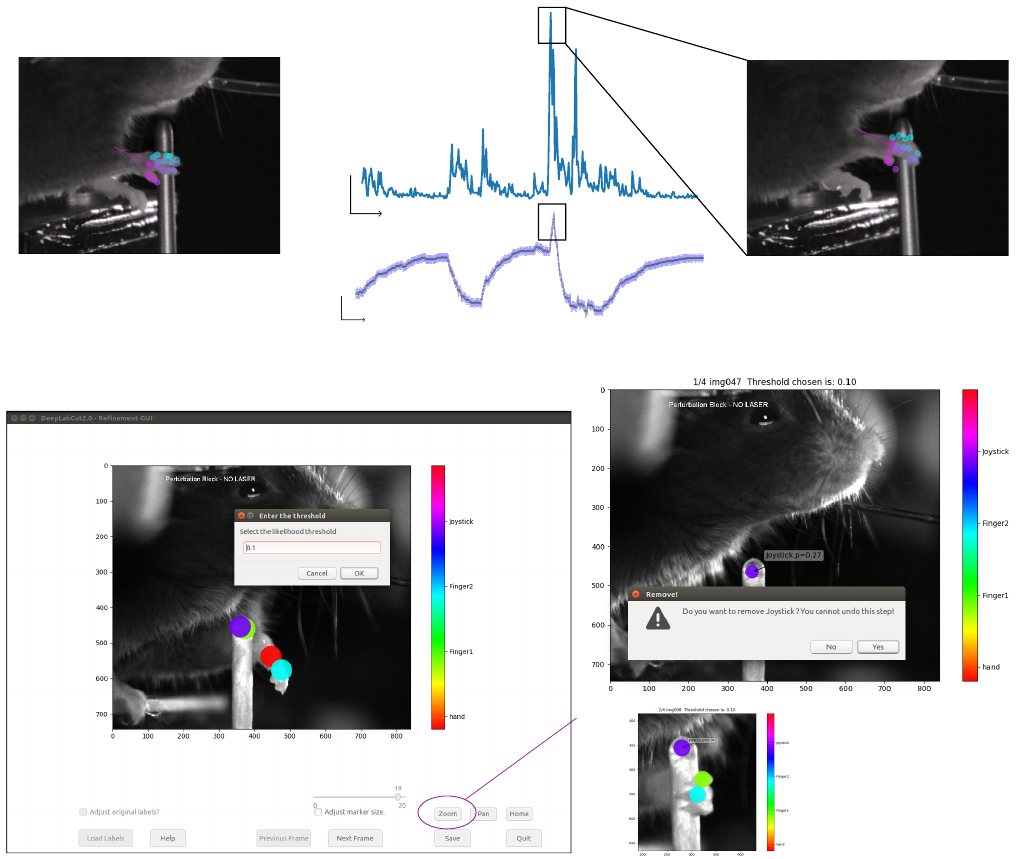
Refine DLC applied label location(s) Remove label i.e. from an occluded point

a

bc

SARIMAX

Identify outlier frames

good frame putative outlier frame

back of hand from DLC

ARIMA fit

CI

50 pixels

frame index

5 pixels

frame index

Average Distance

back of hand

back of hand

deeplabcut.refine_frames(config_path)

ZOOM

FIG. 6. Refinement Tools. A user can refine the network by first extracting outliers and then by manually correcting

the annotations based a dedicated graphical user interface (a) Outlier detection: For illustration we depict the x-coordinate

estimate by DeepLabCut for the back of the hand and an ARIMA fit with 99%-confidence interval in blue. The average

Euclidean distance for the tracked 17 body parts of the hand to the fit is also depicted. This distance can be used to find

putative outliers as indicated by the corresponding frames. (b-c) Then adjust the labels and/or remove occluded labels.

the position of the label, hover the mouse over the labels to identify the specific body part, left click+drag it to a

different location. To delete a specific label, right click on the label (once a label is deleted, it cannot be retrieved).

After correcting the labels for all the frames in each of the subdirectories, the users should merge the data set to

create a new dataset. The iteration parameter in the config.yaml file is automatically updated.

>> deeplabcut.merge_datasets(config_path)

Once the dataset is merged, the user can test if the merging process was successful by plotting all the labels (Step E).

Next, with this expanded training set the user can now create a novel training set and train the network as described

in Steps Fand G. The training dataset will be stored in the same place as before but under a different ‘iteration #’

subdirectory, where the ‘#’ is the new value of ‘iteration’ variable stored in the project’s configuration file (this is

automatically done).

If after training the network generalizes well to the data, proceed to Step Ito analyze new videos. Otherwise,

consider labeling more data (Section J).

.CC-BY-NC-ND 4.0 International licenseIt is made available under a

(which was not peer-reviewed) is the author/funder, who has granted bioRxiv a license to display the preprint in perpetuity.

The copyright holder for this preprint. http://dx.doi.org/10.1101/476531doi: bioRxiv preprint first posted online Nov. 24, 2018;

19

L. Anticipated Results

DeepLabCut has been used for pose estimation of various points of interest for different behaviors and animals

(Fig 1). Due to the initial pre-training of the ResNet (i.e. the ResNet is first pre-trained on ImageNet [51]), as we

have shown in our original study [12], DeepLabCut does not typically require many labeled frames to train on. We

previously showed that even as little as 100 frames could be labeled for accurate tracking of a mouse snout in an open

field-like scenario with challenging background and lighting statistics. The technical report also contains examples for

hand articulation and fruit fly pose-estimation during egg-laying [12].

Here, we provide a new use case, where the experimenters wanted to quantitatively track the 3D kinematics of

a cheetah performing a high-speed pursuit task as would be done during hunting in the wild [52]. This specific

application has many challenges for any pose-estimation approach: highly variable scene statistics where the animal

traverses over a field of grass and stirs up dust, different weather conditions, the size of the animal in the frame changes

dramatically as it runs into a “camera trap” of 6 high-speed cameras (90 FPS, 1080p resolution), and the different

cheetahs have diverse coats and highly articulated leg and body movements (Figure 5a,b). In total, we labeled 255

frames across multiple cameras (some of which come from the video in the figure) using the toolbox presented in this

guide. Thus, the 3D kinematics can be reconstructed from one network being trained on multiple views, and the

user only needs the camera calibration files to reconstruct their data. This camera calibration can be done in many

programs, including OpenCV [36].

Specifically, we first selected 10 frames each from 12 different videos by using the uniform random sampling across

the length of each video. Next, labeling was performed on the initial set using the supplied GUI. We trained with

automatic cropping and rescaling; due to the large input size image of 1920 x 1080 pixels, we changed ’max_input_size’

to 2000. After training, we iteratively refined images and re-trained the network until we had a set of 255 frames

that allowed for reasonable performance and generalization. In Figure 7we show how multiple cameras can be used

Camera 1

Camera 2

Camera 3

Camera 4

Camera 5

Camera 6

camera-invariant labels learned

Train a single network for

all camera angles

for 3D reconstruction

a

cam 1cam 2

AU (z)

AU (y)

AU (x)

Example predictions of trained network for data from two different cameras

3D stereo-reconstruction of one cheetah side view

b

c

FIG. 7. An example use case for pose estimation of a hunting cheetah. (a) Images collected from multiple cameras

can be used to train a single network. (b) Example frames with overlaid body parts extracted by DeepLabCut, as well as a

trajectory of past movements from previous frames. The same network was trained for multiple views, and is used to extract

the poses. (b) 3D reconstruction of body parts from cheetah’s side facing both cameras from the same series of frames as in b.

.CC-BY-NC-ND 4.0 International licenseIt is made available under a

(which was not peer-reviewed) is the author/funder, who has granted bioRxiv a license to display the preprint in perpetuity.

The copyright holder for this preprint. http://dx.doi.org/10.1101/476531doi: bioRxiv preprint first posted online Nov. 24, 2018;

20

to train a single network (Figure 7a), and an example image sequence with trajectories of past actions (Figure 7b),

and using 2 cameras we show a 3D reconstruction [53,54] of one body side (Figure 7c). This is an ongoing project

studying the biomechanics of cheetah hunting and will be published elsewhere. Yet, we hope this example use case

shows how DeepLabCut can be utilized even for very challenging, large video-resolution tracking problems “in the

wild”, and empowers the user to apply this approach to their own unique and exciting experiments.

M. Jupyter Notebooks for Demonstration of the DeepLabCut Work-flow

We also provide two Jupyter notebooks for using DeepLabCut on both a pre-labeled dataset, and on the end user’s

own dataset. Firstly, we prepared an interactive Jupyter notebook called run_yourowndata.ipynb that can serve as a

template for the user to develop a project. Furthermore, we provide a notebook for an already started project with

labeled data. The example project, named as Reaching-Mackenzie-2018-08-30 consists of a project configuration file

with default parameters and 20 images, which are cropped around the region of interest as an example dataset. These

images are extracted from a video, which was recorded in a study of skilled motor control in mice [55]. Some example

labels for these images are also provided. The notebooks can be started by typing in the terminal:

jupyter-notebook Demo-labeledexample-MouseReaching.ipynb

jupyter-notebook Demo-yourowndata.ipynb

N. Overview of Commands

Here is a ‘quick-guide’ of the minimal commands used for running DeepLabCut in Python/ipython. All these

functions have additional optional parameters that the user may change. The user can invoke ‘help’ for any function

and get more information about these optional parameters as follows:

In ipython/Jupyter Notebooks: deeplabcut.nameofthefunction?

In Python: help(deeplabcut.nameofthefunction)

TABLE I: Summary of Commands

Steps Command

Open ipython or Python

import deeplabcut

ipython (or python)

import deeplabcut

Create a new project.

See section Afor details

Python/ipython:

>> deeplabcut.create_new_project(‘project name’,‘experimenter’,

[‘path of video 1’,‘path of video2’,..])

Set a config_path

for ease of use >> config_path = ‘yourdirectory/your_deeplabcut/config.yaml’

Extract frames

See section Cfor details

Python/ipython:

>> deeplabcut.extract_frames(config_path,mode= ‘automatic’)

Label frames

See section Dfor details

Python/ipython:

>> deeplabcut.label_frames(config_path)

Check labels

[OPTIONAL]

See section Efor details

Python/ipython:

>> deeplabcut.check_labels(config_path)

Create training dataset

See section Ffor details

Python/ipython:

>> deeplabcut.create_training_dataset(config_path)

.CC-BY-NC-ND 4.0 International licenseIt is made available under a

(which was not peer-reviewed) is the author/funder, who has granted bioRxiv a license to display the preprint in perpetuity.

The copyright holder for this preprint. http://dx.doi.org/10.1101/476531doi: bioRxiv preprint first posted online Nov. 24, 2018;

21

Train the network

See section Gfor details

Python/ipython:

>> deeplabcut.train_network(config_path)

Evaluate the trained net-

work

See section Hfor details

Python/ipython:

>> deeplabcut.evaluate_network(config_path)

Video analysis and plot-

ting Results

See section Ifor details

Python/ipython:

>> deeplabcut.analyze_videos(config_path,

[‘path of video 1’,‘path of video2’, ...])

Video analysis and plot-

ting Results

See section Ifor details

Python/ipython:

>> deeplabcut.create_labeled_video(config_path,

[‘path of video 1’,‘path of video2’,..])

Video analysis and plot-

ting Results

See section Ifor details

Python/ipython:

>> deeplabcut.plot_trajectories(config_path,

[‘path of video 1’,‘path of video2’,..])

Refinement: Extract

outlier frames

See section Jfor details

Python/ipython:

>> deeplabcut.extract_outlier_frames(config_path,[‘path of video 1’,

‘path of video 2’])

Refine Labels: Augmen-

tation of the training

dataset

See section Kfor details

Python/ipython:

>> deeplabcut.refine_labels(config_path)

Combine datasets: Aug-

mentation of the training

dataset

See section Kfor details

Python/ipython:

>> deeplabcut.merge_datasets(config_path)

O. Troubleshooting

The Jupyter Notebooks provided on GitHub have been already executed so the user can see the expected outputs.

They are also annotated with potential errors and considerations. Additionally, when running the Notebooks on

Colaboratory (https://colab.research.google.com) the user can directly search for any error messages that arise,

as they can involve TensorFlow or other packages not managed by us. In the DeepLabCut code we strived to make

error messages intuitive for each step, and each output directs the user to the next step in the process.

There is also an actively maintained GitHub repository that has an “Issues” section for users to look

for solutions to problems others encountered or report new ones, as well as a wiki page with FAQ

(https://github.com/AlexEMG/DeepLabCut/wiki/Troubleshooting-Tips).

Funding:

The authors thank NVIDIA Corporation for GPU Grants to MWM and AM.AM: Marie Sklodowska-Curie Inter-

national Fellowship within the 7th European Community Framework Program under grant agreement No. 622943 and

by DFG grant MA 6176/1-1. AP:Oppenheimer Memorial Trust Fellowship and the National Research Foundation of

South Africa (Grant: 99380). MB: German Science foundation (DFG) through the CRC 1233 on “Robust Vision” and

from IARPA through the MICrONS program. MWM: Rowland Fellowship from the Rowland Institute at Harvard.

.CC-BY-NC-ND 4.0 International licenseIt is made available under a

(which was not peer-reviewed) is the author/funder, who has granted bioRxiv a license to display the preprint in perpetuity.

The copyright holder for this preprint. http://dx.doi.org/10.1101/476531doi: bioRxiv preprint first posted online Nov. 24, 2018;

22

Acknowledgments:

DeepLabCut is an open-source tool on GitHub and has benefited from suggestions and edits by many individuals

including Ronny Eichler, Jonas Rauber, Richard Warren, Taiga Abe, Hao Wu, and Jonny Saunders. In particular,

the authors thank Ronny Eichler for input on the modularized version. The authors thank members of the Bethge

Lab for providing the initial version of the Docker container. We also thank Meng Li, Jennifer Li & Drew Robson

for use of the zebrafish image, Byron Rogers for use of the horse images, and Kevin Cury for the fly images. The

authors are grateful to Eldar Insafutdinov and Christoph Lassner for suggestions on how to best use the TensorFlow

implementation of DeeperCut. We also thank Adrian Hoffmann, Pranav Mamidanna and Gary Kane for comments

throughout this project. Lastly, the authors thank the Ann van Dyk Cheetah Centre (Pretoria, South Africa) for

kindly providing access to their cheetahs.

Contributions:

Conceptualization: AM, TN, MWM. AM, TN and MWM wrote the code. AP provided the cheetah data; AC labeled

the cheetah data; AC, AM and AP analyzed the cheetah data. AM, MWM and TN wrote the manuscript with inputs

from all authors. MWM and MB supervised the project.

[1] Ilg, E. et al. Flownet 2.0: Evolution of optical flow estimation with deep networks. In IEEE conference on computer vision

and pattern recognition (CVPR), vol. 2, 6 (2017).

[2] Toshev, A. & Szegedy, C. DeepPose: Human pose estimation via deep neural networks. In Proceedings of the IEEE

conference on computer vision and pattern recognition, 1653–1660 (2014). URL http://ieeexplore.ieee.org/document/

6909610/.

[3] Levine, S., Pastor, P., Krizhevsky, A., Ibarz, J. & Quillen, D. Learning hand-eye coordination for robotic grasping with

deep learning and large-scale data collection. The International Journal of Robotics Research 37, 421–436 (2018).

[4] Wainberg, M., Merico, D., Delong, A. & Frey, B. J. Deep learning in biomedicine. Nature biotechnology 36, 829 (2018).

[5] LeCun, Y., Bengio, Y. & Hinton, G. Deep learning. nature 521, 436 (2015).

[6] Donahue, J. et al. DeCaf: A deep convolutional activation feature for generic visual recognition. In International conference

on machine learning, 647–655 (2014). URL https://arxiv.org/abs/1310.1531.

[7] Yosinski, J., Clune, J., Bengio, Y. & Lipson, H. How transferable are features in deep neural networks? In Advances in

neural information processing systems, 3320–3328 (2014). URL https://arxiv.org/abs/1411.1792.

[8] Goodfellow, I., Bengio, Y. & Courville, A. Deep learning, vol. 1 (MIT press Cambridge, 2016).

[9] Kümmerer, M., Wallis, T. S. & Bethge, M. Deepgaze ii: Reading fixations from deep features trained on object recognition.

arXiv preprint arXiv:1610.01563 (2016). URL https://arxiv.org/abs/1610.01563.

[10] Insafutdinov, E., Pishchulin, L., Andres, B., Andriluka, M. & Schiele, B. DeeperCut: A deeper, stronger, and faster

multi-person pose estimation model. In European Conference on Computer Vision, 34–50 (Springer, 2016). URL https:

//arxiv.org/abs/1605.03170.

[11] Insafutdinov, E. et al. Arttrack: Articulated multi-person tracking in the wild. In CVPR’17 (2017). URL http://arxiv.

org/abs/1612.01465.

[12] Mathis, A. et al. Deeplabcut: markerless pose estimation of user-defined body parts with deep learning. Nature neuroscience

21, 1281–1289 (2018).

[13] Dell, A. I. et al. Automated image-based tracking and its application in ecology. Trends Ecol. Evol. (Amst.) 29, 417–428

(2014). URL http://www.cell.com/trends/ecology-evolution/abstract/S0169-5347(14)00107-4.

[14] Anderson, D. J. & Perona, P. Toward a science of computational ethology. Neuron 84, 18–31 (2014). URL https:

//doi.org/10.1016/j.neuron.2014.09.005.

[15] Egnor, S. R. & Branson, K. Computational analysis of behavior. Annual review of neuroscience 39, 217–236 (2016).

[16] Dollár, P., Welinder, P. & Perona, P. Cascaded pose regression. In Computer Vision and Pattern Recognition (CVPR),

2010 IEEE Conference on, 1078–1085 (IEEE, 2010). URL http://ieeexplore.ieee.org/document/5540094/.

[17] Gomez-Marin, A., Partoune, N., Stephens, G. J. & Louis, M. Automated tracking of animal posture and movement during

exploration and sensory orientation behaviors. PLOS ONE 7, 1–9 (2012). URL https://doi.org/10.1371/journal.

pone.0041642.

[18] Matsumoto, J. et al. A 3D-video-based computerized analysis of social and sexual interactions in rats. PLoS ONE 8,

e78460 (2013). URL http://journals.plos.org/plosone/article?id=10.1371/journal.pone.0078460.

[19] Uhlmann, V., Ramdya, P., Delgado-Gonzalo, R., Benton, R. & Unser, M. FlyLimbTracker: An active contour based

approach for leg segment tracking in unmarked, freely behaving Drosophila. PLoS ONE 12, e0173433 (2017). URL

https://doi.org/10.1371/journal.pone.0173433.

[20] Ben-Shaul, Y. Optimouse: a comprehensive open source program for reliable detection and analysis of mouse body and

nose positions. BMC Biology 15, 41 (2017). URL http://dx.doi.org/10.1186/s12915-017-0377-3.

[21] Pereira, T. D. et al. Fast animal pose estimation using deep neural networks. bioRxiv 331181 (2018).

[22] Winter, D. Biomechanics and motor control of human movement (John Wiley & Sons, 2009).

.CC-BY-NC-ND 4.0 International licenseIt is made available under a

(which was not peer-reviewed) is the author/funder, who has granted bioRxiv a license to display the preprint in perpetuity.

The copyright holder for this preprint. http://dx.doi.org/10.1101/476531doi: bioRxiv preprint first posted online Nov. 24, 2018;

23

[23] Zhou, H. & Hu, H. Human motion tracking for rehabilitation – a survey. Biomedical Signal Processing and Control 3,

1–18 (2008).

[24] Kays, R., Crofoot, M. C., Jetz, W. & Wikelski, M. Terrestrial animal tracking as an eye on life and planet. Science 348,

aaa2478 (2015).

[25] Colyer, S. L., Evans, M., Cosker, D. P. & Salo, A. I. A review of the evolution of vision-based motion analysis and the

integration of advanced computer vision methods towards developing a markerless system. Sports medicine-open 4, 24

(2018).

[26] Wei, K. & Kording, K. P. Behavioral tracking gets real. Nature neuroscience 21, 1146 (2018).

[27] Mathis, A. & Warren, R. A. On the inference speed and video-compression robustness of deeplabcut. bioRxiv (2018). URL

https://www.biorxiv.org/content/early/2018/10/30/457242.

[28] Aguillon Rodriguez, V. et al. The international brain laboratory: Reproducing a single decision-making behavior in mice

across labs. Program No. 613.01. 2018 Neuroscience Meeting Planner. San Diego, CA: Society for Neuroscience, 2018.

(2018).

[29] Felzenszwalb, P. F. & Huttenlocher, D. P. Pictorial structures for object recognition. International journal of computer

vision 61, 55–79 (2005). URL https://link.springer.com/article/10.1023/B:VISI.0000042934.15159.49.

[30] Andriluka, M., Pishchulin, L., Gehler, P. & Schiele, B. 2d human pose estimation: New benchmark and state of the art

analysis. In Proceedings of the IEEE Conference on computer Vision and Pattern Recognition, 3686–3693 (2014). URL

http://ieeexplore.ieee.org/document/6909866/.

[31] Wei, S.-E., Ramakrishna, V., Kanade, T. & Sheikh, Y. Convolutional pose machines 4724–4732 (2016). URL https:

//arxiv.org/abs/1602.00134.

[32] Cao, Z., Simon, T., Wei, S.-E. & Sheikh, Y. Realtime multi-person 2d pose estimation using part affinity fields. In CVPR

(2017).

[33] Simon, T., Joo, H., Matthews, I. & Sheikh, Y. Hand keypoint detection in single images using multiview bootstrapping.

In CVPR (2017).

[34] He, K., Zhang, X., Ren, S. & Sun, J. Deep residual learning for image recognition. In Proceedings of the IEEE conference

on computer vision and pattern recognition, 770–778 (2016). URL https://arxiv.org/abs/1512.03385.

[35] Dong, H. et al. Tensorlayer: a versatile library for efficient deep learning development. In Proceedings of the 2017 ACM

on Multimedia Conference, 1201–1204 (ACM, 2017).

[36] OpenCV. Open source computer vision library. https://github.com/itseez/opencv (2015).

[37] Lucas, B. D., Kanade, T. et al. An iterative image registration technique with an application to stereo vision (1981).

[38] Oliphant, T. E. Python for scientific computing. Computing in Science & Engineering 9(2007).

[39] Abadi, M. et al. Tensorflow: a system for large-scale machine learning. In OSDI, vol. 16, 265–283 (2016).

[40] Merkel, D. Docker: lightweight linux containers for consistent development and deployment. Linux Journal 2014, 2 (2014).

[41] McKinney, W. pandas: a foundational python library for data analysis and statistics. Python for High Performance and

Scientific Computing 1–9 (2011).

[42] Hunter, J. D. Matplotlib: A 2d graphics environment. Computing in science & engineering 9, 90–95 (2007).

[43] Kabra, M., Robie, A. A., Rivera-Alba, M., Branson, S. & Branson, K. Jaaba: interactive machine learning for automatic

annotation of animal behavior. nature methods 10, 64 (2013).

[44] Berman, G. J., Choi, D. M., Bialek, W. & Shaevitz, J. W. Mapping the stereotyped behaviour of freely moving fruit flies.

Journal of The Royal Society Interface 11 (2014).

[45] Wiltschko, A. B. et al. Mapping sub-second structure in mouse behavior. Neuron 88, 1121–1135 (2015).

[46] Vogelstein, J. T. et al. Discovery of brainwide neural-behavioral maps via multiscale unsupervised structure learning.

Science 344, 386–392 (2014).

[47] Priebe, C. E., Marchette, D. J. & Healy, D. M. Integrated sensing and processing for statistical pattern recognition. Mod.

Signal Process. 46, 223 (2003).

[48] Todd, J. G., Kain, J. S. & de Bivort, B. L. Systematic exploration of unsupervised methods for mapping behavior. Physical

biology 14, 015002 (2017).

[49] Durbin, J. & Koopman, S. J. Time series analysis by state space methods, vol. 38 (Oxford University Press, 2012).

[50] Seabold, S. & Perktold, J. Statsmodels: Econometric and statistical modeling with python. In Proceedings of the 9th

Python in Science Conference, vol. 57, 61 (2010).

[51] Russakovsky, O. et al. Imagenet large scale visual recognition challenge. International Journal of Computer Vision 115,

211–252 (2015).

[52] Wilson, A. M. et al. Locomotion dynamics of hunting in wild cheetahs. Nature 498, 185 (2013).

[53] Jackson, B. E., Evangelista, D. J., Ray, D. D. & Hedrick, T. L. 3d for the people: multi-camera motion capture in the

field with consumer-grade cameras and open source software. Biology open bio–018713 (2016).

[54] Urban, S., Leitloff, J. & Hinz, S. Improved wide-angle, fisheye and omnidirectional camera calibration. ISPRS Journal of

Photogrammetry and Remote Sensing 108, 72–79 (2015).

[55] Mathis, M. W., Mathis, A. & Uchida, N. Somatosensory cortex plays an essential role in forelimb motor adaptation in

mice. Neuron 93, p1493–1503.e6 (2017).

.CC-BY-NC-ND 4.0 International licenseIt is made available under a

(which was not peer-reviewed) is the author/funder, who has granted bioRxiv a license to display the preprint in perpetuity.

The copyright holder for this preprint. http://dx.doi.org/10.1101/476531doi: bioRxiv preprint first posted online Nov. 24, 2018;