DTU Aqua Rapport 332 2018 Same Risk Area Assessment Users Manual V2
User Manual:
Open the PDF directly: View PDF ![]() .
.
Page Count: 81
- forside
- User-manual SRAAM version 1.0-stub-ftho-asch-ftho-kaede
- Preface
- 1. Short description of the tool
- 2. User interface
- 3. Hydrographic data formats
- 4. Application examples
- 5. Installation guide
- 6. References
- bagside
DTU Aqua report no. 332-2018
By Flemming Thorbjørn Hansen
and Asbjørn Christensen
Same-Risk-Area Assessment Model (SRAAM)
User’s manual. Version 2.0

Same-Risk-Area Assessment Model (SRAAM)
User's Manual. Version 2.0
DTU Aqua report no. 332-2018
Flemming Thorbjørn Hansen and Asbjørn Christensen
Title:
Same-Risk-Area Assessment Model (SRAAM). User’s manual. Version 2.0
Authors:
Flemming Thorbjørn Hansen and Asbjørn Christensen
DTU Aqua report no.:
332-2018
Year:
August 2018
Reference:
Hansen, F. T. & Christensen, A. (2018). Same-Risk-Area Assessment Model
(
SRAAM). User’s manual. Version 2.0. DTU Aqua report no. 332-2018. National
Institute of Aquatic Resources, Technical University of Denmark. 80 pp.
Cover:
An example from the SRAAM-tool of a delineation of hydrographic regions in the
North Sea, Skagerrak, Kattegat, the Danish Belts and Western Baltic Sea.
Copyright:
Total or partial reproduction of this publication is authorised provided the source is
acknowledged
Published by:
National Institute for Aquatic Resources, Kemitorvet, 2800 Kgs. Lyngby, Denmark
Download:
www.aqua.dtu.dk/publications
ISSN:
1395-8216
ISBN:
978-87-7481-252-4

3
Preface
This user’s manual describes the installation and use of the Same-Risk-Area Assessment
Model (SRAAM), which has been prepared by DTU Aqua for the Danish Environmental
Protection Agency and funded by
The Danish Maritime Fund (DDMF).
Kgs. Lyngby, Denmark, August 2018
Flemming Thorbjørn Hansen
Senior Consultant
DTU Aqua
4
Contents
Preface .................................................................................................................................................................... 3
1. Short description of the tool ................................................................................. 6
1.1 Background ............................................................................................................... 6
1.2 SRAAM Overview ..................................................................................................... 6
2. User interface .......................................................................................................... 9
2.1 User interface overview ............................................................................................ 9
2.2 The “Interface” tab .................................................................................................. 11
2.2.1 Working directory ..................................................................................... 11
2.2.2 World view setup ..................................................................................... 13
2.2.3 Animate results ........................................................................................ 14
2.2.4 Map tools ................................................................................................. 16
2.2.5 World View ............................................................................................... 22
2.2.6 Command center ..................................................................................... 22
2.3 The “Agent Release Settings” tab ........................................................................... 23
2.3.1 Select how to release agent .................................................................... 23
2.3.2 Release area coordinates ........................................................................ 24
2.3.3 Release habitat map ................................................................................ 24
2.3.4 Agent release depth interval .................................................................... 26
2.3.5 Agent release time ................................................................................... 26
2.3.6 Number of agents .................................................................................... 26
2.4 The “Dispersal parameters” tab .............................................................................. 27
2.4.1 Pelagic Larvae Duration (PLD) ................................................................ 27
2.4.2 Settling dynamics .................................................................................... 27
2.4.3 Vertical Distribution range ....................................................................... 28
2.4.4 Dispersion ................................................................................................ 29
2.4.5 Vertical Sinking speed ............................................................................. 29
2.4.6 Diurnal vertical migration ......................................................................... 29
2.5 The “Simulation Settings” tab .................................................................................. 30
2.5.1 Select Hydrographic data format ............................................................. 31
2.5.2 Simulation start and end time .................................................................. 31
2.5.3 Simulation results storing frequency ....................................................... 31
2.5.4 Simulation result file name ...................................................................... 31
2.5.5 Run simulation ......................................................................................... 32
2.6 The “Connectivity Analysis” tab .............................................................................. 34
2.6.1 Select a simulation result file ................................................................... 35
2.6.2 Set resolution of connectivity grid ............................................................ 35
2.6.3 Set Agent Filters ...................................................................................... 36
2.6.4 Create Connectivity Matrix ...................................................................... 37
2.7 The “Cluster Analysis” tab ....................................................................................... 39
2.7.1 Multiple generation analysis .................................................................... 40
2.7.2 Select Cluster analysis method ............................................................... 40
2.7.3 Delineate Regions ................................................................................... 41
5
2.8 Tips and tricks ......................................................................................................... 43
2.8.1 IBMlib execution ...................................................................................... 43
2.8.2 R-scripts ................................................................................................... 43
3. Hydrographic data formats .................................................................................. 46
3.1 Bootstrapped testing configuration ......................................................................... 46
3.2 Generic POM data format ....................................................................................... 46
3.2.1 Grid descriptor file format ........................................................................ 47
3.2.2 Hydrographic data format ........................................................................ 48
3.3 COARDS-compliant data formats ........................................................................... 50
3.4 HBM data format ..................................................................................................... 51
4. Application examples ........................................................................................... 53
4.1 Example using the Static hydrographic dataset ...................................................... 53
4.1.1 SRAAM input ........................................................................................... 53
4.1.2 Results ..................................................................................................... 54
4.2 Example using a dynamic hydrographic dataset .................................................... 58
4.2.1 SRAAM input ........................................................................................... 62
4.2.2 Results ..................................................................................................... 63
5. Installation guide .................................................................................................. 69
5.1 R installation ............................................................................................................ 69
5.1.1 Install R 3.2.3 for Windows ...................................................................... 69
5.1.2 Install R extensions ................................................................................. 70
5.2 Netlogo installation .................................................................................................. 71
5.2.1 Install Netlogo 5.3.1 for Windows ............................................................ 71
5.2.2 Install Netlogo extensions ........................................................................ 71
5.3 Download SRAAM tool setup files .......................................................................... 72
5.3.1 The SRAAM setup folder ......................................................................... 72
5.3.2 The IBMrun sub-folder ............................................................................. 73
5.4 Setting the paths ..................................................................................................... 74
5.4.1 Setting the path to R-extensions in Netlogo ............................................ 74
5.4.2 Setting system paths for R-extension ...................................................... 75
6. References ............................................................................................................. 78
6
1. Short description of the tool
1.1 Background
The Ballast Water Management Convention (BMWC) entered into force on
September 8, 2017. The primary objective of the BWMC is to prevent the spread of marine
invasive species via the ships’ ballast water. Therefor the BWMC requires ballast water to be
treated before discharged into the marine environment. In some cases, however, national
authorities may grant exemptions to the BWMC. This requires a risk-assessment to be carried
out. In the G7 guideline of the BWMC there is an option for an area-based risk-assessment, a
so called Same-Risk-Area (SRA). An SRA is a marine area between two or more countries
within which ships are exempted from the BWMC’s requirement to treat ballast water. An
exemption based on an SRA will only apply to ships operating exclusively within the SRA and is
granted for a 5 year period. Typical types of shipping may include ferries, supply ships and
similar types of short sea shipping operators. The exemption does not apply to ships that
occasionally or frequently enter or leave an SRA.
The main prerequisite for an SRA is that the risk of natural spread of invasive species inside an
SRA is high, and that the contribution of ballast water mediated transfer of marine invasive
species does not contribute significantly to the overall risk. The rationale is that if the risk of
natural spread is high the marine invasive species may spread within the SRA due to natural
processes within a given time frame. In other words, if the risk remains more or less unchanged
it doesn’t matter if the ballast water is treated or not, and an SRA may be considered by the
respective national authorities. Because natural spread is the key parameter of the SRA risk-
assessment, some sort of estimate of the natural spread of marine invasive species is required
for supporting decision makers.
The Same Risk Area Assessment Model (SRAAM) has been developed to support decision
makers in the risk assessment process of identifying a possible SRA. The SRAAM provides a
number of outputs and tools to analyze the natural dispersal of marine invasive species in a
given area, but the final risk assessment still needs to be carried out by scientific staff and
decision makers and rely on expert judgement and decisions. For information on how to
address the SRA risk assessment we refer to Stuer-Lauritsen et al. (2016), Stuer-Lauritzen et
al. (2018) and Hansen et al. (2018).
1.2 SRAAM Overview
In short the SRAAM tool is a software tool that calculates dispersal trajectories of agents
representing individual marine pelagic life stages, i.e. life stages that occur as suspended in the
water and hence subject to drift. Dispersal trajectories are calculated based on existing
hydrographic data produced by hydro-dynamic models describing the physical environment
(e.g. ocean currents), and based on biological parameters that affect the dispersal of an
organism. The simulated agent trajectories are used to analyze the connectivity of the study
area considered and the study area may subsequently be subdivided into well-connected sub-
areas using data clustering techniques.
7
The SRAAM relies on existing 3D hydrographic data available and the current version of
SRAAM supports a number of hydrographic model data formats. More will be added and may
already be available on request (contact ftho@aqua.dtu.dk or asc@aqua.dtu.dk). The formats currently
supported include:
- HBM (North Sea and the Western Baltic Sea)
- POM (The North Sea)
- NEMO (Mediterranean)
- NCOM (Caribbean)
The hydrographic data parameters used for simulating agent trajectories include current speed,
current direction, salinity and water temperature. The biological parameters that can be set for
the agents include the duration of the pelagic life stages (referred to as PLD or Pelagic Larvae
Duration), which may vary from a few hours to several months (or the entire life cycle for fully
pelagic organisms), the positioning and/or vertical migration of the organism in the water
column, habitat preferences/requirements, settling behavior (for benthic species with limited
pelagic life stages) and environmental tolerance limits to salinity and water temperature. The
results from the agent dispersal calculation are stored in a result file that keeps track of the start
and end positions (X,Y and Z) of each agent (For visualization and animation purposes
additional time steps can be stored.), and the minimum and maximum salinity and temperature
experienced during the pelagic stage (used for agent querying – see the connectivity analysis
section 2.6.3).
The connectivity analysis is then carried out first by specifying a sub-division of the study area
into a ‘connectivity grid’ representing a number of regular shaped subareas (e.g. 20x20 grid,
50x30 grid etc.) and secondly by populating an connectivity adjacency matrix by counting the
number of agents with start and end positions connecting each pair of sub-areas in the
‘connectivity grid’. The connectivity adjacency matrix can be translated into a connectivity
probability matrix representing connectivity as probabilities instead of absolute numbers. In
biological terms the connectivity probability represents the probability that an organism starts its
pelagic life stage in one area (e.g. as an larvae) will end up (~settle) in any of the other areas
within the extent of the connectivity grid.
The connectivity probability matrix can be further analyzed using cluster analysis, to identify
clusters (~assemblies) of sub-areas where the connectivity between sub-areas within the
clusters are high, and where the connectivity to neighboring clusters are low. These clusters are
here referred to as “hydrographic regions” (as proposed by Vincent et al. (2014)), and the
delineation together with metrics on the within and between cluster connectivity probabilities are
the primary outputs of the SRAAM tool, to support the risk assessment for identification of a
Same-Risk-Area (SRA). The individual steps involved in the generation of hydrographic regions
using the SRAAM tool are shown in Figure 1.

8
Figure 1. Individual steps supported by the SRAAM tool: 1. Larvae dispersal simulation based on existing
hydrographic data. 2. Area subdivision, - dividing the model domain into a regular grid. 3. Calculation of a
connectivity probability matrix. 4. Cluster analysis for dividing the model domain into hydrographic regions
representing regions with high connectivity within each region, and low connectivity between regions.
The animation of simulated larvae trajectories is mostly an option available for visualizing the
dispersal patterns and drivers in the system analyzed, and should only be done using simulation
results for relatively limited number of agents, e.g. ~ up to max 10 000 agents for 1 year
simulation with stored time step interval of 1 day, due to pc-processing time and memory, and
optimal visualization.
The SRAAM tool utilizes a combination of 3 freeware/open source software:
- Netlogo is one of the most popular software for Agent-Based / Individual-Based
Modeling (Wilensky, U. 1999). NetLogo is used as the SRAAM user interface for setting
up simulations and analyzing simulation results.
- R is a popular software package for statistical and mathematical data analyses and
processing (R Core Team 2013). Most of the data pre- and post-processing in SRAAM
is handled using R scripts and a Netlogo extension linking Netlogo with R.
- IBMlib is a modelling system (~model library) specifically developed for linking agent-
based simulations to simulated 3D hydrodynamic data (Christensen 2008, Christensen
et al. in review). It is used in SRAAM as the calculation engine for the agent-based
simulations.
9
2. User interface
2.1 User interface overview
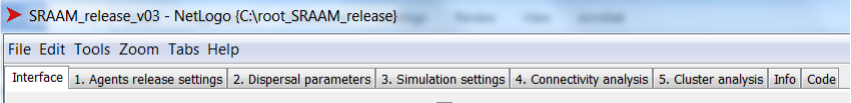
The SRAAM user interface is generated in Netlogo 5.3.1 using standard Netlogo interface
components and the Netlogo extension “xw” (~”Extra widgets”) supporting multiple tabs for user
interface customization. An overview of the primary tab is shown in Figure 2.
All SRAAM user inputs are organized in 3 standard Netlogo tabs and 5 tabs specific for SRAAM
user inputs. The 3 standard Netlogo tabs include:
- “Interface”
- “Info”
- “Code”
The tabs specific to SRAAM include 5 additional tabs
- “1. Agent Release Settings”
- “2. Dispersal Parameters”
- “3. Simulation Settings”
- “4. Connectivity Analysis”
- “5. Cluster Analysis”
The numbers 1-5 indicate the order of the typical workflow.
Figure 2. The SRAAM user interface in Netlogo is organized in to a number of tabs.
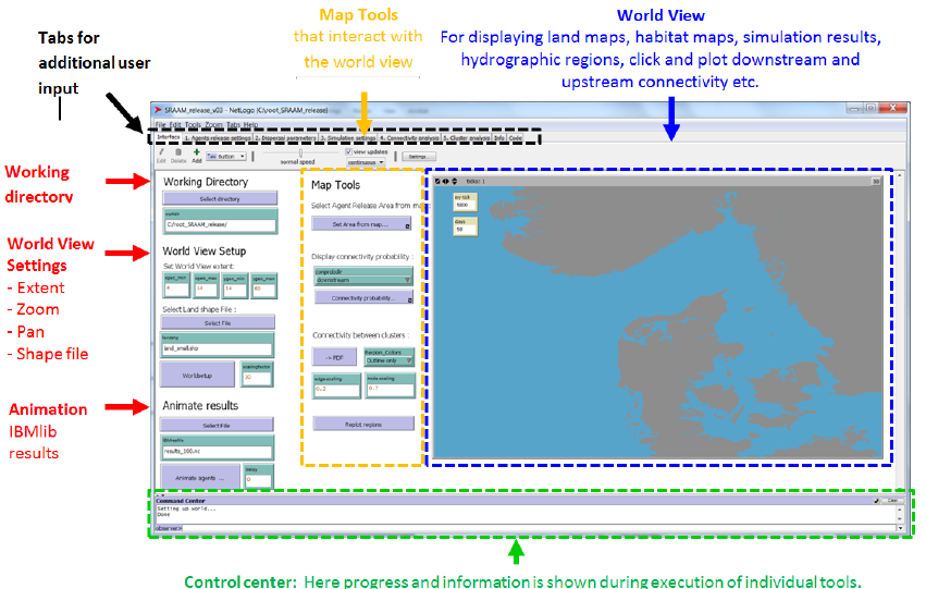
The standard Netlogo tab “Interface” is the main tab of Netlogo. This is where the “World view”
is located which is a 2D map display (see Figure 3). In SRAAM the “World view” represents the
extent of the geographical world to be analyzed, ideally identical to the extent of the
hydrographic data set used for dispersal modelling, or a subarea here-off. It is possible to add
shape files representing land or another polygon feature to be displayed within the world view
extent. SRAAM functionalities that interact directly with, - or that set the extent/zoom of, - the
world view, are all located in this tab to the left of the “Word view”.
The Standard Netlogo tab “info” is for adding information of the spedific netlogo file. Useful for
including documentation embedded in the *.nlogo file.
The standard Netlogo tab “code” holds all the SRAAM code executed when interacting with the
individual tabs.
10
The SRAAM specific tabs are ordered from 1 to 5 to reflect the typical order of required user
input, i.e. setting the parameters and input for the dispersal simulation and subsequent
simulation execution (1-3), calculation of the connectivity matrices based on the dispersal
simulation results (4) and finally delineating hydrographic regions based on the generated
connectivity matrices (5). The required input and procedures are described in detail in the
proceeding sections.
In addition to the SRAAM specific user interface components the standard Netlogo user
interface supports a number of standard functions for displaying, editing and programing agent
based model and agent based model results. To get acquainted with the standard Netlogo user
interface, please refer to the Netlogo Dictionary:
file:///C:/Program Files/NetLogo 5.3.1/app/docs/index2.html.
Or visit the Netlogo homepage:
https://ccl.northwestern.edu/netlogo/
Figure 3. The SRAAM tool Graphical User-Interface showing the Netlogo “interface” tab which is the main tab.
This is where the 2D map interface, the so called “World view”, is located. The “World View” (Blue) extent has
to be setup to represent the geographical extent (or parts) of the area covered by the hydrographic data to be
used for the agent dispersal simulation. Tools that interact directly (Orange) or indirectly (Red) with “World
view” are located to the left. In the top section of the interface (Black) the user has access to the SRAAM
specific tabs for user input. In the bottom section (Green) the Netlogo control center is located. This is where
progress and information is shown during execution of individual tools.
11
In addition to these tool specific sections, - the lower part of the “interface” tab consist of the
Netlogo “control center”. Here progress and information during SRAAM tool execusions are
shown. Also if some error may occur.
2.2 The “Interface” tab
The main tab in Netlogo is the “interface” tab. This is where the 2D map display referred to as
the ”World view” is located. The main tab is divided in to 4 main headings supporting user input:
- Working directory
For setting the working directory where all generated files are stored and where the
hydrographic data set needs to be located (see later)
- World view setup
For setting up the “World view” extent and specifying a shape file for land boundaries.
- Animate results
For animation of dispersal simulation results.
- Map tools
These are tools that interact directly with the “World view” by e.g. clicking or pointing
with the mouse curser.
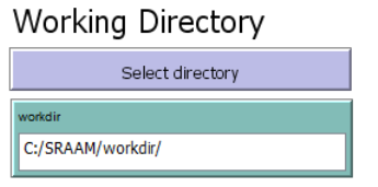
2.2.1 Working directory
The working directory has to be set for SRAAM to function properly. You can select any
directory location either by using the “Select directory” button, or by typing the path manually
into the “workdir” input box. Notice that the path has to be specified using forward slash. To
select a working directory click on the “Select directory” button:
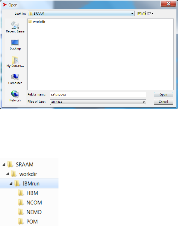
12
A windows explorer window will open. Select the working directory and click “open”:
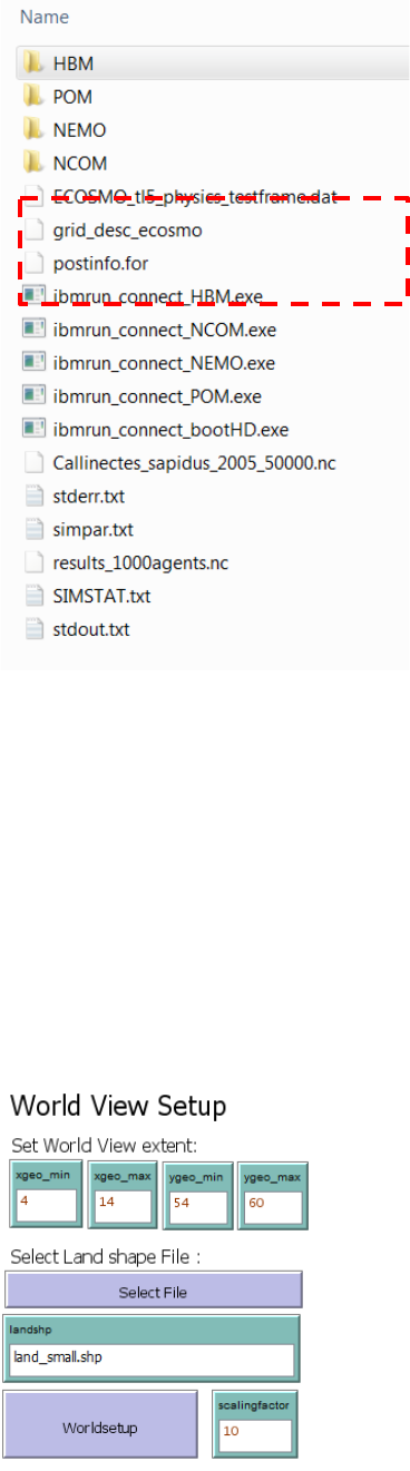
The only requirement is that the working directory include a subfolder name “IBMrun” where the
hydrographic data sets are stored. In the IBMrun-folder each hydrographic data set must be
stored in individual sub-folders named depending on the hydrographic data format:
In the “IBMrun” directory the IBMlib executable files have to be stored “IBMrun_connect_...
.exe”. The available IBMlib executables are:
- IBMrun_connect_HBM .exe
- IBMrun_connect_POM.exe
- IBMrun_connect_COARDS.exe
- IBMrun_connect_HDboot.exe
The latter “IBMrun_connect_HDboot.exe” is an IBMlib version that supports a dataset
comprising a single time-step of ECOSMO data for the NorthSea and the western Baltic Sea.
(4-14 degree east, 54 – 60 degree north). It is used for demonstration purpose only, and can
execute simulations within seconds or minutes. The IBMrun_connect_HDboot.exe does not
require a subfolder for storing hydrographic results. Instead 3 files has to be located in the
IBMrun-directory, - the 3 files are outlined in red below:
13
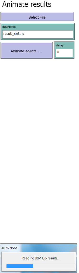
2.2.2 World view setup
Before any visualization of larvae dispersal trajectories or delineation of hydrographic regions
can be done, the World View needs to be setup to cover the model domain, or a part of the
model domain.
The settings include:
- Set World View extent
- Select Land Shape File
- Scaling factor
- World setup
14
Set World View Extent
The World View Extent is set by specifying minimum and maximum for the X and Y coordinates
respectively (xgeo_min, xgeo_max, ygeo_min, ygeo_max). The extent should cover the extent
of the hydrographic data set to be used, or a subarea hereof. To zoom into an area, the 4
parameters will have to be changed manually. Every time changes has been made, the “World
Setup” button must be activated.
Select Land Shape File
The land GIS file must be an ESRI shape file (*.shp) with land areas represented as polygons.
If the file name including the “shp”-extension is written manually without the path in the
“landshp” input box, the shape file set is assumed to be located in the working directory. If you
choose a file from another location using the “Select File” button, a prescript “…/’filename’” will
be included in front of the file name to indicate the file is not located in the working directory.
Scaling factor
The scaling factor is used as an easy option to set the visual extent of the World View within the
graphical user interface. E.g. if the scale factor is doubled the extent of the world view is
doubled in both the X and Y direction. This is useful e.g. when zooming into a small area (by
changing the min and max values of the X and Y coordinates of the World View extent) where a
small World View extent should be accompanied with an increase in the scaling factor. NOTICE!
If you by accident type a very large scaling factor the program may freeze.
World setup
This button executes the world view setup based on the settings set for the World View extent,
Scaling factor, and specified land shape file.
For more options controlling the World View the Netlogo World View customization can be
accessed by right click within the World View extent and select “edit” from the pop-up menu. For
details please refer to the Netlogo documentation.
2.2.3 Animate results
Once an IBMlib simulation has been successfully executed, the results can be animated in the
world view. The IBMlib stores results in a NetCDF data format (with the file extension “.nc”) with
a user specified time step frequency (see “Simulation setting” section). Animation of the results
displays the dispersal trajectories for all simulated agent time-step-by-time-step with the current
location represented by a point (red) and with the trajectories shown as a line (yellow).
Because IBMlib results may include unlimited number of agents, animations should only be
attempted for limited data sets: Depending on the PC an upper limit may be a simulation with a
maximum number of agents of 50 000, covering a simulation period of up to 1 year, and with
daily or weekly time step between stored results. If there is a need to display larger data files
one option could be to store only the last time step in the IBMlib simulation. This way the end
positions of larger data files can be displayed.
15
The settings in the animation section include:
- Select file
- Setting the “delay” – parameter
- Launch “Animate agents”
Select file
To select a IBMlib result file, click on the “Select file” button or write the name of the file
manually in the “IBMresfile” text input box. The file must be a NetCDF file (*.nc)
If the file name including the “nc”-extension is written manually without the path in the
“IBMresfile” input box, the file set is assumed to be located in the sub-directory “IBMrun” in the
working directory. If you choose a file from another location using the “Select File” button, a
prescript “…/’filename’” will be included in front of the file name to indicate the file is not located
in the working directory.
When a new IBMlib simulation is successfully executed the “IBMresfile” text input box is
automatically updated with the latest results file.
Delay-parameter
The “delay” parameter input box is an option for controlling the speed with which the agent
trajectories are animated in the World View. The default value is “0”. For small result files, e.g.
including 100-1000 agents the animation may be very fast, almost instantaneous, and setting
the “delay” paramter to 0.00001, 0.0001 0r 0.001 will slow down the animation. If the animation
takes too long or if the animation should be interrupted for some other reason, the animation
can be interrupted using the Netlogo “Halt” function located in the “Tools” menu.
Animate Agents
To animate the agent trajectories of the IBMlib result file, click on the “Animate Agents…”
button. A progress bar will be displayed while IBMlib results are loaded into Netlogo:
16
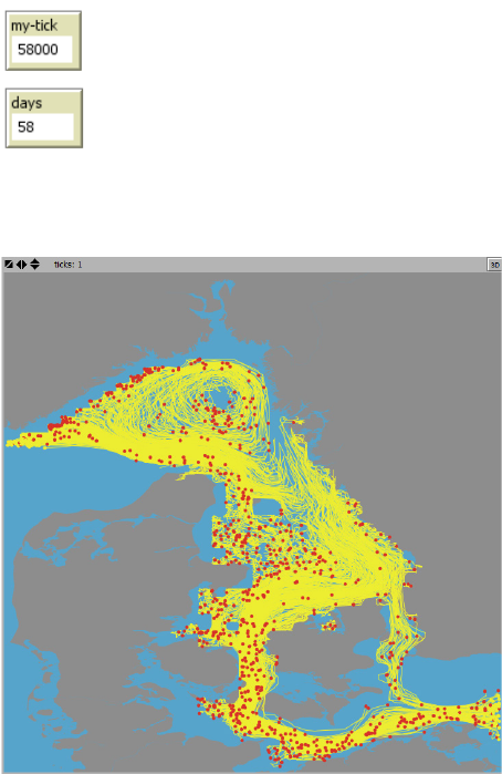
Agent trajectories are subsequently animated in the World View, see Figure 4. For keeping
track of the time step displayed during the animation two small info boxes are shown next to the
upper left corner of the World View,- counting the number of ticks as the product of number of
agents and the number of timesteps (“my-tick”) and the number of days (“days”) from the onset
of the animation, respectively:
Figure 4. Example of an animation of agent trajectories from a IBMlib simulation. Current agent positions is
shown as a “red” dot and where the individual trajectories prior to the “current” position is shown as a yellow
line track. Background colors: Grey = Land. Blue = water.
2.2.4 Map tools
The Map tools are tools which support user interaction with the World View. Therefore the
different tools are placed here in the “Interface” tab next to World View, but may serve very
different purposes, and support SRAAM functionalities otherwise organized in the SRAAM
specific tabs 1 – 5.
17
The tools include:
- Select agent release area from map
- Display connectivity probabilities
- Connectivity between clusters
- Replot regions
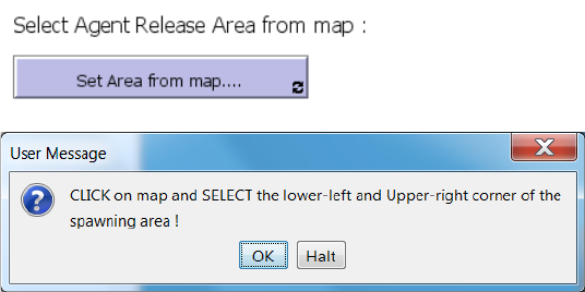
Select Agent Release Area from map
Prior to the execution of a IBMlib simulation initial positions of agents (~release positions) have
to be set. Agent release settings are set in the “1. Agent Release Settings” tab manually by
specifying X Y coordinates for a release area, or by specifying a habitat map representing an
outline of a species specific habitat for agent release. As an additional feature to specify X Y
corner coordinates, this tool support a World View interactive selection of a lower left and upper
right sets of corner coordinates by simply pointing and clicking in the world view.
The tool is activated by clicking on the “Set area from map…” and while activated (button
appears black), first the lower left corner is selected, then the upper right corner:
18
Figure 5. The Map tool ”Selelct Agent Release Area from map” where the user points at the lower left and upper
right corner coordinates of the Agent Release Area (red squares) and subsequently prompts the user for
accepting the input.
Once selected the user is prompted for accepting the input. Once accepted the corner
coordinates input boxes in the “1. Agent Release Settings” tab are updated.

19
Figure 6. The initial positions of agents (~agent release positions) of a simulation based on the corner
coordinates set using the Map Tool “Select Agent release area from map…” – see Figure 5.
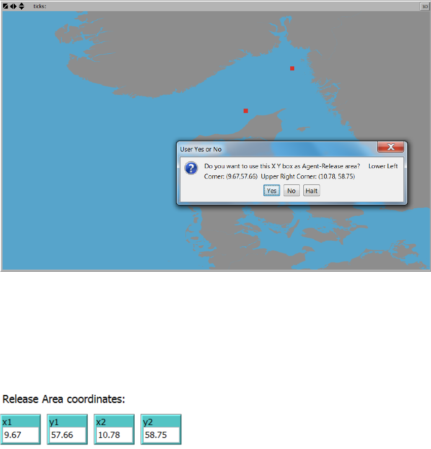
Display connectivity probability
This tool is included to explore the connectivity output from the connectivity analysis in more
detail. It is a click-and-plot tool, where a click at a specific location in the World View, will display
the corresponding “downstream” or “upstream” connectivity for that specific location in the
connectivity grid (see section “Connectivity Analysis” for details on connectivity analysis and
connectivity grid). “Downstream” connectivity refers to the probability that an agent with an initial
position corresponding to the selected grid cell in the connectivity grid will disperse to and end
up in any of the other grid cells in the connectivity grid. The “Upstream” connectivity refers to the
opposite direction, i.e. the probability that an agents that ends up in the user specified grid cell
in the connectivity grid, originates from any of the other grid cells in the connectivity grid.
“Downstream” and “Upstream” connectivity are selected from the pull down menu. Then press
the “Connectivity probability…” –button, and left click using the mouse cursor in the desired
location in the World View.
20
An example of “Downstream” and “Upstream” connectivity plots is shown in Figure 7. The
Minimum and maximum probability values of the graduated color legend is shown in the
Netlogo command center, e.g.:
To retrieve the exact value for each connectivity grid cell right click on the cell and from the
Netlogo pop-up menu choose “inspect patch ….” to access the patch values associated with the
specific location.
Figure 7. Examples of ”Downstream” (left) and ”Upstream” (right) connectivities using the click-and-plot tool
“Display Connectivity probability…”. Click positions indicated by blue arrows. Grey = Land. Blue = Zero values.
Red graduated colors = connectivity probabilities. Downstream connectivity legend max color (black/dark red)
= 0.07. Upstream connectivity legend max color (black/dark red) = 0.26.
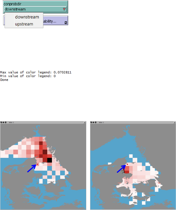
Connectivity between clusters
This tool is included to provide a more informative plotting representation of the hydrographic
regions derived from the cluster analysis (for details see the cluster analysis section). The tool
uses a graph representation of the hydrographic regions and their connections exported to a
pdf-format (see Figure 8).
The centroids of each region are indicated with numbered circles representing the graph nodes.
Numbers represent the coherence (or “self-recruitment”) of each region in percent, i.e. the
fraction of agents that have both their initial and their end positions in the same region. Lines

21
between nodes represent graph edges and indicate the direction (arrows) and probabilities (line
thickness) of the connectivity between regions. Two plot layouts are available, one displaying
regions as hollow polygons with colored outline, and on displaying regions as filled colored
polygons. Edge thickness and node-sizes can be modified using the “Edge-scaling” and “node-
scaling” parameters.
The tool uses the latest output from the Cluster Analysis for plotting (See Cluster Analysis
section).
To export the hydrographic regions from the latest cluster analysis, simply press “-> PDF”
button.
To select one of the two possible layouts select from the “Regions Colors” pull down menu, and
select between “Filled” or “Outline only”.
Thickness of the graph edges and size of the graph nodes are set in the “edge-scaling” and
“node-scaling” input boxes.
22
Figure 8. Examples of the output of the Map tool ”Connectivity between clusters” represented as graphs. Each
cluster or hydrographic region is assigned a unique color. The centroid of each region is indicated with a
numbered circle representing the graph nodes. Numbers represent the coherence (or “self-recruitment”) in
percent, i.e. the fraction of agents that have both their initial and their end positions in the same region. Lines
between nodes represent graph edges and indicate the direction (arrow) and probability (line thickness) of
connectivity between regions. The two plot show the same data, but the 2 different layouts.
Replot regions
The last Map tool is an option for replotting the hydrographic regions from the last cluster
analysis.
2.2.5 World View
Detail description of the World View and customization apart from what has been described in
the previous sections, please refer to the Netlogo documentation.
2.2.6 Command center
The Netlogo “control center” is located the bottom of the user interface. Here progress and
usefull information during SRAAM tool execusions are shown.

23
2.3 The “Agent Release Settings” tab
The “Agent Release Settings” tab is where parameters and inputs are set for specifying how
agent are “released” in the simulation.
The tab include:
- Select how to release agents
- Release area coordinates
- Release habitat map
- Agent release depth interval
- Agent release time
- Number of agents
2.3.1 Select how to release agent
Agents can be released in the model domain in two ways. Either by specifying corner
coordinates of the lower left and upper right corner of a rectangular release area, or by
specifying a habitat map.
24
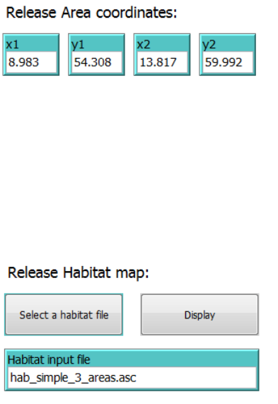
2.3.2 Release area coordinates
Release coordinates can be set manually by typing in the lower left and upper right corner
coordinates in x1, y1, x2 and y2 input boxes, or by using the tool “Select release area from
map…” located in the “Interface” tab (see section 2.2.4). The latter will automatically update the
input boxes accordingly.
2.3.3 Release habitat map
To specify a habitat map for agent release, click on the “Select a habitat file” –button and select
a habitat map file. The file must be an asci grid with the value 1 representing habitat, and a “no
data” value (-9999) representing no habitat. Notice that the resolution of the habitat grid may
affect input data processing time, so optimally use a relatively low resolution (a few grid cell as
possible still representing the habitat detail level necessary).
To show the habitat map in the World View, click the “Display” button and the “interface” tab will
be launched and the habitat map shown with light green color in the World View (see Figure 9).
If the habitat map does not show, check the coordinate extent of the habitat asci grid and that
the grid values have the right format.

25
Figure 9. Display of an ascii habitat map (green) used for agent release.
When using a habitat map the start position of each agent is selected randomly among habitat
grid cells, and also the position inside a grid cell itself is selected randomly in space. The time of
release is selected randomly from the release time interval specified (see section 2.3.5) ). All
random selections are assuming a uniform random distribution in time and space. This option
generates a single line for each agent in the IBMlib simulation parameter file “simapar.txt” (see
section 2.5). When simulating larger numbers of agents (e.g. >> 50 000) this may slow down
simulation time considerably. In such cases the agent release specification in the simpar.txt file
can be simplified by preparing the agent release specification using at text editor to edit the
simpar.txt file.
The section in the Simpar.txt file for agent release looks like this:
! ===============================================================
! Release dynamics
! ================================================================
dry_emission_boxes = ignore
!
emitbox = 2009 03 02 0 2009 03 02 0 11.44 56.53 0 11.93 57.12 0 100 par1 5.6 whatever

26
Any number of emitbox-lines can be included and uses the following syntax:
For more information see the IBMlib user manual: https://github.com/IBMlib/IBMlib .
2.3.4 Agent release depth interval
The Agent release depth interval refers to the vertical distribution of the initial position of the
agents. To specify an absolute depth interval use negative values. To specify relative depth
interval use positive values between 0 and 1. Zero values refer to the surface. Minimum and
maximum depths are specified in the “Min depth” and “Max depth” input boxes.
2.3.5 Agent release time
Time interval for agent release is speicified in the “Start time” and “End time” input boxes. The
format used is: “YYYY MM DD h”
2.3.6 Number of agents
The total number of agent be released in the IBMlib simulation is given as an integer and
specified in the “No. of agents” input box.
27
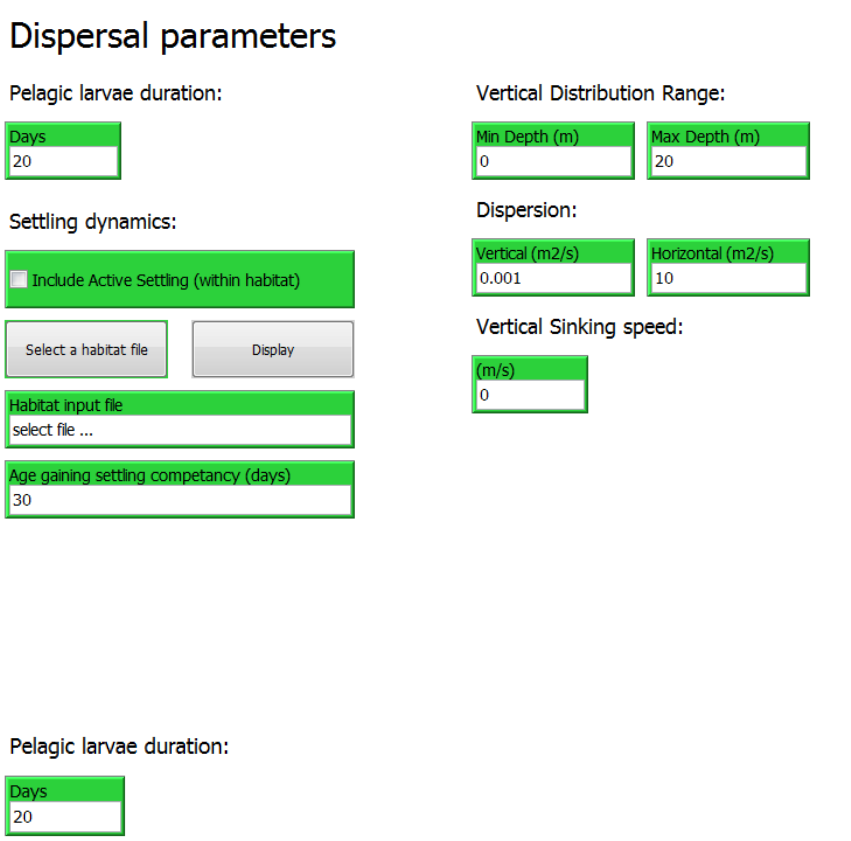
2.4 The “Dispersal parameters” tab
The “Dispersal parameters” tab is where parameters and inputs are set for specifying how agent
are dispersed during in the IBMlib simulation.
The tab include settings for:
- Pelagic Larvae Duration (PLD)
- Settling dynamics
- Vertical distribution range
- Dispersion
- Vertical sinking speed
2.4.1 Pelagic Larvae Duration (PLD)
The Pelagic Larvae Duration (PLD) is the duration of the pelagic life stage where the organism
is suspended in the water column and subject to drift. The PLD is specified in the “Days” input
box with the unit “days”.
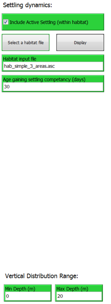
2.4.2 Settling dynamics
Settling dynamics is an option to mimic active settling behavior, i.e. a behavior observed in
some species where pelagic larval stages at a certain age achieve settling competency, e.g.
28
coral larvae. When settling competency is achieved, the larvae may settle if exposed to the right
environmental cues. Such a behavior can optimize settling so that it happens when the
organism is conveyed to an area where habitat conditions are favorable.
To enable settling dynamics the check box “Include Active Settling (within habitat):
To select a habitat file for settling click the “Select a habitat file” button and select a habitat file
from any location. If the habitat file is not located in the SRAAM working directory a prefix “…/”
will be shown in front of the file name. The habitat file must be an asci grid format (*.asc) similar
to the habitat file specified for agent release, see section 2.3.3.
Notice that if a habitat file has been specified in the “1.Agent Release Settings” –tab the “habitat
input file” input text box in the “Settling dynamics” section is automatically updated with the
same habitat file. For most organisms the same habitat support both spawning and settling.
However for some species like many fish species spawning and settling habitats are not
identical. Although in SRAAM the settling habitat can be specified as different from the release-
(or spawning) habitat, please notice that the clustering techniques available in SRAAM for
analyzing the connectivity matrices may not give meaningful results.
The competency age is specified in the input box “Age gaining settling competency (unit: days).
2.4.3 Vertical Distribution range
The vertical position of the simulated agents during simulation can be limited to a vertical
distribution range by setting minimum and maximum depths as positive number, in the “Min
Depth” and “Max depth” input boxes.
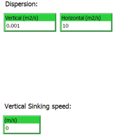
29
2.4.4 Dispersion
The vertical and horizontal dispersion coefficients are specified in the “Vertical (m2/s)” and
“Horizontal (m2/s)” input boxes. The dispersion coefficient can be included in the simulation to
represent hydrodynamic processes not resolved by the hydrodynamic data and/or to represent
spatial (and random) dispersal due to biological behavioral processes. The vertical dispersion is
limited by depth interval specified in the previous section.
2.4.5 Vertical Sinking speed
A vertical sinking speed can be set at se constant speed (m/s) in the “(m/s)” input box. By
combining the vertical sinking speed with the vertical dispersion parameter and the depth
distribution range, the vertical distribution of agents can be biased towards the upper or lower
vertical distribution range.
2.4.6 Diurnal vertical migration
Pelagic stages of many aquatic species exhibit more or less pronounced diurnal vertical
migration (DVM), e.g. by migrating towards the surface when light disappears at dusk, and
towards the deeper parts when light increases during dawn. DVM is not included as an option
in the SRAAM user interface, however, IBMlib supports DVM and settings has to be added
manually to the IBMlib simulation parameter file “simpar.txt”.
active = 2 ! (0=no active swimming, 1=keep within depth min and max, 2=DVM)
swim_depth_min = 0 ! [m] upper confinement level > 0 (active>0)
swim_depth_max = 20 ! [m] lower confinement level (or sea bed, if shallower) (active>0)
swim_speed_light = 0 ! [m/s] swim speed when light, positive down (active = 2)
swim_speed_dark = 0 ! [m/s] swim speed when dark, positive down (active = 2)
30
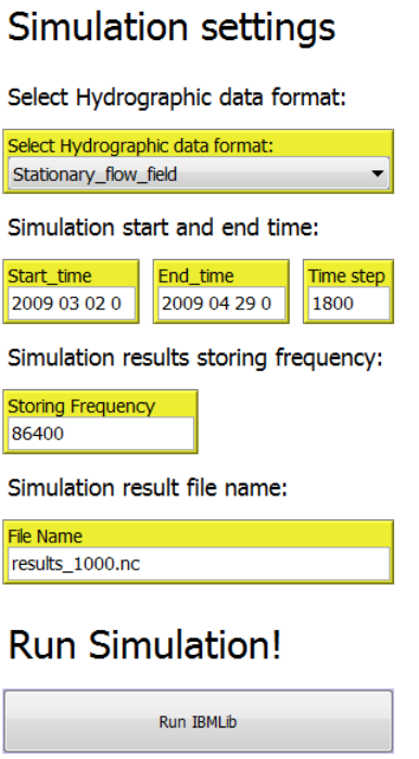
2.5 The “Simulation Settings” tab
The “Simulation Settings” tab is where parameters are set for specifying the simulation
parameters for the IBMlib simulation.
The tab includes:
- Select hydrographic data format
- Simulation start and end time
- Simulation results storing frequency
- Simulation result file name
- Run simulation

31
2.5.1 Select Hydrographic data format
The hydrographic data to be used for the IBMlib dispersal simulation has to be selected from
the “Select Hydrograhpic data format” pull down menu. The formats currently available and
format discriptions are found in section 3. Apart from the “Stationary_flow_field” the each data
set has to be stored in a subfolder with the same name in the IBMrun directory., i.e.. “HBM”,
“POM”, “NEMO” and “NCOM”.
2.5.2 Simulation start and end time
Simuation start and end time has to specified in the input boxes “Start time” and “End time”
respectively. The format used is “YYYY MM DD h”. The IBMlib simulation time step must be
specified in the “Time step” input box (unit: seconds).
2.5.3 Simulation results storing frequency
The IBMlib simulation results storing frequency has to be specified in the “Storing Frequency”
input box (unit: seconds).
2.5.4 Simulation result file name
A file name for the IBMlib results has to be specified in the “File name” input box. The file name
must have the file extension “.nc”. The file will be saved to the “IBMrun” folder located in the
working directory.

32
2.5.5 Run simulation
To start the IBMlib simulation click on the “Run IBMlib” button.
During the IBMlib execution in addition to the IBMlib result file three files are saved to the
IBMrun-folder:
SIMSTAT.txt
The file stores the simulation progress i.e. the number of that completed time steps, and the
total number for time steps in the simulation.
stout.txt
This file is the IBMlib simulation log file. In case IBMlib execution fails to complete, the log file
may provide information on when or why the execution stopped.
sterr.txt
Explicit IBMlilb execution errors will be displayed here.
The IBMlib result file is stored in a NetCDF file format . The file include up to 19 variables:
19 variables (excluding dimension variables):
float topolon[nxtop]
meaning: topography sampling zonal grid
unit: degrees East
float topolat[nytop]
meaning: topography sampling meridional grid
unit: degrees North
float topography[nytop,nxtop]
meaning: topography sampling on grid
unit: meters below sea surface
float lon[nparticles,nframes]
meaning: particles zonal position
unit: degrees East
float lon0[nparticles]
meaning: particles zonal initial position
unit: degrees East
float lat[nparticles,nframes]
meaning: particles meridional position
33
unit: degrees North
float lat0[nparticles]
meaning: particles meridional initial position
unit: degrees North
int time[i4,nframes]
meaning: time corresponding to particles frames
unit: year, month, day, second_in_day
float depth[nparticles,nframes]
meaning: particles vertical position
unit: meters below sea surface
float depth0[nparticles]
meaning: particles vertical position
unit: meters below sea surface
byte is_out_of_domain[nparticles]
int is_settled[nparticles]
float age_at_settling[nparticles]
float degree_days[nparticles]
float max_temp[nparticles]
float min_temp[nparticles]
float max_salt[nparticles]
float min_salt[nparticles]
float connectivity_matrix[nsource,ndest]
meaning: probability of particle transport
unit: 0 < probability < 1
34
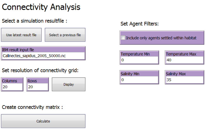
2.6 The “Connectivity Analysis” tab
The “Connectivity Analysis” tab is where parameters are set for the connectivity analysis. The
connectivity analysis requires a subdivision of the study area into smaller areas (a connectivity
grid). The IBMlib results are analysed and translated into a connectivity probability matrix that
represents the probability that an agent released in on sub-area ends up in any other subarea. If
the study area is divided into 20x20 grid, a total of 400 subareas are included, and the
connectivity probability matrix will express all pairwise connectivity probabilities,i.e. in a 400x400
matrix.
The tab includes :
- Select a simulation result file
- Set resolution of connectivity grid
- Set Agent Filters
- Create Connectivity Matrix
35
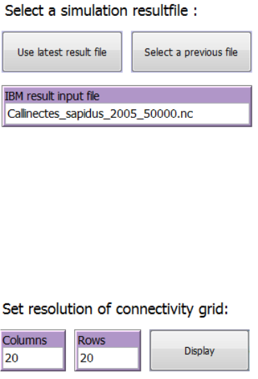
2.6.1 Select a simulation result file
To select the IBMlib result file to be used as input to the connectivity analysis, click on “Use
latest result file” to use the latest IBMlib result file generated, or click on “Select a previous file”
to select file from any location. The file name will be shown in the “IBMlib result input file” input
box. If the file is not located in the IBMrun subdirectory of the working directory, the file name
will include a prefix “…/”.
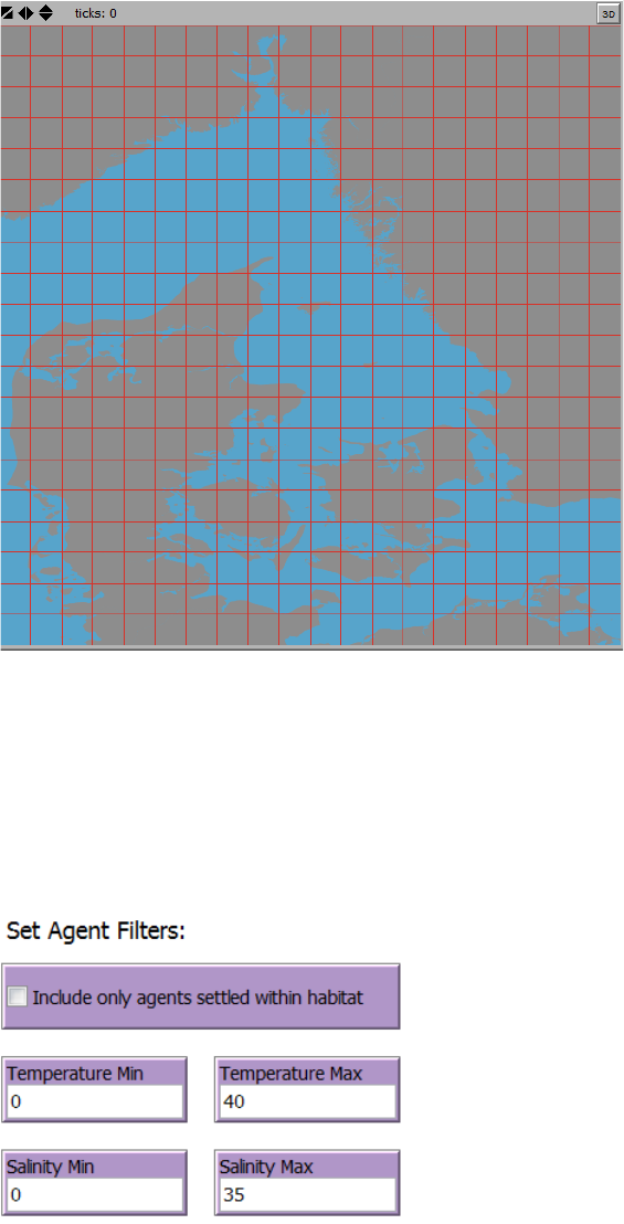
2.6.2 Set resolution of connectivity grid
The connectivity grid is specified as number of columns and rows in the input boxes “Columns”
and “Rows”, and will divide any current extent of the World View into the number of rows and
columns specified. To show the resulting grid on the current World View extent press “Display”
button, see Figure 10.
36
Figure 10. An example of a connectivity grid as specified in the “Connectivity Analysis” tab in the section “Set
resolution of connectivity grid”. Here the number of columns and number of rows are set to “20”. Note that the
extent of the connectivity grid is defined by the current extent of the World View.
2.6.3 Set Agent Filters
It is possible to apply filters to the IBMlib result file used in the connectivity analysis.
To include only agents that successfully settle within a settling habitat (as specified in the
“Dispersal parameters” tab (see section 2.4.2) mark the check box “Include only agents settled
within habitat”.
37
To include only agents that disperse within a given temperature tolerance interval set the
minimum and maximum temperature (as degree Celsius) in the “Temperature Min” and
“Temperature Max” input boxes.
To include only agents that disperse within a given salinity tolerance interval set the minimum
and maximum salinity (as PSU) in the “Salinity Min” and “Salinity max” input boxes.
Note that salinity and temperature filters are based on the minimum and maximum values of
salinity and temperature experienced by each agent during the entire simulation. I.e. if the
salinity or temperature experienced by an agent exceeds a threshold value in a single time step
the agent will be excluded from connectivity analysis.
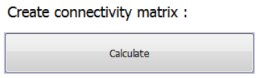
2.6.4 Create Connectivity Matrix
To calculate the connectivity adjacency and connectivity probability matrices press “Calculate”.
This may take some time depending on the size of the result file. The agent filter “Include only
agents settled within habitat” may be time consuming depending on the resolution of the habitat
grid applied. Progress bar will inform on the progress of the individual steps. Note that progress
bars may be hidden behind you program interface depending on the PC settings.
The output of the connectivity analysis calculation are stored in a number of csv-files located in
the working directory: sourcelist.csv and sourcelist_hab.csv
These comma separated files are used as input for the cluster analysis, see next section.
sinklist.csv and sinklist_hab.csv
These comma separated files are used as input for the cluster analysis, see next section.
conmatnos_colllist.csv
This is a comma separated file storing the connectivity adjacency matrix
conmatprob_collist.csv
This is a comma separated file storing the connectivity probability matrix
NOTICE: if any of the csv-files has been opened by other programs such as spreadsheets or
GIS software, the “Calculate” connectivity matrix may return an unspecified error. Close the
programs used for opening the csv-files and try again.
To display the density and distribution of initial positions of agents included in the connectivity
analysis a grid showing the density of initial positions are shown in the World View when the
connectivity matrices calculations are done. The grid is saved to an ascii grid file “ininopar.asc”
stored in the SRAAM working directory and can be imported in to a GIS system. The minimum
and maximum values of the grid color legend is shown in the command center. To inspect
38
individual values, right click on the grid cell in the world view, and select “Inspect patch…” from
the Netlogo pop-up menu to access patch values.
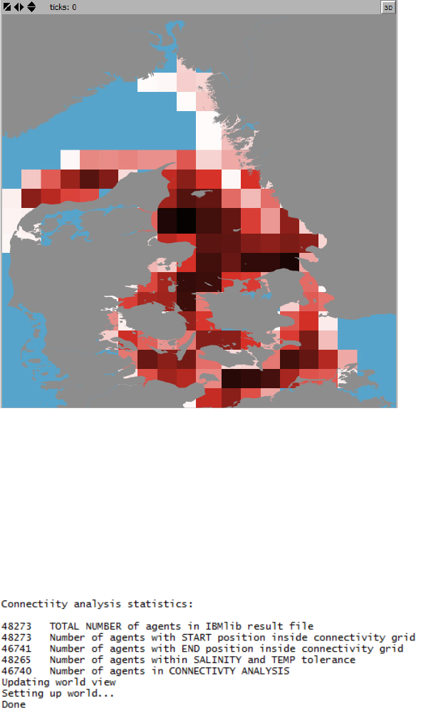
Figure 11. Example of the grid produced by the connectivity analysis showing the densities of initial positions
of agents included in the connectivity analysis. Legend (Minimum value – 2 , Maximum value – 785).
In the control center the connectivity analysis statistics are displayed. Depending on the agent
filters settings and the extent covered by the connectivity grid, the final number of agents
included in the connectivity analysis may be considerably smaller than the number of agents
released originally in the IBMlib simulation. An example is given below:
39
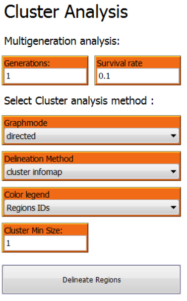
2.7 The “Cluster Analysis” tab
The “Cluster Analysis” tab is where parameters are set for the delineation of hydrographic
regions using cluster analysis.
The current version of SRAAM supports the clustering method named “Infomap” (Rosvall and
Bergstrom 2008). This clustering techniques is based on information theory principles and has
been used recently to delineate hydrographic regions in the Mediterranean, see: Vincent et
al.(2014). The use of Infomap requires that the connectivity probability matrix is converted into a
graph (i.e. as in the context of Graph Theory) where graph nodes represent each sub-area in
the connectivity grid, and where pairwise connectivity probabilities are translated into weights of
graph edges between nodes in a directed graph (“directed” refers to the connectivity probability
from A to B may be different from the connectivity probability from B to A). The tab is prepared
to include more alternative cluster techniques in future versions of SRAAM.
The cluster analysis tab provides an option for including multiple generation clustering
mimicking the dispersal of organisms through multiple generations and with a given between-
generations survival probability. Multiple generation connectivity probabilities are simply
calculated by multiplying the connectivity probability matrix by itself a number of times
corresponding to the number of generations. The connectivity probabilities between generations
can be adjusted assuming a constant survival rate. Note that this way of analyzing the
connectivity across multiple generations is a strong simplification and the outcome will be highly
dependent on which hydrographic year is used, the number of generations included and the
survival rate assumption applied.
40
The tab includes:
- Multiple generation analyses
- Select Cluster analysis method
- Delineate Regions
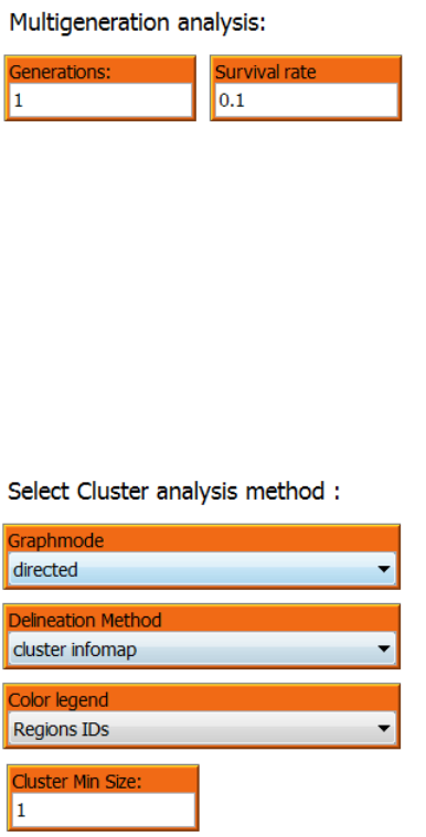
2.7.1 Multiple generation analysis
To include multiple generation connectivity in the cluster analysis, specify an integer different
from “1” in the “Generations” input box. A between generations survival rate can be specified in
the “Survival rate” input box.
2.7.2 Select Cluster analysis method
The cluster analysis option currently includes only one method “Infomap”. The user interface is
prepared for adding additional clustering methods. Currently the pulldown menu’s show, i.e.
“Graphmode”, “Delineation method” and “Color legend” are included for information only.
The minimum size of hydrographic regions generated using the cluster analysis method can be
set in the “Cluster min Size” input box. The “size” refers to the number for sub-areas or grid cells
in the connectivity grid.
41
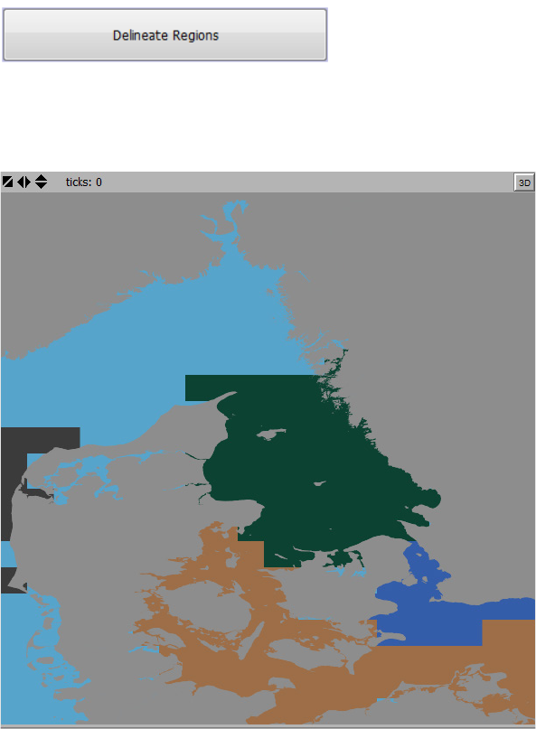
2.7.3 Delineate Regions
To execute the cluster analysis and delineate hydrographic regions, press the “Delineate
Regions” button.
When the cluster analysis finalizes, the delineated hydrographic regions are shown in the World
View, see Figure 12.
Figure 12. Hydrographic regions displayed in the World View following the termination of the cluster analysis.
This example show 4 regions with unique colors.
To display the hydrographic regions using a graph representation use the “Connectivity
between clusters” Map tool (see section 2.2.4) located in the “Interface” tab next to the World
View.
A number of outputs of the cluster analysis are saved to the SRAAM working directory and can
be used for use in a GIS environment. The outputs include:
hydregids.asc
this is an ascii grid file with values representing the hydrographic regions IDs.
42
centroids.shp
This is a point shape file representing the hydrographic regions as graph nodes, with
geographical positions corresponding to the centroids of areal extent of the hydrographic
regions. There are 6 fields in the centroids.shp attribute table:
Id The ID of the hydrographic region
Lat The geographical latitude of the node position (~centroid of the region extent)
Long The geographical longitude of the node position (~centroid of the region extent)
Cohprob The coherence as probability
Cohnos The coherence as absolute number of agents
Ininos The initial number of agents included in the connectivity analysis
edges.shp
This is a line shape file representing the connectivity probability between hydrographic regions
as graph edges. Note that the graph representation is directional so that there may be 2 edges
between 2 nodes, which cannot be seen using default GIS plotting since the edges overlap.
There are 9 fields in the edges.shp attribute table:
Id The ID of the hydrographic region
From The “from” ID of the edge
To The “to” ID of the edge
Weight The the weight of the edge corresponding to connectivity probability
lat1 The latitude of the “from” node position
long1 The longitude of the “from” node position
lat2 The latitude of the “to” node position
long2 The longitude of the “to” node position
nos The total number of agents exported from “from” node to “to” node
clconnos.csv
this is a comma separated data file representing a matrix with between cluster connectivities
with values representing absolute numbers.
clconprob.csv
This is a comma separated data file representing a matrix with between cluster connectivities
with values representing probabilities.
43
2.8 Tips and tricks
It is possible to work with SRAAM without the use of the user interface
2.8.1 IBMlib execution
The IBMlib execution can be done from a windows command line, or windows batch file for
multiple simulations to be executed one by one, e.g.
C:\workdir\ibmrun\ibmrun_connect_HBM.exe simpart1.txt > stdout.txt
C:\workdir\ibmrun\ibmrun_connect_HBM.exe simpart2.txt > stdout.txt
C:\workdir\ibmrun\ibmrun_connect_HBM.exe simpart3.txt > stdout.txt
Etc.
To generate a simpar.txt file open an existing simpart.txt file in a text editor and change the
sections accordingly. I SRAAM each time you click “Run IBMlib” a new simpar.txt file is created.
Before the IBMlib executes, the user is prompted for if the IBMlib execution should proceed. If
“No” the simpar.txt file is generated and located in the IBMrun sub-folder, but without execution.
The simpar.txt can then be replicated and edited to create any number of simpar.txt files to
support batch execution of IBMlib. Make sure that the “output” filename in each “simpar.txt” file
are assigned a unique filename to avoid files to be overwritten. To disable the IBMlib logfile add
" > NUL" to the end of the IBMlib command syntax instead of " > stdout.txt".
2.8.2 R-scripts
The individual calculation procedures in SRAAM is carried out using R, by translating the input
in the SRAAM user interface to R-scripts that are subsequently executed. The generated scripts
are automatically save to the SRAAM working directory. The scripts included are summarized
below.
Reading IBMlib results
ncdf2array.r
This script reads all time steps and agent positions of the IBMlib result file ( ~ NetCDF file). It is
used for animation of agent trajectories stored in the IBMlib result file.
Agent release boxes
relhabasc2ibmlib.r
This script is used to create the “Release dynamics” section in the IBMlib simulation parameter
file “simpar.txt” when the agent release are based on a user specified habitat file. The script
creates one line in the simpar.txt file for each agent where the initial position and initial time is
sampled randomly from the spatial habitat extent and the user specified release start and end
dates.
Agent settling boxes
sethabasc2ibmlib.r
44
This script is used to create the “Settlement dynamics” section in the IBMlib simulation
parameter file “simpar.txt” when the agent settlement is based on a user specified habitat file.
The script creates one line for each grid cell in the habitat ascii grid with values different from
“no-value” (= -9999).
Connectivty grid
conmatpolylines.r
The script generates a line shape file (congridlinesxy.shp) with the lines representing the outline
of the connectivity grid subdivision. The file(s) is saved to the SRAAM working directory. Notice
that the origo of the file is per default (0,0) because the extent is linked directly to the World
View setup. To display the shape file correctly in a GIS you need to set the correct origo
coresponding the coordinate system applied.
Connectivity matrices
conmat.r
This script calculates the connectivity matrices (absolute numbers and probabilities) based on
the IBMlib simulated agent trajectories, the specified connectivity grid and the agent filters. The
output of the script include:
Conmatnos_collist.csv - the connectivity matrix, values representing absolute numbers
Conmatprob_collist.cv - the connectivity matrix, values representing probabilities
Sourcelist_hab.csv - list with agent ID, start position X and Y
Sinklist_hab.csv - list wit agents ID, end positions X and Y
Ininopar.asc - an Asciii grid with the number of agents included in the connectivity analysis
with start positions in each grid cell in the connectivity grid. This is the output shown in the
World View after termination of the connectivity analysis.
Cluster analysis
cluster.r
This script performs the cluster analysis based on the connectivity matrices calculated. The
script saves the cluster analysis output, the hydrographic regions, as an ascii grid file with
numbers representing hydrographic region ID’s. The file “hydregids.asc” is saved to the working
directiory.
Between clusters connectivity
clconmatrix.r
The script calculates the between clusters connectivity in terms of absolute numbers and
probabilities. The output include:
Centroids.shp - point shape file representing regions as graph nodes (see
section 2.7.3)
45
Edges.shp - line shape file representing regions connectivity as graph edges
(see section 2.7.3)
Clconnos.csv - between clusters connnectiviy matrix as absolute numbers (see
section 2.7.3)
Clconprob.csv - between clusters connectivity martrix as probabilities. (see
section 2.7.3)
Hydrographic regions PDF plot
clcon2pdf
This script creates a graph representation of between clusters connectivity in terms of “nodes”
and “edges” representing “hydrographic regions” and “between regions connectivity”
respectively. The graph is saved as temporary pdf file and opened in the default pdf viewer or
browser.
46
3. Hydrographic data formats
The normal way to interface IBMlib with a new hydrographic format is to add a new physical
interface layer that couples the data set to IBMlib. This procedure does not require reformatting
of the hydrographic data set, but IBMlib can then read data as-provided. Alternatively, one can
recast (~translate) a new hydrographic data set into a format corresponding to an already
implemented interface; this alternative should be pursued with caution, because (i) recasting
may involve numerical truncation and thus accuracy loss and (ii) recasting may be faulty
because the translator either have misunderstood the native hydrographic format or the format
specification and (iii) some special features of the hydrographic data set may be lost because it
can not be represented by the target format. Extensive testing is therefore recommended before
actual result generating runs are performed.
IBMlib on this web site comes in 4 pre-compiled versions: (i) at hydrographic testing
environment, based on a realistic hydrographic model, (ii) a version reading a generic data
format, based on the POM output format, (iii) a version reading COARD-compliant data formats,
e.g. NEMO and NCOM output, and (iv) a version reading the HBM data format.
3.1 Bootstrapped testing configuration
In many practical applications of individual-based simulations in marine environments, the
simulation is conducted off-line, i.e. hydrographic data is loaded from a precomputed database,
which contains hydrographic data for the time period, where the simulation is conducted. The
most time consuming part is loading hydrographic data from the database, which often contains
TB of data. To speed up the production cycle during a testing phase, it is useful have a testing
environment, which limits time-consuming data reading from the hydrographic database. One
trick to do this is to recycle a hydrographic time frame (~time step) over and over again, rather
than loading a new data frame for each time point; we call this the bootstrapped hydrography
mode. In this way, one can test a setup in a setting with a realistic topography and hydrographic
variability, but without temporal variability. The precompiled bootstrapped version on this web
site is based on the ECOSMO (Schrum et al, 1999; 2006) coupled physical-biogeochemical
model, and the SRAAM setup files include a single time frame of hydrography. The testing area
is the North Sea/Baltic region with 10 km horizontal resolution, and only the physical variables
enabled.
3.2 Generic POM data format
The suggested target format for recasting is based on the POM (Blumberg and Mellor, 1987)
output layout, which is relatively simple and transparent; the abundance of regional POM setups
also gives a chance that very little data transformation actually has to be done. The format will
support many typical usages of IBMlib. The target grid is regular longitude-latitude (with
arbitrary user provided longitude-latitude spacing), with vertically sigma-type (with number of
layers specified by user), dynamic sea-level elevation and arbitrary topography. Data is stored
as daily averaged hydrography data frames with a filename corresponding to the date. The
format is stored in netCDF (see http://www.unidata.ucar.edu/software/netcdf/) and consists of:
47
(1) A grid desciptor file "grid.nc"
(2) A sequence of daily hydrography frames with filename "hydrography_YYYY_MM_DD.nc"
where (YYYY, MM, DD) is year, month and day-in-month number, respectively, with prepended
zeroes as necessary, i.e. hydrography for February 15 2016 should be stored in file
"hydrography_2016_02_15.nc". For convenience, the grid desciptor file may be merged with
each hydrography file, but this requires a little extra storage, because the grid desciptor is
duplicated many times. The templates for grid desciptor and hydrography frames are provided
"grid.CDL" and "hydrography_YYYY_MM_DD.CDL" (see sections 3.2.1 and 3.2.2 respectively).
CDL is the text translation of netCDF, so these files show exactly what IBMlib expects - just
show the CDL file to your hydrography data provider. The period where you can conduct
simulations correspond to the period covered by files hydrography_YYYY_MM_DD.nc. At
runtime IBMlib tries to read the needed files hydrography_YYYY_MM_DD.nc and stops, if the
file is not found (with the expected filename in the expected folder). You don't have to structure
or declare the hydrographic database further, just place expected files in the path announced in
the simulation input file with the proper names hydrography_YYYY_MM_DD.nc. In SRAAM the
expected folder is the “POM” folder in the “IBMrun” directory located in your working directory.
If the format for one reason or another does not support your specific needs, it is recommended
that you follow instructions within IBMlib for creating a specific physical interface for the data set
and recompile IBMlib for your setup (see: https://github.com/IBMlib/IBMlib). IBMlib is free and
open source, but if you are not familiar with fortran programming and code compilation, you may
contact the IBMlib developers to explore possibilities and conditions for a collaboration. Below
you will find the content of "grid.CDL" and "hydrography_YYYY_MM_DD.CDL" that can be
copied and pasted into a plain text file, if needed.
3.2.1 Grid descriptor file format
// --------------------------------------------------------------------------------------------
// Grid is regular longitude-latitude (with arbitrary user provided longitude-latitude spacing),
// vertically sigma-type (with number of layers specified by user), dynamic sea-level elevation
// and arbitrary topography. This grid descriptor may be embedded in each hydrographic data
// frame hydrography_YYYY_MM_DD for simplicity.
// POM employs sigma coordinates, which are bottom-following coordinates that map the
vertical
// coordinate from the vertical coordinate from -H < z < eta onto -1 < sigma_POM < 0, where z is
// -depth below ref level (not sea surface)
// H > 0 is the static variable h(x,y) (in grid file) loaded into wdepth0
// eta is dynamic variable elb(x,y) (in physics file) )
// fsm > 0.0 for wet points, fsm == 0.0 for dry points
// --------------------------------------------------------------------------------------------
netcdf grid {
dimensions:
x = 182 ; // longitude grid points
y = 125 ; // latitude grid points
z = 35 ; // vertical grid points
variables:
double zz(z) ;
48
zz:long_name = "sigma of cell centre" ;
zz:units = "sigma_level" ;
zz:standard_name = "ocean_sigma_coordinate" ;
zz:formula_terms = "sigma: zz eta: elb depth: h" ;
double east_e(y, x) ; // cell centers
east_e:long_name = "easting of elevation points" ;
east_e:units = "degree" ;
east_e:coords = "east_e north_e" ;
double north_e(y, x) ; // cell centers
north_e:long_name = "northing of elevation points" ;
north_e:units = "degree" ;
north_e:coords = "east_e north_e" ;
double h(y, x) ; // at cell centers
h:long_name = "undisturbed water depth" ;
h:units = "metre" ;
h:coords = "east_e north_e" ;
double fsm(y, x) ;
fsm:long_name = "free surface mask" ;
fsm:units = "dimensionless" ;
fsm:coords = "east_e north_e" ;
// global attributes:
:title = "black_sea" ;
:description = "POM grid file" ;
}
3.2.2 Hydrographic data format
// ------------------------------------------------------------------------------
// POM employs sigma coordinates, which are bottom-following coordinates that map the
// vertical coordinate from the vertical coordinate from -H < z < eta onto -1 < sigma_POM < 0, /
// where z is -depth below ref level (not sea surface)
// H > 0 is the static variable h(x,y) (in grid file) loaded into wdepth0 eta is dynamic variable
// elb(x,y) (in physics file) )
// nz is number of faces vertically so that the number of wet cells is nz-1 vertically.
// Cell-centered arrays like t (temperature) are padded with an arbitrary value in last
// element iz=35 (surface cell at iz=1)
// netCDF variable w(x,y,z) refers to vertical faces (not cell centers), so w(x,y,1) ~ 0
// at sea surface and w(x,y,nz=35) = 0 at the sea bed.
// Currently load these fields (in native units/conventions, c-declaration index order):
// float elb(y, x) = "surface elevation in external mode at -dt" units = "metre" ;
// staggering = (east_e, north_e)
// float u(z, y, x) = "x-velocity" units = "metre/sec" ;
// staggering = (east_u, north_u, zz)
// float v(z, y, x) = "y-velocity" units = "metre/sec" ;
// staggering = (east_v, north_v, zz)
// float w(z, y, x) = "sigma-velocity" units = "metre/sec" ;
49
// staggering = (east_e, north_e, z)
// float t(z, y, x) = "potential temperature" ; units = "K" ;
// staggering = (east_e, north_e, zz)
// float s(z, y, x) = "salinity x rho / rhoref" ; units = "PSS" ;
// staggering = (east_e, north_e, zz)
// float rho(z, y, x) = "(density-1000)/rhoref" ; units = "dimless"
// staggering = (east_e, north_e, zz)
// float kh(z, y, x) = "vertical diffusivity" ; units = "m^2/sec";
// staggering = (east_e, north_e, zz)
// float aam(z, y, x) = "horizontal kinematic viscosity" ; units = "metre^2/sec";
// staggering = (east_e, north_e, zz)
// u(ix,iy,iz) in grid position (ix-0.5, iy , iz) (i.e. western cell face)
// v(ix,iy,iz) in grid position (ix , iy-0.5, iz) (i.e. southern cell face)
// w(ix,iy,iz) in grid position (ix , iy, iz-0.5) (i.e. upper cell face)
// The boundary condition: w( ix, iy, nz+0.5 ) = 0 is implicit
// ------------------------------------------------------------------------------
netcdf hydrography_YYYY_MM_DD {
dimensions:
z = 35 ;
y = 125 ;
x = 182 ;
variables:
float elb(y, x) ;
elb:long_name = "surface elevation in external mode at -dt" ;
elb:units = "metre" ;
elb:coordinates = "east_e north_e" ;
float u(z, y, x) ;
u:long_name = "x-velocity" ;
u:units = "metre/sec" ;
u:coordinates = "east_u north_u zz" ;
float v(z, y, x) ;
v:long_name = "y-velocity" ;
v:units = "metre/sec" ;
v:coordinates = "east_v north_v zz" ;
float w(z, y, x) ;
w:long_name = "sigma-velocity" ;
w:units = "metre/sec" ;
w:coordinates = "east_e north_e zz" ;
float t(z, y, x) ;
t:long_name = "potential temperature" ;
t:units = "K" ;
t:coordinates = "east_e north_e zz" ;
float s(z, y, x) ;
s:long_name = "salinity x rho / rhoref" ;
s:units = "PSS" ;
s:coordinates = "east_e north_e zz" ;
float rho(z, y, x) ;
50
rho:long_name = "(density-1000)/rhoref" ;
rho:units = "dimensionless" ;
rho:coordinates = "east_e north_e zz" ;
float kh(z, y, x) ;
kh:long_name = "vertical diffusivity" ;
kh:units = "metre^2/sec" ;
kh:coordinates = "east_e north_e zz" ;
float aam(z, y, x) ;
aam:long_name = "horizontal kinematic viscosity" ;
aam:units = "metre^2/sec" ;
aam:coordinates = "east_e north_e zz" ;
// global attributes:
:title = "black_sea" ;
:description = "restart file" ;
}
3.3 COARDS-compliant data formats
An often used data format for exchanging and storing hydrographic data is the COARDS format
(NOAA, 1995). The precompiled IBMlib version supporting this may run in single or multi file
mode. In single file mode, all physical variables at all times are collected in a single file; for a
long time series, this file can become pretty large, if the spatial resolution is high or the
simulation domain is extended. It is also possible to have each physical variable in separate
files, so all 3D temperature data is in one file, all 3D salinity data in another etc.; this also
reduce the file size a little by spreading data over several files, without increasing the net
volume of data. Because variable names are not fixed in the COARDS format, this information
must be passed to IBMlib, so it knows what to look for in the NetCDF files provided. In the
SRAAM setup, this is built into the GUI for NEMO and NCOM data; in this way you should be
able to run your simulation with free data from Copernicus or NOAA. If you apply another
COARDS compliant data set, you should make sure the simulation passed from the SRAAM
GUI to IBMlib contain these entries:
Single file mode:
!
hydroDBpath = /home/data/NCOM_NOAA_Caribia
!
! Either all data in one file (hydrography_file)
! or split in three files (current_file, temperature_file, salinity_file)
!
hydrography_file = NCOM_amseas_latest3d_bec1_fd79_ea18.nc
!
! specify which variable names apply to each variable
!
longitude_name = longitude
latitude_name = latitude
51
temperature_name = water_temp
salinity_name = salinity
u_name = water_u
v_name = water_v
!w_name = ! optional
Multi file mode:
!
hydroDBpath = /home/data/NEMO_MedSea
!
! Either all data in one file (hydrography_file)
! or split in three files (current_file, temperature_file, salinity_file)
!
current_file = sv03-med-ingv-cur-rean-d_1528702309049.nc
temperature_file = sv03-med-ingv-tem-rean-d_1528702936527.nc
salinity_file = sv03-med-ingv-sal-rean-d_1528702809386.nc
!
! specify which variable names apply to each variable
!
longitude_name = lon
latitude_name = lat
temperature_name = votemper
salinity_name = vosaline
u_name = vozocrtx
v_name = vomecrty
!w_name = ! optional
Notice that no grid descriptor is needed, IBMlib detects time points for data and the
hydrographic grid and the topography directly from the netCFD data set.
When you download the SRAAM tool small examples of the NEMO and NCOM datasets are
include for the Mediterranean and the Caribean respectively. Both data sets covers the period
01-01-2012 to 10-01-2012. The NEMO data set covers the spatial extent 9 – 11 degrees east,
and 38 – 40 degree north. The NCOM data set covers the spatial extent of 275 – 276 degree
east, and 23 – 24 degree north.
3.4 HBM data format
Many IBMlib studies have been conducted using data from the HBM model. The HBM
(HIROMB-BOOS Model) in the operational setup by DMI (Danish Meteorological Institute)
covers the Baltic-North Sea region (DMI, 2017). The model has been jointly developed by HBM
consortium and used as an operational model in Denmark, Estonia, Finland and Germany. A
biogeochemical module (ERGOM) is dynamically embedded in the HBM. With two-way
dynamical nesting, HBM enables high resolution in regional seas and very high resolution in
narrow straits and channels. With its support for both distributed and shared memory
parallelization, HBM has matured as an efficient and portable, high quality ocean model code.
52
The HBM setup for the present hydrographic dataset has a horizontal grid spacing of 6 nautical
miles (nm) in the North Sea and in the Baltic Sea, and 1 nm in the inner Danish waters. In the
vertical the model has up to 50 levels in the North Sea and the Baltic Sea, and 52 levels in the
inner Danish waters with a top layer thickness of 2 m. HBM is forced by DMI-HIRLAM with 10 m
wind fields, sea level pressure, 2 m temperature and humidity and cloud cover. At open model
boundaries between Scotland and Norway and in the English Channel, tides composed of the 8
major constituents and pre-calculated surges from a barotropic model of North Atlantic (Dick et
al., 2001) are applied. Freshwater runoff from the 79 major rivers in the region is obtained from
a mixture of observations, climatology (North Sea rivers) and hydrological models (Baltic Sea).
At the surface the model is forced with atmospheric data from numerical weather prediction
model HIRLAM (Petersen et al, 2005). The HBM setup performance has been validated on
several occasions, e.g. Schmith and Borch 2013; Wan et al, 2012; Berg, 2012; Maar et al, 2011;
She et al 2007a, She et al 2007b.
53
4. Application examples
The two examples shown here cover the region including the North Sea, Skagerrak, Kattegat,
The inner Danish straits and the western Baltic Sea. The first example is based on a static
hydrographic dataset provided when the SRAAM software components and user data is
installed and consists of hydrographic data set with a single time step that are continuously
repeated during the simulation. The second example is based on a dynamic hydrographic
dataset that corresponds to the HBM model for the regions setup and operated by Danish
Meteorological Institute (DMI). This data set is not available as part of the installation, however
output file is included in the SRAAM setup files (Arcuatula_senhousia_2005_2e+05.nc). For
details on data and methodology, see Hansen et al. (2018).
4.1 Example using the Static hydrographic dataset
This is an example that can be run for demonstration purpose with the files that comes with the
SRAAM installation. Because this example is based on a static hydrographic dataset with no
temporal variability in current direction and magnitude, the results are not realistic but serve as
an example on how the SRAAM functionality works. In the proceeding section 4.2 a more
realistic example is shown.
4.1.1 SRAAM input
Flow directions and speed varies in space but are constant in time. The following SRAAM
settings were used:
World view setup
Xgeo_min: 4
Xgeo_max: 14
Ygeo_min: 54
Ygeo_max: 60
Agent release settings
Agent release: Specified corner coordinates
Agent release period: 2009 03 02 – 2009 04 02
Agent release area: 4/54 14/60 (1 box)
Agent release depth interval:
Min depth 0 meters
Max depth 0 meters
No. of agents: 10 000
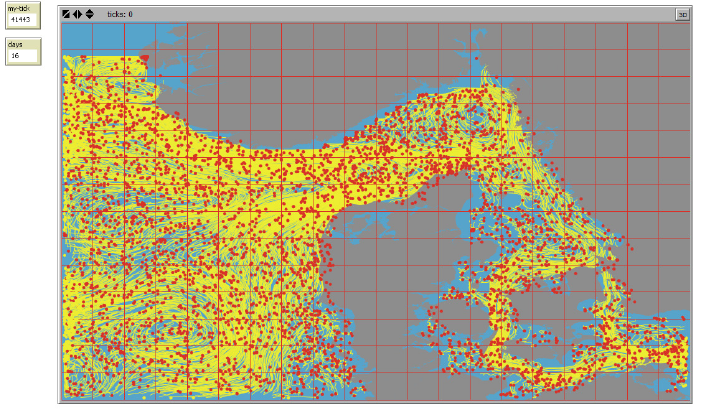
54
Dipsersal paramters
Pelagic larvae duation (PLD) 31 days
Include Active settling: disabled
Vertical distribution range: 0 – 20 meters
Dispersion, vertical: 0.001 m2/s
Dispersion, horizontal: 10 m2/s
Vertical sinking speed: 0
Simulation settings
Hyrdographic data format: Stationary_flow_field
Start time: 2009 03 02 0
End time: 2009 05 02 0
Time step: 1800 sec
Storing Frequency: 86400 sec
Result file: Results_SFF_10000.nc
Connectivity analysis parameters
Connectivity grid: 14 rows / 20 columns
Include only agents settled within habitat: Disabled
Temperature minimum tolerance: 0
Temperature maximum tolerance: 40
Salinity minimum tolerance: 0
Salinity maximum tolerance: 40
4.1.2 Results
A snapshot of agent distribution (red dots) on day 16 including agent trajectories (yellow tracks)
is shown below together with the applied connectivity grid used in the connectivity analysis (red
lines):
Figure 13. A snapshot of agent positions on day 16 (red dots) including agent trajectories (yellow tracks) and
the connectivity grid (red lines) used for the connectivity analysis.
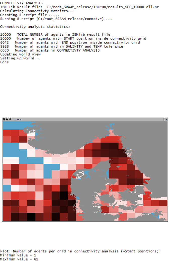
55
The output statistics of the connectivity analysis (below) shows that out of the 10 000 agents
included in the IBMlib simulation, 10 000 agents have an initial position inside the user specified
connectivity grid, 6042 have an end position inside the connectivity grid, 9988 agents lie within
the salinity and temperature intervals, and 6030 agents in total were included in the connectivity
analysis. If the option “Include only agents settled within habitat” had been enabled, the number
of agents successfully settled within the habitat would have been included in the statistics.
The densitiy of the initial positions of agents of each connectivity grid cell and which are
included in the connectivity analysis is shown in figure Figure 14. The somewhat uneven
distribution with low (or no) densities in some areas can be explained by the fact that agents
with an initial position in these areas are exported out of the area covered by the connectivity
grid as a result of ocean currents, and thus are not included in the connectivity analysis.
Figure 14. Density of initial positions of agents per grid in the connectivity grid included in the connectivity
analysis. Minimum value 1 (~white) , maximum value 81 (dark red). Blue color refers to “0”.
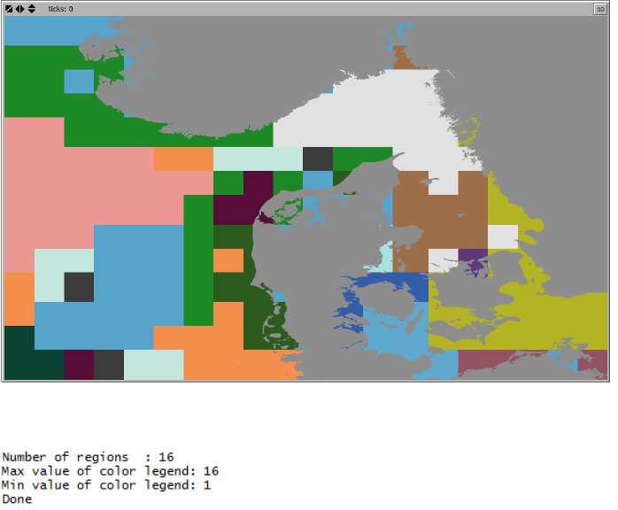
56
The delineation of hydrographic regions using the cluster analysis methodology “Infomap”,
results in 16 well define regions, see Figure 15.
Figure 15. Example of delineated hydrographic regions using the cluster analysis methology “Infomap”.
Regions plotted as a graph representation are shown in Figure 16. Each Node represents the
geometrical centroid of the individual region. Node numbers refer to the coherence (or self-
recruitement) of each region as probabilities (in pct) refering to the probabiilty that an agent with
an initial position inside the region settle within the same region. Edges (~arrows) direction and
thichness refer to the probabilities (in pct) that an agent with an initial position inside a region
will settle in one of the other regions. Regions and region centroids/nodes have the same color.
Notice that sometimes connectivity grid cells far apart may belong to the same region, and thus
region nodes here defined as geomtrical centroid may be placed “outside” the regions outline.
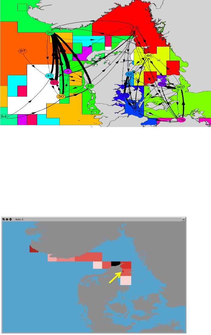
57
Figure 16. Graph representation of the within and between region connectivity probability.
To access the exact values representing the between regions connectivity probability, please
refer to the clconprob_collist.csv or edges.shp files.
I Figures 17 and 18 are shown examples on how to extract downstream and upstream
connectivity probabilites for a single location using the “Display connectivity probability” tool as
described in section 2.2.4.
Figure 17. Downstream connectivity probability of a specified location indicated by yellow arrow. The color
legend range from 0 (blue) to 0.196 (darkest red). Values represent the probability that an agent released in the
specific location (grid cell indicated by a yellow arrow) will end up in any other grid cell.
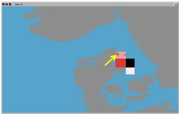
58
Figure 18. Upstream connectivity probability of a specified location indicated by yellow arrow. The color legend
range from 0 (blue) to 0.356 (darkest red). Values represent the probability that an agent with an end position in
the specified location (grid cell indicated by a yellow arrow) will originate from (~have their start position in)
any other grid cell.
4.2 Example using a dynamic hydrographic dataset
This example uses the hydrographic dataset generated by the HBM model for the North Sea,
Skagerrak, Kattegat, Inner Danish Straits and the Baltic Sea (for details: Berg and Poulsen
2012). The model uses a nested horizontal grid with a grid resolution of 3 nautical miles (~ 5.6
km’s) in the North Sea and Skagerrak and 0.5 nautical miles (~0.9 km’s) in the Kattegat, Inner
Danish Straits and the Western Baltic sea, The vertical resolution is 50 layers in the North Sea
and 52 layers in transition zone between the North Sea and the Baltic Sea including the
Kattegat, the Inner Danish Straits and the Western Baltic Sea. The dataset used for the SRAAM
setup include current speed and direction, water temperature and salinity. All values are stored
as daily means.
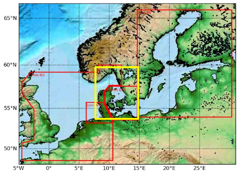
59
Figure 19. The map shows the extent of the HBM model setup for the North Sea, Skagerrak, Kattegat, the Inner
Danish Straits and the Baltic Sea (Berg and Poulsen 2012). Red color outline indicate nested sub-areas of the
model domain with different horizontal grid resolutions. Yellow outline indicate the sub-area of the example of a
SRAAM application covered in this section.
The study area including Skagerrak, Kattegat, Inner Danish Straits and the Wester Baltic Sea
represent a transition area between the highly saline North Sea and the brackish Baltic Sea.
Thus, the study area is subject to highly variable salinity conditions due to wind stowing
processes and tides. Figure 20 gives an indication of the salinity gradient of annual mean
bottom salinities along the salinity gradient from the saline North Sea to the brackish Baltic Sea.
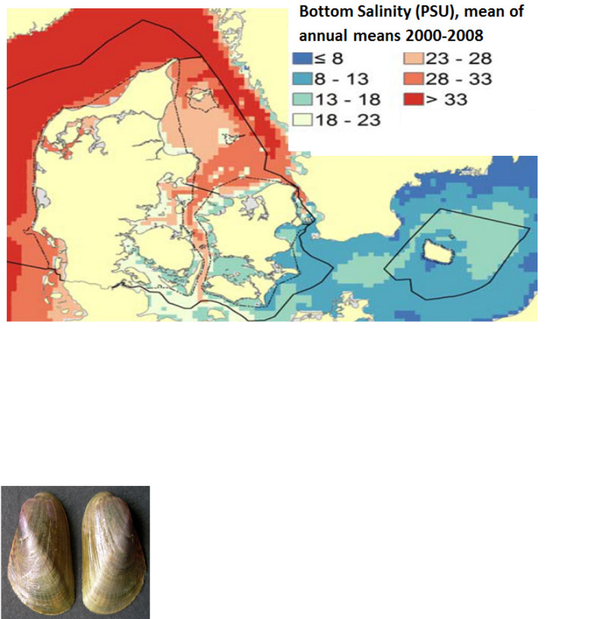
60
Figure 20. Mean of annual means of bottom salinity (PSU) 2000-2008. Data extracted from a hydrodynamic
model (see: Hansen et al. 2012).
In this SRAAM example we use the marine invasive species Asian Date Mussel (Arcuatula
senhousia), Figure 21.
Figure 21. Picture of the Asian Date Mussel (Arcuatula senhousia). Source: www.cabi.org.
Dispersal parameters and habitat preferences are shown in Tables 1 and 2. A habitat
distribution map is shown in Figure 22. The habitat map is derived based on habitat preferences
(Table 2) including preferred bottom substrate for sessile stages, salinity preferences/tolerances
and preferred water depths. The suitable habitat is divided into two types indicating the
optimal(green) and sub-optimal yellow) distribution of preferred habitat within the study area that
comply with the known salinity tolerance. For details see Hansen et al. (2018). In short, to
classify the suitable habitat into two areas according to the salinity tolerance, minimum and
maximum salinities where extracted from the hydrographic dataset for 3 selected hydrographic
years. Then the mean of the 3 years were calculated, and areas where the mean of annual
minimum values were above the minimum salinity threshold were colored “green”. Areas where
the mean of the annual maximum values were above minimum threshold were colored “yellow”.

61
This way, “green” areas represent habitats where salinity conditions are expected to be
favorable at all times (or most of the time), while “yellow” areas represent habitats where salinity
conditions are expected to be favorable only within shorter or longer periods. Both green and
yellow areas are used as spawning areas in the IBMlib simulation, however the discrimination
between primary (green) and secondary (yellow) habitat may be used as part of the result
interpretation and in particular in case where results are to be used in risk assessment context.
Table 1. Dispersal paramters for Asian Date Mussel (Arcuatula senhousia).
PLD (days)
14
No. of generations per year
1
Start month for spawning
7
End month for spawning
8
Table 2. Habitat preferences for Asian Date Mussel (Arcuatula senhousia)
Depth (m)
0 – 20
Substrate
All types
Sallinity min (psu)
17 psu
Salinity max (psu)
-
Temp. min (deg.C)
-
Temp. max (deg.C)
-
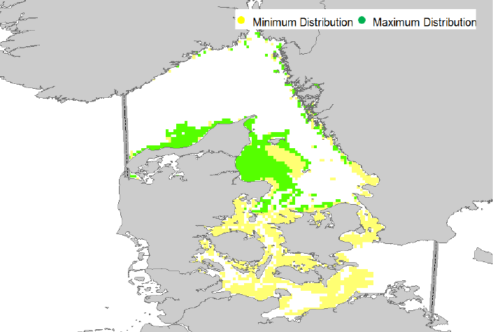
62
Figure 22. The map show the distribution of preferred habitats for Asian Date Mussel (Arcuatula senhousia) in
the study area. Habitat selected based on habitat preferences (Table 2) including preferred bottom substrate for
sessile stages, salinity preferences/tolerances and preferred water depths. Green areas represent areas where
salinity conditions are expected to be favorable all (or most) of the time, while yellow areas represent habitats
where salinity conditions are expected to be favorable in shorter or longer periods. The grey border lines
indicate the western and eastern boundaries of the study area respectively.
4.2.1 SRAAM input
The SRAAM input are desdcribed below. The result file from the IBMlib simulation is available in
the SRAAM setup files (Arcuatula_senhousia_2005_2e+05.nc) in order to be able to reproduce
the maps and outputs presented in the following. The file include only the last time step,
however initial positions are stored as part of the result file (see section 2.5.5). The HBM
hydrographic dataset is not included.
World view setup
Xgeo_min: 8
Xgeo_max: 14
Ygeo_min: 54
Ygeo_max: 60
Landshp: land_small.shp
Scaling factor: 10
63
Agent release settings
Agent release: Habitat map
Agent release period: 2005 07 01 – 2005 09 01
Agent release area: Habitat map (see Figure 22)
Agent release depth interval
Min depth: 0 meters
Max depth: 0 meters
No. of agents: 200 000
Dipsersal parameters
Pelagic larvae duation (PLD) 14 days
Include Active settling: disabled
Habitat input file: "hab_arcuatula_119x200_all_0-20m_stt-maxrange.asc”
Vertical distribution range: 0 – 40 meters
Dispersion, vertical: 0.001 m2/s
Dispersion, horizontal: 10 m2/s
Vertical sinking speed: 0
Simulation settings
Hyrdographic data format: HBM (nested)
Start time: 2005 07 01 0
End time: 2005 09 15 0
Time step: 1800 sec
Connectivity analysis parameters
Connectivity grid: 20 rows / 20 columns
Include only agents settled within habitat: Enabled
Temperature minimum tolerance: 0
Temperature maximum tolerance: 40
Salinity minimum tolerance: 17
Salinity maximum tolerance: 40
4.2.2 Results
The initial and end positions of all simulated agents are shown in Figure 23. The initial and end
positions are stored in the files sourcelist_hab.csv and sinklist_hab.csv respectively. To plot the
same figures as shown in Figure 23 load the csv files into a GIS system and make XY plots.
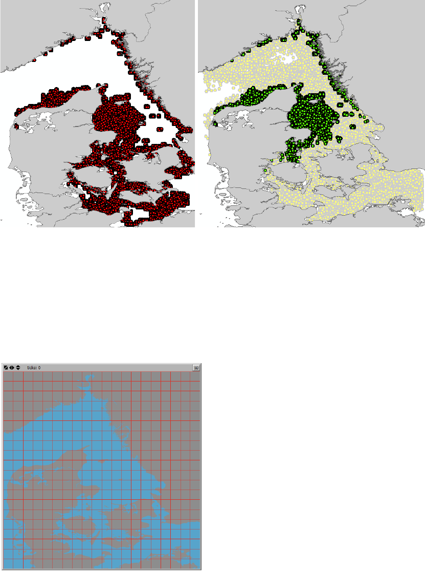
64
Figure 23. Left: Initial positions of all simulated agents. Right: end position of all simulated agents. Green color
indicates agents that successfully settle within suitable habitat. Yellow indicates agents that settle outside
suitable habitat.
The connectivity grid used for the connectivity analysis include 20 rows and 20 columns, see
Figure 24.
Figure 24. The 20x20 connectivity grid used for the connectivity analysis.
The results presented below, are based on a connectivity analysis using agent filters, i.e.
including only agents that successfully settle within suitable habitat (Figure 22), AND, excluding
all agents experiencing salinities below the minimum tolerance threshold of 17 psu. As shown
below, out of a total of 186 162 agents successfully simulated in the IBMlib simulation, only 12
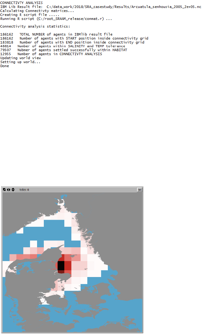
65
955 agents are included in the connectivity analysis. A large proportion of the agents are settled
outside the suitable habitat, and similarly a large proportion of the agents are excluded because
of unfavorable salinity conditions.
Figure 25 shows the densities of 12 955 agents with initial positions within suitable habitat that
eventually also settle successfully within suitable habitat, AND, that do not experience
exceedance of the salinity tolerance interval during the simulated dispersal. Values vary
considerably between 0 and 1597 number of agents per grid cell, with the largest numbers in
the core area of the preferred habitat (in the central part of the study area) and smaller values
towards the edge of the habitat extent and towards the southern distribution. This pattern is
partly due to agents being more likely to be exported to areas with unfavorable physical habitat
conditions by ocean currents if the initial position is located at the edge of the habitat extent,
and partly because the experienced salinity during dispersal exceeds the species salinity
tolerance interval. The latter is the primary reason for the absence of agents included in the
connectivity analysis with an initial position located in the southern part of the study area where
salinities decreases towards the Baltic sea.
Figure 25. Densities of agents with initial positions withing suiable habitats that eventually settle successfully
within suitable habitat, AND, that do not experience exceedance of the salinity tolerance interval during the
simulated dispersal. Color legend – blue = “0”, dark red = 1597.
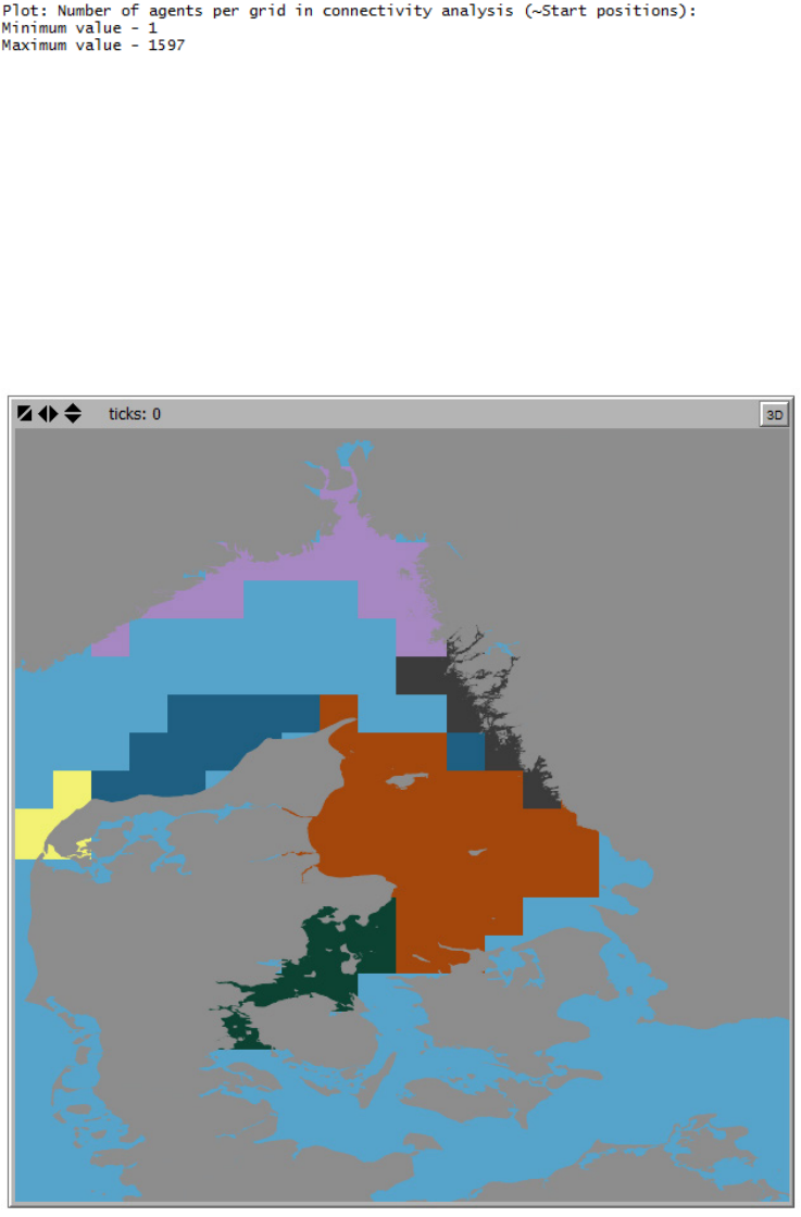
66
The output of the cluster analysis for Arcuatula senhousia including 6 hydrographic regions are
shown in Figures 26 and 27 as a simple region map and as a graph representation of the within
and between regions connectivity respectively. The graph representation in Figure 27 shows
individual regions with unique colors. Graph nodes (= circles) represent individual regions with
numbers representing the coherence (~self-recruitment) in pct, i.e. the proportion of agents that
have an initial position within the regions, which eventually settle within the same region. Graph
edges between nodes (arrows) indicate the direction of the connectivity between individual
regions, and the thickness of the edges indicates the relative magnitude of the connectivity
probabilities.
Figure 26. The output of the cluster analysis for Arcuatula senhousia shows 6 well defined Hydrographic
regions, here represented with unique coloring in the Netlogo World View.
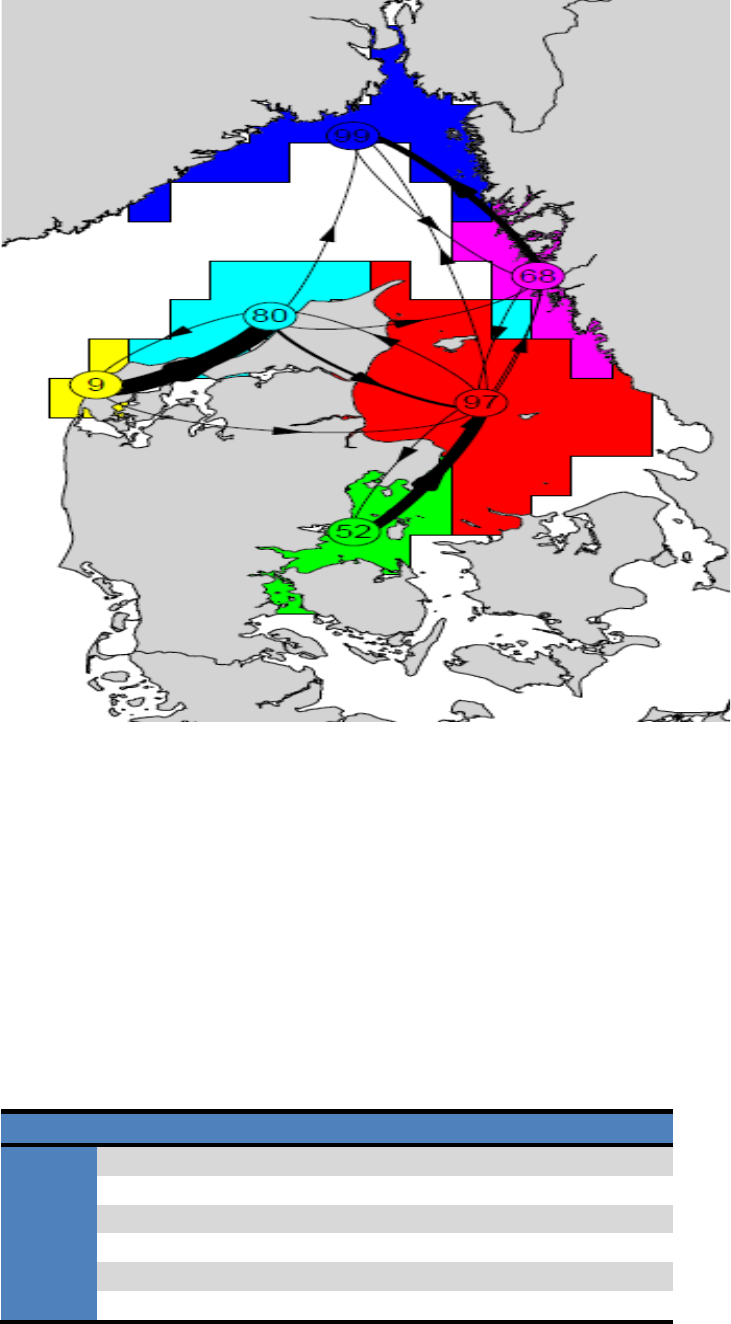
67
Figure 27. The output of the cluster analysis for Arcuatula senhousia with 6 hydrographic regions shown as a
graph representation (pdf) with unique colors for individual regions. Graph nodes (= circles) represent
individual regions with numbers representing the coherence (~self recruitement) in pct. Graph edges between
nodes (arrows) indicate the direction of the connectivity and the thickniess of the edges indicate the relative
magnitude of the connectivity probabilities.
The exact values used for the graph representation of the within and between regions
connectivities are strored in 2 comma separated files: “clconnos.csv” and “clconprob.csv”. See
Table 3 and Table 4 respectively.
Table 3. The table represent between regions connectivity adjacency matrix, with absolute number of agents
connecting the 6 regions. Species: Arcuatula senhousia. File: clconnos.csv.
1
2
3
4
5
6
1
8004
0
6
5
63
149
2
4
28
0
285
0
0
3
460
0
498
0
0
5
4
322
1
0
1667
39
57
5
0
0
0
0
521
7
6
12
0
0
0
215
491
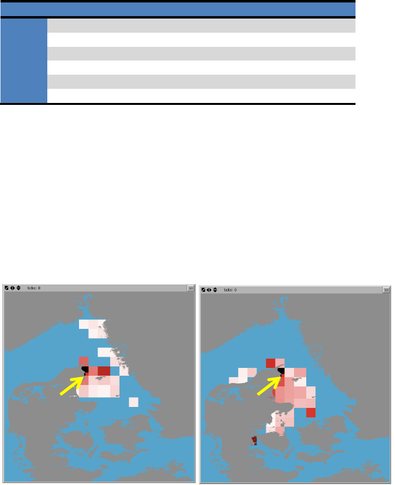
68
Table 4. The table represents between regions connectivity probability matrix, with probabilities (values
between 0 and 1) representing the chances of agents with an initial position in one region, will end up in one of
the other 5 regions. Species: Arcuatula senhousia. File: clconprob.csv.
1
2
3
4
5
6
1
0.972894
0
0.000729
0.000608
0.007658
0.018111
2
0.012618
0.088328
0
0.899054
0
0
3
0.477674
0
0.517134
0
0
0.005192
4
0.154362
0.000479
0
0.799137
0.018696
0.027325
5
0
0
0
0
0.986742
0.013258
6
0.016713
0
0
0
0.299443
0.683844
An example of extracting the downstream (left) and upstream (right) connectivity probabilities for
a specific location from the connectivity probability matrix is shown in Figure 28. In this case a
location corresponding to one of the main harbors in Kattegat, Frederikshavn. The downstream
connectivity probability map (Figure 28 left)) shows values that represent the probability (or
likelihood) that an agent released close to Frederikshavn harbor (~grid cell indicated by a yellow
arrow) will end up in any other grid cell. In a similar way, the upstream connectivity probability
map (Figure 28 right) shows values that represent the probability (or likelihood) that an agent
that ends in at location near Frederikshavn has come from any of the other grids cell in the
study area.
Figure 28. Example of displaying the downstream (left) and upstream (right) connectivity probabilities for a
specific location, in this case a location corresponding to one of the main harbors in Kattegat, Frederikshavn
(indicated by yellow arrows). Blue color = “0”. Darkest red = “0.273”.
For a more comprehensive insight into various considerations regarding the setup, simulation
and result interpretation and presentation, please see Hansen et al. (2018 in prep) and Stuer-
Lauritzen et al. (2018).
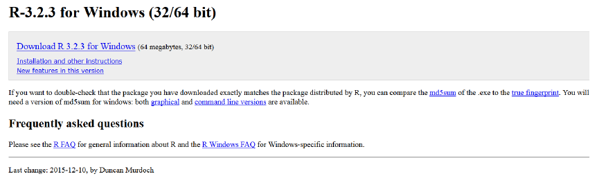
69
5. Installation guide
The installation of the SRAAM tool require as a minimum 3 software components:
- R 3.2.3 for Windows
- Netlogo 5.3.1
- IBMLib
Since Netlogo requires JAVA, make sure you have the latest JAVA version installed on your pc.
The tool comprising the individual software components has been tested on Windows 7 and
Windows 10 64-bit operation systems.
5.1 R installation
5.1.1 Install R 3.2.3 for Windows
The R software can be downloaded here:
https://cran.r-project.org/bin/windows/base/old/3.2.3/
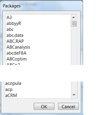
70
5.1.2 Install R extensions
To run the SRAAM tool, you need the following R-extension packages:
- diagram
- igraph
- maps
- maptools
- Matrix
- magrittr
- ncdf4
- raster
- Rcpp
- rgeos
- rJava
- shape
- shapefiles
- sp
The packages have been included in the SRAAM download in the “r-packages” – folder. You
can copy all the sub-folders included in the “r-packages”-folder into the R installation folder
depending on which installation folder you chose when installing, e.g. : “C:\Program Files\R\R-
3.2.3\library\”. Alternative the “r-packages” folders can be copied to the user
C:\Users\”..username..”\Documents\R\win-library\3.2.
To check if these R extensions are already installed, open the R Console (default window when
opening RGui from the Windows Start menu). Type e.g. “library(raster)”. If no error occurs then
this extension is installed and has been loaded. If an error occurs in the R-GUI, you need to
install the packages as described above. Alternatively install the packaged by opening the R
program and select the menu “Packages > Install package(s)”. To select a CRAN Mirror to
install from a “HTTPS CRAN Mirror” selection box will be shown. Select the country and the
server from where you want to install the extension. Next, from a selection box “Packages”, all
available extensions are listed in alphabetical order:
…
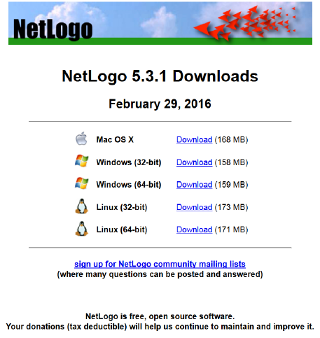
71
Scroll down and select the extension “raster” to install the “raster” extension for R. Repeat for
each of the required R-extensions.
If packages are correctly installed, but loading packages from within R GUI fails, you will need
to check and update the system paths, see 5.4, and reboot the pc.
5.2 Netlogo installation
5.2.1 Install Netlogo 5.3.1 for Windows
The Netlogo 5.3.1 installation file can be found here:
https://ccl.northwestern.edu/netlogo/5.3.1/
Select either 32-bit or 64-bit version for Windows.
Note that this version has been developed and tested only on a 64-bit version for Windows 7
and Windows 10.
5.2.2 Install Netlogo extensions
Six extensions need to be installed for your Netlogo installation.
– gis
– r
– shell
– matrix
– csv
– xw
The extensions are included in the SRAAM download in the subfolder “Netlogo_extension”.
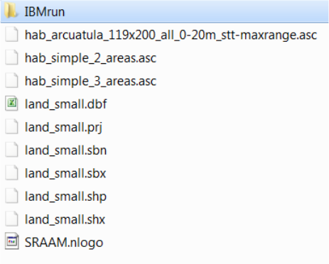
72
All extension have to be saved to the “extensions” sub-folder located in the directory where
Netlogo is installed, e.g.:
C:\Program Files\NetLogo 5.3.1\app\extensions\
Each extension consist of a folder with the extension name and with extension files (*.jar) inside
the folder.
You can also find the extension here:
https://github.com/NetLogo/NetLogo/wiki/Extensions/
Download/copy the extensions, and place the extension folders in “ ….\NetLogo
5.3.1\app\extensions\”. For details on the R extension for Netlogo, see: Thiele and Grimm
(2010).
5.3 Download SRAAM tool setup files
Download and un-zip the SRAAM tool and setup files available at:
https://github.com/IBMlib/SRAAM
into a working directory of your choice. E.g. C:\SRAAM\setup\.
5.3.1 The SRAAM setup folder
The SRAAM setup folder is where input files for the SRAAM tool is located. Hydrographic input
and outpout files for the IBMlib simulation are stored in the IBMrun-sub-folder, see next section.
The files included in the SRAAM setup folder include:
The SRAAM.nlogo file is the Netlogo file that opens the SRAAM user interface. From within the
SRAAM userinterface any changes to the setup may be saved to this file or another filename.
The 3 ascii files (file extentions: *.asc) are example of habitat maps used in the examples
presented in section 4.2.

73
The files named “land_small.*” are shapefiles used to represent land areas in the examples
presented in section 4.2. The default SRAAM.nlogo file include a World View extension that
covers the North Sea and The Wester Baltic Sea and the land areas of the shape file. This
default settings support the Hydrographic data format “Stationary_flow_field” for tool
demonstration purposes.
5.3.2 The IBMrun sub-folder
The subfolder “IBMrun” is where the IBMlib simulation input (and output) files are stored:
The 4 subfolders are where the applied hydrographic dataset needs to be stored. The
subfolders are named referring to the model the hydrographic data has been generated by, i.e.
HBM, POM, NEMO and NCOM.
For each compatible hydrographic data format an IBMlib executable exists, i.e.
ibmrun_connect_HBM.exe, ibmrun_connect_COARDS.exe, ibmrun_connect_genericHD.exe
and ibmrun_connect_bootHD.
In addition 3 files are included supporting the statistic hydrographic flow field for demonstration
purpose:
- ECOSMO_tl5_physics_testframe.dat
- Grid_desc_ecosmo
- Postinfo.for
Finally, a result file based on the HBM hydrographic data set and used for simulating the
dispersal and connectivity of the Asian Date Mussel (Arcuatula senhousia) as presented in
section 4.2 is included:
- Arcuatula_senhousia_2005_2e+05.nc
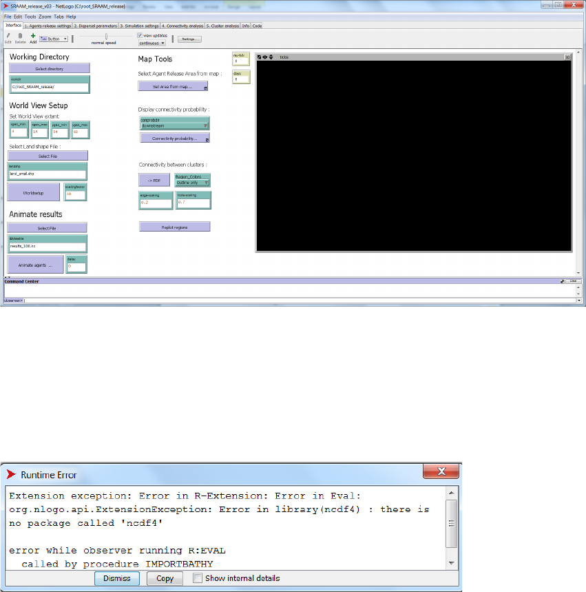
74
To open the SRAAM user interface, open the “Setup” folder, and click on the “SRAAM.nlogo”
file to open the SRAAM project file:
5.4 Setting the paths
5.4.1 Setting the path to R-extensions in Netlogo
Depending on where you have installed the R-extensions (see 5.1.2), you need to set the path
in Netlogo before the SRAAM tool will function correctly. Otherwise you will get an error like this:
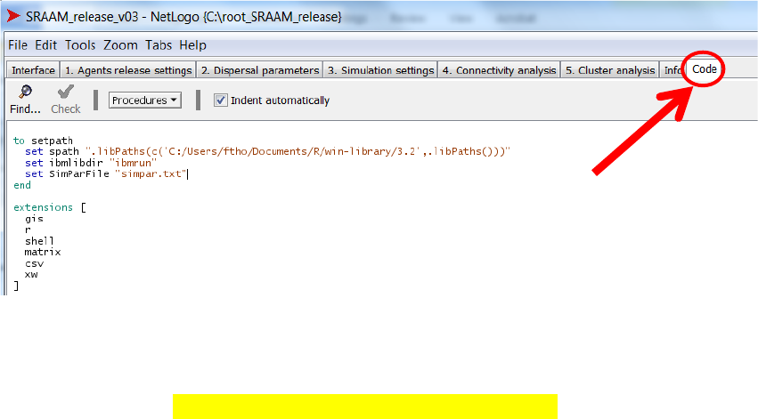
75
In the Netlogo user interface, click on the “code” tab:
In the top section you have to set the path:
to setpath
set spath ".libPaths(c('C:/Users/StartUser/Documents/R/win-library/3.2',.libPaths()))"
…
….
end
Replace the yellow highlighted path-string with the path that points to the folder where R-
extensions are installed on your PC. Save the project and proceed applying the SRAAM tools.
5.4.2 Setting system paths for R-extension
When you are running 64-bit Netlogo version you need manually to set the system paths for
three system variables:
- R_HOME (required)
- JRI_HOME (required)
- JAVA_HOME (if rJava extentions cannot be loaded from R)
If variables are not correctly set, this error may occur when you open the nlogo-file
“SRAAM.nlogo”:
“Error in R-extension: Error in runOnce: java.lang.NullPointerException”.
Make sure you have installed 64-bit versions of R, and Java.
Then follow the procedure for installation 64-bit version of R-extension for Netlogo. The
document is located in the Netlogo installation folder:
C:\Program Files\NetLogo 5.3.1\app\extensions\r\doc\Install_R-xtension_on_Win_with64bit.pdf
Follow the procedures including the testing of individual steps. Remember to reboot the
computer when the paths have been updated.
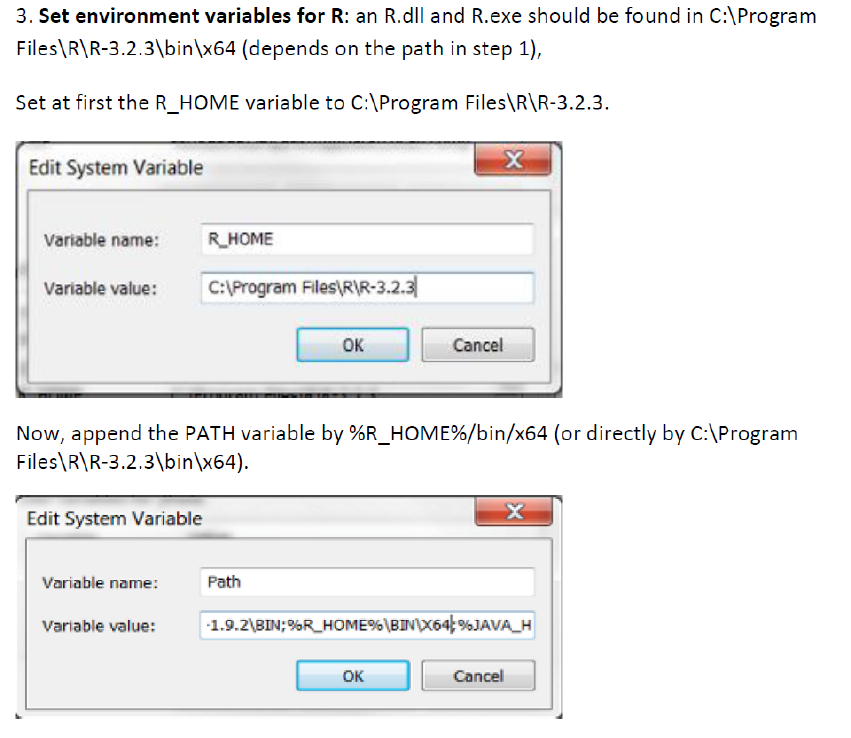
76
If you are already familiar with the path settings of system variables, see below. :
In short, you need to set the paths to the 2 (possibly 3) system variables as specified below,
adjusted to the folder structures of your installations. After pc reboot, if errors still occur re-
opening SRAAM.nlogo, please go through the procedures in detail as described in “Install_R-
xtension_on_Win_with64bit.pdf”.
R_HOME
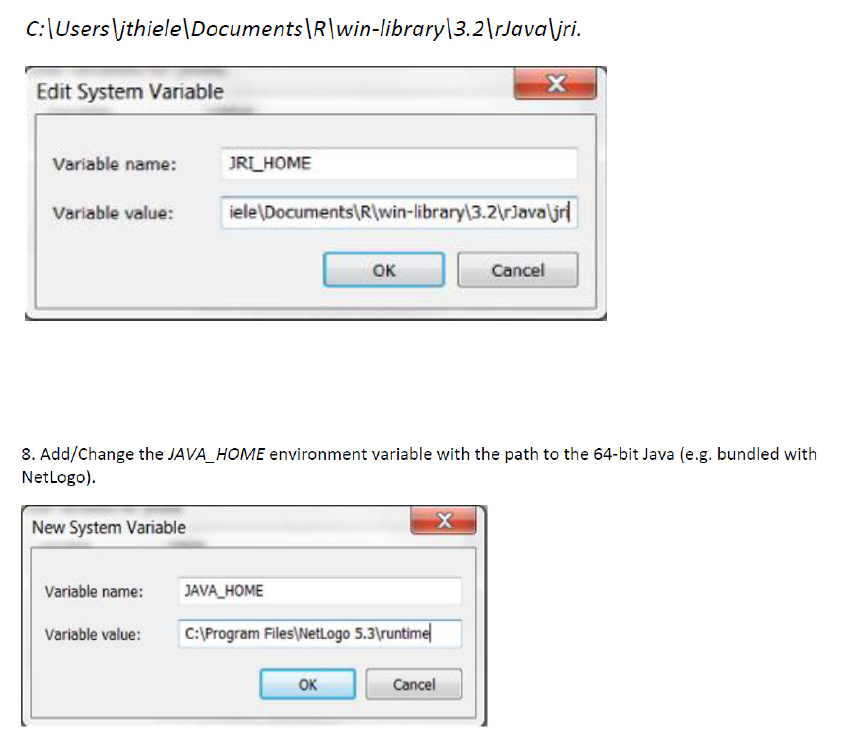
77
JRI_HOME
JAVA_HOME
Remember to restart you pc for the changes you have made to be registered properly.
78
6. References
Berg P, Poulsen J W, 2012. Implementation Details for HBM. DMI Technical Report, No.
12-11, Copenhagen.
Blumberg, A F and Mellor G L, 1987. A description of a three-dimensional coastal ocean
circulation model. Three-Dimensional Coastal ocean Models Edited by N. Heaps, 208 pp.,
American Geophysical Union. See also http://www.ccpo.odu.edu/POMWEB/
Christensen A, 2008, Bank resolved prognoses of sandeel fishing potential in the North Sea”.
Final report for the project "Fiskeriudsigt for tobis i Nordsøen på bankeniveau. (FIUF, 2005-
2007).
Christensen A, Mariani P, Payne M R, in review. A generic framework for individual-based
modelling and physical-biological interaction. Environmental Modelling and Software.
Dick S, Kleine E, Müller-Navarra S H, Klein H, and Komo H, 2001. The operational circulation
model of BSH (BSHcmod) – model description and validation. Berichte des BSH, 29, 49 pp.,
DMI (2018). http://ocean.dmi.dk/models/hbm.uk.php
Hansen F T, Christensn A, Stuer-Lauritzen F, 2018 (in prep). Same-Risk-Area Case study for
Øresund and Kattegat. Final report prepared by DTU AQUA for Dampsskibsselskabet Orients
Fond, StenaLine Group and Danish Ferries.
Hansen J W, Windelin A, Göke C, Jørgensen E T, Hansen F T, Uhrenholt T, 2012. Fysisk
kemiske forhold. Technical Note prepared for Danish Nature Agency by Danish Center of
Environment and Energy, Aarhus University.
Maar M, Møller E F, Larsen J, Madsen K S, Wan Z, She J, Jonasson L, 2011.
Ecosystem modelling across a salinity gradient from the North Sea to the Baltic Sea.
Ecological Modelling, 222: 1696–1711.
NOAA 1995. Conventions for the standardization of NetCDF Files . Sponsored by the
"Cooperative Ocean/Atmosphere Research Data Service," a NOAA/university cooperative for
the sharing and distribution of global atmospheric and oceanographic research data sets . May
1995. See also http://cfconventions.org/Data/cf-conventions/cf-conventions-1.1/build/cf-
conventions.html
Poulsen, J W and Berg P, 2012. More details on HBM - general modelling theory and survey of
recent studies. DMI technical report No 12-16
Schmith, T and Borch U, 2013. Horns Rev 3 Offshore Wind Farm - validation of DMI's model
suite for the Horns Rev 3 area. Report for Energinet.dk by Orbicon and DMI, May 2013
79
She J, Berg P, Larsen J and Nielsen J W, 2007. Operational three dimensional ocean
modelling for the Baltic Sea. Environ. Res., Eng. and Management, 2007, No.1(39), 3-7.
She, J, Berg P, Berg J, 2007. Bathymetry impacts on water exchange modelling through the
Danish Straits. Journal of Marine Systems, 65.
R Core Team, 2013. R: A language and environment for statistical computing. R Foundation for
Statistical Computing, Vienna, Austria. ISBN 3-900051-07-0, URL http://www.R-project.org/.
Rosvall M and Bergstrom C T, 2008. Maps of random walks on complex networks reveal
community structure. Proc. Natl. Acad. S ci. U.S. A., 105(4), 1118–1123.
Schrum C, Backhaus J O, 1999. Sensitivity of atmosphere-ocean heat exchange and heat
content in North Sea and Baltic Sea. A comparitive assessment. Tellus. 1999; 51A:526–549.
https://doi.org/10.3402/tellusa.v51i4.13825.
Schrum C, Alekseeva I, St John M, 2006. Development of a coupled physical-biological
ecosystem model ECOSMO Part I: Model description and validation for the North Sea. J Mar
Sys.
Stuer-Lauridsen F, Drillet G, Hansen F T , Saunders J, 2018. Same Risk Area: An area-based
approach for the management of bioinvasion risks from ships' ballast water. Marine Policy.
Accepted. DOI: 10.1016/j.marpol.2018.05.009.
Stuer-Lauridsen F, Hansen F T , Overgaard S B, 2016. Same Risk Area Concept.Procedure
and Scientific Basis. Final report. By Litehauz Aps for ITERFERRY and Danish Nature Agency.
Thiele J C, Grimm V, 2010. NetLogo meets R: Linking agent-based models with a toolbox for
their analysis. Environmental Modelling and Software 25(8): 972 - 974.
DOI: 10.1016/j.envsoft.2010.02.008.
Vincent R, Ser-Giacomi E, López C, Hernández-García E, 2014. Hydrodynamic provinces and
oceanic connectivity from a transport network help designing marine reserves. Geophysical
Research Letters 41, 2883-2891 (2014). DOI: 10.1002/2014GL059540.
Wan Z, She J, Maar M, Jonasson L, Baasch-Larsen J, 2012. Assessment of a physical-
biogeochemical coupled model system for operational service in the Baltic Sea. Ocean Sci. 8,
683-701.
Wilensky U, 1999. NetLogo. http://ccl.northwestern.edu/netlogo/. Center for Connected
Learning and Computer-Based Modeling, Northwestern University, Evanston, IL.
DTU Aqua
National Institute of Aquatic Resources
Technical University of Denmark
Kemitorvet
2800 Kgs. Lyngby
Denmark
Tel: + 45 35 88 33 00
aqua@aqua.dtu.dk
www.aqua.dtu.dk
