Sols.dvi Daphne Koller, Benjamin Packer Instructor’s Manual For Probabilistic Graphical S (2010)

User Manual:

Open the PDF directly: View PDF .
Page Count: 59

Instructor’s Manual for Probabilistic Graphical Models

Daphne Koller, Benjamin Packer, and many generations of TAs

October 2010

Foreword and Disclaimer

This instructor’s manual contains solutions for a few of the problems in the textbook Probabilisic

Graphical Models: Principles and Techniques, by Daphne Koller and Nir Friedman. The exercises

for which solutions are provided are those that were used over the years in Daphne Koller’s course

on this topic. (Most of these exercises were included in the textbook, but a few are new.) Hence,

the coverage of the solutions is highly biased to those topics covered in the course.

For some solutions, we have included relative point allocation to diﬀerent parts of the question,

which can help indicate their relative diﬃculty. To assist in grading, we have also sometimes

included common errors and the number of points deducted.

Since the solutions were developed over several years, while the book was being written (and

rewritten), the notation and formatting used might not always be entirely consistent with the

ﬁnal version of the book. There may also be slight inaccuracies and errors. For all of these we

apologize.

We hope that this instructor’s manual will be an ongoing eﬀort, with solutions added and

improved over time. In particular, any instructor who wants to contribute material — new

solutions to exercises, improvements or corrections to solutions provided, or even entirely new

problems and solutions — please send an email to pgm-solutions@cs.stanford.edu, and I will

add them to this instructor’s manual (with attribution). Thank you.

1 Chapter 2

Exercise 2.7 — Independence properties [17 points] Note that P(X|Z=z) is undeﬁned

if P(Z=z) = 0, so be sure to consider the deﬁnition of conditional independence when proving

these properties.

1. [7 points] Prove that the Weak Union and Contraction properties hold for any probability

distribution P.

Weak Union:

(X⊥Y,W|Z) =⇒(X⊥Y|Z,W)

Answer: It is important to understand that the independence statements above hold for all

speciﬁc values of the variables X, Y, Z, and W. Implicit in every such statement, and every

probability statement such as P(X, Y, W |Z) = P(X|Z)·P(Y, W |Z), is the qualiﬁer “for

every possible possible of X, Y, Z, and W.” See, for example, Def. 2.1.6 and the surrounding

discussion.

So our goal is to prove that the above statement holds for all possible values of the variables.

We proceed by cases, ﬁrst examining the cases in which the probabilities of some values may

be 0, and then considering all other cases.

If P(W=w, Z =z) = 0, then (X⊥Y|Z, W )holds trivially from Def. 2.1.4. Similarly, if

P(Z=z) = 0 =⇒P(W=w, Z =z) = 0, so (X⊥Y|Z, W )also holds.

Now consider the case that P(Z)6= 0, P (Z, W )6= 0. We have

P(X, Y |Z, W ) = P(X, Y, W |Z)

P(W|Z)[cond.indep rule, P (W|Z)6= 0 by assumption]

=P(X|Z)·P(Y, W |Z)

P(W|Z)[since (X⊥Y, W |Z)]

=P(X|Z)P(Y|Z, W )

We can also use the Decomposition rule (2.8) (X⊥Y, W |Z) =⇒(X⊥W, Z)to deduce

(X⊥W, Z)⇐⇒ P(X|Z) = P(X|W, Z). Thus, we obtain

P(X, Y |Z, W ) = P(X|Z, W )P(Y|Z, W )

which implies (X⊥Y|Z, W ).

It’s important to note that (X⊥Y, W |Z)does not necessarily mean that P(X, Y, W |Z) =

P(X|Z)P(Y, W |Z); if P(Z=z) = 0 for any z∈Val(Z), then the conditional probabilities

in the latter equations are undeﬁned.

Contraction:

(X⊥W|Z,Y) & (X⊥Y|Z) =⇒(X⊥Y,W|Z).

Answer: Again, if P(Z=z) = 0,(X⊥Y, W |Z)holds trivially from the deﬁnition. If

P(Z=z)6= 0 but P(Z=z, Y =y) = 0 you can check that P(X, Y, W |Z) = 0 = P(X|

Z)P(W, Y |Z).

Now assume P(Z=z)6= 0, P (Z=z, Y =y)6= 0. Then

P(X, Y, W |Z) = P(X, W |Z, Y )P(Y|Z)

=P(X|Z, Y )P(W|Z, Y )P(Y|Z) [since (X⊥W|Z, Y )]

=P(X|Z, Y )P(W, Y |Z)

=P(X|Z)P(W, Y |Z) [since (X⊥Y|Z)]

which proves (X⊥Y, W |Z).

This proves the Contraction rule for all distributions P.

Here, the common short proof was that P(X|Y, W, Z) = P(X|Y, Z) = P(X|Z)where

the ﬁrst step follows from (X⊥W|Z, Y )and the second step follow sfrom (X⊥Y|Z).

Again, this fails if P(X|Y, W, Z)is undeﬁned.

2. [7 points] Prove that the Intersection property holds for any positive probability distri-

bution P. You should assume that X,Y,Z, and Ware disjoint.

Intersection:

(X⊥Y|Z,W) & (X⊥W|Z,Y) =⇒(X⊥Y,W|Z).

Answer: If we could prove (X⊥Y|Z), we can use the Contraction rule to derive the

desired conditional independence: (X⊥W|Z, Y ) & (X⊥Y|Z) =⇒(X⊥Y, W |Z).

P(X|Z) = X

w∈W

P(X, w |Z) = X

w∈W

P(X|Z, w)P(w|Z)

w∈W

P(X|Y, w, Z)P(w|Z) [since (X⊥Y|Z, W )]

w∈W

P(X|Y, Z)P(w|Z) [since (X⊥W|Z, Y )]

=P(X|Y, Z)X

w∈W

P(w|Z) = P(X|Y, Z)

This proves (X⊥Y|Z), and by applying Contraction rule we are done. Note that if the

distribution is non-positive, many of the conditional probabilities we use in the proof may be

undeﬁned.

3. [3 points] Provide a counter-example to the Intersection property in cases where the

distribution Pis not positive.

Answer: Consider a distribution where X=Y=Walways holds, and their values are

independent of the value of Z. Then (X⊥W|Z, Y ), since Ydirectly determines X, and

similarly (X⊥Y|Z, W ). However, it is not the case that (X⊥Y, W |Z)because knowing

Zdoes not help us choose between the values X=Y=W= 1 or X=Y=W= 0.

Note that the independence (X⊥Y|Z)does not hold here. It is not the case that for any

value of Y=y,P(X|Z) = P(X|Y=y, Z).

Chapter 3

Exercise 3.11 — Marginalization and independencies [24 points]

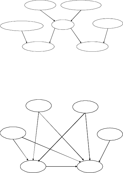
1. [6 points] Consider the alarm network shown below:

Burglary Earthquake

Alarm

JohnCall MaryCall

SportsOnTV Naptime

Construct a Bayesian network structure with nodes Burglary, Earthquake, JohnCall, MaryCall,

SportsOnTV, and Naptime, which is a minimal I-map for the marginal distribution over

those variables deﬁned by the above network. Be sure to get all dependencies that remain

from the original network.

Answer:

Burglary Earthquake

JohnCall MaryCall

Naptime

SportsOnTv

Burglary Earthquake

JohnCall MaryCall

Naptime

SportsOnTv

In order to construct a minimal I-map, we would like to preserve all independencies (assum-

ing Alarm is always unobserved) that were present in the original graph, without adding any

unnecessary edges. Let’s start with the remaining nodes and add edges only as needed.

We see that with Alarm unobserved, there exist active paths between Alarm’s direct ancestors

and children. Thus, direct edges between the parents, Burglary and Earthquake, should be

added to connect to both children, JohnCall and Mary Call. Similarly, since any two children

of Alarm also now have an active path between them, a direct edge between JohnCall and

MaryCall should be added. Without loss of generality, we direct this edge to go from JohnCall

to MaryCall.

Next, since SportsOnTv and JohnCall as well as Naptime and MaryCall were directly connected

in the original graph, removing Alarm doesn’t aﬀect their dependencies and the two edges must

be preserved.

Now we must consider any independencies that may have changed. In the old graph, because

of the v-structure between Alarm and co-parent SportsOnTv, if Alarm was unobserved and

JohnCall observed, there existed an active path between SportsOnTv and MaryCall. In the

new graph however, because of the added direct edge between the two children JohnCall and

MaryCall, if JohnCall is observed, the path between SportsOnTv and MaryCall is actually

rendered inactive. Thus, an alternate path that does not introduce any other dependencies

needs to be introduced, and a direct edge is added between SportsOnTv and MaryCall.

Common mistakes:

(a) [3 points] Missing edge from SportsOnTv to MaryCall (or Naptime to John-

Call).

(b) [3 points] Missing edge from JohnCall to MaryCall (or MaryCall to JohnCall).

cies.

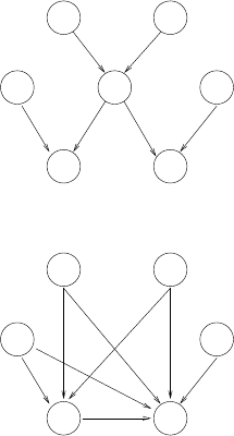
2. [18 points] Generalize the procedure you used above to an arbitrary network. More

precisely, assume we are given a network BN , an ordering X1, . . . , Xnthat is consistent

with the ordering of the variables in BN, and a node Xito be removed. Specify a network

BN ′such that BN ′is consistent with this ordering, and such that BN ′is a minimal I-map

of PB(X1,...,Xi−1, Xi+1,...,Xn). Your answer must be an explicit speciﬁcation of the

set of parents for each variable in BN ′.

Answer:

A B

C D

E F

is transformed into

A B

C D

E F

A general node elimination algorithm goes as follows. Suppose we want to remove Xfrom

BN . This is similar to skipping Xin the I-map construction process. As the distribution in

question is the same except for marginalizing X, the construction process is the same until we

reach the removed node.

Suppose the algorithm now adds the ﬁrst direct descendent of X, which we’ll call E. What

arcs must be added? Well, all the original parents of Emust be added (or we’d be asserting

incorrect independence assumptions). But how do we replace the arc between Xand E? As

before, we must add arcs between the parents of Xand E— this preserves the v-structure

d-separation between Xand its parents as well as the dependence of Eon the parents of X.

Now suppose we add another direct descendant, called F. Again, all the original parents of

Fmust be added and we also connect the parents of Xto F. Is that all? No, we must also

connect Eto F, in order to preserve the dependence that existed in the original graph (as an

active path existed between Eand Fthrough X). Now is that all? No. Notice that if E, is

observed then there is a active path between Cand F. But this path is blocked in our new

graph if all other parents of F(E, A, B, D) are observed. Hence, we have to add and edge

between Cand F.

So for every direct descendant of X, we add arcs to it from the parents of X, from the other

direct descendants of Xpreviously added and from the parents of the previously added direct

descendants of X.

What about the remaining nodes in the ordering? No changes need to be made for the arcs

added for these nodes: if a node Xmwas independent of X1,...,Xm−1(including X), given

its parents, it is also independent of {X1,...,Xm−1} − {X}given its (same set of) parents.

Guaranteeing that the local Markov assumptions hold for all variables is suﬃcient to show that

the new graph has the required I-map properties. The following speciﬁcation captures this

procedure.

Let T={X1,...,Xn}be the topological ordering of the nodes and let C={Xj|Xj∈

ChildrenXi}be the set of children of Xiin BN . For each node X′

jin BN ′we have the

following parent set:

Pa′

Xj=PaXjfor all Xj/∈C

PaXj∪PaXi∪ {Xk,PaXk|Xk∈C, k < j}\Xifor all Xj∈C

Common mistakes

(a) [15 points] Using the I-map construction algorithm or d-separation tests in

order to construct the new graph. The problem asks for a transformation of the

old graph into a new one, but doesn’t ask you to construct the new graph from

scratch. Essentially, we were looking for an eﬃcient algorithm based solely on

the structure of the graph, not one based on expensive d-separation queries.

(b) [5 points] Forgetting that the new graph should maintain consistent ordering

with the new graph.

(d) [4 points] Forgetting edges from PaXito Xj.

(e) [4 points] Forgetting edges from Xk, k < j to Xj.

(f) [4 points] Forgetting edges from PaXk, k < j to Xj.

(g) [2 points] Adding any additional edges not needed to satisfy I-map require-

ments.

(h) [1 points] Not writing explicit parent sets.

Exercise 3.16 — same skeleton and v-structures ⇒I-equivalence [16 points]

1. [12 points] Prove theorem 3.7: Let G1and G2be two graphs over X. If they have the

same skeleton and the same set of v-structures then they are I-equivalent.

Answer: It suﬃces to show:

(a) G1and G2have the same set of trails.

(b) a trail is active in G1iﬀ it is active in G2.

We show that if the trail from Ato Cis an active trail in G1, then it is an active trail in G2.

First note that because G1and G2have the same structure, if there is a trail Ato Cis G1,

there is a trail Ato Cin G2.

Let Xbe a node on the active trail from Ato Cin G1. Let Yand Zbe the neighbors of X

on the trail. There are two cases to consider:

(a) (Y, X, Z)is not a v-structure in G1. Then if this subtrail is active, Xis not set. Because G2

has the same v-structures as G1, we know (Y, X, Z)is not a v-structure in G2. Therefore

we know we have one of the following three in G2:Y→X→Z,Y←X→Zand

Y←X←Z. In all three cases, if Xis not set, the subtrail is also active in G2.

(b) (Y, X, Z)is a v-structure in G1. Then if this trail is active either Xis set or one of its

descendants is set. If Xis set in G1, then because G2has the same v-structure as G1,

the subtrail will be active in G2. Suppose it is active through some node X′that is a

descendant of Xin G1, but is not a descendant of Xin G2. Since G1and G2have the

same skeleton, there is a trail from Xto X′in G2. Since X′is not a descendent of X

in G2, there must be some edge that does not point toward X′on the trail from Xto

X′in G2. This is a v-structure in G2that does not exist in G1. We have a contradiction.

Therefore, the subtrail will be active in G2.

We can use a similar argument to show that any active trail in G2is active in G1.

The most common error in this problem was to forget that observing descendants of a v-

structure middle node Xcan activate trails passing through X. Also, we need to prove that if

a node is a descendant of X(the node in the middle of the v-structure) in G1, it must also be

a descendant of this node in G2.

Common mistakes:

(a) [6 points] One of the most common mistakes on this problem was to forget

to address the possibility of a descendant activating a v-structure.

(b) [1 points] Minor logical leap, informality, or ambiguity in the proof.

addressing the case when a subtrail is not a v-structure. This could be

because the proof dealt with the issue at too abstract a level (not dealing

with active three-node subtrails), or because it was simply missed entirely.

2. [4 points] How many networks are equivalent to the simple directed chain X1→X2→

...→Xn?

Answer: The result in the previous part holds only in one direction: same skeleton and same

set of v-structures guarantees I-equivalent networks. However, the reverse does not always

hold. Instead, we will use Theorem 3.3.13, which says that two I-equivalent graphs must have

the same skeleton and the same set of immoralities.

The ﬁrst requirement constrains the possible edges to the original edges in the chain. Moreover,

all original edges have to be present, because removing any edge breaks the set of nodes into

two non-interacting subsets.

The second requirement limits us to networks which have no immoralities, and no v-structures

(because the original chain has none). There are a total of n−1such networks, excluding the

original chain, where we are allowed a single structure Xi−1←Xi→Xi+1 in the chain (two

such subgroups would create a v-structure). The n−1possibilities come from,aligning this

structure on top of any node X2,...,Xn, with the rest of the edges propagating away from

node Xi.

Common mistakes:

(a) [1 points] Oﬀ by one. (Note that both n and (n-1) were acceptable answers)

(b) [4 points] Missed this part entirely. Answer way oﬀ of (n-1) or n. Common

answers here are 2and 2n.

Exercise 3.20 — requisite CPD [15 points] In this question, we will consider the sensitivity

of a particular query P(X|Y) to the CPD of a particular node Z. Let Xand Zbe nodes,

and Ybe a set of nodes. Provide a sound and “complete” criterion for determining when the

result of the query P(X|Y) is not aﬀected by the choice of the CPD P(Z|PaZ). More

precisely, consider two networks B1and B2that have identical graph structure Gand identical

CPDs everywhere except at the node Z. Provide a transformation G′of Gsuch that we can

test whether PB1(Z|PaZ) = PB2(Z|PaZ) using a single d-separation query on G′. Note that

Zmay be the same as X, and that Zmay also belong to Y. Your criterion should always be

sound, but only be complete in the same sense that d-separation is complete, i.e., for “generic”

CPDs.

Hint: Although it is possible to do this problem using laborious case analysis, it is signiﬁcantly

easier to think of how a d-separation query on a transformed graph G′can be used to detect

whether a perturbation on the CPD P(Z|PaZ) makes a diﬀerence to P(X|Y).

Answer:

Construct a new network G′from the original network Gby adding one node Wand one edge from

Wto Z, i.e., Wis an extra parent of Z. We set the CPD for Zso that if W=w1, then Zbehaves as

in B1, and if W=w2, then Zbehaves as in B2. More precisely, P(Z|PaZ, w1) = PB1(Z|PaZ),

and P(Z|PaZ, w2) = PB2(Z|PaZ). It is therefore clear that PB1(X|Y) = PB2(X|Y)if

and only if PB′(X|Y, w1) = PB′(X|Y, w2), where B′is our modiﬁed network with W. We

can guarantee that the value of Wdoesn’t matter precisely when Wis d-separated from Xgiven

Y. This criterion is always sound, because when Wis d-separated, the choice of CPD for Zcannot

aﬀect the query P(X|Y). It is complete in the same sense that d-separation is complete: There

might be some conﬁguration of CPDs in the network where the CPD of Zhappens not to make a

diﬀerence, although in other circumstances it could. This criterion will not capture cases of this type.

It was possible to earn full points for a case-based solution. The two important points were

1. Unless Z or one of its descendents is instantiated, active paths which reach Z from X through

one of Z’s parents are not “CPD-active”; that is, changing the CPD of Z will not aﬀect X

along this path.

2. The case where Z is in Y needs to be handled, since our deﬁnition of d-sep means that if Z is in

Y, d-sep(X;Z—Y), yet paths which reach Z through one of its parents are still “CPD-active”.

Solutions which used the case-based approach were scored based on how they handled these two

issues.

Common mistakes:

1. [11 points] Answer dsep(X;Z|Y)or anything else which doesn’t handle either observed Z or

cases where Z does/does not have observed descedents

2. [3 points] Correct answer, but not fully justiﬁed (usually incomplete case analysis)

3. [5 points] Don’t handle cases when Z is observed (in the case-based analysis)

4. [1 points] Minor miscellaneous error

5. [6 points] Don’t correctly deal with case where Z has no observed descendents

6. [3 points] Medium miscellaneous error

Chapter 4

Exercise 4.4 — Canonical parameterization

Prove theorem 4.7 for the case where Hconsists of a single clique.

Answer: Our log probability is deﬁned as:

ln ˜

P(ξ) = X

Di⊆X

ǫDi[ξ].

Substituting in the deﬁnition of ǫDi[ξ], we get

ln ˜

P(ξ) = X

DiX

Z⊆Di

(−1)|Di−Z|ℓ(σZ[ξ])

ℓ(σZ[ξ]) X

Di⊇Z

(−1)|Di−Z|.

For all Z6=X, the number of subsets containing Zis even, with exactly half of them having an

odd number of additional elements and the other half having an even number of additional elements.

Hence, the internal summation is zero except for Z=X, giving:

ln ˜

P(ξ) = ℓ(σZ[ξ]) = ln P(ξ),

proving the desired result.

Exercise 4.8 — Pairwise to Markov independencies Prove proposition 4.3. More precisely,

let Psatisfy Iℓ(H), and assume that Xand Yare two nodes in Hthat are not connected directly

by an edge. Prove that Psatisﬁes (X⊥Y| X − {X, Y }).

Answer: This result follows easily from the Weak Union property. Let Z=NH(X)and let

W=X − Z− {X, Y }. Then the Markov assumption for Xtells us that

(X⊥ {Y} ∪ W|Z).

From the Weak Union property, it follows that

(X⊥Y|Z∪W),

which is precisely the desired property.

Exercise 4.9 — Positive to global independencies

Complete the proof of theorem 4.4. Assume that equation (4.1) holds for all disjoint sets X,Y,Z,

with |Z| ≥ k. Prove that equation (4.1) also holds for any disjoint X,Y,Zsuch that X∪Y∪Z6=

Xand |Z|=k−1.

Answer: Because X∪Y∪Z6=X, there exists at least one node Athat is not in X∪Y∪Z.

From the monotonicity of graph separation, we have that sepH(X;Y|Z∪ {A}).

Because Xand Yare separated given Z, there cannot both be a path between Xand Agiven Z

and between Yand Agiven Z. Assume, without loss of generality, that there is no path between

Xand Agiven Z. By monotonicity of separation, there is also no path between Xand Agiven

Z∪Y. We then have that sepH(X;A|Z∪Y).

The sets Z∪ {A}and Z∪Yhave size at least k. Therefore, the inductive hypothesis equation (4.1)

holds, and we conclude

(X⊥Y|Z∪ {A}) &(X⊥A|Z∪Y).

Because Pis positive, we can apply the intersection property (equation (2.11)) and conclude that P

satisﬁes (X⊥Y|Z), as required.

Exercise 4.11 — Minimal I-map [15 points]

In this exercise you will prove theorem 4.6. Consider some speciﬁc node X, and let Ube the set

of all subsets Usatisfying P|= (X⊥ X − {X} − U|U). Deﬁne U∗to be the intersection of all

U∈ U.

1. [8 points] Prove that U∗∈ U. Conclude that M BP(X) = U∗

Answer: This follows directly from the intersection property. Speciﬁcally, let U1and U2be

two sets in U, that is, P|= (X⊥ X − {X} − Ui|Ui). Deﬁne Yi=Ui−U∗; it now follows

that

P|= (X⊥Y1|U2)

P|= (X⊥Y2|U1)

Equivalently,

P|= (X⊥Y1|U∗∪Y2)

P|= (X⊥Y2|U∗∪Y1)

From the intersection property, it follows that

P|= (X⊥U∗|Y1,Y2).

All that remains is to show that U∗=MBP(X). Recall that M BP(X)is deﬁned to be the

minimal set of nodes Usuch that P|= (X⊥ X − {X} − U|U). This deﬁnition implies that

MBP(X)is the minimal set of nodes U∈ U. We see that this is indeed U∗.

A common mistake is to use a form of the intersection property which isn’t explicitly proven.

One such form is (X⊥A,Y|W,Z)and (X⊥A,W|Y,Z)−→ (X⊥A,Y,W|Z).

This is true, but requires a Weak Union step for completeness. Another common mistake in the

ﬁrst three parts of the problem was to use the monotonic property of conditional independence

relations induced by a graph Hto justify adding variables to the right side of a conditional.

We must remember, however, that in these parts of the problem we are dealing only with a

distribution that may not correspond to a graph.

2. [2 points] Prove that if P|= (X⊥Y| X − {X, Y }) then Y6∈ M BP(X).

Answer: We see that we can rewrite this independence as P|= (X⊥ X − {X} − U′|U′)

where U′=X − {X, Y }. But U′∈ U and Y6∈ U′, thus Ycannot be in the intersection of

all U∈ U. This means Y6∈ U∗or equivalently Y6∈ MBP(X).

3. [3 points] Prove that if Y6∈ MBP(X) then P|= (X⊥Y| X − {X, Y }).

Answer: We know that P|= (X⊥ X − {X} − M BP(X)|MBP(X)). If Y6∈ MBP(X)

then we must have Y∈ X − {X} − MBP(X), allowing us to rewrite the independency

as P|= (X⊥ {Y},X − {X, Y } − MBP(X)|MBP(X)). By weak union we then have

P|= (X⊥ {Y} | X − {X, Y } − M BP(X), MBP(X)) or just P|= (X⊥Y| X − {X, Y }).

4. [2 points] Conclude that MBP(X) is precisely the set of neighbors of Xin the graph

deﬁned in theorem 4.5, showing that the construction of theorem 4.6 also produces a

minimal I-map.

Answer: (b) shows that MBP(X)is a subset of the neighbors deﬁned in the graph of

Theorem 4.5, while (c) shows that it is a superset.

Exercise 4.15 — Markov network proof of d-separation [22 points] Prove Proposition

4.10: Let X,Y,Zbe three disjoint sets of nodes in a Bayesian network G. Let U=X∪Y∪Z,

and let G′=G+[U] be the induced Bayesian network over Ancestors(U)∪U. Let Hbe the

moralized graph M[G′]. Prove that d-sepG(X;Y|Z) if and only if sepH(X;Y|Z).

Answer:

[11 points] Suppose not d-sepG(X;Y|Z). Then there is an active path in Gbetween some X∈X

and some Y∈Y. The active path, like any path, is formed of overlapping unidirectional segments

W1→... →Wn. Note that Wnin each segment is either X,Y, or the base of some active

v-structure. As such, either Wnor one of its descendants is in U, and so all nodes and edges in teh

segment W1→... →Wnare in the induced graph over Ancestors(U)∪U. So the active path in

Gis a path in H, and in H, the path can only contain members of Zat the bases of v-structures in

G(otherwise, the path would have been active in G). Because His the moralized graph M[G′], we

know that those members of Zhave been bypassed: their parents in the v-structure must have an

edge between them in H. So there is an active path between Xand Yin H, so not sepH(X;Y|Z).

[11 points] Now we prove the converse. Suppose that Xand Yare d-separated given Z. Consider

an arbitrary path in Gbetween some X∈Xand some Y∈Y. Any path between Xand Yin G

must either be blocked by a member of Zor an inactive v-structure in G. First, suppose the path is

blocked by a member of Z. Then the path in H(if it exists–it may not because His the induced

graph) will also be blocked by that member of Z.

Of course, if the path between Xand Yin Gis not blocked by a member of Z, it must be blocked

by an inactive v-structure. Because the v-structure is inactive, its base (and any of its descendants)

must not be in the induced graph H. As such, the path will not exist in H. Neither the base nor

its descendants can be in Z, and they cannot be in Xor Yeither, because then we would have an

active path from a member of Xto a member of Y.

Recall that the edges added in moralization are necessary to create an active path in Honly when

paths would be blocked by the observed root node of a v-structure in G. In this case, the segment

would have been active in G, so moralization edges cannot eﬀect segments in Hcorresponding to

inactive segments in G; this is what our proof depends on. Because of all the above, there are no

active paths in Hbetween arbitrary X∈Xand Y∈Y, so we have sepH(x;Y|Z).

Common mistakes:

D-separation to separation

1. [4 points]Failed to show that root node of an inactive v-structure in Gwill

not be in H, or that an active path in H through an inactive v-structure is not

possible.

2. [3 points] Failed to show modiﬁcations necessary to handle moralized edges.

3. [1 points] Considered only paths existing in G, failed to consider possibility of

entirely new paths in H.

4. [1 points] Described only 3-node paths without demonstrating how the cases

combine into paths of arbitrary length.

5. [1 points] Assumed that for active v-structures, center node must be observed,

didn’t consider its descendants.

6. [3 points] Other signiﬁcant logical error or omission.

7. [1 points] Other minor logical error/omission.

Separation to d-separation

1. [4 points] Failed to demonstrate that all the nodes along an active path in G

will still appear in H.

2. [3 points] Failed to show that an active v-structure in Gwill not result in

blockage in H.

3. [2 points] Describe only 3-node paths without describing how these combine

into arbitrary paths, in particular, why those nodes will all still appear in H.

4. [1 points] Assumed that for active v-structures, center node must be observed,

didn’t consider its descendants.

5. [3 points] Other signiﬁcant logical error or omission.

6. [1 points] Other minor logical error/omission.

Exercise 4.18 — Markov networks and Bayesian networks Let Gbe a Bayesian network

with no immoralities. Let Hbe a Markov network with the same skeleton as G. Show that H

is an I-map of I(G).

Answer: We need to prove that I(H)⊂ I(G); that is, if (X⊥Y|Z)∈ I(H)then (X⊥Y|

Z)∈ I(G).

Proving the contrapositive: if (X⊥Y|Z)/∈ I(G)then (X⊥Y|Z)/∈ I(H). Suppose

(X⊥Y|Z)/∈ I(G). Then there is an active trail τfrom Xto Ygiven Zin G. Consider a triplet

A−B−Con t. If it is a v-structure, then by the deﬁnition of active trails, Bmust be observed

(B∈Z). Then by the deﬁnition of active trails, for all triplets A−B−Con t, it must be the case

that A−B−Cis not a v-structure either it’s not a v-structure and A, B, C /∈Zor it is a v-structure

and B∈Z. If

Let τbe an active trail from some node Xto some node Yin Ggiven a set of nodes E. Then we

can ﬁnd an active trail from Xto Yin Ggiven Ethat contains no v-structures by the following

recursive process:

1. If τcontains no v-structures, then return T.

2. If τcontains a v-structure, then let A→B←Cbe the v-structure on Tclosest to X. Because

Gcontains no immoralities, there must be an edge from Ato C. Let trail τ′be equal to τ.

(a) If A=X, then replace the edges A→B←Cwith A→Cin τ′.τ′has exactly one

less v-structure than

(b) Otherwise, if the incoming edge to Aon τ′is →, then replace the edges A→B←C

with A→Cin τ′.

with A←Cin τ′.

Chapter 5

Exercise 5.5 — tree-structured factors in a Markov network [15 points]

Instead of using a table to represent the CPD in a Bayesian network we can also use a CPD-tree.

1. [3 points] How can we use a tree in a similar way to represent a factor in a Markov

network? What do the values at the leaves of such a tree represent?

Answer: We use a tree in exactly the same way it is used to represent CPDs. The diﬀerence

is that the leaves now store only one value — the factor entry associated with the context of

the leaf, rather than a distribution.

2. [6 points] Given a context U=u, deﬁne a simple algorithm that takes a tree factor φ(Y)

(from a Markov network) and returns the reduced factor φ[u](Y−U) (see deﬁnition 5.2.7),

also represented as a tree.

Answer: Traverse the tree in any order (DFS, BFS, inorder). For every node X∈Uconnect

the parent of Xwith the one child that is consistent with the context u. Delete X, its children

that were non consistent with u, and their subtrees.

3. [6 points] In some cases it turns out we can further reduce the scope of the resulting tree

factor. Give an example and specify a general rule for when a variable that is not in Ucan

be eliminated from the scope of the reduced tree-factor.

Answer: In the algorithm above, in addition to removing from the tree all the nodes in U,

we also deleted entire subtrees. It might be that by doing that we also removed from the tree

all instances of some other variable Zwhich is not in U. If this is the case, we can safely

remove Zfrom the scope of the reduced tree factor, as its value no-longer depends on the

instantiation of Z. In general, we can remove from the scope of a tree-factor all the variables

that do not appear in it.

Many students gave a slightly diﬀerent answer. They said that an additional variable can be

removed from the tree (and hence from the scope) if in the resulting reduced factor its children

sub-trees are equivalent. This answer is correct, but it requires further changes to the tree, and

in addition it depends on the actual values of the factor in the leaves. Conversly, in the case

for Zabove, we can safely change the scope of the reduced factor without making any further

changes to the tree, and without considering any speciﬁc factor values.

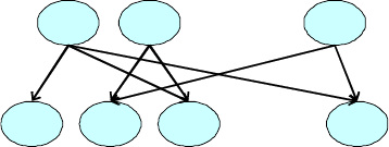
Exercise 5.14 — Simplifying BN2O networks [22 points]

F2...

...

Figure 1: A two-layer noisy or network

Consider the network shown in Figure 1, where we assume that all variables are binary, and that

the Fivariables in the second layer all have noisy or CPDs (You can ﬁnd more details about

this network in Concept 4.3 on page 138). Speciﬁcally, the CPD of Fiis given by:

P(f0

i|PaFi) = (1 −λi,0)Y

Dj∈PaFi

(1 −λi,j )dj

where λi,j is the noise parameter associated with parent Djof variable Fi. This network archi-

tecture, called a BN2O network is characteristic of several medical diagnosis applications, where

the Divariables represent diseases (e.g., ﬂu, pneumonia), and the Fivariables represent medical

ﬁndings (e.g., coughing, sneezing).

Our general task is medical diagnosis: We obtain evidence concerning some of the ﬁndings, and

we are interested in the resulting posterior probability over some subset of diseases. However,

we are only interested in computing the probability of a particular subset of the diseases, so

that we wish (for reasons of computational eﬃciency) to remove from the network those disease

variables that are not of interest at the moment.

1. [15 points] Begin by considering a particular variable Fi, and assume (without loss of

generality) that the parents of Fiare D1,...,Dk, and that we wish to maintain only the

parents D1,...,Dℓfor ℓ < k. Show how we can construct a new noisy or CPD for Fithat

preserves the correct joint distribution over D1,...,Dℓ, Fi.

Answer: This can be done by summing out the Djvariables that we wish to remove and

incorporating their eﬀects into the leak noise parameter. We show how to remove a single

parent Dk:

P(Fi=f0

i|D1, . . . Dk−1) = X

P(Fi=f0

i, Dk|D1,...,Dk−1)

P(Fi=f0

i|D1,...,Dk−1, Dk)P(Dk|D2,...Dk−1)

P(Fi=f0

i|D1,...Dk)P(Dk)

(1 −λi,0)



j=1

(1 −λi,j )Dj

P(Dk)

= (1 −λi,0)



k−1

j=1

(1 −λi,j )Dj

X

(1 −λi,k )DkP(Dk)

Thus, we could replace the previous leak parameter λi,0by a new leak parameter λ′i,0=

1−(1 −λ0)PDk(1 −λi,k )DkP(Dk)and we have maintained the noisy OR structure of the Fi

CPD. This process can then be repeated sequentially for Dℓ+1,...,Dk−1. Some of you noted

that PDk(1 −λi,k )DkP(Dk) = (1 −P(d1

k)) + (1 −λi,k )P(d1

k) = 1 −λi,kP(d1

k)which was

ﬁne as well.

If we repeat this process for all the variables that we wish to remove, we come to the solution:

P(Fi=f0

i|D1,...Dl) = (1 −λi,0)



j=1

(1 −λi,j )Dj



m=l+1 "X

(1 −λi,m)DmP(Dm)#

producing a ﬁnal leak parameter λ′

i,0= 1 −(1 −λi,0)Qk

m=l+1 PDm(1 −λi,m)DmP(Dm).

Common errors:

(a) [3 points] Did not show that the transformation results in a noisy-or network.

To receive credit for this, you needed to explicitly show the relationship between

the λ′and the expressions derived above.

(b) [3 points] Minor algebraic error: the ﬁnal form of the answer for the new leak

parameter was not exactly correct but only due to a small algebraic error in the

derivation.

(d) [12 points] More major error.

If you had a major algebraic error, you most likely lost 6 to 8 points on this problem. The most

common major algebraic errors was the use of the following “identity”: P(F1|D1,...,Dk−1) =

PDkP(F1|D1, . . . , Dk)

2. [7 points] We now remove some ﬁxed set of disease variables Dfrom the network, executing

this pruning procedure for all the ﬁnding variables Fi, removing all parents Dj∈D. Is

this transformation exact? In other words, if we compute the posterior probability over

some variable Di6∈ D, will we get the correct posterior probability (relative to our original

model)? Justify your answer.

Answer: In the general case, this transformation is not exact. As an example, consider a

simple network with D1, D2and F1, F2where the parents of F1are D1, D2and the parent of F2

is D2. Before the transformation, D1is not independent of F2given F1. After eliminating D2

from the network, then F2is disconnected from the other variables, giving (D1⊥F2|F1). In

terms of posterior probabilities this means that while for some distributions, P(D1|F1, f0

2)6=

P(D1|F1, f1

2)in the original network, in the transformed network, it is always the case that

P(D1|F1, f0

2) = P(D1|F1, f1

2); thus, the results of the posterior probability calculations are

not necessarily preserved after variable D2is summed out.

Note, however, that if each of the Divariables eliminated has exactly one Fichild in the

network, then this transformation is exact.

Exercise 5.8 — Soundness of CSI-separation[23 points]

Consider a Bayesian network Bparameterized by a set of tree-CPDs. Recall that in such cases,

the network also exhibits context-speciﬁc independencies (CSI). In this exercise, we deﬁne a

simple graph-based procedure for testing for these independencies; your task will be to prove

that this procedure is sound.

Consider a particular assignment of evidence Z=z. We deﬁne an edge X→Yto be spurious

in the context zif, in the tree CPD for Y, all paths down that tree that are consistent with the

context zdo not involve X. (Example 4.3.6 in the notes provides two examples.) We deﬁne X

and Yto be CSI-separated given zif they are d-separated in the graph where we remove all

edges that are spurious in the context z.

You will now show that CSI-separation is a sound procedure for detecting independencies. That

is: If Pis the distribution deﬁned by B, and Xand Yare CSI-separated given zin B(written

CSI-sepB(X;Y|z)), then P|= ((X⊥Y|z)).

This proof will 4.9. However, the proof of Theorem 4.9 does not provide enough details, so we

will provide you with an outline of a proof of the above statement, which you must complete.

1. [4 points] Let U=X∪Y∪Z, let G′=G+[U] be the induced Bayesian network over

U∪Ancestors(U), and let B′be the Bayesian network deﬁned over G′as follows: the CPD

for any variable in B′is the same as in B. You may assume without proof for the rest of

this problem that PB′(U) = PB(U).

Deﬁne a Markov network Hover the variables U∪Ancestors(U) such that PH=PB′.

Answer: Let Hhave structure M[B′], and have the factors of Hbe the CPDs of B′. Then

PH=PB′.

2. [4 points] Deﬁne spurious edges and therefore CSI-separation for Markov networks. Your

deﬁnition should be a natural one, but in order to receive credit, parts (3) and (4) must

hold.

Answer: An edge from Xto Yis spurious for a Markov net if no factor contains both X

and Y. Speciﬁcally for the case of tree-factors (as used in Problem 3 of Problem Set 1), an

edge from Xto Yis spurious for a Markov net if no reduced factor contains both Xand Y.

Then we deﬁne: CSI-sepH(X;Y|z)if sepH′(X;Y|z), where H′is Hwith all spurious edge

removed.

3. [12 points] Show that if CSI-sepB(X;Y|z) then CSI-sepH(X;Y|z). (Hint: as one

part of this step, use proposition 4.10.)

Answer: Let Bcand Hcbe Band H, respectively, with spurious edges (in the context

z) removed, and let Hm=M[Bc]. If CSI-sepB(X;Y|z)then d-sepBc(X;Y|z). Then

sepHm(X;Y|z)due to proposition 4.10.

Now, Hm=Hc, because, by construction, spurious edges in Hexactly correspond to edges in

Bthat are either spurious or are moralizing of spurious edges. Hence, sepHc(X;Y|z)and

therefore, by deﬁnition, CSI-sepH(X;Y|z).

4. [2 points] Show that if CSI-sepH(X;Y|z) then PH|= (X⊥Y|z). Answer: If

CSI-sepH(X;Y|z)then sepHc(X;Y|z). By the soundness of Markov nets, PHc|= ((X⊥

Y|z)). Since PHc=PH(since the reduced factors induce the same probability as the full

factors), PH|= ((X⊥Y|z)).

5. [1 points] Conclude that if Xand Yare CSI-separated given zin B, then PB|= (X⊥

Y|z).

Answer: This follows immediately from (d) and the fact that PB=PH.

Chapter 9

Exercise 9.10 — Variable Elimination Ordering Heuristics [25 points]

Greedy VE Ordering

•initialize all nodes as unmarked

•for k= 1 : n

–choose the unmarked node that minimizes some greedy function f

–assign it to be Xkand mark it

–add edges between all of the unmarked neighbors of Xk

•output X1...Xk

Consider three greedy functions ffor the above algorithm:

•fA(Xi) = number of unmarked neighbors of Xi

•fB(Xi) = size of the intermediate factor produced by eliminating Xiat this stage

•fC(Xi) = number of added edges caused by marking Xi

Show that none of the these functions produces an algorithm that dominates the others. That

is, give an example (a BN G) where fAproduces a more eﬃcient elimination ordering than fB.

Then give an example where fBproduces a better ordering than fC. Finally, provide an example

where fCis more eﬃcient than fA. For each case, deﬁne the undirected graph, the factors over

it, and the number of values each variable can take. From these three examples, argue that none

of the above heuristic functions are optimal.

Answer: We will show an example where fBis better than both fAand fCand an example where

fAis better than fC.

Z W

Figure 2: fBbetter than fAand fC

Consider Figure (2). Suppose pairwise factors φ(X, Y ),φ(Y, W ),φ(X, Z), and φ(Z, W ). Suppose

fBcould choose the ordering Y,Z,X,W(it’s ensured to pick one of Zor Yﬁrst to avoid creating

a large factor over both Zand Y). The cost of variable elimination under this ordering is Dd2

multiplications and (D−1)d2additions to eliminate Y,Dd2multiplications and (D−1)d2additions

to eliminate Y,d2multiplications and (d−1)dadditions to eliminate X, and (d−1) additions to

eliminate W.

fAand fCcould each choose the ordering X,Y,Z,W(any possible ordering is equally attractive

to these heuristics because they don’t consider information about domain sizes). The cost of variable

elimination under this ordering is D2dmultiplications and D2(d−1) additions to eliminate X,D2d

multiplications and (D−1)Dd additions to eliminate Y,Dd multiplications and (D−1)dadditions

to eliminate Z, and (d−1) additions to eliminate W.

Since D≫dthe D2(d−1) terms in the cost of variable elimination under an ordering produced by

fCor fAoutweigh the cost of variable elimination under an ordering produced by fB. So neither fA

nor fCdominates. The intuition in this example is that fAand fCcan create unnecessarily large

factors because they don’t consider the domain sizes of variables.

VX WZY

Figure 3: fAbetter than fB

Consider Figure (3). Suppose pairwise factors φ(X, Y ),φ(Y, Z),φ(Z, W ), and φ(W, V ). Suppose

fAcould choose the ordering X,Y,Z,W,V(it’s ensured to only pick from the ends of chain). The

cost of variable elimination under this ordering is (D−1)dadditions to eliminate X,d2multiplications

and (d−1)dadditions to eliminate Y,d2multiplications and (d−1)dadditions to eliminate Z,Dd

multiplications and (d−1)Dadditions to eliminate W, and (D−1) additions to eliminate V. This

is 34 multiplications and 53 additions.

fBcould choose the ordering Z,X,Y,W,V(it’s ensured to pick Zﬁrst since the size of a factor

over X,Z,Wis 8, which is less than that for eliminating Xor V(26) and less than that for

eliminating Yor W(52)). The cost of variable elimination under this ordering is d3multiplications

and (d−1)d2additions to eliminate Z,Dd multiplications and (D−1)dadditions to eliminate X,

d2multiplications and (d−1)dadditions to eliminate Y,Dd multiplications and (d−1)Dadditions

to eliminate W, and (D−1) additions to eliminate V. This is 64 multiplications and 55 additions.

So fBdoesn’t dominate. The intuition in this example is that fBcan avoid dealing with large

intermediate factors that it will eventually have to deal with anyways, and in the meantime create a

bigger mess for itself.

Chapter 10

Exercise 10.2 (one direction) — clique-tree sepset separation [20 points]

In this problem, you will show that the set of variables in a clique tree separator separates the

original Markov network into two conditionally independent pieces.

Let Sbe a clique separator in the clique tree T. Let Xbe the set of all variables mentioned in

Ton one side of the separator and let Ybe the set of all variables mentioned on the other side

of the separator. Prove that sepI(X;Y|S).

Answer: First we prove a short lemma: all nodes that are in both Xand Yare in S.

Proof of lemma: Suppose Sseparates C1and C2. Now, consider any node Dthat is in both

Xand Y. Then there must be at least one clique on each side of the clique separator which each

contain D. By the running intersection property, Dis contained in C1and C2. Therefore, Dis in S.

Proof of sepI(X,Y|S):We will prove the result by contradiction. Suppose it is not the case

that sepI(X,Y|S). Then there is some node Xin X, some node Yin Yand a path πin G

between them such that no variable along πis in S. Since we never pass through any variable in

S, the above lemma guarantees that πmust pass directly from some variable Dwhich is in Xbut

not in Yto some variable Ewhich is in Ybut not in X. Since πpasses directly from Dto E, we

know that Dand Eshare an edge in I. So Dand Eform a clique in Iwhich must be part of some

maximal clique in the clique tree. But, by the deﬁnition of Xand Ywe know that all cliques in the

tree must be a subset of Xor a subset of Y. So no clique in the tree can contain Dand E, and we

have reached a contradiction. Thus sepI(X,Y|S).

Exercise 10.6 — modifying a clique tree [12 points] Assume that we have constructed a

clique tree Tfor a given Bayesian network graph G, and that each of the cliques in Tcontains

at most knodes. Now the user decides to add a single edge to the Bayesian network, resulting

in a network G′. (The edge can be added between any pair of nodes in the network, as long as it

maintains acyclicity.) What is the tightest bound you can provide on the maximum clique size

in a clique tree T′for G′? Justify your response by explaining how to construct such a clique

tree. (Note: You do not need to provide the optimal clique tree T′. The question asks for the

tightest clique tree that you can construct, using only the fact that Tis a clique tree for G. Hint:

Construct an example.)

Answer: The bound on maximum clique size is k+ 1. Suppose the user decides to add the

edge X→Y. We must update our clique tree to satisfy the family preservation and the running

intersection property. (Note that any tree satisfying these two properties is a valid clique tree.) Since

the original clique satisﬁes the family preservation property, it must contain a clique Cthat contains

Yand the original parents of Y. Adding Xto Crestores the family preservation property in the

new clique tree. To restore the running intersection property, we simply add Xto all the cliques on

a path between Cand some other clique containing X. Since we added at most one node to each

clique, the bound on maximum clique size is k+ 1.

Exercise 10.15 — Variable Elimination for Pairwise Marginals [10 points] Consider the

task of using a calibrated clique tree Tover factors Fto compute all of the pairwise marginals

of variables, PF(X, Y ) for all X, Y . Assume that our probabilistic network consists of a chain

X1−X2− · · · − Xn, and that our clique tree has the form C1− · · · − Cn−1where Scope[Ci] =

{Xi, Xi+1}. Also assume that each variable Xihas |Val(Xi)|=d.

1. [2 points]

What is the total cost of doing variable elimination over the tree, as described in the

algorithm of Figure 1 of the supplementary handout (see online), for all n

2variable pairs?

Describe the time complexity in term of nand d.

Answer: To compute PF(Xi, Xj)using CTree-Query in Figure 2, we need to eliminate

j−i−1 = O(n)variables. The largest factor generated has three nodes. Therefore, the

complexity for each query is O(nd3), assuming each of X1,...,Xnhas domain size d. Since

we need to run the query n

2=O(n2)times, the total time complexity is O(n3d3).

2. [8 points]

Since we are computing marginals for all variable pairs, we may store any computations

done for the previous pairs and use them to save time for the remaining pairs. Construct

such a dynamic programming algorithm that achieves a running time which is asymptoti-

cally signiﬁcantly smaller. Describe the time complexity of your algorithm.

Answer: Due to the conditional independence properties implied by the network, we have

that, for i < j −1:

P(Xi, Xj) = X

Xj−1

P(Xi, Xj−1, Xj)

Xj−1

P(Xi, Xj−1)P(Xj|Xi, Xj−1)

Xj−1

P(Xi, Xj−1)P(Xj|Xj−1)

The term P(Xj|Xj−1)can be computed directly from the marginals in the calibrated clique

tree, while P(Xi, Xj−1)is computed and stored from a previous step if we arrange the com-

putation in a proper order. Following is the algorithm:

------------------------

// πj=P(Xj, Xj+1): calibrate potential in clique Cj.

// µj−1,j =P(Xj): message between clique Cj−1and Cj.

µ0,1=PX2π1(X1, X2)

for j = 1 to n - 1 do

ψ(Xj) = πj

µj−1,j

φ(Xj, Xj+1) = πj

for i = 1 to n - 2 do

for j = i + 2 to n do

φ(Xi, Xj) = PXj−1φ(Xi, Xj−1)×ψ(Xj−1)

------------------------

where ψ(Xj) = P(Xj+1|Xj)and φ(Xi, Xj) = P(Xi, Xj).

The algorithm run through the double loop i, j for O(n2)times. Each time, it performs a

Product-Sum of two factors. The immediate factor has three variables and thus it costs O(d3)

time. Therefore, the total time complexity is O(n2d3)which is asymptotically signiﬁcantly

smaller.

New problem — Maximum expected grade [20 points] You are taking the ﬁnal exam for

a course on computational complexity theory. Being somewhat too theoretical, your professor

has insidiously snuck in some unsolvable problems, and has told you that exactly Kof the N

problems have a solution. Out of generosity, the professor has also given you a probability

distribution over the solvability of the Nproblems.

To formalize the scenario, let X={X1,...,XN}be binary-valued random variables correspond-

ing to the Nquestions in the exam where Val(Xi) = {0(unsolvable),1(solvable)}. Furthermore,

let Bbe a Bayesian network parameterizing a probability distribution over X(i.e., problem i

may be easily used to solve problem jso that the probabilities that iand jare solvable are not

independent in general).

(Note: Unlike the some of the problems given by professor described above, every part of this

problem is solvable!)

1. [8 points] We begin by describing a method for computing the probability of a question

being solvable. That is we want to compute P(Xi= 1, P ossible(X) = K) where

P ossible(X) = X

1{Xi= 1}

is the number of solvable problems assigned by the professor.

To this end, we deﬁne an extended factor φas a “regular” factor ψand an index so that it

deﬁnes a function φ(X, L) : V al(X)× {0,...,N} 7→ IR where X=Scope[φ]. A projection

of such a factor [φ]lis a regular factor ψ:V al(X)7→ IR, such that ψ(X) = φ(X, l).

Provide a deﬁnition of extended factor multiplication and extended factor marginalization

such that

P(Xi, P ossible(X) = K) = 

X

X −{Xi}Y

φ∈F

φ

K

(1)

where each φ∈ F is an extended factor corresponding to some CPD of the Bayesian

network, deﬁned as follows:

φXi({Xi} ∪ PaXi, k) = P(Xi|PaXi) if Xi=k

0 otherwise

(Hint: Note the similarity of Eq. (1) to the standard clique tree identities. If you have

done this correctly, the algorithm for clique tree calibration (algorithm 10.2) can be used

as is to compute P(Xi= 1, P ossible(X) = K).)

Answer: Intuitively, what we need to do is to associate the probability mass for each entry

in a factor with the number of problems which are solvable among the variables “seen so far”.

More precisely, we say that a variable Xihas been “seen” in a particular intermediate factor

φwhich arises during variable elimination if its corresponding CPD P(Xi|PaXi)was used

in creating φ. Below, we provide deﬁnitions for extended factor product and marginalization

analogous to the deﬁnitions in section 7.2.1 of the textbook.

Extended factor product

Let X,Y, and Zbe three disjoint sets of variables, and let φ1(X,Y, k1)and

φ2(Y,Z, k2)be two extended factors. We deﬁne the extended factor product φ1×φ2

to be an extended factor ψ:V al(X,Y,Z)× {0,...,N} 7→ IR such that:

ψ(X,Y,Z, k) = X

k1+k2=k

φ1(X,Y, k1)·φ2(Y,Z, k2).

The intuition behind this deﬁnition is that when computing some intermediate factor ψ(X,Y,Z, k)

during variable elimination, we want ψ(x,y,z, k)to correspond with the probability mass for

which kof the variables seen so far had a value 1. This can occur if k1variables are “seen”

in φ1and k2=k−k1variables are “seen” in φ2. Notice that in this deﬁnition, the factor

corresponding to any CPD P(Xi|PaXi)is never involved in the creation of both φ1and φ2, so

there is no “double-counting” of seen variables. Notice also that there are in general multiple

ways that seen variables might be partitioned between φ1and φ2, so the summation is needed.

Extended factor marginalization

Let Xbe a set of variables, and Y /∈Xa variable. Let φ(X, Y, k)be an extended

factor. We deﬁne the extended factor marginalization of Yin φto be an extended

factor ψ:V al(X)× {0,...,N} 7→ IR such that:

ψ(X, k) = X

φ(X, Y, k).

The deﬁnition for extended factor marginalization is almost exactly the same as in the case

of regular factor marginalization. Here, it is important to note that summing out a variable

should not change the value of kassociated with some particular probability mass—kacts as

a label of how many variables are set to 1 among those “seen” thus far. In the ﬁnal potential,

kgives the total number of variables set to 1 in X.

To show that these deﬁnitions actually work (though we didn’t require it), one can show by

induction (using the deﬁnition of initial factors in the problem set) that

ψ(X1,...,Xi,PaX1,...,PaXi, k) = 1{X1+...+Xi=k}



j=1

P(Xj|PaXj)



and the result follows since X1+...+XN=Kis equivalent to P ossible(X) = K. Showing

that variable elimination works requires that we show a result for the commutativity of the sum

and product operators analogous to that for regular factors.

2. [6 points] Realistically, you will have time to work on exactly Mproblems (1 ≤M≤N).

Obviously, your goal is to maximize the expected number of solvable problems that you

ﬁnish (you neither gain nor lose credit for working on an unsolvable problem). Let Ybe

a subset of Xindicating exactly Mproblems you choose to work on and let

Correct(X,Y) = X

Xi∈Y

1{Xi= 1}

be the number of solvable problems that you attempt (luckily for you, every solvable

problem that you attempt you will solve correctly!). Thus, your goal is to ﬁnd

argmaxY:|Y|=ME[Correct(X,Y)|P ossible(X) = K].

Show that

by constructing a simple example in which equality fails to hold.

Answer: Consider a case in which N= 3, and M= 1, and suppose the Bayesian network

Bencodes the following distribution:

•with probability p,X1is solvable while X2and X3are not, and

•with probability 1−p,X2and X3are solvable while X1is not.

If exactly K= 2 problems are solvable, we know automatically that X2and X3must be

solvable and that X1is not:

YE[Correct(X,Y)] E[Correct(X,Y)|P ossible(X) = K]

{X1}1p+ 0(1 −p) = p0

{X2or X3}0p+ 1(1 −p) = 1 −p1

Thus, the problems chosen by the two methods diﬀer when p > 1−p(i.e., p > 1/2).

3. [6 points] Using the posterior probabilities calculated in (a), give an eﬃcient algorithm

for computing E[Correct(X,Y)|P ossible(X) = K]. Based on this, give an eﬃcient

algorithm for ﬁnding argmaxY:|Y|=ME[Correct(X,Y)|P ossible(X) = K]. (Hint: Use

linearity of expectations.)

Answer: Note that

E[Correct(X,Y)|P ossible(X) = K] = E"X

Xi∈Y

1{Xi= 1}|P ossible(X) = K#

Xi∈Y

E[1{Xi= 1}|P ossible(X) = K]

Xi∈Y

P(Xi= 1|P ossible(X) = K)

Xi∈Y

P(Xi= 1, P ossible(X) = K).

where Z=P(P ossible(X) = K)is a normalizing constant. To maximize this expression over

all sets Ysuch that |Y|=M, note that the contribution of each selected element Xi∈Y

is independent of the contributions of all other selected elements. Thus, it suﬃces to ﬁnd the

Mlargest values in the set {P(Xi= 1, P ossible(X) = K) : 1 ≤i≤N}and select their

corresponding problems.

Chapter 11

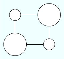
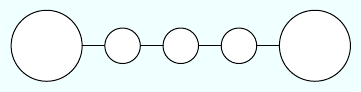
Exercise 11.17 — Markov Networks for Image Segmentation [18 points]

In class we mentioned that Markov Networks are commonly used for many image processing

tasks. In this problem, we will investigate how to use such a network for image segmentation.

The goal of image segmentation is to divide the image into large contiguous regions (segments),

such that each segment is internally consistent in some sense.

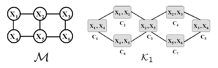
We begin by considering the case of a small 3 ×2 image. We deﬁne a variable Xifor each

node (pixel) in the network, and each can take on the values 1...K for Kimage segments. The

resulting Markov Network Mis shown in Figure 4.

Figure 4: Markov Network for image segmentation.

We will perform our segmentation by assigning factors to this network over pairs of variables.

Speciﬁcally, we will introduce factors φi,j over neighboring pixels iand jthat quantify how

strong the aﬃnity between the two pixels are (i.e., how strongly the two pixels in question want

to be assigned to the same segment).

We now want to perform inference in this network to determine the segmentation. Because we

eventually want to scale to larger networks, we have chosen to use loopy belief propagation on a

cluster graph. Figure 4 also shows the cluster graph K1that we will use for inference.

1. [1 points] Write the form of the message δ3→6that cluster C3will send to cluster C6

during the belief update, in terms of the φ’s and the other messages.

Answer: The form of the message is:

δ3→6(X5) = X

φ2,5(X2, X5)δ2→3(X2)δ4→3(X2)δ7→3(X5).

2. [6 points] Now, consider the form of the initial factors. We are ambivalent to the actual

segment labels, but we want to choose factors that make two pixels with high “aﬃnity”

(similarity in color, texture, intensity, etc.) more likely to be assigned together. In order

to do this, we will choose factors of the form (assume K= 2):

φi,j (Xi, Xj) = αi,j 1

1αi,j (2)

Where αi,j is the aﬃnity between pixels iand j. A large αi,j makes it more likely that

Xi=Xj(i.e., pixels iand jare assigned to the same segment), and a small value makes it

less likely. With this set of factors, compute the initial message δ3→6, assuming that this

is the ﬁrst message sent during loopy belief propagation. Note that you can renormalize

the messages at any point, because everything will be rescaled at the end anyway. What

will be the ﬁnal marginal probability, P(X4, X5), in cluster C6? What’s wrong with this

approach?

Answer: The form of the message is:

δ3→6(X5) = 1 + α2,5

1 + α2,5∝1

1

Here we see that the initial message (and indeed all subsequent messages) will be equal to the

1message. This means that the cluster beliefs will never be updated. Therefore:

P(X4, X5)∝π6(X4, X5) = φ4,5

P(X4, X5) = (1

2+2α4,5if X46=X5,

α4,5

2+2α4,5if X4=X5,

In this approach, because the initial potentials are symmetric, and the messages are over single

variables, no information is ever propagated around the cluster graph. This results in the ﬁnal

beliefs being the same as the initial beliefs. This construction is, as a result, completely useless

for this task.

Chapter 12

Exercise 12.13 — Stationary distribution for Gibbs chain [18 points]

Show directly from Eq. (12.21) (without using the detailed balance equation) that the posterior

distribution P(X | e) is a stationary distribution of the Gibbs chain (Eq. (12.22)). In other

words, show that, if a sample xis generated from this posterior distribution, and x′is the next

sample generated by the Gibbs chain starting from x, then x′is also generated from the posterior

distribution.

Answer: The time tdistribution is:

P(t)(x′)≈P(t+1)(x′) = X

x∈Val(X)

P(t)(x)T(x→x′).

Equation (12.21) refers to the global transition model, which in the case of the Gibbs Chain corre-

sponds to the probability of choosing a variable to ﬂip and then applying the local transition model.

All variables are equally likely to be ﬂipped. The varable xiis sampled from the distribution P(xi|ui)

where uiis the assignment to all variables other than xi.

Notice in the case of the Gibbs chain, only one value is changed at a time.

|X | X

k∈|X | X

xk∈Val(Xk)

P(xk,uk|e)P(x′

k|uk,e)

|X | X

k∈|X | X

xk∈Val(Xk)

P(xk|uk)P(x′

k,uk|e)

P(X′|e)1

|X | X

k∈|X | X

xk∈Val(Xk)

P(xk|uk)

P(X′|e)

New exercise— Data Association and Collapsed MCMC [20 points]

Consider a data association problem for an airplane tracking application. We have a set of K

sensor measurements blips on a radar screen U={u1,...,uK}and another set of Mairplanes

V={v1,...,vM}, and we wish to map U’s to V’s. We introduce a set of correspondence

variables C={C1,...,CK}such that Val(Ci) = {1,...,M}. Here, Ci=jindicates that ui

is matched to vj(The fact that each variable Citakes on only a single value implies that each

measurement is derived from only a single object. But the mutual exclusion constraints in the

other direction are not forced.). In addition, for each ui, we have a set of readings denoted

as a vector Bi= (Bi1, Bi2,...,BiL); for each vj, we have a three dimensional random vector

Aj= (Aj1, Aj2, Aj3) corresponding to the location of the airplane vjin the space. (Assume

that |V al(Ajk )|=d, which is not too large in the sense that summing over all values of Ajis

tractable.)

Now suppose that we have a prior distribution over the location of vj, i.e., we have P(Aj), and

we have observed all Bi, and a set of φij (Aj,Bi, Ci) such that φij (aj,bi, Ci) = 1 for all aj,bi

if Ci6=j. The model contains no other potentials.

We wish to compute the posterior over Ajusing collapsed Gibbs sampling, where we sample the

Ci’s but maintain a closed form posterior over the Aj’s.

1. [1 points] Brieﬂy explain why sampling the Ci’s would be a good idea.

Answer: To compute the posterior over all joint Aj’s or a single Ajusing exact inference

is hard, since it requires exponentially large computation. We use sampling based method to

approximate the posterior by sampling Ci’s resulting in the conditional independence between

Aj’s given Bi’s and Ci’s. This factorization gives us a closed form over each Aj, which makes

the computation tractable. Moveover, since Ci’s serve as selector variables, the context after

sampling them further reduces many factors to be uniform (context independence: Ajdoesn’t

change the belief over Biif Ci6=j). In addition, the space over the joint Aj’s (d3M) might

be larger than that of Ci’s (MK), since dis usually much larger than Mand K, and Mis

likely to be larger than K. Sampling in a lower dimensional space is better in terms of smaller

number of samples and better approximation.

2. [6 points] Show clearly the sampling distribution for the Civariables and the correspond-

ing Markov chain kernels.

Answer: Let Φdenote the set of all factors (note that P(Aj)’s are also the factors in our

model), then the distribution over Ci’s which we want to sample from is

P(C1, C2, . . . , CK|b1,b2,...,bK) = PΦ[¯

b](C1, C2,...,CK) (3)

A′

jsY

P(Aj)Y

φij (Aj,bi, Ci) (4)

where Zis the partition function. In order to get samples from the posterior above, we can

sample from a Markov chain whose stationary distribution is our target. To do so, we deﬁne

the Markov chain kernel for each Ckas:

PΦ[¯

b](Ck|c−k) = PΦ[¯

b](Ck,c−k)

PC′

kPΦ[¯

b](C′

k,c−k).(5)

For each value of Ck=ck, ck= 1,2,...,M, we have

PΦ[¯

b](Ck=ck|c−k) = PΦ[¯

b](ck,c−k)

PΦ[¯

b](c−k)(6)

A1,A2,...,AM

PΦ[¯

b](ck,c−k,A1,A2,...,AM) (7)

A1,A2,...,AM

j=1

P(Aj)Y

i:ci=j

φij (Aj,bi, j) (8)

j=1 X



P(Aj)Y

i:ci=j

φij (Aj,bi, j)

(9)

j=1 X

Ψj,[c1,c2,...,cK](Aj) (10)

where

Ψj,[c1,c2,...,cK](Aj) = P(Aj)Y

i:ci=j

φij (Aj,bi, j) (11)

and

Z=X

j=1 X

Ψj,[ck,c−k](Aj) (12)

Note that to the summation over Aj’s can be pushed into the product so that when we sum

over a speciﬁc Aj, the summation is only over a factor Ψj,[c1,c2,...,cK](Aj)whose scope only

contains Aj. And as mentioned in the question, we assume that summing over a single Ajis

tractable.

3. [8 points] Give a closed form equation for the distribution over the Ajvariables given the

assignment to the Ci’s. (A closed form equation must satisfy two criteria: it must contain

only terms whose values we have direct access to, and it must be tractable to compute.)

Answer: Since Aj’s are independent given all Ci’s, the joint distribution over Aj’s can be

factorized as the product of the marginal distributions over each single Aj. Therefore, we only

specify the marginal distribution over a single Aj:

P(Aj|¯

b,¯c) = 1

ZP(Aj)Y

i:ci=j

φij (Aj,bi, ci).(13)

where, Z=PAjP(Aj)Qi:ci=jφ(Aj,bi, ci),¯

b={b1,b2,...,bK}and ¯c={c1,...,cK}.

4. [5 points] Show the equation for computing the posterior over Ajbased on the two steps

above.

Answer: After the Markov chain converges to its stationary distribution, i.e., the posterior

over Ci’s, we can collect Minstances each of which is denoted by ¯c[m], m = 1,2,...,M, and

with their distributional parts P(Aj|¯

b, ¯c[m]), we can estimate the posterior over Ajas:

P(Aj=aj|¯

b) = 1

m=1

Z[m]P(aj)Y

i:ci[m]=j

φij (aj,bi, ci[m]) (14)

m=1

P(aj)Qi:ci[m]=jφij (aj,bi, ci[m])

Pa′

jP(a′

j)Qi:ci[m]=jφij (a′

j,bi, ci[m]) (15)

where ajis a speciﬁc value that Ajtakes.

Chapter 15

Exercise 15.3 — Entanglement in DBNs I [6 points]

Prove Proposition 15.1:

Let Ibe the inﬂuence graph for a 2-TBN B→. Then Icontains a directed path from Xto Yif

and only if, in the unrolled DBN, for every t, there exists a directed path from X(t)to Y(t′)for

some t′≥t.

Answer: First, we will prove the only if direction. Let the path between Xand Yin Ibe the set

of nodes (X, X1,··· , Y ). By deﬁnition of I, for every two consecutive nodes Xi—Xi+1 in this set,

for every t, there exists a directed edge from X(t)

ito X(t+1)

i+1 or X(t)

i+1. Now, starting at Xt, construct

the directed path in the unrolled by joining these directed edges. This construction holds for any t.

Hence, we shown the existence of the path in the unrolled DBN.

To prove the if direction, let us look at a path in the unrolled DBN, starting at any X(t)represented

by X, X1,··· , Y . Consider the directed edge from Xito Xi+1 on this path for any i; there must be a

directed edge in the inﬂuence graph Ifrom the node corresponding to Xito the node corresponding

to Xi+1. This is true otherwise it violates the construction of the inﬂuence graph. Now, connect all

the directed edges in the inﬂurence graph corresponding to the path in the unrolled DBN. Hence, we

have shown that such a path always exists. concludes our proof.

Exercise 15.4 — Entanglement in DBNs II [14 points]

1. [10 points] Prove the entanglement theorem, Theorem 15.1:

Let hG0,G→ibe a fully persistent DBN structure over X=X∪O, where the state variables

X(t)are hidden in every time slice, and the observation variables O(t)are observed in every

time slice. Furthermore, assume that, in the inﬂuence graph for G→:

•there is a trail (not necessarily a directed path) between every pair of nodes, i.e., the

graph is connected;

•every state variable Xhas some directed path to some evidence variable in O.

Then there is no persistent independence (X⊥Y|Z) which holds for every DBN hB0,B→i

over this DBN structure.

Answer: Note that we will need the additional assumption that Z∩(X∪Y)6=∅. We ﬁrst

show that I(X,Y| ∅)cannot hold persistently.

Assume by contradiction that I(X,Y| ∅)does indeed hold persistently. By decomposition

this implies that I(X, Y | ∅)must hold persistently for all X∈Xand Y∈Y. We now pick a

particular t,X, and Yand examine the statement we have assumed to hold: I(X(t), Y (t)| ∅).

We ﬁrst prove the existence of a trail between X(t)and Y(t)in our DBN. As our inﬂuence

graph is connected it must contain a trail from Xto Y. As the inﬂuence graph was deﬁned

over the 2-TBN this implies a trail in the 2-TBN (using persistence edges to alternate between

interface variables and non-interface variables as necessary). This trail implies the existence of

a corresponding trail between X(t)and Y(t)in the tand t+ 1 timeslices of the DBN. Call this

trail π. For I(X(t), Y (t)| ∅)to hold we must have that πis not active. This can occur in two

ways:

(a) πgoes through an observed node that is not the center of a v-structure. This is impossible

as our only observed nodes are leaves in the DBN.

(b) πgoes through a v-structure A→B←Cwhere neither Bnor any of its descendents

are observed. This cannot be the case because either B∈Oor Bis a state variable.

However, if Bis a state variable we know that a descendant of Bis in Oby Proposition

19.3.4 and our assumption that every state variable has a directed path to an observation

variable in the inﬂuence graph.

Thus the trail must be active, giving us a contradiction.

We’ve thus shown that I(X,Y| ∅)does not hold persistently and will prove that I(X,Y|

Z). To do this we note that by decomposition we must have I(X, Y |Z)(and also by our

assumption X, Y /∈Z). Part (c) will prove that this cannot be the case when we have that

I(X, Y | ∅)does not hold persistently (as we have shown above.)

We now prove that I(X,Y|Z)does not hold persistently with the additional assumption

that X, Y /∈Z.

Assume by contradiction that I(X, Y |Z)holds persistently but that I(X, Y | ∅)does not.

By assumption there must exist some time tsuch that I(X(t), Y (t)| ∅)does not hold. This

implies the existence of an active trail πbetween X(t)and Y(t)in the unrolled DBN. We then

consider some time slice t′which has no nodes in common with π. By assumption we must

have I(X(t′), Y (t′)|Z(t′)). But now we can construct an active trail π′between X(t′)and

Y(t′)given Z(t′). We do so by ﬁrst going from X(t′)to X(t)in πvia the persistance edges,

travelling through π, and then connecting Y(t)and Y(t′)via the persistence edges between

them. Note that Z(t′)cannot interfere by the assumption that timeslice t′contained no nodes

in πand that X, Y /∈Z. This active trail, however, implies that I(X, Y |Z)does not hold at

time t′and thus is not a persistent independence. Therefore, we have a contradiction.

2. [4 points] Is there any 2-TBN (not necessarily fully persistent) whose unrolled DBN is a

single connected component, for which (X⊥Y|Z) holds persistently but (X⊥Y| ∅)

does not? If so, give an example. If not, explain formally why not.

Answer: There are many counterexamples for the case that the 2-TBN is not fully persistent.

One such example has persistent edge X2→X′

2and other edges X′

1←X′

2→X′

3. Here

X(t)

1⊥X(t)

3|X(t)

2holds persistently, but X(t)

1⊥X(t)

3| ∅ does not.

Exercise 15.13 — Collapsed MCMC for Particle Filtering [22 points]

Consider a robot moving around in a space with nstationary landmarks. The positions of the

robot and the landmarks are unknown. The position of the robot (also called a pose) at time tis

denoted X(t). The (ﬁxed) position of landmark iis denoted Li. At each time t, the robot obtains

a (noisy) measurement O(t)

iof its current position relative to each landmark k. The model is

parameterized using two components. Robot poses evolve via a motion model:P(X(t+1) |X(t)).

Sensor measurements are governed by a measurement model:P(O(t)

i|X(t), Li). Both the motion

model and the measurement model are known.

Denote X(1:t)={X(1), . . . , X(t)},L={L1,...,Ln}, and O(1:t)={O(1)

1,...,O(1)

n, O(2)

1,...,O(t)

n}.

We want to use the measurements O(1:t)to localize both the robot and landmarks; i.e., we want

to compute P(X(t),L|o(1:t)).

1. [2 points] Draw a DBN model for this problem. What is the dimension (number of

variables) of the belief state for one time slice in this problem? (Assume that the belief

state at time tis over all variables about which we are uncertain at time t.)

Answer: The simplest way to represent this is to extend our model for a DBN to allow some static

variables, which are not part of each timeslice. We can think of them as existing before the ﬁrst

timeslice. Unrolled, it looks like this:

But to store it compactly, whereas we previously needed only representations of B0and B→, repre-

senting the initial state and transition model, here we have a third network, representing the static

variables, which we will denote Bs. Note that in principle, with this extension to the notion of a

DBN, the static variables could actually be a standard Bayes net, with some of them depending on

each other; but in our case they will not, so their CPDs have no parents to condition on. However,

the CPDs in B→can then use the variables in Bsas parents, in addition to any inter-timeslice and

intra-timeslice edges.

Of course, we could alternately represent it by including all the static variables in the 2-TBN, each

with a deterministic CPD simply propagating its values forward, never changing.

A belief state now corresponds to a set of beliefs for the static variables as well as the state variables

of the current timeslice, so in our DBN, the belief state will have a dimension of n+ 1.

We want to use particle ﬁltering to solve our tracking problem, but particle ﬁltering tends to

break down in very high dimensional spaces. To address this issue, we plan to use particle ﬁltering

with collapsed particles. For our localization and mapping problem, we have two obvious ways of

constructing these collapsed particles. We now consider one such approach in detail, and brieﬂy

consider the implications of the other.

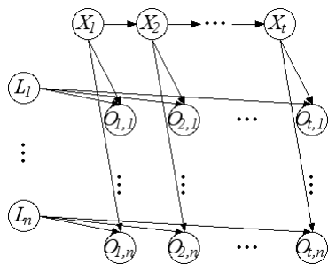
1. [15 points] We select the robot pose trajectory X(1:t)as the set of sampled variables, and

maintain a closed form distribution over L. Thus, at time twe have a set of weighted

particles, each of which speciﬁes a full sampled trajectory x(1:t)[m], a distribution over

landmark locations P(t)

m(L), and a weight w(t)[m].

(a) The distribution over Lis still exponentially large in principle. Show how you can

represent it compactly in closed form. (Hint: Write out the full form of P(t)

m(L)

recalling the deﬁnition of collapsed particles, and note that our samples represent

entire pose trajectories X(1:t). )

Answer: Since each particle instantiates all of x(1:t)[m]and o(1:t)[m], there is no active

trail from Lito Ljfor i6=j, and so the Livariables are all independent, given a particle.

Also, each landmark’s location is independent of the observations of the other landmarks,

given a trajectory. Thus we can decompose our distribution over the landmarks’ locations

as the following product of marginals:

P(t)

m(L) = P(L|x(1:t)[m],o(1:t)[m])

P(Li|x(1:t)[m],o(1:t)[m])

P(Li|x(1:t)[m], o(1:t)

i[m])

P(t)

m(Li)

Note that it is not in closed form yet. We will show how to compute P(t)

m(Li)in part ii.

(b) Describe how to perform a forward propagation step in our collapsed particle ﬁltering

algorithm. Speciﬁcally show how to:

•generate a new set of particles for time t+ 1

•compute the weight w(t+1)[m] of each particle;

•compute the distribution P(t+1)

m(L).

Answer: To generate new particles, we basically just follow standard particle ﬁltering –

normalize the weights of the particles from the previous timeslice; select a particle under

that normalized distribution; then sample its forward propagation based on the motion model

P(X(t+1) |X(t)).

To see how to compute our new distribution over L, we ﬁrst make the following observation:

P(t+1)

m(Li) = P(Li|x(1:t+1)[m], o(1:t+1)

i[m])

ZP(o(1:t+1)

i[m]|Li, x(1:t+1)[m])P(Li|x(1:t+1)[m])

ZP(o(1:t+1)

i[m]|Li, x(1:t+1)[m])P(Li)

ZP(Li)

t+1

t′=1

P(o(t′)

i[m]|Li, x(t′)[m])

for some normalizing constant

Z=X

P(li)

t+1

t′=1

P(o(t′)

i[m]|li, x(t′)[m])

which does not depend on Li. Note that P(Li)is the prior for the location of the landmark,

as encoded by Bs(or B0if using deterministic CPDs to propagate the Livariables through all

timeslices); and each factor of the product is just a lookup in the known measurement model.

However, since

P(t)

m(Li) = 1

Z′P(Li)

t′=1

P(o(t′)

i[m]|Li, x(t′)[m])

for some other normalizing constant

Z′=X

P(li)

t′=1

P(o(t′)

i[m]|li, x(t′)[m])

which similarly does not depend on Li, then

P(t+1)

m(Li) = 1

Z′′ P(t)

m(Li)P(o(t+1)

i[m]|Li, x(t+1)[m])

for some normalizing constant Z′′ =Z

Z′which does not depend on Li. Thus, to update our

beliefs about the location of the landmarks, we just multiply in the probability of the new

observations from the measurement model and renormalize.

Having updated our distribution over the locations of the landmarks, we now need to compute

the weight for the particle. In standard particle ﬁltering, we use the likelihood of the new

observations given the complete particle; here, our particle does not contain the location of the

landmarks, so we must compute our weights using the other given information. We can consider

the reweighting to be given all of the previously sampled variables together with all observations.

Using this insight, we can compute the particles by marginalizing out the landmark locations:

w(t+1)[m] = P(o(t+1)[m]|x(1:t+1)[m],o(1:t)[m])

l∈V al(L)

P(o(t+1)[m],l|x(1:t+1)[m],o(1:t)[m])

l∈V al(L)

P(l|x(1:t+1)[m],o(1:t)[m])P(o(t+1)[m]|x(1:t+1)[m],o(1:t)[m],l)

l∈V al(L)

P(l|x(1:t)[m],o(1:t)[m])P(o(t+1)[m]|x(t+1)[m],l)

l∈V al(L)

i=1

P(li|x(1:t)[m], o(1:t)

i[m])P(o(t+1)

i[m]|x(t+1)[m], li)

l∈V al(L)

i=1

P(t)

m(li)P(o(t+1)

i[m]|x(t+1)[m], li)

Thus we see how to compute the weight for the particle in the new timeslice using the normal-

ized distribution P(t)

m(L)from the previous timeslice, together with our measurement model

P(o(t)

i[m]|x(t)[m], li).

2. [5 points] As another alternative, we can select the landmark positions Las our set of

sampled variables. Thus, for each particle l[m], we maintain a distribution P(t)

m(X(t)).

Without describing the details of how to perform a forward propagation step in our col-

lapsed particle ﬁltering algorithm, we can think about the eﬀectiveness of such an approach.

In this algorithm, what will happen to the particles and their weights eventually (i.e., after

a large number of time steps)? What are the necessary conditions for this algorithm to

converge to the correct map?

Answer: Since we never generate any new assignments l[m], on each forward propagation,

with some nonzero probability, one or more of the particles will “die oﬀ”. Thus eventually, we

will be left with a single particle l[m]with a weight of 1.

The single map to which we converge will be the correct map only if our initial generation of

particles included the correct map among its hypotheses. Since we never generate any new

hypotheses, we certainly cannot converge on the right one if we failed to start with it as a

hypothesis. However, although this is necessary, it is not suﬃcient, since even if we start with

the correct hypothesis as an available option, it is possible that by chance we might discard it,

especially early on when, with few observations, its weight may not be much more than that

of the other hypotheses.

As there are exponentially many assignments to L, unless we have a very well-speciﬁed prior

over them, it is highly unlikely the correct solution will be generated as an initial hypothesis.

Chapter 18

Exercise 18.8 — Bayesian score structure equivalence I [5 points]

Show that if Gis I-equivalent to G′, then if we use table CPDs, we have that scoreL(G:D) =

scoreL(G′:D) for any choice of D.

Hint: consider the set of distributions that can be represented by parameterization each network

structure.

Answer: Using table CPDs for G, we can represent any joint probability distribution that complies

with the conditional independence implied by the G. Since G′implies the same conditional indepen-

dence as G, they represent exactly the same set of distributions. Therefore, for any parameterization

θGof G, there is a corresponding parameterization θG′of G′which generates the same distribution.

Since the likelihood of data set Donly depends on the underlying distribution, we have:

scoreL(G:D) = ℓ(hG,ˆ

θGi:D) = ℓ(hG′,θG′i:D)≤scoreL(G′:D)

where ˆ

θGare the maximum likelihood parameters for G, and θG′are the corresponding parameters

in G′.

By the same reasoning, we have scoreL(G′:D)≤scoreL(G:D). Therefore:

scoreL(G:D) = scoreL(G′:D)

Exercise 18.9 — Bayesian score structure equivalence II [10 points]

Show that if Gis I-equivalent to G′, then if we use table CPDs, we have that scoreBIC (G:D) =

scoreBIC (G′:D) for any choice of D.

Answer: The BIC score is deﬁned as: scoreBIC (G:D) = scoreL(G:D)−log M

2Dim[G]and

by (6a) we know scoreL(G:D) = scoreL(G′:D). Therefore, to prove scoreBIC (G:D) =

scoreBIC (G′:D), we only need to show Dim[G] = Dim[G′].

We ﬁrst consider the case where Gand G′only diﬀers by one safe edge reversal such that X→Y∈ G

and X←Y∈ G′. All the other variables except Xand Yhave the same parents in Gand G′and

thus have the same number of parameters. Assume variables Zare the common parents of Xand

Y. Denote SIZEG(N)to be the number of parameters for variable Nin G:

Dim[G]

N∈G

N6=X,Y

SIZEG(N) + SIZEG(X) + SIZEG(Y)

N∈G

N6=X,Y

SIZEG(N) + (|Val(()X)| − 1)|V al(Z)|+ (|V al(Y)| − 1)|V al(Z)||V al(X)|

N∈G

N6=X,Y

SIZEG(N) + (|V al(Y)||V al(Z)||V al(X)| − |V al(Z)|

N∈G′

N6=X,Y

SIZEG′(N) + (|Val(()Y)| − 1)|V al(Z)|+ (|V al(X)| − 1)|V al(Z)||V al(Y)|

N∈G′

N6=X,Y

SIZEG′(N) + SIZEG′(Y) + SIZEG′(X)

= Dim[G′]

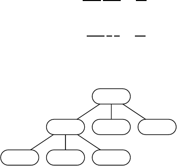
In general, for any two I-equivalent Gand G′, they can be connected by a sequence of safe edge

reversal. Therefore, Gand G′have the same number of parameters and thus the same BIC score.

Exercise 18.10 — Bayesian score structure equivalence III [10 points]

Show that the Bayesian score with a K2 prior in which we have a Dirichlet prior Dirichlet(1,1,...,1)

for each set of multinomial parameters is not score equivalent.

Hint: construct a data set for which the score of the network X→Ydiﬀers from the score of

the network X←Y.

Answer: Construct Gto be X→Yand G′to be X←Y. They are I-equivalent. Construct Dto

be {(x1, y1),(x1, y0)}.

P(D|G) = 1·2

2·3

1·1

2·3=1

On the other hand:

P(D|G′) = 1·1

2·3

2=1

Therefore, their Bayesian scores are diﬀerent assuming equal structure prior.

Exercise 18.26 — Ordering-based search in structure learning [12 points]

1, 2, 3, 4

2, 1, 3, 4 1, 3, 2, 4 1, 2, 4, 3

2, 3, 1, 41, 2, 3, 4 2, 1, 4, 2

Figure 5: Partial search tree example for orderings over variables

X1, X2, X3, X4. Successors to ≺= (1,2,3,4) and ≺′= (2,1,3,4)

shown.

Consider learning the structure of a Bayesian network for some given ordering, ≺, of the variables,

X1,...,Xn. This can be done eﬃciently, as described in section 18.4.2 of the course reader. Now

assume that we want to perform search over the space of orderings, i.e. we are searching for

the network (with bounded in-degree k) that has the highest score. We do this by deﬁning the

score of an ordering as the score of the (bounded in-degree) network with the maximum score

consistent with that ordering, and then searching for the ordering with the highest score. We

bound the in-degree so that we have a smaller and smoother search space.

We will deﬁne our search operator, o, to be “Swap Xiand Xi+1” for some i= 1,...,n−1.

Starting from some given ordering, ≺, we evaluate the BIC-score of all successor orderings, ≺′,

where a successor ordering is found by applying oto ≺(see Figure 5). We now choose a particular

successor, ≺′. Provide an algorithm for computing as eﬃciently as possible the BIC-score for the

successors of the new ordering, ≺′, given that we have already computed the scores for successors

of ≺.

Answer: Notation: Let hbe the variable that was swapped for ≺′, let ibe the variable to be

swapped for candidate ≺′′, and let Succj(≺)be the jth candidate successor of ≺.

The BIC-score is decomposable so we only need to consider the family scores. We cache all family

scores of ≺as well as all family scores of all candidates for ≺′. We can discard all previously cached

values prior to those pertaining to ≺. We consider the family score FamScorej(≺′′ :D)for each

variable Xj, j = 1,...,n:

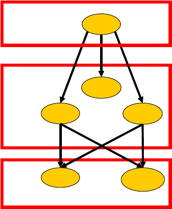
•If j > i + 1,FamScorej(≺′′ :D) = FamScorej(≺′:D).

•If j < i,FamScorej(≺′′ :D) = FamScorej(≺′:D).

•If j=ior j=i+ 1:

–If i=h,FamScorej(≺′′ :D) = FamScorej(≺:D).

–If i > h + 1 or i < h −1,FamScorej(≺′′ :D) = FamScorej(Succi(≺) : D).

–If i=h+ 1 or i=h−1, compute the family score from scratch: FamScorej(≺′′ :D) =

argmaxU∈{Xk:Xk≺′′ Xj}FamScore(Xj|Uj:D)

Problem 18.22 — Module network learning [15 points]

In this problem, we will consider the task of learning a generalized type of Bayesian networks

that involves shared structure and parameters. Let Xbe a set of variables, which we assume are

all binary-valued. A module network over Xpartitions the variables Xinto Kdisjoint clusters,

for K≪n=|X |. All of the variables assigned to the same cluster have precisely the same

parents and CPD. More precisely, such a network deﬁnes:

•An assignment function A, which deﬁnes for each variable X, a cluster assignment A(X)∈

{C1,...,CK}.

•For each cluster Ck(k= 1,...,K), a graph Gwhich deﬁnes a set of parents PaCk=Uk⊂ X

and a CPD Pk(X|Uk).

The cluster network structure deﬁnes a ground Bayesian network where, for each variable X, we

have the parents Ukfor k=A(X) and the CPD Pk(X|Uk). Figure 6 shows an example of

such a network.

Cluster III

Cluster II

Cluster I

Figure 6: A simple module network

Assume that our goal is to learn a cluster network that maximizes the BIC score given a data set

D, where we need to learn both the assignment of variables to clusters and the graph structure.

1. [5 points] Deﬁne an appropriate set of parameters and an appropriate notion of suﬃcient

statistics for this class of models, and write down a precise formula for the likelihood

function of a pair (A,G) in terms of the parameters and suﬃcient statistics.

Answer: To parameterize a module network, we only need one CPD for each cluster,

i.e., Pk(X|Uk), k = 1,2,...,K. The set of parameters for each Pk(X|Uk)is {θx1|uk|uk∈

|V al(Uk)|}. The suﬃcient statistics for each CPD are simply aggregated from each family in

the cluster. Given the suﬃcient statistics for each cluster, the likelihood function looks the

same as the ordinary BN case (view each cluster as a single family with the CPD Pk(X|Uk)).

2. We use greedy local search to learn the structure of the cluster network. We will use the

following types of operators (each operation should remain the graph acyclic):

•Add operators that add a parent for a cluster;

•Delete operators that delete a parent for a cluster;

•Node-Move operators ok→k′(X)that change from A(X) = kto A(X) = k′. (If

X∈PaCk′, moving Xto k′is not allowed.)

As usual, we want to reduce the computational cost by caching our evaluations of operators

and reusing them from step to step.

(a) [2 points] Why did we not include edge reversal in our set of operators? Answer: In

ordinary BN, an edge represents a one-to-one relationship between two variable, however,

in the module networks, an edge from a variable to another variable actually represents

a one-to-many relation between the variable and all the variables in the cluster. So the

relation is not symmetry, reversing the edge is not well-deﬁned.

(b) [2 points] Describe an eﬃcient implementation for the update associated with the

Node-Move operator. Answer: When Xis moved from cluster kto k′, only the

local scores of these two modules change. So the rescoring of these two modules can be

eﬃciently calculated by substracting X’s statistics from the suﬃcient statistics of Ckand

adding the suﬃcient statistics regarding Xto the overall suﬃcient statistics of Ck′.

uated once the operator has been taken. Brieﬂy justify your response. (Suppose that

we cache and update evaluations of operators and reuse them to save the computa-

tion.)

Answer: For adding and deleting operators, if the operator changes the parents of

cluster Ck, then we only need to update the changes in score for those operators that

involve Ck. For moving operators, if the operator is to move a variable from cluster kto

k′, then we only need to update the changes in score for those operators that involve Ck

and Ck′.

New exercise (chapters 12, 18) — Sampling on a Tree [15 points]

Suppose we have a distribution P(X,E) over two sets of variables Xand E. Our distribution

is represented by a nasty Bayes Net with very dense connectivity, and our sets of variables X

and Eare spread arbitrarily throughout the network. In this problem our goal is to use the

sampling methods we learned in class to estimate the posterior probability P(X=x|E=e).

More speciﬁcally, we will use a tree-structured Bayes Net as the proposal distribution for use in

the importance sampling algorithm.

1. [1 points] For a particular value of xand e, can we compute P(x|e) exactly, in a

tractable way? Can we sample directly from the distribution P(X|e)? Can we compute

P(x|e) = P(x,e) exactly, in a tractable way? For each question, provide a Yes/No

answer and a single sentence explanation or description.

Answer: No, No, Yes

2. [7 points] Now, suppose your friendly TAs have given you a tree network, where X1is the

root and each Xifor i6= 1 has exactly one parent Xp(i). They tell you that the distribution

Q(X,E) deﬁned by this network is “close” to the distribution P(X,E). You now want to

use the posterior in Qas your proposal distribution for importance sampling.

(a) Show how to sample from the posterior in Q. More speciﬁcally, provide an explicit

construction for a clique tree over this network, and show how to use it to compute

the posterior Q(X|E=e). Describe how to sample from this posterior, once it has

been computed. Answer: Create a clique tree where each clique is a pair of variables

(child and parent). Multiply in the indicator functions for the evidence E=e. The

distribution across the tree now represents Q(X,E|E=e). Calibrate the tree. Now,

the belief at a clique over (X, PaX)is proportional to Q(X, PaX|E=e). From this

belief, we can easily compute Q(X|PaX,E=e)(use Bayes’ Rule). Using these CPDs,

we can now forward sample directly from the posterior in Q(sample the ﬁrst variable,

then instantiate it in neighboring cliques, repeating to forward sample).

(b) Now you must reweight the samples according to the rules of importance sampling.

You want your weighted samples to accurately represent the actual posterior in the

original network P(X|E=e). Show precisely how you determine the weights w[m]

for the samples. Answer: The weight of the particle is:

w[m] = P′(x[m],e[m])

Q(x[m],e[m]|e)

P(X=x|E=e) for P(X=x|E=e),

in terms of the samples from part i, and the weights from part ii. Answer: The

estimator:

P(X=x|E=e) = PM

m=1 w[m]1{x[m] = x}

m=1 w[m]

3. [7 points] Examining the results of your sampling, you ﬁnd that your TAs were wrong,

and the original tree from which you sampled did not provide very good estimates for

the posterior. You therefore decide to produce a better tree, and rerun the importance

sampling again. This better tree should represent a distribution which is “closer” to the

posterior from which you are trying to sample. Show how you can use the samples produced

in the previous step to learn the best tree (i.e., a tree that best represents the posterior

distribution as estimated in part b, according to the likelihood score). Assume you have

access to a maximum spanning tree algorithm, and your job is to deﬁne the weights for

the edges in terms of the estimator computed above. Answer: We will use the maximum

spanning tree algorithm to select edges where the weight for a candidate edge between Xiand

Xjis computed as:

wij =F amScore(Xi|Xj:D)−F amScore(Xi:D)

=I(Xi;Xj) + H(Xi)

xiX

M[xi, xj] log ¯

M[xi, xj]

M[xi]−X

M[xi] log ¯

M[xi]

where the ¯

Mterms are the suﬃcient statistics from the weighted dataset:

M[xi, xj] = X

1{xi[m] = xi, xj[m] = xj}w[m],

etc.

Exercise 18.23 — Optimal reinsertion structure learning [10 points]

More complex search operators are sometimes useful in Bayesian Network structure learning.

In the problem we will consider an operator that we will call the Reinsertion operator. This

operator works as follows:

Assume that we have been searching for awhile, and our current structure is Gt. We now choose

a variable Xto be our target variable. The ﬁrst step is to remove the variable from the network,

by severing all connections into and out of this target variable. We then select the optimal set of

parents and children for X, and reinsert it into the network with edges from the selected parents

and to the selected children. In addition, consider that we will limit the number of parents to a

variable to Kpand the number of children to Kc. This restriction helps us to avoid the need to

consider overly complex networks.

Throughout this problem, assume the use of the BIC score for structure evaluation.

1. [2 points] Let Xibe our current target variable, and assume for the moment that we have

somehow chosen Uito be optimal parents of Xi. Consider the case of Kc= 1, where we

want to choose the single optimal child for Xi. Candidate children — those that do not

introduce a cycle in the graph — are Y1,...,Yℓ. Write an argmax expression for ﬁnding

the optimal child C. Explain your answer.

Answer: Because the BIC score is decomposable by family, we can consider only the family

of the proposed child when computing the change in score that would result from adding that

child. Thus, we choose the child YCsuch that:

YC= arg max

F amScore(Yi|PaYi, X)

= arg max

YiMII ˆ

P(Yi;PaYi, X)−II ˆ

P(Yi;PaYi)−log M

2∆Dim

We choose this Yconly among variables that are not ancestors of any of the variables in Ui.

2. [4 points] Now consider the case of Kc= 2. How do we ﬁnd the optimal pair of children?

Assuming that our family score for any {Xk,Uk}can be computed in a constant time

f, what is the best asymptotic computational complexity of ﬁnding the optimal pair of

children? Explain. Extend your analysis to larger values of Kc. What is the computational

complexity of this task?

Answer: For the same reason as above, we can “score” each child independently, and

choose the top Kcof them. The total cost for Kc= 2 children is O(fN)and for general

Kcwe can compute the scores, sort them, and select the top candidates. The complexity of

this is O(f N +Nlog N). It is also possible to use a better sort if you only need the top Kc

candidates, and that the complexity becomes O(f N +Nlog Kc).

3. [3 points] We now consider the choice of parents for Xi. We now assume that we have

already somehow chosen the optimal set of children and will hold them ﬁxed. Can we do

the same trick when choosing the parents? If so, show how. If not, argue why not.

Answer: No we cannot do this. The family score for the child cannot be evaluated indepen-

dently for each parent. Instead we must consider all combinations of parents. The complexity

of this task is exponential in Kp.

New exercise — Structure learning for tree-augmented naive Bayes [21 points] Now, consider

the problem of learning a classiﬁer network structure which augments the Naive Bayes model.

Here, we have a class variable Cin addition to the feature variables X1,...,Xn.

1. [5 points] We begin by assuming that the class variable Cis connected to each of the

Xi’s, but in addition, each of the Xi’s may have at most one additional parent. Modify the

algorithm of section 18.4.1 to ﬁnd the highest-scoring network subject to these constraints.

You may assume that we use a structure-equivalent scoring function.

Answer: In this problem, we again are optimizing with respect to the BIC score, but this

time, our baseline graph is the regular Naive Bayes model (which we shall call GN B ), which

contains an edge from the class variable Cto each feature Xi. Thus, we are interested in

maximizing

∆(G) = score(G:D)−score(GN B :D).

To do this, we redeﬁne the weights

wXj→Xi= FamScore(Xi|Xj, C :D)−FamScore(Xi|C:D)

=M[II ˆ

P(Xi;Xj, C)−II ˆ

P(Xi;C)] −log M

2|Val(Xi)−1||Val(Xj)−1||C|

=M[II ˆ

P(Xi;Xj, C)−II ˆ

P(Xi;C)] −log M.

As before, it is a useful and easy exercise to check that wXj→Xi=wXi→Xj. Thus, picking a

graph which maximizes ∆(G)simply involves using an maximum weight undirected spanning

tree or forest approach identical to the procedure given in part (a). Using such a method to

ﬁnd edges between the Xi’s, we ﬁnish by directing all edges (as before) and adding an edge

from Cto each Xi.

2. [16 points] (*) Now, assume that we allow ourselves even more ﬂexibility: for each Xi,

we need to decide separately whether to add Cas a parent or not. We want to pick the

highest scoring network where each node Ximay or may not have Cas a parent, and

each Xican have at most one additional parent Xj. (The node Cis always a root.) Show

how to reduce this problem to one of ﬁnding the maximum-weight directed spanning tree.

(Hint: Consider separately each possible family for each node Xi.)

Note: You do not need to present an algorithm for computing maximum-weight directed

spanning trees, but only to show how you could solve the problem of ﬁnding an optimal

BN of this type if you had a maximum-weight directed spanning tree algorithm to use as

a subroutine.

Answer: There are several possible correct answers to this problems; we sketch a few working

approaches here.

Method 1

We start with the empty graph (G0) as our baseline. For each Xi, the possible (non-empty)

parent sets of Xiare: (1) {Xj}(for some Xj), (2) {Xj, C}(for some Xj), and (3) {C}.

Relative to the empty graph, the change in BIC score resulting from using each of the parent

sets above is:

∆{Xj}= FamScore(Xi|Xj:D)−FamScore(Xi:D)

=MII ˆ

P(Xi;Xj)−log M

∆{Xj,C}= FamScore(Xi|Xj, C :D)−FamScore(Xi:D)

=MII ˆ

P(Xi;Xj, C)−3 log M

∆{C}= FamScore(Xi|C:D)−FamScore(Xi:D)

=MII ˆ

P(Xi;C)−log M

Our goal is to pick a single parent set (which may be empty) for each Xiwhile making sure that

the generated network is acyclic. To do this, consider a graph over the nodes C, X1,...,Xn,

with edges from the class variable Cto each feature Xiand from each feature Xjto every other

feature Xi. We use the edge weights wC→Xi= ∆{C}and wXj→Xi= max(∆{Xj,C},∆{Xj}).

Note that in the latter term, we take a max since the presence or absence of Cin the parent

set of Xidoes not make a diﬀerence with regard to acyclicity of the generated network, as

sorted out during the maximum directed spanning forest algorithm; thus, we can simply use

the higher scoring option.

Given a maximum directed spanning forest Ffor this graph, we deﬁne the parent set of each

feature Xiin the resulting network as follows:

PaG

i=









{Xj}if Xj→Xi∈ F and ∆{Xj}≥∆{Xj,C},

{Xj, C}if Xj→Xi∈ F and ∆{Xj}<∆{Xj,C},

{C}if C→Xi∈ F, and

∅otherwise.

By construction, these four cases are disjoint and hence the parent set of each feature is well-

deﬁned. Furthermore, it is easy to verify that any cycle in the generated network implies the

existence of a corresponding cycle in F, an impossibility. (To see this, note that Xj→Xi

in the network can only happen if Xj→Xi∈ F by the deﬁnition given above; apply this

to all edges in a cycle of the generated network.) Thus, any spanning forest gives a well-

formed Bayesian network. Similarly, one may also show that any valid Bayesian network which

meets the constraints of the problem statement gives rise to a valid directed spanning forest.

Since total weight of any forest is identical to the BIC score of the corresponding network, it

follows that this algorithm generates an optimal BIC-scoring network subject to the problem

constraints.

As a ﬁnal note, if we are restricted to using a maximum weighted directed spanning tree

algorithm, the method of zeroing out negative weights described in part (a) works here as well.

Method 2

We again use G0as our baseline, and deﬁne ∆{Xj},∆{Xj,C}, and ∆{C}as before for each

Xi. For the reduction to the maximum weighted directed spanning forest problem, we deﬁne

a graph containing Cand X1,...,Xnas before, with directed edges from Cto each Xiand

from each Xjto Xi. This time, however, we also introduce new nodes CX1,...,CXn, and

create edges from CXjto Xifor all i6=j, and edges from Xito CXifor all i. For each Xi,

the weight of the Cto Xiedge is ∆{C}, the weight of the Xjto Xiedge (for all j6=i) is

∆{Xj}, the weight of the CXjto Xiedge (for all j6=i) is ∆{Xj,C}, and the weight of the Xi

to CXiis set to a suﬃciently large positive constant (to ensure that the Xito CXiis always

selected by the maximum weighted directed spanning forest algorithm).

Given a maximum directed spanning forest Ffor this graph, we deﬁne the parent set of each

feature Xiin the resulting network as follows:

PaG

i=









{Xj}if Xj→Xi∈ F

{Xj, C}if CXj→Xi∈ F

{C}if C→Xi∈ F, and

∅otherwise.

Clearly, the parent set of each Xiis well-deﬁned. Again, we can check that cycles in the

generated network imply cycles in F. (As a simple example, note that if Xj→Xi∈ F, then

selecting either Xi→Xjor CXi→Xjfor the spanning forest will generate a cycle because

of the required edge Xi→CXi; you can generalize this reasoning to cycles of length greater

than two.) The remaining arguments for correctness follow similarly to those given in Method

Method 3

In the last method, we do not use G0as the baseline; rather, we use a graph G′

0in which we

include the C→Xiedge for each Xisuch that ∆{C}>0(using the deﬁnition from Method

1). We then redeﬁne for each Xi,

∆{Xj}= FamScore(Xi|Xj:D)−max(FamScore(Xi:D),FamScore(Xi|C:D))

∆{Xj,C}= FamScore(Xi|Xj, C :D)−max(FamScore(Xi:D),FamScore(Xi|C:D))

and create a graph over only the Xi’s such that each edge Xj→Xiis given weight max(∆{Xj},∆{Xj,C}).

Given a maximum directed spanning forest Ffor this graph, we deﬁne the parent set of each

feature Xiin the resulting network as follows:

PaG

i=









{Xj}if Xj→Xi∈ F and ∆{Xj}≥∆{Xj,C},

{Xj, C}if Xj→Xi∈ F and ∆{Xj}<∆{Xj,C},

{C}if Xj→Xi/∈ F and C→Xi∈ G′

0, and

∅if Xj→Xi/∈ F and C→Xi/∈ G′

Arguing that the choice of parent set is well-deﬁned and that the resulting Bayesian network

must be acyclic is easy (a cycle in the generated network implies a cycle in Fby construction).

This time, it is not true that any valid Bayesian network ﬁtting the constraints in the problem

corresponds to some directed spanning forest; in particular, it might be the case that for some

network where Xihas parent set ∅, no corresponding directed forest exists since C→Xi∈ G′

However, one can argue that the highest scoring Bayesian network does correspond to some

directed spanning forest. To see why, note that in the previous scenario, C→Xi∈ G′

0implies

that ∆{C}>0for Xi, so changing the parent set of Xito {C}yields an improvement in

the total score of the network without generating cycles. Thus, any network which has no

corresponding directed spanning forest cannot be optimal.

Finally, it suﬃces to note that the weight of any directed spanning forest is equal to the

score corresponding Bayesian network minus the score of G′

0, so an maximum weight directed

spanning forest implies a maximal scoring Bayesian network.

Common errors:

(a) Constructions similar to Method 3, but which used G0as the baseline graph and attempted

to account for C→Xiedges as a postprocessing step. This fails for a simple network

X1←C→X2in which all three variables are strongly correlated (but X1and X2are

conditionally independent given C). The score for adding an X1→X2edge (with or

without Cas another parent of X2) is certainly higher than that of not including X1→X2

in the baseline graph G0(where X1and X2are independent of C). Thus, the maximum

weighted directed spanning forest algorithm will be forced to select an X1→X2edge

even though such an edge does not exist in the true network.

(b) Constructions similar to Method 2, but which failed to include the forced edges Xi→

CXi, resulting in possible cycles in the resulting network. Without these forced edges, a

maximum weight directed spanning forest might contain both CXj→Xiand CXi→Xj,

causing the resulting network to have an Xi↔Xjcycle.

instead set edge weights wXj→Xi= max(∆{Xj,C},∆{Xj},∆{C}). A minor problem here

is that for a network with nfeature variables, we know that any maximum weight directed

spanning tree contains at most n−1edges. Hence, we can make decisions for the parent

set of at most n−1feature variables. In the degenerate case of a network with one

feature variable X1, the returned network will always have Cdisconnected from X1.

(d) [6 points] Constructions which omit the possibility of letting Xihave the parent set {C}.

Chapter 19

Exercise 19.3 — EM for CPD-trees [6 points]

Consider the problem of applying EM to parameter estimation for a variable Xwhose local

probabilistic model is a CPD-tree. We assume that the network structure Gincludes the structure

of the CPD-trees in it, so that we have a structure Tfor X. We are given a data set Dwith

some missing values, and we want to run EM to estimate the parameters of T. Explain how we

can adapt the EM algorithm in order to accomplish this task.

Answer: Consider the leaves of tree T. Each contains a distribution over the values of X

corresponding to a speciﬁc set of values qfor Q, where Qis a subset of the parent nodes U. What

does this subset of parent nodes represent? It represents the relevant parents in a given situation,

speciﬁcally whenever Q=q. The other parents become irrelevant in this case, as their values do

not change the resulting distribution over values for X. In other words, when Q=q, it is as if X

only has Qas parents. More formally, whenever q⊆u,P(X|U=u) = P(X|Q=q). Notice

that for each leaf Qcorresponds to the variables encountered on the path from the root of the tree

to that leaf.

For simplicity let us assume that all variables are binary. Consider a leaf in the tree. We determine

its relevant subset of parents and the values assigned to this subset (Qand qfrom the above). Then

the parameter that represent that leaf looks like θX|q. We will get a similar parameter for every other

leaf in the tree. If we had complete data, the parameters would be estimated using the suﬃcient

statistics:

θX|q=Mx,q

=PM

j=1 1(X[j] = x, Q[j] = q)

j=1 1(Q[j] = q)

Similarly, each iteration then updates the parameters as using the expected suﬃcient statistics:

θX|q=˜

Mx,q

=PM

j=1 P(x, q|d[j],θold)

j=1 P(q|d[j],θold)

Exercise 19.4 — EM for noisy-OR [9 points] Consider the problem of applying EM to

parameter estimation for a variable Xwhose local probabilistic model is a noisy-or. Assume that

Xhas parents Y1,...,Yk, so that our task for Xis to estimate the noise parameters λ0,...,λk.

Explain how we can use the EM algorithm to accomplish this task. (Hint: Utilize the structural

decomposition of the noisy-or node, as in ﬁgure (4.12) of the reader.)

Answer:

Suppose we decompose the noisy-or node into table CPT nodes as done in ﬁgure (4.12) of the reader

(see Figure 7 above). Since X’s CPT becomes a deterministic OR, we leave its CPT ﬁxed in the EM

algorithm. We treat the Y′

ias unobserved variables. The only parameters we need to estimate for

this expanded noisy-or are the noise parameters λicontained in the CPTs for Y′

iand λ0contained

in the CPT for Y′

0. We have λi=θY′

i=1|Yi=1 =P(Y′

i= 1 |Yi= 1) and λ0=θY′

0=1 =P(Y′

0= 1).

The parameters θY′

i=0|Yi=0 and θY′

i=1|Yi=0 are ﬁxed during EM to 1and 0, respectively.

So when we use EM we update these parameters as follows:

λi=PM

j=1 P(Y′

i= 1, Yi= 1 |d[j],θold)

j=1 P(Yi= 1 |d[j],θold)

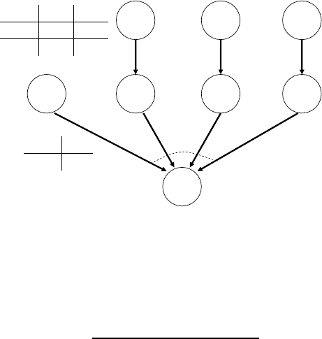
Y1Y2Y3

Y1' Y2' Y3'Y0'

λi

0Yi' = 1

1-λi

1Yi' = 0

Yi = 1Yi = 0

λ0

Y0' = 1

1-λ0

Y0' = 0

Figure 7: Noisy Or Decomposition

λ0=PM

j=1 P(Y′

0= 1 |d[j],θold)

Exercise 19.15 — Message passing with EM [15 points]

Suppose that we have an incomplete data set D, and network structure Gand matching pa-

rameters. Moreover, suppose that we are interested in learning the parameters of a single CPD

P(Xi|Ui). That is, we assume that the parameters we were given for all other families are

frozen and do not change during the learning. This scenario can arise for several reasons: we

might have good prior knowledge about these parameters; or we might be using an incremental

approach (for example, see the section in Box 19.C on accelerating convergence).

We now consider how this scenario can change the computational cost of the EM algorithm.

1. [10 points] Assume we have a clique tree for the network Gand that the CPD P(Xi|Ui)

was assigned to clique Cj. Analyze which messages change after we update the parameters

for P(Xi|Ui). Use this analysis to show how, after an initial pre-computation step, we

can perform a single iteration of EM over this single family with a computational cost that

depends only on the size of Cjand not the size of the rest of the cluster tree.

Answer: As an initial pre-computation step, we will fully calibrate Mtrees, one for each

instantiation of the observations o[m].

Now suppose we have updated the parameters for P(Xi|Ui), and now will consider what

computation is necessary to perform a full EM step. The E-step involves calibration of the

clique trees. During calibration, only the outgoing messages and other messages pointing away

from Cjwill change. To complete the E-step, we collect the suﬃcient statistics:

M[xi,ui] =

m=1

P(xi,ui|o[m], θ)

Then to perform the M-step, which consists of updating P(Xi|Ui), we calculate:

P(Xi|Ui) = ¯

M[xi,ui]

M[ui]

Now we work backward to see what computation was necessary to perform these calculations.

To calculate the probabilities in the E-step, we use part of the result of calibration:

P(xi,¯ui|¯o[m], θ) = X

Cj−{Xi,¯

Ui}

β′

j(Cj|¯o[m], θ)

where β′

jis the updated belief of Cj.

β′

j(Cj|¯o[m], θ) = ψ′

i∈N (|)

δi→j

where ψ′

jis the updated initial belief of Cj.

ψ′

j=Y

k:α(k)=j

φk

where αis the function that assigns factors to cliques; we know that the updated P(Xi|Ui)

is one of these factors for Cj.

Note that the only messages that are used (δi→j) were unchanged during calibration (since

incoming messages to Cjremain unchanged. Therefore, we actually don’t need to perform

any calibration computation at all. Furthermore, the computation described in each of the

equations above only involves the scope of Cj; therefore the computational cost depends only

on the size of Cj(and also on M, since we do this for each of the M trees), and not on the

size of the rest of the tree.

2. [5 points] Would this conclusion change if we update the parameters of several families

that are all assigned to the same cluster in the cluster tree? Explain.

Answer: The conclusion does not change. All of the calculations above remain the same;

the only diﬀerence is that multiple factors used to calculate the initial belief ψ′

jwill have been

updated when this calculation is performed.

Exercise 19.16 — Incremental EM Suppose we are given a Bayes net G, and a partition of

the variables into ksubsets, X=X1∪X2∪... ∪Xk. For each M-step, we choose, according to

some strategy, one subset Xi, and then instead of optimizing all the parameters of the network

at once, we optimize only the parameters θX|PaXfor X∈Xi.

Is this modiﬁed version of EM still guaranteed to converge? In other words, does

ℓ(θt:D)≤ℓ(θt+1 :D)

still hold? If so, prove the result. If not, explain why not.

Answer: We ﬁrst use theorem 19.5 to conclude that the improvement in the log-likelihood is

lower-bounded by the expected log-likelihood, i.e.,

ℓ(θt+1 :D)−ℓ(θt:D)≥IEP(H|D,θt)ℓ(θt+1 :D+)−IEP(H|D,θt)ℓ(θt:D+)

The above holds for any choice of parameters, θt+1 and θt. Now, say in the current iteration, we

are maximizing over the parameters in set i. We compute θt+1 by selecting the parameter that

maximizes

IEP(H|D,θt)ℓ(θ:D+)

subject to the constraint that all the parameters not in set iremain the same. Hence, within the

constrained space because of the maximization operation

IEP(H|D,θt)ℓ(θt+1 :D+)−IEP(H|D,θt)ℓ(θt:D+)≥0

Thus, we conclude that the log-likelihood increases at every iteration of EM.

Note that this is not suﬃcient to say that EM converges. For EM to converge, an upper-bound to the

log-likelihood function must exist. In the case of discrete data, it is at most zero because maximal

likelihood assigns 1 to each instance. However, in the case of continuous distributions, this is untrue

because the density function may assign arbitrarily large support to a point. If the likelihood function

is upper-bounded, then EM will converge to a local maxima, minima or a saddle point.

Exercise 19.27 — Structural EM

Recall that structural EM (SEM) uses the existing candidate Bayesian network to complete the

data, and then uses the completed data to evaluate each candidate successor network. One

possible scheme to discovering hidden variables in a Bayesian network is to introduce a discon-

nected hidden variable Hinto our current candidate, then use structural EM to “hook it up”

to the remaining network. Speciﬁcally, assume that our current candidate BN structure in the

structure search contains some set of known variables X1,...,Xn(ones that are observed at

least sometimes) and a hidden variable H(one which is never observed). Our current structure

Ghas the Xi’s connected to each other in some way, but the variable His not connected to

any other variable. As usual, SEM completes the data (including for the hidden variable) using

the network G, and uses the completed data to evaluate the potential successor BNs. It then

greedily chooses the successor network G′that most improves the score (we are using the BIC

(equivalently, MDL) score, so there may be no network improving the score). Show that, in the

chosen successor G′,Hwill still necessarily be disconnected from the Xi’s.

Answer: Recall that in SEM, we perform structure search by completing the data for our original

model G, which we then use to calculate parameters in successor networks G′. In our current candidate

network, we know that His disjoint from the rest of the network and never observed. Because H

is disjoint, we are asserting that His independent of all the other variables in the network no matter

the observation.

In SEM, we maintain a distribution Qover completed datasets implicitly as a pair hGQ,θGQi. An ob-

servation o[i]’s contribution to the expected suﬃcient statistic for His P(H|o[i],GQ,θGQ). Because

His independent of every other variable in G, though, this is simply the prior probablity of Hin θGQ.

Thus, the expected suﬃcient statistic for Hover the entire dataset is ¯

M[h] = M·P(h|GQ,θGQ). If

we were running standard parametric EM, H’s parameters would never change.

In the following, we will use the shorthand that P(x|y,GQ,θGQ) = PG(x|y)when it is convenient

(to avoid clutter).

Now, let us consider what happens in SEM. In SEM, we use the current completion of the data

relative to hG,θGQito compute suﬃcient statistics. Let xbe an instantiation to some subset of the

nodes X1, ...Xn. Then

M[x, h] =

i=1

P(x, h |o[i],GQ,θGQ)

His disconnected from the rest of the nodes, so

M[x, h] =

i=1

P(x|o[i],GQ,θGQ)P(h|o[i],GQ,θGQ)

Since His also never observed, it is never a part of o[i]. So His independent from any o[i]and

M[x, h] =

i=1

PG(x|o[i])PG(h) = PG(h)

i=1

PG(x|o[i]) = PG(h)¯

M[x].

Now, consider what happens if SEM tries to add an edge from Hto some node Xi.PaXiis the set

of parents of Xiin the current network G. The only family that changes in the new network G′is

the family of Xi, so the diﬀerence between the log-likelihood scores of Gand G′is:

scoreL(G′:D)−scoreL(G:D)

= FamScoreL(Xi|PaXi∪H:D)−FamScoreL(Xi|PaXi:D)

u∈Val(PaXi),h X

M[xi,u, h] log ¯

M[xi,u, h]

M[u, h]−X

u∈Val(PaXi)X

M[xi,u] log ¯

M[xi,u]

M[u]

xiX

PG(h)¯

M[xi,u] log ¯

M[xi,u]

M[u]−X

M[xi,u] log ¯

M[xi,u]

M[u]= 0.

Similarly, if SEM tries to add an edge from Xito Hthe only family that changes is the family of H.

We have

scoreL(G′:D)−scoreL(G:D)

h,xi

M[xi, h] log ¯

M[xi, h]

M[xi]−X

M[h] log ¯

M[h]

=MX

h,xi

PG(h) log PG(h)¯

M[xi]

M[xi]−MX

PG(h) log PG(h) = 0.

So, adding any arc H—Xwould not increase the likelihood component of the BIC score in SEM.

The BIC scoring function penalizes extra parameters, so the sucessor network with an arc between H

and Xwould actually score less than the current candidate network. Thus SEM would never choose

the sucessor network with an edge to or from H.

Exercise 19.28 — EM with Uniform Initialization [8 points]

Consider the Naive Bayes model with class variable Cand discrete evidence variables X1,...,Xn.

The CPDs for the model are parameterized by P(C=c) = θcand P(Xi=x|C=c) = θxi|c

for i= 1,...,n, and for all assignments xi∈Val(Xi) and classes c∈Val(C).

Now given a data set D={x[1],...,x[M]}, where each x[m] is a complete assignment to the

evidence variables, X1, . . . , Xn, we can use EM to learn the parameters of our model. Note that

the class variable, C, is never observed.

Show that if we initialize the parameters uniformly,

θ0

c=1

|Val(C)|and θ0

xi|c=1

|Val(Xi)|,

for all xi, c, then the EM algorithm converges in one iteration, and give a closed form expression

for the parameter values at this convergence point.

Answer: Computing the ﬁrst iteration of EM (with initialization given above) we get:

θ1

C=c=¯

Mθt[c]

M=1

P(c|x[m],θ0)

P(x[m]|c, θ0)P(c|θ0)

P(x[m]|θ0)

P(x[m]|c, θ0)P(c|θ0)

Pc′∈Val(C)P(x[m]|c′,θ0)P(c′|θ0)

P(c|θ0)Qn

i=1 P(xi[m]|c, θ0)

Pc′∈Val(C)P(c′|θ0)Qn

i=1 P(xi[m]|c′,θ0)

|Val(C)|Qn

i=1 1

|Val(Xi)|

Pc′∈Val(C)1

|Val(C)|Qn

i=1 1

|Val(Xi)|

|Val(C)|

and

θ1

Xi=x|C=c=¯

Mθ0[x, c]

Mθ0[c]=PmP(c|x[m],θ0)11{xi[m] = x}

PmP(c|x[m],θ0)

=Pm

|Val(C)|11{xi[m] = x}

|Val(C)|

from above

11{xi[m] = x}=M[x]

where M[x]is the number of times Xi=xappears in the data D.

We will now show by induction that for all t≥1,θt

C=c=1

|Val(C)|and θt

Xi=x|C=c=M[x]

M. The

second parameter implies that P(xi[m]|c, θt) = P(xi[m]|c′,θt)for all c, c′∈Val(C). We have

just shown this for t= 1, so assuming true for some t, we have for t+ 1,

θt+1

C=c=¯

Mθt[c]

M=1

P(c|x[m],θt)

P(x[m]|c, θt)P(c|θt)

P(x[m]|θt)

P(x[m]|c, θt)P(c|θt)

Pc′∈Val(C)P(x[m]|c′,θt)P(c′|θt)

P(c|θt)Qn

i=1 P(xi[m]|c, θt)

Pc′∈Val(C)P(c′|θt)Qn

i=1 P(xi[m]|c′,θt)

|Val(C)|Qn

i=1 P(xi[m]|c, θt)

i=1 P(xi[m]|c, θt)·Pc′∈Val(C)1

|Val(C)|

|Val(C)|=1

|Val(C)|

and

θt+1

Xi=x|C=c=¯

Mθt[x, c]

Mθt[c]=PmP(c|x[m],θt)11{xi[m] = x}

PmP(c|x[m],θt)

=Pm

|Val(C)|11{xi[m] = x}

|Val(C)|

from above

11{xi[m] = x}=M[x]

Thus we have shown that initializing the parameters uniformly the EM algorithm converges in one

iteration to

θt

C=c=1

|Val(C)|and θt

Xi=x|C=c=M[x]

Chapter 20

Exercise 20.11 — Multi-conditional training [12 points] In this problem, we will con-

sider the problem of learning parameters for a Markov network using a speciﬁc objective func-

tion. In particular assume that we have two sets of variables Yand X, and a dataset D=

{hx[1],y[1]i,...,hx[m],y[m]i} We will estimate the model parameters θ= [θ1...θn] by maxi-

mizing the following objective function:

f(θ:D) = (1 −α)ℓY|X(θ:D) + αℓX|Y(θ:D)

where ℓX|Y(θ:D) means the conditional log-likelihood of the dataset Dusing the distribution

P(X|Y) deﬁned by the Markov network with parameters θ(similarly for ℓY|X). Thus, our

objective is a mixture of two conditional log-likelihoods (0 < α < 1). As usual, we consider a

log-linear parameterization of a Markov network, using a set of nfeatures φi[Xi,Yi] where Xi

and Yiare some (possibly empty) subsets of the variables Xand Y, respectively.

1. [4 points] Write down the full objective function f(θ:D) in terms of the features φiand

weights θi

Answer: The objective function can be written as:

f(θ:D) =

m=1 X

θiφi[Xi[m],Yi[m]]!−(1 −α) log X

exp X

θiφi[Xi[m],Yi]−

αlog X

exp X

θiφi[X,Yi[m]]

2. [8 points] Derive ∂

∂θif(θ:D): the derivative of the objective with respect to a weight θi.

Write your ﬁnal answer in terms of feature expectations IEQ[φi], where Qis either: the

empirical distribution of our dataset ˆ

P; or a conditional distribution of the form Pθ(W|

Z=z) (for some sets of variables W,Z, and assignment z.)

Answer: The derivative has the form:

∂

∂θi

f(θ:D) =

m=1 IE ˆ

P[φi]−(1 −α)IEPθ(Yi|X=x[m])[φi]−αIEPθ(Xi|Y=y[m])[φi]

Chapter 21

Exercise 21.1a — Causal query simpliﬁcation Let Cbe a causal model over the graph

structure G. Then:

P(Y|do(Z:= z),do(X:= x),W=w) = P(Y|do(Z:= z),X=x,W=w)

if Yis d-separated from Xgiven Z,Win the graph GZ X .

Answer: We will prove the contrapositive. Suppose P(Y|do(Z:= z),do(X:= x),W=w)6=

P(Y|do(Z:= z),X=x,W=w). Then there is an active path in GZfrom some observed Uto

some Y∈Ygiven XZW −Uthat contains an edge between some X∈Xand its parent. Choose

the last such segment along the path to Yand the active path from this ˆ

Xto Y. Note that this path

cannot contain a segment between an X′∈Xand its child; otherwise the path would be inactive

since X′is observed and this wouldn’t be a v-structure (since the edge is from X′to its child). So

the path from ˆ

Xto Ywould also be active in GZX and so not d-sepGZ X (Y;X|ZW ).

Exercise 21.3 — Intervention queries

For probabilistic queries, we have that

min

xP(y|x)≤P(y)≤max

xP(y|x).

Show that the same property does not hold for intervention queries. Speciﬁcally, provide an

example where it is not the case that:

min

xP(y|do(x)) ≤P(y)≤max

xP(y|do(x)).

Answer: Consider the case of an XOR network over binary variables, where P(Z= 1) = 0.5,

X=Z, and Y=X⊕Z. In this case, P(Y= 1) = 0, but if we intervene at X, we get

P(Y|do(X= 1)) = P(Y|do(X= 0)) = 0.5.

Exercise 21.11 — Causal independence

1. [6 points] As for probabilistic independence, we can deﬁne a notion of causal independence:

(X⊥CY|Z) if, for any values x,x′∈Val(X), we have that P(Y|do(Z),do(x)) =

P(Y|do(Z),do(x′)). (Note that, unlike probabilistic independence — (X⊥Y|Z) —

causal independence is not symmetric over X,Y.) Is causal independence equivalent to

the statement: “For any value x∈Val(X), we have that P(Y|do(Z),do(x)) = P(Y|

do(Z)).” (Hint: Use exercise 21.3.)

Answer: No, they are not the same. In the case above, we have that P(Y= 1 |do(X)) = 0.5

for all values of X, but still P(Y= 1) 6=P(Y= 1 |do(X)).

2. [7 points] Prove that (X⊥CY|Z,W) and (W⊥CY|X,Z) implies that (X,W⊥C

Y|Z). Intuitively, this property states that, if changing Xcannot aﬀect P(Y) when W

is ﬁxed, and changing Wcannot aﬀect P(Y) when Xis ﬁxed, then changing Xand W

together cannot aﬀect P(Y).

Answer: Here is a simpliﬁed version of the proof:

For any x,x′∈Val(()X)and w,w′∈Val(()W)we have:

P(Y|do(x,w),do(Z)) = P(Y|do(x),do(w),do(Z)) (16)

=P(Y|do(x′),do(w),do(Z)) (17)

=P(Y|do(x′),do(w′),do(Z)) (18)

=P(Y|do(x′,w′),do(Z)) (19)

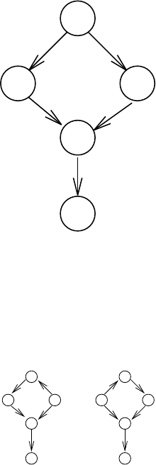
Where line 2 is true from (X⊥CY|Z,W), line 3 is true from (W⊥CY|X,Z). The

result shows that we have (X,W⊥CY|Z).

Exercise 21.12 — Learning Causal Models [17 points]

An important question in scientiﬁc discovery is using data to extract causal knowledge, i.e., the

existence of a causal path between two variables. Note that a causal path exists from Xto Yif

in any graph that is an I-map of the distribution, there is a causal (i.e., directed) path from Xto

Y. In this problem, we will consider the interaction between this problem and hidden variables.

Assume that our learning algorithm came up with the following network:

B C

which we are willing to assume is a perfect map for the distribution over the variables A, B, C, D, E

(i.e., it exactly captures the independencies and dependencies among them). Under this assump-

tion, among which pairs of these variables does there necessarily exist a causal path . . .

1. [7 points] . . . if we assume there are no hidden variables?

Answer: From the ﬁgures below we can see that the paths from Ato Band from Ato C

are not necessarily causal.

B C

E E

B C

The only way we could break the causal chain from Ato Dand Ewould be by making Athe

bottom of a v-structure (we would have to have Band Cas parents. If we do this, however,

we lose the independence assumption that I(B, C |A). We can refer to the arguments from

class to see that the other paths are causal. Thus, we have the following causal paths: Ato

D,Ato E,Bto D,Bto E,Cto D,Cto E, and Dto E.

2. [10 points] . . . if we allow the possibility of one or more hidden variables ?

Answer: We know from part (a) that paths from Ato Band Ato Care not necessarily

causal.

Now, consider the paths from Band Cto D. We know that observing Dmust activate a

path between Band C, which means Dmust be the bottom of a v-structure which links an

active path from Bto Dand an active path from Cto D. Since any new variables we add are

never observed, there can be no new v-structures between Band Dand no new v-structures

between Cand D. (If there were such a v-structure, we would now have the property that

I(B, C |A, D)which does not hold in the original network.)

Since Dmust be the bottom of a v-structure, we know that the paths which link Band C

to Dmust have their arrows pointing towards D. The only way left to break the causal path

from B(or C) to Dis to make a hidden variable a common parent of both Band D(or C

and D). There are 2 ways we might do this while preserving the arcs from Ato Band Ato C:

we can make Ha child of Awith 2 children: B(or C) and D, we can just replace the direct

connection from B(or C) to Dwith a path from Hto B(or C) and a path from Hto D. In

either case we lose the property that I(A, D |B, C)which holds in our original network.

If we reverse the arc from B(or C) to Aas in the ﬁgure for part (a), we can replace the link

from B(or C) to Dby a hidden variable Hwhich is a common parent of B(or C) and D.

This network satisﬁes the same independence assumptions. However, while we lose the direct

causal edge from B(or C) to D, a new causal path through Ais now present. Note that the

only way we were able to do this was by reversing the arc between Aand B(or C), so the only

way this new causal path from B(or C) to Dcan be broken is by breaking the causal path

from Ato Dwhich we consider below.

Thus, the only way of breaking causal paths still open to us is to alter the path from Bto C

through A. We know that observing Amust block an active path between Band C. Clearly, the

active path which observing Ablocks goes through A. Thus there cannot be any v-structures

along the path from Bto Cthrough A. If Awere at the bottom of such a v-structure then

we would activate the path from Bto Cby instantiating Awhich means we would lose the

property that I(B, C |A). If a hidden variable Hwere at the bottom we would break the

active path through A, i.e., we would now have I(B, C)which is not true. (We cannot correct

for this new independence by adding a direct path between Band Cthrough a hidden variable

because we would then lose the property that I(B, C |A).) These remarks hold true whether

we are considering modiﬁcations to the initial network (with paths from Ato Band C) or to

either of the modifcations shown in the ﬁgures in part (a).

Thus, the paths that are guaranteed to be causal are from Ato D,Ato E,Bto D,Bto E,

Cto D,Cto E, and Dto E.

Chapter 22

New exercise (chapter 22) — Decomposable Utility Functions [8 points]

Recall that a utility function is a mapping from an outcome (assignment to variables) to a

real number. Suppose we have Mvariables, X1...XM, each of which has a domain of size

|Val(Xi)|=d, and a utility function U(X1. . . XM) over these variables. Our goal in this problem

is to ﬁnd the “ideal” outcome (i.e., the one that gives us the highest utility). Concretely, we are

searching for:

(x∗

1...x∗

M) = arg max

x1...xM

U(x1...xM).

Assume that this outcome is unique (that is, there are no ties for ﬁrst-place outcome).

Suppose that our Uis decomposable as a sum of utilities for relatively small subsets of the

variables:

U(X1. . . XM) =

i=1

U(Yi),

where Yi⊂ {X1. . . XM}.

1. [5 points] Describe an algorithm that exactly determines (x∗

1. . . x∗

M) and U(x∗

1...x∗

and that exploits the structure of the utility function to make it computationally more

eﬃcient. You may use as a subroutine any algorithm that we described in class.

Answer: Let V(X) = exp(U(X)). Perform max-product with the set of factors deﬁned

by V. Then U∗=U(x∗) = log V(x∗), where x∗is the maximizing assignment found by

max-product.

2. [3 points] Show that your algorithm requires a computational complexity of O(M d2) for

the case of chain decomposability, where:

U(X1. . . XM) =

M−1

i=1

U(Xi, Xi+1).

Answer: The biggest clique you need is of size 2, so you have O(d2)operations per clique,

giving a total run time of O(M d2).

Chapter 23

Exercise 23.14 — Value of Perfect Information [16 points]

1. [10 points] Let Ibe an inﬂuence diagram, Da decision variable in I, and Xa chance

variable which is a non-descendant of D. Prove that VPII(D|X)≥0. Moreover, show

that equality is achieved if and only if the decision at Dis unchanged for any value xof

Xand any assignment wto D’s other parents W. (Assume that ties are broken in some

prespeciﬁed way when two actions have the same expected utility.)

Answer: We prove this result for the case where Icontains only a single decision variable.

To show that VPII(D|X)≥0, it suﬃces to show that MEU[I′]≥MEU[I]where I′is the

inﬂuence diagram obtained by adding an edge from Xto Din I.

Let σ∗be an optimal strategy corresponding to the maximal expected utility in I, and let

δσ∗

D(D|PaD)be the probability distribution over choices of Dgiven values of its parents

speciﬁed by σ∗. Similarly, let γ∗be an optimal strategy for I′, and let δγ∗

D(D|X, PaD)be its

corresponding decision rule. We know that

MEU[I] = arg maxσEU[I[σ]] = EU[I[σ∗]]

U∈U X

u∈Val(U)

uPBI[σ∗](U=u)

U∈U X

u∈Val(U)X

x∈Val(X)X

d∈Val(D)

uP (U=u|x, d)PBI[σ∗](x, d)

where

PBI[σ∗](x, d) = δσ∗

D(d|paD)Y

Y∈X

P(y|paY).

Now, consider a strategy ˆγfor ID′in which we “ignore” the value of Xin our choice of

action at the decision node Dand act optimally otherwise; this corresponds to the decision

rule δˆγ

D(D|X, PaD) = δσ∗

D(D|PaD). Then,

PBI′[ˆγ](x, d) = δˆγ

D(d|paD)Y

Y∈X

P(y|paY)

=δσ∗

D(d|paD)Y

Y∈X

P(y|paY)

=PBI[σ∗](x, d),

so it follows that MEU[I] = EU[I[σ∗]] = EU[I′[ˆγ]] ≤EU[I′[γ∗]] = MEU[I′].

In particular, if the optimal strategy γ∗in I′does not diﬀer from the optimal strategy σ∗in I

for any value xand assignment paD, then γ∗= ˆγ, so the equality holds and VPII(D|X) = 0.

On the other hand, if the optimal strategy γ∗in I′does diﬀer for some value xand assignment

paD, then strategy γ∗must give strictly higher expected utility that strategy ˆγ(otherwise,

our tie-breaking convention would have ensured that we would stay with ˆγ). This implies

that MEU[I′] = EU[I′[γ∗]] >EU[I′[ˆγ]] = EU[I[σ∗]] = MEU[I], or VPII(D|X)>0, as

desired.

2. [6 points] Is the value of learning the values of two variables equal to the sum of the values

of learning each of them? I.e., is VPII(D|Y, Z) = VPII(D|Y) + VPII(D|Z). Either

prove that this assertion holds, or provide a counterexample.

Answer: No, the value of learning the values of two variables is not necessarily equal to the

sum of the values of learning each of them. We provide a counterexample.

Consider an inﬂuence diagram consisting of two binary-valued chance variables Yand Z, a

binary-valued decision node D, and a utility node U. Suppose that Yhas a uniform prior over

its two possible values, Zis deterministically related to its parent Yby the relationship Z=Y,

and U(x, y, d)is 1if x=y=dand 0otherwise.

Without additional information, the optimal action at Dis to select randomly. Calling this

strategy σ, we have MEU[I] = EU[I[σ]] = 1

2·0 + 1

2·1 = 1

2. Given knowledge of one of the

variables (say, Y), an optimal action at Dis to pick D=Y. Calling this strategy σ1and letting

the inﬂuence diagram I1contain an edge from Yto D, we have MEU[I1] = EU[I1[σ1]] = 1.

If we add another edge from Zto D, however, we don’t have any more information than before.

Calling this strategy σ2and letting the inﬂuence diagram I2contain edges from both Yand

Zto D, it follows that MEU[I2] = EU[I2[σ2]] = EU[I1[σ1]] = MEU[I1].

Thus, VPII(D|Z) = VPII(D|Y) = MEU[I1]−MEU[I] = MEU[I2]−MEU[I] =

VPII(D|Z, Y ) = 1

2, so VPII(D|Y, Z) = 1

2<1 = VPII(D|Y) + VPII(D|Z).

New (chapter 23) — Value of Imperfect Information [7 points]

In a decision problem, we know how to calculate the value of perfect information of Xat decision

D. Now imagine that we cannot observe the exact value of X, but we can instead observe a

noisy estimate of X.

For this problem, assume Xis binary. Also assume the noisy observation has a false positive

rate of pand a false negative rate of q. (That is when X= 0 we observe 1 with probability p,

and when X= 1 we observe 0 with probability q.)

Give a simple method by which we can calculate the improvement in MEU from observing this

imperfect information. (Your answer should be just a couple lines long, but you should explain

exactly how pand qare used.)

Answer: We introduce a new node, X′into our inﬂuence diagram, as a child of X, and CPD

according to the given noise model - P(X′|X) = 1 −p, q;p, 1−q. Then simply calculate the VPI

for X′at decision D.

Sols.dvi Daphne Koller, Benjamin Packer Instructor’s Manual For Probabilistic Graphical S (2010)

Navigation menu

Versions of this User Manual:

Views

Navigation