Defining The Work Flow
User Manual: Defining the Work Flow
Open the PDF directly: View PDF ![]() .
.
Page Count: 244 [warning: Documents this large are best viewed by clicking the View PDF Link!]
- Title
- Copyright
- Disclaimer
- Contents
- Chapter 01 Introduction
- Chapter 02 File
- Chapter 03 Home
- Chapter 04 Layout
- Chapter 05 Components
- 5.1 Components > Properties
- 5.1.1 Material Properties Forms – Screen Captures
- 5.1.2 Frame Properties Forms – Screen Captures
- 5.1.3 Section Designer – Screen Capture
- 5.1.4 Cable Properties Form – Screen Capture
- 5.1.5 Tendon Properties Form - Screen Capture
- 5.1.6 Link/Support Properties Form - Screen Capture
- 5.1.7 Rebar Properties Form - Screen Capture
- 5.2 Components > Superstructure
- 5.3 Component > Substructure
- 5.1 Components > Properties
- Chapter 06 Loads
- Chapter 07 Bridge
- 7.1 Bridge > Bridge Objects
- 7.1.1 Bridge Object > Spans – Screen Captures
- 7.1.2 Bridge Object > Span Items – Screen Captures
- 7.1.3 Bridge Object > Supports – Screen Captures
- 7.1.4 Bridge Object > Superelevation – Screen Capture
- 7.1.5 Bridge Object > Prestress Tendons – Screen Captures
- 7.1.6 Bridge Object > Girder Rebar – Screen Capture
- 7.1.7 Bridge Object > Loads – Screen Captures
- 7.1.8 Bridge Object > Groups – Screen Captures
- 7.2 Update
- 7.1 Bridge > Bridge Objects
- Chapter 08 Analysis
- 8.1 Analysis > Load Cases
- 8.1.1 Analysis > Load Cases – Type
- 8.1.1.1 Static – Screen Capture
- 8.1.1.2 Nonlinear Staged Construction – Screen Capture
- 8.1.1.3 Multi-Step Static – Screen Capture
- 8.1.1.4 Modal – Screen Capture
- 8.1.1.5 Response Spectrum – Screen Capture
- 8.1.1.6 Time History – Screen Capture
- 8.1.1.7 Moving Load – Screen Capture
- 8.1.1.8 Buckling – Screen Capture
- 8.1.1.9 Steady State – Screen Capture
- 8.1.1.10 Power Spectral Density – Screen Capture
- 8.1.1.11 Hyperstatic – Screen Capture
- 8.1.2 Analysis > Load Cases > Schedule Stages – Screen Capture
- 8.1.3 Analysis > Load Cases > Convert Combos – Screen Captures
- 8.1.4 Analysis > Load Cases >Show Tree
- 8.1.1 Analysis > Load Cases – Type
- 8.2 Analysis > Bridge
- 8.3 Analysis > Lock
- 8.4 Analysis > Analyze
- 8.5 Analysis > Shape Finding
- 8.1 Analysis > Load Cases
- Chapter 09 Design-Rating
- Chapter 10 Advanced
- Bibliography

Defining the Work Flow

CSiBridge®
Defining
the Work Flow
ISO BRG102816M2 Rev. 0
Proudly developed in the United States of America October 2016

Copyright
Copyright Computers & Structures, Inc., 1978-2016
All rights reserved.
The CSI Logo® and CSiBridge® are registered trademarks of Computers & Structures,
Inc. Watch & LearnTM is a trademark of Computers & Structures, Inc. Adobe® and
Acrobat® are registered trademarks of Adobe Systems Incorported. AutoCAD® is a
registered trademark of Autodesk, Inc.
The computer program CSiBridge® and all associated documentation are proprietary and
copyrighted products. Worldwide rights of ownership rest with Computers & Structures,
Inc. Unlicensed use of these programs or reproduction of documentation in any form,
without prior written authorization from Computers & Structures, Inc., is explicitly
prohibited.
No part of this publication may be reproduced or distributed in any form or by any
means, or stored in a database or retrieval system, without the prior explicit written
permission of the publisher.
Further information and copies of this documentation may be obtained from:
Computers & Structures, Inc.
www.csiamerica.com
info@csiamerica.com (for general information)
support@csiamerica.com (for technical support)
DISCLAIMER
CONSIDERABLE TIME, EFFORT AND EXPENSE HAVE GONE INTO THE
DEVELOPMENT AND TESTING OF THIS SOFTWARE. HOWEVER, THE USER
ACCEPTS AND UNDERSTANDS THAT NO WARRANTY IS EXPRESSED OR
IMPLIED BY THE DEVELOPERS OR THE DISTRIBUTORS ON THE ACCURACY
OR THE RELIABILITY OF THIS PRODUCT.
THIS PRODUCT IS A PRACTICAL AND POWERFUL TOOL FOR STRUCTURAL
DESIGN. HOWEVER, THE USER MUST EXPLICITLY UNDERSTAND THE BASIC
ASSUMPTIONS OF THE SOFTWARE MODELING, ANALYSIS, AND DESIGN
ALGORITHMS AND COMPENSATE FOR THE ASPECTS THAT ARE NOT
ADDRESSED.
THE INFORMATION PRODUCED BY THE SOFTWARE MUST BE CHECKED BY
A QUALIFIED AND EXPERIENCED ENGINEER. THE ENGINEER MUST
INDEPENDENTLY VERIFY THE RESULTS AND TAKE PROFESSIONAL
RESPONSIBILITY FOR THE INFORMATION THAT IS USED.

Contents
Chapter 1 Introduction
1.1 Graphical User Interface 1-3
1.2 Organization 1-12
1.3 Recommended Reading/Practice 1-13
Chapter 2 File
2.1 File > New 2-2
2.2 File > Open 2-4
2.3 File > Save and Save As 2-5
2.4 File > Import 2-5
2.5 File > Export 2-7
2.6 File > Batch File 2-10
2.7 File > Print 2-10
2.8 File > Report 2-11
i

CSiBridge – Defining the Work Flow
2.9 File > Pictures 2-14
2.10 File > Settings 2-15
2.11 File > Language 2-21
Chapter 3 Home
3.1 Home > Bridge Wizard 3-1
3.1.1 Using the Bridge Wizard 3-5
3.1.2 Steps of the Bridge Wizard 3-6
3.2 Home > View 3-15
3.3 Home > Snap 3-17
3.4 Home > Select 3-18
3.5 Home > Display 3-21
Chapter 4 Layout
4.1 Layout > Layout 4-2
4.1.1 Bridge Layout Preferences Form – Screen
Capture 4-5
4.1.2 Bridge Layout Line Data Form – Screen
Capture 4-6
4.2 Layout > Lanes 4-10
4.2.1 Bridge Lane Data Form – Screen Capture 4-14
4.2.2 Lane Data Form – Screen Capture 4-15
Chapter 5 Components
5.1 Components > Properties 5-2
5.1.1 Material Properties Forms – Screen Capture 5-7
5.1.2 Frame Properties Form – Screen Capture 5-10
5.1.3 Section Designer – Screen Capture 5-11
ii

Contents
5.1.4 Cable Properties Form – Screen Capture 5-13
5.1.5 Tendon Properties Form – Screen Capture 5-14
5.1.6 Link/Support Properties Form – Screen
Capture 5-15
5.1.7 Rebar Properties Form – Screen Capture 5-16
5.2 Components > Superstructure 5-16
5.2.1 Bridge Deck Section Form – Screen
Capture 5-20
5.2.2 Bridge Diaphragm Form – Screen Capture 5-22
5.2.3 Parametric Variation Forms – Screen
Capture 5-24
5.3 Components > Substructure 5-25
5.3.1 Bridge Bearing Data Form – Screen
Capture 5-30
5.3.2 Bridge Restrainer Data Form – Screen
Capture 5-31
5.3.3 Foundation Spring Data Form –
Screen Capture 5-32
5.3.4 Bridge Abutment Data Form – Screen
Capture 5-33
5.3.5 Bridge Bent Forms – Screen Captures 5-34
Chapter 6 Loads
6.1 Loads > Vehicles 6-2
6.1.1 Vehicle Data Forms – Screen Captures 6-4
6.1.2 Vehicle Classes Data Forms – Screen
Capture 6-6
6.2 Loads > Load Patterns 6-7
6.3 Loads > Functions 6-9
iii

CSiBridge – Defining the Work Flow
6.3.1 Response Spectrum Forms – Example
Screen Capture 6-14
6.3.2 Time History Form – Example Screen
Capture 6-15
6.4 Loads > Loads 6-16
6.4.1 Point Load Form – Screen Capture 6-20
6.4.2 Line Load Form – Screen Capture 6-20
6.4.3 Area Load Form – Screen Capture 6-21
6.4.4 Temperature Gradient Form – Screen
Capture 6-21
Chapter 7 Bridge
7.1 Bridge > Bridge Objects 7-2
7.1.1 Bridge Object > Span – Screen Capture 7-8
7.1.2 Bridge Object > Span Items – Screen
Captures 7-10
7.1.3 Bridge Object > Supports 7-13
7.1.4 Bridge Object > Superelevation – Screen
Capture 7-14
7.1.5 Bridge Object > Prestress Tendons –
Screen Captures 7-15
7.1.6 Bridge Object > Girder Rebar – Screen
Capture 7-16
7.1.7 Bridge Object > Loads – Screen Capture 7-16
7.1.8 Bridge Object > Groups – Screen Captures 7-19
7.2 Update 7-20
7.2.1 Update > Update 7-21
7.2.2 Update > Auto Update 7-22
Chapter 8 Analysis
8.1 Analysis > Load Cases 8-2
8.1.1 Analysis > Load Cases – Type 8-9
iv

Contents
8.1.2 Analysis > Load Cases > Schedule Stages –
Screen Capture 8-16
8.1.3 Analysis > Load Cases > Convert Combos –
Screen Captures 8-17
8.1.4 Analysis > Load Cases > Show Tree 8-18
8.2 Analysis > Bridge 8-18
8.3 Analysis > Model Lock 8-20
8.4 Analysis > Analyze 8-20
8.4.1 Analysis > Analysis Options – Screen
Captures 8-22
8.4.2 Analysis > Run Analysis – Screen Capture 8-22
8.4.3 Analysis > Last Run Details 8-23
8.5 Analysis > Shape Finding 8-23
Chapter 9 Design/Rating
9.1 Design/Rating > Load Combinations 9-2
9.2 Design/Rating > Superstructure Design 9-7
9.2.1 Superstructure Design > Preferences – Screen
Capture 9-9
9.2.2 Superstructure Design > Design Requests –
Screen Capture 9-10
9.2.3 Superstructure Design > Run Super – Screen
Capture 9-11
9.2.4 Superstructure Design > Optimize – Screen
Capture 9-11
9.3 Design/Rating > Seismic Design 9-12
9.3.1 Seismic Design > Preferences – Screen
Capture 9-14
9.3.2 Seismic Design > Design Requests –
Screen Capture 9-15
9.3.3 Seismic Design > Run Seismic – Screen
v

CSiBridge – Defining the Work Flow
Capture 9-16
9.4 Design/Rating > Load Rating 9-16
9.4.1 Load Rating > Preferences – Screen
Capture 9-18
9.4.2 Load Rating > Rating Requests – Screen
Capture 9-19
9.4.3 Load Rating > Run Rating – Screen Capture 9-20
9.4.4 Load Rating > Optimize – Screen Capture 9-21
Chapter 10 Advanced
10.1 Advanced > Edit 10-1
10.2 Advanced > Define 10-4
10.3 Advanced > Draw 10-8
10.4 Advanced > Assign 10-10
10.5 Advanced > Assign Loads 10-22
10.6 Advanced > Analyze 10-27
10.7 Advanced > Tools 10-33
Bibliography
vi

CHAPTER 1 Introduction
CSiBridge is the most productive bridge design package in the industry
because it integrates modeling, analysis, and design of bridge structures
into a versatile and easy-to-use computerized tool. Terms familiar to
bridge engineers are used to define bridge models parametrically: layout
lines, spans, bearings, abutments, bents, hinges, and post-tensioning.
Spine, shell, or solid object models can be created and update automati-
cally as the bridge definition parameters are changed. Simple or complex
bridge models can be built and changes can be made efficiently while
maintaining total control over the design process. Lanes and vehicles can
be defined quickly and can include width effects. Simple and practical
Gantt charts can be created to simulate modeling of construction se-
quences and scheduling.
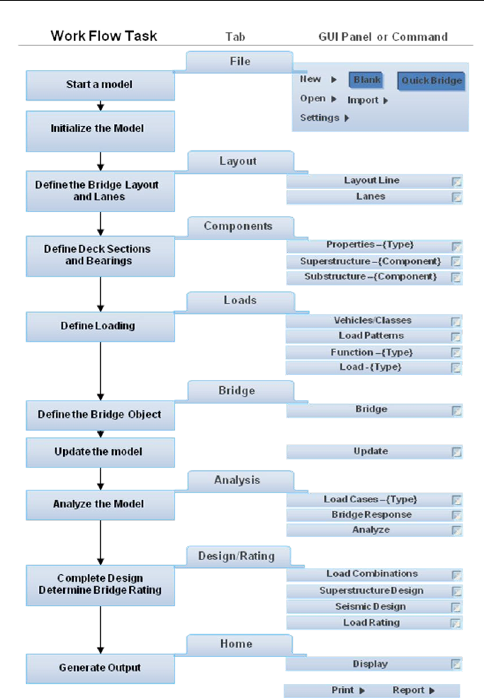
This manual provides a quick reference to the features and commands
available in CSiBridge. Figure 1-1 identifies a general work flow and the
related graphical user interface (GUI) components used to accomplish
the tasks shown. This chapter describes the GUI, the organization of
subsequent chapters, and suggested additional reading material.
Note: When the program first launches, a Welcome form will dis-
play. Click Continue in the lower right-hand corner to move past
the form. Click the Do not show this Welcome Screen again check
box to permanently close the form.
Graphical User Interface 1 - 1
CSiBridge – Defining the Work Flow
Figure 1-1 Basic Work Flow and
Related Graphical User Interface Tabs and Panels or Commands
1 - 2 Graphical User Interface

CHAPTER 1 Introduction
The Bridge Wizard is a key feature in the program; it is a step-wise
guide through the model creation and analysis. The Wizard is an asset to
both the beginner and more advanced user because it works seamlessly
with other program functions, meaning that users are not “locked in” to
the Wizard. A model can be initiated using the Wizard and then individ-
ual commands “outside” the Wizard can be used to adjust the model ge-
ometry, components, analysis and design parameters, and so on. Similar-
ly, the Wizard can be used at any point to “pick up” the modeling pro-
cess that was not initiated using the Wizard by selecting the appropriate
“Bridge Object.” Details about the Bridge Wizard are provided in Chap-
ter 3.
1.1 Graphical User Interface
The GUI consists of some elements familiar to Microsoft Windows users
as well as command functions familiar to users of other CSi programs.
The components of the interface and the logic behind their arrangement
is explained in this section. More detailed descriptions of commands can
be found in subsequent chapters.
The title bar, display window(s), and status bar are common elements in
Windows-based programs.
As is typical, the title bar displays the name of the program (i.e.,
CSiBridge) and the name of the model file. The far right-hand side of
that bar includes the Windows minimize, maximize, and close buttons.
When a model file is opened, it is shown in a display window. Click
in the window to activate it; actions related to the model (e.g., draw,
select, and so on) are carried out in an “active window.” Click the
“expand arrow” on the far upper right-hand corner of the display win-
dow to display the “+ Add New Window” option and open an addi-
tional window. The tab on the left-hand side of the display window
identifies the type of view (e.g., 3D, X-Y Plane @ Z=0). Click the “x”
close button in the upper right-hand corner of the tab to close a display
window. At least one display window must remain open.
Graphical User Interface 1 - 3

CSiBridge – Defining the Work Flow
The status bar at the very bottom of the program window shows the
x, y, and z coordinates of the mouse cursor in the active display win-
dow, the coordinate system being used by the display, and the units
being used in the model.
Figure 1-2 shows a ribbon of the user interface, annotated with the ter-
minology used in this manual.
Figure 1-2 A ribbon of the Graphical User Interface
annotated with the terminology used in this manual
When the File tab is clicked, a drop-down menu of commands displays.
Table 1-1 identifies the features available on the File menu. More infor-
mation about the File is provided in Chapter 2.
Table 1-1 File Commands and Features – See Chapter 2 for more information
Command Features
New
Initialize the model
Set the base units
Record project information (client name, and so on)
Select a start option: Blank or Quick Bridge
A display area on the right-hand side of the menu shows the
recently stored model files
Open Open an existing model file
Save / Save
As Save a bridge model / Save the model using a new name
1 - 4 Graphical User Interface

CHAPTER 1 Introduction
Table 1-1 File Commands and Features – See Chapter 2 for more information
Command Features
Import
Import files in these formats: text stored in ASCII format; Excel;
Access; SAP2000; CIS/2; SDNF; AutoCAD; IFC; IGES; Nastran;
STAAD/ GTSTRUDL; StruCAD*3D; LandXML
Export
Export files in these formats: text into ASCII format; Excel; Ac-
cess; CIS/2; SDNF; AutoCAD; IFC; IGES; Perform 3D (text file),
Perform 3D Structure
Batch File
Run the analysis and manage the analysis files for a list of
CSiBridge
model files with no additional action required by the
user; useful for running multiple models when the computer is
unattended (e.g., overnight)
Print
Print Graphics
Print Tables
Print Setup
Report
Create Report
Report Setup
Advanced Report Writer
Pictures
Create files in bitmap format of the entire screen, the main pro-
gram window, the current window including the title bar; the cur-
rent window without the title bar, or a user specified region.
Create a metafile of the current display window.
Create a multi-
step animation video or a cyclic animation video
of the model showing the current analysis results.
Settings
Units – Set the number formatting to be followed by any data-
base generated by the program.
Tolerance –
Auto merge tolerance, 2D view cutting plane, plan
fine grid spacing, plan nudge value, screen selection tolerance,
screen snap to tolerance, screen line thickness, printer line
thickness, maximum graphic font size, minimum graphi
c font
size, auto zoom step, shrink factor, maximum line length in text
file
Database table utilities and settings --
Set Current Format File
Source, Edit Format File, Set Current Table Name Source, Write
Default Tables Names to XML, Documentation to Word, Auto
Regenerate Hinges after Import
Colors – Change default color settings for on-screen display and
printed output.
Other settings –
Graphics mode, auto save, auto refresh, show
bounding plane, moment diagrams on tension side, sound, show
result values while scrolling
Project Information –
Company name, client name, project
name, project number, model name, model description, revision
Graphical User Interface 1 - 5

CSiBridge – Defining the Work Flow
Table 1-1 File Commands and Features – See Chapter 2 for more information
Command Features
number, frame type, engineer, checker, supervisor, issue code,
design code
Comments and Log – Track the status of the model, keep a “to-
do” list, and retain key results that can be used to monitor the ef-
fects of changes to the model.
Languages English and Chinese
Resources
Help, Documentation, CSI on the Web, CSiBridge News, About
CSiBridge
Exit Closes the program
When a form is displayed in the program, clicking the F1 key will dis-
play a context-sensitive help topic.
Near the top of the program window, but beneath the title bar, is a short
menu bar of icons that can be clicked to perform frequently required
tasks, such as Save or Lock and Unlock a model. In addition, a right
click will display the Customized Quick Access Toolbar. Click a com-
mand on the list of commands to add that command to the menu bar. A
check mark preceding a command indicates that the command has been
added. To remove a command, click the command to uncheck it. After a
command has been added to the menu bar, clicking it will immediately
execute the command. An option is also available to change the color –
blue, silver, black – used to display the ribbon.
Below that menu bar of icons and to the right File tab is a series of eight
other tabs: Home, Layout, Components, Loads, Bridge, Analysis,
Design/Rating, and Advanced. When read from left to right, the names
of the tabs generally reflect the sequence of actions required to generate
a model. Click any tab at any time to display its contents, which consists
of panels.
Panels are grouped on a particular tab because of the generally common
nature of their function. For example, the Home tab includes the View,
Snap, Select and Display panels. The names of those panels reflect the
functions related to working with the active view. The View panel in-
1 - 6 Graphical User Interface

CHAPTER 1 Introduction
cludes commands to set a 3D, XY, or XZ view, to access zoom features,
to Set Display Options, and many other view-related commands.
The Snap panel tools are used to increase accuracy and speed when
drawing and editing objects in the active view. The Select panel includes
the commands used to select and deselect objects in the active view. The
Display panel includes the commands to specify what is shown on the
model in the active view.
The composition of the panels varies somewhat, depending on their gen-
eral function. For example, the View, Snap, Select, and Display panels on
the Home tab have icons and drop-down lists of commands that general-
ly immediately execute actions or display forms with options to filter ac-
tions, such as selecting material properties. Alternatively, the Compo-
nents tab, for example, includes panels of commands that are used to
add, modify, or delete bridge component definitions (e.g., material,
frame, or cable properties; deck sections or diaphragms; bearings, re-
strainers, or foundation springs). Thus, the panels on the Components
tab have Type and Item commands to select the type of bridge compo-
nent and associated commands and expand arrows that when clicked,
display {component type} definition forms that are used to name a defi-
nition and that have buttons that can be used to display {component
type} data forms that are used to specify parameters for the named defi-
nition.
Note: Hover text displays the functions of icons and drop-down
lists when the mouse cursor is moved over them.
Clicking the small expand arrow in the lower right-hand corner of a
panel displays the form used to add, modify, or delete definitions.
(That definition form may have buttons that subsequently can be used
to display the data form referenced in the next bullet item.)
In most cases, clicking the first of the four commands above the drop-
down list on a panel is a “shortcut” to the form used to define data for
a new definition. (The hover text for the first of the four command
icons should read something similar to “New, Add a new {compo-
nent},” while hover text that displays when the cursor is placed over
Graphical User Interface 1 - 7

CSiBridge – Defining the Work Flow
the down arrow of the drop-down list should read something similar to
“Current {Property or Item}.”) Note that clicking the third command
icon (hover text may read “Modify, Modify/Show the specified {com-
ponent or item type}”) will display the data form for the definition se-
lected in the drop-down list.
Some panels include “More” buttons. Clicking those buttons displays
drop-down menus of additional commands.
IMPORTANT NOTE: For the sake of brevity, the use of the words
tab, panel, and icon in command names has been eliminated. For
example, the command used to access the Display Options for
Active Window form is the Home > View > Set Display Options
command, which means: click the Home tab, then on the View
panel, click the Set Display Options icon.
The program actions/options on each of the tabs are identified briefly in
Table 1-2. The table also identifies the chapters in this manual devoted
to each of the tabs.
Table 1-2 CSiBridge Tabs, Panels, Actions/Options and Associated Chapters
Tab Panel Actions/Options
Home
(Chapter 3) Bridge
Wizard Step-wise guide through the creation, analysis,
and design processes
View Zoom features, pan, set views, rotate a view or
perspective toggle, refresh window, shrink ob-
jects, set display options, set limits, show grids,
show axes,
invert view selection, remove and
restore selection from view, show all, refresh
view
Snap
Snap to points; snap perpendicular; snap to
ends and midpoints; snap to lines and edges;
snap to intersections; snap to fine grids
Select Pointer/window, poly, intersecting poly, intersect-
ing line, coordinate specification (3D box, speci-
fied coordinate range, click joint in XY plane, XZ
plane, YZ plane), select lines parallel to (click
straight line ob
ject, coordinate axes or plane),
properties (materials, fr
ame sections, cables,
tendons, area sections, solids, links, frequency
dependent link), assignments (joint supports,
1 - 8 Graphical User Interface

CHAPTER 1 Introduction
Table 1-2 CSiBridge Tabs, Panels, Actions/Options and Associated Chapters
Tab Panel Actions/Options
joint constraints), groups, labels, all; deselect;
select using tables, invert selection, get previous
selection, select using intersecting
line, clear
selection
Home
(Chapter 3)
(continued)
Display Show undeformed shape, show bridge super-
structure forces/stresses, show deformed shape,
show shell force/stress plots, show bridge loads,
show bridge superstructure design results, show
joint reaction forces, show solid stress plots,
show tables, show influence lines/surfaces,
show frame/ca
ble/tendon force diagrams, show
link force diagrams; save named display, show
named display
, show load assignments, show
miscellaneous assignments, show lane
s, show
plot functions, show static pushover curve, show
hinge results, show response spectrum curves,
show virtual work dia
grams, show plane stress
plots, show asolid stress points, show input/log
files
Layout
(Chapter 4) Layout Line Preferences; initial and end stations; bearing;
initial grade, vertical or horizontal layout varia-
tions
Lanes Selection of the layout line and station for speci-
fica
tion of centerline offset and lane width; lane
edge type (interior, exterior); object loading by
group or program determined; load discretization
lengths along and across lanes
Components
(Chapter 5) Properties
Materials, frames, cables, tendons and links,
rebar sizes
Superstructure Decks, diaphragms, parametric variations
Substructure
Bearings, restrainers, foundation springs, abut-
ments, bents
Loads
(Chapter 6) Vehicles Vehicles, vehicle classes
Load patterns Dead, vehicle live, wind, temperature, quake,
more…
Function Response spectrum, time history
Loads
Point, line, area, temperature gradient
Bridge
(Chapter 7) Bridge Objects
Bridge object, spans, span items (diaphragms,
hinges, user points), supports (abutments,
bents), superelevation, prestress tendons, girder
rebar, loads (point, line, area, temperature gra-
dient), groups
Graphical User Interface 1 - 9

CSiBridge – Defining the Work Flow
Table 1-2 CSiBridge Tabs, Panels, Actions/Options and Associated Chapters
Tab Panel Actions/Options
Update Update and auto update
Analysis
(Chapter 8) Load Cases All, static, nonlinear stage construction, multistep
static, modal, response spectrum, time history,
moving load, buckling, steady state, power spec-
tral density, hyperstatic; schedule stages (con-
struction schedule
s), convert combinations,
show tree
Bridge Bridge response
Lock Model lock and unlock
Analyze
Analysis options, run analysis, last run (show
results of last analysis run)
Shape Finding Model geometry, reset geometry
Design/Rating
(Chapter 9) Load
Combinations Combination type (Linear Add, Envelope, Abso-
lute Add, SSRS, Range Add, and load case with
applicable scale factor), add defaults (code-
generated combos)
Superstructure
design Preferences (code) and design request -- check
type, station ranges (i.e., where in the structure
the de
sign applies), design parameters (e.g.,
flexure or stress factors), and demand sets (load
combinations to be considered in the design),
run superstructure design, optimize design
Seismic de-
sign Preferences (code) and design request -- an
extensive array
of parameters (e.g., response
spectrum function, seismic design category, P-
Delta analysis and so on), run seismic, report
Load Rating Preferences (code), rating request, including
Rating Type (e.g., flexure, shear, minimum re-
bar), Station Ranges (i.e., where in the structure
the rating applies), Rating Parameters (depends
on the Rating Type), Demand Sets (load combi-
nations to be considered in the rating) and if
appli
cable, Live Load Distribution Factors (see
Chapter 3 of the Bridge Superstructure Design
manual), run rating, optimize rating
Advanced
(Chapter 10) Edit
Points, lines, areas, undo/redo, cut/copy/paste,
de
lete, add to model from template, interactive
database editing, replicate, extrude, move, di-
vide solids, show duplicates, merge duplicates,
change labels
1 - 10 Graphical User Interface

CHAPTER 1 Introduction
Table 1-2 CSiBridge Tabs, Panels, Actions/Options and Associated Chapters
Tab Panel Actions/Options
Define
Section properties, mass source, coordinate
sys
tems/ grids, joint constraints, joint patterns,
groups, section cuts, generalized displacements,
functions, named property sets (frame and area
modifiers, frame releases), pushover parameter
sets
(force v displacement, ATC 40 capacity
spectrum, FEMA 356 coefficient method, FEMA
440 equivalent linearization, FEMA 440 dis-
placement modification), named sets (tables,
virtual work, pushover named sets, joint TH re-
sponse spectra, plot function traces)
Draw Set select mode, set reshape object mode, draw
one joint link, draw two joint link, draw
frame/cable/ tendon, quick
draw/frame/cable/tendon, quick draw braces,
quick draw secondary beams, draw poly area,
draw rectangular area, quick draw areas, draw
special joint, quick draw link, draw section cut,
draw developed elevation definition, draw refer-
ence point, draw/edit general reference line, new
labels
Assign Joints (restraints, constraints, sprin
gs, panel
zones, masses, local axes, merge number, joint
patterns), frames
(sections, property modifiers,
material prop
erty overwrites, releases/partial
fixity, local axes, reverse connectivity, end length
offsets, insertion point, end skews, fireproofing,
output stations, P-Delta force, lane, ten-
sion/compression limits, hinges, hinge over-
writes, line springs, line mass, material tempera-
ture, automatic frame mesh), areas (section,
stiffness modifiers, material property overwrites,
thickness overwrites, local axes, reverse local 3
axis direction, area springs, area mass, material
temperature, automatic area mesh, general
edge constraints), cable (section, property modi-
fiers, material property, output stations, insertion
point, line mass, reverse connectivity, material
temperature), tendon (proper
ties, local axes,
material temperature, tension/compression lim-
its), solid (properties, surface spring, local axes,
edge constraints, material temperature, automat-
ic solid mesh, switch faces), link/support (proper-
ties, local axes, connectivity)
, assign to group,
update all generated hinge properties, clear dis-
Graphical User Interface 1 - 11

CSiBridge – Defining the Work Flow
Table 1-2 CSiBridge Tabs, Panels, Actions/Options and Associated Chapters
Tab Panel Actions/Options
play of assigns, copy assigns, paste assigns
Advanced
(Chapter 10)
(continued)
Assign Loads
Joints (forces, displacements, vehicle response
components), frames (gravity, point, distributed,
tem
perature, strain, deformation, target force,
auto wave loading parameters, open structure
wind parameters, vehicle response compo-
nents), areas (gravity, uniform, uniform to frame,
surface pressures, pore pressure, temperature,
strain, rotate, wind pressure coefficient, vehicle
response components), cables (gravity, distrib-
uted, deformation, strain, target force, tempera-
ture, vehicle response components), tendons
(gravity, deformation, strain, target force, tem-
perature, tendon force, vehicle response com-
ponents) solids (gravity, strain, pore pressure,
surface pressure, temperature, vehicle response
components) link/support (gravity, deformation,
target force, response components)
Analyze Create analysis model, Model-Alive
Frame Design Steel, concrete, overwrite frame design proce-
dure, lateral bracing
Tools Add/show plug ins, CSi load optimizer
1.2 Organization
Chapter 1 of this manual describes the user interface. Chapter 2 explains
the function of the File tab. Chapters 3 through 10 describe the various
other tabs in the program, using similar content structure. That is, each
chapter begins by identifying the general features provided by the tab.
An explanation is then provided correlating the tabs to the default defini-
tions created when the Quick Bridge template is used to start the model,
and when the Bridge Wizard or the Blank option (i.e., import model da-
ta) is used to work with a model. An annotated graphic of each panel is
provided, followed by a table that briefly explains the function of the
commands on the panel. When applicable, screen captures follow the ta-
ble.
1 - 12 Organization

CHAPTER 1 Introduction
1.3 Recommended Reading/Practice
Review of “Watch & Learn” Series™ tutorials, which are found at
http://www.csiamerica.com, is strongly recommended before attempting
to design a bridge using CSiBridge. Additional information can be found
in the on-line Help facility available from the File > Resources com-
mand.
Also, other bridge related manuals include the following:
Introduction to CSiBridge – Introduces CSiBridge design when mod-
eling concrete box girder bridges and precast concrete girder bridges.
The basic steps involved in creating a bridge model are described.
Then an explanation of how loads are applied is provided, including
the importance of lanes, vehicle definitions, vehicle classes, and load
cases. The Introduction concludes with an overview of the analysis
and display of design output.
Bridge Superstructure Design/Rating – Describes using CSiBridge to
complete (1) bridge design in accordance with the AASHTO STD
2002 or AASHTO LRFD 2012 code, the CAN/CSA-S6-06 code and
the EUROCODE for concrete box girder bridges, or the AASHTO
2012 LRFD code, the CAN/CSA-S6-06 code and the EUROCODE
for bridges when the superstructure includes precast concrete girder or
steel I girder bridges with a composite slab, and (2) bridge rating in
accordance with the 2011 AASHTO Rating code for concrete box
girder bridges and precast concrete girder or steel I girder bridges with
a composite slab. Loading and load combinations as well as Live Load
Distribution Factors are described. The manual explains how to define
and run a design request and provides the algorithms used by
CSiBridge in completing concrete box girder, cast-in-place multi-cell
concrete box, and precast concrete bridge design in accordance with
the AASHTO code. The manual concludes with a description of de-
sign output, which can be presented graphically as plots, in data ta-
bles, and in reports generated using the Advanced Report Writer fea-
ture.
Recommended Reading/Practice 1 - 13

CSiBridge – Defining the Work Flow
Seismic Analysis and Design – Describes the eight simple steps need-
ed to complete response spectrum and pushover analyses, determine
the demand and capacity displacements, and report the de-
mand/capacity ratios for an Earthquake Resisting System (ERS).
1 - 14 Recommended Reading/Practice

CHAPTER 2 File
Clicking the File tab displays a drop-down menu of commands related to
maintaining the model file (create a new file, open an existing file, save
a file), importing data into and exporting data from a model file, setting
up a batch of files upon which to run analysis without further user input,
producing output (graphics, reports, bitmaps, metafile, animation video),
and setting a range of parameters used within the program (units, toler-
ances, display color, sound, project information, comments and log, and
the like). The Recent Models display area shows the recently stored
models. Resources and Exit buttons are along the very bottom of that
display area. Use the Resources button to access help-type resources, in-
cluding About CSiBridge and Documentation. When a form is displayed
in the program, clicking the F1 key will display a context-sensitive help
topic.
This chapter describes the commands found in the File tab.
IMPORTANT NOTE: This manual addresses work flow for mod-
els created using the Blank option or the Quick Bridge template.
The other templates, which can be used, are not the focus of this
manual.
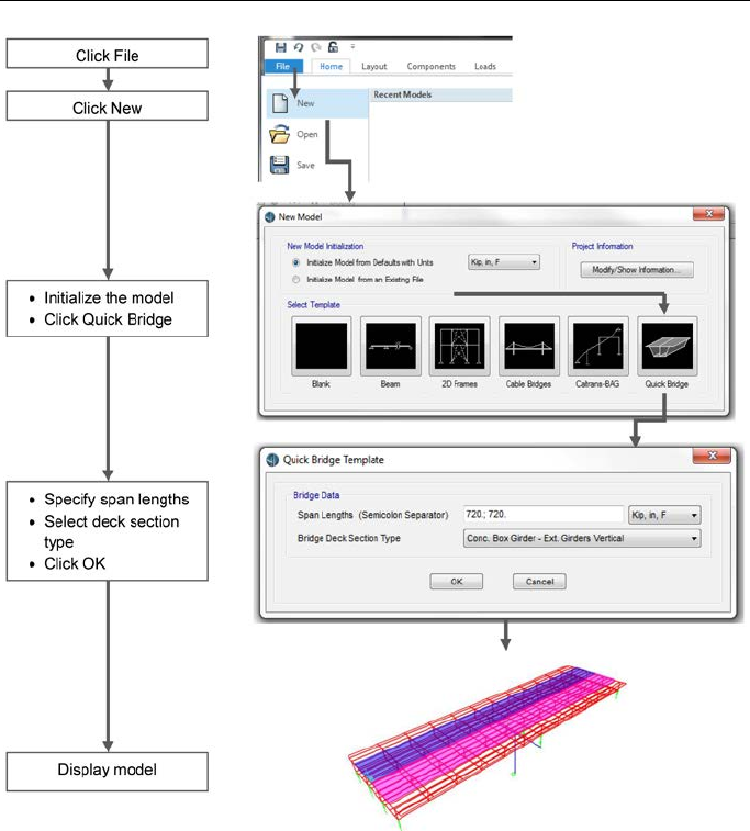
Figure 2-1 illustrates the work flow when starting a model using the
Quick Bridge template.
File > New 2- 1
CSiBridge – Defining the Work Flow
Figure 2-1 Work flow for starting a new model using Quick Bridge
2.1 File > New
Start a new model file by clicking the File > New command, which dis-
plays the New Model form shown in Figure 2-1. The form has options to
initialize the model and to start the model from templates.
2 - 2 File > New

CHAPTER 2 File
Initializing the model determines the units to be used and the default def-
initions of all properties, components, loading definitions, design set-
tings, and other defined items. Bridge objects and other physical objects
(lines, areas, links, and the like), and assignments to these objects, are
not included in the initialization process.
When the Initialize Model for Defaults with Units option is selected,
CSiBridge will use the default program definitions. The default defini-
tions are typical for the type of bridge selected. Use the drop-down list to
specify the units to be used in the model.
Note: The units used to start a model become the base units for
that model. If different units are used in the model, they are al-
ways converted to and from the base units. The model will always
open in the base units, so choose the units carefully.
When the Initialize Model from an Existing File option is selected,
CSiBridge picks up the initial definitions from a previous model. This
option generally is preferred if common sets of properties and definitions
are used for a number of models of the same project or across projects
that benefit from consistency (e.g., for the same client). If this option is
selected, click one of the template buttons and, when the program dis-
plays the Open Model File form, select the “previous model.”
The Quick Bridge option typically produces structures with uniform
spacing, unless the spacing is modified using the form that displays after
Quick Bridge template has been selected. Table 2-1 identifies the tem-
plates.
IMPORTANT NOTE: This manual addresses work flow for mod-
els created using the Blank option or the Quick Bridge template.
Thus, the work flow in this manual describes using the Bridge
Wizard and the various tabs of the graphical user interface: Lay-
out, Components, Loads, Bridge, Analysis, Design/Rating, and
Advanced.
File > New 2 - 3

CSiBridge – Defining the Work Flow
Table 2-1 File > New > {Template}
Templates Description
Blank Opens the program without any template being loaded. This op-
tion can be helpful when a File > Import command will be used
to initiate a model. Use this option to build the model, analyze it,
and design it using the commands on various tabs of the
CSiBridge ribbon. The Bridge Wizard, a step-wise guide though
the bridge modeling and analysis processes, can also be used
for model creation and analysis. The Bridge Wizard is described
in more detail in Chapter 3.
Beam Opens a single beam bridge model based on a user-specified
number of spans and the lengths of the spans, and selection or
specification of a section property.
2D Frame Opens a 2D Frame model based on user-specified parameters.
Select from three frame types: Portal Frame, Concentrically
Braced Frame and Eccentrically Braced Frame.
Cable Bridge
Creates a cable suspension bridge model based on specification
of the deck width, minimum middle sag, and the number of divi-
sions on the left, right, and middle spans.
Caltrans BAG Opens a model using the Bridge Analysis Generator, which gen-
erates a model to perform response spectrum dynamic analysis
and static analysis for a concrete bridge structure. The template
is most suited for use by the California Department of Transpor-
tation in the USA.
Quick Bridge Opens a typical bridge model based on initial, specified span
lengths and selection of a deck section type from a drop-down list
of com
mon bridge construction configurations. This template
works well with the Bridge Wizard or with the commands on the
program tabs.
2.2 File > Open
After a CSiBridge model has been created and saved, it may be opened
using the File > Open command. The CSiBridge file may be selected by
browsing to locate the appropriate file folder.
2 - 4 File > Open
CHAPTER 2 File
2.3 File > Save and File > Save As
The File > Save command opens a standard Microsoft Windows-type
save window. Use the form to specify the name and path for storing the
file. The file will have a .BDB extension.
The File > Save As command can be used to save the file using a new
filename.
2.4 File > Import
Clicking the File > Import command displays a list of subcommands
that can be used to import model data in a variety of formats. Various
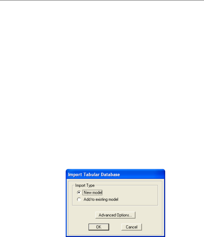
forms will display depending on the type of import. As an example, Fig-
ure 2-2 shows the form that displays after the File > Import > Text, File
> Import > Excel, or the File > Import Access commands are used.
The options on the form can be used to start a new model with the im-
ported data or add the imported data to an existing model.
Figure 2-2 Import Tabular Database form
If the Add to existing model option is selected, clicking the Advanced
Options button will open a form that can be used to resolve conflicts be-
tween the data in the existing model and the data being imported. Con-
flicts could be items with the same name or items in the same location,
for example.
Table 2-2 identifies the subcommands and the types of files that can be
imported.
File > Save and File > Save As 2 - 5

CSiBridge – Defining the Work Flow
Table 2-2 File > Import > {Command}
Command File
Extension Description
Excel .xls Imports model definition data that has been stored in
Microsoft Excel spreadsheet format as a tabular
database, usually with an .xls extension.
Access .mdb Imports model definition data that has been stored in
a Microsoft Access database format as a tabular
database, usually with an .mdb extension.
Text .$br, .b2k Imports SAP2000/Bridge or CSiBridge model data
that has been stored in plain (ASCII) text format.
Each time a model is saved, CSiBridge automatical-
ly writes the complete model definition as a tabular
database in a text file with a .$br extension. The .$br
file is intended for recovering the model in emergen-
cy crash situations. Thus, if for some reason the
.BDB file will not open, import the corresponding
.$br file.
SAP2000 .sdb Import a SAP2000 model, (i.e., .sdb).
CIS/2 .STP Imports an .stp file created using the CIMsteel Inte-
gration Standard (CIS), which is a set of formal
computing specifications used in the steel industry
to make software applications mutually compatible.
SDNF .sdnf, .dat Imports an .sdnf file created using a Steel Detailing
Neutral File. This file format contains steel fabrica-
tion and shop drawing information, and can be im-
ported to the model to compare or sync steel mem-
bers. Used primarily in the USA.
AutoCAD .dxf Imports a .dxf file, an AutoCAD Drawing Interchange
file. This feature is intended to facilitate importing
model geometry from AutoCAD, including AutoCAD
r14, AutoCAD 2000 and AutoCAD2002.
IFC .ifc
Imports Industry Foundation Classes (IFC) model
data. IFC is an object-oriented file developed to fa-
cilitate interoperability in the building industry.
IGES
.igs
Imports Initial Graphics Exchange Specification
(IGES) data, which allows digital exchange of infor-
mation among computer-aided design systems.
Nastran .dat
Imports structural analysis models created using
NASTRAN; includes geometry, connectivity, materi-
al and section properties, loads, and constraint con-
ditions. Assumes that the NASTRAN files are com-
patible with MSC/NASTRAN Version 68.
2 - 6 File > Import

CHAPTER 2 File
Table 2-2 File > Import > {Command}
Command File
Extension Description
STAAD/
GTSTRU-
DL
.std/.gti
Imports structural analysis models created using
GTSTRUDL/STAAD; includes geometry, connectivi-
ty, material and section properties, loads, and con-
straint conditions. Because GTSTRUDL/STAAD and
CSiBridge have different FEM libraries and different
analytical capabilities, not all GTSTRUDL/ STAAD
data can be imported.
StruCAD
*3D Imports StruCAD*3D model data. StruCAD*3D is a
3D Finite Element Method software program used in
the structural analysis and design of steel and con-
crete structures.
LandXML .xml Import a text-
based file to allow project data to be
exchanged across different software packages, in-
cluding points, point groups, description keys, sur-
faces, parcels, horizontal alignments, profiles, cross-
sections.
Note: The Bridge Object, which is generated using the options on
the Bridge tab and described in Chapter 7, is the backbone of the
modeling process. The Bridge Object definition includes the layout
line, the spans, span items (diaphragms, hinges, user points),
supports (abutments, bents), superelevation, prestress tendons,
girder rebar, and loads. Therefore, CSiBridge cannot automatical-
ly incorporate imported data into a Bridge Object definition unless
the data previously was defined as part of a SAP2000/Bridge or
CSiBridge model.
2.5 File > Export
Clicking the File > Export command displays a list of subcommands
that can be used to export model data in a variety of formats. Exporting
to a text file or to Microsoft Excel and Microsoft Access files is among
the more common uses of the Export command. When the subcommands
for these types of exports are used, a figure similar to that shown in Fig-
ure 2-3 is displayed. Use the options on the form to select the specific
File > Export 2 - 7

CSiBridge – Defining the Work Flow
data to be exported. If necessary, with the form displayed, depress the F1
key to access a context-sensitive help topic.
Table 2-3 identifies the Export subcommands and the types of data that
can be exported. As many files as necessary can be exported from a giv-
en CSiBridge model. Each file may contain different tables or may apply
to different parts of the model. The files may be used for processing by
other programs, for modification before re-importing into CSiBridge, or
for any other purpose. However, if the exported file is to contain a com-
plete description of the model, be sure to export all importable model-
definition data for the entire structure.
Figure 2-3 Export Tables form
2 - 8 File > Export

CHAPTER 2 File
Table 2-3 File > Export > {Command}
Com-
mand File
Extension Description
Text .$br, .b2k Exports user-selected data to a user-specified file-
name that will have a .b2k extension. The .$br file is
intended for recovering the model in emergency crash
situations. The .$br file is not a substitute for the data-
base file, but it does contain all of the information nec-
essary to recreate the model.
Excel .xls Exports user-selected data to a user-specified file-
name that will have a .xls extension. Depending on the
selection made on the
Choose Tables for Export to
Excel form, Microsoft Excel may launch and open the
newly created .xls file.
Access .mdb Exports user-selected data to a user-specified file-
name that will have a .mdb extension. Depending on
the selection made on the Choose Tables for Export to
Access form, Microsoft Access may launch and open
the newly created .mdb file.
CIS/2 .STP Exports a file using the CIMSteel Integration Stand-
ards (CIS). CIS is a set of formal computing specifica-
tions used in the steel industry to make software appli-
cations mutually com
patible. This file type is often
used by steel fabricators outside the USA.
SDNF .sdnf, .dat Exports a file using a Steel Detailing Neutral File
(SDNF)
. This file format is used by steel fabricators to
translate steel members from models to shop draw-
ings. Used primarily in the USA.
AutoCAD .dxf Exports a dxf file. This file format can be read by many
graphics programs and is commonly used to exchange
drawings between programs. The .dxf export feature is
intended to facilitate exporting geometry data into Au-
toCAD format compatible with AutoCAD r14, AutoCAD
2000 and AutoCAD 2002, and other .dxf compatible
programs
IFC
.ifc
Exports Industry Foundation Classes (IFC) model da-
ta. IFC is an object-oriented file developed to facilitate
interoperability in the building industry.
IGES .igs Exports Initial Graphics Exchange Specification (IGES)
data, which allows digital exchange of information
among computer-
aided design systems. IGES is a
neutral exchange format for 2D and 3D models, draw-
ings, and graphics.
File > Export 2 - 9

CSiBridge – Defining the Work Flow
Table 2-3 File > Export > {Command}
Com-
mand File
Extension Description
Peform3D Exports a text file of analysis results in a format com-
patible with Perform-
3D, a highly focused nonlinear
software tool for earthquake resistant design.
Per-
form3D
Structure
Export a model file in a binary format compatible with
Perform-3D Structure, a highly focused nonlinear soft-
ware tool for earthquake resistant design
2.6 File > Batch File
A batch file is a list of CSiBridge model files. When a batch file is run,
CSiBridge will open the listed model files in succession, run their anal-
yses, and manage the analysis files (save all, save some files, or delete
all files) with no action required by the user. Thus, the File > Batch File
command is useful for running multiple models when the computer is
unattended (e.g., overnight).
First use the Analyze > Analysis Options command to specify that
model definition and analysis results tables be automatically saved after
an analysis has been run. Then, use the File > Batch File command to
generate the analysis results of multiple model files (i.e., output tables)
as well as the analysis files for those models (i.e., binary files).
2.7 File > Print
The File > Print command has three subcommands. Table 2-4 briefly
describes these subcommands.
Table 2-4 File > Print > {Command}
Command Description
Print Graphics Prints the graphic displayed in the active CSiBridge window.
The displayed print is sent immediately to the default or last
used printing device (plotter, printer, and so on). It may be
prudent to use the Print Setup command (see below) before
using this command.
2 - 10 File > Batch File

CHAPTER 2 File
Print Tables Displays a form similar to that shown in Figure 2-3. Use the
form to specify the data to be printed and the format to be
used (e.g., rich text format, text, hypertext markup language,
and so on).
Print Setup Use this command to select a default printer that will be used
when the print command is activated as well as to set the size
and orientation of the paper.
2.8 File > Report
Clicking the File > Report command displays a menu of subcommands:
Create Report, Report Setup and Advanced Report Writer. The
Create Report and Report Setup commands would generally be used
in conjunction. That is, the Create Report command prints a report us-
ing the settings specified using the Report Setup command, including
the data source, the output format, and the data types. Alternatively, the
Advanced Report Writer command “starts from scratch,” allowing the
user to specify both the content and the format of a report in a more de-
tailed process. Table 2-5 provides a brief description of the features of
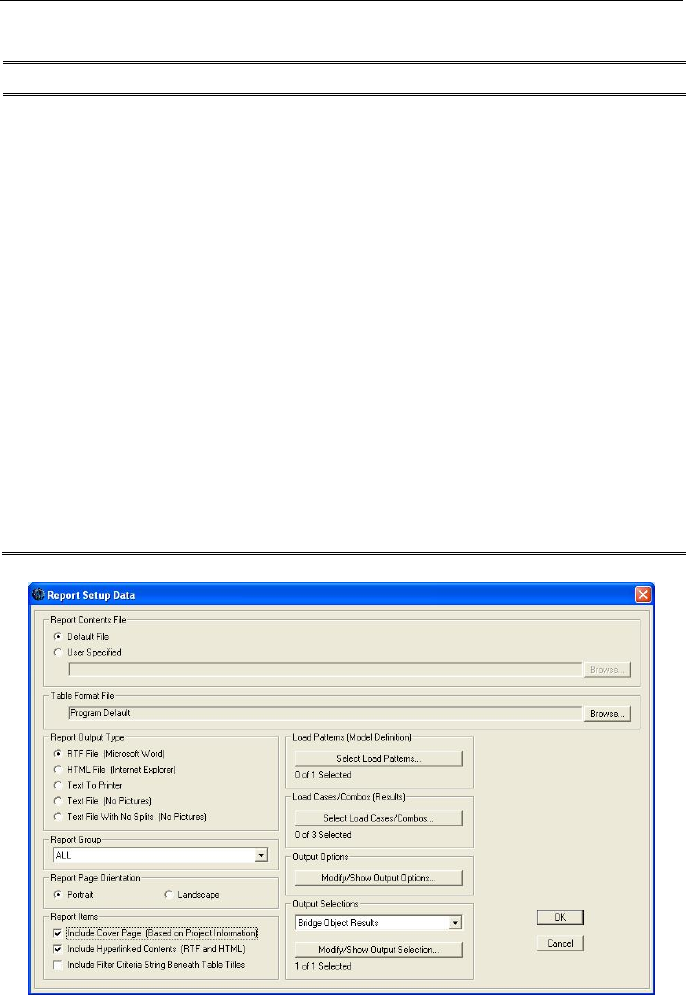
each command. Figure 2-4 shows the Report Setup Data form that dis-
plays when the File > Report > Report Setup command is used. Figure
2-5 shows the Create Custom Report form that displays when the File >
Report > Advanced Report Writer command is used. Recall that de-
pressing the F1 key will display context sensitive help when a form is
shown in the active window.
Table 2-5 File > Report > {Command}
Command Description
Create
Report
Generates a report for the open file using the data source, output
format, and data types selected using the Report Setup com-
mand.
Report Setup Does not generate a report; opens the Report Setup form (Figure
2-4). Use that form to specify the following:
Report contents, as specified in an .xml file, including instruction
to include a user-supplied company logo and company name on
the cover page as lifted from the Project Information form (see
Project Information in Table 2-7).
Table format file (.fmt), which specifies the database fields to be
used, the width of data columns, number format (zero tolerance,
number of decimal places and so on), any data filtering, data
File > Report 2 - 11

CSiBridge – Defining the Work Flow
Table 2-5 File > Report > {Command}
Command Description
sorting order.
Output type, including .rft, .html, text to printer, text without pic-
tures, text without splits and no pictures.
Group(s) for which data will be included in the report (helpful in
focusing the report on key components in a model)
Portrait or landscape page orientation.
Report Setup
(continued)
Report components to be included: cover page using information
from the Project Information form (see Project Information in Ta-
ble 2-7); hyperlinked table of contents, in RTF and HTML formats
only; printing of filter criteria (as specified in the table format file-
see above) beneath the table title(s).
Data to be included: load patterns; results of selected load cas-
es/load combos.
Output parameters for each load case type.
Name(s) of the Bridge Object for which results are to be includ-
ed.
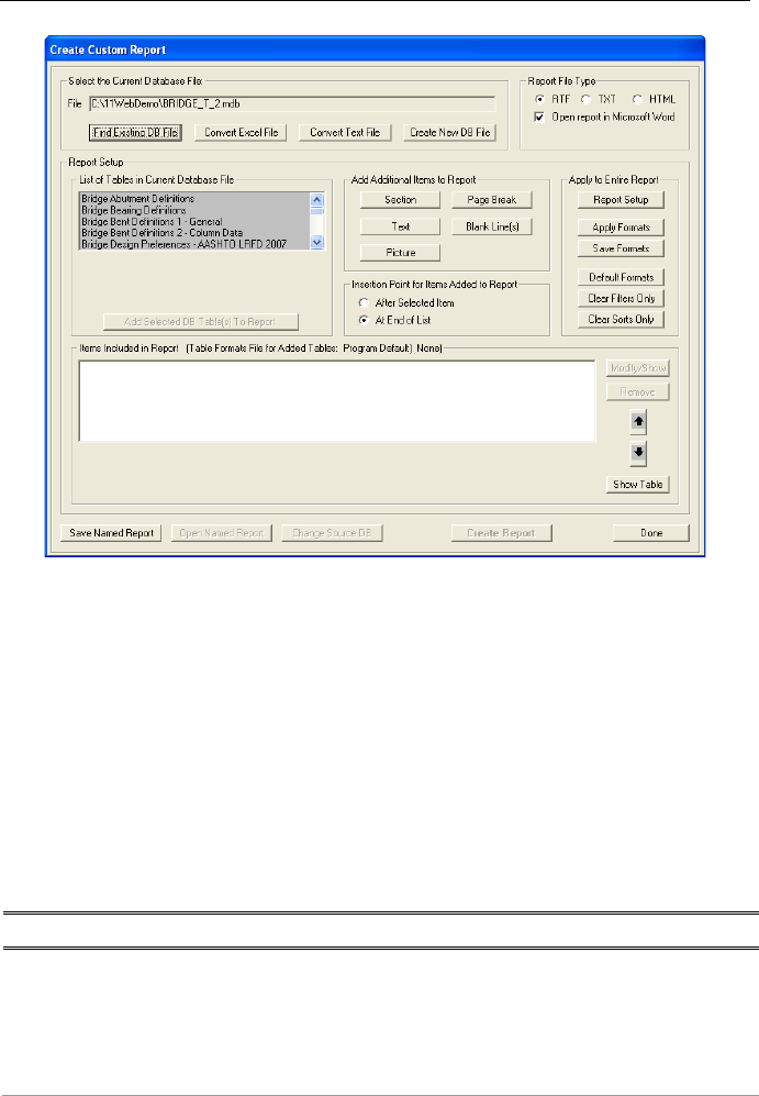
Advanced
Report Writer Displays the Create Custom Report form (Figure 2-5). Allows the
user to select the content and format for the report and then cre-
ates the report in accordance with user specifications. Use the
form to select the following:
Source file(s) for the data to be included in the report. This fea-
ture can be used to combine data from multiple sources, includ-
ing the database of the open model file, data from an Excel file or
a text file, and data exported from the model file into a new Ac-
cess .mdb file. As each data source is selected, the other options
on the form can be used to specify how the data will be present-
ed (e.g., with or without section headings, with or without page
breaks before or after).
Report output type, including .rtf, .txt, or .html. The user can opt
to open the generated report using the appropriate program
(e.g., Microsoft Word for the .rft format; default text editor for .txt)
Data to be included on a database-table-by-database-table ba-
sis. That is, a display area shows the data tables available from
the selected source; highlight a table name and click the Add
Selected DB Table(s) to Report button to add it to the Items
Included in Report list. Note that after at least one item has been
added to the list, the Change Source DB button becomes avail-
able. This button can be used to switch to another .mdb file from
a different model file.
2 - 12 File > Report
CHAPTER 2 File
Table 2-5 File > Report > {Command}
Command Description
Advanced
Report Writer
(continued)
Layout of the report, including levels of heads (1, 2, 3) and
alignment for section headings; text of section headings; pic-
tures/graphics and their alignment, caption, dimensions and so
on; insertion of page breaks; insertion of blank lines. These items
are added to the list of data items to be included in the report
(see previous bullet) after a selected item or at the end of the list,
depending on user selection.
Report setup items similar to those achieved using the File >
Report > Report Setup
command, including table formatting,
filtering crite
ria, sorting order, hyperlinked table of contents and
page orientation. Also includes page setup with respect to mar-
gins; specification of fonts for table titles, field headings, data in
the tables, headings, text, figure captions, specification of the in-
dividual items to be included on a cover page.
Saving of the format specified using the form and also applying a
previ
ously saved format. Note that after a format file (.fmt) has
bee
n generated using this command, the .fmt file can also be
used with the Report Setup command.
Removing any filter criteria that has been applied.
Removing any sort order that has been applied.
Command: File > Report > Report Setup
Figure 2-4 Report Setup Data
File > Report 2 - 13
CSiBridge – Defining the Work Flow
Command: File > Report > Advanced Report Writer
Figure 2-5 Create Custom Report form
2.9 File > Pictures
The File > Pictures command displays a menu of subcommands that en-
ables capturing of screen images of the active window as bitmaps and
metafiles, as well as creating multi-step videos or cyclic animations.
Table 2-6 identifies the subcommands and briefly describes them.
Table 2-6 File > Pictures > Subcommands
Subcommand Description
Bitmap - Entire Screen Creates a bitmap (.bmp) of the entire Windows screen,
including any exposed Windows wallpaper and the en-
tire CSiBridge window, including the File, the menu bar
of icons, the tabs, the display window(s) that shows the
current model, and the status bars for both CSiBridge
and Windows (e.g., the start button).
2 - 14 File > Pictures

CHAPTER 2 File
Table 2-6 File > Pictures > Subcommands
Subcommand Description
Bitmap - Main Window Creates a .bmp of the CSiBridge window, including the
File, the menu bar of icons, the tabs, the display win-
dow(s) that shows the current model, and the CSiBridge
status bar (e.g., XYZ coordinates, coordi
nate system,
units).
Bitmap - Current
Window with Title bar
Creates a .bmp of the active display window (where the
model is shown) and the title bar along the top of the
window.
Bitmap - Current
Window without Title
bar
Creates a .bmp of the active display window (where the
model is shown) but does not include the title bar along
the top of the window.
Create Multi-Step
Animation Video Saves an .avi file of the movement of the model struc-
ture after a time history analysis has been run. The
saved .avi can be played using the media player sup-
plied with the Windows program.
Create Cyclic
Animation Video
Saves an .avi file of the animated mode shapes and
other deformed shape plots of the model structure. The
saved .avi can be played using the media player sup-
plied with the Windows program.
2.10 File > Settings
The File > Settings command displays a menu of subcommands that can
be used to set the display and output units, the tolerances, the database
table utilities/settings, the display and output color settings, and
other miscellaneous setting, as well as to record project information and
comments and review the program-generated information log. Table 2-7
identifies the subcommands and describes them briefly. Figures 2-6
through 2-8 illustrate some of the forms that display when the subcom-
mands of the File > Settings command are used.
File > Settings 2 - 15

CSiBridge – Defining the Work Flow
Table 2-7 File > Settings > {Command}
Command Description
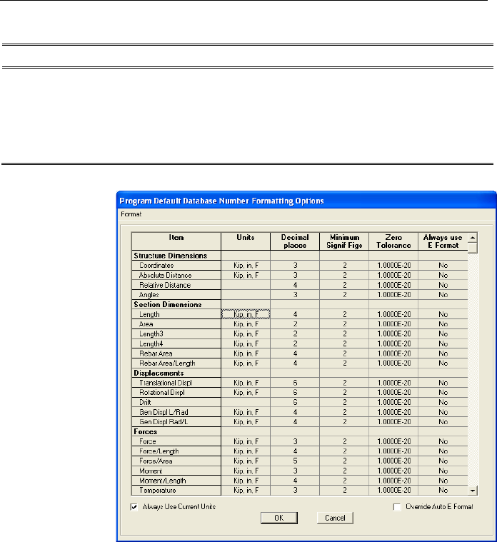
Units Specifies the number formatting to be applied in any of the da-
tabases generated by the program. This feature allows different
units to be set for a given item. For example, the base units set
when the model file was initialized could be Kip, in, F, which
means all dimensions throughout the program are converted to
Kip, in, F whenever the file is saved. This feature could be used
to change the units used for lengths for one item, such as Sec-
tion Dimensions, to Kip, ft., F. The Format option allows users to
convert all of the units to English, Metric or Current Consistent
units. Some caution is warranted here to ensure that errors re-
lated to variation in units are not made.
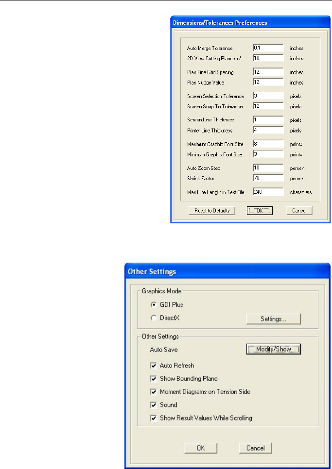
Tolerances
Used to set parameters applied to various program features
involving proximity considerations (e.g., minimum distance for
spacing fine grids; minimum dis
tances allowed when working
with the Snap To feature) and model dis
play (e.g., minimum
pixel size for line thickness, minimum point size for fonts).
Please consult the context sensitive help topic for further details
con
cerning each dimension or tolerance item (depress the F1
key when the form shown in Figure 2-7 is displayed).
Database Table
Utilities and
Settings
Displays a form with multiple buttons that when clicked display
the forms used to manage the program database files, includ-
ing:
> Set Current Format File Source – Allows selection of the
database table format file (.fmt) to be used as the basis for
formatting tabular output. Options include the programmed
format, an .fmt file that ships with the program, and a user
specified file in the appropriate format.
> Edit Format File – Use to make changes to the tables includ-
ed a format file (.fmt).
> Set Current Table Name Source –
Use to alter database
table names.
> Write Default Table Names to XML – Use to select data
tables for inclusion in a saved .xml file that subsequently can
be used in generating reports.
> Documentation to Word – Use to create a file(s) in Microsoft
Word that identifies the types of data in the database, includ-
ing a brief description of the function of the data, the units, the
format, and so on. Caution, the All Tables file is large.
2 - 16 File > Settings

CHAPTER 2 File
Table 2-7 File > Settings > {Command}
Command Description
Database Table
Utilities and
Settings
(continued)
> The Auto Regenerate Hinges After Import check box on this
form is a toggle that when enabled (a check mark precedes
the name) instructs
the program to automatically regenerate
any hinges in the model after data has been imported into the
model from an external source.
Colors Change the default settings for display and output colors.
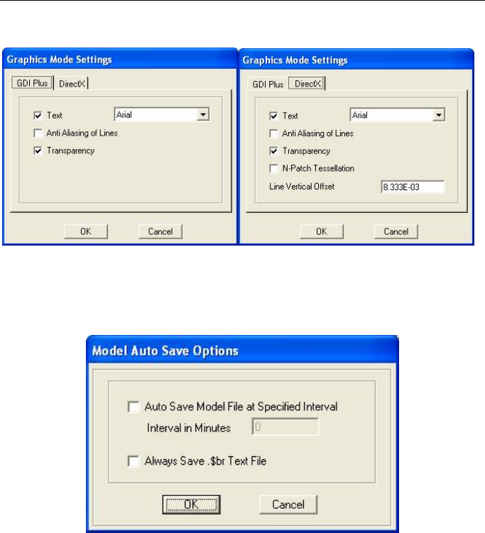
Other Settings
Displays a form with options that control graphical display and
some operational features of the program.
> Graphics Mode – Choose the mode for display: GDI Plus or
Direct X. GDI Plus makes two-dimensional drawing easier. Di-
rect X is better suited for displaying full color graphics and 3D
animation.
> Auto Save – Click the Modify/Show button to display a form
with options to specify that the model be saved automatically
at specific intervals and that the emergency backup file (i.e.,
the
.$2k text file) always be saved each time the auto save
occurs.
> Auto Refresh – Toggle to indicate if the program should re-
f
resh the model view after changes have been made to the
model data.
> Show Bounding Plane – Toggle to turn off or on the cyan-
colored line that shows the location of the active plan or ele-
vation view. For example, if a plan view is active and a 3D
view is al
so showing, the bounding plane appears in the 3D
view around the level associated with the plan view.
> Moment Diagram on Tension Side – Toggle to plot the mo-
ment diagrams for frame elements with the positive values on
the tension side of the member or on the compression side of
the member.
> Sound – Toggle to turn sound off or on when viewing anima-
tion of deformed shapes and mode shapes.
> Show Result Values While Scrolling – Toggle to turn off or
on the display of a small text box when the mouse cursor is
moved over a deformed shape.
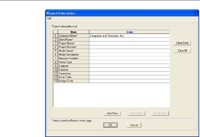
Project
Information
Use to record project data that subsequently could be included
in printed output tables or reports or in an exported file or an on-
screen display. Data includes company name, client name, pro-
ject name, projec
t number, model name, model description,
revision number, frame type, engineer, checker, supervisor,
issue code, design code.
File > Settings 2 - 17
CSiBridge – Defining the Work Flow
Table 2-7 File > Settings > {Command}
Command Description
Comments and
Log Displays an up-to-
date record of when and where the file was
stored. The comment log may also be used to track the status of
the model, to keep a "to-do" list for the model, and to retain key
results that can be used to monitor the effects of changes to the
model. Those notations can be deleted or modified and com-
ments may be typed directly into the comment log at any time.
Figure 2-6 Program Default Database Number Formatting
Options form
This command
(see Table 2-7)
displays this
form.
File > Settings
> Units.
2 - 18 File > Settings
CHAPTER 2 File
Figure 2-7 Dimensions/Tolerances
Preferences
Figure 2-8 Other Settings
This command (see Ta-
ble 2-7) displays this
form.
File > Settings >
Tolerances.
This command
(see Table 2-7)
displays this form.
File > Settings >
Other Settings.
File > Settings 2 - 19
CSiBridge – Defining the Work Flow
File > Settings > Other Settings > Settings button
Figure 2-9 Graphics Mode Settings
File > Settings > Other Settings > Modify/Show button
Figure 2-10 Model Auto Save Options
2 - 20 File > Settings
CHAPTER 2 File
Figure 2-11 Project Information
2.11 File > Language
CSiBridge is currently available in English and Chinese. Use the File >
Language command to change languages.
This command
(see Table 2-7)
displays this
form.
File > Settings
> Project
Information.
File > Language 2 - 21

CHAPTER 3 Home
The Home tab consists of the Wizard, View, Snap, Select, and Display
panels. The Bridge Wizard can be used to step through the modeling and
analysis processes when the Quick Bridge template or the Blank option
is used to start the model (see Chapter 2).
The commands on the View, Snap, Select, and Display panels can be
used to manage the active view (e.g., zoom features, set 3D, XY, XZ,
ZY views. and so on), improve the accuracy of operations in the active
view (e.g., apply Snap tools to ensure that the end of a drawn line object
connects exactly to an existing point object or grid coordinate), assist
operations in the active view through targeted selection (e.g., select ob-
jects based on their material property assignment), and determine the re-
sults to be shown in the active view. Thus, the Home tab has the com-
mands needed to adjust the active view and to work in it efficiently.
Each of these features and their associated commands are described
briefly in this chapter.
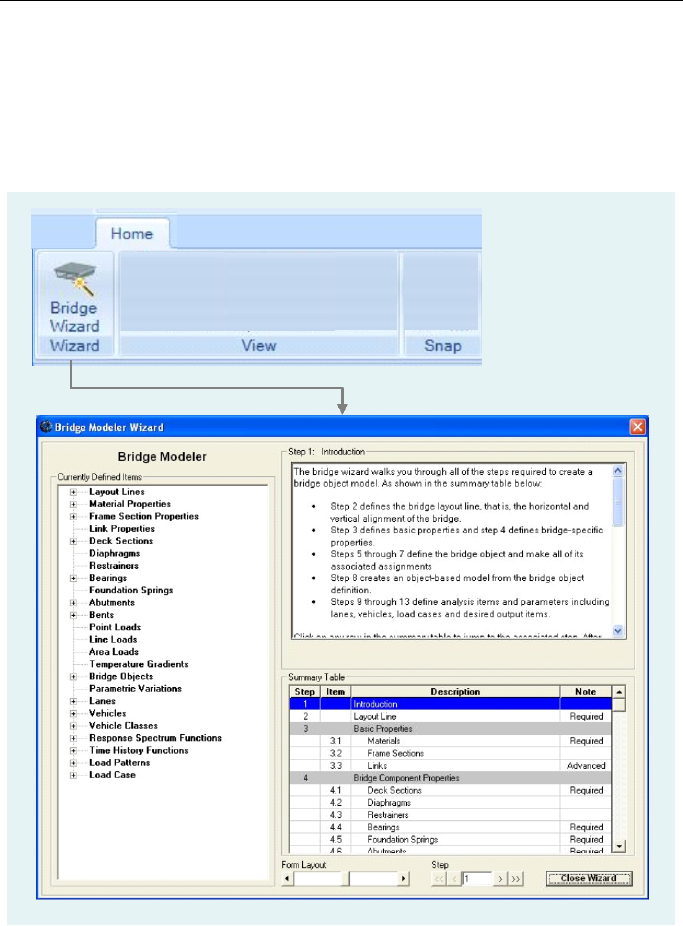
3.1 Home > Bridge Wizard
The Bridge Wizard provides a simple and easy way to navigate through
the bridge modeling and analysis processes. Unlike other program “wiz-
Home > Bridge Wizard 3 - 1
CSiBridge – Defining the Work Flow
ards,” it is possible to “pick up” and “leave” the Bridge Wizard at any
time. Figure 3-1 shows the Home > Bridge Wizard command and the
Bridge Modeler Wizard form that displays when this command is used.
Note that the commands on the other panels have been blocked from this
illustration.
Figure 3-1 Home > Bridge Wizard command and Bridge Modeler Wizard form
Note that the tree structure on the left-hand side of the form keeps a cur-
rent record of the components that have been defined for the bridge
model. The informational display area in the upper right-hand side of the
3 - 2 Home > Bridge Wizard

CHAPTER 3 Home
form changes depending on the Step/Item/Description selected from the
Summary Table in the lower right-hand side of the form. That is, the in-
formation displayed briefly explains the selected Step/Item. Clicking on
an item in the tree view “jumps” the informational display and the Sum-
mary Table to the Step/Item associated with the selected tree view item.
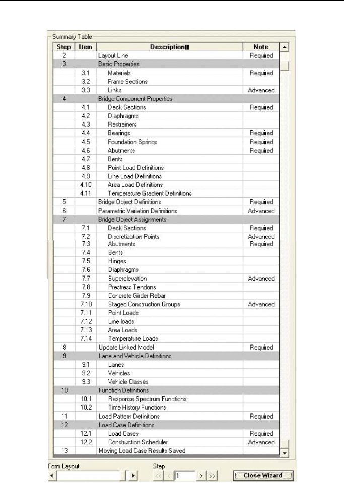
Note the Form Layout slide bar near the center at the bottom of the form.
Use that slide bar to reveal more of the information display area (slide
the bar to the left) or more of the Summary Table (slide the bar to the
right). Figure 3-2 shows the complete set of Steps/Items in the Summary
Table area.
It is possible to move around the Summary Table area as follows:
Click on any row to jump to that Step.
Depress the up and down arrow keys of the keyboard to move up or
down one Step at a time.
Type a Step number into the Step control near the bottom of the form
and depress the Enter key on the keyboard to jump directly to the
specified Step.
Use the Step control arrows to move to the first Step (<<), previous
Step (<), next Step (>) or last Step (>>).
The slide bar on the right-hand side of the Summary Table can be used
to move down and up along the display to expose areas not shown.
The “Note” column in the Summary Table identifies some Steps as Re-
quired and others as Advanced. The Steps identified as Required must be
completed to create a bridge model. The Steps designated as Advanced
are those that generally are not used in a typical model. Those Steps with
no designation should be used in a model at the user’s discretion.
Home > Bridge Wizard 3 - 3
CSiBridge – Defining the Work Flow
Figure 3-2 Bridge Wizard Summary Table
3 - 4 Home > Bridge Wizard

CHAPTER 3 Home
3.1.1 5B5BUsing the Bridge Wizard
Recall from Chapter 2 that the Bridge Wizard is designed to be used
when a model is started by clicking the Blank option or the Quick Bridge
template.
When the Blank option is used, it is possible to immediately open the
Bridge Wizard by clicking on it on the Home tab. In that case, the
Bridge Wizard is used to create the entire model. Thus, the first step
is to define the layout line, and then continue following the Steps as
outlined in the Summary Table and as explained in the information
display area.
When the Quick Bridge template is used, the span lengths and the
deck section type are initially defined, before the Bridge Wizard be-
comes accessible on the Home tab. When the span lengths and deck
section are specified, the program defines the layout line as well as de-
fault material property and frame section property definitions suitable
for the selected deck section type. The program also defines bearings,
abutments, and bents, and generates a Bridge Object, which is the
backbone of the model. In generating the Bridge Object, the various
definitions are assigned to the span length(s). The program also adds
default definitions for lanes, vehicles, response spectrum functions,
time history functions, load patterns and load cases. In this case, the
Bridge Wizard can be used to review the default definitions, and
where necessary adjust them.
In either case (i.e., starting from the Blank option or Quick Bridge tem-
plate), it is possible to use the various tabs of the graphical user interface
to add, modify, and delete the initial default definitions and to add fur-
ther definitions, for example: link properties; diaphragms; restrainers;
foundation springs; point, line, and area loads and temperature gradients.
More importantly, after the Bridge Object has been generated, the com-
mands on the Analysis and Design/Rating tabs can be used to define the
load combinations used in the analysis; complete the Design Request for
superstructure and seismic design; and complete the rating request. Re-
Home > Bridge Wizard 3 - 5

CSiBridge – Defining the Work Flow
ports also can be generated using commands on the Design/Rating tab,
or using the File > Report commands.
3.1.2 6B6BSteps of the Bridge Wizard
A general overview of the Steps on the Bridge Wizard (see Figure 3-2)
is as follows:
Step 2 defines the bridge layout line; that is, the horizontal and vertical
alignment of the bridge.
Step 3 defines basic properties for materials, frame sections, and links
(where applicable).
Step 4 defines bridge-specific properties (deck sections, diaphragms,
restrainers, bearings, foundation springs, and so on).
Steps 5 through 7 define the bridge object and make all of its associat-
ed assignments. That is, after the geometry has been defined (i.e., the
layout line definition) and the bridge components have been defined,
these steps assign the definitions to the span lengths.
Step 8 creates an object-based model from the bridge object definition.
Steps 9 through 13 define analysis items and parameters, including
lanes, vehicles, load cases, and desired output items.
For each step in the Bridge Wizard (except Step 1, the Introduction) a
button appears immediately below the informational display area. Click-
ing the button opens the form associated with the Step. In a few cases the
button may be disabled. This occurs when prerequisite Steps have not
been completed, such as:
A layout line and a deck section property are required before a bridge
object definition.
A bridge object definition is required before any bridge object assign-
ments can be made.
3 - 6 Home > Bridge Wizard

CHAPTER 3 Home
A layout line definition or frame objects must exist in the model be-
fore lanes can be defined.
For the Bridge Object Assignments, a Bridge Object drop-down list also
displays immediately below the informational text. The assignments
made using the listed Steps will be applied to the Bridge Object selected
from that drop-down list.
Table 3-1 briefly describes the Steps/features of the Bridge Wizard.
Table 3-1 Home > Bridge Wizard > {Step}
Step
Description
Layout Line Defines the layout line, which is used for defining the horizontal
and vertical alignment of the bridge and the vehicle lanes. Layout
line definitions are based on stations for linear dimensions, bear-
ings for horizontal align
ment, and grades for vertical alignment.
Layout lines may be straight, bent, or curved both horizontally and
vertically. Horizontal curves are circular with spirals, if necessary.
Vertical curves are parabolic or circular.
The forms used to define the layout line are identified in Chapter 4
Layout.
Basic
Properties
Material Properties – Defines the material properties used in
the frame section property definition and the deck section prop-
erty definition.
Frame Sections – Defines the frame section properties used in
the cap beams and columns in bent property definitions, girder
sections in some deck section property definitions, continuous
beam sections in some abutment property definitions, and frame
sections in some diaphragm property definitions.
Links – Defines link properties that are used in restrainer prop-
erty definitions, bearing property definitions, and foundation
spring property definitions. In each of those property definitions,
a user method of specifying the desired property, without refer-
ence to a link property, is available. In general, we recommend
that you use the user method rather than specifying your own
link properties. If you do use link properties, take special care to
make sure the local axes are defined correctly.
The forms used to define the material properties, frame sections
and link properties are identified in Chapter 5 Components.
Bridge
Component
Properties
Deck Sections – Used to define the bridge superstructure, se-
lect from various parametric deck sections, including concrete
box girder, concrete flat slab, precast concrete girder and steel
girder deck sections.
Home > Bridge Wizard 3 - 7

CSiBridge – Defining the Work Flow
Table 3-1 Home > Bridge Wizard > {Step}
Step Description
Bridge
Component
Properties
(continued)
Diaphragms – Specify data for vertical diaphragms that span
across the bridge. A diaphragm property can be solid concrete;
steel X, V or K bracing; a single steel beam or steel plate. Solid
concrete diaphragms are applicable only at locations where
concrete su
perstructure deck sections exist. Steel diaphragms
are applicable only at locations where steel girder superstructure
deck sections exist. In area object and solid object bridge mod-
els, the diaphragms are modeled using area and solid objects,
respectively. In spine models an automatically generated link ob-
ject is added at each diaphragm location to represent the dia-
phragm mass and weight.
Restrainers – Specify data for restrainer cables, which are used
as tension ties across superstructure discontinuities. Restrainers
may be assigned at abutments, hinges and at bents where the
superstructure is discontinuous over the bent. When specified,
the program assumes that a restrainer cable exists at each gird-
er location. A restrainer property can be specified as a
Link/Support property or it can be user defined. The user defined
restrainer is recommended. The user defined restrainer is speci-
fied by a length, area and modulus of elasticity.
Bearings – Specify data for bridge bearings, which are used in
abut
ment, bent, and hinge assignments to the bridge object. At
abutments, bearings are used in the connection between the
girders and the substructure. At bents, bearings are used in the
connection between the girders and the bent cap beam. At hing-
es, bearings are used in the connection between the girders on
the two sides of the hinge. A bearing property can be specified
as a Link/Support property or it can be user defined. The user
defined bearing is recommended and allows each of the six de-
grees of freedom to be specified as fixed, free or partially re-
strained with a specified spring constant.
3 - 8 Home > Bridge Wizard

CHAPTER 3 Home
Table 3-1 Home > Bridge Wizard > {Step}
Step Description
Bridge
Component
Properties
(continued)
Foundation Springs – Specify data for the connection of the
substructure to the ground. Foundation spring properties are
used in abutment and bent property definitions. At bents, foun-
dation springs may be used at the base of each column. In this
case the foundation springs are used as point springs. At abut-
ments, foundation springs are used as point springs for a foun-
dation spring-
type substructure, and they are used as spring
properties per unit length for a continuous beam-type substruc-
ture. A foundation spring property can be specifie
d as a
Link/Support property or it can be user defined. The user defined
spring is recommended. The user defined foundation spring al-
lows each of the six degrees of freedom to be specified as fixed,
free or partially restrained with a specified spring constant. For
cases where the spring property is used for a continuous beam
support, a factor is specified indicating the length over which the
specified properties apply.
Abutments – Specify the support conditions at the ends of the
bridge. Abutment propert
ies are used in abutment assignments
to the bridge object. The abutment property allows specification
of the connection between the abutment and the girders as ei-
ther integral or connected to the bottom of the girders only. The
abutment property also allows the abutment substructure to be
specified as a series of point springs (one for each girder) or a
continuously supported beam.
Bents – Specify the geometry and section properties of the bent
cap and the bent columns. They also specify the base support
condition of the bent columns. Bent properties are used in abut-
ment assignments to the bridge object. The bent property allows
specification of the connection between the abutment and the
girders as either integral or connected to the bottom of the gird-
ers only. The bent prop
erty also allows specification of a single
bearing line (continuous superstructure) or a double bearing line
(discontinuous superstructure). When double bearing lines are
used, the distance from the bent location (that is specified in the
bridge object definition) to each bearing line is included in the
bent property.
Home > Bridge Wizard 3 - 9

CSiBridge – Defining the Work Flow
Table 3-1 Home > Bridge Wizard > {Step}
Step Description
Bridge
Component
Properties
(continued)
Point, Line, Area Load Definitions – Allows definition of
unique point, line, and area loads that have a user defined direc-
tion, value and location. The loads may be defined in Force or
Moment. An example of a point load might be signage on the
bridge structure. These loads are assigned to the bridge model
using the Bridge Object (see Chapter 7).
Temperature Gradient Definitions – Defines temperature gra-
dient patterns over the height of the bridge superstructure for
later use in bridge object temperature load assignments. Several
code-
specified temperature gradient definitions are available as
well as user temperature gradient definitions.
The forms used to define bridge component properties are identi-
fied in Chapter 5 Components. The forms used to define the point,
line, and area loads are identified in Chapter 6 Loads.
Bridge
Object
Definition
The main component of CSiBridge, the
bridge object definition
in
cludes definition of bridge spans and the following assignments:
deck sections to each span; additional discretization points, includ-
ing their skews, along each span; abutments, including their
skews, at each end of the bridge; bents, including their skews, at
each bent location; hinges, including their skews, along each
span; diaphragms, including their skews, along each span; super-
elevations; prestress tendons; girder rebar; bridge construction
groups; point, line and area loads; and temperature loads.
The forms used to define bridge spans and make these assign-
ments are identified in Chapter 7 Bridge. Recall that the forms
used in creating most of these definitions (see previous Bridge
Component Properties step) are identified in Chapter 5 Compo-
nents, with forms associated with point, line, and area loads identi-
fied in Chapter 6 Loads.
Parametric
Variations
Parametric Variation Definitions – Can be used to define variations
in the deck section along the length of the bridge. Almost all pa-
rameters used in the parametric definition of a deck section can be
specified to vary. More than one parameter can vary at the same
time, if necessary. Each varying parameter can have its own
unique variation. Example uses of parametric variations include
varying the bridge depth and the thickness of girders and slabs
along the length of the bridge. The variations may be linear, para-
bolic, or circular. After a variation has been defined, it can be as-
signed as part of the deck section assignment to bridge objects.
The forms used to define a parametric variation are identified in
Chapter 5 Components.
3 - 10 Home > Bridge Wizard

CHAPTER 3 Home
Table 3-1 Home > Bridge Wizard > {Step}
Step Description
Bridge
Object
Assignments
Deck Sections – Allows a deck section property to be specified
for each span, and variation of the superstructure along the
length of the span can be assigned.
Discretization Points – Allows users to specify points among
the span where the bridge object will be discretized. Also a skew
associated with a discretization point can be specified. User dis-
cretization points
supplement the discretization specified when
the linked model is updated. In most models, creating user spec-
ified discretization points is unnecessary. The discretization
specified when the linked model is updated typically is sufficient.
Abutments – Allows users to specify, at each end of the bridge,
end skews; end diaphragm properties, if any; substructure as-
signment for the abutment which may be None, an abutment
property, or a bent property; vertical elevation and horizontal
location of the substructure; bearing property, elevation, and ro-
tation angle of the bridge default. Note that the elevations speci-
fied for the substructure and the bearings are Global Z coordi-
nates.
Bents –
Allows users to specify the superstructure assignment,
including a diaphr
agm property that, for bents at superstructure
disconti
nuities, can be specified on each side of the discontinuity
along with a restrainer property, restrainer vertical elevation, and
initial gap openings at the top and bottom of the superstructure;
bent property orientation; vertical elevation and horizontal loca-
tion of the bent; and bearing property, elevation and rotation an-
gle from the bridge default – note that for bents at superstructure
discontinuities bearings are separately specified on each side of
the discontinuity.
Note also that the elevations specified for the restrainer, bent,
and the bearings are Global Z directions. Typically, along each
bearing line there is one bearing for each girder.
Hinges –Allow users to specify, for each hinge, the location and
orien
tation, the bearing property, elevation, and rotation angle
from the bridge default, the restrainer property and elevation, di-
aphragm properties before and after the hinge, initial gap open-
ings at the top and bottom of the superstructure. Note that the
elevations specified fro the bearing and restrainer are Global Z
coordinates. Typically there is one bearing and one restrainer
for each girder.
Diaphragms –
A diaphragm assignment includes a diaphragm
location, property, and orientation. Th
e diaphragms assigned
here are in-span diaphragms. Diaphragms that occur at abut-
ments, bents, and hinges are assigned as part of the bridge ob-
ject abutment, bent and hinge assignments, respectively. Alt-
hough any diaphragm property can be assigned within a span, a
Home > Bridge Wizard 3 - 11

CSiBridge – Defining the Work Flow
Table 3-1 Home > Bridge Wizard > {Step}
Step Description
concrete diaphragm will be used by the program only if it occurs
within a span with a concrete deck section, and a steel dia-
phragm will be used by the program only if it occurs within a
span with a steel deck section.
Superelevation – A supereleva
tion assignment for a bridge
object is referenced to the layout line. The superelevation is
specified in percent and it indicates the rotation of the super-
structure about its longitudinal axis. The superelevataion may be
constant or it may vary along the bridge. In most bridge model
including superelevation is probably an unnecessary refinement.
Prestress Tendons –Tendon assignments include the location
of the start and end of the tendon, the vertical and horizontal
layout of the tendon, tendon section properties, loss parameters
and jacking options, tendon load specified as a force or a stress,
the tendon model
ing options as loads or as elements. Several
quick start options are available to assist in defining the layout of
parabolic tendons.
Concrete Girder Rebar –
Allow users to specify rebar in the
girders of concrete deck sections. The rebar is used by the pro-
gram when designing the superstructure. Both transverse
(shear) and longitudinal rebar can be assigned.
Staged Construction Groups – Allow users to specify data so
that the program can automatically create groups that can be
used in staged construction load cases. In the assignment, a
group is specified to contain certain elements of the bridge struc-
ture. such as girders between two sections along the bridge.
When the linked bridge object is updated, the program automati-
cally fills the group with the appropriate objects.
Point, Line and Area Loads – Allows users to assign prede-
fined point, line, and area loads to the bridge superstructure.
Temperature Loads – Apply pre-defined temperature gradient
loads to the superstructure. Loads may be constant temperature
changes or temperature gradient changes over the height of the
superstructure.
Update
Linked
Model
Creates the object-based model from the Bridge Object definition.
Spine, area, and solid models can be created when the model is
updated. The model must be updated each time the definitions are
changed for the changes to take effect. The type of model can be
changed at any time. This command also accesses options that
allow the user to specify discretization of the object-based model.
The form used to update the bridge model is identified in Chapter
7 Bridge.
3 - 12 Home > Bridge Wizard

CHAPTER 3 Home
Table 3-1 Home > Bridge Wizard > {Step}
Step Description
Lane and
Vehicle
Definitions
Lanes – Must be defined to analyze a bridge model for vehicle
live loads. Lanes are used in the definition of moving load type
load cases and in the definition of bridge live type load patterns,
which are used in static and dynamic multi-
step load cases.
Lanes can be defined with reference to layout lines or existing
frame objects. Typically, when using CSiBridge, lanes should be
defined from layout lines. Lanes can be defined with width, if de-
sired.
Vehicles – Must be defined to analyze a bridge model for vehi-
cle live loads. Vehicle loads are applied to the structure through
lanes. Numerous standard vehicles are built into the program. In
addition, the general vehicle feature allows creation of custom-
ized vehicle definitions. Each vehicle definition consists of one or
more concentrated or uniform loads.
Vehicle Classes – Must be defined to analyze a bridge model
for ve
hicle live loads using a moving load load case. A vehicle
class is simply a group of one or more vehicles for which a mov-
ing load analysis is performed (one vehicle at a time).
The forms used to define lanes, vehicles, and vehicle classes are
identified in Chapter 4 Layout.
Function
Definitions
Response Spectrum Functions – Required for creating re-
sponse spectrum load cases. If a response spectrum analysis is
to be performed for a bridge model, use this step to define the
func
tion. Many standard response spectrum functions are built
into the program. In addition,
the user function feature creates
user-
defined functions, and the function from file feature obtains
a function definition from an external file.
Time History Functions –
Required for creating time history
load cases. If a time history analysis is to be performed for a
bridge model, use this step to define the required functions.
Some generic time history functions are built into the program. In
addition, the user function feature can be used to create user-
defined functions
, and the function from file feature obtains a
function definition from an external file.
The forms used to create these function definitions are identified in
Chapter 6 Load.
Home > Bridge Wizard 3 - 13

CSiBridge – Defining the Work Flow
Table 3-1 Home > Bridge Wizard > {Step}
Step Description
Load
Pattern
Definitions
A load pattern is a specified spatial distribution of forces, dis-
placements, temperatures, and other effects that act upon the
structure. A load pat
tern by itself does not cause any response in
the structure. Load patterns must be applied in load cases in order
to produce re
sults. One special type of load pattern available in
CSiBridge is the Bridge Live load pattern. In this type of load pat-
tern, one or more vehicles that move across the bridge are speci-
fied. For each vehicle, a time is speci
fied for the vehicle to start
loading the bridge, the initial vehicle location, the direction of travel
and the speed. When used in a multi-step static or multi-step dy-
namic (direct integration time history) load case, this type of load
pattern is useful in evaluating special vehicle loads.
The forms used to define a load pattern are identified in Chapter 6
Loads.
Load Case
Definitions
Load Cases – Defines how loads are to be applied to the struc-
ture (e.g., statically or dynamically), how the structure responds
(e.g., linearly or nonlinearly), and how the analysis is to be per-
formed (e.g., modally or by direct-
integration). Any load case
type can be used when analyzing a bridge model.
For seismic analysis, static, response spectrum and time history
load case types are useful. Pushover analysis can be performed
using a nonlinear static load case. Staged construction analysis
is also performed using nonlinear static load cases.
Several analysis options are available that are specialized for
analysis of vehicle live loads. Moving load cases compute influ-
ence lines for various quantities and solve all permutations of lane
loading to obtain the maximum and minimum response quantities.
Multi-step static and multi-step dynamic (direct integration time
history) load cases can be used to analyze one or more vehicles
moving across the bridge at a specified speed. These multi-step
load cases are defined using special bridge live load patterns that
define the direction, starting time, and speed of vehicles moving
along lanes (see previous Load Pattern Definition item).
Construction Scheduler – Useful in performing staged con-
struction analysis, the Construction Scheduler automatically cre-
ates the re
quired stage construction load cases to analyze the
bri
dge based on the specified schedule. Use the schedule to
identify tasks, their durations, tasks that must be completed be-
fore others (i.e., predecessors), and “Operations” that specify
the effects of the tasks on structure development with respect to
staged construction analysis.
The forms used to define the load case and to schedule con-
struction are identified in Chapter 8 Analysis.
3 - 14 Home > Bridge Wizard
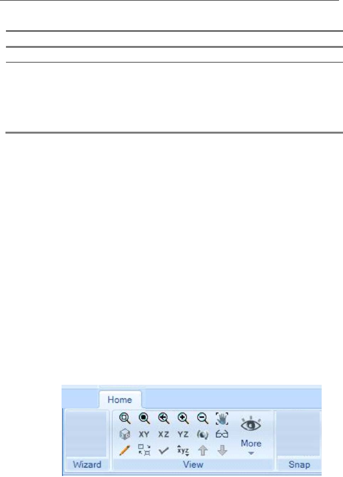
CHAPTER 3 Home
Table 3-1 Home > Bridge Wizard > {Step}
Step Description
Moving Load
Case
Results
Saved
Allows explicit specification of the analysis results to be produced
for a moving load load case. This feature reduces the computa-
tionally inten
sive and time consuming nature of the analysis of
moving load load cases, particularly for larger models.
The form used to specify the results to be saved is identified in
Chapter 8.
Note that Chapter 8 Analysis and Chapter 9 Design/Rating describe the
additional tasks/steps required to complete definition of the load combi-
nations to be used in the design; the design request for superstructure de-
sign and seismic design using the identified load combinations; and the
rating request required to obtain the rating for the bridge model. Report
generation is also covered in Chapter 9 Design/Rating and in Chapter 2
File.
3.2 Home > View
Viewing a model is controlled using Home > View > {Command}. Fig-
ure 3-3 shows the Home > View commands; the Wizard and Snap
commands have been blocked from this image. Table 3-2 provides a
brief explanation of the action of each command. Most of the view
commands provide an immediate response when clicked. In some cases
an additional form appears.
Figure 3-3 Home > View commands
Home > View 3 - 15
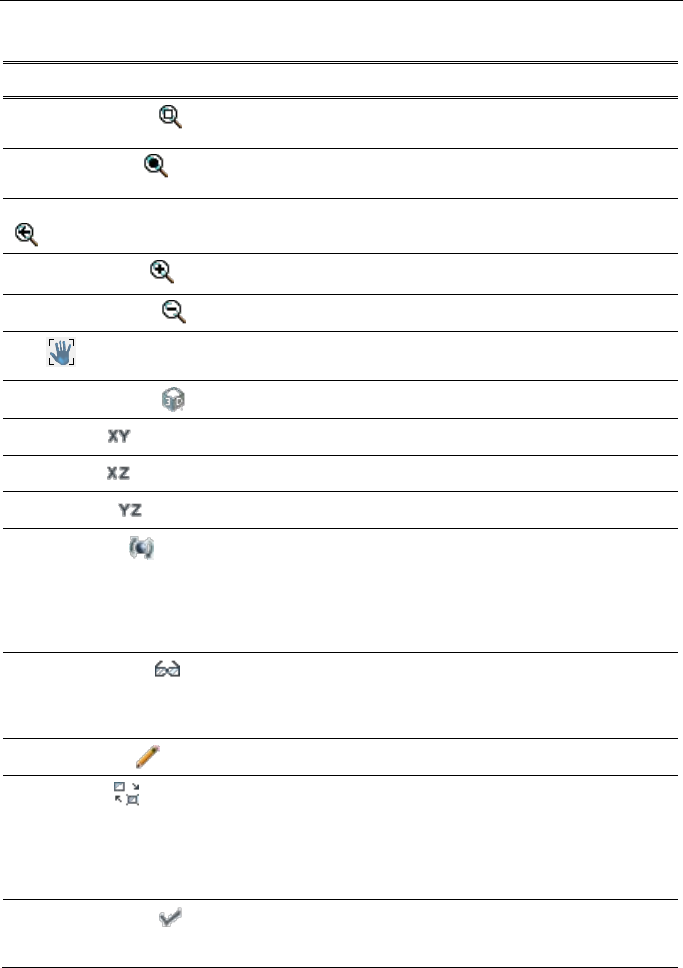
CSiBridge – Defining the Work Flow
Table 3-2 Home > View > {Command}
Command Action
Rubber Band Zoom Immediately zooms in on the portion of the model that lies
within a drawn rubber band window.
Restore Full View Immediately restores the view such that the entire model fills
the window.
Restore Previous Zoom
Immediately returns the view one step back to the previous
zoom setting.
Zoom In One Step Immediately zooms the view in one step.
Zoom Out One Step Immediately zooms the view out one step.
Pan Immediately allows the model to be moved around in the
active window.
Set Default 3D View Immediately sets the view to the default 3-D View.
Set XY View Immediately sets the view to the default XY View.
Set XZ View Immediately sets the view to the default XZ View.
Set Plan View Immediately sets the view to the default YZ View.
Rotate 3D View Only active when a 3D view of the model is being displayed,
immediately allows the model to be rotated in any direction.
The model is rotated about a point defined by clicking on the
screen to begin the model rotation. After the mouse button
has been released, the command must be reused to enable
further rotation.
Perspective Toggle Immediately turns the perspective view effects on and off. If a
model is viewed in elevation or plan and the Perspective
Toggled is activated, the view will change from a planer view
to a 3D perspective view.
Refresh Window Immediately redraws the window without rescaling.
Object Shrink Graphically toggles the size of object between a smaller size
and the original size. The shrink factor is specified using the
File > Settings > Tolerances command. This is a graphical
change only. No changes in member connectivity or size are
made to the analytical model. This feature is particularly use-
ful to see how members are divided or subdivided.
Set Display Options Display a form that can be used to control display, such as
which objects, labels, and property identifiers are displayed,
along with how they are displayed, e.g., show extrusions.
3 - 16 Home > View
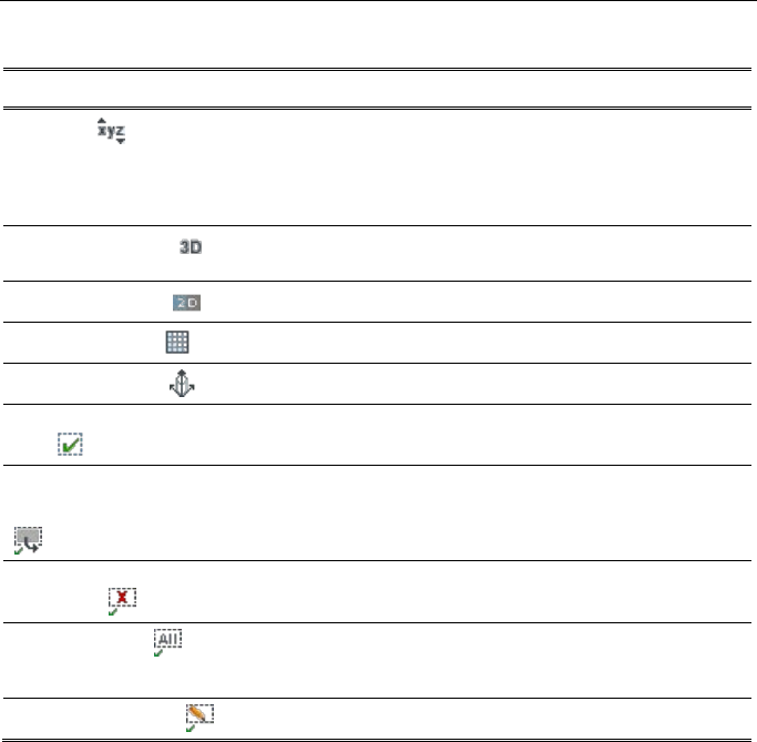
CHAPTER 3 Home
Table 3-2 Home > View > {Command}
Command Action
Set Limits Displays a form that can be used to define the portion of a
model to be displayed. This is especially useful with large
models. The view limits are defined by specifying X, Y and Z
coordinate ranges. Portions of a model located outside of the
specified X, Y and Z range limits are not displayed.
More > Set 3D View Can be used to define the view angles for the plan, elevation
and aperture.
More > Set 2DView Can be used to define the View Plane as YZ, XZ or XY.
More > Show Grid Toggles the display of grids in view on and off.
More > Show Axes Toggles the display of the global axes in a view on and off.
More > Show Selection
Only Use to view the features of a model that have been selected.
More > Invert View Selec-
tion
Deselects all of the selected items and selects all of the pre-
viously unselected items.
More > Remove Selection
from View Use to view the features of a model that are not selected.
More > Show All Restores the view to include all features of the model set to
be viewed as defined using the Set Display Options com-
mand.
More > Refresh View Reactivates the display of the current model view.
3.3 Home > Snap
Various snap commands allow the user to position the select arrow on
the desired point, line, area, or solid object. Figure 3-4 shows the Home
> Snap commands; the Wizard and View commands have been blocked
from this image. Table 3-3 provides a brief explanation of the actions of
each command.
Home > Snap 3 - 17
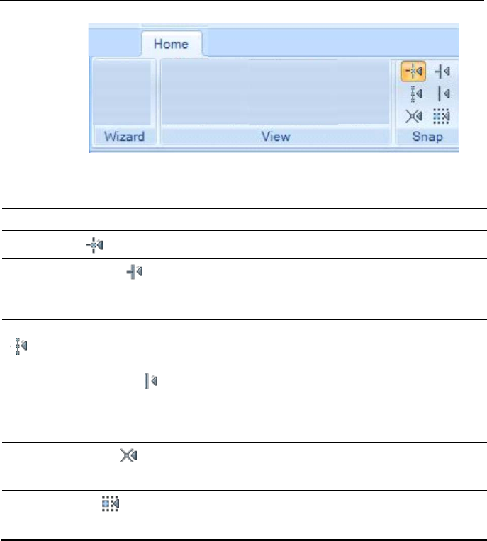
CSiBridge – Defining the Work Flow
Figure 3-4 Home > Snap commands
Table 3-3 Home > Snap > {Command}
Command Action
Snap to points Finds and snaps to the points closest to the mouse pointer.
Snap to Perpendicular Snaps to the intersection point of a line drawn from the last
entered point perpendicular to the frame objects or area
edge closest to the mouse pointer. This is a helpful way to
make sure that lines are perpendicular to each other.
Snap to Ends and Midpoints
Finds and snaps to the closest midpoint or end of frames
and shells. It also will snap to the end points of NL Link
elements.
Snap to Lines and Edges Finds and snaps or “hugs” the closest frame object, grid
line or edge of the closest area object. Even though this
does not provide the same level of accuracy as the other
snap options, it is a good way to make sure that the object
being drawn is located on the object being “hugged.”
Snap to Intersections Finds and snaps to the intersection of two frame objects
and a frame object with an area object, regardless of
whether there is a joint at the intersection location.
Snap to Fine Grid Finds and snaps to the intersections of the fine grids in a
planar view. The Fine Grid spacing may be controlled
using the File > Settings > Tolerances command.
3.4 Home > Select
With the program in Select mode, objects can be selected graphically in
the active display window using the mouse cursor. Selected objects are
indicated by dashed lines. Figure 3-5 shows the Home > Select com-
mands; the Home tab has been moved so that it would be included in the
graphic and the Display commands have been blocked from this image.
Table 3-4 provides a brief explanation of the action of the Select com-
mands.
3 - 18 Home > Select
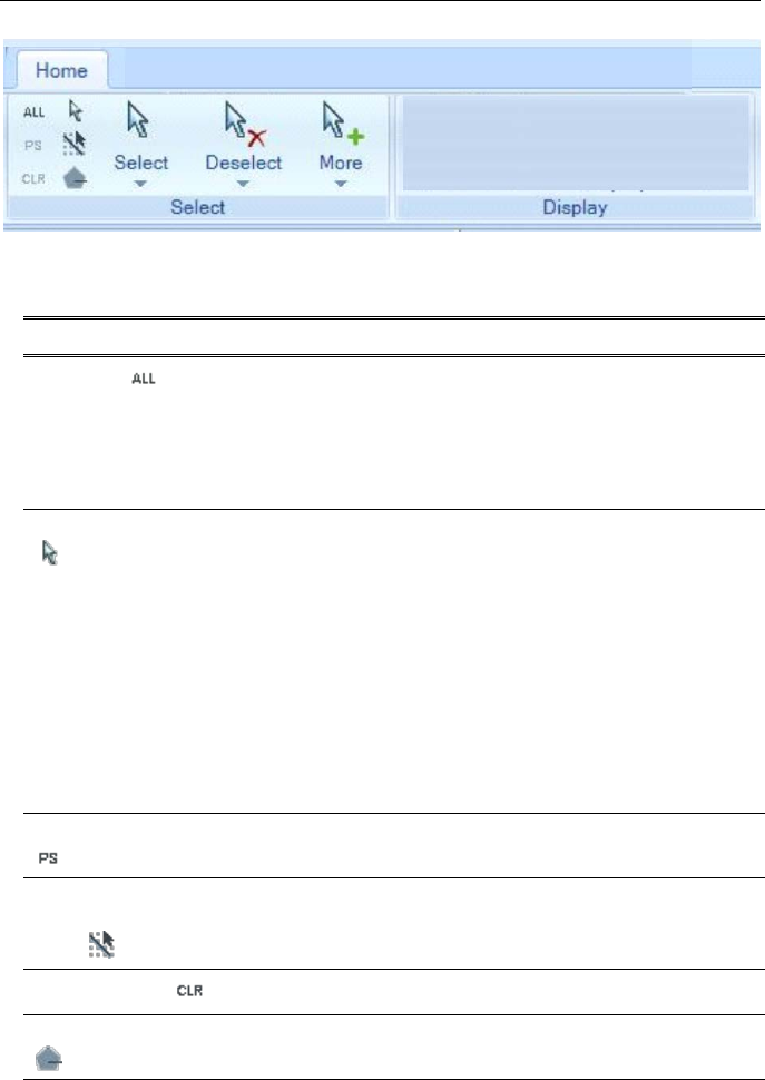
CHAPTER 3 Home
Figure 3-5 Home > Select commands
Table 3-4 Home > Select > {Command}
Command/Button Action
Select All Selects all of the objects in the model. The total num-
ber of objects selected is displayed on the status bar.
Be careful using this command. The command does
not select only the objects shown in a particular win-
dow, but rather it literally selects all objects in the
model.
Select Pointer/ Window
By Pointer – Selects/deselects objects with each
mouse click on the object. Only a single object at a
time can be selected/ deselected. When in Select
mode, selection/deselection By Pointer is always
available. An object remains selected until it is dese-
lected or the Clear Selection command (see below)
is used. Use the Selection List when multiple objects
are present within the screen selection tolerance of
the mouse click.
By Window - Draw a window around one or more
objects to select them. Drag the mouse over the ob-
ject(s) to be selected.
Get Previous Selection
Use to reselect the previously selected objects.
Select Using Intersect-
ing
Lines
Click this command and draw a line through one or
more objects to select them.
Clear Selection Clears the selection of all currently selected objects.
Select Using Polygon
Use the Select Using Polygon command to select
objects by enclosing them within a polygon shape.
Select
> Pointer/Window – See previous description for
Select Pointer/Window.
Home > Select 3 - 19

CSiBridge – Defining the Work Flow
Table 3-4 Home > Select > {Command}
Command/Button Action
> Poly - Selects objects using left mouse clicks to
define a poly shape around the object to be select-
ed.
> Intersecting Poly – Similar to poly selection with
the additional selection of any objects intersected
by the “lines” between mouse clicks that define the
poly shape.
> Intersecting Line –
Selects objects by dragging
the mouse across objects to “draw” a “selection
line.”
> Coordinate Specification
3D Box –
Works in a 3D View to select objects
giving full
consideration to connections among
points, frames, cables, tendons, areas, or solids.
Specified Coordinate Range – Displays a form
that can be used to select objects based on
specification of X, Y and Z coordinates.
XY Plane - Use to select all objects in the XY
plane.
XZ Plane -
Use to select all objects in the XZ
plane.
YZ Plane -
Use to select all objects in the YZ
plane.
> Select Lines Parallel To
Click Straight Line Object – Select all line ob-
jects parallel to the line object selected after the
command is used.
Coordinate Axes or Plane – Displays a form
that can be used to specify when line objects will
be selected on the basis of their orientation rela-
tive to specified coordinate axes and planes, or
line or area objects.
> Properties – Material Properties, Frame Sections,
Cable Properties, Tendon Properties, Area Sec-
tions, Solid Properties, Link Properties, Frequency
Dependent Link Properties – Selects objects with
the specified property or section.
3 - 20 Home > Select

CHAPTER 3 Home
Table 3-4 Home > Select > {Command}
Command/Button Action
> Assignments
Joint Supports - Selects objects based on joint
support assignments.
Joint Constraints - Selects objects based on
joint constraint assignments.
> Groups - Selects objects based on group assign-
ments.
> Labels - Selects objects based on their labels. Can
be used to select a single object or multiple objects
by specifying a labeling increment or by selecting
from a list of object labels.
> All - See previous description of the Select All
command.
Deselect
Offers the same options as the Select command (see
above), but is used to deselect the specified object(s)
using the chosen method.
More
> Select Using Tables – Displays a form that has
options to select objects by selecting table names.
> Invert Selection – Selects objects that are not se-
lected and deselects objects that are selected.
3.5 Home > Display
The display command controls what and how various features of a mod-
el are to be displayed in the active window. Figure 3-6 shows the Home
> Display commands; the Home tab has been moved so that it would be
included in the graphic and the Select commands have been blocked
from this image. Table 3-5 provides a brief explanation of the actions of
the various Home > Display commands.
Home > Display 3 - 21

CSiBridge – Defining the Work Flow
Figure 3-6 Home > Display commands
Table 3-5 Home > Display > {Command}
Command Action
Show Undeformed
Shape
Displays the undeformed shape of the model. Addi-
tionally, if a model is being created, it clears the dis-
play of any assignments that are showing on the
model.
Show Bridge Super-
structure Forc-
es/Stress
After analysis, displays the
force/stress component
selected from a drop-down list. When viewing forces,
the entire bridge deck or individual girders may be
viewed. Tabular data is also available for viewing or
exporting.
Show Deformed
Shape
After analysis, u
se to display the Deformed Shape
form, which has options to tailor the display, such as
the load case or load combination to be displayed;
scaling options; contour options; wire shadow or cu-
bic curve.
Show Shell
Force/Stress Plots
After analysis, displays
internal area object forces
and stresses on shell elem
ents. The internal shell
element forces are forces-per-unit-length acting along
the mid-
surface of the shell element (area object).
The internal shell element stresses are stresses act-
ing on the edges (not positive 3-axis face and nega-
tive 3-axis face) of the shell element (area object).
Show Bridge Loads Displays a form with options to select a load pattern;
show loads for all Bridge Objects or for a selected
Bridge Object; show the loads as force or moment;
show point, line, and area loads; and display area
loads as pressures or discretized line loads.
Show Bridge Super-
structure Design Re-
sults
Use to view design results and unity checks (de-
mand/ capacity ratios). Results may also be viewed in
Excel spreadsheets or exported.
3 - 22 Home > Display
CHAPTER 3 Home
Table 3-5 Home > Display > {Command}
Command Action
Show Joint Reaction
Forces
Show support reactions as forces acting on the ele-
ments connected to the support. The reaction forces
are reported with respect to the global coordinate
system. Positive support reaction forces act in the
same direction as the positive global axes. The sense
of positive moments can be de
termined using the
right-
hand rule. As an example, consider a bridge
bent column that is supporting gravity load. This grav-
ity load acts in a downward direction. Thus the force
imposed on the bottom of the column acts in an up-
ward direction. This is the reaction force reported by
CSiBridge
. Since the upward force is in the same
direction as the positive global Z-axis, the reaction is
reported as a positive value acting in the Z direction.
Show Solid Stress
Plots
Displays solid member stresses.
Show tables Dis
play the Choose Tables for Display form. Check
the check box(es) associated with the item(s) to be
displayed.
Show Influence Lines/
Surfaces
Displays influence lines for the various displace-
ments, reactions, forces, moments, shears, and tor-
sion or axial loads on joints, frames, shells, planes,
asol
ids, solids, and links resulting from a unit load on
a defined bridge lane in the structure.
Show Frame/Cable/
Tendon Force Diagram
Displays column, beam, brace, or cable forces direct-
ly on the model.
Show Link Force
Diagram
Displays link force diagrams.
Named Display
> Save Named Display/View –Use to save the cur-
rent display and view settings.
Display settings may include, for example, the dis-
play of forces or stresses after an analysis.
View settings show, for example, a 2D elevation
view rotated 90 degrees from default.
> Show Named Display -- Use to display a named
display of a model.
Home > Display 3 - 23

CSiBridge – Defining the Work Flow
Table 3-5 Home > Display > {Command}
Command Action
Named Display
(continued)
> Show Named View – Use to display a named view
of a model.
More
> Show Load Assignments – Joint, Frame/Cable/
Tendon, Area, Solid, Link –
Displays forms to
specify the load pattern and other parameters as-
sociated with displaying loads for the selected ob-
ject type.
> Show Miscellaneous Assignments – Joint, Frame/
Cable/Tendon, Area, Solid, Link – Displays forms to
select the assignment to be displayed for the se-
lected object type.
> Show Lanes – Shows the lane centerline or the
lane width. In addition, options may be used to dis-
play the lane loading points used by the program in
a Moving Load load case and the connections of
the lane loading points to the joints in the analysis
model.
> Show Plot Functions – Displays a form that can
be used to specify the load case and the function to
be displayed.
> Show Static Pushover Curve – Displays a form
that can be used to specify the static nonlinear
case for which the pushover curve is being dis-
played.
> Show Hinge Results – Displays a plot of the plas-
tic rotation vs. moment, plastic deformation vs.
shear force, and plastic moment vs. axial force for a
selected hinge.
> Show Response Spectrum Curves – Displays a
response spectrum curve for a selected time history
case.
> Show Virtual Work Diagrams – Displays virtual
work diagrams, which show the percentage of vir-
tual work of an element relative to the balance of
the structural members. This display can be used to
reduce structural deflection by indicating which el-
ements have the highest percentage of energy and
thus will most affect the deflection if their stiffness-
es were to be modified.
3 - 24 Home > Display

CHAPTER 3 Home
Table 3-5 Home > Display > {Command}
Command Action
> Show Plane Stress Plots – Displays sress con-
tours for planes in the active window using stress
averaging.
> Show Asolid Stress Plots – Displays stress con-
tours for asolids in the active window using stress
averaging.
> Show Input/Log Files – Displays input and output
text files.
More (continued)
Home > Display 3 - 25

CHAPTER 4 Layout
The Layout tab consists of commands that allow efficient access to the
data forms needed to add, copy, or modify layout line and lane defini-
tions. A delete command also is available for deleting a selected defini-
tion. A method of displaying the definition form that lists all definitions
and that has buttons that perform the same functions as the commands on
the Layout tab also is available. This chapter describes those data and
definition forms.
If the Quick Bridge template was used to start the bridge model, the pro-
gram will have created a default layout line and some lane definitions.
These definitions can be viewed using the commands on the Layout tab.
If the Bridge Wizard is being used, highlighting the Layout Line and
Lanes items in the Summary Table and clicking the Define/Show Lay-
out Lines and Define/Show Lanes buttons will display the Define
Bridge Layout Line form and the Define Lanes form that can then be
used to access the same data forms as those that can be accessed directly
using the Layout tab commands.
The commands on the Layout tab also can be used if the Blank option
was used to start the model and the Bridge Wizard is not being used
(i.e., the model is being built “from scratch” or by importing model da-
ta).
Layout > Layout Lines 4 - 1

CSiBridge – Defining the Work Flow
4.1 Layout > Layout Lines
Layout lines are reference lines to which bridge span lengths are as-
signed. Thus, bridge alignment is defined using layout lines. The layout
line defines both the vertical and horizontal bridge alignments, which
may be defined as straight or curved.
Figure 4-1 shows the commands on the Layout Line panel of the Layout
tab.
Figure 4-1 Layout tab with annotated Layout Line panel
As indicated in the figure, clicking the expand arrow in the lower right-
hand corner of the Layout Line panel will display the Define Bridge
Layout Line form shown in Figure 4-2. The previously defined layout
lines are shown in the Layout Lines display area on the left-hand side of
the form. The buttons in the “Click to:” area on the right-hand side of the
form can be used to add, copy, modify, or delete layout line definitions.
The buttons in the “Click to:” area display the same forms or function in
the same manner as the New, Copy, Modify and Delete commands on
the Layout Line panel (see Figure 4-1). In essence, the commands on the
Layout Line panel by-pass the definition form shown in Figure 4-2 and
provide a short cut to the data form for the layout line definition.
IMPORTANT NOTE: The preceding statement has one excep-
tion. The Define Bridge Layout Line form has an additional but-
4 - 2 Layout > Layout Lines
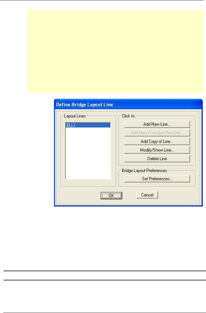
CHAPTER 4 Layout
tons, Add New From Gen Ref Line that does not have a corre-
sponding command on the Layout panel of the Layout tab. This
button is available only if a general reference line has been drawn
in the model (Advanced > Draw > More > Draw/Edit General
Reference Line command). When the Add New From Gen Ref
Line button is clicked, the Bridge Layout Line From General Ref-
erence Line form displays (see Section 4.1.2). Use the options on
the form to select the general reference line and specify the be-
ginning of the bridge layout line and any x, y, or z offset of the
layout line from the general reference line.
Figure 4-2 Definition form showing
previously defined layout lines
Table 4-1 briefly explains the functions of the commands on the Layout
Line panel. Screen captures of the forms identified in Table 4-1 are pro-
vided in the subsection that follows.
Table 4-1 Form Data - Layout > Layout Line >
Command
Data Form Parameters
Preferences Displays the Bridge Layout Preferences form (see Section 4.1.1).
Orient the bridge model by setting the direction of the North Arrow,
in degrees, as measured counterclockwise from the positive global
X axis. That is, with a typical window setup, the global X axis ex-
tends horizontally to the right. A default 90-degree orientation is
Use this command
to display this
form:
Layout > expand
arrow on Layout
Line panel
Layout > Layout Lines 4 - 3

CSiBridge – Defining the Work Flow
Table 4-1 Form Data - Layout > Layout Line >
Command Data Form Parameters
offered in the form so that the North Arrow points straight up, ori-
enting the model.
The curve discretization also may be set by defining the maximum
subtended angle to be used by the program to define a bridge
curve. The smaller the curve discretization value the smoother the
curve.
Multiple layout lines can be defined within the same model file. All
layout lines within the same model comply with the North Arrow
orienta
tion and curve discretization parameters set on the Bridge
Layout Preferences form.
Add Displays the Bridge Layout Line Data form - The layout lines spec-
ify orientation of the bridge relative to the coordinate system. The
placement of bridge objects (e.g., abutments, col
umns, bents,
hinges, spans) is accomplished relative to the layout line. The
initial and end station locations
for the layout line, and thus the
Bridge Object, are defined using this form. The form has the fol-
lowing buttons that pro
vide access to additional data forms used
to refine the bridge alignment.
Modify Layout Line Stations button. Displays a form that can
be used to shift the layout line, which will shift all of the stations
on the bridge objects and the lanes that reference the layout
line. Shifting the layout lines moves the initial station location the
specified dis
tance in the global X direction from the coordinate
system origin. Note that multiple layout lines can be defined for
a single bridge model. Individual layout lines can be shifted in-
dependently of each other. Thus, the bridge objects and lanes
that reference a specific layout line can be shifted easily using
this form.
Define Horizontal Layout Data button. Displays a form that
can be used to define the horizontal bridge layout. It is possible
for a layout line to be defined using combinations of multiple
straight and curved segments, including Straight at Previous
Bearing to Station, Straight at New Bearing Station, Curved
Right at New Bearing Station, or Curved Left at New Bearing
Station. The station locations are specified as lengths, meas-
ured from left to right, from the initial station location.
Define Vertical Layout Data button. Displays a form that can
be used to define the vertical bridge layout. It is possible for a
layout line to be defined using combinations of multiple grades,
including Constant at Previous Grade to Station, Constant at
New Grade to Station, Constant Grade to New Elevation at Sta-
tion, Parabolic to New Grade at Station, and Circular to New
Grade at Station. The station locations are specified as lengths,
4 - 4 Layout > Layout Lines
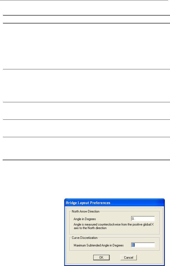
CHAPTER 4 Layout
Table 4-1 Form Data - Layout > Layout Line >
Command Data Form Parameters
measured from left to right, from the initial station location.
Horizontal Layout Line Data – Quick Start button. Displays a
form with a variety of template horizontal layout alignments,
such as Straight – Bend Right, Straight – Curve Left, Straight –
Curve Left – Straight – Curve Left – Straight, and so on. These
template defini
tions transfer to the horizontal layout data form.
As the name suggests, this from is a “quick start” for defining the
horizontal layout data.
Vertical Layout Line Data – Quick Start button. Displays a
form with a variety of template horizontal layout alignments,
such as Straight – Bend Down, Straight – Bend Up, Parabolic
Up, and so on. These template definitions transfer to the hori-
zontal layout data form. As the name suggests, this form is a
“quick start” for defining the vertical layout data.
Copy
Creates a copy of the layout line definition selected in the Current
Layout Line drop-
down list. The definition data can be modified as
described for the preceding Add command.
Modify Dis
plays the layout line definition selected in the Current Layout
Line drop-down list. The definition data can be modified as de-
scribed for the preceding
Add
command.
Delete
Deletes the layout line definition selected in the Current Layout
Line drop-down list unless the definition is being used in a Bridge
Ob
ject definition (see Chapter 7). A layout line in use in a Bridge
Object can not be deleted unless the Bridge Object is first deleted.
4.1.1 Bridge Layout Preferences Form – Screen Capture
Use these commands (see Table 4-1) to display this form.
Layout > Preferences
or
Layout > expand
arrow on the Lay-
out Line panel >
Set Preferences
button
Layout > Layout Lines 4 - 5
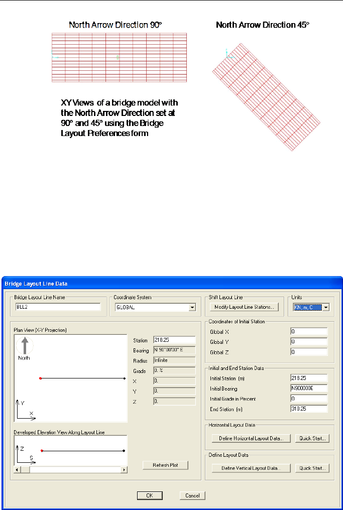
CSiBridge – Defining the Work Flow
Examples of North Arrow Orientation
4.1.2 Bridge Layout Line Data Form – Screen Captures
Use these commands (see Table 4-1) to display this form:
Layout > Add
Or
Layout > expand arrow on Layout Line panel
> Add New Line button
4 - 6 Layout > Layout Lines

CHAPTER 4 Layout
Use these commands (see Table 4-1) to display this form:
Layout > Add > Define
Horizontal Layout Data
button
Or
Layout > expand arrow on Layout Line panel
> Add New Line button > Define Horizontal
Layout Data button
Use these commands (see Table
4-1) to display this form:
Layout > Add > Modify Layout
Line Stations button
Or
Layout > expand arrow on Lay-
out Line panel > Add New Line
button > Modify Layout Line
Stations button
Layout > Layout Lines 4 - 7
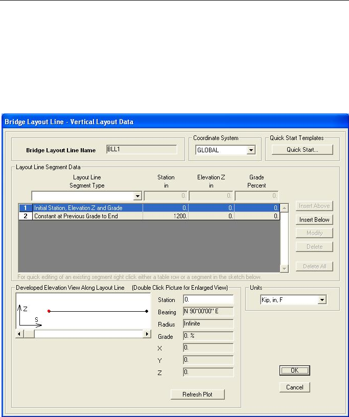
CSiBridge – Defining the Work Flow
Use these commands (see Table 4-1) to display this form:
Layout > Add > Define Vertical Layout Data button
Or
Layout > expand arrow on Layout Line panel > Add New Line
button > Define Vertical Layout Data button
4 - 8 Layout > Layout Lines
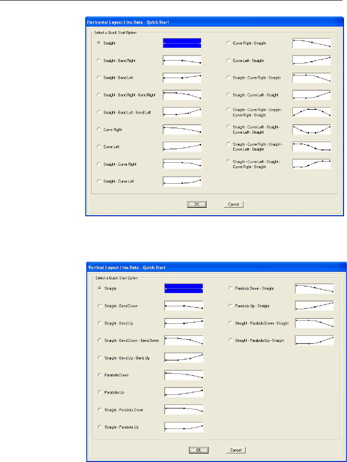
CHAPTER 4 Layout
Use these com-
mands (see Table
4-1) to display
this form:
Layout > Add >
Define Vertical
Layout Data –
Quick Start but-
ton
Or
Layout > expand
arrow on Layout
Line panel > Add
New Line
button > Define
Vertical Layout
Data – Quick
Start button
Use these com-
mands (see Table
4-1) to display this
form:
Layout > Add >
Define Vertical
Layout Data –
Quick Start but-
ton
Or
Layout > expand
arrow on Layout
Line panel > Add
New Line
button > Define
Vertical Layout
Data – Quick
Start button
Layout > Layout Lines 4 - 9
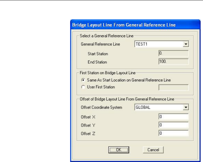
CSiBridge – Defining the Work Flow
Use this commands (see
Table 4-1) to display this
form:
Add a reference line to the
model using the Ad-
vanced > Draw > More >
Draw/Edit General Ref-
erence Line command;
then click the Layout >
expand arrow > Add New
From Gen Ref Line but-
ton.
4.2 Layout > Lanes
Lanes must be defined to analyze a bridge model for live load. They are
used in the definition of moving load type load cases (see Chapter 8) and
in the definition of bridge live type load patterns (see Chapter 6), which
are used in static and dynamic multi-step load cases.
Vehicle live loads are considered to act in traffic lanes transversely
spaced across the bridge roadway. The number of lanes and their trans-
verse spacing can be chosen to satisfy the appropriate design code re-
quirements. Lanes need not be parallel or be of the same length. The
number of lanes across a roadway may vary along the length to accom-
modate merges.
For simple bridges with a single roadway, the lanes will usually be paral-
lel and evenly spaced, and will run the full length of the bridge structure.
4 - 10 Layout > Lanes

CHAPTER 4 Layout
For complex structures, such as interchanges, multiple roadways may be
considered; those roadways can merge and split. Multiple patterns of
lanes on the same roadway may be created to examine the effect of
different lateral placement of vehicles. For design purposes, a single lane
may be defined and loaded. The distribution of live loads to the girders
may be defined using the options available within the superstructure
design request definition (see Chapter 9).
Figure 4-3 shows the commands on the Lanes panel of the Layout tab
Figure 4-3 Layout tab with annotated Lane panel
Clicking the expand arrow in the lower right-hand corner of the Lanes
panel will display the Define Lanes form shown in Figure 4-4.
The Define Lanes form shows the previously defined lanes in the Lanes
display area on the left-hand side of the form. The buttons in the “Click
to” area of the form can be used to add, copy, modify, and delete lane
definitions. The buttons in the “Click to:” area display the same forms or
function in the same manner as the New, Copy, Modify and Delete
commands on the Lanes panel (see Figure 4-3). That is, most of the but-
tons on the Define Lanes form and the commands on the Lanes panel
display the Bridge Lane Data form (see Section 4.2.1); or in the case of
the delete buttons, delete the selected/specified lane definition. In
essence, the commands on the Lanes panel by-pass the definition form
shown in Figure 4-3 and provide a short cut to the data forms used to de-
fine a lane.
Layout > Lanes 4 - 11
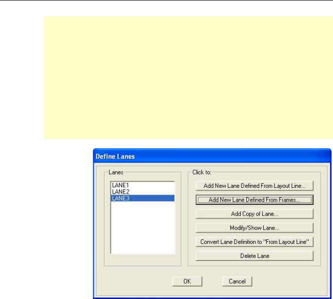
CSiBridge – Defining the Work Flow
IMPORTANT NOTE: The preceding statement has one excep-
tion. The Define Lanes form has two additional buttons, Add New
Lane Defined From Frames and Convert Lane Definition to
“From Layout Line,” that do not have corresponding commands
on the Lanes panel of the Layout tab. When the Add New Lane
Defined From Frames button is clicked, the Lane Data form dis-
plays (see Section 4.2.2). When the Convert Lane Definition to
“From Layout Line” button is clicked the conversion is immedi-
ate and irreversible.
Figure 4-4 Definition form showing
previously defined lanes
Table 4-2 briefly explains the Layout > Lanes commands.
Use this command
to display this
form:
Layout > expand
arrow on Lanes
panel
4 - 12 Layout > Lanes

CHAPTER 4 Layout
Table 4-2 Form Data - Layout > Lanes >
Com-
mand Data Form Parameters
Add
Displays the Define Lane Data form. This form has an option to se-
lect the layout line to be used as the reference in aligning the lane
(see Section 4.1). Edit boxes can be used to specify the station loca-
tion measured from left to right relative to the start of the bridge, a
centerline offset (relative to the layout line), and a lane width.
Note that the centerline offset can be varied by station, thereby off-
setting only a segment of the entire lane.
The entire lane can be moved by clicking the Move Lane button,
which will display the Move Lane form. Use that form to move the
entire lane by changing the offset by a specified amount or by mov-
ing the start of the lane to a specified offset.
The lane can be loaded by the program, or based on user-selected
groups of model objects. Options are available to specify how the
load is discretized along lanes and across them, with additional dis-
cretiza
tion possible along the span and along the lane lengths. The
left and right edges of the lanes can be specified as interior or exte-
rior.
The form shows a Plan View plot of the lane, along with the bearing
based on the layout line, and it shows the radius, grade, and X, Y,
and Z coordi
nates of the mouse cursor when the cursor is moved
along the lane in the plot.
Two lines of data are required to define a single lane. One data line
is needed to define the lane start station location and the second is
needed to define the lane end station location.
Copy
Creates a copy of the lane definition selected in the Current Lane
drop-down list. The definition data can be modified as described for
the preceding Add command.
Modify Displays the lane definition selected in the Current Lane drop-down
list. The definition data can be modified as described for the preced-
ing Add command.
Delete Deletes the lane definition selected in the Current Lane drop-down
list
Layout > Lanes 4 - 13
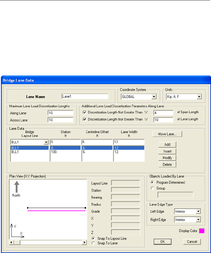
CSiBridge – Defining the Work Flow
4.2.1 Bridge Lane Data Form – Screen Capture
Use these commands (see Table 4-2) to display this form:
Lane > Add
Or
Lane > expand arrow on Lanes panel > Add
New Lane Defined From Layout Line button
4 - 14 Layout > Lanes
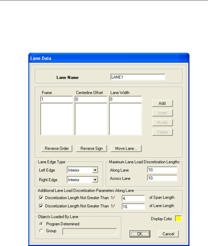
CHAPTER 4 Layout
4.2.2 Lane Data Form – Screen Capture
Use this command (see Table 4-2) to display this form:
Lane > expand arrow on Lanes panel > Add New Lane Defined
From Layout Line button > Add New Lane Define From Frames button
The Lane Data form has many of the same options as the Bridge Lane
Data form – centerline offset, lane width, lane edge type, lane loading
that is program determined or based on grouped model objects, discreti-
zation of loads along and across lanes, and discretization along span and
lane lengths.
Similar to specifying the layout line to be used as the reference for the
lane, the Lane Data form requires that the frame member label be input
Layout > Lanes 4 - 15

CSiBridge – Defining the Work Flow
to identify the frame member to be used to locate the lane. Multiple
frame members may be used to define a single lane in the case where a
particular lane is longer than a single frame member.
Note that the centerline offset applies to the entire length of the frame,
not just a portion of it. Therefore, to move the entire lane, change the
offset.
TIP: Use the Home > View > Set Display Options command to dis-
play the Display Options for Active Window form. Click the Labels
check box in the Frames/Cable/Tendons area of the form to display
frame labels.
4 - 16 Layout > Lanes

CHAPTER 5 Components
The Components tab consists of the commands that allow efficient ac-
cess to the data forms needed to add, copy, or modify definitions for ma-
terial, frame, cable, tendon, and link properties (Properties panel); deck
sections, diaphragms, and parametric variations (Superstructure panel);
bearings, restrainers, foundation springs, abutments, and bents (Sub-
structure panel). A command to specify rebar sizes is available (Proper-
ties panel), and a delete command is available for deleting a selected def-
inition. A method for displaying the definition form that lists all defini-
tions and that has buttons that perform the same functions as the com-
mands on the Components tab also is available. This chapter identifies
those data and definition forms.
If the Quick Bridge template was used to start the bridge model, the pro-
gram will have created default definitions for material and frame section
properties; a deck section; a bearing; an abutment; and a bent. These def-
initions can be viewed using the commands on the Components tab.
If the Bridge Wizard is being used, highlighting the Materials, Frame
Sections, and Links items, the Deck Sections item, the Bearings item, the
Abutments item, and the Bents item in the Summary Table and clicking
the Define/Show Material Properties, Define/Show Frame Sections,
Define/Show Link Properties, Define/Show Deck Sections, De-
fine/Show Bearings, Define/Show Abutments, and Define/Show Bents
Components > Properties 5 - 1
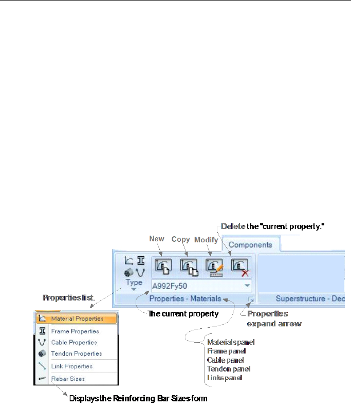
CSiBridge - Defining the Work Flow
buttons will display the definition forms that can then be used to access
the same data forms as those that can be accessed directly using the
Components tab commands.
The commands on the Components tab also can be used if the Blank op-
tion was used to start the model and the Bridge Wizard is not being
used (i.e., the model is being built from scratch or by importing model
data).
5.1 Components > Properties
Figure 5-1 shows the commands on the Properties panel of the Compo-
nents tab.
Figure 5-1 Components tab with annotated Properties panel
As suggested in Figure 5-1, clicking the Type command displays a drop-
down list of property types (material, frame, cable, tendon, link) and re-
bar sizes. The name of the panel changes depending on the property type
selected (i.e., panel names are Properties – Materials; Properties –
Frame; Properties – Cable; Properties – Tendon; Properties – Links).
After a property type has been selected, clicking the expand arrow dis-
plays one of the forms shown in Figure 5-2.
5 - 2 Components > Properties

CHAPTER 5 Components
Figure 5-2 Definition forms showing previously defined properties
These forms list all previously defined property definitions in display
areas on the left-hand side of the forms. Generally, the buttons in the
“Click to” area on the right-hand sides of the forms display the data
forms listed in the second column of Table 5-1.
Components > Properties 5 - 3

CSiBridge - Defining the Work Flow
Referring to Figure 5-1, the New, Copy, and Modify commands on the
Properties – {Type} panel bypass the definition forms listed in column
one of Table 5-1 and display the forms listed in column two, thereby
creating a short cut to the data forms. The forms listed in column three
generally are displayed by checking a check box (e.g., Show Advanced
Material Properties) or clicking a topic-relevant button on the Data
Form.
Table 5-1 Forms List - Components > Type > {Property}
Click:
> Expand arrow
> Buttons on
Definitions Forms
> Check Box or Topic-Relevant
Button on Data Forms
Definition Forms
Data Forms
Parameter Forms
Define Materials *Add New Material ---
Material Property Data
Material Property Options**
Nonlinear Material Data
Time Dependent Properties
Additional Material Damping
Thermal Properties
Frame Properties ***Import Frame Section
Property
Section Property File
Data form
{Section Type} Section
Add Frame Section
Property
Bridge Section
{Section Type} Section
Cable Sections
Cable Section Data
Cable Property/Stiffness
Modification Factors
Tendon Sections
Tendon Section Data
---
Link/Support
Properties Link/Support Property Data
Advanced Link P-Delta
Parameters
{Line Type} Direction Properties
*NOTE: In the Add Material Property form, select the Region, Material
Type, Standard and Grade that are pre-defined in the CSiMaterial-
Library*.xml located in subfolder "Property Libraries" under the CSiBridge
installation folder to define the new material.
**NOTE: The Material Property Options form is the “gateway” to the but-
tons that provide access to Advanced Material Property Data (e.g., Non-
linear Material Data, Time Dependent Properties, Additional Material
Damping, Thermal Properties). The Material Property Options form dis-
plays when the Show Advanced Properties check box on the Define Ma-
terials form is checked, or when the Switch to Advanced Property Display
check box is checked on the Material Property Data form. In both cases,
clicking the Modify/Show Material Properties button displays a version
of the Material Property Data form that includes buttons that provide ac-
5 - 4 Components > Properties

CHAPTER 5 Components
cess to the forms for Advanced Material Property Data. The Material
Property Options form also includes a Material Properties are Tempera-
ture Dependent check box that when checked displays the Temperature
Dependent Material Properties form; use that form to designate tempera-
tures at which specified parameters apply.
***NOTE: The Import Frame Section Property form can be displayed on-
ly by clicking the Components > Type > Frame Properties > Expand
arrow > Import New Property button. Use the Import Frame Section
Property form to access a database of frame sections, including a user
specified database.
TIP: If the Material Property Options form displays when the Compo-
nents > Type > Material Properties > Add or Copy or Modify com-
mand is clicked, but Advanced Material Property Data is not needed for a
material definition, use the Components > Type > Material Properties >
Expand arrow command to display the Define Materials form and un-
check the Show Advanced Properties check box. Then either click the
appropriate add, copy, or modify button on the Define Materials form, or
close that form and click the Components > Type > Material Properties
> Add or Copy or Modify command to display the standard Material
Property Data form.
Context-sensitive help can be accessed by displaying the form and then
depressing the F1 key.
Table 5-2 provides a brief description of data that is input or included in
the data forms identified in column two of Table 5-1.
Table 5-2 Form Data - Components > Properties > {Type} >
Add, Copy, Modify
Type Data Form Parameters
Material
Proper-
ties
Displays the Material Property Data form. Material types may be
steel, concrete, rebar, or tendon. Definitions include weight and mass,
isotropic parameters (modulus of elasticity, Poisson’s Ratio, coeffi-
cient of thermal expansion, and shear modulus) and other parameters
(such as minimum yield stress, specified concrete compressive
strength, and so on). Many pre-defined material properties of com-
monly used materials are included as defaults. New material proper-
ties can be added and
default properties can be edited. Definitions
may include advanced material property data, such as nonlinear ma-
Components > Properties 5 - 5

CSiBridge - Defining the Work Flow
Table 5-2 Form Data - Components > Properties > {Type} >
Add, Copy, Modify
Type Data Form Parameters
terial data, time dependent properties, material damping properties
and thermal properties. Material property definitions are used in frame
section property and deck section property definitions.
Frame
Proper-
ties
Property type may be steel, concrete, or other. Steel sections may be
I/wide flange, channel, tee, angle, double angle, double channel, pipe,
tube, or steel joist. Concrete sections may be rectangular, circular,
pipe, tube, precast I or precast U. Built-up steel section may include
hybrid I, hybrid U and cover plated I. Aluminum sections may include
I and channel sections. Cold formed sections may include C, Z, and
hat sections. “Other” may include general, nonprismatic, and Section
Designer sections, which can be used to define rebar layouts for both
longitudinal reinforcing and transverse reinforcement (see Section
5.1.2). Definitions include materials (see preceding Material Proper-
ties), dimensions, section properties (e.g., torsional constant, moment
of inertia, section modulus, radius of gyration and so on), and stiff-
ness modification factors. Concrete sections may be based on stand-
ard sections (e.g., WSDOT Standard U Girder U54G4).
Frame property definitions are used in cap beams and columns in
bent property definitions, girder sections in some deck section proper-
ty defini
tions, continuous beam sections in some abutment property
definitions, and frame sections in some diaphragm property defini-
tions.
Cable
Proper-
ties
Definition includes material property and specification of the cable
diameter or the cable area. The program calculates the torsional con-
stant, moment of inertia and shear area based on the cable diameter
or area. Stiffness modification factors may also be specified (cross-
sectional [axial] area; mass, weight). Cable property definitions are an
advanced feature available for use if cables are added to the model.
Tendon
Proper-
ties
Tendons can be modeled as loads or as elements. Definition includes
material property and specification of the tendon diameter or area.
The program calculates the torsional constant, moment of inertia and
shear area based on the tendon diameter or area. Tendon property
definitions are used in prestress tendon definitions as part of the
Bridge Object definition (see Chapter 7).
Link
Proper-
ties
Definition includes link/support type (linear, multilinear elastic, multi-
linear plastic, damper, gap, hook, plastic [wren] and rubber isolator);
mass and weight; rotational inertia; factors for line, area, and solid
springs; directional properties; and advanced P-Delta parameters.
Link property definitions can be used in restrainer, bearing, and foun-
dation spring property definitions. Using links in lieu of bearings and
foundation springs gives a wider range of modeling options. Support
bearings at abutments and bents may be defined as isolators using
links. P-Y soil springs may also be represented as links.
5 - 6 Components > Properties
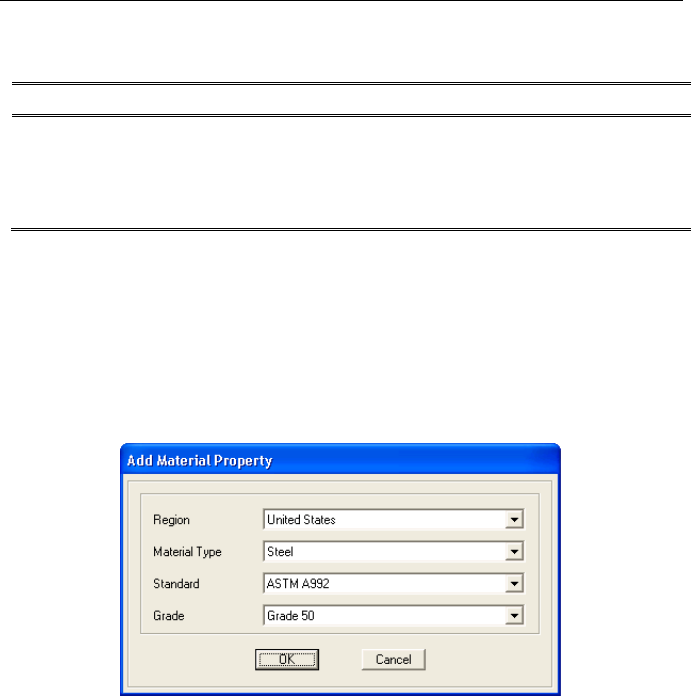
CHAPTER 5 Components
Table 5-2 Form Data - Components > Properties > {Type} >
Add, Copy, Modify
Type Data Form Parameters
Rebar
Sizes
Displays the Reinforcing Bar Sizes form. The form can be used to
add, modify, or delete reinforcing bar. The definition for a rebar in-
cludes the bar ID, the bar area, and the bar diameter. Rebar size def-
initions may be used in specifying the bridge girder deck reinforce-
ment as part of the Bridge Object definition (see Chapter 7).
5.1.1 Material Properties Forms – Screen Captures
This command (see Table 5-2) displays this form:
Components > Type > Material Properties > New, or
Components > Type > Material Properties > Expand arrow >
Click the Add New Material button on the Define Materials form
Components > Properties 5 - 7
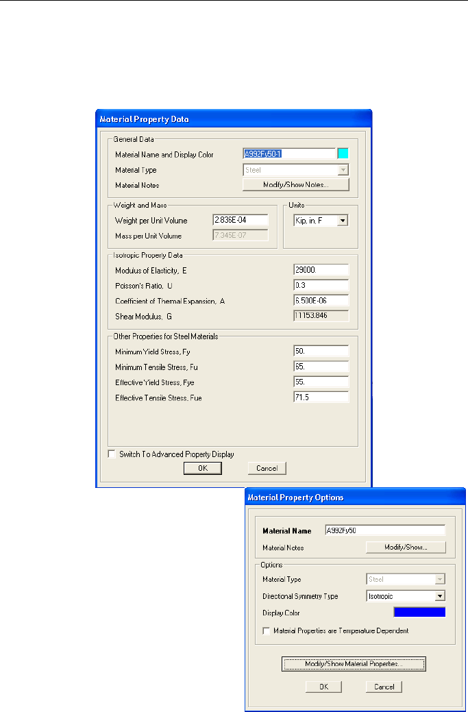
CSiBridge - Defining the Work Flow
This command (see Table 5-2) displays this form:
Components > Type > Material Properties > Copy
or Modify command
This command (see Table 5-2) displays
this form
:
Comp
onents > Type >
Material Properties >
Expand arrow >
Check the Show Ad-
vanced Properties
check box on the De-
fine Materials form > Click
Add New Ma-
terials
button
5 - 8 Components > Properties

CHAPTER 5 Components
These commands (see Table 5-2) display this form:
Components > Type > Material Prop-
erties > Expand arrow > Check the
Show Advanced Properties check box
on the Define Materials form > Click
Modify/Show Materials button; click the
Modify/Show Material Properties but-
ton
OR
Components > Type > Material Prop-
erties > Copy, or Modify command >
Check the Switch to Advanced Property
Display check box on the “standard” Ma-
terial Property Data form; click the Modi-
fy/Show Material Properties button
Components > Properties 5 - 9
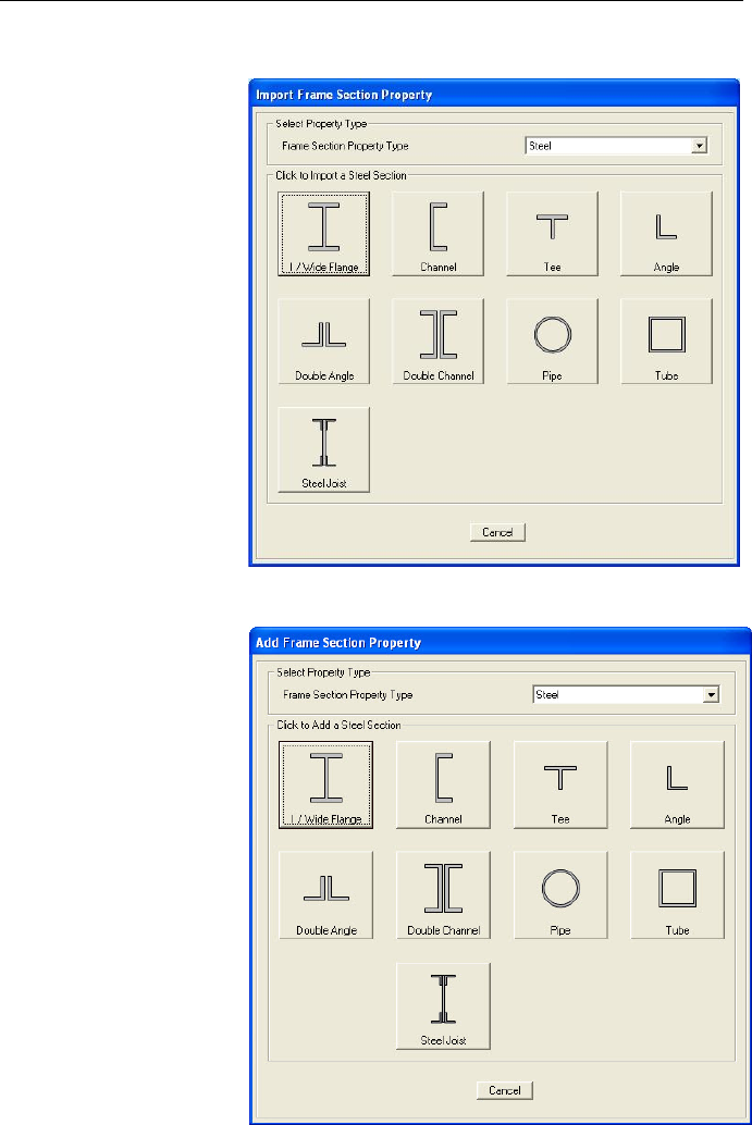
CSiBridge - Defining the Work Flow
5.1.2 Frame Properties Forms – Screen Captures
These commands
(see Table 5-2)
display this form:
Components > Type >
Frame Properties >
Add command
OR
Components > Type >
Frame Properties >
Expand arrow >
Add New Property
button
This command (see
Table 5-2) displays this
form:
Components > Type >
Frame Properties >
Expand arrow >
Import New Property
button
5 - 10 Components > Properties
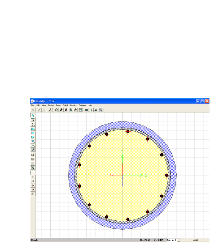
CHAPTER 5 Components
5.1.3 Section Designer – Screen Capture
Section properties may be defined based on their dimensions using the
Section Designer utility.
This command (see Table 5-2) displays this form:
Components > Type > Frame Properties > Add command > On the
Add Frame Section Property form, set the Frame Section Property Type
to Other > Click the Section Designer button.
View of Section Designer Window Displaying an
Example of a Concrete Cross-Section Definition
The Section Designer feature provides a powerful means to define com-
plex cross-sectional shapes and details, including rebar layouts for both
longitudinal reinforcing and transverse reinforcement.
Components > Properties 5 - 11
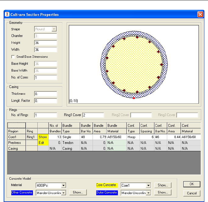
CSiBridge - Defining the Work Flow
View of Section Designer Window Displaying the
Column Rebar Form; Use to Locate Rebar
5 - 12 Components > Properties
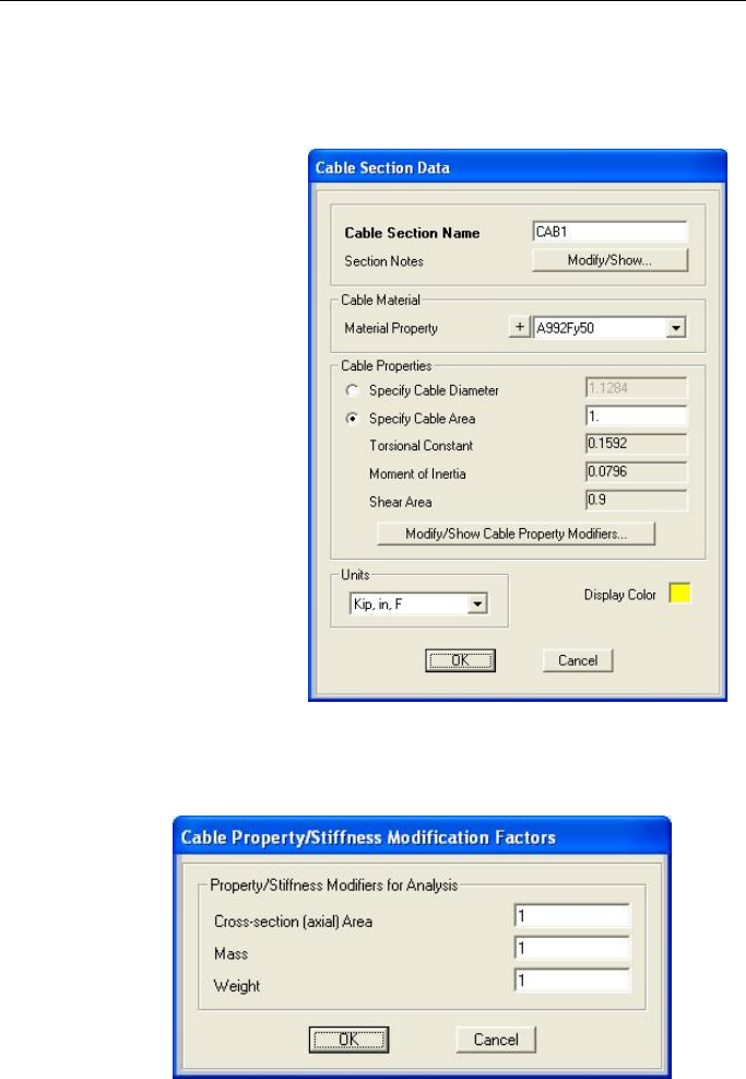
CHAPTER 5 Components
5.1.4 Cable Properties Form – Screen Capture
These commands (see Table 5-2) display this form:
Components >
Type > Cable
Properties >
Add, Copy, Mod-
ify command
OR
Components >
Type > Cable
Properties > Ex-
pand arrow >
Add New Section
button
>Modify/Show Cable Property Modifiers button:
Components > Properties 5 - 13
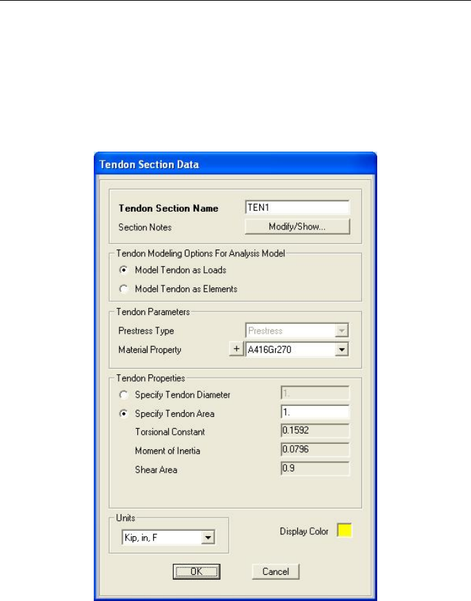
CSiBridge - Defining the Work Flow
5.1.5 Tendon Properties Form - Screen Capture
These commands (see Table 5-2) display this form:
Components > Type >
Tendon Properties >
Add, Copy, Modify com-
mand
OR
Components > Type >
Tendon Properties >
Expand arrow >
Add New Section button
5 - 14 Components > Properties
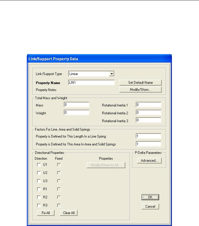
CHAPTER 5 Components
5.1.6 Link/Support Properties Form - Screen Capture
These commands (see Table 5-2) display this form:
Components > Type >
Link Properties > Add
command
OR
Components > Type > Link
Properties > Expand arrow >
Add New Property button
Components > Properties 5 - 15
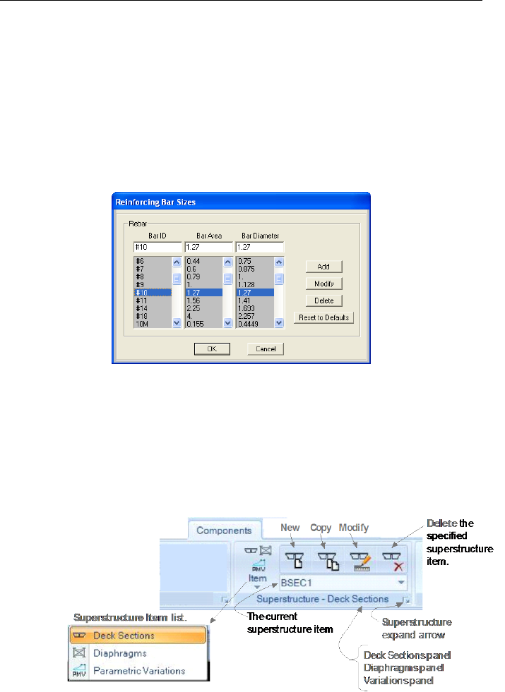
CSiBridge - Defining the Work Flow
5.1.7 Rebar Properties Form - Screen Capture
Although the program includes several default reinforcement bar defini-
tions, the Reinforcing Bar Sizes form can be used to add, modify, and
delete rebar definitions.
Use this command (see Table 5-2) to display that form:
Components > Type > Rebar Sizes command
5.2 Components > Superstructure
The superstructure of a CSiBridge model consists of a deck section and
diaphragms and is supported by a substructure. The deck section dimen-
sions may vary in accordance with a parametric variation definition.
Figure 5-5 shows the Superstructure panel of the Components tab.
Figure 5-5 Superstructure panel on the Components tab
5 - 16 Components > Superstructure
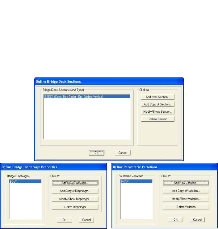
CHAPTER 5 Components
As suggested in Figure 5-5, clicking the Item command displays a drop-
down list of the Superstructure items (i.e., Deck Sections, Diaphragms,
and Parametric Variations). The name of the panel changes depending
on the superstructure item selected (i.e., panels names are Superstructure
– Deck Sections; Superstructure – Diaphragms; Superstructure – Varia-
tions). After an item has been selected, clicking the expand arrow dis-
plays the forms shown in Figure 5-6.
Figure 5-6 Definition forms showing previously defined superstructure items
These forms list all previously defined superstructure item definitions in
display areas on the left-hand side of the forms. The buttons in the
“Click to” area on the right-hand sides of the forms display the data
forms shown in Section 5.2.1, 5.2.2, and 5.2.3.
Referring to Figure 5-5, the New, Copy, and Modify commands on the
Superstructure – {Type} panel bypass the definition forms shown in Fig-
ure 5-6, thereby creating a short cut to the data forms described in Table
5-3.
Components > Superstructure 5 - 17

CSiBridge - Defining the Work Flow
Table 5-3 Form Data - Component > Superstructure > {Item} > Add, Copy,
Modify
Item Data Form Parameters
Deck
Sections Displays the Select Bridge Deck Section Type form, shown in Sec-
tion 5.2.1. Concrete deck sections include box, multi-cell box, Tee
beam, flat slab, precast I-girder, and precast U-girder types.
Steel bridge decks include steel I-girder and steel U-girder types.
Clicking a deck section type displays a Define Bridge Section Data
– {Type} form. As an example, Section 5.2.1 includes the Precast
Concrete I Girder form. In this example, customization of the gen-
eral data for the deck section consists of naming the deck section,
and defining the material properties, number of interior girders,
width and girder layout. Properties for the slab thickness, haunch
thickness, and constant girder sections may be modified. Girder
sections available for selection include all I-girders previously de-
fined (see
Components tab > Type > Frame Section > Expand
arrow > Frame Properties form; if no girder properties have been
defined, continue to click Add New Property > Concrete > Pre-
cast I Girder command to define a section).
Further parameters in the definition may include the deck dimen-
sions, curb locations, and insertion point. Note that the curb loca-
tions are used to determine the extent of vehicle loading across the
deck. The curb locations are used to determine the live load distri-
bution factors (LLDF), and the extent of vehicle loading. Users may
add curb and rail loads using the Loads > Loads - Lines command
(see Chapter 6). The insertion point feature may be needed when a
deck section is not centered on a layout line.
Dia-
phragms Displays the Bridge Diaphragm Property
form. The diaphragm
types may be solid (concrete bridges only), chord and brace (steel
bridges only), single beam (steel bridges only), or steel plate (steel
U-girder bridges only). Section 5.2.2 shows the forms for each dia-
phragm type.
For concrete bridges with a
solid diaphragm, the definition is
based on the width of the concrete diaphragm. The depth of the
concrete is set to match the depth of the concrete deck section.
For steel bridges with a chord and brace diaphragm, the definition
includes frame section properties for the top and bottom chords
and the brace; specification of the brace type (V Brace, Inverted
V Brace, X Brace), and specification of the brace work point loca-
tion. The brace work point is defined in terms of the change in el-
evation from the work point of the chord and brace to the top of
the adjacent girder and the change in elevation from the bottom
work point of the chord and brace to the elevation of the bottom
of the adjacent girder.
For steel bridges with a single
beam diaphragm, the definition
includes beam section property and specification of the change in
5 - 18 Components > Superstructure
CHAPTER 5 Components
Table 5-3 Form Data - Component > Superstructure > {Item} > Add, Copy,
Modify
Item Data Form Parameters
elevation from the top of the beam to the top of the adjacent gird-
er.
For steel U-girder bridges with a steel plate diaphragm, the defini-
tion includes the web and flange dimensions, and the material of
the diaphragm.
Parametric
Variations Displays the Variation Definition form shown in Section 5.2.3. Par-
ametric variat
ions can define variations in the deck section along
the length of the bridge. Almost all parameters used in the paramet-
ric definition of a deck section can be specified to vary. More than
one parameter can vary at the same time, if necessary. Each vary-
ing pa
rameter can have its own unique variation. The variations
may be linear, parabolic, or circular.
Quick Start button on the Variation Definition form can be used to
access the Parametric Variations - Quick Start form shown in Sec-
tion 5.2.3. Use the form to specify a parametric variation based on
template alignments. After a selection has been made and the OK
button has been clicked on the Parametric Variations - Quick Start
form, the selected variation alignment will trans
fer automatically
from the Quick Start form to the Variation Definition form, where the
variation can be further refined.
Components > Superstructure 5 - 19
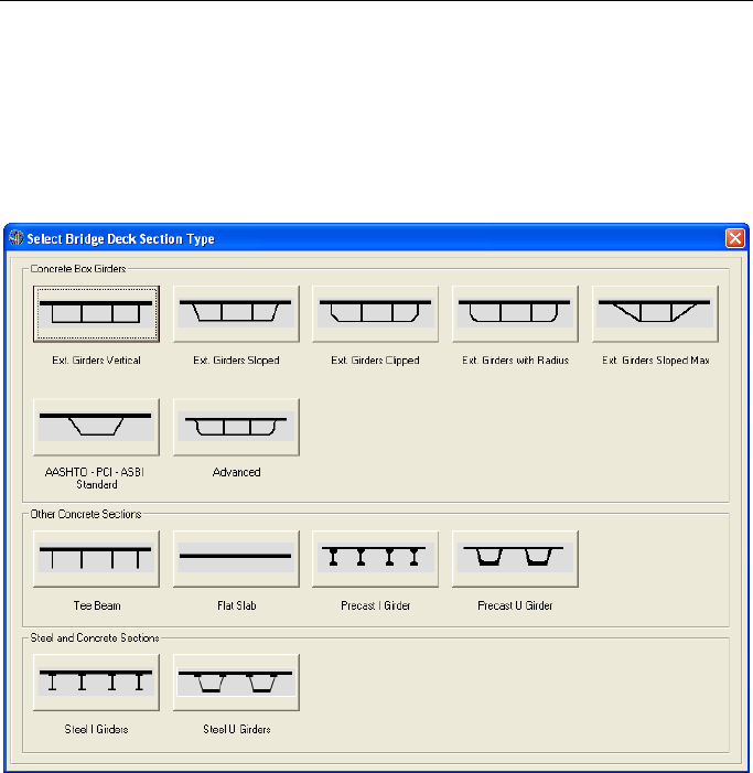
CSiBridge - Defining the Work Flow
5.2.1 Bridge Deck Section Form - Screen Captures
These commands (see Table 5-3) displays this form:
Components > Superstruc-
ture Item > Deck Sections >
Add command
OR
Components > Superstructure
Item > Deck Sections Expand ar-
row > Add New Section button
5 - 20 Components > Superstructure
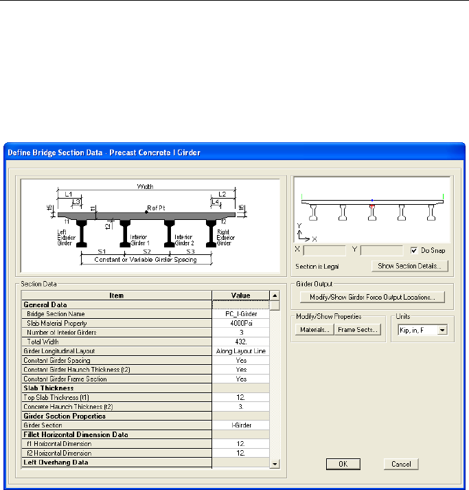
CHAPTER 5 Components
These commands (see Table 5-3) display this form:
Components > Superstructure
Item > Deck Sections > Select
deck section name from Current
Superstructure Item drop-down
list > Copy or Modify command
OR
Components > Superstructure Item
> Deck Sections > Expand arrow >
Add New Section button > {Deck
Section Template} button
Components > Superstructure 5 - 21
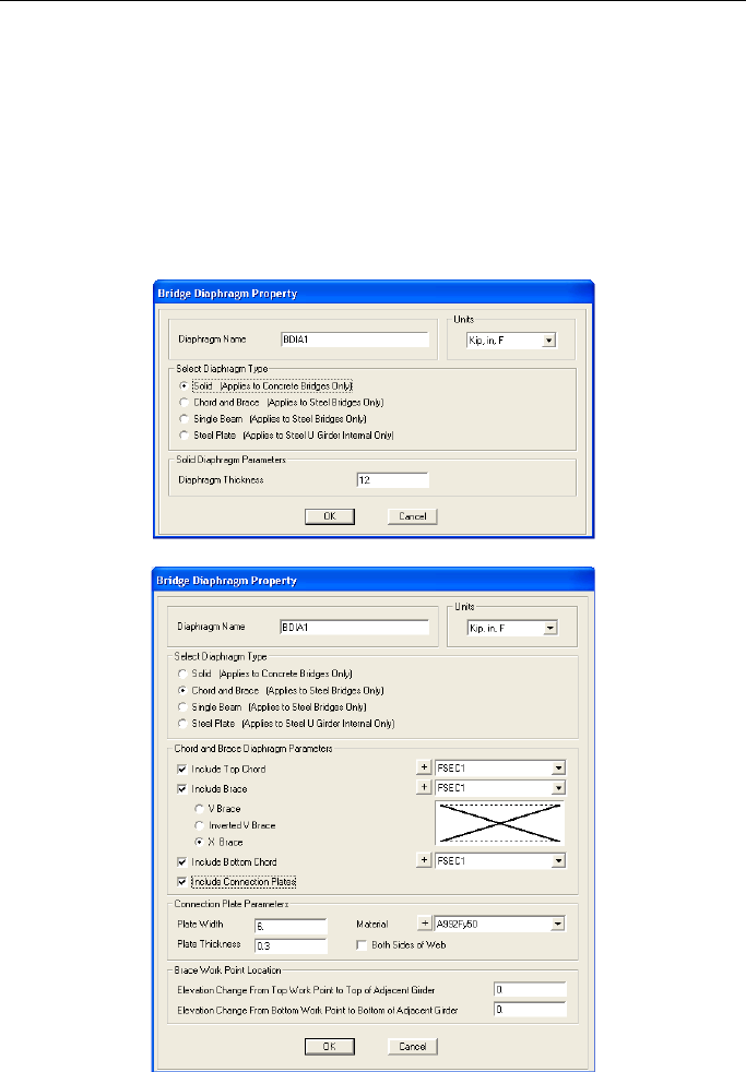
CSiBridge - Defining the Work Flow
5.2.2 Bridge Diaphragm Form - Screen Captures
These commands (see Table 5-3) display this form:
Components > {Superstruc-
ture} Item > Diaphragm > Add
command
OR
Components > {Superstructure} Item >
Superstructure - Diaphragm Expand
arrow > Add New Diaphragm button
5 - 22 Components > Superstructure
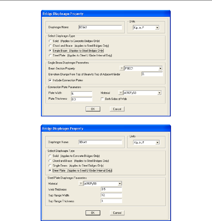
CHAPTER 5 Components
Components > Superstructure 5 - 23
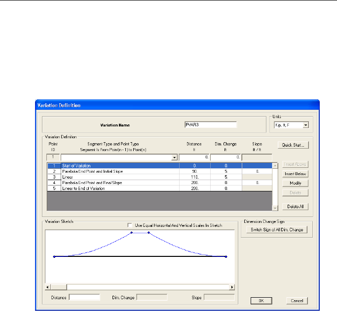
CSiBridge - Defining the Work Flow
5.2.3 Parametric Variation Forms - Screen Captures
These commands (see Table 5-3) display these forms:
Components > {Superstruc-
ture} Item > Parametric Varia-
tions > Add command
OR
Components > {Superstructure} Item >
Superstructure - Variations Expand
arrow > Add New Variation button
5 - 24 Components > Superstructure
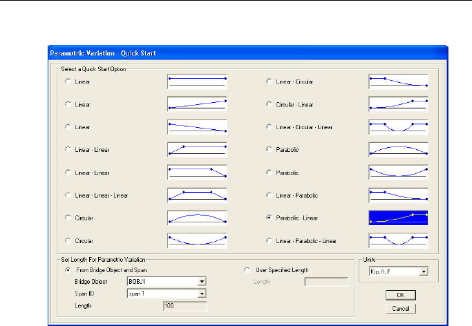
CHAPTER 5 Components
> Click Quick Start button
5.3 Component > Substructure
The substructure definitions for a CSiBridge model may include bear-
ings, restrainers, foundation springs, abutments, and bents. Each of these
components, if used in a bridge model, will become part of the total
bridge assembly based on their locations and definitions in the Bridge
Object (see Chapter 7).
Figure 5-12 shows the Substructure panel of the Components tab.
Component > Substructure 5 - 25
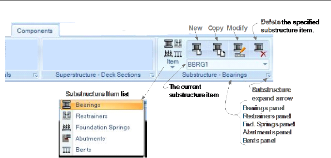
CSiBridge - Defining the Work Flow
Figure 5-12 Substructure panel on the Components tab
As suggested in Figure 5-12, clicking the Item command displays a
drop-down list of the Substructure items (i.e., Bearings, Restrainers,
Foundation Springs, Abutments, and Bents). The name of the panel
changes depending on the substructure item selected (i.e., panels names
are Substructure – Bearings; Substructure – Restrainers; Superstructure
– Fnd. Springs; Substructure – Abutments; Substructure -- Bents). After
an item has been selected, clicking the expand arrow displays the defini-
tion forms shown in Figure 5-13.
Those forms list all previously defined substructure item definitions in
display areas on the left-hand side of the forms. The buttons in the
“Click to” area on the right-hand sides of the forms display the data
forms shown in Section 5.3.1 through 5.3.5. Referring to Figure 5-12,
the New, Copy, and Modify commands on the Superstructure – {Type}
panel bypass the definition forms shown in Figure 5-13, thereby creating
a short cut to the data forms, which are identified in Table 5-4.
5 - 26 Component > Substructure
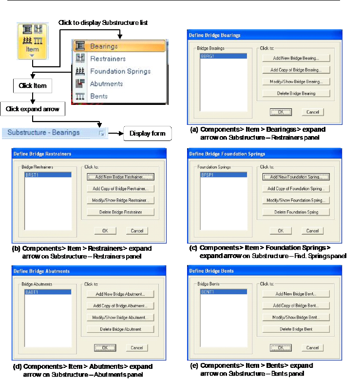
CHAPTER 5 Components
Figure 5-13 Definition forms showing previously defined substructure items
Component > Substructure 5 - 27

CSiBridge - Defining the Work Flow
Table 5-4 Form Data - Component > Substructure > {Item} >
Add, Copy, Modify
Item Data Form Parameters
Bearings Displays the Bearing Data form shown in Section 5.3.1. Bearing
properties are used in ab
utment, bent and hinge assignments to
the bridge object. At abutments, bearings are used in the connec-
tion between the girders and the substructure. At bents, bearings
are used in the connection between the girders and the bent cap
beam. At hinges, bearings are used in the connection between the
girders on the two sides of the hinge. A bearing property can be
specified as a Link/Support property or it can be user defined. The
user defined bear
ing is recommended. The user defined bearing
allows each of the six degrees of freedom to be specified as fixed,
free or partially restrained with a specified user defined spring
con
stant. The user may select the release type as Free, Fixed or
Partial Fixity for each of the six degrees of freedom.
Restrainers Displays the Bridge Restrainer data form shown in Section 5.3.2.
Re
strainer cables are used as tension ties across superstructure
discontinuities. Restrainers may be assigned at abutments, hing-
es, and at bents where the superstructure is discontinuous over
the abu
tment or bent. When specified, the program assumes that
a restrainer cable exists at each girder location. A restrainer prop-
erty can be specified as a Link/Support property or it can be user
defined. The user defined restrainer is recommended. The user
defined restrainer is specified by a length, area, and modulus of
elasticity.
Foundation
Springs Displays the Foundation Spring data form shown in Section 5.3.3.
Foundation spring properties specify data for the connection of the
substructure to the ground. Foundation spring properties are used
in abutment and bent property definitions. At bents, foundation
springs may be used at the base of each column. In that case, the
foundation springs are used as point springs. At abutments, foun-
dation springs are used as point springs for a foundation spring-
type substructure, and they are used as spring properties per unit
length for a continuous beam-type substructure.
A foundation spring property can be specified as a Link/Support
property or it can be user defined. The user defined spring is rec-
ommended. The user defined foundation spring allows each of the
six degrees of freedom to be specified as fixed, free or partially
restrained with a specified spring constant. For cases where the
spring property is used for a continuous beam support, a factor is
specified indicating the length over which the specified properties
apply.
5 - 28 Component > Substructure

CHAPTER 5 Components
Table 5-4 Form Data - Component > Substructure > {Item} >
Add, Copy, Modify
Item Data Form Parameters
Abutments Displays the Bridge Abutment data form shown in Section 5.3.4.
Abut
ment (end bent) properties specify the support conditions at
the ends of the bridge. Abutment properties are used in abutment
assignments to the bridge object. The abutment property allows
specification of the connection between the abutment and the
girders as either integral or connected to the bottom of the girders
only. The abutment property also allows the abutment substruc-
ture to be specified as a series of point springs (one for each gird-
er) or a continuously supported beam.
Bents Displays the Bridge Bent Data form shown in Section 5.3.5. Bent
properties specify the geometry and section properties of the bent
cap and the bent columns. They also specify the base support
condition of the bent columns. Bent properties may be used in
abutment assignments to the bridge object. The bent property
allows specification of the connec
tion between the abutment and
the girders as either integral or con
nected to the bottom of the
girders only. The bent property also allows specification of a single
bearing line (continuous superstructure) or a double bearing line
(discontinuous superstructure). The bridge superstructure will be
updated as continuous or discontinuous based on the Bent Type
option.
The Modify/Show Column Data
button opens the Bridge Bent
Column data form shown in Figure 5-19 that is used to define the
column locations, heights, seismic hinge data, and base support
condition.
Component > Substructure 5 - 29

CSiBridge - Defining the Work Flow
5.3.1 Bridge Bearing Data Form – Screen Capture
These commands (see Table 5-4) display this form:
Components > {Substructure}
Item > Bearings > Add com-
mand
OR
Components > {Substructure} Item >
Substructure - Bearings Expand arrow
> Add New Bridge Bearing button
5 - 30 Component > Substructure
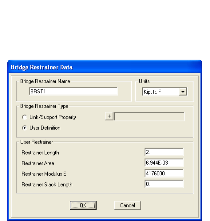
CHAPTER 5 Components
5.3.2 Bridge Restrainer Data Form – Screen Capture
These commands (see Table 5-4) display this form:
Components > {Substructure}
Item > Restrainers > Add
command
OR
Components > {Substructure} Item >
Substructure - Restrainers Expand ar-
row > Add New Bridge Restrainer button
Component > Substructure 5 - 31
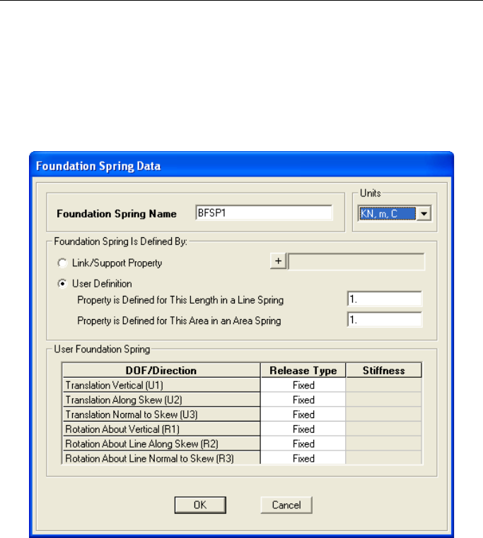
CSiBridge - Defining the Work Flow
5.3.3 Foundation Spring Data Form – Screen Capture
These commands (see Table 5-4) display this form:
Components > {Substructure}
Item > Foundation Springs >
Add command
OR
Components > {Substructure} Item >
Substructure – Fnd. Springs Expand
arrow > Add New Foundation Spring
button
5 - 32 Component > Substructure
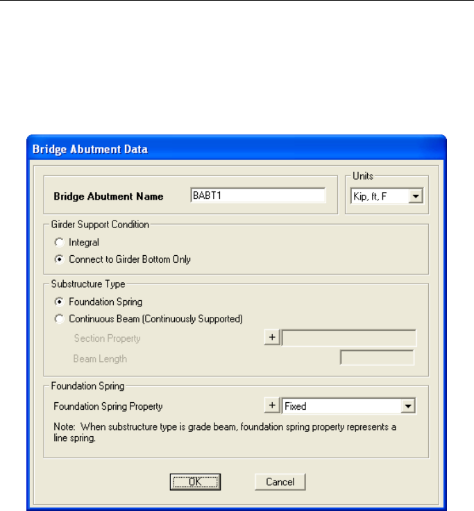
CHAPTER 5 Components
5.3.4 Bridge Abutment Data Form – Screen Capture
These commands (see Table 5-4) display this form:
Components > {Substructure}
Item > Abutments > Add
command
OR
Components > {Substructure} Item >
Substructure – Abutments Expand ar-
row > Add New Bridge Abutment button
Component > Substructure 5 - 33
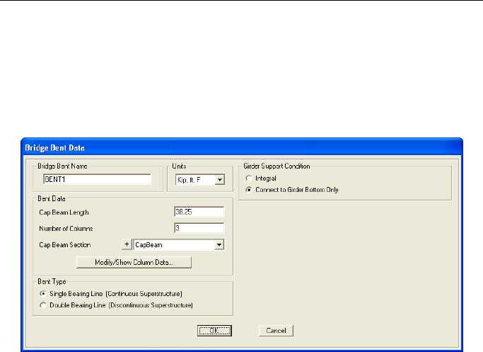
CSiBridge - Defining the Work Flow
5.3.5 Bridge Bent Forms – Screen Captures
These commands (see Table 5-4) display this form:
Components > {Substructure}
Item > Bents > Add
command
OR
Components > {Substructure} Item >
Substructure – Bents Expand arrow >
Add New Bridge Bent button
> Click Modify/Show Column Data button
5 - 34 Component > Substructure
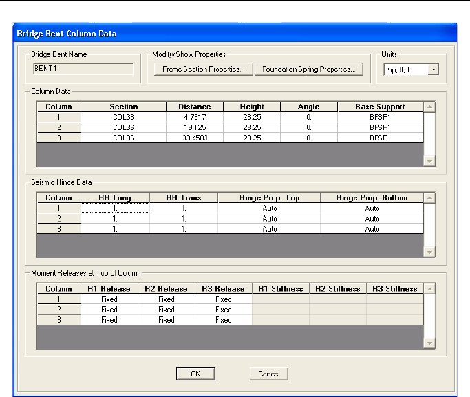
CHAPTER 5 Components
Component > Substructure 5 - 35

CHAPTER 6 Loads
The Loads tab consists of the commands that allow efficient access to
the data forms needed to add, copy, or modify definitions for vehicles
and vehicle classes; load patterns; and response spectrum or time history
functions; and point, line or area loads. A delete command is available
for deleting a selected definition. A method for displaying the definition
form that lists all definitions and that has buttons that perform the same
functions as the commands on the Loads tab also is available. This chap-
ter identifies those data and definition forms.
If the Quick Bridge template was used to start the bridge model, the pro-
gram will have created default definitions for vehicles, vehicle classes,
load patterns and response spectrum and time history functions. These
definitions can be viewed using the commands on the Loads tab.
If the Bridge Wizard is being used, highlighting the Vehicles, Vehicle
Classes, Response Spectrum Functions, Time History Functions, and
Load Pattern Definitions items in the Summary Table and clicking the
Define/Show Vehicles, Define/Show Vehicle Classes, Define/Show
Resp. Spec. Funcs., Define/Show Time History Funcs., and De-
fine/Show Load Patterns buttons will display the definition forms that
can then be used to access the same data forms as those that can be ac-
cessed directly using the Loads tab commands.
Loads > Vehicles 6 - 1
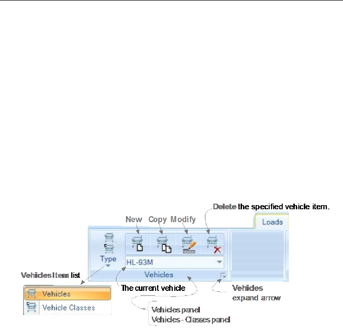
CSiBridge – Defining the Work Flow
The commands on the Loads tab also can be used if the Blank option
was used to start the model and the Bridge Wizard is not being used (i.e.,
the model is being built from scratch or by importing model data).
6.1 Loads > Vehicles
Vehicles must be defined to analyze a bridge model for vehicle live
loads. In CSiBridge, vehicle loads are applied to the structure through
lanes (for lane definitions, see Chapter 3). Each vehicle definition con-
sists of one or more concentrated or uniform loads.
Figure 6-1 shows the commands on the Vehicles panel of the Loads tab.
Figure 6-1 Loads tab with annotated Vehicle panel
As suggested in Figure 6-1, clicking the Vehicles Type command dis-
plays a drop-down list that can be used to select Vehicles or Vehicles
Classes. The name of the panel changes from Vehicles to Vehicles –
Class depending on the selection made. After Vehicle or Vehicle Classes
has been selected, clicking the expand arrow displays one of the forms
shown in Figure 6-2.
6 - 2 Loads > Vehicles

CHAPTER 6 Loads
Figure 6-2 Definition forms showing previously defined
vehicles and vehicle classes
These forms list all previously defined vehicles and vehicles classes in
display areas on the left-hand side of the forms. Generally, clicking the
buttons in the “Click to” area on the right-hand sides of the forms dis-
play the data forms described in Table 6-1 and shown in Sections 6.1.2
and 6.1.3. Referring to Figure 6-1, the New, Copy, and Modify com-
mands on the Vehicles panel or the Vehicles Classes panel bypass the
definition forms shown in Figure 6-2, and display the forms shown in
Sections 6.1.2 and 6.1.3, thereby creating a shortcut to the data forms.
Table 6-1 Form Data - Loads > Vehicles > {Type} > Add, Copy, Modify
Type
Data Form Parameters
Vehicles Displays the Vehicle Data form or the General Vehicle Data form (see
Section 6.1.1). Numerous standard vehicle definitions are built into the
program. The general vehicle form can be used to create customized
vehicle definitions.
Standard vehicle data – Several vehicles types to represent vehicle
live loads specified in various design codes are available for selection
using the drop-down lists on the form. The variables available within
the various drop-down lists are interdependent. F
or example, when
the Region is set to Europe, the Standard is automatically set to a Eu-
ropean code
and the selection of available Vehicle Types reflects that
code. The associated Scale Factor, Dynamic Allowance, and Class
edit boxes become enabled when an applicable Vehicle Type has
been selected. Whenever a Vehicle definition is created, CSiBridge
automatically creates a Vehicle Class of the same name, containing
only that single vehicle definition with a scale factor of 1.0.
Loads > Vehicles 6 - 3

CSiBridge – Defining the Work Flow
Table 6-1 Form Data - Loads > Vehicles > {Type} > Add, Copy, Modify
Type Data Form Parameters
o The integer scale factor specifies the nominal weight of the vehicle
in a specific set of units. For example, for H & HS vehicles the units
are tons; for UIC vehicles the units are kN/m; and so on.
o A dynamic load allowance is the additive percentage by which the
concentrated truck or tandem axle loads will be increased. The uni-
form lane load is not affected. Thus, if the dynamic allowance
equals 33, all concentrated axle loads for the vehicle will be multi-
plied by the factor 1.33.
General vehicle data – The general vehicle may represent an actual
vehicle or a notional vehicle used by a design code. The general vehi-
cle consists of n axles with specified distances between them. Con-
centrated loads may exist at the axles. Uniform loads may exist be-
tween pairs of axles, in front of the first axle, and behind the last axle.
The distance between any one pair of axles may vary over a specified
range; the other distances are fixed. The leading and trailing uniform
loads are of infinite extent. Addi
tional “floating” concentrated loads
may be specified that are independent of the position of the axles.
Vehicles
Classes Displays the Vehicle Class Data form (see Section 6.1.2). A vehicle
class is simply a group of one or more vehicles that is used in a mov-
ing load analysis (one vehicle at a time). Vehicle classes may be de-
fined to include any number of individual vehicles to allow considera-
tion of the max
imum and minimum response of the bridge to the most
extreme of several type of vehicles rather than the effect of the individ-
ual vehicles. However, w
henever a Vehicle definition is created,
CSiBridge automatically creates a Vehicle Class of the same name,
containing only that single vehicle definition with a scale factor of 1.0.
The automatically created Vehicle Class definition cannot be modified
or deleted except by modifying or deleting the vehicle. The maximum
and minimum force and displacement response quantities for a vehicle
class will be the maximum and minimum values obtained for any indi-
vidual
vehicle in that class. For influence based analysis, all vehicle
loads are applied to the traffic lanes using vehicle classes. To apply an
individual vehicle load, define a vehicle class that contains only a sin-
gle vehicle. For step-by-step analysis, vehicle loads are applied directly
without the use of classes since no enveloping is performed.
6.1.1 Vehicle Data Forms – Screen Captures
Use these commands (see Table 6-1) to display the following form and de-
fine a standard vehicle:
6 - 4 Loads > Vehicles
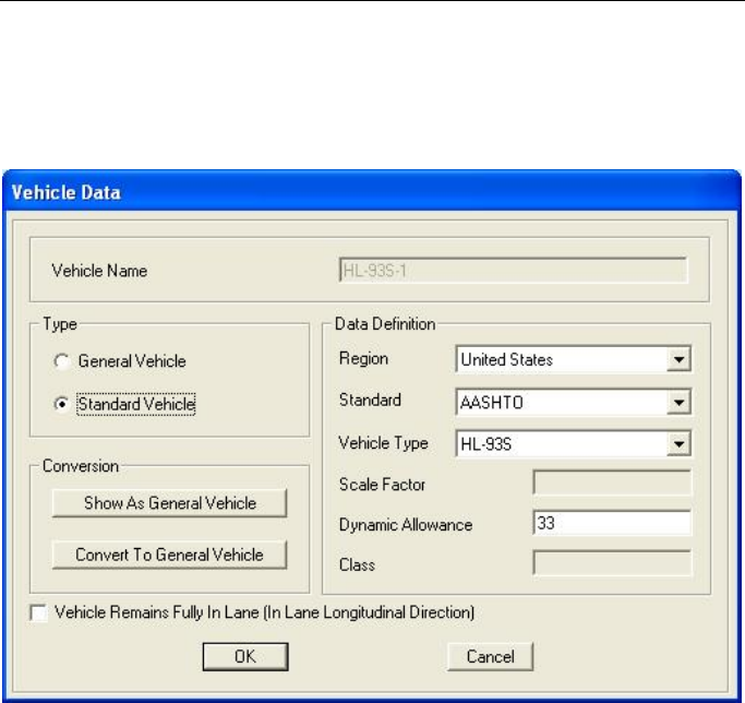
CHAPTER 6 Loads
Loads > Type > Vehicles > Expand arrow > Add Vehicle command or Loads >
Type > Vehicles > Add command.
Alternatively, click Loads > Type > Vehicles > select a Standard Vehicle definition
from the Current Vehicle drop-down list > Copy, Modify
Use these commands (see Table 6-1) to display this form and
define a general vehicle.
Loads > Type > Vehicles > Expand arrow > click the Add Vehicle
button > select the General Vehicle option
Or
Loads > Type > Vehicles > Expand arrow > click the Add Vehi-
cle button > click the Convert to General Vehicle button > choose
Yes*
Or
Loads > Type > Vehicles > select a General Vehicle definition
from the Current Vehicle drop-down list > Copy, Modify
*After a Standard Vehicle definition has been converted to a General
Vehicle definition, the conversion cannot be reversed.
Loads > Vehicles 6 - 5
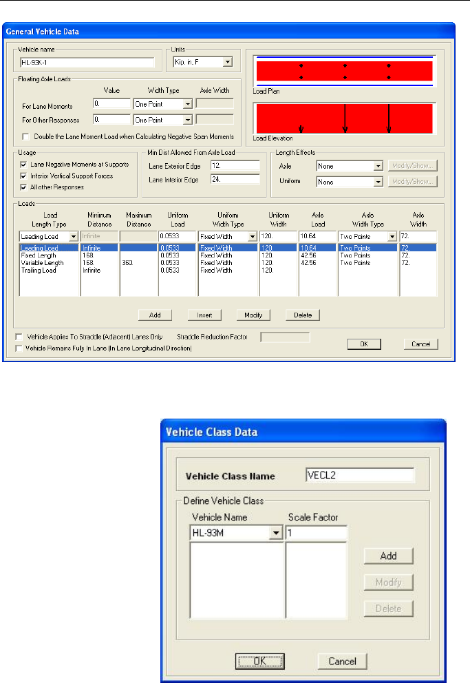
CSiBridge – Defining the Work Flow
6.1.2 Vehicle Classes Data Forms – Screen Capture
These commands
(see Table 6-1) dis-
play this form.
Loads > Type > Ve-
hicle Classes > Ex-
pand arrow > Add
New Class button
Or
Loads > Type >
Vehicle Classes >
Add, Copy, Modify
6 - 6 Loads > Vehicles

CHAPTER 6 Loads
6.2 Loads > Load Patterns
Clicking the Loads > Load Patterns command immediately displays
the form for defining a load pattern. A load pattern has a name, load type
and a specified spatial distribution of forces, displacements, tempera-
tures, and other effects that act upon a structure. A load pattern by itself
does not cause any response in the structure. Load patterns must be ap-
plied in load cases to produce results (see Chapter 9).
Figure 6-3 shows the Loads > Load Patterns command and the result-
ing forms that are used to define the load pattern as well as generate a
multi step bridge live load pattern. In turn, the multi step bridge live load
pattern is used in a multi-step static or multi-step dynamic (direct inte-
gration time history) load case to evaluate special vehicle load responses
(see Chapter 8 Analysis). Table 6-2 briefly describes the data used to de-
fine a load pattern in CSiBridge.
Table 6-2 Form Data - Loads > Load Patterns
Command Data Form Parameters
Load
Patterns Displays the Define Load P
atterns form. Each load pattern must
have a unique name. The Type drop-
down list provides access to
the various load types defined in the AASHTO LRFD code for use
as part of a load pattern definition. The load type is used to deter-
mine the Auto Load Combinations (see Chapter 9).
The Vehicle Live load pattern is among the more significant load
types for a bridge model in CSiBridge. In a vehicle Live load pat-
tern, one or more vehicles is selected and assigned to a specific
lane along with a starting time, direction, and speed. When used in
a multi-step static or multi-step dy
namic (direct integration time
history) load case, this type of load pattern is useful in evaluating
special vehicle load responses. The direct integration time history
analysis will produce response spectrum output data for the user
specified imposed vehicle live loads.
The Self Weight Multiplier is a scale factor that multiplies the weight
of the structure and applies it as a force in the gravity direction
(negative global Z direction). The self-weight of the structure is de-
termined by multiplying the weight per unit volume of each object
that has structural properties times the vol
ume of the object. The
weight per unit volume is specified in the material properties (see
Chapter 5)
Loads > Load Patterns 6 - 7
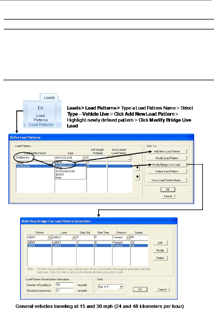
CSiBridge – Defining the Work Flow
Table 6-2 Form Data - Loads > Load Patterns
Command Data Form Parameters
The Auto Lateral Load Pattern is applicable to Quake, Wave, and
Wind load types. With this option, the user can specify that code-
compliant loads be created automatically for the load pattern. Alter-
natively, when a quake, wave, or wind load is being specified, the
user can select “None” here and then apply loads manually by as-
signing them using applicable Advanced > Assign Loads com-
mands (see Chapter 10).
Figure 6-3 Load Patterns panel on the Loads tab, and screen captures of the
forms used to define a load pattern that includes a vehicle live load
6 - 8 Loads > Load Patterns
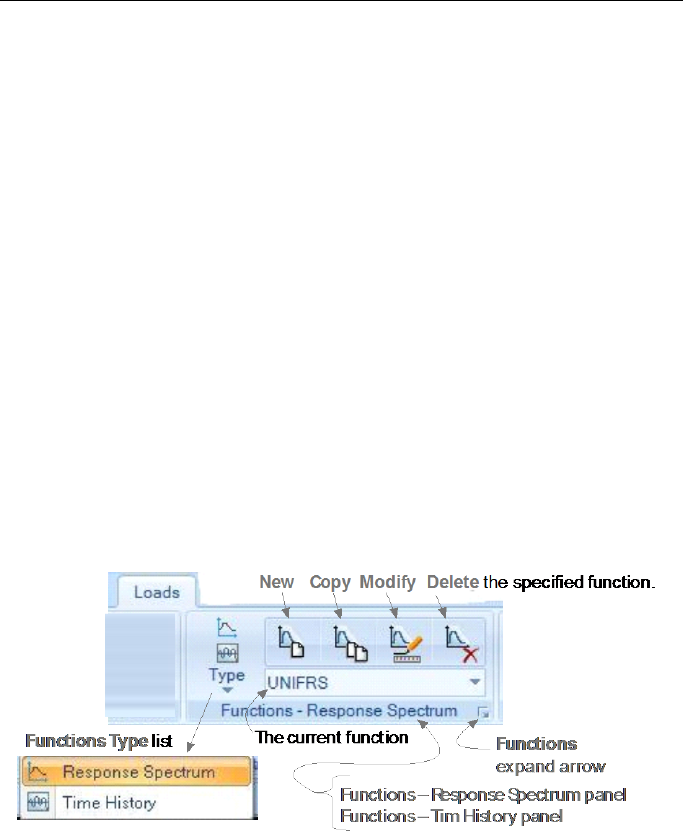
CHAPTER 6 Loads
With the forms displayed, depress the F1 key for context sensitive Help.
6.3 Loads > Functions
In addition to the dead, live, and moving load cases (see previous sec-
tion), CSiBridge provides for bridge structures to be analyzed using re-
sponse spectrum and time history load cases (see Chapter 8). To define a
response spectrum or time history load case, the user must first define a
response spectrum or time history function that will be used as part of a
load case definition.
Figure 6-4 shows the commands on the Functions panel of the Loads
tab. As suggested in the figure, clicking the Functions Type command
displays a drop-down list that can be used to select a Response Spectrum
or Time History function. The name of the panel changes from Function
- Response Spectrum to Function - Time History depending on the selec-
tion made. After Response Spectrum or Time History has been selected,
clicking the expand arrow displays the forms shown in Figure 6-5.
Figure 6-4 Loads tab with annotated Functions panel
Loads > Functions 6 - 9
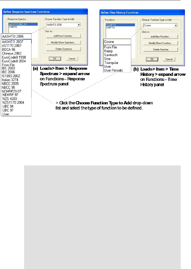
CSiBridge – Defining the Work Flow
Figure 6-5 Definition forms that show all previously defined functions and
that have drop-down lists for choosing the type of
response spectrum or time history function to be defined
The forms in Figure 6-5a and 6-5b list all previously defined functions in
display areas on the left-hand side of the forms.
Note: The type of function selected from the Choose Function
Type to Add drop-down list on the Define Response Spectrum
Functions form or the Define Time History Functions form deter-
mines which of the many data/definition forms will be displayed
when the Add New Function or Modify/Show Spectrum button
is clicked. Similarly, the Function selected in the Current Function
drop-down list on the Functions – {Type} panel (see Figure 6-4)
determines which form will be displayed when the Copy or Modi-
fy commands on that panel is clicked. When the Add command
on the panel is selected, a Response Spectrum or Time History
form displays with a single drop-down list for selecting the type of
response spectrum function/time history function to be defined.
The data form then displays, with parameters that apply to the
type of function being defined.
6 - 10 Loads > Functions

CHAPTER 6 Loads
Table 6-3 briefly describes the various types of functions. Sections 6.3.1
and 6.3.2 provide screen captures of an AASHTO 2007 code-compliant
response spectrum function definition and a “Function from File” time
history function definition as examples of the data forms used.
After a response spectrum or time history function has been defined, it
may be used in a load case definition, which is created using the Analy-
sis > Load Cases > Type-Response Spectrum or Type-Time History
command (See Chapter 8).
Table 6-3 Form Data - Loads > Functions > {Type} > Copy, Modify
Type
Data Form Parameters
Response
Spectrum Displays a Response Spectrum {Type} Function Definition form. A
response-spectrum function is a list of period versus spectral-
acceleration values. In CSiBridge
, the acceleration values in the
function are assumed to be normalized; that is, the functions them-
selves are not assumed to have units. Instead, the units are associ-
ated with a scale factor that multiplies the function and that is speci-
fied when the response-spectrum load case is defined. By default,
the program pre-defines a unit constant response-spectrum function.
This function may be modified or deleted.
A response-
spectrum function may be defined for any period range,
T0 to Tn. For periods less than the first given period, T0, the func-
tion value is assumed to be constant at the function value specified
for T0. For all periods greater than the last given period, Tn, the
function value is assumed to be constant at the function value speci-
fied for Tn. Numerous options exist for defining the response spec-
trum function. Among the more relevant to bridge design are AASH-
TO 2006 and AASHTO 2007:
AASHTO 2006 –
Specify values for the function damping ratio
acceleration coefficient and select the soil profile type. Default
values for period and acceleration are provided; alternatively, click
the Convert To User Defined button to display a form that allows
entry of the Period and Acceleration values.
AASHTO 2007 – Based on the procedures described in AASHTO
Guide Specifications for LRFD Seismic Bridge Design, Section
3.4.1, the Ss, S1 and PGA values may be taken from USGS and
AASHTO maps contained within CSiBridge; in which case, define
the bridge location using latitude and longitude or by specifying a
zip code. Alternatively, enter the Ss, S1 and PGA values directly.
Loads > Functions 6 - 11

CSiBridge – Defining the Work Flow
Table 6-3 Form Data - Loads > Functions > {Type} > Copy, Modify
Type Data Form Parameters
Other function types include:
From File -
Any response spectrum text file may be read into a
CSiBridge model file. Requires a user-
specified file name and
damping ratio. Files may be in a frequency or period verses values
format.
AS1170 2007 – Constructed as specified in
AS 1170.4:2007
clause 7.2(a).
BOCA96 – Based on 1996 BOCA Section 1610.5.5. The response
spectrum is constructed by plotting the model seismic design coef-
ficient, Csm, versus the modal period of vibration, Tm. For a given
period, Tm, the value of Csm is determined using Equation 11-3.
Chinese 2002 – Specified using the maximum value for the seis-
mic lateral influence factor, AlphaMax; the factor of seismic lateral
influence, alpha1
, obtained from the 2002 Chinese Design Code
response spectrum for the fundamental period; the seismic intensi-
ty, SI; the damping ratio, zeta (to adjust the shape of the response
spectrum curve); the characteristic ground period, Tg, in seconds;
the fundamen
tal period, T1, multiplied by the period time discount
factor, PTDF, before determining the value of alpha1 from the
2002 Chinese Design Code response spectrum curve.
Eurocode8 1998 – Constructed
as described in 1998 Eurocode
ENV 1998-1-
1:1994 Section 4.2.2. The ordinates of the response
spectrum are calculated using Equations 4.1 through 4.4, also in
Section 4.2.2. The values of bo, TB, TC, TC k1, k2, and S are tak-
en from Table 4.1 in 1998 Eurocode ENV 19981-1:1994 Section
4.2.2. Note that the value of these parameters depends on the
specified subsoil class.
Eurocode8 2004 – Constructed as described in EN 1998-1-1:2004
Section 3.2.25. The ordinates of the response spectrum are calcu-
lated using Equations 3.13 through 3.16 in EN 1998-1-1:2004 Sec-
tion 3.2.2.5. The value of TB, TC, TC, and S are taken from Table
3.2 or 3.3 in 1998 Eurocode EN 1998-1-
1:2004 Section 3.2.2.5.
Note that the value of these parameters depends on the specified
ground type and spectrum type.
IBC 2006 –
Based on procedures described in IBC2003 Section
1613.2.1.4 (ASCE 7-05 11.4).
NBCC 2005 – Based on item 72
in Commentary J of the 2005
NBCC (Canadian).
6 - 12 Loads > Functions

CHAPTER 6 Loads
Table 6-3 Form Data - Loads > Functions > {Type} > Copy, Modify
Type Data Form Parameters
NBCC 95 –
Based on item 44(a) in Commentary J of the 1995
NBCC.
NEHRP97 –
Based on the procedures described in 1997 NEHRP
Section 4.1.2.6.
NZS1170 2004 –
Constructed as specified in NZS 1170.5:2004
Section 3.1.1.
NZS4203 –
Construction as specified in 1992 NZS42003 Section
4.6.
UBC 94 – Based on Figure 16-3 of Chapter 16 of the 1994 UBC.
The digitization of these response spectra is based on Section
C106.2.1 in the 1996 SEAOC Recommended Lateral Force Re-
quirement
s and Commentary (more commonly known as the
SEAOC Blue Book).
UBC 97 – Constructed as shown in Figure 163 in Chapter 16 of
the 1997 UBC. See Tables 16Q and 16R in the 1997 UBC for typi-
cal input values.
With a form displayed, depress the F1 key for context sensitive help.
The additional type options are shown in the list in Figure 6-5.
Time
History Displays a Time History {Type} Function Definitions form. A time
history function may be a list of time and function values or just a list
of function values that are assumed to occur at equally spaced inter-
vals. The function values in a time history function may be normal-
ized ground acceleration values or they may be multipliers for speci-
fied (force or displace
ment) load patterns. A time history function
may be defined for any time range, t0 to tn. For all times before the
first given time, t0, the function value is assumed to be zero. At time
t0
, the function quickly ramps up to the first specified function value.
Be sure to specify a final point with zero function value if the function
is to end at zero value. This is particularly important for acceleration
records supplied in a file from other sources. Numerous options exist
for defining the response spectrum function. A listing of the type op-
tions is shown in Figure 6-5.
Cosine – The cosine time history function is a periodic function. A
co
sine function cycle starts at its positive maximum value (positive
value of amplitude), proceeds to a value of zero, continues to its
negative minimum value (negative value of amplitude), and returns
to a value of zero gain, and finally returns to its positive maximum
value again.
From File – Uses a text file of time history function data.
Loads > Functions 6 - 13

CSiBridge – Defining the Work Flow
Table 6-3 Form Data - Loads > Functions > {Type} > Copy, Modify
Type Data Form Parameters
Ramp – A ramp function is defined by three points (time, function
value). Those poi
nts, in order, are (0,0), (Ramp time, Amplitude)
and (Maximum time, Amplitude).
Sawtooth – A periodic function. A single cycle is defined by seven
points (time, function values). Those seven points, in order, are
(0,0), (Ramp time, Amplitude), (0.5×Period Ramp time, Ampli-
tude), (0.5×Period, 0), (0.5×Period+ Ramp time, Amplitude), (Peri-
od Ramp time, Amplitude), and (Period, 0).
Sine –
A periodic function. A cycle starts at a function value of
zero, proceeds to its positive maximum value (positive value of
amplitude), continues to a value of zero, progresses to its negative
minimum value (negative value of amplitude), and returns to a val-
ue of zero again.
Triangular –
A periodic function. A single cycle is defined by five
points (time, function value). Those five points, in order, are (0,0),
(0.25×Period, Amplitude), (0.5×Period, 0), (0.75×Period, Ampli-
tude), and (Period, 0).
User –
Defines a time history function based on user specified
time and function values.
User Periodic – A periodic function. Defines a time history function
based on user specified time and function values.
With a form displayed, depress the F1 key for context sensitive help.
6.3.1 Response Spectrum Forms – Example Screen Capture
Use these commands (see Table 6-3) to display this form and define an
AASHTO 2007 code-compliant response spectrum function.
Loads > Type > Response Spectrum > Expand arrow on Functions
– Response Spectrum panel > select AASHTO 2007 from the Choose
Function Type to Add drop-down list > Add New Function button
Or
Loads > Type > Response Spectrum > Add > select AASHTO 2007
> click OK
Or
Loads > select a previously defined AASHTO2007 function definition
from the Current Functions drop-down list > Copy, Modify
6 - 14 Loads > Functions

CHAPTER 6 Loads
6.3.2 Time History Forms – Example Screen Capture
Use these commands (see Table 6-3) to display this from and define a
“from file” time history function.
Loads > Type > Time History > Expand arrow on Functions – Time
History panel > select From File from the Choose Function Type to
Add drop-down list > Add New Function button
Or
Loads > Type > Time History > Add > select From File > click OK
Or
Loads > select a previously defined From File function definition from
the Current Functions drop-down list > Copy, Modify
Loads > Functions 6 - 15
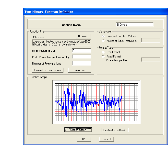
CSiBridge – Defining the Work Flow
6.4 Loads > Loads
Point, line, area and temperature loads may be applied to the bridge
model as part of the Bridge Object definition (see Chapter 7). Before the
loads can be assigned, however, the loads must first be defined.
Figure 6-6 shows the commands on the Loads – {Type} panel of the
Loads tab.
6 - 16 Loads > Loads
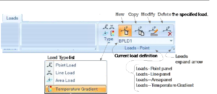
CHAPTER 6 Loads
Figure 6-6 Loads tab with annotated Loads – {Type} panel
As suggested in the figure, clicking the Loads Type command displays a
drop-down list that can be used to select Point, Line, Area, and Tempera-
ture Gradient loads. The name of the panel changes depending on the se-
lection made. After a load has been selected, clicking the expand arrow
displays the forms shown in Figure 6-7.
The forms shown in Figure 6-7a, b, c, and d list all previously defined
bridge loads in display areas on the left-hand side of the forms. General-
ly, the buttons in the “Click to” area on the right-hand sides of the forms
display the data forms described in Table 6-4 and shown in the screen
captures in Sections 6.4.1 through 6.4.4. Referring to Figure 6-6, the
New, Copy, and Modify commands on the Loads – {Type} panel bypass
the definition forms shown in Figure 6-7, and display the same forms,
thereby creating a shortcut to the data forms.
After the point, line, area, or temperature gradient load data have been
defined, the {type} load may be assigned as a load case using the Bridge
> Bridge Object > Loads > {Point Load, Line Load, Area Load,
Temperature Load} command (see Chapter 7).
Loads > Loads 6 - 17
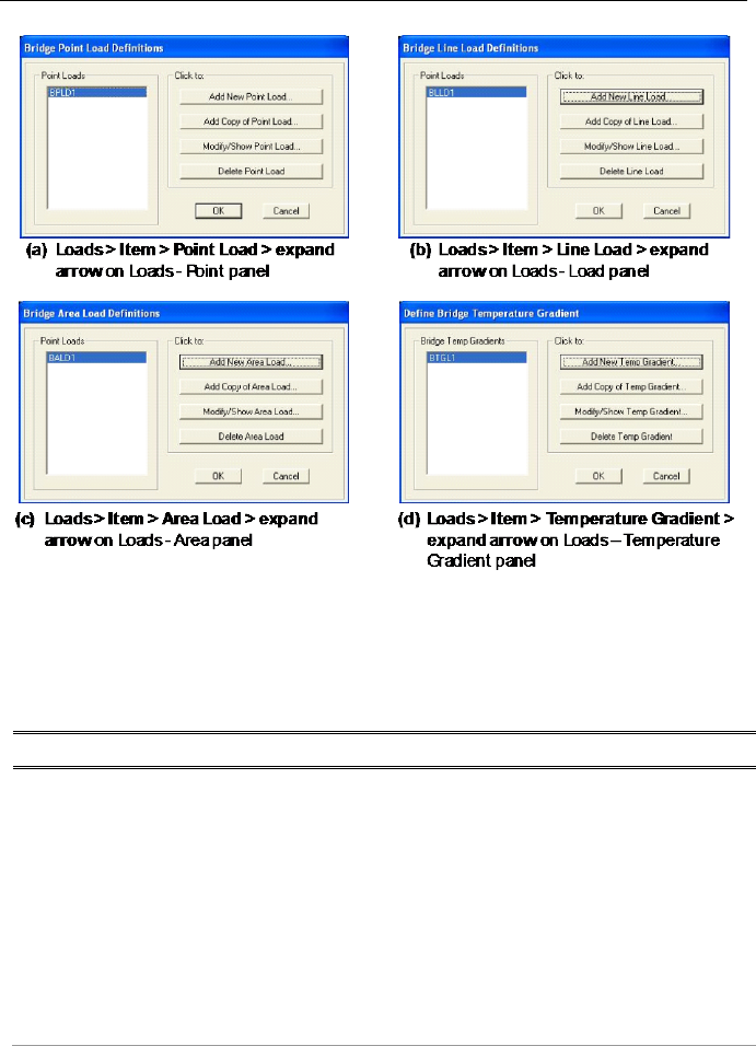
CSiBridge – Defining the Work Flow
Figure 6-7 Definitions forms that show all previously defined loads
Table 6-4 Form Data - Loads > Loads > {Type} > Add, Copy, Modify
Type
Data Form Parameters
Point Load Displays the Bridge Point Load Definition Data form shown in Sec-
tion 6.4.1. Allows definition of a unique point load that has a user
defined direction, value and location. The point load type can be
specified as Force or Mo
ment. The coordinate system may be
Global or Local. When the Global coordinate system is used, the
direction of the load as Gravity, X, Y or Z may be assigned. When
the Local coordinate system is used, the direction may be as-
signed as Along the Horizontal Projection of the Layout Line (1),
Vertical (2) or Normal to the Horizontal Projection of the Layout
Line (3). The location of the point load in the transverse direction
is made with reference to the left or right edge of the deck.
6 - 18 Loads > Loads

CHAPTER 6 Loads
Table 6-4 Form Data - Loads > Loads > {Type} > Add, Copy, Modify
Type Data Form Parameters
Line Load Displays the Bridge Line Load Definition Data form shown in Sec-
tion 6.4.2. Allows definition of a unique line load that has a user
defined direction, value and location. The line load type can be
specified as Force or
Moment. The coordinate system may be
Global or Local. When the Global coordinate system is used, the
direction of the load as Gravity, X, Y or Z may be assigned. When
the Local coordinate system is used, the direction may be as-
signed as Along the Horizontal Projection of the Layout Line (1),
Vertical (2) or Normal to the Horizontal Pro
jection of the Layout
Line (3). The location of the line load in the transverse direction is
made with reference to the left or right edge of the deck.
Area Load Displays the Bridge Area Load Definition Data form shown in Sec-
tion 6.4.3. Allows defi
nition of a unique area load that has a user
defined direction, value and location. The area load type can be
specified as Force or Moment. The coordinate system may be
Global or Local. When the Global coordinate system is used, the
direction of the load as Gravity, X, Y or Z may be assigned. When
the Local coordinate system is used, the direction may be as-
signed as Along the Horizontal Projection of the Layout Line (1),
Vertical (2) or Normal to the Horizontal Projection of the Layout
Line (3). The location of the line load in the transverse direction is
made with reference to the left or right edge of the deck. Both
distances are necessary to define a transverse boundary for the
area load.
Temperature
Gradient Displays the Bridge Temperature Gradient Data form
shown in
Section 6.4.4
. Allows definition of a unique temperature gradient
that is based on compliance with AASHTO or Chinese JTG D60
codes, or that is defined by the user. The form includes a schemat-
ic illustrating the loca
tions of input parameters for positive and
negative temperature values.
In the case of AASHTO or JTG D60 compliant definitions, those
values are set and cannot be edited.
In the case of a user definition, some or all of the values can be
modified, depending on the Type of definition being specified
(General—all values; AASHTO or JTG D60—select values).
Loads > Loads 6 - 19
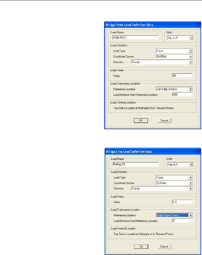
CSiBridge – Defining the Work Flow
6.4.1 Point Load Form – Screen Capture
6.4.2 Line Load Form – Screen Capture
Use these commands (see
Table 6-4) to display this
form and define a point
load.
Loads > Type > Point Loads
> expand arrow on the Loads
– Point panel > click Add New
Point Load button
OR
Loads > Type > Point Loads
> Add, Copy, Modify com-
mand
Use these commands (see
Table 6-4) to display this form
and define a line load.
Loads > Type > Line Loads >
expand arrow on the Loads –
Point panel > click Add New
Line Load button
OR
Loads > Type > Line Loads >
Add, Copy, Modify command
6 - 20 Loads > Loads
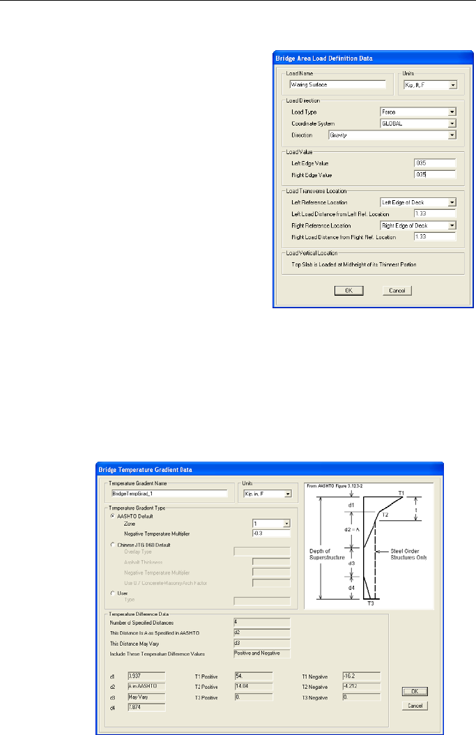
CHAPTER 6 Loads
6.4.3 Area Load Form – Screen Capture
6.4.4 Temperature Gradient Form – Screen Capture
Use these commands (see Table 6-4) to display this form and de-
fine a temperature gradient load.
Loads > Type > Temperature Gradient
> expand arrow on the Loads – Tem-
perature Gradient panel > click Add
New Temp. Gradient button
OR
Loads > Type > Tempera-
ture Gradient > Add,
Copy, Modify command
Use these commands (see
Table 6-4) to display this form
and define an area load.
Loads > Type > Area Loads >
expand arrow on the Loads –
Area panel > click Add New Ar-
ea Load button
Or
Loads > Type > Area Loads >
Add, Copy, Modify command
Loads > Loads 6 - 21

CHAPTER 7 Bridge
The Bridge tab consists of the commands that allow efficient access to
the forms needed to add, copy, or modify Bridge Object definitions as
well as delete a selected Bridge Object definition and update a bridge
model manually or automatically. Other commands provide access to the
data forms needed to review spans, span items (diaphragms, hinges, de-
scretization), supports (abutments, bents), superelevation, prestress ten-
dons, and loads as part of the process of assigning them to the specified
Bridge Object. A command on this tab can be used to add girder rebar,
and another command can be used to specify bridge groups for use in
staged construction analysis.
If the Quick Bridge template was used to start the bridge model, the pro-
gram will have created a Bridge Object using default assignments, in-
cluding spans, abutments, bents, and a bridge group for staged construc-
tion analysis. These assignments can be viewed using the commands on
the Bridge tab.
If the Bridge Wizard is being used, highlighting the Bridge Object As-
signments – Deck Sections, Discretization Points, Abutments, Bents,
Hinges, Diaphragms, Superelevation, Prestress Tendon, Concrete Girder
Rebar, Staged Construction Groups, Point Loads, Area Loads, Tempera-
ture Loads – and clicking the Assign/Show Deck Sections, As-
sign/Show Disc. Points, Assign/Show Abutments, Assign/Show Bents,
Bridge > Bridge Objects 7 - 1

CSiBridge – Defining the Work Flow
Assign/Show Hinges, Assign/Show Diaphragms, Assign/Show Super-
elevation, Assign/Show Tendons, Assign/Show Girder Rebar, As-
sign/Show Staged Groups, Assign/Show Point Loads, Assign/Show
Line Loads, Assign/Show Area Loads, and Assign/Show Temp Loads
buttons will display the same forms that are displayed when the com-
mands on the Bridge tab are used.
The commands on the Bridge tab also can be used if the Blank option
was used to start the model and the Bridge Wizard is not being used (i.e.,
the model is being built from scratch or by importing model data).
7.1 Bridge > Bridge Objects
A bridge model is represented parametrically with a set of high-level ob-
jects: layout (alignment) lines, spans, bents (pier supports), abutments
(end supports), deck cross sections, diaphragms, prestress tendons, su-
perelevation, groups, and more. Using assignments, the Bridge Object
definition brings together these Layout, Component, and Load defini-
tions in preparation for generating a spine, area object, or solid object
model (see Section 7.2). Typically a single Bridge Object represents the
entire structure, although multiple Bridge Objects may be needed if a
model includes parallel structures, or if merges or splits are to be consid-
ered.
Figure 7-1 shows the Bridge Object panel commands on the Bridge tab.
Figure 7-1 Bridge tab with annotated Bridge Object panel
7 - 2 Bridge > Bridge Objects
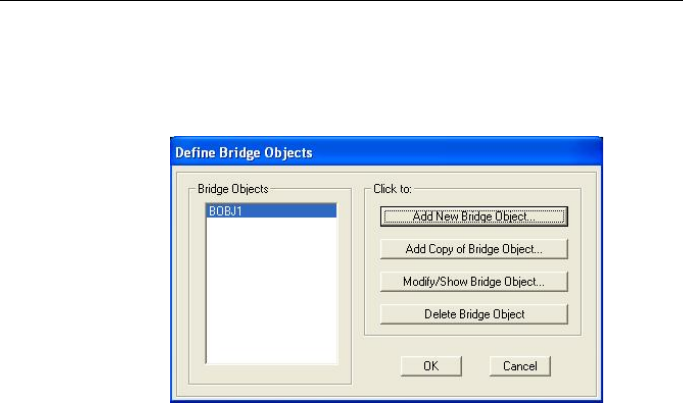
CHAPTER 7 - Bridge
Clicking the expand arrow in the lower right-hand corner of the Bridge
Object panel displays the Define Bridge Objects form shown in Figure
7-2.
Bridge > Expand arrow on the Bridge Object panel
Figure 7-2 Definition form showing previously defined Bridge Objects
All of the previously defined Bridge Objects are listed on the left-hand
side of the form. Clicking the buttons in the “Click to” area on the right-
hand side of the form display the same form as is displayed when the
New, Copy, and Modify commands on the Bridge Object panel are
used. That form is shown in Figure 7-3.
The Modify/Show Assignments list on the right-hand side of the Bridge
Object Data form (Figure 7-3) identifies the various assignments that can
be made to a Bridge Object. Selecting an item and clicking the Modi-
fy/Show button displays the same forms as are displayed when the indi-
vidual commands on the Bridge Object panel of the Bridge tab are
clicked. That is, for example, clicking the Spans item in the Modify/Show
Assignments list and then clicking the Modify/Show button on the
Bridge Object Data form displays the same form as is displayed when
the Bridge > Bridge Object > Spans command is used. Thus, the com-
mands on the Bridge Object panel are intended to be used as shortcuts to
the data/assignments forms. It may be helpful to define an initial Bridge
Object using the Modify/Show Assignments list on the Bridge Object Da-
ta form and then use the individual commands on the Bridge tab to ad-
just the definition.
Bridge > Bridge Objects 7 - 3

CSiBridge – Defining the Work Flow
Figure 7-3 Bridge Object Data form that can be used to assign to the Bridge
Object the definitions created using the Layout, Component, and Loads tabs
Table 7-1 briefly identifies the data/assignments available from the
Bridge Object panel on the Bridge tab. The name that appears in the
Modify/Show Assignments list on the Bridge Object Data form is shown
in parenthesis in the Command column when the names differ.
Table 7-1 Form Data/Assignments - Bridge > Bridge Object > {Command}
Command
Data / Assignment / Definition Forms
Spans
Displays the Bridge Object Span Assignments form (see Section
7.1.1) That form is used to assign the deck section definition speci-
fied using the Components > Item > Deck Sections command. It
is also possible to apply a parametric variation(s) (depress F1 to
access context sensitive help, or see Chapter 5 Components for an
explanation of parametric variations).
Span Items
Span Items are used to define the locations of in-span cross dia-
phragms, hinges, and user discretization points.
7 - 4 Bridge > Bridge Objects

CHAPTER 7 - Bridge
Table 7-1 Form Data/Assignments - Bridge > Bridge Object > {Command}
Command Data / Assignment / Definition Forms
Span Items
(continued)
(In-Span
Cross Dia-
phragm)
> Diaphragms – Displays the Bridge Object In-Span Cross-
Diaphragm Assignments form (see Section 7.1.1). The in-span
diaphragm assignment includes
selection of the span to which
the diaphragm is be
ing assigned (along its length), identification
of the diaphragm property, specification of the location of the dia-
phragm relative to the beginning of the span, and indication of the
bearing (skew) measured in degrees relative to the bridge layout
line.
[In-Span
Hinges
(Expansion
Jts)}
> Hinges – Displays the Bridge Object Hinge Assignments form;
use the buttons
in the “Click to” area of that form to display the
Bridge Object Hinge Assignment Data form (see Section 7.1.1).
Use that
data form to specify the hinge location and orientation;
the bearing property, elevation, and rotation angle from the bridge
default;
the restrainer property and elevation; the diaphragm
properties before and after the hinge; and the initial gap openings
at the top and bottom of the superstructure. A Modify/Show
Overwrites
button is available that displays forms that can be
used to overwrite the bearing and restrainer properties on a gird-
er-by-girder basis.
(User Dis-
cretization
Points)
> User Points – Displays the Bridge Object Discretization Points
As
signments form (see Section 7.1.1). In most models it is not
necessary to create user discretization points because the dis-
cretization speci
fied when the linked model is updated generally
is sufficient (see Section 7.2). However, because user discretiza-
tion points supplement the discretization specified when the
linked model is updated, this form provides a means of controlling
the mesh points along the span. That is, user discretization points
allow specification of points along the span where the bridge ob-
ject will be discretized. Thus, user discretization points may be
used if output at a specific point is needed. A skew also can be
specified associated with the discretization point.
Supports
Abutments (end bents) and Bents (interior supports) can be as-
signed as part of a Bridge Object definition.
> Abutments – Displays the Bridge Object Abutment Assignments
form (see Section 7.1.2). Abutment assignments allow specifica-
tion of the following items at the start and end of the bridge: end
skews; end diaphragm property, if any; substructure assignment
for the abutment, which may be none, an abutment property, or a
bent property; vertical elevation and horizontal location of the
substructure; and the bearing property, elevation and rotation an-
gle from the bridge default. The elevation of the bearing refers to
the action point of the bearing,
which is the point at which all
translations and rotations occur. Care should be taken to provide
the proper bearing elevations (and restraint definitions) because
Bridge > Bridge Objects 7 - 5

CSiBridge – Defining the Work Flow
Table 7-1 Form Data/Assignments - Bridge > Bridge Object > {Command}
Command Data / Assignment / Definition Forms
of the kinematics that are captured by CSiBridge.
Supports
(continued)
> Bents – Displays the Bent Object Bent Assignments form (see
Section 7.1.2). The bent assignments allow specification of the
following items for each bent: superstructure assignments, includ-
ing diaphragm property (for bents at superstructure discontinui-
ties, a diaphragm property can be specified on each side of the
discontinuity, as well as a restrainer property, restrainer vertical
elevation and initial gap openings at the top and bottom of the
superstructure); bent property and bent orientation; vertical eleva-
tion and horizontal location of the bent; the bearing property, ele-
vation and rotation angle from the bridge default (for bents at su-
perstructure discontinuities, bearings are separately specified on
each side of the discontinuity).
Super-
elevation
Displays the Bridge Object Superstructure Assignment form (see
Sec
tion 7.1.3). A superelevation assignment for a bridge object is
referenced to the layout line. The superelevation is specified in per-
centage, and it indicates the rotation of the superstructure about its
longitudinal axis. The superelevation may be constant, or it may
vary along the bridge. In most bridge models including supereleva-
tion is probably an unnecessary refinement.
Prestress
Tendons
Displays the Assign Prestress Tendons form, which displays all
previou
sly defined tendons and has buttons that provide access to
the Bridge Tendon Data form (see Section 7.1.4). Use the data
from to assign the following: the location of the start and end of the
tendon; the vertical and horizontal layout of the tendon; tendon sec-
tion properties, loss parameters and jacking options; tendon loads
as a force or a stress; and modeling of tendons as loads or ele-
ments.
Girder Re-
bar
Displays the Bridge Girders Reinforcement Layout form (see Sec-
tion 7.1.5). Vertical and longitudinal girder reinforcing may be add-
ed to spans girder-by-girder. The girder rebar is used in the bridge
rating calculations (see Chapter 9 Design/Rating). Transverse rein-
forcing is specified in terms of the area, spacing, number of spaces,
and the start and end locations. Similarly, the longitudinal reinforc-
ing is specified by the rebar area, and the distance from the top or
bottom edge of the girder along with the start and end station loca-
tions along the length of the girder.
Loads
(Point Load
Assigns)
Point, line, area and temperature loads may be applied to the
bridge model as part of the Bridge Object definition.
Point Loads – Displays the Point Load Assignments form (see
Section 7.1.6). Use that form to apply a defined point load to a
defined load pattern as part of a Bridge Object definition (i.e., ap-
plies the load to the spans identified in the Bridge Object defini-
7 - 6 Bridge > Bridge Objects

CHAPTER 7 - Bridge
Table 7-1 Form Data/Assignments - Bridge > Bridge Object > {Command}
Command Data / Assignment / Definition Forms
tion).
Loads
Point Loads
(continued)
The point load and load pattern can be defined using the appro-
priate commands on the Loads tab (see Chapter 6 Loads), or us-
ing the forms that display when Define Load Patterns and De-
fine Point Loads
buttons on the Point Load Assignments form
are used. A transverse variation can be applied using a paramet-
ric variation definition (use the F1 key to access context sensitive
help or see Chapter 5 Components for more
information about
parametric variations). The load pattern can then be used in a
load case (see Chapter 8 Analysis).
(Line Load
Assigns)
(Area Load
Assigns)
(Tempera-
ture Load
Assigns)
> Line Loads – Displays the Line Load Assignments form (see
Section 7.1.6) Use that form to apply a defined line load to a de-
fined load pattern as part of a Bridge Object definition (i.e., ap-
plies the load to the spans identified in the Bridge Object defini-
tion). The line load and load pattern can be defined using the ap-
propriate commands on the Loads tab (see Chapter 6 Loads), or
using the forms that display when Define Load Patterns and De-
fine Line Loads buttons on the Line Load Assignments form are
used. A transverse variation can be applied using a parametric
variation definition (use the F1 key to access context sensitive
help or see Chapter 5 Components for more
information about
parametric variations). The load pattern can then be used in a
load combination (see Chapter 8 Analysis).
> Area Loads –
Displays the Area Load Assignments form (see
Section 7.1.6). Use that form to apply a defined area load to a
defined load pattern as part of a Bridge Object definition (i.e., ap-
plies the load to the spans identified in the Bridge Object defini-
tion). The area load and load pattern can be defined using the
appropriate commands on the Loads tab (see Chapter 6 Loads),
or using the forms that display when Define Load Patterns and
Define Area Loads buttons on the Area Load Assignments form
are used. A transverse variation can be applied using a paramet-
ric variation definition (use the F1 key to access context sensitive
help or see Chapter 5 Components for more
information about
parametric variations). The load pattern can then be used in a
load combination (see Chapter 8 Analysis).
Temperature Loads –
Displays the Assign Bridge Temperature
Loads form (see Section 7.1.6), which can be used to access the
Bridge Temperature Load Assignments form. Use the latter form
to define the temperature load assignment, which applies to the
bridge superstructure. Assignments can be uniform temperature
changes or temperature gradient changes over the height of the
superstructure. Temperature gradient load assignments use pre-
defined temperature gradient definitions, which are defined using
Bridge > Bridge Objects 7 - 7
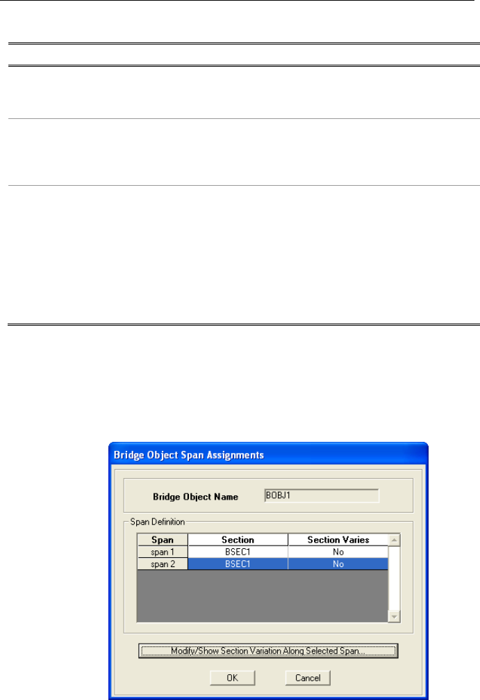
CSiBridge – Defining the Work Flow
Table 7-1 Form Data/Assignments - Bridge > Bridge Object > {Command}
Command Data / Assignment / Definition Forms
the Bridge Temperature Gradient Data form (use the F1 key to
access context sensitive help for that form or see Chapter 6
Loads for more information about that form).
Loads
Tempera-
ture Loads
(continued)
Appropriate thermal loads are developed for the linked model
(spine [frame], shell, or solid models). Those loads also can be
automatically included in Load Combinations generated for AASH-
TO or JTG design codes (see Chapter 8 Analysis).
Groups
(Stage
Construc-
tion
Groups)
Displays the Define Bridge Groups form. Clicking the Bridge Object
Staged Construction Groups Assignments form (see Section 7.1.7).
Use the form to add new groups to the model file and specify the
bridge group type (e.g., section, top slab, web, bottom slab, beam,
diaphragm/crossframe, sup
port structure, bearing, hinge, tendon,
mixed, ). Groups can be used in defining a staged construction load
case, or the Bridge Object to which the group has been assigned
can be used in a seismic design request (e.g., foundation items).
Depress the F1 key for context sensitive help with this form.
7.1.1 Bridge Object > Spans – Screen Captures
This command (see Table 7-1) displays this form: Bridge > Bridge Ob-
ject > Spans
7 - 8 Bridge > Bridge Objects

CHAPTER 7 - Bridge
This command displays this form: Bridge > Bridge Object > Spans >
Modify/Show Section Variation Along Selected Span button
Bridge > Bridge Objects 7 - 9

CSiBridge – Defining the Work Flow
7.1.2 Bridge Object > Span Items – Screen Captures
7.1.2.1 Bridge Object > Span Items > Diaphragms – Screen
Capture
This command (see Table 7-1) displays this form: Bridge > Bridge Ob-
ject > Span Items > Diaphragms
7.1.2.2 Bridge Object > Span Items > Hinges – Screen Cap-
tures
This command (see Table 7-1) displays this form: Bridge > Bridge Ob-
ject > Span Items > Hinges
Diaphragms may be staggered for steel girder
bridges and precast I-girder bridge
7 - 10 Bridge > Bridge Objects

CHAPTER 7 - Bridge
This command (see Table 7-1) displays this form: Bridge > Bride Ob-
ject > Span Items > Hinges > Add New Bridge Hinge button
Bridge > Bridge Objects 7 - 11
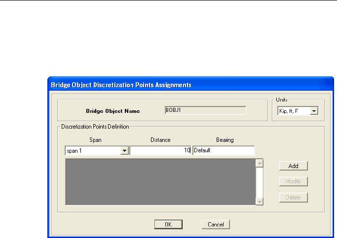
CSiBridge – Defining the Work Flow
7.1.2.3 Bridge Object > Span Items > User Points – Screen
Capture
This command (see Table 7-1) displays this form: Bridge > Bridge Ob-
ject > Span Items > User Points
7 - 12 Bridge > Bridge Objects
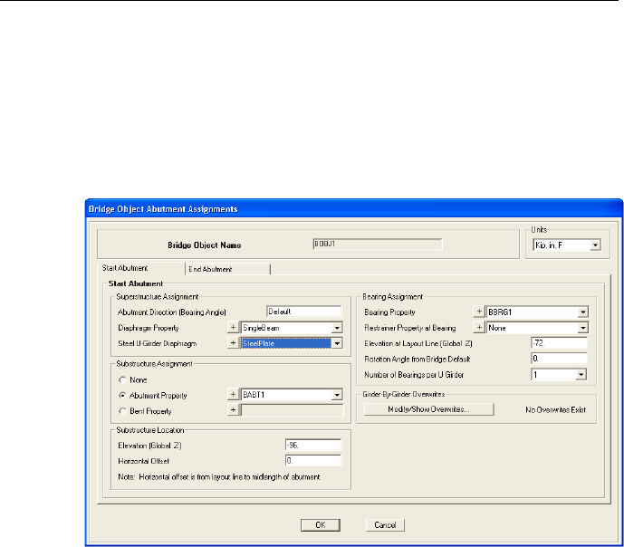
CHAPTER 7 - Bridge
7.1.3 Bridge Object > Supports – Screen Captures
7.1.3.1 Bridge Object > Supports > Abutments – Screen
Capture
This command (see Table 7-1) displays this form: Bridge > Bridge Ob-
ject > Supports > Abutments
Bridge > Bridge Objects 7 - 13
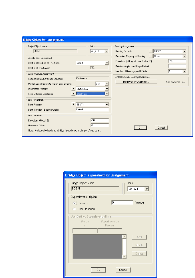
CSiBridge – Defining the Work Flow
7.1.3.2 Bridge Object > Supports > Bents – Screen Capture
This command (see Table 7-1) displays this form: Bridge > Bridge Ob-
ject > Supports > Bents
7.1.4 Bridge Object > Superelevation – Screen Capture
This command (see Table 7-1) displays this form: Bridge > Bridge Ob-
ject > Superelevation
7 - 14 Bridge > Bridge Objects
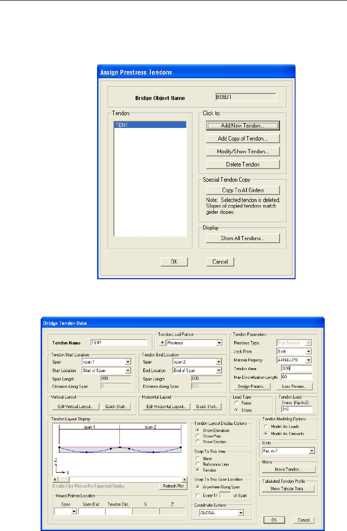
CHAPTER 7 - Bridge
7.1.5 Bridge Object > Prestress Tendons – Screen Captures
This command (see Table 7-1) displays this form: Bridge > Bridge Ob-
ject > Prestress Tendons
This command displays this form: Bridge > Bridge Object > Prestress
Tendons > Add New Tendon button
Bridge > Bridge Objects 7 - 15

CSiBridge – Defining the Work Flow
7.1.6 Bridge Object > Girder Rebar – Screen Capture
This command (see Table 7-1) displays this form: Bridge > Bridge Ob-
ject > Girder Rebar
7.1.7 Bridge Object > Loads – Screen Captures
This command (see Table 7-1) displays this form: Bridge > Bridge Ob-
ject > Loads > Point Load
7 - 16 Bridge > Bridge Objects
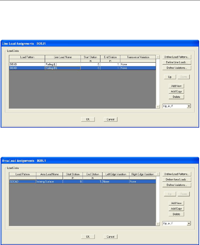
CHAPTER 7 - Bridge
This command (see Table 7-1) displays this form: Bridge > Bridge Ob-
ject > Loads > Line Load
This command (see Table 7-1) displays this form: Bridge > Bridge Ob-
ject > Loads > Area Load
Bridge > Bridge Objects 7 - 17
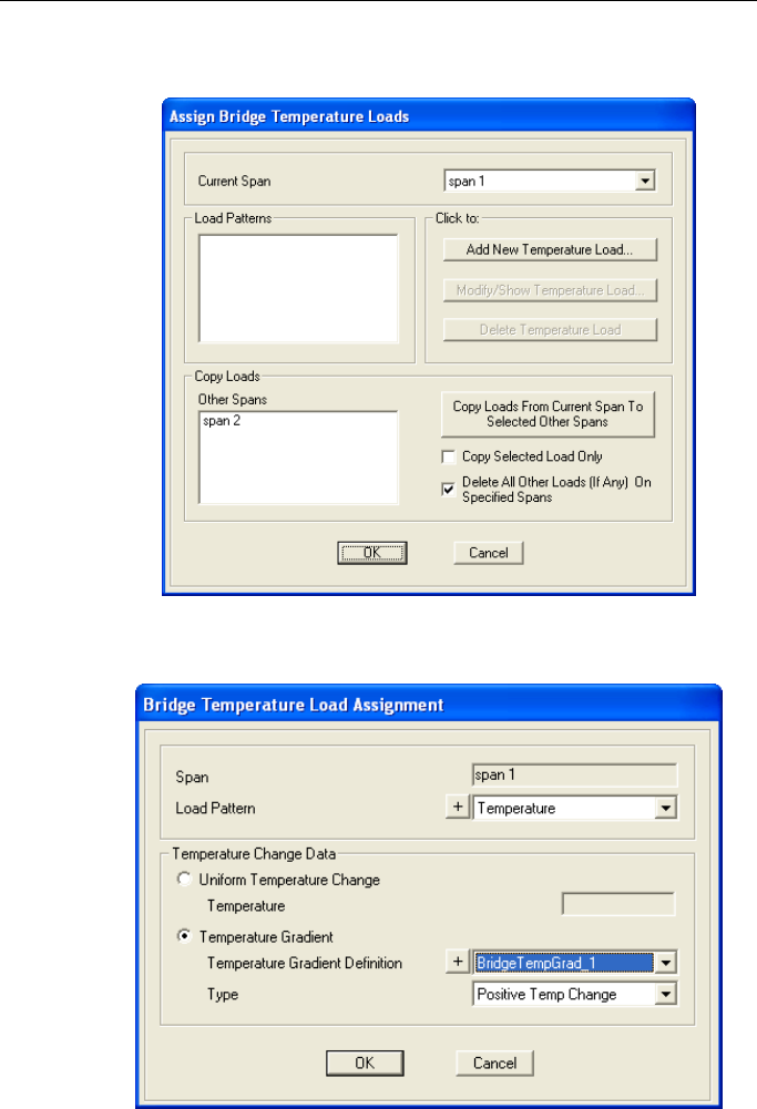
CSiBridge – Defining the Work Flow
This command (see Table 7-1) displays this form: Bridge > Bridge Ob-
ject > Loads > Temperature Load
This command displays this form: Bridge > Bridge Object > Loads >
Temperature Load > Add New Temperature Load button.
7 - 18 Bridge > Bridge Objects
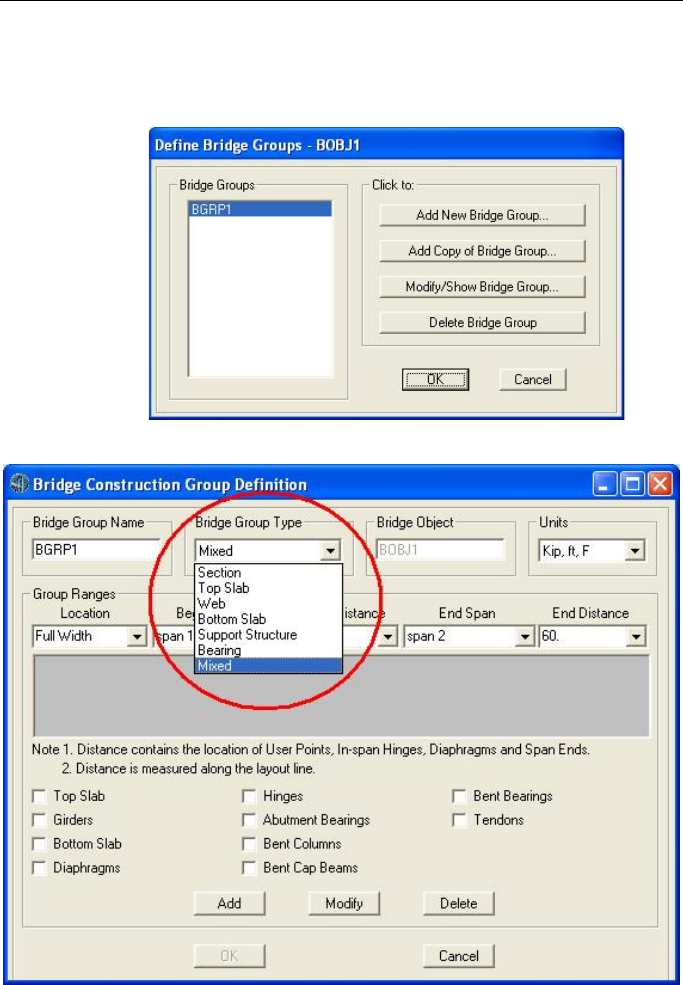
CHAPTER 7 - Bridge
7.1.8 Bridge Object > Groups – Screen Captures
This command (see Table 7-1) displays this form: Bridge > Bridge Ob-
ject > Groups
> Add New Bridge Group accesses this form:
Next, select a Bridge Group Type from the drop-down list (shown cir-
cled in the figure).
Bridge > Bridge Objects 7 - 19
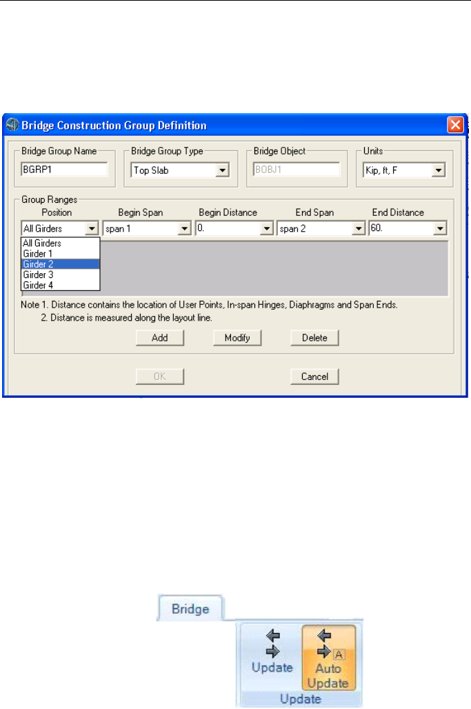
CSiBridge – Defining the Work Flow
The Bridge Construction Group Definition form will change depending
on the Bridge Object Type selected. Several deck section types allow for
the group ranges to apply to specific girders, as noted in this figure by
the circled text.
7.2 Update
After a Bridge Object has been defined, the object-based model used for
analysis and design will not be assembled until the Bridge Object has
been updated. The update process essentially creates or restores the ob-
ject-based model based on the parametric bridge object definition.
Figure 7-4 shows the two commands on the Update panel.
Figure 7-4 Update panel on the Bridge tab
7 - 20 Update

CHAPTER 7 - Bridge
The next two subsections briefly describe the two commands on the Up-
date panel
7.2.1 Update > Update
The first time the Bridge > Update > Update command is used for a
given bridge object, CSiBridge creates a new object-based model for
analysis and design from the parametric definition of the Bridge Object
(see Section 7.1). This is done in accordance with the options selected on
the Update Bridge Structure Model form which displays when the
Bridge > Update > Update command is used, as shown in Figure 7-5.
If a linked object-based model of the selected Bridge Object already ex-
ists (i.e., the command has been used previously), the existing model is
overwritten when the new object-based model is created. The new ob-
ject-based model includes all of the latest changes to the Bridge Object
definition. Note also, however, that the update operation may undo some
changes to the object-based model if these changes were made without
using the Bridge Object forms described in Section 7.1. For example, if
edits are made to an updated bridge model using the draw or delete
commands on the Advanced tab, those edits may not be reflected in the
parametric Bridge Object definitions and therefore may be lost the next
time the bridge model is updated. The details of how this is handled de-
pend on the “Action” chosen.
Figure 7-5 Update Bridge Structural Model form
Update 7 - 21

CSiBridge – Defining the Work Flow
The “Action” options on the Update Bridge Structural Model form in-
clude the following:
• Clear and Create Linked Model: This deletes all model objects pre-
viously created from the Bridge Object, if any, and then creates a
new linked model. Any user modifications on previously generated
model objects will not be preserved. CSiBridge will update the
model as a spine, area-object, or solid-object model, depending on
the option chosen on the right-hand side of the form. The type of ob-
ject-based model created can be switched at any time. For the area-
and solid-object models, the maximum sub-meshing size also can be
specified. This option allows area and solid objects to be divided in-
to smaller objects in the object-based model, and meshed into ele-
ments in the analysis model. Keep in mind that smaller mesh sizes
require more memory and time when the analysis is run.
• Update Linked Model: When performed for the first time on the se-
lected Bridge Object, this operation is the same as Clear and Create
Linked Model described above. When the linked model was previ-
ously updated, CSiBridge will preserve user modifications on the
previously generated objects, such as property modifiers, local axes,
additional loads, etc., whenever possible. This can only occur when
the generated object (joint, frame, shell, solid, link) is regenerated in
the exact same location as before, and the user modification does
not conflict with changes made to the Bridge Object parametric def-
inition. User modifications would typically have been made using
commands on the Advanced tab.
• Clear All from Linked Model: This deletes all model objects previ-
ously created from the Bridge Object. The Bridge Object itself is not
affected and can be updated at a later time to create a new linked
model. Alternatively, the Bridge Object can be deleted if it is no
longer needed.
1. Convert to Unlinked Model: This is a one-way action that discon-
nects all model objects previously generated from the Bridge Ob-
ject, but does not delete them. The Bridge Object itself is not affect-
ed and can be updated at a later time to create a new linked model.
7 - 22 Update

CHAPTER 7 - Bridge
If that is done, the generated objects could conflict with the unlinked
model objects, so this should be done with care. Note that bridge
display, design, and rating are not available for an unlinked model
unless the Bridge Object is updated again to create a new linked
model. Alternatively, the Bridge Object can be deleted if it is no
longer needed.
The form also includes discretization options to specify the maximum
segment length for deck spans, bent cap beams, and bent columns. These
lengths determine the smoothness of curves for on-screen display and
graphical printed output; the smaller the length, the smoother the curve.
For steel I-girder bridge with the girder web modeled as area objects, the
option to mesh slab at critical steel I-girder locations is available.
CSiBridge will subdivide the slab area objects at the critical locations
such as girder staggered-diaphragm connections, girder staggered splic-
es, and girder section-transition locations. Local girder section cuts will
be generated at these critical locations in addition to the global bridge
section cuts. The Bridge Response Display form will display additional
girder responses at these critical location. This option is used for ad-
vanced steel I-girder bridge design and rating and is only available for
steel I-girder bridges when the girder webs are modeled as area objects.
7.2.2 Update > Auto Update
The Bridge > Update > Auto Update command is a toggle. When ena-
bled, CSiBridge will automatically Clear and Update the linked object-
based model when any changes are made to the Bridge Object definition
or its components.
Update 7 - 23

CHAPTER 8 Analysis
The Analysis tab consists of the commands that allow efficient access to
the forms needed to manage load case definitions; define a construction
schedule that is useful when performing staged construction analysis of a
bridge model; convert load combinations to nonlinear cases; show a tree
of load case; specify results to be saved for all moving load cases; and
run the analysis, including specifying the analysis options and displaying
the results of the last analysis. The tab also has a command to unlock a
locked model and lock an unlocked one, and another pair of commands
that modify the geometry of a deformed shape and then reset the original
geometry.
If the Quick Bridge template was used to start the bridge model, the pro-
gram will have created default load case definitions.
If the Bridge Wizard is being used, highlighting the Load Cases, Con-
struction Scheduler, and Moving Load Case Results Saved items in the
Summary Table and clicking the Define/Show Load Cases,
Define/Show Schedule and Define/Show Results Saved buttons will
display the same forms that are displayed when the commands on the
Analysis tab are used. The other commands available on the Analysis
tab are not duplicated on the Bridge Wizard.
Analysis > Load Cases 8 - 1
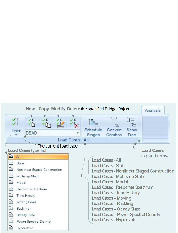
CSiBridge - Defining the Work Flow
The commands on the Analysis tab also can be used if the Blank option
was used to start the model and the Bridge Wizard is not being used (i.e.,
the model is being built from scratch or by importing model data).
8.1 Analysis > Load Cases
A load case defines how loads are to be applied to the structure (e.g.,
statically or dynamically), how the structure responds (e.g., linearly or
nonlinearly), and how the analysis is to be performed (e.g., modally or
by direct-integration).
Figure 8-1 shows the Load Cases panel commands on the Analysis tab.
Figure 8-1 Analsis tab with annotated Load Cases panel
As shown in the figure, clicking the Type command displays a drop-
down list of load case types. Any of these load case types can be used
when analyzing a bridge model.
8 - 2 Analysis > Load Cases

CHAPTER 8 - Analysis
Static, response spectrum, and time history load case types are useful for
seismic analysis. Pushover analysis can be performed using a nonlinear
static load case. Stage construction analysis is also performed using non-
linear static load cases.
Several options are specialized for analyzing vehicle live loads. Moving
load load cases compute influence lines for various quantities and solve
all permutations of lane loading to obtain the maximum and minimum
response quantities.
Multi-step static and multi-step dynamic (direct integration time history)
load cases can be used to analyze one or more vehicles moving across
the bridge at a specified speed. These multi-step load cases are defined
using special bridge live load patterns that define the direction, starting
time, and speed of vehicles moving along lanes (see Chapter 6 Loads).
To access the forms, select a Type and then click the Add, Copy, or
Modify commands. In all cases, except the “All” type, the data form
needed to complete the load case definition displays.
When the Analysis > Load Cases > All command is used, the Define
Load Cases form displays. Note that clicking the Analysis > Load Cas-
es > Expand arrow on the Load Case panel (arrow in the lower right-
hand corner of the panel; see Figure 8-1) also displays this form, regard-
less of the Type selected. Figure 8-2 displays the Define Load Cases
form. All previously defined load cases are listed on the left-hand side of
the form.
The buttons in the “Click to” area on the right-hand side of the form dis-
play the Load Case Data form, defaulted to the Linear Static type. The
Load Case Type drop-down list on the right-hand side of that form can
be used to select a different load case type. The forms that can be ac-
cessed using that drop-down list are the same forms that display when
the Analysis > Load Cases > Type > {Select from list} > Add, Copy,
or Modify commands are used. Thus, the commands on the Load Cases
panel bypass the need to use the Load Case Type drop-down list on the
Load Case Data form, providing a shortcut to the data forms needed to
define a particular load case type.
Analysis > Load Cases 8 - 3

CSiBridge - Defining the Work Flow
Figure 8-2 Definitions form showing all previously defined load cases
The Schedule Stages, Convert Combos, and Show Tree commands
provide more direct access to the forms required to complete their de-
signed functions. That is, these commands do not access a “summary”
style of form that provides an indication of the previous activity com-
pleted using the commands. Note that by clicking the checkbox “Simu-
late Staged Construction”, at the top right of the form is checked, the us-
er can simulate the staged construction sequence without analyzing the
model by clicking each stage under each staged construction load case.
Table 8-1 briefly explains the commands on the Load Cases −{Type}
panel of the Analysis tab.
Table 8-1 Form Data - Analysis > {Command} >
Command
Data / Assignment / Definition Forms
Type
> Add
> Copy
> Modify
Any of the following load case types can be used in the analysis of
a bridge model.
> All − Displays the Define Load Cases form. An explanation of this
command precedes this table.
> Static − Displays the Load Case Data – Linear Static form (see
Section 8.1.1.1
).The most common type of analysis, loads are
applied without dynamic effects.
> Nonlinear Staged Construction − Displays the Load Case Data
– Non
linear Static Staged Construction form (see Section
8.1.1.2). A direct integration time history analysis solves equa-
tions for the entire structure at each time step, whereas a modal
8 - 4 Analysis > Load Cases

CHAPTER 8 - Analysis
Table 8-1 Form Data - Analysis > {Command} >
Command Data / Assignment / Definition Forms
time history analysis uses the method of mode superposition.
The nonlinear staged construction load case defines loads at us-
er-specified stages for selected operations involving user-defined
groups of model objects.
Analysis > Load Cases 8 - 5

CSiBridge - Defining the Work Flow
Table 8-1 Form Data - Analysis > {Command} >
Command Data / Assignment / Definition Forms
Type
> Add
> Copy
> Modify
(continued)
> Multistep Static − Displays the Load Case Data – Linear Multi-
Step Static form
(see Section 8.1.1.3). A multi step static load
case completes linear static analysis for multi-stepped load cas-
es, making this load case useful in examining vehicle responses
on a bridge. This method of applying vehicle loads to a bridge
takes into consi
deration the vehicle direction and speed. It is
possible to consider multiple vehicles in multiple lanes. The multi-
step static load case does not, however, consider the dynamic ef-
fects. If dynamic effects are needed, a time history analysis may
be used. Defining a multistep static load case requires that a Ve-
hicle
Live Load Pattern be defined and further that a multi step
bridge live load pattern be generated (see Chapter 6 Loads). A
multi step vehicle live load pattern is used to define the vehicle,
lane,
start location, start time, direction and speed. It should be
noted that the vehicles used as part of a multi step static load
case cannot have any uniform load assignments (see definition of
vehicles in Chapter 4 Layout). Vehicles can have only axle loads.
Generation of the multi step bridge live load pattern also defines
the duration of the loading and the time step discretization. After
the multi-
step static analysis has been run, the results may be
viewed by stepping through each time step.
> Modal − Displays the Load Case Data – Modal form (see Section
8.1.1.4). A modal load case calculates the dynamic modes of the
structure using Eigenvector or Ritz-
vector methods. Loads are
not actually applied, although they can be used to generate Ritz
vectors. The Load Case Data - Modal form is used to view and
change the defi
nition of a modal load case. A modal analysis is
always linear. Eigenvector analysis determines the undamped
free-
vibration mode shapes and frequencies of the system.
These natural modes provide an excellent insight into the behav-
ior of the structure. Ritz-vector analysis seeks to find modes that
are excited by a particular loading. Ritz-vectors can provide a
better basis than do eigenvectors when used for response-
spectrum or time-history analyses that are based on modal su-
perposition
> Response Spectrum − Displays the Load Case Data – Re-
sponse Spectrum form (see Section 8.1.1.5). A response spec-
trum load case statistically calculates the response caused by
acceleration or displacement inertia loads. A response spectrum
function must be defined before this load case can be used (see
Chapter 6 Loads).
> Time History − Displays the Load Case Data – Linear Modal
History form (see Section 8.1.1.6). Time-varying loads are ap-
plied for this load case type. A time history function must be de-
fined before this load case can be used (see Chapter 6 Loads).
The solution may be by modal superposition or direct integration
methods and the solution may be linear or nonlinear.
8 - 6 Analysis > Load Cases

CHAPTER 8 - Analysis
Table 8-1 Form Data - Analysis > {Command} >
Command Data / Assignment / Definition Forms
> Time
History
(continued)
For bridge applications, a time history load case may be used to
de
termine the dynamical response to a vehicle live load. After a
Bridge Live load pattern has been defined (see information about
load patterns in Chapter 6 Loads), a time history load case may
be defined using the Vehicle Live load pattern name.
> Moving Load − Displays the Load Case Data – Moving Load
form (see Section 8.1.1.7). V
ehicles, lanes and vehicle classes
must be defined before a moving load load case can be defined
(see Chapter 4 Layout). A moving load case calculates the most
severe response resulting from vehicle live loads moving along
lanes on the structure. The load case uses defined vehicle loads
and defined lanes rather than the load patterns that are used by
other analysis types. With Influence-
based enveloping analysis,
vehicles are moved
in both directions along each Lane of the
bridge. Using the influence surface, vehicles are automatically lo-
cated at such positions along the length and width of the lanes so
as to produce the maximum a
nd minimum response quantities
throughout the structure. Each vehicle may be allowed to act on
every lane or be restricted to certain lanes. The program can au-
tomatically find the maximum and minimum response quantities
throughout the structure resulting from the placement of different
vehicles in different lanes. For each maximum or minimum ex-
treme response quantity, the corresponding values for the other
components of response also can be computed.
Buckling − Displays the Load Case Data – Buckling form (see
Section 8.1.1.8). A buckling load case calculates the buckling
modes under the application of loads. Linear buckling analysis
seeks the instability modes of a structure as a result of the P-
delta effect under a specified set of loads. Each eigenvalue-
ei
genvector pair is called a buckling mode of the structure. The
modes are identified by numbers from 1 to n in the order in which
the modes are found by the program. The eigenvalue, λ, is
called the buckling factor. It is the scale factor that must multiply
the applied loads to cause buckling in the given mode. Any num-
ber of linear buckling Load Cases can be created. For each case
a combination is specified of one or more Load Patterns or
Acceleration Loads that make up the load vector r. The number
of modes to be found also may be specified as well as a conver-
gence tolerance. It is strongly recommended that more than one
buckling mode be sought
, since often the first few buckling
mo
des may have very similar buckling factors. A minimum of six
modes is recommended.
Analysis > Load Cases 8 - 7

CSiBridge - Defining the Work Flow
Table 8-1 Form Data - Analysis > {Command} >
Command Data / Assignment / Definition Forms
> Time
History
> Buckling
(continued)
It is important to understand that buckling modes depend on the
load. There is no one set of buckling modes for the structure in
the same way that there is for natural vibration modes. Buckling
for each set of loads of concern must be explicitly evaluated. For
each linear buckling load case, it may be specified that the pro-
gram use the stiffness matrix of the full structure in its unstressed
state (the default) or the stiffness of the structure at the end of a
nonlinear load case. The most common reasons for using the
stiffness at the end of a nonlinear case are to include P-delta ef-
fects from an initial P-delta analysis, include tension-stiffening ef-
fects in a cable structure, and consider a partial model that re-
sults from staged construction
> Steady State − Displays the Load Case Data – Steady State
form (see Section 8.1.1.9). A steady state load case solves for
the response of the structure resulting from cyclic (harmonic, si-
nusoidal) loading at one or more frequencies of interest. Steady-
state analysis seeks the response of the structure at one or more
frequencies to loading. After analysis, we can plot the deflected
shape or force/stress response at any of the requested frequen-
cies and at any phase angle. For example, the response at phase
angle 0° primarily represents the behavior due to horizontal load-
ing plus a damping component due to vertical loading. We can
instead plot the magnitude of the response at any requested fre-
quency, where the magnitude is given by the square-root of the
sum of the squares of the real (0°) and imaginary (90°) response
components. It is also possible to display plots of any response
quantity as a function of frequency, yielding a frequency spec-
trum. This can be completed for the component at any phase an-
gle, or for the magnitude of the response.
> Power Spectral Density − Displays the Load Case Data – Pow-
er Spectral Density form (see Section 8.1.1.10). A power spec-
tral density load case solves for the response of the structure re-
sulting from cyclic (harmonic, sinusoidal) loading over a range of
frequencies, and then integrates the resulting spectrum weighted
by a probabilistic power spectral density function to get a root
means square (RMS) expected response.
> Hyperstatic − Displays the Load Case Data – Hyperstatic form
(see Section 8.1.1.11). A hyperstatic load case calculates the lin-
ear response of the structure with all supports removed and load-
ed only by the reactions from another linear static load case. This
is typically to calculate the secondary forces under prestress
loading.
> Delete
Deletes the load case definition selected in the Current Load Case
8 - 8 Analysis > Load Cases

CHAPTER 8 - Analysis
Table 8-1 Form Data - Analysis > {Command} >
Command Data / Assignment / Definition Forms
drop-down list (see Figure 8-1).
Schedule
Stages
Displays the Construction Scheduler forms (see Section 8.1.2). Use
the cells in the rows and cells of the Schedule Table to identify the
activity being scheduled, its duration, any tasks that must be com-
pleted before the current tasks can be completed (i.e., predeces-
sors), and the Operation, which specifies how the task affects de-
velopment of the structure with respect to staged construction anal-
ysis. A Stage is a collection of Opera
tions that are executed at a
given time. Each Stage has a defined duration in days that must be
an integer greater than or equal to zero. Each Stage starts with
initial conditions equal to the end of the previous Stage. The first
stage will start with the initial conditions defined for the Staged-
Construction Load Case. During the analysis, the model is first ad-
justed based on specified Operations and then analyzed for time
dependent effects based on the duration of the Stage. If output is
requested, it reflects the stress and deflection state of the structure
at the end of the stage.
Convert
Combos
Displays a selection list form (see Section 8.1.3). Use that form to
specify which load combination(s) is to be converted to a static non-
linear load case. This command is a convenient way to create a
nonlinear load while making use of an exis
ting load combination
when nonlinear effects, such as P-Delta, are required.
Note that
load combinations are created using the De
sign/Rating > Load
Combinations > Add, Copy, Modify commands (see Chapter 9).
Show Tree
Displays the Load Case Tree form (see Section 8.1.4). This form
shows the load cases that have been defined for the model file us-
ing the commands previously described in this table. Options on the
form can be used to expand and view the various defined stages if
a staged construction load case has been defined.
8.1.1 Analysis > Load Cases – Type
The following subsections provide screen captures of the forms that dis-
play when a Type of load case is selected on the Analysis tab and the
Add, Copy, or Modify commands on the Load Cases – {Type} panel is
used.
Analysis > Load Cases 8 - 9
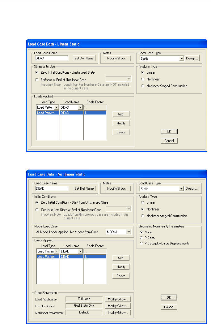
CSiBridge - Defining the Work Flow
8.1.1.1 Static – Screen Capture
This command (see Table 8-1) displays this form: Analysis > Load
Cases > Type > Static > Load Case Type: Static
This command (see Table 8-1) displays this form: Analysis > Load
Cases > Type > Static > Load Case Type: Nonlinear.
8 - 10 Analysis > Load Cases
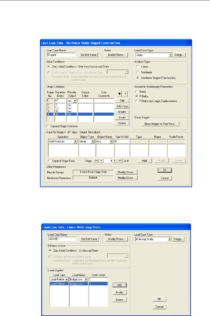
CHAPTER 8 - Analysis
8.1.1.2 Nonlinear Staged Construction – Screen Capture
This command (see Table 8-1) displays this form: Analysis > Load
Cases > Type > Nonlinear Staged Construction
8.1.1.3 Multi-Step Static – Screen Capture
This command (see Table 8-1) displays this form: Analysis > Load
Cases > Type > Multistep Static > Add, Copy, Modify
Analysis > Load Cases 8 - 11
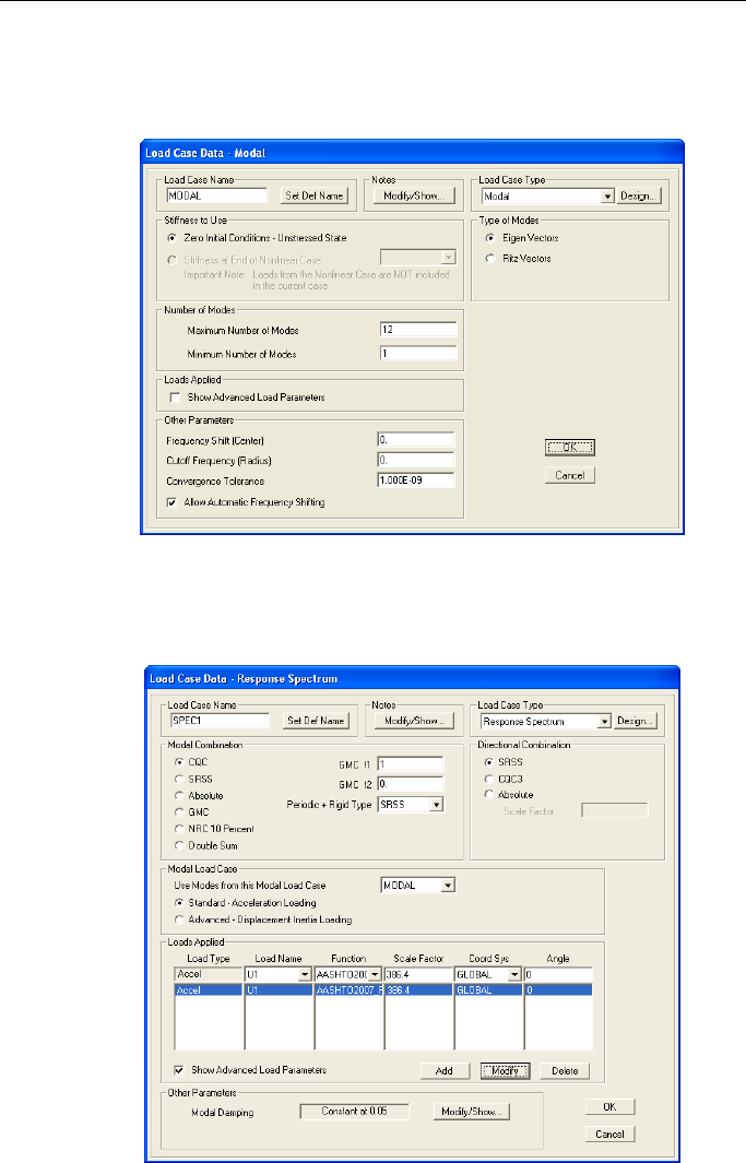
CSiBridge - Defining the Work Flow
8.1.1.4 Modal – Screen Capture
This command (see Table 8-1) displays this form: Analysis > Load
Cases > Type > Modal > Add, Copy, Modify
8.1.1.5 Response Spectrum – Screen Capture
This command (see Table 8-1) displays this form: Analysis > Load
Cases > Type > Response Spectrum > Add, Copy, Modify
8 - 12 Analysis > Load Cases
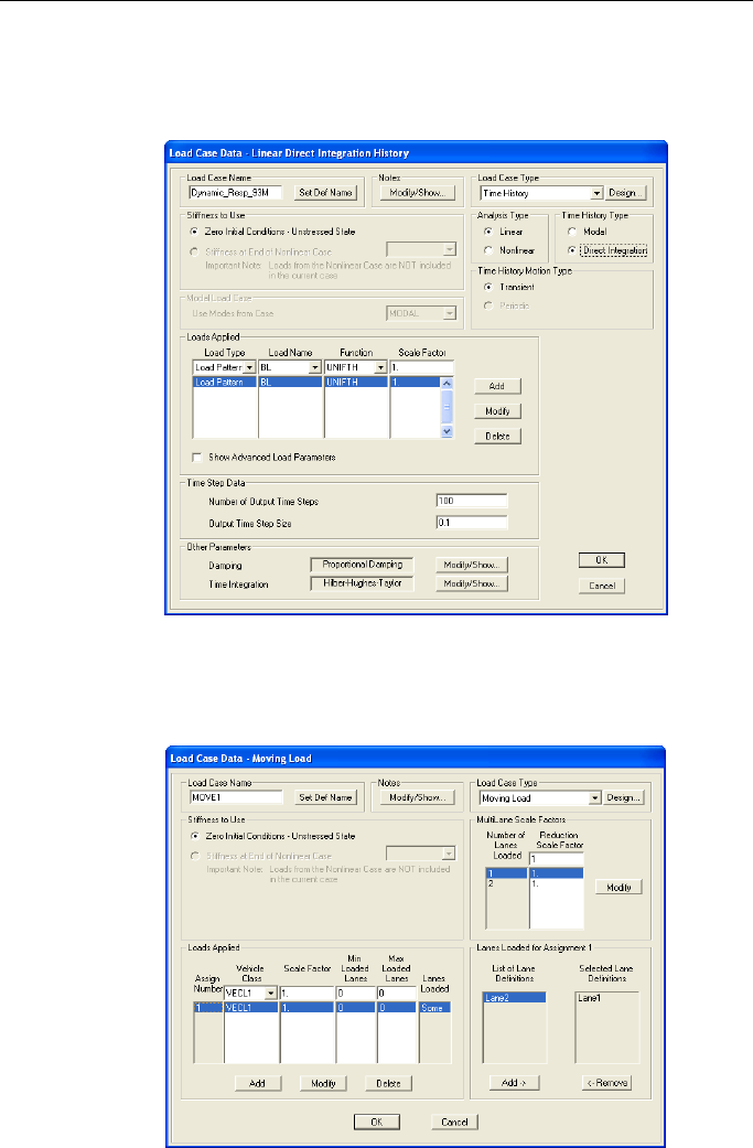
CHAPTER 8 - Analysis
8.1.1.6 Time History – Screen Capture
This command (see Table 8-1) displays this form: Analysis > Load
Cases > Type > Time History > Add, Copy, Modify
8.1.1.7 Moving Load – Screen Capture
This command (see Table 8-1) displays this form: Analysis > Load
Cases > Type > Moving Load > Add, Copy, Modify
Analysis > Load Cases 8 - 13
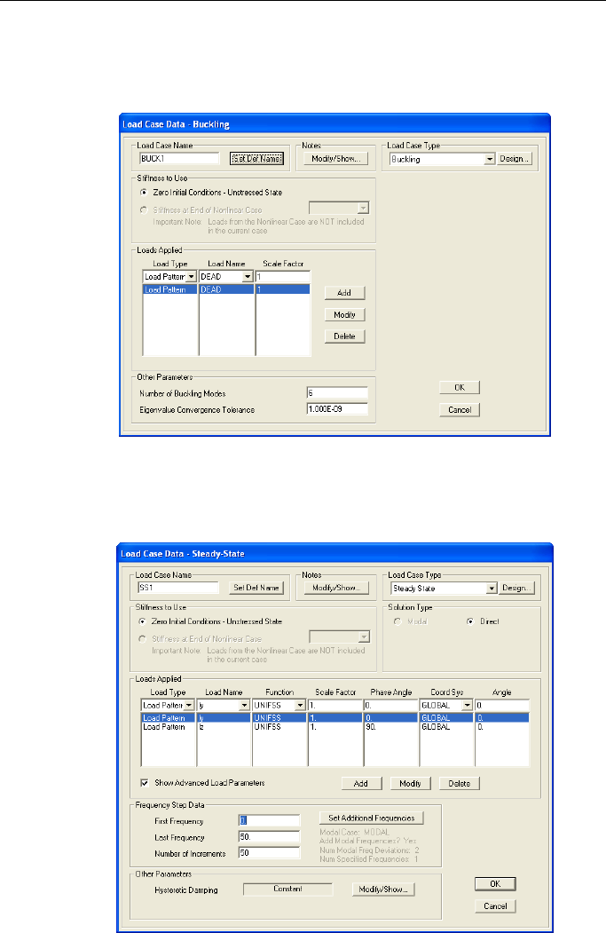
CSiBridge - Defining the Work Flow
8.1.1.8 Buckling – Screen Capture
This command (see Table 8-1) displays this form: Analysis > Load
Cases > Type > Buckling > Add, Copy, Modify
8.1.1.9 Steady State – Screen Capture
This command (see Table 8-1) displays this form: Analysis > Load
Cases > Type > Steady State > Add, Copy, Modify
8 - 14 Analysis > Load Cases
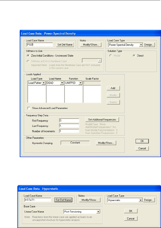
CHAPTER 8 - Analysis
8.1.1.10 Power Spectral Density – Screen Capture
This command (see Table 8-1) displays this form: Analysis > Load
Cases > Type > Power Spectral Density > Add, Copy, Modify
8.1.1.11 Hyperstatic – Screen Capture
This command (see Table 8-1) displays this form: Analysis > Load
Cases > Type > Hyperstatic > Add, Copy, Modify
Analysis > Load Cases 8 - 15
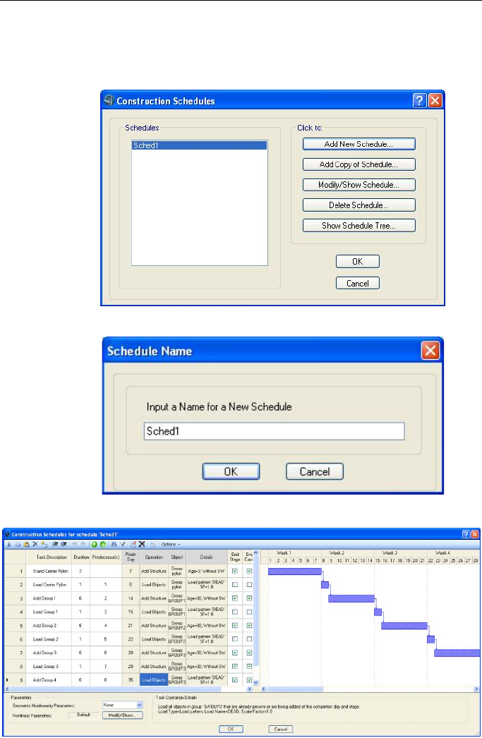
CSiBridge - Defining the Work Flow
8.1.2 Analysis > Load Cases > Schedule Stages – Screen Capture
This command (see Table 8-1) display this form: Analysis > Load Cas-
es > Schedule Stages
> Add New Schedule
Specify a name, then > OK
8 - 16 Analysis > Load Cases
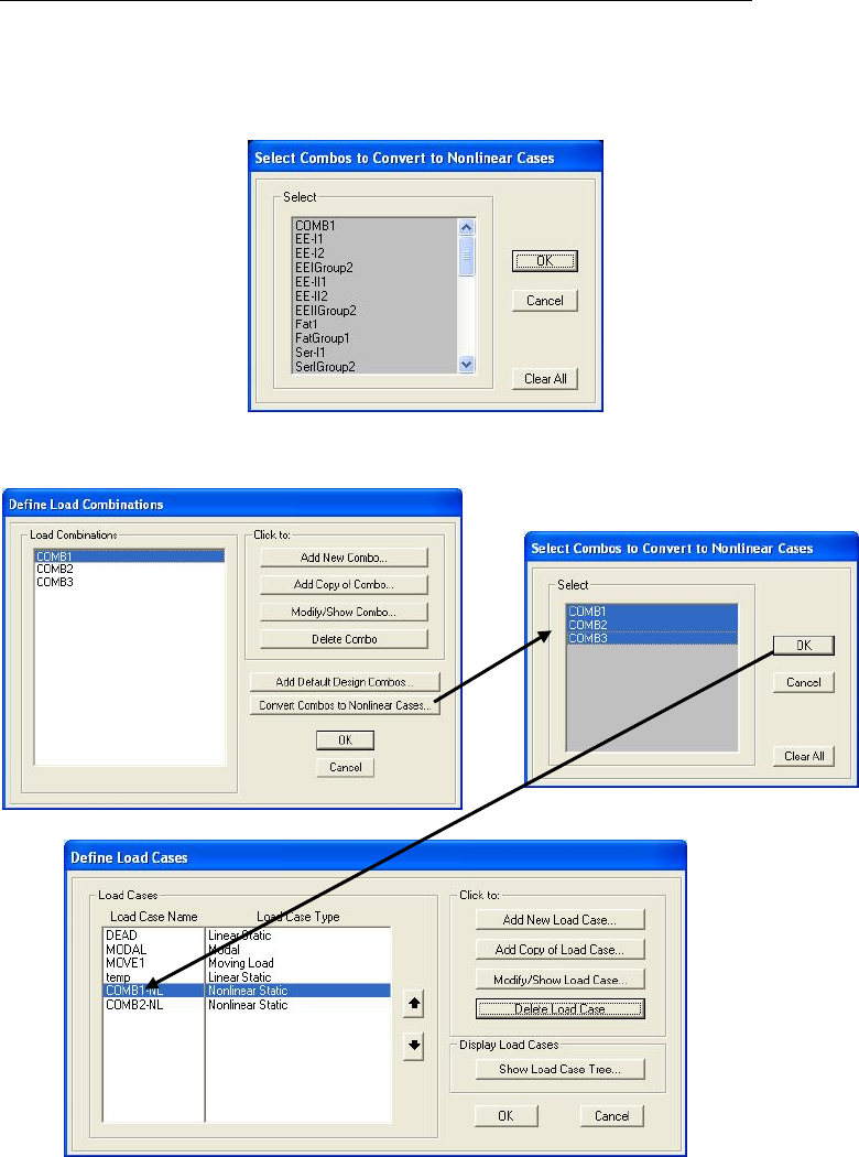
CHAPTER 8 - Analysis
8.1.3 Analysis > Load Cases > Convert Combos – Screen Captures
This command (see Table 8-1) displays this form: Analysis > Load
Cases > Convert Combos
The following forms show combination names that have been converted
(see Chapter 9 Design/Rating for more information).
Analysis > Load Cases 8 - 17
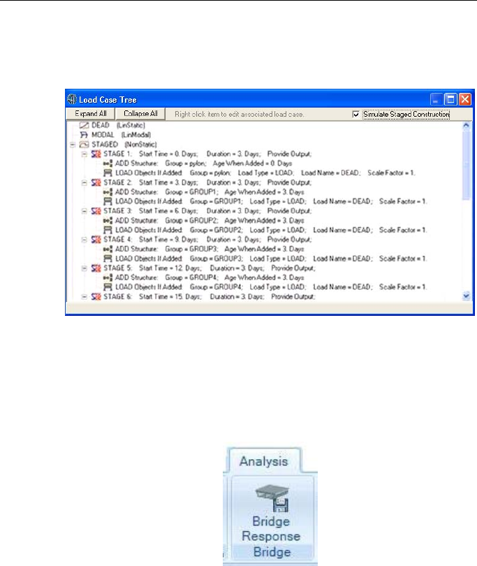
CSiBridge - Defining the Work Flow
8.1.4 Analysis > Load Cases >Show Tree
This command (see Table 8-1) displays this form: Analysis > Load
Cases > Show Tree
8.2 Analysis > Bridge
The Bridge panel on the Analysis tab has only one command: the
Bridge Response command. Figure 8-3 shows the Bridge panel.
Figure 8-3 The Bridge Response command on the
Bridge panel of the Analysis tab
This command displays the Moving Load Case Results Saved form,
shown in Figure 8-4. The options on that form can be used to selectively
control what information is calculated for joints and frame objects in the
computationally intensive moving-load analysis.
8 - 18 Analysis > Bridge
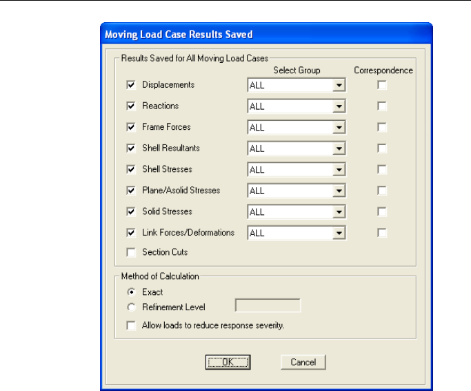
CHAPTER 8 - Analysis
Analysis > Bridge > Bridge Response
Figure 8-4 The Moving Load Case Results Saved form
As shown in Figure 8-4, response calculations can be limited to specific
types of results (e.g., displacements, reactions, and so on), as well as to
specified Groups of model objects, including the groups created by
Bridge Object (see Chapter 7). An option exists to use the Max/Min Cor-
respondence in design of frame sections when using moving loads; note
that this is a very time-intensive operation so use it only when it is re-
quired. The method for calculating responses can be exact or with a
specified degree of refinement, which is used to determine the shape of
the influence line or area surface; this option provides "fast results” for
preliminary review. The larger the integer, the greater the level of re-
finement. The integer reflects the number of points used to define the in-
fluence line or surface discretizations.
Analysis > Bridge 8 - 19
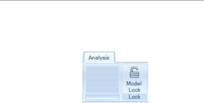
CSiBridge - Defining the Work Flow
8.3 Analysis > Lock
The Lock panel on the Analysis tab has only one command: Model
Lock. Figure 8-5 show the Model Lock command on the Lock panel.
Figure 8-5 The Model Lock command on the
Lock panel of the Analysis tab
This command is a toggle, alternately locking and unlocking the model.
Locking the model prevents changes being made to it. CSiBridge auto-
matically locks the model after running an analysis to prevent any
changes that would invalidate the analysis results. When the model is
locked, commands on the Layout, Components, and Loads tabs and the
Bridge Object > Add, Copy, Modify and Delete commands on the
Bridge tab are not available. Load cases on the Analysis tab, however,
may be used to define or modify a load case when the model is locked. If
the definition of a load case that has already been run is changed,
CSiBridge will display a warning that the analysis results will be deleted
for that case and for all cases that depend on it. Design operations are
performed on a locked model (see Chapter 9 Design/Rating). Commands
that affect groups (Bridge tab), and views and display items (Home tab)
are not locked. When a model for which analysis results are available is
unlocked, CSiBridge will display a warning that unlocking the model
will cause all analysis results to be deleted.
8.4 Analysis > Analyze
The Analyze panel of the Analysis tab has commands that provide direct
access to the forms needed to select the analysis options, run the analy-
8 - 20 Analysis > Lock
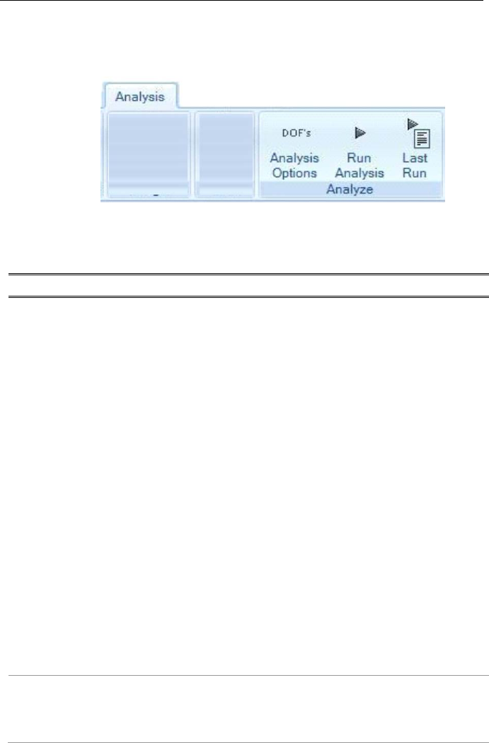
CHAPTER 8 - Analysis
sis, and view the results of the last analysis run. Figure 8-6 shows the
Analyze panel commands.
Figure 8-6 The commands on the Analyze panel
of the Analysis tab
Table 8-2 Analysis > {Command} >
Command
Data / Assignment / Definition Forms
Analysis
Options
Displays the Analysis Options form (see Section 8.4.1). Use that
form to set the available degrees of freedom (DOF). If the DOF is
set as available (i.e., the direction – UX, UY, YX, RX, RY, RZ – is
preceded by a check mark on the form), displacements are possi-
ble in that direction at every joint. The occurrence of a displacement
at a given joint will depend on the structure, loading, and restraint
condi
tions at the joint. If the DOF is not available (i..e, the direction
is not checked on the form), no displacements are possible in that
direction at any joint. Effectively, every joint is restrained in that
direction. Buttons on the form can be used to quickly set the six
available DOF’s to correspond to common structure types.
CSiBridge offers equation solving options (click the Solver Options
button on the form)
. The advanced equation solver can be one or
two orders of magnitude faster than the stand solver for larger prob-
lems, and it also uses less disk space. Because the two solvers
perform numerical operations in a different order, it is possible that
sensitive problems may yield slightly different results be
cause of
numerical roundoffs. In extremely sensitive, nonlinear, history-
dependent problems, the difference may be pronounced. The ad-
vanced solver is based on proprietary CSi technology that uses, in
part, code derived from the TAUCS family of solvers.
An option also is included to automatically save Microsoft Access or
Excel tabular files after each analysis using a specified filename for
a selected set of database tables and grouped objects.
Run Analy-
sis
Displays the Set Load Cases to Run form (see Section 8.4.2). As
the name suggests, use the form to specify the load cases to be
included in the analysis run. The form also can be used to delete
results for a selected load case or for all load case.
Analysis > Analyze 8 - 21
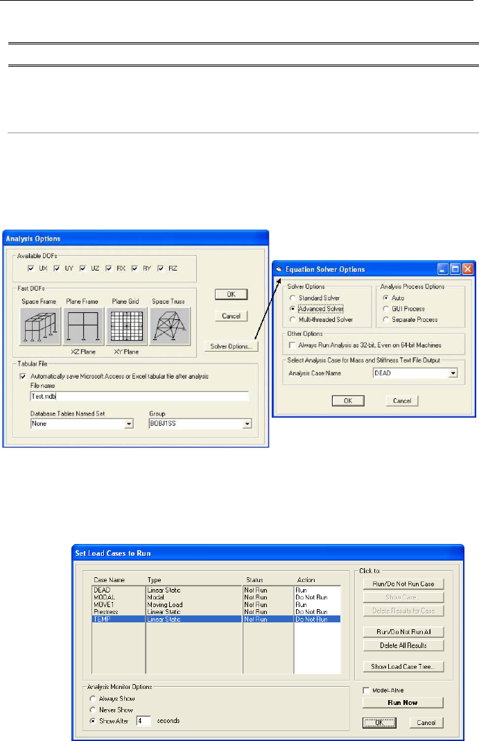
CSiBridge - Defining the Work Flow
Table 8-2 Analysis > {Command} >
Command Data / Assignment / Definition Forms
Last Run
Displays the Analysis Window (see Section 8.4.3), which displays
the most recent analysis
results. The form indicates the filename,
the start and finish times for the analysis run, the elapsed time, and
the run status (e.g., Done – Analysis Complete).
8.4.1 Analyze > Analysis Options – Screen Captures
This command (see Table 8-2) displays these form: Analysis > Analyze
> Analysis Options; click the Solver Options button to display the sec-
ond form.
8.4.2 Analyze > Run Analysis – Screen Capture
This command (see Table 8-2) displays this form: Analysis > Analyze
> Run Analysis
8 - 22 Analysis > Analyze
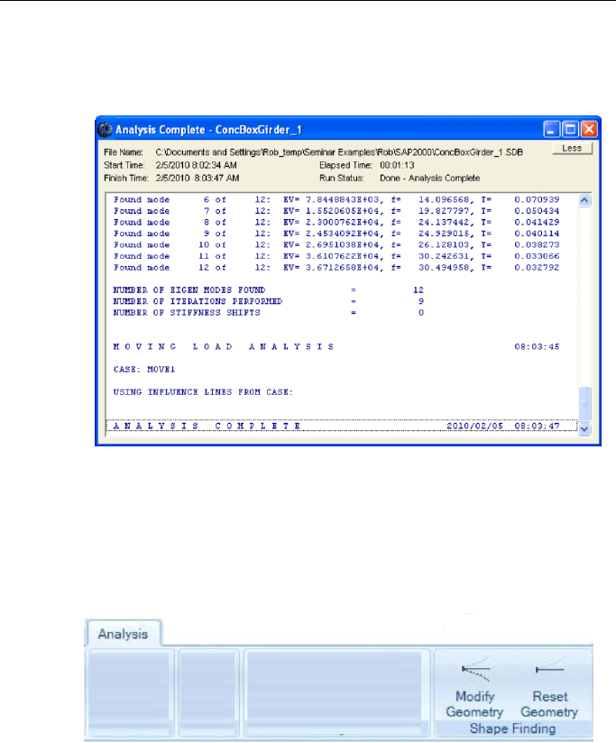
CHAPTER 8 - Analysis
8.4.3 Analyze > Last Run Details
This command (see Table 8-2) displays this form: Analysis > Analyze
> Last Run
8.5 Analysis > Shape Finding
The Shape Finding panel on the Analysis tab has two commands that
work in conjunction: Modify Geometry and Reset Geometry. Figure 8-7
shows the commands on the Shape Finding panel on the Analysis tab.
Figure 8-7 Commands on the Shape Finding panel
of the Analysis tab
After at least one analysis has been run, the Analysis > Shape Finding >
Modify Geometry command can be used to modify the undeformed ge-
ometry of the structure to achieve a desired deformed shape. The original
undeformed geometry of the structure (geometry when the structure was
first defined) is assumed to be the target for the deformed geometry of
Analysis > Shape Finding 8 - 23
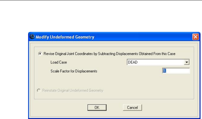
CSiBridge - Defining the Work Flow
the structure under a user-specified load case. Figure 8-8 shows the form
used to apply the modification.
Analysis > Shape Finding > Modify Geometry
Figure 8-8 The form used to modify the undeformed geometry to
achieve a target deformed geometry
A load case is selected and a scale factor for displacement is specified to
modify the shape (inverse of the deflected shape). Use a scale factor
greater than 1 if the convergence toward the target shape is too slow; use
a scale factor less than 1 if the geometry is overshooting the target shape.
Several iterations may be needed to achieve the target for the deformed
shape. If after re-running the analysis the change in geometry signifi-
cantly changes the load-carrying mechanism, convergence may be diffi-
cult. For example, a flexible flat slab may be changed to a domed shape
that is much stiffer. Be aware that the deformed shape of some structures
cannot be determined using this procedure, such as cables and mem-
branes, because their shapes are determined by the loading.
The Analysis > Shape Finding > Reset Geometry command restores
the original geometry.
8 - 24 Analysis > Shape Finding

CHAPTER 9 Design/Rating
The Design/Rating tab consists of the commands that allow efficient ac-
cess to the forms needed to add, copy, or modify load combinations, in-
cluding adding default combinations; set the preferences and create a su-
perstructure design request as well as generate subsequent results; set the
preferences and create a seismic design request as well as generate sub-
sequent results; and set the preferences and generate a bridge load rating
before obtaining results. The preferences include the codes and the nec-
essary parameters for the designs. The available design codes are
AASHTO LRFD 2012, AASHTO STD 2002, CAN/CSA-S6-06 and
EUROCODE for the superstructure design, AASHTO Seismic 2011 for
the bridge seismic design and AASHTO Rating 2011 for the bridge load
rating.
Unlike the other tabs, starting a model using the Quick Bridge template
has no effect on the tasks on the Design/Rating tab (i.e., no defaults as-
sociated with the Design/Rating tab are generated).
Unlike the other tabs, the Bridge Wizard can not be used to complete
any of the tasks associated with the Design/Rating tab.
The commands on the Design/Rating tab can be used if the Blank option
was used to start the model (i.e., the model is being built from scratch or
by importing model data).
Design/Rating > Load Combinations 9 - 1
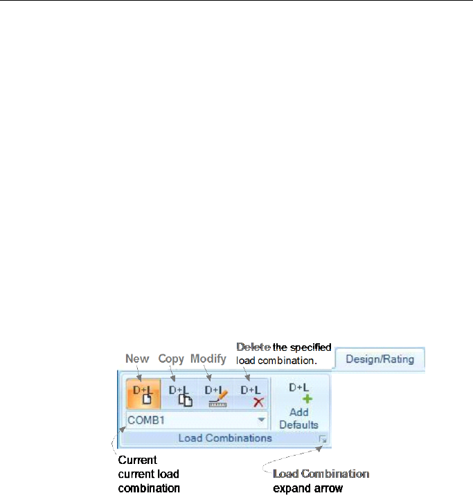
CSiBridge - Defining the Work Flow
9.1 Design/Rating > Load Combinations
In CSiBridge, load combinations are defined by the user manually or
added as defaults based on a selected code. Combinations based on a
code subsequently can be modified to meet specific needs.
Combinations are used in the design process (described later in this
chapter) and may be used when viewing analysis results (see context
sensitive help for the Home > Display > Show Deformed Shape com-
mand). Thus, although combinations may be defined before or after an
analysis has been run, to use them in reviewing results, the analysis must
first be run, and to run a design (i.e., use the combos in design), an anal-
ysis must first be run.
Figure 9-1 shows the commands on the Load Combinations panel on the
Design/Rating tab.
Figure 9-1 Design/Rating tab with annotated
Load Combinations panel
Clicking the expand arrow in the lower right-hand corner of the Load
Combinations panel displays the Define Load Combinations form shown
in Figure 9-2. All of the previously defined Load Combinations are listed
on the left-hand side of the Define Load Combinations form. The buttons
in the “Click to” area on the right-hand side of the form display the same
form − the Load Combination Data form, shown in Figure 9-3 − as is
displayed when the New, Copy, and Modify commands on the Load
Combinations panel are used. Thus, the commands on the Load Combi-
9 - 2 Design/Rating > Load Combinations
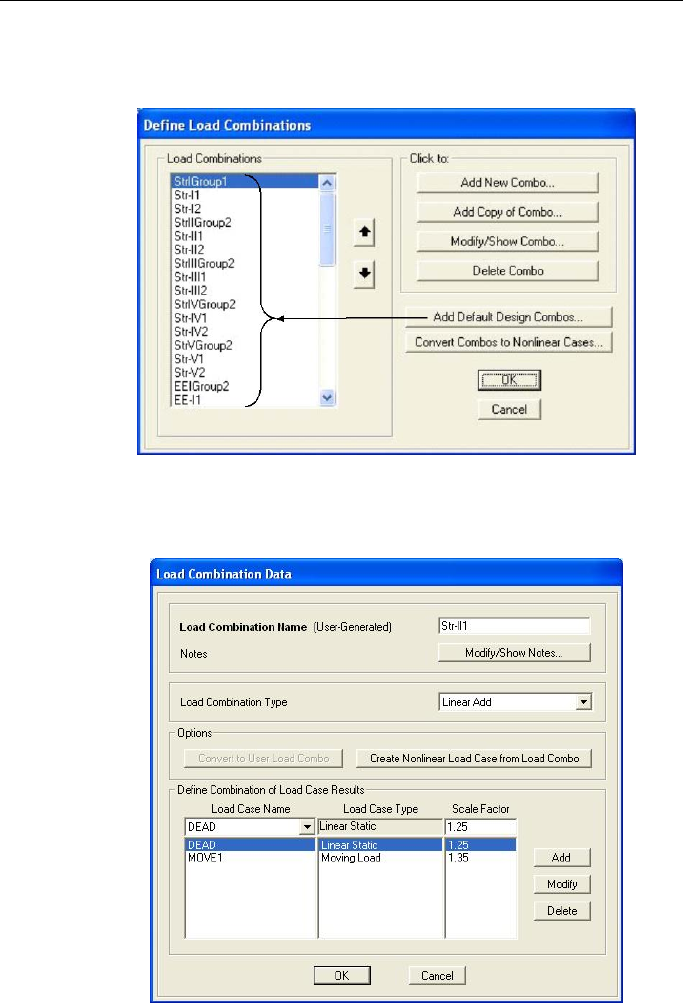
CHAPTER 9 - Design/Rating
nations panel bypass the definitions form (Figure 9-2), creating a
shortcut to the data form used to define a load combination.
Design/Rating > Load Combinations > expand arrow
Figure 9-2 Definition form showing previously defined load combinations;
in this figure, the default design combinations have been added
Design/Rating > Load Combinations > Add, Modify, Copy
Figure 9-3 The data form used to define a load combination manually
Design/Rating > Load Combinations 9 - 3
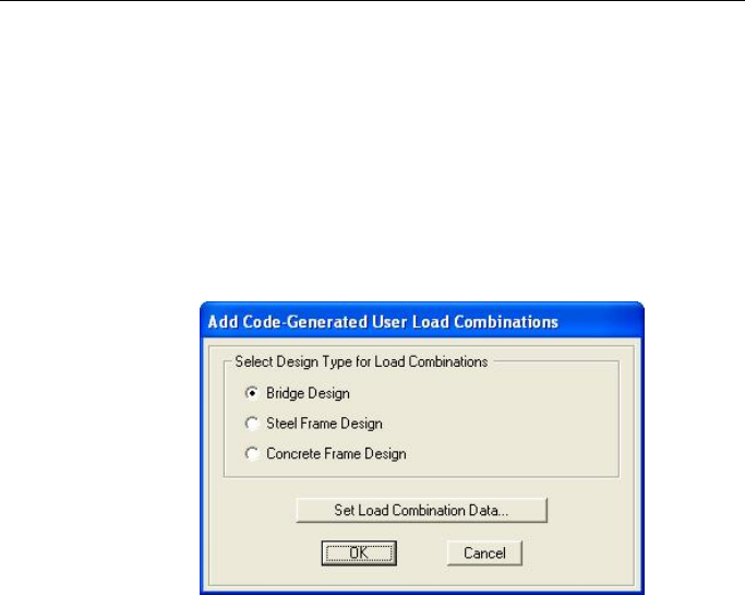
CSiBridge - Defining the Work Flow
The Load Combinations shown on the left-hand side of the form in Fig-
ure 9-2 are an example of default design combinations, which can be
added by clicking the Add Default Design Combos button. That button
duplicates the action of the Design/Rating > Load Combinations >
Add Defaults command (see Figure 9-1). After using the button or the
command, the Add Code-Generated User Load Combinations form
shown in Figure 9-4 displays; that form can be used to select Bridge
Design as the design type.
Design/Rating > Load Combinations > Expand
arrow > Add Default Design Combos button
Figure 9-4 Form used to select the type of design
(and apply the code) as the basis for generating the load combination
The Set Load Combination Data button on that form can be used to
display another form (Figure 9-5) that has a range of options based on
the selected code (see subsequent section on superstructure design and
the Design/Rating > Superstructure Design > Preferences command).
Thus, the load combination generated based on the code can be modified
to meet specific needs, if necessary, using the form shown in Figure 9-5
(or one similar to it).
9 - 4 Design/Rating > Load Combinations
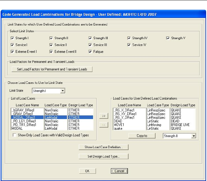
CHAPTER 9 - Design/Rating
Design/Rating > Load Combinations > Expand arrow >
Add Default Design Combos button > Set Load Combination Data button
Figure 9-5 An example of the fom used to review/define a load combination
based on the selected code;
the load cases shown were defined using the Add Defaults command
The Convert Combos to Nonlinear Cases button on the Define Load
Combinations form (Figure 9-2) functions similar to the Create Nonlin-
ear Load Case for Load Combos button on the Load Combination Da-
ta form (Figure 9-3). In both cases, linear static load cases can be con-
verted to nonlinear load cases. This is a convenient way to create a non-
linear load while making use of an existing load combination when non-
linear effects, such as P-Delta, are required. The conversion is immediate
and irreversible.
Table 9-1 briefly explains load combinations and the types of combos
that are available.
Design/Rating > Load Combinations 9 - 5

CSiBridge - Defining the Work Flow
Table 9-1 Load Combinations -- Design/Rating > Load Combinations
Types of
Combos Description
A load combination is a named combination of the results from
load cases (see Chapter 8 Analysis) or other load combinations.
Combo resul
ts include all displacements and forces at the joints
and internal forces or stresses in the elements. Each combo pro-
duces a pair of values for each response quantity: a maximum
and a minimum. For some types of combos, both values are used.
For other type
s, only the value with the larger absolute value is
used.
Each contributing load case is multiplied by a scale factor before
being included in the combo. Five types of combos are available.
Linear Add. All load case results are multiplied by their scale factor and added
together. This Combo Type can be used for static loads.
Envelope
A max/min Envelope of the defined load cases is evaluated for
each frame output segment and object joint. The load cases that
give the maximum and minimum components are
used for this
combo. Therefore the load Combo holds two values for each out-
put segment and joint. The Combo Type can be used for moving
loads and any load case where the load producing the maximum
or minimum force/stress is required.
Absolute
Add The abso
lutes of the individual load case results are summed and
posi
tive and negative values are automatically produced for each
output segment and joint. Use this Combo Type for lateral loads.
SRSS The Square Root Sum of the Squares calculation is performed on
the load cases and positive and negative values are automatically
produced for each output segment and joint. Use this Combo Type
for lateral loads.
Range
The combined maximum is the sum of the positive maximum val-
ues from each of the contributing cases (a case with a negative
maximum does not contribute), and the combined minimum is the
sum of the negative minimum values from each of the contributing
cases (a case with a positive minimum does not contribute). This
Combo Type is useful for pattern or skip-
type loading where all
permutations of the contributing load case must be considered.
9 - 6 Design/Rating > Load Combinations
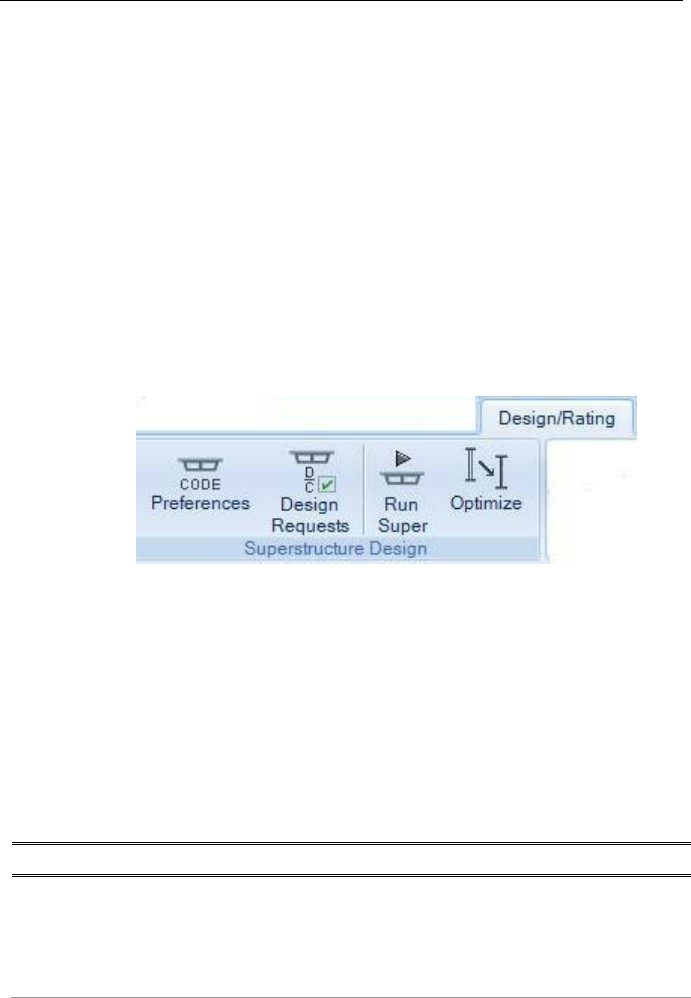
CHAPTER 9 - Design/Rating
9.2 Design/Rating > Superstructure Design
Design using CSiBridge is based on load patterns (see Chapter 6 Loads),
load cases (see Chapter 8 Analysis), load combinations (see previous
section in this chapter), and design requests (described in this section). It
should be noted that the design of a bridge superstructure is a complex
subject and that the design codes cover many aspects of this process.
CSiBridge is a tool to help the user with that process. Only the aspects of
design documented in CSI’s design manuals (see Recommended Reading
in Chapter 1 Introduction) are automated by the CSiBridge. The user
must check the results produced and address other aspects not covered
by CSiBridge. Figure 9-6 shows the commands on the Superstructure
Design panel on the Design/Rating tab.
Figure 9-6 Commands on the Superstructure Design panel
on the Design/Ratings tab
These commands provide access to the forms needed to select the design
code and other parameters; add, copy, modify, or delete a design request;
select the design request to be run; and optimize design when the bridge
is steel girder bridge.
Table 9-2 explains these commands briefly.
Table 9-2 Commands on the Design/Rating > Superstructure Design Panel
Command
Description
Preferences
Displays the Bridge Design Preferences form (see Section 9.2.1).
Use this form to set the design code, and if available, other design
parameters. Note that similar Preference commands are available
on the Seismic Design and Load Rating panels on the De-
sign/Rating tab.
Design/Rating > Superstructure Design 9 - 7

CSiBridge - Defining the Work Flow
Table 9-2 Commands on the Design/Rating > Superstructure Design Panel
Command Description
Design
Request Displays the Bridge Design Requests – {Code} form. That form is
used to add, copy, modify, and delete design requests. The Add
New Request, Add Copy of Request, and Modify/Show Re-
quest buttons provide access to the Bridge Design Request form
(see Section 9.2.2). The design request definition requires a
unique design request name, selection of the bridge object for
which the design request is being defined; the check type (flexure,
stress shear, and so on), station range (portion of the bridge to be
designed), design parameters (e.g., stress factors), demand sets
(loading combinations – see previous section), and where applica-
ble live load distribution factors.
> Check Type – Determines the check to be completed when the
design request is run. The list of available check types reflects
the deck types used in the specified Bridge Object; that is, the
checks that are possible are relevant to the deck type used in
the Bridge Object.
> Station Ranges –
Defines the start and end locations to be
considered in the superstructure design. Use the station range
to specify that the design is to be carried out over the entire
length of the bridge or in just a particular zone. Multiple zones
may be specified within a single design request.
> Demand Sets –
Identifies the load combination to be used in
the design. Multiple demand sets may be defined for a single
design request.
The combinations selected for Bridge Design
typically will be envelopes of other combinations, and the design
will be performed for each combo within the selected enveloping
combo.
> Live Load Distribution Factors (LLDF) to Girders – Some
check types include consideration of LLDFs. Users can chose
how these factors are determined: user specified; in accord-
ance with the code; directly from individual girder forces from
CSiBridge; or uniformly distributed onto all girders. Note that the
only time multiple lanes are necessary for a design is when the
“directly from individual girder forces from CSiBridge” method is
selected. Otherwise, moving live loads should be applied to only
a single lane. The extent to which a vehicle load may be applied
to a bridge deck is defined in the bridge deck definition (see
Components > Superstructure > Deck Sections).
Run Super
Displays the Perform Bridge Design – Superstructure form (see
Section 9.2.3). Use the form to select the design request to be run.
Note that an analysis must be run before a superstructure design
can be run. This is the case because each load case that is part of
a load combination that is included in a design request must be
9 - 8 Design/Rating > Superstructure Design
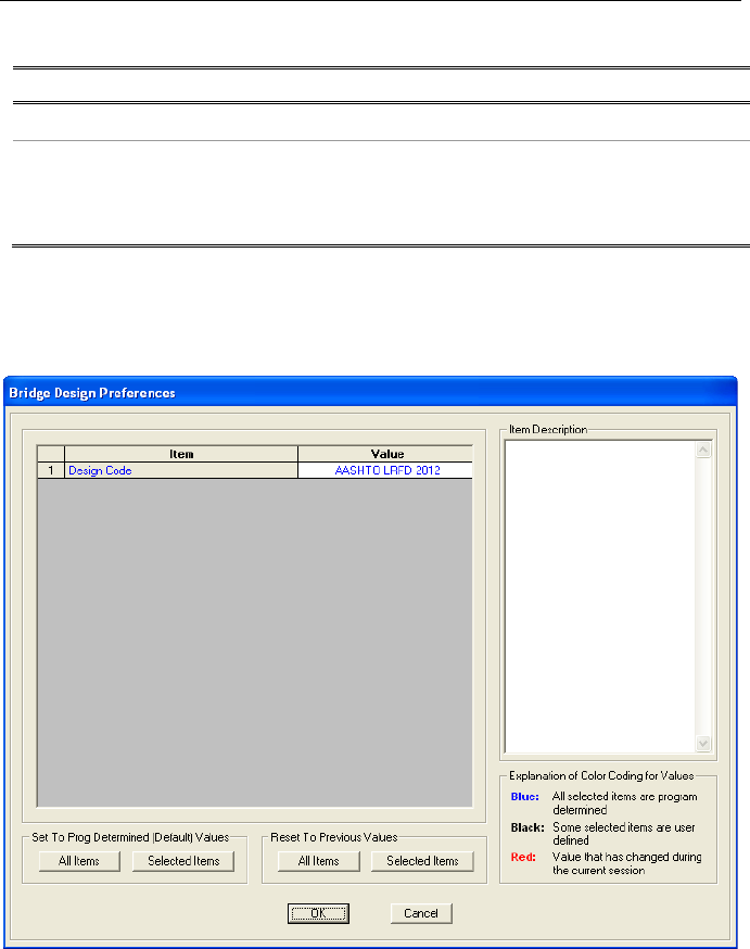
CHAPTER 9 - Design/Rating
Table 9-2 Commands on the Design/Rating > Superstructure Design Panel
Command Description
run before starting superstructure design.
Optimize
Display the Bridge Object Superstructure Design and Optimization
form (see section 9.2.4). After analysis and design of a steel girder
bridge model has been completed, use the options on this form to
interactively optimize design of the bridge model.
9.2.1 Superstructure Design > Preferences – Screen Capture
This command displays this form:
Design/Rating > Superstructure Design > Preferences
Design/Rating > Superstructure Design 9 - 9
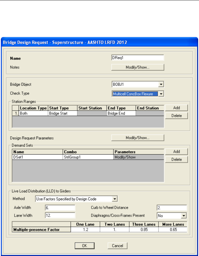
CSiBridge - Defining the Work Flow
9.2.2 Superstructure Design > Design Requests – Screen Capture
This command displays this form:
Design/Rating > Design Requests > Add, Copy, Modify button
9 - 10 Design/Rating > Superstructure Design
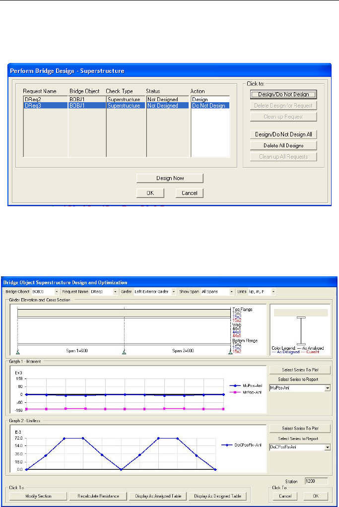
CHAPTER 9 - Design/Rating
9.2.3 Superstructure Design > Run Super – Screen Capture
This command displays this form:
Design/Rating > Superstructure Design > Run Super
9.2.4 Superstructure Design > Optimize – Screen Capture
For a steel bridge after an analysis and design has been run, this com-
mand displays this form: Design/Rating > Superstructure Design >
Optimize
Design/Rating > Superstructure Design 9 - 11
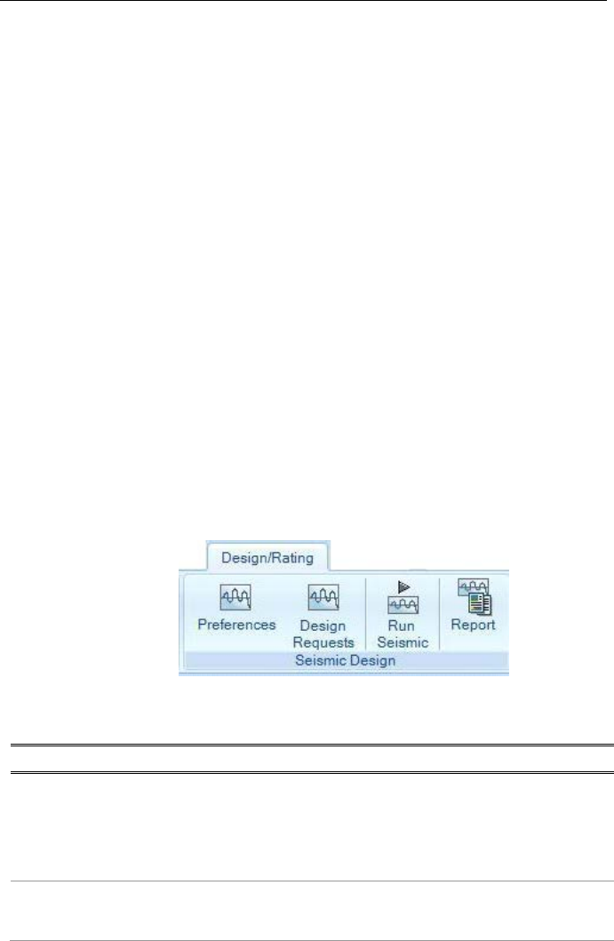
CSiBridge - Defining the Work Flow
9.3 Design/Rating > Seismic Design
CSiBridge allows engineers to define specific seismic design parameters
to be applied to the bridge model during an automated cycle of analysis
through design. By making appropriate definitions using Components >
Properties (Chapter 5), Loads > Functions – Response Spectrum
(Chapter 6), and Analysis > Load Cases > Static > Nonlinear Static
(Chapter 8), engineers may use CSiBridge to automate the determination
of cracked section properties, response spectrum demand analyses as
well as the nonlinear static pushover analyses, or use program defaults.
Furthermore, CSiBridge will determine the displacement demand/
capacity ratios for the Earthquake Resisting System (ERS).
Figure 9-7 shows the Seismic Design panel on the Design/Rating tab.
These commands provide access to the forms needed to select the design
code and other parameters; add, copy, modify, or delete a design request,
including specify design parameters, such as the response spectrum
function and pushover target displacement ratio among several other pa-
rameters; select the design request to be run; and generate a summary
input and seismic design output report. Table 9-3 explains these com-
mands briefly.
Figure 9-7 The Seismic Design panel on the Design/Rating tab
Table 9-3 Commands on the Design/Rating > Seismic Design Panel
Command
Description
Preferences
Displays the Bridge Design Preferences form (see Section 9.3.1).
Use that form to set the design code, and if available, other design
parame
ters. Note that similar Preference commands are available
on the Superstructure Design and Load Rating panels on the De-
sign/Rating tab.
Design
Request Displays the Bridge Seismic Design Requests – {Code} form. That
form is used to add, copy, modify, and delete design requests. The
Add New Request, Add Copy of Request, and Modify/Show
9 - 12 Design/Rating > Seismic Design

CHAPTER 9 - Design/Rating
Table 9-3 Commands on the Design/Rating > Seismic Design Panel
Command Description
Request buttons provide access to the Bridge Design Request –
Substructure Seismic – {Code} form (see Section 9.3.2). That form
is used to specify a unique name for the design request and to
select the Bridge Object to which the design applies; clicking the
Design Request Parameters Modify/Show
button displays the
Substructure Seismic Design Request Parameters form (see Sec-
tion 9.3.2). That form can be used to select the response spectrum
function to be used in a particular design as well as the seismic
design category and other seismic design parameters. If founda-
tions have been included in a bridge model
, Support Structure
should be selected as a Bridge Group Type on the Bridge Con-
struction Group Definition form so that the Bridge Object creates a
group(s) of the support structures
for use in this seismic design
(Bridge > Bridge Object > Groups command); then, in this form,
the Bridge Object that includes the support structure group should
be selected for the Foundation Group item (shown as number 22
in the figure in Section 9.3.2)
Run Seismic Displays the Perform Bridge Design – Seismic form (see Section
9.3.3). Use that form to specify the seismic design to be run.
Report A summary input and seismic design output report will be generat-
ed. The report will contain a table of contents and the images of all
of the pushover plots as well as the output data files contained in
the table seismic design summaries.
Design/Rating > Seismic Design 9 - 13

CSiBridge - Defining the Work Flow
9.3.1 Seismic Design > Preferences – Screen Capture
Use this command to display this form:
Design/Rating > Seismic Design > Preferences
9 - 14 Design/Rating > Seismic Design
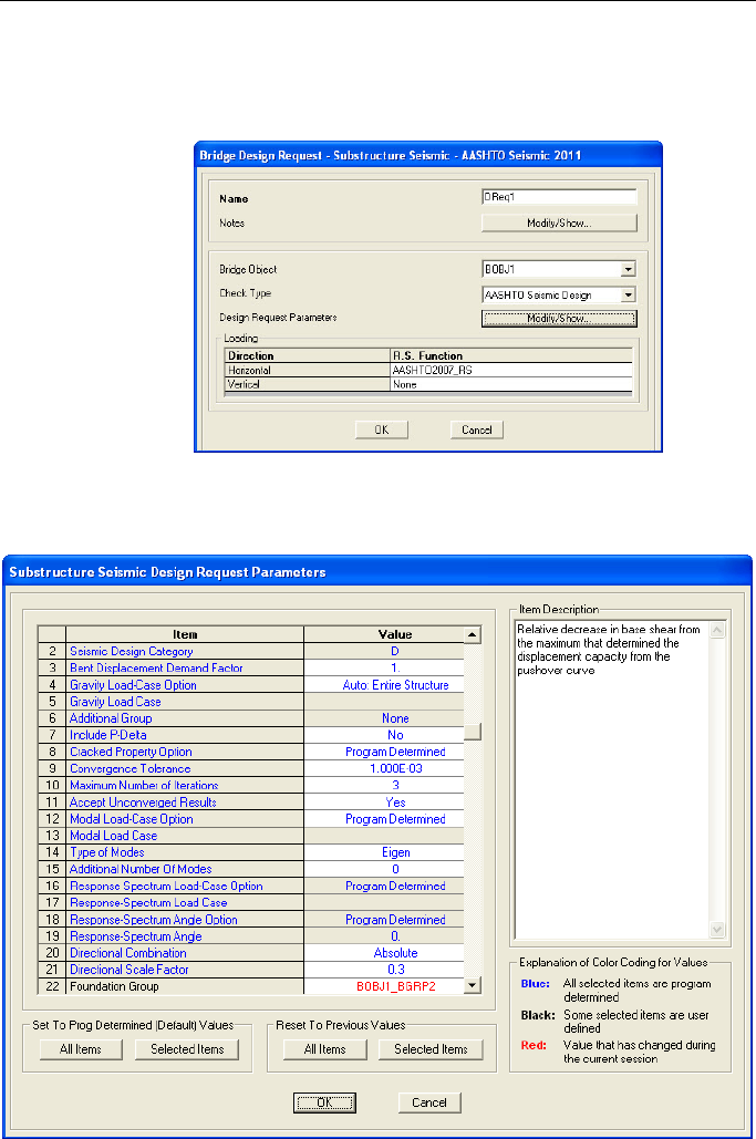
CHAPTER 9 - Design/Rating
9.3.2 Seismic Design > Design Requests – Screen Capture
This command displays this form:
Design/Rating > Seismic Design > Design Requests
This command displays this form:
Design/Rating > Seismic Design > Design Requests
.
Design/Rating > Seismic Design 9 - 15
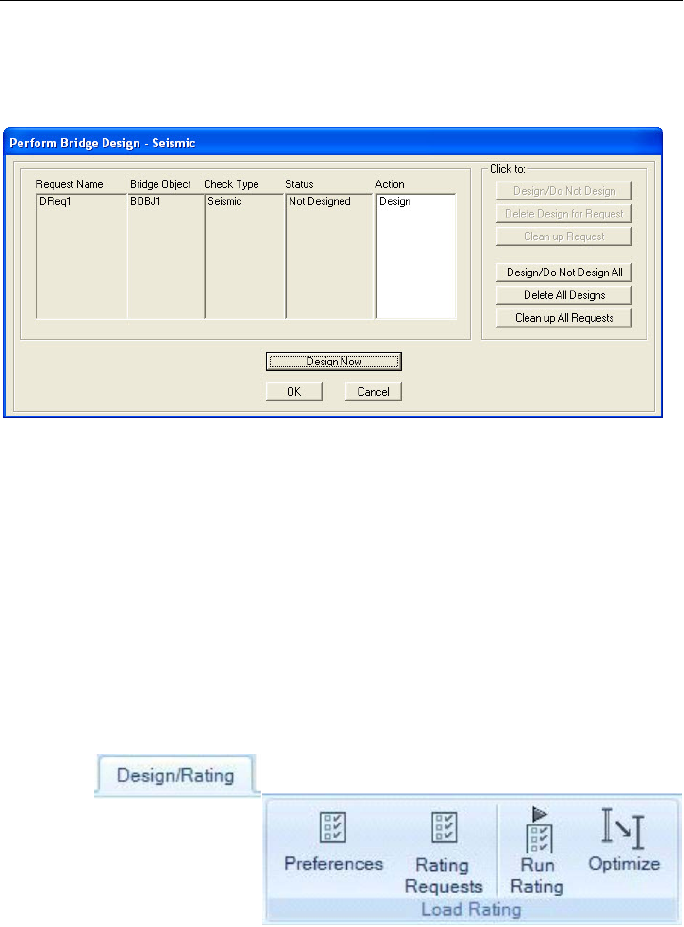
CSiBridge - Defining the Work Flow
9.3.3 Seismic Design > Run Seismic – Screen Capture
This command displays this form:
Design/Rating > Seismic Design > Run Seismic
9.4 Design/Rating > Load Rating
CSiBridge may be used to determine the Load Rating of a concrete
bridge. Three different bridge deck types may be rated. For a complete
description of the load rating algorithms and methodology, display the
Bridge Rating Manual using the Help > Documentation > Bridge
command. A brief description of the deck types and applicable codes and
equations follows.
Figure 9-8 shows the Load Rating panel on the Design/Rating tab.
Figure 9-8 The Load Rating panel on the Design/Rating tab
These commands provide access to the forms needed to select the rating
code and other parameters; add, copy, modify, or delete a rating request,
including specify rating parameters, such as the response spectrum func-
9 - 16 Design/Rating > Load Rating

CHAPTER 9 - Design/Rating
tion and pushover target displacement ratio among several other parame-
ters; and select the rating request to be run. Table 9-4 explains these
commands briefly.
Table 9-4 Commands on the Design Rating > Load Rating Panel
Command
Description
Preferences
Displays the Bridge Design Preferences form (see Section 9.4.1).
Use this form to set the design code, and if available, other design
parame
ters. Note that similar Preference commands are available
on the Superstructure Design and Seismic Design panels on the
Design/Rating tab.
Rating
Requests
Displays the Bridge Rating Requests – {Code} form. That form is
used to add, copy, modify, and delete rating requests. The Add
New Request, Add Copy of Request, and Modify/Show Re-
quest buttons provide access to the Bridge Rating Request – Su-
perstructure – {Code} form (see Section 9.4.2). The rating request
definition requires a unique rating request name, selection of the
Bridge Object to which the rating request applies; the rating type
(flexure, minimum rebar,
shear), station range (portion of the
bridge to be rated), design rating parameters (e.g., flexure), and
demand sets (loading combinations – see Section 9.1).
> Rating Type –
Determines the rating check to be completed
when the rating request is run. The list of available rating types
reflects the deck types used in the specified Bridge Object; that
is, the rating that are possible are relevant to the deck type used
in the Bridge Object.
> Station Ranges – The Station Ranges specify where the rating
ap
plies. Use the start and end options to specify that the rating
be performed for the entire length of the bridge or for just a par-
ticular zone. Multiple zones may be specified within a single rat-
ing request.
> Design Rating Parameters > Modify/Show
button. Displays
the Superstructure Design Request Parameters form. Use the
form to specify v
arious parameters (e.g., phi factors for flexure,
rupture and moment for minimum rebar, phi factors for shear
along with positive and negative strain limits), depending on the
rating type selected.
> Demand Sets – Identifies the load combination to be used in
the rating. Multiple demand sets may be defined for a single rat-
ing request. The rating factor is a ratio of the superstructure re-
serve capacity moment to the bridge live load demand moment.
Design/Rating > Load Rating 9 - 17
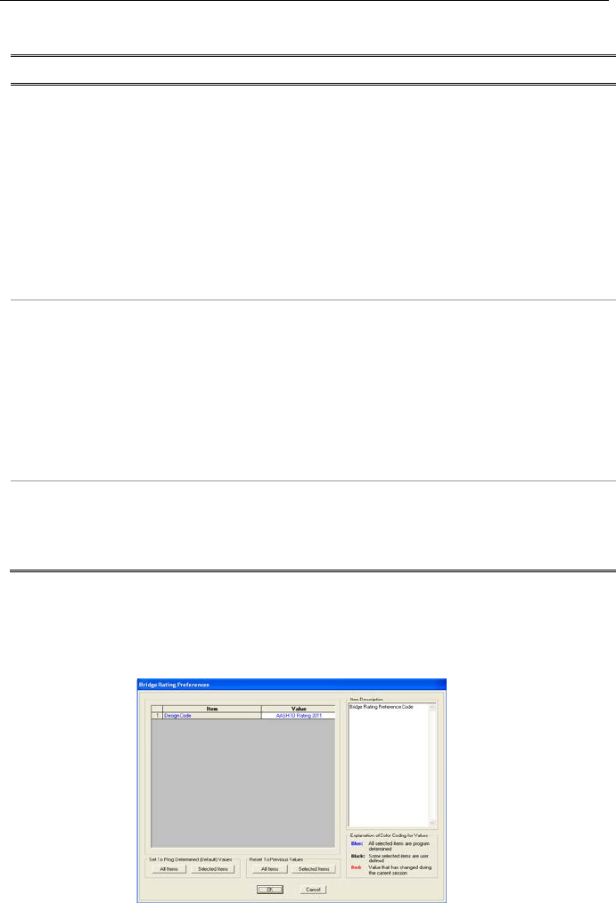
CSiBridge - Defining the Work Flow
Table 9-4 Commands on the Design Rating > Load Rating Panel
Command Description
> Live Load Distribution Factors (LLDF) to Girders – Some
ratin
g types include consideration of LLDFs. Users can chose
how these factors are determined: user specified; in accord-
ance with the code; directly from individual girder forces from
CSiBridge; or uniformly distributed onto all girders. Note that the
only time multiple lanes are necessary for a design is when the
“directly from individual girder forces from CSiBridge” method is
selected. Otherwise, moving live loads should be applied to only
a single lane. The extent to which a vehicle load may be applied
to a
bridge deck is defined in the bridge deck definition (see
Components > Superstructure > Deck Sections).
Run Rating Displays the Perform Bridge Superstructure Rating form (see Sec-
tion 9.4.3). Use the form to select the rating request to be run.
Note that an analysis must be run before a rating request can be
run. This is the case because each load case that is part of a load
combination that is included in a rating request must be run before
starting superstructure rating. After the rating has been run, the
Bridge Object Response Display form is called up (see Section
9.4.3). The form shows the bridge response plot for the forces,
stresses, and design/rating.
Optimize Displays the Bridge Object Superstructure Design and Optimiza-
tion form (see Section 9.4.4). After analysis and design of a steel
girder bridge model has been completed, use the options on this
form to interactively optimize rating of the bridge model.
9.4.1 Load Rating > Preferences – Screen Capture
This command displays this form:
Design/Rating > Load Rating > Preferences
9 - 18 Design/Rating > Load Rating
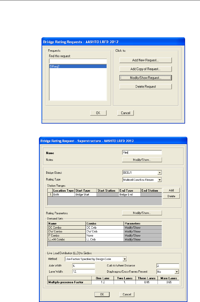
CHAPTER 9 - Design/Rating
9.4.2 Load Rating > Rating Requests – Screen Capture
This command displays this form:
Design/Rating > Load Rating > Rating Requests
> Add New Request
Design/Rating > Load Rating 9 - 19
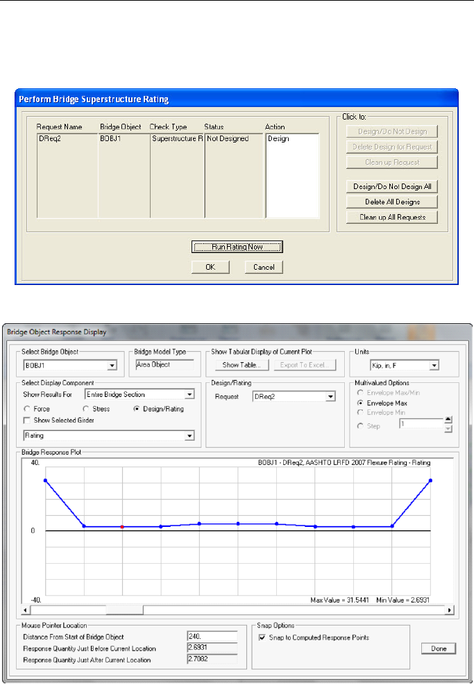
CSiBridge - Defining the Work Flow
9.4.3 Load Rating > Run Rating – Screen Capture
These commands display these forms:
Design/Rating > Load Rating > Run Rating
> Design Now
Plot of the Load Rating Response – Note that the rating factor of
2.7082 at station point 240 denotes that the bridge is adequate to support
9 - 20 Design/Rating > Load Rating
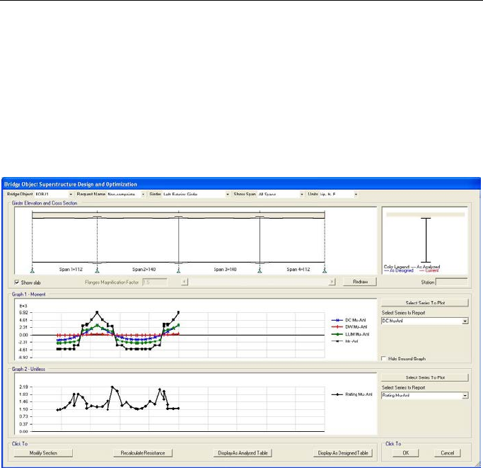
CHAPTER 9 - Design/Rating
a vehicle weighing 2.7082 times greater than the vehicle used to load the
bridge.
9.4.4 Load Rating > Optimize – Screen Capture
For a steel bridge after an analysis and design has been run, this com-
mand displays this form: Design/Rating > Load Rating > Optimize
Design/Rating > Load Rating 9 - 21

CHAPTER 10 Advanced
The Advanced tab consists of the commands that can be used to edit se-
lected objects; add definitions; draw objects (e.g., areas, special joints,
frames, cables and tendons); assign definitions to joints, frames, areas,
cables, tendons, solids, links/supports; assign loads to selected joints,
frames, areas, cables, tendons, solids, link/supports; complete steel and
concrete frame design, overwrite frame design procedures, specify lat-
eral bracing; and add plug ins. The majority of these commands must be
used when the model is unlocked. These commands can be used irre-
spective of how the bridge model was initiated: the using Quick Bridge
template, the Bridge Wizard, or the Blank option (i.e., the model is being
built “from scratch” or by importing model data). A bridge model can be
created, analyzed, and designed in CSiBridge without using any of the
commands on this tab.
The Advanced tab has eight panels: Edit, Define, Assign, Assign Loads,
Analyze, Frame Design, and Tools. Tables 10-1 through 10-7 briefly de-
scribe the commands on the various panels.
10.1 Advanced > Edit
Table 10-1 describes the commands on the Edit panel of the Advanced
tab.
Advanced > Edit 10 - 1

CSiBridge - Defining the Work Flow
Table 10-1 Advanced > Edit
Command Description
> Points
> Add Grid at Selected Points – Use to add grid lines in the
current coordinate/grid system.
> Merge Joints – Use to automatically merge selected joints with
the default auto merge tolerance of one another.
> Align Points – Use to align selected points with the specified
X, Y, or Z coordinates or to the nearest line.
> Disconnect – All objects connected to each other normally
share a common joint. Use this command to break off the ob-
jects from the joint and will add duplicate joints to each of those
objects.
> Connect – Use in conjunction with the Disconnect command
to connect all selected objects that have been disconnected
from each other or that were connected to independent joints.
When objects are reconnected, the independent joints are col-
lapsed into a common joint that is shared by all the combined
objects.
> Lines
> Divide Frames – Use to divide a selected frame into user-
specified segments of user-defined size, or break a frame at in-
tersections with selected frames and joints.
> Join Frames – Use to immediately join the selected frame
objects into a single object and remove unused joints remain-
ing after the joining process.
> Trim/Extend Frames – Use to lengthen frame elements that
are too short, or shorten frame element that are too long.
> Edit Curved Frame Geometry – Use to edit selected curved
frame objects. Only one object can be edited at a time.
> Edit Cable Geometry – Use to edit selected cable objects.
Only one object can be edited at a time.
> Edit Tendon Profile – Use to edit a line object drawn as a
tendon.
> Areas
> Divide Areas – CSiBridge allows area objects to be divided
into smaller objects in the object-based model, and meshed in-
to elements in the analysis model. Dividing the object is ac-
complished using this command. Meshing an area object is ac-
complished using the Advanced > Assign > Areas > Auto-
matic Area Mesh command.
10 - 2 Advanced > Edit

CHAPTER 10 - Advanced
Table 10-1 Advanced > Edit
Command Description
> Merge Areas – Merge selected area objects that are in the
same plane and share a common edge or with overlapping ar-
ea edges.
> Expand/Shrink Areas – Use to specify offsets for area edges
to make areas larger or smaller.
> Add Point to Area Edge – Add collinear points to the edges of
area objects.
> Remove Points from Area – Remove selected points from the
edges of area objects.
> More
> Undo/Redo – Use the Undo command to reverse an action
performed during the modeling process back to the last time
the model was saved. If the command is used for too many
steps, the steps will begin to be “redone.” Use the Redo com-
mand to restore an action performed during the modeling pro-
cess.
> Cut, Copy, Paste – Work similar to standard, cut, copy, and
paste Windows commands. The entire structure or any select-
ed part of it may be cut or copied and then pasted back into the
model at any user-specified location.
> Delete – Deletes selected objects.
> Add to Model From Template – Add objects to a model using
a template.
> Interactive Database Editing – Use to create or edit model
defini
tion data in a tabular format rather than in graphical mode
or using the Draw or Assign menu forms. Only model definition
data (not analysis results or design data) can be edited in this
way. The model must be unlocked to use this feature.
> Replicate – Replicate is a very powerful way of generating a
large model from a small model when the objects and/or joints
form a linear or radial pattern or are symmetrical about a plane.
When joints or objects are replicated, the assignments on
those joints and objects are also replicated (for example, mem-
ber section assign
ments, member loads, joint loads and joint
restraints). This is a major benefit of using Replicate rather
than the Cut, Copy and Paste commands, which can be used
to cut, copy, or paste lines, areas and joints but not their as-
signments or loads.
> Areas
(continued)
Advanced > Edit 10 - 3

CSiBridge - Defining the Work Flow
Table 10-1 Advanced > Edit
Command Description
> Extrude – Use to sweep selected objects through space to
create new objects of higher dimension or to convert lines to
areas and areas to solids with the same thickness as the orig-
inal line or area object. The process of extrusion increases the
dimensional space of an existing object by one. In other
words, line objects are of one dimension that can be generat-
ed from a dimensionless object, the point object. In a similar
manner, a two-dimensional object, area or plate/shell can be
generated from a one-dimensional object, the line object. This
feature is especially suited to creating solid objects from
plate
/shells, plate/shell objects from beams and
beams/columns from points/nodes.
> Move – Use to move selected parts of a structure to a new
location in the model.
> Divide Solids – Use to divide selected solid objects on all
faces.
> Show Duplicates – Use to verify that duplicates are included
in the model and, if so, where they are located. Duplicate ob-
jects can be defined as objects of the same type (joints,
frames, shells, a
solids, solids and so forth) that have the
same coordinates in the model. If duplicate objects are un-
necessary, this command is useful in locating them so that
they can be deleted or merged. Duplicates can not be drawn
or created; they can result when data is imported from other
programs, such as AutoCAD, CIS/2 Step and so on.
> Merge Duplicates – Use in conjunction with the Show Dupli-
cates command to combine duplicate objects into one object.
> Change Labels – By default, the names (labels) of the ob-
jects and all defined entities (loads, properties, and so on) in
the model are sequentially designated by the program using
alphanumeric characters. Use this command to access the In-
teractive Name Change form and change the name of any of
the named items.
10.2 Advanced > Define
Table 10-2 describes the command on the Define panel of the Advanced
tab.
> More
(continued)
10 - 4 Advanced > Define

CHAPTER 10 - Advanced
Table 10-2 Advanced > Define
Command Description
> Section
Properties
Use the subcommands to add area section, solid property, fre-
quency dependent property, and hinge property definitions.
> Mass
Source
Specify how CSiBridge calculates mass for the model. In
CSiBridge, mass and weight serve different func
tions. Mass is
used for the inertia in dynamic analyses, and for calculating the
built-in acceleration loads. Weight is a load that users define and
assign in one or more loads (see Assign - Area Loads, Frame
Loads, Cable Loads, Ten
don Loads, Joint Loads, Link Loads,
and Solid Loads), which can then be applied in one or more load
cases.
> Coordinate
Systems/
Grids
Coordinate systems are defined by specifying their origins and
orientations with respect to the fixed Global coordinate system.
They are used to define the location and orientation of the asso-
ciated grid system. Thus, coordinate systems are always defined
as part of a coordinate/grid system pair. However, when only a
coordinate system is needed, such as when viewing the model,
defining the model (object local axes, loads, and the like), and
reporting results, a coordinate/grid system can be defined with no
grid lines.
A grid system is a set of intersecting lines used to aid in drawing
the model. Grid systems may be Cartesian (rectangular), cylindri-
cal, or general. Each grid system is defined with respect to its
own coordinate system, so, as indicated previously, grid and co-
ordinate systems are defined together as a single entity. An un-
limited number of coordinate/grid systems can be defined, each
with a unique name. A regular system is any coordinate/grid sys-
tem having a Cartesian (rectangular) or cylindrical grid system. A
general system is a system comprised of arbitrarily defined grid
lines.
> Joint
Con-
straints
Add, modify, or delete constraint definitions. Rigid-type con-
straints are those when all joints in the constraint move together
as some type of rigid body. Rotational and translational degrees
of freedom may be coupled together. Equal-type constraints are
those when individual degrees of freedom of different joints are
identical. These are usually used for connection and for sym-
metry conditions. Interpolation constraints are those when de-
grees of freedom at one joint are interpolated from the degrees of
freedom at some other joints. These are usually used to connect
incompatible meshes.
Advanced > Define 10 - 5

CSiBridge - Defining the Work Flow
Table 10-2 Advanced > Define
Command Description
> Joint
Patterns
Use to specify the name of a joint pattern, which is a set of scalar
val
ues defined at the joints. The specified named joint pattern
can be referenced when assigning temperature or pressure loads
to objects. This feature allows description of more complex distri-
butions of tem
perature and pressure over the structure. Joint
patterns by themselves create no loads on the structure.
> Groups
The concept of groups is the backbone of some powerful tools in
CSiBridge. A group is a collection of objects that is assigned a
unique name. Groups may be used for many different purposes.
Each object may be part of as many groups as needed. All ob-
jects are part of the built-in group named "ALL."
> Section
Cuts
Use to obtain resultant forces acting at section cuts through a
model. Section cuts can be defined before or after an analysis
has been run; however, it is safest to wait until after the analysis
has been run. Typically do not define section cuts, and more im-
portantly, the groups used in the section cut definition, until all
manual meshing of the model (if any) has been completed (see
Frame - Automatic Frame Mesh, Area - Automatic Area Mesh or
Solid - Automatic Solid Mesh for more information about mesh-
ing). If the groups are defined before manual meshing, some of
the point objects that should be in the group may not yet be cre-
ated
> General-
ized Dis-
place-
ments
A generalized displacement is a named displacement measure
that is user defined. It is simply a linear combination of displace-
ment degrees of freedom from one or more joints. For example, a
defined generalized displacement named "DRIFTX" could be the
difference of the UX displacements at two joints on different sto-
ries of a building. Another defined generalized displacement
named AVGRZ could be the sum of three rotations about the Z
axis, each scaled by 1/3.
Generalized displacements are primarily used for output purpos-
es, except that a generalized displacement also can be used to
monitor a displacement-controlled nonlinear static analysis.
> Functions
> Steady State – Use to add, modify, or delete a steady-state
function. A steady-
state function is a list of function values
versus frequency of excitation. Th
e function values in a
steady-state function may be normalized ground acceleration
values or they may be multipliers for specified (force or dis-
placement) load patterns.
10 - 6 Advanced > Define

CHAPTER 10 - Advanced
Table 10-2 Advanced > Define
Command Description
> Functions
(continued)
> Power Spectral Density – Use to add, modify, or delete
power
spectral density functions. A power spectral density
function is a list of function values versus frequency of excita-
tion. The function values in a power-spectral-density function
may refer to normalized ground acceleration values or to mul-
tipliers for specified (force or displacement) load patterns.
This is a probabilistic type of function. Function values are
specified as the square of the input value per unit of frequen-
cy
. In other words, this function should be specified so that the
square-root of the
integral of the function over the frequency
range gives the expected RMS (root-mean-square) magnitude
of loading. Function values may not be negative. The program
defines a default unit constant power spectral density function.
> Named
Property
Sets
> Frame Modifiers, Area Modifiers – A named set of property
modifiers can be applied to a frame or area object during
staged construction to change the property modifiers that
were previously assigned or applied to the object. The effect
of property modifiers in a named set is exactly the same as
the effect of those modifiers that can be assigned directly to
frame and area objects using the
Advanced > Assign >
Frame > Property Modifiers command or the Advanced >
Assign > Area > Area Stiffness Modifiers command. By de-
fault, all objects use the property modifiers that are assigned
to them unless explicitly changed by applying a named set
during staged construction, in which case they replace the
previously assigned or applied property modifiers for all sub-
sequent loading in the analysis. Named sets of property modi-
fiers affect only the element values of the modifiers, not those
that are defined as part of the frame/area section properties.
> Frame Releases – A named set of frame releases can be
applied to a frame objec
t during staged construction to
change the releases that were previously assigned or applied
to the object. The effect of frame releases in a named set is
exactly the same as the effect of those releases that can be
assigned directly to selected frame objects using the Ad-
vanced > Assign > Frame > Releases/Partial Fixity com-
mand
. By default, all frame objects use the releases that are
assigned to them unless explicitly changed by applying a
named set during staged construction, in which case they re-
place the previously assigned or applied releases for all sub-
sequent loading in the analysis.
Advanced > Define 10 - 7

CSiBridge - Defining the Work Flow
Table 10-2 Advanced > Define
Command Description
> Pushover
Parame-
ters Sets
Specify the parameters for displaying pushover curves. The pa-
rameters are saved as a named definition so they can be recalled
and applied quickly.
> Named
Sets
Save the options selected on the various forms used to generate
out
put (tables, curves, and the like) as a definition known as a
Named Set. The options can then be recalled and applied quick-
ly.
10.3 Advanced > Draw
Table 10-3 describes the command on the Draw panel of the Advanced
tab.
Table 10-3 Advanced > Draw
Command Description
> Set Select Mode
CSiBridge has two modes of mouse-cursor operation in a
display window: Draw mode and Select mode. The pro-
gram can be in one mode at a time only. After a new mod-
el has been started, by default, the program is in Select
mode. The mouse cursor is used to select objects before
performing certain editing, assignment, display, and output
operations. When the model is locked, the program is al-
ways in Select mode.
> Set Reshape
Object Mode
In reshape mode, click on an area, line or point object and
modify it in one of several ways. If you have difficulties
using any of the methods, try using the method in a differ-
ent view. A Properties of Object form will display with a
number of Drawing Control options. The controls are as-
sumed to be self-explanatory.
> Draw One Joint
Link
Add a joint link when the model is displayed in a 2-D view.
> Draw Two Joint
Link
Draw a two joint link when the model is displayed in a2-D
view.
> Draw Frame/
Cable/Tendon
Draw a straight or curved frame object, a cable, or a ten-
don.
10 - 8 Advanced > Draw

CHAPTER 10 - Advanced
Table 10-3 Advanced > Draw
Command Description
> Quick Draw
Frame/Cable/
Tendon
Draw a straight or curved frame object, a cable, or a ten-
don using grid lines.
> Quick Draw
Braces
Click in a grid space, bounded by four grid lines, to draw a
quick brace.
> Quick Draw
Secondary
Beams
Click in a grid space bounded by four grid lines to draw
quick secondary beams.
> Draw Poly Area
Click on a grid intersection, a previously define joint, or
any point in a plane in clockwise or counterclockwise di-
rection, collinear or not, to draw the poly area.
> Draw Rectangu-
lar Area
Click on a grid intersection, a previously define joint, or
any point in a plane to draw one corner of the rectangular
area; click again on the opposite corner of the shape.
> Quick Draw Are-
as
Click in a grid space, bounded by four grid lines, to draw a
quick single area object.
> Draw
Special Joint
In creating a CSiBridge model, it is not necessary to pre-
define joints. The joints are automatically added to the
ends or corners of objects. Special Joints are those joints
added by the user. Adding joints may be necessary in rare
cases, such as at one end of an NLLink Element - an end
where there is no other object present and hence no au-
tomatically generated joint. Click on a grid intersection or
any other point in the plane to add a joint.
> More
> Draw Solid – Use to draw a solid object; works only in
a 3D view that already contains a structural model that
has three dimensions. Click at the first corner point of
t
he solid. Move the mouse to a second and third or
fourth point to complete the outline of the area of the
solid. Then drag the mouse down or up to specify the
depth of the solid.
> Quick Draw Link – Draw a link using a grid line.
Advanced > Draw 10 - 9

CSiBridge - Defining the Work Flow
Table 10-3 Advanced > Draw
Command Description
> More (continued)
> Draw Section Cut – Use to display integrated forces
along a specified section cut. With a deformed shape
showing in the active window, move the mouse point-
er/cursor to the starting point of the section cut to be
drawn on the deformed shape and click the left mouse
button. Drag the mouse to the ending point for the sec-
tion cut.
> Draw Developed Elevation Definition – Define a
developed elevation graphically. Name the elevation
and then click the left mouse button at a point repre-
senting the beginning point for the developed elevation.
Continue selecting points to define the location of the
developed elevation.
> Draw Reference Point – Draw individual reference
points in a plan view for facilitating the placement of
other objects
> Draw/Edit General Reference Line – Add, change or
delete a general reference line. Objects can be extrud-
ed relative to a general reference line, and bridge lay-
out lines
can be specified using a general reference
line as long as the reference line complies with the re-
strictions applicable to layout lines with respect to verti-
cal and horizontal alignment.
> New Labels – The labels in CSiBridge are alphanu-
meric. By default the program automatically assigns a
numeric numbering scheme to the joints and objects.
However, it is possible to assign an alphanumeric la-
beling scheme by giving an alpha prefix and a starting
numeric sequence. All objects added after the scheme
is initialized will be affected by the scheme.
10.4 Advanced > Assign
Table 10-4 describes the command on the Assign panel of the Advanced
tab.
10 - 10 Advanced > Assign

CHAPTER 10 - Advanced
Table 10-4 Advanced > Assign
Command Description
> Joints
> Restraints – A joint restraint is the same as a joint support. It
is a rigid connection of the joint to the ground. Restraints are
specified independently for each degree of freedom at a joint.
Restraints are always applied in the joint local coordinate sys-
tem. By default, this is the same as the Global coordinate sys-
tem, i.e., joint local axes 1, 2, and 3 are the same as the glob-
al axes X, Y, and Z, respectively. If necessary, use the Ad-
vanced > Assign > Joint > Local Axes command to specify
the local axes for selected joints. To impose a specified dis-
placement at a joint degree of freedom, first restrain that de-
gree of freedom using this command. This is because dis-
placement loads are actually specified for the ground, and the
restraint will force the joint to move with the ground.
> Constraints – A constraint is a group of joints that are con-
nected. When a constraint is assigned to a joint, the joint be-
comes a part of the constraint and connects to other joints in
the constraint.
> Springs – Springs are flexible connections to ground and are
always linear elastic. Assigning a spring to a joint is only
meaningful if structural objects are connected to the joint.
Otherwise, the spring will
support air, so to speak; that is, it
will not support anything. Use this command to assign to se-
lected joints springs that are oriented in the global axes direc-
tions. Both translational and rotational springs can be as-
signed to a joint
> Panel Zones – A panel zone assignment to a point object
allows differential rotation and in some cases differential
translation at beams-to-other-objects, braces-to-other-objects,
or from column connections. Multiple panel zones can not be
assigned to the same point object.
> Masses – Every object contributes mass to the structure from
the mass density of its material. Use this command to assign
additional joint mass to a joint. Note that the additional joint
mass is considered by CSiBridge only if the mass source has
been specified to be based on element masses and additional
masses, not from a specified load combination.
Advanced > Assign 10 - 11

CSiBridge - Defining the Work Flow
Table 10-4 Advanced > Assign
Command Description
> Joints
(continued)
> Local Axes – By default, the joint local 1-2-3 coordinate sys-
tem is identical to the global X-Y-Z coordinate system. How-
ever, it m
ay be necessary to use different local coordinate
systems at some or all joints in the following cases: skewed
restraints (supports) are present; constraints are used to im-
pose rotational symmetry; constraints are used to impose
symmetry about a plane that is not parallel to a global coordi-
nate plane; the principal axes for the joint mass (translational
or rotational) are not aligned with the global axes; and joint
displacement and force output is desired in another coordi-
nate system.
Joint local coordinate systems need only be defined for the af-
fected joints. The global system is used for all joints for which
no local coordinate system is explicitly specified. Advanced
methods are available to define a joint local coordinate sys-
tem. These may be used separately or together. Local coordi-
nate axes may be defined to be parallel to arbitrary coordinate
directions in an arbitrary coordinate system or to vectors be-
tween pairs of joints. In addition, the joint local coordinate sys-
tem may be specified by a set of three joint coordinate angles.
Use this command to assign the same local axes to one or
more selected joints.
> Merge Number – Assign merge numbers to selected points.
When the analysis model is created, points that occur in the
same location and have the s
ame merge number will be
merged into a single point. Assigning different merge numbers
to points in the same location that have been disconnected in
the object based model assures that those points will remain
disconnected in the analysis model.
>
Joint Patterns – Use to assign a previously defined joint pattern
to a selected joint. A joint pattern is a set of scalar values defined
at the joints. The specified named joint pattern can be referenced
when assigning temperature or pressure loads to objects. This
feature allows description of more complex distributions of tem-
perature and pressure over the structure. Joint patterns by them-
selves create no loads on the structure.
> Frames
> Sections – Use to assign frame section properties to frame
objects.
10 - 12 Advanced > Assign

CHAPTER 10 - Advanced
Table 10-4 Advanced > Assign
Command Description
> Frames
(continued)
> Property Modifiers – Modification factors can be defined as
part of frame section properties and assigned directly to frame
objects. Note that when modification factors are assigned di-
rectly to a frame that also has modification factors defined as
part of its frame section properties, the two factors are multi-
plied. Therefore, it is intended that modification factors be
specified using a frame section property definition or a frame
assignment, not both. The definition of modification factors as
part of frame section properties allows application of modifica-
tion factors whenever a particu
lar property definition is used.
The assignment made using this command allows application
of modification factors on a "line-object-by-line-object" basis
(although multiple objects can be selected). This may be
needed to incorporate the effect of cracking of sections or the
enhancement in a particular property of the section because
of the presence of other members that may, for some reason,
not have been modeled. CSiBridge allows these properties to
be changed for frame objects.
> Material Property Overwrites – By default, the program uses
the material properties associated with the section assigned to
the frames. Use this command to specify that a previously
defined material property be assigned to a selected object(s).
> Release/Partial Fixity – Use to assign end releases and par-
tial fixity to selected frame objects.
> Local Axes – The program automatically determines the local
axis for frames from their connectivity and orientation. This
command can be used to modify those axes when necessary.
>
> Reverse Connectivity – When a frame object is drawn, the
first end point created is the "End I" or the "Start" of the object,
and the second end point is the "End J" or the "End" of the ob-
ject. The local 1 axis of the object runs from End I to End J.
The local axes affect the assignments of some properties and
loads, as well as the interpretation of results. Make sure that
the local 1 axis of each frame object is
in the direction that
makes the most sense for the model.
This command can be used to switch, or reverse, the local I
and J Ends of a frame object. This reversing of ends results in
a change in the ori
entation of the object’s local axes, allowing
the user
to change the local axes to be consistent with other
members, if so desired.
Advanced > Assign 10 - 13

CSiBridge - Defining the Work Flow
Table 10-4 Advanced > Assign
Command Description
> Frames
(continued)
> End (Length) Offsets – Use to assign frame end offsets to
selected frame objects.
> Insertion Point – Assign both the cardinal point and any joint
offsets
to selected frame/cable objects. This feature is useful,
as an example, for modeling beams and columns when the
beams do not frame into the center of the column. It will not
generally be needed for modeling cables. Joint offsets are
specified along with the cardinal point as part of the insertion
point assignment, even though they are independent features.
Joint offsets are used first to calculate the object axis and
therefore the local coordinate system, then the cardinal point is
located in the resulting local 2-3 plane.
> End Skews – Use to assign skews to selected frame objects.
> Fireproofing – Specify the type and density of fireproofing
ap
plied to selected frames. The program automatically add the
weight of the fireproofing to all load cases specified to include
self weight.
> Output Stations – Assign output stations to selected frame
objects. For each load pattern and load combination, the frame
object internal forces and moments are computed and reported
at each output station on the frame. The spacing of the stations
may be based on a maximum spacing size or a minimum num-
ber of stations that are then spaced equally along the frame.
> P-Delta Force – This is a specialized option intended primarily
as a substitute for a true P-delta analysis. We recommend that
you use nonlinear static analysis to calculate P-delta effects.
> Lane – Assign frame objects to defined lanes as part of a
bridge analysis process.
> Tension/Compression Limits – An upper limit on the amount
of tension and compression force supported by a frame object
can be assigned. The behavior modeled is nonlinear but elas-
tic. For example, assume a compression limit of zero has been
set. If the object tries to go into axial compression, it will short-
en without any stiffness. If the load reverses, it will recover its
shortening with no stiffness, then engage with full stiffness
when it reaches its original length.
> Hinges – Assign hinge definitions to selected frame objects.
10 - 14 Advanced > Assign

CHAPTER 10 - Advanced
Table 10-4 Advanced > Assign
Command Description
> Frames
(continued)
> Hinge Overwrites – Assign an auto subdivision at the selected
frame or modify the hinge behavior so that the hinges cannot
drop load.
> Line Springs – Assign line springs to frame objects. Line
springs can be assigned in any of the local axes directions of a
frame object. CSiBridge distributes the springs associated with
the frame object to all of the nodes associated with the internal-
to-CSiBridge (analysis model) representation of the line object.
Note that internally CSiBridge may mesh (break up) a line ob-
ject into several elements with associated points between each
element.
> Frames > Line Mass – Assign line mass to frame objects.
Every object contributes mass to the structure from the mass
density of its material. Use this command to assign additional
line mass to a frame. Any additional mass assigned to a frame
object is added to the object mass to give the total mass of the
structure. The additional mass might be used to account for
partitions, cladding, and the like.
> Material Temperature – Assign a material temperature to se-
lected frame objects. The material temperature is the tempera-
ture at which temperature-
dependent properties are evaluated
for the ob
ject. The properties at this fixed temperature are used
for all analyses, regardless of any temperature changes expe-
rienced by the object during loading. The object material tem-
peratures are (a) interpolated over an object from values given
over joints, or (b) considered as uniform.
> Automatic Frame Mesh – Assign automatic meshing to se-
lected straight or curved frame objects.
> Areas
> Sections – Assign area section definition to selected areas.
Advanced > Assign 10 - 15

CSiBridge - Defining the Work Flow
Table 10-4 Advanced > Assign
Command Description
Areas
(continued)
> Stiffness Modifiers – Modification factors can be defined as
part of area section properties and
assigned directly to area
objects. Note that when modification factors are assigned di-
rectly to an area object that also has modification factors de-
fined as part of its area section properties, the two factors are
multiplied. Therefore, it is intended that you specify modifica-
tion factors using area section property definition or area object
assignment, not both. The definition of modification factors as
part of area section properties allows application of modifica-
tion factors on the basis of section type. The area object as-
signment allows application of modification factors on an "ob-
ject-by-object" basis (although multiple objects can be select-
ed) regardless of section type. Note that the modification fac-
tors affect only the analysis properties. They do not affect the
design
properties. The CSiBridge default for all modification
factors is 1.
> Material Property Overwrites – Specify that a previously de-
fined material property be assigned to a selected object(s).
> Thickness Overwrites (Shells) – Use to modify the thickness
of an area object.
> Local Axes – Each Shell object (and other types of area ob-
jects) has its own object local coordinate system used to define
Material properties, loads and output. The axes of this local
system are denoted 1, 2, and 3. The first two axes lie in the
plane of the object with a user-specified orientation; the third
axis is normal. It is important to understand the definition of the
object local 1-2-3 coordinate system and its relationship to the
global X-Y-Z coordinate system. Both systems are right-
handed coordinate systems. The user defines the local sys-
t
ems that simplify data input and interpretation of results. In
most structures the definition of the object local coordinate sys-
tem is extremely simple. The program also provides advanced
options to define the orientation of the tangential local 1 and 2
axes, with respect to an arbitrary reference vector when the ob-
ject coordinate angle, ang, is zero. If ang is different from zero,
it is the angle through which the local 1 and 2 axes are rotated
about the positive local 3 axis from the orientation determined
by the reference vector. The local 3 axis is always normal to
the plane of the object. Use this command to rotate the local
axis 2 of an object around the local axis 3.
10 - 16 Advanced > Assign

CHAPTER 10 - Advanced
Table 10-4 Advanced > Assign
Command Description
> Areas
(contin-
ued)
> Reverse Local 3 Axes Direction – The orientation of the area
local
3 axis (which is perpendicular to the plane of the area) is
very im
portant. The pressure load and other assignments are
all made in conjunction with the local 3 axis. The local 3 axis for
area objects is assigned automatically by the program accord-
ing to the node numbering and at times may not be as desired.
Make sure that the area local 3 axis is in the desired direction,
otherwise all assign
ments will be reversed on the area object.
Use this command to reverse the orientation of the Local 3 ax-
is.
> Area Springs – Assign area springs to area objects. CSiBridge
distributes the springs associated with the area object to all of
the nodes associated with the internal-to-CSiBridge (analysis
model) representation of the area object. Note that in some
cases, internally CSiBridge may mesh (break up) an area ob-
ject into several elements with associated joints between each
element.
> Area Mass – Every object contributes mass to the structure
from the mass density of its material. Use this command to as-
sign additional area mass to an area object. Note that the addi-
tional area mass is considered by CSiBridge only if the mass
source
is based on object masses and additional masses, not
from a specified load combination. The additional area mass is
applied only in the three translational degrees of freedom.
> Material Temperature – Use this command to assign selected
area objects an object material temperature. This is the tem-
perature at which temperature dependent properties are evalu-
ated for the object. Temperature dependent properties are in-
ternal to the program.
> Automatic Area Mesh – CSiBridge allows area objects to be
divided into smaller objects in the object-based model, and
meshed into elements in the analysis model. Dividing the ob-
ject is accomplished using the Advanced > Edit > Areas > Di-
vide Areas command. Meshing an area object is accomplished
using the Assign menu > Area > Automatic Area Mesh
command.
Advanced > Assign 10 - 17

CSiBridge - Defining the Work Flow
Table 10-4 Advanced > Assign
Command Description
> Areas
(continued)
> Generate Edge Constraints – Add or remove edge con-
straints from area objects in the model. This command can be
useful to model transitions where two incompatible meshes
meet along an edge, for example where a finer mesh in one
area has elements half as wide as elements in the coarser
mesh in the other area.
More >
Cable >
> Cable Properties – Assign a cable property to line objects that
have been drawn as cables.
> Property Modifiers – Modification factors can be defined as
part of cable properties and assigned directly to cable objects.
Note that when modification factors are assigned directly to a
cable that also has modification factors defined as part of its
cable properties, the two factors are multiplied. Therefore, it is
intended that modification factors be specified using a cable
property definition or a cable assignment, not both. The defini-
tion of modification factors as part of cable properties allows
application of modification factors whenever a particular cable
property definition is used. The property modifier assignment
allows application of the modification factors on a "cable-object-
by-cable-object" basis (although multiple cables can be select-
ed). CSiBridge allows you to change these properties for
frame, cable, and area objects.
> Material Property Overwrites – By default, the program uses
the material properties associated with the section assigned to
the cables. Use this command to specify that a previously de-
fined material property be assigned to a selected object(s).
> Reverse Connectivity – When a cable object is drawn, the
first end point created is the "End I" or the "Start" of the object,
and the second end point is the "End J" or the "End" of the ob-
ject. The local 1 axis of the object runs from End I to End J.
The local axes affect the assignments of some properties and
loads, as well as the interpretation of results. Make sure that
the local 1 axis of each cable object is in the direction that
makes the most sense. Use this command to switch, or re-
verse, the local I and J Ends of a cable object. This reversing of
ends results in a change in the orientation of the object’s local
axes, allowing the user to change the local axes to be con-
sistent with other members, if so desired.
> Insertion Point – Assign any joint offsets to selected cable
objects. Joint offsets are used to calculate the object axis.
10 - 18 Advanced > Assign

CHAPTER 10 - Advanced
Table 10-4 Advanced > Assign
Command Description
> More >
Cable
(continued)
> Output Stations – For each load pattern and load combina-
tion, the cable object internal forces and moments are comput-
ed and reported at each output station on the cable. The spac-
ing of the stations may be based on a maximum spacing size
or a minimum number of stations that are then spaced equally
along the cable.
>
> Line Mass – Every object contributes mass to the structure
from the mass density of its material. Use this command to as-
sign additional line mass to a cable. Any additional mass as-
signed to a cable is added to the object mass to give the total
mass of the building. The additional mass might be used to ac-
count for cable coatings
and the like. The additional line mass
is considered by CSiBridge
only if the mass source is to be
based on o
bject masses and additional masses, not from a
specified load combination. Also, the additional line mass is
applied only in the three translational degrees of freedom
> Material Temperature – The material temperature is the tem-
perature at which temperature-dependent properties are evalu-
ated for the object. The properties at this fixed temperature are
used for all analyses, regardless of any temperature changes
ex
perienced by the object during loading. The object material
temperatures are (a) interpolated o
ver an object from values
given over joints, or (b) considered as uniform.
More >
Tendon
> Tendon Properties – Assign a tendon section to a line object
that was drawn as a tendon.
> Local Axes – The program automatically determines the local
axes for tendons from their connectivity and orientation. This
command can be used to modify those axes when necessary.
Advanced > Assign 10 - 19

CSiBridge - Defining the Work Flow
Table 10-4 Advanced > Assign
Command Description
> More >
Tendon
(continued)
> Tension/Compression Limits – An upper limit on the amount
of tension and compression force supported by a tendon object
can be assigned. The behavior modeled is nonlinear but elas-
tic. For example, assume a compression limit of zero has been
set. If the object tries to go into axial compression, it will short-
en without any stiffness. If the load reverses, it will recover its
shortening with no stiffness, then engage with full stiffness
when it reaches its original length. This feature is useful for
modeling cables and braces that can reasonably be represent-
ed by a single straight object when the analysis is focused
more on the effect of the cable/brace on the structure than on
the detailed behavior of the cable/brace itself. To model the de-
formation of the cable or brace in detail, break the cable/brace
into several sub-objects, and use large-displacements analysis
without compression limits. Under compression, the ca-
ble/brace will buckle out of the way in a more realistic repre-
sentation of the true behavior
>
> Material Temperature – The material temperature is the tem-
perature at which temperature-dependent properties are evalu-
ated for the object. The properties at this fixed temperature are
used for all analyses, regardless of any temperature changes
experienced by the object during loading. The object material
temperatures are (a) interpolated over an object from values
given over joints, or (b) considered as uniform. Use this com-
mand to assign a material temperature as a uniform tempera-
ture or as an average of the temperature for the joints as ap-
plied using a joint pattern.
> More >
Solid
> Properties – Assign previously define solid properties to se-
lected solid objects.
> Local Axes – Specify the local axes for the selected solid ob-
ject(s).
> Surface Spring – Assign solid surface springs to selected solid
objects. Solid surface springs can be assigned on any face of
the solid object
> Material Temperature – Each solid object can be assigned an
element material temperature. This is the temperature at which
temperature-dependent properties are evaluated for the ele-
ment.
> Switch Faces – Switch the faces of a solid object.
10 - 20 Advanced > Assign

CHAPTER 10 - Advanced
Table 10-4 Advanced > Assign
Command Description
> More >
Solid
(continued)
> Automatic Solid Mesh – Use the options on the form that
displays when this command is used to specify how
CSiBridge internally subdivides the selected solid object(s).
> More >
Link/Support
> Link/Support Properties – Assign link properties to a link
object drawn as a one joint link or a two joint link, or that was
drawn using the Advanced > Draw > Quick Draw Link com-
mand.
> Frequency Dep. Link Properties – Assign a frequency de-
pendent property to an existing link or add, modify or delete the
definition of frequency dependent link properties. Frequency
dependent link properties are used in steady state and power
spectral density analysis.
> Local Axes – Each link/support object has its own element
local coordinate system used to define force deformation prop-
erties and output. The axes of this local system are denoted 1,
2, and 3. The first axis is directed along the length of the object
and corresponds to extensional deformation. The remaining
two axes lie in the plane perpendicular to the element and have
a user-
specified orientation; those directions correspond to
shear deformation. It is important to clearly understand the def-
inition of the element local 1- 2-3 coordinate system and its re-
lationship to the global X-Y-Z coordinate system. Both systems
are right-handed coordinate systems. It is up to the user to de-
fine local systems that simplify data input and interpretation of
results.
> Reverse Connectivity – Switch the Start Joint (I-end) and End
Joint (J-end).
> More
> Assign to Group -- Select the objects to be included in a
group. When making a selection of objects to perform an oper-
ation, consider if those same objects are likely to be selected
again, poten
tially for another operation. If so, assigning those
objects to a group can save time.
> Update All Generated Hinge Properties – Update auto hinge
properties. It is not necessary to select any objects in the mod-
el before using this command.
Advanced > Assign 10 - 21

CSiBridge - Defining the Work Flow
Table 10-4 Advanced > Assign
Command Description
> More
(continued)
> Clear Display of Assigns – After performing an assignment
operation, the active display window shows all assignments for
that type of assignment. For example, when force loads are
assigned to joints, the active window displays on the model the
location, direction, and a value for the force that has been ap-
plied for the specified load pattern. Use this command to re-
move the display of assignments.
> Copy Assigns / Paste Assigns – Copy assignments from one
object and then paste them to another object of the same type
(i.e., point to point, line to line, area to area, solid to solid, link
to link).
10.5 Advanced > Assign Loads
Table 10-5 describes the command on the Assign Loads panel of the Ad-
vanced tab.
Table 10-5 Advanced >Assign Loads
Command Description
> Joints
> Forces – The force load is used to apply concentrated forces
and moments at the joints. Values may be specified in a fixed
coordinate system (global or user-defined system) or the joint
local coordinate system. All forces and moments at a joint are
transformed to the joint local coordinate system and added to-
gether. Forces and moments applied along restrained degrees
of freedom add to the corresponding reaction, but do not oth-
erwise affect the structure. Use this command to assign a force
load to a selected joint(s).
> Displacements – Assign displacement loads to selected joints.
Dis
placement should be applied to restrained joints only. The
joint restraint should be in the degree of freedom in which the
load is placed.
> Vehicle Response Components – Overwrite the program
assumed components and their values
that contribute to the
reaction or moment of a joint as a result of vehicle loading.
10 - 22 Advanced > Assign Loads

CHAPTER 10 - Advanced
Table 10-5 Advanced >Assign Loads
Command Description
> Frames
> Gravity – Add the factored self weight of the members as a
force in any of the global directions. It is recommended that the
actual self weight of the structure be included in the definition
of the static load pattern.
> Point – Assign concentrated forces and moments along the
length of frame objects. The loads may be as simple or as
complicated as required.
> Distributed – Assign distributed (Uniform and Trapezoidal)
forces and moments along the length of frame objects. The
loads may be as simple or as complicated as required.
> Temperature – Assign a temperature load to one or more se-
lected frames. The temperature load creates thermal strain in
the frame object. This strain is given by the product of the ma-
terial coefficient of thermal expansion and the temperature
change of the object, which is the temperature being specified
here.
> Strain – Specify a strain load on the selected frames.
> Deformation – Assign deformation loads to selected frames.
> Target Force – Assign a target force load to one or more se-
lected frames.
> Auto Wave Loading Parameters – Specify overwrites for
offshore wave load
analyses. Wave load overwrites are basic
properties that apply only to the frame objects to which they are
specifically as
signed. Default values are provided for all wave
load overwrite items. Thus, specifying overwrites it is not re-
quired. However, at least review the default values for the
overwrite items and change them
if necessary to make sure
they are acceptable.
> Open Structure Wind Parameters – Specify overwrites for
wind loads on open structures. Wind load overwrites are basic
properties that apply only to the frame objects to which they are
specifically assigned.
Default values are provided for all wind
load overwrite items. Thus, it is not required that you specify or
change any of the overwrites. However, at least review the de-
fault values for the overwrite items to make sure they are ac-
ceptable.
Advanced > Assign Loads 10 - 23

CSiBridge - Defining the Work Flow
Table 10-5 Advanced >Assign Loads
Command Description
> Frames
(continued)
> Vehicle Response Components – Overwrite the program
assumed components and their values that contribute to the
reaction or moment of a frame as a result of vehicle loading.
Assign vehicle response overwrites to selected frame objects.
> Areas
> Gravity (All) – Add a factored self weight of the members as a
force in any of the global directions. The self-weight load itself
acts equally on all objects of the structure and always in the
global Z direction. It is recommended that the actual self weight
of the structure be included in the definition of the static load
patterns.
> Uniform (Shell) – Apply uniformly distributed forces to the mid
surfaces of area objects. The direction of the loading may be
specified in a fixed coordinate system (global or user-defined
system) or in the object local coordinate system.
> Uniform to Frame (Shell) – Apply uniformly distributed forces
to the frames of area objects. The direction of the loading may
be specified in a fixed coordinate system (global or user-
defined system) or in the object local coordinate system.
> Surface Pressure (All) – Surface pressure always acts normal
to the area object face. Positive pressures are directed towards
the inte
rior of the object. The pressure may be constant over
the face or in
terpolated from values given at the joints. The
values at the joints are obtained from joint patterns and need
not be the same for different faces. Joint patterns can be used
to easily apply hydrostatic pressure.
> Pore Pressure (Plane, Asolid) – Assign pore pressure to an
area object(s). Pore pressure loads are used to model the drag
and buoyancy effects of a fluid within a solid medium.
> Temperature (All) – Assign temperature load to one or more
selected area objects. The temperature load creates thermal
strain in an area object. This strain is given by the product of
the material coefficient of thermal expansion and the tempera-
ture of the object.
> Strain (All) – Specify strain load on selected area objects.
10 - 24 Advanced > Assign Loads

CHAPTER 10 - Advanced
Table 10-5 Advanced >Assign Loads
Command Description
> Areas
(continued)
> Rotate (Asolid) – Apply centrifugal force to an object. Each
object is assumed to rotate about its own axis of symmetry at a
constant an
gular velocity. The angular velocity creates a load
on the object that is proportional to its mass, distance from the
axis of rotation, and the
square of the angular velocity. This
load acts in the posi
tive radial direction and is apportioned to
each joint of the object. No Rotate Load will be produced by an
object with zero mass density.
> Wind Pressure Coefficient (All) – Apply pressure coefficients
to selected area objects.
> Vehicle Response Components (All) – Overwrite the pro-
gram assumed components and their values that contribute to
the reaction or moment of an area object as a result of vehicle
loading. Assign vehicle response overwrites to selected area
objects.
> More >
Cable Loads
> Gravity – Add the factored self weight of the members as a
force in any of the global directions. It is recommended that the
actual self weight of the structure be included in the definition
of the static load pattern.
> Distributed – Assign distributed (Uniform) forces and moments
along the length of cable objects. The loads may be as simple
or as complicated as required. Loads are specified in force-per-
length or moment-per-length units.
> Temperature – The temperature load creates thermal strain in
the cable object. This strain is given by the product of the mate-
rial coefficient of thermal expansion and the temperature
change of the object, which is the temperature being specified
here.
> Strain – Specify the strain load on the selected cable(s).
> Deformation – Assign deformation load to selected cables.
> Target Force – Assign target force to selected cables.
> Vehicle Response Component – Overwrite the program as-
sumed components and their values that contribute to the reac-
tion or moment of a cable as a result of vehicle loading. As-
sign vehicle response overwrites to selected cables.
Advanced > Assign Loads 10 - 25

CSiBridge - Defining the Work Flow
Table 10-5 Advanced >Assign Loads
Command Description
More >
Tendon
Loads
> Gravity – Add the factored self weight of the members as a
force in any of the global directions. It is recommended that the
actual self weight of the structure be included in the definition
of the static load pattern.
> Tendon Force Stress – Assign tension force/stress on a se-
lected tendon.
> Temperature – Assign temperature load to a selected tendon.
The temperature load creates thermal strain in a tendon object.
This strain is given by the product of the material coefficient of
thermal ex
pansion and the temperature change of the object,
which is the temperature being specified here.
> Strain – Specify the strain load on selected tendons.
> Deformation – Assign deformation load to one or more select-
ed tendons.
> Target Force – Assign target force load to one or more select-
ed tendons.
> Vehicle Response Components – Overwrite the program
assumed component
s and their values that contribute to the
reaction or moment of a selected tendon as a result of vehicle
loading.
More >
Solid Loads
> Gravity – Add the factored self weight of the objects as a force
in any of the global directions. It is recommended that the actu-
al self weight of the structure be included in the definition of the
static load pattern. The load is calculated based on the mass
density of the material used to define the material assigned to
the corresponding section.
> Surface Pressure – Surface pressure always acts normal to
the element face. Positive pressures are directed towards the
interior of the element. The pressure may be constant over the
face or interpolated from values given at the joints. The values
at the joints are obtained from Joint Patterns, and need not be
the same for different faces. Joint Patterns can be used to easi-
ly apply hydrostatic pressure.
> Pore Pressure – Assign a pore pressure load to selected solid
ob
jects. Pore pressure loads are used to model the drag and
buoyancy effects of a fluid within a solid medium.
10 - 26 Advanced > Assign Loads

CHAPTER 10 - Advanced
Table 10-5 Advanced >Assign Loads
Command Description
> More >
Solid Loads
(continued)
> Temperature – Assign a temperature load to one or more se-
lected solid objects. The temperature load creates thermal
strain in the solid element. This strain is given by the product of
the material coefficient of thermal expansion and the tempera-
ture change of the object, which is the temperature being
specified here.
> Strain – Specify the strain load on selected solid objects.
> Vehicle Response Components – Overwrite the program
assumed components and their values that contribute to the
reaction or moment of a solid object as a result of vehicle load-
ing.
> More >
Link/Support
Loads
> Gravity – Add the factored self weight of the members as a
force in any of the global directions. It is recommended that the
actual self weight of the structure be included in the definition
of the static load pattern.
> Vehicle Response Components – Overwrite the program
assumed components and their values that contribute to the
reaction or moment of a selected link as a result of vehicle
loading.
10.6 Advanced > Analyze
Table 10-6 describes the command on the Analyze panel of the Ad-
vanced tab.
Table 10-6 Advanced > Analyze
Command
Description
> Frame De-
sign > Steel
> View/Revise Preferences – Preferences are basic settings
that control design parameters, including the design code. De-
fault values that generally reflect the design code are provided
so that specification of the individual parameters is not neces-
sary; however, it is advisable to review the preferences to en-
sure that they are acceptable, and where needed, to change
them.
Advanced > Analyze 10 - 27

CSiBridge - Defining the Work Flow
Table 10-6 Advanced > Analyze
Command Description
> Frame De-
sign > Steel
(continued)
> View/Revise Overwrites – Overwrites are basic properties
that apply only to the frame/cable elements to which they are
specifically assigned. Default values are provided for all over-
write items. Thus, it is not required that overwrites be specified.
However, at least review the default values for the overwrite
items and change them if necessary to make sure they are ac-
ceptable. Some of the default overwrite values are based on
prefer
ences. Thus define the preferences before defining the
overwrites (and before designing or checking any frame mem-
bers). When changes are made to overwrite items, the program
applies the changes only to the ele
ments to which they are
specifically assigned; that is, to the elements that are selected
when the overwrites are changed.
> Select Design Groups – Elements can be grouped for steel
frame design. When a group is specified for design, all ele-
ments in the group are given the same section.
> Select Design Combos – It is not necessary to run the analy-
sis or select an object before using the command. Use the
command to review and modify the design load combinations
used during design.
> Set Displacement Targets – For displacement optimization,
CSiBridge predicts which members should be increased in size
to control the displacements based on the energy per unit vol-
ume in the members. The members with more energy per unit
volume are increased in size a larger percentage than those
with smaller energies per unit volume. Some members with
small energy per unit volume may be decreased in size if they
are still acceptable for strength considerations.
Auto select lists must be assigned to the frame members for
the displacement optimization to work. When CSiBridge in-
creases or decreases a section size, it uses the available sizes
in the auto select list. If the appropriate sections are not includ-
ed in the auto select lists, the desired displacement target may
never be reached no matter how many times the analysis and
design are rerun.
10 - 28 Advanced > Analyze

CHAPTER 10 - Advanced
Table 10-6 Advanced > Analyze
Command Description
> Frame De-
sign > Steel
(continued)
> Set Time Period Targets – For time period targets, specify a
mode and a target period for that mode. Then, during design,
CSiBridge automatically optimiz
es the structure to meet the
target period using energy considerations. During the optimiza-
tion process, mem
bers with large energy per unit volume are
changed more than those with small energy per unit volume.
Auto select section lists must be assigned to frame members
for the time period optimization to work. When CSiBridge in-
creases or decreases a section size, it uses the available sizes
in the auto select section list. If the appropriate sections are not
included in the auto select lists, the displacement target may
never be met, no matter how many times the analysis and de-
sign are rerun.
> Start Design/Check of Structure – Starts the steel frame de-
sign process.
> Interactive Steel Frame Design – Use to review the design
results for any frame element and
to interactively change the
design overwrites and immediately view the results.
> Display Design Information – Display design input and output
parameters in the active window.
> Make Auto Select Section Null – Replace the Auto Select
section assignments for the selected members with the current
design sec
tion previously chosen from the auto select group.
This is an irre
versible action, i.e. once the Auto Select sections
are turned off they will no longer be available for optimal de-
sign. After using this co
mmand, Auto Select sections would
need to be reassigned if they were to once again be included in
the design selection process.
> Change Design Section – Because design is an iterative pro-
cess, after a steel frame design has been run, it may be neces-
sary to change the design section property assigned to one or
more elements. CSiBridge allows multiple design iteration runs
without rerunning the analysis, which can save computing time.
Use this command to change the design section; then, rede-
sign the structure without rerunning the analysis.
> Reset Design Section to Last Analysis – In some instances
design sections may change several times (before the analysis
is rerun) and then the design section for one or more frame el-
ements may need to be restored to match the last used analy-
sis section. This command is a quick and easy way to reset the
design section to match the last analysis section.
Advanced > Analyze 10 - 29

CSiBridge - Defining the Work Flow
Table 10-6 Advanced > Analyze
Command Description
Frame Design
> Steel
(continued)
Verify Analysis vs Design Section – When the iterative de-
sign process is complete, the last used analysis section proper-
ty for a frame element and the current design section property
for that frame element should be the same. If this is not the
case, the frame element may not have been designed for the
correct forces. This command is useful for verifying that the last
used analysis section and the current design section are the
same for all steel frame elements in the model. When the
command is used, CSiBridge identifies how many frame ele-
ments with the Steel Frame design procedure have different
analysis and design sections and then selects those frame el-
ements, if you ask it to. Typically this command would be used
after the final design iteration to verify that the analysis and de-
sign properties used are consistent. It is not necessary to se-
lect any elements before using this command. This command
automatically checks all frame sections with the Steel Frame
design procedure.
> Verify All Members Passed – Report if structural members
passed the stress/capacity check.
> Reset All Steel Overwrites – Resets the overwrites for all
frame sections with the Steel Frame design procedure to their
default val
ues. It is not necessary to make a selection before
using this command. This command automatically applies to all
frame sections with the Steel Fr
ame design procedure. The
command can be used to reverse changes made using the
View/Review Overwrites command.
> Delete Steel Design Results – Deletes all of the steel frame
design results. It is not necessary to make a selection before
using this command. This command automatically applies to all
frame sections with the Steel Frame design procedure.
Frame De-
sign > Con-
crete
> View/Revise Preferences – Preferences are basic settings
that control design parameters, including the design code. De-
fault values that generally reflect the design code are provided
so that specification of the individual parameters is not neces-
sary; however, it is advisable to review the preferences to en-
sure that they are acceptable, and where needed, to change
them.
10 - 30 Advanced > Analyze

CHAPTER 10 - Advanced
Table 10-6 Advanced > Analyze
Command Description
Frame Design
> Concrete
(continued)
> View/Revise Overwrites – Overwrites are basic properties
that apply only to the frame/cable elements to which they are
specifically assigned. Default values are provided for all over-
write items. Thus, it is not required that overwrites be specified.
However, at least review the default values for the overwrite
items and change them if necessary to make sure they are ac-
ceptable. Some of the default overwrite values are based on
preferences. Thus define the preferences before defining the
overwrites (and before designing or checking any frame mem-
bers). When changes are made to overwrite items, the program
applies the changes only to the elements to which they are
specifically assigned; that is, to the elements that are selected
when the overwrites are changed.
> Select Design Combos – It is not necessary to run the analy-
sis or select an object before using the command. Use the
command to review and modify the design load combinations
used during design.
> Start Design/Check of Structure – Starts the steel frame de-
sign process.
> Interactive Concrete Frame Design – Use to review the de-
sign results for any frame element and to interactively change
the design overwrites and immediately view the results.
> Display Design Information – Display design input and output
parameters in the active window.
> Change Design Section – Because design is an iterative pro-
cess, after a concrete frame design has been run, it may be
necessary to change the design section property assigned to
one or more elements. CSiBridge allows multiple design itera-
tion runs without rerunning the analysis, which can save com-
puting time. Use this command to change the design section;
then, redesign the structure without rerunning the analysis.
> Reset Design Section to Last Analysis – In some instances
design sections may change several times (before the analysis
is rerun) and then the design section for one or more frame el-
ements may need to be restored to match the last used analy-
sis section. This command is a quick and easy way to reset the
design section to match the last analysis section.
Advanced > Analyze 10 - 31

CSiBridge - Defining the Work Flow
Table 10-6 Advanced > Analyze
Command Description
Frame Design
> Concrete
(continued)
> Verify Analysis vs Design Section – When the iterative de-
sign process is complete, the last used analysis section proper-
ty for a frame element and the current design section property
for that frame element should be the same. If this is not the
case, the frame element may not have been designed for the
correct forces. This command is useful for verifying that the last
used analysis section and the current design section are the
same for all concrete frame elements in the model. When the
command is used, CSiBridge identifies how many frame ele-
ments with the Concrete Frame design procedure have differ-
ent analysis and design sections and then selects those frame
elements, if you ask it to. Typically this command would be
used after the final design iteration to verify that the analysis
and design properties used are consistent. It is not necessary
to select any elements before using this command. This com-
mand automatically checks all frame sections with the Con-
crete Frame design procedure.
> Verify All Members Passed – Report if structural members
passed the stress/capacity check.
> Reset All Concrete Overwrites – Resets the overwrites for all
frame sections wi
th the Concrete Frame design procedure to
their default values. It is not necessary to make a selection be-
fore using this command. This command automatically applies
to all frame sections with the Concrete Frame design proce-
dure. The command can be used to reverse changes made us-
ing the View/Review Overwrites command.
> Delete Concrete Design Results – Deletes all of the concrete
frame design results. It is not necessary to make a selection
before using this command. This command automatically ap-
plies to all frame sections with the Concrete Frame design pro-
cedure.
More
> Overwrite Frame Design Procedure – Specify that a line ob-
ject should not be designed. Line objects without a designated
design procedure display None
for the Design Procedure on
the Line Information form.
> Lateral Bracing – Specify design of lateral bracing for the se-
lected frame object(s).
10 - 32 Advanced > Analyze

CHAPTER 10 - Advanced
10.7 Advanced > Tools
Table 10-7 describes the command on the Tools panel of the Advanced
tab.
Table 10-7 Advanced > Tools
Command Description
Add/Show
Plut Ins
A plug in is a software tool from an external source (i.e., not from
CSi) that works inside CSiBridge to provide additional features to
the program. For example, a plug in may add import/export ca-
pabilities, customized model-building templates, customized de-
sign or other post-processing of results, or it may perform para-
metric studies. Many other possibilities can be envisioned.
CSiLoad
Optimizer
Use in determining an optimal set of loads, including cable ten-
sioning, to achieve specified goals in a s
tructural model. The
loads to be optimized can be applied in any static load case,
which can be of type linear, nonlinear, or staged-construction.
The goals are specified as the values to be attained for response
quantities such as joint displacements, generalized displace-
ments, joint reactions, member forces or moments, and/or bridge
superstructure forces and mo
ments. The optimization operation
consists of determining the scale factors of variable loads in the
static load case linear to best meet these goals.
Advanced > Tools 10 - 33

Bibliography
ACI, 2007. Building Code Requirements for Structural Concrete (ACI 318-08)
and Commentary (ACI 318R-08), American Concrete Institute, P.O.
Box 9094, Farmington Hills, Michigan.
AASHTO, 2009. AASHTO Guide Specifications for LRFD Seismic Bridge
Design. American Association of Highway and Transportation Offi-
cials, 444 North Capital Street, NW Suite 249, Washington, DC 2001
Canadian Standards Association (CSA), 2006. Canadian Highway Bridge De-
sign Code. Canadian Standards Association, 5060 Spectrum Way,
Suite 100, Mississauga, Ontario, Canada, L4W 5N6. November.
CSI, 2011. Analysis Reference Manual. Computers and Structures, Inc., 1995
University Avenue, Berkeley, California, 94704.
Bibliography - 1
