Detecting And Avoiding Likely False Positive Findings A Practical Guide: False‐positive – Guide Forstmeier Et Al 2

Detecting%20and%20avoiding%20likely%20false%E2%80%90positive%20findings%20%E2%80%93%20a%20practical%20guide%20Forstmeier_et_al-2

User Manual:

Open the PDF directly: View PDF .
Page Count: 28

Biol. Rev. (2017), 92, pp. 1941–1968. 1941

doi: 10.1111/brv.12315

Detecting and avoiding likely false-positive

ﬁndings – a practical guide

Wolfgang Forstmeier1∗, Eric-Jan Wagenmakers2and Timothy H. Parker3

1Department of Behavioural Ecology and Evolutionary Genetics, Max Planck Institute for Ornithology, 82319 Seewiesen, Germany

2Department of Psychology, University of Amsterdam, PO Box 15906, 1001 NK Amsterdam, The Netherlands

3Department of Biology, Whitman College, Walla Walla, WA 99362, U.S.A.

ABSTRACT

Recently there has been a growing concern that many published research ﬁndings do not hold up in attempts to

replicate them. We argue that this problem may originate from a culture of ‘you can publish if you found a signiﬁcant

effect’. This culture creates a systematic bias against the null hypothesis which renders meta-analyses questionable and

may even lead to a situation where hypotheses become difﬁcult to falsify. In order to pinpoint the sources of error

and possible solutions, we review current scientiﬁc practices with regard to their effect on the probability of drawing a

false-positive conclusion. We explain why the proportion of published false-positive ﬁndings is expected to increase with

(i) decreasing sample size, (ii) increasing pursuit of novelty, (iii) various forms of multiple testing and researcher ﬂexibility,

and (iv) incorrect P-values, especially due to unaccounted pseudoreplication, i.e. the non-independence of data points

(clustered data). We provide examples showing how statistical pitfalls and psychological traps lead to conclusions that

are biased and unreliable, and we show how these mistakes can be avoided. Ultimately, we hope to contribute to a

culture of ‘you can publish if your study is rigorous’. To this end, we highlight promising strategies towards making

science more objective. Speciﬁcally, we enthusiastically encourage scientists to preregister their studies (including a priori

hypotheses and complete analysis plans), to blind observers to treatment groups during data collection and analysis,

and unconditionally to report all results. Also, we advocate reallocating some efforts away from seeking novelty and

discovery and towards replicating important research ﬁndings of one’s own and of others for the beneﬁt of the scientiﬁc

community as a whole. We believe these efforts will be aided by a shift in evaluation criteria away from the current

system which values metrics of ‘impact’ almost exclusively and towards a system which explicitly values indices of

scientiﬁc rigour.

Key words: conﬁrmation bias, HARKing, hindsight bias, overﬁtting, P-hacking, power, preregistration, replication,

researcher degrees of freedom, Type I error.

CONTENTS

I. Introduction ..............................................................................................1942

II. Problems .................................................................................................1943

(1) The argument of Ioannidis and some extensions .....................................................1943

(2) Multiple testing in all of its manifestations ............................................................1946

(a) The temptation of selective reporting .............................................................1948

(b) Cryptic multiple testing during stepwise model simpliﬁcation .....................................1949

(d) Researcher degrees of freedom: (1) stopping rules ................................................1950

(e) Researcher degrees of freedom: (2) ﬂexibility in analysis ..........................................1951

(3) Incorrect P-values ....................................................................................1952

(a) Pseudoreplication at the individual level ..........................................................1953

(b) Pseudoreplication due to genetic relatedness ......................................................1954

(d) Pseudoreplication renders P-curve analysis invalid ...............................................1956

* Address for correspondence (Tel.: +49-8157-932346; E-mail: forstmeier@orn.mpg.de).

This is an open access article under the terms of the Creative Commons Attribution License, which permits use, distribution and reproduction in any medium, provided the original

work is properly cited.

1942 W. Forstmeier and others

(4) Errors in interpretation of patterns ...................................................................1956

(a) Overinterpretation of apparent differences .......................................................1956

(b) Misinterpretation of measurement error ..........................................................1957

(5) Cognitive biases ......................................................................................1958

III. Solutions .................................................................................................1959

(1) Need for replication and rigorous assessment of context dependence .................................1959

(a) Obstacles to replication ...........................................................................1959

(b) Overcoming the obstacles .........................................................................1960

(d) Is the world more complex or less complex than we think? .......................................1961

(2) Collecting evidence for the null and the elimination of zombie hypotheses ...........................1961

(3) Making science more objective .......................................................................1962

(a) Why should I preregister my next study? .........................................................1962

(b) Badges make good scientiﬁc practice visible ......................................................1962

(d) Objective reporting of non-registered studies .....................................................1963

(e) Concluding recommendations for funding agencies ..............................................1963

IV. Conclusions ..............................................................................................1964

V. Glossary ..................................................................................................1964

VI. Acknowledgements .......................................................................................1966

VII. References ................................................................................................1966

I. INTRODUCTION

Several research ﬁelds appear to be in crisis of conﬁdence

(McNutt, 2014; Nuzzo, 2014, 2015; Horton, 2015; Parker

et al., 2016) as evidence emerges that the majority of published

research ﬁndings cannot be replicated (Ioannidis, 2005;

Pereira & Ioannidis, 2011; Prinz, Schlange & Asadullah,

2011; Begley & Ellis, 2012; Open Science Collaboration,

2015). According to a recent survey in Nature (Baker, 2016),

52% of researchers believe that there is ‘a signiﬁcant crisis’,

38% see ‘a slight crisis’, and only 3% see ‘no crisis’. This

suggests that many scientists are starting to contemplate the

following key questions: (i) to what extent are the ﬁndings in

my ﬁeld reliable? (ii) How shall I judge the existing literature?

(iii) Can I distinguish ﬁndings that are likely false from those

that are likely true? (iv) How can I avoid building my own

research project on earlier ﬁndings that are false? (v)How

do I avoid repeating the mistakes that others seem to have

made? (vi) Which statistical approaches minimize my risk of

drawing false conclusions?

This review has the goal of providing guidance towards

answering these important questions. This requires a good

understanding of some basic statistical principles. To serve

as a practical guide for those less experienced or less versed

in statistics, we make an effort to explain basic concepts in

an easily accessible way (see also the Glossary in Section V),

and we choose a conversational style of writing to motivate

the reader to work through this important material. We have

compiled a collection of common pitfalls and illustrate them

with accessible examples. Our hope is that these examples

will prime our readers to recognize weaknesses or mistakes

when they critically examine the literature or review

manuscripts and help them avoid these mistakes when they

design their own studies and analyse their own data.

Our examples originate from our own research

experiences in behavioural ecology and evolutionary

genetics, but the same statistical issues occur across a wide

range of probabilistic scientiﬁc disciplines such as ecology,

physiology, neuroscience, medical sciences, and psychology.

Statistical analyses have been important in biology since the

development of tools like analysis of variance in the early

decades of the 20th century (Fisher, 1925), and statistical tools

remain essential and continue to proliferate (e.g. advanced

Bayesian statistics) across the biological sciences. Yet, no

matter whether you are running a simple t-test or a restricted

maximum likelihood animal model, there is always a risk

of getting it wrong [for examples of mistakes that lead

to over-conﬁdence see Hadﬁeld et al. (2010) and Valcu &

Valcu (2011)]. Hence, our ﬁrst point is that there are some

common mistakes in the use of statistical tools and that these

mistakes often lead to nominal signiﬁcance (P<0.05), yet

the P-value is often incorrect and (frequently) too small,

thereby contributing to false-positive claims in the literature.

Our second point is more philosophical but is a complement

to our ﬁrst point. Statistically signiﬁcant ﬁndings typically

seem more interesting than non-signiﬁcant ﬁndings and are

thus easier to publish. This has created our current scientiﬁc

culture of actively seeking statistical signiﬁcance, often with

practices that lead to misleading results. We hence try to raise

the general awareness of psychological biases that we need

to keep in check in order to ensure an objective reporting of

research outcomes. We believe that these two issues explain

much of the current crisis in science, and that we need to

rethink critically some of our common research practices.

The pitfalls we outline are unlikely to be equally serious

in all ﬁelds of science, so we want to avoid creating the false

impression that all current science is fundamentally ﬂawed.

Our radical critique of the current research culture may leave

Avoiding false-positive ﬁndings 1943

some readers frustrated and depressed, because it will be evi-

dent that making real scientiﬁc progress is much harder than

iconic research papers seem to suggest. However, instead

of frustration and depression we hope to offer optimism. We

invite our readers to be among the ﬁrst to implement new

standards that will dramatically improve the reliability and

objectivity of research. This should be appealing and exciting

not only because researchers would like to have conﬁdence

in the reliability of their own work, but also because new

tools allow them to signal the reliability of their research

ﬁndings to others. As this signalling (Gintis, Smith & Bowles,

2001) becomes more widespread, it will be harder for others

to cut corners and present results that are likely wrong.

Section II of our article outlines the existing problems.

We begin by reviewing the statistical parameters (prior

probability, realized αand β) that determine which

proportion of the published positive ﬁndings will be

false-positives (Section II.1). We show that unaccounted-for

multiple testing is a major source of false-positive ﬁndings,

and we present examples that illustrate how easily this

source of error creeps into our research if we fail to

develop a clear predetermined research plan. Flexibility in

deﬁning and testing our hypotheses, combined with selective

reporting of apparent cases of success hence leads to a high

risk of publishing false-positive ﬁndings (Section II.2). This

risk increases further if we fail to acknowledge that the

data points we collected may not be independent of each

other. P-values derived from such pseudoreplicated data

will often mislead us into seeing patterns where none exist

(Section II.3). Sections II.2 and II.3 make up the bulk of

the present article because there are quite a few statistical

pitfalls to avoid. False-positive conclusions can also arise from

over-interpretation of differences or from misinterpretation

of measurement error, which we address in Section II.4.

Finally, we brieﬂy touch on cognitive biases that render it

difﬁcult to collect and interpret data objectively (Section II.5).

Section III focuses on possible solutions. Only a few

research ﬁelds have developed rigorous methodology that

limits the extent of false-positive reporting and ensures

that negative results are just as likely to get published as

positive results; consequently, many scientiﬁc disciplines

face a literature where it is difﬁcult to distinguish likely

truth from falsehood. We therefore highlight the need for

rigorous replication studies (Section III.1) that help eliminate

hypotheses that are likely to be false (Section III.2). We then

conclude by discussing novel methods, like preregistration of

studies, which promote greater objectivity and less bias in

what gets reported in scientiﬁc publications (Section III.3).

II. PROBLEMS

(1) The argument of Ioannidis and some extensions

Approximately 10 years ago John Ioannidis famously

explained ‘Why Most Published Research Findings Are

False’ (Ioannidis, 2005). Although the title is somewhat

misleading (Ioannidis did not actually prove that most

ﬁndings are false), understanding his argument is essential

for an intuitive feeling of how likely it is that any published

positive ﬁnding is true or false. It is therefore worth following

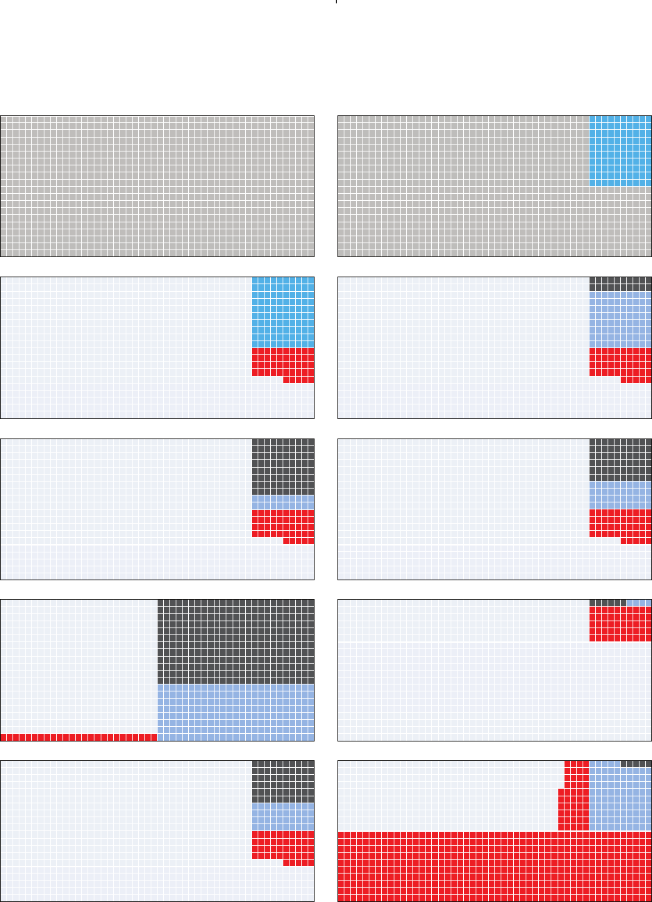
every step of the argument that we illustrate in Fig. 1 (see

also Lakens & Evers, 2014).

Consider a thousand hypotheses H1 that we might wish to

test (Fig. 1A). Many of these may not be true, so let us start

with a scenario where only 10% of the hypotheses at hand are

in fact true (Fig. 1B). This proportion of hypotheses being

true is often described with the symbol π(here π=0.1).

When testing the 900 hypotheses that are not true (dark grey

in Fig. 1B), we allow for 5% false-positive ﬁndings if we set

our signiﬁcance threshold at α=0.05 (the accepted level of

making Type I errors). This means we will obtain 45 (i.e.

900 ×0.05) false-positive answers (red in Fig. 1C), where we

state that our data provide signiﬁcant support for the hypoth-

esis H1 (or more formally speaking of ‘evidence against the

null hypothesis H0’) even though that hypothesis H1 is false

(and H0 is true). Now, when testing the 100 true hypotheses,

we will sometimes fall short of the signiﬁcance threshold, i.e.

cases where we would conclude that the data do not support

that hypothesis H1, although it is true and H0 is false (a

false-negative or Type II error). The frequency with which

our test of the empirical data falls short of reaching signiﬁ-

cance despite the hypothesis H1 being true is known as the

probability β(the probability of making a Type II error). The

probability βdepends on sample size (and effect size). When

the data set is very large, the risk of falling short of signiﬁcance

is small, so we speak of the study having high statistical power

(which is deﬁned as 1 −β). In our example in Fig. 1D, we

have a large sample size and hence a high power (80%) to sup-

port 80 out of the 100 true hypotheses correctly. In this case, β

will be 20%, leading to 20 false-negative conclusions shown in

black (i.e. where we reject the hypothesis despite it being true).

Here is the essential point of Ioannidis’ argument

(Ioannidis, 2005): when we consider only the subset of

positive outcomes, where a hypothesis H1 has been supported

by the data (the 45 red and the 80 blue cases in

Fig. 1D), 36% (i.e. 45/(45 +80)) will not be true. This

is the fraction of positive research ﬁndings (where data

provided signiﬁcant support for a hypothesis) that are false.

This is also known as the false-positive report probability

(FPRP =(α(1 −π)/[α(1 −π)+(1 −β)π]). Notably, this

fraction is much higher than 5%. This highlights the fact

that a 5% false positive rate (i.e. setting αat 0.05) does not

mean that only 5% of signiﬁcant research ﬁndings are false.

The situation may get worse. In many studies, sample sizes

are low, resulting in statistical power that is often as low as

20% (Møller & Jennions, 2002; Smith, Hardy & Gammell,

2011; Button et al., 2013; Parker et al., 2016). In this situation

we will have 80 instead of 20 cases of false-negative results

(black in Fig. 1E). If we then consider the positive outcomes

only, we observe that 69% of the signiﬁcant research ﬁndings

are false [the red out of the red plus blue fraction in Fig. 1E;

45/(45 +20) =0.69]. This disturbingly high proportion is

what made Ioannidis (2005) claim that most ﬁndings are false.

1944 W. Forstmeier and others

1000 hypotheses

10%

true

5% false-

positives

36% false

20% power

69% false

40% power

53% false

Unlikely hypotheses (1 in 10)

Likely hypotheses (1 in 2)

11% false

Highly unlikely hypotheses (1 in 100)

93% false

53% false

Unlikely hypotheses (1 in 10)

85% false

Unlikely hypotheses (1 in 10)

effective α= 60.7%

(B)(A)

(D)(C)

(F)(E)

(H)(G)

(J)(I)

10%

true 80%

power

40% power

95% power

Fig. 1. Different scenarios of testing 1000 hypotheses, of which a limited proportion is true. The colours in panels (B and C) refer to

hypotheses that are actually true (bright blue) or false (dark grey). The colours in panels (C–J) indicate false-positive ﬁndings (Type I

error; red), true positive ﬁndings (pale blue), false-negative ﬁndings (Type II error; black), and true negative ﬁndings (light grey). For

details see the main text. Illustration adopted and extended from http://www.economist.com/blogs/graphicdetail/2013/10/daily-

chart-2.

Avoiding false-positive ﬁndings 1945

For the following calculations, we will settle for an

intermediate sample size (larger than is typical in ecology

and evolution), which gives us a statistical power of 40%.

Under this condition, 53% of the positive ﬁndings will be

false (Fig. 1F). Now, it is essential to remember that we

started with a scenario where only 10% of the hypotheses

were actually true. That is, we were testing moderately

unlikely hypotheses to begin with (Fig. 1F). If, in contrast,

you are working in a research area where people mostly

test hypotheses that are likely (every second hypothesis being

actually true), the proportion of false-positive reports is quite

small (Fig. 1G). We would obtain only 25 false positive reports

(red in Fig. 1G), but as many as 200 true positives (blue in

Fig. 1G). In this case, readers of publications that present

positive ﬁndings will not often be misled (11% false). If,

however, a research ﬁeld is testing highly unlikely hypotheses

(only one in a hundred being true) nearly all positive reports

will be incorrect (93% false, Fig. 1H).

To illustrate one ﬁnal point, let us return to a situation

with moderately unlikely hypotheses (10% true) and still

intermediate power (1 −β=40%), which is shown in Fig. 1I.

Let us add a new dimension, which was brought up in

a seminal publication of Simmons, Nelson & Simonsohn

(2011). They stated that researchers actually have so much

ﬂexibility in deciding how to analyse their data that this

ﬂexibility allows them to coax statistically signiﬁcant results

from nearly any data set [for similar insights see Barber

(1976), De Groot (1956/2014), Feynman (1974) and Gelman

& Loken (2014)].

Simmons et al. (2011) called this ﬂexibility ‘researcher

degrees of freedom’. We will address these researcher degrees

of freedom in detail below, and we will give a range of

illustrative examples. For now, imagine that researchers have

to make many arbitrary decisions in data analysis, and if they

are trying hard (even unintentionally through self-deception)

to provide positive evidence for their hypothesis, at every

arbitrary step they may always go for the option that produces

the lowest P-value (‘signiﬁcance seeking’). Using simulations,

Simmons et al. (2011) show that the combination of always

choosing the better option in four consecutive arbitrary steps

(each of which seems of minor importance, e.g. analysing

yearlings and adults together versus separately) adds up to

a dramatic effect of raising the α-level from α=0.050 to

0.607. That means, if we systematically chose the option

that reduces the P-value in each of the four steps, we will

be able to present an effect of interest as being statistically

signiﬁcant (P<0.05) in 607 out of 1000 cases in which no

real effect exists (hence the formulation ‘allows presenting

anything as signiﬁcant’). If this scenario of raising αto 60.7%

is applied to Ioannidis (2005) calculations, we would see 535

false positives (red in Fig. 1J) compared to approximately 95

true positives (blue in Fig 1J; note that this latter number is

a rough guess and not based on simulations), which would

mean that about 85% of all positive ﬁndings would be false.

According to the calculations illustrated in Fig. 1, the

proportion of false-positive reports (out of all positive reports)

will be highest for: (i) ﬁelds with mostly underpowered studies

(small sample size); (ii) ﬁelds with unlikely hypotheses (driven

by pursuit of novelty); (iii) ﬁelds that poorly guard against

raising the level of α(signiﬁcance seeking).

More can be said about each of these inﬂuential factors:

1 A comparison between Fig. 1D,E illustrates why low

power produces relatively more false-positive ﬁndings.

The absolute number of false positives stays the same

(always 45 red cells), but we see fewer correct positives

(20 rather than 80 blue cells) as power drops from 0.80

to 0.20. Hence the proportion of positive ﬁndings that

are correct is decreasing. If you want to carry out your

own calculations to see how the statistical power in

your experiment depends on sample size, you will ﬁnd

suitable calculator tools online (e.g. GPower; Faul et al.,

2009), but they will always ask you about the size of

the effect that you wish to detect. This is hard to know

a priori. In the ﬁelds of ecology and evolution observed

effect sizes are typically small (e.g. r=0.19; Møller &

Jennions, 2002), which is still likely an overestimate

(Hereford, Hansen & Houle, 2004; Parker et al., 2016).

Hence, large sample sizes are required to detect such

effects (required N=212, for detecting r=0.19 with

80% power). While studies in animal behaviour have a

reasonable power of around 70% for detecting a large

effect of r=0.5, the power for detecting an effect of

r=0.19 lies only around 15–20% [own calculations

using GPower 3.1 (Faul et al., 2009) based on results of

Jennions & Møller (2003) and Smith et al. (2011)].

2 The relative proportion of false-positive reports is most

strongly inﬂuenced by how likely one’s hypothesis is to

begin with (compare Fig. 1G with 1H). However, this

quantity may be difﬁcult to gauge. Most researchers

would probably think (or at least hope) that they

are testing relatively likely hypotheses (much closer to

Fig. 1G than 1H). However, people’s impressions may

be deceiving. The existing literature is heavily biased

towards stories of success (Parker et al., 2016), with

84% of all publications ﬁnding support for their initial

hypotheses (Fanelli, 2010). As we will see in Section

II.2, this ﬁgure is far from an objective representation of

all hypothesis tests that have been conducted, because

null ﬁndings (non-signiﬁcant results) are less likely to

get published (Rosenthal, 1979; Simonsohn et al., 2014),

and because various common data-analysis practices

increase the rate of false positives as well as the average

strength of reported effects among those results that are

published (Anderson, Martinson & De Vries, 2007;

Simmons et al., 2011; John, Loewenstein & Prelec,

2012; Parker et al., 2016). Even without problematic

data analysis, some (false) positive evidence can emerge

for any hypothesis (Fig. 1H). Thus, just because we see

support for a theory in the literature does not mean we

should assume that our hypothesis, which is based on

this theory, is likely to be true. Finally, one should realize

that high-impact journals are always on the lookout

for the most novel and surprising research ﬁndings.

1946 W. Forstmeier and others

Thus when researchers ﬁnd evidence for surprising

hypotheses (Fig. 1H) and manage to secure publication

in these high-impact journals, other researchers may

be tempted to test increasingly far-fetched (non-trivial,

surprising) hypotheses. This could push a research ﬁeld

into an arms race that comes at the expense of tests for

less-surprising hypotheses.

3 There are so many different ways in which the α-level

can be raised above the conventional threshold of 5%

(Fig. 1J) that this will keep us busy for most of this

review. Conceptually it is helpful to distinguish between

two problems. First (treated in Section II.2), there is

the issue of multiple hypothesis testing that comes in

various forms and can sometimes be deceivingly cryptic

(Parker et al., 2016). Here it is important to keep track

of the extent of multiple testing. This may allow us to

adjust α-levels accordingly, so that P-values can still

be interpreted in a meaningful way. Second (treated

in Section II.3), there are many ways of carrying

out statistical tests incorrectly which often will yield

highly signiﬁcant P-values that are misleading and

incorrect to an extent that cannot be adjusted for.

The probably most important source of error here is

the non-independence of data points (Milinski, 1997),

which is typically referred to as pseudoreplication

(independent data points are considered as proper

replicates, while non-independent data points are

considered as pseudoreplicates) or as clustered data

(Weissgerber et al., 2016).

Table 1 provides an overview of the statistical and

psychological issues that will be addressed herein together

with a collection of possible solutions.

(2) Multiple testing in all of its manifestations

In this chapter we will focus on how multiple testing and

selective attention or reporting lead to inﬂated rates of Type

I error. If researchers were forced to report the outcome of

every single statistical test that they conduct, every obtained

P-value could be taken at face value. With αset at 0.05,

for each hypothesis H1 that is not true we would only have

a 5% risk of drawing a false-positive conclusion. However,

as soon as reporting becomes conditional on the outcome

(typically: positive ﬁndings being more likely to get reported)

or when we focus our attention on the promising outcomes

(ignoring or forgetting about negative outcomes), the risk of

a false-positive conclusion is much higher than 5% (e.g. 53%

in Fig. 1F).

When the total number of statistical tests conducted is

known (e.g. 10 tests), then it is possible to calculate the

probability of obtaining at least one signiﬁcant result by

chance alone (1 −0.9510 =40%), and it is possible to adjust

α-levels (0.05/10 =0.005) for each test to ensure that the

probability of making one or several Type I errors remains

at about 5% (1 −0.99510 =4.9%). This adjustment is known

as the classical Bonferroni correction (Dunn, 1961). While

using such a strict α-threshold is effective in limiting Type

I errors, it inevitably will increase the number of Type II

errors (i.e. true effects that are discarded because they do not

pass this threshold). Hence, if you are more worried about

making Type II errors than about making Type I errors,

you may well discard the Bonferroni correction (Nakagawa,

2004), or go for less-strict methods of correction based on

false-discovery rate (Benjamini & Hochberg, 1995; Pike,

2011). Yet, whenever we allow our Type I error rate to rise

in the interest of keeping the Type II error rate low, we

will produce many false positives and thus need to seek to

replicate these exploratory ﬁndings (Pike, 2011). For instance,

if your aim is to discover a new treatment for a disease, you

want to make sure that you do not miss out on something

potentially interesting (and hence limit Type II errors). This is

the exploratory part of science. It is essential and important.

However, once you identiﬁed a potential treatment, you

should be interested in making sure that you are right so

as not to waste money or even cause harm, and hence you

want to reduce Type I errors. This is the conﬁrmatory part

of science, the proper testing of a priori hypotheses.

Adjustments of αto multiple testing are typically called for

when researchers present large tables containing numerous

statistical tests, of which only a small fraction reaches

signiﬁcance (P<0.05). Such tables elicit skepticism in

experienced researchers, who rightly worry that the content

of the entire table may be consistent with the null hypothesis.

As a pre-emptive response to such skepticism, authors may

avoid presenting too many non-signiﬁcant results alongside

their positive ﬁndings. A threshold of P<0.05 seems fairly

reasonable when only a few P-values are shown and these

P-values mostly lie below the 0.05 threshold. By contrast,

referees may request a more stringent threshold when many

non-signiﬁcant results are presented alongside, because the

long list clearly reveals the extent of multiple testing.

Problematically, when authors are free to choose which

results to present in their publication, it becomes impossible

to judge the appropriate statistical signiﬁcance of the ﬁndings.

When, for instance, the authors highlight a single signiﬁcant

ﬁnding from a pool of 10 tests they report, this inspires much

less conﬁdence in that ﬁnding than if it had arisen from

a single planned test. This is a serious dilemma. Justiﬁed

skepticism from reviewers creates an incentive for reduced

transparency in scientiﬁc publications, thereby lowering the

overall utility of the reported work. This problem could

be mitigated if reviewers and editors would acknowledge

and appreciate the greater scientiﬁc value of a paper that

comprehensively reports all outcomes of a study compared

to the minimalistic presentation of a single ﬁnding.

There is compelling evidence that many tests do, in

fact, go unreported. As mentioned above, across scientiﬁc

disciplines, 84% of all studies present positive support for

their key hypothesis (Fanelli, 2010). Such a high success

rate is impossible to obtain without selective reporting or

biased attention that de-emphasizes non-signiﬁcant ﬁndings

or likely a combination of both (see Fig. 1G). Even if all tested

hypotheses were true (which they are not), a statistical power

of 84% (rarely ever achieved) would be required to yield

Avoiding false-positive ﬁndings 1947

Table 1. Collection of problems and possible solutions

Section Problems Solutions

II.1 •Small sample size (e.g. data hard to obtain) •Acknowledge preliminary nature

•Multi-laboratory collaborations

II.1 •Novelty seeking •Regard ‘surprising’ ﬁndings sceptically prior to replication

II.2a•Multiple testing and selective reporting (e.g. due

to too much trust in hypotheses, hindsight bias,

pressure from referees)

•Avoid excessive testing (think before data exploration)

•Keep track of number of tests conducted and report all tests

•Bonferroni correction, false-discovery rate or emphasize

preliminary nature of ﬁndings

•Average effect sizes across conceptually similar tests

•Referees and editors promote comprehensive and unbiased

reporting

II.2b•Multiple testing within models (stepwise model

simpliﬁcation)

•Report the initial full model

•Global test of full model against null

•Test a pre-determined subset of models

•Average effects of individual variables across models

II.2b•Overﬁtting of models (inﬂated signiﬁcance) •Keep N>3kfor correct P-values, where kis number of

parameters to be estimated (N>8kfor reliable parameter

estimates)

II.2c•HARKing (hypothesizing after the results are

known) and hindsight bias

•Preregister hypotheses

•Keep track of number of tests conducted

•Comprehensive reporting

II.2d•Data collection ends with reaching P<0.05 •Declare stopping rule

•Adjust P-value for multiple testing

II.2d•Discarding ‘unsuccessful’ experiments until an

experiment ‘works’

•Complete reporting of all experiments

II.2e•Arbitrary decision in analysis (e.g. selective

removal of outliers) are taken conditional on

reaching signiﬁcance (conﬁrmation bias)

•Make decisions apriori(preregistration)

•Ask colleagues to make decisions for you

•Blinding yourself during data analysis

•Speciﬁcation-curve analysis: try all versions to examine

robustness of ﬁndings

II.3 •Non-independence of data points (e.g. related

individuals, temporal and spatial autocorrela-

tion)

•Test for non-independence, autocorrelation

•Fit grouping variables as random effects (intercepts, slopes,

space, time, pedigrees)

•Run analysis at the level where independence is met

•Balance experiments for confounding effects

II.3c•Overdispersed data •Transform data

•Control for overdispersion (random effects, quasi-likelihood)

II.4a•Over-interpretation of apparent differences •Test signiﬁcance of interaction term

•Test context dependence in follow-up study

II.4b•Misinterpretation of regression to the mean •Avoid allocating individuals to different treatment groups

according to phenotype

•Set up a control group

•Model the expected effect

II.5 •Conﬁrmation bias in data collection •Blinding observers to treatment groups

III.1 •Lack of close replication studies •Regard unreplicated ﬁndings as preliminary

•Preferentially cite conﬁrmatory replication studies as the most

convincing evidence

•Replicate own ﬁndings

•Replicate important foundational studies as part of new

research

1948 W. Forstmeier and others

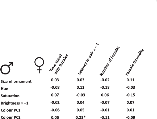
Fig. 2. A ﬁctional table of correlation coefﬁcients between

measures of male ornamentation and measures of male success

in pairing with females. The asterisk highlights a signiﬁcant

correlation. Some parameters were multiplied by −1, such that

positive correlations indicate higher mating success for more

ornamented males.

this rate of success. Hence, this means that most disciplines

presumably sit on a huge pile of ‘failed’ experiments and

unpublished null results that are inaccessible because they

are hidden in the ﬁle-drawers of the experimenters [known

as the ‘ﬁle-drawer problem’ (Rosenthal, 1979)].

In the following we will discuss various forms of multiple

testing by giving typical examples to increase principle

awareness of problematic situations.

(a)The temptation of selective reporting

Imagine you study mate choice in species xy, and you would

like to understand why males of species xy have a colourful

plumage ornament that is absent in females. Hence, on the

side of males, you measure the size of the ornament as well

as its colour in terms of hue, saturation, and brightness, and

you also summarize the measures of the reﬂectance spectra

in two principal component scores. To assess female choice,

you measure how much time females spend close to each

male, the latency for males to secure a female partner, the

number of females each male sires offspring with, and the

number of eggs laid by females after pairing with a male of a

given ornamentation. You then look for positive correlations

between the degree of male ornamentation and their success

in attracting and pairing with females (Fig. 2).

The longer you look at this table of correlations with

one association being signiﬁcant, the more tempting it

may become to convince yourself that, maybe, principal

component analysis actually represents the most objective

way of summarizing complex colour information, and that

maybe the latency to pair is the most meaningful measure

of male pairing success in this study species. Surely this

signiﬁcant ﬁnding must be a true positive effect, since why

else would males have evolved these beautiful colours. Also

the use of Bonferroni correction has often been criticized

(Nakagawa, 2004) for being too conservative and leading to

many false-negative outcomes (Type II errors). Hence, we

might be tempted to publish only the association of ‘latency

to pair’ with ‘Colour PC1’ and ‘Colour PC2’ without

mentioning the remaining 22 null results (focussing on PC2

only without reporting on PC1 would be too extreme). We

might not even perceive this as unscientiﬁc conduct because

we have convinced ourselves of the biological and statistical

logic behind our ‘discovery’. As we convince ourselves that

the biology is right, we presumably feel an obligation to

share our discovery. Thus our personal focus on discovery

motivates us to publish this as a positive ﬁnding. Humans

are highly efﬁcient at ﬁnding post-hoc justiﬁcations for their

choices (Trivers, 2011) if those choices produce a more

desirable outcome [positive results are likely easier to publish

than null ﬁndings (Franco, Malhotra & Simonovits, 2014)].

When we selectively report only 2 out of the 24 correlations

shown in Fig. 2, we often forget that the remaining 22

correlations actually represented equally valid tests of our

hypothesis that greater ornamentation enhances mating

success. A more objective approach would be to average

the 24 correlation coefﬁcients to yield an estimate of the

overall effect of ornamentation. This can be done because all

variables were coded in such a way that high values always

refer to increased ornamentation and increased mating

success, meaning that positive correlations count as support

for the hypothesis. In our example, the average correlation

between ornamentation and mating success is exactly zero

(the mean of all positive and negative correlations is r=0.00).

Hence, if we started with the aim of objectively quantifying

something (rather than discovering something) we should

face less of a risk of misleading ourselves and our colleagues

and of having wasted efforts for the short-term beneﬁt of

possibly publishing in a higher-ranking journal.

This hypothetical case clearly shows that ‘data do not

always speak for themselves’. Without knowing the context

of why the author decided to focus on principle component

analysis and on ‘latency to pair’, we cannot judge the

statistical signiﬁcance of the ﬁnding. We will explore other

examples of deceiving statistical results below.

The literature on sexual selection acting on ornamental

traits is plagued by this problem of potential selective

reporting (not every study is biased, but there is no label

that would identify unbiased reporting). Since we have no

way of telling the extent of reporting bias, it is not clear

how we could draw a general conclusion about the strength

of sexual selection on ornaments from several decades of

work (Parker, 2013). This illustrates how inefﬁcient research

can sometimes be if it fails to ensure maximal objectivity in

reporting. Meta-analyses that summarize all published effects

are not able to take into account these arbitrary decisions

made by authors (Ferguson & Heene, 2012). Although any

meta-analytic summary would certainly reveal a strong effect

of ornaments on mating success, it is unclear whether or to

what extent this is evidence for a theory as opposed to

evidence of selective reporting driven by a theory. There

are probably more than a few research areas where we

might beneﬁt from a new round of empirical investigation

in which all results were made available. If we all begin now

with studies adhering to a standard of unbiased reporting

and we make such studies identiﬁable with the use of

Avoiding false-positive ﬁndings 1949

badges (see Section III.3b), in a few years’ time we could

conduct meta-analysis comparing studies with and without

such badges to conﬁrm or refute our past work.

(b)Cryptic multiple testing during stepwise model simpliﬁcation

A table like that shown in Fig. 2 immediately reminds

researchers that they have to be aware of the issue of multiple

testing. A much less obvious form of multiple testing happens

when researchers ﬁt complex models to explain variation in a

dependent variable by a combination of multiple predictors.

This has been termed ‘cryptic multiple hypotheses testing’

(Forstmeier & Schielzeth, 2011).

Imagine you are trying to explain variation in a variable

of interest with a set of six possible predictors. Besides the

six main effects that you are interested in, there is also the

possibility that any pair of two predictors might interact with

each other in inﬂuencing the dependent variable. To explore

all these possibilities you start by ﬁtting a rather complex full

model where the dependent variable is a function of 6 predic-

tors plus their 15 two-way interactions, and you then carry

out a standard procedure of model simpliﬁcation where, at

each step, you always delete the least signiﬁcant term from

the model until you have only signiﬁcant predictors (main

effects or interactions) left in the minimal model. Such exten-

sive data exploration minimizes the risk that you overlook a

potentially complex combination of factors that affects your

variable of interest. However, this widespread procedure

(recommended by some standard statistical textbooks, e.g.

Crawley, 2002) comes with a very high risk of Type I error.

In a simulation study it was shown (Forstmeier & Schielzeth,

2011), that when all null hypotheses are true (using randomly

generated data), the chance of ﬁnding at least one signiﬁcant

effect lies close to 70%). This means that most of the time you

will be able to present a signiﬁcant minimal model that seems

to reveal an interesting pattern [see also Mundry & Nunn

(2009) and Whittingham et al. (2006)]. Many researchers

seem unaware that they have actually examined 21 different

hypotheses at once, and that a Bonferroni correction of

setting αto 0.05/21 =0.0024 would be required to keep the

false-positive rate at the desired 5%.

This Bonferroni correction works reliably as long as the

full model was built on a reasonably sized data set. However,

when sample size becomes low relative to the number of

parameters to be estimated, then the estimation of model

ﬁt and P-values becomes highly unreliable. This happens

because a small number of data points can often be explained

almost perfectly by a combination of predictors selected from

a relatively large pool of predictors. For instance, if the same

6 main effects and their 15 two-way interactions are ﬁtted

to only 30 data points, the resulting minimal models are

often excessively signiﬁcant. As many as 26% of the minimal

models cross even the Bonferroni-corrected threshold of

0.05/21 =0.0024, such that a much stricter correction to

0.05/286 =0.00017 would be required to ensure that only

5% of the minimal models pass that threshold. In other words,

running through such an automated assessment of your six

predictors and their two-way interactions by step-wise model

simpliﬁcation is expected to give you P-values that are as low

as you would get from always picking the most signiﬁcant

among an incredible 286 hypothesis tests.

Surely, this is an extreme case where P-values are no

longer correct (and not adjustable by Bonferroni correction)

because they are derived from an over-ﬁtted model. Simula-

tions (Forstmeier & Schielzeth, 2011) revealed that P-values

begintobecomeexcessivelysmalloncetherearefewerthan

three data points per predictor (N<3kwith kbeing the num-

ber of parameters to be estimated). Regarding this result from

the other side, the observation that P-values were correct

(adjustable by Bonferroni correction) as long as there were

more than three data points per parameter, does not imply

that this sample size is sufﬁcient in all respects. Statisticians

often recommend that at least eight data points per estimated

parameter should be available (e.g. N>8k+50; Field, 2005),

and they would consider the over-ﬁtting of models described

in the previous paragraph a ‘statistical crime’. However,

when screening the literature in the ﬁeld of ecology and

evolution, Forstmeier & Schielzeth (2011) found that authors

rarely described the initial full model that they had ﬁtted.

This means that the extent of multiple testing and of possible

over-ﬁtting could often not be reconstructed. Out of 50 stud-

ies examined, 28 used models with two or more predictors,

6 of which ﬁtted between 6 and 17 effects, and 3 of which

violated the rule to not over-ﬁt (N<3k). Moreover, and most

strikingly, none of the 28 studies considered any adjustment

of P-values for multiple testing (e.g. Bonferroni correction).

In some ﬁelds, iterative model building of the sort

we just described has become less common, but what

has replaced it is often not substantially better (Mundry,

2011). The replacement is typically a process by which

researchers develop a set of ‘plausible models’ and evaluate

them with measures of overall model ﬁt (e.g. likelihood

ratio) or ﬁt accounting for the number of predictors [e.g.

Akaike Information Criterion (AIC), or Bayesian Information

Criterion (BIC)]. Researchers may then assess parameter

estimates or tests of signiﬁcance for individual predictors only

in the ‘best’ model. Just as with an iterative procedure, it is

unreasonable to assess the statistical signiﬁcance of individual

variables in the ‘best’ model without correction for multiple

comparisons. Similarly, assessing the strength of effects in

only the ‘best’ model is also likely to produce an inﬂated effect.

(c)A priori hypothesis testing versus HARKing: Does it matter?

The above approach of exploratory data analysis means that

a fairly large number of hypotheses get tested in a very short

time (i.e. without careful thinking about speciﬁc hypotheses

considered plausible) and this comes with a high risk of

drawing a false-positive conclusion if we only report on the

subset of signiﬁcant predictors. In fact, such exploratory

analysis could be seen as an act of generating hypotheses

rather than as an act of testing hypotheses, because you

only start thinking about the respective hypothesis once you

have discovered a signiﬁcant association. This approach is

not wrong per se, as long as you are aware and honest

about the fact that the hypothesis was derived from the data.

1950 W. Forstmeier and others

The problem starts where researchers fail to acknowledge

this. The psychologist Norbert Kerr called this ‘HARKing’

(hypothesising after the results are known; Kerr, 1998).

Yet, does it really matter in terms of likelihood of a positive

ﬁnding being true whether we thought of the hypothesis a

priori (i.e. before data inspection) and then use the data to test

that hypothesis, or whether we came across the hypothesis

only after having explored the data and having focused on

only signiﬁcant effects to begin with? Intuitively, we would

probably think that a priori hypothesis testing is less prone to

yield mistakes than ‘ﬁshing for signiﬁcance’ and HARKing,

but is that intuition correct?

In both cases we would use exactly the same data set (and

arrive at the same P-values), so for any given hypothesis,

the statistical outcome appears exactly the same. Although

this is true for any given hypothesis, ﬁshing, HARKing,

and hindsight bias often produce hypotheses that researchers

never would have deduced from theory. Hindsight bias or the

‘knew-it-all-along’ effect (Fischhoff, 1975) is the phenomenon

that, after having seen the results of data analysis, these

results appear logical, inevitable, and in line with what we

must have predicted before. Hindsight bias is particularly

dangerous because we overestimate the plausibility of our

hypothesis (which in fact is a post hoc explanation, a hypothesis

that was derived from the data, not one that we had a priori).

Sometimes it is easy to spot unlikely hypotheses that were

derived from the data. When the title of a publication starts

with ‘Complex patterns of ...’ and the main ﬁnding of

the study consists of a difﬁcult interaction between several

explanatory variables, then this complex hypothesis may well

have been derived from the data.

However, data exploration is not fundamentally a bad

thing. In fact when conducted transparently, it is very useful.

It may allow you to discover something for which theory has

not even been developed yet, or you may actually correctly

identify a complex pattern of interactions for which theory is

too simplistic. Yet, the main problem with data exploration is

that we normally do not keep track of the number of tests that

we have conducted or would have been willing to entertain,

so there exists no objective way of correcting for the extent

of multiple testing (De Groot, 1956/2014). Once a discovery

has been made (P<0.05) and a plausible explanation has

been found, it is very easy to deceive oneself into thinking

that one actually had that hypothesis in mind before starting

the exploration, and nothing seems wrong with writing up a

publication saying ‘here we test the hypothesis that ...’.

The failings of this approach were explained long ago

by De Groot (1956/2014) and they are strongly linked

to points we have already made. In exploratory analyses,

we are open to an array of possible relationships and

resulting interpretations. As the array of possible detectable

relationships expands, the likelihood that we might detect

false relationships expands as well. Of course we may well

also detect real relationships, but at this stage, we cannot

distinguish what is false from what is real. We have generated

a suite of hypotheses with our data exploration, and next we

(or others in the years to come) need to gather additional

data. With the new data, we should conduct only the very

limited set of analyses designed to test the hypotheses derived

from the exploratory work. Thus in this second round of

data collection and analyses, we can operate with a much

lower probability of detecting false positives. In other words,

we test hypotheses rather than just generate them.

In some ﬁelds it is common practice to masquerade

exploratory analyses as conﬁrmatory hypothesis testing

because exploratory work is often perceived as inferior

or old-fashioned. In the distant past, data exploration

was presented in the Results section, and its subjective

interpretation was given in the Discussion section. Then

biologists adopted (or at least pretended to adopt) Popper’s

idea about hypothesis testing, and in the process started

to move their data-derived (post hoc) hypotheses to the

Introduction so they could pretend they were testing a priori

hypotheses. Unsurprisingly, when we ‘test’ a hypothesis with

the same data that generated that hypothesis, it tends to be

conﬁrmed. In other words, you simply cannot ‘cherry-pick’

the hypothesis you wanted to test after having seen the

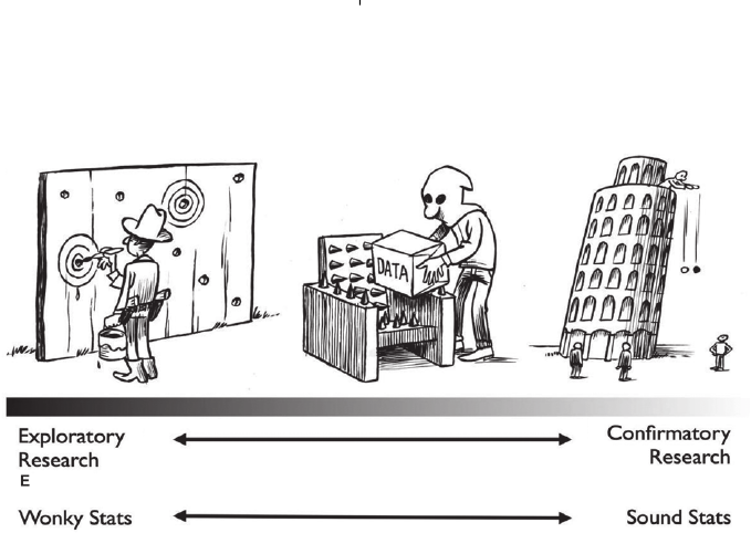
outcome of statistical analyses (Fig. 3).

(d)Researcher degrees of freedom: (1) stopping rules

As promised earlier, we now return to the issue of ‘researcher

degrees of freedom’ (Simmons et al., 2011), which refers to

researchers’ ﬂexibility in how to collect and how to analyse

their data. One striking issue regards stopping rules for data

collection. How do you decide that you have enough data?

Say you are trying to test whether females of species xy

prefer males that sing with a lower-pitched voice. Initially,

you do not know how large such an effect might be, so

you start by collecting data on 10 females, after which

you conduct a simple regression test (pitch predicts female

response to song). Now let’s say you obtained a trend

in the expected direction (slight preference for low-pitch

voice), but the effect does not reach signiﬁcance. You might

suspect that the effect is real but small, and that you lacked

statistical power to reach signiﬁcance. You then collect data

on another 10 females and then conduct your regression

test again with all 20 females. Although the rationale behind

such a sampling design seems perfectly understandable, the

risk of making a Type I error has just risen from 5% to

approximately 7.7 (Simmons et al., 2011). This is because

you gave the data two chances of reaching signiﬁcance.

Since the ﬁrst data set is included in the second, these are

not two fully independent chances (which would yield 9.75%

false positives; 1 −(0.95 ×0.95) =0.0975), so the combined

risk of drawing a false-positive lies somewhere between 5

and 10% (this risk can be estimated from simulations). Thus,

when decisions about sample size are not made a priori,

and data sets are subject to iterative tests for signiﬁcance as

data accumulate, you must correct for multiple testing. The

more often you stop data collection to check for signiﬁcance,

the greater your risk of a false positive. It is important

to remember here that your decision to collect data on

another 10 females was conditional on the ﬁrst outcome.

If you had obtained a statistically signiﬁcant effect at the

Avoiding false-positive ﬁndings 1951

Fig. 3. The graded di stinction between exploratory, hypothesis-generating research and conﬁrmatory, hypothesis-testing research

(Wagenmakers et al., 2012). On the right side of the continuum, a purely conﬁrmatory test is conducted. The test is transparent,

relevant hypotheses have been explicated beforehand, and a data analysis plan is present. This exempliﬁes the scenario of

hypothesis-testing research. For this type of research – and only for this type of research – statistical tests have their intended

meaning. On the left side of the continuum, a purely exploratory test takes place. The ‘Texas sharpshooter’ ﬁrst ﬁres at a fence,

and then proceeds to draw the targets around the bullet holes. There is no prediction here – there is only postdiction. This scenario

exempliﬁes the scenario of hypothesis-generating research. For this type of research, the resulting statistical tests (invented exclusively

for hypothesis-testing research) are misleading, or, in Ben Goldacre’s terms, ‘wonky’. In between the two extremes lies a continuum

where research is conducted that is partially conﬁrmatory, typiﬁed by a degree of data massaging – in the ﬁgure, the data are

‘tortured until they confess’. The statistical results are partially wonky. Unfortunately, it is far too easy to make the mistake of

masquerading hypothesis generation as hypothesis testing. Most researchers, including the authors, admit to having done this (John

et al., 2012), either because of ignorance of the problem or because of self-deception [see Fischhoff (1975) and Trivers (2011)]. Figure

courtesy of Dirk-Jan Hoek.

ﬁrst try, you would presumably not have collected more

data, but rather you would have concluded that the effect

seemed to be large because it reached signiﬁcance with

only 10 females. In a scenario in which reaching statistical

signiﬁcance always triggers an end to data gathering, there

is never an opportunity to discover whether a larger sample

size might eliminate signiﬁcance.

In a worst-case scenario where you keep testing after every

sample until the expected effect reaches signiﬁcance, you

are certain to ﬁnd the effect eventually, since P-values will

undergo a random walk (Rouder et al., 2009) and will at

some point cross the 5% threshold (unadjusted for multiple

testing). Our own (unpublished) simulations with randomly

generated numbers show that you can expect to cross the

threshold of signiﬁcance within the ﬁrst N=100 in about 3 of

10 attempts (hence α=0.3 rather than α=0.05), although

if you are willing to continue to sample indeﬁnitely, you will

eventually reach statistical signiﬁcance in every single case

(Armitage, McPherson & Rowe, 1969). Hence, continued

sampling and a stopping rule based on reaching signiﬁcance

unambiguously elevates Type I error rates and thus we expect

this to be one of the many factors leading to false positives

in the literature. Fortunately, as researchers are increasingly

becoming aware of this problem, it is slowly becoming good

practice to specify one’s stopping rule for sample size in the

methods section of a publication.

In a wider context, the same issue of multiple testing

applies to situations where researchers discard one or two

initial experiments that were ‘unsuccessful’ (for instance

because of a putative confounding factor that was not yet

controlled) and then have full trust in the ﬁrst experiment

that yields the desired result.

(e)Researcher degrees of freedom: (2) ﬂexibility in analysis

When analysing data, we face a wide variety of rather

arbitrary decisions that we have to make, such as: (i) should

I include covariate xin the model as a possible confounding

factor, and should xbe log-transformed or should I subdivide

it into categories (and how many)? (ii) Should I include or

exclude a particular outlier or an inﬂuential data point (high

leverage)? (iii) Should I transform the dependent variable

to approximate normality better, and which transformation

should I choose? (iv) Should I add baseline measures taken

before the start of the experiment as a covariate into the

model in order to remove some noise in the data? (v) Should

I control for sex as a ﬁxed effect or also model a sex by

treatment interaction term? (vi) Should I exclude individuals

from the analysis for which the number of observations is

low? (vii) Should I remove a third treatment category that

seems unaffected by the treatment or should I lump it with

the control group?

With all these decisions to make, there is again a risk

of trying several versions (multiple testing) and of favouring

the version that renders the more interesting story (selective

reporting). Often, we may subconsciously favour the version

1952 W. Forstmeier and others

that minimizes the P-value for the effect of interest because we

convince ourselves that this version must be the correct one or

the most powerful one. Since we often believe that an effect of

interest exists (and we designed the experiment to reveal the

effect), we tend to have greater trust in analyses that conﬁrm

our belief. This powerful component of human nature

is called conﬁrmation bias, and it has been documented

in a wide array of settings (Nickerson, 1998). Obviously,

conﬁrmation bias can render our science highly subjective

unless we make all these arbitrary decisions a priori (if possible)

or at least blind to the outcome. By contrast, exploratory

analyses that are presented as conﬁrmatory are always a

threat to objectivity. Unfortunately, full disclosure of post-hoc

decision making may often be quite challenging and requires

substantial conscientiousness, but increased awareness of the

issue is a ﬁrst step towards mastering this challenge.

In an unpublished manuscript, A. Gelman & E. Loken

called this ‘the garden of forking paths’, which nicely

illustrates that there may be a near-endless diversity of

combinations of decision variants. Simonsohn, Simmons

& Nelson (2015) hence suggested an automated routine

of going through all possible combinations of identiﬁed

decisions in terms of their inﬂuence on the effect of interest

(the effect at the heart of the ‘story’ of a publication; see also

Steegen et al., 2016). Simonsohn et al. (2015) call this routine

‘Speciﬁcation-Curve Analysis’ (SCA), and they demonstrate

its utility using the example of a recent study (Jung et al.,

2014) that led to some controversy about subjectivity in

decision making. In that study there were seven decisions to

be made, some of which had more than two options to choose

from, leading to a total of 3 ×6×2×2×2×4×3=1728

possible ways of analysis. SCA shows that only 37 out of these

1728 versions (2%) yield signiﬁcant support for the prediction

that Jung et al. (2014) evaluated and conﬁrmed in their

publication. A particularly problematic aspect of researcher

ﬂexibility is the decision to remove outliers after having seen

their inﬂuence on the P-value. Selective removal of outliers

has a high potential of generating biased results (Holman et al.,

2016), so the removal of data points is generally discouraged.

Publications should always explain the reasons behind any

attrition (loss of data points between study initiation and

data analysis) and should discuss whether the missed samples

might have led to biased results. Up to this point we have

been dealing with the problem of multiple testing in all kinds

of versions, and we have seen that this problem can be

addressed by (i) limiting the number of tests conducted, and

(ii) adjusting α-thresholds to keep the false-positive rate at

some desired level. In all cases we assumed P-values to be

calculated correctly. Yet, in the following chapter we will see

that P-values are often incorrect (often too small), deceiving

us into over-conﬁdence in our result.

(3) Incorrect P-values

P-values indicate how often chance alone will produce a

pattern of at least the strength observed in the experiment.

Accordingly, for any given sample size, if P=0.05 we might

still be sceptical whether the pattern could have arisen by

chance, but if P=0.0001 we will probably be much more

conﬁdent that we have discovered a true effect. However, this

conﬁdence is only justiﬁed if the statistical test that yielded

the P-value was applied appropriately in the ﬁrst place, but

not if the data violated the assumptions that underlie the

test. Statistical tests may have many underlying assumptions

(e.g. normally distributed residuals), although many of these

assumptions can be violated without drastic effects on the

P-values. One assumption, however, is crucial for P-values,

and that is the independence of data points. If data points do

not represent true independent replicates but are grouped in

clusters (‘clustered data’; Weissgerber et al., 2016), we speak

of pseudoreplication, and this may lead to over-optimistically

low P-values (Hurlbert, 1984). As we will see below, some

kind of structure in the data leading to non-independence

is ubiquitous. However, such structure only becomes a

problem for testing the signiﬁcance of a predictor of interest

(e.g. treatment effect), if the samples are non-independent

with respect to the predictor. The latter is what deﬁnes

pseudoreplication.

There are many sources of non-independence of data:

repeated measures from the same individual, measures

from individuals that are closely genetically related to each

other, and measures from species that are related through

phylogeny are all non-independent of each other. Variation

in space, for instance in territory quality, may introduce

non-independence of measurements. The occurrence of a

disease may vary not only in space, but also in time, just like

data on daily weather or minute-by-minute data on whether

a bird is singing will show temporal non-independence.

All these dependencies lead to problems in P-value esti-

mation, the full extent of which is truly unknown. From own

experiences as reviewer or editor of manuscripts we gained

the impression that a substantial proportion of submitted

manuscripts contain analyses that are clearly incorrect, and

that the rate at which referees spot and eliminate these mis-

takes is not sufﬁciently high to ensure that the published liter-

ature would not contain numerous errors. Surely, awareness

of the pseudoreplication issue is well developed in some areas

like experimental design (Hurlbert, 1984; Milinski, 1997;

Ruxton & Colegrave, 2010) or phylogenetically controlled

analysis (Felsenstein, 1985; Freckleton, Harvey & Pagel,

2002). However, in some other ﬁelds, non-independence of

data has been overlooked for an extended period of time

because dependencies may be deceivingly cryptic (Schielzeth

& Forstmeier, 2009; Hadﬁeld et al., 2010; Valcu & Kempe-

naers, 2010) and it seems likely that more such problems

will get highlighted and become better known in the

future.

Generally we feel that there is insufﬁcient recognition

of the extent to which incorrect P-values resulting from

pseudoreplication have contributed to the current reliability

crisis. We therefore provide a practical introduction into

some aspects of pseudoreplication, starting from the most

basic principle that most readers will already be familiar with

and then exploring some less-obvious and more-specialized

examples. Those who feel sufﬁciently versed in statistics could

Avoiding false-positive ﬁndings 1953

skip the remainder of Section III.3, while the less experienced

may want to go through the examples that we provide.

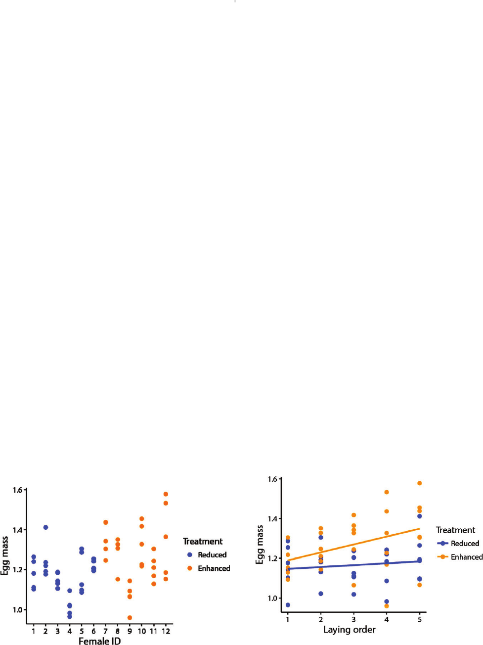
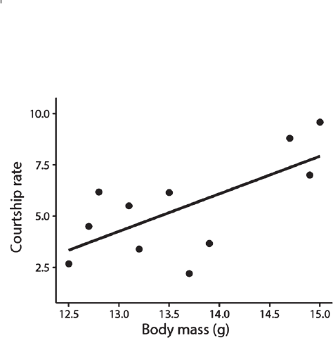
(a)Pseudoreplication at the individual level

Imagine an experiment where you want to test whether

females lay larger eggs when mated to an attractive

male compared to an unattractive male (differential

allocation hypothesis; Sheldon, 2000). For that purpose you

experimentally enhance or reduce the ornamentation of

males of species xy, and you measure the size of the eggs that

females lay when paired to such males. You have 6 females,

each of which you pair to a different male with enhanced

ornamentation, and 6 different females each assigned to a

different male with reduced ornamentation, and for each of

the 12 females you measure the size of 5 eggs (60 eggs in

total; see Fig. 4). The ﬁve eggs that come from the same

female are obviously not independent of each other (i.e. they

are pseudoreplicates with respect to the treatment) and this is

problematic, because females are rather consistent in laying

eggs of a certain size (Fig. 4).

If this non-independence is ignored, and you test the 30

eggs from ‘enhanced’ against the 30 eggs from ‘reduced’, you

will get a highly misleading P=0.002 in this case [R-code:

glm(egg_mass∼treatment)]. Note that this P-value would

be correct if you had had 30 independent females in each

treatment group and if you had measured only one egg from

each of them. In the present case, you can either eliminate

pseudoreplication at the level of individuals by calculating

mean egg size per female and testing the six ‘enhanced’

means against the six ‘reduced’ means which yields P=0.10

[R-code: glm(mean_of_egg_mass∼treatment)], or you can

account statistically for the non-independence by ﬁtting

female identity (ID) as a random effect (‘random intercepts’)

in your model [R-code using the lme4 package (Bates et al.,

2014): lmer(egg_mass∼treatment+(1|female_ID))], which

Fig. 4. Pseudoreplication at the individual level: different

intercepts. Fictional data on egg mass of 5 eggs from each

of 12 females, half of which were assigned to a male with

experimentally enhanced ornamentation and half to a male

with reduced ornaments. Individual females differ in their mean

egg mass (12 different intercepts).

should yield about the same P-value as the ﬁrst option

(here P=0.07). Thus, it is important to acknowledge that, in

this example, the effective sample size is 6 females rather than

30 eggs per group. Therefore, always make sure to choose

the correct unit of analysis (where independence is ensured),

or make sure to identify sources of non-independence and

to model them correctly as random effects (watch out for

repeated measures on the same individual). Cases of such

overt pseudoreplication have become rare in the literature,

but they still persist in some research areas.

However, there is a risk of making another mistake,

less often spotted. After obtaining a non-signiﬁcant result

(P=0.07) from testing the a priori hypothesis that females

would lay larger eggs for ‘enhanced’ males, it is tempting

to use the data set for further exploratory analysis. Maybe

the treatment effect will come out more clearly if we also

consider the order in which the ﬁve eggs of each female have

been laid (laying order).

In our example, egg mass typically increases from the

ﬁrst to the ﬁfth egg (Fig. 5). We do not know the function

(the adaptive value) of this increase, but we could speculate

that it mitigates competitive conditions for the last-hatching

chicks. We also notice that the increase in egg mass over

the laying sequence appears to be steeper for the ‘enhanced’

group (Fig. 5). We therefore test whether the treatment

interacts with laying order in its effect on egg mass [R-code

using the lme4 package: lmer(egg_mass∼treatment*

laying_order+(1|female_ID))], and indeed the interaction

term seems signiﬁcant (P=0.042). This speciﬁcation of the

model has been widely used, but it is in fact incorrect and

may yield 30% false-positive outcomes for the treatment

by laying order interaction term (Schielzeth & Forstmeier,

2009). So where is the mistake?

Fig. 5. Pseudoreplication at the individual level: different

slopes. Fictional data on egg mass from Fig. 4, but this time

plotted against the order in which the ﬁve eggs from each

female were laid. Egg mass appears to increase more steeply in

the ‘enhanced’ group (compared to the ‘reduced’ group), but

statistical testing requires speciﬁcation of female-speciﬁc slopes

(six ‘enhanced’ versus six ‘reduced’ slopes).

1954 W. Forstmeier and others

Note that we have shifted our interest from testing for a

treatment main effect (Fig. 4) to testing for a treatment by

laying-order interaction, i.e. a difference in slopes between

treatments (Fig. 5). The former requires modelling of

individual-speciﬁc intercepts [R-code lme4: (1|female_ID)],

to acknowledge correctly that we are actually testing only

six versus six intercepts. The latter, testing for a difference

in slopes, requires modelling of individual-speciﬁc slopes

[R-code lme4: (laying_order|female_ID)], to acknowledge

correctly that we are actually testing only six versus six

slopes. Again, the mistake is to think that you could use

all 30 eggs from ‘enhanced’ for calculating the ‘enhanced’

slope (and the other 30 for the ‘reduced’ slope) as

if they were fully independent of each other. In fact,

each female has its own slope that you could calculate

and then do a t-test of six versus six slope estimates,

and, given the small sample size, this will rarely reach

signiﬁcance. Indeed, when the full model is speciﬁed

correctly [R-code using lme4: lmer(egg_mass∼treatment*

laying_order+(laying_order|female_ID))] the P-value for

the treatment by laying-order interaction is clearly

non-signiﬁcant (P=0.22).

Again, make it clear to yourself which hypothesis you are

testing (a difference in slopes), and what the independent

units are (female-speciﬁc slopes) for testing that hypothesis.

As in the earlier example (Fig. 4) where you had the option of

eliminating pseudoreplication by calculating mean egg mass

of each female, you here have the same option of calculating

a slope for each female and doing the testing on the derived

statistic. Yet in reality, not every female will lay exactly ﬁve

eggs, so the derived statistic (mean or slope) will vary in its

precision among females (most uncertain for females that lay

only two eggs). In that case, the method of choice is to ﬁt

a model with the appropriate random-effects structure that

accounts for all non-independence in the data that is relevant

for hypothesis testing.

(b)Pseudoreplication due to genetic relatedness

In the previous section we focussed on repeated measures

within individuals that were obviously not independent of

each other. In this section we consider only one measurement

per individual, but focus on how individuals can be

non-independent of each other because of kinship (Hadﬁeld

et al., 2010). This is most often a problem in observational

studies, and less so in experimental studies, because the latter

allow us to e.g. split up a pair of brothers into the two

treatment groups (making the confounding structure in the

data independent of the predictor of interest).

When working with animals that you breed yourself in

captivity, you rapidly begin to realize that individuals are not

independent of each other. Not surprisingly, pairs of siblings

tend to be more similar to each other when compared

to less-related individuals (Burley & Bartels, 1990). For

instance, you may ﬁnd that across all individuals there

is a signiﬁcant positive correlation (r=0.68, P=0.021)

between two phenotypic traits, here male body mass and

male courtship rate (Fig. 6).

Fig. 6. Pseudoreplication at the family level. Fictional data

showing the rate of male courtship (N=11 males) as a function

of male body mass (r=0.68, P=0.021). Note that signiﬁcance

may be overestimated if the three males on the right come from

the same family that happens to carry alleles for high mass and

high courtship rate.

However, the statistical signiﬁcance of that relationship

may have been overestimated if the 11 data points are

non-independent. Both phenotypic traits (mass and courtship

rate) are partly genetically inherited, and it might be the

case that the three males with the highest body mass and

highest courtship rate are three brothers. If this is the case,

we need to ﬁt family identity as a random effect into the

model [R-code lme4: lmer(courtship∼mass+(1|family_ID))]

and let’s say that the other eight males come from eight

independent families. This changes the P-value for the effect

of mass on courtship rate from P=0.021 to 0.084. This is

still a trend, but one that is more likely to have come about

by chance, and so we should not have too much conﬁdence

that we will observe the same pattern in other males. Some

researchers may argue that correcting for pseudoreplication

is misguided in this case since it could mask a real relationship

among these individuals. If the goal were only to describe the

pattern in this population of 11 males, then we would agree.

However, if we wanted to predict the likely pattern in other

populations or in the species in general, we want to avoid

being misled by chance associations driven by relatedness

among individuals in our sample (in which case P=0.084 is

a more realistic estimate of the probability that the observed

pattern arose by chance alone).

In the above example, relatedness may lead to inﬂated

signiﬁcance because both the dependent variable (courtship

rate) and the predictor (body mass) are partly genetically

inherited. This confounding effect gets even larger when

the predictor is inherited entirely, as the next example

will show. Let’s say we study male courtship rate in zebra

ﬁnches (Taeniopygia guttata) in relation to alleles at genes that

are good candidates for affecting courtship rate (so-called

phenotype–genotype associations). We ﬁnd that a particular

allele (ESR1_10) at the oestrogen receptor locus (ESR1)

Avoiding false-positive ﬁndings 1955

Fig. 7. Average courtship rate (corrected for

between-generation differences) of 1556 male zebra ﬁnches as

a function of the number of ESR1_10 alleles they carry. Jitter

was added to the x-axis in order to increase the visibility of data

points. The regression line (y=0.4x−0.1) indicates by how

much courtship rate increases per gene copy, explaining 1.4%

of the total variance.

was associated with increased male courtship (Forstmeier,

Mueller & Kempenaers, 2010).

If we assume statistical independence of the 1556 males

from our captive zebra ﬁnch population (comprising

seven generations of birds) and model courtship rate as

a function of the genotype as illustrated in Fig. 7 we

obtain a remarkably signiﬁcant P-value of P<10–15

[R-code: glm(courtship∼ESR1_10_copies)]. If we ﬁt family

identity as a random effect into this model [R-code lme4:

lmer(courtship∼ESR1_10_copies+(1|family_ID))], where

family_ID groups together all full-brothers that come from

the same parents within each generation, the model yields

P<10–9, still a remarkably signiﬁcant effect. However,

this coding of families accounts for non-independence of

brothers within generations, but ignores that both alleles

and behaviour are passed on longitudinally from father

to sons, making the corresponding family groups similar

in terms of alleles and behaviour. Hence, to account

for all genetic relationships, we need to ﬁt the entire

seven-generations pedigree as a random effect into a

so-called ‘animal model’ [R-code for the pedigreemm

package (Vazquez et al., 2010; Bates & Vazquez, 2014):

pedigreemm(courtship∼ESR1_10_copies+(1|animal))].

Soberingly, this analysis yields P=0.015 for the effect of

this allele on courtship rate. Maybe this effect is still real,

but the exceedingly high conﬁdence we had from the initial

analyses was unwarranted. As an aside, another lesson here

is that P-values are not useful for indicating strength of

effect. P-values here varied dramatically based on effective

sample size, but any effect of these alleles on courtship rate

was always weak as indicated by the r2value (0.014).

What is most disturbing about the problem of

non-independence driven by relatedness is that the problem

would be much harder to ﬁx when studying a population

of animals in the wild (if relatedness is also high there). If

pedigree information is unavailable, we could genotype each

individual at say 10000 single nucleotide polymorphism

(SNP) markers, run a principal component analysis over

these data, and ﬁt the principal components as ﬁxed effects

to control for patterns of relatedness in this wild population

(Price et al., 2006). If we went through this trouble, we might

discover that a promising-looking phenotype–genotype

association has entirely evaporated in terms of its statistical

signiﬁcance. This would no doubt be very disappointing, but

learning that this pattern is unreliable should save us from

wasting money on other expensive follow-up projects that

would have been built on an unreliable foundation.

(c)Pseudoreplication due to spatial and temporal autocorrelation

Above we have considered the case that individuals yield

non-independent data points because they are inﬂuenced by

the same genetic effects (shared alleles). Besides the effects of

genetics, individual phenotypes are inﬂuenced by numerous

environmental factors. Such environmental factors typically

vary in space and time, so individuals that are close to each

other in space and time will often share the same effects and

hence will be more similar to each other (non-independent).

Any such shared inﬂuences will create spatial and temporal

autocorrelation in the data. To examine those, you may want

to consider sorting your data either by time or in space and

checking the extent to which the preceding measurement

predicts the following one (this can be easily done by copying

your y-variable column into a new column but shifted down

by one row, and then quantifying the correlation between

the columns). However, remember that other confounding

factors (like repeated measures on the same individual) can

induce the illusion of temporal autocorrelation if subsequent

measures are typically from the same individual. If you

ﬁnd autocorrelation in your data, you may want to consult

some of these references for methods of accounting for

non-independence (Cliff & Ord, 1981; Valcu & Kempenaers,

2010; Dale & Fortin, 2014).

When designing an experiment, it is always good

to consider the possibility of temporal and spatial

non-independence, because this will remind you to allocate

your treatments carefully (blocking is often better than

randomizing). You obviously should not locate all your

nutrient-enrichment plots in one ﬁeld and your control plots

in another ﬁeld. For the same reasons, you should not put the

cages holding the ‘enhanced’ males close to the room win-

dow and the ‘reduced’ males on the corridor side. Although

it may not be the case that daylight will affect egg size, this

will nevertheless put you into a situation where you lose

all power to detect a treatment effect, because you need to

control for the distance to the window as a covariate, which

will be strongly collinear with your treatment and hence the

two potential effects will be difﬁcult to tease apart. Likewise,

putting all males of one treatment category into one aviary

1956 W. Forstmeier and others

and all males of the other category into another aviary,

will leave you with N=1versus N =1, because you need to

control for the effect of aviary identity as a random effect.

Temporal non-independence of events also often leads to

the phenomenon of data being ‘overdispersed’. This means

that extreme values are more frequently observed than would

be expected from chance alone. For instance, subsequent

eggs are often more alike, not only in size (Fig. 5) but also

with regard to paternity. Studies of female promiscuity that

measure the proportion of eggs within a clutch that is sired by

an extra-pair male typically observe that extreme outcomes

(0 or 100% of extra-pair young) are more frequent than

expected by chance (Neuh¨

auser, Forstmeier & Bretz, 2001).

Such overdispersion in the data needs to be accounted for;

otherwise this will again result in anti-conservative P-values.

For this, the sequence of eggs does not have to be known, and

using clutch identity (unique code for every clutch) as a ran-

dom effect will typically help solve the issue. Hence, overdis-

persion may be easy to account for in cases where we under-

stand the source of non-independence (here clutch identity).

Another way of correcting for overdispersion is through the

use of quasi-likelihood models (Wedderburn, 1974).

A ﬁnal mistake related to overdispersion that one can

sometimes observe is that measurements of latency (e.g. the

number of seconds that a bird takes to return to its nest) are

modelled as a Poisson trait (for count data). Rather obviously,

subsequent seconds are not statistically independent events,

and hence the data will typically be strongly overdispersed.

Also, when you compare different options, you will see that

P-values will strongly depend on whether you counted the

time in hours, minutes, seconds, or even milliseconds. An

example is shown in Fig. 8, where the latency to return to

the nest is analysed as a function of a measure of the bird’s

exploratory behaviour.

What is striking about this example (adopted and modiﬁed

from an unpublished study) is that a remarkably shallow

Fig. 8. Fictional data on the latency of 70 birds to return to

their nest after disturbance as a function of their exploratory

behaviour recorded in another test. The line is based on ordinary

least-squares regression on untransformed data.

regression line compared to the total range of variation is

accompanied by a P-value of <10–7.Inthisexample,each

minute gets evaluated as an independent event, and a few

very high values on the left side (up to 559 min) cause all

the apparent statistical signiﬁcance. If the same data are

modelled (again wrongly) as counts of hours (ranging from

0 to 9), we arrive at P=0.078 although the data look

almost the same [R-code: glm(hours∼exploration, family =

‘poisson’)]. Latencies can often be transformed into a nice

normal distribution by taking the logarithm of the number of

minutes or seconds [here the choice does not really matter,

but note that ln(0) is not deﬁned]. Modelling the natural

logarithm of the number of seconds as a Gaussian trait, we

obtain P=0.26, which ﬁts the impression of a weak trend

given by Fig. 8 [R-code: glm(lnsec∼exploration)].

(d)Pseudoreplication renders P-curve analysis invalid

Simonsohn et al. (2014) recently suggested that one could

examine the subset of all published P-values that reach

signiﬁcance (P<0.05) in order to ﬁnd out whether a true

effect exists or not (referred to as ‘P-curve analysis’). In

the presence of a true effect, P-values between 0 and 0.01

should be more frequent than P-values between 0.04 and

0.05, i.e. there should be an excess of highly signiﬁcant

P-values. Hence, right-skewed P-curves have been suggested

to be evidential for true effects (Jager & Leek, 2014;

Simonsohn et al., 2014). However, if genetic relatedness and

temporal or spatial autocorrelation are ubiquitous in real

data sets, and often lead to pseudoreplication that remains

unaccounted for (e.g. because relatedness is unknown),

then such pseudoreplication will cause an excess of overly

signiﬁcant P-values that renders invalid such interpretation

of right-skewed P-curves as evidence for a true effect. The

assumptions of P-curve analyses are almost certainly seriously

violated in multiple other ways as well and so unfortunately

this brieﬂy promising method for assessing biased reporting

cannot fulﬁl expectations (Gelman & O’Rourke, 2014;

Bishop & Thompson, 2016; Bruns & Ioannidis, 2016).

(4) Errors in interpretation of patterns

(a)Overinterpretation of apparent differences

Humans have a tendency readily to recognize patterns, even

where none exist. This may be partly enhanced by binary

thinking in terms of effect (if P<0.05) versus no effect (if

P>0.05). Accordingly, one can also ﬁnd this as a common

mistake in the scientiﬁc literature: the title of a paper may

claim that ‘sexes differ in their response to a treatment’, but

the study only found that an effect was signiﬁcant in males

and non-signiﬁcant in females. This does not mean per se that

the sexes are actually different. Whether the difference itself

reaches signiﬁcance has to be assessed by testing the sex by

treatment effect interaction term (Gelman & Stern, 2006).

Only if the P-value for that interaction passes the threshold of

P<0.05 can we conclude that the sexes differ signiﬁcantly in

that treatment effect on whatever the dependent variable was.

Avoiding false-positive ﬁndings 1957

Likewise, there is often a tendency to jump prematurely to

the conclusion that the ﬁndings of two studies are different.

Are they signiﬁcantly different? Not very intuitively, a

parameter estimate from a replication study has a probability

of about one in six (16.6%) to fall outside the 95% conﬁdence

interval of the estimate from the initial study (Cumming,

Williams & Fidler, 2004). This may come as a surprise,

because one may think that the 95% conﬁdence interval

should contain 95% of the replication results (Cumming

et al., 2004). However, the 95% conﬁdence interval is deﬁned

in a way that it contains the (typically unknown) true value

of the parameter with a probability of 95%. And while the

true value is a ﬁxed number, both the estimate from the ﬁrst

study and the estimate from the second study come with

uncertainty. This means that either the ﬁrst or the second

study could have yielded an unlikely (unusually extreme)

outcome, so the probability that they agree is lower than the

probability of one estimate agreeing with the ﬁxed true value.

Again, a formal test for the study by effect interaction term

will inform you correctly about the probability of obtaining

such a difference between two studies by chance alone. So

make sure you are not over-interpreting a difference that

may not be real.

(b)Misinterpretation of measurement error

There is one ﬁnal statistical phenomenon that we would

like to highlight: ‘regression to the mean’ (Barnett, van der

Pols & Dobson, 2005). Although it is not related to any of

the examples above, it is a sufﬁciently common trap and

has led to errors in a wide range of scientiﬁc disciplines

(Kelly & Price, 2005; Danchin, Wajnberg & Wagner, 2014).

Moreover, since the regression to the mean will consistently

produce a spurious but often signiﬁcant effect, and since we

typically publish when encountering something signiﬁcant,

one can readily ﬁnd erroneous interpretations of this artefact

in the literature.

‘Regression to the mean’ is a phenomenon that results from

measurement error. Say we measure a group of individuals

once (e.g. we measure, with some error, the attractiveness of

individuals), and then divide them into two groups according

to the ﬁrst measurement, namely those that lie above the

mean (attractive half) and those that lie below the mean

(unattractive half). If we then measure the individuals from

the two groups a second time, we can predict that the two

group averages will deviate less from the population mean

than in the ﬁrst measure (hence ‘regression toward the mean’;

i.e. the attractive group will become less attractive, while the

unattractive group will become more attractive). Figure 9

illustrates the origin of this effect.

Regression to the mean leads to an apparent systematic

change in the phenotype of the individuals (on average, the

orange dots in Fig. 9 decreased and the blue dots increased

their trait values from ﬁrst to second measurement). This

change has often been misinterpreted as resulting from an

experimental treatment that was also applied between the

ﬁrst and the second measurement. When we know the

expected amount of measurement error that is inherent to

each measure (i.e. 1 −repeatability), we can make predictions

about the expected magnitude of regression toward the mean,

and we can test whether the experimental treatment had any

additional effects beyond this statistical artefact (Barnett et al.,

2005). However, in practice one should avoid such situations

whenever possible (Danchin et al., 2014). Hence, the rule

Fig. 9. The panel on the left shows the true trait values of 100 individuals sorted by their rank in trait values. In practice, such

true trait values are unknown, and we can only measure trait values with some measurement error (central panel). If we then assign

individuals into categories (‘below average’ in blue and ‘above average’ in orange) based on our ﬁrst measurement, we make some

misassignments with respect to their true ranks (e.g. some with true rank >50 get assigned to the ‘below average’ group). A second

measurement on the same individuals will again approximate the true values with equal amount of error, but most of the previously

misassigned individuals and some of the correctly assigned ones will this time fall on the other side of the population average. As

a consequence, the means for the two groups (blue and orange asterisks) will move closer together (and closer to the population

average). Also note how the standard errors around the two group means (indicated by horizontal bars) increase from the ﬁrst to the

second measurement because values can now vary over a wider range (no longer restricted by the ‘deﬁnition’ of having to lie above

or below the average).

1958 W. Forstmeier and others

should be ‘never assign individuals to different treatments

according to their phenotype!’ If you cannot come up with a

better experimental design, you should at least be aware of the

phenomenon, i.e. you should expect that the more aggressive

individuals will become less aggressive when measured again,

and that the previously preferred option in a choice test will

become less preferred next time.

(5) Cognitive biases

Somewhat surprisingly, it appears that the human brain has

not evolved to maximize the objectivity of its judgements

(Haselton, Nettle & Murray, 2005). Accordingly, psycholo-

gists have described a near-endless list of cognitive biases that

inﬂuence our perception, reasoning and memory. In Table 2

we have compiled a selection of biases which should also

have an impact on the judgements made by scientists. Of

these, we have already discussed the hindsight bias in Section

II.2c, which makes it sometimes difﬁcult to recall whether a

hypothesis was derived from the data or whether the test was

planned a priori. We further have touched on conﬁrmation

bias in Section II.2ewhen discussing how wishful thinking

may inﬂuence our arbitrary decisions on how to analyse

our data. Another form of conﬁrmation bias is worth

mentioning, namely that preconceptions may inﬂuence our

observations (‘observer bias’). In other words, if an observer

expects a treatment to produce a certain measureable effect,

the observer’s measurements may be unconsciously biased

towards detecting that effect. This bias can be minimized

by ‘blinding’ observers to the hypotheses being tested or to

the treatment categories of the individuals being measured.

However, blinding is rare. For example, in a collection of 79

studies of nest-mate recognition in ants, just 29% of the stud-

ies were conducted blind. This rarity of blinding appears to

have seriously impacted observations since non-blind studies

were much less likely (21%) to report aggression among

nest-mates than blind ones (73%), leading to a twofold

overestimation of effect size (van Wilgenburg & Elgar,

2013). In 83 pairs of evolutionary biology studies matched

for type of experiment, non-blind studies had substantially

larger effect sizes than blind studies (mean ±S.E. difference

in Hedges’ g=0.55 ±0.25), and the non-blind study had

a higher effect size than its matched blinded experiment in

signiﬁcantly more cases (Holman et al., 2015). Comparisons

with much larger samples lend considerable support to these

observations. In 7644 papers identiﬁed via automated text

mining (from 4511 journals in the Open Access collection

of PubMed), the proportion of signiﬁcant P-values in a paper

was signiﬁcantly lower in blind than in non-blind papers

(Holman et al., 2015). Among a sample of 492 papers from

the disciplines of ecology, evolution, and behaviour pub-

lished in high-impact-factor journals in 2012, 248 presented

studies ‘that could have been inﬂuenced by observer bias’.

However, only 13% of these studies appeared to have

gathered data through a blind process (Kardish et al., 2015).

If we recognize our cognitive biases as fundamental to our

nature rather than as character ﬂaws to be ashamed of, we

can structure our scientiﬁc endeavours in ways to minimize

their effects. We blind observers not because observers are

Table 2. A collection of cognitive biases that may hinder objectivity of researchers. Names and explanations were adopted from

Wikipedia (www.wikipedia.org) and inspired by a compilation of 175 cognitive biases by Buster Benson (https://betterhumans

.coach.me/cognitive-bias-cheat-sheet-55a472476b18)

Bias Explanation

Conﬁrmation bias The tendency to search for, interpret, favour, and recall information in a way that conﬁrms one’s

pre-existing beliefs or hypotheses, while giving disproportionately less consideration to alternative

possibilities

Selective perception The tendency not to notice and more quickly forget stimuli that cause emotional discomfort and

contradict our prior beliefs

Bias blind spot The cognitive bias of recognizing the impact of biases on the judgement of others, while failing to

see the impact of biases on one’s own judgment

Confabulation The production of fabricated, distorted or misinterpreted memories about oneself or the world,

without the conscious intention to deceive. This may help us in making sense of what we see

Clustering illusion The tendency to erroneously consider the inevitable ‘streaks’ or ‘clusters’ arising in small samples

from random distributions to be non-random

Illusion of validity A cognitive bias in which a person overestimates his or her ability to interpret and predict accurately

the outcome when analysing a set of data, in particular when the data analysed show a very

consistent pattern – that is, when the data ‘tell’ a coherent story

Belief bias The tendency to judge the strength of arguments based on the plausibility of their conclusion rather

than how strongly they support that conclusion. This is an error in reasoning, such as accepting

an invalid argument because it supports a conclusion that is plausible

Hindsight bias The inclination, after an event has occurred, to see the event as having been predictable, despite

there having been little or no objective basis for predicting it

Overconﬁdence effect A bias in which a person’s subjective conﬁdence in his or her judgments is reliably greater than the

objective accuracy of those judgments

Appeal to novelty A fallacy in which one prematurely claims that an idea or proposal is correct or superior, exclusively

because it is new and modern

Avoiding false-positive ﬁndings 1959

dishonest, but because we know that we all have a tendency

to see what we expect to see. We preregister analysis plans

only because we know that even people with the purest

conscious motives are more likely to choose the method that

produces the story that they most believe.

III. SOLUTIONS

(1) Need for replication and rigorous assessment of

context dependence

In face of the problems that we have outlined above

(multiple testing including researcher degrees of freedom,

pseudoreplication, selective reporting, and HARKing), it is

clear that we should be fastidiously sceptical consumers of

published scientiﬁc results. Given publication bias in favour

of positive results and given the rather soft criteria for

reaching signiﬁcance, it is currently possible to ﬁnd positive

‘evidence’ in the scientiﬁc literature for almost any possible

phenomenon. If you recognize this, you presumably will also

recognize that the extreme pursuit of novelty (by high-impact

journals) and researchers’ pursuit of impact (imposed by

employers and funding agencies) will contribute to an

ever-increasing body of false-positive claims that hampers

scientiﬁc progress (Ware & Munafo, 2015).

Hence, we need to promote scepticism of spectacular

but highly unlikely claims and turn attention to sorting out

all the false-positives from the true positives. How can this

be done? As we have seen, we can use a variety of clues

to identify ﬁndings that are less likely to be true, but what

we really need is a rigorous method of assessment in the

form of well-controlled and standardized attempts to closely

replicate previous studies (Nakagawa & Parker, 2015).

Further, institutions need to favour the publication of the

results of replication independent of their outcome. To see

the utility of unbiased replication attempts, we can look to the

recent coordinated effort to replicate 100 ﬁndings published

in top journals in the ﬁeld of psychology (Open Science

Collaboration, 2015). This large-scale initiative found that

about 40% of the ﬁndings appear to hold up (reminding us

of Fig. 1F), while most of the remainder were contradicted

or not supported (but see Etz & Vandekerckhove, 2016).

The high statistical power of most of the replications lend

strength to the conclusion that many of the original studies

were either the result of error or were more dependent on

subtle differences in context than had been assumed.

(a)Obstacles to replication

In face of the request for novelty, researchers often address

a commonly asked question in a new species or with new

methods. However, in such quasi-replications (Palmer, 2000),

if results differ from the original, we are left to speculate

about why the outcomes differed and we will rarely be able

to identify the true reason for the difference in outcomes,

because quasi-replicates differ in so many aspects. Close

replication, by contrast, minimizes differences among studies

and facilitates the identiﬁcation of plausible hypotheses to

explain divergent results. Unfortunately, close replications

are rare in many disciplines (Palmer, 2000; Kelly, 2006;

Drotar, 2010; Nakagawa & Parker, 2015). There are two

interrelated explanations for this. First, many researchers

have not yet come to appreciate the important role of

replication in developing robust scientiﬁc inference, and

second, the institutions that inﬂuence scientists’ choices do

not reward close replication (Nosek, Spies & Motyl, 2012).

Funding agencies and journal editors focus on novelty.

This is particularly hard to justify on the part of funders

since failing to invest in replication means failing to seek

robust answers to questions they already have made a

commitment to answering. If the answer truly was worth

paying for, then the replication should also be worth paying

for (Nakagawa & Parker, 2015). Promoting the funding of

replication studies would be relatively straightforward. Most

obviously, agencies could set aside funds for important and

well-justiﬁed replications. Agencies could also incentivize

replication by preferentially funding novel studies when

those studies rest on well-replicated foundations (Parker,

2013). They could also preferentially fund researchers whose

prior work has often been successfully replicated.

In the case of journals, pursuit of novelty may be harder

to curb, but there are paths to reducing the tyranny

of this pursuit. Journals seek novelty in part because of

the competition for impact factors. Studies which report

surprising (i.e. unlikely) ﬁndings are often highly cited and

thus contribute to the stature of the journal. Thus, ‘the more

surprising, the better’. This effect may be exacerbated by

the for-proﬁt publishing industry. Fortunately, replications

can also be heavily cited. Recent attempts to replicate classic

studies in psychology have received citations at a much higher

rate than the average study in the journal in question. In

2014, the journal Social Psychology published an issue (issue 3,

May) devoted to replications of previously published studies.

As of 15 March 2016, the mean number of citations from

those 15 replications (of 15 different earlier studies) was 7.1

(median =4, with no articles having gone uncited). By the

same date in 2016, the average article from the previous

two issues (1 and 2 from 2014), including no replications,

had received 1.2 citations (median =1, with 5 of 12 articles

remaining uncited). Of course this may be in part due

to the current novelty of replication research (ironically).

However, robust, well-conducted replications of important

work will presumably attract considerable attention in the

future, especially as awareness grows about the importance

of replication in assessing validity of prior work. We expect

that as more journals explicitly invite replications (as some

are beginning to do), more researchers will come to recognize

their utility, and thus researchers will more often seek to cite

replications because of the strong inferences they facilitate.

Even without institutional obstacles, there are important

social obstacles to navigate. An attempt to replicate closely

someone else’s ﬁnding may be perceived as a personal attack

on the original researcher. The very act of replication implies

1960 W. Forstmeier and others

insufﬁcient conﬁdence in the original ﬁndings, and in cases

of failure to conﬁrm the original ﬁnding, the researcher

who published the original study may fear for his or her

reputation (although we expect this phenomenon to be less

common as replications become more frequent and failure

to get conﬁrmed is recognized as normal). Journals almost

invariably ask the author of the previous study to review the

replication manuscript since he or she is the expert and is

directly concerned. This reviewer will often be predisposed to

be negative, sometimes trying to save his or her own results by

questioning the quality of the replication (e.g. making the case

that an incompetent person will often fail to get the correct

result; Bissell, 2013). Thus it may often be difﬁcult to publish

a replication, especially when that replication contradicts

earlier work, and this is a strong disincentive to replicate.

(b)Overcoming the obstacles

A partial solution to this dilemma could come from

researchers replicating their own ﬁndings. This eliminates the

quality issue as well as issues related to dissimilarity in materi-

als or methods. A simple and cheap way of getting this started

was suggested by one of our colleagues, Jarrod Hadﬁeld (Had-

ﬁeld, 2015). He proposed that researchers running long-term

studies could publish addenda to their previous publications,

declaring in a one-page publication that their original ﬁnding

did or did not hold up in the data of the following years (after

the publication), and comparing the effect sizes between the

original data and the newer data. This would be a quick

way of producing another publication, and it would be enor-

mously helpful for the scientiﬁc ﬁeld. This may also relax the

feeling of stigma when something does not hold up to future

evaluation. Admitting a failure to replicate could actually

be perceived as a signal of a researcher’s integrity and be

praised as a contribution to the scientiﬁc community. For

grant applications, funding agencies could even speciﬁcally

ask for visible signs of such integrity rather than exclusively

focussing on metrics of productivity and impact.

Apart from publishing addenda, how should we go about

conducting replication studies? First of all, the study should

be preregistered (see Section III.3) in order to solve two issues:

(i) preregistration of analysis plans takes out any researcher

degrees of freedom that would risk biasing the observed

effect size in the direction desired by the researcher (either

conﬁrmation of the previous ﬁnding or clear refutation of it),

and (ii) preregistered studies that do not make it to the stage

of publication will still be accessible at a public repository,

documenting the attempt and hopefully also the reason for

failure. Besides being preregistered, replication studies should

attempt to match the previous study as closely as possible in

methods and materials and should aim for a larger sample

size. Incentives to preregister should be particularly strong for

replication studies since a study and analysis plan effectively

already exist, and preregistration will clearly signal to

reviewers and editors that the presentation of results has not

been altered in an attempt to achieve a particular outcome.

A particularly compelling option for publishing replica-

tions is through a process known as registered reports, a

format advocated by Chris Chambers (2013). Registered

reports involve preregistration, but with a registered report,

the researcher ﬁrst submits the study and analysis plan to a

journal for review, potential revision of methods plans, and

preliminary acceptance prior to conducting the study. Thus

a proposed replication could be reviewed, and if judged mer-

itorious, provisionally accepted independent of results. This

would give the scientist who published the original study the

opportunity to recommend changes to methods of the repli-

cation before it was initiated, and thus increase the quality

of the replication while also reducing the opportunity for a

critique, spurious or genuine, of the quality of replication.

(c)Interpretation of differences in ﬁndings

When a replication fails to conﬁrm the original result,

this is often interpreted as context dependence (e.g. ‘this

was a wetter year’, ‘this location contained more conifers’,

or ‘these animals were raised on a higher-protein diet’).

After all, we know that ecology and behaviour are highly

complex and we expect variability. However, in this situation

context dependence is simply an untested post-hoc hypothesis.

We cannot claim that divergent results stem from context

dependence without explicit testing with new data. As

explained in Section II.4a, it may be that the difference

in effect sizes observed in the two studies is no larger than

what one would expect from chance alone (sampling noise).

Meta-analysts (researchers who summarize effect sizes across

numerous studies) are very familiar with this idea, and

they quantify the extent of disagreement between studies as

‘heterogeneity’ in effect sizes. Since each observed effect size

is accompanied by a measure of uncertainty (for instance a

standard error or 95% conﬁdence interval, both of which

depend on sample size), one can test statistically whether

there is signiﬁcant heterogeneity in effect sizes. Such tests

are frequently signiﬁcant, but does this observation provide

strong evidence for context dependence? Unfortunately not!

For tests of heterogeneity to provide insight into context

dependence, we need to minimize other sources of hetero-

geneity. One source of heterogeneity is publication bias in

favour of stronger effects, often facilitated by use of researcher

degrees of freedom to reach signiﬁcance more often than

expected by chance. In an extreme example, two studies

could yield non-signiﬁcant trends in opposite directions (a

small difference due to sampling noise), but those differences

could get ampliﬁed by ‘researcher degrees of freedom’ and

selective reporting, because each team of researchers (in good

faith of doing the right thing) feels obliged to emphasize the

outcome of their study by selecting the conditions where

trends approach or reach statistical signiﬁcance. When pub-

lication bias is common, effect sizes often vary as a function

of sample size because as sample size declines, deriving a sta-

tistically signiﬁcant effect requires larger effect sizes (Gelman

& Weakliem, 2009). This too can generate estimates of signif-

icant heterogeneity among studies in the absence of context

dependence. Thus an important step towards using tests for

heterogeneity as reasonable indicators of context dependence

Avoiding false-positive ﬁndings 1961

is minimizing sources of bias, for instance through preregis-

tered studies. Heterogeneity can also arise due to differences

in study methods that are unrelated to hypothesized contex-

tual differences. If we are truly interested in context depen-

dence and its sources, then we should design replication stud-

ies explicitly to investigate context dependence. This means

systematically evaluating environmental variables that we

hypothesize may be driving context dependence using ‘repli-

cation batteries’, in which conditions hypothesized to drive

differences in results are manipulated while attempting to

hold other variables constant (Kelly, 2006). Post-hoc hypothe-

ses about context dependence are valid, but they remain

nothing more than hypotheses before studies have been

designed and implemented speciﬁcally to evaluate them.

(d)Is the world more complex or less complex than we think?

The tendency of many researchers to interpret all apparent

differences as important (see Section II.4a) and to attribute

these differences to context dependence by default has a

remarkable effect on the development of our world view.

Such world views become increasingly complex, emphasizing

the importance of context dependence which results in

hard-to-interpret interaction terms. By contrast, the sceptic

who emphasizes the large amount of sampling noise in most

sets of data which further may get inﬂated by researcher

ﬂexibility, may often hold a nihilistic world view where most

or all effects are spurious. This is an interesting debate which

we only will be able to resolve by promoting transparency

and by replicating studies as rigorously as possible.

(2) Collecting evidence for the null and the

elimination of zombie hypotheses

Given the many false-positive ﬁndings in the literature, it is

the foremost goal of rigorous replication studies to validate or

reject previous ﬁndings. This will often mean that evidence

we collect contradicts the biological hypothesis. But can this

evidence lead to rejection of our biological hypothesis? After

all, we can never rule out the possibility that this hypothesis

might apply in some other context and that some unknown,

uncontrolled difference between our replication and the orig-

inal study led to our failure to replicate. In practice, however,

we think we can at least approximate rejection of the original

hypothesis. The key is multiple replications and some sort of

meta-analytical framework. For instance, when reporting a

result, we may calculate a 95% conﬁdence interval around

our estimate, and then highlight that our study shows an

effect that is signiﬁcantly smaller than this or that quantity.

We can calculate a weighted average of the two results, and

as we accumulate more independent replications, we gain

conﬁdence in our average, and if this average approximates

zero, we become more conﬁdent that the hypothesis in ques-

tion is wrong, or at least of extremely narrow applicability

(Seguin & Forstmeier, 2012; Nakagawa & Parker, 2015).

Another excellent tool for drawing conclusions from a

series of replications is Bayesian statistics which allow us to

pitch two competing hypotheses (H0 and H1) against each

other and to evaluate which of them is better supported by

the data (Dienes, 2016). The Bayes factor (BF) can be used to

quantify how many times more likely the observed data are

if the hypothesis H1 is true rather than if H0 is true. A Bayes

factor of 1 means that the data are equally likely under both

hypotheses, so the data contribute no information towards

resolving the question of which hypothesis may be true.

Depending a bit on conventions, a Bayes factor larger than

3 is typically considered as substantial or moderate evidence

for H1, while a Bayes factor smaller than 1/3 represents

substantial or moderate evidence for the null hypothesis H0,

and these thresholds are approximately comparable to the

threshold of α=0.05 in signiﬁcance testing (Dienes, 2016).

For the purpose of contrasting a speciﬁed hypothesis H1

(usually deﬁned by the effect size reported in a previous study

that we want to replicate) against the null hypothesis H0,

Bayesian statistics hence allow us to assess whether the new

data from the replication study support either H1 or H0.

Of course Bayesian statistics do not guarantee that we will

resolve the issue (if 1/3 <BF <3). This lack of clarity may

come, for instance, if there is some truth to the published

ﬁnding, but the true effect size lies half-way between the one

that is published and the null (overestimation by a factor of

about two would make BF =1 a likely outcome).

In fact it is well known that published effect sizes tend

to be overestimates of true effects. It is frequently observed

that the ﬁrst publications on a given topic report larger effect

sizes than later follow-up studies, leading to a general decline

in effect sizes over time (Jennions & Møller, 2002; Barto

& Rillig, 2012; Koricheva, Jennions & Lau, 2013). Equally

problematic is the observation that sample size and effect size

are typically negatively correlated in meta-analyses meaning

that only the studies with the largest sample size will yield

trustworthy effect-size estimates (Levine, Asada & Carpenter,

2009). Meta-analysts examine this phenomenon in so-called

funnel plots where effect sizes of studies are plotted in

relation to sample size (Pillemer & Light, 1984). Funnel

plots can be used to detect publication bias in meta-analyses

(Egger et al., 1997), but such tests should be regarded with

caution (Ioannidis & Trikalinos, 2007). Modest amounts of

publication bias, that may not be apparent from funnel plots,

can render the conclusion of a meta-analysis invalid (Scargle,

1999; Ferguson & Heene, 2012).

Besides many true effects being overestimated, it is

conceivable that some ﬁelds of research could exist for

extended periods of time in the complete absence of any

true effects of theoretical relevance. More than 40 years ago,

Greenwald (1975) complained that systematic ‘‘prejudice

against the null hypothesis’’ can lead to a dysfunctional system

of research and publication that allows untrue hypotheses

to persist undefeated, similar to what was recently proposed

for a substantial body of sexual selection research (Prum,

2010). More recently, and along the same lines, Ferguson &

Heene (2012) argued that our aversion to the null will result

in ‘a vast graveyard of undead theories’. We feel that it is

high time to overcome this aversion, and to remind ourselves

that researchers are supposed to be the unbiased referee in

1962 W. Forstmeier and others

a game between H1 and H0, and that falsiﬁcation of untrue

hypotheses lies at the heart of making scientiﬁc progress.

(3) Making science more objective

The weight of all these obstacles to objective science could

leave you frustrated and depressed. Scientists are often

unaware of many of the ways that science is not maximally

objective and the ways that scientiﬁc practices often serve

only the short-term interest of the scientist who is under

pressure to produce success stories in order to attract the

next grant. Fortunately, unscientiﬁc practices like ﬁshing for

signiﬁcance, HARKing, and many others are on their way

out, as a growing community becomes more aware of the

risks and better able to recognize the signs of bad practices.

Further, as discussions of these issues become more common,

we hope that more researchers will realize that sticking to

protocols that promote objectivity is the best strategy in

the long run. For instance, anyone who conducts a series

of studies in the same system will beneﬁt from drawing

robust conclusions in their foundational work. Maximizing

objectivity, for instance through preregistering your studies,

should also bolster your reputation. Then, if one of your

ﬁndings is contradicted by later work you need not worry

about your reputation, and maybe more important, you can

feel good about the fact that you interpreted the data in the

most objective way. In this context, a recent commentary by

Markowetz (2015) is an interesting read. He lists ﬁve selﬁsh

reasons why you should work reproducibly.

We have already touched on a couple of promising ways to

make science more reliable, and we add more details below.

(a)Why should I preregister my next study?

As noted above, preregistration of study plans solves the issues

of (i) HARKing, because you registered your hypotheses in

advance, (ii) researcher degrees of freedom, because you

registered your data-analysis strategy in advance, and (iii)

publication bias, because the added rigour makes nearly

every ﬁnding worth publishing (or otherwise the reason for

failure to publish gets documented in a public space). What

might hold you back from preregistering your next study?

1 I have checked the requirements, and it looks like a

substantial amount of work.

Preregistering your study may take you a couple of days, but

in the long run it will beneﬁt you tremendously by forcing

you to think through your study plans very carefully. Likely

you will discover some weaknesses in your questions, study

design or analysis plan and you still have time to ﬁx or

amend these issues before starting data collection. Also, the

preparatory work will make the data analysis easier since you

will already have a detailed plan, and it will make writing

your paper much easier, since you will already have written

your Methods section.

2 My colleagues are not preregistering their work, so why

should I?

If you are thinking of preregistering your study now, it is not

unlikely that you will be among the ﬁrst in your ﬁeld to do

so. Would you like to be able to say that you were among

the ﬁrst to embrace this new tool that ensures objectivity?

Give it a try and you will likely discover that preregistering is

emotionally rewarding like the submission of a manuscript.

It also lends importance to your project.

3 I am worried that someone will steal my project idea.

No reason to worry. You can embargo your plans, and they

will only become publicly visible later.

4 I need more ﬂexibility in study design.

Preregistration does not limit the freedom of the researcher;

it only documents the ideas and plans at any given time,

making the process maximally transparent. You always have

the possibility of modifying your study plans, and the exact

time of modiﬁcation and reasons for modiﬁcation will be

documented, probably still long before ﬁnal data analysis

when researcher degrees of freedom would come into play.

The original study plan will always remain visible with its

date of registration, but making failed aspects of a plan

visible to others might also save them from repeating the

same mistake.

5 What if I make an unexpected discovery?

Having preregistered your study does not prevent you

from publishing any analysis you believe is interesting or

informative. All that preregistration does is clarify what tests

were formulated a priori and what tests were not. For instance,

you may subdivide your publication into a part that covers

the original analysis plan (the rigorous a priori testing part)

and a second part that explores the data post hoc and yields

unexpected discoveries.

If you have other questions, or want to start registering,

check out the website of the Center for Open Science

(https://cos.io/and speciﬁcally https://cos.io/prereg/). The

Center for Open Science is currently sponsoring a

‘Preregistration Challenge’ in which they will award

US$1000 to the ﬁrst 1000 researchers to publish preregistered

studies. An alternative site that offers a maximally convenient

and hassle-free opportunity to preregister your study is

provided by AsPredicted (https://aspredicted.org/).

(b)Badges make good scientiﬁc practice visible

The Open Science Framework (https://osf .io/) has also

started an initiative to make good scientiﬁc practice

visible by awarding badges to studies that meet certain

criteria, currently including preregistration, the availability

of archived data, and the availability of detailed materials.

Avoiding false-positive ﬁndings 1963

Journals decide if they want to award badges to publications

that meet the criteria, and a few journals (mostly from

the ﬁeld of psychology) have already started doing so.

Authors, when they submit their paper, apply for the

badge by declaring that the study complies with the

criteria. Editors or referees may check whether this is

true but they may also leave the responsibility with the

authors for making correct declarations (thereby minimizing

the additional workload for journals). There is already

evidence that awarding badges is effective in promoting

the sharing of data (Kidwell et al., 2016). Badges might

also facilitate evaluation of bias. For instance, badges could

make it possible to identify preregistered studies and thus to

compare effect sizes meta-analytically between preregistered

and non-preregistered studies. If you want to publish a

preregistered experiment, it may well make sense to contact

the editor-in-chief of the journal prior to submission to ask

whether they would be ready to give you a badge in case

of acceptance. Currently it seems that journal editors are

waiting to see whether they start receiving such requests

before deciding to join the list of journals that award badges

(see https://osf.io/tvyxz/wiki/5.%20Adoptions%20and%

20Endorsements/).

(c)Blinding during data collection and analysis

To rule out cognitive biases (Section II.5) such as the observer

effect during data collection or conﬁrmation bias during data

analysis, it is generally a good idea to blind the researcher

(MacCoun & Perlmutter, 2015).

During data collection, blinding ourselves to treatment

groups provides an important protection against any intrinsic

subconscious biases that we may have (van Wilgenburg &

Elgar, 2013; Holman et al., 2015; MacCoun & Perlmutter,

2015). In all cases where data collection is not entirely

objective and free of observer effects, it is almost impossible

not to end up with bias. Despite the importance of observer

effects in many ﬁelds of science, strategies of observer blinding

are implemented in fewer studies than one would hope (van

Wilgenburg & Elgar, 2013; Holman et al., 2015; Kardish

et al., 2015).

During data analysis, blinding the researcher from the

effect of arbitrary decisions on statistical signiﬁcance of the

hypothesis test is an important tool that ensures objectivity

(MacCoun & Perlmutter, in press). Hence, you should try

to take your choices of analysis variants before seeing their

effects on P-values. If this is not possible, you could ask

someone else to make these choices blindly (without regard

to outcome) for you, always going for the option that sounds

more reasonable based on criteria other than signiﬁcance or

effect size.

(d)Objective reporting of non-registered studies

If you have not preregistered your hypotheses and analysis

plan, how can you reach comparable levels of objectivity

in your publication? First, you should explicitly distinguish

your a priori hypotheses (typically just a few, namely the

ones you designed the study for) from your exploratory data

analysis. Second, you should avoid selective reporting. For

any question or ﬁeld of questions within your study, you

should attempt to consider all possibly relevant dependent

variables and predictors (see Fig. 2). If this makes the

manuscript too long, you can always put large tables of

results in an electronic supplementary ﬁle. You can then

report averaged effect sizes in the paper itself. Third, you

should avoid reporting estimates that are biased towards

signiﬁcance by non-blind choice of ‘researcher degrees of

freedom’. If you cannot use blinding as described above,

you may want to consider using speciﬁcation-curve analysis

(SCA) (Simonsohn et al., 2015) to go through all combinations

of analysis variants, and to average effect sizes across all

combinations. Currently, U. Simonsohn and co-workers are

planning to create an R-package that would make SCA easy

to carry out. A less-ambitious, but still noteworthy option has

been suggested by the same set of authors (Simmons, Nelson

& Simonsohn, 2012) who advocate ‘a 21 word solution’

of the problem in your Methods section. Speciﬁcally, your

Methods should say: ‘We report how we determined our

sample size, all data exclusions (if any), all manipulations,

and all measures in the study.’ This should take out a range of

researcher degrees of freedom, and should reduce the bias in

reported effects (see also http://www.researchtransparency

.org/). Note that it also covers the issue of specifying a

stopping rule for sample size.

Finally, when attempting to publish your manuscript, you

should emphasize its goal of yielding maximally objective

and unbiased estimates of effect sizes, as opposed to ﬁshing,

HARKing and overselling. Remember that most effect sizes

are small and hence single studies usually lack the power

to detect them. Hence, any parameter estimate is worth

publishing, but only if it has been derived in an unbiased way.

(e)Concluding recommendations for funding agencies

In the future, what will scientists say when they look back on

our current organization of the scientiﬁc undertaking? We

think there are good reasons for calling this system inefﬁcient

and wasteful.

The key problem is that we are expecting too much from

every single empirical study (despite knowing that most effect

sizes are small and hence power is very limited), meaning that

we set up the unrealistic expectation that each study should

yield a clear-cut conclusion by itself. This leads to a situation

where junior scientists complain when their laborious efforts

of data collection have not yielded a signiﬁcant ﬁnding,

meaning that their work cannot be published. In response

senior scientists help with advice on alternative data analyses

designed to squeeze out something signiﬁcant (see the torture

of data in Fig. 9). And there are more consequences of our

unrealistic expectations.

Weendupwithalargeamountofwastedeffortbecause

non-signiﬁcant parameter estimates end up unpublished in

the so-called ‘ﬁle-drawer’. And, the studies that make it to

the publication stage often yield parameter estimates that

are biased upwards or are simply false positive, and these

1964 W. Forstmeier and others

estimates therefore paint a distorted picture of the reality

that we set out to study. How absurd is a system in which

we measure an effect of interest with meticulous accuracy,

but then subject our measure to a self-imposed censorship by

only reporting it if it exceeded a certain strength?

It appears that this practice is currently ubiquitous across

a wide swathe of scientiﬁc disciplines (John et al., 2012),

despite the fact that it is fundamentally anti-scientiﬁc. We

believe that this practice could be stopped most effectively by

adequate measures from funding bodies. In an ideal world,

all measures of effect size would be reported (not necessarily

in peer-reviewed journals) and the respective raw data would

be made openly available (see also Morey et al., 2016).

Further, as preregistration became the norm, exploratory

studies would become more transparent and studies without

preregistration would come to be viewed as more provisional.

If funding bodies rewarded preregistration and unbiased

reporting practices along with intellectual merit rather than

rewarding only success in attracting citations, then we would

rapidly have a transition from a fairly dysfunctional to a

much more objective science.

Such a change in incentives would also be good news

for the above-mentioned junior scientists who would worry

about the rigour and merit of their experiments rather

than the outcome. They could move forward knowing that

well-designed tests of interesting ideas would make all their

parameter estimates valuable and publishable.

IV. CONCLUSIONS

(1) False-positive ﬁndings can easily arise when statistical

methods are applied incorrectly or when P-values

are interpreted without sufﬁcient understanding of the

multiple-testing problem (false-positive report probability).

Incorrect P-values can arise from the over-ﬁtting of

models or from a failure to control for pseudoreplication,

autocorrelation, or overdispersion. It is also essential to

understand the consequences of multiple testing that arise

from conditional stopping rules, from researcher ﬂexibility

when choosing an analysis strategy post hoc, or from multiple

testing during the process of model selection.

(2) Psychological biases may also lead to false-positive

results. Researchers may be systematically biased against

the null hypothesis because positive ﬁndings are more

appealing than null results, and this bias may get ampliﬁed

by the selective interest of journals in discoveries. This

incentive is problematic because it can motivate a widespread

but unhelpful scientiﬁc practice: namely, extensive data

exploration in search for patterns that reach nominal

signiﬁcance, followed by selective reporting of the most

interesting (signiﬁcant) results, combined with depicting data

exploration as conﬁrmatory testing of a priori hypotheses.

Researchers may often be unaware that such practice is

problematic, because hindsight bias can make many chance

ﬁndings appear plausible and in line with theory. Finally,

conﬁrmation bias during data collection by non-blinded

observers may also contribute to biased results. Because of

these inﬂuences, ‘data do not speak for themselves’, but need

to be judged within the context of the procedures of data

collection, analysis, and presentation.

(3) Preregistration of hypotheses, research methods and

complete analysis plans solves many of these issues.

It prevents both HARKing and subjective choice of

analysis methods that is conditional on signiﬁcance because

hypotheses and analysis plans have been speciﬁed in advance.

It also mitigates the problem of publication bias. Labelling

preregistered studies with badges may allow us to quantify

how much these biases contribute to overall effect-size

estimates.

(4) Non-preregistered studies should implement a strategy

of comprehensive and unbiased reporting that is not

conditional on signiﬁcance. Researcher blinding during

analysis or speciﬁcation-curve analysis are helpful techniques

that promote objectivity.

(5) Seeking novelty and discovery may be emotionally

rewarding, but in light of the currently low thresholds for

reaching nominal signiﬁcance, isolated, unreplicated reports

of ﬁndings should be regarded as preliminary until conﬁrmed

by rigorous replication studies. The term ‘evidence’ should

be used more cautiously (when there is consensus from

conﬁrmatory tests) and the expression ‘as predicted’ should

maybe be limited to predictions that have been documented

or to those that strictly follow from theory. The crucial

second step from exploratory to conﬁrmatory research

should be encouraged by funding bodies supporting rigorous

replication studies and by citation practices of researchers

who might want to prefer citing the rigorous conﬁrmatory

over the initial exploratory study.

(6) A research system in which results are much more

likely to get reported if they reach statistical signiﬁcance

violates scientiﬁc objectivity and is highly inefﬁcient if our

interest lies in the quantiﬁcation of effect sizes because

unbiased effect-size estimates are difﬁcult to obtain in such

a system. Hence, researchers should recognize the value of

unbiased reporting and funding bodies should reward such

practice during the review process. The latter will have to

think of ways of assessing researcher performance in terms of

scientiﬁc rigour and integrity, because the current assessment

in terms of productivity and impact causes unwanted natural

selection pressure in favour of bad science (Smaldino &

McElreath, 2016).

V. GLOSSARY

Alpha probability = the accepted risk of drawing a

false-positive conclusion in a single statistical test, which

in most ﬁelds is arbitrarily set to α=5%.

A priori = typically before gathering data, but potentially just

before analysis or before seeing the data.

Attrition = reduction in sample size between study initiation

and data analysis, which might lead to a bias in the

results (e.g. when outliers are selectively removed).

Avoiding false-positive ﬁndings 1965

Bayesian statistics = a statistical method that quantiﬁes

uncertainty about parameters and models using the

laws of probability theory.

Bayes factor = a measure of predictive performance for two

competing models or hypotheses.

Beta probability = the accepted risk of drawing a

false-negative conclusion in a single statistical test (e.g.

β=20% when the statistical power equals 80%).

Bias = a systematic deviation from a true or representative

value (note how this differs from sampling noise which

causes a random deviation, with equal probability of

being too high or too low).

Bonferroni correction = adjustment of αthat allows us to

limit the risk of drawing one or more false-positive

conclusions from a whole series of tests.

Close (or exact) replication = an attempt to repeat an earlier

study with maximally similar methods.

Clustered data = non-independence of data points.

Collinearity = two or more predictors that are correlated

with each other, making it difﬁcult to disentangle their

respective effects on the dependent variable.

Conﬁrmatory testing = a planned test that seeks additional

evidence for a hypothesis (derived from theory or from

previous observations).

Exploratory analysis = a broad search for patterns in a given

data set with statistical or graphical methods.

False-negative ﬁnding = concluding an absence of effect

despite the opposite being true (failure to detect an

existing effect; =Type II error).

False-positive ﬁnding = concluding that an effect exists while

in fact it does not (=Type I error).

False-positive report probability (FPRP) = the probabil-

ity that a statistically signiﬁcant ﬁnding is not

true (FPRP =(α(1 −π)/[α(1 −π)+(1 −β)π], with

α=Type I error probability, β=Type II error proba-

bility, π=the proportion of tested hypotheses that are

true).

File-drawer problem = studies with null-results (no signif-

icant effect) often do not get published and remain

hidden in the ﬁle-drawers of the researchers.

Fishing for signiﬁcance = a range of strategies that can

be employed to increase the chance of obtaining a

statistically signiﬁcant result.

HARKing = hypothesising after the results are known (see

Hindsight bias).

Heterogeneity in effect sizes = the degree to which estimates

of effects differ from one another (e.g. across a range

of studies). There is a range of statistical descriptors

of heterogeneity (Q,T2,I2) that come with different

properties and interpretation.

Hindsight bias = also known as ‘knew-it-all-along’ bias, this

is the tendency to underestimate the extent to which

outcomes were caused by noise, after these outcomes

have been observed. It can be a self-deceiving tendency

to believe, after seeing the data, that the result had

been predicted a priori when there was in fact no a priori

prediction.

Hypothesis testing = statistical analysis of data that usually

serves to reject a hypothesis.

Interaction term = two or more factors that interact with

each other rather than having effects that simply add up

(e.g. lifespan may be affected by smoking and gender,

but if the effect of smoking is larger in one sex than the

other, then the two factors interact in their effects on

lifespan).

Leverage = a data point that is an outlier with regard to the

dependent variable, which hence has a strong effect on

the position of a ﬁtted regression line (such inﬂuential

data points are said to have high leverage).

Multiple hypotheses testing = the testing of several hypothe-

ses at once (which leads to a high probability of ﬁnding

at least one signiﬁcant effect).

Outlier = a data point with an extreme value that has no

other data points nearby.

Overﬁtting = estimating too many parameters simultane-

ously from a limited number of data points, which

results in unreliable parameter estimates and P-values.

Pi (π) = symbol used for the proportion of hypotheses that

are in fact true.

P-hacking = another term for ‘ﬁshing for signiﬁcance’ (see

above).

P-value = probability that chance alone will produce an

effect (e.g. a correlation, a difference) as strong as or

stronger than the one observed in the data.

Post hoc = after analysis or after seeing the data.

Power (statistical power) = the probability that an existing

effect (of given size) will be detected (i.e. will reach

statistical signiﬁcance) in a data set (of given size).

Power is deﬁned as 1 −β, the probability of failing to

detect the effect.

Preregistration = submitting a document to a repository in

which one outlines the hypotheses, methods and analysis

strategies of a planned study before conducting the

study. This prevents post-hoc modiﬁcation of hypotheses

(HARKing) and researcher ﬂexibility in analysis and

thus reduces the risk of unreported multiple hypothesis

testing.

Pseudoreplication = independent data points represent

proper replicates, while non-independent data points

are referred to as pseudoreplicates. Such dependent

data points do not contribute as much information as

independent data points would. Most statistical tests

assume that data points are independent, and violating

this assumption leads to P-values that are too small.

Quasi-replication = replicating a study in a wider sense with

a different approach (e.g. different methods or different

species). In contrast to close replications, this leaves a

lot of room for interpreting differences in ﬁndings.

Researcher degrees of freedom = ﬂexibility of the

researcher, who can choose how to analyse the

data, giving him/her the opportunity to select whatever

yields the desired outcome.

Sampling noise = random ﬂuctuations in outcomes under

an identical data-generating process. Sampling noise

1966 W. Forstmeier and others

arises from the fact that when sampling at random

from a population, we could have collected a different,

but equally random, sample leading to different

estimates.

Type I error = concluding that an effect exists while in fact

it does not (=false-positive ﬁnding).

Type II error = concluding an absence of effect despite the

opposite being true (failure to detect an existing effect;

=false-negative ﬁnding).

VI. ACKNOWLEDGEMENTS

We thank Martin Bulla, Malika Ihle, Bart Kempenaers,

Ulrich Knief, Holger Schielzeth and Isabel Winney for

critical comments on the manuscript, Malika Ihle and

Martin Bulla for help with ﬁgures, and Tim Coulson,

Jarrod Hadﬁeld, Shinichi Nakagawa, and the other workshop

participants for inspiring and sometimes controversial

discussions. We also thank three referees for their very

constructive comments. We further thank the National

Science Foundation (DEB: 1548207), the Laura and John

Arnold Foundation and the Centre for Open Science

for supporting the workshop ‘Improving Inference in

Evolutionary Biology and Ecology’ which brought together

the authors and inspired the writing of this manuscript, which

was then supported by the Max Planck Society.

VII. REFERENCES

Anderson,M.S.,Martinson,B.C.&De Vries,R.(2007). Normative dissonance

in science: results from a national survey of US scientists. Journal of Empirical Research

on Human Research Ethics 2, 3–14.

Armitage,P.,McPherson,C.K.&Rowe,B.C.(

1969). Repeated signiﬁcance

tests on accumulating data. Journal of the Royal Statistical Society, Series A (General) 132,

235– 244.

Baker,M.(

2016). Is there a reproducibility crisis? Nature 533, 452–454.

Barber,T.X.(

1976). Pitfalls in Human Research: Ten Pivotal Points. Pergamon Press Inc.,

New York.

Barnett,A.G.,van der Pols,J.C.&Dobson,A.J.(

2005). Regression to the

mean: what it is and how to deal with it. International Journal of Epidemiology 34,

215– 220.

Barto,E.K.&Rillig,M.C.(

2012). Dissemination biases in ecology: effect sizes

matter more than quality. Oikos 121, 228–235.

Bates,D.,Maechler,M.,Bolker,B.&Walker,S.(

2014). lme4: linear

mixed-effects models using Eigen and S4. R package, version 1.1-7.

Bates,D.&Vazquez,A.I.(

2014). pedigreemm: pedigree-based mixed-effects models.

R package, version 0.3-3, http://CRAN.R-project.org/package=pedigreemm

Accessed 15.4.2015.

Begley,C.G.&Ellis,L.M.(

2012). Raise standards for preclinical cancer research.

Nature 483, 531– 533.

Benjamini,Y.&Hochberg,Y.(

1995). Controlling the false discovery rate – a

practical and powerful approach to multiple testing. Journal of the Royal Statistical

Society, Series B (Methodological) 57, 289– 300.

Bishop,D.V.M.&Thompson,P.A.(

2016). Problems in using p-curve analysis and

text-mining to detect rate of p-hacking and evidential value. PeerJ 4, e1715.

Bissell,M.(

2013). The risks of the replication drive. Nature 503, 333–334.

Bruns,S.B.&Ioannidis,J.P.A.(

2016). P-Curve and p-Hacking in observational

research. PLoS One 11, e0149144.

Burley,N.&Bartels,P.J.(

1990). Phenotypic similarities of sibling zebra ﬁnches.

Animal Behaviour 39, 174–180.

Button,K.S.,Ioannidis,J.P.A.,Mokrysz,C.,Nosek,B.A.,Flint,J.,

Robinson,E.S.J.&Munafo,M.R.(

2013). Power failure: why small sample size

undermines the reliability of neuroscience. Nature Reviews. Neuroscience 14, 365 –376.

Chambers,C.D.(

2013). Registered reports: a new publishing initiative at cortex.

Cortex 49, 609– 610.

Cliff,A.D.&Ord,J.K.(

1981). Spatial Processes: Models & Applications. Pion, London.

Crawley,M.J.(

2002). Statistical Computing. An Introduction to Data Analysis using S-Plus.

Wiley, Chichester.

Cumming,G.,Williams,J.&Fidler,F.(

2004). Replication and researchers’

understanding of conﬁdence intervals and standard error bars. Understanding Statistics

3, 299– 311.

Dale,M.R.T.&Fortin,M.-J.(

2014). Spatial Analysis: A Guide for Ecologists. Cambridge

University Press, Cambridge, UK.

Danchin,E.,Wajnberg,E.&Wagner,R.H.(

2014). Avoiding pitfalls in estimating

heritability with the common options approach. Scientiﬁc Reports 4, 3974.

De Groot,A.D.(

1956/2014). The meaning of ‘‘signiﬁcance’’ for different types of

research. Translated and annotated by Eric-Jan Wagenmakers, Denny Borsboom,

Josine Verhagen, Rogier Kievit, Marjan Bakker, Angelique Cramer, Dora Matzke,

Don Mellenbergh, and Han L. J. van der Maas. Acta Psychologica 148, 188–194.

Dienes,Z.(

2016). How Bayes factor change scientiﬁc practice. Journal of Mathematical

Psychology 72, 78– 89.

Drotar,D.(

2010). Editorial: a call for replications of research in Pediatric Psychology

and guidance for authors. Journal of Pediatric Psychology 35, 801– 805.

Dunn,O.J.(

1961). Multiple comparisons among means. Journal of the American Statistical

Association 56, 52– 64.

Egger,M.,Smith,G.D.,Schneider,M.&Minder,C.(

1997). Bias in meta-analysis

detected by a simple, graphical test. British Medical Journal 315, 629– 634.

Etz,A.&Vandekerckhove,J.(

2016). A Bayesian perspective on the reproducibility

project: psychology. PLoS One 11, e0149794.

Fanelli,D.(

2010). ‘‘Positive’’ results increase down the hierarchy of the sciences.

PLoS One 5, e10068.

Faul, F., Erdfelder,E.,Buchner,A.&Lang,A.-G.(

2009). Statistical power

analyses using G*Power 3.1: tests for correlation and regression analyses. Behavior

Research Methods 41, 1149–1160.

Felsenstein,J.(

1985). Phylogenies and the comparative method. The American

Naturalist 125, 1–15.

Ferguson,C.J.&Heene,M.(

2012). A vast graveyard of undead theories: publication

bias and psychological science’s aversion to the null. Perspectives on Psychological Science

7, 555– 561.

Feynman,R.P.(

1974). Cargo cult science. Engineering and Science 37, 10 –13.

Field,A.(

2005). Discovering Statistics Using SPSS. Sage, London.

Fischhoff,B.(

1975). Hindsight not equal to foresight – effect of outcome knowledge

on judgment under uncertainty. Journal of Experimental Psychology: Human Perception and

Performance 1, 288– 299.

Fisher,R.A.(

1925). Statistical Methods for Research Workers. Genesis Publishing Pvt Ltd,

Guildford, UK.

Forstmeier,W.,Mueller,J.C.&Kempenaers,B.(

2010). A polymorphism in

the oestrogen receptor gene explains covariance between digit ratio and mating

behaviour. Proceedings of the Royal Society of London B: Biological Sciences 277, 3353–3361.

Forstmeier,W.&Schielzeth,H.(

2011). Cryptic multiple hypotheses testing in

linear models: overestimated effect sizes and the winner’s curse. Behavioral Ecology and

Sociobiology 65, 47– 55.

Franco,A.,Malhotra,N.&Simonovits,G.(

2014). Publication bias in the social

sciences: unlocking the ﬁle drawer. Science 345, 1502–1505.

Freckleton,R.P.,Harvey,P.H.&Pagel,M.(

2002). Phylogenetic analysis

and comparative data: a test and review of evidence. The American Naturalist 160,

712– 726.

Gelman,A.&Loken,E.(

2014). The statistical crisis in science. The American Scientist

102, 460– 465.

Gelman,A.&O’Rourke,K.(

2014). Discussion: difﬁculties in making inferences

about scientiﬁc truth from distributions of published p-values. Biostatistics 15, 18–23.

Gelman,A.&Stern,H.(

2006). The difference between ‘‘signiﬁcant’’ and ‘‘not

signiﬁcant’’ is not itself statistically signiﬁcant. The American Statistician 60, 328–331.

Gelman,A.&Weakliem,D.(

2009). Of beauty, sex and power: statistical challenges

in estimating small effects. The American Scientist 97, 310– 316.

Gintis,H.,Smith,E.A.&Bowles,S.(

2001). Costly signaling and cooperation.

Journal of Theoretical Biology 213, 103–119.

Greenwald,A.G.(

1975). Consequences of prejudice against the null hypothesis.

Psychological Bulletin 82, 1– 20.

Hadﬁeld,J.(

2015). There’s Madness in our Methods: improving infer-

ence in ecology and evolution. Methods.blog, https://methodsblog.wordpress.

com/2015/11/26/madness-in-our-methods Accessed 3.1.2016.

Hadﬁeld,J.D.,Wilson,A.J.,Garant,D.,Sheldon,B.C.&Kruuk,L.E.B.

(2010). The misuse of BLUP in ecology and evolution. The American Naturalist 175,

116– 125.

Haselton,M.G.,Nettle,D.&Murray,D.R.(

2005). The evolution of cognitive

bias. In The Handbook of Evolutionary Psychology (ed. D. M. Buss), pp. 968–987. Wiley,

New York.

Hereford,J.,Hansen,T.F.&Houle,D.(

2004). Comparing strengths of directional

selection: how strong is strong? Evolution 58, 2133–2143.

Avoiding false-positive ﬁndings 1967

Holman,L.,Head,M.L.,Lanfear,R.&Jennions,M.D.(2015). Evidence of

experimental bias in the Life Sciences: why we need blind data recording. PLoS

Biology 13, e1002190.

Holman,C.,Piper,S.K.,Grittner,U.,Diamantaras,A.A.,Kimmelman,

J., Siegerink,B.&Dirnagl,U.(

2016). Where have all the rodents gone? The

effects of attrition in experimental research on cancer and stroke. PLoS Biology 14,

e1002331.

Horton,R.(

2015). Ofﬂine: What is medicine’s 5 sigma? The Lancet 385, 1380.

Hurlbert,S.H.(

1984). Pseudoreplication and the design of ecological ﬁeld

experiments. Ecological Monographs 54,187–211.

Ioannidis,J.P.A.(

2005). Why most published research ﬁndings are false. PLoS

Medicine 2, 696– 701.

Ioannidis,J.P.A.&Trikalinos,T.A.(

2007). The appropriateness of asymmetry

tests for publication bias in meta-analyses: a large survey. Canadian Medical Association

Journal 176, 1091– 1096.

Jager,L.R.&Leek,J.T.(

2014). An estimate of the science-wise false discovery rate

and application to the top medical literature. Biostatistics 15, 1– 12.

Jennions,M.D.&Møller,A.P.(

2002). Relationships fade with time: a meta-analysis

of temporal trends in publication in ecology and evolution. Proceedings of the Royal

Society of London B: Biological Sciences 269, 43–48.

Jennions,M.D.&Møller,A.P.(

2003). A survey of the statistical power of research

in behavioral ecology and animal behavior. Behavioral Ecology 14, 438– 445.

John,L.K.,Loewenstein,G.&Prelec,D.(

2012). Measuring the prevalence of

questionable research practices with incentives for truth telling. Psychological Science

23, 524– 532.

Jung,K.,Shavitt,S.,Viswanathan,M.&Hilbe,J.M.(

2014). Female hurricanes

are deadlier than male hurricanes. Proceedings of the National Academy of Sciences of the

United States of America 111, 8782–8787.

Kardish,M.R.,Mueller,U.G.,Amador-Vargas,S.,Dietrich,E.I.,Ma,R.,

Barrett,B.&Fang,C.-C.(

2015). Blind trust in unblinded observation in ecology,

evolution and behavior. Frontiers in Ecology and Evolution 3, 51.

Kelly,C.D.(

2006). Replicating empirical research in behavioral ecology: how and

why it should be done but rarely ever is. The Quarterly Review of Biology 81, 221–236.

Kelly,C.&Price,T.D.(

2005). Correcting for regression to the mean in behavior

and ecology. The American Naturalist 166, 700–707.

Kerr,N.L.(

1998). HARKing: hypothesizing after the results are known. Personality

and Social Psychology Review 2, 196–217.

Kidwell,M.C.,Lazarevi´

c,L.B.,Baranski,E.,Hardwicke,T.E.,

Piechowski,S.,Falkenberg, L.-S., Kennett,C.,Slowik,A.,Sonnleitner,

C., Hess-Holden,C.,Errington,T.M.,Fiedler,S.&Nosek,B.A.(

2016).

Badges to acknowledge open practices: a simple, low cost, effective method for

increasing transparency. PLoS Biology 14, e1002456.

Koricheva,J.,Jennions,M.D.&Lau,J.(

2013). Temporal trends in effect sizes:

causes, detection, & implications. In Handbook of Meta-analysis in Ecology and Evolution

(eds J. Gurevitch,J.Koricheva and K. Mengersen), pp. 237– 254. Princeton

University Press, Princeton.

Lakens,D.&Evers,E.R.K.(

2014). Sailing from the seas of chaos into the corridor

of stability: practical recommendations to increase the informational value of studies.

Perspectives on Psychological Science 9, 278–292.

Levine,T.,Asada,K.J.&Carpenter,C.(

2009). Sample sizes and effect sizes are

negatively correlated in meta-analyses: evidence and implications of a publication

bias against nonsigniﬁcant ﬁndings. Communication Monographs 76, 286–302.

MacCoun,R.&Perlmutter,S.(

2015). Hide results to seek the truth. Nature 526,

187– 189.

MacCoun,R.&Perlmutter,S.(

0000). Blind analysis as a correction for

conﬁrmatory bias in physics and in psychology. In Psychological Science Under Scrutiny:

Recent Challenges and Proposed Solutions (eds S. O. Lilienfeld and I. Waldman),

pp. 589– 612. Wiley, New York.

Markowetz,F.(

2015). Five selﬁsh reasons to work reproducibly. Genome Biology 16,1.

McNutt,M.(

2014). Reproducibility. Science 343,231–231.

Milinski,M.(

1997). How to avoid seven deadly sins in the study of behavior. Advances

in the Study of Behavior 26, 159–180.

Møller,A.P.&Jennions,M.D.(

2002). How much variance can be explained by

ecologists and evolutionary biologists? Oecologia 132, 492–500.

Morey,R.D.,Chambers,C.D.,Etchells,P.J.,Harris,C.R.,Hoekstra,R.,

Lakens,D.,Lewandowsky,S.,Morey,C.C.,Newman,D.P.,Schonbrodt,

F. D., Vanpaemel,W.,Wagenmakers,E.-J.&Zwaan,R.A.(

2016). The peer

reviewers’ openness initiative: incentivizing open research practices through peer

review. Royal Society Open Science 3, 150547.

Mundry,R.(

2011). Issues in information theory-based statistical inference – a

commentary from a frequentist’s perspective. Behavioral Ecology and Sociobiology 65,

57–68.

Mundry,R.&Nunn,C.L.(

2009). Stepwise model ﬁtting and statistical inference:

turning noise into signal pollution. The American Naturalist 173, 119–123.

Nakagawa,S.(

2004). A farewell to Bonferroni: the problems of low statistical power

and publication bias. Behavioral Ecology 15, 1044–1045.

Nakagawa,S.&Parker,T.H.(

2015). Replicating research in ecology and evolution:

feasibility, incentives, and the cost-beneﬁt conundrum. BMC Biology 13,88.

Neuh¨

auser,M.,Forstmeier,W.&Bretz,F.(

2001). The distribution of extra-pair

young within and among broods – a technique to calculate deviations from

randomness. Journal of Avian Biology 32, 358– 363.

Nickerson,R.S.(

1998). Conﬁrmation bias: a ubiquitous phenomenon in many

guises. Review of General Psychology 2, 175– 220.

Nosek,B.A.,Spies,J.R.&Motyl,M.(

2012). Scientiﬁc utopia: II. restructuring

incentives and practices to promote truth over publishability. Perspectives on

Psychological Science 7, 615–631.

Nuzzo,R.(

2014). Statistical errors. Nature 506, 150– 152.

Nuzzo,R.(

2015). Foolong ourselves. Nature 526, 182– 185.

Open Science Collaboration (2015). Estimating the reproducibility of psychological

science. Science 349, aac4716.

Palmer,A.R.(

2000). Quasireplication and the contract of error: lessons from sex

ratios, heritabilities and ﬂuctuating asymmetry. Annual Review of Ecology and Systematics

31, 441– 480.

Parker,T.H.(

2013). What do we really know about the signalling role of plumage

colour in blue tits? A case study of impediments to progress in evolutionary biology.

Biological Reviews 88, 511–536.

Parker,T.H.,Forstmeier,W.,Koricheva,J.,Fidler, F., Hadﬁeld,J.D.,

Chee,Y.E.,Kelly,C.D.,Gurevitch,J.&Nakagawa,S.(

2016). Transparency

in ecology and evolution: real problems, real solutions. Trends in Ecology & Evolution

31, 711– 719.

Pereira,T.V.&Ioannidis,J.P.A.(

2011). Statistically signiﬁcant meta-analyses of

clinical trials have modest credibility and inﬂated effects. Journal of Clinical Epidemiology

64, 1060– 1069.

Pike,N.(

2011). Using false discovery rates for multiple comparisons in ecology and

evolution. Methods in Ecology and Evolution 2, 278–282.

Pillemer,D.&Light,R.(

1984). Summing up: the science of reviewing research.Harvard

University Press, Cambridge.

Price,A.L.,Patterson,N.J.,Plenge,R.M.,Weinblatt,M.E.,Shadick,N.

A. & Reich,D.(

2006). Principal components analysis corrects for stratiﬁcation in

genome-wide association studies. Nature Genetics 38, 904–909.

Prinz, F., Schlange,T.&Asadullah,K.(

2011). Believe it or not: how much can

we rely on published data on potential drug targets? Nature Reviews. Drug Discovery 10,

712.

Prum,R.O.(

2010). The Lande-Kirkpatrick mechanism is the null model of evolution

by intersexual selection: implications for meaning, honesty, and design in intersexual

signals. Evolution 64, 3085– 3100.

Rosenthal,R.(

1979). The ﬁle drawer problem and tolerance for null results.

Psychological Bulletin 86, 638– 641.

Rouder,J.N.,Speckman,P.L.,Sun,D.,Morey,R.D.&Iverson,G.(

2009).

Bayesian t tests for accepting and rejecting the null hypothesis. Psychonomic Bulletin

& Review 16, 225–237.

Ruxton,G.&Colegrave,N.(

2010). Experimental Design for the Life Sciences.Oxford

University Press, Oxford, UK.

Scargle,J.D.(

1999). Publication bias (the ‘‘File-Drawer Problem’’) in scientiﬁc

inference. arXiv preprint physics/9909033.

Schielzeth,H.&Forstmeier,W.(

2009). Conclusions beyond support:

overconﬁdent estimates in mixed models. Behavioral Ecology 20, 416–420.

Seguin,A.&Forstmeier,W.(

2012). No band color effects on male courtship rate

or body mass in the zebra ﬁnch: four experiments and a meta-analysis. PLoS One 7,

e37785.

Sheldon,B.C.(

2000). Differential allocation: tests, mechanisms and implications.

Trends in Ecology & Evolution 15, 397–402.

Simmons,J.P.,Nelson,L.D.&Simonsohn,U.(

2011). False-positive psychology:

undisclosed ﬂexibility in data collection and analysis allows presenting anything as

signiﬁcant. Psychological Science 22, 1359–1366.

Simmons,J.P.,Nelson,L.D.&Simonsohn,U.(

2012). A 21 word solution.

Available at http://ssrn.com/abstract=2160588 Accessed 4.3.2014.

Simonsohn,U.,Nelson,L.D.&Simmons,J.P.(

2014). P-curve: a key to the

ﬁle-drawer. Journal of Experimental Psychology: General 143, 534 –547.

Simonsohn,U.,Simmons,J.P.&Nelson,L.D.(

2015). Speciﬁcation curve:

descriptive and inferential statistics on all reasonable speciﬁcations. Manuscript

available at http://ssrn.com/abstract=2694998 Accessed 30.10.2015.

Smaldino,P.E.&McElreath,R.(

2016). The natural selection of bad science.

arXiv preprint arXiv:1605.09511.

Smith,D.R.,Hardy,I.C.W.&Gammell,M.P.(

2011). Power rangers: no

improvement in the statistical power of analyses published in Animal Behaviour.

Animal Behaviour 81, 347–352.

Steegen,S.,Tuerlinckx, F., Gelman,A.&Vanpaemel,W.(

2016). Increasing

transparency through a multiverse analysis. Perspectives on Psychological Science 11,

702– 712.

Trivers,R.(

2011). The Folly of Fools.Basic,NewYork.

Valcu,M.&Kempenaers,B.(

2010). Spatial autocorrelation: an overlooked concept

in behavioral ecology. Behavioral Ecology 21, 902–905.

Valcu,M.&Valcu,C.M.(

2011). Data transformation practices in biomedical

sciences. Nature Methods 8, 104–105.

1968 W. Forstmeier and others

van Wilgenburg,E.&Elgar,M.A.(2013). Conﬁrmation bias in studies of

nestmate recognition: a cautionary note for research into the behaviour of animals.

PLoS One 8, e53548.

Vazquez,A.I.,Bates,D.M.,Rosa,G.J.M.,Gianola,D.&Weigel,K.A.(

2010).

Technical note: an R package for ﬁtting generalized linear mixed models in animal

breeding. Journal of Animal Science 88, 497–504.

Wagenmakers,E.-J.,Wetzels,R.,Borsboom,D.,van der Maas,H.L.J.&

Kievit,R.A.(

2012). An agenda for purely conﬁrmatory research. Perspectives on

Psychological Science 7, 632–638.

Ware,J.J.&Munafo,M.R.(

2015). Signiﬁcance chasing in research practice: causes,

consequences and possible solutions. Addiction 110,4–8.

Wedderburn,R.W.M.(

1974). Quasi-likelihood functions, generalized linear models,

and the Gauss-Newton method. Biometrika 61, 439–447.

Weissgerber,T.L.,Garovic,V.D.,Milin-Lazovic,J.S.,Winham,S.J.,

Obradovic,Z.,Trzeciakowski,J.P.&Milic,N.M.(

2016). Reinventing

biostatistics education for basic scientists. PLoS Biology 14, e1002430.

Whittingham,M.J.,Stephens,P.A.,Bradbury,R.B.&Freckleton,R.P.

(2006). Why do we still use stepwise modelling in ecology and behaviour? Journal of

Animal Ecology 75, 1182– 1189.

(Received 25 May 2016; revised 17 October 2016; accepted 19 October 2016; published online 23 November 2016)

Detecting And Avoiding Likely False Positive Findings A Practical Guide: False‐positive – Guide Forstmeier Et Al 2

Detecting%20and%20avoiding%20likely%20false%E2%80%90positive%20findings%20%E2%80%93%20a%20practical%20guide%20Forstmeier_et_al-2

Navigation menu

Versions of this User Manual:

Views

Navigation