ENGE401 Manual S1 2019 Oneside
User Manual:
Open the PDF directly: View PDF ![]() .
.
Page Count: 120 [warning: Documents this large are best viewed by clicking the View PDF Link!]

School of Engineering, Computer, and Mathematical Sciences
Engineering Mathematics
ENGE 401
2019 Semester 1
Engineering Mathematics - ENGE401
Course Manual
Auckland University Of Technology
This project is on GitHub, find it
and download the source files at:
https://github.com/millecodex/ENGE401
Licenced under MIT General License ©2019
Version 2.1 by Jeff Nijsse, 2019.
Jeff.Nijsse@aut.ac.nz
Version 1.0 by Peter Watson, 2010.
Contents
1 Algebra 1
1.1 Introductory Algebra .................................... 1
1.2 Functions .......................................... 3
1.3 Polynomials ......................................... 6
1.4 Systems of Equations .................................... 7
1.5 Chapter Exercises ..................................... 11
2 Trigonometry 15
2.1 The Unit Circle ....................................... 15
2.2 Right-Angled Triangles ................................... 17
2.3 Trig Functions of Real Numbers .............................. 23
2.4 Applications ......................................... 26
2.5 Chapter Exercises ..................................... 31
3 Exponential Functions 37
3.1 ex.............................................. 39
3.2 Logarithmic Functions ................................... 40
3.3 Exponential and Logarithmic Equations ......................... 45
3.4 Exponential Modelling ................................... 48
3.5 Chapter Exercises ..................................... 49
4 Differentiation 54
4.1 Derivatives from 1st Principles .............................. 56
4.2 Standard Derivatives .................................... 57
4.3 Maximums, Minimums, and Tangents .......................... 58
4.4 The Product, Quotient, and Chain Rules ........................ 60
4.5 Parametric Differentiation ................................. 63
4.6 Related Rates ........................................ 64
4.7 Optimisation ........................................ 66
4.8 Chapter Exercises ..................................... 69
5 Integration 77
5.1 Standard Integrals ..................................... 77
5.2 Area ............................................. 79
5.3 Volume ........................................... 84
5.4 Integration by Substitution ................................ 86
5.5 Integration by Parts .................................... 89
5.6 Applications of Integration ................................ 92
5.7 Chapter Exercises ..................................... 96


1|Algebra
Engineering Mathematics begins by reviewing foundational algebra. Many of the skills used in
this chapter are foundational mathematical tools that you will need to keep using repeatedly both
in this course and beyond. Refer to the course website blackboard.aut.ac.nz for additional
review material covering the basics of algebra.
1.1 Introductory Algebra
Some of the foundational algebraic properties will be covered here. This section is not comprehen-
sive, and the student should refer to an introductory algebra book if some of these properties are
not clear.
Expanding and Factorising
Multiplying algebraic expressions is usually called expanding and the reverse process is called fac-
torising. We usually use the word factorising in New Zealand, however, most textbooks use the
term factoring. We will use both terms interchangeably in this course. Factor(is)ing and expanding
can be viewed as opposite operations; one undoes the other.
Example Expand the following algebraic expression (remove the brackets): x(x−7)
Solution x(x−7) = x2−7x
Example Expand: (x+3)(x−3). Note there is a mnemonic FOIL that may help you remember
how to expand here: First, Inside, Outside, Last.
Solution =x2+ 3x−3x−9 = x2−9
Example Expand: x(x+ 1)(x−2)
Solution Begin by expanding the first two terms:
= (x2+ 1)(x−2)
=x3−2x2+x−2
Factoring involves removing common terms from expressions and then writing them as products.
Recall that product means multiply and can be shown algebraically by writing terms in brackets.
Example Factor the following algebraic expression: 2x−4x2+ 6x3
Solution Remove a common factor of 2x: 2x−4x2+ 6x3= 2x(1 −2x2+ 3x3)
Example Factorise: x2−5x−6. Note that this is a quadratic equation and will factor into two
sets of brackets.
Solution For these examples you are required to find a pair of numbers that add together to

1.1. Introductory Algebra 2
give −5 and multiply together to give −6. In this case the numbers are −6 and +1. So the answer
is
x2−5x−6=(x−6) (x+ 1)
This can easily be verified by expanding the brackets.
Example Factor: x2−4x+ 4
Solution = (x−2)(x−2) = (x−2)2
Solving Equations
An equation is a mathematical expression separated by two lines of equal length (=). There must
be symbols (either numbers or algebraic letters) on both sides of the equality. For example, 5x= 25
is an equation, however, 5(1) + 25 is just an expression. An equation can be solved; in the previous
example, x= 5 is a solution, whereas an expression may be simplified (5(1) +25 = 30). Conversely,
factoring the quadratic x2−4x+ 4 = (x−2)2is not solving the expression.
When solving an equation the order of operations is important. The acronym BEDMAS is used
for simplifying expressions starting with B=brackets, and ending with S=subtraction. The reverse
is true for solving equations. First you must undo any subtraction or addition to isolate the variable.
Example Solve the equation for x:x−11 = 7
Solution To isolate xwe will add 11 to both sides: x−11+11 = 7+11
And simplify: x= 18
Example Solve the equation: 2x+ 5 = 10
Solution To isolate xfirst we have to subtract 5 from both sides: 2x= 10 −5
And then we divide both sides by 2: 2x
2=10−5
2
And simplify: x=5
2
A general rule for solving equations is that you can do any mathematical operation to the
equation as long as you do it to both sides. For example, add 5 to both sides, divide both
sides by 2, multiply both side by sin(x), and so on.
Example Find x:x2+ 1 = 3
Solution Subtract 1 from both sides: x2= 2 Recall bedmas in reverse order, now we have an
exponent. To solve for a power of 2, take the square root of both sides: √x2=√2, and simplify
to x=√2
Indices
Indices go by a few different names, sometimes they are called powers or exponents. In the expres-
sion x3the index, exponent, or power is 3. This does not have to be an integer, or even a number:
xnhas index n;x2
3has a fractional exponent; x−1has a negative exponent; and xcos xhas another
expression for its power.

1.2. Functions 3
The Rules of Exponents
•xn:xis called the base and nthe exponent (or power)
•When multiply exponents of the same base, add the exponents: x3×x4=x3+4 =x7
•When dividing exponents of the same base, subtract the exponents: x6
x5=x6−5=x1
•If an expression is raised to another power, multiply the exponents: x34=x3×4=x12
Negative Exponents
One of the most important rules for manipulating mathematics is the exponent of negative one. A
negative power is equivalent to the inverse of the same expression with a positive power. (Inverse
means one divided by the same expression.)
x−1=1
xx−4=1
x4
2
7y3=2y−3
72−3=1
23=1
8
Fractional Exponents
Exponents can decimal numbers, integers, expressions, variables, and also fractions. Fractional
exponents can written using a root sign, this is called surd form. x1
2is also known as the square
root of x. Using rules of exponents you can see that x1
2×x1
2=x1
2+1
2=x1=x. Converting between
surd and index form is quite handy, especially when we get to differentiation using the power rule.
Index form: x1
2x3
4641
3xa
b
Surd form: √x4
√x33
√64 b
√xa
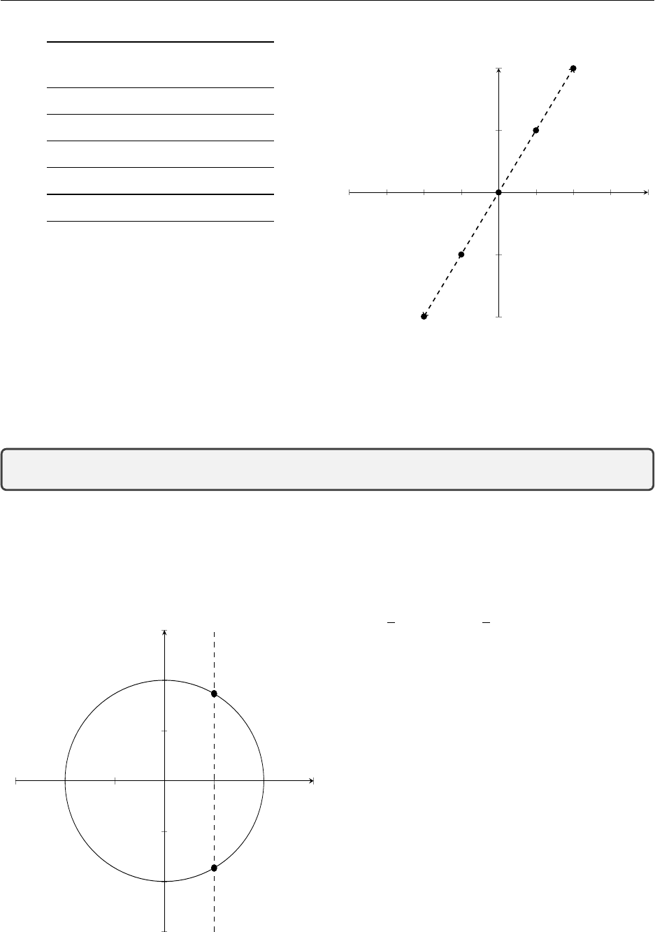
1.2 Functions
A function is a mathematical relationship between groups. Given an element in one group, the
function says how to get to the other group. For example the function could be a formula that says
if you have x, the output is 2x. This can be written as f(x)=2xwhere f(x) is called function
notation and in Cartesian coordinates also means y=f(x). We can depict this function visually
using xand ycoordinates. Begin by selecting some inputs (xvalues) and then calculate the outputs
(f(x) values) from the formula f(x) = 2x.
This method is called making a table of values and in this example any real number for xproduces
exactly one output for y(also a real number). The figure below plots the points on an (x, y) grid.
Connecting the points creates the line y= 2x.
1.2. Functions 4
inputs outputs
x f(x) = 2x
−2f(−2) = 2(−2) = −4
−1f(−1) = 2(−1) = −2
0f(0) = 2(0) = 0
1f(1) = 2(1) = 2
2f(2) = 2(2) = 4
Atable of values for the function f(x)=2x
−4−3−2−1 1 2 3 4
−4
−2
2
4
f(x)=2x
x
y
Aplot of the points showing a linear relation-
ship
Lets write a precise definition of a function:
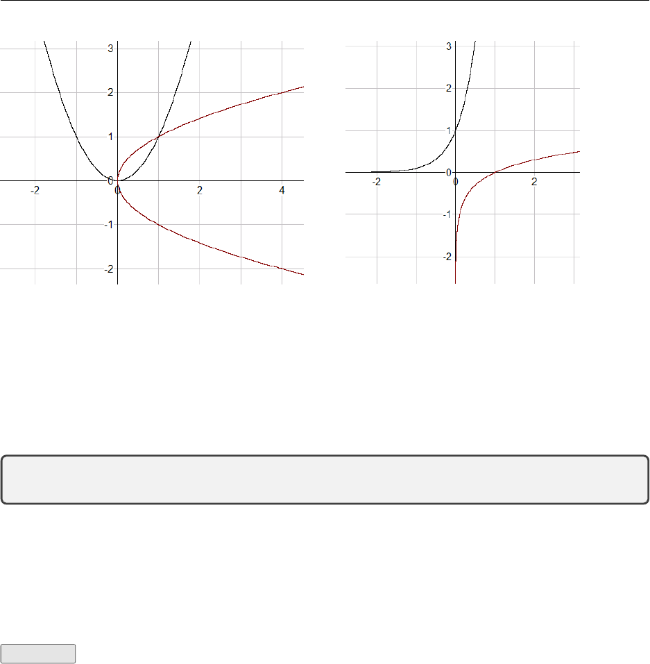
A function f(x) has exactly one output value, y, for any given input value, x.
In the line plotted above, we see that every xvalue has only one corresponding yvalue. This means
that y= 2xis a function. Conversely, a relationship that has two or more output values is not a
function.
−3−2−1 1 2 3
−3
−2
−1
1
2
3
x
y
The circle has two output values at x= 1: both
y= +√3 and y=−√3 are points on the circle.
The dashed line in the figure represents what
is called the vertical line test. If a vertical line
passes through more than one point on a curve,
then it is not considered a function.
Domain & Range
The domain of a function is the set of all inputs
that are valid; usually these are the x−values.
The range of a function is the set of all outputs
that are valid; usually these are the y−values.
For the line we plotted above, f(x)=2x, any
value could be substituted into the function,
therefore the domain was all the real numbers.
This is written as: Domain x∈R. Similarly the
range was all the y−values, or y∈R. We will
return to domain and range later.
1.2. Functions 5
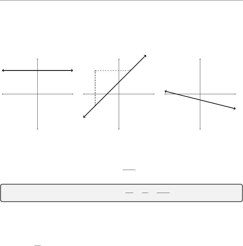
Linear Functions
Linear functions can represented nicely as a straight line on a standard Cartesian (x, y) coordinate
system. The following are all examples of linear functions, and not surprisingly, can be drawn as a
lines.
x
y
(a) zero slope
x
y
rise
run
(b) positive slope
x
y
(c) negative slope
Linear functions have a few characteristics that we will get used to manipulating. The slope of a
line is often represented by the letter mand can be calculated by taking any two points on the line
(x1, y1), and (x2, y2) and using the formula: m=y2−y1
x2−x1. This is also known as the gradient, a term
that will be used often in calculus.
slope=m=gradient= rise
run =∆y
∆x=y2−y1
x2−x1
The standard form for an equation of a line is: y=mx +cwhere mis the slope described above,
and cis the y−intercept. Alternatively if you know the slope and any given point (x1, y1), the
equation of a line is y−y1=m(x−x1) where x1and y1are the coordinates of a point on the line.
Note that a vertical line has an undefined slope. Using the formula above, a vertical line has a
slope of m=∆y
0because it has the same xvalues everywhere. Dividing by zero is undefined (try
on your calculator) and therefore a vertical line is not considered a function.
Question Does a vertical line pass or fail the vertical line test? Why?
Quadratic Functions
A quadratic relationship scales with the square of the input values. The following are all examples
of quadratic functions:
•y=x2−5
•s(t) = −4.9t2−15t+ 3
•b2+ 7b−1=0
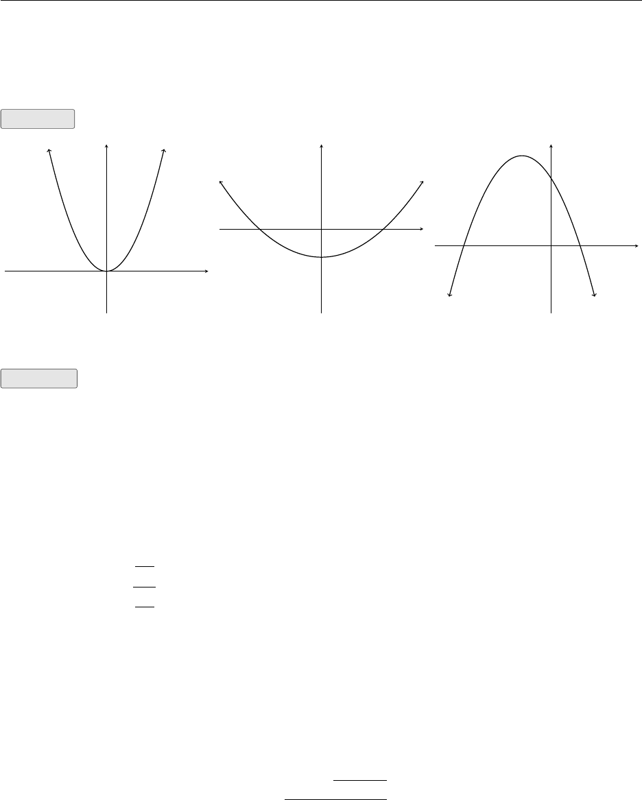
1.3. Polynomials 6
Note that they all have a power of 2 in the equation, and that is the highest exponent. This type
of relationship is also referred to as parabolic. When a parabola equation is plotted, the solutions
represent where the function crosses the x−axis. These points are called roots.
Example Find the roots of the following parabolas.
x
y
(a) y=x2
x
y
(b) y= 0.3x2−1
x
y
(c) f(x) = −x2−2∗x+ 3
Solution The roots are where the function intersects the x−axis. The x−axis is where y= 0,
so we will substitute y= 0 into the functions and solve the equations for x.
(a) Substituting in y= 0 gives the equation 0 = x2. This solves directly for x= 0. Therefore the
root to y=x2is 0.
(b) Solve the equation
0=0.3x2−1
1=0.3x2
1
0.3=x2
r1
0.3=x
Therefore x=±1.826
(c)
0 = −x2−2x+ 3 here you can divide by −1
0 = x2+ 2x−3 and factor
0=(x+ 3)(x−1)
Therefore x=−3 and x= 1
The parabola from part (c) above was solved by factoring. Not all quadratic equations can be
solved in this manner. The standard form of a quadratic equation is written ax2+bx +c= 0. If
we solve this equation for xwe get the quadratic formula:
x=−b±√b2−4ac
2a
where a, b, and care coefficients (a6= 0). Note here there are two possible solutions because of the
plus-minus sign (±).
1.3 Polynomials
A polynomial is a type of function that comes up a lot. The quadratic equations above are all
examples of polynomials. The standard form of a quadratic equation is shown below with some of
the terminology.
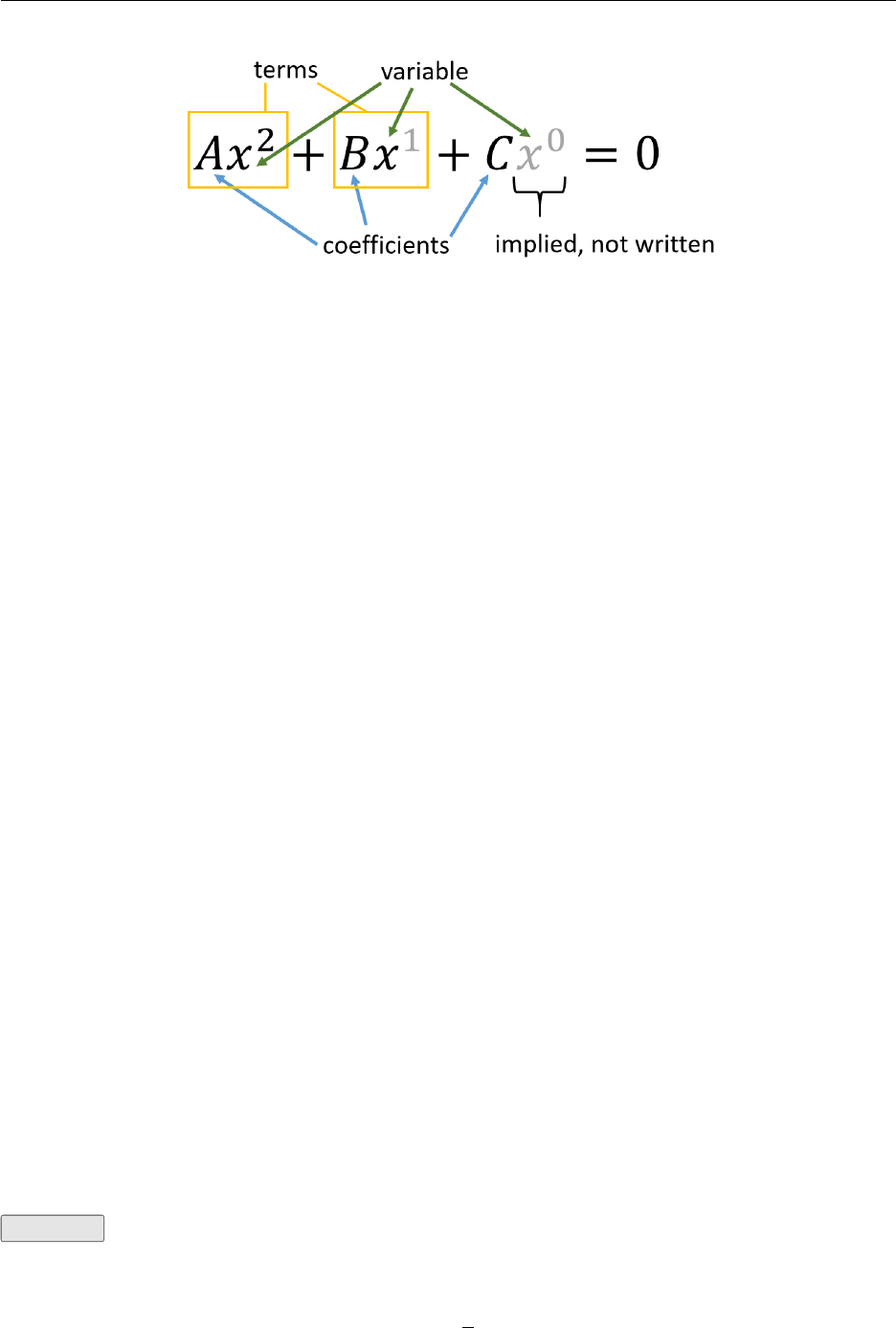
1.4. Systems of Equations 7
The prefix poly means many, and polynomials are not limited to three terms. The general form of
a polynomial can be written as:
A1xn+A2xn−1+A3xn−2+··· +Anx1+C= 0
where the terms are written in decreasing powers of x, with
•n≥0, n ∈Z. This means the exponents must be integers.
•A1, . . . , Anare real numbers.
•Cis a constant.
•The order or degree of the polynomial is n(the highest exponent).
•Here, xis the variable. You may have more than one variable in a polynomial, for example
4x2+y−xy + 4 is a valid polynomial.
1.4 Systems of Equations
A system of equations means having more than one relationship represented within a common
context. Revenue and costs may have different functions but both relate to the same product. We
will study systems composed of two equations and two unknowns. Systems with more equations
and more variables are possible and will be covered in future courses. Three approaches to solve
systems of equations will be covered here:
•graphing •elimination •substitution
It helps if you can visualise the shape of the two functions so that the meaning of the solution is
clear in your mind. Later in the course we will find the area between two curves using integration
where the intersection of these two curves represents the solution to a system of two equations. See
section XX.
We know that linear equations in two variables are represented by straight lines. Straight lines will
always intersect unless they are parallel. The coordinates of the point of intersection of the straight
lines is called the solution. you could use a graphical method or one of the two algebraic methods
(substitution or elimination) to find the solution. We will start with a graphical method.
Example Find the solution to the set of linear relationships given by:
2y=x−4
y=x
4
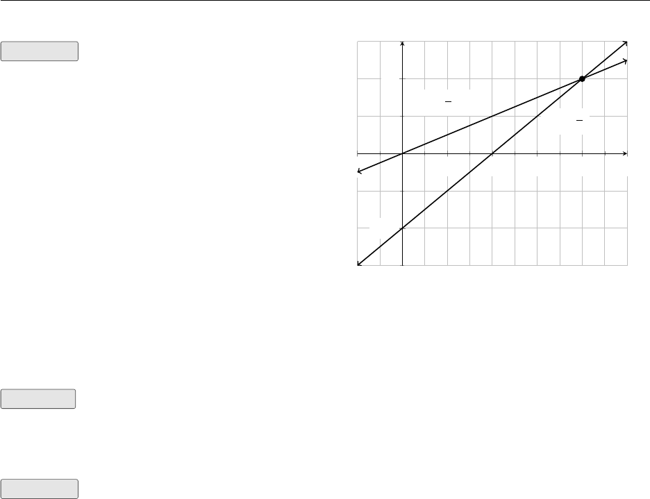
1.4. Systems of Equations 8
Solution Here we have two linear equations
(we know they are linear because the highest ex-
ponent is 1) and if the lines intersect, that point
of intersection represents a solution.
From the plot we can see the point of intersection
is (8,2). Therefore the solution to the system of
linear equations is (8,2). Try plotting the lines
yourself with desmos .
Its not always convenient to graph a system of
equations to find the solution; you may not have
access to a computer, or the solution may not
be integers. Solving by direct substitution is the
next method.
−2 2 4 6 8 10
−2
2
y=x
2−4
y=x
4
x
y
Solution by Substitution
Example Consider the system of equations
x2+y2= 25 (1)
3y+x= 15 (2)
Solution Without knowing what the functions look like or plotting them, we can isolate a
variable and substitute it into the other equation. Rearrange equation (2) to isolate xand substitute
into equation (1):
x= 15 −3y
Equation (1) becomes
(15 −3y)2+y2= 25 (expand and simplify)
225 −90y+ 9y2+y2= 25
10y2−90y+ 200 = 0 (divide by 10)
y2−9y+ 20 = 0 (factor the quadratic)
(y−5) (y−4) = 0
Either y−5 = 0 so y= 5
or y−4 = 0 so y= 4
Lastly, back-substitute the y−values into equation (2):
When y= 5, 3y+x= 15 15 + x= 15 ⇐⇒ x= 0. This means (0,5) is a solution.
When y= 4, 3y+x= 15 12 + x= 15 ⇐⇒ x= 3. This means (3,4) is a solution. Note there
are two solutions here. Verify by graphing the functions.
Solution by Elimination
The third method is called elimination and works by eliminating one of the variables from the
equation set, then solving for the other variable.
1.4. Systems of Equations 9
Example Solve the system by the method of elimination:
4x−3y= 5 (1)
4x+y= 1 (2)
Solution If we subtract equation (2) from equation (1) columnwise then the xterm is elimi-
nated because 4x−4x= 0.
4x−3y= 5
−4x+y= 1
0x−4y= 4
Now there is one equation with one unknown: −4y= 4 so y=−1. Back-substitute into either
previous equation to solve for x=1
2. Therefore the solution is x=1
2, y =−1.
Example Solve the system by the method of elimination:
3a−7b=−3 (1)
b=6a−4
2(2)
Solution The first step is to write the equations so the variables line up in columns. Multiply
equation (2) by 2 to get 2b= 6a−4 and rearrange the terms to match equation (1).
The system now looks like:
3a−7b=−3 (1)
6a−2b= 4 (3)
We can’t eliminate any vari-
ables because the coefficients
are different.
Multiply equation (1) by 2.
6a−14b=−6 (4)
6a−2b= 4 (3)
Now calculate (4) −(3).
6a−14b=−6
−6a−2b= 4
0 + 12b= 10
b=5
6
Back-substitute binto equation (1) to solve for a: 3a−7(5
6) = −3. Verify that a=17
18 .
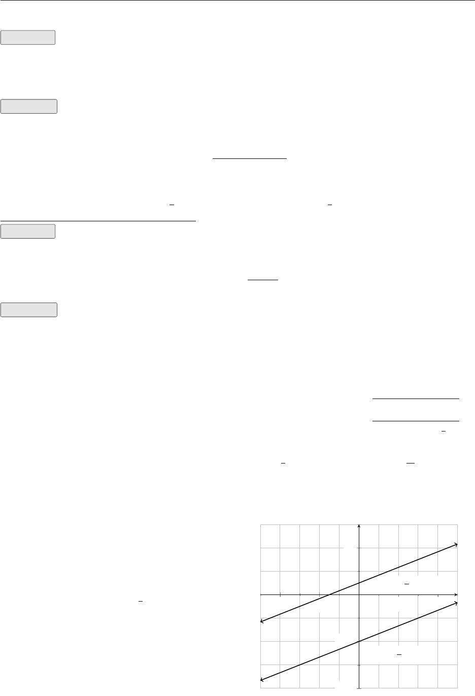
Special Cases
Consider the parallel lines shown. What is the
solution to this system? Parallel lines will never
meet by definition and so will have no point of
intersection. In this case the system has no solu-
tion – which is a perfectly valid solution! Notice
the slope of both the lines is 1
3which means they
are parallel.
Sometimes the two equations will be two differ-
ent representations of the same line. Imagine two
line plotted on top of one another. In this case
the system has an infinite number of solutions
because every single point on the first function
is also on the second function.
−4−2 2 4
−4
−2
2
y=x
3−2
y=x
3+ 0.5
x
y

1.4. Systems of Equations 10
Example If you start with a linear equation such as y−2x= 3 and multiply each term by a
constant you will get an equivalent equation. If you multiply the equation by another number you
will get a further equivalent equation.
y−2x= 3
Multiply by 2
2y−4x= 6
Multiply by −3
−3y+ 6x=−9
Solution We know these are both just different ways of writing the original equation y−2x= 3
or y= 2x+ 3. To say the system has an infinite number of solutions we are really saying every
point on y= 2x+ 3 is a solution.
Guidelines for Solving Systems of Equations
These guideline provide a useful way to tackle any problems where equations are involved.
1. Identify the variables. We often call them xand y, but you may chose any name or
letter you want.
2. Express all unknown quantities in terms of the variables.
3. Set up a system of equations using the facts provided by the problem.
4. Solve the system of equations and use the solution to check it satisfies the conditions
of the problem. Write a sentence describing the answer to the original problem.
Example It takes a boat travelling downstream 1 hour to cover the 20 mile distance. On the
return trip it take the boat 2.5 hours. What is the speed of the boat and the speed of the current?
Solution This is about a boat travelling with the current and against the current and depends
on you knowing that velocities are vectors that can be added and subtracted. Let the speed of the
boat be xmi/h and the speed of the current be ymi/h.
Upstream speed = x−y
Downstream speed = x+y
Speed = Total distance
Total time
so Total distance = Speed ×Total time
20 miles = (x+y)×1 hour
20 = x+y(1)
Also 20 miles = (x−y)×5
2hours
8 = x−y(2)
Now we can add equations (1) and (2) and yis eliminated
28 = 2x
x= 14
1.5. Chapter Exercises 11
Back-substitute into either equation (1) or (2) to solve for y= 6.
Check: The boat travels at 14 mi/h and the current travels at 6 mi/h so the effective speed of the
boat is 20 mi/h. At 20 mi/h the 20 mi trip took 1 h. Upstream the speed is 8 mi/h.
Total time = Total distance
Speed
=20
8=5
2h
Therefore the speed of the boat is 14 mi/h and the speed of the current is 6 mi/h.
1.5 Chapter Exercises
§1.1 Introductory Algebra
1. Remove the brackets and simplify
−(x+y)(a) −3(5x−2y)(b)
x2+ 5x−1−(2x−3)(c) (2x−1) (2x+ 1)(d)
2. Calculate the value of
(15.3)0
(a) 10−2
(b) ππ
(c) 4
7×0.5(d)
3. Simplify
3a2b2
(a) x
33x3
(b) abc
a−2b22c
(c)
1
2x2
3
x
(d)
4. Evaluate
4
√2.7 accurate to 2 decimal places.(a) 1
8−1
5to 3 decimal places.(b)
5. Factorise the expressions by removing the common factors.
7y2−14z2
(a) x(y−2) + x2
(b)
(a+c)2−4(a+c)(c) SA = 2πrh + 2πr2
(d)
6. Factorise the quadratics.
x2+ 11x+ 28(a) 2x2−5x−12(b)
b2−b−20(c) 3x2−7x+ 2(d)
7. Solve the equations
7x−16 = 2
3x+ 4(a) (x−2)2= 15(b)
x2−2x−8=0(c) 2x2+ 5x−4=0(d)
x3−2x2−x−1 = 0(e) x(x−1) (x+ 2) = 1
6x(f)
1.5. Chapter Exercises 12
§1.2 Functions
1. Make tthe subject of the equation
v=u+at(a) l=l0(1 + αt)(b)
2. If f(x) = x2and g(x) = x3evaluate
f(2)(a) f(−2)(b)
g(3)(c) f(g(2))(d)
3. The volume of a pipe with length l, inner radius rand outer radius Ris V=πR2−r2l.
Find the volume when R= 3.1m, r= 2.2m and l= 5.3m.
4. Sketch the following graphs (without using Desmos).
y= 4x−4(a) 2y=x
3+ 1(b)
y=x2−3(c) y=−(x+ 1)2
(d)
5. Find the xand yintercepts for the graph of y=x2−3
6. Use the grid provided to answer the following questions.
Show the points A(3,5) and B(−2,−5) on the graph.(a)
Calculate the slope of the line through Aand B. i.e. the slope of ¯
AB.(b)
What is the equation of the line AB?(c)
What is the equation of the line parallel to the line AB through the point (−2,3) ?(d)
Starting from the point Bon the graph frame draw a line with a slope of 4
5.(e)
−6−4−2 2 4 6
−6
−4
−2
2
4
6
x
y
1.5. Chapter Exercises 13
7. Complete the table of values for the function g(x) = x3−xand sketch the graph
x g(x) = x3−x
−1.5
−1
−0.5
0
0.5
1
1.5
−2−1 1 2
−2
−1
1
2
x
y
8. Graph the three functions on a common screen using desmos . How are the graphs related?
y=x2, y =−x2, y =x2sin x(a)
y=ex, y =−ex, y =exsin 5πx(b)
9. Given f(x) = xand g(x) = sin x, graph f,g, and f+gon a common screen to illustrate
graphical addition.
§1.3 Polynomials
1. What is the degree of the polynomial?
y=x2
(a) 4x3−2x2+ 6 = 0(b)
a99 −99a2=−99(c) ey4−ey3+ey2−ey1+e(d)
2. Are the following considered polynomials?
π(a) πx
(b) Ax2+Bx +C(c) 4x3−2x3
2+1 = 0(d)
3. Make up your own polynomials of degree 1,2,3, and 4.
§1.4 Systems of Equations
1. Solve the system of equations graphically. For the non-linear ones you may want to use desmos .
y= 2x+ 6
y=−x+ 5
(a)
3y
4+ 1= x
−x=y
(b)
−x+1
2y=−5
2x−y= 10
(c) x2
9+y2
18 = 1
y=−x2+ 6x−2
(d)
2. Solve the system using substitution.
1.5. Chapter Exercises 14
x−y= 2
2x+ 3y= 9
(a) 2x−3y= 12
−x+3
2y= 4
(b)
x+y= 8
y=−8−x
8
(c) x+y2= 0
2x+ 5y2= 75
(d)
3. Solve the system by eliminating a variable.
x+ 2y= 5
2x+ 3y= 8
(a) x2−2y= 1
x2+ 5y= 29
(b)
3x2−y2= 11
x2+ 4y2= 8
(c) 12x+ 15y=−18
2x+ 5y=−3
(d)
§1.5 Word Problems
1. A rectangle has an area of 180cm2and a perimeter of 54cm. What are its dimensions?
2. The admission fee at an amusement park is $1.50 for children and $4.00 for adults. On a certain
day, 2200 people entered the park and the admission fees collected totalled $5050. How many
children and how many adults were admitted?
3. A woman keeps fit by bicycling and running every day. One Monday she spends 1
2h at each
activity and covers a total of 12 1
2mi. On Tuesday she runs for 12min and cycles for 45min,
covering a total of 16mi. Assuming her running and cycling speeds don’t change from day to
day, find these speeds.
4. A customer in a coffee shop purchases a blend of two coffees: Kenyan, costing $3.50 a pound,
and Sri Lankan, costing $5.60 a pound. He buys 3lb of the blend, which costs him $11.55. How
many pounds of each kind went into the mixture?
2|Trigonometry
In the first half of this chapter the three trigonometric functions (sine, cosine and tangent) will
be viewed as functions of angles. The second half of the chapter will approach trigonometry as
functions of real numbers.
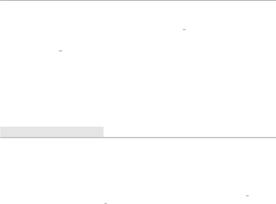
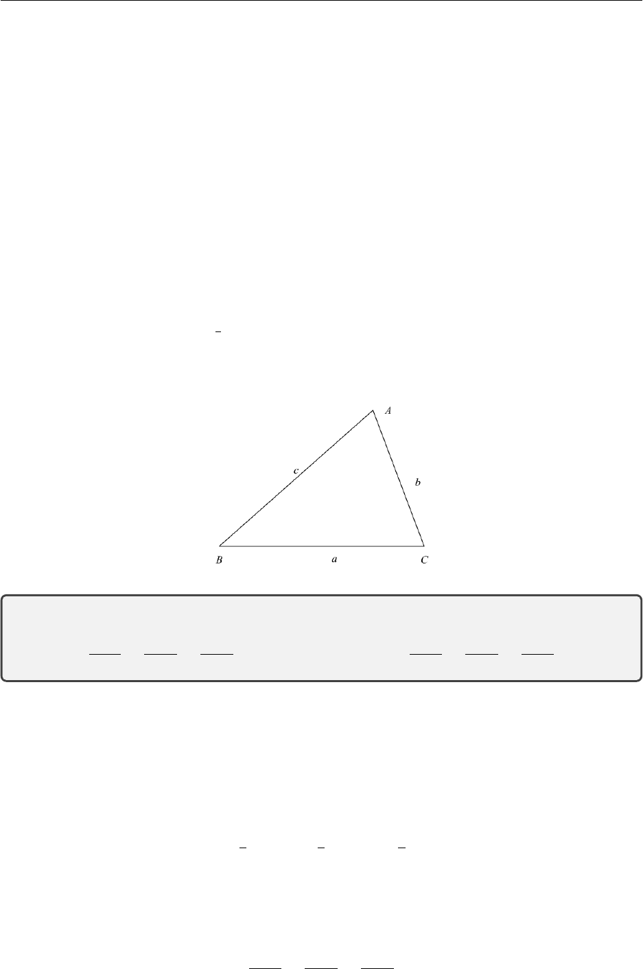
Pythagoras
Pythagoras is one of the most well known historical figures in mathematics and philosophy, primarily
for his eponymous theorem. Given a right-angled triangle, the square of the hypotenuse equals the
sum of the squares of the other sides.
The Pythagorean Theorem:
a2+b2=c2
This diagram will be the basis for a lot of our study of triangles. We will return to the Pythagorean
theorem in section 2.2 when discussing some special trigonometry relationships.
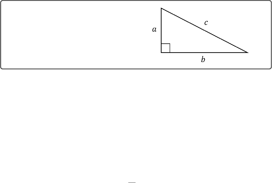
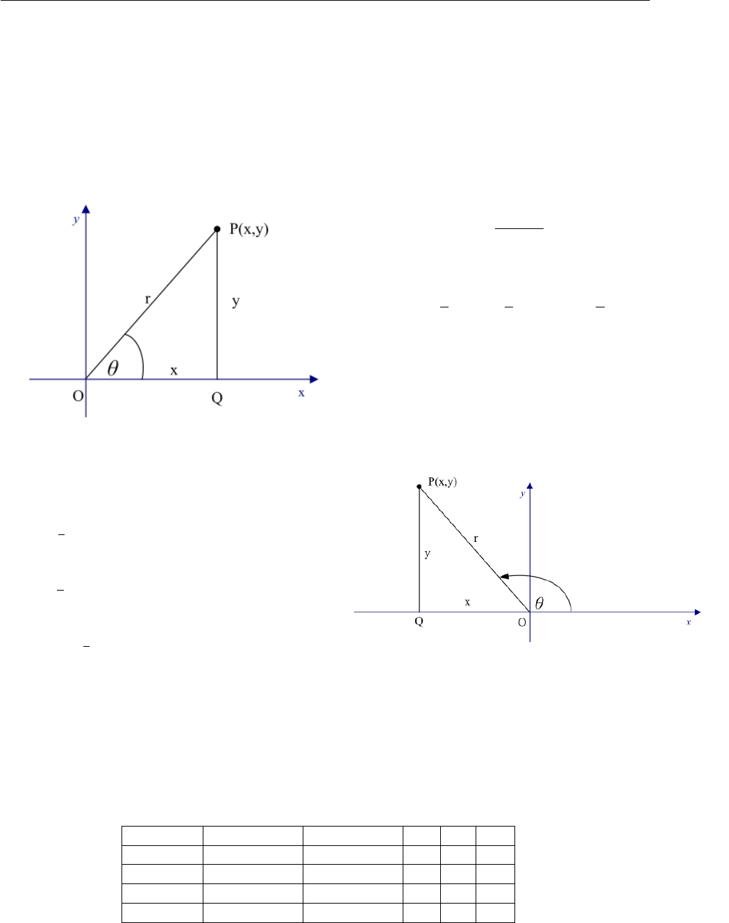
2.1 The Unit Circle
It should come as no surprise that the convention for measuring angles should be the same as for
measuring the distance around the perimeter of the unit circle.. An angle is measured in degrees
and is the amount of rotation between two rays about a vertex. If the vertex is placed at the point
(0,0) and one ray is placed along the positive x-axis then we let the second ray go through the
point P(x, y) on the unit circle so that the relationship between the angle and the arc length tcan
be established. The convention is that the positive direction for measuring angles is anticlockwise
and the negative direction for measuring angles is clockwise. You will be aware that one complete
cycle measures 360°. One degree therefore is 1
360 of one complete cycle. In this subject the word
revolution is often used instead of cycle. Other terms with which you might be familiar are “a
quarter turn” for 90°and “a half turn” for 180°.
If you draw a unit circle (centre (0,0) radius 1) then you can draw the ray through any terminal
point and show the relationship between tand the angle at the vertex (0,0).
Definition: If the unit circle is drawn and the distance tis measured around the perimeter from
(1,0) to the point P(x, y) then we say the angle is measured as tradians.
The abbreviation for radians is rad. This abbreviation will be used in the examples. Some books
2.1. The Unit Circle 16
uses the term “angles in standard position” to describe this situation. We will not define this term
unless it is unavoidable and will stick to rad.
Using the language of geometry, the unit circle
is cut by two rays one through the points (0,0)
and (1,0) and the other through the points
(0,0) and P(x, y).
tis referred to as ”the length of the arc”. The
angle θbetween the two rays is referred to as
”the angle subtended at the point (0,0)”. We
will often leave out the word ”subtended” how-
ever as it is implied.
We can say therefore that the angle measured in radians is related to the same angle measured in
degrees. the relationship between these two measures must be understood and must be able to be
derived.
Relationship between Degrees and Radians
One complete revolution is 360°if the angle is measured in degrees and 2πif the angle is measured
in radians. So
2πrad = 360°
or πrad = 180°
You should derive this formula whenever you are asked to convert degrees to radians or radians to
degrees.
Example (a) Convert 36°to radians (b) Convert π
3rad to degrees (c) Convert 1 rad to degrees
Solution
180°=πrad
1°=π
180rad
36°=π
180 ×36 = π
5rad
(a)
πrad = 180°
π
3rad = 180°
3= 60°
(b)
πrad = 180°
1rad = 180°
π
≈57.295 779 51°
≈57.3°
(c)
Note the similarity between the answers to (b) and (c). This is because π
3= 1.047197551 so you
would expect the values in degrees to be similar. With this terminology we leave out the word
measured when we talk about measuring angles. We say “the angle is 60°” when we mean it has
been measured as 60°or “the angle is π
3” to mean it has been measured as π
3rad. Notice we always
2.2. Right-Angled Triangles 17
put in the degree symbol and often omit the units when the angle is measured in radians. Should
units be omitted assume the angle is measured in radians. We often use the Greek symbol θfor
the angle subtended at the centre of the unit circle so θ= 60°or θ=π
3are further examples of
terminology that is commonly used.
Arc Length
Let θbe the angle subtended at the centre for the ends of an arc of any circle then the fraction of
the circumference of the circle is θ
2πif θis measured in radians and θ
360°if θis measured in degrees.
The length of the circumference of any circle whose radius is ris 2πr. If θis measured in radians
Length of arc = θ
2π×2πr =θrorrθ
If θis measured in degrees
Length of arc = θ
360°×2πr
The simplicity of the first formula shows why working with radians is preferred.
Example Find the length of an arc that subtends an angle of 45°at the centre of a circle whose
radius is 9 cm.
Solution
Method 1:
Length of arc = θ
360◦×2πr
=45
360 ×2π×9
= 2.25πcm
≈7.07cm
If an exact answer is required you should
leave the answer as 2.25πcm. (Or 9π
4cm.)
(1) Method 2: Change degrees to radians first
180◦=πrad
1◦=π
180
45◦=π
180 ×45
=π
4
Now, the length of arc = rθ = 9 ×π
4=9π
4cm.
(2)
2.2 Right-Angled Triangles
A right angled triangle is uniquely defined, if as well as the 90°angle, you are given one side and
one angle or two sides. To be given two angles does is not enough information as the scale of the
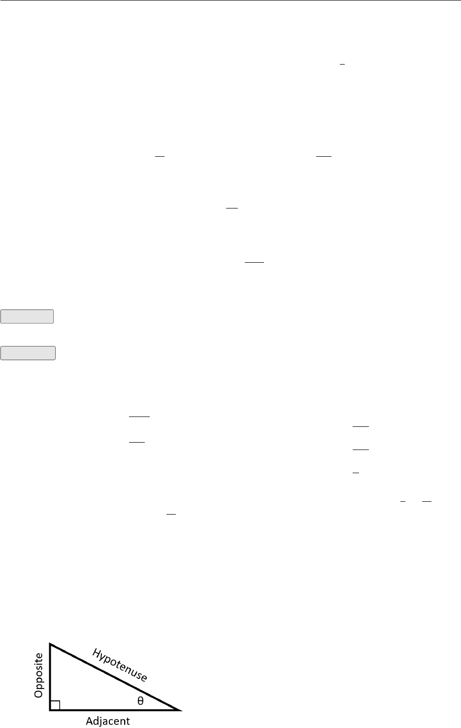
triangle is not known. The sides of the triangle have names with respect to the angle of interest, θ
in the diagram.
Notice that if θchanges, then the sides op-
posite and adjacent are reversed. These side
names are helpful in defining the trigonomet-
ric ratios of sine, cosine and tangent.
2.2. Right-Angled Triangles 18
The phrase SOH-CAH-TOA is useful to remember the ratios.
sine θ=opposite
hypotenuse; cosine θ=adjacent
hypotenuse; tangent θ=opposite
adjacent
S O H C A H T O A
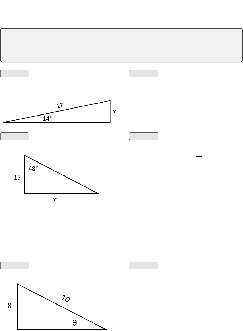
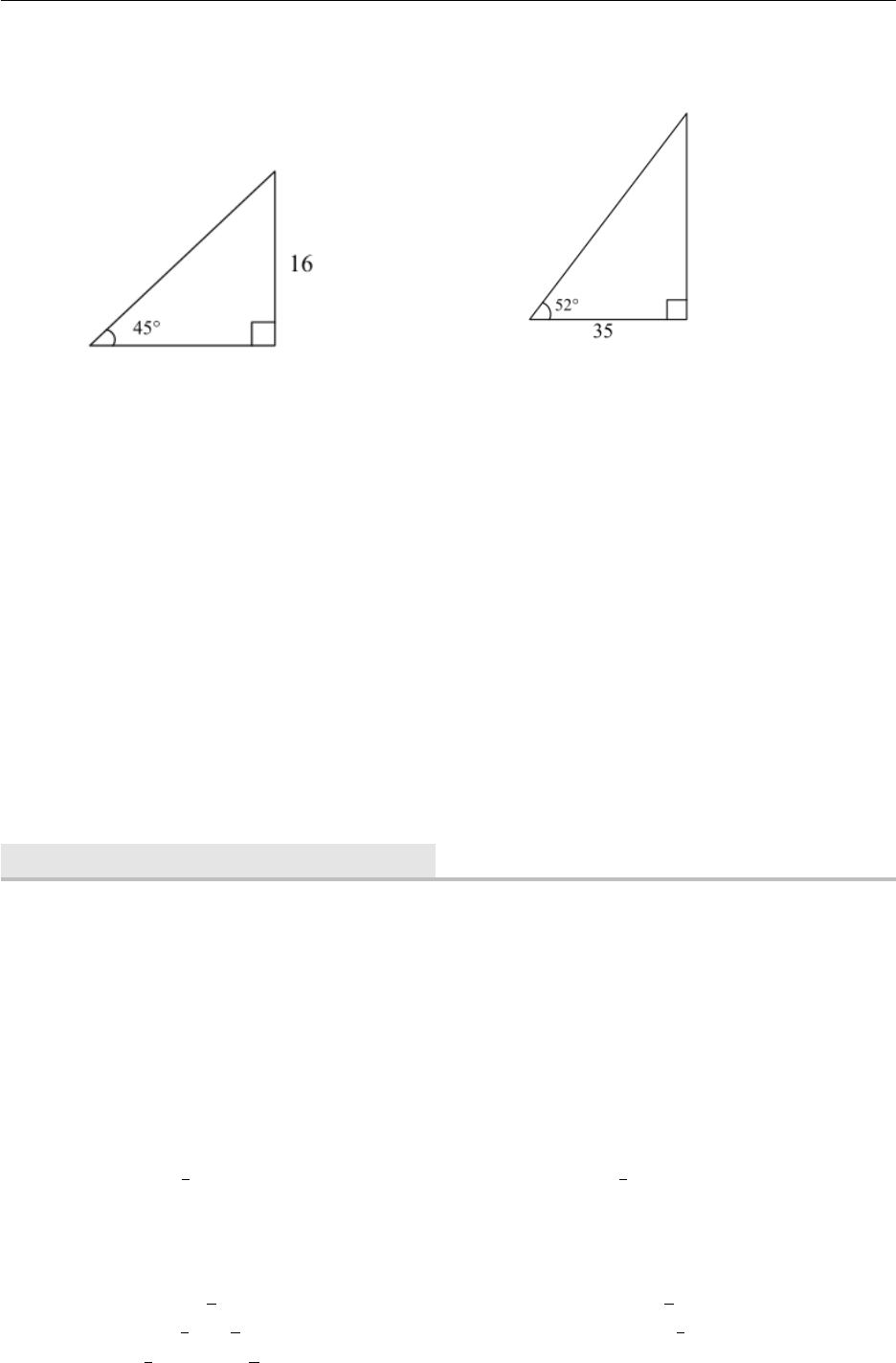
Example Find the unknown side xSolution Write the sine ratio and solve
for x.
sin 14 = x
17
x= 17 sin 14
x= 4.11
Example Find the unknown side xSolution Write the tangent ratio and
solve for x.
tan 48 = x
15
x= 15 tan 28
x= 16.7
The calculator gives approximate values of the trigonometric ratios. You must look at your question
to check whether angles are in degrees or radians and ensure the calculator is first set in the right
mode. Questions where degrees are to be used will give angles marked with a ◦symbol.
When solving for an angle on your calculator you select the appropriate trigonometry ratio and use
the shift button with sin, cos or tan to find sin−1, cos−1or tan−1.
Example Find the unknown angle xSolution Write the sine ratio and solve
for θ.
sin θ=8
10
sin θ= 0.8
θ= sin−1(0.8)
θ= 53.1°
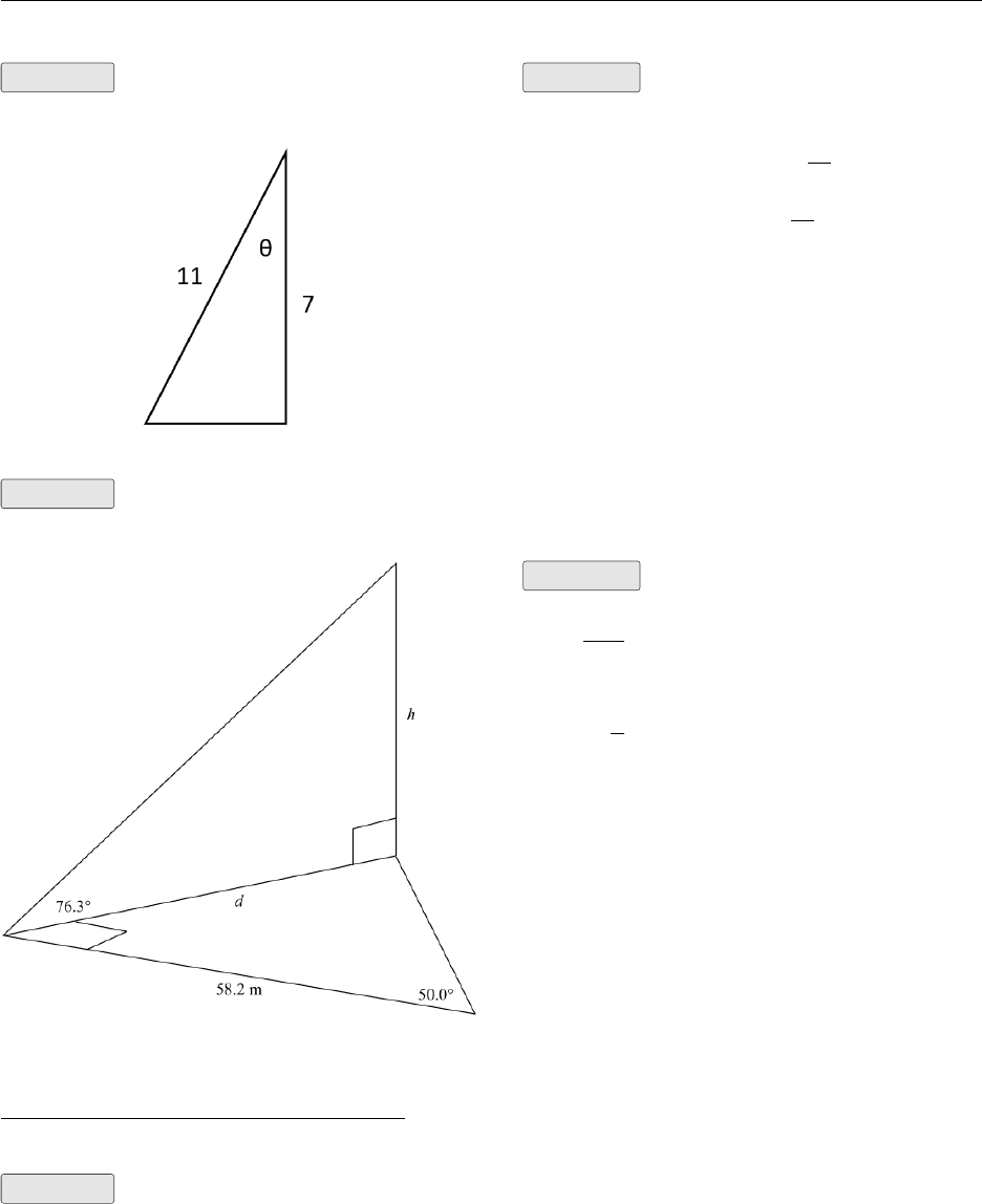
2.2. Right-Angled Triangles 19
Example Find the unknown angle xSolution Write the cosine ratio and solve
for θ.
cos θ=7
11
θ= cos−17
11
θ= 50.5°
Example The height of a steep cliff is to be measured from a point on the opposite side of the
river. The following diagram shows the measurements taken. Estimate the height of the cliff.
Solution
d
58.2= tan 50.0°
d= 58.2×tan 50.0°
h
d= tan 76.3°
h=d×tan 76.3°
= 58.2×tan 50.0°×tan 76.3°
≈284.526397
≈284.5m
Example To estimate the height of a mountain above a level plane the angle of elevation of
the top of the mountain is measured to be 30°. 600m closer to the mountain across the plane it is
found that the angle of elevation is 36°. Estimate the height of the mountain.
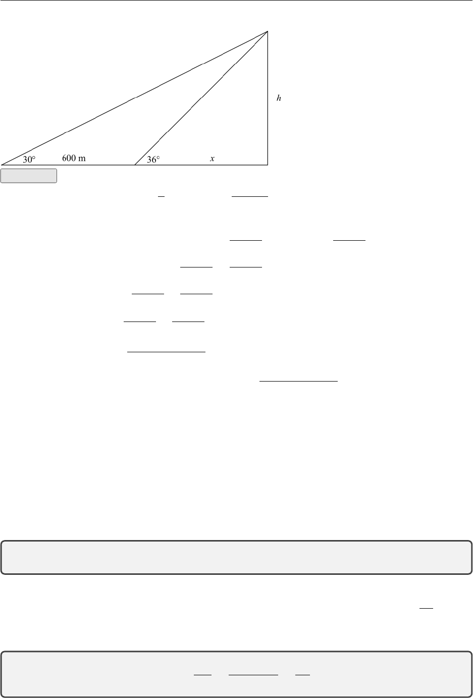
2.2. Right-Angled Triangles 20
Solution
h
x= tan 36°and h
x+ 600 = tan 30°
We want hso we eliminate xbetween these two equations
x=h
tan 36°andx+ 600 = h
tan 30°
h
tan 30°=h
tan 36°+ 600
h
tan 30°−h
tan 36°= 600
h1
tan 30°−1
tan 36°= 600
htan 36°−tan 30°
tan 30°tan 36°= 600
h= 600 ×tan 30°tan 36°
tan 36°−tan 30°
≈600 ×2.811603815
≈1687m
Identities
The unit circle has equation x2+y2= 1 and we define x= cos θand y= sin θso
x2+y2= 1 (cos θ)2+ (sin θ)2= 1
This is always written
sin2θ+ cos2θ= 1
This is an identity which means it is true for all values of θ. There are many identities in trigonom-
etry, we will only use the Pythagorean identity (above) and one more. Given sin = opp
adj we can
solve for opp = (sin)(hyp). Similarly from cosine: adj = (cos)(hyp). Substituting these into the
tangent relationship:
tan = opp
adj =(sin)(hyp)
(cos)(hyp) =sin
cos
The sine and cosine law are two more unique relationships that we will cover in section 2.4.
2.2. Right-Angled Triangles 21
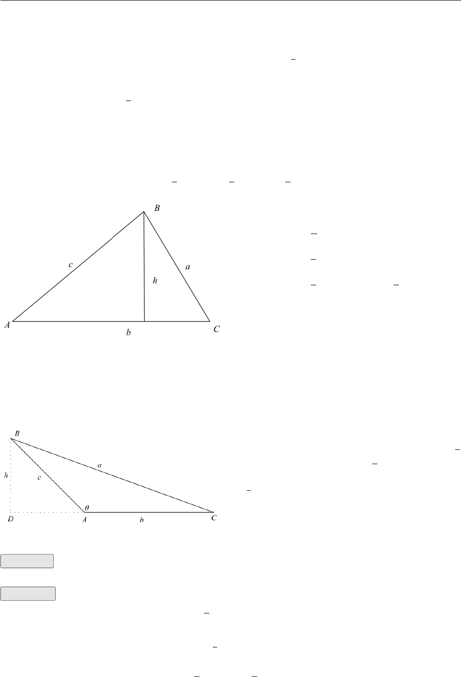
All Students Take Calculus
In the previous section the angles were between 0°and 90°. In this section the angles can take
any value. Initially we consider angles between 0°and 360°and relate these to the radian measure
between 0 and 2π. We remind you that angles are measured anticlockwise from the positive x-axis.
If the point P(x, y) is in the first quadrant, θis the angle between OP and the positive x-axis and
we complete the right triangle then we have created the following situation.
Let the hypotenuse be rthen
r=px2+y2
Therefore
sin θ=y
rcos θ=x
rand tan θ=y
x
We now let θbe any angle and define sine, co-
sine and tangent in the same way. For instance
if P(x, y) is in the second quadrant:
sin θ=y
rbecause yis positive sin θwill be
positive. (ris positive by convention.)
cos θ=x
rbecause xis negative cos θwill be
negative.
tan θ=y
xbecause yis positive and
xis negative tan θwill be negative.
This pattern can be extended to quadrants 3 and 4. The mnemonic (All Students Take Calculus)
might help you remember which one is positive although you can always work it out if you need to.
The value of a trigonometric function consists of two parts the numerical part and the sign. you
must get both parts correct. In the previous section you related the values of a terminal point
to another point in the first quadrant. A point on the unit circle could be in any one of the four
quadrants.
Quadrant x-coordinate y-coordinate cos sin tan
1 + + + + +
2−+−+−
3− − − − +
4 + −+− −
Some people learn this as a mnemonic All sin tan cos. (Meaning all are positive in the first quadrant,
only sine is positive in the second quadrant, only tangent is positive in the third quadrant and only
cosine is positive in the fourth quadrant.)
2.2. Right-Angled Triangles 22
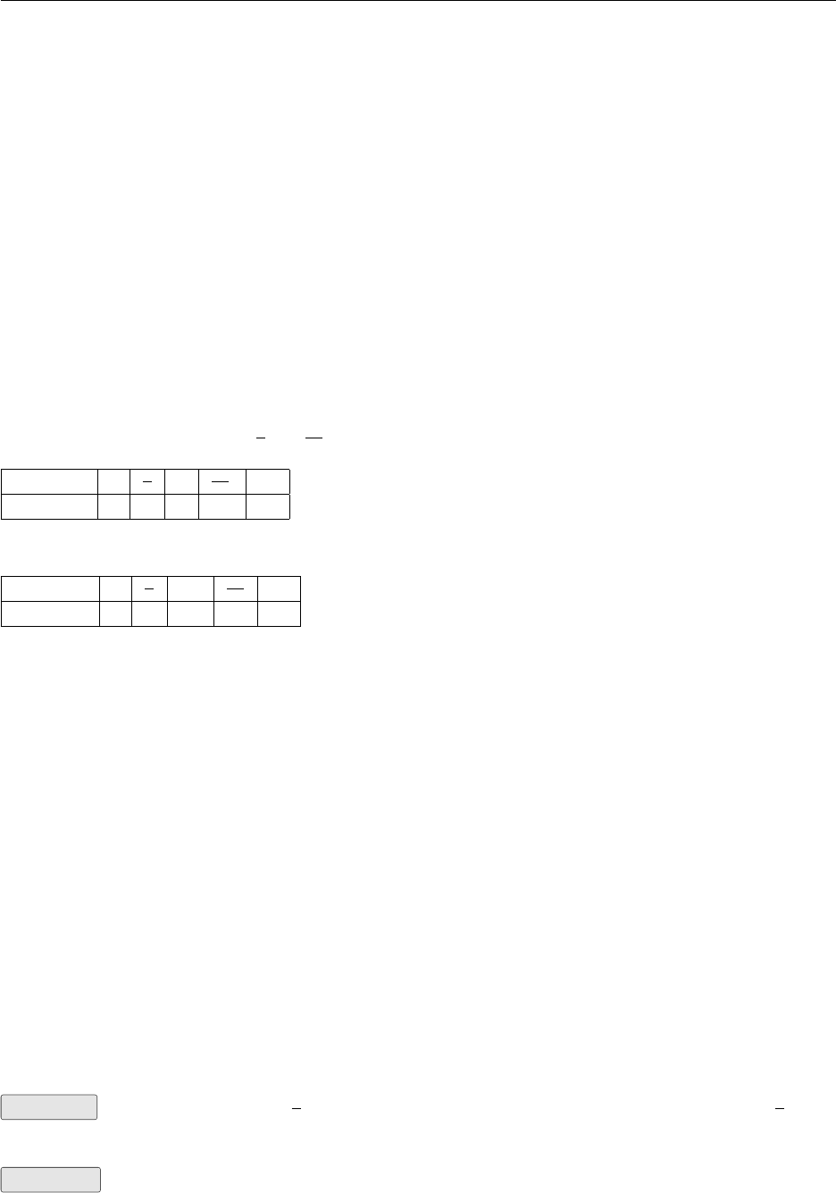
The Area of a Triangle
The fundamental formula for the area of a triangle is Area = 1
2×base ×height Using the trigono-
metric functions the height can be replaced and the formula becomes:
Area = 1
2×product of two sides ×sine of the included angle
The formula is particularly easy to remember in symbolic form. Let the triangle have vertices A,
Band C, so the the sides opposite these angles are a,band crespectively. Then the area can be
expressed symbolically as
Area = 1
2ab sin C=1
2bc sin A=1
2ac sin B
sin A=h
cand h=csin A
Area = 1
2×base ×height
=1
2×b×csin A=1
2bc sin A
It depends where you draw hand which angle you choose to use as to which formula you finish up
with. The key point to remember is band care two sides and Ais the angle between them. The
triangle above shows Aas an acute angle (between 0°and 90°). If the angle is obtuse (between 90°
and 180°) the formula still holds.
The angle is in the second quadrant and
sin(180 −θ) = sin θ, so sin(180 −θ) = h
c
can be written as sin θ=h
cor h=csin θor
h=csin Awhere Ais obtuse. So the area is
1
2bc sin A
Example A triangle has two sides of 5cm and 8cm and the angle between them is 150°. Find
its area.
Solution
Area = 1
2×5×8×sin 150°
It helps to remember that sin 150 = sin 30 = 1
2
Area = 1
2×5×8×1
2= 10 cm2
2.3. Trig Functions of Real Numbers 23
2.3 Trig Functions of Real Numbers
In this next part of the chapter the three main trigonometric functions (sine, cosine and tangent) will
be studied. They will be viewed as functions of real numbers rather than angles. The trigonometric
functions defined in these two ways are identical and there is a simple rule connecting the domains.
Why do we show you the two approaches? Trigonometry will be used to solve a variety of problems
and these can be divided into two groups, dynamic problems and static problems. When dynamic
problems (such as problems involving motion) are being solved real numbers will be used. When
static problems (such as finding distances and angles for triangles) are being solved angles will be
used.
You should be familiar with the fundamental graphs of y= sin xand y= cos x. These graphs are
the basis of this section. Desmos can easily show you the shape of y= sin xand y= cos xso if
you are asked to draw a rough sketch of these curves you should plot a few key points and draw a
smooth curve between them. You will usually be given the required domain however if you are not
you would choose to draw these for one complete cycle (0 −2π). To sketch y= sin xit is enough
to select as key points x= 0, π
2,π,3π
2, 2π.
x0π
2π3π
22π
y= sin x0 1 0 −1 0
Similarly to sketch y= cos xthe same values of xgive:
x0π
2π3π
22π
y= cos x1 0 −1 0 1
You will be aware that these curves repeat this pattern every 2πwhere xextends in both the
positive and negative directions. 0 to 2πrepresents one complete cycle. Mathematically we say
sin (x+ 2nπ) = sin xfor any integer n
cos (x+ 2nπ) = cos xfor any integer n
Aside: instead of “for any integer n” we can write ∀n∈Z. A function that displays this charac-
teristic is described as periodic and for y= sin xand y= cos xthe period is 2π.
Transformations
The following six transformations can be applied to any function including sine, cosine, and tangent.
Vertical shift•Horizontal shift•Vertical stretch•
Horizontal stretch•Reflection in the x-axis•Reflection in the y-axis•
Example Sketch y= sin x−π
2+ 3. This may be considered as a sine curve shifted π
2units
to the right. Note for periodic functions like a sine wave a horizontal shift is called a phase shift.
and 3 units upwards.
Solution 1. Beginning with the special points for sin x, a table shows the evolution of the
points.
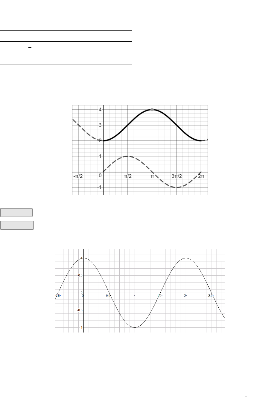
2.3. Trig Functions of Real Numbers 24
x0π
2π3π
22π←x-values, plot these
sin x0 1 0 −1 0
sin x−π
2−1 0 1 0 −1
sin x−π
2+ 3 2 3 4 3 2 ←y-values, plot these
2. Plot the transformed values with the original special points and connect with a smooth, contin-
uous line. Desmos confirms our transformation. The dashed plot shows y= sin xas reference.
Example Sketch y= cos(x−π
6).
Solution You could use a table of values however this is y= cos xwith a horizontal shift of π
6
to the right. Sketch the transformation on top of the graph of y= cos x.
In general y=asin xrepresents a vertical stretch of y= sin xby a. If ais negative the transfor-
mation can either be described as a negative stretch or (preferably) as a stretch of |a|followed by a
reflection in the x-axis. Recall the reflection of y=f(x) in the x-axis is y=−f(x). The number
|a|is called the amplitude for both y= sin xand y= cos xshown below.
If 0 <a<1 the fractional stretch causes the curve to shrink vertically. For instance the curve
y= sin xhas a maximum value of 1 and a minimum value of −1. the curve y=1
2sin xhas a
maximum value of 1
2and a minimum value of −1
2.
2.3. Trig Functions of Real Numbers 25
Example
Sketch y= cos(−t)
Example
Sketch y= sin 1
2x
Example
Sketch y= cos(2x)
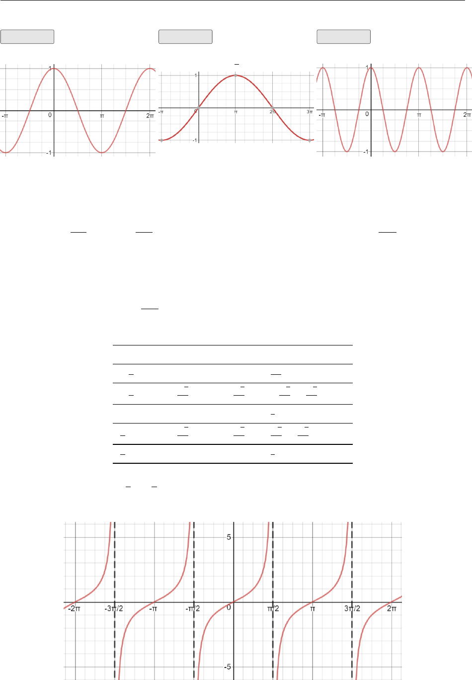
Tangent
There are other trig functions that we will not be covering here, for example the reciprocal functions
are cosecant= 1
sin θ, secant= 1
cos θ, and the inverse tangent function, cotangent= 1
tan θ. By focussing
on sine, cosine and tangent the majority of problems we encounter can be solved. Tangent is the
odd function out of the trio of common ones.
Previously we learnt that the period for the sine and cosine functions was 2π. Tangent is also a
periodic function and it has a period of π(not 2π). This means that it goes through one complete
cycle every π. Recall tan x=sin x
cos x. To analyse the behaviour of the tangent function it helps if you
know what you are looking for. Some key values of tangent will show the pattern.
xsin xcos xtan x
−π
2−1 0 −1
0=−∞
−π
4−√2
2
√2
2−√2
2÷√2
2=−1
0 0 1 0
1= 0
π
4
√2
2
√2
2
√2
2÷√2
2= 1
π
21 0 1
0=∞
As xtakes values from −π
2to π
2, tan(x) takes values from −∞ to ∞. This pattern is repeated
every π. A desmos graph can show this relationship. The dashed lines are the asymptotes.
The graph can be seen to have point symmetry. If you rotate the tangent curve through a half
2.4. Applications 26
turn using the origin as axis the curve will lie on top of itself. This is a pictorial representation of
an odd function.
Aside: You must not confuse y= tan xwith y=x3. While they may appear to be similar in shape
the only similarities are that they both pass through the origin and continue towards ∞in the first
quadrant and −∞ in the third quadrant.
2.4 Applications
The Sine Rule
The Sine Rule is a relationship that allows you to find the sides and angles in triangles without a
right angle. In the next section we use the Cosine Rule to find sides and angles in triangles also, so
as you study these two sections you need to learn which problems require the Sine Rule and which
require the Cosine Rule. Previously, we met the formula for the area of a triangle given two sides
and the included angle area = 1
2ab sin C. The Sine Rule and Cosine Rule also require specific
combinations of sides and angles. Using standard side and angle labelling for a triangle →∆ABC
and let the sides be a,band cwhere ais opposite ∠Aetc.
The Sine Rule states that in any triangle
sin A
a=sin B
b=sin C
cor, inversely as: a
sin A=b
sin B=c
sin C
Textbooks may use the term “The Law of Sines” whereas in these notes the term “The Sine Rule
will be used.
Proof of the Sine Rule
The Sine Rule is easy to prove from the formula for the area of a triangle
Area = 1
2bc sin A=1
2ac sin B=1
2ab sin C
Multiply right through by 2
bc sin A=ac sin B=ab sin C
Divide right through by abc sin A
a=sin B
b=sin C
c
2.4. Applications 27
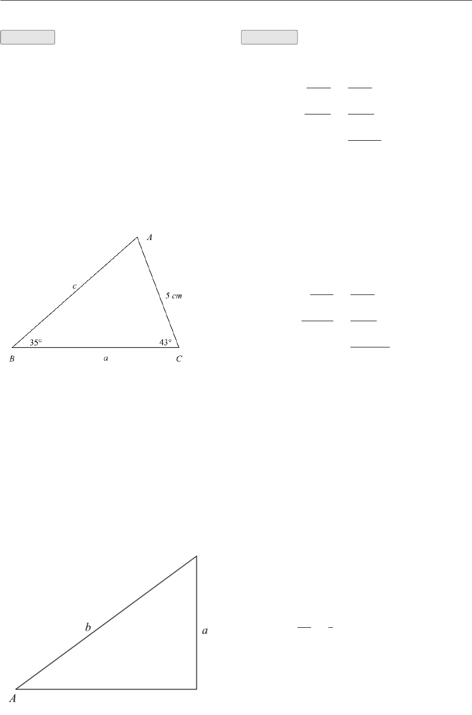
Example Find side lengths aand cin the
following triangle.
Solution
(a) To find c
c
sin C=b
sin B
c
sin 43 =5
sin 35
c=5 sin 43
sin 35
≈5.95cm(2 dp)
(b) To find a(i) A= 180°−(35°+ 43°) =
180°−78°= 102°(ii) It is usually wise to go back
to the original data (i.e. use band Brather than
cand C).
a
sin A=b
sin B
a
sin 102 =5
sin 35
a=5 sin 102
sin 35
≈8.53cm(2 dp)
These two calculations illustrate the first two cases in which the Sine Rule is used. You will notice
that the triangle has been completely solved in the course of this example. We started with one
side and two angles and we found the other two sides and the other angle.
The third case is not as straight forward. Given two sides and an angle there could be no triangle
formed, one triangle formed or two triangles formed depending on the length of the side opposite
the given angle. You should develop an insight into the reasons why this is so. Imagine the second
side given is the boom of a crane and the angle given is the angle between the boom and the ground.
The side opposite the given angle is represented by the cable. It is clear that for certain lengths of
the cable the hook will not reach the ground. Then as the hook is lowered a point will be reached
when the hook just touches the ground.
It is no surprise that the length ato create this
situation is a=bsin A.
We are after all dealing with the Sine Rule
which becomes the fundamental sine formula
sin A=opp
hyp =a
bwhen the triangle has a
right angle.
2.4. Applications 28
If the cable is held taut and is extended a little more it will touch the ground in two places (provided
it is kept in the same plane). As the cable is extended further the time will come where the cable
is as long as boom. At this point there is only one solution again, the one straight out in front of
the crane). Further extensions of the cable will produce only one solution (straight out in front
of the crane) as the cable will theoretically reach behind the crane boom thus creating a different
triangle altogether.
The two solutions case is often referred to as the ambiguous case. The discussion above shows the
range of values of athat will give two solutions.
bsin A<a<b
Example Given a= 30°,a= 8 and b= 7 solve the triangle (i.e. find B,Cand c).
Because 8 >7 this is the one solution case.
Solution
Find B
sin B
b=sin A
a
sin B=bsin A
a
=7 sin 30
8= 0.4375
B= sin−10.4375 ≈25.94°
(1) Find C
C= 180°−(30°+ 25.94°)
= 124.06°
(2) Find c
c
sin C=a
sin A
c=asin C
sin a
=8 sin 124.06
sin 30
≈13.3
(3)
Example The Ambiguous Case
Given A= 30°,a= 6 and b= 7 solve the triangle.
Solution In this case bsin A= 3.5 and b= 7 so as alies between 3.5 and 7. This is the
ambiguous case, therefore there are two solutions as the side lengths and angle can product two
different trianges.
It is best to visualise these two solutions on the same diagram so that the isosceles triangle can
2.4. Applications 29
help lead to the two results.
First solution (Proceed as before)
Find B
sin B
b=sin A
a
sin B=bsin A
a
=7 sin 30
6= 0.58˙
3
B= sin−10.58˙
3≈35.69°
(1) Find C
C= 180°−(30°+ 35.69°)
= 114.31°
(2) Find c
c
sin C=a
sin A
c=asin C
sin A
=6 sin 114.31
sin 30
≈10.9
(3)
Second solution
Find the second value of B
B= 180°−35.69°= 144.31°
(1) Find C
C= 180°−(30°+ 144.31°) = 180°−174.31°=
5.69°
(2)
(Or if you remember the rule that the exterior angle of a triangle is the sum of the two interior
opposite angles C+ 30°= 35.69°so C= 35.69°−30°= 5.69°)
Find c
c
sin C=a
sin A
c=asin C
sin A
=6 sin 5.69
sin 30
≈1.2
(3)
The Cosine Rule
In this section we will state and prove the Cosine Rule (which is called ”The Law of Cosines” in
the textbook). The proof is given here for completeness. You will not be tested on your ability
to reproduce it. The section will give examples where the Cosine Rule is used to solve problems
using the triangle of vectors and we will include revision of bearings and the use of trigonometry
in navigation.
2.4. Applications 30
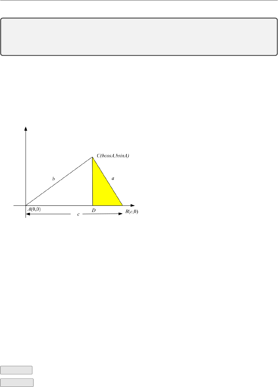
For any triangle side sides a,b, and cand angle Aopposite side a:
a2=b2+c2−2bc cos A
Proof of The Cosine Rule
To prove: For any triangle ∆ABC,a2=b2+c2−2bc cos A
By Pythagoras’ Theorem
BC2=CD2+DB2
a2= (c−bcos A)2+ (bsin A)2
=c2−2bc cos A+b2cos2A+b2sin2A
=c2−2bc cos A+b2cos2A+ sin2A
=c2−2bc cos A+b2as cos2A+ sin2A= 1
This is usually written
a2=b2+c2−2bc cos A
The diagram has been drawn to simplify the way the proof unfolds. You will see that by placing
the vertex Aat the origin the side ais found in terms of b,c, and A. The proof would have been
the same had Aand Bbeen as shown and Cplaced in the second quadrant. (Thus producing a
triangle with an obtuse angle at A.) This rule is symmetrical. You need to be given two sides and
the included angle (b,cand A) and the formula allows you to calculate a. Most textbooks will
therefore show you three equivalent formulae
a2=b2+c2−2bc cos A
b2=c2+a2−2ca cos B
c2=a2+b2−2ab cos C
Example Given a= 5, b= 6 and C= 50°, find c.
Solution
c2=a2+b2−2ab cos C
= 52+ 62−2×5×6×cos 50
≈22.43274342
2.5. Chapter Exercises 31
c≈√22.43274342
≈4.736321718 ≈4.7 (1dp)
Example Given a= 5, b= 6 and C= 130°, find c.
Solution
c2=a2+b2−2ab cos C
= 52+ 62−2×5×6×cos 130
≈99.56725658
c≈√99.56725658
≈9.97833937 ≈10.0 (1dp)
These two examples show that when the two sides and the included angle are given the third side
(opposite the given angle) can be found.
Example Find the angle given three side lengths; given a= 5, b= 6 and c= 9, find A.
Solution Because ais the smallest side Awill most certainly be an acute angle.
cos A=b2+c2−a2
2bc
=62+ 92−52
2×6×9
≈0.851851851
A≈cos−1(0.851851851)
≈31.6°
2.5 Chapter Exercises
§2.1 Unit Circle
1. Find the radian measure of the angle with the given degree measurements.
36°(a) −480°(b)
60°(c) −135°(d)
2. Find the degree measure of the angle with the given radian measure.
3π
4
(a) 5π
6
(b)
−1.5(c) −π
12
(d)
2.5. Chapter Exercises 32
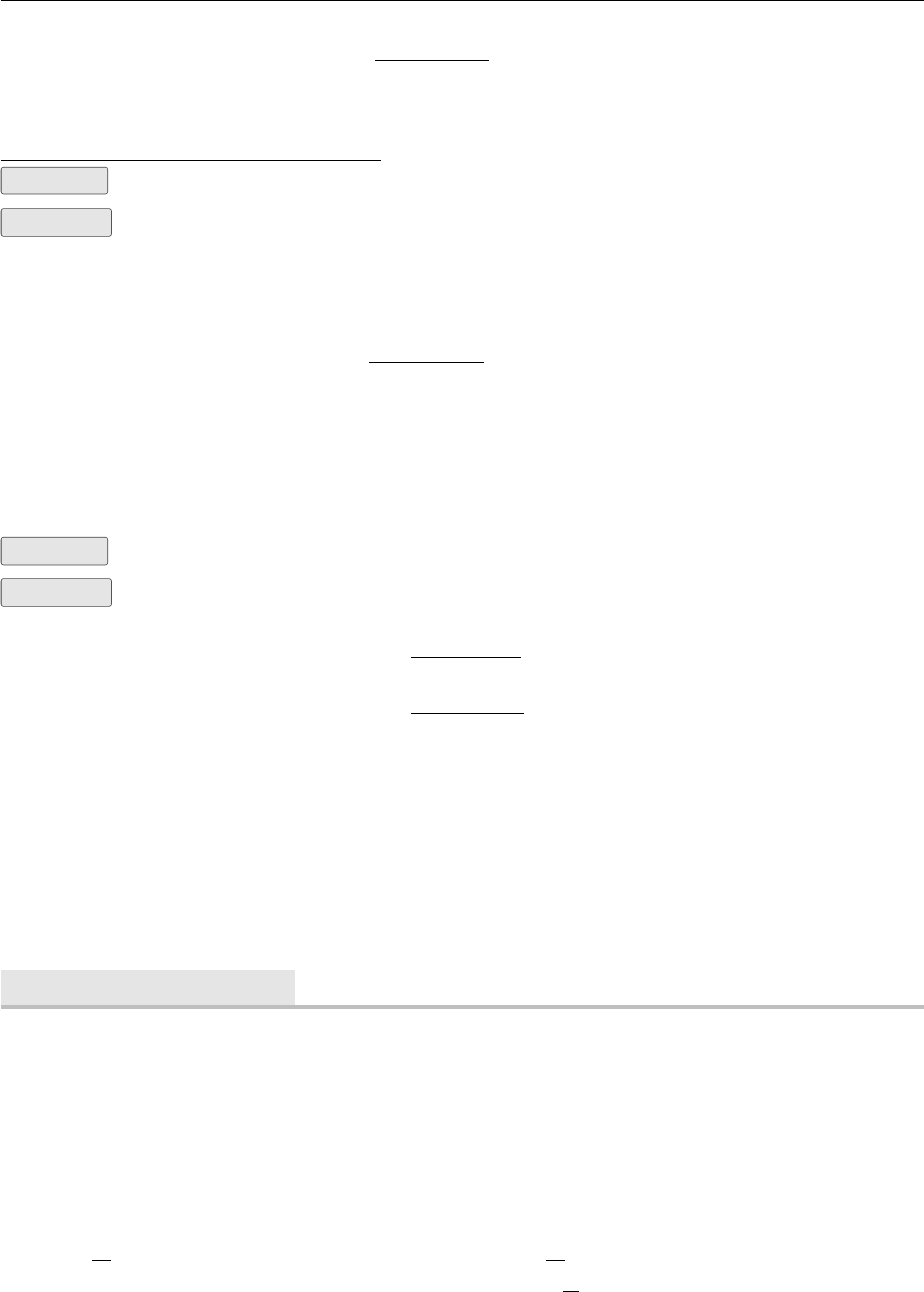
3. Arc length
Find the length of the arc sin the figure.
The radius is 5.
(a) Find the radius rof the circle in the fig-
ure.
(b)
4. Find the length of an arc that subtends a central angle of 2rad in a circle of radius 2mi.
5. Find the radius of the circle if an arc of length 6m on the circle subtends a central angle of π/6
rad.
6. Pittsburgh, Pennsylvania and Miami, Florida lie approximately on the same meridian. Pitts-
burgh has a latitude of 40.5◦N and Miami is 25.5◦N. Find the distance between these two
cities. (The radius of the earth is 3960mi.)
7. Find the distance the earth travels in one day in its path around the sun. Assume the year has
365 days and that the path of the earth around the sun is a circle of radius 93 million miles.
§2.2 Right Angled Triangles
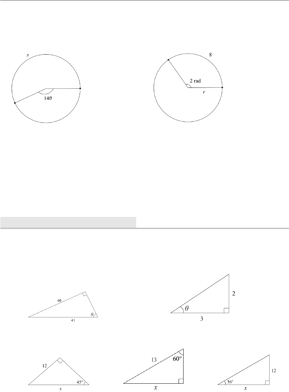
1. Find the exact value of sin θ, cos θand tan θof the angle θin the triangle.
2. Find sin θ, cos θand tan θin the following triangles.
(a) (b)
3. Find the side length labelled xfor the following triangles.
(a) (b) (c)
2.5. Chapter Exercises 33
4. Solve the triangles.
(a) (b)
5. The angle of elevation to the top of the Empire State Building in New York is found to be 11◦
from the ground at a distance of 1mi from the base of the building. Using this information,
find the height of the Empire State Building.
6. A laser beam is to be directed towards the centre of the moon but the beam strays 0.5◦from
its intended path.
How far has the beam diverged from its assigned target when it reaches the moon? (The
distance of the earth to the moon is 240 000mi.)
(a)
The radius of the moon is about 1000mi. Will the beam strike the moon?(b)
7. A water tower is located 325ft from a building. From a window in the building it is observed
that the angle of elevation to the top of the tower is 39◦and the angle of depression to the
bottom of the tower is 25◦. How tall is the tower? How high is the window?
8. Find the area of a triangle with sides of length 7 and 9 and included angle 72◦.
9. A triangle has an area of 16in2, and two of the sides of the triangle have lengths 5in and 7in.
Find the angle included by these two sides.
§2.3 Trigonometric Functions
1. Sketch the functions by hand.
y= 1 + sin x(a) y= 1 −cos x(b)
y=−2 sin x(c) y= 4 −2 cos x(d)
y=|cos x|(e)
2. Find the amplitude and period of the function and sketch its graph.
y= cos 4x(a) y= 3 sin 3x(b)
y= 10 sin 1
2x(c) y=−cos 1
3x(d)
y= 3 cos 3πx(e)
3. Find the amplitude, period and phase shift of the function, and plot using desmos .
y= cos x−π
2
(a) y=−sin x−π
6
(b)
y= 2 sin 2
3x−π
6
(c) y= 3 cos πx+1
2
(d)
y=−1
2cos 2x−π
3
(e) y= sin (3x+π)(f)
2.5. Chapter Exercises 34
§2.4 Applications
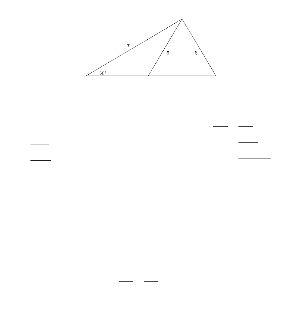
1. Use the Sine Rule to find side xor angle θ
(a) (b)
2. Solve the triangle using the Sine Rule.
3. Sketch each triangle and then solve using the Sine Rule.
∠A= 50◦,∠B= 68◦,c= 230(a) ∠B= 29◦,∠C= 51◦,b= 44(b)
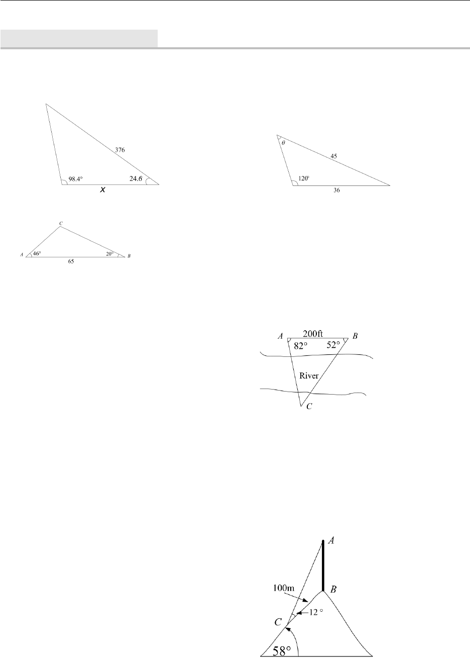
4. To find the distance across a river, a sur-
veyor chooses points Aand B, which are
200ft apart on one side of the river. She then
chooses a reference point Con the opposite
side of the river and finds that ∠BAC ≈82◦
and ∠ABC ≈52◦. Find the approximate
distance from Ato C.
5. The path of a satellite circling the earth causes it to pass directly over two tracking stations A
and B, which are 50mi apart. When the satellite is on one side of thetwo stations, the angle of
elevation at Aand Bare measured to be 87.0◦and 84.2◦, respectively.
How far is the satellite from station A?(a) How high is the satellite above the ground?(b)
6. A communication tower is located at the top
of a steep hill. The angle of inclination of
the hill is 58◦. A guy wire is attached to the
top of the tower and to the ground, 100m
downhill from the base of the tower. The
angle between the slope of the hill and the
guy wire is measured as 12◦. Find AC, the
length of cable required for the guy wire.
2.5. Chapter Exercises 35
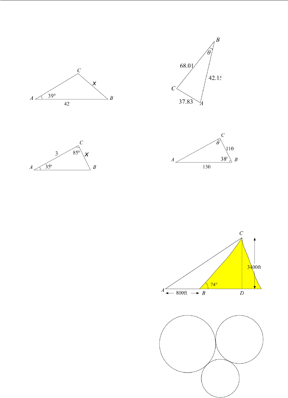
7. Use the Cosine Rule to find side xgiven AC = 44.3 and θ.
(a) (b)
8. Use either the Sine Rule or Cosine Rule as appropriate to find xand θ.
(a) (b)
9. Two straight roads diverge at an angle of 65◦. Two cars leave the intersection at 2.00 P.M.,
one traveling at 50mi/h and the other at 30mi/h. How far apart are the cars at 2.30 P.M.?
10. A pilot flies in a straight path for 1h 30min. She then makes a course correction, heading 10◦
to the right of her original course, and flies for 2h in the new direction. If she maintains a
constant speed of 625mi/h how far is she from her starting point?
11. A steep mountain is inclined 74◦to the hor-
izontal and rises 3400ft above the surround-
ing plain. A cable car is to be installed from
a point 800ft from the base to the top of
the mountain, as shown. Find the shortest
length of cable needed.
12. Three circles of radii 4, 5, and 6cm respec-
tively are mutually tangent. Find the area
enclosed between the circles.
2.5. Chapter Exercises 36
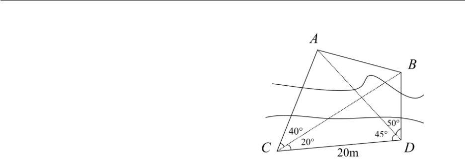
13. A surveyor wishes to find the distance be-
tween two points Aand Bon the opposite
side of a river. on her side of the river she
chooses two points Cand Dthat are 20m
apart and measures the angles shown. Find
the distance between Aand B.
3|Exponential & Logarithmic
Functions
We defined the polynomial axin chapter 1, however xwas restricted to rational numbers. We now
want to explore axwhere and xis any real number.
We can show that values exist simply by pressing buttons on the calculator or drawing a graph
using desmos , however an intuitive understanding can be obtained by considering appropriate
values.
Consider 2π. We know π= 3.141592654 . . .. 2πshould be between 23and 24. That is between 8
and 16. We can evaluate
23.18.5741877
23.14 8.815240927
23.141 8.821353305
23.1415 8.824411082
23.14159 8.824961595
23.141592 8.824973829
23.1415926 8.824977499
23.14159265 8.824977805
23.141592654 8.82497783
We could continue this process. If we enter 2πon the calculator the answer obtained is
2π= 8.824977827
The graph of y= 2x,∀x∈Ris shown.
Recall y=f(x) is a function and y=f(−x) is the same function with every xreplaced with −x,
i.e. y=f(−x) is the reflection of y=f(x) in the y-axis.
If y= 2xthen y= 2−xis the reflection of y= 2xin the y-axis. But y= 2−x=2−1x=1
2x.
Graphing Exercise Use Desmos to verify that y= 2−xand y=1
2
xare equivalent.
38
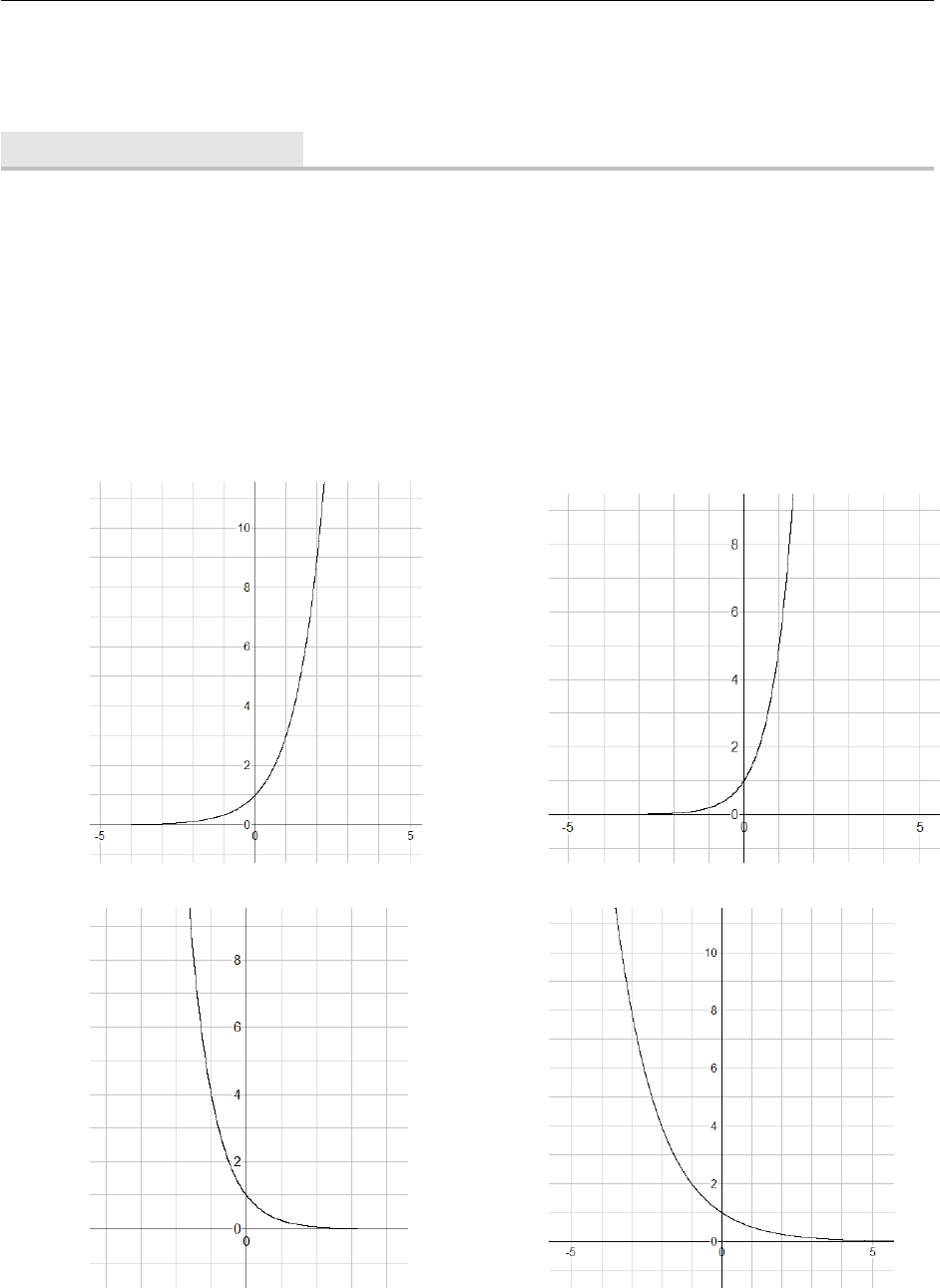
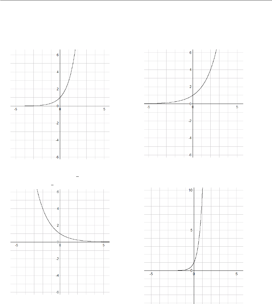
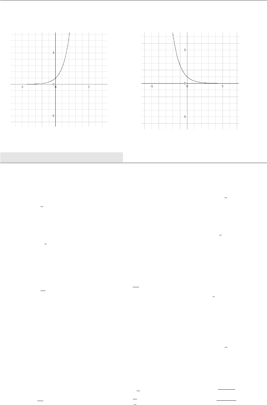
The Exponential Function f(x) = ax
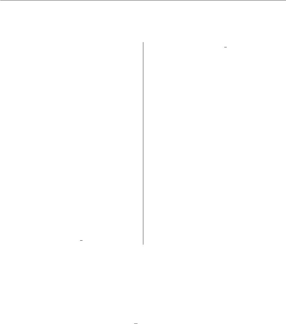
Let y=axwhere a > 0
When 0 < a < 1y=axlooks like
When a= 1 y=ax= 1x= 1 looks like
When a > 1y=axlooks like
f(x) = axis called an exponential function. ais called the base of the exponential function. The
domain is R. the range is (0,∞). The x-axis is an asymptote.
Example Find the equation of the exponential function that passes through (0,1) and (3,125).
Solution An exponential function that passes through (0,1) is of the form f(x) = ax. As
f(3) = 125 we substitute x= 3 and get
a3= 125
a=3
√125 = 5
∴f(x)=5xsatisfies the conditions.
Transformations of Exponential Functions
Recall the transformations we have met so far
Vertical stretch of a y =f(x) y=af(x)
Horizontal stretch of 1
by=f(x) y=f(bx)
Vertical shift of c↑y=f(x) y=f(x) + c
Horizontal shift of d−→ y=f(x) y=f(x−d)
Reflection in x-axis y=f(x) y=−f(x)
Reflection in y-axis y=f(x) y=f(−x)
Each of these transformations can be applied to an exponential function.
3.1. ex39
Graphing Exercise Given y= 2xapply the following transformations. Draw a sketch showing
where the graph crosses the y-axis, its shape, its asymptote and one other point it passes through.
1. Horizontal shift of +2
2. Vertical shift of −3
3. Horizontal stretch of 2
4. Vertical stretch of 4
5. Horizontal stretch of 1
3
6. Vertical stretch of 1
2
7. Reflection in the x-axis
8. Reflection in the y-axis
9. (Challenge) Reflection in y=−1
10. (Challenge) Reflection in x= 1
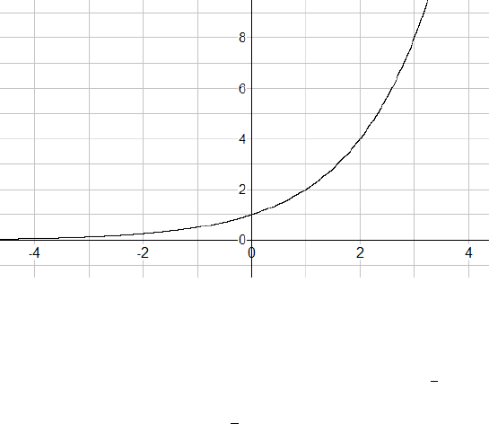
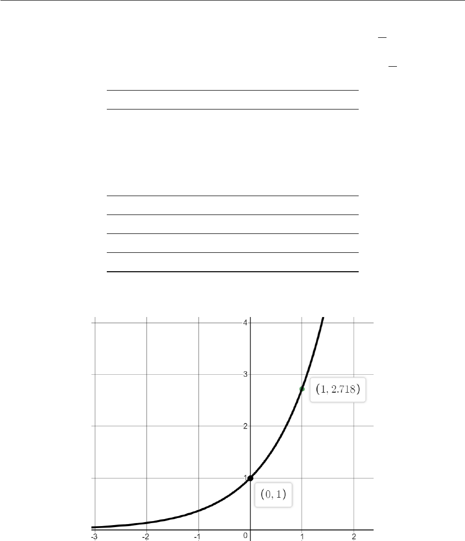
3.1 The Natural Exponential Function
The natural exponential function has wide application in mathematics engineering. It arises natu-
rally and crops up in applications such as finance, population, radioactivity, charge on a capacitor,
and more. We have defined f(x) = axand there is a particular value of athat we denote by the
letter e. It is an irrational number (like π,√2 etc.) and has a button on your calculator. To 10
decimal places it is
e≈2.7182818285 . . .
The natural exponential function f(x) = exis often simply referred to as the exponential function.
Compound interest can demonstrate an example of how the value above is found. Imagine a bank
that pays 100% interest on your money. Given an initial deposit of $1, at the end of year you
will receive $1 in interest payment and have a total of $2. Compounded interest allows this to
happen at intervals smaller than 1 year. If the interest is compounded twice per year, then after 6
months, you will receive 50% interest and have $1.50. In the second half of the year you now have
an additional $0.50 available to earn the second half interest. Now, $1.50 ×50% = $0.75, so at the
end of the year you have $1.50+$0.75=$2.25.
3.2. Logarithmic Functions 40
Lets say the interest is compounded monthly, then after 1 month you will receive 1
12 ×100% = 8.33%
interest for $1+$0.0833=$1.0833. The second month will earn the same rate (8.33%) on $1.0833,
for a total of $1.1736. After 12 months, your dollar will now be worth $1.00×1 + 1
12 12 = $2.6130.
compounding periods interest ($) total ($)
1 (yearly) 1.00 2.00
2 1.25 2.25
3 1.3704 2.3704
4 (quarterly) 1.4414 2.4414
5 1.48832 2.48832
6 1.521626 2.521626
12 (monthly) 1.613035 2.613035
52 (weekly) 1.692597 2.692597
365 (daily) 1.714567 2.714567
continuous 1.718282 2.718282. . .
As a function, f(x) = ex, is plotted below:
3.2 Logarithmic Functions
The logarithmic function is the inverse of the function f(x) = ax. Recall the inverse of a function
is the reflection of the function in the line y=x. Mathematically this is equivalent to swapping the
xand the y in y=ax. So x=ayis the inverse of y=ax. We have another notation for the inverse
of a function, which is a little more complicated. Let y=f(x) be a function of xthen y=f−1(x)
is the inverse of this function.
Sometimes the inverse of the function is also a function. For example the inverse of y=x2is
x=y2.y=x2is a function (vertical line test always applies), whereas x=y2is not a function
(vertical line test is broken).
3.2. Logarithmic Functions 41
The inverse of y= 10xis x= 10y.y= 10xis a function (vertical line test always applies) and so
is x= 10y.
Another useful fact to remember about inverses concerns the domain and range. The domain of f
is the range of f−1and the range of fis the domain of f−1.
We have a notation for x=ayit is y= logax:
y= logax⇔x=ay
In x=aysubstitute y= logaxand we get x=alogax. This means that given a base of athe power
(or exponent) to which amust be raised to get xis logax.
Problems involving logarithms will often require us to switch back and forth between y= logax
and x=ay, however it is also helpful if you can remember to substitute for yand write x=alogax
so that you can say “the logarithm is the power”.
Example
(a) log10 100 = 2 because 102= 100
(b) log381 = 4 because 34= 81
(c) log10 0.01 = −2 because 10−2= 0.01
The graph of y= logax
The exponential function y=axwhere a > 0 is now known and its domain is Rand its range is
the positive real numbers. We often write R+instead of (0,∞).
The graph of f(x) = axcan be reflected in the line y=xand the result is f−1(x) = logax.
Graphing Exercise On the same set of axes draw:
y= 10x
(a) y= log10 x(b) y=x(c) x= 10y
(d)
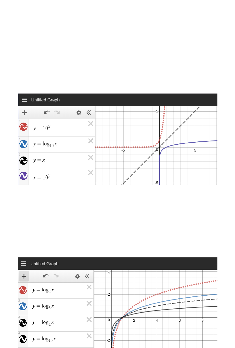
3.2. Logarithmic Functions 42
Make a comment about each statement below.
Check the graphs in (a), (b) and (c) are you confident that y= log10 xis the reflection of
y= 10xin the line y=x?
1.
When you enter x= 10ydescribe what takes place.2.
Graphing Exercise Solution Using desmos we can see the different plots. Plots (b) and (d) are
equivalent, so are on top of each other.
Graphing Exercise On the same set of axes draw:
y= log2x(a) y= log3x(b) y= log4x(c) y= log10 x(d)
Graphing Exercise Solution Using desmos we can see the relationship between the different
bases in the log equation:
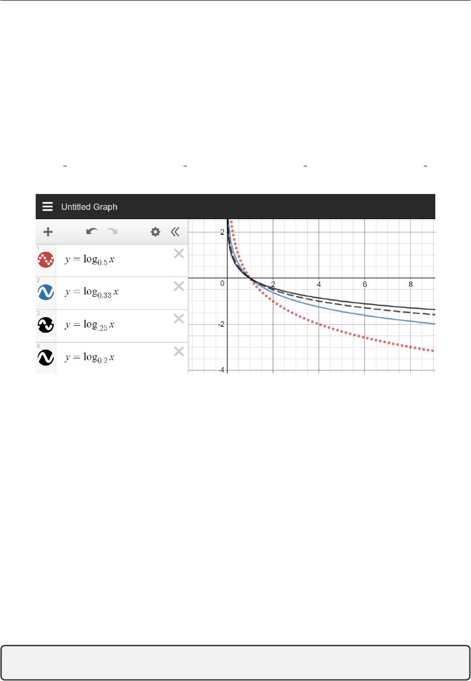
3.2. Logarithmic Functions 43
Notice the point that is common to all curves and the behaviour of the family of curves for x > 1
and for 0 <x<1.
Property 1: A property of logarithms is loga1 = 0 and this can be seen on the graphs where
every graph goes through (1,0).
The pattern you observe as the base gets bigger might not be evident for values of the base between
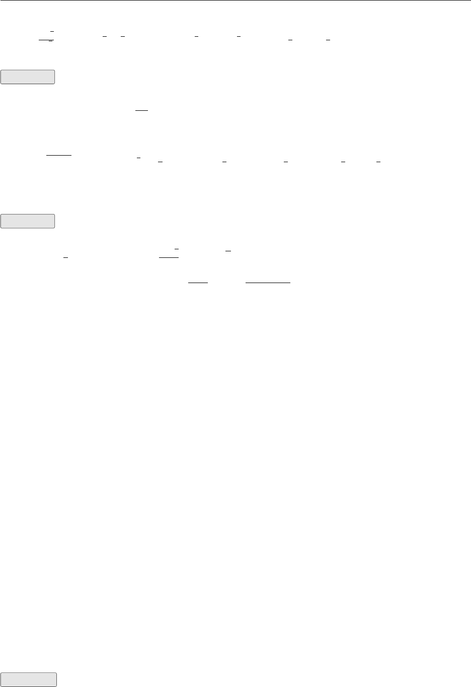
0 and 1. On the same set of axes draw the following:
y= log1
2x(a) y= log 1
3x(b) y= log 1
4x(c) y= log 1
5x(d)
To say the pattern is the same you have to be careful to describe the base. Explain how changing
the base gives the same pattern as for (a) to (d).
Property 2: A second property of logarithms is logaa= 1. That is a1=aor the power to which
you have to raise ato get ais 1. On your curves above locate a point on each curve that shows
this. You should in each case be looking for the point (a, 1).
Property 3: A third property of logarithms is logaax=x. This useful property must be under-
stood if logarithm problems are to be mastered. You should understand what logaaxis saying. a
is the base so logaax=xsays “The power to which amust be raised to get axis x.”
Common Logarithms
When the base is 10 we write y= log10 x= log x. If you see no base you assume it is base 10.
y= log xis called the common logarithm of x. Desmos and other programs with mathematics
incorporated recognise ”log” as ”logarithm to the base 10”. The log key on the calculator gives the
common logarithm of any positive number.
y= log x⇔10y=x

3.2. Logarithmic Functions 44
Natural Logarithms
When the base is ewe write y= logex= ln x. If you see ln xyou assume it is logex.y= ln x
is called the natural logarithm of x. Desmos and other programs with mathematics incorporated
recognise ”ln” as ”logarithm to the base e”. The ln key on the calculator gives the natural logarithm
of any positive number.
y= ln x⇔ey=x
Graphing Exercise Use Desmos to sketch the following. Describe in words how each curve is
related to y= ln x.
y= ln x(a) y= ln(−x)(b) y=−ln x(c)
y= ln(x−1)(d) y= ln(x)−1(e) y= ln(−1−x)(f)
The Laws of Logarithms
loga(XY ) = logaX+ logaYLaw 1:
logaX
Y= logaX−logaYLaw 2:
logaXc=clogaXLaw 3:
It is a useful exercise to prove these laws as the proofs show the connection between the laws for
exponents and the laws for logarithms.
Proof of Law 1
Let logaX=uso au=X
and logaY=vso av=Y
XY =auav=au+v
Take logarithms of both sides to the base a
logaXY = logaau+v=u+v(property 3) = logaX+ logaY
Proof of Law 2
X
Y=au
av=au−v
Take logarithms of both sides to the base a
logaX
Y= logaau−v=u−v(property 3) = logaX−logaY
Proof of Law 3
Xc= (au)c=auc =acu
Take logarithms of both sides to the base a
logaXc= logaacu =cu (property 3) =clogaX//
Example Expand using the logarithm laws
(a) log √3 = log 3 1
2=1
2log 3
3.3. Exponential and Logarithmic Equations 45
(b) ln a√b
3
√c= ln ab1
2c−1
3= ln a+ ln b1
2+ ln c−1
3= ln a+1
2ln b−1
3ln c
Example Evaluate
(a) log2112 −log27 = log2112
7= log216 = log224= 4 log22=4
(b) log2823 = log22323 = log2269= 69 log22 = 69
(c) log √0.001 = log (0.001)1
2=1
2log 0.001 = 1
2log 10−3=1
2× −3 = −3
2=−11
2
(d) e2 ln 4 =eln 42= 42= 16 (Let ln 4 = xthen ex= 4 so eln x= 4)
Example Rewrite as a single logarithm term using the logarithm laws
(a) log 12 + 1
2log 5 −log 3 = log 12√5
3= log 4√5
(b) log3x2−1−log3(x−1) = log3x2−1
x−1= log3
(x+1)(x−1)
x−1= log3(x+ 1)
3.3 Exponential and Logarithmic Equations
The types of problems we meet in this section will be able to be rearranged so that they look like
af(x)=b
Where aand bare real numbers, xis the unknown variable we are trying to find and f(x) is an
expression in x. The technique we will use will be the same for every problem we solve.
Step 1 Our first step is to inspect the problem to see if the unknown variable is in the exponent.
Step 2 Now that we have established that we are solving an exponential equation we rearrange it
until it is in the form af(x)=b
Step 3 Take the logarithm of both sides. In most practical situations we either take logarithms
to the base 10 or logarithms to the base e. there are three situations
Case 1 The problem has reduced to 10f(x)=b. Take logarithms to the base 10.
Case 2 The problem has reduced to ef(x)=b. Take logarithms to the base e.
Case 3 The problem has reduced to af(x)=bwhere ais neither 10 nor e. You can take logarithms
to the base 10 or eas you wish, either is correct.
Step 4 Solve the equation you obtain.
Example 1 Solve 3x= 5. This is an example of case 3 above.
Solution Two methods will be explored below:
3.3. Exponential and Logarithmic Equations 46
Take logarithms to the base 10
log 3x= log 5
xlog 3 = log 5
x=log 5
log 3
≈1.464973521 ≈1.46(2 dp)
Method 1
Take logarithms to the base e
ln 3x= ln 5
xln 3 = ln 5
x=ln 5
ln 3
≈1.464973521 ≈1.46(2 dp)
Method 2
This shows it is immaterial whether you take logarithms to base 10 or logarithms to base e.
Solve 32x+1 = 5
Solution Take logarithms to the base 10:
log 32x+1 = log 5
(2x+ 1) log 3 = log 5
2x+ 1 = log 5
log 3
2x=log 5
log 3 −1
x=1
2log 5
log 3 −1
≈0.23248676 ≈0.23(2 dp)
Example 2 Solve 4 1 + 105x= 9
Solution This must first be rearranged:
1 + 105x=9
4= 2.25
105x= 2.25 −1=1.25
10 log 105x= log 1.25
5x= log 1.25
x=1
5log 1.25
≈0.019382002 ≈0.019(3 dp)
Example 3
Example 4 Solve 10
1+e−x= 3.
Solution
1 + e−x=10
3
e−x=10
3−1
=10 −3
3=7
3
−x= ln 7 −ln 3
x≈ −0.85(2 dp)
Solving Logarithmic Equations
Whereas exponential equations have the unknown variable in an exponent, logarithmic equations
are equations containing the logarithm of an unknown variable.
Step 1 You recognise you are dealing with a logarithmic equation by inspecting the problem to
see if you have a logarithm of a term containing the unknown variable.
3.3. Exponential and Logarithmic Equations 47
Step 2 Rearrange the equation until it is in the form
loga(term containing unknown) = b
where bis a number.
Step 3 Take “antilogarithms ”. That is if logaX=bthen ab=X
Step 4 Solve the equation. (aand bare known and Xis an expression containing the unknown
variable.)
Example 1 Solve ln x= 5 .
Solution Take antilogarithms with base e:
e5=x
x≈148.4131591 ≈148.4(1 dp)
Example 2 Solve 5 + 4 log (5x) = 17.
Solution Isolate the log and solve:
4 log (5x) = 17 −5 = 12
log 5x= 3
103= 5x
x=1000
5= 200
Check: Substitute x= 200
LHS = 5 + 4 log (5 ×200)
= 5 + 4 log 1000 = 5 + 4 log 103
= 5 + 4 ×3 = 5 + 12 = 17 = RHS
Solve log x+ log (x−1) = log 4x
Solution
log x+ log (x−1) −log 4x= 0
log x(x−1)
4x= 0
log 1
4(x−1) = 0
100=1
4(x−1) = 1
x−1 = 4; x= 5
Check:
LHS = log 5 + log 4 = log (5 ×4) = log 20
RHS = log 4 ×5 = log 20 = LHS
Example 3 The velocity of a sky diver t
seconds after jumping is given by
v(t) = 80 1−e−0.2t
After how many seconds is the velocity 70 ft/s?
Solution
70 = 80 1−e−0.2t
70
80 = 1 −e−0.2t
e−0.2t= 1 −70
80
= 1 −7
8=1
8= 0.125
−0.2t= ln 0.125
t=ln 0.125
−0.2≈10.39s
Example 4
3.4. Exponential Modelling 48
3.4 Exponential Modelling
The natural exponential function, ex, is used in a variety of situations where there is exponential
growth or decay.
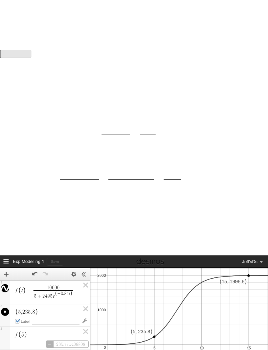
Example The exponential function can be used to model the way populations grow and diseases
spread. The following example is about the spread of an infectious disease in a small city whose
population is 10,000. After tdays the number of people who have caught the disease is modelled
by the function
f(t) = 10000
5 + 2495e−0.84t
How many people had the disease initially? Initially in this sense means right at the beginning,
or when the clock is still at zero. Substitute t= 0 into the function:
f(0) = 10000
5 + 2495e0=10000
2500 = 4 people
(a)
How many people have the disease after 1 day? Substitute t= 1 into the function:
f(1) = 10000
5 + 2495e−0.84 =10000
5 + 2495(0.4317) =10000
1082.1≈9.24; 9 people
(b)
How many people have the disease after 5 days? Following from part (b), find f(5):
f(5) = 10000
5 + 2495e−0.84(5) =10000
42.41 ≈235.77; 236 people
(c)
Use desmos to graph the function and describe its behaviour.(d)
The graph has distinctive characteristics. It starts at a particular non-zero value (when t= 0) and
increases slowly at first then more rapidly. It slows down after a time and levels off because the
exponential function in the denominator 0 when t ∞. Graphs with these characteristics are
called logistic curves. The particular model is called a logistic growth model.
3.5. Chapter Exercises 49
3.5 Chapter Exercises
§3.1 exfunctions
1. Use your calculator to evaluate to 5dp
e4
(a) 2e−0.7
(b) e3.1
(c) ee
(d)
2. Use Desmos to sketch:
f(x) = e−x
(a) g(x)=2e0.1x
(b) h(x) = −2.1e−0.12x
(c)
3. Find the exponential function f(x) = axwhose graph is given.
(a) (b)
(c) (d)
3.5. Chapter Exercises 50
4. Sketch the transformed graph
The graph is y= 3x.
Draw y=−3x.
(a) The graph is y= 2x.
Draw y= 2x−3.
(b)
The graph is y=1
2
x.
Draw y= 4 + 1
2
x.
(c) The graph is y= 10x.
Draw y= 10x+3.
(d)
3.5. Chapter Exercises 51
The graph is y=ex.
Draw y=−ex.
(e) The graph is y=e−x.
Draw y=e−x−1.
(f)
§3.2 Logarithmic Functions
1. Express the equation in exponential form.
log525 = 2(a) log51=0(b) log82 = 1
3
(c)
log21
8=−3(d) ln 5 = x(e) ln y= 5(f )
2. Express the equation in logarithmic form
53= 125(a) 10−4= 0.0001(b) 8−1=1
8
(c)
2−3=1
8
(d) ex= 2(e) e3=y(f)
3. Evaluate the expression
log33(a) log31(b) log332
(c)
log636(d) log981(e) log7710
(f)
log31
27
(g) log10 √10(h) log50.2(i)
2log237
(j) 3log38
(k) eln √5
(l)
log80.25(m) ln e4
(n) ln (1/e)(o)
4. Use the definition of the logarithmic function to find x.
log2x= 5(a) log216 = x(b) log3243 = x(c)
log10 x= 2(d) logx16 = 4(e) logx8 = 3
2
(f)
5. Use the Laws of Logarithms to rewrite the expression in a form with no logarithms of products,
quotients roots or powers.
log2(2x)(a) log2(x(x−1))(b) log 610
(c)
log2AB2
(d) log3x√y
(e) log5
3
√x2+ 1(f)
ln √ab(g) ln xqy
z
(h) log 4
px2+y2
(i)

3.5. Chapter Exercises 52
6. Evaluate the expressions
log5√125(a) log 2 + log 5(b) log4192 −log43(c)
ln 6 −ln 15 + ln 20(d) 102 log 4
(e) log log 100010,000
(f)
7. Rewrite the expression as a single logarithm
log35 + 5 log32(a) log2A+log2B−2 log2C(b) ln 5+2 ln x+3 ln x2+ 5
(c)
§3.3 Logarithmic Equations
1. Find the solution of the exponential equation, correct to four decimal places.
ex= 16(a) 102x= 5(b) 3ex= 10(c)
e1−4x= 2(d) 80.4x= 5(e) 5−x/100 = 2(f)
5x= 4x+1
(g) 23x+1 = 3x−2
(h) 100 (1.04)2t= 300(i)
2. Solve the equations for x
x22x−2x= 0(a) 4x3e−3x−3x4e−3x= 0(b)
e4x+ 4e2x−21 = 0(c) ln x= 10(d)
log (3x+ 5) = 2(e) 2−ln (3 −x)=0(f)
log x+ log (x−1) = log (4x)(g) log5(x+ 1) −log5(x−1) = 2(h)
§3.4 Modelling
1. A radioactive substance decays in such a way that the amount of mass remaining after tdays
is given by the function
m(t) = 13e−0.015t
Where m(t) is measured in kilograms.
Find the mass at time t= 0.(a)
How much of the mass remains after 45 days?(b)
2. A sky diver jumps from a reasonable height above the ground. The air resistance she experiences
is proportional to her velocity, and the constant of proportionality is 0.2. It can be shown that
the downward velocity of the sky diver at time tis given by
v(t) = 80 1−e−0.2t
where tis measured in seconds and v(t) is measured in feet per second (ft/s).
Find the initial velocity of the sky diver.(a)
Find the velocity after 5s and after 10s.(b)
Draw a graph of the velocity function v(t).(c)
The maximum velocity of a falling object with wind resistance is called the terminal
velocity. From the graph in part (c) find the terminal velocity of the sky diver.
(d)
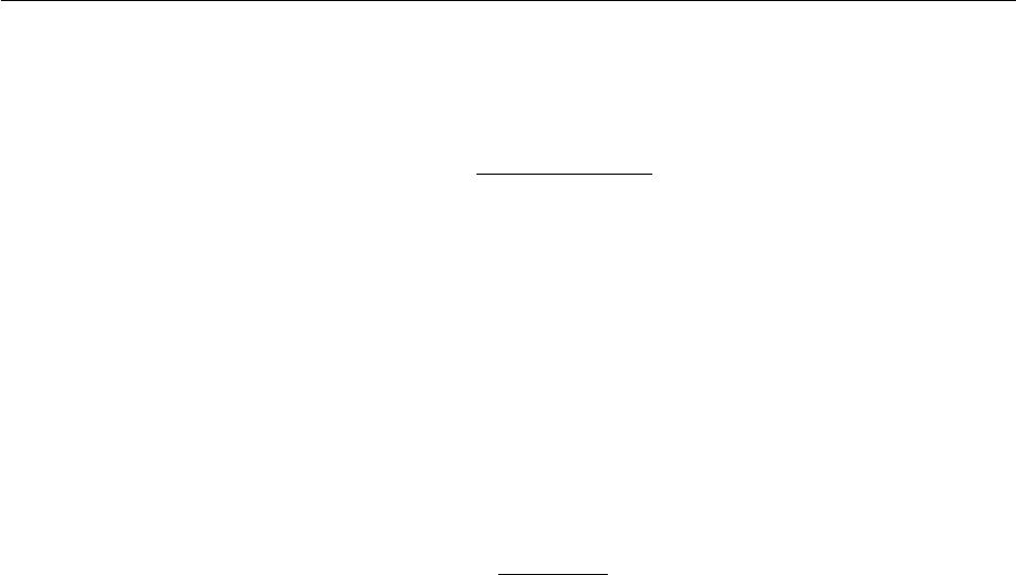
3.5. Chapter Exercises 53
3. The population of a certain species of bird is limited by the type of habitat required for nesting.
The population behaves according to the logistic growth model
n(t) = 5600
0.5 + 27.5e−0.044t
where tis measured in years.
Find the initial bird population.(a)
Draw a graph of the function n(t).(b)
What size does the population approach as time goes on?(c)
4. A 15g sample of radioactive iodine decays in such a way that the mass remaining after tdays
is given by m(t) = 15e−0.087twhere m(t) is measured in grams. After how many days is there
only 5g remaining?
5. A small lake is stocked with a certain species of fish. The fish population is modelled by the
function
P=10
1+4e−0.8t
where Pis the number of fish in thousands and tis measured in years since the lake was stocked.
Find the fish population after 3 years.(a)
After how many years will the fish population reach 5000 fish?(b)

4|Differentiation
Rate of Change
We are all familiar with the concept of average speed. If you travel a distance of 120 km in 2 hours
then your average speed is 60 kph. There is a formula that you will have met
Average speed = distance travelled
time elapsed
A distance/time graph can be drawn. The average speed can be expressed using function notation
Average speed = s(b)−s(a)
b−a
Finding the average rate of change is important in many contexts and in fact the average rate of
change can be defined for any function.
The average rate of change of the function y=f(x) is change in y
change in xor f(b)−f(a)
b−a(1)
The average rate of change is the slope of the secant line between x=aand x=bon the graph
of f, that is the slope of the line that passes through (a, f(a)) and (b, f (b)).
Example Calculate the average rate of change for the function f(x) = x2+ 4 between the
following points:
x= 2 and x= 6
Solution
Using the function notation
in (1) above,
f(2) −f(6)
2−6=8−40
−4
=−32
−4= 8
(1) x= 5 and x= 10
Solution
f(5) −f(10)
5−10 =29 −104
−5= 15
(2) x=aand x=a+h
(h6= 0)
Solution
f(a)−f(a+h)
a−(a+h)
=a2+ 4 −([a+h]2−4)
a+h
Can this be simplified further?
(3)
Tangents
We now investigate the process of changing the value of (b−a) in formula (1). As (b−a) is made
smaller and smaller the slope of the secant approaches the slope of the tangent at x=a. The
notation for this process is as follows.
Definition: The tangent line to the curve y=f(x) at the point P(a, f(a)) is the line through
Pwith slope m=lim
x→a
f(x)−f(a)
x−aprovided that the limit exists. This means that as the value of x

55
gets close to athe function remains smooth. Imagine zooming in on a function, from far away it
may appear smooth, but up close it could have some gaps or discontinuities. Limits do not exist
at sharp transitions in a graph, or where the function does not exist (think of piecewise functions).
We sometimes refer to the slope of the tangent line to a curve at a point as the slope of the curve
at that point. The idea is that if we zoom in far enough towards the point then the curve looks
almost like a straight line. The more we zoom in the more the parabola looks like a straight line.
Using function notation for the tangent line is usually easier to use and is often preferred. The
slope of the secant line between x=aand x=a+his f(a+h)−f(a)
h. This looks familiar from
example 3 above. We can now use this as a definition:
slope = m=lim
h→0
f(a+h)−f(a)
h
This is limit notation, lim
h→0, and we would say ‘the limit as happroaches 0’. Note that if h= 0 the
function is now undefined (math error). So his allowed to get close to zero, but not actually equal
zero.
Velocities
When this process is applied to the average velocity the result of computing the average velocity
over shorter and shorter time intervals produces the instantaneous velocity. Let s=f(t) be the
displacement at time tthen the instantaneous velocity is
v(a) = lim
h→0
f(a+h)−f(a)
h
This is often referred to as the velocity at t=a.
Suppose yis a quantity that depend on another quantity x. Thus yis a function of xand we write
y=f(x). If we change from x1to x2then the change in xis called an increment in xand is
denoted by ∆x=x2−x1and the corresponding increment in y is denoted by ∆y=y2−y1.
The average rate of change of ywith respect to xover the interval [x1, x2] is denoted by
∆y
∆x=f(x2)−f(x1)
x2−x1
and can be interpreted geometrically as the slope of the secant line. As we did with velocities we
can compute the average rate of change over smaller and smaller intervals by letting x2approach
x1and therefore letting ∆xapproach 0. The limit of this process is called the instantaneous rate
of change of ywith respect to xat x=x1. This is interpreted geometrically as the slope of the
tangent to the curve y=f(x) at (x1, f(x1)).
Instantaneous rate of change = lim
∆x→0
∆y
∆x=lim
x2→x1
f(x2)−f(x1)
x2−x1
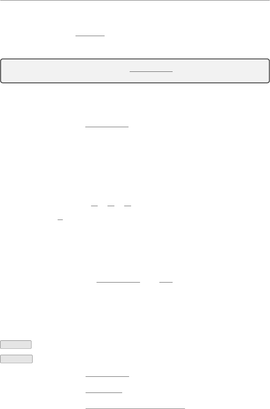
4.1. Derivatives from 1st Principles 56
4.1 Derivatives from 1st Principles
Because the expression lim
h→0
f(a+h)−f(a)
hoccurs so widely it is given a special name and notation.
The derivative of a function at a number a, denoted by f0(a) is
Definition of the derivative: f0(a) = lim
h→0
f(a+h)−f(a)
h
The process of finding the derivative using the above definition is called finding the derivative from
first principles. So far we have found a derivative of a function fat a fixed number a. If we replace
ain this equation with a variable xwe obtain
f0(x) = lim
h→0
f(x+h)−f(x)
h*Note the difference from above
given any number xfor which this limit exists. We assign to xthe number f0(x). So we can regard
f0as a new function which we call the derived function or the derivative of x.
Alternate Notation for the Derived Function
Given the notation y=f(x) for the function the following alternative notations for f0(x) are
common:
f0(x) = y0=dy
dx =df
dx =d
dxf(x), also = Df(x) = Dxf(x)
The symbols Dand d
dx are called differential operators.
Derivatives of Polynomial Functions
The constant function f(x) = cis considered a polynomial of degree zero. Using the method of
first principles we can find the derivative as follows:
f0(x) = lim
h→0
f(x+h)−f(x)
h=lim
h→0
c−c
h=lim
h→00=0
Higher Power Polynomials
When f(x) = xit can be shown from first principles that f0(x) = 1. Similarly when f(x) = x2it
can be shown that f0(x)=2xand when f(x) = x3it can be shown that f0(x)=3x2.
Example Find f0(x) for f(x) = x4from first principles.
Solution
f0(x) = lim
h→0
f(x+h)−f(x)
h
=lim
h→0
(x+h)4−x4
h
=lim
h→0
x4+ 4x3h+ 6x2h2+ 4xh3+h4−x4
h

4.2. Standard Derivatives 57
=lim
h→0
4x3h+ 6x2h2+ 4xh3+h4
h
=lim
h→0(4x3+ 6x2h+ 4xh2+h3) here, substitute h= 0
f0(x) = 4x3
This pattern will follow for any similar polynomial: If f(x) = xnthen f0(x) = nxn−1. Or alterna-
tively
The Power Rule for Differentiation: d
dx(xn) = nxn−1
This pattern implies that nmust be a positive integer. It can be shown that from the definition of
a derivative d
dx 1
x=−1
x2or y=x−1then dy
dx =−1×x−2, which proves the power rule for n=−1.
Similarly if the exponent is a fraction it can be shown that the power rule holds e.g. if f(x) = √x
then f0(x) = 1
2√xor f(x) = x1
2then f0(x) = 1
2x−1
2. It can be shown that the power rule holds for
any real number n.
4.2 Standard Derivatives
The basic functions have easily repeatable patterns to find their derivatives. The common ones are
summarized in the table below:
Function Derivative Notes
f(x)f0(x) notation
xnnxn−1‘power rule’
exexexponential
ln(x)1
xlogarithmic
sin(x) cos(x)
cos(x)−sin(x) trigonometric
tan(x) sec2(x)
The Natural Exponential
Recall the natural exponential function from section 3.1. Here we can see why precisely it is so
special. Using limit notation, we can say that eis the number such that lim
h→0
eh−1
h= 1. The
derivative is:
The Derivative of the Natural Exponential Function
d
dx (ex) = ex
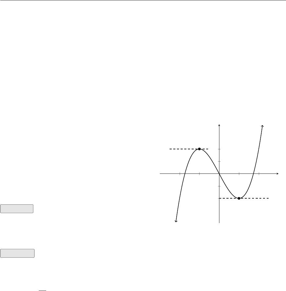
4.3. Maximums, Minimums, and Tangents 58
The natural exponential function is unique because it has its own derivative! Geometrically
this means that the slope of the tangent at any point is the same as the y-coordinate, f(x), of that
point.
4.3 Maximums, Minimums, and Tangents
Turning points occur at the boundary between regions in a function. A function that transitions
from increasing to decreasing must have a turning point. In the function below, f(−1) = 2 means
the point (−1,2) is a turning point. More specifically this is a local maximum of our function.
It is the highest point in its local neighbourhood. Notice that the other boundary has different
properties: it is the lowest point. So f(1) = −2 means the point (1,−2) is a local minimum.
The boundary means that the slope of the
tangent has gone from increasing to decreas-
ing. Or from positive to negative. During this
transition it had to go through zero, and so a
turning point can be found anywhere the slope
is equal to zero: f0(x) = 0. Remember that
the first derivative represents the slope of the
function.
Example Find the turning points for
f(x) = x3−3x
-2 -1 1 2
-2
-1
1
2
f0(1) = 0
local minimum
f0(−1) = 0
local maximum
x
y
Solution
Set the derivative equal to zero and solve for
values of x.
dy
dx = 3x2−3
0=3x2−3
3=3x2
1 = x2
x= 1,and x=−1
Therefore the x−values of the turning points
are 1 and −1. Note there are two turning
points in our function so there should be two
corresponding solutions.
f(1) = (1)3−3(1)
= 1 −3 = −2
Therefore (1,−2) is the first turning point.
Similarly, (−1,2) is found as the other turn-
ing point. These are both shown in the figure
above.
Second Derivative Test
We know from the graph that these turning points are maximum and minimum. The graph is not
always provided to identify maxima and minima, so it helps to have a test to determine if a point
is a max or min.
We know first derivative represents the slope of the function. Looking at the parabola y=x2and
following the function from left to right we can plot some values of the first derivative. The graph
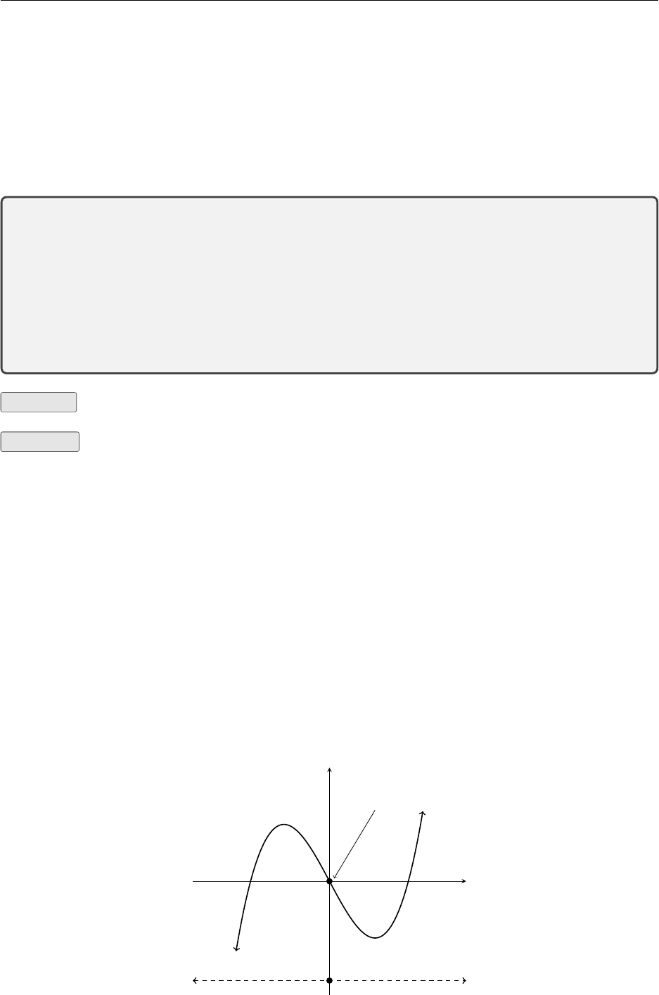
4.3. Maximums, Minimums, and Tangents 59
tells us that the turning point is at (0,0) and is a minimum. The value of the 1st derivative is
-2,-1,0,1,2 : these numbers are increasing. This trend is always true for a local minimum.
How do we test for this trend of increasing slopes? The rate of change of the slopes is the second
derivative, and if this number (at the point (0,0)) is positive, then the point is a minimum.
This is called the second derivative test.
Second Derivative Test
•If f0(x) = 0, and f00(x)>0, then the point (x, f(x)) is a local minimum. The graph
in this neighbourhood is concave up.
•If f0(x) = 0, and f00(x)<0, then the point (x, f(x)) is a local maximum. The graph
in this neighbourhood is concave down.
Example Use the second derivative test to determine if the turning point (−1,2) is a maximum
or minimum on the function f(x) = x3−3x
Solution Find the second derivative and substitute the turning point.
f0(x)=3x2−3
f00(x)=6x
f00(−1) = 6(−1) = −6
−6<0
therefore the turning point (−1,2) is a local maximum.
Points of Inflection
There is one last feature of the initial function that can be found. There is a point in between the
maximum and minimum points where the change in slopes of the function change from decreasing
to increasing. This is called a point of inflection. It is where the concavity of the function changes
between down and up.
concave up
concave down
point of inflection
x
y

4.4. The Product, Quotient, and Chain Rules 60
The second derivative test can be used to determine if a function is concave-up (>0) or concave
down (<0). Note there is no = in these inequalities. In between is where the point of inflection
can be found:
Second Derivative Test for Concavity
•If f00(x) = 0, then the point (x, f(x)) is a point of inflection.
Example Find where the function changes from concave-up to concave-down.
f(x)=3x3−12x2+ 7
Solution Find the second derivative and set equal to zero to find the point of inflection.
f0(x)=9x2−24x
f00(x) = 18x−24
0 = 18x−24
4
3=x
Sub back into f(x) to find the y−value:
f4
3= 3 4
33
−12 4
32
+ 7
=−72
9
Therefore, the point 4
3,−72
9is a point of in-
flection.
4.4 The Product, Quotient, and Chain Rules
The Product Rule
Let f(x) = xand g(x) = x2. What is the derivative of f(x)×g(x)? The question helps to show
that the answer is NOT f0(x)×g0(x)
f(x)×g(x) = x×x2=x3and we know the derivative of x3is 3x2. Also we know that f0(x)=1
and g0(x)=2xso f0(x)×g0(x)=1×2x= 2xnot 3x2.
So the derivative of the product of two functions is not the product of the derivatives of each
function. In symbols this can be written
(fg)06=f0g0
Theorem If fand gare both differentiable then
d
dx [f(x)g(x)] = f(x)d
dx [g(x)] + g(x)d
dx [f(x)]
The Product rule is often seen in an abbreviated form as (uv)0=uv0+vu0.
The Quotient Rule
Let u=f(x) and v=g(x) be differentiable functions of xthen we can show that
4.4. The Product, Quotient, and Chain Rules 61
d
dxf(x)
g(x)=g(x)d
dx [f(x)] −f(x)d
dx [g(x)]
[g(x)]2
or in abbreviated form as u
v0=vu0−uv0
v2
Example See blackboard course notes for examples of the product and quotient rules.
Chain Rule
When functions are combined with other functions, they are often called composite functions.
These require special treatment when differentiating.
Let f(x) = x2and g(x) = 2x+1 then (f◦g) This means f‘composed of’ gis f(g(x)) = f(2x+1) =
(2x+ 1)2.
Also, g‘composed of’ fwould be: (g◦f) (x) = gx2= 2 x2+ 1 = 2x2+ 1.
The differentiation rules we have met so far allow us to differentiate pairs of functions that have
been added, subtracted, multiplied or divided. They do not allow us to differentiate an expression
that is made from a function that is within another function.
The following are all examples of composite functions.
1. We can differentiate x2but we can’t use the same procedure to differentiate (1 −x)2. Here
we can imagine if f(x) = x2and g(x)=1−xthen (f◦g) (x) = f(1 −x) = (1 −x)2.
2. We can differentiate 1
x2but we can’t use the same procedure to differentiate 1
x2+1 .
3. We can differentiate exbut we can’t use the same procedure to differentiate ex2.
A name often used for functions of this type is function of a function.
Once we recognise we are dealing with a composite function we need a procedure to differentiate
it. You will find that you are far more likely to be required to differentiate a composite function
in a practical situation than a simple one. It can be proved that the derivative of the composite
function f◦gis the product of the derivatives of fand g. This important rule is given the name
the Chain Rule. A substitution method is often used to add clarity to the differentiation process.
Let y=u2and let u= 1 −x. Then dy
du = 2uand du
dx =−1. Now dy
dx =dy
du ·du
dx = 2u×(−1) = −2u=
−2(1 −x) = 2(x−1).
The Leibniz form of the Chain Rule dy
dx =dy
du
du
dx is what gives the rule its name. Because of the
apparent cancelling it is particularly easy to learn in this form.
As an aside let us verify the rule for this example. Given y= (1 −x)2. We will expand the right
hand side of the equation. It becomes y=x2−2x+ 1. So y0= 2x−2 = 2(x−1) as before.
Using function notation the Chain Rule states: If fand gare both differentiable and F=f◦gis
the composite function F(x) = f(g(x)), then Fis differentiable and F0=f0(g(x))g0(x).
4.4. The Product, Quotient, and Chain Rules 62
A Comment on the Leibniz form of the Chain Rule
dy
dx =dy
du ·du
dx gives the impression that the du could cancel but remember we have not defined du.
We have defined dy
du as the rate of change of ywith respect to uand du
dx as the rate of change of u
with respect to x. However the apparent cancelling helps us to remember the way the differentials
are arranged. it also helps us to accept the extension of the Chain Rule to cover a function of a
function of a function etc. e.g.
Lety=f(u),u=g(v)andv=h(x)
Then dy
dx =dy
du ·du
dv ·dv
dx
Example Find F0(x) when F(x) = 1
x2+1 .
Solution Using function notation F(x)=(f◦g) (x) = f(g(x))
where
f(u) = u−1and g(x) = x2+ 1
f0(u) = −u−2andg0(x)=2x
and
F0(x) = f0(g(x))g0(x)
=−1
(x2+ 1)2·2x
=−2x
(x2+ 1)2
Using the Leibniz notation let u=x2+ 1 and y=u−1then
F0(x) = dy
du
du
dx =−u−2(2x)
=−1
(x2+ 1)2(2x) = −2x
(x2+ 1)2
To use the method we need to bring a new variable into the problem we are trying to solve. It
is recommended that you use the variable uwherever possible so that you follow through using a
pattern you are familiar with.
In summary: if gis differentiable at xand fis differentiable at g(x), then the composite function
F=f◦gdefined by F(x) = f(g(x)) is differentiable at xand F0is given by the product
F0(x) = f0(g(x)) ·g0(x)
In Leibniz notation, if y=f(u) and u=g(x) are both differentiable functions, then
dy
dx =dy
du ·du
dx
The Chain Rule will be found in many situations where functions are added, subtracted, multiplied
or divided. As an example we will focus on combining the Chain Rule with the Product Rule,
however any combination of these rules could be found in a problem.

4.5. Parametric Differentiation 63
Example Differentiate xe−x2.
Solution We can see that there is a product of two functions present in this example, i.e.
f(x) = xand g(x) = e−x2. Also g(x) is a composite function.
We have from the Product Rule
(fg)0=fg0+gf0
By inspection we can see that of the four expressions on the right side of this equation f,gand f0
can be put into the equation immediately and only g0requires some effort to be worked out.
g(x) is a composite function so g0(x) is computed using the Chain Rule.
Let u=−x2then du
dx =−2x. Also g(u) = euso dg
du =eu.
dg
dx =dg
du
du
dx
=eu· −2x
=e−x2· −2x
=−2x e−x2
So g0(x) = −2x e−x2
Putting this all together
(fg)0=fg0+gf0
=x· −2x e−x2+e−x2·1
=e−x21−2x2
4.5 Parametric Differentiation
Parametric Curves xand yare both given as functions of a third variable t(called the parameter ).
Let the equations be
x=f(t) and y=g(t)
Each value of tgives a point (x, y). As tvaries the point (x, y) = (f(t), g(t)) traces out a curve in
the coordinate plane called a parametric curve.
Using the Chain Rule to find the Derivative dy
dx
Given the parametric equations x=f(t) and y=g(t) define a parametric curve. If fand gare
both differentiable the Chain Rule gives
dy
dt =dy
dx ·
dx
dt
provided yis also a differentiable function of x. So provided dx
dt 6= 0
dy
dx =dy
dt ÷dx
dt
4.6. Related Rates 64
=dy
dt ×dt
dx
Example See blackboard course notes for examples of parametric differentiation.
4.6 Related Rates
The concept of related rates is best understood by exploring some examples.
Example 1. Air is being pumped into a spherical balloon so that its volume is increasing at a
rate of 100 cm3/s. How fast is the radius of the balloon increasing when the diameter is 50 cm?
You have to find the related rates in the question. Let Vbe the volume and rbe the radius at
time t. The volume is increasing at the rate of 100 cm3/s so dV
dt = 100. The question asks how fast
is the radius increasing. In other words what is dr
dt ?
Solution We need a formula that connects Vand rif we are to find the relationship between
dV
dt and dr
dt .
The formula
V=4
3πr3
is of the form V=f(r) so we can find dV
dr
dV
dr = 4πr2(1)
From the Chain Rule we can write dV
dt =dV
dr ·dr
dt (2)
Substituting dV
dt = 100 and dV
dr = 4πr2in equation (2) we get
100 = 4πr2·dr
dt
dr
dt =100
4πr2
=25
πr2
Now we substitute r= 25. (Diameter = 50 so radius = 25)
dr
dt r=25 =25
π×252
=1
25π
So the radius is increasing at the rate of 1
25πcm/s
Example 2. A ladder 5 m long rests against a vertical wall. If the bottom of the ladder slides
away from the wall at the rate of 0.5 m/s how fast is the top of the ladder sliding down the wall
when the bottom of the ladder is 3 m from the wall?

4.6. Related Rates 65
Solution Let the origin be placed at the corner where the wall meets the floor, let xbe the
distance of the foot of the ladder from the wall and let ybe the distance of the top of the ladder
from the corner. The ladder forms a right angled triangle whose sides are x,yand with hypotenuse
5. We are given that dx
dt = 0.5 and are asked to find dy
dt when x= 3.
Pythagoras theorem gives
x2+y2= 52(1)
Differentiate equation (1) with respect to t
2xdx
dt + 2ydy
dt = 0
Solve for dy
dt dy
dt =−x
y·dx
dt
Using Pythagoras theorem when x= 3 and the hypotenuse = 5, y= 4
Substitute dx
dt = 0.5, x= 3 and y= 4
dy
dt =−3
4·0.5
=−0.375
The top of the ladder is moving vertically downwards at the rate of 0.375 m/s
Example 3. A water tank has the shape of an inverted circular cone with a base radius of 2 m
and height of 4 m. If water is being pumped into the tank at a rate of 2 m3/min find the rate at
which the water level is rising when the water is 3 m deep.
Solution Let V,rand hbe the volume of water the radius of the surface and the height at
time t. We are given dV
dt = 2m3/min
We are asked to find dh
dt when h= 3.
Draw a diagram to show that the relationship between rand hcan be found by similar triangles.
r
h=2
4
r=h
2(1)
The formula for the volume is
V=1
3πr2h(2)
Substituting equation (1) in equation (2)
V=1
3πh
22
h
4.7. Optimisation 66
=π
12h3
Differentiate with respect to t
dV
dt =π
12 ·3h2·dh
dt
=π
4h2·dh
dt
So dh
dt =4
πh2·dV
dt
Substitute h= 3 and dV
dt = 2
dh
dt =4
π(3)3·2
=8
9π
The water level is rising at the rate of 8
9πm/min.
4.7 Optimisation
Optimisation is the process of using calculus to find the best result for a situation involving a
changing quantity (variable). Examples include maximizing profit, minimizing cost, maximizing
volume, minimizing amount materials used, and so on. As long as the quantities in question can
be represented by a function, calculus can used to find the special points of the function and their
nature.
A general method to approach an optimisation problem
1. Write down the known variables and draw a diagram
2. Form an equation of the situation by placing the unknown variable in terms of the
known variables
3. Use the facts of the problem to reduce the expression until it becomes a relationship
between the unknown quantity and one of the known quantities
4. Optimize by finding a maximum or minimum value
Example A farmer wishes to fence a paddock using an existing wall as one side of the paddock.
She has 100 meters of fencing and wants to know the dimensions of the paddock to enclose the
maximum area.
4.7. Optimisation 67
existing wall
fence length 1
fence length 2
area of the
paddock
Solution Following the steps outlined above, draw a diagram and label the variables. Let
Trepresent the total fence length which cannot be more than 100m. Write this as an equation:
T= 100. There are 3 individual lengths that make up the total, so let lrepresent the long side of
the paddock, and wrepresent the short side.
T=l+ 2w
100 = l+ 2w
The quantity to be optimised is area (A) of the paddock (remember it is a rectangle):
A=lw
The next step is to represent the quantity to be optimised (area) as a function of one other variable.
We can rearrange our earlier equation to solve for length: l= 100−2w. This can now be substituted
into the area equation:
A=lw
= (100 −2w)w
= 100w−2w2
This is now an equation that can optimised using calculus.
dA
dw = 100 −4w
0 = 100 −4w
w= 25
Therefore the paddock width is 25 meters to maximize the total area. Going back to the original
constraint of 100m total length means that the paddock length is 100 −2(25) = 50 meters.
Example A cylindrical can is to be made to hold 1 litre of oil. Find the dimensions that will
minimise the cost of the aluminium to manufacture the can. Note that 1 L = 1000 cm3.
Solution The minimum cost of the aluminium will be the minimum surface area of the cylinder.
The can can be deconstructed into two circles and a rectangle. We will label the variables required
to calculate area.
Let SA represent surface area of the can. The total surface area is:
SA =πr2+πr2+ (height ∗circumference)
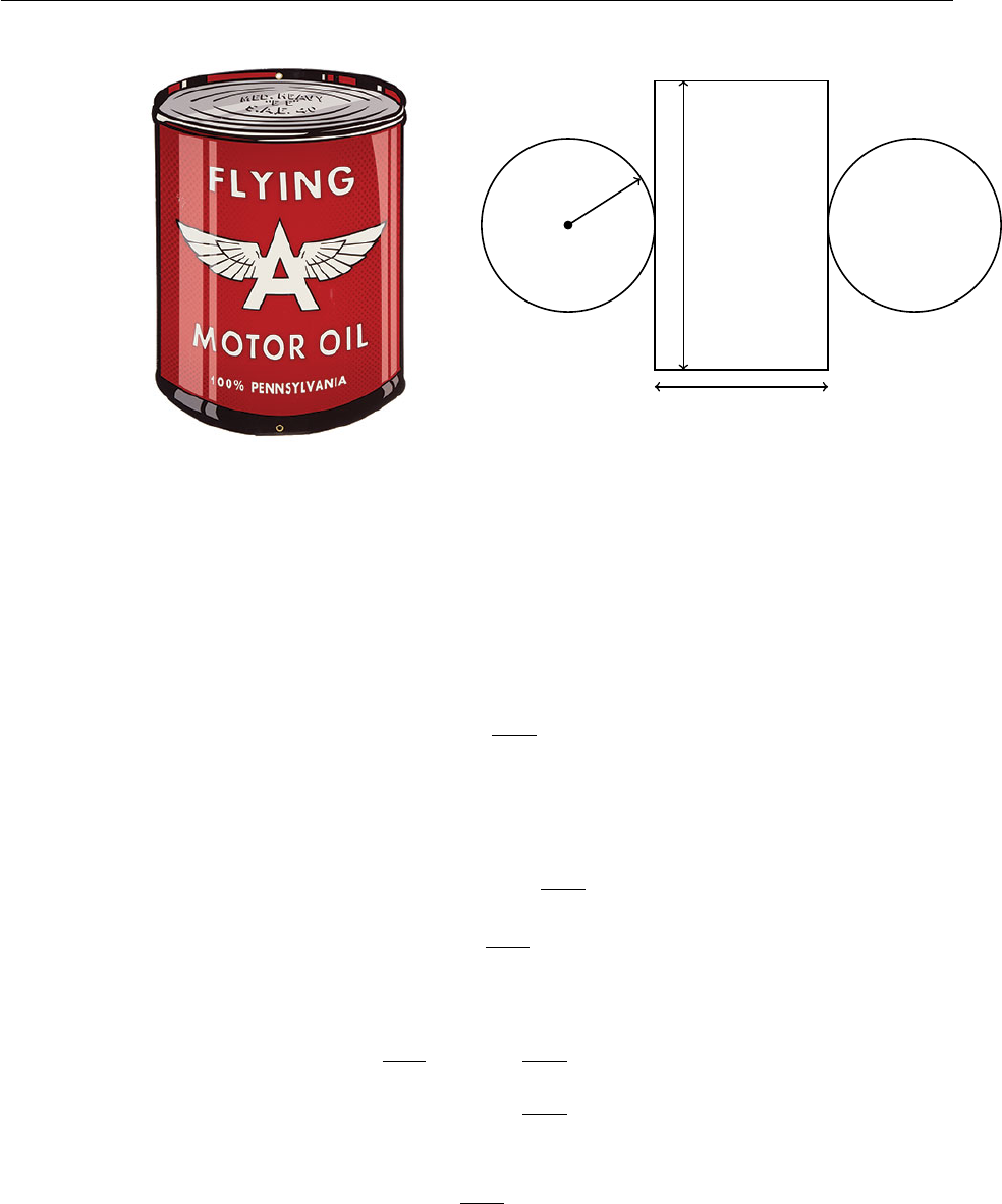
4.7. Optimisation 68
height of can
circumference
r
= 2πr2+ 2πrh
Note that we have 2 variables that are unknown, r, and h. We need to express one variable in
terms of the other in order to proceed. Use the additional information in the problem. The volume
of the can must be 1000 cm3.
V=πr2h
1000 = πr2h
h=1000
πr2
Substitute this form for hinto the surface area function:
SA = 2πr2+ 2πrh
= 2πr2+ 2πr 1000
πr2
= 2πr2+2000
r
This function is now the surface area in terms of a single variable, r, and can be optimised:
dSA
dr = 4πr −2000
r2
0=4πr −2000
r2
= 4πr3−2000
r3=2000
4π
r= 5.419 cm
Therefore the final dimensions of the can optimised for minimum cost are radius= 5.42 cm, and
height= 10.8 cm.
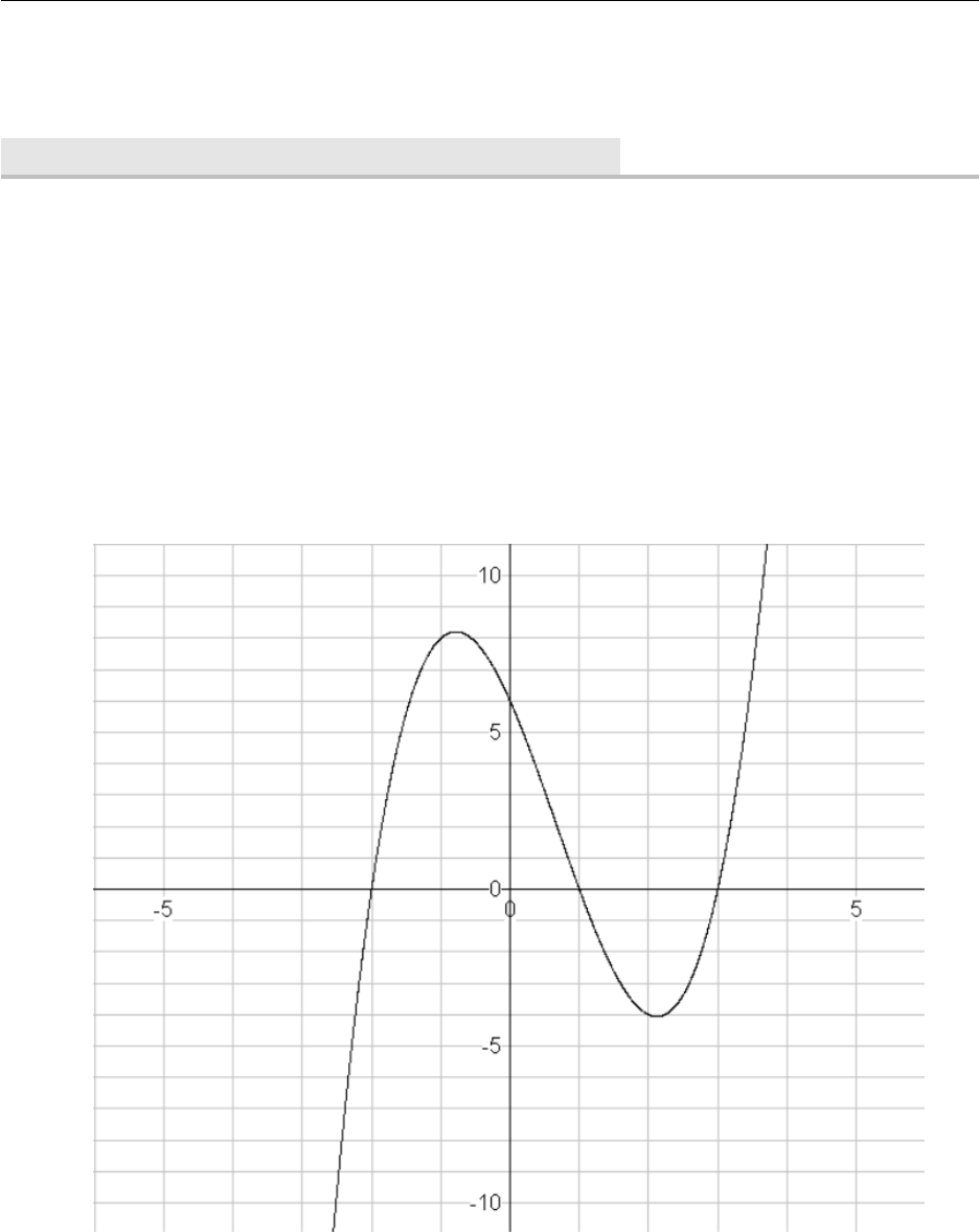
4.8. Chapter Exercises 69
4.8 Chapter Exercises
§4.1 Differentiation from First Principles
1. Find the derivative of the function at the given value using the method of first principles.
f(x) = 5x2+ 3x−1 at the number 2(a)
f(x) = 1 −3x2at the number 2(b)
f(x) = x4at the number 1, given (x+h)4=x4+ 4x3h+ 6x2h2+ 4xh3+h4
(c)
Graphing Exercises
2. The graph of f(x) = (x−1)(x+ 2)(x−3) is drawn below. On the same set of axes, sketch
the graph of the derived function, f0(x). What is the shape of the graph of the derived function?
4.8. Chapter Exercises 70
3. The graph of f(x) = (x+ 1)(x−1)(x−2)(x+ 3) is drawn below. On the same set of axes,
sketch the graph of the derived function, f0(x)
What is the order of f(x)? What is the order of f0(x)?
4. The graph of f(x) = exis drawn below. On the same set of axes, sketch the graph of the
derived function, f0(x)
What is the shape of the graph of the derived function?
4.8. Chapter Exercises 71
5. The graph of f(x) = 10x2ex(x+ 1) is drawn below. On the same set of axes, sketch the graph
of the derived function, f0(x)
6. Differentiate
f(x) = 1
x2
(a) y=3
√x2
(b) y=x5
(c)
y=1
x3
(d) y=x−4
(e) y=x3/4
(f)
y=1
√x
(g)
§4.2 Standard Derivatives
1. Find dy
dx
y=2
5x5
(a) y=−10(b)
y=−3x4
(c) y=2
x4
(d)
y=1
3x3
(e)
2. Differentiate
f(t) = √t(a) f(t) = √t3
(b)
f(z) = 3
√z5
(c) f(x) = 2x3.2
(d)
3. Find the derivative
f(x) = 2x3−3x2+ 4x−1(a) f(x) = x2+x+1+ 1
x
(b)
x8+ 12x5−4x4+ 10x3−6x+ 5(c)

4.8. Chapter Exercises 72
4. Given s= 4t2−7t+ 5 find ds
dt
(a) Find d(3x)
dx
(b)
Find d(3u4)
du
(c) Given f(x) = 2x−3 find Df(x)(d)
Given f(x) = ex−xfind f0(x). Sketch
the graph.
(e) Differentiate f(x) = (3x)3
(f)
Differentiate g(x) = x35
(g) Find the derivative of f(x) = ex−xe
(h)
5. Find the derived function
f(x) = 1
x3−1
4
√x3
(a) f(x) = √x+3
√x
4
√x
(b)
g(x) = ex2+ 2ex+xe2+xe2
(c) f(x) = 3
√x+5
√2(d)
6. Sketch the graphs and label your axes in radians
f0(x) where f(x) = sin x(a) g0(x) where g(x) = cos x(b)
h0(x) where g(x) = tan x(c)
7. Differentiate the trigonometric functions
y=x2sin x(a) f(x) = √xsin x(b)
h(x) = tan(5x)(c) y=x
cos x
(d)
g(t) = cos(ωt +δ)(e)
8. Find the tangent line to the curve y=excos xat the point (0,1).
9. A ladder 10m long rests against a vertical wall. Let θbe the angle between the top of the
ladder and the wall and let xbe the distance between the bottom of the ladder and the wall.
If the bottom of the ladder slides away from the wall, how fast is xchanging with respect to θ
when θ=π
3?
10. Find the derivative
sin 4x(a) 2
πsin πx(b) 5 cos 3x(c)
tan 3x(d) 3 tan (x+ 2)(e) sin3x(f)
sin23x(g) sin3(x−1)2
(h) tan22x(i)
§4.3 Maximums, Minimums, and Tangents
1. The function y= 7x−3 has no turning point. Why?
2. Turning points are sometimes referred to as stationary points. Find the stationary points of
the following functions:
y=x3
3−4x(a) y=x2+16
x
(b) f(x) = −x4+4x3−4x2+
1
(c)
3. Find the turning points and use the second derivative test to show if they are local maxima or
local minima:

4.8. Chapter Exercises 73
y= 4 −(3 −x)2
(a) y=x3
3−x(b)
f(x) = (3 −x)(x+ 2)(x+ 5)(c)
4. Consider f(x) = xex. Do you think this function has a local max or min? Think of the graph
of y=ex. Plot the function using Desmos and find the turning point.
5. Find the equations of the tangent line and the normal line to the curve y=x√xat the point
(1,1).
6. Find the points on the curve y=x4−6x2+ 4 where the tangent line is horizontal.
7. At what point on the curve y=exis the tangent line parallel to the line y= 2x?
8. Find a point aon the curve f(x) = x3+ 2x2+ 3x+ 4 where f0(a)=2
9. Find where the tangent line to the function f(x) = x3−x+ 1 is parallel to the line y=x.
Graphing Exercise
10. If f(x) = 2x2−x3find f0,f00,f000,f(4). Use Desmos to graph f,f0,f00, and f000 on a common
screen. Describe whether these graphs are consistent with a geometric interpretation of these
derivatives.
11. If f(x) = 1
xfind f0(x) and f00(x) then graph f,f0and f00 on a common screen. Are your answers
reasonable?
§4.4 Product, Quotient, & Chain Rules
1. Use the product rule to find the derivative
f(x) = xex
(a) g(x) = x2ex
(b)
2. Differentiate with respect to x
x3ex
(a) x−3ex
(b)
(x+ 1) ex
(c) (x+ 2) (x−2) ex
(d)
3. Use the quotient rule to find the derivative
y=3x+1
2x−1
(a) y=ex
x+1
(b)
f(t) = 2t
1+t2find df
dt
(c) f(x) = A
B+Cex
(d)
4. Differentiate
3x2
1−x
(a) x
x+2
(b)
√x
x+2
(c) 2x2+3x+2
ex
(d)
Exercises involving Tangent and Normals
5. Find the equation of the tangent line and normal line to the curve y=xexat the point (0,0).
6. The curve y= 1/(1 + x2) has the name witch of Maria Agnesi.
Find the equation of the tangent line to this curve at the point 1,1
2.(a)
Use Desmos to draw the graph of the curve and the tangent line on the same grid.(b)

4.8. Chapter Exercises 74
7. The curve y=x/(1 + x2) is called a serpentine.
Find the equation of the tangent line at the point 1,1
2.(a)
Use Desmos to draw the graph of the curve and the tangent line on the same grid.(b)
Composite Functions
8. Let f(x) = √xand g(x) = x3find (f◦g) (x) and (g◦f) (x).
9. Given h(x) = exand j(x) = x2
2find (h◦j) (x) and (j◦h) (x).
10. The chain rule
Find F0(x) when F(x) = √1 + x2.(a)
Given y=1−x25find dy
dx .(b)
Find the derivative of ex2.(c)
Find the derived function for eex.(d)
11. Differentiate with respect to x
(3x+ 2)3
(a) (5x+ 3)3
5
(b)
1
2x+1
(c) 3
(4−x)3
(d)
√2x−5(e) 3
√5−x2
(f)
1
√x+2
(g) e2x3
(h)
12. You may have to combine rules to differentiate the following
y=x2e−2x
(a) (1 −2x)2e−x
(b)
p+1
√p2+1
(c) x2+ 32(x−4)(d)
(x−3)3(x+ 2)(e) √x+ 1 (x−1)2
(f)
ex2√x+ 1(g) x2+x+2
(x+1)2
(h)
§4.5 Parametric Differentiation
1. Use desmos to sketch the parametric curves
x=t2−2tand y=t+ 1 where 0 6t64(a) x= cos tand y= sin twhere 0 6t62π(b)
x= 2 cos tand y= sin tfor 0 6t62π(c) x= cos tand y= sin 2twhere 0 6t62π(d)
x= 1.5 cos t−cos 40tand y= 1.5 sin t−sin 40twhere 0 6t62π(e)
2. Given y= 2tand x=t2
Find dy
dx .(a)
By finding the appropriate value of tshow that (1,2) lies on the parametric curve.(b)
Find the equation of the tangent line to the parametric curve at (1,2).(c)

4.8. Chapter Exercises 75
3. Given x= cos tand y= sin tfind the equation of the tangent line at the point √2
2,√2
2.
Where does this curve have horizontal or vertical tangent lines?
4. Given x= cos tand y= sin 2tfind the equation of the tangent line at the point √3
2,√3
2.
Where does this curve have horizontal or vertical tangent lines?
5. Find dy
dx in terms of the parameter
x=t2+t y =t3−t2
(a) x=etcos t y =etsin t(b)
x=at2y= 2at (ais constant)(c) x=asin θ y =bcos θ(d)
x= 2 sin θ y = cos 2θ(e) x=a(θ−sin θ)y=a(1 −cos θ)(f)
§4.6 Related Rates
1. If Vis the volume of a cube with edge length xand the cube is expanding as time passes, find
dV
dt in terms of dx
dt .
2. Each side of a square is increasing at a rate of 6cm/s. At what rate is the area of the square
increasing when the area of the square is 16cm2?
3. If Ais the area of a circle with radius rand the circle expands as time passes find dA
dt in
terms of dr
dt .
(a)
Suppose oil spills from a ruptured tanker and spreads in a circular pattern. If the radius
of the oil spill increases at a constant rate of 1m/s how fast is the area of the spill increasing
when the radius is 30m?
(b)
4. If a snowball melts so that its surface area decreases at a rate of 1cm2/min, find the rate at
which the diameter decreases when the diameter is 10 cm. The following steps may help you
to solve this problem.
What quantities are given in the problem?(i)
What is the unknown?(ii)
Draw a picture of the situation for any time t.(iii)
Write an equation that relates the quantities.(iv)
Solve for the unknown quantities.(v)
5. At noon ship A is 150km west of a ship B. Ship A is sailing east at 35km/h and ship B is sailing
north at 25km/h. How fast is the distance between the ships changing at 4:00 P.M.?
6. A plane flying horizontally at an altitude of 2km and a speed of 800km/h passes directly over
a radar station. Find the rate at which the distance from the plane to the station is increasing
when it is 3km away from the station.
§4.7 Optimisation
1. Divide 50 into two parts such that the product of the two parts is a maximum.
2. Find the number that exceeds its square by the greatest amount.
4.8. Chapter Exercises 76
3. A farmer has 2400m of fencing and wants to fence off a rectangular field that borders a straight
river. He needs no fence along the river. What are the dimensions of the field that has the
greatest area?
4. A farmer wishes to fence off a corner of a field where there is an existing hedge on two sides.
The hedge is to be used to fence the two sides. If he has 300m of fencing available, find the
dimensions aand bso that he encloses the maximum area.
5. The volume of the cone is given by the formula V(r) = 10πr2
3−πr3
3. Find the radius of the cone
at its maximum volume.
6. The total cost of holding a large event is composed of the venue hire, V, times the venue tax,
T, plus the entertainment, E. These values can all be estimated based on the number of people
attending the event, p, such that: V(p) = 50p+80, T(p) = 0.002p−0.4, and E(p) = 36000−60p.
Find the minimum cost.
7. Find the area of the greatest rectangle that can be inscribed in a semicircle of radius r.
8. If 1200cm2of material is available to make a box with a square base and an open top. Find
the largest possible volume of the box. (Hint: There is no wasted material.)

5|Integration <R>
In mathematics we are often given a function fand asked to find a function Fwhose derivative
is f.Fin this situation is called the integral of f. It is usual to develop a list of integrals by
differentiating a range of functions then using those to work backwards. The terms integration and
anti-differentiation are synonymous. Generally we will use the term integration, however, both are
acceptable.
Using derivatives to infer the integral
1. Because y=x2gives y0= 2xwe can say that an integral of 2xis x2.
2. Because y=x2+ 1 gives y0= 2xwe can say that another integral of 2xis x2+ 1.
3. Because y=x2+cwhere cis a constant gives y0= 2xwe can say that an integral of 2xis
x2+c.
4. Because y=exgives y0=exwe can say that an integral of exis ex. In fact we say that the
integrals of exare ex+cwhere cis a constant.
5. Because y= ln x+cwhere cis a constant gives y0=1
xwe can say that a family of integrals
of 1
xis ln x+c. This is often written ln kx where c= ln kis the constant
6. This can be generalised. y= ln |x|+calso gives y0=1
xso in general the integrals of 1
xare
ln |x|+c.
The process of ‘reversing’ or ‘undoing’ a derivate has its own symbol, the integrand.
Zf0(x)dx =f(x)
5.1 Standard Integrals
The examples shown above begin the process of establishing the start of a list of integration rules.
It is not the intention here to list all of the rules that are required however at this stage let us
explore the Power Rule to establish a rule for antedifferentiating an expression of the form y=xn
f f0
x1
x22x
x33x2
x44x3
or
f f0
x1
1
2x2x
1
3x3x2
1
4x4x3
so we can say
f0f
1x+c
x1
2x2+c
x21
3x3+c
x31
4x4+c
or
f F
1x+c
x1
2x2+c
x21
3x3+c
x31
4x4+c

5.1. Standard Integrals 78
This establishes the pattern and if you think about the rule for differentiating y=xnyou can soon
establish the rule for integrating xn.
The Power Rule for Integrating
Zxndx =xn+1
n+ 1 +c, where n6=−1
If f(x) = x−1then the integral of fis ln |x|+cor ln |kx|
All of the differentiation rules we have met so far lead to integration rules. For instance we can
establish standards for sin x, cos x, and sec2x. The standard integrals are summarized in the table
below.
function integral
f(x)Rf(x)dx
xn, n 6=−1xn+1
n+1 +C
exex+C
1
xln |x|+C
sin(x)−cos(x) + C
cos(x) sin(x) + C
sec2(x) tan(x) + C
To allow us to combine these integrals and thus extend the range of questions we can tackle we use
two important rules for integrals
Sum Rule The integral of the sum of two functions is the sum of the integrals of the
functions. Z[f(x) + g(x)] dx =Zf(x)dx +Zg(x)dx
This is easily extended to the sum or difference of a number of functions.
Constant Multiple Rule The integral of a constant times a function is the constant times
the integral of the function. Zcf (x)dx =cZf(x)dx
clearpage Example Integrate the following functions; find Zf(x).

5.2. Area 79
f(x)=3x2
Solution Applying the power rule:
Z3x2dx =3x2+1
2+1 +C
=x3+C
(a) f(x)=7
Solution Here we are integrating a constant:
Z7dx = 7x+C
(b)
f(x) = x2
3
Solution The power rule still applies to frac-
tional indices:
Zx2
3dx =x2
3+1
2
3+ 1 +C
=3x5/3
5+C
(c) f(x) = 1
2√x+1
√2
Solution Here we need to combine the sum
rule and the power rule:
Zf(x)dx =Z(1
2√x)dx +Z(1
√2)dx
=1
2Zx−1
2+1
√2x+C
=√x+x
√2+C
(d)
Example Find f(x) given f00(x)=6
Solution Here we have a second derivative, indicated by the double-prime symbol, f00. Knowing
that Rf0(x) = f(x) we can safely assume that
Zf00(x)dx =f0(x).
So f0(x) = Rf00(x) = R6dx = 6x+C. Now we need to integrate a second time to get f.
Z(6x+C)dx = 6x2+Cx +D
We end up with two unknown values, Cand Das opposed to just a single value.
The previous two examples of equations involving derivatives. Any equation involving derivatives
of a function is called a differential equation. We will look into this subject in the next chapter.
5.2 Area
In this section we attempt to find the area under a curve. That is the area that lies between a
curve and the x-axis from x=ato x=b. The area is bounded by the x-axis, a continuous curve
y=f(x) and the two vertical lines x=aand x=b. This is shown in the figure below with the
area shaded in.
5.2. Area 80
Figure: A parabola showing the area
under the curve between x= 0, and
x= 1.5. Note the area stops at the
axis. Area as calculated by integra-
tion is always in reference to the axis.
Previously, when we wanted to find the slope of a tangent line we found the slope of a secant line
and applied the limiting process lim
h→0. A similar procedure will be used to find the area. We first
approximate the area with rectangular strips then we take the limit of the areas of these rectangular
strips by making the strips narrower and narrower and thus the number of strips between x=a
and x=bgreater and greater.
Example Consider the curve y=x2. Use rectangles to find the area under this curve between
0 and 1.
Solution Consider 4 strips by constructing vertical lines at x=1
4,x=1
2,x=3
4and x= 1.
Define the left sum as the sum of the rectangles whose left side is formed using x=1
4,x=1
2,x=3
4
and x= 1. Define the right sum as the sum of the rectangles whose right side is formed by x=1
4,
x=1
2,x=3
4and x= 1.
Left sum = 1
4·02+1
41
42
+1
41
22
+1
43
42
= 0 + 1
64 +1
16 +9
64 =1+4+9
64 =7
32 = 0.21875
Right sum = 1
41
42
+1
41
22
+1
43
42
+1
4(1)2
=1
64 +1
16 +9
64 +1
4=1+4+9+16
64 =15
32 = 0.46875
It is clear from a diagram that the actual area is larger that the left sum and smaller than the right
sum.
0.21875 <A<0.46875
We could repeat this process with a larger number of strips but it is clear the process would quickly
become tedious. We can however simulate this process using a spreadsheet like Excel.
For the curve y=x2set up a spreadsheet to show 10 strips or 20 strips or 30 strips etc. The table
gives the results you should obtain for a selection of numbers of strips

5.2. Area 81
nLeft sum Right sum
10 0.2850000 0.3850000
20 0.3087500 0.3587500
30 0.3168519 0.3501852
100 0.3283500 0.3383500
1000 0.3328335 0.3338335
It can be seen that a very accurate approximation to the area can be obtained as the number
of rectangles increases. It should be clear that as n→ ∞ both the left sum and the right sum
approach the area under the curve we write
A=lim
n→∞ Left Sum = lim
n→∞ Right Sum
This process can be generalised by selecting any height within each rectangular strip and finding
the area of each strip using this height. Let there be nstrips and consider the ith strip. Select
a value of xin the ith strip call it xi. The height of this rectangle will be f(xi). Consider the
situation described above where the area is bounded by the x-axis, a continuous curve y=f(x)
and the two vertical lines x=aand x=b.
With nrectangles the length of the base of each rectangle is ∆x=b−a
n
The area of the ith rectangle is f(xi)∆x
The sum of all the rectangles is
n
X
i=1
f(xi)∆x=f(x1) ∆x+f(x2) ∆x+. . . +f(xn) ∆x
And
A= lim
n→∞ "n
X
i=1
f(xi)∆x#
If fis a continuous function defined on the interval [a, b] then as n→ ∞ the number represented
by Pn
i=1
f(xi)∆x→Athe area under the curve y=f(x). This number is called the definite integral
of ffrom ato band is denoted by Rb
afor Rb
af(x)dx
Zb
a
f(x)dx = lim
n→∞ "n
X
i=1
f(xi)∆x#
This process is called a Riemann sum after the German mathematician Bernard Riemann (1826-
1866) who defined the integral in this way. The symbol Rwas introduced by Leibniz and is called
the integral sign.
Definite Integrals
The method of computing Riemann sums is often long and to achieve a result that is accurate
enough requires a computer. Both Sir Isaac Newton and Leibniz discovered a much simpler way
based on the integral. This discovery is called The Evaluation Theorem.

5.2. Area 82
Given Fis an integral of fi.e. F0=f, provided fis continuous on the interval [a, b] then
Evaluating definite integrals
Zb
a
f(x)dx =F(b)−F(a)
This is an amazing result in view of the fact that it replaces such a complex procedure as finding
Riemann sums over greater and greater numbers of elementary rectangles.
Example Evaluate R1
0x2dx.
Solution Because we know a particular integral of f(x) = x2is F(x) = 1
3x3We have from the
Evaluation Theorem Z1
0
x2dx =F(1) −F(0) = 1
3·13−1
3·03=1
3
Looking back at the calculation of left sum and right sum above we can now see that the actual
area that we were endeavouring to calculate was in fact 1/3 or 0.˙
3.
These are some of the different notations for using the Evaluation Theorem
F(b)−F(a) = F(x)|b
a= [F(x)]b
a=F(x)]b
a
Definite Integrals and Areas
Areas above the x-axis have positive definite integrals and areas below the x-axis have negative
definite integrals. You need to be careful therefore to answer the question that is being asked. If
the question is about definite integrals then they are evaluated by following the definition. If the
question is about areas you must find the parts of the question that have areas above the x-axis and
those parts that have areas below the x-axis and evaluate them separately. The definite integral
calculates the result as the net sum of the positive and negative areas. To find the total area you
drop the signs (|Ai|) and treat each area as if it is positive before adding them together
Total area = X
i|Ai|
To illustrate this point consider y=x3−x.
Example Find the area under the curve y=x3−xbetween x=−1 and x= 1.
Solution This can be factorised to give y=x(x+1)(x−1). This cubic curve crosses the x-axis
at −1, 0, and 1. Here, this area must be found in two parts. (Refer to the figure on the next page.)
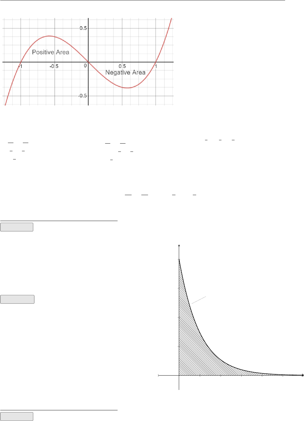
5.2. Area 83
Figure: A cubic showing how area
‘under’ the curve is evaluated. The
area for −1≤x≤0 is positive (above
the axis), and the area for 0 ≤x≤1
is negative.
R1
0(x3−x)dx
=x4
4−x2
2|1
0
= [1
4−1
2]−0
=−1
4
R0
−1(x3−x)dx
=x4
4−x2
2|0
−1
= 0 −[1
4−1
2]
= +1
4
Therefore the total area is
| − 1
4|+1
4=1
2.
We will compare with a single integral from −1 to 1.
Z1
−1
(x3−x)dx =x4
4−x2
2|1
−1=−1
4−(−1
4) = 0
Area must be non-negative, and so this result is nonsensical given the context.
Example
The energy, or electrical charge, that a ca-
pacitor can discharge is found by taking the
integral of the voltage-time function. This can
neatly be represented as the area under the
voltage-time curve. Find the total discharge
from the capacitor after 5 seconds. The units
for charge are coulombs.
Solution Integrate the V(t) function to
find the area:
area = Zb
a
V(t)dt = 8 Z5
0e−tdt
= 8 −1e−t
5
0
= 8 −e−5−(−e0)= 8.054 coulombs
V(t) = 8e−t
−1 123456
2
4
6
8
time(s)
voltage(V)
Example A logo is formed by the shaded area between the cubic function f(x) = 4x−x3and
a parabola g(x) = 2x−x2. The two curves intersects at x= 0 and x= 2. Find the shaded area.
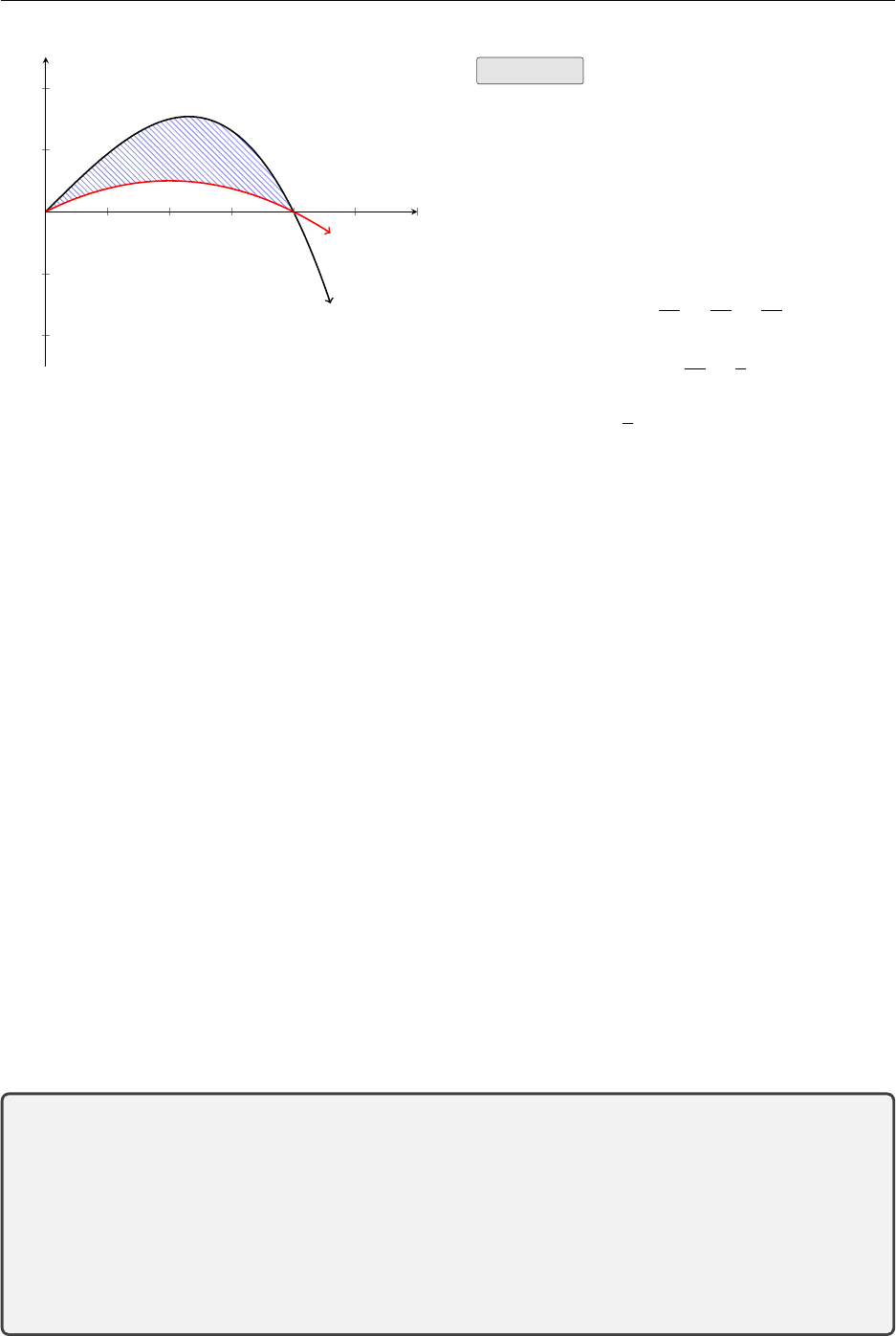
5.3. Volume 84
0.511.5 2 2.5 3
−4
−2
2
4
x
Solution
Shaded area = Zb
a
(f(x)−g(x))dx
=Z2
0(4x−x3)−(2x−x2)dx
=Z2
0(2x−x3+x2)dx
=2x2
2−x4
4+x3
3
2
0
=4−16
4+8
3−(0)
=8
3units2
Indefinite Integrals
Although Rf(x)dx looks very similar to Rb
af(x)dx they are quite different and must not be
confused or used in place of each other. Rf(x)dx is a function of xor a family of functions of x
and Rb
af(x)dx is a number. They are connected of course, provided f(x) is a continuous function
of xon [a, b]. In this case the Evaluation Theorem gives the connection between them.
Zb
a
f(x)dx =Zf(x)dxb
a
The indefinite integral represents either a particular integral or a family of integrals. These will use
a constant Cwhere Ctakes a different value for each member of the family. Cis called the constant
of integration. Our ability to find indefinite integrals depends on the number of derivatives we have
met so far and as we meet more and more different functions and learn how to differentiate them
we add to our list.
5.3 Volume
If a function is revolved around an axis it creates a volume between the axis and the function.
Similar to how if we integrate a function, it results in an area — if we integrate and area it results
in a volume.
Volume rotated around the x-axis
Volume = Zb
a
πy2dx =Zb
a
π(f(x))2dx
Volume rotated around the y-axis
Volume = Zd
c
πx2dy =Zd
c
π(f(y))2dy
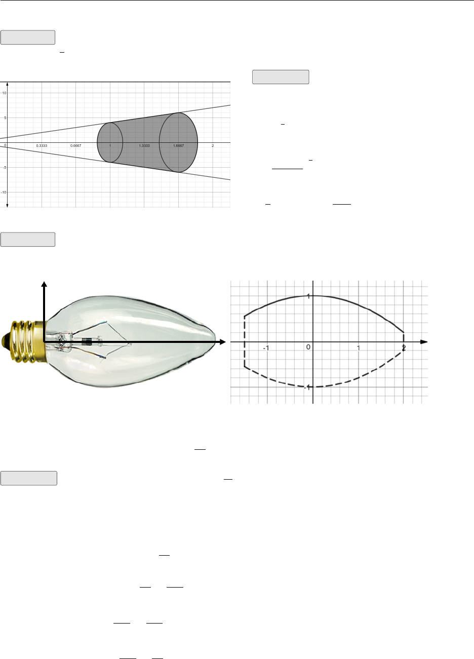
5.3. Volume 85
Example A connector was obtained by revolving the function f(x) = 3x+ 1 around the x−axis
for 1 ≤x≤5
3. Calculate the volume of the connector.
Solution
volume = Rb
aπ[f(x)]2dx
=πR5
3
1(3x+ 1)2dx
=π(3x+1)3
3·3
5
3
1
=π
963−43=152π
9≈53.058 units3
Example Fluorescent and incandescent light bulbs are often filled with the inert gas krypton.
Find the volume of krypton gas required to fill the bulb shown.
You have estimated the function to be:
f(x) = 1 −x2
5for −1.5≤x≤2 cm
Solution You will have to calculate 1−x2
52before integrating
volume = Zb
a
π[f(x)]2dx
=πZ2
−1.51−x2
52
dx
=πZ2
−1.5x4
25 −2x2
5+ 1dx
=πx5
125 −2x3
15 +x
2
−1.5
=π32
125 −16
15 + 2−(−0.06075 − −0.45 −1.5)= 2.3π≈7.23 cm3
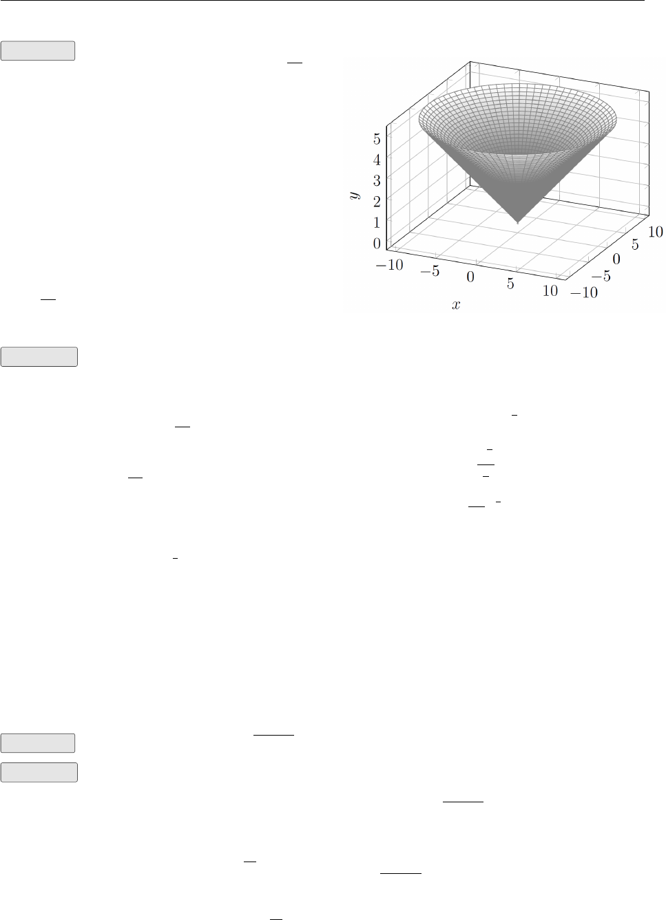
5.4. Integration by Substitution 86
Example Calculate the volume of the con-
tainer found by rotating the curve y=√x3
around the y−axis for 0 ≤y≤5.
Here the volume is created by rotation about
the y-axis, and therefore we need to adjust
our formula. First we will solve the equation
y=√x3for x, and then integrate.
Solution Volume = Rb
aπf(y)2dy
Rearrange the function to isolate x:
y=√x3
y2=x3
3
py2=x
Integrate to find volume:
V=πZ5
0
(y2
3)2dy
=πZ5
0
y4
3dy
=πy7
3
7
3
5
0
=3π
757
3−0
≈57.6 units3
5.4 Integration by Substitution
Earlier we stated that every differentiation rule leads to an integration rule. The chain rule for
differentiation leads to the substitution rule for integration, i.e. the substitution rule for integration.
A series of examples will illustrate how integration by substitution works.
Example Find the integral: R2x√1 + x2dx.
Solution This cannot be integrated using the techniques discussed so far. This is an example
of a function that can be integrated using the substitution rule. They are often recognised by
noting the presence of a composite function. In this example the √1 + x2is a composite function.
We introduce a new variable which simplifies the composite function.
Let u= 1 + x2. We then differentiatedu
dx = 2x. You have probably noticed that we have throughout
the chapter on integration written expressions like R2x√1 + x2dx where the dx has been placed
at the right of the expression we are integrating to denote we are integrating with respect to the
variable x. We now write the expression du
dx = 2xas du = 2x dx. In this course we accept that this
can be done and leave the proof to a later course.
If we now look back at the original question we are ready to substitute expressions containing u
5.4. Integration by Substitution 87
for expressions containing x.
Z2xp1 + x2dx =Zp1 + x2·2x dx
=Z√u du
=Zu1
2du
=u1
2+1
1
2+ 1 +C
=u3
2
3
2
+C
=2√u3
3+C
=2q(1 + x2)3
3+C
or = 2
31 + x23/2+C
Notice the last few steps are tidy-up steps. It is usual to begin and end with an expression in xso
at the end we back-substitute the expression we substituted with u.
The Substitution Rule can be stated formally as follows. If u=g(x) is a differentiable function
whose range is an interval Iand fis continuous on I, then Rf(g(x)) g0(x)dx =Rf(u)du.dx
and du are known as differentials. The Substitution Rule permits us to replace g0(x)dx with du.
Example Find Rxsin x2dx
Solution Using the procedure from the previous example try u=x2. This gives du = 2x dx.
Zxsin x2dx =Zsin x2·x dx
=Zsin u·1
2du
=1
2Zsin u du
=−1
2cos u+C
=−1
2cos x2+C
It is clear the challenge of the Substitution Rule is to come up with a suitable substitution. Earlier
examples often have fairly obvious substitutions but they can quickly become quite complicated
and result in many false starts.
Example Find Rx
√1−x2dx
Solution Let u= 1 −x2. Then du =−2x dx. So x dx =−1
2du. These are now substituted
into the original expression
Zx
√1−x2dx =−1
2Z1
√udu =−1
2Zu−1/2du =−1
22u1/2+C=−p1−x2+C
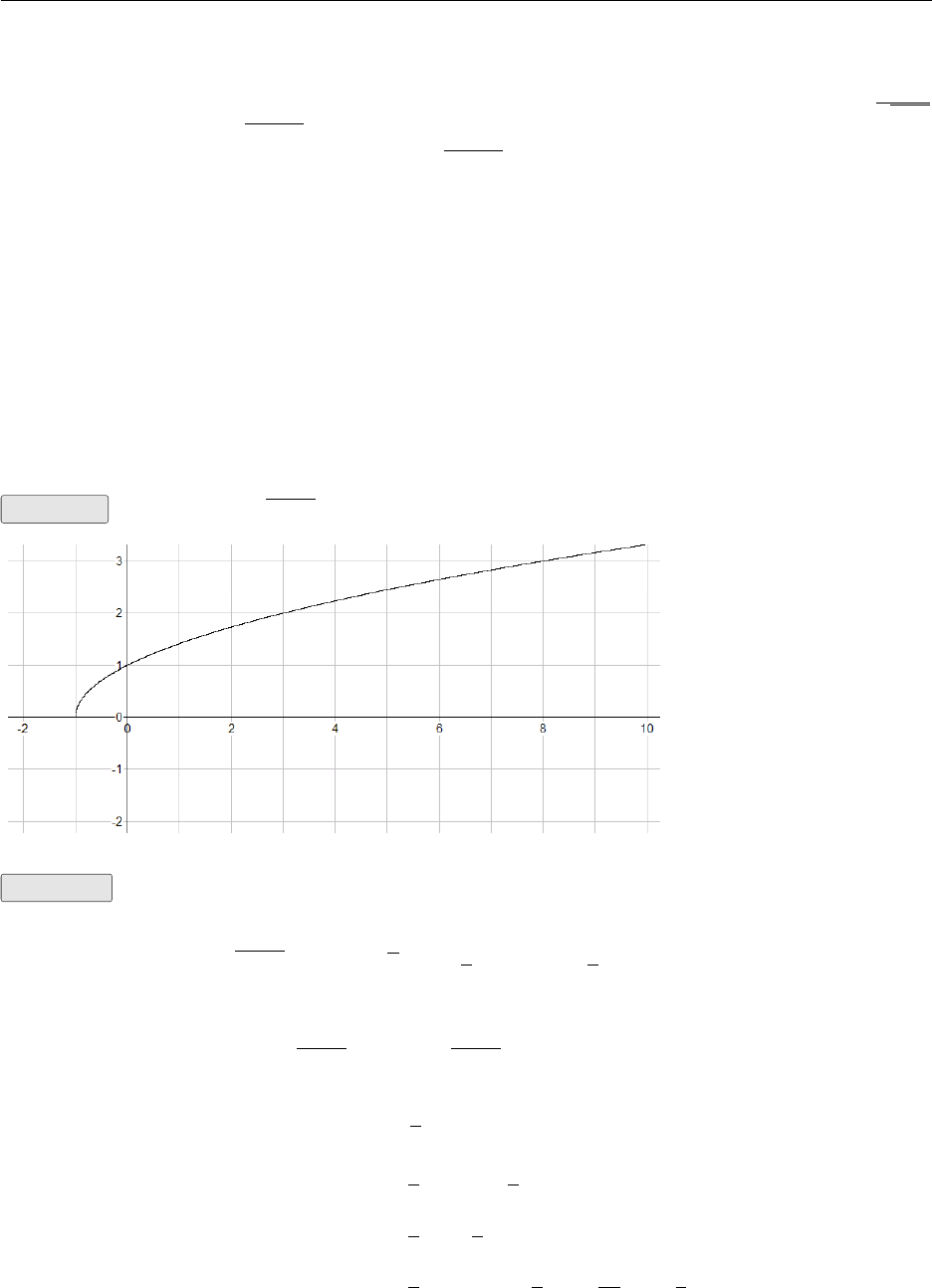
5.4. Integration by Substitution 88
In each of the above 3 examples you could use desmos to compare the original function and the
integral to see if the result is reasonable. For example 3 try graphing the original function y=x
√1−x2
and the integral y=−√1−x2on the same axes and check the original function represents the
slope of the tangent lines to the curve y=−√1−x2.
Evaluating Definite Integrals by Substitution
There are two ways to evaluate a definite integral when you have used the Substitution Rule for
the integration.
Method 1 Find the indefinite integral then use the Evaluation Theorem.
Method 2 Make the substitution to the integrand and differential (as before) and also use the
same substitution to change the limits to those for the new variable (in our questions we usually
use u).
Example Evaluate R8
0√x+ 1 dx. Graphing provides us with the following screen
Figure: The curve is clearly
continuous. If we let u=
x+ 1 then u0= 1, this is
also continuous.
Solution Method 1 Substitute u=x+ 1 then du =dx. Substituting these values in the
indefinite integral we get
Z√x+ 1 dx =Z√u du =2
3u3/2+C=2
3(x+ 1)3/2+C
So
Z8
0
√x+ 1 dx =Z√x+ 1 dx8
0
=2
3(x+ 1)3/28
0
=2
3(9)3/2−2
3(1)3/2
=2
327 −2
31
=2
3(27 −1) = 2
326 = 52
3= 171
3
Method 2 Again we let u=x+ 1 so du =dx. Also we calculate the new limits for uusing
u=x+ 1.
x= 0 gives u= 0 + 1 = 1
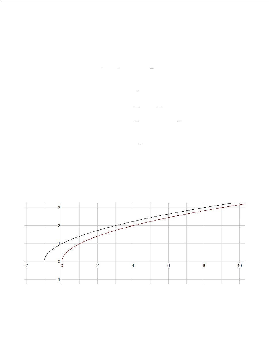
5.5. Integration by Parts 89
x= 8 gives u= 8 + 1 = 9
Now the definite integral is transformed into a definite integral in u.
Z8
0
√x+ 1 dx =Z9
1
√u du
=2
3u3/29
1
=2
393/2−2
313/2
=2
3(27 −1) = 171
3
A check on the graph will show that an area of 171
3appears to be reasonable.
Method 2 is usually preferred as the step where the indefinite integral is first calculated has been
neatly incorporated into the method. The difficulty with method 2 is that once the values for u
have been calculated the integral is completely transformed and we never return to the original
question. We answer a different question that, because of the transformation, has the same answer.
This concept might cause confusion. However a graph of the situation shows what has happened.
It is clear that the area under the first graph between 0 and 8 is the same as the area under the
second graph between 1 and 9.
5.5 Integration by Parts
Recall the rule for the differentiation of a product
d
dx (f(x)·g(x)) = f(x)·g0(x) + g(x)·f0(x)
We can antidifferentiate each side and write the process as follows
f(x)·g(x) = Zf(x)·g0(x) + g(x)·f0(x)dx

5.5. Integration by Parts 90
=Zf(x)·g0(x)dx +Zg(x)·f0(x)dx
This is rewritten in a particular way to become the formula for integration by parts.
Zf(x)·g0(x)dx =f(x)·g(x)−Zg(x)·f0(x)dx (1)
or Zf(x)·g0(x)dx =f(x)·g(x)−Zf0(x)·g(x)dx (2)
This formula is written in a number of different ways in textbooks. Here are two ways
Let u=f(x) and v=g(x) then du =f0(x)dx and dv =g0(x)dx so using the substitution rule
equation (1) becomes Zu dv =uv −Zv du (3)
Let Rf(x)·g0(x)dx be regarded as the the integral of the product of two functions then g=Rg0.
We can write equation (2) as
Zfg0=fg −Zf0g(4)
Equations (3) and (4) are the common forms that are best to remember.
The success of this method depends on the discovery that a simpler integral results from this
process. Sometimes the process results in a worse situation than you started with so should be
abandoned. Sometimes you produce a pattern which leads to a solution after 2 or more applications
of the integration by parts rule. The patterns that produce solvable problems can be discovered as
different questions are tried.
Example Find Rxcos x dx. This can be seen as the integral of a product. The two functions
are f(x) = xand g(x) = cos x. So f0(x) = 1 and Rg(x) = sin xare easy to find. Notice though
that f0(x) = 1 gives us a clue that integration by parts is going to be a fruitful method.
Solution Using equation (2)
Zxcos x dx =f(x)·g(x)−Zf0(x)·g(x)dx
=x·sin x−Z1·sin x dx
=x·sin x−Zsin x dx
=x·sin x−(−cos x) + C
=xsin x+ cos x+C
Example Use integration by parts to find Rln x dx. This is a function that has arisen in the
course as the integral of 1
x, however we are now able to use this fact to help with this question.
Solution Notice there is only one function here so we have to create two functions by stating

5.5. Integration by Parts 91
ln x= 1 ·ln x. The two functions are therefore f(x) = ln xand g(x) = 1. Can we find f0and Rg?
Yes!
Zln x dx =Zln x·1dx
= ln x·x−Z1
x·x dx
=xln x−Z1dx
=xln x−x+C
Example Find Rexcos x dx This is an example where a pattern is established and perseverance
leads to the solution.
Solution Let f(x) = cos xand g(x) = ex. Can we find f0and Rg? Yes!
Zexcos x dx = cos x·ex−Z−sin x·exdx
=excos x+Zexsin x dx
This is an integral that is very similar in appearance to the original question with the cos xtrans-
formed into sin x. We continue by repeating the integration by parts process with the new integral
Rexsin x dx
Zexcos x dx =excos x+
Rexsin x dx
z }| {
sin x·ex−Zcos x·exdx
=excos x+exsin x−Zexcos x dx
Notice the original integral has now appeared on the right hand side of the equation. We now
simply solve the equation for Rexcos x dx and add the constant of integration.
2Zexcos x dx =excos x+exsin x
Zexcos x dx =ex
2(cos x+ sin x) + C
This can easily be verified by differentiating.
Definite Integrals
Integration by parts can be combined with the Evaluation Theorem to evaluate definite integrals.
If we assume f0and g0are continuous then we can use the Evaluation Theorem and write equation
(1) as follows Zb
a
f(x)·g0(x)dx =f(x)·g(x)]b
a−Zb
a
g(x)·f0(x)dx (5)
Example Evaluate R1
0xexdx. A graph of y=xexshows the area required and gives us an idea
of the answer to expect.
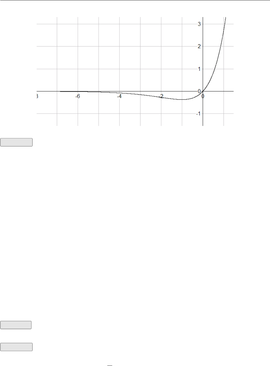
5.6. Applications of Integration 92
Solution Notice xbecomes simpler when differentiated and exis unchanged when it is inte-
grated
Z1
0
xexdx =xex]1
0−Z1
0
1·exdx
=xex]1
0−ex]1
0
=1e1−0e0−e1−e0
=e1−e1+e0
=e0= 1
5.6 Applications of Integration
Rectilinear Motion
We will use integration to analyse the motion of an object moving in a straight line. Let the
position function for the object be s=f(t) where tis the time. The velocity function is v(t) = s0(t).
Therefore the position function is the integral of the velocity function. Also the acceleration function
is a(t) = v0(t) so the velocity function is the integral of the acceleration function. We can obtain
the position function from the acceleration function by antidifferentiating twice. This process will
generate two constants of integration so we need two additional pieces of information to find the
particular solution. Usually s(0) and v(0) are given.
Example A particle moves in a straight line with an acceleration of a(t)=4t+ 2. If the initial
velocity is −4cm/s and the initial displacement is 5cm, find the position function.
Solution Because v0(t) = a(t) = 4t+ 2 we can antidifferentiate a(t) to obtain v(t)
v(t) = 4t2
2+ 2t+C1= 2t2+ 2t+C1
Substitute t= 0 because we are given the initial velocity i.e. v(0) = −4
v(0) = 2 ·02+ 2 ·0 + C1=−4
SoC1=−4and therefore
5.6. Applications of Integration 93
v(t)=2t2+ 2t−4
Because s0(t) = v(t) we can antidifferentiate v(t) to obtain s(t).
s(t)=2t3
3+ 2t2
2−4t+C2
=2
3t3+t2−4t+C2
Substitute t= 0 because we are given the initial displacement i.e. s(0) = 5
s(0) = 2
3·03+ 02−4·0 + C2= 5
SoC2= 5and therefore
s(t) = 2
3t3+t2−4t+ 5
You should know about the gravitational force near the earth that produces a downwards accelera-
tion given the symbol g. We assume gis constant and about 9.8m/s2
Example A ball is thrown vertically upwards with a speed of 24.5m/s from the edge of a cliff
that is 147m above the ground.
Find the position function.(a) Find the time when the ball reaches its
maximum height.
(b)
Find the maximum height above the ground.(c) When does the ball hit the ground?(d)
Solution (a) It is usual to choose the positive direction to be upwards this means that the
acceleration due to gravity must be −9.8m/s2.
Soa(t) = v0(t) = −9.8therefore
v(t) = −9.8t+C1
Substituting v(0) = 24.5 we get that C1= 24.5 so
v(t) = −9.8t+ 24.5
Because s0(t) = v(t) we antidifferentiate v(t)
s(t) = −9.8t2
2+ 24.5t+C2
Substitute s(0) = 147. We get C2= 147.
Sos(t) = −4.9t2+ 24.5t+ 147
This expression will hold true until the ball hits the ground provided you assume the ball continues
on its trajectory without striking the cliff.

5.6. Applications of Integration 94
(b) The maximum height is reached when v(t) = 0.
−9.8t+ 24.5=0
24.5=9.8t
t=24.5
9.8
= 2.5
So the maximum height is reached after 2.5s.
(c) The maximum height is found by substituting t= 2.5 in s(t)
s(2.5) = −4.9·2.52+ 24.5·2.5 + 147
=−30.625 + 61.25 + 147 = 177.625m
(d) The ball hits the ground when s(t)=0
So −4.9t2+ 24.5t+ 147 = 0
t2−5t−30 = 0
Use the quadratic formula t=−b±√b2−4ac
2a
t=5±√25 −4×1× −30
2
=5±√145
2
≈8.5s or −3.5s
You will be aware that the position function is a parabola so it is not surprising that the theoretical
result shows a solution about 3.5 s before the ball is thrown. The answer is that the ball hits the
ground about 8.5 s after it is thrown. You will also be aware that we did not test whether the
value of twhen v(t) = 0 gives a maximum or minimum. This is also because we are aware of the
behaviour of a parabola with a negative t2coefficient.
Work
The strategy we use to allow us to apply calculus to a problem in engineering is the same as we
used to evaluate areas. The physical quantity is divided up into a large number of small parts, each
one approximately equal to the theoretical quantity it represents. These are then summed and a
limit taken as the number of small parts, n→ ∞. This process allows us to evaluate the resulting
integral.
You will recall that from Newton’s Second Law of Motion
F=ma =md2s
dt2(1)
Where s(t) is the position function, mis the mass of an object and Fis the force required to
produce an acceleration of a. (Where a=d2s
dt2).

5.6. Applications of Integration 95
We usually measure mass in kilograms (kg), distance in metres (m) and force in Newtons (N)
(N=kg ·m/s2). If the acceleration is constant then the force to produce that acceleration will
also be constant.
Work = force ×distance or
W=F d (2)
If Fis in Newtons and dis in metres then Wis in Newton-metres. One Newton-metre is called a
Joule (J).
Example A mass of 3.5kg lifted 0.5m requires a force of F=ma = 3.5×9.8 = 34.3N. This is
the force required to counter the force exerted by gravity. Calculate the work done.
Solution The work done is calculated using equation 2
W=F d = 34.3×0.5 = 17.15J
If the force is variable this formula can no longer be applied. Let the force acting on an object
as it moves along the x-axis in a positive direction from ato bbe f(x), where fis a continuous
function of x. Divide the interval from ato binto nsubintervals of width ∆xwhere ∆x=b−a
n.
For simplicity we let the end points of these subintervals be x0,x1,x2, ..., xnWe select the ith
subinterval and select a representative x-value in this interval x∗
i. The work done when we move
the object from xi−1to xiis
Wi≈f(x∗
i)∆x
The total work done is
W=
n
X
i=1
f(x∗
i)∆x(3)
As we did with area we find the limit as n→ ∞ of this sum. As this is a Riemann sum the limit
is a definite integral
W=
n
X
i=1
f(x∗
i)∆x=Zb
a
f(x)dx (4)
Example If the force on a particle is given by the equation f(x) = 3x2−2xN, how much work
is done moving the particle from x= 2 to x= 3?
Solution The graph of f(x) = 3x2−2xshows that for the interval [2,3] the area is above the
x-axis.
W=Zb
a
f(x)dx
=Z3
23x2−2xdx
= 3x3
3−2x2
23
2
=x3−x23
2
=33−32−23−22
= 18 −4 = 14 joules
Example Hooke’s Law states that the force required to maintain a spring stretched xunits

5.7. Chapter Exercises 96
beyond its natural length is proportional to x, the spring displacement, such that f(x) = kx where
kis the spring constant. This law holds provided xdoes not get too large. A force of 20N is
required to stretch a spring from its natural length of 5cm to a length of 7cm. How much work is
required to stretch the spring from a length of 12cm to 13cm?
Solution As the force is measured in Newtons we convert all lengths to metres. Our first step
is to use Hooke’s Law to evaluate the spring constant
f(x) = kx
So20 = k·0.02
k= 1000
Sof(x) = 1000x
The work done in stretching the spring from 12cm to 13cm is
W=Z0.08
0.07
1000x dx
= 500x20.08
0.07
= 500 0.082−0.072
= 500 (0.0064 −0.0049) = 500 ×0.0015
= 0.75J
5.7 Chapter Exercises
§5.1 Standard Integrals
1. Find the general integral in each case.
4x7
(a) 10(b) 8x3
3
(c)
3.2ex
(d) 1
2x
(e) √x(f)
x1.2
(g) xπ
(h) 4
3
√x4
(i)
x−2
3
(j) (2x+ 1)2
(k) ex+xe
(l)
2. Find the indefinite integrals.
Rx−1
x2dx(a) Rx√x dx(b) R(sin x−2 cos x)dx(c)
R(1 −x) (2 −x)dx(d) Rsin2x+ cos2xdx(e) R2
x+3
√xdx(f)
Rcos x
2dx(g) R1
2sec2x dx(h) Rx+1+ 1
xdx(i)
Rπr2−x2dx(j) R1
2xdx(k) R2πr dr(l)

5.7. Chapter Exercises 97
§5.2 Area
1. Evaluate the integrals.
R2
−1x5dx(a) R3
11+2x−4x3dx(b) R1
0x2/3dx(c)
R3
1exdx(d) R3
1
1
xdx(e)
2. Find the area under the curve.
y=x3between x=−1 and x= 3(a)
y= (x+ 1) (x−1) between x=−2 and x= 3(b)
3. Find the integral and evaluate according to the limits.
R2
0(x−1) (x+ 5) dx(a) R2
1
x3−6
x2dx(b) R3
2
dx
3x
(c)
R1
03exdx(d) R2
−2x4dx(e) R1
−1x3dx(f)
§5.3 Volume
1. Determine the volumes of the solids of revolution which are generated by rotating the following
areas for one complete revolution about the x-axis.
y= 2x+ 1 between x= 0 and x= 3(a) y= 6x2+ 1 between x= 1 and x= 4(b)
y=−3xbetween x=−2 and x= 0(c) 5√xfor 1 ≤x≤2(d)
2. Determine the volume found when the function is rotated one revolution around the y-axis.
y=x−1 between y=−1 and y= 3(a) y=x2−3 between y=−3 and y= 0(b)
y=√xfor 0 ≤y≤2(c) y=√x+ 4 from y= 0 to y= 4(d)
3. The volume for a cylinder with radius rand height his given by V=πr2hUse integration to
show that this formula is correct. Hint: Which curve y=f(x) is rotated around the x-axis to
form a cylindrical solid of rotation?
§5.4 Integration by Substitution
1. Use the given substitution to find the integral.
Re4xdx,u= 4x(a) Rtan x dx,u= cos x(b)
Resin θcos θ dθ,u= sin θ(c) R(4x−3)15 dx,u= 4x−3(d)
Rxex2dx,u=x2
(e) Rx
x2+1 dx,u=x2+ 1(f)
R2xx2+ 23dx u =x2+ 2(g) Rsin2xcos x dx, u = sin x(h)
Rx
√1+xdx, u = 1 + x(i) Rdx
√x+x, u =√x(j)

5.7. Chapter Exercises 98
2. Integrate the following. The substitution has not been given.
R√2x+ 1 dx(a) Rdx
√x+1
(b) Rex
ex+1 dx(c)
Rln x
xdx(d) Rcos x
sin x+1 dx(e) Rcos x
2dx(f)
Rcos 2x dx(g) Rex+e−x
2dx(h) R2
0(x−1)11 dx(i)
3. Use an appropriate substitution and then evaluate the integral.
R2
0x√2x2+ 1 dx(a) Rπ
4
0sin x+π
2dx(b)
R1
0(3 −2x)4dx(c) R−1
−2
dx
(2x+1)2
(d)
R9
4
dx
2x+1
(e) Rπ
4
0tan x dx(f)
§5.5 Integration by Parts
1. Find the integral using integration by parts.
Rxln x dx(a) Rxsin x dx(b)
Rxcos 3x dx(c) Rexsin x dx(d)
Rln (2x)dx(e)
2. By writing sin2xas sin x·sin xand using integration by parts show that
Zsin2x dx =1
2(x−sin x·cos x) + C
3. Integrate.
Rxe2xdx(a) Rxe−xdx(b)
Rx2sin x dx(c) R(x−1) exdx(d)
Rln x
xdx(e)
4. Integrate and evaluate.
R5
0xe−xdx(a) R1
0x2exdx(b) Rπ
0exsin x dx(c)
R3
1xln x dx(d) Rπ
0sin2x dx(e) Rπ
2
0xsin x dx(f)
R1
0xe2xdx(g) R7
5xcos x dx(h) R2
1(x−1) exdx(i)
R4
2
ln x
xdx(j) R3
0x2sin x dx(k)
§5.6 Applications
1. A particle is moving in a straight line with an acceleration given by a(t) = 6t+ 4.Its initial
velocity is v(0) = −6cm/s and its initial displacement is s(0) = 9cm. Find the position function
s(t).
5.7. Chapter Exercises 99
2. A ball is thrown upwards with an initial velocity of 15m/s from the edge of a cliff 140m above
the ground. Find its height above the ground tseconds later. When does it reach its maximum
height? When does it hit the ground?
Hits the ground after t≈7.1s
3. A particle is moving along a straight line with an acceleration of a(t) = 3 + 4t−12t2. Its initial
velocity, v(0) is 4m/s and its initial displacement, s(0) is 5m. Find the position function, s(t).
4. A stone is dropped off a cliff and hits the ground with a speed of 40m/s. What is the height of
the cliff?
5. A car is travelling at 50km/h when the brakes are firmly applied producing a constant deceler-
ation of 5 m/s2. How far will the car travel before coming to rest?
6. A car is travelling at 100km/h when the driver sees a railway crossing 80m ahead and slams on
the brakes. What constant deceleration is required so that the car will stop in 80m?
7. Two balls are thrown upwards from the edge of the cliff in exercise 2 above. The first is thrown
with a speed of 15m/s and the second is thrown one second later with a speed of 8m/s. Do the
balls ever pass each other?
8. A particle moves along a straight line with a velocity function v(t) = sin t−cos tand its initial
displacement is s(0) = 0m. Find its position function.
9. A car braked with a constant deceleration 5m/s2, producing skid marks measuring 60m before
coming to rest. How fast was the car travelling when the brakes were first applied?
10. A particle is moved along the x-axis by a force given by the equation f(x)=6/(1 + x)2N at a
point xmetres from the origin. Find the work done in moving the particle from the origin to
a distance of 5 metres.
11. When a particle is located a distance of xmetres from the origin a force of cos (πx/3) Newtons
acts on it. How much work is done in moving the particle from x= 1 to x= 2? Interpret your
answer by considering the work done from x= 1 to x= 1.5 and from x= 1.5 to x= 2. By
drawing the graph of y= cos (πx/3) the reason should become apparent.
12. The graph shows a force function . (Force in
Newtons against distance in metres.) The
force increases at a constant rate until it
reaches its maximum value then remains
constant. How much work is done by the
force in moving an object a distance of 7m?
13. A spring has a natural length of 20cm. If a 25N force is required to keep it stretched to a length
of 30 cm how much work is done stretching it from a length of 20cm to 25cm?
14. Suppose that 2J of work is needed to stretch a spring from its natural length of 20cm to a
length of 30cm. How much work is needed to stretch it from a length of 22cm to 28cm?

5.7. Chapter Exercises 100
15. If 6J of work is needed to stretch a spring from 10cm to 12cm and 10J is needed to stretch it
from 12cm to 14cm, what is the natural length of the spring?
6|Differential Equations
In the last chapter we said that any equation involving derivatives of a function is called a differential
equation. In this chapter we explore this idea further and look at some mathematical models that
take the form of differential equations. Change is a concept that we are familiar with. When we
are imagining what something we are familiar with today will be like in the future we can be pretty
certain that it will be different. Differential equations can arise when we formulate mathematical
models. We can develop our understanding of this process by considering the mathematical models
of some physical phenomena.
6.1 Basic Differential Equations
One model of population growth arises from the assumption that the rate at which the population
grows is proportional to the size of the population. Let Nbe the size of the population at time t
then the rate of change of population with respect to time is dN
dt . So the model can be expressed
as a differential equation dN
dt =kN
where kis the constant of proportionality.
To make any sense of this model we need to explore the range of values of Nand k.Ncannot be
zero (otherwise there would be nothing to change). We assume that Nis a function of tand that
N(t)>0. Similarly for us to have population “growth” k > 0
∴dN(t)
dt >0
We have already shown the properties of the exponential function. The general exponential function
is
N(t) = N0ekt
Let N(t) be N0when t= 0. i.e. N(0) = N0.N0is called the initial value of N(t).
Now
dN(t)
dt =N0ekt ×k
=kN(t)
Thus we have shown that N(t) = N0ekt is a solution of the differential equation dN(t)
dt =kN(t)
This solution arises because we are familiar with the behaviour of the exponential function. Our
ability to “guess” the answer is limited so the subject of differential equations involves developing
techniques to handle physical situations that are more and more realistic and more and more
complex. The answer to this problem came so simply to us we have to wonder if there are other
equations for N(t) that give the same answer.
6.1. Basic Differential Equations 102
The Order of a Differential Equation
The differential equation dN (t)
dt =kN(t) is referred to as a first order differential equation because
the order of the highest derivative is one.
Here is an example of a second order differential equation
md2x
dt2=−kx
d2x
dt2is a second derivative. This is the differential equation that arises from Hooke’s Law. This
subject will be developed further in later courses.
The Solution of a Differential Equation
When you are asked to “solve” a differential equation you are expected to find all possible solutions
of the differential equation. In chapter 4 we met a range of simple differential equations and showed
how to express all possible solutions.
Example Find all possible solutions of the differential equation dy
dx = 2x. This differential equa-
tion could also be expressed as y0= 2x.
Solution By antidifferentiating we obtain
y=x2+C
Where Cis the constant of integration. This is an arbitrary constant and gives us a family of
functions all of which are solutions of the differential equation y0= 2x. This family of solutions is
often referred to as the general solution.
In a physical situation we are often provided with additional information and this will allow us to
find a particular solution. This is easy to visualise when considering y0= 2x. The general solution is
y=x2+Cand if you are also told that the curve passes through (2,6) you can use this information
to evaluate C.
6=22+C
C= 2
So the particular solution is y=x2+ 2. To appreciate the concept of this particular solution you
only need to use desmos to draw y=x2+Cfor various values of C.
Initial-Value Problems
In a physical problem when you are given the conditions for the particular solution in the form
y(t0) = y0where t0is the initial value of tand y0is the initial value of y(t), the point (t0, y0) is
called an initial condition and the problem of finding the particular solution given the differential
equation is referred to as an initial-value problem.
Example For the differential equation y0=−y2
(a) Verify that y=1
t+Cis the general solution
6.2. Separable Equations 103
(b) Find the solution of the initial-value problem y0=−y2and y(0) = 0.5
Solution
(a) Given y=1
t+C= (t+C)−1
y0=−(t+C)−2
=−1
(t+C)2
=−1
t+C2
=−y2
So y=1
t+Cis the general solution of y0=−y2
(b) Substitute (0,0.5) in y=1
t+C
0.5 = 1
0 + C
1
2=1
C
C= 2
The particular solution is y=1
t+2
6.2 Separable Equations
In some special cases we can find explicit solutions of differential equations. One type of equation
can be written in the form dy
dx =f(x)
g(y)
Expressed in this form we simply have to recognise that f(x) is a function without any y’s in it
and g(y) is a function without any x’s in it.
To solve dy
dx =f(x)
g(y)we rewrite the equation as
g(y)dy =f(x)dx
Then we integrate both sides Zg(y)dy =Zf(x)dx
This procedure can be verified by differentiating both sides with respect to x
d
dx Zg(y)dy =d
dx Zf(x)dx
By the chain rule the left hand side becomes
d
dy Zg(y)dy ×dy
dx
So
d
dy Zg(y)dy ×dy
dx =d
dx Zf(x)dx
6.2. Separable Equations 104
g(y)×dy
dx =f(x)
or dy
dx =f(x)
g(y)
Example Solve dy
dx =x2
y2
Solution
y2dy =x2dx
Zy2dy =Zx2dx
y3
3=x3
3+C
y3=x3+ 3C
=x3+C1
Where C1is a new arbitrary constant
y=3
px3+C1
Find C1given y(0) = 2
2 = 3
p03+C1
C1= 8
y=3
px3+ 8
Example Solve y0= 3x2y
Solution First write y0=dy
dx dy
dx = 3x2y
Separate the variables 1
ydy = 3x2dx
Integrate
Z1
ydy =Z3x2dx
ln |y|=x3+C(1)
We usually write this by writing in exponential form
|y|=ex3+C
=ex3eC
y=±eCex3
And write A=±eCwhere the value of Ais used that satisfies the particular problem
y=Aex3(2)
In practice we usually jump from line (1) to line (2) and leave out the intermediate steps.

6.3. Chapter Exercises 105
6.3 Chapter Exercises
§6.1 Differential Equations
1. Solve the following differential equations and use the given conditions to find the particular
solution.
dy
dt =et+ 2t y(0) = 2(a) dy
dx = sin 2x+ cos 2x y(0) = 0(b)
tdy
dt = 1 −t2y(0) = 2(c) x2dP
dx = 2 + x P (1) = 2(d)
2. Show that y=x+1
xis a solution of the differential equation xy0+y= 2x
3. Verify that y= sin xcos x−cos xis a solution of the initial-value problem
y0+ (tan x)y= cos2x y(0) = −1
on the interval −π
2<x<π
2.
4. Which of the following functions are solutions of the differential equation y00 +y= sin x
(a) y= sin x(b) y= cos x(c) y=1
2xsin x(d) y=−1
2xcos x
5. A mass falling to earth with a constant acceleration of 9.8m/s2satisfies the differential equation
dv
dt = 9.8
where vis the velocity at time t. Find an expression for vif
The mass is dropped from a stationary position.(a)
The mass is fired towards earth with an initial velocity of 100m/s.(b)
6. The angular velocity ωof a flywheel under constant braking torque of Nis given by the
differential equation
Idω
dt +N= 0.
where Iis the moment of inertia (Iis a constant)
Find ωin terms of tgiven that ω=ω0when t= 0.(a)
Calculate the time taken to bring the flywheel to rest from an initial speed of 60πrad/s
given that the moment of inertia is 100kg m2under a braking torque of 40N m.
(b)
§6.2 Separable Equations
1. Solve the following differential equations
ydy
dx =xgiven y= 4 when x= 0(a)
1
t
dv
dt = 2 given v= 2 when t= 1(b)
exdy
dx + 2 = 0 given y= 5 when x= 0(c)

6.3. Chapter Exercises 106
(x+ 2) dy
dx =y+ 3 given y= 0 when x= 0(d)
di
dt +i= 1 given i= 10 when t= 0(e)
dy
dx −2x= 0 y(0) = 2(f)
2. The rate at which the atoms of a radioactive substance split up is given by dN
dt =−λN, where
Nis the number of atoms present after tseconds and λis a constant.
Show that N=N0e−λt where N0is the number of atoms present initially (i.e. when
t= 0).
(a)
Find the time in years for half of the atoms of a given mass of radium to disintegrate if
λ= 1.37 ×10⁻¹¹ for radium.
(b)
3. A body falling in a medium where the resistance is proportional to the velocity vat time t
obeys the differential equation dv
dt = 10 −0.2v
If the body falls from rest find vin terms of tand show that as t→ ∞ the velocity
approaches 50m/s.
(a)
How long would it take for the body to reach a velocity of 25m/s?(b)
4. On a hot summer’s day a bottle of beer is placed in a fridge set at 4◦C. The rate of change of the
bottle’s temperature θ◦C after tminutes is given by Newton’s Law of Cooling, dθ
dt =−k(θ−4)
where kis a constant that is specific to the beer.
Find θin terms of t. If the initial temperature (t= 0) of the bottle of beer was 22◦C and
it took 10min to cool to 20◦C, find the value of k, and the particular solution.
(a)
How long would it take the bottle to reach the ideal drinking temperature of 8◦C?(b)
5. Brine containing 2 grams of salt per litre flows into a tank initially filled with 50 litres of water
containing 10 grams of salt. The brine enters the tank at 5 litres/min, the concentration is kept
constant by stirring and the mixture flows out through a tap at the same rate so that the tank
at all times continues to contain 50 L of mixture. Let there be Qgrams of salt in the tank after
tminutes.
Show that dQ
dt = 10 −Q
10
(a)
Solve this differential equation to obtain an expression for Qin terms of t.(b)
How much salt is in the tank after 10 minutes?(c)
Sketch the graph of Qagainst t.(d)
What happens to Qas t→ ∞?(e)
6. A rectangular tank is divided into two equal compartments by a vertical porous membrane.
Liquid in one compartment, initially at a depth of 40cm, passes into the other compartment
which is initially empty, at a rate proportional to the difference in levels
If the depth of the liquid in the second compartment is xcm after tminutes show that
dx
dt =k(40 −2x) .
(a)
Show that the solution of this differential equation is x= 20 1−e−2kt.(b)

6.3. Chapter Exercises 107
If the level in the second compartment rises 2cm in the first 5 minutes, after how much
time will the difference in levels be 2cm?
(c)
Interpret what is happening.(d)
7. Under certain conditions the relative density ρof a gas and its temperature T◦C satisfies the
differential equation dρ
dT =−n2ρ2(where nis a constant). Express ρin terms of Tgiven that
ρ= 0.002 when T= 30◦C and ρ= 0.0016 when T= 45◦C.
7|Answers
Answers to selected exercises.
CHAPTER 1
§1.1, p.11, Introductory Algebra
1. −x−y(a)
−15x+ 6y(b)
x2+ 3x+ 2(c)
4x2−1(d)
2. 1(a)
0.01(b)
36.462(c)
2
7
(d)
3. 9a4b2
(a)
x6
27
(b)
a3
2b
(c)
x3
12
(d)
4. 1.28(a)
1.516(b)
5. 7(y2−2z2)(a)
x[(y−2) + x](b)
(a+c)(−3a−3c)(c)
2πr(h+r)(d)
6. (x+ 7) (x+ 4)(a)
(2x+ 3) (x−4)(b)
(b−5)(b−4)(c)
(3x−1)(x−2)(d)
7. 3.16(a)
−1.87 or 5.87(b)
4 or −2(c)
0.637 or −3.137(d)
x= 2.547(e)
x={−2.055,0,1.055}(f)
§1.2, p.12, Functions
1. t=v−u
a
(a)
t=1
αl
l0−1
(b)
2. 4(a)
4(b)
27(c)
64(d)
3. 79.4m3
4. y= 4x−4(a)
2y=x
3+ 1(b)
y=x2−3(c)
y=−(x+ 1)2
(d)
5. x−intercepts 1.73 and −1.73 and y−intercept −3
6. Show the points A(3,5) and B(−2,−5) on
the graph.
(a)
2(b)
y= 2x−1(c)
y= 2x+ 7(d)
draw a line with a slope of 4
5
(e)
7. Table of Values
x g(x) = x3−x
−1.5−1.875
−1 0
−0.5 0.375
0 0
0.5−0.375
1 0
1.5 1.875
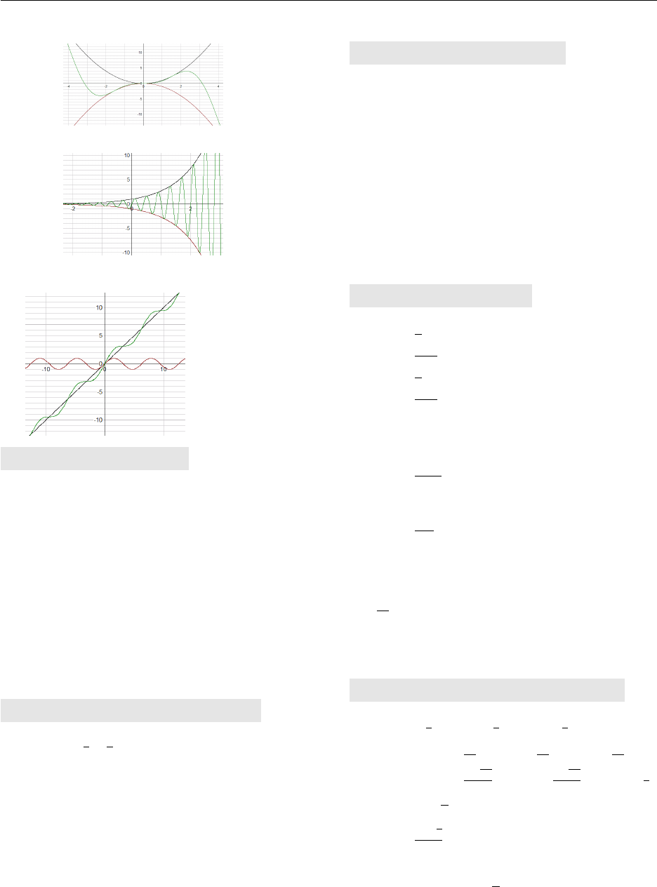
109
8.
(a)
(b)
9.
§1.3, p.13, Polynomials
1. 2(a)
3(b)
99(c)
4(d)
2. No, there is no variable term(a)
No, a variable in the exponent is an
exponential equation
(b)
Yes(c)
No, the powers must be integers(d)
§1.4, p.13, Systems of Equations
1. (−1
3,51
3)(a)
(0.571,−0.571)(b)
infinite solutions(c)
(1.23,3.87) ,(−0.35,−4.21)(d)
2. (3,1)(a)
no solution; parallel lines(b)
(18.29,−10.29)(c)
(−25,5), and (−25,−5)(d)
3. (1,2)(a)
(−3,4) and (3,4)(b)
(−2,−1) , (−2,1) , (2,−1) , (2,1)(c)
(−1.5,0)(d)
§1.5, p.14, Word Problems
1. 12cm by 15cm
2. The number of children admitted was 1500
and the number of adults was 700.
3. Run 5mi/h, cycle 20mi/h
4. 2.5 pounds of Kenyan coffee and 0.5 pounds
of Sri Lankan coffee should be mixed.
CHAPTER 2
§2.1, p.31, Unit Circle
1. π
5≈0.628rad(a)
−8π
3≈ −8.378rad(b)
π
3≈1.047rad(c)
−3π
4≈ −2.356rad(d)
2. 135°(a)
150°(b)
−270
π≈ −85.9°(c)
−15°(d)
3. 55π
9≈19.2(a)
4(b)
4. 4mi
5. 36
π≈11.459m
6. 330π≈1037mi
7. 1.6 million mi
§2.2, p.32, Right Angled Triangles
1. sin θ=4
5,cos θ=3
5,tan θ=4
3
2. sin θ=40
41 ,cos θ=9
41 ,tan θ=40
9
(a)
sin θ=2√13
13 ,cos θ=3√13
13 ,tan θ=2
3
(b)
3. 12√2(a)
13√3
2
(b)
16.51658(c)
4. 45◦,16,16√2≈22.63(a)
38◦,44.79,56.85(b)
5. 1026ft
6. 2100mi(a)
No(b)
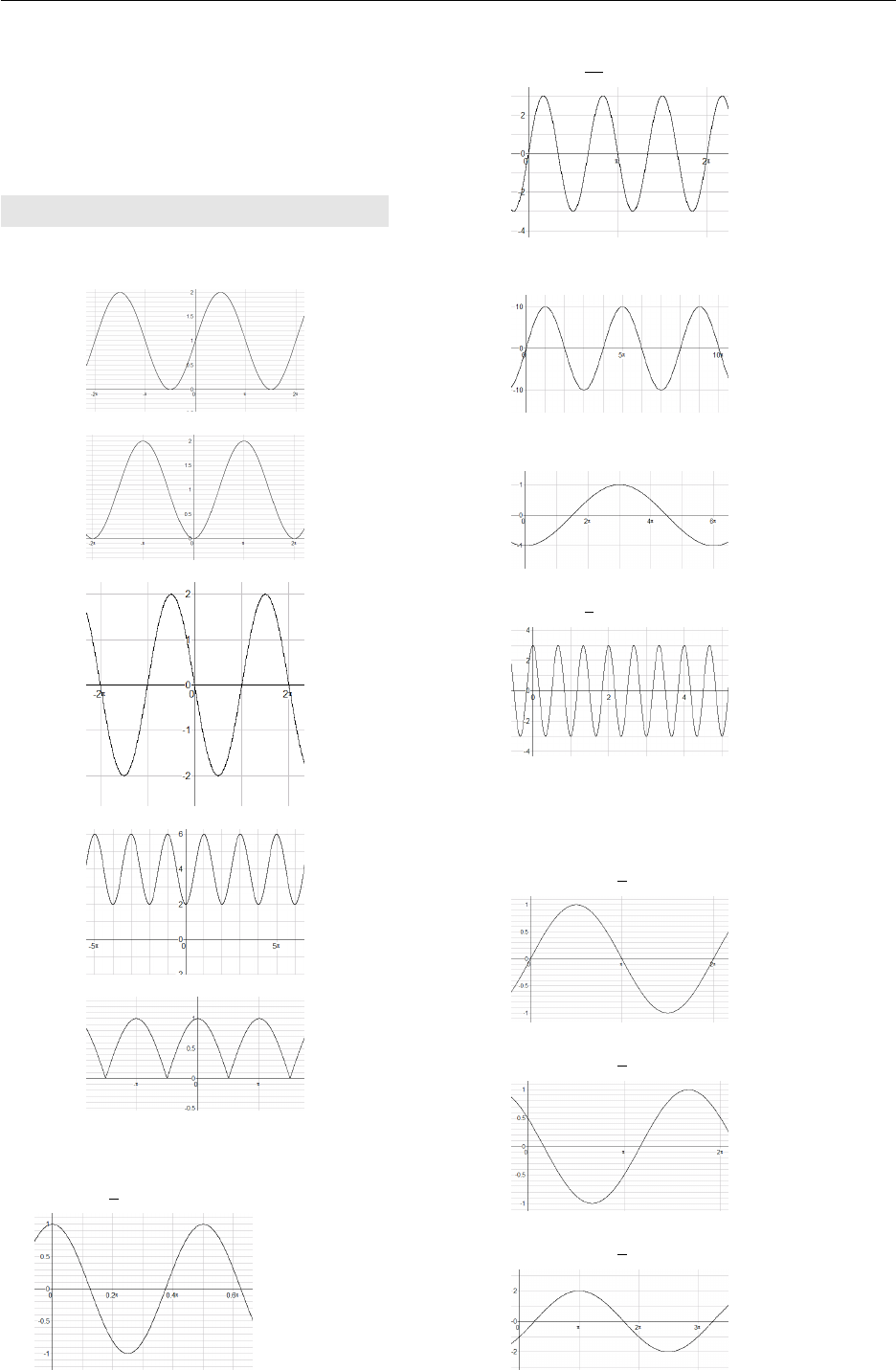
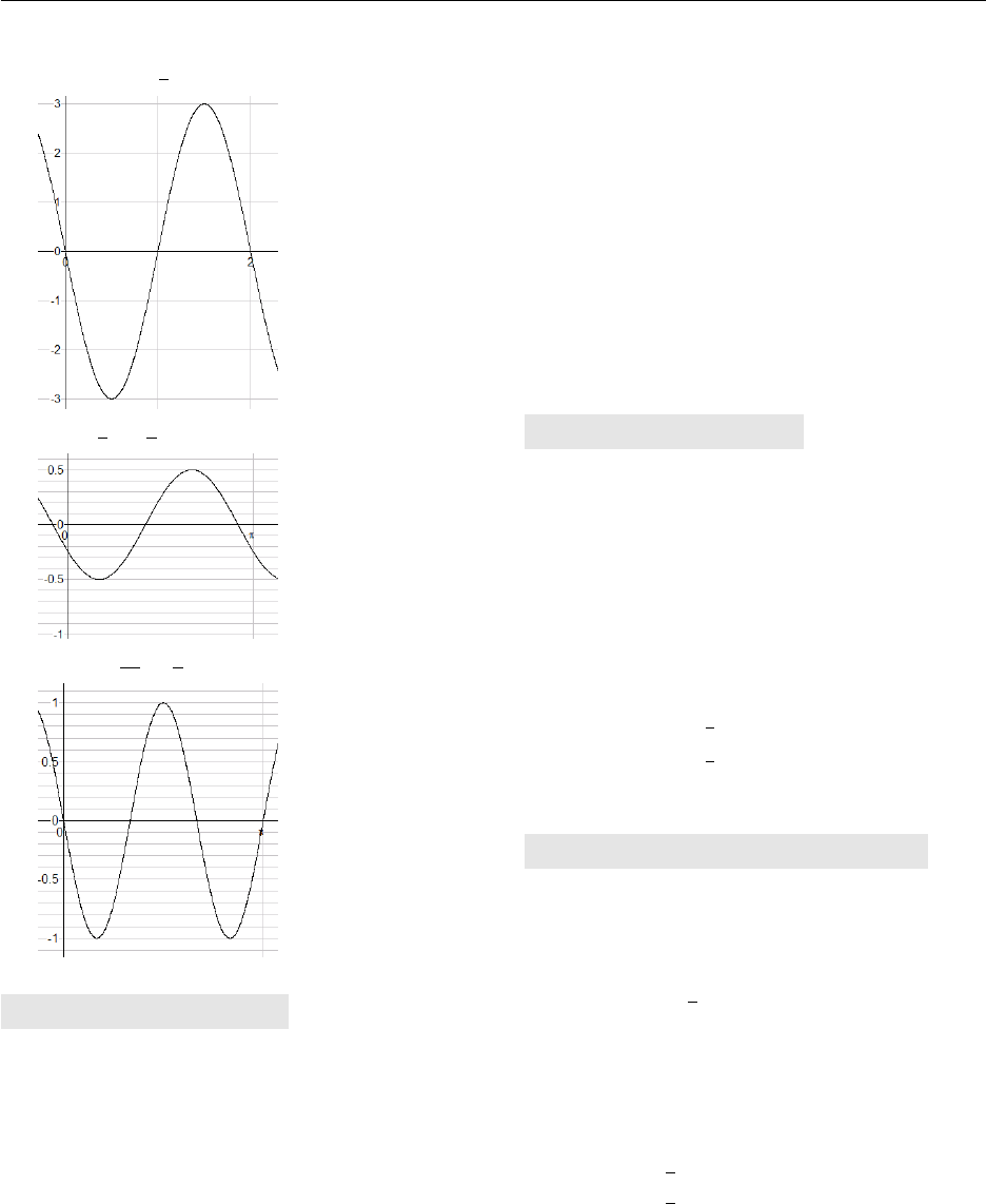
111
3,2,−1
2
(d)
1
2, π, π
6
(e)
1,2π
3,−π
3
(f)
§2.4, p.34, Applications
1. 318.8(a)
44°(b)
2. ∠C= 114◦, a ≈51, b ≈24
3. ∠C= 62◦, a ≈200b≈242(a)
∠A= 100◦, a ≈89, c ≈71(b)
4. 219ft
5. 1018mi,(a)
1017mi(b)
6. 155m
7. 28.9(a)
28.89°(b)
8. 2(a)
84.6°(b)
9. 23.1mi
10. 2179mi
11. 3835ft
12. 3.85cm2
13. 14.3m
CHAPTER 3
§3.1, p.49,exfunctions
1. 54.59815(a)
0.99317(b)
22.19795(c)
15.15426(d)
2. Use desmos to verify
3. f(x) = 3x
(a)
f(x) = 5x
(b)
f(x) = 1
4x
(c)
f(x) = 1
2x
(d)
4. Use desmos to verify
§3.2, p.51, Logarithmic Functions
1. 52= 25(a)
50= 1(b)
81/3= 2(c)
2−3=1
8
(d)
ex= 5(e)
e5=y(f)
2. log5125 = 3(a)
log10 0.0001 = −4(b)
log81
8=−1(c)
log21
8=−3(d)
ln 2 = x(e)
ln y= 3(f )
3. 1(a)
0(b)
2(c)
2(d)
2(e)
10(f)
−3(g)

112
1
2
(h)
−1(i)
37(j)
8(k) √5(l)
−2
3
(m)
4(n)
−1(o)
4. 32(a)
4(b)
5(c)
100(d)
2(e)
4(f)
5. 1 + log2x(a)
log2x+ log2(x−1)(b)
10 log 6(c)
log2A+ 2 log2B(d)
log3x+1
2log3y(e)
1
3log5x2+ 1
(f)
1
2(ln a+ ln b)(g)
ln x+1
2(ln y−ln z)(h)
1
4log x2+y2
(i)
6. 3
2
(a)
1(b)
3(c)
ln 8(d)
16(e)
4 + log 3(f)
7. log3160(a)
log2AB/C2
(b)
ln h5x2x2+ 53i
(c)
§3.3, p.52, Logarithmic Equations
1. 2.7726(a)
0.3495(b)
1.2040(c)
0.0767(d)
1.9349(e)
−43.0677(f)
6.2126(g)
−2.9469(h)
14.0055(i)
2.
±1(a)
0,4
3
(b)
1
2ln 3 ≈0.5493(c)
e10 ≈22026(d)
95
3
(e)
3−e2≈ −4.3891(f )
5(g)
13
12
(h)
§3.4, p.52, Modelling
1. 13kg(a)
6.6kg(b)
2. 0ft
s
(a)
50.6ft
s, 69.2ft
s
(b)
Use desmos to plot the graph(c)
80 ft
s
(d)
3. 200(a)
Use desmos to plot the graph(b)
11,200(c)
4. 13 days
5. 7337(a)
1.73 years(b)
CHAPTER 4
§4.1, p.69, Differentiation from First Principles
1. 23(a)
-12(b)
4(c)
2. Use Desmos to plot the graph
and compare to yours
3. Use Desmos to check
4. Use Desmos to check
5. Use Desmos to check
6. f0(x) = −2x−3=−2
x3
(a)
f0(x) = 2
3x−1
3=2
33
√x
(b)
y0= 5x4
(c)
y0=−3x−4
(d)
y0=−4x−5
(e)
y0=3
4x−1
4
(f)
y0=−1
2x−3
2
(g)

113
§4.2, p.71, Standard Derivatives
1. 2x4
(a)
0(b)
−12x3
(c)
−8x−5=−8
x5
(d)
−x−4=−1
x4
(e)
2. 1
2t−1
2=1
2√t
(a)
3
2t1
2=3√t
2
(b)
5
3z2
3=53
√z2
3
(c)
6.4x2.2
(d)
3. f0(x)=6x2−6x+ 4(a)
f0(x) = 2x+ 1 −1
x2
(b)
8x7+ 60x4−16x3+ 30x2−6(c)
4. ds
dt = 8t−7(a)
d(3x)
dx = 3(b)
d(3u4)
du = 12u3
(c)
Df (x) = 2(d)
f0(x) = ex−1(e)
f0(x) = 81x2
(f)
g0(x) = 15x14
(g)
f0(x) = ex−exe−1
(h)
5. f0(x) = −3x−4+3
4x−13
4=−3
x4+3
44
√x7
(a)
f0(x) = 1
4x−3
4+1
12 x−11
12 =1
44
√x3+1
12 12
√x11
(b)
g0(x)=2ex + 2ex+e2+e2xe2−1
(c)
f0(x) = 1
3x−2
3=1
33
√x2
(d)
6. Check with Desmos(a)
Check with Desmos(b)
Check with Desmos(c)
7. x2cos x+ 2xsin x(a) √xcos x+1
2√xsin x(b)
5 sec25x(c)
cos x+xsin x
cos2x
(d)
−ωsin (ωt +δ)(e)
8. y−x−1=0
9. dx
dθ = 5m/rad
10. 4 cos 4x(a)
2 cos πx(b)
−15 sin 3x(c)
3 sec23x(d)
3 sec2(x+ 2)(e)
3 sin2xcos x(f)
6 sin 3xcos 3x(g)
6 (x−1) sin2(x−1)2cos (x−1)2
(h)
4 tan 2xsec22x(i)
§4.3, p.72, Maximums, Minimums, and Tangents
1. y= 7x−3 is a linear function and so has
no maximum or minimum value. Its deriva-
tive is constant.
2. (2,0) and (−2,0)(a)
(2,12)(b)
(0,1) and (1,0) and (2,1)(c)
3. (3,4) is a local maximum(a)
(−1,0.667) is a local maximum and
(1,−0.667) is a local minimum
(b)
(−3.67,−14.82) min and (1,36) max(c)
4. There is a local minimum at (−1,−0.368)
If you know how to use the product rule
for differentiation you can find out
without using desmos.
5. Tangent line is 2y−3x+ 1 = 0
Normal line is 3y+ 2x−5 = 0
6. (0,4) ,√3,−5,−√3,−5
7. (ln 2,2) ≈(0.69,2)
8. a=−1
3or −1
9. x=±q2
3
10. See Desmos
11. See Desmos
§4.4, p.73, Product, Quotient, & Chain Rules
1. f0(x) = xex+ex=ex(x+ 1)(a)
g0(x) = x2ex+ 2xex=xex(x+ 2)(b)
2. x3ex0=x3ex+ 3x2ex=x2ex(x+ 3)(a)
x−3ex0=x−3ex−3x−4ex
=ex
x4(x−3)
(b)
((x+ 1) ex)0=ex(x+ 2)(c)
((x+ 2) (x−2) ex)0=exx2+ 2x−4
(d)

114
3. y0=−5
(2x−1)2
(a)
y0=xex
(x+1)2
(b)
df
dt =2−2t2
(1+t2)2
(c)
f0(x) = −ACex
(B+Cex)2
(d)
4. −3x(x−2)
(x−1)2
(a)
2
(x+1)2
(b)
2−x
2√x(x+2)2
(c)
1 + x−2x2e−x
(d)
5. Tangent y=xNormal y=−x
6. 2y+x−2=0(a)
(b)
7. Horizontal line y=1
2
(a)
(b)
8. (f◦g) (x) = √x3
(g◦f) (x)=(√x)3
9. (h◦j) (x) = ex2
2=ex2/2
(j◦h) (x) = e2x
2
10. F0(x) = x
√1+x2
(a)
dy
dx =−10x1 + x24
(b)
ex20= 2xex2
(c)
eex0=eex·ex=eex+x
(d)
11. 9 (3x+ 2)2
(a)
3
(5x+3)2/5
(b)
−2
(2x+1)2
(c)
9
(4−x)4
(d)
1
√2x−5
(e)
−2
33
√(5−x2)2
(f)
−1
2√(x+2)3
(g)
6x2e2x3
(h)
12. 2xe−2x(1 −x)(a)
−e−x(1 −2x) (5 −2x)(b)
1−p
(p2+1)√p2+1
(c)
x2+ 35x2−16x+ 3
(d)
(x−3)2(2x−1)(e)
(x−1)(5x+3)
2√x+1
(f)
ex2(2x+1)2
2√x+1
(g)
x−3
(x+1)3
(h)
§4.5, p.74, Parametric Differentiation
1. Check with desmos
2. dy
dx =1
t
(a)
Lett = 1(b)
y−x= 0(c)
3. y+x=√2, horizontal when t=π
2or 3π
2,
Vertical when t= 0 or π
4. 2y+ 4√3x= 6 + √3, horizontal when
t=π
4,3π
4,5π
4,7π
4vertical when t= 0, π
5. t(3t2+1)
2t+1
(a)
cos t+sin t
cos t−sin t
(b)
1
t
(c)
−b
atan θ(d)
−2 sin θbecause sin 2θ= 2 sin θcos θ(e)
sin θ
1−cos θ
(f)
§4.6, p.75, Related Rates
1. 3x2dx
dt
2. dA
dt = 48cm2/s
3. dA
dt =dr
dt ·dA
dr
(a)
dA
dt = 60πm/s(b)
4. −1
20πdecreasing at a rate of 1
20πcm/min
5. 215
√101 ≈21.4m/h
6. 800√5
3≈596.3km/h
§4.7, p.75, Optimisation
1. 25 and 25
2. 1
2
3. 1200m by 600m
4. 150m by 150m
5. 20
3cm
6. $20,032.00 for 399 people
7. Area = r2
8. 20 by 20 by 10, Volume = 4000cm3

115
CHAPTER 5
§5.1, p.96, Standard Integrals
1. x8
2+C(a)
10x+C(b)
2
3x4+C(c)
3.2ex
(d)
1
2ln |x|+C(e)
2x3/2
3+C(f )
x2.2
2.2+C(g)
xπ+1
π+1 +C(h)
−12
3
√x+C(i)
33
√x+C(j)
4
3x3+ 2x2+x+C(k)
ex+xe+1
e+1 +C(l)
2. x2
2+x−1+C(a)
2√x5
5+C(b)
−cos x−2 sin x+C(c)
2x−3
2x2+x3
3+C(d)
x+C(e)
2 ln |x|+ 6√x+C(f)
1
2sin x+C(g)
1
2tan x+C(h)
x2
2+x+ ln |x|+C(i)
πr2x+πx3
3+C(j)
1
2ln |x|+C(k)
πr2+C(l)
§5.2, p.97, Area
1. 21
2
(a)
−70(b)
3
5
(c)
e3−e(d)
ln 3(e)
2. 201
2
(a)
91
3
(b)
3. 2
3
(a)
−11
2
(b)
1
3ln 3
2≈0.135(c)
3 (e−1) ≈5.155(d)
124
5
(e)
1
4−1
4= 0 Area = 1
2
(f)
§5.3, p.97, Volume
1. 57π(a)
36828
5π(b)
24π(c)
75π
2
(d)
2. 64
3π(a)
4.5π(b)
32π
5
(c)
≈308(d)
§5.4, p.97, Integration by Substitution
1. 1
4e4x+C(a)
ln |cos x|+C(b)
esin θ+C(c)
1
64 (4x−3)16 +C(d)
1
2ex2+C(e)
1
2ln x2+ 1+Cas x2+ 1
is always positive
(f)
1
4x2+ 24+C(g)
1
3sin3x+C(h)
2√(1+x)3
3−2√1 + x+C(i)
2 ln (1 + √x) + Cas 1 + √x
is always positive
(j)
2. 1
3(2x+ 1)3/2+C(a)
2√x+1+C(b)
ln (ex+ 1) + Cas ex+ 1
is always positive
(c)
1
2(ln x)2+C, x > 0 because ln x
x
does not exist when x≤0
(d)
ln |sin x+ 1|+C(e)
2 sin x
2+C(f)
1
2sin 2x+C(g)
ex−e−x
2+C(h)
0, Area = 1
12 ×2 = 1
6
(i)
3. 41
3
(a) √2
2
(b)
121
5= 24.2(c)

116
−5
12
(d)
1
2ln 19
9≈0.374(e)
ln √2
2=−0.347, Area = 0.347 units2
(f)
§5.5, p.98, Integration by Parts
1. x2
2ln x−x2
4+C(a)
sin x−xcos x+C(b)
x
3sin 3x+1
9cos 3x+C(c)
1
2ex(sin x−cos x) + C(d)
xln |2x| − x+C(e)
2.
3. 1
2xe2x−1
4e2x+C(a)
−e−x(x+ 1) + C(b)
−x2cos x+ 2xsin x+ 2 cos x+C(c)
ex(x−2) + C(d)
1
2(ln x)2+C, x > 0 because ln x
x
does not exist when x≤0
(e)
4. −6e−5+ 1 ≈0.9596(a)
e−2≈0.718(b)
1
2(eπ+ 1) ≈12.07(c)
9
2ln 3 −1
2ln 1 −2≈2.9(d)
π
2≈1.57(e)
1(f)
1
4e2−1≈1.597(g)
7 sin 7 + cos 7 −(5 sin 5 + cos 5)
≈9.864
(h)
e≈2.718(i)
1
2h(ln 4)2−(ln 2)2i≈0.721(j)
5.777(k)
§5.6, p.98, Applications
1. s(t) = t3+ 2t2−6t+ 9
2. s(t) = −4.9t2+ 15t+ 140, hits ground after
t≈7.1s
3. s(t) = 5 + 4t+3
2t2+2
3t3−t4
4. ≈81.6m
5. 19.3m
6. ≈ −4.8m/s2or −62500km/h2
7. Pass after approximately 4.6s
8. s(t) = −cos t−sin t+ 1
9. √600 ≈24.5m/s
10. 5J
11. 3
π2−√3≈0.256
12. 275J
13. 0.3125J
14. 1.2J
15. 8cm
CHAPTER 6
§6.1, p.105, Differential Equations
1. y=et+t2+ 1(a)
y=1
2(sin 2x−cos 2x+ 1)(b)
y= ln |t| − t2
2+ 1(c)
P=−2
x+ ln |x|+ 4(d)
2.
3.
4. y=−1
2xcos x
5. (a) v= 9.8t(b) v= 9.8t+ 100
6. (a) ω=ω0−N
It
(b) 47.1s
§6.2, p.105, Separable Equations
1. y2=x2+ 16(a)
v=t2+ 1(b)
y= 2e−x+ 3(c)
y=3
2x(d)
i=−(9e)−t+ 1(e)
y=x2+ 2(f)
2. 5×10¹⁰ years
3. (a) v= 50 −50e−0.2t
(b) 3.47s
4. (a) θ= 4 + 18e−kt k= 0.011778303
(b) 127.6989838 ≈128 min (3sf)
5. (b) Q= 100 −90e−0.1t
(c) 66.9g
(e) Q→100g
6. (c) 142.165794 ≈142min
7. ρ=81
3t+ 250−1
