Econometrics1.dvi Whirlpool 338 Econometrics
User Manual: Whirlpool 338
Open the PDF directly: View PDF ![]() .
.
Page Count: 556 [warning: Documents this large are best viewed by clicking the View PDF Link!]
ECONOMETRICS
Bruce E. Hansen
c
°2000, 20181
University of Wisconsin
Department of Economics
This Revision: January 2018
Comments Welcome
1This manuscript may be printed and reproduced for individual or instructional use, but may not be
printed for commercial purposes.
Contents
Preface .............................................. x
1 Introduction 1
1.1 WhatisEconometrics?................................... 1
1.2 TheProbabilityApproachtoEconometrics ....................... 1
1.3 EconometricTermsandNotation............................. 2
1.4 ObservationalData..................................... 3
1.5 StandardDataStructures ................................. 4
1.6 SourcesforEconomicData ................................ 6
1.7 EconometricSoftware ................................... 7
1.8 DataFilesforTextbook .................................. 7
1.9 ReadingtheManuscript .................................. 8
1.10CommonSymbols ..................................... 10
2 Conditional Expectation and Projection 11
2.1 Introduction......................................... 11
2.2 TheDistributionofWages................................. 11
2.3 ConditionalExpectation.................................. 13
2.4 Log Differences* ...................................... 15
2.5 ConditionalExpectationFunction ............................ 16
2.6 ContinuousVariables.................................... 17
2.7 LawofIteratedExpectations ............................... 18
2.8 CEFError.......................................... 20
2.9 Intercept-OnlyModel ................................... 21
2.10RegressionVariance .................................... 22
2.11BestPredictor ....................................... 22
2.12ConditionalVariance.................................... 23
2.13HomoskedasticityandHeteroskedasticity......................... 25
2.14RegressionDerivative ................................... 26
2.15LinearCEF......................................... 26
2.16 Linear CEF with Nonlinear Effects............................ 28
2.17LinearCEFwithDummyVariables............................ 28
2.18BestLinearPredictor ................................... 30
2.19LinearPredictorErrorVariance.............................. 36
2.20 Regression Coefficients................................... 37
2.21 Regression Sub-Vectors . . . . . . . . . . . . . . . . . . . . . . . . . . . . . . . . . . 37
2.22 CoefficientDecomposition................................. 38
2.23OmittedVariableBias................................... 39
2.24BestLinearApproximation ................................ 40
2.25RegressiontotheMean .................................. 41
2.26ReverseRegression..................................... 42
2.27 Limitations of the Best Linear Projection . . . . . . . . . . . . . . . . . . . . . . . . 43
i
CONTENTS ii
2.28 Random CoefficientModel................................. 43
2.29 Causal Effects........................................ 45
2.30 Expectation: Mathematical Details* . . . . . . . . . . . . . . . . . . . . . . . . . . . 50
2.31 Moment Generating and Characteristic Functions* . . . . . . . . . . . . . . . . . . . 52
2.32 Existence and Uniqueness of the Conditional Expectation* . . . . . . . . . . . . . . 52
2.33 Identification*........................................ 53
2.34TechnicalProofs*...................................... 54
Exercises ............................................. 58
3 The Algebra of Least Squares 61
3.1 Introduction......................................... 61
3.2 Samples ........................................... 61
3.3 MomentEstimators .................................... 62
3.4 LeastSquaresEstimator.................................. 63
3.5 SolvingforLeastSquareswithOneRegressor...................... 65
3.6 SolvingforLeastSquareswithMultipleRegressors................... 65
3.7 Illustration ......................................... 67
3.8 LeastSquaresResiduals .................................. 68
3.9 DemeanedRegressors ................................... 69
3.10ModelinMatrixNotation................................. 69
3.11ProjectionMatrix ..................................... 71
3.12 Orthogonal Projection . . . . . . . . . . . . . . . . . . . . . . . . . . . . . . . . . . . 72
3.13EstimationofErrorVariance ............................... 73
3.14AnalysisofVariance .................................... 74
3.15RegressionComponents .................................. 74
3.16ResidualRegression .................................... 76
3.17PredictionErrors...................................... 77
3.18 InfluentialObservations .................................. 78
3.19CPSDataSet........................................ 80
3.20Programming........................................ 81
3.21TechnicalProofs*...................................... 84
Exercises ............................................. 85
4 Least Squares Regression 88
4.1 Introduction......................................... 88
4.2 RandomSampling ..................................... 88
4.3 SampleMean ........................................ 89
4.4 LinearRegressionModel.................................. 90
4.5 MeanofLeast-SquaresEstimator............................. 90
4.6 VarianceofLeastSquaresEstimator ........................... 92
4.7 Gauss-MarkovTheorem .................................. 94
4.8 GeneralizedLeastSquares................................. 95
4.9 Residuals .......................................... 96
4.10EstimationofErrorVariance ............................... 97
4.11Mean-SquareForecastError................................ 99
4.12CovarianceMatrixEstimationUnderHomoskedasticity ................100
4.13CovarianceMatrixEstimationUnderHeteroskedasticity ................101
4.14StandardErrors.......................................104
4.15CovarianceMatrixEstimationwithSparseDummyVariables .............105
4.16Computation ........................................106
4.17MeasuresofFit.......................................107
4.18EmpiricalExample.....................................108
CONTENTS iii
4.19Multicollinearity ......................................110
4.20ClusteredSampling.....................................113
4.21InferencewithClusteredSamples.............................119
Exercises .............................................121
5 Normal Regression and Maximum Likelihood 126
5.1 Introduction.........................................126
5.2 TheNormalDistribution..................................126
5.3 Chi-SquareDistribution ..................................128
5.4 StudenttDistribution ...................................129
5.5 FDistribution .......................................130
5.6 JointNormalityandLinearRegression..........................131
5.7 NormalRegressionModel .................................131
5.8 Distribution of OLS Coefficient Vector . . . . . . . . . . . . . . . . . . . . . . . . . . 133
5.9 Distribution of OLS Residual Vector . . . . . . . . . . . . . . . . . . . . . . . . . . . 134
5.10DistributionofVarianceEstimate.............................135
5.11t-statistic ..........................................135
5.12 Confidence Intervals for Regression Coefficients .....................136
5.13 ConfidenceIntervalsforErrorVariance..........................138
5.14tTest ............................................138
5.15LikelihoodRatioTest ...................................140
5.16LikelihoodProperties....................................142
5.17InformationBoundforNormalRegression........................143
5.18GammaFunction* .....................................144
5.19TechnicalProofs*......................................145
6 An Introduction to Large Sample Asymptotics 154
6.1 Introduction.........................................154
6.2 AsymptoticLimits .....................................155
6.3 ConvergenceinProbability ................................156
6.4 WeakLawofLargeNumbers ...............................157
6.5 AlmostSureConvergenceandtheStrongLaw*.....................158
6.6 Vector-ValuedMoments ..................................159
6.7 ConvergenceinDistribution................................160
6.8 CentralLimitTheorem ..................................161
6.9 MultivariateCentralLimitTheorem ...........................164
6.10HigherMoments ......................................165
6.11FunctionsofMoments ...................................166
6.12DeltaMethod........................................168
6.13StochasticOrderSymbols .................................169
6.14 Uniform Stochastic Bounds* . . . . . . . . . . . . . . . . . . . . . . . . . . . . . . . . 171
6.15 Semiparametric Efficiency.................................171
6.16TechnicalProofs*......................................174
Exercises .............................................181
7 Asymptotic Theory for Least Squares 184
7.1 Introduction.........................................184
7.2 ConsistencyofLeast-SquaresEstimator .........................185
7.3 AsymptoticNormality ...................................186
7.4 JointDistribution .....................................189
7.5 ConsistencyofErrorVarianceEstimators ........................193
CONTENTS iv
7.6 HomoskedasticCovarianceMatrixEstimation......................194
7.7 HeteroskedasticCovarianceMatrixEstimation .....................194
7.8 SummaryofCovarianceMatrixNotation.........................196
7.9 AlternativeCovarianceMatrixEstimators* .......................197
7.10 Functions of Parameters . . . . . . . . . . . . . . . . . . . . . . . . . . . . . . . . . . 198
7.11AsymptoticStandardErrors................................200
7.12t-statistic ..........................................202
7.13 ConfidenceIntervals ....................................203
7.14RegressionIntervals ....................................205
7.15ForecastIntervals......................................206
7.16WaldStatistic........................................208
7.17HomoskedasticWaldStatistic...............................208
7.18 ConfidenceRegions.....................................209
7.19 Semiparametric EfficiencyintheProjectionModel ...................210
7.20 Semiparametric EfficiencyintheHomoskedasticRegressionModel*..........211
7.21UniformlyConsistentResiduals* .............................213
7.22AsymptoticLeverage* ...................................214
Exercises .............................................216
8 Restricted Estimation 223
8.1 Introduction.........................................223
8.2 ConstrainedLeastSquares.................................224
8.3 ExclusionRestriction....................................225
8.4 FiniteSampleProperties..................................225
8.5 MinimumDistance.....................................228
8.6 AsymptoticDistribution..................................229
8.7 VarianceEstimationandStandardErrors ........................231
8.8 EfficientMinimumDistanceEstimator..........................231
8.9 ExclusionRestrictionRevisited..............................232
8.10VarianceandStandardErrorEstimation.........................234
8.11HausmanEquality .....................................234
8.12 Example: Mankiw, Romer and Weil (1992) . . . . . . . . . . . . . . . . . . . . . . . 235
8.13 Misspecification.......................................239
8.14NonlinearConstraints ...................................241
8.15InequalityRestrictions...................................242
8.16TechnicalProofs*......................................243
Exercises .............................................245
9 Hypothesis Testing 248
9.1 Hypotheses .........................................248
9.2 AcceptanceandRejection .................................249
9.3 TypeIError ........................................250
9.4 ttests ............................................250
9.5 TypeIIErrorandPower..................................252
9.6 Statistical Significance...................................252
9.7 P-Values...........................................253
9.8 t-ratiosandtheAbuseofTesting.............................255
9.9 WaldTests .........................................256
9.10HomoskedasticWaldTests.................................258
9.11Criterion-BasedTests ...................................259
9.12MinimumDistanceTests..................................259
9.13MinimumDistanceTestsUnderHomoskedasticity ...................260
CONTENTS v
9.14FTests ...........................................261
9.15HausmanTests .......................................262
9.16ScoreTests .........................................264
9.17ProblemswithTestsofNonlinearHypotheses......................265
9.18MonteCarloSimulation ..................................268
9.19 ConfidenceIntervalsbyTestInversion ..........................271
9.20MultipleTestsandBonferroniCorrections........................272
9.21PowerandTestConsistency................................273
9.22AsymptoticLocalPower..................................274
9.23AsymptoticLocalPower,VectorCase ..........................277
9.24TechnicalProofs*......................................278
Exercises .............................................280
10 Multivariate Regression 287
10.1Introduction.........................................287
10.2RegressionSystems.....................................287
10.3Least-SquaresEstimator..................................288
10.4MeanandVarianceofSystemsLeast-Squares ......................290
10.5AsymptoticDistribution..................................291
10.6CovarianceMatrixEstimation...............................293
10.7SeeminglyUnrelatedRegression..............................293
10.8MaximumLikelihoodEstimator..............................295
10.9ReducedRankRegression .................................296
Exercises .............................................300
11 Instrumental Variables 302
11.1Introduction.........................................302
11.2Examples ..........................................303
11.3InstrumentalVariables...................................304
11.4Example:CollegeProximity................................306
11.5ReducedForm .......................................308
11.6ReducedFormEstimation.................................309
11.7 Identification ........................................310
11.8InstrumentalVariablesEstimator.............................311
11.9DemeanedRepresentation.................................313
11.10WaldEstimator.......................................314
11.11Two-StageLeastSquares .................................315
11.12LimitedInformationMaximumLikeihood ........................318
11.13Consistencyof2SLS ....................................321
11.14AsymptoticDistributionof2SLS .............................322
11.15Determinantsof2SLSVariance..............................324
11.16CovarianceMatrixEstimation...............................324
11.17AsymptoticDistributionandCovarianceEstimationforLIML.............326
11.18Functions of Parameters . . . . . . . . . . . . . . . . . . . . . . . . . . . . . . . . . . 327
11.19HypothesisTests ......................................328
11.20FiniteSampleTheory ...................................328
11.21ClusteredDependence ...................................329
11.22GeneratedRegressors ...................................329
11.23Regression with Expectation Errors . . . . . . . . . . . . . . . . . . . . . . . . . . . . 333
11.24ControlFunctionRegression................................335
11.25EndogeneityTests .....................................338
11.26Subset Endogeneity Tests . . . . . . . . . . . . . . . . . . . . . . . . . . . . . . . . . 341
CONTENTS vi
11.27OverIdentificationTests ..................................343
11.28Subset OverIdentificationTests ..............................345
11.29Local Average Treatment Effects . . . . . . . . . . . . . . . . . . . . . . . . . . . . . 348
11.30IdentificationFailure....................................351
11.31WeakInstruments .....................................352
11.32Weak Instruments with 21..............................359
11.33ManyInstruments .....................................362
11.34Example: Acemoglu, Johnson and Robinson (2001) . . . . . . . . . . . . . . . . . . . 365
11.35Example: Angrist and Krueger (1991) . . . . . . . . . . . . . . . . . . . . . . . . . . 366
11.36Programming........................................369
Exercises .............................................371
12 Generalized Method of Moments 379
12.1MomentEquationModels .................................379
12.2MethodofMomentsEstimators..............................379
12.3 OveridentifiedMomentEquations.............................381
12.4LinearMomentModels...................................382
12.5GMMEstimator ......................................382
12.6DistributionofGMMEstimator .............................383
12.7 EfficientGMM .......................................384
12.8 EfficientGMMversus2SLS ................................385
12.9 Estimation of the EfficientWeightMatrix ........................385
12.10IteratedGMM .......................................386
12.11CovarianceMatrixEstimation...............................387
12.12ClusteredDependence ...................................387
12.13WaldTest..........................................388
12.14Restricted GMM . . . . . . . . . . . . . . . . . . . . . . . . . . . . . . . . . . . . . . 389
12.15ConstrainedRegression ..................................390
12.16DistanceTest........................................391
12.17Continuously-UpdatedGMM ...............................392
12.18OverIdentificationTest...................................393
12.19Subset OverIdentificationTests ..............................394
12.20EndogeneityTest......................................395
12.21Subset Endogeneity Test . . . . . . . . . . . . . . . . . . . . . . . . . . . . . . . . . . 395
12.22GMM:TheGeneralCase .................................396
12.23ConditionalMomentEquationModels ..........................397
12.24TechnicalProofs*......................................399
Exercises .............................................401
13 The Bootstrap 407
13.1 DefinitionoftheBootstrap ................................407
13.2TheEmpiricalDistributionFunction...........................407
13.3NonparametricBootstrap .................................409
13.4BootstrapEstimationofBiasandVariance .......................409
13.5PercentileIntervals.....................................410
13.6Percentile-tEqual-TailedInterval.............................412
13.7SymmetricPercentile-tIntervals .............................412
13.8AsymptoticExpansions ..................................413
13.9One-SidedTests ......................................415
13.10SymmetricTwo-SidedTests................................415
13.11Percentile ConfidenceIntervals ..............................417
13.12BootstrapMethodsforRegressionModels........................417
CONTENTS vii
13.13BootstrapGMMInference.................................418
Exercises .............................................420
14 Univariate Time Series 424
14.1StationarityandErgodicity ................................424
14.2Autoregressions.......................................426
14.3StationarityofAR(1)Process...............................427
14.4LagOperator ........................................427
14.5StationarityofAR(k) ...................................428
14.6Estimation .........................................428
14.7AsymptoticDistribution..................................429
14.8BootstrapforAutoregressions...............................430
14.9TrendStationarity .....................................430
14.10TestingforOmittedSerialCorrelation ..........................431
14.11Model Selection . . . . . . . . . . . . . . . . . . . . . . . . . . . . . . . . . . . . . . . 432
14.12AutoregressiveUnitRoots.................................432
15 Multivariate Time Series 434
15.1VectorAutoregressions(VARs) ..............................434
15.2Estimation .........................................435
15.3 Restricted VARs . . . . . . . . . . . . . . . . . . . . . . . . . . . . . . . . . . . . . . 435
15.4SingleEquationfromaVAR ...............................435
15.5TestingforOmittedSerialCorrelation ..........................436
15.6SelectionofLagLengthinanVAR............................436
15.7GrangerCausality .....................................437
15.8Cointegration........................................437
15.9CointegratedVARs.....................................438
16 Panel Data 440
16.1 Individual-EffectsModel..................................440
16.2 Fixed Effects ........................................440
16.3DynamicPanelRegression.................................442
Exercises .............................................443
17 NonParametric Regression 444
17.1Introduction.........................................444
17.2BinnedEstimator......................................444
17.3KernelRegression......................................446
17.4LocalLinearEstimator...................................447
17.5NonparametricResidualsandRegressionFit ......................448
17.6Cross-ValidationBandwidthSelection ..........................450
17.7AsymptoticDistribution..................................453
17.8ConditionalVarianceEstimation .............................455
17.9StandardErrors.......................................456
17.10MultipleRegressors.....................................457
18 Series Estimation 459
18.1ApproximationbySeries..................................459
18.2Splines............................................459
18.3PartiallyLinearModel...................................461
18.4AdditivelySeparableModels ...............................461
18.5UniformApproximations..................................461
CONTENTS viii
18.6Runge’sPhenomenon....................................463
18.7ApproximatingRegression.................................463
18.8ResidualsandRegressionFit ...............................466
18.9 Cross-Validation Model Selection . . . . . . . . . . . . . . . . . . . . . . . . . . . . . 466
18.10ConvergenceinMean-Square ...............................467
18.11UniformConvergence....................................468
18.12AsymptoticNormality ...................................469
18.13AsymptoticNormalitywithUndersmoothing ......................470
18.14RegressionEstimation ...................................471
18.15KernelVersusSeriesRegression..............................472
18.16TechnicalProofs ......................................472
Exercises .............................................478
19 Empirical Likelihood 479
19.1Non-ParametricLikelihood ................................479
19.2AsymptoticDistributionofELEstimator ........................481
19.3OveridentifyingRestrictions................................482
19.4Testing............................................483
19.5NumericalComputation ..................................484
20 Regression Extensions 486
20.1NonlinearLeastSquares..................................486
20.2GeneralizedLeastSquares.................................489
20.3TestingforHeteroskedasticity...............................492
20.4TestingforOmittedNonlinearity .............................492
20.5LeastAbsoluteDeviations.................................493
20.6QuantileRegression ....................................495
Exercises .............................................498
21 Limited Dependent Variables 500
21.1BinaryChoice........................................500
21.2CountData.........................................501
21.3CensoredData .......................................502
21.4SampleSelection ......................................503
Exercises .............................................505
22 Nonparametric Density Estimation 506
22.1KernelDensityEstimation.................................506
22.2AsymptoticMSEforKernelEstimates..........................507
A Matrix Algebra 510
A.1 Notation...........................................510
A.2 ComplexMatrices*.....................................511
A.3 MatrixAddition ......................................511
A.4 MatrixMultiplication ...................................512
A.5 Trace.............................................513
A.6 RankandInverse......................................513
A.7 Determinant.........................................515
A.8 Eigenvalues .........................................516
A.9 Positive DefiniteMatrices .................................517
A.10GeneralizedEigenvalues ..................................517
A.11ExtremaofQuadraticForms ...............................518
CONTENTS ix
A.12IdempotentMatrices....................................520
A.13SingularValues.......................................521
A.14CholeskyDecomposition..................................521
A.15MatrixCalculus.......................................522
A.16KroneckerProductsandtheVecOperator........................523
A.17VectorNorms........................................524
A.18MatrixNorms........................................527
A.19MatrixInequalities.....................................529
B Probability Inequalities 532
Preface
This book is intended to serve as the textbook a first-year graduate course in econometrics.
Students are assumed to have an understanding of multivariate calculus, probability theory,
linear algebra, and mathematical statistics. A prior course in undergraduate econometrics would
be helpful, but not required. Two excellent undergraduate textbooks are Wooldridge (2015) and
Stock and Watson (2014).
For reference, some of the basic tools of matrix algebra and probability inequalites are reviewed
in the Appendix.
For students wishing to deepen their knowledge of matrix algebra in relation to their study of
econometrics, I recommend Matrix Algebra by Abadir and Magnus (2005).
An excellent introduction to probability and statistics is Statistical Inference by Casella and
Berger (2002). For those wanting a deeper foundation in probability, I recommend Ash (1972)
or Billingsley (1995). For more advanced statistical theory, I recommend Lehmann and Casella
(1998), van der Vaart (1998), Shao (2003), and Lehmann and Romano (2005).
For further study in econometrics beyond this text, I recommend Davidson (1994) for asymp-
totic theory, Hamilton (1994) and Kilian and Lütkepohl (2017) for time-series methods, Wooldridge
(2010) for panel data and discrete response models, and Li and Racine (2007) for nonparametrics
and semiparametric econometrics. Beyond these texts, the Handbook of Econometrics series pro-
vides advanced summaries of contemporary econometric methods and theory.
The end-of-chapter exercises are important parts of the text and are meant to help teach students
of econometrics. Answers are not provided, and this is intentional.
I would like to thank Ying-Ying Lee and Wooyoung Kim for providing research assistance in
preparing some of the empirical examples presented in the text.
This is a manuscript in progress. Chapters 1-11 are mostly complete. Chapters 12-18 are
incomplete.
x
Chapter 1
Introduction
1.1 What is Econometrics?
The term “econometrics” is believed to have been crafted by Ragnar Frisch (1895-1973) of
Norway, one of the three principal founders of the Econometric Society, first editor of the journal
Econometrica, and co-winner of the first Nobel Memorial Prize in Economic Sciences in 1969. It
is therefore fitting that we turn to Frisch’s own words in the introduction to the first issue of
Econometrica to describe the discipline.
A word of explanation regarding the term econometrics may be in order. Its defini-
tion is implied in the statement of the scope of the [Econometric] Society, in Section I
of the Constitution, which reads: “The Econometric Society is an international society
for the advancement of economic theory in its relation to statistics and mathematics....
Its main object shall be to promote studies that aim at a unification of the theoretical-
quantitative and the empirical-quantitative approach to economic problems....”
But there are several aspects of the quantitative approach to economics, and no single
one of these aspects, taken by itself, should be confounded with econometrics. Thus,
econometrics is by no means the same as economic statistics. Nor is it identical with
what we call general economic theory, although a considerable portion of this theory has
adefininitely quantitative character. Nor should econometrics be taken as synonomous
with the application of mathematics to economics. Experience has shown that each
of these three view-points, that of statistics, economic theory, and mathematics, is
a necessary, but not by itself a sufficient, condition for a real understanding of the
quantitative relations in modern economic life. It is the unification of all three that is
powerful. And it is this unification that constitutes econometrics.
Ragnar Frisch, Econometrica, (1933), 1, pp. 1-2.
This definition remains valid today, although some terms have evolved somewhat in their usage.
Today, we would say that econometrics is the unified study of economic models, mathematical
statistics, and economic data.
Within the field of econometrics there are sub-divisions and specializations. Econometric the-
ory concerns the development of tools and methods, and the study of the properties of econometric
methods. Applied econometrics is a term describing the development of quantitative economic
models and the application of econometric methods to these models using economic data.
1.2 The Probability Approach to Econometrics
The unifying methodology of modern econometrics was articulated by Trygve Haavelmo (1911-
1999) of Norway, winner of the 1989 Nobel Memorial Prize in Economic Sciences, in his seminal
1

CHAPTER 1. INTRODUCTION 2
paper “The probability approach in econometrics” (1944). Haavelmo argued that quantitative
economic models must necessarily be probability models (by which today we would mean stochas-
tic). Deterministic models are blatently inconsistent with observed economic quantities, and it
is incoherent to apply deterministic models to non-deterministic data. Economic models should
be explicitly designed to incorporate randomness; stochastic errors should not be simply added to
deterministic models to make them random. Once we acknowledge that an economic model is a
probability model, it follows naturally that an appropriate tool way to quantify, estimate, and con-
duct inferences about the economy is through the powerful theory of mathematical statistics. The
appropriate method for a quantitative economic analysis follows from the probabilistic construction
of the economic model.
Haavelmo’s probability approach was quickly embraced by the economics profession. Today no
quantitative work in economics shuns its fundamental vision.
While all economists embrace the probability approach, there has been some evolution in its
implementation.
The structural approach is the closest to Haavelmo’s original idea. A probabilistic economic
model is specified, and the quantitative analysis performed under the assumption that the economic
model is correctly specified. Researchers often describe this as “taking their model seriously.” The
structural approach typically leads to likelihood-based analysis, including maximum likelihood and
Bayesian estimation.
A criticism of the structural approach is that it is misleading to treat an economic model
as correctly specified. Rather, it is more accurate to view a model as a useful abstraction or
approximation. In this case, how should we interpret structural econometric analysis? The quasi-
structural approach to inference views a structural economic model as an approximation rather
than the truth. This theory has led to the concepts of the pseudo-true value (the parameter value
defined by the estimation problem), the quasi-likelihood function, quasi-MLE, and quasi-likelihood
inference.
Closely related is the semiparametric approach. A probabilistic economic model is partially
specified but some features are left unspecified. This approach typically leads to estimation methods
such as least-squares and the Generalized Method of Moments. The semiparametric approach
dominates contemporary econometrics, and is the main focus of this textbook.
Another branch of quantitative structural economics is the calibration approach. Similar
to the quasi-structural approach, the calibration approach interprets structural models as approx-
imations and hence inherently false. The difference is that the calibrationist literature rejects
mathematical statistics (deeming classical theory as inappropriate for approximate models) and
instead selects parameters by matching model and data moments using non-statistical ad hoc1
methods.
1.3 Econometric Terms and Notation
In a typical application, an econometrician has a set of repeated measurements on a set of vari-
ables. For example, in a labor application the variables could include weekly earnings, educational
attainment, age, and other descriptive characteristics. We call this information the data, dataset,
or sample.
We use the term observations to refer to the distinct repeated measurements on the variables.
An individual observation often corresponds to a specific economic unit, such as a person, household,
corporation, firm, organization, country, state, city or other geographical region. An individual
observation could also be a measurement at a point in time, such as quarterly GDP or a daily
interest rate.
1Ad hoc means“forthispurpose”—amethoddesignedforaspecific problem — and not based on a generalizable
principle.

CHAPTER 1. INTRODUCTION 3
Economists typically denote variables by the italicized roman characters , and/or The
convention in econometrics is to use the character to denote the variable to be explained, while
the characters and are used to denote the conditioning (explaining) variables.
Following mathematical convention, real numbers (elements of the real line R,alsocalled
scalars) are written using lower case italics such as , and vectors (elements of R)bylower
case bold italics such as xe.g.
x=⎛
⎜
⎜
⎜
⎝
1
2
.
.
.
⎞
⎟
⎟
⎟
⎠
Upper case bold italics such as Xare used for matrices.
We denote the number of observations by the natural number and subscript the variables
by the index to denote the individual observation, e.g. xand z. In some contexts we use
indices other than , such as in time-series applications where the index is common and is used
to denote the number of observations. In panel studies we typically use the double index to refer
to individual at a time period .
The observation is the set (xz)The sample is the set
{(xz):=1}
It is proper mathematical practice to use upper case for random variables and lower case for
realizations or specific values. Since we use upper case to denote matrices, the distinction between
random variables and their realizations is not rigorously followed in econometric notation. Thus the
notation will in some places refer to a random variable, and in other places a specific realization.
This is undesirable but there is little to be done about it without terrifically complicating the
notation. Hopefully there will be no confusion as the use should be evident from the context.
We typically use Greek letters such as and 2to denote unknown parameters of an econo-
metric model, and will use boldface, e.g. βor θ, when these are vector-valued. Estimates are
typically denoted by putting a hat “^”, tilde “~” or bar “-” over the corresponding letter, e.g. b
and e
are estimates of
The covariance matrix of an econometric estimator will typically be written using the capital
boldface Voften with a subscript to denote the estimator, e.g. V
=var
³b
β´as the covariance
matrix for b
βHopefully without causing confusion, we will use the notation V=avar(
b
β)to denote
theasymptoticcovariancematrixof√³b
β−β´(the variance of the asymptotic distribution).
Estimates will be denoted by appending hats or tildes, e.g. b
Vis an estimate of V.
1.4 Observational Data
A common econometric question is to quantify the impact of one set of variables on another
variable. For example, a concern in labor economics is the returns to schooling — the change in
earnings induced by increasing a worker’s education, holding other variables constant. Another
issue of interest is the earnings gap between men and women.
Ideally, we would use experimental data to answer these questions. To measure the returns
to schooling, an experiment might randomly divide children into groups, mandate different levels
of education to the different groups, and then follow the children’s wage path after they mature
and enter the labor force. The differences between the groups would be direct measurements of
the effects of different levels of education. However, experiments such as this would be widely

CHAPTER 1. INTRODUCTION 4
condemned as immoral! Consequently, in economics non-laboratory experimental data sets are
typicallynarrowinscope.
Instead, most economic data is observational. To continue the above example, through data
collection we can record the level of a person’s education and their wage. With such data we
can measure the joint distribution of these variables, and assess the joint dependence. But from
observational data it is difficult to infer causality, as we are not able to manipulate one variable to
see the direct effect on the other. For example, a person’s level of education is (at least partially)
determined by that person’s choices. These factors are likely to be affected by their personal abilities
and attitudes towards work. The fact that a person is highly educated suggests a high level of ability,
which suggests a high relative wage. This is an alternative explanation for an observed positive
correlation between educational levels and wages. High ability individuals do better in school,
and therefore choose to attain higher levels of education, and their high ability is the fundamental
reason for their high wages. The point is that multiple explanations are consistent with a positive
correlation between schooling levels and education. Knowledge of the joint distribution alone may
not be able to distinguish between these explanations.
Most economic data sets are observational, not experimental. This means
that all variables must be treated as random and possibly jointly deter-
mined.
This discussion means that it is difficult to infer causality from observational data alone. Causal
inference requires identification, and this is based on strong assumptions. We will discuss these
issues on occasion throughout the text.
1.5 Standard Data Structures
There are five major types of economic data sets: cross-sectional, time-series, panel, clustered,
and spatial. They are distinguished by the dependence structure across observations.
Cross-sectional data sets have one observation per individual. Surveys and administrative
records are a typical source for cross-sectional data. In typical applications, the individuals surveyed
are persons, households, firms or other economic agents. In many contemporary econometric cross-
section studies the sample size is quite large. It is conventional to assume that cross-sectional
observations are mutually independent. Most of this text is devoted to the study of cross-section
data.
Time-series data are indexed by time. Typical examples include macroeconomic aggregates,
prices and interest rates. This type of data is characterized by serial dependence. Most aggregate
economic data is only available at a low frequency (annual, quarterly or perhaps monthly) so the
sample size is typically much smaller than in cross-section studies. An exception is financial data
where data are available at a high frequency (weekly, daily, hourly, or by transaction) so sample
sizes can be quite large.
Panel data combines elements of cross-section and time-series. These data sets consist of a set
of individuals (typically persons, households, or corporations) measured repeatedly over time. The
common modeling assumption is that the individuals are mutually independent of one another,
but a given individual’s observations are mutually dependent. In some panel data contexts, the
number of time series observations per individual is small while the number of individuals is
large. In other panel data contexts (for example when countries or states are taken as the unit of
measurement) the number of individuals can be small while the number of time series observations
can be moderately large. An important issue in econometric panel data is the treatment of error
components.

CHAPTER 1. INTRODUCTION 5
Clustered samples are increasing popular in applied economics, and is related to panel data.
In clustered sampling, the observations are grouped into “clusters” which are treated as mutually
independent, yet allowed to be dependent within the cluster. The major difference with panel data
is that clustered sampling typically does not explicitly model error component structures, nor the
dependence within clusters, but rather is concerned with inference which is robust to arbitrary
forms of within-cluster correlation.
Spatial dependence is another model of interdependence. The observations are treated as mutu-
ally dependent according to a spatial measure (for example, geographic proximity). Unlike cluster-
ing, spatial models allow all observations to be mutually dependent, and typically rely on explicit
modeling of the dependence relationships. Spatial dependence can also be viewed as a generalization
of time series dependence.
Data Structures
•Cross-section
•Time-series
•Panel
•Clustered
•Spatial
As we mentioned above, most of this text will be devoted to cross-sectional data under the
assumption of mutually independent observations. By mutual independence we mean that the
observation (xz)is independent of the observation (xz)for 6=. (Sometimes the
label “independent” is misconstrued. It is a statement about the relationship between observations
and , not a statement about the relationship between and xand/or z.) In this case we say
that the data are independently distributed.
Furthermore, if the data is randomly gathered, it is reasonable to model each observation as
a draw from the same probability distribution. In this case we say that the data are identically
distributed. If the observations are mutually independent and identically distributed, we say that
the observations are independent and identically distributed,iid,orarandom sample.For
most of this text we will assume that our observations come from a random sample.
Definition 1.5.1 The observations (xz)are a sample from the dis-
tribution if they are identically distributed across =1 with joint
distribution .
Definition 1.5.2 The observations (xz)are a random sample if
they are mutually independent and identically distributed (iid)across=
1
CHAPTER 1. INTRODUCTION 6
In the random sampling framework, we think of an individual observation (xz)as a re-
alization from a joint probability distribution ( xz)which we can call the population.This
“population” is infinitely large. This abstraction can be a source of confusion as it does not cor-
respond to a physical population in the real world. It is an abstraction since the distribution
is unknown, and the goal of statistical inference is to learn about features of from the sample.
The assumption of random sampling provides the mathematical foundation for treating economic
statistics with the tools of mathematical statistics.
The random sampling framework was a major intellectual breakthrough of the late 19th century,
allowing the application of mathematical statistics to the social sciences. Before this conceptual
development, methods from mathematical statistics had not been applied to economic data as the
latter was viewed as non-random. The random sampling framework enabled economic samples to
be treated as random, a necessary precondition for the application of statistical methods.
1.6 Sources for Economic Data
Fortunately for economists, the internet provides a convenient forum for dissemination of eco-
nomic data. Many large-scale economic datasets are available without charge from governmental
agencies. An excellent starting point is the Resources for Economists Data Links, available at
rfe.org.Fromthissiteyoucanfind almost every publically available economic data set. Some
specific data sources of interest include
•Bureau of Labor Statistics
•US Census
•Current Population Survey
•Survey of Income and Program Participation
•Panel Study of Income Dynamics
•Federal Reserve System (Board of Governors and regional banks)
•National Bureau of Economic Research
•U.S. Bureau of Economic Analysis
•CompuStat
•International Financial Statistics
Another good source of data is from authors of published empirical studies. Most journals
in economics require authors of published papers to make their datasets generally available. For
example, in its instructions for submission, Econometrica states:
Econometrica has the policy that all empirical, experimental and simulation results must
be replicable. Therefore, authors of accepted papers must submit data sets, programs,
and information on empirical analysis, experiments and simulations that are needed for
replication and some limited sensitivity analysis.
The American Economic Review states:
All data used in analysis must be made available to any researcher for purposes of
replication.
The Journal of Political Economy states:
CHAPTER 1. INTRODUCTION 7
It is the policy of the Journal of Political Economy to publish papers only if the data
used in the analysis are clearly and precisely documented and are readily available to
any researcher for purposes of replication.
If you are interested in using the data from a published paper, firstcheckthejournal’swebsite,
as many journals archive data and replication programs online. Second, check the website(s) of
the paper’s author(s). Most academic economists maintain webpages, and some make available
replication files complete with data and programs. If these investigations fail, email the author(s),
politely requesting the data. You may need to be persistent.
As a matter of professional etiquette, all authors absolutely have the obligation to make their
data and programs available. Unfortunately, many fail to do so, and typically for poor reasons.
The irony of the situation is that it is typically in the best interests of a scholar to make as much of
their work (including all data and programs) freely available, as this only increases the likelihood
of their work being cited and having an impact.
Keep this in mind as you start your own empirical project. Remember that as part of your end
product, you will need (and want) to provide all data and programs to the community of scholars.
The greatest form of flattery is to learn that another scholar has read your paper, wants to extend
your work, or wants to use your empirical methods. In addition, public openness provides a healthy
incentive for transparency and integrity in empirical analysis.
1.7 Econometric Software
Economists use a variety of econometric, statistical, and programming software.
Stata (www.stata.com) is a powerful statistical program with a broad set of pre-programmed
econometric and statistical tools. It is quite popular among economists, and is continuously being
updated with new methods. It is an excellent package for most econometric analysis, but is limited
when you want to use new or less-common econometric methods which have not yet been programed.
R (www.r-project.org), GAUSS (www.aptech.com), MATLAB (www.mathworks.com), and Ox-
Metrics (www.oxmetrics.net) are high-level matrix programming languages with a wide variety of
built-in statistical functions. Many econometric methods have been programed in these languages
and are available on the web. The advantage of these packages is that you are in complete control
of your analysis, and it is easier to program new methods than in Stata. Some disadvantages are
that you have to do much of the programming yourself, programming complicated procedures takes
significant time, and programming errors are hard to prevent and difficult to detect and eliminate.
Of these languages, GAUSS used to be quite popular among econometricians, but currently MAT-
LAB is more popular. A smaller but growing group of econometricians are enthusiastic fans of R,
which of these languages is uniquely open-source, user-contributed, and best of all, completely free!
For highly-intensive computational tasks, some economists write their programs in a standard
programming language such as Fortran or C. This can lead to major gains in computational speed,
at the cost of increased time in programming and debugging.
As these different packages have distinct advantages, many empirical economists end up using
more than one package. As a student of econometrics, you will learn at least one of these packages,
andprobablymorethanone.
1.8 Data Files for Textbook
On the textbook webpage http://www.ssc.wisc.edu/~bhansen/econometrics/ there are posted
anumberoffiles containing data sets which are used in this textbook both for illustration and
for end-of-chapter empirical exercises. For each data sets there are four files: (1) Description (pdf
format); (2) Excel data file; (3) Text data file; (4) Stata data file. The three data files are identical
CHAPTER 1. INTRODUCTION 8
in content, the observations and variables are listed in the same order in each, all have variable
labels.
For example, the text makes frequent reference to a wage data set extracted from the Current
Population Survey. This data set is named cps09mar, and is represented by the files cps09mar_description.pdf,
cps09mar.xlsx,cps09mar.txt,andcps09mar.dta.
The data sets currently included are
•cps09mar
—household survey data extracted from the March 2009 Current Population Survey
•DDK2011
—Data file from Duflo, Dupas and Kremer (2011)
•invest
—Data file from B.E. Hansen (1999), extracted from Hall and Hall (1993)
•Nerlove1963
—Data file from Nerlov (1963)
•MRW1992
—Data file from Mankiw, Romer and Weil (1992)
•Card1995
—Data file from Card (1995)
•AJR2001
—Data file from Acemoglu, Johnson and Robinson (2001)
•AK1991
—Data file from Angrist and Krueger (1991)
•hprice1
—Housing price data. The only files posted are hprice1.txt and hprice1.pdf which are
the data in text format and description, respectively
1.9 Reading the Manuscript
I have endeavored to use a unified notation and nomenclature. The development of the material
is cumulative, with later chapters building on the earlier ones. Nevertheless, every attempt has been
made to make each chapter self-contained, so readers can pick and choose topics according to their
interests.
To fully understand econometric methods, it is necessary to have a mathematical understanding
of its mechanics, and this includes the mathematical proofs of the main results. Consequently, this
text is self-contained, with nearly all results proved with full mathematical rigor. The mathematical
development and proofs aim at brevity and conciseness (sometimes described as mathematical
CHAPTER 1. INTRODUCTION 9
elegance), but also at pedagogy. To understand a mathematical proof, it is not sufficient to simply
read the proof, you need to follow it, and re-create it for yourself.
Nevertheless, many readers will not be interested in each mathematical detail, explanation, or
proof. This is okay. To use a method it may not be necessary to understand the mathematical
details. Accordingly I have placed the more technical mathematical proofs and details in chapter
appendices. These appendices and other technical sections are marked with an asterisk (*). These
sections can be skipped without any loss in exposition.
CHAPTER 1. INTRODUCTION 10
1.10 Common Symbols
scalar
xvector
Xmatrix
Rreal line
REuclidean space
E()mathematical expectation
var ()variance
cov ( )covariance
var (x)covariance matrix
corr( )correlation
Pr probability
−→ limit
−→ convergence in probability
−→ convergence in distribution
plim→∞ probability limit
N(01) standard normal distribution
N( 2)normal distribution with mean and variance 2
2
chi-square distribution with degrees of freedom
I×identity matrix
tr Atrace
A0matrix transpose
A−1matrix inverse
A0positive definite
A≥0positive semi-definite
kakEuclidean norm
kAkmatrix (Frobinius or spectral) norm
≈approximate equality
=definitional equality
∼is distributed as
log natural logarithm

Chapter 2
Conditional Expectation and
Projection
2.1 Introduction
The most commonly applied econometric tool is least-squares estimation, also known as regres-
sion. As we will see, least-squares is a tool to estimate an approximate conditional mean of one
variable (the dependent variable) given another set of variables (the regressors,conditioning
variables,orcovariates).
In this chapter we abstract from estimation, and focus on the probabilistic foundation of the
conditional expectation model and its projection approximation.
2.2 The Distribution of Wages
Suppose that we are interested in wage rates in the United States. Since wage rates vary across
workers, we cannot describe wage rates by a single number. Instead, we can describe wages using a
probability distribution. Formally, we view the wage of an individual worker as a random variable
with the probability distribution
()=Pr( ≤)
When we say that a person’s wage is random we mean that we do not know their wage before it is
measured, and we treat observed wage rates as realizations from the distribution Treating un-
observed wages as random variables and observed wages as realizations is a powerful mathematical
abstraction which allows us to use the tools of mathematical probability.
A useful thought experiment is to imagine dialing a telephone number selected at random, and
then asking the person who responds to tell us their wage rate. (Assume for simplicity that all
workers have equal access to telephones, and that the person who answers your call will respond
honestly.) In this thought experiment, the wage of the person you have called is a single draw from
the distribution of wages in the population. By making many such phone calls we can learn the
distribution of the entire population.
When a distribution function is differentiable we define the probability density function
()=
()
The density contains the same information as the distribution function, but the density is typically
easier to visually interpret.
11
CHAPTER 2. CONDITIONAL EXPECTATION AND PROJECTION 12
Dollars per Hour
Wage Distribution
0 10203040506070
0.0 0.1 0.2 0.3 0.4 0.5 0.6 0.7 0.8 0.9 1.0
Dollars per Hour
Wage Density
0 102030405060708090100
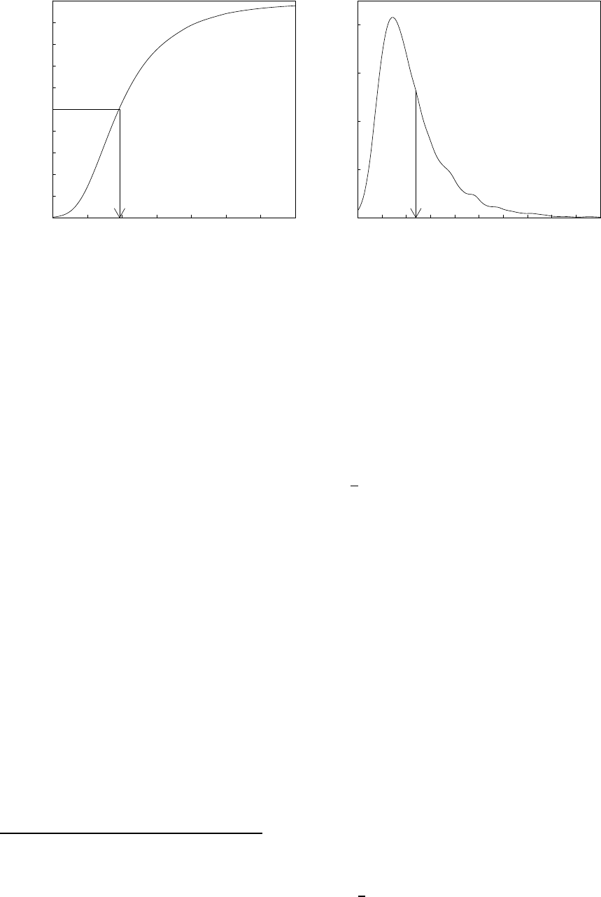
Figure 2.1: Wage Distribution and Density. All full-time U.S. workers
In Figure 2.1 we display estimates1of the probability distribution function (on the left) and
density function (on the right) of U.S. wage rates in 2009. We see that the density is peaked around
$15, and most of the probability mass appears to lie between $10 and $40. These are ranges for
typical wage rates in the U.S. population.
Important measures of central tendency are the median and the mean. The median of a
continuous2distribution is the unique solution to
()=1
2
The median U.S. wage ($19.23) is indicated in the left panel of Figure 2.1 by the arrow. The median
is a robust3measure of central tendency, but it is tricky to use for many calculations as it is not a
linear operator.
The expectation or mean of a random variable with density is
=E()=Z∞
−∞
()
Here we have used the common and convenient convention of using the single character to denote
a random variable, rather than the more cumbersome label .Ageneraldefinition of the mean
is presented in Section 2.30. The mean U.S. wage ($23.90) is indicated in the right panel of Figure
2.1 by the arrow.
We sometimes use the notation Einstead of E()when the variable whose expectation is being
taken is clear from the context. There is no distinction in meaning.
The mean is a convenient measure of central tendency because it is a linear operator and
arises naturally in many economic models. A disadvantage of the mean is that it is not robust4
especially in the presence of substantial skewness or thick tails, which are both features of the wage
1The distribution and density are estimated nonparametrically from the sample of 50,742 full-time non-military
wage-earners reported in the March 2009 Current Population Survey. The wage rate is constructed as annual indi-
vidual wage and salary earnings divided by hours worked.
2If is not continuous the definition is =inf{:()≥1
2}
3The median is not sensitive to pertubations in the tails of the distribution.
4The mean is sensitive to pertubations in the tails of the distribution.
CHAPTER 2. CONDITIONAL EXPECTATION AND PROJECTION 13
distribution as can be seen easily in the right panel of Figure 2.1. Another way of viewing this
is that 64% of workers earn less that the mean wage of $23.90, suggesting that it is incorrect to
describe the mean as a “typical” wage rate.
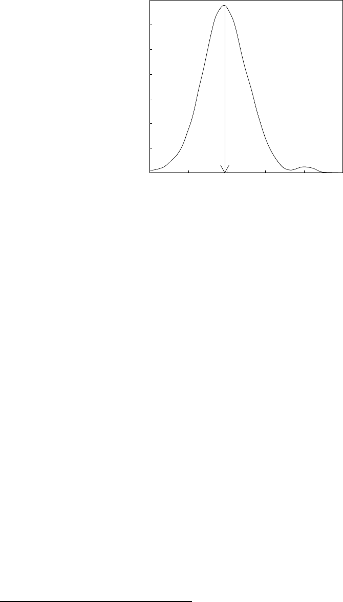
Log Dollars per Hour
Log Wage Density
123456
Figure 2.2: Log Wage Density
In this context it is useful to transform the data by taking the natural logarithm5. Figure 2.2
shows the density of log hourly wages log()for the same population, with its mean 2.95 drawn
in with the arrow. The density of log wages is much less skewed and fat-tailed than the density of
the level of wages, so its mean
E(log()) = 295
is a much better (more robust) measure6of central tendency of the distribution. For this reason,
wage regressions typically use log wages as a dependent variable rather than the level of wages.
Another useful way to summarize the probability distribution ()is in terms of its quantiles.
For any ∈(01)the quantile of the continuous7distribution is the real number which
satisfies
()=
Thequantilefunctionviewed as a function of is the inverse of the distribution function
The most commonly used quantile is the median, that is, 05= We sometimes refer to quantiles
by the percentile representation of and in this case they are often called percentiles, e.g. the
median is the 50 percentile.
2.3 Conditional Expectation
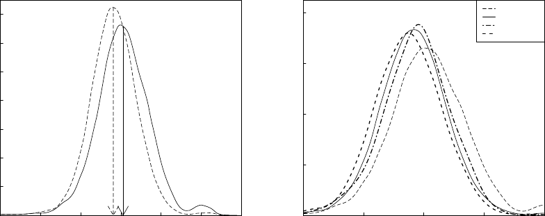
We saw in Figure 2.2 the density of log wages. Is this distribution the same for all workers, or
does the wage distribution vary across subpopulations? To answer this question, we can compare
wage distributions for different groups — for example, men and women. The plot on the left in
Figure 2.3 displays the densities of log wages for U.S. men and women with their means (3.05 and
2.81) indicated by the arrows. We can see that the two wage densities take similar shapes but the
density for men is somewhat shifted to the right with a higher mean.
5Throughout the text, we will use log()or log to denote the natural logarithm of
6More precisely, the geometric mean exp (E(log )) = $1911 is a robust measure of central tendency.
7If is not continuous the definition is =inf{:()≥}
CHAPTER 2. CONDITIONAL EXPECTATION AND PROJECTION 14
Log Dollars per Hour
Log Wage Density
0123456
MenWomen
(a) Women and Men
Log Dollars per Hour
Log Wage Density
12345
white men
white wome
n
black men
black wome
n
(b) By Sex and Race
Figure 2.3: Log Wage Density by Sex and Race
The values 3.05 and 2.81 are the mean log wages in the subpopulations of men and women
workers. They are called the conditional means (or conditional expectations) of log wages
given sex. We can write their specificvaluesas
E(log()| =)=305 (2.1)
E(log()| =)=281(2.2)
We call these means conditional as they are conditioning on a fixed value of the variable sex.
While you might not think of a person’s sex as a random variable, it is random from the viewpoint
of econometric analysis. If you randomly select an individual, the sex of the individual is unknown
and thus random. (In the population of U.S. workers, the probability that a worker is a woman
happens to be 43%.) In observational data, it is most appropriate to view all measurements as
random variables, and the means of subpopulations are then conditional means.
As the two densities in Figure 2.3 appear similar, a hasty inference might be that there is not
a meaningful difference between the wage distributions of men and women. Before jumping to this
conclusion let us examine the differences in the distributions of Figure 2.3 more carefully. As we
mentioned above, the primary difference between the two densities appears to be their means. This
difference equals
E(log()| =)−E(log()| =)=305 −281
=024(2.3)
Adifference in expected log wages of 0.24 implies an average 24% difference between the wages
of men and women, which is quite substantial. (For an explanation of logarithmic and percentage
differences see Section 2.4.)
Consider further splitting the men and women subpopulations by race, dividing the population
into whites, blacks, and other races. We display the log wage density functions of four of these
groups on the right in Figure 2.3. Again we see that the primary difference between the four density
functions is their central tendency.

CHAPTER 2. CONDITIONAL EXPECTATION AND PROJECTION 15
men women
white 3.07 2.82
black 2.86 2.73
other 3.03 2.86
Table 2.1: Mean Log Wages by Sex and Race
Focusing on the means of these distributions, Table 2.1 reports the mean log wage for each of
the six sub-populations.
The entries in Table 2.1 are the conditional means of log()given sex and race. For example
E(log()| = =)=307
and
E(log()| = =-)=273
One benefit of focusing on conditional means is that they reduce complicated distributions
to a single summary measure, and thereby facilitate comparisons across groups. Because of this
simplifying property, conditional means are the primary interest of regression analysis and are a
major focus in econometrics.
Table 2.1 allows us to easily calculate average wage differences between groups. For example,
we can see that the wage gap between men and women continues after disaggregation by race, as
the average gap between white men and white women is 25%, and that between black men and
black women is 13%. We also can see that there is a race gap, as the average wages of blacks are
substantially less than the other race categories. In particular, the average wage gap between white
men and black men is 21%, and that between white women and black women is 9%.
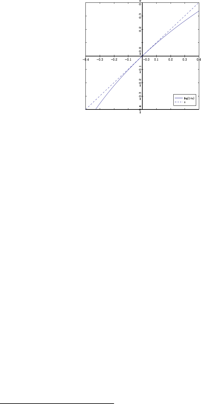
2.4 Log Differences*
A useful approximation for the natural logarithm for small is
log (1 + )≈ (2.4)
This can be derived from the infinite series expansion of log (1 + ):
log (1 + )=−2
2+3
3−4
4+···
=+(2)
The symbol (2)means that the remainder is bounded by 2as →0for some ∞Aplot
of log (1 + )and the linear approximation isshowninFigure2.4. Wecanseethatlog (1 + )
and the linear approximation are very close for ||≤01, and reasonably close for ||≤02, but
the difference increases with ||.
Now, if ∗is %greater than then
∗=(1+100)
Taking natural logarithms,
log ∗=log+log(1+100)
or
log ∗−log =log(1+100) ≈
100
where the approximation is (2.4). This shows that 100 multiplied by the difference in logarithms
is approximately the percentage difference between and ∗, and this approximation is quite good
for ||≤10
CHAPTER 2. CONDITIONAL EXPECTATION AND PROJECTION 16
Figure 2.4: log(1 + )
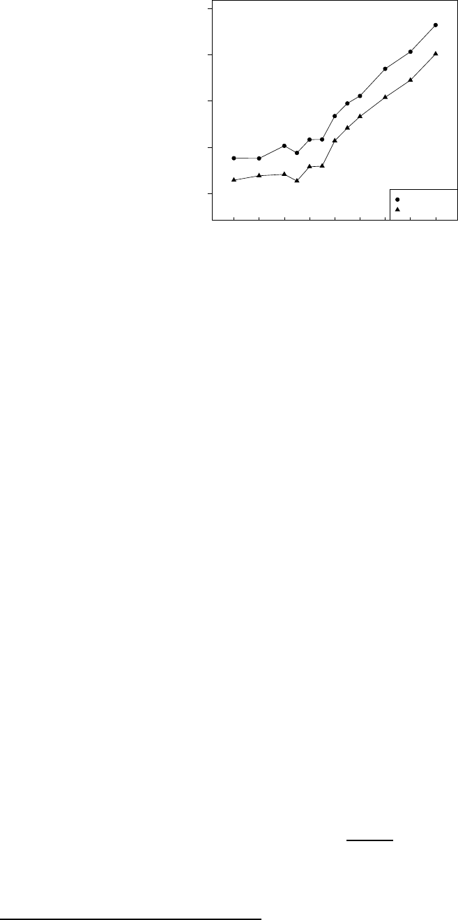
2.5 Conditional Expectation Function
An important determinant of wage levels is education. In many empirical studies economists
measure educational attainment by the number of years8of schooling, and we will write this variable
as education.
The conditional mean of log wages given sex,race,andeducation is a single number for each
category. For example
E(log()| = = = 12) = 284
We display in Figure 2.5 the conditional means of log()for white men and white women as a
function of education. The plot is quite revealing. We see that the conditional mean is increasing in
years of education, but at a different rate for schooling levels above and below nine years. Another
striking feature of Figure 2.5 is that the gap between men and women is roughly constant for all
education levels. As the variables are measured in logs this implies a constant average percentage
gap between men and women regardless of educational attainment.
In many cases it is convenient to simplify the notation by writing variables using single charac-
ters, typically and/or . It is conventional in econometrics to denote the dependent variable
(e.g. log()) by the letter a conditioning variable (such as sex ) by the letter and multiple
conditioning variables (such as race,education and sex) by the subscripted letters 1
2
.
Conditional expectations can be written with the generic notation
E(|1
2
)=(1
2
)
We call this the conditional expectation function (CEF). The CEF is a function of (1
2
)
as it varies with the variables. For example, the conditional expectation of =log()given
(1
2)=(sex race )is given by the six entries of Table 2.1. The CEF is a function of (sexrace)
as it varies across the entries.
For greater compactness, we will typically write the conditioning variables as a vector in R:
x=⎛
⎜
⎜
⎜
⎝
1
2
.
.
.
⎞
⎟
⎟
⎟
⎠(2.5)
8Here, education is defined as years of schooling beyond kindergarten. A high school graduate has education =12,
a college graduate has education =16, a Master’s degree has education =18, and a professional degree (medical, law or
PhD) has education =20.
CHAPTER 2. CONDITIONAL EXPECTATION AND PROJECTION 17
2.0 2.5 3.0 3.5 4.0
Years of Education
Log Dollars per Hour
4 6 8 10 12 14 16 18 20
white men
white women
Figure 2.5: Mean Log Wage as a Function of Years of Education
Here we follow the convention of using lower case bold italics xto denote a vector. Given this
notation, the CEF can be compactly written as
E(|x)=(x)
The CEF E(|x)is a random variable as it is a function of the random variable x.Itis
also sometimes useful to view the CEF as a function of x. In this case we can write (u)=
E(|x=u), which is a function of the argument u. The expression E(|x=u)is the conditional
expectation of given that we know that the random variable xequals the specificvalueu.
However, sometimes in econometrics we take a notational shortcut and use E(|x)to refer to this
function. Hopefully, the use of E(|x)should be apparent from the context.
2.6 Continuous Variables
In the previous sections, we implicitly assumed that the conditioning variables are discrete.
However, many conditioning variables are continuous. In this section, we take up this case and
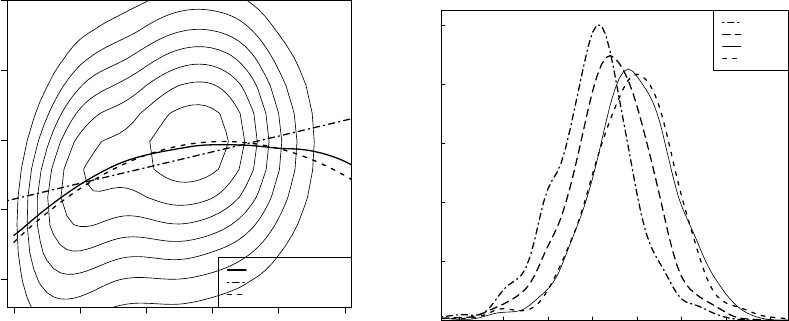
assume that the variables ( x)are continuously distributed with a joint density function ( x)
As an example, take =log()and =experience, the number of years of potential labor
market experience9. The contours of their joint density are plotted on the left side of Figure 2.6
for the population of white men with 12 years of education.
Given the joint density ( x)the variable xhas the marginal density
(x)=Z∞
−∞
(x)
For any xsuch that (x)0the conditional density of given xis defined as
|(|x)=( x)
(x)(2.6)
The conditional density is a (renormalized) slice of the joint density ( x)holding xfixed. The
slice is renormalized (divided by (x)so that it integrates to one and is thus a density.) We can
9Here, is defined as potential labor market experience, equal to − −6
CHAPTER 2. CONDITIONAL EXPECTATION AND PROJECTION 18
Labor Market Experience (Years)
Log Dollars per Hour
0 1020304050
2.0 2.5 3.0 3.5 4.0
Conditional Mean
Linear Projection
Quadratic Projectio
n
(a) Joint density of log(wage) and experience and
conditional mean
Log Dollars per Hour
Log Wage Conditional Density
Exp=5
Exp=1
0
Exp=2
5
Exp=4
0
1.0 1.5 2.0 2.5 3.0 3.5 4.0 4.5
(b) Conditional density
Figure 2.6: White men with education =12
visualize this by slicing the joint density function at a specific value of xparallel with the -axis.
For example, take the density contours on the left side of Figure 2.6 and slice through the contour
plot at a specific value of experience, and then renormalize the slice so that it is a proper density.
This gives us the conditional density of log()for white men with 12 years of education and
this level of experience. We do this for four levels of experience (5, 10, 25, and 40 years), and plot
these densities on the right side of Figure 2.6. We can see that the distribution of wages shifts to
the right and becomes more diffuse as experience increases from5to10years,andfrom10to25
years, but there is little change from 25 to 40 years experience.
The CEF of given xis the mean of the conditional density (2.6)
(x)=E(|x)=Z∞
−∞
|(|x) (2.7)
Intuitively, (x)is the mean of for the idealized subpopulation where the conditioning variables
are fixed at x. This is idealized since xis continuously distributed so this subpopulation is infinitely
small.
This definition (2.7) is appropriate when the conditional density (2.6) is well defined. However,
the conditional mean ()exists quite generally. In Theorem 2.32.1 in Section 2.32 we show that
()exists so long as E||∞.
In Figure 2.6 the CEF of log()given experience is plotted as the solid line. We can see
that the CEF is a smooth but nonlinear function. The CEF is initially increasing in experience,
flattens out around experience =30, and then decreases for high levels of experience.
2.7 Law of Iterated Expectations
An extremely useful tool from probability theory is the law of iterated expectations.An
important special case is the known as the Simple Law.

CHAPTER 2. CONDITIONAL EXPECTATION AND PROJECTION 19
Theorem 2.7.1 Simple Law of Iterated Expectations
If E||∞then for any random vector x,
E(E(|x)) = E()
The simple law states that the expectation of the conditional expectation is the unconditional
expectation. In other words, the average of the conditional averages is the unconditional average.
When xis discrete
E(E(|x)) = ∞
X
=1
E(|x)Pr(x=x)
and when xis continuous
E(E(|x)) = ZR
E(|x)(x)x
Going back to our investigation of average log wages for men and women, the simple law states
that
E(log()| =)Pr( =)
+E(log()| =)Pr( =)
=E(log())
Or numerically,
305 ×057 + 279 ×043 = 292
The general law of iterated expectations allows two sets of conditioning variables.
Theorem 2.7.2 Law of Iterated Expectations
If E||∞then for any random vectors x1and x2,
E(E(|x1x2)|x1)=E(|x1)
Notice the way the law is applied. The inner expectation conditions on x1and x2,while
the outer expectation conditions only on x1The iterated expectation yields the simple answer
E(|x1)the expectation conditional on x1alone. Sometimes we phrase this as: “The smaller
information set wins.”
As an example
E(log()| = =)Pr( =| =)
+E(log()| = =-)Pr( =-| =)
+E(log()| = =)Pr( =| =)
=E(log()| =)
or numerically
307 ×084 + 286 ×008 + 303 ×008 = 305
A property of conditional expectations is that when you condition on a random vector xyou
can effectively treat it as if it is constant. For example, E(x|x)=xand E((x)|x)=(x)for
any function (·)The general property is known as the Conditioning Theorem.

CHAPTER 2. CONDITIONAL EXPECTATION AND PROJECTION 20
Theorem 2.7.3 Conditioning Theorem
If E||∞then
E((x)|x)=(x)E(|x)(2.8)
In in addition
E|(x)|∞(2.9)
then
E((x))=E((x)E(|x)) (2.10)
The proofs of Theorems 2.7.1, 2.7.2 and 2.7.3 are given in Section 2.34.
2.8 CEF Error
The CEF error is defined as the difference between and the CEF evaluated at the random
vector x:
=−(x)
By construction, this yields the formula
=(x)+ (2.11)
In (2.11) it is useful to understand that the error is derived from the joint distribution of
( x)and so its properties are derived from this construction.
A key property of the CEF error is that it has a conditional mean of zero. To see this, by the
linearity of expectations, the definition (x)=E(|x)and the Conditioning Theorem
E(|x)=E((−(x)) |x)
=E(|x)−E((x)|x)
=(x)−(x)
=0
This fact can be combined with the law of iterated expectations to show that the unconditional
mean is also zero.
E()=E(E(|x)) = E(0) = 0
We state this and some other results formally.
Theorem 2.8.1 Properties of the CEF error
If E||∞then
1. E(|x)=0
2. E()=0
3. If E||∞for ≥1then E||∞
4. For any function (x)such that E|(x)|∞then E((x))=0
The proof of the third result is deferred to Section 2.34
The fourth result, whose proof is left to Exercise 2.3, implies that is uncorrelated with any
function of the regressors.
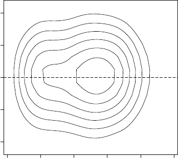
CHAPTER 2. CONDITIONAL EXPECTATION AND PROJECTION 21
Labor Market Experience (Years)
e
0 1020304050
−1.0 −0.5 0.0 0.5 1.0
Figure 2.7: Joint density of CEF error and experience for white men with education =12.
The equations
=(x)+
E(|x)=0
together imply that (x)is the CEF of given x. It is important to understand that this is not
a restriction. These equations hold true by definition.
The condition E(|x)=0is implied by the definition of as the difference between and the
CEF (x)The equation E(|x)=0is sometimes called a conditional mean restriction, since
the conditional mean of the error is restricted to equal zero. The property is also sometimes called
mean independence, for the conditional mean of is 0 and thus independent of x.However,
it does not imply that the distribution of is independent of xSometimes the assumption “is
independent of x” is added as a convenient simplification, but it is not generic feature of the con-
ditional mean. Typically and generally, and xare jointly dependent, even though the conditional
mean of is zero.
As an example, the contours of the joint density of and experience are plotted in Figure 2.7
for the same population as Figure 2.6. The error has a conditional mean of zero for all values of
experience, but the shape of the conditional distribution varies with the level of experience.
Asasimpleexampleofacasewhereand are mean independent yet dependent, let =
where and are independent N(01)Then conditional on the error has the distribution
N(0
2)Thus E(|)=0and is mean independent of yet is not fully independent of
Mean independence does not imply full independence.
2.9 Intercept-Only Model
A special case of the regression model is when there are no regressors x.Inthiscase(x)=
E()=, the unconditional mean of We can still write an equation for in the regression
format:
=+
E()=0
This is useful for it unifies the notation.

CHAPTER 2. CONDITIONAL EXPECTATION AND PROJECTION 22
2.10 Regression Variance
An important measure of the dispersion about the CEF function is the unconditional variance
of the CEF error We write this as
2=var()=E³(−E)2´=E¡2¢
Theorem 2.8.1.3 implies the following simple but useful result.
Theorem 2.10.1 If E¡2¢∞then 2∞
We can call 2the regression variance or the variance of the regression error. The magnitude
of 2measures the amount of variation in which is not “explained” or accounted for in the
conditional mean E(|x)
The regression variance depends on the regressors x. Consider two regressions
=E(|x1)+1
=E(|x1x2)+2
We write the two errors distinctly as 1and 2as they are different — changing the conditioning
information changes the conditional mean and therefore the regression error as well.
In our discussion of iterated expectations, we have seen that by increasing the conditioning
set, the conditional expectation reveals greater detail about the distribution of What is the
implication for the regression error?
It turns out that there is a simple relationship. We can think of the conditional mean E(|x)
as the “explained portion” of The remainder =−E(|x)is the “unexplained portion”. The
simple relationship we now derive shows that the variance of this unexplained portion decreases
when we condition on more variables. This relationship is monotonic in the sense that increasing
the amont of information always decreases the variance of the unexplained portion.
Theorem 2.10.2 If E¡2¢∞then
var ()≥var (−E(|x1)) ≥var (−E(|x1x2))
Theorem 2.10.2 says that the variance of the difference between and its conditional mean
(weakly) decreases whenever an additional variable is added to the conditioning information.
The proof of Theorem 2.10.2 is given in Section 2.34.
2.11 Best Predictor
Suppose that given a realized value of x, we want to create a prediction or forecast of We can
write any predictor as a function (x)of x. The prediction error is the realized difference −(x)
A non-stochastic measure of the magnitude of the prediction error is the expectation of its square
E³(−(x))2´(2.12)
We can define the best predictor as the function (x)which minimizes (2.12). What function
isthebestpredictor?ItturnsoutthattheansweristheCEF(x). This holds regardless of the
joint distribution of ( x)

CHAPTER 2. CONDITIONAL EXPECTATION AND PROJECTION 23
To see this, note that the mean squared error of a predictor (x)is
E³(−(x))2´=E³(+(x)−(x))2´
=E¡2¢+2E(((x)−(x))) + E³((x)−(x))2´
=E¡2¢+E³((x)−(x))2´
≥E¡2¢
=E³(−(x))2´
where the first equality makes the substitution =(x)+andthethirdequalityusesTheorem
2.8.1.4. The right-hand-side after the third equality is minimized by setting (x)=(x), yielding
the inequality in the fourth line. The minimum is finite under the assumption E¡2¢∞as shown
by Theorem 2.10.1.
We state this formally in the following result.
Theorem 2.11.1 Conditional Mean as Best Predictor
If E¡2¢∞then for any predictor (x),
E³(−(x))2´≥E³(−(x))2´
where (x)=E(|x).
It may be helpful to consider this result in the context of the intercept-only model
=+
E()=0
Theorem 2.11.1 shows that the best predictor for (in the class of constants) is the unconditional
mean =E()in the sense that the mean minimizes the mean squared prediction error.
2.12 Conditional Variance
While the conditional mean is a good measure of the location of a conditional distribution,
it does not provide information about the spread of the distribution. A common measure of the
dispersion is the conditional variance.Wefirstgivethegeneraldefinition of the conditional
variance of a random variable .
Definition 2.12.1 If E¡2¢∞the conditional variance of given
xis
var (|x)=E³(−E(|x))2|x´
Notice that the conditional variance is the conditional second moment, centered around the
conditional first moment. Given this definition, we define the conditional variance of the regression
error.

CHAPTER 2. CONDITIONAL EXPECTATION AND PROJECTION 24
Definition 2.12.2 If E¡2¢∞the conditional variance of the re-
gression error is
2(x)=var(|x)=E¡2|x¢
Generally, 2(x)is a non-trivial function of xand can take any form subject to the restriction
that it is non-negative. One way to think about 2(x)is that it is the conditional mean of 2
given x.Noticeaswellthat2(x)=var(|x)so it is equivalently the conditional variance of the
dependent variable.
The variance is in a different unit of measurement than the original variable. To convert the
variance back to the same unit of measure we define the conditional standard deviation as its
square root (x)=p2(x)
As an example of how the conditional variance depends on observables, compare the conditional
log wage densities for men and women displayed in Figure 2.3. The difference between the densities
is not purely a location shift, but is also a difference in spread. Specifically, we can see that the
density for men’s log wages is somewhat more spread out than that for women, while the density
for women’s wages is somewhat more peaked. Indeed, the conditional standard deviation for men’s
wages is 3.05 and that for women is 2.81. So while men have higher average wages, they are also
somewhat more dispersed.
The unconditional error variance and the conditional variance are related by the law of iterated
expectations
2=E¡2¢=E¡E¡2|x¢¢=E¡2(x)¢
That is, the unconditional error variance is the average conditional variance.
Given the conditional variance, we can define a rescaled error
=
(x)(2.13)
We can calculate that since (x)is a function of x
E(|x)=Eµ
(x)|x¶=1
(x)E(|x)=0
and
var (|x)=E¡2|x¢=Eµ2
2(x)|x¶=1
2(x)E¡2|x¢=2(x)
2(x)=1
Thus has a conditional mean of zero, and a conditional variance of 1.
Notice that (2.13) can be rewritten as
=(x)
and substituting this for in the CEF equation (2.11), we find that
=(x)+(x) (2.14)
This is an alternative (mean-variance) representation of the CEF equation.
Many econometric studies focus on the conditional mean (x)and either ignore the condi-
tional variance 2(x)treat it as a constant 2(x)=2or treat it as a nuisance parameter (a
parameter not of primary interest). This is appropriate when the primary variation in the condi-
tional distribution is in the mean, but can be short-sighted in other cases. Dispersion is relevant
to many economic topics, including income and wealth distribution, economic inequality, and price
dispersion. Conditional dispersion (variance) can be a fruitful subject for investigation.
The perverse consequences of a narrow-minded focus on the mean has been parodied in a classic
joke:

CHAPTER 2. CONDITIONAL EXPECTATION AND PROJECTION 25
An economist was standing with one foot in a bucket of boiling water
and the other foot in a bucket of ice. When asked how he felt, he
replied, “On average I feel just fine.”
Clearly, the economist in question ignored variance!
2.13 Homoskedasticity and Heteroskedasticity
An important special case obtains when the conditional variance 2(x)is a constant and inde-
pendent of x.Thisiscalledhomoskedasticity.
Definition 2.13.1 The error is homoskedastic if E¡2|x¢=2
does not depend on x.
In the general case where 2(x)depends on xwe say that the error is heteroskedastic.
Definition 2.13.2 The error is heteroskedastic if E¡2|x¢=2(x)
depends on x.
It is helpful to understand that the concepts homoskedasticity and heteroskedasticity concern
the conditional variance, not the unconditional variance. By definition, the unconditional variance
2is a constant and independent of the regressors x. So when we talk about the variance as a
function of the regressors, we are talking about the conditional variance 2(x).
Some older or introductory textbooks describe heteroskedasticity as the case where “the vari-
ance of varies across observations”. This is a poor and confusing definition. It is more constructive
to understand that heteroskedasticity means that the conditional variance 2(x)depends on ob-
servables.
Older textbooks also tend to describe homoskedasticity as a component of a correct regression
specification, and describe heteroskedasticity as an exception or deviance. This description has
influenced many generations of economists, but it is unfortunately backwards. The correct view
is that heteroskedasticity is generic and “standard”, while homoskedasticity is unusual and excep-
tional. The default in empirical work should be to assume that the errors are heteroskedastic, not
the converse.
In apparent contradiction to the above statement, we will still frequently impose the ho-
moskedasticity assumption when making theoretical investigations into the properties of estimation
and inference methods. The reason is that in many cases homoskedasticity greatly simplifies the
theoretical calculations, and it is therefore quite advantageous for teaching and learning. It should
always be remembered, however, that homoskedasticity is never imposed because it is believed to
be a correct feature of an empirical model, but rather because of its simplicity.

CHAPTER 2. CONDITIONAL EXPECTATION AND PROJECTION 26
2.14 Regression Derivative
One way to interpret the CEF (x)=E(|x)is in terms of how marginal changes in the
regressors ximply changes in the conditional mean of the response variable It is typical to
consider marginal changes in a single regressor, say 1, holding the remainder fixed. When a
regressor 1is continuously distributed, we define the marginal effect of a change in 1, holding
the variables 2
fixed, as the partial derivative of the CEF
1
(1
)
When 1is discrete we define the marginal effect as a discrete difference. For example, if 1is
binary, then the marginal effect of 1on the CEF is
(1
2
)−(0
2
)
We can unify the continuous and discrete cases with the notation
∇1(x)=⎧
⎪
⎪
⎨
⎪
⎪
⎩
1
(1
)if 1is continuous
(1
2
)−(0
2
)if 1is binary.
Collecting the effects into one ×1vector, we define the regression derivative with respect to
x:
∇(x)=⎡
⎢
⎢
⎢
⎣
∇1(x)
∇2(x)
.
.
.
∇(x)
⎤
⎥
⎥
⎥
⎦
When all elements of xare continuous, then we have the simplification ∇(x)=
x(x),the
vector of partial derivatives.
There are two important points to remember concerning our definition of the regression deriv-
ative.
First, the effect of each variable is calculated holding the other variables constant. This is the
ceteris paribus concept commonly used in economics. But in the case of a regression derivative,
the conditional mean does not literally hold all else constant. It only holds constant the variables
included in the conditional mean. This means that the regression derivative depends on which
regressors are included. For example, in a regression of wages on education, experience, race and
sex, the regression derivative with respect to education shows the marginal effect of education on
mean wages, holding constant experience, race and sex. But it does not hold constant an individual’s
unobservable characteristics (such as ability), nor variables not included in the regression (such as
the quality of education).
Second, the regression derivative is the change in the conditional expectation of ,notthe
change in the actual value of for an individual. It is tempting to think of the regression derivative
as the change in the actual value of , but this is not a correct interpretation. The regression
derivative ∇(x)is the change in the actual value of only if the error is unaffected by the
change in the regressor x. We return to a discussion of causal effects in Section 2.29.
2.15 Linear CEF
An important special case is when the CEF (x)=E(|x)is linear in xIn this case we can
write the mean equation as
(x)=11+22+···+++1

CHAPTER 2. CONDITIONAL EXPECTATION AND PROJECTION 27
Notationally it is convenient to write this as a simple function of the vector x.Aneasywaytodo
so is to augment the regressor vector xby listing the number “1” as an element. We call this the
“constant” and the corresponding coefficient is called the “intercept”. Equivalently, specify that
the final element10 of the vector xis =1. Thus (2.5) has been redefined as the ×1vector
x=
⎛
⎜
⎜
⎜
⎜
⎜
⎝
1
2
.
.
.
−1
1
⎞
⎟
⎟
⎟
⎟
⎟
⎠
(2.15)
With this redefinition, the CEF is
(x)=11+22+···+
=x0β(2.16)
where
β=⎛
⎜
⎝
1
.
.
.
⎞
⎟
⎠(2.17)
is a ×1coefficient vector. This is the linear CEF model. It is also often called the linear
regression model, or the regression of on x
In the linear CEF model, the regression derivative is simply the coefficient vector. That is
∇(x)=β
This is one of the appealing features of the linear CEF model. The coefficients have simple and
natural interpretations as the marginal effects of changing one variable, holding the others constant.
Linear CEF Model
=x0β+
E(|x)=0
If in addition the error is homoskedastic, we call this the homoskedastic linear CEF model.
Homoskedastic Linear CEF Model
=x0β+
E(|x)=0
E¡2|x¢=2
10The order doesn’t matter. It could be any element.

CHAPTER 2. CONDITIONAL EXPECTATION AND PROJECTION 28
2.16 Linear CEF with Nonlinear Effects
The linear CEF model of the previous section is less restrictive than it might appear, as we can
include as regressors nonlinear transformations of the original variables. In this sense, the linear
CEF framework is flexible and can capture many nonlinear effects.
For example, suppose we have two scalar variables 1and 2The CEF could take the quadratic
form
(1
2)=11+22+2
13+2
24+125+6(2.18)
This equation is quadratic in the regressors (1
2)yet linear in the coefficients β=(1
6)0
We will descriptively call (2.18) a quadratic CEF, and yet (2.18) is also a linear CEF in the sense
of being linear in the coefficients. The key is to understand that (2.18) is quadratic in the variables
(1
2)yet linear in the coefficients β
To simplify the expression, we define the transformations 3=2
1
4=2
2
5=12and
6=1and redefine the regressor vector as x=(1
6)0With this redefinition,
(1
2)=x0β
which is linear in β. For most econometric purposes (estimation and inference on β) the linearity
in βis all that is important.
An exception is in the analysis of regression derivatives. In nonlinear equations such as (2.18),
the regression derivative should be defined with respect to the original variables, not with respect
to the transformed variables. Thus
1
(1
2)=1+213+25
2
(1
2)=2+224+15
We see that in the model (2.18), the regression derivatives are not a simple coefficient, but are
functions of several coefficients plus the levels of (12)Consequently it is difficult to interpret
the coefficients individually. It is more useful to interpret them as a group.
We typically call 5the interaction effect. Notice that it appears in both regression derivative
equations, and has a symmetric interpretation in each. If 50then the regression derivative
with respect to 1is increasing in the level of 2(and the regression derivative with respect to 2
is increasing in the level of 1)while if 50the reverse is true.
2.17 Linear CEF with Dummy Variables
When all regressors take a finite set of values, it turns out the CEF can be written as a linear
function of regressors.
This simplest example is a binary variable, which takes only two distinct values. For example,
in most data sets the variable sex takes only the values man and woman (or male and female).
Binary variables are extremely common in econometric applications, and are alternatively called
dummy variables or indicator variables.
Consider the simple case of a single binary regressor. In this case, the conditional mean can
only take two distinct values. For example,
E(|)=⎧
⎨
⎩
0if sex=man
1if sex=woman
To facilitate a mathematical treatment, we typically record dummy variables with the values {01}
For example
1=½0if sex=man
1if sex=woman (2.19)
CHAPTER 2. CONDITIONAL EXPECTATION AND PROJECTION 29
Given this notation we can write the conditional mean as a linear function of the dummy variable
1that is
E(|1)=11+2
where 1=1−0and 2=0. In this simple regression equation the intercept 2is equal to
the conditional mean of for the 1=0subpopulation (men) and the slope 1is equal to the
difference in the conditional means between the two subpopulations.
Equivalently, we could have defined 1as
1=½1if sex=man
0if sex=woman (2.20)
In this case, the regression intercept is the mean for women (rather than for men) and the regression
slope has switched signs. The two regressions are equivalent but the interpretation of the coefficients
has changed. Therefore it is always important to understand the precise definitions of the variables,
and illuminating labels are helpful. For example, labelling 1as “sex” does not help distinguish
between definitions (2.19) and (2.20). Instead, it is better to label 1as “women” or “female” if
definition (2.19) is used, or as “men” or “male” if (2.20) is used.
Now suppose we have two dummy variables 1and 2For example, 2=1if the person is
married, else 2=0The conditional mean given 1and 2takes at most four possible values:
E(|1
2)=⎧
⎪
⎪
⎨
⎪
⎪
⎩
00 if 1=0and 2=0 (unmarried men)
01 if 1=0and 2=1 (married men)
10 if 1=1and 2=0 (unmarried women)
11 if 1=1and 2=1 (married women)
In this case we can write the conditional mean as a linear function of 1,2and their product
12:
E(|1
2)=11+22+312+4
where 1=10 −00
2=01 −00
3=11 −10 −01 +00and 4=00
We can view the coefficient 1as the effect of sex on expected log wages for unmarried wage
earners, the coefficient 2as the effect of marriage on expected log wages for men wage earners, and
the coefficient 3as the difference between the effects of marriage on expected log wages among
women and among men. Alternatively, it can also be interpreted as the difference between the effects
of sex on expected log wages among married and non-married wage earners. Both interpretations
are equally valid. We often describe 3as measuring the interaction between the two dummy
variables, or the interaction effect, and describe 3=0as the case when the interaction effect is
zero.
In this setting we can see that the CEF is linear in the three variables (1
2
12)Thus to
put the model in the framework of Section 2.15, we would define the regressor 3=12and the
regressor vector as
x=⎛
⎜
⎜
⎝
1
2
3
1
⎞
⎟
⎟
⎠
So even though we started with only 2 dummy variables, the number of regressors (including the
intercept) is 4.
If there are 3 dummy variables 1
2
3then E(|1
2
3)takes at most 23=8distinct
values and can be written as the linear function
E(|1
2
3)=11+22+33+412+513+623+7123+8
which has eight regressors including the intercept.
CHAPTER 2. CONDITIONAL EXPECTATION AND PROJECTION 30
In general, if there are dummy variables 1
then the CEF E(|1
2
)takes
at most 2distinct values, and can be written as a linear function of the 2regressors including
1
2
and all cross-products. This might be excessive in practice if is modestly large. In
the next section we will discuss projection approximations which yield more parsimonious parame-
terizations.
We started this section by saying that the conditional mean is linear whenever all regressors
take only a finite number of possible values. How can we see this? Take a categorical variable,
such as race. For example, we earlier divided race into three categories. We can record categorical
variables using numbers to indicate each category, for example
3=⎧
⎨
⎩
1if white
2if black
3if other
When doing so, the values of 3have no meaning in terms of magnitude, they simply indicate the
relevant category.
When the regressor is categorical the conditional mean of given 3takes a distinct value for
each possibility:
E(|3)=⎧
⎨
⎩
1if 3=1
2if 3=2
3if 3=3
This is not a linear function of 3itself, but it can be made a linear function by constructing
dummy variables for two of the three categories. For example
4=½1if black
0if not black
5=½1if other
0if not other
In this case, the categorical variable 3is equivalent to the pair of dummy variables (4
5)The
explicit relationship is
3=⎧
⎨
⎩
1if 4=0and 5=0
2if 4=1and 5=0
3if 4=0and 5=1
Given these transformations, we can write the conditional mean of as a linear function of 4and
5
E(|3)=E(|4
5)=14+25+3
We can write the CEF as either E(|3)or E(|4
5)(they are equivalent), but it is only linear
as a function of 4and 5
This setting is similar to the case of two dummy variables, with the difference that we have not
included the interaction term 45This is because the event {4=1and 5=1}is empty by
construction, so 45=0by definition.
2.18 Best Linear Predictor
While the conditional mean (x)=E(|x)is the best predictor of among all functions
of xits functional form is typically unknown. In particular, the linear CEF model is empirically
unlikely to be accurate unless xis discrete and low-dimensional so all interactions are included.
Consequently in most cases it is more realistic to view the linear specification (2.16) as an approx-
imation. In this section we derive a specific approximation with a simple interpretation.

CHAPTER 2. CONDITIONAL EXPECTATION AND PROJECTION 31
Theorem 2.11.1 showed that the conditional mean (x)is the best predictor in the sense
that it has the lowest mean squared error among all predictors. By extension, we can define an
approximation to the CEF by the linear function with the lowest mean squared error among all
linear predictors.
For this derivation we require the following regularity condition.
Assumption 2.18.1
1. E¡2¢∞
2. Ekxk2∞
3. Q =E(xx0)is positive definite.
In Assumption 2.18.1.2 we use the notation kxk=(x0x)12to denote the Euclidean length of
the vector x.
The first two parts of Assumption 2.18.1 imply that the variables and xhave finite means,
variances, and covariances. The third part of the assumption is more technical, and its role will
become apparent shortly. It is equivalent to imposing that the columns of the matrix Q =E(xx0)
are linearly independent, or that the matrix is invertible.
Alinearpredictorforis a function of the form x0βfor some β∈R. The mean squared
prediction error is
(β)=E³¡−x0β¢2´
The best linear predictor of given x, written P(|x)is found by selecting the vector βto
minimize (β)
Definition 2.18.1 The Best Linear Predictor of given xis
P(|x)=x0β
where βminimizes the mean squared prediction error
(β)=E³¡−x0β¢2´
The minimizer
β=argmin
∈R
(b)(2.21)
is called the Linear Projection Coefficient.
We now calculate an explicit expression for its value. The mean squared prediction error can
be written out as a quadratic function of β:
(β)=E¡2¢−2β0E(x)+β0E¡xx0¢β
The quadratic structure of (β)means that we can solve explicitly for the minimizer. The first-
order condition for minimization (from Appendix A.15) is
0=
β(β)=−2E(x)+2E¡xx0¢β(2.22)

CHAPTER 2. CONDITIONAL EXPECTATION AND PROJECTION 32
Rewriting (2.22) as
2E(x)=2E¡xx0¢β
and dividing by 2, this equation takes the form
Q=Qβ(2.23)
where Q=E(x)is ×1and Q =E(xx0)is ×. The solution is found by inverting the
matrix Q, and is written
β=Q−1
Q
or
β=¡E¡xx0¢¢−1E(x)(2.24)
It is worth taking the time to understand the notation involved in the expression (2.24). Q is a
×matrix and Qis a ×1column vector. Therefore, alternative expressions such as E()
E(0)
or E(x)(E(xx0))−1are incoherent and incorrect. We also can now see the role of Assumption
2.18.1.3. It is equivalent to assuming that Q has an inverse Q−1
which is necessary for the
normal equations (2.23) to have a solution or equivalently for (2.24) to be uniquely defined. In the
absence of Assumption 2.18.1.3 there could be multiple solutions to the equation (2.23).
We now have an explicit expression for the best linear predictor:
P(|x)=x0¡E¡xx0¢¢−1E(x)
This expression is also referred to as the linear projection of on x.
The projection error is
=−x0β(2.25)
This equals the error (2.11) from the regression equation when (and only when) the conditional
mean is linear in xotherwise they are distinct.
Rewriting, we obtain a decomposition of into linear predictor and error
=x0β+ (2.26)
In general we call equation (2.26) or x0βthe best linear predictor of given x, or the linear
projection of on x. Equation (2.26) is also often called the regression of on xbut this can
sometimes be confusing as economists use the term regression in many contexts. (Recall that we
said in Section 2.15 that the linear CEF model is also called the linear regression model.)
An important property of the projection error is
E(x)=0(2.27)
To see this, using the definitions (2.25) and (2.24) and the matrix properties AA−1=Iand
Ia =a
E(x)=E¡x¡−x0β¢¢
=E(x)−E¡xx0¢¡E¡xx0¢¢−1E(x)
=0(2.28)
as claimed.
Equation (2.27) is a set of equations, one for each regressor. In other words, (2.27) is equivalent
to
E()=0 (2.29)

CHAPTER 2. CONDITIONAL EXPECTATION AND PROJECTION 33
for =1 As in (2.15), the regressor vector xtypically contains a constant, e.g. =1.In
this case (2.29) for =is the same as
E()=0(2.30)
Thus the projection error has a mean of zero when the regressor vector contains a constant. (When
xdoes not have a constant, (2.30) is not guaranteed. As it is desirable for to have a zero mean,
this is a good reason to always include a constant in any regression model.)
It is also useful to observe that since cov()=E()−E()E()then (2.29)-(2.30)
together imply that the variables and are uncorrelated.
This completes the derivation of the model. We summarize some of the most important prop-
erties.
Theorem 2.18.1 Properties of Linear Projection Model
Under Assumption 2.18.1,
1. The moments E(xx0)and E(x)exist with finite elements.
2. The Linear Projection Coefficient (2.21) exists, is unique, and equals
β=¡E¡xx0¢¢−1E(x)
3. The best linear predictor of given xis
P(|x)=x0¡E¡xx0¢¢−1E(x)
4. The projection error =−x0βexists and satisfies
E¡2¢∞
and
E(x)=0
5. If xcontains an constant, then
E()=0
6. If E||∞and Ekxk∞for ≥2then E||∞
A complete proof of Theorem 2.18.1 is given in Section 2.34.
It is useful to reflect on the generality of Theorem 2.18.1. The only restriction is Assumption
2.18.1. Thus for any random variables ( x)with finite variances we can define a linear equation
(2.26) with the properties listed in Theorem 2.18.1. Stronger assumptions (such as the linear CEF
model) are not necessary. In this sense the linear model (2.26) exists quite generally. However,
it is important not to misinterpret the generality of this statement. The linear equation (2.26) is
defined as the best linear predictor. It is not necessarily a conditional mean, nor a parameter of a
structural or causal economic model.
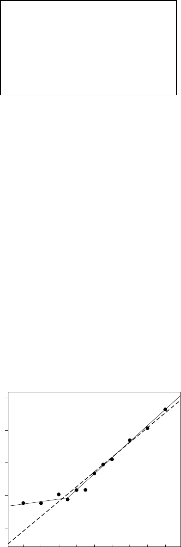
CHAPTER 2. CONDITIONAL EXPECTATION AND PROJECTION 34
Linear Projection Model
=x0β+
E(x)=0
β=¡E¡xx0¢¢−1E(x)
We illustrate projection using three log wage equations introduced in earlier sections.
For our first example, we consider a model with the two dummy variables for sex and race
similar to Table 2.1. As we learned in Section 2.17, the entries in this table can be equivalently
expressed by a linear CEF. For simplicity, let’s consider the CEF of log()as a function of
Black and Female.
E(log()|- -)=−020- −024-+010- ×-+306(2.31)
This is a CEF as the variables are binary and all interactions are included.
Now consider a simpler model omitting the interaction effect. This is the linear projection on
the variables - and -
P(log()|--)=−015- −023-+306(2.32)
What is the difference? The full CEF (2.31) shows that the race gap is differentiated by sex: it
is 20% for black men (relative to non-black men) and 10% for black women (relative to non-black
women). The projection model (2.32) simplifies this analysis, calculating an average 15% wage gap
for blacks, ignoring the role of sex. Notice that this is despite the fact that the sex variable is
included in (2.32).
2.0 2.5 3.0 3.5 4.0
Years of Education
Log Dollars per Hour
4 6 8 10 12 14 16 18 20
Figure 2.8: Projections of log() onto Education
For our second example we consider the CEF of log wages as a function of years of education
for white men which was illustrated in Figure 2.5 and is repeated in Figure 2.8. Superimposed on
the figure are two projections. The first (given by the dashed line) is the linear projection of log
wages on years of education
P(log()|)=011 +15
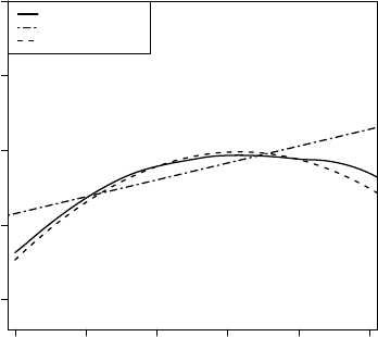
CHAPTER 2. CONDITIONAL EXPECTATION AND PROJECTION 35
This simple equation indicates an average 11% increase in wages for every year of education. An
inspection of the Figure shows that this approximation works well for education ≥9, but under-
predicts for individuals with lower levels of education. To correct this imbalance we use a linear
spline equation which allows different rates of return above and below 9 years of education:
P(log()|( −9) ×1( 9))
=002 +010 ×( −9) ×1( 9) + 23
This equation is displayed in Figure 2.8 using the solid line, and appears to fit much better. It
indicates a 2% increase in mean wages for every year of education below 9, and a 12% increase in
mean wages for every year of education above 9. It is still an approximation to the conditional
mean but it appears to be fairly reasonable.
0 1020304050
2.0 2.5 3.0 3.5 4.0
Labor Market Experience (Years)
Log Dollars per Hour
Conditional Mean
Linear Projection
Quadratic Projection
Figure 2.9: Linear and Quadratic Projections of log()ontoExperience
For our third example we take the CEF of log wages as a function of years of experience for
white men with 12 years of education, which was illustrated in Figure 2.6 and is repeated as the
solid line in Figure 2.9. Superimposed on the figure are two projections. The first (given by the
dot-dashed line) is the linear projection on experience
P(log()|)=0011 +25
and the second (given by the dashed line) is the linear projection on experience and its square
P(log()|)=0046 −000072+23
It is fairly clear from an examination of Figure 2.9 that the first linear projection is a poor approx-
imation. It over-predicts wages for young and old workers, and under-predicts for the rest. Most
importantly, it misses the strong downturn in expected wages for older wage-earners. The second
projection fits much better. We can call this equation a quadratic projection since the function
is quadratic in

CHAPTER 2. CONDITIONAL EXPECTATION AND PROJECTION 36
Invertibility and Identification
The linear projection coefficient β=(E(xx0))−1E(x)exists and is
unique as long as the ×matrix Q =E(xx0)is invertible. The matrix
Q is sometimes called the design matrix, as in experimental settings
the researcher is able to control Q by manipulating the distribution of
the regressors x
Observe that for any non-zero α∈R
α0Qα=E¡α0xx0α¢=E¡α0x¢2≥0
so Q by construction is positive semi-definite. The assumption that
it is positive definite means that this is a strict inequality, E(α0x)2
0Equivalently, there cannot exist a non-zero vector αsuch that α0x=
0identically. This occurs when redundant variables are included in x
Positive semi-definite matrices are invertible if and only if they are positive
definite. When Q is invertible then β=(E(xx0))−1E(x)exists and is
uniquely defined. In other words, in order for βto be uniquely defined, we
must exclude the degenerate situation of redundant variables.
Theorem 2.18.1 shows that the linear projection coefficient βis iden-
tified (uniquely determined) under Assumption 2.18.1. The key is invert-
ibility of Q. Otherwise, there is no unique solution to the equation
Qβ=Q(2.33)
When Q is not invertible there are multiple solutions to (2.33), all of
which yield an equivalent best linear predictor x0β. In this case the coeffi-
cient βis not identified as it does not have a unique value. Even so, the
best linear predictor x0βstill identified. One solution is to set
β=¡E¡xx0¢¢−E(x)
where A−denotes the generalized inverse of A(see Appendix A.6).
2.19 Linear Predictor Error Variance
As in the CEF model, we define the error variance as
2=E¡2¢
Setting =E¡2¢and Q=E(x0)we can write 2as
2=E³¡−x0β¢2´
=E¡2¢−2E¡x0¢β+β0E¡xx0¢β
= −2QQ−1
Q+QQ−1
QQ−1
Q
= −QQ−1
Q
=·(2.34)
One useful feature of this formula is that it shows that ·= −QQ−1
Qequals the
variance of the error from the linear projection of on x.

CHAPTER 2. CONDITIONAL EXPECTATION AND PROJECTION 37
2.20 Regression Coefficients
Sometimes it is useful to separate the constant from the other regressors, and write the linear
projection equation in the format
=x0β++(2.35)
where is the intercept and xdoes not contain a constant.
Taking expectations of this equation, we find
E()=E¡x0β¢+E()+E()
or
=μ0
β+
where =E()and μ=E(x)since E()=0from (2.30). (While xdoes not contain a
constant, the equation does so (2.30) still applies.) Rearranging, we find
=−μ0
β
Subtracting this equation from (2.35) we find
−=(x−μ)0β+ (2.36)
a linear equation between the centered variables −and x−μ. (They are centered at their
means, so are mean-zero random variables.) Because x−μis uncorrelated with (2.36) is also
a linear projection, thus by the formula for the linear projection model,
β=¡E¡(x−μ)(x−μ)0¢¢−1E((x−μ)(−))
=var(x)−1cov (x)
a function only of the covariances11 of xand
Theorem 2.20.1 In the linear projection model
=x0β++
then
=−μ0
β(2.37)
and
β=var(x)−1cov (x)(2.38)
2.21 Regression Sub-Vectors
Let the regressors be partitioned as
x=µx1
x2¶(2.39)
11The covariance matrix between vectors and is cov ()=E(−E)(−E)0The (co)variance
matrix of the vector is var ()=cov()=E(−E)(−E)0
CHAPTER 2. CONDITIONAL EXPECTATION AND PROJECTION 38
We can write the projection of on xas
=x0β+
=x0
1β1+x0
2β2+(2.40)
E(x)=0
In this section we derive formula for the sub-vectors β1and β2
Partition Q conformably with x
Q =∙Q11 Q12
Q21 Q22 ¸=∙E(x1x0
1)E(x1x0
2)
E(x2x0
1)E(x2x0
2)¸
and similarly Q
Q=∙Q1
Q2¸=∙E(x1)
E(x2)¸
By the partitioned matrix inversion formula (A.4)
Q−1
=∙Q11 Q12
Q21 Q22 ¸−1
=∙Q11 Q12
Q21 Q22 ¸=∙Q−1
11·2−Q−1
11·2Q12Q−1
22
−Q−1
22·1Q21Q−1
11 Q−1
22·1¸(2.41)
where Q11·2
=Q11 −Q12Q−1
22 Q21 and Q22·1
=Q22 −Q21Q−1
11 Q12.Thus
β=µβ1
β2
=∙Q−1
11·2−Q−1
11·2Q12Q−1
22
−Q−1
22·1Q21Q−1
11 Q−1
22·1¸∙Q1
Q2¸
=µQ−1
11·2¡Q1−Q12Q−1
22 Q2¢
Q−1
22·1¡Q2−Q21Q−1
11 Q1¢
=µQ−1
11·2Q1·2
Q−1
22·1Q2·1
We have shown that
β1=Q−1
11·2Q1·2
β2=Q−1
22·1Q2·1
2.22 Coefficient Decomposition
In the previous section we derived formulae for the coefficient sub-vectors β1and β2We now use
these formulae to give a useful interpretation of the coefficients in terms of an iterated projection.
Take equation (2.40) for the case dim(1)=1so that 1∈R
=11+x0
2β2+ (2.42)
Now consider the projection of 1on x2:
1=x0
2γ2+1
E(x21)=0
From (2.24) and (2.34), γ2=Q−1
22 Q21 and E2
1=Q11·2=Q11 −Q12Q−1
22 Q21We can also calculate
that
E(1)=E¡¡1−γ0
2x2¢¢=E(1)−γ0
2E(x2)=Q1−Q12Q−1
22 Q2=Q1·2

CHAPTER 2. CONDITIONAL EXPECTATION AND PROJECTION 39
We have found that
1=Q−1
11·2Q1·2=E(1)
E¡2
1¢
the coefficient from the simple regression of on 1
What this means is that in the multivariate projection equation (2.42), the coefficient 1equals
the projection coefficient from a regression of on 1the error from a projection of 1on the
other regressors x2The error 1can be thought of as the component of 1which is not linearly
explained by the other regressors. Thus the coefficient 1equals the linear effect of 1on after
stripping out the effects of the other variables.
There was nothing special in the choice of the variable 1This derivation applies symmetrically
to all coefficients in a linear projection. Each coefficient equals the simple regression of on the
error from a projection of that regressor on all the other regressors. Each coefficient equals the
linear effect of that variable on after linearly controlling for all the other regressors.
2.23 Omitted Variable Bias
Again, let the regressors be partitioned as in (2.39). Consider the projection of on x1only.
Perhaps this is done because the variables x2are not observed. This is the equation
=x0
1γ1+(2.43)
E(x1)=0
Notice that we have written the coefficient on x1as γ1rather than β1and the error as rather
than This is because (2.43) is different than (2.40). Goldberger (1991) introduced the catchy
labels long regression for (2.40) and short regression for (2.43) to emphasize the distinction.
Typically, β16=γ1, except in special cases. To see this, we calculate
γ1=¡E¡x1x0
1¢¢−1E(x1)
=¡E¡x1x0
1¢¢−1E¡x1¡x0
1β1+x0
2β2+¢¢
=β1+¡E¡x1x0
1¢¢−1E¡x1x0
2¢β2
=β1+Γ12β2
where Γ12 =Q−1
11 Q12 is the coefficient matrix from a projection of x2on x1, where we use the
notation from Section 2.21.
Observe that γ1=β1+Γ12β26=β1unless Γ12 =0or β2=0Thus the short and long
regressions have different coefficients on x1They are the same only under one of two conditions.
First, if the projection of x2on x1yields a set of zero coefficients (they are uncorrelated), or second,
if the coefficient on x2in (2.40) is zero. In general, the coefficient in (2.43) is γ1rather than β1
The difference Γ12β2between γ1and β1is known as omitted variable bias. It is the consequence
of omission of a relevant correlated variable.
To avoid omitted variables bias the standard advice is to include all potentially relevant variables
in estimated models. By construction, the general model will be free of such bias. Unfortunately
in many cases it is not feasible to completely follow this advice as many desired variables are
not observed. In this case, the possibility of omitted variables bias should be acknowledged and
discussed in the course of an empirical investigation.
For example, suppose is log wages, 1is education, and 2is intellectual ability. It seems
reasonable to suppose that education and intellectual ability are positively correlated (highly able
individuals attain higher levels of education) which means Γ12 0. It also seems reasonable to
suppose that conditional on education, individuals with higher intelligence will earn higher wages
on average, so that 20This implies that Γ1220and 1=1+Γ122
1Therefore,
CHAPTER 2. CONDITIONAL EXPECTATION AND PROJECTION 40
it seems reasonable to expect that in a regression of wages on education with ability omitted, the
coefficient on education is higher than in a regression where ability is included. In other words,
in this context the omitted variable biases the regression coefficient upwards. It is possible, for
example, that 1=0so that education has no direct effect on wages yet 1=Γ1220meaning
that the regression coefficient on education alone is positive, but is a consequence of the unmodeled
correlation between education and intellectual ability.
Unfortunately the above simple characterization of omitted variable bias does not immediately
carry over to more complicated settings, as discovered by Luca, Magnus, and Peracchi (2017). For
example, suppose we compare three nested projections
=x0
1γ1+1
=x0
1δ1+x0
2δ2+2
=x0
1β1+x0
2β2+x0
3β3+
We can call them the short, medium, and long regressions. Suppose that the parameter of interest
is β1in the long regression. We are interested in the consequences of omitting x3when estimating
the medium regression, and of omitting both x2and x3when estimating the short regression. In
particular we are interested in the question: Is it better to estimate the short or medium regression,
given that both omit x3? Intuition suggests that the medium regression should be “less biased”
but it is worth investigating in greater detail. By similar calculations to those above, we find that
γ1=β1+Γ12β2+Γ13β3
1=β1+Γ13·2β3
where Γ13·2=Q−1
11·2Q13·2using the notation from Section 2.21.
We see that the bias in the short regression coefficient is Γ12β2+Γ13β3which depends on both
β2and β3, while that for the medium regression coefficient is Γ13·2β3which only depends on β3.
So the bias for the medium regression is less complicated, and intuitively seems more likely to be
smaller than that of the short regression. However it is impossible to strictly rank the two. It is
quitepossiblethatγ1is less biased than δ1. Thus as a general rule it is strictly impossible to state
that estimation of the medium regression will be less biased than estimation of the short regression.
2.24 Best Linear Approximation
Therearealternativewayswecouldconstruct a linear approximation x0βto the conditional
mean (x)In this section we show that one alternative approach turns out to yield the same
answer as the best linear predictor.
We start by defining the mean-square approximation error of x0βto (x)as the expected
squared difference between x0βand the conditional mean (x)
(β)=E³¡(x)−x0β¢2´(2.44)
The function (β)is a measure of the deviation of x0βfrom (x)If the two functions are identical
then (β)=0otherwise (β)0We can also view the mean-square difference (β)as a density-
weighted average of the function ((x)−x0β)2since
(β)=ZR¡(x)−x0β¢2(x)x
where (x)is the marginal density of x
Wecanthendefine the best linear approximation to the conditional (x)as the function x0β
obtained by selecting βto minimize (β):
β=argmin
∈R
(b)(2.45)

CHAPTER 2. CONDITIONAL EXPECTATION AND PROJECTION 41
Similar to the best linear predictor we are measuring accuracy by expected squared error. The
difference is that the best linear predictor (2.21) selects βto minimize the expected squared predic-
tion error, while the best linear approximation (2.45) selects βto minimize the expected squared
approximation error.
Despite the different definitions, it turns out that the best linear predictor and the best linear
approximation are identical. By the same steps as in (2.18) plus an application of conditional
expectations we can find that
β=¡E¡xx0¢¢−1E(x(x)) (2.46)
=¡E¡xx0¢¢−1E(x)(2.47)
(see Exercise 2.19). Thus (2.45) equals (2.21). We conclude that the definition (2.45) can be viewed
as an alternative motivation for the linear projection coefficient.
2.25 Regression to the Mean
The term regression originated in an influential paper by Francis Galton (1886), where he
examined the joint distribution of the stature (height) of parents and children. Effectively, he was
estimating the conditional mean of children’s height given their parent’s height. Galton discovered
that this conditional mean was approximately linear with a slope of 2/3. This implies that on
average a child’s height is more mediocre (average) than his or her parent’s height. Galton called
this phenomenon regression to the mean, and the label regression has stuck to this day to
describe most conditional relationships.
One of Galton’s fundamental insights was to recognize that if the marginal distributions of
and are the same (e.g. the heights of children and parents in a stable environment) then the
regression slope in a linear projection is always less than one.
To be more precise, take the simple linear projection
= ++(2.48)
where equals the height of the child and equals the height of the parent. Assume that and
have the same mean, so that == Then from (2.37)
=(1−)
so we can write the linear projection (2.48) as
P(|)=(1−)+
This shows that the projected height of the child is a weighted average of the population average
height and the parent’s height with the weight equal to the regression slope When the
height distribution is stable across generations, so that var()=var()then this slope is the
simple correlation of and Using (2.38)
=cov ( )
var()= corr( )
By the properties of correlation (e.g. equation (??) in the Appendix), −1≤corr( )≤1with
corr( )=1only in the degenerate case = Thus if we exclude degeneracy, is strictly less
than 1.
This means that on average a child’s height is more mediocre (closer to the population average)
than the parent’s.

CHAPTER 2. CONDITIONAL EXPECTATION AND PROJECTION 42
Sir Francis Galton
Sir Francis Galton (1822-1911) of England was one of the leading figures in
late 19th century statistics. In addition to inventing the concept of regres-
sion, he is credited with introducing the concepts of correlation, the standard
deviation, and the bivariate normal distribution. His work on heredity made
asignificant intellectual advance by examing the joint distributions of ob-
servables, allowing the application of the tools of mathematical statistics to
the social sciences.
A common error — known as the regression fallacy —istoinferfrom1that the population
is converging, meaning that its variance is declining towards zero. This is a fallacy because we
derived the implication 1under the assumption of constant means and variances. So certainly
1does not imply that the variance is less than than the variance of
Another way of seeing this is to examine the conditions for convergence in the context of equation
(2.48). Since and are uncorrelated, it follows that
var()=2var()+var()
Then var()var()if and only if
21−var()
var()
which is not implied by the simple condition ||1
The regression fallacy arises in related empirical situations. Suppose you sort families into groups
by the heights of the parents, and then plot the average heights of each subsequent generation over
time. If the population is stable, the regression property implies that the plots lines will converge
— children’s height will be more average than their parents. The regression fallacy is to incorrectly
conclude that the population is converging. A message to be learned from this example is that such
plots are misleading for inferences about convergence.
The regression fallacy is subtle. It is easy for intelligent economists to succumb to its temptation.
A famous example is The Triumph of Mediocrity in Business by Horace Secrist, published in 1933.
In this book, Secrist carefully and with great detail documented that in a sample of department
stores over 1920-1930, when he divided the stores into groups based on 1920-1921 profits, and
plotted the average profits of these groups for the subsequent 10 years, he found clear and persuasive
evidence for convergence “toward mediocrity”. Of course, there was no discovery — regression to
the mean is a necessary feature of stable distributions.
2.26 Reverse Regression
Galton noticed another interesting feature of the bivariate distribution. There is nothing special
about a regression of on We can also regress on (In his heredity example this is the best
linear predictor of the height of parents given the height of their children.) This regression takes
the form
=∗+∗+∗(2.49)
This is sometimes called the reverse regression. In this equation, the coefficients ∗
∗and
error ∗are defined by linear projection. In a stable population we find that
∗=corr( )=
∗=(1−)=

CHAPTER 2. CONDITIONAL EXPECTATION AND PROJECTION 43
which are exactly the same as in the projection of on !The intercept and slope have exactly the
same values in the forward and reverse projections!
While this algebraic discovery is quite simple, it is counter-intuitive. Instead, a common yet
mistaken guess for the form of the reverse regression is to take the equation (2.48), divide through
by and rewrite to find the equation
=1
−
−1
(2.50)
suggesting that the projection of on should have a slope coefficient of 1 instead of and
intercept of − rather than What went wrong? Equation (2.50) is perfectly valid, because
it is a simple manipulation of the valid equation (2.48). The trouble is that (2.50) is neither a
CEF nor a linear projection. Inverting a projection (or CEF) does not yield a projection (or CEF).
Instead, (2.49) is a valid projection, not (2.50).
In any event, Galton’s finding was that when the variables are standardized, the slope in both
projections (on and and )equals the correlation, and both equations exhibit regression to
the mean. It is not a causal relation, but a natural feature of all joint distributions.
2.27 Limitations of the Best Linear Projection
Let’s compare the linear projection and linear CEF models.
From Theorem 2.8.1.4 we know that the CEF error has the property E(x)=0Thus a linear
CEF is the best linear projection. However, the converse is not true as the projection error does not
necessarily satisfy E(|x)=0Furthermore, the linear projection may be a poor approximation
to the CEF.
To see these points in a simple example, suppose that the true process is =+2with
∼N(01)In this case the true CEF is ()=+2and there is no error. Now consider the
linear projection of on and a constant, namely the model = ++ Since ∼N(01)
then and 2are uncorrelated and the linear projection takes the form P(|)=+1This is
quite different from the true CEF ()=+2The projection error equals =2−1which is
a deterministic function of yet is uncorrelated with . We see in this example that a projection
error need not be a CEF error, and a linear projection can be a poor approximation to the CEF.
Another defect of linear projection is that it is sensitive to the marginal distribution of the
regressors when the conditional mean is non-linear. We illustrate the issue in Figure 2.10 for a
constructed12 joint distribution of and . The solid line is the non-linear CEF of given The
data are divided in two groups — Group 1 and Group 2 — which have different marginal distributions
for the regressor andGroup1hasalowermeanvalueofthan Group 2. The separate linear
projections of on for these two groups are displayed in the Figure by the dashed lines. These
two projections are distinct approximations to the CEF. A defect with linear projection is that it
leads to the incorrect conclusion that the effect of on is different for individuals in the two
groups. This conclusion is incorrect because in fact there is no difference in the conditional mean
function. The apparent difference is a by-product of a linear approximation to a nonlinear mean,
combined with different marginal distributions for the conditioning variables.
2.28 Random Coefficient Model
A model which is notationally similar to but conceptually distinct from the linear CEF model
is the linear random coefficient model. It takes the form
=x0η
12The in Group 1 are N(21) and those in Group 2 are N(41)and the conditional distribution of given is
N(()1) where ()=2−26
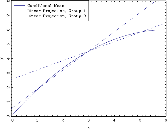
CHAPTER 2. CONDITIONAL EXPECTATION AND PROJECTION 44
Figure 2.10: Conditional Mean and Two Linear Projections
where the individual-specificcoefficient ηis random and independent of x. For example, if xis
years of schooling and is log wages, then ηis the individual-specific returns to schooling. If
a person obtains an extra year of schooling, ηis the actual change in their wage. The random
coefficient model allows the returns to schooling to vary in the population. Some individuals might
have a high return to education (a high η) and others a low return, possibly 0, or even negative.
In the linear CEF model the regressor coefficient equals the regression derivative — the change
in the conditional mean due to a change in the regressors, β=∇(x).Thisisnottheeffect on a
given individual, it is the effect on the population average. In contrast, in the random coefficient
model, the random vector η=∇(x0η)is the true causal effect — the change in the response variable
itself due to a change in the regressors.
It is interesting, however, to discover that the linear random coefficient model implies a linear
CEF. To see this, let βand Σdenote the mean and covariance matrix of η:
β=E(η)
Σ=var(η)
and then decompose the random coefficient as
η=β+u
where uis distributed independently of xwith mean zero and covariance matrix ΣThen we can
write
E(|x)=x0E(η|x)=x0E(η)=x0β
so the CEF is linear in x, and the coefficients βequal the mean of the random coefficient η.
We can thus write the equation as a linear CEF
=x0β+(2.51)
where =x0uand u=η−β. The error is conditionally mean zero:
E(|x)=0

CHAPTER 2. CONDITIONAL EXPECTATION AND PROJECTION 45
Furthermore
var (|x)=x0var (η)x
=x0Σx
so the error is conditionally heteroskedastic with its variance a quadratic function of x.
Theorem 2.28.1 In the linear random coefficient model =x0ηwith η
independent of x,Ekxk2∞and Ekηk2∞then
E(|x)=x0β
var (|x)=x0Σx
where β=E(η) Σ=var(η)
2.29 Causal Effects
So far we have avoided the concept of causality, yet often the underlying goal of an econometric
analysis is to uncover a causal relationship between variables. It is often of great interest to
understand the causes and effects of decisions, actions, and policies. For example, we may be
interested in the effect of class sizes on test scores, police expenditures on crime rates, climate
change on economic activity, years of schooling on wages, institutional structure on growth, the
effectiveness of rewards on behavior, the consequences of medical procedures for health outcomes,
or any variety of possible causal relationships. In each case, the goal is to understand what is the
actual effect on the outcome due to a change in the input We are not just interested in the
conditional mean or linear projection, we would like to know the actual change.
Two inherent barriers are that the causal effect is typically specific to an individual and that it
is unobserved.
Consider the effect of schooling on wages. The causal effect is the actual difference a person
would receive in wages if we could change their level of education holding all else constant.This
is specific to each individual as their employment outcomes in these two distinct situations is
individual. The causal effect is unobserved because the most we can observe is their actual level
of education and their actual wage, but not the counterfactual wage if their education had been
different.
To be even more specific, suppose that there are two individuals, Jennifer and George, and
both have the possibility of being high-school graduates or college graduates, but both would have
received different wages given their choices. For example, suppose that Jennifer would have earned
$10 an hour as a high-school graduate and $20 an hour as a college graduate while George would
have earned $8 as a high-school graduate and $12 as a college graduate. In this example the causal
effect of schooling is $10 a hour for Jennifer and $4 an hour for George. The causal effects are
specific to the individual and neither causal effect is observed.
Avariable1canbesaidtohaveacausaleffect on the response variable if the latter changes
when all other inputs are held constant. To make this precise we need a mathematical formulation.
We can write a full model for the response variable as
=(1x2u)(2.52)
where 1and x2are the observed variables, uis an ×1unobserved random factor, and is a
functional relationship. This framework, called the potential outcomes framework, includes as

CHAPTER 2. CONDITIONAL EXPECTATION AND PROJECTION 46
a special case the random coefficient model (2.28) studied earlier. We define the causal effect of 1
within this model as the change in due to a change in 1holding the other variables x2and u
constant.
Definition 2.29.1 In the model (2.52) the causal effect of 1on is
(1x2u)=∇1(1x2u)(2.53)
the change in due to a change in 1holding x2and uconstant.
To understand this concept, imagine taking a single individual. As far as our structural model is
concerned, this person is described by their observables 1and x2and their unobservables u.Ina
wage regression the unobservables would include characteristics such as the person’s abilities, skills,
work ethic, interpersonal connections, and preferences. The causal effect of 1(say, education) is
the change in the wage as 1changes, holding constant all other observables and unobservables.
It may be helpful to understand that (2.53) is a definition, and does not necessarily describe
causality in a fundamental or experimental sense. Perhaps it would be more appropriate to label
(2.53) as a structural effect (the effect within the structural model).
Sometimes it is useful to write this relationship as a potential outcome function
(1)=(1x2u)
where the notation implies that (1)is holding x2and uconstant.
A popular example arises in the analysis of treatment effects with a binary regressor 1.Let1=
1indicate treatment (e.g. a medical procedure) and 1=0indicate non-treatment. In this case
(1)can be written
(0) = (0x2u)
(1) = (1x2u)
Intheliteratureontreatmenteffects, it is common to refer to (0) and (1) as the latent outcomes
associated with non-treatment and treatment, respectively. That is, for a given individual, (0) is
the health outcome if there is no treatment, and (1) is the health outcome if there is treatment.
The causal effect of treatment for the individual is the change in their health outcome due to
treatment — the change in as we hold both x2and uconstant:
(x2u)=(1) −(0)
This is random (a function of x2and u) as both potential outcomes (0) and (1) are different
across individuals.
In a sample, we cannot observe both outcomes from the same individual, we only observe the
realized value
=⎧
⎨
⎩
(0) if 1=0
(1) if 1=1
As the causal effect varies across individuals and is not observable, it cannot be measured on
the individual level. We therefore focus on aggregate causal effects, in particular what is known as
the average causal effect.

CHAPTER 2. CONDITIONAL EXPECTATION AND PROJECTION 47
Definition 2.29.2 In the model (2.52) the average causal effect of 1
on conditional on x2is
(1x2)=E((1x2u)|1x2)(2.54)
=ZR
∇1(1x2u)(u|1x2)u
where (u|1x2)is the conditional density of ugiven 1x2.
We can think of the average causal effect (1x2)as the average effect in the general
population. In our Jennifer & George schooling example given earlier, supposing that half of the
population are Jennifer’s and the other half George’s, then the average causal effect of college is
(10+4)2=$7an hour. This is not the individual causal effect, it is the average of the causal effect
across all individuals in the population. Given data on only educational attainment and wages, the
ACEof$7isthebestwecanhopetolearn.
When we conduct a regression analysis (that is, consider the regression of observed wages
on educational attainment) we might hope that the regression reveals the average causal effect.
Technically, that the regression derivative (the coefficient on education) equals the ACE. Is this the
case? In other words, what is the relationship between the average causal effect (1x2)and
the regression derivative ∇1(1x2)? Equation (2.52) implies that the CEF is
(1x2)=E((1x2u)|1x2)
=ZR
(1x2u)(u|1x2)u
the average causal equation, averaged over the conditional distribution of the unobserved component
u.
Applying the marginal effect operator, the regression derivative is
∇1(1x2)=ZR
∇1(1x2u)(u|1x2)u
+ZR
(1x2u)∇1(u|1x2)u
=(1x2)+ZR
(1x2u)∇1(u|1x2)u(2.55)
Equation (2.55) shows that in general, the regression derivative does not equal the average
causal effect. The difference is the second term on the right-hand-side of (2.55). The regression
derivative and ACE equal in the special case when this term equals zero, which occurs when
∇1(u|1x2)=0that is, when the conditional density of ugiven (1x2) does not depend on
1When this condition holds then the regression derivative equals the ACE, which means that
regression analysis can be interpreted causally, in the sense that it uncovers average causal effects.
The condition is sufficiently important that it has a special name in the treatment effects
literature.
Definition 2.29.3 Conditional Independence Assumption (CIA).
Conditional on x2the random variables 1and uare statistically inde-
pendent.

CHAPTER 2. CONDITIONAL EXPECTATION AND PROJECTION 48
The CIA implies (u|1x2)=(u|x2)does not depend on 1and thus ∇1(u|1x2)=0
Thus the CIA implies that ∇1(1x2)=(1x2)the regression derivative equals the average
causal effect.
Theorem 2.29.1 In the structural model (2.52), the Conditional Indepen-
dence Assumption implies
∇1(1x2)=(1x2)
the regression derivative equals the average causal effect for 1on condi-
tional on x2.
This is a fascinating result. It shows that whenever the unobservable is independent of the
treatment variable (after conditioning on appropriate regressors) the regression derivative equals the
average causal effect. In this case, the CEF has causal economic meaning, giving strong justification
to estimation of the CEF. Our derivation also shows the critical role of the CIA. If CIA fails, then
the equality of the regression derivative and ACE fails.
This theorem is quite general. It applies equally to the treatment-effects model where 1is
binary or to more general settings where 1is continuous.
It is also helpful to understand that the CIA is weaker than full independence of ufrom the
regressors (1x2)The CIA was introduced precisely as a minimal sufficient condition to obtain
the desired result. Full independence implies the CIA and implies that each regression derivative
equals that variable’s average causal effect, but full independence is not necessary in order to
causally interpret a subset of the regressors.
To illustrate, let’s return to our education example involving a population with equal numbers
of Jennifer’s and George’s. Recall that Jennifer earns $10 as a high-school graduate and $20 as a
college graduate (and so has a causal effect of $10) while George earns $8 as a high-school graduate
and $12 as a college graduate (so has a causal effect of $4). Given this information, the average
causal effect of college is $7, which is what we hope to learn from a regression analysis.
Now suppose that while in high school all students take an aptitude test, and if a student gets
a high (H) score he or she goes to college with probability 3/4, and if a student gets a low (L)
score he or she goes to college with probability 1/4. Suppose further that Jennifer’s get an aptitude
score of H with probability 3/4, while George’s get a score of H with probability 1/4. Given this
situation, 62.5% of Jennifer’s will go to college13, while 37.5% of George’s will go to college14.
An econometrician who randomly samples 32 individuals and collects data on educational at-
tainment and wages will find the following wage distribution:
$8 $10 $12 $20 Mean
High-School Graduate 10 6 0 0 $8.75
College Graduate 0 0 6 10 $17.00
Let -- denote a dummy variable taking the value of 1 for a college graduate, otherwise 0.
Thus the regression of wages on college attendance takes the form
E( |--)=825-- +875
The coefficient on the college dummy, $8.25, is the regression derivative, and the implied wage effect
of college attendance. But $8.25 overstates the average causal effect of $7. The reason is because
13Pr (--|)=Pr(--|)Pr(|)+Pr(--|)Pr(|)=(34)2+(14)2
14Pr (--|)=Pr(--|)Pr(|)+Pr(--|)Pr(|)=(34)(14) + (14)(34)
CHAPTER 2. CONDITIONAL EXPECTATION AND PROJECTION 49
the CIA fails. In this model the unobservable uis the individual’s type (Jennifer or George) which
is not independent of the regressor 1(education), since Jennifer is more likely to go to college than
George. Since Jennifer’s causal effect is higher than George’s, the regression derivative overstates
the ACE. The coefficient $8.25 is not the average benefit of college attendance, rather it is the
observed difference in realized wages in a population whose decision to attend college is correlated
with their individual causal effect. At the risk of repeating myself, in this example, $8.25 is the true
regression derivative, it is the difference in average wages between those with a college education and
those without. It is not, however, the average causal effect of college education in the population.
This does not mean that it is impossible to estimate the ACE. The key is conditioning on the
appropriate variables. The CIA says that we need to find a variable 2such that conditional on
2uand 1(type and education) are independent. In this example a variable which will achieve
this is the aptitude test score. The decision to attend college was based on the test score, not on
an individual’s type. Thus educational attainment and type are independent once we condition on
the test score.
This also alters the ACE. Notice that Definition 2.29.2 is a function of 2(the test score).
Among the students who receive a high test score, 3/4 are Jennifer’s and 1/4 are George’s. Thus
the ACE for students with a score of H is (34) ×10 + (14) ×4=$850Among the students who
receive a low test score, 1/4 are Jennifer’s and 3/4 are George’s. Thus the ACE for students with
ascoreofLis(14) ×10 + (34) ×4=$550The ACE varies between these two observable groups
(those with high test scores and those with low test scores). Again, we would hope to be able to
learn the ACE from a regression analysis, this time from a regression of wages on education and
test scores.
To see this in the wage distribution, suppose that the econometrician collects data on the
aptitude test score as well as education and wages. Given a random sample of 32 individuals we
would expect to find the following wage distribution:
$8 $10 $12 $20 Mean
High-School Graduate + High Test Score 1 3 0 0 $9.50
CollegeGraduate+HighTestScore 0039$18.00
High-School Graduate + Low Test Score 9 3 0 0 $8.50
CollegeGraduate+LowTestScore 0031$14.00
Define the dummy variable which takes the value 1 for students who received a
high test score, else zero. The regression of wages on college attendance and test scores (with
interactions) takes the form
E( |-- )=100 +550-- +300 ×-- +850
The coefficient on --, $5.50, is the regression derivative of college attendance for those with low
test scores, and the sum of this coefficient with the interaction coefficient, $8.50, is the regression
derivative for college attendance for those with high test scores. These equal the average causal
effect as calculated above. Furthermore, since 1/2 of the population achieves a high test score and
1/2 achieve a low test score, the measured average causal effect in the entire population is $7, which
precisely equals the true value.
In this example, by conditioning on the aptitude test score, the average causal effect of education
on wages can be learned from a regression analysis. What this shows is that by conditioning on the
proper variables, it may be possible to achieve the CIA, in which case regression analysis measures
average causal effects.

CHAPTER 2. CONDITIONAL EXPECTATION AND PROJECTION 50
2.30 Expectation: Mathematical Details*
We define the mean or expectation E()of a random variable as follows. If is discrete
on the set {1
2}then
E()= ∞
X
=1
Pr (=)
and if is continuous with density then
E()=Z∞
−∞
()
We can unify these definitions by writing the expectation as the Lebesgue integral with respect to
the distribution function
E()=Z∞
−∞
()(2.56)
In the event that the integral (2.56) is not finite, separately evaluate the two integrals
1=Z∞
0
()(2.57)
2=−Z0
−∞
()(2.58)
If 1=∞and 2∞then it is typical to define E()=∞If 1∞and 2=∞then we define
E()=−∞However, if both 1=∞and 2=∞then E()is undefined. If
E||=Z∞
−∞
|| ()=1+2∞
then E()exists and is finite. In this case it is common to say that the mean E()is “well-defined”.
More generally, has a finite moment if
E||∞(2.59)
By Liapunov’s Inequality (B.13), (2.59) implies E||∞for all 1≤≤ Thus, for example, if
the fourth moment is finite then the first, second and third moments are also finite, and so is the
39 moment.
It is common in econometric theory to assume that the variables, or certain transformations of
the variables, have finite moments of a certain order. How should we interpret this assumption?
How restrictive is it?
One way to visualize the importance is to consider the class of Pareto densities given by
()=−−11
The parameter of the Pareto distribution indexes the rate of decay of the tail of the density.
Larger means that the tail declines to zero more quickly. See Figure 2.11 below where we plot
the Pareto density for =1and =2The parameter also determines which moments are finite.
We can calculate that
E||=⎧
⎪
⎨
⎪
⎩
R∞
1−−1 =
−if
∞if ≥
This shows that if is Pareto distributed with parameter then the moment of is finite if
andonlyifHigher means higher finite moments. Equivalently, the faster the tail of the
density declines to zero, the more moments are finite.
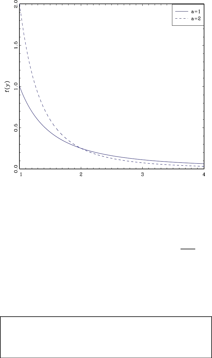
CHAPTER 2. CONDITIONAL EXPECTATION AND PROJECTION 51
Figure 2.11: Pareto Densities, =1and =2
This connection between tail decay and finite moments is not limited to the Pareto distribution.
We can make a similar analysis using a tail bound. Suppose that has density ()which satisfies
the bound ()≤||−−1for some ∞and 0.Since()is bounded below a scale of a
Pareto density, its tail behavior is similarly bounded. This means that for
E||=Z∞
−∞
||() ≤Z1
−1
() +2Z∞
1
−−1 ≤1+ 2
−∞
Thus if the tail of the density declines at the rate ||−−1or faster, then has finite moments up
to (but not including) Broadly speaking, the restriction that has a finite moment means
that the tail of ’s density declines to zero faster than −−1The faster decline of the tail means
that the probability of observing an extreme value of is a more rare event.
We complete this section by adding an alternative representation of expectation in terms of the
distribution function.
Theorem 2.30.1 For any non-negative random variable
E()=Z∞
0
Pr ()
ProofofTheorem2.30.1:Let ∗()=Pr()=1−(),where()is the distribution
function. By integration by parts
E()=Z∞
0
()=−Z∞
0
∗()=−[∗()]∞
0+Z∞
0
∗() =Z∞
0
Pr ()
as stated. ¥

CHAPTER 2. CONDITIONAL EXPECTATION AND PROJECTION 52
2.31 Moment Generating and Characteristic Functions*
For a random variable with distribution its moment generating function (MGF) is
()=E(exp ()) = Zexp() ()(2.60)
This is also known as the Laplace transformation of the density of . The MGF is a function of
the argument , and is an alternative representation of the distribution .Itiscalledthemoment
generating function since the derivative evaluated at zero is the uncentered moment. Indeed,
()()=Eµ
exp()¶=E(exp ())
and thus the derivative at =0is
()(0) = E()
A major limitation with the MGF is that it does not exist for many random variables. Essen-
tially, existence of the integral (2.60) requires the tail of the density of to decline exponentially.
This excludes thick-tailed distributions such as the Pareto.
This limitation is removed if we consider the characteristic function (CF) of ,whichis
defined as
()=E(exp (i)) = Zexp(i) ()
where i=√−1. Like the MGF, the CF is a function of its argument and is a representation of
the distribution function . The CF is also known as the Fourier transformation of the density
of . Unlike the MGF, the CF exists for all random variables and all values of since exp (i)=
cos ()+isin()is bounded.
Similarly to the MGF, the derivative of the characteristic function evaluated at zero takes
the simple form
()(0) = iE()(2.61)
when such expectations exist. A further connection is that the moment is finite if and only if
()()is continuous at zero.
For random vectors zwith distribution we define the multivariate MGF as
(t)=E¡exp ¡t0z¢¢=Zexp(t0z) (z)(2.62)
when it exists. Similarly, we define the multivariate CF as
(t)=E¡exp ¡it0z¢¢=Zexp(it0z) (z)
2.32 Existence and Uniqueness of the Conditional Expectation*
In Sections 2.3 and 2.6 we defined the conditional mean when the conditioning variables xare
discrete and when the variables ( x)have a joint density. We have explored these cases because
these are the situations where the conditional mean is easiest to describe and understand. However,
the conditional mean exists quite generally without appealing to the properties of either discrete
or continuous random variables.
To justify this claim we now present a deep result from probability theory. What it says is that
the conditional mean exists for all joint distributions ( x)for which has a finite mean.

CHAPTER 2. CONDITIONAL EXPECTATION AND PROJECTION 53
Theorem 2.32.1 Existence of the Conditional Mean
If E||∞then there exists a function (x)such that for all sets Xfor
which Pr (x∈X)is defined,
E(1 (x∈X))=E(1 (x∈X)(x)) (2.63)
The function (x)is almost everywhere unique, in the sense that if (x)
satisfies (2.63), then there is a set such that Pr()=1and (x)=(x)
for x∈ The function (x)is called the conditional mean and is
written (x)=E(|x)
See, for example, Ash (1972), Theorem 6.3.3.
The conditional mean (x)defined by (2.63) specializes to (2.7) when ( x)have a joint density.
The usefulness of definition (2.63) is that Theorem 2.32.1 shows that the conditional mean (x)
exists for all finite-mean distributions. This definition allows to be discrete or continuous, for xto
be scalar or vector-valued, and for the components of xto be discrete or continuously distributed.
You may have noticed that Theorem 2.32.1 applies only to sets Xfor which Pr (x∈X)is
defined. This is a technical issue —measurability — which we largely side-step in this textbook.
Formal probability theory only applies to sets which are measurable — for which probabilities are
defined, as it turns out that not all sets satisfy measurability. This is not a practical concern for
econometrics, so we defer such distinctions for formal theoretical treatments.
2.33 Identification*
A critical and important issue in structural econometric modeling is identification, meaning that
a parameter is uniquely determined by the distribution of the observed variables. It is relatively
straightforward in the context of the unconditional and conditional mean, but it is worthwhile to
introduce and explore the concept at this point for clarity.
Let denote the distribution of the observed data, for example the distribution of the pair
( )Let Fbe a collection of distributions Let be a parameter of interest (for example, the
mean E()).
Definition 2.33.1 A parameter ∈Ris identified on Fif for all ∈F
there is a uniquely determined value of
Equivalently, is identified if we can write it as a mapping =()on the set FThe restriction
to the set Fis important. Most parameters are identified only on a strict subset of the space of all
distributions.
Take, for example, the mean =E()It is uniquely determined if E||∞so it is clear
that is identified for the set F=n:R∞
−∞ || ()∞o.However,is also well defined when
it is either positive or negative infinity. Hence, defining 1and 2as in (2.57) and (2.58), we can
deduce that is identified on the set F={:{1∞}∪{2∞}}
Next, consider the conditional mean. Theorem 2.32.1 demonstrates that E||∞is a sufficient
condition for identification.

CHAPTER 2. CONDITIONAL EXPECTATION AND PROJECTION 54
Theorem 2.33.1 Identification of the Conditional Mean
If E||∞the conditional mean (x)=E(|x)is identified almost
everywhere.
It might seem as if identification is a general property for parameters, so long as we exclude
degenerate cases. This is true for moments of observed data, but not necessarily for more compli-
cated models. As a case in point, consider the context of censoring. Let be a random variable
with distribution Instead of observing we observe ∗defined by the censoring rule
∗=½if ≤
if
That is, ∗is capped at the value A common example is income surveys, where income responses
are “top-coded”, meaning that incomes above the top code are recorded as the top code. The
observed variable ∗has distribution
∗()=½()for ≤
1for ≥
We are interested in features of the distribution not the censored distribution ∗For example,
we are interested in the mean wage =E()The difficultyisthatwecannotcalculatefrom
∗except in the trivial case where there is no censoring Pr (≥)=0Thus the mean is not
generically identified from the censored distribution.
A typical solution to the identification problem is to assume a parametric distribution. For
example, let Fbe the set of normal distributions ∼N( 2)It is possible to show that the
parameters ( 2)are identified for all ∈FThat is, if we know that the uncensored distribution
is normal, we can uniquely determine the parameters from the censored distribution. This is often
called parametric identification as identification is restricted to a parametric class of distribu-
tions. In modern econometrics this is generally viewed as a second-best solution, as identification
has been achieved only through the use of an arbitrary and unverifiable parametric assumption.
A pessimistic conclusion might be that it is impossible to identify parameters of interest from
censored data without parametric assumptions. Interestingly, this pessimism is unwarranted. It
turns out that we can identify the quantiles of for ≤Pr (≤)For example, if 20%
of the distribution is censored, we can identify all quantiles for ∈(008)This is often called
nonparametric identification as the parameters are identified without restriction to a parametric
class.
What we have learned from this little exercise is that in the context of censored data, moments
can only be parametrically identified, while non-censored quantiles are nonparametrically identified.
Part of the message is that a study of identification can help focus attention on what can be learned
from the data distributions available.
2.34 Technical Proofs*
Proof of Theorem 2.7.1: For convenience, assume that the variables have a joint density ( x).
Since E(|x)is a function of the random vector xonly, to calculate its expectation we integrate
with respect to the density (x)of xthat is
E(E(|x)) = ZR
E(|x)(x)x

CHAPTER 2. CONDITIONAL EXPECTATION AND PROJECTION 55
Substituting in (2.7) and noting that |(|x)(x)=( x)we find that the above expression
equals ZRµZR
|(|x)¶(x)x=ZRZR
( x)x=E()
the unconditional mean of ¥
ProofofTheorem2.7.2: Again assume that the variables have a joint density. It is useful to
observe that
(|x1x2)(x2|x1)=( x1x2)
(x1x2)
(x1x2)
(x1)=( x2|x1)(2.64)
the density of ( x2)given x1Here, we have abused notation and used a single symbol to denote
the various unconditional and conditional densities to reduce notational clutter.
Note that
E(|x1x2)=ZR
(|x1x2) (2.65)
Integrating (2.65) with respect to the conditional density of x2given x1, and applying (2.64) we
find that
E(E(|x1x2)|x1)=ZR2
E(|x1x2)(x2|x1)x2
=ZR2µZR
(|x1x2)¶(x2|x1)x2
=ZR2ZR
(|x1x2)(x2|x1)x2
=ZR2ZR
( x2|x1)x2
=E(|x1)
as stated. ¥
ProofofTheorem2.7.3:
E((x)|x)=ZR
(x)|(|x) =(x)ZR
|(|x) =(x)E(|x)
This is (2.8). Equation (2.10) follows by applying the Simple Law of Iterated Expectations to (2.8).
¥
ProofofTheorem2.8.1. Applying Minkowski’s Inequality (B.12) to =−(x)
(E||)1 =(E|−(x)|)1 ≤(E||)1 +(E|(x)|)1 ∞
where the two parts on the right-hand are finite since E||∞by assumption and E|(x)|∞
by the Conditional Expectation Inequality (B.7). The fact that (E||)1 ∞implies E||
∞¥
ProofofTheorem2.10.2: The assumption that E¡2¢∞implies that all the conditional
expectations below exist.
Using the law of iterated expectations E(|x1)=E(E(|x1x2)|x1)and the conditional
Jensen’s inequality (B.6),
(E(|x1))2=(E(E(|x1x2)|x1))2≤E³(E(|x1x2))2|x1´
CHAPTER 2. CONDITIONAL EXPECTATION AND PROJECTION 56
Taking unconditional expectations, this implies
E³(E(|x1))2´≤E³(E(|x1x2))2´
Similarly,
(E())2≤E³(E(|x1))2´≤E³(E(|x1x2))2´(2.66)
The variables E(|x1)and E(|x1x2)all have the same mean E()so the inequality
(2.66) implies that the variances are ranked monotonically:
0≤var (E(|x1)) ≤var (E(|x1x2)) (2.67)
Define =−E(|x)and =E(|x)−so that we have the decomposition
−=+
Notice E(|x)=0and is a function of x. Thus by the Conditioning Theorem, E()=0so
and are uncorrelated. It follows that
var ()=var()+var()=var(−E(|x)) + var (E(|x)) (2.68)
The monotonicity of the variances of the conditional mean (2.67) applied to the variance decom-
position (2.68) implies the reverse monotonicity of the variances of the differences, completing the
proof. ¥
ProofofTheorem2.18.1. For part 1, by the Expectation Inequality (B.8), (A.24) and Assump-
tion 2.18.1, °
°E¡xx0¢°
°≤E°
°xx0°
°=E³kxk2´∞
Similarly, using the Expectation Inequality (B.8), the Cauchy-Schwarz Inequality (B.10) and As-
sumption 2.18.1,
kE(x)k≤Ekxk≤³E³kxk2´´12¡E¡2¢¢12∞
Thus the moments E(x)and E(xx0)are finite and well defined.
For part 2, the coefficient β=(E(xx0))−1E(x)is well defined since (E(xx0))−1exists under
Assumption 2.18.1.
Part 3 follows from Definition 2.18.1 and part 2.
For part 4, first note that
E¡2¢=E³¡−x0β¢2´
=E¡2¢−2E¡x0¢β+β0E¡xx0¢β
=E¡2¢−2E¡x0¢¡E¡xx0¢¢−1E(x)
≤E¡2¢
∞
The first inequality holds because E(x0)(E(xx0))−1E(x)is a quadratic form and therefore nec-
essarily non-negative. Second, by the Expectation Inequality (B.8), the Cauchy-Schwarz Inequality
(B.10) and Assumption 2.18.1,
kE(x)k≤Ekxk=³E³kxk2´´12¡E¡2¢¢12∞
It follows that the expectation E(x)is finite, and is zero by the calculation (2.28).
CHAPTER 2. CONDITIONAL EXPECTATION AND PROJECTION 57
For part 6, Applying Minkowski’s Inequality (B.12) to =−x0β
(E||)1 =¡E¯¯−x0β¯¯¢1
≤(E||)1 +¡E¯¯x0β¯¯¢1
≤(E||)1 +(Ekxk)1 kβk
∞
the final inequality by assumption¥

CHAPTER 2. CONDITIONAL EXPECTATION AND PROJECTION 58
Exercises
Exercise 2.1 Find E(E(E(|x1x2x3)|x1x2)|x1)
Exercise 2.2 If E(|)=+ find E()as a function of moments of
Exercise 2.3 Prove Theorem 2.8.1.4 using the law of iterated expectations.
Exercise 2.4 Suppose that the random variables and only take the values 0and 1, and have
the following joint probability distribution
=0 =1
=0 .1 .2
=1 .4 .3
Find E(|)E¡2|¢and var (|)for =0and =1
Exercise 2.5 Show that 2(x)is the best predictor of 2given x:
(a) Write down the mean-squared error of a predictor (x)for 2
(b) What does it mean to be predicting 2?
(c) Show that 2(x)minimizes the mean-squared error and is thus the best predictor.
Exercise 2.6 Use =(x)+to show that
var ()=var((x)) + 2
Exercise 2.7 Show that the conditional variance can be written as
2(x)=E¡2|x¢−(E(|x))2
Exercise 2.8 Suppose that is discrete-valued, taking values only on the non-negative integers,
and the conditional distribution of given xis Poisson:
Pr (=|x)=exp (−x0β)(x0β)
!=012
Compute E(|x)and var (|x)Does this justify a linear regression model of the form =
x0β+?
Hint: If Pr (=)=exp(−)
!then E()=and var()=
Exercise 2.9 Suppose you have two regressors: 1is binary (takes values 0 and 1) and 2is
categorical with 3 categories ( )Write E(|1
2)as a linear regression.
Exercise 2.10 True or False. If = + ∈Rand E(|)=0then E¡2¢=0
Exercise 2.11 True or False. If = + ∈Rand E()=0then E¡2¢=0
Exercise 2.12 True or False. If =x0β+and E(|x)=0then is independent of x
Exercise 2.13 True or False. If =x0β+and E(x)=0then E(|x)=0

CHAPTER 2. CONDITIONAL EXPECTATION AND PROJECTION 59
Exercise 2.14 True or False. If =x0β+,E(|x)=0and E¡2|x¢=2a constant, then
is independent of x
Exercise 2.15 Consider the intercept-only model =+defined as the best linear predictor.
Show that =E()
Exercise 2.16 Let and have the joint density ( )=3
2¡2+2¢on 0≤≤10≤≤1
Compute the coefficients of the best linear predictor =++ Compute the conditional mean
()=E(|)Are the best linear predictor and conditional mean different?
Exercise 2.17 Let be a random variable with =E()and 2=var()Define
¡| 2¢=µ−
(−)2−2
Show that E(| )=0ifandonlyif=and =2
Exercise 2.18 Suppose that
x=⎛
⎝
1
2
3
⎞
⎠
and 3=1+22is a linear function of 2
(a) Show that Q =E(xx0)is not invertible.
(b) Use a linear transformation of xto find an expression for the best linear predictor of given
x. (Be explicit, do not just use the generalized inverse formula.)
Exercise 2.19 Show (2.46)-(2.47), namely that for
(β)=E¡(x)−x0β¢2
then
β=argmin
∈R
(b)
=¡E¡xx0¢¢−1E(x(x))
=¡E¡xx0¢¢−1E(x)
Hint: To show E(x(x)) = E(x)use the law of iterated expectations.
Exercise 2.20 Verify that (2.63) holds with (x)definedin(2.7)when( x)have a joint density
( x)
Exercise 2.21 Consider the short and long projections
=1+
=1+22+
(a) Under what condition does 1=1?
(b) Now suppose the long projection is
=1+32+
Is there a similar condition under which 1=1?
CHAPTER 2. CONDITIONAL EXPECTATION AND PROJECTION 60
Exercise 2.22 Take the homoskedastic model
=x0
1β1+x0
22+
E(|x1x2)=0
E¡2|x1x2¢=2
E(x2|x1)=Γx1
Γ6=0
Suppose the parameter β1is of interest. We know that the exclusion of x2creates omited variable
bias in the projection coefficient on x2It also changes the equation error. Our question is: what
is the effect on the homoskedasticity property of the induced equation error? Does the exclusion of
x2induce heteroskedasticity or not? Be specific.

Chapter 3
The Algebra of Least Squares
3.1 Introduction
In this chapter we introduce the popular least-squares estimator. Most of the discussion will be
algebraic, with questions of distribution and inference deferred to later chapters.
3.2 Samples
In Section 2.18 we derived and discussed the best linear predictor of given xfor a pair of
random variables ( x)∈R×Rand called this the linear projection model. We are now interested
in estimating the parameters of this model, in particular the projection coefficient
β=¡E¡xx0¢¢−1E(x)(3.1)
We can estimate βfrom observational data which includes joint measurements on the variables
( x)For example, supposing we are interested in estimating a wage equation, we would use
a dataset with observations on wages (or weekly earnings), education, experience (or age), and
demographic characteristics (gender, race, location). One possible dataset is the Current Popula-
tion Survey (CPS), a survey of U.S. households which includes questions on employment, income,
education, and demographic characteristics.
Notationally we wish to distinguish observations from the underlying random variables. The
convention in econometrics is to denote observations by appending a subscript which runs from
1to thus the observation is (x)and denotes the sample size. The dataset is then
{(x); =1}. We call this the sample or the observations.
From the viewpoint of empirical analysis, a dataset is an array of numbers often organized as
a table, where the columns of the table correspond to distinct variables and the rows correspond
to distinct observations. For empirical analysis, the dataset and observations are fixedinthesense
that they are numbers presented to the researcher. For statistical analysis we need to view the
dataset as random, or more precisely as a realization of a random process.
In order for the coefficient βdefinedin(3.1)tomakesenseasdefined, the expectations over the
random variables (x)need to be common across the observations. The most elegant approach to
ensure this is to assume that the observations are draws from an identical underlying population
This is the standard assumption that the observations are identically distributed:
Assumption 3.2.1 The observations {(1x1)(x)(x)}are
identically distributed; they are draws from a common distribution .
61

CHAPTER 3. THE ALGEBRA OF LEAST SQUARES 62
This assumption does not need to be viewed as literally true, rather it is a useful modeling
device so that parameters such as βare well defined. This assumption should be interpreted as
howweviewanobservationapriori,beforeweactuallyobserveit. IfItellyouthatwehave
asamplewith=59observations set in no particular order, then it makes sense to view two
observations, say 17 and 58, as draws from the same distribution. We have no reason to expect
anything special about either observation.
In econometric theory, we refer to the underlying common distribution as the population.
Some authors prefer the label the data-generating-process (DGP). You can think of it as a the-
oretical concept or an infinitely-large potential population. In contrast we refer to the observations
available to us {(x); =1}asthesample or dataset. In some contexts the dataset con-
sists of all potential observations, for example administrative tax records may contain every single
taxpayer in a political unit. Even in this case we view the observations as if they are random draws
from an underlying infinitely-large population, as this will allow us to apply the tools of statistical
theory.
The linear projection model applies to the random observations (x)This means that the
probability model for the observations is the same as that described in Section 2.18. We can write
the model as
=x0
β+(3.2)
where the linear projection coefficient βis defined as
β=argmin
∈R
(b)(3.3)
the minimizer of the expected squared error
(β)=E³¡−x0
β¢2´(3.4)
and has the explicit solution
β=¡E¡xx0
¢¢−1E(x)(3.5)
3.3 Moment Estimators
We want to estimate the coefficient βdefined in (3.5) from the sample of observations. Notice
that βis written as a function of certain population expectations. In this context an appropriate
estimator is the same function of the sample moments. Let’s explain this in detail.
To start, suppose that we are interested in the population mean of a random variable with
distribution function
=E()=Z∞
−∞
()(3.6)
The mean is a function of the distribution as written in (3.6). To estimate given a sample
{1
}a natural estimator is the sample mean
b==1
X
=1
Notice that we have written this using two pieces of notation. The notation with the bar on top
is conventional for a sample mean. The notation bwith the hat “^” is conventional in econometrics
to denote an estimator of the parameter . In this case, the sample mean of is the estimator of ,
so band are the same. The sample mean can be viewed as the natural analog of the population
mean (3.6) because equals the expectation (3.6) with respect to the empirical distribution —
the discrete distribution which puts weight 1 on each observation . There are many other
justifications for as an estimator for , we will defer these discussions for now. Suffice it to say

CHAPTER 3. THE ALGEBRA OF LEAST SQUARES 63
that it is the conventional estimator in the lack of other information about or the distribution of
.
Now suppose that we are interested in a set of population means of possibly non-linear functions
of a random vector y,sayμ=E(h(y)). For example, we may be interested in the first two moments
of ,E()and E(2
). In this case the natural estimator is the vector of sample means,
b
μ=1
X
=1
h(y)
For example, b1=1
P
=1 and b2=1
P
=1 2
. This is not really a substantive change. We call
b
μthe moment estimator for μ
Now suppose that we are interested in a nonlinear function of a set of moments. For example,
consider the variance of
2=var()=E(2
)−(E())2
In general, many parameters of interest, say β, can be written as a function of moments of y.
Notationally,
β=g(μ)
μ=E(h(y))
Here, yare the random variables, h(y)are functions (transformations) of the random variables,
and μis the mean (expectation) of these functions. βis the parameter of interest, and is the
(nonlinear) function g(·)of these means.
In this context a natural estimator of βis obtained by replacing μwith b
μ.
b
β=g(b
μ)
b
μ=1
X
=1
h(y)
The estimator b
βis often called a “plug-in” estimator, and sometimes a “substitution” estimator.
We typically call b
βa moment, or moment-based, estimator of β, since it is a natural extension of
the moment estimator b
μ.
Take the example of the variance 2=var(). Its moment estimator is
b2=b2−b2
1=1
X
=1
2
−Ã1
X
=1
!2
This is not the only possible estimator for 2(there is the well-known bias-corrected version ap-
propriate for independent observations) but it a straightforward and simple choice.
3.4 Least Squares Estimator
The linear projection coefficient βis defined in (3.3) as the minimizer of the expected squared
error (β)defined in (3.4). For given β, the expected squared error is the expectation of the
squared error (−x0
β)2The moment estimator of (β)is the sample average:
b
(β)= 1
X
=1 ¡−x0
β¢2(3.7)
=1
(β)
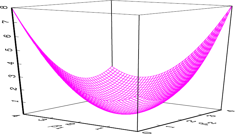
CHAPTER 3. THE ALGEBRA OF LEAST SQUARES 64
Figure 3.1: Sum-of-Squared Errors Function
where
(β)=
X
=1 ¡−x0
β¢2(3.8)
is called the sum-of-squared-errors function.
Since b
(β)is a sample average, we can interpret it as an estimator of the expected squared
error (β). Examining b
(β)as a function of βis informative about how (β)varies with βSince
the projection coefficient minimizes (β)an analog estimator minimizes (3.7):
b
β=argmin
∈Rb
(β)
Alternatively, as b
(β)is a scale multiple of (β)we may equivalently define b
βas the minimizer
of (β)Hence b
βis commonly called the least-squares (LS) estimator of β. (The estimator
is also commonly refered to as the ordinary least-squares OLS estimator. For the origin of
this label see the historical discussion on Adrien-Marie Legendre below.) Here, as is common in
econometrics, we put a hat “^” over the parameter βto indicate that b
βis a sample estimate of β
This is a helpful convention. Just by seeing the symbol b
βwe can immediately interpret it as an
estimator (because of the hat) of the parameter β. Sometimes when we want to be explicit about
the estimation method, we will write b
βols to signify that it is the OLS estimator. It is also common
to see the notation b
βwhere the subscript “” indicates that the estimator depends on the sample
size
It is important to understand the distinction between population parameters such as βand
sample estimates such as b
β. The population parameter βis a non-random feature of the population
while the sample estimate b
βis a random feature of a random sample. βis fixed, while b
βvaries
across samples.
To visualize the quadratic function b
(β), Figure 3.1 displays an example sum-of-squared errors
function (β)for the case =2The least-squares estimator b
βis the the pair (b
1b
2)which
minimize this function.

CHAPTER 3. THE ALGEBRA OF LEAST SQUARES 65
3.5 Solving for Least Squares with One Regressor
For simplicity, we start by considering the case =1so that the coefficient is a scalar. Then
the sum of squared errors is a simple quadratic
()=
X
=1
(−)2
=Ã
X
=1
2
!−2Ã
X
=1
!+2Ã
X
=1
2
!
The OLS estimator b
minimizes this function. From elementary algebra we know that the minimizer
of the quadratic function −2 +2is = Thus the minimizer of ()is
b
=P
=1
P
=1 2
(3.9)
The intercept-only model is the special case =1In this case we find
b
=P
=1 1
P
=1 12=1
X
=1
= (3.10)
thesamplemeanofHere, as is common, we put a bar “−”overto indicate that the quantity
is a sample mean. This calculation shows that the OLS estimator in the intercept-only model is
thesamplemean.
3.6 Solving for Least Squares with Multiple Regressors
We now consider the case with ≥1so that the coefficient βis a vector.
To solve for b
β, expand the SSE function to find
(β)=
X
=1
2
−2β0
X
=1
x+β0
X
=1
xx0
β
This is a quadratic expression in the vector argument β.Thefirst-order-condition for minimization
of (β)is
0=
β(b
β)=−2
X
=1
x+2
X
=1
xx0
b
β(3.11)
We have written this using a single expression, but it is actually a system of equations with
unknowns (the elements of b
β).
The solution for b
βmay be found by solving the system of equations in (3.11). We can write
this solution compactly using matrix algebra. Inverting the ×matrix P
=1 xx0
we find an
explicit formula for the least-squares estimator
b
β=Ã
X
=1
xx0
!−1Ã
X
=1
x!(3.12)
This is the natural estimator of the best linear projection coefficient βdefinedin(3.3),andcan
also be called the linear projection estimator.
We see that (3.12) simplifies to the expression (3.9) when =1The expression (3.12) is a
notationally simple generalization but requires a careful attention to vector and matrix manipula-
tions.

CHAPTER 3. THE ALGEBRA OF LEAST SQUARES 66
Alternatively, equation (3.5) writes the projection coefficient βas an explicit function of the
population moments Q and QTheir moment estimators are the sample moments
b
Q=1
X
=1
x
b
Q =1
X
=1
xx0
The moment estimator of βreplaces the population moments in (3.5) with the sample moments:
b
β=b
Q−1
b
Q
=Ã1
X
=1
xx0
!−1Ã1
X
=1
x!
=Ã
X
=1
xx0
!−1Ã
X
=1
x!
which is identical with (3.12).
Least Squares Estimation
Definition 3.6.1 The least-squares estimator b
βis
b
β=argmin
∈Rb
(β)
where
b
(β)= 1
X
=1 ¡−x0
β¢2
and has the solution
b
β=Ã
X
=1
xx0
!−1Ã
X
=1
x!

CHAPTER 3. THE ALGEBRA OF LEAST SQUARES 67
Adrien-Marie Legendre
The method of least-squares was first published in 1805 by the French math-
ematician Adrien-Marie Legendre (1752-1833). Legendre proposed least-
squares as a solution to the algebraic problem of solving a system of equa-
tions when the number of equations exceeded the number of unknowns. This
was a vexing and common problem in astronomical measurement. As viewed
byLegendre,(3.2)isasetofequations with unknowns. As the equations
cannot be solved exactly, Legendre’s goal was to select βto make the set of
errors as small as possible. He proposed the sum of squared error criterion,
and derived the algebraic solution presented above. As he noted, the first-
order conditions (3.11) is a system of equations with unknowns, which
can be solved by “ordinary” methods. Hence the method became known
as Ordinary Least Squares and to this day we still use the abbreviation
OLS to refer to Legendre’s estimation method.
3.7 Illustration
We illustrate the least-squares estimator in practice with the data set used to calculate the
estimates reported in Chapter 2. This is the March 2009 Current Population Survey, which has
extensive information on the U.S. population. This data set is described in more detail in Section
3.19. For this illustration, we use the sub-sample of married (spouse present) black female wage
earners with 12 years potential work experience. This sub-sample has 20 observations. Let be
log wages and xbe years of education and an intercept. Then
X
=1
x=µ99586
6264 
X
=1
xx0
=µ5010 314
314 20 
and Ã
X
=1
xx0
!−1
=µ00125 −0196
−0196 3124 
Thus
b
β=µ00125 −0196
−0196 3124 ¶µ99586
6264 
=µ0155
0698 ¶(3.13)
We often write the estimated equation using the format
\
log()=0155 +0698(3.14)
An interpretation of the estimated equation is that each year of education is associated with a 16%
increase in mean wages.
Equation (3.14) is called a bivariate regression as there are only two variables. A multivari-
ate regression has two or more regressors, and allows a more detailed investigation. Let’s take

CHAPTER 3. THE ALGEBRA OF LEAST SQUARES 68
an example similar to (3.14) but include all levels of experience. This time, we use the sub-sample
of single (never married) Asian men, which has 268 observations. Including as regressors years
of potential work experience (experience) and its square (experience2100) (we divide by 100 to
simplify reporting), we obtain the estimates
\
log()=0143 +0036 −0071 2100 + 0575(3.15)
These estimates suggest a 14% increase in mean wages per year of education, holding experience
constant.
3.8 Least Squares Residuals
As a by-product of estimation, we define the fitted value
b=x0
b
β
and the residual
b=−b=−x0
b
β(3.16)
Sometimes bis called the predicted value, but this is a misleading label. The fitted value bis a
function of the entire sample, including , and thus cannot be interpreted as a valid prediction of
. It is thus more accurate to describe bas a fitted rather than a predicted value.
Note that =b+band
=x0
b
β+b(3.17)
We make a distinction between the error and the residual bThe error is unobservable while
the residual bis a by-product of estimation. These two variables are frequently mislabeled, which
can cause confusion.
Equation (3.11) implies that
X
=1
xb=0(3.18)
To see this by a direct calculation, using (3.16) and (3.12),
X
=1
xb=
X
=1
x³−x0
b
β´
=
X
=1
x−
X
=1
xx0
b
β
=
X
=1
x−
X
=1
xx0
Ã
X
=1
xx0
!−1Ã
X
=1
x!
=
X
=1
x−
X
=1
x
=0
When xcontains a constant, an implication of (3.18) is
1
X
=1 b=0(3.19)
Thus the residuals have a sample mean of zero and the sample correlation between the regressors
and the residual is zero. These are algebraic results, and hold true for all linear regression estimates.

CHAPTER 3. THE ALGEBRA OF LEAST SQUARES 69
3.9 Demeaned Regressors
Sometimes it is useful to separate the constant from the other regressors, and write the linear
projection equation in the format
=x0
β++
where is the intercept and xdoes not contain a constant. The least-squares estimates and
residuals can be written as
=x0
b
β+b+b
In this case (3.18) can be written as the equation system
X
=1 ³−x0
b
β−b´=0
X
=1
x³−x0
b
β−b´=0
The first equation implies
b=−x0b
β
Subtracting from the second we obtain
X
=1
x³(−)−(x−x)0b
β´=0
Solving for b
βwe find
b
β=Ã
X
=1
x(x−x)0!−1Ã
X
=1
x(−)!
=Ã
X
=1
(x−x)(x−x)0!−1Ã
X
=1
(x−x)(−)!(3.20)
Thus the OLS estimator for the slope coefficients is a regression with demeaned data.
The representation (3.20) is known as the demeaned formula for the least-squares estimator.
3.10 Model in Matrix Notation
For many purposes, including computation, it is convenient to write the model and statistics in
matrix notation. The linear equation (2.26) is a system of equations, one for each observation.
We can stack these equations together as
1=x0
1β+1
2=x0
2β+2
.
.
.
=x0
β+
Now define
y=⎛
⎜
⎜
⎜
⎝
1
2
.
.
.
⎞
⎟
⎟
⎟
⎠X=⎛
⎜
⎜
⎜
⎝
x0
1
x0
2
.
.
.
x0
⎞
⎟
⎟
⎟
⎠e=⎛
⎜
⎜
⎜
⎝
1
2
.
.
.
⎞
⎟
⎟
⎟
⎠

CHAPTER 3. THE ALGEBRA OF LEAST SQUARES 70
Observe that yand eare ×1vectors, and Xis an ×matrix. Then the system of equations
can be compactly written in the single equation
y=Xβ+e(3.21)
Sample sums can be written in matrix notation. For example
X
=1
xx0
=X0X
X
=1
x=X0y
Therefore the least-squares estimator can be written as
b
β=¡X0X¢−1¡X0y¢(3.22)
The matrix version of (3.17) and estimated version of (3.21) is
y=Xb
β+b
e
or equivalently the residual vector is
b
e=y−Xb
β
Using the residual vector, we can write (3.18) as
X0b
e=0(3.24)
Using matrix notation we have simple expressions for most estimators. This is particularly
convenient for computer programming, as most languages allow matrix notation and manipulation.
Important Matrix Expressions
y=Xβ+e
b
β=¡X0X¢−1¡X0y¢
b
e=y−Xb
β
X0b
e=0
Early Use of Matrices
The earliest known treatment of the use of matrix methods
to solve simultaneous systems is found in Chapter 8 of the
Chinese text The Nine Chapters on the Mathematical Art,
written by several generations of scholars from the 10th to
2nd century BCE.

CHAPTER 3. THE ALGEBRA OF LEAST SQUARES 71
3.11 Projection Matrix
Define the matrix
P=X¡X0X¢−1X0
Observe that
PX =X¡X0X¢−1X0X=X
This is a property of a projection matrix. More generally, for any matrix Zwhich can be written
as Z=XΓfor some matrix Γ(we say that Zlies in the range space of X)then
PZ =PXΓ=X¡X0X¢−1X0XΓ=XΓ=Z
As an important example, if we partition the matrix Xinto two matrices X1and X2so that
X=[X1X2]
then PX1=X1.(SeeExercise3.7.)
The matrix Pis symmetric (P0=P)andidempotent (PP =P). (See Section ??.) To see
that it is symmetric,
P0=³X¡X0X¢−1X0´0
=¡X0¢0³¡X0X¢−1´0(X)0
=X³¡X0X¢0´−1X0
=X³(X)0¡X0¢0´−1X0
=P
To establish that it is idempotent, the fact that PX =Ximplies that
PP =PX¡X0X¢−1X0
=X¡X0X¢−1X0
=P
The matrix Phas the property that it creates the fitted values in a least-squares regression:
Py =X¡X0X¢−1X0y=Xb
β=b
y
Because of this property, Pis also known as the “hat matrix”.
A special example of a projection matrix occurs when X=1is an -vector of ones. Then
P1=1¡101¢−110
=1
110
Note that
P1y=1¡101¢−110y
=1
creates an -vector whose elements are the sample mean of
The diagonal element of P=X(X0X)−1X0is
=x0
¡X0X¢−1x(3.25)
which is called the leverage of the observation.
TwousefulpropertiesofthethematrixPand the leverage values are now summarized.

CHAPTER 3. THE ALGEBRA OF LEAST SQUARES 72
Theorem 3.11.1
X
=1
=trP=(3.26)
and
0≤ ≤1(3.27)
To show (3.26),
tr P=tr³X¡X0X¢−1X0´
=tr³¡X0X¢−1X0X´
=tr(I)
=
See Appendix A.5 for definition and properties of the trace operator. The proof of (3.27) is defered
to Section 3.21. One implication is that the rank of Pis
3.12 Orthogonal Projection
Define
M=I−P
=I−X¡X0X¢−1X0
where Iis the ×identity matrix. Note that
MX =(I−P)X=X−PX =X−X=0(3.28)
Thus Mand Xare orthogonal. We call Man orthogonal projection matrix, or more colorfully
an annihilator matrix, due to the property that for any matrix Zin the range space of Xthen
MZ =Z−PZ =0
For example, MX1=0for any subcomponent X1of X,andMP =0(see Exercise 3.7).
The orthogonal projection matrix Mhas similar properties with P, including that Mis sym-
metric (M0=M) and idempotent (MM =M). Similarly to (3.26) we can calculate
tr M=− (3.29)
(See Exercise 3.9.) One implication is that the rank of Mis −
While Pcreates fitted values, Mcreates least-squares residuals:
My =y−Py =y−Xb
β=b
e(3.30)
As discussed in the previous section, a special example of a projection matrix occurs when X=1
is an -vector of ones, so that P1=1(101)−110Similarly, set
M1=I−P1
=I−1¡101¢−110

CHAPTER 3. THE ALGEBRA OF LEAST SQUARES 73
While P1creates a vector of sample means, M1creates demeaned values:
M1y=y−1
For simplicity we will often write the right-hand-side as y− The element is − the
demeaned value of
We can also use (3.30) to write an alternative expression for the residual vector. Substituting
y=Xβ+einto b
e=My and using MX =0we find
b
e=My =M(Xβ+e)=Me (3.31)
which is free of dependence on the regression coefficient β.
3.13 Estimation of Error Variance
The error variance 2=E¡2
¢is a moment, so a natural estimator is a moment estimator. If
were observed we would estimate 2by
e2=1
X
=1
2
(3.32)
However, this is infeasible as is not observed. In this case it is common to take a two-step
approach to estimation. The residuals bare calculated in the first step, and then we substitute b
for in expression (3.32) to obtain the feasible estimator
b2=1
X
=1 b2
(3.33)
In matrix notation, we can write (3.32) and (3.33) as
e2=−1e0e
and
b2=−1b
e0b
e(3.34)
Recall the expressions b
e=My =Me from (3.30) and (3.31). Applied to (3.34) we find
b2=−1b
e0b
e
=−1y0MMy
=−1y0My
=−1e0Me (3.35)
the third equality since MM =M.
An interesting implication is that
e2−b2=−1e0e−−1e0Me
=−1e0Pe
≥0
The final inequality holds because Pis positive semi-definite and e0Pe is a quadratic form. This
shows that the feasible estimator b2is numerically smaller than the idealized estimator (3.32).

CHAPTER 3. THE ALGEBRA OF LEAST SQUARES 74
3.14 Analysis of Variance
Another way of writing (3.30) is
y=Py+My =b
y+b
e(3.36)
This decomposition is orthogonal,thatis
b
y0b
e=(Py)0(My)=y0PMy =0
It follows that
y0y=b
y0b
y+2
b
y0b
e+b
e0b
e=b
y0b
y+b
e0b
e
or
X
=1
2
=
X
=1 b2
+
X
=1 b2
Subtracting ¯from both sizes of (3.36) we obtain
y−1=b
y−1+b
e
This decomposition is also orthogonal when Xcontains a constant, as
(b
y−1)0b
e=b
y0b
e−10b
e=0
under (3.19). It follows that
(y−1)0(y−1)=(ˆy−1)0(ˆy−1)+b
e0b
e
or
X
=1
(−)2=
X
=1
(b−)2+
X
=1 b2
This is commonly called the analysis-of-variance formula for least squares regression.
A commonly reported statistic is the coefficient of determination or R-squared:
2=P
=1 (b−)2
P
=1 (−)2=1−P
=1 b2
P
=1 (−)2
It is often described as the fraction of the sample variance of which is explained by the least-
squares fit. 2is a crude measure of regression fit. We have better measures of fit, but these require
a statistical (not just algebraic) analysis and we will return to these issues later. One deficiency
with 2is that it increases when regressors are added to a regression (see Exercise 3.16) so the
“fit” can be always increased by increasing the number of regressors.
3.15 Regression Components
Partition
X=[X1X2]
and
β=µβ1
β2
Then the regression model can be rewritten as
y=X1β1+X2β2+e(3.37)

CHAPTER 3. THE ALGEBRA OF LEAST SQUARES 75
The OLS estimator of β=(β0
1β0
2)0is obtained by regression of yon X=[X1X2]and can be
written as
y=Xb
β+b
e=X1b
β1+X2b
β2+b
e(3.38)
We are interested in algebraic expressions for b
β1and b
β2
The algebra for the estimator is identical as that for the population coefficients as presented in
Section 2.21.
Partition b
Q as
b
Q =⎡
⎣b
Q11 b
Q12
b
Q21 b
Q22
⎤
⎦=⎡
⎢
⎢
⎣
1
X0
1X1
1
X0
1X2
1
X0
2X1
1
X0
2X2
⎤
⎥
⎥
⎦
and similarly b
Q
b
Q=⎡
⎣b
Q1
b
Q2
⎤
⎦=⎡
⎢
⎢
⎣
1
X0
1y
1
X0
2y
⎤
⎥
⎥
⎦
By the partitioned matrix inversion formula (A.4)
b
Q−1
=⎡
⎣b
Q11 b
Q12
b
Q21 b
Q22
⎤
⎦
−1
=⎡
⎢
⎣b
Q11 b
Q12
b
Q21 b
Q22
⎤
⎥
⎦=⎡
⎢
⎣b
Q−1
11·2−b
Q−1
11·2b
Q12 b
Q−1
22
−b
Q−1
22·1b
Q21 b
Q−1
11 b
Q−1
22·1
⎤
⎥
⎦(3.39)
where b
Q11·2=b
Q11 −b
Q12 b
Q−1
22 b
Q21 and b
Q22·1=b
Q22 −b
Q21 b
Q−1
11 b
Q12
Thus
b
β=Ãb
β1
b
β2!
="b
Q−1
11·2−b
Q−1
11·2b
Q12 b
Q−1
22
−b
Q−1
22·1b
Q21 b
Q−1
11 b
Q−1
22·1#"b
Q1
b
Q2#
=Ãb
Q−1
11·2b
Q1·2
b
Q−1
22·1b
Q2·1!
Now
b
Q11·2=b
Q11 −b
Q12 b
Q−1
22 b
Q21
=1
X0
1X1−1
X0
1X2µ1
X0
2X2¶−11
X0
2X1
=1
X0
1M2X1
where
M2=I−X2¡X0
2X2¢−1X0
2
is the orthogonal projection matrix for X2Similarly b
Q22·1=1
X0
2M1X2where
M1=I−X1¡X0
1X1¢−1X0
1

CHAPTER 3. THE ALGEBRA OF LEAST SQUARES 76
is the orthogonal projection matrix for X1Also
b
Q1·2=b
Q1−b
Q12 b
Q−1
22 b
Q2
=1
X0
1y−1
X0
1X2µ1
X0
2X2¶−11
X0
2y
=1
X0
1M2y
and b
Q2·1=1
X0
2M1y
Therefore b
β1=¡X0
1M2X1¢−1¡X0
1M2y¢(3.40)
and b
β2=¡X0
2M1X2¢−1¡X0
2M1y¢(3.41)
These are algebraic expressions for the sub-coefficient estimates from (3.38).
3.16 Residual Regression
As first recognized by Frisch and Waugh (1933), expressions (3.40) and (3.41) can be used to
show that the least-squares estimators b
β1and b
β2can be found by a two-step regression procedure.
Take (3.41). Since M1is idempotent, M1=M1M1and thus
b
β2=¡X0
2M1X2¢−1¡X0
2M1y¢
=¡X0
2M1M1X2¢−1¡X0
2M1M1y¢
=³f
X0
2f
X2´−1³f
X0
2e
e1´
where f
X2=M1X2
and
e
e1=M1y
Thus the coefficient estimate b
β2is algebraically equal to the least-squares regression of e
e1on
f
X2Notice that these two are yand X2, respectively, premultiplied by M1.Butweknowthat
multiplication by M1is equivalent to creating least-squares residuals. Therefore e
e1is simply the
least-squares residual from a regression of yon X1and the columns of f
X2are the least-squares
residuals from the regressions of the columns of X2on X1
We have proven the following theorem.
Theorem 3.16.1 Frisch-Waugh-Lovell (FWL)
In the model (3.37), the OLS estimator of β2and the OLS residuals ˆe
may be equivalently computed by either the OLS regression (3.38) or via
the following algorithm:
1. Regress yon X1obtain residuals e
e1;
2. Regress X2on X1obtain residuals f
X2;
3. Regress e
e1on f
X2obtain OLS estimates b
β2and residuals b
e

CHAPTER 3. THE ALGEBRA OF LEAST SQUARES 77
In some contexts, the FWL theorem can be used to speed computation, but in most cases there
is little computational advantage to using the two-step algorithm.
This result is a direct analogy of the coefficient representation obtained in Section 2.22. The
result obtained in that section concerned the population projection coefficients, the result obtained
here concern the least-squares estimates. The key message is the same. In the least-squares
regression (3.38), the estimated coefficient b
β2numerically equals the regression of yon the regressors
X2only after the regressors X1have been linearly projected out. Similarly, the coefficient estimate
b
β1numerically equals the regression of yon the regressors X1after the regressors X2have been
linearly projected out. This result can be very insightful when interpreting regression coefficients.
A common application of the FWL theorem is the demeaning formula for regression obtained in
(3.20).. Partition X=[X1X2]where X1=1is a vector of ones and X2is a matrix of observed
regressors. In this case,
M1=I−1¡101¢−110
Observe that f
X2=M1X2=X2−X2
and
M1y=y−y
are the “demeaned” variables. The FWL theorem says that b
β2is the OLS estimate from a regression
of −on x2−x2:
b
β2=Ã
X
=1
(x2−x2)(x2−x2)0!−1Ã
X
=1
(x2−x2)(−)!
This is (3.20).
Ragnar Frisch
Ragnar Frisch (1895-1973) was co-winner with Jan Tinbergen of the first
Nobel Memorial Prize in Economic Sciences in 1969 for their work in devel-
oping and applying dynamic models for the analysis of economic problems.
Frisch made a number of foundational contributions to modern economics
beyond the Frisch-Waugh-Lovell Theorem, including formalizing consumer
theory, production theory, and business cycle theory.
3.17 Prediction Errors
The least-squares residual bare not true prediction errors, as they are constructed based on
the full sample including . A proper prediction for should be based on estimates constructed
using only the other observations. We can do this by defining the leave-one-out OLS estimator
of βas that obtained from the sample of −1observations excluding the observation:
b
β(−)=⎛
⎝1
−1X
6=
xx0
⎞
⎠
−1⎛
⎝1
−1X
6=
x⎞
⎠
=³X0
(−)X(−)´−1X(−)y(−)(3.42)

CHAPTER 3. THE ALGEBRA OF LEAST SQUARES 78
Here, X(−)and y(−)are the data matrices omitting the row. The leave-one-out predicted
value for is
e=x0
b
β(−)
and the leave-one-out residual or prediction error or prediction residual is
e=−e
A convenient alternative expression for b
β(−)(derived in Section 3.21) is
b
β(−)=b
β−(1 −)−1¡X0X¢−1xb(3.43)
where are the leverage values as definedin(3.25).
Using (3.43) we can simplify the expression for the prediction error:
e=−x0
b
β(−)
=−x0
b
β+(1−)−1x0
¡X0X¢−1xb
=b+(1−)−1b
=(1−)−1b(3.44)
To write this in vector notation, define
M∗=(I−diag{11
})−1
=diag{(1 −11)−1(1 −)−1}(3.45)
Then (3.44) is equivalent to
e
e=M∗b
e(3.46)
A convenient feature of this expression is that it shows that computation of the full vector of
prediction errors e
eis based on a simple linear operation, and does not really require separate
estimations.
One use of the prediction errors is to estimate the out-of-sample mean squared error
e2=1
X
=1 e2
=1
X
=1
(1 −)−2b2
(3.47)
This is also known as the sample mean squared prediction error.Itssquareroote=√e2is
the prediction standard error.
3.18 Influential Observations
Another use of the leave-one-out estimator is to investigate the impact of influential obser-
vations, sometimes called outliers. We say that observation is influential if its omission from
the sample induces a substantial change in a parameter estimate of interest.
For illustration, consider Figure 3.2 which shows a scatter plot of random variables (
).
The 25 observations shown with the open circles are generated by ∼[110] and ∼(4)
The 26 observation shown with the filled circle is 26 =9
26 =0(Imagine that 26 =0was
incorrectly recorded due to a mistaken key entry.) The Figure shows both the least-squares fitted
line from the full sample and that obtained after deletion of the 26 observation from the sample.
Inthisexamplewecanseehowthe26 observation (the “outlier”) greatly tilts the least-squares
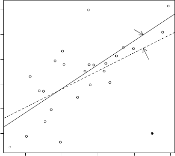
CHAPTER 3. THE ALGEBRA OF LEAST SQUARES 79
246810
0246810
x
y
leave−one−out OLS
OLS
Figure 3.2: Impact of an influential observation on the least-squares estimator
fitted line towards the 26 observation. In fact, the slope coefficient decreases from 0.97 (which
is close to the true value of 1.00) to 0.56, which is substantially reduced. Neither 26 nor 26 are
unusual values relative to their marginal distributions, so this outlier would not have been detected
from examination of the marginal distributions of the data. The change in the slope coefficient of
−041 is meaningful and should raise concern to an applied economist.
From (3.43)-(3.44) we know that
b
β−b
β(−)=(1−)−1¡X0X¢−1xb
=¡X0X¢−1xe(3.48)
By direct calculation of this quantity for each observation we can directly discover if a specific
observation is influential for a coefficient estimate of interest.
For a general assessment, we can focus on the predicted values. The difference between the
full-sample and leave-one-out predicted values is
b−e=x0
b
β−x0
b
β(−)
=x0
¡X0X¢−1xe
=e
which is a simple function of the leverage values and prediction errors eObservation is
influential for the predicted value if |e|is large, which requires that both and |e|are large.
One way to think about this is that a large leverage value gives the potential for observation
to be influential. A large means that observation is unusual in the sense that the regressor x
is far from its sample mean. We call an observation with large aleverage point. A leverage
point is not necessarily influential as the latter also requires that the prediction error eis large.
To determine if any individual observations are influential in this sense, several diagnostics have
been proposed (some names include DFITS, Cook’s Distance, and Welsch Distance). Unfortunately,
from a statistical perspective it is difficult to recommend these diagnostics for applications as they
are not based on statistical theory. Probably the most relevant measure is the change in the
coefficient estimates given in (3.48). The ratio of these changes to the coefficient’s standard error
is called its DFBETA, and is a postestimation diagnostic available in Stata. While there is no
magic threshold, the concern is whether or not an individual observation meaningfully changes an
CHAPTER 3. THE ALGEBRA OF LEAST SQUARES 80
estimated coefficient of interest. A simple diagnostic for influential observations is to calculate
- =max
1≤≤|b−e|=max
1≤≤|e|
This is the largest (absolute) change in the predicted value due to a single observation. If this diag-
nostic is large relative to the distribution of it may indicate that that observation is influential.
If an observation is determined to be influential, what should be done? As a common cause
of influential observations is data entry error, the influential observations should be examined for
evidence that the observation was mis-recorded. Perhaps the observation falls outside of permitted
ranges, or some observables are inconsistent (for example, a person is listed as having a job but
receives earnings of $0). If it is determined that an observation is incorrectly recorded, then the
observation is typically deleted from the sample. This process is often called “cleaning the data”.
The decisions made in this process involve a fair amount of individual judgment. When this is done
it is proper empirical practice to document such choices. (It is useful to keep the source data in its
original form, a revised data file after cleaning, and a record describing the revision process. This
is especially useful when revising empirical work at a later date.)
It is also possible that an observation is correctly measured, but unusual and influential. In
this case it is unclear how to proceed. Some researchers will try to alter the specification to
properly model the influential observation. Other researchers will delete the observation from the
sample. The motivation for this choice is to prevent the results from being skewed or determined
by individual observations, but this practice is viewed skeptically by many researchers who believe
it reduces the integrity of reported empirical results.
For an empirical illustration, consider the log wage regression (3.15) for single Asian males.
This regression, which has 268 observations, has - =029This means that the most
influential observation, when deleted, changes the predicted (fitted) value of the dependent variable
log()by 029or equivalently the wage by 29%. This is a meaningful change and suggests
further investigation. We examine the influential observation, and find that its leverage is 0.33,
which is disturbingly large. (Recall that the leverage values are all positive and sum to .One
twelfth of the leverage in this sample of 268 observations is contained in just this single observation!)
Examining further, we find that this individual is 65 years old with 8 years education, so that his
potential experience is 51 years. This is the highest experience in the subsample — the next highest
is 41 years. The large leverage is due to his unusual characteristics (very low education and very
high experience) within this sample. Essentially, regression (3.15) is attempting to estimate the
conditional mean at experience=51with only one observation, so it is not surprising that this
observation determines the fit and is thus influential. A reasonable conclusion is the regression
function can only be estimated over a smaller range of experience. We restrict the sample to
individuals with less than 45 years experience, re-estimate, and obtain the following estimates.
\
log()=0144 +0043 −0095 2100 + 0531(3.49)
For this regression, we calculate that - =011which is greatly reduced relative to the
regression (3.15). Comparing (3.49) with (3.15), the slope coefficient for education is essentially
unchanged, but the coefficients in experience and its square have slightly increased.
By eliminating the influential observation, equation (3.49) can be viewed as a more robust
estimate of the conditional mean for most levels of experience. Whether to report (3.15) or (3.49)
in an application is largely a matter of judgment.
3.19 CPS Data Set
In this section we describe the data set used in the empirical illustrations.

CHAPTER 3. THE ALGEBRA OF LEAST SQUARES 81
The Current Population Survey (CPS) is a monthly survey of about 57,000 U.S. households
conducted by the Bureau of the Census of the Bureau of Labor Statistics. The CPS is the primary
source of information on the labor force characteristics of the U.S. population. The survey covers
employment, earnings, educational attainment, income, poverty, health insurance coverage, job
experience, voting and registration, computer usage, veteran status, and other variables. Details
can be found at www.census.gov/cps and dataferrett.census.gov.
From the March 2009 survey we extracted the individuals with non-allocated variables who
were full-time employed (defined as those who had worked at least 36 hours per week for at least
48 weeks the past year), and excluded those in the military. This sample has 50,742 individ-
uals. We extracted 14 variables from the CPS on these individuals and created the data files
cps09mar.dta (Stata format), cps09mar.xlsx (Excel format) and cps09mar.txt (text format).
The variables are described in the file cps09mar_description.pdf All data files are available at
http://www.ssc.wisc.edu/~bhansen/econometrics/
3.20 Programming
Most packages allow both interactive programming (where you enter commands one-by-one) and
batch programming (where you run a pre-written sequence of commands from a file). Interactive
programming can be useful for exploratory analysis, but eventually all work should be executed in
batch mode. This is the best way to control and document your work.
Batch programs are text files where each line executes a single command. For Stata, this file
needs to have the filename extension “.do”, and for MATLAB “.m”. For R there is no specific
naming requirements, though it is typical to use the extension “.r”.
To execute a program file, you type a command within the program.
Stata: do chapter3 executes the file chapter3.do
MATLAB: run chapter3 executes the file chapter3.m
R: source(“chapter3.r”) executes the file chapter3.r
When writing batch files, it is useful to include comments for documentation and readability.
We illustrate programming files for Stata, R, and MATLAB, which execute a portion of the
empirical illustrations from Sections 3.7 and 3.18.
Stata do File
* Clear memory and load the data
clear
use cps09mar.dta
* Generate transformations
gen wage=ln(earnings/(hours*week))
gen experience = age - education - 6
gen exp2 = (experience^2)/100
* Create indicator for subsamples
genmbf=(race==2)&(marital=2)&(female==1)
gen sam = (race == 4) & (marital == 7) & (female == 0)
*Regressions
reg wage education if (mbf == 1) & (experience == 12)
reg wage education experience exp2 if sam == 1
* Leverage and influence
predict leverage,hat
predict e,residual
gen d=e*leverage/(1-leverage)
summarize d if sam ==1

CHAPTER 3. THE ALGEBRA OF LEAST SQUARES 82
R Program File
# Load the data and create subsamples
dat - read.table("cps09mar.txt")
experience - dat[,1]-dat[,4]-6
mbf - (dat[,11]==2)&(dat[,12]=2)&(dat[,2]==1)&(experience==12)
sam - (dat[,11]==4)&(dat[,12]==7)&(dat[,2]==0)
dat1 -dat[mbf,]
dat2 - dat[sam,]
# First regression
y- as.matrix(log(dat1[,5]/(dat1[,6]*dat1[,7])))
x- cbind(dat1[,4],matrix(1,nrow(dat1),1))
beta - solve(t(x)%*%x,t(x)%*%y)
print(beta)
# Second regression
y- as.matrix(log(dat2[,5]/(dat2[,6]*dat2[,7])))
experience - dat2[,1]-dat2[,4]-6
exp2 - (experience^2)/100
x- cbind(dat2[,4],experience,exp2,matrix(1,nrow(dat2),1))
beta - solve(t(x)%*%x,t(x)%*%y)print(beta)
# Create leverage and influence
e-y-x%*%beta
leverage - rowSums(x*(x%*%solve(t(x)%*%x)))
r- e/(1-leverage)
d- leverage*e/(1-leverage)
print(max(abs(d)))

CHAPTER 3. THE ALGEBRA OF LEAST SQUARES 83
MATLAB Program File
% Load the data and create subsamples
load cps09mar.txt;
dat=cps09mar;
experience=dat(:,1)-dat(:,4)-6;
mbf = (dat(:,11)==2)&(dat(:,12)=2)&(dat(:,2)==1)&(experience==12);
sam = (dat(:,11)==4)&(dat(:,12)==7)&(dat(:,2)==0);
dat1=dat(mbf,:);
dat2=dat(sam,:);
% First regression
y=log(dat1(:,5)./(dat1(:,6).*dat1(:,7)));
x=[dat1(:,4),ones(length(dat1),1)];
beta=inv(x’*x)*(x’*y);display(beta);
% Second regression
y=log(dat2(:,5)./(dat2(:,6).*dat2(:,7)));
experience=dat2(:,1)-dat2(:,4)-6;
exp2 = (experience.^2)/100;
x=[dat2(:,4),experience,exp2,ones(length(dat2),1)];
beta=inv(x’*x)*(x’*y);display(beta);
% Create leverage and influence
e=y-x*beta;
leverage=sum((x.*(x*inv(x’*x)))’)’;d=leverage.*e./(1-leverage);
influence=max(abs(d));
display(influence);
Instead, to load from an excel file, we can replace the first two lines (‘load’ and ‘dat=’) with
dat=xlsread(’cps09mar.xlsx’);
CHAPTER 3. THE ALGEBRA OF LEAST SQUARES 84
3.21 Technical Proofs*
Proof of Theorem 3.11.1, equation (3.27): First, =x0
(X0X)−1x≥0sinceitisa
quadratic form and X0X0Next, since is the diagonal element of the projection matrix
P=X(X0X)−1X, then
=s0Ps
where
s=
⎛
⎜
⎜
⎜
⎜
⎜
⎜
⎝
0
.
.
.
1
.
.
.
0
⎞
⎟
⎟
⎟
⎟
⎟
⎟
⎠
is a unit vector with a 1 in the place (and zeros elsewhere).
By the spectral decomposition of the idempotent matrix P(see equation (A.10))
P=B0∙I0
00
¸B
where B0B=I. Thus letting b=Bs denote the column of B, and partitioning b0=¡b0
1b0
2¢
then
=s0B0∙I0
00
¸Bs
=b0
1∙I0
00
¸b1
=b0
1b1
≤b0b
=1
the final equality since bis the column of Band B0B=IWe have shown that ≤1
establishing (3.27). ¥
ProofofEquation(3.43). The Sherman—Morrison formula (A.3) from Appendix A.6 states that
for nonsingular Aand vector b
¡A−bb0¢−1=A−1+¡1−b0A−1b¢−1A−1bb0A−1
This implies ¡X0X−xx0
¢−1=¡X0X¢−1+(1−)−1¡X0X¢−1xx0
¡X0X¢−1
and thus
b
β(−)=¡X0X−xx0
¢−1¡X0y−x¢
=¡X0X¢−1X0y−¡X0X¢−1x
+(1−)−1¡X0X¢−1xx0
¡X0X¢−1¡X0y−x¢
=b
β−¡X0X¢−1x+(1−)−1¡X0X¢−1x³x0
b
β−´
=b
β−(1 −)−1¡X0X¢−1x³(1 −)−x0
b
β+´
=b
β−(1 −)−1¡X0X¢−1xb
the third equality making the substitutions b
β=(X0X)−1X0yand =x0
(X0X)−1xand the
remainder collecting terms. ¥

CHAPTER 3. THE ALGEBRA OF LEAST SQUARES 85
Exercises
Exercise 3.1 Let be a random variable with =E()and 2=var()Define
¡ 2¢=µ−
(−)2−2
Let (b b2)be the values such that (b b2)=0where ( )=−1P
=1 ()Show that
band b2are the sample mean and variance.
Exercise 3.2 Consider the OLS regression of the ×1vector yon the ×matrix X.Consider
an alternative set of regressors Z=XCwhere Cis a ×non-singular matrix. Thus, each
column of Zis a mixture of some of the columns of XCompare the OLS estimates and residuals
from the regression of yon Xto the OLS estimates from the regression of yon Z
Exercise 3.3 Using matrix algebra, show X0b
e=0
Exercise 3.4 Let b
ebe the OLS residual from a regression of yon X=[X1X2].FindX0
2b
e
Exercise 3.5 Let b
ebe the OLS residual from a regression of yon XFind the OLS coefficient
from a regression of b
eon X
Exercise 3.6 Let b
y=X(X0X)−1X0yFind the OLS coefficient from a regression of ˆyon X
Exercise 3.7 Show that if X=[X1X2]then PX1=X1and MX1=0
Exercise 3.8 Show that Mis idempotent: MM =M
Exercise 3.9 Show that tr M=−
Exercise 3.10 Show that if X=[X1X2]and X0
1X2=0then P=P1+P2.
Exercise 3.11 Show that when Xcontains a constant, 1
P
=1 b=
Exercise 3.12 A dummy variable takes on only the values 0 and 1. It is used for categorical
data, such as an individual’s gender. Let d1and d2be vectors of 1’s and 0’s, with the element
of d1equaling 1 and that of d2equaling 0 if the person is a man, and the reverse if the person is a
woman. Suppose that there are 1men and 2womeninthesample. Considerfitting the following
three equations by OLS
y=+d11+d22+e(3.50)
y=d11+d22+e(3.51)
y=+d1+e(3.52)
Can all three equations (3.50), (3.51), and (3.52) be estimated by OLS? Explain if not.
(a) Compare regressions (3.51) and (3.52). Is one more general than the other? Explain the
relationship between the parameters in (3.51) and (3.52).
(b) Compute ι0d1and ι0d2where ιis an ×1vector of ones.
(c) Letting α=(12)0write equation (3.51) as y=Xα+ Consider the assumption E(x)=
0. Is there any content to this assumption in this setting?

CHAPTER 3. THE ALGEBRA OF LEAST SQUARES 86
Exercise 3.13 Let d1and d2be defined as in the previous exercise.
(a) In the OLS regression
y=d1b1+d2b2+b
u
show that b1is the sample mean of the dependent variable among the men of the sample
(1),andthatb2isthesamplemeanamongthewomen(2).
(b) Let X(×)be an additional matrix of regressors. Describe in words the transformations
y∗=y−d11−d22
X∗=X−d1x0
1−d2x0
2
where x1and x2are the ×1means of the regressors for men and women, respectively.
(c) Compare e
βfrom the OLS regression
y∗=X∗e
β+e
e
with b
βfrom the OLS regression
y=d1b1+d2b2+Xb
β+b
e
Exercise 3.14 Let b
β=(X0
X)−1X0
ydenote the OLS estimate when yis ×1and Xis
×. A new observation (+1x+1)becomes available. Prove that the OLS estimate computed
using this additional observation is
b
β+1 =b
β+1
1+x0
+1 (X0
X)−1x+1 ¡X0
X¢−1x+1 ³+1 −x0
+1 b
β´
Exercise 3.15 Prove that 2is the square of the sample correlation between yand b
y
Exercise 3.16 Consider two least-squares regressions
y=X1e
β1+e
e
and
y=X1b
β1+X2b
β2+b
e
Let 2
1and 2
2be the -squared from the two regressions. Show that 2
2≥2
1Is there a case
(explain) when there is equality 2
2=2
1?
Exercise 3.17 Show that e2≥b2Is equality possible?
Exercise 3.18 For which observations will b
β(−)=b
β?
Exercise 3.19 Consider the least-squares regression estimates
=1b
1+2b
2+b
and the “one regressor at a time” regression estimates
=e
11+e1=e
22+e2
Under what condition does e
1=b
1and e
2=b
2?
CHAPTER 3. THE ALGEBRA OF LEAST SQUARES 87
Exercise 3.20 You estimate a least-squares regression
=x0
1e
β1+e
and then regress the residuals on another set of regressors
e=x0
2e
β2+e
Does this second regression give you the same estimated coefficients as from estimation of a least-
squares regression on both set of regressors?
=x0
1b
β1+x0
2b
β2+b
In other words, is it true that e
β2=b
β2?Explain your reasoning.
Exercise 3.21 The data matrix is (yX)with X=[X1X2]and consider the transformed
regressor matrix Z=[X1X2−X1]Suppose you do a least-squares regression of yon Xand a
least-squares regression of yon ZLet b2and e2denote the residual variance estimates from the
two regressions. Give a formula relating b2and e2?(Explain your reasoning.)
Exercise 3.22 Use the data set from Section 3.19 and the sub-sample used for equation (3.49)
(see Section 3.20) for data construction)
(a) Estimate equation (3.49) and compute the equation 2and sum of squared errors.
(b) Re-estimate the slope on education using the residual regression approach. Regress log(Wage)
on experience and its square, regress education on experience and its square, and the residuals
on the residuals. Report the estimates from this final regression, along with the equation 2
and sum of squared errors. Does the slope coefficient equal the value in (3.49)? Explain.
(c) Are the 2and sum-of-squared errors from parts (a) and (b) equal? Explain.
Exercise 3.23 Estimate equation (3.49) as in part (a) of the previous question. Let bbe the
OLS residual, bthe predicted value from the regression, 1be education and 2be experience.
Numerically calculate the following:
(a) P
=1 b
(b) P
=1 1b
(c) P
=1 2b
(d) P
=1 2
1b
(e) P
=1 2
2b
(f) P
=1 bb
(g) P
=1 b2
Are these calculations consistent with the theoretical properties of OLS? Explain.
Exercise 3.24 Use the data set from Section 3.19.
(a) Estimate a log wage regression for the subsample of white male Hispanics. In addition to
education, experience, and its square, include a set of binary variables for regions and marital
status. For regions, you create dummy variables for Northeast, South and West so that
Midwest is the excluded group. For marital status, create variables for married, widowed or
divorced, and separated, so that single (never married) is the excluded group.
(b) Repeat this estimation using a different econometric package. Compare your results. Do they
agree?

Chapter 4
Least Squares Regression
4.1 Introduction
In this chapter we investigate some finite-sample properties of the least-squares estimator in the
linear regression model. In particular, we calculate the finite-sample mean and covariance matrix
and propose standard errors for the coefficient estimates.
4.2 Random Sampling
Assumption 3.2.1 specified that the observations have identical distributions. To derive the
finite-sample properties of the estimators we will need to additionally specify the dependence struc-
ture across the observations.
The simplest context is when the observations are mutually independent, in which case we
say that they are independent and identically distributed,ori.i.d. It is also common to
describe iid observations as a random sample. Traditionally, random sampling has been the
default assumption in cross-section (e.g. survey) contexts. It is quite conveneint as iid sampling
leads to straightforward expressions for estimation variance. The assumption seems appropriate
(meaning that it should be approximately valid) when samples are small and relatively dispersed.
That is, if you randomly sample 1000 people from a large country such as the United States it
seems reasonable to model their responses as mutually independent.
Assumption 4.2.1 The observations {(1x1)(x) (x)}are in-
dependent and identically distributed.
For most of this chapter, we will use Assumption 4.2.1 to derive properties of the OLS estimator.
Assumption 4.2.1 means that if you take any two individuals 6=in a sample, the values (x)
are independent of the values (x)yet have the same distribution. Independence means that
the decisions and choices of individual do not affect the decisions of individual , and conversely.
This assumption may be violated if individuals in the sample are connected in some way, for
example if they are neighbors, members of the same village, classmates at a school, or even firms
within a specific industry. In this case, it seems plausible that decisions may be inter-connected
and thus mutually dependent rather than independent. Allowing for such interactions complicates
inference and requires specialized treatment. A currently popular approach which allows for mutual
dependence is known as clustered dependence, which assumes that that observations are grouped
into “clusters” (for example, schools). We will discuss clustering in more detail in Section 4.20.
88

CHAPTER 4. LEAST SQUARES REGRESSION 89
4.3 Sample Mean
To start with the simplest setting, we first consider the intercept-only model
=+
E()=0
which is equivalent to the regression model with =1and =1In the intercept model, =E()
is the mean of (See Exercise 2.15.) The least-squares estimator b=equals the sample mean
as shown in equation (3.10).
We now calculate the mean and variance of the estimator .Sincethesamplemeanisalinear
function of the observations, its expectation is simple to calculate
E()=EÃ1
X
=1
!=1
X
=1
E()=
This shows that the expected value of the least-squares estimator (the sample mean) equals the
projection coefficient(thepopulationmean).Anestimatorwiththepropertythatitsexpectation
equals the parameter it is estimating is called unbiased.
Definition 4.3.1 An estimator b
for is unbiased if E³b
´=.
We next calculate the variance of the estimator under Assumption 4.2.1. Making the substi-
tution =+we find
−=1
X
=1
Then
var ()=E(−)2
=E⎛
⎝Ã1
X
=1
!⎛
⎝1
X
=1
⎞
⎠⎞
⎠
=1
2
X
=1
X
=1
E()
=1
2
X
=1
2
=1
2
The second-to-last inequality is because E()=2for =yet E()=0for 6=due to
independence.
We have shown that var ()= 1
2. This is the familiar formula forthevarianceofthesample
mean.

CHAPTER 4. LEAST SQUARES REGRESSION 90
4.4 Linear Regression Model
We now consider the linear regression model. Throughout this chapter we maintain the follow-
ing.
Assumption 4.4.1 Linear Regression Model
The observations (x)satisfy the linear regression equation
=x0
β+(4.1)
E(|x)=0(4.2)
The variables have finite second moments
E¡2
¢∞
Ekxk2∞
and an invertible design matrix
Q =E¡xx0
¢0
We will consider both the general case of heteroskedastic regression, where the conditional
variance
E¡2
|x¢=2(x)=2
is unrestricted, and the specialized case of homoskedastic regression, where the conditional variance
is constant. In the latter case we add the following assumption.
Assumption 4.4.2 Homoskedastic Linear Regression Model
In addition to Assumption 4.4.1,
E¡2
|x¢=2(x)=2(4.3)
is independent of x
4.5 Mean of Least-Squares Estimator
In this section we show that the OLS estimator is unbiased in the linear regression model. This
calculation can be done using either summation notation or matrix notation. We will use both.
First take summation notation. Observe that under (4.1)-(4.2)
E(|X)=E(|x)=x0
β(4.4)
The first equality states that the conditional expectation of given {x1x}only depends on
xsince the observations are independent across The second equality is the assumption of a
linear conditional mean.
CHAPTER 4. LEAST SQUARES REGRESSION 91
Using definition (3.12), the conditioning theorem, the linearity of expectations, (4.4), and prop-
erties of the matrix inverse,
E³b
β|X´=E⎛
⎝Ã
X
=1
xx0
!−1Ã
X
=1
x!|X⎞
⎠
=Ã
X
=1
xx0
!−1
EÃÃ
X
=1
x!|X!
=Ã
X
=1
xx0
!−1
X
=1
E(x|X)
=Ã
X
=1
xx0
!−1
X
=1
xE(|X)
=Ã
X
=1
xx0
!−1
X
=1
xx0
β
=β
Now let’s show the same result using matrix notation. (4.4) implies
E(y|X)=⎛
⎜
⎜
⎝
.
.
.
E(|X)
.
.
.
⎞
⎟
⎟
⎠=⎛
⎜
⎜
⎝
.
.
.
x0
β
.
.
.
⎞
⎟
⎟
⎠=Xβ(4.5)
Similarly
E(e|X)=⎛
⎜
⎜
⎝
.
.
.
E(|X)
.
.
.
⎞
⎟
⎟
⎠=⎛
⎜
⎜
⎝
.
.
.
E(|x)
.
.
.
⎞
⎟
⎟
⎠=0(4.6)
Using definition (3.22), the conditioning theorem, the linearity of expectations, (4.5), and the
properties of the matrix inverse,
E³b
β|X´=E³¡X0X¢−1X0y|X´
=¡X0X¢−1X0E(y|X)
=¡X0X¢−1X0Xβ
=β
At the risk of belaboring the derivation, another way to calculate the same result is as follows.
Insert y=Xβ+einto the formula (3.22) for b
βto obtain
b
β=¡X0X¢−1¡X0(Xβ+e)¢
=¡X0X¢−1X0Xβ+¡X0X¢−1¡X0e¢
=β+¡X0X¢−1X0e(4.7)
This is a useful linear decomposition of the estimator b
βinto the true parameter βand the stochastic
component (X0X)−1X0eOnce again, we can calculate that
E³b
β−β|X´=E³¡X0X¢−1X0e|X´
=¡X0X¢−1X0E(e|X)
=0

CHAPTER 4. LEAST SQUARES REGRESSION 92
Regardless of the method, we have shown that E³b
β|X´=β
We have shown the following theorem.
Theorem 4.5.1 Mean of Least-Squares Estimator
In the linear regression model (Assumption 4.4.1) and i.i.d. sam-
pling (Assumption 4.2.1)
E³b
β|X´=β(4.8)
Equation (4.8) says that the estimator b
βis unbiased for β, conditional on X. This means
that the conditional distribution of b
βis centered at β. By “conditional on X” this means that the
distribution is unbiased (centered at β) for any realization of the regressor matrix X. In conditional
models, we simply refer to this as saying “b
βis unbiased for β”.
Strictly speaking, “unbiasedness” is a property of the unconditional distribution. Assuming
the unconditional mean is well defined, that is E°
°
°b
β°
°
°∞, then applying the law of iterated
expectations, we find that the unconditional mean of b
βis also β
E³b
β´=E³E³b
β|X´´=β(4.9)
4.6 Variance of Least Squares Estimator
In this section we calculate the conditional variance of the OLS estimator.
For any ×1random vector Zdefine the ×covariance matrix
var(Z)=E¡(Z−E(Z)) (Z−E(Z))0¢
=E¡ZZ0¢−(E(Z)) (E(Z))0
and for any pair (ZX)define the conditional covariance matrix
var(Z|X)=E¡(Z−E(Z|X)) (Z−E(Z|X))0|X¢
We define
V
=var
³b
β|X´
as the conditional covariance matrix of the regression coefficient estimates. We now derive its form.
The conditional covariance matrix of the ×1regression error eis the ×matrix
var(e|X)=E¡ee0|X¢
=D
The diagonal element of Dis
E¡2
|X¢=E¡2
|x¢=2
while the off-diagonal element of Dis
E(|X)=E(|x)E(|x)=0

CHAPTER 4. LEAST SQUARES REGRESSION 93
where the first equality uses independence of the observations (Assumption 1.5.2) and the second
is (4.2). Thus Dis a diagonal matrix with diagonal element 2
:
D=diag¡2
1
2
¢=⎛
⎜
⎜
⎜
⎝
2
10··· 0
02
2··· 0
.
.
..
.
.....
.
.
00··· 2
⎞
⎟
⎟
⎟
⎠(4.10)
In the special case of the linear homoskedastic regression model (4.3), then
E¡2
|x¢=2
=2
andwehavethesimplification
D=I2
In general, however, Dneed not necessarily take this simplified form.
For any ×matrix A=A(X),
var(A0y|X)=var(A0e|X)=A0DA(4.11)
In particular, we can write b
β=A0ywhere A=X(X0X)−1and thus
V
=var(
b
β|X)=A0DA =¡X0X¢−1X0DX ¡X0X¢−1
It is useful to note that
X0DX =
X
=1
xx0
2
a weighted version of X0X.
In the special case of the linear homoskedastic regression model, D=I2,soX0DX =
X0X2and the variance matrix simplifies to
V
=¡X0X¢−12
Theorem 4.6.1 Variance of Least-Squares Estimator
In the linear regression model (Assumption 4.4.1) and i.i.d. sampling (As-
sumption 4.2.1)
V
=var³b
β|X´
=¡X0X¢−1¡X0DX¢¡X0X¢−1(4.12)
where Dis defined in (4.10).
In the homoskedastic linear regression model (Assumption 4.4.2) and i.i.d.
sampling (Assumption 4.2.1)
V
=2¡X0X¢−1(4.13)

CHAPTER 4. LEAST SQUARES REGRESSION 94
4.7 Gauss-Markov Theorem
Now consider the class of estimators of βwhich are linear functions of the vector yand thus
can be written as e
β=A0y
where Ais an ×function of X. As noted before, the least-squares estimator is the special case
obtained by setting A=X(X0X)−1What is the best choice of A?The Gauss-Markov theorem,
which we now present, says that the least-squares estimator is the best choice among linear unbiased
estimators when the errors are homoskedastic, in the sense that the least-squares estimator has the
smallest variance among all unbiased linear estimators.
To see this, since E(y|X)=Xβ,then for any linear estimator e
β=A0ywe have
E³e
β|X´=A0E(y|X)=A0Xβ
so e
βis unbiased if (and only if) A0X=IFurthermore, we saw in (4.11) that
var ³e
β|X´=var¡A0y|X¢=A0DA =A0A2
the last equality using the homoskedasticity assumption D=I2. The “best” unbiased linear
estimator is obtained by finding the matrix A0satisfying A0
0X=Isuch that A0
0A0is minimized
in the positive definite sense, in that for any other matrix Asatisfying A0X=Ithen A0A−A0
0A0
is positive semi-definite.
Theorem 4.7.1 Gauss-Markov. In the homoskedastic linear regression
model (Assumption 4.4.2) and i.i.d. sampling (Assumption 4.2.1), if e
βis
a linear unbiased estimator of βthen
var ³e
β|X´≥2¡X0X¢−1
The Gauss-Markov theorem provides a lower bound on the variance matrix of unbiased linear
estimators under the assumption of homoskedasticity. It says that no unbiased linear estimator
can have a variance matrix smaller (in the positive definite sense) than 2(X0X)−1.Sincethe
variance of the OLS estimator is exactly equal to this bound, this means that the OLS estimator
is efficient in the class of linear unbiased estimator. This gives rise to the description of OLS as
BLUE, standing for “best linear unbiased estimator”. This is is an efficiency justification for the
least-squares estimator. The justification is limited because the class of models is restricted to
homoskedastic linear regression and the class of potential estimators is restricted to linear unbiased
estimators. This latter restriction is particularly unsatisfactory as the theorem leaves open the
possibility that a non-linear or biased estimator could have lower mean squared error than the
least-squares estimator.
We give a proof of the Gauss-Markov theorem below.
ProofofTheorem4.7.1.1.LetAbe any ×function of Xsuch that A0X=IThe variance
of the least-squares estimator is (X0X)−12and that of A0yis A0A2It is sufficient to show

CHAPTER 4. LEAST SQUARES REGRESSION 95
that the difference A0A−(X0X)−1is positive semi-definite. Set C=A−X(X0X)−1Note that
X0C=0Then we calculate that
A0A−¡X0X¢−1=³C+X¡X0X¢−1´0³C+X¡X0X¢−1´−¡X0X¢−1
=C0C+C0X¡X0X¢−1+¡X0X¢−1X0C
+¡X0X¢−1X0X¡X0X¢−1−¡X0X¢−1
=C0C
The matrix C0Cis positive semi-definite (see Appendix A.9) as required.
4.8 Generalized Least Squares
Take the linear regression model in matrix format
y=Xβ+e(4.14)
Consider a generalized situation where the observation errors are possibly correlated and/or het-
eroskedastic. Specifically, suppose that
E(e|X)=0(4.15)
var(e|X)=Ω(4.16)
for some ×covariance matrix Ω, possibly a function of X. This includes the iid sampling
framework where Ω=Dbut allows for non-diagonal covariance matrices as well.
Under these assumptions, by similar arguments we can calculate the mean and variance of the
OLS estimator:
E³b
β|X´=β(4.17)
var( b
β|X)=¡X0X¢−1¡X0ΩX¢¡X0X¢−1(4.18)
(see Exercise 4.5).
We have an analog of the Gauss-Markov Theorem.
Theorem 4.8.1 If (4.15)-(4.16) hold and if e
βis a linear unbiased esti-
mator of βthen
var ³e
β|X´≥¡X0Ω−1X¢−1
We leave the proof for Exercise 4.6.
The theorem provides a lower bound on the variance matrix of unbiased linear estimators. The
bound is different from the variance matrix of the OLS estimator except when Ω=I2.This
suggests that we may be able to improve on the OLS estimator.
This is indeed the case when Ωis known up to scale. That is, suppose that Ω=2Σwhere
20is real and Σis ×and known. Take the linear model (4.14) and pre-multiply by Σ−12.
This produces the equation
e
y=f
Xβ+e
e
CHAPTER 4. LEAST SQUARES REGRESSION 96
where e
y=Σ−12y,f
X=Σ−12X,ande
e=Σ−12e. Consider OLS estimation of βin this equation
e
βgls =³f
X0f
X´−1f
X0e
y
=µ³Σ−12X´0³Σ−12X´¶−1³Σ−12X´0³Σ−12y´
=¡X0Σ−1X¢−1X0Σ−1y(4.19)
This is called the Generalized Least Squares (GLS) estimator of β
You can calculate that
E³e
βgls |X´=β(4.20)
var( e
βgls |X)=¡X0Ω−1X¢−1(4.21)
This shows that the GLS estimator is unbiased, and has a covariance matrix which equals the lower
bound from Theorem 4.8.1. This shows that the lower bound is sharp when Σis known and the
GLS is efficient in the class of linear unbiased estimators.
In the linear regression model with independent observations and known conditional variances,
where Ω=Σ=D=diag¡2
1
2
¢, the GLS estimator takes the form
e
βgls =¡X0D−1X¢−1X0D−1y
=Ã
X
=1
−2
xx0
!−1Ã
X
=1
−2
x!
In practice, the covariance matrix Ωis unknown, so the GLS estimator as presented here is
not feasible. However, the form of the GLS estimator motivates feasible versions, effectively by
replacing Ωwith an estimate. We return to this issue in Section 20.2.
4.9 Residuals
What are some properties of the residuals b=−x0
b
βand prediction errors e=−x0
b
β(−),
at least in the context of the linear regression model?
Recall from (3.31) that we can write the residuals in vector notation as
b
e=Me
where M=I−X(X0X)−1X0is the orthogonal projection matrix. Using the properties of
conditional expectation
E(b
e|X)=E(Me |X)=ME(e|X)=0
and
var (b
e|X)=var(Me |X)=Mvar (e|X)M=MDM (4.22)
where Dis defined in (4.10).
We can simplify this expression under the assumption of conditional homoskedasticity
E¡2
|x¢=2
In this case (4.22) simplifies to
var (b
e|X)=M2(4.23)

CHAPTER 4. LEAST SQUARES REGRESSION 97
In particular, for a single observation we can find the (conditional) variance of bby taking the
diagonal element of (4.23). Since the diagonal element of Mis 1− as defined in (3.25)
we obtain
var (b|X)=E¡b2
|X¢=(1−)2(4.24)
As this variance is a function of and hence x, the residuals bare heteroskedastic even if the
errors are homoskedastic. Notice as well that this implies b2
is a biased estimator of 2.
Similarly, recall from (3.46) that the prediction errors e=(1−)−1bcan be written in
vector notation as e
e=M∗b
ewhere M∗is a diagonal matrix with diagonal element (1 −)−1
Thus e
e=M∗MeWe can calculate that
E(e
e|X)=M∗ME(e|X)=0
and
var (e
e|X)=M∗Mvar (e|X)MM∗=M∗MDMM∗
which simplifies under homoskedasticity to
var (e
e|X)=M∗MMM∗2
=M∗MM∗2
The variance of the prediction error is then
var (e|X)=E¡e2
|X¢
=(1−)−1(1 −)(1−)−12
=(1−)−12
A residual with constant conditional variance can be obtained by rescaling. The standardized
residuals are
¯=(1−)−12b(4.25)
and in vector notation
¯e=(¯1¯)0=M∗12Me(4.26)
From our above calculations, under homoskedasticity,
var (¯e|X)=M∗12MM∗122
and
var (¯|X)=E¡¯2
|X¢=2(4.27)
and thus these standardized residuals have the same bias and variance as the original errors when
the latter are homoskedastic.
4.10 Estimation of Error Variance
The error variance 2=E¡2
¢can be a parameter of interest even in a heteroskedastic regression
or a projection model. 2measures the variation in the “unexplained” part of the regression. Its
method of moments estimator (MME) is the sample average of the squared residuals:
b2=1
X
=1 b2
In the linear regression model we can calculate the mean of b2From (3.35) and the properties
of the trace operator, observe that
b2=1
e0Me =1
tr ¡e0Me¢=1
tr ¡Mee0¢

CHAPTER 4. LEAST SQUARES REGRESSION 98
Then
E¡b2|X¢=1
tr ¡E¡Mee0|X¢¢
=1
tr ¡ME¡ee0|X¢¢
=1
tr (MD)(4.28)
Adding the assumption of conditional homoskedasticity E¡2
|x¢=2so that D=I2then
(4.28) simplifies to
E¡b2|X¢=1
tr ¡M2¢
=2µ−
the final equality by (3.29). This calculation shows that b2is biased towards zero. The order of
the bias depends on , the ratio of the number of estimated coefficients to the sample size.
Another way to see this is to use (4.24). Note that
E¡b2|X¢=1
X
=1
E¡b2
|X¢
=1
X
=1
(1 −)2
=µ−
¶2(4.29)
the last equality using Theorem 3.11.1.
Since the bias takes a scale form, a classic method to obtain an unbiased estimator is by rescaling
the estimator. Define
2=1
−
X
=1 b2
(4.30)
By the above calculation,
E¡2|X¢=2(4.31)
and
E¡2¢=2
Hence the estimator 2is unbiased for 2Consequently, 2is known as the “bias-corrected esti-
mator” for 2and in empirical practice 2is the most widely used estimator for 2
Interestingly, this is not the only method to construct an unbiased estimator for 2.Anesti-
mator constructed with the standardized residuals ¯from (4.25) is
2=1
X
=1
¯2
=1
X
=1
(1 −)−1b2
(4.32)
You can show (see Exercise 4.9) that
E¡2|X¢=2(4.33)
and thus 2is unbiased for 2(in the homoskedastic linear regression model).
When is small (typically, this occurs when is large), the estimators b2
2and 2are
likely to be close. However, if not then 2and 2are generally preferred to b2Consequently it is
best to use one of the bias-corrected variance estimators in applications.

CHAPTER 4. LEAST SQUARES REGRESSION 99
4.11 Mean-Square Forecast Error
A major purpose of estimated regressions is to predict out-of-sample values. Consider an out-
of-sample observation (+1x+1)where x+1 is observed but not +1.Giventhecoefficient
estimate b
βthe standard point estimate of E(+1 |x+1)=x0
+1βis e+1 =x0
+1 b
βThe forecast
error is the difference between the actual value +1 and the point forecast e+1. Thisistheforecast
error e+1 =+1 −e+1The mean-squared forecast error (MSFE) is its expected squared value
=E¡e2
+1¢
In the linear regression model, e+1 =+1 −x0
+1 ³b
β−β´so
=E¡2
+1¢−2E³+1x0
+1 ³b
β−β´´ (4.34)
+Eµx0
+1 ³b
β−β´³b
β−β´0x+1
The first term in (4.34) is 2The second term in (4.34) is zero since +1x0
+1 is independent
of b
β−βand both are mean zero. Using the properties of the trace operator, the third term in
(4.34) is
tr µE¡x+1x0
+1¢Eµ³b
β−β´³b
β−β´0¶¶
=trµE¡x+1x0
+1¢EµEµ³b
β−β´³b
β−β´0|X¶¶¶
=tr³E¡x+1x0
+1¢E³V
´´
=Etr ³¡x+1x0
+1¢V
´
=E³x0
+1V
x+1´(4.35)
whereweusethefactthatx+1 is independent of b
β, the definition V
=Eµ³b
β−β´³b
β−β´0|X
and the fact that x+1 is independent of V
.Thus
=2+E³x0
+1V
x+1´
Under conditional homoskedasticity, this simplifies to
=2³1+E³x0
+1 ¡X0X¢−1x+1´´
A simple estimator for the MSFE is obtained by averaging the squared prediction errors (3.47)
e2=1
X
=1 e2
where e=−x0
b
β(−)=b(1 −)−1Indeed, we can calculate that
E¡e2¢=E¡e2
¢
=E³−x0
³b
β(−)−β´´2
=2+Eµx0
³b
β(−)−β´³b
β(−)−β´0x

CHAPTER 4. LEAST SQUARES REGRESSION 100
By a similar calculation as in (4.35) we find
E¡e2¢=2+E³x0
V
(−)x´=−1
This is the MSFE based on a sample of size −1rather than size The difference arises because
the in-sample prediction errors efor ≤are calculated using an effective sample size of −1,while
the out-of sample prediction error e+1 is calculated from a sample with the full observations.
Unless is very small we should expect −1(the MSFE based on −1observations) to
be close to (the MSFE based on observations). Thus e2is a reasonable estimator for
Theorem 4.11.1 MSFE
In the linear regression model (Assumption 4.4.1) and i.i.d. sampling (As-
sumption 4.2.1)
=E¡e2
+1¢=2+E³x0
+1V
x+1´
where V
=var³b
β|X´Furthermore, e2defined in (3.47) is an unbiased
estimator of −1:
E¡e2¢=−1
4.12 Covariance Matrix Estimation Under Homoskedasticity
For inference, we need an estimate of the covariance matrix V
of the least-squares estimator.
In this section we consider the homoskedastic regression model (Assumption 4.4.2).
Under homoskedasticity, the covariance matrix takes the relatively simple form
V0
=¡X0X¢−12
which is known up to the unknown scale 2. In Section 4.10 we discussed three estimators of 2
The most commonly used choice is 2leading to the classic covariance matrix estimator
b
V0
=¡X0X¢−12(4.36)
Since 2is conditionally unbiased for 2,itissimpletocalculatethat b
V0
is conditionally
unbiased for V
under the assumption of homoskedasticity:
E³b
V0
|X´=¡X0X¢−1E¡2|X¢
=¡X0X¢−12
=V
This was the dominant covariance matrix estimator in applied econometrics for many years,
and is still the default method in most regression packages. For example, Stata uses the covariance
matrix estimator (4.36) by default in linear regression unless an alternative is specified.
If the estimator (4.36) is used, but the regression error is heteroskedastic, it is possible for b
V0
to
be quite biased for the correct covariance matrix V
=(X0X)−1(X0DX)(X0X)−1For example,

CHAPTER 4. LEAST SQUARES REGRESSION 101
suppose =1and 2
=2
with E()=0Theratioofthetruevarianceoftheleast-squares
estimator to the expectation of the variance estimator is
V
E³b
V0
|X´=P
=1 4
2P
=1 2
'E¡4
¢
¡E¡2
¢¢2
=
(Noticethatweusethefactthat2
=2
implies 2=E¡2
¢=E¡2
¢)The constant is the
standardized fourth moment (or kurtosis) of the regressor and can be any number greater than
one. For example, if ∼N¡0
2¢then =3so the true variance V
is three times larger
than the expected homoskedastic estimator b
V0
.Butcan be much larger. Suppose, for example,
that ∼2
1−1In this case =15so that the true variance V
is fifteen times larger than
the expected homoskedastic estimator b
V0
. While this is an extreme and constructed example,
the point is that the classic covariance matrix estimator (4.36) may be quite biased when the
homoskedasticity assumption fails.
4.13 Covariance Matrix Estimation Under Heteroskedasticity
In the previous section we showed that that the classic covariance matrix estimator can be
highly biased if homoskedasticity fails. In this section we show how to construct covariance matrix
estimators which do not require homoskedasticity.
Recall that the general form for the covariance matrix is
V
=¡X0X¢−1¡X0DX¢¡X0X¢−1
This depends on the unknown matrix Dwhich we can write as
D=diag¡2
1
2
¢
=E¡ee0|X¢
=E(D0|X)
where D0=diag¡2
1
2
¢Thus D0is a conditionally unbiased estimator for DIf the squared
errors 2
were observable, we could construct the unbiased estimator
b
V-
=¡X0X¢−1¡X0D0X¢¡X0X¢−1
=¡X0X¢−1Ã
X
=1
xx0
2
!¡X0X¢−1
Indeed,
E³b
V-
|X´=¡X0X¢−1Ã
X
=1
xx0
E¡2
|X¢!¡X0X¢−1
=¡X0X¢−1Ã
X
=1
xx0
2
!¡X0X¢−1
=¡X0X¢−1¡X0DX¢¡X0X¢−1
=V
verifying that b
V-
is unbiased for V

CHAPTER 4. LEAST SQUARES REGRESSION 102
Since the errors 2
are unobserved, b
V-
is not a feasible estimator. However, we can replace
the errors with the least-squares residuals bMaking this substitution we obtain the estimator
b
V
=¡X0X¢−1Ã
X
=1
xx0
b2
!¡X0X¢−1(4.37)
We know, however, that b2
is biased towards zero (recall equation (4.24)). To estimate the variance
2the unbiased estimator 2scales the moment estimator b2by (−).Makingthesame
adjustment we obtain the estimator
b
V
=µ
−¶¡X0X¢−1Ã
X
=1
xx0
b2
!¡X0X¢−1(4.38)
While the scaling by (−)is ad hoc, it is recommended over the unscaled estimator (4.37).
Alternatively, we could use the prediction errors eor the standardized residuals ¯yielding the
estimators
e
V
=¡X0X¢−1Ã
X
=1
xx0
e2
!¡X0X¢−1
=¡X0X¢−1Ã
X
=1
(1 −)−2xx0
b2
!¡X0X¢−1(4.39)
and
V
=¡X0X¢−1Ã
X
=1
xx0
¯2
!¡X0X¢−1
=¡X0X¢−1Ã
X
=1
(1 −)−1xx0
b2
!¡X0X¢−1(4.40)
The four estimators b
V
b
V
e
V
and V
are collectively called robust,heteroskedasticity-
consistent,orheteroskedasticity-robust covariance matrix estimators. The estimator b
V
was first developed by Eicker (1963) and introduced to econometrics by White (1980), and is
sometimes called the Eicker-White or White covariance matrix estimator. The degree-of-freedom
adjustment in b
V
was recommended by Hinkley (1977), and is the default robust covariance matrix
estimator implemented in Stata. (It is implement by the “,r” option, for example by a regression
executed with the command “reg y x, r”. In current applied econometric practice, this is the method
used by most users.) The estimator V
was introduced by Horn, Horn and Duncan (1975) (and is
implemented using the vce(hc2) option in Stata). The estimator e
V
was derived by MacKinnon and
White from the jackknife principle, and by Andrews (1991) based on the principle of leave-one-out
cross-validation (and is implemented using the vce(hc3) option in Stata).
Since (1−)−2(1−)−11it is straightforward to show that
b
V
V
e
V
(4.41)
(See Exercise 4.10). The inequality ABwhen applied to matrices means that the matrix B−A
is positive definite.

CHAPTER 4. LEAST SQUARES REGRESSION 103
In general, the bias of the covariance matrix estimators is quite complicated, but they greatly
simplify under the assumption of homoskedasticity (4.3). For example, using (4.24),
E³b
V
|X´=¡X0X¢−1Ã
X
=1
xx0
E¡b2
|X¢!¡X0X¢−1
=¡X0X¢−1Ã
X
=1
xx0
(1 −)2!¡X0X¢−1
=¡X0X¢−12−¡X0X¢−1Ã
X
=1
xx0
!¡X0X¢−12
¡X0X¢−12
=V
This calculation shows that b
V
is biased towards zero.
By a similarly calculation (again under homoskedasticity) we can calculate that the estimator
V
is unbiased
E³V
|X´=¡X0X¢−12(4.42)
(See Exercise 4.11.)
It might seem rather odd to compare the bias of heteroskedasticity-robust estimators under the
assumption of homoskedasticity, but it does give us a baseline for comparison.
Another interesting calculation shows that in general (that is, without assuming homoskedas-
ticity) e
V
is biased away from zero. Indeed, using the definition of the prediction errors (3.44)
e=−x0
b
β(−)=−x0
³b
β(−)−β´
so
e2
=2
−2x0
³b
β(−)−β´+³x0
³b
β(−)−β´´2
Note that and b
β(−)are functions of non-overlapping observations and are thus independent.
Hence E³³b
β(−)−β´|X´=0and
E¡e2
|X¢=E¡2
|X¢−2x0
E³³b
β(−)−β´|X´+Eµ³x0
³b
β(−)−β´´2|X
=2
+Eµ³x0
³b
β(−)−β´´2|X
≥2
It follows that
E³e
V
|X´=¡X0X¢−1Ã
X
=1
xx0
E¡e2
|X¢!¡X0X¢−1
≥¡X0X¢−1Ã
X
=1
xx0
2
!¡X0X¢−1
=V
This means that e
V
is conservative in the sense that it is weakly larger (in expectation) than the
correct variance for any realization of X.

CHAPTER 4. LEAST SQUARES REGRESSION 104
We have introduced five covariance matrix estimators, b
V0
b
V
b
V
e
V
and V
Which
should you use? The classic estimator b
V0
is typically a poor choice, as it is only valid under
the unlikely homoskedasticity restriction. For this reason it is not typically used in contemporary
econometric research. Unfortunately, standard regression packages set their default choice as b
V0
so users must intentionally select a robust covariance matrix estimator.
Of the four robust estimators, b
V
is the most commonly used as it is the default robust
covariance matrix option in Stata. However, e
V
may be the preferred choice since it is conservative
for any X.Ase
V
is simple to implement, this should not be a barrier.
Halbert L. White
Hal White (1950-2012) of the United States was an influential econometri-
cian of recent years. His 1980 paper on heteroskedasticity-consistent covari-
ance matrix estimation for many years has been the most cited paper in
economics. His research was central to the movement to view econometric
models as approximations, and to the drive for increased mathematical rigor
in the discipline. In addition to being a highly prolificandinfluential scholar,
he also co-founded the economic consulting firm Bates White.
4.14 Standard Errors
A variance estimator such as b
V
is an estimate of the variance of the distribution of b
β.A
more easily interpretable measure of spread is its square root — the standard deviation. This is
so important when discussing the distribution of parameter estimates, we have a special name for
estimates of their standard deviation.
Definition 4.14.1 Astandard error (b
)for a real-valued estimator b
is an estimate of the standard deviation of the distribution of b
When βis a vector with estimate b
βand covariance matrix estimate b
V
, standard errors for
individual elements are the square roots of the diagonal elements of b
V
That is,
(b
)=qb
Vˆ
=rhb
V
i
When the classical covariance matrix estimate (4.36) is used, the standard error takes the particu-
larly simple form
(b
)=rh(X0X)−1i(4.43)
As we discussed in the previous section, there are multiple possible covariance matrix estimators,
so standard errors are not unique. It is therefore important to understand what formula and method
is used by an author when studying their work. It is also important to understand that a particular
standard error may be relevant under one set of model assumptions, but not under another set of
assumptions.

CHAPTER 4. LEAST SQUARES REGRESSION 105
To illustrate, we return to the log wage regression (3.14) of Section 3.7. We calculate that
2=0160Therefore the homoskedastic covariance matrix estimate is
b
V0
=µ5010 314
314 20 ¶−1
0160 = µ0002 −0031
−0031 0499 
We also calculate that
X
=1
(1 −)−1xx0
ˆ2
=µ76326 48513
48513 31078 
Therefore the Horn-Horn-Duncan covariance matrix estimate is
V
=µ5010 314
314 20 ¶−1µ76326 48513
48513 31078 ¶µ5010 314
314 20 ¶−1
=µ0001 −0015
−0015 0243 ¶(4.44)
The standard errors are the square roots of the diagonal elements of these matrices. A conventional
format to write the estimated equation with standard errors is
\
log()= 0155
(0031)
+0698
(0493)
Alternatively, standard errors could be calculated using the other formulae. We report the
different standard errors in the following table.
Education Intercept
Homoskedastic (4.36) 0.045 0.707
White (4.37) 0.029 0.461
Scaled White (4.38) 0.030 0.486
Andrews (4.39) 0.033 0.527
Horn-Horn-Duncan (4.40) 0.031 0.493
The homoskedastic standard errors are noticeably different (larger, in this case) than the others,
but the four robust standard errors are quite close to one another.
4.15 Covariance Matrix Estimation with Sparse Dummy Variables
The heteroskedasticity-robust covariance matrix estimators can be quite imprecise in some con-
texts. One is in the presence of sparse dummy variables — when a dummy variable only takes
the value 1 or 0 for very few observations. In these contexts one component of the variance matrix
is estimated on just those few observations and thus will be imprecise. This is effectively hidden
from the user.
To see the problem, let 1be a dummy variable (takes on the values 1 and 0) for “group 1”
and let 2=1−1be the complement for “group 2” Consider the dummy-only regression
=11+22+
which excludes the intercept for identification. The number of observations in the two “groups”
are 1=P
−11and 2=P
−12. The least-squares estimates for 1and 2are the averages

CHAPTER 4. LEAST SQUARES REGRESSION 106
withinthetwogroups. Wesaythedesignissparseifeither1or 2is small. One implication is
that the coefficient for the small group will be imprecisely estimated.
An extreme situation is when 1=1, thus group 1 has only a single observation. This would be
unlikely to occur intentionally, but is actually remarkably likely when a large number of interactions
are included in a regression. In this context, the least-squares estimate for 1is b
1=1,wherefor
simplicity we have assumed that the first observation is the one for which 1=1. This means that
the corresponding residual is b1=0.
The implication for covariance matrix estimation is rather unpleasant. The White estimator is
b
V
=Ã00
02
−1!
where b2is a variance estimator computed with all observations excluding the first. The covariance
matrix b
V
is singular, and in particular produces the standard error (b
1)=0!Thatis,the
standard regression package will print out a standard error of 0 for the least-precisely estimated
coefficient!
The reason is that the estimator is effectively estimating the variance of b
1from a single
observation. The point estimate of a variance from a single observation is 0. Essentially, while
it is impossible to estimate a variance from a single observation the standard formula gives a
misleadingly precise answer.
In most practical regressions, estimated standard errors will not be zero as we typically estimate
models with an omitted dummy category and an intercept. What are the implications? In this
case, while the reported “standard errors” are non-zero, the covariance matrix estimator itself is
singular. This means that there is a linear combination of the estimates with a zero estimated
variance. This is generally troubling as this situation is largely hidden from the user.
This problem does not arise if the homoskedastic form of the covariance matrix estimate is used.
In the above example, the estimate is
b
V0
=Ã20
02
−1!
Consequently, in models with sparse dummy variable designs, it may be prudent to use (or at least
check) the homoskedastic standard error formulae.
In general, users should be cautious about regression results when dummy variables (and inter-
actions of dummy variables) are sparse.
4.16 Computation
We illustrate methods to compute standard errors for equation (3.15) extending the code of
Section 3.20.
Stata do File (continued)
* Homoskedastic formula (4.36):
reg wage education experience exp2 if (mnwf == 1)
* Scaled White formula (4.38):
reg wage education experience exp2 if (mnwf == 1), r
* Andrews formula (4.39):
reg wage education experience exp2 if (mnwf == 1), vce(hc3)
* Horn-Horn-Duncan formula (4.40):
reg wage education experience exp2 if (mnwf == 1), vce(hc2)

CHAPTER 4. LEAST SQUARES REGRESSION 107
R Program File (continued)
n-nrow(y)
k-ncol(x)
a-n/(n-k)
sig2 - (t(e) %*% e)/(n-k)
u1 - x*(e%*%matrix(1,1,k))
u2 - x*((e/(1-leverage))%*%matrix(1,1,k))
u3 - x*((e/sqrt(1-leverage))%*%matrix(1,1,k))
v0 - xx*sig2
xx - solve(t(x)%*%x)
v1 - xx %*% (t(u1)%*%u1) %*% xx
v1a - a * xx %*% (t(u1)%*%u1) %*% xx
v2 - xx %*% (t(u2)%*%u2) %*% xx
v3 - xx %*% (t(u3)%*%u3) %*% xx
s0 - sqrt(diag(v0)) # Homoskedastic formula
s1 - sqrt(diag(v1)) # White formula
s1a - sqrt(diag(v1a)) # Scaled White formula
s2 - sqrt(diag(v2)) # Andrews formula
s3 - sqrt(diag(v3)) # Horn-Horn-Duncan formula
MATLAB Program File (continued)
[n,k]=size(x);
a=n/(n-k);
sig2=(e’*e)/(n-k);
u1=x.*(e*ones(1,k));
u2=x.*((e./(1-leverage))*ones(1,k));u3=x.*((e./sqrt(1-
leverage))*ones(1,k));
xx=inv(x’*x);
v0=xx*sig2;
v1=xx*(u1’*u1)*xx;
v1a=a*xx*(u1’*u1)*xx;
v2=xx*(u2’*u2)*xx;
v3=xx*(u3’*u3)*xx;
s0=sqrt(diag(v0)); # Homoskedastic formula
s1=sqrt(diag(v1)); # White formula
s1a=sqrt(diag(v1a)); # Scaled White formula
s2=sqrt(diag(v2)); # Andrews formula
s3=sqrt(diag(v3)); # Horn-Horn-Duncan formula
4.17 Measures of Fit
As we described in the previous chapter, a commonly reported measure of regression fitisthe
regression 2defined as
2=1−P
=1 b2
P
=1 (−)2=1−b2
b2

CHAPTER 4. LEAST SQUARES REGRESSION 108
where b2
=−1P
=1 (−)2
2can be viewed as an estimator of the population parameter
2=var (x0
β)
var()=1−2
2
However, b2and b2
are biased estimators. Theil (1961) proposed replacing these by the unbi-
ased versions 2and e2
=(−1)−1P
=1 (−)2yielding what is known as R-bar-squared or
adjusted R-squared:
2=1−2
e2
=1−(−1) P
=1 b2
(−)P
=1 (−)2
While 2is an improvement on 2a much better improvement is
e
2=1−P
=1 e2
P
=1 (−)2=1−e2
b2
where eare the prediction errors (3.44) and e2is the MSPE from (3.47). As described in Section
(4.11), e2is a good estimator of the out-of-sample mean-squared forecast error, so e
2is a good
estimator of the percentage of the forecast variance which is explained by the regression forecast.
In this sense, e
2is a good measure of fit.
One problem with 2which is partially corrected by 2and fully corrected by e
2is that 2
necessarily increases when regressors are added to a regression model. This occurs because 2is a
negative function of the sum of squared residuals which cannot increase when a regressor is added.
In contrast, 2and e
2are non-monotonic in the number of regressors. e
2canevenbenegative,
which occurs when an estimated model predicts worse than a constant-only model.
In the statistical literature the MSPE e2is known as the leave-one-out cross validation
criterion, and is popular for model comparison and selection, especially in high-dimensional (non-
parametric) contexts. It is equivalent to use e
2or e2to compare and select models. Models with
high e
2(or low e2)are better models in terms of expected out of sample squared error. In contrast,
2cannot be used for model selection, as it necessarily increases when regressors are added to a
regression model. 2is also an inappropriate choice for model selection (it tends to select models
with too many parameters), though a justification of this assertion requires a study of the theory
of model selection. Unfortunately, 2is routinely used by some economists, possibly as a hold-over
from previous generations.
In summary, it is recommended to calculate and report e
2and/or e2in regression analysis,
and omit 2and 2
Henri Theil
Henri Theil (1924-2000) of the Netherlands invented 2and two-stage least
squares, both of which are routinely seen in applied econometrics. He also
wrote an early influential advanced textbook on econometrics (Theil, 1971).
4.18 Empirical Example
We again return to our wage equation, but use a much larger sample of all individuals with at
least 12 years of education. For regressors we include years of education, potential work experience,
experience squared, and dummy variable indicators for the following: female, female union member,

CHAPTER 4. LEAST SQUARES REGRESSION 109
male union member, married female1, married male, formerly married female2, formerly married
male, Hispanic, black, American Indian, Asian, and mixed race3. The available sample is 46,943
so the parameter estimates are quite precise and reported in Table 4.1. For standard errors we use
the unbiased Horn-Horn-Duncan formula.
Table 4.1 displays the parameter estimates in a standard tabular format. The table clearly
states the estimation method (OLS), the dependent variable (log(Wage)), and the regressors are
clearly labeled. Both parameter estimates and standard errors are reported for all coefficients. In
addition to the coefficient estimates, the table also reports the estimated error standard deviation
and the sample sizeThese are useful summary measures of fitwhichaidreaders.
Table 4.1
OLS Estimates of Linear Equation for Log(Wage)
b
(b
)
Education 0.117 0.001
Experience 0.033 0.001
Experience2100 -0.056 0.002
Female -0.098 0.011
Female Union Member 0.023 0.020
Male Union Member 0.095 0.020
Married Female 0.016 0.010
Married Male 0.211 0.010
Formerly Married Female -0.006 0.012
Formerly Married Male 0.083 0.015
Hispanic -0.108 0.008
Black -0.096 0.008
American Indian -0.137 0.027
Asian -0.038 0.013
Mixed Race -0.041 0.021
Intercept 0.909 0.021
b0.565
Sample Size 46,943
Note: Standard errors are heteroskedasticity-consistent (Horn-Horn-Duncan formula)
As a general rule, it is advisable to always report standard errors along with parameter estimates.
This allows readers to assess the precision of the parameter estimates, and as we will discuss in
later chapters, form confidence intervals and t-tests for individual coefficients if desired.
The results in Table 4.1 confirm our earlier findings that the return to a year of education is
approximately 12%, the return to experience is concave, that single women earn approximately
10% less then single men, and blacks earn about 10% less than whites. In addition, we see that
Hispanics earn about 11% less than whites, American Indians 14% less, and Asians and Mixed races
about 4% less. We also see there are wage premiums for men who are members of a labor union
(about 10%), married (about 21%) or formerly married (about 8%), but no similar premiums are
apparent for women.
1Defining “married” as marital code 1, 2, or 3.
2Defining “formerly married” as marital code 4, 5, or 6.
3Race code 6 or higher.

CHAPTER 4. LEAST SQUARES REGRESSION 110
4.19 Multicollinearity
If X0Xis singular, then (X0X)−1and b
βare not defined. This situation is called strict
multicollinearity,asthecolumnsofXare linearly dependent, i.e., there is some α6=0such that
Xα=0Most commonly, this arises when sets of regressors are included which are identically
related. For example, if Xincludes both the logs of two prices and the log of the relative prices,
log(1)log(2)and log(12)then X0Xwill necessarily be singular. When this happens, the
applied researcher quickly discovers the error as the statistical software will be unable to construct
(X0X)−1Since the error is discovered quickly, this is rarely a problem for applied econometric
practice.
Themorerelevantsituationisnear multicollinearity, which is often called “multicollinearity”
for brevity. This is the situation when the X0Xmatrix is near singular, when the columns of Xare
close to linearly dependent. This definitionisnotprecise,becausewehavenotsaidwhatitmeans
for a matrix to be “near singular”. This is one difficulty with the definition and interpretation of
multicollinearity.
One potential complication of near singularity of matrices is that the numerical reliability of
the calculations may be reduced. In practice this is rarely an important concern, except when the
number of regressors is very large.
A more relevant implication of near multicollinearity is that individual coefficient estimates will
be imprecise. We can see this most simply in a homoskedastic linear regression model with two
regressors
=11+22+
and 1
X0X=µ1
1
In this case
var ³b
β|X´=2
µ1
1¶−1
=2
(1 −2)µ1−
−1
The correlation indexes collinearity, since as approaches 1 the matrix becomes singular. We
can see the effect of collinearity on precision by observing that the variance of a coefficient esti-
mate 2£¡1−2¢¤−1approaches infinity as approaches 1. Thus the more “collinear” are the
regressors, the worse the precision of the individual coefficient estimates.
What is happening is that when the regressors are highly dependent, it is statistically difficult to
disentangle the impact of 1from that of 2As a consequence, the precision of individual estimates
are reduced. The imprecision, however, will be reflected by large standard errors, so there is no
distortion in inference.
Some earlier textbooks overemphasized a concern about multicollinearity. A very amusing
parody of these texts appeared in Chapter 23.3 of Goldberger’s ACourseinEconometrics(1991),
which is reprinted below. To understand his basic point, you should notice how the estimation
variance 2£¡1−2¢¤−1depends equally and symmetrically on the correlation and the sample
size .

CHAPTER 4. LEAST SQUARES REGRESSION 111
Arthur S. Goldberger
Art Goldberger (1930-2009) was one of the most distinguished members
of the Department of Economics at the University of Wisconsin. His PhD
thesis developed an early macroeconometric forecasting model (known as the
Klein-Goldberger model) but most of his career focused on microeconometric
issues. He was the leading pioneer of what has been called the Wisconsin
Tradition of empirical work — a combination of formal econometric theory
with a careful critical analysis of empirical work. Goldberger wrote a series of
highly regarded and influential graduate econometric textbooks, including
Econometric Theory (1964), Topics in Regression Analysis (1968), and A
Course in Econometrics (1991).

CHAPTER 4. LEAST SQUARES REGRESSION 112
Micronumerosity
Arthur S. Goldberger
ACourseinEconometrics(1991), Chapter 23.3
Econometrics texts devote many pages to the problem of multicollinearity in
multiple regression, but they say little about the closely analogous problem of
small sample size in estimating a univariate mean. Perhaps that imbalance is
attributable to the lack of an exotic polysyllabic name for “small sample size.” If
so, we can remove that impediment by introducing the term micronumerosity.
Suppose an econometrician set out to write a chapter about small sample size
in sampling from a univariate population. Judging from what is now written about
multicollinearity, the chapter might look like this:
1. Micronumerosity
The extreme case, “exact micronumerosity,” arises when =0in which case
the sample estimate of is not unique. (Technically, there is a violation of
the rank condition 0:the matrix 0is singular.) The extreme case is
easy enough to recognize. “Near micronumerosity” is more subtle, and yet
very serious. It arises when the rank condition 0is barely satisfied. Near
micronumerosity is very prevalent in empirical economics.
2. Consequences of micronumerosity
The consequences of micronumerosity are serious. Precision of estimation is
reduced. There are two aspects of this reduction: estimates of may have
large errors, and not only that, but ¯will be large.
Investigators will sometimes be led to accept the hypothesis =0because
¯b¯is small, even though the true situation may be not that =0but
simply that the sample data have not enabled us to pick up.
Theestimateofwill be very sensitive to sample data, and the addition of
a few more observations can sometimes produce drastic shifts in the sample
mean.
The true may be sufficiently large for the null hypothesis =0to be
rejected, even though ¯=2 is large because of micronumerosity. But if
the true is small (although nonzero) the hypothesis =0may mistakenly
be accepted.

CHAPTER 4. LEAST SQUARES REGRESSION 113
3. Testing for micronumerosity
Tests for the presence of micronumerosity require the judicious use
of various fingers. Some researchers prefer a single finger, others use
their toes, still others let their thumbs rule.
A generally reliable guide may be obtained by counting the number
of observations. Most of the time in econometric analysis, when is
close to zero, it is also far from infinity.
Several test procedures develop critical values ∗such that micron-
umerosity is a problem only if is smaller than ∗But those proce-
dures are questionable.
4. Remedies for micronumerosity
If micronumerosity proves serious in the sense that the estimate of
has an unsatisfactorily low degree of precision, we are in the statistical
position of not being able to make bricks without straw. The remedy
lies essentially in the acquisition, if possible, of larger samples from
the same population.
But more data are no remedy for micronumerosity if the additional
data are simply “more of the same.” So obtaining lots of small samples
from the same population will not help.
4.20 Clustered Sampling
In Section 4.2 we briefly mentioned clustered sampling as an alternative to the assumption of
random sampling. We now introduce the framework in more detail and extend the primary results
of this Chapter to encompass clustered dependence.
It might be easiest to understand the idea of clusters by considering a concrete example. Duflo,
Dupas and Kremer (2011) investigate the impact of tracking (assigning students based on initial
test score) on educational attainment in a randomized experiment. An extract of their data set is
available on the textbook webpage in the file DDK2011.
In 2005, 140 primary schools in Kenya received funding to hire an extra first grade teacher to
reduce class sizes. In half of the schools (selected randomly), students were assigned to classrooms
based on an initial test score (“tracking”); in the remaining schools the students were randomly
assigned to classrooms. For their analysis, the authors restricted attention to the 121 schools which
initially had a single first-grade class, and if we further restrict attention to those with full data
availability the resulting sample has 111 schools.
The key regression in the paper takes the form
=−0082 + 0147
+ (4.45)
where
is the standardized test score (normalized to have mean 0 and variance 1) of
student in school ,and
is a dummy equal to 1 if school was tracking. The OLS
estimates indicate that schools which tracked the students had an overall increase in test scores by
015 standard deviations, which is quite meaningful. More general versions of this regression are
estimated, many of which take the form
=++x0
β+ (4.46)

CHAPTER 4. LEAST SQUARES REGRESSION 114
where x is a set of controls specific to the student (including age, sex and initial test score).
Adifficulty with applying the classical regression framework is that student achievement is likely
to be dependent within a given school. Student achievement may be affected by local demographics,
individual teachers, and classmates, all of which imply dependence within a school. These concerns,
however, do not suggest that achievement will be correlated across schools, so it seems reasonable
to model achievement across schools as mutually independent.
In clustering contexts it is convenient to double index the observations as (x)where
=1 indexes the cluster and =1
indexes the individual within the cluster.
The number of observations per cluster may vary across clusters. The number of clusters is .
The total number of observations is =P
=1 . In the Kenyan schooling example, the number
of clusters (schools) in the estimation sample is = 111, the number of students per school varies
from 19 to 62, and the total number of observations is = 5269
While it is typical to write the observations using the double index notation (x),itisalso
useful to use cluster-level notation. Let y=(1 )0and X=(x1x)0denote the
×1vector of dependent variables and ×matrix of regressors for the cluster. A linear
regression model can be written for the individual observations as
=x0
β+
and using cluster notation as
y=Xβ+e(4.47)
where e=(1
)0is a ×1error vector.
Using this notation we can write the sums over the observations using the double sum P
=1 P
=1.
This is the sum across clusters of the sum across observations within each cluster. The OLS esti-
mator can be written as
b
β=⎛
⎝
X
=1
X
=1
xx0
⎞
⎠
−1⎛
⎝
X
=1
X
=1
x⎞
⎠
or
b
β=⎛
⎝
X
=1
X0
X⎞
⎠
−1⎛
⎝
X
=1
X0
y⎞
⎠(4.48)
The OLS residuals are b = −x0
b
βin individual level notation and b
e=y−Xb
βin cluster
level notation.
The standard clustering assumption is that the clusters are known to the researcher and that
the observations are independent across clusters.
Assumption 4.20.1 The clusters (yX)are mutually independent across
clusters .
In our example, clusters are schools. In other common applications, cluster dependence has
been assumed within individual classrooms, families, villages, regions, and within larger units such
as industries and states. This choice is up to the researcher, though the justification will depend on
the context, the nature of the data, and will reflect information and assumptions on the dependence
structure across observations.
The model is a linear regression under the assumption
E(e|X)=0(4.49)

CHAPTER 4. LEAST SQUARES REGRESSION 115
This is the same as assuming that the individual errors are conditionally mean zero
E( |X)=0
or that the conditional mean of ygiven Xis linear. As in the independent case, equation (4.49)
means that the linear regression model is correctly specified. In the clustered regression model, this
requires that all all interaction effects within clusters have been accounted for in the specification
of the individual regressors x.
In the regression (4.45), the conditional mean is necessarily linear and satisfies (4.49) since the
regressor
is a dummy variable at the cluster level. In the regression (4.46) with individual
controls, (4.49) requires that the achievement of any student is unaffected by the individual controls
(e.g. age, sex and initial test score) of other students within the same school.
Given (4.49), we can calculate the mean of the OLS estimator. Substituting (4.47) into (4.48)
we find
b
β−β=⎛
⎝
X
=1
X0
X⎞
⎠
−1⎛
⎝
X
=1
X0
e⎞
⎠
The mean of b
β−βconditioning on all the regressors is
E³b
β−β|X´=⎛
⎝
X
=1
X0
X⎞
⎠
−1⎛
⎝
X
=1
X0
E(e|X)⎞
⎠
=⎛
⎝
X
=1
X0
X⎞
⎠
−1⎛
⎝
X
=1
X0
E(e|X)⎞
⎠
=0
The first equality holds by linearity, the second by Assumption 4.20.1 and the third by (4.49).
This shows that OLS is unbiased under clustering if the conditional mean is linear.
Theorem 4.20.1 In the clustered linear regression model (As-
sumption 4.20.1 and (4.49))
E³b
β|X´=β
Now consider the covariance matrix of b
β.Let
Σ=E¡ee0
|X¢
denote the ×conditional covariance matrix of the errors within the cluster. Since the
observations are independent across clusters,
var ⎛
⎝⎛
⎝
X
=1
X0
e⎞
⎠|X⎞
⎠=
X
=1
var ¡X0
e|X¢
=
X
=1
X0
E¡ee0
|X¢X
=
X
=1
X0
ΣX
=Ω(4.50)

CHAPTER 4. LEAST SQUARES REGRESSION 116
It follows that
V
=var³b
β|X´
=¡X0X¢−1Ω¡X0X¢−1(4.51)
where we write X0X=P
=1 X0
X=P
=1 P
=1 xx0
.
This differs from the formula in the independent case due to the correlation between observations
within clusters. The magnitude of the difference depends on the degree of correlation between
observations within clusters and the number of observations within clusters. To see this, suppose
that all clusters have the same number of observations =,E³2
|x´=2E( |x)=
2for 6=, and the regressors x do not vary within a cluster. In this case the exact variance
of the OLS estimator equals
V
=¡X0X¢−12(1 + (−1))
If 0, this shows that the actual variance is appropriately a multiple of the conventional
formula. In the Kenyan school example, the average cluster size is 48, so if the correlation between
students is =025 the actual variance exceeds the conventional formula by a factor of about
twelve. In this case the correct standard errors (the square root of the variance) should be a
multiple of about three times the conventional formula. This is a substantial difference, and should
not be neglected.
The typical solution is to use a covariance matrix estimate which extends the robust White
formula to allow for general correlation within clusters. Recall that the insight of the White
covariance estimator is that the squared error 2
is unbiased for E¡2
|x¢=2
. Similarly with
cluster dependence the matrix ee0
is unbiased for E¡ee0
|X¢=Σ. This means that an
unbiased estimate for (4.50) is e
Ω=P
=1 X0
ee0
X.Thisisnotfeasible,butwecanreplacethe
unknown errors by the OLS residuals to obtain the estimator
b
Ω=
X
=1
X0
b
eb
e0
X
=
X
=1
X
=1
X
=1
xx0
bb
=
X
=1 Ã
X
=1
xb!Ã
X
=1
xb!0
(4.52)
The three expressions in (4.50) give three equivalent formula which could be used to calculate b
Ω.
The final expression writes b
Ωin terms of the cluster sums P
=1 xb which is basis for our
example R and MATLAB codes shown below.
Given the expressions (4.50)-(4.51), a natural cluster covariance matrix estimator takes the form
b
V
=¡X0X¢−1b
Ω¡X0X¢−1(4.53)
where the term is a possible finite-sample adjustment. The Stata cluster command uses
=µ−1
−¶µ
−1¶(4.54)
The factor (−1) was derived by Chris Hansen (2007) in the context of equal-sized clusters
to improve performance when the number of clusters is small. The factor (−1)(−)is an

CHAPTER 4. LEAST SQUARES REGRESSION 117
ad hoc generalization which nests the adjustment used in (4.38), since when =we have the
simplification =(−).
Alternative cluster-robust covariance matrix estimators can be constructed using cluster-level
prediction errors such as
e=y−Xb
β−
where b
β−is the least-squares estimator omitting cluster . We then have the robust covariance
matrix estimator
e
V
=¡X0X¢−1⎛
⎝
X
=1
X0
ee0
X⎞
⎠¡X0X¢−1
Similarly to the heteroskedastic-robust case, you can show that e
V
is a conservative estimator
for V
in the sense that the conditional expectation of e
V
exceeds V
. This covariance matrix
estimator is more cumbersome to implement, however, as the cluster-level prediction errors do not
have a simple computational form so require a loop to estimate.
To illustrate in the context of the Kenyan schooling example, we present the regression of
student test scores on the school-level tracking dummy, with two standard errors displayed. The
first (in parenthesis) is the conventional robust standard error. The second [in square brackets] is
the clustered standard error, where clustering is at the level of the school.
=−0082
(0020)
[0054]
+0147
(0028)
[0077]
+ (4.55)
We can see that the cluster-robust standard errors are roughly three times the conventional
robust standard errors. Consequently, confidence intervals for the coefficients are greatly affected
by the choice.
For illustration, we list here the commands needed to produce the regression results with clus-
tered standard errors in Stata, R, and MATLAB.
Stata do File
* Load data:
use "DDK2011.dta"
* Standard the test score variable to have mean zero and unit variance:
egen testscore = std(totalscore)
* Regression with standard errors clustered at the school level:
reg testscore tracking, cluster(schoolid)
You can see that clustered standard errors are simple to calculate in Stata.

CHAPTER 4. LEAST SQUARES REGRESSION 118
R Program File
# Load the data and create variables
data - read.table("DDK2011.txt",header=TRUE,sep="\t")
y- scale(as.matrix(data$totalscore))
n-nrow(y)
x- cbind(as.matrix(data$tracking),matrix(1,n,1))
schoolid - as.matrix(data$schoolid)
k-ncol(x)
invx - solve(t(x)%*%x)
beta - invx%*%t(x)%*%y
xe - x*rep(y-x%*%beta,times=k)
# Clustered robust standard error
xe_sum - rowsum(xe,schoolid)
G-nrow(xe_sum)
omega - t(xe_sum)%*%xe_sum
scale - G/(G-1)*(n-1)/(n-k)
V_clustered = scale*invx%*%omega%*%invx
se_clustered - sqrt(diag(V_clustered))
print(beta)
print(se_clustered)
Programming clustered standard errors in R is also relatively easy due to the convenient rowsum
command, which sums variables within clusters.
MATLAB Program File
% Load the data and create variables
data = xlsread(’DDK2011.xlsx’);
schoolid = data(:,2);
tracking = data(:,7);
totalscore = data(:,62);
y = (totalscore - mean(totalscore))./std(totalscore);
x = [tracking,ones(size(y,1),1)];
[n,k] = size(x);
invx = inv(x’*x);
beta = invx*(x’*y);
e = y - x*beta;
% Clustered robust standard error
[schools,~,schoolidx] = unique(schoolid);
G = size(schools,1);
cluster_sums = zeros(G,k);
for j = 1:k
cluster_sums(:,j) = accumarray(schoolidx,x(:,j).*e);end
omega = cluster_sums’*cluster_sums;
scale = G/(G-1)*(n-1)/(n-k);
V_clustered = scale*invx*omega*invx;
se_clustered = sqrt(diag(V_clustered));
display(beta);
display(se_clustered);
CHAPTER 4. LEAST SQUARES REGRESSION 119
Here we see that programming clustered standard errors in MATLAB is less convenient than
the other packages, but still can be executed with just a few lines of code. This example uses the
accumarray command, which is similar to the rowsum command in R, but only can be applied to
vectors (hence the loop across the regressors) and works best if the clusterid variable are indices
(which is why the original schoolid variable is transformed into indices in schoolidx. Application of
these commands requires considerable case and attention.
4.21 Inference with Clustered Samples
In this section we give some cautionary remarks and general advice about cluster-robust in-
ference in econometric practice. There has been remarkably little theoretical research about the
properties of cluster-robust methods — until quite recently — so these remarks may become dated
rather quickly.
In many respects cluster-robust inference should be viewed similarly to heteroskedaticity-robust
inference, with where a “cluster” in the cluster-robust case is interpreted similarly to an “observa-
tion” in the heteroskedasticity-robust case. In particular, the effective sample size should be viewed
as the number of clusters, not the “sample size” . This is because the cluster-robust covariance
matrix estimator effectively treats each cluster as a single observation, and estimates the covari-
ance matrix based on the variation across cluster means. Hence if there are only =50clusters,
inference should be viewed as (at best) similar to heteroskedasticity-robust inference with =50
observations. This is a bit unsettling, for if the number of regressors is large (say =20), then the
covariance matrix will be estimated quite imprecisely.
Furthermore, most cluster-robust theory (for example, the work of Chris Hansen (2007)) as-
sumes that the clusters are homogeneous, including the assumption that the cluster sizes are all
identical. This turns out to be a very important simplication. When this is violated — when, for
example, cluster sizes are highly heterogeneous — this should be viewed as roughly equivalent to the
heteroskedasticity-robust case with an extremely high degree of heteroskedasticity. If observations
themselves are i.i.d. then cluster sums have variances which are proportional to the cluster sizes,
so if the latter is heterogeneous so will be the variances of the cluster sums. This also has a large
effect on finite sample inference. When clusters are heterogeneous then cluster-robust inference is
similar to heteroskedasticity-robust inference with highly heteroskedastic observations.
Put together, if the number of clusters is small and the number of observations per cluster
is highly varied, then we should interpret inferential statements with a great degree of caution.
Unfortunately, this is the norm. Many empirical studies on U.S. data cluster at the “state” level,
meaning that there are 50 or 51 clusters (the District of Columbia is typically treated as a state).
The number of observations vary considerably across states, since the populations are highly un-
equal. Thus when you read empirical papers with individual-level data but clustered at the “state”
level you should be very cautious, and recognize that this is equivalent to inference with a small
number of extremely heterogeneous observations.
A further complication occurs when we are interested in treatment, as in the tracking example
given in the previous section. In many cases (including Duflo, Dupas and Kremer (2011)) the
interest is in the effect of a specific treatment which is applied at the cluster level (in their case,
treatment applies to schools). In many cases (not, however, Duflo, Dupas and Kremer (2011)), the
number of treated clusters is small relative to the total number of clusters, in an extreme case there
is just a single treated cluster. Based on the reasoning given above, these applications should be
interpreted as equivalent to heteroskedasticity-robust inference with a sparse dummy variable, as
discussed in Section 4.15. As discussed there, standard error estimates can be erroneously small.
In the extreme of a single treated cluster (in the example, if only a single school was tracked)
then if the regression is estimated using the pure dummy (no intercept) design, the estimated
tracking coefficient will have a cluster standard error of 0. In general, reported standard errors will
understate the imprecision of parameter estimates.
CHAPTER 4. LEAST SQUARES REGRESSION 120
A practical question which arises in the context of cluster-robust inference is “At what level
should we cluster?” In some examples you could cluster at a very fine level, such as families or
classrooms, or at higher levels of aggregation, such as neighborhoods, schools, towns, counties, or
states. What is the correct level at which to cluster? Rules of thumb have been advocated by
practitioners, but at present there is little formal analysis to provide useful guidance. What do we
know? If cluster dependence is ignored or imposed at too fine a level, then variance estimators will
be biased and inference will be inaccurate. Typically this means that standard errors will be too
small, giving rise to spurious indications of significance and precision. On the other hand when
cluster-robust inference is based on higher levels of dependence, then the precision of the covariance
matrix estimators will decrease, meaning that standard errors will be very imprecise estimates of
the actual sampling uncertain. This means that there is a trade-offbetween bias and variance in
the estimation of the covariance matrix by cluster-robust methods. It is not at all clear — based on
current theory — what to do. I state this emphatically. We really do not know what is the “correct”
level at which to do cluster-robust inference. This is a very interesting question and should certainly
be explored by econometric research.

CHAPTER 4. LEAST SQUARES REGRESSION 121
Exercises
Exercise 4.1 For some integer ,set=E().
(a) Construct an estimator bfor .
(b) Show that bis unbiased for .
(c) Calculate the variance of b,sayvar(b). What assumption is needed for var(b)to be finite?
(d) Propose an estimator of var(b).
Exercise 4.2 Calculate ((−)3), the skewness of . Under what condition is it zero?
Exercise 4.3 Explain the difference between and .Explainthedifference between −1P
=1 xx0
and E(xx0
).
Exercise 4.4 True or False. If =+,∈RE(|)=0and bis the OLS residual
from the regression of on then P
=1 2
b=0
Exercise 4.5 Prove (4.17) and (4.18)
Exercise 4.6 Prove Theorem 4.8.1.
Exercise 4.7 Let e
βbe the GLS estimator (4.19) under the assumptions (4.15) and (4.16). Assume
that Ω=2Σwith Σknown and 2unknown. Define the residual vector e
e=y−Xe
βand an
estimator for 2
e2=1
−e
e0Σ−1e
e
(a) Show (4.20).
(b) Show (4.21).
(c) Prove that e
e=M1ewhere M1=I−X¡X0Σ−1X¢−1X0Σ−1
(d) Prove that M0
1Σ−1M1=Σ−1−Σ−1X¡X0Σ−1X¢−1X0Σ−1
(e) Find E¡e2|X¢
(f) Is e2a reasonable estimator for 2?
Exercise 4.8 Let (x)be a random sample with E(y|X)=XβConsider the Weighted
Least Squares (WLS) estimator of β
e
βwls =¡X0WX¢−1¡X0Wy¢
where W=diag(1
)and =−2
,where is one of the x
(a) In which contexts would e
βwls be a good estimator?
(b) Using your intuition, in which situations would you expect that e
βwls would perform better
than OLS?
Exercise 4.9 Show (4.33) in the homoskedastic regression model.

CHAPTER 4. LEAST SQUARES REGRESSION 122
Exercise 4.10 Prove (4.41).
Exercise 4.11 Show (4.42) in the homoskedastic regression model.
Exercise 4.12 Let =E()
2=E³(−)2´and 3=E³(−)3´and consider the sample
mean =1
P
=1 Find E³(−)3´as a function of 2
3and
Exercise 4.13 Take the simple regression model =+,∈RE(|)=0.Define
2
=E(2
|)and 3=E(3
|)and consider the OLS coefficient b
Find Eµ³b
−´3|X
Exercise 4.14 Take a regression model with i.i.d. observations (
)and scalar
=+
E(|)=0
The parameter of interest is =2. Consider the OLS estimates b
and b
=b
2.
(a) Find E(b
|X)using our knowledge of E(b
|X)and
=var(
b
|X)Is b
biased for ?
(b) Suggest an (approximate) biased-corrected estimator b
∗using an estimate b
for
(c) For b
∗to be potentially unbiased, which estimate of
is most appropriate?
Under which conditions is b
∗unbiased?
Exercise 4.15 Consider an iid sample {x}=1 where xis ×1. Assume the linear
conditional expectation model
=x0
β+
E(|x)=0
Assume that −1X0X=I(orthonormal regressors). Consider the OLS estimator b
βfor β
(a) Find V
=var(
b
β)
(b) In general, are b
and b
for 6=correlated or uncorrelated?
(c) Find a sufficient condition so that b
and b
for 6=are uncorrelated.
Exercise 4.16 Take the linear homoskedastic CEF
∗
=x0
β+(4.56)
E(|x)=0
E(2
|x)=2
and suppose that ∗
is measured with error. Instead of ∗
we observe which satisfies
=∗
+
where is measurement error. Suppose that and are independent and
E(|x)=0
E(2
|x)=2
(x)

CHAPTER 4. LEAST SQUARES REGRESSION 123
(a) Derive an equation for as a function of x. Be explicit to write the error term as a function
of the structural errors and What is the effect of this measurement error on the model
(4.56)?
(b) Describe the effect of this measurement error on OLS estimation of βin the feasible regression
of the observed on x.
(c) Describe the effect (if any) of this measurement error on appropriate standard error calculation
for b
β.
Exercise 4.17 Suppose that for a pair of observables (
)with 0that an economic model
implies
E(|)=(+)12(4.57)
A friend suggests that (given an iid sample) you estimate and by the linear regression of 2
on
, that is, to estimate the equation
2
=++(4.58)
(a) Investigate your friend’s suggestion. Define =−(+)12Show that E(|)=0
is implied by (4.57).
(b) Use =(+)12+to calculate E¡2
|¢. What does this tell you about the implied
equation (4.58)?
(c) Can you recover either and/or from estimation of (4.58)? Are additional assumptions
required?
(d) Is this a reasonable suggestion?
Exercise 4.18 Take the model
=x0
1β1+x0
2β2+
E(|x)=0
E¡2
|x¢=2
where x=(x1x2)with x11×1and x22×1. Consider the short regression
=x0
1b
β1+b
and define the error variance estimator
2=1
−1
X
=1 b2
Find E¡2|X¢
Exercise 4.19 Let ybe ×1Xbe × and X∗=XC where Cis ×and full-rank. Let
b
βbe the least-squares estimator from the regression of yon Xand let b
Vbetheestimateofits
asymptotic covariance matrix. Let b
β∗and b
V∗be those from the regression of yon X∗.Derivean
expression for b
V∗as a function of b
V

CHAPTER 4. LEAST SQUARES REGRESSION 124
Exercise 4.20 Take the model
y=Xβ+e
E(e|X)=0
E¡ee0|X¢=Ω
Assume for simplicity that Ωis known. Consider the OLS and GLS estimators b
β=(X0X)−1(X0y)
and e
β=¡X0Ω−1X¢−1¡X0Ω−1y¢Compute the (conditional) covariance between b
βand ˜
:
Eµ³b
β−β´³e
β−β´0|X
Find the (conditional) covariance matrix for b
β−e
β:
Eµ³b
β−e
β´³b
β−e
β´0|X
Exercise 4.21 The model is
=x0
β+
E(|x)=0
E¡2
|x¢=2
Ω=(2
1
2
)
The parameter is estimated both by OLS b
β=(X0X)−1X0yand GLS e
β=¡X0Ω−1X¢−1
X0Ω−1y.Let
b
e=y−Xb
βand e
e=y−Xe
βdenote the residuals. Let b
2=1−b
e0b
e(y∗0y∗)
and e
2=1−e
e0e
e(y∗0y∗)denote the equation 2where y∗=y−. If the error is truly
heteroskedastic will b
2or e
2be smaller?
Exercise 4.22 An economist friend tells you that the assumption that the observations (x)
are i.i.d. implies that the regression =x0
β+is homoskedastic. Do you agree with your friend?
How would you explain your position?
Exercise 4.23 Take the linear regression model with E(y|X)=X Define the ridge regression
estimator b
β=¡X0X+I¢−1X0y
where 0is a fixed constant. Find ³b
β|X´Is b
βbiased for β?
Exercise 4.24 Continue the empirical analysis in Exercise 3.22.
(a) Calculate standard errors using the homoskedasticity formula and using the four covariance
matrices from Section 4.13.
(b) Repeat in your second programming language. Are they identical?
Exercise 4.25 Continue the empirical analysis in Exercise 3.24. Calculate standard errors using
the Horn-Horn-Duncan method. Repeat in your second programming language. Are they identical?
Exercise 4.26 Extend the empirical analysis reported in Section 4.20. Do a regression of stan-
dardized test score (totalscore normalized to have zero mean and variance 1) on tracking, age, sex,
being assigned to the contract teacher, and student’s percentile in the initial distribution. Calculate
standard errors using both the conventional robust formula, and clustering based on the school.
CHAPTER 4. LEAST SQUARES REGRESSION 125
(a) Compare the two sets of standard errors. Which standard error changes the most by cluster-
ing? Which changes the least?
(b) How does the coefficient on tracking change by inclusion of the individual controls (in com-
parison to the results from (4.55))?

Chapter 5
Normal Regression and Maximum
Likelihood
5.1 Introduction
This chapter introduces the normal regression model and the method of maximum likelihood.
The normal regression model is a special case of the linear regression model. It is important as
normality allows precise distributional characterizations and sharp inferences. It also provides a
baseline for comparison with alternative inference methods, such as asymptotic approximations and
the bootstrap.
The method of maximum likelihood is a powerful statistical method for parametric models (such
as the normal regression model) and is widely used in econometric practice.
5.2 The Normal Distribution
We say that a random variable has the standard normal distribution,orGaussian,
written ∼N(01) if it has the density
()= 1
√2exp µ−2
2¶−∞ ∞(5.1)
The standard normal density is typically written with the symbol ()and the corresponding
distribution function by Φ(). It is a valid density function by the following result.
Theorem 5.2.1 Z∞
0
exp ¡−22¢ =r
2(5.2)
All moments of the normal distribution are finite. Since the density is symmetric about zero
all odd moments are zero. By integration by parts, you can show (see Exercises 5.2 and 5.3) that
E¡2¢=1and E¡4¢=3In fact, for any positive integer ,
E¡2¢=(2−1)!! = (2−1) ·(2−3) ···1
The notation !! = ·(−2) ···1is known as the double factorial. For example, E¡6¢=15
E¡8¢= 105and E¡10¢=945
126

CHAPTER 5. NORMAL REGRESSION AND MAXIMUM LIKELIHOOD 127
We say that has a univariate normal distribution, written ∼N¡ 2¢if it has the
density
()= 1
√22exp Ã−(−)2
22!−∞ ∞
The mean and variance of are and 2, respectively.
We say that the -vector Xhas a multivariate normal distribution, written X∼N(μΣ)
if it has the joint density
(x)= 1
(2)2det (Σ)12exp µ−(x−μ)0Σ−1(x−μ)
2¶x∈R
The mean and covariance matrix of Xare μand Σ, respectively. By setting =1you can check
that the multivariate normal simplifies to the univariate normal.
For technical purposes it is useful to know the form of the moment generating and characteristic
functions.
Theorem 5.2.2 If X∼N(μΣ)then its moment generating funtion is
(t)=E¡exp ¡t0X¢¢=expµt0μ+1
2t0Σt
(see Exercise 5.8) and its characteristic function is
(t)=E¡exp ¡it0X¢¢=expµiμ0λ−1
2t0Σt
(see Exercise 5.9).
An important property of normal random vectors is that affine functions are also multivariate
normal.
Theorem 5.2.3 If X∼N(μΣ)and Y=a+BX,thenY∼
N(a+BμBΣB0)
One simple implication of Theorem 5.2.3 is that if Xis multivariate normal, then each compo-
nent of Xis univariate normal.
Another useful property of the multivariate normal distribution is that uncorrelatedness is
the same as independence. That is, if a vector is multivariate normal, subsets of variables are
independent if and only if they are uncorrelated.
Theorem 5.2.4 If X=(X0
1X0
2)0is multivariate normal, X1and X2
are uncorrelated if and only if they are independent.

CHAPTER 5. NORMAL REGRESSION AND MAXIMUM LIKELIHOOD 128
The normal distribution is frequently used for inference to calculate critical values and p-values.
This involves evaluating the normal cdf Φ()and its inverse. Since the cdf Φ()is not available
in closed form, statistical textbooks have traditionally provided tables for this purpose. Such
tables are not used currently as now these calculations are embedded in statistical software. For
convenience, we list the appropriate commands in MATLAB and R to compute the cumulative
distribution function of commonly used statistical distributions.
Numerical Cumulative Distribution Function Calculation
To calculate Pr(≤)for given
MATLAB R Stata
N(01) normcdf(x) pnorm(x) normal(x)
2
chi2cdf(x,r) pchisq(x,r) chi2(r,x)
tcdf(x,r) pt(x,r) 1-ttail(r,x)
fcdf(x,r,k) pf(x,r,k) F(r,k,x)
2
()ncx2cdf(x,r,d) pchisq(x,r,d) nchi2(r,d,x)
()ncfcdf(x,r,k,d) pf(x,r,k,d) 1-nFtail(r,k,d,x)
Here we list the appropriate commands to compute the inverse probabilities (quantiles) of the
same distributions.
Numerical Quantile Calculation
To calculate which solves =Pr(≤)for given
MATLAB R Stata
N(01) norminv(p) qnorm(p) invnormal(p)
2
chi2inv(p,r) qchisq(p,r) invchi2(r,p)
tinv(p,r) qt(p,r) invttail(r,1-p)
finv(p,r,k) qf(p,r,k) invF(r,k,p)
2
()ncx2inv(p,r,d) qchisq(p,r,d) invnchi2(r,d,p)
()ncfinv(p,r,k,d) qf(p,r,k,d) invnFtail(r,k,d,1-p)
5.3 Chi-Square Distribution
Many important distributions can be derived as transformation of multivariate normal random
vectors, including the chi-square, the student ,andthe. In this section we introduce the chi-
square distribution.
Let X∼N(0I)be multivariate standard normal and define =X0X. The distribution of
is called chi-square with degrees of freedom, written as ∼2
.
The mean and variance of ∼2
are and 2, respectively. (See Exercise 5.10.)
The chi-square distribution function is frequently used for inference (critical values and p-
values). In practice these calculations are performed numerically by statistical software, but for
completeness we provide the density function.

CHAPTER 5. NORMAL REGRESSION AND MAXIMUM LIKELIHOOD 129
Theorem 5.3.1 The density of 2
is
()= 1
22Γ¡
2¢2−1−20(5.3)
where Γ()=R∞
0−1− is the gamma function (Section 5.18).
For some theoretical applications, including the study of the power of statistical tests, it is useful
to define a non-central version of the chi-square distribution. When X∼N(μI)is multivariate
normal, we say that =X0Xhas a non-central chi-square distribution, with degrees of
freedom and non-centrality parameter =μ0μ, and is written as ∼2
(). The non-central
chi-square simplifies to the central (conventional) chi-square when =0,sothat2
(0) = 2
.
Theorem 5.3.2 The density of 2
()is
()= ∞
X
=0
−2
!µ
2
+2()0(5.4)
where +2()is the 2
+2density function (5.3).
Interestingly, as can be seen from the formula (5.4), the distribution of 2
()only depends on
the scalar non-centrality parameter , not the entire mean vector μ.
A useful fact about the central and non-central chi-square distributions is that they also can be
derived from multivariate normal distributions with general covariance matrices.
Theorem 5.3.3 If X∼N(μA)with A0,×,thenX0A−1X∼
2
()where =μ0A−1μ.
In particular, Theorem 5.3.3 applies to the central chi-squared distribution, so if X∼N(0A)
then X0A−1X∼2
5.4 Student t Distribution
Let ∼N(01) and ∼2
be independent, and define =p. The distribution of
is called the student twith degrees of freedom, and is written ∼. Like the chi-square, the
distribution only depends on the degree of freedom parameter .
Theorem 5.4.1 The density of is
()= Γ¡+1
2¢
√Γ¡
2¢µ1+2
¶−(+1
2)
−∞ ∞

CHAPTER 5. NORMAL REGRESSION AND MAXIMUM LIKELIHOOD 130
The density function of the student is bell-shaped like the normal density function, but the
has thicker tails. The distribution has the property that moments below are finite, but absolute
moments greater than or equal to are infinite.
The student can also be seen as a generalization of the standard normal, for the latter is
obtained as the limiting case where is taken to infinity.
Theorem 5.4.2 Let ()be the student density. As →∞,()→
()
Another special case of the student distribution occurs when =1and is known as the
Cauchy distribution. The Cauchy density function is
()= 1
(1 + 2)−∞ ∞
A Cauchy random variable =12can also be derived as the ratio of two independent N(01)
variables. The Cauchy has the property that it has no finite integer moments.
William Gosset
William S. Gosset (1876-1937) of England is most famous for his derivation
of the student’s t distribution, published in the paper “The probable error
of a mean” in 1908. At the time, Gosset worked at Guiness Brewery, which
prohibited its employees from publishing in order to prevent the possible
loss of trade secrets. To circumvent this barrier, Gosset published under the
pseudonym “Student”. Consequently, this famous distribution is known as
the student rather than Gosset’s !
5.5 F Distribution
Let ∼2
and ∼2
be independent. The distribution of =()()is called
the distribution with degree of freedom parameters and ,andwewrite∼.
Theorem 5.5.1 The density of is
()= ¡
¢22−1Γ¡+
2¢
Γ¡
2¢Γ¡
2¢¡1+
¢(+)20
If =1then we can write 1=2where ∼(01),and=2()=³p´2=
2, the square of a student with degree of freedom. Thus the distribution with =1is
equal to the squared student distribution. In this sense the distribution is a generalization of
the student .
As a limiting case, as →∞the distribution simplifies to →,anormalized2
.
Thus the distribution is also a generalization of the 2
distribution.

CHAPTER 5. NORMAL REGRESSION AND MAXIMUM LIKELIHOOD 131
Theorem 5.5.2 Let ()be the density of .As→∞,()→
(), the density of 2
Similarly with the non-central chi-square we define the non-central distribution. If ∼
2
()and ∼2
are independent, then =()()is called a non-central with
degree of freedom parameters and and non-centrality parameter .
5.6 Joint Normality and Linear Regression
Suppose the variables ( x)are jointly normally distributed. Consider the best linear predictor
of given x
=x0β++
By the properties of the best linear predictor, E(x)=0and E()=0,soxand are uncorrelated.
Since ( x)is an affine transformation of the normal vector ( x)it follows that ( x)is jointly
normal (Theorem 5.2.3). Since ( x)is jointly normal and uncorrelated they are independent
(Theorem 5.2.4). Independence implies that
E(|x)=E()=0
and
E¡2|x¢=E¡2¢=2
which are properties of a homoskedastic linear CEF.
We have shown that when ( x)are jointly normally distributed, they satisfy a normal linear
CEF
=x0β++
where
∼N(0
2)
is independent of x.
This is a classical motivation for the linear regression model.
5.7 Normal Regression Model
The normal regression model is the linear regression model with an independent normal error
=x0β+(5.5)
∼N(0
2)
As we learned in Section 5.6, the normal regression model holds when ( x)are jointly normally
distributed. Normal regression, however, does not require joint normality. All that is required is
that the conditional distribution of given xis normal (the marginal distribution of xis unre-
stricted). In this sense the normal regression model is broader than joint normality. Notice that
for notational convenience we have written (5.5) so that xcontains the intercept.
Normal regression is a parametric model, where likelihood methods can be used for estimation,
testing, and distribution theory. The likelihood is the name for the joint probability density of the
data, evaluated at the observed sample, and viewed as a function of the parameters. The maximum
likelihood estimator is the value which maximizes this likelihood function. Let us now derive the
likelihood of the normal regression model.

CHAPTER 5. NORMAL REGRESSION AND MAXIMUM LIKELIHOOD 132
First, observe that model (5.5) is equivalent to the statement that the conditional density of
given xtakes the form
(|x)= 1
(22)12exp µ−1
22¡−x0β¢2
Under the assumption that the observations are mutually independent, this implies that the con-
ditional density of (1
)given (x1x)is
(1
|x1x)=
Y
=1
(|x)
=
Y
=1
1
(22)12exp µ−1
22¡−x0
β¢2
=1
(22)2exp Ã−1
22
X
=1 ¡−x0
β¢2!
=(β
2)
and is called the likelihood function.
For convenience, it is typical to work with the natural logarithm
log (1
|x1x)=−
2log(22)−1
22
X
=1 ¡−x0
β¢2
=log(β
2)(5.6)
which is called the log-likelihood function.
The maximum likelihood estimator (MLE)(
b
βmleb2
mle)is the value which maximizes the
log-likelihood. (It is equivalent to maximize the likelihood or the log-likelihood. See Exercise 5.15.)
We can write the maximization problem as
(b
βmleb2
mle) = argmax
∈R,20
log (β
2)(5.7)
In most applications of maximum likelihood, the MLE must be found by numerical methods.
However, in the case of the normal regression model we can find an explicit expression for b
βmle and
b2
mle as functions of the data.
The maximizers (b
βmleb2
mle)of (5.7) jointly solve the first-order conditions (FOC)
0=
βlog (β
2)¯¯¯¯=
mle2=2
mle
=1
b2
mle
X
=1
x³−x0
b
βmle´(5.8)
0=
2log (β
2)¯¯¯¯=
mle2=2
mle
=−
2b2
mle
+1
b4
mle
X
=1 ³−x0
b
βmle´2(5.9)
The first FOC (5.8) is proportional to the first-order conditions for the least-squares minimization
problem of Section 3.6. It follows that the MLE satisfies
b
βmle =Ã
X
=1
xx0
!−1Ã
X
=1
x!=b
βols
That is, the MLE for βis algebraically identical to the OLS estimator.

CHAPTER 5. NORMAL REGRESSION AND MAXIMUM LIKELIHOOD 133
Solving the second FOC (5.9) for b2
mle we find
b2
mle =1
X
=1 ³−x0
b
βmle´2=1
X
=1 ³−x0
b
βols´2=1
X
=1 b2
=b2
ols
Thus the MLE for 2is identical to the OLS/moment estimator from (3.33).
Since the OLS estimate and MLE under normality are equivalent, b
βis described by some
authors as the maximum likelihood estimator, and by other authors as the least-squares estimator.
It is important to remember, however, that b
βis only the MLE when the error has a known normal
distribution, and not otherwise.
Plugging the estimators into (5.6) we obtain the maximized log-likelihood
log ³b
βmleb2
mle´=−
2log ¡2b2
mle¢−
2(5.10)
The log-likelihood is typically reported as a measure of fit.
It may seem surprising that the MLE b
βmle is numerically equal to the OLS estimator, despite
emerging from quite different motivations. It is not completely accidental. The least-squares
estimator minimizes a particular sample loss function — the sum of squared error criterion — and
most loss functions are equivalent to the likelihood of a specific parametric distribution, in this case
the normal regression model. In this sense it is not surprising that the least-squares estimator can
be motivated as either the minimizer of a sample loss function or as the maximizer of a likelihood
function.
Carl Friedrich Gauss
The mathematician Carl Friedrich Gauss (1777-1855) proposed the normal
regression model, and derived the least squares estimator as the maximum
likelihood estimator for this model. He claimed to have discovered the
method in 1795 at the age of eighteen, but did not publish the result until
1809. Interest in Gauss’s approach was reinforced by Laplace’s simultane-
ous discovery of the central limit theorem, which provided a justification for
viewing random disturbances as approximately normal.
5.8 Distribution of OLS Coefficient Vector
In the normal linear regression model we can derive exact sampling distributions for the
OLS/MLE estimates, residuals, and variance estimate. In this section we derive the distribution of
the OLS coefficient estimate.
The normality assumption |x∼N¡0
2¢combined with independence of the observations
has the multivariate implication
e|X∼N¡0I2¢
That is, the error vector eis independent of Xand is normally distributed.
Recall that the OLS estimator satisfies
b
β−β=¡X0X¢−1X0e

CHAPTER 5. NORMAL REGRESSION AND MAXIMUM LIKELIHOOD 134
which is a linear function of e. Since linear functions of normals are also normal (Theorem 5.2.3),
this implies that conditional on X,
b
β−β¯¯¯∼¡X0X¢−1X0N¡0I2¢
∼N³0
2¡X0X¢−1X0X¡X0X¢−1´
=N³0
2¡X0X¢−1´
An alternative way of writing this is
b
β¯¯¯∼N³β
2¡X0X¢−1´
This shows that under the assumption of normal errors, the OLS estimate has an exact normal
distribution.
Theorem 5.8.1 In the linear regression model,
b
β¯¯¯∼N³β
2¡X0X¢−1´
Theorems 5.2.3 and 5.8.1 imply that any affine function of the OLS estimate is also normally
distributed, including individual estimates. Letting and b
denote the elements of βand b
β,
we have
b
¯¯¯∼Nµ
2h¡X0X¢−1i¶(5.11)
5.9 Distribution of OLS Residual Vector
Now consider the OLS residual vector. Recall from (3.31) that b
e=Me where M=I−
X(X0X)−1X0. This shows that b
eis linear in e. So conditional on X,
b
e=Me|∼N¡0
2MM¢=N¡0
2M¢
the final equality since Mis idempotent (see Section 3.12). This shows that the residual vector
has an exact normal distribution.
Furthermore, it is useful to understand the joint distribution of b
βand b
e. This is easiest done
by writing the two as a stacked linear function of the error e. Indeed,
µb
β−β
b
e¶=µ(X0X)−1X0e
Me ¶=µ(X0X)−1X0
M¶e
which is is a linear function of e. The vector thus has a joint normal distribution with covariance
matrix µ2(X0X)−10
02M
Thecovarianceiszerobecause(X0X)−1X0M=0as X0M=0from (3.28). Since the covariance
is zero, it follows that b
βand b
eare statistically independent (Theorem 5.2.4).
Theorem 5.9.1 In the linear regression model, b
e|∼N¡0
2M¢and is
independent of b
β
The fact that b
βand b
eare independent implies that b
βis independent of any function of the
residual vector, including individual residuals band the variance estimate 2and b2.

CHAPTER 5. NORMAL REGRESSION AND MAXIMUM LIKELIHOOD 135
5.10 Distribution of Variance Estimate
Next, consider the variance estimator 2from (4.30). Using (3.35), it satisfies (−)2=b
e0b
e=
e0MeThe spectral decomposition of M(see equation (A.10)) is M=HΛH0where H0H=I
and Λis diagonal with the eigenvalues of Mon the diagonal. Since Mis idempotent with rank
−(see Section 3.12) it has −eigenvalues equalling 1 and eigenvalues equalling 0,so
Λ=∙I−0
00
¸
Let u=H0e∼N¡0I2¢(see Exercise 5.13) and partition u=(u0
1u0
2)0where u1∼N¡0I−2¢.
Then
(−)2=e0Me
=e0H∙I−0
00
¸H0e
=u0∙I−0
00
¸u
=u0
1u1
∼22
−
We see that in the normal regression model the exact distribution of 2is a scaled chi-square.
Since b
eis independent of b
βit follows that 2is independent of b
βas well.
Theorem 5.10.1 In the linear regression model,
(−)2
2∼2
−
and is independent of b
β.
5.11 t-statistic
An alternative way of writing (5.11) is
b
−
r2h(X0X)−1i
∼N(01)
This is sometimes called a standardized statistic, as the distribution is the standard normal.
Now take the standardized statistic and replace the unknown variance 2with its estimate 2.
We call this a t-ratio or t-statistic
=b
−
r2h(X0X)−1i
=b
−
(b
)
where (b
)is the classical (homoskedastic) standard error for b
from (4.43). We will sometimes
write the t-statistic as ()to explicitly indicate its dependence on the parameter value ,and

CHAPTER 5. NORMAL REGRESSION AND MAXIMUM LIKELIHOOD 136
sometimes will simplify notation and write the t-statistic as when the dependence is clear from
the context.
By some algebraic re-scaling we can write the t-statistic as the ratio of the standardized statistic
and the square root of the scaled variance estimate. Since the distributions of these two components
are normal and chi-square, respectively, and independent, then we can deduce that the t-statistic
has the distribution
=b
−
r2h(X0X)−1i
,s(−)2
2Á(−)
∼N(01)
q2
−±(−)
∼−
a student distribution with −degrees of freedom.
This derivation shows that the t-ratio has a sampling distribution which depends only on the
quantity −. The distribution does not depend on any other features of the data. In this context,
we say that the distribution of the t-ratio is pivotal, meaning that it does not depend on unknowns.
The trick behind this result is scaling the centered coefficient by its standard error, and recog-
nizing that each depends on the unknown only through scale. Thus the ratio of the two does not
depend on . This trick (scaling to eliminate dependence on unknowns) is known as studentiza-
tion.
Theorem 5.11.1 In the normal regression model, ∼−
An important caveat about Theorem 5.11.1 is that it only applies to the t-statistic constructed
with the homoskedastic (old-fashioned) standard error estimate. It does not apply to a t-statistic
constructed with any of the robust standard error estimates. In fact, the robust t-statistics can
have finite sample distributions which deviate considerably from −even when the regression
errors are independent (02). Thus the distributional result in Theorem 5.11.1, and the use of
the t distribution in finite samples, should only be applied to classical t-statistics.
5.12 Confidence Intervals for Regression Coefficients
An OLS estimate b
is a point estimate for a coefficient . A broader concept is a set or
interval estimate which takes the form b
=[
b
b
]. The goal of an interval estimate b
is to
contain the true value, e.g. ∈b
with high probability.
The interval estimate b
is a function of the data and hence is random.
An interval estimate b
is called a 1−confidence interval when Pr(∈b
)=1−for a
selected value of .Thevalue1−is called the coverage probabilityTypical choices for the
coverage probability 1−are 0.95 or 0.90.
The probability calculation Pr(∈b
)is easily mis-interpreted as treating as random and b
as fixed. (The probability that is in b
.) This is not the appropriate interpretation. Instead, the
correct interpretation is that the probability Pr(∈b
)treats the point as fixed and the set b
as
random. It is the probability that the random set b
covers (or contains) the fixed true coefficient
.

CHAPTER 5. NORMAL REGRESSION AND MAXIMUM LIKELIHOOD 137
There is not a unique method to construct confidence intervals. For example, one simple (yet
silly) interval is
b
=(Rwith probability 1−
nb
owith probability
If b
has a continuous distribution, then by construction Pr(∈b
)=1− so this confidence
interval has perfect coverage. However, b
is uninformative about b
and is therefore not useful.
Instead, a good choice for a confidence interval for the regression coefficient is obtained by
adding and subtracting from the estimate b
afixed multiple of its standard error:
b
=hb
−·(b
)b
+·(b
)i(5.12)
where 0is a pre-specified constant. This confidence interval is symmetric about the point
estimate b
and its length is proportional to the standard error (b
)
Equivalently, b
is the set of parameter values for such that the t-statistic ()is smaller (in
absolute value) than that is
b
={:|()|≤}=(:−≤b
−
(b
)≤)
The coverage probability of this confidence interval is
Pr ³∈b
´=Pr(|()|≤)
=Pr(−≤()≤)(5.13)
Since the t-statistic ()has the −distribution, (5.13) equals ()−(−),where()is the
student distribution function with −degrees of freedom. Since (−)=1−()(see Exercise
5.19) we can write (5.13) as
Pr ³∈b
´=2()−1
This is the coverage probability of the interval b
, and only depends on the constant .
As we mentioned before, a confidence interval has the coverage probability 1−. This requires
selecting the constant so that ()=1−2. This holds if equals the 1−2quantile of the
−distribution. As there is no closed form expression for these quantiles, we compute their values
numerically. For example, by tinv(1-alpha/2,n-k) in MATLAB. With this choice the confidence
interval (5.12) has exact coverage probability 1−. By default, Stata reports 95% confidence
intervals b
for each estimated regression coefficient using the same formula.
Theorem 5.12.1 In the normal regression model, (5.12) with =−1(1−
2) has coverage probability Pr ³∈b
´=1−.
When the degree of freedom is large the distinction between the student and the normal
distribution is negligible. In particular, for −≥61 we have ≤200 for a 95% interval. Using
this value we obtain the most commonly used confidence interval in applied econometric practice:
b
=hb
−2(b
)b
+2(b
)i(5.14)
This is a useful rule-of-thumb. This 95% confidence interval b
is simple to compute and can be
easily calculated from coefficient estimates and standard errors.

CHAPTER 5. NORMAL REGRESSION AND MAXIMUM LIKELIHOOD 138
Theorem 5.12.2 In the normal regression model, if −≥61 then (5.14)
has coverage probability Pr ³∈b
´≥095.
Confidenceintervalsareasimpleyeteffective tool to assess estimation uncertainty. When
reading a set of empirical results, look at the estimated coefficient estimates and the standard
errors. For a parameter of interest, compute the confidence interval b
and consider the meaning of
the spread of the suggested values. If the range of values in the confidence interval are too wide to
learn about then do not jump to a conclusion about based on the point estimate alone.
5.13 Confidence Intervals for Error Variance
Wecanalsoconstructaconfidence interval for the regression error variance 2using the sam-
pling distribution of 2from Theorem 5.10.1, which states that in the normal regression model
(−)2
2∼2
−(5.15)
Let ()denote the 2
−distribution function, and for some set 1=−1(2) and 2=
−1(1 −2) (the 2and 1−2quantiles of the 2
−distribution). Equation (5.15) implies
that
Pr µ1≤(−)2
2≤2¶=(2)−(1)=1−
Rewriting the inequalities we find
Pr ¡(−)22≤2≤(−)21¢=1−
This shows that an exact 1−confidence interval for 2is
=∙(−)2
2
(−)2
1¸(5.16)
Theorem 5.13.1 In the normal regression model, (5.16) has coverage
probability Pr ¡2∈¢=1−.
The confidence interval (5.16) for 2is asymmetric about the point estimate 2, due to the
latter’s asymmetric sampling distribution.
5.14 t Test
A typical goal in an econometric exercise is to assess whether or not coefficient equals a
specificvalue0. Often the specific value to be tested is 0=0but this is not essential. This is
called hypothesis testing, a subject which will be explored in detail in Chapter 9. In this section
and the following we give a short introduction specific to the normal regression model.
For simplicity write the coefficient to be tested as .Thenull hypothesis is
H0:=0(5.17)

CHAPTER 5. NORMAL REGRESSION AND MAXIMUM LIKELIHOOD 139
This states that the hypothesis is that the true value of the coefficient equals the hypothesized
value 0
The alternative hypothesis is the complement of H0, and is written as
H1:6=0
This states that the true value of does not equal the hypothesized value.
We are interested in testing H0against H1. The method is to design a statistic which is
informative about H1. Iftheobservedvalueofthestatistic is consistent with random variation
under the assumption that H0is true, then we deduce that there is no evidence against H0and
consequently do not reject H0. However, if the statistic takes a value which is unlikely to occur
under the assumption that H0is true, then we deduce that there is evidence against H0,and
consequently we reject H0in favor of H1. The steps are to design a test statistic and characterize
its sampling distribution under the assumption that H0is true to control the probability of making
a false rejection.
The standard statistic to test H0against H1is the absolute value of the t-statistic
||=¯¯¯¯¯b
−0
(b
)¯¯¯¯¯(5.18)
If H0is true, then we expect ||to be small, but if H1is true then we would expect ||to be large.
Hence the standard rule is to reject H0in favor of H1for large values of the t-statistic ||,and
otherwise fail to reject H0. Thus the hypothesis test takes the form
Reject H0if ||
The constant which appears in the statement of the test is called the critical value.Itsvalue
is selected to control the probability of false rejections. When the null hypothesis is true, ||has
an exact student distribution (with −degrees of freedom) in the normal regression model.
Thus for a given value of the probability of false rejection is
Pr (Reject H0|H0)=Pr(|||H0)
=Pr(|H0)+Pr(−|H0)
=1−()+(−)
=2(1−())
where ()is the −distribution function. This is the probability of false rejection, and is
decreasing in the critical value . Weselectthevalueso that this probability equals a pre-selected
value called the significance level, which is typically written as . It is conventional to set
=005though this is not a hard rule. We then select so that ()=1−2, which means that
is the 1−2quantile(inverseCDF)ofthe−distribution, the same as used for confidence
intervals. With this choice, the decision rule “Reject H0if ||”hasasignificance level (false
rejection probability) of
Theorem 5.14.1 In the normal regression model, if the null hypothesis
(5.17) is true, then for ||defined in (5.18), ||∼−.Ifis set so that
Pr (|−|≥)=, then the test “Reject H0in favor of H1if ||” has
significance level .

CHAPTER 5. NORMAL REGRESSION AND MAXIMUM LIKELIHOOD 140
To report the result of a hypothesis test we need to pre-determine the significance level in
order to calculate the critical value . This can be inconvenient and arbitrary. A simplification is
to report what is known as the p-value of the test. In general, when a test takes the form “Reject
H0if ”andhas null distribution (), then the p-value of the test is =1−().A
test with significance level can be restated as “Reject H0if ”. It is sufficient to report the
p-value , and we can interpret the value of as indexing the test’s strength of rejection of the null
hypothesis. Thus a p-value of 0.07 might be interpreted as “nearly significant”, 0.05 as “borderline
significant”, and 0.001 as “highly significant”. In the context of the normal regression model, the
p-value of a t-statistic ||is =2(1−−(||)) where −is the CDF of the student with
−degrees of freedom. For example, in MATLAB the calculation is 2*(1-tcdf(abs(t),n-k)).
In Stata, the default is that for any estimated regression, t-statistics for each estimated coefficient
are reported along with their p-values calculated using this same formula. These t-statistics test
the hypotheses that each coefficient is zero.
A p-value reports the stength of evidence against H0but is not itself a probability. A common
misunderstanding is that the p-value is the “probability that the null hypothesis is true”. This is
an incorrect interpretation. It is a statistic, and is random, and is a measure of the evidence against
H0, nothing more.
5.15 Likelihood Ratio Test
In the previous section we described the t-test as the standard method to test a hypothesis on
asinglecoefficient in a regression. In many contexts, however, we want to simultaneously assess
a set of coefficients. In the normal regression model, this can be done by an test, which can be
derived from the likelihood ratio test.
Partition the regressors as x=(x0
1x0
2)and similarly partition the coefficient vector as β=
(β0
1β0
2)0. Then the regression model can be written as
=x0
1β1+x0
2β2+(5.19)
Let =dim(x),1=dim(x1),and=dim(x2),sothat=1+. Partition the variables so
that the hypothesis is that the second set of coefficients are zero, or
H0:β2=0(5.20)
If H0is true, then the regressors x2can be omitted from the regression. In this case we can write
(5.19) as
=x0
1β1+(5.21)
We call (5.21) the null model. The alternative hypothesis is that at least one element of β2is
non-zero and is written as
H1:β26=0
When models are estimated by maximum likelihood, a well-accepted testing procedure is to
reject H0in favor of H1for large values of the Likelihood Ratio — the ratio of the maximized
likelihood function under H1and H0, respectively. We now construct this statistic in the normal
regression model. Recall from (5.10) that the maximized log-likelihood equals
log (b
βb2)=−
2log ¡2b2¢−
2
We similarly need to calculate the maximized log-likelihood for the constrained model (5.21). By
the same steps for derivation of the unconstrained MLE, we can find that the MLE for (5.21) is
OLS of on x1. We can write this estimator as
e
β1=¡X0
1X1¢−1X0
1y

CHAPTER 5. NORMAL REGRESSION AND MAXIMUM LIKELIHOOD 141
with residual
e=−x0
1e
β1
and error variance estimate
e2=1
X
=1 e2
We use the tildes “~” rather than the hats “^” above the constrained estimates to distinguish
them from the unconstrained estimates. You can calculate similar to (5.10) that the maximized
constrained log-likelihood is
log (e
β1e2)=−
2log ¡2e2¢−
2
A classic testing procedure is to reject H0for large values of the ratio of the maximized likeli-
hoods. Equivalently, the test rejects H0for large values of twice the difference in the log-likelihood
functions. (Multiplying the likelihood difference by two turns out to be a useful scaling.) This
equals
=2³³−
2log ¡2b2¢−
2´−³−
2log ¡2e2¢−
2´´
=log µe2
b2¶(5.22)
The likelihood ratio test rejects for large values of , or equivalently (see Exercise 5.21), for large
values of
=¡e2−b2¢
b2(−)(5.23)
This is known as the statistic for the test of hypothesis H0against H1
To develop an appropriate critical value, we need the null distribution of . Recall from
(3.35) that b2=e0Me where M=I−Pwith P=X(X0X)−1X0. Similarly, under H0,
e2=e0M1ewhere M=I−P1with P1=X1(X0
1X1)−1X0
1. You can calculate that
M1−M=P−P1is idempotent with rank . Furthermore, (M1−M)M=0It follows
that e0(M1−M)e∼2
and is independent of e0Me.Hence
=e0(M1−M)e
e0Me(−)∼2
2
−(−)∼−
an exact distribution with degrees of freedom and −, respectively. Thus under H0,the
statistic has an exact distribution.
The critical values are selected from the upper tail of the distribution. For a given significance
level (typically =005) we select the critical value so that Pr (−≥)=.(Forexample,
in MATLAB the expression is finv(1-,q,n-k).) The test rejects H0in favor of H1if and
does not reject H0otherwise. The p-value of the test is =1−−()where −()is the
−distribution function. (In MATLAB, the p-value is computed as 1-fcdf(f,q,n-k).) It is
equivalent to reject H0if or .
In Stata, the command to test multiple coefficients takes the form ‘test X1 X1’ where X1 and
X2 are the names of the variables whose coefficients are tested. Stata then reports the F statistic
for the hypothesis that the coefficients are jointly zero along with the p-value calculated using the
distribution.
Theorem 5.15.1 In the normal regression model, if the null hypothesis
(5.20) is true, then for defined in (5.23), ∼−.Ifis set so that
Pr (−≥)=, then the test “Reject H0in favor of H1if ” has
significance level

CHAPTER 5. NORMAL REGRESSION AND MAXIMUM LIKELIHOOD 142
Theorem 5.15.1 justifies the test in the normal regression model with critical values taken
from the distribution.
5.16 Likelihood Properties
In this section we present some general properties of the likelihood which hold broadly — not
just in normal regression.
Suppose that a random vector yhas the conditional density (y|xθ)where the function
is known, and the parameter vector θtakes values in a parameter space Θ. The log-likelihood
function for a random sample {y|x:=1}takes the form
log (θ)=
X
=1
log (y|xθ)
A key property is that the expected log-likelihood is maximized at the true value of the parame-
ter vector. At this point it is useful to make a notational distinction between a generic parameter
value θand its true value θ0.SetX=(x1x).
Theorem 5.16.1 θ0=argmax
∈ΘE(log (θ)|X)
This motivates estimating θby finding the value which maximizes the log-likelihood function.
This is the maximum likelihood estimator (MLE):
b
θ=argmax
∈Θ
log (θ)
The score of the likelihood function is the vector of partial derivatives with respect to the
parameters, evaluated at the true values,
θlog (θ)¯¯¯¯=0
=
X
=1
θlog (y|xθ)¯¯¯¯=0
The covariance matrix of the score is known as the Fisher information:
I=varµ
θlog (θ0)|X
Some important properties of the score and information are now presented.
Theorem 5.16.2 If log (y|xθ)is second differentiable and the support
of ydoes not depend on θthen
1. E³
log (θ)¯¯=0|X´=0
2. I=
P
=1
E¡
log (y|xθ0)
log (y|xθ0)0|x¢
=−E³2
0log (θ0)|X´

CHAPTER 5. NORMAL REGRESSION AND MAXIMUM LIKELIHOOD 143
The first result says that the score is mean zero. The second result shows that the variance of
the score equals the negative expectation of the second derivative matrix. This is known as the
Information Matrix Equality.
We now establish the famous Cramér-Rao Lower Bound.
Theorem 5.16.3 (Cramér-Rao) Under the assumptions of Theorem
5.16.2, if e
θis an unbiased estimator of θ,thenvar ³e
θ|X´≥I−1
Theorem 5.16.3 shows that the inverse of the information matrix is a lower bound for the
covariance matrix of unbiased estimators. This result is similar to the Gauss-Markov Theorem
which established a lower bound for unbiased estimators in homoskedastic linear regression.
Ronald Fisher
The British statistician Ronald Fisher (1890-1962) is one of the core founders
of modern statistical theory. His contributions include the distribution,
p-values, the concept of Fisher information, and that of sufficient statistics.
5.17 Information Bound for Normal Regression
Recall the normal regression log-likelihood which has the parameters βand 2. The likelihood
scores for this model are
βlog (β
2)= 1
2
X
=1
x¡−x0
β¢
=1
2
X
=1
x
and
2log (β
2)=−
22+1
24
X
=1 ¡−x0
β¢2
=1
24
X
=1 ¡2
−2¢
It follows that the information matrix is
I=varµ
log (β
2)
2log (β2)|X¶=µ1
2X0X0
0
24¶(5.24)
(see Exercise 5.22). The Cramér-Rao Lower Bound is
I−1=Ã2(X0X)−10
024
!

CHAPTER 5. NORMAL REGRESSION AND MAXIMUM LIKELIHOOD 144
This shows that the lower bound for estimation of βis 2(X0X)−1and the lower bound for 2is
24
Since in the homoskedastic linear regression model the OLS estimator is unbiased and has
variance 2(X0X)−1, it follows that OLS is Cramér-Rao efficient in the normal regression model,
in the sense that no unbiased estimator has a lower variance matrix. This expands on the Gauss-
Markov theorem, which stated that no linear unbiased estimator has a lower variance matrix in the
homoskedastic regression model. Notice that that the results are complementary. Gauss-Markov
efficiency concerns a more narrow class of estimators (linear) but allows a broader model class
(linear homoskedastic rather than normal regression). The Cramér-Rao efficiency result is more
powerful in that it does not restrict the class of estimators (beyond unbiasedness) but is more
restrictive in the class of models allowed (normal regression).
In contrast, the unbiased estimator 2of 2has variance 24(−)(see Exercise 5.23) which
is larger than the Cramér-Rao lower bound 24. Thus in contrast to the coefficient estimator,
the variance estimator is not Cramér-Rao efficient.
5.18 Gamma Function*
The normal and related distributions make frequent use of the what is known as the gamma
function.For0it is defined as
Γ()=Z∞
0
−1exp (−) (5.25)
While it appears quite simple, it has some advanced properties. One is that Γ()does not have
a close-form solution (except for special values of ). Thus it is typically represented using the
symbol Γ()and implemented computationally using numerical methods.
Special values include
Γ(1) = Z∞
0
exp (−) =1 (5.26)
and
Γµ1
2¶=√ (5.27)
The latter holds by making the change of variables =2in (5.25) and applying (5.2).
By integration by parts you can show that it satisfies the property
Γ(1 + )=Γ()
Combined with (5.26) we find that for positive integers
Γ()=(−1)!
This shows that the gamma function is a continuous version of the factorial.
Ausefulfactis Z∞
0
−1exp (−) =−Γ()(5.28)
which can be found by applying change-of-variables to the definition (5.25).
Another useful fact is for for ∈R
lim
→∞
Γ(+)
Γ()=1(5.29)

CHAPTER 5. NORMAL REGRESSION AND MAXIMUM LIKELIHOOD 145
5.19 Technical Proofs*
ProofofTheorem5.2.1. Squaring expression (5.2)
µZ∞
0
exp ¡−22¢¶2
=Z∞
0
exp ¡−22¢ Z∞
0
exp ¡−22¢
=Z∞
0Z∞
0
exp ¡−¡2+2¢2¢
=Z∞
0Z2
0
exp ¡−22¢
=
2Z∞
0
exp ¡−22¢
=
2
The third equality is the key. It makes the change-of-variables to polar coordinates =cos and
=sin so that 2+2=2. The Jacobian of this transformation is . The region of integration
in the ( )units is the positive orthont (upper-right region), which corresponds to integrating
from 0 to 2in polar coordinates. The final two equalities are simple integration. Taking the
square root we obtain (5.2). ¥
ProofofTheorem5.2.3.Let(t)=exp¡t0μ+1
2t0Σt¢be the moment generating function of
Xby Theorem 5.2.2. Then the MGF of Yis
E¡exp ¡s0Y¢¢=Eexp ¡s0(a+BX)¢
=exp¡s0a¢Eexp ¡s0BX¢
=exp¡s0a¢(B0s)
=exp¡s0a¢exp µs0Bμ+1
2s0BΣB0s
=expµs0(a+Bμ)+1
2s0¡BΣB0¢s
which is the MGF of N(a+BμBΣB0).ThusY∼N(a+BμBΣB0)as claimed. ¥
Proof of Theorem 5.2.4. Let 1and 2denote the dimensions of X1and X2and set =1+2.
If the components are uncorrelated then the covariance matrix for Xtakes the form
Σ=∙Σ10
0Σ2¸
In this case the joint density function of Xequals
(x1x2)= 1
(2)2(det (Σ1)det(Σ2))12
·exp µ−(x1−μ1)0Σ−1
1(x1−μ1)+(x2−μ2)0Σ−1
2(x2−μ2)
2
=1
(2)12(det (Σ1))12exp µ−(x1−μ1)0Σ−1
1(x1−μ1)
2
·1
(2)22(det (Σ2))12exp µ−(x2−μ2)0Σ−1
2(x2−μ2)
2

CHAPTER 5. NORMAL REGRESSION AND MAXIMUM LIKELIHOOD 146
This is the product of two multivariate normal densities in x1and x2. Joint densities factor if (and
only if) the components are independent. This shows that uncorrelatedness implies independence.
The converse (that independence implies uncorrelatedness) holds generally. ¥
Proof of Theorem 5.3.1. We demonstrate that =X0Xhas density function (5.3) by verifying
that both have the same moment generating function (MGF). First, the MGF of X0Xis
E¡exp ¡X0X¢¢=Z∞
−∞
exp ¡x0x¢1
(2)2exp µ−x0x
2¶x
=Z∞
−∞
1
(2)2exp µ−x0x
2(1 −2)¶x
=(1−2)−2Z∞
−∞
1
(2)2exp µ−u0u
2¶u
=(1−2)−2(5.30)
The fourth equality uses the change of variables u=(1−2)12xand the final equality is the
normal probability integral. Second, the MGF of the density (5.3) is
Z∞
0
exp ()() =Z∞
0
exp ()1
Γ¡
2¢222−1exp (−2)
=Z∞
0
1
Γ¡
2¢222−1exp (−(12−))
=1
Γ¡
2¢22(12−)−2Γ³
2´
=(1−2)−2(5.31)
the third equality using the gamma integral (5.28). The MGFs (5.30) and (5.31) are equal, verifying
that (5.3) is the density of as claimed. ¥
Proof of Theorem 5.3.2. As in the proof of Theorem 5.3.1 we verify that the MGF of =X0X
when X∼N(μI)is equal to the MGF of the density function (5.4).
First, we calculate the MGF of =X0Xwhen X∼N(μI). Construct an orthogonal ×
matrix H=[h1H2]whose first column equals h1=μ(μ0μ)−12Note that h0
1μ=12and
H0
2μ=0Define Z=H0X∼N(μ∗I)where
μ∗=H0μ=µh0
1μ
H0
2μ¶=µ12
0¶1
−1
It follows that =X0X=Z0Z=2
1+Z0
2Z2where 1∼N¡121¢and Z2∼N(0I−1)are

CHAPTER 5. NORMAL REGRESSION AND MAXIMUM LIKELIHOOD 147
independent. Notice that Z0
2Z2∼2
−1so has MGF (1 −2)−(−1)2by (5.31). The MGF of 2
1is
E¡exp ¡2
1¢¢=Z∞
−∞
exp ¡2¢1
√2exp µ−1
2³−√´2
=Z∞
−∞
1
√2exp µ−1
2³2(1 −2)−2√+´
=(1−2)−12exp µ−
2¶Z∞
−∞
1
√2exp Ã−1
2Ã2−2r
1−2!!
=(1−2)−12exp µ−
1−2¶Z∞
−∞
1
√2exp ⎛
⎝−1
2Ã−r
1−2!2⎞
⎠
=(1−2)−12exp µ−
1−2
where the third equality uses the change of variables =(1−2)12.ThustheMGFof=
2
1+Z0
2Z2is
E(exp ()) = E¡exp ¡¡2
1+Z0
2Z2¢¢¢
=E¡exp ¡2
1¢¢E¡exp ¡Z0
2Z2¢¢
=(1−2)−2exp µ−
1−2¶(5.32)
Second, we calculate the MGF of (5.4). It equals
Z∞
0
exp ()∞
X
=0
−2
!µ
2
+2()
=∞
X
=0
−2
!µ
2¶Z∞
0
exp ()+2()
=∞
X
=0
−2
!µ
2
(1 −2)−(+2)2
=−2(1 −2)−2∞
X
=0
1
!µ
2(1−2)
=−2(1 −2)−2exp µ
2(1−2)
=(1−2)−2exp µ
1−2¶(5.33)
where the second equality uses (5.31), and the fourth uses exp()=P∞
=0
!. Wecanseethat
(5.32) equals (5.33), verifying that (5.4) is the density of as stated. ¥
ProofofTheorem5.3.3.The fact that A0meansthatwecanwriteA=CC0where Cis
non-singular (see Section A.9). Then A−1=C−10C−1and by Theorem 5.2.3
C−1X∼N¡C−1μC−1AC−10¢=N¡C−1μC−1CC0C−10¢=N(μ∗I)
where μ∗=C−1μ. Thus by the definition of the non-central chi-square
X0A−1X=X0C−10C−1X=¡C−1X¢0¡C−1X¢∼2
¡μ∗0μ∗¢

CHAPTER 5. NORMAL REGRESSION AND MAXIMUM LIKELIHOOD 148
Since
μ∗0μ∗=μ0C−10C−1μ=μ0A−1μ=
this equals 2
()as claimed. ¥
ProofofTheorem5.4.1. Using the simple law of iterated expectations, has density
()=
Pr Ã
p ≤!
=
E(≤r
)
=
E"Pr ̲r
|!#
=E
ΦÃr
!
=EÃÃr
!r
!
=Z∞
0µ1
√2exp µ−2
2¶¶r
Ã1
Γ¡
2¢222−1exp (−2)!
=Γ¡+1
2¢
√Γ¡
2¢µ1+2
¶−(+1
2)
using the gamma integral (5.28). ¥
ProofofTheorem5.4.2. Notice that for large , by the properties of the logarithm
log õ1+2
¶−(+1
2)!=−µ+1
2¶log µ1+2
¶'−µ+1
2¶2
→−2
2
the limit as →∞, and thus
lim
→∞ µ1+2
¶−(+1
2)
=expµ−2
2¶(5.34)
Using a property of the gamma function (5.29)
lim
→∞
Γ(+)
Γ()=1
with =2and =12we find
lim
→∞
Γ¡+1
2¢
√Γ¡
2¢µ1+2
¶−(+1
2)
=1
√2exp µ−2
2¶=()
¥
ProofofTheorem5.5.1.Let∼2
and ∼2
be independent and set = .Let()
be the 2
density. By a similar argument as in the proof of Theorem 5.4.1, has the density

CHAPTER 5. NORMAL REGRESSION AND MAXIMUM LIKELIHOOD 149
function
()=E(( ))
=Z∞
0
()()
=1
2(+)2Γ¡
2¢Γ¡
2¢Z∞
0
()2−1−22−2
=2−1
2(+)2Γ¡
2¢Γ¡
2¢Z∞
0
(+)2−1−(+1)2
=2−1
Γ¡
2¢Γ¡
2¢(1 + )(+)2Z∞
0
(+)2−1−
=2−1Γ¡+
2¢
Γ¡
2¢Γ¡
2¢(1 + )(+)2
The fifth equality make the change-of variables =2(1 + ), and the sixth uses the definition of
the Gamma function Γ()=R∞
0−1−. Making the change-of-variables =,weobtain
the density as stated. ¥
ProofofTheorem5.5.2. The density of is
2−1Γ¡+
2¢
2Γ¡
2¢Γ¡
2¢¡1+
¢(+)2(5.35)
Using (5.29) with =2and =2we have
lim
→∞
Γ¡+
2¢
2Γ¡
2¢=2
−2
and similarly to (5.34) we have
lim
→∞ ³1+
´−(+
2)=exp³−
2´
Together, (5.35) tends to
2−1exp ¡−
2¢
22Γ¡
2¢
which is the 2
density. ¥
ProofofTheorem5.16.1.Sincelog()is concave we apply Jensen’s inequality (B.5), take ex-
pectations are with respect to the true density (y|xθ0), and note that the density (y|xθ),
integrates to 1 for any θ∈Θ,tofind that
Eµlog (θ)
(θ0)|X¶≤log Eµ(θ)
(θ0)|X
=logZ···Z⎛
⎜
⎜
⎝
Q
=1
(y|xθ)
Q
=1
(y|xθ0)
⎞
⎟
⎟
⎠
Y
=1
(y|xθ0)y1···y
=logZ···Z
Y
=1
(y|xθ)y1···y
=log1
=0

CHAPTER 5. NORMAL REGRESSION AND MAXIMUM LIKELIHOOD 150
This implies for any θ∈Θ,E(log (θ)) ≤E(log (θ0)).Henceθ0maximizes E(log (θ)) as
claimed. ¥
Proof of Theorem 5.16.2. For part 1, Since the support of ydoes not depend on θwe can
exchange integration and differentiation:
EÃ
θlog (θ)¯¯¯¯=0
|X!=
θE¡log (θ)|=0|X¢
Theorem 5.16.1 showed that E(log (θ)) is maximized at θ0, which has the first-order condition
θE¡log (θ)|=0|X¢=0
as needed.
For part 2, using part 1 and the fact the observations are independent
I=varµ
θlog (θ0)|X
=Eµµ
θlog (θ0)¶µ
θlog (θ0)¶0
|X
=
X
=1
Eµµ
θ(y|xθ0)¶µ
θ(y|xθ0)¶0
|x
which is the first equality.
For the second, observe that
θlog (y|xθ)=
(y|xθ)
(y|xθ)
and
2
θθ0log (y|xθ)=
2
0(y|xθ)
(y|xθ)−
(y|xθ)
(y|xθ)0
(y|xθ)2
=
2
0(y|xθ)
(y|xθ)−
θlog (y|xθ)
θlog (y|xθ)0
It follows that
I=
X
=1
Eµµ
θlog (y|xθ0)¶µ
θlog (y|xθ0)¶0
|x
=−
X
=1
Eµ2
θθ0(y|xθ0)|x¶+
X
=1
EÃ2
0(y|xθ0)
(y|xθ0)|x!
However, by exchanging integration and differentiation we can check that the second term is zero:
EÃ2
0(y|xθ0)
(y|xθ0)|x!=Z⎛
⎜
⎝
2
0(y|xθ0)¯¯¯=0
(y|xθ0)⎞
⎟
⎠(y|θ0)y
=Z2
θθ0(y|xθ0)¯¯¯¯=0
y
=2
θθ0Z(y|xθ0)y|=0
=2
θθ01
=0

CHAPTER 5. NORMAL REGRESSION AND MAXIMUM LIKELIHOOD 151
This establishes the second inequality. ¥
ProofofTheorem5.16.3Let Y=(y1y)be the sample, let (Yθ)=
Q
=1
(yθ)denote
the joint density of the sample, and note log ()=log(Yθ).Set
S=
θlog (θ0)
which by Theorem (5.16.2) has mean zero and variance Iconditional on X. Write the estimator
e
θ=e
θ(Y)as a function of the data. Since e
θis unbiased, for any θ
θ=E³e
θ|X´=Ze
θ(Y)(Yθ)Y
Differentiating with respect to θ
I=Ze
θ(Y)
θ0(Yθ)Y
=Ze
θ(Y)
θ0log (Yθ)(Yθ)Y
Evaluating at θ0yields
I=E³e
θS0|X´=E³³e
θ−θ0´S0|X´(5.36)
the second equality since E(S|X)=0.
By the matrix Cauchy-Schwarz inequality (B.11), (5.36)and var (S|X)=E(SS0|X)=I
var ³e
θ|X´=Eµ³e
θ−θ0´³e
θ−θ0´0|X
≥E³³e
θ−θ0´S0|X´¡E¡SS0|X¢¢−1EµS³e
θ−θ0´0|X
=¡E¡SS0|X¢¢−1
=I−1
as stated. ¥

CHAPTER 5. NORMAL REGRESSION AND MAXIMUM LIKELIHOOD 152
Exercises
Exercise 5.1 For the standard normal density (), show that 0()=−()
Exercise 5.2 Use the result in Exercise 5.1 and integration by parts to show that for ∼N(01),
E2=1.
Exercise 5.3 Use the results in Exercises 5.1 and 5.2, plus integration by parts, to show that for
∼N(01),E4=3.
Exercise 5.4 Show that the moment generating function (mgf) of ∼N(01) is ()=E(exp ()) =
exp ¡22¢. (For the definition of the mgf see Section 2.31).
Exercise 5.5 Use the mgf from Exercise 5.4 to verify that for ∼N(01),E¡2¢=00(0) = 1
and E¡4¢=(4)(0) = 3.
Exercise 5.6 Write the multivariate N(0I)density as the product of N(01) density functions.
That is, show that
1
(2)2exp µ−x0x
2¶=(1)···()
Exercise 5.7 Show that the mgf of X∼N(0I)is E(exp (t0X)) = exp ¡1
2t0t¢
Hint: Use Exercise 5.4 and the fact that the elements of Xare independent.
Exercise 5.8 Show that the mgf of X∼N(μΣ)is
(t)=E¡exp ¡t0X¢¢=expµt0μ+1
2t0Σt
Hint: Write X=μ+Σ12Zwhere Z∼N(0I).
Exercise 5.9 Show that the characteristic function of X∼N(μΣ)is
(t)=E¡exp ¡it0X¢¢=expµiμ0λ−1
2t0Σt
For the definition of the characteristic function see Section 2.31
Hint: For ∼N(01), establish E(exp (i)) = exp ¡−1
22¢by integration. Then generalize
to X∼N(μΣ)using the same steps as in Exercises 5.7 and 5.8.
Exercise 5.10 Show that if ∼2
,thenE()=and var ()=2
Hint: Use the representation =P
=1 2
with independent N(01)
Exercise 5.11 Show that if ∼2
(),thenE()=+
Exercise 5.12 Suppose are independent N¡
2
¢. Find the distribution of the weighted sum
P
=1 .
Exercise 5.13 Show that if e∼N¡0I2¢and H0H=Ithen u=H0e∼N¡0I2¢
Exercise 5.14 Show that if e∼N(0Σ)and Σ=AA0then u=A−1e∼N(0I)
Exercise 5.15 Show that b
θ=argmax
∈Θlog (θ) = argmax∈Θ(θ)

CHAPTER 5. NORMAL REGRESSION AND MAXIMUM LIKELIHOOD 153
Exercise 5.16 For the regression in-sample predicted values bshow that b|∼N¡x0
β
2¢
where are the leverage values (3.25).
Exercise 5.17 In the normal regression model, show that the leave-one out prediction errors e
and the standardized residuals ¯are independent of b
β, conditional on X
Hint: Use (3.46) and (4.26).
Exercise 5.18 In the normal regression model, show that the robust covariance matrices b
V
,
b
V
,e
V
and V
are independent of the OLS estimate b
β, conditional on X.
Exercise 5.19 Let ()be the distribution function of a random variable whose density is
symmetric about zero. (This includes the standard normal and the student .) Show that (−)=
1−()
Exercise 5.20 Let =[ ]be a 1−confidence interval for , and consider the transformation
=()where (·)is monotonically increasing. Consider the confidence interval =[()()]
for . Show that Pr (∈)=Pr(∈)Use this result to develop a confidence interval for .
Exercise 5.21 Show that the test “Reject H0if ≥1”for defined in (5.22), and the test
“Reject H0if ≥2”fordefined in (5.23), yield the same decisions if 2=(exp(1)−1) (−
). Why does this mean that the two tests are equivalent ?
Exercise 5.22 Show (5.24).
Exercise 5.23 In the normal regression model, let 2be the unbiased estimator of the error vari-
ance 2from (4.30).
(a) Show that var ¡2¢=24(−).
(b) Show that var ¡2¢is strictly larger than the Cramér-Rao Lower Bound for 2.

Chapter 6
An Introduction to Large Sample
Asymptotics
6.1 Introduction
For inference (confidence intervals and hypothesis testing) on unknown parameters we need
sampling distributions, either exact or approximate, of estimates and other statistics.
In Chapter 4 we derived the mean and variance of the least-squares estimator in the context of
the linear regression model, but this is not a complete description of the sampling distribution and
is thus not sufficient for inference. Furthermore, the theory does not apply in the context of the
linear projection model, which is more relevant for empirical applications.
In Chapter 5 we derived the exact sampling distribution of the OLS estimator, t-statistics,
and F-statistics for the normal regression model, allowing for inference. But these results are
narrowly confined to the normal regression model, which requires the unrealistic assumption that
the regression error is normally distributed and independent of the regressors. Perhaps we can
view these results as some sort of approximation to the sampling distributions without requiring
the assumption of normality, but how can we be precise about this?
To illustrate the situation with an example, let and be drawn from the joint density
( )= 1
2 exp µ−1
2(log −log )2¶exp µ−1
2(log )2
and let b
be the slope coefficient estimate from a least-squares regression of on and a constant.
Using simulation methods, the density function of b
was computed and plotted in Figure 6.1 for
sample sizes of =25= 100 and = 800The vertical line marks the true projection coefficient.
From the figure we can see that the density functions are dispersed and highly non-normal. As
the sample size increases the density becomes more concentrated about the population coefficient.
Is there a simple way to characterize the sampling distribution of b
?
In principle the sampling distribution of b
is a function of the joint distribution of (
)
and the sample size but in practice this function is extremely complicated so it is not feasible to
analytically calculate the exact distribution of b
except in very special cases. Therefore we typically
rely on approximation methods.
In this chapter we introduce asymptotic theory, which approximates by taking the limit of the
finite sample distribution as the sample size tends to infinity. It is important to understand that
this is an approximation technique, as the asymptotic distributions are used to assess the finite
sample distributions of our estimators in actual practical samples. The primary tools of asymptotic
theory are the weak law of large numbers (WLLN), central limit theorem (CLT), and continuous
mapping theorem (CMT). With these tools we can approximate the sampling distributions of most
econometric estimators.
154
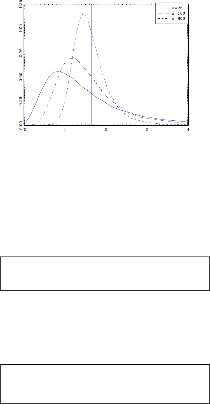
CHAPTER 6. AN INTRODUCTION TO LARGE SAMPLE ASYMPTOTICS 155
Figure 6.1: Sampling Density of ˆ
In this chapter we provide a concise summary. It will be useful for most students to review this
material, even if most is familiar.
6.2 Asymptotic Limits
“Asymptotic analysis” is a method of approximation obtained by taking a suitable limit. There
is more than one method to take limits, but the most common is to take the limit of the sequence
of sampling distributions as the sample size tends to positive infinity, written “as →∞.” It is
not meant to be interpreted literally, but rather as an approximating device.
The first building block for asymptotic analysis is the concept of a limit of a sequence.
Definition 6.2.1 Asequencehas the limit written −→ as
→∞or alternatively as lim→∞ = if for all 0there is some
∞such that for all ≥|−|≤
In words, has the limit if the sequence gets closer and closer to as gets larger. If a
sequence has a limit, that limit is unique (a sequence cannot have two distinct limits). If has
the limit we also say that converges to as →∞
Not all sequences have limits. For example, the sequence {121212}does not have a
limit. It is therefore sometimes useful to have a more general definition of limits which always
exist, and these are the limit superior and limit inferior of a sequence.
Definition 6.2.2 lim inf→∞
=lim
→∞ inf≥
Definition 6.2.3 lim sup→∞
=lim
→∞ sup≥

CHAPTER 6. AN INTRODUCTION TO LARGE SAMPLE ASYMPTOTICS 156
The limit inferior and limit superior always exist (including ±∞as possibilities), and equal
when the limit exists. In the example given earlier, the limit inferior of {121212}is 1, and
the limit superior is 2.
6.3 Convergence in Probability
A sequence of numbers may converge to a limit, but what about a sequence of random variables?
Forexample,considerasamplemean=−1P
=1 based on an random sample of observations.
As increases, the distribution of changes. In what sense can we describe the “limit” of ?In
what sense does it converge?
Since is a random variable, we cannot directly apply the deterministic concept of a sequence of
numbers. Instead, we require a definition of convergence which is appropriate for random variables.
There are more than one such definition, but the most commonly used is called convergence in
probability.
Definition 6.3.1 A random variable ∈Rconverges in probability
to as →∞denoted
−→ or alternatively plim→∞ =,iffor
all 0
lim
→∞ Pr (|−|≤)=1(6.1)
We call the probability limit (or plim)of.
The definition looks quite abstract, but it formalizes the concept of a sequence of random
variables concentrating about a point. The event {|−|≤}occurs when is within of
the point Pr (|−|≤)is the probability of this event — that is within of the point
. Equation (6.1) states that this probability approaches 1 as the sample size increases. The
definition of convergence in probability requires that this holds for any So for any small interval
about the distribution of concentrates within this interval for large
You may notice that the definition concerns the distribution of the random variables ,not
their realizations. Furthermore, notice that the definition uses the concept of a conventional (deter-
ministic) limit, but the latter is applied to a sequence of probabilities, not directly to the random
variables or their realizations.
Two comments about the notation are worth mentioning. First, it is conventional to write the
convergence symbol as
−→ where the “” above the arrow indicates that the convergence is “in
probability”. You should try and adhere to this notation, and not simply write −→ . Second,
it is important to include the phrase “as →∞”tobespecific about how the limit is obtained.
A common mistake is to confuse convergence in probability with convergence in expectation:
E()−→ E()(6.2)
They are related but distinct concepts. Neither (6.1) nor (6.2) implies the other.
To see the distinction it might be helpful to think through a stylized example. Consider a
discrete random variable which takes the value 0with probability 1−−1and the value 6=0
with probability −1,or
Pr (=0)=1−1
(6.3)
Pr (=)= 1

CHAPTER 6. AN INTRODUCTION TO LARGE SAMPLE ASYMPTOTICS 157
In this example the probability distribution of concentrates at zero as increases, regardless of
the sequence Youcancheckthat
−→ 0as →∞
In this example we can also calculate that the expectation of is
E()=
Despite the fact that converges in probability to zero, its expectation will not decrease to zero
unless →0If diverges to infinity at a rate equal to (or faster) then E()will not
converge to zero. For example, if = then E()=1for all even though
−→ 0This
example might seem a bit artificial, but the point is that the concepts of convergence in probability
and convergence in expectation are distinct, so it is important not to confuse one with the other.
Another common source of confusion with the notation surrounding probability limits is that
the expression to the right of the arrow “
−→” must be free of dependence on the sample size
Thus expressions of the form “
−→ ” are notationally meaningless and should not be used.
6.4 Weak Law of Large Numbers
In large samples we expect parameter estimates to be close to the population values. For
example, in Section 4.3 we saw that the sample mean is unbiased for =E()and has variance
2 As gets large its variance decreases and thus the distribution of concentrates about the
population mean It turns out that this implies that the sample mean converges in probability
to the population mean.
When has a finite variance there is a fairly straightforward proof by applying Chebyshev’s
inequality.
Theorem 6.4.1 Chebyshev’s Inequality. For any random variable
and constant 0
Pr (|−E|≥)≤var()
2
Chebyshev’s inequality is terrifically important in asymptotic theory. While its proof is a
technical exercise in probability theory, it is quite simple so we discuss it forthwith. Let ()
denote the distribution of −EThen
Pr (|−E|≥)=Pr³(−E)2≥2´=Z{2≥2}
()
The integral is over the event ©2≥2ª, so that the inequality 1≤2
2holds throughout. Thus
Z{2≥2}
()≤Z{2≥2}
2
2()≤Z2
2()=E(−E)2
2=var()
2
which establishes the desired inequality.
Applied to the sample mean which has variance 2 , Chebyshev’s inequality shows that for
any 0
Pr (|−E()|≥)≤2
2

CHAPTER 6. AN INTRODUCTION TO LARGE SAMPLE ASYMPTOTICS 158
For fixed 2and the bound on the right-hand-side shrinks to zero as →∞(Specifically, for any
0set ≥2¡2¢. Then the right-hand-side is less than or equal to .) Thus the probability
that is within of E()=approaches 1 as gets large, or
lim
→∞ Pr (|−|)=1
This means that converges in probability to as →∞
This result is called the weak law of large numbers. Our derivation assumed that has a
finite variance, but with a more careful derivation all that is necessary is a finite mean.
Theorem 6.4.2 Weak Law of Large Numbers (WLLN)
If are independent and identically distributed and E||∞then as
→∞,
=1
X
=1
−→ E()
The proof of Theorem 6.4.2 is presented in Section 6.16.
The WLLN shows that the estimator converges in probability to the true population mean .
In general, an estimator which converges in probability to the population value is called consistent.
Definition 6.4.1 An estimator b
of a parameter is consistent if b
−→
as →∞
Theorem 6.4.3 If are independent and identically distributed and
E||∞then b=is consistent for the population mean
Consistency is a good property for an estimator to possess. It means that for any given data
distributionthere is a sample size sufficiently large such that the estimator b
will be arbitrarily
close to the true value with high probability. The theorem does not tell us, however, how large
this has to be. Thus the theorem does not give practical guidance for empirical practice. Still,
it is a minimal property for an estimator to be considered a “good” estimator, and provides a
foundation for more useful approximations.
6.5 Almost Sure Convergence and the Strong Law*
Convergence in probability is sometimes called weak convergence. A related concept is
almost sure convergence,alsoknownasstrong convergence. (In probability theory the term
“almost sure” means “with probability equal to one”. An event which is random but occurs with
probability equal to one is said to be almost sure.)

CHAPTER 6. AN INTRODUCTION TO LARGE SAMPLE ASYMPTOTICS 159
Definition 6.5.1 A random variable ∈Rconverges almost surely
to as →∞denoted
−→ if for every 0
Pr ³lim
→∞ |−|≤´=1(6.4)
The convergence (6.4) is stronger than (6.1) because it computes the probability of a limit
rather than the limit of a probability. Almost sure convergence is stronger than convergence in
probability in the sense that
−→ implies
−→ .
In the example (6.3) of Section 6.3, the sequence converges in probability to zero for any
sequence but this is not sufficient for to converge almost surely. In order for to converge
to zero almost surely, it is necessary that →0.
In the random sampling context the sample mean can be shown to converge almost surely to
the population mean. This is called the strong law of large numbers.
Theorem 6.5.1 Strong Law of Large Numbers (SLLN)
If are independent and identically distributed and E||∞then as
→∞,
=1
X
=1
−→ E()
The proof of the SLLN is technically quite advanced so is not presented here. For a proof see
Billingsley (1995, Theorem 22.1) or Ash (1972, Theorem 7.2.5).
The WLLN is sufficient for most purposes in econometrics, so we will not use the SLLN in this
text.
6.6 Vector-Valued Moments
Our preceding discussion focused on the case where is real-valued (a scalar), but nothing
important changes if we generalize to the case where y∈Ris a vector. To fix notation, the
elements of yare
y=⎛
⎜
⎜
⎜
⎝
1
2
.
.
.
⎞
⎟
⎟
⎟
⎠
The population mean of yis just the vector of marginal means
μ=E(y)=⎛
⎜
⎜
⎜
⎝
E(1)
E(2)
.
.
.
E()
⎞
⎟
⎟
⎟
⎠
When working with random vectors yit is convenient to measure their magnitude by their
Euclidean length or Euclidean norm
kyk=¡2
1+···+2
¢12

CHAPTER 6. AN INTRODUCTION TO LARGE SAMPLE ASYMPTOTICS 160
In vector notation we have
kyk2=y0y
It turns out that it is equivalent to describe finiteness of moments in terms of the Euclidean
norm of a vector or all individual components.
Theorem 6.6.1 For y∈REkyk∞if and only if E||∞for
=1
The ×variance matrix of yis
V=var(y)=E¡(y−μ)(y−μ)0¢
Vis often called a variance-covariance matrix. You can show that the elements of Vare finite if
Ekyk2∞
A random sample {y1y}consists of observations of independent and identically distrib-
uted draws from the distribution of y(Each draw is an -vector.) The vector sample mean
y=1
X
=1
y=⎛
⎜
⎜
⎜
⎝
1
2
.
.
.
⎞
⎟
⎟
⎟
⎠
is the vector of sample means of the individual variables.
Convergence in probability of a vector can be defined as convergence in probability of all ele-
ments in the vector. Thus y
−→ μifandonlyif
−→ for =1 Since the latter holds
if E||∞for =1 or equivalently Ekyk∞we can state this formally as follows.
Theorem 6.6.2 WLLN for random vectors
If yare independent and identically distributed and Ekyk∞then as
→∞,
y=1
X
=1
y
−→ E(y)
6.7 Convergence in Distribution
The WLLN is a useful first step, but does not give an approximation to the distribution of an
estimator. A large-sample or asymptotic approximation can be obtained using the concept of
convergence in distribution.
We say that a sequence of random vectors zconverges in distribution if the sequence of
distribution functions (u)=Pr(z≤u)converges to a limit distribution function.

CHAPTER 6. AN INTRODUCTION TO LARGE SAMPLE ASYMPTOTICS 161
Definition 6.7.1 Let zbe a random vector with distribution (u)=
Pr (z≤u)We say that zconverges in distribution to zas →∞,
denoted z
−→ zif for all uat which (u)=Pr(z≤u)is continuous,
(u)→(u)as →∞
Under these conditions, it is also said that converges weakly to .Itiscommontorefer
to zand its distribution ()as the asymptotic distribution,large sample distribution,or
limit distribution of z.
When the limit distribution zis degenerate (that is, Pr (z=c)=1for some c)wecanwrite
the convergence as z
−→ c, which is equivalent to convergence in probability, z
−→ c.
Technically, in most cases of interest it is difficult to establish the limit distributions of sample
statistics zby working directly with their distribution function. It turns out that in most cases it is
easier to work with their characteristic function (λ)=E¡exp ¡iλ0z¢¢, which is a transformation
of the distribution. (See Section 2.31 for the definition.) While this is more technical than needed
for most applied economists, we introduce this material to give a complete reference for large sample
approximations.
The characteristic function (t)completely describes the distribution of z. It therefore seems
reasonable to expect that if (t)converges to a limit function (t), then the the distribution of
zconverges as well. This turns out to be true, and is known as Lévy’s continuity theorem.
Theorem 6.7.1 Lévy’s Continuity Theorem.z
−→ zif and only if
E(exp (it0z)) →E(exp (it0z)) for every t∈R
While this result seems quite intuitive, a rigorous proof is quite advanced and so is not presented
here. See Van der Vaart (2008) Theorem 2.13.
Finally, we mention a standard trick which is commonly used to establish multivariate conver-
gence results.
Theorem 6.7.2 Cramér-Wold Device.z
−→ zif and only if
λ0z
−→ λ0zfor every λ∈Rwith λ0λ=1.
We present a proof in Section 6.16 which is a simple application of Lévy’s continuity theorem.
6.8 Central Limit Theorem
We would like to obtain a distributional approximation to the sample mean . We start un-
der the random sampling assumption so that the observations are independent and identically
distributed, and have a finite mean =E()and variance 2=var().
Let’s start by finding the asymptotic distribution of , in the sense that
−→ for some random
variable . From the WLLN we know that
−→ . Since convergence in probability to a constant
is the same as convergence in distribution, this means that
−→ aswell. Thisisnotauseful
distributional result as the limit distribution is a constant. To obtain a non-degenerate distribution

CHAPTER 6. AN INTRODUCTION TO LARGE SAMPLE ASYMPTOTICS 162
we need to rescale . Recall that var (−)=2, which means that var (√(−)) = 2.
This suggests renormalizing the statistic as
=√(−)
Notice that E()=0and var ()=2. This shows that the mean and variance have been
stabilized. We now seek to determine the asymptotic distribution of .
The answer is provided by the central limit theorem (CLT) which states that standardized
sample averages converge in distribution to normal random vectors. There are several versions
of the CLT. The most basic is the case where the observations are independent and identically
distributed.
Theorem 6.8.1 Lindeberg—Lévy Central Limit Theorem.Ifare
independent and identically distributed and E¡2
¢∞then as →∞
√(−)
−→ N¡02¢
where =E()and 2=E(−)2
The proof of the CLT is rather technical (so is presented in Section 6.16) but at the core is a
quadratic approximation of the log of the characteristic function.
As we discussed above, in finite samples the standardized sum =√(−)has mean zero
and variance 2. What the CLT adds is that is also approximately normally distributed, and
that the normal approximation improves as increases.
The CLT is one of the most powerful and mysterious results in statistical theory. It shows that
the simple process of averaging induces normality. The first version of the CLT (for the number
of heads resulting from many tosses of a fair coin) was established by the French mathematician
Abraham de Moivre in an article published in 1733. This was extended to cover an approximation
to the binomial distribution in 1812 by Pierre-Simon Laplace in his book Théorie Analytique des
Probabilités, and the most general statements are credited to articles by the Russian mathematician
Aleksandr Lyapunov (1901) and the Finnish mathematician Jarl Waldemar Lindeberg (1920, 1922).
The above statement is known as the classic (or Lindeberg-Lévy) CLT due to contributions by
Lindeberg (1920) and the French mathematician Paul Pierre Lévy.
A more general version which allows heterogeneous distributions was provided by Lindeberg
(1922). The following is the most general statement.
Theorem 6.8.2 Lindeberg-Feller Central Limit Theorem.Suppose
are independent but not necessarily identically distributed with finite
means =E()and variances 2
=E( −)2Set 2
=
−1P
=1 2
.If2
0and for all 0
lim
→∞
1
2
X
=1
E³( −)21³( −)2≥2
´´=0 (6.5)
then as →∞ √(−E())
12
−→ N(01)

CHAPTER 6. AN INTRODUCTION TO LARGE SAMPLE ASYMPTOTICS 163
The proof of the Lindeberg-Feller CLT is substantially more technical, so we do not present it
here. See Billingsley (1995, Theorem 27.2).
The Lindeberg-Feller CLT is quite general as it puts minimal conditions on the sequence of
means and variances. The key assumption is equation (6.5) which is known as Lindeberg’s
Condition.Initsrawformitisdifficult to interpret. The intuition for (6.5) is that it excludes
any single observation from dominating the asymptotic distribution. Since (6.5) is quite abstract,
in most contexts we use more elementary conditions which are simpler to interpret.
One such alternative is called Lyapunov’s condition:Forsome0
lim
→∞
1
1+22+
X
=1
E³| −|2+´=0(6.6)
Lyapunov’s condition implies Lindeberg’s condition, and hence the CLT. Indeed, the left-side of
(6.5) is bounded by
lim
→∞
1
2
X
=1
EÃ| −|2+
| −|1³| −|2≥2
´!
≤lim
→∞
1
21+22+
X
=1
E³| −|2+´
=0
by (6.6).
Lyapunov’s condition is still awkward to interpret. A still simpler condition is a uniform moment
bound: For some 0
sup
E||2+∞(6.7)
This is typically combined with the lower variance bound
lim inf
→∞ 2
0(6.8)
These bounds together imply Lyapunov’s condition. To see this, (6.7) and (6.8) imply there is
some ∞such that sup E||2+≤and lim inf→∞ 2
≥−1Without loss of generality
assume =0. Then the left side of (6.6) is bounded by
lim
→∞
2+2
2=0
so Lyapunov’s condition holds and hence the CLT.
An alternative to (6.8) is to assume that the average variance 2
converges to a constant, that
is,
2
=−1
X
=1
2
→2∞(6.9)
This assumption is reasonable in many applications.
We now state the simplest and most commonly used version of a heterogeneous CLT based on
the Lindeberg-Feller Theorem.
Theorem 6.8.3 Suppose are independent but not necessarily identi-
cally distributed. If (6.7) and (6.9) hold, then as →∞
√(−E())
−→ N¡0
2¢(6.10)
One advantage of Theorem 6.8.3 is that it allows 2=0(unlike Theorem 6.8.2).

CHAPTER 6. AN INTRODUCTION TO LARGE SAMPLE ASYMPTOTICS 164
6.9 Multivariate Central Limit Theorem
Multivariate central limit theory applies when we consider vector-valued observations yand
sample averages y. In the i.i.d. case we know that the mean of yis the mean vector μ=E(y)
and its variance is −1Vwhere V=E¡(y−μ)(y−μ)0¢. Againwewishtotransformyso that
its mean and variance do not depend on . We do this again by centering and scaling, by setting
z=√(y−μ).Thishasmean0and variance V, which are independent of as desired.
To develop a distributional approximation for zwe use a multivariate central limit theorem.
We present three such results, corresponding to the three univariate results from the previous
section. Each is derived from the univariate theory by the Cramér-Wold device (Theorem 6.7.2).
We first present the multivariate version of Theorem 6.8.1.
Theorem 6.9.1 Multivariate Lindeberg—Lévy Central Limit Theo-
rem.Ify∈Rare independent and identically distributed and Ekyk2
∞then as →∞ √(y−μ)
−→ N(0V)
where μ=E(y)and V=E¡(y−μ)(y−μ)0¢
We next present a multivariate version of Theorem 6.8.2.
Theorem 6.9.2 Multivariate Lindeberg-Feller CLT.Suppose
y ∈Rare independent but not necessarily identically dis-
tributed with finite means μ =E(y)and variance matrices
V =E¡(y −μ)(y −μ)0¢Set V=−1P
=1 V and
2
=min(V).If2
0and for all 0
lim
→∞
1
2
X
=1
E³ky −μk21³ky −μk2≥2
´´=0 (6.11)
then as →∞
V−12
√(y−E(y))
−→ N(0I)
We finally present a multivariate version of Theorem 6.8.3.
Theorem 6.9.3 Suppose y ∈Rare independent but not necessarily
identically distributed with finite means μ =E(y)and variance matri-
ces V =E¡(y −μ)(y −μ)0¢Set V=−1P
=1 V .If
V→V0(6.12)
and for some 0
sup
Ekyk2+∞(6.13)
then as →∞ √(y−E(y))
−→ N(0V)

CHAPTER 6. AN INTRODUCTION TO LARGE SAMPLE ASYMPTOTICS 165
Similarly to Theorem 6.8.3, an advantage of Theorem 6.9.3 is that it allows the variance matrix
Vto be singular.
6.10 Higher Moments
Often we want to estimate a parameter μwhich is the expected value of a transformation of a
random vector y.Thatis,μcan be written as
μ=E(h(y))
for some function h:R→RFor example, the second moment of is E¡2¢the is E()
the moment generating function is E(exp ()) and the distribution function is E(1 {≤})
Estimating parameters of this form fits into our previous analysis by defining the random
variable z=h(y)for then μ=E(z)is just a simple moment of z. This suggests the moment
estimator
b
μ=1
X
=1
z=1
X
=1
h(y)
For example, the moment estimator of E()is −1P
=1
that of the moment generating function
is −1P
=1 exp ()and for the distribution function the estimator is −1P
=1 1{≤}.
Since b
μis a sample average, and transformations of iid variables are also i.i.d., the asymptotic
results of the previous sections immediately apply.
Theorem 6.10.1 If yare independent and identically distributed, μ=
E(h(y)) and Ekh(y)k∞then for b
μ=1
P
=1 h(y)as →∞,
b
μ
−→ μ
Theorem 6.10.2 If yare independent and identically distributed, μ=
E(h(y)) and Ekh(y)k2∞then for b
μ=1
P
=1 h(y)as →∞
√(b
μ−μ)
−→ N(0V)
where V=E¡(h(y)−μ)(h(y)−μ)0¢
Theorems 6.10.1 and 6.10.2 show that the estimate b
μis consistent for μand asymptotically
normally distributed, so long as the stated moment conditions hold.
A word of caution. Theorems 6.10.1 and 6.10.2 give the impression that it is possible to estimate
any moment of Technically this is the case so long as that moment is finite. What is hidden
by the notation, however, is that estimates of high order moments can be quite imprecise. For
example, consider the sample 8 moment b8=1
P
=1 8
and suppose for simplicity that is
N(01)Then we can calculate1that var (b8)=−12016000which is immense, even for large !
In general, higher-order moments are challenging to estimate because their variance depends upon
even higher moments which can be quite large in some cases.
1By the formula for the variance of a mean var (8)=−1E16−E82Since is N(01)E16=
15!! = 2027025 and E8= 7!! = 105 where !! isthedoublefactorial.

CHAPTER 6. AN INTRODUCTION TO LARGE SAMPLE ASYMPTOTICS 166
6.11 Functions of Moments
We now expand our investigation and consider estimation of parameters which can be written
as a continuous function of μ=E(h(y)). That is, the parameter of interest can be written as
β=g(μ)=g(E(h(y))) (6.14)
for some functions g:R→Rand h:R→R
As one example, the geometric mean of wages is
=exp(E(log ())) (6.15)
This is (6.14) with ()=exp()and ()=log()
A simple yet common example is the variance
2=E(−E())2
=E¡2¢−(E())2
This is (6.14) with
h()=µ
2
and
(1
2)=2−2
1
Similarly, the skewness of the wage distribution is
=
E³(−E())3´
³E³(−E())2´´32
This is (6.14) with
h()=⎛
⎝
2
3⎞
⎠
and
(1
2
3)=3−321+23
1
¡2−2
1¢32(6.16)
The parameter β=g(μ)is not a population moment, so it does not have a direct moment
estimator. Instead, it is common to use a plug-in estimate formed by replacing the unknown μ
with its point estimate b
μand then “plugging” this into the expression for β.Thefirst step is
b
μ=1
X
=1
h(y)
and the second step is b
β=g(b
μ)
Again, the hat “^” indicates that b
βis a sample estimate of β
For example, the plug-in estimate of the geometric mean of the wage distribution from (6.15)
is
b=exp(b)
with
b=1
X
=1
log ()

CHAPTER 6. AN INTRODUCTION TO LARGE SAMPLE ASYMPTOTICS 167
The plug-in estimate of the variance is
b2=1
X
=1
2
−Ã1
X
=1
!2
=1
X
=1
(−)2
The estimator for the skewness is
c
=b3−3b2b1+2b3
1
¡b2−b2
1¢32
=
1
P
=1 (−)3
³1
P
=1 (−)2´32
where
b=1
X
=1
A useful property is that continuous functions are limit-preserving.
Theorem 6.11.1 Continuous Mapping Theorem (CMT).Ifz
−→
cas →∞and g(·)is continuous at cthen g(z)
−→ g(c)as →∞.
The proof of Theorem 6.11.1 is given in Section 6.16.
For example, if
−→ as →∞then
+
−→ +
−→
2
−→ 2
as the functions ()=+ ()= and ()=2are continuous. Also
−→
if 6=0The condition 6=0is important as the function ()= is not continuous at =0
If yare independent and identically distributed, μ=E(h(y)) and Ekh(y)k∞then for
b
μ=1
P
=1 h(y)as →∞,b
μ
−→ μApplying the CMT, b
β=g(b
μ)
−→ g(μ)=β
Theorem 6.11.2 If yare independent and identically distributed, β=
g(E(h(y))) Ekh(y)k∞and g(u)is continuous at u=μ, then for
b
β=g¡1
P
=1 h(y)¢as →∞b
β
−→ β
To apply Theorem 6.11.2 it is necessary to check if the function gis continuous at μ.Inour
first example ()=exp()is continuous everywhere. It therefore follows from Theorem 6.6.2 and
Theorem 6.11.2 that if E|log ()|∞then as →∞b
−→
Intheexampleofthevariance,is continuous for all μ.ThusifE¡2¢∞then as →∞
b2
−→ 2
In our third example defined in (6.16) is continuous for all μsuch that var()=2−2
10
which holds unless has a degenerate distribution. Thus if E||3∞and var()0then as
→∞c
−→

CHAPTER 6. AN INTRODUCTION TO LARGE SAMPLE ASYMPTOTICS 168
6.12 Delta Method
Inthissectionweintroducetwotools—anextended version of the CMT and the Delta Method
— which allow us to calculate the asymptotic distribution of the parameter estimate b
β.
We first present an extended version of the continuous mapping theorem which allows conver-
gence in distribution.
Theorem 6.12.1 Continuous Mapping Theorem
If z
−→ zas →∞and g:R→Rhas the set of discontinuity points
such that Pr (z∈)=0then g(z)
−→ g(z)as →∞.
For a proof of Theorem 6.12.1 see Theorem 2.3 of van der Vaart (1998). It was first proved by
Mann and Wald (1943) and is therefore sometimes referred to as the Mann-Wald Theorem.
Theorem 6.12.1 allows the function gto be discontinuous only if the probability at being at a
discontinuity point is zero. For example, the function ()=−1is discontinuous at =0but if
−→ ∼N(01) then Pr (=0)=0so −1
−→ −1
A special case of the Continuous Mapping Theorem is known as Slutsky’s Theorem.
Theorem 6.12.2 Slutsky’s Theorem
If
−→ and
−→ as →∞,then
1. +
−→ +
2.
−→
3.
−→
if 6=0
Even though Slutsky’s Theorem is a special case of the CMT, it is a useful statement as it
focuses on the most common applications — addition, multiplication, and division.
Despite the fact that the plug-in estimator b
βis a function of b
μfor which we have an asymptotic
distribution, Theorem 6.12.1 does not directly give us an asymptotic distribution for b
βThis is
because b
β=g(b
μ)is written as a function of b
μ, not of the standardized sequence √(b
μ−μ)
We need an intermediate step — a first order Taylor series expansion. This step is so critical to
statistical theory that it has its own name — The Delta Method.
Theorem 6.12.3 Delta Method:
If √(b
μ−μ)
−→ ξwhere g(u)is continuously differentiable in a neigh-
borhood of μthen as →∞
√(g(b
μ)−g(μ))
−→ G0ξ(6.17)
where G(u)=
g(u)0and G=G(μ)In particular, if ξ∼N(0V)then
as →∞ √(g(b
μ)−g(μ))
−→ N¡0G0VG
¢(6.18)

CHAPTER 6. AN INTRODUCTION TO LARGE SAMPLE ASYMPTOTICS 169
The Delta Method allows us to complete our derivation of the asymptotic distribution of the
estimator b
βof β. By combining Theorems 6.10.2 and 6.12.3 we can find the asymptotic distribution
of the plug-in estimator b
β.
Theorem 6.12.4 If yare independent and identically distributed, μ=
E(h(y)),β=g(μ)Ekh(y)k2∞and G(u)=
ug(u)0is continuous
inaneighborhoodofμ, then for b
β=g¡1
P
=1 h(y)¢as →∞
√³b
β−β´
−→ N¡0G0VG
¢
where V=E¡(h(y)−μ)(h(y)−μ)0¢and G=G(μ)
Theorem 6.11.2 established the consistency of b
βfor β, and Theorem 6.12.4 established its
asymptotic normality. It is instructive to compare the conditions required for these results. Consis-
tency required that h(y)have a finite mean, while asymptotic normality requires that this variable
have a finite variance. Consistency required that g(u)be continuous, while our proof of asymptotic
normalityusedtheassumptionthatg(u)is continuously differentiable.
6.13 Stochastic Order Symbols
It is convenient to have simple symbols for random variables and vectors which converge in
probability to zero or are stochastically bounded. In this section we introduce some of the most
commonly found notation.
It might be useful to review the common notation for non-random convergence and boundedness.
Let and =12 be non-random sequences. The notation
=(1)
(pronounced “small oh-one”) is equivalent to →0as →∞. The notation
=()
is equivalent to −1
→0as →∞The notation
=(1)
(pronounced “big oh-one”) means that is bounded uniformly in — there exists an ∞such
that ||≤for all The notation
=()
is equivalent to −1
=(1)
We now introduce similar concepts for sequences of random variables. Let and =12
be sequences of random variables. (In most applications, is non-random.) The notation
=(1)
(“small oh-P-one”) means that
−→ 0as →∞For example, for any consistent estimator b
β
for βwe can write b
β=β+(1)

CHAPTER 6. AN INTRODUCTION TO LARGE SAMPLE ASYMPTOTICS 170
We also write
=()
if −1
=(1)
Similarly, the notation =(1) (“big oh-P-one”) means that is bounded in probability.
Precisely, for any 0there is a constant ∞such that
lim sup
→∞
Pr (||
)≤
Furthermore, we write
=()
if −1
=(1)
(1) is weaker than (1) in the sense that =(1) implies =(1) but not the reverse.
However, if =()then =()for any such that →0
If a random vector converges in distribution z
−→ z(for example, if z∼N(0V)) then
z=(1)It follows that for estimators b
βwhich satisfy the convergence of Theorem 6.12.4 then
we can write b
β=β+(−12)
In words, this statement says that the estimator b
βequals the true coefficient βplus a random
component which is bounded when scaled by 12. Equivalently, we can write
12³b
β−β´=(1)
Another useful observation is that a random sequence with a bounded moment is stochastically
bounded.
Theorem 6.13.1 If zis a random vector which satisfies
Ekzk=()
for some sequence and 0then
z=(1
)
Similarly, Ekzk=()implies z=(1
)
This can be shown using Markov’s inequality (B.14). The assumptions imply that there is some
∞such that Ekzk≤for all For any set =µ
¶1
Then
Pr ³−1
kzk
´=Prµkzk
¶≤
Ekzk≤
as required.
There are many simple rules for manipulating (1) and (1) sequences which can be deduced
from the continuous mapping theorem or Slutsky’s Theorem. For example,
(1) + (1) = (1)
(1) + (1) = (1)
(1) + (1) = (1)
(1)(1) = (1)
(1)(1) = (1)
(1)(1) = (1)

CHAPTER 6. AN INTRODUCTION TO LARGE SAMPLE ASYMPTOTICS 171
6.14 Uniform Stochastic Bounds*
For some applications it can be useful to obtain the stochastic order of the random variable
max
1≤≤||
This is the magnitude of the largest observation in the sample {1
}If the support of the
distribution of is unbounded, then as the sample size increases, the largest observation will
also tend to increase. It turns out that there is a simple characterization.
Theorem 6.14.1 If yare identically distributed and E||∞then as
→∞ −1 max
1≤≤||
−→ 0(6.19)
Furthermore, if E(exp()) ∞for some 0then for any 0
(log )−(1+)max
1≤≤||
−→ 0(6.20)
The proof of Theorem 6.14.1 is presented in Section 6.16.
Equivalently, (6.19) can be written as
max
1≤≤||=(1)(6.21)
and (6.22) as
max
1≤≤||=(log )(6.22)
Equation (6.21) says that if has finite moments, then the largest observation will diverge
at a rate slower than 1.Asincreases this rate decreases. Equation (6.22) shows that if we
strengthen this to having all finite moments and a finite moment generating function (for example,
if is normally distributed) then the largest observation will diverge slower than log .Thusthe
higher the moments, the slower the rate of divergence.
To simplify the notation, we write (6.21) as =(1)uniformly in 1≤≤ It is important
to understand when the or symbols are applied to subscript random variables whether the
convergence is pointwise in , or is uniform in in the sense of (6.21)-(6.22).
Theorem 6.14.1 applies to random vectors. For example, if Ekyk∞then
max
1≤≤kyk=(1)
6.15 Semiparametric Efficiency
In this section we argue that the sample mean b
μand plug-in estimator b
β=g(b
μ)are efficient
estimators of the parameters μand β. Our demonstration is based on the rich but technically
challenging theory of semiparametric efficiency bounds. An excellent accessible review has been
provided by Newey (1990). We will also appeal to the asymptotic theory of maximum likelihood
estimation (see Chapter 5).
We start by examining the sample mean b
μfor the asymptotic efficiency of b
βwill follow from
that of b
μ
Recall, we know that if E³kyk2´∞then the sample mean has the asymptotic distribution
√(b
μ−μ)
−→ N(0V)We want to know if b
μis the best feasible estimator, or if there is another

CHAPTER 6. AN INTRODUCTION TO LARGE SAMPLE ASYMPTOTICS 172
estimator with a smaller asymptotic variance. While it seems intuitively unlikely that another
estimator could have a smaller asymptotic variance, how do we know that this is not the case?
When we ask if b
μisthebestestimator,weneedtobeclearabouttheclassofmodels—theclass
of permissible distributions. For estimation of the mean μof the distribution of ythe broadest
conceivable class is L1={:Ekyk∞}This class is too broad for our current purposes, as b
μ
is not asymptotically N(0V)for all ∈L1A more realistic choice is L2=n:E³kyk2´∞o
—theclassoffinite-variance distributions. When we seek an efficient estimator of the mean μin
the class of models L2what we are seeking is the best estimator, given that all we know is that
∈L2
To show that the answer is not immediately obvious, it might be helpful to review a set-
ting where the sample mean is inefficient. Suppose that ∈Rhas the double exponential den-
sity (|)=2
−12exp ¡−|−|√2¢Since var ()=1we see that the sample mean satis-
fies √(e−)
−→ N(01). In this model the maximum likelihood estimator (MLE) efor
is the sample median. Recall from the theory of maximum likelihood that the MLE satisfies
√(e−)
−→ N³0¡E¡2¢¢−1´where =
log (|)=−√2sgn(−)is the score. We
can calculate that E¡2¢=2and thus conclude that √(e−)
−→ N(012) The asymptotic
variance of the MLE is one-half that of the sample mean. Thus when the true density is known to
be double exponential the sample mean is inefficient.
But the estimator which achieves this improved efficiency — the sample median — is not generi-
cally consistent for the population mean. It is inconsistent if the density is asymmetric or skewed.
So the improvement comes at a great cost. Another way of looking at this is that the sample
median is efficient in the class of densities ©(|)=2
−12exp ¡−|−|√2¢ªbut unless it is
known that this is the correct distribution class this knowledge is not very useful.
The relevant question is whether or not the sample mean is efficient when the form of the
distribution is unknown. We call this setting semiparametric as the parameter of interest (the
mean) is finite dimensional while the remaining features of the distribution are unspecified. In the
semiparametric context an estimator is called semiparametrically efficient if it has the smallest
asymptotic variance among all semiparametric estimators.
The mathematical trick is to reduce the semiparametric model to a set of parametric “submod-
els”. The Cramer-Rao variance bound can be found for each parametric submodel. The variance
bound for the semiparametric model (the union of the submodels) is then defined as the supremum
of the individual variance bounds.
Formally, suppose that the true density of yis the unknown function (y)with mean μ=
E(y)=Ry(y)yA parametric submodel for (y)is a density (y|θ)which is a smooth
function of a parameter θ, and there is a true value θ0such that (y|θ0)=(y)The index
indicates the submodels. The equality (y|θ0)=(y)means that the submodel class passes
through the true density, so the submodel is a true model. The class of submodels and parameter
θ0depend on the true density In the submodel (y|θ)the mean is μ(θ)=Ry(y|θ)y
which varies with the parameter θ.Let∈ℵbe the class of all submodels for
Since each submodel is parametric we can calculate the efficiency bound for estimation of μ
within this submodel. Specifically, given the density (y|θ)its likelihood score is
S=
θlog (y|θ0)
so the Cramer-Rao lower bound for estimation of θis ³E³SS0
´´−1Defining M=
μ(θ0)0
by Theorem 5.16.3 the Cramer-Rao lower bound for estimation of μwithin the submodel is
V=M0
³E³SS0
´´−1M.
As Vis the efficiency bound for the submodel class (y|θ)no estimator can have an
asymptotic variance smaller than Vfor any density (y|θ)in the submodel class, including the

CHAPTER 6. AN INTRODUCTION TO LARGE SAMPLE ASYMPTOTICS 173
true density . This is true for all submodels Thus the asymptotic variance of any semiparametric
estimator cannot be smaller than Vfor any conceivable submodel. Taking the supremum of the
Cramer-Rao bounds from all conceivable submodels we define2
V=sup
∈ℵ
V
The asymptotic variance of any semiparametric estimator cannot be smaller than V, since it cannot
be smaller than any individual VWe call Vthe semiparametric asymptotic variance bound
or semiparametric efficiency bound for estimation of μ, as it is a lower bound on the asymptotic
variance for any semiparametric estimator. If the asymptotic variance of a specific semiparametric
estimator equals the bound Vwe say that the estimator is semiparametrically efficient.
For many statistical problems it is quite challenging to calculate the semiparametric variance
bound. However, in some cases there is a simple method to find the solution. Suppose that we can
find a submodel 0whose Cramer-Rao lower bound satisfies V0=Vwhere Vis the asymptotic
variance of a known semiparametric estimator. In this case, we can deduce that V=V0=V.
Otherwise (that is, if V0is not the efficiency bound) there would exist another submodel 1whose
Cramer-Rao lower bound satisfies V0V1(because V0is not the supremum). This would
imply VV1which contradicts the Cramer-Rao Theorem (since when submodel 1is true
then no estimator can have a lower variance than V1).
We now find this submodel for the sample mean b
μOur goal is to find a parametric submodel
whose Cramer-Rao bound for μis VThis can be done by creating a tilted version of the true
density. Consider the parametric submodel
(y|θ)=(y)¡1+θ0V−1(y−μ)¢(6.23)
where (y)isthetruedensityandμ=EyNote that
Z(y|θ)y=Z(y)y+θ0V−1Z(y)(y−μ)y=1
and for all θclose to zero (y|θ)≥0Thus (y|θ)is a valid density function. It is a parametric
submodel since (y|θ0)=(y)when θ0=0This parametric submodel has the mean
μ(θ)=Zy(y|θ)y
=Zy(y)y+Z(y)y(y−μ)0V−1θy
=μ+θ
which is a smooth function of θ
Since
θlog (y|θ)=
θlog ¡1+θ0V−1(y−μ)¢=V−1(y−μ)
1+θ0V−1(y−μ)
it follows that the score function for θis
S=
θlog (y|θ0)=V−1(y−μ)(6.24)
By Theorem 5.16.3 the Cramer-Rao lower bound for θis
¡E¡SS0
¢¢−1=¡V−1E¡(y−μ)(y−μ)0¢V−1¢−1=V(6.25)
2It is not obvious that this supremum exists, as is a matrix so there is not a unique ordering of matrices.
However, in many cases (including the ones we study) the supremum exists and is unique.

CHAPTER 6. AN INTRODUCTION TO LARGE SAMPLE ASYMPTOTICS 174
The Cramer-Rao lower bound for μ(θ)=μ+θis also V, and this equals the asymptotic variance
of the moment estimator b
μThiswaswhatwesetouttoshow.
In summary, we have shown that in the submodel (6.23) the Cramer-Rao lower bound for
estimation of μis Vwhich equals the asymptotic variance of the sample mean. This establishes
the following result.
Proposition 6.15.1 In the class of distributions ∈L2the semipara-
metric variance bound for estimation of μis V=var()and the sample
mean b
μis a semiparametrically efficient estimator of the population mean
μ.
We call this result a proposition rather than a theorem as we have not attended to the regularity
conditions.
It is a simple matter to extend this result to the plug-in estimator b
β=g(b
μ).Weknowfrom
Theorem 6.12.4 that if Ekyk2∞and g(u)is continuously differentiable at u=μthen the plug-
in estimator has the asymptotic distribution √³b
β−β´
−→ N(0G0VG)We therefore consider
the class of distributions
L2(g)=n:Ekyk2∞g(u)is continuously differentiable at u=E(y)o
For example, if =12where 1=E(1)and 2=E(2)then
L2()=©:E¡2
1¢∞E¡2
2¢∞and E(2)6=0
ª
For any submodel the Cramer-Rao lower bound for estimation of β=g(μ)is G0VG.For
the submodel (6.23) this bound is G0VGwhich equals the asymptotic variance of b
βfrom Theorem
6.12.4. Thus b
βis semiparametrically efficient.
Proposition 6.15.2 In the class of distributions ∈L2(g)the semi-
parametric variance bound for estimation of β=g(μ)is G0VGand the
plug-in estimator b
β=g(b
μ)is a semiparametrically efficient estimator of
β.
The result in Proposition 6.15.2 is quite general. Smooth functions of sample moments are
efficient estimators for their population counterparts. This is a very powerful result, as most
econometric estimators can be written (or approximated) as smooth functions of sample means.
6.16 Technical Proofs*
In this section we provide proofs of some of the more technical points in the chapter. These
proofs may only be of interest to more mathematically inclined students.
ProofofTheorem6.4.2:Without loss of generality, we can assume E()=0by recentering
on its expectation.
We need to show that for all 0and 0there is some ∞so that for all ≥
Pr (||)≤ Fix and Set =3Pick ∞large enough so that
E(||1(||)) ≤(6.26)

CHAPTER 6. AN INTRODUCTION TO LARGE SAMPLE ASYMPTOTICS 175
(where 1(·)is the indicator function) which is possible since E||∞Define the random variables
=1(||≤)−E(1(||≤))
=1(||)−E(1(||))
so that
=+
and
E||≤E||+E||(6.27)
We now show that sum of the expectations on the right-hand-side can be bounded below 3
First, by the Triangle Inequality (A.26) and the Expectation Inequality (B.8),
E||=E|1(||)−E(1(||))|
≤E|1(||)|+|E(1(||))|
≤2E|1(||)|
≤2 (6.28)
and thus by the Triangle Inequality (A.26) and (6.28)
E||=E¯¯¯¯¯
1
X
=1
¯¯¯¯¯≤1
X
=1
E||≤2 (6.29)
Second, by a similar argument
||=|1(||≤)−E(1(||≤))|
≤|1(||≤)|+|E(1(||≤))|
≤2|1(||≤)|
≤2(6.30)
where the final inequality is (6.26). Then by Jensen’s Inequality (B.5), the fact that the are iid
and mean zero, and (6.30),
(E||)2≤E³||2´=E¡2
¢
≤42
≤2(6.31)
the final inequality holding for ≥422=36222. Equations (6.27), (6.29) and (6.31)
together show that
E||≤3(6.32)
as desired.
Finally, by Markov’s Inequality (B.14) and (6.32),
Pr (||)≤E||
≤3
=
the final equality by the definition of We have shown that for any 0and 0then for all
≥36222Pr (||)≤ as needed. ¥
ProofofTheorem6.6.1:By Loève’s Inequality (A.16)
kyk=⎛
⎝
X
=1
2
⎞
⎠
12
≤
X
=1
||

CHAPTER 6. AN INTRODUCTION TO LARGE SAMPLE ASYMPTOTICS 176
Thus if E||∞for =1 then
Ekyk≤
X
=1
E||∞
For the reverse inequality, the Euclidean norm of a vector is larger than the length of any individual
component, so for any ||≤kykThus, if Ekyk∞then E||∞for =1 ¥
Proof of Theorem 6.7.2: By Lévy’s Continuity Theorem (Theorem 6.7.1), z
−→ zif and only
if E(exp (is0z)) →E(exp (is0z)) for every s∈R.Wecanwrites=λwhere ∈Rand λ∈R
with λ0λ=1. Thus the convergence holds if and only if E¡exp ¡iλ0z¢¢→E¡exp ¡iλ0z¢¢for
every ∈Rand λ∈Rwith λ0λ=1. Again by Lévy’s Continuity Theorem, this holds if and only
if λ0z
−→ λ0zfor every λ∈Rand with λ0λ=1.¥
Proof of Theorem 6.8.1: The moment bound E¡2
¢∞is sufficient to guarantee that and
2are well defined and finite. Without loss of generality, it is sufficient to consider the case =0
Our proof method is to calculate the characteristic function of √and show that it converges
pointwise to exp ¡−222¢, the characteristic function of N¡0
2¢. By Lévy’s Continuity Theorem
(Theorem 6.7.1) this implies √
−→ N¡0
2¢.
Let ()=Eexp (i)denote the characteristic function of and set ()=log(),whichis
sometimes called the cumulant generating function. We start by calculating a second order Taylor
series expansion of ()about =0which requires computing the first two derivatives of ()at
=0. These derivatives are
0()=0()
()
00()=00()
()−µ0()
()¶2
Using (2.61) and =0we find
(0) = 0
0(0) = 0
00(0) = −2
Then the second-order Taylor series expansion of ()about =0equals
()=(0) + 0(0)+1
200(∗)t2
=1
200(∗)2(6.33)
where ∗lies on the line segment joining 0 and
We now compute ()=Eexp (i√)the characteristic function of √By the properties

CHAPTER 6. AN INTRODUCTION TO LARGE SAMPLE ASYMPTOTICS 177
of the exponential function, the independence of the and the definition of ()
log ()=logEÃexp Ãi1
√
X
=1
!!
=logEÃ
Y
=1
exp µi1
æ!
=log
Y
=1
Eµexp µi1
√¶¶
=
X
=1
log Eµexp µi1
√¶¶
= µ
æ
=1
200()2
For large the argument √is in a neighborhood of 0. Since the second moment of is finite,
00()is continuous at =0. Thus we can apply a second order Taylor series expansion about 0,
and apply (0) = 0(0) = 0 to find that
log ()= µ
æ
=Ã(0) + 0(0)
√+1
200 µ
√¶µ
æ2!
=1
200 µ
æ2
where lies on the line segment joining 0 and .Sinceis bounded we deduce that 00 (√)→
00(0) = −2Hence, as →∞
log ()→−1
222
and
()→exp µ−1
222
which is the characteristic function of the N¡0
2¢distribution, as shown in Exercise 5.9. This
completes the proof. ¥
Proof of Theorem 6.8.3: Suppose that 2=0.Thenvar (√(−E())) = 2
→2=0so
√(−E())
−→ 0and hence √(−E())
−→ 0. The random variable N¡0
2¢=N(00) is
0 with probability 1, so this is √(−E())
−→ N¡0
2¢as stated.
Now suppose that 20. This implies (6.8). Together with (6.7) this implies Lyapunov’s
condition, and hence Lindeberg’s condition, and hence Theorem 6.8.2, which states
√(−E())
12
−→ N(01)
Combined with (6.9) we deduce √(−E())
−→ N¡0
2¢as stated. ¥

CHAPTER 6. AN INTRODUCTION TO LARGE SAMPLE ASYMPTOTICS 178
Proof of Theorem 6.9.1: Set λ∈Rwith λ0λ=1and define =λ0(y−μ).Theare i.i.d
with E¡2
¢=λ0Vλ∞. By Theorem 6.8.1,
λ0√(y−μ)= 1
√
X
=1
−→ N¡0λ0Vλ¢
Notice that if z∼N(0V)then λ0z∼N¡0λ0Vλ¢.Thus
λ0√(y−μ)
−→ λ0z
Since this holds for all λ, the conditions of Theorem 6.7.2 are satisfied and we deduce that
√(y−μ)
−→ z∼N(0V)
as stated. ¥
Proof of Theorem 6.9.2: Set λ∈Rwith with λ0λ=1and define =λ0V−12
(y −μ).
Notice that are independent and has variance 2
=λ0V−12
VV−12
λand 2
=−1P
=1 2
=
1.Itissufficient to verify (6.5). By the Cauchy-Schwarz inequality,
2
=³λ0V−12
(y −μ)´2
≤λ0V−1
λky −μk2
≤ky −μk2
min ¡V¢
=ky −μk2
2
Then
1
2
X
=1
E¡2
1¡2
≥2
¢¢=1
X
=1
E¡2
1¡2
≥¢¢
≤1
2
X
=1
E³ky −μk21³ky −μk2≥2
´´
→0
by (6.11). This establishes (6.5). We deduce from Theorem 6.8.2 that
1
√
X
=1
=λ0√V−12
(y−E(y))
−→ N(01) = λ0z
where z∼N(0I). Since this holds for all λ, the conditions of Theorem 6.7.2 are satisfied and
we deduce that √V−12
(y−E(y))
−→ N(0I)
as stated. ¥
Proof of Theorem 6.9.3: Set λ∈Rwith λ0λ=1and define =λ0(y −μ).Usingthe
triangle inequality and (6.13) we obtain
sup
E³||2+´≤sup
E³ky −μk2+´∞

CHAPTER 6. AN INTRODUCTION TO LARGE SAMPLE ASYMPTOTICS 179
which is (6.7). Notice that
1
X
=1
E¡2
¢=λ01
X
=1
Vλ=λ0Vλ→λ0Vλ
which is (6.9). Since the are independent, by Theorem 6.9.1,
λ0√(y−E(y)) = 1
√
X
=1
−→ N¡0λ0Vλ¢=λ0z
where z∼N(0V). Since this holds for all λ, the conditions of Theorem 6.7.2 are satisfied and
we deduce that √(y−E(y))
−→ N(0V)
as stated. ¥
ProofofTheorem6.12.3: By a vector Taylor series expansion, for each element of g
(θ)=(θ)+(θ∗
)(θ−θ)
where θ∗
lies on the line segment between θand θand therefore converges in probability to θ
It follows that =(θ∗
)−
−→ 0Stacking across elements of gwe find
√(g(θ)−g(θ)) = (G+)0√(θ−θ)
−→ G0ξ(6.34)
The convergence is by Theorem 6.12.1, as G+
−→ G√(θ−θ)
−→ ξand their product is
continuous. This establishes (6.17)
When ξ∼N(0V)the right-hand-side of (6.34) equals
G0=G0N(0V)=N¡0G0VG
¢
establishing (6.18). ¥
Proof of Theorem 6.14.1: First consider (6.19). Take any 0The event ©max1≤≤||
1ª
meansthatatleastoneofthe||exceeds 1which is the same as the event S
=1 ©||
1ª
or equivalently S
=1 {||
}Since the probability of the union of events is smaller than the
sum of the probabilities,
Pr µ−1 max
1≤≤||
¶=PrÃ
[
=1
{||
}!
≤
X
=1
Pr (||
)
≤1
X
=1
E(||1(||
))
=1
E(||1(||
))
where the second inequality is the strong form of Markov’s inequality (Theorem B.15) and the
final equality is since the are iid. Since E(||)∞this final expectation converges to zero as
→∞This is because
E(||)=Z|| ()∞
CHAPTER 6. AN INTRODUCTION TO LARGE SAMPLE ASYMPTOTICS 180
implies
E(||1(||)) = Z||
|| ()→0(6.35)
as →∞This establishes (6.19).
Now consider (6.20). Take any 0and pick large enough so that (log ) ≥1By a
similar calculation
Pr µ(log )−(1+)max
1≤≤||
¶=PrÃ
[
=1 nexp ||exp ³(log )1+´o!
≤
X
=1
Pr (exp ||)
≤E(exp ||1 (exp ||))
where the second line uses exp ³(log )1+´≥exp (log )= The assumption E(exp())
∞means E(exp ||1(exp||)) →0as →∞by the same argument as in (6.35). This
establishes (6.20). ¥

CHAPTER 6. AN INTRODUCTION TO LARGE SAMPLE ASYMPTOTICS 181
Exercises
Exercise 6.1 For the following sequences, show →0as →∞
(a) =1
(b) =1
sin ³
2´
Exercise 6.2 Does the sequence =sin³
2´converge? Find the liminf and limsup as →∞
Exercise 6.3 A weighted sample mean takes the form ∗=1
P
=1 for some non-negative
constants satisfying 1
P
=1 =1Assume is iid.
(a) Show that ∗is unbiased for =E()
(b) Calculate var(∗)
(c) Show that a sufficient condition for ∗
−→ is that 1
2P
=1 2
−→ 0
(d) Show that a sufficient condition for the condition in part 3 is max≤=()
Exercise 6.4 Consider a random variable with the probability distribution
=⎧
⎨
⎩
−with probability 1
0with probability 1−2
with probability 1
(a) Does →0as →∞?
(b) Calculate E()
(c) Calculate var()
(d) Now suppose the distribution is
=½0with probability 1−
with probability 1
Calculate E()
(e) Conclude that →0as →∞and E()→0are unrelated.
Exercise 6.5 A weighted sample mean takes the form ∗=1
P
=1 for some non-negative
constants satisfying 1
P
=1 =1Assume is iid.
(a) Show that ∗is unbiased for =E()
(b) Calculate var(∗)
(c) Show that a sufficient condition for ∗
−→ is that 1
2P
=1 2
−→ 0
(d) Show that a sufficient condition for the condition in part c is max≤ →0
Exercise 6.6 Take a random sample {1
}. Which statistics converge in probability by the
weak law of large numbers and continuous mapping theorem, assuming the moment exists?
(a) 1
P
=1 2

CHAPTER 6. AN INTRODUCTION TO LARGE SAMPLE ASYMPTOTICS 182
(b) 1
P
=1 3
(c) max≤
(d) 1
P
=1 2
−¡1
P
=1 ¢2
(e)
=1 2
=1 assuming E()0
(f) 1¡1
P
=1 0¢where
1()=½1if is true
0if is not true
Exercise 6.7 Take a random sample {1
}where 0. Consider the sample geometric
mean
b=Ã
Y
=1
!1
and population geometric mean
=exp(E(log ))
Assuming is finite, show that b→as →∞.
Exercise 6.8 Take a random variable such that E()=0and var()=1Use Chebyshev’s
inequality to find a such that Pr (||)≤005Contrast this with the exact which solves
Pr (||)=005 when ∼N(01) Comment on the difference.
Exercise 6.9 Find the moment estimator b3of 3=E¡3
¢and show that √(b3−3)
−→
N¡0
2¢for some 2Write 2as a function of the moments of
Exercise 6.10 Suppose
−→ as →∞Show that 2
−→ 2as →∞using the definition
of convergence in probability, but not appealing to the CMT.
Exercise 6.11 Let =E¡¢for some integer ≥1.
(a) Write down the natural moment estimator bof .
(b) Find the asymptotic distribution of √(b−)as →∞.(Assume E¡2¢∞.)
Exercise 6.12 Let =¡E¡¢¢1 for some integer ≥1.
(a) Write down an estimator bof .
(b) Find the asymptotic distribution of √(b−)as →∞.
Exercise 6.13 Suppose √(b−)
−→ N¡0
2¢and set =2and b
=b2
(a) Use the Delta Method to obtain an asymptotic distribution for √³b
−´
(b) Now suppose =0Describe what happens to the asymptotic distribution from the previous
part.
(c) Improve on the previous answer. Under the assumption =0find the asymptotic distribu-
tion for b
=b2
(d) Comment on the differences between the answers in parts 1 and 3.

CHAPTER 6. AN INTRODUCTION TO LARGE SAMPLE ASYMPTOTICS 183
Exercise 6.14 Let be distributed Bernoulli (=1)=and (=0)=1−for some
unknown 01.
(a) Show that =E()
(b) Write down the natural moment estimator bof .
(c) Find var (b)
(d) Find the asymptotic distribution of √(b−)as →∞.

Chapter 7
Asymptotic Theory for Least Squares
7.1 Introduction
It turns out that the asymptotic theory of least-squares estimation applies equally to the pro-
jection model and the linear CEF model, and therefore the results in this chapter will be stated for
the broader projection model described in Section 2.18. Recall that the model is
=x0
β+
for =1 where the linear projection βis
β=¡E¡xx0
¢¢−1E(x)
Some of the results of this section hold under random sampling (Assumption 1.5.2) and finite
second moments (Assumption 2.18.1). We restate this condition here for clarity.
Assumption 7.1.1
1. The observations (x)=1 are independent and identically
distributed.
2. E¡2¢∞
3. Ekxk2∞
4. Q =E(xx0)is positive definite.
Some of the results will require a strengthening to finite fourth moments.
Assumption 7.1.2 In addition to Assumption 7.1.1, E¡4
¢∞and
Ekxk4∞
184

CHAPTER 7. ASYMPTOTIC THEORY FOR LEAST SQUARES 185
7.2 Consistency of Least-Squares Estimator
In this section we use the weak law of large numbers (WLLN, Theorem 6.4.2 and Theorem
6.6.2) and continuous mapping theorem (CMT, Theorem 6.11.1) to show that the least-squares
estimator b
βis consistent for the projection coefficient β
This derivation is based on three key components. First, the OLS estimator can be written as
a continuous function of a set of sample moments. Second, the WLLN shows that sample moments
converge in probability to population moments. And third, the CMT states that continuous func-
tions preserve convergence in probability. We now explain each step in brief and then in greater
detail.
First, observe that the OLS estimator
b
β=Ã1
X
=1
xx0
!−1Ã1
X
=1
x!=b
Q−1
b
Q
is a function of the sample moments b
Q =1
P
=1 xx0
and b
Q=1
P
=1 x
Second, by an application of the WLLN these sample moments converge in probability to the
population moments. Specifically, the fact that (x)are mutually independent and identically
distributed implies that any function of (x)is iid, including xx0
and xThese variables also
have finite expectations under Assumption 7.1.1. Under these conditions, the WLLN (Theorem
6.6.2) implies that as →∞
b
Q =1
X
=1
xx0
−→ E¡xx0
¢=Q (7.1)
and
b
Q=1
X
=1
x
−→ E(x)=Q(7.2)
Third, the CMT ( Theorem 6.11.1) allows us to combine these equations to show that b
βcon-
verges in probability to βSpecifically, as →∞
b
β=b
Q−1
b
Q
−→ Q−1
Q
=β(7.3)
We have shown that b
β
−→ β,as→∞In words, the OLS estimator converges in probability to
the projection coefficient vector βas the sample size gets large.
To fully understand the application of the CMT we walk through it in detail. We can write
b
β=g³b
Qb
Q´
where g(Ab)=A−1bis a function of Aand bThe function g(Ab)is a continuous function of
Aand bat all values of the arguments such that A−1exists. Assumption 7.1.1 specifies that Q−1
exists and thus g(Ab)is continuous at A=QThis justifies the application of the CMT in
(7.3).
For a slightly different demonstration of (7.3), recall that (4.7) implies that
b
β−β=b
Q−1
b
Q(7.4)
where
b
Q=1
X
=1
x

CHAPTER 7. ASYMPTOTIC THEORY FOR LEAST SQUARES 186
The WLLN and (2.27) imply
b
Q
−→ E(x)=0(7.5)
Therefore
b
β−β=b
Q−1
b
Q
−→ Q−1
0
=0
which is the same as b
β
−→ β.
Theorem 7.2.1 Consistency of Least-Squares
Under Assumption 7.1.1, b
Q
−→ Qb
Q
−→ Qb
Q−1
−→ Q−1
b
Q
−→ 0and b
β
−→ βas →∞
Theorem 7.2.1 states that the OLS estimator b
βconverges in probability to βas increases,
and thus b
βis consistent for β. In the stochastic order notation, Theorem 7.2.1 can be equivalently
written as b
β=β+(1)(7.6)
To illustrate the effect of sample size on the least-squares estimator consider the least-squares
regression
ln(
)=1+2+32
+4+
We use the sample of 24,344 white men from the March 2009 CPS. Randomly sorting the observa-
tions, and sequentially estimating the modelbyleast-squares,startingwiththefirst 5 observations,
and continuing until the full sample is used, the sequence of estimates are displayed in Figure 7.1.
You can see how the least-squares estimate changes with the sample size, but as the number of
observations increases it settles down to the full-sample estimate b
β1=0114
7.3 Asymptotic Normality
We started this chapter discussing the need for an approximation to the distribution of the OLS
estimator b
βIn Section 7.2 we showed that b
βconverges in probability to β. Consistency is a good
first step, but in itself does not describe the distribution of the estimator. In this section we derive
an approximation typically called the asymptotic distribution.
The derivation starts by writing the estimator as a function of sample moments. One of the
moments must be written as a sum of zero-mean random vectors and normalized so that the central
limit theorem can be applied. Thestepsareasfollows.
Take equation (7.4) and multiply it by √ This yields the expression
√³b
β−β´=Ã1
X
=1
xx0
!−1Ã1
√
X
=1
x!(7.7)
This shows that the normalized and centered estimator √³b
β−β´is a function of the sample
average 1
P
=1 xx0
and the normalized sample average 1
√P
=1 xFurthermore, the latter has
mean zero so the central limit theorem (CLT, Theorem 6.8.1) applies.
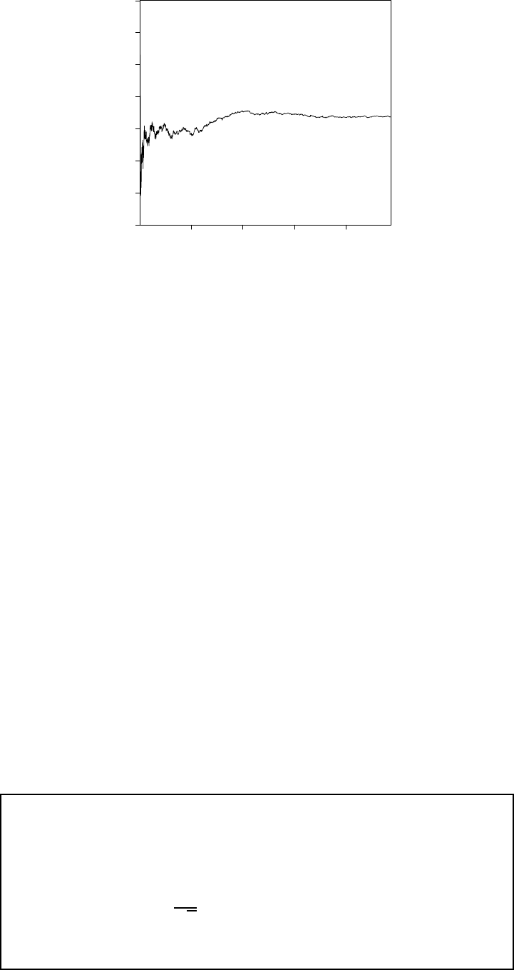
CHAPTER 7. ASYMPTOTIC THEORY FOR LEAST SQUARES 187
5000 10000 15000 20000
0.08 0.09 0.10 0.11 0.12 0.13 0.14 0.15
Number of Observations
OLS Estimation
Figure 7.1: The least-squares estimator b
β1as a function of sample size
The product xis iid (since the observations are iid) and mean zero (since E(x)=0)
Define the ×covariance matrix
Ω=E¡xx0
2
¢(7.8)
We require the elements of Ωto be finite, written Ω∞It will be useful to recall that Theorem
2.18.1.6 shows that Assumption 7.1.2 implies that E¡4
¢∞.
The element of Ωis E¡2
¢. By the Expectation Inequality (B.8), the element of
Ωis ¯¯E¡2
¢¯¯≤E¯¯2
¯¯=E¡||||2
¢
By two applications of the Cauchy-Schwarz Inequality (B.10), this is smaller than
¡E¡2
2
¢¢12¡E¡4
¢¢12≤¡E¡4
¢¢14¡E¡4
¢¢14¡E¡4
¢¢12∞
where the finiteness holds under Assumption 7.1.2.
An alternative way to show that the elements of Ωare finite is by using a matrix norm k·k
(See Appendix A.18). Then by the Expectation Inequality, the Cauchy-Schwarz Inequality, and
Assumption 7.1.2
kΩk≤E°
°xx0
2
°
°=E³kxk22
´≤³Ekxk4´12¡E¡4
¢¢12∞
This is a more compact argument (often described as more elegant) but such manipulations should
not be done without understanding the notation and the applicability of each step of the argument.
Regardless, the finiteness of the covariance matrix means that we can then apply the CLT
(Theorem 6.8.1).
Theorem 7.3.1 Under Assumption 7.1.2,
Ω∞(7.9)
and
1
√
X
=1
x
−→ N(0Ω)(7.10)
as →∞

CHAPTER 7. ASYMPTOTIC THEORY FOR LEAST SQUARES 188
Putting together (7.1), (7.7), and (7.10),
√³b
β−β´
−→ Q−1
N(0Ω)
=N¡0Q−1
ΩQ−1
¢
as →∞where the final equality follows from the property that linear combinations of normal
vectors are also normal (Theorem 5.2.3).
We have derived the asymptotic normal approximation to the distribution of the least-squares
estimator.
Theorem 7.3.2 Asymptotic Normality of Least-Squares Estima-
tor
Under Assumption 7.1.2, as →∞
√³b
β−β´
−→ N(0V)
where
V=Q−1
ΩQ−1
(7.11)
Q =E(xx0
)and Ω=E¡xx0
2
¢
In the stochastic order notation, Theorem 7.3.2 implies that
b
β=β+(−12)(7.12)
which is stronger than (7.6).
The matrix V=Q−1
ΩQ−1
is the variance of the asymptotic distribution of √³b
β−β´
Consequently, Visoftenreferredtoastheasymptotic covariance matrix of b
βThe expression
V=Q−1
ΩQ−1
is called a sandwich form, as the matrix Ωis sandwiched between two copies of
Q−1
.
It is useful to compare the variance of the asymptotic distribution given in (7.11) and the
finite-sample conditional variance in the CEF model as given in (4.12):
V
=var³b
β|X´=¡X0X¢−1¡X0DX¢¡X0X¢−1(7.13)
Notice that V
is the exact conditional variance of b
βand Vis the asymptotic variance of
√³b
β−β´Thus Vshould be (roughly) times as large as V
,orV≈V
. Indeed,
multiplying (7.13) by and distributing, we find
V
=µ1
X0X¶−1µ1
X0DX¶µ1
X0X¶−1
which looks like an estimator of V. Indeed, as →∞
V
−→ V
The expression V
is useful for practical inference (such as computation of standard errors and
tests) since it is the variance of the estimator b
β,whileVis useful for asymptotic theory as it

CHAPTER 7. ASYMPTOTIC THEORY FOR LEAST SQUARES 189
is well definedinthelimitasgoes to infinity. Wewillmakeuseofbothsymbolsanditwillbe
advisable to adhere to this convention.
There is a special case where Ωand Vsimplify. Suppose that
cov(xx0
2
)=0(7.14)
Condition (7.14) holds in the homoskedastic linear regression model, but is somewhat broader.
Under (7.14) the asymptotic variance formulae simplify as
Ω=E¡xx0
¢E¡2
¢=Q2(7.15)
V=Q−1
ΩQ−1
=Q−1
2≡V0
(7.16)
In (7.16) we define V0
=Q−1
2whether (7.14) is true or false. When (7.14) is true then V=V0
otherwise V6=V0
We call V0
the homoskedastic asymptotic covariance matrix.
Theorem 7.3.2 states that the sampling distribution of the least-squares estimator, after rescal-
ing, is approximately normal when the sample size is sufficiently large. This holds true for all joint
distributions of (x)which satisfy the conditions of Assumption 7.1.2, and is therefore broadly
applicable. Consequently, asymptotic normality is routinely used to approximate the finite sample
distribution of √³b
β−β´
Adifficulty is that for any fixed the sampling distribution of b
βcan be arbitrarily far from the
normal distribution. In Figure 6.1 we have already seen a simple example where the least-squares
estimate is quite asymmetric and non-normal even for reasonably large sample sizes. The normal
approximation improves as increases, but how large should be in order for the approximation
to be useful? Unfortunately, there is no simple answer to this reasonable question. The trouble
is that no matter how large is the sample size, the normal approximation is arbitrarily poor for
some data distribution satisfying the assumptions. We illustrate this problem using a simulation.
Let =1+2+where is N(01) and is independent of with the Double Pareto
density ()=
2||−−1||≥1If 2the error has zero mean and variance (−2)
As approaches 2, however, its variance diverges to infinity. In this context the normalized least-
squares slope estimator q−2
³b
1−1´has the N(01) asymptotic distribution for any 2.
In Figure 7.2 we display the finite sample densities of the normalized estimator q−2
³b
1−1´
setting =100and varying the parameter .For=30the density is very close to the N(01)
density. As diminishes the density changes significantly, concentrating most of the probability
mass around zero.
Another example is shown in Figure 7.3. Here the model is =+where
=
−E(
)
³E¡2
¢−(E(
))2´12(7.17)
and ∼N(01) and some integer ≥1We show the sampling distribution of √³b
−´setting
= 100for =14, 6 and 8. As increases, the sampling distribution becomes highly skewed
and non-normal. The lesson from Figures 7.2 and 7.3 is that the N(01) asymptotic approximation
is never guaranteed to be accurate.
7.4 Joint Distribution
Theorem 7.3.2 gives the joint asymptotic distribution of the coefficient estimates. We can use
the result to study the covariance between the coefficient estimates. For simplicity, suppose =2
with no intercept, both regressors are mean zero and the error is homoskedastic. Let 2
1and 2
2be
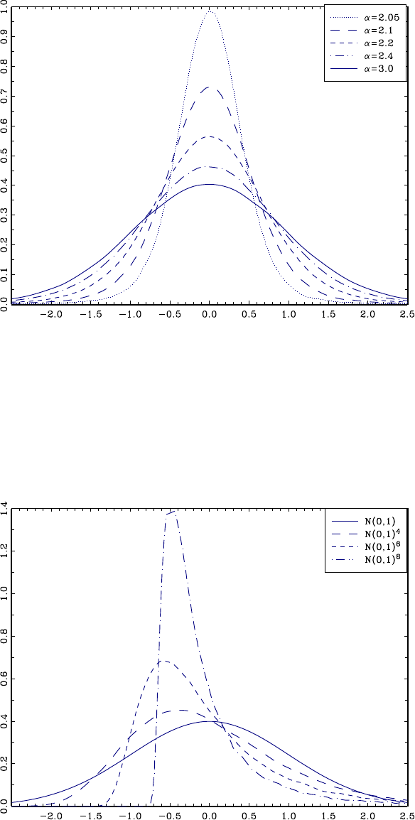
CHAPTER 7. ASYMPTOTIC THEORY FOR LEAST SQUARES 190
Figure 7.2: Density of Normalized OLS estimator with Double Pareto Error
Figure 7.3: Density of Normalized OLS estimator with error process (7.17)
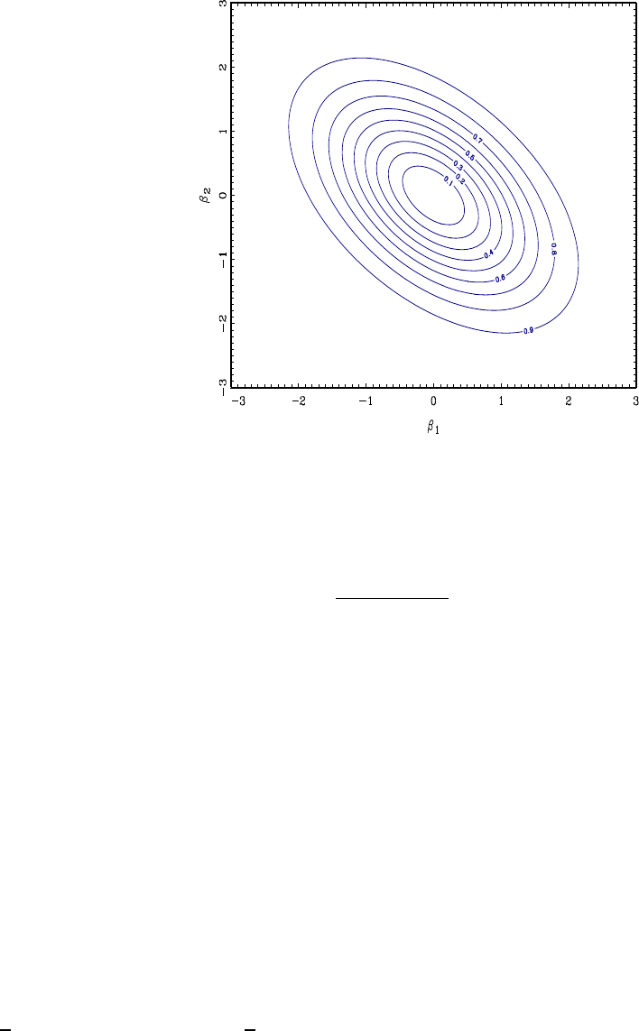
CHAPTER 7. ASYMPTOTIC THEORY FOR LEAST SQUARES 191
Figure 7.4: Contours of Joint Distribution of (b
β1b
β2)homoskedastic case
the variances of 1and 2and be their correlation. Then using the formula for inversion of a
2×2matrix,
V0
=2Q−1
=2
2
12
2(1 −2)∙2
2−12
−122
1¸
Thus if 1and 2are positively correlated (0) then b
1and b
2are negatively correlated (and
vice-versa).
For illustration, Figure 7.4 displays the probability contours of the joint asymptotic distribution
of b
1−1and b
2−2when 1=2=0
2
1=2
2=2=1and =05The coefficient estimates
are negatively correlated since the regressors are positively correlated. This means that if b
1is
unusually negative, it is likely that b
2is unusually positive, or conversely. It is also unlikely that
we will observe both b
1and b
2unusually large and of the same sign.
This finding that the correlation of the regressors is of opposite sign of the correlation of the coef-
ficient estimates is sensitive to the assumption of homoskedasticity. If the errors are heteroskedastic
then this relationship is not guaranteed.
This can be seen through a simple constructed example. Suppose that 1and 2only take
the values {−1+1}symmetrically, with Pr (1=2=1) = Pr(1=2=−1) = 38and
Pr (1=1
2=−1) = Pr (1=−1
2=1)=18You can check that the regressors are mean
zero, unit variance and correlation 0.5, which is identical with the setting displayed in Figure 7.4.
Now suppose that the error is heteroskedastic. Specifically, suppose that E¡2
|1=2¢=
5
4and E¡2
|16=2¢=1
4YoucancheckthatE¡2
¢=1E¡2
12
¢=E¡2
22
¢=1and
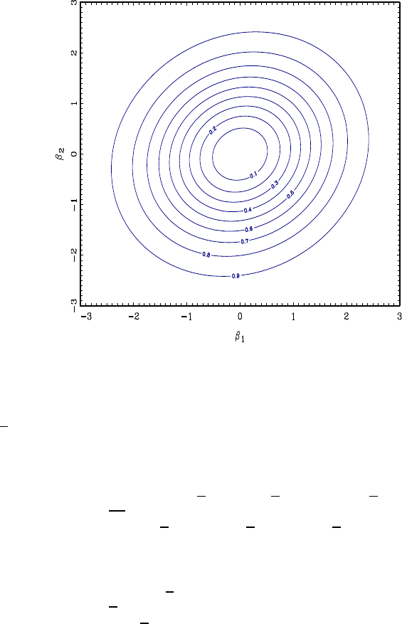
CHAPTER 7. ASYMPTOTIC THEORY FOR LEAST SQUARES 192
Figure 7.5: Contours of Joint Distribution of b
1and b
2heteroskedastic case
E¡122
¢=7
8Therefore
V=Q−1
ΩQ−1
=9
16 ⎡
⎢
⎣
1−1
2
−1
21
⎤
⎥
⎦⎡
⎢
⎣
17
8
7
81
⎤
⎥
⎦⎡
⎢
⎣
1−1
2
−1
21
⎤
⎥
⎦
=4
3⎡
⎢
⎣
11
4
1
41
⎤
⎥
⎦
Thus the coefficient estimates b
1and b
2are positively correlated (their correlation is 14)The
joint probability contours of their asymptotic distribution is displayed in Figure 7.5. We can see
how the two estimates are positively associated.
What we found through this example is that in thepresenceofheteroskedasticity there is no
simple relationship between the correlation of the regressors and the correlation of the parameter
estimates.
We can extend the above analysis to study the covariance between coefficient sub-vectors. For
example, partitioning x0
=(x0
1x0
2)and β0=¡β0
1β0
2¢we can write the general model as
=x0
1β1+x0
2β2+
and the coefficient estimates as b
β0=³b
β0
1b
β0
2´Make the partitions
Q =∙Q11 Q12
Q21 Q22 ¸Ω=∙Ω11 Ω12
Ω21 Ω22 ¸(7.18)
From (2.41)
Q−1
=∙Q−1
11·2−Q−1
11·2Q12Q−1
22
−Q−1
22·1Q21Q−1
11 Q−1
22·1¸

CHAPTER 7. ASYMPTOTIC THEORY FOR LEAST SQUARES 193
where Q11·2=Q11 −Q12Q−1
22 Q21 and Q22·1=Q22 −Q21Q−1
11 Q12. Thus when the error is ho-
moskedastic,
cov ³b
β1b
β2´=−2Q−1
11·2Q12Q−1
22
which is a matrix generalization of the two-regressor case.
In the general case, you can show that (Exercise 7.5)
V=∙V11 V12
V21 V22 ¸(7.19)
where
V11 =Q−1
11·2¡Ω11 −Q12Q−1
22 Ω21 −Ω12Q−1
22 Q21 +Q12Q−1
22 Ω22Q−1
22 Q21¢Q−1
11·2(7.20)
V21 =Q−1
22·1¡Ω21 −Q21Q−1
11 Ω11 −Ω22Q−1
22 Q21 +Q21Q−1
11 Ω12Q−1
22 Q21¢Q−1
11·2(7.21)
V22 =Q−1
22·1¡Ω22 −Q21Q−1
11 Ω12 −Ω21Q−1
11 Q12 +Q21Q−1
11 Ω11Q−1
11 Q12¢Q−1
22·1(7.22)
Unfortunately, these expressions are not easily interpretable.
7.5 Consistency of Error Variance Estimators
Using the methods of Section 7.2 we can show that the estimators b2=1
P
=1 b2
and 2=
1
−P
=1 b2
are consistent for 2
The trick is to write the residual bas equal to the error plus a deviation term
b=−x0
b
β
=+x0
β−0
b
β
=−x0
³b
β−β´
Thus the squared residual equals the squared error plus a deviation
b2
=2
−2x0
³b
β−β´+³b
β−β´0xx0
³b
β−β´(7.23)
So when we take the average of the squared residuals we obtain the average of the squared errors,
plus two terms which are (hopefully) asymptotically negligible.
b2=1
X
=1
2
−2Ã1
X
=1
x0
!³b
β−β´(7.24)
+³b
β−β´0Ã1
X
=1
xx0
!³b
β−β´
Indeed, the WLLN shows that
1
X
=1
2
−→ 2
1
X
=1
x0
−→ E¡x0
¢=0
1
X
=1
xx0
−→ E¡xx0
¢=Q
and Theorem 7.2.1 shows that b
β
−→ β. Hence (7.24) converges in probability to 2as desired.

CHAPTER 7. ASYMPTOTIC THEORY FOR LEAST SQUARES 194
Finally, since (−)→1as →∞it follows that
2=µ
−¶b2
−→ 2
Thus both estimators are consistent.
Theorem 7.5.1 Under Assumption 7.1.1, b2
−→ 2and 2
−→ 2as
→∞
7.6 Homoskedastic Covariance Matrix Estimation
Theorem 7.3.2 shows that √³b
β−β´is asymptotically normal with asymptotic covariance
matrix V. For asymptotic inference (confidence intervals and tests) we need a consistent estimate
of V. Under homoskedasticity, Vsimplifies to V0
=Q−1
2and in this section we consider the
simplified problem of estimating V0
The standard moment estimator of Q is b
Q defined in (7.1), and thus an estimator for Q−1
is b
Q−1
. Also, the standard estimator of 2is the unbiased estimator 2defined in (4.30). Thus a
natural plug-in estimator for V0
=Q−1
2is b
V0
=b
Q−1
2
Consistency of b
V0
for V0
follows from consistency of the moment estimates b
Q and 2
and an application of the continuous mapping theorem. Specifically, Theorem 7.2.1 established
that b
Q
−→ Qand Theorem 7.5.1 established 2
−→ 2The function V0
=Q−1
2is a
continuous function of Q and 2so long as Q 0which holds true under Assumption 7.1.1.4.
It follows by the CMT that
b
V0
=b
Q−1
2
−→ Q−1
2=V0
so that b
V0
is consistent for V0
as desired.
Theorem 7.6.1 Under Assumption 7.1.1, b
V0
−→ V0
as →∞
It is instructive to notice that Theorem 7.6.1 does not require the assumption of homoskedastic-
ity. That is, b
V0
is consistent for V0
regardless if the regression is homoskedastic or heteroskedastic.
However, V0
=V=avar(
b
β)only under homoskedasticity. Thus in the general case, b
V0
is con-
sistent for a well-defined but non-useful object.
7.7 Heteroskedastic Covariance Matrix Estimation
Theorems 7.3.2 established that the asymptotic covariance matrix of √³b
β−β´is V=
Q−1
ΩQ−1
We now consider estimation of this covariance matrix without imposing homoskedas-
ticity. The standard approach is to use a plug-in estimator which replaces the unknowns with
sample moments.
As described in the previous section, a natural estimator for Q−1
is b
Q−1
,where b
Q defined
in (7.1).

CHAPTER 7. ASYMPTOTIC THEORY FOR LEAST SQUARES 195
The moment estimator for Ωis
b
Ω=1
X
=1
xx0
b2
(7.25)
leading to the plug-in covariance matrix estimator
b
V
=b
Q−1
b
Ωb
Q−1
(7.26)
Youcancheckthat b
V
=b
V
where b
V
is the White covariance matrix estimator introduced
in (4.37).
As shown in Theorem 7.2.1, b
Q−1
−→ Q−1
so we just need to verify the consistency of b
Ω.
The key is to replace the squared residual b2
with the squared error 2
and then show that the
difference is asymptotically negligible.
Specifically, observe that
b
Ω=1
X
=1
xx0
b2
=1
X
=1
xx0
2
+1
X
=1
xx0
¡b2
−2
¢(7.27)
The first term is an average of the iid random variables xx0
2
and therefore by the WLLN
converges in probability to its expectation, namely,
1
X
=1
xx0
2
−→ E¡xx0
2
¢=Ω
Technically, this requires that Ωhas finite elements, which was shown in (7.9).
So to establish that b
Ωis consistent for Ωit remains to show that
1
X
=1
xx0
¡b2
−2
¢
−→ 0(7.28)
There are multiple ways to do this. A reasonable straightforward yet slightly tedious derivation is
to start by applying the Triangle Inequality (A.26) using a matrix norm:
°
°
°
°
°
1
X
=1
xx0
¡b2
−2
¢°
°
°
°
°≤1
X
=1 °
°xx0
¡b2
−2
¢°
°
=1
X
=1
kxk2¯¯b2
−2
¯¯(7.29)
Then recalling the expression for the squared residual (7.23), apply the Triangle Inequality and
then the Schwarz Inequality (A.20) twice
¯¯b2
−2
¯¯≤2¯¯¯x0
³b
β−β´¯¯¯+³b
β−β´0xx0
³b
β−β´
=2||¯¯¯x0
³b
β−β´¯¯¯+¯¯¯¯³b
β−β´0x¯¯¯¯
2
≤2||kxk°
°
°b
β−β°
°
°+kxk2°
°
°b
β−β°
°
°2(7.30)

CHAPTER 7. ASYMPTOTIC THEORY FOR LEAST SQUARES 196
Combining (7.29) and (7.30), we find
°
°
°
°
°
1
X
=1
xx0
¡b2
−2
¢°
°
°
°
°≤2Ã1
X
=1
kxk3||!°
°
°b
β−β°
°
°
+Ã1
X
=1
kxk4!°
°
°b
β−β°
°
°2
=(1)(7.31)
The expression is (1) because°
°
°b
β−β°
°
°
−→ 0and both averages in parenthesis are averages of
random variables with finite mean under Assumption 7.1.2 (and are thus (1)). Indeed, by
Hölder’s Inequality (B.9)
E³kxk3||´≤µE³kxk3´43¶34¡E¡4
¢¢14
=³E³kxk4´´34¡E¡4
¢¢14∞
We have established (7.28), as desired.
Theorem 7.7.1 Under Assumption 7.1.2, as →∞b
Ω
−→ Ωand
b
V
−→ V
For an alternative proof of this result, see Section 7.21.
7.8 Summary of Covariance Matrix Notation
The notation we have introduced may be somewhat confusing so it is helpful to write it down in
one place. The exact variance of b
β(under the assumptions of the linear regression model) and the
asymptotic variance of √³b
β−β´(under the more general assumptions of the linear projection
model) are
V
=var³b
β|X´=¡X0X¢−1¡X0DX¢¡X0X¢−1
V=avar³√³b
β−β´´=Q−1
ΩQ−1
The White estimates of these two covariance matrices are
b
V
=¡X0X¢−1Ã
X
=1
xx0
b2
!¡X0X¢−1
b
V
=b
Q−1
b
Ωb
Q−1
and satisfy the simple relationship
b
V
=b
V
Similarly, under the assumption of homoskedasticity the exact and asymptotic variances simplify
to
V0
=¡X0X¢−12
V0
=Q−1
2

CHAPTER 7. ASYMPTOTIC THEORY FOR LEAST SQUARES 197
and their standard estimators are
b
V0
=¡X0X¢−12
b
V0
=b
Q−1
2
which also satisfy the relationship
b
V0
=b
V0
The exact formula and estimates are useful when constructing test statistics and standard errors.
However, for theoretical purposes the asymptotic formula (variances and their estimates) are more
useful, as these retain non-generate limits as the sample sizes diverge. That is why both sets of
notation are useful.
7.9 Alternative Covariance Matrix Estimators*
In Section 7.7 we introduced b
V
as an estimator of V.b
V
is a scaled version of b
V
from
Section 4.13, where we also introduced the alternative heteroskedasticity-robust covariance matrix
estimators b
V
e
V
and V
We now discuss the consistency properties of these estimators.
To do so we introduce their scaled versions, e.g. b
V=b
V
,e
V=e
V
,andV=V
These are (alternative) estimates of the asymptotic covariance matrix V
First, consider b
V.Noticethatb
V=b
V
=
−b
V
where b
V
was defined in (7.26) and
shown consistent for Vin Theorem 7.7.1. If is fixed as →∞then
−→1and thus
b
V=(1+(1)) b
V
−→ V
Thus b
Vis consistent for V
The alternative estimators e
Vand Vtake the form (7.26) but with b
Ωreplaced by
e
Ω=1
X
=1
(1 −)−2xx0
b2
and
Ω=1
X
=1
(1 −)−1xx0
b2
respectively. To show that these estimators also consistent for Vgiven b
Ω
−→ Ω,itissufficient
to show that the differences e
Ω−b
Ωand Ω−b
Ωconverge in probability to zero as →∞
The trick is to use the fact that the leverage values are asymptotically negligible:
∗
=max
1≤≤ =(1)(7.32)
(See Theorem 7.22.1 in Section 7.22).) Then using the Triangle Inequality
°
°
°Ω−b
Ω°
°
°≤1
X
=1 °
°xx0
°
°b2
¯¯¯(1 −)−1−1¯¯¯
≤Ã1
X
=1
kxk2b2
!¯¯¯(1 −∗
)−1−1¯¯¯
The sum in parenthesis can be shown to be (1) under Assumption 7.1.2 by the same argument
as in in the proof of Theorem 7.7.1. (In fact, it can be shown to converge in probability to

CHAPTER 7. ASYMPTOTIC THEORY FOR LEAST SQUARES 198
E³kxk22
´) The term in absolute values is (1) by (7.32). Thus the product is (1),which
means that Ω=b
Ω+(1) −→ Ω.
Similarly,
°
°
°e
Ω−b
Ω°
°
°≤1
X
=1 °
°xx0
°
°b2
¯¯¯(1 −)−2−1¯¯¯
≤Ã1
X
=1
kxk2b2
!¯¯¯(1 −∗
)−2−1¯¯¯
=(1)
Theorem 7.9.1 Under Assumption 7.1.2, as →∞e
Ω
−→ Ω,Ω
−→ Ω,
b
V
−→ Ve
V
−→ Vand V
−→ V
Theorem 7.9.1 shows that the alternative covariance matrix estimators are also consistent for
theasymptoticcovariancematrix.
7.10 Functions of Parameters
In most serious applications the researcher is actually interested in a specific transformation
of the coefficient vector β=(1
)Forexample,heorshemaybeinterestedinasingle
coefficient or a ratio -More generally, interest may focus on a quantity such as consumer
surplus which could be a complicated function of the coefficients. In any of these cases we can
write the parameter of interest θas a function of the coefficients, e.g. θ=r(β)for some function
r:R→R. The estimate of θis b
θ=r(b
β)
By the continuous mapping theorem (Theorem 6.11.1) and the fact b
β
−→ βwe can deduce
that b
θis consistent for θ(if the function r(·)is continuous).
Theorem 7.10.1 Under Assumption 7.1.1, if r(β)is continuous at the
true value of βthen as →∞b
θ
−→ θ
Furthermore, if the transformation is sufficiently smooth, by the Delta Method (Theorem 6.12.3)
we can show that b
θis asymptotically normal.
Assumption 7.10.1 r(β):R→Ris continuously differentiable at the
true value of βand R=
r(β)0has rank

CHAPTER 7. ASYMPTOTIC THEORY FOR LEAST SQUARES 199
Theorem 7.10.2 Asymptotic Distribution of Functions of Para-
meters
Under Assumptions 7.1.2 and 7.10.1, as →∞
√³b
θ−θ´
−→ N(0V)(7.33)
where
V=R0VR(7.34)
In many cases, the function r(β)is linear:
r(β)=R0β
for some ×matrix RIn particular, if Ris a “selector matrix”
R=µI
0¶(7.35)
then we can partition β=(β0
1β0
2)0so that R0β=β1for β=(β0
1β0
2)0Then
V=¡I0¢VµI
0¶=V11
the upper-left sub-matrix of V11 given in (7.20). In this case (7.33) states that
√³b
β1−β1´
−→ N(0V11)
That is, subsets of b
βare approximately normal with variances given by the conformable subcom-
ponents of V.
To illustrate the case of a nonlinear transformation, take the example =-for 6=- Then
R=
βr(β)=
⎛
⎜
⎜
⎜
⎜
⎜
⎜
⎜
⎜
⎜
⎜
⎜
⎜
⎝
1(-)
.
.
.
(-)
.
.
.
(-)
.
.
.
(-)
⎞
⎟
⎟
⎟
⎟
⎟
⎟
⎟
⎟
⎟
⎟
⎟
⎟
⎠
=
⎛
⎜
⎜
⎜
⎜
⎜
⎜
⎜
⎜
⎜
⎜
⎜
⎝
0
.
.
.
1-
.
.
.
−2
-
.
.
.
0
⎞
⎟
⎟
⎟
⎟
⎟
⎟
⎟
⎟
⎟
⎟
⎟
⎠
(7.36)
so
V=V2
-+V--2
4
-−2V-3
-
where V denotes the element of V
For inference we need an estimate of the asymptotic variance matrix V=R0VR,andfor
this it is typical to use a plug-in estimator. The natural estimator of Ris the derivative evaluated
at the point estimates
b
R=
βr(b
β)0(7.37)
The derivative in (7.37) may be calculated analytically or numerically. By analytically, we mean
working out for the formula for the derivative and replacing the unknowns by point estimates. For

CHAPTER 7. ASYMPTOTIC THEORY FOR LEAST SQUARES 200
example, if =-then
r(β)is (7.36). However in some cases the function r(β)may be
extremely complicated and a formula for the analytic derivative may not be easily available. In
this case calculation by numerical differentiation may be preferable. Let -=(0··· 1··· 0)0be
the unit vector with the “1”inthe- place. Then the -’th element of a numerical derivative b
Ris
b
R- =r(b
β+-)−r(b
β)
for some small
TheestimateofVis
b
V=b
R0b
Vb
R(7.38)
Alternatively, b
V0
e
Vor Vmaybeusedinplaceof b
VFor example, the homoskedastic covari-
ance matrix estimator is b
V0
=b
R0b
V0
b
R=b
R0b
Q−1
b
R2(7.39)
Given (7.37), (7.38) and (7.39) are simple to calculate using matrix operations.
As the primary justification for b
Vis the asymptotic approximation (7.33), b
Vis often called
an asymptotic covariance matrix estimator.
The estimator b
Vis consistent for Vunder the conditions of Theorem 7.10.2 since b
V
−→ V
by Theorem 7.7.1, and
b
R=
βr(b
β)0
−→
βr(β)0=R
since b
β
−→ βand the function
r(β)0is continuous in β.
Theorem 7.10.3 Under Assumptions 7.1.2 and 7.10.1, as →∞
b
V
−→ V
Theorem 7.10.3 shows that b
Vis consistent for Vand thus may be used for asymptotic
inference. In practice, we may set
b
V
=b
R0b
V
b
R=−1b
R0b
Vb
R(7.40)
as an estimate of the variance of b
θ, or substitute an alternative covariance estimator such as V
7.11 Asymptotic Standard Errors
As described in Section 4.14, a standard error is an estimate of the standard deviation of the
distribution of an estimator. Thus if b
V
is an estimate of the covariance matrix of b
β, then standard
errors are the square roots of the diagonal elements of this matrix. These take the form
(b
)=qb
V
=rhb
V
i
Standard errors for b
θare constructed similarly. Supposing that =1(so (β)is real-valued), then
the standard error for b
is the square root of (7.40)
(b
)=rb
R0b
V
b
R=q−1b
R0b
Vb
R

CHAPTER 7. ASYMPTOTIC THEORY FOR LEAST SQUARES 201
When the justification is based on asymptotic theory we call (b
)or (b
)an asymptotic standard
error for b
or b
. When reporting your results, it is good practice to report standard errors for each
reported estimate, and this includes functions and transformations of your parameter estimates.
This helps users of the work (including yourself) assess the estimation precision.
We illustrate using the log wage regression
log()=1 +2 +32100 + 4+
Consider the following three parameters of interest.
1. Percentage return to education:
1= 1001
(100 times the partial derivative of the conditional expectation of log wages with respect to
.)
2. Percentage return to experience for individuals with 10 years of experience:
2=1002+203
(100 times the partial derivative of the conditional expectation of log wages with respect to
, evaluated at =10.)
3. Experience level which maximizes expected log wages:
3=−5023
(The level of at which the partial derivative of the conditional expectation of log
wages with respect to equals 0.)
The 4×1vector Rfor these three parameters is
R=⎛
⎜
⎜
⎝
100
0
0
0
⎞
⎟
⎟
⎠⎛
⎜
⎜
⎝
0
100
20
0
⎞
⎟
⎟
⎠⎛
⎜
⎜
⎝
0
−503
5022
3
0
⎞
⎟
⎟
⎠
respectively.
We use the subsample of married black women (all experience levels), which has 982 observa-
tions. The point estimates and standard errors are
\
log()= 0118
(0008)
+0016
(0006)
−0022
(0012)
2100 + 0947
(0157)
(7.41)
The standard errors are the square roots of the Horn-Horn-Duncan covariance matrix estimate
V
=⎛
⎜
⎜
⎝
0632 0131 −0143 −111
0131 0390 −0731 −625
−0143 −0731 148 943
−111−625 943 246
⎞
⎟
⎟
⎠×10−4(7.42)
We calculate that
b
1= 100b
1
= 100 ×0118
=118

CHAPTER 7. ASYMPTOTIC THEORY FOR LEAST SQUARES 202
(b
1)=p1002×0632 ×10−4
=08
b
2=100
b
2+20b
3
=100×0016 −20 ×0022
=116
(b
2)=s¡100 20 ¢µ0390 −0731
−0731 148 ¶µ100
20 ¶×10−4
=055
b
3=−50b
2b
3
=50×00160022
=352
(b
3)=v
u
u
t³−50b
350b
2/b
2
3´µ0390 −0731
−0731 148 ¶Ã−50b
3
50b
2/b
2
3!×10−4
=70
The calculations show that the estimate of the percentage return to education (for married
black women) is about 12% per year, with a standard error of 0.8. The estimate of the percentage
return to experience for those with 10 years of experience is 1.2% per year, with a standard error
of 0.6. And the estimate of the experience level which maximizes expected log wages is 35 years,
with a standard error of 7.
7.12 t-statistic
Let =(β):R→Rbe a parameter of interest, b
its estimate and (b
)its asymptotic
standard error. Consider the statistic
()= b
−
(b
)(7.43)
Different writers have called (7.43) a t-statistic,at-ratio,az-statistic or a studentized sta-
tistic, sometimes using the different labels to distinguish between finite-sample and asymptotic
inference. As the statistics themselves are always (7.43) we won’t make this distinction, and will
simply refer to ()as a t-statistic or a t-ratio. We also often suppress the parameter dependence,
writing it as The t-statistic is a simple function of the estimate, its standard error, and the
parameter.
By Theorems 7.10.2 and 7.10.3, √³b
−´
−→ N(0
)and b
−→ Thus
()= b
−
(b
)
=
√³b
−´
qb
−→ N(0
)
√
=Z∼N(01)

CHAPTER 7. ASYMPTOTIC THEORY FOR LEAST SQUARES 203
The last equality is by the property that affine functions of normal distributions are normal (The-
orem 5.2.3).
Thus the asymptotic distribution of the t-ratio ()is the standard normal. Since this distrib-
ution does not depend on the parameters, we say that ()is asymptotically pivotal.Infinite
samples ()is not necessarily pivotal (as in the normal regression model) but the property states
that the dependence on unknowns diminishes as increases.
As we will see in the next section, it is also useful to consider the distribution of the absolute
t-ratio |()|Since ()
−→ Z, the continuous mapping theorem yields |()|
−→ |Z|Letting
Φ()=Pr(Z≤)denote the standard normal distribution function, we can calculate that the
distribution function of |Z|is
Pr (|Z|≤)=Pr(−≤Z≤)
=Pr(Z≤)−Pr (Z −)
=Φ()−Φ(−)
=2Φ()−1(7.44)
Theorem 7.12.1 Under Assumptions 7.1.2 and 7.10.1, ()
−→ Z∼
N(01) and |()|
−→ |Z|
The asymptotic normality of Theorem 7.12.1 is used to justify confidence intervals and tests for
the parameters.
7.13 Confidence Intervals
The estimate b
θis a point estimate for θ, meaning that b
θis a single value in R. A broader
concept is a set estimate b
which is a collection of values in RWhen the parameter is real-
valued then it is common to focus on sets of the form b
=[
b
b
]which is called an interval
estimate for .
An interval estimate b
is a function of the data and hence is random. The coverage proba-
bility of the interval b
=[
b
b
]is Pr(∈b
)The randomness comes from b
as the parameter is
treated as fixed. In Section 5.12 we introduced confidence intervals for the normal regression model,
whichusedthefinite sample distribution of the t-statistic to construct exact confidence intervals
for the regression coefficients. When we are outside the normal regression model we cannot rely
on the exact normal distribution theory, but instead use asymptotic approximations. A benefitis
that we can construct confidence intervals for general parameters of interest , not just regression
coefficients.
An interval estimate b
is called a confidence interval when the goal is to set the coverage
probability to equal a pre-specified target such as 90% or 95%. b
is called a 1−confidence
interval if infPr(∈b
)=1−
When b
is asymptotically normal with standard error (b
)the conventional confidence interval
for takes the form b
=hb
−·(b
)b
+·(b
)i(7.45)
where equals the 1−quantile of the distribution of |Z|. Using (7.44) we calculate that is
equivalently the 1−2quantile of the standard normal distribution. Thus, solves
2Φ()−1=1−

CHAPTER 7. ASYMPTOTIC THEORY FOR LEAST SQUARES 204
This can be computed by, for example, norminv(1-2)in MATLAB. The confidence interval
(7.45) is symmetric about the point estimate b
and its length is proportional to the standard error
(b
)
Equivalently, (7.45) is the set of parameter values for such that the t-statistic ()is smaller
(in absolute value) than that is
b
={:|()|≤}=(:−≤b
−
(b
)≤)
The coverage probability of this confidence interval is
Pr ³∈b
´=Pr(|()|≤)→Pr (|Z|≤)=1−
where the limit is taken as →∞, and holds since ()is asymptotically |Z|by Theorem 7.12.1. We
call the limit the asymptotic coverage probability,andcall b
an asymptotic 1−%confidence
interval for . Since the t-ratio is asymptotically pivotal, the asymptotic coverage probability is
independent of the parameter
It is useful to contrast the confidence interval (7.45) with (5.12) for the normal regression
model. They are similar, but there are differences. The normal regression interval (5.12) only
applies to regression coefficients , not to functions of the coefficients. The normal interval
(5.12) also is constructed with the homoskedastic standard error, while (7.45) can be constructed
with a heteroskedastic-robust standard error. Furthermore, the constants in (5.12) are calculated
using the student distribution, while in (7.45) are calculated using the normal distribution. The
difference between the student and normal values are typically small in practice (since sample sizes
are large in typical economic applications). However, since the student values are larger, it results
in slightly larger confidence intervals, which is probably reasonable. (A practical rule of thumb is
that if the sample sizes are sufficiently small that it makes a difference, then probably neither (5.12)
nor (7.45) should be trusted.) Despite these differences, the coincidence of the intervals means that
inference on regression coefficients is generally robust to using either the exact normal sampling
assumption or the asymptotic large sample approximation, at least in large samples.
In Stata, by default the program reports 95% confidence intervals for each coefficient where
the critical values are calculated using the −distribution. This is done for all standard error
methods even though it is only justified for homoskedastic standard errors and under normality.
The standard coverage probability for confidence intervals is 95%, leading to the choice =196
for the constant in (7.45). Rounding 1.96 to 2, we obtain what might be the most commonly used
confidence interval in applied econometric practice
b
=hb
−2(b
)b
+2(b
)i(7.46)
This is a useful rule-of thumb. This asymptotic 95% confidence interval b
is simple to compute and
can be roughly calculated from tables of coefficient estimates and standard errors. (Technically, it
is an asymptotic 95.4% interval, due to the substitution of 2.0 for 1.96, but this distinction is overly
precise.)
Theorem 7.13.1 Under Assumptions 7.1.2 and 7.10.1, for b
defined in
(7.45), with =Φ−1(1 −2),Pr ³∈b
´−→ 1− For =196
Pr ³∈b
´−→ 095

CHAPTER 7. ASYMPTOTIC THEORY FOR LEAST SQUARES 205
Confidenceintervalsareasimpleyeteffective tool to assess estimation uncertainty. When
reading a set of empirical results, look at the estimated coefficient estimates and the standard
errors. For a parameter of interest, compute the confidence interval and consider the meaning
of the spread of the suggested values. If the range of values in the confidence interval are too wide
to learn about then do not jump to a conclusion about based on the point estimate alone.
For illustration, consider the three examples presented in Section 7.11 based on the log wage
regression for married black women.
Percentage return to education. A 95% asymptotic confidence interval is 118±196×08=[102
133]
Percentage return to experience for individuals with 10 years experience. A 90% asymptotic
confidence interval is 11±1645 ×04=[0518]
Experience level which maximizes expected log wages. An 80% asymptotic confidence interval
is 35 ±128 ×7=[2644]
7.14 Regression Intervals
In the linear regression model the conditional mean of given x=xis
(x)=E(|x=x)=x0β
In some cases, we want to estimate (x)at a particular point xNotice that this is a linear
function of βLetting (β)=x0βand =(β)we see that b(x)=b
=x0b
βand R=xso
(b
)=qx0b
V
xThus an asymptotic 95% confidence interval for (x)is
∙x0b
β±196qx0b
V
x¸
It is interesting to observe that if this is viewed as a function of xthe width of the confidence set
is dependent on x
To illustrate, we return to the log wage regression (3.14) of Section 3.7. The estimated regression
equation is
\
log()=x0b
β=0155+0698
where =. The covariance matrix estimate from (4.44) is
b
V
=µ0001 −0015
−0015 0243 
Thus the 95% confidence interval for the regression takes the form
0155+0698 ±196p00012−0030+0243
The estimated regression and 95% intervals are shown in Figure 7.6. Notice that the confidence
bands take a hyperbolic shape. This means that the regression line is less precisely estimated for
very large and very small values of education.
Plots of the estimated regression line and confidence intervals are especially useful when the
regression includes nonlinear terms. To illustrate, consider the log wage regression (7.41) which
includes experience and its square, with covariance matrix (7.42). We are interested in plotting
the regression estimate and regression intervals as a function of experience. Since the regression
also includes education, to plot the estimates in a simple graph we need to fixeducation at a
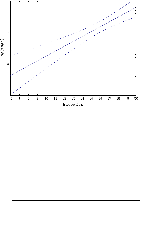
CHAPTER 7. ASYMPTOTIC THEORY FOR LEAST SQUARES 206
Figure 7.6: Wage on Education Regression Intervals
specificvalue. Weselecteducation =12. This only affects the level of the estimated regression, since
education enters without an interaction. Define the points of evaluation
z()=⎛
⎜
⎜
⎝
12
2100
1
⎞
⎟
⎟
⎠
where =experience.
Thus the 95% regression interval for =12, as a function of =experience is
0118 ×12 + 0016 −0022 2100 + 0947
±196v
u
u
u
u
u
tz()0⎛
⎜
⎜
⎝
0632 0131 −0143 −111
0131 0390 −0731 −625
−0143 −0731 148 943
−111−625 943 246
⎞
⎟
⎟
⎠z()×10−4
=0016 −00022 2+236
±00196p70608 −9356 +054428 2−001462 3+0000148 4
The estimated regression and 95% intervals are shown in Figure 7.7. The regression interval
widens greatly for small and large values of experience, indicating considerable uncertainty about
the effect of experience on mean wages for this population. The confidence bands take a more
complicated shape than in Figure 7.6 due to the nonlinear specification.
7.15 Forecast Intervals
Suppose we are given a value of the regressor vector x+1 for an individual outside the sample,
and we want to forecast (guess) +1 for this individual. This is equivalent to forecasting +1
given x+1 =xwhich will generally be a function of x. A reasonable forecasting rule is the condi-
tional mean (x)as it is the mean-square-minimizing forecast. A point forecast is the estimated
conditional mean b(x)=x0b
β. We would also like a measure of uncertainty for the forecast.
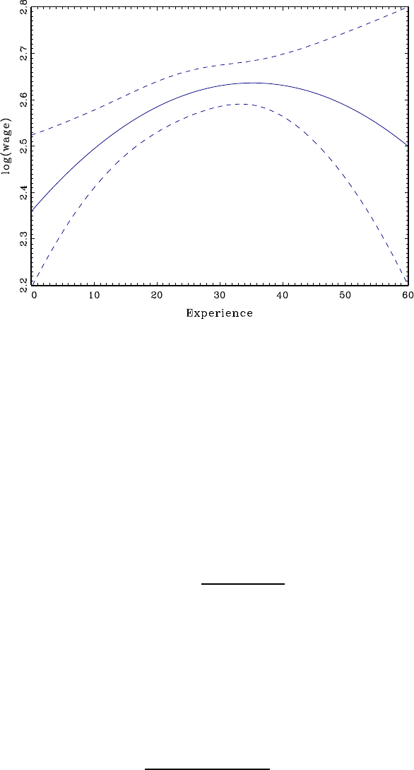
CHAPTER 7. ASYMPTOTIC THEORY FOR LEAST SQUARES 207
Figure 7.7: Wage on Experience Regression Intervals
The forecast error is b+1 =+1 −b(x)=+1 −x0³b
β−β´. As the out-of-sample error +1
is independent of the in-sample estimate b
βthis has conditional variance
E¡b2
+1|x+1 =x¢=E³2
+1 −2x0³b
β−β´+1 +x0³b
β−β´³b
β−β´x|x+1 =x´
=E¡2
+1 |x+1 =x¢+x0E³b
β−β´³b
β−β´0x
=2(x)+x0V
x
Under homoskedasticity E¡2
+1 |x+1¢=2the natural estimate of this variance is b2+x0b
V
x
so a standard error for the forecast is b(x)=qb2+x0b
V
xNotice that this is different from the
standard error for the conditional mean.
The conventional 95% forecast interval for +1 uses a normal approximation and sets
hx0b
β±2b(x)i
It is difficult, however, to fully justify this choice. It would be correct if we have a normal approx-
imation to the ratio
+1 −x0³b
β−β´
b(x)
The difficulty is that the equation error +1 is generally non-normal, and asymptotic theory cannot
be applied to a single observation. The only special exception is the case where +1 has the exact
distribution N(0
2)which is generally invalid.
To get an accurate forecast interval, we need to estimate the conditional distribution of +1
given x+1 =xwhich is a much more difficult task. Perhaps due to this difficulty, many applied
forecastersusethesimpleapproximateintervalhx0b
β±2b(x)idespite the lack of a convincing
justification.

CHAPTER 7. ASYMPTOTIC THEORY FOR LEAST SQUARES 208
7.16 Wald Statistic
Let θ=r(β):R→Rbe any parameter vector of interest, b
θits estimate and b
V
its
covariance matrix estimator. Consider the quadratic form
(θ)=³b
θ−θ´0b
V−1
³b
θ−θ´=³b
θ−θ´0b
V−1
³b
θ−θ´(7.47)
where b
V=b
V
When =1then ()=()2is the square of the t-ratio. When 1()
is typically called a Wald statistic. We are interested in its sampling distribution.
The asymptotic distribution of ()is simple to derive given Theorem 7.10.2 and Theorem
7.10.3, which show that √³b
θ−θ´
−→ Z∼N(0V)
and b
V
−→ V
Note that V0since Ris full rank under Assumption 7.10.1. It follows that
(θ)=√³b
θ−θ´0b
V−1
√³b
θ−θ´
−→ Z0V−1
Z(7.48)
a quadratic in the normal random vector ZAs shown in Theorem 5.3.3, the distribution of this
quadratic form is 2
, a chi-square random variable with degrees of freedom.
Theorem 7.16.1 Under Assumptions 7.1.2 and 7.10.1, as →∞
(θ)
−→ 2
Theorem 7.16.1 is used to justify multivariate confidence regions and multivariate hypothesis
tests.
7.17 Homoskedastic Wald Statistic
Under the conditional homoskedasticity assumption E¡2
|x¢=2we can construct the Wald
statistic using the homoskedastic covariance matrix estimator b
V0
defined in (7.39). This yields a
homoskedastic Wald statistic
0(θ)=³b
θ−θ´0³b
V0
´−1³b
θ−θ´=³b
θ−θ´0³b
V0
´−1³b
θ−θ´(7.49)
Under the additional assumption of conditional homoskedasticity, it has the same asymptotic
distribution as ()
Theorem 7.17.1 Under Assumptions 7.1.2 and 7.10.1, and E¡2
|x¢=
2as →∞
0(θ)
−→ 2
CHAPTER 7. ASYMPTOTIC THEORY FOR LEAST SQUARES 209
7.18 Confidence Regions
Aconfidence region b
is a set estimator for θ∈Rwhen 1Aconfidence region b
is a set in
Rintended to cover the true parameter value with a pre-selected probability 1− Thus an ideal
confidence region has the coverage probability Pr(θ∈b
)=1−. Inpracticeitistypicallynot
possible to construct a region with exact coverage, but we can calculate its asymptotic coverage.
When the parameter estimate satisfies the conditions of Theorem 7.16.1, a good choice for a
confidence region is the ellipse b
={θ:(θ)≤1−}
with 1−the 1−quantile of the 2
distribution. (Thus (1−)=1−)It can be computed
by, for example, chi2inv(1-,q)in MATLAB.
Theorem 7.16.1 implies
Pr ³θ∈b
´→Pr ¡2
≤1−¢=1−
which shows that b
has asymptotic coverage 1−
To illustrate the construction of a confidence region, consider the estimated regression (7.41) of
the model
\
log()=1 +2 +32100 + 4
Suppose that the two parameters of interest are the percentage return to education 1= 1001and
the percentage return to experience for individuals with 10 years experience 2= 1002+203.
These two parameters are a linear transformation of the regression parameters with point estimates
b
θ=µ100 0 0 0
0 100 20 0 ¶b
β=µ118
12
and have the covariance matrix estimate
b
V
=µ0 100 0 0
0 0 100 20 ¶b
V
⎛
⎜
⎜
⎝
00
100 0
0100
020
⎞
⎟
⎟
⎠
=µ0632 0103
0103 0157 
with inverse
b
V−1
=µ177 −116
−116 713 
Thus the Wald statistic is
(θ)=³b
θ−θ´0b
V−1
³b
θ−θ´
=µ118−1
12−2¶0µ177 −116
−116 713 ¶µ118−1
12−2
=177 (118−1)2−232 (118−1)(12−2)+713 (12−2)2
The 90% quantile of the 2
2distribution is 4.605 (we use the 2
2distribution as the dimension
of θis two), so an asymptotic 90% confidence region for the two parameters is the interior of the
ellipse (θ)=4605 which is displayed in Figure 7.8. Since the estimated correlation of the two
coefficient estimates is modest (about 0.3) the region is modestly elliptical.
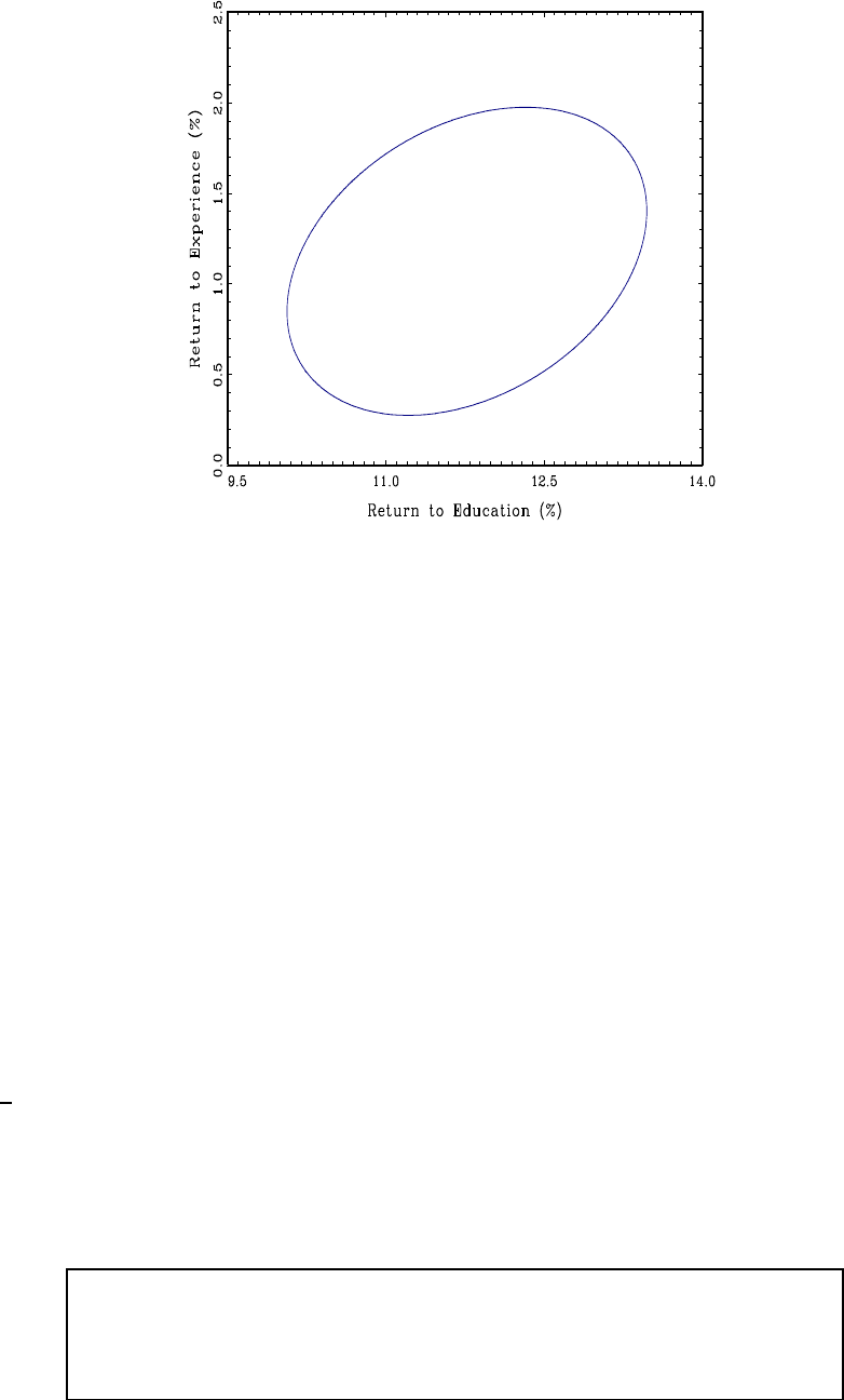
CHAPTER 7. ASYMPTOTIC THEORY FOR LEAST SQUARES 210
Figure 7.8: Confidence Region for Return to Experience and Return to Education
7.19 Semiparametric Efficiency in the Projection Model
In Section 4.7 we presented the Gauss-Markov theorem, which stated that in the homoskedastic
CEF model, in the class of linear unbiased estimators the one with the smallest variance is least-
squares. As we noted in that section, the restriction to linear unbiased estimators is unsatisfactory
as it leaves open the possibility that an alternative (non-linear) estimator could have a smaller
asymptotic variance. In addition, the restriction to the homoskedastic CEF model is also unsatis-
factory as the projection model is more relevant for empirical application. The question remains:
what is the most efficient estimator of the projection coefficient β(or functions θ=h(β))inthe
projection model?
It turns out that it is straightforward to show that the projection model falls in the estimator
class considered in Proposition 6.15.2. It follows that the least-squares estimator is semiparametri-
cally efficient in the sense that it has the smallest asymptotic variance in the class of semiparametric
estimators of β. This is a more powerful and interesting result than the Gauss-Markov theorem.
To see this, it is worth rephrasing Proposition 6.15.2 with amended notation. Suppose that
a parameter of interest is θ=g(μ)where μ=E(z)forwhichthemomentestimatorsare
b
μ=1
P
=1 zand b
θ=g(b
μ)Let
L2(g)=n:Ekzk2∞g(u)is continuously differentiable at u=E(z)o
be the set of distributions for which b
θsatisfies the central limit theorem.
Proposition 7.19.1 In the class of distributions ∈L2(g)b
θis semi-
parametrically efficient for θin the sense that its asymptotic variance equals
the semiparametric efficiency bound.
Proposition 7.19.1 says that under the minimal conditions in which b
θis asymptotically normal,
then no semiparametric estimator can have a smaller asymptotic variance than b
θ.

CHAPTER 7. ASYMPTOTIC THEORY FOR LEAST SQUARES 211
To show that an estimator is semiparametrically efficient it is sufficient to show that it falls in
the class covered by this Proposition. To show that the projection model falls in this class, we write
β=Q−1
Q=g(μ)where μ=E(z)and z=(xx0
x)The class L2(g)equals the class of
distributions
L4(β)=n:E¡4¢∞Ekxk4∞E¡xx0
¢0o
Proposition 7.19.2 In the class of distributions ∈L4(β)the least-
squares estimator b
βis semiparametrically efficient for β.
The least-squares estimator is an asymptotically efficient estimator of the projection coefficient
because the latter is a smooth function of sample moments and the model implies no further
restrictions. However, if the class of permissible distributions is restricted to a strict subset of L4(β)
then least-squares can be inefficient. For example, the linear CEF model with heteroskedastic errors
is a strict subset of L4(β)and the GLS estimator has a smaller asymptotic variance than OLS. In
this case, the knowledge that true conditional mean is linear allows for more efficient estimation of
the unknown parameter.
From Proposition 7.19.1 we can also deduce that plug-in estimators b
θ=h(b
β)are semiparamet-
rically efficient estimators of θ=h(β)when his continuously differentiable. We can also deduce
that other parameters estimators are semiparametrically efficient, such as b2for 2To see this,
note that we can write
2=E³¡−x0
β¢2´
=E¡2
¢−2E¡x0
¢β+β0E¡xx0
¢β
= −QQ−1
Q
which is a smooth function of the moments Qand QSimilarly the estimator b2equals
b2=1
X
=1 b2
=b
−b
Qb
Q−1
b
Q
Since the variables 2
x0
and xx0
all have finite variances when ∈L4(β)the conditions of
Proposition 7.19.1 are satisfied. We conclude:
Proposition 7.19.3 In the class of distributions ∈L4(β)b2is semi-
parametrically efficient for 2.
7.20 Semiparametric Efficiency in the Homoskedastic Regression
Model*
In Section 7.19 we showed that the OLS estimator is semiparametrically efficient in the projec-
tion model. What if we restrict attention to the classical homoskedastic regression model? Is OLS
still efficient in this class? In this section we derive the asymptotic semiparametric efficiency bound

CHAPTER 7. ASYMPTOTIC THEORY FOR LEAST SQUARES 212
for this model, and show that it is the same as that obtained by the OLS estimator. Therefore it
turns out that least-squares is efficient in this class as well.
Recall that in the homoskedastic regression model the asymptotic variance of the OLS estimator
b
βfor βis V0
=Q−1
2Therefore, as described in Section 6.15, it is sufficient to find a parametric
submodel whose Cramer-Rao bound for estimation of βis V0
This would establish that V0
is
the semiparametric variance bound and the OLS estimator b
βis semiparametrically efficient for β
Letthejointdensityofand xbe written as ( x)=1(|x)2(x)the product of the
conditional density of given xand the marginal density of x. Now consider the parametric
submodel
( x|θ)=1(|x)¡1+¡−x0β¢¡x0θ¢2¢2(x)(7.50)
You can check that in this submodel the marginal density of xis 2(x)and the conditional density
of given xis 1(|x)¡1+(−x0β)(x0θ)2¢To see that the latter is a valid conditional
density, observe that the regression assumption implies that R1(|x) =x0βand therefore
Z1(|x)¡1+¡−x0β¢¡x0θ¢2¢
=Z1(|x) +Z1(|x)¡−x0β¢ ¡x0θ¢2
=1
In this parametric submodel the conditional mean of given xis
E(|x)=Z1(|x)¡1+¡−x0β¢¡x0θ¢2¢
=Z1(|x) +Z1(|x)¡−x0β¢¡x0θ¢2
=Z1(|x) +Z¡−x0β¢21(|x)¡x0θ¢2
+Z¡−x0β¢1(|x) ¡x0β¢¡x0θ¢2
=x0(β+θ)
using the homoskedasticity assumption R(−x0β)21(|x) =2This means that in this
parametric submodel, the conditional mean is linear in xand the regression coefficient is β(θ)=
β+θ.
We now calculate the score for estimation of θSince
θlog ( x|θ)=
θlog ¡1+¡−x0β¢¡x0θ¢2¢=x(−x0β)2
1+(−x0β)(x0θ)2
the score is
s=
θlog ( x|θ0)=x2
The Cramer-Rao bound for estimation of θ(and therefore β(θ)as well) is
¡E¡ss0¢¢−1=¡−4E¡(x)(x)0¢¢−1=2Q−1
=V0
We have shown that there is a parametric submodel (7.50) whose Cramer-Rao bound for estimation
of βis identical to the asymptotic variance of the least-squares estimator, which therefore is the
semiparametric variance bound.

CHAPTER 7. ASYMPTOTIC THEORY FOR LEAST SQUARES 213
Theorem 7.20.1 In the homoskedastic regression model, the semipara-
metric variance bound for estimation of βis V0=2Q−1
and the OLS
estimator is semiparametrically efficient.
This result is similar to the Gauss-Markov theorem, in that it asserts the efficiency of the least-
squares estimator in the context of the homoskedastic regression model. The difference is that the
Gauss-Markov theorem states that OLS has the smallest variance among the set of unbiased linear
estimators, while Theorem 7.20.1 states that OLS has the smallest asymptotic variance among all
regular estimators. This is a much more powerful statement.
7.21 Uniformly Consistent Residuals*
It seems natural to view the residuals bas estimates of the unknown errors Are they
consistent estimates? In this section we develop an appropriate convergence result. This is not a
widely-used technique, and can safely be skipped by most readers.
Notice that we can write the residual as
b=−x0
b
β
=+x0
β−0
b
β
=−x0
³b
β−β´(7.51)
Since b
β−β
−→ 0it seems reasonable to guess that bwill be close to if is large.
We can bound the difference in (7.51) using the Schwarz inequality (A.20) to find
|b−|=¯¯¯x0
³b
β−β´¯¯¯≤kxk°
°
°b
β−β°
°
°(7.52)
To bound (7.52) we can use °
°
°b
β−β°
°
°=(−12)from Theorem 7.3.2, but we also need to
bound the random variable kxk. If the regressor is bounded, that is, kxk≤∞,then
|b−|≤°
°
°b
β−β°
°
°=(−12)However if the regressor does not have bounded support then
we have to be more careful.
The key is Theorem 6.14.1 which shows that Ekxk∞implies x=¡1¢uniformly in
or
−1 max
1≤≤kxk
−→ 0
Applied to (7.52) we obtain
max
1≤≤|b−|≤max
1≤≤kxk°
°
°b
β−β°
°
°
=(−12+1)
We have shown the following.
Theorem 7.21.1 Under Assumption 7.1.2 and Ekxk∞,thenuni-
formly in 1≤≤
b=+(−12+1)(7.53)

CHAPTER 7. ASYMPTOTIC THEORY FOR LEAST SQUARES 214
The rate of convergence in (7.53) depends on Assumption 7.1.2 requires ≥4so the rate
of convergence is at least (−14)As increases, the rate improves. As a limiting case, from
Theorem 6.14.1 we see that if E(exp(t0x)) ∞for some t6=0then x=³(log )1+´uniformly
in , and thus b=+³−12(log )1+´
We mentioned in Section 7.7 that there are multiple ways to prove the consistent of the co-
variance matrix estimator b
Ω. We now show that Theorem 7.21.1 provides one simple method to
establish (7.31) and thus Theorem 7.7.1. Let =max
1≤≤|b−|=(−14).Since
b2
−2
=2(b−)+(b−)2
then
°
°
°
°
°
1
X
=1
xx0
¡b2
−2
¢°
°
°
°
°≤1
X
=1 °
°xx0
°
°¯¯b2
−2
¯¯
≤2
X
=1
kxk2|||b−|+1
X
=1
kxk2|b−|2
≤2
X
=1
kxk2||+1
X
=1
kxk22
≤(−14)
7.22 Asymptotic Leverage*
Recall the definition of leverage from (3.25)
=x0
¡X0X¢−1x
These are the diagonal elements of the projection matrix Pandappearintheformulaforleave-
one-out prediction errors and several covariance matrix estimators. We can show that under iid
sampling the leverage values are uniformly asymptotically small.
Let min(A)and max(A)denote the smallest and largest eigenvalues of a symmetric square
matrix Aand note that max(A−1)=(min(A))−1
Since 1
X0X
−→ Q 0then by the CMT, min ¡1
X0X¢
−→ min (Q)0(The latter
is positive since Q is positive definite and thus all its eigenvalues are positive.) Then by the
Quadratic Inequality (A.28)
=x0
¡X0X¢−1x
≤max ³¡X0X¢−1´¡x0
x¢
=µmin µ1
X0X¶¶−11
kxk2
≤(min (Q)+(1))−11
max
1≤≤kxk2(7.54)
Theorem 6.14.1 shows that Ekxk∞implies max1≤≤kxk2=(max
1≤≤kxk)2=¡2¢
and thus (7.54) is ¡2−1¢.

CHAPTER 7. ASYMPTOTIC THEORY FOR LEAST SQUARES 215
Theorem 7.22.1 If xis independent and identically distributed and
Ekxk∞for some ≥2then uniformly in 1≤≤, =
¡2−1¢
For any ≥2then =(1) (uniformly in ≤)Larger implies a stronger rate of
convergence, for example =4implies =¡−12¢
Theorem (7.22.1) implies that under random sampling with finite variances and large samples,
no individual observation should have a large leverage value. Consequently individual observations
should not be influential, unless one of these conditions is violated.

CHAPTER 7. ASYMPTOTIC THEORY FOR LEAST SQUARES 216
Exercises
Exercise 7.1 Take the model =x0
1β1+x0
2β2+with E(x)=0Suppose that β1is
estimated by regressing on x1only. Find the probability limit of this estimator. In general, is
it consistent for β1? If not, under what conditions is this estimator consistent for β1?
Exercise 7.2 Let ybe ×1Xbe ×(rank )y=Xβ+ewith E(x)=0Define the ridge
regression estimator
b
β=Ã
X
=1
xx0
+I!−1Ã
X
=1
x!(7.55)
here 0is a fixed constant. Find the probability limit of b
βas →∞Is b
βconsistent for β?
Exercise 7.3 For the ridge regression estimator (7.55), set = where 0is fixed as →∞
Find the probability limit of b
βas →∞
Exercise 7.4 Verify some of the calculations reported in Section 7.4. Specifically, suppose that
1and 2only take the values {−1+1}symmetrically, with
Pr (1=2=1)=Pr(1=2=−1) = 38
Pr (1=1
2=−1) = Pr (1=−1
2=1)=18
E¡2
|1=2¢=5
4
E¡2
|16=2¢=1
4
Verify the following:
(a) E(1)=0
(b) E¡2
1¢=1
(c) E(12)=1
2
(d) E¡2
¢=1
(e) E¡2
12
¢=1
(f) E¡122
¢=7
8
Exercise 7.5 Show (7.19)-(7.22).
Exercise 7.6 The model is
=x0
β+
E(x)=0
Ω=E¡xx0
2
¢
Find the method of moments estimators (b
βb
Ω)for (βΩ)
(a) In this model, are (b
βb
Ω)efficient estimators of (βΩ)?
(b) If so, in what sense are they efficient?

CHAPTER 7. ASYMPTOTIC THEORY FOR LEAST SQUARES 217
Exercise 7.7 Of the variables (∗
x)only the pair (x)are observed. In this case, we say
that ∗
is a latent variable. Suppose
∗
=x0
β+
E(x)=0
=∗
+
where is a measurement error satisfying
E(x)=0
E(∗
)=0
Let b
βdenote the OLS coefficient from the regression of on x
(a) Is βthe coefficient from the linear projection of on x?
(b) Is b
βconsistent for βas →∞?
(c) Find the asymptotic distribution of √³b
β−β´as →∞
Exercise 7.8 Find the asymptotic distribution of √¡b2−2¢as →∞
Exercise 7.9 The model is
=+
E(|)=0
where ∈RConsider the two estimators
b
=P
=1
P
=1 2
e
=1
X
=1
(a) Under the stated assumptions, are both estimators consistent for ?
(b) Are there conditions under which either estimator is efficient?
Exercise 7.10 In the homoskedastic regression model y=Xβ+ewith E(|x)=0and
E(2
|x)=2suppose b
βis the OLS estimate of βwith covariance matrix estimate b
V
based
on a sample of size Let b2betheestimateof2You wish to forecast an out-of-sample value
of +1 given that x+1 =xThus the available information is the sample (yX)the estimates
(b
βb
V
b2), the residuals b
eand the out-of-sample value of the regressors, x+1
(a) Find a point forecast of +1
(b) Find an estimate of the variance of this forecast.
Exercise 7.11 Take a regression model with i.i.d. observations (
)and scalar
=+
E(|)=0
Ω=E¡2
2
¢

CHAPTER 7. ASYMPTOTIC THEORY FOR LEAST SQUARES 218
Let b
be the OLS estimate of with residuals b=−b
. Consider the estimates of Ω
e
Ω=1
X
=1
2
2
b
Ω=1
X
=1
2
b2
(a) Find the asymptotic distribution of √³e
Ω−Ω´as →∞.
(b) Find the asymptotic distribution of √³b
Ω−Ω´as →∞.
(c) How do you use the regression assumption E(|)=0in your answer to (b)?
Exercise 7.12 Consider the model
=++
E()=0
E()=0
with both and scalar. Assuming 0and 0, suppose the parameter of interest is the
area under the regression curve (e.g. consumer surplus), which is =−22.
Let b
θ=(b b
)0be the least-squares estimates of θ=( )0so that √³b
θ−θ´→(0V)
and let b
Vbe a standard consistent estimate for V.
(a) Given the above, describe an estimator of .
(b) Construct an asymptotic (1 −)confidence interval for .
Exercise 7.13 Consider an iid sample {
}=1 where and are scalar. Consider the
reverse projection model
=+
E()=0
and define the parameter of interest as =1
(a) Propose an estimator bof .
(b) Propose an estimator b
of .
(c) Find the asymptotic distribution of b
.
(d) Find an asymptotic standard error for b
.
Exercise 7.14 Take the model
=11+22+
E()=0
with both 1∈Rand 2∈R, and define the parameter
=12

CHAPTER 7. ASYMPTOTIC THEORY FOR LEAST SQUARES 219
(a) What is the appropriate estimator b
for ?
(b) Find the asymptotic distribution of b
under standard regularity conditions.
(c) Show how to calculate an asymptotic 95% confidence interval for .
Exercise 7.15 Take the linear model
=+
E(|)=0
with observations and is scalar (real-valued). Consider the estimator
b
=P
=1 3
P
=1 4
Find the asymptotic distribution of √³b
−´as →∞
Exercise 7.16 Out of an iid sample (x)of size you randomly take half the observations and
estimate the least-squares regression of on xusing only this sub-sample.
=x0
b
β+b
Is the estimated slope coefficient b
βconsistent for the population projection coefficient? Explain
your reasoning.
Exercise 7.17 An economist reports a set of parameter estimates, including the coefficient esti-
mates b
1=10b
2=08and standard errors (b
1)=007 and (b
2)=007The author writes
“The estimates show that 1is larger than 2.”
(a) Write down the formula for an asymptotic 95% confidence interval for =1−2expressed
as a function of b
1b
2(b
1)(b
2)and b where bis the estimated correlation between b
1
and b
2.
(b) Can bbe calculated from the reported information?
(c) Is the author correct? Does the reported information support the author’s claim?
Exercise 7.18 Suppose an economic model suggests
()=E(|=)=0+1+22
where ∈RYou have a random sample (
)=1
(a) Describe how to estimate ()at a given value
(b) Describe (be specific) an appropriate confidence interval for ()
Exercise 7.19 Take the model
=x0
β+
E(x)=0
and suppose you have observations =12. (The number of observations is 2)You ran-
domly split the sample in half, (each has observations), calculate b
β1by least-squares on the first
sample, and b
β2by least-squares on the second sample. What is the asymptotic distribution of
√³b
β1−b
β2´?

CHAPTER 7. ASYMPTOTIC THEORY FOR LEAST SQUARES 220
Exercise 7.20 The data {x
}is from a random sample, =1 The parameter is
estimated by minimizing the criterion function
(β)=
X
=1
¡−x0
β¢2
That is b
β=argmin
(β).
(a) Find an explicit expression for b
β.
(b) What population parameter βis b
βestimating? (Be explicit about any assumptions you need
to impose. But don’t make more assumptions than necessary.)
(c) Find the probability limit for b
βas →∞.
(d) Find the asymptotic distribution of √³b
β−β´as →∞
Exercise 7.21 Take the model
=x0
β+
E(|x)=0
E¡2
|x¢=2
=z0
γ
where zis a (vector) function of xThesampleis=1with iid observations. For simplicity,
assume that z0
γ0for all z. Suppose you are interested in forecasting +1 given x+1 =x
and z+1 =zfor some out-of-sample observation +1Describe how you would construct a point
forecast and a forecast interval for +1
Exercise 7.22 Take the model
=x0
β+
E(|x)=0
=¡x0
β¢+
E(|x)=0
Your goal is to estimate (Note that is scalar.) You use a two-step estimator:
•Estimate b
βby least-squares of on x.
•Estimate bby least-squares of on x0
b
β.
(a) Show that bis consistent for
(b) Find the asymptotic distribution of bwhen =0.
Exercise 7.23 The model is
=+
E(|)=0
where ∈ Consider the the estimator
e
=1
X
=1
Find conditions under which e
is consistent for as →∞.

CHAPTER 7. ASYMPTOTIC THEORY FOR LEAST SQUARES 221
Exercise 7.24 Of the random variables (∗
x)only the pair (x)are observed. (In this
case, we say that ∗
is a latent variable.) Suppose E(∗
|x)=x0
βand =∗
+where
is a measurement error satisfying E(|∗
x)=0Let b
βdenote the OLS coefficient from the
regression of on x
(a) Find E(|x)
(b) Is b
βconsistent for βas →∞?
(c) Find the asymptotic distribution of √³b
β−β´as →∞
Exercise 7.25 The parameter of is defined in the model
=∗
+
where is independent of ∗
E()=0E¡2
¢=2The observables are (
)where
=∗
and 0is random measurement error. Assume that is independent of ∗
and Also assume
that and ∗
are non-negative and real-valued. Consider the least-squares estimator b
for
(a) Find the plim of b
expressed in terms of and moments of (
)
(b) Can you find a non-trivial condition under which b
is consisent for ?(By non-trivial, we
mean something other than =1)
Exercise 7.26 Take the standard model
=x0
β+
E(x)=0
For a positive function (x)let =(x). Consider the estimator
e
β=Ã
X
=1
xx0
!−1Ã
X
=1
x!
Find the probability limit (as →∞)ofe
β(Do you need to add an assumption?) Is e
βconsistent
for e
β?If not, under what assumption is e
βconsistent for β?
Exercise 7.27 Take the regression model
=x0
β+
E(|x)=0
E¡2
|x¢=2
with x∈Assume that Pr (=0)=0. Consider the infeasible estimator
e
β=Ã
X
=1
−2
xx0
!−1Ã
X
=1
−2
x!
This is a WLS estimator using the weights −2
(a) Find the asymptotic distribution of e
β

CHAPTER 7. ASYMPTOTIC THEORY FOR LEAST SQUARES 222
(b) Contrast your result with the asymptotic distribution of infeasible GLS.
Exercise 7.28 The model is
=x0
β+
E(|x)=0
An econometrician is worried about the impact of some unusually large values of the regressors.
The model is thus estimated on the subsample for which |x|≤ for some fixed Let e
βdenote
the OLS estimator on this subsample. It equals
e
β=Ã
X
=1
xx0
1(|x|≤)!−1Ã
X
=1
x1(|x|≤)!
where 1(·)denotes the indicator function.
(a) Show that e
β→β
(b) Find the asymptotic distribution of √³e
β−β´
Exercise 7.29 As in Exercise 3.24, use the CPS dataset and the subsample of white male Hispan-
ics. Estimate the regression
\
log()=1 +2 +32100 + 4
(a) Report the coefficients and robust standard errors.
(b) Let be the ratio of the return to one year of education to the return to one year of experi-
ence. Write as a function of the regression coefficients and variables. Compute b
from the
estimated model.
(c) Write out the formula for the asymptotic standard error for b
as a function of the covariance
matrix for b
β. Compute b(b
)from the estimated model.
(d) Construct a 90% asymptotic confidence interval for from the estimated model.
(e) Compute the regression function at =12and experience=20. Compute a 95% confidence
interval for the regression function at this point.
(f) Consider an out-of-sample individual with 16 years of education and 5 years experience.
Construct an 80% forecast interval for their log wage and wage. [To obtain the forecast
interval for the wage, apply the exponential function to both endpoints.]
Chapter 8
Restricted Estimation
8.1 Introduction
In the linear projection model
=x0
β+
E(x)=0
a common task is to impose a constraint on the coefficient vector β. For example, partitioning
x0
=(x0
1x0
2)and β0=¡β0
1β0
2¢a typical constraint is an exclusion restriction of the form
β2=0In this case the constrained model is
=x0
1β1+
E(x)=0
At first glance this appears the same as the linear projection model, but there is one important
difference: the error is uncorrelated with the entire regressor vector x0
=(x0
1x0
2)not just the
included regressor x1
In general, a set of linear constraints on βtakes the form
R0β=c(8.1)
where Ris × rank(R)=and cis ×1The assumption that Ris full rank means that
the constraints are linearly independent (there are no redundant or contradictory constraints). We
can define the restricted parameter space Bas the set of values of βwhich satisfy (8.1), that is
B=©β:R0β=cª
The constraint β2=0discussed above is a special case of the constraint (8.1) with
R=µ0
I¶(8.2)
a selector matrix, and c=0.
Another common restriction is that a set of coefficients sum to a known constant, i.e. 1+2=1
This constraint arises in a constant-return-to-scale production function. Other common restrictions
include the equality of coefficients 1=2and equal and offsetting coefficients 1=−2
A typical reason to impose a constraint is that we believe (or have information) that the con-
straintistrue. Byimposingtheconstraintwehopetoimproveestimationefficiency. The goal is
to obtain consistent estimates with reduced variance relative to the unconstrained estimator.
The questions then arise: How should we estimate the coefficient vector βimposing the linear
restriction (8.1)? If we impose such constraints, what is the sampling distribution of the resulting
estimator? How should we calculate standard errors? These are the questions explored in this
chapter.
223

CHAPTER 8. RESTRICTED ESTIMATION 224
8.2 Constrained Least Squares
An intuitively appealing method to estimate a constrained linear projection is to minimize the
least-squares criterion subject to the constraint R0β=c.
The constrained least-squares estimator is
e
βcls =argmin
0=
(β)(8.3)
where
(β)=
X
=1 ¡−x0
β¢2=y0y−2y0Xβ+β0X0Xβ(8.4)
The estimator e
βcls minimizes the sum of squared errors over all βsuch that β∈B, or equivalently
such that the restriction (8.1) holds. We call e
βcls the constrained least-squares (CLS) estimator.
We follow the convention of using a tilde “~” rather than a hat “^” to indicate that e
βcls is a restricted
estimator in contrast to the unrestricted least-squares estimator b
βand write it as e
βcls to be clear
that the estimation method is CLS.
One method to find the solution to (8.3) uses the technique of Lagrange multipliers. The
problem (8.3) is equivalent to the minimization of the Lagrangian
L(βλ)=1
2(β)+λ0¡R0β−c¢(8.5)
over (βλ)where λis an ×1vector of Lagrange multipliers. The first-order conditions for
minimization of (8.5) are
βL(e
βclse
λcls)=−X0y+X0Xe
βcls +Re
λcls =0(8.6)
and
λL(e
βclse
λcls)=R0e
β−c=0(8.7)
Premultiplying (8.6) by R0(X0X)−1we obtain
−R0b
β+R0e
βcls +R0¡X0X¢−1Re
λcls =0(8.8)
where b
β=(X0X)−1X0yis the unrestricted least-squares estimator. Imposing R0e
βcls −c=0from
(8.7) and solving for e
λcls we find
e
λcls =hR0¡X0X¢−1Ri−1³R0b
β−c´
Notice that (X0X)−10and Rfull rank imply that R0(X0X)−1R0and is hence invertible.
(See Section A.9.)
Substituting this expression into (8.6) and solving for e
βcls we find the solution to the constrained
minimization problem (8.3)
e
βcls =b
β−¡X0X¢−1RhR0¡X0X¢−1Ri−1³R0b
β−c´(8.9)
(See Exercise 8.5 to verify that (8.9) satisfies (8.1).)
This is a general formula for the CLS estimator. It also can be written as
e
βcls =b
β−b
Q−1
R³R0b
Q−1
R´−1³R0b
β−c´(8.10)
The CLS residuals are
e=−x0
e
βcls
and the ×1vector of residuals are written in vector notation as e
e.
In Stata, constrainded least squares is implemented using the cnsreg command.
CHAPTER 8. RESTRICTED ESTIMATION 225
8.3 Exclusion Restriction
While (8.9) is a general formula for the CLS estimator, in most cases the estimator can be
found by applying least-squares to a reparameterized equation. To illustrate, let us return to the
first example presented at the beginning of the chapter — a simple exclusion restriction. Recall the
unconstrained model is
=x0
1β1+x0
2β2+(8.11)
the exclusion restriction is β2=0and the constrained equation is
=x0
1β1+(8.12)
In this setting the CLS estimator is OLS of on 1(See Exercise 8.1.) We can write this as
e
β1=Ã
X
=1
x1x0
1!−1Ã
X
=1
x1!(8.13)
The CLS estimator of the entire vector β0=¡β0
1β0
2¢is
e
β=µe
β1
0¶(8.14)
It is not immediately obvious, but (8.9) and (8.14) are algebraically (and numerically) equivalent.
To see this, the first component of (8.9) with (8.2) is
e
β1=¡I0¢"b
β−b
Q−1
µ0
I¶∙¡0I¢b
Q−1
µ0
I¶¸−1¡0I¢b
β#
Using (3.39) this equals
e
β1=b
β1−b
Q12 ³b
Q22´−1b
β2
=b
β1+b
Q−1
11·2b
Q12 b
Q−1
22 b
Q22·1b
β2
=b
Q−1
11·2³b
Q1−b
Q12 b
Q−1
22 b
Q2´
+b
Q−1
11·2b
Q12 b
Q−1
22 b
Q22·1b
Q−1
22·1³b
Q2−b
Q21 b
Q−1
11 b
Q1´
=b
Q−1
11·2³b
Q1−b
Q12 b
Q−1
22 b
Q21 b
Q−1
11 b
Q1´
=b
Q−1
11·2³b
Q11 −b
Q12 b
Q−1
22 b
Q21´b
Q−1
11 b
Q1
=b
Q−1
11 b
Q1
which is (8.14) as originally claimed.
8.4 Finite Sample Properties
In this section we explore some of the properties of the CLS estimator in the linear regression
model
=x0
β+(8.15)
E(|x)=0(8.16)
First, it is useful to write the estimator, and the residuals, as linear functions of the error vector.
These are algebraic relationships and do not rely on the linear regression assumptions.

CHAPTER 8. RESTRICTED ESTIMATION 226
Theorem 8.4.1 Define P=X(X0X)−1X0and
A=¡X0X¢−1R³R0¡X0X¢−1R´−1R0¡X0X¢−1
Then
1. R0b
β−c=R0(X0X)−1X0e
2. e
βcls −β=³(X0X)−1X0−AX0´e
3. e
e=(I−P+XAX0)e
4. I−P+XAX is symmetric and idempotent
5. tr (I−P+XAX)=−+
SeeExercise8.6.
Given the linearity of Theorem 8.4.1.2, it is not hard to show that the CLS estimator is unbiased
for β
Theorem 8.4.2 In the linear regression model (8.15-(8.16) under 8.6.1,
E³e
βcls |X´=β.
SeeExercise8.7.
Given the linearity we can also calculate the variance matrix of e
βcls. For this we will add the
assumption of conditional homoskedasticity to simplify the expression.
Theorem 8.4.3 In the homoskedastic linear regression model (8.15-(8.16)
with E¡2
|x¢=2, under 8.6.1,
V0
=var³e
βcls |X´
=µ¡X0X¢−1−¡X0X¢−1R³R0¡X0X¢−1R´−1R0¡X0X¢−1¶2
SeeExercise8.8.WeusetheV0
notation to emphasize that this is the variance matrix under
the assumption of conditional homoskedasticity.
For inference we need an estimate of V0
. A natural estimator is
b
V0
=µ¡X0X¢−1−¡X0X¢−1R³R0¡X0X¢−1R´−1R0¡X0X¢−1¶2
cls
where
2
cls =1
−+
X
=1 e2
(8.17)

CHAPTER 8. RESTRICTED ESTIMATION 227
is a biased-corrected estimator of 2. Standard errors for the components of βare then found by
taking the squares roots of the diagonal elements of b
V
, for example
(b
)=rhb
V0
i
The estimator (8.17) has the property that it is unbiased for 2under conditional homoskedas-
ticity. To see this, using the properties of Theorem 8.4.1,
(−+)2
cls =e
e0e
e
=e0¡I−P+XAX0¢¡I−P+XAX0¢e
=e0¡I−P+XAX0¢e(8.18)
We defer the remainder of the proof to Exercise 8.9.
Theorem 8.4.4 In the homoskedastic linear regression model (8.15-(8.16)
with E¡2
|x¢=2, under 8.6.1, E¡2
cls |X¢=2and E³b
V0
|X´=
V0
.
Now consider the distributional properties in the normal regression model
=x0
β+
∼N(0
2)
By the linearity of Theorem 8.4.1.2, conditional on X,e
βcls −βis normal. Given Theorems
8.4.2 and 8.4.3, we deduce that e
βcls ∼N(βV0
).
Similarly, from Exericise 8.4.1 we know e
e=(I−P+XAX0)eis linear in eso is also condi-
tionally normal. Furthermore, since (I−P+XAX0)³X(X0X)−1−XA´=0,e
eand e
βcls are
uncorrelated and thus independent. Thus 2
cls and e
βcls are independent.
From (8.18) and the fact that I−P+XAX0is idempotent with rank −+, it follows that
2
cls ∼22
−+(−+)
It follows that the t-statistic has the exact distribution
=b
−
(b
)
∼N(01)
r2
−+.(−+)
∼−+
a student distribution with −+degrees of freedom.
The relevance of this calculation is that the “degrees of freedom” for a CLS regression problem
equal −+rather than −as in the OLS regression problem. Essentially, the model has −
free parameters instead of . Another way of thinking about this is that estimation of a model
with coefficients and restrictions is equivalent to estimation with −coefficients.
We summarize the properties of the normal regression model

CHAPTER 8. RESTRICTED ESTIMATION 228
Theorem 8.4.5 In the normal linear regression model linear regression
model (8.15-(8.16), under 8.6.1,
e
βcls ∼N(βV0
)
(−+)2
cls
2∼2
−+
∼−+
An interesting relationship is that in the homoskedastic regression model
³b
βols −e
βclse
βcls´=Eµ³b
βols −e
βcls´³e
βcls −β´0
=E³¡AX0¢³X¡X0X¢−1−XA´´2=0
so b
βols −e
βcls and e
βcls are uncorrelated and hence independent. One corollary is
cov ³b
βolse
βcls´=var³e
βcls´
A second corollary is
var ³b
βols −e
βcls´=var³b
βols´−var ³e
βcls´(8.19)
=¡X0X¢−1R³R0¡X0X¢−1R´−1R0¡X0X¢−12
This also shows us the difference between the CLS and OLS variances
var ³b
βols´−var ³e
βcls´=¡X0X¢−1R³R0¡X0X¢−1R´−1R0¡X0X¢−12≥0
the final equality meaning positive semi-definite. It follows that var ³b
βols´≥var ³e
βcls´in the
positive definite sense, and thus CLS is more efficient than OLS. Both estimators are unbiased (in
the linear regression model), and CLS has a lower variance matrix (in the linear homoskedastic
regression model).
The relationship (8.19) is rather interesting and will appear again. The expression says that the
variance of the difference between the estimators is equal to the difference between the variances.
This is rather special. It occurs (generically) when we are comparing an efficient and an inefficient
estimator. We call (8.19) the Hausmann Equality as it was first pointed out in econometrics by
Hausman (1978).
8.5 Minimum Distance
The previous section explored the finite sample distribution theory under the assumptions of
the linear regression model, homoskedastic regression model, and normal regression model. We
now return to the general projection model where we do not impose linearity, homoskedasticity,
nor normality. We are interested in the question: Can we do better than CLS in this setting?
A minimum distance estimator tries to find a parameter value which satisfies the constraint
which is as close as possible to the unconstrained estimate. Let b
βbe the unconstrained least-
squares estimator, and for some ×positive definite weight matrix c
W0define the quadratic
criterion function
(β)=³b
β−β´0c
W³b
β−β´(8.20)

CHAPTER 8. RESTRICTED ESTIMATION 229
This is a (squared) weighted Euclidean distance between b
βand β(β)is small if βis close to b
β,
and is minimized at zero only if β=b
β.Aminimum distance estimator e
βmd for βminimizes
(β)subject to the constraint (8.1), that is,
e
βmd =argmin
0=
(β)(8.21)
The CLS estimator is the special case when c
W=b
Qand we write this criterion function as
0(β)=³b
β−β´0b
Q ³b
β−β´(8.22)
To see the equality of CLS and minimum distance, rewrite the least-squares criterion as follows.
Write the unconstrained least-squares fittedequationas=x0
b
β+band substitute this equation
into (β)to obtain
(β)=
X
=1 ¡−x0
β¢2
=
X
=1 ³x0
b
β+b−x0
β´2
=
X
=1 b2
+³b
β−β´0Ã
X
=1
xx0
!³b
β−β´
=b2+0(β)(8.23)
where the third equality uses the fact that P
=1 xb=0and the last line uses P
=1 xx0
=b
Q.
The expression (8.23) only depends on βthrough 0(β)Thus minimization of (β)and 0(β)
are equivalent, and hence e
βmd =e
βcls when c
W=b
Q
We can solve for e
βmd explicitly by the method of Lagrange multipliers. The Lagrangian is
L(βλ)=1
2³βc
W´+λ0¡R0β−c¢
which is minimized over (βλ)The solution is
e
λmd =³R0c
W−1R´−1³R0b
β−c´(8.24)
e
βmd =b
β−c
W−1R³R0c
W−1R´−1³R0b
β−c´(8.25)
(See Exercise 8.10.) Comparing (8.25) with (8.10) we can see that e
βmd specializes to e
βcls when we
set c
W=b
Q
An obvious question is which weight matrix c
Wis best. We will address this question after we
derive the asymptotic distribution for a general weight matrix.
8.6 Asymptotic Distribution
We first show that the class of minimum distance estimators are consistent for the population
parameters when the constraints are valid.
Assumption 8.6.1 R0β=cwhere Ris ×with rank(R)=

CHAPTER 8. RESTRICTED ESTIMATION 230
Assumption 8.6.2 c
W
−→ W0
Theorem 8.6.1 Consistency
Under Assumptions 7.1.1, 8.6.1, and 8.6.2, e
βmd
−→ βas →∞
For a proof, see Exercise 8.11.
Theorem 8.6.1 shows that consistency holds for any weight matrix with a positive definite limit,
so the result includes the CLS estimator.
Similarly, the constrained estimators are asymptotically normally distributed.
Theorem 8.6.2 Asymptotic Normality
Under Assumptions 7.1.2, 8.6.1, and 8.6.2,
√³e
βmd −β´
−→ N(0V(W)) (8.26)
as →∞where
V(W)=V−W−1R¡R0W−1R¢−1R0V
−VR¡R0W−1R¢−1R0W−1
+W−1R¡R0W−1R¢−1R0VR¡R0W−1R¢−1R0W−1(8.27)
and V=Q−1
ΩQ−1
For a proof, see Exercise 8.12.
Theorem 8.6.2 shows that the minimum distance estimator is asymptotically normal for all
positive definite weight matrices. The asymptotic variance depends on W. The theorem includes
the CLS estimator as a special case by setting W=Q
Theorem 8.6.3 Asymptotic Distribution of CLS Estimator
Under Assumptions 7.1.2 and 8.6.1, as →∞
√³e
βcls −β´
−→ N(0Vcls)
where
Vcls =V−Q−1
R¡R0Q−1
R¢−1R0V
−VR¡R0Q−1
R¢−1R0Q−1
+Q−1
R¡R0Q−1
R¢−1R0VR¡R0Q−1
R¢−1R0Q−1
For a proof, see Exercise 8.13.

CHAPTER 8. RESTRICTED ESTIMATION 231
8.7 Variance Estimation and Standard Errors
Earlier we intruduce the covariance matrix estimator under the assumption of conditional ho-
moskedasticity. We now introduce an estimator which does not impose homoskedasticity.
TheasymptoticcovariancematrixVcls may be estimated by replacing Vwith a consistent
estimates such as b
V.Amoreefficient estimate is obtained by using the restricted estimates.
Given the constrained least-squares squares residuals e=−x0
e
βcls we can estimate the matrix
Ω=E¡xx0
2
¢by
e
Ω=1
−+
X
=1
xx0
e2
Notice that we have defined e
Ωusing an adjusted degrees of freedom. This is an ad hoc adjustment
designed to mimic that used for estimation of the error variance 2.Givene
Ωthe moment estimator
of Vis
e
V=b
Q−1
e
Ωb
Q−1
and that for Vcls is
e
Vcls =e
V−b
Q−1
R³R0b
Q−1
R´−1R0e
V
−e
VR³R0b
Q−1
R´−1R0b
Q−1
+b
Q−1
R³R0b
Q−1
R´−1R0e
VR³R0b
Q−1
R´−1R0b
Q−1
We can calculate standard errors for any linear combination h0e
βcls so long as hdoes not lie in
the range space of R. A standard error for h0e
βis
(h0e
βcls)=³−1h0e
Vclsh´12
8.8 Efficient Minimum Distance Estimator
Theorem 8.6.2 shows that the minimum distance estimators, which include CLS as a special
case, are asymptotically normal with an asymptotic covariance matrix which depends on the weight
matrix W. The asymptotically optimal weight matrix is the one which minimizes the asymptotic
variance V(W)This turns out to be W=V−1
as is shown in Theorem 8.8.1 below. Since V−1
is unknown this weight matrix cannot be used for a feasible estimator, but we can replace V−1
with
a consistent estimate b
V−1
and the asymptotic distribution (and efficiency) are unchanged. We call
the minimum distance estimator setting c
W=b
V−1
the efficient minimum distance estimator
and takes the form
e
βemd =b
β−b
VR³R0b
VR´−1³R0b
β−c´(8.28)
The asymptotic distribution of (8.28) can be deduced from Theorem 8.6.2. (See Exercises 8.14 and
8.15.)

CHAPTER 8. RESTRICTED ESTIMATION 232
Theorem 8.8.1 Efficient Minimum Distance Estimator
Under Assumptions 7.1.2 and 8.6.1,
√³e
βemd −β´
−→ N(0Vemd)
as →∞where
Vemd =V−VR¡R0VR¢−1R0V(8.29)
Since
Vemd ≤V(8.30)
the estimator (8.28) has lower asymptotic variance than the unrestricted
estimator. Furthermore, for any W
Vemd ≤V(W)(8.31)
so (8.28) is asymptotically efficient in the class of minimum distance esti-
mators.
Theorem 8.8.1 shows that the minimum distance estimator with the smallest asymptotic vari-
ance is (8.28). One implication is that the constrained least squares estimator is generally inef-
ficient. The interesting exception is the case of conditional homoskedasticity, in which case the
optimal weight matrix is W=¡V0
¢−1so in this case CLS is an efficient minimum distance esti-
mator. Otherwise when the error is conditionally heteroskedastic, there are asymptotic efficiency
gains by using minimum distance rather than least squares.
ThefactthatCLSisgenerallyinefficient is counter-intuitive and requires some reflection to
understand. Standard intuition suggests to apply the same estimation method (least squares) to
the unconstrained and constrained models, and this is the most common empirical practice. But
Theorem8.8.1showsthatthisisnottheefficient estimation method. Instead, the efficient minimum
distance estimator has a smaller asymptotic variance. Why? The reason is that the least-squares
estimator does not make use of the regressor x2It ignores the information E(x2)=0.This
information is relevant when the error is heteroskedastic and the excluded regressors are correlated
with the included regressors.
Inequality (8.30) shows that the efficient minimum distance estimator e
βemd has a smaller as-
ymptotic variance than the unrestricted least squares estimator b
βThis means that estimation is
more efficient by imposing correct restrictions when we use the minimum distance method.
8.9 Exclusion Restriction Revisited
We return to the example of estimation with a simple exclusion restriction. The model is
=x0
1β1+x0
2β2+
with the exclusion restriction β2=0We have introduced three estimators of β1The first is
unconstrained least-squares applied to (8.11), which can be written as
b
β1=b
Q−1
11·2b
Q1·2
From Theorem 7.33 and equation (7.20) its asymptotic variance is
avar(b
β1)=Q−1
11·2¡Ω11 −Q12Q−1
22 Ω21 −Ω12Q−1
22 Q21 +Q12Q−1
22 Ω22Q−1
22 Q21¢Q−1
11·2

CHAPTER 8. RESTRICTED ESTIMATION 233
The second estimator of β1is the CLS estimator, which can be written as
e
β1cls =b
Q−1
11 b
Q1
Its asymptotic variance can be deduced from Theorem 8.6.3, but it is simpler to apply the CLT
directly to show that
avar(e
β1cls)=Q−1
11 Ω11Q−1
11 (8.32)
The third estimator of β1is the efficient minimum distance estimator. Applying (8.28), it equals
e
β1md =b
β1−b
V12 b
V−1
22 b
β2(8.33)
wherewehavepartitioned
b
V="b
V11 b
V12
b
V21 b
V22 #
From Theorem 8.8.1 its asymptotic variance is
avar(e
β1md)=V11 −V12V−1
22 V21(8.34)
See Exercise 8.16 to verify equations (8.32), (8.33), and (8.34).
In general, the three estimators are different, and they have different asymptotic variances.
It is quite instructive to compare the asymptotic variances of the CLS and unconstrained least-
squares estimators to assess whether or not the constrained estimator is necessarily more efficient
than the unconstrained estimator.
First, consider the case of conditional homoskedasticity. In this case the two covariance matrices
simplify to
avar(b
β1)=2Q−1
11·2
and
avar(e
β1cls)=2Q−1
11
If Q12 =0(so x1and x2are orthogonal) then these two variance matrices are equal and the
two estimators have equal asymptotic efficiency. Otherwise, since Q12Q−1
22 Q21 ≥0then Q11 ≥
Q11 −Q12Q−1
22 Q21and consequently
Q−1
11 2≤¡Q11 −Q12Q−1
22 Q21¢−12
This means that under conditional homoskedasticity, e
β1cls has a lower asymptotic variance matrix
than b
β1Therefore in this context, constrained least-squares is more efficient than unconstrained
least-squares. This is consistent with our intuition that imposing a correct restriction (excluding
an irrelevant regressor) improves estimation efficiency.
However, in the general case of conditional heteroskedasticity this ranking is not guaranteed.
In fact what is really amazing is that the variance ranking can be reversed. The CLS estimator
can have a larger asymptotic variance than the unconstrained least squares estimator.
To see this let’s use the simple heteroskedastic example from Section 7.4. In that example,
11 =22 =1
12 =1
2Ω11 =Ω22 =1and Ω12 =7
8We can calculate (see Exercise 8.17) that
Q11·2=3
4and
avar(b
β1)=2
3(8.35)
avar(e
β1cls)=1 (8.36)

CHAPTER 8. RESTRICTED ESTIMATION 234
avar(e
β1md)=5
8(8.37)
Thus the restricted least-squares estimator e
β1cls has a larger variance than the unrestricted least-
squares estimator b
β1! The minimum distance estimator has the smallest variance of the three, as
expected.
What we have found is that when the estimation method is least-squares, deleting the irrelevant
variable 2can actually increase estimation varianceor equivalently, adding an irrelevant variable
can actually decrease the estimation variance.
To repeat this unexpected finding, we have shown in a very simple example that it is possible
for least-squares applied to the short regression (8.12) to be less efficient for estimation of β1than
least-squares applied to the long regression (8.11), even though the constraint β2=0is valid!
This result is strongly counter-intuitive. It seems to contradict our initial motivation for pursuing
constrained estimation — to improve estimation efficiency.
It turns out that a more refined answer is appropriate. Constrained estimation is desirable,
but not constrained least-squares estimation. While least-squares is asymptotically efficient for
estimation of the unconstrained projection model, it is not an efficient estimator of the constrained
projection model.
8.10 Variance and Standard Error Estimation
We have discussed covariance matrix estimation for the CLS estimator, but not yet for the
EMD estimator.
The asymptotic covariance matrix (8.29) may be estimated by replacing Vwith a consistent
estimate. It is best to construct the variance estimate using e
βemd. The EMD residuals are e=
−x0
e
βemd. Using these we can estimate the matrix Ω=E¡xx0
2
¢by
e
Ω=1
−+
X
=1
xx0
e2
Following the formula for CLS we recommend an adjusted degrees of freedom. Given e
Ωthe moment
estimator of Vis
e
V=b
Q−1
e
Ωb
Q−1
Given this, we construct the variance estimator
e
Vemd =e
V−e
VR³R0e
VR´−1R0e
V(8.38)
A standard error for h0e
βis then
(h0e
β)=³−1h0e
Vemdh´12(8.39)
8.11 Hausman Equality
Form (8.28) we have
√³b
βols −e
βemd´=b
VR³R0b
VR´−1√³R0b
βols −c´
−→ N³0VR¡R0VR¢−1R0V´

CHAPTER 8. RESTRICTED ESTIMATION 235
It follows that the asymptotic variances of the estimators satisfy the relationship
avar ³b
βols −e
βemd´=avar³b
βols´−avar ³e
βemd´(8.40)
We call (8.40) the Hausman Equality: the asymptotic variance of the difference between an efficient
and inefficient estimator is the difference in the asymptotic variances.
8.12 Example: Mankiw, Romer and Weil (1992)
We illustrate the methods by replicating some of the estimates reported in a well-known paper
by Mankiw, Romer, and Weil (1992). The paper investigates the implications of the Solow growth
model using cross-country regressions. A key equation in their paper regresses the change between
1960 and 1985 in log GDP per capita on (1) log GDP in 1960, (2) the log of the ratio of aggregate
investment to GDP, (3) the log of the sum of the population growth rate , the technological
growth rate , and the rate of depreciation , and (4) the log of the percentage of the working-age
population that is in secondary schoool (School ), the latter a proxy for human-capital accumulation.
The data is available on the textbook webpage in the file MRW1992.
The sample is 98 non-oil-producing countries, and the data was reported in the published paper.
As and were unknown the authors set +=005. We report least-squares estimates in the
first column of the table below, using the authors’ original data. The estimates are consistent with
the Solow theory due to the positive coefficients on investment and human capital and negative
coefficient for population growth. The estimates are also consistent with the convergence hypothesis
(that income levels tend towards a common mean over time) as the coefficient on intial GDP is
negative.
The authors show that in the Solow model the 2,3
and 4 coefficients sum to zero. They
reestimated the equation imposing this contraint. We present constrained least-squares estimates
in the second column, and efficient minimum distance estimates in the third column. Most of
the coefficients and standard errors only exhibit small changes by imposing the constaint. The one
exception is the coefficient on log population growth, which increases in magnitude and its standard
error decreases substantially. The differences between the CLS and EMD estimates are modest but
not inconsequential.
Table
Estimates of Solow Growth Model
Dependent Variable log 1985
1960
b
b
b
log 1960 −029
(005) −030
(005) −030
(005)
log
052
(011)
050
(009)
046
(008)
log (++)−051
(025) −074
(008) −071
(008)
log - 023
(007)
024
(007)
025
(007)
Intercept 302
(074)
246
(044)
248
(044)

CHAPTER 8. RESTRICTED ESTIMATION 236
Note: Standard errors are heteroskedasticity-consistent
We now present Stata, R and MATLAB code which implements these estimates.
You may notice that the Stata code has a section which uses the Mata matrix programming
language. This is used because Stata does not implement the efficient minimum distance estimator,
so needs to be separately programmed. As illustrated here, the Mata language allows a Stata user
to implement methods using commands which are quite similar to MATLAB.
Stata do File
use "MRW1992.dta", clear
gen lndY = log(Y85)-log(Y60)
gen lnY60 = log(Y60)
gen lnI = log(invest/100)
gen lnG = log(pop_growth/100+0.05)
gen lnS = log(school/100)
// Unrestricted regression
reg lndY lnY60 lnI lnG lnS if N==1, r
// Store result for efficient minimum distance
mat b = e(b)’
scalar k = e(rank)
mat V = e(V)
// Constrained regression
constraint define 1 lnI+lnG+lnS=0
cnsreg lndY lnY60 lnI lnG lnS if N==1, constraints(1) r
// Efficient minimum distance
mata{
data = st_data(.,("lnY60","lnI","lnG","lnS","lndY","N"))
data_select = select(data,data[.,6]:==1)
y = data_select[.,5]
n=rows(y)
x = (data_select[.,1..4],J(n,1,1))
k = cols(x)
invx = invsym(x’*x)
b_ols = st_matrix("b")
V_ols = st_matrix("V")
R=(0\1\1\1\0)
b_emd = b_ols-V_ols*R*invsym(R’*V_ols*R)*R’*b_ols
e_emd = J(1,k,y-x*b_emd)
xe_emd = x:*e_emd
xe_emd’*xe_emd
V2 = (n/(n-k+1))*invx*(xe_emd’*xe_emd)*invx
V_emd = V2 - V2*R*invsym(R’*V2*R)*R’*V2
se_emd = diagonal(sqrt(V_emd))
st_matrix("b_emd",b_emd)
st_matrix("se_emd",se_emd)}
matlistb_emd
matlistse_emd

CHAPTER 8. RESTRICTED ESTIMATION 237
R Program File
# Load the data and create variables
data - read.table("MRW1992.txt",header=TRUE)
N- matrix(data$N,ncol=1)
lndY - matrix(log(data$Y85)-log(data$Y60),ncol=1)
lnY60 - matrix(log(data$Y60),ncol=1)
lnI - matrix(log(data$invest/100),ncol=1)
lnG - matrix(log(data$pop_growth/100+0.05),ncol=1)
lnS - matrix(log(data$school/100),ncol=1)
xx - as.matrix(cbind(lnY60,lnI,lnG,lnS,matrix(1,nrow(lndY),1)))
x-xx[N==1,]
y- lndY[N==1]
n-nrow(x)
k-ncol(x)
# Unrestricted regression
invx -solve(t(x)%*%x)
beta_ols - invx%*%t(x)%*%y
e_ols - rep((y-x%*%beta_ols),times=k)
xe_ols -x*e_ols
V_ols - (n/(n-k))*invx%*%(t(xe_ols)%*%xe_ols)%*%invx
se_ols - sqrt(diag(V_ols))
print(beta_ols)
print(se_ols)
# Constrained regression
R- c(0,1,1,1,0)
iR = invx%*%R%*%solve(t(R)%*%invx%*%R)%*%t(R)
b_cls -b_ols-iR%*%b_ols
e_cls - rep((y-x%*%b_cls),times=k)
xe_cls -x*e_cls
V_tilde - (n/(n-k+1))*invx%*%(t(xe_cls)%*%xe_cls)%*%invx
V_cls - V_tilde - iR%*%V_tilde - V_tilde%*%t(iR) +
iR%*%V_tilde%*%t(iR)
print(b_cls)
print(se_cls)
#Efficient minimum distance
Vr = V_ols%*%R%*%solve(t(R)%*%V_ols%*%R)%*%t(R)
b_emd -b_ols-Vr%*%b_ols
e_emd - rep((y-x%*%b_emd),times=k)
xe_emd -x*e_emd
V2 - (n/(n-k+1))*invx%*%(t(xe_emd)%*%xe_emd)%*%invx
V_emd - V2 - V2%*%R%*%solve(t(R)%*%V2%*%R)%*%t(R)%*%V2
se_emd - sqrt(diag(V_emd))

CHAPTER 8. RESTRICTED ESTIMATION 238
MATLAB Program File
% Load the data and create variables
data = xlsread(’MRW1992.xlsx’);
N = data(:,1);
Y60 = data(:,4);
Y85 = data(:,5);
pop_growth = data(:,7);
invest = data(:,8);
school = data(:,9);
lndY = log(Y85)-log(Y60);
lnY60 = log(Y60);
lnI = log(invest/100);
lnG = log(pop_growth/100+0.05);
lnS = log(school/100);
xx = [lnY60,lnI,lnG,lnS,ones(size(lndY,1),1)];
x = xx(N==1,:);
y = lndY(N==1);
[n,k] = size(x);
% Unrestricted regression
invx = inv(x’*x);
beta_ols = invx*x’*y;
e_ols = repmat((y-x*beta_ols),1,k);
xe_ols = x.*e_ols;
V_ols = (n/(n-k))*invx*(xe_ols’*xe_ols)*invx;
se_ols = sqrt(diag(V_ols));
display(beta_ols);
display(se_ols);
% Constrained regression
R = [0;1;1;1;0];
iR = invx*R*inv(R’*invx*R)*R’;
beta_cls = beta_ols - iR*beta_ols;
e_cls = repmat((y-x*beta_cls),1,k);
xe_cls = x.*e_cls;
V_tilde = (n/(n-k+1))*invx*(xe_cls’*xe_cls)*invx;
V_cls = V_tilde - iR*V_tilde - V_tilde*(iR’)...
+ iR*V_tilde*(iR’);
se_cls = sqrt(diag(V_cls));
display(beta_cls);
display(se_cls);
%(3)Efficient minimum distance
beta_emd = beta_ols-V_ols*R*inv(R’*V_ols*R)*R’*beta_ols;
e_emd = repmat((y-x*beta_emd),1,k);
xe_emd = x.*e_emd;
V2 = (n/(n-k+1))*invx*(xe_emd’*xe_emd)*invx;
V_emd = V2 - V2*R*inv(R’*V2*R)*R’*V2;
se_emd = sqrt(diag(V_emd));
display(beta_emd);display(se_emd);

CHAPTER 8. RESTRICTED ESTIMATION 239
8.13 Misspecification
What are the consequences for a constrained estimator e
βif the constraint (8.1) is incorrect?
To be specific, suppose that
R0β=c∗
where c∗is not necessarily equal to c
This situation is a generalization of the analysis of “omitted variable bias” from Section 2.23,
where we found that the short regression (e.g. (8.13)) is estimating a different projection coefficient
than the long regression (e.g. (8.11)).
One mechanical answer is that we can use the formula (8.25) for the minimum distance estimator
to find that e
βmd
−→ β∗
md =β−W−1R¡R0W−1R¢−1(c∗−c)(8.41)
The second term, W−1R¡R0W−1R¢−1(c∗−c), shows that imposing an incorrect constraint leads
to inconsistency — an asymptotic bias. We can call the limiting value β∗
md the minimum-distance
projection coefficient or the pseudo-true value implied by the restriction.
However, we can say more.
For example, we can describe some characteristics of the approximating projections. The CLS
estimator projection coefficient has the representation
β∗
cls =argmin
0=
E¡−x0
β¢2
the best linear predictor subject to the constraint (8.1). The minimum distance estimator converges
to
β∗
md =argmin
0=
(β−β0)0W(β−β0)
where β0isthetruecoefficient. That is, β∗
md is the coefficient vector satisfying (8.1) closest to
the true value in the weighted Euclidean norm. These calculations show that the constrained
estimators are still reasonable in the sense that they produce good approximations to the true
coefficient, conditional on being required to satisfy the constraint.
We can also show that e
βmd has an asymptotic normal distribution. The trick is to define the
pseudo-true value
β∗
=β−c
W−1R³R0c
W−1R´−1(c∗−c)(8.42)
(Note that (8.41) and (8.42) are different!) Then
√³e
βmd −β∗
´=√³b
β−β´−c
W−1R³R0c
W−1R´−1√³R0b
β−c∗´
=µI−c
W−1R³R0c
W−1R´−1R0¶√³b
β−β´
−→ ³I−W−1R¡R0W−1R¢−1R0´N(0V)
=N(0V(W)) (8.43)
In particular √³e
βemd −β∗
´
−→ N¡0V∗
¢
This means that even when the constraint (8.1) is misspecified, the conventional covariance matrix
estimator (8.38) and standard errors (8.39) are appropriate measures of the sampling variance,
though the distributions are centered at the pseudo-true values (or projections) β∗
rather than β
The fact that the estimators are biased is an unavoidable consequence of misspecification.

CHAPTER 8. RESTRICTED ESTIMATION 240
An alternative approach to the asymptotic distribution theory under misspecification uses the
concept of local alternatives. It is a technical device which might seem a bit artificial, but it is a
powerful method to derive useful distributional approximations in a wide variety of contexts. The
idea is to index the true coefficient βby via the relationship
R0β=c+δ−12(8.44)
Equation (8.44) specifies that βviolates (8.1) and thus the constraint is misspecified. However,
the constraint is “close” to correct, as the difference R0β−c=δ−12is “small” in the sense that
it decreases with the sample size . We call (8.44) local misspecification.
The asymptotic theory is then derived as →∞under the sequence of probability distributions
with the coefficients β. The way to think about this is that the true value of the parameter is
β, and it is “close” to satisfying (8.1). The reason why the deviation is proportional to −12is
because this is the only choice under which the localizing parameter δappears in the asymptotic
distribution but does not dominate it. The best way to see this is to work through the asymptotic
approximation.
Since βisthetruecoefficient value, then =x0
β+and we have the standard representation
for the unconstrained estimator, namely
√³b
β−β´=Ã1
X
=1
xx0
!−1Ã1
√
X
=1
x!
−→ N(0V)(8.45)
There is no difference under fixed (classical) or local asymptotics, since the right-hand-side is
independent of the coefficient β.
Adifference arises for the constrained estimator. Using (8.44), c=R0β−δ−12so
R0b
β−c=R0³b
β−β´+δ−12
and
e
βmd =b
β−c
W−1R³R0c
W−1R´−1³R0b
β−c´
=b
β−c
W−1R³R0c
W−1R´−1R0³b
β−β´+c
W−1R³R0c
W−1R´−1δ−12
It follows that
√³e
βmd −β´=µI−c
W−1R³R0c
W−1R´−1R0¶√³b
β−β´
+c
W−1R³R0c
W−1R´−1δ
The first term is asymptotically normal (from 8.45)). The second term converges in probability to
a constant. This is because the −12local scaling in (8.44) is exactly balanced by the √scaling
of the estimator. No alternative rate would have produced this result.
Consequently, we find that the asymptotic distribution equals
√³e
βmd −β´
−→ N(0V)+W−1R¡R0W−1R¢−1δ
=N(δ∗V(W)) (8.46)
where
δ∗=W−1R¡R0W−1R¢−1δ

CHAPTER 8. RESTRICTED ESTIMATION 241
The asymptotic distribution (8.46) is an approximation of the sampling distribution of the
restricted estimator under misspecification. The distribution (8.46) contains an asymptotic bias
component δ∗The approximation is not fundamentally different from (8.43) — they both have the
same asymptotic variances, and both reflect the bias due to misspecification. The difference is that
(8.43) puts the bias on the left-side of the convergence arrow, while (8.46) has the bias on the
right-side. There is no substantive difference between the two, but (8.46) is more convenient for
some purposes, such as the analysis of the power of tests, as we will explore in the next chapter.
8.14 Nonlinear Constraints
In some cases it is desirable to impose nonlinear constraints on the parameter vector β.They
can be written as
r(β)=0(8.47)
where r:R→RThis includes the linear constraints (8.1) as a special case. An example of
(8.47) which cannot be written as (8.1) is 12=1which is (8.47) with (β)=12−1
The constrained least-squares and minimum distance estimators of βsubjectto(8.47)solvethe
minimization problems e
βcls =argmin
()=0
(β)(8.48)
e
βmd =argmin
()=0
(β)(8.49)
where (β)and (β)are defined in (8.4) and (8.20), respectively. The solutions minimize the
Lagrangians
L(βλ)=1
2(β)+λ0r(β)(8.50)
or
L(βλ)=1
2(β)+λ0r(β)(8.51)
over (βλ)
Computationally, there is no general closed-form solution for the estimator so they must be
found numerically. Algorithms to numerically solve (8.48) and (8.49) are known as constrained
optimization methods, and are available in programming languages including MATLAB, GAUSS
and R.
Assumption 8.14.1 r(β)=0,r(β)is continuously differentiable at the
true β,andrank(R)= where R=
βr(β)0
The asymptotic distribution is a simple generalization of the case of a linear constraint, but the
proof is more delicate.

CHAPTER 8. RESTRICTED ESTIMATION 242
Theorem 8.14.1 Under Assumptions 7.1.2, 8.14.1, and 8.6.2, for e
β=
e
βmd and e
β=e
βcls defined in (8.48) and (8.49),
√³e
β−β´
−→ N(0V(W))
as →∞where V(W) defined in (8.27). For e
βcls,W=Q and
V(W)=Vcls as defined in Theorem 8.6.3. V(W)is minimized with
W=V−1
in which case the asymptotic variance is
V∗
=V−VR¡R0VR¢−1R0V
Theasymptoticvariancematrixfortheefficient minimum distance estimator can be estimated
by
b
V∗
=b
V−b
Vb
R³b
R0b
Vb
R´−1b
R0b
V
where
b
R=
βr(e
βmd)0(8.52)
Standard errors for the elements of e
βmd are the square roots of the diagonal elements of b
V∗
=
−1b
V∗
8.15 Inequality Restrictions
Inequality constraints on the parameter vector βtake the form
r(β)≥0(8.53)
for some function r:R→RThe most common example is a non-negative constraint
1≥0
The constrained least-squares and minimum distance estimators can be written as
e
βcls =argmin
()≥0
(β)(8.54)
and e
βmd =argmin
()≥0
(β)(8.55)
Except in special cases the constrained estimators do not have simple algebraic solutions. An
important exception is when there is a single non-negativity constraint, e.g. 1≥0with =1
In this case the constrained estimator can be found by two-step approach. First compute the
uncontrained estimator b
β.Ifb
1≥0then e
β=b
βSecond, if b
10then impose 1=0(eliminate
the regressor 1) and re-estimate. This yields the constrained least-squares estimator. While this
method works when there is a single non-negativity constraint, it does not immediately generalize
to other contexts.
The computational problems (8.54) and (8.55) are examples of quadratic programming
problems. Quick and easy computer algorithms are available in programming languages including
MATLAB, GAUSS and R.

CHAPTER 8. RESTRICTED ESTIMATION 243
Inference on inequality-constrained estimators is unfortunately quite challenging. The conven-
tional asymptotic theory gives rise to the following dichotomy. If the true parameter satisfies the
strict inequality r(β)0, then asymptotically the estimator is not subject to the constraint and the
inequality-constrained estimator has an asymptotic distribution equal to the unconstrained case.
However if the true parameter is on the boundary, e.g. r(β)=0, then the estimator has a trun-
cated structure. This is easiest to see in the one-dimensional case. If we have an estimator ˆ
which
satisfies √³b
−´
−→ Z=N(0
)and =0then the constrained estimator e
=max[
b
0]
will have the asymptotic distribution √e
−→ max[Z0]a “half-normal” distribution.
8.16 Technical Proofs*
Proof of Theorem 8.8.1, Equation (8.31).LetR⊥be a full rank ×(−)matrix satisfying
R0
⊥VR=0andthensetC=[RR⊥]which is full rank and invertible. Then we can calculate
that
C0V∗
C=∙R0V∗
RR
0V∗
R⊥
R0
⊥V∗
RR
0
⊥V∗
R⊥¸
=∙00
0R0
⊥VR⊥¸
and
C0V(W)C
=∙R0V∗
(W)RR
0V∗
(W)R⊥
R0
⊥V∗
(W)RR
0
⊥V∗
(W)R⊥¸
=∙00
0R0
⊥VR⊥+R0
⊥WR(R0WR)−1R0VR(R0WR)−1R0WR
⊥¸
Thus
C0¡V(W)−V∗
¢C
=C0V(W)C−C0V∗
C
=∙00
0R0
⊥WR(R0WR)−1R0VR(R0WR)−1R0WR
⊥¸
≥0
Since Cis invertible it follows that V(W)−V∗
≥0which is (8.31). ¥
cls
Proof of Theorem 8.14.1. We show the result for the minimum distance estimator e
β=e
βmd,as
the proof for the constrained least-squares estimator is similar. For simplicity we assume that the
constrained estimator is consistent e
β
−→ β. Thiscanbeshownwithmoreeffort, but requires a
deeper treatment than appropriate for this textbook.
For each element (β)of the -vector r(β)by the mean value theorem there exists a β∗
on
thelinesegmentjoininge
βand βsuch that
r(e
β)=r(β)+
βr(β∗
)0³e
β−β´(8.56)
Let R∗
be the ×matrix
R∗=∙
βr1(β∗
1)
βr2(β∗
2)···
βr(β∗
)¸

CHAPTER 8. RESTRICTED ESTIMATION 244
Since e
β
−→ βit follows that β∗
−→ β,andbytheCMT,R∗
−→ RStacking the (8.56), we obtain
r(e
β)=r(β)+R∗0³e
β−β´
Since r(e
β)=0by construction and r(β)=0by Assumption 8.6.1, this implies
0=R∗0³e
β−β´(8.57)
The first-order condition for (8.51) is
c
W³b
β−e
β´=b
Re
λ
where b
Ris defined in (8.52).
Premultiplying by R∗0c
W−1inverting, and using (8.57), we find
e
λ=³R∗0c
W−1b
R´−1R∗0³b
β−e
β´=³R∗0c
W−1b
R´−1R∗0³b
β−β´
Thus
e
β−β=µI−c
W−1b
R³R∗0
c
W−1b
R´−1R∗0
¶³b
β−β´(8.58)
From Theorem 7.3.2 and Theorem 7.7.1 we find
√³e
β−β´=µI−c
W−1b
R³R∗0
c
W−1e
R´−1R∗0
¶√³b
β−β´
−→ ³I−W−1R¡R0W−1R¢−1R0´N(0V)
=N(0V(W))
¥
CHAPTER 8. RESTRICTED ESTIMATION 245
Exercises
Exercise 8.1 In the model y=X1β1+X2β2+eshow directly from definition (8.3) that the
CLS estimate of β=(β1β2)subject to the constraint that β2=0is the OLS regression of yon
X1
Exercise 8.2 In the model y=X1β1+X2β2+eshow directly from definition (8.3) that the
CLS estimate of β=(β1β2)subject to the constraint that β1=c(where cis some given vector)
is the OLS regression of y−X1con X2
Exercise 8.3 In the model y=X1β1+X2β2+ewith X1and X2each × find the CLS
estimate of β=(β1β2)subject to the constraint that β1=−β2
Exercise 8.4 In the linear projection model =+x0
β+, consider the restriction β=0.
(a) Find the constrained least-squares (CLS) estimator of under the restriction β=0.
(b) Find an expression for the efficient minimum distance estimator of under the restriction
β=0.
Exercise 8.5 Verify that for e
βcls defined in (8.9) that R0e
βcls =c
Exercise 8.6 Prove Theorem 8.4.1
Exercise 8.7 Prove Theorem 8.4.2, that is, E³e
βcls |X´=βunder the assumptions of the linear
regression regression model and (8.1).
Hint: Use Theorem 8.4.1.
Exercise 8.8 Prove Theorem 8.4.3.
Exercise 8.9 Prove Theorem 8.4.4, that is, E¡2
cls |X¢=2under the assumptions of the ho-
moskedastic regression model and (8.1).
Exercise 8.10 Verify (8.24) and (8.25), and that the minimum distance estimator e
βmd with c
W=
b
Q equals the CLS estimator.
Exercise 8.11 Prove Theorem 8.6.1.
Exercise 8.12 Prove Theorem 8.6.2.
Exercise 8.13 Prove Theorem 8.6.3. (Hint: Use that CLS is a special case of Theorem 8.6.2.)
Exercise 8.14 Verify that (8.29) is V(W)with W=V−1
Exercise 8.15 Prove (8.30). Hint: Use (8.29).
Exercise 8.16 Verify (8.32), (8.33) and (8.34)
Exercise 8.17 Verify (8.35), (8.36), and (8.37).

CHAPTER 8. RESTRICTED ESTIMATION 246
Exercise 8.18 Suppose you have two independent samples
1=x0
1β1+1
and
2=x0
2β2+2
both of sample size ,andbothx1and x2are ×1You estimate β1and β2byOLSoneach
sample, b
β1and b
β2say, with asymptotic covariance matrix estimators b
V1and b
V2(which are
consistent for the asymptotic covariance matrices V1and V2)Consider efficient minimimum
distance estimation under the restriction β1=β2
(a) Find the estimator e
βof β=β1=β2
(b) Find the asymptotic distribution of e
β.
(c) How would you approach the problem if the sample sizes are different, say 1and 2?
Exercise 8.19 As in Exercise 7.29 and 3.24, use the CPS dataset and the subsample of white male
Hispanics.
(a) Estimate the regression
\
log()=1 +2 +32100 + 41
+52+63+7+8 +9 +10
where 1,2,and3are the first three marital status codes as listed
in Section 3.19.
(b) Estimate the equation using constrained least-squares, imposing the constraints 4=7and
8=9, and report the estimates and standard errors
(c) Estimate the equation using efficient minimum distance, imposing the same constraints, and
report the estimates and standard errors
(d) Under what constraint on the coefficients is the wage equation non-decreasing in experience
for experience up to 50?
(e) Estimate the equation imposing 4=7,8=9, and the inequality from part (d).
Exercise 8.20 Take the model
=()+
()=0+1+22+···+
E()=0
=(1
)0
()=
()
with iid observations (
)=1 The order of the polynomial is known.
(a) How should we interpret the function ()given the projection assumption? How should we
interpret ()?(Briefly)
(b) Describe an estimator b()of ()

CHAPTER 8. RESTRICTED ESTIMATION 247
(c) Find the asymptotic distribution of √(b()−()) as →∞
(d) Show how to construct an asymptotic 95% confidence interval for ()(for a single ).
(e) Assume =2Describe how to estimate ()imposing the constraint that ()is concave.
(f) Assume =2Describe how to estimate ()imposing the constraint that ()is increasing
on the region ∈[
]
Exercise 8.21 Take the linear model with restrictions
=x0
β+
E(x)=0
R0β=c
with observations. Consider three estimators for β
•b
β, the unconstrained least squares estimator
•e
β, the constrained least squares estimator
•β, the constrained efficient minimum distance estimator
For each estimator, define the residuals b=−x0
b
βe=−x0
e
β=−x0
βand variance
estimators b2=1
P
=1 b2
e2=1
P
=1 e2
and 2=1
P
=1 2
(a) As βis the most efficient estimator and b
βthe least, do you expect that 2e2b2,in
large samples?
(b) Consider the statistic
=b−2
X
=1
(b−e)2
Find the asymptotic distribution for when R0β=cis true.
(c) Does the result of the previous question simplify when the error is homoskedastic?
Exercise 8.22 Take the linear model
=11+22+
E(x)=0
with observations. Consider the restriction
1
2
=2
(a) Find an explicit expression for the constrained least-squares (CLS) estimator e
β=(
e
1e
2)of
=(1
2)under the restriction. Your answer should be specific to the restriction, it should
not be a generic formula for an abstract general restriction.
(b) Derive the asymptotic distribution of e
1under the assumption that the restriction is true.

Chapter 9
Hypothesis Testing
In Chapter 5 we briefly introduced hypothesis testing in the context of the normal regression
model. In this chapter we explore hypothesis testing in greater detail, with a particular emphasis
on asymptotic inference.
9.1 Hypotheses
In Chapter 8 we discussed estimation subject to restrictions, including linear restrictions (8.1),
nonlinear restrictions (8.47), and inequality restrictions (8.53). In this chapter we discuss tests of
such restrictions.
Hypothesis tests attempt to assess whether there is evidence to contradict a proposed parametric
restriction. Let
θ=r(β)
be a ×1parameter of interest where r:R→Θ⊂Ris some transformation. For example, θ
may be a single coefficient, e.g. θ=the difference between two coefficients, e.g. θ=−or
the ratio of two coefficients, e.g. θ=
A point hypothesis concerning θis a proposed restriction such as
θ=θ0(9.1)
where θ0is a hypothesized (known) value.
More generally, letting β∈B⊂Rbe the parameter space, a hypothesis is a restriction β∈B0
where B0is a proper subset of B. This specializes to (9.1) by setting B0={β∈B:r(β)=θ0}
In this chapter we will focus exclusively on point hypotheses of the form (9.1) as they are the
most common and relatively simple to handle.
The hypothesis to be tested is called the null hypothesis.
Definition 9.1.1 The null hypothesis,writtenH0is the restriction θ=
θ0or β∈B0
We often write the null hypothesis as H0:θ=θ0or H0:r(β)=θ0
The complement of the null hypothesis (the collection of parameter values which do not satisfy
the null hypothesis) is called the alternative hypothesis.
Definition 9.1.2 The alternative hypothesis, written H1is the set
{θ∈Θ:θ6=θ0}or {∈B:/∈B0}
248

CHAPTER 9. HYPOTHESIS TESTING 249
We often write the alternative hypothesis as H1:θ6=θ0or H1:r(β)6=θ0For simplicity, we
often refer to the hypotheses as “the null” and “the alternative”.
In hypothesis testing, we assume that there is a true (but unknown) value of θand this value
either satisfies H0or does not satisfy H0The goal of hypothesis testing is to assess whether or not
H0is true, by asking if H0is consistent with the observed data.
To be specific, take our example of wage determination and consider the question: Does union
membership affect wages? We can turn this into a hypothesis test by specifying the null as the
restriction that a coefficient on union membership is zero in a wage regression. Consider, for
example, the estimates reported in Table 4.1. The coefficient for “Male Union Member” is 0.095 (a
wage premium of 9.5%) and the coefficient for “Female Union Member” is 0.022 (a wage premium of
2.2%). These are estimates, not the true values. The question is: Are the true coefficients zero? To
answer this question, the testing method asks the question: Are the observed estimates compatible
with the hypothesis, in the sense that the deviation from the hypothesis can be reasonably explained
by stochastic variation? Or are the observed estimates incompatible with the hypothesis, in the
sense that that the observed estimates would be highly unlikely if the hypothesis were true?
9.2 Acceptance and Rejection
A hypothesis test either accepts the null hypothesis or rejects the null hypothesis in favor of
the alternative hypothesis. We can describe these two decisions as “Accept H0” and “Reject H0”.
In the example given in the previous section, the decision would be either to accept the hypothesis
that union membership does not affect wages, or to reject the hypothesis in favor of the alternative
that union membership does affect wages.
The decision is based on the data, and so is a mapping from the sample space to the decision
set. This splits the sample space into two regions 0and 1such that if the observed sample
falls into 0we accept H0, while if the sample falls into 1we reject H0.Theset0is called the
acceptance region and the set 1the rejection or critical region.
It is convenient to express this mapping as a real-valued function called a test statistic
=((1x1)(x))
relative to a critical value . The hypothesis test then consists of the decision rule
1. Accept H0if ≤
2. Reject H0if
A test statistic should be designed so that small values are likely when H0is true and large
values are likely when H1is true. There is a well developed statistical theory concerning the design
of optimal tests. We will not review that theory here, but instead refer the reader to Lehmann
and Romano (2005). In this chapter we will summarize the main approaches to the design of test
statistics.
The most commonly used test statistic is the absolute value of the t-statistic
=|(0)|(9.2)
where
()= b
−
(b
)(9.3)
is the t-statistic from (7.43), b
is a point estimate, and (b
)its standard error. is an appropriate
statistic when testing hypotheses on individual coefficients or real-valued parameters =(β)
and 0is the hypothesized value. Quite typically, 0=0as interest focuses on whether or not
acoefficient equals zero, but this is not the only possibility. For example, interest may focus on
whether an elasticity equals 1, in which case we may wish to test H0:=1.
CHAPTER 9. HYPOTHESIS TESTING 250
9.3 Type I Error
A false rejection of the null hypothesis H0(rejecting H0when H0is true) is called a Type I
error. The probability of a Type I error is
Pr (Reject H0|H0true)=Pr(|H0true)(9.4)
The finite sample size of the test is defined as the supremum of (9.4) across all data distributions
which satisfy H0A primary goal of test construction is to limit the incidence of Type I error by
bounding the size of the test.
For the reasons discussed in Chapter 7, in typical econometric models the exact sampling
distributions of estimators and test statistics are unknown and hence we cannot explicitly calculate
(9.4). Instead, we typically rely on asymptotic approximations. Suppose that the test statistic has
an asymptotic distribution under H0That is, when H0is true
−→ (9.5)
as →∞for some continuously-distributed random variable . This is not a substantive restriction,
as most conventional econometric tests satisfy (9.5). Let ()=Pr(≤)denote the distribution
of .Wecall(or )theasymptotic null distribution.
It is generally desirable to design test statistics whose asymptotic null distribution is
known and does not depend on unknown parameters. In this case we say that the statistic is
asymptotically pivotal.
For example, if the test statistic equals the absolute t-statistic from (9.2), then we know from
Theorem 7.12.1 that if =0(that is, the null hypothesis holds), then
−→ |Z|as →∞where
Z∼N(01). This means that ()=Pr(|Z|≤)=2Φ()−1the distribution of the absolute
value of the standard normal as shown in (7.44). This distribution does not depend on unknowns
and is pivotal.
We define the asymptotic size of the test as the asymptotic probability of a Type I error:
lim
→∞ Pr (|H0true)=Pr()
=1−()
Weseethattheasymptoticsizeofthetestisasimple function of the asymptotic null distribution
and the critical value . For example, the asymptotic size of a test based on the absolute t-statistic
with critical value is 2(1−Φ())
In the dominant approach to hypothesis testing, the researcher pre-selects a significance level
∈(01) and then selects so that the (asymptotic) size is no larger than When the asymptotic
null distribution is pivotal, we can accomplish this by setting equal to the 1−quantile of
the distribution . (If the distribution is not pivotal, more complicated methods must be used,
pointing out the great convenience of using asymptotically pivotal test statistics.) We call the
asymptotic critical value because it has been selected from the asymptotic null distribution.
For example, since 2(1−Φ(196)) = 005, it follows that the 5% asymptotic critical value for
the absolute t-statistic is =196. Calculation of normal critical values is done numerically in
statistical software. For example, in MATLAB the command is norminv(1-2).
9.4 t tests
As we mentioned earlier, the most common test of the one-dimensional hypothesis
H0:=0(9.6)

CHAPTER 9. HYPOTHESIS TESTING 251
against the alternative
H1:6=0(9.7)
is the absolute value of the t-statistic (9.3). We now formally state its asymptotic null distribution,
which is a simple application of Theorem 7.12.1.
Theorem 9.4.1 Under Assumptions 7.1.2, 7.10.1, and H0:=0
(0)
−→ Z
For satisfying =2(1−Φ())
Pr (|(0)||H0)−→
and the test “Reject H0if |(0)|” asymptotic size
The theorem shows that asymptotic critical values can be taken from the normal distribution.
As in our discussion of asymptotic confidence intervals (Section 7.13), the critical value could
alternatively be taken from the student distribution, which would be the exact test in the normal
regression model (Section 5.14). Indeed, t critical values are the default in packages such as Stata.
Since the critical values from the student distribution are (slightly) larger than those from the
normal distribution, using student critical values decreases the rejection probability of the test.
In practical applications the difference is typically unimportant unless the sample size is quite small
(in which case the asymptotic approximation should be questioned as well).
The alternative hypothesis 6=0is sometimes called a “two-sided” alternative. In contrast,
sometimes we are interested in testing for one-sided alternatives such as
H1:
0(9.8)
or
H1:
0(9.9)
Tests of =0against
0or
0are based on the signed t-statistic =(0).The
hypothesis =0is rejected in favor of
0if where satisfies =1−Φ()Negative
values of are not taken as evidence against H0as point estimates b
less than 0do not point to
0. Since the critical values are taken from the single tail of the normal distribution, they are
smaller than for two-sided tests. Specifically, the asymptotic 5% critical value is =1645Thus,
we reject =0in favor of
0if 1645
Conversely, tests of =0against
0reject H0for negative t-statistics, e.g. if ≤−.
For this alternative large positive values of are not evidence against H0An asymptotic 5% test
rejects if −1645
There seems to be an ambiguity. Should we use the two-sided critical value 1.96 or the one-
sided critical value 1.645? The answer is that we should use one-sided tests and critical values only
when the parameter space is known to satisfy a one-sided restriction such as ≥0This is when
the test of =0against
0makes sense. If the restriction ≥0is not known apriori,
then imposing this restriction to test =0against
0does not makes sense. Since linear
regression coefficients typically do not have a priori sign restrictions, the standard convention is to
use two-sided critical values.
This may seem contrary to the way testing is presented in statistical textbooks, which often
focus on one-sided alternative hypotheses. The latter focus is primarily for pedagogy, as the one-
sided theoretical problem is cleaner and easier to understand.

CHAPTER 9. HYPOTHESIS TESTING 252
9.5 Type II Error and Power
A false acceptance of the null hypothesis H0(accepting H0when H1is true) is called a Type II
error. The rejection probability under the alternative hypothesis is called the power of the test,
and equals 1 minus the probability of a Type II error:
(θ)=Pr(Reject H0|H1true)=Pr(|H1true)
We call (θ)the power function and is written as a function of θto indicate its dependence on
the true value of the parameter θ
In the dominant approach to hypothesis testing, the goal of test construction is to have high
power subject to the constraint that the size of the test is lower than the pre-specified significance
level. Generally, the power of a test depends on the true value of the parameter θ,andforawell
behaved test the power is increasing both as θmoves away from the null hypothesis θ0and as the
sample size increases.
Given the two possible states of the world (H0or H1) and the two possible decisions (Accept H0
or Reject H0), there are four possible pairings of states and decisions as is depicted in the following
chart.
Hypothesis Testing Decisions
Accept H0Reject H0
H0true Correct Decision Type I Error
H1true Type II Error Correct Decision
Given a test statistic , increasing the critical value increases the acceptance region 0while
decreasing the rejection region 1. This decreases the likelihood of a Type I error (decreases the
size) but increases the likelihood of a Type II error (decreases the power). Thus the choice of
involves a trade-offbetween size and the power. This is why the significance level of the test
cannot be set arbitrarily small. (Otherwise the test will not have meaningful power.)
It is important to consider the power of a test when interpreting hypothesis tests, as an overly
narrowfocusonsizecanleadtopoordecisions. Forexample,itiseasytodesignatestwhichhas
perfect size yet has trivial power. Specifically, for any hypothesis we can use the following test:
Generate a random variable ∼[01] and reject H0if . Thistesthasexactsizeof.Yet
the test also has power precisely equal to . When the power of a test equals the size, we say that
the test has trivial power. Nothing is learned from such a test.
9.6 Statistical Significance
Testing requires a pre-selected choice of significance level , yet there is no objective scientific
basis for choice of Nevertheless the common practice is to set =005 (5%). Alternative values
are =010 (10%) and =001 (1%). These choices are somewhat the by-product of traditional
tables of critical values and statistical software.
The informal reasoning behind the choice of a 5% critical value is to ensure that Type I errors
should be relatively unlikely — that the decision “Reject H0”hasscientific strength — yet the test
retains power against reasonable alternatives. The decision “Reject H0” means that the evidence
is inconsistent with the null hypothesis, in the sense that it is relatively unlikely (1 in 20) that data
generated by the null hypothesis would yield the observed test result.
In contrast, the decision “Accept H0” is not a strong statement. It does not mean that the
evidence supports H0, only that there is insufficient evidence to reject H0. Because of this, it is
more accurate to use the label “Do not Reject H0” instead of “Accept H0”.
CHAPTER 9. HYPOTHESIS TESTING 253
When a test rejects H0at the 5% significance level it is common to say that the statistic is
statistically significant and if the test accepts H0it is common to say that the statistic is not
statistically significant or that it is statistically insignificant. It is helpful to remember that
this is simply a compact way of saying “Using the statistic ,thehypothesisH0can [cannot] be
rejected at the asymptotic 5% level.” Furthermore, when the null hypothesis H0:=0is rejected
it is common to say that the coefficient is statistically significant, because the test has rejected
the hypothesis that the coefficient is equal to zero.
Let us return to the example about the union wage premium as measured in Table 4.1. The
absolute t-statistic for the coefficient on “Male Union Member” is 00950020 = 47which is
greater than the 5% asymptotic critical value of 1.96. Therefore we reject the hypothesis that
union membership does not affect wages for men. In this case, we can say that union membership
is statistically significant for men. However, the absolute t-statistic for the coefficient on “Female
Union Member” is 00230020 = 12which is less than 1.96 and therefore we do not reject the
hypothesis that union membership does not affect wages for women. In this case we find that
membership for women is not statistically significant.
When a test accepts a null hypothesis (when a test is not statistically significant) a common
misinterpretation is that this is evidence that the null hypothesis is true. This is incorrect. Failure
to reject is by itself not evidence. Without an analysis of power, we do not know the likelihood of
making a Type II error, and thus are uncertain. In our wage example, it would be a mistake to
writethat“theregressionfinds that female union membership has no effectonwages”.Thisisan
incorrect and most unfortunate interpretation. The test has failed to reject the hypothesis that the
coefficient is zero, but that does not mean that the coefficient is actually zero.
When a test rejects a null hypothesis (when a test is statistically significant)itisstrongevi-
dence against the hypothesis (since if the hypothesis were true then rejection is an unlikely event).
Rejection should be taken as evidence against the null hypothesis. However, we can never conclude
that the null hypothesis is indeed false, as we cannot exclude the possibility that we are making a
Type I error.
Perhaps more importantly, there is an important distinction between statistical and economic
significance. If we correctly reject the hypothesis H0:=0it means that the true value of is
non-zero. This includes the possibility that may be non-zero but close to zero in magnitude. This
only makes sense if we interpret the parameters in the context of their relevant models. In our
wage regression example, we might consider wage effects of 1% magnitude or less as being “close
to zero”. In a log wage regression this corresponds to a dummy variable with a coefficient less
than 0.01. If the standard error is sufficiently small (less than 0.005) then a coefficient estimate
of 0.01 will be statistically significant, but not economically significant. This occurs frequently in
applications with very large sample sizes where standard errors can be quite small.
The solution is to focus whenever possible on confidence intervals and the economic meaning of
the coefficients. For example, if the coefficient estimate is 0.005 with a standard error of 0.002 then
a 95% confidence interval would be [00010009] indicating that the true effect is likely between
0% and 1%, and hence is slightly positive but small. This is much more informative than the
misleading statement “the effect is statistically positive”.
9.7 P-Values
Continuing with the wage regression estimates reported in Table 4.1, consider another question:
Does marriage status affect wages? To test the hypothesis that marriage status has no effect on
wages, we examine the t-statistics for the coefficients on “Married Male” and “Married Female” in
Table 4.1, which are 02110010 = 22 and 00160010 = 17respectively. The first exceeds the
asymptotic 5% critical value of 1.96, so we reject the hypothesis for men, though not for women.
But the statistic for men is exceptionally high, and that for women is only slightly below the
critical value. Suppose in contrast that the t-statistic had been 2.0, which is more than the critical
CHAPTER 9. HYPOTHESIS TESTING 254
value. This would lead to the decision “Reject H0” rather than “Accept H0”. Should we really
bemakingadifferent decision if the t-statistic is 1.7 rather than 2.0? The difference in values is
small, shouldn’t the difference in the decision be also small? Thinking through these examples it
seems unsatisfactory to simply report “Accept H0” or “Reject H0”. These two decisions do not
summarize the evidence. Instead, the magnitude of the statistic suggests a “degree of evidence”
against H0How can we take this into account?
The answer is to report what is known as the asymptotic p-value
=1−()
Since the distribution function is monotonically increasing, the p-value is a monotonically de-
creasing function of and is an equivalent test statistic. Instead of rejecting H0at the significance
level if we can reject H0if Thus it is sufficient to report and let the reader
decide. In practice, the p-value is calculated numerically. For example, in MATLAB the command
is 2*(1-normalcdf(abs(t))).
In is instructive to interpret as the marginal significance level: the largest value of for
which the test “rejects” the null hypothesis. That is, =011 means that rejects H0for all
significance levels greater than 0.11, but fails to reject H0for significance levels less than 0.11.
Furthermore, the asymptotic p-value has a very convenient asymptotic null distribution. Since
−→ under H0then =1−()
−→ 1−(), which has the distribution
Pr (1 −()≤)=Pr(1−≤())
=1−Pr ¡≤−1(1 −)¢
=1−¡−1(1 −)¢
=1−(1 −)
=
which is the uniform distribution on [01](This calculation assumes that ()is strictly increasing
which is true for conventional asymptotic distributions such as the normal.) Thus
−→ U[01]
This means that the “unusualness” of is easier to interpret than the “unusualness” of
An important caveat is that the p-value should not be interpreted as the probability that
either hypothesis is true. A common mis-interpretation is that is the probability “that the null
hypothesis is true.” This is incorrect. Rather, is the marginal significance level — a measure of
the strength of information against the null hypothesis.
For a t-statistic, the p-value can be calculated either using the normal distribution or the student
distribution, the latter presented in Section 5.14. p-values calculated using the student will be
slightly larger, though the difference is small when the sample size is large.
Returning to our empirical example, for the test that the coefficient on “Married Male” is zero,
the p-value is 0.000. This means that it would be nearly impossible to observe a t-statistic as large
as 22 when the true value of the coefficient is zero. When presented with such evidence we can say
that we “strongly reject” the null hypothesis, that the test is “highly significant”, or that “the test
rejects at any conventional critical value”. In contrast, the p-value for the coefficient on “Married
Female” is 0.094. In this context it is typical to say that the test is “close to significant”, meaning
that the p-value is larger than 0.05, but not too much larger.
A related (but somewhat inferior) empirical practice is to append asterisks (*) to coefficient
estimates or test statistics to indicate the level of significance. A common practice to to append
a single asterisk (*) for an estimate or test statistic which exceeds the 10% critical value (i.e., is
significant at the 10% level), append a double asterisk (**) for a test which exceeds the 5% critical
value, or append a triple asterisk (***) for a test which exceeds the 1% critical value. Such a practice
can be better than a table of raw test statistics as the asterisks permit a quick interpretation of
significance. On the other hand, asterisks are inferior to p-values, which are also easy and quick to
CHAPTER 9. HYPOTHESIS TESTING 255
interpret. The goal is essentially the same; it seems wiser to report p-values whenever possible and
avoid the use of asterisks.
Our recommendation is that the best empirical practice is to compute and report the asymptotic
p-value rather than simply the test statistic , the binary decision Accept/Reject, or appending
asterisks. The p-value is a simple statistic, easy to interpret, and contains more information than
the other choices.
We now summarize the main features of hypothesis testing.
1. Select a significance level
2. Select a test statistic with asymptotic distribution
−→ under H0
3. Set the asymptotic critical value so that 1−()= where is the distribution function
of
4. Calculate the asymptotic p-value =1−()
5. Reject H0if or equivalently
6. Accept H0if ≤ or equivalently ≥
7. Report to summarize the evidence concerning H0versus H1
9.8 t-ratios and the Abuse of Testing
In Section 4.18, we argued that a good applied practice is to report coefficient estimates b
and
standard errors (b
)for all coefficients of interest in estimated models. With b
and (b
)the reader
can easily construct confidence intervals [b
±2(b
)] and t-statistics ³b
−0´(b
)for hypotheses
of interest.
Some applied papers (especially older ones) report t-ratios =b
(b
)instead of standard errors.
This is poor econometric practice. While the same information is being reported (you can back out
standard errors by division, e.g. (b
)=b
)standard errors are generally more helpful to readers
than t-ratios. Standard errors help the reader focus on the estimation precision and confidence
intervals, while t-ratios focus attention on statistical significance. While statistical significance
is important, it is less important that the parameter estimates themselves and their confidence
intervals. The focus should be on the meaning of the parameter estimates, their magnitudes, and
their interpretation, not on listing which variables have significant (e.g. non-zero) coefficients.
In many modern applications, sample sizes are very large so standard errors can be very small.
Consequently t-ratios can be large even if the coefficient estimates are economically small. In
such contexts it may not be interesting to announce “The coefficient is non-zero!” Instead, what is
interesting to announce is that “The coefficient estimate is economically interesting!”
In particular, some applied papers report coefficient estimates and t-ratios, and limit their
discussion of the results to describing which variables are “significant” (meaning that their t-ratios
exceed 2) and the signs of the coefficient estimates. This is very poor empirical work, and should be
studiously avoided. It is also a recipe for banishment of your work to lower tier economics journals.
Fundamentally, the common t-ratio is a test for the hypothesis that a coefficient equals zero.
This should be reported and discussed when this is an interesting economic hypothesis of interest.
But if this is not the case, it is distracting.
One problem is that standard packages, such as Stata, by default report t-statistics and p-values
for every estimated coefficient. While this can be useful (as a user doesn’t need to explicitly ask
to test an desired coefficient) it can be misleading as it may unintentionally suggest that the entire
list of t-statistics and p-values are important. Instead, a user should focus on tests of scientifically
motivated hypotheses.

CHAPTER 9. HYPOTHESIS TESTING 256
In general, when a coefficient is of interest, it is constructive to focus on the point estimate,
its standard error, and its confidence interval. The point estimate gives our “best guess” for the
value. The standard error is a measure of precision. The confidence interval gives us the range
of values consistent with the data. If the standard error is large then the point estimate is not
a good summary about The endpoints of the confidence interval describe the bounds on the
likely possibilities. If the confidence interval embraces too broad a set of values for then the
dataset is not sufficiently informative to render useful inferences about On the other hand if
the confidence interval is tight, then the data have produced an accurate estimate, and the focus
should be on the value and interpretation of this estimate. In contrast, the statement “the t-ratio
is highly significant” has little interpretive value.
The above discussion requires that the researcher knows what the coefficient means (in terms
of the economic problem) and can interpret values and magnitudes, not just signs. This is critical
for good applied econometric practice.
For example, consider the question about the effect of marriage status on mean log wages. We
had found that the effect is “highly significant” for men and “close to significant” for women. Now,
let’s construct asymptotic 95% confidence intervals for the coefficients. The one for men is [019
023] andthatforwomenis[−000003]This shows that average wages for married men are
about 19-23% higher than for unmarried men, which is substantial, while the difference for women
is about 0-3%, which is small. These magnitudes are more informative than the results of the
hypothesis tests.
9.9 Wald Tests
The t-test is appropriate when the null hypothesis is a real-valued restriction. More generally,
there may be multiple restrictions on the coefficient vector βSuppose that we have 1restric-
tions which can be written in the form (9.1). It is natural to estimate θ=r(β)by the plug-in
estimate b
θ=r(b
β)To test H0:θ=θ0against H1:θ6=θ0one approach is to measure the
magnitude of the discrepancy b
θ−θ0. As this is a vector, there is more than one measure of its
length. One simple measure is the weighted quadratic form known as the Wald statistic.Thisis
(7.47) evaluated at the null hypothesis
=(θ0)=³b
θ−θ0´0b
V−1
³b
θ−θ0´(9.10)
where b
V
=b
R0b
V
b
Ris an estimate of V
and b
R=
βr(b
β)0. Noticethatwecanwrite
alternatively as
=³b
θ−θ0´0b
V−1
³b
θ−θ0´
using the asymptotic variance estimate b
Vor we can write it directly as a function of b
βas
=³r(b
β)−θ0´0³b
R0b
V
b
R´−1³r(b
β)−θ0´(9.11)
Also, when r(β)=R0βis a linear function of βthen the Wald statistic simplifies to
=³R0b
β−θ0´0³R0b
V
R´−1³R0b
β−θ0´
The Wald statistic is a weighted Euclidean measure of the length of the vector b
θ−θ0When
=1then =2the square of the t-statistic, so hypothesis tests based on and ||are
equivalent. The Wald statistic (9.10) is a generalization of the t-statistic to the case of multiple
restrictions. As the Wald statistic is symmetric in the argument b
θ−θ0it treats positive and
negative alternatives symmetrically. Thus the inherent alternative is always two-sided.

CHAPTER 9. HYPOTHESIS TESTING 257
As shown in Theorem 7.16.1, when βsatisfies r(β)=θ0then
−→ 2
a chi-square random
variable with degrees of freedom. Let ()denote the 2
distribution function. For a given
significance level the asymptotic critical value satisfies =1−().Forexample,the5%
critical values for =1=2and =3are 3.84, 5.99, and 7.82, respectively, and in general
the level critical value can be calculated in MATLAB as chi2inv(1-,q). An asymptotic test
rejects H0in favor of H1if As with t-tests, it is conventional to describe a Wald test as
“significant” if exceeds the 5% asymptotic critical value.
Theorem 9.9.1 Under Assumptions 7.1.2 and 7.10.1, and H0:θ=θ0
then
−→ 2
and for satisfying =1−()
Pr (|H0)−→
so the test “Reject H0if ” asymptotic size
Notice that the asymptotic distribution in Theorem 9.9.1 depends solely on ,thenumberof
restrictions being tested. It does not depend on the number of parameters estimated.
The asymptotic p-value for is =1−(), and this is particularly useful when testing
multiple restrictions. For example, if you write that a Wald test on eight restrictions (=8)has
the value =112it is difficult for a reader to assess the magnitude of this statistic unless they
have quick access to a statistical table or software. Instead, if you write that the p-value is =019
(asisthecasefor=112and =8) then it is simple for a reader to interpret its magnitude
as “insignificant”. To calculate the asymptotic p-value for a Wald statistic in MATLAB, use the
command 1-chi2cdf(w,q).
Some packages (including Stata) and papers report versions of Wald statistics. That is, for
any Wald statistic which tests a -dimensional restriction, the version of the test is
=
When is reported, it is conventional to use −critical values and p-values rather than 2
values. The connection between Wald and F statistics is demonstrated in Section 9.14 we show
that when Wald statistics are calculated using a homoskedastic covariance matrix, then =
is identicial to the F statistic of (5.23). While there is no formal justification to using the −
distribution for non-homoskedastic covariance matrices, the −distribution provides continuity
with the exact distribution theory under normality and is a bit more conservative than the 2
distribution. (Furthermore, the difference is small when −is moderately large.)
To implement a test of zero restrictions in Stata, an easy method is to use the command “test
X1 X2” where X1 and X2 are the names of the variables whose coefficients are hypothesized to equal
zero. This command should be executed after executing a regression command. The version of
the Wald statistic is reported, using the covariance matrix calculated using the method specified
in the regression command. A p-value is reported, calculated using the −distribution.
To illustrate, consider the empirical results presented in Table 4.1. The hypothesis “Union
membership does not affect wages” is the joint restriction that both coefficients on “Male Union
Member” and “Female Union Member” are zero. We calculate the Wald statistic for this joint
hypothesis and find =23(or =125)withap-valueof=0000Thus we reject the null
hypothesis in favor of the alternative that at least one of the coefficients is non-zero. This does not
mean that both coefficients are non-zero, just that one of the two is non-zero. Therefore examining
both the joint Wald statistic and the individual t-statistics is useful for interpretation.

CHAPTER 9. HYPOTHESIS TESTING 258
As a second example from the same regression, take the hypothesis that married status has
no effectonmeanwagesforwomen. Thisisthejointrestrictionthatthecoefficients on “Married
Female” and “Formerly Married Female” are zero. The Wald statistic for this hypothesis is =64
(=32) with a p-value of 0.04. Such a p-value is typically called “marginally significant”, in the
sense that it is slightly smaller than 0.05.
Abraham Wald
The Hungarian mathematician/statistician/econometrician Abraham Wald
(1902-1950) developed an optimality property for the Wald test in terms of
weighted average power. He also developed the field of sequential testing
and the design of experiments.
9.10 Homoskedastic Wald Tests
If the error is known to be homoskedastic, then it is appropriate to use the homoskedastic Wald
statistic (7.49) which replaces b
V
with the homoskedastic estimate b
V0
. This statistic equals
0=³b
θ−θ0´0³b
V0
´−1³b
θ−θ0´
=³r(b
β)−θ0´0³R0¡X0X¢−1b
R´−1³r(b
β)−θ0´2(9.12)
InthecaseoflinearhypothesesH0:R0β=θ0we can write this as
0=³R0b
β−θ0´0³R0¡X0X¢−1R´−1³R0b
β−θ0´2(9.13)
We call (9.12) or (9.13) a homoskedastic Wald statistic as it is an appropriate test when the
errors are conditionally homoskedastic.
As for when =1then 0=2the square of the t-statistic where the latter is computed
with a homoskedastic standard error.
Theorem 9.10.1 Under Assumptions 7.1.2 and 7.10.1, E¡2
|x¢=2,
and H0:θ=θ0then
0
−→ 2
and for satisfying =1−()
Pr ¡0|H0¢−→
so the test “Reject H0if 0” asymptotic size
CHAPTER 9. HYPOTHESIS TESTING 259
9.11 Criterion-Based Tests
The Wald statistic is based on the length of the vector b
θ−θ0: the discrepancy between the
estimate b
θ=r(b
β) and the hypothesized value θ0. An alternative class of tests is based on the
discrepancy between the criterion function minimized with and without the restriction.
Criterion-based testing applies when we have a criterion function, say (β)with β∈B,which
is minimized for estimation, and the goal is to test H0:β∈B0versus H1:β∈B0where
B0⊂B. Minimizing the criterion function over Band B0we obtain the unrestricted and restricted
estimators
b
β=argmin
∈
(β)
e
β=argmin
∈0
(β)
The criterion-based statistic for H0versus H1is proportional to
=min
∈0
(β)−min
∈(β)
=(e
β)−(b
β)
The criterion-based statistic is sometimes called a distance statistic, a minimum-distance
statistic, or a likelihood-ratio-like statistic.
Since B0is a subset of B(e
β)≥(b
β)and thus ≥0The statistic measures the cost (on
the criterion) of imposing the null restriction β∈B0.
9.12 Minimum Distance Tests
The minimum distance test is a criterion-based test where (β)is the minimum distance
criterion (8.20)
(β)=³b
β−β´0c
W³b
β−β´(9.14)
with b
βthe unrestricted (LS) estimator. The restricted estimator e
βmd minimizes (9.14) subject to
β∈B0Observing that (b
β)=0the minimum distance statistic simplifies to
=(e
βmd)=³b
β−e
βmd´0c
W³b
β−e
βmd´(9.15)
The efficient minimum distance estimator e
βemd is obtained by setting c
W=b
V−1
in (9.14) and
(9.15). The efficient minimum distance statistic for H0:β∈B0is therefore
∗=³b
β−e
βemd´0b
V−1
³b
β−e
βemd´(9.16)
Consider the class of linear hypotheses H0:R0β=θ0In this case we know from (8.28) that
the efficient minimum distance estimator e
βemd subject to the constraint R0β=θ0is
e
βemd =b
β−b
VR³R0b
VR´−1³R0b
β−θ0´
and thus
b
β−e
βemd =b
VR³R0b
VR´−1³R0b
β−θ0´

CHAPTER 9. HYPOTHESIS TESTING 260
Substituting into (9.16) we find
∗=³R0b
β−θ0´0³R0b
VR´−1R0b
Vb
V−1
b
VR³R0b
VR´−1³R0b
β−θ0´
=³R0b
β−θ0´0³R0b
VR´−1³R0b
β−θ0´
= (9.17)
which is the Wald statistic (9.10).
ThusforlinearhypothesesH0:R0β=θ0,theefficient minimum distance statistic ∗is identical
to the Wald statistic (9.10). For non-linear hypotheses, however, the Wald and minimum distance
statistics are different.
Newey and West (1987) established the asymptotic null distribution of ∗for linear and non-
linear hypotheses.
Theorem 9.12.1 Under Assumptions 7.1.2 and 7.10.1, and H0:θ=θ0
then ∗
−→ 2
.
Testing using the minimum distance statistic ∗is similar to testing using the Wald statistic .
Critical values and p-values are computed using the 2
distribution. H0is rejected in favor of H1
if ∗exceeds the level critical value, which can be calculated in MATLAB as chi2inv(1-,q).
Theasymptoticp-valueis=1−(∗). In MATLAB, use the command 1-chi2cdf(J,q).
9.13 Minimum Distance Tests Under Homoskedasticity
If we set c
W=b
Q2in (9.14) we obtain the criterion (8.22)
0(β)=³b
β−β´0b
Q ³b
β−β´2
A minimum distance statistic for H0:β∈B0is
0=min
∈0
0(β)
Equation (8.23) showed that
(β)=b2+20(β)
and so the minimizers of (β)and 0(β)are identical. Thus the constrained minimizer of
0(β)is constrained least-squares
e
βcls =argmin
∈0
0(β) = argmin
∈0
(β)(9.18)
and therefore
0
=0
(e
βcls)
=³b
β−e
βcls´0b
Q ³b
β−e
βcls´2
In the special case of linear hypotheses H0:R0β=θ0, the constrained least-squares estimator
subject to R0β=θ0has the solution (8.10)
e
βcls =b
β−b
Q−1
R³R0b
Q−1
R´−1³R0b
β−θ0´

CHAPTER 9. HYPOTHESIS TESTING 261
and solving we find
0=³R0b
β−θ0´0³R0b
Q−1
R´−1³R0b
β−θ0´2=0(9.19)
This is the homoskedastic Wald statistic (9.13). Thus for testing linear hypotheses, homoskedastic
minimum distance and Wald statistics agree.
For nonlinear hypotheses they disagree, but have the same null asymptotic distribution.
Theorem 9.13.1 Under Assumptions 7.1.2 and 7.10.1, E¡2
|x¢=2
and H0:θ=θ0then 0
−→ 2
.
9.14 F Tests
In Section 5.15 we introduced the test for exclusion restrictions in the normal regression
model. More generally, the Fstatistic for testing H0:β∈B0is
=¡e2−b2¢
b2(−)(9.20)
where
b2=1
X
=1 ³−x0
b
β´2
and b
βare the unconstrained estimators of βand 2,
e2=1
X
=1 ³−x0
e
βcls´2
and e
βcls are the constrained least-squares estimators from (9.18), is the number of restrictions,
and is the number of unconstrained coefficients.
We can alternatively write
=(e
βcls)−(b
β)
2(9.21)
where
(β)=
X
=1 ¡−x0
β¢2
is the sum-of-squared errors. Thus is a criterion-based statistic. Using (8.23) we can also write
as
=0
so the Fstatistic is identical to the homoskedastic minimum distance statistic divided by the
number of restrictions
As we discussed in the previous section, in the special case of linear hypotheses H0:R0β=θ0,
0=0It follows that in this case =0. Thus for linear restrictions the statistic equals
the homoskedastic Wald statistic divided by It follows that they are equivalent tests for H0
against H1

CHAPTER 9. HYPOTHESIS TESTING 262
Theorem 9.14.1 For tests of linear hypotheses H0:R0β=θ0,
=0
the statistic equals the homoskedastic Wald statistic divided by the degrees
of freedom. Thus under 7.1.2 and 7.10.1, E¡2
|x¢=2and H0:θ=θ0
then
−→ 2
When using an statistic, it is conventional to use the −distribution for critical val-
ues and p-values. Critical values are given in MATLAB by finv(1-,q,n-k), and p-values by
1-fcdf(F,q,n-k). Alternatively, the 2
distribution can be used, using chi2inv(1-,q)/q and
1-chi2cdf(F*q,q), respectively. Using the −distribution is a prudent small sample adjust-
ment which yields exact answers if the errors are normal, and otherwise slightly increasing the
critical values and p-values relative to the asymptotic approximation. Once again, if the sample
size is small enough that the choice makes a difference, then probably we shouldn’t be trusting the
asymptotic approximation anyway!
An elegant feature about (9.20) or (9.21) is that they are directly computable from the standard
output from two simple OLS regressions, as the sum of squared errors (or regression variance) is
a typical printed output from statistical packages, and is often reported in applied tables. Thus
can be calculated by hand from standard reported statistics even if you don’t have the original
data (or if you are sitting in a seminar and listening to a presentation!).
If you are presented with an statistic (or a Wald statistic, as you can just divide by ) but
don’t have access to critical values, a useful rule of thumb is to know that for large the 5%
asymptotic critical value is decreasing as increases, and is less than 2for ≥7
A word of warning: In many statistical packages, when an OLS regression is estimated an
“-statistic” is automatically reported, even though no hypothesis test was requested. What the
package is reporting is an statistic of the hypothesis that all slope coefficients1are zero. This was
a popular statistic in the early days of econometric reporting when sample sizes were very small
and researchers wanted to know if there was “any explanatory power” to their regression. This is
rarelyanissuetoday,assamplesizesaretypicallysufficiently large that this statistic is nearly
always highly significant. While there are special cases where this statistic is useful, these cases
are not typical. As a general rule, there is no reason to report this statistic.
9.15 Hausman Tests
Hausman (1978) introduced a general idea about how to test a hypothesis H0.Ifyouhave
two estimators, one which is efficient under H0but inconsistent under H1, and another which is
consistent under H1, then construct a test as a quadratic form in the differences of the estimators.
In the case of testing a hypothesis H0:r(β)=θ0let b
βols denote the unconstrained least-squares
estimator and let e
βemd denote the efficient minimum distance estimator which imposes r(β)=θ0.
Both estimators are consistent under H0, but e
βemd is asymptotically efficient. Under H1,b
βols is
consistent for βbut e
βemd is inconsistent. The difference has the asymptotic distribution
√³b
βols −e
βemd´
−→ N³0VR¡R0VR¢−1R0V´
1All coefficients except the intercept.

CHAPTER 9. HYPOTHESIS TESTING 263
Let A−denote the Moore-Penrose generalized inverse. The Hausman statistic for H0is
=³b
βols −e
βemd´0davar ³b
βols −e
βemd´−³b
βols −e
βemd´
=³b
βols −e
βemd´0µb
Vb
R³b
R0b
Vb
R´−1b
R0b
V¶−³b
βols −e
βemd´
The matrix b
V12
b
R³b
R0b
Vb
R´−1b
R0b
V12
idempotent so its generalized inverse is itself. (See Section
??.) It follows that
µb
Vb
R³b
R0b
Vb
R´−1b
R0b
V¶−=b
V−12
µb
V12
b
R³b
R0b
Vb
R´−1b
R0b
V12
¶−b
V−12
=b
V−12
b
V12
b
R³b
R0b
Vb
R´−1b
R0b
V12
b
V−12
=b
R³b
R0b
Vb
R´−1b
R0
Thus the Hausman statistic is
=³b
βols −e
βemd´0b
R³b
R0b
Vb
R´−1b
R0³b
βols −e
βemd´
In the context of linear restrictions, b
R=Rand R0e
β=θ0so the statistic takes the form
=³R0b
βols −θ0´0b
R³R0b
VR´−1³R0b
βols −θ0´
which is precisely the Wald statistic. With nonlinear restrictions then can differ.
In either case we see that that the asymptotic null distribution of the Hausman statistic is
2
, so the appropriate test is to reject H0in favor of H1if where is a critical value taken
from the 2
distribution.
Theorem 9.15.1 For general hypotheses the Hausman test statistic is
=³b
βols −e
βemd´0b
R³b
R0b
Vb
R´−1b
R0³b
βols −e
βemd´
and has the asymptotic distribution under H0:r(β)=θ0,
−→ 2
Jerry Hausman
Jerry Hausman (1946- ) of the United States is a leading micro-
econometrician, best known for his influential contributions on specification
testing and panel data.

CHAPTER 9. HYPOTHESIS TESTING 264
9.16 Score Tests
Score tests are traditionally derived in likelihood analysis, but can more generally be constructed
from first-order conditions evaluated at restricted estimates. We focus on the likelihood derivation.
Given the log likelihood function log (β
2), a restriction H0:r(β)=θ0, and restricted
estimators e
βand e2,thescore statistic for H0is defined as
=µ
βlog (e
βe2)¶0µ−2
ββ0log (e
βe2)¶−1µ
βlog (e
βe2)
The idea is that if the restriction is true, then the restricted estimators should be close to the
maximum of the log-likelihood where the derivative should be small. However if the restriction is
false then the restricted estimators should be distant from the maximum and the derivative should
be large. Hence small values of are expected under H0and large values under H1.TestsofH0
thus reject for large values of .
We explore the score statistic in the context of the normal regression model and linear hypotheses
r(β)=R0β. Recall that in the normal regression log-likelihood function is
log (β
2)=−
2log(22)−1
22
X
=1 ¡−x0
β¢2
The constrained MLE under linear hypotheses is constrained least squares
e
β=b
β−¡X0X¢−1RhR0¡X0X¢−1Ri−1³R0b
β−c´
e=−x0
e
β
e2=1
X
=1 e2
We can calculate that the derivative and Hessian are
βlog (e
βe2)= 1
e2
X
=1
x³−x0
e
β´=1
e2X0e
e
−2
ββ0log (e
βe2)= 1
e2
X
=1
xx0
=1
e2X0X
Since e
e=y−Xe
βwe can further calculate that
βlog (e
βe2)= 1
e2¡X0X¢³¡X0X¢−1X0y−¡X0X¢−1X0Xe
β´
=1
e2¡X0X¢³b
β−e
β´
=1
e2RhR0¡X0X¢−1Ri−1³R0b
β−c´
Together we find that
=³R0b
β−c´0³R0¡X0X¢−1R´−1³R0b
β−c´e2
This is identical to the homoskedastic Wald statistic, with 2replaced by e2. We can also write
as a monotonic transformation of the statistic, since
=¡e2−b2¢
e2=µ1−b2
e2¶=Ã1−1
1+
−!

CHAPTER 9. HYPOTHESIS TESTING 265
The test “Reject H0for large values of ” is identical to the test “Reject H0for large values of
”, so they are identical tests. Since for the normal regression model the exact distribution of
is known, it is better to use the statistic with p-values.
In more complicated settings a potential advantage of score tests is that they are calculated
using the restricted parameter estimates e
βrather than the unrestricted estimates b
β.Thuswhen
e
βis relatively easy to calculate there can be a preference for score statistics. This is not a concern
for linear restrictions.
More generally, score and score-like statistics can be constructed from first-order conditions
evaluated at restricted parameter estimates. Also, when test statistics are constructed using co-
variance matrix estimators which are calculated using restricted parameter estimates (e.g. restricted
residuals) then these are often described as score tests.
An example of the latter is the Wald-type statistic
=³r(b
β)−θ0´0³b
R0e
V
b
R´−1³r(b
β)−θ0´
where the covariance matrix estimate e
V
is calculated using the restricted residuals e=−x0
e
β.
Thismaybedonewhenβand θare high-dimensional, so there is wory that the estimator b
V
is
imprecise.
9.17 Problems with Tests of Nonlinear Hypotheses
While the t and Wald tests work well when the hypothesis is a linear restriction on βthey
can work quite poorly when the restrictions are nonlinear. This can be seen by a simple example
introduced by Lafontaine and White (1986). Take the model
=+
∼N(02)
and consider the hypothesis
H0:=1
Let b
and b2be the sample mean and variance of The standard Wald test for H0is
=³b
−1´2
b2
Now notice that H0is equivalent to the hypothesis
H0():=1
for any positive integer Letting ()=and noting R=−1we find that the standard
Wald test for H0()is
()=³b
−1´2
b22b
2−2
While the hypothesis =1is unaffected by the choice of the statistic ()varies with This
is an unfortunate feature of the Wald statistic.
To demonstrate this effect, we have plotted in Figure 9.1 the Wald statistic ()as a function
of setting b2=10The increasing solid line is for the case b
=08The decreasing dashed
line is for the case b
=16It is easy to see that in each case there are values of for which the
test statistic is significant relative to asymptotic critical values, while there are other values of
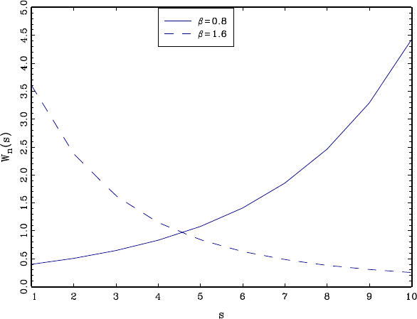
CHAPTER 9. HYPOTHESIS TESTING 266
Figure 9.1: Wald Statistic as a function of
for which the test statistic is insignificant. This is distressing since the choice of is arbitrary and
irrelevant to the actual hypothesis.
Our first-order asymptotic theory is not useful to help pick as ()
−→ 2
1under H0for any
This is a context where Monte Carlo simulation can be quite useful as a tool to study and
compare the exact distributions of statistical procedures in finite samples. The method uses random
simulation to create artificial datasets, to which we apply the statistical tools of interest. This
produces random draws from the statistic’s sampling distribution. Through repetition, features of
this distribution can be calculated.
In the present context of the Wald statistic, one feature of importance is the Type I error
of the test using the asymptotic 5% critical value 3.84 — the probability of a false rejection,
Pr (()384 |=1)Given the simplicity of the model, this probability depends only on
and 2In Table 9.1 we report the results of a Monte Carlo simulation where we vary these three
parameters. The value of is varied from 1to 10, is varied among 20, 100 and 500, and is
varied among 1 and 3. The Table reports the simulation estimate of the Type I error probability
from 50,000 random samples. Each row of the table corresponds to a different value of — and thus
corresponds to a particular choice of test statistic. The second through seventh columns contain the
Type I error probabilities for different combinations of and . These probabilities are calculated
as the percentage of the 50,000 simulated Wald statistics ()which are larger than 3.84. The
null hypothesis =1is true, so these probabilities are Type I error.
To interpret the table, remember that the ideal Type I error probability is 5% (.05) with devia-
tions indicating distortion. Type I error rates between 3% and 8% are considered reasonable. Error
rates above 10% are considered excessive. Rates above 20% are unacceptable. When comparing
statistical procedures, we compare the rates row by row, looking for tests for which rejection rates
are close to 5% and rarely fall outside of the 3%-8% range. For this particular example the only
test which meets this criterion is the conventional =(1) test. Any other choice of leads to
a test with unacceptable Type I error probabilities.
Table 9.1
Type I Error Probability of Asymptotic 5% ()Test

CHAPTER 9. HYPOTHESIS TESTING 267
=1 =3
=20 = 100 = 500 =20 = 100 =500
1.06 .05 .05 .07 .05 .05
2.08 .06 .05 .15 .08 .06
3.10 .06 .05 .21 .12 .07
4.13 .07 .06 .25 .15 .08
5.15 .08 .06 .28 .18 .10
6.17 .09 .06 .30 .20 .11
7.19 .10 .06 .31 .22 .13
8.20 .12 .07 .33 .24 .14
9.22 .13 .07 .34 .25 .15
10 .23 .14 .08 .35 .26 .16
Note: Rejection frequencies from 50,000 simulated random samples
In Table 9.1 you can also see the impact of variation in sample size. In each case, the Type I
error probability improves towards 5% as the sample size increases. There is, however, no magic
choice of for which all tests perform uniformly well. Test performance deteriorates as increases,
which is not surprising given the dependence of ()on as shown in Figure 9.1.
In this example it is not surprising that the choice =1yields the best test statistic. Other
choices are arbitrary and would not be used in practice. While this is clear in this particular
example, in other examples natural choices are not always obvious and the best choices may in fact
appear counter-intuitive at first.
This point can be illustrated through another example which is similar to one developed in
Gregory and Veall (1985). Take the model
=0+11+22+(9.22)
E(x)=0
and the hypothesis
H0:1
2
=0
where 0is a known constant. Equivalently, define =12so the hypothesis can be stated as
H0:=0
Let b
β=(
b
0b
1b
2)be the least-squares estimates of (9.22), let b
V
be an estimate of the
covariance matrix for b
βand set b
=b
1b
2.Define
b
R1=
⎛
⎜
⎜
⎜
⎜
⎜
⎜
⎜
⎜
⎜
⎝
0
1
b
2
−b
1
b
2
2
⎞
⎟
⎟
⎟
⎟
⎟
⎟
⎟
⎟
⎟
⎠
so that the standard error for b
is (b
)=³b
R0
1b
V
b
R1´12In this case a t-statistic for H0is
1=³
1
2−0´
(b
)
An alternative statistic can be constructed through reformulating the null hypothesis as
H0:1−02=0

CHAPTER 9. HYPOTHESIS TESTING 268
A t-statistic based on this formulation of the hypothesis is
2=b
1−0b
2
³R0
2b
V
R2´12
where
R2=⎛
⎝
0
1
−0
⎞
⎠
To compare 1and 2we perform another simple Monte Carlo simulation. We let 1and 2
be mutually independent N(01) variables, be an independent N(02)draw with =3,and
normalize 0=0and 1=1This leaves 2as a free parameter, along with sample size We vary
2among 1.25, .50, .75, and 1.0 and among 100 and 500
Table 9.2
Type I Error Probability of Asymptotic 5% t-tests
= 100 = 500
Pr (−1645) Pr (1645) Pr (−1645) Pr (1645)
212121212
.10 .47 .06 .00 .06 .28 .05 .00 .05
.25 .26 .06 .00 .06 .15 .05 .00 .05
.50 .15 .06 .00 .06 .10 .05 .00 .05
.75 .12 .06 .00 .06 .09 .05 .00 .05
1.00 .10 .06 .00 .06 .07 .05 .02 .05
The one-sided Type I error probabilities Pr (−1645) and Pr (1645) are calculated
from 50,000 simulated samples. The results are presented in Table 9.2. Ideally, the entries in the
table should be 0.05. However, the rejection rates for the 1statistic diverge greatly from this
value, especially for small values of 2The left tail probabilities Pr (1−1645) greatly exceed
5%, while the right tail probabilities Pr (11645) are close to zero in most cases. In contrast,
the rejection rates for the linear 2statistic are invariant to the value of 2and are close to the
ideal 5% rate for both sample sizes. The implication of Table 8.2 is that the two t-ratios have
dramatically different sampling behavior.
The common message from both examples is that Wald statistics are sensitive to the algebraic
formulation of the null hypothesis.
A simple solution is to use the minimum distance statistic , which equals with =1in the
first example, and |2|in the second example. The minimum distance statistic is invariant to the
algebraic formulation of the null hypothesis, so is immune to this problem. Whenever possible, the
Wald statistic should not be used to test nonlinear hypotheses.
9.18 Monte Carlo Simulation
In Section 9.17 we introduced the method of Monte Carlo simulation to illustrate the small
sample problems with tests of nonlinear hypotheses. In this section we describe the method in
more detail.
Recall, our data consist of observations (x)which are random draws from a population
distribution Let θbe a parameter and let =((1x1)(x)θ)be a statistic of
interest, for example an estimator b
or a t-statistic (b
−)(b
)The exact distribution of is
( )=Pr(≤|)

CHAPTER 9. HYPOTHESIS TESTING 269
While the asymptotic distribution of mightbeknown,theexact(finite sample) distribution
is generally unknown.
Monte Carlo simulation uses numerical simulation to compute ( )for selected choices of
This is useful to investigate the performance of the statistic in reasonable situations and sample
sizes. The basic idea is that for any given the distribution function ( )can be calculated
numerically through simulation. The name Monte Carlo derives from the famous Mediterranean
gambling resort where games of chance are played.
The method of Monte Carlo is quite simple to describe. The researcher chooses (the dis-
tribution of the data) and the sample size .A“true”valueofθis implied by this choice, or
equivalently the value θis selected directly by the researcher which implies restrictions on .
Then the following experiment is conducted by computer simulation:
1. independent random pairs (∗
x∗
)=1 are drawn from the distribution using
the computer’s random number generator.
2. The statistic =((∗
1x∗
1)(∗
x∗
)θ)is calculated on this pseudo data.
For step 1, computer packages have built-in random number procedures including U[01] and
N(01). From these most random variables can be constructed. (For example, a chi-square can be
generated by sums of squares of normals.)
For step 2, it is important that the statistic be evaluated at the “true” value of θcorresponding
to the choice of
The above experiment creates one random draw from the distribution ( )This is one
observation from an unknown distribution. Clearly, from one observation very little can be said.
So the researcher repeats the experiment times, where is a large number. Typically, we set
= 1000or= 5000We will discuss this choice later.
Notationally, let the experiment result in the draw =1 These results are stored.
After all experiments have been calculated, these results constitute a random sample of size
from the distribution of ( )=Pr(≤)=Pr(≤|)
From a random sample, we can estimate any feature of interest using (typically) a method of
moments estimator. We now describe some specificexamples.
Suppose we are interested in the bias, mean-squared error (MSE), and/or variance of the dis-
tribution of b
− We then set =b
− run the above experiment, and calculate
\
(ˆ
)= 1
X
=1
=1
X
=1 b
−
\
(ˆ
)= 1
X
=1
()2=1
X
=1 ³b
−´2
\
var(b
)= \
(b
)−µ\
(b
)¶2
Suppose we are interested in the Type I error associated with an asymptotic 5% two-sided t-test.
We would then set =¯¯¯b
−¯¯¯(b
)and calculate
b
=1
X
=1
1(≥196) (9.23)
the percentage of the simulated t-ratios which exceed the asymptotic 5% critical value.
Suppose we are interested in the 5% and 95% quantile of =b
or =³b
−´(b
).Wethen
compute the 5% and 95% sample quantiles of the sample {}The sample quantile is a number

CHAPTER 9. HYPOTHESIS TESTING 270
such that 100%of the sample are less than A simple way to compute sample quantiles is
to sort the sample {}from low to high. Then is the number in this ordered sequence,
where =(+1) It is therefore convenient to pick so that is an integer. For example, if
we set = 999then the 5% sample quantile is 50 sorted value and the 95% sample quantile is
the 950 sorted value.
The typical purpose of a Monte Carlo simulation is to investigate the performance of a statistical
procedure (estimator or test) in realistic settings. Generally, the performance will depend on and
In many cases, an estimator or test may perform wonderfully for some values, and poorly for
others. It is therefore useful to conduct a variety of experiments, for a selection of choices of and
As discussed above, the researcher must select the number of experiments, Often this is
called the number of replications. Quite simply, a larger results in more precise estimates of
the features of interest of but requires more computational time. In practice, therefore, the
choice of is often guided by the computational demands of the statistical procedure. Since the
results of a Monte Carlo experiment are estimates computed from a random sample of size it
is straightforward to calculate standard errors for any quantity of interest. If the standard error is
too large to make a reliable inference, then will have to be increased.
In particular, it is simple to make inferences about rejection probabilities from statistical tests,
such as the percentage estimate reported in (9.23). The random variable 1(≥196) is iid
Bernoulli, equalling 1 with probability =E(1 (≥196)) The average (9.23) is therefore an
unbiased estimator of with standard error (b)=p(1 −).Asis unknown, this may be
approximated by replacing with bor with an hypothesized value. For example, if we are assessing
an asymptotic 5% test, then we can set (b)=p(05) (95) '22√ Hence, standard errors
for =1001000, and 5000, are, respectively, (b)=022007and .003.
Most papers in econometric methods, and some empirical papers, include the results of Monte
Carlo simulations to illustrate the performance of their methods. When extending existing results,
it is good practice to start by replicating existing (published) results. This is not exactly possible
in the case of simulation results, as they are inherently random. For example suppose a paper
investigates a statistical test, and reports a simulated rejection probability of 0.07 based on a
simulation with =100replications. Suppose you attempt to replicate this result, and find a
rejection probability of 0.03 (again using = 100 simulation replications). Should you conclude
that you have failed in your attempt? Absolutely not! Under the hypothesis that both simulations
are identical, you have two independent estimates, b1=007 and b2=003, of a common probability
Theasymptotic(as→∞) distribution of their difference is √(b1−b2)
−→ N(02(1−))so
a standard error for b1−b2=004 is b=p2(1 −) '003using the estimate =(b1+b2)2
Since the t-ratio 004003 = 13is not statistically significant, it is incorrect to reject the null
hypothesis that the two simulations are identical. The difference between the results b1=007 and
b2=003 is consistent with random variation.
What should be done? The first mistake was to copy the previous paper’s choice of = 100
Instead, suppose you set = 5000Suppose you now obtain b2=004Then b1−b2=003 and
a standard error is b=p(1 −)(1100 + 15000) '002Still we cannot reject the hypothesis
that the two simulations are different. Even though the estimates (007 and 004)appeartobe
quite different, the difficulty is that the original simulation used a very small number of replications
(= 100) so the reported estimate is quite imprecise. In this case, it is appropriate to conclude
that your results “replicate” the previous study, as there is no statistical evidence to reject the
hypothesis that they are equivalent.
Most journals have policies requiring authors to make available their data sets and computer
programs required for empirical results. They do not have similar policies regarding simulations.
Nevertheless, it is good professional practice to make your simulations available. The best practice
is to post your simulation code on your webpage. This invites others to build on and use your
results, leading to possible collaboration, citation, and/or advancement.

CHAPTER 9. HYPOTHESIS TESTING 271
9.19 Confidence Intervals by Test Inversion
There is a close relationship between hypothesis tests and confidence intervals. We observed in
Section 7.13 that the standard 95% asymptotic confidence interval for a parameter is
b
=hb
−196 ·(b
)b
+196 ·(b
)i(9.24)
={:|()|≤196}
That is, we can describe b
as “The point estimate plus or minus 2 standard errors” or “The set of
parameter values not rejected by a two-sided t-test.” The second definition, known as test statistic
inversion is a general method for finding confidence intervals, and typically produces confidence
intervals with excellent properties.
Given a test statistic ()and critical value , the acceptance region “Accept if ()≤”
is identical to the confidence interval b
={:()≤}. Since the regions are identical, the
probability of coverage Pr ³∈b
´equals the probability of correct acceptance Pr (Accept|)which
is exactly 1 minus the Type I error probability. Thus inverting a test with good Type I error
probabilities yields a confidence interval with good coverage probabilities.
Now suppose that the parameter of interest =(β)is a nonlinear function of the coefficient
vector β. In this case the standard confidence interval for is the set b
as in (9.24) where b
=(b
β)
is the point estimate and (b
)=qb
R0b
V
b
Ris the delta method standard error. This confidence
interval is inverting the t-test based on the nonlinear hypothesis (β)= The trouble is that in
Section 9.17 we learned that there is no unique t-statistic for tests of nonlinear hypotheses and that
the choice of parameterization matters greatly.
For example, if =12then the coverage probability of the standard interval (9.24) is 1
minus the probability of the Type I error, which as shown in Table 8.2 can be far from the nominal
5%.
In this example a good solution is the same as discussed in Section 9.17 — to rewrite the
hypothesis as a linear restriction. The hypothesis =12is the same as 2=1The t-
statistic for this restriction is
()= b
1−b
2
³R0b
V
R´12
where
R=µ1
−
and b
V
is the covariance matrix for (b
1b
2)A 95% confidence interval for =12is the set of
values of such that |()|≤196Since appears in both the numerator and denominator, ()
is a non-linear function of so the easiest method to find the confidence set is by grid search over
For example, in the wage equation
log()=1 +22100 + ···
the highest expected wage occurs at =−5012From Table 4.1 we have the point
estimate b
=298and we can calculate the standard error (b
)=0022 for a 95% confidence interval
[29829.9]. However, if we instead invert the linear form of the test we can numerically find the
interval [29130.6] which is much larger. From the evidence presented in Section 9.17 we know the
first interval can be quite inaccurate and the second interval is greatly preferred.

CHAPTER 9. HYPOTHESIS TESTING 272
9.20 Multiple Tests and Bonferroni Corrections
In most applications, economists examine a large number of estimates, test statistics, and p-
values. What does it mean (or does it mean anything) if one statistic appears to be “significant”
after examining a large number of statistics? This is known as the problem of multiple testing
or multiple comparisons.
To be specific, suppose we examine a set of coefficients, standard errors and t-ratios, and
consider the “significance” of each statistic. Based on conventional reasoning, for each coefficient
we would reject the hypothesis that the coefficient is zero with asymptotic size if the absolute t-
statistic exceeds the 1−critical value of the normal distribution, or equivalently if the p-value for
the t-statistic is smaller than . If we observe that one of the statistics is “significant” based on
this criteria, that means that one of the p-values is smaller than , or equivalently, that the smallest
p-value is smaller than . We can then rephrase the question: Under the joint hypothesis that a set
of hypotheses are all true, what is the probability that the smallest p-value is smaller than ?In
general, we cannot provide a precise answer to this quesion, but the Bonferroni correction bounds
this probability by . The Bonferroni method furthermore suggests that if we want the familywise
error probability (the probability that one of the tests falsely rejects) is bounded below ,then
an appropriate rule is to reject only if thesmallestp-valueissmallerthan.Equivalenlty,the
Bonferroni familywise p-value is min≤.
Formally, suppose we have hypotheses H=1. For each we have a test and associated
p-value with the property that when His true lim→∞ Pr ()=. We then observe that
among the tests, one of the will appear “significant” if min≤. This event can be written
as ½min
≤
¾=
[
=1
{}
Boole’s inequality states that for any events ,Pr ⎛
⎝
[
=1
⎞
⎠≤P
=1 Pr ().Thus
Pr µmin
≤
¶≤
X
=1
Pr ()−→
as stated. This demonstates that the familywise rejection probability is at most times the
individual rejection probability.
Furthermore,
Pr µmin
≤
¶≤
X
=1
Pr ³
´−→
This demonstrates that the family rejection probability can be controlled (bounded below )if
each individual test is subjected to the stricter standard that a p-value must be smaller than
to be labeled as “significant.”
Toillustrate,supposewehavetwocoefficient estimates, with individual p-values 0.04 and
0.15. Based on a conventional 5% level, the standard individual tests would suggest that the first
coefficient estimate is “significant” but not the second. A Bonferroni 5% test, however, does not
reject as it would require that the smallest p-value be smaller than 0.025, which is not the case in
this example. Alternatively, the Bonferroni familywise p-value is 0.08, which is not significant at
the 5% level.
In contrast, if the two p-values are 0.01 and 0.15, then the Bonferroni familywise p-value is 0.02,
which is significant at the 5% level.

CHAPTER 9. HYPOTHESIS TESTING 273
9.21 Power and Test Consistency
The power of a test is the probability of rejecting H0when H1is true.
For simplicity suppose that is i.i.d. ( 2)with 2known, consider the t-statistic ()=
√(¯−) and tests of H0:=0against H1:0. We reject H0if =(0) Note that
=()+√
and ()has an exact N(01) distribution. This is because ()is centered at the true mean
while the test statistic (0) is centered at the (false) hypothesized mean of 0.
The power of the test is
Pr (|)=Pr¡Z+√ ¢=1−Φ¡−√¢
This function is monotonically increasing in and and decreasing in and .
Notice that for any and 6=0the power increases to 1 as →∞This means that for ∈H1
the test will reject H0with probability approaching 1 as the sample size gets large. We call this
property test consistency.
Definition 9.21.1 AtestofH0:θ∈Θ0is consistent against fixed
alternatives if for all θ∈Θ1Pr (Reject H0|)→1as →∞
For tests of the form “Reject H0if ”, a sufficient condition for test consistency is that the
diverges to positive infinity with probability one for all θ∈Θ1
Definition 9.21.2
−→ ∞ as →∞if for all ∞Pr (≤)→
0as →∞. Similarly,
−→ −∞ as →∞if for all ∞
Pr (≥−)→0as →∞.
In general, t-tests and Wald tests are consistent against fixed alternatives. Take a t-statistic for
a test of H0:=0
=b
−0
(b
)
where 0is a known value and (b
)=q−1b
.Notethat
=b
−
(b
)+√(−0)
qb
The first term on the right-hand-side converges in distribution to N(01)The second term on the
right-hand-side equals zero if =0converges in probability to +∞if
0and converges
in probability to −∞ if
0Thus the two-sided t-test is consistent against H1:6=0and
one-sided t-tests are consistent against the alternatives for which they are designed.
Theorem 9.21.1 Under Assumptions 7.1.2 and 7.10.1, for θ=r(β)6=θ0
and =1then ||
−→ ∞, so for any ∞the test “Reject H0if ||”
consistent against fixed alternatives.

CHAPTER 9. HYPOTHESIS TESTING 274
The Wald statistic for H0:θ=r(β)=θ0against H1:θ6=θ0is
=³b
θ−θ0´0b
V−1
³b
θ−θ0´
Under H1b
θ
−→ θ6=θ0Thus ³b
θ−θ0´0b
V−1
³b
θ−θ0´
−→ (θ−θ0)0V−1
(θ−θ0)0Hence
under H1
−→ ∞. Again, this implies that Wald tests are consistent tests.
Theorem 9.21.2 Under Assumptions 7.1.2 and 7.10.1, for θ=r(β)6=
θ0then
−→ ∞, so for any ∞the test “Reject H0if ”
consistent against fixed alternatives.
9.22 Asymptotic Local Power
Consistency is a good property for a test, but does not give a useful approximation to the power
of a test. To approximate the power function we need a distributional approximation.
The standard asymptotic method for power analysis uses what are called local alternatives.
This is similar to our analysis of restriction estimation under misspecification (Section 8.13). The
technique is to index the parameter by sample size so that the asymptotic distribution of the
statistic is continuous in a localizing parameter. In this section we consider t-tests on real-valued
parameters and in the next section consider Wald tests. Specifically, we consider parameter vectors
βwhich are indexed by sample size and satisfy the real-valued relationship
=(β)=0+−12(9.25)
where the scalar is called a localizing parameter. We index βand by sample size to
indicate their dependence on . The way to think of (9.25) is that the true value of the parameters
are βand . The parameter is close to the hypothesized value 0, with deviation −12.
The specification (9.25) states that for any fixed ,approaches 0as gets large. Thus
is “close” or “local” to 0. The concept of a localizing sequence (9.25) might seem odd since
in the actual world the sample size cannot mechanically affect the value of the parameter. Thus
(9.25) should not be interpreted literally. Instead, it should be interpreted as a technical device
which allows the asymptotic distribution of the test statistic to be continuous in the alternative
hypothesis.
To evaluate the asymptotic distribution of the test statistic we start by examining the scaled
estimate centered at the hypothesized value 0Breaking it into a term centered at the true value
and a remainder we find
√³b
−0´=√³b
−´+√(−0)
=√³b
−´+
where the second equality is (9.25). The first term is asymptotically normal:
√³b
−´
−→ pZ
where Z∼N(01).Therefore √³b
−0´
−→ pZ+
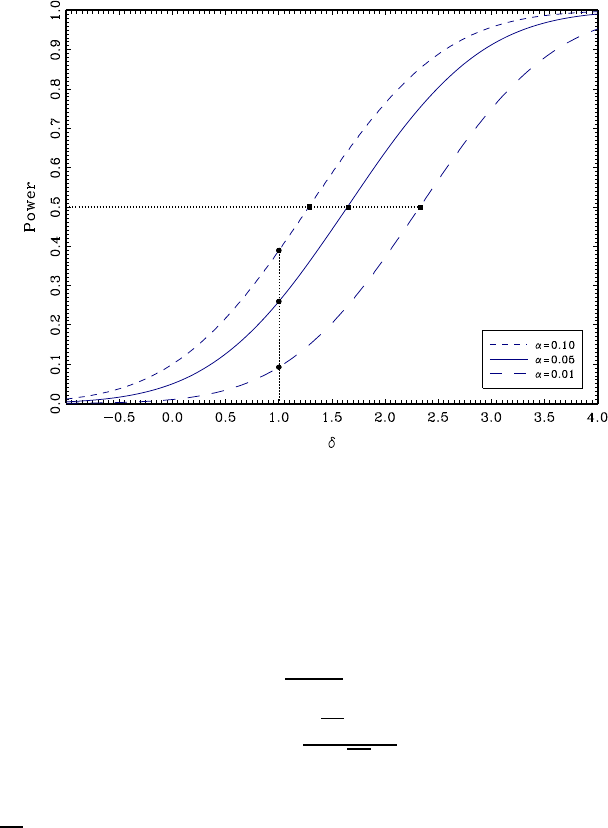
CHAPTER 9. HYPOTHESIS TESTING 275
Figure 9.2: Asymptotic Local Power Function of One-Sided t Test
or N( )This is a continuous asymptotic distribution, and depends continuously on the localizing
parameter .
Applied to the t statistic we find
=b
−0
(b
)
−→ √Z+
√
∼Z+(9.26)
where =√. This generalizes Theorem 9.4.1 (which assumes H0is true) to allow for local
alternatives of the form (9.25).
Consider a t-test of H0against the one-sided alternative H1:
0which rejects H0for
where Φ()=1−.Theasymptotic local power of this test is the limit (as the sample size
diverges) of the rejection probability under the local alternative (9.25)
lim
→∞ Pr (Reject H0)= lim
→∞ Pr ()
=Pr(Z+)
=1−Φ(−)
=Φ(−)
=()
We call ()the asymptotic local power function.
In Figure 9.2 we plot the local power function ()as a function of ∈[−14] for tests of
asymptotic size =010,=005,and=001.=0corresponds to the null hypothesis so
()=. The power functions are monotonically increasing in . Note that the power is lower
than for 0due to the one-sided nature of the test.
We can see that the three power functions are ranked by so that the test with =010 has
higher power than the test with =001. This is the inherent trade-offbetween size and power.
Decreasing size induces a decrease in power, and conversely.

CHAPTER 9. HYPOTHESIS TESTING 276
The coefficient can be interpreted as the parameter deviation measured as a multiple of the
standard error (b
)To see this, recall that (b
)=−12qb
'−12√andthennotethat
=
√
'−12
(b
)=−0
(b
)
Thus approximately equals the deviation −0expressed as multiples of the standard error (b
).
Thus as we examine Figure 9.2, we can interpret the power function at =1(e.g. 26% for a 5% size
test) as the power when the parameter is one standard error above the hypothesized value. For
example, from Table 4.1 the standard error for the coefficient on “Married Female” is 0.010. Thus
in this example, =1corresponds to =0010 or an 1.0% wage premium for married females.
Our calculations show that the asymptotic power of a one-sided 5% test against this alternative is
about 26%.
The difference between power functions can be measured either vertically or horizontally. For
example, in Figure 9.2 there is a vertical dotted line at =1showing that the asymptotic local
power function ()equals 39% for =010equals 26% for =005 and equals 9% for =001.
This is the difference in power across tests of differing size, holding fixed the parameter in the
alternative.
A horizontal comparison can also be illuminating. To illustrate, in Figure 9.2 there is a hori-
zontal dotted line at 50% power. 50% power is a useful benchmark, as it is the point where the
test has equal odds of rejection and acceptance. The dotted line crosses the three power curves at
=129 (=010), =165 (=005), and =233 (=001). This means that the parameter
must be at least 1.65 standard errors above the hypothesized value for a one-sided 5% test to
have 50% (approximate) power.
The ratio of these values (e.g. 165129 = 128 for the asymptotic 5% versus 10% tests)
measures the relative parameter magnitude needed to achieve the same power. (Thus, for a 5% size
test to achieve 50% power, the parameter must be 28% larger than for a 10% size test.) Even more
interesting, the square of this ratio (e.g. (165129)2=164) can be interpreted as the increase
in sample size needed to achieve the same power under fixed parameters. That is, to achieve 50%
power, a 5% size test needs 64% more observations than a 10% size test. This interpretation follows
by the following informal argument. By definition and (9.25) =√=√(−0)√Thus
holding and fixed, 2is proportional to .
The analysis of a two-sided t test is similar. (9.26) implies that
=¯¯¯¯¯b
−0
(b
)¯¯¯¯¯
−→ |Z+|
and thus the local power of a two-sided t test is
lim
→∞ Pr (Reject H0)= lim
→∞ Pr ()
=Pr(|Z+|)
=Φ(−)−Φ(−−)
which is monotonically increasing in ||.

CHAPTER 9. HYPOTHESIS TESTING 277
Theorem 9.22.1 Under Assumptions 7.1.2 and 7.10.1, and =(β)=
0+−12 then
(0)= b
−0
(b
)
−→ Z+
where Z∼N(01) and =√For such that Φ()=1−,
Pr ((0))−→ Φ(−)
Furthermore, for such that Φ()=1−2
Pr (|(0)|)−→ Φ(−)−Φ(−−)
9.23 Asymptotic Local Power, Vector Case
In this section we extend the local power analysis of the previous section to the case of vector-
valued alternatives. We generalize (9.25) to allow θto be vector-valued. The local parameteriza-
tion takes the form
θ=r(β)=θ0+−12h(9.27)
where his ×1
Under (9.27),
√³b
θ−θ0´=√³b
θ−θ´+h
−→ Z∼N(hV)
a normal random vector with mean hand variance matrix V.
Applied to the Wald statistic we find
=³b
θ−θ0´0b
V−1
³b
θ−θ0´
−→ Z0
V−1
Z∼2
()(9.28)
where =h0V−1h.2
()is a non-central chi-square random variable with non-centrality para-
meter . (See Section 5.3 and Theorem 5.3.3.)
The convergence (9.28) shows that under the local alternatives (9.27),
−→ 2
()This
generalizes the null asymptotic distribution which obtains as the special case =0We can use this
result to obtain a continuous asymptotic approximation to the power function. For any significance
level 0set the asymptotic critical value so that Pr ¡2
¢= Then as →∞
Pr ()−→ Pr ¡2
()
¢
=()
The asymptotic local power function ()depends only on ,and.
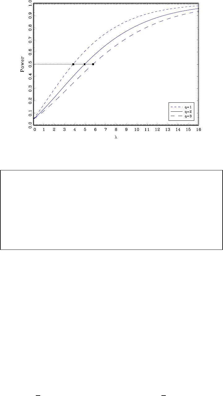
CHAPTER 9. HYPOTHESIS TESTING 278
Figure 9.3: Asymptotic Local Power Function, Varying
Theorem 9.23.1 Under Assumptions 7.1.2 and 7.10.1, and θ=
r(β)=θ0+−12hthen
−→ 2
()
where =h0V−1
hFurthermore, for such that Pr ¡2
¢=,
Pr ()−→ Pr ¡2
()
¢
Figure 9.3 plots ()as a function of for =1,=2,and=3,and=005.The
asymptotic power functions are monotonically increasing in and asymptote to one.
Figure 9.3 also shows the power loss for fixed non-centrality parameter as the dimensionality
of the test increases. The power curves shift to the right as increases, resulting in a decrease
in power. This is illustrated by the dotted line at 50% power. The dotted line crosses the three
power curves at =385 (=1), =496 (=2), and =577 (=3). The ratio of these
values correspond to the relative sample sizes needed to obtain the same power. Thus increasing
the dimension of the test from =1to =2requires a 28% increase in sample size, or an increase
from =1to =3requires a 50% increase in sample size, to obtain a test with 50% power.
9.24 Technical Proofs*
ProofofTheorem9.12.1. The conditions of Theorem 8.14.1 hold, since H0implies Assumption
8.6.1. From (8.58) with c
W=b
V, we see that
√³b
β−e
βemd´=b
Vb
R³R∗0
b
Vb
R´−1R∗0
√³b
β−β´
−→ VR¡R0VR¢−1R0N(0V)
=VRZ
CHAPTER 9. HYPOTHESIS TESTING 279
where Z∼N(0(R0VR)−1)Thus
∗=³b
β−e
βemd´0b
V−1
³b
β−e
βemd´
−→ Z0R0VV−1
VRZ
=Z
0¡R0VR¢Z
=2
¥

CHAPTER 9. HYPOTHESIS TESTING 280
Exercises
Exercise 9.1 Prove that if an additional regressor X+1 is added to XTheil’s adjusted 2
increases if and only if |+1|1where +1 =b
+1(b
+1)is the t-ratio for b
+1 and
(b
+1)=¡2[(X0X)−1]+1+1¢12
is the homoskedasticity-formula standard error.
Exercise 9.2 You have two independent samples (y1X1)and (y2X2)which satisfy y1=X1β1+
e1and y2=X2β2+e2where E(x11)=0and E(x22)=0and both X1and X2have
columns. Let b
β1and b
β2be the OLS estimates of β1and β2. For simplicity, you may assume that
both samples have the same number of observations
(a) Find the asymptotic distribution of √³³b
β2−b
β1´−(β2−β1)´as →∞
(b) Find an appropriate test statistic for H0:β2=β1
(c) Find the asymptotic distribution of this statistic under H0
Exercise 9.3 Let be a t-statistic for H0:=0versus 1:6=0.Since||→||under 0,
someone suggests the test “Reject H0if ||
1or ||
2,where1is the 2quantile of ||
and 2is the 1−2quantile of ||.
(a) Show that the asymptotic size of the test is .
(b) IsthisagoodtestofH0versus H1?Whyorwhynot?
Exercise 9.4 Let be a Wald statistic for H0:θ=0versus H1:θ6=0,whereθis ×1.Since
→2
under 0, someone suggests the test “Reject H0if
1or
2,where1is the
2quantile of 2
and 2is the 1−2quantile of 2
.
(a) Show that the asymptotic size of the test is .
(b) IsthisagoodtestofH0versus H1?Whyorwhynot?
Exercise 9.5 Take the linear model
=x0
1β1+x0
2β2+
E(x)=0
where both x1and x2are ×1. Show how to test the hypotheses H0:β1=β2against
H1:β16=β2
Exercise 9.6 Suppose a researcher wants to know which of a set of 20 regressors has an effect on a
variable testscore. He regresses testscore on the 20 regressors and reports the results. One of the 20
regressors (studytime) has a large t-ratio (about 2.5), while other t-ratios are insignificant (smaller
than 2 in absolute value). He argues that the data show that studytime is the key predictor for
testscore. Do you agree with this conclusion? Is there a deficiency in his reasoning?
Exercise 9.7 Take the model
=1+2
2+
E(|)=0
where is wages (dollars per hour) and is age. Describe how you would test the hypothesis that
the expected wage for a 40-year-old worker is $20 an hour.

CHAPTER 9. HYPOTHESIS TESTING 281
Exercise 9.8 You want to test H0:β2=0against H1:β26=0in the model
=x0
1β1+x0
2β2+
E(x)=0
You read a paper which estimates model
=x0
1b
γ1+(x2−x1)0b
γ2+b
and reports a test of H0:γ2=0against H1:γ26=0. Is this related to the test you wanted to
conduct?
Exercise 9.9 Suppose a researcher uses one dataset to test a specifichypothesisH0against H1,
and finds that he can reject H0. A second researcher gathers a similar but independent dataset, uses
similar methods and finds that she cannot reject H0. How should we (as interested professionals)
interpret these mixed results?
Exercise 9.10 In Exercise 7.8, you showed that √¡b2−2¢→N(0)as →∞for some .
Let b
be an estimate of .
(a) Using this result, construct a t-statistic for H0:2=1against H1:26=1.
(b) Using the Delta Method, find the asymptotic distribution of √(b−).
(c) Use the previous result to construct a t-statistic for H0:=1against H1:6=1.
(d) Are the null hypotheses in (a) and (c) the same or are they different? Are the tests in (a)
and (c) the same or are they different? If they are different, describe a context in which the
two tests would give contradictory results.
Exercise 9.11 Consider a regression such as Table 4.1 where both experience and its square are
included. A researcher wants to test the hypothesis that experience does not affect mean wages,
and does this by computing the t-statistic for experience. Is this the correct approach? If not, what
is the appropriate testing method?
Exercise 9.12 A researcher estimates a regression and computes a test of H0against H1and finds
a p-value of =008, or “not significant”. She says “I need more data. If I had a larger sample
the test will have more power and then the test will reject.” Is this interpretation correct?
Exercise 9.13 A common view is that “If the sample size is large enough, any hypothesis will be
rejected.” What does this mean? Interpret and comment.
Exercise 9.14 Take the model
=x0
β+
E(x)=0
with parameter of interest =R0βwith R×1.Letb
βbe the least-squares estimate and b
V
its
variance estimate.
(a) Write down b
, the 95% asymptotic confidence interval for ,intermsofb
β,b
V
,R,and
=196 (the 97.5% quantile of N(01)).
(b) Show that the decision “Reject H0if 0∈b
” is an asymptotic 5% test of H0:=0.

CHAPTER 9. HYPOTHESIS TESTING 282
Exercise 9.15 You are at a seminar where a colleague presents a simulation study of a test of
ahypothesisH0with nominal size 5%. Based on = 100 simulation replications under H0the
estimated size is 7%. Your colleague says: “Unfortunately the test over-rejects.”
(a) Do you agree or disagree with your colleague? Explain. Hint: Use an asymptotic (large )
approximation.
(b) Suppose the number of simulation replications were =1000yet the estimated size is still
7%. Does your answer change?
Exercise 9.16 You have iid observations (
1
2)and consider two alternative regression
models
=x0
1β1+1(9.29)
E(x11)=0
=x0
2β2+2(9.30)
E(x22)=0
where x1and x2have at least some different regressors. (For example, (9.29) is a wage regression
on geographic variables and (2) is a wage regression on personal appearance measurements.) You
want to know if model (9.29) or model (9.30) fits the data better. Define 2
1=¡2
1¢and
2
2=¡2
2¢. You decide that the model with the smaller variance fit (e.g., model (9.29) fits better
if 2
1
2
2.) You decide to test for this by testing the hypothesis of equal fitH0:2
1=2
2against
the alternative of unequal fitH1:2
16=2
2. For simplicity, suppose that 1and 2are observed.
(a) Construct an estimate b
of =2
1−2
2
(b) Find the asymptotic distribution of √³b
−´as →∞
(c) Find an estimator of the asymptotic variance of b
.
(d) Propose a test of asymptotic size of H0against H1
(e) Suppose the test accepts H0.Briefly, what is your interpretation?
Exercise 9.17 You have two regressors 1and 2, and estimate a regression with all quadratic
terms
=+11+22+32
1+42
2+512+
One of your advisors asks: Can we exclude the variable 2from this regression?
How do you translate this question into a statistical test? When answering these questions, be
specific, not general.
(a) What is the relevant null and alternative hypotheses?
(b) What is an appropriate test statistic? Be specific.
(c) What is the appropriate asymptotic distribution for the statistic? Be specific.
(d) What is the rule for acceptance/rejection of the null hypothesis?

CHAPTER 9. HYPOTHESIS TESTING 283
Exercise 9.18 The observed data is {xz}∈R×R×R1and 1=1 An
econometrician first estimates
=x0
b
β+b
by least squares. The econometrician next regresses the residual bon zwhich can be written as
b=z0
e
γ+e
(a) Define the population parameter γbeing estimated in this second regression.
(b) Find the probability limit for e
γ
(c) Suppose the econometrician constructs a Wald statistic for H0:γ=0from the second
regression, ignoring the regression. Write down the formula for .
(d) Assuming E(zx0
)=0find the asymptotic distribution for under H0:γ=0.
(e) If E(zx0
)6=0will your answer to (d) change?
Exercise 9.19 An economist estimates =11+22+by least-squares and tests the
hypothesis H0:2=0against H1:26=0. She obtains a Wald statistic =034.Thesample
size is = 500.
(a) What is the correct degrees of freedom for the 2distribution to evaluate the significance of
the Wald statistic?
(b) The Wald statistic is very small. Indeed, is it less than the 1% quantile of the appropriate
2distribution? If so, should you reject H0? Explain your reasoning.
Exercise 9.20 You are reading a paper, and it reports the results from two nested OLS regressions:
=x0
1e
β1+e
=x0
1b
β1+x0
2b
β2+b
Some summary statistics are reported:
Short Regression Long Regression
2=20 2=26
P
=1 e2
= 106 P
=1 b2
= 100
#ofcoefficients=5 # of coefficients=8
=50 =50
You are curious if the estimate b
β2is statistically different from the zero vector. Is there a way to
determine an answer from this information? Do you have to make any assumptions (beyond the
standard regularity conditions) to justify your answer?
Exercise 9.21 Take the model
=11+22+33+44+
E(x)=0
Describe how you would test
H0:1
2
=3
4
against
H1:1
2
6=3
4

CHAPTER 9. HYPOTHESIS TESTING 284
Exercise 9.22 You have a random sample from the model
=1+2
2+
E(|)=0
where is wages (dollars per hour) and is age. Describe how you would test the hypothesis that
the expected wage for a 40-year-old worker is $20 an hour.
Exercise 9.23 Let be a test statistic such that under H0
→2
3.Since¡2
37815¢=
005an asymptotic 5% test of H0rejects when 7815An econometrician is interested in the
Type I error of this test when = 100 and the data structure is well specified. She performs the
following Monte Carlo experiment
•= 200 samples of size = 100 are generated from a distribution satisfying H0
•On each sample, the test statistic is calculated.
•She calculates b=1
P
=1 1( 7815) = 0070
•The econometrician concludes that the test is oversized in this context — it rejects too
frequently under H0
Is her conclusion correct, incorrect, or incomplete? Be specificinyouranswer.
Exercise 9.24 Do a Monte Carlo simulation. Take the model
=++
E()=0
where the parameter of interest is =exp(). Your data generating process (DGP) for the
simulation is: is [01]
is independent of and (01),=50.Set=0and =1.
Generate = 1000 independent samples with . On each, estimate the regression by least-squares,
calculate the covariance matrix using a standard (heteroskedasticity-robust) formula, and similarly
estimate and its standard error. For each replication, store b
,b
,=³b
−´ ³b
´,and
=³b
−´ ³b
´
(a) Does the value of matter? Explain why the described statistics are invariant to and
thus setting =0is irrelevant.
(b) From the 1000 replications estimate E³b
´and E³b
´. Discuss if you see evidence if either
estimatorisbiasedorunbiased.
(c) From the 1000 replications estimate Pr (1645) and Pr (1645).Whatdoesasymp-
totic theory predict these probabilities should be in large samples? What do your simulation
results indicate?
Exercise 9.25 The data set invest on the textbook website contains data on 565 U.S. firms
extracted from Compustat for the year 1987. (This is one year from a panel data set used by B.
E. Hansen (1999). The original data was compiled by Hall and Hall (1993).) The variables are
•Investment to Capital Ratio (multiplied by 100).
•Total Market Value to Asset Ratio (Tobin’s Q).
CHAPTER 9. HYPOTHESIS TESTING 285
•Cash Flow to Asset Ratio.
•Long Term Debt to Asset Ratio.
The flow variables are annual sums for 1987. The stock variables are beginning of year.
(a) Estimate a linear regression of on the other variables. Calculate appropriate standard
errors.
(b) Calculate asymptotic confidence intervals for the coefficients.
(c) This regression is related to Tobin’s theory of investment, which suggests that investment
should be predicted solely by Thus the coefficient on should be positive and the others
should be zero. Test the joint hypothesis that the coefficients on and are zero. Test the
hypothesis that the coefficient on is zero. Are the results consistent with the predictions
of the theory?
(d) Now try a non-linear (quadratic) specification. Regress on
,
2
2
,2
Test the joint hypothesis that the six interaction and quadratic coefficients are
zero.
Exercise 9.26 In a paper in 1963, Marc Nerlove analyzed a cost function for 145 American electric
companies. His data set Nerlove1963 is on the textbook website. The variables are
•CTotalcost
•Q Output
•PL Unit price of labor
•PK Unit price of capital
•PL Unit price of labor
Nerlov was interested in estimating a cost function :=()
(a) First estimate an unrestricted Cobb-Douglass specification
log =1+2log +3log
+4log
+5log
+(9.31)
Report parameter estimates and standard errors.
(b) What is the economic meaning of the restriction H0:3+4+5=1?
(c) Estimate (9.31) by constrained least-squares imposing 3+4+5=1. Report your parameter
estimates and standard errors.
(d) Estimate (9.31) by efficient minimum distance imposing 3+4+5=1. Report your
parameter estimates and standard errors.
(e) Test H0:3+4+5=1using a Wald statistic.
(f) Test H0:3+4+5=1using a minimum distance statistic.
Exercise 9.27 In Section 8.12 we report estimates from Mankiw, Romer and Weil (1992). We
reported estimation both by unrestricted least-squares and by constrained estimation, imposing
theconstraintthatthreecoefficients (2,3
and 4 coefficients) sum to zero, as implied by the
Solow growth theory. Using the same dataset MRW1992 estimate the unrestricted model and test
the hypothesis that the three coefficients sum to zero.
CHAPTER 9. HYPOTHESIS TESTING 286
Exercise 9.28 Using the CPS dataset and the subsample of non-hispanic blacks (race code = 2),
test the hypothesis that marriage status does not affect mean wages.
(a) Take the regression reported in Table 4.1. Which variables will need to be omitted to estimate
a regression for the subsample of blacks?
(b) Express the hypothesis “marriage status does not affect mean wages” as a restriction on the
coefficients. How many restrictions is this?
(c) Find the Wald (or F) statistic for this hypothesis. What is the appropriate distribution for
the test statistic? Calculate the p-value of the test.
(d) What do you conclude?
Exercise 9.29 Using the CPS dataset and the subsample of non-hispanic blacks (race code = 2)
and whites (race code = 1), test the hypothesis that the returns to education is common across
groups.
(a) Allow the return to education to vary across the four groups (white male, white female, black
male, black female) by interacting dummy variables with education. Estimate an appropriate
version of the regression reported in Table 4.1.
(b) Find the Wald (or F) statistic for this hypothessis. What is the appropriate distribution for
the test statistic? Calculate the p-value of the test.
(c) What do you conclude?

Chapter 10
Multivariate Regression
10.1 Introduction
Multivariate regression is a system of regression equations. Multivariate regression is used
as reduced form models for instrumental variable estimation (explored in Chaper 11), vector au-
toregressions (explored in Chapter 15), demand systems (demand for multiple goods), and other
contexts.
Multivariate regression is also called by the name systems of regression equations. Closely
related is the method of Seemingly Unrelated Regressions (SUR) which we introduce in Section
10.7.
Most of the tools of single equation regression generalize naturally to multivariate regression.
Amajordifference is a new set of notation to handle matrix estimates.
10.2 Regression Systems
A system of linear regressions takes the form
=x0
β+ (10.1)
for variables =1 and observations =1, where the regressor vectors x are ×1
and is an error. The coefficient vectors βare ×1. The total number of coefficients are
=P
=1 . The regression system specializes to univariate regression when =1.
It is typical to treat the observations as independent across observations but correlated across
variables . As an example, the observations could be expenditures by household on good .
The standard assumptions are that households are mutually independent, but expenditures by an
individual household are correlated across goods.
To describe the dependence between the dependent variables, we can define the ×1error
vector e=(1
)0and its ×variance matrix
Σ=E¡ee0
¢
The diagonal elements are the variances of the errors ,andtheoff-diagonals are the covariances
across variables. It is typical to allow Σto be unconstrained.
We can group the equations (10.1) into a single equation as follows. Let y=(1
)0
be the ×1vector of dependent variables, define the ×matrix of regressors
X=⎛
⎜
⎝
x10··· 0
.
.
.x2
.
.
.
00··· x
⎞
⎟
⎠
287

CHAPTER 10. MULTIVARIATE REGRESSION 288
and define the ×1stacked coefficient vector
β=⎛
⎜
⎝
β1
.
.
.
β
⎞
⎟
⎠
Then the regression equations can jointly be written as
y=X0
β+e(10.2)
Theentiresystemcanbewritteninmatrixnotationbystackingthevariables.Define
y=⎛
⎜
⎝
y1
.
.
.
y
⎞
⎟
⎠e=⎛
⎜
⎝
e1
.
.
.
e
⎞
⎟
⎠X=⎛
⎜
⎝
X0
1
.
.
.
X0
⎞
⎟
⎠
which are ×1, ×1,and ×, respectively. The system can be written as
y=Xβ+e
In many (perhaps most) applications the regressor vectors x are common across the variables
,sox =xand =. By this we mean that the same variables enter each equation with no
exclusion restrictions. Several important simplifications occur in this context. One is that we can
write (10.2) using the notation
y=B0x+e
where B=(β1β2··· β)is ×. Another is that we can write the system in the ×matrix
notation
Y=XB +E
where
Y=⎛
⎜
⎝
y0
1
.
.
.
y0
⎞
⎟
⎠E=⎛
⎜
⎝
e0
1
.
.
.
e0
⎞
⎟
⎠X=⎛
⎜
⎝
x0
1
.
.
.
x0
⎞
⎟
⎠
Another convenient implication of common regressors is that we have the simplification
X=⎛
⎜
⎝
x0··· 0
.
.
.x
.
.
.
00··· x
⎞
⎟
⎠=I⊗x
where ⊗is the Kronecker product (see Appendix A.16).
10.3 Least-Squares Estimator
Consider estimating each equation (10.1) by least-squares. This takes the form
b
β=Ã
X
=1
xx0
!−1Ã
X
=1
x!
The combined estimate of βis the stacked vector
b
β=⎛
⎜
⎝b
β1
.
.
.
b
β
⎞
⎟
⎠

CHAPTER 10. MULTIVARIATE REGRESSION 289
Itturnsthatwecanwritethisestimator using the systems notation
b
β=³X0X´−1³X0y´=Ã
X
=1
XX0
!−1Ã
X
=1
Xy!(10.3)
To see this, observe that
X0X=¡X1··· X¢⎛
⎜
⎝
X0
1
.
.
.
X0
⎞
⎟
⎠
=
X
=1
XX0
=
X
=1
⎛
⎜
⎝
x10··· 0
.
.
.x2
.
.
.
00··· x
⎞
⎟
⎠⎛
⎜
⎝
x0
10··· 0
.
.
.x0
2
.
.
.
00··· x0
⎞
⎟
⎠
=⎛
⎜
⎝P
=1 x1x0
10··· 0
.
.
.P
=1 x2x0
2
.
.
.
00··· P
=1 xx0
⎞
⎟
⎠
and
X0y=¡X1··· X¢⎛
⎜
⎝
y1
.
.
.
y
⎞
⎟
⎠
=
X
=1
Xy
=
X
=1
⎛
⎜
⎝
x10··· 0
.
.
.x2
.
.
.
00··· x
⎞
⎟
⎠⎛
⎜
⎝
1
.
.
.
⎞
⎟
⎠
=⎛
⎜
⎝P
=1 x11
.
.
.
P
=1 x
⎞
⎟
⎠
Hence
³X0X´−1³X0y´=Ã
X
=1
XX0
!−1Ã
X
=1
Xy!
=⎛
⎜
⎝
(P
=1 x1x0
1)−1(P
=1 x11)
.
.
.
(P
=1 xx0
)−1(P
=1 x)
⎞
⎟
⎠
=b
β
as claimed.
The ×1residual vector for the observation is
b
e=y−X0
b
β

CHAPTER 10. MULTIVARIATE REGRESSION 290
and the least-squares estimate of the ×error variance matrix is
b
Σ=1
X
=1 b
eb
e0
(10.4)
In the case of common regressors, observe that
b
β=Ã
X
=1
xx0
!−1Ã
X
=1
x!
We can set b
B=³b
β1b
β2··· b
β´=¡X0X¢−1¡X0Y¢(10.5)
In Stata, multivariate regression can be implemented using the mvreg command.
10.4 Mean and Variance of Systems Least-Squares
We can calculate the finite-sample mean and variance of b
βunder the conditional mean assump-
tion
E(e|x)=0(10.6)
where xis the union of the regressors x. Equation (10.6) is equivalent to E( |x)=x0
β,or
that the regression model is correctly specified.
We can center the estimator as
b
β−β=³X0X´−1³X0e´=Ã
X
=1
XX0
!−1Ã
X
=1
Xe!
Taking conditional expectations, we find E³b
β|X´=β. Consequently, systems least-squares is
unbiased under correct specification.
To compute the variance of the estimator, define the conditional covariance matrix of the errors
of the observation
E¡ee0
|x¢=Σ
which in general is unrestricted. Observe that if the observations are mutually independent, then
E¡ee0|X¢=E⎛
⎜
⎝⎛
⎜
⎝
e1e1e1e2··· e1e
.
.
.....
.
.
ee1ee2··· ee
⎞
⎟
⎠|X⎞
⎟
⎠
=⎛
⎜
⎝
Σ10··· 0
.
.
.....
.
.
00··· Σ
⎞
⎟
⎠
Also, by independence across observations,
var Ã
X
=1
Xe|X!=
X
=1
var (Xe|x)=
X
=1
XΣX0
It follows that
var ³b
β|X´=³X0X´−1Ã
X
=1
XΣX0
!³X0X´−1

CHAPTER 10. MULTIVARIATE REGRESSION 291
When the regressors are common so that X=I⊗xthen the covariance matrix can be
written as
var ³b
β|X´=³I⊗¡X0X¢−1´Ã
X
=1 ¡Σ⊗xx0
¢!³I⊗¡X0X¢−1´
Alternatively, if the errors are conditionally homoskedastic
E¡ee0
|x¢=Σ(10.7)
then the covariance matrix takes the form
var ³b
β|X´=³X0X´−1Ã
X
=1
XΣX0
!³X0X´−1
If both simplifications (common regressors and conditional homoskedasticity) hold then we have
the considerable simplication
var ³b
β|X´=Σ⊗¡X0X¢−1
10.5 Asymptotic Distribution
For an asymptotic distribution it is sufficient to consider the equation-by-equation projection
model in which case
E(x)=0(10.8)
First, consider consistency. Since b
βare the standard least-squares estimators, they are consis-
tent for the projection coefficients β.
Second, consider the asymptotic distribution. Again by our single equation theory it is immedi-
atethattheb
βare asymptotically normally distributed. But our previous theory does not provide
a joint distribution of the b
βacross . For this we need a joint theory for the stacked estimates b
β,
which we now provide.
Since the vector
Xe=⎛
⎜
⎝
x11
.
.
.
x
⎞
⎟
⎠
is i.i.d. across and mean zero under (10.8), the central limit theorem implies
Ã1
√
X
=1
Xe!
−→ N(0Ω)
where
Ω=E¡Xee0
X0
¢=E¡XΣX0
¢
The matrix Ωis the covariance matrix of the variables x across equations. Under conditional
homoskedasticity (10.7) the matrix Ωsimplifies to
Ω=E¡XΣX0
¢(10.9)
(see Exercise 10.1). When the regressors are common then it simplies to
Ω=E¡ee0
⊗xx0
¢(10.10)
(see Exercise 10.2) and under both conditions (homoskedasticity and common regressors) it sim-
plifies to
Ω=Σ⊗E¡xx0
¢(10.11)

CHAPTER 10. MULTIVARIATE REGRESSION 292
(see Exercise 10.3).
Applied to the centered and normalized estimator we obtain the asymptotic distribution.
Theorem 10.5.1 Under Assumption 7.1.2,
√³b
β−β´
−→ N(0V)
where
V=Q−1ΩQ−1
Q=E¡XX0
¢=⎛
⎜
⎝
E(x1x0
1)0··· 0
.
.
.....
.
.
00··· E(xx0
)
⎞
⎟
⎠
For a proof, see Exercise 10.4.
When the regressors are common then the matrix Qsimplies as
Q=I⊗E¡xx0
¢(10.12)
(See Exercise 10.5).
If both the regressors are common and the errors are conditionally homoskedastic (10.7) then
we have the simplication
V=Σ⊗¡E¡xx0
¢¢−1(10.13)
(see Exercise 10.6).
Sometimes we are interested in parameters θ=(β1β)=(β)which are functions of the
coefficients from multiple equations. In this case the least-squares estimate of θis b
θ=(b
β).The
asymptotic distribution of b
θcan be obtained from Theorem 10.5.1 by the delta method.
Theorem 10.5.2 Under Assumptions 7.1.2 and 7.10.1,
√³b
θ−θ´
−→ N(0V)
where
V=R0VR
R=
βr(β)0
For a proof, see Exercise 10.7.
Theorem 10.5.2 is an example where multivariate regression is fundamentally distinct from
univariate regression. Only by treating the least-squares estimates as a joint estimator can we
obtain a distributional theory for an estimator b
θwhich is a function of estimates from multiple
equations and thereby construct standard errors, confidence intervals, and hypothesis tests.

CHAPTER 10. MULTIVARIATE REGRESSION 293
10.6 Covariance Matrix Estimation
From the finite sample and asymptotic theory we can construct appropriate estimators for the
variance of b
β. In the general case we have
b
V
=³X0X´−1Ã
X
=1
Xb
eb
e0
X0
!³X0X´−1
Under conditional homoskedasticity (10.7) an appropriate estimator is
b
V0
=³X0X´−1Ã
X
=1
Xb
ΣX0
!³X0X´−1
When the regressors are common then these estimators equal
b
V
=³I⊗¡X0X¢−1´Ã
X
=1 ¡b
eb
e0
⊗xx0
¢!³I⊗¡X0X¢−1´
and b
V0
=b
Σ⊗¡X0X¢−1
respectively.
Covariance matrix estimators for b
θare found as
b
V
=b
R0b
V
b
R
b
V0
=b
R0b
V0
b
R
b
R=
βr³b
β´0
Theorem 10.6.1 Under Assumption 7.1.2,
b
V
−→ V
and
b
V0
−→ V0
For a proof, see Exercise 10.8.
10.7 Seemingly Unrelated Regression
Consider the systems regression model under the conditional mean and conditional homoskedas-
ticity assumptions
y=X0
β+e(10.14)
E(e|x)=0
E¡ee0
|x¢=Σ

CHAPTER 10. MULTIVARIATE REGRESSION 294
Since the errors are correlated across equations we can consider estimation by Generalized Least
Squares (GLS). To derive the estimator, premultiply (10.14) by Σ−12so that the transformed error
vector is i.i.d. with covariance matrix I. Then apply least-squares and rearrange to find
b
βgls =Ã
X
=1
XΣ−1X0
!−1Ã
X
=1
XΣ−1y!(10.15)
(see Exercise 10.9). Another approach is to take the vector representation
y=Xβ+e
and calculate that the equation error ehas variance E(ee0)=I⊗Σ. Premultiply the equation
by I⊗Σ−12so that the transformed error has variance matrix I andthenapplyleast-squares
to find
b
βgls =³X0¡I⊗Σ−1¢X´−1³X0¡I⊗Σ−1¢y´(10.16)
(see Exercise 10.10).
Expressions (10.15) and (10.16) are algebraically equivalent. To see the equivalence, observe
that
X0¡I⊗Σ−1¢X=¡X1··· X¢⎛
⎜
⎝
Σ−10··· 0
.
.
.Σ−1.
.
.
00··· Σ−1
⎞
⎟
⎠⎛
⎜
⎝
X0
1
.
.
.
X0
⎞
⎟
⎠
=
X
=1
XΣ−1X0
and
X0¡I⊗Σ−1¢y=¡X1··· X¢⎛
⎜
⎝
Σ−10··· 0
.
.
.Σ−1.
.
.
00··· Σ−1
⎞
⎟
⎠⎛
⎜
⎝
y1
.
.
.
y
⎞
⎟
⎠
=
X
=1
XΣ−1y
Since Σis unknown it must be replaced by an estimator. Using b
Σfrom (10.4) we obtain a
feasible GLS estimator.
b
βsur =Ã
X
=1
Xb
Σ−1X0
!−1Ã
X
=1
Xb
Σ−1y!
=³X0³I⊗b
Σ−1´X´−1³X0³I⊗b
Σ−1´y´(10.17)
This is known as the Seemingly Unrelated Regression (SUR) estimator.
The estimator b
Σcan be updated by calculating the SUR residuals b
e=y−X0
b
β and the
covariance matrix estimate b
Σ=1
P
=1 b
eb
e0
. Substituted into (10.17) we find an iterated SUR
estimator, and this can be iterated until convergence.
Under conditional homoskedasticity (10.7) we can derive its asymptotic distribution.
Theorem 10.7.1 Under Assumption 7.1.2 and (10.7)
√³b
βsur −β´
−→ N¡0V∗
¢
where
V∗
=¡E¡XΣ−1X0
¢¢−1

CHAPTER 10. MULTIVARIATE REGRESSION 295
For a proof, see Exercise 10.11.
Under these assumptions, SUR is more efficient than least-squares (in particular, under the
assumption of conditional homoskedasticity).
Theorem 10.7.2 Under Assumption 7.1.2 and (10.7)
V∗
=¡E¡XΣ−1X0
¢¢−1
≤¡E¡XX0
¢¢−1E¡XΣX0
¢¡E¡XX0
¢¢−1
=V
and thus b
βsur is asymptotically more efficient than b
β
For a proof, see Exercise 10.12.
An appropriate estimator of the variance of b
β is
b
V
=Ã
X
=1
Xb
Σ−1X0
!−1
Theorem 10.7.3 Under Assumption 7.1.2 and (10.7)
b
V
−→ V
and thus b
β is asymptotically more efficient than b
β
For a proof, see Exercise 10.13.
In Stata, the seemingly unrelated regressions estimator is implemented using the sureg com-
mand.
Arnold Zellner
Arnold Zellner (1927-2000 ) of the United States was a founding father of
the econometrics field. He was a pioneer in Bayesian econometrics. One of
his core contributions was the method of Seemingly Unrelated Regressions.
10.8 Maximum Likelihood Estimator
Take the linear model under the assumption that the error is independent of the regressors and
multivariate normally distributed. Thus
y=X0
β+e
e∼N(0Σ).

CHAPTER 10. MULTIVARIATE REGRESSION 296
In this case we can consider the maximum likelihood estimator (MLE) of the coefficients.
It is convenient to reparameterize the covariance matrix in terms of its inverse, thus S=Σ−1.
With this reparameterization, the conditional denstiy of ygiven Xequals
(y|X)=det (S)12
(2)2exp µ−1
2¡y−X0
β¢0S¡y−X0
β¢
The log-likelihood function for the sample is
log (βS)=−
2log (2)+
2log det (S)−1
2
X
=1 ¡y−X0
β¢0S¡y−X0
β¢
The maximum likelihood estimator ³b
βb
S´maximizes the log-likelihood function. The first
order conditions are
0=
βlog (βS)¯¯¯¯=
=
=
X
=1
Xb
S³y−X0
b
β´
and
0=
Slog (βΣ)¯¯¯¯=
=
=
2b
S−1−1
2tr Ã
X
=1 ³y−X0
b
β´³y−X0
b
β´0!
The second equation uses the matrix results
log det (S)=S−1and
tr (AB)=A0from
Appendix A.15.
Solving and making the substitution b
Σ=b
S−1we obtain
b
β=Ã
X
=1
Xb
Σ−1X0
!−1Ã
X
=1
Xb
Σ−1y!
b
Σ=1
X
=1 ³y−X0
b
β´³y−X0
b
β´0
Notice that each equation refers to the other. Hence these are not closed-form expressions, but can
be solved via iteration. The solution is identical to the iterated SUR estimator. Thus the SUR
estimator (iterated) is identical to the MLE under normality.
Recall that the SUR estimator simplifies to OLS when the regressors are common across equa-
tions. The same occurs for the MLE. Thus when X=I⊗xwe find that b
β =b
β and
b
Σ =b
Σ .
10.9 Reduced Rank Regression
One context where systems estimation is important is when it is desired to impose or test
restrictions across equations. Restricted systems are commonly estimated by maximum likelihood
under normality. In this section we explore one important special case of restricted multivariate
regression known as reduced rank regression. The model was originally proposed by Anderson
(1951) and extended by Johansen (1995).

CHAPTER 10. MULTIVARIATE REGRESSION 297
The unrestricted model is
y=B0x+C0z+e(10.18)
E¡ee0
|xz¢=Σ
where Bis ×,Cis ×,andxand zare regressors. We separate the regressors xand z
because the coefficient matrix Bwill be restricted while Cwill be unrestricted.
The matrix Bis full rank if
rank (B)=min( )
The reduced rank restriction is that
rank (B)=min( )
for some known .
The reduced rank restriction implies that we can write the coefficient matrix Bin the factored
form
B=GA0(10.19)
where Ais ×and Gis ×. This representation is not unique (as we can replace Gwith
GQ and Awith AQ−10for any invertible Qand the same relation holds). Identification therefore
requires a normalization of the coefficients. A conventional normalization is
G0DG =I
for given D.
Equivalently, the reduced rank restriction can be imposed by requiring that Bsatisfy the
restriction BA⊥=GA0A⊥=0for some ×(−)coefficient matrix A⊥.SinceGis full rank
this requires that A0A⊥=0, hence A⊥is the orthogonal complement to A.NotethatA⊥is not
unique as it can be replaced by A⊥Qfor any (−)×(−)invertible Q.ThusifA⊥is to be
estimated it requires a normalization.
We discuss methods for estimation of G,A,Σ,C,andA⊥. The standard approach is maximum
likelihood under the assumption that e∼N(0Σ). The log-likelihood function for the sample is
log (GACΣ)=−
2log (2)−
2log det (Σ)
−1
2
X
=1 ¡y−AG0x−C0z¢0Σ−1¡y−AG0x−C0z¢
Anderson (1951) derived the MLE by imposing the constraint BA⊥=0via the method of
Lagrange multipliers. This turns out to be algebraically cumbersome.
Johansen (1995) instead proposed a concentration method which turns out to be relatively
straightforward. The method is as follows. First, treat Gas if it is known. Then maximize the
log-likelihood with respect to the other parameters. Resubstituting these estimates, we obtain the
concentrated log-likelihood function with respect to G. This can be maximized to find the MLE for
G. The other parameter estimates are then obtain by substitution. We now describe these steps
in detail.
Given G, the likelihood is a normal multivariate regression in the variables G0xand z,so
the MLE for A,Cand Σare least-squares. In particular, using the Frisch-Waugh-Lovell residual
regression formula, we can write the estimators for Aand Σas
b
A(G)=³e
Y0f
XG´³G0f
X0f
XG´−1
and
b
Σ(G)= 1
µe
Y0e
Y−e
Y0f
XG³G0f
X0f
XG´−1G0f
X0e
Y

CHAPTER 10. MULTIVARIATE REGRESSION 298
where
e
Y=Y−Z¡Z0Z¢−1Z0Y
f
X=X−Z¡Z0Z¢−1Z0X
Substituting these estimators into the log-likelihood function, we obtain the concentrated like-
lihood function, which is a function of Gonly
log e
(G)=log³Gb
A(G)b
C(G)b
Σ(G)´
=
2(log (2)−1) −
2log det µe
Y0e
Y−e
Y0f
XG³G0f
X0f
XG´−1G0f
X0e
Y
=
2(log (2)−1) −
2log det ³e
Y0e
Y´det µG0µf
X0f
X−f
X0e
Y³e
Y0e
Y´−1Y0f
X¶G
det ³G0f
X0f
XG´
The third equality uses Theorem A.7.1.8. The MLE b
Gfor Gis the maximizer of log e
(G),or
equivalently equals
b
G=argmin
det µG0µf
X0f
X−f
X0e
Y³e
Y0e
Y´−1Y0f
X¶G
det ³G0f
X0f
XG´(10.20)
=argmax
det µG0f
X0e
Y³e
Y0e
Y´−1Y0f
XG
det ³G0f
X0f
XG´(10.21)
={v1v}
which are the generalized eigenvectors of f
X0e
Y³e
Y0e
Y´−1Y0f
Xwith respect to f
X0f
Xcorresponding
to the largest generalized eigenvalues. (Generalized eigenvalues and eigenvectors are discussed in
Section A.10.) The estimator satisfies the normalization b
G0f
X0f
Xb
G=I. Letting v∗
denote the
eigenvectors of (10.20), we can also express b
G=©v∗
v∗
−+1ª.
This is computationally straightforward. In MATLAB, for example, the generalized eigenvalues
and eigenvectors of a matrix Awith respect to Bare found using the command eig(A,B).
Given b
G,theMLE b
Ab
Cb
Σare found by least-squares regression of yon b
G0xand z.In
particular, b
A=b
G0f
X0e
Ysince b
G0f
X0f
Xb
G=I.
We now discuss the estimator b
A⊥of A⊥. It turns out that
b
A⊥=argmax
det µA0µe
Y0e
Y−e
Y0f
X³f
X0f
X´−1f
X0e
Y¶A
det ³A0e
Y0e
YA
´(10.22)
={w1w−}
the eigenvectors of e
Y0e
Y−e
Y0f
X³f
X0f
X´−1f
X0e
Ywith respect to e
Y0e
Yassociated with the largest
−eigenvalues.
By the dual eigenvalue relation (Theorem A.10.1), the eigenvalue problems in equations (10.20)
and (10.22) have the same non-unit eigenvalues , and the associated eigenvectors v∗
and wsatisfy

CHAPTER 10. MULTIVARIATE REGRESSION 299
the relationship w=−12
³e
Y0e
Y´−1e
Y0f
Xv∗
. Letting Λ=diag{
−+1}this implies
{ww−+1}=³e
Y0e
Y´−1e
Y0f
X©v∗
v∗
−+1ªΛ
=³e
Y0e
Y´−1b
AΛ
The second equality holds since b
G=©v∗
v∗
−+1ªand b
A=e
Y0f
Xb
G. Since the eigenvectors
wsatisfy the orthogonality property w0
e
Y0e
Yw
=0for 6=, it follows that
0= b
A0
⊥e
Y0e
Y{ww−+1}=b
A0
⊥b
AΛ
Since Λ0we conclude that b
A0
⊥b
A=0as desired.
The solution b
A⊥in (10.22) can be represented several ways. One which is computationally
convenient is to observe that
e
Y0e
Y−e
Y0f
X³f
X0f
X´−1e
Y0f
X=Y0MY=e
e0e
e
where M=I−(XZ)¡(XZ)0(XZ)¢−1(XZ)0and e
e=MYis the residual from the
unrestricted least-squares regression of Yon Xand Z.Thefirst equality follows by the Frisch-
Waugh-Lovell theorem. This shows that b
A⊥are the generalized eigenvectors of e
e0e
ewith respect
to e
Y0e
Ycorresponding to the −largest eigenvalues. In MATLAB, for example, these can be
computed using the eig(A,B) command.
Another representation is to write M=I−Z(Z0Z)−1Z0so that
b
A⊥=argmax
det (A0Y0MYA)
det (A0Y0MYA)=argmin
det (A0Y0MYA)
det (A0Y0MYA)
We summarize our findings.
Theorem 10.9.1 The MLE for the reduced rank model (10.18) under e∼N(0Σ)is given as
follows. b
G={v1v}, the generalized eigenvectors of f
X0e
Y³e
Y0e
Y´−1Y0f
Xwith respect to f
X0f
X
corresponding to the largest eigenvalues. b
A,b
Cand b
Σare obtained by the least-squares regression
y=b
Ab
G0x+b
C0z+b
e
b
Σ=1
X
=1 b
eb
e0
b
A⊥equals the generalized eigenvectors of e
e0e
ewith respect to e
Y0e
Ycorresponding to the −
smallest eigenvalues.

CHAPTER 10. MULTIVARIATE REGRESSION 300
Exercises
Exercise 10.1 Show (10.9) when the errors are conditionally homoskedastic (10.7).
Exercise 10.2 Show (10.10) when the regressors are common across equations x =x
Exercise 10.3 Show (10.11) when the regressors are common across equations x =xand the
errors are conditionally homoskedastic (10.7).
Exercise 10.4 Prove Theorem 10.5.1.
Exercise 10.5 Show (10.12) when the regressors are common across equations x =x
Exercise 10.6 Show (10.13) when the regressors are common across equations x =xand the
errors are conditionally homoskedastic (10.7).
Exercise 10.7 Prove Theorem 10.5.2.
Exercise 10.8 Prove Theorem 10.6.1.
Exercise 10.9 Show that (10.15) follows from the steps described.
Exercise 10.10 Show that (10.16) follows from the steps described.
Exercise 10.11 Prove Theorem 10.7.1.
Exercise 10.12 Prove Theorem 10.7.2.
Hint: First, show that it is sufficient to show that
E¡XX0
¢¡E¡XΣ−1X0
¢¢−1E¡XX0
¢≤E¡XΣX0
¢
Second, rewrite this equation using the transformations U=XΣ12and V=XΣ−12,and
then apply the matrix Cauchy-Schwarz inequality (B.11).
Exercise 10.13 Prove Theorem 10.7.3
Exercise 10.14 Take the model
=π0
β+
π=E(x|z)=Γ0z
E(|)=0
where , scalar, xis a vector and zis an vector. βand πare ×1and Γis × The
sample is (xz:=1)with πunobserved.
Consider the estimator b
βfor βby OLS of on b
π=b
Γ0zwhere b
Γis the OLS coefficient from
the multivariate regression of xon z
(a) Show that b
βis consistent for β
(b) Find the asymptotic distribution √³b
β−β´as →∞assuming that β=0
(c) Why is the assumption β=0an important simplifying condition in part (b)?
(d) Using the result in (c), construct an appropriate asymptotic test for the hypothesis H0:β=0.
CHAPTER 10. MULTIVARIATE REGRESSION 301
Exercise 10.15 The observations are iid, (1
2x:=1)The dependent variables 1
and 2are real-valued. The regressor xis a -vector. The model is the two-equation system
1=x0
β1+1
E(x1)=0
2=0
β2+2
E(x2)=0
(a) What are the appropriate estimators b
β1and b
β2for β1and β2?
(b) Find the joint asymptotic distribution of b
β1and b
β2
(c) Describe a test for H0:β1=β2.
Chapter 11
Instrumental Variables
11.1 Introduction
We say that there is endogeneity in the linear model
=x0
β+(11.1)
if βis the parameter of interest and
E(x)6=0(11.2)
This is a core problem in econometrics and largely differentiates econometrics from many branches
of statistics. To distinguish (11.1) from the regression and projection models, we will call (11.1)
astructural equation and βastructural parameter. When (11.2) holds, it is typical to say
that xis endogenous for β.
Endogeneity cannot happen if the coefficient is defined by linear projection. Indeed, we can
define the linear projection coefficient β∗=E(xx0
)−1E(x)and linear projection equation
=x0
β∗+∗
E(x∗
)=0
However, under endogeneity (11.2) the projection coefficient β∗does not equal the structural pa-
rameter. Indeed,
β∗=¡E¡xx0
¢¢−1E(x)
=¡E¡xx0
¢¢−1E¡x¡x0
β+¢¢
=β+¡E¡xx0
¢¢−1E(x)
6=β
the final relation since E(x)6=0
Thus endogeneity requires that the coefficient be defined differently than projection. We de-
scribe such definitions as structural. We will present three examples in the following section.
Endogeneity implies that the least-squares estimator is inconsistent for the structural parameter.
Indeed, under i.i.d. sampling, least-squares is consistent for the projection coefficient, and thus is
inconsistent for β.b
β
−→ ¡E¡xx0
¢¢−1E(x)=β∗6=β
The inconsistency of least-squares is typically referred to as endogeneity bias or estimation
bias due to endogeneity. (This is an imperfect label as the actual issue is inconsistency, not bias.)
As the structural parameter βis the parameter of interest, endogeneity requires the development
of alternative estimation methods. We discuss those in later sections.
302

CHAPTER 11. INSTRUMENTAL VARIABLES 303
11.2 Examples
The concept of endogeneity may be easiest to understand by example. We discuss three dis-
tinct examples. In each case it is important to see how the structural parameter βis defined
independently from the linear projection model.
Example: Measurement error in the regressor. Suppose that (z)are joint random
variables, E(|z)=z0
βis linear, βis the structural parameter, and zis not observed. Instead
we observe x=z+uwhere uis a ×1measurement error, independent of and zThis
is an example of a latent variable model, where “latent” refers to a structural variable which is
unobserved.
The model x=z+uwith zand uindependent and E(u)=0is known as classical
measurement error.Thismeansthatxis a noisy but unbiased measure of z.
By substitution we can express as a function of the observed variable x.
=z0
β+
=(x−u)0β+
=x0
β+
where =−u0
βThis means that (x)satisfy the linear equation
=x0
β+
with an error . But this error is not a projection error. Indeed,
E(x)=E£(z+u)¡−u0
β¢¤=−E¡uu0
¢β6=0
if β6=0and E(uu0
)6=0. As we learned in the previous section, if E(x)6=0then least-squares
estimation will be inconsistent.
We can calculate the form of the projection coefficient (which is consistently estimated by
least-squares). For simplicity suppose that =1.Wefind
β∗=β+E()
E¡2
¢=βÃ1−
E¡2
¢
E¡2
¢!
Since E¡2
¢E¡2
¢1the projection coefficient shrinks the structural parameter βtowards zero.
This is called measurement error bias or attenuation bias.
Example: Supply and Demand.Thevariablesand (quantity and price) are determined
jointly by the demand equation
=−1+1
and the supply equation
=2+2
Assume that e=µ1
2¶is i.i.d., E(e)=0and E(ee0
)=I2(the latter for simplicity). The
question is: if we regress on what happens?
It is helpful to solve for and in terms of the errors. In matrix notation,
∙11
1−2¸µ
¶=µ1
2

CHAPTER 11. INSTRUMENTAL VARIABLES 304
so
µ
¶=∙11
1−2¸−1µ1
2
=∙21
1−1¸µ1
2¶µ 1
1+2
=µ(21+12)(1+2)
(1−2)(1+2)
The projection of on yields
=∗+∗
E(∗
)=0
where
∗=E()
E¡2
¢=2−1
2
Thus the projection coefficient ∗equals neither the demand slope 1nor the supply slope 2, but
equals an average of the two. (The fact that it is a simple average is an artifact of the simple
covariance structure.)
Hence the OLS estimate satisfies b
−→ ∗and the limit does not equal either 1or 2The
fact that the limit is neither the supply nor demand slope is called simultaneous equations bias.
This occurs generally when and are jointly determined, as in a market equilibrium.
Generally, when both the dependent variable and a regressor are simultaneously determined,
then the variables should be treated as endogenous.
Example: Choice Variables as Regressors. Take the classic wage equation
log ()= +
with the average causal effect of education on wages. If wages are affected by unobserved ability,
and individuals with high ability self-select into higher education, then contains unobserved
ability, so education and will be positively correlated. Hence education is endogenous. The
positive correlation means that the linear projection coefficient ∗will be upward biased relative
to the structural coefficient . Thus least-squares (which is estimating the projection coefficient)
will tend to over-estimate the causal effect of education on wages.
This type of endogeneity occurs generally when and are both choices made by an economic
agent, even if they are made at different points in time.
Generally, when both the dependent variable and a regressor are choice variables made by the
same agent, the variables should be treated as endogenous.
11.3 Instrumental Variables
We have defined endogeneity as the context where the regressor is correlated with the equation
error. In most applications we only treat a subset of the regressors as endogenous; most of the
regressors will be treated as exogenous, meaning that they are assumed uncorrelated with the
equation error. To be specific, we make the partition
x=µx1
x2¶1
2(11.3)
and similarly
β=µβ1
β2¶1
2

CHAPTER 11. INSTRUMENTAL VARIABLES 305
so that the structural equation is
=x0
β+(11.4)
=x0
1β1+x0
2β2+
The regressors are assumed to satisfy
E(x1)=0
E(x2)6=0
We call x1exogenous and x2endogenous for the structural parameter β. As the dependent
variable is also endogenous, we sometimes differentiate x2by calling x2the endogenous
right-hand-side variables.
In matrix notation we can write (11.4) as
y=Xβ+e(11.5)
=X1β1+X2β2+e
The endogenous regressors x2are the critical variables discussed in the examples of the previous
section — simultaneous variables, choice variables, mis-measured regressors — that are potentially
correlated with the equation error . In most applications the number 2of variables treated as
endogenous is small (1 or 2). The exogenous variables x1are the remaining regressors (including
the equation intercept) and can be low or high dimensional.
To consistently estimate βwe require additional information. Onetypeofinformationwhich
is commonly used in economic applications are what we call instruments.
Definition 11.3.1 The ×1random vector zis an instrumental vari-
able for (11.4) if
E(z)=0(11.6)
E¡zz0
¢0(11.7)
rank ¡E¡zx0
¢¢= (11.8)
There are three components to the definition as given. The first(11.6)isthattheinstruments
are uncorrelated with the regression error. The second (11.7) is a normalization which excludes
linearly redundant instruments. The third (11.8) is often called the relevance condition and is
essential for the identification of the model, as we discuss later. A necessary condition for (11.8) is
that ≥.
Condition (11.6) — that the instruments are uncorrelated with the equation error, is often
described as that they are exogenous in the sense that they are determined outside the model for
.
Notice that the regressors x1satisfy condition (11.6) and thus should be included as instru-
mental variables. It is thus a subset of the variables z. Notationally we make the partition
z=µz1
z2¶=µx1
z2¶1
2(11.9)
Here, x1=z1are the included exogenous variables,andz2are the excluded exogenous
variables.Thatis,z2are variables which could be included in the equation for (in the sense
CHAPTER 11. INSTRUMENTAL VARIABLES 306
that they are uncorrelated with )yet can be excluded, as they would have true zero coefficients
in the equation.
Many authors simply label x1as the “exogenous variables”, x2as the “endogenous variables”,
and z2as the “instrumental variables”.
We say that the model is just-identified if =(and 2=2)and over-identified if
(and 2
2)
What variables can be used as instrumental variables? From the definition E(z)=0we see
that the instrument must be uncorrelated with the equation error, meaning that it is excluded from
the structural equation as mentioned above. From the rank condition (11.8) it is also important
that the instrumental variable be correlated with the endogenous variables x2after controlling for
the other exogenous variables x1These two requirements are typically interpreted as requiring
that the instruments be determined outside the system for (x2), causally determine x2, but do
not causally determine except through x2.
Let’s take the three examples given above.
Measurement error in the regressor.Whenxis a mis-measured version of z,acommon
choice for an instrument z2is an alternative measurement of z.Forthisz2to satisfy the property
of an instrumental variable the measurement error in z2must be independent of that in x.
Supply and Demand. An appropriate instrument for price in a demand equation is a
variable 2which influences supply but not demand. Such a variable affects the equilibrium values
of and but does not directly affect price except through quantity. Variables which affect supply
but not demand are typically related to production costs.
An appropriate instrument for price in a supply equation is a variable which influences demand
but not supply. Such a variable affects the equilibrium values of price and quantity but only affects
price through quantity.
Choice Variable as Regressor.Anidealinstrumentaffects the choice of the regressor
(education) but does not directly influence the dependent variable (wages) except through the
indirect effect on the regressor. We will discuss an example in the next section.
11.4 Example: College Proximity
In a influential paper, David Card (1995) suggested if a potential student lives close to a college,
this reduces the cost of attendence and thereby raises the likelihood that the student will attend
college. However, college proximity does not directly affect a student’s skills or abilities, so should
not have a direct effect on his or her market wage. These considerations suggest that college
proximity can be used as an instrument for education in a wage regression. We use the simplist
model reported in Card’s paper to illustrate the concepts of instrumental variables throughout the
chapter.
Card used data from the National Longitudinal Survey of Young Men (NLSYM) for 1976. A
baseline least-squares wage regression for his data set is reported in the first column of Table
11.1. The dependent variable is the log of weekly earnings. The regressors are education (years
of schooling), experience (years of work experience, calculated as age (years) less education+6 ),
experience2100,black,south (an indicator for residence in the southern region of the U.S.), and
urban (an indicator for residence in a standard metropolitan statistical area). We drop observations
for which wage is missing. The remaining sample has 3,010 observations. His data is the file
Card1995 on the textbook website.
The point estimate obtained by least-squares suggests an 8% increase in earnings for each year
of education.
Table 11.1
Dependent variable log(wage)

CHAPTER 11. INSTRUMENTAL VARIABLES 307
OLS IV(a) IV(b) 2SLS(a) 2SLS(b) LIML
education 0074 0132 0133 0161 0160 0164
(0004) (0049) (0051) (0040) (0041) (0042)
experience 0084 0107 0056 0119 0047 0120
(0007) (0021) (0026) (0018) (0025) (0019)
experience2100 −0224 −0228 −0080 −0231 −0032 −0231
(0032) (0035) (0133) (0037) (0127) (0037)
black −0190 −0131 −0103 −0102 −0064 −0099
(0017) (0051) (0075) (0044) (0061) (0045)
south −0125 −0105 −0098 −0095 −0086 −0094
(0015) (0023) (00287) (0022) (0026) (0022)
urban 0161 0131 0108 0116 0083 0115
(0015) (0030) (0049) (0026) (0041) (0027)
Sargan 082 052 082
p-value 036 047 037
Notes:
1. IV(a) uses college as an instrument for education.
2. IV(b) uses college,age,and2as instruments for education,experience,and2100.
3. 2SLS(a) uses public and private as instruments for education.
4. 2SLS(b) uses public,private,age,and2as instruments for education,experience,and
2100.
5. LIML uses public and private as instruments for education.
As discussed in the previous sections, it is reasonable to view years of education as a choice
made by an individual, and thus is likely endogenous for the structural return to education. This
means that least-squares is an estimate of a linear projection, but is inconsistent for coefficient
of a structural equation representing the causal impact of years of education on expected wages.
Labor economics predicts that ability, education, and wages will be positively correlated. This
suggests that the population projection coefficient estimated by leat-squares will be higher than
the structural parameter (and hence upwards biased). However, the sign of the bias is uncertain
since there are multiple regressors and there are other potential sources of endogeneity.
To instrument for the endogeneity of education, Card suggested that a reasonable instrument
is a dummy variable indicating if the individual grew up near a college. We will consider three
measures: college Grew up in same county as a 4-year college
public Grew up in same county as a 4-year public college
private Grew up in same county as a 4-year private college.
David Card
David Card (1956- ) is a Canadian-American labor economist whose research
has changed our understanding of labor markets, the impact of minimum
wage legislation, and immigration. His methodological innovations in applied
econometrics have transformed empirical microeconomics.
CHAPTER 11. INSTRUMENTAL VARIABLES 308
11.5 Reduced Form
The reduced form is the relationship between the regressors xand the instruments z.Alinear
reduced form model for xis
x=Γ0z+u(11.10)
This is a multivariate regression as introduced in Chapter 10. The ×coefficient matrix Γcan
be defined by linear projection. Thus
Γ=E¡zz0
¢−1E¡zx0
¢(11.11)
so that
E¡zu0
¢=0
In matrix notation, we can write (11.10) as
X=ZΓ+U(11.12)
where Uis ×. Notice that the projection coefficient (11.11) is well defined and unique under
(11.7).
Since zand xhave the common variables x1we can focus on the reduced form for the the
endogenous regressors x2. Recalling the partitions (11.3) and (11.9) we can partition Γconformably
as
Γ=
12
∙Γ11 Γ12
Γ21 Γ22 ¸1
2
=∙IΓ12
0Γ22 ¸(11.13)
and similarly partition u. Then (11.10) can be rewritten as two equation systems
x1=z1(11.14)
x2=Γ0
12z1+Γ0
22z2+u2(11.15)
The first equation (11.14) is a tautology. The second equation (11.15) is the primary reduced form
equation of interest. It is a multivariate linear regression for x2as a function of the included and
excluded exogeneous variables z1and z2.
We can also construct a reduced form equation for . Substituting (11.10) into (11.4), we find
=¡Γ0z+u¢0β+
=z0
λ+(11.16)
where
λ=Γβ(11.17)
and
=u0
β+
Observe that
E(z)=E¡zu0
¢β+E(z)=0
Thus (11.16) is a projection equation. It is the reduced form for , as it expresses as a function
of exogeneous variables only. Since it is a projection equation we can write the reduced form
coefficient as
λ=E¡zz0
¢−1E(z)(11.18)
CHAPTER 11. INSTRUMENTAL VARIABLES 309
which is well defined under (11.7).
Alternatively, we can substitute (11.15) into (11.4) and use x1=z1to obtain
=x0
1β1+¡Γ0
12z1+Γ0
22z2+u2¢0β2+
=z0
1λ1+z0
2λ2+(11.19)
where
λ1=β1+Γ12β2(11.20)
λ2=Γ22β2(11.21)
which is an alternative (and equivalent) expression of (11.17) given (11.13).
(11.10) and (11.16) together (or (11.15) and (11.19) together) are the reduced form equations
for the system
=z0
λ+
x=Γ0z+u
The relationships (11.17) and (11.20)-(11.21) are critically important for understanding the
identification of the structural parameters β1and β2, as we discuss below. These equations show
the tight relationship between the parameters of the structural equations (β1and β2)andthoseof
the reduced form equations (λ1,λ2,Γ12 and Γ22).
11.6 Reduced Form Estimation
The reduced form equations are projections, so the coefficient matrices may be estimated by
least-squares (see Chapter 10). The least-squares estimate of (11.10) is
b
Γ=Ã
X
=1
zz0
!−1Ã
X
=1
zx0
!(11.22)
The estimates of equation (11.10) can be written as
x=b
Γ0z+b
u(11.23)
In matrix notation, these can be written as
b
Γ=¡Z0Z¢−1¡Z0X¢
and
X=Zb
Γ+b
U
Since Xand Zhave a common sub-matrix, we have the partition
b
Γ="Ib
Γ12
0b
Γ22 #
The reduced form estimates of equation (11.15) can be written as
x2=b
Γ0
12z1+b
Γ0
22z2+b
u2
or in matrix notation as
X2=Z1b
Γ12 +Z2b
Γ22 +b
U2
CHAPTER 11. INSTRUMENTAL VARIABLES 310
We can write the submatrix estimates as
"b
Γ12
b
Γ22 #=Ã
X
=1
zz0
!−1Ã
X
=1
zx0
2!=¡Z0Z¢−1¡Z0X2¢
The reduced form estimate of equation (11.16) is
b
λ=Ã
X
=1
zz0
!−1Ã
X
=1
z!
=z0
b
λ+b
=z0
1b
λ1+z0
2b
λ2+b
or in matrix notation
b
λ=¡Z0Z¢−1¡Z0y¢
y=Zb
λ+b
v
=Z1b
λ1+Z2b
λ2+b
v
11.7 Identification
A parameter is identified if it is a unique function of the probability distribution of the ob-
servables. One way to show that a parameter is identified is to write it as an explicit function of
population moments. For example, the reduced form coefficient matrices Γand λare identified
since they can be written as explicit functions of the moments of the observables (xz).That
is,
Γ=E¡zz0
¢−1E¡zx0
¢(11.24)
λ=E¡zz0
¢−1E(z)(11.25)
These are uniquely determined by the probability distribution of (xz)if Definition 11.3.1
holds, since this includes the requirement that E(zz0
)is invertible.
We are interested in the structural parameter β.Itrelatesto(λΓ)through (11.17), or
λ=Γβ(11.26)
It is identified if it uniquely determined by this relation. This is a set of equations with unknowns
with ≥. From standard linear algebra we know that there is a unique solution if and only if Γ
has full rank .
rank (Γ)= (11.27)
Under (11.27), βcan be uniquely solved from the linear system λ=Γβ. On the other hand if
rank (Γ)then λ=Γβhas fewer mutually independent linear equations than coefficients so
there is not a unique solution.
From the definitions (11.24)-(11.25) the identification equation (11.26) is the same as
E(z)=E¡zx0
¢β
which is again a set of equations with unknowns. This has a unique solution if (and only if)
rank ¡E¡zx0
¢¢=(11.28)
which was listed in (11.8) as a conditions of Definition 11.3.1. (Indeed, this is why it was listed as
part of the definition.) We can also see that (11.27) and (11.28) are equivalent ways of expressing the

CHAPTER 11. INSTRUMENTAL VARIABLES 311
same requirement. If this condition fails then βwill not be identified. The condition (11.27)-(11.28)
is called the relevance condition.
It is useful to have explicit expressions for the solution β. The easiest case is when =.Then
(11.27) implies Γis invertible, so the structural parameter equals β=Γ−1λ. It is a unique solution
because Γand λare unique and Γis invertible.
When we can solve for βby applying least-squares to the system of equations λ=Γβ.
This is equations with unknowns and no error. The least-squares solution is β=(Γ0Γ)−1Γ0λ.
Under (11.27) the matrix Γ0Γis invertible so the solution is unique.
βis identified if rank(Γ)= which is true if and only if rank(Γ22)=2(by the upper-diagonal
structure of Γ)Thus the key to identification of the model rests on the 2×2matrix Γ22 in
(11.15). To see this, recall the reduced form relationships (11.20)-(11.21). We can see that β2is
identified from (11.21) alone, and the necessary and sufficient condition is rank(Γ22)=2.Ifthis
is satisfied then the solution can be written as β2=(Γ0
22Γ22)−1Γ0
22λ2.Thenβ1is identified from
this and (11.20), with the explicit solution β1=λ1−Γ12 (Γ0
22Γ22)−1Γ0
22λ2. In the just-identified
case (2=2)these equations simplify to take the form β2=Γ−1
22 λ2and β1=λ1−Γ12Γ−1
22 λ2.
11.8 Instrumental Variables Estimator
In this section we consider the special case where the model is just-identified, so that =.
The assumption that zis an instrumental variable implies that
E(z)=0
Making the substitution =−x0
βwe find
E¡z¡−x0
β¢¢=0
Expanding,
E(z)−E¡zx0
¢β=0
This is a system of =equations and unknowns. Solving for βwe find
β=¡E¡zx0
¢¢−1E(z)
This solution assumes that the matrix E(zx0
)is invertible, which holds under (11.8) or equivalently
(11.27).
The instrumental variables (IV) estimator βreplaces the population moments by their
sample versions. We find
b
βiv =Ã1
X
=1
zx0
!−1Ã1
X
=1
z!
=Ã
X
=1
zx0
!−1Ã
X
=1
z!
=¡Z0X¢−1¡Z0y¢(11.29)
More generally, it is common to refer to any estimator of the form
b
βiv =¡W0X¢−1¡W0y¢
given an ×matrix Was an IV estimator for βusing the instrument W.

CHAPTER 11. INSTRUMENTAL VARIABLES 312
Alternatively, recall that when =the structural parameter can be written as a function of
the reduced form parameters as β=Γ−1λ.ReplacingΓand λby their least-squares estimates we
can construct what is called the Indirect Least Squares (ILS) estimator:
b
βils =b
Γ−1b
λ
=³¡Z0Z¢−1¡Z0X¢´−1³¡Z0Z¢−1¡Z0y¢´
=¡Z0X¢−1¡Z0Z¢¡Z0Z¢−1¡Z0y¢
=¡Z0X¢−1¡Z0y¢
We see that this equals the IV estimator (11.29). Thus the ILS and IV estimators are equivalent.
Given the IV estimator we define the residual vector
b
e=y−Xb
βiv
which satisfies
Z0b
e=Z0y−Z0X¡Z0X¢−1¡Z0y¢=0(11.30)
Since Zincludes an intercept, this means that the residuals sum to zero, and are uncorrelated with
the included and excluded instruments.
To illustrate, we estimate the reduced form equations corresponding to the college proximity
example of Table 11.1, now treating education as endogenous and using college as an instrumental
variable. The reduced form equations for log(wage) and education are reported in the first and
second columns of Table 11.2.
Table 11.2
Reduced Form Regressions
log(wage) education education experience experience2100 education
experience 0053 −0410 −0413
(0007) (0032) (0032)
experience2100 −0219 0073 0093
(0033) (0170) (0171)
black −0264 −1006 −1468 1468 0282 −1006
(0018) (0088) (0115) (0115) (0026) (0088)
south −0143 −0291 −0460 0460 0112 −0267
(0017) (0078) (0103) (0103) (0022) (0079)
urban 0185 0404 0835 −0835 −0176 0400
(0017) (0085) (0112) (0112) (0025) (0085)
college 0045 0337 0347 −0347 −0073
(0016) (0081) (0109) (0109) (0023)
public 0430
(0086)
private 0123
(0101)
age 1061 −0061 −0555
(0296) (0296) (0065)
age2100 −1876 1876 1313
(0516) (0516) (0116)
1751 822 1581 1112 1387
Of particular interest is the equation for the endogenous regressor (education), and the coef-
ficients for the excluded instruments — in this case college. The estimated coefficient equals 0.346

CHAPTER 11. INSTRUMENTAL VARIABLES 313
with a small standard error. This implies that growing up near a 4-year college increases average
educational attainment by 0.3 years. This seems to be a reasonable magnitude.
Since the structural equation is just-identified with one right-hand-side endogenous variable,
we can calculate the ILS/IV estimate for the education coefficient as the ratio of the coefficient
estimates for the instrument college in the two equations, e.g. 03460047 = 0135, implying a 13%
return to each year of education. This is substantially greater than the 8% least-squares estimate
from the first column of Table 11.1.
The IV estimates of the full equation are reported in the second column of Table 11.1.
Card (1995) also points out that if education is endogenous, then so is our measure of experience,
since it is calculated by subtracting education from age.Hesuggeststhatwecanusethevariables
age and age2as instruments for experience and experience2, as they are clearly exogeneous and yet
highly correlated with experience and experience2. Notice that this approach treats experience2as
a variable separate from experience. Indeed, this is the correct approach.
Following this recommendation we now have three endogenous regressors and three instruments.
We present the three reduced form equations for the three endogenous regressors in the third
through fifth columns of Table 11.2. It is interesting to compare the equations for education and
experience.Thetwosetsofcoefficients are simply the sign change of the other, with the exception
of the coefficient on age. Indeed this must be the case, because the three variables are linearly
related. Does this cause a problem for 2SLS? Fortunately, no. The fact that the coefficient on age
is not simply a sign change means that the equations are not linearly singular. Hence Assumption
(11.27) is not violated.
The IV estimates using the three instruments college,age and age2for the endogenous regressors
education,experience and experience2is presented in the third column of Table 11.1. The estimate
of the returns to schooling is not affected by this change in the instrument set, but the estimated
return to experience profile flattens (the quadratic effect diminishes).
The IV estimator may be calculated in Stata using the ivregress 2sls command.
11.9 Demeaned Representation
Does the well-known demeaned representation for linear regression (3.20) carry over to the IV
estimator? To see this, write the linear projection equation in the format
=x0
β++
where is the intercept and xdoes not contain a constant. Similarly, partition the instrument as
(1z)where zdoes not contain an intercept. We can write the IV estimates as
=x0
b
βiv +biv +b
The orthogonality (11.30) implies the two-equation system
X
=1 ³−x0
b
βiv −biv´=0
X
=1
z³−x0
b
βiv −biv´=0
The first equation implies
biv =−x0b
βiv
Substituting into the second equation
X
=1
z³(−)−(x−x)0b
βiv´

CHAPTER 11. INSTRUMENTAL VARIABLES 314
and solving for b
βiv we find
b
βiv =Ã
X
=1
z(x−x)0!−1Ã
X
=1
z(−)!
=Ã
X
=1
(z−z)(x−x)0!−1Ã
X
=1
(z−z)(−)!(11.31)
Thus the demeaning equations for least-squares carry over to the IV estimator. The coefficient
estimate b
βiv is a function only of the demeaned data.
11.10 Wald Estimator
In many cases, including the Card proximity example, the excluded instrument is a binary
(dummy) variable. Let’s focus on that case, and suppose that the model has just one endogenous
regressor and no other regressors beyond the intercept. Thus the model can be written as
=++
E(|)=0
with binary.
Notice that if we take expectations of the structural equation given =1and =0,respec-
tively, we obtain
E(|=1)=E(|=1)+
E(|=0)=E(|=0)+
Subtracting and dividing, we obtain an expression for the slope coefficient
=E(|=1)−E(|=0)
E(|=1)−E(|=0)
(11.32)
The natural moment estimator for replaces the expectations by the averages within the
“grouped data” where =1and =0, respectively. That is, define the group means
1=P
=1
P
=1
0=P
=1 (1 −)
P
=1 (1 −)
1=P
=1
P
=1
0=P
=1 (1 −)
P
=1 (1 −)
and the moment estimator
b
=1−0
1−0
(11.33)
This is known as the “Wald estimator” as it was proposed by Wald (1940).
These expressions are rather insightful. (11.32) shows that the structural slope coefficient is the
expected change in due to changing the instrument divided by the expected change in due to
changing the instrument. Informally, it is the change in (due to ) over the change in (due to
). Equation (11.33) shows that slope coefficient can be estimated by a simple ratio in means.
The expression (11.33) may appear like a distinct estimator from the IV estimator b
βiv, but it
turns out that they are the same. That is, b
β=b
βiv. To see this, use (11.31) to find
b
βiv =P
=1 (−)
P
=1 (−)
=1−
1−

CHAPTER 11. INSTRUMENTAL VARIABLES 315
Then notice
1−=1−Ã1
X
=1
1+1
X
=1
(1 −)0!=1
X
=1
(1 −)(1−0)
and similarly
1−=1
X
=1
(1 −)(1−0)
and hence
b
βiv =
1
P
=1 (1 −)(1−0)
1
P
=1 (1 −)(1−0)=b
as defined in (11.33). Thus the Wald estimator equals the IV estimator.
We can illustrate using the Card proximity example. If we estimate a simple IV model with
no covariates we obtain the estimate b
βiv =019. If we estimate the group-mean log wages and
education levels based on the instrument college,wefind
near college not near college
log(wage) 6.311 6.156
education 13.527 12.698
Based on these estimates the Wald estimator of the slope coefficient is (6311 −6156) (13527 −12698) =
019, the same as the IV estimator.
11.11 Two-Stage Least Squares
The IV estimator described in the previous section presumed =. Now we allow the general
case of ≥. Examining the reduced-form equation (11.16) we see
=z0
Γβ+
E(z)=0
Defining w=Γ0zwe can write this as
=w0
β+
E(w)=0
Suppose that Γwere known. Then we would estimate βby least-squares of on w=Γ0z
b
β=¡W0W¢−1¡W0y¢
=¡Γ0Z0ZΓ¢−1¡Γ0Z0y¢
While this is infeasible, we can estimate Γfrom the reduced form regression. Replacing Γwith its
estimate b
Γ=(Z0Z)−1(Z0X)we obtain
b
β2sls =³b
Γ0Z0Zb
Γ´−1³b
Γ0Z0y´
=³X0Z¡Z0Z¢−1Z0Z¡Z0Z¢−1Z0X´−1X0Z¡Z0Z¢−1Z0y
=³X0Z¡Z0Z¢−1Z0X´−1X0Z¡Z0Z¢−1Z0y(11.34)
This is called the two-stage-least squares (2SLS) estimator. It was originally proposed by Theil
(1953) and Basmann (1957), and is a standard estimator for linear equations with instruments.
CHAPTER 11. INSTRUMENTAL VARIABLES 316
If the model is just-identified, so that = then 2SLS simplifies to the IV estimator of the
previous section. Since the matrices X0Zand Z0Xare square, we can factor
³X0Z¡Z0Z¢−1Z0X´−1=¡Z0X¢−1³¡Z0Z¢−1´−1¡X0Z¢−1
=¡Z0X¢−1¡Z0Z¢¡X0Z¢−1
(Once again, this only works when =.) Then
b
β2sls =³X0Z¡Z0Z¢−1Z0X´−1X0Z¡Z0Z¢−1Z0y
=¡Z0X¢−1¡Z0Z¢¡X0Z¢−1X0Z¡Z0Z¢−1Z0y
=¡Z0X¢−1¡Z0Z¢¡Z0Z¢−1Z0y
=¡Z0X¢−1Z0y
=b
βiv
as claimed. This shows that the 2SLS estimator as defined in (11.34) is a generalization of the IV
estimator definedin(11.29).
There are several alternative representations of the 2SLS estimator which we now describe.
First, defining the projection matrix
P=Z¡Z0Z¢−1Z0(11.35)
we can write the 2SLS estimator more compactly as
b
β2sls =¡X0PX¢−1X0Py(11.36)
This is useful for representation and derivations, but is not useful for computation as the ×
matrix Pis too large to compute when is large.
Second, define the fitted values for Xfrom the reduced form
c
X=PX=Zb
Γ
Then the 2SLS estimator can be written as
b
β2sls =³c
X0X´−1c
X0y
This is an IV estimator as defined in the previous section using c
Xas the instrument.
Third, since Pis idempotent, we can also write the 2SLS estimator as
b
β2sls =¡X0PPX¢−1X0Py
=³c
X0c
X´−1c
X0y
which is the least-squares estimator obtained by regressing yon the fitted values c
X.
This is the source of the “two-stage” name is since it can be computed as follows.
•First regress Xon Zvis., b
Γ=(Z0Z)−1(Z0X)and c
X=Zb
Γ=PX
•Second, regress yon c
Xvis., b
β2sls =³c
X0c
X´−1c
X0y
CHAPTER 11. INSTRUMENTAL VARIABLES 317
It is useful to scrutinize the projection c
XRecall, X=[X1X2]and Z=[X1Z2]Notice
c
X1=PX1=X1since X1lies in the span of ZThen
c
X=hc
X1c
X2i=hX1c
X2i
Thus in the second stage, we regress yon X1and c
X2So only the endogenous variables X2are
replaced by their fitted values: c
X2=X1b
Γ12 +Z2b
Γ22
This least squares estimator can be written as
y=X1b
β1+c
X2b
β2+b
ε
A fourth representation of 2SLS can be obtained from the previous representation for b
β2.Set
P1=X1(X0
1X1)−1X0
1. Applying the FWL theorem we obtain
b
β2=³c
X0
2(I−P1)c
X2´−1³c
X0
2(I−P1)y´
=¡X0
2P(I−P1)PX2¢−1¡X0
2P(I−P1)y¢
=¡X0
2(P−P1)X2¢−1¡X0
2(P−P1)y¢
since PP1=P1.
Afifth representation can be obtained by a further projection. The projection matrix Pcan
be replaced by the projection onto the pair [X1e
Z2]where e
Z2=(I−P1)Z2is Z2projected
orthogonal to X1.SinceX1and e
Z2are orthogonal, P=P1+P2where P2=e
Z2³e
Z0
2e
Z2´−1e
Z0
2.
Thus P−P1=P2and
b
β2=¡X0
2P2X2¢−1¡X0
2P2y¢
=µX0
2e
Z2³e
Z0
2e
Z2´−1e
Z0
2X2¶−1µX0
2e
Z2³e
Z0
2e
Z2´−1e
Z0
2y¶(11.37)
Given the 2SLS estimator we define the residual vector
b
e=y−Xb
β2sls
When the model is overidentified, the instruments and residuals are not orthogonal. That is
Z0b
e6=0
It does, however, satisfy
c
X0b
e=b
Γ0Z0b
e
=X0Z¡Z0Z¢−1Z0b
e
=X0Z¡Z0Z¢−1Z0y−X0Z¡Z0Z¢−1Z0Xb
β2sls
=0
Returning to Card’s college proxity example, suppose that we treat experience as exogeneous,
but that instead of using the single instrument college (grew up near a 4-year college) we use the
two instruments (public, private) (grew up near a public/private 4-year college, respectively). In
this case we have one endogenous variable (education ) and two instruments (public, private). The
estimated reduced form equation for education is presented in the sixth column of Table 11.2. In
this specification, the coefficient on public — growing up near a public 4-year college — is larger
CHAPTER 11. INSTRUMENTAL VARIABLES 318
than that found for the variable college in the previous specification (column 2). Furthermore, the
coefficient on private — growing up near a private 4-year college — is much smaller. This indicates
that the key impact of proximity on education is via public colleges rather than private colleges.
The 2SLS estimates obtained using these two instruments are presented in the fourth column
of Table 11.1. The coefficient on education increases to 0.162, indicating a 16% return to a year
of education. This is roughly twice as large as the estimate obtained by least-squares in the first
column.
Additionally, if we follow Card and treat experience as endogenous and use age as an instru-
ment, we now have three endogenous variables (education,experience, experience2100) and four
instruments (public, private, age, age2). We present the 2SLS estimates using this specification in
the fifth column of Table 11.1. The estimate of the return to education remains about 16%, but
again the return to experience flattens.
You might wonder if we could use all three instruments — college,public,andprivate.The
answer is no. This is because -- =- + so the three variables are colinear. Since
the instruments are linearly related, the three together would violate the full-rank condition (11.7).
The 2SLS estimator may be calculated in Stata using the ivregress 2sls command.
11.12 Limited Information Maximum Likeihood
An alternative method to estimate the parameters of the structural equation is by maximum
likelihood. Anderson and Rubin (1949) derived the maximum likelihood estimator for the joint
distribution of (x2). The estimator is known as limited information maximum likelihood,
or LIML.
This estimator is called “limited information” because it is based on the structural equation
for combined with the reduced form equation for x2. If maximum likelihood is derived based
on a structural equation for x2as well, then this leads to what is known as full information
maximum likelihood (FIML). The advantage of the LIML approach relative to FIML is that the
former does not require a structural model for x2, and thus allows the researcher to focus on the
structural equation of interest — that for . We do not describe the FIML estimator here as it is
not commonly used in applied econometric practice.
While the LIML estimator is less widely used among economists than 2SLS, it has received a
resurgence of attention from econometric theorists.
To derive the LIML estimator, start by writing the joint reduced form equations (11.19) and
(11.15) as
w=µ
x2
=∙λ0
1λ0
2
Γ0
12 Γ0
22 ¸µz1
z2¶+µ
u2
=Π0
1z1+Π0
2z2+ξ(11.38)
where Π1=£λ1Γ12 ¤,Π2=£λ2Γ22 ¤and ξ0
=£u0
2¤. The LIML estimator is derived
under the assumption that ξis multivariate normal.
Define γ0=£1−β0
2¤. From (11.21) we find
Π2γ=λ2−Γ22β2=0
Thus the 2×(2+1)coefficient matrix Π2in (11.38) has deficient rank. Indeed, its rank must be
2,sinceΓ22 has full rank.
This means that the model (11.38) is precisely the reduced rank regression model of Section
10.9. Theorem 10.9.1 presents the maximum likelihood estimators for the reduced rank parameters.

CHAPTER 11. INSTRUMENTAL VARIABLES 319
In particular, the MLE for γis
b
γ=argmin
γ0W0M1Wγ
γ0W0MWγ(11.39)
where Wis the ×(1 + 2)matrix of the stacked w0
=¡x0
2¢,M1=I−Z1(Z0
1Z1)−1Z0
1
and M=I−Z(Z0Z)−1Z0. The minimization (11.39) is sometimes called the “least variance
ratio” problem.
The minimization problem (11.39) is invariant to the scale of (that is, b
γis equivalently the
argmin for any ) so a normalization is required. For estimation of the structural parameters a
convenient normalization is γ0=£1−β0
2¤. Another is to set γ0W0MWγ=1.Inthiscase,
from the theory of the minimum of quadratic forms (Section A.11), b
γis the generalized eigenvector
of W0M1Wwith respect to W0MWassociated with the smalled generalized eigenvalue. (See
Section A.10 for the definition of generalized eigenvalues and eigenvectors.) Computationally this
is straightforward. For example, in MATLAB, the generalized eigenvalues and eigenvectors of the
matrix Awith respect to Bis found by the command eig(A,B).Onceb
γis found, to obtain the
MLE for β2, make the partition b
γ0=£b1b
γ0
2¤and set b
β2=−b
γ2b1.
To obtain the MLE for β1, recall the structural equation =x0
1β1+x0
2β2+.Replacing
β2with the MLE b
β2and then applying regression we obtain the MLE for β1.Thus
b
β1=¡X0
1X1¢−1X0
1³Y−X2b
β2´(11.40)
These solutions are the MLE (known as the LIML estimator) for the structural parameters β1and
β2.
Many previous econometrics textbooks do not present a derivation of the LIML estimator as
the original derivation by Anderson and Rubin (1949) is lengthy and not particularly insightful. In
contrast, the derivation given here based on reduced rank regression is relatively simple.
There is an alternative (and traditional) expression for the LIML estimator. Define the minimum
obtained in (11.39)
b=min
γ0W0M1Wγ
γ0W0MWγ(11.41)
which is the smallest generalized eigenvalue of W0M1Wwith respect to W0MW.TheLIML
estimator then can be written as
b
βliml =¡X0(I−bM)X¢−1¡X0(I−bM)y¢(11.42)
We defer the derivation of (11.42) until the end of this section. Expression (11.42) does not simplify
the computation (since brequires solving the same eigenvector problem that yields b
β2). However
(11.42) is important for the distribution theory of of the LIML estimator, and to reveal the algebraic
connection between LIML, least-squares, and 2SLS.
The estimator class (11.42) with arbitrary is known as a class estimator of β.Whilethe
LIML estimator obtains by setting =b, the least-squares estimator is obtained by setting =0
and 2SLS is obtained by setting =1. It is worth observing that the LIML solution to (11.41)
satisfies b≥1.
When the model is just-identified, the LIML estimator is identical to the IV and 2SLS estimators.
They are only different in the over-identified setting. (One corollary is that under just-identification
the IV estimator is MLE under normality.)
For inference, it is useful to observe that (11.42) shows that b
βliml can be written as an IV
estimator
b
βliml =³f
X0X´−1³f
X0y´
using the instrument
f
X=(I−bM)X=µX1
X2−bb
U2

CHAPTER 11. INSTRUMENTAL VARIABLES 320
where b
U2=MX2are the (reduced-form) residuals from themultivariateregressionoftheen-
dogenous regressors x2on the instruments z. Expressing LIML using this IV formula is useful
for variance estimation.
Asymptotically the LIML estimator has the same distribution as 2SLS. However, they can have
quite different behaviors in finite samples. There is considerable evidence that the LIML estimator
has superior finite sample performance to 2SLS when there are many instruments or the reduced
form is weak. (We review these cases in the following sections.) However, on the other hand there is
worry that since the LIML estimator is derived under normality it may not be robust in non-normal
settings.
We now derive the expression (11.42). Use the normaliaation γ0=£1−β0
2¤to write (11.39)
as
b
β2=argmin
2
(Y−X2β2)0M1(Y−X2β2)
(Y−X2β2)0M(Y−X2β2)
The first-order-condition for minimization
2
X0
2M1³Y−X2b
β2´
³Y−X2b
β2´0M³Y−X2b
β2´−2³Y−X2b
β2´0M1³Y−X2b
β2´
³Y−X2b
β2´0M³Y−X2b
β2´2X0
2M³Y−X2b
β2´=0
Multiplying by ³Y−X2b
β2´0M³Y−X2b
β2´2and using definition (11.41) we find
X0
2M1³Y−X2b
β2´−bX0
2M³Y−X2b
β2´=0
Rewriting,
X0
2(M1−bM)X2b
β2=X0
2(M1−bM)y(11.43)
Equation (11.42) is the same as the two equation system
X0
1X1b
β1+X0
1X2b
β2=X0
1y
X0
2X1b
β1+¡X0
2(I−bM)X2¢b
β2=X0
2(I−bM)y
The first equation is (11.40). Using (11.40), the second is
X0
2X1¡X0
1X1¢−1X0
1³Y−X2b
β2´+¡X0
2(I−bM)X2¢b
β2=X0
2(I−bM)y
which is (11.43) when rearranged. We have thus shown that (11.42) is equivalent to (11.40) and
(11.43) and is thus a valid expression for the LIML estimator.
Returning to the Card college proximity example, we now present the LIML estimates of the
equation with the two instruments (public,private). They are reported in the final column of Table
11.1. They are quite similar to the 2SLS estimates in this application.
The LIML estimator may be calculated in Stata using the ivregress liml command.
Theodore Anderson
Theodore (Ted) Anderson (1918-2016) was a American statistician and
econometrician, who made fundamental contributions to multivariate sta-
tistical theory. Important contributions include the Anderson-Darling dis-
tribution test, the Anderson-Rubin statistic, the method of reduced rank
regression, and his most famous econometrics contribution — the LIML es-
timator. He continued working throughout his long life, even publishing
theoretical work at the age of 97!

CHAPTER 11. INSTRUMENTAL VARIABLES 321
11.13 Consistency of 2SLS
We now present a demonstration of the consistency of the 2SLS estimate for the structural
parameter. The following is a set of regularity conditions.
Assumption 11.13.1
1. The observations (xz)=1 are independent and identi-
cally distributed.
2. E¡2¢∞
3. Ekxk2∞
4. Ekzk2∞
5. E(zz0)is positive definite.
6. E(zx0)has full rank
7. E(ze)=0
Assumptions 11.13.1.2-4 state that all variables have finite variances. Assumption 11.13.1.5
states that the instrument vector has an invertible design matrix, which is identical to the core
assumption about regressors in the linear regression model. This excludes linearly redundant in-
struments. Assumptions 11.13.1.6 and 11.13.1.7 are the key identification conditions for instru-
mental variables. Assumption 11.13.1.6 states that the instruments and regressors have a full-rank
cross-moment matrix. This is often called the relevance condition. Assumption 11.13.1.7 states
that the instrumental variables and structural error are uncorrelated. Assumptions 11.13.1.5-7 are
identical to Definition 11.3.1.
Theorem 11.13.1 Under Assumption 11.13.1, b
β2sls
−→ βas →∞
The proof of the theorem is provided below
This theorem shows that the 2SLS estimator is consistent for the structural coefficient βunder
similar moment conditions as the least-squares estimator. The key differences are the instrumental
variables assumption E(ze)=0and the identification assumption rank (E(zx0)) = .
The result includes the IV estimator (when =) as a special case.
The proof of this consistency result is similar to that for the least-squares estimator. Take the
structural equation y=Xβ+ein matrix format and substitute it into the expression for the
estimator. We obtain
b
β2sls =³X0Z¡Z0Z¢−1Z0X´−1X0Z¡Z0Z¢−1Z0(Xβ+e)
=β+³X0Z¡Z0Z¢−1Z0X´−1X0Z¡Z0Z¢−1Z0e(11.44)

CHAPTER 11. INSTRUMENTAL VARIABLES 322
This separates out the stochastic component. Re-writing and applying the WLLN and CMT
b
β2sls −β=õ1
X0Z¶µ1
Z0Z¶−1µ1
Z0X¶!−1
·µ1
X0Z¶µ1
Z0Z¶−1µ1
Z0e
−→ ¡QQ−1
Q¢−1QQ−1
E(z)=0
where
Q =E¡xz0
¢
Q =E¡zz0
¢
Q =E¡zx0
¢
The WLLN holds under the i.i.d. Assumption 11.13.1.1 and the finite second moment Assumptions
11.13.1.2-4. The continuous mapping theorem applies if the matrices Q and QQ−1
Q are
invertible, which hold under the identification Assumptions 11.13.1.5 and 11.13.1.6. The final
equality uses Assumption 11.13.1.7.
11.14 Asymptotic Distribution of 2SLS
We now show that the 2SLS estimator satisfies a central limit theorem. We first state a set of
sufficient regularity conditions.
Assumption 11.14.1 In addition to Assumption 11.13.1,
1. E¡4¢∞
2. Ekzk4∞
Assumption 11.14.1 strengthens Assumption 11.13.1 by requiring that the dependent variable
and instruments have finite fourth moments. This is used to establish the central limit theorem.
Theorem 11.14.1 Under Assumption 11.14.1, as →∞
√³b
β2sls −β´
−→ N(0V)
where
V=¡QQ−1
Q¢−1¡QQ−1
ΩQ−1
Q¢¡QQ−1
Q¢−1
and
Ω=E¡zz0
2
¢

CHAPTER 11. INSTRUMENTAL VARIABLES 323
This shows that the 2SLS estimator converges at a √rate to a normal random vector. It
shows as well the form of the covariance matrix. The latter takes a substantially more complicated
form than the least-squares estimator.
As in the case of least-squares estimation, the asymptotic variance simplifies under a conditional
homoskedasticity condition. For 2SLS the simplification occurs when E¡2
|z¢=2. This holds
when zand are independent. It may be reasonable in some contexts to conceive that the error
is independent of the excluded instruments z2, since by assumption the impact of z2on is only
through x, but there is no reason to expect to be independent of the included exogenous variables
x1. Hence heteroskedasticity should be equally expected in 2SLS and least-squares regression.
Nevertheless, under the homoskedasticity condition then we have the simplifications Ω=Q2
and V=V0
=¡QQ−1
Q¢−12.
The derivation of the asymptotic distribution builds on the proof of consistency. Using equation
(11.44) we have
√³b
β2sls −β´=õ1
X0Z¶µ1
Z0Z¶−1µ1
Z0X¶!−1
·µ1
X0Z¶µ1
Z0Z¶−1µ1
√Z0e
We apply the WLLN and CMT for the moment matrices involving Xand Zthesameasinthe
proof of consistency. In addition, by the CLT for i.i.d. observations
1
√Z0e=1
√
X
=1
z
−→ N(0Ω)
because the vector zis i.i.d. and mean zero under Assumptions 11.13.1.1 and 11.13.1.7, and has
afinite second moment as we verify below.
We obtain
√³b
β2sls −β´=õ1
X0Z¶µ1
Z0Z¶−1µ1
Z0X¶!−1
·µ1
X0Z¶µ1
Z0Z¶−1µ1
√Z0e
−→ ¡QQ−1
Q¢−1QQ−1
N(0Ω)=N(0V)
as stated.
For completeness, we demonstrate that zhas a finite second moment under Assumption
11.14.1. To see this, note that by Minkowski’s inequality
¡E¡4¢¢14=³E³¡−x0β¢4´´14
≤¡E¡4¢¢14+kβk³Ekxk4´14∞
under Assumptions 11.14.1.1 and 11.14.1.2. Then by the Cauchy-Schwarz inequality
Ekzk2≤³Ekzk4´12¡E¡4¢¢12∞
using Assumptions 11.14.1.3.
CHAPTER 11. INSTRUMENTAL VARIABLES 324
11.15 Determinants of 2SLS Variance
It is instructive to examine the asymptotic variance of the 2SLS estimator to understand the
factors which determine the precision (or lack thereof) of the estimator. As in the least-squares
case, it is more transparent to examine the variance under the assumption of homoskedasticity. In
this case the asymptotic variance takes the form
V0
=¡QQ−1
Q¢−12
=³E¡xz0
¢¡E¡zz0
¢¢−1E¡zx0
¢´−1E¡2
¢
Asintheleast-squarescase,wecanseethatthevarianceisincreasinginthevarianceoftheerror
, and decreasing in the variance of x.Whatisdifferent is that the variance is decreasing in the
(matrix-valued) correlation between xand z.
It is also useful to observe that the variance expression is not affected by the variance structure
of z. Indeed, V0
is invariant to rotations of z(if you replace zwith Czfor invertible Cthe
expression does not change). This means that the variance expression is not affected by the scaling
of z, and is not directly affected by correlation among the z.
We can also use this expression to examine the impact of increasing the instrument set. Suppose
we partition z=(zz)where dim(z)≥so we can construct the 2SLS estimator using z.
Let b
βand b
βdenote the 2SLS estimators constructed using the instrument sets z and (zz),
respectively. Without loss of generality we can assume that z and z are uncorrelated (if not,
replace z with the projection error after projecting onto z). In this case both E(zz0
)and
(E(zz0
))−1are block diagonal, so
avar ³b
β´=³E¡xz0
¢¡E¡zz0
¢¢−1E¡zx0
¢´−12
=³E¡xz0
¢¡E¡zz0
¢¢−1E¡zx0
¢+E¡xz0
¢¡E¡zz0
¢¢−1E¡zx0
¢´−12
≤³E¡xz0
¢¡E¡zz0
¢¢−1E¡zx0
¢´−12
=avar³b
β´
with strict inequality if E(xz0
)6=0. Thus the 2SLS estimator with the full instrument set has a
smaller asymptotic variance than the estimator with the smaller instrument set.
What we have shown is that the asymptotic variance of the 2SLS estimator is decreasing as the
number of instruments increases. From the viewpoint of asymptotic efficiency, thie means that it is
better to use more instruments (when they are available and are all known to be valid instruments)
rather than less.
Unfortunately, there is always a catch. In this case it turns out that the finite sample bias of the
2SLS estimator (which cannot be calculated exactly, but can be approximated using asymptotic
expansions) is generically increasing linearily as the number of instruments increases. We will see
some calculations illustrating this phenomenon in Section 11.33. Thus the choice of instruments in
practice induces a trade-offbetween bias and variance.
11.16 Covariance Matrix Estimation
Estimation of the asymptotic variance matrix Vis done using similar techniques as for least-
squares estimation. The estimator is constructed by replacing the population moment matrices by
sample counterparts. Thus
b
V=³b
Q b
Q−1
b
Q´−1³b
Q b
Q−1
b
Ωb
Q−1
b
Q´³b
Q b
Q−1
b
Q´−1(11.45)

CHAPTER 11. INSTRUMENTAL VARIABLES 325
where
b
Q =1
X
=1
zz0
=1
Z0Z
b
Q =1
X
=1
xz0
=1
X0Z
b
Ω=1
X
=1
zz0
b2
b=−x0
b
β2sls
The homoskedastic variance matrix can be estimated by
b
V0
=³b
Q b
Q−1
b
Q´−1b2
b2=1
X
=1 b2
Standard errors for the coefficients are obtained as the square roots of the diagonal elements of
−1b
V.Confidence intervals, t-tests, and Wald tests may all be constructed from the coefficient
estimates and covariance matrix estimate exactly as for least-squares regression.
In Stata, the ivregress command by default calculates the covariance matrix estimator using
the homoskedastic variance matrix. To obtain covariance matrix estimation and standard errors
with the robust estimator b
V,usethe“,r” option.
Theorem 11.16.1 Under Assumption 11.14.1, as →∞,
b
V0
−→ V0
b
V
−→ V
To prove Theorem 11.16.1 the key is to show b
Ω
−→ Ωas the other convergence results were
established in the proof of consistency. We defer this to Exercise 11.6.
It is important that the covariance matrix be constructed using the correct residual formula
b=−x0
b
β2sls. Thisisdifferent than what would be obtained if the “two-stage” computation
method is used. To see this, let’s walk through the two-stage method. First, we estimate the
reduced form
x=b
Γ0z+b
u
to obtain the predicted values b
x=b
Γ0z. Second, we regress on b
xto obtain the 2SLS estimator
b
β2sls. This latter regression takes the form
=b
x0
b
β2sls +b(11.46)
where bare least-squares residuals. The covariance matrix (and standard errors) reported by this
regression are constructed using the residual b. For example, the homoskedastic formula is
b
V=µ1
c
X0c
X¶−1
b2
=³b
Q b
Q−1
b
Q´−1b2
b2
=1
X
=1 b2

CHAPTER 11. INSTRUMENTAL VARIABLES 326
which is proportional to the variance estimate b2
rather than b2. This is important because the
residual bdiffers from b. We can see this because the regression (11.46) uses the regressor b
x
rather than x. Indeed, we can calculate that
b=−x0
b
β2sls +(x−b
x)0b
β2sls
=b+b
u0
b
β2sls
6=b
This means that standard errors reported by the regression (11.46) will be incorrect.
This problem is avoided if the 2SLS estimator is constructed directly and the standard errors
calculated with the correct formula rather than taking the “two-step” shortcut.
11.17 Asymptotic Distribution and Covariance Estimation for LIML
Recall, the LIML estimator has several representations, including
b
βliml =¡X0(I−bM)X¢−1¡X0(I−bM)y¢
=¡X0PX−bX0MX¢−1¡X0Py−bX0My¢
where b=b−1and
b=min
γ0W0M1Wγ
γ0W0MWγ
Using multivariate regression analysis, we can show that b
−→ 1and thus b
−→ 0.Itfollows
that
√³b
βliml −β´=µ1
X0PX−b1
X0MX¶−1µ1
√X0Pe−b1
√X0Me
=µ1
X0PX−(1)¶−1µ1
√X0Pe−(1)
=√³b
β2sls −β´+(1)
which means that LIML and 2SLS have the same asymptotic distribution. This holds under the
same assumptions as for 2SLS, and in particular does not require normality of the errors.
Consequently, one method to obtain an asymptotically valid covariance estimate for LIML is
to use the same formula as for 2SLS. However, this is not the best choice. Rather, consider the IV
representation for LIML
b
βliml =³f
X0X´−1³f
X0y´
where
f
X=µX1
X2−bb
U2
and b
U2=MX2. The asymptotic covariance matrix formula for an IV estimator is
b
V=µ1
f
X0X¶−1b
Ωµ1
X0f
X¶−1
(11.47)
where
b
Ω=1
X
=1 e
xe
xb2
b=−x0
b
βliml
This simplifies to the 2SLS formula when b=1but otherwise differs. The estimator (11.47) is a
better choice than the 2SLS formula for covariance matrix estimation as it takes advantage of the
LIML estimator structure.

CHAPTER 11. INSTRUMENTAL VARIABLES 327
11.18 Functions of Parameters
Given the distribution theory in Theorems 11.14.1 and 11.16.1 it is straightforward to derive
the asymptotic distribution of smooth nonlinear functions of the coefficients.
Specifically, given a function r(β):R→Θ⊂Rwe define the parameter
θ=r(β)
Given b
β2sls a natural estimator of θis b
θ2sls =r³b
β2sls´.
Consistency follows from Theorem 11.13.1 and the continuous mapping theorem.
Theorem 11.18.1 Under Assumption 11.13.1, if r(β)is continuous at
β,thenb
θ2sls
−→ θas →∞
If r(β)is differentiable then an estimator of the asymptotic covariance matrix for b
θis
b
V=b
R0b
Vb
R
b
R=
βr(b
β2sls)0
We similarly define the homoskedastic variance estimator as
b
V0
=b
R0b
V0
b
R
The asymptotic distribution theory follows from Theorems 11.14.1 and 11.16.1, and the delta
method.
Theorem 11.18.2 Under Assumption 11.14.1, if r(β)is continuously
differentiable at β,thenas→∞
√³b
θ2sls −θ´
−→ N(0V)
where
V=R0VR
R=
βr(β)0
and b
V
−→ V
When =1, a standard error for b
θ2sls is (b
θ2sls)=q−1b
V.
For example, let’s take the parameter estimates from the fifth column of Table 11.1, which are
the 2SLS estimates with three endogenous regressors and four excluded instruments. Suppose we
are interested in the return to experience, which depends on the level of experience. The estimated
return at =10is 00473 −0032 ∗2∗10100 = 0041 and its standard error is 0003.
This implies a 4% increase in wages per year of experience and is precisely estimated. Or suppose
we are interested in the level of experience at which the function maximizes. The estimate is
50 ∗00470032 = 73. This has a standard error of 249. The large standard error implies that the
estimate (73 years of experience) is without precision and is thus uninformative.

CHAPTER 11. INSTRUMENTAL VARIABLES 328
11.19 Hypothesis Tests
As in the previous section, for a given function r(β):R→Θ⊂Rwe define the parameter
θ=r(β)and consider tests of hypotheses of the form
H0:θ=θ0
against
H1:θ6=θ0
The Wald statistic for H0is
=³b
θ−θ0´0b
V−1
³b
θ−θ0´
From Theorem 11.18.2 we deduce that is asymptotically chi-square distributed. Let ()
denote the 2
distribution function.
Theorem 11.19.1 Under Assumption 11.14.1, if r(β)is continuously
differentiable at β,andH0holds, then as →∞,
−→ 2
For satisfying =1−()
Pr (|H0)−→
so the test “Reject H0if ” asymptotic size
In linear regression we often report the version of the Wald statistic (by dividing by degrees
of freedom) and use the distribution for inference, as this is justified in the normal sampling
model. For 2SLS estimation, however, this is not done as there is no finite sample justification
for the version of the Wald statistic.
To illustrate, once again let’s take the parameter estimates from the fifth column of Table 11.1
and again consider the return to experience which is determined by the coefficients on experience
and 2100. Neither coefficient is statisticially signfiicant at the 5% level, so it is unclear
from a casual look if the overall effect is statistically significant. We can assess this by testing the
joint hypothesis that both coefficients are zero. The Wald statistic for this hypothesis is = 254,
which is highly significant with an asymptotic p-value of 00000. Thus by examining the joint test,
in contrast to the individual tests, is quite clear that experience has a non-zero effect.
11.20 Finite Sample Theory
In Chapter 5 we reviewed the rich exact distribution available for the linear regression model
under the assumption of normal innovations. There was a similarly rich literature in econometrics
which developed a distribution theory for IV, 2SLS and LIML estimators. This theory is reviewed
by Peter Phillips (1983), and much of the theory was developed by Peter Phillips in a series of
papers in the 1970s and early 1980s.
This theory was developed under the assumption that the structural error vector eand reduced
form error u2are multivariate normally distributed. The challenge is that the IV estimators are non-
linear functions of u2and are thus non-normally distributed. Formulae for the exact distributions
have been derived, but are unfortunately functions of model parameters and hence are not directly
useful for finite sample inference.
CHAPTER 11. INSTRUMENTAL VARIABLES 329
One important implication of this literature is that it is quite clear that even in this optimal
context of exact normal innovations, the finite sample distributions of the IV estimators are non-
normal and the finite sample distributions of test statistics are not chi-squared. The normal and chi-
squared approximations hold asymptotically, but there is no reason to expect these approximations
to be accurate in finite samples.
11.21 Clustered Dependence
In Section 4.20 we introduced clustered dependence. We can also use the methods of clustered
dependence for 2SLS estimation. Recall, the cluster has the observations y=(1
)0,
X=(x1x)0and Z=(z1z)0. The structural equation for the cluster can be
written as the matrix system
y=Xβ+e
Using this notation the centere 2SLS estimator can be written as
b
β2sls −β=³X0Z¡Z0Z¢−1Z0X´−1X0Z¡Z0Z¢−1Z0e
=³X0Z¡Z0Z¢−1Z0X´−1X0Z¡Z0Z¢−1⎛
⎝
X
=1
Z0
e⎞
⎠
The cluster-robust covariance matrix estimator for b
β2sls thus takes the form
b
V=³X0Z¡Z0Z¢−1Z0X´−1X0Z¡Z0Z¢−1b
S¡Z0Z¢−1Z0X³X0Z¡Z0Z¢−1Z0X´−1
with
b
S=
X
=1
Z0
b
eb
e0
Z
and the clustered residuals
b
e=y−Xb
β2sls
The difference between the heteroskedasticity-robust estimator and the cluster-robust estimator
is the covariance estimator b
S.
11.22 Generated Regressors
The “two-stage” form of the 2SLS estimator is an example of what is called “estimation with
generated regressors”. We say a regressor is a generated if it is an estimate of an idealized
regressor, or if it is a function of estimated parameters. Typically, a generated regressor b
wis an
estimate of an unobserved ideal regressor w. As an estimate, b
wis a function of the sample, not
just observation . Hence it is not “i.i.d.” as it is dependent across observations, which invalidates
the conventional regression assumptions. Consequently, the sampling distribution of regression
estimates is affected. Unless this is incorporated into our inference methods, covariance matrix
estimates and standard errors will be incorrect.
The econometric theory of generated regressors was developed by Pagan (1984) for linear models,
and extended to non-linear models and more general two-step estimators by Pagan (1986). Here
we focus on the linear model:
=w0
β+(11.48)
w=A0z
E(z)=0

CHAPTER 11. INSTRUMENTAL VARIABLES 330
The observables are (z).Wealsohaveanestimateb
Aof A.
Given b
Awe construct the estimate b
w=b
A0zof w, replace win (11.48) with b
w,andthen
estimate βby least-squares, resulting in the estimator
b
β=Ã
X
=1 b
wb
w0
!−1Ã
X
=1 b
w!(11.49)
The regressors b
ware called generated regressors. The properties of b
βare different than least-
squares with i.i.d. observations, since the generated regressors are themselves estimates.
This framework includes the 2SLS estimator as well as other common estimators. The 2SLS
model can be written as (11.48) by looking at the reduced form equation (11.16), with w=Γ0z,
A=Γ,and b
A=b
Γis (11.22).
The examples which motivated Pagan (1984) emerged from the macroeconomics literature,
in particular the work of Barro (1977) which examined the impact of inflation expectations and
expectation errors on economic output. For example, let denote realized inflation and zbe the
information available to economic agents. A model of inflation expectations sets =E(|z)=
γ0zand a model of expectation error sets =−E(|z)=−γ0z. Since expectations
and errors are not observed they are replaced in applications with the fitted values b=b
γ0zor
residuals b=−b
γ0zwhere b
γis a coefficient estimate from a regression of on z.
The generated regressor framework includes all of these examples.
The goal is to obtain a distributional approximation for b
βin order to construct standard errors,
confidence intervals and conduct tests. Start by substituting equation (11.48) into (11.49). We
obtain
b
β=Ã
X
=1 b
wb
w0
!−1Ã
X
=1 b
w¡w0
β+¢!
Next, substitute w0
β=b
w0
β+(w−b
w)0β.Weobtain
b
β−β=Ã
X
=1 b
wb
w0
!−1Ã
X
=1 b
w¡(w−b
w)0β+¢!(11.50)
Effectively, this shows that the distribution of b
β−βhas two random components, one due to the con-
ventional regression component b
w, and the second due to the generated regressor (w−b
w)0β.
Conventional variance estimators do not address this second component and thus will be biased.
Interestingly, the distribution in (11.50) dramatically simplifies in the special case that the
“generated regressor term” (w−b
w)0βdisappears. This occurs when the slope coefficients on
the generated regressors are zero. To be specific, partition w=(w1w2),b
w=(w1b
w2)
and β=(β1β2)so that w1are the conventional observed regressors and b
w2are the generated
regressors. Then (w−b
w)0β=(w2−b
w2)0β2.Thusifβ2=0this term disappears. In this case
(11.50) equals
b
β−b
β=Ã
X
=1 b
wb
w0
!−1Ã
X
=1 b
w!
This is a dramatic simplification.
Furthermore, since b
w=b
A0zwe can write the estimator as a function of sample moments:
√³b
β−β´=Ãb
A0Ã1
X
=1
zz0
!b
A!−1
b
A0Ã1
√
X
=1
z!
If b
A
−→ Awe find from standard manipulations that
√³b
β−β´
−→ N(0V)

CHAPTER 11. INSTRUMENTAL VARIABLES 331
where
V=¡A0E¡zz0
¢A¢−1¡A0E¡zz0
2
¢A¢¡A0E¡zz0
¢A¢−1(11.51)
The conventional asymptotic covariance matrix estimator for b
βtakes the form
b
V=Ã1
X
=1 b
wb
w0
!−1Ã1
X
=1 b
wb
w0
b2
!Ã1
X
=1 b
wb
w0
!−1
(11.52)
where b=−b
w0
b
β. Under the given assumptions, b
V
−→ V. Thus inference using b
Vis
asymptotically valid. This is useful when we are interested in tests of β2=0. Often this is of
major interest in applications.
To test H0:β2=0we partition b
β=³b
β1b
β2´and construct a conventional Wald statistic
=b
β0
2³hb
Vi22´−1b
β2
Theorem 11.22.1 Take model (11.48) with E¡4
¢∞,Ekzk4∞,
A0E(zz0
)A0,b
A
−→ Aand b
w=(w1b
w2).UnderH0:β2=0,then
as →∞,√³b
β−β´
−→ N(0V)
where Vis given in (11.51). For b
Vgiven in (11.52),
b
V
−→ V
Furthermore,
−→ 2
where =dim(β2).Forsatisfying =1−()
Pr (|H0)−→
so the test “Reject H0if ” asymptotic size
In the special case that b
A=A(XZ)and |xz∼N¡02¢then there is a finite sample
version of the previous result. Let 0be the Wald statistic constructed with a homoskedastic
variance matrix estimator, and let
= (11.53)
be the the statistic, where =dim(β2).
Theorem 11.22.2 Take model (11.48) with b
A=A(XZ),|xz∼
N¡0
2¢and b
w=(w1b
w2).UnderH0:β2=0, t-statistics have ex-
act N(01) distributions, and the statistic (11.53) has an exact −
distribution, where =dim(β2)and =dim(β).

CHAPTER 11. INSTRUMENTAL VARIABLES 332
The theory introduced above allows tests of H0:β2=0but does not lead to methods to
construct standard errors or confidence intervals. For this, we need to work out the distribution
without imposing the simplification β2=0. This often needs to be worked out case-by-case,
or by using methods based on the generalized method of moments to be introduced in Chapter
12. However, in some important set of examples it is straightforward to work out the asymptotic
distribution.
For the remainder of this section we examine the setting where the estimators b
Atake a least-
squares form, so for some Xcan be written as b
A=(Z0Z)−1(Z0X). Such estimators correspond
to the multivariate projection model
x=A0z+u(11.54)
E¡zu0
¢=0
This class of estimators directly includes 2SLS and the expectation model described above. We can
write the matrix of generated regressors as c
W=Zb
Aand then (11.50) as
b
β−β=³c
W0c
W´−1³c
W0³³W−c
W´β+v´´
=³b
A0Z0Zb
A´−1³b
A0Z0³−Z¡Z0Z¢−1¡Z0U¢β+v´´
=³b
A0Z0Zb
A´−1³b
A0Z0(−Uβ+v)´
=³b
A0Z0Zb
A´−1³b
A0Z0e´
where
=−u0
β=−x0
β(11.55)
This estimator has the asymptotic distribution
√³b
β−β´
−→ N(0V)
where
V=¡A0E¡zz0
¢A¢−1¡A0E¡zz0
2
¢A¢¡A0E¡zz0
¢A¢−1(11.56)
Under conditional homoskedasticity the covariance matrix simplifies to
V=¡A0E¡zz0
¢A¢−1E¡2
¢
An appropriate estimator of Vis
b
V=µ1
c
W0c
W¶−1Ã1
X
=1 b
wb
w0
b2
!µ1
c
W0c
W¶−1
(11.57)
b=−x0
b
β
Under the assumption of conditional homoskedasticity this can be simplified as usual.
This appears to be the usual covariance matrix estimator, but it is not, because the least-squares
residuals b=−b
w0
b
βhave been replaced with b=−x0
b
β. This is exactly the substitution
made by the 2SLS covariance matrix formula. Indeed, the covariance matrix estimator b
Vprecisely
equals the estimator (11.45).

CHAPTER 11. INSTRUMENTAL VARIABLES 333
Theorem 11.22.3 Take model (11.48) and (11.54) with E¡4
¢∞,
Ekzk4∞,A0E(zz0
)A0,and b
A=(Z0Z)−1(Z0X).As→∞,
√³b
β−β´
−→ N(0V)
where Vis given in (11.56) with defined in (11.55). For b
Vgiven in
(11.57),
b
V
−→ V
Since the parameter estimates are asymptotically normal and the covariance matrix is consis-
tently estimated, standard errors and test statistics constructed from b
Vare asymptotically valid
with conventional interpretations.
We now summarize the results of this section. In general, care needs to be exercised when
estimating models with generated regressors. As a general rule, generated regressors and two-
step estimation affects sampling distributions and variance matrices. An important simplication
occurs for tests that the generated regressors have zero slopes. In this case conventional tests have
conventional distributions, both asymptotically and in finite samples. Another important special
case occurs when the generated regressors are least-squares fitted values. In this case the asymptotic
distribution takes a conventional form, but the conventional residual needs to be replaced by one
constructed with the forecasted variable. With this one modification asymptotic inference using
the generated regressors is conventional.
11.23 Regression with Expectation Errors
In this section we examine a generated regressor model which includes expectation errors in the
regression. This is an important class of generated regressor models, and is relatively straightfor-
ward to characterize.
The model is
=w0
β+u0
α+
w=A0z
x=w+u
E(z)=0
E(u)=0
E¡zu0
¢=0
The observables are (xz). This model states that wis the expectation of x(or more generally,
the projection of xon z)anduis its expectation error. The model allows for exogenous regressors
as in the standard IV model if they are listed in w,xand z. This model is used, for example, to
decompose the effect of expectations from expectation errors. In some cases it is desired to include
only the expecation error u, not the expecation w. This does not change the results described
here.
The model is estimated as follows. First, Ais estimated by multivariate least-squares of x
on z,b
A=(Z0Z)−1(Z0X), which yields as by-products the fitted values c
W=Zb
Aand residuals
b
U=c
X−c
W. Second, the coefficients are estimated by least-squares of on the fitted values b
w
and residuals b
u
=b
w0
b
β+b
u0
b
α+b
We now examine the asymptotic distributions of these estimates.

CHAPTER 11. INSTRUMENTAL VARIABLES 334
By the first-step regression Z0b
U=0,c
W0b
U=0and W0b
U=0. This means that b
βand b
αcan
be computed separately. Notice that
b
β=³c
W0c
W´−1c
W0y
and
y=c
Wβ+Uα+³W−c
W´β+v
Substituting, using c
W0b
U=0and W−c
W=−Z(Z0Z)−1Z0Uwe find
b
β−β=³c
W0c
W´−1c
W0³Uα+³W−c
W´β+v´
=³b
A0Z0Zb
A´−1b
A0Z0(Uα−Uβ+v)
=³b
A0Z0Zb
A´−1b
A0Z0e
where
=+u0
(α−β)=−x0
β
We also find
b
α=³b
U0b
U´−1b
U0y
Since b
U0W=0,U−b
U=Z(Z0Z)−1Z0Uand b
U0Z=0then
b
α−α=³b
U0b
U´−1b
U0³Wβ+³U−b
U´α+v´
=³b
U0b
U´−1b
U0v
Together, we establish the following distributional result.
Theorem 11.23.1 For the model and estimates described in this section,
with E¡4
¢∞,Ekzk4∞,Ekxk4∞,A0E(zz0
)A0,and
E(uu0
)0,as→∞
õb
β−β
b
α−α
−→ N(0V)(11.58)
where
V=µV V
V V 
and
V =¡A0E¡zz0
¢A¢−1¡A0E¡zz0
2
¢A¢¡A0E¡zz0
¢A¢−1
V =¡E¡uu0
¢¢−1¡E¡uz0
¢A¢¡A0E¡zz0
¢A¢−1
V =¡E¡uu0
¢¢−1E¡uu0
2
¢¡E¡uu0
¢¢−1

CHAPTER 11. INSTRUMENTAL VARIABLES 335
The asymptotic covariance matrix is estimated by
b
V =µ1
c
W0c
W¶−1Ã1
X
=1 b
wb
w0
b2
!µ1
c
W0c
W¶−1
b
V =µ1
b
U0b
U¶−1Ã1
X
=1 b
ub
w0
bb!µ1
c
W0c
W¶−1
b
V =µ1
b
U0b
U¶−1Ã1
X
=1 b
ub
u0
b2
!µ1
b
U0b
U¶−1
where
b
w=b
A0z
b
u=b
x−b
w
b=−x0
b
β
b=−b
w0
b
β−b
u0
b
α
Under conditional homoskedasticity, specifically
Eµµ 2
2
¶|z¶=
then V =0and the coefficient estimates b
βand b
αare asymptotically independent. The variance
components also simplify to
V =¡A0E¡zz0
¢A¢−1E¡2
¢
V =¡E¡uu0
¢¢−1E¡2
¢
In this case we have the covariance matrix estimators
b
V0
=µ1
c
W0c
W¶−1Ã1
X
=1 b2
!
b
V0
=µ1
b
U0b
U¶−1Ã1
X
=1 b2
!
and b
V0
=0.
11.24 Control Function Regression
In this section we present an alternative way of computing the 2SLS estimator by least squares.
It is useful in more complicated nonlinear contexts, and also in the linear model to construct tests
for endogeneity.
The structural and reduced form equations for the standard IV model are
=x0
1β1+x0
2β2+
x2=Γ0
12z1+Γ0
22z2+u2
Since the instrumental variable assumption specifies that E(z)=0,x2is endogenous (correlated
with )ifandonlyifu2and are correlated. We can therefore consider the linear projection of
CHAPTER 11. INSTRUMENTAL VARIABLES 336
on u2
=u0
2α+
α=¡E¡u2u0
2¢¢−1E(u2)
E(u2)=0
Substituting this into the structural form equation we find
=x0
1β1+x0
2β2+u0
2α+(11.59)
E(x1)=0
E(x2)=0
E(u2)=0
Notice that x2is uncorrelated with .Thisisbecausex2is correlated with only through u2,
and is the error after has been projected orthogonal to u2.
If u2were observed we could then estimate (11.59) by least-squares. While it is not observed,
we can estimate u2by the reduced-form residual
b
u2=x2−b
Γ0
12z1−b
Γ0
22z2
as defined in (11.23). Then the coefficients (β1β2α)can be estimated by least-squares of on
(x1x2b
u2).Wecanwritethisas
=x0
b
β+b
u0
2b
α+b(11.60)
or in matrix notation as
y=Xb
β+b
U2b
α+b
ε.
This turns out to be an alternative algebraic expression for the 2SLS estimator.
Indeed, we now show that b
β=b
β2sls. First, note that the reduced form residual can be written
as b
U2=(I−P)X2
where Pis defined in (11.35). By the FWL representation
b
β=³f
X0f
X´−1³f
X0y´(11.61)
where f
X=hf
X1f
X2i,with
f
X1=X1−b
U2³b
U0
2b
U2´−1b
U0
2X1=X1
(since b
U0
2X1=0)and
f
X2=X2−b
U2³b
U0
2b
U2´−1b
U0
2X2
=X2−b
U2¡X0
2(I−P)X2¢−1X0
2(I−P)X2
=X2−b
U2
=PX2.
Thus f
X=[X1PX2]=PX. Substituted into (11.61) we find
b
β=¡X0PX¢−1¡X0Py¢=b
β2sls

CHAPTER 11. INSTRUMENTAL VARIABLES 337
which is (11.36) as claimed.
Again, what we have found is that OLS estimation of equation (11.60) yields algebraically the
2SLS estimator b
β2sls.
We now consider the distribution of the control function estimates. It is a generated regression
model, and in fact is covered by the model examined in Section 11.23 after a slight reparametriza-
tion. Let w=Γ0zand u=x−Γ0z=(00u0
2)0. Then the main equation (11.59) can be written
as
=w0
β+u0
2γ+
where γ=α+β2. This is the model in Section 11.23.
Set b
γ=b
α+b
β2It follows from (11.58) that as →∞we have the joint distribution
õb
β2−β2
b
γ−γ
−→ N(0V)
where
V=µV22 V2
V2V 
V22 =h¡Γ0E¡zz0
¢Γ¢−1¡Γ0E¡zz0
2
Γ¢¢¡Γ0E¡zz0
¢Γ¢−1i22
V2=h¡E¡u2u0
2¢¢−1¡E¡uz0
¢Γ¢¡Γ0E¡zz0
¢Γ¢−1i·2
V =¡E¡u2u0
2¢¢−1E¡u2u0
22
¢¡E¡u2u0
2¢¢−1
=−x0
β
The asymptotic distribution of b
γ=b
α−b
β2can then be deduced.
Theorem 11.24.1 If E¡4
¢∞,Ekzk4∞,Ekxk4∞,
A0E(zz0
)A0,andE(uu0
)0,as→∞
√(b
α−α)
−→ N(0V)
where
V=V22 +V −V2−V2
√(b
α−α)
−→ N(0V)
where
V=V22 +V −V2−V2
Under conditional homoskedasticity we have the important simplifications
V22 =h¡Γ0E¡zz0
¢Γ¢−1i22
E¡2
¢
V =¡E¡u2u0
2¢¢−1E¡2
¢
V2=0
V=V22 +V
An estimator for Vin the general case is
b
V=b
V22 +b
V −b
V2−b
V2(11.62)

CHAPTER 11. INSTRUMENTAL VARIABLES 338
where
b
V22 ="1
¡X0PX¢−1X0Z¡Z0Z¢−1Ã
X
=1
zz0
b2
!¡Z0Z¢−1Z0X¡X0PX¢−1#22
b
V2="1
³b
U0b
U´−1Ã
X
=1 b
ub
w0
bb!¡X0PX¢−1#·2
b=−x0
b
β
b=−x0
b
β−b
u0
2b
α
Under the assumption of conditional homoskedasticity we have the estimator
b
V0
=b
V0
+b
V0
b
V =h¡X0PX¢−1i22 Ã
X
=1 b2
!
b
V =³b
U0b
U´−1Ã
X
=1 b2
!
11.25 Endogeneity Tests
The 2SLS estimator allows the regressor x2to be endogenous, meaning that x2is correlated
with the structural error . If this correlation is zero, then x2is exogenous and the structural
equation can be estimated by least-squares. This is a testable restriction. Effectively, the null
hypothesis is
H0:E(x2)=0
with the alternative
H1:E(x2)6=0
The maintained hypothesis is E(z)=0.Sincex1is a component of z,thisimpliesE(x1)=0.
Consequently we could alternatively write the null as H0:E(x)=0(and some authors do so).
Recall the control function regression (11.59)
=x0
1β1+x0
2β2+u0
2α+
α=¡E¡u2u0
2¢¢−1E(u2)
Notice that E(x2)=0if and only if E(u2)=0, so the hypothesis can be restated as H0:α=0
against H1:α6=0. Thus a natural test is based on the Wald statistic for α=0in the
control function regression (11.24). Under Theorem 11.22.1 and Theorem 11.22.2, under H0
is asymptotically chi-square with 2degrees of freedom. In addition, under the normal regression
assumptions the statistic has an exact (2 −1−22)distribution. We accept the null
hypothesis that x2is exogenous if (or ) is smaller than the critical value, and reject in favor
of the hypothesis that x2is endogenous if the statistic is larger than the critical value.
Specifically, estimate the reduced form by least squares
x2=b
Γ0
12z1+b
Γ0
22z2+b
u2
to obtain the residuals. Then estimate the control function by least squares
=x0
b
β+b
u0
2b
α+b(11.63)
Let ,0and =02denote the Wald statistic, homoskedastic Wald statistic, and statistic
for α=0.

CHAPTER 11. INSTRUMENTAL VARIABLES 339
Theorem 11.25.1 Under H0,
−→ 2
2.Let1−solve
Pr ¡2
2≤1−¢=1−.Thetest“RejectH0if
1−” has asymptotic
size .
Theorem 11.25.2 Suppose |xz∼N¡0
2¢.UnderH0,∼
(2−1−22).Let1−solve Pr ((2−1−22)≤1−)=1−.
The test “Reject H0if
1−” has exact size .
Since in general we do not want to impose homoskedasticity, these results suggest that the
most appropriate test is the Wald statistic constructed with the robust heteroskedastic covariance
matrix. This can be computed in Stata using the command estat endogenous after ivregress
when the latter uses a robust covariance option. Stata reports the Wald statistic in form (and
thus uses the distribution to calculate the p-value) as “Robust regression F”. Using the rather
than the 2distribution is not formally justified but is a reasonable finite sample adjustment. If
the command estat endogenous is applied after ivregress without a robust covariance option,
Stata reports the statistic as “Wu-Hausman F”.
There is an alternative (and traditional) way to derive a test for endogeneity. Under H0,both
OLS and 2SLS are consistent estimators. But under H1,theyconvergetodifferent values. Thus
the difference between the OLS and 2SLS estimators is a valid test statistic for endogeneity. It also
measures what we often care most about — the impact of endogeneity on the parameter estimates.
This literature was developed under the assumption of conditional homoskedasticity (and it is
important for these results) so we assume this condition for the development of the statistics.
Let b
β=³b
β1b
β2´be the OLS estimator and let e
β=³e
β1e
β2´be the 2SLS estimator. Under H0
(and homoskedasticity) the OLS estimator is Gauss-Markov efficient, so by the Hausman equality
var ³b
β2−e
β2´=var³e
β2´−var ³b
β2´
=³¡X0
2(P−P1)X2¢−1−¡X0
2M1X2¢−1´2
where P=Z(Z0Z)−1Z0,P1=X1(X0
1X1)−1X0
1,andM1=I−P1. Thus a valid test
statistic for H0is
=³b
β2−e
β2´0³(X0
2(P−P1)X2)−1−(X0
2M1X2)−1´−1³b
β2−e
β2´
b2(11.64)
for some estimate b2of 2. Durbin (1954) first proposed as a test for endogeneity in the context
of IV estimation, setting b2to be the least-squares estimate of 2. Wu (1973) proposed as a
test for endogeneity in the context of 2SLS estimation, considering a set of possible estimates b2,
including the regression estimate from (11.63). Hausman (1978) proposed a version of based on
the full contrast b
β−e
β, and observed that it equals the regression Wald statistic 0described
earlier. In fact, when b2is the regression estimate from (11.63), the statistic (11.64) algebraically
equals both 0and the version of (11.64) based on the full contrast b
β−e
β. We show these
equalities below. Thus these three approaches yield exactly the same statistic except for possible
differences regarding the choice of b2. Since the regression test described earlier has an exact
distribution in the normal sampling model, and thus can exactly control test size, this is the

CHAPTER 11. INSTRUMENTAL VARIABLES 340
preferred version of the test. The general class of tests are called Durbin-Wu-Hausman tests,
Wu-Hausman tests, or Hausman tests, depending on the author.
When 2=1(there is one right-hand-side endogenous variable) which is quite common in
applications, the endogeneity test can be equivalently expressed at the t-statistic for bin the
estimated control function. Thus it is sufficient to estimate the control function regression and
check the t-statistic for b.If|b|2then we can reject the hypothesis that x2is exogenous for β.
We illustrate using the Card proximity example using the two instruments public and private.
We first estimate the reduced form for education, obtain the residual, and then estimate the control
function regression. The residual has a coefficient −0088 with a standard error of 0.037 and a
t-statistic of 2.4. Since the latter exceeds the 5% crtical value (its p-value is 0.017) we reject
exogeneity. This means that the 2SLS estimates are statistically different from the least-squares
estimates of the structural equation and supports our decision to treat education as an endogenous
variable. (Alternatively, the statistic is 242=57with the same p-value).
We now show the equality of the various statistics.
We first show that the statistic (11.64) is not altered if based on the full contrast b
β−e
β. Indeed,
b
β1−e
β1is a linear function of b
β2−e
β2, so there is no extra information in the full contrast. To see
this, observe that given b
β2, we can solve by least-squares to find
b
β1=¡X0
1X1¢−1³X0
1³y−X2b
β2´´
and similarly
e
β1=¡X0
1X1¢−1³X0
1³y−PX2e
β´´
=¡X0
1X1¢−1³X0
1³y−X2e
β´´
the second equality since PX1=X1.Thus
b
β1−e
β1=¡X0
1X1¢−1X0
1³y−X2b
β2´−¡X0
1X1¢−1X0
1³y−PX2e
β´
=¡X0
1X1¢−1X0
1X2³e
β2−b
β2´
as claimed.
We next show that in (11.64) equals the homoskedastic Wald statistic 0for b
αfrom the
regression (11.63). Consider the latter regression. Since X2is contained in X,thecoefficient esti-
mate b
αis invariant to replacing b
U2=X2−c
X2with −c
X2=−PX2. By the FWL representation,
setting M=I−X(X0X)−1X0
b
α=−³c
X0
2Mc
X2´−1c
X0
2My(11.65)
=−¡X0
2PMPX2¢−1X0
2PMy
It follows that
0=y0MPX2(X0
2PMPX2)−1X0
2PMy
b2
Our goal is to show that =0.Define f
X2=(I−P1)X2so b
β2=³f
X0
2f
X2´−1f
X0
2y.Then

CHAPTER 11. INSTRUMENTAL VARIABLES 341
defining using (P−P1)(I−P1)=(P−P1)and defining Q=f
X2³f
X0
2f
X2´−1f
X0
2
∆
=¡X0
2(P−P1)X2¢³e
β2−b
β2´
=X0
2(P−P1)y−¡X0
2(P−P1)X2¢³f
X0
2f
X2´−1f
X0
2y
=X0
2(P−P1)(I−Q)y
=X0
2(P−P1−PQ)y
=X0
2P(I−P1−Q)y
=X0
2PMy
The third-to-last equality is P1Q=0and the final uses M=I−P1−Q. We also calculate
that
Q∗
=¡X0
2(P−P1)X2¢³¡X0
2(P−P1)X2¢−1−¡X0
2M1X2¢−1´
·¡X0
2(P−P1)X2¢
=X0
2(P−P1−(P−P1)Q(P−P1)) X2
=X0
2(P−P1−PQP )X2
=X0
2PMPX2
Thus
=∆0Q∗−1∆
b2
=y0MPX2(X0
2PMPX2)−1X0
2PMy
b2
=0
as claimed.
11.26 Subset Endogeneity Tests
In some cases we may only wish to test the endogeneity of a subset of the variables. In the Card
proximity example, we may wish test the exogeneity of education separately from experience and
its square. To execute a subset endogeneity test it is useful to partition the regressors into three
groups, so that the structural model is
=x0
1β1+x0
2β2+x0
3β3+
E(z)=0
As before, the instrument vector zincludes x1.Thevariablesx3is treated as endogenous, and
x2is treated as potentially endogenous. The hypothesis to test is that x2is exogenous, or
H0:E(x2)=0
against
H1:E(x2)6=0
Under homoskedasticity, a straightfoward test can be constructed by the Durbin-Wu-Hausman
principle. Under H0, the appropriate estimator is 2SLS using the instruments (zx2). Let this
estimator of β2be denoted b
β2. Under H1, the appropriate estimator is 2SLS using the smaller

CHAPTER 11. INSTRUMENTAL VARIABLES 342
instrument set z. Let this estimator of β2be denoted e
β2. A Durbin-Wu-Hausman-type test of H0
against H1is
=³b
β2−e
β2´0³cvar ³e
β2´−cvar ³b
β2´´−1³b
β2−e
β2´
The asymptotic distribution under H0is 2
2where 2=dim(x2), so we reject the hypothesis that
the variables x2are exogenous if exceeds an upper critical value from the 2
2distribution.
Instead of using the Wald statistic, one could use the version of the test by dividing by 2
and using the distribution for critical values. There is no finite sample justification for this
modification, however, since x3is endogenous under the null hypothesis.
In Stata, the command estat endogenous (adding the variable name to specify which variable
to test for exogeneity) after ivregress without a robust covariance option reports the version
of this statistic as “Wu-Hausman F”. For example,intheCardproximityexampleusingthefour
instruments public,private,age and age2, if we estimate the equation by 2SLS with a non-robust
covariance matrix, and then compute the endogeneity test for education, we find = 272 with a
p-value of 00000, but if we compute the test for experience and its square we find =298 with
a p-value of 0051. In this equation, education is clearly endogenous but the experience variables
are unclear.
A heteroskedasticity or cluster-robust test cannot be constructed easily by the Durbin-Wu-
Hausman approach, since the covariance matrix does not take a simple form. Instead, we can use
the regression approach if we account for the generated regressor problem.The ideal control function
regression takes the form
=x0
β+u0
2α2+u0
3α3+
where u2and u3are the reduced-form errors from the projections of x2and x3on the instruments
z.Thecoefficients α2and α3solve the equations
µE(u2u0
2)E(u2u0
3)
E(u3u0
2)E(u3u0
3)¶µα2
α3¶=µE(u2)
E(u3)
The null hypothesis E(x2)=0is equivalent to E(u2)=0.Thisimplies
Ψ0µα2
α3¶=0(11.66)
where
Ψ=µE(u2u0
2)
E(u3u0
2)
This suggests that an appropriate regression-based test of H0versus H1is to construct a Wald
statistic for the restriction (11.66) in the control function regression
=x0
b
β+b
u0
2b
α2+b
u0
3b
α3+b(11.67)
where b
u2and b
u3are the least-squares residuals from the regressions of x2and x3on the instru-
ments z, respectively, and Ψis estimated by
b
Ψ=µ1
P
=1 b
u2b
u0
2)
1
P
=1 b
u3b
u0
2
A complication is that the regression (11.67) has generated regressors which have non-zero coef-
ficients under H0. The solution is to use the control-function-robust covariance matrix estimator
(11.62) for (b
α2b
α3). This yields a valid Wald statistic for H0versus H1. The asymptotic dis-
tribution of the statistic under H0is 2
2where 2=dim(x2), so the null hypothesis that x2is
exogenous is rejected if the Wald statistic exceeds the upper critical value from the 2
2distribution.
Heteroskedasticity-robust and cluster-robust subset endogeneity tests are not currently imple-
mented in Stata.
CHAPTER 11. INSTRUMENTAL VARIABLES 343
11.27 OverIdentification Tests
When the model is overidentified meaning that there are more moments than free
parameters. This is a restriction and is testable. Such tests are callled overidentification tests.
The instrumental variables model specifies that
E(z)=0
Equivalently, since =−x0
β,thisisthesameas
E(z)−E¡zx0
¢β=0
This is an ×1vector of restrictions on the moment matrices E(z)and E(zx0
).Yetsinceβis
of dimension whichislessthan, it is not certain if indeed such a βexists.
To make things a bit more concrete, suppose there is a single endogenous regressor 2,no1,
and two instruments 1and 2. Then the model specifies that
E(1)=E(12)
and
E(2)=E(22)
Thus solves both equations. This is rather special.
Another way of thinking about this is that in this context we could solve for using either
one equation or the other. In terms of estimation, this is equivalent to estimating by IV using just
the instrument 1or instead just using the instrument 2. These two estimators (in finite samples)
will be different. But if the overidentification hypothesis is correct, both are estimating the same
parameter, and both are consistent for (if the instruments are relevant). In contrast, if the
overidentification hypothesis is false, then the two estimators will converge to different probability
limits and it is unclear if either probability limit is interesting.
For example, take the 2SLS estimates in the fourth column of Table 11.1, which use public
and private as instruments for education. Suppose we instead estimate by IV, using just public
as an instrument, and then repeat using private.TheIVcoefficient for education in the first case
is 0.17, and in the second case 0.27. These appear to be quite different. However, the second
estimate has quite a large standard error (0.17) so perhaps the difference is sampling variation. An
overidentification test addresses this question formally.
For a general overidentification test, the null and alternative hypotheses are
H0:E(z)=0
H1:E(z)6=0
We will also add the conditional homoskedasticity assumption
E(2
|z)=2(11.68)
To avoid imposing (11.68), it is best to take a GMM approach, which we defer until Chapter 12.
To implement a test of H0, consider a linear regression of the error on the instruments z
=z0
α+(11.69)
with
α=¡E(zz0
)¢−1E(z)
We can rewrite H0as α=0.Whileis not observed we can replace it with the 2SLS residual b,
and estimate αby least-squares regression
b
α=¡Z0Z¢−1Z0b
e

CHAPTER 11. INSTRUMENTAL VARIABLES 344
Sargan (1958) proposed testing H0via a score test, which takes the form
=b
α0(cvar ( b
α))−b
α=b
e0Z(Z0Z)−1Z0b
e
b2(11.70)
where b2=1
b
e0b
e. Basmann (1960) independently proposed a Wald statistic for H0,whichis
with b2replaced with e2=−1b
ε0b
εwhere b
ε=b
e−Zb
α. By the equivalence of homoskedastic score
and Wald tests (see Section 9.16), Basmann’s statistic is a monotonic function of Sargan’s statistic
and hence they yield equivalent tests. Sargan’s version is more typically reported.
The Sargan test rejects H0in favor of H1if for some critical value . An asymptotic
test sets as the 1−quantile of the 2
−distribution. This is justified by the asymptotic null
distribution of which we now derive.
Theorem 11.27.1 Under Assumption 11.14.1 and E(2
|z)=2,thenas
→∞
−→ 2
−
For satisfying =1−−()
Pr (|H0)−→
so the test “Reject H0if ” asymptotic size
We prove Theorem 11.27.1 below.
The Sargan statistic is an asymptotic test of the overidentifying restrictions under the as-
sumption of conditional homoskedasticity. It has some limitations. First, it is an asymptotic test,
and does not have a finite sample (e.g. ) counterpart. Simulation evidence suggests that the test
can be oversized (reject too frequently) in small and moderate sample sizes. Consequently, p-values
should be interpreted cautiously. Second, the assumption of conditional homoskedasticity is unre-
alistic in applications. The best way to generalize the Sargan statistic to allow heteroskedasticity
is to use the GMM overidentification statistic — which we will examine in Chapter 12. For 2SLS,
Wooldrige (1995) suggested a robust score test, but Baum, Schaffer and Stillman (2003) point out
that it is numerically equivalent to the GMM overidentification statistic. Hence the bottom line
appears to be that to allow heteroskedasticity or clustering, it is best to use a GMM approach.
In overidentified applications, it is always prudent to report an overidentification test. If the
test is insignificant it means that the overidentifying restrictions are not rejected, supporting the
estimated model. If the overidentifying test statistic is highly significant (if the p-value is very
small) this is evidence that the overidentifying restrictions are violated. In this case we should be
concerned that the model is misspecified and interpreting the parameter estimates should be done
cautiously.
When reporting the results of an overidentification test, it seems reasonable to focus on very
small sigificance levels, such as 1%. This means that we should only treat a model as “rejected” if
the Sargan p-value is very small, e.g. less than 0.01. The reason to focus on very small significance
levels is because it is very difficult to interpret the result “The model is rejected”. Stepping back
a bit, it does not seem credible that any overidentified model is literally true, rather what seems
potentially credible is that an overidentified model is a reasonable approximation. A test is asking
the question “Is there evidence that a model is not true” when we really want to know the answer
to “Is there evidence that the model is a poor approximation”. Consequently it seems reasonable
to require strong evidence to lead to the conclusion “Let’s reject this model”. The recommendation
is that mild rejections (p-values between 1% and 5%) should be viewed as mildly worrisome, but

CHAPTER 11. INSTRUMENTAL VARIABLES 345
not critical evidence against a model. The results of an overidentification test should be integrated
with other information before making a strong decision.
We illustrate the methods with the Card college proximity example. We have estimated two
overidentified models by 2SLS, in columns 4 & 5 of Table 11.1. In each case, the number of overi-
dentifying restrictions is 1. We report the Sargan statistic and its asymptotic p-value (calculated
using the 2
1distribution) in the table. Both p-values (036 and 052) are far from significant,
indicating that there is no evidence that the models are misspecified.
We now prove Theorem 11.27.1. The statistic is invariant to rotations of Z(replacing Zwith
ZC) so without loss of generality we assume E(zz0
)=I.As→∞,−12Z0e
−→ Zwhere
Z∼N(0I).Also1
Z0Z
−→ Iand 1
Z0X
−→ Q,say.Then
−12Z0b
e=ÃI−µ1
Z0X¶µ1
X0PX¶−1µ1
X0Z¶µ1
Z0Z¶−1!−12Z0e
−→ ³I−Q¡Q0Q¢−1Q0´Z
Since b2
−→ 2it follows that
−→ Z0³I−Q¡Q0Q¢−1Q0´Z∼2
−
The distribution is 2
−since I−Q(Q0Q)−1Q0is idempotent with rank −.
The Sargan statistic test can be implemented in Stata using the command estat overid after
ivregress 2sls or ivregres liml if a standard (non-robust) covariance matrix has been specified
(that is, without the ‘,r’ option), or by the command estat overid, forcenonrobust otherwise.
11.28 Subset OverIdentification Tests
Tests of H0:E(z)=0are typically interpreted as tests of model specification. The alternative
H1:E(z)6=0means that at least one element of zis correlated with the error and is thus
an invalid instrumental variable. In some cases it may be reasonable to test only a subset of the
moment conditions.
As in the previous section we restrict attention to the homoskedasticity case E(2
|z)=2.
Partition z=(zz)with dimensions and , respectively, where z contains the instru-
ments which are believed to be uncorrelated with ,andz contains the instruments which may be
correlated with . It is necessary to select this partition so that , or equivalently −.
This means that the model with just the instruments z is over-identified, or that is smaller
than the number of overidentifying restrictions. (If =then the tests described here exist but
reduce to the Sargan test so are not interesting.) Hence the tests require that −1, that the
number of overidentifying restrictions exceeds one.
Given this partition, the maintained hypothesis is that E(z)=0. The null and alternative
hypotheses are
H0:E(z)=0
H1:E(z)6=0
That is, the null hypothesis is that the full set of moment conditions are valid, while the alternative
hypothesis is that the instrument subset z is correlated with and thus an invalid instrument.
Rejection of H0in favor of H1is then interpreted as evidence that z is misspecified as an instru-
ment.
Based on the same reasoning as described in the previous section, to test H0against H1we
consider a partitioned version of the regression (11.69)
=z0
α+z0
α+

CHAPTER 11. INSTRUMENTAL VARIABLES 346
but now focus on the coefficient α.GivenE(z)=0,H0is equivalent to α=0. The equation
is estimated by least-squares, replacing the unobseved with the 2SLS residual bThe estimate
of αis
b
α=¡Z0
MZ¢−1Z0
Mb
e
where M=I−Z(Z0
Z)−1Z0
. Newey (1985) showed that an optimal (asymptotically most
powerful) test of H0against H1is to reject for large values of the score statistic
=b
α0
³\
var ( b
α)´−b
α
=b
e0RµR0R−R0c
X³c
X0c
X´−1c
X0R¶−1
R0b
e
b2
where c
X=PX,P=Z(Z0Z)−1Z0,R=MZ,andb2=1
b
e0b
e.
Independently from Newey (1985), Eichenbaum, Hansen, and Singleton (1988) proposed a test
based on the difference of Sargan statistics. Letting be the Sargan test statistic (11.70) based
on the full instrument set and be the Sargan test based on the instrument set z, the Sargan
difference statistic is
=−
Specifically, let e
β2sls be the 2SLS estimator using the instruments z only, set e=−x0
e
β2sls,
and set e2=1
e
e0e
e.Then
=e
e0Z(Z0
Z)−1Z0
e
e
e2
An advantage of the statisticisthatitisquitesimpletocalculate from the standard regression
output.
Atthispointitisusefultoreflect on our stated requirement that . Indeed, if
then z fails the order condition for identification and e
β2sls cannot be calculated. Thus ≥is
necessary to compute and hence .Furthermore,if=then z is just identified so while
e
β2sls can be calculated, the statistic =0so =.Thuswhen=the subset test equals the
full overidentification test so there is no gain from considering subset tests.
The statistic is asymptotically equivalent to replacing e2in with b2, yielding the
statistic
∗=b
e0Z(Z0Z)−1Z0b
e
b2−e
e0Z(Z0
Z)−1Z0
e
e
b2
It turns out that this is Newey’s statistic . These tests have chi-square asymptotic distributions.
Let satisfy =1−()
Theorem 11.28.1 Algebraically, =∗. Under Assumption 11.14.1
and E(2
|z)=2,as→∞,
−→ 2
and
−→ 2
. Thus the
tests “Reject H0if ”and“RejectH0if ” are asymptotically
equivalent and asymptotic size
Theorem 11.28.1 shows that and ∗are identical, and are near equivalents to the convenient
statistic ∗, and the appropriate asymptotic distribution is 2
. Computationally, the easiest
method to implement a subset overidentification test is to estimate the model twice by 2SLS, first
using the full instrument set zand the second using the partial instrument set z. Compute
the Sargan statistics for both 2SLS regressions, and compute as the difference in the Sargan
statistics. In Stata, for example, this is simple to implement with a few lines of code.

CHAPTER 11. INSTRUMENTAL VARIABLES 347
We illustrate using the Card college proximity example. Our reported 2SLS estimates have
−=1so there is no role for a subset overidentification test. (Recall, the number of overidentifying
restrictions must exceed one.) To illustrate we consider adding extra instruments to the estimates
in column 5 of Table 1.1 (the 2SLS estimates using public,private,age,and2as instruments
for education,experience,and2100). We add two instruments: the years of education
of the father and the mother of the worker. These variables had been used in the earlier labor
economics literature as instruments, but Card did not. (He used them as regression controls in some
specifications.) The motivation for using parent’s education as instruments is the hypothesis that
parental education influences children’s educational attainment, but does not directly influence
their ability. The more modern labor economics literature has disputed this idea, arguing that
children are educated in part at home, and thus parent’s education has a direct impact on the skill
attainment of children (and not just an indirect impact via educational attainment). The older
view was that parent’s education is a valid instrument, the modern view is that it is not valid. We
can test this dispute using a overidentification subset test.
We do this by estimating the wage equation by 2SLS using public,private,age,2,father,
and mother, as instruments for education,experience,and2100). We do not report
the parameter estimates here, but observe that this model is overidentified with 3 overidentifying
restrictions. We calculate the Sargan overidentification statistic. It is 7.9 with an asymptotic
p-value (calculated using 2
3)of0048. This is a mild rejection of the null hypothesis of correct
specification. As we argued in the previous section, this by itself is not reason to reject the model.
Now we consider a subset overidentification test. We are interested in testing the validity of the
two instruments father and mother, not the instruments public,private,age,2. To test the
hypothesis that these two instruments are uncorrelated with the structural error, we compute the
difference in Sargan statistic, =79−05=74, which has a p-value (calculated using 2
2)of
0025. This is marginally statistically significant, meaning that there is evidence that father and
mother are not valid instruments for the wage equation. Since the p-value is not smaller than 1%,
it is not overwhelming evidence, but it still supports Card’s decision to not use parental education
as instruments for the wage equation.
We now prove the results in Theorem 11.28.1.
We first show that =∗.Define P=Z(Z0
Z)−1Z0
and P=R(R0R)−1R0.Since
[ZR]span Zwe find P=P+Pand PP=0.Itwillbeusefultonotethat
Pc
X=PPX =PX
c
X0c
X−c
X0Pc
X=X0(P−P)X=X0PX
The fact that X0Pb
e=c
X0b
e=0=implies X0Pb
e=−X0Pb
e. Finally, since y=Xb
β+b
e,
e
e=³I−X¡X0PX¢−1X0P´b
e
so
e
e0Pe
e=b
e0³P−PX¡X0PX¢−1X0P´b
e
Applying the Woodbury matrix equality to the definition of , and the above algebraic rela-
tionships,
=b
e0Pb
e+b
e0Pc
X³c
X0c
X−c
X0Pc
X´−1c
X0Pb
e
b2
=b
e0Pb
e−b
e0Pb
e+b
e0PX(X0PX)−1X0Pb
e
b2
=b
e0Pb
e−e
e0Pe
e
b2
=∗

CHAPTER 11. INSTRUMENTAL VARIABLES 348
as claimed.
We next establish the asymptotic distribution. Since Zis a subset of Z,PM=MP,thus
PR=Rand R0X=R0c
X.Consequently
1
√R0b
e=1
√R0³y−Xb
β´
=1
√R0µI−X³c
X0c
X´−1c
X0¶e
=1
√R0µI−c
X³c
X0c
X´−1c
X0¶e
−→ N(0V2)
where
V2=plim
→∞ Ã1
R0R−1
R0c
Xµ1
c
X0c
X¶−11
c
X0R!
It follows that =∗
−→ 2
as claimed. Since =∗+(1) it has the same limiting
distribution.
11.29 Local Average Treatment Effects
In a pair of influential papers, Imbens and Angrist (1994) and Angrist, Imbens and Rubin
(1996) proposed an new interpretation of the instrumental variables estimator using the potential
outcomes model introduced in Section 2.29.
We will restrict attention to the case that the endogenous regressor and excluded instrument
are binary variables. We write the model as a pair of potential outcome functions. The dependent
variable is a function of the regressor and an unobservable vector u
=( u)
and the endogenous regressor is a function of the instrument and u
=( u)
By specifying uas a vector there is no loss of generality in letting both equations depend on u
In this framework, the outcomes are determined by the random vector uand the exogenous
instrument . This determines , which determines . To put this in the context of the college prox-
imity example, the variable uis everything specific about an individual. Given college proximity
, the person decides to attend college or not. The person’s wage is determined by the individual
attributes uas well as college attendence , but is not directly affected by college proximity .
We can omit the random variable ufrom the notation as follows. An individual has a re-
alization u.Wethenset()=( u)and ()=( u). Also, given a realization the
observables are =()and =().
In this model the causal effect of college is for individual is
=(1) −(0)
As discussed in Section 2.29, in general this is individual-specific.
We would like to learn about the distribution of the causal effects, or at least features of the
distribution. A common feature of interest is the average treatment effect (ATE)
=E()=E((1) −(0))

CHAPTER 11. INSTRUMENTAL VARIABLES 349
This,however,ittypicallynotfeasible to estimate allowing for endogenous without strong as-
sumptions (such as that the causal effect is constant across individuals). The treatment effect
literature has explored what features of the distribution of can be estimated.
One particular feature of interest, and emphasized by Imbens and Angrist (1994), is known as the
local average treatment effect (LATE), and is roughly the average effect upon those effected by the
instrumental variable. To understand LATE, it is helpful to consider the college proximity example
using the potential outcomes framework. In this framework, each person is fully characterized by
their individual unobservable u.Givenu, their decision to attend college is a function of the
proximity indicator . For some students, proximity has no effect on their decision. For other
students, it has an effect in the specific sense that given =1they choose to attend college while
if =0they choose to not attend. We can summarize the possibilites with the following chart,
which is based on labels developed by Angrist, Imbens and Rubin (1996).
(0) = 0 (0) = 1
(1) = 0 Never Takers Deniers
(1) = 1 Compliers Always Takers
The columns indicate the college attendence decision given =0. The rows indicate the college
attendence decision given =1. The four entries are labels given four types of individuals based on
these decisions. The upper-left entry are the individuals who do not attend college regardless of .
They are called “Never Takers”. The lower-right entry are the individuals who conversely attend
college regardless of . They are called “Always Takers”. The bottom left are the individuals who
only attend college if they live close to one. They are called “Compliers”. The upper right entry
is a bit of a challenge. These are individuals who attend college only if they do not live close to
one. They are called “Deniers”. Imbens and Angrist discovered that to identify the parameters
of interest we need to assume that there are no Deniers, or equivalently that (1) ≥(0),which
they label as a “monotonicity” condition — that increasing the instrument cannot decrease for
any individual.
We can distinguish the types in the table by the relative values of (1)−(0). For Never-Takers
and Always-Takers, (1) −(0) = 0,whileforDeniers,(1) −(0) = 1
We are interested in the causal effect =(1u)−(0u)of college attendence on wages.
Consider the average causal effect among the different types. Among Never-Takers and Always-
Takers, (1) = (0) so
E((1) −(0)|(1) = (0))
Suppose we try and estimate its average value, conditional for each the three types of individuals:
Never-Takers, Always-Takers, and Compliers. It would impossible for the Never-Takers and Always-
Takers. For the former, none attend college so it would be impossible to ascertain the effect of college
attendence, and similarly for the latter since they all attend college. Thus the only group for which
we can estimate the average causal effect are the Compliers. This is
LATE = E((1) −(0)|(1)
(0))
Imbens and Angrist called this the local average treatment effect (LATE) as it is the
average treatment effect for the sub-population whose endogenous regressor is affected by changes
in the instrumental variable.
Interestingly, we show below that
LATE = E(|=1)−E(|=0)
E(|=1)−E(|=0)
(11.71)
That is, LATE equals the Wald expression (11.32) for the slope coefficient in the IV regression
model. This means that the standard IV estimator is an estimator of LATE. Thus when treatment
effects are potentially heterogeneous, we can interpret IV as an estimator of LATE. The equality
(11.71) occurs under the following conditions.
CHAPTER 11. INSTRUMENTAL VARIABLES 350
Assumption 11.29.1 uand are independent; and Pr ((1) −(0) 0) = 0
One interesting feature about LATE is that its value can depend on the instrument and the
distribution of causal effects in the population. To make this concrete, suppose that instead
of the Card proximity instrument, we consider an instrument based on the financial cost of local
college attendence. It is reasonable to expect that while the set of students affected by these two
instruments are similar, the two sets of students will not be the same. That is, some students may
be responsive to proximity but not finances, and conversely. If the causal effect has a different
average in these two groups of students, then LATE will be different when calculated with these
two instruments. Thus LATE can vary by the choice of instrument.
How can that be? How can a well-defined parameter depend on the choice of instrument?
Doesn’t this contradict the basic IV regression model? The answer is that the basic IV regression
model is more restrictive — it specifies that the causal effect is common across all individuals.
Thus its value is the same regardless of the choice of specific instrument (so long as it satisfies
the instrumental variables assumptions). In contrast, the potential outcomes framework is more
general, allowing for the causal effect to vary across individuals. What this analysis shows us is
that in this context is quite possible for the LATE coefficient to vary by instrument. This occurs
when causal effects are heterogeneous.
One implication of the LATE framework is that IV estimates should be interpreted as causal
effects only for the population of compliers. Interpretation should focus on the population of
potential compliers and extension to other populations should be done with caution. For example,
in the Card proximity model, the IV estimates of the causal return to schooling presented in Table
11.1 should be interpreted as applying to the population of students who are incentivized to attend
college by the presence of a college within their home county. The estimates should not be applied
to other students.
Formally, the analysis of this section examined the case of a binary instrument and endogenous
regressor. How does this generalize? Suppose that the regressor is discrete, taking +1 discrete
values. We can then rewrite the model as one with binary endogenous regressors. If we then have
binary instruments, we are back in the Imbens-Angrist framework (assuming the instruments have
a monotonic impact on the endogenous regressors). A benefitisthatwithalargersetofinstruments
it is plausible that the set of compliers in the population is expanded.
We close this section by showing (11.71) under Assumption 11.29.1. The realized value of
can be written as
=(1−)(0) + (1) = (0) + ((1) −(0))
Similarly
=(0) + ((1) −(0)) = (0) +
Combining,
=(0) + (0)+((1) −(0))
The independence of uand implies independence of ((0)
(1)
(0)
(1)
)and .Thus
E(|=1)=E((0)) + E((0))+E(((1) −(0)) )
and
E(|=0)=E((0)) + E((0))
Subtracting we obtain
E(|=1)−E(|=0)=E(((1) −(0)) )
=1·E(|(1) −(0) = 1) Pr ((1) −(0) = 1)
+0·E(|(1) −(0) = 0) Pr ((1) −(0) = 0)
+(−1) ·E(|(1) −(0) = −1) Pr ((1) −(0) = −1)
=E(|(1) −(0) = 1) (E(|=1)−E(|=0))

CHAPTER 11. INSTRUMENTAL VARIABLES 351
where the final equality uses Pr ((1) −(0) 0) = 0 and
Pr ((1) −(0) = 1) = E((1) −(0)) = E(|=1)−E(|=0)
Rearranging
LATE = E(|(1) −(0) = 1) = E(|=1)−E(|=0)
E(|=1)−E(|=0)
as claimed.
11.30 Identification Failure
Recall the reduced form equation
x2=Γ0
12z1+Γ0
22z2+u2
The parameter βfails to be identified if Γ22 has deficient rank. The consequences of identification
failureforinferencearequitesevere.
Take the simplest case where 1=0and 2=2=1Then the model may be written as
=+(11.72)
=+
and Γ22 ==E()E¡2
¢We see that is identified if and only if 6=0which occurs
when E()6=0. Thus identification hinges on the existence of correlation between the excluded
exogenous variable and the included endogenous variable.
Suppose this condition fails. In this case =0and E()=0We now analyze the distribution
of the least-squares and IV estimators of . For simplicity we assume conditional homoskedasticity
and normalize the variances to unity. Thus
var µµ
¶|¶=µ1
1¶(11.73)
E¡2
¢=1
The errors have non-zero correlation 6=0which occurs when the variables are endogenous.
By the CLT we have the joint convergence
1
√
X
=1 µ
−→ µ1
2¶∼Nµ0µ1
1¶¶(11.74)
It is convenient to define 0=1−2which is normal and independent of 2.
As a benchmark, it is useful to observe that the least-squares estimator of satisfies
b
ols −=−1P
=1
−1P
=1 2
−→ 6=0 (11.75)
so endogeneity causes b
ols to be inconsistent for .
Under identification failure =0the asymptotic distribution of the IV estimator is
b
iv −=
1
√P
=1
1
√P
=1
−→ 1
2
=+0
2

CHAPTER 11. INSTRUMENTAL VARIABLES 352
This asymptotic convergence result uses the continuous mapping theorem, which applies since the
function 12is continuous everywhere except at 2=0, which occurs with probability equal to
zero.
This limiting distribution has several notable features.
First, b
iv does not converge in probability to a limit, rather it converges in distribution to a
random variable. Thus the IV estimator is inconsistent. Indeed, it is not possible to consistently
estimate an unidentified parameter and is not identified when =0.
Second, the ratio 02is symmetrically distributed about zero, so the median of the limiting
distribution of b
iv is +. This means that the IV estimator is median biased under endogeneity.
Thus under identification failure the IV estimator does not correct the centering (median bias) of
least-squares.
Third, the ratio 02of two independent normal random variables is Cauchy distributed. This
is particularly nasty, as the Cauchy distribution does not have a finite mean. The distribution
has thick tails meaning that extreme values occur with higher frequency than the normal, and
inferences based on the normal distribution can be quite incorrect.
Together, these results show that =0renders the IV estimator particularly poorly behaved —
it is inconsistent, median biased, and non-normally distributed.
We can also examine the behavior of the t-statistic. For simplicity consider the classical (ho-
moskedastic) t-statistic. The error variance estimate has the asymptotic distribution
b2=1
X
=1 ³−b
iv´2
=1
X
=1
2
−2
X
=1
³b
iv −´+1
X
=1
2
³b
iv −´2
−→ 1−21
2
+µ1
2¶2
Thus the t-statistic has the asymptotic distribution
=b
iv −
qb2P
=1 2
|P
=1 |
−→ 12
r1−21
2+³1
2´2
The limiting distribution is non-normal, meaning that inference using the normal distribution will
be (considerably) incorrect. This distribution depends on the correlation . The distortion from the
normal is increasing in . Indeed as →1we have 12→1and the unexpected finding b2→0.
The latter means that the conventional standard error (b
iv)for b
iv also converges in probability
to zero. This implies that the t-statistic diverges in the sense ||→∞. In this situations users
may incorrectly interpret estimates as precise, despite the fact that they are useless.
11.31 Weak Instruments
In the previous section we examined the extreme consequences of full identification failure.
Unfortunately many of the same problems extend to the context where identification is weak in the
sense that the reduced form coefficient matrix Γ22 is full rank but small.
A rich asymptotic distribution theory has been developed to understand this setting by modeling
Γ22 as “local-to-zero”. The seminal contributions are Staiger and Stock (1997) and Stock and Yogo
(2005). The theory was extended to nonlinear GMM estimation by Stock and Wright (2000).
In this section we focus exclusively on the case of one right-hand-side endogenous variable
(2=1). We consider the case of multiple endogenous variables in the next section. Our general
theory will allow for any arbitrary number of instruments and regressors, but for the sake of clear

CHAPTER 11. INSTRUMENTAL VARIABLES 353
exposition we will focus on the very simple case of no included exogenous variables (1=0)and
just one exogenous instrument (2=1), which is model (11.72) from the previous section
=+
=+
Furthermore, as in Section 11.30 we assume conditional homoskedasticity and normalize the vari-
ances as in (11.73).
The question of primary interest is to determine conditions on the reduced form under which
the IV estimator of the structural equation is well behaved, and secondly, what statistical tests can
be used to learn if these conditions are satisfied.
In Section 11.30 we assumed complete identification failure in the sense that =0.Wenow
want to assume that identification does not completely fail, but is weak in the sense that is small.
The technical device which yields a useful distributional theory is to assume that the reduced form
parameter is local-to-zero,specifically
=−12(11.76)
where is a free parameter. The −12scaling is picked because it provides just the right balance
to allow a useful distribution theory. The local-to-zero assumption (11.76) is not meant to be taken
literally but rather is meant to be a useful distributional approximation. The parameter indexes
thedegreeofidentification. Larger ||implies stronger identification; smaller ||implies weaker
identification.
We now derive the asymptotic distribution of the least-squares and IV estimators under the
local-to-unity assumption (11.76).
First, the least-squares estimator satisfies
b
ols −=−1P
=1
−1P
=1 2
=−1P
=1
−1P
=1 2
+(1)
−→ 6=0
which is the same as in (11.75). Thus the least-squares estimator is inconsistent for under
endogeneity.
Second, we derive the distribution of the IV estimator. The joint convergence (11.74) holds,
and the local-to-zero assumption implies
1
√
X
=1
=1
√
X
=1
2
+1
√
X
=1
=1
X
=1
2
+1
√
X
=1
−→ +2
This allows us to calculate the asymptotic distribution of the IV estimator.
b
ols −=
1
√P
=1
1
√P
=1
−→ 1
+2
This asymptotic convergence result uses the continuous mapping theorem, which applies since the
function 1(+2)is a continuous function everywhere except at 2=−, which occurs with
probability equal to zero.
As in the case of complete identification failure, we find that b
iv is inconsistent for and its
asymptotic distribution is non-normal. The distortion is affected by the coefficient .As→∞

CHAPTER 11. INSTRUMENTAL VARIABLES 354
the distribution converges in probability to zero, meaning that b
iv is consistent for . Thisisthe
classic “strong identification” context.
We also examine the behavior of the classical (homoskedastic) t-statistic for the IV estimator.
Note
b2=1
X
=1 ³−b
iv´2
=1
X
=1
2
−2
X
=1
³b
iv −´+1
X
=1
2
³b
iv −´2
−→ 1−21
+2
+µ1
+2¶2
Thus
=b
iv −
qb2P
=1 2
|P
=1 |
−→ 1
r1−21
+2+³1
+2´2
= (11.77)
In general, is non-normal, and its distribution depends on the parameters and .
Can we use the distribution for inference on ? The distribution depends on two unknown
parameters, and neither is consistently estimable. (Thus we cannot simply use the distribution in
(11.77) with and replaced with estimates.) To eliminate the dependence on one possibility
is to use the “worst case” value, which turns out to be =1. By worst-case we mean that value
which causes the greatest distortion away from normal critical values. Setting =1we have the
considerable simplification
=1=¯¯¯¯1+
¯¯¯¯(11.78)
where ∼N(01). When the model is strongly identified (so ||is very large) then 1≈is
standard normal, consistent with classical theory. However when ||is very small (but non-zero)
|1|≈2 (in the sense that this term dominates), which is a scaled 2
1and quite far from normal.
As ||→0we find the extreme case |1|→∞.
While (11.78) is a convenient simplification it does not yield a useful approximation for inference
since the distribution in (11.78) is highly dependent on the unknown . If we try to take the worst-
case value of ,whichis=0,wefind that |1|diverges and all distributional approximations
fail.
To break this impasse, Stock and Yogo (2005) recommended a constructive alternative. Rather
than using the worst-case , they suggested finding a threshold such that if exceeds this threshold
then the distribution (11.78) is not “too badly” distorted from the normal distribuiton.
Specifically, the Stock-Yogo recommendation can be summarized by two steps. First, the dis-
tributionresult(11.78)canbeusedtofind a threshold value 2such that if 2≥2then the
size of the nominal15% test “Reject if ||≥196” has asymptotic size Pr (|1|≥196) ≤015.
This means that while the goal is to obtain a test with size 5%, we recognize that there may be
size distortion due to weak instruments and are willing to tolerate a specificsizedistortion,for
example 10% distortion (allow for actual size up to 15%, or more generally ). Second, they use the
asymptotic distribution of the reduced-form (first stage) statistic to test if the actual unknown
value of 2exceeds the threshold 2. These two steps together give rise to the rule-of-thumb that
the first-stage statistic should exceed 10 in order to achieve reliable IV inference. (This is for
the case of one instrumental variable. If there is more than one instrument then the rule-of-thumb
changes.) We now describe the steps behind this reasoning in more detail.
1The term “nominal size” of a test is the official intended size — the size which would obtain under ideal circum-
stances. In this context the test “Reject if ||≥196”hasnominalsize005 as this would be the asymptotic rejection
probability in the ideal context of strong instruments.

CHAPTER 11. INSTRUMENTAL VARIABLES 355
The first step is to use the distribution (11.77) to determine the threshold 2.Formally,the
goal is to find the value of 2=2at which the asymptotic size of a nominal 5% test is actually
(e.g. =015)
Pr (|1|≥196) ≤
By some algebra and using the quadratic formula the event |(1 + )|is the same as
2
4− ³+
2´22
4+
The random variable between the inequalities is distributed 2
1(24), a noncentral chi-square with
one degree of freedom and noncentrality parameter 24.Thus
Pr (|1|≥)=Prµ2
1µ2
4¶≥2
4+¶+Prµ2
1µ2
4¶≤2
4−
=1−µ2
4+ 2
4¶+µ2
4− 2
4¶(11.79)
where ( )is the distribution function of 2
1(). Hence the desired threshold 2solves
1−µ2
4+196 2
4¶+µ2
4−196 2
4¶=
or effectively
µ2
4+196 2
4¶=1−
since 24−1960for relevant values of . The numerical solution (computed with the non-
central chi-square distribution function, e.g. ncx2cdf in MATLAB) is 2=170 when =015.
(That is, the command ncx2cdf(1.7/4+1.96*sqrt(1.7),1,1.7/4) yields the answer 0.8500.
Stock and Yogo (2005) approximate the same calculation using simulation methods and report
2=182.)
This calculation means that if the true reduced form coefficient satisfies 2≥17, or equivalently
if 2≥17, then the (asymptotic) size of a nominal 5% test on the structural parameter is no
larger than 15%.
To summarize the Stock-Yogo first step, we calculate the minimum value 2for 2sufficient to
ensure that the asymptotic size of a nominal 5% t-test does not exceed ,andfind that 2=170
for =015.
The Stock-Yogo second step is to find a critical value for the first-stage statistic sufficient to
reject the hypothesis that H0:2=2against H1:2
2. We now describe this procedure.
They suggest testing H0:2=2atthe5%sizeusingthefirst stage statistic. If the
statistic is small so that the test does not reject then we should be worried that the true value of
2is small and there is a weak instrument problem. On the other hand if the statistic is large
so that the test rejects then we can have some confidence that the true value of 2is sufficiently
large that the weak instrument problem is not too severe.
To implement the test we need to calculate an appropriate critical value. It should be calculated
under the null hypothesis H0:2=2.Thisisdifferent from a conventional test (which has the
null hypothesis H0:2=0).
We start by calculating the asymptotic distribution of . Since there is just one regressor and
one instrument in our simplified setting, the first-stage statistic is the squared t-statistic from
the reduced form, and given our previous calculations has the asymptotic distribution
=b2
(b)2=(P
=1 )2
¡P
=1 2
¢b2
−→ (+2)2∼2
1¡2¢

CHAPTER 11. INSTRUMENTAL VARIABLES 356
This is a non-central chi-square distribution with one degree of freedom and non-centrality para-
meter 2. The distribution function of the latter is ( 2).
To test H0:2=2against H1:2
2we reject for ≥where is selected so that the
asymptotic rejection probability
Pr (≥)→Pr ¡2
1¡2¢≥¢=1−¡ 2¢
equals 005 under H0:2=2, or equivalently
¡ 2¢=( 17) = 095
This can be found using the non-central chi-square quantile function, e.g. the function ( )
which solves (( ))=.Wefind that
=(09517) = 87
In MATLAB, this can be computed by ncx2inv(.95,1.7).(Stock and Yogo (2005) report =90
since they used 2=182.)
This means that if 87we can reject H0:2=17against H1:217with an asymptotic
5% test. In this context we should expect the IV estimate and tests to be reasonably well behaved.
However, if 87then we should be cautious about the IV estimator, confidence intervals, and
tests. This finding led Staiger and Stock (1997) to propose the informal “rule of thumb” that the
first stage statistic should exceed 10. Notice that exceeding 8.7 (or 10) is equivalent to the
reduced form t-statistic exceeding 2.94 (or 3.16), which is considerably larger than a conventional
check if the t-statistic is “significant”. Equivalently, the recommended rule-of-thumb for the case
of a single instrument is to estimate the reduced form and verify that the t-statistic for exclusion
of the instrumental variable exceeds 3 in absolute value.
Does the proposed procedure control the asymptotic size of a 2SLS test? The first step has
asymptotic size bounded below (e.g. 15%). The second step has asymptotic size 5%. By the
Bonferroni bound (see Section 9.20) the two steps together have asymptotic size bounded below
+005 (e.g. 20%). We can thus call the Stock-Yogo procedure a rigorous test with asymptotic
size +005 (or 20%).
Our analysis has been confined to the case 2=2=1. Stock and Yogo (2005) also examine
thecaseof21(which requires numerical simulation to solve), and both the 2SLS and LIML
estimators. They show that the statistic critical values depend on the number of instruments 2
as well as the estimator. We report their calculations here.
F Statistic 5% Critical Value for Weak Instruments, 2=1
Maximal Size
2SLS LIML
20.10 0.15 0.20 0.25 0.10 0.15 0.20 0.25
116.4 9.0 6.7 5.5 16.4 9.0 6.7 5.5
219.9 11.6 8.7 7.2 8.7 5.3 4.4 3.9
322.3 12.8 9.5 7.8 6.5 4.4 3.7 3.3
424.6 14.0 10.3 8.3 5.4 3.9 3.3 3.0
526.9 15.1 11.0 8.8 4.8 3.6 3.0 2.8
629.2 16.2 11.7 9.4 4.4 3.3 2.9 2.6
731.5 17.4 12.5 9.9 4.2 3.2 2.7 2.5
833.8 18.5 13.2 10.5 4.0 3.0 2.6 2.4
936.2 19.7 14.0 11.1 3.8 2.9 2.5 2.3
10 38.5 20.9 14.8 11.6 3.7 2.8 2.5 2.2
15 50.4 26.8 18.7 12.2 3.3 2.5 2.2 2.0
20 62.3 32.8 22.7 17.6 3.2 2.3 2.1 1.9
25 74.2 38.8 26.7 20.6 3.8 2.2 2.0 1.8
30 86.2 44.8 30.7 23.6 3.9 2.2 1.9 1.7
CHAPTER 11. INSTRUMENTAL VARIABLES 357
One striking feature about these critical values is that those for the 2SLS estimator are strongly
increasing in 2while those for the LIML estimator are decreasing in 2. This means that when the
number of instruments 2is large, 2SLS requires a much stronger reduced form (larger 2)inorder
for inference to be reliable, but this is not the case for LIML. This is direct evidence that inference
is less sensitive to weak instruments when estimation is by LIML rather than 2SLS. This makes a
strong case for using LIML rather than 2SLS, especially when 2is large or the instruments are
potentially weak.
We now summarize the recommended Staiger-Stock/Stock-Yogo procedure for 1≥1,2=1,
and 2≥1. The structural equation and reduced form equations are
=x0
1β1+22+
2=x0
1γ1+z0
2γ2+
The reduced form is estimated by least-squares
2=x0
1b
γ1+z0
2b
γ2+b
and the structural equation by either 2SLS or LIML:
=x0
1b
β1+2b
2+b
Let be the statistic for H0:γ2=0in the reduced form equation. Let (b
2)be a standard
error for 2in the structural equation. The procedure is:
1. Compare with the critical values in the above table, with the row selected to match the
number of excluded instruments 2, and the columns to match the estimation method (2SLS
or LIML) and the desired size .
2. If then report the 2SLS or LIML estimates with conventional inference.
The Stock-Yogo test can be implemented in Stata using the command estat firststage after
ivregress 2sls or ivregres liml if a standard (non-robust) covariance matrix has been specified
(that is, without the ‘,r’ option).
There are possible extensions to the Stock-Yogo procedure.
One modest extension is to use the information to convey the degree of confidence in the
accuracy of a confidence interval. Suppose in an application you have 2=5excluded instruments
and have estimated your equation by 2SLS. Now suppose that your reduced form statistic equals
12. You check the Stock-Yogo table, and find that =12is significant with =020.Thuswe
can interpret the conventional 2SLS confidence interval as having coverage of 80% (or 75% if we
make the Bonferroni correction). On the other hand if =27we would conclude that the test
for weak instruments is significant with =010, meaning that the conventional 2SLS confidence
interval can be interpreted as having coverage of 90% (or 85% after Bonferroni correction).
A more substantive extension, which we now discuss, reverses the steps. Unfortunately this
discussion will be limited to the case 2=1, where 2SLS and LIML are equivalent. First, use
the reduced form statistic to find a one-sided confidence interval for 2of the form [2
∞).
Second, use the lower bound 2
to calculate a critical value for 1such that the 2SLS test
has asymptotic size bounded below 0.05. This produces better size control than the Stock-Yogo
procedure and produces more informative confidence intervals for 2. Wenowdescribethesteps
in detail.
The first goal is to find a one-sided confidence interval for 2. This is found by test inversion.
As we described earlier, for any 2we reject H0:2=2in favor of H1:2
2if
where ( 2)=095. Equivalently, we reject if ( 2)095. By the test inversion principle,
an asymptotic 95% confidence interval [2
∞)can be formed as the set of all values of 2which

CHAPTER 11. INSTRUMENTAL VARIABLES 358
are not rejected by this test. Since ( 2)≥095 for all 2in this set, the lower bound 2
satisfies ( 2
)=095. The lower bound is found from this equation. Since this solution is not
generally programmed, it needs to be found numerically. In MATLAB, the solution is mu2 when
ncx2cdf(F,1,mu2) returns 0.95.
The second goal is to find the critical value such that Pr (|1|≥)=005 when 2=2
.
From (11.79), this is achieved when
1−µ2
4+2
4¶+µ2
4−2
4¶=005(11.80)
This can be solved as
µ2
4+2
4¶=095
(The third term on the left-hand-side of (11.80) is zero for all solutions so can be ignored.) Using
the non-central chi-square quantile function ( ),thisequals
=
³0952
4´−2
4
For example, in MATLAB this is found as C=(ncx2inv(.95,1,mu2/4)-mu2/4)/sqrt(mu2). 95%
confidence intervals for 2are then calculated as
b
±(b
iv)
We can also calculate a p-value for the t-statistic for 2.Theseare
=1−µ2
4+||2
4¶+µ2
4−||2
4
where the third term equals zero if ||≥4. In MATLAB, for example, this can be calculated
by the commands
T1 =mu24+abs(T)∗sqrt(mu2);
T2 =mu24−abs(T)∗sqrt(mu2);
p=−ncx2cdf(T11mu24)+ncx2cdf(T21mu24);
These confidence intervals and p-values will be larger than the conventional intervals and p-
values, reflecting the incorporation of information about the strength of the instruments through
the first-stage statistic. Also, by the Bonferroni bound these tests have asymptotic size bounded
below 10% and the confidence intervals have asymptotic converage exceeding 90%, unlike the Stock-
Yogo method which has size of 20% and coverage of 80%.
The augmented procedure suggested here, only for the 2=1case, is
1. Find 2
which solves ¡ 2
¢=095 . InMATLAB,thesolutionismu2 when ncx2cdf(F,1,mu2)
returns 0.95.
2. Find which solves ¡2
4+
2
4¢=095.InMATLAB,thecommandis
C=(ncx2inv(.95,1,mu2/4)-mu2/4)/sqrt(mu2)
3. Report the confidence interval b
2±(b
2)for 2.
4. For the t statistic =³b
2−2´(b
2)the asymptotic p-value is
=1−µ2
4+||2
4¶+µ2
4−||2
4
which is computed in MATLAB by T1=mu2/4+abs(T)*sqrt(mu2); T2=mu2/4-abs(T)*sqrt(mu2);
and p=1-ncx2cdf(T1,1,mu2/4)+ncx2cdf(T2,1,mu2/4).

CHAPTER 11. INSTRUMENTAL VARIABLES 359
We have described an extension to the Stock-Yogo procedure for the case of one instrumental
variable 2=1. This restriction was due to the use of the analytic formula (11.80) for the asymptotic
distribution, which is only available when 20In principle the procedure could be extended using
simulation or bootstrap methods, but this has not been done to my knowledge.
To illustrate the Stock-Yogo and extended procedures, let us return to the Card proximity
example. First, let’s take the IV estimates reported in the second column of Table 11.1 which used
college proximity as a single instrument. The reduced form estimates for the endogenous variable
education is reported in the second column of Table 11.2. The excluded instrument college has a
t-ratio of 4.2 which implies an statistic of 17.8. The statistic exceeds the rule-of thumb of 10, so
the structural estimates pass the Stock-Yogo threshold. Based on the Stock-Yogo recommendation,
this means that we can interpret the estimates conventionally. However, the conventional confidence
interval, e.g. for the returns to education, 0132 ±0049 ∗196 = [004023] has an asymptotic
coverage of 80%, rather than the nominal 95% rate.
Now consider the extended procedure. Given =178we can calculate the lower bound
2
=66. This implies a critical value of =27. Hence an improved confidence interval for the
returnstoeducationinthisequationis0132 ±0049 ∗27=[001026]. Thisisawiderconfidence
interval, but has improved asymptotic coverage of 90%. The p-value for 2=0is =0012
Next, let’s take the 2SLS estimates reported in the fourth column of Table 11.1 which use the
two instruments public and private. The reduced form equation is reported in column six of Table
11.2. An statistic for exclusion of the two instruments is =139, which exceeds the 15% size
threshold for 2SLS and all thresholds for LIML, indicating that the structural estimates pass the
Stock-Yogo threshold test and can be interpreted conventionally.
The weak instrument methods described here are important for applied econometrics as they
discipline researchers to assess the quality of their reduced form relationships before reporting
structural estimates. The theory, however, has limitations and shortcomings. A major limitation
is that the theory requires the strong assumption of conditional homoskedasticity. Despite this
theoretical limitation, in practice researchers apply the Stock-Yogo recommendations to estimates
computed with heteroskedasticity-robust standard errors as it is the currently the best known
approach. This is an active area of research so the recommended methods may change in the years
ahead.
James Stock
James Stock (1955-) is a American econometrician and empirical macro-
economist who has made several important contributions, most notably his
work on weak instruments, unit root testing, cointegration, and forecast-
ing. He is also well-known for his undergraduate textbook Introduction to
Econometrics (2014) co-authored with Mark Watson
11.32 Weak Instruments with 21
When there are more than one endogenous regressor (21) it is better to examine the reduced
form as a system. Staiger and Stock (1997) and Stock and Yogo (2005) provided an analysis of
this case and constructed a test for weak instruments. The theory is considerably more involved
than the 2=1case, so we briefly summarize it here excluding many details, emphasizing their
suggested methods.

CHAPTER 11. INSTRUMENTAL VARIABLES 360
The structural equation and reduced form equations are
=x0
1β1+x0
2β2+
x2=Γ0
12z1+Γ0
22z2+u2
As in the previous section we assume that the errors are conditionally homoskedastic.
Identification of β2requires the matrix Γ22 to be full rank. A necessary condition is that each
row of Γ0
22 is non-zero, but this is not sufficient.
We focus on the size performance of the homoskedastic Wald statistic for the 2SLS estimator
of β2. For simplicity assume that the variance of is known and normalized to one. Using
representation (11.37), the Wald statistic can be written as
=e0e
Z2³e
Z0
2e
Z2´−1e
Z0
2X2µX0
2e
Z2³e
Z0
2e
Z2´−1e
Z0
2X2¶−1µX0
2e
Z2³e
Z0
2e
Z2´−1e
Z0
2e
where e
Z2=(I−P1)Z2and P1=X1(X0
1X1)−1X0
1.
Stock and Staiger model the excluded instruments z2as weak by setting Γ22 =−12Cfor
some matrix C. This is the multivariate analog of the simple case examined in the previous section.
In this framework we have the asymptotic distribution results
1
e
Z0
2e
Z2
−→ Q=E(z2z0
2)−E(z2z0
1)¡E(z1z0
1)¢−1E(z1z0
2)
1
√e
Z0
2e
−→ Q12ξ0
where ξ0is a matrix normal variate whose columns are independent N(0I). Furthermore, setting
Σ=E(u2u0
2)and C=Q12CΣ−12,
1
√e
Z0
2X2=1
e
Z0
2e
Z2C+1
√e
Z0
2U2
−→ Q12CΣ12+Q12ξ2Σ12
where ξ2is a matrix normal variates whose columns are independent N(0I).Thevariablesξ0and
ξ2are correlated. Together we obtain the asymptotic distribution of the Wald statistic
−→ =ξ0
0¡C+ξ2¢³C0C´−1¡C+ξ2¢0ξ0
Using the spectral decomposition, C0C=H0ΛHwhere H0H=Iand Λis diagonal. Thus we
can write
=ξ0
0ξ2Λ−1ξ0
2ξ0
where ξ2=CH0+ξ2H0.Thematrixξ∗=(ξ0ξ2)is multivariate normal, so ξ∗0ξ∗has what is
called a non-central Wishart distribution. It only depends on the matrix Cthrough HC0CH0=Λ,
which are the eigenvalues of C0C.Sinceis a function of ξ∗only through ξ0
2ξ0we conclude that
is a function of Conly through these eigenvalues.
This is a very quick derivation of a rather involved derivation, but the conclusion drawn by Stock
and Yogo is that the asymptotic distribution of the Wald statistic is non-standard, and a function
of the model parameters only through the eigenvalues of C0Cand the correlations between the
normal variates ξ0and ξ2. The worst-case can be summarized by the maximal correlation between
ξ0and ξ2and the smallest eigenvalue of C0C. For convenience, they rescale the latter by dividing
by the number of endogenous variables. Define
G=C0C2=Σ−12C0QCΣ−122
and
=min (G)=min ³Σ−12C0QCΣ−12´2

CHAPTER 11. INSTRUMENTAL VARIABLES 361
This can be estimated from the reduced-form regression
x2=b
Γ0
12z1+b
Γ0
22z2+b
u2
The estimator is
b
G=b
Σ−12b
Γ0
22 ³e
Z0
2e
Z2´b
Γ22 b
Σ−122
=b
Σ−12µX0
2e
Z2³e
Z0
2e
Z2´−1e
Z0
2X2¶b
Σ−122
b
Σ=1
−
X
=1 b
u2b
u0
2
b=min ³b
G´
b
Gis a matrix -type statistic for the coefficient matrix b
Γ22.
The statistic bwas proposed by Craig and Donald (1993) as a test for underidentification. Stock
and Yogo (2005) use it as a test for weak instruments. Using simulation methods, they determined
critical values for bsimilar to those for the 2=1case. For given size 005, there is a critical
value (reported in the table below) such that if b, then the 2SLS (or LIML) Wald statistic
for b
β2has asymptotic size bounded below . On the other hand, if b≤then we cannot bound
the asymptotic size below and we cannot reject the hypothesis of weak instruments.
The Stock-Yogo critical values for 2=2are presented in the following table. The methods and
theory applies to the cases 22as well, but those critical values have not been calculated. As for
the 2=1case, the critical values for 2SLS are dramatically increasing in 2. Thus when the model
is over-identified, we need quite a large value of bto reject the hypothesis of weak instruments. This
is a strong cautionary message to check the bstatistic in applications. Furthermore, the critical
values for LIML are generally decreasing in 2(except for =010, where the critical values are
increasing for large 2). This means that for over-identified models, LIML inference is much less
sensitive to weak instruments than 2SLS, and may be the preferred estimation method.
The Stock-Yogo test can be implemented in Stata for 2≤2using the command estat
firststage after ivregress 2sls or ivregres liml if a standard (non-robust) covariance matrix
has been specified (that is, without the ‘,r’ option).
b5% Critical Value for Weak Instruments, 2=2
Maximal Size
2SLS LIML
20.10 0.15 0.20 0.25 0.10 0.15 0.20 0.25
27.0 4.6 3.9 3.6 7.0 4.6 3.9 3.6
313.4 8.2 6.4 5.4 5.4 3.8 3.3 3.1
416.9 9.9 7.5 6.3 4.7 3.4 3.0 2.8
519.4 11.2 8.4 6.9 4.3 3.1 2.8 2.6
621.7 12.3 9.1 7.4 4.1 2.9 2.6 2.5
723.7 13.3 9.8 7.9 3.9 2.8 2.5 2.4
825.6 14.3 10.4 8.4 3.8 2.7 2.4 2.3
927.5 15.2 11.0 8.8 3.7 2.7 2.4 2.2
10 29.3 16.2 11.6 9.3 3.6 2.6 2.3 2.1
15 38.0 20.6 14.6 11.6 3.5 2.4 2.1 2.0
20 46.6 25.0 17.6 13.8 3.6 2.4 2.0 1.9
25 55.1 29.3 20.6 16.1 3.6 2.4 1.97 1.8
30 63.5 33.6 23.5 18.3 4.1 2.4 1.95 1.7

CHAPTER 11. INSTRUMENTAL VARIABLES 362
11.33 Many Instruments
Some applications have available a large number of instruments. If they are all valid, using a
large number should reduce the asymptotic variance relative to estimation with a smaller number
of instruments. Is it then good practice to use many instruments? Or is there a cost to this
practice? Bekker (1994) initiated a large literature investigating this question by formalizing the
idea of “many instruments”. Bekker proposed an asymptotic approximation which treats the
number of instruments as proportional to the sample size, that is =,orequivalentlythat
→∈[01).
We examine this idea in the simplified setting of one endogenous regressor and no included
exogenous regressors
=+(11.81)
=z0
γ+
with z×1. As in the previous two sections we make the simplifying assumption that the errors
are conditionally homoskedastic and unit variance
var µµ
¶|z¶=µ1
1¶(11.82)
In addition we assume that the conditional fourth moments are bounded
E¡4
|z¢≤∞E¡4
|z¢≤∞(11.83)
The idea that there are “many instruments” is formalized by the assumption that the number
of instruments is increasing proportionately with the sample size
−→ (11.84)
The best way to think about this is to view as the ratio of to in a given sample. Thus if an
application has = 100 observations and =10instruments, then we should treat =010.
Consider the variance of the endogenous regressor from the reduced form: var ()=var(z0
γ)+
var (). Suppose that var ()and var ()are unchanging as increases. This implies that var (z0
γ)
is unchanging as well. This will be a useful assumption, as it implies that the population 2of the
reduced form is not changing with . We don’t need this exact condition, rather we simply assume
that the sample version converges in probability to a fixed constant
1
X
=1
γ0zz0
γ
−→ (11.85)
for 0∞. Again, this essentially implies that the 2of the reduced form regression for
converges to a constant.
As a baseline it is useful to examine the behavior of the least-squares estimator of .First,
observe that the variances of −1P
=1 γ0zand −1P
=1 γ0z, conditional on Z,areboth
equal to
−2
X
=1
γ0zz0
γ
−→ 0
by (11.85). Thus they converge in probability to zero:
−1
X
=1
γ0z
−→ 0(11.86)

CHAPTER 11. INSTRUMENTAL VARIABLES 363
and
−1
X
=1
γ0zu
−→ 0(11.87)
Combined with (11.85) and the WLLN we find
1
X
=1
=1
X
=1
γ0z+1
X
=1
−→
1
X
=1
2
=1
X
=1
γ0zz0
γ+2
X
=1
γ0z+1
X
=1
2
−→ +1
Hence
b
ols =+
1
P
=1
1
P
=1 2
−→ +
+1
Thus least-squares is inconsistent for under endogeneity.
Now consider the 2SLS estimator. In matrix notation, setting P=Z(Z0Z)−1Z0,
b
2sls −=
1
X0Pe
1
X0PX =
1
γ0Z0e+1
u0Pe
1
γ0Z0Zγ+2
γ0Z0u+1
u0Pu(11.88)
In the expression on the right-side of (11.88), three of the components have been examined in
(11.85), (11.86), and (11.87). We now examine the remaining components 1
u0Peand 1
u0Pe =u.
First, it it simple to take their expectations under the conditional homoskedasticity assumption.
We have
Eµ1
u0Pe
¶=1
tr E¡Peu
0¢=1
tr (P)=
(11.89)
since tr (P)=. Similarly
Eµ1
u0Pu
¶=1
tr E¡Puu
0¢=1
tr (P)=
Second, we examine their variances, which is a more cumbersome exercise. Let =z0
(Z0Z)−1z
be the element of P.Thenu0Pe =P
=1 P
=1 and u0Pu=P
=1 P
=1 .
The matrix Pis idempotent. It therefore has the properties P
=1 =tr(P)=and
0≤ ≤1. The property PP =Palso implies P
=1 2
=.Then
var µ1
u0Pe
¶=1
2E⎛
⎝
X
=1
X
=1
(−1(=)) ⎞
⎠
2
=1
2E⎛
⎝
X
=1
X
=1
X
=1
X
-=1
(−1(=)) (-−1(=-)) -⎞
⎠
=1
2
X
=1
E³(−)22
´(11.90)
+1
2
X
=1 X
6=
E¡2
2
2
¢(11.91)
+1
2
X
=1 X
6=
E¡2
¢(11.92)

CHAPTER 11. INSTRUMENTAL VARIABLES 364
=1
2
X
=1
E¡2
2
2
¢−2
2
X
=1
E¡2
¢+21
2
X
=1
E¡2
¢
The third equality holds because the remaining cross-products have zero expectation since the
observations are independent and the errors have zero mean. We then calculate that (11.90) is
bounded by
¡−2¢1
2
X
=1
E2
≤¡−2¢1
2
X
=1
E()=¡−2¢
2−→ 0
under (11.84). The first inequality is ≤1and the equality is P
=1 =. Next, the conditional
homoskedasticity assumption implies that (11.91) plus (11.92) equals ¡1+2¢times
1
2
X
=1 X
6=
E¡2
¢≤1
2
X
=1
X
=1
E¡2
¢=1
2
X
=1
E()=
2−→ 0
under (11.84). The first equality is P
=1 2
=. Together, we have shown that
var µ1
u0Pe
¶−→ 0
Using (11.89) and Markov’s inequality
1
u0Pe−
−→ 0
Combined with (11.84) we find 1
u0Pe
−→ (11.93)
The analysis for 1
u0Pu is quite similar. We deduce that
1
u0Pu
−→ (11.94)
Returning to the 2SLS estimator (11.88) and combining (11.85), (11.86), (11.87), (11.93) and
(11.94), we find
b
2sls
−→ +
+
We can state this formally.
Theorem 11.33.1 In model (11.81), under assumptions (11.82), (11.83)
and (11.84), then as →∞
b
ols
−→ +
+1
b
2sls
−→ +
+
This result is quite insightful. It shows that while endogeneity (6=0) renders the least-squares
estimator inconsistent, the 2SLS estimator is also inconsistent if the number of instruments diverges
proportionately with . The limit in Theorem 11.33.1 shows a continuity between least-squares and
2SLS. The probability limit of the 2SLS estimator is continuous in , with the extreme case (=1)
CHAPTER 11. INSTRUMENTAL VARIABLES 365
implying that 2SLS and least-squares have the same probability limit. The general implication is
that the inconsistency of 2SLS is increasing in .
Hence using a large number of instruments in an application comes at a cost.
In an application, users should calculate the “many instrument ratio” =. Unfortunately
there is no known rule-of-thumb for which should lead to acceptable inference, but a minimum
criterion is that if ≥005 you should be seriously concerned about the many-instrument problem.
In general, if it is desired to use a large number of instruments then it is recommended to use an
estimation method other than 2SLS such as LIML.
11.34 Example: Acemoglu, Johnson and Robinson (2001)
One particularly well-cited instrument variable regression is in Acemoglu, Johnson and Robinson
(2001) with additional details published in (2012). They are interested in the effect of political
institutions on economic performance. The theory is that good institutions (rule-of-law, property
rights) should result in a country having higher long-term economic output than if the same country
had poor institutions. To investigate this question, they focus on a sample of 64 former European
colonies. Their data is in the file AJR2001 on the textbook website.
The authors’ premise is that modern political institutions will have been influenced by the
colonizing country. In particular, they argue that colonizing countries tended to set up colonies
as either an “extractive state” or as a “migrant colony”. An extractive state was used by the
colonizer to extract resources for the colonizing country, but was not largely settled by the European
colonists. In this case the colonists would have had no incentive to set up good political institutions.
In contrast, if a colony was set up as a “migrant colony”, then large numbers of European settlers
migrated to the colony to live. These settlers would have desired institutions similar to those in their
home country, and hence would have had a positive incentive to set up good political institutions.
The nature of institutions is quite persistent over time, so these 19-century foundations would
affect the nature of modern institutions. The authors conclude that the 19-century nature of
the colony should be predictive of the nature of modern institutions, and hence modern economic
growth.
To start the investigation they report an OLS regression of log GDP per capita in 1995 on a
measure of political institutions they call “risk”, which is a measure of the protection against expro-
priation risk. This variable ranges from 0 to 10, with 0 the lowest protection against appropriation,
and 10 the highest. For each country the authors take the average value of the index over 1985 to
1995 (the mean is 6.5 with a standard deviation of 1.5). Their reported OLS estimates (intercept
omitted) are
\
log( )= 052
(006)
(11.95)
These estimates imply a 52% difference in GDP between countries with a 1-unit difference in risk.
The authors argue that the risk is likely endogenous, since economic output influences political
institutions, and because the variable risk is undoubtedly measured with error. These issues induce
least-square bias in different directions and thus the overall bias effect is unclear.
To correct for the endogeneity bias the authors argue the need for an instrumental variable which
does not directly affect economic performance yet is associated with political institutions. Their
innovative suggestion was to use the mortality rate which faced potential European settlers in the
19 century. Colonies with high expected mortality would have been less attractive to European
setters, resulting in lower levels of European migrants. As a consequence the authors expect such
colonies to have been more likely structured as an extractive state rather than a migrant colony.
To measure the expected mortality rate the authors use estimates provided by historical research
of the annualized deaths per 1000 soldiers, labeled mortality. (They used military mortality rates
CHAPTER 11. INSTRUMENTAL VARIABLES 366
as the military maintained high-quality records.) The first-stage regression is
=−061
(013)
log(-)+b (11.96)
These estimates confirm that 19-century high settler mortality rates are associated with countries
with lower quality modern institutions. Using log(-)as an instrument for ,they
estimate the structural equation using 2SLS and report
\
log( )= 094
(016)
(11.97)
This estimate is much higher than the OLS estimate from (11.95). The estimate is consistent with
a near doubling of GDP due to a 1-unit difference in the risk index.
These are simple regressions involving just one right-hand-side variable. The authors considered
a range of other models. Included in these results are a reversal of a traditional finding. In a
conventional (least-squares) regression two relevant varibles for output are latitude (distance from
the equator) and africa (a dummy variable for countries from Africa), both of which are difficult
to interpret causally. But in the proposed instrumental variables regression the variables latitude
and africa have much smaller — and statistically insignificant — coefficients.
To assess the specification, we can use the Stock-Yogo and endogeneity tests. The Stock-Yogo
test is from the reduced form (11.96). The instrument has a t-ratio of 4.8 (or =23)which
exceeds the Stock-Yogo critical value and hence can be treated as strong. For an endogeneity test,
we take the least-squares residual bfrom this equation and include it in the structural equation and
estimate by least-squares. We find a coefficient on bof −057 with a t-ratio of 4.7, which is highly
significant. We conclude that the least-squares and 2SLS estimates are statistically different, and
reject the hypothesis that the variable risk is exogenous for the GDP structural equation.
In Exercise 11.23 you will replicate and extend these results using the authors’ data.
This paper is a creative and careful use of the instrumental variables method. The creativity
stems from the careful historical analysis which lead to the focus on mortality as a potential
predictor of migration choices. The care comes in the implementation, as the authors needed to
gather country-level data on political institutions and mortality from distinct sources. Putting
these pieces together is the art of the project.
11.35 Example: Angrist and Krueger (1991)
Another influential instrument variable regression is in Angrist and Krueger (1991). Their
concern, similar to Card (1995), is estimation of the structural returns to education while treating
educational attainment as endogenous. Like Card, their goal is to find an instrument which is
exogenous for wages yet has an impact on educational attainment. A subset of their data in the
file AK1991 on the textbook website.
Their creative suggestion was to focus on compulsory school attendance policies and their
interaction with birthdates. Compulsory schooling laws vary across states in the United States, but
typically require that youth remain in school until their sixteenth or seventeenth birthday. Angrist
and Krueger argue that compulsory schooling has a causal effect on wages — youth who would have
chosen to drop out of school stay in school for more years — and thus have more education which
causally impacts their earnings as adults.
Angrist and Krueger next observe that these policies have differential impact on youth who
are born early or late in the school year. Students who are born early in the calendar year are
typically older when they enter school. Conseqeuntly when they attain the legal dropout age they
CHAPTER 11. INSTRUMENTAL VARIABLES 367
have attended less school than those born near the end of the year. This means that birthdate
(early in the calendar year versus late) exogenously impacts educational attainment, and thus wages
through education. Yet birthdate must be exogenous for the structural wage equation, as there is
no reason to believe that birthdate itself has a causal impact on a person’s ability or wages. These
considerations together suggest that birthdate is a valid instrumental variable for education in a
causal wage equation.
Typical wage datasets include age, but not birthdates. To obtain information on birthdate,
Angrist and Krueger used a U.S. Census data which includes an individual’s quarter of birth
(January-March, April-June, etc.). They use this variable to construct 2SLS estimates of the
return to education.
Their paper carefully documents that educational attainment varies by quarter of birth (as
predicted by the above discussion), and reports a large set of least-squares and 2SLS estimates.
We focus on two estimates at the core of their analysis, reported in column (6) of their Tables
V and VII. This involves data from the 1980 census with men born in 1930-1939, with 329,509
observations. The first equation is
\
log()= 0080
(0016)
−0230
(0026)
- +0158
(0017)
+0244
(0005)
(11.98)
where years of education, and -,,and are dummy variables indicating race
(1 if black, 0 otherwise), lives in a metropolitan area, and if married. In addition to the reported
coefficients, the equation also includes as regressors nine year-of-birth dummies and eight region-
of-residence dummies. The equation is estimated by 2SLS. The instrumental variables are the 30
interactions of three quarter-of-birth times ten year-of-birth dummy variables.
This equation indicates an 8% increase in wages due to each year of education.
Angrist and Krueger observe that the effect of compulsory education laws are likely to vary
across states, so expand the instrument set to include interactions with state-of-birth. They esti-
mate the following equation by 2SLS
\
log()= 0083
(0010)
−0233
(0011)
- +0151
(0010)
+0
244
(0003)
(11.99)
This equation also adds fifty state-of-birth dummy variables as regressors. The instrumental vari-
ables are the 180 interactions of quarter-of-birth times year-of-birth dummy variables, plus quarter-
of-birth times state-of-birth interactions.
This equation shows a similar estimated causal effect of education on wages as in (11.98). More
notably, the standard error is smaller in (11.99), suggesting improved precision by the expanded
instrumental variable set.
However, these estimates seem excellent candidates for weak instruments and many instruments.
Indeed, this paper (published in 1991) helped sparked these two literatures. We can use the
Stock-Yogo tools to explore the instrument strength and the implications for the Angrist-Krueger
estimates.
We first take equation (11.98). Using the original Angrist-Krueger data, we estimate the cor-
reponding reduced form, and calculate the statistic for the 30 excluded instruments. We find
=47. It has an asymptotic p-value of 0.000, suggesting that we can reject (at any significance
level) the hypothesis that the coefficients on the excluded instruments are zero. Thus Angrist and
Krueger appear to be correct that quarter of birth helps to explain educational attainment and are
thus a valid instrumental variable set. However, using the Stock-Yogo test, =47is not high
enough to reject the hypothesis that the instruments are weak. Specifically, for 2=30the critical
value for the statistic is 45 (if we want to bound size below 15%). The actual value of 4.7 is
CHAPTER 11. INSTRUMENTAL VARIABLES 368
far below 45. Since we cannot reject that the instruments are weak, this indicates that we cannot
interpret the 2SLS estimates and test statistics in (11.98) as reliable.
Second, take (11.99) with the expanded regressor and instrument set. Estimating the corre-
sponding reduced form, we find the statistic for the 180 excluded instruments is =215 which
also has an asymptotic p-value of 0.000 indicating that we can reject at any significance level the
hypothesis that the excluded instruments have no effect on educational attainment. However, using
the Stock-Yogo test we also cannot reject the hypothesis that the instruments are weak. While
Stock and Yogo did not calculate the critical values for 2= 180, the 2SLS critical values are
increasing in 2so we we can use those for 2=30as a lower bound. Hence the observed value of
=215 is far below the level needed for significance. Consequently the results in (11.99) cannot
be viewed as reliable. In particular, the observation that the standard errors in (11.99) are smaller
than those in (11.98) should not be interpreted as evidence of greater precision. Rather, they should
be viewed as evidence of unreliability due to weak instruments.
When instruments are weak, one constructive suggestion is to use LIML estimation rather than
2SLS. Another constructive suggestion is to alter the instrument set. While Angrist and Krueger
used a large number of instrumental variables, we can consider using a smaller set. Take equation
(11.98). Rather than estimating it using the 30 interaction instruments, consider using only the
three quarter-of-birth dummy variables. We report the reduced form estimates here:
d
=−157
(002)
-+105
(001)
+0225
(0016)
+0050
(0016)
2+0101
(0016)
3+0142
(0016)
4
(11.100)
where 2,3and 4are dummy variables for birth in the 2,3
,and4 quarter. The regression
also includes nine year-of-birth and eight region-of-residence dummy variables.
The reduced form coefficients in (11.100) on the quarter-of-birth dummies are quite instructive.
The coefficients are positive and increasing, consistent with the Angrist-Krueger hypothesis that
individuals born later in the year achieve higher average education. Focusing on the weak instru-
ment problem, the test for exclusion of these three variables is =30. The Stock-Yogo critical
value is 12.8 for 2=3and a size of 15%, and is 22.3 for a size of 10%. Since =30exceeds
both these thresholds we can reject the hypothesis that this reduced form is weak. Estimating the
model by 2SLS with these three instruments we find
\
log()= 0098
(0020)
−0217
(0022)
- +0137
(0017)
+0240
(0006)
(11.101)
These estimates indicate a slightly larger (10%) causal impact of education on wages, but with
a larger standard error. The Stock-Yogo analysis indicates that we can interpret the confidence
intervals from these estimates as having asymptotic coverge 85%.
While the original Angrist-Krueger estimates suffer due to weak instruments, their paper is a
very creative and thoughtful application of the natural experiment methodology. They discov-
ered a completely exogenous variation present in the world — birthdate — and showed how this has
a small but measurable effect on educational attainment, and thereby on earnings. Their crafting
of this natural experiment regression is extremely clever and demonstrates a style of analysis which
can successfully underlie an effective instrumental variables empirical analysis.

CHAPTER 11. INSTRUMENTAL VARIABLES 369
Joshua Angrist
Joshua Angrist (1960-) is an Israeli-American econometrician and labor
economist who is known for his advocacy of natural experiments to motivate
instrumental variables estimation. He is also well-known for his book Mostly
Harmless Econometrics (2009) co-authored with Jörn-Steffen Pischke.
11.36 Programming
We now present Stata code for some of the empirical work reported in this chapter.
Stata do File for Card Example
use Card1995.dta, clear
set more off
gen exp = age76 - ed76 - 6
gen exp2 = (exp^2)/100
*Dropobservationswithmissingwage
drop if lwage76==.
* Least squares baseline
reg lwage76 ed76 exp exp2 smsa76r reg76r, r
* Reduced form estimates using college as instrument
reg lwage76 nearc4 exp exp2 smsa76r reg76r, r
reg ed76 nearc4 exp exp2 smsa76r reg76r, r
*IVestimates
ivregress 2sls lwage76 exp exp2 smsa76r reg76r (ed76=nearc4), r
* Reduced form using public and private as instruments
reg ed76 nearc4a nearc4b exp exp2 smsa76r reg76r, r
* F test for excluded instruments
testparm nearc4a nearc4b
predict u2, residual
* 2SLS estimates using both instruments
ivregress 2sls lwage76 exp exp2 smsa76r reg76r (ed76=nearc4a nearc4b), r
* Control function regressions
reg lwage76 ed76 exp exp2 smsa76r reg76r u2
reg lwage76 ed76 exp exp2 smsa76r reg76r u2, r
* LIML estimates
ivregress liml lwage76 exp exp2 smsa76r reg76r (ed76=nearc4a nearc4b), r
Stata do File for Acemoglu-Johnson-Robinson Example
use AJR2001.dta, clear
reg loggdp risk
reg risk logmort0
predict u, residual
ivregress 2sls loggdp (risk=logmort0)
reg loggdp risk u

CHAPTER 11. INSTRUMENTAL VARIABLES 370
Stata do File for Angrist-Krueger Example
use AK1991.dta, clear
ivregress 2sls logwage black smsa married i.yob i.region (edu = i.qob#i.yob)
reg edu black smsa married i.yob i.region i.qob#i.yob
testparm i.qob#i.yob
ivregress 2sls logwage black smsa married i.yob i.region i.state (edu =
i.qob#i.yob i.qob#i.state)
reg edu black smsa married i.yob i.region i.state i.qob#i.yob i.qob#i.state
testparm i.qob#i.yob i.qob#i.state
reg edu black smsa married i.yob i.region i.qob
testparm i.qob
ivregress 2sls logwage black smsa married i.yob i.region (edu = i.qob)
CHAPTER 11. INSTRUMENTAL VARIABLES 371
Exercises
Exercise 11.1 Consider the single equation model
=+
where and are both real-valued (1×1).Let
b
denote the IV estimator of using as an
instrument a dummy variable (takes only the values 0 and 1). Find a simple expression for the
IV estimator in this context.
Exercise 11.2 In the linear model
=x0
β+
E(|x)=0
suppose 2
=E¡2
|¢is known. Show that the GLS estimator of βcan be written as an IV
estimator using some instrument z(Findanexpressionforz)
Exercise 11.3 Take the linear model
y=Xβ+e
Let the OLS estimator for βbe b
and the OLS residual be b
e=y−Xb
β.
Let the IV estimator for βusing some instrument Zbe e
βand the IV residual be e
e=y−Xe
β.
If Xis indeed endogenous, will IV “fit” better than OLS, in the sense that e
e0e
eb
e0b
eat least in
large samples?
Exercise 11.4 The reduced form between the regressors xand instruments ztakes the form
x=Γ0z+u
or
X=ZΓ+U
where xis ×1zis -×1Xis × Zis ×- Uis × and Γis -× The parameter Γis
defined by the population moment condition
E¡zu0
¢=0
Show that the method of moments estimator for Γis b
Γ=(Z0Z)−1(Z0X)
Exercise 11.5 In the structural model
y=Xβ+e
X=ZΓ+U
with Γ-× - ≥ we claim that βis identified (can be recovered from the reduced form) if
rank(Γ)= Explain why this is true. That is, show that if rank(Γ)then βcannot be
identified.
Exercise 11.6 For Theorem 11.16.1, establish that b
V
−→ V
Exercise 11.7 Take the linear model
=+
E(|)=0
where and are 1×1
CHAPTER 11. INSTRUMENTAL VARIABLES 372
(a) Show that E()=0and E¡2
¢=0Is z=(2
)0a valid instrumental variable for
estimation of ?
(b) Define the 2SLS estimator of using zas an instrument for Howdoesthisdiffer from
OLS?
Exercise 11.8 Suppose that price and quantity are determined by the intersection of the linear
demand and supply curves
Demand :=0+1+2+e1
Supply :=0+1+2+e2
where income ()and wage ()are determined outside the market. In this model, are the
parameters identified?
Exercise 11.9 Consider the model
=x0
β+
E(|z)=0
with scalar and xand zeach a vector. You have a random sample (xz:=1)
(a) Suppose that xis exogeneous in the sense that (|zx)=0. Is the IV estimator b
βiv
unbiased for β?
(b) Continuingtoassumethatxis exogeneous, find the variance matrix for b
βiv,var ³b
βiv|XZ´.
Exercise 11.10 Consider the model
=x0
β+
x=Γ0z+u
E(z)=0
E¡zu0
¢=0
with scalar and xand zeach a vector. You have a random sample (xz:=1)
Take the control function equation
=u0
γ+
E(u)=0
and assume for simplicity that uis observed. Inserting into the structural equation we find
=z0
β+u0
γ+
The control function estimator (b
βb
γ)is OLS estimation of this equation.
(a) Show that E(x)=0(algebraically)
(b) Derive the asymptotic distribution of (b
βb
γ).
Exercise 11.11 Consider the structural equation
=0+1+22
+(11.102)
with treated as endogenous so that ()6=0. Assume and are scalar. Suppose we also
have a scalar instructment which satisfies
E(|)=0
so in particular E()=0,E()=0and E¡2
¢=0.
CHAPTER 11. INSTRUMENTAL VARIABLES 373
(a) Should 2
be treated as endogenous or exogenous?
(b) Suppose we have a scalar instrument which satisfies
=0+1+(11.103)
with independent of and mean zero.
Consider using (1
2
)as instruments. Is this a sufficient number of instruments? (Would
this be just-identified, over-identified, or under-identified)?
(c) Write out the reduced form equation for 2
. Under what condition on the reduced form
parameters (11.103) are the parameters in (11.102) identified?
Exercise 11.12 Consider the structural equation and reduced form
=2
+
=+
E()=0
E()=0
with 2
treated as endogenous so that E¡2
¢6=0. For simplicity assume no intercepts.
and are scalar. Assume 6=0. Consider the following estimator. First, estimate by OLS of
on and construct the fitted values b=b. Second, estimate by OLS of on b2
.
(a) Write out this estimator b
explicitly as a function of the sample
(b) Find its probability limit as →∞
(c) In general, is b
consistent for ? Is there a reasonable condition under which b
is consistent?
Exercise 11.13 Consider the structural equation
=x0
1β1+x0
2β2+
E(z)=0
where x2is 2×1and treated as endogenous. The variables z=(x1z2)are treated as exogenous,
where z2is 2×1and 2≥2. You are interested in testing the hypothesis
H0:β2=0
Consider the reduced form equation for
=x0
1λ1+z0
2λ2+(11.104)
Show how to test H0using only the OLS estimates of (11.104).
Hint: This will require an analysis of the reduced form equations and their relation to the
structural equation.
Exercise 11.14 Take the linear instrumental variables equation
=x0
1β1+x0
2β2+
E(z)=0
where x1is 1×1,x2is 2×1,andzis ×1,with≥=1+2Thesamplesizeis. Assume
that Q =E(zz0
)0and =E(zx0
)has full rank
Suppose that only (x1z)are available, and x2is missing from the dataset.
Consider the 2SLS estimator b
β1of β1obtained from the misspecified IV regression, by regressing
on x1only, using zas an instrument for x1.

CHAPTER 11. INSTRUMENTAL VARIABLES 374
(a) Find a stochastic decomposition b
β1=β1+b1+r1where r1depends on the error ,and
b1does not depend on the error
(b) Show that r1→0as →∞
(c) Find the probability limit of b1and b
β1as →∞.
(d) Does b
β1suffer from “omitted variables bias”? Explain. Under what conditions is there no
omitted variables bias?
(e) Find the asymptotic distribution as →∞of
√³b
β1−β1−b1´
Exercise 11.15 Take the linear instrumental variables equation
=1+2+
E(|)=0
where for simplicity both and are scalar 1×1
(a) Can the coefficients (1
2)be estimated by 2SLS using as an instrument for ?
Why or why not?
(b) Can the coefficients (1
2)be estimated by 2SLS using and 2
as instruments?
(c) For the 2SLS estimator suggested in (b), what is the implicit exclusion restriction?
(d) In (b), what is the implicit assumption about instrument relevance?
[Hint: Write down the implied reduced form equation for .]
(e) In a generic application, would you be comfortable with the assumptions in (c) and (d)?
Exercise 11.16 Take a linear equation with endogeneity and a just-identified linear reduced form
=+
=+
where both and are scalar 1×1. Assume that
E()=0
E()=0
(a) Derive the reduced form equation
=+
Show that = if 6=0and that E()=0
(b) Let b
denote the OLS estimate from linear regression of on ,andletbdenote the OLS
estimate from linear regression of on .Write=( )0and let b
=(
b
b)0Define the
error vector ξ=µ
¶.Write
√³b
−´using a single expression as a function of the
error ξ
(c) Show that E(ξ)=0

CHAPTER 11. INSTRUMENTAL VARIABLES 375
(d) Derive the joint asymptotic distribution of √³b
−´as →∞Hint: Define Ω=
E¡2
ξξ0
¢
(e) Using the previous result and the Delta Method, find the asymptotic distribution of the
Indirect Least Squares estimator b
=b
b
(f) Is the answer in (e) the same as the asymptotic distribution of the 2SLS estimator in Theorem
11.14.1?
Hint: Show that ¡1−¢ξ=and ¡1−¢Ωµ1
−¶=E¡2
2
¢
Exercise 11.17 Take the model
=x0
β+
E()=0
and consider the two-stage least-squares estimator. The first-stage estimate is
c
X=Zb
Γ
b
Γ=¡Z0Z¢−1Z0X
and the second-stage is least-squares of on b
x:
b
β=³c
X0c
X´−1c
X0y
with least-squares residuals
b
e=y−c
Xb
β
Consider b2=1
b
e0b
eas an estimator for 2=E¡2
¢Is this appropriate? If not, propose an
alternative estimator.
Exercise 11.18 You have two independent iid samples (1x1z1:=1)and (2x2z2:
=1)The dependent variables 1and 2are real-valued. The regressors x1and x2and
instruments z1and z2are -vectors. The model is standard just-identified linear instrumental
variables
1=x0
1β1+1
E(z11)=0
2=x0
2β2+2
E(z22)=0
For concreteness, sample 1 are women and sample 2 are men. You want to test H0:β1=β2
that the two samples have the same coefficients.
(a) Develop a test statistic for H0
(b) Derive the asymptotic distribution of the test statistic.
(c) Describe (in brief) the testing procedure.
Exercise 11.19 To estimate in the model =+with scalar and endogenous, with
household level data, you want to use as an the instrument the state of residence.
(a) What are the assumptions needed to justify this choice of instrument?
CHAPTER 11. INSTRUMENTAL VARIABLES 376
(b) Is the model just identified or overidentified?
Exercise 11.20 The model is
=x0
β+
E(z)=0
An economist wants to obtain the 2SLS estimates and standard errors for βHe uses the following
steps
•Regresses xon zobtains the predicted values b
x
•Regresses on b
xobtains the coefficient estimate b
βand standard error (b
β)from this
regression.
Is this correct? Does this produce the 2SLS estimates and standard errors?
Exercise 11.21 Let
=x0
1β1+x0
2β2+
Let (b
β1b
β2)denote the 2SLS estimates of (β1β2)when z2is used as an instrument for x2and
they are the same dimension (so the model is just identified). Let (b
λ1b
λ2)be the OLS estimates
from the regression
=x0
1b
λ1+z0
2b
λ2+
Show that b
β1=b
λ1
Exercise 11.22 In the linear model
=+
suppose 2
=¡2
|¢is known. Show that the GLS estimator of can be written as an
instrumental variables estimator using some instrument (Find an expression for )
Exercise 11.23 You will replicate and extend the work reported in Acemoglu, Johnson and Robin-
son (2001). The authors provided an expanded set of controls when they published their 2012
extension and posted the data on the AER website. This dataset is AJR2001 on the textbook
website..
(a) Estimate the OLS regression (11.95), the reduced form regression (11.96) and the 2SLS re-
gression (11.97). (Which point estimate is different by 0.01 from the reported values? This
is a common phenomenon in empirical replication).
(b) For the above estimates, calculate both homoskedastic and heteroskedastic-robust standard
errors. Which were used by the authors (as reported in (11.95)-(11.96)-(11.97)?)
(c) Calculate the 2SLS estimates by the Indirect Least Squares formula. Are they the same?
(d) Calculate the 2SLS estimates by the two-stage approach. Are they the same?
(e) Calculate the 2SLS estimates by the control variable approach. Are they the same?
(f) Acemoglu, Johnson and Robinson (2001) reported many specifications including alternative
regressor controls, for example latitude and africa. Estimate by least-squares the equation for
logGDP adding latitude and africa as regressors. Does this regression suggest that latitude
and africa arepredictiveofthelevelofGDP?
CHAPTER 11. INSTRUMENTAL VARIABLES 377
(g) Now estimate the same equation as in (f) but by 2SLS using log mortality as an instrument
for risk. How does the interpretation of the effect of latitude and africa change?
(h) Return to our baseline model (without including latitude and africa ). The authors’ reduced
form equation uses log(mortality) as the instrument, rather than, say, the level of mortality.
Estimate the reduced form for risk with mortality as the instrument. (This variable is not
provided in the dataset, so you need to take the exponential of the mortality variable.) Can
you explain why the authors preferred the equation with log(mortality)?
(i) Try an alternative reduced form, including both log(mortality) and the square of log(mortality).
Interpret the results. Re-estimate the structural equation by 2SLS using both log(mortality)
and its square as instruments. How do the results change?
(j) For the estimates in (i), are the instruments strong or weak using the Stock-Yogo test?
(k) Calculate and interpret a test for exogeneity of the instruments.
(l) Estimate the equation by LIML, using the instruments log(mortality) and the square of
log(mortality).
Exercise 11.24 You will replicate and extend the work reported in the chapter relating to Card
(1995). The data is from the author’s website, and is posted as Card1995. The model we focus
on is labeled 2SLS(a) in Table 11.1, which uses public and private as instruments for Edu.The
variables you will need for this exercise include lwage76,ed76 ,age76,smsa76r,reg76r,nearc2,
nearc4,nearc4a,nearc4b. See the description file for definitions.
log()=0+1 +2 +32100 + 4 +5- +e
where = (Years), = (Years), and and - are regional
and racial dummy variables. The variables = − −6and Exp2100 are not in the
dataset, they need to be generated.
(a) First, replicate the reduced form regression presented in the final column of Table 11.2, and
the 2SLS regression described above (using public and private as instruments for Edu)to
verify that you have the same variable defintions.
(b) Now try a different reduced form model. The variable nearc2 means “grew up near a 2-year
college”. See if adding it to the reduced form equation is useful.
(c) Now try more interactions in the reduced form. Create the interactions nearc4a*age76 and
nearc4a*age76 2100, and add them to the reduced form equation. Estimate this by least-
squares. Interpret the coefficients on the two new variables.
(d) Estimate the structural equation by 2SLS using the expanded instrument set
{nearc4a, nearc4b,nearc4a*age76, nearc4a*age76 2100}.
What is the impact on the structural estimate of the return to schooling?
(e) Using the Stock-Yogo test, are the instruments strong or weak?
(f) Test the hypothesis that is exogenous for the structural return to schooling.
(g) Re-estimate the last equation by LIML. Do the results change meaningfully?
Exercise 11.25 You will extend Angrist and Krueger (1991). In their Table VIII, they report
their estimates of an analog of (11.99) for the subsample of 26,913 black men. Use this sub-sample
for the following analysis.
CHAPTER 11. INSTRUMENTAL VARIABLES 378
(a) Start by considering estimation of an equation which is identical in form to (11.99), with
the same additional regressors (year-of-birth, region-of-residence, and state-of-birth dummy
variables) and 180 excluded instrumental variables (the interactions of quarter-of-birth times
year-of-birth dummy variables, and quarter-of-birth times state-of-birth interactions). But
now, it is estimated on the subsample of black men. One regressor must be omitted to achieve
identification. Which variable is this?
(b) Estimate the reduced form for the above equation by least-squares. Calculate the statistic
for the excluded instruments. What do you conclude about the strength of the instruments?
(c) Repeat, now estimating the reduced form for the analog of (11.98) which has 30 excluded
instrumental variables, and does not include the state-of-birth dummy variables in the regres-
sion. What do you conclude about the strength of the instruments?
(d) Repeat, now estimating the reduced form for the analog of (11.101) which has only 3 excluded
instrumental variables. Are the instruments sufficiently strong for 2SLS estimation? For
LIML estimation?
(e) Estimate the structural wage equation using what you believe is the most appropriate set of
regressors, instruments, and the most appropriate estimation method. What is the estimated
return to education (for the subsample of black men) and its standard error? Without doing
a formal hypothesis test, do these results (or in which way?) appear meaningfully different
from the results for the full sample?

Chapter 12
Generalized Method of Moments
12.1 Moment Equation Models
All of the models that have been introduced so far can be written as moment equation
models, where the population parameters solve a system of moment equations. Moment equation
models are much broader than the models so far considered, and understanding their common
structure opens up straightforward techniques to handle new econometric models.
Moment equation models take the following form. Let g(β)be a known ×1function of the
observation and a ×1parameter β. A moment equation model is summarized by the moment
equations
E(g(β)) = 0(12.1)
and a parameter space β∈B. For example, in the instrumental variables model g(β)=
z(−x0
β).
In general, we say that a parameter βis identified if there is a unique mapping from the
data distribution to β. In the context of the model (12.1) this means that there is a unique β
satisfying (12.1). Since (12.1) is a system of equations with unknowns, then it is necessary
that ≥for there to be a unique solution. If =we say that the model is just identified,
meaning that there is just enough information to identify the parameters. If we say that the
model is overidentified, meaning that there is excess information (which can improve estimation
efficiency). If we say that the model is underidentified, meaning that there is insufficient
information to identify the parameters. In general, we assume that ≥so the model is either
just identified or overidentified.
12.2 Method of Moments Estimators
In this section we consider the just-identified case =.
Define the sample analog of (12.5)
g(β)= 1
X
=1
g(β)(12.2)
The method of moments estimator (MME) b
βmm for βis defined as the parameter value which
sets g(β)=0.Thus
g(b
βmm)= 1
X
=1
g(b
βmm)=0(12.3)
The equations (12.3) are known as the estimating equations as they are the equations which
determine the estimator b
βmm.
379

CHAPTER 12. GENERALIZED METHOD OF MOMENTS 380
In some contexts (such as those discussed in the examples below), their is an explicit solution
for b
βmm. In other cases the solution must be found numerically.
We now show how most of the estimators discussed so far in the textbook can be written as
method of moments estimators.
Mean:Set()=−. The MME is b=1
P
=1 .
Mean and Variance:Set
g¡ 2¢=µ−
(−)2−2
The MME are b=1
P
=1 and b2=1
P
=1 (−b)2
OLS:Setg(β)=x(−x0
β). The MME is b
β=(X0X)−1(X0y).
OLS and Variance:Set
g¡β
2¢=µx(−x0
β)
(−x0
β)2−2
The MME is b
β=(X0X)−1(X0y)and b2=1
P
=1 ³−x0
b
β´2
Multivariate Least Squares, vector form:Setg(β)=X(y−X0
β).TheMMEis
b
β=
(P
=1 XX0
)−1(P
=1 Xy)which is (10.3).
Multivariate Least Squares, matrix form:Setg(B)=vec(x(y0
−x0
B)).TheMMEis
b
B=(
P
=1 xx0
)−1(P
=1 xy0
)which is (10.5).
Seemingly Unrelated Regression:Set
g(βΣ)=ÃXΣ−1(y−X0
β)
vec ³Σ−(y−X0
β)(y−X0
β)0´!
The MME is b
β=³P
=1 Xb
Σ−1X0
´−1³P
=1 Xb
Σ−1y´and b
Σ=−1P
=1 ³y−X0
b
β´³y−X0
b
β´0
IV:Setg(β)=z(−x0
β). The MME is b
β=(
P
=1 zx0
)−1(P
=1 z).
Generated Regressors:Set
g(βA)=µA0z(−z0
Aβ)
vec (z(x0
−z0
A)) 
The MME is b
A=(
P
=1 zz0
)−1(P
=1 zx0
)and b
β=³b
A0P
=1 zz0
b
A´−1³b
A0P
=1 z´
A common feature unifying these examples is that the estimator can be written as the solution to
a set of estimating equations (12.3). This provides a common framework which enables a convenient
development of a unified distribution theory.

CHAPTER 12. GENERALIZED METHOD OF MOMENTS 381
12.3 Overidentified Moment Equations
In the instrumental variables model (β)=z(−x0
β). Thus (12.2) is
g(β)= 1
X
=1
g(β)= 1
X
=1
z¡−x0
β¢=1
¡Z0y−Z0Xβ¢(12.4)
We have defined the method of moments estimator for βas the parameter value which sets g(β)=
0. However, when the model is overidentified (if ) then this is generally impossible as there
are more equations than free parameters. Equivalently, there is no choice of βwhich sets (12.4) to
zero. Thus the method of moments estimator is not defined for the overidentified case.
While we cannot find an estimator which sets g(β)equal to zero, can can try to find an
estimator which makes g(β)as close to zero as possible. Let’s think what that means. Since
g(β)is an ×1vector, this means we are trying to find a value for βwhich sets g(β)as close
as possible to the zero vector.
One way to think about this is to define the vector μ=Z0y,thematrixG=Z0Xand the
“error” η=μ−Gβ. Then we can write (12.4) as
μ=Gβ+η
This looks like a regression equation with the ×1dependent variable μ,the×regressor matrix
G,andthe×1error vector η. Recall, the goal is to make the error vector ηas small as possible.
Recalling our knowledge about least-squares, we know that a simple method is to use least-squares
regression of μon G, which minimzes the sum-of-squares η0η. This is certainly one way to make
η“small”. This least-squares solution is b
β=(G0G)−1(G0μ).
More generally, we know that when errors are non-homogeneous it can be more efficient to
estimate by weighted least squares. Thus for some weight matrix W, consider the estimator
b
β=¡G0WG
¢−1¡G0Wμ¢
=¡X0ZWZ0X¢−1¡X0ZWZ0y¢
This minimizes the weighted sum of squares η0Wη. This solution is known as the generalized
method of moments (GMM).
The estimator is typically defined as follows. Given a set of moment equations (12.2) and an
×weight matrix W0, the GMM criterion function is defined as
(β)=·g(β)0W g(β)
The factor “” is not important for the definition of the estimator, but is convenient for the
distribution theory. The criterion (β)is the weighted sum of squared moment equation errors.
When W=Ithen (β)=·g(β)0g(β)=·kg(β)k2the square of the Euclidean length.
Since we restrict attention to positive definite weight matrices W,thecriterion(β)is always
non-negative.
The Generalized Method of Moments (GMM) estimator is defined as the minimizer of
the GMM criterion (β).
Definition 12.3.1 The Generalized Method of Moments estimator is
b
βgmm =argmin
(β)

CHAPTER 12. GENERALIZED METHOD OF MOMENTS 382
Recall that in the just-identified case = the method of moments estimator b
βmm solves
g(b
βmm)=0. Hence in this case ³b
βmm´=0which means that b
βmm minimizes (β)and
equals b
βgmm =b
βmm. This means that GMM includes MME as a special case. This implies that
all of our results for GMM will apply to any method of moments estimators as a special case.
In the over-identified case the GMM estimator will depend on the choice of weight matrix W
and so this is an important focus of the theory. In the just-identified case, the GMM estimator
simplifies to the MME which does not depend on W.
The method and theory of the generalized method of moments was developed in an influential
paper by Lars Hansen (1982). This paper introduced the method, its asymptotic distribution, the
form of the efficient weight matrix, and tests for overidentification.
Lars Peter Hansen
Lars Hansen (1952-) is an American econometrician and macroeconomist.
In econometrics, he is famously known for the GMM estimator which has
transformed theoretical and empirical economics. He was awarded the Nobel
Memorial Prize in Economics in 2013.
12.4 Linear Moment Models
One of the great advantages of the moment equation framework is that it allows both linear
and nonlinear models. However, when the moment equations are linear in the parameters then
we have explicit solutions for the estimates and a straightforward asymptotic distribution theory.
Hencewestartbyconfining attention to linear moment equations, and return to nonlinear moment
equations later. In the examples listed earlier, the estimators which have linear moment equations
include the sample mean, OLS, multivariate least squares, IV, and 2SLS. The estimates which have
non-linear moment equations include the sample variance, SUR, and generated regressors.
In particular, we focus on the overidentified IV model
g(β)=z(−x0
β)(12.5)
where zis ×1and xis ×1.
12.5 GMM Estimator
Given (12.5) the sample moment equations are (12.4). The GMM criterion can be written as
(β)=¡Z0y−Z0Xβ¢0W¡Z0y−Z0Xβ¢
The GMM estimator minimizes (β).Thefirst order conditions are
0=
β(b
β)
=2
βg(b
β)0W g(b
β)
=−2µ1
X0Z¶Wµ1
Z0³y−Xb
β´
The solution is given as follows.

CHAPTER 12. GENERALIZED METHOD OF MOMENTS 383
Theorem 12.5.1 For the overidentified IV model
b
βgmm =¡X0ZWZ0X¢−1¡X0ZWZ0y¢(12.6)
While the estimator depends on Wthe dependence is only up to scale. This is because if W
is replaced by Wfor some 0b
βgmm does not change.
When Wis fixed by the user, we call b
βgmm aone-step GMM estimator.
The GMM estimator (12.6) resembles the 2SLS estimator (11.34). In fact they are equal when
W=(Z0Z)−1. This means that the 2SLS estimator is a one-step GMM estimator for the linear
model. In the just-identified case it also simplifies to the IV estimator (11.29).
Theorem 12.5.2 If W=(Z0Z)−1then b
βgmm =b
β2sls
Furthermore, if =then b
βgmm =b
βiv
12.6 Distribution of GMM Estimator
Let
Q=E¡zx0
¢
and
Ω=E¡zz0
2
¢=E¡gg0
¢
where g=zThen µ1
X0Z¶Wµ1
Z0X
−→ Q0WQ
and µ1
X0Z¶Wµ1
√Z0e
−→ Q0W·N(0Ω)
We conclude:
Theorem 12.6.1 Asymptotic Distribution of GMM Estimator.
Under Assumption 11.14.1, as →∞
√³b
β−β´
−→ N(0V)
where
V=¡Q0WQ
¢−1¡Q0WΩWQ
¢¡Q0WQ
¢−1(12.7)
We find that the GMM estimator is asymptotically normal with a “sandwich form” asymptotic
variance.
Our derivation treated the weight matrix Was if it is non-random, but Theorem 12.6.1 carries
overtothecasewheretheweightmatrixc
Wis random so long as it converges in probability to
some positive definite limit W. This may require scaling the weight matrix, for example replacing
c
W=(Z0Z)−1with c
W=¡−1Z0Z¢−1. Since rescaling the weight matrix does not affect the
estimator this is ignored in implementation.

CHAPTER 12. GENERALIZED METHOD OF MOMENTS 384
12.7 Efficient GMM
The asymptotic distribution of the GMM estimator b
βgmm depends on the weight matrix W
through the asymptotic variance V. The asymptotically optimal weight matrix W0is one which
minimizes VThis turns out to be W0=Ω−1The proof is left to Exercise 12.4.
When the GMM estimator b
βis constructed with W=W0=Ω−1(or a weight matrix which
is a consistent estimator of W0)wecallittheEfficient GMM estimator:
b
βgmm =¡X0ZΩ−1Z0X¢−1¡X0ZΩ−1Z0y¢
Its asymptotic distribution takes a simpler form than in Theorem 12.6.1. By substituting W=
W0=Ω−1into (12.7) we find
V=¡Q0Ω−1Q¢−1¡Q0Ω−1ΩΩ−1Q¢¡Q0Ω−1Q¢−1=¡Q0Ω−1Q¢−1
This is the asymptotic variance of the efficient GMM estimator.
Theorem 12.7.1 Asymptotic Distribution of GMM with Efficient
Weight Matrix. Under Assumption 11.14.1 and Ω0,as→∞
√³b
βgmm −β´
−→ N(0V)
where
V=¡Q0Ω−1Q¢−1
Theorem 12.7.2 Efficient GMM. Under Assumption 11.14.1 and Ω
0, for any W0,
¡Q0WQ
¢−1¡Q0WΩWQ
¢¡Q0WQ
¢−1−¡Q0Ω−1Q¢−10
Thus if b
βgmm is the efficient GMM estimator and e
βgmm is another GMM
estimator, then
avar ³b
βgmm´≤avar ³e
βgmm´
For a proof, see Exercise 12.4.
This means that the smallest possible GMM covariance matrix (in the positive definite sense)
is achieved by the efficient GMM weight matrix.
W0=Ω−1is not known in practice but it can be estimated consistently as we discuss in
Section 12.9. For any c
W
−→ W0the asymptotic distribution in Theorem 12.7.1 is unaffected.
Consequently we still call any b
βgmm constructed with an estimate of the efficient weight matrix an
efficient GMM estimator.
By “efficient”, we mean that this estimator has the smallest asymptotic variance in the class
of GMM estimators with this set of moment conditions. This is a weak concept of optimality,
as we are only considering alternative weight matrices c
WHowever, it turns out that the GMM
estimator is semiparametrically efficient as shown by Gary Chamberlain (1987). If it is known
that E(g(wβ)) = 0and this is all that is known, this is a semi-parametric problem as the

CHAPTER 12. GENERALIZED METHOD OF MOMENTS 385
distribution of the data is unknown. Chamberlain showed that in this context no semiparametric
estimator (one which is consistent globally for the class of models considered) can have a smaller
asymptotic variance than ¡G0Ω−1G¢−1where G=E³
0g(β)´Since the GMM estimator has
this asymptotic variance, it is semiparametrically efficient.
The results in this section show that in the linear model no estimator has better asymptotic
efficiency than the efficient linear GMM estimator. No estimator can do better (in this first-order
asymptotic sense), without imposing additional assumptions.
12.8 Efficient GMM versus 2SLS
For the linear model we introduced the 2SLS estimator as a standard estimator for β.Now
we have introduced the GMM estimator which includes 2SLS as a special case. Is there a context
where 2SLS is efficient?
To answer this question, recall that the 2SLS estimator is GMM given the weight matrix c
W=
(Z0Z)−1or equivalently c
W=¡−1Z0Z¢−1since scaling doesn’t matter. Since c
W
−→ (E(zz0
))−1,
this is asymptotically equivalent to using the weight matrix W=(E(zz0
))−1. In contrast, the
efficient weight matrix takes the form ¡E¡zz0
2
¢¢−1. Now suppose that the structural equation
error is conditionally homoskedastic in the sense that E¡2
|z¢=2. Then the efficient weight
matrix equals W=(E(zz0
))−1−2, or equivalently W=(E(zz0
))−1since scaling doesn’t
matter. The latter weight matrix is the same as the 2SLS asymptotic weight matrix. This shows
that the 2SLS weight matrix is the efficient weight matrix under conditional homoskedasticity.
Theorem 12.8.1 Under Assumption 11.14.1 and E¡2
|z¢=2then
b
β2sls is efficient GMM.
This shows that 2SLS is efficient under homoskedasticity. When homoskedasticity holds, there
is no reason to use efficient GMM over 2SLS. More broadly, when homoskedasticity is a reasonable
approximation then 2SLS will be a reasonable estimator. However, this result also shows that in
the general case where the error is conditionally heteroskedastic, then 2SLS is generically inefficient
relative to efficient GMM.
12.9 Estimation of the Efficient Weight Matrix
To construct the efficient GMM estimator we need a consistent estimator c
Wof W0=Ω−1.
The convention is to form an estimate b
Ωof Ωandthenset c
W=b
Ω−1.
The two-step GMM estimator proceeds by using a one-step consistent estimate of βto
construct the weight matrix estimator c
W. In the linear model the natural one-step estimator for
βis the 2SLS estimator b
β2sls.Sete=−x0
b
β2sls,e
g=g(e
β)=zeand g=−1P
=1 e
g.Two
moment estimators of Ωare then
b
Ω=1
X
=1 e
ge
g0
(12.8)
and
b
Ω∗=1
X
=1
(e
g−g)(
e
g−g)0(12.9)
The estimator (12.8) is an uncentered covariance matrix estimator while the estimator (12.9)
is a centered version. Either estimator is consistent when E(z)=0which holds under correct

CHAPTER 12. GENERALIZED METHOD OF MOMENTS 386
specification. However under misspecification we may have E(z)6=0. In the latter context b
Ω∗
maybeviewedasarobustestimator. Forsometesting problems it turns out to be preferable to
use a covariance matrix estimator which is robust to the alternative hypothesis. For these reasons
estimator (12.9) is generally preferred. Unfortunately, estimator (12.8) is more commonly seen in
practice since it is the default choice by most packages. It is also worth observing that when the
model is just identified then g=0so the two are algebraically identically.
Given the choice of covariance matrix estimator we set c
W=b
Ω−1or c
W=b
Ω∗−1.Giventhis
weight matrix, we then construct the two-step GMM estimator as (12.6) using the weight
matrix c
W.
Since the 2SLS estimator is consistent for β, by arguments nearly identical to those used for
covariance matrix estimation, we can show that b
Ωand b
Ω∗are consistent for Ωand thus c
Wis
consistent for Ω−1. See Exercise 12.3.
This also means that the two-step GMM estimator satisfies the conditions for Theorem 12.7.1.
We have established.
Theorem 12.9.1 Under Assumption 11.14.1 and Ω0,ifc
W=b
Ω−1
or c
W=b
Ω∗−1where the latter are defined in (12.8) and (12.9) then as
→∞ √³b
βgmm −β´
−→ N(0V)
where
V=¡Q0Ω−1Q¢−1
This shows that the two-step GMM estimator is asymptotically efficient.
The two-step GMM estimator of the IV regression equation can be computed in Stata using
the ivregress gmm command. By default it uses formula (12.8). The centered version (12.9) may
be selected using the center option.
12.10 Iterated GMM
The asymptotic distribution of the two-step GMM estimator does not depend on the choice of
the preliminary one-step estimator. However, the actual value of the estimator depends on this
choice, and so will the finite sample distribution. This is undesirable and likely inefficient. To
remove this dependence we can iterate the estimation sequence. Specifically, given b
βgmm we can
construct an updated weight matrix estimate c
Wand then re-estimate b
βgmm. This updating can be
iterated until convergence1. The result is called the iterated GMM estimator and is a common
implementation of efficient GMM.
Interestingly, B. Hansen and Lee (2018) show that the iterated GMM estimator is unaffected
if the weight matrix is computed with or without centering. Standard errors and test statistics,
however, will be affected by the choice.
The iterated GMM estimator of the IV regression equation can be computed in Stata using the
ivregress gmm command using the igmm option.
1In practice, “convergence” obtains when the difference between the estimates obtained at subsequent steps is
smaller than a pre-specified tolerance. A sufficient condition for convergence is that the sequence is a contraction
mapping. Indeed, B. Hansen and Lee (2018) have shown that the iterated GMM estimator generally satisfies this
condition in large samples.

CHAPTER 12. GENERALIZED METHOD OF MOMENTS 387
12.11 Covariance Matrix Estimation
An estimator of the asymptotic variance of b
βgmm can be obtained by replacing the matrices in
the asymptotic variance formula by consistent estimates.
For the one-step GMM estimator the covariance matrix estimator is
b
V=³b
Q0c
Wb
Q´−1³b
Q0c
Wb
Ωc
Wb
Q´³b
Q0c
Wb
Q´−1
where
b
Q=1
X
=1
zx0
and using either the uncentered estimator (12.8) or centered estimator (12.9) with the residuals
b=−x0
b
βgmm.
For the two-step or iterated gmm estimator the covariance matrix estimator is
b
V=³b
Q0b
Ω−1b
Q´−1=µµ1
X0Z¶b
Ω−1µ1
Z0X¶¶−1
(12.10)
Again, b
Ωcan be computed using either the uncentered estimator (12.8) or centered estimator
(12.9), but should use the final residuals b=−x0
b
βgmm.
Asymptotic standard errors are given by the square roots of the diagonal elements of −1b
V
In Stata, the default covariance matrix estimation method is determined by the choice of weight
matrix. Thus if the centered estimator (12.9) is used for the weight matrix, it is also used for the
covariance matrix estimator.
12.12 Clustered Dependence
In Section 4.20 we introduced clustered dependence and in Section 11.21 described covariance
matrix estimation for 2SLS. The methods extend naturally to GMM, but with the additional
complication of potentially altering weight matrix calculation.
As before, the structural equation for the cluster can be written as the matrix system
y=Xβ+e
Using this notation the centered GMM estimator with weight matrix Wcan be written as
b
βgmm =¡X0ZWZ0X¢−1X0ZW ⎛
⎝
X
=1
Z0
e⎞
⎠
The cluster-robust covariance matrix estimator for b
βgmm is then
b
V=¡X0ZWZ0X¢−1X0ZW b
SWZ0X¡X0ZWZ0X¢−1(12.11)
with
b
S=
X
=1
Z0
b
eb
e0
Z(12.12)
and the clustered residuals
b
e=y−Xb
βgmm(12.13)
The cluster-robust estimator (12.11) is appropriate for the one-step GMM estimator. It is
also appropriate for the two-step and iterated estimators when the latter use a conventional (non-
clustered) efficient weight matrix. However in the clustering context it is more natural to use a

CHAPTER 12. GENERALIZED METHOD OF MOMENTS 388
cluster-robust weight matrix such as W=b
S−1where b
Sis a cluster-robust covariance estimator
as in (12.12) based on a one-step or iterated residual. This gives rise to the cluster-robust GMM
estimator
b
βgmm =³X0Zb
S−1Z0X´−1X0Zb
S−1Z0y(12.14)
For this estimator an appropriate cluster-robust covariance matrix estimator is
b
V=³X0Zb
S−1Z0X´−1
where b
Sis calculated using the final residuals.
To implement a cluster-robust weight matrix, use the 2SLS estimator for first step estimator.
Compute the cluster residuals (12.13) and covariance matrix (12.12). Then (12.14) is the two-step
GMM estimator. Updating the residuals and covariance matrix, we can iterate the sequence to
obtain the iterated GMM estimator.
In Stata, using the ivregress gmm command with the cluster option implements the two-
step GMM estimator using the cluster-robust weight matrix and cluster-robust covariance matrix
estimator. To use the centered covariance matrix use the center option, and to implement the
iterated GMM estimator use the igmm option. Alternatively, you can use the wmatrix and vce
options to separately specify the weight matrix and covariance matrix estimation methods.
12.13 Wald Test
For a given function r(β):R→Θ⊂Rwe define the parameter θ=r(β).TheGMMesti-
mator of θis b
θgmm =r³b
βgmm´. By the delta method it is asymptotically normal with covariance
matrix
V=R0VR
R=
βr(β)0
An estimator of the asymptotic covariance matrix is
b
V=b
R0b
Vb
R
b
R=
βr(b
βgmm)0
When is scalar then an asymptotic standard error for b
gmm is formed as q−1b
V.
A standard test of the hypothesis
H0:θ=θ0
against
H1:θ6=θ0
is based on the Wald statistic
=³b
θ−θ0´0b
V−1
³b
θ−θ0´
Let ()denote the 2
distribution function.

CHAPTER 12. GENERALIZED METHOD OF MOMENTS 389
Theorem 12.13.1 Under Assumption 11.14.1 and Ω0,ifr(β)is con-
tinuously differentiable at β,andH0holds, then as →∞,
−→ 2
For satisfying =1−()
Pr (|H0)−→
so the test “Reject H0if ” asymptotic size
In Stata, the commands test and testparm can be used after ivregress gmm to implement
Wald tests of linear hypotheses. The commands nlcom and testnl can be used after ivregress
gmm to implement Wald tests of nonlinear hypotheses.
12.14 Restricted GMM
It is often desirable to impose restrictions on the coefficients. In this section we consider
estimation subject to the constraints r(β)=0.
The constrained GMM estimator minimizes the GMM criterion subject to the constraint. It is
defined as b
βcgmm =argmin
()=0
(β)
This is the parameter vector which makes the estimating equations as close to zero as possible with
respect to the weighted quadratic distance while imposing the restriction on the parameters.
It is useful to separately consider the cases wheres r(β)are linear and nonlinear.
First let’s consider the linear case, where r(β)=R0β−c. Using the methods of Chapter 8 it
is straightforward to derive that given any weight matrix Wthe constrained GMM estimator is
b
βcgmm =b
βgmm −¡X0ZWZ0X¢−1R³R0¡X0ZWZ0X¢−1R´−1³R0b
βgmm −c´(12.15)
In particular, when the efficient weight matrix W=b
Ω−1is used the constrained GMM estimator
can be written as
b
βcgmm =b
βgmm −b
VR³R0b
VR´−1³R0b
βgmm −c´(12.16)
which is the same formula (8.28) as efficient minimum distance.
To derive the asymptotic distribution under the assumption that the restriction is true, make
the substitution c=R0βin (12.15) to find
√³b
βcgmm −β´=µI−¡X0ZWZ0X¢−1R³R0¡X0ZWZ0X¢−1R´−1R0¶√³b
βgmm −β´
(12.17)
which is a linear function of √³b
βgmm −β´. Since the asymptotic distribution of the latter is
known, it is straightforward to derive that of √³b
βcgmm −β´. Wepresenttheresultforthe
efficient case in Theorem 12.14.1 below.
Second, let’s consider the nonlinear case, meaning that r(β)is not an affine function of β.
In this case there is (in general) no explicit solution for b
βcgmm. Instead, the solution needs to
be found numerically. Fortunately there are excellent nonlinear constrainted optimization solvers
which make the task quite feasible. We do not review these here, but can be found in any numerical
software system.

CHAPTER 12. GENERALIZED METHOD OF MOMENTS 390
For the asymptotic distribution assume again that the restriction r(β)=0is true. Then, using
the same methods as in the proof of Theorem 8.14.1 we can show that (12.15) approximately holds,
in the sense that
√³b
βcgmm −β´=µI−¡X0ZWZ0X¢−1R³R0¡X0ZWZ0X¢−1R´−1R0¶√³b
βgmm −β´+(1)
(12.18)
where R=
r(β)0. Thus the asymptotic distribution of the constrained estimator takes the same
form as in the linear case.
Theorem 12.14.1 Under Assumptions 11.14.1 and 8.14.1, and Ω0,
for the efficient constrained GMM estimator (12.16)
√³b
βcgmm −β´
−→ N(0Vcgmm)
as →∞where
Vcgmm =V−VR¡R0VR¢−1R0V
The asymptotic covariance matrix is estimated by
b
Vcgmm =e
V−e
Vb
R³b
R0e
Vb
R´−1b
R0e
V
e
V=³b
Q0e
Ω−1b
Q´−1
e
Ω=1
X
=1
zz0
e2
e=−x0
b
βcgmm
b
R=
βr³b
βcgmm´0
12.15 Constrained Regression
Take the conventional projection model
=x0
β+
E(x)=0
We can view this as a very special case of GMM. It is model (12.5) with z=x. This is just-
identified GMM and the estimator is least-squares b
βgmm =b
βols.
In Chapter 8 we discussed estimation of the projection model subject to linear constraints
R0β=c, which includes exclusion restrictions. Since the projection model is a special case of
GMM, the constrained projection model is also constrained GMM. From the results of the previous
section we find that the efficient constrained GMM estimator is
b
βcgmm =b
βols −b
VR³R0b
VR´−1³R0b
βols −c´=b
βemd
the efficient minimum distance estimator. Thus for linear constraints on the linear projection model,
efficient GMM equals efficient minimum distance. Thus one convenient method to implement
efficient minimum distance is by using GMM methods.

CHAPTER 12. GENERALIZED METHOD OF MOMENTS 391
12.16 Distance Test
As in Section 12.13 consider testing the hypothesis H0:θ=θ0where θ=r(β)for a given
function r(β):R→Θ⊂R.Whenr(β)is non-linear, a better approach than the Wald
statistic is use a criterion-based statistic. This is sometimes called the GMM Distance statistic and
sometimes called a LR-like statistic (the LR is for likelihood-ratio). The idea was first put forward
by Newey and West (1987).
The idea is to compare the unrestricted and restricted estimators by contrasting the criterion
functions. The unrestricted estimator takes the form
b
βgmm =argmin
(β)
where b
(β)=·g(β)0b
Ω−1g(β)
is the unrestricted GMM criterion which depends on an efficient weight matrix estimate b
Ω.The
minimized value of the criterion is b
=b
(b
βgmm)
As in Section 12.14, the estimator subject to r(β)=θ0is
b
βcgmm =argmin
()=0e
(β)
where e
(β)=·g(β)0e
Ω−1g(β)
which depends on an efficient weight matrix estimate e
Ω. One possibility is to set e
Ω=b
Ω.The
minimized value of the criterion is e
=e
(b
βcgmm)
The GMM distance (or LR-like) statistic is the difference in the criterions
=e
−b
The distance test shares the useful feature of LR tests in that it is a natural by-product of the
computation of alternative models.
The test has the following large sample distribution.
Theorem 12.16.1 Under Assumptions 11.14.1 and 8.14.1, Ω0,and
H0holds, then as →∞,
−→ 2
For satisfying =1−()
Pr (|H0)−→
so the test “Reject H0if ” asymptotic size
The proof is given in Section 12.24.
Theorem 12.16.1 shows that the distance statistic has a large sample distribution similar to that
of Wald and likelihood ratio statistics, and can be interpreted in much the same say. Small values
of mean that imposing the restriction does not result in a large value of the moment equations.
Hence the restrictions appear to be compatible with the data. On the other hand, large values

CHAPTER 12. GENERALIZED METHOD OF MOMENTS 392
of mean that imposing the restriction results in a much larger value of the moment equations,
implying that the restrictions do not appear to be compatible with the data. The finding that the
asymptotic distribution is chi-squared means that it is simple to obtain asymptotic critical values
and p-values for the test.
We now discuss the choice of weight matrix. As mentioned above, one simple choice is to set
e
Ω=b
Ω. In this case we have the following result.
Theorem 12.16.2 If e
Ω=b
Ωthen ≥0.Furthermore,ifris linear in
βthen equals the Wald statistic.
The statement that e
Ω=b
Ωimplies ≥0follows from the fact that in this case the criterion
functions b
(β)= e
(β)are identical, so the constrained minimum cannot be smaller than the
unconstrained. The statement that linear hypotheses and an efficient weight matrix implies =
follows from applying the expression for the constrained GMM estimator (12.16) and using the
variance matrix formula (12.10).
This result shows some advantages to using the same weight matrix to estimate both b
βgmm and
b
βcgmm. In particular, the non-negativity finding motivated Newey and West (1987) to recommend
using e
Ω=b
Ω. However, this is not an important advantage. Alternatively, we can set e
Ω=
1
P
=1 zz0
e2
where eare residuals using the constrained estimator. This seems rather natural
as in this case b
and e
are simple outputs from iterated gmm. In the event that 0the test
simply fails to reject H0at any significance level.
As discussed in Section 9.17, for tests of nonlinear hypotheses the Wald statistic can work quite
poorly. In particular, the Wald statistic is affected by how the hypothesis r(β)is formulated. In
contrast, the distance statistic is not affected by the algebraic formulation of the hypothesis.
Current evidence suggests that the statistic appears to have good sampling properties, and is a
preferred test statistic relative to the Wald statistic for nonlinear hypotheses.
In Stata, the command estat overid after ivregress gmm canbeusedtoreportthevalueof
the GMM criterion . ByestimatingthetwonestedGMMregressionsthevalues b
and e
can be
obtained and computed.
12.17 Continuously-Updated GMM
An alternative to the two-step GMM estimator can be constructed by letting the weight matrix
be an explicit function of βThese leads to the criterion function
(β)=·g(β)0Ã1
X
=1
g(wβ)g(wβ)0!−1
g(β)
The b
βwhich minimizes this function is called the continuously-updated GMM (CU-GMM)estimator,
and was introduced by L. Hansen, Heaton and Yaron (1996).
A complication is that the continuously-updated criterion (β)is not quadratic in β.This
means that minimization requires numerical methods. It may appear that the CU-GMM estimator
is the same as the iterated GMM estimator, but this is not the case at all. They solve distinct
first-order conditions, and can be quite different in applications.
Relative to traditional GMM, the CU-GMM estimator has lower bias but thicker distributional
tails. While it has received considerable theoretical attention, it is not used commonly in applica-
tions.

CHAPTER 12. GENERALIZED METHOD OF MOMENTS 393
12.18 OverIdentification Test
In Section 11.27 we introduced the Sargan (1958) overidentification test for the 2SLS estimator
under the assumption of homoskedasticity. L. Hansen (1982) generalized the test to cover the GMM
estimator allowing for general heteroskedasticity.
Recall, overidentified models ()are special in the sense that there may not be a parameter
value βsuch that the moment condition
E(g(β)) = 0
holds. Thus the model — the overidentifying restrictions — are testable.
For example, take the linear model =β0
1x1+β0
2x2+with E(x1)=0and E(x2)=0
It is possible that β2=0so that the linear equation may be written as =β0
1x1+However,
it is possible that β26=0and in this case it would be impossible to find a value of β1so that
both E(x1(−x0
1β1)) = 0and E(x2(−x0
1β1)) = 0hold simultaneously. In this sense an
exclusion restriction can be seen as an overidentifying restriction.
Note that g
−→ E(g)and thus gcan be used to assess whether or not the hypothesis that
E(g)=0is true or not. Assuming that an efficientweightmatrixestimateisused,thecriterion
function at the parameter estimates is
=(b
βgmm)
=g0
b
Ω−1g
is a quadratic form in gandisthusanaturalteststatisticforH0:E(g)=0.Notethatwe
assume that the criterion function is constructed with an efficient weight matrix estimate. This is
important for the distribution theory.
Theorem 12.18.1 Under Assumption 11.14.1 and Ω0,thenas→
∞,
=(b
βgmm)
−→ 2
−
For satisfying =1−−()
Pr (|H0)−→
so the test “Reject H0if ” asymptotic size
The proof of the theorem is left to Exercise 12.8.
The degrees of freedom of the asymptotic distribution are the number of overidentifying restric-
tions. If the statistic exceeds the chi-square critical value, we can reject the model. Based on
this information alone it is unclear what is wrong, but it is typically cause for concern. The GMM
overidentification test is a very useful by-product of the GMM methodology, and it is advisable to
report the statistic whenever GMM is the estimation method. When over-identified models are
estimated by GMM, it is customary to report the statistic as a general test of model adequacy.
In Stata, the command estat overid afer ivregress gmm can be used to implement the overi-
dentification test. The GMM criterion and its asymptotic p-value using the 2
−distribution are
reported.

CHAPTER 12. GENERALIZED METHOD OF MOMENTS 394
12.19 Subset OverIdentification Tests
In Section 11.28 we introduced subset overidentification tests for the 2SLS estimator under the
assumption of homoskedasticity. In this section we describe how to construct analogous tests for
the GMM estimator under general heteroskedasticity.
Recall, subset overidentification tests are used when it is desired to focus attention on a subset
of instruments whose validity is questioned. Partition z=(zz)with dimensions and ,
respectively, where z contains the instruments which are believed to be uncorrelated with ,and
z contains the instruments which may be correlated with . It is necessary to select this partition
so that , so that the instruments z alone identify the parameters. The instruments z are
potentially valid additional instruments.
Given this partition, the maintained hypothesis is that E(z)=0. The null and alternative
hypotheses are
H0:E(z)=0
H1:E(z)6=0
The GMM test is constructed as follows. First, estimate the model by efficient GMM with only
the smaller set z of instruments. Let e
denote the resulting GMM criterion. Second, estimate the
model by efficient GMM with the full set z=(zz)of instruments. Let b
denote the resulting
GMM criterion. The test statistic is the difference in the criterion functions:
=b
−e
This is similar in form to the GMM distance statistic presented in Section 12.16. The difference is
that the distance statistic compares models which differ based on the parameter restrictions, while
the statistic compares models based on different instrument sets.
Typically, the model with the greater instrument set will produce a larger value for so that
≥0. However negative values can algebraically occur. That is okay for this simply leads to a
non-rejection of H0.
If the smaller instrument set z is just-identified so that =then e
=0so =b
is simply
the standard overidentification test. This is why we have restricted attention to the case .
The test has the following large sample distribution.
Theorem 12.19.1 Under Assumption 11.14.1, Ω0,andE(zx0
)has
full rank ,thenas→∞,
−→ 2
For satisfying =1−()
Pr (|H0)−→
so the test “Reject H0if ” asymptotic size
The proof of Theorem 12.19.1 is presented in Section 12.24.
In Stata, the command estat overid zb afer ivregress gmm canbeusedtoimplementa
subset overidentification test, where zb is the name(s) of the instruments(s) tested for validity. The
statistic and its asymptotic p-value using the 2
2distribution are reported.

CHAPTER 12. GENERALIZED METHOD OF MOMENTS 395
12.20 Endogeneity Test
In Section 11.25 we introduced tests for endogeneity in the context of 2SLS estimation. Endo-
geneity tests are simple to implement in the GMM framework as a subset overidentification test.
The model is
=x0
1β1+x0
2β2+
where the maintained assumption is that the regressors x1and excluded instruments z2are
exogenous so that E(x1)=0and E(z2)=0. The question is whether or not x2is endogenous.
Thus the null hypothesis is
H0:E(x2)=0
with the alternative
H1:E(x2)6=0
The GMM test is constructed as follows. First, estimate the model by efficient GMM using
(x1z2)as instruments for (x1x2).Lete
denote the resulting GMM criterion. Second, estimate
the model by efficient GMM using (x1x2z2)as instruments for (x1x2).Letb
denote the
resulting GMM criterion. The test statistic is the difference in the criterion functions:
=b
−e
The distribution theory for the test is a special case of the theory of overidentification testing.
Theorem 12.20.1 Under Assumption 11.14.1, Ω0,andE(z2x0
2)has
full rank 2,thenas→∞,
−→ 2
2
For satisfying =1−2()
Pr (|H0)−→
so the test “Reject H0if ” asymptotic size
In Stata, the command estat endogenous afer ivregress gmm can be used to implement the
test for endogeneity. The statistic and its asymptotic p-value using the 2
2distribution are
reported.
12.21 Subset Endogeneity Test
In Section 11.26 we introduced subset endogeneity tests for 2SLS estimation. GMM tests are
simple to implement as subset overidentification tests. The model is
=x0
1β1+x0
2β2+x0
3β3+
E(z)=0
where the instrument vector is z=(x1z2).The3×1variables x3are treated as endogenous,
and the 2×1variables x2are treated as potentially endogenous. The hypothesis to test is that
x2is exogenous, or
H0:E(x2)=0

CHAPTER 12. GENERALIZED METHOD OF MOMENTS 396
against
H1:E(x2)6=0
The test requires that 2≥(2+3)so that the model can be estimated under H1.
The GMM test is constructed as follows. First, estimate the model by efficient GMM using
(x1z2)as instruments for (x1x2x3).Lete
denote the resulting GMM criterion. Second,
estimate the model by efficient GMM using (x1x2z2)as instruments for (x1x2x3).Letb
denote the resulting GMM criterion. The test statistic is the difference in the criterion functions:
=b
−e
The distribution theory for the test is a special case of the theory of overidentification testing.
Theorem 12.21.1 Under Assumption 11.14.1, Ω0,and
E(z2(x0
2x0
3)) has full rank 2+3,thenas→∞,
−→ 2
2
For satisfying =1−2()
Pr (|H0)−→
so the test “Reject H0if ” asymptotic size
In Stata, the command estat endogenous x2 afer ivregress gmm canbeusedtoimplement
the test for endogeneity, where x2 is the name(s) of the variable(s) tested for endogeneity. The
statistic and its asymptotic p-value using the 2
2distribution are reported.
12.22 GMM: The General Case
In its most general form, GMM applies whenever an economic or statistical model implies the
×1moment condition
E(g(β)) = 0
Often, this is all that is known. Identification requires ≥=dim(β)The GMM estimator
minimizes
(β)=·g(β)0c
Wg(β)
for some weight matrix c
W,where
g(β)= 1
X
=1
g(β)
The efficient GMM estimator can be constructed by setting
c
W=Ã1
X
=1 b
gb
g0
−gg0
!−1
with b
g=g(we
β)constructed using a preliminary consistent estimator e
β, perhaps obtained by
first setting c
W=I
As in the case of the linear model, the weight matrix can be iterated until convergence to obtain
the iterated GMM estimator.

CHAPTER 12. GENERALIZED METHOD OF MOMENTS 397
Proposition 12.22.1 Distribution of Nonlinear GMM Estimator
Under general regularity conditions,
√³b
βgmm −β´
−→ N(0V)
where
V=¡Q0WQ
¢−1¡Q0WΩWQ
¢¡Q0WQ
¢−1
with
Ω=E¡gg0
¢
and
Q=Eµ
β0g(β)
If the efficient weight matrix is used then
V=¡Q0Ω−1Q¢−1
The proof of this result is omitted as it uses more advanced techniques.
The asymptotic covariance matrices can be estimated by sample counterparts of the population
matrices. For the case of a general weight matrix,
b
V=³b
Q0c
Wb
Q´−1³b
Q0c
Wb
Ωc
Wb
Q´³b
Q0c
Wb
Q´−1
where
b
Ω=1
X
=1 ³g(b
β)−g´³g(b
β)−g´0
g=−1
X
=1
g(b
β)
and
b
Q=1
X
=1
β0g(b
β)
For the case of the iterated efficient weight matrix,
b
V=³b
Q0b
Ω−1b
Q´−1
All of the methods discussed in this chapter — Wald tests, constrained estimation, Distance
tests, overidentification tests, endogeneity tests — apply similarly to the nonlinear GMM estimator
(under the same regularity conditions as the latter).
12.23 Conditional Moment Equation Models
In many contexts, an economic model implies more than an unconditional moment restriction
of the form E(g(wβ)) = 0It implies a conditional moment restriction of the form
E(e(β)|z)=0
where e(β)is some ×1function of the observation and the parameters. In many cases, =1.
The variable zis often called an instrument.

CHAPTER 12. GENERALIZED METHOD OF MOMENTS 398
It turns out that this conditional moment restriction is much more powerful, and restrictive,
than the unconditional moment equation model discussed throughout this chapter.
For example, the linear model =x0
β+with instruments zfalls into this class under the
assumption E(|z)=0In this case, (β)=−x0
β
It is also helpful to realize that conventional regression models also fall into this class, except
that in this case x=zFor example, in linear regression, (β)=−x0
β, while in a nonlinear
regression model (β)=−g(xβ)In a joint model of the conditional mean E(|x)=x0β
and variance var (|x)=(x)0γ,then
e(βγ)=⎧
⎨
⎩
−x0
β
(−x0
β)2−(x)0γ
Here =2
Given a conditional moment restriction, an unconditional moment restriction can always be
constructed. That is for any ×1function φ(zβ)we can set g(β)=φ(zβ)(β)which
satisfies E(g(β)) = 0and hence defines an unconditional moment equation model. The obvious
problem is that the class of functions φis infinite. Which should be selected?
This is equivalent to the problem of selection of the best instruments. If ∈Ris a valid
instrument satisfying E(|)=0then
2
3
etc., are all valid instruments. Which should
be used?
One solution is to construct an infinite list of potent instruments, and then use the first
instruments. How is to be determined? This is an area of theory still under development. A
recent study of this problem is Donald and Newey (2001).
Another approach is to construct the optimal instrument. The form was uncovered by
Chamberlain (1987). Take the case =1Let
R=Eµ
β(β)|z
and
2
=E¡(β)2|z¢
Then the “optimal instrument” is
A=−−2
R
so the optimal moment is
g(β)=A(β)
Setting g(β)to be this choice (which is ×1so is just-identified) yields the best GMM estimator
possible.
In practice, Ais unknown, but its form does help us think about construction of optimal
instruments.
In the linear model (β)=−x0
βnote that
R=−E(x|z)
and
2
=E¡2
|z¢
so
A=−2
E(x|z)
In the case of linear regression, x=zso A=−2
zHence efficient GMM is equivalently to
optimal GLS.

CHAPTER 12. GENERALIZED METHOD OF MOMENTS 399
In the case of endogenous variables, note that the efficient instrument Ainvolves the estimation
of the conditional mean of xgiven zIn other words, to get the best instrument for xwe need the
best conditional mean model for xgiven z, not just an arbitrary linear projection. The efficient
instrument is also inversely proportional to the conditional variance of This is the same as the
GLS estimator; namely that improved efficiency can be obtained if the observations are weighted
inversely to the conditional variance of the errors.
12.24 Technical Proofs*
ProofofTheorem12.16.1.Set
e
e=y−Xb
βcgmm
b
e=y−Xb
βgmm
By standard covariance matrix analysis b
Ω
−→ Ωand e
Ω
−→ Ω.Thuswecanreplaceb
Ωand e
Ωin
the criteria without affecting the asymptotic distribution. With this substitution b
(β)= e
(β)=
·g(β)0Ω−1g(β). From (12.18) and setting W=Ω−1
√³b
βcgmm −β´=³I−VR¡R0VR
¢−1R0´√³b
βgmm −β´+(1)
Thus
√g(b
βcgmm)= 1
√Z0e
e
=1
√Z0b
e+1
Z0XV R¡R0VR
¢−1R0√³b
βgmm −β´+(1)
The first-order condition for b
βgmm is X0ZΩ−1Z0b
e=0so the two components in this last expression
are orthogonal with respect to the weight matrix Ω−1.Hence
b
(b
βcgmm)=µ1
√Z0e
e¶0
Ω−1µ1
√Z0e
e
=µ1
√Z0b
e¶Ω−1µ1
√Z0b
e
+³b
βgmm −β´0R¡R0VR
¢−1R0V1
X0ZΩ−11
Z0XV R¡R0VR
¢−1R0³b
βgmm −β´
+(1)
=b
(b
βgmm)+³b
βgmm −β´0R¡R0VR
¢−1R0³b
βgmm −β´+(1)
Thus
=b
(b
βcgmm)−b
(b
βgmm)
=³b
βgmm −β´0R¡R0VR
¢−1R0³b
βgmm −β´+(1)
which converges in distribution to 2
as claimed. ¥
ProofofTheorem12.19.1.Lete
βdenote the GMM estimate obtained with the instrument set

CHAPTER 12. GENERALIZED METHOD OF MOMENTS 400
z and let b
βdenote the GMM estimates obtained with the instrument set z.Set
e
e=y−Xe
β
b
e=y−Xb
β
e
Ω=−1
X
=1
zz0
e2
b
Ω=−1
X
=1
zz0
b2
Let Rbe the ×selector matrix so that z =R0z.Notethat
e
Ω=R0−1
X
=1
zz0
e2
R
By standard covariance matrix analysis, b
Ω
−→ Ωand e
Ω
−→ R0ΩRAlso, 1
Z0X
−→ Q,say. By
the CLT, −12Z0e
−→ Zwhere Z∼N(0Ω).Then
−12Z0b
e=ÃI−µ1
Z0X¶µ1
X0Zb
Ω−11
Z0X¶−1µ1
X0Z¶b
Ω−1!−12Z0e
−→ ³I−Q¡Q0Ω−1Q¢−1Q0Ω−1´Z
and
−12Z0
e
e=R0ÃI−µ1
Z0X¶µ1
X0ZRe
Ω−1R01
Z0X¶−1µ1
X0Z¶Re
Ω−1R0!−12Z0e
−→ R0µI−Q³Q0R¡R0ΩR¢−1R0Q´−1Q0R¡R0ΩR¢−1R0¶Z
jointly. Thus
b
−→ Z0³Ω−1−Ω−1Q¡Q0Ω−1Q¢−1Q0Ω−1´Z
and
e
−→ Z0µR¡R0ΩR¢−1R0−R¡R0ΩR¢−1R0Q³Q0R¡R0ΩR¢−1R0Q´−1Q0R¡R0ΩR¢−1R0¶Z
By linear rotations of Zand Rwe can set Ω=Ito simplify the notation. It follows that
−→ Z0AZ
where
A=³I−P−P+PQ¡Q0PQ¢−1Q0P´
P=R(R0R)−1R0,P=Q(Q0Q)−1Q0,andZ∼N(0I). Thisisaquadraticformina
standard normal vector, and the matrix Ais idempotent (this is straightforward to check). It is
thus distributed as 2
with degrees of freedom equal to the rank of A.Thisis
rank (A)=tr³I−P−P+PQ¡Q0PQ¢−1Q0P´
=−−+
=
Thus the asymptotic distribution of is 2
as claimed. ¥

CHAPTER 12. GENERALIZED METHOD OF MOMENTS 401
Exercises
Exercise 12.1 Take the model
=x0
β+
E(x)=0
2
=z0
γ+
E(z)=0
Find the method of moments estimators ³b
βb
γ´for (βγ)
Exercise 12.2 Takethesingleequation
y=Xβ+e
E(e|Z)=0
Assume E¡2
|z¢=2Show that if b
βgmm is the GMM estimated by GMM with weight matrix
W=(Z0Z)−1then √³b
β−β´
−→ N³0
2¡Q0M−1Q¢−1´
where Q=E(zx0
)and M=E(zz0
)
Exercise 12.3 Take the model =x0
β+with E(z)=0Let e=−x0
e
βwhere e
βis
consistent for β(e.g. a GMM estimator with arbitrary weight matrix). Define an estimate of the
optimal GMM weight matrix
c
W=Ã1
X
=1
zz0
e2
!−1
Show that c
W
−→ Ω−1where Ω=E¡zz0
2
¢
Exercise 12.4 In the linear model estimated by GMM with general weight matrix Wthe asymp-
totic variance of b
β is
V=¡Q0WQ
¢−1Q0WΩWQ¡Q0WQ
¢−1
(a) Let V0be this matrix when W=Ω−1Show that V0=¡Q0Ω−1Q¢−1
(b) WewanttoshowthatforanyWV−V0is positive semi-definite (for then V0is the smaller
possiblecovariancematrixandW=Ω−1is the efficient weight matrix). To do this, start by
finding matrices Aand Bsuch that V=A0ΩAand V0=B0ΩB
(c) Show that B0ΩA=B0ΩBand therefore that B0Ω(A−B)=0
(d) Use the expressions V=A0ΩAA=B+(A−B)and B0Ω(A−B)=0to show that
V≥V0
Exercise 12.5 The equation of interest is
=m(xβ)+
E(z)=0
The observed data is (zx).zis ×1and βis ×1≥ Show how to construct an efficient
GMM estimator for β.

CHAPTER 12. GENERALIZED METHOD OF MOMENTS 402
Exercise 12.6 As a continuation of Exercise 11.7, derive the efficient GMM estimator using the
instrument z=(2
)0.Doesthisdiffer from 2SLS and/or OLS?
Exercise 12.7 In the linear model y=Xβ+ewith E(x)=0a Generalized Method of
Moments (GMM) criterion function for βis defined as
(β)= 1
(y−Xβ)0Xb
Ω−1X0(y−Xβ)(12.19)
where b
Ω=1
P
=1 xx0
b2
b=−x0
b
βare the OLS residuals, and b
β=(X0X)−1X0yis LSThe
GMM estimator of βsubject to the restriction r(β)=0is defined as
e
β=argmin
()=0
(β)
The GMM test statistic (the distance statistic) of the hypothesis r(β)=0is
=(e
β)= min
()=0(β)(12.20)
(a) Show that you can rewrite (β)in (12.19) as
(β)=³β−b
β´0b
V−1
³β−b
β´
thus e
βis the same as the minimum distance estimator.
(b) Show that under linear hypotheses the distance statistic in (12.20) equals the Wald statistic.
Exercise 12.8 Take the linear model
=x0
β+
E(z)=0
and consider the GMM estimator b
βof βLet
=g(b
β)0b
Ω−1g(b
β)
denote the test of overidentifying restrictions. Show that
−→ 2
−as →∞by demonstrating
each of the following:
(a) Since Ω0we can write Ω−1=CC0and Ω=C0−1C−1
(b) =³C0g(b
β)´0³C0b
ΩC´−1C0g(b
β)
(c) C0g(b
β)=DC0g(β)where
D=I−C0µ1
Z0X¶µµ1
X0Z¶b
Ω−1µ1
Z0X¶¶−1µ1
X0Z¶b
Ω−1C0−1
g(β)= 1
Z0e
(d) D
−→ I−R(R0R)−1R0where R=C0E(zx0
)
(e) 12C0g(β)
−→ u∼N(0I)

CHAPTER 12. GENERALIZED METHOD OF MOMENTS 403
(f)
−→ u0³I−R(R0R)−1R0´u
(g) u0³I−R(R0R)−1R0´u∼2
−
Hint: I−R(R0R)−1R0is a projection matrix.
Exercise 12.9 Take the model
=x0
β+
E(z)=0
scalar, xavector and zan vector, ≥. Assume iid observations. Consider the statistic
()=m(β)0W m(β)
m(β)= 1
X
=1
z¡−x0
β¢
for some weight matrix W0.
(a) Take the hypothesis
H0:β=β0
Derive the asymptotic distribution of (β0)under H0as →∞
(b) What choice for Wyields a known asymptotic distributioninpart(a)? (Bespecificabout
degrees of freedom.)
(c)Writedownanappropriateestimator c
Wfor Wwhich takes advantage of H0.(Youdonot
need to demonstrate consistency or unbiasedness.)
(d) Describe an asymptotic test of H0against H1:β6=β0based on this statistic.
(e) Use the result in part (d) to construct a confidence region for β. What can you say about
the form of this region? For example, does the confidence region take the form of an ellipse,
similar to conventional confidence regions?
Exercise 12.10 Consider the model
=x0
β+
E(z)=0(12.21)
R0β=0(12.22)
with scalar, xavector and zan vector with .ThematrixRis ×with 1≤.
You have a random sample (xz:=1)
For simplicity, assume the “efficient” weight matrix W=¡E¡zz0
2
¢¢−1is known.
(a) Write out the GMM estimator b
βof βgiven the moment conditions (12.21) but ignoring
constraint (12.22).
(b) Write out the GMM estimator e
βof βgiven the moment conditions (12.21) and constraint
(12.22).
(c) Find the asymptotic distribution of √³e
β−β´as →∞under the assumption that (12.21)
and (12.22) are correct.

CHAPTER 12. GENERALIZED METHOD OF MOMENTS 404
Exercise 12.11 The observed data is {
z}∈R×R×R1and 1=1
The model is
=x0
β+
E(z)=0 (12.23)
(a) Given a weight matrix W0, write down the GMM estimator b
βfor β
(b) Suppose the model is misspecified in that
=−12+(12.24)
E(|z)=0
with μ=E(z)6=0and 6=0. Show that (12.24) implies (12.23) is false
(c) Express√³b
β−β´as a function of Wand the variables (xz
)
(d) Find the asymptotic distribution of √³b
β−β´under Assumption (12.24).
Exercise 12.12 The model is
=++
E(|)=0
Thus is potentially endogenous and is exogenous. Assume that and are scalar. Someone
suggests estimating ()by GMM, using the pair (
2
)as the instruments. Is this feasible?
Under what conditions, if any, (in additional to those described above) is this a valid estimator?
Exercise 12.13 The observations are iid, (xq:=1)where xis ×1and qis ×1
The model is
=x0
β+
E(x)=0
E(q)=0
Find the efficient GMM estimator for β
Exercise 12.14 You want to estimate =E()under the assumption that E()=0,where
and are scalar and observed from a random sample. Find an efficient GMM estimator for
Exercise 12.15 Consider the model
=x0
β+
E(z)=0
R0β=0
The dimensions are x∈z∈The matrix Ris × 1≤Derive an efficient
GMM estimator for βfor this model.
Exercise 12.16 Take the linear equation =x0
β+ and consider the following estimators of β
1. b
β:2SLS using the instruments z1
2. e
β:2SLS using the instruments z1

CHAPTER 12. GENERALIZED METHOD OF MOMENTS 405
3. β:GMM using the instruments z=(z1z2)and the weight matrix
W=Ã(Z0
1Z1)−10
0(Z0
2Z2)−1(1 −)!
for ∈(01).Findanexpressionforβwhich shows that it is a specific weighted average of
b
βand e
β
Exercise 12.17 Consider the just-identified model
=x0
1β1+x0
2β2+
E(x)=0
where x=(x0
1x0
2)0and zare ×1. We want to test H0:β1=0. Three econometricians are
called to advise on how to test H0
•Econometrician 1 proposes testing H0by a Wald statistic.
•Econometrician 2 suggests testing H0by the GMM Distance Statistic.
•Econometrician 3 suggests testing H0using the test of overidentifying restrictions.
You are asked to settle this dispute. Explain the advantages and/or disadvantages of the
different procedures, in this specific context.
Exercise 12.18 Take the model
=x0
β+
E(x)=0
β=Qθ
where βis ×1Qis ×with and Qis known. Assume that the observations (x)
are i.i.d. across =1.
Under these assumptions, what is the efficient estimator of θ?
Exercise 12.19 Take the model
=+
E(x)=0
with (x)a random sample. is real-valued and xis ×11
(a) Find the efficient GMM estimator of
(b) Is this model over-identified or just-identified?
(c) Find the GMM test statistic for over-identification.
Exercise 12.20 Continuation of Exercise 11.23, based on the empirical work reported in Ace-
moglu, Johnson and Robinson (2001)
(a) Re-estimate the model estimated part (j) by efficient GMM. I suggest that you use the 2SLS
estimatesasthefirst-step to get the weight matrix, and then calculate the GMM estimator
from this weight matrix without further iteration. Report the estimates and standard errors.
CHAPTER 12. GENERALIZED METHOD OF MOMENTS 406
(b) Calculate and report the statistic for overidentification.
(c) Compare the GMM and 2SLS estimates. Discuss your findings
Exercise 12.21 Continuation of Exercise 11.24, which involved estimation of a wage equation by
2SLS.
(a) Re-estimate the model in part (a) by efficient GMM. Do the results change meaningfully?
(b) Re-estimate the model in part (d) by efficient GMM. Do the results change meaningfully?
(c) Report the statistic for overidentification.
Chapter 13
The Bootstrap
13.1 Definition of the Bootstrap
Let denote the distribution function for the population of observations (x)Let
=((1x1)(x))
be a statistic of interest, for example an estimator b
or a t-statistic ³b
−´(b
)Note that we
write as possibly a function of . For example, the t-statistic is a function of the parameter
=()which itself is a function of
The exact CDF of when the data are sampled from the distribution is
( )=Pr(≤|)
In general, ( )depends on and , meaning that changes as or changes.
Ideally, inference would be based on ( ). This is generally impossible since is unknown.
Asymptotic inference is based on approximating ( )with ( )=lim
→∞ ( )
When ( )=()does not depend on we say that is asymptotically pivotal and use the
distribution function ()for inferential purposes.
In a seminal contribution, Efron (1979) proposed the bootstrap, which makes a different ap-
proximation. The unknown is replaced by a consistent estimate b
(one choice is discussed in the
next section). Plugged into ( )we obtain
∗
()=( b
)(13.1)
We call ∗
the bootstrap distribution. Bootstrap inference is based on ∗
()
Let (∗
x∗
)denote random variables from the distribution b
A random sample {(∗
x∗
):=
1}from this distribution is called the bootstrap data.Thestatistic∗=³(∗
1x∗
1)(∗
x∗
)b
´
constructed on this sample is a random variable with distribution ∗
That is, Pr(∗≤)=∗
()
We call ∗the bootstrap statisticThe distribution of ∗is identical to that of when the true
CDF is b
rather than
The bootstrap distribution is itself random, as it depends on the sample through the estimator
b
In the next sections we describe computation of the bootstrap distribution.
13.2 The Empirical Distribution Function
Recall that ( x)=Pr(≤ x≤x)=E(1 (≤)1(x≤x)) where 1(·)is the indicator
function. This is a population moment. The method of moments estimator is the corresponding
407
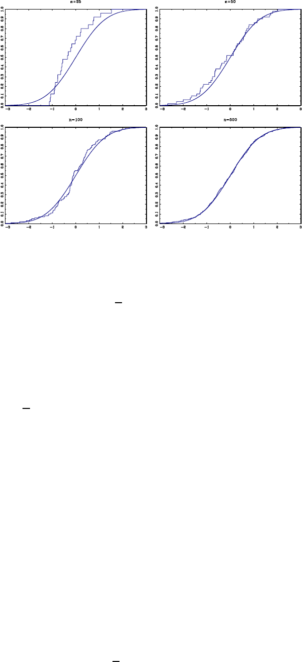
CHAPTER 13. THE BOOTSTRAP 408
Figure 13.1: Empirical Distribution Functions
sample moment:
b
( x)= 1
X
=1
1(≤)1(x≤x)(13.2)
b
( x)is called the empirical distribution function (EDF) and is a nonparametric estimate of
Note that while may be either discrete or continuous, b
is by construction a step function.
The EDF is a consistent estimator of the CDF. To see this, note that for any ( x)1(≤)1(x≤x)
is an iid random variable with expectation ( x)Thus by the WLLN (Theorem 6.4.2), b
( x)
−→
( x)Furthermore, by the CLT (Theorem 6.8.1),
√³b
( x)−(x)´
−→ N(0 ( x)(1−(x)))
To see the effect of sample size on the EDF, in Figure 13.1, I have plotted the EDF and true
CDF for three random samples of size =2550, 100, and 500. The random draws are from the
N(01) distribution. For =25the EDF is only a crude approximation to the CDF, but the
approximation appears to improve for the large . In general, as the sample size gets larger, the
EDF step function gets uniformly close to the true CDF.
The EDF is a valid discrete probability distribution which puts probability mass 1 at each
pair (x),=1 Notationally, it is helpful to think of a random pair (∗
x∗
)with the
distribution b
That is,
Pr(∗
≤x∗
≤x)= b
( x)
We can easily calculate the moments of functions of (∗
x∗
):
E((∗
x∗
)) = Z( x)b
( x)
=
X
=1
(x)Pr(∗
=x∗
=x)
=1
X
=1
(x)
the empirical sample average.

CHAPTER 13. THE BOOTSTRAP 409
13.3 Nonparametric Bootstrap
The nonparametric bootstrap is obtained when the bootstrap distribution (13.1) is defined
using the EDF (13.2) as the estimate b
of
Since the EDF b
is a multinomial (with support points), in principle the distribution ∗
could
be calculated by direct methods. However, as there are ¡2−1
¢possible samples {(∗
1x∗
1)(∗
x∗
)}
such a calculation is computationally infeasible. The popular alternative is to use simulation to ap-
proximate the distribution. The algorithm is identical to our discussion of Monte Carlo simulation,
with the following points of clarification:
•Thesamplesizeused for the simulation is the same as the sample size.
•The random vectors (∗
x∗
)are drawn randomly from the empirical distribution. This is
equivalent to sampling a pair (x)randomly from the sample.
The bootstrap statistic ∗=³(∗
1x∗
1)(∗
x∗
)b
´is calculated for each bootstrap sam-
ple. This is repeated times. is known as the number of bootstrap replications. A theory
for the determination of the number of bootstrap replications has been developed by Andrews
and Buchinsky (2000). It is desirable for to be large, so long as the computational costs are
reasonable. = 1000 typically suffices.
When the statistic is a function of it is typically through dependence on a parameter. For
example, the t-ratio ³b
−´(b
)depends on As the bootstrap statistic replaces with b
it
similarly replaces with ∗=(b
)the value of implied by b
Typically ∗=b
the parameter
estimate. (When in doubt use b
)
Sampling from the EDF is particularly easy. Since b
is a discrete probability distribution
putting probability mass 1 at each sample point, sampling from the EDF is equivalent to random
samplingapair(x)from the observed data with replacement.Inconsequence,abootstrap
sample {(∗
1x∗
1)(∗
x∗
)}will necessarily have some ties and multiple values, which is generally
not a problem.
13.4 Bootstrap Estimation of Bias and Variance
The bias of b
is =E(b
−)The bootstrap counterparts are b
∗=b
((∗
1x∗
1)(∗
x∗
)) and
∗=E(b
∗−∗). The latter can be estimated by the simulation described in the previous section.
This estimator is
b∗=1
X
=1 ³b
∗
−b
´
=b
∗−b
If b
is biased, it might be desirable to construct a biased-corrected estimator for (one with
reduced bias). Ideally, this would be e
=b
−
but is unknown. The (estimated) bootstrap biased-corrected estimator is
e
∗=b
−b∗
=b
−(b
∗−b
)
=2
b
−b
∗

CHAPTER 13. THE BOOTSTRAP 410
Note, in particular, that the biased-corrected estimator is not b
∗Intuitively, the bootstrap makes
the following experiment. Suppose that b
is the truth. Then what is the average value of b
calculated from such samples? The answer is b
∗If this is lower than b
this suggests that the
estimator is downward-biased, so a biased-corrected estimator of should be larger than b
and the
bestguessisthedifference between b
and b
∗Similarly if b
∗is higher than b
then the estimator is
upward-biased and the biased-corrected estimator should be lower than b
.
Recall that variance of b
is
=E³(b
−E³b
´)2´
The bootstrap analog is the variance of b
∗which is
∗=E³(b
∗−E³b
∗´)2´
The simulation estimate is
b
∗
=1
X
=1 ³b
∗
−b
∗´2
A bootstrap standard error for b
is the square root of the bootstrap estimate of variance,
∗(b
)=qb
∗
. These are frequently reported in applied economics instead of asymptotic standard
errors.
13.5 Percentile Intervals
Consider an estimator b
for and suppose we wish to construct a confidence interval for .Let
( )denote the distribution of b
and let ()=( )denote its quantile function. This is
the function which solves
(())=
Let ∗()=( b
)denote the quantile function of the bootstrap distribution. Note that this
function will change depending on the underlying statistic whose distribution is
In 100(1 −)% of samples, b
lies in the region [(2)(1 −2)]This motivates a confidence
interval proposed by Efron: b
1=[∗(2)
∗(1 −2)]
This is often called the percentile confidence interval.
Computationally, the quantile ∗()is estimated by b∗()the sample quantile of the
simulated statistics {∗
1∗
}as discussed in the section on Monte Carlo simulation. The 1−
Efron percentile interval is then [b∗(2)b∗(1 −2)]
The interval b
1is a popular bootstrap confidence interval often used in empirical practice. This
is because it is easy to compute, simple to motivate, was popularized by Efron early in the history
of the bootstrap, and also has the feature that it is translation invariant. That is, if we define
=()as the parameter of interest for a monotonically increasing function then percentile
method applied to this problem will produce the confidence interval [(∗(2))(∗(1 −2))]
which is a naturally good property.
However, as we show now, b
1can work poorly unless the sampling distribution of b
is symmetric
about .
It will be useful if we introduce an alternative definition of b
1.Let()and ∗()be the
quantile functions of b
−and b
∗−b
(These are the original quantiles, with and b
subtracted.)
Then b
1can alternatively be written as
b
1=[
b
+∗(2)ˆ
+∗(1 −2)]

CHAPTER 13. THE BOOTSTRAP 411
This is a bootstrap estimate of the “ideal” confidence interval
b
0
1=[
b
+(2)b
+(1 −2)]
The latter has coverage probability
Pr ³∈b
0
1´=Pr³b
+(2) ≤≤b
+(1 −2)´
=Pr³−(1 −2) ≤b
−≤−(2)´
=(−(2))−(−(1 −2))
which generally is not 1−!There is one important exception. If b
−has a symmetric distribution
about 0,then(− )=1−( )so
Pr ³∈b
0
1´=(−(2))−(−(1 −2))
=(1−((2))) −(1 −((1 −2)))
=³1−
2´−³1−³1−
2´´
=1−
and this idealized confidence interval is accurate. Therefore, b
0
1and b
1are designed for the case
that b
has a symmetric distribution about
When b
does not have a symmetric distribution, b
1may perform quite poorly.
However, by the translation invariance argument presented above, it also follows that if there
exists some monotonically increasing transformation (·)such that (b
)is symmetrically distributed
about ()then the idealized percentile bootstrap method will be accurate.
Based on these arguments, many argue that the percentile interval should not be used unless
the sampling distribution is close to unbiased and symmetric.
The problems with the percentile method can be circumvented, at least in principle, by an
alternative method. Again, let ()and ∗()be the quantile functions of b
−and b
∗−b
.Then
1−=Pr³(2) ≤b
−≤(1 −2)´
=Pr³b
−(1 −2) ≤≤b
−(2)´
so an exact 1−confidence interval for is
b
0
2=[
b
−(1 −2)b
−(2)]
This motivates a bootstrap analog
b
2=[
b
−∗(1 −2)b
−∗(2)]
Notice that generally this is very different from the Efron interval b
1!They coincide in the special
case that ∗
()is symmetric about b
but otherwise they differ.
Computationally, this interval can be estimated from a bootstrap simulation by sorting the
bootstrap statistics ∗=b
∗−b
These are sorted to yield the quantile estimates b∗(025) and
b∗(975)The 95% confidence interval is then [b
−b∗(975)b
−b∗(025)]
This confidence interval is discussed in most theoretical treatments of the bootstrap, but is not
widely used in practice.

CHAPTER 13. THE BOOTSTRAP 412
13.6 Percentile-t Equal-Tailed Interval
Suppose we want to test H0:=0against H1:
0at size We would set ()=
³b
−´(b
)and reject H0in favor of H1if (0)where would be selected so that
Pr ((0))=
Thus =()Since this is unknown, a bootstrap test replaces ()with the bootstrap estimate
∗()and the test rejects if (0)
∗()
Similarly, if the alternative is H1:
0the bootstrap test rejects if (0)
∗(1 −)
Computationally, these critical values can be estimated from a bootstrap simulation by sorting
the bootstrap t-statistics ∗=³b
∗−b
´(b
∗)Note, and this is important, that the bootstrap test
statistic is centered at the estimate b
and the standard error (b
∗)is calculated on the bootstrap
sample. These t-statistics are sorted to find the estimated quantiles b∗()and/or b∗(1 −)
Let ()=³b
−´(b
). Then taking the intersection of two one-sided intervals,
1−=Pr((2) ≤(0)≤(1 −2))
=Pr³(2) ≤³b
−0´(b
)≤(1 −2)´
=Pr³ˆ
−(b
)(1 −2) ≤0≤ˆ
−(b
)(2)´
An exact (1 −)% confidence interval for is
b
0
3=[
b
−(b
)(1 −2)b
−(b
)(2)]
This motivates a bootstrap analog
b
3=[
b
−(b
)∗(1 −2)b
−(b
)∗(2)]
This is often called a percentile-t confidence interval.Itisequal-tailed or central since the
probability that is below the left endpoint approximately equals the probability that is above
the right endpoint, each 2
Computationally, this is based on the critical values from the one-sided hypothesis tests, dis-
cussed above.
13.7 Symmetric Percentile-t Intervals
Suppose we want to test H0:=0against H1:6=0at size We would set ()=
³b
−´(b
)and reject H0in favor of H1if |(0)|where would be selected so that
Pr (|(0)|)=
Note that
Pr (|(0)|)=Pr(−(0))
=()−(−)
≡()
which is a symmetric distribution function. The ideal critical value =(1−)solves the equation
((1 −)) = 1 −

CHAPTER 13. THE BOOTSTRAP 413
Equivalently, (1 −)is the 1−quantile of the distribution of |(0)|
The bootstrap estimate is ∗(1−)the 1−quantile of the distribution of |∗|or the number
which solves the equation
∗
(∗(1 −)) = ∗
(∗(1 −)) −∗
(−∗(1 −)) = 1 −
Computationally, ∗(1 −)is estimated from a bootstrap simulation by sorting the bootstrap
t-statistics |∗|=¯¯¯b
∗−b
¯¯¯(b
∗)and taking the 1−quantile. The bootstrap test rejects if
|(0)|
∗(1 −)
Let b
4=[
b
−(b
)∗(1 −)b
+(b
)∗(1 −)]
where ∗
(1 −)is the bootstrap critical value for a two-sided hypothesis test. b
4is called the
symmetric percentile-t interval. It is designed to work well since
Pr ³∈b
4´=Pr³b
−(b
)∗(1 −)≤≤b
+(b
)∗(1 −)´
=Pr(|()|
∗(1 −))
'Pr (|()|(1 −))
=1−
If θis a vector, then to test H0:θ=θ0against H1:θ6=θ0at size we would use a Wald
statistic
(θ)=³b
θ−θ´0b
V−1
³b
θ−θ´
or a similar asymptotically chi-square statistic. The ideal test rejects if ≥(1 −)where
(1 −)is the 1−quantile of the distribution of The bootstrap test rejects if ≥∗(1 −)
where ∗(1 −)is the 1−quantile of the distribution of
∗=³b
θ∗−b
θ´0b
V∗−1
³b
θ∗−b
θ´
Computationally, the critical value ∗(1 −)is found as the quantile from simulated values of ∗
Note in the simulation that the Wald statistic is a quadratic form in ³b
θ∗−b
θ´not ³b
θ∗−θ0´
(The latter is a common mistake made by practitioners.)
13.8 Asymptotic Expansions
Let ∈Rbe a statistic such that
−→ N(0
2)(13.3)
In some cases, such as when is a t-ratio, then 2=1In other cases 2is unknown. Equivalently,
writing ∼( )then for each and
lim
→∞ ( )=Φ³
´
or
( )=Φ³
´+(1) (13.4)
While (13.4) says that converges to Φ¡
¢as →∞it says nothing, however, about the rate
of convergenceor the size of the divergence for any particular sample size A better asymptotic
approximation may be obtained through an asymptotic expansion.

CHAPTER 13. THE BOOTSTRAP 414
Notationally, it is useful to recall the stochastic order notation of Section 6.13. Also, it is
convenient to define even and odd functions. We say that a function ()is even if (−)=()
and a function ()is odd if (−)=−()The derivative of an even function is odd, and
vice-versa.
Theorem 13.8.1 Under regularity conditions and (13.3),
( )=Φ³
´+1
121( )+ 1
2( )+(−32)
uniformly over where 1is an even function of and 2is an odd
function of Moreover, 1and 2are differentiable functions of and
continuous in relative to the supremum norm on the space of distribution
functions.
The expansion in Theorem 13.8.1 is often called an Edgeworth expansion.
We can interpret Theorem 13.8.1 as follows. First, ( )converges to the normal limit at
rate 12To a second order of approximation,
( )≈Φ³
´+−121( )
Since the derivative of 1is odd, the density function is skewed. To a third order of approximation,
( )≈Φ³
´+−121( )+−12( )
which adds a symmetric non-normal component to the approximate density (for example, adding
leptokurtosis).
As a side note, when =√¡¯
−¢ a standardized sample mean, then
1()=−1
63¡2−1¢()
2()=−µ1
244¡3−3¢+1
722
3¡5−103+15¢¶()
where ()is the standard normal pdf, and
3=E³(−)3´3
4=E³(−)4´4−3
the standardized skewness and excess kurtosis of the distribution of Note that when 3=0
and 4=0then 1=0and 2=0so the second-order Edgeworth expansion corresponds to the
normal distribution.
Francis Edgeworth
Francis Ysidro Edgeworth (1845-1926) of Ireland, founding editor of the Eco-
nomic Journal, was a profound economic and statistical theorist, developing
the theories of indifference curves and asymptotic expansions. He also could
be viewed as the first econometrician due to his early use of mathematical
statistics in the study of economic data.

CHAPTER 13. THE BOOTSTRAP 415
13.9 One-Sided Tests
Using the expansion of Theorem 13.8.1, we can assess the accuracy of one-sided hypothesis tests
and confidence regions based on an asymptotically normal t-ratio . An asymptotic test is based
on Φ()
To the second order, the exact distribution is
Pr ()=( )=Φ()+ 1
121( )+(−1)
since =1The difference is
Φ()−( )= 1
121( )+(−1)
=(−12)
so the order of the error is (−12)
A bootstrap test is based on ∗
()which from Theorem 13.8.1 has the expansion
∗
()=( b
)=Φ()+ 1
121( b
)+(−1)
Because Φ()appears in both expansions, the difference between the bootstrap distribution and
thetruedistributionis
∗
()−( )= 1
12³1( b
)−1( )´+(−1)
Since b
converges to at rate √ and 1is continuous with respect to the difference ³1( b
)−1( )´
converges to 0at rate √ Heuristically,
1( b
)−1( )≈
1( )³b
−´
=(−12)
The “derivative”
1( )is only heuristic, as is a function. We conclude that
∗
()−( )=(−1)
or
Pr (∗≤)=Pr(≤)+(−1)
which is an improved rate of convergence over the asymptotic test (which converged at rate
(−12)). This rate can be used to show that one-tailed bootstrap inference based on the t-
ratio achieves a so-called asymptotic refinement — the Type I error of the test converges at a
faster rate than an analogous asymptotic test.
13.10 Symmetric Two-Sided Tests
If a random variable has distribution function ()=Pr(≤)then the random variable
||has distribution function
()=()−(−)
since
Pr (||≤)=Pr(−≤≤)
=Pr(≤)−Pr (≤−)
=()−(−)

CHAPTER 13. THE BOOTSTRAP 416
For example, if ∼N(01)then ||has distribution function
Φ()=Φ()−Φ(−)=2Φ()−1
Similarly, if has exact distribution ( )then ||has the distribution function
( )=( )−(− )
A two-sided hypothesis test rejects H0for large values of ||Since
−→ then ||
−→ ||∼
ΦThus asymptotic critical values are taken from the Φdistribution, and exact critical values are
taken from the ( )distribution. From Theorem 13.8.1, we can calculate that
( )=( )−(− )
=µΦ()+ 1
121( )+ 1
2( )
−µΦ(−)+ 1
121(− )+ 1
2(− )¶+(−32)
=Φ()+ 2
2( )+(−32)(13.5)
where the simplifications are because 1is even and 2is odd. Hence the difference between the
asymptotic distribution and the exact distribution is
Φ()−( 0)= 2
2( 0)+(−32)=(−1)
The order of the error is (−1)
Interestingly, the asymptotic two-sided test has a better coverage rate than the asymptotic
one-sided test. This is because the first term in the asymptotic expansion, 1is an even function,
meaning that the errors in the two directions exactly cancel out.
Applying (13.5) to the bootstrap distribution, we find
∗
()=( b
)=Φ()+ 2
2( b
)+(−32)
Thus the difference between the bootstrap and exact distributions is
∗
()−( )= 2
³2( b
)−2( )´+(−32)
=(−32)
the last equality because b
converges to at rate √ and 2is continuous in Another way of
writing this is
Pr (|∗|)=Pr(||)+(−32)
so the error from using the bootstrap distribution (relative to the true unknown distribution) is
(−32)This is in contrast to the use of the asymptotic distribution, whose error is (−1)Thus
a two-sided bootstrap test also achieves an asymptotic refinement, similar to a one-sided test.
A reader might get confused between the two simultaneous effects. Two-sided tests have better
rates of convergence than the one-sided tests, and bootstrap tests have better rates of convergence
than asymptotic tests.
The analysis shows that there may be a trade-offbetweenone-sidedandtwo-sidedtests.Two-
sided tests will have more accurate size (Reported Type I error), but one-sided tests might have
more power against alternatives of interest. Confidence intervals based on the bootstrap can be
asymmetric if based on one-sided tests (equal-tailed intervals) and can therefore be more informative
and have smaller length than symmetric intervals. Therefore, the choice between symmetric and
equal-tailed confidence intervals is unclear, and needs to be determined on a case-by-case basis.

CHAPTER 13. THE BOOTSTRAP 417
13.11 Percentile Confidence Intervals
To evaluate the coverage rate of the percentile interval, set =√³b
−´We know that
−→ N(0)which is not pivotal, as it depends on the unknown Theorem 13.8.1 shows that
afirst-order approximation
( )=Φ³
´+(−12)
where =√and for the bootstrap
∗
()=( b
)=Φ³
ˆ´+(−12)
where b=(b
)is the bootstrap estimate of The difference is
∗
()−( )=Φ³
b´−Φ³
´+(−12)
=−³
´
(b−)+(−12)
=(−12)
Hence the order of the error is (−12)
The good news is that the percentile-type methods (if appropriately used) can yield √-
convergent asymptotic inference. Yet these methods do not require the calculation of standard
errors! This means that in contexts where standard errors are not available or are difficult to
calculate, the percentile bootstrap methods provide an attractive inference method.
The bad news is that the rate of convergence is disappointing. It is no better than the rate
obtained from an asymptotic one-sided confidence region. Therefore if standard errors are available,
it is unclear if there are any benefits from using the percentile bootstrap over simple asymptotic
methods.
Based on these arguments, the theoretical literature (e.g. Hall, 1992, Horowitz, 2001) tends to
advocate the use of the percentile-t bootstrap methods rather than percentile methods.
13.12 Bootstrap Methods for Regression Models
Thebootstrapmethodswehavediscussedhaveset∗
()=( b
)where b
is the EDF. Any
other consistent estimate of maybeusedtodefine a feasible bootstrap estimator. The advantage
of the EDF is that it is fully nonparametric, it imposes no conditions, and works in nearly any
context. But since it is fully nonparametric, it may be inefficient in contexts where more is known
about We discuss bootstrap methods appropriate for the linear regression model
=x0
β+
E(|x)=0
The non-parametric bootstrap resamples the observations (∗
x∗
)from the EDF, which implies
∗
=x∗0
b
β+∗
E(x∗
∗
)=0
but generally
E(∗
|x∗
)6=0
The bootstrap distribution does not impose the regression assumption, and is thus an inefficient
estimator of the true distribution (when in fact the regression assumption is true.)
CHAPTER 13. THE BOOTSTRAP 418
One approach to this problem is to impose the very strong assumption that the error is
independent of the regressor xThe advantage is that in this case it is straightforward to con-
struct bootstrap distributions. The disadvantage is that the bootstrap distribution may be a poor
approximation when the error is not independent of the regressors.
To impose independence, it is sufficient to sample the x∗
and ∗
independently, and then create
∗
=x∗0
b
β+∗
There are different ways to impose independence. A non-parametric method
is to sample the bootstrap errors ∗
randomly from the OLS residuals {b1b}A parametric
method is to generate the bootstrap errors ∗
from a parametric distribution, such as the normal
∗
∼N(0b2)
For the regressors x∗
, a nonparametric method is to sample the x∗
randomly from the EDF
or sample values {x1x}A parametric method is to sample x∗
from an estimated parametric
distribution. A third approach sets x∗
=xThis is equivalent to treating the regressors as fixed
in repeated samples. If this is done, then all inferential statements are made conditionally on the
observed values of the regressors, which is a valid statistical approach. It does not really matter,
however, whether or not the xare really “fixed” or random.
The methods discussed above are unattractive for most applications in econometrics because
they impose the stringent assumption that xand are independent. Typically what is desirable
is to impose only the regression condition E(|x)=0Unfortunately this is a harder problem.
One proposal which imposes the regression condition without independence is the Wild Boot-
strap. The idea is to construct a conditional distribution for ∗
so that
E(∗
|x)=0
E¡∗2
|x¢=b2
E¡∗3
|x¢=b3
A conditional distribution with these features will preserve the main important features of the data.
This can be achieved using a two-point distribution of the form
Pr Ã∗
=Ã1+√5
2!b!=√5−1
2√5
Pr Ã∗
=Ã1−√5
2!b!=√5+1
2√5
For each xyou sample ∗
using this two-point distribution.
13.13 Bootstrap GMM Inference
Consider an unconditional moment model
E(g(β)) = 0
and let b
βbe the 2SLS or GMM estimator of β.UsingtheEDFofw=(zx), we can apply
bootstrap methods to compute estimates of the bias and variance of b
βand construct confidence
intervals for βidentically as in the regression model. However, caution should be applied when
interpreting such results.
A straightforward application of the nonparametric bootstrap works in the sense of consistently
achieving the first-order asymptotic distribution. This has been shown by Hahn (1996). However,
it fails to achieve an asymptotic refinement when the model is over-identified, jeopardizing the
theoretical justification for percentile-t methods. Furthermore, the bootstrap applied test will
yield the wrong answer.

CHAPTER 13. THE BOOTSTRAP 419
The problem is that in the sample, b
βis the “true” value and yet g(b
β)6=0Thus according to
random variables (∗
z∗
x∗
)drawn from the EDF
E³g(b
β)´=g(b
β)6=0
This means that (∗
z∗
x∗
)do not satisfy the same moment conditions as the population distrib-
ution.
A correction suggested by Hall and Horowitz (1996) can solve the problem. Given the bootstrap
sample (y∗Z∗X∗)define the bootstrap GMM criterion
∗(β)=·³g∗
(β)−g(b
β)´0c
W∗³g∗
(β)−g(b
β)´
where g(b
β)is from the in-sample data, not from the bootstrap data.
Let b
β∗minimize ∗(β)and define all statistics and tests accordingly. In the linear model, this
implies that the bootstrap estimator is
b
β∗=¡X∗0Z∗W∗Z∗0X∗¢−1³X∗0Z∗c
W∗¡Z∗0y∗−Z0b
e¢´
where b
e=y−Xb
βare the in-sample residuals. The bootstrap J statistic is ∗(b
β∗)

CHAPTER 13. THE BOOTSTRAP 420
Exercises
Exercise 13.1 Let b
(x)denote the EDF of a random sample. Show that
√³b
(x)−(x)´
−→ N(0(x)(1−(x)))
Exercise 13.2 Take a random sample {1
}with =E()and 2=var()and set
=−1P
=1 Find the population moments E()and var ()Let {∗
1
∗
}be a random
sample from the empirical distribution function and set ∗
=−1P
=1 ∗
.Findthebootstrap
moments E(∗
)and var (∗
)
Exercise 13.3 Consider the following bootstrap procedure for a regression of on xLet b
β
denote the OLS estimator from the regression of yon X,andb
e=y−Xb
βthe OLS residuals.
(a) Draw a random vector (x∗
∗)from the pair {(xb):=1}That is, draw a random
integer 0from [12]and set x∗=x0and ∗=b0.Set∗=x∗0b
β+∗Draw (with
replacement) such vectors, creating a random bootstrap data set (y∗X∗)
(b) Regress y∗on X∗yielding OLS estimates b
β∗and any other statistic of interest.
Show that this bootstrap procedure is (numerically) identical to the non-parametric bootstrap.
Exercise 13.4 Consider the following bootstrap procedure. Using the non-parametric bootstrap,
generate bootstrap samples, calculate the estimate b
∗on these samples and then calculate
∗=(
b
∗−b
)(b
)
where (b
)is the standard error in the original data. Let ∗(05) and ∗(95) denote the 5% and
95% quantiles of ∗, and define the bootstrap confidence interval
b
=hb
−(b
)∗(95)b
−(b
)∗(05)i
Show that b
exactly equals the Alternative percentile interval (not the percentile-t interval).
Exercise 13.5 You want to test H0:=0against H1:0ThetestforH0is to reject if
=b
(b
)where is picked so that Type I error is You do this as follows. Using the non-
parametric bootstrap, you generate bootstrap samples, calculate the estimates b
∗on these samples
andthencalculate
∗=b
∗(b
∗)
Let ∗(95) denote the 95% quantile of ∗. You replace with ∗(95)and thus reject H0if
=b
(b
)
∗(95)What is wrong with this procedure?
Exercise 13.6 Suppose that in an application, b
=12and (b
)=2Using the non-parametric
bootstrap, 1000 samples are generated from the bootstrap distribution, and b
∗is calculated on each
sample. The b
∗are sorted, and the 2.5% and 97.5% quantiles of the b
∗are .75 and 1.3, respectively.
(a) Report the 95% Efron Percentile interval for
(b) Report the 95% Alternative Percentile interval for
(c) With the given information, can you report the 95% Percentile-t interval for ?
CHAPTER 13. THE BOOTSTRAP 421
Exercise 13.7 Consider the model
=x0
β+
E(|x)=0
with scalar and xavector. You have a random sample (x:=1)You are interested
in estimating the regression function (x)=(|x=x)at a fixed vector and constructing a
95% confidence interval.
(a) Write the standard estimator and asymptotic confidence interval for (x).
(b) Describe the percentile bootstrap confidence interval for (x).
(c) Describe the percentile-t bootstrap confidence interval for (x).
Exercise 13.8 The observed data is {
}∈R×R1=1 Take the model
=x0
β+
E()=0
3=E¡3
¢
(a) Write down an estimator for 3
(b) Explain how to use the Efron percentile method to construct a 90% confidence interval for
3in this specificmodel.
Exercise 13.9 Take the model
=x0
β+
E()=0
E¡2
¢=2
Describe the bootstrap percentile confidence interval for 2
Exercise 13.10 The model is
=x0
1β1+x0
2β2+
E(x)=0
with 2scalar. Describe how to test H0:2=0against H1:26=0using the nonparametric
bootstrap.
Exercise 13.11 The model is
=x0
1β1+22+
E(x)=0
with both x1and x1×1. Describe how to test H0:β1=β2against H1:β16=β2using the
nonparametric bootstrap.
Exercise 13.12 Suppose a PhD student has a sample (
:=1)and estimates by
OLS the equation
=b+0
b
+b
where is the coefficient of interest and she is interested in testing H0:=0against H1:
6=0. She obtains b=20with standard error (b)=10so the value of the t-ratio for H0is
=b(b)=20.Toassesssignificance, the student decides to use the bootstrap. She uses the
following algorithm

CHAPTER 13. THE BOOTSTRAP 422
1. Samples (∗
∗
∗
)randomly from the observations. (Random sampling with replacement).
Creates a random sample with observations.
2. On this pseudo-sample, estimates the equation
∗
=∗
ˆ∗+∗0
ˆ
∗+ˆ∗
by OLS and computes standard errors, including (b∗).Thet-ratioforH0
∗=b∗(b∗)is
computed and stored.
3. This is repeated = 9999 times.
4. The 95% empirical quantile b∗
95 of the bootstrap absolute t-ratios |∗|is computed. It is
b∗
95 =35
5. The student notes that while ||=2196 (and thus an asymptotic 5% size test rejects
H0), ||=2b∗
95 =35and thus the bootstrap test does not reject H0As the bootstrap is
more reliable, the student concludes that H0cannot be rejected in favor of H1
Question: Do you agree with the student’s method and reasoning? Do you see an error in her
method?
Exercise 13.13 Take the model
=11+22+
E(x)=0
The parameter of interest is =12Show how to construct a confidence interval for using the
following three methods.
1. Asymptotic Theory
2. Percentile Bootstrap
3. Equal-Tailed Percentile-t Bootstrap.
Your answer should be specific to this problem, not general.
Exercise 13.14 Let ybe iid, =E()0and =−1Let b=be the sample mean and
b
=b−1
(a) Is b
unbiased for ?
(b) If b
is biased, can you determine the direction of the bias E³b
−´(up or down)?
(c) Could the nonparametric bootstrap be used to estimate the bias? If so, explain how.
Exercise 13.15 Take the model
=11+22+
E(x)=0
=1
2
Assume that the observations (
1
2)are i.i.d. across =1.Describehowyouwould
construct the percentile-t bootstrap confidence interval for
CHAPTER 13. THE BOOTSTRAP 423
Exercise 13.16 The model is iid data, =1
=x0
β+
E(|x)=0
Does the presence of conditional heteroskedasticity invalidate the application of the non-parametric
bootstrap? Explain.
Exercise 13.17 The RESET specification test for nonlinearity in a random sample is the following.
The null hypothesis is a linear regression
=x0
β+
E(|x)=0
The parameter βis estimated by OLS yielding predicted values bThen a second-stage least-
squares regression is estimated including both xand b
=x0
e
β+(b)2e+e
The RESET test statistic is the squared t-ratio on e
A colleague suggests obtaining the critical value for the test using the bootstrap. He proposes
the following bootstrap implementation.
•Draw observations (∗
x∗
)randomly from the observed sample pairs (x)to create a
bootstrap sample.
•Compute the statistic ∗on this bootstrap sample as described above.
•Repeat this 999 times. Sort the bootstrap statistics ∗take number 950 (the 95% percentile)
and use this as the critical value.
•Reject the null hypothesis if exceeds this critical value, otherwise do not reject.
Is this procedure a correct implementation of the bootstrap in this context? If not, propose a
modified bootstrap.
Exercise 13.18 The model is
=x0
β+
E(x)6=0
so the regressor xis endogenous. We know that in this case, the OLS estimator is biased for
the parameter βWe also know that the non-parametric bootstrap is (generally) a good method
to estimate bias, and thereby make bias-adjusted. Explain whether or not the non-parametric
bootstrap can be used to estimate the bias of OLS in the above context.
Exercise 13.19 The datafile hprice1.txt contains data on house prices (sales), with variables
listed in the file hprice1.pdf. Estimate a linear regression of price on the number of bedrooms, lot
size, size of house, and the colonial dummy. Calculate 95% confidence intervals for the regression
coefficients using both the asymptotic normal approximation and the percentile-t bootstrap.

Chapter 14
Univariate Time Series
A time series is a process observed in sequence over time, =1. To indicate the
dependence on time, we adopt new notation, and use the subscript to denote the individual
observation, and to denote the number of observations.
Because of the sequential nature of time series, we expect that and −1are not independent,
so classical assumptions are not valid.
We can separate time series into two categories: univariate (∈Ris scalar); and multivariate
(∈Ris vector-valued). The primary model for univariate time series is autoregressions (ARs).
The primary model for multivariate time series is vector autoregressions (VARs).
14.1 Stationarity and Ergodicity
Definition 14.1.1 {}is covariance (weakly) stationary if
E()=
is independent of and
cov (
−)=()
is independent of for all ()is called the autocovariance function.
()=()(0) = corr(
−)
is the autocorrelation function.
Definition 14.1.2 {}is strictly stationary if the joint distribution of
(
−)is independent of for all
Definition 14.1.3 A stationary time series is ergodic if ()→0as
→∞.
424

CHAPTER 14. UNIVARIATE TIME SERIES 425
The following two theorems are essential to the analysis of stationary time series. The proofs
are rather difficult, however.
Theorem 14.1.1 If is strictly stationary and ergodic and =
(
−1)is a random variable, then is strictly stationary and er-
godic.
Theorem 14.1.2 (Ergodic Theorem). If is strictly stationary and er-
godic and E||∞then as →∞
1
X
=1
−→ E()
This allows us to consistently estimate parameters using time-series moments:
The sample mean:
b=1
X
=1
The sample autocovariance
b()= 1
X
=1
(−b)(−−b)
The sample autocorrelation
b(()=b(()
b((0)
Theorem 14.1.3 If is strictly stationary and ergodic and E¡2
¢∞
then as →∞
1. b
−→ E();
2. b()
−→ ();
3. b()
−→ ()
ProofofTheorem14.1.3. Part (1) is a direct consequence of the Ergodic theorem. For Part
(2), note that
b()= 1
X
=1
(−b)(−−b)
=1
X
=1
−−1
X
=1
b−1
X
=1
−b+b2

CHAPTER 14. UNIVARIATE TIME SERIES 426
By Theorem 14.1.1 above, the sequence −is strictly stationary and ergodic, and it has a finite
mean by the assumption that E¡2
¢∞Thus an application of the Ergodic Theorem yields
1
X
=1
−
−→ E(−)
Thus
b()
−→ E(−)−2−2+2=E(−)−2=()
Part (3) follows by the continuous mapping theorem: b()=b()b(0)
−→ ()(0) = ()
14.2 Autoregressions
In time-series, the series { 1
2
}are jointly random. We consider the conditional
expectation
E(|F
−1)
where F−1={−1
−2}is the past history of the series.
An autoregressive (AR) model specifies that only a finite number of past lags matter:
E(|F
−1)=E(|−1
−)
A linear AR model (the most common type used in practice) specifies linearity:
E(|F
−1)=0+1−1+2−1+···+−
Letting
=−E(|F
−1)
then we have the autoregressive model
=0+1−1+2−1+···+−+
E(|F
−1)=0
The last property defines a special time-series process.
Definition 14.2.1 is a martingale difference sequence (MDS) if
E(|F
−1)=0
Regression errors are naturally a MDS. Some time-series processes may be a MDS as a conse-
quence of optimizing behavior. For example, some versions of the life-cycle hypothesis imply that
either changes in consumption, or consumption growth rates, should be a MDS. Most asset pricing
models imply that asset returns should be the sum of a constant plus a MDS.
The MDS property for the regression error plays the same role in a time-series regression as
does the conditional mean-zero property for the regression error in a cross-section regression. In
fact, it is even more important in the time-series context, as it is difficult to derive distribution
theories without this property.
A useful property of a MDS is that is uncorrelated with any function of the lagged information
F−1Thus for 0E(−)=0

CHAPTER 14. UNIVARIATE TIME SERIES 427
14.3 Stationarity of AR(1) Process
A mean-zero AR(1) is
=−1+
Assume that is iid, E()=0and E¡2
¢=2∞
By back-substitution, we find
=+−1+2−2+
=∞
X
=0
−
Loosely speaking, this series converges if the sequence −gets small as →∞This occurs
when ||1
Theorem 14.3.1 If and only if ||1then is strictly stationary and
ergodic.
We can compute the moments of using the infinite sum:
E()= ∞
X
=0
E(−)=0
var()= ∞
X
=0
2var (−)= 2
1−2
If the equation for has an intercept, the above results are unchanged, except that the mean
of can be computed from the relationship
E()=0+1E(−1)
and solving for E()=E(−1)we find E()=0(1 −1)
14.4 Lag Operator
An algebraic construct which is useful for the analysis of autoregressive models is the lag oper-
ator.
Definition 14.4.1 The lag operator Lsatisfies L=−1
Defining L2=LLwe see that L2=L−1=−2In general, L=−
The AR(1) model can be written in the format
−−1=
or
(1 −L) =
The operator (L) = (1 −L) is a polynomial in the operator LWe say that the root of the
polynomial is 1 since ()=0when =1 We call (L) the autoregressive polynomial of .
From Theorem 14.3.1, an AR(1) is stationary iff||1Note that an equivalent way to say
this is that an AR(1) is stationary iffthe root of the autoregressive polynomial is larger than one
(in absolute value).

CHAPTER 14. UNIVARIATE TIME SERIES 428
14.5 Stationarity of AR(k)
The AR(k) model is
=1−1+2−2+···+−+
Using the lag operator,
−1L−2L2−···−L=
or
(L)=
where
(L) = 1 −1L−2L2−···−L
We call (L) the autoregressive polynomial of
The Fundamental Theorem of Algebra says that any polynomial can be factored as
()=¡1−−1
1¢¡1−−1
2¢···¡1−−1
¢
where the 1
are the complex roots of ()which satisfy ()=0
We know that an AR(1) is stationary iffthe absolute value of the root of its autoregressive
polynomial is larger than one. For an AR(k), the requirement is that all roots are larger than one.
Let ||denote the modulus of a complex number
Theorem 14.5.1 The AR(k) is strictly stationary and ergodic if and only
if ||1for all
One way of stating this is that “All roots lie outside the unit circle.”
If one of the roots equals 1, we say that (L)and hence “has a unit root”. This is a special
case of non-stationarity, and is of great interest in applied time series.
14.6 Estimation
Let
x=¡1−1−2··· −¢0
β=¡012··· ¢0
Then the model can be written as
=x0
β+
The OLS estimator is b
β=¡X0X¢−1X0y
To study b
βit is helpful to define the process =xNote that is a MDS, since
E(|F
−1)=E(x|F
−1)=xE(|F
−1)=0
By Theorem 14.1.1, it is also strictly stationary and ergodic. Thus
1
X
=1
x=1
X
=1
−→ E()=0(14.1)

CHAPTER 14. UNIVARIATE TIME SERIES 429
The vector xis strictly stationary and ergodic, and by Theorem 14.1.1, so is xx0
Thus by the
Ergodic Theorem,
1
X
=1
xx0
−→ E¡xx0
¢=Q
Combined with (14.1) and the continuous mapping theorem, we see that
b
β−β=Ã1
X
=1
xx0
!−1Ã1
X
=1
x!
−→ Q−10=0
We have shown the following:
Theorem 14.6.1 If the AR(k) process is strictly stationary and ergodic
and E¡2
¢∞then b
β
−→ βas →∞
14.7 Asymptotic Distribution
Theorem 14.7.1 MDS CLT. If uis a strictly stationary and ergodic
MDS and E(uu0
)=Ω∞then as →∞
1
√
X
=1
u
−→ N(0Ω)
Since xis a MDS, we can apply Theorem 14.7.1 to see that
1
√
X
=1
x
−→ N(0Ω)
where
Ω=E(xx0
2
)
Theorem 14.7.2 If the AR(k) process is strictly stationary and ergodic
and E¡4
¢∞then as →∞
√³b
β−β´
−→ N¡0Q−1ΩQ−1¢
This is identical in form to the asymptotic distribution of OLS in cross-section regression. The
implication is that asymptotic inference is the same. In particular, the asymptotic covariance
matrix is estimated just as in the cross-section case.
CHAPTER 14. UNIVARIATE TIME SERIES 430
14.8 Bootstrap for Autoregressions
In the non-parametric bootstrap, we constructed the bootstrap sample by randomly resampling
from the data values {x}This creates an iid bootstrap sample. Clearly, this cannot work in a
time-series application, as this imposes inappropriate independence.
Briefly, there are two popular methods to implement bootstrap resampling for time-series data.
Method 1: Model-Based (Parametric) Bootstrap.
1. Estimate b
βand residuals b
2. Fix an initial condition (−+1
−+2
0)
3. Simulate iid draws ∗
from the empirical distribution of the residuals {b1b}
4. Create the bootstrap series ∗
by the recursive formula
∗
=b0+b1∗
−1+b2∗
−2+···+b∗
−+∗
This construction imposes homoskedasticity on the errors ∗
which may be different than the
properties of the actual It also presumes that the AR(k) structure is the truth.
Method 2: Block Resampling
1. Divide the sample into blocks of length
2. Resample complete blocks. For each simulated sample, draw blocks.
3. Paste the blocks together to create the bootstrap time-series ∗
4. This allows for arbitrary stationary serial correlation, heteroskedasticity, and for model-
misspecification.
5. The results may be sensitive to the block length, and the way that the data are partitioned
into blocks.
6. May not work well in small samples.
14.9 Trend Stationarity
=0+1+(14.2)
=1−1+2−2+···+−+(14.3)
or
=0+1+1−1+2−1+···+−+(14.4)
There are two essentially equivalent ways to estimate the autoregressive parameters (1
)
•You can estimate (14.4) by OLS.
•You can estimate (14.2)-(14.3) sequentially by OLS. That is, first estimate (14.2), get the
residual ˆ
and then perform regression (14.3) replacing with ˆ
This procedure is some-
times called Detrending.
CHAPTER 14. UNIVARIATE TIME SERIES 431
The reason why these two procedures are (essentially) the same is the Frisch-Waugh-Lovell
theorem.
Seasonal Effects
There are three popular methods to deal with seasonal data.
•Include dummy variables for each season. This presumes that “seasonality” does not change
over the sample.
•Use “seasonally adjusted” data. The seasonal factor is typically estimated by a two-sided
weighted average of the data for that season in neighboring years. Thus the seasonally
adjusted data is a “filtered” series. This is a flexible approach which can extract a wide range
of seasonal factors. The seasonal adjustment, however, also alters the time-series correlations
of the data.
•First apply a seasonal differencing operator. If is the number of seasons (typically =4or
= 12)
∆=−−
or the season-to-season change. The series ∆is clearly free of seasonality. But the long-run
trend is also eliminated, and perhaps this was of relevance.
14.10 Testing for Omitted Serial Correlation
For simplicity, let the null hypothesis be an AR(1):
=0+1−1+(14.5)
We are interested in the question if the error is serially correlated. We model this as an AR(1):
=−1+(14.6)
with a MDS. The hypothesis of no omitted serial correlation is
H0:=0
H1:6=0
We want to test H0against H1
To combine (14.5) and (14.6), we take (14.5) and lag the equation once:
−1=0+1−2+−1
We then multiply this by and subtract from (14.5), to find
−−1=0−0+1−1−1−1+−−1
or
=0(1 −)+(1+)−1−1−2+=(2)
Thus under H0
is an AR(1), and under H1it is an AR(2). H0may be expressed as the restriction
that the coefficient on −2is zero.
An appropriate test of H0against H1is therefore a Wald test that the coefficient on −2is
zero. (A simple exclusion test).
In general, if the null hypothesis is that is an AR(k), and the alternative is that the error is an
AR(m), this is the same as saying that under the alternative is an AR(k+m), and this is equivalent
to the restriction that the coefficients on −−1
−−are jointly zero. An appropriate test is
the Wald test of this restriction.

CHAPTER 14. UNIVARIATE TIME SERIES 432
14.11 Model Selection
What is the appropriate choice of in practice? This is a problem of model selection.
A good choice is to minimize the AIC information criterion
()=logb2()+2
where b2()is the estimated residual variance from an AR(k)
One ambiguity in defining the AIC criterion is that the sample available for estimation changes
as changes. (If you increase you need more initial conditions.) This can induce strange behavior
in the AIC. The appropriate remedy is to fix a upper value andthenreservethefirst as initial
conditions, and then estimate the models AR(1), AR(2), ..., AR()on this (unified) sample.
14.12 Autoregressive Unit Roots
The AR(k) model is
(L)=0+
(L) = 1 −1L−···−L
As we discussed before, has a unit root when (1) = 0or
1+2+···+=1
In this case, is non-stationary. The ergodic theorem and MDS CLT do not apply, and test
statistics are asymptotically non-normal.
A helpful way to write the equation is the so-called Dickey-Fuller reparameterization:
∆=0−1+1∆−1+···+−1∆−(−1) +(14.7)
These models are equivalent linear transformations of one another. The DF parameterization
is convenient because the parameter 0summarizes the information about the unit root, since
(1) = −0To see this, observe that the lag polynomial for the computed from (14.7) is
(1 −L) −0L−1(L −L2)−···−−1(L−1−L)
But this must equal (L)as the models are equivalent. Thus
(1) = (1 −1) −0−(1 −1) −···−(1 −1) = −0
Hence, the hypothesis of a unit root in can be stated as
H0:0=0
Note that the model is stationary if 00So the natural alternative is
H1:00
Under H0the model for is
∆=+1∆−1+···+−1∆−(−1) +
which is an AR(k-1) in the first-difference ∆Thus if has a (single) unit root, then ∆is a
stationary AR process. Because of this property, we say that if is non-stationary but ∆is
stationary, then is “integrated of order ”or ()Thus a time series with unit root is (1)

CHAPTER 14. UNIVARIATE TIME SERIES 433
Since 0is the parameter of a linear regression, the natural test statistic is the t-statistic for
H0from OLS estimation of (14.7). Indeed, this is the most popular unit root test, and is called the
Augmented Dickey-Fuller (ADF) test for a unit root.
It would seem natural to assess the significance of the ADF statistic using the normal table.
However, under H0
is non-stationary, so conventional normal asymptotics are invalid. An
alternative asymptotic framework has been developed to deal with non-stationary data. We do not
have the time to develop this theory in detail, but simply assert the main results.
Theorem 14.12.1 Dickey-Fuller Theorem.
If 0=0then as →∞
b0
−→ (1 −1−2−···−−1)
=ˆ0
(ˆ0)→
The limit distributions and are non-normal. They are skewed to the left, and have
negative means.
The first result states that b0converges to its true value (of zero) at rate rather than the
conventional rate of 12This is called a “super-consistent” rate of convergence.
The second result states that the t-statistic for b0converges to a limit distribution which is
non-normal, but does not depend on the parameters This distribution has been extensively
tabulated, and may be used for testing the hypothesis H0Note: The standard error (ˆ0)is the
conventional (“homoskedastic”) standard error. But the theorem does not require an assumption
of homoskedasticity. Thus the Dickey-Fuller test is robust to heteroskedasticity.
Since the alternative hypothesis is one-sided, the ADF test rejects H0in favor of H1when
where is the critical value from the ADF table. If the test rejects H0this means that
the evidence points to being stationary. If the test does not reject H0a common conclusion is
that the data suggests that is non-stationary. This is not really a correct conclusion, however.
Allwecansayisthatthereisinsufficient evidence to conclude whether the data are stationary or
not.
We have described the test for the setting of with an intercept. Another popular setting includes
as well a linear time trend. This model is
∆=1+2+0−1+1∆−1+···+−1∆−(−1) +(14.8)
This is natural when the alternative hypothesis is that the series is stationary about a linear time
trend. If the series has a linear trend (e.g. GDP, Stock Prices), then the series itself is non-
stationary, but it may be stationary around the linear time trend. In this context, it is a silly waste
of time to fit an AR model to the level of the series without a time trend, as the AR model cannot
conceivably describe this data. The natural solution is to include a time trend in the fitted OLS
equation. When conducting the ADF test, this means that it is computed as the t-ratio for 0from
OLS estimation of (14.8).
If a time trend is included, the test procedure is the same, but different critical values are
required. The ADF test has a different distribution when the time trend has been included, and a
different table should be consulted.
Most texts include as well the critical values for the extreme polar case where the intercept has
been omitted from the model. These are included for completeness (from a pedagogical perspective)
but have no relevance for empirical practice where intercepts are always included.
Chapter 15
Multivariate Time Series
A multivariate time series yis a vector process ×1.LetF−1=(y−1y−2)be all lagged
information at time The typical goal is to find the conditional expectation E(y|F
−1)Note
that since yis a vector, this conditional expectation is also a vector.
15.1 Vector Autoregressions (VARs)
A VAR model specifies that the conditional mean is a function of only a finite number of lags:
E(y|F
−1)=E¡y|y−1y−¢
A linear VAR specifies that this conditional mean is linear in the arguments:
E¡y|y−1y−¢=a0+A1y−1+A2y−2+···Ay−
Observe that a0is ×1,and each of A1through Aare ×matrices.
Defining the ×1regression error
=y−E(y|F
−1)
we have the VAR model
y=a0+A1y−1+A2y−2+···Ay−+e
E(e|F
−1)=0
Alternatively, defining the +1vector
x=
⎛
⎜
⎜
⎜
⎜
⎜
⎝
1
y−1
y−2
.
.
.
y−
⎞
⎟
⎟
⎟
⎟
⎟
⎠
and the ×( +1) matrix
A=¡a0A1A2··· A¢
then
y=Ax+e
The VAR model is a system of equations. One way to write this is to let 0
be the th row
of A. Then the VAR system can be written as the equations
=0
x+
Unrestricted VARs were introduced to econometrics by Sims (1980).
434
CHAPTER 15. MULTIVARIATE TIME SERIES 435
15.2 Estimation
Consider the moment conditions
E(x)=0
=1 These are implied by the VAR model, either as a regression, or as a linear projection.
The GMM estimator corresponding to these moment conditions is equation-by-equation OLS
b
a=(X0X)−1X0y
An alternative way to compute this is as follows. Note that
b
a0
=y0
X(X0X)−1
And if we stack these to create the estimate b
Awe find
b
A=⎛
⎜
⎜
⎜
⎝
y0
1
y0
2
.
.
.
y0
+1
⎞
⎟
⎟
⎟
⎠X(X0X)−1
=Y0X(X0X)−1
where
Y=¡y1y2··· y¢
the ×matrix of the stacked y0
This (system) estimator is known as the SUR (Seemingly Unrelated Regressions) estimator,
and was originally derived by Zellner (1962)
15.3 Restricted VARs
The unrestricted VAR is a system of equations, each with the same set of regressors. A
restricted VAR imposes restrictions on the system. For example, some regressors may be excluded
from some of the equations. Restrictions may be imposed on individual equations, or across equa-
tions. The GMM framework gives a convenient method to impose such restrictions on estimation.
15.4 Single Equation from a VAR
Often, we are only interested in a single equation out of a VAR system. This takes the form
=a0
x+
and xconsists of lagged values of and the other 0
- In this case, it is convenient to re-define
the variables. Let =and zbe the other variables. Let = and =Then the single
equation takes the form
=x0
β+(15.1)
and
x=h¡1y−1··· y−z0
−1··· z0
−¢0i
This is just a conventional regression with time series data.

CHAPTER 15. MULTIVARIATE TIME SERIES 436
15.5 Testing for Omitted Serial Correlation
Consider the problem of testing for omitted serial correlation in equation (15.1). Suppose that
is an AR(1). Then
=x0
β+
=−1+(15.2)
E(|F
−1)=0
Then the null and alternative are
H0:=0 H1:6=0
Take the equation =x0
β+and subtract offthe equation once lagged multiplied by to get
−−1=¡x0
β+¢−¡x0
−1β+−1¢
=x0
β−x−1β+−−1
or
=−1+x0
β+x0
−1γ+(15.3)
which is a valid regression model.
So testing H0versus H1is equivalent to testing for the significance of adding (−1x−1)to
the regression. This can be done by a Wald test. We see that an appropriate, general, and simple
way to test for omitted serial correlation is to test the significance of extra lagged values of the
dependent variable and regressors.
You may have heard of the Durbin-Watson test for omitted serial correlation, which once was
very popular, and is still routinely reported by conventional regression packages. The DW test is
appropriate only when regression =x0
β+is not dynamic (has no lagged values on the RHS),
and is iid N(0
2)Otherwise it is invalid.
Another interesting fact is that (15.2) is a special case of (15.3), under the restriction =−β
This restriction, which is called a common factor restriction, may be tested if desired. If valid,
the model (15.2) may be estimated by iterated GLS. (A simple version of this estimator is called
Cochrane-Orcutt.) Since the common factor restriction appears arbitrary, and is typically rejected
empirically, direct estimation of (15.2) is uncommon in recent applications.
15.6 Selection of Lag Length in an VAR
If you want a data-dependent rule to pick the lag length in a VAR, you may either use a testing-
based approach (using, for example, the Wald statistic), or an information criterion approach. The
formula for the AIC and BIC are
()=logdet³b
Ω()´+2
()=logdet³b
Ω()´+log()
b
Ω()= 1
X
=1 b
e()b
e()0
=( +1)
where is the number of parameters in the model, and b
e()is the OLS residual vector from the
model with lags. The log determinant is the criterion from the multivariate normal likelihood.

CHAPTER 15. MULTIVARIATE TIME SERIES 437
15.7 Granger Causality
Partition the data vector into (yz)Define the two information sets
F1=¡yy−1y−2
¢
F2=¡yzy−1z−1y−2z−2
¢
The information set F1is generated only by the history of yand the information set F2is
generated by both yand zThe latter has more information.
We say that zdoes not Granger-cause yif
E(y|F
1−1)=E(y|F
2−1)
That is, conditional on information in lagged ylagged zdoes not help to forecast yIf this
condition does not hold, then we say that zGranger-causes y
The reason why we call this “Granger Causality” rather than “causality” is because this is not
a physical or structure definition of causality. If zis some sort of forecast of the future, such as a
futures price, then zmayhelptoforecastyeven though it does not “cause” yThis definition
of causality was developed by Granger (1969) and Sims (1972).
In a linear VAR, the equation for yis
y=+1y−1+···+y−+z0
−1γ1+···+z0
−γ+
In this equation, zdoes not Granger-cause yifandonlyif
H0:γ1=γ2=···=γ=0
This may be tested using an exclusion (Wald) test.
This idea can be applied to blocks of variables. That is, yand/or zcan be vectors. The
hypothesis can be tested by using the appropriate multivariate Wald test.
If it is found that zdoes not Granger-cause ythen we deduce that our time-series model of
E(y|F
−1)does not require the use of zNote, however, that zmay still be useful to explain
other features of ysuch as the conditional variance.
CliveW.J.Granger
Clive Granger (1934-2009) of England was one of the leading figures in time-
series econometrics, and co-winner in 2003 of the Nobel Memorial Prize in
Economic Sciences (along with Robert Engle). In addition to formalizing
the definition of causality known as Granger causality, he invented the con-
cept of cointegration, introduced spectral methods into econometrics, and
formalized methods for the combination of forecasts.
15.8 Cointegration
The idea of cointegration is due to Granger (1981), and was articulated in detail by Engle and
Granger (1987).

CHAPTER 15. MULTIVARIATE TIME SERIES 438
Definition 15.8.1 The ×1series yis cointegrated if yis (1) yet
there exists β×,ofrank such that z=β0yis (0)The vectors
in βare called the cointegrating vectors.
If the series yis not cointegrated, then =0If = then yis (0)For 0yis
(1) and cointegrated.
In some cases, it may be believed that βis known a priori. Often, β=(1 −1)0For example, if
yis a pair of interest rates, then β=(1 −1)0specifies that the spread (the difference in returns)
is stationary. If y=(log()log())0then β=(1 −1)0specifies that log()is stationary.
In other cases, βmay not be known.
If yis cointegrated with a single cointegrating vector (=1)then it turns out that βcan
be consistently estimated by an OLS regression of one component of yon the others. Thus y=
(1
2)and β=(12)and normalize 1=1Then b
2=(y0
2y2)−1y0
2y1
−→ 2Furthermore
this estimator is super-consistent: (b
2−2)=(1)as first shown by Stock (1987). While
OLS is not, in general, a good method to estimate βit is useful in the construction of alternative
estimators and tests.
We are often interested in testing the hypothesis of no cointegration:
H0:=0
H1:0
Suppose that βis known, so z=β0yis known. Then under H0zis (1)yet under H1zis
(0)Thus H0can be tested using a univariate ADF test on z
When βis unknown, Engle and Granger (1987) suggested using an ADF test on the estimated
residual ˆ=b
β0yfrom OLS of 1on 2Their justification was Stock’s result that b
βis super-
consistent under H1Under H0however, b
βis not consistent, so the ADF critical values are not
appropriate. The asymptotic distribution was worked out by Phillips and Ouliaris (1990).
When the data have time trends, it may be necessary to include a time trend in the estimated
cointegrating regression. Whether or not the time trend is included, the asymptotic distribution of
the test is affected by the presence of the time trend. The asymptotic distribution was worked out
in B. Hansen (1992).
15.9 Cointegrated VARs
We can write a VAR as
A(L)y=e
A(L) = I−A1L−A2L2−···−AL
or alternatively as
∆y=Πy−1+D(L)∆y−1+e
where
Π=−A(1)
=−I+A1+A2+···+A

CHAPTER 15. MULTIVARIATE TIME SERIES 439
Theorem 15.9.1 Granger Representation Theorem
yis cointegrated with ×βif and only if rank(Π)=and Π=αβ0
where is ×,rank (α)=
Thus cointegration imposes a restriction upon the parameters of a VAR. The restricted model
can be written as
∆y=αβ0y−1+D(L)∆y−1+e
∆y=αz−1+D(L)∆y−1+e
If βis known, this can be estimated by OLS of ∆yon z−1and the lags of ∆y
If βis unknown, then estimation is done by “reduced rank regression”, which is least-squares
subject to the stated restriction. Equivalently, this is the MLE of the restricted parameters under
the assumption that eis iid N(0Ω)
One difficulty is that βis not identified without normalization. When =1we typically just
normalize one element to equal unity. When 1this does not work, and different authors have
adopted different identification schemes.
In the context of a cointegrated VAR estimated by reduced rank regression, it is simple to test
for cointegration by testing the rank of ΠThese tests are constructed as likelihood ratio (LR) tests.
As they were discovered by Johansen (1988, 1991, 1995), they are typically called the “Johansen
Max and Trace” tests. Their asymptotic distributions are non-standard, and are similar to the
Dickey-Fuller distributions.

Chapter 16
Panel Data
A panel is a set of observations on individuals, collected over time. An observation is the pair
{x}where the subscript denotes the individual, and the subscript denotes time. A panel
may be balanced:
{x}:=1;=1
or unbalanced:
{x}:For =1 =
16.1 Individual-Effects Model
The standard panel data specification is that there is an individual-specificeffect which enters
linearly in the regression
=x0
β++
The typical maintained assumptions are that the individuals are mutually independent, that
and are independent, that is iid across individuals and time, and that is uncorrelated with
x
OLS of on x is called pooled estimation.Itisconsistentif
E(x)=0 (16.1)
If this condition fails, then OLS is inconsistent. (16.1) fails if the individual-specific unobserved
effect is correlated with the observed explanatory variables xThis is often believed to be
plausible if is an omitted variable.
If (16.1) is true, however, OLS can be improved upon via a GLS technique. In either event,
OLS appears a poor estimation choice.
Condition (16.1) is called the random effects hypothesis.Itisastrongassumption,and
most applied researchers try to avoid its use.
16.2 Fixed Effects
This is the most common technique for estimation of non-dynamic linear panel regressions.
The motivation is to allow to be arbitrary, and have arbitrary correlated with xThe goal
is to eliminate from the estimator, and thus achieve invariance.
There are several derivations of the estimator.
First, let
=⎧
⎨
⎩
1if =
0else
440

CHAPTER 16. PANEL DATA 441
and
d=⎛
⎜
⎝
1
.
.
.
⎞
⎟
⎠
an ×1dummy vector with a “1” in the place. Let
u=⎛
⎜
⎝
1
.
.
.
⎞
⎟
⎠
Then note that
=d0
u
and
=x0
β+d0
u+(16.2)
Observe that
E( |xd)=0
so (16.2) is a valid regression, with das a regressor along with x
OLS on (16.2) yields estimator ³b
βb
u´Conventional inference applies.
Observe that
•This is generally consistent.
•If x contains an intercept, it will be collinear with dso the intercept is typically omitted
from x
•Any regressor in x which is constant over time for all individuals (e.g., their gender) will be
collinear with dso will have to be omitted.
•There are +regression parameters, which is quite large as typically is very large.
Computationally, you do not want to actually implement conventional OLS estimation, as the
parameter space is too large. OLS estimation of βproceeds by the FWL theorem. Stacking the
observations together:
y=Xβ+Du +
then by the FWL theorem,
b
β=¡X0(I−P)X¢−1¡X0(I−P)y¢
=¡X∗0X∗¢−1¡X∗0y∗¢
where
y∗=y−D(D0D)−1D0y
X∗=X−D(D0D)−1D0X
Since the regression of on dis a regression onto individual-specific dummies, the predicted value
from these regressions is the individual specificmeanand the residual is the demean value
∗
= −
The fixed effects estimator b
βis OLS of ∗
on x∗
, the dependent variable and regressors in deviation-
from-mean form.

CHAPTER 16. PANEL DATA 442
Another derivation of the estimator is to take the equation
=x0
β++
and then take individual-specific means by taking the average for the individual:
1
X
=
=1
X
=
x0
β++1
X
=
or
=x0
β++
Subtracting, we find
∗
=x∗0
β+∗
which is free of the individual-effect
16.3 Dynamic Panel Regression
A dynamic panel regression has a lagged dependent variable
=−1+x0
β++(16.3)
This is a model suitable for studying dynamic behavior of individual agents.
Unfortunately, the fixed effects estimator is inconsistent, at least if is held finite as →∞
This is because the sample mean of −1is correlated with that of
The standard approach to estimate a dynamic panel is to combine first-differencing with IV or
GMM. Taking first-differences of (16.3) eliminates the individual-specificeffect:
∆ =∆−1+∆x0
β+∆(16.4)
However, if is iid, then it will be correlated with ∆−1:
E(∆−1∆)=E((−1−−2)( −−1)) = −E(−1−1)=−2
So OLS on (16.4) will be inconsistent.
But if there are valid instruments, then IV or GMM can be used to estimate the equation.
Typically, we use lags of the dependent variable, two periods back, as −2is uncorrelated with
∆Thus values of −≥2, are valid instruments.
Hence a valid estimator of and βis to estimate (16.4) by IV using −2as an instrument for
∆−1(which is just identified). Alternatively, GMM using −2and −3as instruments (which is
overidentified, but loses a time-series observation).
A more sophisticated GMM estimator recognizes that for time-periods later in the sample, there
are more instruments available, so the instrument list should be different for each equation. This is
conveniently organized by the GMM principle, as this enables the moments from the different time-
periods to be stacked together to create a list of all the moment conditions. A simple application
of GMM yields the parameter estimates and standard errors.
CHAPTER 16. PANEL DATA 443
Exercises
Exercise 16.1 Consider the model
=x0
β++
E(z)=0
for =1 and =1. The individual effect is treated as fixed. Assume x and z are
×1vectors.
Write out an appropriate estimator for β.

Chapter 17
NonParametric Regression
17.1 Introduction
When components of xare continuously distributed then the conditional expectation function
E(|x=x)=(x)
can take any nonlinear shape. Unless an economic model restricts the form of (x)to a parametric
function, the CEF is inherently nonparametric, meaning that the function (x)is an element
of an infinite dimensional class. In this situation, how can we estimate (x)? What is a suitable
method, if we acknowledge that (x)is nonparametric?
There are two main classes of nonparametric regression estimators: kernel estimators, and series
estimators. In this chapter we introduce kernel methods.
To get started, suppose that there is a single real-valued regressor Weconsiderthecaseof
vector-valued regressors later.
17.2 Binned Estimator
For clarity, fixthepointand consider estimation of the single point (). Thisisthemean
of for random pairs (
)such that = If the distribution of were discrete then we
could estimate ()by taking the average of the sub-sample of observations for which =
But when is continuous then the probability is zero that exactly equals any specific.So
there is no sub-sample of observations with =and we cannot simply take the average of the
corresponding values. However, if the CEF ()is continuous, then it should be possible to get
a good approximation by taking the average of the observations for which is close to perhaps
for the observations for which |−|≤for some small 0We call abandwidth.This
estimator can be written as
b()=P
=1 1(|−|≤)
P
=1 1(|−|≤)(17.1)
where 1(·)is the indicator function. Alternatively, (17.1) can be written as
b()=
X
=1
()(17.2)
where
()= 1(|−|≤)
P
=1 1(|−|≤)
Notice that P
=1 ()=1so (17.2) is a weighted average of the .
444
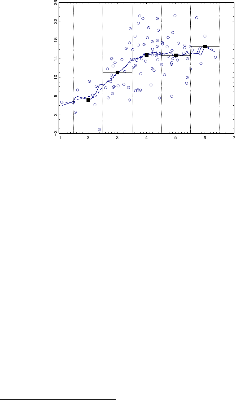
CHAPTER 17. NONPARAMETRIC REGRESSION 445
Figure 17.1: Scatter of (
)and Nadaraya-Watson regression
It is possible that for some values of there are no values of such that |−|≤ which
implies that P
=1 1(|−|≤)=0In this case the estimator (17.1) is undefined for those values
of
To visualize, Figure 17.1 displays a scatter plot of 100 observations on a random pair (
)
generatedbysimulation
1. (The observations are displayed as the open circles.) The estimator
(17.1) of the CEF ()at =2with =12is the average of the for the observations
such that falls in the interval [15≤≤25](Our choice of =12is somewhat arbitrary.
Selection of will be discussed later.) The estimate is b(2) = 516 and is shown on Figure 17.1 by
the firstsolidsquare.Werepeatthecalculation(17.1)for=34, 5, and 6, which is equivalent to
partitioning the support of into the regions [1525][2535][3545][4555]and [5565]
These partitions are shown in Figure 17.1 by the verticle dotted lines, and the estimates (17.1) by
the solid squares.
These estimates b()can be viewed as estimates of the CEF ()Sometimes called a binned
estimator, this is a step-function approximation to ()and is displayed in Figure 17.1 by the
horizontal lines passing through the solid squares. This estimate roughly tracks the central tendency
of the scatter of the observations (
)However, the huge jumps in the estimated step function
at the edges of the partitions are disconcerting, counter-intuitive, and clearly an artifact of the
discrete binning.
If we take another look at the estimation formula (17.1) there is no reason why we need to
evaluate (17.1) only on a course grid. We can evaluate b()for any set of values of In particular,
we can evaluate (17.1) on a fine grid of values of and thereby obtain a smoother estimate of the
CEF. This estimator with =12is displayed in Figure 17.1 with the solid line. This is a
generalization of the binned estimator and by construction passes through the solid squares.
The bandwidth determines the degree of smoothing. Larger values of increase the width
of the bins in Figure 17.1, thereby increasing the smoothness of the estimate b()as a function
of . Smaller values of decrease the width of the bins, resulting in less smooth conditional mean
estimates.
1The distribution is ∼(41) and |∼(()16) with ()=10log()

CHAPTER 17. NONPARAMETRIC REGRESSION 446
17.3 Kernel Regression
One deficiency with the estimator (17.1) is that it is a step function in , as it is discontinuous
at each observation =That is why its plot in Figure 17.1 is jagged. The source of the dis-
continuity is that the weights ()are constructed from indicator functions, which are themselves
discontinuous. If instead the weights are constructed from continuous functions then the CEF
estimator will also be continuous in
To generalize (17.1) it is useful to write the weights 1(|−|≤)in terms of the uniform
density function on [−11]
0()=1
21(||≤1)
Then
1(|−|≤)=1µ¯¯¯¯−
¯¯¯¯≤1¶=20µ−
and (17.1) can be written as
b()=P
=1 0µ−
P
=1 0µ−
¶(17.3)
The uniform density 0()is a special case of what is known as a kernel function.
Definition 17.3.1 A second-order kernel function ()satisfies 0≤
()∞()=(−)R∞
−∞ () =1and 2
=R∞
−∞ 2() ∞
Essentially, a kernel function is a probability density function which is bounded and symmetric
about zero. A generalization of (17.1) is obtained by replacing the uniform kernel with any other
kernel function:
b()=P
=1 µ−
P
=1 µ−
¶(17.4)
The estimator (17.4) also takes the form (17.2) with
()=
µ−
P
=1 µ−
The estimator (17.4) is known as the Nadaraya-Watson estimator, the kernel regression
estimator, or the local constant estimator.
The bandwidth plays the same role in (17.4) as it does in (17.1). Namely, larger values of
will result in estimates b()which are smoother in and smaller values of will result in
estimates which are more erratic. It might be helpful to consider the two extreme cases →0and
→∞As →0we can see that b()→(if the values of are unique), so that b()is
simply the scatter of on In contrast, as →∞then for all b()→ thesamplemean,
so that the nonparametric CEF estimate is a constant function. For intermediate values of b()
will lie between these two extreme cases.

CHAPTER 17. NONPARAMETRIC REGRESSION 447
The uniform density is not a good kernel choice as it produces discontinuous CEF estimates
To obtain a continuous CEF estimate b()it is necessary for the kernel ()to be continuous.
The two most commonly used choices are the Epanechnikov kernel
1()=3
4¡1−2¢1(||≤1)
and the normal or Gaussian kernel
()= 1
√2exp µ−2
2
For computation of the CEF estimate (17.4) the scale of the kernel is not important so long as
the bandwidth is selected appropriately. That is, for any 0
()=−1³
´is a valid kernel
function with the identical shape as ()Kernel regression with the kernel ()and bandwidth
is identical to kernel regression with the kernel ()and bandwidth
The estimate (17.4) using the Epanechnikov kernel and =12is also displayed in Figure 17.1
with the dashed line. As you can see, this estimator appears to be much smoother than that using
the uniform kernel.
Two important constants associated with a kernel function ()are its variance 2
and rough-
ness ,whicharedefined as
2
=Z∞
−∞
2() (17.5)
=Z∞
−∞
()2 (17.6)
Some common kernels and their roughness and variance values are reported in Table 9.1.
Table 9.1: Common Second-Order Kernels
Kernel Equation 2
Uniform 0()=1
21(||≤1) 1213
Epanechnikov 1()=3
4¡1−2¢1(||≤1) 3515
Biweight 2()=15
16 ¡1−2¢21(||≤1) 5717
Triweight 3()=35
32 ¡1−2¢31(||≤1) 350429 19
Gaussian ()= 1
√2exp ³−2
2´1(2√)1
17.4 Local Linear Estimator
The Nadaraya-Watson (NW) estimator is often called a local constant estimator as it locally
(about )approximates the CEF ()as a constant function. One way to see this is to observe
that b()solves the minimization problem
b() = argmin
X
=1
µ−
¶(−)2
This is a weighted regression of on an intercept only. Without the weights, this estimation
problem reduces to the sample mean. The NW estimator generalizes this to a local mean.
This interpretation suggests that we can construct alternative nonparametric estimators of
the CEF by alternative local approximations. Many such local approximations are possible. A
popular choice is the Local Linear (LL) approximation. Instead of approximating ()locally

CHAPTER 17. NONPARAMETRIC REGRESSION 448
as a constant, LL approximates the CEF locally by a linear function, and estimates this local
approximation by locally weighted least squares.
Specifically, for each we solve the following minimization problem
nb()b
()o=argmin
X
=1
µ−
¶(−−(−))2
The local linear estimator of ()is the estimated intercept
b()=b()
and the local linear estimator of the regression derivative ∇()is the estimated slope coefficient
d
∇()=b
()
Computationally, for each set
z()=µ1
−
and
()=µ−
Then
µb()
b
()¶=Ã
X
=1
()z()z()0!−1
X
=1
()z()
=¡Z0KZ¢−1Z0Ky
where K=diag{1()
()}
To visualize, Figure 17.2 displays the scatter plot of the same 100 observations from Figure 17.1,
divided into three regions depending on the regressor :[13][35][57]A linear regression is fit
to the observations in each region, with the observations weighted by the Epanechnikov kernel with
=1The three fitted regression lines are displayed by the three straight solid lines. The values of
these regression lines at =2=4and =6respectively, are the local linear estimates b()at
=24, and 6. This estimation is repeated for all in the support of the regressors, and plotted
as the continuous solid line in Figure 17.2.
One interesting feature is that as →∞the LL estimator approaches the full-sample linear
least-squares estimator b()→b+b
. That is because as →∞all observations receive equal
weight regardless of In this sense we can see that the LL estimator is a flexible generalization of
the linear OLS estimator.
Which nonparametric estimator should you use in practice: NW or LL? The theoretical liter-
ature shows that neither strictly dominates the other, but we can describe contexts where one or
the other does better. Roughly speaking, the NW estimator performs better than the LL estimator
when ()is close to a flat line, but the LL estimator performs better when ()is meaningfully
non-constant. The LL estimator also performs better for values of near the boundary of the
support of
17.5 Nonparametric Residuals and Regression Fit
The fitted regression at =is b()and the fitted residual is
b=−b()
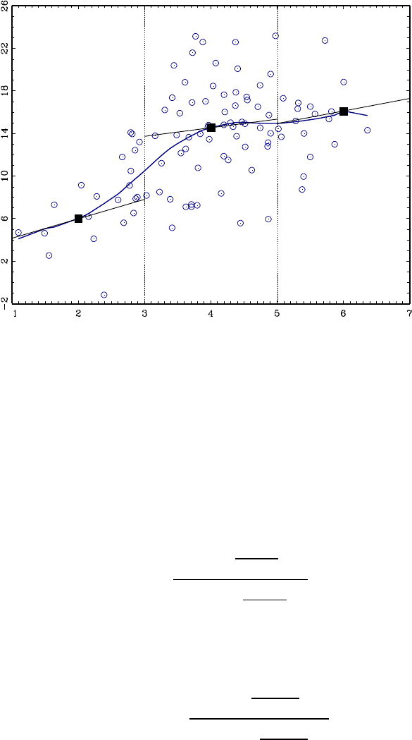
CHAPTER 17. NONPARAMETRIC REGRESSION 449
Figure 17.2: Scatter of (
)and Local Linear fitted regression
As a general rule, but especially when the bandwidth is small, it is hard to view bas a good
measure of the fit of the regression. As →0then b()→and therefore b→0This clearly
indicates overfitting as the true error is not zero. In general, since b()is a local average which
includes the fitted value will be necessarily close to and the residual bsmall, and the degree
of this overfitting increases as decreases.
A standard solution is to measure the fit of the regression at =by re-estimating the model
excluding the observation. For Nadaraya-Watson regression, the leave-one-out estimator of ()
excluding observation is
e−()=P6=µ−
P6=µ−
Notationally, the “−” subscript is used to indicate that the observation is omitted.
The leave-one-out predicted value for at =equals
e=e−()=P6=µ−
P6=µ−
The leave-one-out residuals (or prediction errors) are the difference between the leave-one-out pre-
dicted values and the actual observation
e=−e
Since eis not a function of there is no tendency for eto overfit for small Consequently, e
is a good measure of the fit of the estimated nonparametric regression.
Similarly, the leave-one-out local-linear residual is e=−ewith
µe
e
¶=⎛
⎝X
6=
z z0
⎞
⎠
−1X
6=
z

CHAPTER 17. NONPARAMETRIC REGRESSION 450
z =µ1
−
and
=µ−
17.6 Cross-Validation Bandwidth Selection
As we mentioned before, the choice of bandwidth is crucial. As increases, the kernel
regression estimators (both NW and LL) become more smooth, ironing out the bumps and wiggles.
This reduces estimation variance but at the cost of increased bias and oversmoothing. As decreases
the estimators become more wiggly, erratic, and noisy. It is desirable to select to trade-offthese
features. How can this be done systematically?
To be explicit about the dependence of the estimator on the bandwidth, let us write the esti-
mator of ()with a given bandwidth as b( )and our discussion will apply equally to the
NW and LL estimators.
Ideally, we would like to select to minimize the mean-squared error (MSE) of b( )as a
estimate of ()For a given value of the MSE is
( )=E³(b( )−())2´
We are typically interested in estimating ()for all values in the support of Acommonmeasure
for the average fit is the integrated MSE
()=Z( )()
=ZE³(b( )−())2´()
where ()is the marginal density of Notice that we have defined the IMSE as an integral with
respect to the density ()Other weight functions could be used, but it turns out that this is a
convenient choice
The IMSE is closely related with the MSFE of Section 4.11. Let (+1
+1)be out-of-sample
observations (and thus independent of the sample) and consider predicting +1 given +1 and
the nonparametric estimate b( )The natural point estimate for +1 is b(+1)which has
mean-squared forecast error
()=E³(+1 −b(+1))2´
=E³(+1 +(+1)−b(+1))2´
=2+E³((+1)−b(+1))2´
=2+ZE³(b( )−())2´()
where the final equality uses the fact that +1 is independent of b( )We thus see that
()=2+()
Since 2is a constant independent of the bandwidth ()and ()are equivalent
measures of the fit of the nonparameric regression.
The optimal bandwidth is the value which minimizes ()(or equivalently ())
While these functions are unknown, we learned in Theorem 4.11.1 that (at least in the case of linear

CHAPTER 17. NONPARAMETRIC REGRESSION 451
regression) can be estimated by the sample mean-squared prediction errors. It turns out
that this fact extends to nonparametric regression. The nonparametric leave-one-out residuals are
e()=−e−()
where we are being explicit about the dependence on the bandwidth The mean squared leave-
one-out residuals is
()= 1
X
=1 e()2
This function of is known as the cross-validation criterion.
The cross-validation bandwidth b
is the value which minimizes ()
b
=argmin
≥
()(17.7)
for some 0The restriction ≥is imposed so that ()is not evaluated over unreasonably
small bandwidths.
There is not an explicit solution to the minimization problem (17.7), so it must be solved
numerically. A typical practical method is to create a grid of values for e.g. [1
2
],
evaluate ()for =1 and set
b
=argmin
∈[12]
()
Evaluation using a coarse grid is typically sufficient for practical application. Plots of ()against
are a useful diagnostic tool to verify that the minimum of ()has been obtained.
We said above that the cross-validation criterion is an estimator of the MSFE. This claim is
based on the following result.
Theorem 17.6.1
E( ()) = −1()=−1()+2(17.8)
Theorem 17.6.1 shows that ()is an unbiased estimator of −1()+2The first
term, −1()is the integrated MSE of the nonparametric estimator using a sample of size
−1If is large, −1()and ()will be nearly identical, so ()is essentially
unbiased as an estimator of ()+2. Since the second term (2)is unaffected by the
bandwidth it is irrelevant for the problem of selection of . In this sense we can view ()
as an estimator of the IMSE, and more importantly we can view the minimizer of ()as an
estimate of the minimizer of ()
To illustrate, Figure 17.3 displays the cross-validation criteria ()for the Nadaraya-Watson
and Local Linear estimators using the data from Figure 17.1, both using the Epanechnikov kernel.
The CV functions are computed on a grid with intervals 0.01. The CV-minimizing bandwidths are
=109 for the Nadaraya-Watson estimator and =159 for the local linear estimator. Figure
17.3 shows the minimizing bandwidths by the arrows. It is typical to find that the CV criteria
recommends a larger bandwidth for the LL estimator than for the NW estimator, which highlights
the fact that smoothing parameters such as bandwidths are specific to the particular method.
The CV criterion can also be used to select between different nonparametric estimators. The
CV-selected estimator is the one with the lowest minimized CV criterion. For example, in Figure
17.3, the NW estimator has a minimized CV criterion of 16.88, while the LL estimator has a
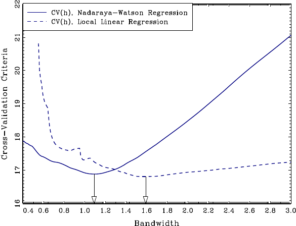
CHAPTER 17. NONPARAMETRIC REGRESSION 452
Figure 17.3: Cross-Validation Criteria, Nadaraya-Watson Regression and Local Linear Regression
minimized CV criterion of 16.81. Since the LL estimator achieves a lower value of the CV criterion,
LL is the CV-selected estimator. The difference (0.07) is small, suggesting that the two estimators
are near equivalent in IMSE.
Figure 17.4 displays the fitted CEF estimates (NW and LL) using the bandwidths selected by
cross-validation. Also displayed is the true CEF ()=10log(). Notice that the nonparametric
estimators with the CV-selected bandwidths (and especially the LL estimator) track the true CEF
quite well.
ProofofTheorem17.6.1. Observe that ()−e−()is a function only of (1
)and
(1
)excluding and is thus uncorrelated with Since e()=()−e−()+
then
E( ()) = E¡e()2¢
=E¡2
¢+E³(e−()−())2´
+2E(( e−()−()) )
=2+E³(e−()−())2´(17.9)
The second term is an expectation over the random variables and e−( )which are indepen-
dent as the second is not a function of the observation. Thus taking the conditional expectation
given the sample excluding the observation, this is the expectation over only, which is the
integral with respect to its density
E−³(e−()−())2´=Z(e−( )−())2()
Taking the unconditional expecation yields
E³(e−()−())2´=EZ(e−( )−())2()
=−1()
where this is the IMSE of a sample of size −1as the estimator e−uses −1observations.
Combined with (17.9) we obtain (17.8), as desired. ¥
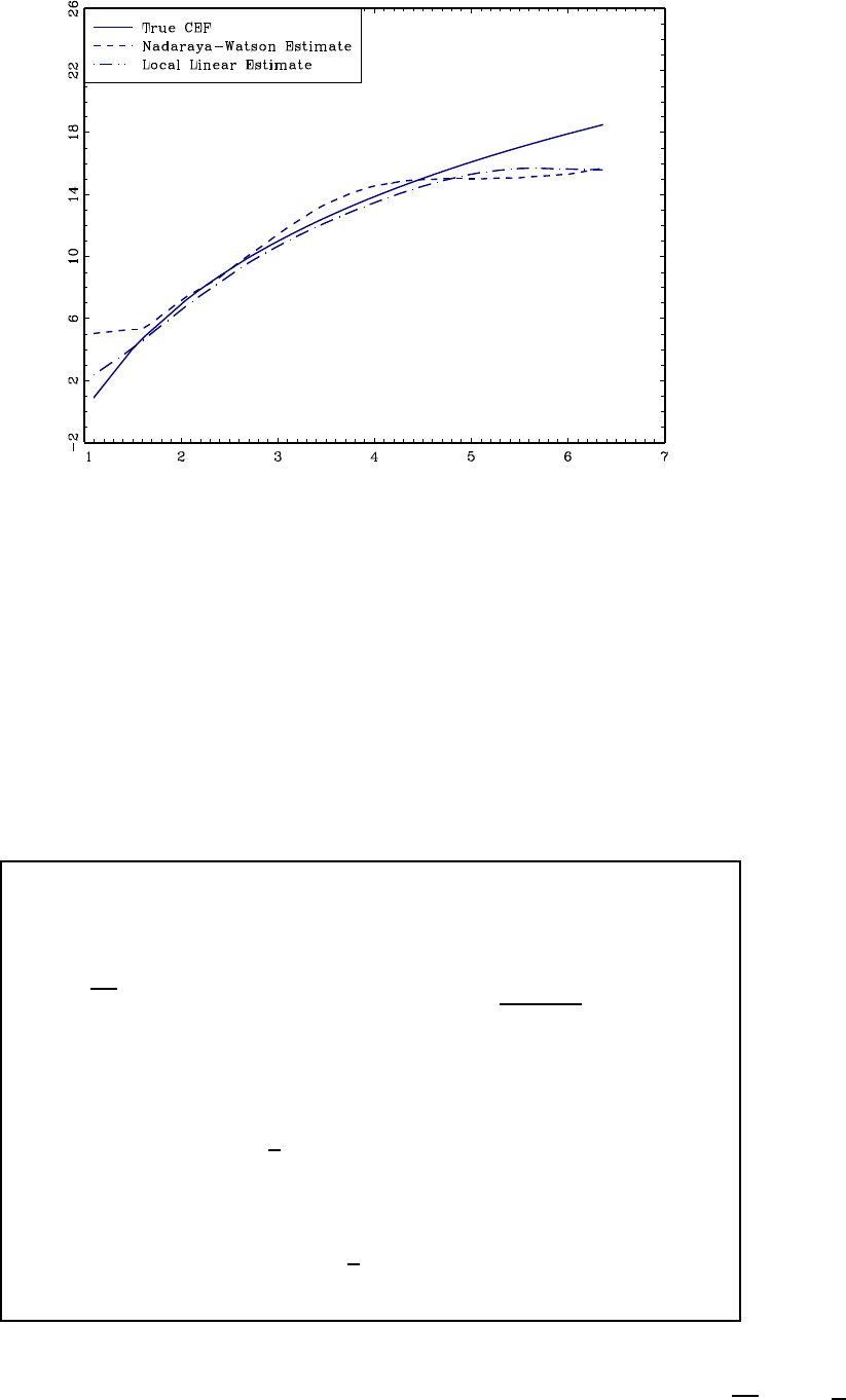
CHAPTER 17. NONPARAMETRIC REGRESSION 453
Figure 17.4: Nonparametric Estimates using data-dependent (CV) bandwidths
17.7 Asymptotic Distribution
There is no finite sample distribution theory for kernel estimators, but there is a well developed
asymptotic distribution theory. The theory is based on the approximation that the bandwidth
decreases to zero as the sample size increases. This means that the smoothing is increasingly
localized as the sample size increases. So long as the bandwidth does not decrease to zero too
quickly, the estimator can be shown to be asymptotically normal, but with a non-trivial bias.
Let ()denote the marginal density of and 2()=E¡2
|=¢denote the conditional
variance of =−()
Theorem 17.7.1 Let b()denote either the Nadarya-Watson or Local
Linear estimator of ()If is interior to the support of and ()0
then as →∞and →0such that →∞
√ ¡b()−()−22
()¢
−→ Nµ02()
()¶(17.10)
where 2
are defined in (17.5) and (17.6). For the Nadaraya-
Watson estimator
()=1
200()+()−10
()0()
and for the local linear estimator
()=1
2()00()
There are several interesting features about the asymptotic distribution which are noticeably
different than for parametric estimators. First, the estimator converges at the rate √ not √

CHAPTER 17. NONPARAMETRIC REGRESSION 454
Since →0√ diverges slower than √ thus the nonparametric estimator converges more
slowly than a parametric estimator. Second, the asymptotic distribution contains a non-neglible
bias term 22
()This term asymptotically disappears since →0Third, the assumptions that
→∞and →0mean that the estimator is consistent for the CEF ().
The fact that the estimator converges at the rate √ has led to the interpretation of as the
“effective sample size”. This is because the number of observations being used to construct b()
is proportional to not as for a parametric estimator.
It is helpful to understand that the nonparametric estimator has a reduced convergence rate
because the object being estimated — ()— is nonparametric. This is harder than estimating a
finite dimensional parameter, and thus comes at a cost.
Unlike parametric estimation, the asymptotic distribution of the nonparametric estimator in-
cludes a term representing the bias of the estimator. The asymptotic distribution (17.10) shows
the form of this bias. Not only is it proportional to the squared bandwidth 2(the degree of
smoothing), it is proportional to the function ()which depends on the slope and curvature of
the CEF ()Interestingly, when ()is constant then ()=0and the kernel estimator has no
asymptotic bias. The bias is essentially increasing in the curvature of the CEF function ()This
is because the local averaging smooths ()and the smoothing induces more bias when ()is
curved.
Theorem 17.7.1 shows that the asymptotic distributions of the NW and LL estimators are
similar, with the only difference arising in the bias function ()The bias term for the NW
estimator has an extra component which depends on the first derivative of the CEF ()while the
bias term of the LL estimator is invariant to the first derivative. The fact that the bias formula for
the LL estimator is simpler and is free of dependence on the first derivative of ()suggests that
the LL estimator will generally have smaller bias than the NW estimator (but this is not a precise
ranking). Since the asymptotic variances in the two distributions are the same, this means that the
LL estimator achieves a reduced bias without an effect on asymptotic variance. This analysis has
led to the general preference for the LL estimator over the NW estimator in the nonparametrics
literature.
One implication of Theorem 17.7.1 is that we can define the asymptotic MSE (AMSE) of b()
as the squared bias plus the asymptotic variance
(b()) = ¡22
()¢2+2()
()(17.11)
Focusing on rates, this says
(b()) ∼4+1
(17.12)
which means that the AMSE is dominated by the larger of 4and ()−1Notice that the bias is
increasing in and the variance is decreasing in (More smoothing means more observations are
used for local estimation: this increases the bias but decreases estimation variance.) To select to
minimize the AMSE, these two components should balance each other. Setting 4∝()−1means
setting ∝−15Another way to see this is to pick to minimize the right-hand-side of (17.12).
The first-order condition for is
µ4+1
¶=43−1
2=0
whichwhensolvedforyields =−15What this means is that for AMSE-efficient estimation
of ()the optimal rate for the bandwidth is ∝−15
Theorem 17.7.2 The bandwidth which minimizes the AMSE (17.12) is
of order ∝−15.With∝−15then (b()) = ¡−45¢and
b()=()+¡−25¢

CHAPTER 17. NONPARAMETRIC REGRESSION 455
This result means that the bandwidth should take the form =−15The optimal constant
depends on the kernel the bias function ()and the marginal density ()Acommonmis-
interpretation is to set =−15which is equivalent to setting =1and is completely arbitrary.
Instead, an empirical bandwidth selection rule such as cross-validation should be used in practice.
When =−15we can rewrite the asymptotic distribution (17.10) as
25(b()−())
−→ Nµ22
()2()
()
In this representation, we see that b()is asymptotically normal, but with a 25rate of conver-
gence and non-zero mean. The asymptotic distribution depends on the constant through the bias
(positively) and the variance (inversely).
The asymptotic distribution in Theorem 17.7.1 allows for the optimal rate =−15but this
rate is not required. In particular, consider an undersmoothing (smaller than optimal) bandwith
with rate =¡−15¢. For example, we could specify that =−for some 0and
151Then √2=((1−5)2)=(1) so the bias term in (17.10) is asymptotically
negligible so Theorem 17.7.1 implies
√ (b()−())
−→ Nµ02()
()
That is, the estimator is asymptotically normal without a bias component. Not having an asymp-
totic bias component is convenient for some theoretical manipuations, so many authors impose the
undersmoothing condition =¡−15¢to ensure this situation. This convenience comes at a cost.
First, the resulting estimator is inefficient as its convergence rate is is ¡−(1−)2¢
¡−25¢
since 15Second, the distribution theory is an inherently misleading approximation as it misses
a critically key ingredient of nonparametric estimation — the trade-offbetween bias and variance.
The approximation (17.10) is superior precisely because it contains the asymptotic bias component
which is a realistic implication of nonparametric estimation. Undersmoothing assumptions should
be avoided when possible.
17.8 Conditional Variance Estimation
Let’s consider the problem of estimation of the conditional variance
2()=var(|=)
=E¡2
|=¢
Even if the conditional mean ()is parametrically specified, it is natural to view 2()as inher-
ently nonparametric as economic models rarely specify the form of the conditional variance. Thus
it is quite appropriate to estimate 2()nonparametrically.
We know that 2()is the CEF of 2
given Therefore if 2
were observed, 2()could be
nonparametrically estimated using NW or LL regression. For example, the ideal NW estimator is
2()=P
=1 ()2
P
=1 ()
Since the errors are not observed, we need to replace them with an empirical residual, such as
b=−b()where b()is the estimated CEF. (The latter could be a nonparametric estimator
such as NW or LL, or even a parametric estimator.) Even better, use the leave-one-out prediction
errors e=−b−()as these are not subject to overfitting.
With this substitution the NW estimator of the conditional variance is
b2()=P
=1 ()e2
P
=1 ()(17.13)

CHAPTER 17. NONPARAMETRIC REGRESSION 456
This estimator depends on a set of bandwidths 1
, but there is no reason for the band-
widths to be the same as those used to estimate the conditional mean. Cross-validation can be used
to select the bandwidths for estimation of b2()separately from cross-validation for estimation of
b()
There is one subtle difference between CEF and conditional variance estimation. The conditional
variance is inherently non-negative 2()≥0and it is desirable for our estimator to satisfy this
property. Interestingly, the NW estimator (17.13) is necessarily non-negative, since it is a smoothed
average of the non-negative squared residuals, but the LL estimator is not guarenteed to be non-
negative for all . For this reason, the NW estimator is preferred for conditional variance estimation.
Fan and Yao (1998, Biometrika) derive the asymptotic distribution of the estimator (17.13).
They obtain the surprising result that the asymptotic distribution of this two-step estimator is
identical to that of the one-step idealized estimator 2().
17.9 Standard Errors
Theorem 17.7.1 shows the asymptotic variances of both the NW and LL nonparametric regres-
sion estimators equal
()=2()
()
For standard errors we need an estimate of ()A plug-in estimate replaces the unknowns by
estimates. The roughness can be found from Table 9.1. The conditional variance can be
estimated using (17.13). The density of can be estimated using the methods from Section 22.1.
Replacing these estimates into the formula for ()we obtain the asymptotic variance estimate
b
()=b2()
b
()
Then an asymptotic standard error for the kernel estimate b(x)is
b()=r1
b
()
Plots of the estimated CEF b()canbeaccompaniedbyconfidence intervals b()±2b()
These are known as pointwise confidence intervals, as they are designed to have correct coverage
at each not uniformly in
One important caveat about the interpretation of nonparametric confidence intervals is that
they are not centered at the true CEF ()but rather are centered at the biased or pseudo-true
value
∗()=()+22
()
Consequently, a correct statement about the confidence interval b()±2b()is that it asymptoti-
cally contains ∗()with probability 95%, not that it asymptotically contains ()with probability
95%. The discrepancy is that the confidence interval does not take into account the bias 22
()
Unfortunately, nothing constructive can be done about this. The bias is difficult and noisy to esti-
mate, so making a bias-correction only inflates estimation variance and decreases overall precision.
A technical “trick” is to assume undersmoothing =¡−15¢but this does not really eliminate
the bias, it only assumes it away. The plain fact is that once we honestly acknowledge that the
true CEF is nonparametric, it then follows that any finite sample estimate will have finite sample
bias, and this bias will be inherently unknown and thus impossible to incorporate into confidence
intervals.

CHAPTER 17. NONPARAMETRIC REGRESSION 457
17.10 Multiple Regressors
Our analysis has focus on the case of real-valued for simplicity of exposition, but the methods
of kernel regression extend easily to the multiple regressor case, at the cost of a reduced rate of
convergence. In this section we consider the case of estimation of the conditional expectation
function
E(|x=x)=(x)
when
x=⎛
⎜
⎝
1
.
.
.
⎞
⎟
⎠
is a -vector.
For any evaluation point xand observation define the kernel weights
(x)=µ1−1
1¶µ2−2
2¶···µ −
a-fold product kernel. The kernel weights (x)assess if the regressor vector xis close to the
evaluation point xin the Euclidean space R.
These weights depend on a set of bandwidths, one for each regressor. We can group them
together into a single vector for notational convenience:
h=⎛
⎜
⎝
1
.
.
.
⎞
⎟
⎠
Given these weights, the Nadaraya-Watson estimator takes the form
b(x)=P
=1 (x)
P
=1 (x)
For the local-linear estimator, define
z(x)=µ1
x−x
and then the local-linear estimator can be written as b(x)=b(x)where
µb(x)
b
(x)¶=Ã
X
=1
(x)z(x)z(x)0!−1
X
=1
(x)z(x)
=¡Z0KZ¢−1Z0Ky
where K=diag{1()
()}
In multiple regressor kernel regression, cross-validation remains a recommended method for
bandwidth selection. The leave-one-out residuals eand cross-validation criterion (h)are de-
fined identically as in the single regressor case. The only difference is that now the CV criterion is
a function over the -dimensional bandwidth h. This is a critical practical difference since finding
the bandwidth vector b
hwhich minimizes (h)can be computationally difficult when his high
dimensional. Grid search is cumbersome and costly, since gridpoints per dimension imply evau-
lation of (h)at distinct points, which can be a large number. Furthermore, plots of (h)
against hare challenging when 2
The asymptotic distribution of the estimators inthemultipleregressorcaseisanextensionof
thesingleregressorcase.Let(x)denote the marginal density of xand 2(x)=E¡2
|x=x¢
the conditional variance of =−(x)Let |h|=12···

CHAPTER 17. NONPARAMETRIC REGRESSION 458
Theorem 17.10.1 Let b(x)denote either the Nadarya-Watson or Local
Linear estimator of (x)If xis interior to the support of xand (x)
0then as →∞and →0such that |h|→∞
p|h|⎛
⎝b(x)−(x)−2
X
=1
2
(x)⎞
⎠
−→ Nµ0
2(x)
(x)
where for the Nadaraya-Watson estimator
(x)=1
2
2
2
(x)+(x)−1
(x)
(x)
and for the Local Linear estimator
(x)=1
2
2
2
(x)
For notational simplicity consider the case that there is a single common bandwidth In this
case the AMSE takes the form
(b(x)) ∼4+1
That is, the squared bias is of order 4the same as in the single regressor case, but the variance is
of larger order ()−1Setting to balance these two components requires setting ∼−1(4+)
Theorem 17.10.2 The bandwidth which minimizes the AMSE is of order
∝−1(4+).With∝−1(4+)then (b(x)) = ¡−4(4+)¢
and b(x)=(x)+¡−2(4+)¢
In all estimation problems an increase in the dimension decreases estimation precision. For
example, in parametric estimation an increase in dimension typically increases the asymptotic vari-
ance. In nonparametric estimation an increase in the dimension typically decreases the convergence
rate, which is a more fundamental decrease in precision. For example, in kernel regression the con-
vergence rate ¡−2(4+)¢decreases as increases. The reason is the estimator b(x)is a local
average of the for observations such that xis close to x, and when there are multiple regressors
the number of such observations is inherently smaller. This phenomenon — that the rate of con-
vergence of nonparametric estimation decreases as the dimension increases — is called the curse of
dimensionality.
Chapter 18
Series Estimation
18.1 Approximation by Series
As we mentioned at the beginning of Chapter 17, there are two main methods of nonparametric
regression: kernel estimation and series estimation. In this chapter we study series methods.
Series methods approximate an unknown function (e.g. the CEF (x)) with a flexible paramet-
ric function, with the number of parameters treated similarly to the bandwidth in kernel regression.
A series approximation to (x)takes the form (x)=(xβ)where (xβ)is a known
parametric family and βis an unknown coefficient. The integer is the dimension of βand
indexes the complexity of the approximation.
A linear series approximation takes the form
(x)=
X
=1
(x)
=z(x)0β(18.1)
where (x)are (nonlinear) functions of xandareknownasbasis functions or basis function
transformations of x
For real-valued a well-known linear series approximation is the -order polynomial
()=
X
=0
where =+1
When x∈Ris vector-valued, a -order polynomial is
(x)=
X
1=0
···
X
=0
1
1···
1
This includes all powers and cross-products, and the coefficient vector has dimension =(+1)
In general, a common method to create a series approximation for vector-valued xis to include all
non-redundant cross-products of the basis function transformations of the components of x
18.2 Splines
Another common series approximation is a continuous piecewise polynomial function known
as a spline. While splines can be of any polynomial order (e.g. linear, quadratic, cubic, etc.),
a common choice is cubic. To impose smoothness it is common to constrain the spline function
to have continuous derivatives up to the order of the spline. Thus a quadratic spline is typically
459
CHAPTER 18. SERIES ESTIMATION 460
constrained to have a continuous first derivative, and a cubic spline is typically constrained to have
a continuous first and second derivative.
There is more than one way to define a spline series expansion. All are based on the number of
knots — the join points between the polynomial segments.
To illustrate, a piecewise linear function with two segments and a knot at is
()=⎧
⎨
⎩
1()=00 +01 (−)
2()=10 +11 (−)≥
(For convenience we have written the segments functions as polyomials in −.) The function
()equals the linear function 1()for and equals 2()for . Its left limit at =
is 00 and its right limit is 10so is continuous if (and only if) 00 =10Enforcing this constraint
is equivalent to writing the function as
()=0+1(−)+2(−)1(≥)
or after transforming coefficients, as
()=0+1+2(−)1(≥)
Notice that this function has =3coefficients, the same as a quadratic polynomial.
A piecewise quadratic function with one knot at is
()=⎧
⎨
⎩
1()=00 +01 (−)+02 (−)2
2()=10 +11 (−)+12 (−)2≥
This function is continuous at =if 00 =10and has a continuous first derivative if 01 =11
Imposing these contraints and rewriting, we obtain the function
()=0+1+22+3(−)21(≥)
Here, =4
Furthermore, a piecewise cubic function with one knot and a continuous second derivative is
()=0+1+22+33+4(−)31(≥)
which has =5
The polynomial order is selected to control the smoothness of the spline, as ()has
continuous derivatives up to −1.
In general, a -order spline with knots at 1,2
with 1
2···
is
()=
X
=0
+
X
=1
(−)1(≥)
which has =++1coefficients.
In spline approximation, the typical approach is to treat the polynomial order as fixed, and
select the number of knots to determine the complexity of the approximation. The knots are
typically treated as fixed. A common choice is to set the knots to evenly partition the support X
of x
CHAPTER 18. SERIES ESTIMATION 461
18.3 Partially Linear Model
A common use of a series expansion is to allow the CEF to be nonparametric with respect
to one variable, yet linear in the other variables. This allows flexibility in a particular variable
of interest. A partially linear CEF with vector-valued regressor x1and real-valued continuous 2
takes the form
(x1
2)=x0
1β1+2(2)
This model is commonly used when x1are discrete (e.g. binary variables) and 2is continuously
distributed.
Series methods are particularly convenient for estimation of partially linear models, as we can
replace the unknown function 2(2)with a series expansion to obtain
(x)'(x)
=x0
1β1+z0
β2
=x0
β
where z=z(2)are the basis transformations of 2(typically polynomials or splines) and β2
are coefficients. After transformation the regressors are x=(x0
1z0
)and the coefficients are
β=(β0
1β0
2)0
18.4 Additively Separable Models
When xis multivariate a common simplification is to treat the regression function (x)as
additively separable in the individual regressors, which means that
(x)=1(1)+2(2)+···+()
Series methods are quite convenient for additively separable models, as we simply apply series
expansions (polynomials or splines) separately for each component ()The advantage of ad-
ditive separability is the reduction in dimensionality. While an unconstrained order polynomial
has (+1)
coefficients, an additively separable polynomial model has only (+1)coefficients.
This can be a major reduction in the number of coefficients. The disadvantage of this simplification
is that the interaction effects have been eliminated.
The decision to impose additive separability can be based on an economic model which suggests
the absence of interaction effects, or can be a model selection decision similar to the selection of
the number of series terms. We will discuss model selection methods below.
18.5 Uniform Approximations
A good series approximation (x)willhavethepropertythatitgetsclosetothetrueCEF
(x)as the complexity increases. Formal statements can be derived from the theory of functional
analysis.
An elegant and famous theorem is the Stone-Weierstrass theorem, (Weierstrass, 1885, Stone
1937, 1948) which states that any continuous function can be arbitrarily uniformly well approxi-
mated by a polynomial of sufficiently high order. Specifically, the theorem states that for x∈R
if (x)is continuous on a compact set X, then for any 0there exists a polynomial (x)of
some order which is uniformly within of (x):
sup
∈X
|(x)−(x)|≤ (18.2)
Thus the true unknown (x)can be arbitrarily well approximately by selecting a suitable polyno-
mial.
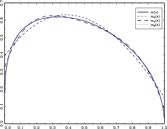
CHAPTER 18. SERIES ESTIMATION 462
Figure 18.1: True CEF and Best Approximations
The result (18.2) can be stengthened. In particular, if the derivative of (x)is continuous
then the uniform approximation error satisfies
sup
∈X
|(x)−(x)|=¡−¢(18.3)
as →∞where =. This result is more useful than (18.2) because it gives a rate at which
the approximation (x)approaches (x)as increases.
Both (18.2) and (18.3) hold for spline approximations as well.
Intuitively, the number of derivatives indexes the smoothness of the function (x)(18.3)
saysthatthebestrateatwhichapolynomialorsplineapproximatestheCEF(x)depends on
the underlying smoothness of (x)Themoresmoothis(x)the fewer series terms (polynomial
order or spline knots) are needed to obtain a good approximation.
To illustrate polynomial approximation, Figure 18.1 displays the CEF ()=14(1 −)12
on ∈[01]In addition, the best approximations using polynomials of order =3=4and
=6are displayed. You can see how the approximation with =3is fairly crude, but improves
with =4and especially =6Approximations obtained with cubic splines are quite similar so
not displayed.
As a series approximation can be written as (x)=z(x)0βas in (18.1), then the coefficient
of the best uniform approximation (18.3) is then
β∗
=argmin
sup
∈X¯¯z(x)0β−(x)¯¯(18.4)
The approximation error is
∗
(x)=(x)−z(x)0β∗
We can write this as
(x)=z(x)0β∗
+∗
(x)(18.5)
to emphasize that the true conditional mean can be written as the linear approximation plus error.
A useful consequence of equation (18.3) is
sup
∈X
|∗
(x)|≤¡−¢(18.6)
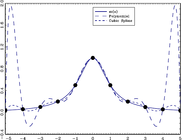
CHAPTER 18. SERIES ESTIMATION 463
Figure 18.2: True CEF, polynomial interpolation, and spline interpolation
18.6 Runge’s Phenomenon
Despite the excellent approximation implied by the Stone-Weierstrass theorem, polynomials
have the troubling disadvantage that they are very poor at simple interpolation. The problem is
known as Runge’s phenomenon, and is illustrated in Figure 18.2. The solid line is the CEF
()=(1+2)−1displayed on [−55]The circles display the function at the =11integers in
this interval. The long dashes display the 10 order polynomial fit through these points. Notice
that the polynomial approximation is erratic and far from the smooth CEF. This discrepancy gets
worse as the number of evaluation points increases, as Runge (1901) showed that the discrepancy
increases to infinity with
In contrast, splines do not exhibit Runge’s phenomenon. In Figure 18.2 the short dashes display
a cubic spline with seven knots fit through the same points as the polynomial. While the fitted
spline displays some oscillation relative to the true CEF, they are relatively moderate.
Because of Runge’s phenomenon, high-order polynomials are not used for interpolation, and are
not popular choices for high-order series approximations. Instead, splines are widely used.
18.7 Approximating Regression
For each observation we observe (x)and then construct the regressor vector z =z(x)
using the series transformations. Stacking the observations in the matrices yand Zthe least
squares estimate of the coefficient βin the series approximation z(x)0βis
b
β=¡Z0
Z¢−1Z0
y
and the least squares estimate of the regression function is
b(x)=z(x)0b
β(18.7)
As we learned in Chapter 2, the least-squares coefficient is estimating the best linear predictor
of given zThis is
β=E¡zz0
¢−1E(z)

CHAPTER 18. SERIES ESTIMATION 464
Given this coefficient, the series approximation is z(x)0βwith approximation error
(x)=(x)−z(x)0β(18.8)
ThetrueCEFequationforis
=(x)+(18.9)
with the CEF error. Defining =(x)we find
=z0
β+
where the equation error is
= +
Observethattheerror includes the approximation error and thus does not have the properties
of a CEF error.
In matrix notation we can write these equations as
y=Zβ+r+e
=Zβ+e(18.10)
We now impose some regularity conditions on the regression model to facilitate the theory.
Define the ×expected design matrix
Q=E¡zz0
¢
let Xdenote the support of xand define the largest normalized length of the regressor vector in
the support of x
=sup
∈X¡z(x)0Q−1
z(x)¢12(18.11)
ζwill increase with . For example, if the support of the variables z(x)is the unit cube [01],
then you can compute that =√. As discussed in Newey (1997) and Li and Racine (2007,
Corollary 15.1) if the support of xis compact then =()for polynomials and =(12)
for splines.
Assumption 18.7.1
1. For some 0the series approximation satisfies (18.3)
2. E¡2
|x¢≤¯2∞
3. min(Q)≥ 0
4. =()is a function of which satisfies →0and 2
→
0as →∞
Assumptions 18.7.1.1 through 18.7.1.3 concern properties of the regression model. Assumption
18.7.1.1 holds with = if Xis compact and the ’th derivative of (x)is continuous. Assump-
tion 18.7.1.2 allows for conditional heteroskedasticity, but requires the conditional variance to be
bounded. Assumption 18.7.1.3 excludes near-singular designs. Since estimates of the conditional
mean are unchanged if we replace z with z∗
=Bz for any non-singular BAssumption
18.7.1.3 can be viewed as holding after transformation by an appropriate non-singular B.
CHAPTER 18. SERIES ESTIMATION 465
Assumption 18.7.1.4 concerns the choice of the number of series terms, which is under the
controloftheuser. Itspecifies that can increase with sample size, but at a controlled rate of
growth. Since =()for polynomials and =(12)for splines, Assumption 18.7.1.4 is
satisfied if 3 →0for polynomials and 2 →0for splines. This means that while the number
of series terms can increase with the sample size, must increase at a much slower rate.
In Section 18.5 we introduced the best uniform approximation, and in this section we introduced
the best linear predictor. What is the relationship? They may be similar in practice, but they are
not the same and we should be careful to maintain the distinction. Note that from (18.5) we can
write (x)=z0
β∗
+∗
where ∗
=∗
(x)satisfies sup|∗
|=(−)from (18.6). Then
the best linear predictor equals
β=E¡zz0
¢−1E(z)
=E¡zz0
¢−1E(z(x))
=E¡zz0
¢−1E¡z(z0
β∗
+∗
)¢
=β∗
+E¡zz0
¢−1E(z∗
)
Thus the difference between the two approximations is
(x)−∗
(x)=z(x)0(β∗
−β)
=z(x)0E¡zz0
¢−1E(z∗
)(18.12)
Observe that by the properties of projection
E¡r∗2
¢−E(r∗
z)0E¡zz0
¢−1E(z∗
)≥0(18.13)
and by (18.6)
E¡∗2
¢=Z∗
(x)2(x)x≤¡−2¢(18.14)
Then applying the Schwarz inequality to (18.12), Definition (18.11), (18.13) and (18.14), we find
|(x)−∗
(x)|≤³z(x)0E¡zz0
¢−1z(x)´12
³E(∗
z)0E¡zz0
¢−1E(z∗
)´12
≤¡−¢(18.15)
It follows that the best linear predictor approximation error satisfies
sup
∈X
|(x)|≤¡−¢(18.16)
The bound (18.16) is probably not the best possible, but it shows that the best linear predictor
satisfies a uniform approximation bound. Relative to (18.6), the rate is slower by the factor
The bound (18.16) term is (1) as →∞if −→0.Asufficient condition is that 1
() for polynomials and 12(2)forsplineswhere =dim(x)and is the number
of continuous derivatives of (x)
It is also useful to observe that since βis the best linear approximation to (x)in mean-
square (see Section 2.24), then
E¡2
¢=E³¡(x)−z0
β¢2´
≤E³¡(x)−z0
β∗
¢2´
≤¡−2¢(18.17)
the final inequality by (18.14).

CHAPTER 18. SERIES ESTIMATION 466
18.8 Residuals and Regression Fit
The fitted regression at x=xis b(x)=z0
b
βand the fitted residual is
b =−b(x)
The leave-one-out prediction errors are
e =−b−(x)
=−z0
b
β−
where b
β−is the least-squares coefficient with the ’th observation omitted. Using (3.44) we can
also write
e =b(1 −)−1
where =z0
(Z0
Z)−1z
As for kernel regression, the prediction errors e are better estimates of the errors than the
fitted residuals b as they do not have the tendency to over-fit when the number of series terms
is large.
To assess the fit of the nonparametric regression, the estimate of the mean-square prediction
error is
e2
=1
X
=1 e2
=1
X
=1 b2
(1 −)−2
and the prediction 2is
e
2
=1−P
=1 e2
P
=1 (−¯)2
18.9 Cross-Validation Model Selection
The cross-validation criterion for selection of the number of series terms is the MSPE
()=e2
=1
X
=1 b2
(1 −)−2
By selecting the series terms to minimize ()or equivalently maximize e
2
we have a data-
dependent rule which is designed to produce estimates with low integrated mean-squared error
(IMSE) and mean-squared forecast error (MSFE). As shown in Theorem 17.6.1, ()is an
approximately unbiased estimated of the MSFE and IMSE, so finding the model which produces
the smallest value of ()is a good indicator that the estimated model has small MSFE and
IMSE. The proof of the result is the same for all nonparametric estimators (series as well as kernels)
so does not need to be repeated here.
As a practical matter, an estimator corresponds to a set of regressors z,thatis,asetof
transformations of the original variables xFor each set of regressions, the regression is estimated
and ()calculated, and the estimator is selected which has the smallest value of ()If
there are ordered regressors, then there are possible estimators. Typically, this calculation is
simple even if is large. However, if the regressors are unordered (and this is typical) then there
are 2possible subsets of conceivable models. If is even moderately large, 2can be immensely
large so brute-force computation of all models may be computationally demanding.

CHAPTER 18. SERIES ESTIMATION 467
18.10 Convergence in Mean-Square
The series estimate b
βare indexed by . The point of nonparametric estimation is to let
be flexible so as to incorporate greater complexity when the data are sufficiently informative.
This means that will typically be increasing with sample size This invalidates conventional
asymptotic distribution theory. However, we can develop extensions which use appropriate matrix
norms, and by focusing on real-valued functions of the parameters including the estimated regression
function itself.
The asymptotic theory we present in this and the next several sections is largely taken from
Newey (1997).
Our first main result shows that the least-squares estimate converges to βin mean-square
distance.
Theorem 18.10.1 Under Assumption 18.7.1, as →∞,
³b
β−β´0Q³b
β−β´=µ
¶+¡−2¢(18.18)
The proof of Theorem 18.10.1 is rather technical and deferred to Section 18.16.
The rate of convergence in (18.18) has two terms. The ()term is due to estimation
variance. Note in contrast that the corresponding rate would be (1)in the parametric case.
The difference is that in the parametric case we assume that the number of regressors is fixed as
increases, while in the nonparametric case we allow the number of regressors to be flexible. As
increases, the estimation variance increases. The ¡−2¢term in (18.18) is due to the series
approximation error.
Using Theorem 18.10.1 we can establish the following convergence rate for the estimated re-
gression function.
Theorem 18.10.2 Under Assumption 18.7.1, as →∞,
Z(b(x)−(x))2(x)x=µ
¶+¡−2¢(18.19)
Theorem 18.10.2 shows that the integrated squared difference between the fitted regression and
the true CEF converges in probability to zero if →∞as →∞The convergence results of
Theorem 18.10.2 show that the number of series terms involves a trade-offsimilar to the role of
the bandwidth in kernel regression. Larger implies smaller approximation error but increased
estimation variance.
The optimal rate which minimizes the average squared error in (18.19) is =¡1(1+2)¢
yielding an optimal rate of convergence in (18.19) of ¡−2(1+2)¢This rate depends on the
unknown smoothness of the true CEF (the number of derivatives ) and so does not directly
syggest a practical rule for determining Still, the implication is that when the function being
estimated is less smooth (is small) then it is necessary to use a larger number of series terms
to reduce the bias. In contrast, when the function is more smooth then it is better to use a smaller
number of series terms to reduce the variance.
To establish (18.19), using (18.7) and (18.8) we can write
b(x)−(x)=z(x)0³b
β−β´−(x)(18.20)

CHAPTER 18. SERIES ESTIMATION 468
Since are projection errors, they satisfy E(z)=0and thus E(z)=0This
means Rz(x)(x)(x)x=0Also observe that Q=Rz(x)z(x)0(x)xand E¡2
¢=
R(x)2(x)x.Then
Z(b(x)−(x))2(x)x
=³b
β−β´0Q³b
β−β´+E¡2
¢
≤µ
¶+¡−2¢
by (18.18) and (18.17), establishing (18.19).
18.11 Uniform Convergence
Theorem 18.10.2 established conditions under which b(x)is consistent in a squared error
norm. It is also of interest to know the rate at which the largest deviation converges to zero. We
have the following rate.
Theorem 18.11.1 Under Assumption 18.7.1, then as →∞
sup
∈X
|b(x)−(x)|=Ãr2
!+¡−¢(18.21)
Relative to Theorem 18.10.2, the error has been increased multiplicatively by This slower
convergence rate is a penalty for the stronger uniform convergence, though it is probably not
the best possible rate. Examining the bound in (18.21) notice that the first term is (1) under
Assumption 18.7.1.4. The second term is (1) if −→0which requires that →∞and
that be sufficiently large. A sufficient condition is that for polynomials and 2for
splineswhere =dim(x)and is the number of continuous derivatives of (x)Thus higher
dimensional xrequire a smoother CEF (x)to ensure that the series estimate b(x)is uniformly
consistent.
The convergence (18.21) is straightforward to show using (18.18). Using (18.20), the Triangle
Inequality, the Schwarz inequality (A.20), Definition (18.11), (18.18) and (18.16),
sup
∈X
|b(x)−(x)|
≤sup
∈X¯¯¯z(x)0³b
β−β´¯¯¯+sup
∈X
|(x)|
≤sup
∈X¡z(x)0Q−1
z(x)¢12µ³b
β−β´0Q³b
β−β´¶12
+¡−¢
≤µµ
¶+¡−2¢¶12
+¡−¢
=Ãr2
!+¡−¢(18.22)
This is (18.21).

CHAPTER 18. SERIES ESTIMATION 469
18.12 Asymptotic Normality
One advantage of series methods is that the estimators are (in finite samples) equivalent to
parametric estimators, so it is easy to calculate covariance matrix estimates. We now show that
we can also justify normal asymptotic approximations.
The theory we present in this section will apply to any linear function of the regression function.
That is, we allow the parameter of interest to be aany non-trivial real-valued linear function of the
entire regression function (·)
=()
This includes the regression function (x)at a given point xderivatives of (x), and integrals
over (x).Givenb(x)=z(x)0b
βas an estimator for (x)the estimator for is
b
=(b)=a0
b
β
for some ×1vector of constants a6=0(The relationship (b)=a0
b
βfollows since is
linear in and bis linear in b
β.)
If were fixed as →∞then by standard asymptotic theory we would expect b
to be
asymptotically normal with variance
=a0
Q−1
ΩQ−1
a
where
Ω=E¡zz0
2
¢
The standard justification, however, is not valid in the nonparametric case, in part because
may diverge as →∞and in part due to the finite sample bias due to the approximation error.
Therefore a new theory is required. Interestingly, it turns out that in the nonparametric case b
is
still asymptotically normal, and is still the appropriate variance for b
. The proof is different
than the parametric case as the dimensions of the matrices are increasing with and we need to
be attentive to the estimator’s bias due to the series approximation.
Theorem 18.12.1 Under Assumption 18.7.1, if in addition E¡4
|x¢≤
4∞,E¡2
|x¢≥20and −=(1)then as →∞
√³b
−+()´
12
−→ N(01) (18.23)
The proof of Theorem 18.12.1 can be found in Section 18.16.
Theorem 18.12.1 shows that the estimator b
is approximately normal with bias −()and
variance The variance is the same as in the parametric case, but the asymptotic distribution
contains an asymptotic bias, similar as is found in kernel regression. We discuss the bias in more
detail below.
Notice that Theorem 18.12.1 requires −=(1)which is similar to that found in Theorem
18.11.1 to establish uniform convergence. The the bound −=(1) allows to be constant
with or to increase with . However, when is increasing the bound requires that be sufficient
large so that grows faster than Asufficient condition is that =for polynomials and
=2for splines. The fact that the condition allows for to be constant means that Theorem
18.12.1 includes parametric least-squares as a special case with explicit attention to estimation bias.

CHAPTER 18. SERIES ESTIMATION 470
One useful message from Theorem 18.12.1 is that the classic variance formula for b
still
applies for series regression. Indeed, we can estimate the asymptotic variance using the standard
White formula
b=a0
b
Q−1
b
Ωb
Q−1
a
b
Ω=1
X
=1
zz0
b2
b
Q=1
X
=1
zz0
Hence a standard error for ˆ
is
ˆ()=r1
a0
b
Q−1
b
Ωb
Q−1
a
It can be shown (Newey, 1997) that b
−→ 1as →∞and thus the distribution in (18.23) is
unchanged if is replaced with ˆ
Theorem 18.12.1 shows that the estimator b
has a bias term ()What is this? It is the
same transformation of the function (x)as =()is of the regression function (x).For
example, if =(x)is the regression at a fixed point x,then()=(x)the approximation
error at the same point. If =
()is the regression derivative, then ()=
(x)is the
derivative of the approximation error.
This means that the bias in the estimator b
for shown in Theorem 18.12.1 is simply the
approximation error, transformed by the functional of interest. If we are estimating the regression
function then the bias is the error in approximating the regression function; if we are estimating
the regression derivative then the bias is the error in the derivative in the approximation error for
the regression function.
18.13 Asymptotic Normality with Undersmoothing
An unpleasant aspect about Theorem 18.12.1 is the bias term. An interesting trick is that
this bias term can be made asymptotically negligible if we assume that increases with at a
sufficiently fast rate.
Theorem 18.13.1 Under Assumption 18.7.1, if in addition E¡4
|x¢≤
4∞,E¡2
|x¢≥20,(∗
)≤(−)
−2→0and
a0
Q−1
ais bounded away from zero, then
√³b
−´
12
−→ N(01) (18.24)
The condition (∗
)≤(−)states that the function of interest (for example, the regression
function, its derivative, or its integral) applied to the uniform approximation error converges to
zero as the number of terms in the series approximation increases. If ()=(x)then this
condition holds by (18.6).
The condition that a0
Q−1
ais bounded away from zero is simply a technical requirement to
exclude degeneracy.

CHAPTER 18. SERIES ESTIMATION 471
The critical condition is the assumption that −2→0This requires that →∞at a
rate faster than 12This is a troubling condition. The optimal rate for estimation of (x)is
=¡1(1+2)¢If we set =1(1+2)by this rule then −2=1(1+2)→∞not zero.
Thus this assumption is equivalent to assuming that is much larger than optimal. The reason
why this trick works (that is, why the bias is negligible) is that by increasing the asymptotic
bias decreases and the asymptotic variance increases and thus the variance dominates. Because
is larger than optimal, we typically say that b(x)is undersmoothed relative to the optimal
series estimator.
Many authors like to focus their asymptotic theory on the assumptions in Theorem 18.13.1, as
the distribution (18.24) appears cleaner. However, it is a poor use of asymptotic theory. There
are three problems with the assumption −2→0and the approximation (18.24). First, it says
that if we intentionally pick to be larger than optimal, we can increase the estimation variance
relative to the bias so the variance will dominate the bias. But why would we want to intentionally
use an estimator which is sub-optimal? Second, the assumption −2→0does not eliminate the
asymptotic bias, it only makes it of lower order than the variance. So the approximation (18.24) is
technically valid, but the missing asymptotic bias term is just slightly smaller in asymptotic order,
and thus still relevant in finite samples. Third, the condition −2→0is just an assumption, it
has nothing to do with actual empirical practice. Thus the difference between (18.23) and (18.24)
is in the assumptions, not in the actual reality or in the actual empirical practice. Eliminating a
nuisance (the asymptotic bias) through an assumption is a trick, not a substantive use of theory.
My strong view is that the result (18.23) is more informative than (18.24). It shows that the
asymptotic distribution is normal but has a non-trivial finite sample bias.
18.14 Regression Estimation
A special yet important example of a linear estimator of the regression function is the regression
function at a fixed point x. In the notation of the previous section, ()=(x)and a=z(x)
The series estimator of (x)is ˆ
=b(x)=z(x)0b
βAs this is a key problem of interest, we
restate the asymptotic results of Theorems 18.12.1 and 18.13.1 for this estimator.
Theorem 18.14.1 Under Assumption 18.7.1, if in addition E¡4
|x¢≤
4∞E¡2
|x¢≥20and −=(1)then as →∞
√(b(x)−(x)+r(x))
12
(x)
−→ N(01) (18.25)
where
(x)=z(x)0Q−1
ΩQ−1
z(x)
If −=(1) is replaced by −2→0and z(x)0Q−1
z(x)is
bounded away from zero, then
√(b(x)−(x))
12
(x)
−→ N(01) (18.26)
There are two important features about the asymptotic distribution (18.25).
First, as mentioned in the previous section, it shows how to construct asymptotic standard
errors for the CEF (x)These are
ˆ(x)=r1
z(x)0b
Q−1
b
Ωb
Q−1
z(x)
CHAPTER 18. SERIES ESTIMATION 472
Second, (18.25) shows that the estimator has the asymptotic bias component r(x)This is
due to the fact that the finite order series is an approximation to the unknown CEF (x)and this
results in finite sample bias.
The asymptotic distribution (18.26) shows that the bias term is negligable if diverges fast
enough so that −2→0As discussed in the previous section, this means that is larger than
optimal.
The assumption that z(x)0Q−1
z(x)is bounded away from zero is a technical condition to
exclude degenerate cases, and is automatically satisfied if z(x)includes an intercept.
Plots of the CEF estimate b(x)can be accompanied by 95% confidence intervals b(x)±
2ˆ(x)As we discussed in the chapter on kernel regression, this can be viewed as a confidence
interval for the pseudo-true CEF ∗
(x)=(x)−r(x)not for the true (x).Asforkernel
regression, the difference is the unavoidable consequence of nonparametric estimation.
18.15 Kernel Versus Series Regression
In this and the previous chapter we have presented two distinct methods of nonparametric
regressionbasedonkernelmethodsandseriesmethods. Whichshouldbeusedinpractice? Both
methods have advantages and disadvantages and there is no clear overall winner.
First, while the asymptotic theory of the two estimators appear quite different, they are actually
rather closely related. When the regression function (x)is twice differentiable (=2) then the
rate of convergence of both the MSE of the kernel regression estimator with optimal bandwidth
and the series estimator with optimal is −2(+4)There is no difference. If the regression
function is smoother than twice differentiable (2) then the rate of the convergence of the series
estimator improves. This may appear to be an advantage for series methods, but kernel regression
can also take advantage of the higher smoothness by using so-called higher-order kernels or local
polynomial regression, so perhaps this advantage is not too large.
Both estimators are asymptotically normal and have straightforward asymptotic standard error
formulae. The series estimators are a bit more convenient for this purpose, as classic parametric
standard error formula work without amendment.
An advantage of kernel methods is that their distributional theory is easier to derive. The
theory is all based on local averages which is relatively straightforward. In contrast, series theory is
more challenging, dealing with increasing parameter spaces. An important difference in the theory
isthatforkernelestimatorswehaveexplicitrepresentationsforthebiaswhileweonlyhaverates
for series methods. This means that plug-in methods can be used for bandwidth selection in kernel
regression. However, typically we rely on cross-validation, which is equally applicable in both kernel
and series regression.
Kernel methods are also relatively easy to implement when the dimension is large. There is
not a major change in the methodology as increases. In contrast, series methods become quite
cumbersome as increases as the number of cross-terms increases exponentially.
A major advantage of series methods is that it has inherently a high degree of flexibility, and
the user is able to implement shape restrictions quite easily. For example, in series estimation it
is relatively simple to implement a partial linear CEF, an additively separable CEF, monotonicity,
concavity or convexity. These restrictions are harder to implement in kernel regression.
18.16 Technical Proofs
Define z =z(x)and let Q12
denote the positive definite square root of QAs mentioned
before Theorem 18.10.1, the regression problem is unchanged if we replace z with a rotated
regressor such as z∗
=Q−12
z. This is a convenient choice for then E(z∗
z∗0
)=IFor
notational convenience we will simply write the transformed regressors as z and set Q=I

CHAPTER 18. SERIES ESTIMATION 473
We start with some convergence results for the sample design matrix
b
Q=1
Z0
Z=1
X
=1
zz0
Theorem 18.16.1 Under Assumption 18.7.1 and Q=I,as→∞,
°
°
°b
Q−I°
°
°=(1) (18.27)
and
min(b
Q)
−→ 1(18.28)
Proof.Since °
°
°b
Q−I°
°
°2=
X
=1
X
=1 Ã1
X
=1
(zz −E(zz))!2
then
Eµ°
°
°b
Q−I°
°
°2¶=
X
=1
X
=1
var Ã1
X
=1
zz!
=−1
X
=1
X
=1
var (zz)
≤−1E⎛
⎝
X
=1
z2
X
=1
z2
⎞
⎠
=−1E³¡z0
z¢2´(18.29)
Since z0
z ≤2
by definition (18.11) and using (A.1) we find
E¡z0
z¢=tr¡E¡zz0
¢¢=trI= (18.30)
so that
E³¡z0
z¢2´≤2
(18.31)
and hence (18.29) is (1) under Assumption 18.7.1.4. Theorem 6.13.1 shows that this implies
(18.27).
Let 1
2
be the eigenvalues of b
Q−Iwhich are real as b
Q−Iis symmetric. Then
¯¯¯min(b
Q)−1¯¯¯=¯¯¯min(b
Q−I)¯¯¯≤Ã
X
=1
2
!12
=°
°
°b
Q−I°
°
°
where the second equality is (A.22). This is (1) by (18.27), establishing (18.28)¥
ProofofTheorem18.10.1. As above, assume that the regressors have been transformed so that
Q=I

CHAPTER 18. SERIES ESTIMATION 474
From expression (18.10) we can substitute to find
b
β−β=¡Z0
Z¢−1Z0
e
=b
Q−1
µ1
Z0
e¶(18.32)
Using (18.32) and the Quadratic Inequality (A.28),
³b
β−β´0³b
β−β´
=−2¡e0
Z¢b
Q−1
b
Q−1
¡Z0
e¢
≤³max ³b
Q−1
´´2−2¡e0
ZZ0
e¢(18.33)
Observe that (18.28) implies
max ³b
Q−1
´=³max ³b
Q´´−1=(1)(18.34)
Since =+and using Assumption 18.7.1.2 and (18.16), then
sup
E¡2
|x¢=2+sup
2
≤2+¡2
−2¢(18.35)
As are projection errors, they satisfy E(z)=0Since the observations are indepen-
dent, using (18.30) and (18.35), then
−2E¡e0
ZZ0
e¢=−2E⎛
⎝
X
=1
z0
X
=1
z⎞
⎠
=−2
X
=1
E¡z0
z2
¢
≤−1E¡z0
z¢sup
E¡2
|x¢
≤2
+µ2
1−2
=2
+¡−2¢(18.36)
since 2
=(1) by Assumption 18.7.1.4. Theorem 6.13.1 shows that this implies
−2e0
ZZ0
e=¡−2¢+¡−2¢(18.37)
Together, (18.33), (18.34) and (18.37) imply (18.18). ¥
ProofofTheorem18.12.1. As above, assume that the regressors have been transformed so that
Q=I
Using (x)=z(x)0β+(x)and linearity
=()
=¡z(x)0β¢+()
=a0
β+()

CHAPTER 18. SERIES ESTIMATION 475
Combined with (18.32) we find
b
−+()=a0
³b
β−β´
=1
a0
b
Q−1
Z0
e
and thus r
³b
−+()´=r
a0
³b
β−β´
=r1
a0
b
Q−1
Z0
e
=1
√
a0
Z0
e(18.38)
+1
√
a0
³b
Q−1
−I´Z0
e(18.39)
+1
√
a0
³b
Q−1
−I´Z0
r(18.40)
wherewehaveusede=e+rWe now take the terms in (18.38)-(18.40) separately.
First, take (18.38). We can write
1
√
a0
Z0
e=1
√
X
=1
a0
z(18.41)
Observe that a0
z are independent across , mean zero, and have variance
E³¡a0
z¢2´=a0
E¡zz0
2
¢a=
We will apply the Lindeberg CLT 6.8.2, for which it is sufficient to verify Lyapunov’s condition
(6.6):
1
22
X
=1
E³¡a0
z¢4´=1
2
E³¡a0
z¢44
´→0(18.42)
The assumption that −=(1) means −≤1for some 1∞Then by the
inequality and E¡4
|x¢≤
sup
E¡4
|x¢≤8sup
¡E¡4
|x¢+4
¢≤8(+1)(18.43)
Using (18.43), the Schwarz Inequality, and (18.31)
E³¡a0
z¢44
´=E³¡a0
z¢4E¡4
|x¢´
≤8(+1)E³¡a0
z¢4´
≤8(+1)¡a0
a¢2E³¡z0
z¢2´
=8(+1)¡a0
a¢22
(18.44)
Since E¡2
|x¢=E¡2
|x¢+2
≥2
=a0
E¡zz0
2
¢a
≥2a0
E¡zz0
¢a
=2a0
a(18.45)

CHAPTER 18. SERIES ESTIMATION 476
Equation (18.44) and (18.45) combine to show that
1
2
E³¡a0
z¢44
´≤8(+1)
4
2
=(1)
under Assumption 18.7.1.4. This establishes Lyapunov’s condition (18.42). Hence the Lindeberg
CLT applies to (18.41) and we conclude
1
√
a0
Z0
e
−→ N(01) (18.46)
Second, take (18.39). Since E(e|X)=0, then applying E¡2
|x¢≤¯2the Schwarz and Norm
Inequalities, (18.45), (18.34) and (18.27),
Eõ1
√
a0
³b
Q−1
−I´Z0
e¶2
|X!
=1
a0
³b
Q−1
−I´Z0
E¡ee0|X¢Z³b
Q−1
−I´a
≤¯2
a0
³b
Q−1
−I´b
Q³b
Q−1
−I´a
=¯2
a0
³b
Q−I´b
Q−1
³b
Q−I´a
≤¯2a0
a
max ³b
Q−1
´°
°
°b
Q−I°
°
°2
≤¯2
2(1)
This establishes 1
√
a0
³b
Q−1
−I´Z0
e
−→ 0(18.47)
Third, take (18.40). By the Cauchy-Schwarz inequality, (18.45), and the Quadratic Inequality,
µ1
√
a0
³b
Q−1
−I´Z0
r¶2
≤a0
a
r0
Z³b
Q−1
−I´³b
Q−1
−I´Z0
r
≤1
2max ³b
Q−1
−I´21
r0
ZZ0
r(18.48)
Observe that since the observations are independent and Ez =0z0
z ≤2
, and (18.17)
Eµ1
r0
ZZ0
r¶=E⎛
⎝1
X
=1
z0
X
=1
z⎞
⎠
=EÃ1
X
=1
z0
z2
!
≤2
E¡2
¢
=¡2
−2¢
=(1)

CHAPTER 18. SERIES ESTIMATION 477
since −2=(1)Thus 1
r0
ZZ0
r=(1)This means that (18.48) is (1) since (18.28)
implies
max ³b
Q−1
−I´=max ³b
Q−1
´−1=(1)(18.49)
Equivalently, 1
√
a0
³b
Q−1
−I´Z0
r
−→ 0(18.50)
Equations (18.46), (18.47) and (18.50) applied to (18.38)-(18.40) show that
r
³b
−+()´
−→ N(01)
completing the proof. ¥
ProofofTheorem18.13.1. The assumption that −2=(1) implies −=¡−12¢.Thus
−≤õ2
¶12!≤õ2
¶12!=(1)
so the conditions of Theorem 18.12.1 are satisfied.Itisthussufficient to show that
r
()=(1)
From (18.12)
(x)=∗
(x)+z(x)0
=E¡zz0
¢−1E(z∗
)
Thus by linearity, applying (18.45), and the Schwarz inequality
r
()=r
¡(∗
)+a0
¢
≤12
2¡a0
a¢12(∗
)(18.51)
+(0
)12
(18.52)
By assumption, 12(∗
)=¡12−¢=(1)By (18.14) and −2=(1)
0
=E¡∗
z0
¢E¡zz0
¢−1E(z∗
)
≤ ¡−2¢
=(1)
Together, both (18.51) and (18.52) are (1)as required. ¥
CHAPTER 18. SERIES ESTIMATION 478
Exercises
Exercise 18.1 You have a friend who wants to estimate in the model
=+
E(|)=0
with both ∈Rand ∈R,andis continuously distributed. Your friend wants to treat the
reduced form equation for as nonparametric
=()+
E(|)=0
Your friend asks you for advice and help to construct an estimator b
of Describe an appropriate
estimator. You do not have to develop the distribution theory, but try to be sufficiently complete
with your advice so your friend can compute b
Chapter 19
Empirical Likelihood
19.1 Non-Parametric Likelihood
An alternative to GMM is empirical likelihood. The idea is due to Art Owen (1988, 2001) and
has been extended to moment condition models by Qin and Lawless (1994). It is a non-parametric
analog of likelihood estimation.
The idea is to construct a multinomial distribution (1
)which places probability
at each observation. To be a valid multinomial distribution, these probabilities must satisfy the
requirements that ≥0and
X
=1
=1(19.1)
Since each observation is observed once in the sample, the log-likelihood function for this multino-
mial distribution is
log (1
)=
X
=1
log()(19.2)
First let us consider a just-identified model. In this case the moment condition places no
additional restrictions on the multinomial distribution. The maximum likelihood estimators of
the probabilities (1
)are those which maximize the log-likelihood subject to the constraint
(19.1). This is equivalent to maximizing
X
=1
log()−Ã
X
=1
−1!
where is a Lagrange multiplier. The first order conditions are 0=−1
− Combined with the
constraint (19.1) we find that the MLE is =−1yielding the log-likelihood −log()
Now consider the case of an overidentified model with moment condition
E(g(β)) = 0
where gis ×1and βis ×1and for simplicity we write g(β)=g(zxβ)The multinomial
distribution which places probability at each observation (xz)will satisfy this condition if
andonlyif
X
=1
g(β)=0(19.3)
The empirical likelihood estimator is the value of βwhich maximizes the multinomial log-
likelihood (19.2) subject to the restrictions (19.1) and (19.3).
479

CHAPTER 19. EMPIRICAL LIKELIHOOD 480
The Lagrangian for this maximization problem is
L(β
1
λ)=
X
=1
log()−Ã
X
=1
−1!−λ0
X
=1
g(β)
where λand are Lagrange multipliers. The first-order-conditions of Lwith respect to , and
λare
1
=+λ0g(β)
X
=1
=1
X
=1
g(β)=0
Multiplying the first equation by , summing over and using the second and third equations, we
find =and
=1
¡1+λ0g(β)¢
Substituting into Lwe find
(βλ)=−log ()−
X
=1
log ¡1+λ0g(β)¢(19.4)
For given βthe Lagrange multiplier λ(β)minimizes (βλ):
λ(β) = argmin
(βλ)(19.5)
This minimization problem is the dual of the constrained maximization problem. The solution
(when it exists) is well defined since (βλ)is a convex function of λThe solution cannot be
obtained explicitly, but must be obtained numerically (see section 6.5). This yields the (profile)
empirical log-likelihood function for β.
(β)=(βλ(β))
=−log ()−
X
=1
log ¡1+λ(β)0g(β)¢
The EL estimate b
βis the value which maximizes (β)or equivalently minimizes its negative
b
β=argmin
[−(β)] (19.6)
Numerical methods are required for calculation of b
β(see Section 19.5).
As a by-product of estimation, we also obtain the Lagrange multiplier b
λ=λ(b
β)probabilities
b=1
³1+b
λ0g³b
β´´
and maximized empirical likelihood
(b
β)=
X
=1
log (b)(19.7)

CHAPTER 19. EMPIRICAL LIKELIHOOD 481
19.2 Asymptotic Distribution of EL Estimator
Define
G(β)=
β0g(β)(19.8)
G=E(G(β))
Ω=E¡g(β)g(β)0¢
and
V=¡G0Ω−1G¢−1(19.9)
V=Ω−G¡G0Ω−1G¢−1G0(19.10)
For example, in the linear model, G(β)=−zx0
G=−E(zx0
),andΩ=E¡zz0
2
¢
Theorem 19.2.1 Under regularity conditions,
√³b
β−β´
−→ N(0V)
√b
λ
−→ Ω−1N(0V)
where Vand Vare defined in (19.9) and (19.10), and √³b
β−β´and
√b
λare asymptotically independent.
The theorem shows that the asymptotic variance Vfor b
βisthesameasforefficient GMM.
Thus the EL estimator is asymptotically efficient.
Chamberlain (1987) showed that Vis the semiparametric efficiency bound for βin the overi-
dentified moment condition model. This means that no consistent estimator for this class of models
can have a lower asymptotic variance than V. Since the EL estimator achieves this bound, it is
an asymptotically efficient estimator for β.
ProofofTheorem19.2.1.(b
βb
λ)jointly solve
0=
λ(b
βb
λ)=−
X
=1
g³b
β´
³1+b
λ0g³ˆ
β´´ (19.11)
0=
β(b
βb
λ)=−
X
=1
G³b
β´0λ
1+b
λ0g³b
β´(19.12)
Let G=1
P
=1 G(β)g=1
P
=1 g(β)and Ω=1
P
=1 g(β)g(β)0
Expanding (19.12) around βand λ=0yields
0'G0
b
λ(19.13)
Expanding (19.11) around β=β0and λ=λ0=0yields
0'−g−G³b
β−β´+Ωb
λ(19.14)

CHAPTER 19. EMPIRICAL LIKELIHOOD 482
Premultiplying by G0
Ω−1
and using (19.13) yields
0'−G0
Ω−1
g−G0
Ω−1
G³b
β−β´+G0
Ω−1
Ωb
λ
=−G0
Ω−1
g−G0
Ω−1
G³b
β−β´
Solving for b
βand using the WLLN and CLT yields
√³b
β−β´'−¡G0
Ω−1
G¢−1G0
Ω−1
√g(19.15)
−→ ¡G0Ω−1G¢−1G0Ω−1N(0Ω)
=N(0V)
Solving (19.14) for b
λand using (19.15) yields
√b
λ'Ω−1
³I−G¡G0
Ω−1
G¢−1G0
Ω−1
´√g(19.16)
−→ Ω−1³I−G¡G0Ω−1G¢−1G0Ω−1´N(0Ω)
=Ω−1N(0V)
Furthermore, since
G0³I−Ω−1G¡G0Ω−1G¢−1G0´=0
√³b
β−β´and √b
λare asymptotically uncorrelated and hence independent.
19.3 Overidentifying Restrictions
In a parametric likelihood context, tests are based on the difference in the log likelihood func-
tions. The same statistic can be constructed for empirical likelihood. Twice the difference between
the unrestricted empirical log-likelihood −log ()and the maximized empirical log-likelihood for
the model (19.7) is
=
X
=1
2log³1+b
λ0g³b
β´´(19.17)
Theorem 19.3.1 If E(g(β)) = 0then
−→ 2
−
The EL overidentification test is similar to the GMM overidentification test. They are asymp-
totically first-order equivalent, and have the same interpretation. The overidentification test is a
very useful by-product of EL estimation, and it is advisable to report the statistic whenever
EL is the estimation method.
ProofofTheorem19.3.1. First, by a Taylor expansion, (19.15), and (19.16),
1
√
X
=1
g³b
β´'√³g+G³b
β−β´´
'³I−G¡G0
Ω−1
G¢−1G0
Ω−1
´√g
'Ω√b
λ

CHAPTER 19. EMPIRICAL LIKELIHOOD 483
Second, since log(1 + )'−22for small,
=
X
=1
2log³1+b
λ0g³b
β´´
'2b
λ0
X
=1
g³b
β´−ˆ
λ0
X
=1
g³b
β´g³b
β´0b
λ
'b
λ0Ωb
λ
−→ N(0V)0Ω−1N(0V)
=2
−
where the proof of the final equality is left as an exercise.
19.4 Testing
Let the maintained model be
E(g(β)) = 0(19.18)
where gis ×1and βis ×1By “maintained” we mean that the overidentfying restrictions
contained in (19.18) are assumed to hold and are not being challenged (at least for the test discussed
in this section). The hypothesis of interest is
h(β)=0
where h:R→RThe restricted EL estimator and likelihood are the values which solve
e
β=argmax
()=0
(β)
(e
β)= max
()=0(β)
Fundamentally, the restricted EL estimator ˜
βis simply an EL estimator with −+overidentifying
restrictions, so there is no fundamental change in the distribution theory for e
βrelative to b
βTo test
the hypothesis h(β)while maintaining (19.18), the simple overidentifying restrictions test (19.17)
is not appropriate. Instead we use the difference in log-likelihoods:
=2³(b
β)−(e
β)´
This test statistic is a natural analog of the GMM distance statistic.
Theorem 19.4.1 Under (19.18) and H0:h(β)=0
−→ 2
The proof of this result is more challenging and is omitted.

CHAPTER 19. EMPIRICAL LIKELIHOOD 484
19.5 Numerical Computation
Derivatives
The numerical calculations depend on derivatives of the dual likelihood function (19.4). Define
g∗
(βλ)= g(β)
¡1+λ0g(β)¢
G∗
(βλ)= G(β)0λ
1+λ0g(β)
The first derivatives of (19.4) are
R=
λ(βλ)=−
X
=1
g∗
(βλ)
R=
β(βλ)=−
X
=1
G∗
(βλ)
The second derivatives are
R =2
λλ0(βλ)=
X
=1
g∗
(βλ)g∗
(βλ)0
R =2
λβ0(βλ)=
X
=1 µg∗
(βλ)G∗
(βλ)0−G(β)
1+λ0g(β)
R =2
ββ0(βλ)=
X
=1
⎛
⎝G∗
(βλ)G∗
(βλ)0−
2
0¡g(β)0λ¢
1+λ0g(β)⎞
⎠
Inner Loop
The so-called “inner loop” solves (19.5) for given βThe modified Newton method takes a
quadratic approximation to (βλ)yielding the iteration rule
λ+1 =λ−(R (βλ))−1R(βλ)(19.19)
where 0is a scalar steplength (to be discussed next). The starting value λ1can be set to the
zero vector. The iteration (19.19) is continued until the gradient (βλ)is smaller than some
prespecified tolerance.
Efficient convergence requires a good choice of steplength One method uses the following
quadratic approximation. Set 0=0
1=1
2and 2=1For =012set
λ=λ−(R (βλ))−1R(βλ))
=(βλ)
A quadratic function can be fit exactly through these three points. The value of which minimizes
this quadratic is
ˆ
=2+30−41
42+40−81
yielding the steplength to be plugged into (19.19).
A complication is that λmust be constrained so that 0≤≤1which holds if
¡1+λ0g(β)¢≥1(19.20)
for all If (19.20) fails, the stepsize needs to be decreased.

CHAPTER 19. EMPIRICAL LIKELIHOOD 485
Outer Loop
The outer loop is the minimization (19.6). This can be done by the modified Newton method
described in the previous section. The gradient for (19.6) is
R=
β(β)=
β(βλ)=R+λ0
R=R
since R(βλ)=0at λ=λ(β)where
λ=
β0λ(β)=−R−1
R
the second equality following from the implicit function theorem applied to R(βλ(β)) = 0
The Hessian for (19.6) is
R =−2
ββ0(β)
=−
β0£R(βλ(β)) + λ0
R(βλ(β))¤
=−¡R (βλ(β)) + R0
λ+λ0
R +λ0
Rλ¢
=R0
R−1
R −R
It is not guaranteed that R 0If not, the eigenvalues of R should be adjusted so that all
are positive. The Newton iteration rule is
β+1 =β−R−1
R
where is a scalar stepsize, and the rule is iterated until convergence.

Chapter 20
Regression Extensions
20.1 Nonlinear Least Squares
In some cases we might use a parametric regression function (xθ)=E(|x=x)which is
a non-linear function of the parameters θWe describe this setting as nonlinear regression.
Example 20.1.1 Exponential Link Regression
(xθ)=exp¡x0θ¢
The exponential link function is strictly positive, so this choice can be useful when it is desired to
constrain the mean to be strictly positive.
Example 20.1.2 Logistic Link Regression
(xθ)=Λ¡x0θ¢
where
Λ()=(1+exp(−))−1(20.1)
is the Logistic distribution function. Since the logistic link function lies in [01]this choice can be
useful when the conditional mean is bounded between 0 and 1.
Example 20.1.3 Exponentially Transformed Regressors
( θ)=1+2exp(3)
Example 20.1.4 Power Transformation
( θ)=1+23
with 0
Example 20.1.5 Box-Cox Transformed Regressors
( θ)=1+2(3)
where
()=⎧
⎨
⎩
−1
if 0
log()if =0
⎫
⎬
⎭(20.2)
and 0The function (20.2) is called the Box-Cox Transformation and was introduced by Box
and Cox (1964). The function nests linearity (=1)andlogarithmic(=0) transformations
continuously.
486

CHAPTER 20. REGRESSION EXTENSIONS 487
Example 20.1.6 Continuous Threshold Regression
( θ)=1+2+3(−4)1(
4)
Example 20.1.7 Threshold Regression
(xθ)=¡0
1x1¢1(2
3)+¡0
2x1¢1(2≥3)
Example 20.1.8 Smooth Transition
(xθ)=0
1x1+¡0
2x1¢Λµ2−3
4
where Λ()is the logit function (20.1).
What differentiates these examples from the linear regression model is that the conditional
mean cannot be written as a linear function of the parameter vector θ.
Nonlinear regression is sometimes adopted because the functional form (xθ)is suggested
by an economic model. In other cases, it is adopted as a flexible approximation to an unknown
regression function.
The least squares estimator b
θminimizes the normalized sum-of-squared-errors
b
(θ)= 1
X
=1
(−(xθ))2
When the regression function is nonlinear, we call b
θthe nonlinear least squares (NLLS) esti-
mator. The NLLS residuals are b=−³xb
θ´
One motivation for the choice of NLLS as the estimation method is that the parameter θis the
solution to the population problem minE(−(xθ))2
Since the criterion b
(θ)is not quadratic, b
θmust be found by numerical methods. See Appendix
E. When (xθ)is differentiable, then the FOC for minimization are
0=
X
=1
m³xb
θ´b(20.3)
where
m(xθ)=
θ(xθ)
Theorem 20.1.1 Asymptotic Distribution of NLLS Estimator
If the model is identified and (xθ)is differentiable with respect to θ,
√³b
θ−θ´
−→ N(0V)
V=¡E¡mm0
¢¢−1¡E¡mm0
2
¢¢¡E¡mm0
¢¢−1
where m=m(xθ0)

CHAPTER 20. REGRESSION EXTENSIONS 488
Based on Theorem 20.1.1, an estimate of the asymptotic variance Vis
b
V=Ã1
X
=1 c
mc
m0
!−1Ã1
X
=1 c
mc
m0
b2
!Ã1
X
=1 c
mc
m0
!−1
where c
m=m(xb
θ)and b=−(xb
θ)
Identification is often tricky in nonlinear regression models. Suppose that
(xθ)=β0
1z+β0
2x()
where x()is a function of xand the unknown parameter γExamples include ()=
()=exp()and (γ)=1(()). The model is linear when β2=0and this is
often a useful hypothesis (sub-model) to consider. Thus we want to test
H0:β2=0
However, under H0,themodelis
=β0
1z+
and both β2and have dropped out. This means that under H0is not identified. This renders
the distribution theory presented in the previous section invalid. Thus when the truth is that
β2=0the parameter estimates are not asymptotically normally distributed. Furthermore, tests
of H0do not have asymptotic normal or chi-square distributions.
The asymptotic theory of such tests have been worked out by Andrews and Ploberger (1994) and
B. E. Hansen (1996). In particular, Hansen shows how to use simulation (similar to the bootstrap)
to construct the asymptotic critical values (or p-values) in a given application.
ProofofTheorem20.1.1(Sketch). NLLS estimation falls in the class of optimization estima-
tors. For this theory, it is useful to denote the true value of the parameter θas θ0
The first step is to show that b
θ
−→ θ0Proving that nonlinear estimators are consistent is more
challenging than for linear estimators. We sketch the main argument. The idea is that b
θminimizes
the sample criterion function b
(θ)which (for any θ) converges in probability to the mean-squared
error function E³(−(xθ))2´Thus it seems reasonable that the minimizer b
θwill converge
in probability to θ0the minimizer of E³(−(xθ))2´. It turns out that to show this rig-
orously, we need to show that b
(θ)converges uniformly to its expectation E³(−(xθ))2´
which means that the maximum discrepancy must converge in probability to zero, to exclude the
possibility that b
(θ)is excessively wiggly in θ. Proving uniform convergence is technically chal-
lenging, but it can be shown to hold broadly for relevant nonlinear regression models, especially if
the regression function (xθ)is differentiable in θFor a complete treatment of the theory of
optimization estimators see Newey and McFadden (1994).
Since b
θ
−→ θ0b
θis close to θ0for large, so the minimization of b
(θ)only needs to be
examined for θclose to θ0Let
0
=+m0
θ0
For θclose to the true value θ0by a first-order Taylor series approximation,
(xθ)'(xθ0)+m0
(θ−θ0)
Thus
−(xθ)'(+(xθ0)) −¡(xθ0)+m0
(θ−θ0)¢
=−m0
(θ−θ0)
=0
−m0
θ

CHAPTER 20. REGRESSION EXTENSIONS 489
Hence the normalized sum of squared errors function is
b
(θ)= 1
X
=1
(−(xθ))2'1
X
=1 ¡0
−m0
θ¢2
and the right-hand-side is the criterion function for a linear regression of 0
on mThus the NLLS
estimator b
θhas the same asymptotic distribution as the (infeasible) OLS regression of 0
on m
which is that stated in the theorem.
20.2 Generalized Least Squares
Intheprojectionmodel,weknowthattheleast-squares estimator is semi-parametrically efficient
for the projection coefficient. However, in the linear regression model
=x0
β+
E(|x)=0
the least-squares estimator is inefficient. The theory of Chamberlain (1987) can be used to show
that in this model the semiparametric efficiency bound is obtained by the Generalized Least
Squares (GLS) estimator (4.19) introduced in Section 4.7.1. The GLS estimator is sometimes
called the Aitken estimator. The GLS estimator (20.2) is infeasible since the matrix Dis unknown.
A feasible GLS (FGLS) estimator replaces the unknown Dwith an estimate ˆ
D=diag{b2
1b2
}
We now discuss this estimation problem.
Suppose that we model the conditional variance using the parametric form
2
=0+z0
1α1
=α0z
where z1is some ×1function of xTypically, z1are squares (and perhaps levels) of some (or
all) elements of xOften the functional form is kept simple for parsimony.
Let =2
Then
E(|x)=0+z0
1α1
and we have the regression equation
=0+z0
1α1+(20.4)
E(|x)=0
This regression error is generally heteroskedastic and has the conditional variance
var (|x)=var¡2
|x¢
=E³¡2
−E¡2
|x¢¢2|x´
=E¡4
|x¢−¡E¡2
|x¢¢2
Suppose (and thus )were observed. Then we could estimate αby OLS:
b
α=¡Z0Z¢−1Z0η
−→ α
and √(b
α−α)
−→ N(0V)

CHAPTER 20. REGRESSION EXTENSIONS 490
where
V=¡E¡zz0
¢¢−1E¡zz0
2
¢¡E¡zz0
¢¢−1(20.5)
While is not observed, we have the OLS residual b=−x0
b
β=−x0
(b
β−β)Thus
≡b−
=b2
−2
=−2x0
³b
β−β´+(
b
β−β)0xx0
(b
β−β)
And then
1
√
X
=1
z=−2
X
=1
zx0
√³b
β−β´+1
X
=1
z(b
β−β)0xx0
(b
β−β)√
−→ 0
Let
e
α=¡Z0Z¢−1Z0ˆη(20.6)
befromOLSregressionofbon zThen
√(e
α−α)=√(b
α−α)+¡−1Z0Z¢−1−12Z0φ
−→ N(0V)(20.7)
Thusthefactthatis replaced with bis asymptotically irrelevant. We call (20.6) the skedastic
regression, as it is estimating the conditional variance of the regression of on xWe have shown
that αis consistently estimated by a simple procedure, and hence we can estimate 2
=z0
αby
e2
=e
α0z(20.8)
Suppose that e2
0for all Then set
e
D=diag{e2
1e2
}
and
e
β=³X0e
D−1X´−1X0e
D−1y
This is the feasible GLS, or FGLS, estimator of βSince there is not a unique specification for
the conditional variance the FGLS estimator is not unique, and will depend on the model (and
estimation method) for the skedastic regression.
One typical problem with implementation of FGLS estimation is that in the linear specification
(20.4), there is no guarantee that e2
0for all If e2
0for some then the FGLS estimator
is not well defined. Furthermore, if e2
≈0for some then the FGLS estimator will force the
regression equation through the point (x)which is undesirable. This suggests that there is a
need to bound the estimated variances away from zero. A trimming rule takes the form
2
=max[e2
b2]
for some 0For example, setting =14means that the conditional variance function is
constrained to exceed one-fourth of the unconditional variance. As there is no clear method to
select , this introduces a degree of arbitrariness. In this context it is useful to re-estimate the
model with several choices for the trimming parameter. If the estimates turn out to be sensitive to
its choice, the estimation method should probably be reconsidered.
It is possible to show that if the skedastic regression is correctly specified, then FGLS is asymp-
totically equivalent to GLS. As the proof is tricky, we just state the result without proof.

CHAPTER 20. REGRESSION EXTENSIONS 491
Theorem 20.2.1 If the skedastic regression is correctly specified,
√³e
β −e
β´
−→ 0
and thus √³e
β −β´
−→ N(0V)
where
V=¡E¡−2
xx0
¢¢−1
Examining the asymptotic distribution of Theorem 20.2.1, the natural estimator of the asymp-
totic variance of e
βis
e
V0
=Ã1
X
=1 e−2
xx0
!−1
=µ1
X0e
D−1X¶−1
which is consistent for Vas →∞This estimator e
V0
is appropriate when the skedastic
regression (20.4) is correctly specified.
It may be the case that α0zis only an approximation to the true conditional variance 2
=
E(2
|x). In this case we interpret α0zas a linear projection of 2
on ze
βshould perhaps be
called a quasi-FGLS estimator of βIts asymptotic variance is not that given in Theorem 20.2.1.
Instead,
V=³E³¡α0z¢−1xx0
´´−1³E³¡α0z¢−22
xx0
´´³E³¡α0z¢−1xx0
´´−1
Vtakes a sandwich form similar to the covariance matrix of the OLS estimator. Unless 2
=α0z,
e
V0
is inconsistent for V.
An appropriate solution is to use a White-type estimator in place of e
V0
This may be written
as
e
V=Ã1
X
=1 e−2
xx0
!−1Ã1
X
=1 e−4
b2
xx0
!Ã1
X
=1 e−2
xx0
!−1
=µ1
X0e
D−1X¶−1µ1
X0e
D−1b
De
D−1X¶µ1
X0e
D−1X¶−1
where b
D=diag{b2
1b2
}This is estimator is robust to misspecification of the conditional vari-
ance, and was proposed by Cragg (1992).
In the linear regression model, FGLS is asymptotically superior to OLS. Why then do we not
exclusively estimate regression models by FGLS? This is a good question. There are three reasons.
First, FGLS estimation depends on specification and estimation of the skedastic regression.
Since the form of the skedastic regression is unknown, and it may be estimated with considerable
error, the estimated conditional variances may contain more noise than information about the true
conditional variances. In this case, FGLS can do worse than OLS in practice.
Second, individual estimated conditional variances may be negative, and this requires trimming
to solve. This introduces an element of arbitrariness which is unsettling to empirical researchers.
Third, and probably most importantly, OLS is a robust estimator of the parameter vector. It
is consistent not only in the regression model, but also under the assumptions of linear projection.
The GLS and FGLS estimators, on the other hand, require the assumption of a correct conditional
CHAPTER 20. REGRESSION EXTENSIONS 492
mean. If the equation of interest is a linear projection and not a conditional mean, then the OLS
and FGLS estimators will converge in probability to different limits as they will be estimating two
different projections. The FGLS probability limit will depend on the particular function selected for
the skedastic regression. The point is that the efficiency gains from FGLS are built on the stronger
assumption of a correct conditional mean, and the cost is a loss of robustness to misspecification.
20.3 Testing for Heteroskedasticity
The hypothesis of homoskedasticity is that E¡2
|x¢=2, or equivalently that
H0:α1=0
in the regression (20.4). We may therefore test this hypothesis by the estimation (20.6) and con-
structing a Wald statistic. In the classic literature it is typical to impose the stronger assumption
that is independent of xin which case is independent of xand the asymptotic variance
(20.5) for ˜αsimplifies to
=¡E¡zz0
¢¢−1E¡2
¢(20.9)
Hence the standard test of H0is a classic (or Wald) test for exclusion of all regressors from the
skedastic regression (20.6). The asymptotic distribution (20.7) and the asymptotic variance (20.9)
under independence show that this test has an asymptotic chi-square distribution.
Theorem 20.3.1 Under H0and independent of xthe Wald test of H0is asymptotically 2
Most tests for heteroskedasticity take this basic form. The main differences between popular
tests are which transformations of xenter zMotivated by the form of the asymptotic variance
of the OLS estimator b
βWhite (1980) proposed that the test for heteroskedasticity be based on
setting zto equal all non-redundant elements of xits squares, and all cross-products. Breusch-
Pagan (1979) proposed what might appear to be a distinct test, but the only difference is that they
allowed for general choice of zand replaced E¡2
¢with 24which holds when is N¡0
2¢If
this simplification is replaced by the standard formula (under independence of the error), the two
tests coincide.
It is important not to misuse tests for heteroskedasticity. It should not be used to determine
whether to estimate a regression equation by OLS or FGLS, nor to determine whether classic or
White standard errors should be reported. Hypothesis tests are not designed for these purposes.
Rather, tests for heteroskedasticity should be used to answer the scientific question of whether or
not the conditional variance is a function of the regressors. If this question is not of economic
interest, then there is no value in conducting a test for heteorskedasticity
20.4 Testing for Omitted Nonlinearity
If the goal is to estimate the conditional expectation E(|x)it is useful to have a general
test of the adequacy of the specification.
One simple test for neglected nonlinearity is to add nonlinear functions of the regressors to the
regression, and test their significance using a Wald test. Thus, if the model =x0
b
β+bhas been
fitbyOLS,letz=h(x)denote functions of xwhich are not linear functions of x(perhaps
squares of non-binary regressors) and then fit=x0
e
β+z0
e
γ+eby OLS, and form a Wald statistic
for γ=0
Another popular approach is the RESET test proposed by Ramsey (1969). The null model is
=x0
β+

CHAPTER 20. REGRESSION EXTENSIONS 493
which is estimated by OLS, yielding predicted values b=x0
b
βNow let
z=⎛
⎜
⎝b2
.
.
.
b
⎞
⎟
⎠
be a (−1)-vector of powers of bThen run the auxiliary regression
=x0
e
β+z0
e
γ+e(20.10)
by OLS, and form the Wald statistic for γ=0It is easy (although somewhat tedious) to show
that under the null hypothesis,
−→ 2
−1Thus the null is rejected at the %level if exceeds
the upper 1−critical value of the 2
−1distribution.
To implement the test, must be selected in advance. Typically, small values such as =2,
3, or 4 seem to work best.
The RESET test appears to work well as a test of functional form against a wide range of
smooth alternatives. It is particularly powerful at detecting single-index models of the form
=(x0
β)+
where (·)is a smooth “link” function. To see why this is the case, note that (20.10) may be
written as
=x0
e
β+³x0
b
β´2e1+³x0
b
β´3e2+···³x0
b
β´e−1+e
which has essentially approximated (·)by a ’th order polynomial
20.5 Least Absolute Deviations
We stated that a conventional goal in econometrics is estimation of impact of variation in x
on the central tendency of We have discussed projections and conditional means, but these are
not the only measures of central tendency. An alternative good measure is the conditional median.
To recall the definition and properties of the median, let be a continuous random variable.
The median =med()is the value such that Pr(≤)=Pr(≥)=05Two useful facts
about the median are that
=argmin
E|−|(20.11)
and
E(sgn (−)) = 0
where
sgn ()=½1if ≥0
−1if 0
is the sign function.
These facts and definitions motivate three estimators of The first definition is the 50
empirical quantile. The second is the value which minimizes 1
P
=1 |−|andthethirddefinition
is the solution to the moment equation 1
P
=1 sgn (−)These distinctions are illusory, however,
as these estimators are indeed identical.
Now let’s consider the conditional median of given a random vector xLet (x)=med(|x)
denote the conditional median of given xThe linear median regression model takes the form
=x0
β+
med (|x)=0
In this model, the linear function med (|x=x)=x0βis the conditional median function, and
the substantive assumption is that the median function is linear in x
Conditional analogs of the facts about the median are

CHAPTER 20. REGRESSION EXTENSIONS 494
•Pr(≤x0β|x=x)=Pr(x0β|x=x)=5
•E(sgn ()|x)=0
•E(xsgn ()) = 0
•β=min
E|−x0
β|
These facts motivate the following estimator. Let
(β)= 1
X
=1 ¯¯−x0
β¯¯
be the average of absolute deviations. The least absolute deviations (LAD) estimator of β
minimizes this function b
β=argmin
(β)
Equivalently, it is a solution to the moment condition
1
X
=1
xsgn ³−x0
b
β´=0(20.12)
The LAD estimator has an asymptotic normal distribution.
Theorem 20.5.1 Asymptotic Distribution of LAD Estimator
When the conditional median is linear in x
√³b
β−β´
−→ N(0V)
where
=1
4¡E¡xx0
(0 |x)¢¢−1¡E¡xx0
¢¢¡E¡xx0
(0 |x)¢¢−1
and (|x)is the conditional density of given x=x
The variance of the asymptotic distribution inversely depends on (0 |x)the conditional
density of the error at its median. When (0 |x)is large, then there are many innovations near
to the median, and this improves estimation of the median. In the special case where the error is
independent of xthen (0 |x)=(0) and the asymptotic variance simplifies
V=(E(xx0
))−1
4(0)2(20.13)
This simplification is similar to the simplification of the asymptotic covariance of the OLS estimator
under homoskedasticity.
Computation of standard error for LAD estimates typically is based on equation (20.13). The
main difficulty is the estimation of (0)the height of the error density at its median. This can
be done with kernel estimation techniques. See Chapter 22. While a complete proof of Theorem
20.5.1 is advanced, we provide a sketch here for completeness.
ProofofTheorem20.5.1: Similar to NLLS, LAD is an optimization estimator. Let β0denote
thetruevalueofβ0

CHAPTER 20. REGRESSION EXTENSIONS 495
The first step is to show that b
β
−→ β0The general nature of the proof is similar to that for the
NLLS estimator, and is sketched here. For any fixed βby the WLLN, (β)
−→ E|−x0
β|
Furthermore, it can be shown that this convergence is uniform in β(Proving uniform convergence
is more challenging than for the NLLS criterion since the LAD criterion is not differentiable in
β.) It follows that ˆ
βthe minimizer of (β)converges in probability to β0the minimizer of
E|−x0
β|.
Since sgn ()=1−2·1(≤0) (20.12) is equivalent to g(b
β)=0where g(β)=−1P
=1 g(β)
and g(β)=x(1 −2·1(≤x0
β)) Let g(β)=E(g(β)). We need three preliminary results.
First, since E(g(β0)) = 0 and E(g(β0)g(β0)0)=E(xx0
), we can apply the central limit theo-
rem (Theorem 6.8.1) and find that
√g(β0)=−12
X
=1
g(β0)
−→ N¡0E¡xx0
¢¢
Second using the law of iterated expectations and the chain rule of differentiation,
β0g(β)=
β0Ex¡1−2·1¡≤x0
β¢¢
=−2
β0E¡xE¡1¡≤x0
β−x0
β0¢|x¢¢
=−2
β0EÃxZ0
−0
0
−∞
(|x)!
=−2E¡xx0
¡x0
β−x0
β0|x¢¢
so
β0g(β)=−2E¡xx0
(0 |x)¢
Third, by a Taylor series expansion and the fact g(β)=0
g(b
β)'
β0g(β)³b
β−β´
Together
√³b
β−β0´'µ
β0g(β0)¶−1√g(b
β)
=¡−2E¡xx0
(0 |x)¢¢−1√³g(b
β)−g(b
β)´
'1
2¡E¡xx0
(0 |x)¢¢−1√(g(β0)−g(β0))
−→ 1
2¡E£xx0
(0 |x)¤¢−1N¡0E¡xx0
¢¢
=N(0V)
The third line follows from an asymptotic empirical process argument and the fact that b
β
−→ β0.
20.6 Quantile Regression
Quantile regression has become quite popular in recent econometric practice. For ∈[01] the
quantile of a random variable with distribution function ()is defined as
=inf{:()≥}

CHAPTER 20. REGRESSION EXTENSIONS 496
When ()is continuous and strictly monotonic, then ()= soyoucanthinkofthequantile
as the inverse of the distribution function. The quantile is the value such that (percent) of
the mass of the distribution is less than The median is the special case =5
The following alternative representation is useful. If the random variable has quantile
then
=argmin
E((−)) (20.14)
where ()is the piecewise linear function
()=½−(1 −)0
≥0(20.15)
=(−1(0))
This generalizes representation (20.11) for the median to all quantiles.
For the random variables (x)with conditional distribution function (|x)the conditional
quantile function (x)is
(x)=inf{:(|x)≥}
Again, when (|x)is continuous and strictly monotonic in ,then((x)|x)= For fixed
the quantile regression function (x)describes how the quantile of the conditional distribution
varies with the regressors.
As functions of xthe quantile regression functions can take any shape. However for computa-
tional convenience it is typical to assume that they are (approximately) linear in x(after suitable
transformations). This linear specification assumes that (x)=β0
xwhere the coefficients β
vary across the quantiles We then have the linear quantile regression model
=x0
β+
where is the error defined to be the difference between and its conditional quantile x0
β
By construction, the conditional quantile of is zero, otherwise its properties are unspecified
without further restrictions.
Given the representation (20.14), the quantile regression estimator b
βfor βsolves the mini-
mization problem b
β=argmin
(β)
where
(β)= 1
X
=1
¡−x0
β¢
and ()is defined in (20.15).
Since the quantile regression criterion function (β)does not have an algebraic solution, nu-
merical methods are necessary for its minimization. Furthermore, since it has discontinuous deriv-
atives, conventional Newton-type optimization methods are inappropriate. Fortunately, fast linear
programming methods have been developed for this problem, and are widely available.
An asymptotic distribution theory for the quantile regression estimator can be derived using
similar arguments as those for the LAD estimator in Theorem 20.5.1.

CHAPTER 20. REGRESSION EXTENSIONS 497
Theorem 20.6.1 Asymptotic Distribution of the Quantile Regres-
sion Estimator
When the conditional quantile is linear in x
√³b
β−β´
−→ N(0V)
where
V=(1 −)¡E¡xx0
(0 |x)¢¢−1¡E¡xx0
¢¢¡E¡xx0
(0 |x)¢¢−1
and (|x)is the conditional density of given x=x
In general, the asymptotic variance depends on the conditional density of the quantile regression
error. When the error is independent of xthen (0 |x)=(0) the unconditional density of
at 0, and we have the simplification
V=(1 −)
(0)2¡E¡xx0
¢¢−1
A recent monograph on the details of quantile regression is Koenker (2005).
CHAPTER 20. REGRESSION EXTENSIONS 498
Exercises
Exercise 20.1 Suppose that =(xθ)+with E(|x)=0b
θis the NLLS estimator, and
ˆ
Vis the estimate of var ³b
θ´You are interested in the conditional mean function E(|x=x)=
(x)at some xFind an asymptotic 95% confidence interval for (x)
Exercise 20.2 In Exercise 9.26, you estimated a cost function on a cross-section of electric com-
panies. The equation you estimated was
log
=1+2log +3log
+4log
+5log
+(20.16)
(a) Following Nerlove, add the variable (log )2to the regression. Do so. Assess the merits of
this new specification using a hypothesis test. Do you agree with this modification?
(b) Now try a non-linear specification. Consider model (20.16) plus the extra term 6where
=log(1 + exp (−(log −7)))−1
In addition, impose the restriction 3+4+5=1This model is called a smooth threshold
model. For values of log much below 7the variable log has a regression slope of 2
For values much above 7the regression slope is 2+6and the model imposes a smooth
transition between these regimes. The model is non-linear because of the parameter 7
The model works best when 7is selected so that several values (in this example, at least
10 to 15) of log are both below and above 7Examine the data and pick an appropriate
range for 7
(c) Estimate the model by non-linear least squares. I recommend the concentration method:
Pick 10 (or more if you like) values of 7in this range. For each value of 7calculate and
estimate the model by OLS. Record the sum of squared errors, and find the value of 7for
which the sum of squared errors is minimized.
(d) Calculate standard errors for all the parameters (1
7).
Exercise 20.3 Using the CPS data set, return to the linear regression model reported in Table
4.1
(a) Re-estimate the model by least-squares. You do not need to report the estimates, but confirm
that you obtain the same results.
(b) Test whether the error variance is different for men and women. Interpret.
(c) Test whether the error variance is different across the race groups (White, Black, American
Indian, Asian, Mixed Race). Interpret.
(d) Construct a model for the conditional variance. Estimate such a model, test for general
heteroskedasticity and report the results.
(e) Using this model for the conditional variance, re-estimate the model from part (c) using
FGLS. Report the results.
(f) Do the OLS and FGLS estimates differ greatly? Note any interesting differences.
(g) Compare the estimated standard errors. Note any interesting differences.
CHAPTER 20. REGRESSION EXTENSIONS 499
Exercise 20.4 For any predictor (x)for the mean absolute error (MAE) is
E|−(x)|
Show that the function (x)which minimizes the MAE is the conditional median (x)=med(|
x)
Exercise 20.5 Define
()=−1(0)
where 1(·)is the indicator function (takes the value 1 if the argument is true, else equals zero).
Let satisfy E((−)) = 0Is a quantile of the distribution of ?
Exercise 20.6 Verify equation (20.14)
Exercise 20.7 You are interested in estimating the equation =x0
β+.Youbelievethe
regressors are exogenous, but you are uncertain about the properties of the error. You estimate the
equation both by least absolute deviations (LAD) and OLS. A colleagye suggests that you should
prefer the OLS estimate, because it produces a higher 2than the LAD estimate. Is your colleague
correct?
Chapter 21
Limited Dependent Variables
is a limited dependent variable if it takes values in a strict subset of R.Themostcommon
cases are
•Binary: ∈{01}
•Multinomial: ∈{012}
•Integer: ∈{012}
•Censored: ∈R+
The traditional approach to the estimation of limited dependent variable (LDV) models is
parametric maximum likelihood. A parametric model is constructed, allowing the construction of
the likelihood function. A more modern approach is semi-parametric, eliminating the dependence
on a parametric distributional assumption. We will discuss only the first (parametric) approach,
due to time constraints. They still constitute the majority of LDV applications. If, however, you
were to write a thesis involving LDV estimation, you would be advised to consider employing a
semi-parametric estimation approach.
For the parametric approach, estimation is by MLE. A major practical issue is construction of
the likelihood function.
21.1 Binary Choice
The dependent variable ∈{01}This represents a Yes/No outcome. Given some regressors
xthe goal is to describe Pr (=1|x)as this is the full conditional distribution.
The linear probability model specifies that
Pr (=1|x)=x0
β
As Pr (=1|x)=E(|x)this yields the regression: =x0
β+which can be estimated by
OLS. However, the linear probability model does not impose the restriction that 0≤Pr (|x)≤1
Even so estimation of a linear probability model is a useful starting point for subsequent analysis.
The standard alternative is to use a function of the form
Pr (=1|x)=¡x0
β¢
where (·)is a known CDF, typically assumed to be symmetric about zero, so that ()=
1−(−)The two standard choices for are
•Logistic: ()=(1+−)−1
500

CHAPTER 21. LIMITED DEPENDENT VARIABLES 501
•Normal: ()=Φ()
If is logistic, we call this the logit model, and if is normal, we call this the probit model.
This model is identical to the latent variable model
∗
=x0
β+
∼(·)
=½1if ∗
0
0otherwise
For then
Pr (=1|x)=Pr(∗
0|x)
=Pr¡x0
β+0|x¢
=Pr¡−x0
β|x¢
=1−¡−x0
β¢
=¡x0
β¢
Estimation is by maximum likelihood. To construct the likelihood, we need the conditional
distribution of an individual observation. Recall that if is Bernoulli, such that Pr(=1)=and
Pr(=0)=1−, then we can write the density of as
()=(1 −)1−=01
In the Binary choice model, is conditionally Bernoulli with Pr (=1|x)==(x0
β)Thus
the conditional density is
(|x)=
(1 −)1−
=¡x0
β¢(1 −¡x0
β¢)1−
Hence the log-likelihood function is
log (β)=
X
=1
log (|x)
=
X
=1
log ¡¡x0
β¢(1 −¡x0
β¢)1−¢
=
X
=1 £log ¡x0
β¢+(1−)log(1−¡x0
β¢)¤
=X
=1
log ¡x0
β¢+X
=0
log(1 −¡x0
β¢)
The MLE b
βis the value of βwhich maximizes log (β)Standard errors and test statistics are
computed by asymptotic approximations. Details of such calculations are left to more advanced
courses.
21.2 Count Data
If ∈{012}a typical approach is to employ Poisson regression.This model specifies
that
Pr (=|x)=exp (−)
!=012
=exp(x0
β)
CHAPTER 21. LIMITED DEPENDENT VARIABLES 502
The conditional density is the Poisson with parameter The functional form for has been
picked to ensure that 0.
The log-likelihood function is
log (β)=
X
=1
log (|x)=
X
=1 ¡−exp(x0
β)+x0
β−log(!)¢
The MLE is the value ˆ
βwhich maximizes log (β)
Since
E(|x)==exp(x0
β)
is the conditional mean, this motivates the label Poisson “regression.”
Also observe that the model implies that
var (|x)==exp(x0
β)
so the model imposes the restriction that the conditional mean and variance of are the same.
This may be considered restrictive. A generalization is the negative binomial.
21.3 Censored Data
The idea of censoring is that some data above or below a threshold are mis-reported at the
threshold. Thus the model is that there is some latent process ∗
with unbounded support, but we
observe only
=½∗
if ∗
≥0
0if ∗
0(21.1)
(This is written for the case of the threshold being zero, any known value can substitute.) The
observed data therefore come from a mixed continuous/discrete distribution.
Censored models are typically applied when the data set has a meaningful proportion (say 5%
or higher) of data at the boundary of the sample support. The censoring process may be explicit
in data collection, or it may be a by-product of economic constraints.
An example of a data collection censoring is top-coding of income. In surveys, incomes above
a threshold are typically reported at the threshold.
The first censored regression model was developed by Tobin (1958) to explain consumption of
durable goods. Tobin observed that for many households, the consumption level (purchases) in a
particular period was zero. He proposed the latent variable model
∗
=x0
β+
∼N(0
2)
with the observed variable generated by the censoring equation (21.1). This model (now called
the Tobit) specifies that the latent (or ideal) value of consumption may be negative (the household
would prefer to sell than buy). All that is reported is that the household purchased zero units of
the good.
The naive approach to estimate βis to regress on x.Thisdoesnotworkbecauseregression
estimates E(|x)not E(∗
|x)=x0
βand the latter is of interest. Thus OLS will be biased
for the parameter of interest β
[Note: it is still possible to estimate E(|x)by LS techniques. The Tobit framework postu-
lates that this is not inherently interesting, that the parameter of βis definedbyanalternative
statistical structure.]

CHAPTER 21. LIMITED DEPENDENT VARIABLES 503
Consistent estimation will be achieved by the MLE. To construct the likelihood, observe that
the probability of being censored is
Pr (=0|x)=Pr(∗
0|x)
=Pr¡x0
β+0|x¢
=Prµ
−x0
β
|x
=Φµ−x0
β
The conditional density function above zero is normal:
−1µ−x0
β
¶0
Therefore, the density function for ≥0can be written as
(|x)=Φµ−x0
β
¶1(=0) ∙−1µ−x0
β
¶¸1(0)
where 1(·)is the indicator function.
Hence the log-likelihood is a mixture of the probit and the normal:
log (β)=
X
=1
log (|x)
=X
=0
log Φµ−x0
β
¶+X
0
log ∙−1µ−x0
β
¶¸
The MLE is the value b
βwhich maximizes log (β)
21.4 Sample Selection
The problem of sample selection arises when the sample is a non-random selection of potential
observations. This occurs when the observed data is systematically different from the population
of interest. For example, if you ask for volunteers for an experiment, and they wish to extrapolate
the effects of the experiment on a general population, you should worry that the people who
volunteer may be systematically different from the general population. This has great relevance for
the evaluation of anti-poverty and job-training programs, where the goal is to assess the effect of
“training” on the general population, not just on the volunteers.
A simple sample selection model can be written as the latent model
=x0
β+1
=1¡z0
γ+00¢
where 1(·)is the indicator function. The dependent variable is observed if (and only if) =1
Else it is unobserved.
For example, could be a wage, which can be observed only if a person is employed. The
equation for is an equation specifying the probability that the person is employed.
The model is often completed by specifying that the errors are jointly normal
µ0
1¶∼Nµ0µ1
2¶¶

CHAPTER 21. LIMITED DEPENDENT VARIABLES 504
It is presumed that we observe {xz
}for all observations.
Under the normality assumption,
1=0+
where is independent of 0∼N(01)A useful fact about the standard normal distribution is
that
E(0|0−)=()= ()
Φ()
and the function ()is called the inverse Mills ratio.
The naive estimator of βisOLSregressionofon xfor those observations for which is
available. The problem is that this is equivalent to conditioning on the event {=1}However,
E(1|=1z)=E¡1|{0−z0
γ}z¢
=E¡0|{0−z0
γ}z¢+E¡|{0−z0
γ}z¢
= ¡z0
γ¢
which is non-zero. Thus
1= ¡z0
γ¢+
where
E(|=1z)=0
Hence
=x0
β+ ¡z0
γ¢+(21.2)
is a valid regression equation for the observations for which =1
Heckman (1979) observed that we could consistently estimate βand from this equation, if γ
were known. It is unknown, but also can be consistently estimated by a Probit model for selection.
The “Heckit” estimator is thus calculated as follows
•Estimate b
γfrom a Probit, using regressors zThe binary dependent variable is
•Estimate ³b
βb´from OLS of on xand (z0
b
γ)
•The OLS standard errors will be incorrect, as this is a two-step estimator. They can be
corrected using a more complicated formula. Or, alternatively, by viewing the Probit/OLS
estimation equations as a large joint GMM problem.
The Heckit estimator is frequently used to deal with problems of sample selection. However,
the estimator is built on the assumption of normality, and the estimator can be quite sensitive
to this assumption. Some modern econometric research is exploring how to relax the normality
assumption.
The estimator can also work quite poorly if (z0
b
γ)does not have much in-sample variation.
This can happen if the Probit equation does not “explain” much about the selection choice. Another
potential problem is that if z=xthen (z0
b
γ)can be highly collinear with xso the second
step OLS estimator will not be able to precisely estimate βBased this observation, it is typically
recommended to find a valid exclusion restriction: a variable should be in zwhich is not in xIf
this is valid, it will ensure that (z0
b
γ)is not collinear with xand hence improve the second stage
estimator’s precision.
CHAPTER 21. LIMITED DEPENDENT VARIABLES 505
Exercises
Exercise 21.1 Your model is
∗
=x0
β+
E(|x)=0
However, ∗
is not observed. Instead only a capped version is reported. That is, the dataset
contains the variable
=⎧
⎨
⎩
∗
if ∗
≤
if ∗
Suppose you regress on using OLS. Is OLS consistent for β?Describethenatureoftheeffect
of the mis-measured observation on the OLS estimate.
Exercise 21.2 Take the model
=x0
β+
E(|x)=0
Let b
βdenote the OLS estimator for βbased on an available sample.
(a) Suppose that the observation is in the sample only if 10where 1is an element of
. Assume Pr (10) 0.
iIsb
βconsistent for b
β?
ii If not, can you obtain an expression for its probability limit?
(For this, you may assume that is independent of xand (0
2))
(b) Suppose that the observation is in the sample only if 0
iIsb
βconsistent for b
β?
ii If not, can you obtain an expression for its probability limit?
(For this, you may assume that is independent of xand N(0
2))
Exercise 21.3 The Tobit model is
∗
=x0
β+
∼N¡0
2¢
=∗
1(∗
≥0)
where 1(·)is the indicator function.
(a) Find E(|x)
Note: You may use the fact that since ∼¡0
2¢,
E(1(≥−)) = ()=()Φ()
(b) Use the result from part (a) to suggest a NLLS estimator for the parameter given a sample
{x}
Exercise 21.4 A latent variable ∗
is generated by
∗
=+
The distribution of , conditional on ,isN(0
2
)where 2
=0+2
1with 00and 10.
The binary variable equals 1 if ∗
≥0else =0Find the log-likelihood function for the
conditional distribution of given (the parameters are 0
1)

Chapter 22
Nonparametric Density Estimation
22.1 Kernel Density Estimation
Let be a random variable with continuous distribution ()and density ()=
()
The goal is to estimate ()from a random sample (1
}While ()can be estimated by
the EDF b
()=−1P
=1 1(≤)we cannot define
b
()since b
()is a step function. The
standard nonparametric method to estimate ()is based on smoothing using a kernel.
While we are typically interested in estimating the entire function ()we can simply focus
on the problem where is a specificfixed number, and then see how the method generalizes to
estimating the entire function.
Themostcommonmethodstoestimatethedensity()is by kernel methods, which are similar
to the nonparametric methods introduced in Section 17. As for kernel regression, density estimation
uses kernel functions (), which are density functions symmetric about zero. See Section 17 for a
discussion of kernel functions.
The kernel functions are used to smooth the data. The amount of smoothing is controlled by
the bandwidth 0.Define the rescaled kernel function
()= 1
³
´
The kernel density estimator of ()is
b
()= 1
X
=1
(−)
This estimator is the average of a set of weights. If a large number of the observations are near
then the weights are relatively large and ˆ
()is larger. Conversely, if only a few are near
then the weights are small and b
()is small. The bandwidth controls the meaning of “near”.
Interestingly, if ()is a second-order kernel then b
()is a valid density. That is, b
()≥0for
all and
Z∞
−∞ b
() =Z∞
−∞
1
X
=1
(−)
=1
X
=1 Z∞
−∞
(−)
=1
X
=1 Z∞
−∞
() =1
where the second-to-last equality makes the change-of-variables =(−)
506

CHAPTER 22. NONPARAMETRIC DENSITY ESTIMATION 507
We can also calculate the moments of the density b
()The mean is
Z∞
−∞
b
() =1
X
=1 Z∞
−∞
(−)
=1
X
=1 Z∞
−∞
(−)()
=1
X
=1
Z∞
−∞
() +1
X
=1
Z∞
−∞
()
=1
X
=1
thesamplemeanofthewhere the second-to-last equality used the change-of-variables =
(−) which has Jacobian
The second moment of the estimated density is
Z∞
−∞
2b
() =1
X
=1 Z∞
−∞
2(−)
=1
X
=1 Z∞
−∞
(−)2()
=1
X
=1
2
−2
X
=1
Z∞
−∞
() +1
X
=1
2Z∞
−∞
2()
=1
X
=1
2
+22
where
2
=Z∞
−∞
2()
is the variance of the kernel (see Section 17). It follows that the variance of the density b
()is
Z∞
−∞
2b
() −µZ∞
−∞
b
()¶2
=1
X
=1
2
+22
−Ã1
X
=1
!2
=b2+22
Thus the variance of the estimated density is inflated by the factor 22
relative to the sample
moment.
22.2 Asymptotic MSE for Kernel Estimates
For fixed and bandwidth observe that
E(−)=Z∞
−∞
(−)()
=Z∞
−∞
()(+)
=Z∞
−∞
()(+)

CHAPTER 22. NONPARAMETRIC DENSITY ESTIMATION 508
The second equality uses the change-of variables =(−) The last expression shows that the
expected value is an average of ()locally about
This integral (typically) is not analytically solvable, so we approximate it using a second order
Taylor expansion of (+)in the argument about =0which is valid as →0Thus
(+)'()+0() +1
200()22
and therefore
E(−)'Z∞
−∞
()µ()+0() +1
200()22
=()Z∞
−∞
() +0()Z∞
−∞
()
+1
200()2Z∞
−∞
()2
=()+1
200()22
The bias of b
()is then
()=E³b
()´−()= 1
X
=1
E((−)) −()=1
200()22
We see that the bias of b
()at depends on the second derivative 00()The sharper the derivative,
the greater the bias. Intuitively, the estimator b
()smooths data local to = so is estimating
a smoothed version of ()The bias results from this smoothing, and is larger the greater the
curvature in ()
We now examine the variance of b
()Since it is an average of iid random variables, using
first-order Taylor approximations and the fact that −1is of smaller order than ()−1
var ³b
()´=1
var ((−))
=1
E³(−)2´−1
(E((−)))2
'1
2Z∞
−∞
µ−
¶2
() −1
()2
=1
Z∞
−∞
()2(+)
'()
Z∞
−∞
()2
=()
where =R∞
−∞ ()2 is called the roughness of (see Section 17).
Together, the asymptotic mean-squared error (AMSE) for fixed is the sum of the approximate
squared bias and approximate variance
()=1
400()244
+()
A global measure of precision is the asymptotic mean integrated squared error (AMISE)
=Z() =44
(00)
4+
(22.1)

CHAPTER 22. NONPARAMETRIC DENSITY ESTIMATION 509
where (00)=R(00())2 is the roughness of 00Notice that the first term (the squared bias)
is increasing in and the second term (the variance) is decreasing in Thus for the AMISE to
decline with we need →0but →∞That is, must tend to zero, but at a slower rate
than −1
Equation (22.1) is an asymptotic approximation to the MSE. We define the asymptotically
optimal bandwidth 0as the value which minimizes this approximate MSE. That is,
0=argmin
It can be found by solving the first order condition
=34
(00)−
2=0
yielding
0=µ
4
(00)¶15
−15(22.2)
This solution takes the form 0=−15where is a function of and but not of We
thus say that the optimal bandwidth is of order (−15)Note that this declines to zero, but at
averyslowrate.
In practice, how should the bandwidth be selected? This is a difficult problem, and there is a
large literature on the subject. The asymptotically optimal choice given in (22.2) depends on
2
and (00)The first two are determined by the kernel function and are given in Section 17.
An obvious difficulty is that (00)is unknown. A classic simple solutionproposedbySilverman
(1986) has come to be known as the reference bandwidth or Silverman’s Rule-of-Thumb.It
uses formula (22.2) but replaces (00)with b−5(00)where is the N(01) distribution and b2is
an estimate of 2=var()This choice for gives an optimal rule when ()is normal, and gives
a nearly optimal rule when ()is close to normal. The downside is that if the density is very far
from normal, the rule-of-thumb can be quite inefficient. We can calculate that (00)=3(8√)
Together with the above table, we find the reference rules for the three kernel functions introduced
earlier.
Gaussian Kernel: - =106b−15
Epanechnikov Kernel: - =234b−15
Biweight (Quartic) Kernel: - =278b−15
Unless you delve more deeply into kernel estimation methods the rule-of-thumb bandwidth is
a good practical bandwidth choice, perhaps adjusted by visual inspection of the resulting estimate
b
()There are other approaches, but implementation can be delicate. I now discuss some of these
choices. The plug-in approach is to estimate (00)in a first step, and then plug this estimate
into the formula (22.2). This is more treacherous than may first appear, as the optimal for
estimation of the roughness (00)is quite different than the optimal for estimation of ()
However, there are modern versions of this estimator work well, in particular the iterative method
of Sheather and Jones (1991). Another popular choice for selection of is cross-validation.This
works by constructing an estimate of the MISE using leave-one-out estimators. There are some
desirable properties of cross-validation bandwidths, but they are also known to converge very slowly
to the optimal values. They are also quite ill-behaved when the data has some discretization (as
is common in economics), in which case the cross-validation rule can sometimes select very small
bandwidths leading to dramatically undersmoothed estimates.
Appendix A
Matrix Algebra
A.1 Notation
Ascalar is a single number.
Avector ais a ×1list of numbers, typically arranged in a column. We write this as
a=⎛
⎜
⎜
⎜
⎝
1
2
.
.
.
⎞
⎟
⎟
⎟
⎠
Equivalently, a vector ais an element of Euclidean space, written as a∈RIf =1then ais
ascalar.
Amatrix Ais a ×rectangular array of numbers, written as
A=⎡
⎢
⎢
⎢
⎣
11 12 ··· 1
21 22 ··· 2
.
.
..
.
..
.
.
12···
⎤
⎥
⎥
⎥
⎦
By convention refers to the element in the row and column of AIf =1then Ais a
column vector. If =1then Ais a row vector. If ==1then Ais a scalar.
A standard convention (which we will follow in this text whenever possible) is to denote scalars
by lower-case italics ()vectors by lower-case bold italics (a)and matrices by upper-case bold
italics (A)Sometimes a matrix Ais denoted by the symbol ( )
A matrix can be written as a set of column vectors or as a set of row vectors. That is,
A=£a1a2··· a¤=⎡
⎢
⎢
⎢
⎣
α1
α2
.
.
.
α
⎤
⎥
⎥
⎥
⎦
where
a=⎡
⎢
⎢
⎢
⎣
1
2
.
.
.
⎤
⎥
⎥
⎥
⎦
are column vectors and
α=£12··· ¤
510

APPENDIX A. MATRIX ALGEBRA 511
are row vectors.
The transpose of a matrix A, denoted A0A>,orA, is obtained by flipping the matrix on
its diagonal. (In most of the econometrics literature, and this textbook, we use A0, but in the
mathematics literature A>is the convention.) Thus
A0=⎡
⎢
⎢
⎢
⎣
11 21 ··· 1
12 22 ··· 2
.
.
..
.
..
.
.
12···
⎤
⎥
⎥
⎥
⎦
Alternatively, letting B=A0then =. NotethatifAis ×,thenA0is × If ais a
×1vector, then a0is a 1×row vector.
Amatrixissquare if = A square matrix is symmetric if A=A0which requires =
Asquarematrixisdiagonal if the off-diagonal elements are all zero, so that =0if 6= A
square matrix is upper (lower) diagonal if all elements below (above) the diagonal equal zero.
An important diagonal matrix is the identity matrix, which has ones on the diagonal. The
×identity matrix is denoted as
I=⎡
⎢
⎢
⎢
⎣
10··· 0
01··· 0
.
.
..
.
..
.
.
00··· 1
⎤
⎥
⎥
⎥
⎦
Apartitioned matrix takes the form
A=⎡
⎢
⎢
⎢
⎣
A11 A12 ··· A1
A21 A22 ··· A2
.
.
..
.
..
.
.
A1A2··· A
⎤
⎥
⎥
⎥
⎦
where the denote matrices, vectors and/or scalars.
A.2 Complex Matrices*
Scalars, vectors and matrices may contain real or complex numbers as entries. (However, most
econometric applications exclusively use real matrices.) If all elements of a vector xare real we say
that xis a real vector, and similarly for matrices.
Recall that a complex number can be written as =+iwhere where i=√−1and and
are real numbers. Similarly a vector with complex elements can be written as x=a+biwhere a
and bare real vectors, and a matrix with complex elements can be written as X=A+Biwhere
Aand Bare real matrices.
Recall that the complex conjugate of =+iis ∗=−i. For matrices, the analogous
concept is the conjugate transpose. The conjugate transpose of X=A+Biis X∗=A0−B0i.It
is obtained by taking the transpose and taking the complex conjugate of each element.
A.3 Matrix Addition
If the matrices A=()and B=( )are of the same order, we define the sum
A+B=( +)
Matrix addition follows the commutative and associative laws:
A+B=B+A
A+(B+C)=(A+B)+C
APPENDIX A. MATRIX ALGEBRA 512
A.4 Matrix Multiplication
If Ais ×and is real, we define their product as
A=A=()
If aand bare both ×1then their inner product is
a0b=11+22+···+=
X
=1
Note that a0b=b0aWe say that two vectors aand bare orthogonal if a0b=0
If Ais ×and Bis × so that the number of columns of Aequals the number of rows
of Bwe say that Aand Bare conformable. In this event the matrix product AB is defined.
Writing Aas a set of row vectors and Bas a set of column vectors (each of length )then the
matrix product is defined as
AB =⎡
⎢
⎢
⎢
⎣
a0
1
a0
2
.
.
.
a0
⎤
⎥
⎥
⎥
⎦£b1b2··· b¤
=⎡
⎢
⎢
⎢
⎣
a0
1b1a0
1b2··· a0
1b
a0
2b1a0
2b2··· a0
2b
.
.
..
.
..
.
.
a0
b1a0
b2··· a0
b
⎤
⎥
⎥
⎥
⎦
Matrix multiplication is not commutative: in general AB 6=BA. However, it is associative
and distributive:
A(BC)=(AB)C
A(B+C)=AB +AC
An alternative way to write the matrix product is to use matrix partitions. For example,
AB =∙A11 A12
A21 A22 ¸∙B11 B12
B21 B22 ¸
=∙A11B11 +A12B21 A11B12 +A12B22
A21B11 +A22B21 A21B12 +A22B22 ¸
As another example,
AB =£A1A2··· A¤⎡
⎢
⎢
⎢
⎣
B1
B2
.
.
.
B
⎤
⎥
⎥
⎥
⎦
=A1B1+A2B2+···+AB
=
X
=1
AB
APPENDIX A. MATRIX ALGEBRA 513
An important property of the identity matrix is that if Ais × then AI=Aand IA=A
We say two matrices Aand Bare orthogonal if A0B=0. This means that all columns of A
are orthogonal with all columns of B.
The ×matrix H,≤,iscalledorthonormal if H0H=I. This means that the columns
of Hare mutually orthogonal, and each column is normalized to have unit length.
A.5 Trace
The trace of a ×square matrix Ais the sum of its diagonal elements
tr (A)=
X
=1
Some straightforward properties for square matrices Aand Band real are
tr (A)=tr (A)
tr ¡A0¢=tr(A)
tr (A+B)=tr(A)+tr(B)
tr (I)=
Also, for ×Aand ×Bwe have
tr (AB)=tr(BA)(A.1)
Indeed,
tr (AB)=tr⎡
⎢
⎢
⎢
⎣
a0
1b1a0
1b2··· a0
1b
a0
2b1a0
2b2··· a0
2b
.
.
..
.
..
.
.
a0
b1a0
b2··· a0
b
⎤
⎥
⎥
⎥
⎦
=
X
=1
a0
b
=
X
=1
b0
a
=tr(BA)
A.6 Rank and Inverse
The rank of the ×matrix (≤)
A=£a1a2··· a¤
is the number of linearly independent columns aand is written as rank (A)We say that Ahas
full rank if rank (A)=
Asquare×matrix Ais said to be nonsingular if it is has full rank, e.g. rank (A)=
This means that there is no ×1c6=0such that Ac =0
If a square ×matrix Ais nonsingular then there exists a unique matrix ×matrix A−1
called the inverse of Awhich satisfies
AA−1=A−1A=I
APPENDIX A. MATRIX ALGEBRA 514
For non-singular Aand Csome important properties include
AA−1=A−1A=I
¡A−1¢0=¡A0¢−1
(AC)−1=C−1A−1
(A+C)−1=A−1¡A−1+C−1¢−1C−1
A−1−(A+C)−1=A−1¡A−1+C−1¢−1A−1
If a ×matrix His orthonormal (so that H0H=I), then His nonsingular and H−1=H0.
Furthermore, HH0=Iand H0−1=H.
Another useful result for non-singular Ais known as the Woodbury matrix identity
(A+BCD)−1=A−1−A−1BC ¡C+CDA−1BC¢−1CDA−1(A.2)
In particular, for C=−1B=band D=b0for vector bwe find what is known as the Sherman—
Morrison formula
¡A−bb0¢−1=A−1+¡1−b0A−1b¢−1A−1bb0A−1(A.3)
The following fact about inverting partitioned matrices is quite useful.
∙A11 A12
A21 A22 ¸−1
=∙A11 A12
A21 A22 ¸=∙A−1
11·2−A−1
11·2A12A−1
22
−A−1
22·1A21A−1
11 A−1
22·1¸(A.4)
where A11·2=A11 −A12A−1
22 A21 and A22·1=A22 −A21A−1
11 A12There are alternative algebraic
representations for the components. For example, using the Woodbury matrix identity you can
show the following alternative expressions
A11 =A−1
11 +A−1
11 A12A−1
22·1A21A−1
11
A22 =A−1
22 +A−1
22 A21A−1
11·2A12A−1
22
A12 =−A−1
11 A12A−1
22·1
A21 =−A−1
22 A21A−1
11·2
Even if a matrix Adoes not possess an inverse, we can still define the Moore-Penrose gen-
eralized inverse A−as the matrix which satisfies
AA−A=A
A−AA−=A−
AA−is symmetric
A−Ais symmetric
For any matrix Athe Moore-Penrose generalized inverse A−exists and is unique.
For example, if
A=∙A11 0
00
¸
and A−1
11 exists then
A−=∙A−1
11 0
00
¸

APPENDIX A. MATRIX ALGEBRA 515
A.7 Determinant
The determinant is a measure of the volume of a square matrix. It is written as det Aor |A|.
While the determinant is widely used, its precise definition is rarely needed. However, we
present the definition here for completeness. Let A=()be a ×matrix . Let =(1
)
denote a permutation of (1)There are !such permutations. There is a unique count of the
number of inversions of the indices of such permutations (relative to the natural order (1)
and let =+1if this count is even and =−1if the count is odd. Then the determinant of A
is defined as
det A=X
1122···
For example, if Ais 2×2then the two permutations of (12) are (12) and (21) for which
(12) =1and (21) =−1.Thus
det A=(12)1122 +(21)2112
=1122 −1221
For a square matrix A,theminor of the element is the determinant of the matrix
obtained by removing the row and column of A.Thecofactor of the element is =
(−1)+. An important representation known as Laplace’s expansion relates the determinant
of Ato its cofactors:
det A=
X
=1
This holds for all =1. This is often presented as a method for computation of a determinant.
Theorem A.7.1 Properties of the determinant
1. det (A)=det(A0)
2. det (A)=det A
3. det (AB)=det(BA)=(detA)(detB)
4. det ¡A−1¢=(detA)−1
5. det ∙AB
CD
¸=(detD)det¡A−BD−1C¢if det D6=0
6. det ∙AB
0D¸=det(A)(detD)and det ∙A0
CD
¸=det(A)(detD)
7. If Ais ×and Bis ×then det (I+AB)=det(I+BA)
8. If Aand Dare invertible then det ¡A−BD−1C¢=det (A)
det (D)det ¡D−CA−1B¢
9. det A6=0ifandonlyifAis nonsingular
10. If Ais triangular (upper or lower), then det A=Q
=1
11. If Ais orthonormal, then det A=±1
12. A−1=(detA)−1Cwhere C=()is the matrix of cofactors
APPENDIX A. MATRIX ALGEBRA 516
A.8 Eigenvalues
The characteristic equation of a ×square matrix Ais
det (I−A)=0
The left side is a polynomial of degree in so it has exactly roots, which are not necessarily
distinct and may be real or complex. They are called the latent roots,characteristic roots,or
eigenvalues of A.Ifis an eigenvalue of Athen I−Ais singular so there exists a non-zero
vector hsuch that (I−A)h=0or
Ah =h
The vector his called a latent vector,characteristic vector,oreigenvector of Acorresponding
to . They are typically normalized so that h0h=1and thus =h0Ah.
Set H=[h1··· h]and Λ=diag{1
}. A matrix expression is
AH =HΛ
We now state some useful properties.
Theorem A.8.1 Properties of eigenvalues. Let and h,=1,denotetheeigenvalues
and eigenvectors of a square matrix A
1. det(A)=Q
=1
2. tr(A)=P
=1
3. Ais non-singular if and only if all its eigenvalues are non-zero.
4. If Ahas distinct eigenvalues, there exists a nonsingular matrix Psuch that A=P−1ΛP
and PAP−1=Λ.
5. The non-zero eigenvalues of AB and BA are identical.
6. If Bis non-singular then Aand B−1AB havethesameeigenvalues.
7. If Ah =hthen (I−A)=h(1 −).SoI−Ahas the eigenvalue 1−and associated
eigenvector h.
Most eigenvalue applications in econometrics concern the case where the matrix Ais real and
symmetric. In this case all eigenvalues of Aare real and its eigenvectors are mutually orthogonal.
Thus His orthonormal so H0H=Iand HH0=I. When the eigenvalues are all real it is
conventional to write them in decending order 1≥2≥···≥.
The following is a very important property of real symmetric matrices, which follows directly
from the equations AH =HΛand H0H=I.
Spectral Decomposition.IfAis a ×real symmetric matrix, then A=HΛH0where H
contains the eigenvectors and Λis a diagonal matrix with the eigenvalues on the diagaonal. The
eigenvalues are all real and the eigenvector matrix satisfies H0H=I. The decomposition can be
alternatively written as H0AH =Λ.
If Ais real, symmetric, and invertible, then by the spectral decomposition and the properties
of orthonormal matrices, A−1=H0−1Λ−1H−1=HΛ−1H0. ThusthecolumnsofHare also the
eigenvectors of A−1, and its eigenvalues are −1
1
−1
2..., −1
APPENDIX A. MATRIX ALGEBRA 517
A.9 Positive Definite Matrices
We say that a ×real symmetric square matrix Ais positive semi-definite if for all c6=0
c0Ac ≥0This is written as A≥0We say that Ais positive definite if for all c6=0c0Ac 0
This is written as A0
Some properties include:
Theorem A.9.1 Properties of positive semi-definite matrices
1. If A=G0BG with B≥0and some matrix G, then Ais positive semi-definite. (For any
c6=0c0Ac =α0Bα≥0where α=Gc)If Ghas full column rank and B0,thenAis
positive definite.
2. If Ais positive definite, then Ais non-singular and A−1exists. Furthermore, A−10
3. A0if and only if it is symmetric and all its eigenvalues are positive.
4. By the spectral decomposition, A=HΛH0where H0H=Iand Λis diagonal with non-
negative diagonal elements. All diagonal elements of Λare strictly positive if (and only if)
A0
5. The rank of Aequals the number of strictly positive eigenvalues.
6. If A0then A−1=HΛ−1H0
7. If A≥0and rank (A)=≤then the Moore-Penrose generalized inverse of Ais A−=
HΛ−H0where Λ−=diag¡−1
1
−1
2
−1
00¢.
8. If A≥0we can find a matrix Bsuch that A=BB0We call Bamatrix square root
of AandistypicallywrittenasB=A12.ThematrixBneed not be unique. One matrix
square root is obtained using the spectral decomposition A=HΛH0.ThenB=HΛ12H0
is itself symmetric and positive definite and satisfies A=BB. Another matrix square root
is the Cholesky decomposition, described in Section A.14.
A.10 Generalized Eigenvalues
Let Aand Bbe ×matrices. The generalized characteristic equation is
det (B−A)=0
The solutions are known as generalized eigenvalues of Awith respect to B. Associated with
each generalized eigenvalue is a generalized eigenvector vwhich satisfies
Av =Bv
They are typically normalized so that v0Bv =1and thus =v0Av.
A matrix expression is
AV =BV M
where M=diag{1
}.
If Aand Bare real and symmetric then the generalized eigenvalues are real.
Suppose in addition that Bis invertible. Then the generalized eigenvalues of Awith respect to
Bare equal to the eigenvalues of B−12AB−120. The generalized eigenvectors Vof Awith respect
to Bare related to the eigenvectors Hof B−12AB−120by the relationship V=B−120H.This
implies V0BV =I. Thus the generalized eigenvectors are orthogonalized with respect to the
matrix B.

APPENDIX A. MATRIX ALGEBRA 518
If Av =Bvthen (B−A)v=Bv(1 −). So a generalized eigenvalue of B−Awith respect
to Bis 1−with associated eigenvector v.
Generalized eigenvalue equations have an interesting dual property. The following is based on
Lemma A.9 of Johansen (1995).
Theorem A.10.1 Suppose that Band Care invertible ×and ×matrices, respectively, and
Ais ×. Then the generalized eigenvalue problems
det ¡B−AC−1A0¢=0 (A.5)
and
det ¡C−A0B−1A¢=0 (A.6)
have the same non-zero generalized eigenvalues. Furthermore, for any such generalized eigenvalue
,ifvand ware the associated generalized eigenvectors of (A.5) and (A.6), then
w=−12C−1A0v(A.7)
Proof:. Let 6=0be an eigenvalue of (A.5). Then using Theorem A.7.1.8
0=det¡B−AC−1A0¢
=det (B)
det (C)det ³C−A0(B)−1A´
=det (B)
det (C)det ¡C−A0B−1A¢
Since det (B)det (C)6=0this implies (A.7) holds. Hence is an eigenvalue of (A.6), as claimed.
We next show that (A.7) is an eigenvector of (A.6). Note that the solutions to (A.5) and (A.6)
satisfy
Bv=AC−1A0v(A.8)
and
Cw=A0B−1Aw (A.9)
and are normalized so that v0Bv =1and w0Cw =1. We show that (A.7) satisfies (A.9). Using
(A.7), we find that the left-side of (A.9) equals
C³−12C−1A0´=A012=A0B−1Bv12=A0B−1AC−1A0v−12=A0B−1Aw
The third equality is (A.8) and the final is (A.7). This shows that (A.9) holds and thus (A.7) is an
eigenvector of (A.6) as stated. ¥
A.11 Extrema of Quadratic Forms
The extrema of quadratic forms in real symmetric matrices can be conveniently be written in
terms of eigenvalues and eigenvectors.
Let Adenote a ×real symmetric matrix. Let 1≥··· ≥be the ordered eigenvalues of
Aand h1hthe associated ordered eigenvectors.
We start with results for the extrema of x0Ax. Throughout this Section, when we refer to the
“solution” of an extremum problem, it is the solution to the normalized expression.
•max
0=1 x0Ax =max
x0Ax
x0x=1The solution is x=h1. (That is, the maximizer of x0Ax
over x0x=1.)

APPENDIX A. MATRIX ALGEBRA 519
•min
0=1 x0Ax =min
x0Ax
x0x=The solution is x=h.
Multivariate generalizations can involve either the trace or the determinant.
•max
0=
tr (X0AX)=max
tr ³(X0X)−1(X0AX)´=P
=1 .
The solution is X=[h1h].
•min
0=
tr (X0AX)=min
³(X0X)−1(X0AX)´=P
=1 −+1.
The solution is X=[h−+1h].
For a proof, see Theorem 11.13 of Magnus and Neudecker (1988).
Suppose as well that A0with ordered eigenvalues 1≥2≥··· ≥and eigenvectors
[h1h]
•max
0=
det (X0AX)=max
det (X0AX)
det (X0X)=
Y
=1
. The solution is X=[h1h].
•min
0=
det (X0AX)=min
det (X0AX)
det (X0X)=
Y
=1
−+1. The solution is X=[h−+1h].
•max
0=
det (X0(I−A)X)=max
det (X0(I−A)X)
det (X0X)=
Y
=1
(1 −−+1).Thesolutionis
X=[h−+1h].
•min
0=
det (X0(I−A)X)=min
det (X0(I−A)X)
det (X0X)=
Y
=1
(1 −).ThesolutionisX=
[h1h].
For a proof, see Theorem 11.15 of Magnus and Neudecker (1988).
We can extend the above results to incorporate generalized eigenvalue equations.
Let Aand Bbe ×real symmetric matrices with B0.Let1≥···≥be the ordered
generalized eigenvalues of Awith respect to Band v1vthe associated ordered eigenvectors.
•max
0=1 x0Ax =max
x0Ax
x0Bx =1The solution is x=v1.
•min
0=1 x0Ax =min
x0Ax
x0Bx =The solution is x=v.
•max
0=
tr (X0AX)=max
tr ³(X0BX)−1(X0AX)´=P
=1 .
The solution is X=[v1v].
•min
0=
tr (X0AX)=min
tr ³(X0BX)−1(X0AX)´=P
=1 −+1.
The solution is X=[v−+1v].
Suppose as well that A0.

APPENDIX A. MATRIX ALGEBRA 520
•max
0=
det (X0AX)=max
det (X0AX)
det (X0BX)=
Y
=1
.
The solution is X=[v1v].
•min
0=
det (X0AX)=min
det (X0AX)
det (X0BX)=
Y
=1
−+1.
The solution is X=[v−+1v].
•max
0=
det (X0(I−A)X)=max
det (X0(I−A)X)
det (X0BX)=
Y
=1
(1 −−+1).
The solution is X=[v−+1v].
•min
0=
det (X0(I−A)X)=min
det (X0(I−A)X)
det (X0BX)=
Y
=1
(1 −).
The solution is X=[v1v]..
By change-of-variables, we can re-express one eigenvalue problem in terms of another. For
example, let A0,B0,andC0.Then
max
det (X0CACX)
det (X0CBCX)=max
det (X0AX)
det (X0BX)
and
min
det (X0CACX)
det (X0CBCX)=min
det (X0AX)
det (X0BX)
A.12 Idempotent Matrices
A×square matrix Ais idempotent if AA =AWhen =1the only idempotent numbers
are 1and 0.For1there are many possibilities. For example, the following matrix is idempotent
A=∙12−12
−1212¸
If Ais idempotent and symmetric with rank ,thenithaseigenvalues which equal 1 and −
eigenvalues which equal 0. To see this, by the spectral decomposition we can write A=HΛH0
where His orthonormal and Λcontains the eigenvalues. Then
A=AA =HΛH0HΛH0=HΛ2H0
We deduce that Λ2=Λand 2
=for =1 Hence each must equal either 0 or 1. Since
the rank of Ais , and the rank equals the number of positive eigenvalues, it follows that
Λ=∙I0
00
−¸
Thus the spectral decomposition of an idempotent matrix Atakes the form
A=H∙I0
00
−¸H0(A.10)
with H0H=I. Additionally, tr(A)=rank(A)and Ais positive semi-definite.

APPENDIX A. MATRIX ALGEBRA 521
If Ais idempotent and symmetric with rank then it does not possess an inverse, but its
Moore-Penrose generalized inverse takes the simple form A−=A.Thiscanbeverified by checking
the conditions for the Moore-Penrose generalized inverse , for example AA−A=AAA =A.
If Ais idempotent then I−Ais also idempotent.
One useful fact is that if Ais idempotent then for any conformable vector c,
c0Ac ≤c0c(A.11)
c0(I−A)c≤c0c(A.12)
To see this, note that
c0c=c0Ac +c0(I−A)c
Since Aand I−Aare idempotent, they are both positive semi-definite, so both c0Ac and
c0(I−A)care non-negative. Thus they must satisfy (A.11)-(A.12).
A.13 Singular Values
The singular values of a ×real matrix Aare the positive square roots of the eigenvalues of
A0A.Thusfor=1
=q(A0A)
Since A0Ais positive semi-definite, its eigenvalues are non-negative. Thus singular values are
always real and non-negative.
The non-zero singular values of Aand A0are the same.
When Ais positive semi-definite then the singular values of Acorrespond to its eigenvalues.
The singular value decomposition of a ×real matrix Atakes the form A=UΛV0where U
is ×,Λis ×and Vis ×,withUand Vorthonormal (U0U=Iand V0V=I)andΛ
is a diagonal matrix with the singular values of Aon the diagonal.
It is convention to write the singular values in decending order 1≥2≥···≥.
A.14 Cholesky Decomposition
For a ×positive definite matrix A,itsCholesky decomposition takes the form
A=LL0
where Lis lower triangular, and thus takes the form
L=⎡
⎢
⎢
⎢
⎣
11 0··· 0
21 22 ··· 0
.
.
..
.
.....
.
.
12···
⎤
⎥
⎥
⎥
⎦
The diagonal elements of Lare all strictly positive.
The Cholesky decomposition is unique (for positive definite A). One intuition is that the
matrices Aand Leach have (+1)2free elements.
The decomposition is very useful for a range of computations, especially when a matrix square
root is required. Algorithms for computation are available in standard packages (for example, chol
in either MATLAB or R).
Lower triangular matrices such as Lhave special properties. One is that its determinant equals
the product of the diagonal elements.

APPENDIX A. MATRIX ALGEBRA 522
Proofs of uniqueness are algorithmic. Here is one such argument for the case =3.Writeout
⎡
⎣
11 21 31
21 22 32
31 32 33
⎤
⎦=A=LL0=⎡
⎣
11 00
21 22 0
31 32 33
⎤
⎦⎡
⎣
11 21 31
022 32
0033
⎤
⎦
=⎡
⎣
2
11 1121 1131
1121 2
21 +2
22 3121 +3222
1131 3121 +3222 2
31 +2
32 +2
33
⎤
⎦
There are six equations, six knowns (the elements of A) and six unknowns (the elements of L). We
can solve for the latter by starting with the first column, moving from top to bottom. The first
element has the simple solution
11 =p11
This has a real solution since 11 0. Moving down, since 11 is known, for the entries beneath
11 we solve and find
21 =21
11
=21
√11
31 =31
11
=31
√11
Next we move to the second column. We observe that 21 is known. Then we solve for 22
22 =q22 −2
21 =s22 −2
21
11
This has a real solution since A0.Thensince22 isknownwecanmovedownthecolumnto
find
32 =32 −3121
22
=32 −3121
11
q22 −2
21
11
Finally we take the third column. All elements except 33 areknown.Sowesolvetofind
33 =q33 −2
31 −2
32 =v
u
u
u
t33 −2
31
11 −³32 −3121
11 ´2
22 −2
21
11
A.15 Matrix Calculus
Let x=(1 )0be ×1and (x)=(1
):R→RThe vector derivative is
x(x)=⎛
⎜
⎝
1(x)
.
.
.
(x)
⎞
⎟
⎠
and
x0(x)=³
1(x)···
(x)´
Some properties are now summarized.
Theorem A.15.1 Properties of matrix derivatives
1.
(a0x)=
(x0a)=a

APPENDIX A. MATRIX ALGEBRA 523
2.
0(Ax)=A
3.
(x0Ax)=(A+A0)x
4. 2
0(x0Ax)=A+A0
5.
tr (BA)=B0
6.
log det (A)=¡A−¢0
The final two results require some justification. Recall from Section A.5 that we can write out
explicitly
tr (BA)=X
X
Thus if we take the derivative with respect to we find
tr (BA)=
which is the element of B0, establishing part 5.
For part 6, recall Laplace’s expansion
det A=
X
=1
where is the cofactor of A.SetC=( ).Observethat for =1 are not
functions of . Thus the derivative with respect to is
log det (A) = (det A)−1
det A=(detA)−1
Together this implies
Alog det (A)=(detA)−1C=A−1
where the second equality is Theorem A.7.1.12.
A.16 Kronecker Products and the Vec Operator
Let A=[a1a2··· a]be × The vec of Adenoted by vec (A)is the ×1vector
vec (A)=⎛
⎜
⎜
⎜
⎝
a1
a2
.
.
.
a
⎞
⎟
⎟
⎟
⎠
Let A=( )be an ×matrix and let Bbe any matrix. The Kronecker product of A
and Bdenoted A⊗Bis the matrix
A⊗B=⎡
⎢
⎢
⎢
⎣
11B12B··· 1B
21B22B··· 2B
.
.
..
.
..
.
.
1B2B··· B
⎤
⎥
⎥
⎥
⎦
Some important properties are now summarized. These results hold for matrices for which all
matrix multiplications are conformable.
APPENDIX A. MATRIX ALGEBRA 524
Theorem A.16.1 Properties of the Kronecker product
1. (A+B)⊗C=A⊗C+B⊗C
2. (A⊗B)(C⊗D)=AC ⊗BD
3. A⊗(B⊗C)=(A⊗B)⊗
4. (A⊗B)0=A0⊗B0
5. tr (A⊗B)=tr(A)tr(B)
6. If Ais ×and Bis × det(A⊗B)=(det(A))(det (B))
7. (A⊗B)−1=A−1⊗B−1
8. If A0and B0then A⊗B0
9. vec (ABC)=(C0⊗A)vec(B)
10. tr (ABCD)=vec(D0)0(C0⊗A)vec(B)
A.17 Vector Norms
Given any vector space (such as Euclidean space R)anorm on is a function :→R
with the properties
1. (a)=||(a)for any complex number and a∈
2. (a+b)≤(a)+(b)
3. If (a)=0then a=0
Aseminormonis a function which satisfies the first two properties. The second property
is known as the triangle inequality, and it is the one property which typically needs a careful
demonstration (as the other two properties typically hold by inspection).
The typical norm used for Euclidean space Ris the Euclidean norm
kak=¡a0a¢12
=Ã
X
=1
2
!12
An alternative norm is the −norm (for ≥1)
kak=Ã
X
=1
||!1
Special cases include the Euclidean norm (=2),the1−norm
kak1=
X
=1
||
and the sup-norm
kak∞=max(|1|||)
For real numbers (=1)these norms coincide.

APPENDIX A. MATRIX ALGEBRA 525
Some standard inequalities for Euclidean space are now given. The Minkowski inequality given
below establishes that any -norm with ≥1(including the Euclidean norm) satisfies the triangle
inequalityandisthusavalidnorm.
Jensen’s Inequality.If(·):R→Ris convex, then for any non-negative weights such that
P
=1 =1and any real numbers
⎛
⎝
X
=1
⎞
⎠≤
X
=1
()(A.13)
In particular, setting =1 then
⎛
⎝1
X
=1
⎞
⎠≤1
X
=1
()(A.14)
If (·):R→Ris concave then the inequalities in (A.13) and (A.14) are reversed.
Weighted Geometric Mean Inequality. For any non-negative real weights such that
P
=1 =1and any non-negative real numbers
1
12
2···
≤
X
=1
(A.15)
Loève’s Inequality.For0
¯¯¯¯¯¯
X
=1
¯¯¯¯¯¯
≤
X
=1
||(A.16)
where =1when ≤1and =−1when ≥1
2Inequality. For any ×1vectors aand b,
(a+b)0(a+b)≤2a0a+2b0b(A.17)
Hölder’s Inequality.If1,1,and1 +1 =1, then for any ×1vectors aand b,
X
=1
||≤kakkbk(A.18)
Minkowski’s Inequality.Forany×1vectors aand b,if≥1,then
ka+bk≤kak+kbk(A.19)
Schwarz Inequality. For any ×1vectors aand b,
¯¯a0b¯¯≤kakkbk(A.20)
ProofofJensen’sInequality(A.13).By the definition of convexity, for any ∈[01]
(1+(1−)2)≤ (1)+(1−)(2)(A.21)

APPENDIX A. MATRIX ALGEBRA 526
This implies
⎛
⎝
X
=1
⎞
⎠=⎛
⎝11+(1−1)
X
=2
1−1
⎞
⎠
≤1(1)+(1−1)⎛
⎝
X
=2
⎞
⎠
where =(1 −1)and P
=2 =1By another application of (A.21) this is bounded by
1(1)+(1−1)⎛
⎝2(2)+(1−2)⎛
⎝
X
=2
⎞
⎠⎞
⎠
=1(1)+2(2)+(1−1)(1−2)⎛
⎝
X
=2
⎞
⎠
where =(1 −2)By repeated application of (A.21) we obtain (A.13). ¥
Proof of Weighted Geometric Mean Inequality. Since the logarithm is strictly concave, by
Jensen’s inequality
log (1
12
2···
)=
X
=1
log ≤log ⎛
⎝
X
=1
⎞
⎠
Applying the exponential yields (A.15). ¥
ProofofLoève’sInequality.For≥1this is simply a rewriting of the finite form Jensen’s
inequality (A.14) with ()=For 1define =||³P
=1 ||´The facts that 0≤≤1
and 1imply ≤
and thus
1=
X
=1
≤
X
=1
which implies ⎛
⎝
X
=1
||⎞
⎠
≤
X
=1
||
The proof is completed by observing that
⎛
⎝
X
=1
⎞
⎠
≤⎛
⎝
X
=1
||⎞
⎠
¥
Proof of 2Inequality.Bytheinequality, (+)2≤22
+22
.Thus
(a+b)0(a+b)=
X
=1
(+)2
≤2
X
=1
2
+2
X
=1
2
=2a0a+2b0b

APPENDIX A. MATRIX ALGEBRA 527
¥
ProofofHölder’sInequality.Set=||kak
and =||kbk
and observe that
P
=1 =1and P
=1 =1. By the weighted geometric mean inequality,
1
1
≤
+
Then since P
=1 =1P
=1 =1and 1 +1 =1
P
=1 ||
kakkbk
=
X
=1
1
1
≤
X
=1 µ
+
¶=1
which is (A.18). ¥
Proof of Minkowski’s Inequality.Se=(−1) so that 1 +1 =1. Using the triangle
inequality for real numbers and two applications of Hölder’s inequality
ka+bk
=
X
=1
|+|
=
X
=1
|+||+|−1
≤
X
=1
|||+|−1+
X
=1
|||+|−1
≤kak⎛
⎝
X
=1
|+|(−1)⎞
⎠
1
+kbk⎛
⎝
X
=1
|+|(−1)⎞
⎠
1
=³kak+kbk´ka+bk−1
Solving, we find (A.19). ¥
ProofofSchwarzInequality. Using Hölder’s inequality with ==2
¯¯a0b¯¯≤
X
=1
||≤kakkbk
¥
A.18 Matrix Norms
Two common norms used for matrix spaces are the Frobenius norm and the spectral norm.
We can write either as kAk, but may write kAkor kAk2when we want to be specific.
The Frobenius norm of an ×matrix Ais the Euclidean norm applied to its elements
kAk=kvec (A)k
=¡tr ¡A0A¢¢12
=⎛
⎝
X
=1
X
=1
2
⎞
⎠
12

APPENDIX A. MATRIX ALGEBRA 528
When ×Ais real symmetric then
kAk=Ã
X
=1
2
!12
where =1 are the eigenvalues of A. To see this, by the spectral decomposition A=
HΛH0with H0H=Iand Λ=diag{1
}so
kAk=¡tr ¡HΛH0HΛH0¢¢12=(tr(ΛΛ))12=Ã
X
=1
2
!12
(A.22)
A useful calculation is for any ×1vectors aand b,using(A.1),
°
°ab0°
°=tr³ba0ab0´12=¡b0ba0a¢12=kakkbk(A.23)
and in particular °
°aa0°
°=kak2(A.24)
The spectral norm of an ×real matrix Ais its largest singular value
kAk2=max (A)=¡max ¡A0A¢¢12
where max (B)denotes the largest eigenvalue of the matrix B.Noticethat
max ¡A0A¢=°
°A0A°
°2
so
kAk2=°
°A0A°
°12
2
If Ais ×and symmetric with eigenvalues then
kAk2=max
≤||
The Frobenius and spectral norms are closely related. They are equivalent when applied to a
matrix of rank 1, since °
°ab0°
°2=kakkbk=°
°ab0°
°. In general, for ×matrix Awith rank
kAk2=¡max ¡A0A¢¢12≤⎛
⎝
X
=1
¡A0A¢⎞
⎠
12
=kAk
Since A0Aalso has rank at most , it has at most non-zero eigenvalues, and hence
kAk=⎛
⎝
X
=1
¡A0A¢⎞
⎠
12
=⎛
⎝
X
=1
¡A0A¢⎞
⎠
12
≤¡max ¡A0A¢¢12=√kAk2
Given any vector norm kakthe induced matrix norm is defined as
kAk=sup
0=1
kAxk=sup
6=0
kAxk
kxk
To see that this is a norm we need to check that it satisfies the triangle inequality. Indeed
kA+Bk=sup
0=1
kAx +Bxk≤sup
0=1
kAxk+sup
0=1
kBxk=kAk+kBk

APPENDIX A. MATRIX ALGEBRA 529
For any vector x, by the definition of the induced norm
kAxk≤kAkkxk
a property which is called consistent norms.
Let Aand Bbe conformable and kAkan induced matrix norm. Then using the property of
consistent norms
kABk=sup
0=1
kABxk≤sup
0=1
kAkkBxk=kAkkBk
A matrix norm which satisfies this property is called a sub-multiplicative norm,andisamatrix
form of the Schwarz inequality.
Of particular interest, the matrix norm induced by the Euclidean vector norm is the spectral
norm. Indeed,
sup
0=1
kAxk2=sup
0=1
x0A0Ax =max ¡A0A¢=kAk2
2
It follows that the spectral norm is consistent with the Euclidean norm, and is sub-multiplicative.
A.19 Matrix Inequalities
Schwarz Matrix Inequality: For any ×and ×matrices Aand B, and either the
Frobenius or spectral norm,
kABk≤kAkkBk(A.25)
Triangle Inequality: For any ×matrices Aand B, and either the Frobenius or spectral
norm,
kA+Bk≤kAk+kBk(A.26)
Trace Inequality. For any ×matrices Aand Bsuch that Ais symmetric and B≥0
tr (AB)≤kAk2tr (B)(A.27)
Quadratic Inequality.Forany×1band ×symmetric matrix A
b0Ab ≤kAk2b0b(A.28)
Strong Schwarz Matrix Inequality. For any conformable matrices Aand B
kABk≤kAk2kBk(A.29)
Norm Equivalence. For any ×matrix Aof rank
kAk2≤kAk≤√kAk2(A.30)
Eigenvalue Product Inequality. For any ×real symmetric matrices A≥0and B≥0
the eigenvalues (AB)are real and satisfy
min (A)min (B)≤(AB)≤max (A)max (B)(A.31)
(Zhang and Zhang, 2006, Corollary 11)
Proof of Schwarz Matrix Inequality: The inequality holds for the spectral norm since it is an
induced norm. Now consider the Frobenius norm. Partition A0=[a1a]and B=[b1b].
APPENDIX A. MATRIX ALGEBRA 530
Then by partitioned matrix multiplication, the definition of the Frobenius norm and the Schwarz
inequality for vectors
kABk=°
°
°
°
°
°
°
a0
1b1a0
1b2···
a0
2b1a0
2b2···
.
.
..
.
....°
°
°
°
°
°
°
≤°
°
°
°
°
°
°
ka1kkb1kka1kkb2k ···
ka2kkb1kka2kkb2k ···
.
.
..
.
....°
°
°
°
°
°
°
=⎛
⎝
X
=1
X
=1
kak2kbk2⎞
⎠
12
=Ã
X
=1
kak2!12Ã
X
=1
kbk2!12
=⎛
⎝
X
=1
X
=1
a2
⎞
⎠
12⎛
⎝
X
=1
X
=1
kbk2⎞
⎠
12
=kAkkBk
¥
ProofofTriangleInequality:The inequality holds for the spectral norm since it is an induced
norm. Now consider the Frobenius norm. Let a=vec(A)and b=vec(B). Then by the definition
of the Frobenius norm and the Schwarz Inequality for vectors
kA+Bk=kvec (A+B)k
=ka+bk
≤kak+kbk
=kAk+kBk
¥
ProofofTraceInequality. By the spectral decomposition for symmetric matices, A=HΛH0
where Λhas the eigenvalues of Aon the diagonal and His orthonormal. Define C=H0BH
which has non-negative diagonal elements since Bis positive semi-definite. Then
tr (AB)=tr(ΛC)=
X
=1
≤max
||
X
=1
=kAk2tr (C)
where the inequality uses the fact that ≥0But note that
tr (C)=tr¡H0BH¢=tr¡HH0B¢=tr(B)
since His orthonormal. Thus tr (AB)≤kAk2tr (B)as stated. ¥
Proof of Quadratic Inequality: In the Trace Inequality set B=bb0and note tr (AB)=b0Ab
and tr (B)=b0b¥
Proof of Strong Schwarz Matrix Inequality. By the definition of the Frobenius norm, the
property of the trace, the Trace Inequality (noting that both A0Aand BB0are symmetric and
APPENDIX A. MATRIX ALGEBRA 531
positive semi-definite), and the Schwarz matrix inequality
kABk=¡tr ¡B0A0AB¢¢12
=¡tr ¡A0ABB0¢¢12
≤¡°
°A0A°
°2tr ¡BB0¢¢12
=kAk2kBk
¥
Appendix B
Probability Inequalities
The following bounds are used frequently in econometric theory, predominantly in asymptotic
analysis.
Monotone Probability Inequality. For any events and such that ⊂,
Pr()≤Pr()(B.1)
Union Equality. For any events and ,
Pr(∪)=Pr()+Pr()−Pr(∩)(B.2)
Boole’s Inequality (Union Bound). For any events and ,
Pr(∪)≤Pr()+Pr()(B.3)
Bonferroni’s Inequality. For any events and ,
Pr(∩)≥Pr()+Pr()−1(B.4)
Jensen’s Inequality.If(·):R→Ris convex, then for any random vector xfor which
Ekxk∞and E|(x)|∞
(E(x)) ≤E((x)) (B.5)
If (·)concave, then the inequality is reversed.
Conditional Jensen’s Inequality.If(·):R→Ris convex, then for any random vectors
(yx)for which Ekyk∞and Ek(y)k∞
(E(y|x)) ≤E((y)|x)(B.6)
If (·)concave, then the inequality is reversed.
Conditional Expectation Inequality. For any ≥1such that E||∞then
E(|E(|x)|)≤E(||)∞(B.7)
Expectation Inequality. For any random matrix Yfor which EkYk∞
kE(Y)k≤EkYk(B.8)
532

APPENDIX B. PROBABILITY INEQUALITIES 533
Hölder’s Inequality.If1and 1and 1
+1
=1then for any random ×matrices X
and Y,
E°
°X0Y°
°≤(E(kXk))1 (E(kYk))1 (B.9)
Cauchy-Schwarz Inequality. For any random ×matrices Xand Y,
E°
°X0Y°
°≤³E³kXk2´´12³E³kYk2´´12(B.10)
Matrix Cauchy-Schwarz Inequality. Tripathi (1999). For any random x∈Rand y∈R,
E¡yx0¢¡E¡xx0¢¢−E¡xy0¢≤E¡yy0¢(B.11)
Minkowski’s Inequality. For any random ×matrices Xand Y,
(E(kX+Yk))1 ≤(E(kXk))1 +(E(kYk))1 (B.12)
Liapunov’s Inequality. For any random ×matrix Xand 1≤≤
(E(kXk))1 ≤(E(kXk))1 (B.13)
Markov’s Inequality (standard form). For any random vector xand non-negative function
(x)≥0
Pr((x))≤−1E((x)) (B.14)
Markov’s Inequality (strong form). For any random vector xand non-negative function
(x)≥0
Pr((x))≤−1E((x)1((x))) (B.15)
Chebyshev’s Inequality. For any random variable
Pr(|−E|)≤var ()
2(B.16)
Proof of Monotone Probability Inequality.Since⊂then =∪{∩}where
is the complement of .Thesetsand {∩}are disjoint. Thus
Pr()=Pr(∪{∩})=Pr()+Pr(∩)≥Pr()
since probabilities are non-negative. Thus Pr()≤Pr()as claimed. ¥
ProofofUnionEquality.{∪}=∪{∩}where and {∩}are disjoint. Also
={∩}∪{∩}where {∩}and {∩}are disjoint. These two relationships imply
Pr(∪)=Pr()+Pr(∩)
Pr()=Pr(∩)+Pr(∩)
Substracting,
Pr(∪)−Pr()=Pr()−Pr(∩)

APPENDIX B. PROBABILITY INEQUALITIES 534
which is (B.2) upon rearrangement. ¥
Proof of Boole’s Inequality. From the Union Equality and Pr(∩)≥0,
Pr(∪)=Pr()+Pr()−Pr(∩)
≤Pr()+Pr()
as claimed. ¥
Proof of Bonferroni’s Inequality. Rearranging the Union Equality and using Pr(∪)≤1
Pr(∩)=Pr()+Pr()−Pr(∪)
≥Pr()+Pr()−1
which is (B.4). ¥
ProofofJensen’sInequality.Since (u)is convex, at any point uthere is a nonempty set of
subderivatives (linear surfaces touching (u)at ubut lying below (u)for all u). Let +b0ube
a subderivative of (u)at u=E(x)Then for all u(u)≥+b0uyet (E(x)) = +b0E(x)
Applying expectations, E((x)) ≥+b0E(x)=(E(x))as stated. ¥
Proof of Conditional Jensen’s Inequality. The same as the proof of Jensen’s Inequality,
but using conditional expectations. The conditional expectations exist since Ekyk∞and
Ek(y)k∞¥
Proof of Conditional Expectation Inequality. As the function ||is convex for ≥1,the
Conditional Jensen’s inequality implies
|E(|x)|≤E(|||x)
Taking unconditional expectations and the law of iterated expectations, we obtain
E(|E(|x)|)≤E(E(|||x)) = E(||)∞
as required. ¥
ProofofExpectationInequality.By the Triangle inequality, for ∈[01]
kU1+(1−)U2k≤kU1k+(1−)kU2k
which shows that the matrix norm (U)=kUkis convex. Applying Jensen’s Inequality (B.5) we
find (B.8). ¥
ProofofHölder’sInequality.Since 1
+1
=1an application of the discrete Jensen’s Inequality
(A.13) shows that for any real and
exp ∙1
+1
¸≤1
exp ()+1
exp ()
Setting =exp()and =exp()this implies
11 ≤
+
and this inequality holds for any 0and 0

APPENDIX B. PROBABILITY INEQUALITIES 535
Set =kXkE(kXk)and =kYkE(kYk)Note that E()=E()=1By the matrix
Schwarz Inequality (A.25), kX0Yk≤kXkkYk.Thus
EkX0Yk
(E(kXk))1 (E(kYk))1 ≤E(kXkkYk)
(E(kXk))1 (E(kYk))1
=E³11´
≤Eµ
+
=1
+1
=1
which is (B.9). ¥
Proof of Cauchy-Schwarz Inequality. Special case of Hölder’s with ==2
ProofofMatrixCauchy-SchwarzInequality. Define =y−(E(yx0)) (E(xx0))−xNote
that E(ee0)≥0is positive semi-definite. We can calculate that
E¡ee0¢=E¡yy0¢−¡E¡yx0¢¢¡E¡xx0¢¢−E¡xy0¢
Since the left-hand-side is positive semi-definite, so is the right-hand-side, which means E(yy0)≥
(E(yx0)) (E(xx0))−E(xy0)as stated. ¥
Proof of Liapunov’s Inequality. The function ()= is convex for 0since ≥ Set
=kXkBy Jensen’s inequality, (E()) ≤E(()) or
(E(kXk)) ≤E³(kXk)´=E(kXk)
Raising both sides to the power 1 yields (E(kXk))1 ≤(E(kXk))1 as claimed. ¥
Proof of Minkowski’s Inequality. Note that by rewriting, using the triangle inequality (A.26),
and then Hölder’s Inequality to the two expectations
E(kX+Yk)=E³kX+YkkX+Yk−1´
≤E³kXkkX+Yk−1´+E³kYkkX+Yk−1´
≤(E(kXk))1 Eµ³kX+Yk(−1)´1
+(E(kYk))1 Eµ³kX+Yk(−1)´1
=³(E(kXk))1 +(E(kYk))1´E³(kX+Yk)(−1)´
where the second equality picks to satisfy 1 +1 =1and the final equality uses this
fact to make the substitution =(−1) and then collects terms. Dividing both sides by
E³(kX+Yk)(−1)´we obtain (B.12). ¥

APPENDIX B. PROBABILITY INEQUALITIES 536
ProofofMarkov’sInequality.Let denote the distribution function of xThen
Pr ((x)≥)=Z{()≥}
(u)
≤Z{()≥}
(u)
(u)
=−1Z1((u))(u) (u)
=−1E((x)1((x)))
the inequality using the region of integration {(u)}This establishes the strong form (B.15).
Since 1((x))≤1the final expression is less than −1E((x)) establishing the standard
form (B.14). ¥
Proof of Chebyshev’s Inequality. Define =(−E)2and note that E()=var()The
events {|−E|}and ©
2ªare equal, so by an application Markov’s inequality we find
Pr(|−E|)=Pr(
2)≤−2E()=−2var ()
as stated. ¥
Bibliography
[1] Abadir, Karim M. and Jan R. Magnus (2005): Matrix Algebra, Cambridge University Press.
[2] Acemoglu, Daron, Simon Johnson, James A. Robinson (2001): “The Colonial Origins of
Comparative Development: An Empirical Investigation,” American Economic Review, 91,
1369-1401.
[3] Acemoglu, Daron, Simon Johnson, James A. Robinson (2012): “The Colonial Origins of
Comparative Development: An Empirical Investigation: Reply,” American Economic Review,
102, 3077—3110.
[4] Aitken, A.C. (1935): “On least squares and linear combinations of observations,” Proceedings
of the Royal Statistical Society, 55, 42-48.
[5] Akaike, H. (1973): “Information theory and an extension of the maximum likelihood prin-
ciple.” In B. Petroc and F. Csake, eds., Second International Symposium on Information
Theory.
[6] Anderson, T.W. and H. Rubin (1949): “Estimation of the parameters of a single equation in
a complete system of stochastic equations,” The Annals of Mathematical Statistics, 20, 46-63.
[7] Andrews, Donald W. K. (1988): “Laws of large numbers for dependent non-identically dis-
tributed random variables,” Econometric Theory, 4, 458-467.
[8] Andrews, Donald W. K. (1991), “Asymptotic normality of series estimators for nonparameric
and semiparametric regression models,” Econometrica, 59, 307-345.
[9] Andrews, Donald W. K. (1993), “Tests for parameter instability and structural change with
unknown change point,” Econometrica, 61, 821-8516.
[10] Andrews, Donald W. K. and Moshe Buchinsky: (2000): “A three-step method for choosing
the number of bootstrap replications,” Econometrica, 68, 23-51.
[11] Andrews, Donald W. K. and Werner Ploberger (1994): “Optimal tests when a nuisance
parameter is present only under the alternative,” Econometrica, 62, 1383-1414.
[12] Angrist, Joshua D., Guido W. Imbens, and Donald B. Rubin (1996): “Identification of causal
effects using instrumental variables,” Journal of the American Statistical Association, 55,
650-659.
[13] Angrist, Joshua D. and Alan B. Krueger (1991): “Does compulsory school attendance affect
schooling and earnings?” Quarterly Journal of Economics, 91, 444-455.
[14] Ash, Robert B. (1972): Real Analysis and Probability, Academic Press.
[15] Barro, Robert J. (1977): “Unanticipated money growth and unemployment in the United
States,” American Economic Review, 67, 101—115
537
BIBLIOGRAPHY 538
[16] Basmann, R. L. (1957): “A generalized classical method of linear estimation of coefficients
in a structural equation,” Econometrica, 25, 77-83.
[17] Basmann, R. L. (1960): “On finite sample distributions of generalized classical linear identi-
fiability test statistics,” Journal of the American Statistical Association, 55, 650-659.
[18] Baum, Christopher F, Mark E. Schaffer, and Steven Stillman (2003): “Instrumental variables
and GMM: Estimation and testing,” The Stata Journal,3,1-31.
[19] Bekker, P.A. (1994): “Alternative approximations to the distributions of instrumental vari-
able estimators, Econometrica, 62, 657-681.
[20] Billingsley, Patrick (1968): Convergence of Probability Measures. New York: Wiley.
[21] Billingsley, Patrick (1995): Probability and Measure, 3rd Edition, New York: Wiley.
[22] Bose, A. (1988): “Edgeworth correction by bootstrap in autoregressions,” Annals of Statistics,
16, 1709-1722.
[23] Box, George E. P. and Dennis R. Cox, (1964). “An analysis of transformations,” Journal of
the Royal Statistical Society, Series B, 26, 211-252.
[24] Breusch, T.S. and A.R. Pagan (1979): “The Lagrange multiplier test and its application to
model specification in econometrics,” Review of Economic Studies, 47, 239-253.
[25] Brown, B. W. and Whitney K. Newey (2002): “GMM, efficient bootstrapping, and improved
inference ,” Journal of Business and Economic Statistics.
[26] Card, David (1995): “Using geographic variation in college proximity to estimate the return
to schooling,” in Aspects of Labor Market Behavior: Essays in Honour of John Vanderkamp,
L.N. Christofides, E.K. Grant, and R. Swidinsky, editors. Toronto: University of Toronto
Press.
[27] Carlstein, E. (1986): “The use of subseries methods for estimating the variance of a general
statistic from a stationary time series,” Annals of Statistics, 14, 1171-1179.
[28] Casella, George and Roger L. Berger (2002): Statistical Inference, 2nd Edition, Duxbury
Press.
[29] Chamberlain, Gary (1987): “Asymptotic efficiency in estimation with conditional moment
restrictions,” Journal of Econometrics, 34, 305-334.
[30] Chow, G.C. (1960): “Tests of equality between sets of coefficients in two linear regressions,”
Econometrica, 28, 591-603.
[31] Cragg, John G. (1992): “Quasi-Aitken Estimation for Heterskedasticity of Unknown Form"
Journal of Econometrics, 54, 179-201.
[32] Cragg, John G. and Stephen G. Donald (1993): “Testing identifiability and specification in
instrumental variable models,” Econometric Theory, 9, 222-240.
[33] Davidson, James (1994): Stochastic Limit Theory: An Introduction for Econometricians.
Oxford: Oxford University Press.
[34] Davison, A.C. and D.V. Hinkley (1997): Bootstrap Methods and their Application. Cambridge
University Press.
[35] De Luca, Giuseppe, Jan R. Magnus, and Franco Peracchi (2017): “Balanced variable addition
in linear models” Journal of Economic Surveys,31.
BIBLIOGRAPHY 539
[36] Dickey, D.A. and W.A. Fuller (1979): “Distribution of the estimators for autoregressive time
series with a unit root,” Journal of the American Statistical Association, 74, 427-431.
[37] Donald Stephen G. and Whitney K. Newey (2001): “Choosing the number of instruments,”
Econometrica, 69, 1161-1191.
[38] Duflo, Esther, Pascaline Dupas, and Michael Kremer (2011): “Peer effects, teacher incentives,
and the impact of tracking: Evidence from a randomized evaluation in Kenya,” American
Economic Review, 101, 1739-1774.
[39] Dufour, Jean-Marie (1997): “Some impossibility theorems in econometrics with applications
to structural and dynamic models,” Econometrica, 65, 1365-1387.
[40] Durbin, James (1954): “Errors in variables,” Review of the International Statistical Institute,
22, 23-32.
[41] Efron, Bradley (1979): “Bootstrap methods: Another look at the jackknife,” Annals of Sta-
tistics,7,1-26.
[42] Efron, Bradley (1982): The Jackknife, the Bootstrap, and Other Resampling Plans.Society
for Industrial and Applied Mathematics.
[43] Efron, Bradley and R.J. Tibshirani (1993): An Introduction to the Bootstrap,NewYork:
Chapman-Hall.
[44] Eichenbaum, Martin S., Lars Peter Hansen, and Kenneth J. Singleton (1988): “A time series
analysis of representative agent models of consumption and leisure choice,” The Quarterly
Journal of Economics, 103, 51-78.
[45] Eicker, F. (1963): “Asymptotic normality and consistency of the least squares estimators for
families of linear regressions,” Annals of Mathematical Statistics, 34, 447-456.
[46] Engle, Robert F. and Clive W. J. Granger (1987): “Co-integration and error correction:
Representation, estimation and testing,” Econometrica, 55, 251-276.
[47] Frisch, Ragnar (1933): “Editorial,” Econometrica,1,1-4.
[48] Frisch, Ragnar and F. Waugh (1933): “Partial time regressions as compared with individual
trends,” Econometrica, 1, 387-401.
[49] Gallant, A. Ronald and D. W. Nychka (1987): “Seminonparametric maximum likelihood
estimation,” Econometrica, 55, 363-390.
[50] Gallant, A. Ronald and Halbert White (1988): AUnified Theory of Estimation and Inference
for Nonlinear Dynamic Models. New York: Basil Blackwell.
[51] Galton, Francis (1886): “Regression Towards Mediocrity in Hereditary Stature,” The Journal
of the Anthropological Institute of Great Britain and Ireland, 15, 246-263.
[52] Goldberger, Arthur S. (1964): Econometric Theory,Wiley.
[53] Goldberger, Arthur S. (1968): Topics in Regression Analysis,Macmillan
[54] Goldberger, Arthur S. (1991): A Course in Econometrics. Cambridge: Harvard University
Press.
[55] Goffe, W.L., G.D. Ferrier and J. Rogers (1994): “Global optimization of statistical functions
with simulated annealing,” Journal of Econometrics, 60, 65-99.
BIBLIOGRAPHY 540
[56] Gosset, William S. (a.k.a. “Student”) (1908): “The probable error of a mean,” Biometrika,
6, 1-25.
[57] Gauss, K. F. (1809): “Theoria motus corporum coelestium,” in Werke, Vol. VII, 240-254.
[58] Granger, Clive W. J. (1969): “Investigating causal relations by econometric models and
cross-spectral methods,” Econometrica, 37, 424-438.
[59] Granger, Clive W. J. (1981): “Some properties of time series data and their use in econometric
specification,” Journal of Econometrics, 16, 121-130.
[60] Granger, Clive W. J. and Timo Teräsvirta (1993): Modelling Nonlinear Economic Relation-
ships,OxfordUniversityPress,Oxford.
[61] Gregory, A. and M. Veall (1985): “On formulating Wald tests of nonlinear restrictions,”
Econometrica, 53, 1465-1468,
[62] Haavelmo, T. (1944): “The probability approach in econometrics,” Econometrica, supple-
ment, 12.
[63] Hall, A. R. (2000): “Covariance matrix estimation and the power of the overidentifying
restrictions test,” Econometrica, 68, 1517-1527.
[64] Hall, B. H. and R. E. Hall (1993): “The Value and Performance of U.S. Corporations” (1993)
Brookings Papers on Economic Activity, 1-49.
[65] Hall, Peter (1992): The Bootstrap and Edgeworth Expansion, New York: Springer-Verlag.
[66] Hall, Peter (1994): “Methodology and theory for the bootstrap,” Handbook of Econometrics,
Vol. IV, eds. R.F. Engle and D.L. McFadden. New York: Elsevier Science.
[67] Hall, Peter and Joel L. Horowitz (1996): “Bootstrap critical values for tests based on
Generalized-Method-of-Moments estimation,” Econometrica, 64, 891-916.
[68] Hahn, Jinyong (1996): “A note on bootstrapping generalized method of moments estimators,”
Econometric Theory, 12, 187-197.
[69] Hamilton, James D. (1994) Time Series Analysis.
[70] Hansen, Bruce E. (1992): “Efficient estimation and testing of cointegrating vectors in the
presence of deterministic trends,” Journal of Econometrics, 53, 87-121.
[71] Hansen, Bruce E. (1996): “Inference when a nuisance parameter is not identified under the
null hypothesis,” Econometrica, 64, 413-430.
[72] Hansen, Bruce E. (1999): “Threshold effects in non-dynamic panels: Estimation, testing and
inference,” Journal of Econometrics, 93, 345-368.
[73] Hansen, Bruce E. (2006): “Edgeworth expansions for the Wald and GMM statistics for non-
linear restrictions,” Econometric Theory and Practice: Frontiers of Analysis and Applied
Research, edited by Dean Corbae, Steven N. Durlauf and Bruce E. Hansen. Cambridge Uni-
versity Press.
[74] Hansen, Bruce E. and Seojeong Lee (2018): “Inference for iterated GMM under misspecifi-
cation and clustering”, working paper.
[75] Hansen, Christoper B. (2007): “Asymptotic properties of a robust variance matrix estimator
for panel data when is large, Journal of Econometrics, 141, 595-620.
BIBLIOGRAPHY 541
[76] Hansen, Lars Peter (1982): “Large sample properties of generalized method of moments
estimators, Econometrica, 50, 1029-1054.
[77] Hansen, Lars Peter, John Heaton, and A. Yaron (1996): “Finite sample properties of some
alternative GMM estimators,” Journal of Business and Economic Statistics, 14, 262-280.
[78] Hausman, J.A. (1978): “Specification tests in econometrics,” Econometrica, 46, 1251-1271.
[79] Heckman, J. (1979): “Sample selection bias as a specification error,” Econometrica, 47, 153-
161.
[80] Hinkley, D. V. (1977): “Jackknifing in unbalanced situations,” Technometrics, 19, 285-292.
[81] Horn, S.D., R.A. Horn, and D.B. Duncan. (1975) “Estimating heteroscedastic variances in
linear model,” Journal of the American Statistical Association, 70, 380-385.
[82] Horowitz, Joel (2001): “The Bootstrap,” Handbook of Econometrics, Vol. 5,J.J.Heckman
and E.E. Leamer, eds., Elsevier Science, 3159-3228.
[83] Imbens, Guido W. (1997): “One step estimators for over-identified generalized method of
moments models,” Review of Economic Studies, 64, 359-383.
[84] Imbens, Guido W., and Joshua D. Angrist (1994): “Identification and estimation of local
average treatment effects,” Econometrica, 62, 467-476.
[85] Imbens, G.W., R.H. Spady and P. Johnson (1998): “Information theoretic approaches to
inference in moment condition models,” Econometrica, 66, 333-357.
[86] Jarque, C.M. and A.K. Bera (1980): “Efficient tests for normality, homoskedasticity and
serial independence of regression residuals, Economic Letters, 6, 255-259.
[87] Johansen, S. (1988): “Statistical analysis of cointegrating vectors,” Journal of Economic
Dynamics and Control, 12, 231-254.
[88] Johansen, S. (1991): “Estimation and hypothesis testing of cointegration vectors in the pres-
ence of linear trend,” Econometrica, 59, 1551-1580.
[89] Johansen, S. (1995): Likelihood-Based Inference in Cointegrated Vector Auto-Regressive Mod-
els,OxfordUniversityPress.
[90] Johansen, S. and K. Juselius (1992): “Testing structural hypotheses in a multivariate cointe-
gration analysis of the PPP and the UIP for the UK,” Journal of Econometrics, 53, 211-244.
[91] Kilian, Lutz and Helmut Lütkepohl: (2017): Structural Vector Autoregressive Analysis,Cam-
bridge University Press, forthcoming.
[92] Kitamura, Y. (2001): “Asymptotic optimality and empirical likelihood for testing moment
restrictions,” Econometrica, 69, 1661-1672.
[93] Kitamura, Y. and M. Stutzer (1997): “An information-theoretic alternative to generalized
method of moments,” Econometrica, 65, 861-874..
[94] Koenker, Roger (2005): Quantile Regression. Cambridge University Press.
[95] Kunsch, H.R. (1989): “The jackknife and the bootstrap for general stationary observations,”
Annals of Statistics, 17, 1217-1241.
BIBLIOGRAPHY 542
[96] Kwiatkowski, D., P.C.B. Phillips, P. Schmidt, and Y. Shin (1992): “Testing the null hypoth-
esis of stationarity against the alternative of a unit root: How sure are we that economic time
series have a unit root?” Journal of Econometrics, 54, 159-178.
[97] Lafontaine, F. and K.J. White (1986): “Obtaining any Wald statistic you want,” Economics
Letters, 21, 35-40.
[98] Legendre, Adrien-Marie (1805): Nouvelles methodes pour la determination des orbites de
cometes [New Methods for the Determination of the Orbits of Comets],Pris:F.Didot.
[99] Lehmann, E.L. and George Casella (1998): Theory of Point Estimation,2
Edition, Springer.
[100] Lehmann, E.L. and Joseph P. Romano (2005): Testing Statistical Hypotheses,3
Edition,
Springer.
[101] Lindeberg, Jarl Waldemar, (1922): “Eine neue Herleitung des Exponentialgesetzes in der
Wahrscheinlichkeitsrechnung,” Mathematische Zeitschrift, 15, 211-225.
[102] Li, Qi and Jeffrey Racine (2007) Nonparametric Econometrics.
[103] Lovell, M.C. (1963): “Seasonal adjustment of economic time series,” Journal of the American
Statistical Association, 58, 993-1010.
[104] MacKinnon, James G. (1990): “Critical values for cointegration,” in Engle, R.F. and C.W.
Granger (eds.) Long-Run Economic Relationships: Readings in Cointegration,Oxford,Oxford
University Press.
[105] MacKinnon, James G. and Halbert White (1985): “Some heteroskedasticity-consistent covari-
ance matrix estimators with improved finite sample properties,” Journal of Econometrics, 29,
305-325.
[106] Magnus, J. R., and H. Neudecker (1988): Matrix Differential Calculus with Applications in
Statistics and Econometrics, New York: John Wiley and Sons.
[107] Mankiw, N. Gregory, David Romer, and David N. Weil (1992): “A contribution to the
empirics of economic growth,” The Quarterly Journal of Economics, 107, 407-437.
[108] Mann, H.B. and A. Wald (1943). “On stochastic limit and order relationships,” The Annals
of Mathematical Statistics 14, 217—226.
[109] Muirhead, R.J. (1982): Aspects of Multivariate Statistical Theory. New York: Wiley.
[110] Nelder, J. and R. Mead (1965): “A simplex method for function minimization,” Computer
Journal, 7, 308-313.
[111] Nerlove, Marc (1963): “Returns to Scale in Electricity Supply,” Chapter 7 of Measurement
in Economics (C. Christ, et al, eds.). Stanford: Stanford University Press, 167-198.
[112] Newey, Whitney K. (1990): “Semiparametric efficiency bounds,” Journal of Applied Econo-
metrics, 5, 99-135.
[113] Newey, Whitney K. (1995): “Generalized method of moments specification testing,” Journal
of Econometrics, 29, 229-256.
[114] Newey, Whitney K. (1997): “Convergence rates and asymptotic normality for series estima-
tors,” Journal of Econometrics, 79, 147-168.
BIBLIOGRAPHY 543
[115] Newey, Whitney K. and Daniel L. McFadden (1994): “Large Sample Estimation and Hy-
pothesis Testing,” in Robert Engle and Daniel McFadden, (eds.) Handbook of Econometrics,
vol. IV, 2111-2245, North Holland: Amsterdam.
[116] Newey, Whitney K. and Kenneth D. West (1987): “Hypothesis testing with efficient method
of moments estimation,” International Economic Review, 28, 777-787.
[117] Owen, Art B. (1988): “Empirical likelihood ratio confidence intervals for a single functional,”
Biometrika, 75, 237-249.
[118] Owen, Art B. (2001): Empirical Likelihood. New York: Chapman & Hall.
[119] Pagan, Adrian (1984): “Econometric issues in the analysis of regressions with generated
regressors,” International Economic Review, 25, 221-247.
[120] Pagan, Adrian (1986): “Two stage and related estimators and their applications,” Review
of Economic Studies, 53, 517-538.
[121] Park, Joon Y. and Peter C. B. Phillips (1988): “On the formulation of Wald tests of nonlinear
restrictions,” Econometrica, 56, 1065-1083,
[122] Phillips, Peter C.B. (1983): “Exact small sample theory in the simultaneous equatios model,”
Handbook of Econometrics, Volume 1, edited by Z. Griliches and M. D. Intriligator, North-
Holland.
[123] Phillips, Peter C.B. and Sam Ouliaris (1990): “Asymptotic properties of residual based tests
for cointegration,” Econometrica, 58, 165-193.
[124] Politis, D.N. and J.P. Romano (1996): “The stationary bootstrap,” Journal of the American
Statistical Association, 89, 1303-1313.
[125] Potscher, B.M. (1991): “Effects of model selection on inference,” Econometric Theory,7,
163-185.
[126] Qin, J. and J. Lawless (1994): “Empirical likelihood and general estimating equations,” The
Annals of Statistics, 22, 300-325.
[127] Ramsey, J. B. (1969): “Tests for specification errors in classical linear least-squares regression
analysis,” Journal of the Royal Statistical Society, Series B, 31, 350-371.
[128] Rudin, W. (1987): Real and Complex Analysis, 3rd edition. New York: McGraw-Hill.
[129] Runge, Carl (1901): “Über empirische Funktionen und die Interpolation zwischen äquidis-
tanten Ordinaten,” Zeitschrift für Mathematik und Physik, 46, 224-243.
[130] Said, S.E. and D.A. Dickey (1984): “Testing for unit roots in autoregressive-moving average
models of unknown order,” Biometrika, 71, 599-608.
[131] Sargan, J.D. (1958): “The estimation of economic relationships using instrumental variables,”
Econometrica, 2 6, 393-415.
[132] Secrist, Horace (1933): The Triumph of Mediocrity in Business. Evanston: Northwestern
University.
[133] Shao, Jun and D. Tu (1995): The Jackknife and Bootstrap. NY: Springer.
[134] Shao, Jun (2003): Mathematical Statistics, 2nd edition, Springer.
BIBLIOGRAPHY 544
[135] Sheather, S.J. and M.C. Jones (1991): “A reliable data-based bandwidth selection method
for kernel density estimation, Journal of the Royal Statistical Society, Series B, 53, 683-690.
[136] Shin, Y. (1994): “A residual-based test of the null of cointegration against the alternative of
no cointegration,” Econometric Theory, 10, 91-115.
[137] Silverman, B.W. (1986): Density Estimation for Statistics and Data Analysis. London: Chap-
man and Hall.
[138] Sims, C.A. (1972): “Money, income and causality,” American Economic Review, 62, 540-552.
[139] Sims, C.A. (1980): “Macroeconomics and reality,” Econometrica, 48, 1-48.
[140] Staiger, D. and James H. Stock (1997): “Instrumental variables regression with weak instru-
ments,” Econometrica, 65, 557-586.
[141] Stock, James H. (1987): “Asymptotic properties of least squares estimators of cointegrating
vectors,” Econometrica, 55, 1035-1056.
[142] Stock, James H. (1991): “Confidence intervals for the largest autoregressive root in U.S.
macroeconomictimeseries,”Journal of Monetary Economics, 28, 435-460.
[143] Stock, James H. and Jonathan H. Wright (2000): “GMM with weak identification,” Econo-
metrica, 68, 1055-1096.
[144] Stock, James H. and Mark W. Watson (2014): Introduction to Econometrics,3
edition,
Pearson.
[145] Stock, James H. and Motohiro Yogo (2005): “Testing for weak instruments in linear IV
regression,” in Identification and Inference for Econometric Models: Essays in Honor of
Thomas Rothenberg, eds Donald W.K. Andrews and James H. Stock, Cambridge University
Press, 80-108.
[146] Stone, Marshall H. (1937): “Applications of the Theory of Boolean Rings to General Topol-
ogy,” Transactions of the American Mathematical Society, 41, 375-481.
[147] Stone, Marshall H. (1948): “The Generalized Weierstrass Approximation Theorem,” Mathe-
matics Magazine, 21, 167-184.
[148] Theil, Henri. (1953): “Repeated least squares applied to complete equation systems,” The
Hague, Central Planning Bureau, mimeo.
[149] Theil, Henri (1961): Economic Forecasts and Policy. Amsterdam: North Holland.
[150] Theil, Henri. (1971): Principles of Econometrics, New York: Wiley.
[151] Tobin, James (1958): “Estimation of relationships for limited dependent variables,” Econo-
metrica, 2 6, 24-36.
[152] Tripathi, Gautam (1999): “A matrix extension of the Cauchy-Schwarz inequality,” Economics
Letters, 63, 1-3.
[153] van der Vaart, A.W. (1998): Asymptotic Statistics, Cambridge University Press.
[154] Wald, Abraham. (1940): “The fitting of straight lines if both variables are subject to error,”
The Annals of Mathematical Statistics, 11, 283-300
BIBLIOGRAPHY 545
[155] Wald, Abraham. (1943): “Tests of statistical hypotheses concerning several parameters when
the number of observations is large,” Transactions of the American Mathematical Society, 54,
426-482.
[156] Weierstrass, K. (1885): “Über die analytische Darstellbarkeit sogenannter willkürlicher Func-
tionen einer reellen Veränderlichen,” Sitzungsberichte der Königlich Preußischen Akademie
der Wissenschaften zu Berlin, 1885.
[157] White, Halbert (1980): “A heteroskedasticity-consistent covariance matrix estimator and a
direct test for heteroskedasticity,” Econometrica, 48, 817-838.
[158] White, Halbert (1984): Asymptotic Theory for Econometricians, Academic Press.
[159] Wooldridge, Jeffrey M. (1995): “Score diagnostics for linear models estimated by two stage
least squares,” In Advances in Econometrics and Quantitative Economics: Essays in honor
ofProfessorC.R.Rao, eds. G. S. Maddala, P.C.B. Phillpis, and T.N. Srinivasan, 66-87.
Cambridge: Blackwell.
[160] Wooldridge, Jeffrey M. (2010) Econometric Analysis of Cross Section and Panel Data,2
edition, MIT Press.
[161] Wooldridge, Jeffrey M. (2015) Introductory Econometrics: A Modern Approach, 6 edition,
Southwestern.
[162] Wu, De-Min (1973): Alternative tests of independence between stochastic regressors and
disturbances,” Econometrica, 41, 733-750.
[163] Zellner, Arnold. (1962): “An efficient method of estimating seemingly unrelated regressions,
and tests for aggregation bias,” Journal of the American Statistical Association, 57, 348-368.
[164] Zhang, Fuzhen and Qingling Zhang (2006): “Eigenvalue inequalities for matrix product,”
IEEE Transactions on Automatic Control, 51, 1506-1509.)
